CosmoMC Readme
Contents
See also the CosmoloGUI readme for information about how to make plots from samples using an easy-to-use graphical user interface.- Introduction
- Downloading and compiling
- Running chains and input parameters
- Analysing samples and plotting
- Convergence statistics
- Parameterizations
- Data
- Programming
- Add-ons and datasets
- Version history
- References
- FAQ
Introduction
CosmoMC is a Fortran 90 Markov-Chain Monte-Carlo (MCMC) engine for exploring cosmological parameter space, together with code for analysing Monte-Carlo samples and importance sampling. The code does brute force (but accurate) theoretical matter power spectrum and Cl calculations with CAMB. See the paper for an introduction, descriptions, and typical results from some pre-WMAP data. It can also be compiled as a generic sampler without using any cosmology codes.On a multi-processor machine you can start to get good results in a couple of hours. On single processors you'll need to set aside rather longer. You can also run on a cluster.
By default CosmoMC uses a simple Metropolis algorithm, but there are options for slice sampling and more powerful methods for exploring complicated distribution or using the fast/slow parameter sub-spaces. The program takes as inputs estimates of central values and posterior uncertainties of the various parameters. The proposal density can use information about parameter correlations from a supplied covariance matrix: use one if possible as it will significantly improve performance. There is an option to estimate the covariance about the best-fit point (though this doesn't work very reliably), and some covariance matrices are supplied for common sets of default base parameters. If you compile and run with MPI (to run across nodes in a cluster), there is an option to dynamically learn the proposal matrix from the covariance of the post-burn-in samples so far. The MPI option also allows you to terminate the computation automatically when a particular convergence criterion is matched. MPI is recommended.
There are two programs supplied cosmomc and getdist. The first does the actual Monte-Carlo and produces sets of .txt chain files and (optionally) .data output files (the binary .data files include the theoretical CMB power spectra etc.). The "getdist" program analyses the .txt files calculating statistics and outputs files for the requested 1D, 2D and 3D plots (and could be used independently of the main cosmomc program). The "cosmomc" program also does post processing on .data files, for example doing importance sampling with new data.
Please e-mail details of any bugs or enhancements to Antony Lewis. If you have any questions please ask in the CosmoCoffee computers and software forum. You can also read answers to other people's questions there.
Downloading and Compiling
- Get the download and unzip and untar it (run "gunzip cosmomc.tar.gz", then "tar -xf cosmomc.tar")
- To use WMAP5 you also need CFITSIO installed
- For WMAP 5-year (obviously skip the first two steps below if already installed somewhere)
- Download the WMAP likelihood code and data from here
- Extract to some separate directory
- Edit WMAP_5yr_options.F90 to hard code the full path instead of data/
- Make and run the test program supplied
If you get seg faults see this CosmoCoffee topic
- Uncomment the relevant top parts of the Makefile in the camb directory depending on what system you are using, and whether or not you want to use OpenMP.
- Run "make all" in the camb subdirectory
- In cosmomc's source subdirectory edit the Makefile for your cfitsio and WMAP directories, and fortran compiler. Uncomment the relevant parts of the Makefile depending on what system you are using and whether or not you want to use MPI and/or OpenMP.
Using MPI simplifies running several chains and proposal optimization. MPI can be used with OpenMP: generally you want to use OpenMP to use all the shared-memory processors on each node of a cluster, and MPI to run multiple chains on different nodes (the program can also just be run on a single CPU).
- Run "make all" in the source subdirectory (try "gmake all" if you get an error)
You will need a Fortran 90 (or higher) compiler - you can get free Intel Linux, G95 or GFortran compilers. Please let me know if you find compiler bugs and have specific fixes. You also need to link to LAPACK (for doing matrix diagonalization, etc) - you may need to edit the Makefile to specify where this on your system. Intel systems often use Intel's MKL.
Using Visual Fortran there's no need to use the Makefile, just open the project file in the source folder, and set params.ini as the program argument. For Compaq CVF do this under Project, Settings, Debug and set the working directory to ..\. Under Tools, Options, Directories set the include path to [cxml path]/CXML/INCLUDE and lib path to [cxml path]/CXML/LIB. Don't install the 6.6C3 update as it gives compiler errors (6.6B is fine). You then need to add cfitsio files to your project depending on where they are on your system.
To change the l_max which is used for generating Cls you'll need to edit the value in cmbtypes.f90, run "make clean" then "make" to rebuild everything. Note l_max should be 50 larger than the largest l which you need accurately. You can also change matter_power_lnzsteps, the number of redshifts at which matter power spectra are sampled.
The default code includes polarization. You can edit the num_cls parameter in cmbtypes.f90 to include just temperature (num_cls=1), TT, TE and EE (num_cls=3) or TT, TE, EE and BB (num_cls=4). You will need the last option if you are including tensors and using polarized data. You can use temperature-only datasets with num_cls 3 or 4, the only disadvantage being that it will be marginally slower, and the .data files with be substantially larger. For WMAP data you need num_cls = 3 or 4.
See BibTex file for relevant citations.CosmoMC as a generic sampler
CosmoMC can also be compiled to sample any function you like, without calling any cosmology codes. Use the supplied Makefile_nowmap and set generic_mcmc = .true. in settings.f90. Also in settings.f90 set num_hard to the number of parameters you want to vary, and num_initpower, and num_norm to zero. Write your likelihood function as a function of the array of parameters in GenericLikelihoodFunction (calclike.f90). You don't need CFITSIO or WMAP code installed to do this, but you will still need to compile CAMB.
See the supplied params.ini file for a fairly self-explanatory list of input parameters and options. The file_root entry gives the root name for all files produced. Running using MPI on a cluster is recommended if possible as you can automatically handle convergence testing and stopping.
- Running individual chains
Run the program using./cosmomc params.ini
The samples will be in file_root.txt, etc. You can start several instances of the program generating separate chains using./cosmomc params.ini 1
In this case samples will be in the files file_root_NN.txt, where NN labels the chain number.
./cosmomc params.ini 2
etc.
- MPI runs on a cluster
If you edit the Makefile to run with MPI (compile with -DMPI), a number of chains will be run according to the number of nodes assigned by MPI when you run the program. Output file names will have "_1","_2" appended to the root name automatically. You may be able to run over 4 nodes using e.g.mpirun -np 4 ./cosmomc params.ini
There is also a supplied perl script runMPI.pl that you may be able to adapt for submitting jobs to a PBS queue, running lamboot, etc, e.g.perl runMPI.pl params 4
to run 4 chains over four nodes using the params.ini parameters file (the script is set up by default for the CITA cluster - edit ppn=2 to the number of CPUs per node you have). A couple of runMPI.pl variations are also supplied (specifically for a couple of Cambridge computers, but may be generally adaptable).
In the parameters file you can set MPI_Converge_Stop to a convergence criterion (see Convergence Diagnostics. Small numbers are better convergence; generally need R-1 < 0.1, but may want much smaller especially for importance sampling or accurate confidence limits. You can also directly impose an error limit on confidence values - see the parameter input file for details). If you set MPI_LearnPropose = T, the proposal density will be updated using the covariance matrix of the last half of all samples (across chains) so far.
Using MPI_LearnPropose will significantly improve performance if you are adding new parameters for which you don't have a pre-computed covariance matrix. However adjusting the proposal density is not strictly Markov, though asymptotically it is as the covariance will converge. The burn in period should therefore be taken to be larger when learning the proposal density to allow for the time it takes the covariance matrix to converge sufficiently (though in practice it probably doesn't matter much in most cases). Note also that as the proposal density changes the number of steps between independent samples is not constant (i.e. the correlation length should decrease along the chain until the covariance has converged). The stopping criterion uses the last half of the samples in each chain, minus a (shortish) initial burn in period. If you don't have a starting covariance matrix a fairly safe thing to do is set ignore_rows=0.5 in the GetDist parameter file to skip the first half of each chain.
You can also set the MPI_R_StopProposeUpdate parameter to stop updating the proposal density after it has converged to R-1 smaller than a specified number. After this point the chain will be strictly Markovian. The number of burn in rows can be calculated by looking at the params.log file for the number of output lines at which R-1 has reached the required value.If things go wrong check the .log and any error files in your cosmomc/scripts directory.
Input Parameters
- Parameter limits and proposal density
The parameter limits, estimated distribution widths and starting points are listed as the paramxxx variables. The proposal density changes parameters using a Gaussian with a standard deviation given by the specified width multiplied by the value of the propose_scale parameter. The widths should be of the order of the posterior width unless the parameter is very correlated in which case it should be smaller. If you specify a propose_matrix (approximate covariance matrix for the parameters), the parameter distribution widths are determined from its eigenvalues instead, and the proposal density changes the parameter eigenvectors. The covariance matrix can be computed using "getdist" once you have done one run - the file_root.covmat file. A .covmat file is supplied for some basic parameter sets. The covariance matrix does not have to include all the parameters that are used - zero entries will be updated from the input propose widths of new parameters (the propose width should be of the size of the conditional distribution of the parameter - typically quite a bit smaller than the marginalized posterior width; generally too small is better than too large). The "start width" paramxxx entry determines the randomly chosen dispersion of the starting position about the given centre, and should be as large or larger than the posterior (for the convergence diagnostic to be reliable, chains should start at widely separated points). The scale of the proposal density relative to the covariance is given by the propose_scale parameter. If your propose_matrix is significantly broader than the expected posterior, this number can be decreased.
If you don't have a propose_matrix, set estimate_propose_matrix = T to automatically esimate it by numerical differentiation about the best fit point. To use this option you should not have parameter priors cutting off the distribution near the maximum likelihood.
- Sampling method
Set sampling_method=1 to use the default Metropolis algorithm in the optimal fast/slow subspaces. Other options are slice sampling (2), slice sampling fast paramters (3), and directional gridding (4). These methods should work fine for most simple distributions; the temperature input parameter can be increased to probe further into the tails if required (e.g. to get better high-confidence limits). Further sampling_method options that you can try for nastier (e.g. multi-modal distributions) are multicanonical sampling (5) and Wang-Landau-like sampling (6). These latter methods could be modified to calculate the evidence, but at the moment are only implemented to sample nastier distributions via importance sampling. Multicanonical sampling probes into the tails a distance proportional to the running time, and all samples can be kept if the distribution turns out to be unimodal. The Wang-Landau-like sampling probes the full likelihood range from the word go, and produces no samples for the first 10,000 or so steps (thereafter all samples are strictly Markovian may be kept without burn in). Methods 5 and 6 can be used with MPI, but MPI stopping should probably be turned off; MPI proposal learning may work with method 6, though this is not extensively tested. Both are likely to require samples = 100000 or larger, hence significantly slow than a basic MCMC run for simple distributions. Settings for methods 5 and 6 can be edited at the top of MCMC.f90. See the notes for a more detailed explanation of sampling methods.
- Best-fit point
Set action =2 to just calculate the best-fit point and stop. Set delta_loglike to the tolerance on the log likelihood for finding the best fit. The values are output to a file called file_root.minimum. Note that this function does not always work very reliably.
- Data file output
Since consecutive points are correlated and the output files can get quite large, you may want to thin the chains automatically: set the indep_sample parameter to determine at what frequency full information is dumped to a binary .data file (which includes the Cls, matter power spectrum, parameters, etc). If zero no .data file is generated. You only need to keep nearly uncorrelated samples for later importance sampling. You can specify a burn_in, though you may prefer to set this to zero and remove entries when you come to process the output samples.
- Threads and run-time adjustment
The num_threads parameter will determine the number of openMP threads (in MPI runs, usually set to the number of CPUs on each node). Scaling is linear up to about 8 processors on most systems, then falls off slowly. It is probably best to run several chains on 8 or fewer processors. You can terminate a run before it finishes by creating a file called file_root_NN.read containing "exit =1" - it will read it in, delete the .read file and stop. The .read file can also have "num_threads =xx" to change the number of threads (per chain) dynamically. If you have multiple chains you can create file_root.read which will be read by all the chains. In this case the .read file is not deleted automatically.
- Post-processing (e.g. importance sampling)
The action variable determines what to do. Use action=1 to process a .data file produced by a previous MCMC run - this is used for importance sampling with new data, correcting results generated by approximate means, or re-calculating the theoretical predictions in more detail. If action=1 set the redo_xxx parameters to determine what to do. With redo_add=F you should include all the data you want used for the final result (e.g. if you generated original samples with CMB data, also include CMB data when you importance sample - it will not be weighted twice). With redo_add=T you should include only data you want to add - the new likelihoods are added to those already stored in the chains. PostProcessing is fastest if you have binary .data files from an original run, however if you do not have these you can use redo_from_text=T to read in chains from .txt files.
- Exploring tails and high-significant limits
The temperature setting allows you to sample from P^(1/T) rather than P - this is good for exploring the tails of distributions, discovering other local minima, and for getting more robust high-confidence error bars. See also the different sampling_methods.
- Checkpointing
Set checkpoint = T in the .ini file to checkpoint: i.e. generate files so that if the processes are terminated they can be restarted again from close to where they left off. With MPI this setting creates file_root.chk files used to store the current status. To continue a prematurely terminated run, just run again using exactly the same commands and files as originally. Note that if you use checkpointing, but you want to overwrite existing chains of the same name, you must manually delete all the file_root.* files (otherwise it will attempt to continue from where they left off). Please note this feature is not fantastically well tested, please let us know of any problems. Also note that for checkpointing to work the first run must run for at least past the initial burn phase (you can see when the file_root.chk files have been produced), otherwise the run will just start from scratch again. - Checkpointing
- The program produces a file_root.txt file listing each accepted set of
parameters; the first column gives the number of iterations staying at
that parameter set (more generally, the sample weight), and the second the likelihood.
- If indep_sample is non-zero, a file_root.data file is produced containing full computed
model information at the independent sample points. These can be used for quick importance sampling using action=1.
- A file_root.log file
contains some info which may be useful to assess performance.
- For post-processing (action=1), the program reads in an existing .data file and processes according to the redo_xxx parameters. At this point the acceptance multiplicities are non-integer, and the output is already thinned by whatever the original indep_sample parameter was. The post-processed file are output to files with root redo_outroot.
Analysing samples and plotting
The getdist program analyses text files produced by the cosmomc program. These are in the formatweight like param1 param2 param3 ...
The weight gives the number of samples (or importance weight) with these parameters. like gives -log(likelihood). The getdist program could be used completely independently of the cosmomc program.
Run getdist distparams.ini to process the chains specified in the parameter input file distparams.ini. This should be fairly self-explanatory, in the same format as the cosmomc parameter input file. Note that sigma_8 is only computed if you are including LSS data when generating the chain (as computing the matter power spectrum slows things down considerably; You can post-process to compute sigma8 if you like, see action=1 in the cosmomc input file).
GetDist Parameters
Of course you should also check that you have set num_bins large enough and that your plots are stable to increasing it. Turning off smoothing can also be a useful check.
Output Text Files
Plotting
Parameter labels are set in distparams.ini - if any are blank the parameter is ignored. You can also specify which parameters to plot, or if parameters are not specified for
the 2D plots or the colour of the 3D plots getdist automatically works out
the most correlated variables and uses them.
The data files used by SuperMongo and MatLab
are output to the plot_data directory.
Performance of the MCMC can be improved by using parameters which have a close to Gaussian posterior distribution. The default parameters (which get implicit flat priors) are
Parameters like H_0 and Omega_lambda are derived from the above. Using theta rather than H_0 is more efficient as it is much less correlated with other parameters. There is an implit prior 40 < H_0 < 100. The .txt chain files list derived parameters after the 13 base parameters. By default these are ΩΛ (14), Age/Gyr (15), Ωm (16), σ8 (17), zre (18), r10 (19) and H0 (20). r10 is the ratio of the tensor to scalar Cl at l=10.
Since the program uses a covariance matrix for the parameters, it knows about (or will learn about) linear combination degeneracies. In particular ln[10^10 A_s] - 2*tau is well constrained, since exp(-2tau)A_s determines the overall amplitude of the observed CMB anisotropy (thus the above parameterization explores the tau-A degeneracy efficiently). The supplied covariance matrix will do this even if you add new parameters.
Changing parameters does in principle change the results as each base parameter has a flat prior. However for well constrained parameters this effect is very small. In particular using theta rather than H_0 has a small effect on marginalized results.
The above parameterization does make use of some knowledge about the physics, in particular the (approximate) formula for the sound horizon. Also supplied is a params_H.f90 file which uses H_0,z_re and A_s instead of theta, tau and log(10^10 A_s) which is more generic. Though slower to converge, this may be useful if you want to play around with different extended models - just edit the Makefile to use params_H.f90 instead of params_CMB.f90. Sample input files and covariance matrix along with params_H.f90 are available here. Since the parameters have a different meaning in this parameterization, you should not try to mix .covmat (or other) files with those from the default parameterization. Note this file tends to get out of synch with the latest CosmoMC version.
The supplied CMB datasets that are used for computing the likelihood are given in
*.dataset files in the data directory (these may not be up to date). These are in a standard .ini format,
and contain the data points and errors, data name, calibration and beam
uncertainties, and window file directory. Code for handling these is in cmbdata.f90. The WMAP data is handled separately as a special case. Various simple priors are encoded in calclike.f90.
The most likely need to modify the code is to change l_max, num_cls, or matter_power_lnzsteps, all specified in cmbtypes.f90. To change the numbers of parameters you'll need to change the constants in settings.f90. Run "make clean" after changing settings before re-compiling. When adding just one additional parameter it's often easiest to re-interpret one of the default parameters rather than adding in new parameters.
You are encouraged to examine what the code is doing and consider carefully
changes you may wish to make. For example, the results can depend on the
parameterization. You may also want to use different CAMB modules, e.g.
slow-roll parameters for inflation, or use a fast approximator. The main
source code files you may want to modify are
The .ini file comments should explain the other options.
Example: Since many people get this wrong, here is an illustration of what happens when generating plots from a tensor run set of chains (with prior r>0):
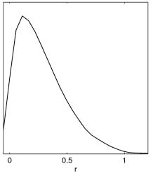
Incorrect result when limits12 is not set. 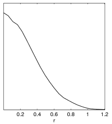
Correct result when setting limits12=0 N.
GetDist produces a file_root.sm file for use with sm. Run sm < file_root.sm to produce file_root.ps containing a plot of the 1D marginalized posterior distributions.
GetDist produces MatLab '.m' files to do 1D, 2D and 3D plots. Type file_root into a MatLab
window set to the directory containing the .m files to produce 1D marginalized plots. You can also do
You can use the blue matlab script (in the mscripts) directory to change to a B&W-friendly colormap (see also other colormaps in that directory). To compare two different sets of chains set compare_num=1 in the .ini file, and compare1 to the root name of some chains you have previously run GetDist on.
Some matlab scripts are also supplied for making custom matlab plots using the files produced by GetDist (see also CosmoloGui). The scripts are in the mscripts directory - you will probably want to add this to your matlab path using e.g. addpath('mscripts'). The scripts are:
confid2D('file_root1',8,17,'-k','b');
hold on;
confid2D('file_root2',8,17,'-k','r');
hold off;
show_contours_behind;
This last (optional) command is a supplied script which will show dotted lines lying behind other solid contours. If the last colour argument is omitted, confid2D plots unfilled contours only.
Convergence diagnostics
The getdist program will output convergence diagnostics, both short summary information when getdist is run, and also more detailed information in the file_root.converge file. When running with MPI the first two of the parameters below can also be calculated when running the chains for comparison with a stopping criterion (see the .ini input file).
Differences between GetDist and MPI run-time statistics
GetDist will cut out ignore_rows from the beginning of each chain, then compute the R statistic using the last half of the remaining samples. The MPI run-time statistic uses the last half of all of the samples. In addition, GetDist will use all the parameters, including derived parameters. If a derived parameter has poor convergence this may show up when running GetDist but not when running the chain (however the eigenvalues of covariance of means is computed using only base parameters). The run-time values also use thinned samples (by default every one in ten), whereas GetDist will use all of them. GetDist will allow you to use only subsets of the chains.
Parameterizations
Hard coded priors
The default installation hard codes a few priors, in some instances you may wish to edit these:
There is no prior on the positivity of Omega_Lambda.
Data
There is also built-in support for 2dF and (few years old) supernovae observations. Adding new data sets should be quite straightforward - you are encouraged to donate anything you add to be used by everyone. See add-ons and datasets.
Programming
This defines what the input variables mean. Change this to use different
variables. You can change which parameterization file to use in the Makefile. params_H.f90 is also supplied for using z_re, A_s and H_0 instead of tau, log(A_s) and theta.
You need to change this file to specify the l_max used. Chains can
be generated at low l_max, then post-processed with a compile using a higher
l_max. You can also change the num_cls number of (temperature plus polarization) Cls to compute and store.
This defines the number of parameters and their types. You will need
to change this if you use more parameters.
This reads in the CMB .dataset information and computes likelihoods.
You may wish to edit this, for example to use likelihood distributions
for the band powers, or to compute the likelihood from actual polarized data. This version assumes polarized data points are an arbitrary combination of the raw TT, TE, EE, and BB Cls, as specified in the window files in data/windows. WMAP data is handled as a special case.
Analagous to cmbdata, but for matter power spectrum measurements. Reads in generic dataset files, supported (fixed) covariance matrices.
This is the proposal density and related constants and subroutines. The efficiency
of MCMC is quite dependent on the proposal. Fast+slow and fast parameter subspaces are proposed separately. See the notes for a discussion of the proposal density and use of fast and slow parameters.
Routines for generating Cls, matter power spectra and sigma8 from CAMB.
Replace this file to use other generators, e.g. a fast approximator like
CMBfit, DASH, PICO, etc.
As of May 2008 uses UNION by default (thanks to Anze Slosar). Other alternative supernovae_xxx files are supplied.
SDSS Lyman alpha data (thanks to Kevork Abazajian). Note this is only tested and likely to be reliable for standard LCDM models. For more general code see the add-ons. Can also replace with lya.f90 and recompile to use with LUQAS (thanks to Matteo Viel, J.Lesgourgues).
Reads in .data files and re-calculates likelihoods or theory predictions. Unused in MCMC runs.
Add in calls to other likelihood calculators, etc., here.
Main program that reads in parameters and calls MCMC or post-processing.
The "getdist" program for analysing chains. Write your own importance
weighting function or parameter mapping.Add-ons and extra datasets
- X-ray cluster gas mass fraction
- COSMOS 3D weak lensing data
- python GetDist
- FuturCMB forecasting with CMB lensing
- CosmoNest Nested sampling add-on.
- Lyman-alpha Forest Power Spectrum from the Sloan Digital Sky Survey
Version History
- June 2008
Fixed problem initializing nuisance parameters. Updated CAMB to June 2008 version (fix for very closed models). - May 2008
supernovae.f90 now replaced by default with UNION Supernovae Ia dataset (previous code now supernovae_ReissSNLS.f90; thanks to Anze Slosar). Additions to Planck_like module; support for sampling and hence marginalizing over data nuisance parameters, point sources, beam uncertainty modes. New GetDist option single_column_chain_files to support WMAP 5-year format chains (thanks to Mike Nolta): 1col_distparams.ini is a supplied sample input file. New GetDist option do_minimal_1d_intervals to calculate equal-likelihood 1-D limits (see 0705.0440, thanks to Jan Hamann). New GetDist option num_contours to produce more than two sets of limits. - April 2008
Includes latest CAMB version with new reionization parameterization - default now assumes first ionization of helium happened at the same time as hydogen, and z_re is defined as the point where xe is half its maximum (the optical depth and z_re are related in a way independent of the speed of the transition in the new parameterization). This changes the z_re numbers at the ~6% level. Fixed bug reading in mpk parameters. - March 2008
Uses WMAP 5-year likelihood code. Added cmb_dataset_SZx and cmb_dataset_SZ_scalex parameters to specify (parameter independent) SZ template for each CMB dataset (WMAP_SZ_VBand.dat included from LAMBDA). Parameter 13 is now ASZ - the scaling of all the SZ templates, as used in WMAP3/WMAP5 papers. Updated supplied covariance params_CMB.covmat for WMAP5. Minor compatibility changes. - February 2008
Added generic_mcmc in settings.f90 to easily use CosmoMC as generic sampling program without calling CAMB etc (write GenericLikelihoodFunction in calclike.f90 and use Makefile_nowmap). Added latest ACBAR dataset. CAMB update (including RECFAST 1.4). New Planck_like.f90 module for Cl likelihoods using approximation of arXiv:0801.0554 (also basic low-l likelihood). Added markerx GetDist parameters for adding vertical lines to parameter x in 1D matlab plots. Various minor changes/compatibility fixes. - November 2006
Updated CBI data. Compiler compatibility tweaks. Fixed error msg in mpk.f90. Minor CAMB update. Better error reporting in conjgrad_wrapper (thanks to Sam Leach). - October 2006
(20th October 2006)Fixed k-scaling for SDSS LRG likelihood in mpk.f90. Changes for new version of WMAP likelihood code. Added out_dir and plot_data_dir options for GetDist. Minor compatibility fixes.
Added support for SDSS LRG data (astro-ph/0608632; thanks to Licia Verde, Hiranya Peiris and Max Tegmark). CAMB fixes and other minor changes. - August 2006
Improved speed of GetDist 2D plot generation, added limitsxxx support when smoothing = F. Added sampling_method = 5,6, preliminary implementations of multicanonical and Wang-Landau sampling for nasty (e.g. multi-modal) distributions (currently does not compute Evidence, just generates weighted samples). Changed matter_power_minkh (cmbtypes) to work around potential rounding errors on some computers. Updated CAMB following August 2006 version. Added warning about missing limitsxx parameters to getdist. Added MPI_Max_R_ProposeUpdateNew parameter (when varying pareters that are fixed in covmat). Updated CBI data files. - May 2006
Supernovae.f90 updated to use SNLS by default, edit to use Riess Gold. 2dF updated (twodf.f90 file deleted, use 2df_2005.dataset); covariance matrix support in mpk.f90. Fixed bug using LSS with non-flat models. Improved error checking and matlab 7 enhancements in getdist. Getdist auto column counting with columnnum=0, various hidden extra options now shown in sample distparams.ini. Extra fix for confid2D. Fixed MPI thinning bug in utils.F90. Makefile fixes. Fixed mpk.f90 analytical marginalization (since March 2006). SDSS likelihood now computed from k/h=1e-4. - April 2006
Fixed bug in lya.f90 (SDSS lyman-alpha now the default; lya.f90 now includes Croft by default). Fixes to Confid2D matlab script. Added .covmat files for WMAP with running and tensors, and basic Planck simulation. Fixed version confusion in GetDist (one-tail limits set to prior limit value). - March 2006
Updated for 3-year WMAP. Added use_lya to include lyman-alpha data (standard LCDM only). Default in lya.f90 is LUQAS (can also compile with SDSSLy-a-v3.f90 for SDSS). New matlab scripts for producing solid contour and 4D plots. New checkpoint option to generate checkpoint files and continue terminated runs. Added action=1 parameters redo_add (adds new likelihoods rather than recalculating) and redo_from_text (if you don't have .data files). Added pivot_k and inflation_consistency for use with default power spectrum parameterization. - July 2005
Added get_sigma8 to force calculation of σ8. Updated .newdat CMB dataset format (also added B03 data files). New use_fast_slow parameter to turn on/off fast-slow optimizations. Fixed bug which resulted in occasional wrong tau values when importance sampling .data files. GetDist now outputs one/two-tail limit info in .margestats file. Updated CAMB version (support for non-linear matter power spectrum). - February 2005
Updated CAMB for new accurate lensed Cl calculation of astro-ph/0502425. Minor changes to getdist (new matlab_version input parameter, all_limits to set same limits for all parameters). cmbdata.f90 includes new format used by BOOMERANG/CBI for polarization. - October 13 2004
Fixed bug in mpk.f90 when using 2df. Changes to GetDist for compatibility with MatLab 7. Fixed Makefile_intel (though now obsolete if you have Intel fortran v8). - October 2004
Added mpk.f90 for reading in general (multiple) matter power spectrum data files in a similar way to CMB dataset files - corresponding changes to input parameter file. Included SDSS data files (note CosmoMC only models linear spectrum). Various minor bug fixes and improved MPI error handling. Included (though not compiled by default) supernovae_riess_gold.f90 file to include more recent supernova data. Some mscripts fixes for compatibility with MatLab 7. - August 2004
Improved proposal density for efficient handling of fast and slow parameters, plus more robust distance proposal (should see significant speed improvement). New sampling_method parameter: new options for slice sampling (robust) and directional gridding (robust and efficient use of fast parameters). Also option to use slice sampling for burn in (more robust than Metropolis in many cases), then switch to Metropolis (faster with good covariance matrix). See the notes for details. Improved MPI handling and minor bug fixes. Fixed effect of reionization on CAMB's lensed Cl results. - June 2004
Uses June 2004 CAMB version: bessel_cache.camb file no longer produced or needed (prevents MPI problems). Increased sig figs of chain output and GetDist analysis. New parameter propose_scale, the ratio of proposal width to st. dev., default 2.4 (following Roberts, Gelman, Gilks, astro-ph/0405462) - often significantly speeds convergence (parameters in .ini file are now estimates of the st. dev., not desired proposal widths). Added MPI_R_StopProposeUpdate to stop updating proposal covariance matrix after a given convergence level has been reached. Added accuracy_level parameter to run at higher CAMB accuracy level (may be useful for forecasting). - March 2004
Added new VSA and CBI datasets. Added first_band= option to .dataset files to cut out low l that aren't wanted. CAMB pivot scale for tensors changed to 0.05/MPc (same as scalar). Fixed various compiler compatibility issues. Corrected CMB_lensing parameter in sample .ini file. Fixed minor typo in params_CMB.f90. Fixed reading in of MPI_Limit_Converge parameter in driver.F90. Fixed bounds checking in MatterPowerAt (harmless with 2df). Added an exact likelihood calculation/data format to cmbdata.f90 for polarized full sky CMB Cl. - December 2003
Added MPI support, with stopping on convergence and optional proposal density updating. Added calculation of matter power spectrum at different redshifts using CAMB (settings in cmbtypes.f90). Fixed bug when restarting chains using "continue_from" parameter [March 2006: now obsolete], and a few compiler compatibility issues. Updated CAMB for more accurate non-flat model results. Added output of parameter auto-correlations to GetDist, along with support for ignore_rows<1 to cut out a fraction of the chain and percentile split-test error estimators. Changed proposal density to proposal a random number of parameter changes on each step. Added GetDist samples_are_chains option - if false, rows can be any samples of anything (starting in column one, without an importance weight or likelihood value as produced by CosmoMC) - useful for analysing samples that don't come from CosmoMC. Added GetDist auto_label parameter to label parameters automatically by their parameter number. - July 2003
Fixed bug in MCMC.f90 affecting all raw chains - weights and likelihoods were displaced by one row. Post-processed results were correct, and effect on parameters is very small. Minor bug fixes in GetDist. Can now make file_root.read file to be read by all chains file_root_1, file_root_2, etc (this file is not auto-deleted after being read). - May 2003
Added support for 'triangle' plots to GetDist (example. Set triangle_plot=T in the .ini file). If truncation is required, the covariance matrix for CMB data sets is now truncated (rather than truncating the inverse covariance). Fixed CAMB bug with non-flat models, and problem setting CAMB parameters when run separately from CosmoMC. - March 4 2003
Fixed bug in GetDist - the .margestats file produced contained incorrect limits (the mean and stddev were OK) - Feb 2003
Support for WMAP data (customized code fixes TE and amplitude bugs). CMB computation now uses Cl transfer functions - complete split possible between transfer functions and the initial power spectrum, so improved efficiency handling fast parameters. Bug fixes and tidying of proposal function. Initial power spectrum no longer assumed smooth for P_k. GetDist limitsxxx variables can be N to auto-size one end (margestats are still one tail). Support of IBM XL fortran (workarounds for bug on Seaborg). GetDist will automatically compute some chain statistics to help diagnose convergence and accuracy. CAMB updated, including more accurate and faster handling of tight coupling. Option to generate chains including CMB lensing effect. Various other changes. - Nov 2002
Added support for polarization, and improved compatibility with different compilers and systems.
Reference links
Probabilistic Inference Using Markov Chain Monte Carlo MethodsInformation Theory, Inference and Learning Algorithms
Raftery and Lewis convergence diagnostics
There are also some notes on the proposal density, fast and slow parameters, and slice sampling as used by CosmoMC. See also the BibTex file of CosmoMC references you should cite, along with some references
of potential interest.
FAQ
- What are the dotted lines on the plots?
Dotted lines are mean likelihoods of samples, solid lines are marginalized probabilities. For Gaussian distributions they should be the same. For skew disctributions, or if chains are poorly converged, they will not be. Sometime there is a much better fit (giving high mean likelihood) in a small region of parameter space which has very low marginalized probability. There is more discussion in the original paper.
- What's in the .likestats file produced by getdist?
These are values for the best-fit sample, and projections of the n-Dimensional confidence region. Usually people only look at the best-fit values. The n-D limits give you some idea of the range of the posterior, and are much more conservative than the marginalized limits.
- I'm writing a paper "constraints on X". How do I add X to cosmomc?
Often the easiest thing to do is to re-interpret one of the unused standard parameters, e.g. w, A_T, etc, depending on whether the parameter is "fast" or not (if in doubt, use one of the slow parameters like w or f_nu). You just need to change the CMBToCAMB routine in CMB_Cls_Simple.f90 so that your parameter is correctly fed into CAMB, change limits appropriately in the params.ini file, etc. See the undocumented references to w_is_w in the code for how w can be re-interpreted as a ratio of isocurvature to adiabatic in CAMB's initial conditions. If you need to add more than a couple of parameters you'll probably instead need to edit settings.f90 to increase the number of parameters, and edit the .ini file accordingly. Slow parameters should have numbers lower than fast parameters (i.e. to insert 5 slow parameters, the index of the fast parameters in the .ini file should increase by 5).
- Why do some chains sometimes appear to get stuck?
Usually this is because the starting position for the chain is a long way from the best fit region. Since the marginal distributions of e.q. A_s are rather narrow, it can take a while for chains to move from into an acceptable region of A_s exp(-2τ). The cure is to check your starting parameter values and start widths (make sure the widths are not too wide), or to use a sampling method that is more robust (e.g. use sampling_method = 4). If you are patient, stuck chains should eventually find a sensible region of parameter space anyway. Occasionally the staring position may be in a corner of parameter space so that prior ranges prevent any resonable proposed moves. In this case check your starting values and ranges, or just try re-starting the chain (a different random starting position will possibly be OK).
- How to I simulate futuristic CMB data? See CosmoCoffee. Also if you want to include lensing potential reconstruction, see this page.
Feel free to ask questions (and read answers to other people's) on the CosmoCoffee software forum. There is also a FAQ in the CosmoloGUI readme.
Antony Lewis. ������������������������������������������������������������������������������������������������������������������������������������������������������������������������������������������������������������������������������������������������������������������������������������������������������������������������������������������������������������������������������������������������������������������������������camb_rpc_full/cosmomc/data/�������������������������������������������������������������������������0000755�0006471�0000403�00000000000�11637143605�016307� 5����������������������������������������������������������������������������������������������������ustar �mmortonson����������������������ccapp������������������������������������������������������������������������������������������������������������������������������������������������������������������������������������������������������������������camb_rpc_full/cosmomc/data/2df_2005_kbands.txt������������������������������������������������������0000644�0006471�0000403�00000013557�11637143605�021526� 0����������������������������������������������������������������������������������������������������ustar �mmortonson����������������������ccapp������������������������������������������������������������������������������������������������������������������������������������������������������������������������������������������������������������������0.001 0.003 0.005 0.007 0.009 0.011 0.013 0.015 0.017 0.019 0.021 0.023 0.025 0.027 0.029 0.031 0.033 0.035 0.037 0.039 0.041 0.043 0.045 0.047 0.049 0.051 0.053 0.055 0.057 0.059 0.061 0.063 0.065 0.067 0.069 0.071 0.073 0.075 0.077 0.079 0.081 0.083 0.085 0.087 0.089 0.091 0.093 0.095 0.097 0.099 0.101 0.103 0.105 0.107 0.109 0.111 0.113 0.115 0.117 0.119 0.121 0.123 0.125 0.127 0.129 0.131 0.133 0.135 0.137 0.139 0.141 0.143 0.145 0.147 0.149 0.151 0.153 0.155 0.157 0.159 0.161 0.163 0.165 0.167 0.169 0.171 0.173 0.175 0.177 0.179 0.181 0.183 0.185 0.187 0.189 0.191 0.193 0.195 0.197 0.199 0.201 0.203 0.205 0.207 0.209 0.211 0.213 0.215 0.217 0.219 0.221 0.223 0.225 0.227 0.229 0.231 0.233 0.235 0.237 0.239 0.241 0.243 0.245 0.247 0.249 0.251 0.253 0.255 0.257 0.259 0.261 0.263 0.265 0.267 0.269 0.271 0.273 0.275 0.277 0.279 0.281 0.283 0.285 0.287 0.289 0.291 0.293 0.295 0.297 0.299 0.301 0.303 0.305 0.307 0.309 0.311 0.313 0.315 0.317 0.319 0.321 0.323 0.325 0.327 0.329 0.331 0.333 0.335 0.337 0.339 0.341 0.343 0.345 0.347 0.349 0.351 0.353 0.355 0.357 0.359 0.361 0.363 0.365 0.367 0.369 0.371 0.373 0.375 0.377 0.379 0.381 0.383 0.385 0.387 0.389 0.391 0.393 0.395 0.397 0.399 0.401 0.403 0.405 0.407 0.409 0.411 0.413 0.415 0.417 0.419 0.421 0.423 0.425 0.427 0.429 0.431 0.433 0.435 0.437 0.439 0.441 0.443 0.445 0.447 0.449 0.451 0.453 0.455 0.457 0.459 0.461 0.463 0.465 0.467 0.469 0.471 0.473 0.475 0.477 0.479 0.481 0.483 0.485 0.487 0.489 0.491 0.493 0.495 0.497 0.499 0.501 0.503 0.505 0.507 0.509 0.511 0.513 0.515 0.517 0.519 0.521 0.523 0.525 0.527 0.529 0.531 0.533 0.535 0.537 0.539 0.541 0.543 0.545 0.547 0.549 0.551 0.553 0.555 0.557 0.559 0.561 0.563 0.565 0.567 0.569 0.571 0.573 0.575 0.577 0.579 0.581 0.583 0.585 0.587 0.589 0.591 0.593 0.595 0.597 0.599 0.601 0.603 0.605 0.607 0.609 0.611 0.613 0.615 0.617 0.619 0.621 0.623 0.625 0.627 0.629 0.631 0.633 0.635 0.637 0.639 0.641 0.643 0.645 0.647 0.649 0.651 0.653 0.655 0.657 0.659 0.661 0.663 0.665 0.667 0.669 0.671 0.673 0.675 0.677 0.679 0.681 0.683 0.685 0.687 0.689 0.691 0.693 0.695 0.697 0.699 0.701 0.703 0.705 0.707 0.709 0.711 0.713 0.715 0.717 0.719 0.721 0.723 0.725 0.727 0.729 0.731 0.733 0.735 0.737 0.739 0.741 0.743 0.745 0.747 0.749 0.751 0.753 0.755 0.757 0.759 0.761 0.763 0.765 0.767 0.769 0.771 0.773 0.775 0.777 0.779 0.781 0.783 0.785 0.787 0.789 0.791 0.793 0.795 0.797 0.799 0.801 0.803 0.805 0.807 0.809 0.811 0.813 0.815 0.817 0.819 0.821 0.823 0.825 0.827 0.829 0.831 0.833 0.835 0.837 0.839 0.841 0.843 0.845 0.847 0.849 0.851 0.853 0.855 0.857 0.859 0.861 0.863 0.865 0.867 0.869 0.871 0.873 0.875 0.877 0.879 0.881 0.883 0.885 0.887 0.889 0.891 0.893 0.895 0.897 0.899 0.901 0.903 0.905 0.907 0.909 0.911 0.913 0.915 0.917 0.919 0.921 0.923 0.925 0.927 0.929 0.931 0.933 0.935 0.937 0.939 0.941 0.943 0.945 0.947 0.949 0.951 0.953 0.955 0.957 0.959 0.961 0.963 0.965 0.967 0.969 0.971 0.973 0.975 0.977 0.979 0.981 0.983 0.985 0.987 0.989 0.991 0.993 0.995 0.997 0.999 1.001 1.003 1.005 1.007 1.009 1.011 1.013 1.015 1.017 1.019 1.021 1.023 1.025 1.027 1.029 1.031 1.033 1.035 1.037 1.039 1.041 1.043 1.045 1.047 1.049 1.051 1.053 1.055 1.057 1.059 1.061 1.063 1.065 1.067 1.069 1.071 1.073 1.075 1.077 1.079 1.081 1.083 1.085 1.087 1.089 1.091 1.093 1.095 1.097 1.099 1.101 1.103 1.105 1.107 1.109 1.111 1.113 1.115 1.117 1.119 1.121 1.123 1.125 1.127 1.129 1.131 1.133 1.135 1.137 1.139 1.141 1.143 1.145 1.147 1.149 1.151 1.153 1.155 1.157 1.159 1.161 1.163 1.165 1.167 1.169 1.171 1.173 1.175 1.177 1.179 1.181 1.183 1.185 1.187 1.189 1.191 1.193 1.195 1.197 1.199 1.201 1.203 1.205 1.207 1.209 1.211 1.213 1.215 1.217 1.219 1.221 1.223 1.225 1.227 1.229 1.231 1.233 1.235 1.237 1.239 1.241 1.243 1.245 1.247 1.249 1.251 1.253 1.255 1.257 1.259 1.261 1.263 1.265 1.267 1.269 1.271 1.273 1.275 1.277 1.279 1.281 1.283 1.285 1.287 1.289 1.291 1.293 1.295 1.297 1.299 1.301 1.303 1.305 1.307 1.309 1.311 1.313 1.315 1.317 1.319 1.321 1.323 1.325 1.327 1.329 1.331 1.333 1.335 1.337 1.339 1.341 1.343 1.345 1.347 1.349 1.351 1.353 1.355 1.357 1.359 1.361 1.363 1.365 1.367 1.369 1.371 1.373 1.375 1.377 1.379 1.381 1.383 1.385 1.387 1.389 1.391 1.393 1.395 1.397 1.399 1.401 1.403 1.405 1.407 1.409 1.411 1.413 1.415 1.417 1.419 1.421 1.423 1.425 1.427 1.429 1.431 1.433 1.435 1.437 1.439 1.441 1.443 1.445 1.447 1.449 1.451 1.453 1.455 1.457 1.459 1.461 1.463 1.465 1.467 1.469 1.471 1.473 1.475 1.477 1.479 1.481 1.483 1.485 1.487 1.489 1.491 1.493 1.495 1.497 1.499 1.501 1.503 1.505 1.507 1.509 1.511 1.513 1.515 1.517 1.519 1.521 1.523 1.525 1.527 1.529 1.531 1.533 1.535 1.537 1.539 1.541 1.543 1.545 1.547 1.549 1.551 1.553 1.555 1.557 1.559 1.561 1.563 1.565 1.567 1.569 1.571 1.573 1.575 1.577 1.579 1.581 1.583 1.585 1.587 1.589 1.591 1.593 1.595 1.597 1.599 1.601 1.603 1.605 1.607 1.609 1.611 1.613 1.615 1.617 1.619 1.621 1.623 1.625 1.627 1.629 1.631 1.633 1.635 1.637 1.639 1.641 1.643 1.645 1.647 1.649 1.651 1.653 1.655 1.657 1.659 1.661 1.663 1.665 1.667 1.669 1.671 1.673 1.675 1.677 1.679 1.681 1.683 1.685 1.687 1.689 1.691 1.693 1.695 1.697 1.699 1.701 1.703 1.705 1.707 1.709 1.711 1.713 1.715 1.717 1.719 1.721 1.723 1.725 1.727 1.729 1.731 1.733 1.735 1.737 1.739 1.741 1.743 1.745 1.747 1.749 1.751 1.753 1.755 1.757 1.759 1.761 1.763 1.765 1.767 1.769 1.771 1.773 1.775 1.777 1.779 1.781 1.783 1.785 1.787 1.789 1.791 1.793 1.795 1.797 1.799 1.801 1.803 1.805 1.807 1.809 1.811 1.813 1.815 1.817 1.819 1.821 1.823 1.825 1.827 1.829 1.831 1.833 1.835 1.837 1.839 1.841 1.843 1.845 1.847 1.849 1.851 1.853 1.855 1.857 1.859 1.861 1.863 1.865 1.867 1.869 1.871 1.873 1.875 1.877 1.879 1.881 1.883 1.885 1.887 1.889 1.891 1.893 1.895 1.897 1.899 1.901 1.903 1.905 1.907 1.909 1.911 1.913 1.915 1.917 1.919 1.921 1.923 1.925 1.927 1.929 1.931 1.933 1.935 1.937 1.939 1.941 1.943 1.945 1.947 1.949 1.951 1.953 1.955 1.957 1.959 1.961 1.963 1.965 1.967 1.969 1.971 1.973 1.975 1.977 1.979 1.981 1.983 1.985 1.987 1.989 1.991 1.993 1.995 1.997 1.999�������������������������������������������������������������������������������������������������������������������������������������������������camb_rpc_full/cosmomc/data/sdss.dataset�������������������������������������������������������������0000644�0006471�0000403�00000001547�11637143605�020641� 0����������������������������������������������������������������������������������������������������ustar �mmortonson����������������������ccapp������������������������������������������������������������������������������������������������������������������������������������������������������������������������������������������������������������������name = sdss # NB. Cosmomc does not do non-linear theory at the moment, # and yet the SDSS window functions go significantly above # k/h=0.3, where the non-linear contribution is significant # (and non-linear biasing may also be a problem) # number of points and kbands in the input files num_mpk_points_full = 22 num_mpk_kbands_full = 97 # decide which bandpowers to use, min to max min_mpk_points_use = 1 max_mpk_points_use = 19 # as in the Tegmark papers # decide which kbands to use N.B. P(k) is set to zero outside # these limits. # Since the windows file starts at k/h=1e-4 then truncate # to matter_power_minkh in cmbtypes. # Similarly the windows file goes to k/h=100, so truncate to 1.00. min_mpk_kbands_use = 1 max_mpk_kbands_use = 65 windows_file = data/sdss_windows.txt kbands_file = data/sdss_kbands.txt measurements_file = data/sdss_measurements.txt ���������������������������������������������������������������������������������������������������������������������������������������������������������camb_rpc_full/cosmomc/data/twodf_june02.dat���������������������������������������������������������0000644�0006471�0000403�00000002651�11637143605�021313� 0����������������������������������������������������������������������������������������������������ustar �mmortonson����������������������ccapp������������������������������������������������������������������������������������������������������������������������������������������������������������������������������������������������������������������0.022117 22928.587891 5483.162109 21833.468750 0.026138 18291.646484 4578.990234 21450.326172 0.030159 16666.125000 3818.981689 20782.740234 0.034180 15283.059570 3263.383057 19955.095703 0.038202 13990.493164 2611.579590 19046.552734 0.042223 14182.396484 2262.832520 18107.730469 0.046244 14255.913086 1871.653198 17170.751953 0.050265 13517.357422 1611.438110 16255.704102 0.054287 13861.277344 1425.576416 15374.788086 0.058308 13870.442383 1267.590454 14534.873047 0.062329 13080.831055 1136.116943 13739.438477 0.066350 13198.610352 1009.898438 12989.611328 0.070372 11173.412109 921.287231 12285.039062 0.074393 11272.038086 818.051697 11624.483398 0.078414 9542.856445 786.182373 11006.068359 0.082435 8595.612305 677.437073 10427.605469 0.086457 8482.800781 632.748535 9886.796875 0.090478 7742.525391 544.964172 9381.233398 0.094499 7591.747559 487.364685 8908.592773 0.098520 6547.371582 431.224243 8466.590820 0.102542 6215.445801 408.895264 8053.035156 0.106563 5849.887695 380.571045 7665.973633 0.110584 5983.527344 343.731903 7303.424805 0.114605 5707.486816 322.583344 6963.608887 0.118627 5871.963379 295.041229 6644.779297 0.122648 5710.937988 277.095856 6345.564941 0.126669 5192.185059 252.696701 6064.459961 0.130690 5182.548340 242.374496 5800.156738 0.134711 4685.800293 213.247238 5551.444824 0.138733 4528.355469 202.061615 5317.155762 0.142754 4526.491699 184.798264 5096.379883 0.146775 4223.802246 170.862671 4888.115234���������������������������������������������������������������������������������������camb_rpc_full/cosmomc/data/sdss_measurements.txt����������������������������������������������������0000644�0006471�0000403�00000003405�11637143605�022616� 0����������������������������������������������������������������������������������������������������ustar �mmortonson����������������������ccapp������������������������������������������������������������������������������������������������������������������������������������������������������������������������������������������������������������������# keff klo khi obs sdev beff # 0.01578 0.01300 0.02195 21573.38836 33320.25582 1.16762 0.01819 0.01502 0.02440 33254.63896 24572.79357 1.16745 0.02099 0.01729 0.02820 13845.52953 17712.46771 1.16716 0.02405 0.01984 0.03136 38360.58264 13320.48227 1.16674 0.02776 0.02300 0.03571 24143.07699 10047.21709 1.16613 0.03201 0.02663 0.04048 19709.29306 7413.82995 1.16532 0.03691 0.03094 0.04601 12595.77528 5485.84481 1.16428 0.04257 0.03591 0.05215 13558.60084 4077.68223 1.16294 0.04912 0.04162 0.05983 18311.08054 2974.15048 1.16124 0.05670 0.04824 0.06873 12080.73574 2140.39514 1.15910 0.06527 0.05561 0.07867 9217.46084 1580.01728 1.15647 0.07529 0.06455 0.08999 9750.49986 1127.95803 1.15317 0.08698 0.07507 0.10351 9529.63935 818.49019 1.14906 0.10037 0.08670 0.11898 6384.82545 601.70752 1.14409 0.11581 0.09985 0.13679 5294.92081 446.65015 1.13813 0.13360 0.11478 0.15748 4629.83669 335.07950 1.13109 0.15412 0.13181 0.18139 3573.92724 254.13547 1.12290 0.17774 0.15114 0.20891 3393.82814 195.23431 1.11358 0.20489 0.17288 0.24062 2298.10000 152.73819 1.10320 0.23592 0.19690 0.27653 1597.14976 123.50981 1.09193 0.27062 0.22219 0.31395 1105.42903 107.20069 1.08019 0.30618 0.23123 0.34782 1012.72489 110.33632 1.06912 �����������������������������������������������������������������������������������������������������������������������������������������������������������������������������������������������������������������������������������������������������������camb_rpc_full/cosmomc/data/dasi_rad_x.dat�����������������������������������������������������������0000644�0006471�0000403�00000000141�11637143605�021072� 0����������������������������������������������������������������������������������������������������ustar �mmortonson����������������������ccapp������������������������������������������������������������������������������������������������������������������������������������������������������������������������������������������������������������������ 159.75 167.089996 195.720001 226.029999 439.529999 710. 726.090027 1182.40002 2109.1001 �������������������������������������������������������������������������������������������������������������������������������������������������������������������������������������������������������������������������������������������������������������������������������������������������������������������������������������������������������������������������������������������������������������������������������camb_rpc_full/cosmomc/data/2df_2005_measurements.txt������������������������������������������������0000644�0006471�0000403�00000004560�11637143605�022766� 0����������������������������������������������������������������������������������������������������ustar �mmortonson����������������������ccapp������������������������������������������������������������������������������������������������������������������������������������������������������������������������������������������������������������������# 2dFGRS final data set: Cole et al. astro-ph/0501174 # k / hMpc^-1, klo, khi, 2dFGRS P(k) / h^-3Mpc^3, 2dFGRS sig / h^-3Mpc^3, covmat P(k) / h^-3Mpc^3, 0.0221168 0.0221168 0.0221168 41707.4 8278.14 56545.8 0.0261381 0.0261381 0.0261381 35455.9 6796.09 50351.4 0.0301593 0.0301593 0.0301593 30056.7 5541.58 44301.7 0.0341805 0.0341805 0.0341805 27285 4573.74 39028 0.0382018 0.0382018 0.0382018 24382.4 3868.88 34725.8 0.042223 0.042223 0.042223 20925.1 3299.47 31368 0.0462442 0.0462442 0.0462442 22258.8 2917.19 28831.4 0.0502655 0.0502655 0.0502655 22548.1 2547.02 26946.2 0.0542867 0.0542867 0.0542867 19250.6 2223.59 25513.1 0.058308 0.058308 0.058308 18341.8 2000.08 24320.7 0.0623292 0.0623292 0.0623292 17345.6 1803.63 23173.4 0.0663504 0.0663504 0.0663504 16451.1 1609.15 21924.8 0.0703717 0.0703717 0.0703717 15185.8 1444.7 20503.3 0.0743929 0.0743929 0.0743929 14757 1312.91 18919.6 0.0784141 0.0784141 0.0784141 13493.6 1199.68 17250.8 0.0824354 0.0824354 0.0824354 12801.6 1088.36 15608 0.0864566 0.0864566 0.0864566 11667.1 983.898 14100.3 0.0904779 0.0904779 0.0904779 10519.2 878.597 12808 0.0944991 0.0944991 0.0944991 10092.9 806.479 11769.9 0.0985203 0.0985203 0.0985203 9047.74 758.656 10983.3 0.102542 0.102542 0.102542 8344.95 720.583 10412.8 0.106563 0.106563 0.106563 8212.02 686.879 10001.6 0.110584 0.110584 0.110584 8169.45 647.823 9682.92 0.114605 0.114605 0.114605 8159.86 607.515 9392.02 0.118626 0.118626 0.118626 7875.62 576.358 9076.73 0.122648 0.122648 0.122648 7311.92 547.186 8705.3 0.126669 0.126669 0.126669 7013.12 510.5 8270.08 0.13069 0.13069 0.13069 6864.6 485.08 7784.65 0.134712 0.134712 0.134712 6214.29 456.865 7276.97 0.138733 0.138733 0.138733 5736.34 434.629 6780.55 0.142754 0.142754 0.142754 5469.52 411.773 6325.09 0.146775 0.146775 0.146775 5222.81 388.769 5931.21 0.150796 0.150796 0.150796 5030.2 369.8 5607.87 0.154818 0.154818 0.154818 4954 353.809 5352.72 0.168892 0.168892 0.168892 4624.78 309.728 4793.75 0.184977 0.184977 0.184977 3938.12 269.241 4152.45������������������������������������������������������������������������������������������������������������������������������������������������camb_rpc_full/cosmomc/data/dasi_rad_matrix.dat������������������������������������������������������0000644�0006471�0000403�00000001764�11637143605�022143� 0����������������������������������������������������������������������������������������������������ustar �mmortonson����������������������ccapp������������������������������������������������������������������������������������������������������������������������������������������������������������������������������������������������������������������ 24.6718998 12.5021 0.579029977 4.502389953E-2 2.645540051E-2 2.982099913E-2 2.857230045E-2 2.726659924E-2 2.410829999E-2 12.5021 109.182999 22.0121002 0.793402016 0.233581007 0.242510006 0.228128999 0.216336995 0.16561 0.579029977 22.0121002 141.542999 22.8152008 1.35195005 0.869746983 0.82921797 0.809683979 0.696195006 4.502389953E-2 0.793402016 22.8152008 101.053299 25.9783001 2.06213999 1.64802003 1.65761006 1.32983994 2.645540051E-2 0.233581007 1.35195005 25.9783001 126.120003 27.3411007 2.80065989 2.5869 2.11741996 2.982099913E-2 0.242510006 0.869746983 2.06213999 27.3411007 162.625 26.5391998 3.63491011 2.76413012 2.857230045E-2 0.228128999 0.82921797 1.64802003 2.80065989 26.5391998 91.153801 25.1611004 3.16971993 2.726659924E-2 0.216336995 0.809683979 1.65761006 2.5869 3.63491011 25.1611004 92.1662979 21.6089001 2.410829999E-2 0.16561 0.696195006 1.32983994 2.11741996 2.76413012 3.16971993 21.6089001 104.2444 ������������camb_rpc_full/cosmomc/data/CBIpol_2.0_final.newdat��������������������������������������������������0000744�0006471�0000403�00000125510�11637143605�022360� 0����������������������������������������������������������������������������������������������������ustar �mmortonson����������������������ccapp������������������������������������������������������������������������������������������������������������������������������������������������������������������������������������������������������������������CBIpol_2.0_windows_ 15 14 5 0 17 0 BAND_SELECTION 2 14 1 14 1 5 0 0 2 16 0 0 1 1.00 0.0260 0 0 0 2 #iliketype TT 1 5788 967.2 967.2 892.3 0.0 360.0 1 2 1415 298.5 298.5 104.8 360.0 495.0 1 3 3618 717.4 717.4 9.254 495.0 570.0 1 4 2331 614.9 614.9 40.21 570.0 635.0 1 5 1582 428.7 428.7 193.5 635.0 710.0 1 6 2648 565.8 565.8 248.4 710.0 775.0 1 7 2344 487.9 487.9 316.5 775.0 855.0 1 8 1943 428.9 428.9 358.4 855.0 940.0 1 9 947.5 272 272 330.5 940.0 1070.0 1 10 1347 325.8 325.8 323.5 1070.0 1170.0 1 11 929.1 229.8 229.8 320.8 1170.0 1300.0 1 12 825.4 195.5 195.5 697.2 1300.0 1500.0 1 13 231.2 256.6 256.6 1141 1500.0 1700.0 1 14 563.8 248 248 1294 1700.0 2000.0 1 15 -235.5 320 320 2940 2000.0 5000.0 1 1.000 -0.193 0.015 -0.006 -0.003 -0.008 -0.017 -0.001 -0.004 -0.001 -0.003 -0.001 -0.008 0.004 -0.010 -0.193 1.000 -0.209 0.038 -0.027 0.019 -0.026 -0.011 0.000 0.001 -0.010 -0.005 -0.008 -0.002 -0.014 0.015 -0.209 1.000 -0.328 0.092 -0.031 0.005 -0.021 0.009 -0.010 0.001 0.001 -0.022 -0.010 0.010 -0.006 0.038 -0.328 1.000 -0.394 0.100 -0.034 0.018 -0.018 -0.007 0.010 0.006 0.003 -0.010 -0.022 -0.003 -0.027 0.092 -0.394 1.000 -0.336 0.089 -0.030 0.003 -0.010 -0.019 -0.008 -0.002 -0.012 0.007 -0.008 0.019 -0.031 0.100 -0.336 1.000 -0.319 0.060 -0.010 -0.001 -0.011 0.006 -0.019 -0.011 0.007 -0.017 -0.026 0.005 -0.034 0.089 -0.319 1.000 -0.267 0.022 -0.020 0.012 -0.013 -0.006 -0.024 0.002 -0.001 -0.011 -0.021 0.018 -0.030 0.060 -0.267 1.000 -0.242 0.033 -0.010 -0.026 -0.001 -0.031 -0.016 -0.004 0.000 0.009 -0.018 0.003 -0.010 0.022 -0.242 1.000 -0.265 -0.006 -0.027 -0.034 -0.036 -0.032 -0.001 0.001 -0.010 -0.007 -0.010 -0.001 -0.020 0.033 -0.265 1.000 -0.255 -0.019 -0.062 -0.015 -0.022 -0.003 -0.010 0.001 0.010 -0.019 -0.011 0.012 -0.010 -0.006 -0.255 1.000 -0.236 -0.055 -0.041 -0.045 -0.001 -0.005 0.001 0.006 -0.008 0.006 -0.013 -0.026 -0.027 -0.019 -0.236 1.000 -0.183 -0.103 -0.012 -0.008 -0.008 -0.022 0.003 -0.002 -0.019 -0.006 -0.001 -0.034 -0.062 -0.055 -0.183 1.000 -0.220 -0.085 0.004 -0.002 -0.010 -0.010 -0.012 -0.011 -0.024 -0.031 -0.036 -0.015 -0.041 -0.103 -0.220 1.000 -0.343 -0.010 -0.014 0.010 -0.022 0.007 0.007 0.002 -0.016 -0.032 -0.022 -0.045 -0.012 -0.085 -0.343 1.000 EE 1 10.66 7.337 7.337 21.57 0.0 460.0 1 2 17.51 8.114 8.114 18.82 460.0 560.0 1 3 8.89 7.761 7.761 23.94 560.0 645.0 1 4 63.97 15.45 15.45 25.64 645.0 720.0 1 5 4.098 14.61 14.61 55.52 720.0 795.0 1 6 1.973 21.39 21.39 64.64 795.0 860.0 1 7 28.95 30.12 30.12 109.9 860.0 935.0 1 8 60.88 32.52 32.52 90.35 935.0 1030.0 1 9 -25.43 27.44 27.44 131.5 1030.0 1110.0 1 10 40.21 25.06 25.06 107.7 1110.0 1215.0 1 11 20.91 22.59 22.59 136.2 1215.0 1365.0 1 12 12.2 38.43 38.43 255.3 1365.0 1525.0 1 13 -4.086 48.48 48.48 569.3 1525.0 1800.0 1 14 -58.87 88.16 88.16 1663 1800.0 5000.0 1 1.000 -0.211 0.024 -0.029 0.004 -0.099 -0.114 0.034 -0.007 0.002 0.004 -0.002 0.000 0.000 -0.211 1.000 -0.331 0.034 -0.018 0.016 -0.025 -0.010 0.009 -0.001 0.000 0.001 -0.001 0.000 0.024 -0.331 1.000 -0.292 0.058 -0.016 0.018 -0.008 -0.004 0.003 -0.000 -0.000 0.000 -0.000 -0.029 0.034 -0.292 1.000 -0.355 0.083 -0.029 0.003 -0.005 0.002 0.001 0.001 -0.000 0.000 0.004 -0.018 0.058 -0.355 1.000 -0.382 0.056 -0.020 0.009 -0.003 0.004 -0.002 0.000 -0.000 -0.099 0.016 -0.016 0.083 -0.382 1.000 -0.307 0.037 -0.018 0.005 -0.007 0.007 -0.001 -0.000 -0.114 -0.025 0.018 -0.029 0.056 -0.307 1.000 -0.320 0.065 -0.005 -0.013 0.000 0.001 -0.000 0.034 -0.010 -0.008 0.003 -0.020 0.037 -0.320 1.000 -0.367 -0.004 -0.016 -0.026 0.010 -0.001 -0.007 0.009 -0.004 -0.005 0.009 -0.018 0.065 -0.367 1.000 -0.365 0.030 -0.022 -0.005 0.002 0.002 -0.001 0.003 0.002 -0.003 0.005 -0.005 -0.004 -0.365 1.000 -0.329 0.033 -0.015 0.004 0.004 0.000 -0.000 0.001 0.004 -0.007 -0.013 -0.016 0.030 -0.329 1.000 -0.322 0.016 0.002 -0.002 0.001 -0.000 0.001 -0.002 0.007 0.000 -0.026 -0.022 0.033 -0.322 1.000 -0.250 0.023 0.000 -0.001 0.000 -0.000 0.000 -0.001 0.001 0.010 -0.005 -0.015 0.016 -0.250 1.000 -0.207 0.000 0.000 -0.000 0.000 -0.000 -0.000 -0.000 -0.001 0.002 0.004 0.002 0.023 -0.207 1.000 BB 1 4.585 4.803 4.803 17.08 0.0 500.0 1 2 -1.467 2.639 2.639 13.86 500.0 700.0 1 3 -0.8345 5.466 5.466 49.98 700.0 1000.0 1 4 5.956 7.635 7.635 95.6 1000.0 1400.0 1 5 -19.32 23.91 23.91 518.7 1400.0 5000.0 1 1.000 -0.249 -0.155 0.011 -0.000 -0.249 1.000 -0.290 0.024 -0.001 -0.155 -0.290 1.000 -0.089 0.006 0.011 0.024 -0.089 1.000 -0.180 -0.000 -0.001 0.006 -0.180 1.000 TE 1 232.1 132.2 132.2 -120.2 0.0 350.0 0 2 68.81 47.05 47.05 -17.39 350.0 440.0 0 3 -174.6 46.59 46.59 20.68 440.0 530.0 0 4 21.59 38.52 38.52 -15.55 530.0 635.0 0 5 -21.56 56.23 56.23 7.18 635.0 710.0 0 6 -75.93 59.52 59.52 -9.303 710.0 785.0 0 7 -64.07 71.58 71.58 28.88 785.0 860.0 0 8 -94.94 84.29 84.29 -64.42 860.0 940.0 0 9 -43.43 92.3 92.3 22.95 940.0 1020.0 0 10 -26.99 73.56 73.56 -79.58 1020.0 1100.0 0 11 -136.1 75.29 75.29 6.084 1100.0 1180.0 0 12 -14.82 59.43 59.43 -46.57 1180.0 1290.0 0 13 -112.5 57.12 57.12 26.42 1290.0 1450.0 0 14 37.86 98.61 98.61 -0.297 1450.0 1600.0 0 15 21.46 110.2 110.2 71.87 1600.0 1800.0 0 16 168.6 171 171 39.32 1800.0 2000.0 0 17 -93.61 249.2 249.2 -219.5 2000.0 5000.0 0 1.000 -0.228 0.036 -0.024 -0.021 -0.003 -0.046 0.016 -0.001 0.002 0.001 -0.001 0.001 0.001 -0.002 0.003 0.000 -0.228 1.000 -0.337 0.023 -0.016 0.025 -0.042 -0.012 -0.002 0.001 -0.003 -0.002 -0.008 0.003 0.006 -0.003 -0.000 0.036 -0.337 1.000 -0.173 0.025 -0.016 0.000 -0.019 0.014 -0.001 0.003 -0.003 0.008 -0.002 -0.002 0.000 -0.001 -0.024 0.023 -0.173 1.000 -0.298 0.042 -0.008 -0.003 -0.011 -0.007 0.001 -0.005 0.002 0.004 0.001 0.000 -0.009 -0.021 -0.016 0.025 -0.298 1.000 -0.307 0.063 -0.016 0.009 -0.006 0.003 0.007 -0.001 -0.009 -0.001 0.005 -0.001 -0.003 0.025 -0.016 0.042 -0.307 1.000 -0.313 0.063 -0.019 0.006 -0.002 -0.004 -0.001 -0.001 -0.004 0.006 0.004 -0.046 -0.042 0.000 -0.008 0.063 -0.313 1.000 -0.304 0.054 -0.018 0.003 0.005 0.000 -0.005 0.000 0.001 0.007 0.016 -0.012 -0.019 -0.003 -0.016 0.063 -0.304 1.000 -0.298 0.061 -0.028 0.001 -0.014 -0.004 0.011 -0.007 0.005 -0.001 -0.002 0.014 -0.011 0.009 -0.019 0.054 -0.298 1.000 -0.319 0.034 -0.009 -0.025 0.016 -0.006 0.001 0.006 0.002 0.001 -0.001 -0.007 -0.006 0.006 -0.018 0.061 -0.319 1.000 -0.315 0.020 -0.007 -0.026 0.015 -0.006 -0.009 0.001 -0.003 0.003 0.001 0.003 -0.002 0.003 -0.028 0.034 -0.315 1.000 -0.260 0.018 -0.032 -0.017 0.003 -0.003 -0.001 -0.002 -0.003 -0.005 0.007 -0.004 0.005 0.001 -0.009 0.020 -0.260 1.000 -0.239 0.006 -0.026 0.012 0.012 0.001 -0.008 0.008 0.002 -0.001 -0.001 0.000 -0.014 -0.025 -0.007 0.018 -0.239 1.000 -0.180 0.011 -0.012 0.008 0.001 0.003 -0.002 0.004 -0.009 -0.001 -0.005 -0.004 0.016 -0.026 -0.032 0.006 -0.180 1.000 -0.216 -0.002 0.004 -0.002 0.006 -0.002 0.001 -0.001 -0.004 0.000 0.011 -0.006 0.015 -0.017 -0.026 0.011 -0.216 1.000 -0.170 -0.028 0.003 -0.003 0.000 0.000 0.005 0.006 0.001 -0.007 0.001 -0.006 0.003 0.012 -0.012 -0.002 -0.170 1.000 -0.251 0.000 -0.000 -0.001 -0.009 -0.001 0.004 0.007 0.005 0.006 -0.009 -0.003 0.012 0.008 0.004 -0.028 -0.251 1.000 9.3558e+05 -5.5576e+04 1.0336e+04 -3.4890e+03 -1.3873e+03 -4.3281e+03 -8.1079e+03 -2.8703e+02 -9.4124e+02 -2.9111e+02 -6.2542e+02 -1.4939e+02 -1.9637e+03 9.2637e+02 -3.1027e+03 9.4983e+01 -6.0456e+01 -2.3859e+00 -3.5128e+01 4.5480e+01 1.4637e+01 -6.4095e+00 6.1363e+01 -9.8728e+00 1.9960e+01 -1.5002e+01 5.6417e+00 -1.9864e+01 -3.1624e+00 9.4930e+00 3.5076e+00 1.9581e+00 -6.4189e-02 -3.5849e+00 3.4560e+04 -2.3300e+02 1.8088e+03 -6.8994e+02 -1.9748e+02 1.4608e+02 -8.7533e+00 7.7365e+01 -5.1972e+02 1.4992e+00 -6.9188e+01 -1.0268e+02 -1.2839e+02 4.9153e+01 -3.2768e+02 1.8504e+02 -4.6304e+02 -5.5576e+04 8.9052e+04 -4.4718e+04 6.9527e+03 -3.4429e+03 3.2133e+03 -3.8169e+03 -1.4450e+03 4.3163e+00 1.0924e+02 -6.6104e+02 -2.7603e+02 -6.4770e+02 -1.7665e+02 -1.3502e+03 -4.8782e+00 1.2836e+02 -2.0242e+01 7.9212e+00 -1.1268e+01 2.7520e+01 -4.9210e+01 6.8616e+00 -1.5938e-01 -2.9295e+00 2.6890e+00 -7.4374e+00 7.3768e+00 -4.3783e+00 1.7451e+00 -5.5362e-01 3.6582e-01 1.7616e-01 -1.3063e+00 -1.2110e+03 1.1264e+03 -3.3333e+03 6.0062e+02 -2.4230e+02 -1.5520e+02 2.7510e+02 -1.1519e+02 4.4860e+01 6.3028e+01 9.4824e+01 7.7078e+01 -1.9999e+01 -2.6106e+02 2.8804e+02 -6.7705e+01 1.1370e+02 1.0336e+04 -4.4718e+04 5.1469e+05 -1.4470e+05 2.8258e+04 -1.2726e+04 1.6772e+03 -6.3280e+03 1.7124e+03 -2.3314e+03 1.6702e+02 1.0492e+02 -4.0785e+03 -1.7068e+03 2.3371e+03 9.0247e+01 1.2411e+02 -6.8676e+01 3.4985e+00 9.2920e+00 -8.8342e+01 8.6162e+01 -3.4625e+01 4.4257e+00 1.0406e+01 -1.2469e+01 2.8790e+00 -1.4220e+01 3.8937e+01 -5.6059e+00 5.8359e-01 -4.9549e+00 6.3717e-01 1.2811e+00 -9.5213e+02 1.8725e+03 -6.8270e+03 -4.4202e+02 1.7794e+02 4.4248e+02 -2.3612e+02 1.3219e+02 3.6211e+02 2.6939e+01 2.5134e+02 -5.0047e+01 -2.3895e+02 1.0755e+02 -6.4593e+02 -7.1601e+01 -3.2936e+01 -3.4890e+03 6.9527e+03 -1.4470e+05 3.7808e+05 -1.0392e+05 3.4957e+04 -1.0262e+04 4.6720e+03 -3.0740e+03 -1.3883e+03 1.4282e+03 7.0728e+02 4.7420e+02 -1.4959e+03 -4.2319e+03 -2.3428e+01 -3.7721e+01 1.3914e+01 -1.8427e+00 -3.7232e+00 2.2246e+01 -2.5392e+01 1.4638e+01 -1.5384e+01 7.1704e+00 -1.3182e+00 1.1002e+01 5.1648e+00 -1.2013e+01 -5.3393e-01 -2.6249e+00 6.7119e+00 -3.4562e-01 3.2035e-01 6.3102e+02 -9.3381e+02 1.5587e+03 1.4409e+03 -5.9156e+02 -6.6241e+02 3.6264e+02 -4.3634e+02 2.2071e+02 2.0438e+00 1.8920e+02 6.9699e+00 -1.0878e+02 -2.3001e+02 8.0323e+02 -3.6363e+02 -4.7094e+02 -1.3873e+03 -3.4429e+03 2.8258e+04 -1.0392e+05 1.8375e+05 -8.1460e+04 1.8710e+04 -5.5666e+03 3.8665e+02 -1.3309e+03 -1.8257e+03 -6.7672e+02 -2.5664e+02 -1.2354e+03 9.4363e+02 -5.1414e+00 1.6826e+01 2.5870e+00 1.5635e+01 -2.5390e+01 1.3347e+00 4.4059e-01 -4.1638e-01 1.7053e+00 1.2427e+00 1.2819e+00 -8.9167e+00 5.9384e+00 4.0595e+00 -1.2715e+00 4.1387e-01 -6.7210e-01 9.0229e-01 -1.0225e-01 -2.6596e+02 3.8746e+02 -2.4774e+02 -6.1879e+02 -1.4892e+03 1.6143e+03 -3.2636e+02 4.6083e+02 -3.9975e+02 9.4912e+01 -2.5199e+02 -1.4189e+02 1.3553e+01 8.9211e+01 -7.0087e+01 -5.9649e+00 6.2111e+02 -4.3281e+03 3.2133e+03 -1.2726e+04 3.4957e+04 -8.1460e+04 3.2014e+05 -8.8142e+04 1.4506e+04 -1.6150e+03 -2.7503e+02 -1.4743e+03 6.2378e+02 -2.6934e+03 -1.5646e+03 1.2215e+03 3.5241e+00 -1.1667e+01 -4.5873e+00 -1.9816e+00 9.1840e+01 -2.2063e+01 1.1758e+01 -6.4143e+00 3.6812e+00 -1.5805e+00 -1.2042e+01 7.9433e+00 -4.4777e+00 -4.1970e+00 2.4753e+00 3.7688e-01 -2.1541e+00 -1.9074e-01 -6.4418e-01 1.8278e+02 -8.2857e+01 -5.3636e+01 2.3841e+02 1.4197e+03 -5.5850e+03 1.6443e+03 -5.5732e+02 1.4544e+02 -4.1426e+02 5.7259e+02 2.9278e+01 4.7614e+01 -5.7587e+00 -5.3299e+02 3.4619e+02 8.2735e+01 -8.1079e+03 -3.8169e+03 1.6772e+03 -1.0262e+04 1.8710e+04 -8.8142e+04 2.3799e+05 -5.5960e+04 2.9392e+03 -3.2138e+03 1.3007e+03 -1.2769e+03 -7.6541e+02 -2.8778e+03 3.7181e+02 4.3105e+00 -7.3762e+00 3.0815e+00 -1.2057e+01 1.6695e+01 7.1363e+01 -5.9688e+01 1.8350e+01 -4.1795e+00 9.0840e+00 2.5345e+00 -8.0177e+00 2.9646e+00 1.9150e+01 -3.9147e-01 -7.1195e-01 1.9621e-01 1.5586e-01 -7.3727e-01 -3.0382e+02 9.6550e+01 -1.4087e+02 1.0948e+02 -3.4596e+02 6.7317e+02 -4.7413e+03 2.3061e+03 -2.8845e+02 1.6730e+02 -5.9991e+01 -1.7819e+02 -1.8538e+01 7.0253e+02 -3.2070e+01 -5.8994e+01 -7.5530e+02 -2.8703e+02 -1.4450e+03 -6.3280e+03 4.6720e+03 -5.5666e+03 1.4506e+04 -5.5960e+04 1.8395e+05 -2.8276e+04 4.6523e+03 -1.0103e+03 -2.1587e+03 -1.4682e+02 -3.3058e+03 -2.2555e+03 -1.2787e+01 5.4281e+00 -3.7102e+00 1.6891e+00 7.0651e+00 -1.2835e+01 7.3956e+01 3.8223e+01 -1.6744e+01 6.1972e+00 5.1905e+00 2.3345e+01 1.3079e+01 -1.7790e+01 5.1123e-01 -8.3458e-01 3.4142e+00 7.5283e-02 -3.3776e+00 1.3777e+02 -4.5123e+01 5.1567e+01 -1.2822e+02 1.1097e+02 9.3735e+01 6.9759e+02 -4.7137e+03 2.1275e+02 7.6117e+01 -1.3695e+02 -1.6948e+02 2.0794e+01 -4.2156e+02 7.4292e+02 1.3432e+02 8.1105e+02 -9.4124e+02 4.3163e+00 1.7124e+03 -3.0740e+03 3.8665e+02 -1.6150e+03 2.9392e+03 -2.8276e+04 7.3971e+04 -2.3525e+04 -3.9743e+02 -1.4422e+03 -2.3661e+03 -2.3991e+03 -2.7953e+03 6.1594e+00 -2.2772e+00 -8.4458e-01 1.5246e+00 -8.9636e-01 4.5984e+00 1.7500e+01 1.0069e+01 4.4709e+00 -9.3496e+00 2.3082e-01 5.3107e+00 -3.2238e+00 -1.0711e+01 -6.9079e-01 -7.1554e-02 -1.1979e+00 -2.8713e-01 7.8335e-01 -2.4111e+02 7.8023e+00 2.4168e+01 -5.8562e+01 7.1141e+01 -1.3758e+02 2.1125e+02 1.7750e+02 -1.0391e+03 -4.9916e+02 5.4639e+02 -9.3292e+01 1.0358e+02 -1.4295e+02 6.5249e+01 -6.1063e+02 6.8270e+02 -2.9111e+02 1.0924e+02 -2.3314e+03 -1.3883e+03 -1.3309e+03 -2.7503e+02 -3.2138e+03 4.6523e+03 -2.3525e+04 1.0618e+05 -1.9116e+04 -1.1890e+03 -5.2119e+03 -1.2144e+03 -2.2526e+03 -3.1189e+00 9.3806e-01 -4.7067e-01 -3.1312e+00 2.9895e+00 -3.7107e+00 1.2685e+01 -1.5702e+01 4.8771e+01 6.7001e+01 -1.9351e+01 4.1495e+00 -9.1035e+00 8.2490e+00 1.0670e+00 -3.2898e-01 3.8443e-01 3.7644e-01 -1.9431e-01 -7.5744e+01 4.3646e+01 -1.4706e+02 -2.8284e+01 7.2649e+01 -3.7354e+01 -1.2049e+02 -9.9277e+01 1.0146e+03 -9.7958e+02 -3.2243e+03 9.7028e+02 -3.9195e+02 3.7561e+02 -5.5303e+02 2.6251e+01 1.1875e+01 -6.2542e+02 -6.6104e+02 1.6702e+02 1.4282e+03 -1.8257e+03 -1.4743e+03 1.3007e+03 -1.0103e+03 -3.9743e+02 -1.9116e+04 5.2790e+04 -1.0618e+04 -3.2513e+03 -2.3129e+03 -3.3210e+03 -3.3525e+00 2.4404e+00 -2.3672e+00 1.4057e+00 -9.7798e-01 1.0939e+00 -3.7409e-01 -1.0301e+01 7.2535e+00 1.2320e+01 9.7896e+00 -2.2400e+01 1.9962e+01 -2.9062e+00 6.1427e-01 -6.5673e-02 6.7071e-01 -4.5171e-01 3.4200e-01 5.6699e+00 -1.1144e+01 3.1793e+01 2.7728e+01 -3.8952e+01 -3.1306e+01 3.5494e+01 4.7978e+01 -3.0649e+02 2.9671e+02 1.5265e+02 -9.4186e+02 2.1828e+02 1.8352e+02 -1.2913e+02 -1.2481e+02 8.6505e+02 -1.4939e+02 -2.7603e+02 1.0492e+02 7.0728e+02 -6.7672e+02 6.2378e+02 -1.2769e+03 -2.1587e+03 -1.4422e+03 -1.1890e+03 -1.0618e+04 3.8223e+04 -9.1584e+03 -4.9955e+03 -7.7422e+02 8.7216e-01 4.4593e-02 1.2826e+00 -1.5686e+00 1.6307e+00 -4.6936e+00 4.0002e+00 -7.6636e-01 -6.4481e+00 -1.1257e+01 1.6882e+01 3.4095e+01 -1.0200e+01 1.2065e+01 -5.8834e-01 2.1519e-01 -1.0671e+00 1.8846e-01 1.2457e+00 1.2543e+02 -6.6015e+00 7.8874e+01 -1.3347e+01 -2.2222e+01 -7.0861e+00 -2.3496e+01 2.1280e+01 -4.7178e+01 1.5335e+02 -1.5679e+02 1.5531e+02 -1.3392e+03 5.9181e+02 -9.3629e+01 -7.1105e+01 -1.1646e+02 -1.9637e+03 -6.4770e+02 -4.0785e+03 4.7420e+02 -2.5664e+02 -2.6934e+03 -7.6541e+02 -1.4682e+02 -2.3661e+03 -5.2119e+03 -3.2513e+03 -9.1584e+03 6.5850e+04 -1.3997e+04 -6.9835e+03 3.8907e+00 -5.2266e+00 3.4188e+00 -3.2220e+00 -6.0778e-01 3.6592e+00 -6.1848e+00 4.0406e+00 -8.6712e-01 -2.0204e+00 -1.2240e+01 3.0543e+01 5.9748e-02 -1.7458e+01 5.3265e-02 2.5846e-01 -9.6028e-01 -1.1689e-01 -2.7725e-01 -3.7102e+01 -8.8945e+01 3.6688e+01 7.7269e+01 8.4968e+01 -5.6027e+01 1.0362e+02 1.3191e+02 7.0304e+00 2.9726e+02 -3.3737e+02 1.1999e+01 2.8112e+02 -4.1426e+02 8.8390e+02 -7.1569e+02 -1.0406e+03 9.2637e+02 -1.7665e+02 -1.7068e+03 -1.4959e+03 -1.2354e+03 -1.5646e+03 -2.8778e+03 -3.3058e+03 -2.3991e+03 -1.2144e+03 -2.3129e+03 -4.9955e+03 -1.3997e+04 6.1515e+04 -2.7218e+04 1.7553e+00 -4.9946e-01 -6.0158e-01 1.2877e+00 -3.4009e+00 1.9445e+00 -4.7754e+00 4.5280e+00 -6.6881e+00 -2.6157e+00 8.3725e+00 -2.8537e+01 1.6874e+01 3.6803e+01 3.6618e-01 4.6090e-01 1.1472e-01 8.8883e-01 3.9627e-01 -3.8547e+01 8.1442e+01 -7.8253e+00 -2.4387e+00 2.1171e+01 8.6928e+01 -6.8474e+01 -1.0688e+00 9.5116e+00 -1.0805e+02 1.7296e+02 1.1354e+02 -1.2208e+02 3.4027e+02 5.4824e+02 2.4020e+03 3.6665e+02 -3.1027e+03 -1.3502e+03 2.3371e+03 -4.2319e+03 9.4363e+02 1.2215e+03 3.7181e+02 -2.2555e+03 -2.7953e+03 -2.2526e+03 -3.3210e+03 -7.7422e+02 -6.9835e+03 -2.7218e+04 1.0242e+05 -2.3326e+00 -1.8814e+00 3.2801e+00 1.2348e+00 1.2788e-01 -7.6207e+00 1.2423e+01 -3.7272e+00 -6.2220e+00 -1.0171e+00 -3.3826e+00 1.7500e+01 -2.5622e+01 7.3553e-01 -6.7222e-01 -2.6912e-01 3.5541e-01 -2.0413e+00 1.5316e+00 2.9649e+01 -4.0685e+01 8.0439e+01 -8.6301e+01 -1.7791e+01 1.4233e+01 6.8459e+01 -4.0680e+02 1.7154e+02 -1.9348e+02 -1.3454e+02 1.3472e+00 -2.8168e+01 -1.0124e+02 -3.5110e+02 6.4382e+02 -5.4144e+03 9.4983e+01 -4.8782e+00 9.0247e+01 -2.3428e+01 -5.1414e+00 3.5241e+00 4.3105e+00 -1.2787e+01 6.1594e+00 -3.1189e+00 -3.3525e+00 8.7216e-01 3.8907e+00 1.7553e+00 -2.3326e+00 5.3833e+01 -1.2589e+01 1.3896e+00 -3.3264e+00 4.7098e-01 -1.5589e+01 -2.5203e+01 8.1361e+00 -1.4614e+00 4.3823e-01 6.7855e-01 -5.2743e-01 4.7804e-02 5.7036e-02 -3.0147e+00 -3.4837e-02 -2.4732e+00 4.2406e-01 -1.2754e-01 9.1539e+01 2.3345e+01 -2.3487e+01 4.0260e+00 -3.3616e+00 1.4616e+00 -5.8977e+00 -1.6838e+01 1.0906e+01 -2.8726e+00 3.2813e-01 -1.2865e-01 7.3740e-01 5.6835e-01 1.0703e-01 7.5661e-01 9.5806e-02 -6.0456e+01 1.2836e+02 1.2411e+02 -3.7721e+01 1.6826e+01 -1.1667e+01 -7.3762e+00 5.4281e+00 -2.2772e+00 9.3806e-01 2.4404e+00 4.4593e-02 -5.2266e+00 -4.9946e-01 -1.8814e+00 -1.2589e+01 6.5846e+01 -2.0845e+01 4.2599e+00 -2.1786e+00 2.7780e+00 -6.1704e+00 -2.7651e+00 1.9761e+00 -2.9572e-01 2.2387e-02 3.9637e-01 -2.7991e-01 8.0870e-02 -3.0676e-01 -8.4688e-01 1.3359e-01 2.8196e-02 2.8681e-02 -3.3953e+01 2.7584e+01 -1.2375e+02 -3.9652e+00 5.1069e+00 6.5869e+00 8.6254e-01 6.8706e+00 -4.1162e+00 2.4349e+00 5.4447e-01 -3.9894e-01 -2.9099e-01 -4.3436e-01 -4.5875e-01 -1.8823e+00 1.8783e+00 -2.3859e+00 -2.0242e+01 -6.8676e+01 1.3914e+01 2.5870e+00 -4.5873e+00 3.0815e+00 -3.7102e+00 -8.4458e-01 -4.7067e-01 -2.3672e+00 1.2826e+00 3.4188e+00 -6.0158e-01 3.2801e+00 1.3896e+00 -2.0845e+01 6.0239e+01 -3.5058e+01 6.5480e+00 -2.5996e+00 4.2383e+00 -2.0803e+00 -9.5266e-01 5.4306e-01 -4.8860e-02 -5.4578e-02 7.3795e-02 -8.6517e-02 4.8512e-01 -1.0077e+00 4.2947e-01 6.7623e-02 -9.9135e-02 1.3802e+01 -9.4054e+00 3.4449e+01 1.7936e+01 -2.1180e+01 3.8953e+00 4.4782e+00 -4.9012e+00 1.5740e+00 -1.4849e+00 -5.5511e-01 2.0011e-01 3.2963e-01 2.7412e-01 2.9699e-01 5.8185e-01 -8.0817e-01 -3.5128e+01 7.9212e+00 3.4985e+00 -1.8427e+00 1.5635e+01 -1.9816e+00 -1.2057e+01 1.6891e+00 1.5246e+00 -3.1312e+00 1.4057e+00 -1.5686e+00 -3.2220e+00 1.2877e+00 1.2348e+00 -3.3264e+00 4.2599e+00 -3.5058e+01 2.3877e+02 -8.0263e+01 2.7272e+01 -1.3692e+01 1.4715e+00 -2.1267e+00 7.5649e-01 1.9661e-01 3.8857e-01 -1.6481e-01 1.3375e-01 -1.0857e+00 -2.6148e-02 -1.4406e+00 1.4003e-01 -3.0780e-02 -4.6290e+01 -2.8105e+00 -1.4411e+00 -1.0111e+01 -4.3901e+01 2.5784e+01 -2.0790e+01 9.9631e+00 -6.8530e+00 3.0838e+00 3.5443e+00 -5.6574e-01 -1.5929e-01 -4.0800e-01 4.6944e-01 -3.0625e-01 -5.1482e-01 4.5480e+01 -1.1268e+01 9.2920e+00 -3.7232e+00 -2.5390e+01 9.1840e+01 1.6695e+01 7.0651e+00 -8.9636e-01 2.9895e+00 -9.7798e-01 1.6307e+00 -6.0778e-01 -3.4009e+00 1.2788e-01 4.7098e-01 -2.1786e+00 6.5480e+00 -8.0263e+01 2.1351e+02 -1.1944e+02 2.4759e+01 -9.4647e+00 3.7761e+00 -1.2282e+00 1.4335e+00 -1.3396e+00 2.6561e-01 -1.0790e-01 -1.9372e+00 2.6362e-01 -2.0381e+00 1.8508e-01 -1.3197e-02 1.0044e+02 -1.2204e+01 8.1365e+00 -1.3781e+01 5.2138e+01 -1.6752e+02 5.3319e+01 -1.6945e+01 -2.8341e+00 -6.0366e+00 2.7642e+00 -1.8441e+00 1.9075e+00 -1.8378e-01 -3.2041e-01 -1.1843e+00 9.8480e-01 1.4637e+01 2.7520e+01 -8.8342e+01 2.2246e+01 1.3347e+00 -2.2063e+01 7.1363e+01 -1.2835e+01 4.5984e+00 -3.7107e+00 1.0939e+00 -4.6936e+00 3.6592e+00 1.9445e+00 -7.6207e+00 -1.5589e+01 2.7780e+00 -2.5996e+00 2.7272e+01 -1.1944e+02 4.5747e+02 -1.9763e+02 2.5727e+01 -1.0718e+01 2.5855e+00 -3.4156e+00 5.8970e+00 -1.0122e+00 -9.7002e-02 -2.8882e+00 4.2474e-01 -2.3238e+00 -1.7378e-01 7.3571e-01 -9.0707e+01 1.3937e+01 1.2715e+01 7.3036e+00 -1.7624e+01 7.2252e+01 -2.0331e+02 1.0507e+02 -2.1723e+00 -5.7645e+00 -1.1877e+00 1.1468e+00 -6.0906e+00 9.2610e-01 2.0191e+00 1.7249e-01 1.4948e-01 -6.4095e+00 -4.9210e+01 8.6162e+01 -2.5392e+01 4.4059e-01 1.1758e+01 -5.9688e+01 7.3956e+01 1.7500e+01 1.2685e+01 -3.7409e-01 4.0002e+00 -6.1848e+00 -4.7754e+00 1.2423e+01 -2.5203e+01 -6.1704e+00 4.2383e+00 -1.3692e+01 2.4759e+01 -1.9763e+02 9.0725e+02 -3.1310e+02 5.3573e+01 -3.4428e+00 -8.8484e+00 2.4693e-01 1.1630e+00 -3.0706e-01 -1.6989e-01 -2.6812e-01 -1.1405e+00 -1.9415e+00 5.8376e-01 -1.2440e+01 -3.5701e+01 -3.9442e+00 -7.7423e+00 2.4633e+01 -9.9188e+00 1.1038e+02 -4.8520e+02 9.5709e+01 -1.6321e+01 -2.4628e+00 9.8250e+00 -1.2037e+00 2.4962e+00 -3.1368e+00 8.5494e+00 -6.3167e+00 6.1363e+01 6.8616e+00 -3.4625e+01 1.4638e+01 -4.1638e-01 -6.4143e+00 1.8350e+01 3.8223e+01 1.0069e+01 -1.5702e+01 -1.0301e+01 -7.6636e-01 4.0406e+00 4.5280e+00 -3.7272e+00 8.1361e+00 -2.7651e+00 -2.0803e+00 1.4715e+00 -9.4647e+00 2.5727e+01 -3.1310e+02 1.0577e+03 -3.2774e+02 -3.5908e+00 -1.1771e+01 -3.3102e+01 1.6254e+01 -3.4070e+00 1.7358e+00 4.5047e-03 -3.0952e+00 -2.7602e+00 1.1457e+00 3.0067e+01 1.2089e+01 8.2283e+00 8.8149e-01 -1.0927e+01 4.8111e+00 -7.8493e+00 8.4311e+01 -3.1079e+02 1.1735e+02 7.6821e+00 6.9712e+00 -4.2146e+00 -1.0060e+01 1.1829e-01 -8.2627e+00 5.9906e+00 -9.8728e+00 -1.5938e-01 4.4257e+00 -1.5384e+01 1.7053e+00 3.6812e+00 -4.1795e+00 -1.6744e+01 4.4709e+00 4.8771e+01 7.2535e+00 -6.4481e+00 -8.6712e-01 -6.6881e+00 -6.2220e+00 -1.4614e+00 1.9761e+00 -9.5266e-01 -2.1267e+00 3.7761e+00 -1.0718e+01 5.3573e+01 -3.2774e+02 7.5258e+02 -2.5096e+02 1.8696e+01 -2.3680e+01 -7.2314e+00 3.9975e+00 -3.6347e-01 2.0029e-01 1.9862e-01 -7.2062e-01 -5.2656e-01 -6.2684e+00 -3.7806e-02 -4.3070e+00 3.4567e-01 4.3289e+00 -1.6672e+00 -8.3098e+00 -1.2818e+01 1.4704e+02 -2.9966e+02 -2.0826e+01 1.3191e+01 1.7053e+00 4.9567e+01 -7.7084e+00 7.7523e-01 -4.6002e-01 1.9960e+01 -2.9295e+00 1.0406e+01 7.1704e+00 1.2427e+00 -1.5805e+00 9.0840e+00 6.1972e+00 -9.3496e+00 6.7001e+01 1.2320e+01 -1.1257e+01 -2.0204e+00 -2.6157e+00 -1.0171e+00 4.3823e-01 -2.9572e-01 5.4306e-01 7.5649e-01 -1.2282e+00 2.5855e+00 -3.4428e+00 -3.5908e+00 -2.5096e+02 6.2803e+02 -1.8652e+02 3.1805e+01 -1.8122e+01 7.9187e+00 -3.6949e-02 -2.4116e-02 -2.2233e-02 -1.7349e+00 -2.8380e-01 5.7003e-01 -2.4280e-01 -2.3121e-01 9.3691e-01 -3.2110e+00 2.7563e+00 -1.4131e+00 9.9038e+00 -3.2079e+01 6.9594e+01 -2.2216e+02 -4.3795e+01 9.8976e+00 -3.3234e+01 1.7994e+00 -5.8117e+00 -1.8444e+00 -1.5002e+01 2.6890e+00 -1.2469e+01 -1.3182e+00 1.2819e+00 -1.2042e+01 2.5345e+00 5.1905e+00 2.3082e-01 -1.9351e+01 9.7896e+00 1.6882e+01 -1.2240e+01 8.3725e+00 -3.3826e+00 6.7855e-01 2.2387e-02 -4.8860e-02 1.9661e-01 1.4335e+00 -3.4156e+00 -8.8484e+00 -1.1771e+01 1.8696e+01 -1.8652e+02 5.1028e+02 -2.7970e+02 1.7333e+01 3.0825e+00 1.2249e-01 1.6132e-02 -1.0922e-01 -4.1808e+00 -5.1115e+00 -3.1616e+00 -2.3890e-01 7.3289e-01 -1.1248e-01 1.2587e+00 -5.8694e+00 6.8410e+00 -1.1503e+01 3.0279e+01 -1.3808e+01 6.1190e+01 -7.8960e+01 -4.0137e+01 3.0528e+01 -5.7615e+00 -2.0117e+00 1.1137e+01 5.6417e+00 -7.4374e+00 2.8790e+00 1.1002e+01 -8.9167e+00 7.9433e+00 -8.0177e+00 2.3345e+01 5.3107e+00 4.1495e+00 -2.2400e+01 3.4095e+01 3.0543e+01 -2.8537e+01 1.7500e+01 -5.2743e-01 3.9637e-01 -5.4578e-02 3.8857e-01 -1.3396e+00 5.8970e+00 2.4693e-01 -3.3102e+01 -2.3680e+01 3.1805e+01 -2.7970e+02 1.4762e+03 -4.6597e+02 7.9096e+01 -6.4656e-02 -2.4593e-02 8.2416e-01 -6.0419e+00 -9.8046e+00 -2.4670e+00 -3.1233e+00 -1.7280e+00 3.2576e-01 4.0641e-01 2.1641e+00 -4.8906e+00 2.8481e+01 -4.3195e+01 9.2203e+00 -6.6516e+00 3.8766e+01 -1.2105e+02 -7.2490e+01 -8.6637e+00 1.6370e+01 -4.8274e+01 -1.9864e+01 7.3768e+00 -1.4220e+01 5.1648e+00 5.9384e+00 -4.4777e+00 2.9646e+00 1.3079e+01 -3.2238e+00 -9.1035e+00 1.9962e+01 -1.0200e+01 5.9748e-02 1.6874e+01 -2.5622e+01 4.7804e-02 -2.7991e-01 7.3795e-02 -1.6481e-01 2.6561e-01 -1.0122e+00 1.1630e+00 1.6254e+01 -7.2314e+00 -1.8122e+01 1.7333e+01 -4.6597e+02 2.3507e+03 -8.8565e+02 -2.9426e-02 -3.7636e-02 7.0392e-03 1.4067e+00 -2.0472e+01 2.7774e+00 1.4453e+00 4.1721e-01 -2.7928e-01 -1.0453e+00 1.1251e-01 3.8754e-01 -7.9457e+00 1.0002e+01 -7.4534e+00 1.4713e+01 -1.1844e+01 4.4160e+01 7.2921e+01 2.9535e+02 -2.8961e+01 1.3486e+02 -3.1624e+00 -4.3783e+00 3.8937e+01 -1.2013e+01 4.0595e+00 -4.1970e+00 1.9150e+01 -1.7790e+01 -1.0711e+01 8.2490e+00 -2.9062e+00 1.2065e+01 -1.7458e+01 3.6803e+01 7.3553e-01 5.7036e-02 8.0870e-02 -8.6517e-02 1.3375e-01 -1.0790e-01 -9.7002e-02 -3.0706e-01 -3.4070e+00 3.9975e+00 7.9187e+00 3.0825e+00 7.9096e+01 -8.8565e+02 7.7733e+03 2.5598e-02 2.6655e-02 -1.2277e-01 1.3073e+00 -1.6587e+01 -3.4989e+00 5.8193e-01 -6.5313e-01 8.8875e-01 1.7567e+00 -2.0007e-01 -1.9985e+00 4.3193e+00 7.8794e-01 6.6568e+00 -1.6756e+00 6.0784e+00 -2.3941e+01 -5.0985e+01 -1.7607e+02 7.5717e+02 -6.3304e+02 9.4930e+00 1.7451e+00 -5.6059e+00 -5.3393e-01 -1.2715e+00 2.4753e+00 -3.9147e-01 5.1123e-01 -6.9079e-01 1.0670e+00 6.1427e-01 -5.8834e-01 5.3265e-02 3.6618e-01 -6.7222e-01 -3.0147e+00 -3.0676e-01 4.8512e-01 -1.0857e+00 -1.9372e+00 -2.8882e+00 -1.6989e-01 1.7358e+00 -3.6347e-01 -3.6949e-02 1.2249e-01 -6.4656e-02 -2.9426e-02 2.5598e-02 2.3073e+01 -3.1546e+00 -4.0623e+00 3.9583e-01 -4.1057e-02 4.0324e+00 -5.1612e+00 3.2841e+00 -4.0195e-01 -2.3792e-01 2.6753e+00 -8.6938e-01 -1.2075e-01 -1.2785e-01 6.3946e-01 -5.9566e-02 4.5713e-02 4.6852e-02 1.1796e-01 -3.3978e-01 3.6394e-01 -8.5317e-01 3.5076e+00 -5.5362e-01 5.8359e-01 -2.6249e+00 4.1387e-01 3.7688e-01 -7.1195e-01 -8.3458e-01 -7.1554e-02 -3.2898e-01 -6.5673e-02 2.1519e-01 2.5846e-01 4.6090e-01 -2.6912e-01 -3.4837e-02 -8.4688e-01 -1.0077e+00 -2.6148e-02 2.6362e-01 4.2474e-01 -2.6812e-01 4.5047e-03 2.0029e-01 -2.4116e-02 1.6132e-02 -2.4593e-02 -3.7636e-02 2.6655e-02 -3.1546e+00 6.9631e+00 -4.1811e+00 4.7948e-01 -8.7938e-02 6.3657e+00 4.7918e-01 -6.1887e-01 -7.4898e-01 1.5654e+00 -1.1789e+00 5.5995e-01 2.5510e-01 -4.3661e-01 3.8258e-01 -3.1199e-02 2.9332e-02 -5.9466e-02 -1.1240e-01 -1.1973e-02 3.6710e-01 -2.9763e-01 1.9581e+00 3.6582e-01 -4.9549e+00 6.7119e+00 -6.7210e-01 -2.1541e+00 1.9621e-01 3.4142e+00 -1.1979e+00 3.8443e-01 6.7071e-01 -1.0671e+00 -9.6028e-01 1.1472e-01 3.5541e-01 -2.4732e+00 1.3359e-01 4.2947e-01 -1.4406e+00 -2.0381e+00 -2.3238e+00 -1.1405e+00 -3.0952e+00 1.9862e-01 -2.2233e-02 -1.0922e-01 8.2416e-01 7.0392e-03 -1.2277e-01 -4.0623e+00 -4.1811e+00 2.9869e+01 -3.7216e+00 7.3709e-01 -4.5352e+00 2.2376e+00 -2.6240e+00 4.0108e-01 -2.1050e+00 1.2822e+00 -1.2505e+00 2.4761e+00 -1.2099e+00 -2.3072e+00 2.0531e-01 6.1867e-01 -1.7438e-01 -4.9434e-01 1.0006e-01 6.5513e-01 1.2916e-01 -6.4189e-02 1.7616e-01 6.3717e-01 -3.4562e-01 9.0229e-01 -1.9074e-01 1.5586e-01 7.5283e-02 -2.8713e-01 3.7644e-01 -4.5171e-01 1.8846e-01 -1.1689e-01 8.8883e-01 -2.0413e+00 4.2406e-01 2.8196e-02 6.7623e-02 1.4003e-01 1.8508e-01 -1.7378e-01 -1.9415e+00 -2.7602e+00 -7.2062e-01 -1.7349e+00 -4.1808e+00 -6.0419e+00 1.4067e+00 1.3073e+00 3.9583e-01 4.7948e-01 -3.7216e+00 5.8297e+01 -3.2825e+01 8.9707e-01 1.1205e-01 -1.1838e-01 2.6131e-01 8.1681e-02 5.3525e-01 -3.4696e-01 1.4558e+00 9.2301e-02 -6.0087e-01 4.5323e-01 9.9631e-01 -1.0379e+00 9.8037e-01 1.3435e-01 4.4169e-01 -7.9501e-01 -3.5849e+00 -1.3063e+00 1.2811e+00 3.2035e-01 -1.0225e-01 -6.4418e-01 -7.3727e-01 -3.3776e+00 7.8335e-01 -1.9431e-01 3.4200e-01 1.2457e+00 -2.7725e-01 3.9627e-01 1.5316e+00 -1.2754e-01 2.8681e-02 -9.9135e-02 -3.0780e-02 -1.3197e-02 7.3571e-01 5.8376e-01 1.1457e+00 -5.2656e-01 -2.8380e-01 -5.1115e+00 -9.8046e+00 -2.0472e+01 -1.6587e+01 -4.1057e-02 -8.7938e-02 7.3709e-01 -3.2825e+01 5.7139e+02 -1.0908e+00 -1.9516e-01 1.7971e-01 2.2803e-02 1.8650e-02 -8.9202e-01 7.2987e-01 -1.9175e+00 2.5135e+00 -1.9570e+00 -2.5307e+00 -3.0965e+00 1.0238e+01 8.8426e+00 -5.9333e+00 -2.6389e+00 9.6161e-02 3.4560e+04 -1.2110e+03 -9.5213e+02 6.3102e+02 -2.6596e+02 1.8278e+02 -3.0382e+02 1.3777e+02 -2.4111e+02 -7.5744e+01 5.6699e+00 1.2543e+02 -3.7102e+01 -3.8547e+01 2.9649e+01 9.1539e+01 -3.3953e+01 1.3802e+01 -4.6290e+01 1.0044e+02 -9.0707e+01 -1.2440e+01 3.0067e+01 -6.2684e+00 5.7003e-01 -3.1616e+00 -2.4670e+00 2.7774e+00 -3.4989e+00 4.0324e+00 6.3657e+00 -4.5352e+00 8.9707e-01 -1.0908e+00 1.7474e+04 -1.4176e+03 2.2243e+02 -1.2055e+02 -1.5649e+02 -2.1587e+01 -4.3778e+02 1.8083e+02 -1.4582e+01 2.2386e+01 7.8629e+00 -8.2577e+00 7.1334e+00 1.2205e+01 -3.1585e+01 6.7847e+01 1.5605e+01 -2.3300e+02 1.1264e+03 1.8725e+03 -9.3381e+02 3.8746e+02 -8.2857e+01 9.6550e+01 -4.5123e+01 7.8023e+00 4.3646e+01 -1.1144e+01 -6.6015e+00 -8.8945e+01 8.1442e+01 -4.0685e+01 2.3345e+01 2.7584e+01 -9.4054e+00 -2.8105e+00 -1.2204e+01 1.3937e+01 -3.5701e+01 1.2089e+01 -3.7806e-02 -2.4280e-01 -2.3890e-01 -3.1233e+00 1.4453e+00 5.8193e-01 -5.1612e+00 4.7918e-01 2.2376e+00 1.1205e-01 -1.9516e-01 -1.4176e+03 2.2141e+03 -7.3905e+02 4.2146e+01 -4.3474e+01 6.9270e+01 -1.4255e+02 -4.7819e+01 -1.0738e+01 4.3554e+00 -1.0270e+01 -4.6374e+00 -2.0773e+01 1.2733e+01 3.0397e+01 -2.4601e+01 -7.0294e-01 1.8088e+03 -3.3333e+03 -6.8270e+03 1.5587e+03 -2.4774e+02 -5.3636e+01 -1.4087e+02 5.1567e+01 2.4168e+01 -1.4706e+02 3.1793e+01 7.8874e+01 3.6688e+01 -7.8253e+00 8.0439e+01 -2.3487e+01 -1.2375e+02 3.4449e+01 -1.4411e+00 8.1365e+00 1.2715e+01 -3.9442e+00 8.2283e+00 -4.3070e+00 -2.3121e-01 7.3289e-01 -1.7280e+00 4.1721e-01 -6.5313e-01 3.2841e+00 -6.1887e-01 -2.6240e+00 -1.1838e-01 1.7971e-01 2.2243e+02 -7.3905e+02 2.1709e+03 -3.1043e+02 6.4678e+01 -4.3144e+01 8.4136e-01 -7.3951e+01 6.0342e+01 -3.9712e+00 1.0629e+01 -9.3726e+00 2.0135e+01 -9.2371e+00 -1.2054e+01 3.1870e+00 -1.0739e+01 -6.8994e+02 6.0062e+02 -4.4202e+02 1.4409e+03 -6.1879e+02 2.3841e+02 1.0948e+02 -1.2822e+02 -5.8562e+01 -2.8284e+01 2.7728e+01 -1.3347e+01 7.7269e+01 -2.4387e+00 -8.6301e+01 4.0260e+00 -3.9652e+00 1.7936e+01 -1.0111e+01 -1.3781e+01 7.3036e+00 -7.7423e+00 8.8149e-01 3.4567e-01 9.3691e-01 -1.1248e-01 3.2576e-01 -2.7928e-01 8.8875e-01 -4.0195e-01 -7.4898e-01 4.0108e-01 2.6131e-01 2.2803e-02 -1.2055e+02 4.2146e+01 -3.1043e+02 1.4838e+03 -6.4474e+02 9.7002e+01 -2.3321e+01 -8.7594e+00 -3.8961e+01 -2.0054e+01 2.4689e+00 -1.1551e+01 3.7344e+00 1.3397e+01 2.4497e+00 5.4914e-01 -8.6153e+01 -1.9748e+02 -2.4230e+02 1.7794e+02 -5.9156e+02 -1.4892e+03 1.4197e+03 -3.4596e+02 1.1097e+02 7.1141e+01 7.2649e+01 -3.8952e+01 -2.2222e+01 8.4968e+01 2.1171e+01 -1.7791e+01 -3.3616e+00 5.1069e+00 -2.1180e+01 -4.3901e+01 5.2138e+01 -1.7624e+01 2.4633e+01 -1.0927e+01 4.3289e+00 -3.2110e+00 1.2587e+00 4.0641e-01 -1.0453e+00 1.7567e+00 -2.3792e-01 1.5654e+00 -2.1050e+00 8.1681e-02 1.8650e-02 -1.5649e+02 -4.3474e+01 6.4678e+01 -6.4474e+02 3.1620e+03 -1.0288e+03 2.5363e+02 -7.6619e+01 4.7709e+01 -2.6628e+01 1.3518e+01 2.2629e+01 -2.0975e+00 -5.1528e+01 -3.4698e+00 4.6881e+01 -1.4738e+01 1.4608e+02 -1.5520e+02 4.4248e+02 -6.6241e+02 1.6143e+03 -5.5850e+03 6.7317e+02 9.3735e+01 -1.3758e+02 -3.7354e+01 -3.1306e+01 -7.0861e+00 -5.6027e+01 8.6928e+01 1.4233e+01 1.4616e+00 6.5869e+00 3.8953e+00 2.5784e+01 -1.6752e+02 7.2252e+01 -9.9188e+00 4.8111e+00 -1.6672e+00 2.7563e+00 -5.8694e+00 2.1641e+00 1.1251e-01 -2.0007e-01 2.6753e+00 -1.1789e+00 1.2822e+00 5.3525e-01 -8.9202e-01 -2.1587e+01 6.9270e+01 -4.3144e+01 9.7002e+01 -1.0288e+03 3.5424e+03 -1.3324e+03 3.1818e+02 -1.0616e+02 2.7296e+01 -9.6824e+00 -1.5625e+01 -3.0266e+00 -7.3436e+00 -2.4136e+01 6.2091e+01 5.4955e+01 -8.7533e+00 2.7510e+02 -2.3612e+02 3.6264e+02 -3.2636e+02 1.6443e+03 -4.7413e+03 6.9759e+02 2.1125e+02 -1.2049e+02 3.5494e+01 -2.3496e+01 1.0362e+02 -6.8474e+01 6.8459e+01 -5.8977e+00 8.6254e-01 4.4782e+00 -2.0790e+01 5.3319e+01 -2.0331e+02 1.1038e+02 -7.8493e+00 -8.3098e+00 -1.4131e+00 6.8410e+00 -4.8906e+00 3.8754e-01 -1.9985e+00 -8.6938e-01 5.5995e-01 -1.2505e+00 -3.4696e-01 7.2987e-01 -4.3778e+02 -1.4255e+02 8.4136e-01 -2.3321e+01 2.5363e+02 -1.3324e+03 5.1246e+03 -1.8342e+03 3.5545e+02 -9.5833e+01 1.8833e+01 2.0897e+01 1.7816e+00 -3.2498e+01 3.8068e+00 9.7019e+00 1.2359e+02 7.7365e+01 -1.1519e+02 1.3219e+02 -4.3634e+02 4.6083e+02 -5.5732e+02 2.3061e+03 -4.7137e+03 1.7750e+02 -9.9277e+01 4.7978e+01 2.1280e+01 1.3191e+02 -1.0688e+00 -4.0680e+02 -1.6838e+01 6.8706e+00 -4.9012e+00 9.9631e+00 -1.6945e+01 1.0507e+02 -4.8520e+02 8.4311e+01 -1.2818e+01 9.9038e+00 -1.1503e+01 2.8481e+01 -7.9457e+00 4.3193e+00 -1.2075e-01 2.5510e-01 2.4761e+00 1.4558e+00 -1.9175e+00 1.8083e+02 -4.7819e+01 -7.3951e+01 -8.7594e+00 -7.6619e+01 3.1818e+02 -1.8342e+03 7.1036e+03 -2.3172e+03 3.7817e+02 -1.7744e+02 5.1535e+00 -6.7366e+01 -3.1384e+01 1.0542e+02 -1.0753e+02 9.9427e+01 -5.1972e+02 4.4860e+01 3.6211e+02 2.2071e+02 -3.9975e+02 1.4544e+02 -2.8845e+02 2.1275e+02 -1.0391e+03 1.0146e+03 -3.0649e+02 -4.7178e+01 7.0304e+00 9.5116e+00 1.7154e+02 1.0906e+01 -4.1162e+00 1.5740e+00 -6.8530e+00 -2.8341e+00 -2.1723e+00 9.5709e+01 -3.1079e+02 1.4704e+02 -3.2079e+01 3.0279e+01 -4.3195e+01 1.0002e+01 7.8794e-01 -1.2785e-01 -4.3661e-01 -1.2099e+00 9.2301e-02 2.5135e+00 -1.4582e+01 -1.0738e+01 6.0342e+01 -3.8961e+01 4.7709e+01 -1.0616e+02 3.5545e+02 -2.3172e+03 8.5199e+03 -2.1639e+03 2.3417e+02 -4.9705e+01 -1.3204e+02 1.4568e+02 -5.6709e+01 1.7377e+01 1.3864e+02 1.4992e+00 6.3028e+01 2.6939e+01 2.0438e+00 9.4912e+01 -4.1426e+02 1.6730e+02 7.6117e+01 -4.9916e+02 -9.7958e+02 2.9671e+02 1.5335e+02 2.9726e+02 -1.0805e+02 -1.9348e+02 -2.8726e+00 2.4349e+00 -1.4849e+00 3.0838e+00 -6.0366e+00 -5.7645e+00 -1.6321e+01 1.1735e+02 -2.9966e+02 6.9594e+01 -1.3808e+01 9.2203e+00 -7.4534e+00 6.6568e+00 6.3946e-01 3.8258e-01 -2.3072e+00 -6.0087e-01 -1.9570e+00 2.2386e+01 4.3554e+00 -3.9712e+00 -2.0054e+01 -2.6628e+01 2.7296e+01 -9.5833e+01 3.7817e+02 -2.1639e+03 5.4105e+03 -1.7464e+03 8.7298e+01 -2.9774e+01 -1.8683e+02 1.2528e+02 -7.6524e+01 -1.6656e+02 -6.9188e+01 9.4824e+01 2.5134e+02 1.8920e+02 -2.5199e+02 5.7259e+02 -5.9991e+01 -1.3695e+02 5.4639e+02 -3.2243e+03 1.5265e+02 -1.5679e+02 -3.3737e+02 1.7296e+02 -1.3454e+02 3.2813e-01 5.4447e-01 -5.5511e-01 3.5443e+00 2.7642e+00 -1.1877e+00 -2.4628e+00 7.6821e+00 -2.0826e+01 -2.2216e+02 6.1190e+01 -6.6516e+00 1.4713e+01 -1.6756e+00 -5.9566e-02 -3.1199e-02 2.0531e-01 4.5323e-01 -2.5307e+00 7.8629e+00 -1.0270e+01 1.0629e+01 2.4689e+00 1.3518e+01 -9.6824e+00 1.8833e+01 -1.7744e+02 2.3417e+02 -1.7464e+03 5.6685e+03 -1.1617e+03 7.7661e+01 -2.3847e+02 -1.3857e+02 3.9309e+01 -5.8910e+01 -1.0268e+02 7.7078e+01 -5.0047e+01 6.9699e+00 -1.4189e+02 2.9278e+01 -1.7819e+02 -1.6948e+02 -9.3292e+01 9.7028e+02 -9.4186e+02 1.5531e+02 1.1999e+01 1.1354e+02 1.3472e+00 -1.2865e-01 -3.9894e-01 2.0011e-01 -5.6574e-01 -1.8441e+00 1.1468e+00 9.8250e+00 6.9712e+00 1.3191e+01 -4.3795e+01 -7.8960e+01 3.8766e+01 -1.1844e+01 6.0784e+00 4.5713e-02 2.9332e-02 6.1867e-01 9.9631e-01 -3.0965e+00 -8.2577e+00 -4.6374e+00 -9.3726e+00 -1.1551e+01 2.2629e+01 -1.5625e+01 2.0897e+01 5.1535e+00 -4.9705e+01 8.7298e+01 -1.1617e+03 3.5315e+03 -8.1110e+02 3.5034e+01 -1.7135e+02 1.2146e+02 1.8056e+02 -1.2839e+02 -1.9999e+01 -2.3895e+02 -1.0878e+02 1.3553e+01 4.7614e+01 -1.8538e+01 2.0794e+01 1.0358e+02 -3.9195e+02 2.1828e+02 -1.3392e+03 2.8112e+02 -1.2208e+02 -2.8168e+01 7.3740e-01 -2.9099e-01 3.2963e-01 -1.5929e-01 1.9075e+00 -6.0906e+00 -1.2037e+00 -4.2146e+00 1.7053e+00 9.8976e+00 -4.0137e+01 -1.2105e+02 4.4160e+01 -2.3941e+01 4.6852e-02 -5.9466e-02 -1.7438e-01 -1.0379e+00 1.0238e+01 7.1334e+00 -2.0773e+01 2.0135e+01 3.7344e+00 -2.0975e+00 -3.0266e+00 1.7816e+00 -6.7366e+01 -1.3204e+02 -2.9774e+01 7.7661e+01 -8.1110e+02 3.2624e+03 -1.0146e+03 6.7020e+01 -1.2140e+02 1.0912e+02 4.9153e+01 -2.6106e+02 1.0755e+02 -2.3001e+02 8.9211e+01 -5.7587e+00 7.0253e+02 -4.2156e+02 -1.4295e+02 3.7561e+02 1.8352e+02 5.9181e+02 -4.1426e+02 3.4027e+02 -1.0124e+02 5.6835e-01 -4.3436e-01 2.7412e-01 -4.0800e-01 -1.8378e-01 9.2610e-01 2.4962e+00 -1.0060e+01 4.9567e+01 -3.3234e+01 3.0528e+01 -7.2490e+01 7.2921e+01 -5.0985e+01 1.1796e-01 -1.1240e-01 -4.9434e-01 9.8037e-01 8.8426e+00 1.2205e+01 1.2733e+01 -9.2371e+00 1.3397e+01 -5.1528e+01 -7.3436e+00 -3.2498e+01 -3.1384e+01 1.4568e+02 -1.8683e+02 -2.3847e+02 3.5034e+01 -1.0146e+03 9.7232e+03 -2.3469e+03 -3.8753e+01 9.4771e+01 -3.2768e+02 2.8804e+02 -6.4593e+02 8.0323e+02 -7.0087e+01 -5.3299e+02 -3.2070e+01 7.4292e+02 6.5249e+01 -5.5303e+02 -1.2913e+02 -9.3629e+01 8.8390e+02 5.4824e+02 -3.5110e+02 1.0703e-01 -4.5875e-01 2.9699e-01 4.6944e-01 -3.2041e-01 2.0191e+00 -3.1368e+00 1.1829e-01 -7.7084e+00 1.7994e+00 -5.7615e+00 -8.6637e+00 2.9535e+02 -1.7607e+02 -3.3978e-01 -1.1973e-02 1.0006e-01 1.3435e-01 -5.9333e+00 -3.1585e+01 3.0397e+01 -1.2054e+01 2.4497e+00 -3.4698e+00 -2.4136e+01 3.8068e+00 1.0542e+02 -5.6709e+01 1.2528e+02 -1.3857e+02 -1.7135e+02 6.7020e+01 -2.3469e+03 1.2146e+04 -3.2117e+03 -7.7668e+02 1.8504e+02 -6.7705e+01 -7.1601e+01 -3.6363e+02 -5.9649e+00 3.4619e+02 -5.8994e+01 1.3432e+02 -6.1063e+02 2.6251e+01 -1.2481e+02 -7.1105e+01 -7.1569e+02 2.4020e+03 6.4382e+02 7.5661e-01 -1.8823e+00 5.8185e-01 -3.0625e-01 -1.1843e+00 1.7249e-01 8.5494e+00 -8.2627e+00 7.7523e-01 -5.8117e+00 -2.0117e+00 1.6370e+01 -2.8961e+01 7.5717e+02 3.6394e-01 3.6710e-01 6.5513e-01 4.4169e-01 -2.6389e+00 6.7847e+01 -2.4601e+01 3.1870e+00 5.4914e-01 4.6881e+01 6.2091e+01 9.7019e+00 -1.0753e+02 1.7377e+01 -7.6524e+01 3.9309e+01 1.2146e+02 -1.2140e+02 -3.8753e+01 -3.2117e+03 2.9234e+04 -1.0689e+04 -4.6304e+02 1.1370e+02 -3.2936e+01 -4.7094e+02 6.2111e+02 8.2735e+01 -7.5530e+02 8.1105e+02 6.8270e+02 1.1875e+01 8.6505e+02 -1.1646e+02 -1.0406e+03 3.6665e+02 -5.4144e+03 9.5806e-02 1.8783e+00 -8.0817e-01 -5.1482e-01 9.8480e-01 1.4948e-01 -6.3167e+00 5.9906e+00 -4.6002e-01 -1.8444e+00 1.1137e+01 -4.8274e+01 1.3486e+02 -6.3304e+02 -8.5317e-01 -2.9763e-01 1.2916e-01 -7.9501e-01 9.6161e-02 1.5605e+01 -7.0294e-01 -1.0739e+01 -8.6153e+01 -1.4738e+01 5.4955e+01 1.2359e+02 9.9427e+01 1.3864e+02 -1.6656e+02 -5.8910e+01 1.8056e+02 1.0912e+02 9.4771e+01 -7.7668e+02 -1.0689e+04 6.2091e+04 ����������������������������������������������������������������������������������������������������������������������������������������������������������������������������������������camb_rpc_full/cosmomc/data/sn_covmat_nosys.txt������������������������������������������������������0000744�0006471�0000403�00001347712�11637143605�022314� 0����������������������������������������������������������������������������������������������������ustar �mmortonson����������������������ccapp������������������������������������������������������������������������������������������������������������������������������������������������������������������������������������������������������������������0.0234545184254 0.0 0.0 0.0 0.0 0.0 0.0 0.0 0.0 0.0 0.0 0.0 0.0 0.0 0.0 0.0 0.0 0.0 0.0 0.0 0.0 0.0 0.0 0.0 0.0 0.0 0.0 0.0 0.0 0.0 0.0 0.0 0.0 0.0 0.0 0.0 0.0 0.0 0.0 0.0 0.0 0.0 0.0 0.0 0.0 0.0 0.0 0.0 0.0 0.0 0.0 0.0 0.0 0.0 0.0 0.0 0.0 0.0 0.0 0.0 0.0 0.0 0.0 0.0 0.0 0.0 0.0 0.0 0.0 0.0 0.0 0.0 0.0 0.0 0.0 0.0 0.0 0.0 0.0 0.0 0.0 0.0 0.0 0.0 0.0 0.0 0.0 0.0 0.0 0.0 0.0 0.0 0.0 0.0 0.0 0.0 0.0 0.0 0.0 0.0 0.0 0.0 0.0 0.0 0.0 0.0 0.0 0.0 0.0 0.0 0.0 0.0 0.0 0.0 0.0 0.0 0.0 0.0 0.0 0.0 0.0 0.0 0.0 0.0 0.0 0.0 0.0 0.0 0.0 0.0 0.0 0.0 0.0 0.0 0.0 0.0 0.0 0.0 0.0 0.0 0.0 0.0 0.0 0.0 0.0 0.0 0.0 0.0 0.0 0.0 0.0 0.0 0.0 0.0 0.0 0.0 0.0 0.0 0.0 0.0 0.0 0.0 0.0 0.0 0.0 0.0 0.0 0.0 0.0 0.0 0.0 0.0 0.0 0.0 0.0 0.0 0.0 0.0 0.0 0.0 0.0 0.0 0.0 0.0 0.0 0.0 0.0 0.0 0.0 0.0 0.0 0.0 0.0 0.0 0.0 0.0 0.0 0.0 0.0 0.0 0.0 0.0 0.0 0.0 0.0 0.0 0.0 0.0 0.0 0.0 0.0 0.0 0.0 0.0 0.0 0.0 0.0 0.0 0.0 0.0 0.0 0.0 0.0 0.0 0.0 0.0 0.0 0.0 0.0 0.0 0.0 0.0 0.0 0.0 0.0 0.0 0.0 0.0 0.0 0.0 0.0 0.0 0.0 0.0 0.0 0.0 0.0 0.0 0.0 0.0 0.0 0.0 0.0 0.0 0.0 0.0 0.0 0.0 0.0 0.0 0.0 0.0 0.0 0.0 0.0 0.0 0.0 0.0 0.0 0.0 0.0 0.0 0.0 0.0 0.0 0.0 0.0 0.0 0.0 0.0 0.0 0.0 0.0 0.0 0.0 0.0 0.0 0.0 0.0 0.0 0.0 0.0 0.0 0.0 0.0 0.0 0.0 0.0 0.0 0.0 0.0 0.0 0.0 0.0 0.0 0.0 0.0 0.0 0.0220386539295 0.0 0.0 0.0 0.0 0.0 0.0 0.0 0.0 0.0 0.0 0.0 0.0 0.0 0.0 0.0 0.0 0.0 0.0 0.0 0.0 0.0 0.0 0.0 0.0 0.0 0.0 0.0 0.0 0.0 0.0 0.0 0.0 0.0 0.0 0.0 0.0 0.0 0.0 0.0 0.0 0.0 0.0 0.0 0.0 0.0 0.0 0.0 0.0 0.0 0.0 0.0 0.0 0.0 0.0 0.0 0.0 0.0 0.0 0.0 0.0 0.0 0.0 0.0 0.0 0.0 0.0 0.0 0.0 0.0 0.0 0.0 0.0 0.0 0.0 0.0 0.0 0.0 0.0 0.0 0.0 0.0 0.0 0.0 0.0 0.0 0.0 0.0 0.0 0.0 0.0 0.0 0.0 0.0 0.0 0.0 0.0 0.0 0.0 0.0 0.0 0.0 0.0 0.0 0.0 0.0 0.0 0.0 0.0 0.0 0.0 0.0 0.0 0.0 0.0 0.0 0.0 0.0 0.0 0.0 0.0 0.0 0.0 0.0 0.0 0.0 0.0 0.0 0.0 0.0 0.0 0.0 0.0 0.0 0.0 0.0 0.0 0.0 0.0 0.0 0.0 0.0 0.0 0.0 0.0 0.0 0.0 0.0 0.0 0.0 0.0 0.0 0.0 0.0 0.0 0.0 0.0 0.0 0.0 0.0 0.0 0.0 0.0 0.0 0.0 0.0 0.0 0.0 0.0 0.0 0.0 0.0 0.0 0.0 0.0 0.0 0.0 0.0 0.0 0.0 0.0 0.0 0.0 0.0 0.0 0.0 0.0 0.0 0.0 0.0 0.0 0.0 0.0 0.0 0.0 0.0 0.0 0.0 0.0 0.0 0.0 0.0 0.0 0.0 0.0 0.0 0.0 0.0 0.0 0.0 0.0 0.0 0.0 0.0 0.0 0.0 0.0 0.0 0.0 0.0 0.0 0.0 0.0 0.0 0.0 0.0 0.0 0.0 0.0 0.0 0.0 0.0 0.0 0.0 0.0 0.0 0.0 0.0 0.0 0.0 0.0 0.0 0.0 0.0 0.0 0.0 0.0 0.0 0.0 0.0 0.0 0.0 0.0 0.0 0.0 0.0 0.0 0.0 0.0 0.0 0.0 0.0 0.0 0.0 0.0 0.0 0.0 0.0 0.0 0.0 0.0 0.0 0.0 0.0 0.0 0.0 0.0 0.0 0.0 0.0 0.0 0.0 0.0 0.0 0.0 0.0 0.0 0.0 0.0 0.0 0.0 0.0 0.0 0.0 0.0 0.0 0.0 0.0 0.0 0.0 0.0 0.0 0.0 0.0 0.0 0.0 0.0 0.0 0.0273640853172 0.0 0.0 0.0 0.0 0.0 0.0 0.0 0.0 0.0 0.0 0.0 0.0 0.0 0.0 0.0 0.0 0.0 0.0 0.0 0.0 0.0 0.0 0.0 0.0 0.0 0.0 0.0 0.0 0.0 0.0 0.0 0.0 0.0 0.0 0.0 0.0 0.0 0.0 0.0 0.0 0.0 0.0 0.0 0.0 0.0 0.0 0.0 0.0 0.0 0.0 0.0 0.0 0.0 0.0 0.0 0.0 0.0 0.0 0.0 0.0 0.0 0.0 0.0 0.0 0.0 0.0 0.0 0.0 0.0 0.0 0.0 0.0 0.0 0.0 0.0 0.0 0.0 0.0 0.0 0.0 0.0 0.0 0.0 0.0 0.0 0.0 0.0 0.0 0.0 0.0 0.0 0.0 0.0 0.0 0.0 0.0 0.0 0.0 0.0 0.0 0.0 0.0 0.0 0.0 0.0 0.0 0.0 0.0 0.0 0.0 0.0 0.0 0.0 0.0 0.0 0.0 0.0 0.0 0.0 0.0 0.0 0.0 0.0 0.0 0.0 0.0 0.0 0.0 0.0 0.0 0.0 0.0 0.0 0.0 0.0 0.0 0.0 0.0 0.0 0.0 0.0 0.0 0.0 0.0 0.0 0.0 0.0 0.0 0.0 0.0 0.0 0.0 0.0 0.0 0.0 0.0 0.0 0.0 0.0 0.0 0.0 0.0 0.0 0.0 0.0 0.0 0.0 0.0 0.0 0.0 0.0 0.0 0.0 0.0 0.0 0.0 0.0 0.0 0.0 0.0 0.0 0.0 0.0 0.0 0.0 0.0 0.0 0.0 0.0 0.0 0.0 0.0 0.0 0.0 0.0 0.0 0.0 0.0 0.0 0.0 0.0 0.0 0.0 0.0 0.0 0.0 0.0 0.0 0.0 0.0 0.0 0.0 0.0 0.0 0.0 0.0 0.0 0.0 0.0 0.0 0.0 0.0 0.0 0.0 0.0 0.0 0.0 0.0 0.0 0.0 0.0 0.0 0.0 0.0 0.0 0.0 0.0 0.0 0.0 0.0 0.0 0.0 0.0 0.0 0.0 0.0 0.0 0.0 0.0 0.0 0.0 0.0 0.0 0.0 0.0 0.0 0.0 0.0 0.0 0.0 0.0 0.0 0.0 0.0 0.0 0.0 0.0 0.0 0.0 0.0 0.0 0.0 0.0 0.0 0.0 0.0 0.0 0.0 0.0 0.0 0.0 0.0 0.0 0.0 0.0 0.0 0.0 0.0 0.0 0.0 0.0 0.0 0.0 0.0 0.0 0.0 0.0 0.0 0.0 0.0 0.0 0.0 0.0 0.0 0.0 0.0 0.0 0.0237254505138 0.0 0.0 0.0 0.0 0.0 0.0 0.0 0.0 0.0 0.0 0.0 0.0 0.0 0.0 0.0 0.0 0.0 0.0 0.0 0.0 0.0 0.0 0.0 0.0 0.0 0.0 0.0 0.0 0.0 0.0 0.0 0.0 0.0 0.0 0.0 0.0 0.0 0.0 0.0 0.0 0.0 0.0 0.0 0.0 0.0 0.0 0.0 0.0 0.0 0.0 0.0 0.0 0.0 0.0 0.0 0.0 0.0 0.0 0.0 0.0 0.0 0.0 0.0 0.0 0.0 0.0 0.0 0.0 0.0 0.0 0.0 0.0 0.0 0.0 0.0 0.0 0.0 0.0 0.0 0.0 0.0 0.0 0.0 0.0 0.0 0.0 0.0 0.0 0.0 0.0 0.0 0.0 0.0 0.0 0.0 0.0 0.0 0.0 0.0 0.0 0.0 0.0 0.0 0.0 0.0 0.0 0.0 0.0 0.0 0.0 0.0 0.0 0.0 0.0 0.0 0.0 0.0 0.0 0.0 0.0 0.0 0.0 0.0 0.0 0.0 0.0 0.0 0.0 0.0 0.0 0.0 0.0 0.0 0.0 0.0 0.0 0.0 0.0 0.0 0.0 0.0 0.0 0.0 0.0 0.0 0.0 0.0 0.0 0.0 0.0 0.0 0.0 0.0 0.0 0.0 0.0 0.0 0.0 0.0 0.0 0.0 0.0 0.0 0.0 0.0 0.0 0.0 0.0 0.0 0.0 0.0 0.0 0.0 0.0 0.0 0.0 0.0 0.0 0.0 0.0 0.0 0.0 0.0 0.0 0.0 0.0 0.0 0.0 0.0 0.0 0.0 0.0 0.0 0.0 0.0 0.0 0.0 0.0 0.0 0.0 0.0 0.0 0.0 0.0 0.0 0.0 0.0 0.0 0.0 0.0 0.0 0.0 0.0 0.0 0.0 0.0 0.0 0.0 0.0 0.0 0.0 0.0 0.0 0.0 0.0 0.0 0.0 0.0 0.0 0.0 0.0 0.0 0.0 0.0 0.0 0.0 0.0 0.0 0.0 0.0 0.0 0.0 0.0 0.0 0.0 0.0 0.0 0.0 0.0 0.0 0.0 0.0 0.0 0.0 0.0 0.0 0.0 0.0 0.0 0.0 0.0 0.0 0.0 0.0 0.0 0.0 0.0 0.0 0.0 0.0 0.0 0.0 0.0 0.0 0.0 0.0 0.0 0.0 0.0 0.0 0.0 0.0 0.0 0.0 0.0 0.0 0.0 0.0 0.0 0.0 0.0 0.0 0.0 0.0 0.0 0.0 0.0 0.0 0.0 0.0 0.0 0.0 0.0 0.0 0.0 0.0 0.0 0.0211170701365 0.0 0.0 0.0 0.0 0.0 0.0 0.0 0.0 0.0 0.0 0.0 0.0 0.0 0.0 0.0 0.0 0.0 0.0 0.0 0.0 0.0 0.0 0.0 0.0 0.0 0.0 0.0 0.0 0.0 0.0 0.0 0.0 0.0 0.0 0.0 0.0 0.0 0.0 0.0 0.0 0.0 0.0 0.0 0.0 0.0 0.0 0.0 0.0 0.0 0.0 0.0 0.0 0.0 0.0 0.0 0.0 0.0 0.0 0.0 0.0 0.0 0.0 0.0 0.0 0.0 0.0 0.0 0.0 0.0 0.0 0.0 0.0 0.0 0.0 0.0 0.0 0.0 0.0 0.0 0.0 0.0 0.0 0.0 0.0 0.0 0.0 0.0 0.0 0.0 0.0 0.0 0.0 0.0 0.0 0.0 0.0 0.0 0.0 0.0 0.0 0.0 0.0 0.0 0.0 0.0 0.0 0.0 0.0 0.0 0.0 0.0 0.0 0.0 0.0 0.0 0.0 0.0 0.0 0.0 0.0 0.0 0.0 0.0 0.0 0.0 0.0 0.0 0.0 0.0 0.0 0.0 0.0 0.0 0.0 0.0 0.0 0.0 0.0 0.0 0.0 0.0 0.0 0.0 0.0 0.0 0.0 0.0 0.0 0.0 0.0 0.0 0.0 0.0 0.0 0.0 0.0 0.0 0.0 0.0 0.0 0.0 0.0 0.0 0.0 0.0 0.0 0.0 0.0 0.0 0.0 0.0 0.0 0.0 0.0 0.0 0.0 0.0 0.0 0.0 0.0 0.0 0.0 0.0 0.0 0.0 0.0 0.0 0.0 0.0 0.0 0.0 0.0 0.0 0.0 0.0 0.0 0.0 0.0 0.0 0.0 0.0 0.0 0.0 0.0 0.0 0.0 0.0 0.0 0.0 0.0 0.0 0.0 0.0 0.0 0.0 0.0 0.0 0.0 0.0 0.0 0.0 0.0 0.0 0.0 0.0 0.0 0.0 0.0 0.0 0.0 0.0 0.0 0.0 0.0 0.0 0.0 0.0 0.0 0.0 0.0 0.0 0.0 0.0 0.0 0.0 0.0 0.0 0.0 0.0 0.0 0.0 0.0 0.0 0.0 0.0 0.0 0.0 0.0 0.0 0.0 0.0 0.0 0.0 0.0 0.0 0.0 0.0 0.0 0.0 0.0 0.0 0.0 0.0 0.0 0.0 0.0 0.0 0.0 0.0 0.0 0.0 0.0 0.0 0.0 0.0 0.0 0.0 0.0 0.0 0.0 0.0 0.0 0.0 0.0 0.0 0.0 0.0 0.0 0.0 0.0 0.0 0.0 0.0 0.0 0.0 0.0 0.0 0.0254386594795 0.0 0.0 0.0 0.0 0.0 0.0 0.0 0.0 0.0 0.0 0.0 0.0 0.0 0.0 0.0 0.0 0.0 0.0 0.0 0.0 0.0 0.0 0.0 0.0 0.0 0.0 0.0 0.0 0.0 0.0 0.0 0.0 0.0 0.0 0.0 0.0 0.0 0.0 0.0 0.0 0.0 0.0 0.0 0.0 0.0 0.0 0.0 0.0 0.0 0.0 0.0 0.0 0.0 0.0 0.0 0.0 0.0 0.0 0.0 0.0 0.0 0.0 0.0 0.0 0.0 0.0 0.0 0.0 0.0 0.0 0.0 0.0 0.0 0.0 0.0 0.0 0.0 0.0 0.0 0.0 0.0 0.0 0.0 0.0 0.0 0.0 0.0 0.0 0.0 0.0 0.0 0.0 0.0 0.0 0.0 0.0 0.0 0.0 0.0 0.0 0.0 0.0 0.0 0.0 0.0 0.0 0.0 0.0 0.0 0.0 0.0 0.0 0.0 0.0 0.0 0.0 0.0 0.0 0.0 0.0 0.0 0.0 0.0 0.0 0.0 0.0 0.0 0.0 0.0 0.0 0.0 0.0 0.0 0.0 0.0 0.0 0.0 0.0 0.0 0.0 0.0 0.0 0.0 0.0 0.0 0.0 0.0 0.0 0.0 0.0 0.0 0.0 0.0 0.0 0.0 0.0 0.0 0.0 0.0 0.0 0.0 0.0 0.0 0.0 0.0 0.0 0.0 0.0 0.0 0.0 0.0 0.0 0.0 0.0 0.0 0.0 0.0 0.0 0.0 0.0 0.0 0.0 0.0 0.0 0.0 0.0 0.0 0.0 0.0 0.0 0.0 0.0 0.0 0.0 0.0 0.0 0.0 0.0 0.0 0.0 0.0 0.0 0.0 0.0 0.0 0.0 0.0 0.0 0.0 0.0 0.0 0.0 0.0 0.0 0.0 0.0 0.0 0.0 0.0 0.0 0.0 0.0 0.0 0.0 0.0 0.0 0.0 0.0 0.0 0.0 0.0 0.0 0.0 0.0 0.0 0.0 0.0 0.0 0.0 0.0 0.0 0.0 0.0 0.0 0.0 0.0 0.0 0.0 0.0 0.0 0.0 0.0 0.0 0.0 0.0 0.0 0.0 0.0 0.0 0.0 0.0 0.0 0.0 0.0 0.0 0.0 0.0 0.0 0.0 0.0 0.0 0.0 0.0 0.0 0.0 0.0 0.0 0.0 0.0 0.0 0.0 0.0 0.0 0.0 0.0 0.0 0.0 0.0 0.0 0.0 0.0 0.0 0.0 0.0 0.0 0.0 0.0 0.0 0.0 0.0 0.0 0.0 0.0 0.0 0.0 0.0 0.0 0.0217354099279 0.0 0.0 0.0 0.0 0.0 0.0 0.0 0.0 0.0 0.0 0.0 0.0 0.0 0.0 0.0 0.0 0.0 0.0 0.0 0.0 0.0 0.0 0.0 0.0 0.0 0.0 0.0 0.0 0.0 0.0 0.0 0.0 0.0 0.0 0.0 0.0 0.0 0.0 0.0 0.0 0.0 0.0 0.0 0.0 0.0 0.0 0.0 0.0 0.0 0.0 0.0 0.0 0.0 0.0 0.0 0.0 0.0 0.0 0.0 0.0 0.0 0.0 0.0 0.0 0.0 0.0 0.0 0.0 0.0 0.0 0.0 0.0 0.0 0.0 0.0 0.0 0.0 0.0 0.0 0.0 0.0 0.0 0.0 0.0 0.0 0.0 0.0 0.0 0.0 0.0 0.0 0.0 0.0 0.0 0.0 0.0 0.0 0.0 0.0 0.0 0.0 0.0 0.0 0.0 0.0 0.0 0.0 0.0 0.0 0.0 0.0 0.0 0.0 0.0 0.0 0.0 0.0 0.0 0.0 0.0 0.0 0.0 0.0 0.0 0.0 0.0 0.0 0.0 0.0 0.0 0.0 0.0 0.0 0.0 0.0 0.0 0.0 0.0 0.0 0.0 0.0 0.0 0.0 0.0 0.0 0.0 0.0 0.0 0.0 0.0 0.0 0.0 0.0 0.0 0.0 0.0 0.0 0.0 0.0 0.0 0.0 0.0 0.0 0.0 0.0 0.0 0.0 0.0 0.0 0.0 0.0 0.0 0.0 0.0 0.0 0.0 0.0 0.0 0.0 0.0 0.0 0.0 0.0 0.0 0.0 0.0 0.0 0.0 0.0 0.0 0.0 0.0 0.0 0.0 0.0 0.0 0.0 0.0 0.0 0.0 0.0 0.0 0.0 0.0 0.0 0.0 0.0 0.0 0.0 0.0 0.0 0.0 0.0 0.0 0.0 0.0 0.0 0.0 0.0 0.0 0.0 0.0 0.0 0.0 0.0 0.0 0.0 0.0 0.0 0.0 0.0 0.0 0.0 0.0 0.0 0.0 0.0 0.0 0.0 0.0 0.0 0.0 0.0 0.0 0.0 0.0 0.0 0.0 0.0 0.0 0.0 0.0 0.0 0.0 0.0 0.0 0.0 0.0 0.0 0.0 0.0 0.0 0.0 0.0 0.0 0.0 0.0 0.0 0.0 0.0 0.0 0.0 0.0 0.0 0.0 0.0 0.0 0.0 0.0 0.0 0.0 0.0 0.0 0.0 0.0 0.0 0.0 0.0 0.0 0.0 0.0 0.0 0.0 0.0 0.0 0.0 0.0 0.0 0.0 0.0 0.0 0.0 0.0 0.0 0.0 0.0 0.0 0.0353537603179 0.0 0.0 0.0 0.0 0.0 0.0 0.0 0.0 0.0 0.0 0.0 0.0 0.0 0.0 0.0 0.0 0.0 0.0 0.0 0.0 0.0 0.0 0.0 0.0 0.0 0.0 0.0 0.0 0.0 0.0 0.0 0.0 0.0 0.0 0.0 0.0 0.0 0.0 0.0 0.0 0.0 0.0 0.0 0.0 0.0 0.0 0.0 0.0 0.0 0.0 0.0 0.0 0.0 0.0 0.0 0.0 0.0 0.0 0.0 0.0 0.0 0.0 0.0 0.0 0.0 0.0 0.0 0.0 0.0 0.0 0.0 0.0 0.0 0.0 0.0 0.0 0.0 0.0 0.0 0.0 0.0 0.0 0.0 0.0 0.0 0.0 0.0 0.0 0.0 0.0 0.0 0.0 0.0 0.0 0.0 0.0 0.0 0.0 0.0 0.0 0.0 0.0 0.0 0.0 0.0 0.0 0.0 0.0 0.0 0.0 0.0 0.0 0.0 0.0 0.0 0.0 0.0 0.0 0.0 0.0 0.0 0.0 0.0 0.0 0.0 0.0 0.0 0.0 0.0 0.0 0.0 0.0 0.0 0.0 0.0 0.0 0.0 0.0 0.0 0.0 0.0 0.0 0.0 0.0 0.0 0.0 0.0 0.0 0.0 0.0 0.0 0.0 0.0 0.0 0.0 0.0 0.0 0.0 0.0 0.0 0.0 0.0 0.0 0.0 0.0 0.0 0.0 0.0 0.0 0.0 0.0 0.0 0.0 0.0 0.0 0.0 0.0 0.0 0.0 0.0 0.0 0.0 0.0 0.0 0.0 0.0 0.0 0.0 0.0 0.0 0.0 0.0 0.0 0.0 0.0 0.0 0.0 0.0 0.0 0.0 0.0 0.0 0.0 0.0 0.0 0.0 0.0 0.0 0.0 0.0 0.0 0.0 0.0 0.0 0.0 0.0 0.0 0.0 0.0 0.0 0.0 0.0 0.0 0.0 0.0 0.0 0.0 0.0 0.0 0.0 0.0 0.0 0.0 0.0 0.0 0.0 0.0 0.0 0.0 0.0 0.0 0.0 0.0 0.0 0.0 0.0 0.0 0.0 0.0 0.0 0.0 0.0 0.0 0.0 0.0 0.0 0.0 0.0 0.0 0.0 0.0 0.0 0.0 0.0 0.0 0.0 0.0 0.0 0.0 0.0 0.0 0.0 0.0 0.0 0.0 0.0 0.0 0.0 0.0 0.0 0.0 0.0 0.0 0.0 0.0 0.0 0.0 0.0 0.0 0.0 0.0 0.0 0.0 0.0 0.0 0.0 0.0 0.0 0.0 0.0 0.0 0.0 0.0 0.0 0.0 0.0 0.0 0.0231989862708 0.0 0.0 0.0 0.0 0.0 0.0 0.0 0.0 0.0 0.0 0.0 0.0 0.0 0.0 0.0 0.0 0.0 0.0 0.0 0.0 0.0 0.0 0.0 0.0 0.0 0.0 0.0 0.0 0.0 0.0 0.0 0.0 0.0 0.0 0.0 0.0 0.0 0.0 0.0 0.0 0.0 0.0 0.0 0.0 0.0 0.0 0.0 0.0 0.0 0.0 0.0 0.0 0.0 0.0 0.0 0.0 0.0 0.0 0.0 0.0 0.0 0.0 0.0 0.0 0.0 0.0 0.0 0.0 0.0 0.0 0.0 0.0 0.0 0.0 0.0 0.0 0.0 0.0 0.0 0.0 0.0 0.0 0.0 0.0 0.0 0.0 0.0 0.0 0.0 0.0 0.0 0.0 0.0 0.0 0.0 0.0 0.0 0.0 0.0 0.0 0.0 0.0 0.0 0.0 0.0 0.0 0.0 0.0 0.0 0.0 0.0 0.0 0.0 0.0 0.0 0.0 0.0 0.0 0.0 0.0 0.0 0.0 0.0 0.0 0.0 0.0 0.0 0.0 0.0 0.0 0.0 0.0 0.0 0.0 0.0 0.0 0.0 0.0 0.0 0.0 0.0 0.0 0.0 0.0 0.0 0.0 0.0 0.0 0.0 0.0 0.0 0.0 0.0 0.0 0.0 0.0 0.0 0.0 0.0 0.0 0.0 0.0 0.0 0.0 0.0 0.0 0.0 0.0 0.0 0.0 0.0 0.0 0.0 0.0 0.0 0.0 0.0 0.0 0.0 0.0 0.0 0.0 0.0 0.0 0.0 0.0 0.0 0.0 0.0 0.0 0.0 0.0 0.0 0.0 0.0 0.0 0.0 0.0 0.0 0.0 0.0 0.0 0.0 0.0 0.0 0.0 0.0 0.0 0.0 0.0 0.0 0.0 0.0 0.0 0.0 0.0 0.0 0.0 0.0 0.0 0.0 0.0 0.0 0.0 0.0 0.0 0.0 0.0 0.0 0.0 0.0 0.0 0.0 0.0 0.0 0.0 0.0 0.0 0.0 0.0 0.0 0.0 0.0 0.0 0.0 0.0 0.0 0.0 0.0 0.0 0.0 0.0 0.0 0.0 0.0 0.0 0.0 0.0 0.0 0.0 0.0 0.0 0.0 0.0 0.0 0.0 0.0 0.0 0.0 0.0 0.0 0.0 0.0 0.0 0.0 0.0 0.0 0.0 0.0 0.0 0.0 0.0 0.0 0.0 0.0 0.0 0.0 0.0 0.0 0.0 0.0 0.0 0.0 0.0 0.0 0.0 0.0 0.0 0.0 0.0 0.0 0.0 0.0 0.0 0.0 0.0 0.0 0.0221290245324 0.0 0.0 0.0 0.0 0.0 0.0 0.0 0.0 0.0 0.0 0.0 0.0 0.0 0.0 0.0 0.0 0.0 0.0 0.0 0.0 0.0 0.0 0.0 0.0 0.0 0.0 0.0 0.0 0.0 0.0 0.0 0.0 0.0 0.0 0.0 0.0 0.0 0.0 0.0 0.0 0.0 0.0 0.0 0.0 0.0 0.0 0.0 0.0 0.0 0.0 0.0 0.0 0.0 0.0 0.0 0.0 0.0 0.0 0.0 0.0 0.0 0.0 0.0 0.0 0.0 0.0 0.0 0.0 0.0 0.0 0.0 0.0 0.0 0.0 0.0 0.0 0.0 0.0 0.0 0.0 0.0 0.0 0.0 0.0 0.0 0.0 0.0 0.0 0.0 0.0 0.0 0.0 0.0 0.0 0.0 0.0 0.0 0.0 0.0 0.0 0.0 0.0 0.0 0.0 0.0 0.0 0.0 0.0 0.0 0.0 0.0 0.0 0.0 0.0 0.0 0.0 0.0 0.0 0.0 0.0 0.0 0.0 0.0 0.0 0.0 0.0 0.0 0.0 0.0 0.0 0.0 0.0 0.0 0.0 0.0 0.0 0.0 0.0 0.0 0.0 0.0 0.0 0.0 0.0 0.0 0.0 0.0 0.0 0.0 0.0 0.0 0.0 0.0 0.0 0.0 0.0 0.0 0.0 0.0 0.0 0.0 0.0 0.0 0.0 0.0 0.0 0.0 0.0 0.0 0.0 0.0 0.0 0.0 0.0 0.0 0.0 0.0 0.0 0.0 0.0 0.0 0.0 0.0 0.0 0.0 0.0 0.0 0.0 0.0 0.0 0.0 0.0 0.0 0.0 0.0 0.0 0.0 0.0 0.0 0.0 0.0 0.0 0.0 0.0 0.0 0.0 0.0 0.0 0.0 0.0 0.0 0.0 0.0 0.0 0.0 0.0 0.0 0.0 0.0 0.0 0.0 0.0 0.0 0.0 0.0 0.0 0.0 0.0 0.0 0.0 0.0 0.0 0.0 0.0 0.0 0.0 0.0 0.0 0.0 0.0 0.0 0.0 0.0 0.0 0.0 0.0 0.0 0.0 0.0 0.0 0.0 0.0 0.0 0.0 0.0 0.0 0.0 0.0 0.0 0.0 0.0 0.0 0.0 0.0 0.0 0.0 0.0 0.0 0.0 0.0 0.0 0.0 0.0 0.0 0.0 0.0 0.0 0.0 0.0 0.0 0.0 0.0 0.0 0.0 0.0 0.0 0.0 0.0 0.0 0.0 0.0 0.0 0.0 0.0 0.0 0.0 0.0 0.0 0.0 0.0 0.0 0.0 0.0 0.0 0.0 0.0 0.0 0.0320701132458 0.0 0.0 0.0 0.0 0.0 0.0 0.0 0.0 0.0 0.0 0.0 0.0 0.0 0.0 0.0 0.0 0.0 0.0 0.0 0.0 0.0 0.0 0.0 0.0 0.0 0.0 0.0 0.0 0.0 0.0 0.0 0.0 0.0 0.0 0.0 0.0 0.0 0.0 0.0 0.0 0.0 0.0 0.0 0.0 0.0 0.0 0.0 0.0 0.0 0.0 0.0 0.0 0.0 0.0 0.0 0.0 0.0 0.0 0.0 0.0 0.0 0.0 0.0 0.0 0.0 0.0 0.0 0.0 0.0 0.0 0.0 0.0 0.0 0.0 0.0 0.0 0.0 0.0 0.0 0.0 0.0 0.0 0.0 0.0 0.0 0.0 0.0 0.0 0.0 0.0 0.0 0.0 0.0 0.0 0.0 0.0 0.0 0.0 0.0 0.0 0.0 0.0 0.0 0.0 0.0 0.0 0.0 0.0 0.0 0.0 0.0 0.0 0.0 0.0 0.0 0.0 0.0 0.0 0.0 0.0 0.0 0.0 0.0 0.0 0.0 0.0 0.0 0.0 0.0 0.0 0.0 0.0 0.0 0.0 0.0 0.0 0.0 0.0 0.0 0.0 0.0 0.0 0.0 0.0 0.0 0.0 0.0 0.0 0.0 0.0 0.0 0.0 0.0 0.0 0.0 0.0 0.0 0.0 0.0 0.0 0.0 0.0 0.0 0.0 0.0 0.0 0.0 0.0 0.0 0.0 0.0 0.0 0.0 0.0 0.0 0.0 0.0 0.0 0.0 0.0 0.0 0.0 0.0 0.0 0.0 0.0 0.0 0.0 0.0 0.0 0.0 0.0 0.0 0.0 0.0 0.0 0.0 0.0 0.0 0.0 0.0 0.0 0.0 0.0 0.0 0.0 0.0 0.0 0.0 0.0 0.0 0.0 0.0 0.0 0.0 0.0 0.0 0.0 0.0 0.0 0.0 0.0 0.0 0.0 0.0 0.0 0.0 0.0 0.0 0.0 0.0 0.0 0.0 0.0 0.0 0.0 0.0 0.0 0.0 0.0 0.0 0.0 0.0 0.0 0.0 0.0 0.0 0.0 0.0 0.0 0.0 0.0 0.0 0.0 0.0 0.0 0.0 0.0 0.0 0.0 0.0 0.0 0.0 0.0 0.0 0.0 0.0 0.0 0.0 0.0 0.0 0.0 0.0 0.0 0.0 0.0 0.0 0.0 0.0 0.0 0.0 0.0 0.0 0.0 0.0 0.0 0.0 0.0 0.0 0.0 0.0 0.0 0.0 0.0 0.0 0.0 0.0 0.0 0.0 0.0 0.0 0.0 0.0 0.0 0.0 0.0 0.0 0.0211060132309 0.0 0.0 0.0 0.0 0.0 0.0 0.0 0.0 0.0 0.0 0.0 0.0 0.0 0.0 0.0 0.0 0.0 0.0 0.0 0.0 0.0 0.0 0.0 0.0 0.0 0.0 0.0 0.0 0.0 0.0 0.0 0.0 0.0 0.0 0.0 0.0 0.0 0.0 0.0 0.0 0.0 0.0 0.0 0.0 0.0 0.0 0.0 0.0 0.0 0.0 0.0 0.0 0.0 0.0 0.0 0.0 0.0 0.0 0.0 0.0 0.0 0.0 0.0 0.0 0.0 0.0 0.0 0.0 0.0 0.0 0.0 0.0 0.0 0.0 0.0 0.0 0.0 0.0 0.0 0.0 0.0 0.0 0.0 0.0 0.0 0.0 0.0 0.0 0.0 0.0 0.0 0.0 0.0 0.0 0.0 0.0 0.0 0.0 0.0 0.0 0.0 0.0 0.0 0.0 0.0 0.0 0.0 0.0 0.0 0.0 0.0 0.0 0.0 0.0 0.0 0.0 0.0 0.0 0.0 0.0 0.0 0.0 0.0 0.0 0.0 0.0 0.0 0.0 0.0 0.0 0.0 0.0 0.0 0.0 0.0 0.0 0.0 0.0 0.0 0.0 0.0 0.0 0.0 0.0 0.0 0.0 0.0 0.0 0.0 0.0 0.0 0.0 0.0 0.0 0.0 0.0 0.0 0.0 0.0 0.0 0.0 0.0 0.0 0.0 0.0 0.0 0.0 0.0 0.0 0.0 0.0 0.0 0.0 0.0 0.0 0.0 0.0 0.0 0.0 0.0 0.0 0.0 0.0 0.0 0.0 0.0 0.0 0.0 0.0 0.0 0.0 0.0 0.0 0.0 0.0 0.0 0.0 0.0 0.0 0.0 0.0 0.0 0.0 0.0 0.0 0.0 0.0 0.0 0.0 0.0 0.0 0.0 0.0 0.0 0.0 0.0 0.0 0.0 0.0 0.0 0.0 0.0 0.0 0.0 0.0 0.0 0.0 0.0 0.0 0.0 0.0 0.0 0.0 0.0 0.0 0.0 0.0 0.0 0.0 0.0 0.0 0.0 0.0 0.0 0.0 0.0 0.0 0.0 0.0 0.0 0.0 0.0 0.0 0.0 0.0 0.0 0.0 0.0 0.0 0.0 0.0 0.0 0.0 0.0 0.0 0.0 0.0 0.0 0.0 0.0 0.0 0.0 0.0 0.0 0.0 0.0 0.0 0.0 0.0 0.0 0.0 0.0 0.0 0.0 0.0 0.0 0.0 0.0 0.0 0.0 0.0 0.0 0.0 0.0 0.0 0.0 0.0 0.0 0.0 0.0 0.0 0.0 0.0 0.0 0.0 0.0 0.0 0.0295632041352 0.0 0.0 0.0 0.0 0.0 0.0 0.0 0.0 0.0 0.0 0.0 0.0 0.0 0.0 0.0 0.0 0.0 0.0 0.0 0.0 0.0 0.0 0.0 0.0 0.0 0.0 0.0 0.0 0.0 0.0 0.0 0.0 0.0 0.0 0.0 0.0 0.0 0.0 0.0 0.0 0.0 0.0 0.0 0.0 0.0 0.0 0.0 0.0 0.0 0.0 0.0 0.0 0.0 0.0 0.0 0.0 0.0 0.0 0.0 0.0 0.0 0.0 0.0 0.0 0.0 0.0 0.0 0.0 0.0 0.0 0.0 0.0 0.0 0.0 0.0 0.0 0.0 0.0 0.0 0.0 0.0 0.0 0.0 0.0 0.0 0.0 0.0 0.0 0.0 0.0 0.0 0.0 0.0 0.0 0.0 0.0 0.0 0.0 0.0 0.0 0.0 0.0 0.0 0.0 0.0 0.0 0.0 0.0 0.0 0.0 0.0 0.0 0.0 0.0 0.0 0.0 0.0 0.0 0.0 0.0 0.0 0.0 0.0 0.0 0.0 0.0 0.0 0.0 0.0 0.0 0.0 0.0 0.0 0.0 0.0 0.0 0.0 0.0 0.0 0.0 0.0 0.0 0.0 0.0 0.0 0.0 0.0 0.0 0.0 0.0 0.0 0.0 0.0 0.0 0.0 0.0 0.0 0.0 0.0 0.0 0.0 0.0 0.0 0.0 0.0 0.0 0.0 0.0 0.0 0.0 0.0 0.0 0.0 0.0 0.0 0.0 0.0 0.0 0.0 0.0 0.0 0.0 0.0 0.0 0.0 0.0 0.0 0.0 0.0 0.0 0.0 0.0 0.0 0.0 0.0 0.0 0.0 0.0 0.0 0.0 0.0 0.0 0.0 0.0 0.0 0.0 0.0 0.0 0.0 0.0 0.0 0.0 0.0 0.0 0.0 0.0 0.0 0.0 0.0 0.0 0.0 0.0 0.0 0.0 0.0 0.0 0.0 0.0 0.0 0.0 0.0 0.0 0.0 0.0 0.0 0.0 0.0 0.0 0.0 0.0 0.0 0.0 0.0 0.0 0.0 0.0 0.0 0.0 0.0 0.0 0.0 0.0 0.0 0.0 0.0 0.0 0.0 0.0 0.0 0.0 0.0 0.0 0.0 0.0 0.0 0.0 0.0 0.0 0.0 0.0 0.0 0.0 0.0 0.0 0.0 0.0 0.0 0.0 0.0 0.0 0.0 0.0 0.0 0.0 0.0 0.0 0.0 0.0 0.0 0.0 0.0 0.0 0.0 0.0 0.0 0.0 0.0 0.0 0.0 0.0 0.0 0.0 0.0 0.0 0.0 0.0 0.0 0.0218836837399 0.0 0.0 0.0 0.0 0.0 0.0 0.0 0.0 0.0 0.0 0.0 0.0 0.0 0.0 0.0 0.0 0.0 0.0 0.0 0.0 0.0 0.0 0.0 0.0 0.0 0.0 0.0 0.0 0.0 0.0 0.0 0.0 0.0 0.0 0.0 0.0 0.0 0.0 0.0 0.0 0.0 0.0 0.0 0.0 0.0 0.0 0.0 0.0 0.0 0.0 0.0 0.0 0.0 0.0 0.0 0.0 0.0 0.0 0.0 0.0 0.0 0.0 0.0 0.0 0.0 0.0 0.0 0.0 0.0 0.0 0.0 0.0 0.0 0.0 0.0 0.0 0.0 0.0 0.0 0.0 0.0 0.0 0.0 0.0 0.0 0.0 0.0 0.0 0.0 0.0 0.0 0.0 0.0 0.0 0.0 0.0 0.0 0.0 0.0 0.0 0.0 0.0 0.0 0.0 0.0 0.0 0.0 0.0 0.0 0.0 0.0 0.0 0.0 0.0 0.0 0.0 0.0 0.0 0.0 0.0 0.0 0.0 0.0 0.0 0.0 0.0 0.0 0.0 0.0 0.0 0.0 0.0 0.0 0.0 0.0 0.0 0.0 0.0 0.0 0.0 0.0 0.0 0.0 0.0 0.0 0.0 0.0 0.0 0.0 0.0 0.0 0.0 0.0 0.0 0.0 0.0 0.0 0.0 0.0 0.0 0.0 0.0 0.0 0.0 0.0 0.0 0.0 0.0 0.0 0.0 0.0 0.0 0.0 0.0 0.0 0.0 0.0 0.0 0.0 0.0 0.0 0.0 0.0 0.0 0.0 0.0 0.0 0.0 0.0 0.0 0.0 0.0 0.0 0.0 0.0 0.0 0.0 0.0 0.0 0.0 0.0 0.0 0.0 0.0 0.0 0.0 0.0 0.0 0.0 0.0 0.0 0.0 0.0 0.0 0.0 0.0 0.0 0.0 0.0 0.0 0.0 0.0 0.0 0.0 0.0 0.0 0.0 0.0 0.0 0.0 0.0 0.0 0.0 0.0 0.0 0.0 0.0 0.0 0.0 0.0 0.0 0.0 0.0 0.0 0.0 0.0 0.0 0.0 0.0 0.0 0.0 0.0 0.0 0.0 0.0 0.0 0.0 0.0 0.0 0.0 0.0 0.0 0.0 0.0 0.0 0.0 0.0 0.0 0.0 0.0 0.0 0.0 0.0 0.0 0.0 0.0 0.0 0.0 0.0 0.0 0.0 0.0 0.0 0.0 0.0 0.0 0.0 0.0 0.0 0.0 0.0 0.0 0.0 0.0 0.0 0.0 0.0 0.0 0.0 0.0 0.0 0.0 0.0 0.0 0.0 0.0 0.0 0.0334395755722 0.0 0.0 0.0 0.0 0.0 0.0 0.0 0.0 0.0 0.0 0.0 0.0 0.0 0.0 0.0 0.0 0.0 0.0 0.0 0.0 0.0 0.0 0.0 0.0 0.0 0.0 0.0 0.0 0.0 0.0 0.0 0.0 0.0 0.0 0.0 0.0 0.0 0.0 0.0 0.0 0.0 0.0 0.0 0.0 0.0 0.0 0.0 0.0 0.0 0.0 0.0 0.0 0.0 0.0 0.0 0.0 0.0 0.0 0.0 0.0 0.0 0.0 0.0 0.0 0.0 0.0 0.0 0.0 0.0 0.0 0.0 0.0 0.0 0.0 0.0 0.0 0.0 0.0 0.0 0.0 0.0 0.0 0.0 0.0 0.0 0.0 0.0 0.0 0.0 0.0 0.0 0.0 0.0 0.0 0.0 0.0 0.0 0.0 0.0 0.0 0.0 0.0 0.0 0.0 0.0 0.0 0.0 0.0 0.0 0.0 0.0 0.0 0.0 0.0 0.0 0.0 0.0 0.0 0.0 0.0 0.0 0.0 0.0 0.0 0.0 0.0 0.0 0.0 0.0 0.0 0.0 0.0 0.0 0.0 0.0 0.0 0.0 0.0 0.0 0.0 0.0 0.0 0.0 0.0 0.0 0.0 0.0 0.0 0.0 0.0 0.0 0.0 0.0 0.0 0.0 0.0 0.0 0.0 0.0 0.0 0.0 0.0 0.0 0.0 0.0 0.0 0.0 0.0 0.0 0.0 0.0 0.0 0.0 0.0 0.0 0.0 0.0 0.0 0.0 0.0 0.0 0.0 0.0 0.0 0.0 0.0 0.0 0.0 0.0 0.0 0.0 0.0 0.0 0.0 0.0 0.0 0.0 0.0 0.0 0.0 0.0 0.0 0.0 0.0 0.0 0.0 0.0 0.0 0.0 0.0 0.0 0.0 0.0 0.0 0.0 0.0 0.0 0.0 0.0 0.0 0.0 0.0 0.0 0.0 0.0 0.0 0.0 0.0 0.0 0.0 0.0 0.0 0.0 0.0 0.0 0.0 0.0 0.0 0.0 0.0 0.0 0.0 0.0 0.0 0.0 0.0 0.0 0.0 0.0 0.0 0.0 0.0 0.0 0.0 0.0 0.0 0.0 0.0 0.0 0.0 0.0 0.0 0.0 0.0 0.0 0.0 0.0 0.0 0.0 0.0 0.0 0.0 0.0 0.0 0.0 0.0 0.0 0.0 0.0 0.0 0.0 0.0 0.0 0.0 0.0 0.0 0.0 0.0 0.0 0.0 0.0 0.0 0.0 0.0 0.0 0.0 0.0 0.0 0.0 0.0 0.0 0.0 0.0 0.0 0.0 0.0 0.0 0.0214712194924 0.0 0.0 0.0 0.0 0.0 0.0 0.0 0.0 0.0 0.0 0.0 0.0 0.0 0.0 0.0 0.0 0.0 0.0 0.0 0.0 0.0 0.0 0.0 0.0 0.0 0.0 0.0 0.0 0.0 0.0 0.0 0.0 0.0 0.0 0.0 0.0 0.0 0.0 0.0 0.0 0.0 0.0 0.0 0.0 0.0 0.0 0.0 0.0 0.0 0.0 0.0 0.0 0.0 0.0 0.0 0.0 0.0 0.0 0.0 0.0 0.0 0.0 0.0 0.0 0.0 0.0 0.0 0.0 0.0 0.0 0.0 0.0 0.0 0.0 0.0 0.0 0.0 0.0 0.0 0.0 0.0 0.0 0.0 0.0 0.0 0.0 0.0 0.0 0.0 0.0 0.0 0.0 0.0 0.0 0.0 0.0 0.0 0.0 0.0 0.0 0.0 0.0 0.0 0.0 0.0 0.0 0.0 0.0 0.0 0.0 0.0 0.0 0.0 0.0 0.0 0.0 0.0 0.0 0.0 0.0 0.0 0.0 0.0 0.0 0.0 0.0 0.0 0.0 0.0 0.0 0.0 0.0 0.0 0.0 0.0 0.0 0.0 0.0 0.0 0.0 0.0 0.0 0.0 0.0 0.0 0.0 0.0 0.0 0.0 0.0 0.0 0.0 0.0 0.0 0.0 0.0 0.0 0.0 0.0 0.0 0.0 0.0 0.0 0.0 0.0 0.0 0.0 0.0 0.0 0.0 0.0 0.0 0.0 0.0 0.0 0.0 0.0 0.0 0.0 0.0 0.0 0.0 0.0 0.0 0.0 0.0 0.0 0.0 0.0 0.0 0.0 0.0 0.0 0.0 0.0 0.0 0.0 0.0 0.0 0.0 0.0 0.0 0.0 0.0 0.0 0.0 0.0 0.0 0.0 0.0 0.0 0.0 0.0 0.0 0.0 0.0 0.0 0.0 0.0 0.0 0.0 0.0 0.0 0.0 0.0 0.0 0.0 0.0 0.0 0.0 0.0 0.0 0.0 0.0 0.0 0.0 0.0 0.0 0.0 0.0 0.0 0.0 0.0 0.0 0.0 0.0 0.0 0.0 0.0 0.0 0.0 0.0 0.0 0.0 0.0 0.0 0.0 0.0 0.0 0.0 0.0 0.0 0.0 0.0 0.0 0.0 0.0 0.0 0.0 0.0 0.0 0.0 0.0 0.0 0.0 0.0 0.0 0.0 0.0 0.0 0.0 0.0 0.0 0.0 0.0 0.0 0.0 0.0 0.0 0.0 0.0 0.0 0.0 0.0 0.0 0.0 0.0 0.0 0.0 0.0 0.0 0.0 0.0 0.0 0.0 0.0 0.0 0.026122508168 0.0 0.0 0.0 0.0 0.0 0.0 0.0 0.0 0.0 0.0 0.0 0.0 0.0 0.0 0.0 0.0 0.0 0.0 0.0 0.0 0.0 0.0 0.0 0.0 0.0 0.0 0.0 0.0 0.0 0.0 0.0 0.0 0.0 0.0 0.0 0.0 0.0 0.0 0.0 0.0 0.0 0.0 0.0 0.0 0.0 0.0 0.0 0.0 0.0 0.0 0.0 0.0 0.0 0.0 0.0 0.0 0.0 0.0 0.0 0.0 0.0 0.0 0.0 0.0 0.0 0.0 0.0 0.0 0.0 0.0 0.0 0.0 0.0 0.0 0.0 0.0 0.0 0.0 0.0 0.0 0.0 0.0 0.0 0.0 0.0 0.0 0.0 0.0 0.0 0.0 0.0 0.0 0.0 0.0 0.0 0.0 0.0 0.0 0.0 0.0 0.0 0.0 0.0 0.0 0.0 0.0 0.0 0.0 0.0 0.0 0.0 0.0 0.0 0.0 0.0 0.0 0.0 0.0 0.0 0.0 0.0 0.0 0.0 0.0 0.0 0.0 0.0 0.0 0.0 0.0 0.0 0.0 0.0 0.0 0.0 0.0 0.0 0.0 0.0 0.0 0.0 0.0 0.0 0.0 0.0 0.0 0.0 0.0 0.0 0.0 0.0 0.0 0.0 0.0 0.0 0.0 0.0 0.0 0.0 0.0 0.0 0.0 0.0 0.0 0.0 0.0 0.0 0.0 0.0 0.0 0.0 0.0 0.0 0.0 0.0 0.0 0.0 0.0 0.0 0.0 0.0 0.0 0.0 0.0 0.0 0.0 0.0 0.0 0.0 0.0 0.0 0.0 0.0 0.0 0.0 0.0 0.0 0.0 0.0 0.0 0.0 0.0 0.0 0.0 0.0 0.0 0.0 0.0 0.0 0.0 0.0 0.0 0.0 0.0 0.0 0.0 0.0 0.0 0.0 0.0 0.0 0.0 0.0 0.0 0.0 0.0 0.0 0.0 0.0 0.0 0.0 0.0 0.0 0.0 0.0 0.0 0.0 0.0 0.0 0.0 0.0 0.0 0.0 0.0 0.0 0.0 0.0 0.0 0.0 0.0 0.0 0.0 0.0 0.0 0.0 0.0 0.0 0.0 0.0 0.0 0.0 0.0 0.0 0.0 0.0 0.0 0.0 0.0 0.0 0.0 0.0 0.0 0.0 0.0 0.0 0.0 0.0 0.0 0.0 0.0 0.0 0.0 0.0 0.0 0.0 0.0 0.0 0.0 0.0 0.0 0.0 0.0 0.0 0.0 0.0 0.0 0.0 0.0 0.0 0.0 0.0 0.0 0.0 0.0 0.0 0.0 0.0 0.0209598645796 0.0 0.0 0.0 0.0 0.0 0.0 0.0 0.0 0.0 0.0 0.0 0.0 0.0 0.0 0.0 0.0 0.0 0.0 0.0 0.0 0.0 0.0 0.0 0.0 0.0 0.0 0.0 0.0 0.0 0.0 0.0 0.0 0.0 0.0 0.0 0.0 0.0 0.0 0.0 0.0 0.0 0.0 0.0 0.0 0.0 0.0 0.0 0.0 0.0 0.0 0.0 0.0 0.0 0.0 0.0 0.0 0.0 0.0 0.0 0.0 0.0 0.0 0.0 0.0 0.0 0.0 0.0 0.0 0.0 0.0 0.0 0.0 0.0 0.0 0.0 0.0 0.0 0.0 0.0 0.0 0.0 0.0 0.0 0.0 0.0 0.0 0.0 0.0 0.0 0.0 0.0 0.0 0.0 0.0 0.0 0.0 0.0 0.0 0.0 0.0 0.0 0.0 0.0 0.0 0.0 0.0 0.0 0.0 0.0 0.0 0.0 0.0 0.0 0.0 0.0 0.0 0.0 0.0 0.0 0.0 0.0 0.0 0.0 0.0 0.0 0.0 0.0 0.0 0.0 0.0 0.0 0.0 0.0 0.0 0.0 0.0 0.0 0.0 0.0 0.0 0.0 0.0 0.0 0.0 0.0 0.0 0.0 0.0 0.0 0.0 0.0 0.0 0.0 0.0 0.0 0.0 0.0 0.0 0.0 0.0 0.0 0.0 0.0 0.0 0.0 0.0 0.0 0.0 0.0 0.0 0.0 0.0 0.0 0.0 0.0 0.0 0.0 0.0 0.0 0.0 0.0 0.0 0.0 0.0 0.0 0.0 0.0 0.0 0.0 0.0 0.0 0.0 0.0 0.0 0.0 0.0 0.0 0.0 0.0 0.0 0.0 0.0 0.0 0.0 0.0 0.0 0.0 0.0 0.0 0.0 0.0 0.0 0.0 0.0 0.0 0.0 0.0 0.0 0.0 0.0 0.0 0.0 0.0 0.0 0.0 0.0 0.0 0.0 0.0 0.0 0.0 0.0 0.0 0.0 0.0 0.0 0.0 0.0 0.0 0.0 0.0 0.0 0.0 0.0 0.0 0.0 0.0 0.0 0.0 0.0 0.0 0.0 0.0 0.0 0.0 0.0 0.0 0.0 0.0 0.0 0.0 0.0 0.0 0.0 0.0 0.0 0.0 0.0 0.0 0.0 0.0 0.0 0.0 0.0 0.0 0.0 0.0 0.0 0.0 0.0 0.0 0.0 0.0 0.0 0.0 0.0 0.0 0.0 0.0 0.0 0.0 0.0 0.0 0.0 0.0 0.0 0.0 0.0 0.0 0.0 0.0 0.0 0.0 0.0 0.0 0.0 0.0 0.0226796216632 0.0 0.0 0.0 0.0 0.0 0.0 0.0 0.0 0.0 0.0 0.0 0.0 0.0 0.0 0.0 0.0 0.0 0.0 0.0 0.0 0.0 0.0 0.0 0.0 0.0 0.0 0.0 0.0 0.0 0.0 0.0 0.0 0.0 0.0 0.0 0.0 0.0 0.0 0.0 0.0 0.0 0.0 0.0 0.0 0.0 0.0 0.0 0.0 0.0 0.0 0.0 0.0 0.0 0.0 0.0 0.0 0.0 0.0 0.0 0.0 0.0 0.0 0.0 0.0 0.0 0.0 0.0 0.0 0.0 0.0 0.0 0.0 0.0 0.0 0.0 0.0 0.0 0.0 0.0 0.0 0.0 0.0 0.0 0.0 0.0 0.0 0.0 0.0 0.0 0.0 0.0 0.0 0.0 0.0 0.0 0.0 0.0 0.0 0.0 0.0 0.0 0.0 0.0 0.0 0.0 0.0 0.0 0.0 0.0 0.0 0.0 0.0 0.0 0.0 0.0 0.0 0.0 0.0 0.0 0.0 0.0 0.0 0.0 0.0 0.0 0.0 0.0 0.0 0.0 0.0 0.0 0.0 0.0 0.0 0.0 0.0 0.0 0.0 0.0 0.0 0.0 0.0 0.0 0.0 0.0 0.0 0.0 0.0 0.0 0.0 0.0 0.0 0.0 0.0 0.0 0.0 0.0 0.0 0.0 0.0 0.0 0.0 0.0 0.0 0.0 0.0 0.0 0.0 0.0 0.0 0.0 0.0 0.0 0.0 0.0 0.0 0.0 0.0 0.0 0.0 0.0 0.0 0.0 0.0 0.0 0.0 0.0 0.0 0.0 0.0 0.0 0.0 0.0 0.0 0.0 0.0 0.0 0.0 0.0 0.0 0.0 0.0 0.0 0.0 0.0 0.0 0.0 0.0 0.0 0.0 0.0 0.0 0.0 0.0 0.0 0.0 0.0 0.0 0.0 0.0 0.0 0.0 0.0 0.0 0.0 0.0 0.0 0.0 0.0 0.0 0.0 0.0 0.0 0.0 0.0 0.0 0.0 0.0 0.0 0.0 0.0 0.0 0.0 0.0 0.0 0.0 0.0 0.0 0.0 0.0 0.0 0.0 0.0 0.0 0.0 0.0 0.0 0.0 0.0 0.0 0.0 0.0 0.0 0.0 0.0 0.0 0.0 0.0 0.0 0.0 0.0 0.0 0.0 0.0 0.0 0.0 0.0 0.0 0.0 0.0 0.0 0.0 0.0 0.0 0.0 0.0 0.0 0.0 0.0 0.0 0.0 0.0 0.0 0.0 0.0 0.0 0.0 0.0 0.0 0.0 0.0 0.0 0.0 0.0 0.0 0.0 0.0 0.0084652338224 0.0 0.0 0.0 0.0 0.0 0.0 0.0 0.0 0.0 0.0 0.0 0.0 0.0 0.0 0.0 0.0 0.0 0.0 0.0 0.0 0.0 0.0 0.0 0.0 0.0 0.0 0.0 0.0 0.0 0.0 0.0 0.0 0.0 0.0 0.0 0.0 0.0 0.0 0.0 0.0 0.0 0.0 0.0 0.0 0.0 0.0 0.0 0.0 0.0 0.0 0.0 0.0 0.0 0.0 0.0 0.0 0.0 0.0 0.0 0.0 0.0 0.0 0.0 0.0 0.0 0.0 0.0 0.0 0.0 0.0 0.0 0.0 0.0 0.0 0.0 0.0 0.0 0.0 0.0 0.0 0.0 0.0 0.0 0.0 0.0 0.0 0.0 0.0 0.0 0.0 0.0 0.0 0.0 0.0 0.0 0.0 0.0 0.0 0.0 0.0 0.0 0.0 0.0 0.0 0.0 0.0 0.0 0.0 0.0 0.0 0.0 0.0 0.0 0.0 0.0 0.0 0.0 0.0 0.0 0.0 0.0 0.0 0.0 0.0 0.0 0.0 0.0 0.0 0.0 0.0 0.0 0.0 0.0 0.0 0.0 0.0 0.0 0.0 0.0 0.0 0.0 0.0 0.0 0.0 0.0 0.0 0.0 0.0 0.0 0.0 0.0 0.0 0.0 0.0 0.0 0.0 0.0 0.0 0.0 0.0 0.0 0.0 0.0 0.0 0.0 0.0 0.0 0.0 0.0 0.0 0.0 0.0 0.0 0.0 0.0 0.0 0.0 0.0 0.0 0.0 0.0 0.0 0.0 0.0 0.0 0.0 0.0 0.0 0.0 0.0 0.0 0.0 0.0 0.0 0.0 0.0 0.0 0.0 0.0 0.0 0.0 0.0 0.0 0.0 0.0 0.0 0.0 0.0 0.0 0.0 0.0 0.0 0.0 0.0 0.0 0.0 0.0 0.0 0.0 0.0 0.0 0.0 0.0 0.0 0.0 0.0 0.0 0.0 0.0 0.0 0.0 0.0 0.0 0.0 0.0 0.0 0.0 0.0 0.0 0.0 0.0 0.0 0.0 0.0 0.0 0.0 0.0 0.0 0.0 0.0 0.0 0.0 0.0 0.0 0.0 0.0 0.0 0.0 0.0 0.0 0.0 0.0 0.0 0.0 0.0 0.0 0.0 0.0 0.0 0.0 0.0 0.0 0.0 0.0 0.0 0.0 0.0 0.0 0.0 0.0 0.0 0.0 0.0 0.0 0.0 0.0 0.0 0.0 0.0 0.0 0.0 0.0 0.0 0.0 0.0 0.0 0.0 0.0 0.0 0.0 0.0 0.0 0.0 0.0 0.0 0.0 0.0 0.0118996890843 0.0 0.0 0.0 0.0 0.0 0.0 0.0 0.0 0.0 0.0 0.0 0.0 0.0 0.0 0.0 0.0 0.0 0.0 0.0 0.0 0.0 0.0 0.0 0.0 0.0 0.0 0.0 0.0 0.0 0.0 0.0 0.0 0.0 0.0 0.0 0.0 0.0 0.0 0.0 0.0 0.0 0.0 0.0 0.0 0.0 0.0 0.0 0.0 0.0 0.0 0.0 0.0 0.0 0.0 0.0 0.0 0.0 0.0 0.0 0.0 0.0 0.0 0.0 0.0 0.0 0.0 0.0 0.0 0.0 0.0 0.0 0.0 0.0 0.0 0.0 0.0 0.0 0.0 0.0 0.0 0.0 0.0 0.0 0.0 0.0 0.0 0.0 0.0 0.0 0.0 0.0 0.0 0.0 0.0 0.0 0.0 0.0 0.0 0.0 0.0 0.0 0.0 0.0 0.0 0.0 0.0 0.0 0.0 0.0 0.0 0.0 0.0 0.0 0.0 0.0 0.0 0.0 0.0 0.0 0.0 0.0 0.0 0.0 0.0 0.0 0.0 0.0 0.0 0.0 0.0 0.0 0.0 0.0 0.0 0.0 0.0 0.0 0.0 0.0 0.0 0.0 0.0 0.0 0.0 0.0 0.0 0.0 0.0 0.0 0.0 0.0 0.0 0.0 0.0 0.0 0.0 0.0 0.0 0.0 0.0 0.0 0.0 0.0 0.0 0.0 0.0 0.0 0.0 0.0 0.0 0.0 0.0 0.0 0.0 0.0 0.0 0.0 0.0 0.0 0.0 0.0 0.0 0.0 0.0 0.0 0.0 0.0 0.0 0.0 0.0 0.0 0.0 0.0 0.0 0.0 0.0 0.0 0.0 0.0 0.0 0.0 0.0 0.0 0.0 0.0 0.0 0.0 0.0 0.0 0.0 0.0 0.0 0.0 0.0 0.0 0.0 0.0 0.0 0.0 0.0 0.0 0.0 0.0 0.0 0.0 0.0 0.0 0.0 0.0 0.0 0.0 0.0 0.0 0.0 0.0 0.0 0.0 0.0 0.0 0.0 0.0 0.0 0.0 0.0 0.0 0.0 0.0 0.0 0.0 0.0 0.0 0.0 0.0 0.0 0.0 0.0 0.0 0.0 0.0 0.0 0.0 0.0 0.0 0.0 0.0 0.0 0.0 0.0 0.0 0.0 0.0 0.0 0.0 0.0 0.0 0.0 0.0 0.0 0.0 0.0 0.0 0.0 0.0 0.0 0.0 0.0 0.0 0.0 0.0 0.0 0.0 0.0 0.0 0.0 0.0 0.0 0.0 0.0 0.0 0.0 0.0 0.0 0.0 0.0 0.0 0.0 0.0 0.013369189764 0.0 0.0 0.0 0.0 0.0 0.0 0.0 0.0 0.0 0.0 0.0 0.0 0.0 0.0 0.0 0.0 0.0 0.0 0.0 0.0 0.0 0.0 0.0 0.0 0.0 0.0 0.0 0.0 0.0 0.0 0.0 0.0 0.0 0.0 0.0 0.0 0.0 0.0 0.0 0.0 0.0 0.0 0.0 0.0 0.0 0.0 0.0 0.0 0.0 0.0 0.0 0.0 0.0 0.0 0.0 0.0 0.0 0.0 0.0 0.0 0.0 0.0 0.0 0.0 0.0 0.0 0.0 0.0 0.0 0.0 0.0 0.0 0.0 0.0 0.0 0.0 0.0 0.0 0.0 0.0 0.0 0.0 0.0 0.0 0.0 0.0 0.0 0.0 0.0 0.0 0.0 0.0 0.0 0.0 0.0 0.0 0.0 0.0 0.0 0.0 0.0 0.0 0.0 0.0 0.0 0.0 0.0 0.0 0.0 0.0 0.0 0.0 0.0 0.0 0.0 0.0 0.0 0.0 0.0 0.0 0.0 0.0 0.0 0.0 0.0 0.0 0.0 0.0 0.0 0.0 0.0 0.0 0.0 0.0 0.0 0.0 0.0 0.0 0.0 0.0 0.0 0.0 0.0 0.0 0.0 0.0 0.0 0.0 0.0 0.0 0.0 0.0 0.0 0.0 0.0 0.0 0.0 0.0 0.0 0.0 0.0 0.0 0.0 0.0 0.0 0.0 0.0 0.0 0.0 0.0 0.0 0.0 0.0 0.0 0.0 0.0 0.0 0.0 0.0 0.0 0.0 0.0 0.0 0.0 0.0 0.0 0.0 0.0 0.0 0.0 0.0 0.0 0.0 0.0 0.0 0.0 0.0 0.0 0.0 0.0 0.0 0.0 0.0 0.0 0.0 0.0 0.0 0.0 0.0 0.0 0.0 0.0 0.0 0.0 0.0 0.0 0.0 0.0 0.0 0.0 0.0 0.0 0.0 0.0 0.0 0.0 0.0 0.0 0.0 0.0 0.0 0.0 0.0 0.0 0.0 0.0 0.0 0.0 0.0 0.0 0.0 0.0 0.0 0.0 0.0 0.0 0.0 0.0 0.0 0.0 0.0 0.0 0.0 0.0 0.0 0.0 0.0 0.0 0.0 0.0 0.0 0.0 0.0 0.0 0.0 0.0 0.0 0.0 0.0 0.0 0.0 0.0 0.0 0.0 0.0 0.0 0.0 0.0 0.0 0.0 0.0 0.0 0.0 0.0 0.0 0.0 0.0 0.0 0.0 0.0 0.0 0.0 0.0 0.0 0.0 0.0 0.0 0.0 0.0 0.0 0.0 0.0 0.0 0.0 0.0 0.0 0.0 0.0114030142424 0.0 0.0 0.0 0.0 0.0 0.0 0.0 0.0 0.0 0.0 0.0 0.0 0.0 0.0 0.0 0.0 0.0 0.0 0.0 0.0 0.0 0.0 0.0 0.0 0.0 0.0 0.0 0.0 0.0 0.0 0.0 0.0 0.0 0.0 0.0 0.0 0.0 0.0 0.0 0.0 0.0 0.0 0.0 0.0 0.0 0.0 0.0 0.0 0.0 0.0 0.0 0.0 0.0 0.0 0.0 0.0 0.0 0.0 0.0 0.0 0.0 0.0 0.0 0.0 0.0 0.0 0.0 0.0 0.0 0.0 0.0 0.0 0.0 0.0 0.0 0.0 0.0 0.0 0.0 0.0 0.0 0.0 0.0 0.0 0.0 0.0 0.0 0.0 0.0 0.0 0.0 0.0 0.0 0.0 0.0 0.0 0.0 0.0 0.0 0.0 0.0 0.0 0.0 0.0 0.0 0.0 0.0 0.0 0.0 0.0 0.0 0.0 0.0 0.0 0.0 0.0 0.0 0.0 0.0 0.0 0.0 0.0 0.0 0.0 0.0 0.0 0.0 0.0 0.0 0.0 0.0 0.0 0.0 0.0 0.0 0.0 0.0 0.0 0.0 0.0 0.0 0.0 0.0 0.0 0.0 0.0 0.0 0.0 0.0 0.0 0.0 0.0 0.0 0.0 0.0 0.0 0.0 0.0 0.0 0.0 0.0 0.0 0.0 0.0 0.0 0.0 0.0 0.0 0.0 0.0 0.0 0.0 0.0 0.0 0.0 0.0 0.0 0.0 0.0 0.0 0.0 0.0 0.0 0.0 0.0 0.0 0.0 0.0 0.0 0.0 0.0 0.0 0.0 0.0 0.0 0.0 0.0 0.0 0.0 0.0 0.0 0.0 0.0 0.0 0.0 0.0 0.0 0.0 0.0 0.0 0.0 0.0 0.0 0.0 0.0 0.0 0.0 0.0 0.0 0.0 0.0 0.0 0.0 0.0 0.0 0.0 0.0 0.0 0.0 0.0 0.0 0.0 0.0 0.0 0.0 0.0 0.0 0.0 0.0 0.0 0.0 0.0 0.0 0.0 0.0 0.0 0.0 0.0 0.0 0.0 0.0 0.0 0.0 0.0 0.0 0.0 0.0 0.0 0.0 0.0 0.0 0.0 0.0 0.0 0.0 0.0 0.0 0.0 0.0 0.0 0.0 0.0 0.0 0.0 0.0 0.0 0.0 0.0 0.0 0.0 0.0 0.0 0.0 0.0 0.0 0.0 0.0 0.0 0.0 0.0 0.0 0.0 0.0 0.0 0.0 0.0 0.0 0.0 0.0 0.0 0.0 0.0 0.0 0.0 0.0 0.0 0.0 0.0312222578061 0.0 0.0 0.0 0.0 0.0 0.0 0.0 0.0 0.0 0.0 0.0 0.0 0.0 0.0 0.0 0.0 0.0 0.0 0.0 0.0 0.0 0.0 0.0 0.0 0.0 0.0 0.0 0.0 0.0 0.0 0.0 0.0 0.0 0.0 0.0 0.0 0.0 0.0 0.0 0.0 0.0 0.0 0.0 0.0 0.0 0.0 0.0 0.0 0.0 0.0 0.0 0.0 0.0 0.0 0.0 0.0 0.0 0.0 0.0 0.0 0.0 0.0 0.0 0.0 0.0 0.0 0.0 0.0 0.0 0.0 0.0 0.0 0.0 0.0 0.0 0.0 0.0 0.0 0.0 0.0 0.0 0.0 0.0 0.0 0.0 0.0 0.0 0.0 0.0 0.0 0.0 0.0 0.0 0.0 0.0 0.0 0.0 0.0 0.0 0.0 0.0 0.0 0.0 0.0 0.0 0.0 0.0 0.0 0.0 0.0 0.0 0.0 0.0 0.0 0.0 0.0 0.0 0.0 0.0 0.0 0.0 0.0 0.0 0.0 0.0 0.0 0.0 0.0 0.0 0.0 0.0 0.0 0.0 0.0 0.0 0.0 0.0 0.0 0.0 0.0 0.0 0.0 0.0 0.0 0.0 0.0 0.0 0.0 0.0 0.0 0.0 0.0 0.0 0.0 0.0 0.0 0.0 0.0 0.0 0.0 0.0 0.0 0.0 0.0 0.0 0.0 0.0 0.0 0.0 0.0 0.0 0.0 0.0 0.0 0.0 0.0 0.0 0.0 0.0 0.0 0.0 0.0 0.0 0.0 0.0 0.0 0.0 0.0 0.0 0.0 0.0 0.0 0.0 0.0 0.0 0.0 0.0 0.0 0.0 0.0 0.0 0.0 0.0 0.0 0.0 0.0 0.0 0.0 0.0 0.0 0.0 0.0 0.0 0.0 0.0 0.0 0.0 0.0 0.0 0.0 0.0 0.0 0.0 0.0 0.0 0.0 0.0 0.0 0.0 0.0 0.0 0.0 0.0 0.0 0.0 0.0 0.0 0.0 0.0 0.0 0.0 0.0 0.0 0.0 0.0 0.0 0.0 0.0 0.0 0.0 0.0 0.0 0.0 0.0 0.0 0.0 0.0 0.0 0.0 0.0 0.0 0.0 0.0 0.0 0.0 0.0 0.0 0.0 0.0 0.0 0.0 0.0 0.0 0.0 0.0 0.0 0.0 0.0 0.0 0.0 0.0 0.0 0.0 0.0 0.0 0.0 0.0 0.0 0.0 0.0 0.0 0.0 0.0 0.0 0.0 0.0 0.0 0.0 0.0 0.0 0.0 0.0 0.0 0.0 0.0 0.0 0.0 0.0347592768566 0.0 0.0 0.0 0.0 0.0 0.0 0.0 0.0 0.0 0.0 0.0 0.0 0.0 0.0 0.0 0.0 0.0 0.0 0.0 0.0 0.0 0.0 0.0 0.0 0.0 0.0 0.0 0.0 0.0 0.0 0.0 0.0 0.0 0.0 0.0 0.0 0.0 0.0 0.0 0.0 0.0 0.0 0.0 0.0 0.0 0.0 0.0 0.0 0.0 0.0 0.0 0.0 0.0 0.0 0.0 0.0 0.0 0.0 0.0 0.0 0.0 0.0 0.0 0.0 0.0 0.0 0.0 0.0 0.0 0.0 0.0 0.0 0.0 0.0 0.0 0.0 0.0 0.0 0.0 0.0 0.0 0.0 0.0 0.0 0.0 0.0 0.0 0.0 0.0 0.0 0.0 0.0 0.0 0.0 0.0 0.0 0.0 0.0 0.0 0.0 0.0 0.0 0.0 0.0 0.0 0.0 0.0 0.0 0.0 0.0 0.0 0.0 0.0 0.0 0.0 0.0 0.0 0.0 0.0 0.0 0.0 0.0 0.0 0.0 0.0 0.0 0.0 0.0 0.0 0.0 0.0 0.0 0.0 0.0 0.0 0.0 0.0 0.0 0.0 0.0 0.0 0.0 0.0 0.0 0.0 0.0 0.0 0.0 0.0 0.0 0.0 0.0 0.0 0.0 0.0 0.0 0.0 0.0 0.0 0.0 0.0 0.0 0.0 0.0 0.0 0.0 0.0 0.0 0.0 0.0 0.0 0.0 0.0 0.0 0.0 0.0 0.0 0.0 0.0 0.0 0.0 0.0 0.0 0.0 0.0 0.0 0.0 0.0 0.0 0.0 0.0 0.0 0.0 0.0 0.0 0.0 0.0 0.0 0.0 0.0 0.0 0.0 0.0 0.0 0.0 0.0 0.0 0.0 0.0 0.0 0.0 0.0 0.0 0.0 0.0 0.0 0.0 0.0 0.0 0.0 0.0 0.0 0.0 0.0 0.0 0.0 0.0 0.0 0.0 0.0 0.0 0.0 0.0 0.0 0.0 0.0 0.0 0.0 0.0 0.0 0.0 0.0 0.0 0.0 0.0 0.0 0.0 0.0 0.0 0.0 0.0 0.0 0.0 0.0 0.0 0.0 0.0 0.0 0.0 0.0 0.0 0.0 0.0 0.0 0.0 0.0 0.0 0.0 0.0 0.0 0.0 0.0 0.0 0.0 0.0 0.0 0.0 0.0 0.0 0.0 0.0 0.0 0.0 0.0 0.0 0.0 0.0 0.0 0.0 0.0 0.0 0.0 0.0 0.0 0.0 0.0 0.0 0.0 0.0 0.0 0.0 0.0 0.0 0.0 0.0 0.0 0.0 0.0508584044614 0.0 0.0 0.0 0.0 0.0 0.0 0.0 0.0 0.0 0.0 0.0 0.0 0.0 0.0 0.0 0.0 0.0 0.0 0.0 0.0 0.0 0.0 0.0 0.0 0.0 0.0 0.0 0.0 0.0 0.0 0.0 0.0 0.0 0.0 0.0 0.0 0.0 0.0 0.0 0.0 0.0 0.0 0.0 0.0 0.0 0.0 0.0 0.0 0.0 0.0 0.0 0.0 0.0 0.0 0.0 0.0 0.0 0.0 0.0 0.0 0.0 0.0 0.0 0.0 0.0 0.0 0.0 0.0 0.0 0.0 0.0 0.0 0.0 0.0 0.0 0.0 0.0 0.0 0.0 0.0 0.0 0.0 0.0 0.0 0.0 0.0 0.0 0.0 0.0 0.0 0.0 0.0 0.0 0.0 0.0 0.0 0.0 0.0 0.0 0.0 0.0 0.0 0.0 0.0 0.0 0.0 0.0 0.0 0.0 0.0 0.0 0.0 0.0 0.0 0.0 0.0 0.0 0.0 0.0 0.0 0.0 0.0 0.0 0.0 0.0 0.0 0.0 0.0 0.0 0.0 0.0 0.0 0.0 0.0 0.0 0.0 0.0 0.0 0.0 0.0 0.0 0.0 0.0 0.0 0.0 0.0 0.0 0.0 0.0 0.0 0.0 0.0 0.0 0.0 0.0 0.0 0.0 0.0 0.0 0.0 0.0 0.0 0.0 0.0 0.0 0.0 0.0 0.0 0.0 0.0 0.0 0.0 0.0 0.0 0.0 0.0 0.0 0.0 0.0 0.0 0.0 0.0 0.0 0.0 0.0 0.0 0.0 0.0 0.0 0.0 0.0 0.0 0.0 0.0 0.0 0.0 0.0 0.0 0.0 0.0 0.0 0.0 0.0 0.0 0.0 0.0 0.0 0.0 0.0 0.0 0.0 0.0 0.0 0.0 0.0 0.0 0.0 0.0 0.0 0.0 0.0 0.0 0.0 0.0 0.0 0.0 0.0 0.0 0.0 0.0 0.0 0.0 0.0 0.0 0.0 0.0 0.0 0.0 0.0 0.0 0.0 0.0 0.0 0.0 0.0 0.0 0.0 0.0 0.0 0.0 0.0 0.0 0.0 0.0 0.0 0.0 0.0 0.0 0.0 0.0 0.0 0.0 0.0 0.0 0.0 0.0 0.0 0.0 0.0 0.0 0.0 0.0 0.0 0.0 0.0 0.0 0.0 0.0 0.0 0.0 0.0 0.0 0.0 0.0 0.0 0.0 0.0 0.0 0.0 0.0 0.0 0.0 0.0 0.0 0.0 0.0 0.0 0.0 0.0 0.0 0.0 0.0 0.0 0.0 0.0 0.0 0.0 0.0353794137136 0.0 0.0 0.0 0.0 0.0 0.0 0.0 0.0 0.0 0.0 0.0 0.0 0.0 0.0 0.0 0.0 0.0 0.0 0.0 0.0 0.0 0.0 0.0 0.0 0.0 0.0 0.0 0.0 0.0 0.0 0.0 0.0 0.0 0.0 0.0 0.0 0.0 0.0 0.0 0.0 0.0 0.0 0.0 0.0 0.0 0.0 0.0 0.0 0.0 0.0 0.0 0.0 0.0 0.0 0.0 0.0 0.0 0.0 0.0 0.0 0.0 0.0 0.0 0.0 0.0 0.0 0.0 0.0 0.0 0.0 0.0 0.0 0.0 0.0 0.0 0.0 0.0 0.0 0.0 0.0 0.0 0.0 0.0 0.0 0.0 0.0 0.0 0.0 0.0 0.0 0.0 0.0 0.0 0.0 0.0 0.0 0.0 0.0 0.0 0.0 0.0 0.0 0.0 0.0 0.0 0.0 0.0 0.0 0.0 0.0 0.0 0.0 0.0 0.0 0.0 0.0 0.0 0.0 0.0 0.0 0.0 0.0 0.0 0.0 0.0 0.0 0.0 0.0 0.0 0.0 0.0 0.0 0.0 0.0 0.0 0.0 0.0 0.0 0.0 0.0 0.0 0.0 0.0 0.0 0.0 0.0 0.0 0.0 0.0 0.0 0.0 0.0 0.0 0.0 0.0 0.0 0.0 0.0 0.0 0.0 0.0 0.0 0.0 0.0 0.0 0.0 0.0 0.0 0.0 0.0 0.0 0.0 0.0 0.0 0.0 0.0 0.0 0.0 0.0 0.0 0.0 0.0 0.0 0.0 0.0 0.0 0.0 0.0 0.0 0.0 0.0 0.0 0.0 0.0 0.0 0.0 0.0 0.0 0.0 0.0 0.0 0.0 0.0 0.0 0.0 0.0 0.0 0.0 0.0 0.0 0.0 0.0 0.0 0.0 0.0 0.0 0.0 0.0 0.0 0.0 0.0 0.0 0.0 0.0 0.0 0.0 0.0 0.0 0.0 0.0 0.0 0.0 0.0 0.0 0.0 0.0 0.0 0.0 0.0 0.0 0.0 0.0 0.0 0.0 0.0 0.0 0.0 0.0 0.0 0.0 0.0 0.0 0.0 0.0 0.0 0.0 0.0 0.0 0.0 0.0 0.0 0.0 0.0 0.0 0.0 0.0 0.0 0.0 0.0 0.0 0.0 0.0 0.0 0.0 0.0 0.0 0.0 0.0 0.0 0.0 0.0 0.0 0.0 0.0 0.0 0.0 0.0 0.0 0.0 0.0 0.0 0.0 0.0 0.0 0.0 0.0 0.0 0.0 0.0 0.0 0.0 0.0 0.0 0.0 0.0 0.0 0.0 0.0278763049664 0.0 0.0 0.0 0.0 0.0 0.0 0.0 0.0 0.0 0.0 0.0 0.0 0.0 0.0 0.0 0.0 0.0 0.0 0.0 0.0 0.0 0.0 0.0 0.0 0.0 0.0 0.0 0.0 0.0 0.0 0.0 0.0 0.0 0.0 0.0 0.0 0.0 0.0 0.0 0.0 0.0 0.0 0.0 0.0 0.0 0.0 0.0 0.0 0.0 0.0 0.0 0.0 0.0 0.0 0.0 0.0 0.0 0.0 0.0 0.0 0.0 0.0 0.0 0.0 0.0 0.0 0.0 0.0 0.0 0.0 0.0 0.0 0.0 0.0 0.0 0.0 0.0 0.0 0.0 0.0 0.0 0.0 0.0 0.0 0.0 0.0 0.0 0.0 0.0 0.0 0.0 0.0 0.0 0.0 0.0 0.0 0.0 0.0 0.0 0.0 0.0 0.0 0.0 0.0 0.0 0.0 0.0 0.0 0.0 0.0 0.0 0.0 0.0 0.0 0.0 0.0 0.0 0.0 0.0 0.0 0.0 0.0 0.0 0.0 0.0 0.0 0.0 0.0 0.0 0.0 0.0 0.0 0.0 0.0 0.0 0.0 0.0 0.0 0.0 0.0 0.0 0.0 0.0 0.0 0.0 0.0 0.0 0.0 0.0 0.0 0.0 0.0 0.0 0.0 0.0 0.0 0.0 0.0 0.0 0.0 0.0 0.0 0.0 0.0 0.0 0.0 0.0 0.0 0.0 0.0 0.0 0.0 0.0 0.0 0.0 0.0 0.0 0.0 0.0 0.0 0.0 0.0 0.0 0.0 0.0 0.0 0.0 0.0 0.0 0.0 0.0 0.0 0.0 0.0 0.0 0.0 0.0 0.0 0.0 0.0 0.0 0.0 0.0 0.0 0.0 0.0 0.0 0.0 0.0 0.0 0.0 0.0 0.0 0.0 0.0 0.0 0.0 0.0 0.0 0.0 0.0 0.0 0.0 0.0 0.0 0.0 0.0 0.0 0.0 0.0 0.0 0.0 0.0 0.0 0.0 0.0 0.0 0.0 0.0 0.0 0.0 0.0 0.0 0.0 0.0 0.0 0.0 0.0 0.0 0.0 0.0 0.0 0.0 0.0 0.0 0.0 0.0 0.0 0.0 0.0 0.0 0.0 0.0 0.0 0.0 0.0 0.0 0.0 0.0 0.0 0.0 0.0 0.0 0.0 0.0 0.0 0.0 0.0 0.0 0.0 0.0 0.0 0.0 0.0 0.0 0.0 0.0 0.0 0.0 0.0 0.0 0.0 0.0 0.0 0.0 0.0 0.0 0.0 0.0 0.0 0.0 0.0 0.0 0.0 0.0 0.0 0.0 0.0385175041599 0.0 0.0 0.0 0.0 0.0 0.0 0.0 0.0 0.0 0.0 0.0 0.0 0.0 0.0 0.0 0.0 0.0 0.0 0.0 0.0 0.0 0.0 0.0 0.0 0.0 0.0 0.0 0.0 0.0 0.0 0.0 0.0 0.0 0.0 0.0 0.0 0.0 0.0 0.0 0.0 0.0 0.0 0.0 0.0 0.0 0.0 0.0 0.0 0.0 0.0 0.0 0.0 0.0 0.0 0.0 0.0 0.0 0.0 0.0 0.0 0.0 0.0 0.0 0.0 0.0 0.0 0.0 0.0 0.0 0.0 0.0 0.0 0.0 0.0 0.0 0.0 0.0 0.0 0.0 0.0 0.0 0.0 0.0 0.0 0.0 0.0 0.0 0.0 0.0 0.0 0.0 0.0 0.0 0.0 0.0 0.0 0.0 0.0 0.0 0.0 0.0 0.0 0.0 0.0 0.0 0.0 0.0 0.0 0.0 0.0 0.0 0.0 0.0 0.0 0.0 0.0 0.0 0.0 0.0 0.0 0.0 0.0 0.0 0.0 0.0 0.0 0.0 0.0 0.0 0.0 0.0 0.0 0.0 0.0 0.0 0.0 0.0 0.0 0.0 0.0 0.0 0.0 0.0 0.0 0.0 0.0 0.0 0.0 0.0 0.0 0.0 0.0 0.0 0.0 0.0 0.0 0.0 0.0 0.0 0.0 0.0 0.0 0.0 0.0 0.0 0.0 0.0 0.0 0.0 0.0 0.0 0.0 0.0 0.0 0.0 0.0 0.0 0.0 0.0 0.0 0.0 0.0 0.0 0.0 0.0 0.0 0.0 0.0 0.0 0.0 0.0 0.0 0.0 0.0 0.0 0.0 0.0 0.0 0.0 0.0 0.0 0.0 0.0 0.0 0.0 0.0 0.0 0.0 0.0 0.0 0.0 0.0 0.0 0.0 0.0 0.0 0.0 0.0 0.0 0.0 0.0 0.0 0.0 0.0 0.0 0.0 0.0 0.0 0.0 0.0 0.0 0.0 0.0 0.0 0.0 0.0 0.0 0.0 0.0 0.0 0.0 0.0 0.0 0.0 0.0 0.0 0.0 0.0 0.0 0.0 0.0 0.0 0.0 0.0 0.0 0.0 0.0 0.0 0.0 0.0 0.0 0.0 0.0 0.0 0.0 0.0 0.0 0.0 0.0 0.0 0.0 0.0 0.0 0.0 0.0 0.0 0.0 0.0 0.0 0.0 0.0 0.0 0.0 0.0 0.0 0.0 0.0 0.0 0.0 0.0 0.0 0.0 0.0 0.0 0.0 0.0 0.0 0.0 0.0 0.0 0.0 0.0 0.0 0.0 0.0 0.0 0.0 0.0329449014854 0.0 0.0 0.0 0.0 0.0 0.0 0.0 0.0 0.0 0.0 0.0 0.0 0.0 0.0 0.0 0.0 0.0 0.0 0.0 0.0 0.0 0.0 0.0 0.0 0.0 0.0 0.0 0.0 0.0 0.0 0.0 0.0 0.0 0.0 0.0 0.0 0.0 0.0 0.0 0.0 0.0 0.0 0.0 0.0 0.0 0.0 0.0 0.0 0.0 0.0 0.0 0.0 0.0 0.0 0.0 0.0 0.0 0.0 0.0 0.0 0.0 0.0 0.0 0.0 0.0 0.0 0.0 0.0 0.0 0.0 0.0 0.0 0.0 0.0 0.0 0.0 0.0 0.0 0.0 0.0 0.0 0.0 0.0 0.0 0.0 0.0 0.0 0.0 0.0 0.0 0.0 0.0 0.0 0.0 0.0 0.0 0.0 0.0 0.0 0.0 0.0 0.0 0.0 0.0 0.0 0.0 0.0 0.0 0.0 0.0 0.0 0.0 0.0 0.0 0.0 0.0 0.0 0.0 0.0 0.0 0.0 0.0 0.0 0.0 0.0 0.0 0.0 0.0 0.0 0.0 0.0 0.0 0.0 0.0 0.0 0.0 0.0 0.0 0.0 0.0 0.0 0.0 0.0 0.0 0.0 0.0 0.0 0.0 0.0 0.0 0.0 0.0 0.0 0.0 0.0 0.0 0.0 0.0 0.0 0.0 0.0 0.0 0.0 0.0 0.0 0.0 0.0 0.0 0.0 0.0 0.0 0.0 0.0 0.0 0.0 0.0 0.0 0.0 0.0 0.0 0.0 0.0 0.0 0.0 0.0 0.0 0.0 0.0 0.0 0.0 0.0 0.0 0.0 0.0 0.0 0.0 0.0 0.0 0.0 0.0 0.0 0.0 0.0 0.0 0.0 0.0 0.0 0.0 0.0 0.0 0.0 0.0 0.0 0.0 0.0 0.0 0.0 0.0 0.0 0.0 0.0 0.0 0.0 0.0 0.0 0.0 0.0 0.0 0.0 0.0 0.0 0.0 0.0 0.0 0.0 0.0 0.0 0.0 0.0 0.0 0.0 0.0 0.0 0.0 0.0 0.0 0.0 0.0 0.0 0.0 0.0 0.0 0.0 0.0 0.0 0.0 0.0 0.0 0.0 0.0 0.0 0.0 0.0 0.0 0.0 0.0 0.0 0.0 0.0 0.0 0.0 0.0 0.0 0.0 0.0 0.0 0.0 0.0 0.0 0.0 0.0 0.0 0.0 0.0 0.0 0.0 0.0 0.0 0.0 0.0 0.0 0.0 0.0 0.0 0.0 0.0 0.0 0.0 0.0 0.0 0.0 0.0 0.0 0.0 0.0 0.0 0.0 0.0282299775889 0.0 0.0 0.0 0.0 0.0 0.0 0.0 0.0 0.0 0.0 0.0 0.0 0.0 0.0 0.0 0.0 0.0 0.0 0.0 0.0 0.0 0.0 0.0 0.0 0.0 0.0 0.0 0.0 0.0 0.0 0.0 0.0 0.0 0.0 0.0 0.0 0.0 0.0 0.0 0.0 0.0 0.0 0.0 0.0 0.0 0.0 0.0 0.0 0.0 0.0 0.0 0.0 0.0 0.0 0.0 0.0 0.0 0.0 0.0 0.0 0.0 0.0 0.0 0.0 0.0 0.0 0.0 0.0 0.0 0.0 0.0 0.0 0.0 0.0 0.0 0.0 0.0 0.0 0.0 0.0 0.0 0.0 0.0 0.0 0.0 0.0 0.0 0.0 0.0 0.0 0.0 0.0 0.0 0.0 0.0 0.0 0.0 0.0 0.0 0.0 0.0 0.0 0.0 0.0 0.0 0.0 0.0 0.0 0.0 0.0 0.0 0.0 0.0 0.0 0.0 0.0 0.0 0.0 0.0 0.0 0.0 0.0 0.0 0.0 0.0 0.0 0.0 0.0 0.0 0.0 0.0 0.0 0.0 0.0 0.0 0.0 0.0 0.0 0.0 0.0 0.0 0.0 0.0 0.0 0.0 0.0 0.0 0.0 0.0 0.0 0.0 0.0 0.0 0.0 0.0 0.0 0.0 0.0 0.0 0.0 0.0 0.0 0.0 0.0 0.0 0.0 0.0 0.0 0.0 0.0 0.0 0.0 0.0 0.0 0.0 0.0 0.0 0.0 0.0 0.0 0.0 0.0 0.0 0.0 0.0 0.0 0.0 0.0 0.0 0.0 0.0 0.0 0.0 0.0 0.0 0.0 0.0 0.0 0.0 0.0 0.0 0.0 0.0 0.0 0.0 0.0 0.0 0.0 0.0 0.0 0.0 0.0 0.0 0.0 0.0 0.0 0.0 0.0 0.0 0.0 0.0 0.0 0.0 0.0 0.0 0.0 0.0 0.0 0.0 0.0 0.0 0.0 0.0 0.0 0.0 0.0 0.0 0.0 0.0 0.0 0.0 0.0 0.0 0.0 0.0 0.0 0.0 0.0 0.0 0.0 0.0 0.0 0.0 0.0 0.0 0.0 0.0 0.0 0.0 0.0 0.0 0.0 0.0 0.0 0.0 0.0 0.0 0.0 0.0 0.0 0.0 0.0 0.0 0.0 0.0 0.0 0.0 0.0 0.0 0.0 0.0 0.0 0.0 0.0 0.0 0.0 0.0 0.0 0.0 0.0 0.0 0.0 0.0 0.0 0.0 0.0 0.0 0.0 0.0 0.0 0.0 0.0 0.0 0.0 0.0 0.0 0.0 0.0301989915595 0.0 0.0 0.0 0.0 0.0 0.0 0.0 0.0 0.0 0.0 0.0 0.0 0.0 0.0 0.0 0.0 0.0 0.0 0.0 0.0 0.0 0.0 0.0 0.0 0.0 0.0 0.0 0.0 0.0 0.0 0.0 0.0 0.0 0.0 0.0 0.0 0.0 0.0 0.0 0.0 0.0 0.0 0.0 0.0 0.0 0.0 0.0 0.0 0.0 0.0 0.0 0.0 0.0 0.0 0.0 0.0 0.0 0.0 0.0 0.0 0.0 0.0 0.0 0.0 0.0 0.0 0.0 0.0 0.0 0.0 0.0 0.0 0.0 0.0 0.0 0.0 0.0 0.0 0.0 0.0 0.0 0.0 0.0 0.0 0.0 0.0 0.0 0.0 0.0 0.0 0.0 0.0 0.0 0.0 0.0 0.0 0.0 0.0 0.0 0.0 0.0 0.0 0.0 0.0 0.0 0.0 0.0 0.0 0.0 0.0 0.0 0.0 0.0 0.0 0.0 0.0 0.0 0.0 0.0 0.0 0.0 0.0 0.0 0.0 0.0 0.0 0.0 0.0 0.0 0.0 0.0 0.0 0.0 0.0 0.0 0.0 0.0 0.0 0.0 0.0 0.0 0.0 0.0 0.0 0.0 0.0 0.0 0.0 0.0 0.0 0.0 0.0 0.0 0.0 0.0 0.0 0.0 0.0 0.0 0.0 0.0 0.0 0.0 0.0 0.0 0.0 0.0 0.0 0.0 0.0 0.0 0.0 0.0 0.0 0.0 0.0 0.0 0.0 0.0 0.0 0.0 0.0 0.0 0.0 0.0 0.0 0.0 0.0 0.0 0.0 0.0 0.0 0.0 0.0 0.0 0.0 0.0 0.0 0.0 0.0 0.0 0.0 0.0 0.0 0.0 0.0 0.0 0.0 0.0 0.0 0.0 0.0 0.0 0.0 0.0 0.0 0.0 0.0 0.0 0.0 0.0 0.0 0.0 0.0 0.0 0.0 0.0 0.0 0.0 0.0 0.0 0.0 0.0 0.0 0.0 0.0 0.0 0.0 0.0 0.0 0.0 0.0 0.0 0.0 0.0 0.0 0.0 0.0 0.0 0.0 0.0 0.0 0.0 0.0 0.0 0.0 0.0 0.0 0.0 0.0 0.0 0.0 0.0 0.0 0.0 0.0 0.0 0.0 0.0 0.0 0.0 0.0 0.0 0.0 0.0 0.0 0.0 0.0 0.0 0.0 0.0 0.0 0.0 0.0 0.0 0.0 0.0 0.0 0.0 0.0 0.0 0.0 0.0 0.0 0.0 0.0 0.0 0.0 0.0 0.0 0.0 0.0 0.0 0.0 0.0 0.0 0.0 0.0438285548374 0.0 0.0 0.0 0.0 0.0 0.0 0.0 0.0 0.0 0.0 0.0 0.0 0.0 0.0 0.0 0.0 0.0 0.0 0.0 0.0 0.0 0.0 0.0 0.0 0.0 0.0 0.0 0.0 0.0 0.0 0.0 0.0 0.0 0.0 0.0 0.0 0.0 0.0 0.0 0.0 0.0 0.0 0.0 0.0 0.0 0.0 0.0 0.0 0.0 0.0 0.0 0.0 0.0 0.0 0.0 0.0 0.0 0.0 0.0 0.0 0.0 0.0 0.0 0.0 0.0 0.0 0.0 0.0 0.0 0.0 0.0 0.0 0.0 0.0 0.0 0.0 0.0 0.0 0.0 0.0 0.0 0.0 0.0 0.0 0.0 0.0 0.0 0.0 0.0 0.0 0.0 0.0 0.0 0.0 0.0 0.0 0.0 0.0 0.0 0.0 0.0 0.0 0.0 0.0 0.0 0.0 0.0 0.0 0.0 0.0 0.0 0.0 0.0 0.0 0.0 0.0 0.0 0.0 0.0 0.0 0.0 0.0 0.0 0.0 0.0 0.0 0.0 0.0 0.0 0.0 0.0 0.0 0.0 0.0 0.0 0.0 0.0 0.0 0.0 0.0 0.0 0.0 0.0 0.0 0.0 0.0 0.0 0.0 0.0 0.0 0.0 0.0 0.0 0.0 0.0 0.0 0.0 0.0 0.0 0.0 0.0 0.0 0.0 0.0 0.0 0.0 0.0 0.0 0.0 0.0 0.0 0.0 0.0 0.0 0.0 0.0 0.0 0.0 0.0 0.0 0.0 0.0 0.0 0.0 0.0 0.0 0.0 0.0 0.0 0.0 0.0 0.0 0.0 0.0 0.0 0.0 0.0 0.0 0.0 0.0 0.0 0.0 0.0 0.0 0.0 0.0 0.0 0.0 0.0 0.0 0.0 0.0 0.0 0.0 0.0 0.0 0.0 0.0 0.0 0.0 0.0 0.0 0.0 0.0 0.0 0.0 0.0 0.0 0.0 0.0 0.0 0.0 0.0 0.0 0.0 0.0 0.0 0.0 0.0 0.0 0.0 0.0 0.0 0.0 0.0 0.0 0.0 0.0 0.0 0.0 0.0 0.0 0.0 0.0 0.0 0.0 0.0 0.0 0.0 0.0 0.0 0.0 0.0 0.0 0.0 0.0 0.0 0.0 0.0 0.0 0.0 0.0 0.0 0.0 0.0 0.0 0.0 0.0 0.0 0.0 0.0 0.0 0.0 0.0 0.0 0.0 0.0 0.0 0.0 0.0 0.0 0.0 0.0 0.0 0.0 0.0 0.0 0.0 0.0 0.0 0.0 0.0 0.0 0.0 0.0 0.0 0.0 0.0440514199971 0.0 0.0 0.0 0.0 0.0 0.0 0.0 0.0 0.0 0.0 0.0 0.0 0.0 0.0 0.0 0.0 0.0 0.0 0.0 0.0 0.0 0.0 0.0 0.0 0.0 0.0 0.0 0.0 0.0 0.0 0.0 0.0 0.0 0.0 0.0 0.0 0.0 0.0 0.0 0.0 0.0 0.0 0.0 0.0 0.0 0.0 0.0 0.0 0.0 0.0 0.0 0.0 0.0 0.0 0.0 0.0 0.0 0.0 0.0 0.0 0.0 0.0 0.0 0.0 0.0 0.0 0.0 0.0 0.0 0.0 0.0 0.0 0.0 0.0 0.0 0.0 0.0 0.0 0.0 0.0 0.0 0.0 0.0 0.0 0.0 0.0 0.0 0.0 0.0 0.0 0.0 0.0 0.0 0.0 0.0 0.0 0.0 0.0 0.0 0.0 0.0 0.0 0.0 0.0 0.0 0.0 0.0 0.0 0.0 0.0 0.0 0.0 0.0 0.0 0.0 0.0 0.0 0.0 0.0 0.0 0.0 0.0 0.0 0.0 0.0 0.0 0.0 0.0 0.0 0.0 0.0 0.0 0.0 0.0 0.0 0.0 0.0 0.0 0.0 0.0 0.0 0.0 0.0 0.0 0.0 0.0 0.0 0.0 0.0 0.0 0.0 0.0 0.0 0.0 0.0 0.0 0.0 0.0 0.0 0.0 0.0 0.0 0.0 0.0 0.0 0.0 0.0 0.0 0.0 0.0 0.0 0.0 0.0 0.0 0.0 0.0 0.0 0.0 0.0 0.0 0.0 0.0 0.0 0.0 0.0 0.0 0.0 0.0 0.0 0.0 0.0 0.0 0.0 0.0 0.0 0.0 0.0 0.0 0.0 0.0 0.0 0.0 0.0 0.0 0.0 0.0 0.0 0.0 0.0 0.0 0.0 0.0 0.0 0.0 0.0 0.0 0.0 0.0 0.0 0.0 0.0 0.0 0.0 0.0 0.0 0.0 0.0 0.0 0.0 0.0 0.0 0.0 0.0 0.0 0.0 0.0 0.0 0.0 0.0 0.0 0.0 0.0 0.0 0.0 0.0 0.0 0.0 0.0 0.0 0.0 0.0 0.0 0.0 0.0 0.0 0.0 0.0 0.0 0.0 0.0 0.0 0.0 0.0 0.0 0.0 0.0 0.0 0.0 0.0 0.0 0.0 0.0 0.0 0.0 0.0 0.0 0.0 0.0 0.0 0.0 0.0 0.0 0.0 0.0 0.0 0.0 0.0 0.0 0.0 0.0 0.0 0.0 0.0 0.0 0.0 0.0 0.0 0.0 0.0 0.0 0.0 0.0 0.0 0.0 0.0 0.0 0.0 0.0798677797703 0.0 0.0 0.0 0.0 0.0 0.0 0.0 0.0 0.0 0.0 0.0 0.0 0.0 0.0 0.0 0.0 0.0 0.0 0.0 0.0 0.0 0.0 0.0 0.0 0.0 0.0 0.0 0.0 0.0 0.0 0.0 0.0 0.0 0.0 0.0 0.0 0.0 0.0 0.0 0.0 0.0 0.0 0.0 0.0 0.0 0.0 0.0 0.0 0.0 0.0 0.0 0.0 0.0 0.0 0.0 0.0 0.0 0.0 0.0 0.0 0.0 0.0 0.0 0.0 0.0 0.0 0.0 0.0 0.0 0.0 0.0 0.0 0.0 0.0 0.0 0.0 0.0 0.0 0.0 0.0 0.0 0.0 0.0 0.0 0.0 0.0 0.0 0.0 0.0 0.0 0.0 0.0 0.0 0.0 0.0 0.0 0.0 0.0 0.0 0.0 0.0 0.0 0.0 0.0 0.0 0.0 0.0 0.0 0.0 0.0 0.0 0.0 0.0 0.0 0.0 0.0 0.0 0.0 0.0 0.0 0.0 0.0 0.0 0.0 0.0 0.0 0.0 0.0 0.0 0.0 0.0 0.0 0.0 0.0 0.0 0.0 0.0 0.0 0.0 0.0 0.0 0.0 0.0 0.0 0.0 0.0 0.0 0.0 0.0 0.0 0.0 0.0 0.0 0.0 0.0 0.0 0.0 0.0 0.0 0.0 0.0 0.0 0.0 0.0 0.0 0.0 0.0 0.0 0.0 0.0 0.0 0.0 0.0 0.0 0.0 0.0 0.0 0.0 0.0 0.0 0.0 0.0 0.0 0.0 0.0 0.0 0.0 0.0 0.0 0.0 0.0 0.0 0.0 0.0 0.0 0.0 0.0 0.0 0.0 0.0 0.0 0.0 0.0 0.0 0.0 0.0 0.0 0.0 0.0 0.0 0.0 0.0 0.0 0.0 0.0 0.0 0.0 0.0 0.0 0.0 0.0 0.0 0.0 0.0 0.0 0.0 0.0 0.0 0.0 0.0 0.0 0.0 0.0 0.0 0.0 0.0 0.0 0.0 0.0 0.0 0.0 0.0 0.0 0.0 0.0 0.0 0.0 0.0 0.0 0.0 0.0 0.0 0.0 0.0 0.0 0.0 0.0 0.0 0.0 0.0 0.0 0.0 0.0 0.0 0.0 0.0 0.0 0.0 0.0 0.0 0.0 0.0 0.0 0.0 0.0 0.0 0.0 0.0 0.0 0.0 0.0 0.0 0.0 0.0 0.0 0.0 0.0 0.0 0.0 0.0 0.0 0.0 0.0 0.0 0.0 0.0 0.0 0.0 0.0 0.0 0.0 0.0 0.0 0.0 0.0 0.0 0.0 0.0853878970979 0.0 0.0 0.0 0.0 0.0 0.0 0.0 0.0 0.0 0.0 0.0 0.0 0.0 0.0 0.0 0.0 0.0 0.0 0.0 0.0 0.0 0.0 0.0 0.0 0.0 0.0 0.0 0.0 0.0 0.0 0.0 0.0 0.0 0.0 0.0 0.0 0.0 0.0 0.0 0.0 0.0 0.0 0.0 0.0 0.0 0.0 0.0 0.0 0.0 0.0 0.0 0.0 0.0 0.0 0.0 0.0 0.0 0.0 0.0 0.0 0.0 0.0 0.0 0.0 0.0 0.0 0.0 0.0 0.0 0.0 0.0 0.0 0.0 0.0 0.0 0.0 0.0 0.0 0.0 0.0 0.0 0.0 0.0 0.0 0.0 0.0 0.0 0.0 0.0 0.0 0.0 0.0 0.0 0.0 0.0 0.0 0.0 0.0 0.0 0.0 0.0 0.0 0.0 0.0 0.0 0.0 0.0 0.0 0.0 0.0 0.0 0.0 0.0 0.0 0.0 0.0 0.0 0.0 0.0 0.0 0.0 0.0 0.0 0.0 0.0 0.0 0.0 0.0 0.0 0.0 0.0 0.0 0.0 0.0 0.0 0.0 0.0 0.0 0.0 0.0 0.0 0.0 0.0 0.0 0.0 0.0 0.0 0.0 0.0 0.0 0.0 0.0 0.0 0.0 0.0 0.0 0.0 0.0 0.0 0.0 0.0 0.0 0.0 0.0 0.0 0.0 0.0 0.0 0.0 0.0 0.0 0.0 0.0 0.0 0.0 0.0 0.0 0.0 0.0 0.0 0.0 0.0 0.0 0.0 0.0 0.0 0.0 0.0 0.0 0.0 0.0 0.0 0.0 0.0 0.0 0.0 0.0 0.0 0.0 0.0 0.0 0.0 0.0 0.0 0.0 0.0 0.0 0.0 0.0 0.0 0.0 0.0 0.0 0.0 0.0 0.0 0.0 0.0 0.0 0.0 0.0 0.0 0.0 0.0 0.0 0.0 0.0 0.0 0.0 0.0 0.0 0.0 0.0 0.0 0.0 0.0 0.0 0.0 0.0 0.0 0.0 0.0 0.0 0.0 0.0 0.0 0.0 0.0 0.0 0.0 0.0 0.0 0.0 0.0 0.0 0.0 0.0 0.0 0.0 0.0 0.0 0.0 0.0 0.0 0.0 0.0 0.0 0.0 0.0 0.0 0.0 0.0 0.0 0.0 0.0 0.0 0.0 0.0 0.0 0.0 0.0 0.0 0.0 0.0 0.0 0.0 0.0 0.0 0.0 0.0 0.0 0.0 0.0 0.0 0.0 0.0 0.0 0.0 0.0 0.0 0.0 0.0 0.0 0.0 0.0 0.0 0.0 0.0765198390824 0.0 0.0 0.0 0.0 0.0 0.0 0.0 0.0 0.0 0.0 0.0 0.0 0.0 0.0 0.0 0.0 0.0 0.0 0.0 0.0 0.0 0.0 0.0 0.0 0.0 0.0 0.0 0.0 0.0 0.0 0.0 0.0 0.0 0.0 0.0 0.0 0.0 0.0 0.0 0.0 0.0 0.0 0.0 0.0 0.0 0.0 0.0 0.0 0.0 0.0 0.0 0.0 0.0 0.0 0.0 0.0 0.0 0.0 0.0 0.0 0.0 0.0 0.0 0.0 0.0 0.0 0.0 0.0 0.0 0.0 0.0 0.0 0.0 0.0 0.0 0.0 0.0 0.0 0.0 0.0 0.0 0.0 0.0 0.0 0.0 0.0 0.0 0.0 0.0 0.0 0.0 0.0 0.0 0.0 0.0 0.0 0.0 0.0 0.0 0.0 0.0 0.0 0.0 0.0 0.0 0.0 0.0 0.0 0.0 0.0 0.0 0.0 0.0 0.0 0.0 0.0 0.0 0.0 0.0 0.0 0.0 0.0 0.0 0.0 0.0 0.0 0.0 0.0 0.0 0.0 0.0 0.0 0.0 0.0 0.0 0.0 0.0 0.0 0.0 0.0 0.0 0.0 0.0 0.0 0.0 0.0 0.0 0.0 0.0 0.0 0.0 0.0 0.0 0.0 0.0 0.0 0.0 0.0 0.0 0.0 0.0 0.0 0.0 0.0 0.0 0.0 0.0 0.0 0.0 0.0 0.0 0.0 0.0 0.0 0.0 0.0 0.0 0.0 0.0 0.0 0.0 0.0 0.0 0.0 0.0 0.0 0.0 0.0 0.0 0.0 0.0 0.0 0.0 0.0 0.0 0.0 0.0 0.0 0.0 0.0 0.0 0.0 0.0 0.0 0.0 0.0 0.0 0.0 0.0 0.0 0.0 0.0 0.0 0.0 0.0 0.0 0.0 0.0 0.0 0.0 0.0 0.0 0.0 0.0 0.0 0.0 0.0 0.0 0.0 0.0 0.0 0.0 0.0 0.0 0.0 0.0 0.0 0.0 0.0 0.0 0.0 0.0 0.0 0.0 0.0 0.0 0.0 0.0 0.0 0.0 0.0 0.0 0.0 0.0 0.0 0.0 0.0 0.0 0.0 0.0 0.0 0.0 0.0 0.0 0.0 0.0 0.0 0.0 0.0 0.0 0.0 0.0 0.0 0.0 0.0 0.0 0.0 0.0 0.0 0.0 0.0 0.0 0.0 0.0 0.0 0.0 0.0 0.0 0.0 0.0 0.0 0.0 0.0 0.0 0.0 0.0 0.0 0.0 0.0 0.0 0.0 0.0 0.0 0.0 0.0 0.0 0.0 0.0714229100362 0.0 0.0 0.0 0.0 0.0 0.0 0.0 0.0 0.0 0.0 0.0 0.0 0.0 0.0 0.0 0.0 0.0 0.0 0.0 0.0 0.0 0.0 0.0 0.0 0.0 0.0 0.0 0.0 0.0 0.0 0.0 0.0 0.0 0.0 0.0 0.0 0.0 0.0 0.0 0.0 0.0 0.0 0.0 0.0 0.0 0.0 0.0 0.0 0.0 0.0 0.0 0.0 0.0 0.0 0.0 0.0 0.0 0.0 0.0 0.0 0.0 0.0 0.0 0.0 0.0 0.0 0.0 0.0 0.0 0.0 0.0 0.0 0.0 0.0 0.0 0.0 0.0 0.0 0.0 0.0 0.0 0.0 0.0 0.0 0.0 0.0 0.0 0.0 0.0 0.0 0.0 0.0 0.0 0.0 0.0 0.0 0.0 0.0 0.0 0.0 0.0 0.0 0.0 0.0 0.0 0.0 0.0 0.0 0.0 0.0 0.0 0.0 0.0 0.0 0.0 0.0 0.0 0.0 0.0 0.0 0.0 0.0 0.0 0.0 0.0 0.0 0.0 0.0 0.0 0.0 0.0 0.0 0.0 0.0 0.0 0.0 0.0 0.0 0.0 0.0 0.0 0.0 0.0 0.0 0.0 0.0 0.0 0.0 0.0 0.0 0.0 0.0 0.0 0.0 0.0 0.0 0.0 0.0 0.0 0.0 0.0 0.0 0.0 0.0 0.0 0.0 0.0 0.0 0.0 0.0 0.0 0.0 0.0 0.0 0.0 0.0 0.0 0.0 0.0 0.0 0.0 0.0 0.0 0.0 0.0 0.0 0.0 0.0 0.0 0.0 0.0 0.0 0.0 0.0 0.0 0.0 0.0 0.0 0.0 0.0 0.0 0.0 0.0 0.0 0.0 0.0 0.0 0.0 0.0 0.0 0.0 0.0 0.0 0.0 0.0 0.0 0.0 0.0 0.0 0.0 0.0 0.0 0.0 0.0 0.0 0.0 0.0 0.0 0.0 0.0 0.0 0.0 0.0 0.0 0.0 0.0 0.0 0.0 0.0 0.0 0.0 0.0 0.0 0.0 0.0 0.0 0.0 0.0 0.0 0.0 0.0 0.0 0.0 0.0 0.0 0.0 0.0 0.0 0.0 0.0 0.0 0.0 0.0 0.0 0.0 0.0 0.0 0.0 0.0 0.0 0.0 0.0 0.0 0.0 0.0 0.0 0.0 0.0 0.0 0.0 0.0 0.0 0.0 0.0 0.0 0.0 0.0 0.0 0.0 0.0 0.0 0.0 0.0 0.0 0.0 0.0 0.0 0.0 0.0 0.0 0.0 0.0 0.0 0.0 0.0 0.0 0.0 0.0816218983058 0.0 0.0 0.0 0.0 0.0 0.0 0.0 0.0 0.0 0.0 0.0 0.0 0.0 0.0 0.0 0.0 0.0 0.0 0.0 0.0 0.0 0.0 0.0 0.0 0.0 0.0 0.0 0.0 0.0 0.0 0.0 0.0 0.0 0.0 0.0 0.0 0.0 0.0 0.0 0.0 0.0 0.0 0.0 0.0 0.0 0.0 0.0 0.0 0.0 0.0 0.0 0.0 0.0 0.0 0.0 0.0 0.0 0.0 0.0 0.0 0.0 0.0 0.0 0.0 0.0 0.0 0.0 0.0 0.0 0.0 0.0 0.0 0.0 0.0 0.0 0.0 0.0 0.0 0.0 0.0 0.0 0.0 0.0 0.0 0.0 0.0 0.0 0.0 0.0 0.0 0.0 0.0 0.0 0.0 0.0 0.0 0.0 0.0 0.0 0.0 0.0 0.0 0.0 0.0 0.0 0.0 0.0 0.0 0.0 0.0 0.0 0.0 0.0 0.0 0.0 0.0 0.0 0.0 0.0 0.0 0.0 0.0 0.0 0.0 0.0 0.0 0.0 0.0 0.0 0.0 0.0 0.0 0.0 0.0 0.0 0.0 0.0 0.0 0.0 0.0 0.0 0.0 0.0 0.0 0.0 0.0 0.0 0.0 0.0 0.0 0.0 0.0 0.0 0.0 0.0 0.0 0.0 0.0 0.0 0.0 0.0 0.0 0.0 0.0 0.0 0.0 0.0 0.0 0.0 0.0 0.0 0.0 0.0 0.0 0.0 0.0 0.0 0.0 0.0 0.0 0.0 0.0 0.0 0.0 0.0 0.0 0.0 0.0 0.0 0.0 0.0 0.0 0.0 0.0 0.0 0.0 0.0 0.0 0.0 0.0 0.0 0.0 0.0 0.0 0.0 0.0 0.0 0.0 0.0 0.0 0.0 0.0 0.0 0.0 0.0 0.0 0.0 0.0 0.0 0.0 0.0 0.0 0.0 0.0 0.0 0.0 0.0 0.0 0.0 0.0 0.0 0.0 0.0 0.0 0.0 0.0 0.0 0.0 0.0 0.0 0.0 0.0 0.0 0.0 0.0 0.0 0.0 0.0 0.0 0.0 0.0 0.0 0.0 0.0 0.0 0.0 0.0 0.0 0.0 0.0 0.0 0.0 0.0 0.0 0.0 0.0 0.0 0.0 0.0 0.0 0.0 0.0 0.0 0.0 0.0 0.0 0.0 0.0 0.0 0.0 0.0 0.0 0.0 0.0 0.0 0.0 0.0 0.0 0.0 0.0 0.0 0.0 0.0 0.0 0.0 0.0 0.0 0.0 0.0 0.0 0.0 0.0 0.0 0.0 0.0 0.0 0.0 0.0954085529746 0.0 0.0 0.0 0.0 0.0 0.0 0.0 0.0 0.0 0.0 0.0 0.0 0.0 0.0 0.0 0.0 0.0 0.0 0.0 0.0 0.0 0.0 0.0 0.0 0.0 0.0 0.0 0.0 0.0 0.0 0.0 0.0 0.0 0.0 0.0 0.0 0.0 0.0 0.0 0.0 0.0 0.0 0.0 0.0 0.0 0.0 0.0 0.0 0.0 0.0 0.0 0.0 0.0 0.0 0.0 0.0 0.0 0.0 0.0 0.0 0.0 0.0 0.0 0.0 0.0 0.0 0.0 0.0 0.0 0.0 0.0 0.0 0.0 0.0 0.0 0.0 0.0 0.0 0.0 0.0 0.0 0.0 0.0 0.0 0.0 0.0 0.0 0.0 0.0 0.0 0.0 0.0 0.0 0.0 0.0 0.0 0.0 0.0 0.0 0.0 0.0 0.0 0.0 0.0 0.0 0.0 0.0 0.0 0.0 0.0 0.0 0.0 0.0 0.0 0.0 0.0 0.0 0.0 0.0 0.0 0.0 0.0 0.0 0.0 0.0 0.0 0.0 0.0 0.0 0.0 0.0 0.0 0.0 0.0 0.0 0.0 0.0 0.0 0.0 0.0 0.0 0.0 0.0 0.0 0.0 0.0 0.0 0.0 0.0 0.0 0.0 0.0 0.0 0.0 0.0 0.0 0.0 0.0 0.0 0.0 0.0 0.0 0.0 0.0 0.0 0.0 0.0 0.0 0.0 0.0 0.0 0.0 0.0 0.0 0.0 0.0 0.0 0.0 0.0 0.0 0.0 0.0 0.0 0.0 0.0 0.0 0.0 0.0 0.0 0.0 0.0 0.0 0.0 0.0 0.0 0.0 0.0 0.0 0.0 0.0 0.0 0.0 0.0 0.0 0.0 0.0 0.0 0.0 0.0 0.0 0.0 0.0 0.0 0.0 0.0 0.0 0.0 0.0 0.0 0.0 0.0 0.0 0.0 0.0 0.0 0.0 0.0 0.0 0.0 0.0 0.0 0.0 0.0 0.0 0.0 0.0 0.0 0.0 0.0 0.0 0.0 0.0 0.0 0.0 0.0 0.0 0.0 0.0 0.0 0.0 0.0 0.0 0.0 0.0 0.0 0.0 0.0 0.0 0.0 0.0 0.0 0.0 0.0 0.0 0.0 0.0 0.0 0.0 0.0 0.0 0.0 0.0 0.0 0.0 0.0 0.0 0.0 0.0 0.0 0.0 0.0 0.0 0.0 0.0 0.0 0.0 0.0 0.0 0.0 0.0 0.0 0.0 0.0 0.0 0.0 0.0 0.0 0.0 0.0 0.0 0.0 0.0 0.0 0.0 0.0 0.0 0.0 0.0732855495374 0.0 0.0 0.0 0.0 0.0 0.0 0.0 0.0 0.0 0.0 0.0 0.0 0.0 0.0 0.0 0.0 0.0 0.0 0.0 0.0 0.0 0.0 0.0 0.0 0.0 0.0 0.0 0.0 0.0 0.0 0.0 0.0 0.0 0.0 0.0 0.0 0.0 0.0 0.0 0.0 0.0 0.0 0.0 0.0 0.0 0.0 0.0 0.0 0.0 0.0 0.0 0.0 0.0 0.0 0.0 0.0 0.0 0.0 0.0 0.0 0.0 0.0 0.0 0.0 0.0 0.0 0.0 0.0 0.0 0.0 0.0 0.0 0.0 0.0 0.0 0.0 0.0 0.0 0.0 0.0 0.0 0.0 0.0 0.0 0.0 0.0 0.0 0.0 0.0 0.0 0.0 0.0 0.0 0.0 0.0 0.0 0.0 0.0 0.0 0.0 0.0 0.0 0.0 0.0 0.0 0.0 0.0 0.0 0.0 0.0 0.0 0.0 0.0 0.0 0.0 0.0 0.0 0.0 0.0 0.0 0.0 0.0 0.0 0.0 0.0 0.0 0.0 0.0 0.0 0.0 0.0 0.0 0.0 0.0 0.0 0.0 0.0 0.0 0.0 0.0 0.0 0.0 0.0 0.0 0.0 0.0 0.0 0.0 0.0 0.0 0.0 0.0 0.0 0.0 0.0 0.0 0.0 0.0 0.0 0.0 0.0 0.0 0.0 0.0 0.0 0.0 0.0 0.0 0.0 0.0 0.0 0.0 0.0 0.0 0.0 0.0 0.0 0.0 0.0 0.0 0.0 0.0 0.0 0.0 0.0 0.0 0.0 0.0 0.0 0.0 0.0 0.0 0.0 0.0 0.0 0.0 0.0 0.0 0.0 0.0 0.0 0.0 0.0 0.0 0.0 0.0 0.0 0.0 0.0 0.0 0.0 0.0 0.0 0.0 0.0 0.0 0.0 0.0 0.0 0.0 0.0 0.0 0.0 0.0 0.0 0.0 0.0 0.0 0.0 0.0 0.0 0.0 0.0 0.0 0.0 0.0 0.0 0.0 0.0 0.0 0.0 0.0 0.0 0.0 0.0 0.0 0.0 0.0 0.0 0.0 0.0 0.0 0.0 0.0 0.0 0.0 0.0 0.0 0.0 0.0 0.0 0.0 0.0 0.0 0.0 0.0 0.0 0.0 0.0 0.0 0.0 0.0 0.0 0.0 0.0 0.0 0.0 0.0 0.0 0.0 0.0 0.0 0.0 0.0 0.0 0.0 0.0 0.0 0.0 0.0 0.0 0.0 0.0 0.0 0.0 0.0 0.0 0.0 0.0 0.0 0.0 0.0 0.0 0.0 0.0 0.0 0.0 0.0777769093538 0.0 0.0 0.0 0.0 0.0 0.0 0.0 0.0 0.0 0.0 0.0 0.0 0.0 0.0 0.0 0.0 0.0 0.0 0.0 0.0 0.0 0.0 0.0 0.0 0.0 0.0 0.0 0.0 0.0 0.0 0.0 0.0 0.0 0.0 0.0 0.0 0.0 0.0 0.0 0.0 0.0 0.0 0.0 0.0 0.0 0.0 0.0 0.0 0.0 0.0 0.0 0.0 0.0 0.0 0.0 0.0 0.0 0.0 0.0 0.0 0.0 0.0 0.0 0.0 0.0 0.0 0.0 0.0 0.0 0.0 0.0 0.0 0.0 0.0 0.0 0.0 0.0 0.0 0.0 0.0 0.0 0.0 0.0 0.0 0.0 0.0 0.0 0.0 0.0 0.0 0.0 0.0 0.0 0.0 0.0 0.0 0.0 0.0 0.0 0.0 0.0 0.0 0.0 0.0 0.0 0.0 0.0 0.0 0.0 0.0 0.0 0.0 0.0 0.0 0.0 0.0 0.0 0.0 0.0 0.0 0.0 0.0 0.0 0.0 0.0 0.0 0.0 0.0 0.0 0.0 0.0 0.0 0.0 0.0 0.0 0.0 0.0 0.0 0.0 0.0 0.0 0.0 0.0 0.0 0.0 0.0 0.0 0.0 0.0 0.0 0.0 0.0 0.0 0.0 0.0 0.0 0.0 0.0 0.0 0.0 0.0 0.0 0.0 0.0 0.0 0.0 0.0 0.0 0.0 0.0 0.0 0.0 0.0 0.0 0.0 0.0 0.0 0.0 0.0 0.0 0.0 0.0 0.0 0.0 0.0 0.0 0.0 0.0 0.0 0.0 0.0 0.0 0.0 0.0 0.0 0.0 0.0 0.0 0.0 0.0 0.0 0.0 0.0 0.0 0.0 0.0 0.0 0.0 0.0 0.0 0.0 0.0 0.0 0.0 0.0 0.0 0.0 0.0 0.0 0.0 0.0 0.0 0.0 0.0 0.0 0.0 0.0 0.0 0.0 0.0 0.0 0.0 0.0 0.0 0.0 0.0 0.0 0.0 0.0 0.0 0.0 0.0 0.0 0.0 0.0 0.0 0.0 0.0 0.0 0.0 0.0 0.0 0.0 0.0 0.0 0.0 0.0 0.0 0.0 0.0 0.0 0.0 0.0 0.0 0.0 0.0 0.0 0.0 0.0 0.0 0.0 0.0 0.0 0.0 0.0 0.0 0.0 0.0 0.0 0.0 0.0 0.0 0.0 0.0 0.0 0.0 0.0 0.0 0.0 0.0 0.0 0.0 0.0 0.0 0.0 0.0 0.0 0.0 0.0 0.0 0.0 0.0 0.0 0.0 0.0 0.0 0.0 0.0855957230305 0.0 0.0 0.0 0.0 0.0 0.0 0.0 0.0 0.0 0.0 0.0 0.0 0.0 0.0 0.0 0.0 0.0 0.0 0.0 0.0 0.0 0.0 0.0 0.0 0.0 0.0 0.0 0.0 0.0 0.0 0.0 0.0 0.0 0.0 0.0 0.0 0.0 0.0 0.0 0.0 0.0 0.0 0.0 0.0 0.0 0.0 0.0 0.0 0.0 0.0 0.0 0.0 0.0 0.0 0.0 0.0 0.0 0.0 0.0 0.0 0.0 0.0 0.0 0.0 0.0 0.0 0.0 0.0 0.0 0.0 0.0 0.0 0.0 0.0 0.0 0.0 0.0 0.0 0.0 0.0 0.0 0.0 0.0 0.0 0.0 0.0 0.0 0.0 0.0 0.0 0.0 0.0 0.0 0.0 0.0 0.0 0.0 0.0 0.0 0.0 0.0 0.0 0.0 0.0 0.0 0.0 0.0 0.0 0.0 0.0 0.0 0.0 0.0 0.0 0.0 0.0 0.0 0.0 0.0 0.0 0.0 0.0 0.0 0.0 0.0 0.0 0.0 0.0 0.0 0.0 0.0 0.0 0.0 0.0 0.0 0.0 0.0 0.0 0.0 0.0 0.0 0.0 0.0 0.0 0.0 0.0 0.0 0.0 0.0 0.0 0.0 0.0 0.0 0.0 0.0 0.0 0.0 0.0 0.0 0.0 0.0 0.0 0.0 0.0 0.0 0.0 0.0 0.0 0.0 0.0 0.0 0.0 0.0 0.0 0.0 0.0 0.0 0.0 0.0 0.0 0.0 0.0 0.0 0.0 0.0 0.0 0.0 0.0 0.0 0.0 0.0 0.0 0.0 0.0 0.0 0.0 0.0 0.0 0.0 0.0 0.0 0.0 0.0 0.0 0.0 0.0 0.0 0.0 0.0 0.0 0.0 0.0 0.0 0.0 0.0 0.0 0.0 0.0 0.0 0.0 0.0 0.0 0.0 0.0 0.0 0.0 0.0 0.0 0.0 0.0 0.0 0.0 0.0 0.0 0.0 0.0 0.0 0.0 0.0 0.0 0.0 0.0 0.0 0.0 0.0 0.0 0.0 0.0 0.0 0.0 0.0 0.0 0.0 0.0 0.0 0.0 0.0 0.0 0.0 0.0 0.0 0.0 0.0 0.0 0.0 0.0 0.0 0.0 0.0 0.0 0.0 0.0 0.0 0.0 0.0 0.0 0.0 0.0 0.0 0.0 0.0 0.0 0.0 0.0 0.0 0.0 0.0 0.0 0.0 0.0 0.0 0.0 0.0 0.0 0.0 0.0 0.0 0.0 0.0 0.0 0.0 0.0 0.0 0.0 0.0 0.0 0.0 0.072012347659 0.0 0.0 0.0 0.0 0.0 0.0 0.0 0.0 0.0 0.0 0.0 0.0 0.0 0.0 0.0 0.0 0.0 0.0 0.0 0.0 0.0 0.0 0.0 0.0 0.0 0.0 0.0 0.0 0.0 0.0 0.0 0.0 0.0 0.0 0.0 0.0 0.0 0.0 0.0 0.0 0.0 0.0 0.0 0.0 0.0 0.0 0.0 0.0 0.0 0.0 0.0 0.0 0.0 0.0 0.0 0.0 0.0 0.0 0.0 0.0 0.0 0.0 0.0 0.0 0.0 0.0 0.0 0.0 0.0 0.0 0.0 0.0 0.0 0.0 0.0 0.0 0.0 0.0 0.0 0.0 0.0 0.0 0.0 0.0 0.0 0.0 0.0 0.0 0.0 0.0 0.0 0.0 0.0 0.0 0.0 0.0 0.0 0.0 0.0 0.0 0.0 0.0 0.0 0.0 0.0 0.0 0.0 0.0 0.0 0.0 0.0 0.0 0.0 0.0 0.0 0.0 0.0 0.0 0.0 0.0 0.0 0.0 0.0 0.0 0.0 0.0 0.0 0.0 0.0 0.0 0.0 0.0 0.0 0.0 0.0 0.0 0.0 0.0 0.0 0.0 0.0 0.0 0.0 0.0 0.0 0.0 0.0 0.0 0.0 0.0 0.0 0.0 0.0 0.0 0.0 0.0 0.0 0.0 0.0 0.0 0.0 0.0 0.0 0.0 0.0 0.0 0.0 0.0 0.0 0.0 0.0 0.0 0.0 0.0 0.0 0.0 0.0 0.0 0.0 0.0 0.0 0.0 0.0 0.0 0.0 0.0 0.0 0.0 0.0 0.0 0.0 0.0 0.0 0.0 0.0 0.0 0.0 0.0 0.0 0.0 0.0 0.0 0.0 0.0 0.0 0.0 0.0 0.0 0.0 0.0 0.0 0.0 0.0 0.0 0.0 0.0 0.0 0.0 0.0 0.0 0.0 0.0 0.0 0.0 0.0 0.0 0.0 0.0 0.0 0.0 0.0 0.0 0.0 0.0 0.0 0.0 0.0 0.0 0.0 0.0 0.0 0.0 0.0 0.0 0.0 0.0 0.0 0.0 0.0 0.0 0.0 0.0 0.0 0.0 0.0 0.0 0.0 0.0 0.0 0.0 0.0 0.0 0.0 0.0 0.0 0.0 0.0 0.0 0.0 0.0 0.0 0.0 0.0 0.0 0.0 0.0 0.0 0.0 0.0 0.0 0.0 0.0 0.0 0.0 0.0 0.0 0.0 0.0 0.0 0.0 0.0 0.0 0.0 0.0 0.0 0.0 0.0 0.0 0.0 0.0 0.0 0.0 0.0 0.0 0.0 0.0 0.0 0.0846290974279 0.0 0.0 0.0 0.0 0.0 0.0 0.0 0.0 0.0 0.0 0.0 0.0 0.0 0.0 0.0 0.0 0.0 0.0 0.0 0.0 0.0 0.0 0.0 0.0 0.0 0.0 0.0 0.0 0.0 0.0 0.0 0.0 0.0 0.0 0.0 0.0 0.0 0.0 0.0 0.0 0.0 0.0 0.0 0.0 0.0 0.0 0.0 0.0 0.0 0.0 0.0 0.0 0.0 0.0 0.0 0.0 0.0 0.0 0.0 0.0 0.0 0.0 0.0 0.0 0.0 0.0 0.0 0.0 0.0 0.0 0.0 0.0 0.0 0.0 0.0 0.0 0.0 0.0 0.0 0.0 0.0 0.0 0.0 0.0 0.0 0.0 0.0 0.0 0.0 0.0 0.0 0.0 0.0 0.0 0.0 0.0 0.0 0.0 0.0 0.0 0.0 0.0 0.0 0.0 0.0 0.0 0.0 0.0 0.0 0.0 0.0 0.0 0.0 0.0 0.0 0.0 0.0 0.0 0.0 0.0 0.0 0.0 0.0 0.0 0.0 0.0 0.0 0.0 0.0 0.0 0.0 0.0 0.0 0.0 0.0 0.0 0.0 0.0 0.0 0.0 0.0 0.0 0.0 0.0 0.0 0.0 0.0 0.0 0.0 0.0 0.0 0.0 0.0 0.0 0.0 0.0 0.0 0.0 0.0 0.0 0.0 0.0 0.0 0.0 0.0 0.0 0.0 0.0 0.0 0.0 0.0 0.0 0.0 0.0 0.0 0.0 0.0 0.0 0.0 0.0 0.0 0.0 0.0 0.0 0.0 0.0 0.0 0.0 0.0 0.0 0.0 0.0 0.0 0.0 0.0 0.0 0.0 0.0 0.0 0.0 0.0 0.0 0.0 0.0 0.0 0.0 0.0 0.0 0.0 0.0 0.0 0.0 0.0 0.0 0.0 0.0 0.0 0.0 0.0 0.0 0.0 0.0 0.0 0.0 0.0 0.0 0.0 0.0 0.0 0.0 0.0 0.0 0.0 0.0 0.0 0.0 0.0 0.0 0.0 0.0 0.0 0.0 0.0 0.0 0.0 0.0 0.0 0.0 0.0 0.0 0.0 0.0 0.0 0.0 0.0 0.0 0.0 0.0 0.0 0.0 0.0 0.0 0.0 0.0 0.0 0.0 0.0 0.0 0.0 0.0 0.0 0.0 0.0 0.0 0.0 0.0 0.0 0.0 0.0 0.0 0.0 0.0 0.0 0.0 0.0 0.0 0.0 0.0 0.0 0.0 0.0 0.0 0.0 0.0 0.0 0.0 0.0 0.0 0.0 0.0 0.0 0.0 0.0 0.0 0.0 0.0 0.0 0.0745333910689 0.0 0.0 0.0 0.0 0.0 0.0 0.0 0.0 0.0 0.0 0.0 0.0 0.0 0.0 0.0 0.0 0.0 0.0 0.0 0.0 0.0 0.0 0.0 0.0 0.0 0.0 0.0 0.0 0.0 0.0 0.0 0.0 0.0 0.0 0.0 0.0 0.0 0.0 0.0 0.0 0.0 0.0 0.0 0.0 0.0 0.0 0.0 0.0 0.0 0.0 0.0 0.0 0.0 0.0 0.0 0.0 0.0 0.0 0.0 0.0 0.0 0.0 0.0 0.0 0.0 0.0 0.0 0.0 0.0 0.0 0.0 0.0 0.0 0.0 0.0 0.0 0.0 0.0 0.0 0.0 0.0 0.0 0.0 0.0 0.0 0.0 0.0 0.0 0.0 0.0 0.0 0.0 0.0 0.0 0.0 0.0 0.0 0.0 0.0 0.0 0.0 0.0 0.0 0.0 0.0 0.0 0.0 0.0 0.0 0.0 0.0 0.0 0.0 0.0 0.0 0.0 0.0 0.0 0.0 0.0 0.0 0.0 0.0 0.0 0.0 0.0 0.0 0.0 0.0 0.0 0.0 0.0 0.0 0.0 0.0 0.0 0.0 0.0 0.0 0.0 0.0 0.0 0.0 0.0 0.0 0.0 0.0 0.0 0.0 0.0 0.0 0.0 0.0 0.0 0.0 0.0 0.0 0.0 0.0 0.0 0.0 0.0 0.0 0.0 0.0 0.0 0.0 0.0 0.0 0.0 0.0 0.0 0.0 0.0 0.0 0.0 0.0 0.0 0.0 0.0 0.0 0.0 0.0 0.0 0.0 0.0 0.0 0.0 0.0 0.0 0.0 0.0 0.0 0.0 0.0 0.0 0.0 0.0 0.0 0.0 0.0 0.0 0.0 0.0 0.0 0.0 0.0 0.0 0.0 0.0 0.0 0.0 0.0 0.0 0.0 0.0 0.0 0.0 0.0 0.0 0.0 0.0 0.0 0.0 0.0 0.0 0.0 0.0 0.0 0.0 0.0 0.0 0.0 0.0 0.0 0.0 0.0 0.0 0.0 0.0 0.0 0.0 0.0 0.0 0.0 0.0 0.0 0.0 0.0 0.0 0.0 0.0 0.0 0.0 0.0 0.0 0.0 0.0 0.0 0.0 0.0 0.0 0.0 0.0 0.0 0.0 0.0 0.0 0.0 0.0 0.0 0.0 0.0 0.0 0.0 0.0 0.0 0.0 0.0 0.0 0.0 0.0 0.0 0.0 0.0 0.0 0.0 0.0 0.0 0.0 0.0 0.0 0.0 0.0 0.0 0.0 0.0 0.0 0.0 0.0 0.0 0.0 0.0 0.0 0.0 0.0 0.0 0.086000786076 0.0 0.0 0.0 0.0 0.0 0.0 0.0 0.0 0.0 0.0 0.0 0.0 0.0 0.0 0.0 0.0 0.0 0.0 0.0 0.0 0.0 0.0 0.0 0.0 0.0 0.0 0.0 0.0 0.0 0.0 0.0 0.0 0.0 0.0 0.0 0.0 0.0 0.0 0.0 0.0 0.0 0.0 0.0 0.0 0.0 0.0 0.0 0.0 0.0 0.0 0.0 0.0 0.0 0.0 0.0 0.0 0.0 0.0 0.0 0.0 0.0 0.0 0.0 0.0 0.0 0.0 0.0 0.0 0.0 0.0 0.0 0.0 0.0 0.0 0.0 0.0 0.0 0.0 0.0 0.0 0.0 0.0 0.0 0.0 0.0 0.0 0.0 0.0 0.0 0.0 0.0 0.0 0.0 0.0 0.0 0.0 0.0 0.0 0.0 0.0 0.0 0.0 0.0 0.0 0.0 0.0 0.0 0.0 0.0 0.0 0.0 0.0 0.0 0.0 0.0 0.0 0.0 0.0 0.0 0.0 0.0 0.0 0.0 0.0 0.0 0.0 0.0 0.0 0.0 0.0 0.0 0.0 0.0 0.0 0.0 0.0 0.0 0.0 0.0 0.0 0.0 0.0 0.0 0.0 0.0 0.0 0.0 0.0 0.0 0.0 0.0 0.0 0.0 0.0 0.0 0.0 0.0 0.0 0.0 0.0 0.0 0.0 0.0 0.0 0.0 0.0 0.0 0.0 0.0 0.0 0.0 0.0 0.0 0.0 0.0 0.0 0.0 0.0 0.0 0.0 0.0 0.0 0.0 0.0 0.0 0.0 0.0 0.0 0.0 0.0 0.0 0.0 0.0 0.0 0.0 0.0 0.0 0.0 0.0 0.0 0.0 0.0 0.0 0.0 0.0 0.0 0.0 0.0 0.0 0.0 0.0 0.0 0.0 0.0 0.0 0.0 0.0 0.0 0.0 0.0 0.0 0.0 0.0 0.0 0.0 0.0 0.0 0.0 0.0 0.0 0.0 0.0 0.0 0.0 0.0 0.0 0.0 0.0 0.0 0.0 0.0 0.0 0.0 0.0 0.0 0.0 0.0 0.0 0.0 0.0 0.0 0.0 0.0 0.0 0.0 0.0 0.0 0.0 0.0 0.0 0.0 0.0 0.0 0.0 0.0 0.0 0.0 0.0 0.0 0.0 0.0 0.0 0.0 0.0 0.0 0.0 0.0 0.0 0.0 0.0 0.0 0.0 0.0 0.0 0.0 0.0 0.0 0.0 0.0 0.0 0.0 0.0 0.0 0.0 0.0 0.0 0.0 0.0 0.0 0.0 0.0 0.0 0.0 0.0 0.0 0.0 0.0 0.0750028490356 0.0 0.0 0.0 0.0 0.0 0.0 0.0 0.0 0.0 0.0 0.0 0.0 0.0 0.0 0.0 0.0 0.0 0.0 0.0 0.0 0.0 0.0 0.0 0.0 0.0 0.0 0.0 0.0 0.0 0.0 0.0 0.0 0.0 0.0 0.0 0.0 0.0 0.0 0.0 0.0 0.0 0.0 0.0 0.0 0.0 0.0 0.0 0.0 0.0 0.0 0.0 0.0 0.0 0.0 0.0 0.0 0.0 0.0 0.0 0.0 0.0 0.0 0.0 0.0 0.0 0.0 0.0 0.0 0.0 0.0 0.0 0.0 0.0 0.0 0.0 0.0 0.0 0.0 0.0 0.0 0.0 0.0 0.0 0.0 0.0 0.0 0.0 0.0 0.0 0.0 0.0 0.0 0.0 0.0 0.0 0.0 0.0 0.0 0.0 0.0 0.0 0.0 0.0 0.0 0.0 0.0 0.0 0.0 0.0 0.0 0.0 0.0 0.0 0.0 0.0 0.0 0.0 0.0 0.0 0.0 0.0 0.0 0.0 0.0 0.0 0.0 0.0 0.0 0.0 0.0 0.0 0.0 0.0 0.0 0.0 0.0 0.0 0.0 0.0 0.0 0.0 0.0 0.0 0.0 0.0 0.0 0.0 0.0 0.0 0.0 0.0 0.0 0.0 0.0 0.0 0.0 0.0 0.0 0.0 0.0 0.0 0.0 0.0 0.0 0.0 0.0 0.0 0.0 0.0 0.0 0.0 0.0 0.0 0.0 0.0 0.0 0.0 0.0 0.0 0.0 0.0 0.0 0.0 0.0 0.0 0.0 0.0 0.0 0.0 0.0 0.0 0.0 0.0 0.0 0.0 0.0 0.0 0.0 0.0 0.0 0.0 0.0 0.0 0.0 0.0 0.0 0.0 0.0 0.0 0.0 0.0 0.0 0.0 0.0 0.0 0.0 0.0 0.0 0.0 0.0 0.0 0.0 0.0 0.0 0.0 0.0 0.0 0.0 0.0 0.0 0.0 0.0 0.0 0.0 0.0 0.0 0.0 0.0 0.0 0.0 0.0 0.0 0.0 0.0 0.0 0.0 0.0 0.0 0.0 0.0 0.0 0.0 0.0 0.0 0.0 0.0 0.0 0.0 0.0 0.0 0.0 0.0 0.0 0.0 0.0 0.0 0.0 0.0 0.0 0.0 0.0 0.0 0.0 0.0 0.0 0.0 0.0 0.0 0.0 0.0 0.0 0.0 0.0 0.0 0.0 0.0 0.0 0.0 0.0 0.0 0.0 0.0 0.0 0.0 0.0 0.0 0.0 0.0 0.0 0.0 0.0 0.0 0.0 0.0 0.0 0.0 0.0 0.0854791664087 0.0 0.0 0.0 0.0 0.0 0.0 0.0 0.0 0.0 0.0 0.0 0.0 0.0 0.0 0.0 0.0 0.0 0.0 0.0 0.0 0.0 0.0 0.0 0.0 0.0 0.0 0.0 0.0 0.0 0.0 0.0 0.0 0.0 0.0 0.0 0.0 0.0 0.0 0.0 0.0 0.0 0.0 0.0 0.0 0.0 0.0 0.0 0.0 0.0 0.0 0.0 0.0 0.0 0.0 0.0 0.0 0.0 0.0 0.0 0.0 0.0 0.0 0.0 0.0 0.0 0.0 0.0 0.0 0.0 0.0 0.0 0.0 0.0 0.0 0.0 0.0 0.0 0.0 0.0 0.0 0.0 0.0 0.0 0.0 0.0 0.0 0.0 0.0 0.0 0.0 0.0 0.0 0.0 0.0 0.0 0.0 0.0 0.0 0.0 0.0 0.0 0.0 0.0 0.0 0.0 0.0 0.0 0.0 0.0 0.0 0.0 0.0 0.0 0.0 0.0 0.0 0.0 0.0 0.0 0.0 0.0 0.0 0.0 0.0 0.0 0.0 0.0 0.0 0.0 0.0 0.0 0.0 0.0 0.0 0.0 0.0 0.0 0.0 0.0 0.0 0.0 0.0 0.0 0.0 0.0 0.0 0.0 0.0 0.0 0.0 0.0 0.0 0.0 0.0 0.0 0.0 0.0 0.0 0.0 0.0 0.0 0.0 0.0 0.0 0.0 0.0 0.0 0.0 0.0 0.0 0.0 0.0 0.0 0.0 0.0 0.0 0.0 0.0 0.0 0.0 0.0 0.0 0.0 0.0 0.0 0.0 0.0 0.0 0.0 0.0 0.0 0.0 0.0 0.0 0.0 0.0 0.0 0.0 0.0 0.0 0.0 0.0 0.0 0.0 0.0 0.0 0.0 0.0 0.0 0.0 0.0 0.0 0.0 0.0 0.0 0.0 0.0 0.0 0.0 0.0 0.0 0.0 0.0 0.0 0.0 0.0 0.0 0.0 0.0 0.0 0.0 0.0 0.0 0.0 0.0 0.0 0.0 0.0 0.0 0.0 0.0 0.0 0.0 0.0 0.0 0.0 0.0 0.0 0.0 0.0 0.0 0.0 0.0 0.0 0.0 0.0 0.0 0.0 0.0 0.0 0.0 0.0 0.0 0.0 0.0 0.0 0.0 0.0 0.0 0.0 0.0 0.0 0.0 0.0 0.0 0.0 0.0 0.0 0.0 0.0 0.0 0.0 0.0 0.0 0.0 0.0 0.0 0.0 0.0 0.0 0.0 0.0 0.0 0.0 0.0 0.0 0.0 0.0 0.0 0.0 0.0 0.0 0.0 0.0 0.0 0.0 0.0 0.021288116293 0.0 0.0 0.0 0.0 0.0 0.0 0.0 0.0 0.0 0.0 0.0 0.0 0.0 0.0 0.0 0.0 0.0 0.0 0.0 0.0 0.0 0.0 0.0 0.0 0.0 0.0 0.0 0.0 0.0 0.0 0.0 0.0 0.0 0.0 0.0 0.0 0.0 0.0 0.0 0.0 0.0 0.0 0.0 0.0 0.0 0.0 0.0 0.0 0.0 0.0 0.0 0.0 0.0 0.0 0.0 0.0 0.0 0.0 0.0 0.0 0.0 0.0 0.0 0.0 0.0 0.0 0.0 0.0 0.0 0.0 0.0 0.0 0.0 0.0 0.0 0.0 0.0 0.0 0.0 0.0 0.0 0.0 0.0 0.0 0.0 0.0 0.0 0.0 0.0 0.0 0.0 0.0 0.0 0.0 0.0 0.0 0.0 0.0 0.0 0.0 0.0 0.0 0.0 0.0 0.0 0.0 0.0 0.0 0.0 0.0 0.0 0.0 0.0 0.0 0.0 0.0 0.0 0.0 0.0 0.0 0.0 0.0 0.0 0.0 0.0 0.0 0.0 0.0 0.0 0.0 0.0 0.0 0.0 0.0 0.0 0.0 0.0 0.0 0.0 0.0 0.0 0.0 0.0 0.0 0.0 0.0 0.0 0.0 0.0 0.0 0.0 0.0 0.0 0.0 0.0 0.0 0.0 0.0 0.0 0.0 0.0 0.0 0.0 0.0 0.0 0.0 0.0 0.0 0.0 0.0 0.0 0.0 0.0 0.0 0.0 0.0 0.0 0.0 0.0 0.0 0.0 0.0 0.0 0.0 0.0 0.0 0.0 0.0 0.0 0.0 0.0 0.0 0.0 0.0 0.0 0.0 0.0 0.0 0.0 0.0 0.0 0.0 0.0 0.0 0.0 0.0 0.0 0.0 0.0 0.0 0.0 0.0 0.0 0.0 0.0 0.0 0.0 0.0 0.0 0.0 0.0 0.0 0.0 0.0 0.0 0.0 0.0 0.0 0.0 0.0 0.0 0.0 0.0 0.0 0.0 0.0 0.0 0.0 0.0 0.0 0.0 0.0 0.0 0.0 0.0 0.0 0.0 0.0 0.0 0.0 0.0 0.0 0.0 0.0 0.0 0.0 0.0 0.0 0.0 0.0 0.0 0.0 0.0 0.0 0.0 0.0 0.0 0.0 0.0 0.0 0.0 0.0 0.0 0.0 0.0 0.0 0.0 0.0 0.0 0.0 0.0 0.0 0.0 0.0 0.0 0.0 0.0 0.0 0.0 0.0 0.0 0.0 0.0 0.0 0.0 0.0 0.0 0.0 0.0 0.0 0.0 0.0 0.0 0.0 0.0 0.0 0.0 0.00595883048149 0.0 0.0 0.0 0.0 0.0 0.0 0.0 0.0 0.0 0.0 0.0 0.0 0.0 0.0 0.0 0.0 0.0 0.0 0.0 0.0 0.0 0.0 0.0 0.0 0.0 0.0 0.0 0.0 0.0 0.0 0.0 0.0 0.0 0.0 0.0 0.0 0.0 0.0 0.0 0.0 0.0 0.0 0.0 0.0 0.0 0.0 0.0 0.0 0.0 0.0 0.0 0.0 0.0 0.0 0.0 0.0 0.0 0.0 0.0 0.0 0.0 0.0 0.0 0.0 0.0 0.0 0.0 0.0 0.0 0.0 0.0 0.0 0.0 0.0 0.0 0.0 0.0 0.0 0.0 0.0 0.0 0.0 0.0 0.0 0.0 0.0 0.0 0.0 0.0 0.0 0.0 0.0 0.0 0.0 0.0 0.0 0.0 0.0 0.0 0.0 0.0 0.0 0.0 0.0 0.0 0.0 0.0 0.0 0.0 0.0 0.0 0.0 0.0 0.0 0.0 0.0 0.0 0.0 0.0 0.0 0.0 0.0 0.0 0.0 0.0 0.0 0.0 0.0 0.0 0.0 0.0 0.0 0.0 0.0 0.0 0.0 0.0 0.0 0.0 0.0 0.0 0.0 0.0 0.0 0.0 0.0 0.0 0.0 0.0 0.0 0.0 0.0 0.0 0.0 0.0 0.0 0.0 0.0 0.0 0.0 0.0 0.0 0.0 0.0 0.0 0.0 0.0 0.0 0.0 0.0 0.0 0.0 0.0 0.0 0.0 0.0 0.0 0.0 0.0 0.0 0.0 0.0 0.0 0.0 0.0 0.0 0.0 0.0 0.0 0.0 0.0 0.0 0.0 0.0 0.0 0.0 0.0 0.0 0.0 0.0 0.0 0.0 0.0 0.0 0.0 0.0 0.0 0.0 0.0 0.0 0.0 0.0 0.0 0.0 0.0 0.0 0.0 0.0 0.0 0.0 0.0 0.0 0.0 0.0 0.0 0.0 0.0 0.0 0.0 0.0 0.0 0.0 0.0 0.0 0.0 0.0 0.0 0.0 0.0 0.0 0.0 0.0 0.0 0.0 0.0 0.0 0.0 0.0 0.0 0.0 0.0 0.0 0.0 0.0 0.0 0.0 0.0 0.0 0.0 0.0 0.0 0.0 0.0 0.0 0.0 0.0 0.0 0.0 0.0 0.0 0.0 0.0 0.0 0.0 0.0 0.0 0.0 0.0 0.0 0.0 0.0 0.0 0.0 0.0 0.0 0.0 0.0 0.0 0.0 0.0 0.0 0.0 0.0 0.0 0.0 0.0 0.0 0.0 0.0 0.0 0.0 0.0 0.0 0.0 0.0 0.0 0.0 0.00359596741518 0.0 0.0 0.0 0.0 0.0 0.0 0.0 0.0 0.0 0.0 0.0 0.0 0.0 0.0 0.0 0.0 0.0 0.0 0.0 0.0 0.0 0.0 0.0 0.0 0.0 0.0 0.0 0.0 0.0 0.0 0.0 0.0 0.0 0.0 0.0 0.0 0.0 0.0 0.0 0.0 0.0 0.0 0.0 0.0 0.0 0.0 0.0 0.0 0.0 0.0 0.0 0.0 0.0 0.0 0.0 0.0 0.0 0.0 0.0 0.0 0.0 0.0 0.0 0.0 0.0 0.0 0.0 0.0 0.0 0.0 0.0 0.0 0.0 0.0 0.0 0.0 0.0 0.0 0.0 0.0 0.0 0.0 0.0 0.0 0.0 0.0 0.0 0.0 0.0 0.0 0.0 0.0 0.0 0.0 0.0 0.0 0.0 0.0 0.0 0.0 0.0 0.0 0.0 0.0 0.0 0.0 0.0 0.0 0.0 0.0 0.0 0.0 0.0 0.0 0.0 0.0 0.0 0.0 0.0 0.0 0.0 0.0 0.0 0.0 0.0 0.0 0.0 0.0 0.0 0.0 0.0 0.0 0.0 0.0 0.0 0.0 0.0 0.0 0.0 0.0 0.0 0.0 0.0 0.0 0.0 0.0 0.0 0.0 0.0 0.0 0.0 0.0 0.0 0.0 0.0 0.0 0.0 0.0 0.0 0.0 0.0 0.0 0.0 0.0 0.0 0.0 0.0 0.0 0.0 0.0 0.0 0.0 0.0 0.0 0.0 0.0 0.0 0.0 0.0 0.0 0.0 0.0 0.0 0.0 0.0 0.0 0.0 0.0 0.0 0.0 0.0 0.0 0.0 0.0 0.0 0.0 0.0 0.0 0.0 0.0 0.0 0.0 0.0 0.0 0.0 0.0 0.0 0.0 0.0 0.0 0.0 0.0 0.0 0.0 0.0 0.0 0.0 0.0 0.0 0.0 0.0 0.0 0.0 0.0 0.0 0.0 0.0 0.0 0.0 0.0 0.0 0.0 0.0 0.0 0.0 0.0 0.0 0.0 0.0 0.0 0.0 0.0 0.0 0.0 0.0 0.0 0.0 0.0 0.0 0.0 0.0 0.0 0.0 0.0 0.0 0.0 0.0 0.0 0.0 0.0 0.0 0.0 0.0 0.0 0.0 0.0 0.0 0.0 0.0 0.0 0.0 0.0 0.0 0.0 0.0 0.0 0.0 0.0 0.0 0.0 0.0 0.0 0.0 0.0 0.0 0.0 0.0 0.0 0.0 0.0 0.0 0.0 0.0 0.0 0.0 0.0 0.0 0.0 0.0 0.0 0.0 0.0 0.0 0.0 0.0 0.0 0.0 0.00514803038126 0.0 0.0 0.0 0.0 0.0 0.0 0.0 0.0 0.0 0.0 0.0 0.0 0.0 0.0 0.0 0.0 0.0 0.0 0.0 0.0 0.0 0.0 0.0 0.0 0.0 0.0 0.0 0.0 0.0 0.0 0.0 0.0 0.0 0.0 0.0 0.0 0.0 0.0 0.0 0.0 0.0 0.0 0.0 0.0 0.0 0.0 0.0 0.0 0.0 0.0 0.0 0.0 0.0 0.0 0.0 0.0 0.0 0.0 0.0 0.0 0.0 0.0 0.0 0.0 0.0 0.0 0.0 0.0 0.0 0.0 0.0 0.0 0.0 0.0 0.0 0.0 0.0 0.0 0.0 0.0 0.0 0.0 0.0 0.0 0.0 0.0 0.0 0.0 0.0 0.0 0.0 0.0 0.0 0.0 0.0 0.0 0.0 0.0 0.0 0.0 0.0 0.0 0.0 0.0 0.0 0.0 0.0 0.0 0.0 0.0 0.0 0.0 0.0 0.0 0.0 0.0 0.0 0.0 0.0 0.0 0.0 0.0 0.0 0.0 0.0 0.0 0.0 0.0 0.0 0.0 0.0 0.0 0.0 0.0 0.0 0.0 0.0 0.0 0.0 0.0 0.0 0.0 0.0 0.0 0.0 0.0 0.0 0.0 0.0 0.0 0.0 0.0 0.0 0.0 0.0 0.0 0.0 0.0 0.0 0.0 0.0 0.0 0.0 0.0 0.0 0.0 0.0 0.0 0.0 0.0 0.0 0.0 0.0 0.0 0.0 0.0 0.0 0.0 0.0 0.0 0.0 0.0 0.0 0.0 0.0 0.0 0.0 0.0 0.0 0.0 0.0 0.0 0.0 0.0 0.0 0.0 0.0 0.0 0.0 0.0 0.0 0.0 0.0 0.0 0.0 0.0 0.0 0.0 0.0 0.0 0.0 0.0 0.0 0.0 0.0 0.0 0.0 0.0 0.0 0.0 0.0 0.0 0.0 0.0 0.0 0.0 0.0 0.0 0.0 0.0 0.0 0.0 0.0 0.0 0.0 0.0 0.0 0.0 0.0 0.0 0.0 0.0 0.0 0.0 0.0 0.0 0.0 0.0 0.0 0.0 0.0 0.0 0.0 0.0 0.0 0.0 0.0 0.0 0.0 0.0 0.0 0.0 0.0 0.0 0.0 0.0 0.0 0.0 0.0 0.0 0.0 0.0 0.0 0.0 0.0 0.0 0.0 0.0 0.0 0.0 0.0 0.0 0.0 0.0 0.0 0.0 0.0 0.0 0.0 0.0 0.0 0.0 0.0 0.0 0.0 0.0 0.0 0.0 0.0 0.0 0.0 0.0 0.0 0.0 0.0 0.0 0.0 0.00512615415453 0.0 0.0 0.0 0.0 0.0 0.0 0.0 0.0 0.0 0.0 0.0 0.0 0.0 0.0 0.0 0.0 0.0 0.0 0.0 0.0 0.0 0.0 0.0 0.0 0.0 0.0 0.0 0.0 0.0 0.0 0.0 0.0 0.0 0.0 0.0 0.0 0.0 0.0 0.0 0.0 0.0 0.0 0.0 0.0 0.0 0.0 0.0 0.0 0.0 0.0 0.0 0.0 0.0 0.0 0.0 0.0 0.0 0.0 0.0 0.0 0.0 0.0 0.0 0.0 0.0 0.0 0.0 0.0 0.0 0.0 0.0 0.0 0.0 0.0 0.0 0.0 0.0 0.0 0.0 0.0 0.0 0.0 0.0 0.0 0.0 0.0 0.0 0.0 0.0 0.0 0.0 0.0 0.0 0.0 0.0 0.0 0.0 0.0 0.0 0.0 0.0 0.0 0.0 0.0 0.0 0.0 0.0 0.0 0.0 0.0 0.0 0.0 0.0 0.0 0.0 0.0 0.0 0.0 0.0 0.0 0.0 0.0 0.0 0.0 0.0 0.0 0.0 0.0 0.0 0.0 0.0 0.0 0.0 0.0 0.0 0.0 0.0 0.0 0.0 0.0 0.0 0.0 0.0 0.0 0.0 0.0 0.0 0.0 0.0 0.0 0.0 0.0 0.0 0.0 0.0 0.0 0.0 0.0 0.0 0.0 0.0 0.0 0.0 0.0 0.0 0.0 0.0 0.0 0.0 0.0 0.0 0.0 0.0 0.0 0.0 0.0 0.0 0.0 0.0 0.0 0.0 0.0 0.0 0.0 0.0 0.0 0.0 0.0 0.0 0.0 0.0 0.0 0.0 0.0 0.0 0.0 0.0 0.0 0.0 0.0 0.0 0.0 0.0 0.0 0.0 0.0 0.0 0.0 0.0 0.0 0.0 0.0 0.0 0.0 0.0 0.0 0.0 0.0 0.0 0.0 0.0 0.0 0.0 0.0 0.0 0.0 0.0 0.0 0.0 0.0 0.0 0.0 0.0 0.0 0.0 0.0 0.0 0.0 0.0 0.0 0.0 0.0 0.0 0.0 0.0 0.0 0.0 0.0 0.0 0.0 0.0 0.0 0.0 0.0 0.0 0.0 0.0 0.0 0.0 0.0 0.0 0.0 0.0 0.0 0.0 0.0 0.0 0.0 0.0 0.0 0.0 0.0 0.0 0.0 0.0 0.0 0.0 0.0 0.0 0.0 0.0 0.0 0.0 0.0 0.0 0.0 0.0 0.0 0.0 0.0 0.0 0.0 0.0 0.0 0.0 0.0 0.0 0.0 0.0 0.0 0.0 0.0 0.0 0.0 0.0 0.0 0.0 0.00402508525101 0.0 0.0 0.0 0.0 0.0 0.0 0.0 0.0 0.0 0.0 0.0 0.0 0.0 0.0 0.0 0.0 0.0 0.0 0.0 0.0 0.0 0.0 0.0 0.0 0.0 0.0 0.0 0.0 0.0 0.0 0.0 0.0 0.0 0.0 0.0 0.0 0.0 0.0 0.0 0.0 0.0 0.0 0.0 0.0 0.0 0.0 0.0 0.0 0.0 0.0 0.0 0.0 0.0 0.0 0.0 0.0 0.0 0.0 0.0 0.0 0.0 0.0 0.0 0.0 0.0 0.0 0.0 0.0 0.0 0.0 0.0 0.0 0.0 0.0 0.0 0.0 0.0 0.0 0.0 0.0 0.0 0.0 0.0 0.0 0.0 0.0 0.0 0.0 0.0 0.0 0.0 0.0 0.0 0.0 0.0 0.0 0.0 0.0 0.0 0.0 0.0 0.0 0.0 0.0 0.0 0.0 0.0 0.0 0.0 0.0 0.0 0.0 0.0 0.0 0.0 0.0 0.0 0.0 0.0 0.0 0.0 0.0 0.0 0.0 0.0 0.0 0.0 0.0 0.0 0.0 0.0 0.0 0.0 0.0 0.0 0.0 0.0 0.0 0.0 0.0 0.0 0.0 0.0 0.0 0.0 0.0 0.0 0.0 0.0 0.0 0.0 0.0 0.0 0.0 0.0 0.0 0.0 0.0 0.0 0.0 0.0 0.0 0.0 0.0 0.0 0.0 0.0 0.0 0.0 0.0 0.0 0.0 0.0 0.0 0.0 0.0 0.0 0.0 0.0 0.0 0.0 0.0 0.0 0.0 0.0 0.0 0.0 0.0 0.0 0.0 0.0 0.0 0.0 0.0 0.0 0.0 0.0 0.0 0.0 0.0 0.0 0.0 0.0 0.0 0.0 0.0 0.0 0.0 0.0 0.0 0.0 0.0 0.0 0.0 0.0 0.0 0.0 0.0 0.0 0.0 0.0 0.0 0.0 0.0 0.0 0.0 0.0 0.0 0.0 0.0 0.0 0.0 0.0 0.0 0.0 0.0 0.0 0.0 0.0 0.0 0.0 0.0 0.0 0.0 0.0 0.0 0.0 0.0 0.0 0.0 0.0 0.0 0.0 0.0 0.0 0.0 0.0 0.0 0.0 0.0 0.0 0.0 0.0 0.0 0.0 0.0 0.0 0.0 0.0 0.0 0.0 0.0 0.0 0.0 0.0 0.0 0.0 0.0 0.0 0.0 0.0 0.0 0.0 0.0 0.0 0.0 0.0 0.0 0.0 0.0 0.0 0.0 0.0 0.0 0.0 0.0 0.0 0.0 0.0 0.0 0.0 0.0 0.0 0.0 0.0 0.0 0.0 0.00399200228957 0.0 0.0 0.0 0.0 0.0 0.0 0.0 0.0 0.0 0.0 0.0 0.0 0.0 0.0 0.0 0.0 0.0 0.0 0.0 0.0 0.0 0.0 0.0 0.0 0.0 0.0 0.0 0.0 0.0 0.0 0.0 0.0 0.0 0.0 0.0 0.0 0.0 0.0 0.0 0.0 0.0 0.0 0.0 0.0 0.0 0.0 0.0 0.0 0.0 0.0 0.0 0.0 0.0 0.0 0.0 0.0 0.0 0.0 0.0 0.0 0.0 0.0 0.0 0.0 0.0 0.0 0.0 0.0 0.0 0.0 0.0 0.0 0.0 0.0 0.0 0.0 0.0 0.0 0.0 0.0 0.0 0.0 0.0 0.0 0.0 0.0 0.0 0.0 0.0 0.0 0.0 0.0 0.0 0.0 0.0 0.0 0.0 0.0 0.0 0.0 0.0 0.0 0.0 0.0 0.0 0.0 0.0 0.0 0.0 0.0 0.0 0.0 0.0 0.0 0.0 0.0 0.0 0.0 0.0 0.0 0.0 0.0 0.0 0.0 0.0 0.0 0.0 0.0 0.0 0.0 0.0 0.0 0.0 0.0 0.0 0.0 0.0 0.0 0.0 0.0 0.0 0.0 0.0 0.0 0.0 0.0 0.0 0.0 0.0 0.0 0.0 0.0 0.0 0.0 0.0 0.0 0.0 0.0 0.0 0.0 0.0 0.0 0.0 0.0 0.0 0.0 0.0 0.0 0.0 0.0 0.0 0.0 0.0 0.0 0.0 0.0 0.0 0.0 0.0 0.0 0.0 0.0 0.0 0.0 0.0 0.0 0.0 0.0 0.0 0.0 0.0 0.0 0.0 0.0 0.0 0.0 0.0 0.0 0.0 0.0 0.0 0.0 0.0 0.0 0.0 0.0 0.0 0.0 0.0 0.0 0.0 0.0 0.0 0.0 0.0 0.0 0.0 0.0 0.0 0.0 0.0 0.0 0.0 0.0 0.0 0.0 0.0 0.0 0.0 0.0 0.0 0.0 0.0 0.0 0.0 0.0 0.0 0.0 0.0 0.0 0.0 0.0 0.0 0.0 0.0 0.0 0.0 0.0 0.0 0.0 0.0 0.0 0.0 0.0 0.0 0.0 0.0 0.0 0.0 0.0 0.0 0.0 0.0 0.0 0.0 0.0 0.0 0.0 0.0 0.0 0.0 0.0 0.0 0.0 0.0 0.0 0.0 0.0 0.0 0.0 0.0 0.0 0.0 0.0 0.0 0.0 0.0 0.0 0.0 0.0 0.0 0.0 0.0 0.0 0.0 0.0 0.0 0.0 0.0 0.0 0.0 0.0 0.0 0.0 0.0 0.0 0.0 0.00463970292089 0.0 0.0 0.0 0.0 0.0 0.0 0.0 0.0 0.0 0.0 0.0 0.0 0.0 0.0 0.0 0.0 0.0 0.0 0.0 0.0 0.0 0.0 0.0 0.0 0.0 0.0 0.0 0.0 0.0 0.0 0.0 0.0 0.0 0.0 0.0 0.0 0.0 0.0 0.0 0.0 0.0 0.0 0.0 0.0 0.0 0.0 0.0 0.0 0.0 0.0 0.0 0.0 0.0 0.0 0.0 0.0 0.0 0.0 0.0 0.0 0.0 0.0 0.0 0.0 0.0 0.0 0.0 0.0 0.0 0.0 0.0 0.0 0.0 0.0 0.0 0.0 0.0 0.0 0.0 0.0 0.0 0.0 0.0 0.0 0.0 0.0 0.0 0.0 0.0 0.0 0.0 0.0 0.0 0.0 0.0 0.0 0.0 0.0 0.0 0.0 0.0 0.0 0.0 0.0 0.0 0.0 0.0 0.0 0.0 0.0 0.0 0.0 0.0 0.0 0.0 0.0 0.0 0.0 0.0 0.0 0.0 0.0 0.0 0.0 0.0 0.0 0.0 0.0 0.0 0.0 0.0 0.0 0.0 0.0 0.0 0.0 0.0 0.0 0.0 0.0 0.0 0.0 0.0 0.0 0.0 0.0 0.0 0.0 0.0 0.0 0.0 0.0 0.0 0.0 0.0 0.0 0.0 0.0 0.0 0.0 0.0 0.0 0.0 0.0 0.0 0.0 0.0 0.0 0.0 0.0 0.0 0.0 0.0 0.0 0.0 0.0 0.0 0.0 0.0 0.0 0.0 0.0 0.0 0.0 0.0 0.0 0.0 0.0 0.0 0.0 0.0 0.0 0.0 0.0 0.0 0.0 0.0 0.0 0.0 0.0 0.0 0.0 0.0 0.0 0.0 0.0 0.0 0.0 0.0 0.0 0.0 0.0 0.0 0.0 0.0 0.0 0.0 0.0 0.0 0.0 0.0 0.0 0.0 0.0 0.0 0.0 0.0 0.0 0.0 0.0 0.0 0.0 0.0 0.0 0.0 0.0 0.0 0.0 0.0 0.0 0.0 0.0 0.0 0.0 0.0 0.0 0.0 0.0 0.0 0.0 0.0 0.0 0.0 0.0 0.0 0.0 0.0 0.0 0.0 0.0 0.0 0.0 0.0 0.0 0.0 0.0 0.0 0.0 0.0 0.0 0.0 0.0 0.0 0.0 0.0 0.0 0.0 0.0 0.0 0.0 0.0 0.0 0.0 0.0 0.0 0.0 0.0 0.0 0.0 0.0 0.0 0.0 0.0 0.0 0.0 0.0 0.0 0.0 0.0 0.0 0.0 0.0 0.0 0.0 0.0 0.0 0.0 0.140116702362 0.0 0.0 0.0 0.0 0.0 0.0 0.0 0.0 0.0 0.0 0.0 0.0 0.0 0.0 0.0 0.0 0.0 0.0 0.0 0.0 0.0 0.0 0.0 0.0 0.0 0.0 0.0 0.0 0.0 0.0 0.0 0.0 0.0 0.0 0.0 0.0 0.0 0.0 0.0 0.0 0.0 0.0 0.0 0.0 0.0 0.0 0.0 0.0 0.0 0.0 0.0 0.0 0.0 0.0 0.0 0.0 0.0 0.0 0.0 0.0 0.0 0.0 0.0 0.0 0.0 0.0 0.0 0.0 0.0 0.0 0.0 0.0 0.0 0.0 0.0 0.0 0.0 0.0 0.0 0.0 0.0 0.0 0.0 0.0 0.0 0.0 0.0 0.0 0.0 0.0 0.0 0.0 0.0 0.0 0.0 0.0 0.0 0.0 0.0 0.0 0.0 0.0 0.0 0.0 0.0 0.0 0.0 0.0 0.0 0.0 0.0 0.0 0.0 0.0 0.0 0.0 0.0 0.0 0.0 0.0 0.0 0.0 0.0 0.0 0.0 0.0 0.0 0.0 0.0 0.0 0.0 0.0 0.0 0.0 0.0 0.0 0.0 0.0 0.0 0.0 0.0 0.0 0.0 0.0 0.0 0.0 0.0 0.0 0.0 0.0 0.0 0.0 0.0 0.0 0.0 0.0 0.0 0.0 0.0 0.0 0.0 0.0 0.0 0.0 0.0 0.0 0.0 0.0 0.0 0.0 0.0 0.0 0.0 0.0 0.0 0.0 0.0 0.0 0.0 0.0 0.0 0.0 0.0 0.0 0.0 0.0 0.0 0.0 0.0 0.0 0.0 0.0 0.0 0.0 0.0 0.0 0.0 0.0 0.0 0.0 0.0 0.0 0.0 0.0 0.0 0.0 0.0 0.0 0.0 0.0 0.0 0.0 0.0 0.0 0.0 0.0 0.0 0.0 0.0 0.0 0.0 0.0 0.0 0.0 0.0 0.0 0.0 0.0 0.0 0.0 0.0 0.0 0.0 0.0 0.0 0.0 0.0 0.0 0.0 0.0 0.0 0.0 0.0 0.0 0.0 0.0 0.0 0.0 0.0 0.0 0.0 0.0 0.0 0.0 0.0 0.0 0.0 0.0 0.0 0.0 0.0 0.0 0.0 0.0 0.0 0.0 0.0 0.0 0.0 0.0 0.0 0.0 0.0 0.0 0.0 0.0 0.0 0.0 0.0 0.0 0.0 0.0 0.0 0.0 0.0 0.0 0.0 0.0 0.0 0.0 0.0 0.0 0.0 0.0 0.0 0.0 0.0 0.0 0.0 0.0 0.0 0.0 0.0 0.0 0.0 0.0 0.0 0.108502485788 0.0 0.0 0.0 0.0 0.0 0.0 0.0 0.0 0.0 0.0 0.0 0.0 0.0 0.0 0.0 0.0 0.0 0.0 0.0 0.0 0.0 0.0 0.0 0.0 0.0 0.0 0.0 0.0 0.0 0.0 0.0 0.0 0.0 0.0 0.0 0.0 0.0 0.0 0.0 0.0 0.0 0.0 0.0 0.0 0.0 0.0 0.0 0.0 0.0 0.0 0.0 0.0 0.0 0.0 0.0 0.0 0.0 0.0 0.0 0.0 0.0 0.0 0.0 0.0 0.0 0.0 0.0 0.0 0.0 0.0 0.0 0.0 0.0 0.0 0.0 0.0 0.0 0.0 0.0 0.0 0.0 0.0 0.0 0.0 0.0 0.0 0.0 0.0 0.0 0.0 0.0 0.0 0.0 0.0 0.0 0.0 0.0 0.0 0.0 0.0 0.0 0.0 0.0 0.0 0.0 0.0 0.0 0.0 0.0 0.0 0.0 0.0 0.0 0.0 0.0 0.0 0.0 0.0 0.0 0.0 0.0 0.0 0.0 0.0 0.0 0.0 0.0 0.0 0.0 0.0 0.0 0.0 0.0 0.0 0.0 0.0 0.0 0.0 0.0 0.0 0.0 0.0 0.0 0.0 0.0 0.0 0.0 0.0 0.0 0.0 0.0 0.0 0.0 0.0 0.0 0.0 0.0 0.0 0.0 0.0 0.0 0.0 0.0 0.0 0.0 0.0 0.0 0.0 0.0 0.0 0.0 0.0 0.0 0.0 0.0 0.0 0.0 0.0 0.0 0.0 0.0 0.0 0.0 0.0 0.0 0.0 0.0 0.0 0.0 0.0 0.0 0.0 0.0 0.0 0.0 0.0 0.0 0.0 0.0 0.0 0.0 0.0 0.0 0.0 0.0 0.0 0.0 0.0 0.0 0.0 0.0 0.0 0.0 0.0 0.0 0.0 0.0 0.0 0.0 0.0 0.0 0.0 0.0 0.0 0.0 0.0 0.0 0.0 0.0 0.0 0.0 0.0 0.0 0.0 0.0 0.0 0.0 0.0 0.0 0.0 0.0 0.0 0.0 0.0 0.0 0.0 0.0 0.0 0.0 0.0 0.0 0.0 0.0 0.0 0.0 0.0 0.0 0.0 0.0 0.0 0.0 0.0 0.0 0.0 0.0 0.0 0.0 0.0 0.0 0.0 0.0 0.0 0.0 0.0 0.0 0.0 0.0 0.0 0.0 0.0 0.0 0.0 0.0 0.0 0.0 0.0 0.0 0.0 0.0 0.0 0.0 0.0 0.0 0.0 0.0 0.0 0.0 0.0 0.0 0.0 0.0 0.0 0.0 0.0 0.0 0.0 0.0 0.104110418753 0.0 0.0 0.0 0.0 0.0 0.0 0.0 0.0 0.0 0.0 0.0 0.0 0.0 0.0 0.0 0.0 0.0 0.0 0.0 0.0 0.0 0.0 0.0 0.0 0.0 0.0 0.0 0.0 0.0 0.0 0.0 0.0 0.0 0.0 0.0 0.0 0.0 0.0 0.0 0.0 0.0 0.0 0.0 0.0 0.0 0.0 0.0 0.0 0.0 0.0 0.0 0.0 0.0 0.0 0.0 0.0 0.0 0.0 0.0 0.0 0.0 0.0 0.0 0.0 0.0 0.0 0.0 0.0 0.0 0.0 0.0 0.0 0.0 0.0 0.0 0.0 0.0 0.0 0.0 0.0 0.0 0.0 0.0 0.0 0.0 0.0 0.0 0.0 0.0 0.0 0.0 0.0 0.0 0.0 0.0 0.0 0.0 0.0 0.0 0.0 0.0 0.0 0.0 0.0 0.0 0.0 0.0 0.0 0.0 0.0 0.0 0.0 0.0 0.0 0.0 0.0 0.0 0.0 0.0 0.0 0.0 0.0 0.0 0.0 0.0 0.0 0.0 0.0 0.0 0.0 0.0 0.0 0.0 0.0 0.0 0.0 0.0 0.0 0.0 0.0 0.0 0.0 0.0 0.0 0.0 0.0 0.0 0.0 0.0 0.0 0.0 0.0 0.0 0.0 0.0 0.0 0.0 0.0 0.0 0.0 0.0 0.0 0.0 0.0 0.0 0.0 0.0 0.0 0.0 0.0 0.0 0.0 0.0 0.0 0.0 0.0 0.0 0.0 0.0 0.0 0.0 0.0 0.0 0.0 0.0 0.0 0.0 0.0 0.0 0.0 0.0 0.0 0.0 0.0 0.0 0.0 0.0 0.0 0.0 0.0 0.0 0.0 0.0 0.0 0.0 0.0 0.0 0.0 0.0 0.0 0.0 0.0 0.0 0.0 0.0 0.0 0.0 0.0 0.0 0.0 0.0 0.0 0.0 0.0 0.0 0.0 0.0 0.0 0.0 0.0 0.0 0.0 0.0 0.0 0.0 0.0 0.0 0.0 0.0 0.0 0.0 0.0 0.0 0.0 0.0 0.0 0.0 0.0 0.0 0.0 0.0 0.0 0.0 0.0 0.0 0.0 0.0 0.0 0.0 0.0 0.0 0.0 0.0 0.0 0.0 0.0 0.0 0.0 0.0 0.0 0.0 0.0 0.0 0.0 0.0 0.0 0.0 0.0 0.0 0.0 0.0 0.0 0.0 0.0 0.0 0.0 0.0 0.0 0.0 0.0 0.0 0.0 0.0 0.0 0.0 0.0 0.0 0.0 0.0 0.0 0.0 0.0 0.0 0.0 0.0 0.0 0.0 0.0868333568376 0.0 0.0 0.0 0.0 0.0 0.0 0.0 0.0 0.0 0.0 0.0 0.0 0.0 0.0 0.0 0.0 0.0 0.0 0.0 0.0 0.0 0.0 0.0 0.0 0.0 0.0 0.0 0.0 0.0 0.0 0.0 0.0 0.0 0.0 0.0 0.0 0.0 0.0 0.0 0.0 0.0 0.0 0.0 0.0 0.0 0.0 0.0 0.0 0.0 0.0 0.0 0.0 0.0 0.0 0.0 0.0 0.0 0.0 0.0 0.0 0.0 0.0 0.0 0.0 0.0 0.0 0.0 0.0 0.0 0.0 0.0 0.0 0.0 0.0 0.0 0.0 0.0 0.0 0.0 0.0 0.0 0.0 0.0 0.0 0.0 0.0 0.0 0.0 0.0 0.0 0.0 0.0 0.0 0.0 0.0 0.0 0.0 0.0 0.0 0.0 0.0 0.0 0.0 0.0 0.0 0.0 0.0 0.0 0.0 0.0 0.0 0.0 0.0 0.0 0.0 0.0 0.0 0.0 0.0 0.0 0.0 0.0 0.0 0.0 0.0 0.0 0.0 0.0 0.0 0.0 0.0 0.0 0.0 0.0 0.0 0.0 0.0 0.0 0.0 0.0 0.0 0.0 0.0 0.0 0.0 0.0 0.0 0.0 0.0 0.0 0.0 0.0 0.0 0.0 0.0 0.0 0.0 0.0 0.0 0.0 0.0 0.0 0.0 0.0 0.0 0.0 0.0 0.0 0.0 0.0 0.0 0.0 0.0 0.0 0.0 0.0 0.0 0.0 0.0 0.0 0.0 0.0 0.0 0.0 0.0 0.0 0.0 0.0 0.0 0.0 0.0 0.0 0.0 0.0 0.0 0.0 0.0 0.0 0.0 0.0 0.0 0.0 0.0 0.0 0.0 0.0 0.0 0.0 0.0 0.0 0.0 0.0 0.0 0.0 0.0 0.0 0.0 0.0 0.0 0.0 0.0 0.0 0.0 0.0 0.0 0.0 0.0 0.0 0.0 0.0 0.0 0.0 0.0 0.0 0.0 0.0 0.0 0.0 0.0 0.0 0.0 0.0 0.0 0.0 0.0 0.0 0.0 0.0 0.0 0.0 0.0 0.0 0.0 0.0 0.0 0.0 0.0 0.0 0.0 0.0 0.0 0.0 0.0 0.0 0.0 0.0 0.0 0.0 0.0 0.0 0.0 0.0 0.0 0.0 0.0 0.0 0.0 0.0 0.0 0.0 0.0 0.0 0.0 0.0 0.0 0.0 0.0 0.0 0.0 0.0 0.0 0.0 0.0 0.0 0.0 0.0 0.0 0.0 0.0 0.0 0.0 0.0 0.0 0.0 0.0 0.0 0.0 0.125276559654 0.0 0.0 0.0 0.0 0.0 0.0 0.0 0.0 0.0 0.0 0.0 0.0 0.0 0.0 0.0 0.0 0.0 0.0 0.0 0.0 0.0 0.0 0.0 0.0 0.0 0.0 0.0 0.0 0.0 0.0 0.0 0.0 0.0 0.0 0.0 0.0 0.0 0.0 0.0 0.0 0.0 0.0 0.0 0.0 0.0 0.0 0.0 0.0 0.0 0.0 0.0 0.0 0.0 0.0 0.0 0.0 0.0 0.0 0.0 0.0 0.0 0.0 0.0 0.0 0.0 0.0 0.0 0.0 0.0 0.0 0.0 0.0 0.0 0.0 0.0 0.0 0.0 0.0 0.0 0.0 0.0 0.0 0.0 0.0 0.0 0.0 0.0 0.0 0.0 0.0 0.0 0.0 0.0 0.0 0.0 0.0 0.0 0.0 0.0 0.0 0.0 0.0 0.0 0.0 0.0 0.0 0.0 0.0 0.0 0.0 0.0 0.0 0.0 0.0 0.0 0.0 0.0 0.0 0.0 0.0 0.0 0.0 0.0 0.0 0.0 0.0 0.0 0.0 0.0 0.0 0.0 0.0 0.0 0.0 0.0 0.0 0.0 0.0 0.0 0.0 0.0 0.0 0.0 0.0 0.0 0.0 0.0 0.0 0.0 0.0 0.0 0.0 0.0 0.0 0.0 0.0 0.0 0.0 0.0 0.0 0.0 0.0 0.0 0.0 0.0 0.0 0.0 0.0 0.0 0.0 0.0 0.0 0.0 0.0 0.0 0.0 0.0 0.0 0.0 0.0 0.0 0.0 0.0 0.0 0.0 0.0 0.0 0.0 0.0 0.0 0.0 0.0 0.0 0.0 0.0 0.0 0.0 0.0 0.0 0.0 0.0 0.0 0.0 0.0 0.0 0.0 0.0 0.0 0.0 0.0 0.0 0.0 0.0 0.0 0.0 0.0 0.0 0.0 0.0 0.0 0.0 0.0 0.0 0.0 0.0 0.0 0.0 0.0 0.0 0.0 0.0 0.0 0.0 0.0 0.0 0.0 0.0 0.0 0.0 0.0 0.0 0.0 0.0 0.0 0.0 0.0 0.0 0.0 0.0 0.0 0.0 0.0 0.0 0.0 0.0 0.0 0.0 0.0 0.0 0.0 0.0 0.0 0.0 0.0 0.0 0.0 0.0 0.0 0.0 0.0 0.0 0.0 0.0 0.0 0.0 0.0 0.0 0.0 0.0 0.0 0.0 0.0 0.0 0.0 0.0 0.0 0.0 0.0 0.0 0.0 0.0 0.0 0.0 0.0 0.0 0.0 0.0 0.0 0.0 0.0 0.0 0.0 0.0 0.0 0.0 0.0 0.0 0.365651825163 0.0 0.0 0.0 0.0 0.0 0.0 0.0 0.0 0.0 0.0 0.0 0.0 0.0 0.0 0.0 0.0 0.0 0.0 0.0 0.0 0.0 0.0 0.0 0.0 0.0 0.0 0.0 0.0 0.0 0.0 0.0 0.0 0.0 0.0 0.0 0.0 0.0 0.0 0.0 0.0 0.0 0.0 0.0 0.0 0.0 0.0 0.0 0.0 0.0 0.0 0.0 0.0 0.0 0.0 0.0 0.0 0.0 0.0 0.0 0.0 0.0 0.0 0.0 0.0 0.0 0.0 0.0 0.0 0.0 0.0 0.0 0.0 0.0 0.0 0.0 0.0 0.0 0.0 0.0 0.0 0.0 0.0 0.0 0.0 0.0 0.0 0.0 0.0 0.0 0.0 0.0 0.0 0.0 0.0 0.0 0.0 0.0 0.0 0.0 0.0 0.0 0.0 0.0 0.0 0.0 0.0 0.0 0.0 0.0 0.0 0.0 0.0 0.0 0.0 0.0 0.0 0.0 0.0 0.0 0.0 0.0 0.0 0.0 0.0 0.0 0.0 0.0 0.0 0.0 0.0 0.0 0.0 0.0 0.0 0.0 0.0 0.0 0.0 0.0 0.0 0.0 0.0 0.0 0.0 0.0 0.0 0.0 0.0 0.0 0.0 0.0 0.0 0.0 0.0 0.0 0.0 0.0 0.0 0.0 0.0 0.0 0.0 0.0 0.0 0.0 0.0 0.0 0.0 0.0 0.0 0.0 0.0 0.0 0.0 0.0 0.0 0.0 0.0 0.0 0.0 0.0 0.0 0.0 0.0 0.0 0.0 0.0 0.0 0.0 0.0 0.0 0.0 0.0 0.0 0.0 0.0 0.0 0.0 0.0 0.0 0.0 0.0 0.0 0.0 0.0 0.0 0.0 0.0 0.0 0.0 0.0 0.0 0.0 0.0 0.0 0.0 0.0 0.0 0.0 0.0 0.0 0.0 0.0 0.0 0.0 0.0 0.0 0.0 0.0 0.0 0.0 0.0 0.0 0.0 0.0 0.0 0.0 0.0 0.0 0.0 0.0 0.0 0.0 0.0 0.0 0.0 0.0 0.0 0.0 0.0 0.0 0.0 0.0 0.0 0.0 0.0 0.0 0.0 0.0 0.0 0.0 0.0 0.0 0.0 0.0 0.0 0.0 0.0 0.0 0.0 0.0 0.0 0.0 0.0 0.0 0.0 0.0 0.0 0.0 0.0 0.0 0.0 0.0 0.0 0.0 0.0 0.0 0.0 0.0 0.0 0.0 0.0 0.0 0.0 0.0 0.0 0.0 0.0 0.0 0.0 0.0 0.0 0.0 0.0 0.0 0.0 0.0 0.214536420917 0.0 0.0 0.0 0.0 0.0 0.0 0.0 0.0 0.0 0.0 0.0 0.0 0.0 0.0 0.0 0.0 0.0 0.0 0.0 0.0 0.0 0.0 0.0 0.0 0.0 0.0 0.0 0.0 0.0 0.0 0.0 0.0 0.0 0.0 0.0 0.0 0.0 0.0 0.0 0.0 0.0 0.0 0.0 0.0 0.0 0.0 0.0 0.0 0.0 0.0 0.0 0.0 0.0 0.0 0.0 0.0 0.0 0.0 0.0 0.0 0.0 0.0 0.0 0.0 0.0 0.0 0.0 0.0 0.0 0.0 0.0 0.0 0.0 0.0 0.0 0.0 0.0 0.0 0.0 0.0 0.0 0.0 0.0 0.0 0.0 0.0 0.0 0.0 0.0 0.0 0.0 0.0 0.0 0.0 0.0 0.0 0.0 0.0 0.0 0.0 0.0 0.0 0.0 0.0 0.0 0.0 0.0 0.0 0.0 0.0 0.0 0.0 0.0 0.0 0.0 0.0 0.0 0.0 0.0 0.0 0.0 0.0 0.0 0.0 0.0 0.0 0.0 0.0 0.0 0.0 0.0 0.0 0.0 0.0 0.0 0.0 0.0 0.0 0.0 0.0 0.0 0.0 0.0 0.0 0.0 0.0 0.0 0.0 0.0 0.0 0.0 0.0 0.0 0.0 0.0 0.0 0.0 0.0 0.0 0.0 0.0 0.0 0.0 0.0 0.0 0.0 0.0 0.0 0.0 0.0 0.0 0.0 0.0 0.0 0.0 0.0 0.0 0.0 0.0 0.0 0.0 0.0 0.0 0.0 0.0 0.0 0.0 0.0 0.0 0.0 0.0 0.0 0.0 0.0 0.0 0.0 0.0 0.0 0.0 0.0 0.0 0.0 0.0 0.0 0.0 0.0 0.0 0.0 0.0 0.0 0.0 0.0 0.0 0.0 0.0 0.0 0.0 0.0 0.0 0.0 0.0 0.0 0.0 0.0 0.0 0.0 0.0 0.0 0.0 0.0 0.0 0.0 0.0 0.0 0.0 0.0 0.0 0.0 0.0 0.0 0.0 0.0 0.0 0.0 0.0 0.0 0.0 0.0 0.0 0.0 0.0 0.0 0.0 0.0 0.0 0.0 0.0 0.0 0.0 0.0 0.0 0.0 0.0 0.0 0.0 0.0 0.0 0.0 0.0 0.0 0.0 0.0 0.0 0.0 0.0 0.0 0.0 0.0 0.0 0.0 0.0 0.0 0.0 0.0 0.0 0.0 0.0 0.0 0.0 0.0 0.0 0.0 0.0 0.0 0.0 0.0 0.0 0.0 0.0 0.0 0.0 0.0 0.0 0.0 0.0 0.0 0.0 0.0792470956018 0.0 0.0 0.0 0.0 0.0 0.0 0.0 0.0 0.0 0.0 0.0 0.0 0.0 0.0 0.0 0.0 0.0 0.0 0.0 0.0 0.0 0.0 0.0 0.0 0.0 0.0 0.0 0.0 0.0 0.0 0.0 0.0 0.0 0.0 0.0 0.0 0.0 0.0 0.0 0.0 0.0 0.0 0.0 0.0 0.0 0.0 0.0 0.0 0.0 0.0 0.0 0.0 0.0 0.0 0.0 0.0 0.0 0.0 0.0 0.0 0.0 0.0 0.0 0.0 0.0 0.0 0.0 0.0 0.0 0.0 0.0 0.0 0.0 0.0 0.0 0.0 0.0 0.0 0.0 0.0 0.0 0.0 0.0 0.0 0.0 0.0 0.0 0.0 0.0 0.0 0.0 0.0 0.0 0.0 0.0 0.0 0.0 0.0 0.0 0.0 0.0 0.0 0.0 0.0 0.0 0.0 0.0 0.0 0.0 0.0 0.0 0.0 0.0 0.0 0.0 0.0 0.0 0.0 0.0 0.0 0.0 0.0 0.0 0.0 0.0 0.0 0.0 0.0 0.0 0.0 0.0 0.0 0.0 0.0 0.0 0.0 0.0 0.0 0.0 0.0 0.0 0.0 0.0 0.0 0.0 0.0 0.0 0.0 0.0 0.0 0.0 0.0 0.0 0.0 0.0 0.0 0.0 0.0 0.0 0.0 0.0 0.0 0.0 0.0 0.0 0.0 0.0 0.0 0.0 0.0 0.0 0.0 0.0 0.0 0.0 0.0 0.0 0.0 0.0 0.0 0.0 0.0 0.0 0.0 0.0 0.0 0.0 0.0 0.0 0.0 0.0 0.0 0.0 0.0 0.0 0.0 0.0 0.0 0.0 0.0 0.0 0.0 0.0 0.0 0.0 0.0 0.0 0.0 0.0 0.0 0.0 0.0 0.0 0.0 0.0 0.0 0.0 0.0 0.0 0.0 0.0 0.0 0.0 0.0 0.0 0.0 0.0 0.0 0.0 0.0 0.0 0.0 0.0 0.0 0.0 0.0 0.0 0.0 0.0 0.0 0.0 0.0 0.0 0.0 0.0 0.0 0.0 0.0 0.0 0.0 0.0 0.0 0.0 0.0 0.0 0.0 0.0 0.0 0.0 0.0 0.0 0.0 0.0 0.0 0.0 0.0 0.0 0.0 0.0 0.0 0.0 0.0 0.0 0.0 0.0 0.0 0.0 0.0 0.0 0.0 0.0 0.0 0.0 0.0 0.0 0.0 0.0 0.0 0.0 0.0 0.0 0.0 0.0 0.0 0.0 0.0 0.0 0.0 0.0 0.0 0.0 0.0 0.0 0.0 0.0 0.0 0.0 0.0846300316617 0.0 0.0 0.0 0.0 0.0 0.0 0.0 0.0 0.0 0.0 0.0 0.0 0.0 0.0 0.0 0.0 0.0 0.0 0.0 0.0 0.0 0.0 0.0 0.0 0.0 0.0 0.0 0.0 0.0 0.0 0.0 0.0 0.0 0.0 0.0 0.0 0.0 0.0 0.0 0.0 0.0 0.0 0.0 0.0 0.0 0.0 0.0 0.0 0.0 0.0 0.0 0.0 0.0 0.0 0.0 0.0 0.0 0.0 0.0 0.0 0.0 0.0 0.0 0.0 0.0 0.0 0.0 0.0 0.0 0.0 0.0 0.0 0.0 0.0 0.0 0.0 0.0 0.0 0.0 0.0 0.0 0.0 0.0 0.0 0.0 0.0 0.0 0.0 0.0 0.0 0.0 0.0 0.0 0.0 0.0 0.0 0.0 0.0 0.0 0.0 0.0 0.0 0.0 0.0 0.0 0.0 0.0 0.0 0.0 0.0 0.0 0.0 0.0 0.0 0.0 0.0 0.0 0.0 0.0 0.0 0.0 0.0 0.0 0.0 0.0 0.0 0.0 0.0 0.0 0.0 0.0 0.0 0.0 0.0 0.0 0.0 0.0 0.0 0.0 0.0 0.0 0.0 0.0 0.0 0.0 0.0 0.0 0.0 0.0 0.0 0.0 0.0 0.0 0.0 0.0 0.0 0.0 0.0 0.0 0.0 0.0 0.0 0.0 0.0 0.0 0.0 0.0 0.0 0.0 0.0 0.0 0.0 0.0 0.0 0.0 0.0 0.0 0.0 0.0 0.0 0.0 0.0 0.0 0.0 0.0 0.0 0.0 0.0 0.0 0.0 0.0 0.0 0.0 0.0 0.0 0.0 0.0 0.0 0.0 0.0 0.0 0.0 0.0 0.0 0.0 0.0 0.0 0.0 0.0 0.0 0.0 0.0 0.0 0.0 0.0 0.0 0.0 0.0 0.0 0.0 0.0 0.0 0.0 0.0 0.0 0.0 0.0 0.0 0.0 0.0 0.0 0.0 0.0 0.0 0.0 0.0 0.0 0.0 0.0 0.0 0.0 0.0 0.0 0.0 0.0 0.0 0.0 0.0 0.0 0.0 0.0 0.0 0.0 0.0 0.0 0.0 0.0 0.0 0.0 0.0 0.0 0.0 0.0 0.0 0.0 0.0 0.0 0.0 0.0 0.0 0.0 0.0 0.0 0.0 0.0 0.0 0.0 0.0 0.0 0.0 0.0 0.0 0.0 0.0 0.0 0.0 0.0 0.0 0.0 0.0 0.0 0.0 0.0 0.0 0.0 0.0 0.0 0.0 0.0 0.0 0.0 0.0 0.0 0.0 0.0 0.0 0.0 0.0812433668349 0.0 0.0 0.0 0.0 0.0 0.0 0.0 0.0 0.0 0.0 0.0 0.0 0.0 0.0 0.0 0.0 0.0 0.0 0.0 0.0 0.0 0.0 0.0 0.0 0.0 0.0 0.0 0.0 0.0 0.0 0.0 0.0 0.0 0.0 0.0 0.0 0.0 0.0 0.0 0.0 0.0 0.0 0.0 0.0 0.0 0.0 0.0 0.0 0.0 0.0 0.0 0.0 0.0 0.0 0.0 0.0 0.0 0.0 0.0 0.0 0.0 0.0 0.0 0.0 0.0 0.0 0.0 0.0 0.0 0.0 0.0 0.0 0.0 0.0 0.0 0.0 0.0 0.0 0.0 0.0 0.0 0.0 0.0 0.0 0.0 0.0 0.0 0.0 0.0 0.0 0.0 0.0 0.0 0.0 0.0 0.0 0.0 0.0 0.0 0.0 0.0 0.0 0.0 0.0 0.0 0.0 0.0 0.0 0.0 0.0 0.0 0.0 0.0 0.0 0.0 0.0 0.0 0.0 0.0 0.0 0.0 0.0 0.0 0.0 0.0 0.0 0.0 0.0 0.0 0.0 0.0 0.0 0.0 0.0 0.0 0.0 0.0 0.0 0.0 0.0 0.0 0.0 0.0 0.0 0.0 0.0 0.0 0.0 0.0 0.0 0.0 0.0 0.0 0.0 0.0 0.0 0.0 0.0 0.0 0.0 0.0 0.0 0.0 0.0 0.0 0.0 0.0 0.0 0.0 0.0 0.0 0.0 0.0 0.0 0.0 0.0 0.0 0.0 0.0 0.0 0.0 0.0 0.0 0.0 0.0 0.0 0.0 0.0 0.0 0.0 0.0 0.0 0.0 0.0 0.0 0.0 0.0 0.0 0.0 0.0 0.0 0.0 0.0 0.0 0.0 0.0 0.0 0.0 0.0 0.0 0.0 0.0 0.0 0.0 0.0 0.0 0.0 0.0 0.0 0.0 0.0 0.0 0.0 0.0 0.0 0.0 0.0 0.0 0.0 0.0 0.0 0.0 0.0 0.0 0.0 0.0 0.0 0.0 0.0 0.0 0.0 0.0 0.0 0.0 0.0 0.0 0.0 0.0 0.0 0.0 0.0 0.0 0.0 0.0 0.0 0.0 0.0 0.0 0.0 0.0 0.0 0.0 0.0 0.0 0.0 0.0 0.0 0.0 0.0 0.0 0.0 0.0 0.0 0.0 0.0 0.0 0.0 0.0 0.0 0.0 0.0 0.0 0.0 0.0 0.0 0.0 0.0 0.0 0.0 0.0 0.0 0.0 0.0 0.0 0.0 0.0 0.0 0.0 0.0 0.0 0.0 0.0 0.0 0.0 0.0 0.0 0.0 0.551428278553 0.0 0.0 0.0 0.0 0.0 0.0 0.0 0.0 0.0 0.0 0.0 0.0 0.0 0.0 0.0 0.0 0.0 0.0 0.0 0.0 0.0 0.0 0.0 0.0 0.0 0.0 0.0 0.0 0.0 0.0 0.0 0.0 0.0 0.0 0.0 0.0 0.0 0.0 0.0 0.0 0.0 0.0 0.0 0.0 0.0 0.0 0.0 0.0 0.0 0.0 0.0 0.0 0.0 0.0 0.0 0.0 0.0 0.0 0.0 0.0 0.0 0.0 0.0 0.0 0.0 0.0 0.0 0.0 0.0 0.0 0.0 0.0 0.0 0.0 0.0 0.0 0.0 0.0 0.0 0.0 0.0 0.0 0.0 0.0 0.0 0.0 0.0 0.0 0.0 0.0 0.0 0.0 0.0 0.0 0.0 0.0 0.0 0.0 0.0 0.0 0.0 0.0 0.0 0.0 0.0 0.0 0.0 0.0 0.0 0.0 0.0 0.0 0.0 0.0 0.0 0.0 0.0 0.0 0.0 0.0 0.0 0.0 0.0 0.0 0.0 0.0 0.0 0.0 0.0 0.0 0.0 0.0 0.0 0.0 0.0 0.0 0.0 0.0 0.0 0.0 0.0 0.0 0.0 0.0 0.0 0.0 0.0 0.0 0.0 0.0 0.0 0.0 0.0 0.0 0.0 0.0 0.0 0.0 0.0 0.0 0.0 0.0 0.0 0.0 0.0 0.0 0.0 0.0 0.0 0.0 0.0 0.0 0.0 0.0 0.0 0.0 0.0 0.0 0.0 0.0 0.0 0.0 0.0 0.0 0.0 0.0 0.0 0.0 0.0 0.0 0.0 0.0 0.0 0.0 0.0 0.0 0.0 0.0 0.0 0.0 0.0 0.0 0.0 0.0 0.0 0.0 0.0 0.0 0.0 0.0 0.0 0.0 0.0 0.0 0.0 0.0 0.0 0.0 0.0 0.0 0.0 0.0 0.0 0.0 0.0 0.0 0.0 0.0 0.0 0.0 0.0 0.0 0.0 0.0 0.0 0.0 0.0 0.0 0.0 0.0 0.0 0.0 0.0 0.0 0.0 0.0 0.0 0.0 0.0 0.0 0.0 0.0 0.0 0.0 0.0 0.0 0.0 0.0 0.0 0.0 0.0 0.0 0.0 0.0 0.0 0.0 0.0 0.0 0.0 0.0 0.0 0.0 0.0 0.0 0.0 0.0 0.0 0.0 0.0 0.0 0.0 0.0 0.0 0.0 0.0 0.0 0.0 0.0 0.0 0.0 0.0 0.0 0.0 0.0 0.0 0.0 0.0 0.0 0.0 0.0 0.0 0.0 0.0 0.0 0.0 0.0 0.0 0.0932406720018 0.0 0.0 0.0 0.0 0.0 0.0 0.0 0.0 0.0 0.0 0.0 0.0 0.0 0.0 0.0 0.0 0.0 0.0 0.0 0.0 0.0 0.0 0.0 0.0 0.0 0.0 0.0 0.0 0.0 0.0 0.0 0.0 0.0 0.0 0.0 0.0 0.0 0.0 0.0 0.0 0.0 0.0 0.0 0.0 0.0 0.0 0.0 0.0 0.0 0.0 0.0 0.0 0.0 0.0 0.0 0.0 0.0 0.0 0.0 0.0 0.0 0.0 0.0 0.0 0.0 0.0 0.0 0.0 0.0 0.0 0.0 0.0 0.0 0.0 0.0 0.0 0.0 0.0 0.0 0.0 0.0 0.0 0.0 0.0 0.0 0.0 0.0 0.0 0.0 0.0 0.0 0.0 0.0 0.0 0.0 0.0 0.0 0.0 0.0 0.0 0.0 0.0 0.0 0.0 0.0 0.0 0.0 0.0 0.0 0.0 0.0 0.0 0.0 0.0 0.0 0.0 0.0 0.0 0.0 0.0 0.0 0.0 0.0 0.0 0.0 0.0 0.0 0.0 0.0 0.0 0.0 0.0 0.0 0.0 0.0 0.0 0.0 0.0 0.0 0.0 0.0 0.0 0.0 0.0 0.0 0.0 0.0 0.0 0.0 0.0 0.0 0.0 0.0 0.0 0.0 0.0 0.0 0.0 0.0 0.0 0.0 0.0 0.0 0.0 0.0 0.0 0.0 0.0 0.0 0.0 0.0 0.0 0.0 0.0 0.0 0.0 0.0 0.0 0.0 0.0 0.0 0.0 0.0 0.0 0.0 0.0 0.0 0.0 0.0 0.0 0.0 0.0 0.0 0.0 0.0 0.0 0.0 0.0 0.0 0.0 0.0 0.0 0.0 0.0 0.0 0.0 0.0 0.0 0.0 0.0 0.0 0.0 0.0 0.0 0.0 0.0 0.0 0.0 0.0 0.0 0.0 0.0 0.0 0.0 0.0 0.0 0.0 0.0 0.0 0.0 0.0 0.0 0.0 0.0 0.0 0.0 0.0 0.0 0.0 0.0 0.0 0.0 0.0 0.0 0.0 0.0 0.0 0.0 0.0 0.0 0.0 0.0 0.0 0.0 0.0 0.0 0.0 0.0 0.0 0.0 0.0 0.0 0.0 0.0 0.0 0.0 0.0 0.0 0.0 0.0 0.0 0.0 0.0 0.0 0.0 0.0 0.0 0.0 0.0 0.0 0.0 0.0 0.0 0.0 0.0 0.0 0.0 0.0 0.0 0.0 0.0 0.0 0.0 0.0 0.0 0.0 0.0 0.0 0.0 0.0 0.0 0.0 0.0 0.0 0.0 0.0 0.0 0.138456933584 0.0 0.0 0.0 0.0 0.0 0.0 0.0 0.0 0.0 0.0 0.0 0.0 0.0 0.0 0.0 0.0 0.0 0.0 0.0 0.0 0.0 0.0 0.0 0.0 0.0 0.0 0.0 0.0 0.0 0.0 0.0 0.0 0.0 0.0 0.0 0.0 0.0 0.0 0.0 0.0 0.0 0.0 0.0 0.0 0.0 0.0 0.0 0.0 0.0 0.0 0.0 0.0 0.0 0.0 0.0 0.0 0.0 0.0 0.0 0.0 0.0 0.0 0.0 0.0 0.0 0.0 0.0 0.0 0.0 0.0 0.0 0.0 0.0 0.0 0.0 0.0 0.0 0.0 0.0 0.0 0.0 0.0 0.0 0.0 0.0 0.0 0.0 0.0 0.0 0.0 0.0 0.0 0.0 0.0 0.0 0.0 0.0 0.0 0.0 0.0 0.0 0.0 0.0 0.0 0.0 0.0 0.0 0.0 0.0 0.0 0.0 0.0 0.0 0.0 0.0 0.0 0.0 0.0 0.0 0.0 0.0 0.0 0.0 0.0 0.0 0.0 0.0 0.0 0.0 0.0 0.0 0.0 0.0 0.0 0.0 0.0 0.0 0.0 0.0 0.0 0.0 0.0 0.0 0.0 0.0 0.0 0.0 0.0 0.0 0.0 0.0 0.0 0.0 0.0 0.0 0.0 0.0 0.0 0.0 0.0 0.0 0.0 0.0 0.0 0.0 0.0 0.0 0.0 0.0 0.0 0.0 0.0 0.0 0.0 0.0 0.0 0.0 0.0 0.0 0.0 0.0 0.0 0.0 0.0 0.0 0.0 0.0 0.0 0.0 0.0 0.0 0.0 0.0 0.0 0.0 0.0 0.0 0.0 0.0 0.0 0.0 0.0 0.0 0.0 0.0 0.0 0.0 0.0 0.0 0.0 0.0 0.0 0.0 0.0 0.0 0.0 0.0 0.0 0.0 0.0 0.0 0.0 0.0 0.0 0.0 0.0 0.0 0.0 0.0 0.0 0.0 0.0 0.0 0.0 0.0 0.0 0.0 0.0 0.0 0.0 0.0 0.0 0.0 0.0 0.0 0.0 0.0 0.0 0.0 0.0 0.0 0.0 0.0 0.0 0.0 0.0 0.0 0.0 0.0 0.0 0.0 0.0 0.0 0.0 0.0 0.0 0.0 0.0 0.0 0.0 0.0 0.0 0.0 0.0 0.0 0.0 0.0 0.0 0.0 0.0 0.0 0.0 0.0 0.0 0.0 0.0 0.0 0.0 0.0 0.0 0.0 0.0 0.0 0.0 0.0 0.0 0.0 0.0 0.0 0.0 0.0 0.0 0.0 0.0 0.0 0.0 0.0 0.193258796391 0.0 0.0 0.0 0.0 0.0 0.0 0.0 0.0 0.0 0.0 0.0 0.0 0.0 0.0 0.0 0.0 0.0 0.0 0.0 0.0 0.0 0.0 0.0 0.0 0.0 0.0 0.0 0.0 0.0 0.0 0.0 0.0 0.0 0.0 0.0 0.0 0.0 0.0 0.0 0.0 0.0 0.0 0.0 0.0 0.0 0.0 0.0 0.0 0.0 0.0 0.0 0.0 0.0 0.0 0.0 0.0 0.0 0.0 0.0 0.0 0.0 0.0 0.0 0.0 0.0 0.0 0.0 0.0 0.0 0.0 0.0 0.0 0.0 0.0 0.0 0.0 0.0 0.0 0.0 0.0 0.0 0.0 0.0 0.0 0.0 0.0 0.0 0.0 0.0 0.0 0.0 0.0 0.0 0.0 0.0 0.0 0.0 0.0 0.0 0.0 0.0 0.0 0.0 0.0 0.0 0.0 0.0 0.0 0.0 0.0 0.0 0.0 0.0 0.0 0.0 0.0 0.0 0.0 0.0 0.0 0.0 0.0 0.0 0.0 0.0 0.0 0.0 0.0 0.0 0.0 0.0 0.0 0.0 0.0 0.0 0.0 0.0 0.0 0.0 0.0 0.0 0.0 0.0 0.0 0.0 0.0 0.0 0.0 0.0 0.0 0.0 0.0 0.0 0.0 0.0 0.0 0.0 0.0 0.0 0.0 0.0 0.0 0.0 0.0 0.0 0.0 0.0 0.0 0.0 0.0 0.0 0.0 0.0 0.0 0.0 0.0 0.0 0.0 0.0 0.0 0.0 0.0 0.0 0.0 0.0 0.0 0.0 0.0 0.0 0.0 0.0 0.0 0.0 0.0 0.0 0.0 0.0 0.0 0.0 0.0 0.0 0.0 0.0 0.0 0.0 0.0 0.0 0.0 0.0 0.0 0.0 0.0 0.0 0.0 0.0 0.0 0.0 0.0 0.0 0.0 0.0 0.0 0.0 0.0 0.0 0.0 0.0 0.0 0.0 0.0 0.0 0.0 0.0 0.0 0.0 0.0 0.0 0.0 0.0 0.0 0.0 0.0 0.0 0.0 0.0 0.0 0.0 0.0 0.0 0.0 0.0 0.0 0.0 0.0 0.0 0.0 0.0 0.0 0.0 0.0 0.0 0.0 0.0 0.0 0.0 0.0 0.0 0.0 0.0 0.0 0.0 0.0 0.0 0.0 0.0 0.0 0.0 0.0 0.0 0.0 0.0 0.0 0.0 0.0 0.0 0.0 0.0 0.0 0.0 0.0 0.0 0.0 0.0 0.0 0.0 0.0 0.0 0.0 0.0 0.0 0.0 0.0 0.0 0.0 0.0 0.0 0.0 0.178575313187 0.0 0.0 0.0 0.0 0.0 0.0 0.0 0.0 0.0 0.0 0.0 0.0 0.0 0.0 0.0 0.0 0.0 0.0 0.0 0.0 0.0 0.0 0.0 0.0 0.0 0.0 0.0 0.0 0.0 0.0 0.0 0.0 0.0 0.0 0.0 0.0 0.0 0.0 0.0 0.0 0.0 0.0 0.0 0.0 0.0 0.0 0.0 0.0 0.0 0.0 0.0 0.0 0.0 0.0 0.0 0.0 0.0 0.0 0.0 0.0 0.0 0.0 0.0 0.0 0.0 0.0 0.0 0.0 0.0 0.0 0.0 0.0 0.0 0.0 0.0 0.0 0.0 0.0 0.0 0.0 0.0 0.0 0.0 0.0 0.0 0.0 0.0 0.0 0.0 0.0 0.0 0.0 0.0 0.0 0.0 0.0 0.0 0.0 0.0 0.0 0.0 0.0 0.0 0.0 0.0 0.0 0.0 0.0 0.0 0.0 0.0 0.0 0.0 0.0 0.0 0.0 0.0 0.0 0.0 0.0 0.0 0.0 0.0 0.0 0.0 0.0 0.0 0.0 0.0 0.0 0.0 0.0 0.0 0.0 0.0 0.0 0.0 0.0 0.0 0.0 0.0 0.0 0.0 0.0 0.0 0.0 0.0 0.0 0.0 0.0 0.0 0.0 0.0 0.0 0.0 0.0 0.0 0.0 0.0 0.0 0.0 0.0 0.0 0.0 0.0 0.0 0.0 0.0 0.0 0.0 0.0 0.0 0.0 0.0 0.0 0.0 0.0 0.0 0.0 0.0 0.0 0.0 0.0 0.0 0.0 0.0 0.0 0.0 0.0 0.0 0.0 0.0 0.0 0.0 0.0 0.0 0.0 0.0 0.0 0.0 0.0 0.0 0.0 0.0 0.0 0.0 0.0 0.0 0.0 0.0 0.0 0.0 0.0 0.0 0.0 0.0 0.0 0.0 0.0 0.0 0.0 0.0 0.0 0.0 0.0 0.0 0.0 0.0 0.0 0.0 0.0 0.0 0.0 0.0 0.0 0.0 0.0 0.0 0.0 0.0 0.0 0.0 0.0 0.0 0.0 0.0 0.0 0.0 0.0 0.0 0.0 0.0 0.0 0.0 0.0 0.0 0.0 0.0 0.0 0.0 0.0 0.0 0.0 0.0 0.0 0.0 0.0 0.0 0.0 0.0 0.0 0.0 0.0 0.0 0.0 0.0 0.0 0.0 0.0 0.0 0.0 0.0 0.0 0.0 0.0 0.0 0.0 0.0 0.0 0.0 0.0 0.0 0.0 0.0 0.0 0.0 0.0 0.0 0.0 0.0 0.0 0.0 0.0 0.0 0.0 0.0 0.0 0.135350488606 0.0 0.0 0.0 0.0 0.0 0.0 0.0 0.0 0.0 0.0 0.0 0.0 0.0 0.0 0.0 0.0 0.0 0.0 0.0 0.0 0.0 0.0 0.0 0.0 0.0 0.0 0.0 0.0 0.0 0.0 0.0 0.0 0.0 0.0 0.0 0.0 0.0 0.0 0.0 0.0 0.0 0.0 0.0 0.0 0.0 0.0 0.0 0.0 0.0 0.0 0.0 0.0 0.0 0.0 0.0 0.0 0.0 0.0 0.0 0.0 0.0 0.0 0.0 0.0 0.0 0.0 0.0 0.0 0.0 0.0 0.0 0.0 0.0 0.0 0.0 0.0 0.0 0.0 0.0 0.0 0.0 0.0 0.0 0.0 0.0 0.0 0.0 0.0 0.0 0.0 0.0 0.0 0.0 0.0 0.0 0.0 0.0 0.0 0.0 0.0 0.0 0.0 0.0 0.0 0.0 0.0 0.0 0.0 0.0 0.0 0.0 0.0 0.0 0.0 0.0 0.0 0.0 0.0 0.0 0.0 0.0 0.0 0.0 0.0 0.0 0.0 0.0 0.0 0.0 0.0 0.0 0.0 0.0 0.0 0.0 0.0 0.0 0.0 0.0 0.0 0.0 0.0 0.0 0.0 0.0 0.0 0.0 0.0 0.0 0.0 0.0 0.0 0.0 0.0 0.0 0.0 0.0 0.0 0.0 0.0 0.0 0.0 0.0 0.0 0.0 0.0 0.0 0.0 0.0 0.0 0.0 0.0 0.0 0.0 0.0 0.0 0.0 0.0 0.0 0.0 0.0 0.0 0.0 0.0 0.0 0.0 0.0 0.0 0.0 0.0 0.0 0.0 0.0 0.0 0.0 0.0 0.0 0.0 0.0 0.0 0.0 0.0 0.0 0.0 0.0 0.0 0.0 0.0 0.0 0.0 0.0 0.0 0.0 0.0 0.0 0.0 0.0 0.0 0.0 0.0 0.0 0.0 0.0 0.0 0.0 0.0 0.0 0.0 0.0 0.0 0.0 0.0 0.0 0.0 0.0 0.0 0.0 0.0 0.0 0.0 0.0 0.0 0.0 0.0 0.0 0.0 0.0 0.0 0.0 0.0 0.0 0.0 0.0 0.0 0.0 0.0 0.0 0.0 0.0 0.0 0.0 0.0 0.0 0.0 0.0 0.0 0.0 0.0 0.0 0.0 0.0 0.0 0.0 0.0 0.0 0.0 0.0 0.0 0.0 0.0 0.0 0.0 0.0 0.0 0.0 0.0 0.0 0.0 0.0 0.0 0.0 0.0 0.0 0.0 0.0 0.0 0.0 0.0 0.0 0.0 0.0 0.0 0.0 0.0 0.0 0.0 0.0 0.316297391473 0.0 0.0 0.0 0.0 0.0 0.0 0.0 0.0 0.0 0.0 0.0 0.0 0.0 0.0 0.0 0.0 0.0 0.0 0.0 0.0 0.0 0.0 0.0 0.0 0.0 0.0 0.0 0.0 0.0 0.0 0.0 0.0 0.0 0.0 0.0 0.0 0.0 0.0 0.0 0.0 0.0 0.0 0.0 0.0 0.0 0.0 0.0 0.0 0.0 0.0 0.0 0.0 0.0 0.0 0.0 0.0 0.0 0.0 0.0 0.0 0.0 0.0 0.0 0.0 0.0 0.0 0.0 0.0 0.0 0.0 0.0 0.0 0.0 0.0 0.0 0.0 0.0 0.0 0.0 0.0 0.0 0.0 0.0 0.0 0.0 0.0 0.0 0.0 0.0 0.0 0.0 0.0 0.0 0.0 0.0 0.0 0.0 0.0 0.0 0.0 0.0 0.0 0.0 0.0 0.0 0.0 0.0 0.0 0.0 0.0 0.0 0.0 0.0 0.0 0.0 0.0 0.0 0.0 0.0 0.0 0.0 0.0 0.0 0.0 0.0 0.0 0.0 0.0 0.0 0.0 0.0 0.0 0.0 0.0 0.0 0.0 0.0 0.0 0.0 0.0 0.0 0.0 0.0 0.0 0.0 0.0 0.0 0.0 0.0 0.0 0.0 0.0 0.0 0.0 0.0 0.0 0.0 0.0 0.0 0.0 0.0 0.0 0.0 0.0 0.0 0.0 0.0 0.0 0.0 0.0 0.0 0.0 0.0 0.0 0.0 0.0 0.0 0.0 0.0 0.0 0.0 0.0 0.0 0.0 0.0 0.0 0.0 0.0 0.0 0.0 0.0 0.0 0.0 0.0 0.0 0.0 0.0 0.0 0.0 0.0 0.0 0.0 0.0 0.0 0.0 0.0 0.0 0.0 0.0 0.0 0.0 0.0 0.0 0.0 0.0 0.0 0.0 0.0 0.0 0.0 0.0 0.0 0.0 0.0 0.0 0.0 0.0 0.0 0.0 0.0 0.0 0.0 0.0 0.0 0.0 0.0 0.0 0.0 0.0 0.0 0.0 0.0 0.0 0.0 0.0 0.0 0.0 0.0 0.0 0.0 0.0 0.0 0.0 0.0 0.0 0.0 0.0 0.0 0.0 0.0 0.0 0.0 0.0 0.0 0.0 0.0 0.0 0.0 0.0 0.0 0.0 0.0 0.0 0.0 0.0 0.0 0.0 0.0 0.0 0.0 0.0 0.0 0.0 0.0 0.0 0.0 0.0 0.0 0.0 0.0 0.0 0.0 0.0 0.0 0.0 0.0 0.0 0.0 0.0 0.0 0.0 0.0 0.0 0.0 0.0 0.0 0.0 0.115389834508 0.0 0.0 0.0 0.0 0.0 0.0 0.0 0.0 0.0 0.0 0.0 0.0 0.0 0.0 0.0 0.0 0.0 0.0 0.0 0.0 0.0 0.0 0.0 0.0 0.0 0.0 0.0 0.0 0.0 0.0 0.0 0.0 0.0 0.0 0.0 0.0 0.0 0.0 0.0 0.0 0.0 0.0 0.0 0.0 0.0 0.0 0.0 0.0 0.0 0.0 0.0 0.0 0.0 0.0 0.0 0.0 0.0 0.0 0.0 0.0 0.0 0.0 0.0 0.0 0.0 0.0 0.0 0.0 0.0 0.0 0.0 0.0 0.0 0.0 0.0 0.0 0.0 0.0 0.0 0.0 0.0 0.0 0.0 0.0 0.0 0.0 0.0 0.0 0.0 0.0 0.0 0.0 0.0 0.0 0.0 0.0 0.0 0.0 0.0 0.0 0.0 0.0 0.0 0.0 0.0 0.0 0.0 0.0 0.0 0.0 0.0 0.0 0.0 0.0 0.0 0.0 0.0 0.0 0.0 0.0 0.0 0.0 0.0 0.0 0.0 0.0 0.0 0.0 0.0 0.0 0.0 0.0 0.0 0.0 0.0 0.0 0.0 0.0 0.0 0.0 0.0 0.0 0.0 0.0 0.0 0.0 0.0 0.0 0.0 0.0 0.0 0.0 0.0 0.0 0.0 0.0 0.0 0.0 0.0 0.0 0.0 0.0 0.0 0.0 0.0 0.0 0.0 0.0 0.0 0.0 0.0 0.0 0.0 0.0 0.0 0.0 0.0 0.0 0.0 0.0 0.0 0.0 0.0 0.0 0.0 0.0 0.0 0.0 0.0 0.0 0.0 0.0 0.0 0.0 0.0 0.0 0.0 0.0 0.0 0.0 0.0 0.0 0.0 0.0 0.0 0.0 0.0 0.0 0.0 0.0 0.0 0.0 0.0 0.0 0.0 0.0 0.0 0.0 0.0 0.0 0.0 0.0 0.0 0.0 0.0 0.0 0.0 0.0 0.0 0.0 0.0 0.0 0.0 0.0 0.0 0.0 0.0 0.0 0.0 0.0 0.0 0.0 0.0 0.0 0.0 0.0 0.0 0.0 0.0 0.0 0.0 0.0 0.0 0.0 0.0 0.0 0.0 0.0 0.0 0.0 0.0 0.0 0.0 0.0 0.0 0.0 0.0 0.0 0.0 0.0 0.0 0.0 0.0 0.0 0.0 0.0 0.0 0.0 0.0 0.0 0.0 0.0 0.0 0.0 0.0 0.0 0.0 0.0 0.0 0.0 0.0 0.0 0.0 0.0 0.0 0.0 0.0 0.0 0.0 0.0 0.0 0.0 0.0 0.0 0.0 0.0 0.0 0.301889215243 0.0 0.0 0.0 0.0 0.0 0.0 0.0 0.0 0.0 0.0 0.0 0.0 0.0 0.0 0.0 0.0 0.0 0.0 0.0 0.0 0.0 0.0 0.0 0.0 0.0 0.0 0.0 0.0 0.0 0.0 0.0 0.0 0.0 0.0 0.0 0.0 0.0 0.0 0.0 0.0 0.0 0.0 0.0 0.0 0.0 0.0 0.0 0.0 0.0 0.0 0.0 0.0 0.0 0.0 0.0 0.0 0.0 0.0 0.0 0.0 0.0 0.0 0.0 0.0 0.0 0.0 0.0 0.0 0.0 0.0 0.0 0.0 0.0 0.0 0.0 0.0 0.0 0.0 0.0 0.0 0.0 0.0 0.0 0.0 0.0 0.0 0.0 0.0 0.0 0.0 0.0 0.0 0.0 0.0 0.0 0.0 0.0 0.0 0.0 0.0 0.0 0.0 0.0 0.0 0.0 0.0 0.0 0.0 0.0 0.0 0.0 0.0 0.0 0.0 0.0 0.0 0.0 0.0 0.0 0.0 0.0 0.0 0.0 0.0 0.0 0.0 0.0 0.0 0.0 0.0 0.0 0.0 0.0 0.0 0.0 0.0 0.0 0.0 0.0 0.0 0.0 0.0 0.0 0.0 0.0 0.0 0.0 0.0 0.0 0.0 0.0 0.0 0.0 0.0 0.0 0.0 0.0 0.0 0.0 0.0 0.0 0.0 0.0 0.0 0.0 0.0 0.0 0.0 0.0 0.0 0.0 0.0 0.0 0.0 0.0 0.0 0.0 0.0 0.0 0.0 0.0 0.0 0.0 0.0 0.0 0.0 0.0 0.0 0.0 0.0 0.0 0.0 0.0 0.0 0.0 0.0 0.0 0.0 0.0 0.0 0.0 0.0 0.0 0.0 0.0 0.0 0.0 0.0 0.0 0.0 0.0 0.0 0.0 0.0 0.0 0.0 0.0 0.0 0.0 0.0 0.0 0.0 0.0 0.0 0.0 0.0 0.0 0.0 0.0 0.0 0.0 0.0 0.0 0.0 0.0 0.0 0.0 0.0 0.0 0.0 0.0 0.0 0.0 0.0 0.0 0.0 0.0 0.0 0.0 0.0 0.0 0.0 0.0 0.0 0.0 0.0 0.0 0.0 0.0 0.0 0.0 0.0 0.0 0.0 0.0 0.0 0.0 0.0 0.0 0.0 0.0 0.0 0.0 0.0 0.0 0.0 0.0 0.0 0.0 0.0 0.0 0.0 0.0 0.0 0.0 0.0 0.0 0.0 0.0 0.0 0.0 0.0 0.0 0.0 0.0 0.0 0.0 0.0 0.0 0.0 0.0 0.0 0.0 0.0 0.0 0.0 0.0 0.220895061479 0.0 0.0 0.0 0.0 0.0 0.0 0.0 0.0 0.0 0.0 0.0 0.0 0.0 0.0 0.0 0.0 0.0 0.0 0.0 0.0 0.0 0.0 0.0 0.0 0.0 0.0 0.0 0.0 0.0 0.0 0.0 0.0 0.0 0.0 0.0 0.0 0.0 0.0 0.0 0.0 0.0 0.0 0.0 0.0 0.0 0.0 0.0 0.0 0.0 0.0 0.0 0.0 0.0 0.0 0.0 0.0 0.0 0.0 0.0 0.0 0.0 0.0 0.0 0.0 0.0 0.0 0.0 0.0 0.0 0.0 0.0 0.0 0.0 0.0 0.0 0.0 0.0 0.0 0.0 0.0 0.0 0.0 0.0 0.0 0.0 0.0 0.0 0.0 0.0 0.0 0.0 0.0 0.0 0.0 0.0 0.0 0.0 0.0 0.0 0.0 0.0 0.0 0.0 0.0 0.0 0.0 0.0 0.0 0.0 0.0 0.0 0.0 0.0 0.0 0.0 0.0 0.0 0.0 0.0 0.0 0.0 0.0 0.0 0.0 0.0 0.0 0.0 0.0 0.0 0.0 0.0 0.0 0.0 0.0 0.0 0.0 0.0 0.0 0.0 0.0 0.0 0.0 0.0 0.0 0.0 0.0 0.0 0.0 0.0 0.0 0.0 0.0 0.0 0.0 0.0 0.0 0.0 0.0 0.0 0.0 0.0 0.0 0.0 0.0 0.0 0.0 0.0 0.0 0.0 0.0 0.0 0.0 0.0 0.0 0.0 0.0 0.0 0.0 0.0 0.0 0.0 0.0 0.0 0.0 0.0 0.0 0.0 0.0 0.0 0.0 0.0 0.0 0.0 0.0 0.0 0.0 0.0 0.0 0.0 0.0 0.0 0.0 0.0 0.0 0.0 0.0 0.0 0.0 0.0 0.0 0.0 0.0 0.0 0.0 0.0 0.0 0.0 0.0 0.0 0.0 0.0 0.0 0.0 0.0 0.0 0.0 0.0 0.0 0.0 0.0 0.0 0.0 0.0 0.0 0.0 0.0 0.0 0.0 0.0 0.0 0.0 0.0 0.0 0.0 0.0 0.0 0.0 0.0 0.0 0.0 0.0 0.0 0.0 0.0 0.0 0.0 0.0 0.0 0.0 0.0 0.0 0.0 0.0 0.0 0.0 0.0 0.0 0.0 0.0 0.0 0.0 0.0 0.0 0.0 0.0 0.0 0.0 0.0 0.0 0.0 0.0 0.0 0.0 0.0 0.0 0.0 0.0 0.0 0.0 0.0 0.0 0.0 0.0 0.0 0.0 0.0 0.0 0.0 0.0 0.0 0.0 0.0 0.0 0.0 0.0 0.0 0.0 0.482215790387 0.0 0.0 0.0 0.0 0.0 0.0 0.0 0.0 0.0 0.0 0.0 0.0 0.0 0.0 0.0 0.0 0.0 0.0 0.0 0.0 0.0 0.0 0.0 0.0 0.0 0.0 0.0 0.0 0.0 0.0 0.0 0.0 0.0 0.0 0.0 0.0 0.0 0.0 0.0 0.0 0.0 0.0 0.0 0.0 0.0 0.0 0.0 0.0 0.0 0.0 0.0 0.0 0.0 0.0 0.0 0.0 0.0 0.0 0.0 0.0 0.0 0.0 0.0 0.0 0.0 0.0 0.0 0.0 0.0 0.0 0.0 0.0 0.0 0.0 0.0 0.0 0.0 0.0 0.0 0.0 0.0 0.0 0.0 0.0 0.0 0.0 0.0 0.0 0.0 0.0 0.0 0.0 0.0 0.0 0.0 0.0 0.0 0.0 0.0 0.0 0.0 0.0 0.0 0.0 0.0 0.0 0.0 0.0 0.0 0.0 0.0 0.0 0.0 0.0 0.0 0.0 0.0 0.0 0.0 0.0 0.0 0.0 0.0 0.0 0.0 0.0 0.0 0.0 0.0 0.0 0.0 0.0 0.0 0.0 0.0 0.0 0.0 0.0 0.0 0.0 0.0 0.0 0.0 0.0 0.0 0.0 0.0 0.0 0.0 0.0 0.0 0.0 0.0 0.0 0.0 0.0 0.0 0.0 0.0 0.0 0.0 0.0 0.0 0.0 0.0 0.0 0.0 0.0 0.0 0.0 0.0 0.0 0.0 0.0 0.0 0.0 0.0 0.0 0.0 0.0 0.0 0.0 0.0 0.0 0.0 0.0 0.0 0.0 0.0 0.0 0.0 0.0 0.0 0.0 0.0 0.0 0.0 0.0 0.0 0.0 0.0 0.0 0.0 0.0 0.0 0.0 0.0 0.0 0.0 0.0 0.0 0.0 0.0 0.0 0.0 0.0 0.0 0.0 0.0 0.0 0.0 0.0 0.0 0.0 0.0 0.0 0.0 0.0 0.0 0.0 0.0 0.0 0.0 0.0 0.0 0.0 0.0 0.0 0.0 0.0 0.0 0.0 0.0 0.0 0.0 0.0 0.0 0.0 0.0 0.0 0.0 0.0 0.0 0.0 0.0 0.0 0.0 0.0 0.0 0.0 0.0 0.0 0.0 0.0 0.0 0.0 0.0 0.0 0.0 0.0 0.0 0.0 0.0 0.0 0.0 0.0 0.0 0.0 0.0 0.0 0.0 0.0 0.0 0.0 0.0 0.0 0.0 0.0 0.0 0.0 0.0 0.0 0.0 0.0 0.0 0.0 0.0 0.0 0.0 0.0 0.0 0.0 0.0 0.0 0.0 0.0 0.0 0.16198488768 0.0 0.0 0.0 0.0 0.0 0.0 0.0 0.0 0.0 0.0 0.0 0.0 0.0 0.0 0.0 0.0 0.0 0.0 0.0 0.0 0.0 0.0 0.0 0.0 0.0 0.0 0.0 0.0 0.0 0.0 0.0 0.0 0.0 0.0 0.0 0.0 0.0 0.0 0.0 0.0 0.0 0.0 0.0 0.0 0.0 0.0 0.0 0.0 0.0 0.0 0.0 0.0 0.0 0.0 0.0 0.0 0.0 0.0 0.0 0.0 0.0 0.0 0.0 0.0 0.0 0.0 0.0 0.0 0.0 0.0 0.0 0.0 0.0 0.0 0.0 0.0 0.0 0.0 0.0 0.0 0.0 0.0 0.0 0.0 0.0 0.0 0.0 0.0 0.0 0.0 0.0 0.0 0.0 0.0 0.0 0.0 0.0 0.0 0.0 0.0 0.0 0.0 0.0 0.0 0.0 0.0 0.0 0.0 0.0 0.0 0.0 0.0 0.0 0.0 0.0 0.0 0.0 0.0 0.0 0.0 0.0 0.0 0.0 0.0 0.0 0.0 0.0 0.0 0.0 0.0 0.0 0.0 0.0 0.0 0.0 0.0 0.0 0.0 0.0 0.0 0.0 0.0 0.0 0.0 0.0 0.0 0.0 0.0 0.0 0.0 0.0 0.0 0.0 0.0 0.0 0.0 0.0 0.0 0.0 0.0 0.0 0.0 0.0 0.0 0.0 0.0 0.0 0.0 0.0 0.0 0.0 0.0 0.0 0.0 0.0 0.0 0.0 0.0 0.0 0.0 0.0 0.0 0.0 0.0 0.0 0.0 0.0 0.0 0.0 0.0 0.0 0.0 0.0 0.0 0.0 0.0 0.0 0.0 0.0 0.0 0.0 0.0 0.0 0.0 0.0 0.0 0.0 0.0 0.0 0.0 0.0 0.0 0.0 0.0 0.0 0.0 0.0 0.0 0.0 0.0 0.0 0.0 0.0 0.0 0.0 0.0 0.0 0.0 0.0 0.0 0.0 0.0 0.0 0.0 0.0 0.0 0.0 0.0 0.0 0.0 0.0 0.0 0.0 0.0 0.0 0.0 0.0 0.0 0.0 0.0 0.0 0.0 0.0 0.0 0.0 0.0 0.0 0.0 0.0 0.0 0.0 0.0 0.0 0.0 0.0 0.0 0.0 0.0 0.0 0.0 0.0 0.0 0.0 0.0 0.0 0.0 0.0 0.0 0.0 0.0 0.0 0.0 0.0 0.0 0.0 0.0 0.0 0.0 0.0 0.0 0.0 0.0 0.0 0.0 0.0 0.0 0.0 0.0 0.0 0.0 0.0 0.0 0.0 0.0 0.0 0.0 0.0 0.78405057283 0.0 0.0 0.0 0.0 0.0 0.0 0.0 0.0 0.0 0.0 0.0 0.0 0.0 0.0 0.0 0.0 0.0 0.0 0.0 0.0 0.0 0.0 0.0 0.0 0.0 0.0 0.0 0.0 0.0 0.0 0.0 0.0 0.0 0.0 0.0 0.0 0.0 0.0 0.0 0.0 0.0 0.0 0.0 0.0 0.0 0.0 0.0 0.0 0.0 0.0 0.0 0.0 0.0 0.0 0.0 0.0 0.0 0.0 0.0 0.0 0.0 0.0 0.0 0.0 0.0 0.0 0.0 0.0 0.0 0.0 0.0 0.0 0.0 0.0 0.0 0.0 0.0 0.0 0.0 0.0 0.0 0.0 0.0 0.0 0.0 0.0 0.0 0.0 0.0 0.0 0.0 0.0 0.0 0.0 0.0 0.0 0.0 0.0 0.0 0.0 0.0 0.0 0.0 0.0 0.0 0.0 0.0 0.0 0.0 0.0 0.0 0.0 0.0 0.0 0.0 0.0 0.0 0.0 0.0 0.0 0.0 0.0 0.0 0.0 0.0 0.0 0.0 0.0 0.0 0.0 0.0 0.0 0.0 0.0 0.0 0.0 0.0 0.0 0.0 0.0 0.0 0.0 0.0 0.0 0.0 0.0 0.0 0.0 0.0 0.0 0.0 0.0 0.0 0.0 0.0 0.0 0.0 0.0 0.0 0.0 0.0 0.0 0.0 0.0 0.0 0.0 0.0 0.0 0.0 0.0 0.0 0.0 0.0 0.0 0.0 0.0 0.0 0.0 0.0 0.0 0.0 0.0 0.0 0.0 0.0 0.0 0.0 0.0 0.0 0.0 0.0 0.0 0.0 0.0 0.0 0.0 0.0 0.0 0.0 0.0 0.0 0.0 0.0 0.0 0.0 0.0 0.0 0.0 0.0 0.0 0.0 0.0 0.0 0.0 0.0 0.0 0.0 0.0 0.0 0.0 0.0 0.0 0.0 0.0 0.0 0.0 0.0 0.0 0.0 0.0 0.0 0.0 0.0 0.0 0.0 0.0 0.0 0.0 0.0 0.0 0.0 0.0 0.0 0.0 0.0 0.0 0.0 0.0 0.0 0.0 0.0 0.0 0.0 0.0 0.0 0.0 0.0 0.0 0.0 0.0 0.0 0.0 0.0 0.0 0.0 0.0 0.0 0.0 0.0 0.0 0.0 0.0 0.0 0.0 0.0 0.0 0.0 0.0 0.0 0.0 0.0 0.0 0.0 0.0 0.0 0.0 0.0 0.0 0.0 0.0 0.0 0.0 0.0 0.0 0.0 0.0 0.0 0.0 0.0 0.0 0.0 0.0 0.0 0.0 0.0 0.0 0.0 0.156137807207 0.0 0.0 0.0 0.0 0.0 0.0 0.0 0.0 0.0 0.0 0.0 0.0 0.0 0.0 0.0 0.0 0.0 0.0 0.0 0.0 0.0 0.0 0.0 0.0 0.0 0.0 0.0 0.0 0.0 0.0 0.0 0.0 0.0 0.0 0.0 0.0 0.0 0.0 0.0 0.0 0.0 0.0 0.0 0.0 0.0 0.0 0.0 0.0 0.0 0.0 0.0 0.0 0.0 0.0 0.0 0.0 0.0 0.0 0.0 0.0 0.0 0.0 0.0 0.0 0.0 0.0 0.0 0.0 0.0 0.0 0.0 0.0 0.0 0.0 0.0 0.0 0.0 0.0 0.0 0.0 0.0 0.0 0.0 0.0 0.0 0.0 0.0 0.0 0.0 0.0 0.0 0.0 0.0 0.0 0.0 0.0 0.0 0.0 0.0 0.0 0.0 0.0 0.0 0.0 0.0 0.0 0.0 0.0 0.0 0.0 0.0 0.0 0.0 0.0 0.0 0.0 0.0 0.0 0.0 0.0 0.0 0.0 0.0 0.0 0.0 0.0 0.0 0.0 0.0 0.0 0.0 0.0 0.0 0.0 0.0 0.0 0.0 0.0 0.0 0.0 0.0 0.0 0.0 0.0 0.0 0.0 0.0 0.0 0.0 0.0 0.0 0.0 0.0 0.0 0.0 0.0 0.0 0.0 0.0 0.0 0.0 0.0 0.0 0.0 0.0 0.0 0.0 0.0 0.0 0.0 0.0 0.0 0.0 0.0 0.0 0.0 0.0 0.0 0.0 0.0 0.0 0.0 0.0 0.0 0.0 0.0 0.0 0.0 0.0 0.0 0.0 0.0 0.0 0.0 0.0 0.0 0.0 0.0 0.0 0.0 0.0 0.0 0.0 0.0 0.0 0.0 0.0 0.0 0.0 0.0 0.0 0.0 0.0 0.0 0.0 0.0 0.0 0.0 0.0 0.0 0.0 0.0 0.0 0.0 0.0 0.0 0.0 0.0 0.0 0.0 0.0 0.0 0.0 0.0 0.0 0.0 0.0 0.0 0.0 0.0 0.0 0.0 0.0 0.0 0.0 0.0 0.0 0.0 0.0 0.0 0.0 0.0 0.0 0.0 0.0 0.0 0.0 0.0 0.0 0.0 0.0 0.0 0.0 0.0 0.0 0.0 0.0 0.0 0.0 0.0 0.0 0.0 0.0 0.0 0.0 0.0 0.0 0.0 0.0 0.0 0.0 0.0 0.0 0.0 0.0 0.0 0.0 0.0 0.0 0.0 0.0 0.0 0.0 0.0 0.0 0.0 0.0 0.0 0.0 0.0 0.0 0.0 0.0 0.0 0.0 0.0 0.0 0.154679647724 0.0 0.0 0.0 0.0 0.0 0.0 0.0 0.0 0.0 0.0 0.0 0.0 0.0 0.0 0.0 0.0 0.0 0.0 0.0 0.0 0.0 0.0 0.0 0.0 0.0 0.0 0.0 0.0 0.0 0.0 0.0 0.0 0.0 0.0 0.0 0.0 0.0 0.0 0.0 0.0 0.0 0.0 0.0 0.0 0.0 0.0 0.0 0.0 0.0 0.0 0.0 0.0 0.0 0.0 0.0 0.0 0.0 0.0 0.0 0.0 0.0 0.0 0.0 0.0 0.0 0.0 0.0 0.0 0.0 0.0 0.0 0.0 0.0 0.0 0.0 0.0 0.0 0.0 0.0 0.0 0.0 0.0 0.0 0.0 0.0 0.0 0.0 0.0 0.0 0.0 0.0 0.0 0.0 0.0 0.0 0.0 0.0 0.0 0.0 0.0 0.0 0.0 0.0 0.0 0.0 0.0 0.0 0.0 0.0 0.0 0.0 0.0 0.0 0.0 0.0 0.0 0.0 0.0 0.0 0.0 0.0 0.0 0.0 0.0 0.0 0.0 0.0 0.0 0.0 0.0 0.0 0.0 0.0 0.0 0.0 0.0 0.0 0.0 0.0 0.0 0.0 0.0 0.0 0.0 0.0 0.0 0.0 0.0 0.0 0.0 0.0 0.0 0.0 0.0 0.0 0.0 0.0 0.0 0.0 0.0 0.0 0.0 0.0 0.0 0.0 0.0 0.0 0.0 0.0 0.0 0.0 0.0 0.0 0.0 0.0 0.0 0.0 0.0 0.0 0.0 0.0 0.0 0.0 0.0 0.0 0.0 0.0 0.0 0.0 0.0 0.0 0.0 0.0 0.0 0.0 0.0 0.0 0.0 0.0 0.0 0.0 0.0 0.0 0.0 0.0 0.0 0.0 0.0 0.0 0.0 0.0 0.0 0.0 0.0 0.0 0.0 0.0 0.0 0.0 0.0 0.0 0.0 0.0 0.0 0.0 0.0 0.0 0.0 0.0 0.0 0.0 0.0 0.0 0.0 0.0 0.0 0.0 0.0 0.0 0.0 0.0 0.0 0.0 0.0 0.0 0.0 0.0 0.0 0.0 0.0 0.0 0.0 0.0 0.0 0.0 0.0 0.0 0.0 0.0 0.0 0.0 0.0 0.0 0.0 0.0 0.0 0.0 0.0 0.0 0.0 0.0 0.0 0.0 0.0 0.0 0.0 0.0 0.0 0.0 0.0 0.0 0.0 0.0 0.0 0.0 0.0 0.0 0.0 0.0 0.0 0.0 0.0 0.0 0.0 0.0 0.0 0.0 0.0 0.0 0.0 0.0 0.0 0.0 0.0 0.0 0.0 0.0 0.178633300067 0.0 0.0 0.0 0.0 0.0 0.0 0.0 0.0 0.0 0.0 0.0 0.0 0.0 0.0 0.0 0.0 0.0 0.0 0.0 0.0 0.0 0.0 0.0 0.0 0.0 0.0 0.0 0.0 0.0 0.0 0.0 0.0 0.0 0.0 0.0 0.0 0.0 0.0 0.0 0.0 0.0 0.0 0.0 0.0 0.0 0.0 0.0 0.0 0.0 0.0 0.0 0.0 0.0 0.0 0.0 0.0 0.0 0.0 0.0 0.0 0.0 0.0 0.0 0.0 0.0 0.0 0.0 0.0 0.0 0.0 0.0 0.0 0.0 0.0 0.0 0.0 0.0 0.0 0.0 0.0 0.0 0.0 0.0 0.0 0.0 0.0 0.0 0.0 0.0 0.0 0.0 0.0 0.0 0.0 0.0 0.0 0.0 0.0 0.0 0.0 0.0 0.0 0.0 0.0 0.0 0.0 0.0 0.0 0.0 0.0 0.0 0.0 0.0 0.0 0.0 0.0 0.0 0.0 0.0 0.0 0.0 0.0 0.0 0.0 0.0 0.0 0.0 0.0 0.0 0.0 0.0 0.0 0.0 0.0 0.0 0.0 0.0 0.0 0.0 0.0 0.0 0.0 0.0 0.0 0.0 0.0 0.0 0.0 0.0 0.0 0.0 0.0 0.0 0.0 0.0 0.0 0.0 0.0 0.0 0.0 0.0 0.0 0.0 0.0 0.0 0.0 0.0 0.0 0.0 0.0 0.0 0.0 0.0 0.0 0.0 0.0 0.0 0.0 0.0 0.0 0.0 0.0 0.0 0.0 0.0 0.0 0.0 0.0 0.0 0.0 0.0 0.0 0.0 0.0 0.0 0.0 0.0 0.0 0.0 0.0 0.0 0.0 0.0 0.0 0.0 0.0 0.0 0.0 0.0 0.0 0.0 0.0 0.0 0.0 0.0 0.0 0.0 0.0 0.0 0.0 0.0 0.0 0.0 0.0 0.0 0.0 0.0 0.0 0.0 0.0 0.0 0.0 0.0 0.0 0.0 0.0 0.0 0.0 0.0 0.0 0.0 0.0 0.0 0.0 0.0 0.0 0.0 0.0 0.0 0.0 0.0 0.0 0.0 0.0 0.0 0.0 0.0 0.0 0.0 0.0 0.0 0.0 0.0 0.0 0.0 0.0 0.0 0.0 0.0 0.0 0.0 0.0 0.0 0.0 0.0 0.0 0.0 0.0 0.0 0.0 0.0 0.0 0.0 0.0 0.0 0.0 0.0 0.0 0.0 0.0 0.0 0.0 0.0 0.0 0.0 0.0 0.0 0.0 0.0 0.0 0.0 0.0 0.0 0.0 0.0 0.0 0.0 0.374443835152 0.0 0.0 0.0 0.0 0.0 0.0 0.0 0.0 0.0 0.0 0.0 0.0 0.0 0.0 0.0 0.0 0.0 0.0 0.0 0.0 0.0 0.0 0.0 0.0 0.0 0.0 0.0 0.0 0.0 0.0 0.0 0.0 0.0 0.0 0.0 0.0 0.0 0.0 0.0 0.0 0.0 0.0 0.0 0.0 0.0 0.0 0.0 0.0 0.0 0.0 0.0 0.0 0.0 0.0 0.0 0.0 0.0 0.0 0.0 0.0 0.0 0.0 0.0 0.0 0.0 0.0 0.0 0.0 0.0 0.0 0.0 0.0 0.0 0.0 0.0 0.0 0.0 0.0 0.0 0.0 0.0 0.0 0.0 0.0 0.0 0.0 0.0 0.0 0.0 0.0 0.0 0.0 0.0 0.0 0.0 0.0 0.0 0.0 0.0 0.0 0.0 0.0 0.0 0.0 0.0 0.0 0.0 0.0 0.0 0.0 0.0 0.0 0.0 0.0 0.0 0.0 0.0 0.0 0.0 0.0 0.0 0.0 0.0 0.0 0.0 0.0 0.0 0.0 0.0 0.0 0.0 0.0 0.0 0.0 0.0 0.0 0.0 0.0 0.0 0.0 0.0 0.0 0.0 0.0 0.0 0.0 0.0 0.0 0.0 0.0 0.0 0.0 0.0 0.0 0.0 0.0 0.0 0.0 0.0 0.0 0.0 0.0 0.0 0.0 0.0 0.0 0.0 0.0 0.0 0.0 0.0 0.0 0.0 0.0 0.0 0.0 0.0 0.0 0.0 0.0 0.0 0.0 0.0 0.0 0.0 0.0 0.0 0.0 0.0 0.0 0.0 0.0 0.0 0.0 0.0 0.0 0.0 0.0 0.0 0.0 0.0 0.0 0.0 0.0 0.0 0.0 0.0 0.0 0.0 0.0 0.0 0.0 0.0 0.0 0.0 0.0 0.0 0.0 0.0 0.0 0.0 0.0 0.0 0.0 0.0 0.0 0.0 0.0 0.0 0.0 0.0 0.0 0.0 0.0 0.0 0.0 0.0 0.0 0.0 0.0 0.0 0.0 0.0 0.0 0.0 0.0 0.0 0.0 0.0 0.0 0.0 0.0 0.0 0.0 0.0 0.0 0.0 0.0 0.0 0.0 0.0 0.0 0.0 0.0 0.0 0.0 0.0 0.0 0.0 0.0 0.0 0.0 0.0 0.0 0.0 0.0 0.0 0.0 0.0 0.0 0.0 0.0 0.0 0.0 0.0 0.0 0.0 0.0 0.0 0.0 0.0 0.0 0.0 0.0 0.0 0.0 0.0 0.0 0.0 0.0 0.0 0.0 0.0 0.0 0.0 0.0 0.0 0.279532276058 0.0 0.0 0.0 0.0 0.0 0.0 0.0 0.0 0.0 0.0 0.0 0.0 0.0 0.0 0.0 0.0 0.0 0.0 0.0 0.0 0.0 0.0 0.0 0.0 0.0 0.0 0.0 0.0 0.0 0.0 0.0 0.0 0.0 0.0 0.0 0.0 0.0 0.0 0.0 0.0 0.0 0.0 0.0 0.0 0.0 0.0 0.0 0.0 0.0 0.0 0.0 0.0 0.0 0.0 0.0 0.0 0.0 0.0 0.0 0.0 0.0 0.0 0.0 0.0 0.0 0.0 0.0 0.0 0.0 0.0 0.0 0.0 0.0 0.0 0.0 0.0 0.0 0.0 0.0 0.0 0.0 0.0 0.0 0.0 0.0 0.0 0.0 0.0 0.0 0.0 0.0 0.0 0.0 0.0 0.0 0.0 0.0 0.0 0.0 0.0 0.0 0.0 0.0 0.0 0.0 0.0 0.0 0.0 0.0 0.0 0.0 0.0 0.0 0.0 0.0 0.0 0.0 0.0 0.0 0.0 0.0 0.0 0.0 0.0 0.0 0.0 0.0 0.0 0.0 0.0 0.0 0.0 0.0 0.0 0.0 0.0 0.0 0.0 0.0 0.0 0.0 0.0 0.0 0.0 0.0 0.0 0.0 0.0 0.0 0.0 0.0 0.0 0.0 0.0 0.0 0.0 0.0 0.0 0.0 0.0 0.0 0.0 0.0 0.0 0.0 0.0 0.0 0.0 0.0 0.0 0.0 0.0 0.0 0.0 0.0 0.0 0.0 0.0 0.0 0.0 0.0 0.0 0.0 0.0 0.0 0.0 0.0 0.0 0.0 0.0 0.0 0.0 0.0 0.0 0.0 0.0 0.0 0.0 0.0 0.0 0.0 0.0 0.0 0.0 0.0 0.0 0.0 0.0 0.0 0.0 0.0 0.0 0.0 0.0 0.0 0.0 0.0 0.0 0.0 0.0 0.0 0.0 0.0 0.0 0.0 0.0 0.0 0.0 0.0 0.0 0.0 0.0 0.0 0.0 0.0 0.0 0.0 0.0 0.0 0.0 0.0 0.0 0.0 0.0 0.0 0.0 0.0 0.0 0.0 0.0 0.0 0.0 0.0 0.0 0.0 0.0 0.0 0.0 0.0 0.0 0.0 0.0 0.0 0.0 0.0 0.0 0.0 0.0 0.0 0.0 0.0 0.0 0.0 0.0 0.0 0.0 0.0 0.0 0.0 0.0 0.0 0.0 0.0 0.0 0.0 0.0 0.0 0.0 0.0 0.0 0.0 0.0 0.0 0.0 0.0 0.0 0.0 0.0 0.0 0.0 0.0 0.0 0.0 0.0 0.0 0.0 0.0 0.158622253593 0.0 0.0 0.0 0.0 0.0 0.0 0.0 0.0 0.0 0.0 0.0 0.0 0.0 0.0 0.0 0.0 0.0 0.0 0.0 0.0 0.0 0.0 0.0 0.0 0.0 0.0 0.0 0.0 0.0 0.0 0.0 0.0 0.0 0.0 0.0 0.0 0.0 0.0 0.0 0.0 0.0 0.0 0.0 0.0 0.0 0.0 0.0 0.0 0.0 0.0 0.0 0.0 0.0 0.0 0.0 0.0 0.0 0.0 0.0 0.0 0.0 0.0 0.0 0.0 0.0 0.0 0.0 0.0 0.0 0.0 0.0 0.0 0.0 0.0 0.0 0.0 0.0 0.0 0.0 0.0 0.0 0.0 0.0 0.0 0.0 0.0 0.0 0.0 0.0 0.0 0.0 0.0 0.0 0.0 0.0 0.0 0.0 0.0 0.0 0.0 0.0 0.0 0.0 0.0 0.0 0.0 0.0 0.0 0.0 0.0 0.0 0.0 0.0 0.0 0.0 0.0 0.0 0.0 0.0 0.0 0.0 0.0 0.0 0.0 0.0 0.0 0.0 0.0 0.0 0.0 0.0 0.0 0.0 0.0 0.0 0.0 0.0 0.0 0.0 0.0 0.0 0.0 0.0 0.0 0.0 0.0 0.0 0.0 0.0 0.0 0.0 0.0 0.0 0.0 0.0 0.0 0.0 0.0 0.0 0.0 0.0 0.0 0.0 0.0 0.0 0.0 0.0 0.0 0.0 0.0 0.0 0.0 0.0 0.0 0.0 0.0 0.0 0.0 0.0 0.0 0.0 0.0 0.0 0.0 0.0 0.0 0.0 0.0 0.0 0.0 0.0 0.0 0.0 0.0 0.0 0.0 0.0 0.0 0.0 0.0 0.0 0.0 0.0 0.0 0.0 0.0 0.0 0.0 0.0 0.0 0.0 0.0 0.0 0.0 0.0 0.0 0.0 0.0 0.0 0.0 0.0 0.0 0.0 0.0 0.0 0.0 0.0 0.0 0.0 0.0 0.0 0.0 0.0 0.0 0.0 0.0 0.0 0.0 0.0 0.0 0.0 0.0 0.0 0.0 0.0 0.0 0.0 0.0 0.0 0.0 0.0 0.0 0.0 0.0 0.0 0.0 0.0 0.0 0.0 0.0 0.0 0.0 0.0 0.0 0.0 0.0 0.0 0.0 0.0 0.0 0.0 0.0 0.0 0.0 0.0 0.0 0.0 0.0 0.0 0.0 0.0 0.0 0.0 0.0 0.0 0.0 0.0 0.0 0.0 0.0 0.0 0.0 0.0 0.0 0.0 0.0 0.0 0.0 0.0 0.0 0.0 0.0 0.0 0.0 0.0 0.0 0.0 0.126203430459 0.0 0.0 0.0 0.0 0.0 0.0 0.0 0.0 0.0 0.0 0.0 0.0 0.0 0.0 0.0 0.0 0.0 0.0 0.0 0.0 0.0 0.0 0.0 0.0 0.0 0.0 0.0 0.0 0.0 0.0 0.0 0.0 0.0 0.0 0.0 0.0 0.0 0.0 0.0 0.0 0.0 0.0 0.0 0.0 0.0 0.0 0.0 0.0 0.0 0.0 0.0 0.0 0.0 0.0 0.0 0.0 0.0 0.0 0.0 0.0 0.0 0.0 0.0 0.0 0.0 0.0 0.0 0.0 0.0 0.0 0.0 0.0 0.0 0.0 0.0 0.0 0.0 0.0 0.0 0.0 0.0 0.0 0.0 0.0 0.0 0.0 0.0 0.0 0.0 0.0 0.0 0.0 0.0 0.0 0.0 0.0 0.0 0.0 0.0 0.0 0.0 0.0 0.0 0.0 0.0 0.0 0.0 0.0 0.0 0.0 0.0 0.0 0.0 0.0 0.0 0.0 0.0 0.0 0.0 0.0 0.0 0.0 0.0 0.0 0.0 0.0 0.0 0.0 0.0 0.0 0.0 0.0 0.0 0.0 0.0 0.0 0.0 0.0 0.0 0.0 0.0 0.0 0.0 0.0 0.0 0.0 0.0 0.0 0.0 0.0 0.0 0.0 0.0 0.0 0.0 0.0 0.0 0.0 0.0 0.0 0.0 0.0 0.0 0.0 0.0 0.0 0.0 0.0 0.0 0.0 0.0 0.0 0.0 0.0 0.0 0.0 0.0 0.0 0.0 0.0 0.0 0.0 0.0 0.0 0.0 0.0 0.0 0.0 0.0 0.0 0.0 0.0 0.0 0.0 0.0 0.0 0.0 0.0 0.0 0.0 0.0 0.0 0.0 0.0 0.0 0.0 0.0 0.0 0.0 0.0 0.0 0.0 0.0 0.0 0.0 0.0 0.0 0.0 0.0 0.0 0.0 0.0 0.0 0.0 0.0 0.0 0.0 0.0 0.0 0.0 0.0 0.0 0.0 0.0 0.0 0.0 0.0 0.0 0.0 0.0 0.0 0.0 0.0 0.0 0.0 0.0 0.0 0.0 0.0 0.0 0.0 0.0 0.0 0.0 0.0 0.0 0.0 0.0 0.0 0.0 0.0 0.0 0.0 0.0 0.0 0.0 0.0 0.0 0.0 0.0 0.0 0.0 0.0 0.0 0.0 0.0 0.0 0.0 0.0 0.0 0.0 0.0 0.0 0.0 0.0 0.0 0.0 0.0 0.0 0.0 0.0 0.0 0.0 0.0 0.0 0.0 0.0 0.0 0.0 0.0 0.0 0.0 0.0 0.0 0.0 0.0 0.0 0.156371916446 0.0 0.0 0.0 0.0 0.0 0.0 0.0 0.0 0.0 0.0 0.0 0.0 0.0 0.0 0.0 0.0 0.0 0.0 0.0 0.0 0.0 0.0 0.0 0.0 0.0 0.0 0.0 0.0 0.0 0.0 0.0 0.0 0.0 0.0 0.0 0.0 0.0 0.0 0.0 0.0 0.0 0.0 0.0 0.0 0.0 0.0 0.0 0.0 0.0 0.0 0.0 0.0 0.0 0.0 0.0 0.0 0.0 0.0 0.0 0.0 0.0 0.0 0.0 0.0 0.0 0.0 0.0 0.0 0.0 0.0 0.0 0.0 0.0 0.0 0.0 0.0 0.0 0.0 0.0 0.0 0.0 0.0 0.0 0.0 0.0 0.0 0.0 0.0 0.0 0.0 0.0 0.0 0.0 0.0 0.0 0.0 0.0 0.0 0.0 0.0 0.0 0.0 0.0 0.0 0.0 0.0 0.0 0.0 0.0 0.0 0.0 0.0 0.0 0.0 0.0 0.0 0.0 0.0 0.0 0.0 0.0 0.0 0.0 0.0 0.0 0.0 0.0 0.0 0.0 0.0 0.0 0.0 0.0 0.0 0.0 0.0 0.0 0.0 0.0 0.0 0.0 0.0 0.0 0.0 0.0 0.0 0.0 0.0 0.0 0.0 0.0 0.0 0.0 0.0 0.0 0.0 0.0 0.0 0.0 0.0 0.0 0.0 0.0 0.0 0.0 0.0 0.0 0.0 0.0 0.0 0.0 0.0 0.0 0.0 0.0 0.0 0.0 0.0 0.0 0.0 0.0 0.0 0.0 0.0 0.0 0.0 0.0 0.0 0.0 0.0 0.0 0.0 0.0 0.0 0.0 0.0 0.0 0.0 0.0 0.0 0.0 0.0 0.0 0.0 0.0 0.0 0.0 0.0 0.0 0.0 0.0 0.0 0.0 0.0 0.0 0.0 0.0 0.0 0.0 0.0 0.0 0.0 0.0 0.0 0.0 0.0 0.0 0.0 0.0 0.0 0.0 0.0 0.0 0.0 0.0 0.0 0.0 0.0 0.0 0.0 0.0 0.0 0.0 0.0 0.0 0.0 0.0 0.0 0.0 0.0 0.0 0.0 0.0 0.0 0.0 0.0 0.0 0.0 0.0 0.0 0.0 0.0 0.0 0.0 0.0 0.0 0.0 0.0 0.0 0.0 0.0 0.0 0.0 0.0 0.0 0.0 0.0 0.0 0.0 0.0 0.0 0.0 0.0 0.0 0.0 0.0 0.0 0.0 0.0 0.0 0.0 0.0 0.0 0.0 0.0 0.0 0.0 0.0 0.0 0.0 0.0 0.0 0.0 0.0 0.0 0.0 0.0 0.137443916997 0.0 0.0 0.0 0.0 0.0 0.0 0.0 0.0 0.0 0.0 0.0 0.0 0.0 0.0 0.0 0.0 0.0 0.0 0.0 0.0 0.0 0.0 0.0 0.0 0.0 0.0 0.0 0.0 0.0 0.0 0.0 0.0 0.0 0.0 0.0 0.0 0.0 0.0 0.0 0.0 0.0 0.0 0.0 0.0 0.0 0.0 0.0 0.0 0.0 0.0 0.0 0.0 0.0 0.0 0.0 0.0 0.0 0.0 0.0 0.0 0.0 0.0 0.0 0.0 0.0 0.0 0.0 0.0 0.0 0.0 0.0 0.0 0.0 0.0 0.0 0.0 0.0 0.0 0.0 0.0 0.0 0.0 0.0 0.0 0.0 0.0 0.0 0.0 0.0 0.0 0.0 0.0 0.0 0.0 0.0 0.0 0.0 0.0 0.0 0.0 0.0 0.0 0.0 0.0 0.0 0.0 0.0 0.0 0.0 0.0 0.0 0.0 0.0 0.0 0.0 0.0 0.0 0.0 0.0 0.0 0.0 0.0 0.0 0.0 0.0 0.0 0.0 0.0 0.0 0.0 0.0 0.0 0.0 0.0 0.0 0.0 0.0 0.0 0.0 0.0 0.0 0.0 0.0 0.0 0.0 0.0 0.0 0.0 0.0 0.0 0.0 0.0 0.0 0.0 0.0 0.0 0.0 0.0 0.0 0.0 0.0 0.0 0.0 0.0 0.0 0.0 0.0 0.0 0.0 0.0 0.0 0.0 0.0 0.0 0.0 0.0 0.0 0.0 0.0 0.0 0.0 0.0 0.0 0.0 0.0 0.0 0.0 0.0 0.0 0.0 0.0 0.0 0.0 0.0 0.0 0.0 0.0 0.0 0.0 0.0 0.0 0.0 0.0 0.0 0.0 0.0 0.0 0.0 0.0 0.0 0.0 0.0 0.0 0.0 0.0 0.0 0.0 0.0 0.0 0.0 0.0 0.0 0.0 0.0 0.0 0.0 0.0 0.0 0.0 0.0 0.0 0.0 0.0 0.0 0.0 0.0 0.0 0.0 0.0 0.0 0.0 0.0 0.0 0.0 0.0 0.0 0.0 0.0 0.0 0.0 0.0 0.0 0.0 0.0 0.0 0.0 0.0 0.0 0.0 0.0 0.0 0.0 0.0 0.0 0.0 0.0 0.0 0.0 0.0 0.0 0.0 0.0 0.0 0.0 0.0 0.0 0.0 0.0 0.0 0.0 0.0 0.0 0.0 0.0 0.0 0.0 0.0 0.0 0.0 0.0 0.0 0.0 0.0 0.0 0.0 0.0 0.0 0.0 0.0 0.0 0.0 0.0 0.0 0.0 0.0 0.0 0.0 0.142322256708 0.0 0.0 0.0 0.0 0.0 0.0 0.0 0.0 0.0 0.0 0.0 0.0 0.0 0.0 0.0 0.0 0.0 0.0 0.0 0.0 0.0 0.0 0.0 0.0 0.0 0.0 0.0 0.0 0.0 0.0 0.0 0.0 0.0 0.0 0.0 0.0 0.0 0.0 0.0 0.0 0.0 0.0 0.0 0.0 0.0 0.0 0.0 0.0 0.0 0.0 0.0 0.0 0.0 0.0 0.0 0.0 0.0 0.0 0.0 0.0 0.0 0.0 0.0 0.0 0.0 0.0 0.0 0.0 0.0 0.0 0.0 0.0 0.0 0.0 0.0 0.0 0.0 0.0 0.0 0.0 0.0 0.0 0.0 0.0 0.0 0.0 0.0 0.0 0.0 0.0 0.0 0.0 0.0 0.0 0.0 0.0 0.0 0.0 0.0 0.0 0.0 0.0 0.0 0.0 0.0 0.0 0.0 0.0 0.0 0.0 0.0 0.0 0.0 0.0 0.0 0.0 0.0 0.0 0.0 0.0 0.0 0.0 0.0 0.0 0.0 0.0 0.0 0.0 0.0 0.0 0.0 0.0 0.0 0.0 0.0 0.0 0.0 0.0 0.0 0.0 0.0 0.0 0.0 0.0 0.0 0.0 0.0 0.0 0.0 0.0 0.0 0.0 0.0 0.0 0.0 0.0 0.0 0.0 0.0 0.0 0.0 0.0 0.0 0.0 0.0 0.0 0.0 0.0 0.0 0.0 0.0 0.0 0.0 0.0 0.0 0.0 0.0 0.0 0.0 0.0 0.0 0.0 0.0 0.0 0.0 0.0 0.0 0.0 0.0 0.0 0.0 0.0 0.0 0.0 0.0 0.0 0.0 0.0 0.0 0.0 0.0 0.0 0.0 0.0 0.0 0.0 0.0 0.0 0.0 0.0 0.0 0.0 0.0 0.0 0.0 0.0 0.0 0.0 0.0 0.0 0.0 0.0 0.0 0.0 0.0 0.0 0.0 0.0 0.0 0.0 0.0 0.0 0.0 0.0 0.0 0.0 0.0 0.0 0.0 0.0 0.0 0.0 0.0 0.0 0.0 0.0 0.0 0.0 0.0 0.0 0.0 0.0 0.0 0.0 0.0 0.0 0.0 0.0 0.0 0.0 0.0 0.0 0.0 0.0 0.0 0.0 0.0 0.0 0.0 0.0 0.0 0.0 0.0 0.0 0.0 0.0 0.0 0.0 0.0 0.0 0.0 0.0 0.0 0.0 0.0 0.0 0.0 0.0 0.0 0.0 0.0 0.0 0.0 0.0 0.0 0.0 0.0 0.0 0.0 0.0 0.0 0.0 0.0 0.0 0.0 0.0 0.0 0.162804517373 0.0 0.0 0.0 0.0 0.0 0.0 0.0 0.0 0.0 0.0 0.0 0.0 0.0 0.0 0.0 0.0 0.0 0.0 0.0 0.0 0.0 0.0 0.0 0.0 0.0 0.0 0.0 0.0 0.0 0.0 0.0 0.0 0.0 0.0 0.0 0.0 0.0 0.0 0.0 0.0 0.0 0.0 0.0 0.0 0.0 0.0 0.0 0.0 0.0 0.0 0.0 0.0 0.0 0.0 0.0 0.0 0.0 0.0 0.0 0.0 0.0 0.0 0.0 0.0 0.0 0.0 0.0 0.0 0.0 0.0 0.0 0.0 0.0 0.0 0.0 0.0 0.0 0.0 0.0 0.0 0.0 0.0 0.0 0.0 0.0 0.0 0.0 0.0 0.0 0.0 0.0 0.0 0.0 0.0 0.0 0.0 0.0 0.0 0.0 0.0 0.0 0.0 0.0 0.0 0.0 0.0 0.0 0.0 0.0 0.0 0.0 0.0 0.0 0.0 0.0 0.0 0.0 0.0 0.0 0.0 0.0 0.0 0.0 0.0 0.0 0.0 0.0 0.0 0.0 0.0 0.0 0.0 0.0 0.0 0.0 0.0 0.0 0.0 0.0 0.0 0.0 0.0 0.0 0.0 0.0 0.0 0.0 0.0 0.0 0.0 0.0 0.0 0.0 0.0 0.0 0.0 0.0 0.0 0.0 0.0 0.0 0.0 0.0 0.0 0.0 0.0 0.0 0.0 0.0 0.0 0.0 0.0 0.0 0.0 0.0 0.0 0.0 0.0 0.0 0.0 0.0 0.0 0.0 0.0 0.0 0.0 0.0 0.0 0.0 0.0 0.0 0.0 0.0 0.0 0.0 0.0 0.0 0.0 0.0 0.0 0.0 0.0 0.0 0.0 0.0 0.0 0.0 0.0 0.0 0.0 0.0 0.0 0.0 0.0 0.0 0.0 0.0 0.0 0.0 0.0 0.0 0.0 0.0 0.0 0.0 0.0 0.0 0.0 0.0 0.0 0.0 0.0 0.0 0.0 0.0 0.0 0.0 0.0 0.0 0.0 0.0 0.0 0.0 0.0 0.0 0.0 0.0 0.0 0.0 0.0 0.0 0.0 0.0 0.0 0.0 0.0 0.0 0.0 0.0 0.0 0.0 0.0 0.0 0.0 0.0 0.0 0.0 0.0 0.0 0.0 0.0 0.0 0.0 0.0 0.0 0.0 0.0 0.0 0.0 0.0 0.0 0.0 0.0 0.0 0.0 0.0 0.0 0.0 0.0 0.0 0.0 0.0 0.0 0.0 0.0 0.0 0.0 0.0 0.0 0.0 0.0 0.0 0.0 0.0 0.0 0.0 0.0 0.271300057829 0.0 0.0 0.0 0.0 0.0 0.0 0.0 0.0 0.0 0.0 0.0 0.0 0.0 0.0 0.0 0.0 0.0 0.0 0.0 0.0 0.0 0.0 0.0 0.0 0.0 0.0 0.0 0.0 0.0 0.0 0.0 0.0 0.0 0.0 0.0 0.0 0.0 0.0 0.0 0.0 0.0 0.0 0.0 0.0 0.0 0.0 0.0 0.0 0.0 0.0 0.0 0.0 0.0 0.0 0.0 0.0 0.0 0.0 0.0 0.0 0.0 0.0 0.0 0.0 0.0 0.0 0.0 0.0 0.0 0.0 0.0 0.0 0.0 0.0 0.0 0.0 0.0 0.0 0.0 0.0 0.0 0.0 0.0 0.0 0.0 0.0 0.0 0.0 0.0 0.0 0.0 0.0 0.0 0.0 0.0 0.0 0.0 0.0 0.0 0.0 0.0 0.0 0.0 0.0 0.0 0.0 0.0 0.0 0.0 0.0 0.0 0.0 0.0 0.0 0.0 0.0 0.0 0.0 0.0 0.0 0.0 0.0 0.0 0.0 0.0 0.0 0.0 0.0 0.0 0.0 0.0 0.0 0.0 0.0 0.0 0.0 0.0 0.0 0.0 0.0 0.0 0.0 0.0 0.0 0.0 0.0 0.0 0.0 0.0 0.0 0.0 0.0 0.0 0.0 0.0 0.0 0.0 0.0 0.0 0.0 0.0 0.0 0.0 0.0 0.0 0.0 0.0 0.0 0.0 0.0 0.0 0.0 0.0 0.0 0.0 0.0 0.0 0.0 0.0 0.0 0.0 0.0 0.0 0.0 0.0 0.0 0.0 0.0 0.0 0.0 0.0 0.0 0.0 0.0 0.0 0.0 0.0 0.0 0.0 0.0 0.0 0.0 0.0 0.0 0.0 0.0 0.0 0.0 0.0 0.0 0.0 0.0 0.0 0.0 0.0 0.0 0.0 0.0 0.0 0.0 0.0 0.0 0.0 0.0 0.0 0.0 0.0 0.0 0.0 0.0 0.0 0.0 0.0 0.0 0.0 0.0 0.0 0.0 0.0 0.0 0.0 0.0 0.0 0.0 0.0 0.0 0.0 0.0 0.0 0.0 0.0 0.0 0.0 0.0 0.0 0.0 0.0 0.0 0.0 0.0 0.0 0.0 0.0 0.0 0.0 0.0 0.0 0.0 0.0 0.0 0.0 0.0 0.0 0.0 0.0 0.0 0.0 0.0 0.0 0.0 0.0 0.0 0.0 0.0 0.0 0.0 0.0 0.0 0.0 0.0 0.0 0.0 0.0 0.0 0.0 0.0 0.0 0.0 0.0 0.0 0.0 0.0 0.0 0.0 0.0 0.0 0.0 0.145957303158 0.0 0.0 0.0 0.0 0.0 0.0 0.0 0.0 0.0 0.0 0.0 0.0 0.0 0.0 0.0 0.0 0.0 0.0 0.0 0.0 0.0 0.0 0.0 0.0 0.0 0.0 0.0 0.0 0.0 0.0 0.0 0.0 0.0 0.0 0.0 0.0 0.0 0.0 0.0 0.0 0.0 0.0 0.0 0.0 0.0 0.0 0.0 0.0 0.0 0.0 0.0 0.0 0.0 0.0 0.0 0.0 0.0 0.0 0.0 0.0 0.0 0.0 0.0 0.0 0.0 0.0 0.0 0.0 0.0 0.0 0.0 0.0 0.0 0.0 0.0 0.0 0.0 0.0 0.0 0.0 0.0 0.0 0.0 0.0 0.0 0.0 0.0 0.0 0.0 0.0 0.0 0.0 0.0 0.0 0.0 0.0 0.0 0.0 0.0 0.0 0.0 0.0 0.0 0.0 0.0 0.0 0.0 0.0 0.0 0.0 0.0 0.0 0.0 0.0 0.0 0.0 0.0 0.0 0.0 0.0 0.0 0.0 0.0 0.0 0.0 0.0 0.0 0.0 0.0 0.0 0.0 0.0 0.0 0.0 0.0 0.0 0.0 0.0 0.0 0.0 0.0 0.0 0.0 0.0 0.0 0.0 0.0 0.0 0.0 0.0 0.0 0.0 0.0 0.0 0.0 0.0 0.0 0.0 0.0 0.0 0.0 0.0 0.0 0.0 0.0 0.0 0.0 0.0 0.0 0.0 0.0 0.0 0.0 0.0 0.0 0.0 0.0 0.0 0.0 0.0 0.0 0.0 0.0 0.0 0.0 0.0 0.0 0.0 0.0 0.0 0.0 0.0 0.0 0.0 0.0 0.0 0.0 0.0 0.0 0.0 0.0 0.0 0.0 0.0 0.0 0.0 0.0 0.0 0.0 0.0 0.0 0.0 0.0 0.0 0.0 0.0 0.0 0.0 0.0 0.0 0.0 0.0 0.0 0.0 0.0 0.0 0.0 0.0 0.0 0.0 0.0 0.0 0.0 0.0 0.0 0.0 0.0 0.0 0.0 0.0 0.0 0.0 0.0 0.0 0.0 0.0 0.0 0.0 0.0 0.0 0.0 0.0 0.0 0.0 0.0 0.0 0.0 0.0 0.0 0.0 0.0 0.0 0.0 0.0 0.0 0.0 0.0 0.0 0.0 0.0 0.0 0.0 0.0 0.0 0.0 0.0 0.0 0.0 0.0 0.0 0.0 0.0 0.0 0.0 0.0 0.0 0.0 0.0 0.0 0.0 0.0 0.0 0.0 0.0 0.0 0.0 0.0 0.0 0.0 0.0 0.0 0.0 0.0 0.0 0.0 0.0 0.0 0.246260267704 0.0 0.0 0.0 0.0 0.0 0.0 0.0 0.0 0.0 0.0 0.0 0.0 0.0 0.0 0.0 0.0 0.0 0.0 0.0 0.0 0.0 0.0 0.0 0.0 0.0 0.0 0.0 0.0 0.0 0.0 0.0 0.0 0.0 0.0 0.0 0.0 0.0 0.0 0.0 0.0 0.0 0.0 0.0 0.0 0.0 0.0 0.0 0.0 0.0 0.0 0.0 0.0 0.0 0.0 0.0 0.0 0.0 0.0 0.0 0.0 0.0 0.0 0.0 0.0 0.0 0.0 0.0 0.0 0.0 0.0 0.0 0.0 0.0 0.0 0.0 0.0 0.0 0.0 0.0 0.0 0.0 0.0 0.0 0.0 0.0 0.0 0.0 0.0 0.0 0.0 0.0 0.0 0.0 0.0 0.0 0.0 0.0 0.0 0.0 0.0 0.0 0.0 0.0 0.0 0.0 0.0 0.0 0.0 0.0 0.0 0.0 0.0 0.0 0.0 0.0 0.0 0.0 0.0 0.0 0.0 0.0 0.0 0.0 0.0 0.0 0.0 0.0 0.0 0.0 0.0 0.0 0.0 0.0 0.0 0.0 0.0 0.0 0.0 0.0 0.0 0.0 0.0 0.0 0.0 0.0 0.0 0.0 0.0 0.0 0.0 0.0 0.0 0.0 0.0 0.0 0.0 0.0 0.0 0.0 0.0 0.0 0.0 0.0 0.0 0.0 0.0 0.0 0.0 0.0 0.0 0.0 0.0 0.0 0.0 0.0 0.0 0.0 0.0 0.0 0.0 0.0 0.0 0.0 0.0 0.0 0.0 0.0 0.0 0.0 0.0 0.0 0.0 0.0 0.0 0.0 0.0 0.0 0.0 0.0 0.0 0.0 0.0 0.0 0.0 0.0 0.0 0.0 0.0 0.0 0.0 0.0 0.0 0.0 0.0 0.0 0.0 0.0 0.0 0.0 0.0 0.0 0.0 0.0 0.0 0.0 0.0 0.0 0.0 0.0 0.0 0.0 0.0 0.0 0.0 0.0 0.0 0.0 0.0 0.0 0.0 0.0 0.0 0.0 0.0 0.0 0.0 0.0 0.0 0.0 0.0 0.0 0.0 0.0 0.0 0.0 0.0 0.0 0.0 0.0 0.0 0.0 0.0 0.0 0.0 0.0 0.0 0.0 0.0 0.0 0.0 0.0 0.0 0.0 0.0 0.0 0.0 0.0 0.0 0.0 0.0 0.0 0.0 0.0 0.0 0.0 0.0 0.0 0.0 0.0 0.0 0.0 0.0 0.0 0.0 0.0 0.0 0.0 0.0 0.0 0.0 0.0 0.0 0.0 0.0 0.0 0.0 0.0 0.203563275329 0.0 0.0 0.0 0.0 0.0 0.0 0.0 0.0 0.0 0.0 0.0 0.0 0.0 0.0 0.0 0.0 0.0 0.0 0.0 0.0 0.0 0.0 0.0 0.0 0.0 0.0 0.0 0.0 0.0 0.0 0.0 0.0 0.0 0.0 0.0 0.0 0.0 0.0 0.0 0.0 0.0 0.0 0.0 0.0 0.0 0.0 0.0 0.0 0.0 0.0 0.0 0.0 0.0 0.0 0.0 0.0 0.0 0.0 0.0 0.0 0.0 0.0 0.0 0.0 0.0 0.0 0.0 0.0 0.0 0.0 0.0 0.0 0.0 0.0 0.0 0.0 0.0 0.0 0.0 0.0 0.0 0.0 0.0 0.0 0.0 0.0 0.0 0.0 0.0 0.0 0.0 0.0 0.0 0.0 0.0 0.0 0.0 0.0 0.0 0.0 0.0 0.0 0.0 0.0 0.0 0.0 0.0 0.0 0.0 0.0 0.0 0.0 0.0 0.0 0.0 0.0 0.0 0.0 0.0 0.0 0.0 0.0 0.0 0.0 0.0 0.0 0.0 0.0 0.0 0.0 0.0 0.0 0.0 0.0 0.0 0.0 0.0 0.0 0.0 0.0 0.0 0.0 0.0 0.0 0.0 0.0 0.0 0.0 0.0 0.0 0.0 0.0 0.0 0.0 0.0 0.0 0.0 0.0 0.0 0.0 0.0 0.0 0.0 0.0 0.0 0.0 0.0 0.0 0.0 0.0 0.0 0.0 0.0 0.0 0.0 0.0 0.0 0.0 0.0 0.0 0.0 0.0 0.0 0.0 0.0 0.0 0.0 0.0 0.0 0.0 0.0 0.0 0.0 0.0 0.0 0.0 0.0 0.0 0.0 0.0 0.0 0.0 0.0 0.0 0.0 0.0 0.0 0.0 0.0 0.0 0.0 0.0 0.0 0.0 0.0 0.0 0.0 0.0 0.0 0.0 0.0 0.0 0.0 0.0 0.0 0.0 0.0 0.0 0.0 0.0 0.0 0.0 0.0 0.0 0.0 0.0 0.0 0.0 0.0 0.0 0.0 0.0 0.0 0.0 0.0 0.0 0.0 0.0 0.0 0.0 0.0 0.0 0.0 0.0 0.0 0.0 0.0 0.0 0.0 0.0 0.0 0.0 0.0 0.0 0.0 0.0 0.0 0.0 0.0 0.0 0.0 0.0 0.0 0.0 0.0 0.0 0.0 0.0 0.0 0.0 0.0 0.0 0.0 0.0 0.0 0.0 0.0 0.0 0.0 0.0 0.0 0.0 0.0 0.0 0.0 0.0 0.0 0.0 0.0 0.0 0.0 0.0 0.0 0.0 0.0 0.0 0.0 0.459332430412 0.0 0.0 0.0 0.0 0.0 0.0 0.0 0.0 0.0 0.0 0.0 0.0 0.0 0.0 0.0 0.0 0.0 0.0 0.0 0.0 0.0 0.0 0.0 0.0 0.0 0.0 0.0 0.0 0.0 0.0 0.0 0.0 0.0 0.0 0.0 0.0 0.0 0.0 0.0 0.0 0.0 0.0 0.0 0.0 0.0 0.0 0.0 0.0 0.0 0.0 0.0 0.0 0.0 0.0 0.0 0.0 0.0 0.0 0.0 0.0 0.0 0.0 0.0 0.0 0.0 0.0 0.0 0.0 0.0 0.0 0.0 0.0 0.0 0.0 0.0 0.0 0.0 0.0 0.0 0.0 0.0 0.0 0.0 0.0 0.0 0.0 0.0 0.0 0.0 0.0 0.0 0.0 0.0 0.0 0.0 0.0 0.0 0.0 0.0 0.0 0.0 0.0 0.0 0.0 0.0 0.0 0.0 0.0 0.0 0.0 0.0 0.0 0.0 0.0 0.0 0.0 0.0 0.0 0.0 0.0 0.0 0.0 0.0 0.0 0.0 0.0 0.0 0.0 0.0 0.0 0.0 0.0 0.0 0.0 0.0 0.0 0.0 0.0 0.0 0.0 0.0 0.0 0.0 0.0 0.0 0.0 0.0 0.0 0.0 0.0 0.0 0.0 0.0 0.0 0.0 0.0 0.0 0.0 0.0 0.0 0.0 0.0 0.0 0.0 0.0 0.0 0.0 0.0 0.0 0.0 0.0 0.0 0.0 0.0 0.0 0.0 0.0 0.0 0.0 0.0 0.0 0.0 0.0 0.0 0.0 0.0 0.0 0.0 0.0 0.0 0.0 0.0 0.0 0.0 0.0 0.0 0.0 0.0 0.0 0.0 0.0 0.0 0.0 0.0 0.0 0.0 0.0 0.0 0.0 0.0 0.0 0.0 0.0 0.0 0.0 0.0 0.0 0.0 0.0 0.0 0.0 0.0 0.0 0.0 0.0 0.0 0.0 0.0 0.0 0.0 0.0 0.0 0.0 0.0 0.0 0.0 0.0 0.0 0.0 0.0 0.0 0.0 0.0 0.0 0.0 0.0 0.0 0.0 0.0 0.0 0.0 0.0 0.0 0.0 0.0 0.0 0.0 0.0 0.0 0.0 0.0 0.0 0.0 0.0 0.0 0.0 0.0 0.0 0.0 0.0 0.0 0.0 0.0 0.0 0.0 0.0 0.0 0.0 0.0 0.0 0.0 0.0 0.0 0.0 0.0 0.0 0.0 0.0 0.0 0.0 0.0 0.0 0.0 0.0 0.0 0.0 0.0 0.0 0.0 0.0 0.0 0.0 0.0 0.0 0.0 0.0 0.0 0.150969193394 0.0 0.0 0.0 0.0 0.0 0.0 0.0 0.0 0.0 0.0 0.0 0.0 0.0 0.0 0.0 0.0 0.0 0.0 0.0 0.0 0.0 0.0 0.0 0.0 0.0 0.0 0.0 0.0 0.0 0.0 0.0 0.0 0.0 0.0 0.0 0.0 0.0 0.0 0.0 0.0 0.0 0.0 0.0 0.0 0.0 0.0 0.0 0.0 0.0 0.0 0.0 0.0 0.0 0.0 0.0 0.0 0.0 0.0 0.0 0.0 0.0 0.0 0.0 0.0 0.0 0.0 0.0 0.0 0.0 0.0 0.0 0.0 0.0 0.0 0.0 0.0 0.0 0.0 0.0 0.0 0.0 0.0 0.0 0.0 0.0 0.0 0.0 0.0 0.0 0.0 0.0 0.0 0.0 0.0 0.0 0.0 0.0 0.0 0.0 0.0 0.0 0.0 0.0 0.0 0.0 0.0 0.0 0.0 0.0 0.0 0.0 0.0 0.0 0.0 0.0 0.0 0.0 0.0 0.0 0.0 0.0 0.0 0.0 0.0 0.0 0.0 0.0 0.0 0.0 0.0 0.0 0.0 0.0 0.0 0.0 0.0 0.0 0.0 0.0 0.0 0.0 0.0 0.0 0.0 0.0 0.0 0.0 0.0 0.0 0.0 0.0 0.0 0.0 0.0 0.0 0.0 0.0 0.0 0.0 0.0 0.0 0.0 0.0 0.0 0.0 0.0 0.0 0.0 0.0 0.0 0.0 0.0 0.0 0.0 0.0 0.0 0.0 0.0 0.0 0.0 0.0 0.0 0.0 0.0 0.0 0.0 0.0 0.0 0.0 0.0 0.0 0.0 0.0 0.0 0.0 0.0 0.0 0.0 0.0 0.0 0.0 0.0 0.0 0.0 0.0 0.0 0.0 0.0 0.0 0.0 0.0 0.0 0.0 0.0 0.0 0.0 0.0 0.0 0.0 0.0 0.0 0.0 0.0 0.0 0.0 0.0 0.0 0.0 0.0 0.0 0.0 0.0 0.0 0.0 0.0 0.0 0.0 0.0 0.0 0.0 0.0 0.0 0.0 0.0 0.0 0.0 0.0 0.0 0.0 0.0 0.0 0.0 0.0 0.0 0.0 0.0 0.0 0.0 0.0 0.0 0.0 0.0 0.0 0.0 0.0 0.0 0.0 0.0 0.0 0.0 0.0 0.0 0.0 0.0 0.0 0.0 0.0 0.0 0.0 0.0 0.0 0.0 0.0 0.0 0.0 0.0 0.0 0.0 0.0 0.0 0.0 0.0 0.0 0.0 0.0 0.0 0.0 0.0 0.0 0.0 0.0 0.0 0.0 0.0 0.0 0.0 0.0 0.13428824873 0.0 0.0 0.0 0.0 0.0 0.0 0.0 0.0 0.0 0.0 0.0 0.0 0.0 0.0 0.0 0.0 0.0 0.0 0.0 0.0 0.0 0.0 0.0 0.0 0.0 0.0 0.0 0.0 0.0 0.0 0.0 0.0 0.0 0.0 0.0 0.0 0.0 0.0 0.0 0.0 0.0 0.0 0.0 0.0 0.0 0.0 0.0 0.0 0.0 0.0 0.0 0.0 0.0 0.0 0.0 0.0 0.0 0.0 0.0 0.0 0.0 0.0 0.0 0.0 0.0 0.0 0.0 0.0 0.0 0.0 0.0 0.0 0.0 0.0 0.0 0.0 0.0 0.0 0.0 0.0 0.0 0.0 0.0 0.0 0.0 0.0 0.0 0.0 0.0 0.0 0.0 0.0 0.0 0.0 0.0 0.0 0.0 0.0 0.0 0.0 0.0 0.0 0.0 0.0 0.0 0.0 0.0 0.0 0.0 0.0 0.0 0.0 0.0 0.0 0.0 0.0 0.0 0.0 0.0 0.0 0.0 0.0 0.0 0.0 0.0 0.0 0.0 0.0 0.0 0.0 0.0 0.0 0.0 0.0 0.0 0.0 0.0 0.0 0.0 0.0 0.0 0.0 0.0 0.0 0.0 0.0 0.0 0.0 0.0 0.0 0.0 0.0 0.0 0.0 0.0 0.0 0.0 0.0 0.0 0.0 0.0 0.0 0.0 0.0 0.0 0.0 0.0 0.0 0.0 0.0 0.0 0.0 0.0 0.0 0.0 0.0 0.0 0.0 0.0 0.0 0.0 0.0 0.0 0.0 0.0 0.0 0.0 0.0 0.0 0.0 0.0 0.0 0.0 0.0 0.0 0.0 0.0 0.0 0.0 0.0 0.0 0.0 0.0 0.0 0.0 0.0 0.0 0.0 0.0 0.0 0.0 0.0 0.0 0.0 0.0 0.0 0.0 0.0 0.0 0.0 0.0 0.0 0.0 0.0 0.0 0.0 0.0 0.0 0.0 0.0 0.0 0.0 0.0 0.0 0.0 0.0 0.0 0.0 0.0 0.0 0.0 0.0 0.0 0.0 0.0 0.0 0.0 0.0 0.0 0.0 0.0 0.0 0.0 0.0 0.0 0.0 0.0 0.0 0.0 0.0 0.0 0.0 0.0 0.0 0.0 0.0 0.0 0.0 0.0 0.0 0.0 0.0 0.0 0.0 0.0 0.0 0.0 0.0 0.0 0.0 0.0 0.0 0.0 0.0 0.0 0.0 0.0 0.0 0.0 0.0 0.0 0.0 0.0 0.0 0.0 0.0 0.0 0.0 0.0 0.0 0.0 0.0 0.0 0.0 0.0 0.0 0.0 0.0423263496202 0.0 0.0 0.0 0.0 0.0 0.0 0.0 0.0 0.0 0.0 0.0 0.0 0.0 0.0 0.0 0.0 0.0 0.0 0.0 0.0 0.0 0.0 0.0 0.0 0.0 0.0 0.0 0.0 0.0 0.0 0.0 0.0 0.0 0.0 0.0 0.0 0.0 0.0 0.0 0.0 0.0 0.0 0.0 0.0 0.0 0.0 0.0 0.0 0.0 0.0 0.0 0.0 0.0 0.0 0.0 0.0 0.0 0.0 0.0 0.0 0.0 0.0 0.0 0.0 0.0 0.0 0.0 0.0 0.0 0.0 0.0 0.0 0.0 0.0 0.0 0.0 0.0 0.0 0.0 0.0 0.0 0.0 0.0 0.0 0.0 0.0 0.0 0.0 0.0 0.0 0.0 0.0 0.0 0.0 0.0 0.0 0.0 0.0 0.0 0.0 0.0 0.0 0.0 0.0 0.0 0.0 0.0 0.0 0.0 0.0 0.0 0.0 0.0 0.0 0.0 0.0 0.0 0.0 0.0 0.0 0.0 0.0 0.0 0.0 0.0 0.0 0.0 0.0 0.0 0.0 0.0 0.0 0.0 0.0 0.0 0.0 0.0 0.0 0.0 0.0 0.0 0.0 0.0 0.0 0.0 0.0 0.0 0.0 0.0 0.0 0.0 0.0 0.0 0.0 0.0 0.0 0.0 0.0 0.0 0.0 0.0 0.0 0.0 0.0 0.0 0.0 0.0 0.0 0.0 0.0 0.0 0.0 0.0 0.0 0.0 0.0 0.0 0.0 0.0 0.0 0.0 0.0 0.0 0.0 0.0 0.0 0.0 0.0 0.0 0.0 0.0 0.0 0.0 0.0 0.0 0.0 0.0 0.0 0.0 0.0 0.0 0.0 0.0 0.0 0.0 0.0 0.0 0.0 0.0 0.0 0.0 0.0 0.0 0.0 0.0 0.0 0.0 0.0 0.0 0.0 0.0 0.0 0.0 0.0 0.0 0.0 0.0 0.0 0.0 0.0 0.0 0.0 0.0 0.0 0.0 0.0 0.0 0.0 0.0 0.0 0.0 0.0 0.0 0.0 0.0 0.0 0.0 0.0 0.0 0.0 0.0 0.0 0.0 0.0 0.0 0.0 0.0 0.0 0.0 0.0 0.0 0.0 0.0 0.0 0.0 0.0 0.0 0.0 0.0 0.0 0.0 0.0 0.0 0.0 0.0 0.0 0.0 0.0 0.0 0.0 0.0 0.0 0.0 0.0 0.0 0.0 0.0 0.0 0.0 0.0 0.0 0.0 0.0 0.0 0.0 0.0 0.0 0.0 0.0 0.0 0.0 0.0 0.0 0.0 0.0 0.0 0.0 0.0223513087563 0.0 0.0 0.0 0.0 0.0 0.0 0.0 0.0 0.0 0.0 0.0 0.0 0.0 0.0 0.0 0.0 0.0 0.0 0.0 0.0 0.0 0.0 0.0 0.0 0.0 0.0 0.0 0.0 0.0 0.0 0.0 0.0 0.0 0.0 0.0 0.0 0.0 0.0 0.0 0.0 0.0 0.0 0.0 0.0 0.0 0.0 0.0 0.0 0.0 0.0 0.0 0.0 0.0 0.0 0.0 0.0 0.0 0.0 0.0 0.0 0.0 0.0 0.0 0.0 0.0 0.0 0.0 0.0 0.0 0.0 0.0 0.0 0.0 0.0 0.0 0.0 0.0 0.0 0.0 0.0 0.0 0.0 0.0 0.0 0.0 0.0 0.0 0.0 0.0 0.0 0.0 0.0 0.0 0.0 0.0 0.0 0.0 0.0 0.0 0.0 0.0 0.0 0.0 0.0 0.0 0.0 0.0 0.0 0.0 0.0 0.0 0.0 0.0 0.0 0.0 0.0 0.0 0.0 0.0 0.0 0.0 0.0 0.0 0.0 0.0 0.0 0.0 0.0 0.0 0.0 0.0 0.0 0.0 0.0 0.0 0.0 0.0 0.0 0.0 0.0 0.0 0.0 0.0 0.0 0.0 0.0 0.0 0.0 0.0 0.0 0.0 0.0 0.0 0.0 0.0 0.0 0.0 0.0 0.0 0.0 0.0 0.0 0.0 0.0 0.0 0.0 0.0 0.0 0.0 0.0 0.0 0.0 0.0 0.0 0.0 0.0 0.0 0.0 0.0 0.0 0.0 0.0 0.0 0.0 0.0 0.0 0.0 0.0 0.0 0.0 0.0 0.0 0.0 0.0 0.0 0.0 0.0 0.0 0.0 0.0 0.0 0.0 0.0 0.0 0.0 0.0 0.0 0.0 0.0 0.0 0.0 0.0 0.0 0.0 0.0 0.0 0.0 0.0 0.0 0.0 0.0 0.0 0.0 0.0 0.0 0.0 0.0 0.0 0.0 0.0 0.0 0.0 0.0 0.0 0.0 0.0 0.0 0.0 0.0 0.0 0.0 0.0 0.0 0.0 0.0 0.0 0.0 0.0 0.0 0.0 0.0 0.0 0.0 0.0 0.0 0.0 0.0 0.0 0.0 0.0 0.0 0.0 0.0 0.0 0.0 0.0 0.0 0.0 0.0 0.0 0.0 0.0 0.0 0.0 0.0 0.0 0.0 0.0 0.0 0.0 0.0 0.0 0.0 0.0 0.0 0.0 0.0 0.0 0.0 0.0 0.0 0.0 0.0 0.0 0.0 0.0 0.0 0.0 0.0 0.0 0.0 0.0 0.0 0.0 0.0 0.0 0.0 0.0753161396844 0.0 0.0 0.0 0.0 0.0 0.0 0.0 0.0 0.0 0.0 0.0 0.0 0.0 0.0 0.0 0.0 0.0 0.0 0.0 0.0 0.0 0.0 0.0 0.0 0.0 0.0 0.0 0.0 0.0 0.0 0.0 0.0 0.0 0.0 0.0 0.0 0.0 0.0 0.0 0.0 0.0 0.0 0.0 0.0 0.0 0.0 0.0 0.0 0.0 0.0 0.0 0.0 0.0 0.0 0.0 0.0 0.0 0.0 0.0 0.0 0.0 0.0 0.0 0.0 0.0 0.0 0.0 0.0 0.0 0.0 0.0 0.0 0.0 0.0 0.0 0.0 0.0 0.0 0.0 0.0 0.0 0.0 0.0 0.0 0.0 0.0 0.0 0.0 0.0 0.0 0.0 0.0 0.0 0.0 0.0 0.0 0.0 0.0 0.0 0.0 0.0 0.0 0.0 0.0 0.0 0.0 0.0 0.0 0.0 0.0 0.0 0.0 0.0 0.0 0.0 0.0 0.0 0.0 0.0 0.0 0.0 0.0 0.0 0.0 0.0 0.0 0.0 0.0 0.0 0.0 0.0 0.0 0.0 0.0 0.0 0.0 0.0 0.0 0.0 0.0 0.0 0.0 0.0 0.0 0.0 0.0 0.0 0.0 0.0 0.0 0.0 0.0 0.0 0.0 0.0 0.0 0.0 0.0 0.0 0.0 0.0 0.0 0.0 0.0 0.0 0.0 0.0 0.0 0.0 0.0 0.0 0.0 0.0 0.0 0.0 0.0 0.0 0.0 0.0 0.0 0.0 0.0 0.0 0.0 0.0 0.0 0.0 0.0 0.0 0.0 0.0 0.0 0.0 0.0 0.0 0.0 0.0 0.0 0.0 0.0 0.0 0.0 0.0 0.0 0.0 0.0 0.0 0.0 0.0 0.0 0.0 0.0 0.0 0.0 0.0 0.0 0.0 0.0 0.0 0.0 0.0 0.0 0.0 0.0 0.0 0.0 0.0 0.0 0.0 0.0 0.0 0.0 0.0 0.0 0.0 0.0 0.0 0.0 0.0 0.0 0.0 0.0 0.0 0.0 0.0 0.0 0.0 0.0 0.0 0.0 0.0 0.0 0.0 0.0 0.0 0.0 0.0 0.0 0.0 0.0 0.0 0.0 0.0 0.0 0.0 0.0 0.0 0.0 0.0 0.0 0.0 0.0 0.0 0.0 0.0 0.0 0.0 0.0 0.0 0.0 0.0 0.0 0.0 0.0 0.0 0.0 0.0 0.0 0.0 0.0 0.0 0.0 0.0 0.0 0.0 0.0 0.0 0.0 0.0 0.0 0.0 0.0 0.0 0.0 0.0 0.0 0.0 0.0447679678093 0.0 0.0 0.0 0.0 0.0 0.0 0.0 0.0 0.0 0.0 0.0 0.0 0.0 0.0 0.0 0.0 0.0 0.0 0.0 0.0 0.0 0.0 0.0 0.0 0.0 0.0 0.0 0.0 0.0 0.0 0.0 0.0 0.0 0.0 0.0 0.0 0.0 0.0 0.0 0.0 0.0 0.0 0.0 0.0 0.0 0.0 0.0 0.0 0.0 0.0 0.0 0.0 0.0 0.0 0.0 0.0 0.0 0.0 0.0 0.0 0.0 0.0 0.0 0.0 0.0 0.0 0.0 0.0 0.0 0.0 0.0 0.0 0.0 0.0 0.0 0.0 0.0 0.0 0.0 0.0 0.0 0.0 0.0 0.0 0.0 0.0 0.0 0.0 0.0 0.0 0.0 0.0 0.0 0.0 0.0 0.0 0.0 0.0 0.0 0.0 0.0 0.0 0.0 0.0 0.0 0.0 0.0 0.0 0.0 0.0 0.0 0.0 0.0 0.0 0.0 0.0 0.0 0.0 0.0 0.0 0.0 0.0 0.0 0.0 0.0 0.0 0.0 0.0 0.0 0.0 0.0 0.0 0.0 0.0 0.0 0.0 0.0 0.0 0.0 0.0 0.0 0.0 0.0 0.0 0.0 0.0 0.0 0.0 0.0 0.0 0.0 0.0 0.0 0.0 0.0 0.0 0.0 0.0 0.0 0.0 0.0 0.0 0.0 0.0 0.0 0.0 0.0 0.0 0.0 0.0 0.0 0.0 0.0 0.0 0.0 0.0 0.0 0.0 0.0 0.0 0.0 0.0 0.0 0.0 0.0 0.0 0.0 0.0 0.0 0.0 0.0 0.0 0.0 0.0 0.0 0.0 0.0 0.0 0.0 0.0 0.0 0.0 0.0 0.0 0.0 0.0 0.0 0.0 0.0 0.0 0.0 0.0 0.0 0.0 0.0 0.0 0.0 0.0 0.0 0.0 0.0 0.0 0.0 0.0 0.0 0.0 0.0 0.0 0.0 0.0 0.0 0.0 0.0 0.0 0.0 0.0 0.0 0.0 0.0 0.0 0.0 0.0 0.0 0.0 0.0 0.0 0.0 0.0 0.0 0.0 0.0 0.0 0.0 0.0 0.0 0.0 0.0 0.0 0.0 0.0 0.0 0.0 0.0 0.0 0.0 0.0 0.0 0.0 0.0 0.0 0.0 0.0 0.0 0.0 0.0 0.0 0.0 0.0 0.0 0.0 0.0 0.0 0.0 0.0 0.0 0.0 0.0 0.0 0.0 0.0 0.0 0.0 0.0 0.0 0.0 0.0 0.0 0.0 0.0 0.0 0.0 0.0 0.0 0.0 0.0 0.0 0.0 0.179759571189 0.0 0.0 0.0 0.0 0.0 0.0 0.0 0.0 0.0 0.0 0.0 0.0 0.0 0.0 0.0 0.0 0.0 0.0 0.0 0.0 0.0 0.0 0.0 0.0 0.0 0.0 0.0 0.0 0.0 0.0 0.0 0.0 0.0 0.0 0.0 0.0 0.0 0.0 0.0 0.0 0.0 0.0 0.0 0.0 0.0 0.0 0.0 0.0 0.0 0.0 0.0 0.0 0.0 0.0 0.0 0.0 0.0 0.0 0.0 0.0 0.0 0.0 0.0 0.0 0.0 0.0 0.0 0.0 0.0 0.0 0.0 0.0 0.0 0.0 0.0 0.0 0.0 0.0 0.0 0.0 0.0 0.0 0.0 0.0 0.0 0.0 0.0 0.0 0.0 0.0 0.0 0.0 0.0 0.0 0.0 0.0 0.0 0.0 0.0 0.0 0.0 0.0 0.0 0.0 0.0 0.0 0.0 0.0 0.0 0.0 0.0 0.0 0.0 0.0 0.0 0.0 0.0 0.0 0.0 0.0 0.0 0.0 0.0 0.0 0.0 0.0 0.0 0.0 0.0 0.0 0.0 0.0 0.0 0.0 0.0 0.0 0.0 0.0 0.0 0.0 0.0 0.0 0.0 0.0 0.0 0.0 0.0 0.0 0.0 0.0 0.0 0.0 0.0 0.0 0.0 0.0 0.0 0.0 0.0 0.0 0.0 0.0 0.0 0.0 0.0 0.0 0.0 0.0 0.0 0.0 0.0 0.0 0.0 0.0 0.0 0.0 0.0 0.0 0.0 0.0 0.0 0.0 0.0 0.0 0.0 0.0 0.0 0.0 0.0 0.0 0.0 0.0 0.0 0.0 0.0 0.0 0.0 0.0 0.0 0.0 0.0 0.0 0.0 0.0 0.0 0.0 0.0 0.0 0.0 0.0 0.0 0.0 0.0 0.0 0.0 0.0 0.0 0.0 0.0 0.0 0.0 0.0 0.0 0.0 0.0 0.0 0.0 0.0 0.0 0.0 0.0 0.0 0.0 0.0 0.0 0.0 0.0 0.0 0.0 0.0 0.0 0.0 0.0 0.0 0.0 0.0 0.0 0.0 0.0 0.0 0.0 0.0 0.0 0.0 0.0 0.0 0.0 0.0 0.0 0.0 0.0 0.0 0.0 0.0 0.0 0.0 0.0 0.0 0.0 0.0 0.0 0.0 0.0 0.0 0.0 0.0 0.0 0.0 0.0 0.0 0.0 0.0 0.0 0.0 0.0 0.0 0.0 0.0 0.0 0.0 0.0 0.0 0.0 0.0 0.0 0.0 0.0 0.0 0.0 0.0 0.0 0.0 0.0 0.0 0.0 0.0 0.0 0.0571743531171 0.0 0.0 0.0 0.0 0.0 0.0 0.0 0.0 0.0 0.0 0.0 0.0 0.0 0.0 0.0 0.0 0.0 0.0 0.0 0.0 0.0 0.0 0.0 0.0 0.0 0.0 0.0 0.0 0.0 0.0 0.0 0.0 0.0 0.0 0.0 0.0 0.0 0.0 0.0 0.0 0.0 0.0 0.0 0.0 0.0 0.0 0.0 0.0 0.0 0.0 0.0 0.0 0.0 0.0 0.0 0.0 0.0 0.0 0.0 0.0 0.0 0.0 0.0 0.0 0.0 0.0 0.0 0.0 0.0 0.0 0.0 0.0 0.0 0.0 0.0 0.0 0.0 0.0 0.0 0.0 0.0 0.0 0.0 0.0 0.0 0.0 0.0 0.0 0.0 0.0 0.0 0.0 0.0 0.0 0.0 0.0 0.0 0.0 0.0 0.0 0.0 0.0 0.0 0.0 0.0 0.0 0.0 0.0 0.0 0.0 0.0 0.0 0.0 0.0 0.0 0.0 0.0 0.0 0.0 0.0 0.0 0.0 0.0 0.0 0.0 0.0 0.0 0.0 0.0 0.0 0.0 0.0 0.0 0.0 0.0 0.0 0.0 0.0 0.0 0.0 0.0 0.0 0.0 0.0 0.0 0.0 0.0 0.0 0.0 0.0 0.0 0.0 0.0 0.0 0.0 0.0 0.0 0.0 0.0 0.0 0.0 0.0 0.0 0.0 0.0 0.0 0.0 0.0 0.0 0.0 0.0 0.0 0.0 0.0 0.0 0.0 0.0 0.0 0.0 0.0 0.0 0.0 0.0 0.0 0.0 0.0 0.0 0.0 0.0 0.0 0.0 0.0 0.0 0.0 0.0 0.0 0.0 0.0 0.0 0.0 0.0 0.0 0.0 0.0 0.0 0.0 0.0 0.0 0.0 0.0 0.0 0.0 0.0 0.0 0.0 0.0 0.0 0.0 0.0 0.0 0.0 0.0 0.0 0.0 0.0 0.0 0.0 0.0 0.0 0.0 0.0 0.0 0.0 0.0 0.0 0.0 0.0 0.0 0.0 0.0 0.0 0.0 0.0 0.0 0.0 0.0 0.0 0.0 0.0 0.0 0.0 0.0 0.0 0.0 0.0 0.0 0.0 0.0 0.0 0.0 0.0 0.0 0.0 0.0 0.0 0.0 0.0 0.0 0.0 0.0 0.0 0.0 0.0 0.0 0.0 0.0 0.0 0.0 0.0 0.0 0.0 0.0 0.0 0.0 0.0 0.0 0.0 0.0 0.0 0.0 0.0 0.0 0.0 0.0 0.0 0.0 0.0 0.0 0.0 0.0 0.0 0.0 0.0 0.0 0.0 0.0 0.0 0.182824912923 0.0 0.0 0.0 0.0 0.0 0.0 0.0 0.0 0.0 0.0 0.0 0.0 0.0 0.0 0.0 0.0 0.0 0.0 0.0 0.0 0.0 0.0 0.0 0.0 0.0 0.0 0.0 0.0 0.0 0.0 0.0 0.0 0.0 0.0 0.0 0.0 0.0 0.0 0.0 0.0 0.0 0.0 0.0 0.0 0.0 0.0 0.0 0.0 0.0 0.0 0.0 0.0 0.0 0.0 0.0 0.0 0.0 0.0 0.0 0.0 0.0 0.0 0.0 0.0 0.0 0.0 0.0 0.0 0.0 0.0 0.0 0.0 0.0 0.0 0.0 0.0 0.0 0.0 0.0 0.0 0.0 0.0 0.0 0.0 0.0 0.0 0.0 0.0 0.0 0.0 0.0 0.0 0.0 0.0 0.0 0.0 0.0 0.0 0.0 0.0 0.0 0.0 0.0 0.0 0.0 0.0 0.0 0.0 0.0 0.0 0.0 0.0 0.0 0.0 0.0 0.0 0.0 0.0 0.0 0.0 0.0 0.0 0.0 0.0 0.0 0.0 0.0 0.0 0.0 0.0 0.0 0.0 0.0 0.0 0.0 0.0 0.0 0.0 0.0 0.0 0.0 0.0 0.0 0.0 0.0 0.0 0.0 0.0 0.0 0.0 0.0 0.0 0.0 0.0 0.0 0.0 0.0 0.0 0.0 0.0 0.0 0.0 0.0 0.0 0.0 0.0 0.0 0.0 0.0 0.0 0.0 0.0 0.0 0.0 0.0 0.0 0.0 0.0 0.0 0.0 0.0 0.0 0.0 0.0 0.0 0.0 0.0 0.0 0.0 0.0 0.0 0.0 0.0 0.0 0.0 0.0 0.0 0.0 0.0 0.0 0.0 0.0 0.0 0.0 0.0 0.0 0.0 0.0 0.0 0.0 0.0 0.0 0.0 0.0 0.0 0.0 0.0 0.0 0.0 0.0 0.0 0.0 0.0 0.0 0.0 0.0 0.0 0.0 0.0 0.0 0.0 0.0 0.0 0.0 0.0 0.0 0.0 0.0 0.0 0.0 0.0 0.0 0.0 0.0 0.0 0.0 0.0 0.0 0.0 0.0 0.0 0.0 0.0 0.0 0.0 0.0 0.0 0.0 0.0 0.0 0.0 0.0 0.0 0.0 0.0 0.0 0.0 0.0 0.0 0.0 0.0 0.0 0.0 0.0 0.0 0.0 0.0 0.0 0.0 0.0 0.0 0.0 0.0 0.0 0.0 0.0 0.0 0.0 0.0 0.0 0.0 0.0 0.0 0.0 0.0 0.0 0.0 0.0 0.0 0.0 0.0 0.0 0.0 0.0 0.0 0.0 0.0 0.0573833021079 0.0 0.0 0.0 0.0 0.0 0.0 0.0 0.0 0.0 0.0 0.0 0.0 0.0 0.0 0.0 0.0 0.0 0.0 0.0 0.0 0.0 0.0 0.0 0.0 0.0 0.0 0.0 0.0 0.0 0.0 0.0 0.0 0.0 0.0 0.0 0.0 0.0 0.0 0.0 0.0 0.0 0.0 0.0 0.0 0.0 0.0 0.0 0.0 0.0 0.0 0.0 0.0 0.0 0.0 0.0 0.0 0.0 0.0 0.0 0.0 0.0 0.0 0.0 0.0 0.0 0.0 0.0 0.0 0.0 0.0 0.0 0.0 0.0 0.0 0.0 0.0 0.0 0.0 0.0 0.0 0.0 0.0 0.0 0.0 0.0 0.0 0.0 0.0 0.0 0.0 0.0 0.0 0.0 0.0 0.0 0.0 0.0 0.0 0.0 0.0 0.0 0.0 0.0 0.0 0.0 0.0 0.0 0.0 0.0 0.0 0.0 0.0 0.0 0.0 0.0 0.0 0.0 0.0 0.0 0.0 0.0 0.0 0.0 0.0 0.0 0.0 0.0 0.0 0.0 0.0 0.0 0.0 0.0 0.0 0.0 0.0 0.0 0.0 0.0 0.0 0.0 0.0 0.0 0.0 0.0 0.0 0.0 0.0 0.0 0.0 0.0 0.0 0.0 0.0 0.0 0.0 0.0 0.0 0.0 0.0 0.0 0.0 0.0 0.0 0.0 0.0 0.0 0.0 0.0 0.0 0.0 0.0 0.0 0.0 0.0 0.0 0.0 0.0 0.0 0.0 0.0 0.0 0.0 0.0 0.0 0.0 0.0 0.0 0.0 0.0 0.0 0.0 0.0 0.0 0.0 0.0 0.0 0.0 0.0 0.0 0.0 0.0 0.0 0.0 0.0 0.0 0.0 0.0 0.0 0.0 0.0 0.0 0.0 0.0 0.0 0.0 0.0 0.0 0.0 0.0 0.0 0.0 0.0 0.0 0.0 0.0 0.0 0.0 0.0 0.0 0.0 0.0 0.0 0.0 0.0 0.0 0.0 0.0 0.0 0.0 0.0 0.0 0.0 0.0 0.0 0.0 0.0 0.0 0.0 0.0 0.0 0.0 0.0 0.0 0.0 0.0 0.0 0.0 0.0 0.0 0.0 0.0 0.0 0.0 0.0 0.0 0.0 0.0 0.0 0.0 0.0 0.0 0.0 0.0 0.0 0.0 0.0 0.0 0.0 0.0 0.0 0.0 0.0 0.0 0.0 0.0 0.0 0.0 0.0 0.0 0.0 0.0 0.0 0.0 0.0 0.0 0.0 0.0 0.0 0.0 0.0 0.0 0.0 0.0 0.0 0.0 0.0 0.650831228586 0.0 0.0 0.0 0.0 0.0 0.0 0.0 0.0 0.0 0.0 0.0 0.0 0.0 0.0 0.0 0.0 0.0 0.0 0.0 0.0 0.0 0.0 0.0 0.0 0.0 0.0 0.0 0.0 0.0 0.0 0.0 0.0 0.0 0.0 0.0 0.0 0.0 0.0 0.0 0.0 0.0 0.0 0.0 0.0 0.0 0.0 0.0 0.0 0.0 0.0 0.0 0.0 0.0 0.0 0.0 0.0 0.0 0.0 0.0 0.0 0.0 0.0 0.0 0.0 0.0 0.0 0.0 0.0 0.0 0.0 0.0 0.0 0.0 0.0 0.0 0.0 0.0 0.0 0.0 0.0 0.0 0.0 0.0 0.0 0.0 0.0 0.0 0.0 0.0 0.0 0.0 0.0 0.0 0.0 0.0 0.0 0.0 0.0 0.0 0.0 0.0 0.0 0.0 0.0 0.0 0.0 0.0 0.0 0.0 0.0 0.0 0.0 0.0 0.0 0.0 0.0 0.0 0.0 0.0 0.0 0.0 0.0 0.0 0.0 0.0 0.0 0.0 0.0 0.0 0.0 0.0 0.0 0.0 0.0 0.0 0.0 0.0 0.0 0.0 0.0 0.0 0.0 0.0 0.0 0.0 0.0 0.0 0.0 0.0 0.0 0.0 0.0 0.0 0.0 0.0 0.0 0.0 0.0 0.0 0.0 0.0 0.0 0.0 0.0 0.0 0.0 0.0 0.0 0.0 0.0 0.0 0.0 0.0 0.0 0.0 0.0 0.0 0.0 0.0 0.0 0.0 0.0 0.0 0.0 0.0 0.0 0.0 0.0 0.0 0.0 0.0 0.0 0.0 0.0 0.0 0.0 0.0 0.0 0.0 0.0 0.0 0.0 0.0 0.0 0.0 0.0 0.0 0.0 0.0 0.0 0.0 0.0 0.0 0.0 0.0 0.0 0.0 0.0 0.0 0.0 0.0 0.0 0.0 0.0 0.0 0.0 0.0 0.0 0.0 0.0 0.0 0.0 0.0 0.0 0.0 0.0 0.0 0.0 0.0 0.0 0.0 0.0 0.0 0.0 0.0 0.0 0.0 0.0 0.0 0.0 0.0 0.0 0.0 0.0 0.0 0.0 0.0 0.0 0.0 0.0 0.0 0.0 0.0 0.0 0.0 0.0 0.0 0.0 0.0 0.0 0.0 0.0 0.0 0.0 0.0 0.0 0.0 0.0 0.0 0.0 0.0 0.0 0.0 0.0 0.0 0.0 0.0 0.0 0.0 0.0 0.0 0.0 0.0 0.0 0.0 0.0 0.0 0.0 0.0 0.0 0.0 0.0 0.0 0.0 0.0 0.0 0.0 0.0924838675315 0.0 0.0 0.0 0.0 0.0 0.0 0.0 0.0 0.0 0.0 0.0 0.0 0.0 0.0 0.0 0.0 0.0 0.0 0.0 0.0 0.0 0.0 0.0 0.0 0.0 0.0 0.0 0.0 0.0 0.0 0.0 0.0 0.0 0.0 0.0 0.0 0.0 0.0 0.0 0.0 0.0 0.0 0.0 0.0 0.0 0.0 0.0 0.0 0.0 0.0 0.0 0.0 0.0 0.0 0.0 0.0 0.0 0.0 0.0 0.0 0.0 0.0 0.0 0.0 0.0 0.0 0.0 0.0 0.0 0.0 0.0 0.0 0.0 0.0 0.0 0.0 0.0 0.0 0.0 0.0 0.0 0.0 0.0 0.0 0.0 0.0 0.0 0.0 0.0 0.0 0.0 0.0 0.0 0.0 0.0 0.0 0.0 0.0 0.0 0.0 0.0 0.0 0.0 0.0 0.0 0.0 0.0 0.0 0.0 0.0 0.0 0.0 0.0 0.0 0.0 0.0 0.0 0.0 0.0 0.0 0.0 0.0 0.0 0.0 0.0 0.0 0.0 0.0 0.0 0.0 0.0 0.0 0.0 0.0 0.0 0.0 0.0 0.0 0.0 0.0 0.0 0.0 0.0 0.0 0.0 0.0 0.0 0.0 0.0 0.0 0.0 0.0 0.0 0.0 0.0 0.0 0.0 0.0 0.0 0.0 0.0 0.0 0.0 0.0 0.0 0.0 0.0 0.0 0.0 0.0 0.0 0.0 0.0 0.0 0.0 0.0 0.0 0.0 0.0 0.0 0.0 0.0 0.0 0.0 0.0 0.0 0.0 0.0 0.0 0.0 0.0 0.0 0.0 0.0 0.0 0.0 0.0 0.0 0.0 0.0 0.0 0.0 0.0 0.0 0.0 0.0 0.0 0.0 0.0 0.0 0.0 0.0 0.0 0.0 0.0 0.0 0.0 0.0 0.0 0.0 0.0 0.0 0.0 0.0 0.0 0.0 0.0 0.0 0.0 0.0 0.0 0.0 0.0 0.0 0.0 0.0 0.0 0.0 0.0 0.0 0.0 0.0 0.0 0.0 0.0 0.0 0.0 0.0 0.0 0.0 0.0 0.0 0.0 0.0 0.0 0.0 0.0 0.0 0.0 0.0 0.0 0.0 0.0 0.0 0.0 0.0 0.0 0.0 0.0 0.0 0.0 0.0 0.0 0.0 0.0 0.0 0.0 0.0 0.0 0.0 0.0 0.0 0.0 0.0 0.0 0.0 0.0 0.0 0.0 0.0 0.0 0.0 0.0 0.0 0.0 0.0 0.0 0.0 0.0 0.0 0.0 0.0 0.0 0.0 0.0 0.0 0.0 1.65534401853 0.0 0.0 0.0 0.0 0.0 0.0 0.0 0.0 0.0 0.0 0.0 0.0 0.0 0.0 0.0 0.0 0.0 0.0 0.0 0.0 0.0 0.0 0.0 0.0 0.0 0.0 0.0 0.0 0.0 0.0 0.0 0.0 0.0 0.0 0.0 0.0 0.0 0.0 0.0 0.0 0.0 0.0 0.0 0.0 0.0 0.0 0.0 0.0 0.0 0.0 0.0 0.0 0.0 0.0 0.0 0.0 0.0 0.0 0.0 0.0 0.0 0.0 0.0 0.0 0.0 0.0 0.0 0.0 0.0 0.0 0.0 0.0 0.0 0.0 0.0 0.0 0.0 0.0 0.0 0.0 0.0 0.0 0.0 0.0 0.0 0.0 0.0 0.0 0.0 0.0 0.0 0.0 0.0 0.0 0.0 0.0 0.0 0.0 0.0 0.0 0.0 0.0 0.0 0.0 0.0 0.0 0.0 0.0 0.0 0.0 0.0 0.0 0.0 0.0 0.0 0.0 0.0 0.0 0.0 0.0 0.0 0.0 0.0 0.0 0.0 0.0 0.0 0.0 0.0 0.0 0.0 0.0 0.0 0.0 0.0 0.0 0.0 0.0 0.0 0.0 0.0 0.0 0.0 0.0 0.0 0.0 0.0 0.0 0.0 0.0 0.0 0.0 0.0 0.0 0.0 0.0 0.0 0.0 0.0 0.0 0.0 0.0 0.0 0.0 0.0 0.0 0.0 0.0 0.0 0.0 0.0 0.0 0.0 0.0 0.0 0.0 0.0 0.0 0.0 0.0 0.0 0.0 0.0 0.0 0.0 0.0 0.0 0.0 0.0 0.0 0.0 0.0 0.0 0.0 0.0 0.0 0.0 0.0 0.0 0.0 0.0 0.0 0.0 0.0 0.0 0.0 0.0 0.0 0.0 0.0 0.0 0.0 0.0 0.0 0.0 0.0 0.0 0.0 0.0 0.0 0.0 0.0 0.0 0.0 0.0 0.0 0.0 0.0 0.0 0.0 0.0 0.0 0.0 0.0 0.0 0.0 0.0 0.0 0.0 0.0 0.0 0.0 0.0 0.0 0.0 0.0 0.0 0.0 0.0 0.0 0.0 0.0 0.0 0.0 0.0 0.0 0.0 0.0 0.0 0.0 0.0 0.0 0.0 0.0 0.0 0.0 0.0 0.0 0.0 0.0 0.0 0.0 0.0 0.0 0.0 0.0 0.0 0.0 0.0 0.0 0.0 0.0 0.0 0.0 0.0 0.0 0.0 0.0 0.0 0.0 0.0 0.0 0.0 0.0 0.0 0.0 0.0 0.0 0.0 0.0 0.0 0.0 0.0 0.0 0.0 0.0 0.0 0.26866694696 0.0 0.0 0.0 0.0 0.0 0.0 0.0 0.0 0.0 0.0 0.0 0.0 0.0 0.0 0.0 0.0 0.0 0.0 0.0 0.0 0.0 0.0 0.0 0.0 0.0 0.0 0.0 0.0 0.0 0.0 0.0 0.0 0.0 0.0 0.0 0.0 0.0 0.0 0.0 0.0 0.0 0.0 0.0 0.0 0.0 0.0 0.0 0.0 0.0 0.0 0.0 0.0 0.0 0.0 0.0 0.0 0.0 0.0 0.0 0.0 0.0 0.0 0.0 0.0 0.0 0.0 0.0 0.0 0.0 0.0 0.0 0.0 0.0 0.0 0.0 0.0 0.0 0.0 0.0 0.0 0.0 0.0 0.0 0.0 0.0 0.0 0.0 0.0 0.0 0.0 0.0 0.0 0.0 0.0 0.0 0.0 0.0 0.0 0.0 0.0 0.0 0.0 0.0 0.0 0.0 0.0 0.0 0.0 0.0 0.0 0.0 0.0 0.0 0.0 0.0 0.0 0.0 0.0 0.0 0.0 0.0 0.0 0.0 0.0 0.0 0.0 0.0 0.0 0.0 0.0 0.0 0.0 0.0 0.0 0.0 0.0 0.0 0.0 0.0 0.0 0.0 0.0 0.0 0.0 0.0 0.0 0.0 0.0 0.0 0.0 0.0 0.0 0.0 0.0 0.0 0.0 0.0 0.0 0.0 0.0 0.0 0.0 0.0 0.0 0.0 0.0 0.0 0.0 0.0 0.0 0.0 0.0 0.0 0.0 0.0 0.0 0.0 0.0 0.0 0.0 0.0 0.0 0.0 0.0 0.0 0.0 0.0 0.0 0.0 0.0 0.0 0.0 0.0 0.0 0.0 0.0 0.0 0.0 0.0 0.0 0.0 0.0 0.0 0.0 0.0 0.0 0.0 0.0 0.0 0.0 0.0 0.0 0.0 0.0 0.0 0.0 0.0 0.0 0.0 0.0 0.0 0.0 0.0 0.0 0.0 0.0 0.0 0.0 0.0 0.0 0.0 0.0 0.0 0.0 0.0 0.0 0.0 0.0 0.0 0.0 0.0 0.0 0.0 0.0 0.0 0.0 0.0 0.0 0.0 0.0 0.0 0.0 0.0 0.0 0.0 0.0 0.0 0.0 0.0 0.0 0.0 0.0 0.0 0.0 0.0 0.0 0.0 0.0 0.0 0.0 0.0 0.0 0.0 0.0 0.0 0.0 0.0 0.0 0.0 0.0 0.0 0.0 0.0 0.0 0.0 0.0 0.0 0.0 0.0 0.0 0.0 0.0 0.0 0.0 0.0 0.0 0.0 0.0 0.0 0.0 0.0 0.0 0.0 0.0 0.0 0.0 0.0 0.0579596191169 0.0 0.0 0.0 0.0 0.0 0.0 0.0 0.0 0.0 0.0 0.0 0.0 0.0 0.0 0.0 0.0 0.0 0.0 0.0 0.0 0.0 0.0 0.0 0.0 0.0 0.0 0.0 0.0 0.0 0.0 0.0 0.0 0.0 0.0 0.0 0.0 0.0 0.0 0.0 0.0 0.0 0.0 0.0 0.0 0.0 0.0 0.0 0.0 0.0 0.0 0.0 0.0 0.0 0.0 0.0 0.0 0.0 0.0 0.0 0.0 0.0 0.0 0.0 0.0 0.0 0.0 0.0 0.0 0.0 0.0 0.0 0.0 0.0 0.0 0.0 0.0 0.0 0.0 0.0 0.0 0.0 0.0 0.0 0.0 0.0 0.0 0.0 0.0 0.0 0.0 0.0 0.0 0.0 0.0 0.0 0.0 0.0 0.0 0.0 0.0 0.0 0.0 0.0 0.0 0.0 0.0 0.0 0.0 0.0 0.0 0.0 0.0 0.0 0.0 0.0 0.0 0.0 0.0 0.0 0.0 0.0 0.0 0.0 0.0 0.0 0.0 0.0 0.0 0.0 0.0 0.0 0.0 0.0 0.0 0.0 0.0 0.0 0.0 0.0 0.0 0.0 0.0 0.0 0.0 0.0 0.0 0.0 0.0 0.0 0.0 0.0 0.0 0.0 0.0 0.0 0.0 0.0 0.0 0.0 0.0 0.0 0.0 0.0 0.0 0.0 0.0 0.0 0.0 0.0 0.0 0.0 0.0 0.0 0.0 0.0 0.0 0.0 0.0 0.0 0.0 0.0 0.0 0.0 0.0 0.0 0.0 0.0 0.0 0.0 0.0 0.0 0.0 0.0 0.0 0.0 0.0 0.0 0.0 0.0 0.0 0.0 0.0 0.0 0.0 0.0 0.0 0.0 0.0 0.0 0.0 0.0 0.0 0.0 0.0 0.0 0.0 0.0 0.0 0.0 0.0 0.0 0.0 0.0 0.0 0.0 0.0 0.0 0.0 0.0 0.0 0.0 0.0 0.0 0.0 0.0 0.0 0.0 0.0 0.0 0.0 0.0 0.0 0.0 0.0 0.0 0.0 0.0 0.0 0.0 0.0 0.0 0.0 0.0 0.0 0.0 0.0 0.0 0.0 0.0 0.0 0.0 0.0 0.0 0.0 0.0 0.0 0.0 0.0 0.0 0.0 0.0 0.0 0.0 0.0 0.0 0.0 0.0 0.0 0.0 0.0 0.0 0.0 0.0 0.0 0.0 0.0 0.0 0.0 0.0 0.0 0.0 0.0 0.0 0.0 0.0 0.0 0.0 0.0 0.0 0.0 0.0 0.0 0.0 0.0 0.0 0.0 0.0 0.929590233126 0.0 0.0 0.0 0.0 0.0 0.0 0.0 0.0 0.0 0.0 0.0 0.0 0.0 0.0 0.0 0.0 0.0 0.0 0.0 0.0 0.0 0.0 0.0 0.0 0.0 0.0 0.0 0.0 0.0 0.0 0.0 0.0 0.0 0.0 0.0 0.0 0.0 0.0 0.0 0.0 0.0 0.0 0.0 0.0 0.0 0.0 0.0 0.0 0.0 0.0 0.0 0.0 0.0 0.0 0.0 0.0 0.0 0.0 0.0 0.0 0.0 0.0 0.0 0.0 0.0 0.0 0.0 0.0 0.0 0.0 0.0 0.0 0.0 0.0 0.0 0.0 0.0 0.0 0.0 0.0 0.0 0.0 0.0 0.0 0.0 0.0 0.0 0.0 0.0 0.0 0.0 0.0 0.0 0.0 0.0 0.0 0.0 0.0 0.0 0.0 0.0 0.0 0.0 0.0 0.0 0.0 0.0 0.0 0.0 0.0 0.0 0.0 0.0 0.0 0.0 0.0 0.0 0.0 0.0 0.0 0.0 0.0 0.0 0.0 0.0 0.0 0.0 0.0 0.0 0.0 0.0 0.0 0.0 0.0 0.0 0.0 0.0 0.0 0.0 0.0 0.0 0.0 0.0 0.0 0.0 0.0 0.0 0.0 0.0 0.0 0.0 0.0 0.0 0.0 0.0 0.0 0.0 0.0 0.0 0.0 0.0 0.0 0.0 0.0 0.0 0.0 0.0 0.0 0.0 0.0 0.0 0.0 0.0 0.0 0.0 0.0 0.0 0.0 0.0 0.0 0.0 0.0 0.0 0.0 0.0 0.0 0.0 0.0 0.0 0.0 0.0 0.0 0.0 0.0 0.0 0.0 0.0 0.0 0.0 0.0 0.0 0.0 0.0 0.0 0.0 0.0 0.0 0.0 0.0 0.0 0.0 0.0 0.0 0.0 0.0 0.0 0.0 0.0 0.0 0.0 0.0 0.0 0.0 0.0 0.0 0.0 0.0 0.0 0.0 0.0 0.0 0.0 0.0 0.0 0.0 0.0 0.0 0.0 0.0 0.0 0.0 0.0 0.0 0.0 0.0 0.0 0.0 0.0 0.0 0.0 0.0 0.0 0.0 0.0 0.0 0.0 0.0 0.0 0.0 0.0 0.0 0.0 0.0 0.0 0.0 0.0 0.0 0.0 0.0 0.0 0.0 0.0 0.0 0.0 0.0 0.0 0.0 0.0 0.0 0.0 0.0 0.0 0.0 0.0 0.0 0.0 0.0 0.0 0.0 0.0 0.0 0.0 0.0 0.0 0.0 0.0 0.0 0.0 0.0 0.0 0.0 0.0 0.0 0.0 0.0 0.0 0.0 0.0979477938212 0.0 0.0 0.0 0.0 0.0 0.0 0.0 0.0 0.0 0.0 0.0 0.0 0.0 0.0 0.0 0.0 0.0 0.0 0.0 0.0 0.0 0.0 0.0 0.0 0.0 0.0 0.0 0.0 0.0 0.0 0.0 0.0 0.0 0.0 0.0 0.0 0.0 0.0 0.0 0.0 0.0 0.0 0.0 0.0 0.0 0.0 0.0 0.0 0.0 0.0 0.0 0.0 0.0 0.0 0.0 0.0 0.0 0.0 0.0 0.0 0.0 0.0 0.0 0.0 0.0 0.0 0.0 0.0 0.0 0.0 0.0 0.0 0.0 0.0 0.0 0.0 0.0 0.0 0.0 0.0 0.0 0.0 0.0 0.0 0.0 0.0 0.0 0.0 0.0 0.0 0.0 0.0 0.0 0.0 0.0 0.0 0.0 0.0 0.0 0.0 0.0 0.0 0.0 0.0 0.0 0.0 0.0 0.0 0.0 0.0 0.0 0.0 0.0 0.0 0.0 0.0 0.0 0.0 0.0 0.0 0.0 0.0 0.0 0.0 0.0 0.0 0.0 0.0 0.0 0.0 0.0 0.0 0.0 0.0 0.0 0.0 0.0 0.0 0.0 0.0 0.0 0.0 0.0 0.0 0.0 0.0 0.0 0.0 0.0 0.0 0.0 0.0 0.0 0.0 0.0 0.0 0.0 0.0 0.0 0.0 0.0 0.0 0.0 0.0 0.0 0.0 0.0 0.0 0.0 0.0 0.0 0.0 0.0 0.0 0.0 0.0 0.0 0.0 0.0 0.0 0.0 0.0 0.0 0.0 0.0 0.0 0.0 0.0 0.0 0.0 0.0 0.0 0.0 0.0 0.0 0.0 0.0 0.0 0.0 0.0 0.0 0.0 0.0 0.0 0.0 0.0 0.0 0.0 0.0 0.0 0.0 0.0 0.0 0.0 0.0 0.0 0.0 0.0 0.0 0.0 0.0 0.0 0.0 0.0 0.0 0.0 0.0 0.0 0.0 0.0 0.0 0.0 0.0 0.0 0.0 0.0 0.0 0.0 0.0 0.0 0.0 0.0 0.0 0.0 0.0 0.0 0.0 0.0 0.0 0.0 0.0 0.0 0.0 0.0 0.0 0.0 0.0 0.0 0.0 0.0 0.0 0.0 0.0 0.0 0.0 0.0 0.0 0.0 0.0 0.0 0.0 0.0 0.0 0.0 0.0 0.0 0.0 0.0 0.0 0.0 0.0 0.0 0.0 0.0 0.0 0.0 0.0 0.0 0.0 0.0 0.0 0.0 0.0 0.0 0.0 0.0 0.0 0.0 0.0 0.0 0.0 0.0 0.0 0.0 0.0 0.0 0.0 0.217586529153 0.0 0.0 0.0 0.0 0.0 0.0 0.0 0.0 0.0 0.0 0.0 0.0 0.0 0.0 0.0 0.0 0.0 0.0 0.0 0.0 0.0 0.0 0.0 0.0 0.0 0.0 0.0 0.0 0.0 0.0 0.0 0.0 0.0 0.0 0.0 0.0 0.0 0.0 0.0 0.0 0.0 0.0 0.0 0.0 0.0 0.0 0.0 0.0 0.0 0.0 0.0 0.0 0.0 0.0 0.0 0.0 0.0 0.0 0.0 0.0 0.0 0.0 0.0 0.0 0.0 0.0 0.0 0.0 0.0 0.0 0.0 0.0 0.0 0.0 0.0 0.0 0.0 0.0 0.0 0.0 0.0 0.0 0.0 0.0 0.0 0.0 0.0 0.0 0.0 0.0 0.0 0.0 0.0 0.0 0.0 0.0 0.0 0.0 0.0 0.0 0.0 0.0 0.0 0.0 0.0 0.0 0.0 0.0 0.0 0.0 0.0 0.0 0.0 0.0 0.0 0.0 0.0 0.0 0.0 0.0 0.0 0.0 0.0 0.0 0.0 0.0 0.0 0.0 0.0 0.0 0.0 0.0 0.0 0.0 0.0 0.0 0.0 0.0 0.0 0.0 0.0 0.0 0.0 0.0 0.0 0.0 0.0 0.0 0.0 0.0 0.0 0.0 0.0 0.0 0.0 0.0 0.0 0.0 0.0 0.0 0.0 0.0 0.0 0.0 0.0 0.0 0.0 0.0 0.0 0.0 0.0 0.0 0.0 0.0 0.0 0.0 0.0 0.0 0.0 0.0 0.0 0.0 0.0 0.0 0.0 0.0 0.0 0.0 0.0 0.0 0.0 0.0 0.0 0.0 0.0 0.0 0.0 0.0 0.0 0.0 0.0 0.0 0.0 0.0 0.0 0.0 0.0 0.0 0.0 0.0 0.0 0.0 0.0 0.0 0.0 0.0 0.0 0.0 0.0 0.0 0.0 0.0 0.0 0.0 0.0 0.0 0.0 0.0 0.0 0.0 0.0 0.0 0.0 0.0 0.0 0.0 0.0 0.0 0.0 0.0 0.0 0.0 0.0 0.0 0.0 0.0 0.0 0.0 0.0 0.0 0.0 0.0 0.0 0.0 0.0 0.0 0.0 0.0 0.0 0.0 0.0 0.0 0.0 0.0 0.0 0.0 0.0 0.0 0.0 0.0 0.0 0.0 0.0 0.0 0.0 0.0 0.0 0.0 0.0 0.0 0.0 0.0 0.0 0.0 0.0 0.0 0.0 0.0 0.0 0.0 0.0 0.0 0.0 0.0 0.0 0.0 0.0 0.0 0.0 0.0 0.0 0.0 0.0 0.0 0.0 0.0 0.0 0.845451377251 0.0 0.0 0.0 0.0 0.0 0.0 0.0 0.0 0.0 0.0 0.0 0.0 0.0 0.0 0.0 0.0 0.0 0.0 0.0 0.0 0.0 0.0 0.0 0.0 0.0 0.0 0.0 0.0 0.0 0.0 0.0 0.0 0.0 0.0 0.0 0.0 0.0 0.0 0.0 0.0 0.0 0.0 0.0 0.0 0.0 0.0 0.0 0.0 0.0 0.0 0.0 0.0 0.0 0.0 0.0 0.0 0.0 0.0 0.0 0.0 0.0 0.0 0.0 0.0 0.0 0.0 0.0 0.0 0.0 0.0 0.0 0.0 0.0 0.0 0.0 0.0 0.0 0.0 0.0 0.0 0.0 0.0 0.0 0.0 0.0 0.0 0.0 0.0 0.0 0.0 0.0 0.0 0.0 0.0 0.0 0.0 0.0 0.0 0.0 0.0 0.0 0.0 0.0 0.0 0.0 0.0 0.0 0.0 0.0 0.0 0.0 0.0 0.0 0.0 0.0 0.0 0.0 0.0 0.0 0.0 0.0 0.0 0.0 0.0 0.0 0.0 0.0 0.0 0.0 0.0 0.0 0.0 0.0 0.0 0.0 0.0 0.0 0.0 0.0 0.0 0.0 0.0 0.0 0.0 0.0 0.0 0.0 0.0 0.0 0.0 0.0 0.0 0.0 0.0 0.0 0.0 0.0 0.0 0.0 0.0 0.0 0.0 0.0 0.0 0.0 0.0 0.0 0.0 0.0 0.0 0.0 0.0 0.0 0.0 0.0 0.0 0.0 0.0 0.0 0.0 0.0 0.0 0.0 0.0 0.0 0.0 0.0 0.0 0.0 0.0 0.0 0.0 0.0 0.0 0.0 0.0 0.0 0.0 0.0 0.0 0.0 0.0 0.0 0.0 0.0 0.0 0.0 0.0 0.0 0.0 0.0 0.0 0.0 0.0 0.0 0.0 0.0 0.0 0.0 0.0 0.0 0.0 0.0 0.0 0.0 0.0 0.0 0.0 0.0 0.0 0.0 0.0 0.0 0.0 0.0 0.0 0.0 0.0 0.0 0.0 0.0 0.0 0.0 0.0 0.0 0.0 0.0 0.0 0.0 0.0 0.0 0.0 0.0 0.0 0.0 0.0 0.0 0.0 0.0 0.0 0.0 0.0 0.0 0.0 0.0 0.0 0.0 0.0 0.0 0.0 0.0 0.0 0.0 0.0 0.0 0.0 0.0 0.0 0.0 0.0 0.0 0.0 0.0 0.0 0.0 0.0 0.0 0.0 0.0 0.0 0.0 0.0 0.0 0.0 0.0 0.0 0.0 0.0 0.0 0.0 0.0 0.0 0.0 0.0 0.0 0.0 0.0 0.086030318101 0.0 0.0 0.0 0.0 0.0 0.0 0.0 0.0 0.0 0.0 0.0 0.0 0.0 0.0 0.0 0.0 0.0 0.0 0.0 0.0 0.0 0.0 0.0 0.0 0.0 0.0 0.0 0.0 0.0 0.0 0.0 0.0 0.0 0.0 0.0 0.0 0.0 0.0 0.0 0.0 0.0 0.0 0.0 0.0 0.0 0.0 0.0 0.0 0.0 0.0 0.0 0.0 0.0 0.0 0.0 0.0 0.0 0.0 0.0 0.0 0.0 0.0 0.0 0.0 0.0 0.0 0.0 0.0 0.0 0.0 0.0 0.0 0.0 0.0 0.0 0.0 0.0 0.0 0.0 0.0 0.0 0.0 0.0 0.0 0.0 0.0 0.0 0.0 0.0 0.0 0.0 0.0 0.0 0.0 0.0 0.0 0.0 0.0 0.0 0.0 0.0 0.0 0.0 0.0 0.0 0.0 0.0 0.0 0.0 0.0 0.0 0.0 0.0 0.0 0.0 0.0 0.0 0.0 0.0 0.0 0.0 0.0 0.0 0.0 0.0 0.0 0.0 0.0 0.0 0.0 0.0 0.0 0.0 0.0 0.0 0.0 0.0 0.0 0.0 0.0 0.0 0.0 0.0 0.0 0.0 0.0 0.0 0.0 0.0 0.0 0.0 0.0 0.0 0.0 0.0 0.0 0.0 0.0 0.0 0.0 0.0 0.0 0.0 0.0 0.0 0.0 0.0 0.0 0.0 0.0 0.0 0.0 0.0 0.0 0.0 0.0 0.0 0.0 0.0 0.0 0.0 0.0 0.0 0.0 0.0 0.0 0.0 0.0 0.0 0.0 0.0 0.0 0.0 0.0 0.0 0.0 0.0 0.0 0.0 0.0 0.0 0.0 0.0 0.0 0.0 0.0 0.0 0.0 0.0 0.0 0.0 0.0 0.0 0.0 0.0 0.0 0.0 0.0 0.0 0.0 0.0 0.0 0.0 0.0 0.0 0.0 0.0 0.0 0.0 0.0 0.0 0.0 0.0 0.0 0.0 0.0 0.0 0.0 0.0 0.0 0.0 0.0 0.0 0.0 0.0 0.0 0.0 0.0 0.0 0.0 0.0 0.0 0.0 0.0 0.0 0.0 0.0 0.0 0.0 0.0 0.0 0.0 0.0 0.0 0.0 0.0 0.0 0.0 0.0 0.0 0.0 0.0 0.0 0.0 0.0 0.0 0.0 0.0 0.0 0.0 0.0 0.0 0.0 0.0 0.0 0.0 0.0 0.0 0.0 0.0 0.0 0.0 0.0 0.0 0.0 0.0 0.0 0.0 0.0 0.0 0.0 0.0 0.0 0.0 0.0 0.0 0.0 0.0619552311131 0.0 0.0 0.0 0.0 0.0 0.0 0.0 0.0 0.0 0.0 0.0 0.0 0.0 0.0 0.0 0.0 0.0 0.0 0.0 0.0 0.0 0.0 0.0 0.0 0.0 0.0 0.0 0.0 0.0 0.0 0.0 0.0 0.0 0.0 0.0 0.0 0.0 0.0 0.0 0.0 0.0 0.0 0.0 0.0 0.0 0.0 0.0 0.0 0.0 0.0 0.0 0.0 0.0 0.0 0.0 0.0 0.0 0.0 0.0 0.0 0.0 0.0 0.0 0.0 0.0 0.0 0.0 0.0 0.0 0.0 0.0 0.0 0.0 0.0 0.0 0.0 0.0 0.0 0.0 0.0 0.0 0.0 0.0 0.0 0.0 0.0 0.0 0.0 0.0 0.0 0.0 0.0 0.0 0.0 0.0 0.0 0.0 0.0 0.0 0.0 0.0 0.0 0.0 0.0 0.0 0.0 0.0 0.0 0.0 0.0 0.0 0.0 0.0 0.0 0.0 0.0 0.0 0.0 0.0 0.0 0.0 0.0 0.0 0.0 0.0 0.0 0.0 0.0 0.0 0.0 0.0 0.0 0.0 0.0 0.0 0.0 0.0 0.0 0.0 0.0 0.0 0.0 0.0 0.0 0.0 0.0 0.0 0.0 0.0 0.0 0.0 0.0 0.0 0.0 0.0 0.0 0.0 0.0 0.0 0.0 0.0 0.0 0.0 0.0 0.0 0.0 0.0 0.0 0.0 0.0 0.0 0.0 0.0 0.0 0.0 0.0 0.0 0.0 0.0 0.0 0.0 0.0 0.0 0.0 0.0 0.0 0.0 0.0 0.0 0.0 0.0 0.0 0.0 0.0 0.0 0.0 0.0 0.0 0.0 0.0 0.0 0.0 0.0 0.0 0.0 0.0 0.0 0.0 0.0 0.0 0.0 0.0 0.0 0.0 0.0 0.0 0.0 0.0 0.0 0.0 0.0 0.0 0.0 0.0 0.0 0.0 0.0 0.0 0.0 0.0 0.0 0.0 0.0 0.0 0.0 0.0 0.0 0.0 0.0 0.0 0.0 0.0 0.0 0.0 0.0 0.0 0.0 0.0 0.0 0.0 0.0 0.0 0.0 0.0 0.0 0.0 0.0 0.0 0.0 0.0 0.0 0.0 0.0 0.0 0.0 0.0 0.0 0.0 0.0 0.0 0.0 0.0 0.0 0.0 0.0 0.0 0.0 0.0 0.0 0.0 0.0 0.0 0.0 0.0 0.0 0.0 0.0 0.0 0.0 0.0 0.0 0.0 0.0 0.0 0.0 0.0 0.0 0.0 0.0 0.0 0.0 0.0 0.0 0.0 0.0 0.0 0.0 0.067367963414 0.0 0.0 0.0 0.0 0.0 0.0 0.0 0.0 0.0 0.0 0.0 0.0 0.0 0.0 0.0 0.0 0.0 0.0 0.0 0.0 0.0 0.0 0.0 0.0 0.0 0.0 0.0 0.0 0.0 0.0 0.0 0.0 0.0 0.0 0.0 0.0 0.0 0.0 0.0 0.0 0.0 0.0 0.0 0.0 0.0 0.0 0.0 0.0 0.0 0.0 0.0 0.0 0.0 0.0 0.0 0.0 0.0 0.0 0.0 0.0 0.0 0.0 0.0 0.0 0.0 0.0 0.0 0.0 0.0 0.0 0.0 0.0 0.0 0.0 0.0 0.0 0.0 0.0 0.0 0.0 0.0 0.0 0.0 0.0 0.0 0.0 0.0 0.0 0.0 0.0 0.0 0.0 0.0 0.0 0.0 0.0 0.0 0.0 0.0 0.0 0.0 0.0 0.0 0.0 0.0 0.0 0.0 0.0 0.0 0.0 0.0 0.0 0.0 0.0 0.0 0.0 0.0 0.0 0.0 0.0 0.0 0.0 0.0 0.0 0.0 0.0 0.0 0.0 0.0 0.0 0.0 0.0 0.0 0.0 0.0 0.0 0.0 0.0 0.0 0.0 0.0 0.0 0.0 0.0 0.0 0.0 0.0 0.0 0.0 0.0 0.0 0.0 0.0 0.0 0.0 0.0 0.0 0.0 0.0 0.0 0.0 0.0 0.0 0.0 0.0 0.0 0.0 0.0 0.0 0.0 0.0 0.0 0.0 0.0 0.0 0.0 0.0 0.0 0.0 0.0 0.0 0.0 0.0 0.0 0.0 0.0 0.0 0.0 0.0 0.0 0.0 0.0 0.0 0.0 0.0 0.0 0.0 0.0 0.0 0.0 0.0 0.0 0.0 0.0 0.0 0.0 0.0 0.0 0.0 0.0 0.0 0.0 0.0 0.0 0.0 0.0 0.0 0.0 0.0 0.0 0.0 0.0 0.0 0.0 0.0 0.0 0.0 0.0 0.0 0.0 0.0 0.0 0.0 0.0 0.0 0.0 0.0 0.0 0.0 0.0 0.0 0.0 0.0 0.0 0.0 0.0 0.0 0.0 0.0 0.0 0.0 0.0 0.0 0.0 0.0 0.0 0.0 0.0 0.0 0.0 0.0 0.0 0.0 0.0 0.0 0.0 0.0 0.0 0.0 0.0 0.0 0.0 0.0 0.0 0.0 0.0 0.0 0.0 0.0 0.0 0.0 0.0 0.0 0.0 0.0 0.0 0.0 0.0 0.0 0.0 0.0 0.0 0.0 0.0 0.0 0.0 0.0 0.0 0.0 0.0 0.0 0.0 0.0 0.0 0.0 0.0 0.0 0.0578657189751 0.0 0.0 0.0 0.0 0.0 0.0 0.0 0.0 0.0 0.0 0.0 0.0 0.0 0.0 0.0 0.0 0.0 0.0 0.0 0.0 0.0 0.0 0.0 0.0 0.0 0.0 0.0 0.0 0.0 0.0 0.0 0.0 0.0 0.0 0.0 0.0 0.0 0.0 0.0 0.0 0.0 0.0 0.0 0.0 0.0 0.0 0.0 0.0 0.0 0.0 0.0 0.0 0.0 0.0 0.0 0.0 0.0 0.0 0.0 0.0 0.0 0.0 0.0 0.0 0.0 0.0 0.0 0.0 0.0 0.0 0.0 0.0 0.0 0.0 0.0 0.0 0.0 0.0 0.0 0.0 0.0 0.0 0.0 0.0 0.0 0.0 0.0 0.0 0.0 0.0 0.0 0.0 0.0 0.0 0.0 0.0 0.0 0.0 0.0 0.0 0.0 0.0 0.0 0.0 0.0 0.0 0.0 0.0 0.0 0.0 0.0 0.0 0.0 0.0 0.0 0.0 0.0 0.0 0.0 0.0 0.0 0.0 0.0 0.0 0.0 0.0 0.0 0.0 0.0 0.0 0.0 0.0 0.0 0.0 0.0 0.0 0.0 0.0 0.0 0.0 0.0 0.0 0.0 0.0 0.0 0.0 0.0 0.0 0.0 0.0 0.0 0.0 0.0 0.0 0.0 0.0 0.0 0.0 0.0 0.0 0.0 0.0 0.0 0.0 0.0 0.0 0.0 0.0 0.0 0.0 0.0 0.0 0.0 0.0 0.0 0.0 0.0 0.0 0.0 0.0 0.0 0.0 0.0 0.0 0.0 0.0 0.0 0.0 0.0 0.0 0.0 0.0 0.0 0.0 0.0 0.0 0.0 0.0 0.0 0.0 0.0 0.0 0.0 0.0 0.0 0.0 0.0 0.0 0.0 0.0 0.0 0.0 0.0 0.0 0.0 0.0 0.0 0.0 0.0 0.0 0.0 0.0 0.0 0.0 0.0 0.0 0.0 0.0 0.0 0.0 0.0 0.0 0.0 0.0 0.0 0.0 0.0 0.0 0.0 0.0 0.0 0.0 0.0 0.0 0.0 0.0 0.0 0.0 0.0 0.0 0.0 0.0 0.0 0.0 0.0 0.0 0.0 0.0 0.0 0.0 0.0 0.0 0.0 0.0 0.0 0.0 0.0 0.0 0.0 0.0 0.0 0.0 0.0 0.0 0.0 0.0 0.0 0.0 0.0 0.0 0.0 0.0 0.0 0.0 0.0 0.0 0.0 0.0 0.0 0.0 0.0 0.0 0.0 0.0 0.0 0.0 0.0 0.0 0.0 0.0 0.0 0.0 0.0 0.0 0.0 0.0 0.0 0.0800533146858 0.0 0.0 0.0 0.0 0.0 0.0 0.0 0.0 0.0 0.0 0.0 0.0 0.0 0.0 0.0 0.0 0.0 0.0 0.0 0.0 0.0 0.0 0.0 0.0 0.0 0.0 0.0 0.0 0.0 0.0 0.0 0.0 0.0 0.0 0.0 0.0 0.0 0.0 0.0 0.0 0.0 0.0 0.0 0.0 0.0 0.0 0.0 0.0 0.0 0.0 0.0 0.0 0.0 0.0 0.0 0.0 0.0 0.0 0.0 0.0 0.0 0.0 0.0 0.0 0.0 0.0 0.0 0.0 0.0 0.0 0.0 0.0 0.0 0.0 0.0 0.0 0.0 0.0 0.0 0.0 0.0 0.0 0.0 0.0 0.0 0.0 0.0 0.0 0.0 0.0 0.0 0.0 0.0 0.0 0.0 0.0 0.0 0.0 0.0 0.0 0.0 0.0 0.0 0.0 0.0 0.0 0.0 0.0 0.0 0.0 0.0 0.0 0.0 0.0 0.0 0.0 0.0 0.0 0.0 0.0 0.0 0.0 0.0 0.0 0.0 0.0 0.0 0.0 0.0 0.0 0.0 0.0 0.0 0.0 0.0 0.0 0.0 0.0 0.0 0.0 0.0 0.0 0.0 0.0 0.0 0.0 0.0 0.0 0.0 0.0 0.0 0.0 0.0 0.0 0.0 0.0 0.0 0.0 0.0 0.0 0.0 0.0 0.0 0.0 0.0 0.0 0.0 0.0 0.0 0.0 0.0 0.0 0.0 0.0 0.0 0.0 0.0 0.0 0.0 0.0 0.0 0.0 0.0 0.0 0.0 0.0 0.0 0.0 0.0 0.0 0.0 0.0 0.0 0.0 0.0 0.0 0.0 0.0 0.0 0.0 0.0 0.0 0.0 0.0 0.0 0.0 0.0 0.0 0.0 0.0 0.0 0.0 0.0 0.0 0.0 0.0 0.0 0.0 0.0 0.0 0.0 0.0 0.0 0.0 0.0 0.0 0.0 0.0 0.0 0.0 0.0 0.0 0.0 0.0 0.0 0.0 0.0 0.0 0.0 0.0 0.0 0.0 0.0 0.0 0.0 0.0 0.0 0.0 0.0 0.0 0.0 0.0 0.0 0.0 0.0 0.0 0.0 0.0 0.0 0.0 0.0 0.0 0.0 0.0 0.0 0.0 0.0 0.0 0.0 0.0 0.0 0.0 0.0 0.0 0.0 0.0 0.0 0.0 0.0 0.0 0.0 0.0 0.0 0.0 0.0 0.0 0.0 0.0 0.0 0.0 0.0 0.0 0.0 0.0 0.0 0.0 0.0 0.0 0.0 0.0 0.0 0.0 0.0 0.0 0.0 0.0 0.0 0.0753221924318 0.0 0.0 0.0 0.0 0.0 0.0 0.0 0.0 0.0 0.0 0.0 0.0 0.0 0.0 0.0 0.0 0.0 0.0 0.0 0.0 0.0 0.0 0.0 0.0 0.0 0.0 0.0 0.0 0.0 0.0 0.0 0.0 0.0 0.0 0.0 0.0 0.0 0.0 0.0 0.0 0.0 0.0 0.0 0.0 0.0 0.0 0.0 0.0 0.0 0.0 0.0 0.0 0.0 0.0 0.0 0.0 0.0 0.0 0.0 0.0 0.0 0.0 0.0 0.0 0.0 0.0 0.0 0.0 0.0 0.0 0.0 0.0 0.0 0.0 0.0 0.0 0.0 0.0 0.0 0.0 0.0 0.0 0.0 0.0 0.0 0.0 0.0 0.0 0.0 0.0 0.0 0.0 0.0 0.0 0.0 0.0 0.0 0.0 0.0 0.0 0.0 0.0 0.0 0.0 0.0 0.0 0.0 0.0 0.0 0.0 0.0 0.0 0.0 0.0 0.0 0.0 0.0 0.0 0.0 0.0 0.0 0.0 0.0 0.0 0.0 0.0 0.0 0.0 0.0 0.0 0.0 0.0 0.0 0.0 0.0 0.0 0.0 0.0 0.0 0.0 0.0 0.0 0.0 0.0 0.0 0.0 0.0 0.0 0.0 0.0 0.0 0.0 0.0 0.0 0.0 0.0 0.0 0.0 0.0 0.0 0.0 0.0 0.0 0.0 0.0 0.0 0.0 0.0 0.0 0.0 0.0 0.0 0.0 0.0 0.0 0.0 0.0 0.0 0.0 0.0 0.0 0.0 0.0 0.0 0.0 0.0 0.0 0.0 0.0 0.0 0.0 0.0 0.0 0.0 0.0 0.0 0.0 0.0 0.0 0.0 0.0 0.0 0.0 0.0 0.0 0.0 0.0 0.0 0.0 0.0 0.0 0.0 0.0 0.0 0.0 0.0 0.0 0.0 0.0 0.0 0.0 0.0 0.0 0.0 0.0 0.0 0.0 0.0 0.0 0.0 0.0 0.0 0.0 0.0 0.0 0.0 0.0 0.0 0.0 0.0 0.0 0.0 0.0 0.0 0.0 0.0 0.0 0.0 0.0 0.0 0.0 0.0 0.0 0.0 0.0 0.0 0.0 0.0 0.0 0.0 0.0 0.0 0.0 0.0 0.0 0.0 0.0 0.0 0.0 0.0 0.0 0.0 0.0 0.0 0.0 0.0 0.0 0.0 0.0 0.0 0.0 0.0 0.0 0.0 0.0 0.0 0.0 0.0 0.0 0.0 0.0 0.0 0.0 0.0 0.0 0.0 0.0 0.0 0.0 0.0 0.0 0.0 0.0 0.0 0.0 0.0 0.0 0.105525844443 0.0 0.0 0.0 0.0 0.0 0.0 0.0 0.0 0.0 0.0 0.0 0.0 0.0 0.0 0.0 0.0 0.0 0.0 0.0 0.0 0.0 0.0 0.0 0.0 0.0 0.0 0.0 0.0 0.0 0.0 0.0 0.0 0.0 0.0 0.0 0.0 0.0 0.0 0.0 0.0 0.0 0.0 0.0 0.0 0.0 0.0 0.0 0.0 0.0 0.0 0.0 0.0 0.0 0.0 0.0 0.0 0.0 0.0 0.0 0.0 0.0 0.0 0.0 0.0 0.0 0.0 0.0 0.0 0.0 0.0 0.0 0.0 0.0 0.0 0.0 0.0 0.0 0.0 0.0 0.0 0.0 0.0 0.0 0.0 0.0 0.0 0.0 0.0 0.0 0.0 0.0 0.0 0.0 0.0 0.0 0.0 0.0 0.0 0.0 0.0 0.0 0.0 0.0 0.0 0.0 0.0 0.0 0.0 0.0 0.0 0.0 0.0 0.0 0.0 0.0 0.0 0.0 0.0 0.0 0.0 0.0 0.0 0.0 0.0 0.0 0.0 0.0 0.0 0.0 0.0 0.0 0.0 0.0 0.0 0.0 0.0 0.0 0.0 0.0 0.0 0.0 0.0 0.0 0.0 0.0 0.0 0.0 0.0 0.0 0.0 0.0 0.0 0.0 0.0 0.0 0.0 0.0 0.0 0.0 0.0 0.0 0.0 0.0 0.0 0.0 0.0 0.0 0.0 0.0 0.0 0.0 0.0 0.0 0.0 0.0 0.0 0.0 0.0 0.0 0.0 0.0 0.0 0.0 0.0 0.0 0.0 0.0 0.0 0.0 0.0 0.0 0.0 0.0 0.0 0.0 0.0 0.0 0.0 0.0 0.0 0.0 0.0 0.0 0.0 0.0 0.0 0.0 0.0 0.0 0.0 0.0 0.0 0.0 0.0 0.0 0.0 0.0 0.0 0.0 0.0 0.0 0.0 0.0 0.0 0.0 0.0 0.0 0.0 0.0 0.0 0.0 0.0 0.0 0.0 0.0 0.0 0.0 0.0 0.0 0.0 0.0 0.0 0.0 0.0 0.0 0.0 0.0 0.0 0.0 0.0 0.0 0.0 0.0 0.0 0.0 0.0 0.0 0.0 0.0 0.0 0.0 0.0 0.0 0.0 0.0 0.0 0.0 0.0 0.0 0.0 0.0 0.0 0.0 0.0 0.0 0.0 0.0 0.0 0.0 0.0 0.0 0.0 0.0 0.0 0.0 0.0 0.0 0.0 0.0 0.0 0.0 0.0 0.0 0.0 0.0 0.0 0.0 0.0 0.0 0.0 0.0 0.0 0.0 0.0 0.0 0.0 0.0 0.12065174813 0.0 0.0 0.0 0.0 0.0 0.0 0.0 0.0 0.0 0.0 0.0 0.0 0.0 0.0 0.0 0.0 0.0 0.0 0.0 0.0 0.0 0.0 0.0 0.0 0.0 0.0 0.0 0.0 0.0 0.0 0.0 0.0 0.0 0.0 0.0 0.0 0.0 0.0 0.0 0.0 0.0 0.0 0.0 0.0 0.0 0.0 0.0 0.0 0.0 0.0 0.0 0.0 0.0 0.0 0.0 0.0 0.0 0.0 0.0 0.0 0.0 0.0 0.0 0.0 0.0 0.0 0.0 0.0 0.0 0.0 0.0 0.0 0.0 0.0 0.0 0.0 0.0 0.0 0.0 0.0 0.0 0.0 0.0 0.0 0.0 0.0 0.0 0.0 0.0 0.0 0.0 0.0 0.0 0.0 0.0 0.0 0.0 0.0 0.0 0.0 0.0 0.0 0.0 0.0 0.0 0.0 0.0 0.0 0.0 0.0 0.0 0.0 0.0 0.0 0.0 0.0 0.0 0.0 0.0 0.0 0.0 0.0 0.0 0.0 0.0 0.0 0.0 0.0 0.0 0.0 0.0 0.0 0.0 0.0 0.0 0.0 0.0 0.0 0.0 0.0 0.0 0.0 0.0 0.0 0.0 0.0 0.0 0.0 0.0 0.0 0.0 0.0 0.0 0.0 0.0 0.0 0.0 0.0 0.0 0.0 0.0 0.0 0.0 0.0 0.0 0.0 0.0 0.0 0.0 0.0 0.0 0.0 0.0 0.0 0.0 0.0 0.0 0.0 0.0 0.0 0.0 0.0 0.0 0.0 0.0 0.0 0.0 0.0 0.0 0.0 0.0 0.0 0.0 0.0 0.0 0.0 0.0 0.0 0.0 0.0 0.0 0.0 0.0 0.0 0.0 0.0 0.0 0.0 0.0 0.0 0.0 0.0 0.0 0.0 0.0 0.0 0.0 0.0 0.0 0.0 0.0 0.0 0.0 0.0 0.0 0.0 0.0 0.0 0.0 0.0 0.0 0.0 0.0 0.0 0.0 0.0 0.0 0.0 0.0 0.0 0.0 0.0 0.0 0.0 0.0 0.0 0.0 0.0 0.0 0.0 0.0 0.0 0.0 0.0 0.0 0.0 0.0 0.0 0.0 0.0 0.0 0.0 0.0 0.0 0.0 0.0 0.0 0.0 0.0 0.0 0.0 0.0 0.0 0.0 0.0 0.0 0.0 0.0 0.0 0.0 0.0 0.0 0.0 0.0 0.0 0.0 0.0 0.0 0.0 0.0 0.0 0.0 0.0 0.0 0.0 0.0 0.0 0.0 0.0 0.0 0.0 0.0 0.0 0.0 0.0 0.0 0.0 0.213729025765 0.0 0.0 0.0 0.0 0.0 0.0 0.0 0.0 0.0 0.0 0.0 0.0 0.0 0.0 0.0 0.0 0.0 0.0 0.0 0.0 0.0 0.0 0.0 0.0 0.0 0.0 0.0 0.0 0.0 0.0 0.0 0.0 0.0 0.0 0.0 0.0 0.0 0.0 0.0 0.0 0.0 0.0 0.0 0.0 0.0 0.0 0.0 0.0 0.0 0.0 0.0 0.0 0.0 0.0 0.0 0.0 0.0 0.0 0.0 0.0 0.0 0.0 0.0 0.0 0.0 0.0 0.0 0.0 0.0 0.0 0.0 0.0 0.0 0.0 0.0 0.0 0.0 0.0 0.0 0.0 0.0 0.0 0.0 0.0 0.0 0.0 0.0 0.0 0.0 0.0 0.0 0.0 0.0 0.0 0.0 0.0 0.0 0.0 0.0 0.0 0.0 0.0 0.0 0.0 0.0 0.0 0.0 0.0 0.0 0.0 0.0 0.0 0.0 0.0 0.0 0.0 0.0 0.0 0.0 0.0 0.0 0.0 0.0 0.0 0.0 0.0 0.0 0.0 0.0 0.0 0.0 0.0 0.0 0.0 0.0 0.0 0.0 0.0 0.0 0.0 0.0 0.0 0.0 0.0 0.0 0.0 0.0 0.0 0.0 0.0 0.0 0.0 0.0 0.0 0.0 0.0 0.0 0.0 0.0 0.0 0.0 0.0 0.0 0.0 0.0 0.0 0.0 0.0 0.0 0.0 0.0 0.0 0.0 0.0 0.0 0.0 0.0 0.0 0.0 0.0 0.0 0.0 0.0 0.0 0.0 0.0 0.0 0.0 0.0 0.0 0.0 0.0 0.0 0.0 0.0 0.0 0.0 0.0 0.0 0.0 0.0 0.0 0.0 0.0 0.0 0.0 0.0 0.0 0.0 0.0 0.0 0.0 0.0 0.0 0.0 0.0 0.0 0.0 0.0 0.0 0.0 0.0 0.0 0.0 0.0 0.0 0.0 0.0 0.0 0.0 0.0 0.0 0.0 0.0 0.0 0.0 0.0 0.0 0.0 0.0 0.0 0.0 0.0 0.0 0.0 0.0 0.0 0.0 0.0 0.0 0.0 0.0 0.0 0.0 0.0 0.0 0.0 0.0 0.0 0.0 0.0 0.0 0.0 0.0 0.0 0.0 0.0 0.0 0.0 0.0 0.0 0.0 0.0 0.0 0.0 0.0 0.0 0.0 0.0 0.0 0.0 0.0 0.0 0.0 0.0 0.0 0.0 0.0 0.0 0.0 0.0 0.0 0.0 0.0 0.0 0.0 0.0 0.0 0.0 0.0 0.0 0.0 0.0 0.0 0.0 0.0 0.0 0.0693885142173 0.0 0.0 0.0 0.0 0.0 0.0 0.0 0.0 0.0 0.0 0.0 0.0 0.0 0.0 0.0 0.0 0.0 0.0 0.0 0.0 0.0 0.0 0.0 0.0 0.0 0.0 0.0 0.0 0.0 0.0 0.0 0.0 0.0 0.0 0.0 0.0 0.0 0.0 0.0 0.0 0.0 0.0 0.0 0.0 0.0 0.0 0.0 0.0 0.0 0.0 0.0 0.0 0.0 0.0 0.0 0.0 0.0 0.0 0.0 0.0 0.0 0.0 0.0 0.0 0.0 0.0 0.0 0.0 0.0 0.0 0.0 0.0 0.0 0.0 0.0 0.0 0.0 0.0 0.0 0.0 0.0 0.0 0.0 0.0 0.0 0.0 0.0 0.0 0.0 0.0 0.0 0.0 0.0 0.0 0.0 0.0 0.0 0.0 0.0 0.0 0.0 0.0 0.0 0.0 0.0 0.0 0.0 0.0 0.0 0.0 0.0 0.0 0.0 0.0 0.0 0.0 0.0 0.0 0.0 0.0 0.0 0.0 0.0 0.0 0.0 0.0 0.0 0.0 0.0 0.0 0.0 0.0 0.0 0.0 0.0 0.0 0.0 0.0 0.0 0.0 0.0 0.0 0.0 0.0 0.0 0.0 0.0 0.0 0.0 0.0 0.0 0.0 0.0 0.0 0.0 0.0 0.0 0.0 0.0 0.0 0.0 0.0 0.0 0.0 0.0 0.0 0.0 0.0 0.0 0.0 0.0 0.0 0.0 0.0 0.0 0.0 0.0 0.0 0.0 0.0 0.0 0.0 0.0 0.0 0.0 0.0 0.0 0.0 0.0 0.0 0.0 0.0 0.0 0.0 0.0 0.0 0.0 0.0 0.0 0.0 0.0 0.0 0.0 0.0 0.0 0.0 0.0 0.0 0.0 0.0 0.0 0.0 0.0 0.0 0.0 0.0 0.0 0.0 0.0 0.0 0.0 0.0 0.0 0.0 0.0 0.0 0.0 0.0 0.0 0.0 0.0 0.0 0.0 0.0 0.0 0.0 0.0 0.0 0.0 0.0 0.0 0.0 0.0 0.0 0.0 0.0 0.0 0.0 0.0 0.0 0.0 0.0 0.0 0.0 0.0 0.0 0.0 0.0 0.0 0.0 0.0 0.0 0.0 0.0 0.0 0.0 0.0 0.0 0.0 0.0 0.0 0.0 0.0 0.0 0.0 0.0 0.0 0.0 0.0 0.0 0.0 0.0 0.0 0.0 0.0 0.0 0.0 0.0 0.0 0.0 0.0 0.0 0.0 0.0 0.0 0.0 0.0 0.0 0.0 0.0 0.0 0.0 0.0 0.0 0.0 0.0 0.0 0.0182791587749 0.0 0.0 0.0 0.0 0.0 0.0 0.0 0.0 0.0 0.0 0.0 0.0 0.0 0.0 0.0 0.0 0.0 0.0 0.0 0.0 0.0 0.0 0.0 0.0 0.0 0.0 0.0 0.0 0.0 0.0 0.0 0.0 0.0 0.0 0.0 0.0 0.0 0.0 0.0 0.0 0.0 0.0 0.0 0.0 0.0 0.0 0.0 0.0 0.0 0.0 0.0 0.0 0.0 0.0 0.0 0.0 0.0 0.0 0.0 0.0 0.0 0.0 0.0 0.0 0.0 0.0 0.0 0.0 0.0 0.0 0.0 0.0 0.0 0.0 0.0 0.0 0.0 0.0 0.0 0.0 0.0 0.0 0.0 0.0 0.0 0.0 0.0 0.0 0.0 0.0 0.0 0.0 0.0 0.0 0.0 0.0 0.0 0.0 0.0 0.0 0.0 0.0 0.0 0.0 0.0 0.0 0.0 0.0 0.0 0.0 0.0 0.0 0.0 0.0 0.0 0.0 0.0 0.0 0.0 0.0 0.0 0.0 0.0 0.0 0.0 0.0 0.0 0.0 0.0 0.0 0.0 0.0 0.0 0.0 0.0 0.0 0.0 0.0 0.0 0.0 0.0 0.0 0.0 0.0 0.0 0.0 0.0 0.0 0.0 0.0 0.0 0.0 0.0 0.0 0.0 0.0 0.0 0.0 0.0 0.0 0.0 0.0 0.0 0.0 0.0 0.0 0.0 0.0 0.0 0.0 0.0 0.0 0.0 0.0 0.0 0.0 0.0 0.0 0.0 0.0 0.0 0.0 0.0 0.0 0.0 0.0 0.0 0.0 0.0 0.0 0.0 0.0 0.0 0.0 0.0 0.0 0.0 0.0 0.0 0.0 0.0 0.0 0.0 0.0 0.0 0.0 0.0 0.0 0.0 0.0 0.0 0.0 0.0 0.0 0.0 0.0 0.0 0.0 0.0 0.0 0.0 0.0 0.0 0.0 0.0 0.0 0.0 0.0 0.0 0.0 0.0 0.0 0.0 0.0 0.0 0.0 0.0 0.0 0.0 0.0 0.0 0.0 0.0 0.0 0.0 0.0 0.0 0.0 0.0 0.0 0.0 0.0 0.0 0.0 0.0 0.0 0.0 0.0 0.0 0.0 0.0 0.0 0.0 0.0 0.0 0.0 0.0 0.0 0.0 0.0 0.0 0.0 0.0 0.0 0.0 0.0 0.0 0.0 0.0 0.0 0.0 0.0 0.0 0.0 0.0 0.0 0.0 0.0 0.0 0.0 0.0 0.0 0.0 0.0 0.0 0.0 0.0 0.0 0.0 0.0 0.0 0.0 0.0 0.0 0.0 0.0 0.0 0.0183667406 0.0 0.0 0.0 0.0 0.0 0.0 0.0 0.0 0.0 0.0 0.0 0.0 0.0 0.0 0.0 0.0 0.0 0.0 0.0 0.0 0.0 0.0 0.0 0.0 0.0 0.0 0.0 0.0 0.0 0.0 0.0 0.0 0.0 0.0 0.0 0.0 0.0 0.0 0.0 0.0 0.0 0.0 0.0 0.0 0.0 0.0 0.0 0.0 0.0 0.0 0.0 0.0 0.0 0.0 0.0 0.0 0.0 0.0 0.0 0.0 0.0 0.0 0.0 0.0 0.0 0.0 0.0 0.0 0.0 0.0 0.0 0.0 0.0 0.0 0.0 0.0 0.0 0.0 0.0 0.0 0.0 0.0 0.0 0.0 0.0 0.0 0.0 0.0 0.0 0.0 0.0 0.0 0.0 0.0 0.0 0.0 0.0 0.0 0.0 0.0 0.0 0.0 0.0 0.0 0.0 0.0 0.0 0.0 0.0 0.0 0.0 0.0 0.0 0.0 0.0 0.0 0.0 0.0 0.0 0.0 0.0 0.0 0.0 0.0 0.0 0.0 0.0 0.0 0.0 0.0 0.0 0.0 0.0 0.0 0.0 0.0 0.0 0.0 0.0 0.0 0.0 0.0 0.0 0.0 0.0 0.0 0.0 0.0 0.0 0.0 0.0 0.0 0.0 0.0 0.0 0.0 0.0 0.0 0.0 0.0 0.0 0.0 0.0 0.0 0.0 0.0 0.0 0.0 0.0 0.0 0.0 0.0 0.0 0.0 0.0 0.0 0.0 0.0 0.0 0.0 0.0 0.0 0.0 0.0 0.0 0.0 0.0 0.0 0.0 0.0 0.0 0.0 0.0 0.0 0.0 0.0 0.0 0.0 0.0 0.0 0.0 0.0 0.0 0.0 0.0 0.0 0.0 0.0 0.0 0.0 0.0 0.0 0.0 0.0 0.0 0.0 0.0 0.0 0.0 0.0 0.0 0.0 0.0 0.0 0.0 0.0 0.0 0.0 0.0 0.0 0.0 0.0 0.0 0.0 0.0 0.0 0.0 0.0 0.0 0.0 0.0 0.0 0.0 0.0 0.0 0.0 0.0 0.0 0.0 0.0 0.0 0.0 0.0 0.0 0.0 0.0 0.0 0.0 0.0 0.0 0.0 0.0 0.0 0.0 0.0 0.0 0.0 0.0 0.0 0.0 0.0 0.0 0.0 0.0 0.0 0.0 0.0 0.0 0.0 0.0 0.0 0.0 0.0 0.0 0.0 0.0 0.0 0.0 0.0 0.0 0.0 0.0 0.0 0.0 0.0 0.0 0.0 0.0 0.0 0.0 0.0 0.0 0.0 0.0 0.0 0.0 0.0 0.050661992786 0.0 0.0 0.0 0.0 0.0 0.0 0.0 0.0 0.0 0.0 0.0 0.0 0.0 0.0 0.0 0.0 0.0 0.0 0.0 0.0 0.0 0.0 0.0 0.0 0.0 0.0 0.0 0.0 0.0 0.0 0.0 0.0 0.0 0.0 0.0 0.0 0.0 0.0 0.0 0.0 0.0 0.0 0.0 0.0 0.0 0.0 0.0 0.0 0.0 0.0 0.0 0.0 0.0 0.0 0.0 0.0 0.0 0.0 0.0 0.0 0.0 0.0 0.0 0.0 0.0 0.0 0.0 0.0 0.0 0.0 0.0 0.0 0.0 0.0 0.0 0.0 0.0 0.0 0.0 0.0 0.0 0.0 0.0 0.0 0.0 0.0 0.0 0.0 0.0 0.0 0.0 0.0 0.0 0.0 0.0 0.0 0.0 0.0 0.0 0.0 0.0 0.0 0.0 0.0 0.0 0.0 0.0 0.0 0.0 0.0 0.0 0.0 0.0 0.0 0.0 0.0 0.0 0.0 0.0 0.0 0.0 0.0 0.0 0.0 0.0 0.0 0.0 0.0 0.0 0.0 0.0 0.0 0.0 0.0 0.0 0.0 0.0 0.0 0.0 0.0 0.0 0.0 0.0 0.0 0.0 0.0 0.0 0.0 0.0 0.0 0.0 0.0 0.0 0.0 0.0 0.0 0.0 0.0 0.0 0.0 0.0 0.0 0.0 0.0 0.0 0.0 0.0 0.0 0.0 0.0 0.0 0.0 0.0 0.0 0.0 0.0 0.0 0.0 0.0 0.0 0.0 0.0 0.0 0.0 0.0 0.0 0.0 0.0 0.0 0.0 0.0 0.0 0.0 0.0 0.0 0.0 0.0 0.0 0.0 0.0 0.0 0.0 0.0 0.0 0.0 0.0 0.0 0.0 0.0 0.0 0.0 0.0 0.0 0.0 0.0 0.0 0.0 0.0 0.0 0.0 0.0 0.0 0.0 0.0 0.0 0.0 0.0 0.0 0.0 0.0 0.0 0.0 0.0 0.0 0.0 0.0 0.0 0.0 0.0 0.0 0.0 0.0 0.0 0.0 0.0 0.0 0.0 0.0 0.0 0.0 0.0 0.0 0.0 0.0 0.0 0.0 0.0 0.0 0.0 0.0 0.0 0.0 0.0 0.0 0.0 0.0 0.0 0.0 0.0 0.0 0.0 0.0 0.0 0.0 0.0 0.0 0.0 0.0 0.0 0.0 0.0 0.0 0.0 0.0 0.0 0.0 0.0 0.0 0.0 0.0 0.0 0.0 0.0 0.0 0.0 0.0 0.0 0.0 0.0 0.0 0.0 0.0 0.0 0.0 0.0 0.0 0.0 0.0205806466524 0.0 0.0 0.0 0.0 0.0 0.0 0.0 0.0 0.0 0.0 0.0 0.0 0.0 0.0 0.0 0.0 0.0 0.0 0.0 0.0 0.0 0.0 0.0 0.0 0.0 0.0 0.0 0.0 0.0 0.0 0.0 0.0 0.0 0.0 0.0 0.0 0.0 0.0 0.0 0.0 0.0 0.0 0.0 0.0 0.0 0.0 0.0 0.0 0.0 0.0 0.0 0.0 0.0 0.0 0.0 0.0 0.0 0.0 0.0 0.0 0.0 0.0 0.0 0.0 0.0 0.0 0.0 0.0 0.0 0.0 0.0 0.0 0.0 0.0 0.0 0.0 0.0 0.0 0.0 0.0 0.0 0.0 0.0 0.0 0.0 0.0 0.0 0.0 0.0 0.0 0.0 0.0 0.0 0.0 0.0 0.0 0.0 0.0 0.0 0.0 0.0 0.0 0.0 0.0 0.0 0.0 0.0 0.0 0.0 0.0 0.0 0.0 0.0 0.0 0.0 0.0 0.0 0.0 0.0 0.0 0.0 0.0 0.0 0.0 0.0 0.0 0.0 0.0 0.0 0.0 0.0 0.0 0.0 0.0 0.0 0.0 0.0 0.0 0.0 0.0 0.0 0.0 0.0 0.0 0.0 0.0 0.0 0.0 0.0 0.0 0.0 0.0 0.0 0.0 0.0 0.0 0.0 0.0 0.0 0.0 0.0 0.0 0.0 0.0 0.0 0.0 0.0 0.0 0.0 0.0 0.0 0.0 0.0 0.0 0.0 0.0 0.0 0.0 0.0 0.0 0.0 0.0 0.0 0.0 0.0 0.0 0.0 0.0 0.0 0.0 0.0 0.0 0.0 0.0 0.0 0.0 0.0 0.0 0.0 0.0 0.0 0.0 0.0 0.0 0.0 0.0 0.0 0.0 0.0 0.0 0.0 0.0 0.0 0.0 0.0 0.0 0.0 0.0 0.0 0.0 0.0 0.0 0.0 0.0 0.0 0.0 0.0 0.0 0.0 0.0 0.0 0.0 0.0 0.0 0.0 0.0 0.0 0.0 0.0 0.0 0.0 0.0 0.0 0.0 0.0 0.0 0.0 0.0 0.0 0.0 0.0 0.0 0.0 0.0 0.0 0.0 0.0 0.0 0.0 0.0 0.0 0.0 0.0 0.0 0.0 0.0 0.0 0.0 0.0 0.0 0.0 0.0 0.0 0.0 0.0 0.0 0.0 0.0 0.0 0.0 0.0 0.0 0.0 0.0 0.0 0.0 0.0 0.0 0.0 0.0 0.0 0.0 0.0 0.0 0.0 0.0 0.0 0.0 0.0 0.0 0.0 0.0 0.0 0.0 0.0 0.0 0.0 0.0347984780456 0.0 0.0 0.0 0.0 0.0 0.0 0.0 0.0 0.0 0.0 0.0 0.0 0.0 0.0 0.0 0.0 0.0 0.0 0.0 0.0 0.0 0.0 0.0 0.0 0.0 0.0 0.0 0.0 0.0 0.0 0.0 0.0 0.0 0.0 0.0 0.0 0.0 0.0 0.0 0.0 0.0 0.0 0.0 0.0 0.0 0.0 0.0 0.0 0.0 0.0 0.0 0.0 0.0 0.0 0.0 0.0 0.0 0.0 0.0 0.0 0.0 0.0 0.0 0.0 0.0 0.0 0.0 0.0 0.0 0.0 0.0 0.0 0.0 0.0 0.0 0.0 0.0 0.0 0.0 0.0 0.0 0.0 0.0 0.0 0.0 0.0 0.0 0.0 0.0 0.0 0.0 0.0 0.0 0.0 0.0 0.0 0.0 0.0 0.0 0.0 0.0 0.0 0.0 0.0 0.0 0.0 0.0 0.0 0.0 0.0 0.0 0.0 0.0 0.0 0.0 0.0 0.0 0.0 0.0 0.0 0.0 0.0 0.0 0.0 0.0 0.0 0.0 0.0 0.0 0.0 0.0 0.0 0.0 0.0 0.0 0.0 0.0 0.0 0.0 0.0 0.0 0.0 0.0 0.0 0.0 0.0 0.0 0.0 0.0 0.0 0.0 0.0 0.0 0.0 0.0 0.0 0.0 0.0 0.0 0.0 0.0 0.0 0.0 0.0 0.0 0.0 0.0 0.0 0.0 0.0 0.0 0.0 0.0 0.0 0.0 0.0 0.0 0.0 0.0 0.0 0.0 0.0 0.0 0.0 0.0 0.0 0.0 0.0 0.0 0.0 0.0 0.0 0.0 0.0 0.0 0.0 0.0 0.0 0.0 0.0 0.0 0.0 0.0 0.0 0.0 0.0 0.0 0.0 0.0 0.0 0.0 0.0 0.0 0.0 0.0 0.0 0.0 0.0 0.0 0.0 0.0 0.0 0.0 0.0 0.0 0.0 0.0 0.0 0.0 0.0 0.0 0.0 0.0 0.0 0.0 0.0 0.0 0.0 0.0 0.0 0.0 0.0 0.0 0.0 0.0 0.0 0.0 0.0 0.0 0.0 0.0 0.0 0.0 0.0 0.0 0.0 0.0 0.0 0.0 0.0 0.0 0.0 0.0 0.0 0.0 0.0 0.0 0.0 0.0 0.0 0.0 0.0 0.0 0.0 0.0 0.0 0.0 0.0 0.0 0.0 0.0 0.0 0.0 0.0 0.0 0.0 0.0 0.0 0.0 0.0 0.0 0.0 0.0 0.0 0.0 0.0 0.0 0.0 0.0 0.0 0.0 0.0 0.0 0.0 0.0 0.0 0.0 0.025118688445 0.0 0.0 0.0 0.0 0.0 0.0 0.0 0.0 0.0 0.0 0.0 0.0 0.0 0.0 0.0 0.0 0.0 0.0 0.0 0.0 0.0 0.0 0.0 0.0 0.0 0.0 0.0 0.0 0.0 0.0 0.0 0.0 0.0 0.0 0.0 0.0 0.0 0.0 0.0 0.0 0.0 0.0 0.0 0.0 0.0 0.0 0.0 0.0 0.0 0.0 0.0 0.0 0.0 0.0 0.0 0.0 0.0 0.0 0.0 0.0 0.0 0.0 0.0 0.0 0.0 0.0 0.0 0.0 0.0 0.0 0.0 0.0 0.0 0.0 0.0 0.0 0.0 0.0 0.0 0.0 0.0 0.0 0.0 0.0 0.0 0.0 0.0 0.0 0.0 0.0 0.0 0.0 0.0 0.0 0.0 0.0 0.0 0.0 0.0 0.0 0.0 0.0 0.0 0.0 0.0 0.0 0.0 0.0 0.0 0.0 0.0 0.0 0.0 0.0 0.0 0.0 0.0 0.0 0.0 0.0 0.0 0.0 0.0 0.0 0.0 0.0 0.0 0.0 0.0 0.0 0.0 0.0 0.0 0.0 0.0 0.0 0.0 0.0 0.0 0.0 0.0 0.0 0.0 0.0 0.0 0.0 0.0 0.0 0.0 0.0 0.0 0.0 0.0 0.0 0.0 0.0 0.0 0.0 0.0 0.0 0.0 0.0 0.0 0.0 0.0 0.0 0.0 0.0 0.0 0.0 0.0 0.0 0.0 0.0 0.0 0.0 0.0 0.0 0.0 0.0 0.0 0.0 0.0 0.0 0.0 0.0 0.0 0.0 0.0 0.0 0.0 0.0 0.0 0.0 0.0 0.0 0.0 0.0 0.0 0.0 0.0 0.0 0.0 0.0 0.0 0.0 0.0 0.0 0.0 0.0 0.0 0.0 0.0 0.0 0.0 0.0 0.0 0.0 0.0 0.0 0.0 0.0 0.0 0.0 0.0 0.0 0.0 0.0 0.0 0.0 0.0 0.0 0.0 0.0 0.0 0.0 0.0 0.0 0.0 0.0 0.0 0.0 0.0 0.0 0.0 0.0 0.0 0.0 0.0 0.0 0.0 0.0 0.0 0.0 0.0 0.0 0.0 0.0 0.0 0.0 0.0 0.0 0.0 0.0 0.0 0.0 0.0 0.0 0.0 0.0 0.0 0.0 0.0 0.0 0.0 0.0 0.0 0.0 0.0 0.0 0.0 0.0 0.0 0.0 0.0 0.0 0.0 0.0 0.0 0.0 0.0 0.0 0.0 0.0 0.0 0.0 0.0 0.0 0.0 0.0 0.0 0.0 0.0 0.0 0.0 0.0 0.0 0.0163229439576 0.0 0.0 0.0 0.0 0.0 0.0 0.0 0.0 0.0 0.0 0.0 0.0 0.0 0.0 0.0 0.0 0.0 0.0 0.0 0.0 0.0 0.0 0.0 0.0 0.0 0.0 0.0 0.0 0.0 0.0 0.0 0.0 0.0 0.0 0.0 0.0 0.0 0.0 0.0 0.0 0.0 0.0 0.0 0.0 0.0 0.0 0.0 0.0 0.0 0.0 0.0 0.0 0.0 0.0 0.0 0.0 0.0 0.0 0.0 0.0 0.0 0.0 0.0 0.0 0.0 0.0 0.0 0.0 0.0 0.0 0.0 0.0 0.0 0.0 0.0 0.0 0.0 0.0 0.0 0.0 0.0 0.0 0.0 0.0 0.0 0.0 0.0 0.0 0.0 0.0 0.0 0.0 0.0 0.0 0.0 0.0 0.0 0.0 0.0 0.0 0.0 0.0 0.0 0.0 0.0 0.0 0.0 0.0 0.0 0.0 0.0 0.0 0.0 0.0 0.0 0.0 0.0 0.0 0.0 0.0 0.0 0.0 0.0 0.0 0.0 0.0 0.0 0.0 0.0 0.0 0.0 0.0 0.0 0.0 0.0 0.0 0.0 0.0 0.0 0.0 0.0 0.0 0.0 0.0 0.0 0.0 0.0 0.0 0.0 0.0 0.0 0.0 0.0 0.0 0.0 0.0 0.0 0.0 0.0 0.0 0.0 0.0 0.0 0.0 0.0 0.0 0.0 0.0 0.0 0.0 0.0 0.0 0.0 0.0 0.0 0.0 0.0 0.0 0.0 0.0 0.0 0.0 0.0 0.0 0.0 0.0 0.0 0.0 0.0 0.0 0.0 0.0 0.0 0.0 0.0 0.0 0.0 0.0 0.0 0.0 0.0 0.0 0.0 0.0 0.0 0.0 0.0 0.0 0.0 0.0 0.0 0.0 0.0 0.0 0.0 0.0 0.0 0.0 0.0 0.0 0.0 0.0 0.0 0.0 0.0 0.0 0.0 0.0 0.0 0.0 0.0 0.0 0.0 0.0 0.0 0.0 0.0 0.0 0.0 0.0 0.0 0.0 0.0 0.0 0.0 0.0 0.0 0.0 0.0 0.0 0.0 0.0 0.0 0.0 0.0 0.0 0.0 0.0 0.0 0.0 0.0 0.0 0.0 0.0 0.0 0.0 0.0 0.0 0.0 0.0 0.0 0.0 0.0 0.0 0.0 0.0 0.0 0.0 0.0 0.0 0.0 0.0 0.0 0.0 0.0 0.0 0.0 0.0 0.0 0.0 0.0 0.0 0.0 0.0 0.0 0.0 0.0 0.0 0.0 0.0 0.0 0.0 0.0 0.0 0.0 0.0 0.0 0.017152150986 0.0 0.0 0.0 0.0 0.0 0.0 0.0 0.0 0.0 0.0 0.0 0.0 0.0 0.0 0.0 0.0 0.0 0.0 0.0 0.0 0.0 0.0 0.0 0.0 0.0 0.0 0.0 0.0 0.0 0.0 0.0 0.0 0.0 0.0 0.0 0.0 0.0 0.0 0.0 0.0 0.0 0.0 0.0 0.0 0.0 0.0 0.0 0.0 0.0 0.0 0.0 0.0 0.0 0.0 0.0 0.0 0.0 0.0 0.0 0.0 0.0 0.0 0.0 0.0 0.0 0.0 0.0 0.0 0.0 0.0 0.0 0.0 0.0 0.0 0.0 0.0 0.0 0.0 0.0 0.0 0.0 0.0 0.0 0.0 0.0 0.0 0.0 0.0 0.0 0.0 0.0 0.0 0.0 0.0 0.0 0.0 0.0 0.0 0.0 0.0 0.0 0.0 0.0 0.0 0.0 0.0 0.0 0.0 0.0 0.0 0.0 0.0 0.0 0.0 0.0 0.0 0.0 0.0 0.0 0.0 0.0 0.0 0.0 0.0 0.0 0.0 0.0 0.0 0.0 0.0 0.0 0.0 0.0 0.0 0.0 0.0 0.0 0.0 0.0 0.0 0.0 0.0 0.0 0.0 0.0 0.0 0.0 0.0 0.0 0.0 0.0 0.0 0.0 0.0 0.0 0.0 0.0 0.0 0.0 0.0 0.0 0.0 0.0 0.0 0.0 0.0 0.0 0.0 0.0 0.0 0.0 0.0 0.0 0.0 0.0 0.0 0.0 0.0 0.0 0.0 0.0 0.0 0.0 0.0 0.0 0.0 0.0 0.0 0.0 0.0 0.0 0.0 0.0 0.0 0.0 0.0 0.0 0.0 0.0 0.0 0.0 0.0 0.0 0.0 0.0 0.0 0.0 0.0 0.0 0.0 0.0 0.0 0.0 0.0 0.0 0.0 0.0 0.0 0.0 0.0 0.0 0.0 0.0 0.0 0.0 0.0 0.0 0.0 0.0 0.0 0.0 0.0 0.0 0.0 0.0 0.0 0.0 0.0 0.0 0.0 0.0 0.0 0.0 0.0 0.0 0.0 0.0 0.0 0.0 0.0 0.0 0.0 0.0 0.0 0.0 0.0 0.0 0.0 0.0 0.0 0.0 0.0 0.0 0.0 0.0 0.0 0.0 0.0 0.0 0.0 0.0 0.0 0.0 0.0 0.0 0.0 0.0 0.0 0.0 0.0 0.0 0.0 0.0 0.0 0.0 0.0 0.0 0.0 0.0 0.0 0.0 0.0 0.0 0.0 0.0 0.0 0.0 0.0 0.0 0.0 0.0 0.0 0.0 0.0 0.0 0.0 0.0 0.0228359036869 0.0 0.0 0.0 0.0 0.0 0.0 0.0 0.0 0.0 0.0 0.0 0.0 0.0 0.0 0.0 0.0 0.0 0.0 0.0 0.0 0.0 0.0 0.0 0.0 0.0 0.0 0.0 0.0 0.0 0.0 0.0 0.0 0.0 0.0 0.0 0.0 0.0 0.0 0.0 0.0 0.0 0.0 0.0 0.0 0.0 0.0 0.0 0.0 0.0 0.0 0.0 0.0 0.0 0.0 0.0 0.0 0.0 0.0 0.0 0.0 0.0 0.0 0.0 0.0 0.0 0.0 0.0 0.0 0.0 0.0 0.0 0.0 0.0 0.0 0.0 0.0 0.0 0.0 0.0 0.0 0.0 0.0 0.0 0.0 0.0 0.0 0.0 0.0 0.0 0.0 0.0 0.0 0.0 0.0 0.0 0.0 0.0 0.0 0.0 0.0 0.0 0.0 0.0 0.0 0.0 0.0 0.0 0.0 0.0 0.0 0.0 0.0 0.0 0.0 0.0 0.0 0.0 0.0 0.0 0.0 0.0 0.0 0.0 0.0 0.0 0.0 0.0 0.0 0.0 0.0 0.0 0.0 0.0 0.0 0.0 0.0 0.0 0.0 0.0 0.0 0.0 0.0 0.0 0.0 0.0 0.0 0.0 0.0 0.0 0.0 0.0 0.0 0.0 0.0 0.0 0.0 0.0 0.0 0.0 0.0 0.0 0.0 0.0 0.0 0.0 0.0 0.0 0.0 0.0 0.0 0.0 0.0 0.0 0.0 0.0 0.0 0.0 0.0 0.0 0.0 0.0 0.0 0.0 0.0 0.0 0.0 0.0 0.0 0.0 0.0 0.0 0.0 0.0 0.0 0.0 0.0 0.0 0.0 0.0 0.0 0.0 0.0 0.0 0.0 0.0 0.0 0.0 0.0 0.0 0.0 0.0 0.0 0.0 0.0 0.0 0.0 0.0 0.0 0.0 0.0 0.0 0.0 0.0 0.0 0.0 0.0 0.0 0.0 0.0 0.0 0.0 0.0 0.0 0.0 0.0 0.0 0.0 0.0 0.0 0.0 0.0 0.0 0.0 0.0 0.0 0.0 0.0 0.0 0.0 0.0 0.0 0.0 0.0 0.0 0.0 0.0 0.0 0.0 0.0 0.0 0.0 0.0 0.0 0.0 0.0 0.0 0.0 0.0 0.0 0.0 0.0 0.0 0.0 0.0 0.0 0.0 0.0 0.0 0.0 0.0 0.0 0.0 0.0 0.0 0.0 0.0 0.0 0.0 0.0 0.0 0.0 0.0 0.0 0.0 0.0 0.0 0.0 0.0 0.0 0.0 0.0 0.0 0.0 0.0 0.0 0.0 0.0 0.0147298999397 0.0 0.0 0.0 0.0 0.0 0.0 0.0 0.0 0.0 0.0 0.0 0.0 0.0 0.0 0.0 0.0 0.0 0.0 0.0 0.0 0.0 0.0 0.0 0.0 0.0 0.0 0.0 0.0 0.0 0.0 0.0 0.0 0.0 0.0 0.0 0.0 0.0 0.0 0.0 0.0 0.0 0.0 0.0 0.0 0.0 0.0 0.0 0.0 0.0 0.0 0.0 0.0 0.0 0.0 0.0 0.0 0.0 0.0 0.0 0.0 0.0 0.0 0.0 0.0 0.0 0.0 0.0 0.0 0.0 0.0 0.0 0.0 0.0 0.0 0.0 0.0 0.0 0.0 0.0 0.0 0.0 0.0 0.0 0.0 0.0 0.0 0.0 0.0 0.0 0.0 0.0 0.0 0.0 0.0 0.0 0.0 0.0 0.0 0.0 0.0 0.0 0.0 0.0 0.0 0.0 0.0 0.0 0.0 0.0 0.0 0.0 0.0 0.0 0.0 0.0 0.0 0.0 0.0 0.0 0.0 0.0 0.0 0.0 0.0 0.0 0.0 0.0 0.0 0.0 0.0 0.0 0.0 0.0 0.0 0.0 0.0 0.0 0.0 0.0 0.0 0.0 0.0 0.0 0.0 0.0 0.0 0.0 0.0 0.0 0.0 0.0 0.0 0.0 0.0 0.0 0.0 0.0 0.0 0.0 0.0 0.0 0.0 0.0 0.0 0.0 0.0 0.0 0.0 0.0 0.0 0.0 0.0 0.0 0.0 0.0 0.0 0.0 0.0 0.0 0.0 0.0 0.0 0.0 0.0 0.0 0.0 0.0 0.0 0.0 0.0 0.0 0.0 0.0 0.0 0.0 0.0 0.0 0.0 0.0 0.0 0.0 0.0 0.0 0.0 0.0 0.0 0.0 0.0 0.0 0.0 0.0 0.0 0.0 0.0 0.0 0.0 0.0 0.0 0.0 0.0 0.0 0.0 0.0 0.0 0.0 0.0 0.0 0.0 0.0 0.0 0.0 0.0 0.0 0.0 0.0 0.0 0.0 0.0 0.0 0.0 0.0 0.0 0.0 0.0 0.0 0.0 0.0 0.0 0.0 0.0 0.0 0.0 0.0 0.0 0.0 0.0 0.0 0.0 0.0 0.0 0.0 0.0 0.0 0.0 0.0 0.0 0.0 0.0 0.0 0.0 0.0 0.0 0.0 0.0 0.0 0.0 0.0 0.0 0.0 0.0 0.0 0.0 0.0 0.0 0.0 0.0 0.0 0.0 0.0 0.0 0.0 0.0 0.0 0.0 0.0 0.0 0.0 0.0 0.0 0.0 0.0 0.0 0.0 0.0 0.0 0.0 0.0 0.0243830071412 0.0 0.0 0.0 0.0 0.0 0.0 0.0 0.0 0.0 0.0 0.0 0.0 0.0 0.0 0.0 0.0 0.0 0.0 0.0 0.0 0.0 0.0 0.0 0.0 0.0 0.0 0.0 0.0 0.0 0.0 0.0 0.0 0.0 0.0 0.0 0.0 0.0 0.0 0.0 0.0 0.0 0.0 0.0 0.0 0.0 0.0 0.0 0.0 0.0 0.0 0.0 0.0 0.0 0.0 0.0 0.0 0.0 0.0 0.0 0.0 0.0 0.0 0.0 0.0 0.0 0.0 0.0 0.0 0.0 0.0 0.0 0.0 0.0 0.0 0.0 0.0 0.0 0.0 0.0 0.0 0.0 0.0 0.0 0.0 0.0 0.0 0.0 0.0 0.0 0.0 0.0 0.0 0.0 0.0 0.0 0.0 0.0 0.0 0.0 0.0 0.0 0.0 0.0 0.0 0.0 0.0 0.0 0.0 0.0 0.0 0.0 0.0 0.0 0.0 0.0 0.0 0.0 0.0 0.0 0.0 0.0 0.0 0.0 0.0 0.0 0.0 0.0 0.0 0.0 0.0 0.0 0.0 0.0 0.0 0.0 0.0 0.0 0.0 0.0 0.0 0.0 0.0 0.0 0.0 0.0 0.0 0.0 0.0 0.0 0.0 0.0 0.0 0.0 0.0 0.0 0.0 0.0 0.0 0.0 0.0 0.0 0.0 0.0 0.0 0.0 0.0 0.0 0.0 0.0 0.0 0.0 0.0 0.0 0.0 0.0 0.0 0.0 0.0 0.0 0.0 0.0 0.0 0.0 0.0 0.0 0.0 0.0 0.0 0.0 0.0 0.0 0.0 0.0 0.0 0.0 0.0 0.0 0.0 0.0 0.0 0.0 0.0 0.0 0.0 0.0 0.0 0.0 0.0 0.0 0.0 0.0 0.0 0.0 0.0 0.0 0.0 0.0 0.0 0.0 0.0 0.0 0.0 0.0 0.0 0.0 0.0 0.0 0.0 0.0 0.0 0.0 0.0 0.0 0.0 0.0 0.0 0.0 0.0 0.0 0.0 0.0 0.0 0.0 0.0 0.0 0.0 0.0 0.0 0.0 0.0 0.0 0.0 0.0 0.0 0.0 0.0 0.0 0.0 0.0 0.0 0.0 0.0 0.0 0.0 0.0 0.0 0.0 0.0 0.0 0.0 0.0 0.0 0.0 0.0 0.0 0.0 0.0 0.0 0.0 0.0 0.0 0.0 0.0 0.0 0.0 0.0 0.0 0.0 0.0 0.0 0.0 0.0 0.0 0.0 0.0 0.0 0.0 0.0 0.0 0.0 0.0 0.0 0.0 0.0 0.0 0.0 0.0 0.0497627253692 0.0 0.0 0.0 0.0 0.0 0.0 0.0 0.0 0.0 0.0 0.0 0.0 0.0 0.0 0.0 0.0 0.0 0.0 0.0 0.0 0.0 0.0 0.0 0.0 0.0 0.0 0.0 0.0 0.0 0.0 0.0 0.0 0.0 0.0 0.0 0.0 0.0 0.0 0.0 0.0 0.0 0.0 0.0 0.0 0.0 0.0 0.0 0.0 0.0 0.0 0.0 0.0 0.0 0.0 0.0 0.0 0.0 0.0 0.0 0.0 0.0 0.0 0.0 0.0 0.0 0.0 0.0 0.0 0.0 0.0 0.0 0.0 0.0 0.0 0.0 0.0 0.0 0.0 0.0 0.0 0.0 0.0 0.0 0.0 0.0 0.0 0.0 0.0 0.0 0.0 0.0 0.0 0.0 0.0 0.0 0.0 0.0 0.0 0.0 0.0 0.0 0.0 0.0 0.0 0.0 0.0 0.0 0.0 0.0 0.0 0.0 0.0 0.0 0.0 0.0 0.0 0.0 0.0 0.0 0.0 0.0 0.0 0.0 0.0 0.0 0.0 0.0 0.0 0.0 0.0 0.0 0.0 0.0 0.0 0.0 0.0 0.0 0.0 0.0 0.0 0.0 0.0 0.0 0.0 0.0 0.0 0.0 0.0 0.0 0.0 0.0 0.0 0.0 0.0 0.0 0.0 0.0 0.0 0.0 0.0 0.0 0.0 0.0 0.0 0.0 0.0 0.0 0.0 0.0 0.0 0.0 0.0 0.0 0.0 0.0 0.0 0.0 0.0 0.0 0.0 0.0 0.0 0.0 0.0 0.0 0.0 0.0 0.0 0.0 0.0 0.0 0.0 0.0 0.0 0.0 0.0 0.0 0.0 0.0 0.0 0.0 0.0 0.0 0.0 0.0 0.0 0.0 0.0 0.0 0.0 0.0 0.0 0.0 0.0 0.0 0.0 0.0 0.0 0.0 0.0 0.0 0.0 0.0 0.0 0.0 0.0 0.0 0.0 0.0 0.0 0.0 0.0 0.0 0.0 0.0 0.0 0.0 0.0 0.0 0.0 0.0 0.0 0.0 0.0 0.0 0.0 0.0 0.0 0.0 0.0 0.0 0.0 0.0 0.0 0.0 0.0 0.0 0.0 0.0 0.0 0.0 0.0 0.0 0.0 0.0 0.0 0.0 0.0 0.0 0.0 0.0 0.0 0.0 0.0 0.0 0.0 0.0 0.0 0.0 0.0 0.0 0.0 0.0 0.0 0.0 0.0 0.0 0.0 0.0 0.0 0.0 0.0 0.0 0.0 0.0 0.0 0.0 0.0 0.0 0.0 0.0 0.0 0.0 0.0 0.0 0.0 0.0 0.0786894826979 0.0 0.0 0.0 0.0 0.0 0.0 0.0 0.0 0.0 0.0 0.0 0.0 0.0 0.0 0.0 0.0 0.0 0.0 0.0 0.0 0.0 0.0 0.0 0.0 0.0 0.0 0.0 0.0 0.0 0.0 0.0 0.0 0.0 0.0 0.0 0.0 0.0 0.0 0.0 0.0 0.0 0.0 0.0 0.0 0.0 0.0 0.0 0.0 0.0 0.0 0.0 0.0 0.0 0.0 0.0 0.0 0.0 0.0 0.0 0.0 0.0 0.0 0.0 0.0 0.0 0.0 0.0 0.0 0.0 0.0 0.0 0.0 0.0 0.0 0.0 0.0 0.0 0.0 0.0 0.0 0.0 0.0 0.0 0.0 0.0 0.0 0.0 0.0 0.0 0.0 0.0 0.0 0.0 0.0 0.0 0.0 0.0 0.0 0.0 0.0 0.0 0.0 0.0 0.0 0.0 0.0 0.0 0.0 0.0 0.0 0.0 0.0 0.0 0.0 0.0 0.0 0.0 0.0 0.0 0.0 0.0 0.0 0.0 0.0 0.0 0.0 0.0 0.0 0.0 0.0 0.0 0.0 0.0 0.0 0.0 0.0 0.0 0.0 0.0 0.0 0.0 0.0 0.0 0.0 0.0 0.0 0.0 0.0 0.0 0.0 0.0 0.0 0.0 0.0 0.0 0.0 0.0 0.0 0.0 0.0 0.0 0.0 0.0 0.0 0.0 0.0 0.0 0.0 0.0 0.0 0.0 0.0 0.0 0.0 0.0 0.0 0.0 0.0 0.0 0.0 0.0 0.0 0.0 0.0 0.0 0.0 0.0 0.0 0.0 0.0 0.0 0.0 0.0 0.0 0.0 0.0 0.0 0.0 0.0 0.0 0.0 0.0 0.0 0.0 0.0 0.0 0.0 0.0 0.0 0.0 0.0 0.0 0.0 0.0 0.0 0.0 0.0 0.0 0.0 0.0 0.0 0.0 0.0 0.0 0.0 0.0 0.0 0.0 0.0 0.0 0.0 0.0 0.0 0.0 0.0 0.0 0.0 0.0 0.0 0.0 0.0 0.0 0.0 0.0 0.0 0.0 0.0 0.0 0.0 0.0 0.0 0.0 0.0 0.0 0.0 0.0 0.0 0.0 0.0 0.0 0.0 0.0 0.0 0.0 0.0 0.0 0.0 0.0 0.0 0.0 0.0 0.0 0.0 0.0 0.0 0.0 0.0 0.0 0.0 0.0 0.0 0.0 0.0 0.0 0.0 0.0 0.0 0.0 0.0 0.0 0.0 0.0 0.0 0.0 0.0 0.0 0.0 0.0 0.0 0.0 0.0 0.0 0.0 0.0 0.0 0.0 0.0 0.0480102829749 0.0 0.0 0.0 0.0 0.0 0.0 0.0 0.0 0.0 0.0 0.0 0.0 0.0 0.0 0.0 0.0 0.0 0.0 0.0 0.0 0.0 0.0 0.0 0.0 0.0 0.0 0.0 0.0 0.0 0.0 0.0 0.0 0.0 0.0 0.0 0.0 0.0 0.0 0.0 0.0 0.0 0.0 0.0 0.0 0.0 0.0 0.0 0.0 0.0 0.0 0.0 0.0 0.0 0.0 0.0 0.0 0.0 0.0 0.0 0.0 0.0 0.0 0.0 0.0 0.0 0.0 0.0 0.0 0.0 0.0 0.0 0.0 0.0 0.0 0.0 0.0 0.0 0.0 0.0 0.0 0.0 0.0 0.0 0.0 0.0 0.0 0.0 0.0 0.0 0.0 0.0 0.0 0.0 0.0 0.0 0.0 0.0 0.0 0.0 0.0 0.0 0.0 0.0 0.0 0.0 0.0 0.0 0.0 0.0 0.0 0.0 0.0 0.0 0.0 0.0 0.0 0.0 0.0 0.0 0.0 0.0 0.0 0.0 0.0 0.0 0.0 0.0 0.0 0.0 0.0 0.0 0.0 0.0 0.0 0.0 0.0 0.0 0.0 0.0 0.0 0.0 0.0 0.0 0.0 0.0 0.0 0.0 0.0 0.0 0.0 0.0 0.0 0.0 0.0 0.0 0.0 0.0 0.0 0.0 0.0 0.0 0.0 0.0 0.0 0.0 0.0 0.0 0.0 0.0 0.0 0.0 0.0 0.0 0.0 0.0 0.0 0.0 0.0 0.0 0.0 0.0 0.0 0.0 0.0 0.0 0.0 0.0 0.0 0.0 0.0 0.0 0.0 0.0 0.0 0.0 0.0 0.0 0.0 0.0 0.0 0.0 0.0 0.0 0.0 0.0 0.0 0.0 0.0 0.0 0.0 0.0 0.0 0.0 0.0 0.0 0.0 0.0 0.0 0.0 0.0 0.0 0.0 0.0 0.0 0.0 0.0 0.0 0.0 0.0 0.0 0.0 0.0 0.0 0.0 0.0 0.0 0.0 0.0 0.0 0.0 0.0 0.0 0.0 0.0 0.0 0.0 0.0 0.0 0.0 0.0 0.0 0.0 0.0 0.0 0.0 0.0 0.0 0.0 0.0 0.0 0.0 0.0 0.0 0.0 0.0 0.0 0.0 0.0 0.0 0.0 0.0 0.0 0.0 0.0 0.0 0.0 0.0 0.0 0.0 0.0 0.0 0.0 0.0 0.0 0.0 0.0 0.0 0.0 0.0 0.0 0.0 0.0 0.0 0.0 0.0 0.0 0.0 0.0 0.0 0.0 0.0 0.0 0.0 0.0 0.0 0.0 0.0 0.105308829081 0.0 0.0 0.0 0.0 0.0 0.0 0.0 0.0 0.0 0.0 0.0 0.0 0.0 0.0 0.0 0.0 0.0 0.0 0.0 0.0 0.0 0.0 0.0 0.0 0.0 0.0 0.0 0.0 0.0 0.0 0.0 0.0 0.0 0.0 0.0 0.0 0.0 0.0 0.0 0.0 0.0 0.0 0.0 0.0 0.0 0.0 0.0 0.0 0.0 0.0 0.0 0.0 0.0 0.0 0.0 0.0 0.0 0.0 0.0 0.0 0.0 0.0 0.0 0.0 0.0 0.0 0.0 0.0 0.0 0.0 0.0 0.0 0.0 0.0 0.0 0.0 0.0 0.0 0.0 0.0 0.0 0.0 0.0 0.0 0.0 0.0 0.0 0.0 0.0 0.0 0.0 0.0 0.0 0.0 0.0 0.0 0.0 0.0 0.0 0.0 0.0 0.0 0.0 0.0 0.0 0.0 0.0 0.0 0.0 0.0 0.0 0.0 0.0 0.0 0.0 0.0 0.0 0.0 0.0 0.0 0.0 0.0 0.0 0.0 0.0 0.0 0.0 0.0 0.0 0.0 0.0 0.0 0.0 0.0 0.0 0.0 0.0 0.0 0.0 0.0 0.0 0.0 0.0 0.0 0.0 0.0 0.0 0.0 0.0 0.0 0.0 0.0 0.0 0.0 0.0 0.0 0.0 0.0 0.0 0.0 0.0 0.0 0.0 0.0 0.0 0.0 0.0 0.0 0.0 0.0 0.0 0.0 0.0 0.0 0.0 0.0 0.0 0.0 0.0 0.0 0.0 0.0 0.0 0.0 0.0 0.0 0.0 0.0 0.0 0.0 0.0 0.0 0.0 0.0 0.0 0.0 0.0 0.0 0.0 0.0 0.0 0.0 0.0 0.0 0.0 0.0 0.0 0.0 0.0 0.0 0.0 0.0 0.0 0.0 0.0 0.0 0.0 0.0 0.0 0.0 0.0 0.0 0.0 0.0 0.0 0.0 0.0 0.0 0.0 0.0 0.0 0.0 0.0 0.0 0.0 0.0 0.0 0.0 0.0 0.0 0.0 0.0 0.0 0.0 0.0 0.0 0.0 0.0 0.0 0.0 0.0 0.0 0.0 0.0 0.0 0.0 0.0 0.0 0.0 0.0 0.0 0.0 0.0 0.0 0.0 0.0 0.0 0.0 0.0 0.0 0.0 0.0 0.0 0.0 0.0 0.0 0.0 0.0 0.0 0.0 0.0 0.0 0.0 0.0 0.0 0.0 0.0 0.0 0.0 0.0 0.0 0.0 0.0 0.0 0.0 0.0 0.0 0.0 0.0 0.0 0.0 0.0 0.0 0.0 0.0 0.0 0.0 0.040243133149 0.0 0.0 0.0 0.0 0.0 0.0 0.0 0.0 0.0 0.0 0.0 0.0 0.0 0.0 0.0 0.0 0.0 0.0 0.0 0.0 0.0 0.0 0.0 0.0 0.0 0.0 0.0 0.0 0.0 0.0 0.0 0.0 0.0 0.0 0.0 0.0 0.0 0.0 0.0 0.0 0.0 0.0 0.0 0.0 0.0 0.0 0.0 0.0 0.0 0.0 0.0 0.0 0.0 0.0 0.0 0.0 0.0 0.0 0.0 0.0 0.0 0.0 0.0 0.0 0.0 0.0 0.0 0.0 0.0 0.0 0.0 0.0 0.0 0.0 0.0 0.0 0.0 0.0 0.0 0.0 0.0 0.0 0.0 0.0 0.0 0.0 0.0 0.0 0.0 0.0 0.0 0.0 0.0 0.0 0.0 0.0 0.0 0.0 0.0 0.0 0.0 0.0 0.0 0.0 0.0 0.0 0.0 0.0 0.0 0.0 0.0 0.0 0.0 0.0 0.0 0.0 0.0 0.0 0.0 0.0 0.0 0.0 0.0 0.0 0.0 0.0 0.0 0.0 0.0 0.0 0.0 0.0 0.0 0.0 0.0 0.0 0.0 0.0 0.0 0.0 0.0 0.0 0.0 0.0 0.0 0.0 0.0 0.0 0.0 0.0 0.0 0.0 0.0 0.0 0.0 0.0 0.0 0.0 0.0 0.0 0.0 0.0 0.0 0.0 0.0 0.0 0.0 0.0 0.0 0.0 0.0 0.0 0.0 0.0 0.0 0.0 0.0 0.0 0.0 0.0 0.0 0.0 0.0 0.0 0.0 0.0 0.0 0.0 0.0 0.0 0.0 0.0 0.0 0.0 0.0 0.0 0.0 0.0 0.0 0.0 0.0 0.0 0.0 0.0 0.0 0.0 0.0 0.0 0.0 0.0 0.0 0.0 0.0 0.0 0.0 0.0 0.0 0.0 0.0 0.0 0.0 0.0 0.0 0.0 0.0 0.0 0.0 0.0 0.0 0.0 0.0 0.0 0.0 0.0 0.0 0.0 0.0 0.0 0.0 0.0 0.0 0.0 0.0 0.0 0.0 0.0 0.0 0.0 0.0 0.0 0.0 0.0 0.0 0.0 0.0 0.0 0.0 0.0 0.0 0.0 0.0 0.0 0.0 0.0 0.0 0.0 0.0 0.0 0.0 0.0 0.0 0.0 0.0 0.0 0.0 0.0 0.0 0.0 0.0 0.0 0.0 0.0 0.0 0.0 0.0 0.0 0.0 0.0 0.0 0.0 0.0 0.0 0.0 0.0 0.0 0.0 0.0 0.0 0.0 0.0 0.0 0.0 0.0 0.0 0.0 0.0 0.0 0.0578022948111 0.0 0.0 0.0 0.0 0.0 0.0 0.0 0.0 0.0 0.0 0.0 0.0 0.0 0.0 0.0 0.0 0.0 0.0 0.0 0.0 0.0 0.0 0.0 0.0 0.0 0.0 0.0 0.0 0.0 0.0 0.0 0.0 0.0 0.0 0.0 0.0 0.0 0.0 0.0 0.0 0.0 0.0 0.0 0.0 0.0 0.0 0.0 0.0 0.0 0.0 0.0 0.0 0.0 0.0 0.0 0.0 0.0 0.0 0.0 0.0 0.0 0.0 0.0 0.0 0.0 0.0 0.0 0.0 0.0 0.0 0.0 0.0 0.0 0.0 0.0 0.0 0.0 0.0 0.0 0.0 0.0 0.0 0.0 0.0 0.0 0.0 0.0 0.0 0.0 0.0 0.0 0.0 0.0 0.0 0.0 0.0 0.0 0.0 0.0 0.0 0.0 0.0 0.0 0.0 0.0 0.0 0.0 0.0 0.0 0.0 0.0 0.0 0.0 0.0 0.0 0.0 0.0 0.0 0.0 0.0 0.0 0.0 0.0 0.0 0.0 0.0 0.0 0.0 0.0 0.0 0.0 0.0 0.0 0.0 0.0 0.0 0.0 0.0 0.0 0.0 0.0 0.0 0.0 0.0 0.0 0.0 0.0 0.0 0.0 0.0 0.0 0.0 0.0 0.0 0.0 0.0 0.0 0.0 0.0 0.0 0.0 0.0 0.0 0.0 0.0 0.0 0.0 0.0 0.0 0.0 0.0 0.0 0.0 0.0 0.0 0.0 0.0 0.0 0.0 0.0 0.0 0.0 0.0 0.0 0.0 0.0 0.0 0.0 0.0 0.0 0.0 0.0 0.0 0.0 0.0 0.0 0.0 0.0 0.0 0.0 0.0 0.0 0.0 0.0 0.0 0.0 0.0 0.0 0.0 0.0 0.0 0.0 0.0 0.0 0.0 0.0 0.0 0.0 0.0 0.0 0.0 0.0 0.0 0.0 0.0 0.0 0.0 0.0 0.0 0.0 0.0 0.0 0.0 0.0 0.0 0.0 0.0 0.0 0.0 0.0 0.0 0.0 0.0 0.0 0.0 0.0 0.0 0.0 0.0 0.0 0.0 0.0 0.0 0.0 0.0 0.0 0.0 0.0 0.0 0.0 0.0 0.0 0.0 0.0 0.0 0.0 0.0 0.0 0.0 0.0 0.0 0.0 0.0 0.0 0.0 0.0 0.0 0.0 0.0 0.0 0.0 0.0 0.0 0.0 0.0 0.0 0.0 0.0 0.0 0.0 0.0 0.0 0.0 0.0 0.0 0.0 0.0 0.0 0.0 0.0 0.0 0.0 0.0 0.0 0.0 0.0 0.0 0.0385461656934 0.0 0.0 0.0 0.0 0.0 0.0 0.0 0.0 0.0 0.0 0.0 0.0 0.0 0.0 0.0 0.0 0.0 0.0 0.0 0.0 0.0 0.0 0.0 0.0 0.0 0.0 0.0 0.0 0.0 0.0 0.0 0.0 0.0 0.0 0.0 0.0 0.0 0.0 0.0 0.0 0.0 0.0 0.0 0.0 0.0 0.0 0.0 0.0 0.0 0.0 0.0 0.0 0.0 0.0 0.0 0.0 0.0 0.0 0.0 0.0 0.0 0.0 0.0 0.0 0.0 0.0 0.0 0.0 0.0 0.0 0.0 0.0 0.0 0.0 0.0 0.0 0.0 0.0 0.0 0.0 0.0 0.0 0.0 0.0 0.0 0.0 0.0 0.0 0.0 0.0 0.0 0.0 0.0 0.0 0.0 0.0 0.0 0.0 0.0 0.0 0.0 0.0 0.0 0.0 0.0 0.0 0.0 0.0 0.0 0.0 0.0 0.0 0.0 0.0 0.0 0.0 0.0 0.0 0.0 0.0 0.0 0.0 0.0 0.0 0.0 0.0 0.0 0.0 0.0 0.0 0.0 0.0 0.0 0.0 0.0 0.0 0.0 0.0 0.0 0.0 0.0 0.0 0.0 0.0 0.0 0.0 0.0 0.0 0.0 0.0 0.0 0.0 0.0 0.0 0.0 0.0 0.0 0.0 0.0 0.0 0.0 0.0 0.0 0.0 0.0 0.0 0.0 0.0 0.0 0.0 0.0 0.0 0.0 0.0 0.0 0.0 0.0 0.0 0.0 0.0 0.0 0.0 0.0 0.0 0.0 0.0 0.0 0.0 0.0 0.0 0.0 0.0 0.0 0.0 0.0 0.0 0.0 0.0 0.0 0.0 0.0 0.0 0.0 0.0 0.0 0.0 0.0 0.0 0.0 0.0 0.0 0.0 0.0 0.0 0.0 0.0 0.0 0.0 0.0 0.0 0.0 0.0 0.0 0.0 0.0 0.0 0.0 0.0 0.0 0.0 0.0 0.0 0.0 0.0 0.0 0.0 0.0 0.0 0.0 0.0 0.0 0.0 0.0 0.0 0.0 0.0 0.0 0.0 0.0 0.0 0.0 0.0 0.0 0.0 0.0 0.0 0.0 0.0 0.0 0.0 0.0 0.0 0.0 0.0 0.0 0.0 0.0 0.0 0.0 0.0 0.0 0.0 0.0 0.0 0.0 0.0 0.0 0.0 0.0 0.0 0.0 0.0 0.0 0.0 0.0 0.0 0.0 0.0 0.0 0.0 0.0 0.0 0.0 0.0 0.0 0.0 0.0 0.0 0.0 0.0 0.0 0.0 0.0 0.0 0.0 0.0 0.0 0.349593878327 0.0 0.0 0.0 0.0 0.0 0.0 0.0 0.0 0.0 0.0 0.0 0.0 0.0 0.0 0.0 0.0 0.0 0.0 0.0 0.0 0.0 0.0 0.0 0.0 0.0 0.0 0.0 0.0 0.0 0.0 0.0 0.0 0.0 0.0 0.0 0.0 0.0 0.0 0.0 0.0 0.0 0.0 0.0 0.0 0.0 0.0 0.0 0.0 0.0 0.0 0.0 0.0 0.0 0.0 0.0 0.0 0.0 0.0 0.0 0.0 0.0 0.0 0.0 0.0 0.0 0.0 0.0 0.0 0.0 0.0 0.0 0.0 0.0 0.0 0.0 0.0 0.0 0.0 0.0 0.0 0.0 0.0 0.0 0.0 0.0 0.0 0.0 0.0 0.0 0.0 0.0 0.0 0.0 0.0 0.0 0.0 0.0 0.0 0.0 0.0 0.0 0.0 0.0 0.0 0.0 0.0 0.0 0.0 0.0 0.0 0.0 0.0 0.0 0.0 0.0 0.0 0.0 0.0 0.0 0.0 0.0 0.0 0.0 0.0 0.0 0.0 0.0 0.0 0.0 0.0 0.0 0.0 0.0 0.0 0.0 0.0 0.0 0.0 0.0 0.0 0.0 0.0 0.0 0.0 0.0 0.0 0.0 0.0 0.0 0.0 0.0 0.0 0.0 0.0 0.0 0.0 0.0 0.0 0.0 0.0 0.0 0.0 0.0 0.0 0.0 0.0 0.0 0.0 0.0 0.0 0.0 0.0 0.0 0.0 0.0 0.0 0.0 0.0 0.0 0.0 0.0 0.0 0.0 0.0 0.0 0.0 0.0 0.0 0.0 0.0 0.0 0.0 0.0 0.0 0.0 0.0 0.0 0.0 0.0 0.0 0.0 0.0 0.0 0.0 0.0 0.0 0.0 0.0 0.0 0.0 0.0 0.0 0.0 0.0 0.0 0.0 0.0 0.0 0.0 0.0 0.0 0.0 0.0 0.0 0.0 0.0 0.0 0.0 0.0 0.0 0.0 0.0 0.0 0.0 0.0 0.0 0.0 0.0 0.0 0.0 0.0 0.0 0.0 0.0 0.0 0.0 0.0 0.0 0.0 0.0 0.0 0.0 0.0 0.0 0.0 0.0 0.0 0.0 0.0 0.0 0.0 0.0 0.0 0.0 0.0 0.0 0.0 0.0 0.0 0.0 0.0 0.0 0.0 0.0 0.0 0.0 0.0 0.0 0.0 0.0 0.0 0.0 0.0 0.0 0.0 0.0 0.0 0.0 0.0 0.0 0.0 0.0 0.0 0.0 0.0 0.0 0.0 0.0 0.0 0.0 0.0 0.0 0.0 0.0 0.0 0.0 0.0 0.0363014333921 0.0 0.0 0.0 0.0 0.0 0.0 0.0 0.0 0.0 0.0 0.0 0.0 0.0 0.0 0.0 0.0 0.0 0.0 0.0 0.0 0.0 0.0 0.0 0.0 0.0 0.0 0.0 0.0 0.0 0.0 0.0 0.0 0.0 0.0 0.0 0.0 0.0 0.0 0.0 0.0 0.0 0.0 0.0 0.0 0.0 0.0 0.0 0.0 0.0 0.0 0.0 0.0 0.0 0.0 0.0 0.0 0.0 0.0 0.0 0.0 0.0 0.0 0.0 0.0 0.0 0.0 0.0 0.0 0.0 0.0 0.0 0.0 0.0 0.0 0.0 0.0 0.0 0.0 0.0 0.0 0.0 0.0 0.0 0.0 0.0 0.0 0.0 0.0 0.0 0.0 0.0 0.0 0.0 0.0 0.0 0.0 0.0 0.0 0.0 0.0 0.0 0.0 0.0 0.0 0.0 0.0 0.0 0.0 0.0 0.0 0.0 0.0 0.0 0.0 0.0 0.0 0.0 0.0 0.0 0.0 0.0 0.0 0.0 0.0 0.0 0.0 0.0 0.0 0.0 0.0 0.0 0.0 0.0 0.0 0.0 0.0 0.0 0.0 0.0 0.0 0.0 0.0 0.0 0.0 0.0 0.0 0.0 0.0 0.0 0.0 0.0 0.0 0.0 0.0 0.0 0.0 0.0 0.0 0.0 0.0 0.0 0.0 0.0 0.0 0.0 0.0 0.0 0.0 0.0 0.0 0.0 0.0 0.0 0.0 0.0 0.0 0.0 0.0 0.0 0.0 0.0 0.0 0.0 0.0 0.0 0.0 0.0 0.0 0.0 0.0 0.0 0.0 0.0 0.0 0.0 0.0 0.0 0.0 0.0 0.0 0.0 0.0 0.0 0.0 0.0 0.0 0.0 0.0 0.0 0.0 0.0 0.0 0.0 0.0 0.0 0.0 0.0 0.0 0.0 0.0 0.0 0.0 0.0 0.0 0.0 0.0 0.0 0.0 0.0 0.0 0.0 0.0 0.0 0.0 0.0 0.0 0.0 0.0 0.0 0.0 0.0 0.0 0.0 0.0 0.0 0.0 0.0 0.0 0.0 0.0 0.0 0.0 0.0 0.0 0.0 0.0 0.0 0.0 0.0 0.0 0.0 0.0 0.0 0.0 0.0 0.0 0.0 0.0 0.0 0.0 0.0 0.0 0.0 0.0 0.0 0.0 0.0 0.0 0.0 0.0 0.0 0.0 0.0 0.0 0.0 0.0 0.0 0.0 0.0 0.0 0.0 0.0 0.0 0.0 0.0 0.0 0.0 0.0 0.0 0.0 0.0 0.0 0.0 0.0 0.0 0.0 0.0 0.0581856318639 0.0 0.0 0.0 0.0 0.0 0.0 0.0 0.0 0.0 0.0 0.0 0.0 0.0 0.0 0.0 0.0 0.0 0.0 0.0 0.0 0.0 0.0 0.0 0.0 0.0 0.0 0.0 0.0 0.0 0.0 0.0 0.0 0.0 0.0 0.0 0.0 0.0 0.0 0.0 0.0 0.0 0.0 0.0 0.0 0.0 0.0 0.0 0.0 0.0 0.0 0.0 0.0 0.0 0.0 0.0 0.0 0.0 0.0 0.0 0.0 0.0 0.0 0.0 0.0 0.0 0.0 0.0 0.0 0.0 0.0 0.0 0.0 0.0 0.0 0.0 0.0 0.0 0.0 0.0 0.0 0.0 0.0 0.0 0.0 0.0 0.0 0.0 0.0 0.0 0.0 0.0 0.0 0.0 0.0 0.0 0.0 0.0 0.0 0.0 0.0 0.0 0.0 0.0 0.0 0.0 0.0 0.0 0.0 0.0 0.0 0.0 0.0 0.0 0.0 0.0 0.0 0.0 0.0 0.0 0.0 0.0 0.0 0.0 0.0 0.0 0.0 0.0 0.0 0.0 0.0 0.0 0.0 0.0 0.0 0.0 0.0 0.0 0.0 0.0 0.0 0.0 0.0 0.0 0.0 0.0 0.0 0.0 0.0 0.0 0.0 0.0 0.0 0.0 0.0 0.0 0.0 0.0 0.0 0.0 0.0 0.0 0.0 0.0 0.0 0.0 0.0 0.0 0.0 0.0 0.0 0.0 0.0 0.0 0.0 0.0 0.0 0.0 0.0 0.0 0.0 0.0 0.0 0.0 0.0 0.0 0.0 0.0 0.0 0.0 0.0 0.0 0.0 0.0 0.0 0.0 0.0 0.0 0.0 0.0 0.0 0.0 0.0 0.0 0.0 0.0 0.0 0.0 0.0 0.0 0.0 0.0 0.0 0.0 0.0 0.0 0.0 0.0 0.0 0.0 0.0 0.0 0.0 0.0 0.0 0.0 0.0 0.0 0.0 0.0 0.0 0.0 0.0 0.0 0.0 0.0 0.0 0.0 0.0 0.0 0.0 0.0 0.0 0.0 0.0 0.0 0.0 0.0 0.0 0.0 0.0 0.0 0.0 0.0 0.0 0.0 0.0 0.0 0.0 0.0 0.0 0.0 0.0 0.0 0.0 0.0 0.0 0.0 0.0 0.0 0.0 0.0 0.0 0.0 0.0 0.0 0.0 0.0 0.0 0.0 0.0 0.0 0.0 0.0 0.0 0.0 0.0 0.0 0.0 0.0 0.0 0.0 0.0 0.0 0.0 0.0 0.0 0.0 0.0 0.0 0.0 0.0 0.0 0.0 0.0 0.0 0.0 0.0 0.0584093304449 0.0 0.0 0.0 0.0 0.0 0.0 0.0 0.0 0.0 0.0 0.0 0.0 0.0 0.0 0.0 0.0 0.0 0.0 0.0 0.0 0.0 0.0 0.0 0.0 0.0 0.0 0.0 0.0 0.0 0.0 0.0 0.0 0.0 0.0 0.0 0.0 0.0 0.0 0.0 0.0 0.0 0.0 0.0 0.0 0.0 0.0 0.0 0.0 0.0 0.0 0.0 0.0 0.0 0.0 0.0 0.0 0.0 0.0 0.0 0.0 0.0 0.0 0.0 0.0 0.0 0.0 0.0 0.0 0.0 0.0 0.0 0.0 0.0 0.0 0.0 0.0 0.0 0.0 0.0 0.0 0.0 0.0 0.0 0.0 0.0 0.0 0.0 0.0 0.0 0.0 0.0 0.0 0.0 0.0 0.0 0.0 0.0 0.0 0.0 0.0 0.0 0.0 0.0 0.0 0.0 0.0 0.0 0.0 0.0 0.0 0.0 0.0 0.0 0.0 0.0 0.0 0.0 0.0 0.0 0.0 0.0 0.0 0.0 0.0 0.0 0.0 0.0 0.0 0.0 0.0 0.0 0.0 0.0 0.0 0.0 0.0 0.0 0.0 0.0 0.0 0.0 0.0 0.0 0.0 0.0 0.0 0.0 0.0 0.0 0.0 0.0 0.0 0.0 0.0 0.0 0.0 0.0 0.0 0.0 0.0 0.0 0.0 0.0 0.0 0.0 0.0 0.0 0.0 0.0 0.0 0.0 0.0 0.0 0.0 0.0 0.0 0.0 0.0 0.0 0.0 0.0 0.0 0.0 0.0 0.0 0.0 0.0 0.0 0.0 0.0 0.0 0.0 0.0 0.0 0.0 0.0 0.0 0.0 0.0 0.0 0.0 0.0 0.0 0.0 0.0 0.0 0.0 0.0 0.0 0.0 0.0 0.0 0.0 0.0 0.0 0.0 0.0 0.0 0.0 0.0 0.0 0.0 0.0 0.0 0.0 0.0 0.0 0.0 0.0 0.0 0.0 0.0 0.0 0.0 0.0 0.0 0.0 0.0 0.0 0.0 0.0 0.0 0.0 0.0 0.0 0.0 0.0 0.0 0.0 0.0 0.0 0.0 0.0 0.0 0.0 0.0 0.0 0.0 0.0 0.0 0.0 0.0 0.0 0.0 0.0 0.0 0.0 0.0 0.0 0.0 0.0 0.0 0.0 0.0 0.0 0.0 0.0 0.0 0.0 0.0 0.0 0.0 0.0 0.0 0.0 0.0 0.0 0.0 0.0 0.0 0.0 0.0 0.0 0.0 0.0 0.0 0.0 0.0 0.0 0.0 0.0 0.0 0.0 0.0 0.0 0.0 0.0 0.0558142263037 0.0 0.0 0.0 0.0 0.0 0.0 0.0 0.0 0.0 0.0 0.0 0.0 0.0 0.0 0.0 0.0 0.0 0.0 0.0 0.0 0.0 0.0 0.0 0.0 0.0 0.0 0.0 0.0 0.0 0.0 0.0 0.0 0.0 0.0 0.0 0.0 0.0 0.0 0.0 0.0 0.0 0.0 0.0 0.0 0.0 0.0 0.0 0.0 0.0 0.0 0.0 0.0 0.0 0.0 0.0 0.0 0.0 0.0 0.0 0.0 0.0 0.0 0.0 0.0 0.0 0.0 0.0 0.0 0.0 0.0 0.0 0.0 0.0 0.0 0.0 0.0 0.0 0.0 0.0 0.0 0.0 0.0 0.0 0.0 0.0 0.0 0.0 0.0 0.0 0.0 0.0 0.0 0.0 0.0 0.0 0.0 0.0 0.0 0.0 0.0 0.0 0.0 0.0 0.0 0.0 0.0 0.0 0.0 0.0 0.0 0.0 0.0 0.0 0.0 0.0 0.0 0.0 0.0 0.0 0.0 0.0 0.0 0.0 0.0 0.0 0.0 0.0 0.0 0.0 0.0 0.0 0.0 0.0 0.0 0.0 0.0 0.0 0.0 0.0 0.0 0.0 0.0 0.0 0.0 0.0 0.0 0.0 0.0 0.0 0.0 0.0 0.0 0.0 0.0 0.0 0.0 0.0 0.0 0.0 0.0 0.0 0.0 0.0 0.0 0.0 0.0 0.0 0.0 0.0 0.0 0.0 0.0 0.0 0.0 0.0 0.0 0.0 0.0 0.0 0.0 0.0 0.0 0.0 0.0 0.0 0.0 0.0 0.0 0.0 0.0 0.0 0.0 0.0 0.0 0.0 0.0 0.0 0.0 0.0 0.0 0.0 0.0 0.0 0.0 0.0 0.0 0.0 0.0 0.0 0.0 0.0 0.0 0.0 0.0 0.0 0.0 0.0 0.0 0.0 0.0 0.0 0.0 0.0 0.0 0.0 0.0 0.0 0.0 0.0 0.0 0.0 0.0 0.0 0.0 0.0 0.0 0.0 0.0 0.0 0.0 0.0 0.0 0.0 0.0 0.0 0.0 0.0 0.0 0.0 0.0 0.0 0.0 0.0 0.0 0.0 0.0 0.0 0.0 0.0 0.0 0.0 0.0 0.0 0.0 0.0 0.0 0.0 0.0 0.0 0.0 0.0 0.0 0.0 0.0 0.0 0.0 0.0 0.0 0.0 0.0 0.0 0.0 0.0 0.0 0.0 0.0 0.0 0.0 0.0 0.0 0.0 0.0 0.0 0.0 0.0 0.0 0.0 0.0 0.0 0.0 0.0 0.0 0.0 0.0 0.0 0.0 0.0 0.0603960163142 0.0 0.0 0.0 0.0 0.0 0.0 0.0 0.0 0.0 0.0 0.0 0.0 0.0 0.0 0.0 0.0 0.0 0.0 0.0 0.0 0.0 0.0 0.0 0.0 0.0 0.0 0.0 0.0 0.0 0.0 0.0 0.0 0.0 0.0 0.0 0.0 0.0 0.0 0.0 0.0 0.0 0.0 0.0 0.0 0.0 0.0 0.0 0.0 0.0 0.0 0.0 0.0 0.0 0.0 0.0 0.0 0.0 0.0 0.0 0.0 0.0 0.0 0.0 0.0 0.0 0.0 0.0 0.0 0.0 0.0 0.0 0.0 0.0 0.0 0.0 0.0 0.0 0.0 0.0 0.0 0.0 0.0 0.0 0.0 0.0 0.0 0.0 0.0 0.0 0.0 0.0 0.0 0.0 0.0 0.0 0.0 0.0 0.0 0.0 0.0 0.0 0.0 0.0 0.0 0.0 0.0 0.0 0.0 0.0 0.0 0.0 0.0 0.0 0.0 0.0 0.0 0.0 0.0 0.0 0.0 0.0 0.0 0.0 0.0 0.0 0.0 0.0 0.0 0.0 0.0 0.0 0.0 0.0 0.0 0.0 0.0 0.0 0.0 0.0 0.0 0.0 0.0 0.0 0.0 0.0 0.0 0.0 0.0 0.0 0.0 0.0 0.0 0.0 0.0 0.0 0.0 0.0 0.0 0.0 0.0 0.0 0.0 0.0 0.0 0.0 0.0 0.0 0.0 0.0 0.0 0.0 0.0 0.0 0.0 0.0 0.0 0.0 0.0 0.0 0.0 0.0 0.0 0.0 0.0 0.0 0.0 0.0 0.0 0.0 0.0 0.0 0.0 0.0 0.0 0.0 0.0 0.0 0.0 0.0 0.0 0.0 0.0 0.0 0.0 0.0 0.0 0.0 0.0 0.0 0.0 0.0 0.0 0.0 0.0 0.0 0.0 0.0 0.0 0.0 0.0 0.0 0.0 0.0 0.0 0.0 0.0 0.0 0.0 0.0 0.0 0.0 0.0 0.0 0.0 0.0 0.0 0.0 0.0 0.0 0.0 0.0 0.0 0.0 0.0 0.0 0.0 0.0 0.0 0.0 0.0 0.0 0.0 0.0 0.0 0.0 0.0 0.0 0.0 0.0 0.0 0.0 0.0 0.0 0.0 0.0 0.0 0.0 0.0 0.0 0.0 0.0 0.0 0.0 0.0 0.0 0.0 0.0 0.0 0.0 0.0 0.0 0.0 0.0 0.0 0.0 0.0 0.0 0.0 0.0 0.0 0.0 0.0 0.0 0.0 0.0 0.0 0.0 0.0 0.0 0.0 0.0 0.0 0.0 0.0 0.0 0.0 0.0 0.044847298053 0.0 0.0 0.0 0.0 0.0 0.0 0.0 0.0 0.0 0.0 0.0 0.0 0.0 0.0 0.0 0.0 0.0 0.0 0.0 0.0 0.0 0.0 0.0 0.0 0.0 0.0 0.0 0.0 0.0 0.0 0.0 0.0 0.0 0.0 0.0 0.0 0.0 0.0 0.0 0.0 0.0 0.0 0.0 0.0 0.0 0.0 0.0 0.0 0.0 0.0 0.0 0.0 0.0 0.0 0.0 0.0 0.0 0.0 0.0 0.0 0.0 0.0 0.0 0.0 0.0 0.0 0.0 0.0 0.0 0.0 0.0 0.0 0.0 0.0 0.0 0.0 0.0 0.0 0.0 0.0 0.0 0.0 0.0 0.0 0.0 0.0 0.0 0.0 0.0 0.0 0.0 0.0 0.0 0.0 0.0 0.0 0.0 0.0 0.0 0.0 0.0 0.0 0.0 0.0 0.0 0.0 0.0 0.0 0.0 0.0 0.0 0.0 0.0 0.0 0.0 0.0 0.0 0.0 0.0 0.0 0.0 0.0 0.0 0.0 0.0 0.0 0.0 0.0 0.0 0.0 0.0 0.0 0.0 0.0 0.0 0.0 0.0 0.0 0.0 0.0 0.0 0.0 0.0 0.0 0.0 0.0 0.0 0.0 0.0 0.0 0.0 0.0 0.0 0.0 0.0 0.0 0.0 0.0 0.0 0.0 0.0 0.0 0.0 0.0 0.0 0.0 0.0 0.0 0.0 0.0 0.0 0.0 0.0 0.0 0.0 0.0 0.0 0.0 0.0 0.0 0.0 0.0 0.0 0.0 0.0 0.0 0.0 0.0 0.0 0.0 0.0 0.0 0.0 0.0 0.0 0.0 0.0 0.0 0.0 0.0 0.0 0.0 0.0 0.0 0.0 0.0 0.0 0.0 0.0 0.0 0.0 0.0 0.0 0.0 0.0 0.0 0.0 0.0 0.0 0.0 0.0 0.0 0.0 0.0 0.0 0.0 0.0 0.0 0.0 0.0 0.0 0.0 0.0 0.0 0.0 0.0 0.0 0.0 0.0 0.0 0.0 0.0 0.0 0.0 0.0 0.0 0.0 0.0 0.0 0.0 0.0 0.0 0.0 0.0 0.0 0.0 0.0 0.0 0.0 0.0 0.0 0.0 0.0 0.0 0.0 0.0 0.0 0.0 0.0 0.0 0.0 0.0 0.0 0.0 0.0 0.0 0.0 0.0 0.0 0.0 0.0 0.0 0.0 0.0 0.0 0.0 0.0 0.0 0.0 0.0 0.0 0.0 0.0 0.0 0.0 0.0 0.0 0.0 0.0 0.0 0.0 0.0 0.0 0.0 0.0 0.0 0.0 0.0381040266872 0.0 0.0 0.0 0.0 0.0 0.0 0.0 0.0 0.0 0.0 0.0 0.0 0.0 0.0 0.0 0.0 0.0 0.0 0.0 0.0 0.0 0.0 0.0 0.0 0.0 0.0 0.0 0.0 0.0 0.0 0.0 0.0 0.0 0.0 0.0 0.0 0.0 0.0 0.0 0.0 0.0 0.0 0.0 0.0 0.0 0.0 0.0 0.0 0.0 0.0 0.0 0.0 0.0 0.0 0.0 0.0 0.0 0.0 0.0 0.0 0.0 0.0 0.0 0.0 0.0 0.0 0.0 0.0 0.0 0.0 0.0 0.0 0.0 0.0 0.0 0.0 0.0 0.0 0.0 0.0 0.0 0.0 0.0 0.0 0.0 0.0 0.0 0.0 0.0 0.0 0.0 0.0 0.0 0.0 0.0 0.0 0.0 0.0 0.0 0.0 0.0 0.0 0.0 0.0 0.0 0.0 0.0 0.0 0.0 0.0 0.0 0.0 0.0 0.0 0.0 0.0 0.0 0.0 0.0 0.0 0.0 0.0 0.0 0.0 0.0 0.0 0.0 0.0 0.0 0.0 0.0 0.0 0.0 0.0 0.0 0.0 0.0 0.0 0.0 0.0 0.0 0.0 0.0 0.0 0.0 0.0 0.0 0.0 0.0 0.0 0.0 0.0 0.0 0.0 0.0 0.0 0.0 0.0 0.0 0.0 0.0 0.0 0.0 0.0 0.0 0.0 0.0 0.0 0.0 0.0 0.0 0.0 0.0 0.0 0.0 0.0 0.0 0.0 0.0 0.0 0.0 0.0 0.0 0.0 0.0 0.0 0.0 0.0 0.0 0.0 0.0 0.0 0.0 0.0 0.0 0.0 0.0 0.0 0.0 0.0 0.0 0.0 0.0 0.0 0.0 0.0 0.0 0.0 0.0 0.0 0.0 0.0 0.0 0.0 0.0 0.0 0.0 0.0 0.0 0.0 0.0 0.0 0.0 0.0 0.0 0.0 0.0 0.0 0.0 0.0 0.0 0.0 0.0 0.0 0.0 0.0 0.0 0.0 0.0 0.0 0.0 0.0 0.0 0.0 0.0 0.0 0.0 0.0 0.0 0.0 0.0 0.0 0.0 0.0 0.0 0.0 0.0 0.0 0.0 0.0 0.0 0.0 0.0 0.0 0.0 0.0 0.0 0.0 0.0 0.0 0.0 0.0 0.0 0.0 0.0 0.0 0.0 0.0 0.0 0.0 0.0 0.0 0.0 0.0 0.0 0.0 0.0 0.0 0.0 0.0 0.0 0.0 0.0 0.0 0.0 0.0 0.0 0.0 0.0 0.0 0.0 0.0 0.0 0.0 0.0 0.0 0.0 0.037911523685 0.0 0.0 0.0 0.0 0.0 0.0 0.0 0.0 0.0 0.0 0.0 0.0 0.0 0.0 0.0 0.0 0.0 0.0 0.0 0.0 0.0 0.0 0.0 0.0 0.0 0.0 0.0 0.0 0.0 0.0 0.0 0.0 0.0 0.0 0.0 0.0 0.0 0.0 0.0 0.0 0.0 0.0 0.0 0.0 0.0 0.0 0.0 0.0 0.0 0.0 0.0 0.0 0.0 0.0 0.0 0.0 0.0 0.0 0.0 0.0 0.0 0.0 0.0 0.0 0.0 0.0 0.0 0.0 0.0 0.0 0.0 0.0 0.0 0.0 0.0 0.0 0.0 0.0 0.0 0.0 0.0 0.0 0.0 0.0 0.0 0.0 0.0 0.0 0.0 0.0 0.0 0.0 0.0 0.0 0.0 0.0 0.0 0.0 0.0 0.0 0.0 0.0 0.0 0.0 0.0 0.0 0.0 0.0 0.0 0.0 0.0 0.0 0.0 0.0 0.0 0.0 0.0 0.0 0.0 0.0 0.0 0.0 0.0 0.0 0.0 0.0 0.0 0.0 0.0 0.0 0.0 0.0 0.0 0.0 0.0 0.0 0.0 0.0 0.0 0.0 0.0 0.0 0.0 0.0 0.0 0.0 0.0 0.0 0.0 0.0 0.0 0.0 0.0 0.0 0.0 0.0 0.0 0.0 0.0 0.0 0.0 0.0 0.0 0.0 0.0 0.0 0.0 0.0 0.0 0.0 0.0 0.0 0.0 0.0 0.0 0.0 0.0 0.0 0.0 0.0 0.0 0.0 0.0 0.0 0.0 0.0 0.0 0.0 0.0 0.0 0.0 0.0 0.0 0.0 0.0 0.0 0.0 0.0 0.0 0.0 0.0 0.0 0.0 0.0 0.0 0.0 0.0 0.0 0.0 0.0 0.0 0.0 0.0 0.0 0.0 0.0 0.0 0.0 0.0 0.0 0.0 0.0 0.0 0.0 0.0 0.0 0.0 0.0 0.0 0.0 0.0 0.0 0.0 0.0 0.0 0.0 0.0 0.0 0.0 0.0 0.0 0.0 0.0 0.0 0.0 0.0 0.0 0.0 0.0 0.0 0.0 0.0 0.0 0.0 0.0 0.0 0.0 0.0 0.0 0.0 0.0 0.0 0.0 0.0 0.0 0.0 0.0 0.0 0.0 0.0 0.0 0.0 0.0 0.0 0.0 0.0 0.0 0.0 0.0 0.0 0.0 0.0 0.0 0.0 0.0 0.0 0.0 0.0 0.0 0.0 0.0 0.0 0.0 0.0 0.0 0.0 0.0 0.0 0.0 0.0 0.0 0.0 0.0 0.0 0.0 0.0 0.0 0.0467336124163 0.0 0.0 0.0 0.0 0.0 0.0 0.0 0.0 0.0 0.0 0.0 0.0 0.0 0.0 0.0 0.0 0.0 0.0 0.0 0.0 0.0 0.0 0.0 0.0 0.0 0.0 0.0 0.0 0.0 0.0 0.0 0.0 0.0 0.0 0.0 0.0 0.0 0.0 0.0 0.0 0.0 0.0 0.0 0.0 0.0 0.0 0.0 0.0 0.0 0.0 0.0 0.0 0.0 0.0 0.0 0.0 0.0 0.0 0.0 0.0 0.0 0.0 0.0 0.0 0.0 0.0 0.0 0.0 0.0 0.0 0.0 0.0 0.0 0.0 0.0 0.0 0.0 0.0 0.0 0.0 0.0 0.0 0.0 0.0 0.0 0.0 0.0 0.0 0.0 0.0 0.0 0.0 0.0 0.0 0.0 0.0 0.0 0.0 0.0 0.0 0.0 0.0 0.0 0.0 0.0 0.0 0.0 0.0 0.0 0.0 0.0 0.0 0.0 0.0 0.0 0.0 0.0 0.0 0.0 0.0 0.0 0.0 0.0 0.0 0.0 0.0 0.0 0.0 0.0 0.0 0.0 0.0 0.0 0.0 0.0 0.0 0.0 0.0 0.0 0.0 0.0 0.0 0.0 0.0 0.0 0.0 0.0 0.0 0.0 0.0 0.0 0.0 0.0 0.0 0.0 0.0 0.0 0.0 0.0 0.0 0.0 0.0 0.0 0.0 0.0 0.0 0.0 0.0 0.0 0.0 0.0 0.0 0.0 0.0 0.0 0.0 0.0 0.0 0.0 0.0 0.0 0.0 0.0 0.0 0.0 0.0 0.0 0.0 0.0 0.0 0.0 0.0 0.0 0.0 0.0 0.0 0.0 0.0 0.0 0.0 0.0 0.0 0.0 0.0 0.0 0.0 0.0 0.0 0.0 0.0 0.0 0.0 0.0 0.0 0.0 0.0 0.0 0.0 0.0 0.0 0.0 0.0 0.0 0.0 0.0 0.0 0.0 0.0 0.0 0.0 0.0 0.0 0.0 0.0 0.0 0.0 0.0 0.0 0.0 0.0 0.0 0.0 0.0 0.0 0.0 0.0 0.0 0.0 0.0 0.0 0.0 0.0 0.0 0.0 0.0 0.0 0.0 0.0 0.0 0.0 0.0 0.0 0.0 0.0 0.0 0.0 0.0 0.0 0.0 0.0 0.0 0.0 0.0 0.0 0.0 0.0 0.0 0.0 0.0 0.0 0.0 0.0 0.0 0.0 0.0 0.0 0.0 0.0 0.0 0.0 0.0 0.0 0.0 0.0 0.0 0.0 0.0 0.0 0.0 0.0 0.0 0.0 0.0 0.0 0.0 0.0 0.0 0.0453518507893 0.0 0.0 0.0 0.0 0.0 0.0 0.0 0.0 0.0 0.0 0.0 0.0 0.0 0.0 0.0 0.0 0.0 0.0 0.0 0.0 0.0 0.0 0.0 0.0 0.0 0.0 0.0 0.0 0.0 0.0 0.0 0.0 0.0 0.0 0.0 0.0 0.0 0.0 0.0 0.0 0.0 0.0 0.0 0.0 0.0 0.0 0.0 0.0 0.0 0.0 0.0 0.0 0.0 0.0 0.0 0.0 0.0 0.0 0.0 0.0 0.0 0.0 0.0 0.0 0.0 0.0 0.0 0.0 0.0 0.0 0.0 0.0 0.0 0.0 0.0 0.0 0.0 0.0 0.0 0.0 0.0 0.0 0.0 0.0 0.0 0.0 0.0 0.0 0.0 0.0 0.0 0.0 0.0 0.0 0.0 0.0 0.0 0.0 0.0 0.0 0.0 0.0 0.0 0.0 0.0 0.0 0.0 0.0 0.0 0.0 0.0 0.0 0.0 0.0 0.0 0.0 0.0 0.0 0.0 0.0 0.0 0.0 0.0 0.0 0.0 0.0 0.0 0.0 0.0 0.0 0.0 0.0 0.0 0.0 0.0 0.0 0.0 0.0 0.0 0.0 0.0 0.0 0.0 0.0 0.0 0.0 0.0 0.0 0.0 0.0 0.0 0.0 0.0 0.0 0.0 0.0 0.0 0.0 0.0 0.0 0.0 0.0 0.0 0.0 0.0 0.0 0.0 0.0 0.0 0.0 0.0 0.0 0.0 0.0 0.0 0.0 0.0 0.0 0.0 0.0 0.0 0.0 0.0 0.0 0.0 0.0 0.0 0.0 0.0 0.0 0.0 0.0 0.0 0.0 0.0 0.0 0.0 0.0 0.0 0.0 0.0 0.0 0.0 0.0 0.0 0.0 0.0 0.0 0.0 0.0 0.0 0.0 0.0 0.0 0.0 0.0 0.0 0.0 0.0 0.0 0.0 0.0 0.0 0.0 0.0 0.0 0.0 0.0 0.0 0.0 0.0 0.0 0.0 0.0 0.0 0.0 0.0 0.0 0.0 0.0 0.0 0.0 0.0 0.0 0.0 0.0 0.0 0.0 0.0 0.0 0.0 0.0 0.0 0.0 0.0 0.0 0.0 0.0 0.0 0.0 0.0 0.0 0.0 0.0 0.0 0.0 0.0 0.0 0.0 0.0 0.0 0.0 0.0 0.0 0.0 0.0 0.0 0.0 0.0 0.0 0.0 0.0 0.0 0.0 0.0 0.0 0.0 0.0 0.0 0.0 0.0 0.0 0.0 0.0 0.0 0.0 0.0 0.0 0.0 0.0 0.0 0.0 0.0 0.0 0.0 0.0 0.0 0.123243295836 0.0 0.0 0.0 0.0 0.0 0.0 0.0 0.0 0.0 0.0 0.0 0.0 0.0 0.0 0.0 0.0 0.0 0.0 0.0 0.0 0.0 0.0 0.0 0.0 0.0 0.0 0.0 0.0 0.0 0.0 0.0 0.0 0.0 0.0 0.0 0.0 0.0 0.0 0.0 0.0 0.0 0.0 0.0 0.0 0.0 0.0 0.0 0.0 0.0 0.0 0.0 0.0 0.0 0.0 0.0 0.0 0.0 0.0 0.0 0.0 0.0 0.0 0.0 0.0 0.0 0.0 0.0 0.0 0.0 0.0 0.0 0.0 0.0 0.0 0.0 0.0 0.0 0.0 0.0 0.0 0.0 0.0 0.0 0.0 0.0 0.0 0.0 0.0 0.0 0.0 0.0 0.0 0.0 0.0 0.0 0.0 0.0 0.0 0.0 0.0 0.0 0.0 0.0 0.0 0.0 0.0 0.0 0.0 0.0 0.0 0.0 0.0 0.0 0.0 0.0 0.0 0.0 0.0 0.0 0.0 0.0 0.0 0.0 0.0 0.0 0.0 0.0 0.0 0.0 0.0 0.0 0.0 0.0 0.0 0.0 0.0 0.0 0.0 0.0 0.0 0.0 0.0 0.0 0.0 0.0 0.0 0.0 0.0 0.0 0.0 0.0 0.0 0.0 0.0 0.0 0.0 0.0 0.0 0.0 0.0 0.0 0.0 0.0 0.0 0.0 0.0 0.0 0.0 0.0 0.0 0.0 0.0 0.0 0.0 0.0 0.0 0.0 0.0 0.0 0.0 0.0 0.0 0.0 0.0 0.0 0.0 0.0 0.0 0.0 0.0 0.0 0.0 0.0 0.0 0.0 0.0 0.0 0.0 0.0 0.0 0.0 0.0 0.0 0.0 0.0 0.0 0.0 0.0 0.0 0.0 0.0 0.0 0.0 0.0 0.0 0.0 0.0 0.0 0.0 0.0 0.0 0.0 0.0 0.0 0.0 0.0 0.0 0.0 0.0 0.0 0.0 0.0 0.0 0.0 0.0 0.0 0.0 0.0 0.0 0.0 0.0 0.0 0.0 0.0 0.0 0.0 0.0 0.0 0.0 0.0 0.0 0.0 0.0 0.0 0.0 0.0 0.0 0.0 0.0 0.0 0.0 0.0 0.0 0.0 0.0 0.0 0.0 0.0 0.0 0.0 0.0 0.0 0.0 0.0 0.0 0.0 0.0 0.0 0.0 0.0 0.0 0.0 0.0 0.0 0.0 0.0 0.0 0.0 0.0 0.0 0.0 0.0 0.0 0.0 0.0 0.0 0.0 0.0 0.0 0.0 0.0 0.0 0.0 0.0 0.0 0.0 0.0 0.0852826070107 0.0 0.0 0.0 0.0 0.0 0.0 0.0 0.0 0.0 0.0 0.0 0.0 0.0 0.0 0.0 0.0 0.0 0.0 0.0 0.0 0.0 0.0 0.0 0.0 0.0 0.0 0.0 0.0 0.0 0.0 0.0 0.0 0.0 0.0 0.0 0.0 0.0 0.0 0.0 0.0 0.0 0.0 0.0 0.0 0.0 0.0 0.0 0.0 0.0 0.0 0.0 0.0 0.0 0.0 0.0 0.0 0.0 0.0 0.0 0.0 0.0 0.0 0.0 0.0 0.0 0.0 0.0 0.0 0.0 0.0 0.0 0.0 0.0 0.0 0.0 0.0 0.0 0.0 0.0 0.0 0.0 0.0 0.0 0.0 0.0 0.0 0.0 0.0 0.0 0.0 0.0 0.0 0.0 0.0 0.0 0.0 0.0 0.0 0.0 0.0 0.0 0.0 0.0 0.0 0.0 0.0 0.0 0.0 0.0 0.0 0.0 0.0 0.0 0.0 0.0 0.0 0.0 0.0 0.0 0.0 0.0 0.0 0.0 0.0 0.0 0.0 0.0 0.0 0.0 0.0 0.0 0.0 0.0 0.0 0.0 0.0 0.0 0.0 0.0 0.0 0.0 0.0 0.0 0.0 0.0 0.0 0.0 0.0 0.0 0.0 0.0 0.0 0.0 0.0 0.0 0.0 0.0 0.0 0.0 0.0 0.0 0.0 0.0 0.0 0.0 0.0 0.0 0.0 0.0 0.0 0.0 0.0 0.0 0.0 0.0 0.0 0.0 0.0 0.0 0.0 0.0 0.0 0.0 0.0 0.0 0.0 0.0 0.0 0.0 0.0 0.0 0.0 0.0 0.0 0.0 0.0 0.0 0.0 0.0 0.0 0.0 0.0 0.0 0.0 0.0 0.0 0.0 0.0 0.0 0.0 0.0 0.0 0.0 0.0 0.0 0.0 0.0 0.0 0.0 0.0 0.0 0.0 0.0 0.0 0.0 0.0 0.0 0.0 0.0 0.0 0.0 0.0 0.0 0.0 0.0 0.0 0.0 0.0 0.0 0.0 0.0 0.0 0.0 0.0 0.0 0.0 0.0 0.0 0.0 0.0 0.0 0.0 0.0 0.0 0.0 0.0 0.0 0.0 0.0 0.0 0.0 0.0 0.0 0.0 0.0 0.0 0.0 0.0 0.0 0.0 0.0 0.0 0.0 0.0 0.0 0.0 0.0 0.0 0.0 0.0 0.0 0.0 0.0 0.0 0.0 0.0 0.0 0.0 0.0 0.0 0.0 0.0 0.0 0.0 0.0 0.0 0.0 0.0 0.0 0.0 0.0 0.0 0.0 0.0 0.0 0.0 0.0 0.0549977978327 0.0 0.0 0.0 0.0 0.0 0.0 0.0 0.0 0.0 0.0 0.0 0.0 0.0 0.0 0.0 0.0 0.0 0.0 0.0 0.0 0.0 0.0 0.0 0.0 0.0 0.0 0.0 0.0 0.0 0.0 0.0 0.0 0.0 0.0 0.0 0.0 0.0 0.0 0.0 0.0 0.0 0.0 0.0 0.0 0.0 0.0 0.0 0.0 0.0 0.0 0.0 0.0 0.0 0.0 0.0 0.0 0.0 0.0 0.0 0.0 0.0 0.0 0.0 0.0 0.0 0.0 0.0 0.0 0.0 0.0 0.0 0.0 0.0 0.0 0.0 0.0 0.0 0.0 0.0 0.0 0.0 0.0 0.0 0.0 0.0 0.0 0.0 0.0 0.0 0.0 0.0 0.0 0.0 0.0 0.0 0.0 0.0 0.0 0.0 0.0 0.0 0.0 0.0 0.0 0.0 0.0 0.0 0.0 0.0 0.0 0.0 0.0 0.0 0.0 0.0 0.0 0.0 0.0 0.0 0.0 0.0 0.0 0.0 0.0 0.0 0.0 0.0 0.0 0.0 0.0 0.0 0.0 0.0 0.0 0.0 0.0 0.0 0.0 0.0 0.0 0.0 0.0 0.0 0.0 0.0 0.0 0.0 0.0 0.0 0.0 0.0 0.0 0.0 0.0 0.0 0.0 0.0 0.0 0.0 0.0 0.0 0.0 0.0 0.0 0.0 0.0 0.0 0.0 0.0 0.0 0.0 0.0 0.0 0.0 0.0 0.0 0.0 0.0 0.0 0.0 0.0 0.0 0.0 0.0 0.0 0.0 0.0 0.0 0.0 0.0 0.0 0.0 0.0 0.0 0.0 0.0 0.0 0.0 0.0 0.0 0.0 0.0 0.0 0.0 0.0 0.0 0.0 0.0 0.0 0.0 0.0 0.0 0.0 0.0 0.0 0.0 0.0 0.0 0.0 0.0 0.0 0.0 0.0 0.0 0.0 0.0 0.0 0.0 0.0 0.0 0.0 0.0 0.0 0.0 0.0 0.0 0.0 0.0 0.0 0.0 0.0 0.0 0.0 0.0 0.0 0.0 0.0 0.0 0.0 0.0 0.0 0.0 0.0 0.0 0.0 0.0 0.0 0.0 0.0 0.0 0.0 0.0 0.0 0.0 0.0 0.0 0.0 0.0 0.0 0.0 0.0 0.0 0.0 0.0 0.0 0.0 0.0 0.0 0.0 0.0 0.0 0.0 0.0 0.0 0.0 0.0 0.0 0.0 0.0 0.0 0.0 0.0 0.0 0.0 0.0 0.0 0.0 0.0 0.0 0.0 0.0 0.0 0.0 0.0 0.0 0.0 0.0 0.0335058295238 0.0 0.0 0.0 0.0 0.0 0.0 0.0 0.0 0.0 0.0 0.0 0.0 0.0 0.0 0.0 0.0 0.0 0.0 0.0 0.0 0.0 0.0 0.0 0.0 0.0 0.0 0.0 0.0 0.0 0.0 0.0 0.0 0.0 0.0 0.0 0.0 0.0 0.0 0.0 0.0 0.0 0.0 0.0 0.0 0.0 0.0 0.0 0.0 0.0 0.0 0.0 0.0 0.0 0.0 0.0 0.0 0.0 0.0 0.0 0.0 0.0 0.0 0.0 0.0 0.0 0.0 0.0 0.0 0.0 0.0 0.0 0.0 0.0 0.0 0.0 0.0 0.0 0.0 0.0 0.0 0.0 0.0 0.0 0.0 0.0 0.0 0.0 0.0 0.0 0.0 0.0 0.0 0.0 0.0 0.0 0.0 0.0 0.0 0.0 0.0 0.0 0.0 0.0 0.0 0.0 0.0 0.0 0.0 0.0 0.0 0.0 0.0 0.0 0.0 0.0 0.0 0.0 0.0 0.0 0.0 0.0 0.0 0.0 0.0 0.0 0.0 0.0 0.0 0.0 0.0 0.0 0.0 0.0 0.0 0.0 0.0 0.0 0.0 0.0 0.0 0.0 0.0 0.0 0.0 0.0 0.0 0.0 0.0 0.0 0.0 0.0 0.0 0.0 0.0 0.0 0.0 0.0 0.0 0.0 0.0 0.0 0.0 0.0 0.0 0.0 0.0 0.0 0.0 0.0 0.0 0.0 0.0 0.0 0.0 0.0 0.0 0.0 0.0 0.0 0.0 0.0 0.0 0.0 0.0 0.0 0.0 0.0 0.0 0.0 0.0 0.0 0.0 0.0 0.0 0.0 0.0 0.0 0.0 0.0 0.0 0.0 0.0 0.0 0.0 0.0 0.0 0.0 0.0 0.0 0.0 0.0 0.0 0.0 0.0 0.0 0.0 0.0 0.0 0.0 0.0 0.0 0.0 0.0 0.0 0.0 0.0 0.0 0.0 0.0 0.0 0.0 0.0 0.0 0.0 0.0 0.0 0.0 0.0 0.0 0.0 0.0 0.0 0.0 0.0 0.0 0.0 0.0 0.0 0.0 0.0 0.0 0.0 0.0 0.0 0.0 0.0 0.0 0.0 0.0 0.0 0.0 0.0 0.0 0.0 0.0 0.0 0.0 0.0 0.0 0.0 0.0 0.0 0.0 0.0 0.0 0.0 0.0 0.0 0.0 0.0 0.0 0.0 0.0 0.0 0.0 0.0 0.0 0.0 0.0 0.0 0.0 0.0 0.0 0.0 0.0 0.0 0.0 0.0 0.0 0.0 0.0 0.0 0.0 0.0 0.0 0.0 0.0 0.593918956322 0.0 0.0 0.0 0.0 0.0 0.0 0.0 0.0 0.0 0.0 0.0 0.0 0.0 0.0 0.0 0.0 0.0 0.0 0.0 0.0 0.0 0.0 0.0 0.0 0.0 0.0 0.0 0.0 0.0 0.0 0.0 0.0 0.0 0.0 0.0 0.0 0.0 0.0 0.0 0.0 0.0 0.0 0.0 0.0 0.0 0.0 0.0 0.0 0.0 0.0 0.0 0.0 0.0 0.0 0.0 0.0 0.0 0.0 0.0 0.0 0.0 0.0 0.0 0.0 0.0 0.0 0.0 0.0 0.0 0.0 0.0 0.0 0.0 0.0 0.0 0.0 0.0 0.0 0.0 0.0 0.0 0.0 0.0 0.0 0.0 0.0 0.0 0.0 0.0 0.0 0.0 0.0 0.0 0.0 0.0 0.0 0.0 0.0 0.0 0.0 0.0 0.0 0.0 0.0 0.0 0.0 0.0 0.0 0.0 0.0 0.0 0.0 0.0 0.0 0.0 0.0 0.0 0.0 0.0 0.0 0.0 0.0 0.0 0.0 0.0 0.0 0.0 0.0 0.0 0.0 0.0 0.0 0.0 0.0 0.0 0.0 0.0 0.0 0.0 0.0 0.0 0.0 0.0 0.0 0.0 0.0 0.0 0.0 0.0 0.0 0.0 0.0 0.0 0.0 0.0 0.0 0.0 0.0 0.0 0.0 0.0 0.0 0.0 0.0 0.0 0.0 0.0 0.0 0.0 0.0 0.0 0.0 0.0 0.0 0.0 0.0 0.0 0.0 0.0 0.0 0.0 0.0 0.0 0.0 0.0 0.0 0.0 0.0 0.0 0.0 0.0 0.0 0.0 0.0 0.0 0.0 0.0 0.0 0.0 0.0 0.0 0.0 0.0 0.0 0.0 0.0 0.0 0.0 0.0 0.0 0.0 0.0 0.0 0.0 0.0 0.0 0.0 0.0 0.0 0.0 0.0 0.0 0.0 0.0 0.0 0.0 0.0 0.0 0.0 0.0 0.0 0.0 0.0 0.0 0.0 0.0 0.0 0.0 0.0 0.0 0.0 0.0 0.0 0.0 0.0 0.0 0.0 0.0 0.0 0.0 0.0 0.0 0.0 0.0 0.0 0.0 0.0 0.0 0.0 0.0 0.0 0.0 0.0 0.0 0.0 0.0 0.0 0.0 0.0 0.0 0.0 0.0 0.0 0.0 0.0 0.0 0.0 0.0 0.0 0.0 0.0 0.0 0.0 0.0 0.0 0.0 0.0 0.0 0.0 0.0 0.0 0.0 0.0 0.0 0.0 0.0 0.0 0.0 0.0 0.0 0.0 0.0 0.0 0.0 0.0 0.0 0.0 0.156742815099 0.0 0.0 0.0 0.0 0.0 0.0 0.0 0.0 0.0 0.0 0.0 0.0 0.0 0.0 0.0 0.0 0.0 0.0 0.0 0.0 0.0 0.0 0.0 0.0 0.0 0.0 0.0 0.0 0.0 0.0 0.0 0.0 0.0 0.0 0.0 0.0 0.0 0.0 0.0 0.0 0.0 0.0 0.0 0.0 0.0 0.0 0.0 0.0 0.0 0.0 0.0 0.0 0.0 0.0 0.0 0.0 0.0 0.0 0.0 0.0 0.0 0.0 0.0 0.0 0.0 0.0 0.0 0.0 0.0 0.0 0.0 0.0 0.0 0.0 0.0 0.0 0.0 0.0 0.0 0.0 0.0 0.0 0.0 0.0 0.0 0.0 0.0 0.0 0.0 0.0 0.0 0.0 0.0 0.0 0.0 0.0 0.0 0.0 0.0 0.0 0.0 0.0 0.0 0.0 0.0 0.0 0.0 0.0 0.0 0.0 0.0 0.0 0.0 0.0 0.0 0.0 0.0 0.0 0.0 0.0 0.0 0.0 0.0 0.0 0.0 0.0 0.0 0.0 0.0 0.0 0.0 0.0 0.0 0.0 0.0 0.0 0.0 0.0 0.0 0.0 0.0 0.0 0.0 0.0 0.0 0.0 0.0 0.0 0.0 0.0 0.0 0.0 0.0 0.0 0.0 0.0 0.0 0.0 0.0 0.0 0.0 0.0 0.0 0.0 0.0 0.0 0.0 0.0 0.0 0.0 0.0 0.0 0.0 0.0 0.0 0.0 0.0 0.0 0.0 0.0 0.0 0.0 0.0 0.0 0.0 0.0 0.0 0.0 0.0 0.0 0.0 0.0 0.0 0.0 0.0 0.0 0.0 0.0 0.0 0.0 0.0 0.0 0.0 0.0 0.0 0.0 0.0 0.0 0.0 0.0 0.0 0.0 0.0 0.0 0.0 0.0 0.0 0.0 0.0 0.0 0.0 0.0 0.0 0.0 0.0 0.0 0.0 0.0 0.0 0.0 0.0 0.0 0.0 0.0 0.0 0.0 0.0 0.0 0.0 0.0 0.0 0.0 0.0 0.0 0.0 0.0 0.0 0.0 0.0 0.0 0.0 0.0 0.0 0.0 0.0 0.0 0.0 0.0 0.0 0.0 0.0 0.0 0.0 0.0 0.0 0.0 0.0 0.0 0.0 0.0 0.0 0.0 0.0 0.0 0.0 0.0 0.0 0.0 0.0 0.0 0.0 0.0 0.0 0.0 0.0 0.0 0.0 0.0 0.0 0.0 0.0 0.0 0.0 0.0 0.0 0.0 0.0 0.0 0.0 0.0 0.0 0.0 0.0 0.0 0.0 0.0 0.0 0.0538086253343 0.0 0.0 0.0 0.0 0.0 0.0 0.0 0.0 0.0 0.0 0.0 0.0 0.0 0.0 0.0 0.0 0.0 0.0 0.0 0.0 0.0 0.0 0.0 0.0 0.0 0.0 0.0 0.0 0.0 0.0 0.0 0.0 0.0 0.0 0.0 0.0 0.0 0.0 0.0 0.0 0.0 0.0 0.0 0.0 0.0 0.0 0.0 0.0 0.0 0.0 0.0 0.0 0.0 0.0 0.0 0.0 0.0 0.0 0.0 0.0 0.0 0.0 0.0 0.0 0.0 0.0 0.0 0.0 0.0 0.0 0.0 0.0 0.0 0.0 0.0 0.0 0.0 0.0 0.0 0.0 0.0 0.0 0.0 0.0 0.0 0.0 0.0 0.0 0.0 0.0 0.0 0.0 0.0 0.0 0.0 0.0 0.0 0.0 0.0 0.0 0.0 0.0 0.0 0.0 0.0 0.0 0.0 0.0 0.0 0.0 0.0 0.0 0.0 0.0 0.0 0.0 0.0 0.0 0.0 0.0 0.0 0.0 0.0 0.0 0.0 0.0 0.0 0.0 0.0 0.0 0.0 0.0 0.0 0.0 0.0 0.0 0.0 0.0 0.0 0.0 0.0 0.0 0.0 0.0 0.0 0.0 0.0 0.0 0.0 0.0 0.0 0.0 0.0 0.0 0.0 0.0 0.0 0.0 0.0 0.0 0.0 0.0 0.0 0.0 0.0 0.0 0.0 0.0 0.0 0.0 0.0 0.0 0.0 0.0 0.0 0.0 0.0 0.0 0.0 0.0 0.0 0.0 0.0 0.0 0.0 0.0 0.0 0.0 0.0 0.0 0.0 0.0 0.0 0.0 0.0 0.0 0.0 0.0 0.0 0.0 0.0 0.0 0.0 0.0 0.0 0.0 0.0 0.0 0.0 0.0 0.0 0.0 0.0 0.0 0.0 0.0 0.0 0.0 0.0 0.0 0.0 0.0 0.0 0.0 0.0 0.0 0.0 0.0 0.0 0.0 0.0 0.0 0.0 0.0 0.0 0.0 0.0 0.0 0.0 0.0 0.0 0.0 0.0 0.0 0.0 0.0 0.0 0.0 0.0 0.0 0.0 0.0 0.0 0.0 0.0 0.0 0.0 0.0 0.0 0.0 0.0 0.0 0.0 0.0 0.0 0.0 0.0 0.0 0.0 0.0 0.0 0.0 0.0 0.0 0.0 0.0 0.0 0.0 0.0 0.0 0.0 0.0 0.0 0.0 0.0 0.0 0.0 0.0 0.0 0.0 0.0 0.0 0.0 0.0 0.0 0.0 0.0 0.0 0.0 0.0 0.0 0.0 0.0 0.0 0.0 0.0 0.0 0.06372617609 0.0 0.0 0.0 0.0 0.0 0.0 0.0 0.0 0.0 0.0 0.0 0.0 0.0 0.0 0.0 0.0 0.0 0.0 0.0 0.0 0.0 0.0 0.0 0.0 0.0 0.0 0.0 0.0 0.0 0.0 0.0 0.0 0.0 0.0 0.0 0.0 0.0 0.0 0.0 0.0 0.0 0.0 0.0 0.0 0.0 0.0 0.0 0.0 0.0 0.0 0.0 0.0 0.0 0.0 0.0 0.0 0.0 0.0 0.0 0.0 0.0 0.0 0.0 0.0 0.0 0.0 0.0 0.0 0.0 0.0 0.0 0.0 0.0 0.0 0.0 0.0 0.0 0.0 0.0 0.0 0.0 0.0 0.0 0.0 0.0 0.0 0.0 0.0 0.0 0.0 0.0 0.0 0.0 0.0 0.0 0.0 0.0 0.0 0.0 0.0 0.0 0.0 0.0 0.0 0.0 0.0 0.0 0.0 0.0 0.0 0.0 0.0 0.0 0.0 0.0 0.0 0.0 0.0 0.0 0.0 0.0 0.0 0.0 0.0 0.0 0.0 0.0 0.0 0.0 0.0 0.0 0.0 0.0 0.0 0.0 0.0 0.0 0.0 0.0 0.0 0.0 0.0 0.0 0.0 0.0 0.0 0.0 0.0 0.0 0.0 0.0 0.0 0.0 0.0 0.0 0.0 0.0 0.0 0.0 0.0 0.0 0.0 0.0 0.0 0.0 0.0 0.0 0.0 0.0 0.0 0.0 0.0 0.0 0.0 0.0 0.0 0.0 0.0 0.0 0.0 0.0 0.0 0.0 0.0 0.0 0.0 0.0 0.0 0.0 0.0 0.0 0.0 0.0 0.0 0.0 0.0 0.0 0.0 0.0 0.0 0.0 0.0 0.0 0.0 0.0 0.0 0.0 0.0 0.0 0.0 0.0 0.0 0.0 0.0 0.0 0.0 0.0 0.0 0.0 0.0 0.0 0.0 0.0 0.0 0.0 0.0 0.0 0.0 0.0 0.0 0.0 0.0 0.0 0.0 0.0 0.0 0.0 0.0 0.0 0.0 0.0 0.0 0.0 0.0 0.0 0.0 0.0 0.0 0.0 0.0 0.0 0.0 0.0 0.0 0.0 0.0 0.0 0.0 0.0 0.0 0.0 0.0 0.0 0.0 0.0 0.0 0.0 0.0 0.0 0.0 0.0 0.0 0.0 0.0 0.0 0.0 0.0 0.0 0.0 0.0 0.0 0.0 0.0 0.0 0.0 0.0 0.0 0.0 0.0 0.0 0.0 0.0 0.0 0.0 0.0 0.0 0.0 0.0 0.0 0.0 0.0 0.0 0.0 0.0 0.0 0.0 0.0 0.0382834536666 0.0 0.0 0.0 0.0 0.0 0.0 0.0 0.0 0.0 0.0 0.0 0.0 0.0 0.0 0.0 0.0 0.0 0.0 0.0 0.0 0.0 0.0 0.0 0.0 0.0 0.0 0.0 0.0 0.0 0.0 0.0 0.0 0.0 0.0 0.0 0.0 0.0 0.0 0.0 0.0 0.0 0.0 0.0 0.0 0.0 0.0 0.0 0.0 0.0 0.0 0.0 0.0 0.0 0.0 0.0 0.0 0.0 0.0 0.0 0.0 0.0 0.0 0.0 0.0 0.0 0.0 0.0 0.0 0.0 0.0 0.0 0.0 0.0 0.0 0.0 0.0 0.0 0.0 0.0 0.0 0.0 0.0 0.0 0.0 0.0 0.0 0.0 0.0 0.0 0.0 0.0 0.0 0.0 0.0 0.0 0.0 0.0 0.0 0.0 0.0 0.0 0.0 0.0 0.0 0.0 0.0 0.0 0.0 0.0 0.0 0.0 0.0 0.0 0.0 0.0 0.0 0.0 0.0 0.0 0.0 0.0 0.0 0.0 0.0 0.0 0.0 0.0 0.0 0.0 0.0 0.0 0.0 0.0 0.0 0.0 0.0 0.0 0.0 0.0 0.0 0.0 0.0 0.0 0.0 0.0 0.0 0.0 0.0 0.0 0.0 0.0 0.0 0.0 0.0 0.0 0.0 0.0 0.0 0.0 0.0 0.0 0.0 0.0 0.0 0.0 0.0 0.0 0.0 0.0 0.0 0.0 0.0 0.0 0.0 0.0 0.0 0.0 0.0 0.0 0.0 0.0 0.0 0.0 0.0 0.0 0.0 0.0 0.0 0.0 0.0 0.0 0.0 0.0 0.0 0.0 0.0 0.0 0.0 0.0 0.0 0.0 0.0 0.0 0.0 0.0 0.0 0.0 0.0 0.0 0.0 0.0 0.0 0.0 0.0 0.0 0.0 0.0 0.0 0.0 0.0 0.0 0.0 0.0 0.0 0.0 0.0 0.0 0.0 0.0 0.0 0.0 0.0 0.0 0.0 0.0 0.0 0.0 0.0 0.0 0.0 0.0 0.0 0.0 0.0 0.0 0.0 0.0 0.0 0.0 0.0 0.0 0.0 0.0 0.0 0.0 0.0 0.0 0.0 0.0 0.0 0.0 0.0 0.0 0.0 0.0 0.0 0.0 0.0 0.0 0.0 0.0 0.0 0.0 0.0 0.0 0.0 0.0 0.0 0.0 0.0 0.0 0.0 0.0 0.0 0.0 0.0 0.0 0.0 0.0 0.0 0.0 0.0 0.0 0.0 0.0 0.0 0.0 0.0 0.0 0.0 0.0 0.0 0.0 0.0 0.0 0.0 0.0 0.0244427436473 0.0 0.0 0.0 0.0 0.0 0.0 0.0 0.0 0.0 0.0 0.0 0.0 0.0 0.0 0.0 0.0 0.0 0.0 0.0 0.0 0.0 0.0 0.0 0.0 0.0 0.0 0.0 0.0 0.0 0.0 0.0 0.0 0.0 0.0 0.0 0.0 0.0 0.0 0.0 0.0 0.0 0.0 0.0 0.0 0.0 0.0 0.0 0.0 0.0 0.0 0.0 0.0 0.0 0.0 0.0 0.0 0.0 0.0 0.0 0.0 0.0 0.0 0.0 0.0 0.0 0.0 0.0 0.0 0.0 0.0 0.0 0.0 0.0 0.0 0.0 0.0 0.0 0.0 0.0 0.0 0.0 0.0 0.0 0.0 0.0 0.0 0.0 0.0 0.0 0.0 0.0 0.0 0.0 0.0 0.0 0.0 0.0 0.0 0.0 0.0 0.0 0.0 0.0 0.0 0.0 0.0 0.0 0.0 0.0 0.0 0.0 0.0 0.0 0.0 0.0 0.0 0.0 0.0 0.0 0.0 0.0 0.0 0.0 0.0 0.0 0.0 0.0 0.0 0.0 0.0 0.0 0.0 0.0 0.0 0.0 0.0 0.0 0.0 0.0 0.0 0.0 0.0 0.0 0.0 0.0 0.0 0.0 0.0 0.0 0.0 0.0 0.0 0.0 0.0 0.0 0.0 0.0 0.0 0.0 0.0 0.0 0.0 0.0 0.0 0.0 0.0 0.0 0.0 0.0 0.0 0.0 0.0 0.0 0.0 0.0 0.0 0.0 0.0 0.0 0.0 0.0 0.0 0.0 0.0 0.0 0.0 0.0 0.0 0.0 0.0 0.0 0.0 0.0 0.0 0.0 0.0 0.0 0.0 0.0 0.0 0.0 0.0 0.0 0.0 0.0 0.0 0.0 0.0 0.0 0.0 0.0 0.0 0.0 0.0 0.0 0.0 0.0 0.0 0.0 0.0 0.0 0.0 0.0 0.0 0.0 0.0 0.0 0.0 0.0 0.0 0.0 0.0 0.0 0.0 0.0 0.0 0.0 0.0 0.0 0.0 0.0 0.0 0.0 0.0 0.0 0.0 0.0 0.0 0.0 0.0 0.0 0.0 0.0 0.0 0.0 0.0 0.0 0.0 0.0 0.0 0.0 0.0 0.0 0.0 0.0 0.0 0.0 0.0 0.0 0.0 0.0 0.0 0.0 0.0 0.0 0.0 0.0 0.0 0.0 0.0 0.0 0.0 0.0 0.0 0.0 0.0 0.0 0.0 0.0 0.0 0.0 0.0 0.0 0.0 0.0 0.0 0.0 0.0 0.0 0.0 0.0 0.0 0.0 0.0 0.0 0.0 0.0 0.106905759828 0.0 0.0 0.0 0.0 0.0 0.0 0.0 0.0 0.0 0.0 0.0 0.0 0.0 0.0 0.0 0.0 0.0 0.0 0.0 0.0 0.0 0.0 0.0 0.0 0.0 0.0 0.0 0.0 0.0 0.0 0.0 0.0 0.0 0.0 0.0 0.0 0.0 0.0 0.0 0.0 0.0 0.0 0.0 0.0 0.0 0.0 0.0 0.0 0.0 0.0 0.0 0.0 0.0 0.0 0.0 0.0 0.0 0.0 0.0 0.0 0.0 0.0 0.0 0.0 0.0 0.0 0.0 0.0 0.0 0.0 0.0 0.0 0.0 0.0 0.0 0.0 0.0 0.0 0.0 0.0 0.0 0.0 0.0 0.0 0.0 0.0 0.0 0.0 0.0 0.0 0.0 0.0 0.0 0.0 0.0 0.0 0.0 0.0 0.0 0.0 0.0 0.0 0.0 0.0 0.0 0.0 0.0 0.0 0.0 0.0 0.0 0.0 0.0 0.0 0.0 0.0 0.0 0.0 0.0 0.0 0.0 0.0 0.0 0.0 0.0 0.0 0.0 0.0 0.0 0.0 0.0 0.0 0.0 0.0 0.0 0.0 0.0 0.0 0.0 0.0 0.0 0.0 0.0 0.0 0.0 0.0 0.0 0.0 0.0 0.0 0.0 0.0 0.0 0.0 0.0 0.0 0.0 0.0 0.0 0.0 0.0 0.0 0.0 0.0 0.0 0.0 0.0 0.0 0.0 0.0 0.0 0.0 0.0 0.0 0.0 0.0 0.0 0.0 0.0 0.0 0.0 0.0 0.0 0.0 0.0 0.0 0.0 0.0 0.0 0.0 0.0 0.0 0.0 0.0 0.0 0.0 0.0 0.0 0.0 0.0 0.0 0.0 0.0 0.0 0.0 0.0 0.0 0.0 0.0 0.0 0.0 0.0 0.0 0.0 0.0 0.0 0.0 0.0 0.0 0.0 0.0 0.0 0.0 0.0 0.0 0.0 0.0 0.0 0.0 0.0 0.0 0.0 0.0 0.0 0.0 0.0 0.0 0.0 0.0 0.0 0.0 0.0 0.0 0.0 0.0 0.0 0.0 0.0 0.0 0.0 0.0 0.0 0.0 0.0 0.0 0.0 0.0 0.0 0.0 0.0 0.0 0.0 0.0 0.0 0.0 0.0 0.0 0.0 0.0 0.0 0.0 0.0 0.0 0.0 0.0 0.0 0.0 0.0 0.0 0.0 0.0 0.0 0.0 0.0 0.0 0.0 0.0 0.0 0.0 0.0 0.0 0.0 0.0 0.0 0.0 0.0 0.0 0.0 0.0 0.0 0.0 0.0 0.0 0.0 0.0 0.0 0.0 0.182551554464 0.0 0.0 0.0 0.0 0.0 0.0 0.0 0.0 0.0 0.0 0.0 0.0 0.0 0.0 0.0 0.0 0.0 0.0 0.0 0.0 0.0 0.0 0.0 0.0 0.0 0.0 0.0 0.0 0.0 0.0 0.0 0.0 0.0 0.0 0.0 0.0 0.0 0.0 0.0 0.0 0.0 0.0 0.0 0.0 0.0 0.0 0.0 0.0 0.0 0.0 0.0 0.0 0.0 0.0 0.0 0.0 0.0 0.0 0.0 0.0 0.0 0.0 0.0 0.0 0.0 0.0 0.0 0.0 0.0 0.0 0.0 0.0 0.0 0.0 0.0 0.0 0.0 0.0 0.0 0.0 0.0 0.0 0.0 0.0 0.0 0.0 0.0 0.0 0.0 0.0 0.0 0.0 0.0 0.0 0.0 0.0 0.0 0.0 0.0 0.0 0.0 0.0 0.0 0.0 0.0 0.0 0.0 0.0 0.0 0.0 0.0 0.0 0.0 0.0 0.0 0.0 0.0 0.0 0.0 0.0 0.0 0.0 0.0 0.0 0.0 0.0 0.0 0.0 0.0 0.0 0.0 0.0 0.0 0.0 0.0 0.0 0.0 0.0 0.0 0.0 0.0 0.0 0.0 0.0 0.0 0.0 0.0 0.0 0.0 0.0 0.0 0.0 0.0 0.0 0.0 0.0 0.0 0.0 0.0 0.0 0.0 0.0 0.0 0.0 0.0 0.0 0.0 0.0 0.0 0.0 0.0 0.0 0.0 0.0 0.0 0.0 0.0 0.0 0.0 0.0 0.0 0.0 0.0 0.0 0.0 0.0 0.0 0.0 0.0 0.0 0.0 0.0 0.0 0.0 0.0 0.0 0.0 0.0 0.0 0.0 0.0 0.0 0.0 0.0 0.0 0.0 0.0 0.0 0.0 0.0 0.0 0.0 0.0 0.0 0.0 0.0 0.0 0.0 0.0 0.0 0.0 0.0 0.0 0.0 0.0 0.0 0.0 0.0 0.0 0.0 0.0 0.0 0.0 0.0 0.0 0.0 0.0 0.0 0.0 0.0 0.0 0.0 0.0 0.0 0.0 0.0 0.0 0.0 0.0 0.0 0.0 0.0 0.0 0.0 0.0 0.0 0.0 0.0 0.0 0.0 0.0 0.0 0.0 0.0 0.0 0.0 0.0 0.0 0.0 0.0 0.0 0.0 0.0 0.0 0.0 0.0 0.0 0.0 0.0 0.0 0.0 0.0 0.0 0.0 0.0 0.0 0.0 0.0 0.0 0.0 0.0 0.0 0.0 0.0 0.0 0.0 0.0 0.0 0.0 0.0 0.0 0.0 0.0 0.0 0.0 0.0 0.0 0.121217345703 0.0 0.0 0.0 0.0 0.0 0.0 0.0 0.0 0.0 0.0 0.0 0.0 0.0 0.0 0.0 0.0 0.0 0.0 0.0 0.0 0.0 0.0 0.0 0.0 0.0 0.0 0.0 0.0 0.0 0.0 0.0 0.0 0.0 0.0 0.0 0.0 0.0 0.0 0.0 0.0 0.0 0.0 0.0 0.0 0.0 0.0 0.0 0.0 0.0 0.0 0.0 0.0 0.0 0.0 0.0 0.0 0.0 0.0 0.0 0.0 0.0 0.0 0.0 0.0 0.0 0.0 0.0 0.0 0.0 0.0 0.0 0.0 0.0 0.0 0.0 0.0 0.0 0.0 0.0 0.0 0.0 0.0 0.0 0.0 0.0 0.0 0.0 0.0 0.0 0.0 0.0 0.0 0.0 0.0 0.0 0.0 0.0 0.0 0.0 0.0 0.0 0.0 0.0 0.0 0.0 0.0 0.0 0.0 0.0 0.0 0.0 0.0 0.0 0.0 0.0 0.0 0.0 0.0 0.0 0.0 0.0 0.0 0.0 0.0 0.0 0.0 0.0 0.0 0.0 0.0 0.0 0.0 0.0 0.0 0.0 0.0 0.0 0.0 0.0 0.0 0.0 0.0 0.0 0.0 0.0 0.0 0.0 0.0 0.0 0.0 0.0 0.0 0.0 0.0 0.0 0.0 0.0 0.0 0.0 0.0 0.0 0.0 0.0 0.0 0.0 0.0 0.0 0.0 0.0 0.0 0.0 0.0 0.0 0.0 0.0 0.0 0.0 0.0 0.0 0.0 0.0 0.0 0.0 0.0 0.0 0.0 0.0 0.0 0.0 0.0 0.0 0.0 0.0 0.0 0.0 0.0 0.0 0.0 0.0 0.0 0.0 0.0 0.0 0.0 0.0 0.0 0.0 0.0 0.0 0.0 0.0 0.0 0.0 0.0 0.0 0.0 0.0 0.0 0.0 0.0 0.0 0.0 0.0 0.0 0.0 0.0 0.0 0.0 0.0 0.0 0.0 0.0 0.0 0.0 0.0 0.0 0.0 0.0 0.0 0.0 0.0 0.0 0.0 0.0 0.0 0.0 0.0 0.0 0.0 0.0 0.0 0.0 0.0 0.0 0.0 0.0 0.0 0.0 0.0 0.0 0.0 0.0 0.0 0.0 0.0 0.0 0.0 0.0 0.0 0.0 0.0 0.0 0.0 0.0 0.0 0.0 0.0 0.0 0.0 0.0 0.0 0.0 0.0 0.0 0.0 0.0 0.0 0.0 0.0 0.0 0.0 0.0 0.0 0.0 0.0 0.0 0.0 0.0 0.0 0.0 0.0 0.0 0.0 0.0 0.0 0.0 0.0 0.474885012248 0.0 0.0 0.0 0.0 0.0 0.0 0.0 0.0 0.0 0.0 0.0 0.0 0.0 0.0 0.0 0.0 0.0 0.0 0.0 0.0 0.0 0.0 0.0 0.0 0.0 0.0 0.0 0.0 0.0 0.0 0.0 0.0 0.0 0.0 0.0 0.0 0.0 0.0 0.0 0.0 0.0 0.0 0.0 0.0 0.0 0.0 0.0 0.0 0.0 0.0 0.0 0.0 0.0 0.0 0.0 0.0 0.0 0.0 0.0 0.0 0.0 0.0 0.0 0.0 0.0 0.0 0.0 0.0 0.0 0.0 0.0 0.0 0.0 0.0 0.0 0.0 0.0 0.0 0.0 0.0 0.0 0.0 0.0 0.0 0.0 0.0 0.0 0.0 0.0 0.0 0.0 0.0 0.0 0.0 0.0 0.0 0.0 0.0 0.0 0.0 0.0 0.0 0.0 0.0 0.0 0.0 0.0 0.0 0.0 0.0 0.0 0.0 0.0 0.0 0.0 0.0 0.0 0.0 0.0 0.0 0.0 0.0 0.0 0.0 0.0 0.0 0.0 0.0 0.0 0.0 0.0 0.0 0.0 0.0 0.0 0.0 0.0 0.0 0.0 0.0 0.0 0.0 0.0 0.0 0.0 0.0 0.0 0.0 0.0 0.0 0.0 0.0 0.0 0.0 0.0 0.0 0.0 0.0 0.0 0.0 0.0 0.0 0.0 0.0 0.0 0.0 0.0 0.0 0.0 0.0 0.0 0.0 0.0 0.0 0.0 0.0 0.0 0.0 0.0 0.0 0.0 0.0 0.0 0.0 0.0 0.0 0.0 0.0 0.0 0.0 0.0 0.0 0.0 0.0 0.0 0.0 0.0 0.0 0.0 0.0 0.0 0.0 0.0 0.0 0.0 0.0 0.0 0.0 0.0 0.0 0.0 0.0 0.0 0.0 0.0 0.0 0.0 0.0 0.0 0.0 0.0 0.0 0.0 0.0 0.0 0.0 0.0 0.0 0.0 0.0 0.0 0.0 0.0 0.0 0.0 0.0 0.0 0.0 0.0 0.0 0.0 0.0 0.0 0.0 0.0 0.0 0.0 0.0 0.0 0.0 0.0 0.0 0.0 0.0 0.0 0.0 0.0 0.0 0.0 0.0 0.0 0.0 0.0 0.0 0.0 0.0 0.0 0.0 0.0 0.0 0.0 0.0 0.0 0.0 0.0 0.0 0.0 0.0 0.0 0.0 0.0 0.0 0.0 0.0 0.0 0.0 0.0 0.0 0.0 0.0 0.0 0.0 0.0 0.0 0.0 0.0 0.0 0.0 0.0 0.0 0.0 0.0 0.0 0.0 0.0 0.0 0.0 0.01864429276 0.0 0.0 0.0 0.0 0.0 0.0 0.0 0.0 0.0 0.0 0.0 0.0 0.0 0.0 0.0 0.0 0.0 0.0 0.0 0.0 0.0 0.0 0.0 0.0 0.0 0.0 0.0 0.0 0.0 0.0 0.0 0.0 0.0 0.0 0.0 0.0 0.0 0.0 0.0 0.0 0.0 0.0 0.0 0.0 0.0 0.0 0.0 0.0 0.0 0.0 0.0 0.0 0.0 0.0 0.0 0.0 0.0 0.0 0.0 0.0 0.0 0.0 0.0 0.0 0.0 0.0 0.0 0.0 0.0 0.0 0.0 0.0 0.0 0.0 0.0 0.0 0.0 0.0 0.0 0.0 0.0 0.0 0.0 0.0 0.0 0.0 0.0 0.0 0.0 0.0 0.0 0.0 0.0 0.0 0.0 0.0 0.0 0.0 0.0 0.0 0.0 0.0 0.0 0.0 0.0 0.0 0.0 0.0 0.0 0.0 0.0 0.0 0.0 0.0 0.0 0.0 0.0 0.0 0.0 0.0 0.0 0.0 0.0 0.0 0.0 0.0 0.0 0.0 0.0 0.0 0.0 0.0 0.0 0.0 0.0 0.0 0.0 0.0 0.0 0.0 0.0 0.0 0.0 0.0 0.0 0.0 0.0 0.0 0.0 0.0 0.0 0.0 0.0 0.0 0.0 0.0 0.0 0.0 0.0 0.0 0.0 0.0 0.0 0.0 0.0 0.0 0.0 0.0 0.0 0.0 0.0 0.0 0.0 0.0 0.0 0.0 0.0 0.0 0.0 0.0 0.0 0.0 0.0 0.0 0.0 0.0 0.0 0.0 0.0 0.0 0.0 0.0 0.0 0.0 0.0 0.0 0.0 0.0 0.0 0.0 0.0 0.0 0.0 0.0 0.0 0.0 0.0 0.0 0.0 0.0 0.0 0.0 0.0 0.0 0.0 0.0 0.0 0.0 0.0 0.0 0.0 0.0 0.0 0.0 0.0 0.0 0.0 0.0 0.0 0.0 0.0 0.0 0.0 0.0 0.0 0.0 0.0 0.0 0.0 0.0 0.0 0.0 0.0 0.0 0.0 0.0 0.0 0.0 0.0 0.0 0.0 0.0 0.0 0.0 0.0 0.0 0.0 0.0 0.0 0.0 0.0 0.0 0.0 0.0 0.0 0.0 0.0 0.0 0.0 0.0 0.0 0.0 0.0 0.0 0.0 0.0 0.0 0.0 0.0 0.0 0.0 0.0 0.0 0.0 0.0 0.0 0.0 0.0 0.0 0.0 0.0 0.0 0.0 0.0 0.0 0.0 0.0 0.0 0.0 0.0 0.0 0.0 0.0 0.0 0.0 0.0 0.0 0.0213470501408 0.0 0.0 0.0 0.0 0.0 0.0 0.0 0.0 0.0 0.0 0.0 0.0 0.0 0.0 0.0 0.0 0.0 0.0 0.0 0.0 0.0 0.0 0.0 0.0 0.0 0.0 0.0 0.0 0.0 0.0 0.0 0.0 0.0 0.0 0.0 0.0 0.0 0.0 0.0 0.0 0.0 0.0 0.0 0.0 0.0 0.0 0.0 0.0 0.0 0.0 0.0 0.0 0.0 0.0 0.0 0.0 0.0 0.0 0.0 0.0 0.0 0.0 0.0 0.0 0.0 0.0 0.0 0.0 0.0 0.0 0.0 0.0 0.0 0.0 0.0 0.0 0.0 0.0 0.0 0.0 0.0 0.0 0.0 0.0 0.0 0.0 0.0 0.0 0.0 0.0 0.0 0.0 0.0 0.0 0.0 0.0 0.0 0.0 0.0 0.0 0.0 0.0 0.0 0.0 0.0 0.0 0.0 0.0 0.0 0.0 0.0 0.0 0.0 0.0 0.0 0.0 0.0 0.0 0.0 0.0 0.0 0.0 0.0 0.0 0.0 0.0 0.0 0.0 0.0 0.0 0.0 0.0 0.0 0.0 0.0 0.0 0.0 0.0 0.0 0.0 0.0 0.0 0.0 0.0 0.0 0.0 0.0 0.0 0.0 0.0 0.0 0.0 0.0 0.0 0.0 0.0 0.0 0.0 0.0 0.0 0.0 0.0 0.0 0.0 0.0 0.0 0.0 0.0 0.0 0.0 0.0 0.0 0.0 0.0 0.0 0.0 0.0 0.0 0.0 0.0 0.0 0.0 0.0 0.0 0.0 0.0 0.0 0.0 0.0 0.0 0.0 0.0 0.0 0.0 0.0 0.0 0.0 0.0 0.0 0.0 0.0 0.0 0.0 0.0 0.0 0.0 0.0 0.0 0.0 0.0 0.0 0.0 0.0 0.0 0.0 0.0 0.0 0.0 0.0 0.0 0.0 0.0 0.0 0.0 0.0 0.0 0.0 0.0 0.0 0.0 0.0 0.0 0.0 0.0 0.0 0.0 0.0 0.0 0.0 0.0 0.0 0.0 0.0 0.0 0.0 0.0 0.0 0.0 0.0 0.0 0.0 0.0 0.0 0.0 0.0 0.0 0.0 0.0 0.0 0.0 0.0 0.0 0.0 0.0 0.0 0.0 0.0 0.0 0.0 0.0 0.0 0.0 0.0 0.0 0.0 0.0 0.0 0.0 0.0 0.0 0.0 0.0 0.0 0.0 0.0 0.0 0.0 0.0 0.0 0.0 0.0 0.0 0.0 0.0 0.0 0.0 0.0 0.0 0.0 0.0 0.0 0.0 0.0 0.0 0.0 0.0 0.0 0.209731611987 0.0 0.0 0.0 0.0 0.0 0.0 0.0 0.0 0.0 0.0 0.0 0.0 0.0 0.0 0.0 0.0 0.0 0.0 0.0 0.0 0.0 0.0 0.0 0.0 0.0 0.0 0.0 0.0 0.0 0.0 0.0 0.0 0.0 0.0 0.0 0.0 0.0 0.0 0.0 0.0 0.0 0.0 0.0 0.0 0.0 0.0 0.0 0.0 0.0 0.0 0.0 0.0 0.0 0.0 0.0 0.0 0.0 0.0 0.0 0.0 0.0 0.0 0.0 0.0 0.0 0.0 0.0 0.0 0.0 0.0 0.0 0.0 0.0 0.0 0.0 0.0 0.0 0.0 0.0 0.0 0.0 0.0 0.0 0.0 0.0 0.0 0.0 0.0 0.0 0.0 0.0 0.0 0.0 0.0 0.0 0.0 0.0 0.0 0.0 0.0 0.0 0.0 0.0 0.0 0.0 0.0 0.0 0.0 0.0 0.0 0.0 0.0 0.0 0.0 0.0 0.0 0.0 0.0 0.0 0.0 0.0 0.0 0.0 0.0 0.0 0.0 0.0 0.0 0.0 0.0 0.0 0.0 0.0 0.0 0.0 0.0 0.0 0.0 0.0 0.0 0.0 0.0 0.0 0.0 0.0 0.0 0.0 0.0 0.0 0.0 0.0 0.0 0.0 0.0 0.0 0.0 0.0 0.0 0.0 0.0 0.0 0.0 0.0 0.0 0.0 0.0 0.0 0.0 0.0 0.0 0.0 0.0 0.0 0.0 0.0 0.0 0.0 0.0 0.0 0.0 0.0 0.0 0.0 0.0 0.0 0.0 0.0 0.0 0.0 0.0 0.0 0.0 0.0 0.0 0.0 0.0 0.0 0.0 0.0 0.0 0.0 0.0 0.0 0.0 0.0 0.0 0.0 0.0 0.0 0.0 0.0 0.0 0.0 0.0 0.0 0.0 0.0 0.0 0.0 0.0 0.0 0.0 0.0 0.0 0.0 0.0 0.0 0.0 0.0 0.0 0.0 0.0 0.0 0.0 0.0 0.0 0.0 0.0 0.0 0.0 0.0 0.0 0.0 0.0 0.0 0.0 0.0 0.0 0.0 0.0 0.0 0.0 0.0 0.0 0.0 0.0 0.0 0.0 0.0 0.0 0.0 0.0 0.0 0.0 0.0 0.0 0.0 0.0 0.0 0.0 0.0 0.0 0.0 0.0 0.0 0.0 0.0 0.0 0.0 0.0 0.0 0.0 0.0 0.0 0.0 0.0 0.0 0.0 0.0 0.0 0.0 0.0 0.0 0.0 0.0 0.0 0.0 0.0 0.0 0.0 0.0 0.0 0.0 0.0 0.0 0.0 0.0 0.0629783090677 0.0 0.0 0.0 0.0 0.0 0.0 0.0 0.0 0.0 0.0 0.0 0.0 0.0 0.0 0.0 0.0 0.0 0.0 0.0 0.0 0.0 0.0 0.0 0.0 0.0 0.0 0.0 0.0 0.0 0.0 0.0 0.0 0.0 0.0 0.0 0.0 0.0 0.0 0.0 0.0 0.0 0.0 0.0 0.0 0.0 0.0 0.0 0.0 0.0 0.0 0.0 0.0 0.0 0.0 0.0 0.0 0.0 0.0 0.0 0.0 0.0 0.0 0.0 0.0 0.0 0.0 0.0 0.0 0.0 0.0 0.0 0.0 0.0 0.0 0.0 0.0 0.0 0.0 0.0 0.0 0.0 0.0 0.0 0.0 0.0 0.0 0.0 0.0 0.0 0.0 0.0 0.0 0.0 0.0 0.0 0.0 0.0 0.0 0.0 0.0 0.0 0.0 0.0 0.0 0.0 0.0 0.0 0.0 0.0 0.0 0.0 0.0 0.0 0.0 0.0 0.0 0.0 0.0 0.0 0.0 0.0 0.0 0.0 0.0 0.0 0.0 0.0 0.0 0.0 0.0 0.0 0.0 0.0 0.0 0.0 0.0 0.0 0.0 0.0 0.0 0.0 0.0 0.0 0.0 0.0 0.0 0.0 0.0 0.0 0.0 0.0 0.0 0.0 0.0 0.0 0.0 0.0 0.0 0.0 0.0 0.0 0.0 0.0 0.0 0.0 0.0 0.0 0.0 0.0 0.0 0.0 0.0 0.0 0.0 0.0 0.0 0.0 0.0 0.0 0.0 0.0 0.0 0.0 0.0 0.0 0.0 0.0 0.0 0.0 0.0 0.0 0.0 0.0 0.0 0.0 0.0 0.0 0.0 0.0 0.0 0.0 0.0 0.0 0.0 0.0 0.0 0.0 0.0 0.0 0.0 0.0 0.0 0.0 0.0 0.0 0.0 0.0 0.0 0.0 0.0 0.0 0.0 0.0 0.0 0.0 0.0 0.0 0.0 0.0 0.0 0.0 0.0 0.0 0.0 0.0 0.0 0.0 0.0 0.0 0.0 0.0 0.0 0.0 0.0 0.0 0.0 0.0 0.0 0.0 0.0 0.0 0.0 0.0 0.0 0.0 0.0 0.0 0.0 0.0 0.0 0.0 0.0 0.0 0.0 0.0 0.0 0.0 0.0 0.0 0.0 0.0 0.0 0.0 0.0 0.0 0.0 0.0 0.0 0.0 0.0 0.0 0.0 0.0 0.0 0.0 0.0 0.0 0.0 0.0 0.0 0.0 0.0 0.0 0.0 0.0 0.0 0.0 0.0 0.0 0.0 0.0 0.0 0.0 0.0 0.0 0.0 0.0 0.0165560634752 0.0 0.0 0.0 0.0 0.0 0.0 0.0 0.0 0.0 0.0 0.0 0.0 0.0 0.0 0.0 0.0 0.0 0.0 0.0 0.0 0.0 0.0 0.0 0.0 0.0 0.0 0.0 0.0 0.0 0.0 0.0 0.0 0.0 0.0 0.0 0.0 0.0 0.0 0.0 0.0 0.0 0.0 0.0 0.0 0.0 0.0 0.0 0.0 0.0 0.0 0.0 0.0 0.0 0.0 0.0 0.0 0.0 0.0 0.0 0.0 0.0 0.0 0.0 0.0 0.0 0.0 0.0 0.0 0.0 0.0 0.0 0.0 0.0 0.0 0.0 0.0 0.0 0.0 0.0 0.0 0.0 0.0 0.0 0.0 0.0 0.0 0.0 0.0 0.0 0.0 0.0 0.0 0.0 0.0 0.0 0.0 0.0 0.0 0.0 0.0 0.0 0.0 0.0 0.0 0.0 0.0 0.0 0.0 0.0 0.0 0.0 0.0 0.0 0.0 0.0 0.0 0.0 0.0 0.0 0.0 0.0 0.0 0.0 0.0 0.0 0.0 0.0 0.0 0.0 0.0 0.0 0.0 0.0 0.0 0.0 0.0 0.0 0.0 0.0 0.0 0.0 0.0 0.0 0.0 0.0 0.0 0.0 0.0 0.0 0.0 0.0 0.0 0.0 0.0 0.0 0.0 0.0 0.0 0.0 0.0 0.0 0.0 0.0 0.0 0.0 0.0 0.0 0.0 0.0 0.0 0.0 0.0 0.0 0.0 0.0 0.0 0.0 0.0 0.0 0.0 0.0 0.0 0.0 0.0 0.0 0.0 0.0 0.0 0.0 0.0 0.0 0.0 0.0 0.0 0.0 0.0 0.0 0.0 0.0 0.0 0.0 0.0 0.0 0.0 0.0 0.0 0.0 0.0 0.0 0.0 0.0 0.0 0.0 0.0 0.0 0.0 0.0 0.0 0.0 0.0 0.0 0.0 0.0 0.0 0.0 0.0 0.0 0.0 0.0 0.0 0.0 0.0 0.0 0.0 0.0 0.0 0.0 0.0 0.0 0.0 0.0 0.0 0.0 0.0 0.0 0.0 0.0 0.0 0.0 0.0 0.0 0.0 0.0 0.0 0.0 0.0 0.0 0.0 0.0 0.0 0.0 0.0 0.0 0.0 0.0 0.0 0.0 0.0 0.0 0.0 0.0 0.0 0.0 0.0 0.0 0.0 0.0 0.0 0.0 0.0 0.0 0.0 0.0 0.0 0.0 0.0 0.0 0.0 0.0 0.0 0.0 0.0 0.0 0.0 0.0 0.0 0.0 0.0 0.0 0.0 0.0 0.0 0.0 0.0 0.0 0.0 0.0 0.0213898575122 0.0 0.0 0.0 0.0 0.0 0.0 0.0 0.0 0.0 0.0 0.0 0.0 0.0 0.0 0.0 0.0 0.0 0.0 0.0 0.0 0.0 0.0 0.0 0.0 0.0 0.0 0.0 0.0 0.0 0.0 0.0 0.0 0.0 0.0 0.0 0.0 0.0 0.0 0.0 0.0 0.0 0.0 0.0 0.0 0.0 0.0 0.0 0.0 0.0 0.0 0.0 0.0 0.0 0.0 0.0 0.0 0.0 0.0 0.0 0.0 0.0 0.0 0.0 0.0 0.0 0.0 0.0 0.0 0.0 0.0 0.0 0.0 0.0 0.0 0.0 0.0 0.0 0.0 0.0 0.0 0.0 0.0 0.0 0.0 0.0 0.0 0.0 0.0 0.0 0.0 0.0 0.0 0.0 0.0 0.0 0.0 0.0 0.0 0.0 0.0 0.0 0.0 0.0 0.0 0.0 0.0 0.0 0.0 0.0 0.0 0.0 0.0 0.0 0.0 0.0 0.0 0.0 0.0 0.0 0.0 0.0 0.0 0.0 0.0 0.0 0.0 0.0 0.0 0.0 0.0 0.0 0.0 0.0 0.0 0.0 0.0 0.0 0.0 0.0 0.0 0.0 0.0 0.0 0.0 0.0 0.0 0.0 0.0 0.0 0.0 0.0 0.0 0.0 0.0 0.0 0.0 0.0 0.0 0.0 0.0 0.0 0.0 0.0 0.0 0.0 0.0 0.0 0.0 0.0 0.0 0.0 0.0 0.0 0.0 0.0 0.0 0.0 0.0 0.0 0.0 0.0 0.0 0.0 0.0 0.0 0.0 0.0 0.0 0.0 0.0 0.0 0.0 0.0 0.0 0.0 0.0 0.0 0.0 0.0 0.0 0.0 0.0 0.0 0.0 0.0 0.0 0.0 0.0 0.0 0.0 0.0 0.0 0.0 0.0 0.0 0.0 0.0 0.0 0.0 0.0 0.0 0.0 0.0 0.0 0.0 0.0 0.0 0.0 0.0 0.0 0.0 0.0 0.0 0.0 0.0 0.0 0.0 0.0 0.0 0.0 0.0 0.0 0.0 0.0 0.0 0.0 0.0 0.0 0.0 0.0 0.0 0.0 0.0 0.0 0.0 0.0 0.0 0.0 0.0 0.0 0.0 0.0 0.0 0.0 0.0 0.0 0.0 0.0 0.0 0.0 0.0 0.0 0.0 0.0 0.0 0.0 0.0 0.0 0.0 0.0 0.0 0.0 0.0 0.0 0.0 0.0 0.0 0.0 0.0 0.0 0.0 0.0 0.0 0.0 0.0 0.0 0.0 0.0 0.0 0.0 0.0 0.0 0.0 0.0 0.0 0.0 0.0 0.0369176074465 0.0 0.0 0.0 0.0 0.0 0.0 0.0 0.0 0.0 0.0 0.0 0.0 0.0 0.0 0.0 0.0 0.0 0.0 0.0 0.0 0.0 0.0 0.0 0.0 0.0 0.0 0.0 0.0 0.0 0.0 0.0 0.0 0.0 0.0 0.0 0.0 0.0 0.0 0.0 0.0 0.0 0.0 0.0 0.0 0.0 0.0 0.0 0.0 0.0 0.0 0.0 0.0 0.0 0.0 0.0 0.0 0.0 0.0 0.0 0.0 0.0 0.0 0.0 0.0 0.0 0.0 0.0 0.0 0.0 0.0 0.0 0.0 0.0 0.0 0.0 0.0 0.0 0.0 0.0 0.0 0.0 0.0 0.0 0.0 0.0 0.0 0.0 0.0 0.0 0.0 0.0 0.0 0.0 0.0 0.0 0.0 0.0 0.0 0.0 0.0 0.0 0.0 0.0 0.0 0.0 0.0 0.0 0.0 0.0 0.0 0.0 0.0 0.0 0.0 0.0 0.0 0.0 0.0 0.0 0.0 0.0 0.0 0.0 0.0 0.0 0.0 0.0 0.0 0.0 0.0 0.0 0.0 0.0 0.0 0.0 0.0 0.0 0.0 0.0 0.0 0.0 0.0 0.0 0.0 0.0 0.0 0.0 0.0 0.0 0.0 0.0 0.0 0.0 0.0 0.0 0.0 0.0 0.0 0.0 0.0 0.0 0.0 0.0 0.0 0.0 0.0 0.0 0.0 0.0 0.0 0.0 0.0 0.0 0.0 0.0 0.0 0.0 0.0 0.0 0.0 0.0 0.0 0.0 0.0 0.0 0.0 0.0 0.0 0.0 0.0 0.0 0.0 0.0 0.0 0.0 0.0 0.0 0.0 0.0 0.0 0.0 0.0 0.0 0.0 0.0 0.0 0.0 0.0 0.0 0.0 0.0 0.0 0.0 0.0 0.0 0.0 0.0 0.0 0.0 0.0 0.0 0.0 0.0 0.0 0.0 0.0 0.0 0.0 0.0 0.0 0.0 0.0 0.0 0.0 0.0 0.0 0.0 0.0 0.0 0.0 0.0 0.0 0.0 0.0 0.0 0.0 0.0 0.0 0.0 0.0 0.0 0.0 0.0 0.0 0.0 0.0 0.0 0.0 0.0 0.0 0.0 0.0 0.0 0.0 0.0 0.0 0.0 0.0 0.0 0.0 0.0 0.0 0.0 0.0 0.0 0.0 0.0 0.0 0.0 0.0 0.0 0.0 0.0 0.0 0.0 0.0 0.0 0.0 0.0 0.0 0.0 0.0 0.0 0.0 0.0 0.0 0.0 0.0 0.0 0.0 0.0 0.0 0.0 0.0 0.0 0.0 0.0 0.0313835879193 0.0 0.0 0.0 0.0 0.0 0.0 0.0 0.0 0.0 0.0 0.0 0.0 0.0 0.0 0.0 0.0 0.0 0.0 0.0 0.0 0.0 0.0 0.0 0.0 0.0 0.0 0.0 0.0 0.0 0.0 0.0 0.0 0.0 0.0 0.0 0.0 0.0 0.0 0.0 0.0 0.0 0.0 0.0 0.0 0.0 0.0 0.0 0.0 0.0 0.0 0.0 0.0 0.0 0.0 0.0 0.0 0.0 0.0 0.0 0.0 0.0 0.0 0.0 0.0 0.0 0.0 0.0 0.0 0.0 0.0 0.0 0.0 0.0 0.0 0.0 0.0 0.0 0.0 0.0 0.0 0.0 0.0 0.0 0.0 0.0 0.0 0.0 0.0 0.0 0.0 0.0 0.0 0.0 0.0 0.0 0.0 0.0 0.0 0.0 0.0 0.0 0.0 0.0 0.0 0.0 0.0 0.0 0.0 0.0 0.0 0.0 0.0 0.0 0.0 0.0 0.0 0.0 0.0 0.0 0.0 0.0 0.0 0.0 0.0 0.0 0.0 0.0 0.0 0.0 0.0 0.0 0.0 0.0 0.0 0.0 0.0 0.0 0.0 0.0 0.0 0.0 0.0 0.0 0.0 0.0 0.0 0.0 0.0 0.0 0.0 0.0 0.0 0.0 0.0 0.0 0.0 0.0 0.0 0.0 0.0 0.0 0.0 0.0 0.0 0.0 0.0 0.0 0.0 0.0 0.0 0.0 0.0 0.0 0.0 0.0 0.0 0.0 0.0 0.0 0.0 0.0 0.0 0.0 0.0 0.0 0.0 0.0 0.0 0.0 0.0 0.0 0.0 0.0 0.0 0.0 0.0 0.0 0.0 0.0 0.0 0.0 0.0 0.0 0.0 0.0 0.0 0.0 0.0 0.0 0.0 0.0 0.0 0.0 0.0 0.0 0.0 0.0 0.0 0.0 0.0 0.0 0.0 0.0 0.0 0.0 0.0 0.0 0.0 0.0 0.0 0.0 0.0 0.0 0.0 0.0 0.0 0.0 0.0 0.0 0.0 0.0 0.0 0.0 0.0 0.0 0.0 0.0 0.0 0.0 0.0 0.0 0.0 0.0 0.0 0.0 0.0 0.0 0.0 0.0 0.0 0.0 0.0 0.0 0.0 0.0 0.0 0.0 0.0 0.0 0.0 0.0 0.0 0.0 0.0 0.0 0.0 0.0 0.0 0.0 0.0 0.0 0.0 0.0 0.0 0.0 0.0 0.0 0.0 0.0 0.0 0.0 0.0 0.0 0.0 0.0 0.0 0.0 0.0 0.0 0.0 0.0 0.0 0.0 0.0 0.0 0.0 0.0 0.0419156565656 0.0 0.0 0.0 0.0 0.0 0.0 0.0 0.0 0.0 0.0 0.0 0.0 0.0 0.0 0.0 0.0 0.0 0.0 0.0 0.0 0.0 0.0 0.0 0.0 0.0 0.0 0.0 0.0 0.0 0.0 0.0 0.0 0.0 0.0 0.0 0.0 0.0 0.0 0.0 0.0 0.0 0.0 0.0 0.0 0.0 0.0 0.0 0.0 0.0 0.0 0.0 0.0 0.0 0.0 0.0 0.0 0.0 0.0 0.0 0.0 0.0 0.0 0.0 0.0 0.0 0.0 0.0 0.0 0.0 0.0 0.0 0.0 0.0 0.0 0.0 0.0 0.0 0.0 0.0 0.0 0.0 0.0 0.0 0.0 0.0 0.0 0.0 0.0 0.0 0.0 0.0 0.0 0.0 0.0 0.0 0.0 0.0 0.0 0.0 0.0 0.0 0.0 0.0 0.0 0.0 0.0 0.0 0.0 0.0 0.0 0.0 0.0 0.0 0.0 0.0 0.0 0.0 0.0 0.0 0.0 0.0 0.0 0.0 0.0 0.0 0.0 0.0 0.0 0.0 0.0 0.0 0.0 0.0 0.0 0.0 0.0 0.0 0.0 0.0 0.0 0.0 0.0 0.0 0.0 0.0 0.0 0.0 0.0 0.0 0.0 0.0 0.0 0.0 0.0 0.0 0.0 0.0 0.0 0.0 0.0 0.0 0.0 0.0 0.0 0.0 0.0 0.0 0.0 0.0 0.0 0.0 0.0 0.0 0.0 0.0 0.0 0.0 0.0 0.0 0.0 0.0 0.0 0.0 0.0 0.0 0.0 0.0 0.0 0.0 0.0 0.0 0.0 0.0 0.0 0.0 0.0 0.0 0.0 0.0 0.0 0.0 0.0 0.0 0.0 0.0 0.0 0.0 0.0 0.0 0.0 0.0 0.0 0.0 0.0 0.0 0.0 0.0 0.0 0.0 0.0 0.0 0.0 0.0 0.0 0.0 0.0 0.0 0.0 0.0 0.0 0.0 0.0 0.0 0.0 0.0 0.0 0.0 0.0 0.0 0.0 0.0 0.0 0.0 0.0 0.0 0.0 0.0 0.0 0.0 0.0 0.0 0.0 0.0 0.0 0.0 0.0 0.0 0.0 0.0 0.0 0.0 0.0 0.0 0.0 0.0 0.0 0.0 0.0 0.0 0.0 0.0 0.0 0.0 0.0 0.0 0.0 0.0 0.0 0.0 0.0 0.0 0.0 0.0 0.0 0.0 0.0 0.0 0.0 0.0 0.0 0.0 0.0 0.0 0.0 0.0 0.0 0.0 0.0 0.0 0.0 0.0 0.0 0.0 0.0 0.0 0.0 0.0 0.0207850890768 0.0 0.0 0.0 0.0 0.0 0.0 0.0 0.0 0.0 0.0 0.0 0.0 0.0 0.0 0.0 0.0 0.0 0.0 0.0 0.0 0.0 0.0 0.0 0.0 0.0 0.0 0.0 0.0 0.0 0.0 0.0 0.0 0.0 0.0 0.0 0.0 0.0 0.0 0.0 0.0 0.0 0.0 0.0 0.0 0.0 0.0 0.0 0.0 0.0 0.0 0.0 0.0 0.0 0.0 0.0 0.0 0.0 0.0 0.0 0.0 0.0 0.0 0.0 0.0 0.0 0.0 0.0 0.0 0.0 0.0 0.0 0.0 0.0 0.0 0.0 0.0 0.0 0.0 0.0 0.0 0.0 0.0 0.0 0.0 0.0 0.0 0.0 0.0 0.0 0.0 0.0 0.0 0.0 0.0 0.0 0.0 0.0 0.0 0.0 0.0 0.0 0.0 0.0 0.0 0.0 0.0 0.0 0.0 0.0 0.0 0.0 0.0 0.0 0.0 0.0 0.0 0.0 0.0 0.0 0.0 0.0 0.0 0.0 0.0 0.0 0.0 0.0 0.0 0.0 0.0 0.0 0.0 0.0 0.0 0.0 0.0 0.0 0.0 0.0 0.0 0.0 0.0 0.0 0.0 0.0 0.0 0.0 0.0 0.0 0.0 0.0 0.0 0.0 0.0 0.0 0.0 0.0 0.0 0.0 0.0 0.0 0.0 0.0 0.0 0.0 0.0 0.0 0.0 0.0 0.0 0.0 0.0 0.0 0.0 0.0 0.0 0.0 0.0 0.0 0.0 0.0 0.0 0.0 0.0 0.0 0.0 0.0 0.0 0.0 0.0 0.0 0.0 0.0 0.0 0.0 0.0 0.0 0.0 0.0 0.0 0.0 0.0 0.0 0.0 0.0 0.0 0.0 0.0 0.0 0.0 0.0 0.0 0.0 0.0 0.0 0.0 0.0 0.0 0.0 0.0 0.0 0.0 0.0 0.0 0.0 0.0 0.0 0.0 0.0 0.0 0.0 0.0 0.0 0.0 0.0 0.0 0.0 0.0 0.0 0.0 0.0 0.0 0.0 0.0 0.0 0.0 0.0 0.0 0.0 0.0 0.0 0.0 0.0 0.0 0.0 0.0 0.0 0.0 0.0 0.0 0.0 0.0 0.0 0.0 0.0 0.0 0.0 0.0 0.0 0.0 0.0 0.0 0.0 0.0 0.0 0.0 0.0 0.0 0.0 0.0 0.0 0.0 0.0 0.0 0.0 0.0 0.0 0.0 0.0 0.0 0.0 0.0 0.0 0.0 0.0 0.0 0.0 0.0 0.0 0.0 0.0 0.0 0.0 0.0 0.0 0.0 0.0 0.0394198679482 0.0 0.0 0.0 0.0 0.0 0.0 0.0 0.0 0.0 0.0 0.0 0.0 0.0 0.0 0.0 0.0 0.0 0.0 0.0 0.0 0.0 0.0 0.0 0.0 0.0 0.0 0.0 0.0 0.0 0.0 0.0 0.0 0.0 0.0 0.0 0.0 0.0 0.0 0.0 0.0 0.0 0.0 0.0 0.0 0.0 0.0 0.0 0.0 0.0 0.0 0.0 0.0 0.0 0.0 0.0 0.0 0.0 0.0 0.0 0.0 0.0 0.0 0.0 0.0 0.0 0.0 0.0 0.0 0.0 0.0 0.0 0.0 0.0 0.0 0.0 0.0 0.0 0.0 0.0 0.0 0.0 0.0 0.0 0.0 0.0 0.0 0.0 0.0 0.0 0.0 0.0 0.0 0.0 0.0 0.0 0.0 0.0 0.0 0.0 0.0 0.0 0.0 0.0 0.0 0.0 0.0 0.0 0.0 0.0 0.0 0.0 0.0 0.0 0.0 0.0 0.0 0.0 0.0 0.0 0.0 0.0 0.0 0.0 0.0 0.0 0.0 0.0 0.0 0.0 0.0 0.0 0.0 0.0 0.0 0.0 0.0 0.0 0.0 0.0 0.0 0.0 0.0 0.0 0.0 0.0 0.0 0.0 0.0 0.0 0.0 0.0 0.0 0.0 0.0 0.0 0.0 0.0 0.0 0.0 0.0 0.0 0.0 0.0 0.0 0.0 0.0 0.0 0.0 0.0 0.0 0.0 0.0 0.0 0.0 0.0 0.0 0.0 0.0 0.0 0.0 0.0 0.0 0.0 0.0 0.0 0.0 0.0 0.0 0.0 0.0 0.0 0.0 0.0 0.0 0.0 0.0 0.0 0.0 0.0 0.0 0.0 0.0 0.0 0.0 0.0 0.0 0.0 0.0 0.0 0.0 0.0 0.0 0.0 0.0 0.0 0.0 0.0 0.0 0.0 0.0 0.0 0.0 0.0 0.0 0.0 0.0 0.0 0.0 0.0 0.0 0.0 0.0 0.0 0.0 0.0 0.0 0.0 0.0 0.0 0.0 0.0 0.0 0.0 0.0 0.0 0.0 0.0 0.0 0.0 0.0 0.0 0.0 0.0 0.0 0.0 0.0 0.0 0.0 0.0 0.0 0.0 0.0 0.0 0.0 0.0 0.0 0.0 0.0 0.0 0.0 0.0 0.0 0.0 0.0 0.0 0.0 0.0 0.0 0.0 0.0 0.0 0.0 0.0 0.0 0.0 0.0 0.0 0.0 0.0 0.0 0.0 0.0 0.0 0.0 0.0 0.0 0.0 0.0 0.0 0.0 0.0 0.0 0.0 0.0 0.0 0.0 0.0 0.0155922498235 0.0 0.0 0.0 0.0 0.0 0.0 0.0 0.0 0.0 0.0 0.0 0.0 0.0 0.0 0.0 0.0 0.0 0.0 0.0 0.0 0.0 0.0 0.0 0.0 0.0 0.0 0.0 0.0 0.0 0.0 0.0 0.0 0.0 0.0 0.0 0.0 0.0 0.0 0.0 0.0 0.0 0.0 0.0 0.0 0.0 0.0 0.0 0.0 0.0 0.0 0.0 0.0 0.0 0.0 0.0 0.0 0.0 0.0 0.0 0.0 0.0 0.0 0.0 0.0 0.0 0.0 0.0 0.0 0.0 0.0 0.0 0.0 0.0 0.0 0.0 0.0 0.0 0.0 0.0 0.0 0.0 0.0 0.0 0.0 0.0 0.0 0.0 0.0 0.0 0.0 0.0 0.0 0.0 0.0 0.0 0.0 0.0 0.0 0.0 0.0 0.0 0.0 0.0 0.0 0.0 0.0 0.0 0.0 0.0 0.0 0.0 0.0 0.0 0.0 0.0 0.0 0.0 0.0 0.0 0.0 0.0 0.0 0.0 0.0 0.0 0.0 0.0 0.0 0.0 0.0 0.0 0.0 0.0 0.0 0.0 0.0 0.0 0.0 0.0 0.0 0.0 0.0 0.0 0.0 0.0 0.0 0.0 0.0 0.0 0.0 0.0 0.0 0.0 0.0 0.0 0.0 0.0 0.0 0.0 0.0 0.0 0.0 0.0 0.0 0.0 0.0 0.0 0.0 0.0 0.0 0.0 0.0 0.0 0.0 0.0 0.0 0.0 0.0 0.0 0.0 0.0 0.0 0.0 0.0 0.0 0.0 0.0 0.0 0.0 0.0 0.0 0.0 0.0 0.0 0.0 0.0 0.0 0.0 0.0 0.0 0.0 0.0 0.0 0.0 0.0 0.0 0.0 0.0 0.0 0.0 0.0 0.0 0.0 0.0 0.0 0.0 0.0 0.0 0.0 0.0 0.0 0.0 0.0 0.0 0.0 0.0 0.0 0.0 0.0 0.0 0.0 0.0 0.0 0.0 0.0 0.0 0.0 0.0 0.0 0.0 0.0 0.0 0.0 0.0 0.0 0.0 0.0 0.0 0.0 0.0 0.0 0.0 0.0 0.0 0.0 0.0 0.0 0.0 0.0 0.0 0.0 0.0 0.0 0.0 0.0 0.0 0.0 0.0 0.0 0.0 0.0 0.0 0.0 0.0 0.0 0.0 0.0 0.0 0.0 0.0 0.0 0.0 0.0 0.0 0.0 0.0 0.0 0.0 0.0 0.0 0.0 0.0 0.0 0.0 0.0 0.0 0.0 0.0 0.0 0.0 0.0 0.0 0.0 0.0 0.0 0.0 0.0 0.0179535135265 0.0 0.0 0.0 0.0 0.0 0.0 0.0 0.0 0.0 0.0 0.0 0.0 0.0 0.0 0.0 0.0 0.0 0.0 0.0 0.0 0.0 0.0 0.0 0.0 0.0 0.0 0.0 0.0 0.0 0.0 0.0 0.0 0.0 0.0 0.0 0.0 0.0 0.0 0.0 0.0 0.0 0.0 0.0 0.0 0.0 0.0 0.0 0.0 0.0 0.0 0.0 0.0 0.0 0.0 0.0 0.0 0.0 0.0 0.0 0.0 0.0 0.0 0.0 0.0 0.0 0.0 0.0 0.0 0.0 0.0 0.0 0.0 0.0 0.0 0.0 0.0 0.0 0.0 0.0 0.0 0.0 0.0 0.0 0.0 0.0 0.0 0.0 0.0 0.0 0.0 0.0 0.0 0.0 0.0 0.0 0.0 0.0 0.0 0.0 0.0 0.0 0.0 0.0 0.0 0.0 0.0 0.0 0.0 0.0 0.0 0.0 0.0 0.0 0.0 0.0 0.0 0.0 0.0 0.0 0.0 0.0 0.0 0.0 0.0 0.0 0.0 0.0 0.0 0.0 0.0 0.0 0.0 0.0 0.0 0.0 0.0 0.0 0.0 0.0 0.0 0.0 0.0 0.0 0.0 0.0 0.0 0.0 0.0 0.0 0.0 0.0 0.0 0.0 0.0 0.0 0.0 0.0 0.0 0.0 0.0 0.0 0.0 0.0 0.0 0.0 0.0 0.0 0.0 0.0 0.0 0.0 0.0 0.0 0.0 0.0 0.0 0.0 0.0 0.0 0.0 0.0 0.0 0.0 0.0 0.0 0.0 0.0 0.0 0.0 0.0 0.0 0.0 0.0 0.0 0.0 0.0 0.0 0.0 0.0 0.0 0.0 0.0 0.0 0.0 0.0 0.0 0.0 0.0 0.0 0.0 0.0 0.0 0.0 0.0 0.0 0.0 0.0 0.0 0.0 0.0 0.0 0.0 0.0 0.0 0.0 0.0 0.0 0.0 0.0 0.0 0.0 0.0 0.0 0.0 0.0 0.0 0.0 0.0 0.0 0.0 0.0 0.0 0.0 0.0 0.0 0.0 0.0 0.0 0.0 0.0 0.0 0.0 0.0 0.0 0.0 0.0 0.0 0.0 0.0 0.0 0.0 0.0 0.0 0.0 0.0 0.0 0.0 0.0 0.0 0.0 0.0 0.0 0.0 0.0 0.0 0.0 0.0 0.0 0.0 0.0 0.0 0.0 0.0 0.0 0.0 0.0 0.0 0.0 0.0 0.0 0.0 0.0 0.0 0.0 0.0 0.0 0.0 0.0 0.0 0.0 0.0 0.0 0.0 0.0 0.0 0.0 0.0 0.292932881338 0.0 0.0 0.0 0.0 0.0 0.0 0.0 0.0 0.0 0.0 0.0 0.0 0.0 0.0 0.0 0.0 0.0 0.0 0.0 0.0 0.0 0.0 0.0 0.0 0.0 0.0 0.0 0.0 0.0 0.0 0.0 0.0 0.0 0.0 0.0 0.0 0.0 0.0 0.0 0.0 0.0 0.0 0.0 0.0 0.0 0.0 0.0 0.0 0.0 0.0 0.0 0.0 0.0 0.0 0.0 0.0 0.0 0.0 0.0 0.0 0.0 0.0 0.0 0.0 0.0 0.0 0.0 0.0 0.0 0.0 0.0 0.0 0.0 0.0 0.0 0.0 0.0 0.0 0.0 0.0 0.0 0.0 0.0 0.0 0.0 0.0 0.0 0.0 0.0 0.0 0.0 0.0 0.0 0.0 0.0 0.0 0.0 0.0 0.0 0.0 0.0 0.0 0.0 0.0 0.0 0.0 0.0 0.0 0.0 0.0 0.0 0.0 0.0 0.0 0.0 0.0 0.0 0.0 0.0 0.0 0.0 0.0 0.0 0.0 0.0 0.0 0.0 0.0 0.0 0.0 0.0 0.0 0.0 0.0 0.0 0.0 0.0 0.0 0.0 0.0 0.0 0.0 0.0 0.0 0.0 0.0 0.0 0.0 0.0 0.0 0.0 0.0 0.0 0.0 0.0 0.0 0.0 0.0 0.0 0.0 0.0 0.0 0.0 0.0 0.0 0.0 0.0 0.0 0.0 0.0 0.0 0.0 0.0 0.0 0.0 0.0 0.0 0.0 0.0 0.0 0.0 0.0 0.0 0.0 0.0 0.0 0.0 0.0 0.0 0.0 0.0 0.0 0.0 0.0 0.0 0.0 0.0 0.0 0.0 0.0 0.0 0.0 0.0 0.0 0.0 0.0 0.0 0.0 0.0 0.0 0.0 0.0 0.0 0.0 0.0 0.0 0.0 0.0 0.0 0.0 0.0 0.0 0.0 0.0 0.0 0.0 0.0 0.0 0.0 0.0 0.0 0.0 0.0 0.0 0.0 0.0 0.0 0.0 0.0 0.0 0.0 0.0 0.0 0.0 0.0 0.0 0.0 0.0 0.0 0.0 0.0 0.0 0.0 0.0 0.0 0.0 0.0 0.0 0.0 0.0 0.0 0.0 0.0 0.0 0.0 0.0 0.0 0.0 0.0 0.0 0.0 0.0 0.0 0.0 0.0 0.0 0.0 0.0 0.0 0.0 0.0 0.0 0.0 0.0 0.0 0.0 0.0 0.0 0.0 0.0 0.0 0.0 0.0 0.0 0.0 0.0 0.0 0.0 0.0 0.0 0.0 0.0 0.0 0.0 0.0 0.0 0.0 0.021625261972 0.0 0.0 0.0 0.0 0.0 0.0 0.0 0.0 0.0 0.0 0.0 0.0 0.0 0.0 0.0 0.0 0.0 0.0 0.0 0.0 0.0 0.0 0.0 0.0 0.0 0.0 0.0 0.0 0.0 0.0 0.0 0.0 0.0 0.0 0.0 0.0 0.0 0.0 0.0 0.0 0.0 0.0 0.0 0.0 0.0 0.0 0.0 0.0 0.0 0.0 0.0 0.0 0.0 0.0 0.0 0.0 0.0 0.0 0.0 0.0 0.0 0.0 0.0 0.0 0.0 0.0 0.0 0.0 0.0 0.0 0.0 0.0 0.0 0.0 0.0 0.0 0.0 0.0 0.0 0.0 0.0 0.0 0.0 0.0 0.0 0.0 0.0 0.0 0.0 0.0 0.0 0.0 0.0 0.0 0.0 0.0 0.0 0.0 0.0 0.0 0.0 0.0 0.0 0.0 0.0 0.0 0.0 0.0 0.0 0.0 0.0 0.0 0.0 0.0 0.0 0.0 0.0 0.0 0.0 0.0 0.0 0.0 0.0 0.0 0.0 0.0 0.0 0.0 0.0 0.0 0.0 0.0 0.0 0.0 0.0 0.0 0.0 0.0 0.0 0.0 0.0 0.0 0.0 0.0 0.0 0.0 0.0 0.0 0.0 0.0 0.0 0.0 0.0 0.0 0.0 0.0 0.0 0.0 0.0 0.0 0.0 0.0 0.0 0.0 0.0 0.0 0.0 0.0 0.0 0.0 0.0 0.0 0.0 0.0 0.0 0.0 0.0 0.0 0.0 0.0 0.0 0.0 0.0 0.0 0.0 0.0 0.0 0.0 0.0 0.0 0.0 0.0 0.0 0.0 0.0 0.0 0.0 0.0 0.0 0.0 0.0 0.0 0.0 0.0 0.0 0.0 0.0 0.0 0.0 0.0 0.0 0.0 0.0 0.0 0.0 0.0 0.0 0.0 0.0 0.0 0.0 0.0 0.0 0.0 0.0 0.0 0.0 0.0 0.0 0.0 0.0 0.0 0.0 0.0 0.0 0.0 0.0 0.0 0.0 0.0 0.0 0.0 0.0 0.0 0.0 0.0 0.0 0.0 0.0 0.0 0.0 0.0 0.0 0.0 0.0 0.0 0.0 0.0 0.0 0.0 0.0 0.0 0.0 0.0 0.0 0.0 0.0 0.0 0.0 0.0 0.0 0.0 0.0 0.0 0.0 0.0 0.0 0.0 0.0 0.0 0.0 0.0 0.0 0.0 0.0 0.0 0.0 0.0 0.0 0.0 0.0 0.0 0.0 0.0 0.0 0.0 0.0 0.0 0.0 0.0 0.0 0.0 0.0 0.0 0.0 0.0 0.0 0.0154296468543 0.0 0.0 0.0 0.0 0.0 0.0 0.0 0.0 0.0 0.0 0.0 0.0 0.0 0.0 0.0 0.0 0.0 0.0 0.0 0.0 0.0 0.0 0.0 0.0 0.0 0.0 0.0 0.0 0.0 0.0 0.0 0.0 0.0 0.0 0.0 0.0 0.0 0.0 0.0 0.0 0.0 0.0 0.0 0.0 0.0 0.0 0.0 0.0 0.0 0.0 0.0 0.0 0.0 0.0 0.0 0.0 0.0 0.0 0.0 0.0 0.0 0.0 0.0 0.0 0.0 0.0 0.0 0.0 0.0 0.0 0.0 0.0 0.0 0.0 0.0 0.0 0.0 0.0 0.0 0.0 0.0 0.0 0.0 0.0 0.0 0.0 0.0 0.0 0.0 0.0 0.0 0.0 0.0 0.0 0.0 0.0 0.0 0.0 0.0 0.0 0.0 0.0 0.0 0.0 0.0 0.0 0.0 0.0 0.0 0.0 0.0 0.0 0.0 0.0 0.0 0.0 0.0 0.0 0.0 0.0 0.0 0.0 0.0 0.0 0.0 0.0 0.0 0.0 0.0 0.0 0.0 0.0 0.0 0.0 0.0 0.0 0.0 0.0 0.0 0.0 0.0 0.0 0.0 0.0 0.0 0.0 0.0 0.0 0.0 0.0 0.0 0.0 0.0 0.0 0.0 0.0 0.0 0.0 0.0 0.0 0.0 0.0 0.0 0.0 0.0 0.0 0.0 0.0 0.0 0.0 0.0 0.0 0.0 0.0 0.0 0.0 0.0 0.0 0.0 0.0 0.0 0.0 0.0 0.0 0.0 0.0 0.0 0.0 0.0 0.0 0.0 0.0 0.0 0.0 0.0 0.0 0.0 0.0 0.0 0.0 0.0 0.0 0.0 0.0 0.0 0.0 0.0 0.0 0.0 0.0 0.0 0.0 0.0 0.0 0.0 0.0 0.0 0.0 0.0 0.0 0.0 0.0 0.0 0.0 0.0 0.0 0.0 0.0 0.0 0.0 0.0 0.0 0.0 0.0 0.0 0.0 0.0 0.0 0.0 0.0 0.0 0.0 0.0 0.0 0.0 0.0 0.0 0.0 0.0 0.0 0.0 0.0 0.0 0.0 0.0 0.0 0.0 0.0 0.0 0.0 0.0 0.0 0.0 0.0 0.0 0.0 0.0 0.0 0.0 0.0 0.0 0.0 0.0 0.0 0.0 0.0 0.0 0.0 0.0 0.0 0.0 0.0 0.0 0.0 0.0 0.0 0.0 0.0 0.0 0.0 0.0 0.0 0.0 0.0 0.0 0.0 0.0 0.0 0.0 0.0 0.0 0.0 0.0 0.0 0.0 0.0 0.0 0.763535283837 0.0 0.0 0.0 0.0 0.0 0.0 0.0 0.0 0.0 0.0 0.0 0.0 0.0 0.0 0.0 0.0 0.0 0.0 0.0 0.0 0.0 0.0 0.0 0.0 0.0 0.0 0.0 0.0 0.0 0.0 0.0 0.0 0.0 0.0 0.0 0.0 0.0 0.0 0.0 0.0 0.0 0.0 0.0 0.0 0.0 0.0 0.0 0.0 0.0 0.0 0.0 0.0 0.0 0.0 0.0 0.0 0.0 0.0 0.0 0.0 0.0 0.0 0.0 0.0 0.0 0.0 0.0 0.0 0.0 0.0 0.0 0.0 0.0 0.0 0.0 0.0 0.0 0.0 0.0 0.0 0.0 0.0 0.0 0.0 0.0 0.0 0.0 0.0 0.0 0.0 0.0 0.0 0.0 0.0 0.0 0.0 0.0 0.0 0.0 0.0 0.0 0.0 0.0 0.0 0.0 0.0 0.0 0.0 0.0 0.0 0.0 0.0 0.0 0.0 0.0 0.0 0.0 0.0 0.0 0.0 0.0 0.0 0.0 0.0 0.0 0.0 0.0 0.0 0.0 0.0 0.0 0.0 0.0 0.0 0.0 0.0 0.0 0.0 0.0 0.0 0.0 0.0 0.0 0.0 0.0 0.0 0.0 0.0 0.0 0.0 0.0 0.0 0.0 0.0 0.0 0.0 0.0 0.0 0.0 0.0 0.0 0.0 0.0 0.0 0.0 0.0 0.0 0.0 0.0 0.0 0.0 0.0 0.0 0.0 0.0 0.0 0.0 0.0 0.0 0.0 0.0 0.0 0.0 0.0 0.0 0.0 0.0 0.0 0.0 0.0 0.0 0.0 0.0 0.0 0.0 0.0 0.0 0.0 0.0 0.0 0.0 0.0 0.0 0.0 0.0 0.0 0.0 0.0 0.0 0.0 0.0 0.0 0.0 0.0 0.0 0.0 0.0 0.0 0.0 0.0 0.0 0.0 0.0 0.0 0.0 0.0 0.0 0.0 0.0 0.0 0.0 0.0 0.0 0.0 0.0 0.0 0.0 0.0 0.0 0.0 0.0 0.0 0.0 0.0 0.0 0.0 0.0 0.0 0.0 0.0 0.0 0.0 0.0 0.0 0.0 0.0 0.0 0.0 0.0 0.0 0.0 0.0 0.0 0.0 0.0 0.0 0.0 0.0 0.0 0.0 0.0 0.0 0.0 0.0 0.0 0.0 0.0 0.0 0.0 0.0 0.0 0.0 0.0 0.0 0.0 0.0 0.0 0.0 0.0 0.0 0.0 0.0 0.0 0.0 0.0 0.0 0.0 0.0 0.0 0.0 0.0 0.0 0.0 0.0 0.0 0.0 0.0 0.0342163644515 0.0 0.0 0.0 0.0 0.0 0.0 0.0 0.0 0.0 0.0 0.0 0.0 0.0 0.0 0.0 0.0 0.0 0.0 0.0 0.0 0.0 0.0 0.0 0.0 0.0 0.0 0.0 0.0 0.0 0.0 0.0 0.0 0.0 0.0 0.0 0.0 0.0 0.0 0.0 0.0 0.0 0.0 0.0 0.0 0.0 0.0 0.0 0.0 0.0 0.0 0.0 0.0 0.0 0.0 0.0 0.0 0.0 0.0 0.0 0.0 0.0 0.0 0.0 0.0 0.0 0.0 0.0 0.0 0.0 0.0 0.0 0.0 0.0 0.0 0.0 0.0 0.0 0.0 0.0 0.0 0.0 0.0 0.0 0.0 0.0 0.0 0.0 0.0 0.0 0.0 0.0 0.0 0.0 0.0 0.0 0.0 0.0 0.0 0.0 0.0 0.0 0.0 0.0 0.0 0.0 0.0 0.0 0.0 0.0 0.0 0.0 0.0 0.0 0.0 0.0 0.0 0.0 0.0 0.0 0.0 0.0 0.0 0.0 0.0 0.0 0.0 0.0 0.0 0.0 0.0 0.0 0.0 0.0 0.0 0.0 0.0 0.0 0.0 0.0 0.0 0.0 0.0 0.0 0.0 0.0 0.0 0.0 0.0 0.0 0.0 0.0 0.0 0.0 0.0 0.0 0.0 0.0 0.0 0.0 0.0 0.0 0.0 0.0 0.0 0.0 0.0 0.0 0.0 0.0 0.0 0.0 0.0 0.0 0.0 0.0 0.0 0.0 0.0 0.0 0.0 0.0 0.0 0.0 0.0 0.0 0.0 0.0 0.0 0.0 0.0 0.0 0.0 0.0 0.0 0.0 0.0 0.0 0.0 0.0 0.0 0.0 0.0 0.0 0.0 0.0 0.0 0.0 0.0 0.0 0.0 0.0 0.0 0.0 0.0 0.0 0.0 0.0 0.0 0.0 0.0 0.0 0.0 0.0 0.0 0.0 0.0 0.0 0.0 0.0 0.0 0.0 0.0 0.0 0.0 0.0 0.0 0.0 0.0 0.0 0.0 0.0 0.0 0.0 0.0 0.0 0.0 0.0 0.0 0.0 0.0 0.0 0.0 0.0 0.0 0.0 0.0 0.0 0.0 0.0 0.0 0.0 0.0 0.0 0.0 0.0 0.0 0.0 0.0 0.0 0.0 0.0 0.0 0.0 0.0 0.0 0.0 0.0 0.0 0.0 0.0 0.0 0.0 0.0 0.0 0.0 0.0 0.0 0.0 0.0 0.0 0.0 0.0 0.0 0.0 0.0 0.0 0.0 0.0 0.0 0.0 0.0 0.0 0.0 0.0 0.0 0.0 0.0 0.0296050436069 0.0 0.0 0.0 0.0 0.0 0.0 0.0 0.0 0.0 0.0 0.0 0.0 0.0 0.0 0.0 0.0 0.0 0.0 0.0 0.0 0.0 0.0 0.0 0.0 0.0 0.0 0.0 0.0 0.0 0.0 0.0 0.0 0.0 0.0 0.0 0.0 0.0 0.0 0.0 0.0 0.0 0.0 0.0 0.0 0.0 0.0 0.0 0.0 0.0 0.0 0.0 0.0 0.0 0.0 0.0 0.0 0.0 0.0 0.0 0.0 0.0 0.0 0.0 0.0 0.0 0.0 0.0 0.0 0.0 0.0 0.0 0.0 0.0 0.0 0.0 0.0 0.0 0.0 0.0 0.0 0.0 0.0 0.0 0.0 0.0 0.0 0.0 0.0 0.0 0.0 0.0 0.0 0.0 0.0 0.0 0.0 0.0 0.0 0.0 0.0 0.0 0.0 0.0 0.0 0.0 0.0 0.0 0.0 0.0 0.0 0.0 0.0 0.0 0.0 0.0 0.0 0.0 0.0 0.0 0.0 0.0 0.0 0.0 0.0 0.0 0.0 0.0 0.0 0.0 0.0 0.0 0.0 0.0 0.0 0.0 0.0 0.0 0.0 0.0 0.0 0.0 0.0 0.0 0.0 0.0 0.0 0.0 0.0 0.0 0.0 0.0 0.0 0.0 0.0 0.0 0.0 0.0 0.0 0.0 0.0 0.0 0.0 0.0 0.0 0.0 0.0 0.0 0.0 0.0 0.0 0.0 0.0 0.0 0.0 0.0 0.0 0.0 0.0 0.0 0.0 0.0 0.0 0.0 0.0 0.0 0.0 0.0 0.0 0.0 0.0 0.0 0.0 0.0 0.0 0.0 0.0 0.0 0.0 0.0 0.0 0.0 0.0 0.0 0.0 0.0 0.0 0.0 0.0 0.0 0.0 0.0 0.0 0.0 0.0 0.0 0.0 0.0 0.0 0.0 0.0 0.0 0.0 0.0 0.0 0.0 0.0 0.0 0.0 0.0 0.0 0.0 0.0 0.0 0.0 0.0 0.0 0.0 0.0 0.0 0.0 0.0 0.0 0.0 0.0 0.0 0.0 0.0 0.0 0.0 0.0 0.0 0.0 0.0 0.0 0.0 0.0 0.0 0.0 0.0 0.0 0.0 0.0 0.0 0.0 0.0 0.0 0.0 0.0 0.0 0.0 0.0 0.0 0.0 0.0 0.0 0.0 0.0 0.0 0.0 0.0 0.0 0.0 0.0 0.0 0.0 0.0 0.0 0.0 0.0 0.0 0.0 0.0 0.0 0.0 0.0 0.0 0.0 0.0 0.0 0.0 0.0 0.0 0.0 0.0 0.0 0.0 0.0 0.0223352796152 0.0 0.0 0.0 0.0 0.0 0.0 0.0 0.0 0.0 0.0 0.0 0.0 0.0 0.0 0.0 0.0 0.0 0.0 0.0 0.0 0.0 0.0 0.0 0.0 0.0 0.0 0.0 0.0 0.0 0.0 0.0 0.0 0.0 0.0 0.0 0.0 0.0 0.0 0.0 0.0 0.0 0.0 0.0 0.0 0.0 0.0 0.0 0.0 0.0 0.0 0.0 0.0 0.0 0.0 0.0 0.0 0.0 0.0 0.0 0.0 0.0 0.0 0.0 0.0 0.0 0.0 0.0 0.0 0.0 0.0 0.0 0.0 0.0 0.0 0.0 0.0 0.0 0.0 0.0 0.0 0.0 0.0 0.0 0.0 0.0 0.0 0.0 0.0 0.0 0.0 0.0 0.0 0.0 0.0 0.0 0.0 0.0 0.0 0.0 0.0 0.0 0.0 0.0 0.0 0.0 0.0 0.0 0.0 0.0 0.0 0.0 0.0 0.0 0.0 0.0 0.0 0.0 0.0 0.0 0.0 0.0 0.0 0.0 0.0 0.0 0.0 0.0 0.0 0.0 0.0 0.0 0.0 0.0 0.0 0.0 0.0 0.0 0.0 0.0 0.0 0.0 0.0 0.0 0.0 0.0 0.0 0.0 0.0 0.0 0.0 0.0 0.0 0.0 0.0 0.0 0.0 0.0 0.0 0.0 0.0 0.0 0.0 0.0 0.0 0.0 0.0 0.0 0.0 0.0 0.0 0.0 0.0 0.0 0.0 0.0 0.0 0.0 0.0 0.0 0.0 0.0 0.0 0.0 0.0 0.0 0.0 0.0 0.0 0.0 0.0 0.0 0.0 0.0 0.0 0.0 0.0 0.0 0.0 0.0 0.0 0.0 0.0 0.0 0.0 0.0 0.0 0.0 0.0 0.0 0.0 0.0 0.0 0.0 0.0 0.0 0.0 0.0 0.0 0.0 0.0 0.0 0.0 0.0 0.0 0.0 0.0 0.0 0.0 0.0 0.0 0.0 0.0 0.0 0.0 0.0 0.0 0.0 0.0 0.0 0.0 0.0 0.0 0.0 0.0 0.0 0.0 0.0 0.0 0.0 0.0 0.0 0.0 0.0 0.0 0.0 0.0 0.0 0.0 0.0 0.0 0.0 0.0 0.0 0.0 0.0 0.0 0.0 0.0 0.0 0.0 0.0 0.0 0.0 0.0 0.0 0.0 0.0 0.0 0.0 0.0 0.0 0.0 0.0 0.0 0.0 0.0 0.0 0.0 0.0 0.0 0.0 0.0 0.0 0.0 0.0 0.0 0.0 0.0 0.0 0.0 0.0 0.0 0.0 0.0 0.0 0.0 0.0 0.022656799143 0.0 0.0 0.0 0.0 0.0 0.0 0.0 0.0 0.0 0.0 0.0 0.0 0.0 0.0 0.0 0.0 0.0 0.0 0.0 0.0 0.0 0.0 0.0 0.0 0.0 0.0 0.0 0.0 0.0 0.0 0.0 0.0 0.0 0.0 0.0 0.0 0.0 0.0 0.0 0.0 0.0 0.0 0.0 0.0 0.0 0.0 0.0 0.0 0.0 0.0 0.0 0.0 0.0 0.0 0.0 0.0 0.0 0.0 0.0 0.0 0.0 0.0 0.0 0.0 0.0 0.0 0.0 0.0 0.0 0.0 0.0 0.0 0.0 0.0 0.0 0.0 0.0 0.0 0.0 0.0 0.0 0.0 0.0 0.0 0.0 0.0 0.0 0.0 0.0 0.0 0.0 0.0 0.0 0.0 0.0 0.0 0.0 0.0 0.0 0.0 0.0 0.0 0.0 0.0 0.0 0.0 0.0 0.0 0.0 0.0 0.0 0.0 0.0 0.0 0.0 0.0 0.0 0.0 0.0 0.0 0.0 0.0 0.0 0.0 0.0 0.0 0.0 0.0 0.0 0.0 0.0 0.0 0.0 0.0 0.0 0.0 0.0 0.0 0.0 0.0 0.0 0.0 0.0 0.0 0.0 0.0 0.0 0.0 0.0 0.0 0.0 0.0 0.0 0.0 0.0 0.0 0.0 0.0 0.0 0.0 0.0 0.0 0.0 0.0 0.0 0.0 0.0 0.0 0.0 0.0 0.0 0.0 0.0 0.0 0.0 0.0 0.0 0.0 0.0 0.0 0.0 0.0 0.0 0.0 0.0 0.0 0.0 0.0 0.0 0.0 0.0 0.0 0.0 0.0 0.0 0.0 0.0 0.0 0.0 0.0 0.0 0.0 0.0 0.0 0.0 0.0 0.0 0.0 0.0 0.0 0.0 0.0 0.0 0.0 0.0 0.0 0.0 0.0 0.0 0.0 0.0 0.0 0.0 0.0 0.0 0.0 0.0 0.0 0.0 0.0 0.0 0.0 0.0 0.0 0.0 0.0 0.0 0.0 0.0 0.0 0.0 0.0 0.0 0.0 0.0 0.0 0.0 0.0 0.0 0.0 0.0 0.0 0.0 0.0 0.0 0.0 0.0 0.0 0.0 0.0 0.0 0.0 0.0 0.0 0.0 0.0 0.0 0.0 0.0 0.0 0.0 0.0 0.0 0.0 0.0 0.0 0.0 0.0 0.0 0.0 0.0 0.0 0.0 0.0 0.0 0.0 0.0 0.0 0.0 0.0 0.0 0.0 0.0 0.0 0.0 0.0 0.0 0.0 0.0 0.0 0.0 0.0 0.0 0.0 0.0 0.0 0.0 0.0294821181009 0.0 0.0 0.0 0.0 0.0 0.0 0.0 0.0 0.0 0.0 0.0 0.0 0.0 0.0 0.0 0.0 0.0 0.0 0.0 0.0 0.0 0.0 0.0 0.0 0.0 0.0 0.0 0.0 0.0 0.0 0.0 0.0 0.0 0.0 0.0 0.0 0.0 0.0 0.0 0.0 0.0 0.0 0.0 0.0 0.0 0.0 0.0 0.0 0.0 0.0 0.0 0.0 0.0 0.0 0.0 0.0 0.0 0.0 0.0 0.0 0.0 0.0 0.0 0.0 0.0 0.0 0.0 0.0 0.0 0.0 0.0 0.0 0.0 0.0 0.0 0.0 0.0 0.0 0.0 0.0 0.0 0.0 0.0 0.0 0.0 0.0 0.0 0.0 0.0 0.0 0.0 0.0 0.0 0.0 0.0 0.0 0.0 0.0 0.0 0.0 0.0 0.0 0.0 0.0 0.0 0.0 0.0 0.0 0.0 0.0 0.0 0.0 0.0 0.0 0.0 0.0 0.0 0.0 0.0 0.0 0.0 0.0 0.0 0.0 0.0 0.0 0.0 0.0 0.0 0.0 0.0 0.0 0.0 0.0 0.0 0.0 0.0 0.0 0.0 0.0 0.0 0.0 0.0 0.0 0.0 0.0 0.0 0.0 0.0 0.0 0.0 0.0 0.0 0.0 0.0 0.0 0.0 0.0 0.0 0.0 0.0 0.0 0.0 0.0 0.0 0.0 0.0 0.0 0.0 0.0 0.0 0.0 0.0 0.0 0.0 0.0 0.0 0.0 0.0 0.0 0.0 0.0 0.0 0.0 0.0 0.0 0.0 0.0 0.0 0.0 0.0 0.0 0.0 0.0 0.0 0.0 0.0 0.0 0.0 0.0 0.0 0.0 0.0 0.0 0.0 0.0 0.0 0.0 0.0 0.0 0.0 0.0 0.0 0.0 0.0 0.0 0.0 0.0 0.0 0.0 0.0 0.0 0.0 0.0 0.0 0.0 0.0 0.0 0.0 0.0 0.0 0.0 0.0 0.0 0.0 0.0 0.0 0.0 0.0 0.0 0.0 0.0 0.0 0.0 0.0 0.0 0.0 0.0 0.0 0.0 0.0 0.0 0.0 0.0 0.0 0.0 0.0 0.0 0.0 0.0 0.0 0.0 0.0 0.0 0.0 0.0 0.0 0.0 0.0 0.0 0.0 0.0 0.0 0.0 0.0 0.0 0.0 0.0 0.0 0.0 0.0 0.0 0.0 0.0 0.0 0.0 0.0 0.0 0.0 0.0 0.0 0.0 0.0 0.0 0.0 0.0 0.0 0.0 0.0 0.0 0.0 0.0 0.0 0.0 0.0 0.0 0.0 0.0161616408108 0.0 0.0 0.0 0.0 0.0 0.0 0.0 0.0 0.0 0.0 0.0 0.0 0.0 0.0 0.0 0.0 0.0 0.0 0.0 0.0 0.0 0.0 0.0 0.0 0.0 0.0 0.0 0.0 0.0 0.0 0.0 0.0 0.0 0.0 0.0 0.0 0.0 0.0 0.0 0.0 0.0 0.0 0.0 0.0 0.0 0.0 0.0 0.0 0.0 0.0 0.0 0.0 0.0 0.0 0.0 0.0 0.0 0.0 0.0 0.0 0.0 0.0 0.0 0.0 0.0 0.0 0.0 0.0 0.0 0.0 0.0 0.0 0.0 0.0 0.0 0.0 0.0 0.0 0.0 0.0 0.0 0.0 0.0 0.0 0.0 0.0 0.0 0.0 0.0 0.0 0.0 0.0 0.0 0.0 0.0 0.0 0.0 0.0 0.0 0.0 0.0 0.0 0.0 0.0 0.0 0.0 0.0 0.0 0.0 0.0 0.0 0.0 0.0 0.0 0.0 0.0 0.0 0.0 0.0 0.0 0.0 0.0 0.0 0.0 0.0 0.0 0.0 0.0 0.0 0.0 0.0 0.0 0.0 0.0 0.0 0.0 0.0 0.0 0.0 0.0 0.0 0.0 0.0 0.0 0.0 0.0 0.0 0.0 0.0 0.0 0.0 0.0 0.0 0.0 0.0 0.0 0.0 0.0 0.0 0.0 0.0 0.0 0.0 0.0 0.0 0.0 0.0 0.0 0.0 0.0 0.0 0.0 0.0 0.0 0.0 0.0 0.0 0.0 0.0 0.0 0.0 0.0 0.0 0.0 0.0 0.0 0.0 0.0 0.0 0.0 0.0 0.0 0.0 0.0 0.0 0.0 0.0 0.0 0.0 0.0 0.0 0.0 0.0 0.0 0.0 0.0 0.0 0.0 0.0 0.0 0.0 0.0 0.0 0.0 0.0 0.0 0.0 0.0 0.0 0.0 0.0 0.0 0.0 0.0 0.0 0.0 0.0 0.0 0.0 0.0 0.0 0.0 0.0 0.0 0.0 0.0 0.0 0.0 0.0 0.0 0.0 0.0 0.0 0.0 0.0 0.0 0.0 0.0 0.0 0.0 0.0 0.0 0.0 0.0 0.0 0.0 0.0 0.0 0.0 0.0 0.0 0.0 0.0 0.0 0.0 0.0 0.0 0.0 0.0 0.0 0.0 0.0 0.0 0.0 0.0 0.0 0.0 0.0 0.0 0.0 0.0 0.0 0.0 0.0 0.0 0.0 0.0 0.0 0.0 0.0 0.0 0.0 0.0 0.0 0.0 0.0 0.0 0.0 0.0 0.0 0.0 0.0 0.0 0.0 0.0 0.0 0.0 0.0341472231365 0.0 0.0 0.0 0.0 0.0 0.0 0.0 0.0 0.0 0.0 0.0 0.0 0.0 0.0 0.0 0.0 0.0 0.0 0.0 0.0 0.0 0.0 0.0 0.0 0.0 0.0 0.0 0.0 0.0 0.0 0.0 0.0 0.0 0.0 0.0 0.0 0.0 0.0 0.0 0.0 0.0 0.0 0.0 0.0 0.0 0.0 0.0 0.0 0.0 0.0 0.0 0.0 0.0 0.0 0.0 0.0 0.0 0.0 0.0 0.0 0.0 0.0 0.0 0.0 0.0 0.0 0.0 0.0 0.0 0.0 0.0 0.0 0.0 0.0 0.0 0.0 0.0 0.0 0.0 0.0 0.0 0.0 0.0 0.0 0.0 0.0 0.0 0.0 0.0 0.0 0.0 0.0 0.0 0.0 0.0 0.0 0.0 0.0 0.0 0.0 0.0 0.0 0.0 0.0 0.0 0.0 0.0 0.0 0.0 0.0 0.0 0.0 0.0 0.0 0.0 0.0 0.0 0.0 0.0 0.0 0.0 0.0 0.0 0.0 0.0 0.0 0.0 0.0 0.0 0.0 0.0 0.0 0.0 0.0 0.0 0.0 0.0 0.0 0.0 0.0 0.0 0.0 0.0 0.0 0.0 0.0 0.0 0.0 0.0 0.0 0.0 0.0 0.0 0.0 0.0 0.0 0.0 0.0 0.0 0.0 0.0 0.0 0.0 0.0 0.0 0.0 0.0 0.0 0.0 0.0 0.0 0.0 0.0 0.0 0.0 0.0 0.0 0.0 0.0 0.0 0.0 0.0 0.0 0.0 0.0 0.0 0.0 0.0 0.0 0.0 0.0 0.0 0.0 0.0 0.0 0.0 0.0 0.0 0.0 0.0 0.0 0.0 0.0 0.0 0.0 0.0 0.0 0.0 0.0 0.0 0.0 0.0 0.0 0.0 0.0 0.0 0.0 0.0 0.0 0.0 0.0 0.0 0.0 0.0 0.0 0.0 0.0 0.0 0.0 0.0 0.0 0.0 0.0 0.0 0.0 0.0 0.0 0.0 0.0 0.0 0.0 0.0 0.0 0.0 0.0 0.0 0.0 0.0 0.0 0.0 0.0 0.0 0.0 0.0 0.0 0.0 0.0 0.0 0.0 0.0 0.0 0.0 0.0 0.0 0.0 0.0 0.0 0.0 0.0 0.0 0.0 0.0 0.0 0.0 0.0 0.0 0.0 0.0 0.0 0.0 0.0 0.0 0.0 0.0 0.0 0.0 0.0 0.0 0.0 0.0 0.0 0.0 0.0 0.0 0.0 0.0 0.0 0.0 0.0 0.0 0.0 0.0 0.0 0.0 0.0 0.0 0.0 0.0203331063607 0.0 0.0 0.0 0.0 0.0 0.0 0.0 0.0 0.0 0.0 0.0 0.0 0.0 0.0 0.0 0.0 0.0 0.0 0.0 0.0 0.0 0.0 0.0 0.0 0.0 0.0 0.0 0.0 0.0 0.0 0.0 0.0 0.0 0.0 0.0 0.0 0.0 0.0 0.0 0.0 0.0 0.0 0.0 0.0 0.0 0.0 0.0 0.0 0.0 0.0 0.0 0.0 0.0 0.0 0.0 0.0 0.0 0.0 0.0 0.0 0.0 0.0 0.0 0.0 0.0 0.0 0.0 0.0 0.0 0.0 0.0 0.0 0.0 0.0 0.0 0.0 0.0 0.0 0.0 0.0 0.0 0.0 0.0 0.0 0.0 0.0 0.0 0.0 0.0 0.0 0.0 0.0 0.0 0.0 0.0 0.0 0.0 0.0 0.0 0.0 0.0 0.0 0.0 0.0 0.0 0.0 0.0 0.0 0.0 0.0 0.0 0.0 0.0 0.0 0.0 0.0 0.0 0.0 0.0 0.0 0.0 0.0 0.0 0.0 0.0 0.0 0.0 0.0 0.0 0.0 0.0 0.0 0.0 0.0 0.0 0.0 0.0 0.0 0.0 0.0 0.0 0.0 0.0 0.0 0.0 0.0 0.0 0.0 0.0 0.0 0.0 0.0 0.0 0.0 0.0 0.0 0.0 0.0 0.0 0.0 0.0 0.0 0.0 0.0 0.0 0.0 0.0 0.0 0.0 0.0 0.0 0.0 0.0 0.0 0.0 0.0 0.0 0.0 0.0 0.0 0.0 0.0 0.0 0.0 0.0 0.0 0.0 0.0 0.0 0.0 0.0 0.0 0.0 0.0 0.0 0.0 0.0 0.0 0.0 0.0 0.0 0.0 0.0 0.0 0.0 0.0 0.0 0.0 0.0 0.0 0.0 0.0 0.0 0.0 0.0 0.0 0.0 0.0 0.0 0.0 0.0 0.0 0.0 0.0 0.0 0.0 0.0 0.0 0.0 0.0 0.0 0.0 0.0 0.0 0.0 0.0 0.0 0.0 0.0 0.0 0.0 0.0 0.0 0.0 0.0 0.0 0.0 0.0 0.0 0.0 0.0 0.0 0.0 0.0 0.0 0.0 0.0 0.0 0.0 0.0 0.0 0.0 0.0 0.0 0.0 0.0 0.0 0.0 0.0 0.0 0.0 0.0 0.0 0.0 0.0 0.0 0.0 0.0 0.0 0.0 0.0 0.0 0.0 0.0 0.0 0.0 0.0 0.0 0.0 0.0 0.0 0.0 0.0 0.0 0.0 0.0 0.0 0.0 0.0 0.0 0.0 0.0 0.0 0.0 0.0 0.0 0.0 0.380289000098 0.0 0.0 0.0 0.0 0.0 0.0 0.0 0.0 0.0 0.0 0.0 0.0 0.0 0.0 0.0 0.0 0.0 0.0 0.0 0.0 0.0 0.0 0.0 0.0 0.0 0.0 0.0 0.0 0.0 0.0 0.0 0.0 0.0 0.0 0.0 0.0 0.0 0.0 0.0 0.0 0.0 0.0 0.0 0.0 0.0 0.0 0.0 0.0 0.0 0.0 0.0 0.0 0.0 0.0 0.0 0.0 0.0 0.0 0.0 0.0 0.0 0.0 0.0 0.0 0.0 0.0 0.0 0.0 0.0 0.0 0.0 0.0 0.0 0.0 0.0 0.0 0.0 0.0 0.0 0.0 0.0 0.0 0.0 0.0 0.0 0.0 0.0 0.0 0.0 0.0 0.0 0.0 0.0 0.0 0.0 0.0 0.0 0.0 0.0 0.0 0.0 0.0 0.0 0.0 0.0 0.0 0.0 0.0 0.0 0.0 0.0 0.0 0.0 0.0 0.0 0.0 0.0 0.0 0.0 0.0 0.0 0.0 0.0 0.0 0.0 0.0 0.0 0.0 0.0 0.0 0.0 0.0 0.0 0.0 0.0 0.0 0.0 0.0 0.0 0.0 0.0 0.0 0.0 0.0 0.0 0.0 0.0 0.0 0.0 0.0 0.0 0.0 0.0 0.0 0.0 0.0 0.0 0.0 0.0 0.0 0.0 0.0 0.0 0.0 0.0 0.0 0.0 0.0 0.0 0.0 0.0 0.0 0.0 0.0 0.0 0.0 0.0 0.0 0.0 0.0 0.0 0.0 0.0 0.0 0.0 0.0 0.0 0.0 0.0 0.0 0.0 0.0 0.0 0.0 0.0 0.0 0.0 0.0 0.0 0.0 0.0 0.0 0.0 0.0 0.0 0.0 0.0 0.0 0.0 0.0 0.0 0.0 0.0 0.0 0.0 0.0 0.0 0.0 0.0 0.0 0.0 0.0 0.0 0.0 0.0 0.0 0.0 0.0 0.0 0.0 0.0 0.0 0.0 0.0 0.0 0.0 0.0 0.0 0.0 0.0 0.0 0.0 0.0 0.0 0.0 0.0 0.0 0.0 0.0 0.0 0.0 0.0 0.0 0.0 0.0 0.0 0.0 0.0 0.0 0.0 0.0 0.0 0.0 0.0 0.0 0.0 0.0 0.0 0.0 0.0 0.0 0.0 0.0 0.0 0.0 0.0 0.0 0.0 0.0 0.0 0.0 0.0 0.0 0.0 0.0 0.0 0.0 0.0 0.0 0.0 0.0 0.0 0.0 0.0 0.0 0.0 0.0 0.0 0.0 0.0 0.0 0.0 0.0 0.0 0.0 0.0 0.0 0.0165908768506 0.0 0.0 0.0 0.0 0.0 0.0 0.0 0.0 0.0 0.0 0.0 0.0 0.0 0.0 0.0 0.0 0.0 0.0 0.0 0.0 0.0 0.0 0.0 0.0 0.0 0.0 0.0 0.0 0.0 0.0 0.0 0.0 0.0 0.0 0.0 0.0 0.0 0.0 0.0 0.0 0.0 0.0 0.0 0.0 0.0 0.0 0.0 0.0 0.0 0.0 0.0 0.0 0.0 0.0 0.0 0.0 0.0 0.0 0.0 0.0 0.0 0.0 0.0 0.0 0.0 0.0 0.0 0.0 0.0 0.0 0.0 0.0 0.0 0.0 0.0 0.0 0.0 0.0 0.0 0.0 0.0 0.0 0.0 0.0 0.0 0.0 0.0 0.0 0.0 0.0 0.0 0.0 0.0 0.0 0.0 0.0 0.0 0.0 0.0 0.0 0.0 0.0 0.0 0.0 0.0 0.0 0.0 0.0 0.0 0.0 0.0 0.0 0.0 0.0 0.0 0.0 0.0 0.0 0.0 0.0 0.0 0.0 0.0 0.0 0.0 0.0 0.0 0.0 0.0 0.0 0.0 0.0 0.0 0.0 0.0 0.0 0.0 0.0 0.0 0.0 0.0 0.0 0.0 0.0 0.0 0.0 0.0 0.0 0.0 0.0 0.0 0.0 0.0 0.0 0.0 0.0 0.0 0.0 0.0 0.0 0.0 0.0 0.0 0.0 0.0 0.0 0.0 0.0 0.0 0.0 0.0 0.0 0.0 0.0 0.0 0.0 0.0 0.0 0.0 0.0 0.0 0.0 0.0 0.0 0.0 0.0 0.0 0.0 0.0 0.0 0.0 0.0 0.0 0.0 0.0 0.0 0.0 0.0 0.0 0.0 0.0 0.0 0.0 0.0 0.0 0.0 0.0 0.0 0.0 0.0 0.0 0.0 0.0 0.0 0.0 0.0 0.0 0.0 0.0 0.0 0.0 0.0 0.0 0.0 0.0 0.0 0.0 0.0 0.0 0.0 0.0 0.0 0.0 0.0 0.0 0.0 0.0 0.0 0.0 0.0 0.0 0.0 0.0 0.0 0.0 0.0 0.0 0.0 0.0 0.0 0.0 0.0 0.0 0.0 0.0 0.0 0.0 0.0 0.0 0.0 0.0 0.0 0.0 0.0 0.0 0.0 0.0 0.0 0.0 0.0 0.0 0.0 0.0 0.0 0.0 0.0 0.0 0.0 0.0 0.0 0.0 0.0 0.0 0.0 0.0 0.0 0.0 0.0 0.0 0.0 0.0 0.0 0.0 0.0 0.0 0.0 0.0 0.0 0.0 0.0 0.0 0.0 0.0 0.0 0.0 0.0 0.0 0.0164675130858 0.0 0.0 0.0 0.0 0.0 0.0 0.0 0.0 0.0 0.0 0.0 0.0 0.0 0.0 0.0 0.0 0.0 0.0 0.0 0.0 0.0 0.0 0.0 0.0 0.0 0.0 0.0 0.0 0.0 0.0 0.0 0.0 0.0 0.0 0.0 0.0 0.0 0.0 0.0 0.0 0.0 0.0 0.0 0.0 0.0 0.0 0.0 0.0 0.0 0.0 0.0 0.0 0.0 0.0 0.0 0.0 0.0 0.0 0.0 0.0 0.0 0.0 0.0 0.0 0.0 0.0 0.0 0.0 0.0 0.0 0.0 0.0 0.0 0.0 0.0 0.0 0.0 0.0 0.0 0.0 0.0 0.0 0.0 0.0 0.0 0.0 0.0 0.0 0.0 0.0 0.0 0.0 0.0 0.0 0.0 0.0 0.0 0.0 0.0 0.0 0.0 0.0 0.0 0.0 0.0 0.0 0.0 0.0 0.0 0.0 0.0 0.0 0.0 0.0 0.0 0.0 0.0 0.0 0.0 0.0 0.0 0.0 0.0 0.0 0.0 0.0 0.0 0.0 0.0 0.0 0.0 0.0 0.0 0.0 0.0 0.0 0.0 0.0 0.0 0.0 0.0 0.0 0.0 0.0 0.0 0.0 0.0 0.0 0.0 0.0 0.0 0.0 0.0 0.0 0.0 0.0 0.0 0.0 0.0 0.0 0.0 0.0 0.0 0.0 0.0 0.0 0.0 0.0 0.0 0.0 0.0 0.0 0.0 0.0 0.0 0.0 0.0 0.0 0.0 0.0 0.0 0.0 0.0 0.0 0.0 0.0 0.0 0.0 0.0 0.0 0.0 0.0 0.0 0.0 0.0 0.0 0.0 0.0 0.0 0.0 0.0 0.0 0.0 0.0 0.0 0.0 0.0 0.0 0.0 0.0 0.0 0.0 0.0 0.0 0.0 0.0 0.0 0.0 0.0 0.0 0.0 0.0 0.0 0.0 0.0 0.0 0.0 0.0 0.0 0.0 0.0 0.0 0.0 0.0 0.0 0.0 0.0 0.0 0.0 0.0 0.0 0.0 0.0 0.0 0.0 0.0 0.0 0.0 0.0 0.0 0.0 0.0 0.0 0.0 0.0 0.0 0.0 0.0 0.0 0.0 0.0 0.0 0.0 0.0 0.0 0.0 0.0 0.0 0.0 0.0 0.0 0.0 0.0 0.0 0.0 0.0 0.0 0.0 0.0 0.0 0.0 0.0 0.0 0.0 0.0 0.0 0.0 0.0 0.0 0.0 0.0 0.0 0.0 0.0 0.0 0.0 0.0 0.0 0.0 0.0 0.0 0.0 0.0 0.0 0.0 0.0 0.0 0.0266080261885 0.0 0.0 0.0 0.0 0.0 0.0 0.0 0.0 0.0 0.0 0.0 0.0 0.0 0.0 0.0 0.0 0.0 0.0 0.0 0.0 0.0 0.0 0.0 0.0 0.0 0.0 0.0 0.0 0.0 0.0 0.0 0.0 0.0 0.0 0.0 0.0 0.0 0.0 0.0 0.0 0.0 0.0 0.0 0.0 0.0 0.0 0.0 0.0 0.0 0.0 0.0 0.0 0.0 0.0 0.0 0.0 0.0 0.0 0.0 0.0 0.0 0.0 0.0 0.0 0.0 0.0 0.0 0.0 0.0 0.0 0.0 0.0 0.0 0.0 0.0 0.0 0.0 0.0 0.0 0.0 0.0 0.0 0.0 0.0 0.0 0.0 0.0 0.0 0.0 0.0 0.0 0.0 0.0 0.0 0.0 0.0 0.0 0.0 0.0 0.0 0.0 0.0 0.0 0.0 0.0 0.0 0.0 0.0 0.0 0.0 0.0 0.0 0.0 0.0 0.0 0.0 0.0 0.0 0.0 0.0 0.0 0.0 0.0 0.0 0.0 0.0 0.0 0.0 0.0 0.0 0.0 0.0 0.0 0.0 0.0 0.0 0.0 0.0 0.0 0.0 0.0 0.0 0.0 0.0 0.0 0.0 0.0 0.0 0.0 0.0 0.0 0.0 0.0 0.0 0.0 0.0 0.0 0.0 0.0 0.0 0.0 0.0 0.0 0.0 0.0 0.0 0.0 0.0 0.0 0.0 0.0 0.0 0.0 0.0 0.0 0.0 0.0 0.0 0.0 0.0 0.0 0.0 0.0 0.0 0.0 0.0 0.0 0.0 0.0 0.0 0.0 0.0 0.0 0.0 0.0 0.0 0.0 0.0 0.0 0.0 0.0 0.0 0.0 0.0 0.0 0.0 0.0 0.0 0.0 0.0 0.0 0.0 0.0 0.0 0.0 0.0 0.0 0.0 0.0 0.0 0.0 0.0 0.0 0.0 0.0 0.0 0.0 0.0 0.0 0.0 0.0 0.0 0.0 0.0 0.0 0.0 0.0 0.0 0.0 0.0 0.0 0.0 0.0 0.0 0.0 0.0 0.0 0.0 0.0 0.0 0.0 0.0 0.0 0.0 0.0 0.0 0.0 0.0 0.0 0.0 0.0 0.0 0.0 0.0 0.0 0.0 0.0 0.0 0.0 0.0 0.0 0.0 0.0 0.0 0.0 0.0 0.0 0.0 0.0 0.0 0.0 0.0 0.0 0.0 0.0 0.0 0.0 0.0 0.0 0.0 0.0 0.0 0.0 0.0 0.0 0.0 0.0 0.0 0.0 0.0 0.0 0.0 0.0 0.0 0.0 0.0 0.0 0.48586675051 0.0 0.0 0.0 0.0 0.0 0.0 0.0 0.0 0.0 0.0 0.0 0.0 0.0 0.0 0.0 0.0 0.0 0.0 0.0 0.0 0.0 0.0 0.0 0.0 0.0 0.0 0.0 0.0 0.0 0.0 0.0 0.0 0.0 0.0 0.0 0.0 0.0 0.0 0.0 0.0 0.0 0.0 0.0 0.0 0.0 0.0 0.0 0.0 0.0 0.0 0.0 0.0 0.0 0.0 0.0 0.0 0.0 0.0 0.0 0.0 0.0 0.0 0.0 0.0 0.0 0.0 0.0 0.0 0.0 0.0 0.0 0.0 0.0 0.0 0.0 0.0 0.0 0.0 0.0 0.0 0.0 0.0 0.0 0.0 0.0 0.0 0.0 0.0 0.0 0.0 0.0 0.0 0.0 0.0 0.0 0.0 0.0 0.0 0.0 0.0 0.0 0.0 0.0 0.0 0.0 0.0 0.0 0.0 0.0 0.0 0.0 0.0 0.0 0.0 0.0 0.0 0.0 0.0 0.0 0.0 0.0 0.0 0.0 0.0 0.0 0.0 0.0 0.0 0.0 0.0 0.0 0.0 0.0 0.0 0.0 0.0 0.0 0.0 0.0 0.0 0.0 0.0 0.0 0.0 0.0 0.0 0.0 0.0 0.0 0.0 0.0 0.0 0.0 0.0 0.0 0.0 0.0 0.0 0.0 0.0 0.0 0.0 0.0 0.0 0.0 0.0 0.0 0.0 0.0 0.0 0.0 0.0 0.0 0.0 0.0 0.0 0.0 0.0 0.0 0.0 0.0 0.0 0.0 0.0 0.0 0.0 0.0 0.0 0.0 0.0 0.0 0.0 0.0 0.0 0.0 0.0 0.0 0.0 0.0 0.0 0.0 0.0 0.0 0.0 0.0 0.0 0.0 0.0 0.0 0.0 0.0 0.0 0.0 0.0 0.0 0.0 0.0 0.0 0.0 0.0 0.0 0.0 0.0 0.0 0.0 0.0 0.0 0.0 0.0 0.0 0.0 0.0 0.0 0.0 0.0 0.0 0.0 0.0 0.0 0.0 0.0 0.0 0.0 0.0 0.0 0.0 0.0 0.0 0.0 0.0 0.0 0.0 0.0 0.0 0.0 0.0 0.0 0.0 0.0 0.0 0.0 0.0 0.0 0.0 0.0 0.0 0.0 0.0 0.0 0.0 0.0 0.0 0.0 0.0 0.0 0.0 0.0 0.0 0.0 0.0 0.0 0.0 0.0 0.0 0.0 0.0 0.0 0.0 0.0 0.0 0.0 0.0 0.0 0.0 0.0 0.0 0.0 0.0 0.0 0.0 0.0 0.0 0.0 0.0 0.0 0.0 0.0 0.0257413872353 0.0 0.0 0.0 0.0 0.0 0.0 0.0 0.0 0.0 0.0 0.0 0.0 0.0 0.0 0.0 0.0 0.0 0.0 0.0 0.0 0.0 0.0 0.0 0.0 0.0 0.0 0.0 0.0 0.0 0.0 0.0 0.0 0.0 0.0 0.0 0.0 0.0 0.0 0.0 0.0 0.0 0.0 0.0 0.0 0.0 0.0 0.0 0.0 0.0 0.0 0.0 0.0 0.0 0.0 0.0 0.0 0.0 0.0 0.0 0.0 0.0 0.0 0.0 0.0 0.0 0.0 0.0 0.0 0.0 0.0 0.0 0.0 0.0 0.0 0.0 0.0 0.0 0.0 0.0 0.0 0.0 0.0 0.0 0.0 0.0 0.0 0.0 0.0 0.0 0.0 0.0 0.0 0.0 0.0 0.0 0.0 0.0 0.0 0.0 0.0 0.0 0.0 0.0 0.0 0.0 0.0 0.0 0.0 0.0 0.0 0.0 0.0 0.0 0.0 0.0 0.0 0.0 0.0 0.0 0.0 0.0 0.0 0.0 0.0 0.0 0.0 0.0 0.0 0.0 0.0 0.0 0.0 0.0 0.0 0.0 0.0 0.0 0.0 0.0 0.0 0.0 0.0 0.0 0.0 0.0 0.0 0.0 0.0 0.0 0.0 0.0 0.0 0.0 0.0 0.0 0.0 0.0 0.0 0.0 0.0 0.0 0.0 0.0 0.0 0.0 0.0 0.0 0.0 0.0 0.0 0.0 0.0 0.0 0.0 0.0 0.0 0.0 0.0 0.0 0.0 0.0 0.0 0.0 0.0 0.0 0.0 0.0 0.0 0.0 0.0 0.0 0.0 0.0 0.0 0.0 0.0 0.0 0.0 0.0 0.0 0.0 0.0 0.0 0.0 0.0 0.0 0.0 0.0 0.0 0.0 0.0 0.0 0.0 0.0 0.0 0.0 0.0 0.0 0.0 0.0 0.0 0.0 0.0 0.0 0.0 0.0 0.0 0.0 0.0 0.0 0.0 0.0 0.0 0.0 0.0 0.0 0.0 0.0 0.0 0.0 0.0 0.0 0.0 0.0 0.0 0.0 0.0 0.0 0.0 0.0 0.0 0.0 0.0 0.0 0.0 0.0 0.0 0.0 0.0 0.0 0.0 0.0 0.0 0.0 0.0 0.0 0.0 0.0 0.0 0.0 0.0 0.0 0.0 0.0 0.0 0.0 0.0 0.0 0.0 0.0 0.0 0.0 0.0 0.0 0.0 0.0 0.0 0.0 0.0 0.0 0.0 0.0 0.0 0.0 0.0 0.0 0.0 0.0 0.0 0.0 0.0 0.0 0.0 0.0 0.0 0.0 0.0 0.127117883688 0.0 0.0 0.0 0.0 0.0 0.0 0.0 0.0 0.0 0.0 0.0 0.0 0.0 0.0 0.0 0.0 0.0 0.0 0.0 0.0 0.0 0.0 0.0 0.0 0.0 0.0 0.0 0.0 0.0 0.0 0.0 0.0 0.0 0.0 0.0 0.0 0.0 0.0 0.0 0.0 0.0 0.0 0.0 0.0 0.0 0.0 0.0 0.0 0.0 0.0 0.0 0.0 0.0 0.0 0.0 0.0 0.0 0.0 0.0 0.0 0.0 0.0 0.0 0.0 0.0 0.0 0.0 0.0 0.0 0.0 0.0 0.0 0.0 0.0 0.0 0.0 0.0 0.0 0.0 0.0 0.0 0.0 0.0 0.0 0.0 0.0 0.0 0.0 0.0 0.0 0.0 0.0 0.0 0.0 0.0 0.0 0.0 0.0 0.0 0.0 0.0 0.0 0.0 0.0 0.0 0.0 0.0 0.0 0.0 0.0 0.0 0.0 0.0 0.0 0.0 0.0 0.0 0.0 0.0 0.0 0.0 0.0 0.0 0.0 0.0 0.0 0.0 0.0 0.0 0.0 0.0 0.0 0.0 0.0 0.0 0.0 0.0 0.0 0.0 0.0 0.0 0.0 0.0 0.0 0.0 0.0 0.0 0.0 0.0 0.0 0.0 0.0 0.0 0.0 0.0 0.0 0.0 0.0 0.0 0.0 0.0 0.0 0.0 0.0 0.0 0.0 0.0 0.0 0.0 0.0 0.0 0.0 0.0 0.0 0.0 0.0 0.0 0.0 0.0 0.0 0.0 0.0 0.0 0.0 0.0 0.0 0.0 0.0 0.0 0.0 0.0 0.0 0.0 0.0 0.0 0.0 0.0 0.0 0.0 0.0 0.0 0.0 0.0 0.0 0.0 0.0 0.0 0.0 0.0 0.0 0.0 0.0 0.0 0.0 0.0 0.0 0.0 0.0 0.0 0.0 0.0 0.0 0.0 0.0 0.0 0.0 0.0 0.0 0.0 0.0 0.0 0.0 0.0 0.0 0.0 0.0 0.0 0.0 0.0 0.0 0.0 0.0 0.0 0.0 0.0 0.0 0.0 0.0 0.0 0.0 0.0 0.0 0.0 0.0 0.0 0.0 0.0 0.0 0.0 0.0 0.0 0.0 0.0 0.0 0.0 0.0 0.0 0.0 0.0 0.0 0.0 0.0 0.0 0.0 0.0 0.0 0.0 0.0 0.0 0.0 0.0 0.0 0.0 0.0 0.0 0.0 0.0 0.0 0.0 0.0 0.0 0.0 0.0 0.0 0.0 0.0 0.0 0.0 0.0 0.0 0.0 0.0 0.0 0.0 0.0 0.0 0.0 0.0416607960458 0.0 0.0 0.0 0.0 0.0 0.0 0.0 0.0 0.0 0.0 0.0 0.0 0.0 0.0 0.0 0.0 0.0 0.0 0.0 0.0 0.0 0.0 0.0 0.0 0.0 0.0 0.0 0.0 0.0 0.0 0.0 0.0 0.0 0.0 0.0 0.0 0.0 0.0 0.0 0.0 0.0 0.0 0.0 0.0 0.0 0.0 0.0 0.0 0.0 0.0 0.0 0.0 0.0 0.0 0.0 0.0 0.0 0.0 0.0 0.0 0.0 0.0 0.0 0.0 0.0 0.0 0.0 0.0 0.0 0.0 0.0 0.0 0.0 0.0 0.0 0.0 0.0 0.0 0.0 0.0 0.0 0.0 0.0 0.0 0.0 0.0 0.0 0.0 0.0 0.0 0.0 0.0 0.0 0.0 0.0 0.0 0.0 0.0 0.0 0.0 0.0 0.0 0.0 0.0 0.0 0.0 0.0 0.0 0.0 0.0 0.0 0.0 0.0 0.0 0.0 0.0 0.0 0.0 0.0 0.0 0.0 0.0 0.0 0.0 0.0 0.0 0.0 0.0 0.0 0.0 0.0 0.0 0.0 0.0 0.0 0.0 0.0 0.0 0.0 0.0 0.0 0.0 0.0 0.0 0.0 0.0 0.0 0.0 0.0 0.0 0.0 0.0 0.0 0.0 0.0 0.0 0.0 0.0 0.0 0.0 0.0 0.0 0.0 0.0 0.0 0.0 0.0 0.0 0.0 0.0 0.0 0.0 0.0 0.0 0.0 0.0 0.0 0.0 0.0 0.0 0.0 0.0 0.0 0.0 0.0 0.0 0.0 0.0 0.0 0.0 0.0 0.0 0.0 0.0 0.0 0.0 0.0 0.0 0.0 0.0 0.0 0.0 0.0 0.0 0.0 0.0 0.0 0.0 0.0 0.0 0.0 0.0 0.0 0.0 0.0 0.0 0.0 0.0 0.0 0.0 0.0 0.0 0.0 0.0 0.0 0.0 0.0 0.0 0.0 0.0 0.0 0.0 0.0 0.0 0.0 0.0 0.0 0.0 0.0 0.0 0.0 0.0 0.0 0.0 0.0 0.0 0.0 0.0 0.0 0.0 0.0 0.0 0.0 0.0 0.0 0.0 0.0 0.0 0.0 0.0 0.0 0.0 0.0 0.0 0.0 0.0 0.0 0.0 0.0 0.0 0.0 0.0 0.0 0.0 0.0 0.0 0.0 0.0 0.0 0.0 0.0 0.0 0.0 0.0 0.0 0.0 0.0 0.0 0.0 0.0 0.0 0.0 0.0 0.0 0.0 0.0 0.0 0.0 0.0 0.0 0.0 0.0 0.0 0.0 0.0 0.0 0.0 0.0930457956926 0.0 0.0 0.0 0.0 0.0 0.0 0.0 0.0 0.0 0.0 0.0 0.0 0.0 0.0 0.0 0.0 0.0 0.0 0.0 0.0 0.0 0.0 0.0 0.0 0.0 0.0 0.0 0.0 0.0 0.0 0.0 0.0 0.0 0.0 0.0 0.0 0.0 0.0 0.0 0.0 0.0 0.0 0.0 0.0 0.0 0.0 0.0 0.0 0.0 0.0 0.0 0.0 0.0 0.0 0.0 0.0 0.0 0.0 0.0 0.0 0.0 0.0 0.0 0.0 0.0 0.0 0.0 0.0 0.0 0.0 0.0 0.0 0.0 0.0 0.0 0.0 0.0 0.0 0.0 0.0 0.0 0.0 0.0 0.0 0.0 0.0 0.0 0.0 0.0 0.0 0.0 0.0 0.0 0.0 0.0 0.0 0.0 0.0 0.0 0.0 0.0 0.0 0.0 0.0 0.0 0.0 0.0 0.0 0.0 0.0 0.0 0.0 0.0 0.0 0.0 0.0 0.0 0.0 0.0 0.0 0.0 0.0 0.0 0.0 0.0 0.0 0.0 0.0 0.0 0.0 0.0 0.0 0.0 0.0 0.0 0.0 0.0 0.0 0.0 0.0 0.0 0.0 0.0 0.0 0.0 0.0 0.0 0.0 0.0 0.0 0.0 0.0 0.0 0.0 0.0 0.0 0.0 0.0 0.0 0.0 0.0 0.0 0.0 0.0 0.0 0.0 0.0 0.0 0.0 0.0 0.0 0.0 0.0 0.0 0.0 0.0 0.0 0.0 0.0 0.0 0.0 0.0 0.0 0.0 0.0 0.0 0.0 0.0 0.0 0.0 0.0 0.0 0.0 0.0 0.0 0.0 0.0 0.0 0.0 0.0 0.0 0.0 0.0 0.0 0.0 0.0 0.0 0.0 0.0 0.0 0.0 0.0 0.0 0.0 0.0 0.0 0.0 0.0 0.0 0.0 0.0 0.0 0.0 0.0 0.0 0.0 0.0 0.0 0.0 0.0 0.0 0.0 0.0 0.0 0.0 0.0 0.0 0.0 0.0 0.0 0.0 0.0 0.0 0.0 0.0 0.0 0.0 0.0 0.0 0.0 0.0 0.0 0.0 0.0 0.0 0.0 0.0 0.0 0.0 0.0 0.0 0.0 0.0 0.0 0.0 0.0 0.0 0.0 0.0 0.0 0.0 0.0 0.0 0.0 0.0 0.0 0.0 0.0 0.0 0.0 0.0 0.0 0.0 0.0 0.0 0.0 0.0 0.0 0.0 0.0 0.0 0.0 0.0 0.0 0.0 0.0 0.0 0.0 0.0 0.0 0.0 0.0 0.0 0.0 0.0 0.0 0.0 0.0320576113682 0.0 0.0 0.0 0.0 0.0 0.0 0.0 0.0 0.0 0.0 0.0 0.0 0.0 0.0 0.0 0.0 0.0 0.0 0.0 0.0 0.0 0.0 0.0 0.0 0.0 0.0 0.0 0.0 0.0 0.0 0.0 0.0 0.0 0.0 0.0 0.0 0.0 0.0 0.0 0.0 0.0 0.0 0.0 0.0 0.0 0.0 0.0 0.0 0.0 0.0 0.0 0.0 0.0 0.0 0.0 0.0 0.0 0.0 0.0 0.0 0.0 0.0 0.0 0.0 0.0 0.0 0.0 0.0 0.0 0.0 0.0 0.0 0.0 0.0 0.0 0.0 0.0 0.0 0.0 0.0 0.0 0.0 0.0 0.0 0.0 0.0 0.0 0.0 0.0 0.0 0.0 0.0 0.0 0.0 0.0 0.0 0.0 0.0 0.0 0.0 0.0 0.0 0.0 0.0 0.0 0.0 0.0 0.0 0.0 0.0 0.0 0.0 0.0 0.0 0.0 0.0 0.0 0.0 0.0 0.0 0.0 0.0 0.0 0.0 0.0 0.0 0.0 0.0 0.0 0.0 0.0 0.0 0.0 0.0 0.0 0.0 0.0 0.0 0.0 0.0 0.0 0.0 0.0 0.0 0.0 0.0 0.0 0.0 0.0 0.0 0.0 0.0 0.0 0.0 0.0 0.0 0.0 0.0 0.0 0.0 0.0 0.0 0.0 0.0 0.0 0.0 0.0 0.0 0.0 0.0 0.0 0.0 0.0 0.0 0.0 0.0 0.0 0.0 0.0 0.0 0.0 0.0 0.0 0.0 0.0 0.0 0.0 0.0 0.0 0.0 0.0 0.0 0.0 0.0 0.0 0.0 0.0 0.0 0.0 0.0 0.0 0.0 0.0 0.0 0.0 0.0 0.0 0.0 0.0 0.0 0.0 0.0 0.0 0.0 0.0 0.0 0.0 0.0 0.0 0.0 0.0 0.0 0.0 0.0 0.0 0.0 0.0 0.0 0.0 0.0 0.0 0.0 0.0 0.0 0.0 0.0 0.0 0.0 0.0 0.0 0.0 0.0 0.0 0.0 0.0 0.0 0.0 0.0 0.0 0.0 0.0 0.0 0.0 0.0 0.0 0.0 0.0 0.0 0.0 0.0 0.0 0.0 0.0 0.0 0.0 0.0 0.0 0.0 0.0 0.0 0.0 0.0 0.0 0.0 0.0 0.0 0.0 0.0 0.0 0.0 0.0 0.0 0.0 0.0 0.0 0.0 0.0 0.0 0.0 0.0 0.0 0.0 0.0 0.0 0.0 0.0 0.0 0.0 0.0 0.0 0.0 0.0 0.0 0.0 0.0 0.0 0.0 0.0215638685907 0.0 0.0 0.0 0.0 0.0 0.0 0.0 0.0 0.0 0.0 0.0 0.0 0.0 0.0 0.0 0.0 0.0 0.0 0.0 0.0 0.0 0.0 0.0 0.0 0.0 0.0 0.0 0.0 0.0 0.0 0.0 0.0 0.0 0.0 0.0 0.0 0.0 0.0 0.0 0.0 0.0 0.0 0.0 0.0 0.0 0.0 0.0 0.0 0.0 0.0 0.0 0.0 0.0 0.0 0.0 0.0 0.0 0.0 0.0 0.0 0.0 0.0 0.0 0.0 0.0 0.0 0.0 0.0 0.0 0.0 0.0 0.0 0.0 0.0 0.0 0.0 0.0 0.0 0.0 0.0 0.0 0.0 0.0 0.0 0.0 0.0 0.0 0.0 0.0 0.0 0.0 0.0 0.0 0.0 0.0 0.0 0.0 0.0 0.0 0.0 0.0 0.0 0.0 0.0 0.0 0.0 0.0 0.0 0.0 0.0 0.0 0.0 0.0 0.0 0.0 0.0 0.0 0.0 0.0 0.0 0.0 0.0 0.0 0.0 0.0 0.0 0.0 0.0 0.0 0.0 0.0 0.0 0.0 0.0 0.0 0.0 0.0 0.0 0.0 0.0 0.0 0.0 0.0 0.0 0.0 0.0 0.0 0.0 0.0 0.0 0.0 0.0 0.0 0.0 0.0 0.0 0.0 0.0 0.0 0.0 0.0 0.0 0.0 0.0 0.0 0.0 0.0 0.0 0.0 0.0 0.0 0.0 0.0 0.0 0.0 0.0 0.0 0.0 0.0 0.0 0.0 0.0 0.0 0.0 0.0 0.0 0.0 0.0 0.0 0.0 0.0 0.0 0.0 0.0 0.0 0.0 0.0 0.0 0.0 0.0 0.0 0.0 0.0 0.0 0.0 0.0 0.0 0.0 0.0 0.0 0.0 0.0 0.0 0.0 0.0 0.0 0.0 0.0 0.0 0.0 0.0 0.0 0.0 0.0 0.0 0.0 0.0 0.0 0.0 0.0 0.0 0.0 0.0 0.0 0.0 0.0 0.0 0.0 0.0 0.0 0.0 0.0 0.0 0.0 0.0 0.0 0.0 0.0 0.0 0.0 0.0 0.0 0.0 0.0 0.0 0.0 0.0 0.0 0.0 0.0 0.0 0.0 0.0 0.0 0.0 0.0 0.0 0.0 0.0 0.0 0.0 0.0 0.0 0.0 0.0 0.0 0.0 0.0 0.0 0.0 0.0 0.0 0.0 0.0 0.0 0.0 0.0 0.0 0.0 0.0 0.0 0.0 0.0 0.0 0.0 0.0 0.0 0.0 0.0 0.0 0.0 0.0 0.0 0.0 0.0 0.0 0.0 0.015812829739 0.0 0.0 0.0 0.0 0.0 0.0 0.0 0.0 0.0 0.0 0.0 0.0 0.0 0.0 0.0 0.0 0.0 0.0 0.0 0.0 0.0 0.0 0.0 0.0 0.0 0.0 0.0 0.0 0.0 0.0 0.0 0.0 0.0 0.0 0.0 0.0 0.0 0.0 0.0 0.0 0.0 0.0 0.0 0.0 0.0 0.0 0.0 0.0 0.0 0.0 0.0 0.0 0.0 0.0 0.0 0.0 0.0 0.0 0.0 0.0 0.0 0.0 0.0 0.0 0.0 0.0 0.0 0.0 0.0 0.0 0.0 0.0 0.0 0.0 0.0 0.0 0.0 0.0 0.0 0.0 0.0 0.0 0.0 0.0 0.0 0.0 0.0 0.0 0.0 0.0 0.0 0.0 0.0 0.0 0.0 0.0 0.0 0.0 0.0 0.0 0.0 0.0 0.0 0.0 0.0 0.0 0.0 0.0 0.0 0.0 0.0 0.0 0.0 0.0 0.0 0.0 0.0 0.0 0.0 0.0 0.0 0.0 0.0 0.0 0.0 0.0 0.0 0.0 0.0 0.0 0.0 0.0 0.0 0.0 0.0 0.0 0.0 0.0 0.0 0.0 0.0 0.0 0.0 0.0 0.0 0.0 0.0 0.0 0.0 0.0 0.0 0.0 0.0 0.0 0.0 0.0 0.0 0.0 0.0 0.0 0.0 0.0 0.0 0.0 0.0 0.0 0.0 0.0 0.0 0.0 0.0 0.0 0.0 0.0 0.0 0.0 0.0 0.0 0.0 0.0 0.0 0.0 0.0 0.0 0.0 0.0 0.0 0.0 0.0 0.0 0.0 0.0 0.0 0.0 0.0 0.0 0.0 0.0 0.0 0.0 0.0 0.0 0.0 0.0 0.0 0.0 0.0 0.0 0.0 0.0 0.0 0.0 0.0 0.0 0.0 0.0 0.0 0.0 0.0 0.0 0.0 0.0 0.0 0.0 0.0 0.0 0.0 0.0 0.0 0.0 0.0 0.0 0.0 0.0 0.0 0.0 0.0 0.0 0.0 0.0 0.0 0.0 0.0 0.0 0.0 0.0 0.0 0.0 0.0 0.0 0.0 0.0 0.0 0.0 0.0 0.0 0.0 0.0 0.0 0.0 0.0 0.0 0.0 0.0 0.0 0.0 0.0 0.0 0.0 0.0 0.0 0.0 0.0 0.0 0.0 0.0 0.0 0.0 0.0 0.0 0.0 0.0 0.0 0.0 0.0 0.0 0.0 0.0 0.0 0.0 0.0 0.0 0.0 0.0 0.0 0.0 0.0 0.0 0.0 0.0 0.0 0.0 0.0 0.0 0.0 0.0 0.0 0.828851061836 0.0 0.0 0.0 0.0 0.0 0.0 0.0 0.0 0.0 0.0 0.0 0.0 0.0 0.0 0.0 0.0 0.0 0.0 0.0 0.0 0.0 0.0 0.0 0.0 0.0 0.0 0.0 0.0 0.0 0.0 0.0 0.0 0.0 0.0 0.0 0.0 0.0 0.0 0.0 0.0 0.0 0.0 0.0 0.0 0.0 0.0 0.0 0.0 0.0 0.0 0.0 0.0 0.0 0.0 0.0 0.0 0.0 0.0 0.0 0.0 0.0 0.0 0.0 0.0 0.0 0.0 0.0 0.0 0.0 0.0 0.0 0.0 0.0 0.0 0.0 0.0 0.0 0.0 0.0 0.0 0.0 0.0 0.0 0.0 0.0 0.0 0.0 0.0 0.0 0.0 0.0 0.0 0.0 0.0 0.0 0.0 0.0 0.0 0.0 0.0 0.0 0.0 0.0 0.0 0.0 0.0 0.0 0.0 0.0 0.0 0.0 0.0 0.0 0.0 0.0 0.0 0.0 0.0 0.0 0.0 0.0 0.0 0.0 0.0 0.0 0.0 0.0 0.0 0.0 0.0 0.0 0.0 0.0 0.0 0.0 0.0 0.0 0.0 0.0 0.0 0.0 0.0 0.0 0.0 0.0 0.0 0.0 0.0 0.0 0.0 0.0 0.0 0.0 0.0 0.0 0.0 0.0 0.0 0.0 0.0 0.0 0.0 0.0 0.0 0.0 0.0 0.0 0.0 0.0 0.0 0.0 0.0 0.0 0.0 0.0 0.0 0.0 0.0 0.0 0.0 0.0 0.0 0.0 0.0 0.0 0.0 0.0 0.0 0.0 0.0 0.0 0.0 0.0 0.0 0.0 0.0 0.0 0.0 0.0 0.0 0.0 0.0 0.0 0.0 0.0 0.0 0.0 0.0 0.0 0.0 0.0 0.0 0.0 0.0 0.0 0.0 0.0 0.0 0.0 0.0 0.0 0.0 0.0 0.0 0.0 0.0 0.0 0.0 0.0 0.0 0.0 0.0 0.0 0.0 0.0 0.0 0.0 0.0 0.0 0.0 0.0 0.0 0.0 0.0 0.0 0.0 0.0 0.0 0.0 0.0 0.0 0.0 0.0 0.0 0.0 0.0 0.0 0.0 0.0 0.0 0.0 0.0 0.0 0.0 0.0 0.0 0.0 0.0 0.0 0.0 0.0 0.0 0.0 0.0 0.0 0.0 0.0 0.0 0.0 0.0 0.0 0.0 0.0 0.0 0.0 0.0 0.0 0.0 0.0 0.0 0.0 0.0 0.0 0.0 0.0 0.0 0.0 0.0 0.0 0.0 0.0 0.0 0.0 0.0 0.0 0.0 0.0 0.0260031903827 0.0 0.0 0.0 0.0 0.0 0.0 0.0 0.0 0.0 0.0 0.0 0.0 0.0 0.0 0.0 0.0 0.0 0.0 0.0 0.0 0.0 0.0 0.0 0.0 0.0 0.0 0.0 0.0 0.0 0.0 0.0 0.0 0.0 0.0 0.0 0.0 0.0 0.0 0.0 0.0 0.0 0.0 0.0 0.0 0.0 0.0 0.0 0.0 0.0 0.0 0.0 0.0 0.0 0.0 0.0 0.0 0.0 0.0 0.0 0.0 0.0 0.0 0.0 0.0 0.0 0.0 0.0 0.0 0.0 0.0 0.0 0.0 0.0 0.0 0.0 0.0 0.0 0.0 0.0 0.0 0.0 0.0 0.0 0.0 0.0 0.0 0.0 0.0 0.0 0.0 0.0 0.0 0.0 0.0 0.0 0.0 0.0 0.0 0.0 0.0 0.0 0.0 0.0 0.0 0.0 0.0 0.0 0.0 0.0 0.0 0.0 0.0 0.0 0.0 0.0 0.0 0.0 0.0 0.0 0.0 0.0 0.0 0.0 0.0 0.0 0.0 0.0 0.0 0.0 0.0 0.0 0.0 0.0 0.0 0.0 0.0 0.0 0.0 0.0 0.0 0.0 0.0 0.0 0.0 0.0 0.0 0.0 0.0 0.0 0.0 0.0 0.0 0.0 0.0 0.0 0.0 0.0 0.0 0.0 0.0 0.0 0.0 0.0 0.0 0.0 0.0 0.0 0.0 0.0 0.0 0.0 0.0 0.0 0.0 0.0 0.0 0.0 0.0 0.0 0.0 0.0 0.0 0.0 0.0 0.0 0.0 0.0 0.0 0.0 0.0 0.0 0.0 0.0 0.0 0.0 0.0 0.0 0.0 0.0 0.0 0.0 0.0 0.0 0.0 0.0 0.0 0.0 0.0 0.0 0.0 0.0 0.0 0.0 0.0 0.0 0.0 0.0 0.0 0.0 0.0 0.0 0.0 0.0 0.0 0.0 0.0 0.0 0.0 0.0 0.0 0.0 0.0 0.0 0.0 0.0 0.0 0.0 0.0 0.0 0.0 0.0 0.0 0.0 0.0 0.0 0.0 0.0 0.0 0.0 0.0 0.0 0.0 0.0 0.0 0.0 0.0 0.0 0.0 0.0 0.0 0.0 0.0 0.0 0.0 0.0 0.0 0.0 0.0 0.0 0.0 0.0 0.0 0.0 0.0 0.0 0.0 0.0 0.0 0.0 0.0 0.0 0.0 0.0 0.0 0.0 0.0 0.0 0.0 0.0 0.0 0.0 0.0 0.0 0.0 0.0 0.0 0.0 0.0 0.0 0.0 0.0 0.0 0.0 0.0 0.0 0.0 0.0 0.0191807390734 0.0 0.0 0.0 0.0 0.0 0.0 0.0 0.0 0.0 0.0 0.0 0.0 0.0 0.0 0.0 0.0 0.0 0.0 0.0 0.0 0.0 0.0 0.0 0.0 0.0 0.0 0.0 0.0 0.0 0.0 0.0 0.0 0.0 0.0 0.0 0.0 0.0 0.0 0.0 0.0 0.0 0.0 0.0 0.0 0.0 0.0 0.0 0.0 0.0 0.0 0.0 0.0 0.0 0.0 0.0 0.0 0.0 0.0 0.0 0.0 0.0 0.0 0.0 0.0 0.0 0.0 0.0 0.0 0.0 0.0 0.0 0.0 0.0 0.0 0.0 0.0 0.0 0.0 0.0 0.0 0.0 0.0 0.0 0.0 0.0 0.0 0.0 0.0 0.0 0.0 0.0 0.0 0.0 0.0 0.0 0.0 0.0 0.0 0.0 0.0 0.0 0.0 0.0 0.0 0.0 0.0 0.0 0.0 0.0 0.0 0.0 0.0 0.0 0.0 0.0 0.0 0.0 0.0 0.0 0.0 0.0 0.0 0.0 0.0 0.0 0.0 0.0 0.0 0.0 0.0 0.0 0.0 0.0 0.0 0.0 0.0 0.0 0.0 0.0 0.0 0.0 0.0 0.0 0.0 0.0 0.0 0.0 0.0 0.0 0.0 0.0 0.0 0.0 0.0 0.0 0.0 0.0 0.0 0.0 0.0 0.0 0.0 0.0 0.0 0.0 0.0 0.0 0.0 0.0 0.0 0.0 0.0 0.0 0.0 0.0 0.0 0.0 0.0 0.0 0.0 0.0 0.0 0.0 0.0 0.0 0.0 0.0 0.0 0.0 0.0 0.0 0.0 0.0 0.0 0.0 0.0 0.0 0.0 0.0 0.0 0.0 0.0 0.0 0.0 0.0 0.0 0.0 0.0 0.0 0.0 0.0 0.0 0.0 0.0 0.0 0.0 0.0 0.0 0.0 0.0 0.0 0.0 0.0 0.0 0.0 0.0 0.0 0.0 0.0 0.0 0.0 0.0 0.0 0.0 0.0 0.0 0.0 0.0 0.0 0.0 0.0 0.0 0.0 0.0 0.0 0.0 0.0 0.0 0.0 0.0 0.0 0.0 0.0 0.0 0.0 0.0 0.0 0.0 0.0 0.0 0.0 0.0 0.0 0.0 0.0 0.0 0.0 0.0 0.0 0.0 0.0 0.0 0.0 0.0 0.0 0.0 0.0 0.0 0.0 0.0 0.0 0.0 0.0 0.0 0.0 0.0 0.0 0.0 0.0 0.0 0.0 0.0 0.0 0.0 0.0 0.0 0.0 0.0 0.0 0.0 0.0 0.0 0.0 0.0 0.0 0.0 0.0 0.0230424187744 0.0 0.0 0.0 0.0 0.0 0.0 0.0 0.0 0.0 0.0 0.0 0.0 0.0 0.0 0.0 0.0 0.0 0.0 0.0 0.0 0.0 0.0 0.0 0.0 0.0 0.0 0.0 0.0 0.0 0.0 0.0 0.0 0.0 0.0 0.0 0.0 0.0 0.0 0.0 0.0 0.0 0.0 0.0 0.0 0.0 0.0 0.0 0.0 0.0 0.0 0.0 0.0 0.0 0.0 0.0 0.0 0.0 0.0 0.0 0.0 0.0 0.0 0.0 0.0 0.0 0.0 0.0 0.0 0.0 0.0 0.0 0.0 0.0 0.0 0.0 0.0 0.0 0.0 0.0 0.0 0.0 0.0 0.0 0.0 0.0 0.0 0.0 0.0 0.0 0.0 0.0 0.0 0.0 0.0 0.0 0.0 0.0 0.0 0.0 0.0 0.0 0.0 0.0 0.0 0.0 0.0 0.0 0.0 0.0 0.0 0.0 0.0 0.0 0.0 0.0 0.0 0.0 0.0 0.0 0.0 0.0 0.0 0.0 0.0 0.0 0.0 0.0 0.0 0.0 0.0 0.0 0.0 0.0 0.0 0.0 0.0 0.0 0.0 0.0 0.0 0.0 0.0 0.0 0.0 0.0 0.0 0.0 0.0 0.0 0.0 0.0 0.0 0.0 0.0 0.0 0.0 0.0 0.0 0.0 0.0 0.0 0.0 0.0 0.0 0.0 0.0 0.0 0.0 0.0 0.0 0.0 0.0 0.0 0.0 0.0 0.0 0.0 0.0 0.0 0.0 0.0 0.0 0.0 0.0 0.0 0.0 0.0 0.0 0.0 0.0 0.0 0.0 0.0 0.0 0.0 0.0 0.0 0.0 0.0 0.0 0.0 0.0 0.0 0.0 0.0 0.0 0.0 0.0 0.0 0.0 0.0 0.0 0.0 0.0 0.0 0.0 0.0 0.0 0.0 0.0 0.0 0.0 0.0 0.0 0.0 0.0 0.0 0.0 0.0 0.0 0.0 0.0 0.0 0.0 0.0 0.0 0.0 0.0 0.0 0.0 0.0 0.0 0.0 0.0 0.0 0.0 0.0 0.0 0.0 0.0 0.0 0.0 0.0 0.0 0.0 0.0 0.0 0.0 0.0 0.0 0.0 0.0 0.0 0.0 0.0 0.0 0.0 0.0 0.0 0.0 0.0 0.0 0.0 0.0 0.0 0.0 0.0 0.0 0.0 0.0 0.0 0.0 0.0 0.0 0.0 0.0 0.0 0.0 0.0 0.0 0.0 0.0 0.0 0.0 0.0 0.0 0.0 0.0 0.0 0.0 0.0 0.0 0.0 0.0 0.0 0.0 0.0 0.0388388711316 0.0 0.0 0.0 0.0 0.0 0.0 0.0 0.0 0.0 0.0 0.0 0.0 0.0 0.0 0.0 0.0 0.0 0.0 0.0 0.0 0.0 0.0 0.0 0.0 0.0 0.0 0.0 0.0 0.0 0.0 0.0 0.0 0.0 0.0 0.0 0.0 0.0 0.0 0.0 0.0 0.0 0.0 0.0 0.0 0.0 0.0 0.0 0.0 0.0 0.0 0.0 0.0 0.0 0.0 0.0 0.0 0.0 0.0 0.0 0.0 0.0 0.0 0.0 0.0 0.0 0.0 0.0 0.0 0.0 0.0 0.0 0.0 0.0 0.0 0.0 0.0 0.0 0.0 0.0 0.0 0.0 0.0 0.0 0.0 0.0 0.0 0.0 0.0 0.0 0.0 0.0 0.0 0.0 0.0 0.0 0.0 0.0 0.0 0.0 0.0 0.0 0.0 0.0 0.0 0.0 0.0 0.0 0.0 0.0 0.0 0.0 0.0 0.0 0.0 0.0 0.0 0.0 0.0 0.0 0.0 0.0 0.0 0.0 0.0 0.0 0.0 0.0 0.0 0.0 0.0 0.0 0.0 0.0 0.0 0.0 0.0 0.0 0.0 0.0 0.0 0.0 0.0 0.0 0.0 0.0 0.0 0.0 0.0 0.0 0.0 0.0 0.0 0.0 0.0 0.0 0.0 0.0 0.0 0.0 0.0 0.0 0.0 0.0 0.0 0.0 0.0 0.0 0.0 0.0 0.0 0.0 0.0 0.0 0.0 0.0 0.0 0.0 0.0 0.0 0.0 0.0 0.0 0.0 0.0 0.0 0.0 0.0 0.0 0.0 0.0 0.0 0.0 0.0 0.0 0.0 0.0 0.0 0.0 0.0 0.0 0.0 0.0 0.0 0.0 0.0 0.0 0.0 0.0 0.0 0.0 0.0 0.0 0.0 0.0 0.0 0.0 0.0 0.0 0.0 0.0 0.0 0.0 0.0 0.0 0.0 0.0 0.0 0.0 0.0 0.0 0.0 0.0 0.0 0.0 0.0 0.0 0.0 0.0 0.0 0.0 0.0 0.0 0.0 0.0 0.0 0.0 0.0 0.0 0.0 0.0 0.0 0.0 0.0 0.0 0.0 0.0 0.0 0.0 0.0 0.0 0.0 0.0 0.0 0.0 0.0 0.0 0.0 0.0 0.0 0.0 0.0 0.0 0.0 0.0 0.0 0.0 0.0 0.0 0.0 0.0 0.0 0.0 0.0 0.0 0.0 0.0 0.0 0.0 0.0 0.0 0.0 0.0 0.0 0.0 0.0 0.0 0.0 0.0 0.0 0.0 0.0 0.0 0.0 0.0 0.0 0.0 0.0 0.180365869178 0.0 0.0 0.0 0.0 0.0 0.0 0.0 0.0 0.0 0.0 0.0 0.0 0.0 0.0 0.0 0.0 0.0 0.0 0.0 0.0 0.0 0.0 0.0 0.0 0.0 0.0 0.0 0.0 0.0 0.0 0.0 0.0 0.0 0.0 0.0 0.0 0.0 0.0 0.0 0.0 0.0 0.0 0.0 0.0 0.0 0.0 0.0 0.0 0.0 0.0 0.0 0.0 0.0 0.0 0.0 0.0 0.0 0.0 0.0 0.0 0.0 0.0 0.0 0.0 0.0 0.0 0.0 0.0 0.0 0.0 0.0 0.0 0.0 0.0 0.0 0.0 0.0 0.0 0.0 0.0 0.0 0.0 0.0 0.0 0.0 0.0 0.0 0.0 0.0 0.0 0.0 0.0 0.0 0.0 0.0 0.0 0.0 0.0 0.0 0.0 0.0 0.0 0.0 0.0 0.0 0.0 0.0 0.0 0.0 0.0 0.0 0.0 0.0 0.0 0.0 0.0 0.0 0.0 0.0 0.0 0.0 0.0 0.0 0.0 0.0 0.0 0.0 0.0 0.0 0.0 0.0 0.0 0.0 0.0 0.0 0.0 0.0 0.0 0.0 0.0 0.0 0.0 0.0 0.0 0.0 0.0 0.0 0.0 0.0 0.0 0.0 0.0 0.0 0.0 0.0 0.0 0.0 0.0 0.0 0.0 0.0 0.0 0.0 0.0 0.0 0.0 0.0 0.0 0.0 0.0 0.0 0.0 0.0 0.0 0.0 0.0 0.0 0.0 0.0 0.0 0.0 0.0 0.0 0.0 0.0 0.0 0.0 0.0 0.0 0.0 0.0 0.0 0.0 0.0 0.0 0.0 0.0 0.0 0.0 0.0 0.0 0.0 0.0 0.0 0.0 0.0 0.0 0.0 0.0 0.0 0.0 0.0 0.0 0.0 0.0 0.0 0.0 0.0 0.0 0.0 0.0 0.0 0.0 0.0 0.0 0.0 0.0 0.0 0.0 0.0 0.0 0.0 0.0 0.0 0.0 0.0 0.0 0.0 0.0 0.0 0.0 0.0 0.0 0.0 0.0 0.0 0.0 0.0 0.0 0.0 0.0 0.0 0.0 0.0 0.0 0.0 0.0 0.0 0.0 0.0 0.0 0.0 0.0 0.0 0.0 0.0 0.0 0.0 0.0 0.0 0.0 0.0 0.0 0.0 0.0 0.0 0.0 0.0 0.0 0.0 0.0 0.0 0.0 0.0 0.0 0.0 0.0 0.0 0.0 0.0 0.0 0.0 0.0 0.0 0.0 0.0 0.0 0.0 0.0 0.0 0.0 0.0 0.0 0.0 0.0 0.0 0.0 0.218443583566 0.0 0.0 0.0 0.0 0.0 0.0 0.0 0.0 0.0 0.0 0.0 0.0 0.0 0.0 0.0 0.0 0.0 0.0 0.0 0.0 0.0 0.0 0.0 0.0 0.0 0.0 0.0 0.0 0.0 0.0 0.0 0.0 0.0 0.0 0.0 0.0 0.0 0.0 0.0 0.0 0.0 0.0 0.0 0.0 0.0 0.0 0.0 0.0 0.0 0.0 0.0 0.0 0.0 0.0 0.0 0.0 0.0 0.0 0.0 0.0 0.0 0.0 0.0 0.0 0.0 0.0 0.0 0.0 0.0 0.0 0.0 0.0 0.0 0.0 0.0 0.0 0.0 0.0 0.0 0.0 0.0 0.0 0.0 0.0 0.0 0.0 0.0 0.0 0.0 0.0 0.0 0.0 0.0 0.0 0.0 0.0 0.0 0.0 0.0 0.0 0.0 0.0 0.0 0.0 0.0 0.0 0.0 0.0 0.0 0.0 0.0 0.0 0.0 0.0 0.0 0.0 0.0 0.0 0.0 0.0 0.0 0.0 0.0 0.0 0.0 0.0 0.0 0.0 0.0 0.0 0.0 0.0 0.0 0.0 0.0 0.0 0.0 0.0 0.0 0.0 0.0 0.0 0.0 0.0 0.0 0.0 0.0 0.0 0.0 0.0 0.0 0.0 0.0 0.0 0.0 0.0 0.0 0.0 0.0 0.0 0.0 0.0 0.0 0.0 0.0 0.0 0.0 0.0 0.0 0.0 0.0 0.0 0.0 0.0 0.0 0.0 0.0 0.0 0.0 0.0 0.0 0.0 0.0 0.0 0.0 0.0 0.0 0.0 0.0 0.0 0.0 0.0 0.0 0.0 0.0 0.0 0.0 0.0 0.0 0.0 0.0 0.0 0.0 0.0 0.0 0.0 0.0 0.0 0.0 0.0 0.0 0.0 0.0 0.0 0.0 0.0 0.0 0.0 0.0 0.0 0.0 0.0 0.0 0.0 0.0 0.0 0.0 0.0 0.0 0.0 0.0 0.0 0.0 0.0 0.0 0.0 0.0 0.0 0.0 0.0 0.0 0.0 0.0 0.0 0.0 0.0 0.0 0.0 0.0 0.0 0.0 0.0 0.0 0.0 0.0 0.0 0.0 0.0 0.0 0.0 0.0 0.0 0.0 0.0 0.0 0.0 0.0 0.0 0.0 0.0 0.0 0.0 0.0 0.0 0.0 0.0 0.0 0.0 0.0 0.0 0.0 0.0 0.0 0.0 0.0 0.0 0.0 0.0 0.0 0.0 0.0 0.0 0.0 0.0 0.0 0.0 0.0 0.0 0.0 0.0 0.0 0.0 0.0 0.0 0.0 0.0 0.0 0.0683014535919 0.0 0.0 0.0 0.0 0.0 0.0 0.0 0.0 0.0 0.0 0.0 0.0 0.0 0.0 0.0 0.0 0.0 0.0 0.0 0.0 0.0 0.0 0.0 0.0 0.0 0.0 0.0 0.0 0.0 0.0 0.0 0.0 0.0 0.0 0.0 0.0 0.0 0.0 0.0 0.0 0.0 0.0 0.0 0.0 0.0 0.0 0.0 0.0 0.0 0.0 0.0 0.0 0.0 0.0 0.0 0.0 0.0 0.0 0.0 0.0 0.0 0.0 0.0 0.0 0.0 0.0 0.0 0.0 0.0 0.0 0.0 0.0 0.0 0.0 0.0 0.0 0.0 0.0 0.0 0.0 0.0 0.0 0.0 0.0 0.0 0.0 0.0 0.0 0.0 0.0 0.0 0.0 0.0 0.0 0.0 0.0 0.0 0.0 0.0 0.0 0.0 0.0 0.0 0.0 0.0 0.0 0.0 0.0 0.0 0.0 0.0 0.0 0.0 0.0 0.0 0.0 0.0 0.0 0.0 0.0 0.0 0.0 0.0 0.0 0.0 0.0 0.0 0.0 0.0 0.0 0.0 0.0 0.0 0.0 0.0 0.0 0.0 0.0 0.0 0.0 0.0 0.0 0.0 0.0 0.0 0.0 0.0 0.0 0.0 0.0 0.0 0.0 0.0 0.0 0.0 0.0 0.0 0.0 0.0 0.0 0.0 0.0 0.0 0.0 0.0 0.0 0.0 0.0 0.0 0.0 0.0 0.0 0.0 0.0 0.0 0.0 0.0 0.0 0.0 0.0 0.0 0.0 0.0 0.0 0.0 0.0 0.0 0.0 0.0 0.0 0.0 0.0 0.0 0.0 0.0 0.0 0.0 0.0 0.0 0.0 0.0 0.0 0.0 0.0 0.0 0.0 0.0 0.0 0.0 0.0 0.0 0.0 0.0 0.0 0.0 0.0 0.0 0.0 0.0 0.0 0.0 0.0 0.0 0.0 0.0 0.0 0.0 0.0 0.0 0.0 0.0 0.0 0.0 0.0 0.0 0.0 0.0 0.0 0.0 0.0 0.0 0.0 0.0 0.0 0.0 0.0 0.0 0.0 0.0 0.0 0.0 0.0 0.0 0.0 0.0 0.0 0.0 0.0 0.0 0.0 0.0 0.0 0.0 0.0 0.0 0.0 0.0 0.0 0.0 0.0 0.0 0.0 0.0 0.0 0.0 0.0 0.0 0.0 0.0 0.0 0.0 0.0 0.0 0.0 0.0 0.0 0.0 0.0 0.0 0.0 0.0 0.0 0.0 0.0 0.0 0.0 0.0 0.0 0.0 0.0 0.0 0.0 0.0 0.0 0.0 0.0 0.0 0.0174327150857 0.0 0.0 0.0 0.0 0.0 0.0 0.0 0.0 0.0 0.0 0.0 0.0 0.0 0.0 0.0 0.0 0.0 0.0 0.0 0.0 0.0 0.0 0.0 0.0 0.0 0.0 0.0 0.0 0.0 0.0 0.0 0.0 0.0 0.0 0.0 0.0 0.0 0.0 0.0 0.0 0.0 0.0 0.0 0.0 0.0 0.0 0.0 0.0 0.0 0.0 0.0 0.0 0.0 0.0 0.0 0.0 0.0 0.0 0.0 0.0 0.0 0.0 0.0 0.0 0.0 0.0 0.0 0.0 0.0 0.0 0.0 0.0 0.0 0.0 0.0 0.0 0.0 0.0 0.0 0.0 0.0 0.0 0.0 0.0 0.0 0.0 0.0 0.0 0.0 0.0 0.0 0.0 0.0 0.0 0.0 0.0 0.0 0.0 0.0 0.0 0.0 0.0 0.0 0.0 0.0 0.0 0.0 0.0 0.0 0.0 0.0 0.0 0.0 0.0 0.0 0.0 0.0 0.0 0.0 0.0 0.0 0.0 0.0 0.0 0.0 0.0 0.0 0.0 0.0 0.0 0.0 0.0 0.0 0.0 0.0 0.0 0.0 0.0 0.0 0.0 0.0 0.0 0.0 0.0 0.0 0.0 0.0 0.0 0.0 0.0 0.0 0.0 0.0 0.0 0.0 0.0 0.0 0.0 0.0 0.0 0.0 0.0 0.0 0.0 0.0 0.0 0.0 0.0 0.0 0.0 0.0 0.0 0.0 0.0 0.0 0.0 0.0 0.0 0.0 0.0 0.0 0.0 0.0 0.0 0.0 0.0 0.0 0.0 0.0 0.0 0.0 0.0 0.0 0.0 0.0 0.0 0.0 0.0 0.0 0.0 0.0 0.0 0.0 0.0 0.0 0.0 0.0 0.0 0.0 0.0 0.0 0.0 0.0 0.0 0.0 0.0 0.0 0.0 0.0 0.0 0.0 0.0 0.0 0.0 0.0 0.0 0.0 0.0 0.0 0.0 0.0 0.0 0.0 0.0 0.0 0.0 0.0 0.0 0.0 0.0 0.0 0.0 0.0 0.0 0.0 0.0 0.0 0.0 0.0 0.0 0.0 0.0 0.0 0.0 0.0 0.0 0.0 0.0 0.0 0.0 0.0 0.0 0.0 0.0 0.0 0.0 0.0 0.0 0.0 0.0 0.0 0.0 0.0 0.0 0.0 0.0 0.0 0.0 0.0 0.0 0.0 0.0 0.0 0.0 0.0 0.0 0.0 0.0 0.0 0.0 0.0 0.0 0.0 0.0 0.0 0.0 0.0 0.0 0.0 0.0 0.0 0.0 0.0 0.0 0.0 0.0 0.0 0.289435325313 0.0 0.0 0.0 0.0 0.0 0.0 0.0 0.0 0.0 0.0 0.0 0.0 0.0 0.0 0.0 0.0 0.0 0.0 0.0 0.0 0.0 0.0 0.0 0.0 0.0 0.0 0.0 0.0 0.0 0.0 0.0 0.0 0.0 0.0 0.0 0.0 0.0 0.0 0.0 0.0 0.0 0.0 0.0 0.0 0.0 0.0 0.0 0.0 0.0 0.0 0.0 0.0 0.0 0.0 0.0 0.0 0.0 0.0 0.0 0.0 0.0 0.0 0.0 0.0 0.0 0.0 0.0 0.0 0.0 0.0 0.0 0.0 0.0 0.0 0.0 0.0 0.0 0.0 0.0 0.0 0.0 0.0 0.0 0.0 0.0 0.0 0.0 0.0 0.0 0.0 0.0 0.0 0.0 0.0 0.0 0.0 0.0 0.0 0.0 0.0 0.0 0.0 0.0 0.0 0.0 0.0 0.0 0.0 0.0 0.0 0.0 0.0 0.0 0.0 0.0 0.0 0.0 0.0 0.0 0.0 0.0 0.0 0.0 0.0 0.0 0.0 0.0 0.0 0.0 0.0 0.0 0.0 0.0 0.0 0.0 0.0 0.0 0.0 0.0 0.0 0.0 0.0 0.0 0.0 0.0 0.0 0.0 0.0 0.0 0.0 0.0 0.0 0.0 0.0 0.0 0.0 0.0 0.0 0.0 0.0 0.0 0.0 0.0 0.0 0.0 0.0 0.0 0.0 0.0 0.0 0.0 0.0 0.0 0.0 0.0 0.0 0.0 0.0 0.0 0.0 0.0 0.0 0.0 0.0 0.0 0.0 0.0 0.0 0.0 0.0 0.0 0.0 0.0 0.0 0.0 0.0 0.0 0.0 0.0 0.0 0.0 0.0 0.0 0.0 0.0 0.0 0.0 0.0 0.0 0.0 0.0 0.0 0.0 0.0 0.0 0.0 0.0 0.0 0.0 0.0 0.0 0.0 0.0 0.0 0.0 0.0 0.0 0.0 0.0 0.0 0.0 0.0 0.0 0.0 0.0 0.0 0.0 0.0 0.0 0.0 0.0 0.0 0.0 0.0 0.0 0.0 0.0 0.0 0.0 0.0 0.0 0.0 0.0 0.0 0.0 0.0 0.0 0.0 0.0 0.0 0.0 0.0 0.0 0.0 0.0 0.0 0.0 0.0 0.0 0.0 0.0 0.0 0.0 0.0 0.0 0.0 0.0 0.0 0.0 0.0 0.0 0.0 0.0 0.0 0.0 0.0 0.0 0.0 0.0 0.0 0.0 0.0 0.0 0.0 0.0 0.0 0.0 0.0 0.0 0.0 0.0 0.0 0.0 0.0 0.0 0.0 0.0 0.0308359512232 0.0 0.0 0.0 0.0 0.0 0.0 0.0 0.0 0.0 0.0 0.0 0.0 0.0 0.0 0.0 0.0 0.0 0.0 0.0 0.0 0.0 0.0 0.0 0.0 0.0 0.0 0.0 0.0 0.0 0.0 0.0 0.0 0.0 0.0 0.0 0.0 0.0 0.0 0.0 0.0 0.0 0.0 0.0 0.0 0.0 0.0 0.0 0.0 0.0 0.0 0.0 0.0 0.0 0.0 0.0 0.0 0.0 0.0 0.0 0.0 0.0 0.0 0.0 0.0 0.0 0.0 0.0 0.0 0.0 0.0 0.0 0.0 0.0 0.0 0.0 0.0 0.0 0.0 0.0 0.0 0.0 0.0 0.0 0.0 0.0 0.0 0.0 0.0 0.0 0.0 0.0 0.0 0.0 0.0 0.0 0.0 0.0 0.0 0.0 0.0 0.0 0.0 0.0 0.0 0.0 0.0 0.0 0.0 0.0 0.0 0.0 0.0 0.0 0.0 0.0 0.0 0.0 0.0 0.0 0.0 0.0 0.0 0.0 0.0 0.0 0.0 0.0 0.0 0.0 0.0 0.0 0.0 0.0 0.0 0.0 0.0 0.0 0.0 0.0 0.0 0.0 0.0 0.0 0.0 0.0 0.0 0.0 0.0 0.0 0.0 0.0 0.0 0.0 0.0 0.0 0.0 0.0 0.0 0.0 0.0 0.0 0.0 0.0 0.0 0.0 0.0 0.0 0.0 0.0 0.0 0.0 0.0 0.0 0.0 0.0 0.0 0.0 0.0 0.0 0.0 0.0 0.0 0.0 0.0 0.0 0.0 0.0 0.0 0.0 0.0 0.0 0.0 0.0 0.0 0.0 0.0 0.0 0.0 0.0 0.0 0.0 0.0 0.0 0.0 0.0 0.0 0.0 0.0 0.0 0.0 0.0 0.0 0.0 0.0 0.0 0.0 0.0 0.0 0.0 0.0 0.0 0.0 0.0 0.0 0.0 0.0 0.0 0.0 0.0 0.0 0.0 0.0 0.0 0.0 0.0 0.0 0.0 0.0 0.0 0.0 0.0 0.0 0.0 0.0 0.0 0.0 0.0 0.0 0.0 0.0 0.0 0.0 0.0 0.0 0.0 0.0 0.0 0.0 0.0 0.0 0.0 0.0 0.0 0.0 0.0 0.0 0.0 0.0 0.0 0.0 0.0 0.0 0.0 0.0 0.0 0.0 0.0 0.0 0.0 0.0 0.0 0.0 0.0 0.0 0.0 0.0 0.0 0.0 0.0 0.0 0.0 0.0 0.0 0.0 0.0 0.0 0.0 0.0 0.0 0.0 0.0 0.0 0.0 0.0 0.0 0.0 0.0 0.0339243919024 0.0 0.0 0.0 0.0 0.0 0.0 0.0 0.0 0.0 0.0 0.0 0.0 0.0 0.0 0.0 0.0 0.0 0.0 0.0 0.0 0.0 0.0 0.0 0.0 0.0 0.0 0.0 0.0 0.0 0.0 0.0 0.0 0.0 0.0 0.0 0.0 0.0 0.0 0.0 0.0 0.0 0.0 0.0 0.0 0.0 0.0 0.0 0.0 0.0 0.0 0.0 0.0 0.0 0.0 0.0 0.0 0.0 0.0 0.0 0.0 0.0 0.0 0.0 0.0 0.0 0.0 0.0 0.0 0.0 0.0 0.0 0.0 0.0 0.0 0.0 0.0 0.0 0.0 0.0 0.0 0.0 0.0 0.0 0.0 0.0 0.0 0.0 0.0 0.0 0.0 0.0 0.0 0.0 0.0 0.0 0.0 0.0 0.0 0.0 0.0 0.0 0.0 0.0 0.0 0.0 0.0 0.0 0.0 0.0 0.0 0.0 0.0 0.0 0.0 0.0 0.0 0.0 0.0 0.0 0.0 0.0 0.0 0.0 0.0 0.0 0.0 0.0 0.0 0.0 0.0 0.0 0.0 0.0 0.0 0.0 0.0 0.0 0.0 0.0 0.0 0.0 0.0 0.0 0.0 0.0 0.0 0.0 0.0 0.0 0.0 0.0 0.0 0.0 0.0 0.0 0.0 0.0 0.0 0.0 0.0 0.0 0.0 0.0 0.0 0.0 0.0 0.0 0.0 0.0 0.0 0.0 0.0 0.0 0.0 0.0 0.0 0.0 0.0 0.0 0.0 0.0 0.0 0.0 0.0 0.0 0.0 0.0 0.0 0.0 0.0 0.0 0.0 0.0 0.0 0.0 0.0 0.0 0.0 0.0 0.0 0.0 0.0 0.0 0.0 0.0 0.0 0.0 0.0 0.0 0.0 0.0 0.0 0.0 0.0 0.0 0.0 0.0 0.0 0.0 0.0 0.0 0.0 0.0 0.0 0.0 0.0 0.0 0.0 0.0 0.0 0.0 0.0 0.0 0.0 0.0 0.0 0.0 0.0 0.0 0.0 0.0 0.0 0.0 0.0 0.0 0.0 0.0 0.0 0.0 0.0 0.0 0.0 0.0 0.0 0.0 0.0 0.0 0.0 0.0 0.0 0.0 0.0 0.0 0.0 0.0 0.0 0.0 0.0 0.0 0.0 0.0 0.0 0.0 0.0 0.0 0.0 0.0 0.0 0.0 0.0 0.0 0.0 0.0 0.0 0.0 0.0 0.0 0.0 0.0 0.0 0.0 0.0 0.0 0.0 0.0 0.0 0.0 0.0 0.0 0.0 0.0 0.0 0.0 0.0 0.0 0.0 0.0 0.025036788367 0.0 0.0 0.0 0.0 0.0 0.0 0.0 0.0 0.0 0.0 0.0 0.0 0.0 0.0 0.0 0.0 0.0 0.0 0.0 0.0 0.0 0.0 0.0 0.0 0.0 0.0 0.0 0.0 0.0 0.0 0.0 0.0 0.0 0.0 0.0 0.0 0.0 0.0 0.0 0.0 0.0 0.0 0.0 0.0 0.0 0.0 0.0 0.0 0.0 0.0 0.0 0.0 0.0 0.0 0.0 0.0 0.0 0.0 0.0 0.0 0.0 0.0 0.0 0.0 0.0 0.0 0.0 0.0 0.0 0.0 0.0 0.0 0.0 0.0 0.0 0.0 0.0 0.0 0.0 0.0 0.0 0.0 0.0 0.0 0.0 0.0 0.0 0.0 0.0 0.0 0.0 0.0 0.0 0.0 0.0 0.0 0.0 0.0 0.0 0.0 0.0 0.0 0.0 0.0 0.0 0.0 0.0 0.0 0.0 0.0 0.0 0.0 0.0 0.0 0.0 0.0 0.0 0.0 0.0 0.0 0.0 0.0 0.0 0.0 0.0 0.0 0.0 0.0 0.0 0.0 0.0 0.0 0.0 0.0 0.0 0.0 0.0 0.0 0.0 0.0 0.0 0.0 0.0 0.0 0.0 0.0 0.0 0.0 0.0 0.0 0.0 0.0 0.0 0.0 0.0 0.0 0.0 0.0 0.0 0.0 0.0 0.0 0.0 0.0 0.0 0.0 0.0 0.0 0.0 0.0 0.0 0.0 0.0 0.0 0.0 0.0 0.0 0.0 0.0 0.0 0.0 0.0 0.0 0.0 0.0 0.0 0.0 0.0 0.0 0.0 0.0 0.0 0.0 0.0 0.0 0.0 0.0 0.0 0.0 0.0 0.0 0.0 0.0 0.0 0.0 0.0 0.0 0.0 0.0 0.0 0.0 0.0 0.0 0.0 0.0 0.0 0.0 0.0 0.0 0.0 0.0 0.0 0.0 0.0 0.0 0.0 0.0 0.0 0.0 0.0 0.0 0.0 0.0 0.0 0.0 0.0 0.0 0.0 0.0 0.0 0.0 0.0 0.0 0.0 0.0 0.0 0.0 0.0 0.0 0.0 0.0 0.0 0.0 0.0 0.0 0.0 0.0 0.0 0.0 0.0 0.0 0.0 0.0 0.0 0.0 0.0 0.0 0.0 0.0 0.0 0.0 0.0 0.0 0.0 0.0 0.0 0.0 0.0 0.0 0.0 0.0 0.0 0.0 0.0 0.0 0.0 0.0 0.0 0.0 0.0 0.0 0.0 0.0 0.0 0.0 0.0 0.0 0.0 0.0 0.0 0.0 0.0 0.0 0.0 0.0 0.0 0.0 0.241987314896 0.0 0.0 0.0 0.0 0.0 0.0 0.0 0.0 0.0 0.0 0.0 0.0 0.0 0.0 0.0 0.0 0.0 0.0 0.0 0.0 0.0 0.0 0.0 0.0 0.0 0.0 0.0 0.0 0.0 0.0 0.0 0.0 0.0 0.0 0.0 0.0 0.0 0.0 0.0 0.0 0.0 0.0 0.0 0.0 0.0 0.0 0.0 0.0 0.0 0.0 0.0 0.0 0.0 0.0 0.0 0.0 0.0 0.0 0.0 0.0 0.0 0.0 0.0 0.0 0.0 0.0 0.0 0.0 0.0 0.0 0.0 0.0 0.0 0.0 0.0 0.0 0.0 0.0 0.0 0.0 0.0 0.0 0.0 0.0 0.0 0.0 0.0 0.0 0.0 0.0 0.0 0.0 0.0 0.0 0.0 0.0 0.0 0.0 0.0 0.0 0.0 0.0 0.0 0.0 0.0 0.0 0.0 0.0 0.0 0.0 0.0 0.0 0.0 0.0 0.0 0.0 0.0 0.0 0.0 0.0 0.0 0.0 0.0 0.0 0.0 0.0 0.0 0.0 0.0 0.0 0.0 0.0 0.0 0.0 0.0 0.0 0.0 0.0 0.0 0.0 0.0 0.0 0.0 0.0 0.0 0.0 0.0 0.0 0.0 0.0 0.0 0.0 0.0 0.0 0.0 0.0 0.0 0.0 0.0 0.0 0.0 0.0 0.0 0.0 0.0 0.0 0.0 0.0 0.0 0.0 0.0 0.0 0.0 0.0 0.0 0.0 0.0 0.0 0.0 0.0 0.0 0.0 0.0 0.0 0.0 0.0 0.0 0.0 0.0 0.0 0.0 0.0 0.0 0.0 0.0 0.0 0.0 0.0 0.0 0.0 0.0 0.0 0.0 0.0 0.0 0.0 0.0 0.0 0.0 0.0 0.0 0.0 0.0 0.0 0.0 0.0 0.0 0.0 0.0 0.0 0.0 0.0 0.0 0.0 0.0 0.0 0.0 0.0 0.0 0.0 0.0 0.0 0.0 0.0 0.0 0.0 0.0 0.0 0.0 0.0 0.0 0.0 0.0 0.0 0.0 0.0 0.0 0.0 0.0 0.0 0.0 0.0 0.0 0.0 0.0 0.0 0.0 0.0 0.0 0.0 0.0 0.0 0.0 0.0 0.0 0.0 0.0 0.0 0.0 0.0 0.0 0.0 0.0 0.0 0.0 0.0 0.0 0.0 0.0 0.0 0.0 0.0 0.0 0.0 0.0 0.0 0.0 0.0 0.0 0.0 0.0 0.0 0.0 0.0 0.0 0.0 0.0 0.0 0.0 0.0 0.0 0.0 0.0 0.0 0.0 0.0 0.0 0.177258761767 0.0 0.0 0.0 0.0 0.0 0.0 0.0 0.0 0.0 0.0 0.0 0.0 0.0 0.0 0.0 0.0 0.0 0.0 0.0 0.0 0.0 0.0 0.0 0.0 0.0 0.0 0.0 0.0 0.0 0.0 0.0 0.0 0.0 0.0 0.0 0.0 0.0 0.0 0.0 0.0 0.0 0.0 0.0 0.0 0.0 0.0 0.0 0.0 0.0 0.0 0.0 0.0 0.0 0.0 0.0 0.0 0.0 0.0 0.0 0.0 0.0 0.0 0.0 0.0 0.0 0.0 0.0 0.0 0.0 0.0 0.0 0.0 0.0 0.0 0.0 0.0 0.0 0.0 0.0 0.0 0.0 0.0 0.0 0.0 0.0 0.0 0.0 0.0 0.0 0.0 0.0 0.0 0.0 0.0 0.0 0.0 0.0 0.0 0.0 0.0 0.0 0.0 0.0 0.0 0.0 0.0 0.0 0.0 0.0 0.0 0.0 0.0 0.0 0.0 0.0 0.0 0.0 0.0 0.0 0.0 0.0 0.0 0.0 0.0 0.0 0.0 0.0 0.0 0.0 0.0 0.0 0.0 0.0 0.0 0.0 0.0 0.0 0.0 0.0 0.0 0.0 0.0 0.0 0.0 0.0 0.0 0.0 0.0 0.0 0.0 0.0 0.0 0.0 0.0 0.0 0.0 0.0 0.0 0.0 0.0 0.0 0.0 0.0 0.0 0.0 0.0 0.0 0.0 0.0 0.0 0.0 0.0 0.0 0.0 0.0 0.0 0.0 0.0 0.0 0.0 0.0 0.0 0.0 0.0 0.0 0.0 0.0 0.0 0.0 0.0 0.0 0.0 0.0 0.0 0.0 0.0 0.0 0.0 0.0 0.0 0.0 0.0 0.0 0.0 0.0 0.0 0.0 0.0 0.0 0.0 0.0 0.0 0.0 0.0 0.0 0.0 0.0 0.0 0.0 0.0 0.0 0.0 0.0 0.0 0.0 0.0 0.0 0.0 0.0 0.0 0.0 0.0 0.0 0.0 0.0 0.0 0.0 0.0 0.0 0.0 0.0 0.0 0.0 0.0 0.0 0.0 0.0 0.0 0.0 0.0 0.0 0.0 0.0 0.0 0.0 0.0 0.0 0.0 0.0 0.0 0.0 0.0 0.0 0.0 0.0 0.0 0.0 0.0 0.0 0.0 0.0 0.0 0.0 0.0 0.0 0.0 0.0 0.0 0.0 0.0 0.0 0.0 0.0 0.0 0.0 0.0 0.0 0.0 0.0 0.0 0.0 0.0 0.0 0.0 0.0 0.0 0.0 0.0 0.0 0.0 0.0 0.0 0.0 0.0 0.0 0.0 0.0 0.0155919544697 0.0 0.0 0.0 0.0 0.0 0.0 0.0 0.0 0.0 0.0 0.0 0.0 0.0 0.0 0.0 0.0 0.0 0.0 0.0 0.0 0.0 0.0 0.0 0.0 0.0 0.0 0.0 0.0 0.0 0.0 0.0 0.0 0.0 0.0 0.0 0.0 0.0 0.0 0.0 0.0 0.0 0.0 0.0 0.0 0.0 0.0 0.0 0.0 0.0 0.0 0.0 0.0 0.0 0.0 0.0 0.0 0.0 0.0 0.0 0.0 0.0 0.0 0.0 0.0 0.0 0.0 0.0 0.0 0.0 0.0 0.0 0.0 0.0 0.0 0.0 0.0 0.0 0.0 0.0 0.0 0.0 0.0 0.0 0.0 0.0 0.0 0.0 0.0 0.0 0.0 0.0 0.0 0.0 0.0 0.0 0.0 0.0 0.0 0.0 0.0 0.0 0.0 0.0 0.0 0.0 0.0 0.0 0.0 0.0 0.0 0.0 0.0 0.0 0.0 0.0 0.0 0.0 0.0 0.0 0.0 0.0 0.0 0.0 0.0 0.0 0.0 0.0 0.0 0.0 0.0 0.0 0.0 0.0 0.0 0.0 0.0 0.0 0.0 0.0 0.0 0.0 0.0 0.0 0.0 0.0 0.0 0.0 0.0 0.0 0.0 0.0 0.0 0.0 0.0 0.0 0.0 0.0 0.0 0.0 0.0 0.0 0.0 0.0 0.0 0.0 0.0 0.0 0.0 0.0 0.0 0.0 0.0 0.0 0.0 0.0 0.0 0.0 0.0 0.0 0.0 0.0 0.0 0.0 0.0 0.0 0.0 0.0 0.0 0.0 0.0 0.0 0.0 0.0 0.0 0.0 0.0 0.0 0.0 0.0 0.0 0.0 0.0 0.0 0.0 0.0 0.0 0.0 0.0 0.0 0.0 0.0 0.0 0.0 0.0 0.0 0.0 0.0 0.0 0.0 0.0 0.0 0.0 0.0 0.0 0.0 0.0 0.0 0.0 0.0 0.0 0.0 0.0 0.0 0.0 0.0 0.0 0.0 0.0 0.0 0.0 0.0 0.0 0.0 0.0 0.0 0.0 0.0 0.0 0.0 0.0 0.0 0.0 0.0 0.0 0.0 0.0 0.0 0.0 0.0 0.0 0.0 0.0 0.0 0.0 0.0 0.0 0.0 0.0 0.0 0.0 0.0 0.0 0.0 0.0 0.0 0.0 0.0 0.0 0.0 0.0 0.0 0.0 0.0 0.0 0.0 0.0 0.0 0.0 0.0 0.0 0.0 0.0 0.0 0.0 0.0 0.0 0.0 0.0 0.0 0.0 0.0 0.0 0.0 0.0 0.0 0.0 0.0 0.15560014131 0.0 0.0 0.0 0.0 0.0 0.0 0.0 0.0 0.0 0.0 0.0 0.0 0.0 0.0 0.0 0.0 0.0 0.0 0.0 0.0 0.0 0.0 0.0 0.0 0.0 0.0 0.0 0.0 0.0 0.0 0.0 0.0 0.0 0.0 0.0 0.0 0.0 0.0 0.0 0.0 0.0 0.0 0.0 0.0 0.0 0.0 0.0 0.0 0.0 0.0 0.0 0.0 0.0 0.0 0.0 0.0 0.0 0.0 0.0 0.0 0.0 0.0 0.0 0.0 0.0 0.0 0.0 0.0 0.0 0.0 0.0 0.0 0.0 0.0 0.0 0.0 0.0 0.0 0.0 0.0 0.0 0.0 0.0 0.0 0.0 0.0 0.0 0.0 0.0 0.0 0.0 0.0 0.0 0.0 0.0 0.0 0.0 0.0 0.0 0.0 0.0 0.0 0.0 0.0 0.0 0.0 0.0 0.0 0.0 0.0 0.0 0.0 0.0 0.0 0.0 0.0 0.0 0.0 0.0 0.0 0.0 0.0 0.0 0.0 0.0 0.0 0.0 0.0 0.0 0.0 0.0 0.0 0.0 0.0 0.0 0.0 0.0 0.0 0.0 0.0 0.0 0.0 0.0 0.0 0.0 0.0 0.0 0.0 0.0 0.0 0.0 0.0 0.0 0.0 0.0 0.0 0.0 0.0 0.0 0.0 0.0 0.0 0.0 0.0 0.0 0.0 0.0 0.0 0.0 0.0 0.0 0.0 0.0 0.0 0.0 0.0 0.0 0.0 0.0 0.0 0.0 0.0 0.0 0.0 0.0 0.0 0.0 0.0 0.0 0.0 0.0 0.0 0.0 0.0 0.0 0.0 0.0 0.0 0.0 0.0 0.0 0.0 0.0 0.0 0.0 0.0 0.0 0.0 0.0 0.0 0.0 0.0 0.0 0.0 0.0 0.0 0.0 0.0 0.0 0.0 0.0 0.0 0.0 0.0 0.0 0.0 0.0 0.0 0.0 0.0 0.0 0.0 0.0 0.0 0.0 0.0 0.0 0.0 0.0 0.0 0.0 0.0 0.0 0.0 0.0 0.0 0.0 0.0 0.0 0.0 0.0 0.0 0.0 0.0 0.0 0.0 0.0 0.0 0.0 0.0 0.0 0.0 0.0 0.0 0.0 0.0 0.0 0.0 0.0 0.0 0.0 0.0 0.0 0.0 0.0 0.0 0.0 0.0 0.0 0.0 0.0 0.0 0.0 0.0 0.0 0.0 0.0 0.0 0.0 0.0 0.0 0.0 0.0 0.0 0.0 0.0 0.0 0.0 0.0 0.0 0.0 0.0 0.0 0.0 0.0 0.0 0.0 0.0152089362264 0.0 0.0 0.0 0.0 0.0 0.0 0.0 0.0 0.0 0.0 0.0 0.0 0.0 0.0 0.0 0.0 0.0 0.0 0.0 0.0 0.0 0.0 0.0 0.0 0.0 0.0 0.0 0.0 0.0 0.0 0.0 0.0 0.0 0.0 0.0 0.0 0.0 0.0 0.0 0.0 0.0 0.0 0.0 0.0 0.0 0.0 0.0 0.0 0.0 0.0 0.0 0.0 0.0 0.0 0.0 0.0 0.0 0.0 0.0 0.0 0.0 0.0 0.0 0.0 0.0 0.0 0.0 0.0 0.0 0.0 0.0 0.0 0.0 0.0 0.0 0.0 0.0 0.0 0.0 0.0 0.0 0.0 0.0 0.0 0.0 0.0 0.0 0.0 0.0 0.0 0.0 0.0 0.0 0.0 0.0 0.0 0.0 0.0 0.0 0.0 0.0 0.0 0.0 0.0 0.0 0.0 0.0 0.0 0.0 0.0 0.0 0.0 0.0 0.0 0.0 0.0 0.0 0.0 0.0 0.0 0.0 0.0 0.0 0.0 0.0 0.0 0.0 0.0 0.0 0.0 0.0 0.0 0.0 0.0 0.0 0.0 0.0 0.0 0.0 0.0 0.0 0.0 0.0 0.0 0.0 0.0 0.0 0.0 0.0 0.0 0.0 0.0 0.0 0.0 0.0 0.0 0.0 0.0 0.0 0.0 0.0 0.0 0.0 0.0 0.0 0.0 0.0 0.0 0.0 0.0 0.0 0.0 0.0 0.0 0.0 0.0 0.0 0.0 0.0 0.0 0.0 0.0 0.0 0.0 0.0 0.0 0.0 0.0 0.0 0.0 0.0 0.0 0.0 0.0 0.0 0.0 0.0 0.0 0.0 0.0 0.0 0.0 0.0 0.0 0.0 0.0 0.0 0.0 0.0 0.0 0.0 0.0 0.0 0.0 0.0 0.0 0.0 0.0 0.0 0.0 0.0 0.0 0.0 0.0 0.0 0.0 0.0 0.0 0.0 0.0 0.0 0.0 0.0 0.0 0.0 0.0 0.0 0.0 0.0 0.0 0.0 0.0 0.0 0.0 0.0 0.0 0.0 0.0 0.0 0.0 0.0 0.0 0.0 0.0 0.0 0.0 0.0 0.0 0.0 0.0 0.0 0.0 0.0 0.0 0.0 0.0 0.0 0.0 0.0 0.0 0.0 0.0 0.0 0.0 0.0 0.0 0.0 0.0 0.0 0.0 0.0 0.0 0.0 0.0 0.0 0.0 0.0 0.0 0.0 0.0 0.0 0.0 0.0 0.0 0.0 0.0 0.0 0.0 0.0 0.0 0.0 0.0 0.0 0.0 0.0 0.0 0.0 0.0260130317171 0.0 0.0 0.0 0.0 0.0 0.0 0.0 0.0 0.0 0.0 0.0 0.0 0.0 0.0 0.0 0.0 0.0 0.0 0.0 0.0 0.0 0.0 0.0 0.0 0.0 0.0 0.0 0.0 0.0 0.0 0.0 0.0 0.0 0.0 0.0 0.0 0.0 0.0 0.0 0.0 0.0 0.0 0.0 0.0 0.0 0.0 0.0 0.0 0.0 0.0 0.0 0.0 0.0 0.0 0.0 0.0 0.0 0.0 0.0 0.0 0.0 0.0 0.0 0.0 0.0 0.0 0.0 0.0 0.0 0.0 0.0 0.0 0.0 0.0 0.0 0.0 0.0 0.0 0.0 0.0 0.0 0.0 0.0 0.0 0.0 0.0 0.0 0.0 0.0 0.0 0.0 0.0 0.0 0.0 0.0 0.0 0.0 0.0 0.0 0.0 0.0 0.0 0.0 0.0 0.0 0.0 0.0 0.0 0.0 0.0 0.0 0.0 0.0 0.0 0.0 0.0 0.0 0.0 0.0 0.0 0.0 0.0 0.0 0.0 0.0 0.0 0.0 0.0 0.0 0.0 0.0 0.0 0.0 0.0 0.0 0.0 0.0 0.0 0.0 0.0 0.0 0.0 0.0 0.0 0.0 0.0 0.0 0.0 0.0 0.0 0.0 0.0 0.0 0.0 0.0 0.0 0.0 0.0 0.0 0.0 0.0 0.0 0.0 0.0 0.0 0.0 0.0 0.0 0.0 0.0 0.0 0.0 0.0 0.0 0.0 0.0 0.0 0.0 0.0 0.0 0.0 0.0 0.0 0.0 0.0 0.0 0.0 0.0 0.0 0.0 0.0 0.0 0.0 0.0 0.0 0.0 0.0 0.0 0.0 0.0 0.0 0.0 0.0 0.0 0.0 0.0 0.0 0.0 0.0 0.0 0.0 0.0 0.0 0.0 0.0 0.0 0.0 0.0 0.0 0.0 0.0 0.0 0.0 0.0 0.0 0.0 0.0 0.0 0.0 0.0 0.0 0.0 0.0 0.0 0.0 0.0 0.0 0.0 0.0 0.0 0.0 0.0 0.0 0.0 0.0 0.0 0.0 0.0 0.0 0.0 0.0 0.0 0.0 0.0 0.0 0.0 0.0 0.0 0.0 0.0 0.0 0.0 0.0 0.0 0.0 0.0 0.0 0.0 0.0 0.0 0.0 0.0 0.0 0.0 0.0 0.0 0.0 0.0 0.0 0.0 0.0 0.0 0.0 0.0 0.0 0.0 0.0 0.0 0.0 0.0 0.0 0.0 0.0 0.0 0.0 0.0 0.0 0.0 0.0 0.0 0.0 0.0 0.0 0.0 0.0 0.0 0.0 0.0291936564858 0.0 0.0 0.0 0.0 0.0 0.0 0.0 0.0 0.0 0.0 0.0 0.0 0.0 0.0 0.0 0.0 0.0 0.0 0.0 0.0 0.0 0.0 0.0 0.0 0.0 0.0 0.0 0.0 0.0 0.0 0.0 0.0 0.0 0.0 0.0 0.0 0.0 0.0 0.0 0.0 0.0 0.0 0.0 0.0 0.0 0.0 0.0 0.0 0.0 0.0 0.0 0.0 0.0 0.0 0.0 0.0 0.0 0.0 0.0 0.0 0.0 0.0 0.0 0.0 0.0 0.0 0.0 0.0 0.0 0.0 0.0 0.0 0.0 0.0 0.0 0.0 0.0 0.0 0.0 0.0 0.0 0.0 0.0 0.0 0.0 0.0 0.0 0.0 0.0 0.0 0.0 0.0 0.0 0.0 0.0 0.0 0.0 0.0 0.0 0.0 0.0 0.0 0.0 0.0 0.0 0.0 0.0 0.0 0.0 0.0 0.0 0.0 0.0 0.0 0.0 0.0 0.0 0.0 0.0 0.0 0.0 0.0 0.0 0.0 0.0 0.0 0.0 0.0 0.0 0.0 0.0 0.0 0.0 0.0 0.0 0.0 0.0 0.0 0.0 0.0 0.0 0.0 0.0 0.0 0.0 0.0 0.0 0.0 0.0 0.0 0.0 0.0 0.0 0.0 0.0 0.0 0.0 0.0 0.0 0.0 0.0 0.0 0.0 0.0 0.0 0.0 0.0 0.0 0.0 0.0 0.0 0.0 0.0 0.0 0.0 0.0 0.0 0.0 0.0 0.0 0.0 0.0 0.0 0.0 0.0 0.0 0.0 0.0 0.0 0.0 0.0 0.0 0.0 0.0 0.0 0.0 0.0 0.0 0.0 0.0 0.0 0.0 0.0 0.0 0.0 0.0 0.0 0.0 0.0 0.0 0.0 0.0 0.0 0.0 0.0 0.0 0.0 0.0 0.0 0.0 0.0 0.0 0.0 0.0 0.0 0.0 0.0 0.0 0.0 0.0 0.0 0.0 0.0 0.0 0.0 0.0 0.0 0.0 0.0 0.0 0.0 0.0 0.0 0.0 0.0 0.0 0.0 0.0 0.0 0.0 0.0 0.0 0.0 0.0 0.0 0.0 0.0 0.0 0.0 0.0 0.0 0.0 0.0 0.0 0.0 0.0 0.0 0.0 0.0 0.0 0.0 0.0 0.0 0.0 0.0 0.0 0.0 0.0 0.0 0.0 0.0 0.0 0.0 0.0 0.0 0.0 0.0 0.0 0.0 0.0 0.0 0.0 0.0 0.0 0.0 0.0 0.0 0.0 0.0 0.0 0.0 0.0 0.0 0.0 0.0 0.0 0.0 0.0166586874107 0.0 0.0 0.0 0.0 0.0 0.0 0.0 0.0 0.0 0.0 0.0 0.0 0.0 0.0 0.0 0.0 0.0 0.0 0.0 0.0 0.0 0.0 0.0 0.0 0.0 0.0 0.0 0.0 0.0 0.0 0.0 0.0 0.0 0.0 0.0 0.0 0.0 0.0 0.0 0.0 0.0 0.0 0.0 0.0 0.0 0.0 0.0 0.0 0.0 0.0 0.0 0.0 0.0 0.0 0.0 0.0 0.0 0.0 0.0 0.0 0.0 0.0 0.0 0.0 0.0 0.0 0.0 0.0 0.0 0.0 0.0 0.0 0.0 0.0 0.0 0.0 0.0 0.0 0.0 0.0 0.0 0.0 0.0 0.0 0.0 0.0 0.0 0.0 0.0 0.0 0.0 0.0 0.0 0.0 0.0 0.0 0.0 0.0 0.0 0.0 0.0 0.0 0.0 0.0 0.0 0.0 0.0 0.0 0.0 0.0 0.0 0.0 0.0 0.0 0.0 0.0 0.0 0.0 0.0 0.0 0.0 0.0 0.0 0.0 0.0 0.0 0.0 0.0 0.0 0.0 0.0 0.0 0.0 0.0 0.0 0.0 0.0 0.0 0.0 0.0 0.0 0.0 0.0 0.0 0.0 0.0 0.0 0.0 0.0 0.0 0.0 0.0 0.0 0.0 0.0 0.0 0.0 0.0 0.0 0.0 0.0 0.0 0.0 0.0 0.0 0.0 0.0 0.0 0.0 0.0 0.0 0.0 0.0 0.0 0.0 0.0 0.0 0.0 0.0 0.0 0.0 0.0 0.0 0.0 0.0 0.0 0.0 0.0 0.0 0.0 0.0 0.0 0.0 0.0 0.0 0.0 0.0 0.0 0.0 0.0 0.0 0.0 0.0 0.0 0.0 0.0 0.0 0.0 0.0 0.0 0.0 0.0 0.0 0.0 0.0 0.0 0.0 0.0 0.0 0.0 0.0 0.0 0.0 0.0 0.0 0.0 0.0 0.0 0.0 0.0 0.0 0.0 0.0 0.0 0.0 0.0 0.0 0.0 0.0 0.0 0.0 0.0 0.0 0.0 0.0 0.0 0.0 0.0 0.0 0.0 0.0 0.0 0.0 0.0 0.0 0.0 0.0 0.0 0.0 0.0 0.0 0.0 0.0 0.0 0.0 0.0 0.0 0.0 0.0 0.0 0.0 0.0 0.0 0.0 0.0 0.0 0.0 0.0 0.0 0.0 0.0 0.0 0.0 0.0 0.0 0.0 0.0 0.0 0.0 0.0 0.0 0.0 0.0 0.0 0.0 0.0 0.0 0.0 0.0 0.0 0.0 0.0 0.0 0.0 0.0 0.0 0.0 0.0344242766232 0.0 0.0 0.0 0.0 0.0 0.0 0.0 0.0 0.0 0.0 0.0 0.0 0.0 0.0 0.0 0.0 0.0 0.0 0.0 0.0 0.0 0.0 0.0 0.0 0.0 0.0 0.0 0.0 0.0 0.0 0.0 0.0 0.0 0.0 0.0 0.0 0.0 0.0 0.0 0.0 0.0 0.0 0.0 0.0 0.0 0.0 0.0 0.0 0.0 0.0 0.0 0.0 0.0 0.0 0.0 0.0 0.0 0.0 0.0 0.0 0.0 0.0 0.0 0.0 0.0 0.0 0.0 0.0 0.0 0.0 0.0 0.0 0.0 0.0 0.0 0.0 0.0 0.0 0.0 0.0 0.0 0.0 0.0 0.0 0.0 0.0 0.0 0.0 0.0 0.0 0.0 0.0 0.0 0.0 0.0 0.0 0.0 0.0 0.0 0.0 0.0 0.0 0.0 0.0 0.0 0.0 0.0 0.0 0.0 0.0 0.0 0.0 0.0 0.0 0.0 0.0 0.0 0.0 0.0 0.0 0.0 0.0 0.0 0.0 0.0 0.0 0.0 0.0 0.0 0.0 0.0 0.0 0.0 0.0 0.0 0.0 0.0 0.0 0.0 0.0 0.0 0.0 0.0 0.0 0.0 0.0 0.0 0.0 0.0 0.0 0.0 0.0 0.0 0.0 0.0 0.0 0.0 0.0 0.0 0.0 0.0 0.0 0.0 0.0 0.0 0.0 0.0 0.0 0.0 0.0 0.0 0.0 0.0 0.0 0.0 0.0 0.0 0.0 0.0 0.0 0.0 0.0 0.0 0.0 0.0 0.0 0.0 0.0 0.0 0.0 0.0 0.0 0.0 0.0 0.0 0.0 0.0 0.0 0.0 0.0 0.0 0.0 0.0 0.0 0.0 0.0 0.0 0.0 0.0 0.0 0.0 0.0 0.0 0.0 0.0 0.0 0.0 0.0 0.0 0.0 0.0 0.0 0.0 0.0 0.0 0.0 0.0 0.0 0.0 0.0 0.0 0.0 0.0 0.0 0.0 0.0 0.0 0.0 0.0 0.0 0.0 0.0 0.0 0.0 0.0 0.0 0.0 0.0 0.0 0.0 0.0 0.0 0.0 0.0 0.0 0.0 0.0 0.0 0.0 0.0 0.0 0.0 0.0 0.0 0.0 0.0 0.0 0.0 0.0 0.0 0.0 0.0 0.0 0.0 0.0 0.0 0.0 0.0 0.0 0.0 0.0 0.0 0.0 0.0 0.0 0.0 0.0 0.0 0.0 0.0 0.0 0.0 0.0 0.0 0.0 0.0 0.0 0.0 0.0 0.0 0.0 0.0 0.0 0.0 0.0 0.0 0.0 0.0217579336254 0.0 0.0 0.0 0.0 0.0 0.0 0.0 0.0 0.0 0.0 0.0 0.0 0.0 0.0 0.0 0.0 0.0 0.0 0.0 0.0 0.0 0.0 0.0 0.0 0.0 0.0 0.0 0.0 0.0 0.0 0.0 0.0 0.0 0.0 0.0 0.0 0.0 0.0 0.0 0.0 0.0 0.0 0.0 0.0 0.0 0.0 0.0 0.0 0.0 0.0 0.0 0.0 0.0 0.0 0.0 0.0 0.0 0.0 0.0 0.0 0.0 0.0 0.0 0.0 0.0 0.0 0.0 0.0 0.0 0.0 0.0 0.0 0.0 0.0 0.0 0.0 0.0 0.0 0.0 0.0 0.0 0.0 0.0 0.0 0.0 0.0 0.0 0.0 0.0 0.0 0.0 0.0 0.0 0.0 0.0 0.0 0.0 0.0 0.0 0.0 0.0 0.0 0.0 0.0 0.0 0.0 0.0 0.0 0.0 0.0 0.0 0.0 0.0 0.0 0.0 0.0 0.0 0.0 0.0 0.0 0.0 0.0 0.0 0.0 0.0 0.0 0.0 0.0 0.0 0.0 0.0 0.0 0.0 0.0 0.0 0.0 0.0 0.0 0.0 0.0 0.0 0.0 0.0 0.0 0.0 0.0 0.0 0.0 0.0 0.0 0.0 0.0 0.0 0.0 0.0 0.0 0.0 0.0 0.0 0.0 0.0 0.0 0.0 0.0 0.0 0.0 0.0 0.0 0.0 0.0 0.0 0.0 0.0 0.0 0.0 0.0 0.0 0.0 0.0 0.0 0.0 0.0 0.0 0.0 0.0 0.0 0.0 0.0 0.0 0.0 0.0 0.0 0.0 0.0 0.0 0.0 0.0 0.0 0.0 0.0 0.0 0.0 0.0 0.0 0.0 0.0 0.0 0.0 0.0 0.0 0.0 0.0 0.0 0.0 0.0 0.0 0.0 0.0 0.0 0.0 0.0 0.0 0.0 0.0 0.0 0.0 0.0 0.0 0.0 0.0 0.0 0.0 0.0 0.0 0.0 0.0 0.0 0.0 0.0 0.0 0.0 0.0 0.0 0.0 0.0 0.0 0.0 0.0 0.0 0.0 0.0 0.0 0.0 0.0 0.0 0.0 0.0 0.0 0.0 0.0 0.0 0.0 0.0 0.0 0.0 0.0 0.0 0.0 0.0 0.0 0.0 0.0 0.0 0.0 0.0 0.0 0.0 0.0 0.0 0.0 0.0 0.0 0.0 0.0 0.0 0.0 0.0 0.0 0.0 0.0 0.0 0.0 0.0 0.0 0.0 0.0 0.0 0.0 0.0 0.0 0.0 0.0 0.0 0.0 0.0 0.0 0.0 0.0211307988123 0.0 0.0 0.0 0.0 0.0 0.0 0.0 0.0 0.0 0.0 0.0 0.0 0.0 0.0 0.0 0.0 0.0 0.0 0.0 0.0 0.0 0.0 0.0 0.0 0.0 0.0 0.0 0.0 0.0 0.0 0.0 0.0 0.0 0.0 0.0 0.0 0.0 0.0 0.0 0.0 0.0 0.0 0.0 0.0 0.0 0.0 0.0 0.0 0.0 0.0 0.0 0.0 0.0 0.0 0.0 0.0 0.0 0.0 0.0 0.0 0.0 0.0 0.0 0.0 0.0 0.0 0.0 0.0 0.0 0.0 0.0 0.0 0.0 0.0 0.0 0.0 0.0 0.0 0.0 0.0 0.0 0.0 0.0 0.0 0.0 0.0 0.0 0.0 0.0 0.0 0.0 0.0 0.0 0.0 0.0 0.0 0.0 0.0 0.0 0.0 0.0 0.0 0.0 0.0 0.0 0.0 0.0 0.0 0.0 0.0 0.0 0.0 0.0 0.0 0.0 0.0 0.0 0.0 0.0 0.0 0.0 0.0 0.0 0.0 0.0 0.0 0.0 0.0 0.0 0.0 0.0 0.0 0.0 0.0 0.0 0.0 0.0 0.0 0.0 0.0 0.0 0.0 0.0 0.0 0.0 0.0 0.0 0.0 0.0 0.0 0.0 0.0 0.0 0.0 0.0 0.0 0.0 0.0 0.0 0.0 0.0 0.0 0.0 0.0 0.0 0.0 0.0 0.0 0.0 0.0 0.0 0.0 0.0 0.0 0.0 0.0 0.0 0.0 0.0 0.0 0.0 0.0 0.0 0.0 0.0 0.0 0.0 0.0 0.0 0.0 0.0 0.0 0.0 0.0 0.0 0.0 0.0 0.0 0.0 0.0 0.0 0.0 0.0 0.0 0.0 0.0 0.0 0.0 0.0 0.0 0.0 0.0 0.0 0.0 0.0 0.0 0.0 0.0 0.0 0.0 0.0 0.0 0.0 0.0 0.0 0.0 0.0 0.0 0.0 0.0 0.0 0.0 0.0 0.0 0.0 0.0 0.0 0.0 0.0 0.0 0.0 0.0 0.0 0.0 0.0 0.0 0.0 0.0 0.0 0.0 0.0 0.0 0.0 0.0 0.0 0.0 0.0 0.0 0.0 0.0 0.0 0.0 0.0 0.0 0.0 0.0 0.0 0.0 0.0 0.0 0.0 0.0 0.0 0.0 0.0 0.0 0.0 0.0 0.0 0.0 0.0 0.0 0.0 0.0 0.0 0.0 0.0 0.0 0.0 0.0 0.0 0.0 0.0 0.0 0.0 0.0 0.0 0.0 0.0 0.0 0.0 0.0 0.0 0.0 0.0 0.0 0.0 0.316180337604 0.0 0.0 0.0 0.0 0.0 0.0 0.0 0.0 0.0 0.0 0.0 0.0 0.0 0.0 0.0 0.0 0.0 0.0 0.0 0.0 0.0 0.0 0.0 0.0 0.0 0.0 0.0 0.0 0.0 0.0 0.0 0.0 0.0 0.0 0.0 0.0 0.0 0.0 0.0 0.0 0.0 0.0 0.0 0.0 0.0 0.0 0.0 0.0 0.0 0.0 0.0 0.0 0.0 0.0 0.0 0.0 0.0 0.0 0.0 0.0 0.0 0.0 0.0 0.0 0.0 0.0 0.0 0.0 0.0 0.0 0.0 0.0 0.0 0.0 0.0 0.0 0.0 0.0 0.0 0.0 0.0 0.0 0.0 0.0 0.0 0.0 0.0 0.0 0.0 0.0 0.0 0.0 0.0 0.0 0.0 0.0 0.0 0.0 0.0 0.0 0.0 0.0 0.0 0.0 0.0 0.0 0.0 0.0 0.0 0.0 0.0 0.0 0.0 0.0 0.0 0.0 0.0 0.0 0.0 0.0 0.0 0.0 0.0 0.0 0.0 0.0 0.0 0.0 0.0 0.0 0.0 0.0 0.0 0.0 0.0 0.0 0.0 0.0 0.0 0.0 0.0 0.0 0.0 0.0 0.0 0.0 0.0 0.0 0.0 0.0 0.0 0.0 0.0 0.0 0.0 0.0 0.0 0.0 0.0 0.0 0.0 0.0 0.0 0.0 0.0 0.0 0.0 0.0 0.0 0.0 0.0 0.0 0.0 0.0 0.0 0.0 0.0 0.0 0.0 0.0 0.0 0.0 0.0 0.0 0.0 0.0 0.0 0.0 0.0 0.0 0.0 0.0 0.0 0.0 0.0 0.0 0.0 0.0 0.0 0.0 0.0 0.0 0.0 0.0 0.0 0.0 0.0 0.0 0.0 0.0 0.0 0.0 0.0 0.0 0.0 0.0 0.0 0.0 0.0 0.0 0.0 0.0 0.0 0.0 0.0 0.0 0.0 0.0 0.0 0.0 0.0 0.0 0.0 0.0 0.0 0.0 0.0 0.0 0.0 0.0 0.0 0.0 0.0 0.0 0.0 0.0 0.0 0.0 0.0 0.0 0.0 0.0 0.0 0.0 0.0 0.0 0.0 0.0 0.0 0.0 0.0 0.0 0.0 0.0 0.0 0.0 0.0 0.0 0.0 0.0 0.0 0.0 0.0 0.0 0.0 0.0 0.0 0.0 0.0 0.0 0.0 0.0 0.0 0.0 0.0 0.0 0.0 0.0 0.0 0.0 0.0 0.0 0.0 0.0 0.0 0.0 0.0 0.0 0.0 0.0 0.0 0.0 0.0 0.0 0.0 0.0 0.0 0.022600598418 0.0 0.0 0.0 0.0 0.0 0.0 0.0 0.0 0.0 0.0 0.0 0.0 0.0 0.0 0.0 0.0 0.0 0.0 0.0 0.0 0.0 0.0 0.0 0.0 0.0 0.0 0.0 0.0 0.0 0.0 0.0 0.0 0.0 0.0 0.0 0.0 0.0 0.0 0.0 0.0 0.0 0.0 0.0 0.0 0.0 0.0 0.0 0.0 0.0 0.0 0.0 0.0 0.0 0.0 0.0 0.0 0.0 0.0 0.0 0.0 0.0 0.0 0.0 0.0 0.0 0.0 0.0 0.0 0.0 0.0 0.0 0.0 0.0 0.0 0.0 0.0 0.0 0.0 0.0 0.0 0.0 0.0 0.0 0.0 0.0 0.0 0.0 0.0 0.0 0.0 0.0 0.0 0.0 0.0 0.0 0.0 0.0 0.0 0.0 0.0 0.0 0.0 0.0 0.0 0.0 0.0 0.0 0.0 0.0 0.0 0.0 0.0 0.0 0.0 0.0 0.0 0.0 0.0 0.0 0.0 0.0 0.0 0.0 0.0 0.0 0.0 0.0 0.0 0.0 0.0 0.0 0.0 0.0 0.0 0.0 0.0 0.0 0.0 0.0 0.0 0.0 0.0 0.0 0.0 0.0 0.0 0.0 0.0 0.0 0.0 0.0 0.0 0.0 0.0 0.0 0.0 0.0 0.0 0.0 0.0 0.0 0.0 0.0 0.0 0.0 0.0 0.0 0.0 0.0 0.0 0.0 0.0 0.0 0.0 0.0 0.0 0.0 0.0 0.0 0.0 0.0 0.0 0.0 0.0 0.0 0.0 0.0 0.0 0.0 0.0 0.0 0.0 0.0 0.0 0.0 0.0 0.0 0.0 0.0 0.0 0.0 0.0 0.0 0.0 0.0 0.0 0.0 0.0 0.0 0.0 0.0 0.0 0.0 0.0 0.0 0.0 0.0 0.0 0.0 0.0 0.0 0.0 0.0 0.0 0.0 0.0 0.0 0.0 0.0 0.0 0.0 0.0 0.0 0.0 0.0 0.0 0.0 0.0 0.0 0.0 0.0 0.0 0.0 0.0 0.0 0.0 0.0 0.0 0.0 0.0 0.0 0.0 0.0 0.0 0.0 0.0 0.0 0.0 0.0 0.0 0.0 0.0 0.0 0.0 0.0 0.0 0.0 0.0 0.0 0.0 0.0 0.0 0.0 0.0 0.0 0.0 0.0 0.0 0.0 0.0 0.0 0.0 0.0 0.0 0.0 0.0 0.0 0.0 0.0 0.0 0.0 0.0 0.0 0.0 0.0 0.0 0.0 0.0 0.0 0.0 0.0 0.0 0.0 0.0 0.0 0.0 0.0 0.0320463584313 0.0 0.0 0.0 0.0 0.0 0.0 0.0 0.0 0.0 0.0 0.0 0.0 0.0 0.0 0.0 0.0 0.0 0.0 0.0 0.0 0.0 0.0 0.0 0.0 0.0 0.0 0.0 0.0 0.0 0.0 0.0 0.0 0.0 0.0 0.0 0.0 0.0 0.0 0.0 0.0 0.0 0.0 0.0 0.0 0.0 0.0 0.0 0.0 0.0 0.0 0.0 0.0 0.0 0.0 0.0 0.0 0.0 0.0 0.0 0.0 0.0 0.0 0.0 0.0 0.0 0.0 0.0 0.0 0.0 0.0 0.0 0.0 0.0 0.0 0.0 0.0 0.0 0.0 0.0 0.0 0.0 0.0 0.0 0.0 0.0 0.0 0.0 0.0 0.0 0.0 0.0 0.0 0.0 0.0 0.0 0.0 0.0 0.0 0.0 0.0 0.0 0.0 0.0 0.0 0.0 0.0 0.0 0.0 0.0 0.0 0.0 0.0 0.0 0.0 0.0 0.0 0.0 0.0 0.0 0.0 0.0 0.0 0.0 0.0 0.0 0.0 0.0 0.0 0.0 0.0 0.0 0.0 0.0 0.0 0.0 0.0 0.0 0.0 0.0 0.0 0.0 0.0 0.0 0.0 0.0 0.0 0.0 0.0 0.0 0.0 0.0 0.0 0.0 0.0 0.0 0.0 0.0 0.0 0.0 0.0 0.0 0.0 0.0 0.0 0.0 0.0 0.0 0.0 0.0 0.0 0.0 0.0 0.0 0.0 0.0 0.0 0.0 0.0 0.0 0.0 0.0 0.0 0.0 0.0 0.0 0.0 0.0 0.0 0.0 0.0 0.0 0.0 0.0 0.0 0.0 0.0 0.0 0.0 0.0 0.0 0.0 0.0 0.0 0.0 0.0 0.0 0.0 0.0 0.0 0.0 0.0 0.0 0.0 0.0 0.0 0.0 0.0 0.0 0.0 0.0 0.0 0.0 0.0 0.0 0.0 0.0 0.0 0.0 0.0 0.0 0.0 0.0 0.0 0.0 0.0 0.0 0.0 0.0 0.0 0.0 0.0 0.0 0.0 0.0 0.0 0.0 0.0 0.0 0.0 0.0 0.0 0.0 0.0 0.0 0.0 0.0 0.0 0.0 0.0 0.0 0.0 0.0 0.0 0.0 0.0 0.0 0.0 0.0 0.0 0.0 0.0 0.0 0.0 0.0 0.0 0.0 0.0 0.0 0.0 0.0 0.0 0.0 0.0 0.0 0.0 0.0 0.0 0.0 0.0 0.0 0.0 0.0 0.0 0.0 0.0 0.0 0.0 0.0 0.0 0.0 0.0 0.0 0.0 0.0 0.0 0.0 0.0 0.246685157085 0.0 0.0 0.0 0.0 0.0 0.0 0.0 0.0 0.0 0.0 0.0 0.0 0.0 0.0 0.0 0.0 0.0 0.0 0.0 0.0 0.0 0.0 0.0 0.0 0.0 0.0 0.0 0.0 0.0 0.0 0.0 0.0 0.0 0.0 0.0 0.0 0.0 0.0 0.0 0.0 0.0 0.0 0.0 0.0 0.0 0.0 0.0 0.0 0.0 0.0 0.0 0.0 0.0 0.0 0.0 0.0 0.0 0.0 0.0 0.0 0.0 0.0 0.0 0.0 0.0 0.0 0.0 0.0 0.0 0.0 0.0 0.0 0.0 0.0 0.0 0.0 0.0 0.0 0.0 0.0 0.0 0.0 0.0 0.0 0.0 0.0 0.0 0.0 0.0 0.0 0.0 0.0 0.0 0.0 0.0 0.0 0.0 0.0 0.0 0.0 0.0 0.0 0.0 0.0 0.0 0.0 0.0 0.0 0.0 0.0 0.0 0.0 0.0 0.0 0.0 0.0 0.0 0.0 0.0 0.0 0.0 0.0 0.0 0.0 0.0 0.0 0.0 0.0 0.0 0.0 0.0 0.0 0.0 0.0 0.0 0.0 0.0 0.0 0.0 0.0 0.0 0.0 0.0 0.0 0.0 0.0 0.0 0.0 0.0 0.0 0.0 0.0 0.0 0.0 0.0 0.0 0.0 0.0 0.0 0.0 0.0 0.0 0.0 0.0 0.0 0.0 0.0 0.0 0.0 0.0 0.0 0.0 0.0 0.0 0.0 0.0 0.0 0.0 0.0 0.0 0.0 0.0 0.0 0.0 0.0 0.0 0.0 0.0 0.0 0.0 0.0 0.0 0.0 0.0 0.0 0.0 0.0 0.0 0.0 0.0 0.0 0.0 0.0 0.0 0.0 0.0 0.0 0.0 0.0 0.0 0.0 0.0 0.0 0.0 0.0 0.0 0.0 0.0 0.0 0.0 0.0 0.0 0.0 0.0 0.0 0.0 0.0 0.0 0.0 0.0 0.0 0.0 0.0 0.0 0.0 0.0 0.0 0.0 0.0 0.0 0.0 0.0 0.0 0.0 0.0 0.0 0.0 0.0 0.0 0.0 0.0 0.0 0.0 0.0 0.0 0.0 0.0 0.0 0.0 0.0 0.0 0.0 0.0 0.0 0.0 0.0 0.0 0.0 0.0 0.0 0.0 0.0 0.0 0.0 0.0 0.0 0.0 0.0 0.0 0.0 0.0 0.0 0.0 0.0 0.0 0.0 0.0 0.0 0.0 0.0 0.0 0.0 0.0 0.0 0.0 0.0 0.0 0.0 0.0 0.0 0.0 0.0 0.0 0.0 0.0 0.0 0.0 0.0201012336053 0.0 0.0 0.0 0.0 0.0 0.0 0.0 0.0 0.0 0.0 0.0 0.0 0.0 0.0 0.0 0.0 0.0 0.0 0.0 0.0 0.0 0.0 0.0 0.0 0.0 0.0 0.0 0.0 0.0 0.0 0.0 0.0 0.0 0.0 0.0 0.0 0.0 0.0 0.0 0.0 0.0 0.0 0.0 0.0 0.0 0.0 0.0 0.0 0.0 0.0 0.0 0.0 0.0 0.0 0.0 0.0 0.0 0.0 0.0 0.0 0.0 0.0 0.0 0.0 0.0 0.0 0.0 0.0 0.0 0.0 0.0 0.0 0.0 0.0 0.0 0.0 0.0 0.0 0.0 0.0 0.0 0.0 0.0 0.0 0.0 0.0 0.0 0.0 0.0 0.0 0.0 0.0 0.0 0.0 0.0 0.0 0.0 0.0 0.0 0.0 0.0 0.0 0.0 0.0 0.0 0.0 0.0 0.0 0.0 0.0 0.0 0.0 0.0 0.0 0.0 0.0 0.0 0.0 0.0 0.0 0.0 0.0 0.0 0.0 0.0 0.0 0.0 0.0 0.0 0.0 0.0 0.0 0.0 0.0 0.0 0.0 0.0 0.0 0.0 0.0 0.0 0.0 0.0 0.0 0.0 0.0 0.0 0.0 0.0 0.0 0.0 0.0 0.0 0.0 0.0 0.0 0.0 0.0 0.0 0.0 0.0 0.0 0.0 0.0 0.0 0.0 0.0 0.0 0.0 0.0 0.0 0.0 0.0 0.0 0.0 0.0 0.0 0.0 0.0 0.0 0.0 0.0 0.0 0.0 0.0 0.0 0.0 0.0 0.0 0.0 0.0 0.0 0.0 0.0 0.0 0.0 0.0 0.0 0.0 0.0 0.0 0.0 0.0 0.0 0.0 0.0 0.0 0.0 0.0 0.0 0.0 0.0 0.0 0.0 0.0 0.0 0.0 0.0 0.0 0.0 0.0 0.0 0.0 0.0 0.0 0.0 0.0 0.0 0.0 0.0 0.0 0.0 0.0 0.0 0.0 0.0 0.0 0.0 0.0 0.0 0.0 0.0 0.0 0.0 0.0 0.0 0.0 0.0 0.0 0.0 0.0 0.0 0.0 0.0 0.0 0.0 0.0 0.0 0.0 0.0 0.0 0.0 0.0 0.0 0.0 0.0 0.0 0.0 0.0 0.0 0.0 0.0 0.0 0.0 0.0 0.0 0.0 0.0 0.0 0.0 0.0 0.0 0.0 0.0 0.0 0.0 0.0 0.0 0.0 0.0 0.0 0.0 0.0 0.0 0.0 0.0 0.0 0.0 0.0 0.0 0.0 0.0 0.0 0.0 0.0 0.0 0.0 0.0714917833222 0.0 0.0 0.0 0.0 0.0 0.0 0.0 0.0 0.0 0.0 0.0 0.0 0.0 0.0 0.0 0.0 0.0 0.0 0.0 0.0 0.0 0.0 0.0 0.0 0.0 0.0 0.0 0.0 0.0 0.0 0.0 0.0 0.0 0.0 0.0 0.0 0.0 0.0 0.0 0.0 0.0 0.0 0.0 0.0 0.0 0.0 0.0 0.0 0.0 0.0 0.0 0.0 0.0 0.0 0.0 0.0 0.0 0.0 0.0 0.0 0.0 0.0 0.0 0.0 0.0 0.0 0.0 0.0 0.0 0.0 0.0 0.0 0.0 0.0 0.0 0.0 0.0 0.0 0.0 0.0 0.0 0.0 0.0 0.0 0.0 0.0 0.0 0.0 0.0 0.0 0.0 0.0 0.0 0.0 0.0 0.0 0.0 0.0 0.0 0.0 0.0 0.0 0.0 0.0 0.0 0.0 0.0 0.0 0.0 0.0 0.0 0.0 0.0 0.0 0.0 0.0 0.0 0.0 0.0 0.0 0.0 0.0 0.0 0.0 0.0 0.0 0.0 0.0 0.0 0.0 0.0 0.0 0.0 0.0 0.0 0.0 0.0 0.0 0.0 0.0 0.0 0.0 0.0 0.0 0.0 0.0 0.0 0.0 0.0 0.0 0.0 0.0 0.0 0.0 0.0 0.0 0.0 0.0 0.0 0.0 0.0 0.0 0.0 0.0 0.0 0.0 0.0 0.0 0.0 0.0 0.0 0.0 0.0 0.0 0.0 0.0 0.0 0.0 0.0 0.0 0.0 0.0 0.0 0.0 0.0 0.0 0.0 0.0 0.0 0.0 0.0 0.0 0.0 0.0 0.0 0.0 0.0 0.0 0.0 0.0 0.0 0.0 0.0 0.0 0.0 0.0 0.0 0.0 0.0 0.0 0.0 0.0 0.0 0.0 0.0 0.0 0.0 0.0 0.0 0.0 0.0 0.0 0.0 0.0 0.0 0.0 0.0 0.0 0.0 0.0 0.0 0.0 0.0 0.0 0.0 0.0 0.0 0.0 0.0 0.0 0.0 0.0 0.0 0.0 0.0 0.0 0.0 0.0 0.0 0.0 0.0 0.0 0.0 0.0 0.0 0.0 0.0 0.0 0.0 0.0 0.0 0.0 0.0 0.0 0.0 0.0 0.0 0.0 0.0 0.0 0.0 0.0 0.0 0.0 0.0 0.0 0.0 0.0 0.0 0.0 0.0 0.0 0.0 0.0 0.0 0.0 0.0 0.0 0.0 0.0 0.0 0.0 0.0 0.0 0.0 0.0 0.0 0.0 0.0 0.0 0.0 0.0 0.0 0.0 0.0 0.0 0.0 0.0417999897633 0.0 0.0 0.0 0.0 0.0 0.0 0.0 0.0 0.0 0.0 0.0 0.0 0.0 0.0 0.0 0.0 0.0 0.0 0.0 0.0 0.0 0.0 0.0 0.0 0.0 0.0 0.0 0.0 0.0 0.0 0.0 0.0 0.0 0.0 0.0 0.0 0.0 0.0 0.0 0.0 0.0 0.0 0.0 0.0 0.0 0.0 0.0 0.0 0.0 0.0 0.0 0.0 0.0 0.0 0.0 0.0 0.0 0.0 0.0 0.0 0.0 0.0 0.0 0.0 0.0 0.0 0.0 0.0 0.0 0.0 0.0 0.0 0.0 0.0 0.0 0.0 0.0 0.0 0.0 0.0 0.0 0.0 0.0 0.0 0.0 0.0 0.0 0.0 0.0 0.0 0.0 0.0 0.0 0.0 0.0 0.0 0.0 0.0 0.0 0.0 0.0 0.0 0.0 0.0 0.0 0.0 0.0 0.0 0.0 0.0 0.0 0.0 0.0 0.0 0.0 0.0 0.0 0.0 0.0 0.0 0.0 0.0 0.0 0.0 0.0 0.0 0.0 0.0 0.0 0.0 0.0 0.0 0.0 0.0 0.0 0.0 0.0 0.0 0.0 0.0 0.0 0.0 0.0 0.0 0.0 0.0 0.0 0.0 0.0 0.0 0.0 0.0 0.0 0.0 0.0 0.0 0.0 0.0 0.0 0.0 0.0 0.0 0.0 0.0 0.0 0.0 0.0 0.0 0.0 0.0 0.0 0.0 0.0 0.0 0.0 0.0 0.0 0.0 0.0 0.0 0.0 0.0 0.0 0.0 0.0 0.0 0.0 0.0 0.0 0.0 0.0 0.0 0.0 0.0 0.0 0.0 0.0 0.0 0.0 0.0 0.0 0.0 0.0 0.0 0.0 0.0 0.0 0.0 0.0 0.0 0.0 0.0 0.0 0.0 0.0 0.0 0.0 0.0 0.0 0.0 0.0 0.0 0.0 0.0 0.0 0.0 0.0 0.0 0.0 0.0 0.0 0.0 0.0 0.0 0.0 0.0 0.0 0.0 0.0 0.0 0.0 0.0 0.0 0.0 0.0 0.0 0.0 0.0 0.0 0.0 0.0 0.0 0.0 0.0 0.0 0.0 0.0 0.0 0.0 0.0 0.0 0.0 0.0 0.0 0.0 0.0 0.0 0.0 0.0 0.0 0.0 0.0 0.0 0.0 0.0 0.0 0.0 0.0 0.0 0.0 0.0 0.0 0.0 0.0 0.0 0.0 0.0 0.0 0.0 0.0 0.0 0.0 0.0 0.0 0.0 0.0 0.0 0.0 0.0 0.0 0.0 0.0 0.0 0.0 0.0 0.0 0.0 0.0641479997799 0.0 0.0 0.0 0.0 0.0 0.0 0.0 0.0 0.0 0.0 0.0 0.0 0.0 0.0 0.0 0.0 0.0 0.0 0.0 0.0 0.0 0.0 0.0 0.0 0.0 0.0 0.0 0.0 0.0 0.0 0.0 0.0 0.0 0.0 0.0 0.0 0.0 0.0 0.0 0.0 0.0 0.0 0.0 0.0 0.0 0.0 0.0 0.0 0.0 0.0 0.0 0.0 0.0 0.0 0.0 0.0 0.0 0.0 0.0 0.0 0.0 0.0 0.0 0.0 0.0 0.0 0.0 0.0 0.0 0.0 0.0 0.0 0.0 0.0 0.0 0.0 0.0 0.0 0.0 0.0 0.0 0.0 0.0 0.0 0.0 0.0 0.0 0.0 0.0 0.0 0.0 0.0 0.0 0.0 0.0 0.0 0.0 0.0 0.0 0.0 0.0 0.0 0.0 0.0 0.0 0.0 0.0 0.0 0.0 0.0 0.0 0.0 0.0 0.0 0.0 0.0 0.0 0.0 0.0 0.0 0.0 0.0 0.0 0.0 0.0 0.0 0.0 0.0 0.0 0.0 0.0 0.0 0.0 0.0 0.0 0.0 0.0 0.0 0.0 0.0 0.0 0.0 0.0 0.0 0.0 0.0 0.0 0.0 0.0 0.0 0.0 0.0 0.0 0.0 0.0 0.0 0.0 0.0 0.0 0.0 0.0 0.0 0.0 0.0 0.0 0.0 0.0 0.0 0.0 0.0 0.0 0.0 0.0 0.0 0.0 0.0 0.0 0.0 0.0 0.0 0.0 0.0 0.0 0.0 0.0 0.0 0.0 0.0 0.0 0.0 0.0 0.0 0.0 0.0 0.0 0.0 0.0 0.0 0.0 0.0 0.0 0.0 0.0 0.0 0.0 0.0 0.0 0.0 0.0 0.0 0.0 0.0 0.0 0.0 0.0 0.0 0.0 0.0 0.0 0.0 0.0 0.0 0.0 0.0 0.0 0.0 0.0 0.0 0.0 0.0 0.0 0.0 0.0 0.0 0.0 0.0 0.0 0.0 0.0 0.0 0.0 0.0 0.0 0.0 0.0 0.0 0.0 0.0 0.0 0.0 0.0 0.0 0.0 0.0 0.0 0.0 0.0 0.0 0.0 0.0 0.0 0.0 0.0 0.0 0.0 0.0 0.0 0.0 0.0 0.0 0.0 0.0 0.0 0.0 0.0 0.0 0.0 0.0 0.0 0.0 0.0 0.0 0.0 0.0 0.0 0.0 0.0 0.0 0.0 0.0 0.0 0.0 0.0 0.0 0.0 0.0 0.0 0.0 0.0 0.0 0.0 0.0 0.0 0.0 0.0 0.0 0.0 0.0906440867686 0.0 0.0 0.0 0.0 0.0 0.0 0.0 0.0 0.0 0.0 0.0 0.0 0.0 0.0 0.0 0.0 0.0 0.0 0.0 0.0 0.0 0.0 0.0 0.0 0.0 0.0 0.0 0.0 0.0 0.0 0.0 0.0 0.0 0.0 0.0 0.0 0.0 0.0 0.0 0.0 0.0 0.0 0.0 0.0 0.0 0.0 0.0 0.0 0.0 0.0 0.0 0.0 0.0 0.0 0.0 0.0 0.0 0.0 0.0 0.0 0.0 0.0 0.0 0.0 0.0 0.0 0.0 0.0 0.0 0.0 0.0 0.0 0.0 0.0 0.0 0.0 0.0 0.0 0.0 0.0 0.0 0.0 0.0 0.0 0.0 0.0 0.0 0.0 0.0 0.0 0.0 0.0 0.0 0.0 0.0 0.0 0.0 0.0 0.0 0.0 0.0 0.0 0.0 0.0 0.0 0.0 0.0 0.0 0.0 0.0 0.0 0.0 0.0 0.0 0.0 0.0 0.0 0.0 0.0 0.0 0.0 0.0 0.0 0.0 0.0 0.0 0.0 0.0 0.0 0.0 0.0 0.0 0.0 0.0 0.0 0.0 0.0 0.0 0.0 0.0 0.0 0.0 0.0 0.0 0.0 0.0 0.0 0.0 0.0 0.0 0.0 0.0 0.0 0.0 0.0 0.0 0.0 0.0 0.0 0.0 0.0 0.0 0.0 0.0 0.0 0.0 0.0 0.0 0.0 0.0 0.0 0.0 0.0 0.0 0.0 0.0 0.0 0.0 0.0 0.0 0.0 0.0 0.0 0.0 0.0 0.0 0.0 0.0 0.0 0.0 0.0 0.0 0.0 0.0 0.0 0.0 0.0 0.0 0.0 0.0 0.0 0.0 0.0 0.0 0.0 0.0 0.0 0.0 0.0 0.0 0.0 0.0 0.0 0.0 0.0 0.0 0.0 0.0 0.0 0.0 0.0 0.0 0.0 0.0 0.0 0.0 0.0 0.0 0.0 0.0 0.0 0.0 0.0 0.0 0.0 0.0 0.0 0.0 0.0 0.0 0.0 0.0 0.0 0.0 0.0 0.0 0.0 0.0 0.0 0.0 0.0 0.0 0.0 0.0 0.0 0.0 0.0 0.0 0.0 0.0 0.0 0.0 0.0 0.0 0.0 0.0 0.0 0.0 0.0 0.0 0.0 0.0 0.0 0.0 0.0 0.0 0.0 0.0 0.0 0.0 0.0 0.0 0.0 0.0 0.0 0.0 0.0 0.0 0.0 0.0 0.0 0.0 0.0 0.0 0.0 0.0 0.0 0.0 0.0 0.0 0.0 0.0 0.0 0.0 0.0 0.0 0.0 0.212747215141 0.0 0.0 0.0 0.0 0.0 0.0 0.0 0.0 0.0 0.0 0.0 0.0 0.0 0.0 0.0 0.0 0.0 0.0 0.0 0.0 0.0 0.0 0.0 0.0 0.0 0.0 0.0 0.0 0.0 0.0 0.0 0.0 0.0 0.0 0.0 0.0 0.0 0.0 0.0 0.0 0.0 0.0 0.0 0.0 0.0 0.0 0.0 0.0 0.0 0.0 0.0 0.0 0.0 0.0 0.0 0.0 0.0 0.0 0.0 0.0 0.0 0.0 0.0 0.0 0.0 0.0 0.0 0.0 0.0 0.0 0.0 0.0 0.0 0.0 0.0 0.0 0.0 0.0 0.0 0.0 0.0 0.0 0.0 0.0 0.0 0.0 0.0 0.0 0.0 0.0 0.0 0.0 0.0 0.0 0.0 0.0 0.0 0.0 0.0 0.0 0.0 0.0 0.0 0.0 0.0 0.0 0.0 0.0 0.0 0.0 0.0 0.0 0.0 0.0 0.0 0.0 0.0 0.0 0.0 0.0 0.0 0.0 0.0 0.0 0.0 0.0 0.0 0.0 0.0 0.0 0.0 0.0 0.0 0.0 0.0 0.0 0.0 0.0 0.0 0.0 0.0 0.0 0.0 0.0 0.0 0.0 0.0 0.0 0.0 0.0 0.0 0.0 0.0 0.0 0.0 0.0 0.0 0.0 0.0 0.0 0.0 0.0 0.0 0.0 0.0 0.0 0.0 0.0 0.0 0.0 0.0 0.0 0.0 0.0 0.0 0.0 0.0 0.0 0.0 0.0 0.0 0.0 0.0 0.0 0.0 0.0 0.0 0.0 0.0 0.0 0.0 0.0 0.0 0.0 0.0 0.0 0.0 0.0 0.0 0.0 0.0 0.0 0.0 0.0 0.0 0.0 0.0 0.0 0.0 0.0 0.0 0.0 0.0 0.0 0.0 0.0 0.0 0.0 0.0 0.0 0.0 0.0 0.0 0.0 0.0 0.0 0.0 0.0 0.0 0.0 0.0 0.0 0.0 0.0 0.0 0.0 0.0 0.0 0.0 0.0 0.0 0.0 0.0 0.0 0.0 0.0 0.0 0.0 0.0 0.0 0.0 0.0 0.0 0.0 0.0 0.0 0.0 0.0 0.0 0.0 0.0 0.0 0.0 0.0 0.0 0.0 0.0 0.0 0.0 0.0 0.0 0.0 0.0 0.0 0.0 0.0 0.0 0.0 0.0 0.0 0.0 0.0 0.0 0.0 0.0 0.0 0.0 0.0 0.0 0.0 0.0 0.0 0.0 0.0 0.0 0.0 0.0 0.0 0.0 0.0 0.0 0.0 0.0 0.0 0.0 0.0 0.0 0.148412847515 0.0 0.0 0.0 0.0 0.0 0.0 0.0 0.0 0.0 0.0 0.0 0.0 0.0 0.0 0.0 0.0 0.0 0.0 0.0 0.0 0.0 0.0 0.0 0.0 0.0 0.0 0.0 0.0 0.0 0.0 0.0 0.0 0.0 0.0 0.0 0.0 0.0 0.0 0.0 0.0 0.0 0.0 0.0 0.0 0.0 0.0 0.0 0.0 0.0 0.0 0.0 0.0 0.0 0.0 0.0 0.0 0.0 0.0 0.0 0.0 0.0 0.0 0.0 0.0 0.0 0.0 0.0 0.0 0.0 0.0 0.0 0.0 0.0 0.0 0.0 0.0 0.0 0.0 0.0 0.0 0.0 0.0 0.0 0.0 0.0 0.0 0.0 0.0 0.0 0.0 0.0 0.0 0.0 0.0 0.0 0.0 0.0 0.0 0.0 0.0 0.0 0.0 0.0 0.0 0.0 0.0 0.0 0.0 0.0 0.0 0.0 0.0 0.0 0.0 0.0 0.0 0.0 0.0 0.0 0.0 0.0 0.0 0.0 0.0 0.0 0.0 0.0 0.0 0.0 0.0 0.0 0.0 0.0 0.0 0.0 0.0 0.0 0.0 0.0 0.0 0.0 0.0 0.0 0.0 0.0 0.0 0.0 0.0 0.0 0.0 0.0 0.0 0.0 0.0 0.0 0.0 0.0 0.0 0.0 0.0 0.0 0.0 0.0 0.0 0.0 0.0 0.0 0.0 0.0 0.0 0.0 0.0 0.0 0.0 0.0 0.0 0.0 0.0 0.0 0.0 0.0 0.0 0.0 0.0 0.0 0.0 0.0 0.0 0.0 0.0 0.0 0.0 0.0 0.0 0.0 0.0 0.0 0.0 0.0 0.0 0.0 0.0 0.0 0.0 0.0 0.0 0.0 0.0 0.0 0.0 0.0 0.0 0.0 0.0 0.0 0.0 0.0 0.0 0.0 0.0 0.0 0.0 0.0 0.0 0.0 0.0 0.0 0.0 0.0 0.0 0.0 0.0 0.0 0.0 0.0 0.0 0.0 0.0 0.0 0.0 0.0 0.0 0.0 0.0 0.0 0.0 0.0 0.0 0.0 0.0 0.0 0.0 0.0 0.0 0.0 0.0 0.0 0.0 0.0 0.0 0.0 0.0 0.0 0.0 0.0 0.0 0.0 0.0 0.0 0.0 0.0 0.0 0.0 0.0 0.0 0.0 0.0 0.0 0.0 0.0 0.0 0.0 0.0 0.0 0.0 0.0 0.0 0.0 0.0 0.0 0.0 0.0 0.0 0.0 0.0 0.0 0.0 0.0 0.0 0.0 0.0 0.0 0.0 0.0 0.0 0.0 0.0 0.0674564634162 0.0 0.0 0.0 0.0 0.0 0.0 0.0 0.0 0.0 0.0 0.0 0.0 0.0 0.0 0.0 0.0 0.0 0.0 0.0 0.0 0.0 0.0 0.0 0.0 0.0 0.0 0.0 0.0 0.0 0.0 0.0 0.0 0.0 0.0 0.0 0.0 0.0 0.0 0.0 0.0 0.0 0.0 0.0 0.0 0.0 0.0 0.0 0.0 0.0 0.0 0.0 0.0 0.0 0.0 0.0 0.0 0.0 0.0 0.0 0.0 0.0 0.0 0.0 0.0 0.0 0.0 0.0 0.0 0.0 0.0 0.0 0.0 0.0 0.0 0.0 0.0 0.0 0.0 0.0 0.0 0.0 0.0 0.0 0.0 0.0 0.0 0.0 0.0 0.0 0.0 0.0 0.0 0.0 0.0 0.0 0.0 0.0 0.0 0.0 0.0 0.0 0.0 0.0 0.0 0.0 0.0 0.0 0.0 0.0 0.0 0.0 0.0 0.0 0.0 0.0 0.0 0.0 0.0 0.0 0.0 0.0 0.0 0.0 0.0 0.0 0.0 0.0 0.0 0.0 0.0 0.0 0.0 0.0 0.0 0.0 0.0 0.0 0.0 0.0 0.0 0.0 0.0 0.0 0.0 0.0 0.0 0.0 0.0 0.0 0.0 0.0 0.0 0.0 0.0 0.0 0.0 0.0 0.0 0.0 0.0 0.0 0.0 0.0 0.0 0.0 0.0 0.0 0.0 0.0 0.0 0.0 0.0 0.0 0.0 0.0 0.0 0.0 0.0 0.0 0.0 0.0 0.0 0.0 0.0 0.0 0.0 0.0 0.0 0.0 0.0 0.0 0.0 0.0 0.0 0.0 0.0 0.0 0.0 0.0 0.0 0.0 0.0 0.0 0.0 0.0 0.0 0.0 0.0 0.0 0.0 0.0 0.0 0.0 0.0 0.0 0.0 0.0 0.0 0.0 0.0 0.0 0.0 0.0 0.0 0.0 0.0 0.0 0.0 0.0 0.0 0.0 0.0 0.0 0.0 0.0 0.0 0.0 0.0 0.0 0.0 0.0 0.0 0.0 0.0 0.0 0.0 0.0 0.0 0.0 0.0 0.0 0.0 0.0 0.0 0.0 0.0 0.0 0.0 0.0 0.0 0.0 0.0 0.0 0.0 0.0 0.0 0.0 0.0 0.0 0.0 0.0 0.0 0.0 0.0 0.0 0.0 0.0 0.0 0.0 0.0 0.0 0.0 0.0 0.0 0.0 0.0 0.0 0.0 0.0 0.0 0.0 0.0 0.0 0.0 0.0 0.0 0.0 0.0 0.0 0.0 0.0 0.0 0.0 0.0 0.0 0.0 0.0 0.0498662025406 0.0 0.0 0.0 0.0 0.0 0.0 0.0 0.0 0.0 0.0 0.0 0.0 0.0 0.0 0.0 0.0 0.0 0.0 0.0 0.0 0.0 0.0 0.0 0.0 0.0 0.0 0.0 0.0 0.0 0.0 0.0 0.0 0.0 0.0 0.0 0.0 0.0 0.0 0.0 0.0 0.0 0.0 0.0 0.0 0.0 0.0 0.0 0.0 0.0 0.0 0.0 0.0 0.0 0.0 0.0 0.0 0.0 0.0 0.0 0.0 0.0 0.0 0.0 0.0 0.0 0.0 0.0 0.0 0.0 0.0 0.0 0.0 0.0 0.0 0.0 0.0 0.0 0.0 0.0 0.0 0.0 0.0 0.0 0.0 0.0 0.0 0.0 0.0 0.0 0.0 0.0 0.0 0.0 0.0 0.0 0.0 0.0 0.0 0.0 0.0 0.0 0.0 0.0 0.0 0.0 0.0 0.0 0.0 0.0 0.0 0.0 0.0 0.0 0.0 0.0 0.0 0.0 0.0 0.0 0.0 0.0 0.0 0.0 0.0 0.0 0.0 0.0 0.0 0.0 0.0 0.0 0.0 0.0 0.0 0.0 0.0 0.0 0.0 0.0 0.0 0.0 0.0 0.0 0.0 0.0 0.0 0.0 0.0 0.0 0.0 0.0 0.0 0.0 0.0 0.0 0.0 0.0 0.0 0.0 0.0 0.0 0.0 0.0 0.0 0.0 0.0 0.0 0.0 0.0 0.0 0.0 0.0 0.0 0.0 0.0 0.0 0.0 0.0 0.0 0.0 0.0 0.0 0.0 0.0 0.0 0.0 0.0 0.0 0.0 0.0 0.0 0.0 0.0 0.0 0.0 0.0 0.0 0.0 0.0 0.0 0.0 0.0 0.0 0.0 0.0 0.0 0.0 0.0 0.0 0.0 0.0 0.0 0.0 0.0 0.0 0.0 0.0 0.0 0.0 0.0 0.0 0.0 0.0 0.0 0.0 0.0 0.0 0.0 0.0 0.0 0.0 0.0 0.0 0.0 0.0 0.0 0.0 0.0 0.0 0.0 0.0 0.0 0.0 0.0 0.0 0.0 0.0 0.0 0.0 0.0 0.0 0.0 0.0 0.0 0.0 0.0 0.0 0.0 0.0 0.0 0.0 0.0 0.0 0.0 0.0 0.0 0.0 0.0 0.0 0.0 0.0 0.0 0.0 0.0 0.0 0.0 0.0 0.0 0.0 0.0 0.0 0.0 0.0 0.0 0.0 0.0 0.0 0.0 0.0 0.0 0.0 0.0 0.0 0.0 0.0 0.0 0.0 0.0 0.0 0.0 0.0 0.0 0.0 0.0 0.0 0.0 0.0 0.0481346963808 0.0 0.0 0.0 0.0 0.0 0.0 0.0 0.0 0.0 0.0 0.0 0.0 0.0 0.0 0.0 0.0 0.0 0.0 0.0 0.0 0.0 0.0 0.0 0.0 0.0 0.0 0.0 0.0 0.0 0.0 0.0 0.0 0.0 0.0 0.0 0.0 0.0 0.0 0.0 0.0 0.0 0.0 0.0 0.0 0.0 0.0 0.0 0.0 0.0 0.0 0.0 0.0 0.0 0.0 0.0 0.0 0.0 0.0 0.0 0.0 0.0 0.0 0.0 0.0 0.0 0.0 0.0 0.0 0.0 0.0 0.0 0.0 0.0 0.0 0.0 0.0 0.0 0.0 0.0 0.0 0.0 0.0 0.0 0.0 0.0 0.0 0.0 0.0 0.0 0.0 0.0 0.0 0.0 0.0 0.0 0.0 0.0 0.0 0.0 0.0 0.0 0.0 0.0 0.0 0.0 0.0 0.0 0.0 0.0 0.0 0.0 0.0 0.0 0.0 0.0 0.0 0.0 0.0 0.0 0.0 0.0 0.0 0.0 0.0 0.0 0.0 0.0 0.0 0.0 0.0 0.0 0.0 0.0 0.0 0.0 0.0 0.0 0.0 0.0 0.0 0.0 0.0 0.0 0.0 0.0 0.0 0.0 0.0 0.0 0.0 0.0 0.0 0.0 0.0 0.0 0.0 0.0 0.0 0.0 0.0 0.0 0.0 0.0 0.0 0.0 0.0 0.0 0.0 0.0 0.0 0.0 0.0 0.0 0.0 0.0 0.0 0.0 0.0 0.0 0.0 0.0 0.0 0.0 0.0 0.0 0.0 0.0 0.0 0.0 0.0 0.0 0.0 0.0 0.0 0.0 0.0 0.0 0.0 0.0 0.0 0.0 0.0 0.0 0.0 0.0 0.0 0.0 0.0 0.0 0.0 0.0 0.0 0.0 0.0 0.0 0.0 0.0 0.0 0.0 0.0 0.0 0.0 0.0 0.0 0.0 0.0 0.0 0.0 0.0 0.0 0.0 0.0 0.0 0.0 0.0 0.0 0.0 0.0 0.0 0.0 0.0 0.0 0.0 0.0 0.0 0.0 0.0 0.0 0.0 0.0 0.0 0.0 0.0 0.0 0.0 0.0 0.0 0.0 0.0 0.0 0.0 0.0 0.0 0.0 0.0 0.0 0.0 0.0 0.0 0.0 0.0 0.0 0.0 0.0 0.0 0.0 0.0 0.0 0.0 0.0 0.0 0.0 0.0 0.0 0.0 0.0 0.0 0.0 0.0 0.0 0.0 0.0 0.0 0.0 0.0 0.0 0.0 0.0 0.0 0.0 0.0 0.0 0.0 0.0 0.0 0.0 0.0 0.0427955532234 0.0 0.0 0.0 0.0 0.0 0.0 0.0 0.0 0.0 0.0 0.0 0.0 0.0 0.0 0.0 0.0 0.0 0.0 0.0 0.0 0.0 0.0 0.0 0.0 0.0 0.0 0.0 0.0 0.0 0.0 0.0 0.0 0.0 0.0 0.0 0.0 0.0 0.0 0.0 0.0 0.0 0.0 0.0 0.0 0.0 0.0 0.0 0.0 0.0 0.0 0.0 0.0 0.0 0.0 0.0 0.0 0.0 0.0 0.0 0.0 0.0 0.0 0.0 0.0 0.0 0.0 0.0 0.0 0.0 0.0 0.0 0.0 0.0 0.0 0.0 0.0 0.0 0.0 0.0 0.0 0.0 0.0 0.0 0.0 0.0 0.0 0.0 0.0 0.0 0.0 0.0 0.0 0.0 0.0 0.0 0.0 0.0 0.0 0.0 0.0 0.0 0.0 0.0 0.0 0.0 0.0 0.0 0.0 0.0 0.0 0.0 0.0 0.0 0.0 0.0 0.0 0.0 0.0 0.0 0.0 0.0 0.0 0.0 0.0 0.0 0.0 0.0 0.0 0.0 0.0 0.0 0.0 0.0 0.0 0.0 0.0 0.0 0.0 0.0 0.0 0.0 0.0 0.0 0.0 0.0 0.0 0.0 0.0 0.0 0.0 0.0 0.0 0.0 0.0 0.0 0.0 0.0 0.0 0.0 0.0 0.0 0.0 0.0 0.0 0.0 0.0 0.0 0.0 0.0 0.0 0.0 0.0 0.0 0.0 0.0 0.0 0.0 0.0 0.0 0.0 0.0 0.0 0.0 0.0 0.0 0.0 0.0 0.0 0.0 0.0 0.0 0.0 0.0 0.0 0.0 0.0 0.0 0.0 0.0 0.0 0.0 0.0 0.0 0.0 0.0 0.0 0.0 0.0 0.0 0.0 0.0 0.0 0.0 0.0 0.0 0.0 0.0 0.0 0.0 0.0 0.0 0.0 0.0 0.0 0.0 0.0 0.0 0.0 0.0 0.0 0.0 0.0 0.0 0.0 0.0 0.0 0.0 0.0 0.0 0.0 0.0 0.0 0.0 0.0 0.0 0.0 0.0 0.0 0.0 0.0 0.0 0.0 0.0 0.0 0.0 0.0 0.0 0.0 0.0 0.0 0.0 0.0 0.0 0.0 0.0 0.0 0.0 0.0 0.0 0.0 0.0 0.0 0.0 0.0 0.0 0.0 0.0 0.0 0.0 0.0 0.0 0.0 0.0 0.0 0.0 0.0 0.0 0.0 0.0 0.0 0.0 0.0 0.0 0.0 0.0 0.0 0.0 0.0 0.0 0.0 0.0 0.0 0.0 0.0 0.0 0.0 0.0 0.045952553644 0.0 0.0 0.0 0.0 0.0 0.0 0.0 0.0 0.0 0.0 0.0 0.0 0.0 0.0 0.0 0.0 0.0 0.0 0.0 0.0 0.0 0.0 0.0 0.0 0.0 0.0 0.0 0.0 0.0 0.0 0.0 0.0 0.0 0.0 0.0 0.0 0.0 0.0 0.0 0.0 0.0 0.0 0.0 0.0 0.0 0.0 0.0 0.0 0.0 0.0 0.0 0.0 0.0 0.0 0.0 0.0 0.0 0.0 0.0 0.0 0.0 0.0 0.0 0.0 0.0 0.0 0.0 0.0 0.0 0.0 0.0 0.0 0.0 0.0 0.0 0.0 0.0 0.0 0.0 0.0 0.0 0.0 0.0 0.0 0.0 0.0 0.0 0.0 0.0 0.0 0.0 0.0 0.0 0.0 0.0 0.0 0.0 0.0 0.0 0.0 0.0 0.0 0.0 0.0 0.0 0.0 0.0 0.0 0.0 0.0 0.0 0.0 0.0 0.0 0.0 0.0 0.0 0.0 0.0 0.0 0.0 0.0 0.0 0.0 0.0 0.0 0.0 0.0 0.0 0.0 0.0 0.0 0.0 0.0 0.0 0.0 0.0 0.0 0.0 0.0 0.0 0.0 0.0 0.0 0.0 0.0 0.0 0.0 0.0 0.0 0.0 0.0 0.0 0.0 0.0 0.0 0.0 0.0 0.0 0.0 0.0 0.0 0.0 0.0 0.0 0.0 0.0 0.0 0.0 0.0 0.0 0.0 0.0 0.0 0.0 0.0 0.0 0.0 0.0 0.0 0.0 0.0 0.0 0.0 0.0 0.0 0.0 0.0 0.0 0.0 0.0 0.0 0.0 0.0 0.0 0.0 0.0 0.0 0.0 0.0 0.0 0.0 0.0 0.0 0.0 0.0 0.0 0.0 0.0 0.0 0.0 0.0 0.0 0.0 0.0 0.0 0.0 0.0 0.0 0.0 0.0 0.0 0.0 0.0 0.0 0.0 0.0 0.0 0.0 0.0 0.0 0.0 0.0 0.0 0.0 0.0 0.0 0.0 0.0 0.0 0.0 0.0 0.0 0.0 0.0 0.0 0.0 0.0 0.0 0.0 0.0 0.0 0.0 0.0 0.0 0.0 0.0 0.0 0.0 0.0 0.0 0.0 0.0 0.0 0.0 0.0 0.0 0.0 0.0 0.0 0.0 0.0 0.0 0.0 0.0 0.0 0.0 0.0 0.0 0.0 0.0 0.0 0.0 0.0 0.0 0.0 0.0 0.0 0.0 0.0 0.0 0.0 0.0 0.0 0.0 0.0 0.0 0.0 0.0 0.0 0.0 0.0 0.0 0.0 0.0 0.0 0.0 0.0424535708373 0.0 0.0 0.0 0.0 0.0 0.0 0.0 0.0 0.0 0.0 0.0 0.0 0.0 0.0 0.0 0.0 0.0 0.0 0.0 0.0 0.0 0.0 0.0 0.0 0.0 0.0 0.0 0.0 0.0 0.0 0.0 0.0 0.0 0.0 0.0 0.0 0.0 0.0 0.0 0.0 0.0 0.0 0.0 0.0 0.0 0.0 0.0 0.0 0.0 0.0 0.0 0.0 0.0 0.0 0.0 0.0 0.0 0.0 0.0 0.0 0.0 0.0 0.0 0.0 0.0 0.0 0.0 0.0 0.0 0.0 0.0 0.0 0.0 0.0 0.0 0.0 0.0 0.0 0.0 0.0 0.0 0.0 0.0 0.0 0.0 0.0 0.0 0.0 0.0 0.0 0.0 0.0 0.0 0.0 0.0 0.0 0.0 0.0 0.0 0.0 0.0 0.0 0.0 0.0 0.0 0.0 0.0 0.0 0.0 0.0 0.0 0.0 0.0 0.0 0.0 0.0 0.0 0.0 0.0 0.0 0.0 0.0 0.0 0.0 0.0 0.0 0.0 0.0 0.0 0.0 0.0 0.0 0.0 0.0 0.0 0.0 0.0 0.0 0.0 0.0 0.0 0.0 0.0 0.0 0.0 0.0 0.0 0.0 0.0 0.0 0.0 0.0 0.0 0.0 0.0 0.0 0.0 0.0 0.0 0.0 0.0 0.0 0.0 0.0 0.0 0.0 0.0 0.0 0.0 0.0 0.0 0.0 0.0 0.0 0.0 0.0 0.0 0.0 0.0 0.0 0.0 0.0 0.0 0.0 0.0 0.0 0.0 0.0 0.0 0.0 0.0 0.0 0.0 0.0 0.0 0.0 0.0 0.0 0.0 0.0 0.0 0.0 0.0 0.0 0.0 0.0 0.0 0.0 0.0 0.0 0.0 0.0 0.0 0.0 0.0 0.0 0.0 0.0 0.0 0.0 0.0 0.0 0.0 0.0 0.0 0.0 0.0 0.0 0.0 0.0 0.0 0.0 0.0 0.0 0.0 0.0 0.0 0.0 0.0 0.0 0.0 0.0 0.0 0.0 0.0 0.0 0.0 0.0 0.0 0.0 0.0 0.0 0.0 0.0 0.0 0.0 0.0 0.0 0.0 0.0 0.0 0.0 0.0 0.0 0.0 0.0 0.0 0.0 0.0 0.0 0.0 0.0 0.0 0.0 0.0 0.0 0.0 0.0 0.0 0.0 0.0 0.0 0.0 0.0 0.0 0.0 0.0 0.0 0.0 0.0 0.0 0.0 0.0 0.0 0.0 0.0 0.0 0.0 0.0 0.0 0.0 0.0 0.0 0.0 0.0 0.0 0.0 0.0406993107102 0.0 0.0 0.0 0.0 0.0 0.0 0.0 0.0 0.0 0.0 0.0 0.0 0.0 0.0 0.0 0.0 0.0 0.0 0.0 0.0 0.0 0.0 0.0 0.0 0.0 0.0 0.0 0.0 0.0 0.0 0.0 0.0 0.0 0.0 0.0 0.0 0.0 0.0 0.0 0.0 0.0 0.0 0.0 0.0 0.0 0.0 0.0 0.0 0.0 0.0 0.0 0.0 0.0 0.0 0.0 0.0 0.0 0.0 0.0 0.0 0.0 0.0 0.0 0.0 0.0 0.0 0.0 0.0 0.0 0.0 0.0 0.0 0.0 0.0 0.0 0.0 0.0 0.0 0.0 0.0 0.0 0.0 0.0 0.0 0.0 0.0 0.0 0.0 0.0 0.0 0.0 0.0 0.0 0.0 0.0 0.0 0.0 0.0 0.0 0.0 0.0 0.0 0.0 0.0 0.0 0.0 0.0 0.0 0.0 0.0 0.0 0.0 0.0 0.0 0.0 0.0 0.0 0.0 0.0 0.0 0.0 0.0 0.0 0.0 0.0 0.0 0.0 0.0 0.0 0.0 0.0 0.0 0.0 0.0 0.0 0.0 0.0 0.0 0.0 0.0 0.0 0.0 0.0 0.0 0.0 0.0 0.0 0.0 0.0 0.0 0.0 0.0 0.0 0.0 0.0 0.0 0.0 0.0 0.0 0.0 0.0 0.0 0.0 0.0 0.0 0.0 0.0 0.0 0.0 0.0 0.0 0.0 0.0 0.0 0.0 0.0 0.0 0.0 0.0 0.0 0.0 0.0 0.0 0.0 0.0 0.0 0.0 0.0 0.0 0.0 0.0 0.0 0.0 0.0 0.0 0.0 0.0 0.0 0.0 0.0 0.0 0.0 0.0 0.0 0.0 0.0 0.0 0.0 0.0 0.0 0.0 0.0 0.0 0.0 0.0 0.0 0.0 0.0 0.0 0.0 0.0 0.0 0.0 0.0 0.0 0.0 0.0 0.0 0.0 0.0 0.0 0.0 0.0 0.0 0.0 0.0 0.0 0.0 0.0 0.0 0.0 0.0 0.0 0.0 0.0 0.0 0.0 0.0 0.0 0.0 0.0 0.0 0.0 0.0 0.0 0.0 0.0 0.0 0.0 0.0 0.0 0.0 0.0 0.0 0.0 0.0 0.0 0.0 0.0 0.0 0.0 0.0 0.0 0.0 0.0 0.0 0.0 0.0 0.0 0.0 0.0 0.0 0.0 0.0 0.0 0.0 0.0 0.0 0.0 0.0 0.0 0.0 0.0 0.0 0.0 0.0 0.0 0.0 0.0 0.0 0.0 0.0 0.0 0.0 0.0 0.0 0.0 0.0501581725294 0.0 0.0 0.0 0.0 0.0 0.0 0.0 0.0 0.0 0.0 0.0 0.0 0.0 0.0 0.0 0.0 0.0 0.0 0.0 0.0 0.0 0.0 0.0 0.0 0.0 0.0 0.0 0.0 0.0 0.0 0.0 0.0 0.0 0.0 0.0 0.0 0.0 0.0 0.0 0.0 0.0 0.0 0.0 0.0 0.0 0.0 0.0 0.0 0.0 0.0 0.0 0.0 0.0 0.0 0.0 0.0 0.0 0.0 0.0 0.0 0.0 0.0 0.0 0.0 0.0 0.0 0.0 0.0 0.0 0.0 0.0 0.0 0.0 0.0 0.0 0.0 0.0 0.0 0.0 0.0 0.0 0.0 0.0 0.0 0.0 0.0 0.0 0.0 0.0 0.0 0.0 0.0 0.0 0.0 0.0 0.0 0.0 0.0 0.0 0.0 0.0 0.0 0.0 0.0 0.0 0.0 0.0 0.0 0.0 0.0 0.0 0.0 0.0 0.0 0.0 0.0 0.0 0.0 0.0 0.0 0.0 0.0 0.0 0.0 0.0 0.0 0.0 0.0 0.0 0.0 0.0 0.0 0.0 0.0 0.0 0.0 0.0 0.0 0.0 0.0 0.0 0.0 0.0 0.0 0.0 0.0 0.0 0.0 0.0 0.0 0.0 0.0 0.0 0.0 0.0 0.0 0.0 0.0 0.0 0.0 0.0 0.0 0.0 0.0 0.0 0.0 0.0 0.0 0.0 0.0 0.0 0.0 0.0 0.0 0.0 0.0 0.0 0.0 0.0 0.0 0.0 0.0 0.0 0.0 0.0 0.0 0.0 0.0 0.0 0.0 0.0 0.0 0.0 0.0 0.0 0.0 0.0 0.0 0.0 0.0 0.0 0.0 0.0 0.0 0.0 0.0 0.0 0.0 0.0 0.0 0.0 0.0 0.0 0.0 0.0 0.0 0.0 0.0 0.0 0.0 0.0 0.0 0.0 0.0 0.0 0.0 0.0 0.0 0.0 0.0 0.0 0.0 0.0 0.0 0.0 0.0 0.0 0.0 0.0 0.0 0.0 0.0 0.0 0.0 0.0 0.0 0.0 0.0 0.0 0.0 0.0 0.0 0.0 0.0 0.0 0.0 0.0 0.0 0.0 0.0 0.0 0.0 0.0 0.0 0.0 0.0 0.0 0.0 0.0 0.0 0.0 0.0 0.0 0.0 0.0 0.0 0.0 0.0 0.0 0.0 0.0 0.0 0.0 0.0 0.0 0.0 0.0 0.0 0.0 0.0 0.0 0.0 0.0 0.0 0.0 0.0 0.0 0.0 0.0 0.0 0.0 0.0 0.0 0.0 0.0 0.0 0.0 0.0481737954006 0.0 0.0 0.0 0.0 0.0 0.0 0.0 0.0 0.0 0.0 0.0 0.0 0.0 0.0 0.0 0.0 0.0 0.0 0.0 0.0 0.0 0.0 0.0 0.0 0.0 0.0 0.0 0.0 0.0 0.0 0.0 0.0 0.0 0.0 0.0 0.0 0.0 0.0 0.0 0.0 0.0 0.0 0.0 0.0 0.0 0.0 0.0 0.0 0.0 0.0 0.0 0.0 0.0 0.0 0.0 0.0 0.0 0.0 0.0 0.0 0.0 0.0 0.0 0.0 0.0 0.0 0.0 0.0 0.0 0.0 0.0 0.0 0.0 0.0 0.0 0.0 0.0 0.0 0.0 0.0 0.0 0.0 0.0 0.0 0.0 0.0 0.0 0.0 0.0 0.0 0.0 0.0 0.0 0.0 0.0 0.0 0.0 0.0 0.0 0.0 0.0 0.0 0.0 0.0 0.0 0.0 0.0 0.0 0.0 0.0 0.0 0.0 0.0 0.0 0.0 0.0 0.0 0.0 0.0 0.0 0.0 0.0 0.0 0.0 0.0 0.0 0.0 0.0 0.0 0.0 0.0 0.0 0.0 0.0 0.0 0.0 0.0 0.0 0.0 0.0 0.0 0.0 0.0 0.0 0.0 0.0 0.0 0.0 0.0 0.0 0.0 0.0 0.0 0.0 0.0 0.0 0.0 0.0 0.0 0.0 0.0 0.0 0.0 0.0 0.0 0.0 0.0 0.0 0.0 0.0 0.0 0.0 0.0 0.0 0.0 0.0 0.0 0.0 0.0 0.0 0.0 0.0 0.0 0.0 0.0 0.0 0.0 0.0 0.0 0.0 0.0 0.0 0.0 0.0 0.0 0.0 0.0 0.0 0.0 0.0 0.0 0.0 0.0 0.0 0.0 0.0 0.0 0.0 0.0 0.0 0.0 0.0 0.0 0.0 0.0 0.0 0.0 0.0 0.0 0.0 0.0 0.0 0.0 0.0 0.0 0.0 0.0 0.0 0.0 0.0 0.0 0.0 0.0 0.0 0.0 0.0 0.0 0.0 0.0 0.0 0.0 0.0 0.0 0.0 0.0 0.0 0.0 0.0 0.0 0.0 0.0 0.0 0.0 0.0 0.0 0.0 0.0 0.0 0.0 0.0 0.0 0.0 0.0 0.0 0.0 0.0 0.0 0.0 0.0 0.0 0.0 0.0 0.0 0.0 0.0 0.0 0.0 0.0 0.0 0.0 0.0 0.0 0.0 0.0 0.0 0.0 0.0 0.0 0.0 0.0 0.0 0.0 0.0 0.0 0.0 0.0 0.0 0.0 0.0 0.0 0.0 0.0 0.0 0.0 0.0 0.0 0.0 0.0373140025232 0.0 0.0 0.0 0.0 0.0 0.0 0.0 0.0 0.0 0.0 0.0 0.0 0.0 0.0 0.0 0.0 0.0 0.0 0.0 0.0 0.0 0.0 0.0 0.0 0.0 0.0 0.0 0.0 0.0 0.0 0.0 0.0 0.0 0.0 0.0 0.0 0.0 0.0 0.0 0.0 0.0 0.0 0.0 0.0 0.0 0.0 0.0 0.0 0.0 0.0 0.0 0.0 0.0 0.0 0.0 0.0 0.0 0.0 0.0 0.0 0.0 0.0 0.0 0.0 0.0 0.0 0.0 0.0 0.0 0.0 0.0 0.0 0.0 0.0 0.0 0.0 0.0 0.0 0.0 0.0 0.0 0.0 0.0 0.0 0.0 0.0 0.0 0.0 0.0 0.0 0.0 0.0 0.0 0.0 0.0 0.0 0.0 0.0 0.0 0.0 0.0 0.0 0.0 0.0 0.0 0.0 0.0 0.0 0.0 0.0 0.0 0.0 0.0 0.0 0.0 0.0 0.0 0.0 0.0 0.0 0.0 0.0 0.0 0.0 0.0 0.0 0.0 0.0 0.0 0.0 0.0 0.0 0.0 0.0 0.0 0.0 0.0 0.0 0.0 0.0 0.0 0.0 0.0 0.0 0.0 0.0 0.0 0.0 0.0 0.0 0.0 0.0 0.0 0.0 0.0 0.0 0.0 0.0 0.0 0.0 0.0 0.0 0.0 0.0 0.0 0.0 0.0 0.0 0.0 0.0 0.0 0.0 0.0 0.0 0.0 0.0 0.0 0.0 0.0 0.0 0.0 0.0 0.0 0.0 0.0 0.0 0.0 0.0 0.0 0.0 0.0 0.0 0.0 0.0 0.0 0.0 0.0 0.0 0.0 0.0 0.0 0.0 0.0 0.0 0.0 0.0 0.0 0.0 0.0 0.0 0.0 0.0 0.0 0.0 0.0 0.0 0.0 0.0 0.0 0.0 0.0 0.0 0.0 0.0 0.0 0.0 0.0 0.0 0.0 0.0 0.0 0.0 0.0 0.0 0.0 0.0 0.0 0.0 0.0 0.0 0.0 0.0 0.0 0.0 0.0 0.0 0.0 0.0 0.0 0.0 0.0 0.0 0.0 0.0 0.0 0.0 0.0 0.0 0.0 0.0 0.0 0.0 0.0 0.0 0.0 0.0 0.0 0.0 0.0 0.0 0.0 0.0 0.0 0.0 0.0 0.0 0.0 0.0 0.0 0.0 0.0 0.0 0.0 0.0 0.0 0.0 0.0 0.0 0.0 0.0 0.0 0.0 0.0 0.0 0.0 0.0 0.0 0.0 0.0 0.0 0.0 0.0 0.0 0.0 0.0 0.0 0.0 0.0495652114727 0.0 0.0 0.0 0.0 0.0 0.0 0.0 0.0 0.0 0.0 0.0 0.0 0.0 0.0 0.0 0.0 0.0 0.0 0.0 0.0 0.0 0.0 0.0 0.0 0.0 0.0 0.0 0.0 0.0 0.0 0.0 0.0 0.0 0.0 0.0 0.0 0.0 0.0 0.0 0.0 0.0 0.0 0.0 0.0 0.0 0.0 0.0 0.0 0.0 0.0 0.0 0.0 0.0 0.0 0.0 0.0 0.0 0.0 0.0 0.0 0.0 0.0 0.0 0.0 0.0 0.0 0.0 0.0 0.0 0.0 0.0 0.0 0.0 0.0 0.0 0.0 0.0 0.0 0.0 0.0 0.0 0.0 0.0 0.0 0.0 0.0 0.0 0.0 0.0 0.0 0.0 0.0 0.0 0.0 0.0 0.0 0.0 0.0 0.0 0.0 0.0 0.0 0.0 0.0 0.0 0.0 0.0 0.0 0.0 0.0 0.0 0.0 0.0 0.0 0.0 0.0 0.0 0.0 0.0 0.0 0.0 0.0 0.0 0.0 0.0 0.0 0.0 0.0 0.0 0.0 0.0 0.0 0.0 0.0 0.0 0.0 0.0 0.0 0.0 0.0 0.0 0.0 0.0 0.0 0.0 0.0 0.0 0.0 0.0 0.0 0.0 0.0 0.0 0.0 0.0 0.0 0.0 0.0 0.0 0.0 0.0 0.0 0.0 0.0 0.0 0.0 0.0 0.0 0.0 0.0 0.0 0.0 0.0 0.0 0.0 0.0 0.0 0.0 0.0 0.0 0.0 0.0 0.0 0.0 0.0 0.0 0.0 0.0 0.0 0.0 0.0 0.0 0.0 0.0 0.0 0.0 0.0 0.0 0.0 0.0 0.0 0.0 0.0 0.0 0.0 0.0 0.0 0.0 0.0 0.0 0.0 0.0 0.0 0.0 0.0 0.0 0.0 0.0 0.0 0.0 0.0 0.0 0.0 0.0 0.0 0.0 0.0 0.0 0.0 0.0 0.0 0.0 0.0 0.0 0.0 0.0 0.0 0.0 0.0 0.0 0.0 0.0 0.0 0.0 0.0 0.0 0.0 0.0 0.0 0.0 0.0 0.0 0.0 0.0 0.0 0.0 0.0 0.0 0.0 0.0 0.0 0.0 0.0 0.0 0.0 0.0 0.0 0.0 0.0 0.0 0.0 0.0 0.0 0.0 0.0 0.0 0.0 0.0 0.0 0.0 0.0 0.0 0.0 0.0 0.0 0.0 0.0 0.0 0.0 0.0 0.0 0.0 0.0 0.0 0.0 0.0 0.0 0.0 0.0 0.0 0.0 0.0 0.0 0.0 0.0 0.0 0.0 0.671017790404 0.0 0.0 0.0 0.0 0.0 0.0 0.0 0.0 0.0 0.0 0.0 0.0 0.0 0.0 0.0 0.0 0.0 0.0 0.0 0.0 0.0 0.0 0.0 0.0 0.0 0.0 0.0 0.0 0.0 0.0 0.0 0.0 0.0 0.0 0.0 0.0 0.0 0.0 0.0 0.0 0.0 0.0 0.0 0.0 0.0 0.0 0.0 0.0 0.0 0.0 0.0 0.0 0.0 0.0 0.0 0.0 0.0 0.0 0.0 0.0 0.0 0.0 0.0 0.0 0.0 0.0 0.0 0.0 0.0 0.0 0.0 0.0 0.0 0.0 0.0 0.0 0.0 0.0 0.0 0.0 0.0 0.0 0.0 0.0 0.0 0.0 0.0 0.0 0.0 0.0 0.0 0.0 0.0 0.0 0.0 0.0 0.0 0.0 0.0 0.0 0.0 0.0 0.0 0.0 0.0 0.0 0.0 0.0 0.0 0.0 0.0 0.0 0.0 0.0 0.0 0.0 0.0 0.0 0.0 0.0 0.0 0.0 0.0 0.0 0.0 0.0 0.0 0.0 0.0 0.0 0.0 0.0 0.0 0.0 0.0 0.0 0.0 0.0 0.0 0.0 0.0 0.0 0.0 0.0 0.0 0.0 0.0 0.0 0.0 0.0 0.0 0.0 0.0 0.0 0.0 0.0 0.0 0.0 0.0 0.0 0.0 0.0 0.0 0.0 0.0 0.0 0.0 0.0 0.0 0.0 0.0 0.0 0.0 0.0 0.0 0.0 0.0 0.0 0.0 0.0 0.0 0.0 0.0 0.0 0.0 0.0 0.0 0.0 0.0 0.0 0.0 0.0 0.0 0.0 0.0 0.0 0.0 0.0 0.0 0.0 0.0 0.0 0.0 0.0 0.0 0.0 0.0 0.0 0.0 0.0 0.0 0.0 0.0 0.0 0.0 0.0 0.0 0.0 0.0 0.0 0.0 0.0 0.0 0.0 0.0 0.0 0.0 0.0 0.0 0.0 0.0 0.0 0.0 0.0 0.0 0.0 0.0 0.0 0.0 0.0 0.0 0.0 0.0 0.0 0.0 0.0 0.0 0.0 0.0 0.0 0.0 0.0 0.0 0.0 0.0 0.0 0.0 0.0 0.0 0.0 0.0 0.0 0.0 0.0 0.0 0.0 0.0 0.0 0.0 0.0 0.0 0.0 0.0 0.0 0.0 0.0 0.0 0.0 0.0 0.0 0.0 0.0 0.0 0.0 0.0 0.0 0.0 0.0 0.0 0.0 0.0 0.0 0.0 0.0 0.0 0.0 0.0 0.0 0.0 0.0 0.0 0.0 0.0 0.0 0.0 0.0 0.0 0.0729533205969 0.0 0.0 0.0 0.0 0.0 0.0 0.0 0.0 0.0 0.0 0.0 0.0 0.0 0.0 0.0 0.0 0.0 0.0 0.0 0.0 0.0 0.0 0.0 0.0 0.0 0.0 0.0 0.0 0.0 0.0 0.0 0.0 0.0 0.0 0.0 0.0 0.0 0.0 0.0 0.0 0.0 0.0 0.0 0.0 0.0 0.0 0.0 0.0 0.0 0.0 0.0 0.0 0.0 0.0 0.0 0.0 0.0 0.0 0.0 0.0 0.0 0.0 0.0 0.0 0.0 0.0 0.0 0.0 0.0 0.0 0.0 0.0 0.0 0.0 0.0 0.0 0.0 0.0 0.0 0.0 0.0 0.0 0.0 0.0 0.0 0.0 0.0 0.0 0.0 0.0 0.0 0.0 0.0 0.0 0.0 0.0 0.0 0.0 0.0 0.0 0.0 0.0 0.0 0.0 0.0 0.0 0.0 0.0 0.0 0.0 0.0 0.0 0.0 0.0 0.0 0.0 0.0 0.0 0.0 0.0 0.0 0.0 0.0 0.0 0.0 0.0 0.0 0.0 0.0 0.0 0.0 0.0 0.0 0.0 0.0 0.0 0.0 0.0 0.0 0.0 0.0 0.0 0.0 0.0 0.0 0.0 0.0 0.0 0.0 0.0 0.0 0.0 0.0 0.0 0.0 0.0 0.0 0.0 0.0 0.0 0.0 0.0 0.0 0.0 0.0 0.0 0.0 0.0 0.0 0.0 0.0 0.0 0.0 0.0 0.0 0.0 0.0 0.0 0.0 0.0 0.0 0.0 0.0 0.0 0.0 0.0 0.0 0.0 0.0 0.0 0.0 0.0 0.0 0.0 0.0 0.0 0.0 0.0 0.0 0.0 0.0 0.0 0.0 0.0 0.0 0.0 0.0 0.0 0.0 0.0 0.0 0.0 0.0 0.0 0.0 0.0 0.0 0.0 0.0 0.0 0.0 0.0 0.0 0.0 0.0 0.0 0.0 0.0 0.0 0.0 0.0 0.0 0.0 0.0 0.0 0.0 0.0 0.0 0.0 0.0 0.0 0.0 0.0 0.0 0.0 0.0 0.0 0.0 0.0 0.0 0.0 0.0 0.0 0.0 0.0 0.0 0.0 0.0 0.0 0.0 0.0 0.0 0.0 0.0 0.0 0.0 0.0 0.0 0.0 0.0 0.0 0.0 0.0 0.0 0.0 0.0 0.0 0.0 0.0 0.0 0.0 0.0 0.0 0.0 0.0 0.0 0.0 0.0 0.0 0.0 0.0 0.0 0.0 0.0 0.0 0.0 0.0 0.0 0.0 0.0 0.0 0.0 0.0 0.0 0.0 0.0 0.0 0.0520001891372 0.0 0.0 0.0 0.0 0.0 0.0 0.0 0.0 0.0 0.0 0.0 0.0 0.0 0.0 0.0 0.0 0.0 0.0 0.0 0.0 0.0 0.0 0.0 0.0 0.0 0.0 0.0 0.0 0.0 0.0 0.0 0.0 0.0 0.0 0.0 0.0 0.0 0.0 0.0 0.0 0.0 0.0 0.0 0.0 0.0 0.0 0.0 0.0 0.0 0.0 0.0 0.0 0.0 0.0 0.0 0.0 0.0 0.0 0.0 0.0 0.0 0.0 0.0 0.0 0.0 0.0 0.0 0.0 0.0 0.0 0.0 0.0 0.0 0.0 0.0 0.0 0.0 0.0 0.0 0.0 0.0 0.0 0.0 0.0 0.0 0.0 0.0 0.0 0.0 0.0 0.0 0.0 0.0 0.0 0.0 0.0 0.0 0.0 0.0 0.0 0.0 0.0 0.0 0.0 0.0 0.0 0.0 0.0 0.0 0.0 0.0 0.0 0.0 0.0 0.0 0.0 0.0 0.0 0.0 0.0 0.0 0.0 0.0 0.0 0.0 0.0 0.0 0.0 0.0 0.0 0.0 0.0 0.0 0.0 0.0 0.0 0.0 0.0 0.0 0.0 0.0 0.0 0.0 0.0 0.0 0.0 0.0 0.0 0.0 0.0 0.0 0.0 0.0 0.0 0.0 0.0 0.0 0.0 0.0 0.0 0.0 0.0 0.0 0.0 0.0 0.0 0.0 0.0 0.0 0.0 0.0 0.0 0.0 0.0 0.0 0.0 0.0 0.0 0.0 0.0 0.0 0.0 0.0 0.0 0.0 0.0 0.0 0.0 0.0 0.0 0.0 0.0 0.0 0.0 0.0 0.0 0.0 0.0 0.0 0.0 0.0 0.0 0.0 0.0 0.0 0.0 0.0 0.0 0.0 0.0 0.0 0.0 0.0 0.0 0.0 0.0 0.0 0.0 0.0 0.0 0.0 0.0 0.0 0.0 0.0 0.0 0.0 0.0 0.0 0.0 0.0 0.0 0.0 0.0 0.0 0.0 0.0 0.0 0.0 0.0 0.0 0.0 0.0 0.0 0.0 0.0 0.0 0.0 0.0 0.0 0.0 0.0 0.0 0.0 0.0 0.0 0.0 0.0 0.0 0.0 0.0 0.0 0.0 0.0 0.0 0.0 0.0 0.0 0.0 0.0 0.0 0.0 0.0 0.0 0.0 0.0 0.0 0.0 0.0 0.0 0.0 0.0 0.0 0.0 0.0 0.0 0.0 0.0 0.0 0.0 0.0 0.0 0.0 0.0 0.0 0.0 0.0 0.0 0.0 0.0 0.0 0.0 0.0 0.0 0.0 0.0 0.0 0.0474961393971 0.0 0.0 0.0 0.0 0.0 0.0 0.0 0.0 0.0 0.0 0.0 0.0 0.0 0.0 0.0 0.0 0.0 0.0 0.0 0.0 0.0 0.0 0.0 0.0 0.0 0.0 0.0 0.0 0.0 0.0 0.0 0.0 0.0 0.0 0.0 0.0 0.0 0.0 0.0 0.0 0.0 0.0 0.0 0.0 0.0 0.0 0.0 0.0 0.0 0.0 0.0 0.0 0.0 0.0 0.0 0.0 0.0 0.0 0.0 0.0 0.0 0.0 0.0 0.0 0.0 0.0 0.0 0.0 0.0 0.0 0.0 0.0 0.0 0.0 0.0 0.0 0.0 0.0 0.0 0.0 0.0 0.0 0.0 0.0 0.0 0.0 0.0 0.0 0.0 0.0 0.0 0.0 0.0 0.0 0.0 0.0 0.0 0.0 0.0 0.0 0.0 0.0 0.0 0.0 0.0 0.0 0.0 0.0 0.0 0.0 0.0 0.0 0.0 0.0 0.0 0.0 0.0 0.0 0.0 0.0 0.0 0.0 0.0 0.0 0.0 0.0 0.0 0.0 0.0 0.0 0.0 0.0 0.0 0.0 0.0 0.0 0.0 0.0 0.0 0.0 0.0 0.0 0.0 0.0 0.0 0.0 0.0 0.0 0.0 0.0 0.0 0.0 0.0 0.0 0.0 0.0 0.0 0.0 0.0 0.0 0.0 0.0 0.0 0.0 0.0 0.0 0.0 0.0 0.0 0.0 0.0 0.0 0.0 0.0 0.0 0.0 0.0 0.0 0.0 0.0 0.0 0.0 0.0 0.0 0.0 0.0 0.0 0.0 0.0 0.0 0.0 0.0 0.0 0.0 0.0 0.0 0.0 0.0 0.0 0.0 0.0 0.0 0.0 0.0 0.0 0.0 0.0 0.0 0.0 0.0 0.0 0.0 0.0 0.0 0.0 0.0 0.0 0.0 0.0 0.0 0.0 0.0 0.0 0.0 0.0 0.0 0.0 0.0 0.0 0.0 0.0 0.0 0.0 0.0 0.0 0.0 0.0 0.0 0.0 0.0 0.0 0.0 0.0 0.0 0.0 0.0 0.0 0.0 0.0 0.0 0.0 0.0 0.0 0.0 0.0 0.0 0.0 0.0 0.0 0.0 0.0 0.0 0.0 0.0 0.0 0.0 0.0 0.0 0.0 0.0 0.0 0.0 0.0 0.0 0.0 0.0 0.0 0.0 0.0 0.0 0.0 0.0 0.0 0.0 0.0 0.0 0.0 0.0 0.0 0.0 0.0 0.0 0.0 0.0 0.0 0.0 0.0 0.0 0.0 0.0 0.0 0.0 0.0 0.0 0.0 0.0 0.0 0.0531600103749 0.0 0.0 0.0 0.0 0.0 0.0 0.0 0.0 0.0 0.0 0.0 0.0 0.0 0.0 0.0 0.0 0.0 0.0 0.0 0.0 0.0 0.0 0.0 0.0 0.0 0.0 0.0 0.0 0.0 0.0 0.0 0.0 0.0 0.0 0.0 0.0 0.0 0.0 0.0 0.0 0.0 0.0 0.0 0.0 0.0 0.0 0.0 0.0 0.0 0.0 0.0 0.0 0.0 0.0 0.0 0.0 0.0 0.0 0.0 0.0 0.0 0.0 0.0 0.0 0.0 0.0 0.0 0.0 0.0 0.0 0.0 0.0 0.0 0.0 0.0 0.0 0.0 0.0 0.0 0.0 0.0 0.0 0.0 0.0 0.0 0.0 0.0 0.0 0.0 0.0 0.0 0.0 0.0 0.0 0.0 0.0 0.0 0.0 0.0 0.0 0.0 0.0 0.0 0.0 0.0 0.0 0.0 0.0 0.0 0.0 0.0 0.0 0.0 0.0 0.0 0.0 0.0 0.0 0.0 0.0 0.0 0.0 0.0 0.0 0.0 0.0 0.0 0.0 0.0 0.0 0.0 0.0 0.0 0.0 0.0 0.0 0.0 0.0 0.0 0.0 0.0 0.0 0.0 0.0 0.0 0.0 0.0 0.0 0.0 0.0 0.0 0.0 0.0 0.0 0.0 0.0 0.0 0.0 0.0 0.0 0.0 0.0 0.0 0.0 0.0 0.0 0.0 0.0 0.0 0.0 0.0 0.0 0.0 0.0 0.0 0.0 0.0 0.0 0.0 0.0 0.0 0.0 0.0 0.0 0.0 0.0 0.0 0.0 0.0 0.0 0.0 0.0 0.0 0.0 0.0 0.0 0.0 0.0 0.0 0.0 0.0 0.0 0.0 0.0 0.0 0.0 0.0 0.0 0.0 0.0 0.0 0.0 0.0 0.0 0.0 0.0 0.0 0.0 0.0 0.0 0.0 0.0 0.0 0.0 0.0 0.0 0.0 0.0 0.0 0.0 0.0 0.0 0.0 0.0 0.0 0.0 0.0 0.0 0.0 0.0 0.0 0.0 0.0 0.0 0.0 0.0 0.0 0.0 0.0 0.0 0.0 0.0 0.0 0.0 0.0 0.0 0.0 0.0 0.0 0.0 0.0 0.0 0.0 0.0 0.0 0.0 0.0 0.0 0.0 0.0 0.0 0.0 0.0 0.0 0.0 0.0 0.0 0.0 0.0 0.0 0.0 0.0 0.0 0.0 0.0 0.0 0.0 0.0 0.0 0.0 0.0 0.0 0.0 0.0 0.0 0.0 0.0 0.0 0.0 0.0 0.0 0.0 0.0 0.0 0.0 0.0 0.0 0.0552588901633 0.0 0.0 0.0 0.0 0.0 0.0 0.0 0.0 0.0 0.0 0.0 0.0 0.0 0.0 0.0 0.0 0.0 0.0 0.0 0.0 0.0 0.0 0.0 0.0 0.0 0.0 0.0 0.0 0.0 0.0 0.0 0.0 0.0 0.0 0.0 0.0 0.0 0.0 0.0 0.0 0.0 0.0 0.0 0.0 0.0 0.0 0.0 0.0 0.0 0.0 0.0 0.0 0.0 0.0 0.0 0.0 0.0 0.0 0.0 0.0 0.0 0.0 0.0 0.0 0.0 0.0 0.0 0.0 0.0 0.0 0.0 0.0 0.0 0.0 0.0 0.0 0.0 0.0 0.0 0.0 0.0 0.0 0.0 0.0 0.0 0.0 0.0 0.0 0.0 0.0 0.0 0.0 0.0 0.0 0.0 0.0 0.0 0.0 0.0 0.0 0.0 0.0 0.0 0.0 0.0 0.0 0.0 0.0 0.0 0.0 0.0 0.0 0.0 0.0 0.0 0.0 0.0 0.0 0.0 0.0 0.0 0.0 0.0 0.0 0.0 0.0 0.0 0.0 0.0 0.0 0.0 0.0 0.0 0.0 0.0 0.0 0.0 0.0 0.0 0.0 0.0 0.0 0.0 0.0 0.0 0.0 0.0 0.0 0.0 0.0 0.0 0.0 0.0 0.0 0.0 0.0 0.0 0.0 0.0 0.0 0.0 0.0 0.0 0.0 0.0 0.0 0.0 0.0 0.0 0.0 0.0 0.0 0.0 0.0 0.0 0.0 0.0 0.0 0.0 0.0 0.0 0.0 0.0 0.0 0.0 0.0 0.0 0.0 0.0 0.0 0.0 0.0 0.0 0.0 0.0 0.0 0.0 0.0 0.0 0.0 0.0 0.0 0.0 0.0 0.0 0.0 0.0 0.0 0.0 0.0 0.0 0.0 0.0 0.0 0.0 0.0 0.0 0.0 0.0 0.0 0.0 0.0 0.0 0.0 0.0 0.0 0.0 0.0 0.0 0.0 0.0 0.0 0.0 0.0 0.0 0.0 0.0 0.0 0.0 0.0 0.0 0.0 0.0 0.0 0.0 0.0 0.0 0.0 0.0 0.0 0.0 0.0 0.0 0.0 0.0 0.0 0.0 0.0 0.0 0.0 0.0 0.0 0.0 0.0 0.0 0.0 0.0 0.0 0.0 0.0 0.0 0.0 0.0 0.0 0.0 0.0 0.0 0.0 0.0 0.0 0.0 0.0 0.0 0.0 0.0 0.0 0.0 0.0 0.0 0.0 0.0 0.0 0.0 0.0 0.0 0.0 0.0 0.0 0.0 0.0 0.0 0.0 0.0 0.0 0.0 0.0 0.0 0.0649044474055 0.0 0.0 0.0 0.0 0.0 0.0 0.0 0.0 0.0 0.0 0.0 0.0 0.0 0.0 0.0 0.0 0.0 0.0 0.0 0.0 0.0 0.0 0.0 0.0 0.0 0.0 0.0 0.0 0.0 0.0 0.0 0.0 0.0 0.0 0.0 0.0 0.0 0.0 0.0 0.0 0.0 0.0 0.0 0.0 0.0 0.0 0.0 0.0 0.0 0.0 0.0 0.0 0.0 0.0 0.0 0.0 0.0 0.0 0.0 0.0 0.0 0.0 0.0 0.0 0.0 0.0 0.0 0.0 0.0 0.0 0.0 0.0 0.0 0.0 0.0 0.0 0.0 0.0 0.0 0.0 0.0 0.0 0.0 0.0 0.0 0.0 0.0 0.0 0.0 0.0 0.0 0.0 0.0 0.0 0.0 0.0 0.0 0.0 0.0 0.0 0.0 0.0 0.0 0.0 0.0 0.0 0.0 0.0 0.0 0.0 0.0 0.0 0.0 0.0 0.0 0.0 0.0 0.0 0.0 0.0 0.0 0.0 0.0 0.0 0.0 0.0 0.0 0.0 0.0 0.0 0.0 0.0 0.0 0.0 0.0 0.0 0.0 0.0 0.0 0.0 0.0 0.0 0.0 0.0 0.0 0.0 0.0 0.0 0.0 0.0 0.0 0.0 0.0 0.0 0.0 0.0 0.0 0.0 0.0 0.0 0.0 0.0 0.0 0.0 0.0 0.0 0.0 0.0 0.0 0.0 0.0 0.0 0.0 0.0 0.0 0.0 0.0 0.0 0.0 0.0 0.0 0.0 0.0 0.0 0.0 0.0 0.0 0.0 0.0 0.0 0.0 0.0 0.0 0.0 0.0 0.0 0.0 0.0 0.0 0.0 0.0 0.0 0.0 0.0 0.0 0.0 0.0 0.0 0.0 0.0 0.0 0.0 0.0 0.0 0.0 0.0 0.0 0.0 0.0 0.0 0.0 0.0 0.0 0.0 0.0 0.0 0.0 0.0 0.0 0.0 0.0 0.0 0.0 0.0 0.0 0.0 0.0 0.0 0.0 0.0 0.0 0.0 0.0 0.0 0.0 0.0 0.0 0.0 0.0 0.0 0.0 0.0 0.0 0.0 0.0 0.0 0.0 0.0 0.0 0.0 0.0 0.0 0.0 0.0 0.0 0.0 0.0 0.0 0.0 0.0 0.0 0.0 0.0 0.0 0.0 0.0 0.0 0.0 0.0 0.0 0.0 0.0 0.0 0.0 0.0 0.0 0.0 0.0 0.0 0.0 0.0 0.0 0.0 0.0 0.0 0.0 0.0 0.0 0.0 0.0 0.0 0.0 0.0 0.0 0.0 0.0 0.0 0.047190097415 0.0 0.0 0.0 0.0 0.0 0.0 0.0 0.0 0.0 0.0 0.0 0.0 0.0 0.0 0.0 0.0 0.0 0.0 0.0 0.0 0.0 0.0 0.0 0.0 0.0 0.0 0.0 0.0 0.0 0.0 0.0 0.0 0.0 0.0 0.0 0.0 0.0 0.0 0.0 0.0 0.0 0.0 0.0 0.0 0.0 0.0 0.0 0.0 0.0 0.0 0.0 0.0 0.0 0.0 0.0 0.0 0.0 0.0 0.0 0.0 0.0 0.0 0.0 0.0 0.0 0.0 0.0 0.0 0.0 0.0 0.0 0.0 0.0 0.0 0.0 0.0 0.0 0.0 0.0 0.0 0.0 0.0 0.0 0.0 0.0 0.0 0.0 0.0 0.0 0.0 0.0 0.0 0.0 0.0 0.0 0.0 0.0 0.0 0.0 0.0 0.0 0.0 0.0 0.0 0.0 0.0 0.0 0.0 0.0 0.0 0.0 0.0 0.0 0.0 0.0 0.0 0.0 0.0 0.0 0.0 0.0 0.0 0.0 0.0 0.0 0.0 0.0 0.0 0.0 0.0 0.0 0.0 0.0 0.0 0.0 0.0 0.0 0.0 0.0 0.0 0.0 0.0 0.0 0.0 0.0 0.0 0.0 0.0 0.0 0.0 0.0 0.0 0.0 0.0 0.0 0.0 0.0 0.0 0.0 0.0 0.0 0.0 0.0 0.0 0.0 0.0 0.0 0.0 0.0 0.0 0.0 0.0 0.0 0.0 0.0 0.0 0.0 0.0 0.0 0.0 0.0 0.0 0.0 0.0 0.0 0.0 0.0 0.0 0.0 0.0 0.0 0.0 0.0 0.0 0.0 0.0 0.0 0.0 0.0 0.0 0.0 0.0 0.0 0.0 0.0 0.0 0.0 0.0 0.0 0.0 0.0 0.0 0.0 0.0 0.0 0.0 0.0 0.0 0.0 0.0 0.0 0.0 0.0 0.0 0.0 0.0 0.0 0.0 0.0 0.0 0.0 0.0 0.0 0.0 0.0 0.0 0.0 0.0 0.0 0.0 0.0 0.0 0.0 0.0 0.0 0.0 0.0 0.0 0.0 0.0 0.0 0.0 0.0 0.0 0.0 0.0 0.0 0.0 0.0 0.0 0.0 0.0 0.0 0.0 0.0 0.0 0.0 0.0 0.0 0.0 0.0 0.0 0.0 0.0 0.0 0.0 0.0 0.0 0.0 0.0 0.0 0.0 0.0 0.0 0.0 0.0 0.0 0.0 0.0 0.0 0.0 0.0 0.0 0.0 0.0 0.0 0.0 0.0 0.0 0.0 0.0 0.0 0.0 0.0 0.0 0.0 0.0 0.0869929687802 0.0 0.0 0.0 0.0 0.0 0.0 0.0 0.0 0.0 0.0 0.0 0.0 0.0 0.0 0.0 0.0 0.0 0.0 0.0 0.0 0.0 0.0 0.0 0.0 0.0 0.0 0.0 0.0 0.0 0.0 0.0 0.0 0.0 0.0 0.0 0.0 0.0 0.0 0.0 0.0 0.0 0.0 0.0 0.0 0.0 0.0 0.0 0.0 0.0 0.0 0.0 0.0 0.0 0.0 0.0 0.0 0.0 0.0 0.0 0.0 0.0 0.0 0.0 0.0 0.0 0.0 0.0 0.0 0.0 0.0 0.0 0.0 0.0 0.0 0.0 0.0 0.0 0.0 0.0 0.0 0.0 0.0 0.0 0.0 0.0 0.0 0.0 0.0 0.0 0.0 0.0 0.0 0.0 0.0 0.0 0.0 0.0 0.0 0.0 0.0 0.0 0.0 0.0 0.0 0.0 0.0 0.0 0.0 0.0 0.0 0.0 0.0 0.0 0.0 0.0 0.0 0.0 0.0 0.0 0.0 0.0 0.0 0.0 0.0 0.0 0.0 0.0 0.0 0.0 0.0 0.0 0.0 0.0 0.0 0.0 0.0 0.0 0.0 0.0 0.0 0.0 0.0 0.0 0.0 0.0 0.0 0.0 0.0 0.0 0.0 0.0 0.0 0.0 0.0 0.0 0.0 0.0 0.0 0.0 0.0 0.0 0.0 0.0 0.0 0.0 0.0 0.0 0.0 0.0 0.0 0.0 0.0 0.0 0.0 0.0 0.0 0.0 0.0 0.0 0.0 0.0 0.0 0.0 0.0 0.0 0.0 0.0 0.0 0.0 0.0 0.0 0.0 0.0 0.0 0.0 0.0 0.0 0.0 0.0 0.0 0.0 0.0 0.0 0.0 0.0 0.0 0.0 0.0 0.0 0.0 0.0 0.0 0.0 0.0 0.0 0.0 0.0 0.0 0.0 0.0 0.0 0.0 0.0 0.0 0.0 0.0 0.0 0.0 0.0 0.0 0.0 0.0 0.0 0.0 0.0 0.0 0.0 0.0 0.0 0.0 0.0 0.0 0.0 0.0 0.0 0.0 0.0 0.0 0.0 0.0 0.0 0.0 0.0 0.0 0.0 0.0 0.0 0.0 0.0 0.0 0.0 0.0 0.0 0.0 0.0 0.0 0.0 0.0 0.0 0.0 0.0 0.0 0.0 0.0 0.0 0.0 0.0 0.0 0.0 0.0 0.0 0.0 0.0 0.0 0.0 0.0 0.0 0.0 0.0 0.0 0.0 0.0 0.0 0.0 0.0 0.0 0.0 0.0 0.0 0.0 0.0 0.0 0.0 0.0 0.0 0.0 0.0 0.0844601920242 0.0 0.0 0.0 0.0 0.0 0.0 0.0 0.0 0.0 0.0 0.0 0.0 0.0 0.0 0.0 0.0 0.0 0.0 0.0 0.0 0.0 0.0 0.0 0.0 0.0 0.0 0.0 0.0 0.0 0.0 0.0 0.0 0.0 0.0 0.0 0.0 0.0 0.0 0.0 0.0 0.0 0.0 0.0 0.0 0.0 0.0 0.0 0.0 0.0 0.0 0.0 0.0 0.0 0.0 0.0 0.0 0.0 0.0 0.0 0.0 0.0 0.0 0.0 0.0 0.0 0.0 0.0 0.0 0.0 0.0 0.0 0.0 0.0 0.0 0.0 0.0 0.0 0.0 0.0 0.0 0.0 0.0 0.0 0.0 0.0 0.0 0.0 0.0 0.0 0.0 0.0 0.0 0.0 0.0 0.0 0.0 0.0 0.0 0.0 0.0 0.0 0.0 0.0 0.0 0.0 0.0 0.0 0.0 0.0 0.0 0.0 0.0 0.0 0.0 0.0 0.0 0.0 0.0 0.0 0.0 0.0 0.0 0.0 0.0 0.0 0.0 0.0 0.0 0.0 0.0 0.0 0.0 0.0 0.0 0.0 0.0 0.0 0.0 0.0 0.0 0.0 0.0 0.0 0.0 0.0 0.0 0.0 0.0 0.0 0.0 0.0 0.0 0.0 0.0 0.0 0.0 0.0 0.0 0.0 0.0 0.0 0.0 0.0 0.0 0.0 0.0 0.0 0.0 0.0 0.0 0.0 0.0 0.0 0.0 0.0 0.0 0.0 0.0 0.0 0.0 0.0 0.0 0.0 0.0 0.0 0.0 0.0 0.0 0.0 0.0 0.0 0.0 0.0 0.0 0.0 0.0 0.0 0.0 0.0 0.0 0.0 0.0 0.0 0.0 0.0 0.0 0.0 0.0 0.0 0.0 0.0 0.0 0.0 0.0 0.0 0.0 0.0 0.0 0.0 0.0 0.0 0.0 0.0 0.0 0.0 0.0 0.0 0.0 0.0 0.0 0.0 0.0 0.0 0.0 0.0 0.0 0.0 0.0 0.0 0.0 0.0 0.0 0.0 0.0 0.0 0.0 0.0 0.0 0.0 0.0 0.0 0.0 0.0 0.0 0.0 0.0 0.0 0.0 0.0 0.0 0.0 0.0 0.0 0.0 0.0 0.0 0.0 0.0 0.0 0.0 0.0 0.0 0.0 0.0 0.0 0.0 0.0 0.0 0.0 0.0 0.0 0.0 0.0 0.0 0.0 0.0 0.0 0.0 0.0 0.0 0.0 0.0 0.0 0.0 0.0 0.0 0.0 0.0 0.0 0.0 0.0 0.0 0.0 0.0 0.0 0.0 0.0 0.0608249127605 0.0 0.0 0.0 0.0 0.0 0.0 0.0 0.0 0.0 0.0 0.0 0.0 0.0 0.0 0.0 0.0 0.0 0.0 0.0 0.0 0.0 0.0 0.0 0.0 0.0 0.0 0.0 0.0 0.0 0.0 0.0 0.0 0.0 0.0 0.0 0.0 0.0 0.0 0.0 0.0 0.0 0.0 0.0 0.0 0.0 0.0 0.0 0.0 0.0 0.0 0.0 0.0 0.0 0.0 0.0 0.0 0.0 0.0 0.0 0.0 0.0 0.0 0.0 0.0 0.0 0.0 0.0 0.0 0.0 0.0 0.0 0.0 0.0 0.0 0.0 0.0 0.0 0.0 0.0 0.0 0.0 0.0 0.0 0.0 0.0 0.0 0.0 0.0 0.0 0.0 0.0 0.0 0.0 0.0 0.0 0.0 0.0 0.0 0.0 0.0 0.0 0.0 0.0 0.0 0.0 0.0 0.0 0.0 0.0 0.0 0.0 0.0 0.0 0.0 0.0 0.0 0.0 0.0 0.0 0.0 0.0 0.0 0.0 0.0 0.0 0.0 0.0 0.0 0.0 0.0 0.0 0.0 0.0 0.0 0.0 0.0 0.0 0.0 0.0 0.0 0.0 0.0 0.0 0.0 0.0 0.0 0.0 0.0 0.0 0.0 0.0 0.0 0.0 0.0 0.0 0.0 0.0 0.0 0.0 0.0 0.0 0.0 0.0 0.0 0.0 0.0 0.0 0.0 0.0 0.0 0.0 0.0 0.0 0.0 0.0 0.0 0.0 0.0 0.0 0.0 0.0 0.0 0.0 0.0 0.0 0.0 0.0 0.0 0.0 0.0 0.0 0.0 0.0 0.0 0.0 0.0 0.0 0.0 0.0 0.0 0.0 0.0 0.0 0.0 0.0 0.0 0.0 0.0 0.0 0.0 0.0 0.0 0.0 0.0 0.0 0.0 0.0 0.0 0.0 0.0 0.0 0.0 0.0 0.0 0.0 0.0 0.0 0.0 0.0 0.0 0.0 0.0 0.0 0.0 0.0 0.0 0.0 0.0 0.0 0.0 0.0 0.0 0.0 0.0 0.0 0.0 0.0 0.0 0.0 0.0 0.0 0.0 0.0 0.0 0.0 0.0 0.0 0.0 0.0 0.0 0.0 0.0 0.0 0.0 0.0 0.0 0.0 0.0 0.0 0.0 0.0 0.0 0.0 0.0 0.0 0.0 0.0 0.0 0.0 0.0 0.0 0.0 0.0 0.0 0.0 0.0 0.0 0.0 0.0 0.0 0.0 0.0 0.0 0.0 0.0 0.0 0.0 0.0 0.0 0.0 0.0 0.0 0.0 0.0 0.0 0.0 0.0 0.0567541506047 0.0 0.0 0.0 0.0 0.0 0.0 0.0 0.0 0.0 0.0 0.0 0.0 0.0 0.0 0.0 0.0 0.0 0.0 0.0 0.0 0.0 0.0 0.0 0.0 0.0 0.0 0.0 0.0 0.0 0.0 0.0 0.0 0.0 0.0 0.0 0.0 0.0 0.0 0.0 0.0 0.0 0.0 0.0 0.0 0.0 0.0 0.0 0.0 0.0 0.0 0.0 0.0 0.0 0.0 0.0 0.0 0.0 0.0 0.0 0.0 0.0 0.0 0.0 0.0 0.0 0.0 0.0 0.0 0.0 0.0 0.0 0.0 0.0 0.0 0.0 0.0 0.0 0.0 0.0 0.0 0.0 0.0 0.0 0.0 0.0 0.0 0.0 0.0 0.0 0.0 0.0 0.0 0.0 0.0 0.0 0.0 0.0 0.0 0.0 0.0 0.0 0.0 0.0 0.0 0.0 0.0 0.0 0.0 0.0 0.0 0.0 0.0 0.0 0.0 0.0 0.0 0.0 0.0 0.0 0.0 0.0 0.0 0.0 0.0 0.0 0.0 0.0 0.0 0.0 0.0 0.0 0.0 0.0 0.0 0.0 0.0 0.0 0.0 0.0 0.0 0.0 0.0 0.0 0.0 0.0 0.0 0.0 0.0 0.0 0.0 0.0 0.0 0.0 0.0 0.0 0.0 0.0 0.0 0.0 0.0 0.0 0.0 0.0 0.0 0.0 0.0 0.0 0.0 0.0 0.0 0.0 0.0 0.0 0.0 0.0 0.0 0.0 0.0 0.0 0.0 0.0 0.0 0.0 0.0 0.0 0.0 0.0 0.0 0.0 0.0 0.0 0.0 0.0 0.0 0.0 0.0 0.0 0.0 0.0 0.0 0.0 0.0 0.0 0.0 0.0 0.0 0.0 0.0 0.0 0.0 0.0 0.0 0.0 0.0 0.0 0.0 0.0 0.0 0.0 0.0 0.0 0.0 0.0 0.0 0.0 0.0 0.0 0.0 0.0 0.0 0.0 0.0 0.0 0.0 0.0 0.0 0.0 0.0 0.0 0.0 0.0 0.0 0.0 0.0 0.0 0.0 0.0 0.0 0.0 0.0 0.0 0.0 0.0 0.0 0.0 0.0 0.0 0.0 0.0 0.0 0.0 0.0 0.0 0.0 0.0 0.0 0.0 0.0 0.0 0.0 0.0 0.0 0.0 0.0 0.0 0.0 0.0 0.0 0.0 0.0 0.0 0.0 0.0 0.0 0.0 0.0 0.0 0.0 0.0 0.0 0.0 0.0 0.0 0.0 0.0 0.0 0.0 0.0 0.0 0.0 0.0 0.0 0.0 0.0 0.0 0.0 0.0 0.0649116652291 0.0 0.0 0.0 0.0 0.0 0.0 0.0 0.0 0.0 0.0 0.0 0.0 0.0 0.0 0.0 0.0 0.0 0.0 0.0 0.0 0.0 0.0 0.0 0.0 0.0 0.0 0.0 0.0 0.0 0.0 0.0 0.0 0.0 0.0 0.0 0.0 0.0 0.0 0.0 0.0 0.0 0.0 0.0 0.0 0.0 0.0 0.0 0.0 0.0 0.0 0.0 0.0 0.0 0.0 0.0 0.0 0.0 0.0 0.0 0.0 0.0 0.0 0.0 0.0 0.0 0.0 0.0 0.0 0.0 0.0 0.0 0.0 0.0 0.0 0.0 0.0 0.0 0.0 0.0 0.0 0.0 0.0 0.0 0.0 0.0 0.0 0.0 0.0 0.0 0.0 0.0 0.0 0.0 0.0 0.0 0.0 0.0 0.0 0.0 0.0 0.0 0.0 0.0 0.0 0.0 0.0 0.0 0.0 0.0 0.0 0.0 0.0 0.0 0.0 0.0 0.0 0.0 0.0 0.0 0.0 0.0 0.0 0.0 0.0 0.0 0.0 0.0 0.0 0.0 0.0 0.0 0.0 0.0 0.0 0.0 0.0 0.0 0.0 0.0 0.0 0.0 0.0 0.0 0.0 0.0 0.0 0.0 0.0 0.0 0.0 0.0 0.0 0.0 0.0 0.0 0.0 0.0 0.0 0.0 0.0 0.0 0.0 0.0 0.0 0.0 0.0 0.0 0.0 0.0 0.0 0.0 0.0 0.0 0.0 0.0 0.0 0.0 0.0 0.0 0.0 0.0 0.0 0.0 0.0 0.0 0.0 0.0 0.0 0.0 0.0 0.0 0.0 0.0 0.0 0.0 0.0 0.0 0.0 0.0 0.0 0.0 0.0 0.0 0.0 0.0 0.0 0.0 0.0 0.0 0.0 0.0 0.0 0.0 0.0 0.0 0.0 0.0 0.0 0.0 0.0 0.0 0.0 0.0 0.0 0.0 0.0 0.0 0.0 0.0 0.0 0.0 0.0 0.0 0.0 0.0 0.0 0.0 0.0 0.0 0.0 0.0 0.0 0.0 0.0 0.0 0.0 0.0 0.0 0.0 0.0 0.0 0.0 0.0 0.0 0.0 0.0 0.0 0.0 0.0 0.0 0.0 0.0 0.0 0.0 0.0 0.0 0.0 0.0 0.0 0.0 0.0 0.0 0.0 0.0 0.0 0.0 0.0 0.0 0.0 0.0 0.0 0.0 0.0 0.0 0.0 0.0 0.0 0.0 0.0 0.0 0.0 0.0 0.0 0.0 0.0 0.0 0.0 0.0 0.0 0.0 0.0 0.0 0.0 0.0 0.0 0.0 0.0 0.0973913017945 0.0 0.0 0.0 0.0 0.0 0.0 0.0 0.0 0.0 0.0 0.0 0.0 0.0 0.0 0.0 0.0 0.0 0.0 0.0 0.0 0.0 0.0 0.0 0.0 0.0 0.0 0.0 0.0 0.0 0.0 0.0 0.0 0.0 0.0 0.0 0.0 0.0 0.0 0.0 0.0 0.0 0.0 0.0 0.0 0.0 0.0 0.0 0.0 0.0 0.0 0.0 0.0 0.0 0.0 0.0 0.0 0.0 0.0 0.0 0.0 0.0 0.0 0.0 0.0 0.0 0.0 0.0 0.0 0.0 0.0 0.0 0.0 0.0 0.0 0.0 0.0 0.0 0.0 0.0 0.0 0.0 0.0 0.0 0.0 0.0 0.0 0.0 0.0 0.0 0.0 0.0 0.0 0.0 0.0 0.0 0.0 0.0 0.0 0.0 0.0 0.0 0.0 0.0 0.0 0.0 0.0 0.0 0.0 0.0 0.0 0.0 0.0 0.0 0.0 0.0 0.0 0.0 0.0 0.0 0.0 0.0 0.0 0.0 0.0 0.0 0.0 0.0 0.0 0.0 0.0 0.0 0.0 0.0 0.0 0.0 0.0 0.0 0.0 0.0 0.0 0.0 0.0 0.0 0.0 0.0 0.0 0.0 0.0 0.0 0.0 0.0 0.0 0.0 0.0 0.0 0.0 0.0 0.0 0.0 0.0 0.0 0.0 0.0 0.0 0.0 0.0 0.0 0.0 0.0 0.0 0.0 0.0 0.0 0.0 0.0 0.0 0.0 0.0 0.0 0.0 0.0 0.0 0.0 0.0 0.0 0.0 0.0 0.0 0.0 0.0 0.0 0.0 0.0 0.0 0.0 0.0 0.0 0.0 0.0 0.0 0.0 0.0 0.0 0.0 0.0 0.0 0.0 0.0 0.0 0.0 0.0 0.0 0.0 0.0 0.0 0.0 0.0 0.0 0.0 0.0 0.0 0.0 0.0 0.0 0.0 0.0 0.0 0.0 0.0 0.0 0.0 0.0 0.0 0.0 0.0 0.0 0.0 0.0 0.0 0.0 0.0 0.0 0.0 0.0 0.0 0.0 0.0 0.0 0.0 0.0 0.0 0.0 0.0 0.0 0.0 0.0 0.0 0.0 0.0 0.0 0.0 0.0 0.0 0.0 0.0 0.0 0.0 0.0 0.0 0.0 0.0 0.0 0.0 0.0 0.0 0.0 0.0 0.0 0.0 0.0 0.0 0.0 0.0 0.0 0.0 0.0 0.0 0.0 0.0 0.0 0.0 0.0 0.0 0.0 0.0 0.0 0.0 0.0 0.0 0.0 0.0 0.0 0.0 0.0 0.0 0.0 0.0 0.039375746315 0.0 0.0 0.0 0.0 0.0 0.0 0.0 0.0 0.0 0.0 0.0 0.0 0.0 0.0 0.0 0.0 0.0 0.0 0.0 0.0 0.0 0.0 0.0 0.0 0.0 0.0 0.0 0.0 0.0 0.0 0.0 0.0 0.0 0.0 0.0 0.0 0.0 0.0 0.0 0.0 0.0 0.0 0.0 0.0 0.0 0.0 0.0 0.0 0.0 0.0 0.0 0.0 0.0 0.0 0.0 0.0 0.0 0.0 0.0 0.0 0.0 0.0 0.0 0.0 0.0 0.0 0.0 0.0 0.0 0.0 0.0 0.0 0.0 0.0 0.0 0.0 0.0 0.0 0.0 0.0 0.0 0.0 0.0 0.0 0.0 0.0 0.0 0.0 0.0 0.0 0.0 0.0 0.0 0.0 0.0 0.0 0.0 0.0 0.0 0.0 0.0 0.0 0.0 0.0 0.0 0.0 0.0 0.0 0.0 0.0 0.0 0.0 0.0 0.0 0.0 0.0 0.0 0.0 0.0 0.0 0.0 0.0 0.0 0.0 0.0 0.0 0.0 0.0 0.0 0.0 0.0 0.0 0.0 0.0 0.0 0.0 0.0 0.0 0.0 0.0 0.0 0.0 0.0 0.0 0.0 0.0 0.0 0.0 0.0 0.0 0.0 0.0 0.0 0.0 0.0 0.0 0.0 0.0 0.0 0.0 0.0 0.0 0.0 0.0 0.0 0.0 0.0 0.0 0.0 0.0 0.0 0.0 0.0 0.0 0.0 0.0 0.0 0.0 0.0 0.0 0.0 0.0 0.0 0.0 0.0 0.0 0.0 0.0 0.0 0.0 0.0 0.0 0.0 0.0 0.0 0.0 0.0 0.0 0.0 0.0 0.0 0.0 0.0 0.0 0.0 0.0 0.0 0.0 0.0 0.0 0.0 0.0 0.0 0.0 0.0 0.0 0.0 0.0 0.0 0.0 0.0 0.0 0.0 0.0 0.0 0.0 0.0 0.0 0.0 0.0 0.0 0.0 0.0 0.0 0.0 0.0 0.0 0.0 0.0 0.0 0.0 0.0 0.0 0.0 0.0 0.0 0.0 0.0 0.0 0.0 0.0 0.0 0.0 0.0 0.0 0.0 0.0 0.0 0.0 0.0 0.0 0.0 0.0 0.0 0.0 0.0 0.0 0.0 0.0 0.0 0.0 0.0 0.0 0.0 0.0 0.0 0.0 0.0 0.0 0.0 0.0 0.0 0.0 0.0 0.0 0.0 0.0 0.0 0.0 0.0 0.0 0.0 0.0 0.0 0.0 0.0 0.0 0.0 0.0 0.0 0.0 0.0 0.0 0.0 0.0 0.0 0.0 0.08779430078 0.0 0.0 0.0 0.0 0.0 0.0 0.0 0.0 0.0 0.0 0.0 0.0 0.0 0.0 0.0 0.0 0.0 0.0 0.0 0.0 0.0 0.0 0.0 0.0 0.0 0.0 0.0 0.0 0.0 0.0 0.0 0.0 0.0 0.0 0.0 0.0 0.0 0.0 0.0 0.0 0.0 0.0 0.0 0.0 0.0 0.0 0.0 0.0 0.0 0.0 0.0 0.0 0.0 0.0 0.0 0.0 0.0 0.0 0.0 0.0 0.0 0.0 0.0 0.0 0.0 0.0 0.0 0.0 0.0 0.0 0.0 0.0 0.0 0.0 0.0 0.0 0.0 0.0 0.0 0.0 0.0 0.0 0.0 0.0 0.0 0.0 0.0 0.0 0.0 0.0 0.0 0.0 0.0 0.0 0.0 0.0 0.0 0.0 0.0 0.0 0.0 0.0 0.0 0.0 0.0 0.0 0.0 0.0 0.0 0.0 0.0 0.0 0.0 0.0 0.0 0.0 0.0 0.0 0.0 0.0 0.0 0.0 0.0 0.0 0.0 0.0 0.0 0.0 0.0 0.0 0.0 0.0 0.0 0.0 0.0 0.0 0.0 0.0 0.0 0.0 0.0 0.0 0.0 0.0 0.0 0.0 0.0 0.0 0.0 0.0 0.0 0.0 0.0 0.0 0.0 0.0 0.0 0.0 0.0 0.0 0.0 0.0 0.0 0.0 0.0 0.0 0.0 0.0 0.0 0.0 0.0 0.0 0.0 0.0 0.0 0.0 0.0 0.0 0.0 0.0 0.0 0.0 0.0 0.0 0.0 0.0 0.0 0.0 0.0 0.0 0.0 0.0 0.0 0.0 0.0 0.0 0.0 0.0 0.0 0.0 0.0 0.0 0.0 0.0 0.0 0.0 0.0 0.0 0.0 0.0 0.0 0.0 0.0 0.0 0.0 0.0 0.0 0.0 0.0 0.0 0.0 0.0 0.0 0.0 0.0 0.0 0.0 0.0 0.0 0.0 0.0 0.0 0.0 0.0 0.0 0.0 0.0 0.0 0.0 0.0 0.0 0.0 0.0 0.0 0.0 0.0 0.0 0.0 0.0 0.0 0.0 0.0 0.0 0.0 0.0 0.0 0.0 0.0 0.0 0.0 0.0 0.0 0.0 0.0 0.0 0.0 0.0 0.0 0.0 0.0 0.0 0.0 0.0 0.0 0.0 0.0 0.0 0.0 0.0 0.0 0.0 0.0 0.0 0.0 0.0 0.0 0.0 0.0 0.0 0.0 0.0 0.0 0.0 0.0 0.0 0.0 0.0 0.0 0.0 0.0 0.0 0.0 0.0 0.0 0.0 0.0 0.0 0.0520269212995 0.0 0.0 0.0 0.0 0.0 0.0 0.0 0.0 0.0 0.0 0.0 0.0 0.0 0.0 0.0 0.0 0.0 0.0 0.0 0.0 0.0 0.0 0.0 0.0 0.0 0.0 0.0 0.0 0.0 0.0 0.0 0.0 0.0 0.0 0.0 0.0 0.0 0.0 0.0 0.0 0.0 0.0 0.0 0.0 0.0 0.0 0.0 0.0 0.0 0.0 0.0 0.0 0.0 0.0 0.0 0.0 0.0 0.0 0.0 0.0 0.0 0.0 0.0 0.0 0.0 0.0 0.0 0.0 0.0 0.0 0.0 0.0 0.0 0.0 0.0 0.0 0.0 0.0 0.0 0.0 0.0 0.0 0.0 0.0 0.0 0.0 0.0 0.0 0.0 0.0 0.0 0.0 0.0 0.0 0.0 0.0 0.0 0.0 0.0 0.0 0.0 0.0 0.0 0.0 0.0 0.0 0.0 0.0 0.0 0.0 0.0 0.0 0.0 0.0 0.0 0.0 0.0 0.0 0.0 0.0 0.0 0.0 0.0 0.0 0.0 0.0 0.0 0.0 0.0 0.0 0.0 0.0 0.0 0.0 0.0 0.0 0.0 0.0 0.0 0.0 0.0 0.0 0.0 0.0 0.0 0.0 0.0 0.0 0.0 0.0 0.0 0.0 0.0 0.0 0.0 0.0 0.0 0.0 0.0 0.0 0.0 0.0 0.0 0.0 0.0 0.0 0.0 0.0 0.0 0.0 0.0 0.0 0.0 0.0 0.0 0.0 0.0 0.0 0.0 0.0 0.0 0.0 0.0 0.0 0.0 0.0 0.0 0.0 0.0 0.0 0.0 0.0 0.0 0.0 0.0 0.0 0.0 0.0 0.0 0.0 0.0 0.0 0.0 0.0 0.0 0.0 0.0 0.0 0.0 0.0 0.0 0.0 0.0 0.0 0.0 0.0 0.0 0.0 0.0 0.0 0.0 0.0 0.0 0.0 0.0 0.0 0.0 0.0 0.0 0.0 0.0 0.0 0.0 0.0 0.0 0.0 0.0 0.0 0.0 0.0 0.0 0.0 0.0 0.0 0.0 0.0 0.0 0.0 0.0 0.0 0.0 0.0 0.0 0.0 0.0 0.0 0.0 0.0 0.0 0.0 0.0 0.0 0.0 0.0 0.0 0.0 0.0 0.0 0.0 0.0 0.0 0.0 0.0 0.0 0.0 0.0 0.0 0.0 0.0 0.0 0.0 0.0 0.0 0.0 0.0 0.0 0.0 0.0 0.0 0.0 0.0 0.0 0.0 0.0 0.0 0.0 0.0 0.0 0.0 0.0 0.0 0.0 0.0 0.0 0.0 0.0 0.0 0.0672303462317 0.0 0.0 0.0 0.0 0.0 0.0 0.0 0.0 0.0 0.0 0.0 0.0 0.0 0.0 0.0 0.0 0.0 0.0 0.0 0.0 0.0 0.0 0.0 0.0 0.0 0.0 0.0 0.0 0.0 0.0 0.0 0.0 0.0 0.0 0.0 0.0 0.0 0.0 0.0 0.0 0.0 0.0 0.0 0.0 0.0 0.0 0.0 0.0 0.0 0.0 0.0 0.0 0.0 0.0 0.0 0.0 0.0 0.0 0.0 0.0 0.0 0.0 0.0 0.0 0.0 0.0 0.0 0.0 0.0 0.0 0.0 0.0 0.0 0.0 0.0 0.0 0.0 0.0 0.0 0.0 0.0 0.0 0.0 0.0 0.0 0.0 0.0 0.0 0.0 0.0 0.0 0.0 0.0 0.0 0.0 0.0 0.0 0.0 0.0 0.0 0.0 0.0 0.0 0.0 0.0 0.0 0.0 0.0 0.0 0.0 0.0 0.0 0.0 0.0 0.0 0.0 0.0 0.0 0.0 0.0 0.0 0.0 0.0 0.0 0.0 0.0 0.0 0.0 0.0 0.0 0.0 0.0 0.0 0.0 0.0 0.0 0.0 0.0 0.0 0.0 0.0 0.0 0.0 0.0 0.0 0.0 0.0 0.0 0.0 0.0 0.0 0.0 0.0 0.0 0.0 0.0 0.0 0.0 0.0 0.0 0.0 0.0 0.0 0.0 0.0 0.0 0.0 0.0 0.0 0.0 0.0 0.0 0.0 0.0 0.0 0.0 0.0 0.0 0.0 0.0 0.0 0.0 0.0 0.0 0.0 0.0 0.0 0.0 0.0 0.0 0.0 0.0 0.0 0.0 0.0 0.0 0.0 0.0 0.0 0.0 0.0 0.0 0.0 0.0 0.0 0.0 0.0 0.0 0.0 0.0 0.0 0.0 0.0 0.0 0.0 0.0 0.0 0.0 0.0 0.0 0.0 0.0 0.0 0.0 0.0 0.0 0.0 0.0 0.0 0.0 0.0 0.0 0.0 0.0 0.0 0.0 0.0 0.0 0.0 0.0 0.0 0.0 0.0 0.0 0.0 0.0 0.0 0.0 0.0 0.0 0.0 0.0 0.0 0.0 0.0 0.0 0.0 0.0 0.0 0.0 0.0 0.0 0.0 0.0 0.0 0.0 0.0 0.0 0.0 0.0 0.0 0.0 0.0 0.0 0.0 0.0 0.0 0.0 0.0 0.0 0.0 0.0 0.0 0.0 0.0 0.0 0.0 0.0 0.0 0.0 0.0 0.0 0.0 0.0 0.0 0.0 0.0 0.0 0.0 0.0 0.0 0.0 0.0 0.0 0.0 0.0 0.0 0.0399857814058 0.0 0.0 0.0 0.0 0.0 0.0 0.0 0.0 0.0 0.0 0.0 0.0 0.0 0.0 0.0 0.0 0.0 0.0 0.0 0.0 0.0 0.0 0.0 0.0 0.0 0.0 0.0 0.0 0.0 0.0 0.0 0.0 0.0 0.0 0.0 0.0 0.0 0.0 0.0 0.0 0.0 0.0 0.0 0.0 0.0 0.0 0.0 0.0 0.0 0.0 0.0 0.0 0.0 0.0 0.0 0.0 0.0 0.0 0.0 0.0 0.0 0.0 0.0 0.0 0.0 0.0 0.0 0.0 0.0 0.0 0.0 0.0 0.0 0.0 0.0 0.0 0.0 0.0 0.0 0.0 0.0 0.0 0.0 0.0 0.0 0.0 0.0 0.0 0.0 0.0 0.0 0.0 0.0 0.0 0.0 0.0 0.0 0.0 0.0 0.0 0.0 0.0 0.0 0.0 0.0 0.0 0.0 0.0 0.0 0.0 0.0 0.0 0.0 0.0 0.0 0.0 0.0 0.0 0.0 0.0 0.0 0.0 0.0 0.0 0.0 0.0 0.0 0.0 0.0 0.0 0.0 0.0 0.0 0.0 0.0 0.0 0.0 0.0 0.0 0.0 0.0 0.0 0.0 0.0 0.0 0.0 0.0 0.0 0.0 0.0 0.0 0.0 0.0 0.0 0.0 0.0 0.0 0.0 0.0 0.0 0.0 0.0 0.0 0.0 0.0 0.0 0.0 0.0 0.0 0.0 0.0 0.0 0.0 0.0 0.0 0.0 0.0 0.0 0.0 0.0 0.0 0.0 0.0 0.0 0.0 0.0 0.0 0.0 0.0 0.0 0.0 0.0 0.0 0.0 0.0 0.0 0.0 0.0 0.0 0.0 0.0 0.0 0.0 0.0 0.0 0.0 0.0 0.0 0.0 0.0 0.0 0.0 0.0 0.0 0.0 0.0 0.0 0.0 0.0 0.0 0.0 0.0 0.0 0.0 0.0 0.0 0.0 0.0 0.0 0.0 0.0 0.0 0.0 0.0 0.0 0.0 0.0 0.0 0.0 0.0 0.0 0.0 0.0 0.0 0.0 0.0 0.0 0.0 0.0 0.0 0.0 0.0 0.0 0.0 0.0 0.0 0.0 0.0 0.0 0.0 0.0 0.0 0.0 0.0 0.0 0.0 0.0 0.0 0.0 0.0 0.0 0.0 0.0 0.0 0.0 0.0 0.0 0.0 0.0 0.0 0.0 0.0 0.0 0.0 0.0 0.0 0.0 0.0 0.0 0.0 0.0 0.0 0.0 0.0 0.0 0.0 0.0 0.0 0.0 0.0 0.0 0.0 0.0 0.0 0.0 0.0 0.0 0.0667237923742 0.0 0.0 0.0 0.0 0.0 0.0 0.0 0.0 0.0 0.0 0.0 0.0 0.0 0.0 0.0 0.0 0.0 0.0 0.0 0.0 0.0 0.0 0.0 0.0 0.0 0.0 0.0 0.0 0.0 0.0 0.0 0.0 0.0 0.0 0.0 0.0 0.0 0.0 0.0 0.0 0.0 0.0 0.0 0.0 0.0 0.0 0.0 0.0 0.0 0.0 0.0 0.0 0.0 0.0 0.0 0.0 0.0 0.0 0.0 0.0 0.0 0.0 0.0 0.0 0.0 0.0 0.0 0.0 0.0 0.0 0.0 0.0 0.0 0.0 0.0 0.0 0.0 0.0 0.0 0.0 0.0 0.0 0.0 0.0 0.0 0.0 0.0 0.0 0.0 0.0 0.0 0.0 0.0 0.0 0.0 0.0 0.0 0.0 0.0 0.0 0.0 0.0 0.0 0.0 0.0 0.0 0.0 0.0 0.0 0.0 0.0 0.0 0.0 0.0 0.0 0.0 0.0 0.0 0.0 0.0 0.0 0.0 0.0 0.0 0.0 0.0 0.0 0.0 0.0 0.0 0.0 0.0 0.0 0.0 0.0 0.0 0.0 0.0 0.0 0.0 0.0 0.0 0.0 0.0 0.0 0.0 0.0 0.0 0.0 0.0 0.0 0.0 0.0 0.0 0.0 0.0 0.0 0.0 0.0 0.0 0.0 0.0 0.0 0.0 0.0 0.0 0.0 0.0 0.0 0.0 0.0 0.0 0.0 0.0 0.0 0.0 0.0 0.0 0.0 0.0 0.0 0.0 0.0 0.0 0.0 0.0 0.0 0.0 0.0 0.0 0.0 0.0 0.0 0.0 0.0 0.0 0.0 0.0 0.0 0.0 0.0 0.0 0.0 0.0 0.0 0.0 0.0 0.0 0.0 0.0 0.0 0.0 0.0 0.0 0.0 0.0 0.0 0.0 0.0 0.0 0.0 0.0 0.0 0.0 0.0 0.0 0.0 0.0 0.0 0.0 0.0 0.0 0.0 0.0 0.0 0.0 0.0 0.0 0.0 0.0 0.0 0.0 0.0 0.0 0.0 0.0 0.0 0.0 0.0 0.0 0.0 0.0 0.0 0.0 0.0 0.0 0.0 0.0 0.0 0.0 0.0 0.0 0.0 0.0 0.0 0.0 0.0 0.0 0.0 0.0 0.0 0.0 0.0 0.0 0.0 0.0 0.0 0.0 0.0 0.0 0.0 0.0 0.0 0.0 0.0 0.0 0.0 0.0 0.0 0.0 0.0 0.0 0.0 0.0 0.0 0.0 0.0 0.0 0.0 0.0 0.0 0.0 0.0 0.0 0.0 0.0 0.0 0.0523407171822 0.0 0.0 0.0 0.0 0.0 0.0 0.0 0.0 0.0 0.0 0.0 0.0 0.0 0.0 0.0 0.0 0.0 0.0 0.0 0.0 0.0 0.0 0.0 0.0 0.0 0.0 0.0 0.0 0.0 0.0 0.0 0.0 0.0 0.0 0.0 0.0 0.0 0.0 0.0 0.0 0.0 0.0 0.0 0.0 0.0 0.0 0.0 0.0 0.0 0.0 0.0 0.0 0.0 0.0 0.0 0.0 0.0 0.0 0.0 0.0 0.0 0.0 0.0 0.0 0.0 0.0 0.0 0.0 0.0 0.0 0.0 0.0 0.0 0.0 0.0 0.0 0.0 0.0 0.0 0.0 0.0 0.0 0.0 0.0 0.0 0.0 0.0 0.0 0.0 0.0 0.0 0.0 0.0 0.0 0.0 0.0 0.0 0.0 0.0 0.0 0.0 0.0 0.0 0.0 0.0 0.0 0.0 0.0 0.0 0.0 0.0 0.0 0.0 0.0 0.0 0.0 0.0 0.0 0.0 0.0 0.0 0.0 0.0 0.0 0.0 0.0 0.0 0.0 0.0 0.0 0.0 0.0 0.0 0.0 0.0 0.0 0.0 0.0 0.0 0.0 0.0 0.0 0.0 0.0 0.0 0.0 0.0 0.0 0.0 0.0 0.0 0.0 0.0 0.0 0.0 0.0 0.0 0.0 0.0 0.0 0.0 0.0 0.0 0.0 0.0 0.0 0.0 0.0 0.0 0.0 0.0 0.0 0.0 0.0 0.0 0.0 0.0 0.0 0.0 0.0 0.0 0.0 0.0 0.0 0.0 0.0 0.0 0.0 0.0 0.0 0.0 0.0 0.0 0.0 0.0 0.0 0.0 0.0 0.0 0.0 0.0 0.0 0.0 0.0 0.0 0.0 0.0 0.0 0.0 0.0 0.0 0.0 0.0 0.0 0.0 0.0 0.0 0.0 0.0 0.0 0.0 0.0 0.0 0.0 0.0 0.0 0.0 0.0 0.0 0.0 0.0 0.0 0.0 0.0 0.0 0.0 0.0 0.0 0.0 0.0 0.0 0.0 0.0 0.0 0.0 0.0 0.0 0.0 0.0 0.0 0.0 0.0 0.0 0.0 0.0 0.0 0.0 0.0 0.0 0.0 0.0 0.0 0.0 0.0 0.0 0.0 0.0 0.0 0.0 0.0 0.0 0.0 0.0 0.0 0.0 0.0 0.0 0.0 0.0 0.0 0.0 0.0 0.0 0.0 0.0 0.0 0.0 0.0 0.0 0.0 0.0 0.0 0.0 0.0 0.0 0.0 0.0 0.0 0.0 0.0 0.0 0.0 0.0 0.0 0.0 0.0 0.0 0.0805220524965 0.0 0.0 0.0 0.0 0.0 0.0 0.0 0.0 0.0 0.0 0.0 0.0 0.0 0.0 0.0 0.0 0.0 0.0 0.0 0.0 0.0 0.0 0.0 0.0 0.0 0.0 0.0 0.0 0.0 0.0 0.0 0.0 0.0 0.0 0.0 0.0 0.0 0.0 0.0 0.0 0.0 0.0 0.0 0.0 0.0 0.0 0.0 0.0 0.0 0.0 0.0 0.0 0.0 0.0 0.0 0.0 0.0 0.0 0.0 0.0 0.0 0.0 0.0 0.0 0.0 0.0 0.0 0.0 0.0 0.0 0.0 0.0 0.0 0.0 0.0 0.0 0.0 0.0 0.0 0.0 0.0 0.0 0.0 0.0 0.0 0.0 0.0 0.0 0.0 0.0 0.0 0.0 0.0 0.0 0.0 0.0 0.0 0.0 0.0 0.0 0.0 0.0 0.0 0.0 0.0 0.0 0.0 0.0 0.0 0.0 0.0 0.0 0.0 0.0 0.0 0.0 0.0 0.0 0.0 0.0 0.0 0.0 0.0 0.0 0.0 0.0 0.0 0.0 0.0 0.0 0.0 0.0 0.0 0.0 0.0 0.0 0.0 0.0 0.0 0.0 0.0 0.0 0.0 0.0 0.0 0.0 0.0 0.0 0.0 0.0 0.0 0.0 0.0 0.0 0.0 0.0 0.0 0.0 0.0 0.0 0.0 0.0 0.0 0.0 0.0 0.0 0.0 0.0 0.0 0.0 0.0 0.0 0.0 0.0 0.0 0.0 0.0 0.0 0.0 0.0 0.0 0.0 0.0 0.0 0.0 0.0 0.0 0.0 0.0 0.0 0.0 0.0 0.0 0.0 0.0 0.0 0.0 0.0 0.0 0.0 0.0 0.0 0.0 0.0 0.0 0.0 0.0 0.0 0.0 0.0 0.0 0.0 0.0 0.0 0.0 0.0 0.0 0.0 0.0 0.0 0.0 0.0 0.0 0.0 0.0 0.0 0.0 0.0 0.0 0.0 0.0 0.0 0.0 0.0 0.0 0.0 0.0 0.0 0.0 0.0 0.0 0.0 0.0 0.0 0.0 0.0 0.0 0.0 0.0 0.0 0.0 0.0 0.0 0.0 0.0 0.0 0.0 0.0 0.0 0.0 0.0 0.0 0.0 0.0 0.0 0.0 0.0 0.0 0.0 0.0 0.0 0.0 0.0 0.0 0.0 0.0 0.0 0.0 0.0 0.0 0.0 0.0 0.0 0.0 0.0 0.0 0.0 0.0 0.0 0.0 0.0 0.0 0.0 0.0 0.0 0.0 0.0 0.0 0.0 0.0 0.0 0.0 0.0 0.0 0.0 0.0 0.0 0.0524913035909 0.0 0.0 0.0 0.0 0.0 0.0 0.0 0.0 0.0 0.0 0.0 0.0 0.0 0.0 0.0 0.0 0.0 0.0 0.0 0.0 0.0 0.0 0.0 0.0 0.0 0.0 0.0 0.0 0.0 0.0 0.0 0.0 0.0 0.0 0.0 0.0 0.0 0.0 0.0 0.0 0.0 0.0 0.0 0.0 0.0 0.0 0.0 0.0 0.0 0.0 0.0 0.0 0.0 0.0 0.0 0.0 0.0 0.0 0.0 0.0 0.0 0.0 0.0 0.0 0.0 0.0 0.0 0.0 0.0 0.0 0.0 0.0 0.0 0.0 0.0 0.0 0.0 0.0 0.0 0.0 0.0 0.0 0.0 0.0 0.0 0.0 0.0 0.0 0.0 0.0 0.0 0.0 0.0 0.0 0.0 0.0 0.0 0.0 0.0 0.0 0.0 0.0 0.0 0.0 0.0 0.0 0.0 0.0 0.0 0.0 0.0 0.0 0.0 0.0 0.0 0.0 0.0 0.0 0.0 0.0 0.0 0.0 0.0 0.0 0.0 0.0 0.0 0.0 0.0 0.0 0.0 0.0 0.0 0.0 0.0 0.0 0.0 0.0 0.0 0.0 0.0 0.0 0.0 0.0 0.0 0.0 0.0 0.0 0.0 0.0 0.0 0.0 0.0 0.0 0.0 0.0 0.0 0.0 0.0 0.0 0.0 0.0 0.0 0.0 0.0 0.0 0.0 0.0 0.0 0.0 0.0 0.0 0.0 0.0 0.0 0.0 0.0 0.0 0.0 0.0 0.0 0.0 0.0 0.0 0.0 0.0 0.0 0.0 0.0 0.0 0.0 0.0 0.0 0.0 0.0 0.0 0.0 0.0 0.0 0.0 0.0 0.0 0.0 0.0 0.0 0.0 0.0 0.0 0.0 0.0 0.0 0.0 0.0 0.0 0.0 0.0 0.0 0.0 0.0 0.0 0.0 0.0 0.0 0.0 0.0 0.0 0.0 0.0 0.0 0.0 0.0 0.0 0.0 0.0 0.0 0.0 0.0 0.0 0.0 0.0 0.0 0.0 0.0 0.0 0.0 0.0 0.0 0.0 0.0 0.0 0.0 0.0 0.0 0.0 0.0 0.0 0.0 0.0 0.0 0.0 0.0 0.0 0.0 0.0 0.0 0.0 0.0 0.0 0.0 0.0 0.0 0.0 0.0 0.0 0.0 0.0 0.0 0.0 0.0 0.0 0.0 0.0 0.0 0.0 0.0 0.0 0.0 0.0 0.0 0.0 0.0 0.0 0.0 0.0 0.0 0.0 0.0 0.0 0.0 0.0 0.0 0.0 0.0 0.0 0.0 0.0 0.0 0.0780467570191 0.0 0.0 0.0 0.0 0.0 0.0 0.0 0.0 0.0 0.0 0.0 0.0 0.0 0.0 0.0 0.0 0.0 0.0 0.0 0.0 0.0 0.0 0.0 0.0 0.0 0.0 0.0 0.0 0.0 0.0 0.0 0.0 0.0 0.0 0.0 0.0 0.0 0.0 0.0 0.0 0.0 0.0 0.0 0.0 0.0 0.0 0.0 0.0 0.0 0.0 0.0 0.0 0.0 0.0 0.0 0.0 0.0 0.0 0.0 0.0 0.0 0.0 0.0 0.0 0.0 0.0 0.0 0.0 0.0 0.0 0.0 0.0 0.0 0.0 0.0 0.0 0.0 0.0 0.0 0.0 0.0 0.0 0.0 0.0 0.0 0.0 0.0 0.0 0.0 0.0 0.0 0.0 0.0 0.0 0.0 0.0 0.0 0.0 0.0 0.0 0.0 0.0 0.0 0.0 0.0 0.0 0.0 0.0 0.0 0.0 0.0 0.0 0.0 0.0 0.0 0.0 0.0 0.0 0.0 0.0 0.0 0.0 0.0 0.0 0.0 0.0 0.0 0.0 0.0 0.0 0.0 0.0 0.0 0.0 0.0 0.0 0.0 0.0 0.0 0.0 0.0 0.0 0.0 0.0 0.0 0.0 0.0 0.0 0.0 0.0 0.0 0.0 0.0 0.0 0.0 0.0 0.0 0.0 0.0 0.0 0.0 0.0 0.0 0.0 0.0 0.0 0.0 0.0 0.0 0.0 0.0 0.0 0.0 0.0 0.0 0.0 0.0 0.0 0.0 0.0 0.0 0.0 0.0 0.0 0.0 0.0 0.0 0.0 0.0 0.0 0.0 0.0 0.0 0.0 0.0 0.0 0.0 0.0 0.0 0.0 0.0 0.0 0.0 0.0 0.0 0.0 0.0 0.0 0.0 0.0 0.0 0.0 0.0 0.0 0.0 0.0 0.0 0.0 0.0 0.0 0.0 0.0 0.0 0.0 0.0 0.0 0.0 0.0 0.0 0.0 0.0 0.0 0.0 0.0 0.0 0.0 0.0 0.0 0.0 0.0 0.0 0.0 0.0 0.0 0.0 0.0 0.0 0.0 0.0 0.0 0.0 0.0 0.0 0.0 0.0 0.0 0.0 0.0 0.0 0.0 0.0 0.0 0.0 0.0 0.0 0.0 0.0 0.0 0.0 0.0 0.0 0.0 0.0 0.0 0.0 0.0 0.0 0.0 0.0 0.0 0.0 0.0 0.0 0.0 0.0 0.0 0.0 0.0 0.0 0.0 0.0 0.0 0.0 0.0 0.0 0.0 0.0 0.0 0.0 0.0 0.0 0.0 0.0 0.0 0.0 0.0 0.0 0.0982761634773 0.0 0.0 0.0 0.0 0.0 0.0 0.0 0.0 0.0 0.0 0.0 0.0 0.0 0.0 0.0 0.0 0.0 0.0 0.0 0.0 0.0 0.0 0.0 0.0 0.0 0.0 0.0 0.0 0.0 0.0 0.0 0.0 0.0 0.0 0.0 0.0 0.0 0.0 0.0 0.0 0.0 0.0 0.0 0.0 0.0 0.0 0.0 0.0 0.0 0.0 0.0 0.0 0.0 0.0 0.0 0.0 0.0 0.0 0.0 0.0 0.0 0.0 0.0 0.0 0.0 0.0 0.0 0.0 0.0 0.0 0.0 0.0 0.0 0.0 0.0 0.0 0.0 0.0 0.0 0.0 0.0 0.0 0.0 0.0 0.0 0.0 0.0 0.0 0.0 0.0 0.0 0.0 0.0 0.0 0.0 0.0 0.0 0.0 0.0 0.0 0.0 0.0 0.0 0.0 0.0 0.0 0.0 0.0 0.0 0.0 0.0 0.0 0.0 0.0 0.0 0.0 0.0 0.0 0.0 0.0 0.0 0.0 0.0 0.0 0.0 0.0 0.0 0.0 0.0 0.0 0.0 0.0 0.0 0.0 0.0 0.0 0.0 0.0 0.0 0.0 0.0 0.0 0.0 0.0 0.0 0.0 0.0 0.0 0.0 0.0 0.0 0.0 0.0 0.0 0.0 0.0 0.0 0.0 0.0 0.0 0.0 0.0 0.0 0.0 0.0 0.0 0.0 0.0 0.0 0.0 0.0 0.0 0.0 0.0 0.0 0.0 0.0 0.0 0.0 0.0 0.0 0.0 0.0 0.0 0.0 0.0 0.0 0.0 0.0 0.0 0.0 0.0 0.0 0.0 0.0 0.0 0.0 0.0 0.0 0.0 0.0 0.0 0.0 0.0 0.0 0.0 0.0 0.0 0.0 0.0 0.0 0.0 0.0 0.0 0.0 0.0 0.0 0.0 0.0 0.0 0.0 0.0 0.0 0.0 0.0 0.0 0.0 0.0 0.0 0.0 0.0 0.0 0.0 0.0 0.0 0.0 0.0 0.0 0.0 0.0 0.0 0.0 0.0 0.0 0.0 0.0 0.0 0.0 0.0 0.0 0.0 0.0 0.0 0.0 0.0 0.0 0.0 0.0 0.0 0.0 0.0 0.0 0.0 0.0 0.0 0.0 0.0 0.0 0.0 0.0 0.0 0.0 0.0 0.0 0.0 0.0 0.0 0.0 0.0 0.0 0.0 0.0 0.0 0.0 0.0 0.0 0.0 0.0 0.0 0.0 0.0 0.0 0.0 0.0 0.0 0.0 0.0 0.0 0.0 0.0 0.0 0.0 0.0 0.0 0.0 0.0 0.0 0.0626399546438 0.0 0.0 0.0 0.0 0.0 0.0 0.0 0.0 0.0 0.0 0.0 0.0 0.0 0.0 0.0 0.0 0.0 0.0 0.0 0.0 0.0 0.0 0.0 0.0 0.0 0.0 0.0 0.0 0.0 0.0 0.0 0.0 0.0 0.0 0.0 0.0 0.0 0.0 0.0 0.0 0.0 0.0 0.0 0.0 0.0 0.0 0.0 0.0 0.0 0.0 0.0 0.0 0.0 0.0 0.0 0.0 0.0 0.0 0.0 0.0 0.0 0.0 0.0 0.0 0.0 0.0 0.0 0.0 0.0 0.0 0.0 0.0 0.0 0.0 0.0 0.0 0.0 0.0 0.0 0.0 0.0 0.0 0.0 0.0 0.0 0.0 0.0 0.0 0.0 0.0 0.0 0.0 0.0 0.0 0.0 0.0 0.0 0.0 0.0 0.0 0.0 0.0 0.0 0.0 0.0 0.0 0.0 0.0 0.0 0.0 0.0 0.0 0.0 0.0 0.0 0.0 0.0 0.0 0.0 0.0 0.0 0.0 0.0 0.0 0.0 0.0 0.0 0.0 0.0 0.0 0.0 0.0 0.0 0.0 0.0 0.0 0.0 0.0 0.0 0.0 0.0 0.0 0.0 0.0 0.0 0.0 0.0 0.0 0.0 0.0 0.0 0.0 0.0 0.0 0.0 0.0 0.0 0.0 0.0 0.0 0.0 0.0 0.0 0.0 0.0 0.0 0.0 0.0 0.0 0.0 0.0 0.0 0.0 0.0 0.0 0.0 0.0 0.0 0.0 0.0 0.0 0.0 0.0 0.0 0.0 0.0 0.0 0.0 0.0 0.0 0.0 0.0 0.0 0.0 0.0 0.0 0.0 0.0 0.0 0.0 0.0 0.0 0.0 0.0 0.0 0.0 0.0 0.0 0.0 0.0 0.0 0.0 0.0 0.0 0.0 0.0 0.0 0.0 0.0 0.0 0.0 0.0 0.0 0.0 0.0 0.0 0.0 0.0 0.0 0.0 0.0 0.0 0.0 0.0 0.0 0.0 0.0 0.0 0.0 0.0 0.0 0.0 0.0 0.0 0.0 0.0 0.0 0.0 0.0 0.0 0.0 0.0 0.0 0.0 0.0 0.0 0.0 0.0 0.0 0.0 0.0 0.0 0.0 0.0 0.0 0.0 0.0 0.0 0.0 0.0 0.0 0.0 0.0 0.0 0.0 0.0 0.0 0.0 0.0 0.0 0.0 0.0 0.0 0.0 0.0 0.0 0.0 0.0 0.0 0.0 0.0 0.0 0.0 0.0 0.0 0.0 0.0 0.0 0.0 0.0 0.0 0.0 0.0 0.0 0.0 0.0 0.0 0.0600280413484 0.0 0.0 0.0 0.0 0.0 0.0 0.0 0.0 0.0 0.0 0.0 0.0 0.0 0.0 0.0 0.0 0.0 0.0 0.0 0.0 0.0 0.0 0.0 0.0 0.0 0.0 0.0 0.0 0.0 0.0 0.0 0.0 0.0 0.0 0.0 0.0 0.0 0.0 0.0 0.0 0.0 0.0 0.0 0.0 0.0 0.0 0.0 0.0 0.0 0.0 0.0 0.0 0.0 0.0 0.0 0.0 0.0 0.0 0.0 0.0 0.0 0.0 0.0 0.0 0.0 0.0 0.0 0.0 0.0 0.0 0.0 0.0 0.0 0.0 0.0 0.0 0.0 0.0 0.0 0.0 0.0 0.0 0.0 0.0 0.0 0.0 0.0 0.0 0.0 0.0 0.0 0.0 0.0 0.0 0.0 0.0 0.0 0.0 0.0 0.0 0.0 0.0 0.0 0.0 0.0 0.0 0.0 0.0 0.0 0.0 0.0 0.0 0.0 0.0 0.0 0.0 0.0 0.0 0.0 0.0 0.0 0.0 0.0 0.0 0.0 0.0 0.0 0.0 0.0 0.0 0.0 0.0 0.0 0.0 0.0 0.0 0.0 0.0 0.0 0.0 0.0 0.0 0.0 0.0 0.0 0.0 0.0 0.0 0.0 0.0 0.0 0.0 0.0 0.0 0.0 0.0 0.0 0.0 0.0 0.0 0.0 0.0 0.0 0.0 0.0 0.0 0.0 0.0 0.0 0.0 0.0 0.0 0.0 0.0 0.0 0.0 0.0 0.0 0.0 0.0 0.0 0.0 0.0 0.0 0.0 0.0 0.0 0.0 0.0 0.0 0.0 0.0 0.0 0.0 0.0 0.0 0.0 0.0 0.0 0.0 0.0 0.0 0.0 0.0 0.0 0.0 0.0 0.0 0.0 0.0 0.0 0.0 0.0 0.0 0.0 0.0 0.0 0.0 0.0 0.0 0.0 0.0 0.0 0.0 0.0 0.0 0.0 0.0 0.0 0.0 0.0 0.0 0.0 0.0 0.0 0.0 0.0 0.0 0.0 0.0 0.0 0.0 0.0 0.0 0.0 0.0 0.0 0.0 0.0 0.0 0.0 0.0 0.0 0.0 0.0 0.0 0.0 0.0 0.0 0.0 0.0 0.0 0.0 0.0 0.0 0.0 0.0 0.0 0.0 0.0 0.0 0.0 0.0 0.0 0.0 0.0 0.0 0.0 0.0 0.0 0.0 0.0 0.0 0.0 0.0 0.0 0.0 0.0 0.0 0.0 0.0 0.0 0.0 0.0 0.0 0.0 0.0 0.0 0.0 0.0 0.0 0.0 0.0 0.0 0.0 0.0 0.0 0.0750169086618 0.0 0.0 0.0 0.0 0.0 0.0 0.0 0.0 0.0 0.0 0.0 0.0 0.0 0.0 0.0 0.0 0.0 0.0 0.0 0.0 0.0 0.0 0.0 0.0 0.0 0.0 0.0 0.0 0.0 0.0 0.0 0.0 0.0 0.0 0.0 0.0 0.0 0.0 0.0 0.0 0.0 0.0 0.0 0.0 0.0 0.0 0.0 0.0 0.0 0.0 0.0 0.0 0.0 0.0 0.0 0.0 0.0 0.0 0.0 0.0 0.0 0.0 0.0 0.0 0.0 0.0 0.0 0.0 0.0 0.0 0.0 0.0 0.0 0.0 0.0 0.0 0.0 0.0 0.0 0.0 0.0 0.0 0.0 0.0 0.0 0.0 0.0 0.0 0.0 0.0 0.0 0.0 0.0 0.0 0.0 0.0 0.0 0.0 0.0 0.0 0.0 0.0 0.0 0.0 0.0 0.0 0.0 0.0 0.0 0.0 0.0 0.0 0.0 0.0 0.0 0.0 0.0 0.0 0.0 0.0 0.0 0.0 0.0 0.0 0.0 0.0 0.0 0.0 0.0 0.0 0.0 0.0 0.0 0.0 0.0 0.0 0.0 0.0 0.0 0.0 0.0 0.0 0.0 0.0 0.0 0.0 0.0 0.0 0.0 0.0 0.0 0.0 0.0 0.0 0.0 0.0 0.0 0.0 0.0 0.0 0.0 0.0 0.0 0.0 0.0 0.0 0.0 0.0 0.0 0.0 0.0 0.0 0.0 0.0 0.0 0.0 0.0 0.0 0.0 0.0 0.0 0.0 0.0 0.0 0.0 0.0 0.0 0.0 0.0 0.0 0.0 0.0 0.0 0.0 0.0 0.0 0.0 0.0 0.0 0.0 0.0 0.0 0.0 0.0 0.0 0.0 0.0 0.0 0.0 0.0 0.0 0.0 0.0 0.0 0.0 0.0 0.0 0.0 0.0 0.0 0.0 0.0 0.0 0.0 0.0 0.0 0.0 0.0 0.0 0.0 0.0 0.0 0.0 0.0 0.0 0.0 0.0 0.0 0.0 0.0 0.0 0.0 0.0 0.0 0.0 0.0 0.0 0.0 0.0 0.0 0.0 0.0 0.0 0.0 0.0 0.0 0.0 0.0 0.0 0.0 0.0 0.0 0.0 0.0 0.0 0.0 0.0 0.0 0.0 0.0 0.0 0.0 0.0 0.0 0.0 0.0 0.0 0.0 0.0 0.0 0.0 0.0 0.0 0.0 0.0 0.0 0.0 0.0 0.0 0.0 0.0 0.0 0.0 0.0 0.0 0.0 0.0 0.0 0.0 0.0 0.0 0.0 0.0 0.0 0.0 0.0 0.0 0.0788204204448 0.0 0.0 0.0 0.0 0.0 0.0 0.0 0.0 0.0 0.0 0.0 0.0 0.0 0.0 0.0 0.0 0.0 0.0 0.0 0.0 0.0 0.0 0.0 0.0 0.0 0.0 0.0 0.0 0.0 0.0 0.0 0.0 0.0 0.0 0.0 0.0 0.0 0.0 0.0 0.0 0.0 0.0 0.0 0.0 0.0 0.0 0.0 0.0 0.0 0.0 0.0 0.0 0.0 0.0 0.0 0.0 0.0 0.0 0.0 0.0 0.0 0.0 0.0 0.0 0.0 0.0 0.0 0.0 0.0 0.0 0.0 0.0 0.0 0.0 0.0 0.0 0.0 0.0 0.0 0.0 0.0 0.0 0.0 0.0 0.0 0.0 0.0 0.0 0.0 0.0 0.0 0.0 0.0 0.0 0.0 0.0 0.0 0.0 0.0 0.0 0.0 0.0 0.0 0.0 0.0 0.0 0.0 0.0 0.0 0.0 0.0 0.0 0.0 0.0 0.0 0.0 0.0 0.0 0.0 0.0 0.0 0.0 0.0 0.0 0.0 0.0 0.0 0.0 0.0 0.0 0.0 0.0 0.0 0.0 0.0 0.0 0.0 0.0 0.0 0.0 0.0 0.0 0.0 0.0 0.0 0.0 0.0 0.0 0.0 0.0 0.0 0.0 0.0 0.0 0.0 0.0 0.0 0.0 0.0 0.0 0.0 0.0 0.0 0.0 0.0 0.0 0.0 0.0 0.0 0.0 0.0 0.0 0.0 0.0 0.0 0.0 0.0 0.0 0.0 0.0 0.0 0.0 0.0 0.0 0.0 0.0 0.0 0.0 0.0 0.0 0.0 0.0 0.0 0.0 0.0 0.0 0.0 0.0 0.0 0.0 0.0 0.0 0.0 0.0 0.0 0.0 0.0 0.0 0.0 0.0 0.0 0.0 0.0 0.0 0.0 0.0 0.0 0.0 0.0 0.0 0.0 0.0 0.0 0.0 0.0 0.0 0.0 0.0 0.0 0.0 0.0 0.0 0.0 0.0 0.0 0.0 0.0 0.0 0.0 0.0 0.0 0.0 0.0 0.0 0.0 0.0 0.0 0.0 0.0 0.0 0.0 0.0 0.0 0.0 0.0 0.0 0.0 0.0 0.0 0.0 0.0 0.0 0.0 0.0 0.0 0.0 0.0 0.0 0.0 0.0 0.0 0.0 0.0 0.0 0.0 0.0 0.0 0.0 0.0 0.0 0.0 0.0 0.0 0.0 0.0 0.0 0.0 0.0 0.0 0.0 0.0 0.0 0.0 0.0 0.0 0.0 0.0 0.0 0.0 0.0 0.0 0.0 0.0 0.0 0.0 0.0 0.0 0.0419738370531 0.0 0.0 0.0 0.0 0.0 0.0 0.0 0.0 0.0 0.0 0.0 0.0 0.0 0.0 0.0 0.0 0.0 0.0 0.0 0.0 0.0 0.0 0.0 0.0 0.0 0.0 0.0 0.0 0.0 0.0 0.0 0.0 0.0 0.0 0.0 0.0 0.0 0.0 0.0 0.0 0.0 0.0 0.0 0.0 0.0 0.0 0.0 0.0 0.0 0.0 0.0 0.0 0.0 0.0 0.0 0.0 0.0 0.0 0.0 0.0 0.0 0.0 0.0 0.0 0.0 0.0 0.0 0.0 0.0 0.0 0.0 0.0 0.0 0.0 0.0 0.0 0.0 0.0 0.0 0.0 0.0 0.0 0.0 0.0 0.0 0.0 0.0 0.0 0.0 0.0 0.0 0.0 0.0 0.0 0.0 0.0 0.0 0.0 0.0 0.0 0.0 0.0 0.0 0.0 0.0 0.0 0.0 0.0 0.0 0.0 0.0 0.0 0.0 0.0 0.0 0.0 0.0 0.0 0.0 0.0 0.0 0.0 0.0 0.0 0.0 0.0 0.0 0.0 0.0 0.0 0.0 0.0 0.0 0.0 0.0 0.0 0.0 0.0 0.0 0.0 0.0 0.0 0.0 0.0 0.0 0.0 0.0 0.0 0.0 0.0 0.0 0.0 0.0 0.0 0.0 0.0 0.0 0.0 0.0 0.0 0.0 0.0 0.0 0.0 0.0 0.0 0.0 0.0 0.0 0.0 0.0 0.0 0.0 0.0 0.0 0.0 0.0 0.0 0.0 0.0 0.0 0.0 0.0 0.0 0.0 0.0 0.0 0.0 0.0 0.0 0.0 0.0 0.0 0.0 0.0 0.0 0.0 0.0 0.0 0.0 0.0 0.0 0.0 0.0 0.0 0.0 0.0 0.0 0.0 0.0 0.0 0.0 0.0 0.0 0.0 0.0 0.0 0.0 0.0 0.0 0.0 0.0 0.0 0.0 0.0 0.0 0.0 0.0 0.0 0.0 0.0 0.0 0.0 0.0 0.0 0.0 0.0 0.0 0.0 0.0 0.0 0.0 0.0 0.0 0.0 0.0 0.0 0.0 0.0 0.0 0.0 0.0 0.0 0.0 0.0 0.0 0.0 0.0 0.0 0.0 0.0 0.0 0.0 0.0 0.0 0.0 0.0 0.0 0.0 0.0 0.0 0.0 0.0 0.0 0.0 0.0 0.0 0.0 0.0 0.0 0.0 0.0 0.0 0.0 0.0 0.0 0.0 0.0 0.0 0.0 0.0 0.0 0.0 0.0 0.0 0.0 0.0 0.0 0.0 0.0 0.0 0.0 0.0 0.0 0.0 0.0 0.0 0.0418803701485 0.0 0.0 0.0 0.0 0.0 0.0 0.0 0.0 0.0 0.0 0.0 0.0 0.0 0.0 0.0 0.0 0.0 0.0 0.0 0.0 0.0 0.0 0.0 0.0 0.0 0.0 0.0 0.0 0.0 0.0 0.0 0.0 0.0 0.0 0.0 0.0 0.0 0.0 0.0 0.0 0.0 0.0 0.0 0.0 0.0 0.0 0.0 0.0 0.0 0.0 0.0 0.0 0.0 0.0 0.0 0.0 0.0 0.0 0.0 0.0 0.0 0.0 0.0 0.0 0.0 0.0 0.0 0.0 0.0 0.0 0.0 0.0 0.0 0.0 0.0 0.0 0.0 0.0 0.0 0.0 0.0 0.0 0.0 0.0 0.0 0.0 0.0 0.0 0.0 0.0 0.0 0.0 0.0 0.0 0.0 0.0 0.0 0.0 0.0 0.0 0.0 0.0 0.0 0.0 0.0 0.0 0.0 0.0 0.0 0.0 0.0 0.0 0.0 0.0 0.0 0.0 0.0 0.0 0.0 0.0 0.0 0.0 0.0 0.0 0.0 0.0 0.0 0.0 0.0 0.0 0.0 0.0 0.0 0.0 0.0 0.0 0.0 0.0 0.0 0.0 0.0 0.0 0.0 0.0 0.0 0.0 0.0 0.0 0.0 0.0 0.0 0.0 0.0 0.0 0.0 0.0 0.0 0.0 0.0 0.0 0.0 0.0 0.0 0.0 0.0 0.0 0.0 0.0 0.0 0.0 0.0 0.0 0.0 0.0 0.0 0.0 0.0 0.0 0.0 0.0 0.0 0.0 0.0 0.0 0.0 0.0 0.0 0.0 0.0 0.0 0.0 0.0 0.0 0.0 0.0 0.0 0.0 0.0 0.0 0.0 0.0 0.0 0.0 0.0 0.0 0.0 0.0 0.0 0.0 0.0 0.0 0.0 0.0 0.0 0.0 0.0 0.0 0.0 0.0 0.0 0.0 0.0 0.0 0.0 0.0 0.0 0.0 0.0 0.0 0.0 0.0 0.0 0.0 0.0 0.0 0.0 0.0 0.0 0.0 0.0 0.0 0.0 0.0 0.0 0.0 0.0 0.0 0.0 0.0 0.0 0.0 0.0 0.0 0.0 0.0 0.0 0.0 0.0 0.0 0.0 0.0 0.0 0.0 0.0 0.0 0.0 0.0 0.0 0.0 0.0 0.0 0.0 0.0 0.0 0.0 0.0 0.0 0.0 0.0 0.0 0.0 0.0 0.0 0.0 0.0 0.0 0.0 0.0 0.0 0.0 0.0 0.0 0.0 0.0 0.0 0.0 0.0 0.0 0.0 0.0 0.0 0.0 0.0 0.0 0.0 0.0 0.0 0.0400843484763 0.0 0.0 0.0 0.0 0.0 0.0 0.0 0.0 0.0 0.0 0.0 0.0 0.0 0.0 0.0 0.0 0.0 0.0 0.0 0.0 0.0 0.0 0.0 0.0 0.0 0.0 0.0 0.0 0.0 0.0 0.0 0.0 0.0 0.0 0.0 0.0 0.0 0.0 0.0 0.0 0.0 0.0 0.0 0.0 0.0 0.0 0.0 0.0 0.0 0.0 0.0 0.0 0.0 0.0 0.0 0.0 0.0 0.0 0.0 0.0 0.0 0.0 0.0 0.0 0.0 0.0 0.0 0.0 0.0 0.0 0.0 0.0 0.0 0.0 0.0 0.0 0.0 0.0 0.0 0.0 0.0 0.0 0.0 0.0 0.0 0.0 0.0 0.0 0.0 0.0 0.0 0.0 0.0 0.0 0.0 0.0 0.0 0.0 0.0 0.0 0.0 0.0 0.0 0.0 0.0 0.0 0.0 0.0 0.0 0.0 0.0 0.0 0.0 0.0 0.0 0.0 0.0 0.0 0.0 0.0 0.0 0.0 0.0 0.0 0.0 0.0 0.0 0.0 0.0 0.0 0.0 0.0 0.0 0.0 0.0 0.0 0.0 0.0 0.0 0.0 0.0 0.0 0.0 0.0 0.0 0.0 0.0 0.0 0.0 0.0 0.0 0.0 0.0 0.0 0.0 0.0 0.0 0.0 0.0 0.0 0.0 0.0 0.0 0.0 0.0 0.0 0.0 0.0 0.0 0.0 0.0 0.0 0.0 0.0 0.0 0.0 0.0 0.0 0.0 0.0 0.0 0.0 0.0 0.0 0.0 0.0 0.0 0.0 0.0 0.0 0.0 0.0 0.0 0.0 0.0 0.0 0.0 0.0 0.0 0.0 0.0 0.0 0.0 0.0 0.0 0.0 0.0 0.0 0.0 0.0 0.0 0.0 0.0 0.0 0.0 0.0 0.0 0.0 0.0 0.0 0.0 0.0 0.0 0.0 0.0 0.0 0.0 0.0 0.0 0.0 0.0 0.0 0.0 0.0 0.0 0.0 0.0 0.0 0.0 0.0 0.0 0.0 0.0 0.0 0.0 0.0 0.0 0.0 0.0 0.0 0.0 0.0 0.0 0.0 0.0 0.0 0.0 0.0 0.0 0.0 0.0 0.0 0.0 0.0 0.0 0.0 0.0 0.0 0.0 0.0 0.0 0.0 0.0 0.0 0.0 0.0 0.0 0.0 0.0 0.0 0.0 0.0 0.0 0.0 0.0 0.0 0.0 0.0 0.0 0.0 0.0 0.0 0.0 0.0 0.0 0.0 0.0 0.0 0.0 0.0 0.0 0.0 0.0 0.0 0.0 0.0 0.0 0.0426278913256 0.0 0.0 0.0 0.0 0.0 0.0 0.0 0.0 0.0 0.0 0.0 0.0 0.0 0.0 0.0 0.0 0.0 0.0 0.0 0.0 0.0 0.0 0.0 0.0 0.0 0.0 0.0 0.0 0.0 0.0 0.0 0.0 0.0 0.0 0.0 0.0 0.0 0.0 0.0 0.0 0.0 0.0 0.0 0.0 0.0 0.0 0.0 0.0 0.0 0.0 0.0 0.0 0.0 0.0 0.0 0.0 0.0 0.0 0.0 0.0 0.0 0.0 0.0 0.0 0.0 0.0 0.0 0.0 0.0 0.0 0.0 0.0 0.0 0.0 0.0 0.0 0.0 0.0 0.0 0.0 0.0 0.0 0.0 0.0 0.0 0.0 0.0 0.0 0.0 0.0 0.0 0.0 0.0 0.0 0.0 0.0 0.0 0.0 0.0 0.0 0.0 0.0 0.0 0.0 0.0 0.0 0.0 0.0 0.0 0.0 0.0 0.0 0.0 0.0 0.0 0.0 0.0 0.0 0.0 0.0 0.0 0.0 0.0 0.0 0.0 0.0 0.0 0.0 0.0 0.0 0.0 0.0 0.0 0.0 0.0 0.0 0.0 0.0 0.0 0.0 0.0 0.0 0.0 0.0 0.0 0.0 0.0 0.0 0.0 0.0 0.0 0.0 0.0 0.0 0.0 0.0 0.0 0.0 0.0 0.0 0.0 0.0 0.0 0.0 0.0 0.0 0.0 0.0 0.0 0.0 0.0 0.0 0.0 0.0 0.0 0.0 0.0 0.0 0.0 0.0 0.0 0.0 0.0 0.0 0.0 0.0 0.0 0.0 0.0 0.0 0.0 0.0 0.0 0.0 0.0 0.0 0.0 0.0 0.0 0.0 0.0 0.0 0.0 0.0 0.0 0.0 0.0 0.0 0.0 0.0 0.0 0.0 0.0 0.0 0.0 0.0 0.0 0.0 0.0 0.0 0.0 0.0 0.0 0.0 0.0 0.0 0.0 0.0 0.0 0.0 0.0 0.0 0.0 0.0 0.0 0.0 0.0 0.0 0.0 0.0 0.0 0.0 0.0 0.0 0.0 0.0 0.0 0.0 0.0 0.0 0.0 0.0 0.0 0.0 0.0 0.0 0.0 0.0 0.0 0.0 0.0 0.0 0.0 0.0 0.0 0.0 0.0 0.0 0.0 0.0 0.0 0.0 0.0 0.0 0.0 0.0 0.0 0.0 0.0 0.0 0.0 0.0 0.0 0.0 0.0 0.0 0.0 0.0 0.0 0.0 0.0 0.0 0.0 0.0 0.0 0.0 0.0 0.0 0.0 0.0 0.0 0.0 0.0 0.0 0.0 0.0 0.0 0.160758850763 0.0 0.0 0.0 0.0 0.0 0.0 0.0 0.0 0.0 0.0 0.0 0.0 0.0 0.0 0.0 0.0 0.0 0.0 0.0 0.0 0.0 0.0 0.0 0.0 0.0 0.0 0.0 0.0 0.0 0.0 0.0 0.0 0.0 0.0 0.0 0.0 0.0 0.0 0.0 0.0 0.0 0.0 0.0 0.0 0.0 0.0 0.0 0.0 0.0 0.0 0.0 0.0 0.0 0.0 0.0 0.0 0.0 0.0 0.0 0.0 0.0 0.0 0.0 0.0 0.0 0.0 0.0 0.0 0.0 0.0 0.0 0.0 0.0 0.0 0.0 0.0 0.0 0.0 0.0 0.0 0.0 0.0 0.0 0.0 0.0 0.0 0.0 0.0 0.0 0.0 0.0 0.0 0.0 0.0 0.0 0.0 0.0 0.0 0.0 0.0 0.0 0.0 0.0 0.0 0.0 0.0 0.0 0.0 0.0 0.0 0.0 0.0 0.0 0.0 0.0 0.0 0.0 0.0 0.0 0.0 0.0 0.0 0.0 0.0 0.0 0.0 0.0 0.0 0.0 0.0 0.0 0.0 0.0 0.0 0.0 0.0 0.0 0.0 0.0 0.0 0.0 0.0 0.0 0.0 0.0 0.0 0.0 0.0 0.0 0.0 0.0 0.0 0.0 0.0 0.0 0.0 0.0 0.0 0.0 0.0 0.0 0.0 0.0 0.0 0.0 0.0 0.0 0.0 0.0 0.0 0.0 0.0 0.0 0.0 0.0 0.0 0.0 0.0 0.0 0.0 0.0 0.0 0.0 0.0 0.0 0.0 0.0 0.0 0.0 0.0 0.0 0.0 0.0 0.0 0.0 0.0 0.0 0.0 0.0 0.0 0.0 0.0 0.0 0.0 0.0 0.0 0.0 0.0 0.0 0.0 0.0 0.0 0.0 0.0 0.0 0.0 0.0 0.0 0.0 0.0 0.0 0.0 0.0 0.0 0.0 0.0 0.0 0.0 0.0 0.0 0.0 0.0 0.0 0.0 0.0 0.0 0.0 0.0 0.0 0.0 0.0 0.0 0.0 0.0 0.0 0.0 0.0 0.0 0.0 0.0 0.0 0.0 0.0 0.0 0.0 0.0 0.0 0.0 0.0 0.0 0.0 0.0 0.0 0.0 0.0 0.0 0.0 0.0 0.0 0.0 0.0 0.0 0.0 0.0 0.0 0.0 0.0 0.0 0.0 0.0 0.0 0.0 0.0 0.0 0.0 0.0 0.0 0.0 0.0 0.0 0.0 0.0 0.0 0.0 0.0 0.0 0.0 0.0 0.0 0.0 0.0 0.0 0.0 0.0 0.0 0.0 0.0 0.0467477796454 0.0 0.0 0.0 0.0 0.0 0.0 0.0 0.0 0.0 0.0 0.0 0.0 0.0 0.0 0.0 0.0 0.0 0.0 0.0 0.0 0.0 0.0 0.0 0.0 0.0 0.0 0.0 0.0 0.0 0.0 0.0 0.0 0.0 0.0 0.0 0.0 0.0 0.0 0.0 0.0 0.0 0.0 0.0 0.0 0.0 0.0 0.0 0.0 0.0 0.0 0.0 0.0 0.0 0.0 0.0 0.0 0.0 0.0 0.0 0.0 0.0 0.0 0.0 0.0 0.0 0.0 0.0 0.0 0.0 0.0 0.0 0.0 0.0 0.0 0.0 0.0 0.0 0.0 0.0 0.0 0.0 0.0 0.0 0.0 0.0 0.0 0.0 0.0 0.0 0.0 0.0 0.0 0.0 0.0 0.0 0.0 0.0 0.0 0.0 0.0 0.0 0.0 0.0 0.0 0.0 0.0 0.0 0.0 0.0 0.0 0.0 0.0 0.0 0.0 0.0 0.0 0.0 0.0 0.0 0.0 0.0 0.0 0.0 0.0 0.0 0.0 0.0 0.0 0.0 0.0 0.0 0.0 0.0 0.0 0.0 0.0 0.0 0.0 0.0 0.0 0.0 0.0 0.0 0.0 0.0 0.0 0.0 0.0 0.0 0.0 0.0 0.0 0.0 0.0 0.0 0.0 0.0 0.0 0.0 0.0 0.0 0.0 0.0 0.0 0.0 0.0 0.0 0.0 0.0 0.0 0.0 0.0 0.0 0.0 0.0 0.0 0.0 0.0 0.0 0.0 0.0 0.0 0.0 0.0 0.0 0.0 0.0 0.0 0.0 0.0 0.0 0.0 0.0 0.0 0.0 0.0 0.0 0.0 0.0 0.0 0.0 0.0 0.0 0.0 0.0 0.0 0.0 0.0 0.0 0.0 0.0 0.0 0.0 0.0 0.0 0.0 0.0 0.0 0.0 0.0 0.0 0.0 0.0 0.0 0.0 0.0 0.0 0.0 0.0 0.0 0.0 0.0 0.0 0.0 0.0 0.0 0.0 0.0 0.0 0.0 0.0 0.0 0.0 0.0 0.0 0.0 0.0 0.0 0.0 0.0 0.0 0.0 0.0 0.0 0.0 0.0 0.0 0.0 0.0 0.0 0.0 0.0 0.0 0.0 0.0 0.0 0.0 0.0 0.0 0.0 0.0 0.0 0.0 0.0 0.0 0.0 0.0 0.0 0.0 0.0 0.0 0.0 0.0 0.0 0.0 0.0 0.0 0.0 0.0 0.0 0.0 0.0 0.0 0.0 0.0 0.0 0.0 0.0 0.0 0.0 0.0 0.0 0.0 0.0 0.0 0.0 0.0 0.0778368668084 0.0 0.0 0.0 0.0 0.0 0.0 0.0 0.0 0.0 0.0 0.0 0.0 0.0 0.0 0.0 0.0 0.0 0.0 0.0 0.0 0.0 0.0 0.0 0.0 0.0 0.0 0.0 0.0 0.0 0.0 0.0 0.0 0.0 0.0 0.0 0.0 0.0 0.0 0.0 0.0 0.0 0.0 0.0 0.0 0.0 0.0 0.0 0.0 0.0 0.0 0.0 0.0 0.0 0.0 0.0 0.0 0.0 0.0 0.0 0.0 0.0 0.0 0.0 0.0 0.0 0.0 0.0 0.0 0.0 0.0 0.0 0.0 0.0 0.0 0.0 0.0 0.0 0.0 0.0 0.0 0.0 0.0 0.0 0.0 0.0 0.0 0.0 0.0 0.0 0.0 0.0 0.0 0.0 0.0 0.0 0.0 0.0 0.0 0.0 0.0 0.0 0.0 0.0 0.0 0.0 0.0 0.0 0.0 0.0 0.0 0.0 0.0 0.0 0.0 0.0 0.0 0.0 0.0 0.0 0.0 0.0 0.0 0.0 0.0 0.0 0.0 0.0 0.0 0.0 0.0 0.0 0.0 0.0 0.0 0.0 0.0 0.0 0.0 0.0 0.0 0.0 0.0 0.0 0.0 0.0 0.0 0.0 0.0 0.0 0.0 0.0 0.0 0.0 0.0 0.0 0.0 0.0 0.0 0.0 0.0 0.0 0.0 0.0 0.0 0.0 0.0 0.0 0.0 0.0 0.0 0.0 0.0 0.0 0.0 0.0 0.0 0.0 0.0 0.0 0.0 0.0 0.0 0.0 0.0 0.0 0.0 0.0 0.0 0.0 0.0 0.0 0.0 0.0 0.0 0.0 0.0 0.0 0.0 0.0 0.0 0.0 0.0 0.0 0.0 0.0 0.0 0.0 0.0 0.0 0.0 0.0 0.0 0.0 0.0 0.0 0.0 0.0 0.0 0.0 0.0 0.0 0.0 0.0 0.0 0.0 0.0 0.0 0.0 0.0 0.0 0.0 0.0 0.0 0.0 0.0 0.0 0.0 0.0 0.0 0.0 0.0 0.0 0.0 0.0 0.0 0.0 0.0 0.0 0.0 0.0 0.0 0.0 0.0 0.0 0.0 0.0 0.0 0.0 0.0 0.0 0.0 0.0 0.0 0.0 0.0 0.0 0.0 0.0 0.0 0.0 0.0 0.0 0.0 0.0 0.0 0.0 0.0 0.0 0.0 0.0 0.0 0.0 0.0 0.0 0.0 0.0 0.0 0.0 0.0 0.0 0.0 0.0 0.0 0.0 0.0 0.0 0.0 0.0 0.0 0.0 0.0 0.0 0.0 0.0 0.0 0.0 0.0 0.0614556980518 0.0 0.0 0.0 0.0 0.0 0.0 0.0 0.0 0.0 0.0 0.0 0.0 0.0 0.0 0.0 0.0 0.0 0.0 0.0 0.0 0.0 0.0 0.0 0.0 0.0 0.0 0.0 0.0 0.0 0.0 0.0 0.0 0.0 0.0 0.0 0.0 0.0 0.0 0.0 0.0 0.0 0.0 0.0 0.0 0.0 0.0 0.0 0.0 0.0 0.0 0.0 0.0 0.0 0.0 0.0 0.0 0.0 0.0 0.0 0.0 0.0 0.0 0.0 0.0 0.0 0.0 0.0 0.0 0.0 0.0 0.0 0.0 0.0 0.0 0.0 0.0 0.0 0.0 0.0 0.0 0.0 0.0 0.0 0.0 0.0 0.0 0.0 0.0 0.0 0.0 0.0 0.0 0.0 0.0 0.0 0.0 0.0 0.0 0.0 0.0 0.0 0.0 0.0 0.0 0.0 0.0 0.0 0.0 0.0 0.0 0.0 0.0 0.0 0.0 0.0 0.0 0.0 0.0 0.0 0.0 0.0 0.0 0.0 0.0 0.0 0.0 0.0 0.0 0.0 0.0 0.0 0.0 0.0 0.0 0.0 0.0 0.0 0.0 0.0 0.0 0.0 0.0 0.0 0.0 0.0 0.0 0.0 0.0 0.0 0.0 0.0 0.0 0.0 0.0 0.0 0.0 0.0 0.0 0.0 0.0 0.0 0.0 0.0 0.0 0.0 0.0 0.0 0.0 0.0 0.0 0.0 0.0 0.0 0.0 0.0 0.0 0.0 0.0 0.0 0.0 0.0 0.0 0.0 0.0 0.0 0.0 0.0 0.0 0.0 0.0 0.0 0.0 0.0 0.0 0.0 0.0 0.0 0.0 0.0 0.0 0.0 0.0 0.0 0.0 0.0 0.0 0.0 0.0 0.0 0.0 0.0 0.0 0.0 0.0 0.0 0.0 0.0 0.0 0.0 0.0 0.0 0.0 0.0 0.0 0.0 0.0 0.0 0.0 0.0 0.0 0.0 0.0 0.0 0.0 0.0 0.0 0.0 0.0 0.0 0.0 0.0 0.0 0.0 0.0 0.0 0.0 0.0 0.0 0.0 0.0 0.0 0.0 0.0 0.0 0.0 0.0 0.0 0.0 0.0 0.0 0.0 0.0 0.0 0.0 0.0 0.0 0.0 0.0 0.0 0.0 0.0 0.0 0.0 0.0 0.0 0.0 0.0 0.0 0.0 0.0 0.0 0.0 0.0 0.0 0.0 0.0 0.0 0.0 0.0 0.0 0.0 0.0 0.0 0.0 0.0 0.0 0.0 0.0 0.0 0.0 0.0 0.0 0.0 0.0 0.0 0.0 0.0 0.0553983287496 0.0 0.0 0.0 0.0 0.0 0.0 0.0 0.0 0.0 0.0 0.0 0.0 0.0 0.0 0.0 0.0 0.0 0.0 0.0 0.0 0.0 0.0 0.0 0.0 0.0 0.0 0.0 0.0 0.0 0.0 0.0 0.0 0.0 0.0 0.0 0.0 0.0 0.0 0.0 0.0 0.0 0.0 0.0 0.0 0.0 0.0 0.0 0.0 0.0 0.0 0.0 0.0 0.0 0.0 0.0 0.0 0.0 0.0 0.0 0.0 0.0 0.0 0.0 0.0 0.0 0.0 0.0 0.0 0.0 0.0 0.0 0.0 0.0 0.0 0.0 0.0 0.0 0.0 0.0 0.0 0.0 0.0 0.0 0.0 0.0 0.0 0.0 0.0 0.0 0.0 0.0 0.0 0.0 0.0 0.0 0.0 0.0 0.0 0.0 0.0 0.0 0.0 0.0 0.0 0.0 0.0 0.0 0.0 0.0 0.0 0.0 0.0 0.0 0.0 0.0 0.0 0.0 0.0 0.0 0.0 0.0 0.0 0.0 0.0 0.0 0.0 0.0 0.0 0.0 0.0 0.0 0.0 0.0 0.0 0.0 0.0 0.0 0.0 0.0 0.0 0.0 0.0 0.0 0.0 0.0 0.0 0.0 0.0 0.0 0.0 0.0 0.0 0.0 0.0 0.0 0.0 0.0 0.0 0.0 0.0 0.0 0.0 0.0 0.0 0.0 0.0 0.0 0.0 0.0 0.0 0.0 0.0 0.0 0.0 0.0 0.0 0.0 0.0 0.0 0.0 0.0 0.0 0.0 0.0 0.0 0.0 0.0 0.0 0.0 0.0 0.0 0.0 0.0 0.0 0.0 0.0 0.0 0.0 0.0 0.0 0.0 0.0 0.0 0.0 0.0 0.0 0.0 0.0 0.0 0.0 0.0 0.0 0.0 0.0 0.0 0.0 0.0 0.0 0.0 0.0 0.0 0.0 0.0 0.0 0.0 0.0 0.0 0.0 0.0 0.0 0.0 0.0 0.0 0.0 0.0 0.0 0.0 0.0 0.0 0.0 0.0 0.0 0.0 0.0 0.0 0.0 0.0 0.0 0.0 0.0 0.0 0.0 0.0 0.0 0.0 0.0 0.0 0.0 0.0 0.0 0.0 0.0 0.0 0.0 0.0 0.0 0.0 0.0 0.0 0.0 0.0 0.0 0.0 0.0 0.0 0.0 0.0 0.0 0.0 0.0 0.0 0.0 0.0 0.0 0.0 0.0 0.0 0.0 0.0 0.0 0.0 0.0 0.0 0.0 0.0 0.0 0.0 0.0 0.0 0.0 0.0 0.0 0.0 0.0 0.0 0.0 0.0 0.0871237108854 0.0 0.0 0.0 0.0 0.0 0.0 0.0 0.0 0.0 0.0 0.0 0.0 0.0 0.0 0.0 0.0 0.0 0.0 0.0 0.0 0.0 0.0 0.0 0.0 0.0 0.0 0.0 0.0 0.0 0.0 0.0 0.0 0.0 0.0 0.0 0.0 0.0 0.0 0.0 0.0 0.0 0.0 0.0 0.0 0.0 0.0 0.0 0.0 0.0 0.0 0.0 0.0 0.0 0.0 0.0 0.0 0.0 0.0 0.0 0.0 0.0 0.0 0.0 0.0 0.0 0.0 0.0 0.0 0.0 0.0 0.0 0.0 0.0 0.0 0.0 0.0 0.0 0.0 0.0 0.0 0.0 0.0 0.0 0.0 0.0 0.0 0.0 0.0 0.0 0.0 0.0 0.0 0.0 0.0 0.0 0.0 0.0 0.0 0.0 0.0 0.0 0.0 0.0 0.0 0.0 0.0 0.0 0.0 0.0 0.0 0.0 0.0 0.0 0.0 0.0 0.0 0.0 0.0 0.0 0.0 0.0 0.0 0.0 0.0 0.0 0.0 0.0 0.0 0.0 0.0 0.0 0.0 0.0 0.0 0.0 0.0 0.0 0.0 0.0 0.0 0.0 0.0 0.0 0.0 0.0 0.0 0.0 0.0 0.0 0.0 0.0 0.0 0.0 0.0 0.0 0.0 0.0 0.0 0.0 0.0 0.0 0.0 0.0 0.0 0.0 0.0 0.0 0.0 0.0 0.0 0.0 0.0 0.0 0.0 0.0 0.0 0.0 0.0 0.0 0.0 0.0 0.0 0.0 0.0 0.0 0.0 0.0 0.0 0.0 0.0 0.0 0.0 0.0 0.0 0.0 0.0 0.0 0.0 0.0 0.0 0.0 0.0 0.0 0.0 0.0 0.0 0.0 0.0 0.0 0.0 0.0 0.0 0.0 0.0 0.0 0.0 0.0 0.0 0.0 0.0 0.0 0.0 0.0 0.0 0.0 0.0 0.0 0.0 0.0 0.0 0.0 0.0 0.0 0.0 0.0 0.0 0.0 0.0 0.0 0.0 0.0 0.0 0.0 0.0 0.0 0.0 0.0 0.0 0.0 0.0 0.0 0.0 0.0 0.0 0.0 0.0 0.0 0.0 0.0 0.0 0.0 0.0 0.0 0.0 0.0 0.0 0.0 0.0 0.0 0.0 0.0 0.0 0.0 0.0 0.0 0.0 0.0 0.0 0.0 0.0 0.0 0.0 0.0 0.0 0.0 0.0 0.0 0.0 0.0 0.0 0.0 0.0 0.0 0.0 0.0 0.0 0.0 0.0 0.0 0.0 0.0 0.0 0.0 0.0 0.0 0.0 0.0 0.111946605822 0.0 0.0 0.0 0.0 0.0 0.0 0.0 0.0 0.0 0.0 0.0 0.0 0.0 0.0 0.0 0.0 0.0 0.0 0.0 0.0 0.0 0.0 0.0 0.0 0.0 0.0 0.0 0.0 0.0 0.0 0.0 0.0 0.0 0.0 0.0 0.0 0.0 0.0 0.0 0.0 0.0 0.0 0.0 0.0 0.0 0.0 0.0 0.0 0.0 0.0 0.0 0.0 0.0 0.0 0.0 0.0 0.0 0.0 0.0 0.0 0.0 0.0 0.0 0.0 0.0 0.0 0.0 0.0 0.0 0.0 0.0 0.0 0.0 0.0 0.0 0.0 0.0 0.0 0.0 0.0 0.0 0.0 0.0 0.0 0.0 0.0 0.0 0.0 0.0 0.0 0.0 0.0 0.0 0.0 0.0 0.0 0.0 0.0 0.0 0.0 0.0 0.0 0.0 0.0 0.0 0.0 0.0 0.0 0.0 0.0 0.0 0.0 0.0 0.0 0.0 0.0 0.0 0.0 0.0 0.0 0.0 0.0 0.0 0.0 0.0 0.0 0.0 0.0 0.0 0.0 0.0 0.0 0.0 0.0 0.0 0.0 0.0 0.0 0.0 0.0 0.0 0.0 0.0 0.0 0.0 0.0 0.0 0.0 0.0 0.0 0.0 0.0 0.0 0.0 0.0 0.0 0.0 0.0 0.0 0.0 0.0 0.0 0.0 0.0 0.0 0.0 0.0 0.0 0.0 0.0 0.0 0.0 0.0 0.0 0.0 0.0 0.0 0.0 0.0 0.0 0.0 0.0 0.0 0.0 0.0 0.0 0.0 0.0 0.0 0.0 0.0 0.0 0.0 0.0 0.0 0.0 0.0 0.0 0.0 0.0 0.0 0.0 0.0 0.0 0.0 0.0 0.0 0.0 0.0 0.0 0.0 0.0 0.0 0.0 0.0 0.0 0.0 0.0 0.0 0.0 0.0 0.0 0.0 0.0 0.0 0.0 0.0 0.0 0.0 0.0 0.0 0.0 0.0 0.0 0.0 0.0 0.0 0.0 0.0 0.0 0.0 0.0 0.0 0.0 0.0 0.0 0.0 0.0 0.0 0.0 0.0 0.0 0.0 0.0 0.0 0.0 0.0 0.0 0.0 0.0 0.0 0.0 0.0 0.0 0.0 0.0 0.0 0.0 0.0 0.0 0.0 0.0 0.0 0.0 0.0 0.0 0.0 0.0 0.0 0.0 0.0 0.0 0.0 0.0 0.0 0.0 0.0 0.0 0.0 0.0 0.0 0.0 0.0 0.0 0.0 0.0 0.0 0.0 0.0 0.0 0.0 0.0 0.0 0.0 0.0 0.0 0.0 0.0829291945102 0.0 0.0 0.0 0.0 0.0 0.0 0.0 0.0 0.0 0.0 0.0 0.0 0.0 0.0 0.0 0.0 0.0 0.0 0.0 0.0 0.0 0.0 0.0 0.0 0.0 0.0 0.0 0.0 0.0 0.0 0.0 0.0 0.0 0.0 0.0 0.0 0.0 0.0 0.0 0.0 0.0 0.0 0.0 0.0 0.0 0.0 0.0 0.0 0.0 0.0 0.0 0.0 0.0 0.0 0.0 0.0 0.0 0.0 0.0 0.0 0.0 0.0 0.0 0.0 0.0 0.0 0.0 0.0 0.0 0.0 0.0 0.0 0.0 0.0 0.0 0.0 0.0 0.0 0.0 0.0 0.0 0.0 0.0 0.0 0.0 0.0 0.0 0.0 0.0 0.0 0.0 0.0 0.0 0.0 0.0 0.0 0.0 0.0 0.0 0.0 0.0 0.0 0.0 0.0 0.0 0.0 0.0 0.0 0.0 0.0 0.0 0.0 0.0 0.0 0.0 0.0 0.0 0.0 0.0 0.0 0.0 0.0 0.0 0.0 0.0 0.0 0.0 0.0 0.0 0.0 0.0 0.0 0.0 0.0 0.0 0.0 0.0 0.0 0.0 0.0 0.0 0.0 0.0 0.0 0.0 0.0 0.0 0.0 0.0 0.0 0.0 0.0 0.0 0.0 0.0 0.0 0.0 0.0 0.0 0.0 0.0 0.0 0.0 0.0 0.0 0.0 0.0 0.0 0.0 0.0 0.0 0.0 0.0 0.0 0.0 0.0 0.0 0.0 0.0 0.0 0.0 0.0 0.0 0.0 0.0 0.0 0.0 0.0 0.0 0.0 0.0 0.0 0.0 0.0 0.0 0.0 0.0 0.0 0.0 0.0 0.0 0.0 0.0 0.0 0.0 0.0 0.0 0.0 0.0 0.0 0.0 0.0 0.0 0.0 0.0 0.0 0.0 0.0 0.0 0.0 0.0 0.0 0.0 0.0 0.0 0.0 0.0 0.0 0.0 0.0 0.0 0.0 0.0 0.0 0.0 0.0 0.0 0.0 0.0 0.0 0.0 0.0 0.0 0.0 0.0 0.0 0.0 0.0 0.0 0.0 0.0 0.0 0.0 0.0 0.0 0.0 0.0 0.0 0.0 0.0 0.0 0.0 0.0 0.0 0.0 0.0 0.0 0.0 0.0 0.0 0.0 0.0 0.0 0.0 0.0 0.0 0.0 0.0 0.0 0.0 0.0 0.0 0.0 0.0 0.0 0.0 0.0 0.0 0.0 0.0 0.0 0.0 0.0 0.0 0.0 0.0 0.0 0.0 0.0 0.0 0.0 0.0 0.0 0.0 0.0 0.0 0.0 0.142196041273 0.0 0.0 0.0 0.0 0.0 0.0 0.0 0.0 0.0 0.0 0.0 0.0 0.0 0.0 0.0 0.0 0.0 0.0 0.0 0.0 0.0 0.0 0.0 0.0 0.0 0.0 0.0 0.0 0.0 0.0 0.0 0.0 0.0 0.0 0.0 0.0 0.0 0.0 0.0 0.0 0.0 0.0 0.0 0.0 0.0 0.0 0.0 0.0 0.0 0.0 0.0 0.0 0.0 0.0 0.0 0.0 0.0 0.0 0.0 0.0 0.0 0.0 0.0 0.0 0.0 0.0 0.0 0.0 0.0 0.0 0.0 0.0 0.0 0.0 0.0 0.0 0.0 0.0 0.0 0.0 0.0 0.0 0.0 0.0 0.0 0.0 0.0 0.0 0.0 0.0 0.0 0.0 0.0 0.0 0.0 0.0 0.0 0.0 0.0 0.0 0.0 0.0 0.0 0.0 0.0 0.0 0.0 0.0 0.0 0.0 0.0 0.0 0.0 0.0 0.0 0.0 0.0 0.0 0.0 0.0 0.0 0.0 0.0 0.0 0.0 0.0 0.0 0.0 0.0 0.0 0.0 0.0 0.0 0.0 0.0 0.0 0.0 0.0 0.0 0.0 0.0 0.0 0.0 0.0 0.0 0.0 0.0 0.0 0.0 0.0 0.0 0.0 0.0 0.0 0.0 0.0 0.0 0.0 0.0 0.0 0.0 0.0 0.0 0.0 0.0 0.0 0.0 0.0 0.0 0.0 0.0 0.0 0.0 0.0 0.0 0.0 0.0 0.0 0.0 0.0 0.0 0.0 0.0 0.0 0.0 0.0 0.0 0.0 0.0 0.0 0.0 0.0 0.0 0.0 0.0 0.0 0.0 0.0 0.0 0.0 0.0 0.0 0.0 0.0 0.0 0.0 0.0 0.0 0.0 0.0 0.0 0.0 0.0 0.0 0.0 0.0 0.0 0.0 0.0 0.0 0.0 0.0 0.0 0.0 0.0 0.0 0.0 0.0 0.0 0.0 0.0 0.0 0.0 0.0 0.0 0.0 0.0 0.0 0.0 0.0 0.0 0.0 0.0 0.0 0.0 0.0 0.0 0.0 0.0 0.0 0.0 0.0 0.0 0.0 0.0 0.0 0.0 0.0 0.0 0.0 0.0 0.0 0.0 0.0 0.0 0.0 0.0 0.0 0.0 0.0 0.0 0.0 0.0 0.0 0.0 0.0 0.0 0.0 0.0 0.0 0.0 0.0 0.0 0.0 0.0 0.0 0.0 0.0 0.0 0.0 0.0 0.0 0.0 0.0 0.0 0.0 0.0 0.0 0.0 0.0 0.0 0.0 0.0 0.0 0.0 0.0 0.0 0.0704645398089 0.0 0.0 0.0 0.0 0.0 0.0 0.0 0.0 0.0 0.0 0.0 0.0 0.0 0.0 0.0 0.0 0.0 0.0 0.0 0.0 0.0 0.0 0.0 0.0 0.0 0.0 0.0 0.0 0.0 0.0 0.0 0.0 0.0 0.0 0.0 0.0 0.0 0.0 0.0 0.0 0.0 0.0 0.0 0.0 0.0 0.0 0.0 0.0 0.0 0.0 0.0 0.0 0.0 0.0 0.0 0.0 0.0 0.0 0.0 0.0 0.0 0.0 0.0 0.0 0.0 0.0 0.0 0.0 0.0 0.0 0.0 0.0 0.0 0.0 0.0 0.0 0.0 0.0 0.0 0.0 0.0 0.0 0.0 0.0 0.0 0.0 0.0 0.0 0.0 0.0 0.0 0.0 0.0 0.0 0.0 0.0 0.0 0.0 0.0 0.0 0.0 0.0 0.0 0.0 0.0 0.0 0.0 0.0 0.0 0.0 0.0 0.0 0.0 0.0 0.0 0.0 0.0 0.0 0.0 0.0 0.0 0.0 0.0 0.0 0.0 0.0 0.0 0.0 0.0 0.0 0.0 0.0 0.0 0.0 0.0 0.0 0.0 0.0 0.0 0.0 0.0 0.0 0.0 0.0 0.0 0.0 0.0 0.0 0.0 0.0 0.0 0.0 0.0 0.0 0.0 0.0 0.0 0.0 0.0 0.0 0.0 0.0 0.0 0.0 0.0 0.0 0.0 0.0 0.0 0.0 0.0 0.0 0.0 0.0 0.0 0.0 0.0 0.0 0.0 0.0 0.0 0.0 0.0 0.0 0.0 0.0 0.0 0.0 0.0 0.0 0.0 0.0 0.0 0.0 0.0 0.0 0.0 0.0 0.0 0.0 0.0 0.0 0.0 0.0 0.0 0.0 0.0 0.0 0.0 0.0 0.0 0.0 0.0 0.0 0.0 0.0 0.0 0.0 0.0 0.0 0.0 0.0 0.0 0.0 0.0 0.0 0.0 0.0 0.0 0.0 0.0 0.0 0.0 0.0 0.0 0.0 0.0 0.0 0.0 0.0 0.0 0.0 0.0 0.0 0.0 0.0 0.0 0.0 0.0 0.0 0.0 0.0 0.0 0.0 0.0 0.0 0.0 0.0 0.0 0.0 0.0 0.0 0.0 0.0 0.0 0.0 0.0 0.0 0.0 0.0 0.0 0.0 0.0 0.0 0.0 0.0 0.0 0.0 0.0 0.0 0.0 0.0 0.0 0.0 0.0 0.0 0.0 0.0 0.0 0.0 0.0 0.0 0.0 0.0 0.0 0.0 0.0 0.0 0.0 0.0 0.0 0.0 0.0 0.0 0.0 0.0 0.0 0.0439758582479 0.0 0.0 0.0 0.0 0.0 0.0 0.0 0.0 0.0 0.0 0.0 0.0 0.0 0.0 0.0 0.0 0.0 0.0 0.0 0.0 0.0 0.0 0.0 0.0 0.0 0.0 0.0 0.0 0.0 0.0 0.0 0.0 0.0 0.0 0.0 0.0 0.0 0.0 0.0 0.0 0.0 0.0 0.0 0.0 0.0 0.0 0.0 0.0 0.0 0.0 0.0 0.0 0.0 0.0 0.0 0.0 0.0 0.0 0.0 0.0 0.0 0.0 0.0 0.0 0.0 0.0 0.0 0.0 0.0 0.0 0.0 0.0 0.0 0.0 0.0 0.0 0.0 0.0 0.0 0.0 0.0 0.0 0.0 0.0 0.0 0.0 0.0 0.0 0.0 0.0 0.0 0.0 0.0 0.0 0.0 0.0 0.0 0.0 0.0 0.0 0.0 0.0 0.0 0.0 0.0 0.0 0.0 0.0 0.0 0.0 0.0 0.0 0.0 0.0 0.0 0.0 0.0 0.0 0.0 0.0 0.0 0.0 0.0 0.0 0.0 0.0 0.0 0.0 0.0 0.0 0.0 0.0 0.0 0.0 0.0 0.0 0.0 0.0 0.0 0.0 0.0 0.0 0.0 0.0 0.0 0.0 0.0 0.0 0.0 0.0 0.0 0.0 0.0 0.0 0.0 0.0 0.0 0.0 0.0 0.0 0.0 0.0 0.0 0.0 0.0 0.0 0.0 0.0 0.0 0.0 0.0 0.0 0.0 0.0 0.0 0.0 0.0 0.0 0.0 0.0 0.0 0.0 0.0 0.0 0.0 0.0 0.0 0.0 0.0 0.0 0.0 0.0 0.0 0.0 0.0 0.0 0.0 0.0 0.0 0.0 0.0 0.0 0.0 0.0 0.0 0.0 0.0 0.0 0.0 0.0 0.0 0.0 0.0 0.0 0.0 0.0 0.0 0.0 0.0 0.0 0.0 0.0 0.0 0.0 0.0 0.0 0.0 0.0 0.0 0.0 0.0 0.0 0.0 0.0 0.0 0.0 0.0 0.0 0.0 0.0 0.0 0.0 0.0 0.0 0.0 0.0 0.0 0.0 0.0 0.0 0.0 0.0 0.0 0.0 0.0 0.0 0.0 0.0 0.0 0.0 0.0 0.0 0.0 0.0 0.0 0.0 0.0 0.0 0.0 0.0 0.0 0.0 0.0 0.0 0.0 0.0 0.0 0.0 0.0 0.0 0.0 0.0 0.0 0.0 0.0 0.0 0.0 0.0 0.0 0.0 0.0 0.0 0.0 0.0 0.0 0.0 0.0 0.0 0.0 0.0 0.0 0.0 0.0 0.0 0.0 0.0 0.0 0.109920479642 0.0 0.0 0.0 0.0 0.0 0.0 0.0 0.0 0.0 0.0 0.0 0.0 0.0 0.0 0.0 0.0 0.0 0.0 0.0 0.0 0.0 0.0 0.0 0.0 0.0 0.0 0.0 0.0 0.0 0.0 0.0 0.0 0.0 0.0 0.0 0.0 0.0 0.0 0.0 0.0 0.0 0.0 0.0 0.0 0.0 0.0 0.0 0.0 0.0 0.0 0.0 0.0 0.0 0.0 0.0 0.0 0.0 0.0 0.0 0.0 0.0 0.0 0.0 0.0 0.0 0.0 0.0 0.0 0.0 0.0 0.0 0.0 0.0 0.0 0.0 0.0 0.0 0.0 0.0 0.0 0.0 0.0 0.0 0.0 0.0 0.0 0.0 0.0 0.0 0.0 0.0 0.0 0.0 0.0 0.0 0.0 0.0 0.0 0.0 0.0 0.0 0.0 0.0 0.0 0.0 0.0 0.0 0.0 0.0 0.0 0.0 0.0 0.0 0.0 0.0 0.0 0.0 0.0 0.0 0.0 0.0 0.0 0.0 0.0 0.0 0.0 0.0 0.0 0.0 0.0 0.0 0.0 0.0 0.0 0.0 0.0 0.0 0.0 0.0 0.0 0.0 0.0 0.0 0.0 0.0 0.0 0.0 0.0 0.0 0.0 0.0 0.0 0.0 0.0 0.0 0.0 0.0 0.0 0.0 0.0 0.0 0.0 0.0 0.0 0.0 0.0 0.0 0.0 0.0 0.0 0.0 0.0 0.0 0.0 0.0 0.0 0.0 0.0 0.0 0.0 0.0 0.0 0.0 0.0 0.0 0.0 0.0 0.0 0.0 0.0 0.0 0.0 0.0 0.0 0.0 0.0 0.0 0.0 0.0 0.0 0.0 0.0 0.0 0.0 0.0 0.0 0.0 0.0 0.0 0.0 0.0 0.0 0.0 0.0 0.0 0.0 0.0 0.0 0.0 0.0 0.0 0.0 0.0 0.0 0.0 0.0 0.0 0.0 0.0 0.0 0.0 0.0 0.0 0.0 0.0 0.0 0.0 0.0 0.0 0.0 0.0 0.0 0.0 0.0 0.0 0.0 0.0 0.0 0.0 0.0 0.0 0.0 0.0 0.0 0.0 0.0 0.0 0.0 0.0 0.0 0.0 0.0 0.0 0.0 0.0 0.0 0.0 0.0 0.0 0.0 0.0 0.0 0.0 0.0 0.0 0.0 0.0 0.0 0.0 0.0 0.0 0.0 0.0 0.0 0.0 0.0 0.0 0.0 0.0 0.0 0.0 0.0 0.0 0.0 0.0 0.0 0.0 0.0 0.0 0.0 0.0 0.0 0.0 0.0 0.0 0.0 0.0 0.0539112432282 0.0 0.0 0.0 0.0 0.0 0.0 0.0 0.0 0.0 0.0 0.0 0.0 0.0 0.0 0.0 0.0 0.0 0.0 0.0 0.0 0.0 0.0 0.0 0.0 0.0 0.0 0.0 0.0 0.0 0.0 0.0 0.0 0.0 0.0 0.0 0.0 0.0 0.0 0.0 0.0 0.0 0.0 0.0 0.0 0.0 0.0 0.0 0.0 0.0 0.0 0.0 0.0 0.0 0.0 0.0 0.0 0.0 0.0 0.0 0.0 0.0 0.0 0.0 0.0 0.0 0.0 0.0 0.0 0.0 0.0 0.0 0.0 0.0 0.0 0.0 0.0 0.0 0.0 0.0 0.0 0.0 0.0 0.0 0.0 0.0 0.0 0.0 0.0 0.0 0.0 0.0 0.0 0.0 0.0 0.0 0.0 0.0 0.0 0.0 0.0 0.0 0.0 0.0 0.0 0.0 0.0 0.0 0.0 0.0 0.0 0.0 0.0 0.0 0.0 0.0 0.0 0.0 0.0 0.0 0.0 0.0 0.0 0.0 0.0 0.0 0.0 0.0 0.0 0.0 0.0 0.0 0.0 0.0 0.0 0.0 0.0 0.0 0.0 0.0 0.0 0.0 0.0 0.0 0.0 0.0 0.0 0.0 0.0 0.0 0.0 0.0 0.0 0.0 0.0 0.0 0.0 0.0 0.0 0.0 0.0 0.0 0.0 0.0 0.0 0.0 0.0 0.0 0.0 0.0 0.0 0.0 0.0 0.0 0.0 0.0 0.0 0.0 0.0 0.0 0.0 0.0 0.0 0.0 0.0 0.0 0.0 0.0 0.0 0.0 0.0 0.0 0.0 0.0 0.0 0.0 0.0 0.0 0.0 0.0 0.0 0.0 0.0 0.0 0.0 0.0 0.0 0.0 0.0 0.0 0.0 0.0 0.0 0.0 0.0 0.0 0.0 0.0 0.0 0.0 0.0 0.0 0.0 0.0 0.0 0.0 0.0 0.0 0.0 0.0 0.0 0.0 0.0 0.0 0.0 0.0 0.0 0.0 0.0 0.0 0.0 0.0 0.0 0.0 0.0 0.0 0.0 0.0 0.0 0.0 0.0 0.0 0.0 0.0 0.0 0.0 0.0 0.0 0.0 0.0 0.0 0.0 0.0 0.0 0.0 0.0 0.0 0.0 0.0 0.0 0.0 0.0 0.0 0.0 0.0 0.0 0.0 0.0 0.0 0.0 0.0 0.0 0.0 0.0 0.0 0.0 0.0 0.0 0.0 0.0 0.0 0.0 0.0 0.0 0.0 0.0 0.0 0.0 0.0 0.0 0.0 0.0 0.0 0.0 0.0 0.0 0.0 0.0 0.0929586851399 0.0 0.0 0.0 0.0 0.0 0.0 0.0 0.0 0.0 0.0 0.0 0.0 0.0 0.0 0.0 0.0 0.0 0.0 0.0 0.0 0.0 0.0 0.0 0.0 0.0 0.0 0.0 0.0 0.0 0.0 0.0 0.0 0.0 0.0 0.0 0.0 0.0 0.0 0.0 0.0 0.0 0.0 0.0 0.0 0.0 0.0 0.0 0.0 0.0 0.0 0.0 0.0 0.0 0.0 0.0 0.0 0.0 0.0 0.0 0.0 0.0 0.0 0.0 0.0 0.0 0.0 0.0 0.0 0.0 0.0 0.0 0.0 0.0 0.0 0.0 0.0 0.0 0.0 0.0 0.0 0.0 0.0 0.0 0.0 0.0 0.0 0.0 0.0 0.0 0.0 0.0 0.0 0.0 0.0 0.0 0.0 0.0 0.0 0.0 0.0 0.0 0.0 0.0 0.0 0.0 0.0 0.0 0.0 0.0 0.0 0.0 0.0 0.0 0.0 0.0 0.0 0.0 0.0 0.0 0.0 0.0 0.0 0.0 0.0 0.0 0.0 0.0 0.0 0.0 0.0 0.0 0.0 0.0 0.0 0.0 0.0 0.0 0.0 0.0 0.0 0.0 0.0 0.0 0.0 0.0 0.0 0.0 0.0 0.0 0.0 0.0 0.0 0.0 0.0 0.0 0.0 0.0 0.0 0.0 0.0 0.0 0.0 0.0 0.0 0.0 0.0 0.0 0.0 0.0 0.0 0.0 0.0 0.0 0.0 0.0 0.0 0.0 0.0 0.0 0.0 0.0 0.0 0.0 0.0 0.0 0.0 0.0 0.0 0.0 0.0 0.0 0.0 0.0 0.0 0.0 0.0 0.0 0.0 0.0 0.0 0.0 0.0 0.0 0.0 0.0 0.0 0.0 0.0 0.0 0.0 0.0 0.0 0.0 0.0 0.0 0.0 0.0 0.0 0.0 0.0 0.0 0.0 0.0 0.0 0.0 0.0 0.0 0.0 0.0 0.0 0.0 0.0 0.0 0.0 0.0 0.0 0.0 0.0 0.0 0.0 0.0 0.0 0.0 0.0 0.0 0.0 0.0 0.0 0.0 0.0 0.0 0.0 0.0 0.0 0.0 0.0 0.0 0.0 0.0 0.0 0.0 0.0 0.0 0.0 0.0 0.0 0.0 0.0 0.0 0.0 0.0 0.0 0.0 0.0 0.0 0.0 0.0 0.0 0.0 0.0 0.0 0.0 0.0 0.0 0.0 0.0 0.0 0.0 0.0 0.0 0.0 0.0 0.0 0.0 0.0 0.0 0.0 0.0 0.0 0.0 0.0 0.0 0.0 0.0 0.0 0.0 0.0 0.0419192380352 0.0 0.0 0.0 0.0 0.0 0.0 0.0 0.0 0.0 0.0 0.0 0.0 0.0 0.0 0.0 0.0 0.0 0.0 0.0 0.0 0.0 0.0 0.0 0.0 0.0 0.0 0.0 0.0 0.0 0.0 0.0 0.0 0.0 0.0 0.0 0.0 0.0 0.0 0.0 0.0 0.0 0.0 0.0 0.0 0.0 0.0 0.0 0.0 0.0 0.0 0.0 0.0 0.0 0.0 0.0 0.0 0.0 0.0 0.0 0.0 0.0 0.0 0.0 0.0 0.0 0.0 0.0 0.0 0.0 0.0 0.0 0.0 0.0 0.0 0.0 0.0 0.0 0.0 0.0 0.0 0.0 0.0 0.0 0.0 0.0 0.0 0.0 0.0 0.0 0.0 0.0 0.0 0.0 0.0 0.0 0.0 0.0 0.0 0.0 0.0 0.0 0.0 0.0 0.0 0.0 0.0 0.0 0.0 0.0 0.0 0.0 0.0 0.0 0.0 0.0 0.0 0.0 0.0 0.0 0.0 0.0 0.0 0.0 0.0 0.0 0.0 0.0 0.0 0.0 0.0 0.0 0.0 0.0 0.0 0.0 0.0 0.0 0.0 0.0 0.0 0.0 0.0 0.0 0.0 0.0 0.0 0.0 0.0 0.0 0.0 0.0 0.0 0.0 0.0 0.0 0.0 0.0 0.0 0.0 0.0 0.0 0.0 0.0 0.0 0.0 0.0 0.0 0.0 0.0 0.0 0.0 0.0 0.0 0.0 0.0 0.0 0.0 0.0 0.0 0.0 0.0 0.0 0.0 0.0 0.0 0.0 0.0 0.0 0.0 0.0 0.0 0.0 0.0 0.0 0.0 0.0 0.0 0.0 0.0 0.0 0.0 0.0 0.0 0.0 0.0 0.0 0.0 0.0 0.0 0.0 0.0 0.0 0.0 0.0 0.0 0.0 0.0 0.0 0.0 0.0 0.0 0.0 0.0 0.0 0.0 0.0 0.0 0.0 0.0 0.0 0.0 0.0 0.0 0.0 0.0 0.0 0.0 0.0 0.0 0.0 0.0 0.0 0.0 0.0 0.0 0.0 0.0 0.0 0.0 0.0 0.0 0.0 0.0 0.0 0.0 0.0 0.0 0.0 0.0 0.0 0.0 0.0 0.0 0.0 0.0 0.0 0.0 0.0 0.0 0.0 0.0 0.0 0.0 0.0 0.0 0.0 0.0 0.0 0.0 0.0 0.0 0.0 0.0 0.0 0.0 0.0 0.0 0.0 0.0 0.0 0.0 0.0 0.0 0.0 0.0 0.0 0.0 0.0 0.0 0.0 0.0 0.0 0.0 0.0 0.0 0.0 0.0 0.0431500205138 0.0 0.0 0.0 0.0 0.0 0.0 0.0 0.0 0.0 0.0 0.0 0.0 0.0 0.0 0.0 0.0 0.0 0.0 0.0 0.0 0.0 0.0 0.0 0.0 0.0 0.0 0.0 0.0 0.0 0.0 0.0 0.0 0.0 0.0 0.0 0.0 0.0 0.0 0.0 0.0 0.0 0.0 0.0 0.0 0.0 0.0 0.0 0.0 0.0 0.0 0.0 0.0 0.0 0.0 0.0 0.0 0.0 0.0 0.0 0.0 0.0 0.0 0.0 0.0 0.0 0.0 0.0 0.0 0.0 0.0 0.0 0.0 0.0 0.0 0.0 0.0 0.0 0.0 0.0 0.0 0.0 0.0 0.0 0.0 0.0 0.0 0.0 0.0 0.0 0.0 0.0 0.0 0.0 0.0 0.0 0.0 0.0 0.0 0.0 0.0 0.0 0.0 0.0 0.0 0.0 0.0 0.0 0.0 0.0 0.0 0.0 0.0 0.0 0.0 0.0 0.0 0.0 0.0 0.0 0.0 0.0 0.0 0.0 0.0 0.0 0.0 0.0 0.0 0.0 0.0 0.0 0.0 0.0 0.0 0.0 0.0 0.0 0.0 0.0 0.0 0.0 0.0 0.0 0.0 0.0 0.0 0.0 0.0 0.0 0.0 0.0 0.0 0.0 0.0 0.0 0.0 0.0 0.0 0.0 0.0 0.0 0.0 0.0 0.0 0.0 0.0 0.0 0.0 0.0 0.0 0.0 0.0 0.0 0.0 0.0 0.0 0.0 0.0 0.0 0.0 0.0 0.0 0.0 0.0 0.0 0.0 0.0 0.0 0.0 0.0 0.0 0.0 0.0 0.0 0.0 0.0 0.0 0.0 0.0 0.0 0.0 0.0 0.0 0.0 0.0 0.0 0.0 0.0 0.0 0.0 0.0 0.0 0.0 0.0 0.0 0.0 0.0 0.0 0.0 0.0 0.0 0.0 0.0 0.0 0.0 0.0 0.0 0.0 0.0 0.0 0.0 0.0 0.0 0.0 0.0 0.0 0.0 0.0 0.0 0.0 0.0 0.0 0.0 0.0 0.0 0.0 0.0 0.0 0.0 0.0 0.0 0.0 0.0 0.0 0.0 0.0 0.0 0.0 0.0 0.0 0.0 0.0 0.0 0.0 0.0 0.0 0.0 0.0 0.0 0.0 0.0 0.0 0.0 0.0 0.0 0.0 0.0 0.0 0.0 0.0 0.0 0.0 0.0 0.0 0.0 0.0 0.0 0.0 0.0 0.0 0.0 0.0 0.0 0.0 0.0 0.0 0.0 0.0 0.0 0.0 0.0 0.0 0.0 0.0 0.0 0.0 0.0 0.0932523776964 0.0 0.0 0.0 0.0 0.0 0.0 0.0 0.0 0.0 0.0 0.0 0.0 0.0 0.0 0.0 0.0 0.0 0.0 0.0 0.0 0.0 0.0 0.0 0.0 0.0 0.0 0.0 0.0 0.0 0.0 0.0 0.0 0.0 0.0 0.0 0.0 0.0 0.0 0.0 0.0 0.0 0.0 0.0 0.0 0.0 0.0 0.0 0.0 0.0 0.0 0.0 0.0 0.0 0.0 0.0 0.0 0.0 0.0 0.0 0.0 0.0 0.0 0.0 0.0 0.0 0.0 0.0 0.0 0.0 0.0 0.0 0.0 0.0 0.0 0.0 0.0 0.0 0.0 0.0 0.0 0.0 0.0 0.0 0.0 0.0 0.0 0.0 0.0 0.0 0.0 0.0 0.0 0.0 0.0 0.0 0.0 0.0 0.0 0.0 0.0 0.0 0.0 0.0 0.0 0.0 0.0 0.0 0.0 0.0 0.0 0.0 0.0 0.0 0.0 0.0 0.0 0.0 0.0 0.0 0.0 0.0 0.0 0.0 0.0 0.0 0.0 0.0 0.0 0.0 0.0 0.0 0.0 0.0 0.0 0.0 0.0 0.0 0.0 0.0 0.0 0.0 0.0 0.0 0.0 0.0 0.0 0.0 0.0 0.0 0.0 0.0 0.0 0.0 0.0 0.0 0.0 0.0 0.0 0.0 0.0 0.0 0.0 0.0 0.0 0.0 0.0 0.0 0.0 0.0 0.0 0.0 0.0 0.0 0.0 0.0 0.0 0.0 0.0 0.0 0.0 0.0 0.0 0.0 0.0 0.0 0.0 0.0 0.0 0.0 0.0 0.0 0.0 0.0 0.0 0.0 0.0 0.0 0.0 0.0 0.0 0.0 0.0 0.0 0.0 0.0 0.0 0.0 0.0 0.0 0.0 0.0 0.0 0.0 0.0 0.0 0.0 0.0 0.0 0.0 0.0 0.0 0.0 0.0 0.0 0.0 0.0 0.0 0.0 0.0 0.0 0.0 0.0 0.0 0.0 0.0 0.0 0.0 0.0 0.0 0.0 0.0 0.0 0.0 0.0 0.0 0.0 0.0 0.0 0.0 0.0 0.0 0.0 0.0 0.0 0.0 0.0 0.0 0.0 0.0 0.0 0.0 0.0 0.0 0.0 0.0 0.0 0.0 0.0 0.0 0.0 0.0 0.0 0.0 0.0 0.0 0.0 0.0 0.0 0.0 0.0 0.0 0.0 0.0 0.0 0.0 0.0 0.0 0.0 0.0 0.0 0.0 0.0 0.0 0.0 0.0 0.0 0.0 0.0 0.0 0.0 0.0 0.0 0.0 0.0 0.0 0.0 0.0 0.0390283441736 0.0 0.0 0.0 0.0 0.0 0.0 0.0 0.0 0.0 0.0 0.0 0.0 0.0 0.0 0.0 0.0 0.0 0.0 0.0 0.0 0.0 0.0 0.0 0.0 0.0 0.0 0.0 0.0 0.0 0.0 0.0 0.0 0.0 0.0 0.0 0.0 0.0 0.0 0.0 0.0 0.0 0.0 0.0 0.0 0.0 0.0 0.0 0.0 0.0 0.0 0.0 0.0 0.0 0.0 0.0 0.0 0.0 0.0 0.0 0.0 0.0 0.0 0.0 0.0 0.0 0.0 0.0 0.0 0.0 0.0 0.0 0.0 0.0 0.0 0.0 0.0 0.0 0.0 0.0 0.0 0.0 0.0 0.0 0.0 0.0 0.0 0.0 0.0 0.0 0.0 0.0 0.0 0.0 0.0 0.0 0.0 0.0 0.0 0.0 0.0 0.0 0.0 0.0 0.0 0.0 0.0 0.0 0.0 0.0 0.0 0.0 0.0 0.0 0.0 0.0 0.0 0.0 0.0 0.0 0.0 0.0 0.0 0.0 0.0 0.0 0.0 0.0 0.0 0.0 0.0 0.0 0.0 0.0 0.0 0.0 0.0 0.0 0.0 0.0 0.0 0.0 0.0 0.0 0.0 0.0 0.0 0.0 0.0 0.0 0.0 0.0 0.0 0.0 0.0 0.0 0.0 0.0 0.0 0.0 0.0 0.0 0.0 0.0 0.0 0.0 0.0 0.0 0.0 0.0 0.0 0.0 0.0 0.0 0.0 0.0 0.0 0.0 0.0 0.0 0.0 0.0 0.0 0.0 0.0 0.0 0.0 0.0 0.0 0.0 0.0 0.0 0.0 0.0 0.0 0.0 0.0 0.0 0.0 0.0 0.0 0.0 0.0 0.0 0.0 0.0 0.0 0.0 0.0 0.0 0.0 0.0 0.0 0.0 0.0 0.0 0.0 0.0 0.0 0.0 0.0 0.0 0.0 0.0 0.0 0.0 0.0 0.0 0.0 0.0 0.0 0.0 0.0 0.0 0.0 0.0 0.0 0.0 0.0 0.0 0.0 0.0 0.0 0.0 0.0 0.0 0.0 0.0 0.0 0.0 0.0 0.0 0.0 0.0 0.0 0.0 0.0 0.0 0.0 0.0 0.0 0.0 0.0 0.0 0.0 0.0 0.0 0.0 0.0 0.0 0.0 0.0 0.0 0.0 0.0 0.0 0.0 0.0 0.0 0.0 0.0 0.0 0.0 0.0 0.0 0.0 0.0 0.0 0.0 0.0 0.0 0.0 0.0 0.0 0.0 0.0 0.0 0.0 0.0 0.0 0.0 0.0 0.0 0.0 0.0 0.0 0.0 0.0 0.171051155105 0.0 0.0 0.0 0.0 0.0 0.0 0.0 0.0 0.0 0.0 0.0 0.0 0.0 0.0 0.0 0.0 0.0 0.0 0.0 0.0 0.0 0.0 0.0 0.0 0.0 0.0 0.0 0.0 0.0 0.0 0.0 0.0 0.0 0.0 0.0 0.0 0.0 0.0 0.0 0.0 0.0 0.0 0.0 0.0 0.0 0.0 0.0 0.0 0.0 0.0 0.0 0.0 0.0 0.0 0.0 0.0 0.0 0.0 0.0 0.0 0.0 0.0 0.0 0.0 0.0 0.0 0.0 0.0 0.0 0.0 0.0 0.0 0.0 0.0 0.0 0.0 0.0 0.0 0.0 0.0 0.0 0.0 0.0 0.0 0.0 0.0 0.0 0.0 0.0 0.0 0.0 0.0 0.0 0.0 0.0 0.0 0.0 0.0 0.0 0.0 0.0 0.0 0.0 0.0 0.0 0.0 0.0 0.0 0.0 0.0 0.0 0.0 0.0 0.0 0.0 0.0 0.0 0.0 0.0 0.0 0.0 0.0 0.0 0.0 0.0 0.0 0.0 0.0 0.0 0.0 0.0 0.0 0.0 0.0 0.0 0.0 0.0 0.0 0.0 0.0 0.0 0.0 0.0 0.0 0.0 0.0 0.0 0.0 0.0 0.0 0.0 0.0 0.0 0.0 0.0 0.0 0.0 0.0 0.0 0.0 0.0 0.0 0.0 0.0 0.0 0.0 0.0 0.0 0.0 0.0 0.0 0.0 0.0 0.0 0.0 0.0 0.0 0.0 0.0 0.0 0.0 0.0 0.0 0.0 0.0 0.0 0.0 0.0 0.0 0.0 0.0 0.0 0.0 0.0 0.0 0.0 0.0 0.0 0.0 0.0 0.0 0.0 0.0 0.0 0.0 0.0 0.0 0.0 0.0 0.0 0.0 0.0 0.0 0.0 0.0 0.0 0.0 0.0 0.0 0.0 0.0 0.0 0.0 0.0 0.0 0.0 0.0 0.0 0.0 0.0 0.0 0.0 0.0 0.0 0.0 0.0 0.0 0.0 0.0 0.0 0.0 0.0 0.0 0.0 0.0 0.0 0.0 0.0 0.0 0.0 0.0 0.0 0.0 0.0 0.0 0.0 0.0 0.0 0.0 0.0 0.0 0.0 0.0 0.0 0.0 0.0 0.0 0.0 0.0 0.0 0.0 0.0 0.0 0.0 0.0 0.0 0.0 0.0 0.0 0.0 0.0 0.0 0.0 0.0 0.0 0.0 0.0 0.0 0.0 0.0 0.0 0.0 0.0 0.0 0.0 0.0 0.0 0.0 0.0 0.0 0.0 0.0 0.0 0.0 0.0 0.0 0.0 0.0399498016383 0.0 0.0 0.0 0.0 0.0 0.0 0.0 0.0 0.0 0.0 0.0 0.0 0.0 0.0 0.0 0.0 0.0 0.0 0.0 0.0 0.0 0.0 0.0 0.0 0.0 0.0 0.0 0.0 0.0 0.0 0.0 0.0 0.0 0.0 0.0 0.0 0.0 0.0 0.0 0.0 0.0 0.0 0.0 0.0 0.0 0.0 0.0 0.0 0.0 0.0 0.0 0.0 0.0 0.0 0.0 0.0 0.0 0.0 0.0 0.0 0.0 0.0 0.0 0.0 0.0 0.0 0.0 0.0 0.0 0.0 0.0 0.0 0.0 0.0 0.0 0.0 0.0 0.0 0.0 0.0 0.0 0.0 0.0 0.0 0.0 0.0 0.0 0.0 0.0 0.0 0.0 0.0 0.0 0.0 0.0 0.0 0.0 0.0 0.0 0.0 0.0 0.0 0.0 0.0 0.0 0.0 0.0 0.0 0.0 0.0 0.0 0.0 0.0 0.0 0.0 0.0 0.0 0.0 0.0 0.0 0.0 0.0 0.0 0.0 0.0 0.0 0.0 0.0 0.0 0.0 0.0 0.0 0.0 0.0 0.0 0.0 0.0 0.0 0.0 0.0 0.0 0.0 0.0 0.0 0.0 0.0 0.0 0.0 0.0 0.0 0.0 0.0 0.0 0.0 0.0 0.0 0.0 0.0 0.0 0.0 0.0 0.0 0.0 0.0 0.0 0.0 0.0 0.0 0.0 0.0 0.0 0.0 0.0 0.0 0.0 0.0 0.0 0.0 0.0 0.0 0.0 0.0 0.0 0.0 0.0 0.0 0.0 0.0 0.0 0.0 0.0 0.0 0.0 0.0 0.0 0.0 0.0 0.0 0.0 0.0 0.0 0.0 0.0 0.0 0.0 0.0 0.0 0.0 0.0 0.0 0.0 0.0 0.0 0.0 0.0 0.0 0.0 0.0 0.0 0.0 0.0 0.0 0.0 0.0 0.0 0.0 0.0 0.0 0.0 0.0 0.0 0.0 0.0 0.0 0.0 0.0 0.0 0.0 0.0 0.0 0.0 0.0 0.0 0.0 0.0 0.0 0.0 0.0 0.0 0.0 0.0 0.0 0.0 0.0 0.0 0.0 0.0 0.0 0.0 0.0 0.0 0.0 0.0 0.0 0.0 0.0 0.0 0.0 0.0 0.0 0.0 0.0 0.0 0.0 0.0 0.0 0.0 0.0 0.0 0.0 0.0 0.0 0.0 0.0 0.0 0.0 0.0 0.0 0.0 0.0 0.0 0.0 0.0 0.0 0.0 0.0 0.0 0.0 0.0 0.0 0.0 0.0 0.0 0.0 0.0 0.0 0.0 0.0453483593538 0.0 0.0 0.0 0.0 0.0 0.0 0.0 0.0 0.0 0.0 0.0 0.0 0.0 0.0 0.0 0.0 0.0 0.0 0.0 0.0 0.0 0.0 0.0 0.0 0.0 0.0 0.0 0.0 0.0 0.0 0.0 0.0 0.0 0.0 0.0 0.0 0.0 0.0 0.0 0.0 0.0 0.0 0.0 0.0 0.0 0.0 0.0 0.0 0.0 0.0 0.0 0.0 0.0 0.0 0.0 0.0 0.0 0.0 0.0 0.0 0.0 0.0 0.0 0.0 0.0 0.0 0.0 0.0 0.0 0.0 0.0 0.0 0.0 0.0 0.0 0.0 0.0 0.0 0.0 0.0 0.0 0.0 0.0 0.0 0.0 0.0 0.0 0.0 0.0 0.0 0.0 0.0 0.0 0.0 0.0 0.0 0.0 0.0 0.0 0.0 0.0 0.0 0.0 0.0 0.0 0.0 0.0 0.0 0.0 0.0 0.0 0.0 0.0 0.0 0.0 0.0 0.0 0.0 0.0 0.0 0.0 0.0 0.0 0.0 0.0 0.0 0.0 0.0 0.0 0.0 0.0 0.0 0.0 0.0 0.0 0.0 0.0 0.0 0.0 0.0 0.0 0.0 0.0 0.0 0.0 0.0 0.0 0.0 0.0 0.0 0.0 0.0 0.0 0.0 0.0 0.0 0.0 0.0 0.0 0.0 0.0 0.0 0.0 0.0 0.0 0.0 0.0 0.0 0.0 0.0 0.0 0.0 0.0 0.0 0.0 0.0 0.0 0.0 0.0 0.0 0.0 0.0 0.0 0.0 0.0 0.0 0.0 0.0 0.0 0.0 0.0 0.0 0.0 0.0 0.0 0.0 0.0 0.0 0.0 0.0 0.0 0.0 0.0 0.0 0.0 0.0 0.0 0.0 0.0 0.0 0.0 0.0 0.0 0.0 0.0 0.0 0.0 0.0 0.0 0.0 0.0 0.0 0.0 0.0 0.0 0.0 0.0 0.0 0.0 0.0 0.0 0.0 0.0 0.0 0.0 0.0 0.0 0.0 0.0 0.0 0.0 0.0 0.0 0.0 0.0 0.0 0.0 0.0 0.0 0.0 0.0 0.0 0.0 0.0 0.0 0.0 0.0 0.0 0.0 0.0 0.0 0.0 0.0 0.0 0.0 0.0 0.0 0.0 0.0 0.0 0.0 0.0 0.0 0.0 0.0 0.0 0.0 0.0 0.0 0.0 0.0 0.0 0.0 0.0 0.0 0.0 0.0 0.0 0.0 0.0 0.0 0.0 0.0 0.0 0.0 0.0 0.0 0.0 0.0 0.0 0.0 0.0 0.0 0.0 0.0 0.0 0.0 0.11637629486 0.0 0.0 0.0 0.0 0.0 0.0 0.0 0.0 0.0 0.0 0.0 0.0 0.0 0.0 0.0 0.0 0.0 0.0 0.0 0.0 0.0 0.0 0.0 0.0 0.0 0.0 0.0 0.0 0.0 0.0 0.0 0.0 0.0 0.0 0.0 0.0 0.0 0.0 0.0 0.0 0.0 0.0 0.0 0.0 0.0 0.0 0.0 0.0 0.0 0.0 0.0 0.0 0.0 0.0 0.0 0.0 0.0 0.0 0.0 0.0 0.0 0.0 0.0 0.0 0.0 0.0 0.0 0.0 0.0 0.0 0.0 0.0 0.0 0.0 0.0 0.0 0.0 0.0 0.0 0.0 0.0 0.0 0.0 0.0 0.0 0.0 0.0 0.0 0.0 0.0 0.0 0.0 0.0 0.0 0.0 0.0 0.0 0.0 0.0 0.0 0.0 0.0 0.0 0.0 0.0 0.0 0.0 0.0 0.0 0.0 0.0 0.0 0.0 0.0 0.0 0.0 0.0 0.0 0.0 0.0 0.0 0.0 0.0 0.0 0.0 0.0 0.0 0.0 0.0 0.0 0.0 0.0 0.0 0.0 0.0 0.0 0.0 0.0 0.0 0.0 0.0 0.0 0.0 0.0 0.0 0.0 0.0 0.0 0.0 0.0 0.0 0.0 0.0 0.0 0.0 0.0 0.0 0.0 0.0 0.0 0.0 0.0 0.0 0.0 0.0 0.0 0.0 0.0 0.0 0.0 0.0 0.0 0.0 0.0 0.0 0.0 0.0 0.0 0.0 0.0 0.0 0.0 0.0 0.0 0.0 0.0 0.0 0.0 0.0 0.0 0.0 0.0 0.0 0.0 0.0 0.0 0.0 0.0 0.0 0.0 0.0 0.0 0.0 0.0 0.0 0.0 0.0 0.0 0.0 0.0 0.0 0.0 0.0 0.0 0.0 0.0 0.0 0.0 0.0 0.0 0.0 0.0 0.0 0.0 0.0 0.0 0.0 0.0 0.0 0.0 0.0 0.0 0.0 0.0 0.0 0.0 0.0 0.0 0.0 0.0 0.0 0.0 0.0 0.0 0.0 0.0 0.0 0.0 0.0 0.0 0.0 0.0 0.0 0.0 0.0 0.0 0.0 0.0 0.0 0.0 0.0 0.0 0.0 0.0 0.0 0.0 0.0 0.0 0.0 0.0 0.0 0.0 0.0 0.0 0.0 0.0 0.0 0.0 0.0 0.0 0.0 0.0 0.0 0.0 0.0 0.0 0.0 0.0 0.0 0.0 0.0 0.0 0.0 0.0 0.0 0.0 0.0 0.0 0.0 0.0 0.0 0.0 0.0 0.0 0.0 0.0 0.0 0.110954843642 ������������������������������������������������������camb_rpc_full/cosmomc/data/VSAF.dataset�������������������������������������������������������������0000644�0006471�0000403�00000001532�11637143605�020416� 0����������������������������������������������������������������������������������������������������ustar �mmortonson����������������������ccapp������������������������������������������������������������������������������������������������������������������������������������������������������������������������������������������������������������������name =VSAF num_points = 16 calib_uncertainty = 0.03 beam_uncertainty = F window_dir = data/windows N_inv = data/VSAF_mat.dat xfactors = data/VSAF_x.dat data1 =3626.089808 1150.233047 1615.803566 data2 =5560.852691 1232.392550 1561.030564 data3 =5131.142558 958.527539 1122.846546 data4 =2530.634830 410.797517 438.184018 data5 =1569.773342 219.092009 246.478510 data6 =1810.767597 356.024515 383.411016 data7 =2211.972252 273.865011 356.024515 data8 =1735.898062 301.251512 356.024515 data9 =1614.299353 301.251512 328.638013 data10=1628.339699 356.024515 410.797517 data11=2485.826174 246.478510 301.251512 data12=1553.017288 273.865011 273.865011 data13=1135.057225 246.478510 273.865011 data14=676.770102 246.478510 273.865011 data15=937.237173 328.638013 356.024515 data16=757.860013 602.503025 657.276027 ����������������������������������������������������������������������������������������������������������������������������������������������������������������������camb_rpc_full/cosmomc/data/sn_data.dat��������������������������������������������������������������0000644�0006471�0000403�00000003165�11637143605�020417� 0����������������������������������������������������������������������������������������������������ustar �mmortonson����������������������ccapp������������������������������������������������������������������������������������������������������������������������������������������������������������������������������������������������������������������# SN z mBeff sigma_mBeff 1992bi 0.458 23.11 0.46 1994H 0.374 21.72 0.22 1994al 0.420 22.55 0.25 1994F 0.354 22.38 0.33 1994am 0.372 22.26 0.20 1994G 0.425 22.13 0.49 1994an 0.378 22.58 0.37 1995aw 0.400 22.36 0.19 1995as 0.498 23.71 0.25 1995aq 0.453 23.17 0.25 1995ar 0.465 23.33 0.30 1995az 0.450 22.51 0.23 1995ay 0.480 22.96 0.24 1995ba 0.388 22.65 0.20 1995at 0.655 23.27 0.21 1995ax 0.615 23.19 0.25 1996cf 0.570 23.27 0.22 1996cg 0.490 23.10 0.20 1996ci 0.495 22.83 0.19 1996ck 0.656 23.57 0.28 1996cl 0.828 24.65 0.54 1996cm 0.450 23.17 0.23 1996cn 0.430 23.13 0.22 1997F 0.580 23.46 0.23 1997G 0.763 24.47 0.53 1997H 0.526 23.15 0.20 1997I 0.172 20.17 0.18 1997J 0.619 23.80 0.28 1997L 0.550 23.51 0.25 1997N 0.180 20.43 0.17 1997O 0.374 23.52 0.24 1997P 0.472 23.11 0.19 1997Q 0.430 22.57 0.18 1997R 0.657 23.83 0.23 1997S 0.612 23.69 0.21 1997ac 0.320 21.86 0.18 1997af 0.579 23.48 0.22 1997K 0.592 24.42 0.37 1997ai 0.450 22.83 0.30 1997aj 0.581 23.09 0.22 1997am 0.416 22.57 0.20 1997ap 0.830 24.32 0.22 1990O 0.030 16.26 0.20 1990af 0.050 17.63 0.18 1992P 0.026 16.08 0.24 1992ae 0.075 18.43 0.20 1992ag 0.026 16.28 0.20 1992al 0.014 14.47 0.23 1992aq 0.101 19.16 0.23 1992bc 0.020 15.18 0.20 1992bg 0.036 16.66 0.21 1992bh 0.045 17.61 0.19 1992bl 0.043 17.19 0.18 1992bo 0.018 15.61 0.21 1992bp 0.079 18.27 0.18 1992br 0.088 19.28 0.18 1992bs 0.063 18.24 0.18 1993B 0.071 18.33 0.20 1993O 0.052 17.54 0.18 1993ag 0.050 17.69 0.20 �����������������������������������������������������������������������������������������������������������������������������������������������������������������������������������������������������������������������������������������������������������������������������������������������������������������������������������������������������������������������������������������������������������camb_rpc_full/cosmomc/data/B03_NA_21July05.newdat���������������������������������������������������0000644�0006471�0000403�00000123404�11637143605�021734� 0����������������������������������������������������������������������������������������������������ustar �mmortonson����������������������ccapp������������������������������������������������������������������������������������������������������������������������������������������������������������������������������������������������������������������B03_NA_21July05_ 24 7 7 0 9 0 BAND_SELECTION 1 24 1 7 1 7 0 0 1 9 0 0 1 1 0.04 1 11.5 0.23 2 #iliketype TT 1 2264.93 386.38 386.38 0 75.0 76.0 1 2 4074.61 445.27 445.27 0 125.0 126.0 1 3 5220.10 453.36 453.36 0 175.0 176.0 1 4 5476.76 427.93 427.93 0 225.0 226.0 1 5 5194.40 366.88 366.88 0 275.0 276.0 1 6 3157.28 223.28 223.28 0 325.0 326.0 1 7 1826.78 138.66 138.66 145.51 375.0 376.0 1 8 1834.23 132.20 132.20 237.44 425.0 426.0 1 9 2126.73 144.87 144.87 340.57 475.0 476.0 1 10 2314.77 155.23 155.23 483.58 525.0 526.0 1 11 2369.73 159.26 159.26 655.56 575.0 576.0 1 12 1804.61 141.95 141.95 895.45 625.0 626.0 1 13 1659.90 145.14 145.14 1161.04 675.0 676.0 1 14 2053.17 172.81 172.81 1475.42 725.0 726.0 1 15 2387.84 202.82 202.82 1863.73 775.0 776.0 1 16 1887.88 206.71 206.71 2289.53 825.0 826.0 1 17 1901.94 227.45 227.45 2637.80 875.0 876.0 1 18 1467.59 235.31 235.31 2846.71 925.0 926.0 1 19 855.81 234.05 234.05 2744.97 975.0 976.0 1 20 1003.65 273.13 273.13 3115.74 1025.0 1026.0 1 21 994.75 323.51 323.51 3584.20 1075.0 1076.0 1 22 1229.05 382.13 382.13 3925.65 1125.0 1126.0 1 23 770.69 237.69 237.69 5421.43 1225.0 1226.0 1 24 1244.71 464.51 464.51 19728.86 1400.0 1401.0 1 1.000 -0.149 -0.010 -0.014 -0.011 -0.010 -0.013 -0.013 -0.012 -0.011 -0.011 -0.012 -0.013 -0.013 -0.013 -0.015 -0.017 -0.022 -0.028 -0.030 -0.032 -0.030 -0.065 -0.068 -0.149 1.000 -0.136 -0.010 -0.014 -0.012 -0.015 -0.015 -0.013 -0.013 -0.012 -0.014 -0.014 -0.013 -0.013 -0.016 -0.018 -0.022 -0.028 -0.030 -0.031 -0.031 -0.066 -0.070 -0.010 -0.136 1.000 -0.133 -0.007 -0.013 -0.013 -0.013 -0.011 -0.010 -0.010 -0.011 -0.012 -0.010 -0.010 -0.012 -0.013 -0.016 -0.021 -0.022 -0.023 -0.022 -0.051 -0.054 -0.014 -0.010 -0.133 1.000 -0.128 -0.006 -0.014 -0.011 -0.009 -0.008 -0.008 -0.009 -0.009 -0.008 -0.008 -0.008 -0.009 -0.011 -0.014 -0.015 -0.015 -0.015 -0.035 -0.038 -0.011 -0.014 -0.007 -0.128 1.000 -0.134 -0.009 -0.013 -0.008 -0.007 -0.006 -0.007 -0.007 -0.006 -0.006 -0.006 -0.007 -0.008 -0.010 -0.010 -0.010 -0.010 -0.024 -0.027 -0.010 -0.012 -0.013 -0.006 -0.134 1.000 -0.131 -0.002 -0.006 -0.003 -0.003 -0.003 -0.002 -0.002 -0.002 -0.002 -0.002 -0.002 -0.003 -0.003 -0.003 -0.003 -0.008 -0.009 -0.013 -0.015 -0.013 -0.014 -0.009 -0.131 1.000 -0.122 0.003 -0.003 -0.001 0.000 0.000 0.000 0.000 0.001 0.001 0.001 0.001 0.001 0.001 0.001 0.001 0.001 -0.013 -0.015 -0.013 -0.011 -0.013 -0.002 -0.122 1.000 -0.118 0.003 -0.003 -0.001 0.000 0.000 0.000 0.000 0.001 0.001 0.001 0.001 0.001 0.001 0.002 0.002 -0.012 -0.013 -0.011 -0.009 -0.008 -0.006 0.003 -0.118 1.000 -0.123 0.002 -0.004 -0.001 -0.001 0.000 0.000 0.000 0.000 0.000 0.001 0.001 0.001 0.001 0.001 -0.011 -0.013 -0.010 -0.008 -0.007 -0.003 -0.003 0.003 -0.123 1.000 -0.125 0.002 -0.004 -0.002 -0.001 -0.001 0.000 0.000 0.000 0.000 0.000 0.001 0.001 0.001 -0.011 -0.012 -0.010 -0.008 -0.006 -0.003 -0.001 -0.003 0.002 -0.125 1.000 -0.130 0.001 -0.004 -0.002 -0.001 -0.001 0.000 -0.001 0.000 0.000 0.000 0.001 0.002 -0.012 -0.014 -0.011 -0.009 -0.007 -0.003 0.000 -0.001 -0.004 0.002 -0.130 1.000 -0.133 0.003 -0.004 -0.001 0.000 0.000 0.000 0.001 0.001 0.001 0.003 0.004 -0.013 -0.014 -0.012 -0.009 -0.007 -0.002 0.000 0.000 -0.001 -0.004 0.001 -0.133 1.000 -0.136 0.003 -0.004 -0.001 0.000 0.000 0.001 0.001 0.001 0.003 0.004 -0.013 -0.013 -0.010 -0.008 -0.006 -0.002 0.000 0.000 -0.001 -0.002 -0.004 0.003 -0.136 1.000 -0.138 0.003 -0.004 -0.002 -0.001 0.000 0.000 0.000 0.002 0.004 -0.013 -0.013 -0.010 -0.008 -0.006 -0.002 0.000 0.000 0.000 -0.001 -0.002 -0.004 0.003 -0.138 1.000 -0.150 0.003 -0.006 -0.002 -0.001 -0.001 0.000 0.001 0.003 -0.015 -0.016 -0.012 -0.008 -0.006 -0.002 0.001 0.000 0.000 -0.001 -0.001 -0.001 -0.004 0.003 -0.150 1.000 -0.160 0.005 -0.006 -0.001 -0.001 0.000 0.002 0.004 -0.017 -0.018 -0.013 -0.009 -0.007 -0.002 0.001 0.001 0.000 0.000 -0.001 0.000 -0.001 -0.004 0.003 -0.160 1.000 -0.176 0.007 -0.007 -0.001 0.000 0.002 0.004 -0.022 -0.022 -0.016 -0.011 -0.008 -0.002 0.001 0.001 0.000 0.000 0.000 0.000 0.000 -0.002 -0.006 0.005 -0.176 1.000 -0.200 0.013 -0.006 0.000 0.003 0.006 -0.028 -0.028 -0.021 -0.014 -0.010 -0.003 0.001 0.001 0.000 0.000 -0.001 0.000 0.000 -0.001 -0.002 -0.006 0.007 -0.200 1.000 -0.219 0.020 -0.005 0.005 0.008 -0.030 -0.030 -0.022 -0.015 -0.010 -0.003 0.001 0.001 0.001 0.000 0.000 0.001 0.001 0.000 -0.001 -0.001 -0.007 0.013 -0.219 1.000 -0.224 0.022 -0.001 0.008 -0.032 -0.031 -0.023 -0.015 -0.010 -0.003 0.001 0.001 0.001 0.000 0.000 0.001 0.001 0.000 -0.001 -0.001 -0.001 -0.006 0.020 -0.224 1.000 -0.235 0.016 0.006 -0.030 -0.031 -0.022 -0.015 -0.010 -0.003 0.001 0.001 0.001 0.001 0.000 0.001 0.001 0.000 0.000 0.000 0.000 0.000 -0.005 0.022 -0.235 1.000 -0.167 0.018 -0.065 -0.066 -0.051 -0.035 -0.024 -0.008 0.001 0.002 0.001 0.001 0.001 0.003 0.003 0.002 0.001 0.002 0.002 0.003 0.005 -0.001 0.016 -0.167 1.000 -0.077 -0.068 -0.070 -0.054 -0.038 -0.027 -0.009 0.001 0.002 0.001 0.001 0.002 0.004 0.004 0.004 0.003 0.004 0.004 0.006 0.008 0.008 0.006 0.018 -0.077 1.000 EE 1 3.26 3.23 3.23 21.68 150.0 151.0 0 2 4.29 4.16 4.16 32.50 250.0 251.0 0 3 15.32 7.40 7.40 71.63 350.0 351.0 0 4 6.25 9.31 9.31 92.47 450.0 451.0 0 5 29.49 12.06 12.06 215.62 600.0 601.0 0 6 57.00 28.55 28.55 607.22 800.0 801.0 0 7 30.20 72.12 72.12 1700.27 1000.0 1001.0 0 1.000 -0.154 0.008 -0.004 -0.002 -0.001 -0.001 -0.154 1.000 -0.137 0.007 -0.005 -0.001 -0.001 0.008 -0.137 1.000 -0.154 0.003 -0.003 -0.001 -0.004 0.007 -0.154 1.000 -0.133 0.004 -0.002 -0.002 -0.005 0.003 -0.133 1.000 -0.083 -0.001 -0.001 -0.001 -0.003 0.004 -0.083 1.000 -0.089 -0.001 -0.001 -0.001 -0.002 -0.001 -0.089 1.000 BB 1 1.21 2.35 2.35 14.55 150.0 151.0 0 2 1.57 3.24 3.24 25.11 250.0 251.0 0 3 5.25 5.84 5.84 56.32 350.0 351.0 0 4 -1.48 8.07 8.07 86.15 450.0 451.0 0 5 -4.00 9.34 9.34 174.83 600.0 601.0 0 6 19.68 25.15 25.15 554.75 800.0 801.0 0 7 16.33 69.36 69.36 1611.35 1000.0 1001.0 0 1.000 -0.157 0.009 -0.004 -0.002 -0.001 0.000 -0.157 1.000 -0.140 0.007 -0.005 -0.001 -0.001 0.009 -0.140 1.000 -0.153 0.004 -0.003 -0.001 -0.004 0.007 -0.153 1.000 -0.139 0.004 -0.002 -0.002 -0.005 0.004 -0.139 1.000 -0.081 -0.001 -0.001 -0.001 -0.003 0.004 -0.081 1.000 -0.086 0.000 -0.001 -0.001 -0.002 -0.001 -0.086 1.000 TE 1 -51.47 27.30 27.30 12.42 150.0 151.0 0 2 40.20 31.92 31.92 -8.16 250.0 251.0 0 3 57.51 28.49 28.49 -9.14 350.0 351.0 0 4 -89.74 29.25 29.25 6.59 450.0 451.0 0 5 39.81 38.89 38.89 1.27 550.0 551.0 0 6 -18.07 44.62 44.62 -0.87 650.0 651.0 0 7 -86.44 60.37 60.37 -50.14 750.0 751.0 0 8 62.06 74.48 74.48 34.62 850.0 851.0 0 9 -61.18 89.59 89.59 -66.03 950.0 951.0 0 1.000 -0.101 0.001 -0.003 -0.002 -0.001 -0.001 0.000 0.000 -0.101 1.000 -0.105 -0.002 -0.005 -0.003 -0.002 -0.001 -0.001 0.001 -0.105 1.000 -0.130 0.002 -0.005 -0.002 -0.001 -0.001 -0.003 -0.002 -0.130 1.000 -0.121 0.001 -0.004 -0.002 -0.001 -0.002 -0.005 0.002 -0.121 1.000 -0.129 0.001 -0.005 -0.003 -0.001 -0.003 -0.005 0.001 -0.129 1.000 -0.137 0.002 -0.006 -0.001 -0.002 -0.002 -0.004 0.001 -0.137 1.000 -0.144 0.001 0.000 -0.001 -0.001 -0.002 -0.005 0.002 -0.144 1.000 -0.148 0.000 -0.001 -0.001 -0.001 -0.003 -0.006 0.001 -0.148 1.000 1.49293E+05 -2.56609E+04 -1.74538E+03 -2.33392E+03 -1.51751E+03 -8.82270E+02 -6.86702E+02 -6.56152E+02 -6.83052E+02 -6.72383E+02 -6.86034E+02 -6.84652E+02 -7.18722E+02 -8.58537E+02 -9.81785E+02 -1.19561E+03 -1.52221E+03 -1.95549E+03 -2.50727E+03 -3.17233E+03 -3.99850E+03 -4.46391E+03 -5.96628E+03 -1.21709E+04 -1.17150E+00 9.75372E-02 -1.27343E-01 3.25063E-02 -4.08094E-02 1.50150E-01 5.57169E-03 -1.35955E-01 -1.24494E-02 -4.14022E-02 -3.49426E-02 -2.67831E-02 1.74660E-01 6.33882E-01 7.34389E+00 -6.18209E+00 7.90238E+00 -2.25806E+01 6.73653E+00 -5.30347E+00 -1.92857E+01 1.46750E+01 -1.53732E+01 -2.56609E+04 1.98264E+05 -2.74622E+04 -1.82191E+03 -2.22310E+03 -1.21380E+03 -9.27715E+02 -8.84194E+02 -8.55373E+02 -8.76061E+02 -8.84566E+02 -8.79005E+02 -9.35615E+02 -1.03171E+03 -1.21041E+03 -1.43602E+03 -1.81363E+03 -2.28436E+03 -2.93825E+03 -3.65852E+03 -4.47554E+03 -5.25792E+03 -6.99729E+03 -1.45603E+04 8.85794E+00 -3.07079E-01 -1.55487E-01 -7.71532E-03 -1.00027E-01 1.52933E-01 -5.89098E-02 5.80449E-01 -1.82720E-01 -1.19312E-01 -9.21607E-02 -8.35520E-02 1.74922E-01 6.24392E-01 -1.00780E+03 1.22400E+02 1.08573E+01 -2.40570E+01 1.25951E+01 -3.82033E+00 -2.16178E+01 1.79338E+01 -1.54200E+01 -1.74536E+03 -2.74621E+04 2.05534E+05 -2.57472E+04 -1.10515E+03 -1.29172E+03 -8.41785E+02 -7.65005E+02 -7.32309E+02 -7.07217E+02 -7.36183E+02 -7.21330E+02 -7.64908E+02 -8.21082E+02 -9.38556E+02 -1.12018E+03 -1.36446E+03 -1.74509E+03 -2.21744E+03 -2.70813E+03 -3.42427E+03 -3.83418E+03 -5.45826E+03 -1.14290E+04 5.90496E+00 -1.64546E+00 -6.72277E-02 2.88598E-02 -9.81945E-02 1.25142E-01 -7.63094E-02 4.78304E-01 -2.49777E-01 -7.27368E-02 -9.32351E-02 -7.37129E-02 1.44381E-01 4.67844E-01 -6.45742E+02 3.12442E+00 1.86417E+01 -2.23851E+01 1.04718E+01 -3.63953E+00 -1.89242E+01 1.53704E+01 -1.23898E+01 -2.33392E+03 -1.82194E+03 -2.57472E+04 1.83128E+05 -2.00699E+04 -6.03035E+02 -8.48321E+02 -6.38412E+02 -5.80567E+02 -5.49383E+02 -5.31525E+02 -5.35848E+02 -5.49453E+02 -5.98585E+02 -6.56638E+02 -7.47411E+02 -9.13726E+02 -1.13708E+03 -1.41911E+03 -1.74516E+03 -2.14134E+03 -2.44302E+03 -3.58132E+03 -7.63435E+03 -9.96236E-01 2.74774E+00 2.89286E-01 -2.38014E-01 1.04768E-02 1.06337E-01 1.53913E-02 -2.81900E-02 1.73922E-01 6.16386E-04 -3.79778E-02 -1.42535E-02 1.47515E-01 3.87075E-01 6.18628E+01 4.72411E+02 -2.88101E+01 -2.22386E+01 3.82038E+00 -6.75558E+00 -1.63375E+01 8.80247E+00 -9.22519E+00 -1.51752E+03 -2.22311E+03 -1.10514E+03 -2.00699E+04 1.34602E+05 -1.10089E+04 -4.82494E+02 -6.10031E+02 -4.48152E+02 -3.99115E+02 -3.75932E+02 -3.46435E+02 -3.73101E+02 -3.89954E+02 -4.24457E+02 -4.65225E+02 -5.53978E+02 -6.76501E+02 -8.33637E+02 -9.95496E+02 -1.23083E+03 -1.39734E+03 -2.12704E+03 -4.55780E+03 -4.05548E-02 2.30823E+00 -1.74709E-01 -8.03135E-02 -1.64224E-03 6.26235E-02 -1.12431E-02 -5.50340E-02 1.69523E-01 -8.97264E-02 -2.25609E-02 -2.27335E-02 9.76439E-02 2.27809E-01 -7.95378E+00 4.04396E+02 8.28291E+00 -2.26370E+01 2.81601E+00 -5.13932E+00 -1.20812E+01 5.78028E+00 -6.24687E+00 -8.82272E+02 -1.21380E+03 -1.29172E+03 -6.03041E+02 -1.10089E+04 4.98556E+04 -4.04280E+03 -6.19310E+01 -1.86715E+02 -1.19296E+02 -9.96190E+01 -8.68009E+01 -8.03045E+01 -8.72459E+01 -8.63952E+01 -9.43995E+01 -1.04932E+02 -1.25801E+02 -1.51424E+02 -1.76450E+02 -2.18159E+02 -2.48277E+02 -4.11437E+02 -9.05133E+02 -1.25893E-01 -1.85213E-01 3.76931E+00 3.39816E-01 3.37118E-02 -2.43364E-02 -2.89847E-02 -5.32918E-03 -3.67168E-02 3.74800E-01 -3.10282E-02 -3.36697E-02 1.35997E-02 4.70816E-02 1.63884E+01 -2.54042E+01 3.06826E+02 -4.87359E+01 3.02699E+00 -3.09448E+00 -5.01380E+00 9.55966E-01 -2.48722E+00 -6.86711E+02 -9.27728E+02 -8.41794E+02 -8.48332E+02 -4.82504E+02 -4.04281E+03 1.92255E+04 -2.23610E+03 6.38104E+01 -5.57507E+01 -1.60577E+01 -4.78208E+00 1.41754E+00 7.12151E+00 1.03336E+01 1.59009E+01 1.69239E+01 2.50790E+01 2.88142E+01 3.65626E+01 4.34309E+01 5.32566E+01 4.14354E+01 7.33371E+01 -7.97860E-02 -2.02743E-01 3.12198E+00 -1.03117E+00 8.58837E-02 -3.23067E-02 -1.55822E-02 -3.58490E-03 -2.94839E-02 3.19203E-01 -6.70877E-02 -1.39829E-02 -2.85775E-03 9.45881E-03 1.22789E+01 -2.36539E+01 1.67753E+02 -4.79421E+00 -1.65415E+00 -1.35146E+00 -2.02189E+00 -4.08503E-02 -1.10924E+00 -6.56164E+02 -8.84211E+02 -7.65019E+02 -6.38424E+02 -6.10042E+02 -6.19392E+01 -2.23610E+03 1.74777E+04 -2.26903E+03 6.16415E+01 -5.60782E+01 -1.42899E+01 -4.23838E+00 1.96687E+00 1.04663E+01 1.25490E+01 1.74025E+01 2.41906E+01 3.26720E+01 3.99121E+01 5.10561E+01 6.17851E+01 6.13274E+01 1.17816E+02 -8.41137E-02 2.06140E-02 -9.14080E-01 7.01713E+00 3.53248E-02 -5.84363E-02 -4.52279E-02 -4.55851E-03 -7.86271E-04 -4.24331E-02 -1.00023E-01 -4.40627E-02 -2.40605E-02 -9.95411E-03 1.09094E+01 -4.71355E+00 -6.70137E+00 -2.54608E+02 3.92268E+01 -8.33935E-01 1.24197E+00 2.28581E+00 7.48941E-01 -6.83067E+02 -8.55392E+02 -7.32324E+02 -5.80579E+02 -4.48161E+02 -1.86720E+02 6.38094E+01 -2.26903E+03 2.09871E+04 -2.76184E+03 4.92875E+01 -7.22083E+01 -2.91081E+01 -1.84529E+01 -8.59187E+00 2.88357E-02 -1.74883E+00 7.35680E+00 1.18893E+01 2.45166E+01 3.06165E+01 4.37673E+01 4.15743E+01 8.29099E+01 -7.95084E-02 -3.22915E-02 2.27245E-01 6.43585E+00 -1.04988E+00 1.23359E-01 -6.08698E-02 -4.23093E-03 -4.14671E-03 -3.24773E-02 -9.31981E-02 -4.43773E-02 -1.60657E-02 -4.62016E-03 1.07505E+01 -6.15543E+00 2.27918E+01 -2.28007E+02 6.51839E-01 3.03687E+00 3.85584E-01 2.42338E+00 6.37853E-01 -6.72399E+02 -8.76084E+02 -7.07233E+02 -5.49396E+02 -3.99124E+02 -1.19299E+02 -5.57520E+01 6.16390E+01 -2.76184E+03 2.40967E+04 -3.08186E+03 3.97123E+01 -9.18974E+01 -4.38223E+01 -2.79315E+01 -1.68814E+01 -1.08906E+01 -1.13731E+01 -6.32782E-01 7.85615E+00 2.35201E+01 3.26033E+01 3.80796E+01 8.82755E+01 -7.53549E-02 -1.24216E-02 -2.96678E-02 -4.29942E-01 4.29033E-01 -5.54598E-02 1.25280E-02 -3.17301E-03 2.00161E-03 4.92842E-04 3.36830E-03 1.64957E-02 1.55091E-02 3.67858E-02 1.05092E+01 -4.62551E+00 -3.53343E+00 8.90480E+00 9.91448E+01 -1.49821E+01 -1.44417E+00 -4.87476E-02 -1.59799E+00 -6.86050E+02 -8.84590E+02 -7.36205E+02 -5.31538E+02 -3.75943E+02 -9.96221E+01 -1.60586E+01 -5.60789E+01 4.92861E+01 -3.08187E+03 2.53627E+04 -2.94487E+03 2.49247E+01 -1.20954E+02 -5.59485E+01 -3.59573E+01 -2.87652E+01 -1.73190E+01 -2.05577E+01 -2.37231E+00 9.36255E+00 2.93811E+01 3.90028E+01 1.12188E+02 -7.71888E-02 -1.23985E-02 -1.57570E-02 9.88041E-02 4.91396E-01 -8.99369E-02 6.88948E-03 -3.44298E-03 1.42877E-03 -1.56256E-03 -1.89393E-03 2.01445E-02 1.17356E-02 2.96919E-02 1.06092E+01 -4.58713E+00 -1.61934E+00 -6.42242E+00 1.10481E+02 -3.07619E+00 -3.75524E+00 1.02241E-01 -1.70312E+00 -6.84673E+02 -8.79035E+02 -7.21353E+02 -5.35867E+02 -3.46447E+02 -8.68049E+01 -4.78314E+00 -1.42914E+01 -7.22109E+01 3.97091E+01 -2.94489E+03 2.01487E+04 -2.74276E+03 6.60354E+01 -1.03184E+02 -2.96121E+01 -1.48591E+01 -6.05274E-01 1.49212E+01 2.10993E+01 4.58681E+01 6.39380E+01 9.71560E+01 2.39123E+02 -7.61883E-02 -1.05030E-02 -2.48446E-02 -6.88597E-02 1.64361E-02 3.05088E-03 8.24707E-03 -3.31017E-03 1.85235E-03 6.31690E-05 5.88657E-04 3.12152E-02 -2.09932E-02 3.35210E-02 1.04680E+01 -4.38063E+00 -2.06973E+00 3.26929E+00 -5.36043E+00 -3.58076E+01 4.37490E+00 6.59201E-01 -1.03774E-01 -7.18753E+02 -9.35650E+02 -7.64939E+02 -5.49474E+02 -3.73117E+02 -8.03087E+01 1.41648E+00 -4.23982E+00 -2.91103E+01 -9.19009E+01 2.49200E+01 -2.74278E+03 2.10665E+04 -3.40216E+03 9.53101E+01 -1.05286E+02 -3.30325E+01 -8.40904E+00 8.26777E+00 2.96935E+01 4.13757E+01 7.10156E+01 1.12013E+02 2.91536E+02 -8.10145E-02 -1.13810E-02 -2.43374E-02 -4.65495E-02 6.42864E-02 1.38903E-01 -2.57760E-02 -3.52581E-03 1.98022E-03 -1.20575E-04 2.86332E-03 1.05833E-03 8.76049E-02 6.65901E-03 1.11319E+01 -4.64801E+00 -2.01832E+00 2.43655E+00 4.63660E+00 -6.86292E+01 2.56362E+00 1.08902E+00 2.31030E-01 -8.58573E+02 -1.03176E+03 -8.21117E+02 -5.98611E+02 -3.89972E+02 -8.72516E+01 7.12057E+00 1.96551E+00 -1.84549E+01 -4.38252E+01 -1.20959E+02 6.60328E+01 -3.40218E+03 2.98616E+04 -4.83372E+03 1.08672E+02 -1.76154E+02 -6.87040E+01 -3.82587E+01 -1.65049E+01 1.32491E+01 2.31751E+01 8.27755E+01 2.82118E+02 -8.86699E-02 -1.29091E-02 -2.93007E-02 -4.91221E-02 -6.30843E-02 5.00898E+00 -9.13606E-01 -3.94024E-03 1.64427E-03 -2.18868E-03 2.15046E-03 -7.94174E-02 6.03393E+00 -1.00658E+00 1.22285E+01 -5.02971E+00 -2.15540E+00 2.86213E+00 -1.05003E+00 5.58215E+00 -3.65445E+02 6.24875E+01 -1.97168E+00 -9.81832E+02 -1.21047E+03 -9.38602E+02 -6.56668E+02 -4.24478E+02 -8.64003E+01 1.03324E+01 1.04652E+01 -8.59378E+00 -2.79342E+01 -5.59519E+01 -1.03188E+02 9.53072E+01 -4.83372E+03 4.11360E+04 -6.27524E+03 1.17690E+02 -2.76419E+02 -1.15333E+02 -7.66814E+01 -4.12173E+01 -4.42221E+00 4.53699E+01 2.96695E+02 -1.03099E-01 -1.31442E-02 -2.95656E-02 -6.20688E-02 2.21961E-02 4.30059E+00 -1.10041E+00 -4.59301E-03 1.87816E-03 -1.44830E-03 -5.81891E-03 1.97786E-02 5.33551E+00 -1.28662E+00 1.41713E+01 -5.57194E+00 -2.34272E+00 3.10289E+00 -2.68232E+00 2.84654E+01 -3.06645E+02 -9.05040E-02 5.70760E+00 -1.19567E+03 -1.43609E+03 -1.12023E+03 -7.47452E+02 -4.65249E+02 -9.44062E+01 1.58998E+01 1.25473E+01 2.68062E-02 -1.68844E+01 -3.59610E+01 -2.96151E+01 -1.05290E+02 1.08662E+02 -6.27530E+03 4.27281E+04 -7.50543E+03 2.41021E+02 -2.80062E+02 -8.23216E+01 -3.41936E+01 1.25490E+01 9.32657E+01 4.11943E+02 -1.21556E-01 -1.35698E-02 -2.88501E-02 -5.54985E-02 -1.84954E-02 2.86574E-01 9.62717E-01 -5.48447E-03 3.01685E-03 1.57747E-04 5.86363E-03 -1.39350E-02 1.97341E-01 1.50698E+00 1.66190E+01 -6.36148E+00 -2.60212E+00 3.20844E+00 -1.43490E+00 -1.06094E+00 1.36470E+01 2.63323E+02 -4.83317E+01 -1.52228E+03 -1.81371E+03 -1.36453E+03 -9.13773E+02 -5.54007E+02 -1.04939E+02 1.69227E+01 1.74012E+01 -1.75120E+00 -1.08930E+01 -2.87687E+01 -1.48616E+01 -3.30360E+01 -1.76159E+02 1.17679E+02 -7.50546E+03 5.17352E+04 -9.43526E+03 3.74334E+02 -4.18954E+02 -8.98139E+01 -3.89453E+01 8.20582E+01 4.66161E+02 -1.49767E-01 -1.60659E-02 -3.32521E-02 -6.23942E-02 -2.93677E-02 1.34472E+00 -7.17260E-01 -7.24071E-03 3.49278E-03 8.55261E-05 6.27135E-03 -2.36871E-02 1.33239E+00 -1.26410E+00 2.02554E+01 -7.67515E+00 -2.99450E+00 3.74128E+00 -1.75587E+00 1.86924E+00 -2.20318E+01 2.77310E+02 1.29694E+01 -1.95556E+03 -2.28444E+03 -1.74516E+03 -1.13713E+03 -6.76529E+02 -1.25808E+02 2.50781E+01 2.41893E+01 7.35513E+00 -1.13759E+01 -1.73218E+01 -6.07711E-01 -8.41177E+00 -6.87094E+01 -2.76429E+02 2.41011E+02 -9.43530E+03 5.53690E+04 -1.10105E+04 8.46989E+02 -4.89291E+02 -9.85406E+00 1.41867E+02 6.44321E+02 -1.88427E-01 -1.95081E-02 -3.89771E-02 -6.87507E-02 5.33013E-03 -2.65316E-01 2.83222E+00 -9.39975E-03 4.52686E-03 1.08006E-03 5.29759E-03 9.55809E-03 -4.87099E-01 1.01216E+01 2.53518E+01 -9.53061E+00 -3.56364E+00 4.42803E+00 -1.79480E+00 7.42507E-01 8.23585E+00 -1.95879E+01 -3.61003E+02 -2.50733E+03 -2.93832E+03 -2.21749E+03 -1.41914E+03 -8.33660E+02 -1.51429E+02 2.88131E+01 3.26707E+01 1.18876E+01 -6.34890E-01 -2.05606E+01 1.49189E+01 8.26469E+00 -3.82632E+01 -1.15339E+02 -2.80070E+02 3.74338E+02 -1.10107E+04 5.47798E+04 -1.39954E+04 1.51773E+03 -4.81801E+02 2.66881E+02 9.11512E+02 -2.39838E-01 -2.33647E-02 -4.66125E-02 -8.00936E-02 -3.90901E-03 5.23066E-02 3.59128E+00 -1.24619E-02 5.53587E-03 1.04434E-03 7.19407E-03 -6.68520E-03 2.16588E-01 1.26125E+01 3.19890E+01 -1.18502E+01 -4.31014E+00 5.30628E+00 -2.16263E+00 1.16990E+00 4.41028E+00 2.79820E+01 -3.66532E+02 -3.17237E+03 -3.65857E+03 -2.70817E+03 -1.74518E+03 -9.95511E+02 -1.76454E+02 3.65617E+01 3.99106E+01 2.45149E+01 7.85411E+00 -2.37458E+00 2.10966E+01 2.96905E+01 -1.65096E+01 -7.66875E+01 -8.23282E+01 -4.18966E+02 8.46995E+02 -1.39954E+04 7.46020E+04 -1.97902E+04 2.30270E+03 -3.43597E+01 1.07490E+03 -2.94854E-01 -2.87088E-02 -5.50875E-02 -9.01387E-02 2.83600E-03 -1.21012E-01 -1.25366E+00 -1.61926E-02 6.36780E-03 6.08599E-04 8.53318E-03 3.15540E-03 -6.47709E-02 -3.28633E+00 3.92817E+01 -1.44908E+01 -5.11649E+00 6.18320E+00 -2.44471E+00 1.00015E+00 6.83607E+00 -1.24894E+01 6.30126E+01 -3.99855E+03 -4.47561E+03 -3.42432E+03 -2.14137E+03 -1.23085E+03 -2.18163E+02 4.34301E+01 5.10546E+01 3.06146E+01 2.35180E+01 9.35978E+00 4.58657E+01 4.13720E+01 1.32445E+01 -4.12234E+01 -3.42013E+01 -8.98230E+01 -4.89301E+02 1.51773E+03 -1.97902E+04 1.04660E+05 -2.91046E+04 1.24130E+03 9.45889E+02 -3.64187E-01 -3.44995E-02 -6.68495E-02 -1.06747E-01 3.29713E-03 -1.07426E-01 2.56120E-01 -2.01126E-02 8.05619E-03 1.07090E-03 1.01325E-02 6.88616E-03 -2.50425E-01 1.17798E+00 4.84213E+01 -1.78067E+01 -6.25566E+00 7.47703E+00 -2.85393E+00 1.26327E+00 6.80899E+00 -4.24334E+00 -1.88537E+01 -4.46401E+03 -5.25803E+03 -3.83425E+03 -2.44307E+03 -1.39738E+03 -2.48285E+02 5.32547E+01 6.17829E+01 4.37646E+01 3.26002E+01 2.93775E+01 6.39347E+01 7.10116E+01 2.31684E+01 -4.43034E+00 1.25396E+01 -3.89571E+01 -9.86288E+00 -4.81816E+02 2.30279E+03 -2.91050E+04 1.46023E+05 -1.51792E+04 3.11894E+03 -4.20972E-01 -3.83167E-02 -7.35949E-02 -1.15228E-01 1.00530E-02 -1.53112E-01 1.13190E+00 -2.24601E-02 9.91024E-03 2.86475E-03 1.22339E-02 1.71172E-02 -6.81518E-01 1.92521E+01 5.58097E+01 -2.03399E+01 -7.06955E+00 8.34682E+00 -3.13331E+00 1.27267E+00 7.26742E+00 -5.70876E+00 -7.36025E+00 -5.96627E+03 -6.99729E+03 -5.45825E+03 -3.58132E+03 -2.12704E+03 -4.11437E+02 4.14343E+01 6.13252E+01 4.15720E+01 3.80766E+01 3.89995E+01 9.71515E+01 1.12008E+02 8.27680E+01 4.53612E+01 9.32545E+01 8.20445E+01 1.41855E+02 2.66871E+02 -3.43685E+01 1.24130E+03 -1.51790E+04 5.64958E+04 -8.46477E+03 -5.71825E-01 -5.85755E-02 -1.10713E-01 -1.67068E-01 1.16582E-02 -1.43768E-01 5.03341E-01 -3.10494E-02 1.31868E-02 3.25172E-03 1.69038E-02 1.62415E-02 -4.78167E-01 1.11673E+01 7.53501E+01 -2.90206E+01 -1.03845E+01 1.19222E+01 -4.24100E+00 1.70599E+00 8.66235E+00 -6.83615E+00 -7.61908E-01 -1.21709E+04 -1.45603E+04 -1.14290E+04 -7.63436E+03 -4.55779E+03 -9.05137E+02 7.33342E+01 1.17811E+02 8.29042E+01 8.82695E+01 1.12180E+02 2.39113E+02 2.91524E+02 2.82101E+02 2.96675E+02 4.11918E+02 4.66130E+02 6.44290E+02 9.11487E+02 1.07489E+03 9.45871E+02 3.11887E+03 -8.46477E+03 2.15769E+05 -1.19093E+00 -1.27467E-01 -2.39192E-01 -3.49540E-01 2.64916E-02 -1.68238E-01 -2.00375E-01 -6.53436E-02 2.70721E-02 6.12047E-03 3.73277E-02 2.86304E-02 -3.16652E-01 3.49664E+00 1.56782E+02 -6.14418E+01 -2.21737E+01 2.50726E+01 -8.58824E+00 3.47315E+00 1.44562E+01 -1.09294E+01 1.40309E+01 -1.17091E+00 8.85624E+00 5.90577E+00 -9.96103E-01 -4.05039E-02 -1.25897E-01 -7.97926E-02 -8.41174E-02 -7.95101E-02 -7.53551E-02 -7.71894E-02 -7.61879E-02 -8.10133E-02 -8.86689E-02 -1.03097E-01 -1.21553E-01 -1.49763E-01 -1.88421E-01 -2.39833E-01 -2.94851E-01 -3.64181E-01 -4.20962E-01 -5.71825E-01 -1.19093E+00 1.04460E+01 -2.06881E+00 1.89835E-01 -1.27994E-01 -7.30145E-02 -7.52120E-02 -1.18689E-01 -8.22548E-01 -1.35817E-01 -9.44738E-02 -7.79938E-02 -7.04422E-02 -7.02667E-02 -1.16633E-01 -1.33026E+01 1.33855E-02 1.36862E-01 7.17274E-02 4.20472E-02 3.64034E-02 2.64723E-02 1.93869E-02 1.09086E-02 9.74722E-02 -3.06490E-01 -1.64542E+00 2.74751E+00 2.30819E+00 -1.85206E-01 -2.02703E-01 2.06114E-02 -3.23073E-02 -1.24211E-02 -1.23975E-02 -1.05034E-02 -1.13805E-02 -1.29096E-02 -1.31468E-02 -1.35723E-02 -1.60696E-02 -1.95134E-02 -2.33721E-02 -2.87186E-02 -3.45118E-02 -3.83298E-02 -5.85949E-02 -1.27508E-01 -2.06880E+00 1.72682E+01 -4.20732E+00 2.72663E-01 -2.30435E-01 -1.39858E-01 -1.91828E-01 -1.09536E-01 -7.45942E-01 -3.06440E-01 -1.45247E-01 -1.35128E-01 -1.27239E-01 -1.82295E-01 1.50838E+00 1.14938E+01 -1.72492E+00 -9.32619E-02 -7.70657E-02 -4.40472E-02 -3.18858E-02 -3.03726E-02 -1.45926E-02 -1.27246E-01 -1.55356E-01 -6.70425E-02 2.89513E-01 -1.74632E-01 3.76896E+00 3.12119E+00 -9.13787E-01 2.27557E-01 -2.96868E-02 -1.57706E-02 -2.48486E-02 -2.43489E-02 -2.92986E-02 -2.95664E-02 -2.88483E-02 -3.32537E-02 -3.89805E-02 -4.66184E-02 -5.50959E-02 -6.68597E-02 -7.36042E-02 -1.10730E-01 -2.39226E-01 1.89844E-01 -4.20738E+00 5.47507E+01 -1.06391E+01 2.94059E-01 -6.66041E-01 -4.92933E-01 -7.44840E-02 -2.89461E-01 -6.11706E-01 -7.34044E-01 -3.91326E-01 -3.88275E-01 -4.53841E-01 -6.25764E-02 -6.48026E-01 2.47405E+01 8.96826E-01 -1.12072E-01 -2.30073E-01 -1.25299E-01 -1.44525E-01 -8.64063E-02 3.32681E-02 -6.81181E-03 2.96534E-02 -2.37255E-01 -7.95191E-02 3.40811E-01 -1.02989E+00 7.01318E+00 6.43571E+00 -4.29592E-01 9.90781E-02 -6.87520E-02 -4.63235E-02 -4.91161E-02 -6.21034E-02 -5.55389E-02 -6.24393E-02 -6.87994E-02 -8.01597E-02 -9.02209E-02 -1.06848E-01 -1.15343E-01 -1.67231E-01 -3.49884E-01 -1.27995E-01 2.72682E-01 -1.06391E+01 8.66504E+01 -1.49194E+01 1.05847E+00 -1.04671E+00 -5.52579E-02 -1.12040E-01 -5.98763E-01 -6.98901E-01 -7.93027E-01 -5.10359E-01 -5.98408E-01 1.63136E-01 -5.32355E-01 -1.35147E+00 -4.75437E+01 2.66824E+00 9.42795E-01 3.77927E-01 3.82090E-01 2.74547E-01 -4.07664E-02 -9.99522E-02 -9.81679E-02 1.04896E-02 -1.65981E-03 3.36345E-02 8.57403E-02 3.61734E-02 -1.05015E+00 4.26200E-01 4.90457E-01 1.51796E-02 6.20170E-02 -6.30996E-02 2.23127E-02 -1.82288E-02 -2.92431E-02 5.36791E-03 -3.86948E-03 2.87800E-03 3.34344E-03 1.01190E-02 1.17290E-02 2.66180E-02 -7.30141E-02 -2.30441E-01 2.94091E-01 -1.49197E+01 1.45335E+02 -2.86602E+01 -5.01652E-01 -5.24033E-02 -1.18300E-01 -3.49758E-01 -9.01219E-01 -2.80000E+00 -2.26604E+00 -2.13177E+00 1.34120E-01 -8.80471E-02 1.26800E-01 3.37098E+00 1.70172E+01 -8.40435E+00 1.41632E+00 -1.55601E+00 7.71514E-02 1.50538E-01 1.53408E-01 1.25504E-01 1.06617E-01 6.28143E-02 -2.42616E-02 -3.22670E-02 -5.85153E-02 1.23427E-01 -5.48554E-02 -8.96829E-02 3.32744E-03 1.38495E-01 4.99943E+00 4.29867E+00 2.80096E-01 1.34186E+00 -2.64522E-01 5.28595E-02 -1.20433E-01 -1.06644E-01 -1.53182E-01 -1.43663E-01 -1.68176E-01 -7.52116E-02 -1.39858E-01 -6.66045E-01 1.05849E+00 -2.86600E+01 8.15315E+02 -1.83155E+02 -4.93526E-02 -9.81515E-02 -3.01892E-01 -4.89710E-01 -1.83094E+00 -1.08003E+01 -1.12202E+01 1.20984E-01 -1.34211E-01 -2.81044E-01 4.00982E-03 -3.00019E+00 2.53929E+00 -1.16424E+02 5.89688E+01 -1.87054E+00 7.98724E-03 -5.62686E-02 -7.42878E-02 1.67333E-02 -1.04054E-02 -2.87357E-02 -1.55026E-02 -4.51145E-02 -6.07850E-02 1.26638E-02 7.02371E-03 8.31195E-03 -2.55677E-02 -9.11342E-01 -1.09970E+00 9.63990E-01 -7.13613E-01 2.81127E+00 3.58320E+00 -1.26741E+00 2.35115E-01 1.14000E+00 5.04180E-01 -1.98885E-01 -1.18689E-01 -1.91830E-01 -4.92933E-01 -1.04672E+00 -5.01728E-01 -1.83154E+02 5.20174E+03 -7.87007E-02 -1.32176E-01 -3.27691E-01 -5.28666E-01 -1.58428E+00 -9.90106E+00 -4.62773E+01 2.17015E-01 -1.57965E-01 -2.13836E-01 4.30115E-01 -1.10814E-02 -2.16048E-01 2.26856E+01 1.19771E+01 -1.85224E+02 -1.35812E-01 5.80025E-01 4.78161E-01 -2.81416E-02 -5.50161E-02 -5.32495E-03 -3.58685E-03 -4.55707E-03 -4.22869E-03 -3.17144E-03 -3.44175E-03 -3.30874E-03 -3.52416E-03 -3.93848E-03 -4.59109E-03 -5.48198E-03 -7.23748E-03 -9.39562E-03 -1.24564E-02 -1.61861E-02 -2.01042E-02 -2.24501E-02 -3.10362E-02 -6.53166E-02 -8.22550E-01 -1.09532E-01 -7.44850E-02 -5.52583E-02 -5.24027E-02 -4.93524E-02 -7.87000E-02 5.53014E+00 -1.19778E+00 1.17247E-01 -8.29049E-02 -4.42196E-02 -4.78355E-02 -7.76331E-02 1.10520E+00 -1.07294E-01 -1.35656E-02 6.56780E-03 -5.21853E-03 -1.44240E-03 -1.00755E-04 -1.75110E-03 2.09825E-05 -1.24699E-02 -1.82567E-01 -2.49789E-01 1.73556E-01 1.69349E-01 -3.67271E-02 -2.94243E-02 -7.76392E-04 -4.15162E-03 2.00538E-03 1.43274E-03 1.85519E-03 1.98358E-03 1.64715E-03 1.87973E-03 3.01925E-03 3.49484E-03 4.52975E-03 5.53916E-03 6.37168E-03 8.06098E-03 9.91599E-03 1.31954E-02 2.70896E-02 -1.35820E-01 -7.45962E-01 -2.89460E-01 -1.12040E-01 -1.18299E-01 -9.81509E-02 -1.32175E-01 -1.19779E+00 1.04939E+01 -2.65188E+00 1.92319E-01 -1.41635E-01 -9.32190E-02 -1.33522E-01 1.97643E-01 -1.25065E-01 -1.01596E-01 4.08595E-02 -9.23470E-03 3.66351E-03 6.45315E-03 -2.42633E-03 2.66172E-03 -4.13767E-02 -1.19294E-01 -7.27399E-02 7.80213E-04 -8.98195E-02 3.74019E-01 3.18626E-01 -4.24887E-02 -3.23271E-02 5.02991E-04 -1.57382E-03 6.11462E-05 -1.22222E-04 -2.18347E-03 -1.44107E-03 1.68002E-04 9.27349E-05 1.08804E-03 1.05314E-03 6.18624E-04 1.08333E-03 2.87958E-03 3.27283E-03 6.16357E-03 -9.44708E-02 -3.06432E-01 -6.11820E-01 -5.98743E-01 -3.49756E-01 -3.01891E-01 -3.27690E-01 1.17246E-01 -2.65180E+00 3.40614E+01 -7.20073E+00 2.16866E-01 -4.48814E-01 -3.40790E-01 1.59295E-01 -1.87123E-01 3.23997E-01 1.73195E-01 -4.05410E-02 9.47787E-03 1.63149E-02 -1.17470E-02 4.91100E-03 -3.49243E-02 -9.21161E-02 -9.32371E-02 -3.79826E-02 -2.25292E-02 -3.08313E-02 -6.71555E-02 -1.01040E-01 -9.43590E-02 3.42533E-03 -1.53806E-03 7.66743E-04 3.06450E-03 2.23454E-03 -5.84240E-03 5.85337E-03 6.27147E-03 5.30721E-03 7.20312E-03 8.54209E-03 1.01439E-02 1.22475E-02 1.69213E-02 3.73646E-02 -7.79946E-02 -1.45250E-01 -7.34035E-01 -6.98929E-01 -9.01208E-01 -4.89712E-01 -5.28663E-01 -8.29057E-02 1.92312E-01 -7.20089E+00 6.51402E+01 -1.04577E+01 7.84717E-01 -8.75374E-01 1.41023E-01 -1.21885E-01 -3.09675E-01 5.72654E-01 -1.24182E-01 6.20520E-03 4.74358E-02 -3.01531E-02 1.40877E-02 -2.66452E-02 -8.33636E-02 -7.35815E-02 -1.41477E-02 -2.26626E-02 -3.36580E-02 -1.39557E-02 -4.38431E-02 -4.42553E-02 1.41745E-02 1.68891E-02 2.95879E-02 -4.93107E-04 -7.98928E-02 2.00866E-02 -1.36342E-02 -2.35754E-02 9.59650E-03 -6.64525E-03 3.20309E-03 6.93853E-03 1.71743E-02 1.63072E-02 2.87435E-02 -7.04415E-02 -1.35128E-01 -3.91326E-01 -7.93023E-01 -2.80006E+00 -1.83092E+00 -1.58428E+00 -4.42195E-02 -1.41634E-01 2.16866E-01 -1.04575E+01 8.72020E+01 -1.89199E+01 -4.18072E-01 1.26145E-01 -1.04504E-01 -1.70402E-01 3.37789E-01 -1.52572E-01 2.35680E-01 1.18409E-01 -4.23161E-02 4.18989E-02 1.75608E-01 1.76032E-01 1.45280E-01 1.48164E-01 9.80896E-02 1.37400E-02 -2.82017E-03 -2.40254E-02 -1.60143E-02 1.61195E-02 1.24183E-02 -2.02486E-02 8.49748E-02 6.02205E+00 5.33456E+00 1.87863E-01 1.33061E+00 -4.86268E-01 2.17333E-01 -6.44805E-02 -2.50052E-01 -6.81312E-01 -4.78147E-01 -3.16657E-01 -7.02659E-02 -1.27238E-01 -3.88273E-01 -5.10355E-01 -2.26601E+00 -1.08004E+01 -9.90101E+00 -4.78354E-02 -9.32192E-02 -4.48814E-01 7.84694E-01 -1.89200E+01 6.32686E+02 -1.50511E+02 1.27349E-01 -9.67992E-02 -1.56458E-01 2.51184E-01 -2.39803E-01 -4.33393E-02 6.19107E+00 -2.93047E+00 4.63567E-01 6.35168E-01 6.25828E-01 4.68866E-01 3.87769E-01 2.28222E-01 4.72042E-02 9.49944E-03 -9.89168E-03 -4.57226E-03 3.68591E-02 2.97190E-02 3.34491E-02 7.27780E-03 -1.00377E+00 -1.28634E+00 1.50868E+00 -1.26220E+00 1.01015E+01 1.25978E+01 -3.28953E+00 1.16918E+00 1.92500E+01 1.11696E+01 3.49693E+00 -1.16632E-01 -1.82296E-01 -4.53840E-01 -5.98410E-01 -2.13177E+00 -1.12201E+01 -4.62769E+01 -7.76333E-02 -1.33523E-01 -3.40790E-01 -8.75373E-01 -4.18060E-01 -1.50511E+02 4.81071E+03 2.10768E-01 -1.44831E-01 -1.91117E-01 2.91637E-01 -2.09172E-01 4.53807E-02 8.94669E-01 7.28712E-01 -1.40296E+01 7.32897E+00 -1.00783E+03 -6.45742E+02 6.18541E+01 -7.95230E+00 1.63888E+01 1.22792E+01 1.09097E+01 1.07507E+01 1.05094E+01 1.06093E+01 1.04681E+01 1.11319E+01 1.22285E+01 1.41712E+01 1.66189E+01 2.02553E+01 2.53518E+01 3.19894E+01 3.92825E+01 4.84222E+01 5.58105E+01 7.53527E+01 1.56788E+02 -1.33017E+01 1.50831E+00 -6.25361E-02 1.63076E-01 1.34116E-01 1.20973E-01 2.17010E-01 1.10517E+00 1.97628E-01 1.59285E-01 1.41006E-01 1.26137E-01 1.27349E-01 2.10759E-01 7.45213E+02 -8.78467E+01 6.49576E-01 -2.23131E+00 -2.02882E+00 -1.52278E+00 -8.95074E-01 -9.72429E-01 -3.00401E-01 -6.17970E+00 1.22412E+02 3.14592E+00 4.72418E+02 4.04393E+02 -2.54062E+01 -2.36544E+01 -4.71377E+00 -6.15537E+00 -4.62572E+00 -4.58717E+00 -4.38071E+00 -4.64809E+00 -5.02976E+00 -5.57200E+00 -6.36154E+00 -7.67521E+00 -9.53080E+00 -1.18506E+01 -1.44914E+01 -1.78075E+01 -2.03407E+01 -2.90223E+01 -6.14452E+01 1.33389E-02 1.14935E+01 -6.47871E-01 -5.32428E-01 -8.80319E-02 -1.34216E-01 -1.57980E-01 -1.07301E-01 -1.24982E-01 -1.87164E-01 -1.21871E-01 -1.04499E-01 -9.68010E-02 -1.44832E-01 -8.78505E+01 1.01898E+03 -9.50666E+01 -1.99361E+00 -5.68624E+00 -4.47045E+00 -3.52859E+00 -2.37313E+00 -1.65770E+00 7.90508E+00 1.08614E+01 1.86449E+01 -2.88080E+01 8.28849E+00 3.06831E+02 1.67757E+02 -6.69200E+00 2.27927E+01 -3.53334E+00 -1.61945E+00 -2.06980E+00 -2.01845E+00 -2.15550E+00 -2.34283E+00 -2.60224E+00 -2.99463E+00 -3.56386E+00 -4.31047E+00 -5.11694E+00 -6.25621E+00 -7.07012E+00 -1.03856E+01 -2.21759E+01 1.36871E-01 -1.72486E+00 2.47394E+01 -1.35300E+00 1.26993E-01 -2.81054E-01 -2.13828E-01 -1.35639E-02 -1.01606E-01 3.24200E-01 -3.09733E-01 -1.70371E-01 -1.56448E-01 -1.91105E-01 6.49382E-01 -9.50705E+01 8.11731E+02 -1.08684E+02 1.98926E+00 -5.77540E+00 -4.11091E+00 -2.99909E+00 -2.25386E+00 -2.25857E+01 -2.40629E+01 -2.23905E+01 -2.22438E+01 -2.26421E+01 -4.87402E+01 -4.79767E+00 -2.54633E+02 -2.28015E+02 8.90133E+00 -6.42121E+00 3.26911E+00 2.43665E+00 2.86231E+00 3.10304E+00 3.20863E+00 3.74155E+00 4.42841E+00 5.30683E+00 6.18392E+00 7.47791E+00 8.34774E+00 1.19237E+01 2.50760E+01 7.17263E-02 -9.32716E-02 8.96523E-01 -4.75341E+01 3.36981E+00 4.08129E-03 4.30012E-01 6.56601E-03 4.08529E-02 1.73150E-01 5.72903E-01 3.37741E-01 2.51143E-01 2.91581E-01 -2.23150E+00 -1.99424E+00 -1.08688E+02 8.55400E+02 -1.37269E+02 1.59322E+00 -7.36115E+00 -4.98219E+00 -3.76275E+00 6.73865E+00 1.25980E+01 1.04741E+01 3.82181E+00 2.81715E+00 3.02740E+00 -1.65401E+00 3.92318E+01 6.59425E-01 9.91551E+01 1.10468E+02 -5.35613E+00 4.63586E+00 -1.05040E+00 -2.68216E+00 -1.43510E+00 -1.75588E+00 -1.79498E+00 -2.16288E+00 -2.44504E+00 -2.85432E+00 -3.13375E+00 -4.24172E+00 -8.58967E+00 4.20501E-02 -7.70723E-02 -1.11940E-01 2.66594E+00 1.70167E+01 -2.99986E+00 -1.11180E-02 -5.21828E-03 -9.23264E-03 -4.05326E-02 -1.24163E-01 -1.53668E-01 -2.39539E-01 -2.09158E-01 -2.02899E+00 -5.68666E+00 1.98901E+00 -1.37269E+02 1.51273E+03 -2.23973E+02 1.68950E+00 -1.57283E+01 -1.12733E+01 -5.30432E+00 -3.82133E+00 -3.64035E+00 -6.75627E+00 -5.13985E+00 -3.09471E+00 -1.35158E+00 -8.33942E-01 3.03641E+00 -1.49841E+01 -3.07357E+00 -3.58155E+01 -6.86284E+01 5.58778E+00 2.84621E+01 -1.05967E+00 1.86881E+00 7.42696E-01 1.17008E+00 1.00029E+00 1.26345E+00 1.27283E+00 1.70625E+00 3.47374E+00 3.64028E-02 -4.40483E-02 -2.30088E-01 9.42919E-01 -8.40339E+00 2.53776E+00 -2.15861E-01 -1.44249E-03 3.66338E-03 9.46932E-03 6.29979E-03 2.34992E-01 -4.33586E-02 4.54045E-02 -1.52282E+00 -4.47073E+00 -5.77569E+00 1.59280E+00 -2.23976E+02 1.99065E+03 -3.69931E+02 7.81550E+00 -2.26354E+01 -1.92896E+01 -2.16222E+01 -1.89278E+01 -1.63400E+01 -1.20827E+01 -5.01429E+00 -2.02198E+00 1.24222E+00 3.85667E-01 -1.44442E+00 -3.75589E+00 4.37542E+00 2.56496E+00 -3.65444E+02 -3.06619E+02 1.36283E+01 -2.20226E+01 8.23457E+00 4.40981E+00 6.83622E+00 6.80934E+00 7.26775E+00 8.66314E+00 1.44580E+01 2.64717E-02 -3.18854E-02 -1.25298E-01 3.77915E-01 1.41580E+00 -1.16427E+02 2.26861E+01 -1.00692E-04 6.45327E-03 1.63167E-02 4.74243E-02 1.18549E-01 6.19052E+00 8.94580E-01 -8.95080E-01 -3.52876E+00 -4.11112E+00 -7.36142E+00 1.68918E+00 -3.69934E+02 3.64429E+03 -6.48041E+02 5.36953E+00 1.46769E+01 1.79362E+01 1.53723E+01 8.80371E+00 5.78104E+00 9.56120E-01 -4.08550E-02 2.28601E+00 2.42347E+00 -4.87573E-02 1.02448E-01 6.59360E-01 1.08885E+00 6.24882E+01 -9.94980E-02 2.63395E+02 2.77211E+02 -1.95735E+01 2.79925E+01 -1.24887E+01 -4.24366E+00 -5.70851E+00 -6.83693E+00 -1.09300E+01 1.93872E-02 -3.03730E-02 -1.44524E-01 3.82053E-01 -1.55597E+00 5.89715E+01 1.19719E+01 -1.75101E-03 -2.42637E-03 -1.17473E-02 -3.01586E-02 -4.22525E-02 -2.93254E+00 7.29108E-01 -9.72487E-01 -2.37323E+00 -2.99917E+00 -4.98236E+00 -1.57287E+01 7.81541E+00 -6.48042E+02 5.54761E+03 -9.90158E+02 -1.53645E+01 -1.54093E+01 -1.23814E+01 -9.21948E+00 -6.24341E+00 -2.48654E+00 -1.10933E+00 7.48935E-01 6.37807E-01 -1.59806E+00 -1.70302E+00 -1.03763E-01 2.31003E-01 -1.97149E+00 5.70951E+00 -4.83424E+01 1.29940E+01 -3.61065E+02 -3.66617E+02 6.30062E+01 -1.88487E+01 -7.36865E+00 -7.56153E-01 1.40232E+01 1.09091E-02 -1.45926E-02 -8.64042E-02 2.74512E-01 7.71415E-02 -1.87096E+00 -1.85178E+02 2.09973E-05 2.66123E-03 4.90968E-03 1.40825E-02 4.19040E-02 4.63761E-01 -1.40295E+01 -3.00540E-01 -1.65768E+00 -2.25387E+00 -3.76283E+00 -1.12734E+01 -2.26355E+01 5.36849E+00 -9.90152E+02 8.02577E+03 ������������������������������������������������������������������������������������������������������������������������������������������������������������������������������������������������������������������������������������������������������������camb_rpc_full/cosmomc/data/2df_2005.dataset���������������������������������������������������������0000644�0006471�0000403�00000001150�11637143605�020774� 0����������������������������������������������������������������������������������������������������ustar �mmortonson����������������������ccapp������������������������������������������������������������������������������������������������������������������������������������������������������������������������������������������������������������������#2005 2df data from http://www.roe.ac.uk/~jap/2df/powspec/ # Note we use the fixed covariance matrix rather than scaling as in the Cole paper name = 2df_2005 # number of points and kbands in the input files num_mpk_points_full = 36 num_mpk_kbands_full = 1000 # decide which bandpowers to use, min to max min_mpk_points_use = 1 max_mpk_points_use = 32 min_mpk_kbands_use = 1 max_mpk_kbands_use = 1000 Q_marge = T Q_mid = 4.0 Q_sigma = 1.5 Ag = 1.4 windows_file = data/2df_2005_windows.txt kbands_file = data/2df_2005_kbands.txt measurements_file = data/2df_2005_measurements.txt cov_file = data/2df_2005_cov.txt ������������������������������������������������������������������������������������������������������������������������������������������������������������������������������������������������������������������������������������������������������������������������������������������������������������������������������������������������������������������������������������������������������������������������camb_rpc_full/cosmomc/data/sdss_lrgDR4_kbands.txt���������������������������������������������������0000744�0006471�0000403�00000002121�11637143605�022521� 0����������������������������������������������������������������������������������������������������ustar �mmortonson����������������������ccapp������������������������������������������������������������������������������������������������������������������������������������������������������������������������������������������������������������������ 1.00000000E-04 1.15478198E-04 1.33352143E-04 1.53992653E-04 1.77827941E-04 2.05352503E-04 2.37137371E-04 2.73841963E-04 3.16227766E-04 3.65174127E-04 4.21696503E-04 4.86967525E-04 5.62341325E-04 6.49381632E-04 7.49894209E-04 8.65964323E-04 1.00000000E-03 1.15478198E-03 1.33352143E-03 1.53992653E-03 1.77827941E-03 2.05352503E-03 2.37137371E-03 2.73841963E-03 3.16227766E-03 3.65174127E-03 4.21696503E-03 4.86967525E-03 5.62341325E-03 6.49381632E-03 7.49894209E-03 8.65964323E-03 1.00000000E-02 1.15478198E-02 1.33352143E-02 1.53992653E-02 1.77827941E-02 2.05352503E-02 2.37137371E-02 2.73841963E-02 3.16227766E-02 3.65174127E-02 4.21696503E-02 4.86967525E-02 5.62341325E-02 6.49381632E-02 7.49894209E-02 8.65964323E-02 0.10000000 0.11547820 0.13335214 0.15399265 0.17782794 0.20535250 0.23713737 0.27384196 0.31622777 0.36517413 0.42169650 0.48696753 0.56234133 0.64938163 0.74989421 0.86596432 1.0000000 �����������������������������������������������������������������������������������������������������������������������������������������������������������������������������������������������������������������������������������������������������������������������������������������������������������������������������������������������������������������������������������������������������������������������������������������������camb_rpc_full/cosmomc/data/acbar2007_l2000.newdat���������������������������������������������������0000744�0006471�0000403�00000040654�11637143605�021723� 0����������������������������������������������������������������������������������������������������ustar �mmortonson����������������������ccapp������������������������������������������������������������������������������������������������������������������������������������������������������������������������������������������������������������������acbar2007 26 0 0 0 0 0 BAND_SELECTION 1 22 0 0 0 0 0 0 0 0 0 0 1 1.0 0.046 1 5.0 0.13 1 #iliketype TT 1 3528.4014 292.7330 292.7330 192.1789 100.0 350.0 2 2307.2690 102.6812 102.6812 -355.6325 350.0 550.0 3 2035.7449 108.9702 108.9702 -311.8196 550.0 650.0 4 1901.8610 109.7632 109.7632 -274.7211 650.0 730.0 5 2256.6355 141.8876 141.8876 -246.2549 730.0 790.0 6 2559.8501 146.0516 146.0516 -262.5569 790.0 850.0 7 1873.3267 114.2817 114.2817 -169.4114 850.0 910.0 8 1470.1707 90.9829 90.9829 -107.8383 910.0 970.0 9 1117.8647 73.1104 73.1104 -19.2973 970.0 1030.0 10 1053.8728 70.0388 70.0388 17.0116 1030.0 1090.0 11 1195.0903 73.2782 73.2782 34.6930 1090.0 1150.0 12 1120.7378 70.2707 70.2707 76.6174 1150.0 1210.0 13 817.3735 59.0014 59.0014 122.5930 1210.0 1270.0 14 688.0155 54.8828 54.8828 158.6007 1270.0 1330.0 15 813.4183 59.6263 59.6263 198.1038 1330.0 1390.0 16 779.5183 60.1622 60.1622 223.6433 1390.0 1450.0 17 613.2487 55.2258 55.2258 247.8360 1450.0 1510.0 18 528.4179 53.0709 53.0709 234.7037 1510.0 1570.0 19 442.5232 41.7252 41.7252 267.9965 1570.0 1650.0 20 364.4231 36.1787 36.1787 248.1239 1650.0 1750.0 21 358.1533 38.6833 38.6833 271.0229 1750.0 1850.0 22 221.4938 43.1496 43.1496 174.5782 1850.0 1950.0 23 225.2761 36.9288 36.9288 208.8749 1950.0 2100.0 24 161.9738 36.0291 36.0291 250.4482 2100.0 2300.0 25 165.0597 48.8883 48.8883 366.5770 2300.0 2500.0 26 99.9472 49.8376 49.8376 575.0936 2500.0 3000.0 1.0000 -0.0745 0.0044 -0.0012 -0.0003 -0.0003 -0.0003 -0.0003 -0.0003 -0.0003 -0.0003 -0.0002 -0.0003 -0.0002 -0.0002 -0.0002 -0.0002 -0.0002 -0.0002 -0.0002 -0.0002 0.0000 0.0000 0.0000 0.0000 0.0000 -0.0745 1.0000 -0.0947 0.0049 -0.0027 -0.0010 -0.0008 -0.0006 -0.0005 -0.0004 -0.0004 -0.0003 -0.0003 -0.0003 -0.0002 -0.0002 -0.0002 -0.0002 -0.0002 -0.0002 -0.0002 0.0000 0.0000 0.0000 0.0000 0.0000 0.0044 -0.0947 1.0000 -0.1340 0.0109 -0.0040 -0.0010 -0.0009 -0.0007 -0.0006 -0.0004 -0.0004 -0.0003 -0.0003 -0.0003 -0.0002 -0.0002 -0.0002 -0.0002 -0.0002 -0.0002 0.0000 0.0000 0.0000 0.0000 0.0000 -0.0012 0.0049 -0.1340 1.0000 -0.1641 0.0128 -0.0051 -0.0011 -0.0010 -0.0007 -0.0005 -0.0005 -0.0004 -0.0004 -0.0003 -0.0003 -0.0002 -0.0002 -0.0002 -0.0002 -0.0002 0.0000 -0.0001 0.0000 0.0000 0.0000 -0.0003 -0.0027 0.0109 -0.1641 1.0000 -0.1762 0.0161 -0.0051 -0.0009 -0.0009 -0.0006 -0.0005 -0.0004 -0.0004 -0.0003 -0.0003 -0.0002 -0.0002 -0.0002 -0.0002 -0.0002 0.0000 0.0000 0.0000 0.0000 0.0000 -0.0003 -0.0010 -0.0040 0.0128 -0.1762 1.0000 -0.1779 0.0165 -0.0052 -0.0008 -0.0009 -0.0006 -0.0005 -0.0004 -0.0003 -0.0003 -0.0003 -0.0002 -0.0002 -0.0002 -0.0002 0.0000 -0.0001 0.0000 0.0000 0.0000 -0.0003 -0.0008 -0.0010 -0.0051 0.0161 -0.1779 1.0000 -0.1844 0.0179 -0.0054 -0.0007 -0.0009 -0.0006 -0.0005 -0.0005 -0.0004 -0.0003 -0.0003 -0.0003 -0.0003 -0.0003 0.0000 -0.0001 0.0000 0.0000 0.0000 -0.0003 -0.0006 -0.0009 -0.0011 -0.0051 0.0165 -0.1844 1.0000 -0.1869 0.0187 -0.0054 -0.0008 -0.0010 -0.0007 -0.0006 -0.0005 -0.0005 -0.0004 -0.0004 -0.0004 -0.0004 0.0000 -0.0001 -0.0001 0.0000 -0.0001 -0.0003 -0.0005 -0.0007 -0.0010 -0.0009 -0.0052 0.0179 -0.1869 1.0000 -0.1905 0.0183 -0.0054 -0.0009 -0.0011 -0.0008 -0.0007 -0.0007 -0.0006 -0.0006 -0.0006 -0.0005 -0.0001 -0.0001 -0.0001 -0.0001 -0.0001 -0.0003 -0.0004 -0.0006 -0.0007 -0.0009 -0.0008 -0.0054 0.0187 -0.1905 1.0000 -0.1861 0.0184 -0.0056 -0.0009 -0.0011 -0.0008 -0.0008 -0.0007 -0.0007 -0.0007 -0.0006 -0.0001 -0.0002 -0.0001 -0.0001 -0.0001 -0.0003 -0.0004 -0.0004 -0.0005 -0.0006 -0.0009 -0.0007 -0.0054 0.0183 -0.1861 1.0000 -0.1823 0.0187 -0.0057 -0.0009 -0.0011 -0.0008 -0.0007 -0.0008 -0.0007 -0.0006 -0.0001 -0.0002 -0.0001 -0.0001 -0.0001 -0.0002 -0.0003 -0.0004 -0.0005 -0.0005 -0.0006 -0.0009 -0.0008 -0.0054 0.0184 -0.1823 1.0000 -0.1881 0.0198 -0.0057 -0.0008 -0.0011 -0.0009 -0.0009 -0.0009 -0.0007 -0.0001 -0.0002 -0.0001 -0.0001 -0.0001 -0.0003 -0.0003 -0.0003 -0.0004 -0.0004 -0.0005 -0.0006 -0.0010 -0.0009 -0.0056 0.0187 -0.1881 1.0000 -0.1975 0.0208 -0.0061 -0.0009 -0.0013 -0.0012 -0.0011 -0.0010 -0.0001 -0.0003 -0.0002 -0.0002 -0.0002 -0.0002 -0.0003 -0.0003 -0.0004 -0.0004 -0.0004 -0.0005 -0.0007 -0.0011 -0.0009 -0.0057 0.0198 -0.1975 1.0000 -0.1959 0.0213 -0.0066 -0.0010 -0.0016 -0.0014 -0.0012 -0.0002 -0.0003 -0.0003 -0.0002 -0.0002 -0.0002 -0.0002 -0.0003 -0.0003 -0.0003 -0.0003 -0.0005 -0.0006 -0.0008 -0.0011 -0.0009 -0.0057 0.0208 -0.1959 1.0000 -0.1935 0.0217 -0.0067 -0.0012 -0.0016 -0.0013 -0.0002 -0.0003 -0.0003 -0.0002 -0.0002 -0.0002 -0.0002 -0.0002 -0.0003 -0.0003 -0.0003 -0.0004 -0.0005 -0.0007 -0.0008 -0.0011 -0.0008 -0.0061 0.0213 -0.1935 1.0000 -0.2002 0.0233 -0.0068 -0.0012 -0.0015 -0.0003 -0.0004 -0.0003 -0.0003 -0.0003 -0.0002 -0.0002 -0.0002 -0.0002 -0.0002 -0.0003 -0.0003 -0.0005 -0.0007 -0.0008 -0.0008 -0.0011 -0.0009 -0.0066 0.0217 -0.2002 1.0000 -0.2089 0.0206 -0.0061 -0.0013 -0.0006 -0.0005 -0.0004 -0.0003 -0.0003 -0.0002 -0.0002 -0.0002 -0.0002 -0.0002 -0.0002 -0.0003 -0.0004 -0.0006 -0.0007 -0.0007 -0.0009 -0.0013 -0.0010 -0.0067 0.0233 -0.2089 1.0000 -0.1895 0.0174 -0.0048 -0.0004 -0.0008 -0.0005 -0.0004 -0.0005 -0.0002 -0.0002 -0.0002 -0.0002 -0.0002 -0.0002 -0.0003 -0.0004 -0.0006 -0.0007 -0.0008 -0.0009 -0.0012 -0.0016 -0.0012 -0.0068 0.0206 -0.1895 1.0000 -0.1585 0.0132 -0.0034 -0.0010 -0.0009 -0.0006 -0.0007 -0.0002 -0.0002 -0.0002 -0.0002 -0.0002 -0.0002 -0.0003 -0.0004 -0.0006 -0.0007 -0.0007 -0.0009 -0.0011 -0.0014 -0.0016 -0.0012 -0.0061 0.0174 -0.1585 1.0000 -0.1483 0.0127 -0.0042 -0.0013 -0.0010 -0.0011 -0.0002 -0.0002 -0.0002 -0.0002 -0.0002 -0.0002 -0.0003 -0.0004 -0.0005 -0.0006 -0.0006 -0.0007 -0.0010 -0.0012 -0.0013 -0.0015 -0.0013 -0.0048 0.0132 -0.1483 1.0000 -0.1518 0.0148 -0.0036 -0.0009 -0.0013 0.0000 0.0000 0.0000 0.0000 0.0000 0.0000 0.0000 0.0000 -0.0001 -0.0001 -0.0001 -0.0001 -0.0001 -0.0002 -0.0002 -0.0003 -0.0006 -0.0004 -0.0034 0.0127 -0.1518 1.0000 -0.1628 0.0115 -0.0032 -0.0044 0.0000 0.0000 0.0000 -0.0001 0.0000 -0.0001 -0.0001 -0.0001 -0.0001 -0.0002 -0.0002 -0.0002 -0.0003 -0.0003 -0.0003 -0.0004 -0.0005 -0.0008 -0.0010 -0.0042 0.0148 -0.1628 1.0000 -0.1159 0.0078 -0.0118 0.0000 0.0000 0.0000 0.0000 0.0000 0.0000 0.0000 -0.0001 -0.0001 -0.0001 -0.0001 -0.0001 -0.0002 -0.0003 -0.0003 -0.0003 -0.0004 -0.0005 -0.0009 -0.0013 -0.0036 0.0115 -0.1159 1.0000 -0.1021 -0.0235 0.0000 0.0000 0.0000 0.0000 0.0000 0.0000 0.0000 0.0000 -0.0001 -0.0001 -0.0001 -0.0001 -0.0002 -0.0002 -0.0002 -0.0003 -0.0003 -0.0004 -0.0006 -0.0010 -0.0009 -0.0032 0.0078 -0.1021 1.0000 -0.1214 0.0000 0.0000 0.0000 0.0000 0.0000 0.0000 0.0000 -0.0001 -0.0001 -0.0001 -0.0001 -0.0001 -0.0002 -0.0002 -0.0002 -0.0003 -0.0003 -0.0005 -0.0007 -0.0011 -0.0013 -0.0044 -0.0118 -0.0235 -0.1214 1.0000 8.569258E+04 -2.238370E+03 1.410943E+02 -3.732457E+01 -1.340922E+01 -1.393630E+01 -8.967322E+00 -7.097705E+00 -5.928049E+00 -5.865865E+00 -5.428806E+00 -5.102564E+00 -4.318581E+00 -3.736697E+00 -3.286150E+00 -3.381677E+00 -2.830077E+00 -2.690246E+00 -2.282645E+00 -1.944844E+00 -2.024223E+00 -1.984575E-01 -4.739114E-01 -3.865651E-01 -4.416975E-01 -5.993486E-01 -2.238370E+03 1.054343E+04 -1.059221E+03 5.474736E+01 -3.960834E+01 -1.461089E+01 -9.143082E+00 -6.048896E+00 -3.916037E+00 -3.193454E+00 -2.752513E+00 -2.304345E+00 -1.788848E+00 -1.545612E+00 -1.424969E+00 -1.199857E+00 -1.082714E+00 -8.919706E-01 -8.051299E-01 -6.871695E-01 -6.247633E-01 -9.192415E-02 -1.451553E-01 -9.908763E-02 -8.746253E-02 -1.260716E-01 1.410943E+02 -1.059221E+03 1.187451E+04 -1.602563E+03 1.684673E+02 -6.432738E+01 -1.306397E+01 -8.849294E+00 -5.410028E+00 -4.199362E+00 -3.398943E+00 -2.865263E+00 -2.088869E+00 -1.779339E+00 -1.700771E+00 -1.497386E+00 -1.232985E+00 -1.111950E+00 -9.249580E-01 -8.055028E-01 -8.149924E-01 -1.126012E-01 -1.846457E-01 -1.106824E-01 -9.920701E-02 -1.381315E-01 -3.732457E+01 5.474736E+01 -1.602563E+03 1.204797E+04 -2.555789E+03 2.055895E+02 -6.346153E+01 -1.137590E+01 -8.045241E+00 -5.310292E+00 -4.382062E+00 -3.500228E+00 -2.651403E+00 -2.141456E+00 -1.943877E+00 -1.806505E+00 -1.473198E+00 -1.278963E+00 -1.096863E+00 -9.239305E-01 -9.418264E-01 -1.545745E-01 -2.227587E-01 -1.314146E-01 -1.168094E-01 -1.761758E-01 -1.340922E+01 -3.960834E+01 1.684673E+02 -2.555789E+03 2.013210E+04 -3.650587E+03 2.607550E+02 -6.632662E+01 -8.959139E+00 -8.532535E+00 -5.769869E+00 -4.596889E+00 -3.377298E+00 -2.753731E+00 -2.437031E+00 -2.141776E+00 -1.833928E+00 -1.509575E+00 -1.315343E+00 -1.085139E+00 -1.105603E+00 -1.593270E-01 -2.609747E-01 -1.455011E-01 -1.253206E-01 -2.124509E-01 -1.393630E+01 -1.461089E+01 -6.432738E+01 2.055895E+02 -3.650587E+03 2.133108E+04 -2.968919E+03 2.188045E+02 -5.566987E+01 -7.954809E+00 -9.297344E+00 -5.713088E+00 -4.193621E+00 -3.462640E+00 -3.029168E+00 -2.580337E+00 -2.125869E+00 -1.780940E+00 -1.503116E+00 -1.239373E+00 -1.250378E+00 -1.798172E-01 -3.172330E-01 -1.745304E-01 -1.472971E-01 -2.693582E-01 -8.967322E+00 -9.143082E+00 -1.306397E+01 -6.346153E+01 2.607550E+02 -2.968919E+03 1.306030E+04 -1.917075E+03 1.492685E+02 -4.293769E+01 -6.222280E+00 -7.053885E+00 -4.259641E+00 -3.402619E+00 -3.165267E+00 -2.684100E+00 -2.160395E+00 -1.849588E+00 -1.551737E+00 -1.298932E+00 -1.304739E+00 -1.652664E-01 -3.058290E-01 -1.850042E-01 -1.600480E-01 -2.451892E-01 -7.097705E+00 -6.048896E+00 -8.849294E+00 -1.137590E+01 -6.632662E+01 2.188045E+02 -1.917075E+03 8.277890E+03 -1.243330E+03 1.192402E+02 -3.572412E+01 -4.942829E+00 -5.384900E+00 -3.669627E+00 -3.311968E+00 -2.913184E+00 -2.383126E+00 -2.005216E+00 -1.671120E+00 -1.389289E+00 -1.394960E+00 -1.837509E-01 -3.394215E-01 -2.128264E-01 -1.914550E-01 -2.530744E-01 -5.928049E+00 -3.916037E+00 -5.410028E+00 -8.045241E+00 -8.959139E+00 -5.566987E+01 1.492685E+02 -1.243330E+03 5.345132E+03 -9.754566E+02 9.814586E+01 -2.789196E+01 -3.876682E+00 -4.590782E+00 -3.509881E+00 -3.068433E+00 -2.630501E+00 -2.230707E+00 -1.842441E+00 -1.485994E+00 -1.528279E+00 -1.822840E-01 -3.629804E-01 -2.374689E-01 -2.185984E-01 -2.671001E-01 -5.865865E+00 -3.193454E+00 -4.199362E+00 -5.310292E+00 -8.532535E+00 -7.954809E+00 -4.293769E+01 1.192402E+02 -9.754566E+02 4.905433E+03 -9.552011E+02 9.041185E+01 -2.330068E+01 -3.571003E+00 -4.647945E+00 -3.483599E+00 -2.963279E+00 -2.553217E+00 -2.091165E+00 -1.653603E+00 -1.671968E+00 -2.084048E-01 -4.120678E-01 -2.760563E-01 -2.572272E-01 -3.012166E-01 -5.428806E+00 -2.752513E+00 -3.398943E+00 -4.382062E+00 -5.769869E+00 -9.297344E+00 -6.222280E+00 -3.572412E+01 9.814586E+01 -9.552011E+02 5.369696E+03 -9.385509E+02 8.090218E+01 -2.300456E+01 -3.755298E+00 -4.767315E+00 -3.437537E+00 -2.889247E+00 -2.439603E+00 -1.907263E+00 -1.817989E+00 -2.418867E-01 -4.627979E-01 -3.139092E-01 -2.950103E-01 -3.608260E-01 -5.102564E+00 -2.304345E+00 -2.865263E+00 -3.500228E+00 -4.596889E+00 -5.713088E+00 -7.053885E+00 -4.942829E+00 -2.789196E+01 9.041185E+01 -9.385509E+02 4.937974E+03 -7.798498E+02 7.640690E+01 -2.397258E+01 -3.552988E+00 -4.460412E+00 -3.288761E+00 -2.759680E+00 -2.173081E+00 -2.007177E+00 -2.875099E-01 -5.179217E-01 -3.568890E-01 -3.914335E-01 -3.893792E-01 -4.318581E+00 -1.788848E+00 -2.088869E+00 -2.651403E+00 -3.377298E+00 -4.193621E+00 -4.259641E+00 -5.384900E+00 -3.876682E+00 -2.330068E+01 8.090218E+01 -7.798498E+02 3.481167E+03 -6.394618E+02 7.311760E+01 -2.169662E+01 -3.038399E+00 -4.118668E+00 -3.058008E+00 -2.448876E+00 -2.280880E+00 -3.294913E-01 -5.956854E-01 -4.313374E-01 -4.842787E-01 -4.413828E-01 -3.736697E+00 -1.545612E+00 -1.779339E+00 -2.141456E+00 -2.753731E+00 -3.462640E+00 -3.402619E+00 -3.669627E+00 -4.590782E+00 -3.571003E+00 -2.300456E+01 7.640690E+01 -6.394618E+02 3.012119E+03 -6.411649E+02 7.019380E+01 -2.008628E+01 -2.871363E+00 -3.749145E+00 -2.755237E+00 -2.574410E+00 -4.458158E-01 -6.976783E-01 -5.146906E-01 -5.894892E-01 -5.398470E-01 -3.286150E+00 -1.424969E+00 -1.700771E+00 -1.943877E+00 -2.437031E+00 -3.029168E+00 -3.165267E+00 -3.311968E+00 -3.509881E+00 -4.647945E+00 -3.755298E+00 -2.397258E+01 7.311760E+01 -6.411649E+02 3.555293E+03 -6.939569E+02 7.144328E+01 -2.121481E+01 -3.052280E+00 -3.400473E+00 -2.893670E+00 -6.165075E-01 -7.526929E-01 -5.715451E-01 -6.517792E-01 -6.225145E-01 -3.381677E+00 -1.199857E+00 -1.497386E+00 -1.806505E+00 -2.141776E+00 -2.580337E+00 -2.684100E+00 -2.913184E+00 -3.068433E+00 -3.483599E+00 -4.767315E+00 -3.552988E+00 -2.169662E+01 7.019380E+01 -6.939569E+02 3.619495E+03 -6.650296E+02 7.449029E+01 -1.696666E+01 -2.656148E+00 -3.473306E+00 -8.876469E-01 -8.977498E-01 -6.827722E-01 -7.373957E-01 -7.513008E-01 -2.830077E+00 -1.082714E+00 -1.232985E+00 -1.473198E+00 -1.833928E+00 -2.125869E+00 -2.160395E+00 -2.383126E+00 -2.630501E+00 -2.963279E+00 -3.437537E+00 -4.460412E+00 -3.038399E+00 -2.008628E+01 7.144328E+01 -6.650296E+02 3.049893E+03 -6.122108E+02 4.736927E+01 -1.218063E+01 -2.860044E+00 -1.327942E+00 -1.106723E+00 -8.301393E-01 -8.642518E-01 -9.239862E-01 -2.690246E+00 -8.919706E-01 -1.111950E+00 -1.278963E+00 -1.509575E+00 -1.780940E+00 -1.849588E+00 -2.005216E+00 -2.230707E+00 -2.553217E+00 -2.889247E+00 -3.288761E+00 -4.118668E+00 -2.871363E+00 -2.121481E+01 7.449029E+01 -6.122108E+02 2.816523E+03 -4.195941E+02 3.348899E+01 -9.920537E+00 -9.820569E-01 -1.565983E+00 -1.012976E+00 -1.062026E+00 -1.192166E+00 -2.282645E+00 -8.051299E-01 -9.249580E-01 -1.096863E+00 -1.315343E+00 -1.503116E+00 -1.551737E+00 -1.671120E+00 -1.842441E+00 -2.091165E+00 -2.439603E+00 -2.759680E+00 -3.058008E+00 -3.749145E+00 -3.052280E+00 -1.696666E+01 4.736927E+01 -4.195941E+02 1.740991E+03 -2.392681E+02 2.132090E+01 -6.066832E+00 -1.589482E+00 -1.341781E+00 -1.289235E+00 -1.504359E+00 -1.944844E+00 -6.871695E-01 -8.055028E-01 -9.239305E-01 -1.085139E+00 -1.239373E+00 -1.298932E+00 -1.389289E+00 -1.485994E+00 -1.653603E+00 -1.907263E+00 -2.173081E+00 -2.448876E+00 -2.755237E+00 -3.400473E+00 -2.656148E+00 -1.218063E+01 3.348899E+01 -2.392681E+02 1.308896E+03 -2.075395E+02 1.986539E+01 -5.665738E+00 -1.637015E+00 -1.695344E+00 -2.005776E+00 -2.024223E+00 -6.247633E-01 -8.149924E-01 -9.418264E-01 -1.105603E+00 -1.250378E+00 -1.304739E+00 -1.394960E+00 -1.528279E+00 -1.671968E+00 -1.817989E+00 -2.007177E+00 -2.280880E+00 -2.574410E+00 -2.893670E+00 -3.473306E+00 -2.860044E+00 -9.920537E+00 2.132090E+01 -2.075395E+02 1.496401E+03 -2.533997E+02 2.116786E+01 -5.039859E+00 -1.788585E+00 -2.557658E+00 -1.984575E-01 -9.192415E-02 -1.126012E-01 -1.545745E-01 -1.593270E-01 -1.798172E-01 -1.652664E-01 -1.837509E-01 -1.822840E-01 -2.084048E-01 -2.418867E-01 -2.875099E-01 -3.294913E-01 -4.458158E-01 -6.165075E-01 -8.876469E-01 -1.327942E+00 -9.820569E-01 -6.066832E+00 1.986539E+01 -2.533997E+02 1.861885E+03 -2.593523E+02 1.793513E+01 -6.669860E+00 -9.502082E+00 -4.739114E-01 -1.451553E-01 -1.846457E-01 -2.227587E-01 -2.609747E-01 -3.172330E-01 -3.058290E-01 -3.394215E-01 -3.629804E-01 -4.120678E-01 -4.627979E-01 -5.179217E-01 -5.956854E-01 -6.976783E-01 -7.526929E-01 -8.977498E-01 -1.106723E+00 -1.565983E+00 -1.589482E+00 -5.665738E+00 2.116786E+01 -2.593523E+02 1.363733E+03 -1.542369E+02 1.403908E+01 -2.165594E+01 -3.865651E-01 -9.908763E-02 -1.106824E-01 -1.314146E-01 -1.455011E-01 -1.745304E-01 -1.850042E-01 -2.128264E-01 -2.374689E-01 -2.760563E-01 -3.139092E-01 -3.568890E-01 -4.313374E-01 -5.146906E-01 -5.715451E-01 -6.827722E-01 -8.301393E-01 -1.012976E+00 -1.341781E+00 -1.637015E+00 -5.039859E+00 1.793513E+01 -1.542369E+02 1.298099E+03 -1.799023E+02 -4.223768E+01 -4.416975E-01 -8.746253E-02 -9.920701E-02 -1.168094E-01 -1.253206E-01 -1.472971E-01 -1.600480E-01 -1.914550E-01 -2.185984E-01 -2.572272E-01 -2.950103E-01 -3.914335E-01 -4.842787E-01 -5.894892E-01 -6.517792E-01 -7.373957E-01 -8.642518E-01 -1.062026E+00 -1.289235E+00 -1.695344E+00 -1.788585E+00 -6.669860E+00 1.403908E+01 -1.799023E+02 2.390062E+03 -2.957895E+02 -5.993486E-01 -1.260716E-01 -1.381315E-01 -1.761758E-01 -2.124509E-01 -2.693582E-01 -2.451892E-01 -2.530744E-01 -2.671001E-01 -3.012166E-01 -3.608260E-01 -3.893792E-01 -4.413828E-01 -5.398470E-01 -6.225145E-01 -7.513008E-01 -9.239862E-01 -1.192166E+00 -1.504359E+00 -2.005776E+00 -2.557658E+00 -9.502082E+00 -2.165594E+01 -4.223768E+01 -2.957895E+02 2.483791E+03 #SZ 150 Acbar correlated bandpowers - CRC Oct 2007 ������������������������������������������������������������������������������������camb_rpc_full/cosmomc/data/ACBAR_lge800__x.dat������������������������������������������������������0000644�0006471�0000403�00000000117�11637143605�021355� 0����������������������������������������������������������������������������������������������������ustar �mmortonson����������������������ccapp������������������������������������������������������������������������������������������������������������������������������������������������������������������������������������������������������������������ -75.97157 -9.826020 36.05595 110.6292 160.3705 149.4486 276.9597 �������������������������������������������������������������������������������������������������������������������������������������������������������������������������������������������������������������������������������������������������������������������������������������������������������������������������������������������������������������������������������������������������������������������������������������������������camb_rpc_full/cosmomc/data/snls.dat�����������������������������������������������������������������0000644�0006471�0000403�00000010735�11637143605�017766� 0����������������������������������������������������������������������������������������������������ustar �mmortonson����������������������ccapp������������������������������������������������������������������������������������������������������������������������������������������������������������������������������������������������������������������ 0.0502200015 36.6338577 0.138559997 0.0306299999 35.5333023 0.159470007 0.0747900009 37.6437073 0.140059993 0.0259399991 35.3543167 0.161489993 0.1008300040 38.4385605 0.142250001 0.0198299997 34.4953690 0.171729997 0.0451200008 36.7296371 0.143059999 0.0429099984 36.2771492 0.143739998 0.0181399994 34.5773773 0.178670004 0.0788500011 37.4667091 0.137429997 0.0877600014 38.1230621 0.138929993 0.0633599982 37.5420189 0.138999999 0.0263199992 35.5670319 0.192540005 0.0500999987 36.8289413 0.144329995 0.0707599968 37.6053619 0.139400005 0.0248199999 35.1933899 0.159940004 0.0529799983 36.7955017 0.139210001 0.0241599996 35.2292290 0.161369994 0.0161499996 34.0722580 0.196180001 0.0487600006 36.3849297 0.140540004 0.0158799998 34.0843391 0.190329999 0.1247000020 38.8864670 0.140070006 0.0348000005 35.8381996 0.148080006 0.0163100008 34.4068298 0.186989993 0.0168299992 34.3208008 0.186350003 0.0301300008 35.8237991 0.247529998 0.0296100006 35.9960289 0.153620005 0.0166100003 34.4532318 0.188649997 0.0278999992 35.1513100 0.153239995 0.0537099987 36.6080399 0.1417 0.0235099997 35.2518387 0.166010007 0.0172099993 34.2175598 0.183160007 0.0392800011 36.2858887 0.142949998 0.0315600000 35.7903900 0.150580004 0.0176500008 34.4905891 0.180189997 0.0260499995 35.3435097 0.155819997 0.0245600007 34.9321785 0.159339994 0.0364900008 36.1148796 0.146579996 0.0232299995 35.1471291 0.161459997 0.0164500009 34.1306381 0.186480001 0.0218400005 34.9423485 0.165710002 0.0305700004 35.5599976 0.150859997 0.0154299997 34.1194687 0.192919999 0.0173400007 34.1632385 0.182150006 0.5042248370 42.4303703 0.136769995 0.5816246870 42.8827591 0.141760007 0.4959248300 42.1819077 0.136399999 0.3459254800 41.3683586 0.132660002 0.8699242470 44.0963402 0.328079998 0.6789244410 43.3991318 0.157690004 0.8679241540 43.8722801 0.368290007 0.3309256140 40.9474106 0.131679997 0.6879244450 43.0475998 0.140049994 0.7999242540 43.4915390 0.158979997 0.5479246970 42.8262711 0.153760001 0.5319247250 42.5935287 0.155149996 0.4489249890 41.8674202 0.138329998 0.3708253500 41.4898911 0.134460002 0.2911259230 41.0007401 0.13504 0.2485263500 40.5728683 0.132489994 0.4626249370 42.0910721 0.13549 0.4606249330 42.0321121 0.143189996 0.2849259970 40.7322006 0.131950006 0.6329245570 43.1344070 0.145620003 0.8179242610 43.5335312 0.331070006 0.9489241840 43.5089569 0.30182001 0.9270241860 44.5542374 0.401479989 0.6949244140 43.0245819 0.156900004 0.6267245410 42.7479095 0.135690004 0.9049241540 43.7097321 0.289389998 0.6039245130 42.5169907 0.134179994 0.7909242510 43.3549995 0.15151 0.5809245710 42.7628174 0.139190003 0.5919246080 42.5633698 0.158859998 0.5709246400 42.4666100 0.14869 0.5569247010 42.5125198 0.134210005 0.7209243770 43.2106476 0.168650001 0.5259248020 42.6453400 0.142210007 0.3689253630 41.4868889 0.132029995 0.4149251580 41.7739296 0.13369 0.3569254280 41.4427109 0.132290006 0.4299250840 41.7777405 0.136570007 0.5209248660 42.4410095 0.141839996 0.7069243790 43.2384567 0.183730006 0.6909244060 43.1456985 0.188960001 0.7409243580 43.4289589 0.175659999 0.6199245450 43.0319290 0.144099995 0.8299242260 44.4158592 0.370469987 0.6429245470 43.0246887 0.143539995 1.0099240500 44.6742401 0.548950016 0.4699249570 42.2699089 0.134790003 0.6099245550 42.7971268 0.136710003 0.2629261910 40.6840973 0.131720006 0.3577254410 41.4759369 0.131730005 0.7299243810 43.2888870 0.151099995 0.4509249930 42.0394402 0.134470001 0.9099241500 44.2608871 0.369839996 0.5515246990 42.4630089 0.135550007 0.7099244000 43.1775894 0.151800007 0.9299241900 44.4311295 0.44995001 0.3372255860 41.2605286 0.131380007 0.7519243360 43.1711273 0.159240007 0.9829240440 43.9426689 0.513260007 0.8217242960 43.5456772 0.253919989 0.9499241710 43.9551468 0.298310012 0.8169242140 43.6539192 0.285569996 0.3401255610 41.3248100 0.131620005 0.9599241610 43.6240921 0.268440008 0.8099242450 43.6930695 0.328579992 0.7559243440 43.4546394 0.143260002 0.6129245760 42.9621887 0.144649997 0.8399241570 43.4767914 0.226290002 0.5499246720 42.4881287 0.142360002 0.8109242920 43.9517899 0.294669986 0.9609241490 44.0012703 0.318069994 �����������������������������������camb_rpc_full/cosmomc/data/VSAF_mat.dat�������������������������������������������������������������0000644�0006471�0000403�00000003347�11637143605�020410� 0����������������������������������������������������������������������������������������������������ustar �mmortonson����������������������ccapp������������������������������������������������������������������������������������������������������������������������������������������������������������������������������������������������������������������9.99513956396 2.54589765538 0.394080329944 0.0 0.0 0.0 0.0 0.0 0.0 0.0 0.0 0.0 0.0 0.0 0.0 0.0 2.54589765538 23.8353898672 7.50179102843 1.18220758254 0.0 0.0 0.0 0.0 0.0 0.0 0.0 0.0 0.0 0.0 0.0 0.0 0.394080329944 7.50179102843 35.9571005563 7.6583032636 3.37396317339 0.0 0.0 0.0 0.0 0.0 0.0 0.0 0.0 0.0 0.0 0.0 0.0 1.18220758254 7.6583032636 96.4426204142 47.7144145178 2.41131472108 0.0 0.0 0.0 0.0 0.0 0.0 0.0 0.0 0.0 0.0 0.0 0.0 3.37396317339 47.7144145178 592.483504328 58.1283600815 2.90060795249 0.0 0.0 0.0 0.0 0.0 0.0 0.0 0.0 0.0 0.0 0.0 0.0 2.41131472108 58.1283600815 134.40114277 25.2102714038 0.97705408631 0.0 0.0 0.0 0.0 0.0 0.0 0.0 0.0 0.0 0.0 0.0 0.0 2.90060795249 25.2102714038 83.4274752782 31.1216640432 3.2526311347 0.0 0.0 0.0 0.0 0.0 0.0 0.0 0.0 0.0 0.0 0.0 0.0 0.97705408631 31.1216640432 123.370456381 64.4277095511 2.39999151357 0.0 0.0 0.0 0.0 0.0 0.0 0.0 0.0 0.0 0.0 0.0 0.0 3.2526311347 64.4277095511 406.619917144 97.5660175027 5.90200374007 0.0 0.0 0.0 0.0 0.0 0.0 0.0 0.0 0.0 0.0 0.0 0.0 2.39999151357 97.5660175027 160.863112321 43.0176841901 0.138671561552 0.0 0.0 0.0 0.0 0.0 0.0 0.0 0.0 0.0 0.0 0.0 0.0 5.90200374007 43.0176841901 170.016169814 44.028026346 0.403558717902 0.0 0.0 0.0 0.0 0.0 0.0 0.0 0.0 0.0 0.0 0.0 0.0 0.138671561552 44.028026346 718.411273898 115.990015359 3.09776629242 0.0 0.0 0.0 0.0 0.0 0.0 0.0 0.0 0.0 0.0 0.0 0.0 0.403558717902 115.990015359 556.304026595 75.4616946568 0.541397001252 0.0 0.0 0.0 0.0 0.0 0.0 0.0 0.0 0.0 0.0 0.0 0.0 3.09776629242 75.4616946568 355.225929765 36.7106728107 0.180718148027 0.0 0.0 0.0 0.0 0.0 0.0 0.0 0.0 0.0 0.0 0.0 0.0 0.541397001252 36.7106728107 292.620788975 33.2987516976 0.0 0.0 0.0 0.0 0.0 0.0 0.0 0.0 0.0 0.0 0.0 0.0 0.0 0.180718148027 33.2987516976 155.357463356 �����������������������������������������������������������������������������������������������������������������������������������������������������������������������������������������������������������������������������������������������������������������������������������������camb_rpc_full/cosmomc/data/cobe_rad_matrix.dat������������������������������������������������������0000644�0006471�0000403�00000021121�11637143605�022120� 0����������������������������������������������������������������������������������������������������ustar �mmortonson����������������������ccapp������������������������������������������������������������������������������������������������������������������������������������������������������������������������������������������������������������������ 1.48380005 7.993319741E-5 5.391740054E-2 2.121680009E-4 0.156377003 4.747310013E-4 5.931590125E-2 6.939159939E-4 1.087999996E-2 8.364419919E-4 8.190560155E-3 6.773039931E-4 1.278000046E-2 6.287610158E-4 1.283949986E-2 4.137909855E-4 3.156370018E-3 4.220739938E-4 3.221889958E-3 4.374489945E-4 5.559550133E-3 2.846299903E-4 3.620669944E-3 2.505460056E-3 7.993319741E-5 2.54911995 9.629620035E-5 0.135178998 3.791929921E-4 0.140806004 5.751809804E-4 2.790180035E-2 6.331540062E-4 8.848190308E-3 7.390729734E-4 8.678300306E-3 5.828519934E-4 1.741459966E-2 6.252350286E-4 6.471029948E-3 3.085859935E-4 3.499079961E-3 4.497549962E-4 4.550240003E-3 3.885419865E-4 4.437780008E-3 2.919420076E-4 5.03689982E-3 5.391740054E-2 9.629620035E-5 3.75338006 1.993960032E-4 0.146211997 2.902160049E-4 6.206069887E-2 3.12040007E-4 1.323150005E-2 4.352919932E-4 6.665850058E-3 4.112400056E-4 7.584069856E-3 4.126699932E-4 8.876290172E-3 3.100789909E-4 2.752610017E-3 2.673050039E-4 2.684399951E-3 2.883689885E-4 3.425220028E-3 1.852050045E-4 2.592599951E-3 2.079559956E-3 2.121680009E-4 0.135178998 1.993960032E-4 3.30209994 7.670240011E-4 0.423804998 7.443000213E-4 0.112952001 7.648210158E-4 3.717409819E-2 9.899029974E-4 1.507580001E-2 9.613190196E-4 2.372499928E-2 1.006730017E-3 1.252720039E-2 5.960590206E-4 9.451170452E-3 6.870049983E-4 8.950830437E-3 6.507589715E-4 6.062670145E-3 4.655979865E-4 9.079489857E-3 0.156377003 3.791929921E-4 0.146211997 7.670240011E-4 2.66749001 1.075659995E-3 0.509783983 9.808810428E-4 0.163361996 1.353219966E-3 7.398489863E-2 1.406510011E-3 2.041340061E-2 1.549349981E-3 3.203770146E-2 1.172009972E-3 1.713339984E-2 1.135790022E-3 2.016540058E-2 1.093560015E-3 1.056160033E-2 7.353540277E-4 9.533380158E-3 1.238050032E-2 4.747310013E-4 0.140806004 2.902160049E-4 0.423804998 1.075659995E-3 2.54764009 1.124770031E-3 0.496858001 8.673850098E-4 0.237239003 1.311630011E-3 7.025270164E-2 1.297760056E-3 2.321139909E-2 1.576700015E-3 1.945669949E-2 9.932999965E-4 2.786410041E-2 1.216529985E-3 2.566180006E-2 1.001960016E-3 7.265210152E-3 7.393619744E-4 1.361859962E-2 5.931590125E-2 5.751809804E-4 6.206069887E-2 7.443000213E-4 0.509783983 1.124770031E-3 3.94464993 1.158319996E-3 0.414211005 1.308399951E-3 0.263918012 1.39212003E-3 4.449729994E-2 1.61993003E-3 2.651670016E-2 1.501680003E-3 1.997249946E-2 1.463199966E-3 3.322830051E-2 1.420959947E-3 1.611760072E-2 8.3773199E-4 8.959559724E-3 1.435360033E-2 6.939159939E-4 2.790180035E-2 3.12040007E-4 0.112952001 9.808810428E-4 0.496858001 1.158319996E-3 5.25559998 1.271959976E-3 0.457051009 1.315800007E-3 0.186400995 1.318090013E-3 6.951969862E-2 1.626339974E-3 1.724310033E-2 1.261629979E-3 2.523059957E-2 1.478760038E-3 3.09177991E-2 1.264519989E-3 1.177630015E-2 7.917489856E-4 1.180209965E-2 1.087999996E-2 6.331540062E-4 1.323150005E-2 7.648210158E-4 0.163361996 8.673850098E-4 0.414211005 1.271959976E-3 6.12104988 1.714790007E-3 0.622564018 1.436859951E-3 0.171840996 1.569580054E-3 4.660730064E-2 1.509279944E-3 1.848630048E-2 1.706799958E-3 3.188490123E-2 1.630229992E-3 2.565680072E-2 1.189599978E-3 1.05659999E-2 1.126980036E-2 8.364419919E-4 8.848190308E-3 4.352919932E-4 3.717409819E-2 1.353219966E-3 0.237239003 1.308399951E-3 0.457051009 1.714790007E-3 5.93815994 2.606149996E-3 0.570545018 1.984409988E-3 0.318071008 2.353650052E-3 4.115759954E-2 1.697500004E-3 2.843590081E-2 2.211390063E-3 4.162869975E-2 1.893540029E-3 2.436009981E-2 1.462009968E-3 1.970759965E-2 8.190560155E-3 7.390729734E-4 6.665850058E-3 9.899029974E-4 7.398489863E-2 1.311630011E-3 0.263918012 1.315800007E-3 0.622564018 2.606149996E-3 4.09284019 3.076799912E-3 0.949912012 2.785440069E-3 0.333505988 2.109189983E-3 3.821749985E-2 2.359129954E-3 3.703910112E-2 2.619290026E-3 4.665819928E-2 1.914449967E-3 2.880129963E-2 1.575889997E-2 6.773039931E-4 8.678300306E-3 4.112400056E-4 1.507580001E-2 1.406510011E-3 7.025270164E-2 1.39212003E-3 0.186400995 1.436859951E-3 0.570545018 3.076799912E-3 6.4858098 3.529679962E-3 1.03682005 3.42466007E-3 0.190835997 1.816960052E-3 5.087729916E-2 2.605909947E-3 3.871399909E-2 2.560270019E-3 3.059910052E-2 1.887439983E-3 3.807289898E-2 1.278000046E-2 5.828519934E-4 7.584069856E-3 9.613190196E-4 2.041340061E-2 1.297760056E-3 4.449729994E-2 1.318090013E-3 0.171840996 1.984409988E-3 0.949912012 3.529679962E-3 6.04216003 4.513049964E-3 1.15439999 3.079369897E-3 0.222558007 2.681950107E-3 8.69942978E-2 3.277269891E-3 4.41869013E-2 2.606469905E-3 4.10928987E-2 3.774389997E-2 6.287610158E-4 1.741459966E-2 4.126699932E-4 2.372499928E-2 1.549349981E-3 2.321139909E-2 1.61993003E-3 6.951969862E-2 1.569580054E-3 0.318071008 2.785440069E-3 1.03682005 4.513049964E-3 4.52068996 5.625190213E-3 1.01275003 2.782490104E-3 0.391386986 4.108360037E-3 0.111681998 3.77801992E-3 3.274510056E-2 3.078900045E-3 7.085099816E-2 1.283949986E-2 6.252350286E-4 8.876290172E-3 1.006730017E-3 3.203770146E-2 1.576700015E-3 2.651670016E-2 1.626339974E-3 4.660730064E-2 2.353650052E-3 0.333505988 3.42466007E-3 1.15439999 5.625190213E-3 6.20749998 6.220799871E-3 0.866630018 3.898790106E-3 0.518447995 5.076610018E-3 0.108741 3.878320102E-3 5.034229904E-2 6.237129867E-2 4.137909855E-4 6.471029948E-3 3.100789909E-4 1.252720039E-2 1.172009972E-3 1.945669949E-2 1.501680003E-3 1.724310033E-2 1.509279944E-3 4.115759954E-2 2.109189983E-3 0.190835997 3.079369897E-3 1.01275003 6.220799871E-3 8.88471031 6.364400033E-3 0.862706006 4.164250102E-3 0.384294003 3.876940114E-3 6.463640183E-2 3.355369903E-3 5.476310104E-2 3.156370018E-3 3.085859935E-4 2.752610017E-3 5.960590206E-4 1.713339984E-2 9.932999965E-4 1.997249946E-2 1.261629979E-3 1.848630048E-2 1.697500004E-3 3.821749985E-2 1.816960052E-3 0.222558007 2.782490104E-3 0.866630018 6.364400033E-3 10.4779396 8.812700398E-3 1.14207006 6.171619985E-3 0.386269987 3.724680049E-3 7.684700191E-2 5.619020015E-2 4.220739938E-4 3.499079961E-3 2.673050039E-4 9.451170452E-3 1.135790022E-3 2.786410041E-2 1.463199966E-3 2.523059957E-2 1.706799958E-3 2.843590081E-2 2.359129954E-3 5.087729916E-2 2.681950107E-3 0.391386986 3.898790106E-3 0.862706006 8.812700398E-3 8.70707989 1.37165999E-2 1.40316999 9.711089544E-3 0.351401001 4.656909965E-3 0.101093002 3.221889958E-3 4.497549962E-4 2.684399951E-3 6.870049983E-4 2.016540058E-2 1.216529985E-3 3.322830051E-2 1.478760038E-3 3.188490123E-2 2.211390063E-3 3.703910112E-2 2.605909947E-3 8.69942978E-2 4.108360037E-3 0.518447995 4.164250102E-3 1.14207006 1.37165999E-2 7.62377024 1.924839988E-2 2.22008991 1.476749964E-2 0.570459008 0.106867999 4.374489945E-4 4.550240003E-3 2.883689885E-4 8.950830437E-3 1.093560015E-3 2.566180006E-2 1.420959947E-3 3.09177991E-2 1.630229992E-3 4.162869975E-2 2.619290026E-3 3.871399909E-2 3.277269891E-3 0.111681998 5.076610018E-3 0.384294003 6.171619985E-3 1.40316999 1.924839988E-2 7.31492996 2.42928993E-2 1.59337997 1.60597004E-2 0.686433017 5.559550133E-3 3.885419865E-4 3.425220028E-3 6.507589715E-4 1.056160033E-2 1.001960016E-3 1.611760072E-2 1.264519989E-3 2.565680072E-2 1.893540029E-3 4.665819928E-2 2.560270019E-3 4.41869013E-2 3.77801992E-3 0.108741 3.876940114E-3 0.386269987 9.711089544E-3 2.22008991 2.42928993E-2 7.61570978 3.150010109E-2 2.19590998 0.623206019 2.846299903E-4 4.437780008E-3 1.852050045E-4 6.062670145E-3 7.353540277E-4 7.265210152E-3 8.3773199E-4 1.177630015E-2 1.189599978E-3 2.436009981E-2 1.914449967E-3 3.059910052E-2 2.606469905E-3 3.274510056E-2 3.878320102E-3 6.463640183E-2 3.724680049E-3 0.351401001 1.476749964E-2 1.59337997 3.150010109E-2 10.3565197 3.548299894E-2 1.99410999 3.620669944E-3 2.919420076E-4 2.592599951E-3 4.655979865E-4 9.533380158E-3 7.393619744E-4 8.959559724E-3 7.917489856E-4 1.05659999E-2 1.462009968E-3 2.880129963E-2 1.887439983E-3 4.10928987E-2 3.078900045E-3 5.034229904E-2 3.355369903E-3 7.684700191E-2 4.656909965E-3 0.570459008 1.60597004E-2 2.19590998 3.548299894E-2 9.96792984 1.78111005 2.505460056E-3 5.03689982E-3 2.079559956E-3 9.079489857E-3 1.238050032E-2 1.361859962E-2 1.435360033E-2 1.180209965E-2 1.126980036E-2 1.970759965E-2 1.575889997E-2 3.807289898E-2 3.774389997E-2 7.085099816E-2 6.237129867E-2 5.476310104E-2 5.619020015E-2 0.101093002 0.106867999 0.686433017 0.623206019 1.99410999 1.78111005 18.6347008 �����������������������������������������������������������������������������������������������������������������������������������������������������������������������������������������������������������������������������������������������������������������������������������������������������������������������������������������������������������������������������������������������������������������������������������������������camb_rpc_full/cosmomc/data/windows/�����������������������������������������������������������������0000755�0006471�0000403�00000000000�11637143605�020001� 5����������������������������������������������������������������������������������������������������ustar �mmortonson����������������������ccapp������������������������������������������������������������������������������������������������������������������������������������������������������������������������������������������������������������������camb_rpc_full/cosmomc/data/windows/CBIpol_2.0_windows_50��������������������������������������������0000744�0006471�0000403�00000512306�11637143605�023501� 0����������������������������������������������������������������������������������������������������ustar �mmortonson����������������������ccapp������������������������������������������������������������������������������������������������������������������������������������������������������������������������������������������������������������������ 1 3.98091e-09 -1.30964e-08 1.85905e-09 7.53987e-10 2 3.91661e-09 -1.28117e-08 1.82521e-09 7.37745e-10 3 3.85281e-09 -1.25311e-08 1.79174e-09 7.21722e-10 4 3.78953e-09 -1.22545e-08 1.75864e-09 7.05914e-10 5 3.72675e-09 -1.19820e-08 1.72591e-09 6.90323e-10 6 3.66448e-09 -1.17135e-08 1.69354e-09 6.74945e-10 7 3.60271e-09 -1.14489e-08 1.66153e-09 6.59780e-10 8 3.54146e-09 -1.11883e-08 1.62989e-09 6.44826e-10 9 3.48071e-09 -1.09317e-08 1.59860e-09 6.30083e-10 10 3.42048e-09 -1.06789e-08 1.56768e-09 6.15549e-10 11 3.36075e-09 -1.04299e-08 1.53711e-09 6.01222e-10 12 3.30153e-09 -1.01848e-08 1.50690e-09 5.87102e-10 13 3.24283e-09 -9.94349e-09 1.47704e-09 5.73187e-10 14 3.18463e-09 -9.70594e-09 1.44754e-09 5.59476e-10 15 3.12694e-09 -9.47214e-09 1.41839e-09 5.45967e-10 16 3.06977e-09 -9.24204e-09 1.38958e-09 5.32660e-10 17 3.01310e-09 -9.01562e-09 1.36112e-09 5.19553e-10 18 2.95694e-09 -8.79285e-09 1.33301e-09 5.06645e-10 19 2.90130e-09 -8.57371e-09 1.30524e-09 4.93935e-10 20 2.84617e-09 -8.35816e-09 1.27782e-09 4.81421e-10 21 2.79154e-09 -8.14617e-09 1.25073e-09 4.69102e-10 22 2.73743e-09 -7.93772e-09 1.22399e-09 4.56977e-10 23 2.68384e-09 -7.73277e-09 1.19758e-09 4.45044e-10 24 2.63075e-09 -7.53130e-09 1.17151e-09 4.33303e-10 25 2.57817e-09 -7.33328e-09 1.14577e-09 4.21752e-10 26 2.52611e-09 -7.13868e-09 1.12037e-09 4.10389e-10 27 2.47456e-09 -6.94746e-09 1.09530e-09 3.99214e-10 28 2.42353e-09 -6.75961e-09 1.07055e-09 3.88225e-10 29 2.37300e-09 -6.57509e-09 1.04614e-09 3.77422e-10 30 2.32300e-09 -6.39386e-09 1.02205e-09 3.66801e-10 31 2.27350e-09 -6.21591e-09 9.98287e-10 3.56364e-10 32 2.22452e-09 -6.04121e-09 9.74846e-10 3.46107e-10 33 2.17605e-09 -5.86972e-09 9.51727e-10 3.36031e-10 34 2.12809e-09 -5.70141e-09 9.28928e-10 3.26133e-10 35 2.08065e-09 -5.53626e-09 9.06447e-10 3.16412e-10 36 2.03373e-09 -5.37423e-09 8.84283e-10 3.06868e-10 37 1.98732e-09 -5.21530e-09 8.62434e-10 2.97498e-10 38 1.94142e-09 -5.05944e-09 8.40899e-10 2.88302e-10 39 1.89604e-09 -4.90662e-09 8.19675e-10 2.79279e-10 40 1.85117e-09 -4.75681e-09 7.98761e-10 2.70426e-10 41 1.80683e-09 -4.60998e-09 7.78156e-10 2.61743e-10 42 1.76299e-09 -4.46610e-09 7.57858e-10 2.53229e-10 43 1.71967e-09 -4.32515e-09 7.37865e-10 2.44882e-10 44 1.67687e-09 -4.18708e-09 7.18176e-10 2.36701e-10 45 1.63459e-09 -4.05188e-09 6.98789e-10 2.28685e-10 46 1.59282e-09 -3.91952e-09 6.79702e-10 2.20832e-10 47 1.55157e-09 -3.78996e-09 6.60914e-10 2.13142e-10 48 1.51083e-09 -3.66318e-09 6.42424e-10 2.05613e-10 49 1.47061e-09 -3.53914e-09 6.24229e-10 1.98243e-10 50 1.43091e-09 -3.41782e-09 6.06328e-10 1.91031e-10 51 1.39173e-09 -3.29919e-09 5.88719e-10 1.83977e-10 52 1.35307e-09 -3.18322e-09 5.71401e-10 1.77079e-10 53 1.31492e-09 -3.06988e-09 5.54373e-10 1.70335e-10 54 1.27729e-09 -2.95915e-09 5.37631e-10 1.63745e-10 55 1.24019e-09 -2.85098e-09 5.21176e-10 1.57307e-10 56 1.20359e-09 -2.74536e-09 5.05005e-10 1.51020e-10 57 1.16752e-09 -2.64225e-09 4.89116e-10 1.44882e-10 58 1.13197e-09 -2.54163e-09 4.73509e-10 1.38893e-10 59 1.09694e-09 -2.44346e-09 4.58181e-10 1.33050e-10 60 1.06242e-09 -2.34772e-09 4.43131e-10 1.27354e-10 61 1.02843e-09 -2.25437e-09 4.28356e-10 1.21802e-10 62 9.94957e-10 -2.16339e-09 4.13857e-10 1.16393e-10 63 9.62004e-10 -2.07476e-09 3.99630e-10 1.11126e-10 64 9.29571e-10 -1.98843e-09 3.85675e-10 1.06000e-10 65 8.97658e-10 -1.90438e-09 3.71989e-10 1.01014e-10 66 8.66267e-10 -1.82258e-09 3.58571e-10 9.61657e-11 67 8.35396e-10 -1.74301e-09 3.45420e-10 9.14544e-11 68 8.05047e-10 -1.66562e-09 3.32534e-10 8.68788e-11 69 7.75219e-10 -1.59040e-09 3.19911e-10 8.24376e-11 70 7.45913e-10 -1.51732e-09 3.07549e-10 7.81296e-11 71 7.17129e-10 -1.44634e-09 2.95447e-10 7.39535e-11 72 6.88867e-10 -1.37744e-09 2.83604e-10 6.99080e-11 73 6.61127e-10 -1.31058e-09 2.72017e-10 6.59919e-11 74 6.33910e-10 -1.24574e-09 2.60686e-10 6.22039e-11 75 6.07216e-10 -1.18289e-09 2.49608e-10 5.85427e-11 76 5.81044e-10 -1.12200e-09 2.38782e-10 5.50071e-11 77 5.55396e-10 -1.06304e-09 2.28206e-10 5.15959e-11 78 5.30271e-10 -1.00598e-09 2.17878e-10 4.83076e-11 79 5.05669e-10 -9.50796e-10 2.07798e-10 4.51412e-11 80 4.81592e-10 -8.97452e-10 1.97963e-10 4.20953e-11 81 4.58038e-10 -8.45921e-10 1.88371e-10 3.91687e-11 82 4.35008e-10 -7.96174e-10 1.79022e-10 3.63600e-11 83 4.12503e-10 -7.48183e-10 1.69914e-10 3.36681e-11 84 3.90523e-10 -7.01917e-10 1.61044e-10 3.10917e-11 85 3.69067e-10 -6.57349e-10 1.52411e-10 2.86295e-11 86 3.48136e-10 -6.14448e-10 1.44015e-10 2.62802e-11 87 3.27731e-10 -5.73185e-10 1.35852e-10 2.40426e-11 88 3.07851e-10 -5.33532e-10 1.27921e-10 2.19154e-11 89 2.88497e-10 -4.95459e-10 1.20222e-10 1.98974e-11 90 2.69668e-10 -4.58937e-10 1.12751e-10 1.79873e-11 91 2.51366e-10 -4.23936e-10 1.05508e-10 1.61838e-11 92 2.33590e-10 -3.90428e-10 9.84915e-11 1.44856e-11 93 2.16341e-10 -3.58384e-10 9.16989e-11 1.28916e-11 94 1.99618e-10 -3.27774e-10 8.51289e-11 1.14004e-11 95 1.83422e-10 -2.98569e-10 7.87800e-11 1.00107e-11 96 1.67753e-10 -2.70739e-10 7.26505e-11 8.72140e-12 97 1.52612e-10 -2.44257e-10 6.67388e-11 7.53111e-12 98 1.37998e-10 -2.19091e-10 6.10434e-11 6.43861e-12 99 1.23912e-10 -1.95215e-10 5.55625e-11 5.44263e-12 100 1.10354e-10 -1.72597e-10 5.02946e-11 4.54190e-12 101 9.73236e-11 -1.51209e-10 4.52380e-11 3.73515e-12 102 8.48220e-11 -1.31022e-10 4.03912e-11 3.02114e-12 103 7.28490e-11 -1.12007e-10 3.57525e-11 2.39859e-12 104 6.14049e-11 -9.41343e-11 3.13202e-11 1.86624e-12 105 5.04897e-11 -7.73747e-11 2.70928e-11 1.42283e-12 106 4.01038e-11 -6.16993e-11 2.30686e-11 1.06709e-12 107 3.02473e-11 -4.70787e-11 1.92461e-11 7.97754e-13 108 2.09204e-11 -3.34839e-11 1.56236e-11 6.13567e-13 109 1.21234e-11 -2.08857e-11 1.21994e-11 5.13262e-13 110 3.85651e-12 -9.25479e-12 8.97200e-12 4.95575e-13 111 -3.88014e-12 1.43789e-12 5.93974e-12 5.59243e-13 112 -1.10863e-11 1.12215e-11 3.10099e-12 7.03001e-13 113 -1.77618e-11 2.01253e-11 4.54141e-13 9.25588e-13 114 -2.39064e-11 2.81785e-11 -2.00243e-12 1.22574e-12 115 -2.95198e-11 3.54101e-11 -4.27035e-12 1.60219e-12 116 -3.46020e-11 4.18494e-11 -6.35122e-12 2.05367e-12 117 -3.91526e-11 4.75256e-11 -8.24669e-12 2.57893e-12 118 -4.31714e-11 5.24679e-11 -9.95836e-12 3.17670e-12 119 -4.66583e-11 5.67053e-11 -1.14878e-11 3.84572e-12 120 -4.96131e-11 6.02672e-11 -1.28368e-11 4.58472e-12 121 -5.20355e-11 6.31826e-11 -1.40068e-11 5.39243e-12 122 -5.39253e-11 6.54807e-11 -1.49995e-11 6.26760e-12 123 -5.52823e-11 6.71908e-11 -1.58165e-11 7.20897e-12 124 -5.61063e-11 6.83420e-11 -1.64594e-11 8.21526e-12 125 -5.63971e-11 6.89635e-11 -1.69299e-11 9.28521e-12 126 -5.61545e-11 6.90844e-11 -1.72295e-11 1.04176e-11 127 -5.53783e-11 6.87340e-11 -1.73599e-11 1.16111e-11 128 -5.40682e-11 6.79414e-11 -1.73228e-11 1.28644e-11 129 -5.22241e-11 6.67358e-11 -1.71196e-11 1.41764e-11 130 -4.98457e-11 6.51464e-11 -1.67521e-11 1.55457e-11 131 -4.69328e-11 6.32023e-11 -1.62219e-11 1.69711e-11 132 -4.34853e-11 6.09327e-11 -1.55306e-11 1.84513e-11 133 -3.95029e-11 5.83668e-11 -1.46797e-11 1.99851e-11 134 -3.49854e-11 5.55338e-11 -1.36711e-11 2.15712e-11 135 -2.99326e-11 5.24629e-11 -1.25061e-11 2.32083e-11 136 -2.43442e-11 4.91832e-11 -1.11865e-11 2.48952e-11 137 -1.82202e-11 4.57239e-11 -9.71396e-12 2.66305e-11 138 -1.15602e-11 4.21142e-11 -8.08999e-12 2.84131e-11 139 -4.36408e-12 3.83832e-11 -6.31626e-12 3.02417e-11 140 3.36840e-12 3.45602e-11 -4.39438e-12 3.21150e-11 141 1.16374e-11 3.06744e-11 -2.32597e-12 3.40317e-11 142 2.04433e-11 2.67548e-11 -1.12650e-13 3.59906e-11 143 2.97861e-11 2.28307e-11 2.24395e-12 3.79905e-11 144 3.96660e-11 1.89313e-11 4.74222e-12 4.00300e-11 145 5.00834e-11 1.50857e-11 7.38054e-12 4.21078e-11 146 6.10384e-11 1.13231e-11 1.01573e-11 4.42229e-11 147 7.25312e-11 7.67264e-12 1.30708e-11 4.63737e-11 148 8.45621e-11 4.16359e-12 1.61195e-11 4.85592e-11 149 9.71312e-11 8.25083e-13 1.93018e-11 5.07780e-11 150 1.10239e-10 -2.31371e-12 2.26161e-11 5.30289e-11 151 1.23885e-10 -5.22360e-12 2.60606e-11 5.53106e-11 152 1.38070e-10 -7.87542e-12 2.96339e-11 5.76219e-11 153 1.52794e-10 -1.02400e-11 3.33343e-11 5.99614e-11 154 1.68058e-10 -1.22881e-11 3.71601e-11 6.23280e-11 155 1.83860e-10 -1.39907e-11 4.11097e-11 6.47203e-11 156 2.00203e-10 -1.53184e-11 4.51816e-11 6.71371e-11 157 2.17086e-10 -1.62422e-11 4.93741e-11 6.95771e-11 158 2.34508e-10 -1.67329e-11 5.36855e-11 7.20391e-11 159 2.52471e-10 -1.67612e-11 5.81143e-11 7.45218e-11 160 2.70975e-10 -1.62980e-11 6.26589e-11 7.70239e-11 161 2.90019e-10 -1.53142e-11 6.73176e-11 7.95442e-11 162 3.09604e-10 -1.37805e-11 7.20887e-11 8.20814e-11 163 3.29732e-10 -1.16690e-11 7.69722e-11 8.46325e-11 164 3.50422e-10 -8.97783e-12 8.20000e-11 8.71523e-11 165 3.71717e-10 -5.73163e-12 8.72364e-11 8.95540e-11 166 3.93658e-10 -1.95614e-12 9.27472e-11 9.17486e-11 167 4.16286e-10 2.32294e-12 9.85982e-11 9.36475e-11 168 4.39645e-10 7.07988e-12 1.04855e-10 9.51617e-11 169 4.63776e-10 1.22889e-11 1.11583e-10 9.62026e-11 170 4.88720e-10 1.79244e-11 1.18849e-10 9.66812e-11 171 5.14521e-10 2.39606e-11 1.26717e-10 9.65088e-11 172 5.41219e-10 3.03717e-11 1.35255e-10 9.55967e-11 173 5.68857e-10 3.71321e-11 1.44526e-10 9.38559e-11 174 5.97476e-10 4.42160e-11 1.54598e-10 9.11976e-11 175 6.27119e-10 5.15976e-11 1.65536e-10 8.75332e-11 176 6.57827e-10 5.92514e-11 1.77405e-10 8.27737e-11 177 6.89643e-10 6.71514e-11 1.90272e-10 7.68304e-11 178 7.22609e-10 7.52721e-11 2.04202e-10 6.96144e-11 179 7.56765e-10 8.35877e-11 2.19260e-10 6.10370e-11 180 7.92155e-10 9.20725e-11 2.35513e-10 5.10094e-11 181 8.28820e-10 1.00701e-10 2.53027e-10 3.94427e-11 182 8.66802e-10 1.09447e-10 2.71866e-10 2.62482e-11 183 9.06143e-10 1.18285e-10 2.92097e-10 1.13370e-11 184 9.46885e-10 1.27189e-10 3.13785e-10 -5.37965e-12 185 9.89070e-10 1.36134e-10 3.36997e-10 -2.39906e-11 186 1.03274e-09 1.45093e-10 3.61797e-10 -4.45845e-11 187 1.07794e-09 1.54042e-10 3.88252e-10 -6.72504e-11 188 1.12470e-09 1.62955e-10 4.16420e-10 -9.20713e-11 189 1.17293e-09 1.71833e-10 4.46211e-10 -1.19002e-10 190 1.22243e-09 1.80702e-10 4.77382e-10 -1.47867e-10 191 1.27296e-09 1.89587e-10 5.09683e-10 -1.78487e-10 192 1.32432e-09 1.98517e-10 5.42868e-10 -2.10682e-10 193 1.37628e-09 2.07517e-10 5.76685e-10 -2.44272e-10 194 1.42862e-09 2.16615e-10 6.10888e-10 -2.79077e-10 195 1.48112e-09 2.25836e-10 6.45226e-10 -3.14916e-10 196 1.53357e-09 2.35208e-10 6.79452e-10 -3.51610e-10 197 1.58575e-09 2.44757e-10 7.13315e-10 -3.88978e-10 198 1.63742e-09 2.54510e-10 7.46569e-10 -4.26841e-10 199 1.68839e-09 2.64493e-10 7.78963e-10 -4.65018e-10 200 1.73842e-09 2.74734e-10 8.10249e-10 -5.03329e-10 201 1.78729e-09 2.85258e-10 8.40177e-10 -5.41595e-10 202 1.83479e-09 2.96093e-10 8.68501e-10 -5.79635e-10 203 1.88070e-09 3.07266e-10 8.94969e-10 -6.17268e-10 204 1.92480e-09 3.18802e-10 9.19335e-10 -6.54316e-10 205 1.96686e-09 3.30729e-10 9.41348e-10 -6.90598e-10 206 2.00668e-09 3.43073e-10 9.60761e-10 -7.25934e-10 207 2.04402e-09 3.55860e-10 9.77323e-10 -7.60144e-10 208 2.07867e-09 3.69119e-10 9.90787e-10 -7.93047e-10 209 2.11042e-09 3.82874e-10 1.00090e-09 -8.24464e-10 210 2.13903e-09 3.97154e-10 1.00742e-09 -8.54215e-10 211 2.16430e-09 4.11984e-10 1.01010e-09 -8.82119e-10 212 2.18600e-09 4.27392e-10 1.00868e-09 -9.07997e-10 213 2.20393e-09 4.43390e-10 1.00292e-09 -9.31689e-10 214 2.21826e-09 4.59705e-10 9.92667e-10 -9.53493e-10 215 2.22958e-09 4.75771e-10 9.77830e-10 -9.74171e-10 216 2.23847e-09 4.91012e-10 9.58338e-10 -9.94501e-10 217 2.24550e-09 5.04851e-10 9.34117e-10 -1.01526e-09 218 2.25126e-09 5.16710e-10 9.05092e-10 -1.03724e-09 219 2.25634e-09 5.26012e-10 8.71187e-10 -1.06120e-09 220 2.26132e-09 5.32180e-10 8.32329e-10 -1.08794e-09 221 2.26679e-09 5.34637e-10 7.88441e-10 -1.11823e-09 222 2.27332e-09 5.32807e-10 7.39449e-10 -1.15285e-09 223 2.28151e-09 5.26111e-10 6.85278e-10 -1.19258e-09 224 2.29194e-09 5.13973e-10 6.25853e-10 -1.23820e-09 225 2.30519e-09 4.95816e-10 5.61099e-10 -1.29049e-09 226 2.32185e-09 4.71063e-10 4.90942e-10 -1.35023e-09 227 2.34249e-09 4.39136e-10 4.15305e-10 -1.41820e-09 228 2.36772e-09 3.99459e-10 3.34115e-10 -1.49517e-09 229 2.39810e-09 3.51454e-10 2.47296e-10 -1.58194e-09 230 2.43423e-09 2.94545e-10 1.54773e-10 -1.67927e-09 231 2.47669e-09 2.28154e-10 5.64713e-11 -1.78795e-09 232 2.52606e-09 1.51704e-10 -4.76838e-11 -1.90876e-09 233 2.58293e-09 6.46183e-11 -1.57767e-10 -2.04248e-09 234 2.64788e-09 -3.36805e-11 -2.73855e-10 -2.18988e-09 235 2.72149e-09 -1.43769e-10 -3.96020e-10 -2.35176e-09 236 2.80436e-09 -2.66225e-10 -5.24340e-10 -2.52887e-09 237 2.89706e-09 -4.01625e-10 -6.58887e-10 -2.72202e-09 238 3.00015e-09 -5.50491e-10 -7.99777e-10 -2.93194e-09 239 3.11340e-09 -7.12054e-10 -9.48020e-10 -3.15893e-09 240 3.23585e-09 -8.84259e-10 -1.10552e-09 -3.40277e-09 241 3.36647e-09 -1.06499e-09 -1.27424e-09 -3.66322e-09 242 3.50425e-09 -1.25214e-09 -1.45610e-09 -3.94006e-09 243 3.64817e-09 -1.44360e-09 -1.65307e-09 -4.23306e-09 244 3.79723e-09 -1.63725e-09 -1.86708e-09 -4.54199e-09 245 3.95040e-09 -1.83098e-09 -2.10009e-09 -4.86661e-09 246 4.10668e-09 -2.02267e-09 -2.35404e-09 -5.20669e-09 247 4.26504e-09 -2.21022e-09 -2.63088e-09 -5.56201e-09 248 4.42447e-09 -2.39152e-09 -2.93255e-09 -5.93233e-09 249 4.58396e-09 -2.56445e-09 -3.26101e-09 -6.31742e-09 250 4.74249e-09 -2.72689e-09 -3.61819e-09 -6.71705e-09 251 4.89905e-09 -2.87674e-09 -4.00605e-09 -7.13100e-09 252 5.05262e-09 -3.01189e-09 -4.42653e-09 -7.55902e-09 253 5.20220e-09 -3.13022e-09 -4.88157e-09 -8.00089e-09 254 5.34676e-09 -3.22962e-09 -5.37314e-09 -8.45638e-09 255 5.48528e-09 -3.30797e-09 -5.90316e-09 -8.92525e-09 256 5.61676e-09 -3.36318e-09 -6.47359e-09 -9.40728e-09 257 5.74019e-09 -3.39311e-09 -7.08638e-09 -9.90223e-09 258 5.85453e-09 -3.39567e-09 -7.74347e-09 -1.04099e-08 259 5.95879e-09 -3.36873e-09 -8.44681e-09 -1.09300e-08 260 6.05195e-09 -3.31019e-09 -9.19834e-09 -1.14623e-08 261 6.13299e-09 -3.21794e-09 -1.00000e-08 -1.20067e-08 262 6.20089e-09 -3.08986e-09 -1.08538e-08 -1.25628e-08 263 6.25468e-09 -2.92394e-09 -1.17615e-08 -1.31305e-08 264 6.29418e-09 -2.72070e-09 -1.27229e-08 -1.37094e-08 265 6.32000e-09 -2.48312e-09 -1.37356e-08 -1.42991e-08 266 6.33279e-09 -2.21432e-09 -1.47973e-08 -1.48995e-08 267 6.33322e-09 -1.91740e-09 -1.59054e-08 -1.55100e-08 268 6.32192e-09 -1.59549e-09 -1.70576e-08 -1.61303e-08 269 6.29955e-09 -1.25168e-09 -1.82514e-08 -1.67600e-08 270 6.26677e-09 -8.89086e-10 -1.94843e-08 -1.73989e-08 271 6.22422e-09 -5.10820e-10 -2.07539e-08 -1.80466e-08 272 6.17256e-09 -1.19991e-10 -2.20578e-08 -1.87026e-08 273 6.11243e-09 2.80293e-10 -2.33936e-08 -1.93667e-08 274 6.04450e-09 6.86921e-10 -2.47587e-08 -2.00384e-08 275 5.96941e-09 1.09678e-09 -2.61508e-08 -2.07175e-08 276 5.88782e-09 1.50677e-09 -2.75675e-08 -2.14035e-08 277 5.80037e-09 1.91377e-09 -2.90062e-08 -2.20962e-08 278 5.70772e-09 2.31468e-09 -3.04645e-08 -2.27951e-08 279 5.61052e-09 2.70638e-09 -3.19400e-08 -2.34999e-08 280 5.50943e-09 3.08577e-09 -3.34303e-08 -2.42102e-08 281 5.40509e-09 3.44974e-09 -3.49330e-08 -2.49257e-08 282 5.29815e-09 3.79517e-09 -3.64455e-08 -2.56461e-08 283 5.18928e-09 4.11896e-09 -3.79655e-08 -2.63709e-08 284 5.07911e-09 4.41800e-09 -3.94904e-08 -2.70999e-08 285 4.96831e-09 4.68917e-09 -4.10179e-08 -2.78326e-08 286 4.85753e-09 4.92937e-09 -4.25456e-08 -2.85687e-08 287 4.74741e-09 5.13549e-09 -4.40710e-08 -2.93078e-08 288 4.63858e-09 5.30451e-09 -4.55916e-08 -3.00496e-08 289 4.53102e-09 5.43544e-09 -4.71069e-08 -3.07943e-08 290 4.42410e-09 5.52933e-09 -4.86178e-08 -3.15423e-08 291 4.31711e-09 5.58733e-09 -5.01254e-08 -3.22942e-08 292 4.20940e-09 5.61057e-09 -5.16306e-08 -3.30506e-08 293 4.10026e-09 5.60020e-09 -5.31346e-08 -3.38120e-08 294 3.98903e-09 5.55736e-09 -5.46384e-08 -3.45790e-08 295 3.87503e-09 5.48319e-09 -5.61431e-08 -3.53522e-08 296 3.75757e-09 5.37882e-09 -5.76497e-08 -3.61320e-08 297 3.63597e-09 5.24541e-09 -5.91592e-08 -3.69191e-08 298 3.50956e-09 5.08409e-09 -6.06727e-08 -3.77140e-08 299 3.37765e-09 4.89599e-09 -6.21912e-08 -3.85173e-08 300 3.23957e-09 4.68228e-09 -6.37158e-08 -3.93295e-08 301 3.09463e-09 4.44407e-09 -6.52476e-08 -4.01512e-08 302 2.94216e-09 4.18252e-09 -6.67876e-08 -4.09830e-08 303 2.78147e-09 3.89876e-09 -6.83368e-08 -4.18254e-08 304 2.61188e-09 3.59393e-09 -6.98963e-08 -4.26789e-08 305 2.43272e-09 3.26919e-09 -7.14672e-08 -4.35442e-08 306 2.24331e-09 2.92566e-09 -7.30504e-08 -4.44217e-08 307 2.04296e-09 2.56448e-09 -7.46471e-08 -4.53122e-08 308 1.83099e-09 2.18681e-09 -7.62583e-08 -4.62160e-08 309 1.60673e-09 1.79377e-09 -7.78850e-08 -4.71337e-08 310 1.36949e-09 1.38652e-09 -7.95283e-08 -4.80660e-08 311 1.11859e-09 9.66182e-10 -8.11892e-08 -4.90134e-08 312 8.53363e-10 5.33909e-10 -8.28689e-08 -4.99765e-08 313 5.73163e-10 9.08374e-11 -8.45682e-08 -5.09556e-08 314 2.78404e-10 -3.61906e-10 -8.62874e-08 -5.19502e-08 315 -2.94558e-11 -8.23209e-10 -8.80258e-08 -5.29581e-08 316 -3.48914e-10 -1.29196e-09 -8.97828e-08 -5.39773e-08 317 -6.78466e-10 -1.76704e-09 -9.15577e-08 -5.50058e-08 318 -1.01661e-09 -2.24735e-09 -9.33498e-08 -5.60415e-08 319 -1.36184e-09 -2.73177e-09 -9.51585e-08 -5.70822e-08 320 -1.71266e-09 -3.21919e-09 -9.69829e-08 -5.81260e-08 321 -2.06756e-09 -3.70850e-09 -9.88226e-08 -5.91708e-08 322 -2.42503e-09 -4.19858e-09 -1.00677e-07 -6.02144e-08 323 -2.78359e-09 -4.68832e-09 -1.02545e-07 -6.12549e-08 324 -3.14171e-09 -5.17662e-09 -1.04426e-07 -6.22902e-08 325 -3.49791e-09 -5.66235e-09 -1.06319e-07 -6.33181e-08 326 -3.85067e-09 -6.14441e-09 -1.08225e-07 -6.43367e-08 327 -4.19849e-09 -6.62168e-09 -1.10141e-07 -6.53438e-08 328 -4.53987e-09 -7.09306e-09 -1.12068e-07 -6.63375e-08 329 -4.87331e-09 -7.55743e-09 -1.14005e-07 -6.73155e-08 330 -5.19730e-09 -8.01367e-09 -1.15950e-07 -6.82759e-08 331 -5.51035e-09 -8.46069e-09 -1.17905e-07 -6.92166e-08 332 -5.81094e-09 -8.89735e-09 -1.19866e-07 -7.01356e-08 333 -6.09757e-09 -9.32256e-09 -1.21835e-07 -7.10307e-08 334 -6.36874e-09 -9.73520e-09 -1.23810e-07 -7.18998e-08 335 -6.62295e-09 -1.01342e-08 -1.25791e-07 -7.27410e-08 336 -6.85870e-09 -1.05183e-08 -1.27777e-07 -7.35522e-08 337 -7.07447e-09 -1.08866e-08 -1.29767e-07 -7.43312e-08 338 -7.26883e-09 -1.12377e-08 -1.31761e-07 -7.50760e-08 339 -7.44155e-09 -1.15667e-08 -1.33756e-07 -7.57850e-08 340 -7.59364e-09 -1.18650e-08 -1.35749e-07 -7.64569e-08 341 -7.72618e-09 -1.21239e-08 -1.37736e-07 -7.70904e-08 342 -7.84023e-09 -1.23347e-08 -1.39714e-07 -7.76843e-08 343 -7.93685e-09 -1.24887e-08 -1.41678e-07 -7.82372e-08 344 -8.01712e-09 -1.25771e-08 -1.43625e-07 -7.87479e-08 345 -8.08210e-09 -1.25912e-08 -1.45551e-07 -7.92151e-08 346 -8.13285e-09 -1.25222e-08 -1.47453e-07 -7.96376e-08 347 -8.17044e-09 -1.23616e-08 -1.49327e-07 -8.00141e-08 348 -8.19595e-09 -1.21004e-08 -1.51169e-07 -8.03434e-08 349 -8.21043e-09 -1.17300e-08 -1.52975e-07 -8.06240e-08 350 -8.21496e-09 -1.12417e-08 -1.54742e-07 -8.08549e-08 351 -8.21059e-09 -1.06268e-08 -1.56466e-07 -8.10347e-08 352 -8.19840e-09 -9.87642e-09 -1.58144e-07 -8.11621e-08 353 -8.17946e-09 -8.98196e-09 -1.59771e-07 -8.12359e-08 354 -8.15482e-09 -7.93465e-09 -1.61344e-07 -8.12548e-08 355 -8.12556e-09 -6.72578e-09 -1.62860e-07 -8.12176e-08 356 -8.09274e-09 -5.34662e-09 -1.64314e-07 -8.11229e-08 357 -8.05743e-09 -3.78843e-09 -1.65702e-07 -8.09695e-08 358 -8.02070e-09 -2.04249e-09 -1.67023e-07 -8.07562e-08 359 -7.98362e-09 -1.00080e-10 -1.68270e-07 -8.04816e-08 360 -7.94724e-09 2.04753e-09 -1.69441e-07 -8.01445e-08 361 -7.91264e-09 4.40908e-09 -1.70533e-07 -7.97436e-08 362 -7.88088e-09 6.99328e-09 -1.71541e-07 -7.92777e-08 363 -7.85301e-09 9.80821e-09 -1.72461e-07 -7.87456e-08 364 -7.82951e-09 1.28470e-08 -1.73293e-07 -7.81491e-08 365 -7.81034e-09 1.60877e-08 -1.74038e-07 -7.74926e-08 366 -7.79539e-09 1.95077e-08 -1.74697e-07 -7.67808e-08 367 -7.78460e-09 2.30847e-08 -1.75271e-07 -7.60184e-08 368 -7.77787e-09 2.67959e-08 -1.75761e-07 -7.52102e-08 369 -7.77512e-09 3.06189e-08 -1.76169e-07 -7.43607e-08 370 -7.77628e-09 3.45311e-08 -1.76497e-07 -7.34747e-08 371 -7.78124e-09 3.85100e-08 -1.76744e-07 -7.25568e-08 372 -7.78994e-09 4.25331e-08 -1.76912e-07 -7.16116e-08 373 -7.80228e-09 4.65777e-08 -1.77004e-07 -7.06440e-08 374 -7.81819e-09 5.06215e-08 -1.77019e-07 -6.96585e-08 375 -7.83757e-09 5.46417e-08 -1.76960e-07 -6.86598e-08 376 -7.86035e-09 5.86159e-08 -1.76827e-07 -6.76527e-08 377 -7.88644e-09 6.25215e-08 -1.76621e-07 -6.66417e-08 378 -7.91576e-09 6.63360e-08 -1.76345e-07 -6.56316e-08 379 -7.94822e-09 7.00369e-08 -1.75998e-07 -6.46270e-08 380 -7.98374e-09 7.36015e-08 -1.75584e-07 -6.36326e-08 381 -8.02224e-09 7.70075e-08 -1.75101e-07 -6.26531e-08 382 -8.06363e-09 8.02321e-08 -1.74553e-07 -6.16931e-08 383 -8.10782e-09 8.32529e-08 -1.73940e-07 -6.07574e-08 384 -8.15474e-09 8.60474e-08 -1.73263e-07 -5.98506e-08 385 -8.20430e-09 8.85930e-08 -1.72524e-07 -5.89774e-08 386 -8.25642e-09 9.08671e-08 -1.71724e-07 -5.81425e-08 387 -8.31100e-09 9.28472e-08 -1.70864e-07 -5.73504e-08 388 -8.36802e-09 9.45114e-08 -1.69945e-07 -5.66059e-08 389 -8.42837e-09 9.58507e-08 -1.68960e-07 -5.59089e-08 390 -8.49387e-09 9.68693e-08 -1.67893e-07 -5.52555e-08 391 -8.56642e-09 9.75720e-08 -1.66728e-07 -5.46414e-08 392 -8.64788e-09 9.79635e-08 -1.65450e-07 -5.40623e-08 393 -8.74013e-09 9.80486e-08 -1.64041e-07 -5.35140e-08 394 -8.84506e-09 9.78320e-08 -1.62488e-07 -5.29922e-08 395 -8.96453e-09 9.73185e-08 -1.60773e-07 -5.24926e-08 396 -9.10043e-09 9.65127e-08 -1.58881e-07 -5.20109e-08 397 -9.25463e-09 9.54196e-08 -1.56795e-07 -5.15430e-08 398 -9.42901e-09 9.40437e-08 -1.54500e-07 -5.10845e-08 399 -9.62544e-09 9.23899e-08 -1.51981e-07 -5.06312e-08 400 -9.84580e-09 9.04628e-08 -1.49220e-07 -5.01787e-08 401 -1.00920e-08 8.82674e-08 -1.46202e-07 -4.97229e-08 402 -1.03658e-08 8.58082e-08 -1.42912e-07 -4.92595e-08 403 -1.06693e-08 8.30900e-08 -1.39333e-07 -4.87842e-08 404 -1.10041e-08 8.01177e-08 -1.35449e-07 -4.82927e-08 405 -1.13723e-08 7.68959e-08 -1.31245e-07 -4.77808e-08 406 -1.17757e-08 7.34294e-08 -1.26704e-07 -4.72442e-08 407 -1.22162e-08 6.97229e-08 -1.21811e-07 -4.66787e-08 408 -1.26956e-08 6.57812e-08 -1.16549e-07 -4.60799e-08 409 -1.32158e-08 6.16090e-08 -1.10903e-07 -4.54437e-08 410 -1.37787e-08 5.72111e-08 -1.04858e-07 -4.47657e-08 411 -1.43862e-08 5.25922e-08 -9.83957e-08 -4.40416e-08 412 -1.50402e-08 4.77571e-08 -9.15019e-08 -4.32673e-08 413 -1.57423e-08 4.27109e-08 -8.41610e-08 -4.24386e-08 414 -1.64898e-08 3.74672e-08 -7.63768e-08 -4.15544e-08 415 -1.72756e-08 3.20480e-08 -6.81716e-08 -4.06167e-08 416 -1.80922e-08 2.64757e-08 -5.95688e-08 -3.96275e-08 417 -1.89324e-08 2.07727e-08 -5.05916e-08 -3.85890e-08 418 -1.97887e-08 1.49614e-08 -4.12632e-08 -3.75032e-08 419 -2.06539e-08 9.06426e-09 -3.16070e-08 -3.63723e-08 420 -2.15205e-08 3.10366e-09 -2.16461e-08 -3.51983e-08 421 -2.23812e-08 -2.89799e-09 -1.14038e-08 -3.39833e-08 422 -2.32287e-08 -8.91830e-09 -9.03521e-10 -3.27295e-08 423 -2.40556e-08 -1.49348e-08 9.83164e-09 -3.14390e-08 424 -2.48545e-08 -2.09252e-08 2.07784e-08 -3.01137e-08 425 -2.56181e-08 -2.68670e-08 3.19134e-08 -2.87559e-08 426 -2.63390e-08 -3.27379e-08 4.32135e-08 -2.73676e-08 427 -2.70099e-08 -3.85153e-08 5.46554e-08 -2.59510e-08 428 -2.76234e-08 -4.41770e-08 6.62158e-08 -2.45080e-08 429 -2.81722e-08 -4.97005e-08 7.78715e-08 -2.30409e-08 430 -2.86489e-08 -5.50633e-08 8.95992e-08 -2.15516e-08 431 -2.90461e-08 -6.02432e-08 1.01376e-07 -2.00424e-08 432 -2.93566e-08 -6.52176e-08 1.13178e-07 -1.85152e-08 433 -2.95728e-08 -6.99643e-08 1.24982e-07 -1.69723e-08 434 -2.96876e-08 -7.44607e-08 1.36765e-07 -1.54156e-08 435 -2.96935e-08 -7.86844e-08 1.48504e-07 -1.38473e-08 436 -2.95831e-08 -8.26131e-08 1.60175e-07 -1.22696e-08 437 -2.93492e-08 -8.62244e-08 1.71755e-07 -1.06843e-08 438 -2.89846e-08 -8.94963e-08 1.83222e-07 -9.09361e-09 439 -2.84892e-08 -9.24179e-08 1.94554e-07 -7.49497e-09 440 -2.78696e-08 -9.49893e-08 2.05734e-07 -5.88171e-09 441 -2.71327e-08 -9.72111e-08 2.16744e-07 -4.24695e-09 442 -2.62854e-08 -9.90839e-08 2.27567e-07 -2.58379e-09 443 -2.53348e-08 -1.00608e-07 2.38186e-07 -8.85334e-10 444 -2.42877e-08 -1.01785e-07 2.48582e-07 8.55300e-10 445 -2.31511e-08 -1.02614e-07 2.58739e-07 2.64501e-09 446 -2.19319e-08 -1.03096e-07 2.68638e-07 4.49068e-09 447 -2.06370e-08 -1.03232e-07 2.78262e-07 6.39921e-09 448 -1.92734e-08 -1.03023e-07 2.87594e-07 8.37749e-09 449 -1.78481e-08 -1.02468e-07 2.96616e-07 1.04324e-08 450 -1.63679e-08 -1.01569e-07 3.05311e-07 1.25709e-08 451 -1.48398e-08 -1.00326e-07 3.13660e-07 1.47997e-08 452 -1.32707e-08 -9.87402e-08 3.21647e-07 1.71259e-08 453 -1.16677e-08 -9.68114e-08 3.29253e-07 1.95563e-08 454 -1.00375e-08 -9.45404e-08 3.36462e-07 2.20978e-08 455 -8.38716e-09 -9.19279e-08 3.43256e-07 2.47573e-08 456 -6.72361e-09 -8.89743e-08 3.49617e-07 2.75417e-08 457 -5.05379e-09 -8.56803e-08 3.55527e-07 3.04578e-08 458 -3.38462e-09 -8.20465e-08 3.60970e-07 3.35126e-08 459 -1.72305e-09 -7.80734e-08 3.65927e-07 3.67130e-08 460 -7.60129e-11 -7.37616e-08 3.70381e-07 4.00658e-08 461 1.54956e-09 -6.91116e-08 3.74314e-07 4.35779e-08 462 3.14672e-09 -6.41242e-08 3.77710e-07 4.72563e-08 463 4.70866e-09 -5.88004e-08 3.80550e-07 5.11073e-08 464 6.23150e-09 -5.31571e-08 3.82831e-07 5.51253e-08 465 7.71424e-09 -4.72268e-08 3.84562e-07 5.92930e-08 466 9.15603e-09 -4.10426e-08 3.85753e-07 6.35922e-08 467 1.05560e-08 -3.46375e-08 3.86414e-07 6.80050e-08 468 1.19133e-08 -2.80448e-08 3.86553e-07 7.25135e-08 469 1.32272e-08 -2.12974e-08 3.86181e-07 7.70996e-08 470 1.44966e-08 -1.44285e-08 3.85307e-07 8.17453e-08 471 1.57209e-08 -7.47114e-09 3.83941e-07 8.64327e-08 472 1.68990e-08 -4.58516e-10 3.82093e-07 9.11437e-08 473 1.80303e-08 6.57631e-09 3.79772e-07 9.58604e-08 474 1.91137e-08 1.36002e-08 3.76988e-07 1.00565e-07 475 2.01485e-08 2.05802e-08 3.73750e-07 1.05239e-07 476 2.11339e-08 2.74830e-08 3.70069e-07 1.09865e-07 477 2.20688e-08 3.42756e-08 3.65953e-07 1.14424e-07 478 2.29526e-08 4.09249e-08 3.61412e-07 1.18899e-07 479 2.37843e-08 4.73977e-08 3.56457e-07 1.23272e-07 480 2.45632e-08 5.36611e-08 3.51097e-07 1.27525e-07 481 2.52882e-08 5.96818e-08 3.45340e-07 1.31640e-07 482 2.59586e-08 6.54267e-08 3.39198e-07 1.35598e-07 483 2.65736e-08 7.08629e-08 3.32680e-07 1.39382e-07 484 2.71323e-08 7.59571e-08 3.25795e-07 1.42974e-07 485 2.76337e-08 8.06762e-08 3.18552e-07 1.46356e-07 486 2.80771e-08 8.49872e-08 3.10963e-07 1.49509e-07 487 2.84617e-08 8.88569e-08 3.03035e-07 1.52416e-07 488 2.87865e-08 9.22533e-08 2.94780e-07 1.55060e-07 489 2.90512e-08 9.51654e-08 2.86215e-07 1.57435e-07 490 2.92559e-08 9.76038e-08 2.77367e-07 1.59551e-07 491 2.94006e-08 9.95802e-08 2.68262e-07 1.61415e-07 492 2.94854e-08 1.01106e-07 2.58927e-07 1.63036e-07 493 2.95105e-08 1.02193e-07 2.49388e-07 1.64424e-07 494 2.94759e-08 1.02852e-07 2.39671e-07 1.65586e-07 495 2.93817e-08 1.03095e-07 2.29805e-07 1.66532e-07 496 2.92279e-08 1.02934e-07 2.19814e-07 1.67270e-07 497 2.90147e-08 1.02380e-07 2.09726e-07 1.67809e-07 498 2.87422e-08 1.01444e-07 1.99566e-07 1.68158e-07 499 2.84104e-08 1.00138e-07 1.89363e-07 1.68325e-07 500 2.80195e-08 9.84745e-08 1.79142e-07 1.68319e-07 501 2.75694e-08 9.64637e-08 1.68929e-07 1.68149e-07 502 2.70604e-08 9.41175e-08 1.58752e-07 1.67824e-07 503 2.64924e-08 9.14476e-08 1.48638e-07 1.67351e-07 504 2.58656e-08 8.84653e-08 1.38611e-07 1.66741e-07 505 2.51801e-08 8.51823e-08 1.28700e-07 1.66002e-07 506 2.44360e-08 8.16101e-08 1.18930e-07 1.65142e-07 507 2.36332e-08 7.77601e-08 1.09329e-07 1.64170e-07 508 2.27720e-08 7.36439e-08 9.99222e-08 1.63095e-07 509 2.18524e-08 6.92731e-08 9.07370e-08 1.61926e-07 510 2.08745e-08 6.46591e-08 8.17998e-08 1.60671e-07 511 1.98384e-08 5.98135e-08 7.31372e-08 1.59339e-07 512 1.87441e-08 5.47478e-08 6.47756e-08 1.57939e-07 513 1.75919e-08 4.94736e-08 5.67409e-08 1.56479e-07 514 1.63853e-08 4.40049e-08 4.90404e-08 1.54964e-07 515 1.51310e-08 3.83581e-08 4.16630e-08 1.53394e-07 516 1.38358e-08 3.25495e-08 3.45968e-08 1.51769e-07 517 1.25065e-08 2.65957e-08 2.78299e-08 1.50090e-07 518 1.11501e-08 2.05129e-08 2.13505e-08 1.48357e-07 519 9.77325e-09 1.43178e-08 1.51467e-08 1.46570e-07 520 8.38294e-09 8.02661e-09 9.20643e-09 1.44729e-07 521 6.98598e-09 1.65586e-09 3.51796e-09 1.42835e-07 522 5.58920e-09 -4.77802e-09 -1.93065e-09 1.40888e-07 523 4.19946e-09 -1.12586e-08 -7.15130e-09 1.38887e-07 524 2.82360e-09 -1.77695e-08 -1.21559e-08 1.36833e-07 525 1.46847e-09 -2.42942e-08 -1.69563e-08 1.34727e-07 526 1.40905e-10 -3.08163e-08 -2.15644e-08 1.32568e-07 527 -1.15224e-09 -3.73194e-08 -2.59921e-08 1.30358e-07 528 -2.40411e-09 -4.37871e-08 -3.02513e-08 1.28095e-07 529 -3.60788e-09 -5.02028e-08 -3.43540e-08 1.25780e-07 530 -4.75669e-09 -5.65503e-08 -3.83119e-08 1.23414e-07 531 -5.84370e-09 -6.28130e-08 -4.21370e-08 1.20997e-07 532 -6.86205e-09 -6.89745e-08 -4.58411e-08 1.18528e-07 533 -7.80492e-09 -7.50184e-08 -4.94363e-08 1.16009e-07 534 -8.66544e-09 -8.09283e-08 -5.29343e-08 1.13439e-07 535 -9.43678e-09 -8.66877e-08 -5.63470e-08 1.10818e-07 536 -1.01121e-08 -9.22802e-08 -5.96864e-08 1.08148e-07 537 -1.06845e-08 -9.76893e-08 -6.29644e-08 1.05427e-07 538 -1.11475e-08 -1.02899e-07 -6.61923e-08 1.02657e-07 539 -1.15000e-08 -1.07900e-07 -6.93723e-08 9.98431e-08 540 -1.17471e-08 -1.12690e-07 -7.24968e-08 9.69974e-08 541 -1.18937e-08 -1.17266e-07 -7.55579e-08 9.41318e-08 542 -1.19450e-08 -1.21627e-07 -7.85478e-08 9.12579e-08 543 -1.19059e-08 -1.25770e-07 -8.14584e-08 8.83877e-08 544 -1.17817e-08 -1.29693e-07 -8.42819e-08 8.55330e-08 545 -1.15773e-08 -1.33394e-07 -8.70104e-08 8.27057e-08 546 -1.12978e-08 -1.36871e-07 -8.96359e-08 7.99176e-08 547 -1.09484e-08 -1.40122e-07 -9.21506e-08 7.71806e-08 548 -1.05341e-08 -1.43145e-07 -9.45466e-08 7.45065e-08 549 -1.00600e-08 -1.45936e-07 -9.68159e-08 7.19071e-08 550 -9.53117e-09 -1.48495e-07 -9.89507e-08 6.93944e-08 551 -8.95267e-09 -1.50819e-07 -1.00943e-07 6.69802e-08 552 -8.32960e-09 -1.52906e-07 -1.02785e-07 6.46763e-08 553 -7.66703e-09 -1.54754e-07 -1.04468e-07 6.24946e-08 554 -6.97005e-09 -1.56360e-07 -1.05986e-07 6.04469e-08 555 -6.24372e-09 -1.57723e-07 -1.07329e-07 5.85451e-08 556 -5.49315e-09 -1.58840e-07 -1.08490e-07 5.68010e-08 557 -4.72339e-09 -1.59710e-07 -1.09462e-07 5.52265e-08 558 -3.93954e-09 -1.60329e-07 -1.10235e-07 5.38335e-08 559 -3.14668e-09 -1.60696e-07 -1.10803e-07 5.26338e-08 560 -2.34987e-09 -1.60809e-07 -1.11157e-07 5.16392e-08 561 -1.55420e-09 -1.60665e-07 -1.11290e-07 5.08616e-08 562 -7.64758e-10 -1.60263e-07 -1.11193e-07 5.03129e-08 563 1.34710e-11 -1.59600e-07 -1.10859e-07 5.00042e-08 564 7.77436e-10 -1.58679e-07 -1.10292e-07 4.99340e-08 565 1.52603e-09 -1.57508e-07 -1.09507e-07 5.00871e-08 566 2.25825e-09 -1.56094e-07 -1.08519e-07 5.04483e-08 567 2.97305e-09 -1.54444e-07 -1.07343e-07 5.10021e-08 568 3.66944e-09 -1.52566e-07 -1.05995e-07 5.17329e-08 569 4.34639e-09 -1.50468e-07 -1.04489e-07 5.26255e-08 570 5.00288e-09 -1.48157e-07 -1.02843e-07 5.36643e-08 571 5.63789e-09 -1.45640e-07 -1.01069e-07 5.48338e-08 572 6.25041e-09 -1.42926e-07 -9.91853e-08 5.61187e-08 573 6.83941e-09 -1.40022e-07 -9.72056e-08 5.75034e-08 574 7.40388e-09 -1.36934e-07 -9.51455e-08 5.89726e-08 575 7.94281e-09 -1.33672e-07 -9.30205e-08 6.05108e-08 576 8.45516e-09 -1.30242e-07 -9.08459e-08 6.21025e-08 577 8.93993e-09 -1.26651e-07 -8.86370e-08 6.37324e-08 578 9.39610e-09 -1.22909e-07 -8.64092e-08 6.53849e-08 579 9.82265e-09 -1.19021e-07 -8.41778e-08 6.70445e-08 580 1.02186e-08 -1.14995e-07 -8.19580e-08 6.86960e-08 581 1.05828e-08 -1.10840e-07 -7.97654e-08 7.03237e-08 582 1.09144e-08 -1.06562e-07 -7.76151e-08 7.19124e-08 583 1.12122e-08 -1.02169e-07 -7.55226e-08 7.34464e-08 584 1.14754e-08 -9.76683e-08 -7.35032e-08 7.49104e-08 585 1.17028e-08 -9.30680e-08 -7.15721e-08 7.62890e-08 586 1.18935e-08 -8.83755e-08 -6.97449e-08 7.75666e-08 587 1.20464e-08 -8.35981e-08 -6.80367e-08 7.87278e-08 588 1.21606e-08 -7.87435e-08 -6.64622e-08 7.97577e-08 589 1.22361e-08 -7.38190e-08 -6.50218e-08 8.06515e-08 590 1.22740e-08 -6.88321e-08 -6.37010e-08 8.14146e-08 591 1.22754e-08 -6.37901e-08 -6.24848e-08 8.20530e-08 592 1.22414e-08 -5.87003e-08 -6.13584e-08 8.25725e-08 593 1.21733e-08 -5.35701e-08 -6.03066e-08 8.29792e-08 594 1.20720e-08 -4.84068e-08 -5.93146e-08 8.32790e-08 595 1.19388e-08 -4.32179e-08 -5.83674e-08 8.34777e-08 596 1.17748e-08 -3.80107e-08 -5.74500e-08 8.35813e-08 597 1.15811e-08 -3.27925e-08 -5.65474e-08 8.35958e-08 598 1.13588e-08 -2.75707e-08 -5.56446e-08 8.35270e-08 599 1.11090e-08 -2.23526e-08 -5.47268e-08 8.33809e-08 600 1.08329e-08 -1.71457e-08 -5.37788e-08 8.31633e-08 601 1.05317e-08 -1.19572e-08 -5.27858e-08 8.28803e-08 602 1.02063e-08 -6.79448e-09 -5.17328e-08 8.25378e-08 603 9.85807e-09 -1.66498e-09 -5.06047e-08 8.21416e-08 604 9.48801e-09 3.42399e-09 -4.93867e-08 8.16977e-08 605 9.09727e-09 8.46506e-09 -4.80638e-08 8.12121e-08 606 8.68698e-09 1.34509e-08 -4.66209e-08 8.06905e-08 607 8.25828e-09 1.83741e-08 -4.50431e-08 8.01391e-08 608 7.81229e-09 2.32274e-08 -4.33155e-08 7.95637e-08 609 7.35013e-09 2.80033e-08 -4.14230e-08 7.89701e-08 610 6.87294e-09 3.26946e-08 -3.93508e-08 7.83645e-08 611 6.38184e-09 3.72938e-08 -3.70837e-08 7.77526e-08 612 5.87797e-09 4.17937e-08 -3.46069e-08 7.71404e-08 613 5.36247e-09 4.61869e-08 -3.19062e-08 7.65336e-08 614 4.83681e-09 5.04695e-08 -2.89859e-08 7.59343e-08 615 4.30280e-09 5.46409e-08 -2.58685e-08 7.53407e-08 616 3.76226e-09 5.87004e-08 -2.25777e-08 7.47509e-08 617 3.21703e-09 6.26474e-08 -1.91370e-08 7.41628e-08 618 2.66892e-09 6.64813e-08 -1.55698e-08 7.35747e-08 619 2.11975e-09 7.02016e-08 -1.18997e-08 7.29845e-08 620 1.57136e-09 7.38077e-08 -8.15005e-09 7.23904e-08 621 1.02555e-09 7.72990e-08 -4.34448e-09 7.17903e-08 622 4.84170e-10 8.06749e-08 -5.06453e-10 7.11824e-08 623 -5.09722e-11 8.39349e-08 3.34053e-09 7.05647e-08 624 -5.78049e-10 8.70783e-08 7.17297e-09 6.99353e-08 625 -1.09524e-09 9.01045e-08 1.09674e-08 6.92923e-08 626 -1.60071e-09 9.30131e-08 1.47002e-08 6.86337e-08 627 -2.09265e-09 9.58033e-08 1.83480e-08 6.79576e-08 628 -2.56923e-09 9.84747e-08 2.18873e-08 6.72621e-08 629 -3.02863e-09 1.01027e-07 2.52945e-08 6.65452e-08 630 -3.46902e-09 1.03458e-07 2.85462e-08 6.58050e-08 631 -3.88858e-09 1.05770e-07 3.16189e-08 6.50396e-08 632 -4.28548e-09 1.07960e-07 3.44890e-08 6.42470e-08 633 -4.65791e-09 1.10028e-07 3.71331e-08 6.34254e-08 634 -5.00403e-09 1.11974e-07 3.95276e-08 6.25727e-08 635 -5.32203e-09 1.13797e-07 4.16491e-08 6.16870e-08 636 -5.61007e-09 1.15496e-07 4.34740e-08 6.07665e-08 637 -5.86635e-09 1.17071e-07 4.49789e-08 5.98091e-08 638 -6.08910e-09 1.18522e-07 4.61412e-08 5.88130e-08 639 -6.27826e-09 1.19844e-07 4.69593e-08 5.77764e-08 640 -6.43544e-09 1.21033e-07 4.74529e-08 5.66977e-08 641 -6.56234e-09 1.22084e-07 4.76425e-08 5.55754e-08 642 -6.66065e-09 1.22990e-07 4.75484e-08 5.44080e-08 643 -6.73205e-09 1.23746e-07 4.71913e-08 5.31939e-08 644 -6.77823e-09 1.24347e-07 4.65916e-08 5.19315e-08 645 -6.80088e-09 1.24787e-07 4.57698e-08 5.06193e-08 646 -6.80170e-09 1.25060e-07 4.47464e-08 4.92557e-08 647 -6.78237e-09 1.25162e-07 4.35419e-08 4.78393e-08 648 -6.74457e-09 1.25086e-07 4.21768e-08 4.63683e-08 649 -6.69001e-09 1.24827e-07 4.06716e-08 4.48413e-08 650 -6.62037e-09 1.24379e-07 3.90467e-08 4.32567e-08 651 -6.53734e-09 1.23737e-07 3.73227e-08 4.16130e-08 652 -6.44260e-09 1.22896e-07 3.55200e-08 3.99087e-08 653 -6.33786e-09 1.21850e-07 3.36592e-08 3.81421e-08 654 -6.22479e-09 1.20593e-07 3.17607e-08 3.63117e-08 655 -6.10508e-09 1.19120e-07 2.98450e-08 3.44159e-08 656 -5.98044e-09 1.17425e-07 2.79326e-08 3.24533e-08 657 -5.85254e-09 1.15503e-07 2.60441e-08 3.04222e-08 658 -5.72307e-09 1.13348e-07 2.41998e-08 2.83211e-08 659 -5.59373e-09 1.10955e-07 2.24204e-08 2.61485e-08 660 -5.46620e-09 1.08319e-07 2.07262e-08 2.39028e-08 661 -5.34217e-09 1.05433e-07 1.91378e-08 2.15824e-08 662 -5.22334e-09 1.02292e-07 1.76757e-08 1.91858e-08 663 -5.11135e-09 9.88910e-08 1.63598e-08 1.67113e-08 664 -5.00680e-09 9.52384e-08 1.51965e-08 1.41552e-08 665 -4.90927e-09 9.13547e-08 1.41791e-08 1.15116e-08 666 -4.81829e-09 8.72610e-08 1.33002e-08 8.77454e-09 667 -4.73339e-09 8.29788e-08 1.25522e-08 5.93795e-09 668 -4.65409e-09 7.85293e-08 1.19278e-08 2.99590e-09 669 -4.57993e-09 7.39338e-08 1.14196e-08 -5.76084e-11 670 -4.51044e-09 6.92136e-08 1.10200e-08 -3.22856e-09 671 -4.44514e-09 6.43900e-08 1.07217e-08 -6.52293e-09 672 -4.38357e-09 5.94844e-08 1.05173e-08 -9.94671e-09 673 -4.32524e-09 5.45179e-08 1.03992e-08 -1.35059e-08 674 -4.26970e-09 4.95120e-08 1.03602e-08 -1.72065e-08 675 -4.21647e-09 4.44878e-08 1.03926e-08 -2.10544e-08 676 -4.16508e-09 3.94668e-08 1.04892e-08 -2.50556e-08 677 -4.11505e-09 3.44701e-08 1.06424e-08 -2.92163e-08 678 -4.06593e-09 2.95191e-08 1.08449e-08 -3.35422e-08 679 -4.01723e-09 2.46352e-08 1.10893e-08 -3.80394e-08 680 -3.96848e-09 1.98395e-08 1.13680e-08 -4.27139e-08 681 -3.91922e-09 1.51534e-08 1.16736e-08 -4.75717e-08 682 -3.86897e-09 1.05981e-08 1.19988e-08 -5.26188e-08 683 -3.81727e-09 6.19508e-09 1.23360e-08 -5.78611e-08 684 -3.76363e-09 1.96551e-09 1.26779e-08 -6.33046e-08 685 -3.70760e-09 -2.06929e-09 1.30171e-08 -6.89553e-08 686 -3.64869e-09 -5.88802e-09 1.33460e-08 -7.48193e-08 687 -3.58644e-09 -9.46939e-09 1.36573e-08 -8.09024e-08 688 -3.52038e-09 -1.27927e-08 1.39436e-08 -8.72105e-08 689 -3.44987e-09 -1.58523e-08 1.42007e-08 -9.37447e-08 690 -3.37417e-09 -1.86571e-08 1.44272e-08 -1.00502e-07 691 -3.29250e-09 -2.12170e-08 1.46218e-08 -1.07478e-07 692 -3.20410e-09 -2.35416e-08 1.47832e-08 -1.14669e-07 693 -3.10820e-09 -2.56407e-08 1.49104e-08 -1.22072e-07 694 -3.00404e-09 -2.75240e-08 1.50021e-08 -1.29683e-07 695 -2.89084e-09 -2.92012e-08 1.50569e-08 -1.37499e-07 696 -2.76784e-09 -3.06822e-08 1.50737e-08 -1.45515e-07 697 -2.63428e-09 -3.19765e-08 1.50514e-08 -1.53729e-07 698 -2.48938e-09 -3.30940e-08 1.49885e-08 -1.62136e-07 699 -2.33238e-09 -3.40444e-08 1.48839e-08 -1.70732e-07 700 -2.16251e-09 -3.48374e-08 1.47365e-08 -1.79515e-07 701 -1.97901e-09 -3.54828e-08 1.45448e-08 -1.88481e-07 702 -1.78111e-09 -3.59902e-08 1.43078e-08 -1.97625e-07 703 -1.56804e-09 -3.63695e-08 1.40241e-08 -2.06945e-07 704 -1.33904e-09 -3.66303e-08 1.36927e-08 -2.16436e-07 705 -1.09333e-09 -3.67824e-08 1.33121e-08 -2.26095e-07 706 -8.30155e-10 -3.68355e-08 1.28812e-08 -2.35919e-07 707 -5.48744e-10 -3.67993e-08 1.23989e-08 -2.45903e-07 708 -2.48332e-10 -3.66836e-08 1.18637e-08 -2.56044e-07 709 7.18499e-11 -3.64982e-08 1.12746e-08 -2.66339e-07 710 4.12568e-10 -3.62527e-08 1.06302e-08 -2.76783e-07 711 7.74588e-10 -3.59568e-08 9.92936e-09 -2.87373e-07 712 1.15868e-09 -3.56204e-08 9.17086e-09 -2.98105e-07 713 1.56552e-09 -3.52528e-08 8.35341e-09 -3.08976e-07 714 1.99380e-09 -3.48568e-08 7.47460e-09 -3.19969e-07 715 2.44021e-09 -3.44283e-08 6.53093e-09 -3.31054e-07 716 2.90135e-09 -3.39631e-08 5.51884e-09 -3.42202e-07 717 3.37385e-09 -3.34568e-08 4.43478e-09 -3.53384e-07 718 3.85429e-09 -3.29052e-08 3.27518e-09 -3.64570e-07 719 4.33930e-09 -3.23038e-08 2.03650e-09 -3.75731e-07 720 4.82547e-09 -3.16485e-08 7.15169e-10 -3.86838e-07 721 5.30942e-09 -3.09348e-08 -6.92364e-10 -3.97860e-07 722 5.78775e-09 -3.01586e-08 -2.18966e-09 -4.08768e-07 723 6.25707e-09 -2.93154e-08 -3.78027e-09 -4.19533e-07 724 6.71399e-09 -2.84010e-08 -5.46775e-09 -4.30126e-07 725 7.15511e-09 -2.74111e-08 -7.25567e-09 -4.40516e-07 726 7.57705e-09 -2.63413e-08 -9.14757e-09 -4.50675e-07 727 7.97640e-09 -2.51874e-08 -1.11470e-08 -4.60573e-07 728 8.34978e-09 -2.39451e-08 -1.32576e-08 -4.70180e-07 729 8.69379e-09 -2.26099e-08 -1.54828e-08 -4.79467e-07 730 9.00505e-09 -2.11777e-08 -1.78262e-08 -4.88405e-07 731 9.28015e-09 -1.96441e-08 -2.02914e-08 -4.96964e-07 732 9.51570e-09 -1.80049e-08 -2.28820e-08 -5.05114e-07 733 9.70832e-09 -1.62556e-08 -2.56014e-08 -5.12826e-07 734 9.85461e-09 -1.43920e-08 -2.84533e-08 -5.20071e-07 735 9.95118e-09 -1.24099e-08 -3.14412e-08 -5.26818e-07 736 9.99463e-09 -1.03048e-08 -3.45686e-08 -5.33040e-07 737 9.98158e-09 -8.07242e-09 -3.78391e-08 -5.38705e-07 738 9.90877e-09 -5.70903e-09 -4.12558e-08 -5.43786e-07 739 9.77643e-09 -3.22176e-09 -4.48080e-08 -5.48274e-07 740 9.58824e-09 -6.28794e-10 -4.84718e-08 -5.52180e-07 741 9.34800e-09 2.05122e-09 -5.22227e-08 -5.55518e-07 742 9.05957e-09 4.79960e-09 -5.60360e-08 -5.58299e-07 743 8.72675e-09 7.59771e-09 -5.98872e-08 -5.60536e-07 744 8.35337e-09 1.04269e-08 -6.37516e-08 -5.62242e-07 745 7.94326e-09 1.32684e-08 -6.76049e-08 -5.63429e-07 746 7.50025e-09 1.61037e-08 -7.14223e-08 -5.64110e-07 747 7.02816e-09 1.89141e-08 -7.51793e-08 -5.64297e-07 748 6.53082e-09 2.16809e-08 -7.88513e-08 -5.64002e-07 749 6.01205e-09 2.43854e-08 -8.24138e-08 -5.63239e-07 750 5.47567e-09 2.70091e-08 -8.58421e-08 -5.62019e-07 751 4.92552e-09 2.95331e-08 -8.91118e-08 -5.60355e-07 752 4.36542e-09 3.19390e-08 -9.21982e-08 -5.58260e-07 753 3.79919e-09 3.42079e-08 -9.50768e-08 -5.55746e-07 754 3.23066e-09 3.63213e-08 -9.77230e-08 -5.52825e-07 755 2.66366e-09 3.82605e-08 -1.00112e-07 -5.49511e-07 756 2.10201e-09 4.00068e-08 -1.02220e-07 -5.45815e-07 757 1.54953e-09 4.15416e-08 -1.04021e-07 -5.41751e-07 758 1.01006e-09 4.28462e-08 -1.05492e-07 -5.37330e-07 759 4.87419e-10 4.39020e-08 -1.06608e-07 -5.32565e-07 760 -1.45712e-11 4.46902e-08 -1.07344e-07 -5.27469e-07 761 -4.92082e-10 4.51923e-08 -1.07675e-07 -5.22053e-07 762 -9.41287e-10 4.53895e-08 -1.07577e-07 -5.16332e-07 763 -1.35846e-09 4.52640e-08 -1.07027e-07 -5.10316e-07 764 -1.74204e-09 4.48149e-08 -1.06021e-07 -5.04021e-07 765 -2.09269e-09 4.40585e-08 -1.04578e-07 -4.97463e-07 766 -2.41112e-09 4.30116e-08 -1.02715e-07 -4.90656e-07 767 -2.69807e-09 4.16914e-08 -1.00453e-07 -4.83618e-07 768 -2.95427e-09 4.01149e-08 -9.78084e-08 -4.76365e-07 769 -3.18046e-09 3.82989e-08 -9.48016e-08 -4.68911e-07 770 -3.37736e-09 3.62604e-08 -9.14507e-08 -4.61274e-07 771 -3.54572e-09 3.40166e-08 -8.77746e-08 -4.53469e-07 772 -3.68625e-09 3.15843e-08 -8.37920e-08 -4.45513e-07 773 -3.79970e-09 2.89805e-08 -7.95217e-08 -4.37421e-07 774 -3.88680e-09 2.62222e-08 -7.49824e-08 -4.29209e-07 775 -3.94828e-09 2.33265e-08 -7.01928e-08 -4.20893e-07 776 -3.98487e-09 2.03102e-08 -6.51718e-08 -4.12490e-07 777 -3.99730e-09 1.71904e-08 -5.99380e-08 -4.04014e-07 778 -3.98630e-09 1.39840e-08 -5.45102e-08 -3.95483e-07 779 -3.95262e-09 1.07081e-08 -4.89071e-08 -3.86913e-07 780 -3.89698e-09 7.37961e-09 -4.31475e-08 -3.78318e-07 781 -3.82011e-09 4.01552e-09 -3.72502e-08 -3.69716e-07 782 -3.72275e-09 6.32829e-10 -3.12338e-08 -3.61122e-07 783 -3.60562e-09 -2.75149e-09 -2.51172e-08 -3.52552e-07 784 -3.46947e-09 -6.12044e-09 -1.89190e-08 -3.44022e-07 785 -3.31501e-09 -9.45705e-09 -1.26580e-08 -3.35549e-07 786 -3.14300e-09 -1.27443e-08 -6.35307e-09 -3.27148e-07 787 -2.95415e-09 -1.59653e-08 -2.27980e-11 -3.18835e-07 788 -2.74918e-09 -1.91033e-08 6.31443e-09 -3.10625e-07 789 -2.52837e-09 -2.21492e-08 1.26500e-08 -3.02527e-07 790 -2.29155e-09 -2.51013e-08 1.89851e-08 -2.94538e-07 791 -2.03854e-09 -2.79584e-08 2.53212e-08 -2.86656e-07 792 -1.76916e-09 -3.07191e-08 3.16598e-08 -2.78880e-07 793 -1.48323e-09 -3.33823e-08 3.80025e-08 -2.71208e-07 794 -1.18057e-09 -3.59465e-08 4.43508e-08 -2.63637e-07 795 -8.60986e-10 -3.84104e-08 5.07063e-08 -2.56167e-07 796 -5.24306e-10 -4.07729e-08 5.70705e-08 -2.48795e-07 797 -1.70344e-10 -4.30325e-08 6.34449e-08 -2.41519e-07 798 2.01080e-10 -4.51880e-08 6.98311e-08 -2.34337e-07 799 5.90150e-10 -4.72381e-08 7.62306e-08 -2.27248e-07 800 9.97046e-10 -4.91815e-08 8.26450e-08 -2.20250e-07 801 1.42195e-09 -5.10168e-08 8.90757e-08 -2.13340e-07 802 1.86505e-09 -5.27428e-08 9.55243e-08 -2.06517e-07 803 2.32651e-09 -5.43583e-08 1.01992e-07 -1.99780e-07 804 2.80654e-09 -5.58618e-08 1.08482e-07 -1.93125e-07 805 3.30530e-09 -5.72521e-08 1.14993e-07 -1.86552e-07 806 3.82298e-09 -5.85279e-08 1.21529e-07 -1.80058e-07 807 4.35975e-09 -5.96879e-08 1.28090e-07 -1.73642e-07 808 4.91582e-09 -6.07308e-08 1.34679e-07 -1.67301e-07 809 5.49134e-09 -6.16553e-08 1.41296e-07 -1.61035e-07 810 6.08652e-09 -6.24601e-08 1.47943e-07 -1.54840e-07 811 6.70152e-09 -6.31440e-08 1.54622e-07 -1.48716e-07 812 7.33653e-09 -6.37055e-08 1.61335e-07 -1.42659e-07 813 7.99163e-09 -6.41434e-08 1.68081e-07 -1.36669e-07 814 8.66435e-09 -6.44551e-08 1.74838e-07 -1.30743e-07 815 9.34969e-09 -6.46367e-08 1.81560e-07 -1.24877e-07 816 1.00426e-08 -6.46844e-08 1.88198e-07 -1.19067e-07 817 1.07379e-08 -6.45943e-08 1.94706e-07 -1.13312e-07 818 1.14305e-08 -6.43626e-08 2.01037e-07 -1.07606e-07 819 1.21153e-08 -6.39853e-08 2.07141e-07 -1.01946e-07 820 1.27872e-08 -6.34587e-08 2.12974e-07 -9.63304e-08 821 1.34412e-08 -6.27787e-08 2.18485e-07 -9.07540e-08 822 1.40721e-08 -6.19416e-08 2.23630e-07 -8.52140e-08 823 1.46747e-08 -6.09436e-08 2.28359e-07 -7.97069e-08 824 1.52441e-08 -5.97806e-08 2.32625e-07 -7.42292e-08 825 1.57750e-08 -5.84489e-08 2.36382e-07 -6.87776e-08 826 1.62625e-08 -5.69445e-08 2.39581e-07 -6.33485e-08 827 1.67013e-08 -5.52637e-08 2.42176e-07 -5.79387e-08 828 1.70864e-08 -5.34024e-08 2.44118e-07 -5.25447e-08 829 1.74127e-08 -5.13570e-08 2.45360e-07 -4.71629e-08 830 1.76751e-08 -4.91234e-08 2.45855e-07 -4.17902e-08 831 1.78685e-08 -4.66978e-08 2.45556e-07 -3.64229e-08 832 1.79877e-08 -4.40764e-08 2.44414e-07 -3.10577e-08 833 1.80277e-08 -4.12553e-08 2.42383e-07 -2.56911e-08 834 1.79834e-08 -3.82306e-08 2.39415e-07 -2.03198e-08 835 1.78496e-08 -3.49984e-08 2.35463e-07 -1.49402e-08 836 1.76213e-08 -3.15548e-08 2.30479e-07 -9.54908e-09 837 1.72933e-08 -2.78961e-08 2.24415e-07 -4.14289e-09 838 1.68608e-08 -2.40189e-08 2.17228e-07 1.28157e-09 839 1.63236e-08 -1.99357e-08 2.08926e-07 6.72276e-09 840 1.56859e-08 -1.56743e-08 1.99578e-07 1.21745e-08 841 1.49525e-08 -1.12631e-08 1.89252e-07 1.76302e-08 842 1.41280e-08 -6.73089e-09 1.78016e-07 2.30835e-08 843 1.32171e-08 -2.10603e-09 1.65941e-07 2.85279e-08 844 1.22242e-08 2.58290e-09 1.53094e-07 3.39569e-08 845 1.11541e-08 7.30736e-09 1.39545e-07 3.93641e-08 846 1.00114e-08 1.20388e-08 1.25363e-07 4.47431e-08 847 8.80071e-09 1.67487e-08 1.10617e-07 5.00874e-08 848 7.52665e-09 2.14086e-08 9.53751e-08 5.53904e-08 849 6.19384e-09 2.59898e-08 7.97071e-08 6.06458e-08 850 4.80692e-09 3.04639e-08 6.36817e-08 6.58471e-08 851 3.37050e-09 3.48023e-08 4.73679e-08 7.09879e-08 852 1.88921e-09 3.89765e-08 3.08345e-08 7.60616e-08 853 3.67675e-10 4.29579e-08 1.41507e-08 8.10618e-08 854 -1.18948e-09 4.67180e-08 -2.61465e-09 8.59821e-08 855 -2.77763e-09 5.02283e-08 -1.93926e-08 9.08160e-08 856 -4.39215e-09 5.34603e-08 -3.61142e-08 9.55570e-08 857 -6.02842e-09 5.63853e-08 -5.27105e-08 1.00199e-07 858 -7.68182e-09 5.89749e-08 -6.91125e-08 1.04735e-07 859 -9.34771e-09 6.12006e-08 -8.52512e-08 1.09158e-07 860 -1.10215e-08 6.30337e-08 -1.01058e-07 1.13463e-07 861 -1.26985e-08 6.44458e-08 -1.16463e-07 1.17643e-07 862 -1.43741e-08 6.54083e-08 -1.31398e-07 1.21691e-07 863 -1.60438e-08 6.58935e-08 -1.45796e-07 1.25602e-07 864 -1.77040e-08 6.58927e-08 -1.59627e-07 1.29372e-07 865 -1.93520e-08 6.54161e-08 -1.72898e-07 1.33003e-07 866 -2.09853e-08 6.44750e-08 -1.85620e-07 1.36498e-07 867 -2.26014e-08 6.30803e-08 -1.97803e-07 1.39859e-07 868 -2.41977e-08 6.12433e-08 -2.09455e-07 1.43087e-07 869 -2.57717e-08 5.89749e-08 -2.20587e-07 1.46183e-07 870 -2.73208e-08 5.62864e-08 -2.31207e-07 1.49151e-07 871 -2.88425e-08 5.31887e-08 -2.41327e-07 1.51992e-07 872 -3.03341e-08 4.96931e-08 -2.50955e-07 1.54708e-07 873 -3.17933e-08 4.58106e-08 -2.60102e-07 1.57301e-07 874 -3.32174e-08 4.15524e-08 -2.68776e-07 1.59772e-07 875 -3.46038e-08 3.69294e-08 -2.76987e-07 1.62124e-07 876 -3.59501e-08 3.19530e-08 -2.84746e-07 1.64358e-07 877 -3.72537e-08 2.66340e-08 -2.92061e-07 1.66477e-07 878 -3.85119e-08 2.09838e-08 -2.98943e-07 1.68482e-07 879 -3.97224e-08 1.50133e-08 -3.05401e-07 1.70375e-07 880 -4.08825e-08 8.73365e-09 -3.11445e-07 1.72159e-07 881 -4.19896e-08 2.15600e-09 -3.17084e-07 1.73834e-07 882 -4.30413e-08 -4.70857e-09 -3.22328e-07 1.75404e-07 883 -4.40349e-08 -1.18489e-08 -3.27186e-07 1.76869e-07 884 -4.49680e-08 -1.92540e-08 -3.31669e-07 1.78232e-07 885 -4.58380e-08 -2.69127e-08 -3.35786e-07 1.79494e-07 886 -4.66423e-08 -3.48139e-08 -3.39546e-07 1.80658e-07 887 -4.73783e-08 -4.29464e-08 -3.42960e-07 1.81726e-07 888 -4.80436e-08 -5.12987e-08 -3.46036e-07 1.82699e-07 889 -4.86352e-08 -5.98450e-08 -3.48759e-07 1.83580e-07 890 -4.91497e-08 -6.85462e-08 -3.51091e-07 1.84374e-07 891 -4.95839e-08 -7.73621e-08 -3.52993e-07 1.85085e-07 892 -4.99343e-08 -8.62529e-08 -3.54426e-07 1.85717e-07 893 -5.01977e-08 -9.51786e-08 -3.55351e-07 1.86275e-07 894 -5.03707e-08 -1.04099e-07 -3.55730e-07 1.86762e-07 895 -5.04500e-08 -1.12975e-07 -3.55522e-07 1.87182e-07 896 -5.04322e-08 -1.21765e-07 -3.54689e-07 1.87541e-07 897 -5.03141e-08 -1.30431e-07 -3.53191e-07 1.87842e-07 898 -5.00923e-08 -1.38932e-07 -3.50991e-07 1.88089e-07 899 -4.97634e-08 -1.47227e-07 -3.48048e-07 1.88288e-07 900 -4.93242e-08 -1.55278e-07 -3.44323e-07 1.88441e-07 901 -4.87712e-08 -1.63044e-07 -3.39779e-07 1.88553e-07 902 -4.81012e-08 -1.70486e-07 -3.34374e-07 1.88629e-07 903 -4.73108e-08 -1.77562e-07 -3.28072e-07 1.88672e-07 904 -4.63968e-08 -1.84234e-07 -3.20831e-07 1.88687e-07 905 -4.53556e-08 -1.90461e-07 -3.12614e-07 1.88678e-07 906 -4.41841e-08 -1.96203e-07 -3.03381e-07 1.88650e-07 907 -4.28789e-08 -2.01421e-07 -2.93094e-07 1.88606e-07 908 -4.14366e-08 -2.06075e-07 -2.81712e-07 1.88550e-07 909 -3.98540e-08 -2.10123e-07 -2.69198e-07 1.88488e-07 910 -3.81277e-08 -2.13527e-07 -2.55511e-07 1.88423e-07 911 -3.62543e-08 -2.16247e-07 -2.40614e-07 1.88359e-07 912 -3.42305e-08 -2.18243e-07 -2.24467e-07 1.88302e-07 913 -3.20534e-08 -2.19474e-07 -2.07034e-07 1.88253e-07 914 -2.97275e-08 -2.19924e-07 -1.88356e-07 1.88219e-07 915 -2.72653e-08 -2.19592e-07 -1.68554e-07 1.88203e-07 916 -2.46793e-08 -2.18481e-07 -1.47748e-07 1.88208e-07 917 -2.19822e-08 -2.16593e-07 -1.26062e-07 1.88238e-07 918 -1.91866e-08 -2.13930e-07 -1.03618e-07 1.88298e-07 919 -1.63053e-08 -2.10495e-07 -8.05375e-08 1.88390e-07 920 -1.33508e-08 -2.06289e-07 -5.69434e-08 1.88519e-07 921 -1.03358e-08 -2.01315e-07 -3.29578e-08 1.88689e-07 922 -7.27299e-09 -1.95575e-07 -8.70303e-09 1.88902e-07 923 -4.17499e-09 -1.89070e-07 1.56986e-08 1.89164e-07 924 -1.05444e-09 -1.81804e-07 4.01247e-08 1.89478e-07 925 2.07599e-09 -1.73778e-07 6.44532e-08 1.89847e-07 926 5.20365e-09 -1.64994e-07 8.85616e-08 1.90276e-07 927 8.31590e-09 -1.55454e-07 1.12328e-07 1.90768e-07 928 1.14001e-08 -1.45161e-07 1.35629e-07 1.91326e-07 929 1.44435e-08 -1.34116e-07 1.58344e-07 1.91956e-07 930 1.74336e-08 -1.22323e-07 1.80349e-07 1.92661e-07 931 2.03577e-08 -1.09782e-07 2.01523e-07 1.93443e-07 932 2.32031e-08 -9.64968e-08 2.21743e-07 1.94308e-07 933 2.59572e-08 -8.24685e-08 2.40887e-07 1.95259e-07 934 2.86073e-08 -6.76995e-08 2.58833e-07 1.96300e-07 935 3.11408e-08 -5.21920e-08 2.75458e-07 1.97434e-07 936 3.35450e-08 -3.59482e-08 2.90640e-07 1.98666e-07 937 3.58072e-08 -1.89701e-08 3.04257e-07 1.99998e-07 938 3.79153e-08 -1.26138e-09 3.16190e-07 2.01436e-07 939 3.98657e-08 1.71408e-08 3.26404e-07 2.02976e-07 940 4.16638e-08 3.61655e-08 3.34949e-07 2.04611e-07 941 4.33152e-08 5.57404e-08 3.41879e-07 2.06333e-07 942 4.48258e-08 7.57932e-08 3.47245e-07 2.08134e-07 943 4.62012e-08 9.62516e-08 3.51101e-07 2.10005e-07 944 4.74470e-08 1.17043e-07 3.53500e-07 2.11940e-07 945 4.85691e-08 1.38096e-07 3.54495e-07 2.13929e-07 946 4.95732e-08 1.59337e-07 3.54139e-07 2.15965e-07 947 5.04649e-08 1.80694e-07 3.52486e-07 2.18041e-07 948 5.12500e-08 2.02095e-07 3.49588e-07 2.20147e-07 949 5.19342e-08 2.23468e-07 3.45498e-07 2.22276e-07 950 5.25232e-08 2.44740e-07 3.40269e-07 2.24420e-07 951 5.30227e-08 2.65839e-07 3.33954e-07 2.26571e-07 952 5.34385e-08 2.86692e-07 3.26607e-07 2.28721e-07 953 5.37762e-08 3.07228e-07 3.18280e-07 2.30862e-07 954 5.40416e-08 3.27373e-07 3.09027e-07 2.32986e-07 955 5.42403e-08 3.47057e-07 2.98900e-07 2.35085e-07 956 5.43781e-08 3.66205e-07 2.87953e-07 2.37151e-07 957 5.44608e-08 3.84746e-07 2.76238e-07 2.39176e-07 958 5.44939e-08 4.02608e-07 2.63809e-07 2.41152e-07 959 5.44833e-08 4.19719e-07 2.50719e-07 2.43071e-07 960 5.44347e-08 4.36005e-07 2.37020e-07 2.44925e-07 961 5.43536e-08 4.51394e-07 2.22766e-07 2.46707e-07 962 5.42460e-08 4.65815e-07 2.08010e-07 2.48407e-07 963 5.41173e-08 4.79198e-07 1.92804e-07 2.50018e-07 964 5.39693e-08 4.91522e-07 1.77203e-07 2.51539e-07 965 5.37999e-08 5.02821e-07 1.61258e-07 2.52974e-07 966 5.36070e-08 5.13128e-07 1.45022e-07 2.54326e-07 967 5.33884e-08 5.22479e-07 1.28548e-07 2.55600e-07 968 5.31419e-08 5.30907e-07 1.11889e-07 2.56801e-07 969 5.28653e-08 5.38448e-07 9.50971e-08 2.57932e-07 970 5.25564e-08 5.45135e-07 7.82259e-08 2.58998e-07 971 5.22130e-08 5.51002e-07 6.13279e-08 2.60003e-07 972 5.18329e-08 5.56085e-07 4.44559e-08 2.60951e-07 973 5.14140e-08 5.60418e-07 2.76625e-08 2.61847e-07 974 5.09540e-08 5.64035e-07 1.10006e-08 2.62695e-07 975 5.04508e-08 5.66971e-07 -5.47704e-09 2.63499e-07 976 4.99022e-08 5.69259e-07 -2.17177e-08 2.64264e-07 977 4.93059e-08 5.70935e-07 -3.76685e-08 2.64993e-07 978 4.86598e-08 5.72032e-07 -5.32768e-08 2.65691e-07 979 4.79618e-08 5.72586e-07 -6.84897e-08 2.66362e-07 980 4.72095e-08 5.72630e-07 -8.32546e-08 2.67011e-07 981 4.64009e-08 5.72200e-07 -9.75185e-08 2.67642e-07 982 4.55337e-08 5.71328e-07 -1.11229e-07 2.68259e-07 983 4.46057e-08 5.70051e-07 -1.24333e-07 2.68866e-07 984 4.36148e-08 5.68402e-07 -1.36777e-07 2.69467e-07 985 4.25587e-08 5.66416e-07 -1.48510e-07 2.70068e-07 986 4.14353e-08 5.64127e-07 -1.59478e-07 2.70671e-07 987 4.02424e-08 5.61569e-07 -1.69628e-07 2.71282e-07 988 3.89781e-08 5.58775e-07 -1.78909e-07 2.71905e-07 989 3.76464e-08 5.55718e-07 -1.87287e-07 2.72542e-07 990 3.62575e-08 5.52318e-07 -1.94749e-07 2.73195e-07 991 3.48218e-08 5.48487e-07 -2.01282e-07 2.73864e-07 992 3.33498e-08 5.44143e-07 -2.06871e-07 2.74552e-07 993 3.18518e-08 5.39198e-07 -2.11506e-07 2.75260e-07 994 3.03383e-08 5.33569e-07 -2.15171e-07 2.75988e-07 995 2.88197e-08 5.27169e-07 -2.17854e-07 2.76738e-07 996 2.73063e-08 5.19915e-07 -2.19542e-07 2.77512e-07 997 2.58086e-08 5.11721e-07 -2.20222e-07 2.78311e-07 998 2.43371e-08 5.02501e-07 -2.19881e-07 2.79135e-07 999 2.29021e-08 4.92171e-07 -2.18505e-07 2.79986e-07 1000 2.15139e-08 4.80646e-07 -2.16082e-07 2.80867e-07 1001 2.01832e-08 4.67841e-07 -2.12598e-07 2.81776e-07 1002 1.89202e-08 4.53670e-07 -2.08040e-07 2.82717e-07 1003 1.77353e-08 4.38049e-07 -2.02395e-07 2.83690e-07 1004 1.66391e-08 4.20892e-07 -1.95651e-07 2.84697e-07 1005 1.56418e-08 4.02114e-07 -1.87793e-07 2.85739e-07 1006 1.47539e-08 3.81630e-07 -1.78809e-07 2.86817e-07 1007 1.39858e-08 3.59356e-07 -1.68685e-07 2.87932e-07 1008 1.33480e-08 3.35205e-07 -1.57409e-07 2.89086e-07 1009 1.28508e-08 3.09094e-07 -1.44967e-07 2.90280e-07 1010 1.25046e-08 2.80936e-07 -1.31346e-07 2.91515e-07 1011 1.23199e-08 2.50647e-07 -1.16534e-07 2.92793e-07 1012 1.23071e-08 2.18142e-07 -1.00517e-07 2.94114e-07 1013 1.24759e-08 1.83338e-07 -8.32854e-08 2.95481e-07 1014 1.28219e-08 1.46200e-07 -6.49274e-08 2.96892e-07 1015 1.33262e-08 1.06741e-07 -4.56262e-08 2.98345e-07 1016 1.39693e-08 6.49784e-08 -2.55694e-08 2.99839e-07 1017 1.47319e-08 2.09273e-08 -4.94475e-09 3.01370e-07 1018 1.55943e-08 -2.53965e-08 1.60602e-08 3.02936e-07 1019 1.65373e-08 -7.39770e-08 3.72578e-08 3.04536e-07 1020 1.75413e-08 -1.24798e-07 5.84604e-08 3.06166e-07 1021 1.85868e-08 -1.77845e-07 7.94804e-08 3.07824e-07 1022 1.96545e-08 -2.33100e-07 1.00130e-07 3.09509e-07 1023 2.07248e-08 -2.90549e-07 1.20222e-07 3.11217e-07 1024 2.17783e-08 -3.50176e-07 1.39568e-07 3.12947e-07 1025 2.27956e-08 -4.11964e-07 1.57981e-07 3.14696e-07 1026 2.37572e-08 -4.75898e-07 1.75273e-07 3.16462e-07 1027 2.46436e-08 -5.41962e-07 1.91257e-07 3.18243e-07 1028 2.54354e-08 -6.10140e-07 2.05745e-07 3.20036e-07 1029 2.61131e-08 -6.80416e-07 2.18549e-07 3.21838e-07 1030 2.66573e-08 -7.52774e-07 2.29481e-07 3.23649e-07 1031 2.70486e-08 -8.27199e-07 2.38355e-07 3.25464e-07 1032 2.72673e-08 -9.03675e-07 2.44981e-07 3.27283e-07 1033 2.72942e-08 -9.82186e-07 2.49174e-07 3.29102e-07 1034 2.71097e-08 -1.06272e-06 2.50744e-07 3.30920e-07 1035 2.66945e-08 -1.14525e-06 2.49505e-07 3.32734e-07 1036 2.60289e-08 -1.22977e-06 2.45269e-07 3.34541e-07 1037 2.50937e-08 -1.31626e-06 2.37848e-07 3.36340e-07 1038 2.38700e-08 -1.40470e-06 2.27063e-07 3.38129e-07 1039 2.23581e-08 -1.49488e-06 2.12935e-07 3.39903e-07 1040 2.05768e-08 -1.58643e-06 1.95686e-07 3.41659e-07 1041 1.85456e-08 -1.67896e-06 1.75546e-07 3.43392e-07 1042 1.62843e-08 -1.77206e-06 1.52745e-07 3.45100e-07 1043 1.38123e-08 -1.86537e-06 1.27514e-07 3.46778e-07 1044 1.11494e-08 -1.95848e-06 1.00081e-07 3.48421e-07 1045 8.31524e-09 -2.05101e-06 7.06781e-08 3.50025e-07 1046 5.32937e-09 -2.14257e-06 3.95345e-08 3.51588e-07 1047 2.21144e-09 -2.23276e-06 6.88040e-09 3.53103e-07 1048 -1.01890e-09 -2.32121e-06 -2.70540e-08 3.54569e-07 1049 -4.34203e-09 -2.40752e-06 -6.20386e-08 3.55980e-07 1050 -7.73833e-09 -2.49130e-06 -9.78434e-08 3.57332e-07 1051 -1.11882e-08 -2.57216e-06 -1.34238e-07 3.58621e-07 1052 -1.46719e-08 -2.64972e-06 -1.70993e-07 3.59844e-07 1053 -1.81699e-08 -2.72357e-06 -2.07877e-07 3.60996e-07 1054 -2.16626e-08 -2.79335e-06 -2.44661e-07 3.62073e-07 1055 -2.51302e-08 -2.85865e-06 -2.81115e-07 3.63071e-07 1056 -2.85533e-08 -2.91908e-06 -3.17008e-07 3.63986e-07 1057 -3.19121e-08 -2.97427e-06 -3.52111e-07 3.64814e-07 1058 -3.51870e-08 -3.02381e-06 -3.86193e-07 3.65551e-07 1059 -3.83585e-08 -3.06732e-06 -4.19024e-07 3.66193e-07 1060 -4.14068e-08 -3.10440e-06 -4.50374e-07 3.66736e-07 1061 -4.43123e-08 -3.13468e-06 -4.80013e-07 3.67175e-07 1062 -4.70555e-08 -3.15776e-06 -5.07711e-07 3.67507e-07 1063 -4.96171e-08 -3.17326e-06 -5.33242e-07 3.67728e-07 1064 -5.19905e-08 -3.18098e-06 -5.56491e-07 3.67838e-07 1065 -5.41809e-08 -3.18089e-06 -5.77451e-07 3.67838e-07 1066 -5.61945e-08 -3.17297e-06 -5.96119e-07 3.67734e-07 1067 -5.80371e-08 -3.15722e-06 -6.12494e-07 3.67526e-07 1068 -5.97148e-08 -3.13362e-06 -6.26574e-07 3.67220e-07 1069 -6.12335e-08 -3.10215e-06 -6.38356e-07 3.66817e-07 1070 -6.25991e-08 -3.06279e-06 -6.47839e-07 3.66321e-07 1071 -6.38178e-08 -3.01553e-06 -6.55021e-07 3.65735e-07 1072 -6.48953e-08 -2.96036e-06 -6.59900e-07 3.65062e-07 1073 -6.58377e-08 -2.89725e-06 -6.62474e-07 3.64306e-07 1074 -6.66510e-08 -2.82620e-06 -6.62740e-07 3.63469e-07 1075 -6.73412e-08 -2.74718e-06 -6.60698e-07 3.62555e-07 1076 -6.79142e-08 -2.66019e-06 -6.56344e-07 3.61566e-07 1077 -6.83759e-08 -2.56520e-06 -6.49677e-07 3.60506e-07 1078 -6.87324e-08 -2.46220e-06 -6.40695e-07 3.59378e-07 1079 -6.89896e-08 -2.35117e-06 -6.29396e-07 3.58185e-07 1080 -6.91536e-08 -2.23211e-06 -6.15778e-07 3.56930e-07 1081 -6.92302e-08 -2.10498e-06 -5.99838e-07 3.55617e-07 1082 -6.92255e-08 -1.96978e-06 -5.81576e-07 3.54248e-07 1083 -6.91453e-08 -1.82650e-06 -5.60989e-07 3.52826e-07 1084 -6.89958e-08 -1.67511e-06 -5.38074e-07 3.51355e-07 1085 -6.87828e-08 -1.51560e-06 -5.12831e-07 3.49838e-07 1086 -6.85124e-08 -1.34796e-06 -4.85257e-07 3.48278e-07 1087 -6.81904e-08 -1.17216e-06 -4.55349e-07 3.46678e-07 1088 -6.78225e-08 -9.88208e-07 -4.23110e-07 3.45041e-07 1089 -6.74044e-08 -7.96368e-07 -3.88608e-07 3.43362e-07 1090 -6.69221e-08 -5.97174e-07 -3.51980e-07 3.41632e-07 1091 -6.63611e-08 -3.91174e-07 -3.13367e-07 3.39839e-07 1092 -6.57068e-08 -1.78916e-07 -2.72910e-07 3.37972e-07 1093 -6.49450e-08 3.90541e-08 -2.30748e-07 3.36019e-07 1094 -6.40610e-08 2.62188e-07 -1.87021e-07 3.33970e-07 1095 -6.30404e-08 4.89937e-07 -1.41871e-07 3.31814e-07 1096 -6.18688e-08 7.21756e-07 -9.54378e-08 3.29539e-07 1097 -6.05316e-08 9.57096e-07 -4.78611e-08 3.27135e-07 1098 -5.90145e-08 1.19541e-06 7.18371e-10 3.24591e-07 1099 -5.73029e-08 1.43615e-06 5.01603e-08 3.21894e-07 1100 -5.53823e-08 1.67877e-06 1.00324e-07 3.19035e-07 1101 -5.32384e-08 1.92272e-06 1.51070e-07 3.16002e-07 1102 -5.08566e-08 2.16746e-06 2.02258e-07 3.12784e-07 1103 -4.82225e-08 2.41243e-06 2.53747e-07 3.09369e-07 1104 -4.53215e-08 2.65709e-06 3.05396e-07 3.05748e-07 1105 -4.21393e-08 2.90089e-06 3.57066e-07 3.01909e-07 1106 -3.86613e-08 3.14329e-06 4.08616e-07 2.97840e-07 1107 -3.48731e-08 3.38373e-06 4.59906e-07 2.93530e-07 1108 -3.07602e-08 3.62168e-06 5.10796e-07 2.88969e-07 1109 -2.63082e-08 3.85657e-06 5.61144e-07 2.84146e-07 1110 -2.15026e-08 4.08787e-06 6.10812e-07 2.79049e-07 1111 -1.63288e-08 4.31503e-06 6.59658e-07 2.73667e-07 1112 -1.07725e-08 4.53750e-06 7.07542e-07 2.67989e-07 1113 -4.82068e-09 4.75471e-06 7.54320e-07 2.62005e-07 1114 1.50570e-09 4.96586e-06 7.99728e-07 2.55718e-07 1115 8.15160e-09 5.16986e-06 8.43390e-07 2.49145e-07 1116 1.50605e-08 5.36561e-06 8.84924e-07 2.42304e-07 1117 2.21760e-08 5.55202e-06 9.23947e-07 2.35214e-07 1118 2.94415e-08 5.72800e-06 9.60076e-07 2.27890e-07 1119 3.68005e-08 5.89245e-06 9.92930e-07 2.20352e-07 1120 4.41966e-08 6.04428e-06 1.02212e-06 2.12618e-07 1121 5.15732e-08 6.18240e-06 1.04728e-06 2.04705e-07 1122 5.88738e-08 6.30570e-06 1.06801e-06 1.96630e-07 1123 6.60420e-08 6.41311e-06 1.08393e-06 1.88413e-07 1124 7.30213e-08 6.50352e-06 1.09467e-06 1.80070e-07 1125 7.97552e-08 6.57585e-06 1.09983e-06 1.71619e-07 1126 8.61871e-08 6.62899e-06 1.09904e-06 1.63078e-07 1127 9.22606e-08 6.66185e-06 1.09191e-06 1.54466e-07 1128 9.79191e-08 6.67334e-06 1.07807e-06 1.45799e-07 1129 1.03106e-07 6.66237e-06 1.05712e-06 1.37097e-07 1130 1.07766e-07 6.62784e-06 1.02869e-06 1.28375e-07 1131 1.11840e-07 6.56867e-06 9.92398e-07 1.19653e-07 1132 1.15274e-07 6.48374e-06 9.47854e-07 1.10948e-07 1133 1.18011e-07 6.37198e-06 8.94678e-07 1.02278e-07 1134 1.19993e-07 6.23229e-06 8.32489e-07 9.36603e-08 1135 1.21166e-07 6.06357e-06 7.60903e-07 8.51135e-08 1136 1.21471e-07 5.86473e-06 6.79539e-07 7.66550e-08 1137 1.20853e-07 5.63467e-06 5.88013e-07 6.83028e-08 1138 1.19258e-07 5.37239e-06 4.85972e-07 6.00739e-08 1139 1.16691e-07 5.07864e-06 3.73716e-07 5.19736e-08 1140 1.13221e-07 4.75595e-06 2.52198e-07 4.39946e-08 1141 1.08915e-07 4.40694e-06 1.22402e-07 3.61292e-08 1142 1.03843e-07 4.03421e-06 -1.46900e-08 2.83696e-08 1143 9.80738e-08 3.64039e-06 -1.58095e-07 2.07081e-08 1144 9.16770e-08 3.22808e-06 -3.06832e-07 1.31369e-08 1145 8.47214e-08 2.79990e-06 -4.59916e-07 5.64827e-09 1146 7.72763e-08 2.35845e-06 -6.16367e-07 -1.76547e-09 1147 6.94108e-08 1.90636e-06 -7.75200e-07 -9.11209e-09 1148 6.11940e-08 1.44623e-06 -9.35434e-07 -1.63993e-08 1149 5.26952e-08 9.80670e-07 -1.09609e-06 -2.36349e-08 1150 4.39833e-08 5.12299e-07 -1.25617e-06 -3.08267e-08 1151 3.51276e-08 4.37268e-08 -1.41471e-06 -3.79822e-08 1152 2.61972e-08 -4.22434e-07 -1.57072e-06 -4.51094e-08 1153 1.72612e-08 -8.83571e-07 -1.72322e-06 -5.22158e-08 1154 8.38883e-09 -1.33707e-06 -1.87123e-06 -5.93093e-08 1155 -3.50807e-10 -1.78033e-06 -2.01375e-06 -6.63977e-08 1156 -8.88856e-09 -2.21072e-06 -2.14982e-06 -7.34886e-08 1157 -1.71553e-08 -2.62564e-06 -2.27844e-06 -8.05897e-08 1158 -2.50819e-08 -3.02248e-06 -2.39864e-06 -8.77089e-08 1159 -3.25991e-08 -3.39862e-06 -2.50943e-06 -9.48539e-08 1160 -3.96379e-08 -3.75145e-06 -2.60983e-06 -1.02032e-07 1161 -4.61292e-08 -4.07835e-06 -2.69885e-06 -1.09252e-07 1162 -5.20036e-08 -4.37673e-06 -2.77552e-06 -1.16521e-07 1163 -5.71942e-08 -4.64402e-06 -2.83889e-06 -1.23846e-07 1164 -6.16799e-08 -4.87915e-06 -2.88875e-06 -1.31225e-07 1165 -6.54854e-08 -5.08247e-06 -2.92566e-06 -1.38646e-07 1166 -6.86379e-08 -5.25445e-06 -2.95019e-06 -1.46097e-07 1167 -7.11642e-08 -5.39550e-06 -2.96293e-06 -1.53565e-07 1168 -7.30912e-08 -5.50608e-06 -2.96447e-06 -1.61037e-07 1169 -7.44459e-08 -5.58661e-06 -2.95538e-06 -1.68503e-07 1170 -7.52553e-08 -5.63754e-06 -2.93625e-06 -1.75948e-07 1171 -7.55461e-08 -5.65930e-06 -2.90766e-06 -1.83361e-07 1172 -7.53455e-08 -5.65234e-06 -2.87020e-06 -1.90729e-07 1173 -7.46803e-08 -5.61709e-06 -2.82444e-06 -1.98041e-07 1174 -7.35775e-08 -5.55399e-06 -2.77097e-06 -2.05282e-07 1175 -7.20639e-08 -5.46348e-06 -2.71038e-06 -2.12442e-07 1176 -7.01666e-08 -5.34599e-06 -2.64324e-06 -2.19508e-07 1177 -6.79124e-08 -5.20197e-06 -2.57013e-06 -2.26467e-07 1178 -6.53283e-08 -5.03185e-06 -2.49165e-06 -2.33307e-07 1179 -6.24413e-08 -4.83608e-06 -2.40837e-06 -2.40016e-07 1180 -5.92782e-08 -4.61508e-06 -2.32088e-06 -2.46581e-07 1181 -5.58660e-08 -4.36930e-06 -2.22976e-06 -2.52990e-07 1182 -5.22316e-08 -4.09917e-06 -2.13559e-06 -2.59230e-07 1183 -4.84020e-08 -3.80514e-06 -2.03895e-06 -2.65289e-07 1184 -4.44041e-08 -3.48764e-06 -1.94043e-06 -2.71155e-07 1185 -4.02648e-08 -3.14712e-06 -1.84061e-06 -2.76815e-07 1186 -3.60110e-08 -2.78400e-06 -1.74007e-06 -2.82257e-07 1187 -3.16698e-08 -2.39873e-06 -1.63940e-06 -2.87469e-07 1188 -2.72669e-08 -1.99173e-06 -1.53916e-06 -2.92437e-07 1189 -2.28028e-08 -1.56320e-06 -1.43954e-06 -2.97158e-07 1190 -1.82528e-08 -1.11310e-06 -1.34032e-06 -3.01632e-07 1191 -1.35908e-08 -6.41380e-07 -1.24130e-06 -3.05861e-07 1192 -8.79094e-09 -1.47982e-07 -1.14225e-06 -3.09845e-07 1193 -3.82730e-09 3.67140e-07 -1.04295e-06 -3.13586e-07 1194 1.32606e-09 9.04039e-07 -9.43178e-07 -3.17086e-07 1195 6.69506e-09 1.46277e-06 -8.42724e-07 -3.20346e-07 1196 1.23056e-08 2.04337e-06 -7.41364e-07 -3.23368e-07 1197 1.81837e-08 2.64591e-06 -6.38879e-07 -3.26152e-07 1198 2.43553e-08 3.27042e-06 -5.35049e-07 -3.28701e-07 1199 3.08462e-08 3.91697e-06 -4.29656e-07 -3.31016e-07 1200 3.76823e-08 4.58560e-06 -3.22478e-07 -3.33097e-07 1201 4.48898e-08 5.27637e-06 -2.13298e-07 -3.34947e-07 1202 5.24944e-08 5.98932e-06 -1.01896e-07 -3.36567e-07 1203 6.05220e-08 6.72451e-06 1.19487e-08 -3.37958e-07 1204 6.89987e-08 7.48198e-06 1.28454e-07 -3.39122e-07 1205 7.79504e-08 8.26180e-06 2.47840e-07 -3.40060e-07 1206 8.74029e-08 9.06400e-06 3.70326e-07 -3.40773e-07 1207 9.73822e-08 9.88864e-06 4.96132e-07 -3.41264e-07 1208 1.07914e-07 1.07358e-05 6.25476e-07 -3.41532e-07 1209 1.19025e-07 1.16055e-05 7.58578e-07 -3.41581e-07 1210 1.30740e-07 1.24977e-05 8.95658e-07 -3.41410e-07 1211 1.43086e-07 1.34127e-05 1.03694e-06 -3.41023e-07 1212 1.56089e-07 1.43503e-05 1.18263e-06 -3.40419e-07 1213 1.69771e-07 1.53106e-05 1.33294e-06 -3.39600e-07 1214 1.84101e-07 1.62917e-05 1.48759e-06 -3.38578e-07 1215 1.98992e-07 1.72902e-05 1.64583e-06 -3.37369e-07 1216 2.14354e-07 1.83023e-05 1.80689e-06 -3.35992e-07 1217 2.30096e-07 1.93244e-05 1.97001e-06 -3.34467e-07 1218 2.46130e-07 2.03528e-05 2.13441e-06 -3.32810e-07 1219 2.62365e-07 2.13839e-05 2.29933e-06 -3.31042e-07 1220 2.78711e-07 2.24141e-05 2.46399e-06 -3.29180e-07 1221 2.95079e-07 2.34397e-05 2.62763e-06 -3.27242e-07 1222 3.11379e-07 2.44570e-05 2.78948e-06 -3.25248e-07 1223 3.27521e-07 2.54623e-05 2.94876e-06 -3.23216e-07 1224 3.43414e-07 2.64522e-05 3.10472e-06 -3.21164e-07 1225 3.58970e-07 2.74228e-05 3.25657e-06 -3.19111e-07 1226 3.74098e-07 2.83706e-05 3.40356e-06 -3.17075e-07 1227 3.88709e-07 2.92918e-05 3.54491e-06 -3.15075e-07 1228 4.02712e-07 3.01829e-05 3.67985e-06 -3.13130e-07 1229 4.16019e-07 3.10401e-05 3.80762e-06 -3.11257e-07 1230 4.28538e-07 3.18599e-05 3.92744e-06 -3.09476e-07 1231 4.40180e-07 3.26386e-05 4.03855e-06 -3.07805e-07 1232 4.50856e-07 3.33725e-05 4.14017e-06 -3.06261e-07 1233 4.60476e-07 3.40580e-05 4.23154e-06 -3.04865e-07 1234 4.68949e-07 3.46914e-05 4.31189e-06 -3.03634e-07 1235 4.76186e-07 3.52691e-05 4.38044e-06 -3.02588e-07 1236 4.82096e-07 3.57874e-05 4.43644e-06 -3.01743e-07 1237 4.86592e-07 3.62427e-05 4.47911e-06 -3.01119e-07 1238 4.89584e-07 3.66314e-05 4.50770e-06 -3.00734e-07 1239 4.91061e-07 3.69517e-05 4.52199e-06 -3.00588e-07 1240 4.91081e-07 3.72034e-05 4.52227e-06 -3.00662e-07 1241 4.89709e-07 3.73865e-05 4.50888e-06 -3.00938e-07 1242 4.87007e-07 3.75011e-05 4.48212e-06 -3.01397e-07 1243 4.83038e-07 3.75469e-05 4.44231e-06 -3.02021e-07 1244 4.77865e-07 3.75241e-05 4.38979e-06 -3.02791e-07 1245 4.71551e-07 3.74326e-05 4.32485e-06 -3.03689e-07 1246 4.64160e-07 3.72724e-05 4.24784e-06 -3.04695e-07 1247 4.55754e-07 3.70434e-05 4.15905e-06 -3.05791e-07 1248 4.46397e-07 3.67456e-05 4.05883e-06 -3.06959e-07 1249 4.36151e-07 3.63790e-05 3.94748e-06 -3.08179e-07 1250 4.25080e-07 3.59435e-05 3.82532e-06 -3.09434e-07 1251 4.13246e-07 3.54391e-05 3.69268e-06 -3.10704e-07 1252 4.00713e-07 3.48657e-05 3.54987e-06 -3.11970e-07 1253 3.87544e-07 3.42235e-05 3.39722e-06 -3.13215e-07 1254 3.73802e-07 3.35122e-05 3.23504e-06 -3.14419e-07 1255 3.59549e-07 3.27319e-05 3.06366e-06 -3.15564e-07 1256 3.44850e-07 3.18825e-05 2.88339e-06 -3.16631e-07 1257 3.29766e-07 3.09641e-05 2.69455e-06 -3.17602e-07 1258 3.14362e-07 2.99766e-05 2.49747e-06 -3.18457e-07 1259 2.98699e-07 2.89199e-05 2.29246e-06 -3.19178e-07 1260 2.82842e-07 2.77940e-05 2.07984e-06 -3.19747e-07 1261 2.66853e-07 2.65989e-05 1.85994e-06 -3.20145e-07 1262 2.50795e-07 2.53345e-05 1.63307e-06 -3.20353e-07 1263 2.34730e-07 2.40010e-05 1.39955e-06 -3.20353e-07 1264 2.18680e-07 2.25990e-05 1.15968e-06 -3.20144e-07 1265 2.02629e-07 2.11301e-05 9.13741e-07 -3.19741e-07 1266 1.86560e-07 1.95961e-05 6.62007e-07 -3.19161e-07 1267 1.70455e-07 1.79984e-05 4.04756e-07 -3.18418e-07 1268 1.54296e-07 1.63389e-05 1.42265e-07 -3.17528e-07 1269 1.38066e-07 1.46191e-05 -1.25188e-07 -3.16509e-07 1270 1.21746e-07 1.28406e-05 -3.97327e-07 -3.15375e-07 1271 1.05319e-07 1.10051e-05 -6.73873e-07 -3.14143e-07 1272 8.87670e-08 9.11423e-06 -9.54549e-07 -3.12828e-07 1273 7.20727e-08 7.16962e-06 -1.23908e-06 -3.11447e-07 1274 5.52183e-08 5.17290e-06 -1.52719e-06 -3.10015e-07 1275 3.81858e-08 3.12572e-06 -1.81859e-06 -3.08548e-07 1276 2.09578e-08 1.02970e-06 -2.11302e-06 -3.07063e-07 1277 3.51632e-09 -1.11351e-06 -2.41019e-06 -3.05574e-07 1278 -1.41562e-08 -3.30228e-06 -2.70982e-06 -3.04099e-07 1279 -3.20776e-08 -5.53497e-06 -3.01165e-06 -3.02652e-07 1280 -5.02655e-08 -7.80994e-06 -3.31539e-06 -3.01250e-07 1281 -6.87377e-08 -1.01256e-05 -3.62076e-06 -2.99909e-07 1282 -8.75119e-08 -1.24802e-05 -3.92749e-06 -2.98645e-07 1283 -1.06606e-07 -1.48722e-05 -4.23531e-06 -2.97473e-07 1284 -1.26037e-07 -1.72999e-05 -4.54392e-06 -2.96409e-07 1285 -1.45824e-07 -1.97618e-05 -4.85306e-06 -2.95471e-07 1286 -1.65983e-07 -2.22561e-05 -5.16245e-06 -2.94672e-07 1287 -1.86533e-07 -2.47812e-05 -5.47182e-06 -2.94030e-07 1288 -2.07490e-07 -2.73355e-05 -5.78087e-06 -2.93559e-07 1289 -2.28834e-07 -2.99167e-05 -6.08935e-06 -2.93258e-07 1290 -2.50511e-07 -3.25222e-05 -6.39698e-06 -2.93110e-07 1291 -2.72465e-07 -3.51492e-05 -6.70349e-06 -2.93095e-07 1292 -2.94640e-07 -3.77950e-05 -7.00861e-06 -2.93197e-07 1293 -3.16979e-07 -4.04566e-05 -7.31207e-06 -2.93395e-07 1294 -3.39426e-07 -4.31316e-05 -7.61361e-06 -2.93672e-07 1295 -3.61926e-07 -4.58170e-05 -7.91294e-06 -2.94010e-07 1296 -3.84421e-07 -4.85101e-05 -8.20982e-06 -2.94389e-07 1297 -4.06856e-07 -5.12081e-05 -8.50395e-06 -2.94792e-07 1298 -4.29175e-07 -5.39084e-05 -8.79508e-06 -2.95199e-07 1299 -4.51321e-07 -5.66081e-05 -9.08293e-06 -2.95593e-07 1300 -4.73238e-07 -5.93045e-05 -9.36724e-06 -2.95955e-07 1301 -4.94871e-07 -6.19949e-05 -9.64774e-06 -2.96267e-07 1302 -5.16162e-07 -6.46764e-05 -9.92414e-06 -2.96510e-07 1303 -5.37056e-07 -6.73464e-05 -1.01962e-05 -2.96665e-07 1304 -5.57497e-07 -7.00021e-05 -1.04636e-05 -2.96715e-07 1305 -5.77428e-07 -7.26407e-05 -1.07262e-05 -2.96641e-07 1306 -5.96794e-07 -7.52595e-05 -1.09835e-05 -2.96424e-07 1307 -6.15537e-07 -7.78557e-05 -1.12355e-05 -2.96046e-07 1308 -6.33603e-07 -8.04265e-05 -1.14817e-05 -2.95488e-07 1309 -6.50934e-07 -8.29693e-05 -1.17220e-05 -2.94733e-07 1310 -6.67475e-07 -8.54812e-05 -1.19560e-05 -2.93761e-07 1311 -6.83169e-07 -8.79595e-05 -1.21835e-05 -2.92555e-07 1312 -6.97960e-07 -9.04015e-05 -1.24043e-05 -2.91095e-07 1313 -7.11793e-07 -9.28043e-05 -1.26179e-05 -2.89363e-07 1314 -7.24603e-07 -9.51637e-05 -1.28234e-05 -2.87348e-07 1315 -7.36324e-07 -9.74741e-05 -1.30189e-05 -2.85041e-07 1316 -7.46885e-07 -9.97298e-05 -1.32025e-05 -2.82435e-07 1317 -7.56218e-07 -1.01925e-04 -1.33723e-05 -2.79523e-07 1318 -7.64255e-07 -1.04054e-04 -1.35266e-05 -2.76297e-07 1319 -7.70926e-07 -1.06111e-04 -1.36632e-05 -2.72752e-07 1320 -7.76162e-07 -1.08091e-04 -1.37805e-05 -2.68879e-07 1321 -7.79895e-07 -1.09988e-04 -1.38766e-05 -2.64672e-07 1322 -7.82056e-07 -1.11795e-04 -1.39495e-05 -2.60123e-07 1323 -7.82576e-07 -1.13508e-04 -1.39973e-05 -2.55225e-07 1324 -7.81386e-07 -1.15121e-04 -1.40182e-05 -2.49971e-07 1325 -7.78418e-07 -1.16628e-04 -1.40104e-05 -2.44353e-07 1326 -7.73602e-07 -1.18023e-04 -1.39719e-05 -2.38366e-07 1327 -7.66869e-07 -1.19300e-04 -1.39008e-05 -2.32000e-07 1328 -7.58151e-07 -1.20455e-04 -1.37954e-05 -2.25250e-07 1329 -7.47380e-07 -1.21480e-04 -1.36536e-05 -2.18109e-07 1330 -7.34485e-07 -1.22371e-04 -1.34737e-05 -2.10568e-07 1331 -7.19399e-07 -1.23122e-04 -1.32537e-05 -2.02621e-07 1332 -7.02052e-07 -1.23727e-04 -1.29917e-05 -1.94261e-07 1333 -6.82376e-07 -1.24181e-04 -1.26860e-05 -1.85480e-07 1334 -6.60301e-07 -1.24477e-04 -1.23345e-05 -1.76272e-07 1335 -6.35759e-07 -1.24610e-04 -1.19355e-05 -1.66629e-07 1336 -6.08682e-07 -1.24574e-04 -1.14871e-05 -1.56544e-07 1337 -5.79000e-07 -1.24364e-04 -1.09873e-05 -1.46010e-07 1338 -5.46648e-07 -1.23974e-04 -1.04345e-05 -1.35020e-07 1339 -5.11658e-07 -1.23405e-04 -9.82918e-06 -1.23590e-07 1340 -4.74158e-07 -1.22663e-04 -9.17468e-06 -1.11756e-07 1341 -4.34279e-07 -1.21754e-04 -8.47420e-06 -9.95540e-08 1342 -3.92154e-07 -1.20685e-04 -7.73103e-06 -8.70213e-08 1343 -3.47913e-07 -1.19462e-04 -6.94843e-06 -7.41947e-08 1344 -3.01690e-07 -1.18093e-04 -6.12967e-06 -6.11112e-08 1345 -2.53615e-07 -1.16583e-04 -5.27802e-06 -4.78077e-08 1346 -2.03821e-07 -1.14939e-04 -4.39675e-06 -3.43210e-08 1347 -1.52440e-07 -1.13167e-04 -3.48913e-06 -2.06880e-08 1348 -9.96018e-08 -1.11275e-04 -2.55842e-06 -6.94563e-09 1349 -4.54401e-08 -1.09269e-04 -1.60791e-06 6.86924e-09 1350 9.91382e-09 -1.07155e-04 -6.40859e-07 2.07197e-08 1351 6.63282e-08 -1.04940e-04 3.39466e-07 3.45689e-08 1352 1.23671e-07 -1.02630e-04 1.32979e-06 4.83800e-08 1353 1.81811e-07 -1.00231e-04 2.32685e-06 6.21160e-08 1354 2.40616e-07 -9.77517e-05 3.32738e-06 7.57400e-08 1355 2.99954e-07 -9.51970e-05 4.32809e-06 8.92152e-08 1356 3.59693e-07 -9.25737e-05 5.32573e-06 1.02505e-07 1357 4.19702e-07 -8.98884e-05 6.31703e-06 1.15572e-07 1358 4.79849e-07 -8.71478e-05 7.29870e-06 1.28379e-07 1359 5.40002e-07 -8.43582e-05 8.26750e-06 1.40890e-07 1360 6.00028e-07 -8.15262e-05 9.22014e-06 1.53068e-07 1361 6.59798e-07 -7.86585e-05 1.01534e-05 1.64875e-07 1362 7.19177e-07 -7.57615e-05 1.10639e-05 1.76276e-07 1363 7.78039e-07 -7.28416e-05 1.19485e-05 1.87233e-07 1364 8.36322e-07 -6.99026e-05 1.28061e-05 1.97733e-07 1365 8.94038e-07 -6.69459e-05 1.36372e-05 2.07780e-07 1366 9.51198e-07 -6.39725e-05 1.44429e-05 2.17383e-07 1367 1.00782e-06 -6.09834e-05 1.52238e-05 2.26547e-07 1368 1.06390e-06 -5.79799e-05 1.59809e-05 2.35281e-07 1369 1.11948e-06 -5.49630e-05 1.67148e-05 2.43590e-07 1370 1.17454e-06 -5.19338e-05 1.74266e-05 2.51481e-07 1371 1.22912e-06 -4.88934e-05 1.81169e-05 2.58963e-07 1372 1.28322e-06 -4.58430e-05 1.87867e-05 2.66040e-07 1373 1.33685e-06 -4.27836e-05 1.94367e-05 2.72722e-07 1374 1.39002e-06 -3.97163e-05 2.00677e-05 2.79014e-07 1375 1.44276e-06 -3.66423e-05 2.06806e-05 2.84923e-07 1376 1.49507e-06 -3.35627e-05 2.12763e-05 2.90456e-07 1377 1.54697e-06 -3.04785e-05 2.18555e-05 2.95621e-07 1378 1.59846e-06 -2.73909e-05 2.24190e-05 3.00424e-07 1379 1.64957e-06 -2.43010e-05 2.29677e-05 3.04872e-07 1380 1.70029e-06 -2.12099e-05 2.35025e-05 3.08972e-07 1381 1.75066e-06 -1.81186e-05 2.40241e-05 3.12731e-07 1382 1.80067e-06 -1.50284e-05 2.45333e-05 3.16156e-07 1383 1.85035e-06 -1.19402e-05 2.50310e-05 3.19254e-07 1384 1.89969e-06 -8.85529e-06 2.55181e-05 3.22032e-07 1385 1.94873e-06 -5.77468e-06 2.59952e-05 3.24496e-07 1386 1.99747e-06 -2.69948e-06 2.64634e-05 3.26654e-07 1387 2.04592e-06 3.69182e-07 2.69233e-05 3.28513e-07 1388 2.09409e-06 3.43016e-06 2.73757e-05 3.30078e-07 1389 2.14193e-06 6.48110e-06 2.78203e-05 3.31340e-07 1390 2.18930e-06 9.51846e-06 2.82554e-05 3.32270e-07 1391 2.23607e-06 1.25387e-05 2.86793e-05 3.32842e-07 1392 2.28211e-06 1.55381e-05 2.90903e-05 3.33026e-07 1393 2.32729e-06 1.85132e-05 2.94866e-05 3.32794e-07 1394 2.37148e-06 2.14603e-05 2.98667e-05 3.32119e-07 1395 2.41454e-06 2.43759e-05 3.02289e-05 3.30972e-07 1396 2.45634e-06 2.72564e-05 3.05713e-05 3.29326e-07 1397 2.49675e-06 3.00982e-05 3.08924e-05 3.27152e-07 1398 2.53564e-06 3.28977e-05 3.11905e-05 3.24421e-07 1399 2.57287e-06 3.56512e-05 3.14638e-05 3.21107e-07 1400 2.60832e-06 3.83553e-05 3.17107e-05 3.17181e-07 1401 2.64185e-06 4.10063e-05 3.19294e-05 3.12614e-07 1402 2.67333e-06 4.36006e-05 3.21183e-05 3.07380e-07 1403 2.70263e-06 4.61347e-05 3.22758e-05 3.01448e-07 1404 2.72961e-06 4.86049e-05 3.24000e-05 2.94793e-07 1405 2.75415e-06 5.10076e-05 3.24893e-05 2.87384e-07 1406 2.77611e-06 5.33394e-05 3.25421e-05 2.79195e-07 1407 2.79536e-06 5.55965e-05 3.25566e-05 2.70197e-07 1408 2.81177e-06 5.77753e-05 3.25311e-05 2.60362e-07 1409 2.82520e-06 5.98724e-05 3.24639e-05 2.49663e-07 1410 2.83552e-06 6.18841e-05 3.23534e-05 2.38070e-07 1411 2.84261e-06 6.38067e-05 3.21979e-05 2.25556e-07 1412 2.84633e-06 6.56368e-05 3.19956e-05 2.12092e-07 1413 2.84655e-06 6.73708e-05 3.17450e-05 1.97654e-07 1414 2.84326e-06 6.90081e-05 3.14463e-05 1.82258e-07 1415 2.83656e-06 7.05509e-05 3.11017e-05 1.65968e-07 1416 2.82657e-06 7.20014e-05 3.07136e-05 1.48849e-07 1417 2.81339e-06 7.33620e-05 3.02840e-05 1.30966e-07 1418 2.79714e-06 7.46348e-05 2.98154e-05 1.12384e-07 1419 2.77791e-06 7.58222e-05 2.93100e-05 9.31681e-08 1420 2.75583e-06 7.69265e-05 2.87699e-05 7.33826e-08 1421 2.73100e-06 7.79500e-05 2.81976e-05 5.30929e-08 1422 2.70352e-06 7.88949e-05 2.75952e-05 3.23639e-08 1423 2.67352e-06 7.97636e-05 2.69651e-05 1.12605e-08 1424 2.64108e-06 8.05582e-05 2.63094e-05 -1.01523e-08 1425 2.60634e-06 8.12812e-05 2.56305e-05 -3.18095e-08 1426 2.56939e-06 8.19347e-05 2.49306e-05 -5.36462e-08 1427 2.53035e-06 8.25212e-05 2.42120e-05 -7.55974e-08 1428 2.48931e-06 8.30427e-05 2.34768e-05 -9.75982e-08 1429 2.44641e-06 8.35017e-05 2.27275e-05 -1.19584e-07 1430 2.40173e-06 8.39004e-05 2.19663e-05 -1.41489e-07 1431 2.35539e-06 8.42412e-05 2.11953e-05 -1.63249e-07 1432 2.30750e-06 8.45262e-05 2.04170e-05 -1.84798e-07 1433 2.25817e-06 8.47578e-05 1.96334e-05 -2.06073e-07 1434 2.20751e-06 8.49382e-05 1.88470e-05 -2.27007e-07 1435 2.15563e-06 8.50698e-05 1.80600e-05 -2.47536e-07 1436 2.10263e-06 8.51548e-05 1.72745e-05 -2.67595e-07 1437 2.04862e-06 8.51955e-05 1.64930e-05 -2.87119e-07 1438 1.99372e-06 8.51943e-05 1.57176e-05 -3.06045e-07 1439 1.93796e-06 8.51553e-05 1.49493e-05 -3.24350e-07 1440 1.88131e-06 8.50843e-05 1.41883e-05 -3.42053e-07 1441 1.82373e-06 8.49872e-05 1.34342e-05 -3.59175e-07 1442 1.76521e-06 8.48699e-05 1.26872e-05 -3.75736e-07 1443 1.70570e-06 8.47384e-05 1.19471e-05 -3.91755e-07 1444 1.64517e-06 8.45985e-05 1.12137e-05 -4.07254e-07 1445 1.58359e-06 8.44563e-05 1.04871e-05 -4.22253e-07 1446 1.52093e-06 8.43175e-05 9.76714e-06 -4.36772e-07 1447 1.45716e-06 8.41881e-05 9.05370e-06 -4.50831e-07 1448 1.39224e-06 8.40740e-05 8.34672e-06 -4.64452e-07 1449 1.32615e-06 8.39812e-05 7.64611e-06 -4.77653e-07 1450 1.25885e-06 8.39155e-05 6.95178e-06 -4.90456e-07 1451 1.19031e-06 8.38828e-05 6.26365e-06 -5.02880e-07 1452 1.12049e-06 8.38892e-05 5.58162e-06 -5.14947e-07 1453 1.04937e-06 8.39404e-05 4.90562e-06 -5.26676e-07 1454 9.76914e-07 8.40424e-05 4.23556e-06 -5.38088e-07 1455 9.03089e-07 8.42011e-05 3.57134e-06 -5.49203e-07 1456 8.27864e-07 8.44224e-05 2.91288e-06 -5.60042e-07 1457 7.51205e-07 8.47123e-05 2.26010e-06 -5.70625e-07 1458 6.73083e-07 8.50767e-05 1.61290e-06 -5.80972e-07 1459 5.93464e-07 8.55213e-05 9.71207e-07 -5.91103e-07 1460 5.12316e-07 8.60523e-05 3.34923e-07 -6.01039e-07 1461 4.29609e-07 8.66755e-05 -2.96036e-07 -6.10801e-07 1462 3.45309e-07 8.73967e-05 -9.21757e-07 -6.20408e-07 1463 2.59386e-07 8.82218e-05 -1.54232e-06 -6.29881e-07 1464 1.71846e-07 8.91506e-05 -2.15765e-06 -6.39227e-07 1465 8.27256e-08 9.01778e-05 -2.76754e-06 -6.48445e-07 1466 -7.93298e-09 9.12975e-05 -3.37174e-06 -6.57531e-07 1467 -1.00090e-07 9.25039e-05 -3.97002e-06 -6.66481e-07 1468 -1.93703e-07 9.37912e-05 -4.56217e-06 -6.75294e-07 1469 -2.88734e-07 9.51537e-05 -5.14795e-06 -6.83965e-07 1470 -3.85140e-07 9.65856e-05 -5.72713e-06 -6.92491e-07 1471 -4.82882e-07 9.80810e-05 -6.29948e-06 -7.00869e-07 1472 -5.81919e-07 9.96343e-05 -6.86477e-06 -7.09095e-07 1473 -6.82210e-07 1.01239e-04 -7.42277e-06 -7.17168e-07 1474 -7.83714e-07 1.02891e-04 -7.97325e-06 -7.25083e-07 1475 -8.86391e-07 1.04583e-04 -8.51598e-06 -7.32836e-07 1476 -9.90200e-07 1.06309e-04 -9.05074e-06 -7.40426e-07 1477 -1.09510e-06 1.08065e-04 -9.57729e-06 -7.47849e-07 1478 -1.20105e-06 1.09843e-04 -1.00954e-05 -7.55101e-07 1479 -1.30801e-06 1.11639e-04 -1.06048e-05 -7.62179e-07 1480 -1.41595e-06 1.13446e-04 -1.11054e-05 -7.69081e-07 1481 -1.52481e-06 1.15259e-04 -1.15968e-05 -7.75802e-07 1482 -1.63456e-06 1.17072e-04 -1.20789e-05 -7.82341e-07 1483 -1.74515e-06 1.18880e-04 -1.25514e-05 -7.88692e-07 1484 -1.85656e-06 1.20675e-04 -1.30141e-05 -7.94854e-07 1485 -1.96873e-06 1.22453e-04 -1.34667e-05 -8.00823e-07 1486 -2.08162e-06 1.24208e-04 -1.39090e-05 -8.06596e-07 1487 -2.19521e-06 1.25934e-04 -1.43409e-05 -8.12169e-07 1488 -2.30943e-06 1.27625e-04 -1.47620e-05 -8.17540e-07 1489 -2.42426e-06 1.29280e-04 -1.51724e-05 -8.22716e-07 1490 -2.53963e-06 1.30899e-04 -1.55723e-05 -8.27712e-07 1491 -2.65551e-06 1.32486e-04 -1.59618e-05 -8.32545e-07 1492 -2.77183e-06 1.34042e-04 -1.63412e-05 -8.37232e-07 1493 -2.88856e-06 1.35569e-04 -1.67106e-05 -8.41788e-07 1494 -3.00564e-06 1.37068e-04 -1.70704e-05 -8.46231e-07 1495 -3.12302e-06 1.38542e-04 -1.74206e-05 -8.50577e-07 1496 -3.24066e-06 1.39992e-04 -1.77615e-05 -8.54842e-07 1497 -3.35849e-06 1.41421e-04 -1.80933e-05 -8.59044e-07 1498 -3.47648e-06 1.42830e-04 -1.84162e-05 -8.63197e-07 1499 -3.59458e-06 1.44221e-04 -1.87304e-05 -8.67319e-07 1500 -3.71273e-06 1.45596e-04 -1.90361e-05 -8.71426e-07 1501 -3.83088e-06 1.46956e-04 -1.93336e-05 -8.75535e-07 1502 -3.94899e-06 1.48305e-04 -1.96229e-05 -8.79662e-07 1503 -4.06701e-06 1.49643e-04 -1.99044e-05 -8.83824e-07 1504 -4.18488e-06 1.50973e-04 -2.01782e-05 -8.88037e-07 1505 -4.30256e-06 1.52296e-04 -2.04446e-05 -8.92318e-07 1506 -4.42000e-06 1.53615e-04 -2.07036e-05 -8.96683e-07 1507 -4.53714e-06 1.54930e-04 -2.09557e-05 -9.01148e-07 1508 -4.65395e-06 1.56245e-04 -2.12008e-05 -9.05730e-07 1509 -4.77036e-06 1.57561e-04 -2.14394e-05 -9.10446e-07 1510 -4.88633e-06 1.58879e-04 -2.16714e-05 -9.15312e-07 1511 -5.00181e-06 1.60202e-04 -2.18973e-05 -9.20344e-07 1512 -5.11675e-06 1.61532e-04 -2.21171e-05 -9.25559e-07 1513 -5.23110e-06 1.62870e-04 -2.23311e-05 -9.30972e-07 1514 -5.34473e-06 1.64214e-04 -2.25387e-05 -9.36582e-07 1515 -5.45747e-06 1.65557e-04 -2.27391e-05 -9.42365e-07 1516 -5.56912e-06 1.66893e-04 -2.29310e-05 -9.48302e-07 1517 -5.67950e-06 1.68215e-04 -2.31135e-05 -9.54368e-07 1518 -5.78841e-06 1.69517e-04 -2.32854e-05 -9.60542e-07 1519 -5.89567e-06 1.70790e-04 -2.34458e-05 -9.66802e-07 1520 -6.00109e-06 1.72030e-04 -2.35934e-05 -9.73126e-07 1521 -6.10447e-06 1.73229e-04 -2.37273e-05 -9.79492e-07 1522 -6.20563e-06 1.74380e-04 -2.38464e-05 -9.85877e-07 1523 -6.30439e-06 1.75477e-04 -2.39497e-05 -9.92260e-07 1524 -6.40055e-06 1.76513e-04 -2.40359e-05 -9.98618e-07 1525 -6.49392e-06 1.77481e-04 -2.41042e-05 -1.00493e-06 1526 -6.58431e-06 1.78375e-04 -2.41533e-05 -1.01117e-06 1527 -6.67154e-06 1.79188e-04 -2.41823e-05 -1.01732e-06 1528 -6.75541e-06 1.79914e-04 -2.41900e-05 -1.02336e-06 1529 -6.83574e-06 1.80544e-04 -2.41755e-05 -1.02926e-06 1530 -6.91234e-06 1.81074e-04 -2.41376e-05 -1.03501e-06 1531 -6.98502e-06 1.81495e-04 -2.40752e-05 -1.04057e-06 1532 -7.05359e-06 1.81803e-04 -2.39874e-05 -1.04594e-06 1533 -7.11786e-06 1.81988e-04 -2.38729e-05 -1.05108e-06 1534 -7.17764e-06 1.82046e-04 -2.37309e-05 -1.05597e-06 1535 -7.23274e-06 1.81969e-04 -2.35601e-05 -1.06059e-06 1536 -7.28298e-06 1.81751e-04 -2.33595e-05 -1.06493e-06 1537 -7.32816e-06 1.81385e-04 -2.31280e-05 -1.06895e-06 1538 -7.36811e-06 1.80864e-04 -2.28647e-05 -1.07264e-06 1539 -7.40276e-06 1.80183e-04 -2.25697e-05 -1.07599e-06 1540 -7.43219e-06 1.79340e-04 -2.22444e-05 -1.07901e-06 1541 -7.45646e-06 1.78332e-04 -2.18901e-05 -1.08172e-06 1542 -7.47567e-06 1.77155e-04 -2.15084e-05 -1.08412e-06 1543 -7.48988e-06 1.75808e-04 -2.11006e-05 -1.08622e-06 1544 -7.49917e-06 1.74286e-04 -2.06681e-05 -1.08804e-06 1545 -7.50362e-06 1.72587e-04 -2.02124e-05 -1.08960e-06 1546 -7.50329e-06 1.70709e-04 -1.97350e-05 -1.09089e-06 1547 -7.49828e-06 1.68648e-04 -1.92371e-05 -1.09193e-06 1548 -7.48865e-06 1.66402e-04 -1.87202e-05 -1.09274e-06 1549 -7.47447e-06 1.63967e-04 -1.81858e-05 -1.09332e-06 1550 -7.45584e-06 1.61341e-04 -1.76353e-05 -1.09368e-06 1551 -7.43281e-06 1.58521e-04 -1.70701e-05 -1.09385e-06 1552 -7.40548e-06 1.55504e-04 -1.64916e-05 -1.09382e-06 1553 -7.37390e-06 1.52287e-04 -1.59012e-05 -1.09362e-06 1554 -7.33817e-06 1.48867e-04 -1.53004e-05 -1.09324e-06 1555 -7.29835e-06 1.45241e-04 -1.46906e-05 -1.09271e-06 1556 -7.25453e-06 1.41407e-04 -1.40731e-05 -1.09203e-06 1557 -7.20677e-06 1.37362e-04 -1.34495e-05 -1.09122e-06 1558 -7.15515e-06 1.33102e-04 -1.28211e-05 -1.09029e-06 1559 -7.09976e-06 1.28625e-04 -1.21893e-05 -1.08924e-06 1560 -7.04066e-06 1.23928e-04 -1.15557e-05 -1.08810e-06 1561 -6.97793e-06 1.19008e-04 -1.09215e-05 -1.08687e-06 1562 -6.91165e-06 1.13862e-04 -1.02882e-05 -1.08556e-06 1563 -6.84189e-06 1.08488e-04 -9.65729e-06 -1.08419e-06 1564 -6.76876e-06 1.02882e-04 -9.02936e-06 -1.08275e-06 1565 -6.69238e-06 9.70424e-05 -8.40450e-06 -1.08124e-06 1566 -6.61286e-06 9.09662e-05 -7.78270e-06 -1.07966e-06 1567 -6.53034e-06 8.46510e-05 -7.16398e-06 -1.07800e-06 1568 -6.44493e-06 7.80945e-05 -6.54835e-06 -1.07625e-06 1569 -6.35677e-06 7.12939e-05 -5.93583e-06 -1.07440e-06 1570 -6.26597e-06 6.42468e-05 -5.32641e-06 -1.07246e-06 1571 -6.17265e-06 5.69508e-05 -4.72010e-06 -1.07041e-06 1572 -6.07695e-06 4.94032e-05 -4.11693e-06 -1.06825e-06 1573 -5.97898e-06 4.16015e-05 -3.51689e-06 -1.06597e-06 1574 -5.87887e-06 3.35434e-05 -2.92000e-06 -1.06356e-06 1575 -5.77673e-06 2.52261e-05 -2.32627e-06 -1.06102e-06 1576 -5.67270e-06 1.66473e-05 -1.73570e-06 -1.05835e-06 1577 -5.56690e-06 7.80438e-06 -1.14831e-06 -1.05553e-06 1578 -5.45945e-06 -1.30516e-06 -5.64097e-07 -1.05257e-06 1579 -5.35048e-06 -1.06838e-05 1.69163e-08 -1.04944e-06 1580 -5.24010e-06 -2.03341e-05 5.94726e-07 -1.04616e-06 1581 -5.12844e-06 -3.02586e-05 1.16932e-06 -1.04270e-06 1582 -5.01562e-06 -4.04597e-05 1.74069e-06 -1.03907e-06 1583 -4.90178e-06 -5.09401e-05 2.30883e-06 -1.03527e-06 1584 -4.78702e-06 -6.17021e-05 2.87373e-06 -1.03127e-06 1585 -4.67148e-06 -7.27484e-05 3.43538e-06 -1.02708e-06 1586 -4.55528e-06 -8.40814e-05 3.99376e-06 -1.02269e-06 1587 -4.43853e-06 -9.57036e-05 4.54887e-06 -1.01810e-06 1588 -4.32138e-06 -1.07617e-04 5.10069e-06 -1.01329e-06 1589 -4.20398e-06 -1.19822e-04 5.64874e-06 -1.00827e-06 1590 -4.08653e-06 -1.32313e-04 6.19216e-06 -1.00306e-06 1591 -3.96926e-06 -1.45086e-04 6.73003e-06 -9.97654e-07 1592 -3.85237e-06 -1.58137e-04 7.26144e-06 -9.92069e-07 1593 -3.73607e-06 -1.71462e-04 7.78550e-06 -9.86314e-07 1594 -3.62057e-06 -1.85056e-04 8.30129e-06 -9.80400e-07 1595 -3.50608e-06 -1.98914e-04 8.80792e-06 -9.74337e-07 1596 -3.39281e-06 -2.13033e-04 9.30448e-06 -9.68134e-07 1597 -3.28096e-06 -2.27408e-04 9.79006e-06 -9.61802e-07 1598 -3.17076e-06 -2.42034e-04 1.02638e-05 -9.55351e-07 1599 -3.06240e-06 -2.56908e-04 1.07247e-05 -9.48792e-07 1600 -2.95611e-06 -2.72025e-04 1.11719e-05 -9.42133e-07 1601 -2.85208e-06 -2.87381e-04 1.16045e-05 -9.35386e-07 1602 -2.75053e-06 -3.02971e-04 1.20217e-05 -9.28560e-07 1603 -2.65167e-06 -3.18791e-04 1.24224e-05 -9.21665e-07 1604 -2.55570e-06 -3.34837e-04 1.28058e-05 -9.14712e-07 1605 -2.46285e-06 -3.51103e-04 1.31710e-05 -9.07711e-07 1606 -2.37331e-06 -3.67587e-04 1.35171e-05 -9.00671e-07 1607 -2.28729e-06 -3.84284e-04 1.38431e-05 -8.93604e-07 1608 -2.20502e-06 -4.01188e-04 1.41482e-05 -8.86518e-07 1609 -2.12669e-06 -4.18297e-04 1.44315e-05 -8.79424e-07 1610 -2.05251e-06 -4.35605e-04 1.46921e-05 -8.72333e-07 1611 -1.98271e-06 -4.53109e-04 1.49290e-05 -8.65254e-07 1612 -1.91747e-06 -4.70803e-04 1.51413e-05 -8.58197e-07 1613 -1.85702e-06 -4.88683e-04 1.53282e-05 -8.51172e-07 1614 -1.80138e-06 -5.06734e-04 1.54895e-05 -8.44173e-07 1615 -1.75041e-06 -5.24932e-04 1.56256e-05 -8.37182e-07 1616 -1.70396e-06 -5.43252e-04 1.57369e-05 -8.30177e-07 1617 -1.66190e-06 -5.61667e-04 1.58239e-05 -8.23137e-07 1618 -1.62408e-06 -5.80152e-04 1.58871e-05 -8.16043e-07 1619 -1.59035e-06 -5.98683e-04 1.59269e-05 -8.08873e-07 1620 -1.56057e-06 -6.17235e-04 1.59438e-05 -8.01608e-07 1621 -1.53459e-06 -6.35781e-04 1.59383e-05 -7.94226e-07 1622 -1.51227e-06 -6.54297e-04 1.59107e-05 -7.86708e-07 1623 -1.49346e-06 -6.72757e-04 1.58617e-05 -7.79033e-07 1624 -1.47802e-06 -6.91136e-04 1.57916e-05 -7.71180e-07 1625 -1.46580e-06 -7.09409e-04 1.57008e-05 -7.63128e-07 1626 -1.45666e-06 -7.27550e-04 1.55899e-05 -7.54858e-07 1627 -1.45045e-06 -7.45535e-04 1.54594e-05 -7.46349e-07 1628 -1.44703e-06 -7.63338e-04 1.53096e-05 -7.37580e-07 1629 -1.44625e-06 -7.80934e-04 1.51410e-05 -7.28530e-07 1630 -1.44797e-06 -7.98297e-04 1.49542e-05 -7.19180e-07 1631 -1.45205e-06 -8.15402e-04 1.47495e-05 -7.09509e-07 1632 -1.45833e-06 -8.32224e-04 1.45274e-05 -6.99496e-07 1633 -1.46667e-06 -8.48739e-04 1.42885e-05 -6.89121e-07 1634 -1.47693e-06 -8.64919e-04 1.40330e-05 -6.78363e-07 1635 -1.48896e-06 -8.80741e-04 1.37616e-05 -6.67202e-07 1636 -1.50262e-06 -8.96179e-04 1.34746e-05 -6.55617e-07 1637 -1.51776e-06 -9.11207e-04 1.31725e-05 -6.43588e-07 1638 -1.53423e-06 -9.25801e-04 1.28559e-05 -6.31095e-07 1639 -1.55173e-06 -9.39947e-04 1.25254e-05 -6.18145e-07 1640 -1.56981e-06 -9.53641e-04 1.21821e-05 -6.04773e-07 1641 -1.58801e-06 -9.66880e-04 1.18272e-05 -5.91011e-07 1642 -1.60587e-06 -9.79659e-04 1.14617e-05 -5.76895e-07 1643 -1.62293e-06 -9.91977e-04 1.10866e-05 -5.62458e-07 1644 -1.63874e-06 -1.00383e-03 1.07031e-05 -5.47736e-07 1645 -1.65283e-06 -1.01521e-03 1.03123e-05 -5.32763e-07 1646 -1.66475e-06 -1.02613e-03 9.91511e-06 -5.17572e-07 1647 -1.67405e-06 -1.03656e-03 9.51276e-06 -5.02199e-07 1648 -1.68025e-06 -1.04652e-03 9.10628e-06 -4.86678e-07 1649 -1.68291e-06 -1.05600e-03 8.69677e-06 -4.71043e-07 1650 -1.68156e-06 -1.06499e-03 8.28529e-06 -4.55329e-07 1651 -1.67575e-06 -1.07350e-03 7.87292e-06 -4.39570e-07 1652 -1.66502e-06 -1.08151e-03 7.46076e-06 -4.23800e-07 1653 -1.64891e-06 -1.08903e-03 7.04987e-06 -4.08055e-07 1654 -1.62697e-06 -1.09605e-03 6.64134e-06 -3.92367e-07 1655 -1.59873e-06 -1.10257e-03 6.23625e-06 -3.76772e-07 1656 -1.56373e-06 -1.10858e-03 5.83567e-06 -3.61305e-07 1657 -1.52152e-06 -1.11409e-03 5.44069e-06 -3.45999e-07 1658 -1.47165e-06 -1.11909e-03 5.05239e-06 -3.30889e-07 1659 -1.41364e-06 -1.12357e-03 4.67185e-06 -3.16009e-07 1660 -1.34705e-06 -1.12753e-03 4.30015e-06 -3.01394e-07 1661 -1.27141e-06 -1.13098e-03 3.93836e-06 -2.87078e-07 1662 -1.18628e-06 -1.13390e-03 3.58757e-06 -2.73095e-07 1663 -1.09118e-06 -1.13629e-03 3.24884e-06 -2.59480e-07 1664 -9.85838e-07 -1.13816e-03 2.92260e-06 -2.46252e-07 1665 -8.70096e-07 -1.13952e-03 2.60873e-06 -2.33415e-07 1666 -7.43819e-07 -1.14037e-03 2.30704e-06 -2.20974e-07 1667 -6.06870e-07 -1.14073e-03 2.01735e-06 -2.08932e-07 1668 -4.59110e-07 -1.14062e-03 1.73950e-06 -1.97295e-07 1669 -3.00402e-07 -1.14003e-03 1.47331e-06 -1.86067e-07 1670 -1.30608e-07 -1.13899e-03 1.21860e-06 -1.75251e-07 1671 5.04103e-08 -1.13750e-03 9.75209e-07 -1.64852e-07 1672 2.42790e-07 -1.13557e-03 7.42952e-07 -1.54874e-07 1673 4.46670e-07 -1.13322e-03 5.21656e-07 -1.45322e-07 1674 6.62187e-07 -1.13045e-03 3.11149e-07 -1.36199e-07 1675 8.89479e-07 -1.12727e-03 1.11256e-07 -1.27510e-07 1676 1.12868e-06 -1.12371e-03 -7.81973e-08 -1.19260e-07 1677 1.37994e-06 -1.11976e-03 -2.57385e-07 -1.11451e-07 1678 1.64339e-06 -1.11544e-03 -4.26482e-07 -1.04089e-07 1679 1.91916e-06 -1.11076e-03 -5.85662e-07 -9.71784e-08 1680 2.20740e-06 -1.10573e-03 -7.35099e-07 -9.07225e-08 1681 2.50824e-06 -1.10036e-03 -8.74967e-07 -8.47259e-08 1682 2.82182e-06 -1.09467e-03 -1.00544e-06 -7.91928e-08 1683 3.14827e-06 -1.08865e-03 -1.12670e-06 -7.41275e-08 1684 3.48775e-06 -1.08233e-03 -1.23891e-06 -6.95342e-08 1685 3.84038e-06 -1.07572e-03 -1.34224e-06 -6.54172e-08 1686 4.20630e-06 -1.06882e-03 -1.43688e-06 -6.17806e-08 1687 4.58565e-06 -1.06165e-03 -1.52300e-06 -5.86288e-08 1688 4.97856e-06 -1.05421e-03 -1.60077e-06 -5.59658e-08 1689 5.38500e-06 -1.04652e-03 -1.67040e-06 -5.37914e-08 1690 5.80480e-06 -1.03858e-03 -1.73213e-06 -5.21016e-08 1691 6.23778e-06 -1.03038e-03 -1.78619e-06 -5.08920e-08 1692 6.68373e-06 -1.02195e-03 -1.83282e-06 -5.01582e-08 1693 7.14248e-06 -1.01327e-03 -1.87226e-06 -4.98957e-08 1694 7.61383e-06 -1.00436e-03 -1.90475e-06 -5.01004e-08 1695 8.09761e-06 -9.95208e-04 -1.93053e-06 -5.07678e-08 1696 8.59362e-06 -9.85831e-04 -1.94983e-06 -5.18934e-08 1697 9.10168e-06 -9.76226e-04 -1.96290e-06 -5.34731e-08 1698 9.62160e-06 -9.66399e-04 -1.96996e-06 -5.55024e-08 1699 1.01532e-05 -9.56353e-04 -1.97127e-06 -5.79768e-08 1700 1.06963e-05 -9.46091e-04 -1.96705e-06 -6.08922e-08 1701 1.12506e-05 -9.35618e-04 -1.95755e-06 -6.42441e-08 1702 1.18161e-05 -9.24936e-04 -1.94300e-06 -6.80281e-08 1703 1.23925e-05 -9.14050e-04 -1.92364e-06 -7.22398e-08 1704 1.29797e-05 -9.02962e-04 -1.89972e-06 -7.68750e-08 1705 1.35774e-05 -8.91678e-04 -1.87146e-06 -8.19292e-08 1706 1.41855e-05 -8.80199e-04 -1.83911e-06 -8.73981e-08 1707 1.48037e-05 -8.68531e-04 -1.80290e-06 -9.32773e-08 1708 1.54319e-05 -8.56676e-04 -1.76307e-06 -9.95624e-08 1709 1.60700e-05 -8.44638e-04 -1.71987e-06 -1.06249e-07 1710 1.67176e-05 -8.32422e-04 -1.67352e-06 -1.13333e-07 1711 1.73747e-05 -8.20030e-04 -1.62427e-06 -1.20810e-07 1712 1.80410e-05 -8.07465e-04 -1.57236e-06 -1.28675e-07 1713 1.87164e-05 -7.94733e-04 -1.51802e-06 -1.36924e-07 1714 1.94003e-05 -7.81834e-04 -1.46139e-06 -1.45549e-07 1715 2.00918e-05 -7.68770e-04 -1.40252e-06 -1.54537e-07 1716 2.07902e-05 -7.55539e-04 -1.34146e-06 -1.63875e-07 1717 2.14945e-05 -7.42144e-04 -1.27827e-06 -1.73552e-07 1718 2.22039e-05 -7.28584e-04 -1.21298e-06 -1.83554e-07 1719 2.29176e-05 -7.14860e-04 -1.14565e-06 -1.93869e-07 1720 2.36346e-05 -7.00971e-04 -1.07633e-06 -2.04485e-07 1721 2.43542e-05 -6.86919e-04 -1.00506e-06 -2.15389e-07 1722 2.50754e-05 -6.72704e-04 -9.31884e-07 -2.26569e-07 1723 2.57974e-05 -6.58325e-04 -8.56860e-07 -2.38012e-07 1724 2.65193e-05 -6.43784e-04 -7.80032e-07 -2.49705e-07 1725 2.72403e-05 -6.29081e-04 -7.01449e-07 -2.61636e-07 1726 2.79595e-05 -6.14216e-04 -6.21158e-07 -2.73793e-07 1727 2.86761e-05 -5.99190e-04 -5.39207e-07 -2.86163e-07 1728 2.93892e-05 -5.84003e-04 -4.55645e-07 -2.98733e-07 1729 3.00980e-05 -5.68655e-04 -3.70519e-07 -3.11492e-07 1730 3.08015e-05 -5.53146e-04 -2.83878e-07 -3.24426e-07 1731 3.14989e-05 -5.37478e-04 -1.95769e-07 -3.37522e-07 1732 3.21894e-05 -5.21650e-04 -1.06240e-07 -3.50770e-07 1733 3.28721e-05 -5.05663e-04 -1.53395e-08 -3.64155e-07 1734 3.35462e-05 -4.89517e-04 7.68847e-08 -3.77666e-07 1735 3.42107e-05 -4.73212e-04 1.70384e-07 -3.91289e-07 1736 3.48649e-05 -4.56750e-04 2.65112e-07 -4.05013e-07 1737 3.55078e-05 -4.40129e-04 3.61019e-07 -4.18825e-07 1738 3.61387e-05 -4.23351e-04 4.58052e-07 -4.32712e-07 1739 3.67568e-05 -4.06399e-04 5.56032e-07 -4.46666e-07 1740 3.73621e-05 -3.89242e-04 6.54652e-07 -4.60679e-07 1741 3.79540e-05 -3.71849e-04 7.53601e-07 -4.74745e-07 1742 3.85324e-05 -3.54189e-04 8.52567e-07 -4.88857e-07 1743 3.90968e-05 -3.36229e-04 9.51239e-07 -5.03010e-07 1744 3.96472e-05 -3.17938e-04 1.04931e-06 -5.17197e-07 1745 4.01830e-05 -2.99284e-04 1.14645e-06 -5.31411e-07 1746 4.07040e-05 -2.80237e-04 1.24237e-06 -5.45645e-07 1747 4.12100e-05 -2.60763e-04 1.33675e-06 -5.59894e-07 1748 4.17006e-05 -2.40832e-04 1.42928e-06 -5.74151e-07 1749 4.21755e-05 -2.20413e-04 1.51964e-06 -5.88410e-07 1750 4.26344e-05 -1.99472e-04 1.60753e-06 -6.02664e-07 1751 4.30771e-05 -1.77980e-04 1.69263e-06 -6.16906e-07 1752 4.35032e-05 -1.55903e-04 1.77464e-06 -6.31131e-07 1753 4.39123e-05 -1.33212e-04 1.85323e-06 -6.45332e-07 1754 4.43043e-05 -1.09873e-04 1.92810e-06 -6.59502e-07 1755 4.46789e-05 -8.58559e-05 1.99894e-06 -6.73634e-07 1756 4.50356e-05 -6.11285e-05 2.06544e-06 -6.87724e-07 1757 4.53742e-05 -3.56593e-05 2.12728e-06 -7.01763e-07 1758 4.56945e-05 -9.41684e-06 2.18415e-06 -7.15746e-07 1759 4.59960e-05 1.76306e-05 2.23574e-06 -7.29667e-07 1760 4.62786e-05 4.55146e-05 2.28174e-06 -7.43518e-07 1761 4.65419e-05 7.42668e-05 2.32184e-06 -7.57293e-07 1762 4.67856e-05 1.03919e-04 2.35572e-06 -7.70986e-07 1763 4.70094e-05 1.34502e-04 2.38307e-06 -7.84590e-07 1764 4.72131e-05 1.66037e-04 2.40327e-06 -7.98089e-07 1765 4.73964e-05 1.98538e-04 2.41539e-06 -8.11456e-07 1766 4.75592e-05 2.32015e-04 2.41854e-06 -8.24664e-07 1767 4.77013e-05 2.66480e-04 2.41177e-06 -8.37686e-07 1768 4.78225e-05 3.01946e-04 2.39418e-06 -8.50496e-07 1769 4.79226e-05 3.38424e-04 2.36484e-06 -8.63067e-07 1770 4.80013e-05 3.75925e-04 2.32282e-06 -8.75373e-07 1771 4.80586e-05 4.14463e-04 2.26721e-06 -8.87385e-07 1772 4.80942e-05 4.54047e-04 2.19708e-06 -8.99078e-07 1773 4.81079e-05 4.94692e-04 2.11151e-06 -9.10425e-07 1774 4.80995e-05 5.36407e-04 2.00958e-06 -9.21398e-07 1775 4.80689e-05 5.79205e-04 1.89037e-06 -9.31972e-07 1776 4.80158e-05 6.23097e-04 1.75296e-06 -9.42119e-07 1777 4.79400e-05 6.68097e-04 1.59642e-06 -9.51813e-07 1778 4.78414e-05 7.14214e-04 1.41984e-06 -9.61026e-07 1779 4.77198e-05 7.61462e-04 1.22228e-06 -9.69733e-07 1780 4.75749e-05 8.09851e-04 1.00283e-06 -9.77905e-07 1781 4.74066e-05 8.59394e-04 7.60574e-07 -9.85517e-07 1782 4.72146e-05 9.10103e-04 4.94580e-07 -9.92542e-07 1783 4.69989e-05 9.61988e-04 2.03929e-07 -9.98952e-07 1784 4.67591e-05 1.01506e-03 -1.12300e-07 -1.00472e-06 1785 4.64951e-05 1.06934e-03 -4.55029e-07 -1.00982e-06 1786 4.62067e-05 1.12483e-03 -8.25180e-07 -1.01423e-06 1787 4.58938e-05 1.18154e-03 -1.22368e-06 -1.01792e-06 1788 4.55560e-05 1.23949e-03 -1.65144e-06 -1.02085e-06 1789 4.51932e-05 1.29867e-03 -2.10959e-06 -1.02304e-06 1790 4.48050e-05 1.35908e-03 -2.59939e-06 -1.02449e-06 1791 4.43912e-05 1.42070e-03 -3.12212e-06 -1.02522e-06 1792 4.39513e-05 1.48352e-03 -3.67908e-06 -1.02525e-06 1793 4.34851e-05 1.54752e-03 -4.27154e-06 -1.02459e-06 1794 4.29922e-05 1.61270e-03 -4.90079e-06 -1.02326e-06 1795 4.24724e-05 1.67904e-03 -5.56811e-06 -1.02128e-06 1796 4.19252e-05 1.74654e-03 -6.27480e-06 -1.01866e-06 1797 4.13505e-05 1.81516e-03 -7.02212e-06 -1.01543e-06 1798 4.07478e-05 1.88492e-03 -7.81138e-06 -1.01159e-06 1799 4.01168e-05 1.95578e-03 -8.64384e-06 -1.00716e-06 1800 3.94572e-05 2.02775e-03 -9.52080e-06 -1.00217e-06 1801 3.87688e-05 2.10080e-03 -1.04435e-05 -9.96622e-07 1802 3.80511e-05 2.17493e-03 -1.14133e-05 -9.90541e-07 1803 3.73038e-05 2.25012e-03 -1.24315e-05 -9.83940e-07 1804 3.65267e-05 2.32637e-03 -1.34993e-05 -9.76838e-07 1805 3.57194e-05 2.40365e-03 -1.46180e-05 -9.69250e-07 1806 3.48816e-05 2.48196e-03 -1.57889e-05 -9.61193e-07 1807 3.40129e-05 2.56128e-03 -1.70133e-05 -9.52685e-07 1808 3.31131e-05 2.64160e-03 -1.82924e-05 -9.43741e-07 1809 3.21818e-05 2.72291e-03 -1.96276e-05 -9.34380e-07 1810 3.12187e-05 2.80520e-03 -2.10202e-05 -9.24616e-07 1811 3.02234e-05 2.88846e-03 -2.24713e-05 -9.14468e-07 1812 2.91957e-05 2.97266e-03 -2.39824e-05 -9.03951e-07 1813 2.81353e-05 3.05781e-03 -2.55546e-05 -8.93083e-07 1814 2.70428e-05 3.14383e-03 -2.71873e-05 -8.81868e-07 1815 2.59198e-05 3.23062e-03 -2.88780e-05 -8.70300e-07 1816 2.47678e-05 3.31808e-03 -3.06242e-05 -8.58375e-07 1817 2.35887e-05 3.40610e-03 -3.24235e-05 -8.46085e-07 1818 2.23838e-05 3.49457e-03 -3.42732e-05 -8.33424e-07 1819 2.11549e-05 3.58339e-03 -3.61708e-05 -8.20387e-07 1820 1.99036e-05 3.67244e-03 -3.81139e-05 -8.06966e-07 1821 1.86315e-05 3.76162e-03 -4.00999e-05 -7.93157e-07 1822 1.73401e-05 3.85082e-03 -4.21263e-05 -7.78953e-07 1823 1.60312e-05 3.93994e-03 -4.41905e-05 -7.64348e-07 1824 1.47063e-05 4.02887e-03 -4.62901e-05 -7.49336e-07 1825 1.33671e-05 4.11750e-03 -4.84225e-05 -7.33910e-07 1826 1.20151e-05 4.20572e-03 -5.05851e-05 -7.18065e-07 1827 1.06520e-05 4.29343e-03 -5.27756e-05 -7.01794e-07 1828 9.27945e-06 4.38051e-03 -5.49912e-05 -6.85092e-07 1829 7.89897e-06 4.46687e-03 -5.72296e-05 -6.67952e-07 1830 6.51223e-06 4.55240e-03 -5.94881e-05 -6.50367e-07 1831 5.12083e-06 4.63698e-03 -6.17643e-05 -6.32333e-07 1832 3.72639e-06 4.72051e-03 -6.40557e-05 -6.13843e-07 1833 2.33052e-06 4.80289e-03 -6.63597e-05 -5.94890e-07 1834 9.34850e-07 4.88400e-03 -6.86737e-05 -5.75470e-07 1835 -4.59014e-07 4.96375e-03 -7.09954e-05 -5.55574e-07 1836 -1.84945e-06 5.04201e-03 -7.33220e-05 -5.35198e-07 1837 -3.23485e-06 5.11869e-03 -7.56512e-05 -5.14336e-07 1838 -4.61361e-06 5.19368e-03 -7.79804e-05 -4.92981e-07 1839 -5.98430e-06 5.26691e-03 -8.03065e-05 -4.71145e-07 1840 -7.34570e-06 5.33837e-03 -8.26257e-05 -4.48856e-07 1841 -8.69659e-06 5.40803e-03 -8.49345e-05 -4.26140e-07 1842 -1.00358e-05 5.47588e-03 -8.72292e-05 -4.03027e-07 1843 -1.13620e-05 5.54189e-03 -8.95060e-05 -3.79544e-07 1844 -1.26740e-05 5.60604e-03 -9.17613e-05 -3.55720e-07 1845 -1.39707e-05 5.66832e-03 -9.39914e-05 -3.31582e-07 1846 -1.52508e-05 5.72870e-03 -9.61926e-05 -3.07158e-07 1847 -1.65131e-05 5.78717e-03 -9.83613e-05 -2.82477e-07 1848 -1.77563e-05 5.84371e-03 -1.00494e-04 -2.57566e-07 1849 -1.89793e-05 5.89828e-03 -1.02586e-04 -2.32454e-07 1850 -2.01808e-05 5.95088e-03 -1.04635e-04 -2.07169e-07 1851 -2.13597e-05 6.00149e-03 -1.06637e-04 -1.81738e-07 1852 -2.25146e-05 6.05008e-03 -1.08588e-04 -1.56189e-07 1853 -2.36444e-05 6.09664e-03 -1.10484e-04 -1.30552e-07 1854 -2.47479e-05 6.14114e-03 -1.12322e-04 -1.04853e-07 1855 -2.58238e-05 6.18356e-03 -1.14097e-04 -7.91207e-08 1856 -2.68710e-05 6.22389e-03 -1.15807e-04 -5.33833e-08 1857 -2.78881e-05 6.26211e-03 -1.17448e-04 -2.76688e-08 1858 -2.88741e-05 6.29819e-03 -1.19016e-04 -2.00515e-09 1859 -2.98276e-05 6.33212e-03 -1.20507e-04 2.35796e-08 1860 -3.07475e-05 6.36387e-03 -1.21917e-04 4.90574e-08 1861 -3.16325e-05 6.39342e-03 -1.23244e-04 7.44002e-08 1862 -3.24814e-05 6.42077e-03 -1.24483e-04 9.95800e-08 1863 -3.32931e-05 6.44587e-03 -1.25630e-04 1.24569e-07 1864 -3.40673e-05 6.46877e-03 -1.26685e-04 1.49357e-07 1865 -3.48045e-05 6.48951e-03 -1.27650e-04 1.73945e-07 1866 -3.55054e-05 6.50816e-03 -1.28527e-04 1.98339e-07 1867 -3.61707e-05 6.52476e-03 -1.29318e-04 2.22542e-07 1868 -3.68010e-05 6.53939e-03 -1.30024e-04 2.46559e-07 1869 -3.73971e-05 6.55211e-03 -1.30648e-04 2.70394e-07 1870 -3.79594e-05 6.56296e-03 -1.31192e-04 2.94051e-07 1871 -3.84887e-05 6.57202e-03 -1.31658e-04 3.17535e-07 1872 -3.89857e-05 6.57934e-03 -1.32048e-04 3.40849e-07 1873 -3.94509e-05 6.58498e-03 -1.32363e-04 3.63998e-07 1874 -3.98851e-05 6.58900e-03 -1.32607e-04 3.86986e-07 1875 -4.02889e-05 6.59146e-03 -1.32780e-04 4.09817e-07 1876 -4.06629e-05 6.59242e-03 -1.32885e-04 4.32496e-07 1877 -4.10078e-05 6.59193e-03 -1.32924e-04 4.55025e-07 1878 -4.13243e-05 6.59007e-03 -1.32900e-04 4.77411e-07 1879 -4.16129e-05 6.58688e-03 -1.32813e-04 4.99657e-07 1880 -4.18744e-05 6.58243e-03 -1.32666e-04 5.21766e-07 1881 -4.21094e-05 6.57678e-03 -1.32461e-04 5.43744e-07 1882 -4.23186e-05 6.56998e-03 -1.32200e-04 5.65595e-07 1883 -4.25025e-05 6.56210e-03 -1.31886e-04 5.87322e-07 1884 -4.26619e-05 6.55319e-03 -1.31519e-04 6.08930e-07 1885 -4.27974e-05 6.54332e-03 -1.31103e-04 6.30423e-07 1886 -4.29097e-05 6.53254e-03 -1.30638e-04 6.51805e-07 1887 -4.29994e-05 6.52091e-03 -1.30128e-04 6.73081e-07 1888 -4.30672e-05 6.50850e-03 -1.29574e-04 6.94253e-07 1889 -4.31136e-05 6.49533e-03 -1.28977e-04 7.15310e-07 1890 -4.31390e-05 6.48142e-03 -1.28338e-04 7.36221e-07 1891 -4.31441e-05 6.46677e-03 -1.27658e-04 7.56956e-07 1892 -4.31293e-05 6.45140e-03 -1.26937e-04 7.77486e-07 1893 -4.30950e-05 6.43531e-03 -1.26176e-04 7.97779e-07 1894 -4.30418e-05 6.41850e-03 -1.25376e-04 8.17806e-07 1895 -4.29701e-05 6.40100e-03 -1.24536e-04 8.37536e-07 1896 -4.28804e-05 6.38281e-03 -1.23658e-04 8.56940e-07 1897 -4.27732e-05 6.36393e-03 -1.22743e-04 8.75986e-07 1898 -4.26490e-05 6.34438e-03 -1.21791e-04 8.94646e-07 1899 -4.25082e-05 6.32416e-03 -1.20802e-04 9.12888e-07 1900 -4.23514e-05 6.30328e-03 -1.19777e-04 9.30683e-07 1901 -4.21790e-05 6.28176e-03 -1.18716e-04 9.47999e-07 1902 -4.19915e-05 6.25959e-03 -1.17622e-04 9.64808e-07 1903 -4.17894e-05 6.23680e-03 -1.16493e-04 9.81079e-07 1904 -4.15731e-05 6.21338e-03 -1.15330e-04 9.96782e-07 1905 -4.13432e-05 6.18934e-03 -1.14135e-04 1.01189e-06 1906 -4.11002e-05 6.16470e-03 -1.12907e-04 1.02636e-06 1907 -4.08444e-05 6.13947e-03 -1.11648e-04 1.04018e-06 1908 -4.05765e-05 6.11365e-03 -1.10358e-04 1.05330e-06 1909 -4.02969e-05 6.08724e-03 -1.09037e-04 1.06571e-06 1910 -4.00060e-05 6.06027e-03 -1.07687e-04 1.07737e-06 1911 -3.97044e-05 6.03274e-03 -1.06307e-04 1.08825e-06 1912 -3.93925e-05 6.00465e-03 -1.04899e-04 1.09832e-06 1913 -3.90708e-05 5.97602e-03 -1.03462e-04 1.10755e-06 1914 -3.87398e-05 5.94687e-03 -1.01999e-04 1.11593e-06 1915 -3.83999e-05 5.91723e-03 -1.00511e-04 1.12348e-06 1916 -3.80517e-05 5.88716e-03 -9.90004e-05 1.13022e-06 1917 -3.76956e-05 5.85668e-03 -9.74685e-05 1.13616e-06 1918 -3.73321e-05 5.82584e-03 -9.59174e-05 1.14131e-06 1919 -3.69616e-05 5.79467e-03 -9.43490e-05 1.14569e-06 1920 -3.65846e-05 5.76322e-03 -9.27653e-05 1.14932e-06 1921 -3.62017e-05 5.73152e-03 -9.11681e-05 1.15221e-06 1922 -3.58131e-05 5.69962e-03 -8.95594e-05 1.15439e-06 1923 -3.54195e-05 5.66755e-03 -8.79411e-05 1.15585e-06 1924 -3.50213e-05 5.63535e-03 -8.63150e-05 1.15663e-06 1925 -3.46189e-05 5.60306e-03 -8.46831e-05 1.15673e-06 1926 -3.42129e-05 5.57073e-03 -8.30472e-05 1.15617e-06 1927 -3.38037e-05 5.53838e-03 -8.14094e-05 1.15498e-06 1928 -3.33918e-05 5.50606e-03 -7.97714e-05 1.15315e-06 1929 -3.29776e-05 5.47381e-03 -7.81352e-05 1.15071e-06 1930 -3.25616e-05 5.44167e-03 -7.65026e-05 1.14768e-06 1931 -3.21443e-05 5.40968e-03 -7.48757e-05 1.14407e-06 1932 -3.17262e-05 5.37787e-03 -7.32562e-05 1.13990e-06 1933 -3.13077e-05 5.34629e-03 -7.16461e-05 1.13517e-06 1934 -3.08893e-05 5.31497e-03 -7.00474e-05 1.12992e-06 1935 -3.04714e-05 5.28395e-03 -6.84618e-05 1.12415e-06 1936 -3.00546e-05 5.25328e-03 -6.68913e-05 1.11787e-06 1937 -2.96393e-05 5.22299e-03 -6.53378e-05 1.11112e-06 1938 -2.92260e-05 5.19312e-03 -6.38031e-05 1.10389e-06 1939 -2.88146e-05 5.16367e-03 -6.22875e-05 1.09621e-06 1940 -2.84045e-05 5.13462e-03 -6.07897e-05 1.08809e-06 1941 -2.79952e-05 5.10591e-03 -5.93082e-05 1.07956e-06 1942 -2.75862e-05 5.07753e-03 -5.78415e-05 1.07062e-06 1943 -2.71769e-05 5.04944e-03 -5.63884e-05 1.06130e-06 1944 -2.67666e-05 5.02159e-03 -5.49473e-05 1.05160e-06 1945 -2.63549e-05 4.99397e-03 -5.35169e-05 1.04156e-06 1946 -2.59411e-05 4.96653e-03 -5.20957e-05 1.03118e-06 1947 -2.55248e-05 4.93924e-03 -5.06824e-05 1.02048e-06 1948 -2.51052e-05 4.91206e-03 -4.92755e-05 1.00948e-06 1949 -2.46820e-05 4.88496e-03 -4.78735e-05 9.98194e-07 1950 -2.42544e-05 4.85791e-03 -4.64752e-05 9.86641e-07 1951 -2.38220e-05 4.83087e-03 -4.50790e-05 9.74837e-07 1952 -2.33842e-05 4.80380e-03 -4.36836e-05 9.62799e-07 1953 -2.29404e-05 4.77668e-03 -4.22875e-05 9.50543e-07 1954 -2.24900e-05 4.74947e-03 -4.08893e-05 9.38087e-07 1955 -2.20325e-05 4.72213e-03 -3.94877e-05 9.25446e-07 1956 -2.15672e-05 4.69463e-03 -3.80811e-05 9.12639e-07 1957 -2.10938e-05 4.66694e-03 -3.66682e-05 8.99681e-07 1958 -2.06115e-05 4.63902e-03 -3.52476e-05 8.86590e-07 1959 -2.01198e-05 4.61083e-03 -3.38179e-05 8.73382e-07 1960 -1.96182e-05 4.58234e-03 -3.23775e-05 8.60075e-07 1961 -1.91060e-05 4.55353e-03 -3.09252e-05 8.46684e-07 1962 -1.85828e-05 4.52434e-03 -2.94595e-05 8.33228e-07 1963 -1.80479e-05 4.49476e-03 -2.79790e-05 8.19722e-07 1964 -1.75013e-05 4.46475e-03 -2.64834e-05 8.06186e-07 1965 -1.69436e-05 4.43434e-03 -2.49733e-05 7.92642e-07 1966 -1.63751e-05 4.40351e-03 -2.34493e-05 7.79109e-07 1967 -1.57964e-05 4.37228e-03 -2.19121e-05 7.65611e-07 1968 -1.52079e-05 4.34064e-03 -2.03623e-05 7.52168e-07 1969 -1.46102e-05 4.30859e-03 -1.88006e-05 7.38801e-07 1970 -1.40037e-05 4.27615e-03 -1.72277e-05 7.25532e-07 1971 -1.33889e-05 4.24331e-03 -1.56443e-05 7.12383e-07 1972 -1.27663e-05 4.21008e-03 -1.40509e-05 6.99374e-07 1973 -1.21364e-05 4.17646e-03 -1.24483e-05 6.86527e-07 1974 -1.14996e-05 4.14244e-03 -1.08371e-05 6.73863e-07 1975 -1.08566e-05 4.10805e-03 -9.21794e-06 6.61404e-07 1976 -1.02076e-05 4.07327e-03 -7.59153e-06 6.49171e-07 1977 -9.55332e-06 4.03811e-03 -5.95850e-06 6.37186e-07 1978 -8.89414e-06 4.00257e-03 -4.31952e-06 6.25469e-07 1979 -8.23055e-06 3.96666e-03 -2.67524e-06 6.14042e-07 1980 -7.56306e-06 3.93038e-03 -1.02634e-06 6.02926e-07 1981 -6.89215e-06 3.89374e-03 6.26547e-07 5.92143e-07 1982 -6.21830e-06 3.85672e-03 2.28274e-06 5.81715e-07 1983 -5.54201e-06 3.81935e-03 3.94160e-06 5.71661e-07 1984 -4.86374e-06 3.78161e-03 5.60244e-06 5.62005e-07 1985 -4.18401e-06 3.74352e-03 7.26463e-06 5.52766e-07 1986 -3.50328e-06 3.70508e-03 8.92749e-06 5.43968e-07 1987 -2.82205e-06 3.66629e-03 1.05904e-05 5.35630e-07 1988 -2.14081e-06 3.62715e-03 1.22526e-05 5.27773e-07 1989 -1.46025e-06 3.58765e-03 1.39131e-05 5.20400e-07 1990 -7.81225e-07 3.54781e-03 1.55707e-05 5.13496e-07 1991 -1.04619e-07 3.50759e-03 1.72240e-05 5.07045e-07 1992 5.68693e-07 3.46701e-03 1.88717e-05 5.01030e-07 1993 1.23783e-06 3.42604e-03 2.05124e-05 4.95435e-07 1994 1.90193e-06 3.38469e-03 2.21448e-05 4.90244e-07 1995 2.56010e-06 3.34294e-03 2.37675e-05 4.85441e-07 1996 3.21147e-06 3.30079e-03 2.53793e-05 4.81010e-07 1997 3.85517e-06 3.25823e-03 2.69788e-05 4.76935e-07 1998 4.49031e-06 3.21525e-03 2.85646e-05 4.73199e-07 1999 5.11603e-06 3.17185e-03 3.01355e-05 4.69787e-07 2000 5.73144e-06 3.12802e-03 3.16901e-05 4.66681e-07 2001 6.33567e-06 3.08375e-03 3.32271e-05 4.63867e-07 2002 6.92784e-06 3.03903e-03 3.47451e-05 4.61327e-07 2003 7.50708e-06 2.99385e-03 3.62428e-05 4.59047e-07 2004 8.07250e-06 2.94822e-03 3.77188e-05 4.57009e-07 2005 8.62324e-06 2.90211e-03 3.91720e-05 4.55197e-07 2006 9.15842e-06 2.85553e-03 4.06008e-05 4.53596e-07 2007 9.67716e-06 2.80846e-03 4.20040e-05 4.52189e-07 2008 1.01786e-05 2.76090e-03 4.33802e-05 4.50960e-07 2009 1.06618e-05 2.71284e-03 4.47282e-05 4.49893e-07 2010 1.11260e-05 2.66428e-03 4.60465e-05 4.48972e-07 2011 1.15702e-05 2.61520e-03 4.73339e-05 4.48180e-07 2012 1.19936e-05 2.56560e-03 4.85890e-05 4.47502e-07 2013 1.23953e-05 2.51547e-03 4.98105e-05 4.46921e-07 2014 1.27748e-05 2.46483e-03 5.09974e-05 4.46428e-07 2015 1.31319e-05 2.41373e-03 5.21491e-05 4.46019e-07 2016 1.34664e-05 2.36222e-03 5.32650e-05 4.45690e-07 2017 1.37781e-05 2.31033e-03 5.43446e-05 4.45437e-07 2018 1.40669e-05 2.25812e-03 5.53871e-05 4.45257e-07 2019 1.43326e-05 2.20564e-03 5.63921e-05 4.45147e-07 2020 1.45750e-05 2.15292e-03 5.73588e-05 4.45101e-07 2021 1.47938e-05 2.10003e-03 5.82868e-05 4.45118e-07 2022 1.49890e-05 2.04699e-03 5.91753e-05 4.45193e-07 2023 1.51604e-05 1.99387e-03 6.00239e-05 4.45323e-07 2024 1.53077e-05 1.94071e-03 6.08318e-05 4.45503e-07 2025 1.54308e-05 1.88755e-03 6.15985e-05 4.45731e-07 2026 1.55296e-05 1.83444e-03 6.23234e-05 4.46003e-07 2027 1.56037e-05 1.78143e-03 6.30059e-05 4.46314e-07 2028 1.56531e-05 1.72857e-03 6.36454e-05 4.46662e-07 2029 1.56776e-05 1.67589e-03 6.42413e-05 4.47042e-07 2030 1.56770e-05 1.62345e-03 6.47929e-05 4.47452e-07 2031 1.56510e-05 1.57130e-03 6.52997e-05 4.47886e-07 2032 1.55996e-05 1.51948e-03 6.57611e-05 4.48343e-07 2033 1.55226e-05 1.46804e-03 6.61765e-05 4.48818e-07 2034 1.54197e-05 1.41702e-03 6.65453e-05 4.49307e-07 2035 1.52908e-05 1.36648e-03 6.68668e-05 4.49807e-07 2036 1.51357e-05 1.31645e-03 6.71405e-05 4.50314e-07 2037 1.49543e-05 1.26698e-03 6.73657e-05 4.50825e-07 2038 1.47463e-05 1.21813e-03 6.75420e-05 4.51335e-07 2039 1.45124e-05 1.16992e-03 6.76700e-05 4.51845e-07 2040 1.42541e-05 1.12237e-03 6.77516e-05 4.52356e-07 2041 1.39727e-05 1.07550e-03 6.77888e-05 4.52870e-07 2042 1.36698e-05 1.02932e-03 6.77836e-05 4.53390e-07 2043 1.33467e-05 9.83838e-04 6.77380e-05 4.53918e-07 2044 1.30049e-05 9.39084e-04 6.76539e-05 4.54455e-07 2045 1.26459e-05 8.95069e-04 6.75333e-05 4.55004e-07 2046 1.22710e-05 8.51808e-04 6.73783e-05 4.55568e-07 2047 1.18818e-05 8.09319e-04 6.71907e-05 4.56147e-07 2048 1.14797e-05 7.67616e-04 6.69726e-05 4.56745e-07 2049 1.10662e-05 7.26716e-04 6.67259e-05 4.57363e-07 2050 1.06426e-05 6.86635e-04 6.64526e-05 4.58004e-07 2051 1.02104e-05 6.47388e-04 6.61547e-05 4.58670e-07 2052 9.77111e-06 6.08992e-04 6.58342e-05 4.59363e-07 2053 9.32613e-06 5.71463e-04 6.54930e-05 4.60085e-07 2054 8.87691e-06 5.34816e-04 6.51331e-05 4.60838e-07 2055 8.42489e-06 4.99068e-04 6.47566e-05 4.61624e-07 2056 7.97152e-06 4.64235e-04 6.43653e-05 4.62446e-07 2057 7.51826e-06 4.30332e-04 6.39613e-05 4.63305e-07 2058 7.06653e-06 3.97375e-04 6.35466e-05 4.64204e-07 2059 6.61779e-06 3.65381e-04 6.31230e-05 4.65145e-07 2060 6.17349e-06 3.34366e-04 6.26927e-05 4.66131e-07 2061 5.73506e-06 3.04344e-04 6.22575e-05 4.67162e-07 2062 5.30395e-06 2.75334e-04 6.18195e-05 4.68241e-07 2063 4.88159e-06 2.47348e-04 6.13805e-05 4.69371e-07 2064 4.46865e-06 2.20383e-04 6.09418e-05 4.70554e-07 2065 4.06509e-06 1.94412e-04 6.05036e-05 4.71790e-07 2066 3.67085e-06 1.69408e-04 6.00661e-05 4.73081e-07 2067 3.28585e-06 1.45346e-04 5.96295e-05 4.74429e-07 2068 2.91002e-06 1.22198e-04 5.91943e-05 4.75835e-07 2069 2.54329e-06 9.99385e-05 5.87605e-05 4.77302e-07 2070 2.18559e-06 7.85397e-05 5.83284e-05 4.78829e-07 2071 1.83685e-06 5.79754e-05 5.78983e-05 4.80419e-07 2072 1.49699e-06 3.82190e-05 5.74704e-05 4.82073e-07 2073 1.16595e-06 1.92438e-05 5.70450e-05 4.83793e-07 2074 8.43658e-07 1.02322e-06 5.66224e-05 4.85580e-07 2075 5.30037e-07 -1.64694e-05 5.62027e-05 4.87436e-07 2076 2.25018e-07 -3.32607e-05 5.57862e-05 4.89362e-07 2077 -7.14698e-08 -4.93772e-05 5.53732e-05 4.91360e-07 2078 -3.59498e-07 -6.48458e-05 5.49639e-05 4.93431e-07 2079 -6.39138e-07 -7.96929e-05 5.45585e-05 4.95576e-07 2080 -9.10460e-07 -9.39452e-05 5.41574e-05 4.97798e-07 2081 -1.17354e-06 -1.07629e-04 5.37607e-05 5.00098e-07 2082 -1.42844e-06 -1.20772e-04 5.33687e-05 5.02476e-07 2083 -1.67523e-06 -1.33400e-04 5.29817e-05 5.04935e-07 2084 -1.91400e-06 -1.45540e-04 5.25999e-05 5.07477e-07 2085 -2.14480e-06 -1.57218e-04 5.22235e-05 5.10102e-07 2086 -2.36771e-06 -1.68461e-04 5.18528e-05 5.12812e-07 2087 -2.58280e-06 -1.79295e-04 5.14881e-05 5.15609e-07 2088 -2.79015e-06 -1.89748e-04 5.11295e-05 5.18493e-07 2089 -2.98976e-06 -1.99835e-04 5.07773e-05 5.21464e-07 2090 -3.18164e-06 -2.09561e-04 5.04315e-05 5.24514e-07 2091 -3.36576e-06 -2.18932e-04 5.00923e-05 5.27637e-07 2092 -3.54210e-06 -2.27955e-04 4.97596e-05 5.30828e-07 2093 -3.71064e-06 -2.36633e-04 4.94336e-05 5.34080e-07 2094 -3.87136e-06 -2.44972e-04 4.91143e-05 5.37386e-07 2095 -4.02425e-06 -2.52979e-04 4.88019e-05 5.40742e-07 2096 -4.16928e-06 -2.60657e-04 4.84964e-05 5.44140e-07 2097 -4.30643e-06 -2.68014e-04 4.81978e-05 5.47575e-07 2098 -4.43570e-06 -2.75053e-04 4.79063e-05 5.51040e-07 2099 -4.55705e-06 -2.81781e-04 4.76219e-05 5.54529e-07 2100 -4.67047e-06 -2.88203e-04 4.73447e-05 5.58036e-07 2101 -4.77593e-06 -2.94324e-04 4.70748e-05 5.61555e-07 2102 -4.87343e-06 -3.00149e-04 4.68123e-05 5.65080e-07 2103 -4.96294e-06 -3.05685e-04 4.65572e-05 5.68604e-07 2104 -5.04444e-06 -3.10937e-04 4.63097e-05 5.72121e-07 2105 -5.11792e-06 -3.15910e-04 4.60697e-05 5.75626e-07 2106 -5.18335e-06 -3.20608e-04 4.58374e-05 5.79112e-07 2107 -5.24071e-06 -3.25039e-04 4.56129e-05 5.82572e-07 2108 -5.28999e-06 -3.29207e-04 4.53962e-05 5.86001e-07 2109 -5.33117e-06 -3.33118e-04 4.51874e-05 5.89393e-07 2110 -5.36422e-06 -3.36776e-04 4.49866e-05 5.92741e-07 2111 -5.38914e-06 -3.40188e-04 4.47938e-05 5.96039e-07 2112 -5.40589e-06 -3.43359e-04 4.46092e-05 5.99282e-07 2113 -5.41447e-06 -3.46295e-04 4.44328e-05 6.02462e-07 2114 -5.41504e-06 -3.49000e-04 4.42645e-05 6.05576e-07 2115 -5.40795e-06 -3.51482e-04 4.41037e-05 6.08621e-07 2116 -5.39352e-06 -3.53746e-04 4.39501e-05 6.11595e-07 2117 -5.37212e-06 -3.55799e-04 4.38032e-05 6.14496e-07 2118 -5.34408e-06 -3.57647e-04 4.36626e-05 6.17321e-07 2119 -5.30975e-06 -3.59297e-04 4.35278e-05 6.20067e-07 2120 -5.26947e-06 -3.60754e-04 4.33984e-05 6.22733e-07 2121 -5.22360e-06 -3.62025e-04 4.32740e-05 6.25317e-07 2122 -5.17247e-06 -3.63115e-04 4.31540e-05 6.27815e-07 2123 -5.11643e-06 -3.64032e-04 4.30382e-05 6.30225e-07 2124 -5.05582e-06 -3.64782e-04 4.29260e-05 6.32546e-07 2125 -4.99100e-06 -3.65370e-04 4.28170e-05 6.34774e-07 2126 -4.92230e-06 -3.65803e-04 4.27107e-05 6.36908e-07 2127 -4.85008e-06 -3.66087e-04 4.26067e-05 6.38944e-07 2128 -4.77467e-06 -3.66229e-04 4.25046e-05 6.40881e-07 2129 -4.69642e-06 -3.66234e-04 4.24040e-05 6.42717e-07 2130 -4.61568e-06 -3.66110e-04 4.23043e-05 6.44448e-07 2131 -4.53279e-06 -3.65861e-04 4.22052e-05 6.46073e-07 2132 -4.44809e-06 -3.65495e-04 4.21062e-05 6.47590e-07 2133 -4.36194e-06 -3.65017e-04 4.20069e-05 6.48995e-07 2134 -4.27468e-06 -3.64434e-04 4.19068e-05 6.50287e-07 2135 -4.18665e-06 -3.63752e-04 4.18055e-05 6.51463e-07 2136 -4.09820e-06 -3.62978e-04 4.17025e-05 6.52520e-07 2137 -4.00967e-06 -3.62117e-04 4.15975e-05 6.53457e-07 2138 -3.92140e-06 -3.61176e-04 4.14899e-05 6.54272e-07 2139 -3.83356e-06 -3.60158e-04 4.13795e-05 6.54964e-07 2140 -3.74615e-06 -3.59064e-04 4.12663e-05 6.55538e-07 2141 -3.65918e-06 -3.57896e-04 4.11502e-05 6.55997e-07 2142 -3.57263e-06 -3.56654e-04 4.10312e-05 6.56345e-07 2143 -3.48650e-06 -3.55339e-04 4.09091e-05 6.56586e-07 2144 -3.40078e-06 -3.53953e-04 4.07840e-05 6.56723e-07 2145 -3.31547e-06 -3.52497e-04 4.06557e-05 6.56760e-07 2146 -3.23057e-06 -3.50970e-04 4.05243e-05 6.56701e-07 2147 -3.14607e-06 -3.49375e-04 4.03896e-05 6.56550e-07 2148 -3.06197e-06 -3.47713e-04 4.02516e-05 6.56309e-07 2149 -2.97825e-06 -3.45983e-04 4.01102e-05 6.55984e-07 2150 -2.89493e-06 -3.44189e-04 3.99655e-05 6.55578e-07 2151 -2.81198e-06 -3.42329e-04 3.98172e-05 6.55094e-07 2152 -2.72942e-06 -3.40406e-04 3.96654e-05 6.54536e-07 2153 -2.64722e-06 -3.38420e-04 3.95101e-05 6.53909e-07 2154 -2.56540e-06 -3.36373e-04 3.93511e-05 6.53214e-07 2155 -2.48394e-06 -3.34265e-04 3.91883e-05 6.52458e-07 2156 -2.40283e-06 -3.32098e-04 3.90219e-05 6.51642e-07 2157 -2.32208e-06 -3.29871e-04 3.88516e-05 6.50771e-07 2158 -2.24168e-06 -3.27588e-04 3.86774e-05 6.49848e-07 2159 -2.16163e-06 -3.25247e-04 3.84993e-05 6.48878e-07 2160 -2.08191e-06 -3.22851e-04 3.83171e-05 6.47864e-07 2161 -2.00253e-06 -3.20400e-04 3.81310e-05 6.46809e-07 2162 -1.92348e-06 -3.17896e-04 3.79407e-05 6.45718e-07 2163 -1.84476e-06 -3.15339e-04 3.77463e-05 6.44594e-07 2164 -1.76637e-06 -3.12730e-04 3.75477e-05 6.43439e-07 2165 -1.68832e-06 -3.10070e-04 3.73454e-05 6.42252e-07 2166 -1.61064e-06 -3.07360e-04 3.71394e-05 6.41035e-07 2167 -1.53334e-06 -3.04601e-04 3.69300e-05 6.39786e-07 2168 -1.45643e-06 -3.01792e-04 3.67174e-05 6.38507e-07 2169 -1.37993e-06 -2.98935e-04 3.65019e-05 6.37196e-07 2170 -1.30385e-06 -2.96031e-04 3.62837e-05 6.35854e-07 2171 -1.22822e-06 -2.93080e-04 3.60630e-05 6.34480e-07 2172 -1.15304e-06 -2.90084e-04 3.58400e-05 6.33076e-07 2173 -1.07834e-06 -2.87042e-04 3.56150e-05 6.31640e-07 2174 -1.00412e-06 -2.83956e-04 3.53882e-05 6.30173e-07 2175 -9.30408e-07 -2.80825e-04 3.51598e-05 6.28674e-07 2176 -8.57214e-07 -2.77652e-04 3.49301e-05 6.27144e-07 2177 -7.84555e-07 -2.74437e-04 3.46992e-05 6.25582e-07 2178 -7.12447e-07 -2.71180e-04 3.44674e-05 6.23989e-07 2179 -6.40905e-07 -2.67882e-04 3.42350e-05 6.22365e-07 2180 -5.69945e-07 -2.64544e-04 3.40022e-05 6.20709e-07 2181 -4.99583e-07 -2.61166e-04 3.37691e-05 6.19021e-07 2182 -4.29834e-07 -2.57750e-04 3.35361e-05 6.17302e-07 2183 -3.60714e-07 -2.54297e-04 3.33033e-05 6.15551e-07 2184 -2.92238e-07 -2.50805e-04 3.30709e-05 6.13769e-07 2185 -2.24423e-07 -2.47278e-04 3.28393e-05 6.11954e-07 2186 -1.57284e-07 -2.43714e-04 3.26086e-05 6.10108e-07 2187 -9.08357e-08 -2.40116e-04 3.23791e-05 6.08231e-07 2188 -2.50960e-08 -2.36483e-04 3.21509e-05 6.06321e-07 2189 3.98981e-08 -2.32818e-04 3.19242e-05 6.04379e-07 2190 1.04088e-07 -2.29121e-04 3.16987e-05 6.02401e-07 2191 1.67415e-07 -2.25394e-04 3.14744e-05 6.00386e-07 2192 2.29820e-07 -2.21639e-04 3.12510e-05 5.98330e-07 2193 2.91242e-07 -2.17858e-04 3.10286e-05 5.96233e-07 2194 3.51624e-07 -2.14052e-04 3.08068e-05 5.94091e-07 2195 4.10906e-07 -2.10223e-04 3.05856e-05 5.91902e-07 2196 4.69028e-07 -2.06373e-04 3.03649e-05 5.89665e-07 2197 5.25931e-07 -2.02503e-04 3.01444e-05 5.87375e-07 2198 5.81556e-07 -1.98616e-04 2.99240e-05 5.85033e-07 2199 6.35844e-07 -1.94712e-04 2.97036e-05 5.82634e-07 2200 6.88736e-07 -1.90793e-04 2.94831e-05 5.80176e-07 2201 7.40171e-07 -1.86862e-04 2.92623e-05 5.77659e-07 2202 7.90092e-07 -1.82919e-04 2.90411e-05 5.75078e-07 2203 8.38438e-07 -1.78967e-04 2.88193e-05 5.72432e-07 2204 8.85151e-07 -1.75007e-04 2.85967e-05 5.69718e-07 2205 9.30171e-07 -1.71041e-04 2.83733e-05 5.66935e-07 2206 9.73439e-07 -1.67070e-04 2.81489e-05 5.64079e-07 2207 1.01490e-06 -1.63097e-04 2.79233e-05 5.61149e-07 2208 1.05448e-06 -1.59122e-04 2.76964e-05 5.58142e-07 2209 1.09214e-06 -1.55148e-04 2.74681e-05 5.55057e-07 2210 1.12780e-06 -1.51177e-04 2.72382e-05 5.51889e-07 2211 1.16142e-06 -1.47209e-04 2.70066e-05 5.48638e-07 2212 1.19293e-06 -1.43246e-04 2.67731e-05 5.45301e-07 2213 1.22228e-06 -1.39292e-04 2.65376e-05 5.41876e-07 2214 1.24943e-06 -1.35346e-04 2.63001e-05 5.38364e-07 2215 1.27441e-06 -1.31411e-04 2.60609e-05 5.34767e-07 2216 1.29720e-06 -1.27490e-04 2.58201e-05 5.31090e-07 2217 1.31784e-06 -1.23583e-04 2.55779e-05 5.27336e-07 2218 1.33632e-06 -1.19694e-04 2.53346e-05 5.23509e-07 2219 1.35265e-06 -1.15824e-04 2.50903e-05 5.19612e-07 2220 1.36685e-06 -1.11975e-04 2.48454e-05 5.15649e-07 2221 1.37892e-06 -1.08149e-04 2.45999e-05 5.11624e-07 2222 1.38887e-06 -1.04349e-04 2.43541e-05 5.07540e-07 2223 1.39671e-06 -1.00576e-04 2.41082e-05 5.03400e-07 2224 1.40245e-06 -9.68316e-05 2.38624e-05 4.99209e-07 2225 1.40611e-06 -9.31187e-05 2.36169e-05 4.94970e-07 2226 1.40768e-06 -8.94390e-05 2.33719e-05 4.90687e-07 2227 1.40718e-06 -8.57946e-05 2.31277e-05 4.86363e-07 2228 1.40461e-06 -8.21874e-05 2.28844e-05 4.82001e-07 2229 1.39999e-06 -7.86195e-05 2.26423e-05 4.77606e-07 2230 1.39333e-06 -7.50928e-05 2.24016e-05 4.73181e-07 2231 1.38463e-06 -7.16093e-05 2.21624e-05 4.68730e-07 2232 1.37391e-06 -6.81712e-05 2.19250e-05 4.64255e-07 2233 1.36117e-06 -6.47803e-05 2.16896e-05 4.59762e-07 2234 1.34642e-06 -6.14386e-05 2.14563e-05 4.55253e-07 2235 1.32967e-06 -5.81483e-05 2.12255e-05 4.50732e-07 2236 1.31093e-06 -5.49113e-05 2.09973e-05 4.46202e-07 2237 1.29022e-06 -5.17295e-05 2.07720e-05 4.41668e-07 2238 1.26753e-06 -4.86050e-05 2.05496e-05 4.37132e-07 2239 1.24292e-06 -4.55388e-05 2.03304e-05 4.32598e-07 2240 1.21648e-06 -4.25308e-05 2.01142e-05 4.28068e-07 2241 1.18828e-06 -3.95810e-05 1.99011e-05 4.23543e-07 2242 1.15841e-06 -3.66893e-05 1.96910e-05 4.19025e-07 2243 1.12695e-06 -3.38557e-05 1.94839e-05 4.14516e-07 2244 1.09400e-06 -3.10802e-05 1.92797e-05 4.10019e-07 2245 1.05963e-06 -2.83626e-05 1.90783e-05 4.05535e-07 2246 1.02393e-06 -2.57030e-05 1.88799e-05 4.01065e-07 2247 9.86979e-07 -2.31012e-05 1.86842e-05 3.96613e-07 2248 9.48873e-07 -2.05573e-05 1.84913e-05 3.92179e-07 2249 9.09691e-07 -1.80712e-05 1.83011e-05 3.87766e-07 2250 8.69518e-07 -1.56429e-05 1.81137e-05 3.83376e-07 2251 8.28439e-07 -1.32722e-05 1.79289e-05 3.79010e-07 2252 7.86539e-07 -1.09591e-05 1.77467e-05 3.74671e-07 2253 7.43901e-07 -8.70367e-06 1.75671e-05 3.70361e-07 2254 7.00612e-07 -6.50575e-06 1.73900e-05 3.66080e-07 2255 6.56757e-07 -4.36533e-06 1.72154e-05 3.61832e-07 2256 6.12418e-07 -2.28234e-06 1.70433e-05 3.57618e-07 2257 5.67683e-07 -2.56749e-07 1.68736e-05 3.53440e-07 2258 5.22635e-07 1.71151e-06 1.67063e-05 3.49300e-07 2259 4.77359e-07 3.62247e-06 1.65414e-05 3.45200e-07 2260 4.31940e-07 5.47619e-06 1.63787e-05 3.41142e-07 2261 3.86463e-07 7.27273e-06 1.62184e-05 3.37127e-07 2262 3.41013e-07 9.01212e-06 1.60602e-05 3.33159e-07 2263 2.95672e-07 1.06944e-05 1.59043e-05 3.29237e-07 2264 2.50496e-07 1.23202e-05 1.57505e-05 3.25365e-07 2265 2.05508e-07 1.38903e-05 1.55989e-05 3.21543e-07 2266 1.60730e-07 1.54057e-05 1.54495e-05 3.17772e-07 2267 1.16186e-07 1.68673e-05 1.53022e-05 3.14052e-07 2268 7.18974e-08 1.82761e-05 1.51570e-05 3.10386e-07 2269 2.78880e-08 1.96331e-05 1.50139e-05 3.06773e-07 2270 -1.58197e-08 2.09391e-05 1.48730e-05 3.03215e-07 2271 -5.92031e-08 2.21951e-05 1.47342e-05 2.99713e-07 2272 -1.02239e-07 2.34021e-05 1.45975e-05 2.96268e-07 2273 -1.44906e-07 2.45610e-05 1.44629e-05 2.92880e-07 2274 -1.87180e-07 2.56728e-05 1.43304e-05 2.89551e-07 2275 -2.29038e-07 2.67384e-05 1.42000e-05 2.86282e-07 2276 -2.70459e-07 2.77587e-05 1.40716e-05 2.83073e-07 2277 -3.11419e-07 2.87347e-05 1.39453e-05 2.79926e-07 2278 -3.51895e-07 2.96673e-05 1.38211e-05 2.76841e-07 2279 -3.91866e-07 3.05576e-05 1.36989e-05 2.73820e-07 2280 -4.31307e-07 3.14063e-05 1.35788e-05 2.70863e-07 2281 -4.70196e-07 3.22145e-05 1.34607e-05 2.67971e-07 2282 -5.08511e-07 3.29831e-05 1.33446e-05 2.65146e-07 2283 -5.46229e-07 3.37131e-05 1.32305e-05 2.62388e-07 2284 -5.83327e-07 3.44054e-05 1.31185e-05 2.59698e-07 2285 -6.19782e-07 3.50609e-05 1.30084e-05 2.57078e-07 2286 -6.55572e-07 3.56807e-05 1.29004e-05 2.54528e-07 2287 -6.90674e-07 3.62655e-05 1.27943e-05 2.52049e-07 2288 -7.25066e-07 3.68165e-05 1.26902e-05 2.49642e-07 2289 -7.58741e-07 3.73344e-05 1.25880e-05 2.47306e-07 2290 -7.91707e-07 3.78199e-05 1.24877e-05 2.45039e-07 2291 -8.23974e-07 3.82740e-05 1.23892e-05 2.42837e-07 2292 -8.55551e-07 3.86972e-05 1.22923e-05 2.40700e-07 2293 -8.86448e-07 3.90904e-05 1.21971e-05 2.38623e-07 2294 -9.16673e-07 3.94544e-05 1.21034e-05 2.36604e-07 2295 -9.46236e-07 3.97898e-05 1.20112e-05 2.34641e-07 2296 -9.75145e-07 4.00975e-05 1.19203e-05 2.32731e-07 2297 -1.00341e-06 4.03782e-05 1.18307e-05 2.30871e-07 2298 -1.03104e-06 4.06326e-05 1.17423e-05 2.29058e-07 2299 -1.05805e-06 4.08616e-05 1.16551e-05 2.27291e-07 2300 -1.08444e-06 4.10659e-05 1.15689e-05 2.25566e-07 2301 -1.11022e-06 4.12462e-05 1.14837e-05 2.23881e-07 2302 -1.13541e-06 4.14034e-05 1.13994e-05 2.22234e-07 2303 -1.16000e-06 4.15381e-05 1.13159e-05 2.20620e-07 2304 -1.18402e-06 4.16511e-05 1.12332e-05 2.19039e-07 2305 -1.20747e-06 4.17432e-05 1.11510e-05 2.17487e-07 2306 -1.23035e-06 4.18152e-05 1.10695e-05 2.15962e-07 2307 -1.25269e-06 4.18677e-05 1.09885e-05 2.14460e-07 2308 -1.27448e-06 4.19016e-05 1.09078e-05 2.12980e-07 2309 -1.29574e-06 4.19177e-05 1.08276e-05 2.11519e-07 2310 -1.31647e-06 4.19166e-05 1.07475e-05 2.10074e-07 2311 -1.33669e-06 4.18992e-05 1.06676e-05 2.08643e-07 2312 -1.35641e-06 4.18661e-05 1.05879e-05 2.07223e-07 2313 -1.37563e-06 4.18182e-05 1.05081e-05 2.05811e-07 2314 -1.39434e-06 4.17559e-05 1.04284e-05 2.04406e-07 2315 -1.41254e-06 4.16792e-05 1.03486e-05 2.03008e-07 2316 -1.43021e-06 4.15881e-05 1.02689e-05 2.01618e-07 2317 -1.44732e-06 4.14828e-05 1.01893e-05 2.00234e-07 2318 -1.46387e-06 4.13632e-05 1.01098e-05 1.98858e-07 2319 -1.47983e-06 4.12294e-05 1.00304e-05 1.97489e-07 2320 -1.49518e-06 4.10815e-05 9.95115e-06 1.96127e-07 2321 -1.50992e-06 4.09195e-05 9.87211e-06 1.94773e-07 2322 -1.52402e-06 4.07435e-05 9.79329e-06 1.93426e-07 2323 -1.53746e-06 4.05535e-05 9.71472e-06 1.92086e-07 2324 -1.55024e-06 4.03496e-05 9.63643e-06 1.90754e-07 2325 -1.56232e-06 4.01317e-05 9.55845e-06 1.89430e-07 2326 -1.57370e-06 3.99001e-05 9.48080e-06 1.88113e-07 2327 -1.58435e-06 3.96546e-05 9.40351e-06 1.86803e-07 2328 -1.59427e-06 3.93955e-05 9.32661e-06 1.85502e-07 2329 -1.60343e-06 3.91226e-05 9.25014e-06 1.84208e-07 2330 -1.61181e-06 3.88361e-05 9.17412e-06 1.82922e-07 2331 -1.61940e-06 3.85361e-05 9.09857e-06 1.81643e-07 2332 -1.62619e-06 3.82225e-05 9.02353e-06 1.80373e-07 2333 -1.63215e-06 3.78954e-05 8.94903e-06 1.79110e-07 2334 -1.63726e-06 3.75549e-05 8.87510e-06 1.77856e-07 2335 -1.64152e-06 3.72010e-05 8.80176e-06 1.76609e-07 2336 -1.64489e-06 3.68337e-05 8.72904e-06 1.75371e-07 2337 -1.64738e-06 3.64532e-05 8.65698e-06 1.74140e-07 2338 -1.64895e-06 3.60595e-05 8.58559e-06 1.72918e-07 2339 -1.64962e-06 3.56530e-05 8.51490e-06 1.71704e-07 2340 -1.64942e-06 3.52344e-05 8.44490e-06 1.70498e-07 2341 -1.64839e-06 3.48046e-05 8.37558e-06 1.69300e-07 2342 -1.64655e-06 3.43643e-05 8.30694e-06 1.68110e-07 2343 -1.64393e-06 3.39143e-05 8.23898e-06 1.66929e-07 2344 -1.64058e-06 3.34554e-05 8.17169e-06 1.65756e-07 2345 -1.63653e-06 3.29884e-05 8.10506e-06 1.64591e-07 2346 -1.63180e-06 3.25140e-05 8.03910e-06 1.63434e-07 2347 -1.62643e-06 3.20331e-05 7.97379e-06 1.62285e-07 2348 -1.62045e-06 3.15463e-05 7.90914e-06 1.61145e-07 2349 -1.61390e-06 3.10546e-05 7.84514e-06 1.60013e-07 2350 -1.60681e-06 3.05586e-05 7.78178e-06 1.58890e-07 2351 -1.59921e-06 3.00591e-05 7.71906e-06 1.57774e-07 2352 -1.59113e-06 2.95570e-05 7.65698e-06 1.56667e-07 2353 -1.58262e-06 2.90530e-05 7.59553e-06 1.55568e-07 2354 -1.57369e-06 2.85479e-05 7.53471e-06 1.54478e-07 2355 -1.56439e-06 2.80425e-05 7.47451e-06 1.53396e-07 2356 -1.55474e-06 2.75375e-05 7.41493e-06 1.52322e-07 2357 -1.54479e-06 2.70337e-05 7.35596e-06 1.51257e-07 2358 -1.53456e-06 2.65320e-05 7.29760e-06 1.50200e-07 2359 -1.52408e-06 2.60331e-05 7.23984e-06 1.49152e-07 2360 -1.51339e-06 2.55377e-05 7.18269e-06 1.48111e-07 2361 -1.50252e-06 2.50467e-05 7.12613e-06 1.47080e-07 2362 -1.49151e-06 2.45608e-05 7.07016e-06 1.46056e-07 2363 -1.48038e-06 2.40808e-05 7.01478e-06 1.45042e-07 2364 -1.46916e-06 2.36070e-05 6.95999e-06 1.44035e-07 2365 -1.45784e-06 2.31392e-05 6.90579e-06 1.43037e-07 2366 -1.44642e-06 2.26772e-05 6.85218e-06 1.42046e-07 2367 -1.43489e-06 2.22208e-05 6.79917e-06 1.41064e-07 2368 -1.42326e-06 2.17699e-05 6.74676e-06 1.40089e-07 2369 -1.41153e-06 2.13242e-05 6.69495e-06 1.39121e-07 2370 -1.39969e-06 2.08836e-05 6.64375e-06 1.38161e-07 2371 -1.38775e-06 2.04477e-05 6.59316e-06 1.37208e-07 2372 -1.37569e-06 2.00166e-05 6.54318e-06 1.36261e-07 2373 -1.36352e-06 1.95898e-05 6.49383e-06 1.35321e-07 2374 -1.35124e-06 1.91673e-05 6.44509e-06 1.34388e-07 2375 -1.33885e-06 1.87489e-05 6.39697e-06 1.33461e-07 2376 -1.32634e-06 1.83344e-05 6.34949e-06 1.32540e-07 2377 -1.31371e-06 1.79235e-05 6.30263e-06 1.31625e-07 2378 -1.30096e-06 1.75161e-05 6.25641e-06 1.30716e-07 2379 -1.28809e-06 1.71120e-05 6.21083e-06 1.29812e-07 2380 -1.27510e-06 1.67109e-05 6.16589e-06 1.28914e-07 2381 -1.26198e-06 1.63127e-05 6.12159e-06 1.28021e-07 2382 -1.24874e-06 1.59173e-05 6.07794e-06 1.27132e-07 2383 -1.23537e-06 1.55243e-05 6.03494e-06 1.26249e-07 2384 -1.22188e-06 1.51336e-05 5.99260e-06 1.25370e-07 2385 -1.20825e-06 1.47451e-05 5.95091e-06 1.24496e-07 2386 -1.19449e-06 1.43584e-05 5.90989e-06 1.23626e-07 2387 -1.18060e-06 1.39735e-05 5.86953e-06 1.22760e-07 2388 -1.16657e-06 1.35901e-05 5.82984e-06 1.21897e-07 2389 -1.15241e-06 1.32082e-05 5.79080e-06 1.21039e-07 2390 -1.13814e-06 1.28280e-05 5.75238e-06 1.20183e-07 2391 -1.12376e-06 1.24497e-05 5.71454e-06 1.19331e-07 2392 -1.10929e-06 1.20735e-05 5.67725e-06 1.18481e-07 2393 -1.09475e-06 1.16995e-05 5.64047e-06 1.17634e-07 2394 -1.08013e-06 1.13279e-05 5.60418e-06 1.16789e-07 2395 -1.06547e-06 1.09590e-05 5.56833e-06 1.15945e-07 2396 -1.05077e-06 1.05928e-05 5.53288e-06 1.15103e-07 2397 -1.03604e-06 1.02297e-05 5.49782e-06 1.14262e-07 2398 -1.02130e-06 9.86970e-06 5.46309e-06 1.13422e-07 2399 -1.00655e-06 9.51306e-06 5.42867e-06 1.12582e-07 2400 -9.91823e-07 9.15995e-06 5.39452e-06 1.11742e-07 2401 -9.77118e-07 8.81057e-06 5.36061e-06 1.10903e-07 2402 -9.62451e-07 8.46508e-06 5.32690e-06 1.10062e-07 2403 -9.47835e-07 8.12368e-06 5.29336e-06 1.09221e-07 2404 -9.33283e-07 7.78655e-06 5.25995e-06 1.08379e-07 2405 -9.18808e-07 7.45387e-06 5.22663e-06 1.07536e-07 2406 -9.04423e-07 7.12582e-06 5.19338e-06 1.06690e-07 2407 -8.90140e-07 6.80260e-06 5.16016e-06 1.05843e-07 2408 -8.75973e-07 6.48437e-06 5.12693e-06 1.04993e-07 2409 -8.61935e-07 6.17134e-06 5.09366e-06 1.04141e-07 2410 -8.48038e-07 5.86367e-06 5.06032e-06 1.03285e-07 2411 -8.34296e-07 5.56156e-06 5.02686e-06 1.02427e-07 2412 -8.20721e-07 5.26518e-06 4.99327e-06 1.01565e-07 2413 -8.07325e-07 4.97472e-06 4.95949e-06 1.00698e-07 2414 -7.94114e-07 4.69021e-06 4.92552e-06 9.98284e-08 2415 -7.81081e-07 4.41156e-06 4.89136e-06 9.89548e-08 2416 -7.68222e-07 4.13865e-06 4.85704e-06 9.80780e-08 2417 -7.55531e-07 3.87139e-06 4.82254e-06 9.71984e-08 2418 -7.43004e-07 3.60967e-06 4.78789e-06 9.63164e-08 2419 -7.30636e-07 3.35339e-06 4.75310e-06 9.54323e-08 2420 -7.18420e-07 3.10243e-06 4.71816e-06 9.45464e-08 2421 -7.06353e-07 2.85670e-06 4.68310e-06 9.36592e-08 2422 -6.94429e-07 2.61609e-06 4.64792e-06 9.27710e-08 2423 -6.82642e-07 2.38049e-06 4.61262e-06 9.18822e-08 2424 -6.70988e-07 2.14980e-06 4.57723e-06 9.09931e-08 2425 -6.59461e-07 1.92392e-06 4.54174e-06 9.01041e-08 2426 -6.48057e-07 1.70274e-06 4.50616e-06 8.92156e-08 2427 -6.36770e-07 1.48615e-06 4.47052e-06 8.83279e-08 2428 -6.25595e-07 1.27405e-06 4.43481e-06 8.74414e-08 2429 -6.14527e-07 1.06633e-06 4.39904e-06 8.65564e-08 2430 -6.03561e-07 8.62895e-07 4.36322e-06 8.56733e-08 2431 -5.92691e-07 6.63632e-07 4.32736e-06 8.47925e-08 2432 -5.81913e-07 4.68439e-07 4.29148e-06 8.39144e-08 2433 -5.71222e-07 2.77210e-07 4.25558e-06 8.30393e-08 2434 -5.60611e-07 8.98403e-08 4.21966e-06 8.21675e-08 2435 -5.50077e-07 -9.37755e-08 4.18374e-06 8.12994e-08 2436 -5.39613e-07 -2.73742e-07 4.14783e-06 8.04355e-08 2437 -5.29216e-07 -4.50165e-07 4.11194e-06 7.95760e-08 2438 -5.18879e-07 -6.23148e-07 4.07607e-06 7.87213e-08 2439 -5.08604e-07 -7.92782e-07 4.04025e-06 7.78719e-08 2440 -4.98399e-07 -9.59144e-07 4.00452e-06 7.70283e-08 2441 -4.88271e-07 -1.12231e-06 3.96892e-06 7.61912e-08 2442 -4.78227e-07 -1.28236e-06 3.93349e-06 7.53609e-08 2443 -4.68275e-07 -1.43936e-06 3.89827e-06 7.45382e-08 2444 -4.58423e-07 -1.59340e-06 3.86330e-06 7.37236e-08 2445 -4.48677e-07 -1.74454e-06 3.82862e-06 7.29175e-08 2446 -4.39046e-07 -1.89288e-06 3.79427e-06 7.21207e-08 2447 -4.29538e-07 -2.03847e-06 3.76029e-06 7.13335e-08 2448 -4.20158e-07 -2.18140e-06 3.72672e-06 7.05567e-08 2449 -4.10916e-07 -2.32175e-06 3.69360e-06 6.97907e-08 2450 -4.01819e-07 -2.45959e-06 3.66096e-06 6.90361e-08 2451 -3.92874e-07 -2.59500e-06 3.62886e-06 6.82934e-08 2452 -3.84088e-07 -2.72805e-06 3.59733e-06 6.75633e-08 2453 -3.75470e-07 -2.85882e-06 3.56640e-06 6.68462e-08 2454 -3.67026e-07 -2.98738e-06 3.53613e-06 6.61427e-08 2455 -3.58765e-07 -3.11382e-06 3.50655e-06 6.54535e-08 2456 -3.50694e-07 -3.23821e-06 3.47769e-06 6.47789e-08 2457 -3.42820e-07 -3.36062e-06 3.44961e-06 6.41197e-08 2458 -3.35150e-07 -3.48113e-06 3.42233e-06 6.34763e-08 2459 -3.27694e-07 -3.59983e-06 3.39590e-06 6.28493e-08 2460 -3.20457e-07 -3.71677e-06 3.37037e-06 6.22392e-08 2461 -3.13447e-07 -3.83205e-06 3.34576e-06 6.16467e-08 2462 -3.06673e-07 -3.94573e-06 3.32212e-06 6.10723e-08 2463 -3.00140e-07 -4.05789e-06 3.29949e-06 6.05164e-08 2464 -2.93849e-07 -4.16844e-06 3.27783e-06 5.99784e-08 2465 -2.87786e-07 -4.27713e-06 3.25701e-06 5.94561e-08 2466 -2.81943e-07 -4.38372e-06 3.23693e-06 5.89477e-08 2467 -2.76308e-07 -4.48795e-06 3.21745e-06 5.84511e-08 2468 -2.70870e-07 -4.58957e-06 3.19847e-06 5.79641e-08 2469 -2.65618e-07 -4.68834e-06 3.17986e-06 5.74848e-08 2470 -2.60541e-07 -4.78400e-06 3.16150e-06 5.70111e-08 2471 -2.55628e-07 -4.87629e-06 3.14328e-06 5.65409e-08 2472 -2.50869e-07 -4.96498e-06 3.12506e-06 5.60723e-08 2473 -2.46252e-07 -5.04980e-06 3.10674e-06 5.56031e-08 2474 -2.41766e-07 -5.13051e-06 3.08819e-06 5.51314e-08 2475 -2.37401e-07 -5.20686e-06 3.06930e-06 5.46550e-08 2476 -2.33145e-07 -5.27860e-06 3.04994e-06 5.41720e-08 2477 -2.28988e-07 -5.34547e-06 3.03000e-06 5.36803e-08 2478 -2.24918e-07 -5.40722e-06 3.00935e-06 5.31777e-08 2479 -2.20926e-07 -5.46361e-06 2.98787e-06 5.26624e-08 2480 -2.16998e-07 -5.51438e-06 2.96545e-06 5.21323e-08 2481 -2.13126e-07 -5.55928e-06 2.94197e-06 5.15852e-08 2482 -2.09298e-07 -5.59807e-06 2.91730e-06 5.10192e-08 2483 -2.05502e-07 -5.63048e-06 2.89133e-06 5.04322e-08 2484 -2.01729e-07 -5.65628e-06 2.86393e-06 4.98221e-08 2485 -1.97966e-07 -5.67520e-06 2.83500e-06 4.91870e-08 2486 -1.94203e-07 -5.68700e-06 2.80440e-06 4.85247e-08 2487 -1.90430e-07 -5.69143e-06 2.77202e-06 4.78333e-08 2488 -1.86636e-07 -5.68826e-06 2.73774e-06 4.71108e-08 2489 -1.82825e-07 -5.67790e-06 2.70171e-06 4.63598e-08 2490 -1.79018e-07 -5.66137e-06 2.66429e-06 4.55868e-08 2491 -1.75235e-07 -5.63973e-06 2.62586e-06 4.47990e-08 2492 -1.71497e-07 -5.61403e-06 2.58680e-06 4.40032e-08 2493 -1.67825e-07 -5.58533e-06 2.54750e-06 4.32062e-08 2494 -1.64238e-07 -5.55469e-06 2.50834e-06 4.24152e-08 2495 -1.60759e-07 -5.52315e-06 2.46969e-06 4.16369e-08 2496 -1.57406e-07 -5.49177e-06 2.43195e-06 4.08784e-08 2497 -1.54202e-07 -5.46161e-06 2.39548e-06 4.01464e-08 2498 -1.51166e-07 -5.43373e-06 2.36068e-06 3.94481e-08 2499 -1.48320e-07 -5.40917e-06 2.32792e-06 3.87903e-08 2500 -1.45683e-07 -5.38900e-06 2.29758e-06 3.81798e-08 2501 -1.43277e-07 -5.37426e-06 2.27006e-06 3.76238e-08 2502 -1.41122e-07 -5.36601e-06 2.24572e-06 3.71290e-08 2503 -1.39238e-07 -5.36532e-06 2.22495e-06 3.67024e-08 2504 -1.37646e-07 -5.37322e-06 2.20813e-06 3.63510e-08 2505 -1.36368e-07 -5.39078e-06 2.19564e-06 3.60816e-08 2506 -1.35423e-07 -5.41906e-06 2.18787e-06 3.59012e-08 2507 -1.34832e-07 -5.45910e-06 2.18519e-06 3.58168e-08 2508 -1.34616e-07 -5.51196e-06 2.18799e-06 3.58351e-08 2509 -1.34795e-07 -5.57870e-06 2.19665e-06 3.59633e-08 2510 -1.35390e-07 -5.66037e-06 2.21155e-06 3.62082e-08 2511 -1.36421e-07 -5.75803e-06 2.23307e-06 3.65767e-08 2512 -1.37910e-07 -5.87273e-06 2.26159e-06 3.70757e-08 2513 -1.39876e-07 -6.00553e-06 2.29750e-06 3.77123e-08 2514 -1.42341e-07 -6.15747e-06 2.34117e-06 3.84933e-08 2515 -1.45325e-07 -6.32963e-06 2.39299e-06 3.94256e-08 2516 -1.48848e-07 -6.52304e-06 2.45334e-06 4.05162e-08 2517 -1.52932e-07 -6.73878e-06 2.52260e-06 4.17719e-08 2518 -1.57597e-07 -6.97788e-06 2.60115e-06 4.31999e-08 2519 -1.62863e-07 -7.24141e-06 2.68937e-06 4.48068e-08 2520 -1.68751e-07 -7.53042e-06 2.78765e-06 4.65998e-08 2521 -1.75282e-07 -7.84596e-06 2.89636e-06 4.85856e-08 2522 -1.82476e-07 -8.18910e-06 3.01589e-06 5.07713e-08 2523 -1.90354e-07 -8.56088e-06 3.14662e-06 5.31638e-08 2524 -1.98936e-07 -8.96237e-06 3.28893e-06 5.57700e-08 2525 -2.08244e-07 -9.39460e-06 3.44320e-06 5.85968e-08 2526 -2.18297e-07 -9.85865e-06 3.60981e-06 6.16511e-08 2527 -2.29117e-07 -1.03556e-05 3.78915e-06 6.49399e-08 2528 -2.40724e-07 -1.08864e-05 3.98159e-06 6.84701e-08 2529 -2.53138e-07 -1.14522e-05 4.18752e-06 7.22487e-08 2530 -2.66381e-07 -1.20541e-05 4.40732e-06 7.62825e-08 2531 -2.80472e-07 -1.26930e-05 4.64137e-06 8.05785e-08 2532 -2.95433e-07 -1.33700e-05 4.89006e-06 8.51437e-08 2533 -3.11284e-07 -1.40863e-05 5.15375e-06 8.99849e-08 2534 -3.28045e-07 -1.48428e-05 5.43284e-06 9.51090e-08 2535 -3.45738e-07 -1.56406e-05 5.72771e-06 1.00523e-07 2536 -3.64383e-07 -1.64808e-05 6.03873e-06 1.06234e-07 2537 -3.84000e-07 -1.73644e-05 6.36630e-06 1.12249e-07 2538 -4.04611e-07 -1.82925e-05 6.71078e-06 1.18574e-07 2539 -4.26235e-07 -1.92660e-05 7.07257e-06 1.25217e-07 2540 -4.48893e-07 -2.02862e-05 7.45204e-06 1.32184e-07 2541 -4.72607e-07 -2.13540e-05 7.84957e-06 1.39483e-07 2542 -4.97396e-07 -2.24705e-05 8.26555e-06 1.47121e-07 2543 -5.23281e-07 -2.36367e-05 8.70036e-06 1.55103e-07 2544 -5.50283e-07 -2.48537e-05 9.15438e-06 1.63438e-07 2545 -5.78422e-07 -2.61226e-05 9.62798e-06 1.72132e-07 2546 -6.07720e-07 -2.74444e-05 1.01216e-05 1.81193e-07 2547 -6.38196e-07 -2.88202e-05 1.06355e-05 1.90626e-07 2548 -6.69871e-07 -3.02510e-05 1.11702e-05 2.00439e-07 2549 -7.02766e-07 -3.17378e-05 1.17260e-05 2.10639e-07 2550 -7.36902e-07 -3.32818e-05 1.23032e-05 2.21233e-07 2551 -7.72299e-07 -3.48839e-05 1.29024e-05 2.32228e-07 2552 -8.08977e-07 -3.65453e-05 1.35238e-05 2.43630e-07 2553 -8.46958e-07 -3.82670e-05 1.41679e-05 2.55447e-07 2554 -8.86262e-07 -4.00501e-05 1.48350e-05 2.67686e-07 2555 -9.26909e-07 -4.18955e-05 1.55255e-05 2.80353e-07 2556 -9.68921e-07 -4.38044e-05 1.62398e-05 2.93455e-07 2557 -1.01232e-06 -4.57778e-05 1.69782e-05 3.07000e-07 2558 -1.05712e-06 -4.78168e-05 1.77412e-05 3.20994e-07 2559 -1.10335e-06 -4.99224e-05 1.85291e-05 3.35444e-07 2560 -1.15102e-06 -5.20957e-05 1.93424e-05 3.50357e-07 2561 -1.20016e-06 -5.43377e-05 2.01813e-05 3.65740e-07 2562 -1.25079e-06 -5.66495e-05 2.10463e-05 3.81600e-07 2563 -1.30293e-06 -5.90322e-05 2.19378e-05 3.97944e-07 ��������������������������������������������������������������������������������������������������������������������������������������������������������������������������������������������������������������������������������������������������������������������������������������������������������������������������camb_rpc_full/cosmomc/data/windows/VSAF10�����������������������������������������������������������0000644�0006471�0000403�00000020172�11637143605�020626� 0����������������������������������������������������������������������������������������������������ustar �mmortonson����������������������ccapp������������������������������������������������������������������������������������������������������������������������������������������������������������������������������������������������������������������542 2.44679655294e-07 543 4.61405892769e-07 544 4.61405892769e-07 545 6.06974900375e-07 546 8.59117492578e-07 547 8.59117492578e-07 548 8.59117492578e-07 549 8.59117492578e-07 550 8.59117492578e-07 551 8.59117492578e-07 552 1.00000737564e-06 553 1.24468703094e-06 554 1.24468703094e-06 555 1.46141326841e-06 556 1.78357149428e-06 557 1.85912486822e-06 558 1.85912486822e-06 559 2.10380452352e-06 560 2.10380452352e-06 561 2.57267335319e-06 562 2.7182423608e-06 563 2.85913224386e-06 564 3.10381189916e-06 565 3.42597012503e-06 566 3.71824973644e-06 567 3.71824973644e-06 568 4.50153087461e-06 569 4.50153087461e-06 570 4.78827274575e-06 571 5.50153825025e-06 572 5.64710725786e-06 573 6.32688160427e-06 574 6.6471146335e-06 575 7.40244235385e-06 576 7.47245798752e-06 577 8.25573912569e-06 578 9.01106684604e-06 579 9.15663585364e-06 580 1.02321966032e-05 581 1.08408137198e-05 582 1.15961414401e-05 583 1.24137388768e-05 584 1.32390822308e-05 585 1.39232527213e-05 586 1.52097189876e-05 587 1.62515055986e-05 588 1.71465816058e-05 589 1.82639215908e-05 590 1.94792306272e-05 591 2.06665862458e-05 592 2.20648473812e-05 593 2.32463822791e-05 594 2.47201967884e-05 595 2.61940112977e-05 596 2.81588273337e-05 597 2.98435473598e-05 598 3.16038207597e-05 599 3.36505530504e-05 600 3.51603260743e-05 601 3.75292165908e-05 602 3.98624077721e-05 603 4.21897782327e-05 604 4.46685384216e-05 605 4.77512366025e-05 606 5.05817921913e-05 607 5.30965108948e-05 608 5.63590943818e-05 609 6.0090263718e-05 610 6.37093217293e-05 611 6.75448229977e-05 612 7.18489101152e-05 613 7.6181775791e-05 614 8.09123530665e-05 615 8.59274640361e-05 616 9.15885752135e-05 617 9.71710662242e-05 618 0.000103508884955 619 0.000110349605834 620 0.000117505022002 621 0.000125163340317 622 0.000133571448612 623 0.000142334106235 624 0.000151955598371 625 0.000162543323743 626 0.000173235381047 627 0.000185143888984 628 0.000198367099586 629 0.000212093212335 630 0.000226785558322 631 0.000242616017755 632 0.000260118512992 633 0.00027830517872 634 0.000298169700973 635 0.00031917426187 636 0.000342143138182 637 0.000366322927387 638 0.000392109415887 639 0.000420253535259 640 0.000450110068896 641 0.00048210004423 642 0.000516090034315 643 0.00055258322428 644 0.000591321108651 645 0.000632527876603 646 0.000676651367391 647 0.00072321300453 648 0.000773125917035 649 0.000825711155702 650 0.00088154109615 651 0.000940629022038 652 0.00100349421283 653 0.00106954069409 654 0.00113937162022 655 0.00121316107959 656 0.0012907352668 657 0.00137220236778 658 0.00145813397094 659 0.00154828178768 660 0.00164302584979 661 0.00174174144584 662 0.00184549420267 663 0.00195384874262 664 0.00206677157453 665 0.00218448327863 666 0.00230733843412 667 0.00243508239758 668 0.00256751144344 669 0.00270533444108 670 0.00284769609351 671 0.0029953049871 672 0.00314791479999 673 0.00330527531477 674 0.00346767684433 675 0.00363489995004 676 0.0038065573786 677 0.00398320990574 678 0.0041642267401 679 0.00434921071224 680 0.00453909013014 681 0.00473265215214 682 0.00493017770296 683 0.00513117466937 684 0.00533564026755 685 0.00554296284349 686 0.00575354314569 687 0.00596658711019 688 0.00618181488241 689 0.00639886888778 690 0.0066175600705 691 0.0068376235434 692 0.00705828876993 693 0.00727949980169 694 0.0075009223384 695 0.00772163270967 696 0.00794185317947 697 0.00816089375658 698 0.00837803782574 699 0.00859308501115 700 0.00880545433266 701 0.00901485158546 702 0.00922039687859 703 0.00942219150101 704 0.00961991743752 705 0.00981207535768 706 0.00999901041102 707 0.0101801308432 708 0.0103550646426 709 0.0105230725192 710 0.0106839693506 711 0.0108372546642 712 0.0109829021902 713 0.0111198288634 714 0.0112479635681 715 0.0113673893206 716 0.0114776608095 717 0.0115778244855 718 0.0116684483284 719 0.0117486363795 720 0.0118185010333 721 0.0118780057317 722 0.0119268581952 723 0.0119648904391 724 0.0119915568995 725 0.0120074712308 726 0.0120122719212 727 0.0120059947116 728 0.0119888261252 729 0.0119607232827 730 0.0119216479722 731 0.011871898011 732 0.011811390383 733 0.0117405181204 734 0.0116588173167 735 0.0115678351852 736 0.0114663876664 737 0.0113558279461 738 0.0112359794351 739 0.0111074848075 740 0.0109703169687 741 0.0108248260302 742 0.0106715434136 743 0.0105106858452 744 0.0103431207638 745 0.010168988201 746 0.00998816889869 747 0.0098022847652 748 0.0096108625355 749 0.00941451636446 750 0.00921374889505 751 0.00900922690093 752 0.00880120806243 753 0.00859037051169 754 0.00837682714364 755 0.00816103161823 756 0.00794392003093 757 0.00772549594914 758 0.00750621110764 759 0.00728664783615 760 0.00706691104224 761 0.00684767717427 762 0.00662948597533 763 0.00641276421855 764 0.00619686840457 765 0.00598307974488 766 0.00577179516749 767 0.00556279987136 768 0.00535617408897 769 0.00515297684289 770 0.00495317267521 771 0.0047566633339 772 0.00456422684534 773 0.00437507772022 774 0.00419064965982 775 0.0040101887372 776 0.00383421972803 777 0.00366247496133 778 0.00349587946675 779 0.00333360590072 780 0.00317601302096 781 0.00302360204585 782 0.00287579506204 783 0.00273274431786 784 0.00259465321437 785 0.00246177393569 786 0.00233337047612 787 0.00221010050417 788 0.00209137168784 789 0.00197742592298 790 0.00186830059266 791 0.0017642459143 792 0.00166401138013 793 0.0015685944967 794 0.00147703899454 795 0.00139044921296 796 0.00130745566939 797 0.00122896479828 798 0.00115411194442 799 0.00108315478812 800 0.00101597485519 801 0.000952303950234 802 0.000891795830807 803 0.000834973045593 804 0.000781360645863 805 0.00073027968241 806 0.000682841990956 807 0.000637754708877 808 0.000595738323174 809 0.000555901295368 810 0.000518527330423 811 0.000483538949768 812 0.000451192975118 813 0.000420524856995 814 0.000391926769256 815 0.000365252859914 816 0.000340213886266 817 0.000317076675337 818 0.000295079503052 819 0.000274929030592 820 0.000256387182625 821 0.000238744306189 822 0.000222488931864 823 0.000207301372371 824 0.000193400562124 825 0.000180282750036 826 0.000168095754829 827 0.00015701227379 828 0.00014636082065 829 0.000136522568802 830 0.000127543151466 831 0.000119605520741 832 0.000111443700842 833 0.000104323667553 834 9.79514990487e-05 835 9.15790475634e-05 836 8.57797968399e-05 837 8.05471010171e-05 838 7.52507524413e-05 839 7.08414747759e-05 840 6.6539312855e-05 841 6.24228569609e-05 842 5.87974025936e-05 843 5.53883914832e-05 844 5.17690170161e-05 845 4.88631910339e-05 846 4.58862078219e-05 847 4.34124097379e-05 848 4.08627752996e-05 849 3.84941677636e-05 850 3.60901023329e-05 851 3.38969424189e-05 852 3.21424897397e-05 853 3.02357887164e-05 854 2.85513516708e-05 855 2.68256775498e-05 856 2.52109731574e-05 857 2.40239005193e-05 858 2.24091961269e-05 859 2.12221234888e-05 860 1.98938779871e-05 861 1.89932642396e-05 862 1.76650187379e-05 863 1.68399583643e-05 864 1.57226183794e-05 865 1.46528783505e-05 866 1.36811073732e-05 867 1.29969368827e-05 868 1.23174455168e-05 869 1.14165487888e-05 870 1.06332676507e-05 871 9.87793993031e-06 872 9.5159276657e-06 873 8.97732618282e-06 874 7.97731880718e-06 875 7.50873295798e-06 876 7.29782744124e-06 877 6.43870994866e-06 878 6.22226669166e-06 879 5.82455509185e-06 880 5.68366520879e-06 881 4.82454771621e-06 882 4.68365783314e-06 883 4.28594623333e-06 884 4.28594623333e-06 885 3.57239774836e-06 886 3.35595449136e-06 887 3.28593885769e-06 888 3.03379626549e-06 889 2.78911661019e-06 890 2.49683699878e-06 891 2.35594711572e-06 892 2.03378888985e-06 893 2.03378888985e-06 894 1.78910923455e-06 895 1.71355586061e-06 896 1.71355586061e-06 897 1.49682962314e-06 898 1.24468703094e-06 899 1.24468703094e-06 900 1.24468703094e-06 901 1.00000737564e-06 902 8.59117492578e-07 903 8.59117492578e-07 904 7.89101858909e-07 905 7.89101858909e-07 906 7.89101858909e-07 907 7.13548484971e-07 908 4.61405892769e-07 909 2.44679655294e-07 910 2.44679655294e-07 911 2.44679655294e-07 912 2.44679655294e-07 ������������������������������������������������������������������������������������������������������������������������������������������������������������������������������������������������������������������������������������������������������������������������������������������������������������������������������������������������������������������������������������������������������camb_rpc_full/cosmomc/data/windows/VSAF1������������������������������������������������������������0000644�0006471�0000403�00000010240�11637143605�020541� 0����������������������������������������������������������������������������������������������������ustar �mmortonson����������������������ccapp������������������������������������������������������������������������������������������������������������������������������������������������������������������������������������������������������������������67 3.03730750898e-07 68 6.46636788939e-07 69 6.46636788939e-07 70 6.46636788939e-07 71 9.50367539837e-07 72 9.50367539837e-07 73 1.59700432878e-06 74 1.95036929167e-06 75 2.59700608061e-06 76 3.54737362045e-06 77 4.19401040938e-06 78 5.49774291211e-06 79 6.44811045195e-06 80 8.04511478073e-06 81 9.9954840724e-06 82 1.2249584115e-05 83 1.51503209465e-05 84 1.86976945669e-05 85 2.25487989383e-05 86 2.73999050614e-05 87 3.32013787244e-05 88 4.03065848902e-05 89 4.83621585958e-05 90 5.77214648041e-05 91 6.90206813792e-05 92 8.22807261709e-05 93 9.74415060422e-05 94 0.000115209750919 95 0.000135575001876 96 0.000158840989665 97 0.000186057350249 98 0.000217781910919 99 0.000253407210172 100 0.000295236982262 101 0.000341614129725 102 0.000394499480777 103 0.000453599763591 104 0.000520540698859 105 0.000594989839468 106 0.000678250917921 107 0.000771313477043 108 0.000874580516011 109 0.000989002402364 110 0.00111488286685 111 0.00125391818223 112 0.00140615798271 113 0.00157289554187 114 0.00175444504938 115 0.00195119904549 116 0.002164500438 117 0.00239470259187 118 0.00264215887206 119 0.00290821218635 120 0.00319191216722 121 0.00349496554634 122 0.00381636186302 123 0.0041562003857 124 0.00451548111613 125 0.0048929003218 126 0.00528855727114 127 0.00570180532736 128 0.00613198739475 129 0.00657784937501 130 0.00703840172531 131 0.00751342952441 132 0.00800023649781 133 0.00849787227795 134 0.0090047294016 135 0.00951881832416 136 0.0100378353114 137 0.010559476629 138 0.0110824385446 139 0.0116036818775 140 0.0121209028935 141 0.0126314053181 142 0.0131332283231 143 0.0136233431869 144 0.0140989935418 145 0.0145588756554 146 0.014999254076 147 0.015418422072 148 0.0158133404629 149 0.0161828995196 150 0.0165244238853 151 0.0168368534653 152 0.0171173927166 153 0.0173650024621 154 0.017578975972 155 0.0177575673392 156 0.017899941849 157 0.0180058349461 158 0.0180750690113 159 0.018106633584 160 0.0181014790318 161 0.0180595165452 162 0.0179813823019 163 0.0178673408575 164 0.0177193817566 165 0.0175378087299 166 0.0173239255099 167 0.0170797216412 168 0.0168065504905 169 0.0165057053314 170 0.0161794898981 171 0.0158296892729 172 0.0154585680148 173 0.0150675082068 174 0.0146595594884 175 0.0142357218614 176 0.0137987412344 177 0.013350960517 178 0.0128937722513 179 0.0124292365338 180 0.0119600391801 181 0.011487533557 182 0.0110138581116 183 0.0105399736705 184 0.0100686653176 185 0.00960054051442 186 0.00913809107316 187 0.00868162072457 188 0.00823317910635 189 0.00779346248951 190 0.00736352051001 191 0.00694436362853 192 0.00653702056318 193 0.00614216932752 194 0.00575983863793 195 0.00539169605079 196 0.00503708447038 197 0.00469671062663 198 0.00437117152211 199 0.0040602130603 200 0.00376380652482 201 0.00348193099783 202 0.00321495030322 203 0.00296251107602 204 0.00272422077597 205 0.00250012903731 206 0.00228923585826 207 0.00209213824141 208 0.00190754291319 209 0.00173575360433 210 0.00157607404385 211 0.00142783667709 212 0.00129040532621 213 0.00116437699377 214 0.0010477621352 215 0.000940893197606 216 0.000842427273203 217 0.000753325188453 218 0.000671626115142 219 0.000597280419056 220 0.000529984369445 221 0.000469052154232 222 0.000414119949531 223 0.000365198214265 224 0.000320619392045 225 0.000280747306758 226 0.000245532324192 227 0.000214317348634 228 0.000186406109082 229 0.000161848239748 230 0.00014029037567 231 0.000120732515095 232 0.000103831753738 233 8.92739019224e-05 234 7.60197826097e-05 235 6.50798564764e-05 236 5.54723792081e-05 237 4.68753626165e-05 238 3.96212538148e-05 239 3.33279714777e-05 240 2.80346908925e-05 241 2.34272223834e-05 242 1.94376743009e-05 243 1.64873032574e-05 244 1.34872980019e-05 245 1.15369287103e-05 246 9.53692520659e-06 247 7.89028666582e-06 248 6.24364812505e-06 249 5.24364637321e-06 250 4.29327883338e-06 251 3.29327708154e-06 252 2.9503710435e-06 253 2.29327532971e-06 254 1.64663854077e-06 255 1.64663854077e-06 256 1.30373250273e-06 257 6.46636788939e-07 258 6.46636788939e-07 259 6.46636788939e-07 260 6.46636788939e-07 ����������������������������������������������������������������������������������������������������������������������������������������������������������������������������������������������������������������������������������������������������������������������������������������������������������������������������������������������������������������camb_rpc_full/cosmomc/data/windows/dasi2������������������������������������������������������������0000644�0006471�0000403�00000022003�11637143605�020723� 0����������������������������������������������������������������������������������������������������ustar �mmortonson����������������������ccapp������������������������������������������������������������������������������������������������������������������������������������������������������������������������������������������������������������������ 69 -0.10000E-03 70 -0.10000E-03 71 -0.10000E-03 72 -0.10000E-03 73 -0.10000E-03 74 -0.10000E-03 75 -0.10000E-03 76 -0.10000E-03 77 -0.10000E-03 78 -0.10000E-03 79 -0.20000E-03 80 -0.20000E-03 81 -0.20000E-03 82 -0.20000E-03 83 -0.20000E-03 84 -0.20000E-03 85 -0.30000E-03 86 -0.30000E-03 87 -0.30000E-03 88 -0.30000E-03 89 -0.30000E-03 90 -0.40000E-03 91 -0.40000E-03 92 -0.40000E-03 93 -0.40000E-03 94 -0.40000E-03 95 -0.50000E-03 96 -0.50000E-03 97 -0.50000E-03 98 -0.50000E-03 99 -0.60000E-03 100 -0.60000E-03 101 -0.60000E-03 102 -0.60000E-03 103 -0.60000E-03 104 -0.70000E-03 105 -0.70000E-03 106 -0.70000E-03 107 -0.70000E-03 108 -0.70000E-03 109 -0.70000E-03 110 -0.80000E-03 111 -0.80000E-03 112 -0.80000E-03 113 -0.80000E-03 114 -0.80000E-03 115 -0.80000E-03 116 -0.80000E-03 117 -0.80000E-03 118 -0.80000E-03 119 -0.70000E-03 120 -0.70000E-03 121 -0.70000E-03 122 -0.70000E-03 123 -0.60000E-03 124 -0.60000E-03 125 -0.60000E-03 126 -0.50000E-03 127 -0.50000E-03 128 -0.40000E-03 129 -0.30000E-03 130 -0.30000E-03 131 -0.20000E-03 132 -0.10000E-03 134 0.10000E-03 135 0.20000E-03 136 0.30000E-03 137 0.40000E-03 138 0.50000E-03 139 0.60000E-03 140 0.70000E-03 141 0.90000E-03 142 0.10000E-02 143 0.11000E-02 144 0.13000E-02 145 0.14000E-02 146 0.16000E-02 147 0.18000E-02 148 0.20000E-02 149 0.21000E-02 150 0.23000E-02 151 0.25000E-02 152 0.27000E-02 153 0.29000E-02 154 0.31000E-02 155 0.33000E-02 156 0.35000E-02 157 0.38000E-02 158 0.40000E-02 159 0.42000E-02 160 0.44000E-02 161 0.47000E-02 162 0.49000E-02 163 0.51000E-02 164 0.54000E-02 165 0.56000E-02 166 0.59000E-02 167 0.61000E-02 168 0.63000E-02 169 0.66000E-02 170 0.68000E-02 171 0.71000E-02 172 0.73000E-02 173 0.76000E-02 174 0.78000E-02 175 0.80000E-02 176 0.83000E-02 177 0.85000E-02 178 0.87000E-02 179 0.90000E-02 180 0.92000E-02 181 0.94000E-02 182 0.97000E-02 183 0.99000E-02 184 0.10100E-01 185 0.10300E-01 186 0.10500E-01 187 0.10700E-01 188 0.10900E-01 189 0.11100E-01 190 0.11300E-01 191 0.11500E-01 192 0.11700E-01 193 0.11800E-01 194 0.12000E-01 195 0.12200E-01 196 0.12300E-01 197 0.12500E-01 198 0.12600E-01 199 0.12700E-01 200 0.12900E-01 201 0.13000E-01 202 0.13100E-01 203 0.13200E-01 204 0.13300E-01 205 0.13400E-01 206 0.13500E-01 207 0.13500E-01 208 0.13600E-01 209 0.13700E-01 210 0.13700E-01 211 0.13700E-01 212 0.13800E-01 213 0.13800E-01 214 0.13800E-01 215 0.13800E-01 216 0.13800E-01 217 0.13800E-01 218 0.13800E-01 219 0.13800E-01 220 0.13700E-01 221 0.13700E-01 222 0.13600E-01 223 0.13500E-01 224 0.13500E-01 225 0.13400E-01 226 0.13300E-01 227 0.13200E-01 228 0.13100E-01 229 0.13000E-01 230 0.12900E-01 231 0.12700E-01 232 0.12600E-01 233 0.12400E-01 234 0.12300E-01 235 0.12100E-01 236 0.11900E-01 237 0.11800E-01 238 0.11600E-01 239 0.11400E-01 240 0.11200E-01 241 0.11000E-01 242 0.10700E-01 243 0.10500E-01 244 0.10300E-01 245 0.10000E-01 246 0.98000E-02 247 0.95000E-02 248 0.93000E-02 249 0.90000E-02 250 0.88000E-02 251 0.85000E-02 252 0.82000E-02 253 0.80000E-02 254 0.77000E-02 255 0.74000E-02 256 0.71000E-02 257 0.68000E-02 258 0.65000E-02 259 0.62000E-02 260 0.59000E-02 261 0.56000E-02 262 0.53000E-02 263 0.50000E-02 264 0.48000E-02 265 0.45000E-02 266 0.42000E-02 267 0.39000E-02 268 0.36000E-02 269 0.33000E-02 270 0.30000E-02 271 0.27000E-02 272 0.24000E-02 273 0.22000E-02 274 0.19000E-02 275 0.16000E-02 276 0.14000E-02 277 0.11000E-02 278 0.90000E-03 279 0.60000E-03 280 0.40000E-03 281 0.10000E-03 282 -0.10000E-03 283 -0.30000E-03 284 -0.50000E-03 285 -0.70000E-03 286 -0.90000E-03 287 -0.11000E-02 288 -0.13000E-02 289 -0.14000E-02 290 -0.16000E-02 291 -0.18000E-02 292 -0.19000E-02 293 -0.21000E-02 294 -0.22000E-02 295 -0.23000E-02 296 -0.25000E-02 297 -0.26000E-02 298 -0.27000E-02 299 -0.28000E-02 300 -0.29000E-02 301 -0.30000E-02 302 -0.30000E-02 303 -0.31000E-02 304 -0.32000E-02 305 -0.32000E-02 306 -0.33000E-02 307 -0.33000E-02 308 -0.34000E-02 309 -0.34000E-02 310 -0.34000E-02 311 -0.35000E-02 312 -0.35000E-02 313 -0.35000E-02 314 -0.35000E-02 315 -0.35000E-02 316 -0.35000E-02 317 -0.35000E-02 318 -0.34000E-02 319 -0.34000E-02 320 -0.34000E-02 321 -0.34000E-02 322 -0.33000E-02 323 -0.33000E-02 324 -0.32000E-02 325 -0.32000E-02 326 -0.31000E-02 327 -0.31000E-02 328 -0.30000E-02 329 -0.30000E-02 330 -0.29000E-02 331 -0.28000E-02 332 -0.28000E-02 333 -0.27000E-02 334 -0.26000E-02 335 -0.25000E-02 336 -0.25000E-02 337 -0.24000E-02 338 -0.23000E-02 339 -0.22000E-02 340 -0.21000E-02 341 -0.20000E-02 342 -0.20000E-02 343 -0.19000E-02 344 -0.18000E-02 345 -0.17000E-02 346 -0.16000E-02 347 -0.15000E-02 348 -0.14000E-02 349 -0.14000E-02 350 -0.13000E-02 351 -0.12000E-02 352 -0.11000E-02 353 -0.10000E-02 354 -0.90000E-03 355 -0.90000E-03 356 -0.80000E-03 357 -0.70000E-03 358 -0.60000E-03 359 -0.50000E-03 360 -0.50000E-03 361 -0.40000E-03 362 -0.30000E-03 363 -0.20000E-03 364 -0.20000E-03 365 -0.10000E-03 368 0.10000E-03 369 0.10000E-03 370 0.20000E-03 371 0.20000E-03 372 0.30000E-03 373 0.30000E-03 374 0.40000E-03 375 0.40000E-03 376 0.50000E-03 377 0.50000E-03 378 0.60000E-03 379 0.60000E-03 380 0.60000E-03 381 0.70000E-03 382 0.70000E-03 383 0.70000E-03 384 0.80000E-03 385 0.80000E-03 386 0.80000E-03 387 0.80000E-03 388 0.80000E-03 389 0.80000E-03 390 0.90000E-03 391 0.90000E-03 392 0.90000E-03 393 0.90000E-03 394 0.90000E-03 395 0.90000E-03 396 0.90000E-03 397 0.90000E-03 398 0.90000E-03 399 0.90000E-03 400 0.90000E-03 401 0.90000E-03 402 0.90000E-03 403 0.90000E-03 404 0.90000E-03 405 0.80000E-03 406 0.80000E-03 407 0.80000E-03 408 0.80000E-03 409 0.80000E-03 410 0.80000E-03 411 0.80000E-03 412 0.70000E-03 413 0.70000E-03 414 0.70000E-03 415 0.70000E-03 416 0.70000E-03 417 0.60000E-03 418 0.60000E-03 419 0.60000E-03 420 0.60000E-03 421 0.60000E-03 422 0.50000E-03 423 0.50000E-03 424 0.50000E-03 425 0.50000E-03 426 0.40000E-03 427 0.40000E-03 428 0.40000E-03 429 0.40000E-03 430 0.40000E-03 431 0.30000E-03 432 0.30000E-03 433 0.30000E-03 434 0.30000E-03 435 0.30000E-03 436 0.20000E-03 437 0.20000E-03 438 0.20000E-03 439 0.20000E-03 440 0.20000E-03 441 0.10000E-03 442 0.10000E-03 443 0.10000E-03 444 0.10000E-03 445 0.10000E-03 446 0.10000E-03 447 0.10000E-03 456 -0.10000E-03 457 -0.10000E-03 458 -0.10000E-03 459 -0.10000E-03 460 -0.10000E-03 461 -0.10000E-03 462 -0.10000E-03 463 -0.10000E-03 464 -0.10000E-03 465 -0.10000E-03 466 -0.10000E-03 467 -0.10000E-03 468 -0.10000E-03 469 -0.10000E-03 470 -0.10000E-03 471 -0.10000E-03 472 -0.10000E-03 473 -0.10000E-03 474 -0.20000E-03 475 -0.20000E-03 476 -0.20000E-03 477 -0.20000E-03 478 -0.20000E-03 479 -0.20000E-03 480 -0.20000E-03 481 -0.20000E-03 482 -0.20000E-03 483 -0.20000E-03 484 -0.20000E-03 485 -0.20000E-03 486 -0.10000E-03 487 -0.10000E-03 488 -0.10000E-03 489 -0.10000E-03 490 -0.10000E-03 491 -0.10000E-03 492 -0.10000E-03 493 -0.10000E-03 494 -0.10000E-03 495 -0.10000E-03 496 -0.10000E-03 497 -0.10000E-03 498 -0.10000E-03 499 -0.10000E-03 500 -0.10000E-03 501 -0.10000E-03 502 -0.10000E-03 503 -0.10000E-03 504 -0.10000E-03 505 -0.10000E-03 506 -0.10000E-03 507 -0.10000E-03 508 -0.10000E-03 509 -0.10000E-03 510 -0.10000E-03 511 -0.10000E-03 512 -0.10000E-03 513 -0.10000E-03 514 -0.10000E-03 515 -0.10000E-03 516 -0.10000E-03 517 -0.10000E-03 518 -0.10000E-03 �����������������������������������������������������������������������������������������������������������������������������������������������������������������������������������������������������������������������������������������������������������������������������������������������������������������������������������������������������������������������������������������������������������������������������������������������������������������������������������������������������������������������������camb_rpc_full/cosmomc/data/windows/VSAF9������������������������������������������������������������0000644�0006471�0000403�00000020255�11637143605�020560� 0����������������������������������������������������������������������������������������������������ustar �mmortonson����������������������ccapp������������������������������������������������������������������������������������������������������������������������������������������������������������������������������������������������������������������481 2.44680067053e-07 482 4.61406669245e-07 483 6.02296789406e-07 484 6.02296789406e-07 485 7.47866041983e-07 486 1.0000090585e-06 487 1.0000090585e-06 488 1.0000090585e-06 489 1.0000090585e-06 490 1.0000090585e-06 491 1.0000090585e-06 492 1.0000090585e-06 493 1.14089917866e-06 494 1.60230584791e-06 495 1.74787510049e-06 496 1.74787510049e-06 497 1.88876522065e-06 498 2.14090823717e-06 499 2.21646173825e-06 500 2.50320409194e-06 501 2.88877427915e-06 502 2.88877427915e-06 503 3.1052179004e-06 504 3.42737666841e-06 505 3.71965677169e-06 506 3.93056264334e-06 507 4.39168633164e-06 508 4.46170208313e-06 509 4.9302887209e-06 510 5.35792119474e-06 511 5.50349044732e-06 512 6.21675715214e-06 513 6.71994312707e-06 514 7.00640249981e-06 515 7.54500488907e-06 516 7.97235438197e-06 517 8.4755403569e-06 518 9.33437631429e-06 519 9.83174155868e-06 520 1.04104810347e-05 521 1.11599892956e-05 522 1.17329080411e-05 523 1.27046806538e-05 524 1.32775993993e-05 525 1.4633800601e-05 526 1.54234459487e-05 527 1.65349670835e-05 528 1.73243294502e-05 529 1.86522942062e-05 530 1.97984146781e-05 531 2.1126379434e-05 532 2.25243599415e-05 533 2.38869240347e-05 534 2.55713639149e-05 535 2.71857880436e-05 536 2.89103650105e-05 537 3.08057107624e-05 538 3.28521635164e-05 539 3.45709197529e-05 540 3.71205584818e-05 541 3.95188072277e-05 542 4.19926094746e-05 543 4.48987233278e-05 544 4.7406841931e-05 545 5.07403052771e-05 546 5.39325955221e-05 547 5.77271825564e-05 548 6.14580751907e-05 549 6.56846908504e-05 550 6.99530858158e-05 551 7.49292097364e-05 552 7.97287441416e-05 553 8.52833245573e-05 554 9.0977936476e-05 555 9.73503986851e-05 556 0.000103547913598 557 0.000110737974619 558 0.000118438401585 559 0.000126740266722 560 0.000135334128982 561 0.000144922179569 562 0.000155013416132 563 0.000165711345635 564 0.00017701789328 565 0.000189540893604 566 0.000202881775721 567 0.000216942287435 568 0.000232108240373 569 0.000248483183041 570 0.000265759023953 571 0.000284104606695 572 0.000304052495284 573 0.000324719154852 574 0.000347239980304 575 0.00037140320715 576 0.000396817486013 577 0.000423845929826 578 0.000452546695237 579 0.000483212020811 580 0.000515519506339 581 0.000550149168752 582 0.000586919739402 583 0.000625297295033 584 0.000666388135485 585 0.000709549292787 586 0.000755254608344 587 0.000803806918875 588 0.000854681406291 589 0.000908486188112 590 0.000964933380386 591 0.00102431058408 592 0.00108693277801 593 0.00115252068275 594 0.00122132534127 595 0.00129334039067 596 0.00136899900119 597 0.00144815474494 598 0.00153063849537 599 0.00161715166008 600 0.00170712735869 601 0.00180103336076 602 0.00189837230105 603 0.00200016824656 604 0.0021055380204 605 0.00221511847717 606 0.00232838373219 607 0.00244614173336 608 0.00256743810492 609 0.00269327399752 610 0.00282306843002 611 0.00295696921335 612 0.0030949068739 613 0.00323664086858 614 0.00338271457721 615 0.0035321232133 616 0.00368598835399 617 0.00384307163149 618 0.00400408027414 619 0.00416855727142 620 0.00433656824294 621 0.00450772015555 622 0.0046821248378 623 0.00485959490764 624 0.00503961080175 625 0.00522244079906 626 0.00540752269833 627 0.0055948919575 628 0.00578425822168 629 0.00597484067936 630 0.00616756406907 631 0.0063615064361 632 0.00655565944983 633 0.00675109427665 634 0.00694617262835 635 0.00714161580054 636 0.00733673073406 637 0.00753109340538 638 0.00772474226783 639 0.00791671441254 640 0.00810700705567 641 0.00829553996461 642 0.00848164800677 643 0.00866464973097 644 0.00884486150873 645 0.00902146546631 646 0.00919410480407 647 0.0093626328527 648 0.00952650986822 649 0.00968585542508 650 0.00983952170331 651 0.00998761527669 652 0.0101299819714 653 0.0102658149477 654 0.0103951449429 655 0.0105174734916 656 0.0106329757587 657 0.0107410450515 658 0.0108411117471 659 0.0109331373923 660 0.0110173068683 661 0.0110931831092 662 0.011160447852 663 0.0112186421572 664 0.0112682194264 665 0.0113086545586 666 0.0113400129319 667 0.0113619770251 668 0.0113748269763 669 0.0113784312835 670 0.0113725934691 671 0.0113574391364 672 0.0113329182356 673 0.0112992225652 674 0.0112564118941 675 0.0112040331373 676 0.0111433309838 677 0.0110734103227 678 0.0109948795226 679 0.0109081714611 680 0.0108125676264 681 0.0107094239605 682 0.010598249461 683 0.0104797872733 684 0.0103532186986 685 0.0102204382813 686 0.0100806923761 687 0.00993476840239 688 0.00978213108387 689 0.00962434755136 690 0.00946075656782 691 0.00929255633048 692 0.00911971223999 693 0.00894251657645 694 0.00876121594513 695 0.00857641818057 696 0.00838852127802 697 0.00819791080767 698 0.00800490892828 699 0.00780966788846 700 0.00761285446299 701 0.0074149831548 702 0.0072157495417 703 0.0070162715315 704 0.00681644172532 705 0.00661694268245 706 0.00641730274946 707 0.00621877522003 708 0.0060215413628 709 0.0058255245242 710 0.00563126526532 711 0.00543843778493 712 0.00524821982323 713 0.00506029722654 714 0.00487477210106 715 0.00469231761794 716 0.00451319420829 717 0.00433682588658 718 0.00416414264609 719 0.00399460006373 720 0.00382942233809 721 0.00366739273352 722 0.00350953839545 723 0.00335572785541 724 0.00320595140877 725 0.00306029513879 726 0.0029188786468 727 0.00278183169067 728 0.00264906629184 729 0.00252019688011 730 0.00239601255867 731 0.00227618009326 732 0.00216010244186 733 0.00204870241781 734 0.00194127118042 735 0.00183819427002 736 0.0017391486991 737 0.00164393377866 738 0.00155300013254 739 0.0014660253093 740 0.0013828050171 741 0.00130319479478 742 0.00122747309663 743 0.00115520646943 744 0.00108616405895 745 0.00102090359887 746 0.000958707960428 747 0.000899764492173 748 0.000843896887577 749 0.000790625234995 750 0.000740318193174 751 0.000692905987804 752 0.000648411651776 753 0.000606028586762 754 0.000566504658803 755 0.000528653052443 756 0.000493585888255 757 0.000460447867815 758 0.000429554262578 759 0.000400122073069 760 0.000372901090529 761 0.000347252210652 762 0.000323247698909 763 0.000300984416395 764 0.000279825758027 765 0.000260282406207 766 0.000241982601914 767 0.000225068376867 768 0.000209267097533 769 0.000194569334224 770 0.000181011611477 771 0.00016827262914 772 0.000156609209363 773 0.00014530226471 774 0.000134947729079 775 0.000125781692663 776 0.000116930069085 777 0.000108685421428 778 0.000101336992883 779 9.42974394265e-05 780 8.79487369592e-05 781 8.19493296477e-05 782 7.64882417444e-05 783 7.12438804433e-05 784 6.6455105081e-05 785 6.2280485609e-05 786 5.79237388719e-05 787 5.43455954588e-05 788 5.02753080945e-05 789 4.72759041573e-05 790 4.41297893695e-05 791 4.16615248722e-05 792 3.90185960592e-05 793 3.62344941452e-05 794 3.41227047721e-05 795 3.21592684686e-05 796 3.01172118661e-05 797 2.82918818657e-05 798 2.66829954866e-05 799 2.49348612062e-05 800 2.35368806987e-05 801 2.19980100711e-05 802 2.09277260812e-05 803 1.95994783443e-05 804 1.83470670894e-05 805 1.74876889712e-05 806 1.60603304198e-05 807 1.52765058027e-05 808 1.44514440407e-05 809 1.3737635175e-05 810 1.26958468108e-05 811 1.18707850488e-05 812 1.14434355559e-05 813 1.05425373119e-05 814 1.0115187819e-05 815 9.44315825906e-06 816 8.61781351612e-06 817 8.33135414338e-06 818 7.79275175412e-06 819 7.28956577919e-06 820 6.82097914142e-06 821 6.53451976869e-06 822 6.07893382998e-06 823 5.39362059002e-06 824 5.18271471837e-06 825 5.03714546579e-06 826 4.64411232911e-06 827 4.28181647434e-06 828 3.89624628712e-06 829 3.82069278604e-06 830 3.35764389786e-06 831 3.14091729567e-06 832 3.14091729567e-06 833 2.92447367443e-06 834 2.35763483936e-06 835 2.35763483936e-06 836 2.00001811701e-06 837 2.00001811701e-06 838 1.85444886443e-06 839 1.85444886443e-06 840 1.60230584791e-06 841 1.46141572775e-06 842 1.2167356607e-06 843 1.0000090585e-06 844 1.0000090585e-06 845 1.0000090585e-06 846 1.0000090585e-06 847 1.0000090585e-06 848 1.0000090585e-06 849 8.54439805926e-07 850 8.54439805926e-07 851 8.54439805926e-07 852 4.61406669245e-07 853 4.61406669245e-07 854 4.61406669245e-07 ���������������������������������������������������������������������������������������������������������������������������������������������������������������������������������������������������������������������������������������������������������������������������������������������������������������������������������������������������camb_rpc_full/cosmomc/data/windows/coberad22��������������������������������������������������������0000644�0006471�0000403�00000000025�11637143605�021464� 0����������������������������������������������������������������������������������������������������ustar �mmortonson����������������������ccapp������������������������������������������������������������������������������������������������������������������������������������������������������������������������������������������������������������������ 23 0.21300E-01 �����������������������������������������������������������������������������������������������������������������������������������������������������������������������������������������������������������������������������������������������������������������������������������������������������������������������������������������������������������������������������������������������������������������������������������������������������������������������������������������������������������camb_rpc_full/cosmomc/data/windows/acbar20075�������������������������������������������������������0000744�0006471�0000403�00000165164�11637143605�021410� 0����������������������������������������������������������������������������������������������������ustar �mmortonson����������������������ccapp������������������������������������������������������������������������������������������������������������������������������������������������������������������������������������������������������������������ 45 0.00000E+00 46 1.14854E-16 47 4.26599E-16 48 8.86013E-16 49 1.44387E-15 50 2.05096E-15 51 2.65804E-15 52 3.21590E-15 53 3.67531E-15 54 3.98706E-15 55 4.10191E-15 56 3.97065E-15 57 3.54405E-15 58 2.77289E-15 59 1.60795E-15 60 0.00000E+00 61 -2.06736E-15 62 -4.47929E-15 63 -7.08810E-15 64 -9.74614E-15 65 -1.23057E-14 66 -1.46192E-14 67 -1.65389E-14 68 -1.79171E-14 69 -1.86063E-14 70 -1.84586E-14 71 -1.73265E-14 72 -1.50622E-14 73 -1.15182E-14 74 -6.54665E-15 75 0.00000E+00 76 8.15460E-15 77 1.74905E-14 78 2.74664E-14 79 3.75407E-14 80 4.71720E-14 81 5.58188E-14 82 6.29397E-14 83 6.79933E-14 84 7.04380E-14 85 6.97325E-14 86 6.53352E-14 87 5.67048E-14 88 4.32998E-14 89 2.45786E-14 90 0.00000E+00 91 -3.05510E-14 92 -6.54829E-14 93 -1.02777E-13 94 -1.40417E-13 95 -1.76382E-13 96 -2.08656E-13 97 -2.35220E-13 98 -2.54056E-13 99 -2.63146E-13 100 -2.60471E-13 101 -2.44014E-13 102 -2.11757E-13 103 -1.61681E-13 104 -9.17679E-14 105 0.00000E+00 106 1.14050E-13 107 2.44441E-13 108 3.83644E-13 109 5.24126E-13 110 6.58357E-13 111 7.78805E-13 112 8.77940E-13 113 9.48231E-13 114 9.82145E-13 115 9.72153E-13 116 9.10723E-13 117 7.90323E-13 118 6.03424E-13 119 3.42493E-13 120 0.00000E+00 121 -4.25647E-13 122 -9.12281E-13 123 -1.43180E-12 124 -1.95609E-12 125 -2.45704E-12 126 -2.90656E-12 127 -3.27654E-12 128 -3.53887E-12 129 -3.66544E-12 130 -3.62814E-12 131 -3.39888E-12 132 -2.94954E-12 133 -2.25201E-12 134 -1.27820E-12 135 0.00000E+00 136 1.58854E-12 137 3.40469E-12 138 5.34354E-12 139 7.30022E-12 140 9.16982E-12 141 1.08475E-11 142 1.22282E-11 143 1.32072E-11 144 1.36796E-11 145 1.35404E-11 146 1.26848E-11 147 1.10078E-11 148 8.40463E-12 149 4.77033E-12 150 0.00000E+00 151 -5.92851E-12 152 -1.27065E-11 153 -1.99424E-11 154 -2.72448E-11 155 -3.42222E-11 156 -4.04832E-11 157 -4.56364E-11 158 -4.92901E-11 159 -5.10529E-11 160 -5.05335E-11 161 -4.73403E-11 162 -4.10817E-11 163 -3.13665E-11 164 -1.78031E-11 165 0.00000E+00 166 2.21255E-11 167 4.74212E-11 168 7.44260E-11 169 1.01679E-10 170 1.27719E-10 171 1.51086E-10 172 1.70317E-10 173 1.83953E-10 174 1.90532E-10 175 1.88594E-10 176 1.76676E-10 177 1.53319E-10 178 1.17061E-10 179 6.64421E-11 180 0.00000E+00 181 -8.25735E-11 182 -1.76978E-10 183 -2.77762E-10 184 -3.79471E-10 185 -4.76654E-10 186 -5.63859E-10 187 -6.35632E-10 188 -6.86522E-10 189 -7.11076E-10 190 -7.03841E-10 191 -6.59365E-10 192 -5.72195E-10 193 -4.36879E-10 194 -2.47965E-10 195 0.00000E+00 196 3.08168E-10 197 6.60491E-10 198 1.03662E-09 199 1.41621E-09 200 1.77890E-09 201 2.10435E-09 202 2.37221E-09 203 2.56214E-09 204 2.65377E-09 205 2.62677E-09 206 2.46078E-09 207 2.13546E-09 208 1.63046E-09 209 9.25419E-10 210 0.00000E+00 211 -1.15010E-09 212 -2.46499E-09 213 -3.86872E-09 214 -5.28535E-09 215 -6.63894E-09 216 -7.85354E-09 217 -8.85322E-09 218 -9.56202E-09 219 -9.90401E-09 220 -9.80324E-09 221 -9.18377E-09 222 -7.96965E-09 223 -6.08494E-09 224 -3.45371E-09 225 0.00000E+00 226 4.32409E-09 227 9.45433E-09 228 1.52984E-08 229 2.17642E-08 230 2.87592E-08 231 3.61914E-08 232 4.39683E-08 233 5.19978E-08 234 6.01875E-08 235 6.84453E-08 236 7.66787E-08 237 8.47956E-08 238 9.27037E-08 239 1.00311E-07 240 1.07524E-07 241 1.14271E-07 242 1.20550E-07 243 1.26381E-07 244 1.31781E-07 245 1.36769E-07 246 1.41364E-07 247 1.45584E-07 248 1.49447E-07 249 1.52971E-07 250 1.56176E-07 251 1.59080E-07 252 1.61701E-07 253 1.64057E-07 254 1.66167E-07 255 1.68050E-07 256 1.69723E-07 257 1.71204E-07 258 1.72511E-07 259 1.73661E-07 260 1.74671E-07 261 1.75560E-07 262 1.76344E-07 263 1.77041E-07 264 1.77668E-07 265 1.78243E-07 266 1.78784E-07 267 1.79307E-07 268 1.79830E-07 269 1.80371E-07 270 1.80947E-07 271 1.81578E-07 272 1.82292E-07 273 1.83123E-07 274 1.84100E-07 275 1.85256E-07 276 1.86622E-07 277 1.88229E-07 278 1.90109E-07 279 1.92294E-07 280 1.94814E-07 281 1.97703E-07 282 2.00990E-07 283 2.04708E-07 284 2.08887E-07 285 2.13560E-07 286 2.18741E-07 287 2.24373E-07 288 2.30382E-07 289 2.36695E-07 290 2.43238E-07 291 2.49938E-07 292 2.56720E-07 293 2.63511E-07 294 2.70237E-07 295 2.76824E-07 296 2.83200E-07 297 2.89289E-07 298 2.95018E-07 299 3.00314E-07 300 3.05103E-07 301 3.09315E-07 302 3.12898E-07 303 3.15806E-07 304 3.17989E-07 305 3.19401E-07 306 3.19994E-07 307 3.19720E-07 308 3.18532E-07 309 3.16382E-07 310 3.13222E-07 311 3.09006E-07 312 3.03684E-07 313 2.97209E-07 314 2.89535E-07 315 2.80613E-07 316 2.70339E-07 317 2.58387E-07 318 2.44374E-07 319 2.27917E-07 320 2.08632E-07 321 1.86138E-07 322 1.60050E-07 323 1.29986E-07 324 9.55628E-08 325 5.63980E-08 326 1.21082E-08 327 -3.76895E-08 328 -9.33781E-08 329 -1.55340E-07 330 -2.23959E-07 331 -2.99477E-07 332 -3.81569E-07 333 -4.69772E-07 334 -5.63619E-07 335 -6.62648E-07 336 -7.66392E-07 337 -8.74386E-07 338 -9.86167E-07 339 -1.10127E-06 340 -1.21923E-06 341 -1.33958E-06 342 -1.46186E-06 343 -1.58560E-06 344 -1.71033E-06 345 -1.83560E-06 346 -1.96109E-06 347 -2.08712E-06 348 -2.21414E-06 349 -2.34262E-06 350 -2.47302E-06 351 -2.60582E-06 352 -2.74147E-06 353 -2.88044E-06 354 -3.02320E-06 355 -3.17020E-06 356 -3.32191E-06 357 -3.47880E-06 358 -3.64133E-06 359 -3.80996E-06 360 -3.98517E-06 361 -4.16716E-06 362 -4.35511E-06 363 -4.54798E-06 364 -4.74469E-06 365 -4.94419E-06 366 -5.14541E-06 367 -5.34729E-06 368 -5.54876E-06 369 -5.74877E-06 370 -5.94625E-06 371 -6.14013E-06 372 -6.32937E-06 373 -6.51289E-06 374 -6.68962E-06 375 -6.85852E-06 376 -7.01873E-06 377 -7.17027E-06 378 -7.31339E-06 379 -7.44831E-06 380 -7.57529E-06 381 -7.69455E-06 382 -7.80633E-06 383 -7.91088E-06 384 -8.00843E-06 385 -8.09921E-06 386 -8.18348E-06 387 -8.26146E-06 388 -8.33339E-06 389 -8.39951E-06 390 -8.46007E-06 391 -8.51530E-06 392 -8.56549E-06 393 -8.61093E-06 394 -8.65193E-06 395 -8.68876E-06 396 -8.72172E-06 397 -8.75112E-06 398 -8.77723E-06 399 -8.80036E-06 400 -8.82079E-06 401 -8.83882E-06 402 -8.85474E-06 403 -8.86885E-06 404 -8.88144E-06 405 -8.89280E-06 406 -8.90323E-06 407 -8.91302E-06 408 -8.92247E-06 409 -8.93187E-06 410 -8.94153E-06 411 -8.95174E-06 412 -8.96279E-06 413 -8.97498E-06 414 -8.98862E-06 415 -9.00399E-06 416 -9.02139E-06 417 -9.04113E-06 418 -9.06349E-06 419 -9.08878E-06 420 -9.11728E-06 421 -9.14909E-06 422 -9.18341E-06 423 -9.21924E-06 424 -9.25558E-06 425 -9.29143E-06 426 -9.32577E-06 427 -9.35761E-06 428 -9.38595E-06 429 -9.40978E-06 430 -9.42810E-06 431 -9.43991E-06 432 -9.44419E-06 433 -9.43996E-06 434 -9.42620E-06 435 -9.40191E-06 436 -9.36649E-06 437 -9.32090E-06 438 -9.26650E-06 439 -9.20466E-06 440 -9.13673E-06 441 -9.06408E-06 442 -8.98807E-06 443 -8.91005E-06 444 -8.83140E-06 445 -8.75348E-06 446 -8.67763E-06 447 -8.60524E-06 448 -8.53765E-06 449 -8.47624E-06 450 -8.42235E-06 451 -8.37684E-06 452 -8.33846E-06 453 -8.30547E-06 454 -8.27611E-06 455 -8.24862E-06 456 -8.22125E-06 457 -8.19224E-06 458 -8.15984E-06 459 -8.12230E-06 460 -8.07786E-06 461 -8.02476E-06 462 -7.96125E-06 463 -7.88558E-06 464 -7.79598E-06 465 -7.69071E-06 466 -7.56856E-06 467 -7.43047E-06 468 -7.27796E-06 469 -7.11252E-06 470 -6.93564E-06 471 -6.74884E-06 472 -6.55361E-06 473 -6.35145E-06 474 -6.14386E-06 475 -5.93235E-06 476 -5.71840E-06 477 -5.50353E-06 478 -5.28922E-06 479 -5.07699E-06 480 -4.86833E-06 481 -4.66438E-06 482 -4.46487E-06 483 -4.26916E-06 484 -4.07662E-06 485 -3.88661E-06 486 -3.69849E-06 487 -3.51164E-06 488 -3.32541E-06 489 -3.13917E-06 490 -2.95229E-06 491 -2.76413E-06 492 -2.57406E-06 493 -2.38143E-06 494 -2.18562E-06 495 -1.98599E-06 496 -1.78184E-06 497 -1.57214E-06 498 -1.35583E-06 499 -1.13181E-06 500 -8.99014E-07 501 -6.56346E-07 502 -4.02729E-07 503 -1.37079E-07 504 1.41685E-07 505 4.34647E-07 506 7.42889E-07 507 1.06749E-06 508 1.40954E-06 509 1.77012E-06 510 2.15030E-06 511 2.55153E-06 512 2.97658E-06 513 3.42861E-06 514 3.91076E-06 515 4.42617E-06 516 4.97797E-06 517 5.56932E-06 518 6.20335E-06 519 6.88320E-06 520 7.61201E-06 521 8.39294E-06 522 9.22910E-06 523 1.01237E-05 524 1.10797E-05 525 1.21005E-05 526 1.31910E-05 527 1.43641E-05 528 1.56345E-05 529 1.70170E-05 530 1.85263E-05 531 2.01772E-05 532 2.19845E-05 533 2.39629E-05 534 2.61272E-05 535 2.84920E-05 536 3.10723E-05 537 3.38827E-05 538 3.69380E-05 539 4.02530E-05 540 4.38424E-05 541 4.77123E-05 542 5.18347E-05 543 5.61728E-05 544 6.06900E-05 545 6.53493E-05 546 7.01143E-05 547 7.49481E-05 548 7.98140E-05 549 8.46752E-05 550 8.94951E-05 551 9.42370E-05 552 9.88641E-05 553 1.03340E-04 554 1.07627E-04 555 1.11689E-04 556 1.15498E-04 557 1.19059E-04 558 1.22386E-04 559 1.25492E-04 560 1.28391E-04 561 1.31096E-04 562 1.33621E-04 563 1.35980E-04 564 1.38186E-04 565 1.40254E-04 566 1.42195E-04 567 1.44026E-04 568 1.45758E-04 569 1.47405E-04 570 1.48982E-04 571 1.50498E-04 572 1.51952E-04 573 1.53337E-04 574 1.54650E-04 575 1.55884E-04 576 1.57034E-04 577 1.58094E-04 578 1.59060E-04 579 1.59926E-04 580 1.60686E-04 581 1.61336E-04 582 1.61870E-04 583 1.62282E-04 584 1.62568E-04 585 1.62722E-04 586 1.62740E-04 587 1.62628E-04 588 1.62393E-04 589 1.62041E-04 590 1.61581E-04 591 1.61019E-04 592 1.60362E-04 593 1.59618E-04 594 1.58793E-04 595 1.57895E-04 596 1.56930E-04 597 1.55907E-04 598 1.54831E-04 599 1.53711E-04 600 1.52553E-04 601 1.51359E-04 602 1.50109E-04 603 1.48779E-04 604 1.47343E-04 605 1.45778E-04 606 1.44057E-04 607 1.42156E-04 608 1.40050E-04 609 1.37714E-04 610 1.35124E-04 611 1.32253E-04 612 1.29078E-04 613 1.25574E-04 614 1.21715E-04 615 1.17476E-04 616 1.12805E-04 617 1.07534E-04 618 1.01466E-04 619 9.44062E-05 620 8.61579E-05 621 7.65253E-05 622 6.53123E-05 623 5.23230E-05 624 3.73613E-05 625 2.02312E-05 626 7.36693E-07 627 -2.13182E-05 628 -4.61296E-05 629 -7.38934E-05 630 -1.04806E-04 631 -1.38987E-04 632 -1.76260E-04 633 -2.16369E-04 634 -2.59062E-04 635 -3.04084E-04 636 -3.51182E-04 637 -4.00102E-04 638 -4.50590E-04 639 -5.02393E-04 640 -5.55256E-04 641 -6.08926E-04 642 -6.63150E-04 643 -7.17673E-04 644 -7.72242E-04 645 -8.26602E-04 646 -8.80554E-04 647 -9.34105E-04 648 -9.87318E-04 649 -1.04025E-03 650 -1.09297E-03 651 -1.14554E-03 652 -1.19801E-03 653 -1.25045E-03 654 -1.30293E-03 655 -1.35549E-03 656 -1.40821E-03 657 -1.46114E-03 658 -1.51435E-03 659 -1.56790E-03 660 -1.62185E-03 661 -1.67617E-03 662 -1.73045E-03 663 -1.78421E-03 664 -1.83695E-03 665 -1.88818E-03 666 -1.93740E-03 667 -1.98412E-03 668 -2.02785E-03 669 -2.06809E-03 670 -2.10436E-03 671 -2.13614E-03 672 -2.16296E-03 673 -2.18433E-03 674 -2.19973E-03 675 -2.20869E-03 676 -2.21086E-03 677 -2.20653E-03 678 -2.19613E-03 679 -2.18009E-03 680 -2.15886E-03 681 -2.13287E-03 682 -2.10256E-03 683 -2.06835E-03 684 -2.03070E-03 685 -1.99003E-03 686 -1.94678E-03 687 -1.90139E-03 688 -1.85429E-03 689 -1.80592E-03 690 -1.75672E-03 691 -1.70685E-03 692 -1.65539E-03 693 -1.60116E-03 694 -1.54298E-03 695 -1.47964E-03 696 -1.40998E-03 697 -1.33280E-03 698 -1.24691E-03 699 -1.15112E-03 700 -1.04426E-03 701 -9.25133E-04 702 -7.92552E-04 703 -6.45330E-04 704 -4.82282E-04 705 -3.02219E-04 706 -1.04065E-04 707 1.12828E-04 708 3.48996E-04 709 6.04977E-04 710 8.81309E-04 711 1.17853E-03 712 1.49718E-03 713 1.83778E-03 714 2.20089E-03 715 2.58704E-03 716 2.99677E-03 717 3.43060E-03 718 3.88909E-03 719 4.37277E-03 720 4.88217E-03 721 5.41718E-03 722 5.97502E-03 723 6.55226E-03 724 7.14549E-03 725 7.75126E-03 726 8.36615E-03 727 8.98673E-03 728 9.60957E-03 729 1.02312E-02 730 1.08483E-02 731 1.14574E-02 732 1.20550E-02 733 1.26377E-02 734 1.32021E-02 735 1.37448E-02 736 1.42628E-02 737 1.47554E-02 738 1.52222E-02 739 1.56630E-02 740 1.60775E-02 741 1.64654E-02 742 1.68264E-02 743 1.71602E-02 744 1.74665E-02 745 1.77452E-02 746 1.79957E-02 747 1.82180E-02 748 1.84116E-02 749 1.85763E-02 750 1.87119E-02 751 1.88184E-02 752 1.88975E-02 753 1.89514E-02 754 1.89821E-02 755 1.89918E-02 756 1.89826E-02 757 1.89566E-02 758 1.89158E-02 759 1.88625E-02 760 1.87987E-02 761 1.87265E-02 762 1.86480E-02 763 1.85654E-02 764 1.84807E-02 765 1.83961E-02 766 1.83127E-02 767 1.82281E-02 768 1.81388E-02 769 1.80415E-02 770 1.79326E-02 771 1.78087E-02 772 1.76665E-02 773 1.75025E-02 774 1.73133E-02 775 1.70955E-02 776 1.68456E-02 777 1.65603E-02 778 1.62361E-02 779 1.58695E-02 780 1.54572E-02 781 1.49971E-02 782 1.44928E-02 783 1.39493E-02 784 1.33715E-02 785 1.27644E-02 786 1.21330E-02 787 1.14822E-02 788 1.08169E-02 789 1.01422E-02 790 9.46291E-03 791 8.78414E-03 792 8.11078E-03 793 7.44781E-03 794 6.80018E-03 795 6.17286E-03 796 5.56998E-03 797 4.99234E-03 798 4.43993E-03 799 3.91271E-03 800 3.41066E-03 801 2.93375E-03 802 2.48197E-03 803 2.05527E-03 804 1.65365E-03 805 1.27708E-03 806 9.25521E-04 807 5.98959E-04 808 2.97367E-04 809 2.07191E-05 810 -2.31009E-04 811 -4.58093E-04 812 -6.61817E-04 813 -8.43712E-04 814 -1.00531E-03 815 -1.14815E-03 816 -1.27377E-03 817 -1.38368E-03 818 -1.47944E-03 819 -1.56257E-03 820 -1.63460E-03 821 -1.69707E-03 822 -1.75152E-03 823 -1.79947E-03 824 -1.84246E-03 825 -1.88202E-03 826 -1.91937E-03 827 -1.95448E-03 828 -1.98700E-03 829 -2.01659E-03 830 -2.04289E-03 831 -2.06556E-03 832 -2.08425E-03 833 -2.09861E-03 834 -2.10831E-03 835 -2.11298E-03 836 -2.11228E-03 837 -2.10587E-03 838 -2.09339E-03 839 -2.07451E-03 840 -2.04887E-03 841 -2.01625E-03 842 -1.97699E-03 843 -1.93155E-03 844 -1.88037E-03 845 -1.82392E-03 846 -1.76266E-03 847 -1.69704E-03 848 -1.62753E-03 849 -1.55457E-03 850 -1.47864E-03 851 -1.40018E-03 852 -1.31967E-03 853 -1.23754E-03 854 -1.15427E-03 855 -1.07031E-03 856 -9.86098E-04 857 -9.02020E-04 858 -8.18433E-04 859 -7.35699E-04 860 -6.54179E-04 861 -5.74234E-04 862 -4.96225E-04 863 -4.20514E-04 864 -3.47462E-04 865 -2.77429E-04 866 -2.10777E-04 867 -1.47867E-04 868 -8.90610E-05 869 -3.47192E-05 870 1.47968E-05 871 5.92397E-05 872 9.88177E-05 873 1.33853E-04 874 1.64667E-04 875 1.91582E-04 876 2.14920E-04 877 2.35003E-04 878 2.52153E-04 879 2.66691E-04 880 2.78941E-04 881 2.89223E-04 882 2.97860E-04 883 3.05174E-04 884 3.11487E-04 885 3.17120E-04 886 3.22336E-04 887 3.27150E-04 888 3.31519E-04 889 3.35399E-04 890 3.38746E-04 891 3.41518E-04 892 3.43668E-04 893 3.45155E-04 894 3.45934E-04 895 3.45961E-04 896 3.45192E-04 897 3.43584E-04 898 3.41092E-04 899 3.37674E-04 900 3.33284E-04 901 3.27898E-04 902 3.21560E-04 903 3.14336E-04 904 3.06289E-04 905 2.97482E-04 906 2.87981E-04 907 2.77848E-04 908 2.67148E-04 909 2.55944E-04 910 2.44301E-04 911 2.32282E-04 912 2.19951E-04 913 2.07373E-04 914 1.94611E-04 915 1.81728E-04 916 1.68787E-04 917 1.55837E-04 918 1.42924E-04 919 1.30095E-04 920 1.17396E-04 921 1.04875E-04 922 9.25770E-05 923 8.05501E-05 924 6.88403E-05 925 5.74945E-05 926 4.65591E-05 927 3.60809E-05 928 2.61066E-05 929 1.66827E-05 930 7.85588E-06 931 -3.39525E-07 932 -7.91896E-06 933 -1.49102E-05 934 -2.13412E-05 935 -2.72395E-05 936 -3.26332E-05 937 -3.75500E-05 938 -4.20176E-05 939 -4.60640E-05 940 -4.97168E-05 941 -5.30040E-05 942 -5.59534E-05 943 -5.85927E-05 944 -6.09497E-05 945 -6.30524E-05 946 -6.49237E-05 947 -6.65680E-05 948 -6.79849E-05 949 -6.91739E-05 950 -7.01347E-05 951 -7.08668E-05 952 -7.13699E-05 953 -7.16435E-05 954 -7.16872E-05 955 -7.15007E-05 956 -7.10834E-05 957 -7.04351E-05 958 -6.95552E-05 959 -6.84435E-05 960 -6.70994E-05 961 -6.55259E-05 962 -6.37391E-05 963 -6.17583E-05 964 -5.96031E-05 965 -5.72927E-05 966 -5.48467E-05 967 -5.22843E-05 968 -4.96251E-05 969 -4.68885E-05 970 -4.40937E-05 971 -4.12603E-05 972 -3.84077E-05 973 -3.55552E-05 974 -3.27223E-05 975 -2.99284E-05 976 -2.71904E-05 977 -2.45162E-05 978 -2.19108E-05 979 -1.93796E-05 980 -1.69278E-05 981 -1.45607E-05 982 -1.22836E-05 983 -1.01017E-05 984 -8.02022E-06 985 -6.04450E-06 986 -4.17979E-06 987 -2.43133E-06 988 -8.04399E-07 989 6.95753E-07 990 2.06386E-06 991 3.29672E-06 992 4.39935E-06 993 5.37884E-06 994 6.24227E-06 995 6.99672E-06 996 7.64927E-06 997 8.20700E-06 998 8.67699E-06 999 9.06634E-06 1000 9.38210E-06 1001 9.63138E-06 1002 9.82124E-06 1003 9.95878E-06 1004 1.00511E-05 1005 1.01052E-05 1006 1.01275E-05 1007 1.01210E-05 1008 1.00883E-05 1009 1.00318E-05 1010 9.95371E-06 1011 9.85660E-06 1012 9.74283E-06 1013 9.61479E-06 1014 9.47490E-06 1015 9.32555E-06 1016 9.16916E-06 1017 9.00811E-06 1018 8.84483E-06 1019 8.68170E-06 1020 8.52114E-06 1021 8.36490E-06 1022 8.21216E-06 1023 8.06144E-06 1024 7.91127E-06 1025 7.76018E-06 1026 7.60671E-06 1027 7.44937E-06 1028 7.28670E-06 1029 7.11722E-06 1030 6.93948E-06 1031 6.75198E-06 1032 6.55326E-06 1033 6.34186E-06 1034 6.11629E-06 1035 5.87509E-06 1036 5.61736E-06 1037 5.34450E-06 1038 5.05848E-06 1039 4.76129E-06 1040 4.45488E-06 1041 4.14125E-06 1042 3.82236E-06 1043 3.50018E-06 1044 3.17670E-06 1045 2.85388E-06 1046 2.53370E-06 1047 2.21814E-06 1048 1.90917E-06 1049 1.60876E-06 1050 1.31889E-06 1051 1.04107E-06 1052 7.74974E-07 1053 5.19818E-07 1054 2.74813E-07 1055 3.91718E-08 1056 -1.87894E-07 1057 -4.07172E-07 1058 -6.19449E-07 1059 -8.25513E-07 1060 -1.02615E-06 1061 -1.22215E-06 1062 -1.41430E-06 1063 -1.60338E-06 1064 -1.79019E-06 1065 -1.97551E-06 1066 -2.15964E-06 1067 -2.34095E-06 1068 -2.51731E-06 1069 -2.68660E-06 1070 -2.84669E-06 1071 -2.99547E-06 1072 -3.13081E-06 1073 -3.25058E-06 1074 -3.35267E-06 1075 -3.43494E-06 1076 -3.49528E-06 1077 -3.53157E-06 1078 -3.54168E-06 1079 -3.52348E-06 1080 -3.47486E-06 1081 -3.39456E-06 1082 -3.28487E-06 1083 -3.14893E-06 1084 -2.98988E-06 1085 -2.81089E-06 1086 -2.61510E-06 1087 -2.40565E-06 1088 -2.18571E-06 1089 -1.95841E-06 1090 -1.72691E-06 1091 -1.49436E-06 1092 -1.26391E-06 1093 -1.03871E-06 1094 -8.21908E-07 1095 -6.16651E-07 1096 -4.25539E-07 1097 -2.48953E-07 1098 -8.67230E-08 1099 6.13222E-08 1100 1.95353E-07 1101 3.15541E-07 1102 4.22057E-07 1103 5.15071E-07 1104 5.94755E-07 1105 6.61279E-07 1106 7.14814E-07 1107 7.55531E-07 1108 7.83602E-07 1109 7.99196E-07 1110 8.02484E-07 1111 7.93784E-07 1112 7.73989E-07 1113 7.44141E-07 1114 7.05280E-07 1115 6.58447E-07 1116 6.04682E-07 1117 5.45026E-07 1118 4.80518E-07 1119 4.12201E-07 1120 3.41114E-07 1121 2.68298E-07 1122 1.94793E-07 1123 1.21640E-07 1124 4.98799E-08 1125 -1.94476E-08 1126 -8.54338E-08 1127 -1.47699E-07 1128 -2.05996E-07 1129 -2.60078E-07 1130 -3.09697E-07 1131 -3.54605E-07 1132 -3.94556E-07 1133 -4.29302E-07 1134 -4.58595E-07 1135 -4.82189E-07 1136 -4.99836E-07 1137 -5.11288E-07 1138 -5.16298E-07 1139 -5.14619E-07 1140 -5.06004E-07 1141 -4.90350E-07 1142 -4.68137E-07 1143 -4.39990E-07 1144 -4.06533E-07 1145 -3.68392E-07 1146 -3.26192E-07 1147 -2.80556E-07 1148 -2.32111E-07 1149 -1.81481E-07 1150 -1.29290E-07 1151 -7.61641E-08 1152 -2.27278E-08 1153 3.03942E-08 1154 8.25769E-08 1155 1.33195E-07 1156 1.81659E-07 1157 2.27515E-07 1158 2.70343E-07 1159 3.09724E-07 1160 3.45239E-07 1161 3.76468E-07 1162 4.02992E-07 1163 4.24391E-07 1164 4.40247E-07 1165 4.50140E-07 1166 4.53651E-07 1167 4.50359E-07 1168 4.39847E-07 1169 4.21695E-07 1170 3.95482E-07 1171 3.61022E-07 1172 3.19050E-07 1173 2.70532E-07 1174 2.16438E-07 1175 1.57732E-07 1176 9.53833E-08 1177 3.03581E-08 1178 -3.63764E-08 1179 -1.03853E-07 1180 -1.71105E-07 1181 -2.37164E-07 1182 -3.01064E-07 1183 -3.61838E-07 1184 -4.18518E-07 1185 -4.70138E-07 1186 -5.15863E-07 1187 -5.55396E-07 1188 -5.88572E-07 1189 -6.15226E-07 1190 -6.35192E-07 1191 -6.48307E-07 1192 -6.54405E-07 1193 -6.53322E-07 1194 -6.44892E-07 1195 -6.28951E-07 1196 -6.05335E-07 1197 -5.73878E-07 1198 -5.34415E-07 1199 -4.86783E-07 1200 -4.30815E-07 1201 -3.66601E-07 1202 -2.95250E-07 1203 -2.18122E-07 1204 -1.36580E-07 1205 -5.19845E-08 1206 3.43017E-08 1207 1.20917E-07 1208 2.06500E-07 1209 2.89689E-07 1210 3.69121E-07 1211 4.43436E-07 1212 5.11271E-07 1213 5.71265E-07 1214 6.22055E-07 1215 6.62281E-07 1216 6.90970E-07 1217 7.08712E-07 1218 7.16485E-07 1219 7.15270E-07 1220 7.06046E-07 1221 6.89792E-07 1222 6.67486E-07 1223 6.40110E-07 1224 6.08642E-07 1225 5.74061E-07 1226 5.37347E-07 1227 4.99478E-07 1228 4.61435E-07 1229 4.24197E-07 1230 3.88743E-07 1231 3.55803E-07 1232 3.25105E-07 1233 2.96130E-07 1234 2.68356E-07 1235 2.41265E-07 1236 2.14334E-07 1237 1.87043E-07 1238 1.58872E-07 1239 1.29301E-07 1240 9.78084E-08 1241 6.38744E-08 1242 2.69782E-08 1243 -1.34006E-08 1244 -5.77825E-08 1245 -1.06688E-07 1246 -1.60361E-07 1247 -2.17941E-07 1248 -2.78289E-07 1249 -3.40268E-07 1250 -4.02741E-07 1251 -4.64569E-07 1252 -5.24614E-07 1253 -5.81740E-07 1254 -6.34808E-07 1255 -6.82681E-07 1256 -7.24220E-07 1257 -7.58288E-07 1258 -7.83748E-07 1259 -7.99462E-07 1260 -8.04291E-07 1261 -7.97431E-07 1262 -7.79406E-07 1263 -7.51073E-07 1264 -7.13289E-07 1265 -6.66912E-07 1266 -6.12797E-07 1267 -5.51803E-07 1268 -4.84785E-07 1269 -4.12602E-07 1270 -3.36109E-07 1271 -2.56165E-07 1272 -1.73625E-07 1273 -8.93471E-08 1274 -4.18819E-09 1275 8.09949E-08 1276 1.65358E-07 1277 2.48109E-07 1278 3.28467E-07 1279 4.05655E-07 1280 4.78891E-07 1281 5.47397E-07 1282 6.10392E-07 1283 6.67098E-07 1284 7.16735E-07 1285 7.58523E-07 1286 7.91683E-07 1287 8.15434E-07 1288 8.28999E-07 1289 8.31596E-07 1290 8.22447E-07 1291 8.01144E-07 1292 7.68765E-07 1293 7.26761E-07 1294 6.76584E-07 1295 6.19682E-07 1296 5.57508E-07 1297 4.91511E-07 1298 4.23142E-07 1299 3.53852E-07 1300 2.85091E-07 1301 2.18311E-07 1302 1.54961E-07 1303 9.64918E-08 1304 4.43547E-08 1305 0.00000E+00 1306 -3.54936E-08 1307 -6.25346E-08 1308 -8.19036E-08 1309 -9.43810E-08 1310 -1.00747E-07 1311 -1.01783E-07 1312 -9.82683E-08 1313 -9.09840E-08 1314 -8.07104E-08 1315 -6.82280E-08 1316 -5.43172E-08 1317 -3.97586E-08 1318 -2.53325E-08 1319 -1.18195E-08 1320 0.00000E+00 1321 9.51047E-09 1322 1.67561E-08 1323 2.19460E-08 1324 2.52893E-08 1325 2.69952E-08 1326 2.72727E-08 1327 2.63309E-08 1328 2.43791E-08 1329 2.16263E-08 1330 1.82816E-08 1331 1.45543E-08 1332 1.06533E-08 1333 6.78783E-09 1334 3.16703E-09 1335 0.00000E+00 1336 -2.54832E-09 1337 -4.48978E-09 1338 -5.88041E-09 1339 -6.77625E-09 1340 -7.23333E-09 1341 -7.30768E-09 1342 -7.05535E-09 1343 -6.53236E-09 1344 -5.79475E-09 1345 -4.89855E-09 1346 -3.89980E-09 1347 -2.85454E-09 1348 -1.81879E-09 1349 -8.48603E-10 1350 0.00000E+00 1351 6.82821E-10 1352 1.20303E-09 1353 1.57565E-09 1354 1.81569E-09 1355 1.93816E-09 1356 1.95809E-09 1357 1.89047E-09 1358 1.75034E-09 1359 1.55270E-09 1360 1.31256E-09 1361 1.04495E-09 1362 7.64871E-10 1363 4.87344E-10 1364 2.27382E-10 1365 0.00000E+00 1366 -1.82961E-10 1367 -3.22352E-10 1368 -4.22195E-10 1369 -4.86513E-10 1370 -5.19330E-10 1371 -5.24668E-10 1372 -5.06551E-10 1373 -4.69002E-10 1374 -4.16044E-10 1375 -3.51700E-10 1376 -2.79993E-10 1377 -2.04947E-10 1378 -1.30584E-10 1379 -6.09269E-11 1380 0.00000E+00 1381 4.90244E-11 1382 8.63739E-11 1383 1.13127E-10 1384 1.30361E-10 1385 1.39154E-10 1386 1.40584E-10 1387 1.35730E-10 1388 1.25669E-10 1389 1.11479E-10 1390 9.42377E-11 1391 7.50240E-11 1392 5.49153E-11 1393 3.49898E-11 1394 1.63253E-11 1395 0.00000E+00 1396 -1.31360E-11 1397 -2.31438E-11 1398 -3.03122E-11 1399 -3.49301E-11 1400 -3.72862E-11 1401 -3.76695E-11 1402 -3.63687E-11 1403 -3.36728E-11 1404 -2.98706E-11 1405 -2.52509E-11 1406 -2.01026E-11 1407 -1.47145E-11 1408 -9.37548E-12 1409 -4.37436E-12 1410 0.00000E+00 1411 3.51979E-12 1412 6.20137E-12 1413 8.12213E-12 1414 9.35948E-12 1415 9.99081E-12 1416 1.00935E-11 1417 9.74497E-12 1418 9.02261E-12 1419 8.00381E-12 1420 6.76596E-12 1421 5.38648E-12 1422 3.94274E-12 1423 2.51215E-12 1424 1.17211E-12 1425 0.00000E+00 1426 -9.43125E-13 1427 -1.66165E-12 1428 -2.17632E-12 1429 -2.50787E-12 1430 -2.67703E-12 1431 -2.70455E-12 1432 -2.61116E-12 1433 -2.41760E-12 1434 -2.14461E-12 1435 -1.81293E-12 1436 -1.44330E-12 1437 -1.05645E-12 1438 -6.73129E-13 1439 -3.14065E-13 1440 0.00000E+00 1441 2.52710E-13 1442 4.45238E-13 1443 5.83143E-13 1444 6.71980E-13 1445 7.17308E-13 1446 7.24681E-13 1447 6.99658E-13 1448 6.47794E-13 1449 5.74647E-13 1450 4.85774E-13 1451 3.86732E-13 1452 2.83076E-13 1453 1.80364E-13 1454 8.41534E-14 1455 0.00000E+00 1456 -6.77133E-14 1457 -1.19301E-13 1458 -1.56253E-13 1459 -1.80057E-13 1460 -1.92202E-13 1461 -1.94178E-13 1462 -1.87473E-13 1463 -1.73576E-13 1464 -1.53976E-13 1465 -1.30163E-13 1466 -1.03624E-13 1467 -7.58500E-14 1468 -4.83285E-14 1469 -2.25488E-14 1470 0.00000E+00 1471 1.81437E-14 1472 3.19667E-14 1473 4.18678E-14 1474 4.82460E-14 1475 5.15004E-14 1476 5.20298E-14 1477 5.02332E-14 1478 4.65095E-14 1479 4.12578E-14 1480 3.48770E-14 1481 2.77661E-14 1482 2.03239E-14 1483 1.29496E-14 1484 6.04194E-15 1485 0.00000E+00 1486 -4.86160E-15 1487 -8.56544E-15 1488 -1.12184E-14 1489 -1.29275E-14 1490 -1.37995E-14 1491 -1.39413E-14 1492 -1.34599E-14 1493 -1.24622E-14 1494 -1.10550E-14 1495 -9.34527E-15 1496 -7.43990E-15 1497 -5.44578E-15 1498 -3.46983E-15 1499 -1.61893E-15 1500 0.00000E+00 1501 1.30266E-15 1502 2.29510E-15 1503 3.00597E-15 1504 3.46391E-15 1505 3.69756E-15 1506 3.73557E-15 1507 3.60658E-15 1508 3.33923E-15 1509 2.96218E-15 1510 2.50406E-15 1511 1.99351E-15 1512 1.45919E-15 1513 9.29738E-16 1514 4.33792E-16 1515 0.00000E+00 1516 -3.49047E-16 1517 -6.14971E-16 1518 -8.05448E-16 1519 -9.28152E-16 1520 -9.90758E-16 1521 -1.00094E-15 1522 -9.66380E-16 1523 -8.94745E-16 1524 -7.93713E-16 1525 -6.70960E-16 1526 -5.34161E-16 1527 -3.90990E-16 1528 -2.49122E-16 1529 -1.16234E-16 1530 0.00000E+00 1531 9.35269E-17 1532 1.64781E-16 1533 2.15819E-16 1534 2.48697E-16 1535 2.65473E-16 1536 2.68202E-16 1537 2.58941E-16 1538 2.39746E-16 1539 2.12675E-16 1540 1.79783E-16 1541 1.43128E-16 1542 1.04765E-16 1543 6.67522E-17 1544 3.11448E-17 1545 0.00000E+00 1546 -2.50604E-17 1547 -4.41529E-17 1548 -5.78285E-17 1549 -6.66383E-17 1550 -7.11332E-17 1551 -7.18644E-17 1552 -6.93829E-17 1553 -6.42398E-17 1554 -5.69861E-17 1555 -4.81728E-17 1556 -3.83510E-17 1557 -2.80718E-17 1558 -1.78862E-17 1559 -8.34524E-18 1560 0.00000E+00 1561 6.71493E-18 1562 1.18307E-17 1563 1.54951E-17 1564 1.78557E-17 1565 1.90601E-17 1566 1.92560E-17 1567 1.85911E-17 1568 1.72130E-17 1569 1.52694E-17 1570 1.29079E-17 1571 1.02761E-17 1572 7.52181E-18 1573 4.79259E-18 1574 2.23610E-18 1575 0.00000E+00 1576 -1.79926E-18 1577 -3.17004E-18 1578 -4.15190E-18 1579 -4.78441E-18 1580 -5.10714E-18 1581 -5.15963E-18 1582 -4.98147E-18 1583 -4.61221E-18 1584 -4.09141E-18 1585 -3.45865E-18 1586 -2.75348E-18 1587 -2.01546E-18 1588 -1.28417E-18 1589 -5.99161E-19 1590 0.00000E+00 1591 4.82110E-19 1592 8.49409E-19 1593 1.11250E-18 1594 1.28198E-18 1595 1.36845E-18 1596 1.38252E-18 1597 1.33478E-18 1598 1.23584E-18 1599 1.09629E-18 1600 9.26742E-19 1601 7.37792E-19 1602 5.40042E-19 1603 3.44092E-19 1604 1.60545E-19 1605 0.00000E+00 1606 -1.29181E-19 1607 -2.27598E-19 1608 -2.98093E-19 1609 -3.43505E-19 1610 -3.66676E-19 1611 -3.70445E-19 1612 -3.57653E-19 1613 -3.31142E-19 1614 -2.93750E-19 1615 -2.48320E-19 1616 -1.97691E-19 1617 -1.44704E-19 1618 -9.21993E-20 1619 -4.30178E-20 1620 0.00000E+00 1621 3.46139E-20 1622 6.09848E-20 1623 7.98738E-20 1624 9.20420E-20 1625 9.82505E-20 1626 9.92605E-20 1627 9.58330E-20 1628 8.87292E-20 1629 7.87102E-20 1630 6.65371E-20 1631 5.29711E-20 1632 3.87733E-20 1633 2.47047E-20 1634 1.15266E-20 1635 0.00000E+00 1636 -9.27478E-21 1637 -1.63408E-20 1638 -2.14021E-20 1639 -2.46626E-20 1640 -2.63261E-20 1641 -2.65968E-20 1642 -2.56784E-20 1643 -2.37749E-20 1644 -2.10903E-20 1645 -1.78286E-20 1646 -1.41936E-20 1647 -1.03893E-20 1648 -6.61961E-21 1649 -3.08854E-21 1650 0.00000E+00 1651 2.48517E-21 1652 4.37851E-21 1653 5.73468E-21 1654 6.60832E-21 1655 7.05407E-21 1656 7.12658E-21 1657 6.88050E-21 1658 6.37047E-21 1659 5.65114E-21 1660 4.77715E-21 1661 3.80315E-21 1662 2.78379E-21 1663 1.77372E-21 1664 8.27572E-22 1665 0.00000E+00 1666 -6.65899E-22 1667 -1.17322E-21 1668 -1.53660E-21 1669 -1.77069E-21 1670 -1.89013E-21 1671 -1.90956E-21 1672 -1.84362E-21 1673 -1.70696E-21 1674 -1.51422E-21 1675 -1.28003E-21 1676 -1.01905E-21 1677 -7.45916E-22 1678 -4.75267E-22 1679 -2.21747E-22 1680 0.00000E+00 1681 1.78427E-22 1682 3.14363E-22 1683 4.11732E-22 1684 4.74456E-22 1685 5.06459E-22 1686 5.11665E-22 1687 4.93997E-22 1688 4.57379E-22 1689 4.05733E-22 1690 3.42984E-22 1691 2.73054E-22 1692 1.99867E-22 1693 1.27347E-22 1694 5.94170E-23 1695 0.00000E+00 1696 -4.78094E-23 1697 -8.42333E-23 1698 -1.10323E-22 1699 -1.27130E-22 1700 -1.35705E-22 1701 -1.37100E-22 1702 -1.32366E-22 1703 -1.22554E-22 1704 -1.08716E-22 1705 -9.19023E-23 1706 -7.31646E-23 1707 -5.35543E-23 1708 -3.41226E-23 1709 -1.59207E-23 1710 0.00000E+00 1711 1.28105E-23 1712 2.25703E-23 1713 2.95610E-23 1714 3.40644E-23 1715 3.63621E-23 1716 3.67359E-23 1717 3.54674E-23 1718 3.28383E-23 1719 2.91303E-23 1720 2.46251E-23 1721 1.96044E-23 1722 1.43498E-23 1723 9.14313E-24 1724 4.26595E-24 1725 0.00000E+00 1726 -3.43256E-24 1727 -6.04768E-24 1728 -7.92085E-24 1729 -9.12753E-24 1730 -9.74321E-24 1731 -9.84336E-24 1732 -9.50347E-24 1733 -8.79900E-24 1734 -7.80545E-24 1735 -6.59829E-24 1736 -5.25299E-24 1737 -3.84503E-24 1738 -2.44989E-24 1739 -1.14306E-24 1740 0.00000E+00 1741 9.19752E-25 1742 1.62047E-24 1743 2.12238E-24 1744 2.44571E-24 1745 2.61068E-24 1746 2.63752E-24 1747 2.54645E-24 1748 2.35769E-24 1749 2.09146E-24 1750 1.76801E-24 1751 1.40753E-24 1752 1.03027E-24 1753 6.56447E-25 1754 3.06281E-25 1755 0.00000E+00 1756 -2.46447E-25 1757 -4.34204E-25 1758 -5.68691E-25 1759 -6.55327E-25 1760 -6.99531E-25 1761 -7.06721E-25 1762 -6.82318E-25 1763 -6.31740E-25 1764 -5.60406E-25 1765 -4.73736E-25 1766 -3.77147E-25 1767 -2.76061E-25 1768 -1.75894E-25 1769 -8.20678E-26 1770 0.00000E+00 1771 6.60352E-26 1772 1.16345E-25 1773 1.52380E-25 1774 1.75594E-25 1775 1.87439E-25 1776 1.89365E-25 1777 1.82827E-25 1778 1.69274E-25 1779 1.50160E-25 1780 1.26937E-25 1781 1.01056E-25 1782 7.39702E-26 1783 4.71308E-26 1784 2.19900E-26 1785 0.00000E+00 1786 -1.76941E-26 1787 -3.11744E-26 1788 -4.08302E-26 1789 -4.70504E-26 1790 -5.02240E-26 1791 -5.07403E-26 1792 -4.89882E-26 1793 -4.53569E-26 1794 -4.02354E-26 1795 -3.40127E-26 1796 -2.70780E-26 1797 -1.98203E-26 1798 -1.26286E-26 1799 -5.89220E-27 1800 0.00000E+00 1801 4.74111E-27 1802 8.35317E-27 1803 1.09404E-26 1804 1.26071E-26 1805 1.34575E-26 1806 1.35958E-26 1807 1.31264E-26 1808 1.21533E-26 1809 1.07810E-26 1810 9.11367E-27 1811 7.25552E-27 1812 5.31082E-27 1813 3.38384E-27 1814 1.57881E-27 1815 0.00000E+00 1816 -1.27038E-27 1817 -2.23822E-27 1818 -2.93147E-27 1819 -3.37806E-27 1820 -3.60592E-27 1821 -3.64299E-27 1822 -3.51720E-27 1823 -3.25648E-27 1824 -2.88877E-27 1825 -2.44200E-27 1826 -1.94411E-27 1827 -1.42303E-27 1828 -9.06696E-28 1829 -4.23041E-28 1830 0.00000E+00 1831 3.40397E-28 1832 5.99730E-28 1833 7.85486E-28 1834 9.05149E-28 1835 9.66204E-28 1836 9.76136E-28 1837 9.42430E-28 1838 8.72571E-28 1839 7.74043E-28 1840 6.54332E-28 1841 5.20923E-28 1842 3.81300E-28 1843 2.42949E-28 1844 1.13354E-28 1845 0.00000E+00 1846 -9.12090E-29 1847 -1.60697E-28 1848 -2.10470E-28 1849 -2.42534E-28 1850 -2.58894E-28 1851 -2.61555E-28 1852 -2.52523E-28 1853 -2.33805E-28 1854 -2.07404E-28 1855 -1.75328E-28 1856 -1.39581E-28 1857 -1.02169E-28 1858 -6.50979E-29 1859 -3.03730E-29 1860 0.00000E+00 1861 2.44394E-29 1862 4.30587E-29 1863 5.63954E-29 1864 6.49868E-29 1865 6.93704E-29 1866 7.00834E-29 1867 6.76634E-29 1868 6.26477E-29 1869 5.55738E-29 1870 4.69789E-29 1871 3.74006E-29 1872 2.73761E-29 1873 1.74429E-29 1874 8.13842E-30 1875 0.00000E+00 1876 -6.54851E-30 1877 -1.15375E-29 1878 -1.51111E-29 1879 -1.74132E-29 1880 -1.85877E-29 1881 -1.87788E-29 1882 -1.81304E-29 1883 -1.67864E-29 1884 -1.48910E-29 1885 -1.25880E-29 1886 -1.00214E-29 1887 -7.33540E-30 1888 -4.67382E-30 1889 -2.18068E-30 1890 0.00000E+00 1891 1.75467E-30 1892 3.09148E-30 1893 4.04901E-30 1894 4.66584E-30 1895 4.98057E-30 1896 5.03176E-30 1897 4.85802E-30 1898 4.49791E-30 1899 3.99002E-30 1900 3.37294E-30 1901 2.68524E-30 1902 1.96552E-30 1903 1.25235E-30 1904 5.84312E-31 1905 0.00000E+00 1906 -4.70162E-31 1907 -8.28358E-31 1908 -1.08493E-30 1909 -1.25021E-30 1910 -1.33454E-30 1911 -1.34826E-30 1912 -1.30170E-30 1913 -1.20521E-30 1914 -1.06912E-30 1915 -9.03775E-31 1916 -7.19508E-31 1917 -5.26658E-31 1918 -3.35565E-31 1919 -1.56566E-31 1920 0.00000E+00 1921 1.25979E-31 1922 2.21958E-31 1923 2.90706E-31 1924 3.34992E-31 1925 3.57589E-31 1926 3.61264E-31 1927 3.48790E-31 1928 3.22935E-31 1929 2.86470E-31 1930 2.42166E-31 1931 1.92791E-31 1932 1.41118E-31 1933 8.99143E-32 1934 4.19517E-32 1935 0.00000E+00 1936 -3.37561E-32 1937 -5.94734E-32 1938 -7.78943E-32 1939 -8.97609E-32 1940 -9.58156E-32 1941 -9.68005E-32 1942 -9.34580E-32 1943 -8.65302E-32 1944 -7.67595E-32 1945 -6.48881E-32 1946 -5.16583E-32 1947 -3.78124E-32 1948 -2.40925E-32 1949 -1.12409E-32 1950 0.00000E+00 1951 9.04492E-33 1952 1.59359E-32 1953 2.08717E-32 1954 2.40514E-32 1955 2.56737E-32 1956 2.59376E-32 1957 2.50420E-32 1958 2.31857E-32 1959 2.05676E-32 1960 1.73867E-32 1961 1.38418E-32 1962 1.01318E-32 1963 6.45556E-33 1964 3.01200E-33 1965 0.00000E+00 1966 -2.42358E-33 1967 -4.27000E-33 1968 -5.59256E-33 1969 -6.44455E-33 1970 -6.87925E-33 1971 -6.94996E-33 1972 -6.70998E-33 1973 -6.21259E-33 1974 -5.51109E-33 1975 -4.65876E-33 1976 -3.70890E-33 1977 -2.71480E-33 1978 -1.72976E-33 1979 -8.07063E-34 1980 0.00000E+00 1981 6.49396E-34 1982 1.14414E-33 1983 1.49852E-33 1984 1.72681E-33 1985 1.84329E-33 1986 1.86224E-33 1987 1.79793E-33 1988 1.66466E-33 1989 1.47669E-33 1990 1.24831E-33 1991 9.93797E-34 1992 7.27430E-34 1993 4.63488E-34 1994 2.16252E-34 1995 0.00000E+00 1996 -1.74005E-34 1997 -3.06572E-34 1998 -4.01528E-34 1999 -4.62697E-34 2000 -4.93908E-34 2001 -4.98985E-34 2002 -4.81755E-34 2003 -4.46044E-34 2004 -3.95678E-34 2005 -3.34484E-34 2006 -2.66287E-34 2007 -1.94914E-34 2008 -1.24191E-34 2009 -5.79445E-35 2010 0.00000E+00 2011 4.66245E-35 2012 8.21458E-35 2013 1.07589E-34 2014 1.23979E-34 2015 1.32342E-34 2016 1.33703E-34 2017 1.29086E-34 2018 1.19517E-34 2019 1.06022E-34 2020 8.96247E-35 2021 7.13514E-35 2022 5.22271E-35 2023 3.32770E-35 2024 1.55262E-35 2025 0.00000E+00 2026 -1.24930E-35 2027 -2.20109E-35 2028 -2.88284E-35 2029 -3.32202E-35 2030 -3.54610E-35 2031 -3.58255E-35 2032 -3.45885E-35 2033 -3.20245E-35 2034 -2.84084E-35 2035 -2.40149E-35 2036 -1.91186E-35 2037 -1.39942E-35 2038 -8.91654E-36 2039 -4.16023E-36 2040 0.00000E+00 2041 3.34750E-36 2042 5.89782E-36 2043 7.72457E-36 2044 8.90136E-36 2045 9.50179E-36 2046 9.59947E-36 2047 9.26800E-36 2048 8.58100E-36 2049 7.61208E-36 2050 6.43483E-36 2051 5.12286E-36 2052 3.74979E-36 2053 2.38922E-36 2054 1.11475E-36 2055 0.00000E+00 2056 -8.96987E-37 2057 -1.58037E-36 2058 -2.06989E-36 2059 -2.38524E-36 2060 -2.54615E-36 2061 -2.57236E-36 2062 -2.48357E-36 2063 -2.29950E-36 2064 -2.03989E-36 2065 -1.72444E-36 2066 -1.37289E-36 2067 -1.00494E-36 2068 -6.40335E-37 2069 -2.98780E-37 2070 0.00000E+00 2071 2.40450E-37 2072 4.23680E-37 2073 5.54969E-37 2074 6.39594E-37 2075 6.82832E-37 2076 6.89962E-37 2077 6.66259E-37 2078 6.17003E-37 2079 5.47470E-37 2080 4.62937E-37 2081 3.68683E-37 2082 2.69985E-37 2083 1.72120E-37 2084 8.03659E-38 2085 0.00000E+00 2086 -7.51810E-38 2087 -1.34807E-37 2088 -1.49992E-37 2089 -1.73139E-37 2090 -1.85175E-37 2091 -1.87490E-37 2092 -1.81471E-37 2093 -1.68509E-37 2094 -1.49992E-37 2095 -1.27308E-37 2096 -1.01846E-37 2097 -7.49958E-38 2098 -4.81455E-38 2099 -4.14792E-38 2100 0.00000E+00 2101 0.00000E+00 2102 3.37018E-38 2103 4.49975E-38 2104 5.29600E-38 2105 5.78672E-38 2106 5.99967E-38 2107 5.96263E-38 2108 5.70339E-38 2109 5.24971E-38 2110 4.62937E-38 2111 3.87016E-38 2112 2.99983E-38 2113 0.00000E+00 2114 0.00000E+00 2115 0.00000E+00 2116 0.00000E+00 2117 0.00000E+00 2118 0.00000E+00 2119 0.00000E+00 2120 0.00000E+00 2121 0.00000E+00 2122 0.00000E+00 2123 0.00000E+00 2124 0.00000E+00 2125 0.00000E+00 2126 0.00000E+00 2127 0.00000E+00 2128 0.00000E+00 2129 0.00000E+00 2130 0.00000E+00 2131 0.00000E+00 2132 0.00000E+00 2133 0.00000E+00 2134 0.00000E+00 2135 0.00000E+00 2136 0.00000E+00 2137 0.00000E+00 2138 0.00000E+00 2139 0.00000E+00 2140 0.00000E+00 2141 0.00000E+00 2142 0.00000E+00 2143 0.00000E+00 2144 0.00000E+00 2145 0.00000E+00 2146 0.00000E+00 2147 0.00000E+00 2148 0.00000E+00 2149 0.00000E+00 2150 0.00000E+00 2151 0.00000E+00 2152 0.00000E+00 2153 0.00000E+00 2154 0.00000E+00 2155 0.00000E+00 2156 0.00000E+00 2157 0.00000E+00 2158 0.00000E+00 2159 0.00000E+00 2160 0.00000E+00 2161 0.00000E+00 2162 0.00000E+00 2163 0.00000E+00 2164 0.00000E+00 2165 0.00000E+00 2166 0.00000E+00 2167 0.00000E+00 2168 0.00000E+00 2169 0.00000E+00 2170 0.00000E+00 2171 0.00000E+00 2172 0.00000E+00 2173 0.00000E+00 2174 0.00000E+00 2175 0.00000E+00 2176 0.00000E+00 2177 0.00000E+00 2178 0.00000E+00 2179 0.00000E+00 2180 0.00000E+00 2181 0.00000E+00 2182 0.00000E+00 2183 0.00000E+00 2184 0.00000E+00 2185 0.00000E+00 2186 0.00000E+00 2187 0.00000E+00 2188 0.00000E+00 2189 0.00000E+00 2190 0.00000E+00 2191 0.00000E+00 2192 0.00000E+00 2193 0.00000E+00 2194 0.00000E+00 2195 0.00000E+00 2196 0.00000E+00 2197 0.00000E+00 2198 0.00000E+00 2199 0.00000E+00 2200 0.00000E+00 2201 0.00000E+00 2202 0.00000E+00 2203 0.00000E+00 2204 0.00000E+00 2205 0.00000E+00 2206 0.00000E+00 2207 0.00000E+00 2208 0.00000E+00 2209 0.00000E+00 2210 0.00000E+00 2211 0.00000E+00 2212 0.00000E+00 2213 0.00000E+00 2214 0.00000E+00 2215 0.00000E+00 2216 0.00000E+00 2217 0.00000E+00 2218 0.00000E+00 2219 0.00000E+00 2220 0.00000E+00 2221 0.00000E+00 2222 0.00000E+00 2223 0.00000E+00 2224 0.00000E+00 2225 0.00000E+00 2226 0.00000E+00 2227 0.00000E+00 2228 0.00000E+00 2229 0.00000E+00 2230 0.00000E+00 2231 0.00000E+00 2232 0.00000E+00 2233 0.00000E+00 2234 0.00000E+00 2235 0.00000E+00 2236 0.00000E+00 2237 0.00000E+00 2238 0.00000E+00 2239 0.00000E+00 2240 0.00000E+00 2241 0.00000E+00 2242 0.00000E+00 2243 0.00000E+00 2244 0.00000E+00 2245 0.00000E+00 2246 0.00000E+00 2247 0.00000E+00 2248 0.00000E+00 2249 0.00000E+00 2250 0.00000E+00 2251 0.00000E+00 2252 0.00000E+00 2253 0.00000E+00 2254 0.00000E+00 2255 0.00000E+00 2256 0.00000E+00 2257 0.00000E+00 2258 0.00000E+00 2259 0.00000E+00 2260 0.00000E+00 2261 0.00000E+00 2262 0.00000E+00 2263 0.00000E+00 2264 0.00000E+00 2265 0.00000E+00 2266 0.00000E+00 2267 0.00000E+00 2268 0.00000E+00 2269 0.00000E+00 2270 0.00000E+00 2271 0.00000E+00 2272 0.00000E+00 2273 0.00000E+00 2274 0.00000E+00 2275 0.00000E+00 2276 0.00000E+00 2277 0.00000E+00 2278 0.00000E+00 2279 0.00000E+00 2280 0.00000E+00 2281 0.00000E+00 2282 0.00000E+00 2283 0.00000E+00 2284 0.00000E+00 2285 0.00000E+00 2286 0.00000E+00 2287 0.00000E+00 2288 0.00000E+00 2289 0.00000E+00 2290 0.00000E+00 2291 0.00000E+00 2292 0.00000E+00 2293 0.00000E+00 2294 0.00000E+00 2295 0.00000E+00 2296 0.00000E+00 2297 0.00000E+00 2298 0.00000E+00 2299 0.00000E+00 2300 0.00000E+00 2301 0.00000E+00 2302 0.00000E+00 2303 0.00000E+00 2304 0.00000E+00 2305 0.00000E+00 2306 0.00000E+00 2307 0.00000E+00 2308 0.00000E+00 2309 0.00000E+00 2310 0.00000E+00 2311 0.00000E+00 2312 0.00000E+00 2313 0.00000E+00 2314 0.00000E+00 2315 0.00000E+00 2316 0.00000E+00 2317 0.00000E+00 2318 0.00000E+00 2319 0.00000E+00 2320 0.00000E+00 2321 0.00000E+00 2322 0.00000E+00 2323 0.00000E+00 2324 0.00000E+00 2325 0.00000E+00 2326 0.00000E+00 2327 0.00000E+00 2328 0.00000E+00 2329 0.00000E+00 2330 0.00000E+00 2331 0.00000E+00 2332 0.00000E+00 2333 0.00000E+00 2334 0.00000E+00 2335 0.00000E+00 2336 0.00000E+00 2337 0.00000E+00 2338 0.00000E+00 2339 0.00000E+00 2340 0.00000E+00 2341 0.00000E+00 2342 0.00000E+00 2343 0.00000E+00 2344 0.00000E+00 2345 0.00000E+00 2346 0.00000E+00 2347 0.00000E+00 2348 0.00000E+00 2349 0.00000E+00 2350 0.00000E+00 2351 0.00000E+00 2352 0.00000E+00 2353 0.00000E+00 2354 0.00000E+00 2355 0.00000E+00 2356 0.00000E+00 2357 0.00000E+00 2358 0.00000E+00 2359 0.00000E+00 2360 0.00000E+00 2361 0.00000E+00 2362 0.00000E+00 2363 0.00000E+00 2364 0.00000E+00 2365 0.00000E+00 2366 0.00000E+00 2367 0.00000E+00 2368 0.00000E+00 2369 0.00000E+00 2370 0.00000E+00 2371 0.00000E+00 2372 0.00000E+00 2373 0.00000E+00 2374 0.00000E+00 2375 0.00000E+00 2376 0.00000E+00 2377 0.00000E+00 2378 0.00000E+00 2379 0.00000E+00 2380 0.00000E+00 2381 0.00000E+00 2382 0.00000E+00 2383 0.00000E+00 2384 0.00000E+00 2385 0.00000E+00 2386 0.00000E+00 2387 0.00000E+00 2388 0.00000E+00 2389 0.00000E+00 2390 0.00000E+00 2391 0.00000E+00 2392 0.00000E+00 2393 0.00000E+00 2394 0.00000E+00 2395 0.00000E+00 2396 0.00000E+00 2397 0.00000E+00 2398 0.00000E+00 2399 0.00000E+00 2400 0.00000E+00 2401 0.00000E+00 2402 0.00000E+00 2403 0.00000E+00 2404 0.00000E+00 2405 0.00000E+00 2406 0.00000E+00 2407 0.00000E+00 2408 0.00000E+00 2409 0.00000E+00 2410 0.00000E+00 2411 0.00000E+00 2412 0.00000E+00 2413 0.00000E+00 2414 0.00000E+00 2415 0.00000E+00 2416 0.00000E+00 2417 0.00000E+00 2418 0.00000E+00 2419 0.00000E+00 2420 0.00000E+00 2421 0.00000E+00 2422 0.00000E+00 2423 0.00000E+00 2424 0.00000E+00 2425 0.00000E+00 2426 0.00000E+00 2427 0.00000E+00 2428 0.00000E+00 2429 0.00000E+00 2430 0.00000E+00 2431 0.00000E+00 2432 0.00000E+00 2433 0.00000E+00 2434 0.00000E+00 2435 0.00000E+00 2436 0.00000E+00 2437 0.00000E+00 2438 0.00000E+00 2439 0.00000E+00 2440 0.00000E+00 2441 0.00000E+00 2442 0.00000E+00 2443 0.00000E+00 2444 0.00000E+00 2445 0.00000E+00 2446 0.00000E+00 2447 0.00000E+00 2448 0.00000E+00 2449 0.00000E+00 2450 0.00000E+00 2451 0.00000E+00 2452 0.00000E+00 2453 0.00000E+00 2454 0.00000E+00 2455 0.00000E+00 2456 0.00000E+00 2457 0.00000E+00 2458 0.00000E+00 2459 0.00000E+00 2460 0.00000E+00 2461 0.00000E+00 2462 0.00000E+00 2463 0.00000E+00 2464 0.00000E+00 2465 0.00000E+00 2466 0.00000E+00 2467 0.00000E+00 2468 0.00000E+00 2469 0.00000E+00 2470 0.00000E+00 2471 0.00000E+00 2472 0.00000E+00 2473 0.00000E+00 2474 0.00000E+00 2475 0.00000E+00 2476 0.00000E+00 2477 0.00000E+00 2478 0.00000E+00 2479 0.00000E+00 2480 0.00000E+00 2481 0.00000E+00 2482 0.00000E+00 2483 0.00000E+00 2484 0.00000E+00 2485 0.00000E+00 2486 0.00000E+00 2487 0.00000E+00 2488 0.00000E+00 2489 0.00000E+00 2490 0.00000E+00 2491 0.00000E+00 2492 0.00000E+00 2493 0.00000E+00 2494 0.00000E+00 2495 0.00000E+00 2496 0.00000E+00 2497 0.00000E+00 2498 0.00000E+00 2499 0.00000E+00 2500 0.00000E+00 2501 0.00000E+00 2502 0.00000E+00 2503 0.00000E+00 2504 0.00000E+00 2505 0.00000E+00 2506 0.00000E+00 2507 0.00000E+00 2508 0.00000E+00 2509 0.00000E+00 2510 0.00000E+00 2511 0.00000E+00 2512 0.00000E+00 2513 0.00000E+00 2514 0.00000E+00 2515 0.00000E+00 2516 0.00000E+00 2517 0.00000E+00 2518 0.00000E+00 2519 0.00000E+00 2520 0.00000E+00 2521 0.00000E+00 2522 0.00000E+00 2523 0.00000E+00 2524 0.00000E+00 2525 0.00000E+00 2526 0.00000E+00 2527 0.00000E+00 2528 0.00000E+00 2529 0.00000E+00 2530 0.00000E+00 2531 0.00000E+00 2532 0.00000E+00 2533 0.00000E+00 2534 0.00000E+00 2535 0.00000E+00 2536 0.00000E+00 2537 0.00000E+00 2538 0.00000E+00 2539 0.00000E+00 2540 0.00000E+00 2541 0.00000E+00 2542 0.00000E+00 2543 0.00000E+00 2544 0.00000E+00 2545 0.00000E+00 2546 0.00000E+00 2547 0.00000E+00 2548 0.00000E+00 2549 0.00000E+00 2550 0.00000E+00 2551 0.00000E+00 2552 0.00000E+00 2553 0.00000E+00 2554 0.00000E+00 2555 0.00000E+00 2556 0.00000E+00 2557 0.00000E+00 2558 0.00000E+00 2559 0.00000E+00 2560 0.00000E+00 2561 0.00000E+00 2562 0.00000E+00 2563 0.00000E+00 2564 0.00000E+00 2565 0.00000E+00 2566 0.00000E+00 2567 0.00000E+00 2568 0.00000E+00 2569 0.00000E+00 2570 0.00000E+00 2571 0.00000E+00 2572 0.00000E+00 2573 0.00000E+00 2574 0.00000E+00 2575 0.00000E+00 2576 0.00000E+00 2577 0.00000E+00 2578 0.00000E+00 2579 0.00000E+00 2580 0.00000E+00 2581 0.00000E+00 2582 0.00000E+00 2583 0.00000E+00 2584 0.00000E+00 2585 0.00000E+00 2586 0.00000E+00 2587 0.00000E+00 2588 0.00000E+00 2589 0.00000E+00 2590 0.00000E+00 2591 0.00000E+00 2592 0.00000E+00 2593 0.00000E+00 2594 0.00000E+00 2595 0.00000E+00 2596 0.00000E+00 2597 0.00000E+00 2598 0.00000E+00 2599 0.00000E+00 2600 0.00000E+00 2601 0.00000E+00 2602 0.00000E+00 2603 0.00000E+00 2604 0.00000E+00 2605 0.00000E+00 2606 0.00000E+00 2607 0.00000E+00 2608 0.00000E+00 2609 0.00000E+00 2610 0.00000E+00 2611 0.00000E+00 2612 0.00000E+00 2613 0.00000E+00 2614 0.00000E+00 2615 0.00000E+00 2616 0.00000E+00 2617 0.00000E+00 2618 0.00000E+00 2619 0.00000E+00 2620 0.00000E+00 2621 0.00000E+00 2622 0.00000E+00 2623 0.00000E+00 2624 0.00000E+00 2625 0.00000E+00 2626 0.00000E+00 2627 0.00000E+00 2628 0.00000E+00 2629 0.00000E+00 2630 0.00000E+00 2631 0.00000E+00 2632 0.00000E+00 2633 0.00000E+00 2634 0.00000E+00 2635 0.00000E+00 2636 0.00000E+00 2637 0.00000E+00 2638 0.00000E+00 2639 0.00000E+00 2640 0.00000E+00 2641 0.00000E+00 2642 0.00000E+00 2643 0.00000E+00 2644 0.00000E+00 2645 0.00000E+00 2646 0.00000E+00 2647 0.00000E+00 2648 0.00000E+00 2649 0.00000E+00 2650 0.00000E+00 2651 0.00000E+00 2652 0.00000E+00 2653 0.00000E+00 2654 0.00000E+00 2655 0.00000E+00 2656 0.00000E+00 2657 0.00000E+00 2658 0.00000E+00 2659 0.00000E+00 2660 0.00000E+00 2661 0.00000E+00 2662 0.00000E+00 2663 0.00000E+00 2664 0.00000E+00 2665 0.00000E+00 2666 0.00000E+00 2667 0.00000E+00 2668 0.00000E+00 2669 0.00000E+00 2670 0.00000E+00 2671 0.00000E+00 2672 0.00000E+00 2673 0.00000E+00 2674 0.00000E+00 2675 0.00000E+00 2676 0.00000E+00 2677 0.00000E+00 2678 0.00000E+00 2679 0.00000E+00 2680 0.00000E+00 2681 0.00000E+00 2682 0.00000E+00 2683 0.00000E+00 2684 0.00000E+00 2685 0.00000E+00 2686 0.00000E+00 2687 0.00000E+00 2688 0.00000E+00 2689 0.00000E+00 2690 0.00000E+00 2691 0.00000E+00 2692 0.00000E+00 2693 0.00000E+00 2694 0.00000E+00 2695 0.00000E+00 2696 0.00000E+00 2697 0.00000E+00 2698 0.00000E+00 2699 0.00000E+00 2700 0.00000E+00 2701 0.00000E+00 2702 0.00000E+00 2703 0.00000E+00 2704 0.00000E+00 2705 0.00000E+00 2706 0.00000E+00 2707 0.00000E+00 2708 0.00000E+00 2709 0.00000E+00 2710 0.00000E+00 2711 0.00000E+00 2712 0.00000E+00 2713 0.00000E+00 2714 0.00000E+00 2715 0.00000E+00 2716 0.00000E+00 2717 0.00000E+00 2718 0.00000E+00 2719 0.00000E+00 2720 0.00000E+00 2721 0.00000E+00 2722 0.00000E+00 2723 0.00000E+00 2724 0.00000E+00 2725 0.00000E+00 2726 0.00000E+00 2727 0.00000E+00 2728 0.00000E+00 2729 0.00000E+00 2730 0.00000E+00 2731 0.00000E+00 2732 0.00000E+00 2733 0.00000E+00 2734 0.00000E+00 2735 0.00000E+00 2736 0.00000E+00 2737 0.00000E+00 2738 0.00000E+00 2739 0.00000E+00 2740 0.00000E+00 2741 0.00000E+00 2742 0.00000E+00 2743 0.00000E+00 2744 0.00000E+00 2745 0.00000E+00 2746 0.00000E+00 2747 0.00000E+00 2748 0.00000E+00 2749 0.00000E+00 2750 0.00000E+00 2751 0.00000E+00 2752 0.00000E+00 2753 0.00000E+00 2754 0.00000E+00 2755 0.00000E+00 2756 0.00000E+00 2757 0.00000E+00 2758 0.00000E+00 2759 0.00000E+00 2760 0.00000E+00 2761 0.00000E+00 2762 0.00000E+00 2763 0.00000E+00 2764 0.00000E+00 2765 0.00000E+00 2766 0.00000E+00 2767 0.00000E+00 2768 0.00000E+00 2769 0.00000E+00 2770 0.00000E+00 2771 0.00000E+00 2772 0.00000E+00 2773 0.00000E+00 2774 0.00000E+00 2775 0.00000E+00 2776 0.00000E+00 2777 0.00000E+00 2778 0.00000E+00 2779 0.00000E+00 2780 0.00000E+00 2781 0.00000E+00 2782 0.00000E+00 2783 0.00000E+00 2784 0.00000E+00 2785 0.00000E+00 2786 0.00000E+00 2787 0.00000E+00 2788 0.00000E+00 2789 0.00000E+00 2790 0.00000E+00 2791 0.00000E+00 2792 0.00000E+00 2793 0.00000E+00 2794 0.00000E+00 2795 0.00000E+00 2796 0.00000E+00 2797 0.00000E+00 2798 0.00000E+00 2799 0.00000E+00 2800 0.00000E+00 2801 0.00000E+00 2802 0.00000E+00 2803 0.00000E+00 2804 0.00000E+00 2805 0.00000E+00 2806 0.00000E+00 2807 0.00000E+00 2808 0.00000E+00 2809 0.00000E+00 2810 0.00000E+00 2811 0.00000E+00 2812 0.00000E+00 2813 0.00000E+00 2814 0.00000E+00 2815 0.00000E+00 2816 0.00000E+00 2817 0.00000E+00 2818 0.00000E+00 2819 0.00000E+00 2820 0.00000E+00 2821 0.00000E+00 2822 0.00000E+00 2823 0.00000E+00 2824 0.00000E+00 2825 0.00000E+00 2826 0.00000E+00 2827 0.00000E+00 2828 0.00000E+00 2829 0.00000E+00 2830 0.00000E+00 2831 0.00000E+00 2832 0.00000E+00 2833 0.00000E+00 2834 0.00000E+00 2835 0.00000E+00 2836 0.00000E+00 2837 0.00000E+00 2838 0.00000E+00 2839 0.00000E+00 2840 0.00000E+00 2841 0.00000E+00 2842 0.00000E+00 2843 0.00000E+00 2844 0.00000E+00 2845 0.00000E+00 2846 0.00000E+00 2847 0.00000E+00 2848 0.00000E+00 2849 0.00000E+00 2850 0.00000E+00 2851 0.00000E+00 2852 0.00000E+00 2853 0.00000E+00 2854 0.00000E+00 2855 0.00000E+00 2856 0.00000E+00 2857 0.00000E+00 2858 0.00000E+00 2859 0.00000E+00 2860 0.00000E+00 2861 0.00000E+00 2862 0.00000E+00 2863 0.00000E+00 2864 0.00000E+00 2865 0.00000E+00 2866 0.00000E+00 2867 0.00000E+00 2868 0.00000E+00 2869 0.00000E+00 2870 0.00000E+00 2871 0.00000E+00 2872 0.00000E+00 2873 0.00000E+00 2874 0.00000E+00 2875 0.00000E+00 2876 0.00000E+00 2877 0.00000E+00 2878 0.00000E+00 2879 0.00000E+00 2880 0.00000E+00 2881 0.00000E+00 2882 0.00000E+00 2883 0.00000E+00 2884 0.00000E+00 2885 0.00000E+00 2886 0.00000E+00 2887 0.00000E+00 2888 0.00000E+00 2889 0.00000E+00 2890 0.00000E+00 2891 0.00000E+00 2892 0.00000E+00 2893 0.00000E+00 2894 0.00000E+00 2895 0.00000E+00 2896 0.00000E+00 2897 0.00000E+00 2898 0.00000E+00 2899 0.00000E+00 2900 0.00000E+00 2901 0.00000E+00 2902 0.00000E+00 2903 0.00000E+00 2904 0.00000E+00 2905 0.00000E+00 2906 0.00000E+00 2907 0.00000E+00 2908 0.00000E+00 2909 0.00000E+00 2910 0.00000E+00 2911 0.00000E+00 2912 0.00000E+00 2913 0.00000E+00 2914 0.00000E+00 2915 0.00000E+00 2916 0.00000E+00 2917 0.00000E+00 2918 0.00000E+00 2919 0.00000E+00 2920 0.00000E+00 2921 0.00000E+00 2922 0.00000E+00 2923 0.00000E+00 2924 0.00000E+00 2925 0.00000E+00 2926 0.00000E+00 2927 0.00000E+00 2928 0.00000E+00 2929 0.00000E+00 2930 0.00000E+00 2931 2.96315E-38 2932 3.21923E-38 2933 3.36556E-38 2934 3.38646E-38 2935 3.26626E-38 2936 2.98928E-38 2937 0.00000E+00 2938 0.00000E+00 2939 0.00000E+00 2940 0.00000E+00 2941 0.00000E+00 2942 -4.31033E-38 2943 -6.31922E-38 2944 -5.16329E-38 2945 -6.48562E-38 2946 -7.67217E-38 2947 -8.64876E-38 2948 -9.34120E-38 2949 -9.67529E-38 2950 -1.21899E-37 2951 -1.11562E-37 2952 -9.47883E-38 2953 -7.09937E-38 2954 -3.95926E-38 2955 0.00000E+00 2956 4.19311E-38 2957 8.98701E-38 2958 1.41048E-37 2959 1.92697E-37 2960 2.42047E-37 2961 2.86329E-37 2962 3.22776E-37 2963 3.48618E-37 2964 3.61087E-37 2965 3.57413E-37 2966 3.34828E-37 2967 2.90563E-37 2968 2.21849E-37 2969 1.47762E-37 2970 0.00000E+00 2971 -1.56489E-37 2972 -3.35400E-37 2973 -5.26399E-37 2974 -7.19154E-37 2975 -9.03331E-37 2976 -1.06860E-36 2977 -1.20462E-36 2978 -1.30106E-36 2979 -1.34759E-36 2980 -1.33388E-36 2981 -1.24959E-36 2982 -1.08439E-36 2983 -8.27951E-37 2984 -4.69931E-37 2985 0.00000E+00 2986 5.84025E-37 2987 1.25173E-36 2988 1.96455E-36 2989 2.68392E-36 2990 3.37128E-36 2991 3.98806E-36 2992 4.49569E-36 2993 4.85563E-36 2994 5.02929E-36 2995 4.97812E-36 2996 4.66355E-36 2997 4.04701E-36 2998 3.08995E-36 2999 1.75381E-36 3000 0.00000E+00 3001 -2.17961E-36 3002 -4.67152E-36 3003 -7.33179E-36 3004 -1.00165E-35 3005 -1.25818E-35 3006 -1.48836E-35 3007 -1.67782E-35 3008 -1.81214E-35 3009 -1.87696E-35 3010 -1.85786E-35 3011 -1.74046E-35 3012 -1.51037E-35 3013 -1.15319E-35 3014 -6.54529E-36 3015 0.00000E+00 3016 8.13441E-36 3017 1.74343E-35 3018 2.73626E-35 3019 3.73822E-35 3020 4.69558E-35 3021 5.55464E-35 3022 6.26169E-35 3023 6.76301E-35 3024 7.00489E-35 3025 6.93362E-35 3026 6.49548E-35 3027 5.63676E-35 3028 4.30375E-35 3029 2.44273E-35 3030 0.00000E+00 3031 -3.07817E-35 3032 -6.84548E-35 3033 -1.13556E-34 3034 -1.66624E-34 3035 -2.28194E-34 3036 -2.98804E-34 3037 -3.78992E-34 3038 -4.69293E-34 3039 -5.70246E-34 3040 -6.82387E-34 3041 -8.06254E-34 3042 -9.42384E-34 3043 -1.09131E-33 3044 -1.25358E-33 3045 -1.42972E-33 ������������������������������������������������������������������������������������������������������������������������������������������������������������������������������������������������������������������������������������������������������������������������������������������������������������������������������������������������������������������������������������������������������������camb_rpc_full/cosmomc/data/windows/acbar200711������������������������������������������������������0000744�0006471�0000403�00000165164�11637143605�021465� 0����������������������������������������������������������������������������������������������������ustar �mmortonson����������������������ccapp������������������������������������������������������������������������������������������������������������������������������������������������������������������������������������������������������������������ 45 0.00000E+00 46 -8.20953E-31 47 -3.04921E-30 48 -6.33293E-30 49 -1.03203E-29 50 -1.46595E-29 51 -1.89987E-29 52 -2.29861E-29 53 -2.62698E-29 54 -2.84980E-29 55 -2.93189E-29 56 -2.83807E-29 57 -2.53315E-29 58 -1.98196E-29 59 -1.14930E-29 60 0.00000E+00 61 1.47767E-29 62 3.20162E-29 63 5.06630E-29 64 6.96616E-29 65 8.79566E-29 66 1.04492E-28 67 1.18214E-28 68 1.28065E-28 69 1.32990E-28 70 1.31935E-28 71 1.23843E-28 72 1.07659E-28 73 8.23273E-29 74 4.67929E-29 75 0.00000E+00 76 -5.82859E-29 77 -1.25016E-28 78 -1.96319E-28 79 -2.68326E-28 80 -3.37167E-28 81 -3.98971E-28 82 -4.49869E-28 83 -4.85989E-28 84 -5.03464E-28 85 -4.98421E-28 86 -4.66991E-28 87 -4.05304E-28 88 -3.09490E-28 89 -1.75679E-28 90 0.00000E+00 91 2.18367E-28 92 4.68046E-28 93 7.34613E-28 94 1.00364E-27 95 1.26071E-27 96 1.49139E-27 97 1.68126E-27 98 1.81589E-27 99 1.88086E-27 100 1.86175E-27 101 1.74412E-27 102 1.51356E-27 103 1.15563E-27 104 6.55922E-28 105 0.00000E+00 106 -8.15182E-28 107 -1.74717E-27 108 -2.74214E-27 109 -3.74625E-27 110 -4.70568E-27 111 -5.56660E-27 112 -6.27517E-27 113 -6.77758E-27 114 -7.01999E-27 115 -6.94857E-27 116 -6.50949E-27 117 -5.64892E-27 118 -4.31304E-27 119 -2.44801E-27 120 0.00000E+00 121 3.04236E-27 122 6.52063E-27 123 1.02339E-26 124 1.39813E-26 125 1.75620E-26 126 2.07750E-26 127 2.34194E-26 128 2.52944E-26 129 2.61991E-26 130 2.59325E-26 131 2.42938E-26 132 2.10821E-26 133 1.60965E-26 134 9.13611E-27 135 0.00000E+00 136 -1.13543E-26 137 -2.43354E-26 138 -3.81936E-26 139 -5.21791E-26 140 -6.55423E-26 141 -7.75334E-26 142 -8.74026E-26 143 -9.44002E-26 144 -9.77764E-26 145 -9.67816E-26 146 -9.06659E-26 147 -7.86796E-26 148 -6.00730E-26 149 -3.40964E-26 150 0.00000E+00 151 4.23747E-26 152 9.08208E-26 153 1.42540E-25 154 1.94735E-25 155 2.44607E-25 156 2.89359E-25 157 3.26191E-25 158 3.52306E-25 159 3.64907E-25 160 3.61194E-25 161 3.38370E-25 162 2.93636E-25 163 2.24196E-25 164 1.27250E-25 165 0.00000E+00 166 -1.58144E-25 167 -3.38948E-25 168 -5.31968E-25 169 -7.26762E-25 170 -9.12887E-25 171 -1.07990E-24 172 -1.21736E-24 173 -1.31482E-24 174 -1.36185E-24 175 -1.34799E-24 176 -1.26281E-24 177 -1.09587E-24 178 -8.36710E-25 179 -4.74902E-25 180 0.00000E+00 181 5.90203E-25 182 1.26497E-24 183 1.98533E-24 184 2.71231E-24 185 3.40694E-24 186 4.03024E-24 187 4.54325E-24 188 4.90699E-24 189 5.08249E-24 190 5.03078E-24 191 4.71288E-24 192 4.08983E-24 193 3.12264E-24 194 1.77236E-24 195 0.00000E+00 196 -2.20267E-24 197 -4.72094E-24 198 -7.40936E-24 199 -1.01225E-23 200 -1.27149E-23 201 -1.50411E-23 202 -1.69556E-23 203 -1.83131E-23 204 -1.89681E-23 205 -1.87751E-23 206 -1.75887E-23 207 -1.52634E-23 208 -1.16539E-23 209 -6.61453E-24 210 0.00000E+00 211 8.22047E-24 212 1.76188E-23 213 2.76521E-23 214 3.77776E-23 215 4.74526E-23 216 5.61341E-23 217 6.32793E-23 218 6.83456E-23 219 7.07900E-23 220 7.00697E-23 221 6.56420E-23 222 5.69639E-23 223 4.34928E-23 224 2.46858E-23 225 0.00000E+00 226 -3.06792E-23 227 -6.57541E-23 228 -1.03199E-22 229 -1.40988E-22 230 -1.77095E-22 231 -2.09495E-22 232 -2.36162E-22 233 -2.55069E-22 234 -2.64192E-22 235 -2.61504E-22 236 -2.44979E-22 237 -2.12592E-22 238 -1.62317E-22 239 -9.21285E-23 240 0.00000E+00 241 1.14496E-22 242 2.45398E-22 243 3.85144E-22 244 5.26174E-22 245 6.60929E-22 246 7.81847E-22 247 8.81368E-22 248 9.51932E-22 249 9.85977E-22 250 9.75945E-22 251 9.14275E-22 252 7.93405E-22 253 6.05777E-22 254 3.43828E-22 255 0.00000E+00 256 -4.27306E-22 257 -9.15837E-22 258 -1.43738E-21 259 -1.96371E-21 260 -2.46662E-21 261 -2.91789E-21 262 -3.28931E-21 263 -3.55266E-21 264 -3.67972E-21 265 -3.64228E-21 266 -3.41212E-21 267 -2.96103E-21 268 -2.26079E-21 269 -1.28319E-21 270 0.00000E+00 271 1.59473E-21 272 3.41795E-21 273 5.36436E-21 274 7.32866E-21 275 9.20555E-21 276 1.08897E-20 277 1.22759E-20 278 1.32587E-20 279 1.37329E-20 280 1.35932E-20 281 1.27342E-20 282 1.10507E-20 283 8.43738E-21 284 4.78891E-21 285 0.00000E+00 286 -5.95161E-21 287 -1.27560E-20 288 -2.00201E-20 289 -2.73509E-20 290 -3.43556E-20 291 -4.06410E-20 292 -4.58142E-20 293 -4.94821E-20 294 -5.12519E-20 295 -5.07304E-20 296 -4.75247E-20 297 -4.12418E-20 298 -3.14887E-20 299 -1.78725E-20 300 0.00000E+00 301 2.22117E-20 302 4.76059E-20 303 7.47159E-20 304 1.02075E-19 305 1.28217E-19 306 1.51674E-19 307 1.70981E-19 308 1.84670E-19 309 1.91275E-19 310 1.89328E-19 311 1.77365E-19 312 1.53917E-19 313 1.17518E-19 314 6.67009E-20 315 0.00000E+00 316 -8.28952E-20 317 -1.77668E-19 318 -2.78844E-19 319 -3.80950E-19 320 -4.78512E-19 321 -5.66056E-19 322 -6.38109E-19 323 -6.89197E-19 324 -7.13846E-19 325 -7.06583E-19 326 -6.61934E-19 327 -5.74425E-19 328 -4.38581E-19 329 -2.48931E-19 330 0.00000E+00 331 3.09369E-19 332 6.63065E-19 333 1.04066E-18 334 1.42172E-18 335 1.78583E-18 336 2.11255E-18 337 2.38145E-18 338 2.57212E-18 339 2.66411E-18 340 2.63700E-18 341 2.47037E-18 342 2.14378E-18 343 1.63681E-18 344 9.29024E-19 345 0.00000E+00 346 -1.15458E-18 347 -2.47459E-18 348 -3.88379E-18 349 -5.30594E-18 350 -6.66481E-18 351 -7.88414E-18 352 -8.88771E-18 353 -9.59928E-18 354 -9.94260E-18 355 -9.84143E-18 356 -9.21955E-18 357 -8.00070E-18 358 -6.10865E-18 359 -3.46717E-18 360 0.00000E+00 361 4.30896E-18 362 9.23530E-18 363 1.44945E-17 364 1.98021E-17 365 2.48734E-17 366 2.94240E-17 367 3.31694E-17 368 3.58250E-17 369 3.71063E-17 370 3.67287E-17 371 3.44078E-17 372 2.98590E-17 373 2.27978E-17 374 1.29396E-17 375 0.00000E+00 376 -1.60812E-17 377 -3.44666E-17 378 -5.40942E-17 379 -7.39022E-17 380 -9.28288E-17 381 -1.09812E-16 382 -1.23790E-16 383 -1.33701E-16 384 -1.38483E-16 385 -1.37073E-16 386 -1.28412E-16 387 -1.11435E-16 388 -8.50825E-17 389 -4.82914E-17 390 0.00000E+00 391 6.00160E-17 392 1.28631E-16 393 2.01882E-16 394 2.75807E-16 395 3.46442E-16 396 4.09824E-16 397 4.61990E-16 398 4.98978E-16 399 5.16824E-16 400 5.11565E-16 401 4.79239E-16 402 4.15882E-16 403 3.17532E-16 404 1.80226E-16 405 0.00000E+00 406 -2.23983E-16 407 -4.80058E-16 408 -7.53436E-16 409 -1.02933E-15 410 -1.29294E-15 411 -1.52948E-15 412 -1.72417E-15 413 -1.86221E-15 414 -1.92881E-15 415 -1.90919E-15 416 -1.78854E-15 417 -1.55209E-15 418 -1.18505E-15 419 -6.72612E-16 420 0.00000E+00 421 8.35915E-16 422 1.79160E-15 423 2.81186E-15 424 3.84150E-15 425 4.82531E-15 426 5.70811E-15 427 6.43469E-15 428 6.94986E-15 429 7.19843E-15 430 7.12518E-15 431 6.67494E-15 432 5.79249E-15 433 4.42266E-15 434 2.51022E-15 435 0.00000E+00 436 -3.11968E-15 437 -6.68635E-15 438 -1.04940E-14 439 -1.43367E-14 440 -1.80083E-14 441 -2.13029E-14 442 -2.40146E-14 443 -2.59372E-14 444 -2.68649E-14 445 -2.65915E-14 446 -2.49112E-14 447 -2.16179E-14 448 -1.65056E-14 449 -9.36828E-15 450 0.00000E+00 451 1.16428E-14 452 2.49538E-14 453 3.91641E-14 454 5.35051E-14 455 6.72079E-14 456 7.95037E-14 457 8.96237E-14 458 9.67991E-14 459 1.00261E-13 460 9.92410E-14 461 9.29699E-14 462 8.06791E-14 463 6.15996E-14 464 3.49629E-14 465 0.00000E+00 466 -4.34515E-14 467 -9.31288E-14 468 -1.46163E-13 469 -1.99684E-13 470 -2.50823E-13 471 -2.96712E-13 472 -3.34480E-13 473 -3.61259E-13 474 -3.74180E-13 475 -3.70372E-13 476 -3.46968E-13 477 -3.01098E-13 478 -2.29893E-13 479 -1.30483E-13 480 0.00000E+00 481 1.62163E-13 482 3.47561E-13 483 5.45486E-13 484 7.45230E-13 485 9.36085E-13 486 1.10734E-12 487 1.24830E-12 488 1.34824E-12 489 1.39646E-12 490 1.38225E-12 491 1.29490E-12 492 1.12371E-12 493 8.57972E-13 494 4.86970E-13 495 0.00000E+00 496 -6.05201E-13 497 -1.29712E-12 498 -2.03578E-12 499 -2.78124E-12 500 -3.49352E-12 501 -4.13266E-12 502 -4.65871E-12 503 -5.03169E-12 504 -5.21165E-12 505 -5.15862E-12 506 -4.83265E-12 507 -4.19376E-12 508 -3.20200E-12 509 -1.81740E-12 510 0.00000E+00 511 2.25864E-12 512 4.84091E-12 513 7.59764E-12 514 1.03797E-11 515 1.30380E-11 516 1.54233E-11 517 1.73865E-11 518 1.87785E-11 519 1.94501E-11 520 1.92522E-11 521 1.80357E-11 522 1.56513E-11 523 1.19500E-11 524 6.78262E-12 525 0.00000E+00 526 -8.42937E-12 527 -1.80665E-11 528 -2.83548E-11 529 -3.87376E-11 530 -4.86584E-11 531 -5.75606E-11 532 -6.48874E-11 533 -7.00824E-11 534 -7.25889E-11 535 -7.18503E-11 536 -6.73101E-11 537 -5.84115E-11 538 -4.45981E-11 539 -2.53131E-11 540 0.00000E+00 541 3.14588E-11 542 6.74251E-11 543 1.05822E-10 544 1.44571E-10 545 1.81596E-10 546 2.14819E-10 547 2.42163E-10 548 2.61551E-10 549 2.70906E-10 550 2.68149E-10 551 2.51205E-10 552 2.17995E-10 553 1.66442E-10 554 9.44697E-11 555 0.00000E+00 556 -1.17406E-10 557 -2.51634E-10 558 -3.94931E-10 559 -5.39546E-10 560 -6.77724E-10 561 -8.01715E-10 562 -9.03765E-10 563 -9.76122E-10 564 -1.01103E-09 565 -1.00075E-09 566 -9.37509E-10 567 -8.13568E-10 568 -6.21171E-10 569 -3.52566E-10 570 0.00000E+00 571 4.38165E-10 572 9.39111E-10 573 1.47390E-09 574 2.01361E-09 575 2.52930E-09 576 2.99204E-09 577 3.37290E-09 578 3.64294E-09 579 3.77323E-09 580 3.73484E-09 581 3.49883E-09 582 3.03628E-09 583 2.31824E-09 584 1.31579E-09 585 0.00000E+00 586 -1.64939E-09 587 -3.61792E-09 588 -5.88244E-09 589 -8.41980E-09 590 -1.12069E-08 591 -1.42205E-08 592 -1.74375E-08 593 -2.08348E-08 594 -2.43892E-08 595 -2.80776E-08 596 -3.18768E-08 597 -3.57637E-08 598 -3.97152E-08 599 -4.37080E-08 600 -4.77192E-08 601 -5.17139E-08 602 -5.56120E-08 603 -5.93214E-08 604 -6.27505E-08 605 -6.58074E-08 606 -6.84002E-08 607 -7.04371E-08 608 -7.18262E-08 609 -7.24758E-08 610 -7.22940E-08 611 -7.11890E-08 612 -6.90688E-08 613 -6.58418E-08 614 -6.14161E-08 615 -5.56997E-08 616 -4.86517E-08 617 -4.04340E-08 618 -3.12593E-08 619 -2.13403E-08 620 -1.08897E-08 621 -1.20184E-10 622 1.07556E-08 623 2.15248E-08 624 3.19748E-08 625 4.18930E-08 626 5.10666E-08 627 5.92829E-08 628 6.63291E-08 629 7.19927E-08 630 7.60609E-08 631 7.83876E-08 632 7.90928E-08 633 7.83633E-08 634 7.63857E-08 635 7.33466E-08 636 6.94328E-08 637 6.48310E-08 638 5.97276E-08 639 5.43096E-08 640 4.87634E-08 641 4.32758E-08 642 3.80335E-08 643 3.32230E-08 644 2.90311E-08 645 2.56445E-08 646 2.31844E-08 647 2.15107E-08 648 2.04178E-08 649 1.97003E-08 650 1.91524E-08 651 1.85688E-08 652 1.77439E-08 653 1.64721E-08 654 1.45479E-08 655 1.17658E-08 656 7.92024E-09 657 2.80565E-09 658 -3.78349E-09 659 -1.20527E-08 660 -2.22075E-08 661 -3.43582E-08 662 -4.82336E-08 663 -6.34673E-08 664 -7.96929E-08 665 -9.65439E-08 666 -1.13654E-07 667 -1.30656E-07 668 -1.47185E-07 669 -1.62873E-07 670 -1.77355E-07 671 -1.90264E-07 672 -2.01232E-07 673 -2.09895E-07 674 -2.15886E-07 675 -2.18837E-07 676 -2.18511E-07 677 -2.15179E-07 678 -2.09242E-07 679 -2.01099E-07 680 -1.91150E-07 681 -1.79796E-07 682 -1.67435E-07 683 -1.54467E-07 684 -1.41294E-07 685 -1.28313E-07 686 -1.15926E-07 687 -1.04532E-07 688 -9.45317E-08 689 -8.63238E-08 690 -8.03086E-08 691 -7.67488E-08 692 -7.53580E-08 693 -7.57126E-08 694 -7.73889E-08 695 -7.99635E-08 696 -8.30126E-08 697 -8.61126E-08 698 -8.88400E-08 699 -9.07710E-08 700 -9.14822E-08 701 -9.05499E-08 702 -8.75505E-08 703 -8.20603E-08 704 -7.36558E-08 705 -6.19134E-08 706 -4.65854E-08 707 -2.81286E-08 708 -7.17568E-09 709 1.56407E-08 710 3.96879E-08 711 6.43331E-08 712 8.89437E-08 713 1.12887E-07 714 1.35530E-07 715 1.56240E-07 716 1.74385E-07 717 1.89332E-07 718 2.00448E-07 719 2.07100E-07 720 2.08656E-07 721 2.04700E-07 722 1.95682E-07 723 1.82268E-07 724 1.65126E-07 725 1.44922E-07 726 1.22324E-07 727 9.79983E-08 728 7.26113E-08 729 4.68303E-08 730 2.13221E-08 731 -3.24641E-09 732 -2.62084E-08 733 -4.68970E-08 734 -6.46454E-08 735 -7.87866E-08 736 -8.88118E-08 737 -9.48434E-08 738 -9.71619E-08 739 -9.60477E-08 740 -9.17814E-08 741 -8.46433E-08 742 -7.49139E-08 743 -6.28735E-08 744 -4.88028E-08 745 -3.29820E-08 746 -1.56917E-08 747 2.78768E-09 748 2.21758E-08 749 4.21920E-08 750 6.25561E-08 751 8.30001E-08 752 1.03306E-07 753 1.23269E-07 754 1.42683E-07 755 1.61343E-07 756 1.79044E-07 757 1.95581E-07 758 2.10748E-07 759 2.24340E-07 760 2.36151E-07 761 2.45977E-07 762 2.53612E-07 763 2.58850E-07 764 2.61487E-07 765 2.61317E-07 766 2.58161E-07 767 2.51938E-07 768 2.42597E-07 769 2.30084E-07 770 2.14345E-07 771 1.95327E-07 772 1.72976E-07 773 1.47240E-07 774 1.18065E-07 775 8.53976E-08 776 4.91842E-08 777 9.37172E-09 778 -3.40933E-08 779 -8.12642E-08 780 -1.32194E-07 781 -1.86803E-07 782 -2.44470E-07 783 -3.04441E-07 784 -3.65963E-07 785 -4.28283E-07 786 -4.90645E-07 787 -5.52295E-07 788 -6.12481E-07 789 -6.70448E-07 790 -7.25442E-07 791 -7.76709E-07 792 -8.23495E-07 793 -8.65046E-07 794 -9.00608E-07 795 -9.29428E-07 796 -9.50944E-07 797 -9.65370E-07 798 -9.73110E-07 799 -9.74572E-07 800 -9.70161E-07 801 -9.60283E-07 802 -9.45344E-07 803 -9.25749E-07 804 -9.01906E-07 805 -8.74219E-07 806 -8.43095E-07 807 -8.08940E-07 808 -7.72159E-07 809 -7.33159E-07 810 -6.92346E-07 811 -6.50060E-07 812 -6.06390E-07 813 -5.61358E-07 814 -5.14986E-07 815 -4.67298E-07 816 -4.18315E-07 817 -3.68061E-07 818 -3.16558E-07 819 -2.63829E-07 820 -2.09897E-07 821 -1.54784E-07 822 -9.85135E-08 823 -4.11074E-08 824 1.74112E-08 825 7.70197E-08 826 1.37706E-07 827 1.99497E-07 828 2.62433E-07 829 3.26551E-07 830 3.91890E-07 831 4.58488E-07 832 5.26385E-07 833 5.95618E-07 834 6.66226E-07 835 7.38247E-07 836 8.11720E-07 837 8.86683E-07 838 9.63175E-07 839 1.04123E-06 840 1.12090E-06 841 1.20221E-06 842 1.28522E-06 843 1.36998E-06 844 1.45655E-06 845 1.54499E-06 846 1.63534E-06 847 1.72766E-06 848 1.82200E-06 849 1.91843E-06 850 2.01699E-06 851 2.11774E-06 852 2.22074E-06 853 2.32603E-06 854 2.43368E-06 855 2.54373E-06 856 2.65609E-06 857 2.77001E-06 858 2.88460E-06 859 2.99897E-06 860 3.11222E-06 861 3.22346E-06 862 3.33178E-06 863 3.43629E-06 864 3.53611E-06 865 3.63032E-06 866 3.71804E-06 867 3.79838E-06 868 3.87043E-06 869 3.93330E-06 870 3.98609E-06 871 4.02782E-06 872 4.05712E-06 873 4.07252E-06 874 4.07258E-06 875 4.05582E-06 876 4.02079E-06 877 3.96603E-06 878 3.89008E-06 879 3.79147E-06 880 3.66876E-06 881 3.52047E-06 882 3.34514E-06 883 3.14133E-06 884 2.90756E-06 885 2.64238E-06 886 2.34421E-06 887 2.01102E-06 888 1.64065E-06 889 1.23095E-06 890 7.79768E-07 891 2.84957E-07 892 -2.55640E-07 893 -8.44172E-07 894 -1.48279E-06 895 -2.17365E-06 896 -2.91890E-06 897 -3.72069E-06 898 -4.58118E-06 899 -5.50252E-06 900 -6.48685E-06 901 -7.53451E-06 902 -8.63852E-06 903 -9.79007E-06 904 -1.09804E-05 905 -1.22006E-05 906 -1.34420E-05 907 -1.46958E-05 908 -1.59531E-05 909 -1.72051E-05 910 -1.84431E-05 911 -1.96582E-05 912 -2.08417E-05 913 -2.19847E-05 914 -2.30784E-05 915 -2.41141E-05 916 -2.50848E-05 917 -2.59911E-05 918 -2.68353E-05 919 -2.76200E-05 920 -2.83476E-05 921 -2.90204E-05 922 -2.96409E-05 923 -3.02116E-05 924 -3.07349E-05 925 -3.12131E-05 926 -3.16488E-05 927 -3.20443E-05 928 -3.24021E-05 929 -3.27246E-05 930 -3.30142E-05 931 -3.32692E-05 932 -3.34711E-05 933 -3.35970E-05 934 -3.36244E-05 935 -3.35304E-05 936 -3.32924E-05 937 -3.28876E-05 938 -3.22932E-05 939 -3.14867E-05 940 -3.04452E-05 941 -2.91460E-05 942 -2.75664E-05 943 -2.56837E-05 944 -2.34751E-05 945 -2.09180E-05 946 -1.79934E-05 947 -1.46984E-05 948 -1.10337E-05 949 -7.00003E-06 950 -2.59830E-06 951 2.17071E-06 952 7.30622E-06 953 1.28074E-05 954 1.86735E-05 955 2.49037E-05 956 3.14971E-05 957 3.84530E-05 958 4.57706E-05 959 5.34491E-05 960 6.14876E-05 961 6.98791E-05 962 7.85911E-05 963 8.75849E-05 964 9.68217E-05 965 1.06263E-04 966 1.15869E-04 967 1.25603E-04 968 1.35424E-04 969 1.45295E-04 970 1.55176E-04 971 1.65029E-04 972 1.74816E-04 973 1.84496E-04 974 1.94032E-04 975 2.03385E-04 976 2.12517E-04 977 2.21400E-04 978 2.30004E-04 979 2.38302E-04 980 2.46265E-04 981 2.53865E-04 982 2.61074E-04 983 2.67863E-04 984 2.74206E-04 985 2.80072E-04 986 2.85435E-04 987 2.90265E-04 988 2.94536E-04 989 2.98218E-04 990 3.01283E-04 991 3.03685E-04 992 3.05309E-04 993 3.06017E-04 994 3.05677E-04 995 3.04153E-04 996 3.01311E-04 997 2.97016E-04 998 2.91132E-04 999 2.83527E-04 1000 2.74063E-04 1001 2.62608E-04 1002 2.49026E-04 1003 2.33183E-04 1004 2.14944E-04 1005 1.94173E-04 1006 1.70738E-04 1007 1.44510E-04 1008 1.15359E-04 1009 8.31585E-05 1010 4.77797E-05 1011 9.09463E-06 1012 -3.30249E-05 1013 -7.87071E-05 1014 -1.28080E-04 1015 -1.81272E-04 1016 -2.38411E-04 1017 -2.99625E-04 1018 -3.65042E-04 1019 -4.34791E-04 1020 -5.08999E-04 1021 -5.87668E-04 1022 -6.70292E-04 1023 -7.56236E-04 1024 -8.44867E-04 1025 -9.35552E-04 1026 -1.02766E-03 1027 -1.12055E-03 1028 -1.21359E-03 1029 -1.30616E-03 1030 -1.39761E-03 1031 -1.48731E-03 1032 -1.57464E-03 1033 -1.65894E-03 1034 -1.73960E-03 1035 -1.81598E-03 1036 -1.88755E-03 1037 -1.95419E-03 1038 -2.01588E-03 1039 -2.07261E-03 1040 -2.12436E-03 1041 -2.17112E-03 1042 -2.21287E-03 1043 -2.24960E-03 1044 -2.28129E-03 1045 -2.30792E-03 1046 -2.32949E-03 1047 -2.34597E-03 1048 -2.35735E-03 1049 -2.36361E-03 1050 -2.36474E-03 1051 -2.36055E-03 1052 -2.35017E-03 1053 -2.33254E-03 1054 -2.30661E-03 1055 -2.27135E-03 1056 -2.22569E-03 1057 -2.16859E-03 1058 -2.09899E-03 1059 -2.01586E-03 1060 -1.91814E-03 1061 -1.80479E-03 1062 -1.67475E-03 1063 -1.52697E-03 1064 -1.36041E-03 1065 -1.17401E-03 1066 -9.66916E-04 1067 -7.38949E-04 1068 -4.90129E-04 1069 -2.20469E-04 1070 7.00165E-05 1071 3.81313E-04 1072 7.13406E-04 1073 1.06628E-03 1074 1.43993E-03 1075 1.83433E-03 1076 2.24946E-03 1077 2.68533E-03 1078 3.14191E-03 1079 3.61918E-03 1080 4.11714E-03 1081 4.63537E-03 1082 5.17186E-03 1083 5.72421E-03 1084 6.29002E-03 1085 6.86687E-03 1086 7.45237E-03 1087 8.04410E-03 1088 8.63967E-03 1089 9.23666E-03 1090 9.83268E-03 1091 1.04253E-02 1092 1.10122E-02 1093 1.15908E-02 1094 1.21589E-02 1095 1.27139E-02 1096 1.32537E-02 1097 1.37770E-02 1098 1.42824E-02 1099 1.47689E-02 1100 1.52351E-02 1101 1.56799E-02 1102 1.61022E-02 1103 1.65007E-02 1104 1.68742E-02 1105 1.72215E-02 1106 1.75415E-02 1107 1.78328E-02 1108 1.80945E-02 1109 1.83251E-02 1110 1.85236E-02 1111 1.86893E-02 1112 1.88237E-02 1113 1.89288E-02 1114 1.90067E-02 1115 1.90594E-02 1116 1.90889E-02 1117 1.90974E-02 1118 1.90868E-02 1119 1.90592E-02 1120 1.90167E-02 1121 1.89612E-02 1122 1.88949E-02 1123 1.88197E-02 1124 1.87378E-02 1125 1.86511E-02 1126 1.85609E-02 1127 1.84655E-02 1128 1.83623E-02 1129 1.82488E-02 1130 1.81224E-02 1131 1.79806E-02 1132 1.78208E-02 1133 1.76405E-02 1134 1.74372E-02 1135 1.72082E-02 1136 1.69512E-02 1137 1.66634E-02 1138 1.63425E-02 1139 1.59858E-02 1140 1.55907E-02 1141 1.51559E-02 1142 1.46841E-02 1143 1.41792E-02 1144 1.36450E-02 1145 1.30855E-02 1146 1.25044E-02 1147 1.19058E-02 1148 1.12933E-02 1149 1.06709E-02 1150 1.00425E-02 1151 9.41200E-03 1152 8.78315E-03 1153 8.15988E-03 1154 7.54605E-03 1155 6.94553E-03 1156 6.36161E-03 1157 5.79523E-03 1158 5.24673E-03 1159 4.71649E-03 1160 4.20484E-03 1161 3.71215E-03 1162 3.23878E-03 1163 2.78507E-03 1164 2.35138E-03 1165 1.93806E-03 1166 1.54548E-03 1167 1.17399E-03 1168 8.23936E-04 1169 4.95679E-04 1170 1.89574E-04 1171 -9.42389E-05 1172 -3.56476E-04 1173 -5.98069E-04 1174 -8.19948E-04 1175 -1.02304E-03 1176 -1.20829E-03 1177 -1.37661E-03 1178 -1.52894E-03 1179 -1.66622E-03 1180 -1.78936E-03 1181 -1.89931E-03 1182 -1.99699E-03 1183 -2.08333E-03 1184 -2.15927E-03 1185 -2.22574E-03 1186 -2.28353E-03 1187 -2.33292E-03 1188 -2.37404E-03 1189 -2.40705E-03 1190 -2.43207E-03 1191 -2.44926E-03 1192 -2.45874E-03 1193 -2.46067E-03 1194 -2.45518E-03 1195 -2.44241E-03 1196 -2.42250E-03 1197 -2.39560E-03 1198 -2.36184E-03 1199 -2.32137E-03 1200 -2.27432E-03 1201 -2.22090E-03 1202 -2.16157E-03 1203 -2.09686E-03 1204 -2.02730E-03 1205 -1.95340E-03 1206 -1.87569E-03 1207 -1.79471E-03 1208 -1.71096E-03 1209 -1.62499E-03 1210 -1.53731E-03 1211 -1.44846E-03 1212 -1.35894E-03 1213 -1.26931E-03 1214 -1.18006E-03 1215 -1.09174E-03 1216 -1.00481E-03 1217 -9.19476E-04 1218 -8.35904E-04 1219 -7.54246E-04 1220 -6.74658E-04 1221 -5.97296E-04 1222 -5.22316E-04 1223 -4.49872E-04 1224 -3.80120E-04 1225 -3.13217E-04 1226 -2.49317E-04 1227 -1.88576E-04 1228 -1.31151E-04 1229 -7.71952E-05 1230 -2.68658E-05 1231 1.97334E-05 1232 6.27031E-05 1233 1.02195E-04 1234 1.38362E-04 1235 1.71356E-04 1236 2.01328E-04 1237 2.28431E-04 1238 2.52817E-04 1239 2.74638E-04 1240 2.94045E-04 1241 3.11192E-04 1242 3.26230E-04 1243 3.39311E-04 1244 3.50587E-04 1245 3.60210E-04 1246 3.68315E-04 1247 3.74963E-04 1248 3.80199E-04 1249 3.84067E-04 1250 3.86611E-04 1251 3.87876E-04 1252 3.87906E-04 1253 3.86744E-04 1254 3.84436E-04 1255 3.81025E-04 1256 3.76555E-04 1257 3.71072E-04 1258 3.64619E-04 1259 3.57240E-04 1260 3.48980E-04 1261 3.39887E-04 1262 3.30030E-04 1263 3.19480E-04 1264 3.08309E-04 1265 2.96591E-04 1266 2.84397E-04 1267 2.71800E-04 1268 2.58871E-04 1269 2.45684E-04 1270 2.32310E-04 1271 2.18822E-04 1272 2.05293E-04 1273 1.91793E-04 1274 1.78396E-04 1275 1.65174E-04 1276 1.52191E-04 1277 1.39472E-04 1278 1.27036E-04 1279 1.14900E-04 1280 1.03083E-04 1281 9.16009E-05 1282 8.04725E-05 1283 6.97153E-05 1284 5.93469E-05 1285 4.93852E-05 1286 3.98477E-05 1287 3.07522E-05 1288 2.21164E-05 1289 1.39579E-05 1290 6.29461E-06 1291 -8.61815E-07 1292 -7.52305E-06 1293 -1.37067E-05 1294 -1.94303E-05 1295 -2.47116E-05 1296 -2.95680E-05 1297 -3.40172E-05 1298 -3.80769E-05 1299 -4.17645E-05 1300 -4.50977E-05 1301 -4.80941E-05 1302 -5.07713E-05 1303 -5.31469E-05 1304 -5.52385E-05 1305 -5.70637E-05 1306 -5.86376E-05 1307 -5.99661E-05 1308 -6.10523E-05 1309 -6.18995E-05 1310 -6.25110E-05 1311 -6.28902E-05 1312 -6.30402E-05 1313 -6.29644E-05 1314 -6.26661E-05 1315 -6.21485E-05 1316 -6.14149E-05 1317 -6.04686E-05 1318 -5.93130E-05 1319 -5.79512E-05 1320 -5.63865E-05 1321 -5.46254E-05 1322 -5.26864E-05 1323 -5.05913E-05 1324 -4.83617E-05 1325 -4.60194E-05 1326 -4.35861E-05 1327 -4.10834E-05 1328 -3.85331E-05 1329 -3.59568E-05 1330 -3.33764E-05 1331 -3.08134E-05 1332 -2.82897E-05 1333 -2.58268E-05 1334 -2.34465E-05 1335 -2.11705E-05 1336 -1.90162E-05 1337 -1.69833E-05 1338 -1.50673E-05 1339 -1.32637E-05 1340 -1.15679E-05 1341 -9.97527E-06 1342 -8.48138E-06 1343 -7.08163E-06 1344 -5.77148E-06 1345 -4.54636E-06 1346 -3.40173E-06 1347 -2.33304E-06 1348 -1.33573E-06 1349 -4.05256E-07 1350 4.62940E-07 1351 1.27286E-06 1352 2.02634E-06 1353 2.72465E-06 1354 3.36908E-06 1355 3.96091E-06 1356 4.50143E-06 1357 4.99190E-06 1358 5.43362E-06 1359 5.82787E-06 1360 6.17593E-06 1361 6.47908E-06 1362 6.73860E-06 1363 6.95578E-06 1364 7.13189E-06 1365 7.26822E-06 1366 7.36626E-06 1367 7.42831E-06 1368 7.45689E-06 1369 7.45450E-06 1370 7.42367E-06 1371 7.36689E-06 1372 7.28669E-06 1373 7.18557E-06 1374 7.06605E-06 1375 6.93064E-06 1376 6.78185E-06 1377 6.62220E-06 1378 6.45419E-06 1379 6.28034E-06 1380 6.10316E-06 1381 5.92470E-06 1382 5.74521E-06 1383 5.56444E-06 1384 5.38218E-06 1385 5.19819E-06 1386 5.01226E-06 1387 4.82416E-06 1388 4.63366E-06 1389 4.44053E-06 1390 4.24456E-06 1391 4.04551E-06 1392 3.84316E-06 1393 3.63728E-06 1394 3.42765E-06 1395 3.21405E-06 1396 2.99648E-06 1397 2.77591E-06 1398 2.55357E-06 1399 2.33067E-06 1400 2.10840E-06 1401 1.88800E-06 1402 1.67066E-06 1403 1.45761E-06 1404 1.25005E-06 1405 1.04920E-06 1406 8.56269E-07 1407 6.72469E-07 1408 4.99013E-07 1409 3.37112E-07 1410 1.87980E-07 1411 5.24219E-08 1412 -7.03830E-08 1413 -1.81662E-07 1414 -2.82644E-07 1415 -3.74555E-07 1416 -4.58623E-07 1417 -5.36076E-07 1418 -6.08142E-07 1419 -6.76047E-07 1420 -7.41020E-07 1421 -8.04288E-07 1422 -8.67078E-07 1423 -9.30619E-07 1424 -9.96137E-07 1425 -1.06486E-06 1426 -1.13755E-06 1427 -1.21310E-06 1428 -1.28992E-06 1429 -1.36645E-06 1430 -1.44111E-06 1431 -1.51233E-06 1432 -1.57851E-06 1433 -1.63810E-06 1434 -1.68951E-06 1435 -1.73117E-06 1436 -1.76151E-06 1437 -1.77893E-06 1438 -1.78188E-06 1439 -1.76877E-06 1440 -1.73803E-06 1441 -1.68871E-06 1442 -1.62241E-06 1443 -1.54136E-06 1444 -1.44778E-06 1445 -1.34390E-06 1446 -1.23194E-06 1447 -1.11414E-06 1448 -9.92726E-07 1449 -8.69919E-07 1450 -7.47947E-07 1451 -6.29039E-07 1452 -5.15422E-07 1453 -4.09323E-07 1454 -3.12970E-07 1455 -2.28588E-07 1456 -1.57837E-07 1457 -1.00093E-07 1458 -5.41641E-08 1459 -1.88576E-08 1460 7.01862E-09 1461 2.46572E-08 1462 3.52504E-08 1463 3.99907E-08 1464 4.00705E-08 1465 3.66822E-08 1466 3.10182E-08 1467 2.42709E-08 1468 1.76327E-08 1469 1.22961E-08 1470 9.45337E-09 1471 1.00054E-08 1472 1.36860E-08 1473 1.99377E-08 1474 2.82026E-08 1475 3.79232E-08 1476 4.85416E-08 1477 5.95003E-08 1478 7.02416E-08 1479 8.02078E-08 1480 8.88411E-08 1481 9.55840E-08 1482 9.98787E-08 1483 1.01167E-07 1484 9.88927E-08 1485 9.24967E-08 1486 8.16300E-08 1487 6.67757E-08 1488 4.86252E-08 1489 2.78700E-08 1490 5.20122E-09 1491 -1.86896E-08 1492 -4.31111E-08 1493 -6.73720E-08 1494 -9.07809E-08 1495 -1.12646E-07 1496 -1.32277E-07 1497 -1.48982E-07 1498 -1.62069E-07 1499 -1.70847E-07 1500 -1.74625E-07 1501 -1.72970E-07 1502 -1.66480E-07 1503 -1.56015E-07 1504 -1.42430E-07 1505 -1.26585E-07 1506 -1.09337E-07 1507 -9.15434E-08 1508 -7.40618E-08 1509 -5.77500E-08 1510 -4.34657E-08 1511 -3.20666E-08 1512 -2.44103E-08 1513 -2.13546E-08 1514 -2.37571E-08 1515 -3.24755E-08 1516 -4.80356E-08 1517 -6.96357E-08 1518 -9.61424E-08 1519 -1.26422E-07 1520 -1.59341E-07 1521 -1.93766E-07 1522 -2.28564E-07 1523 -2.62601E-07 1524 -2.94743E-07 1525 -3.23857E-07 1526 -3.48809E-07 1527 -3.68466E-07 1528 -3.81695E-07 1529 -3.87361E-07 1530 -3.84332E-07 1531 -3.71868E-07 1532 -3.50808E-07 1533 -3.22387E-07 1534 -2.87838E-07 1535 -2.48395E-07 1536 -2.05291E-07 1537 -1.59761E-07 1538 -1.13038E-07 1539 -6.63558E-08 1540 -2.09481E-08 1541 2.19512E-08 1542 6.11084E-08 1543 9.52897E-08 1544 1.23261E-07 1545 1.43790E-07 1546 1.56029E-07 1547 1.60686E-07 1548 1.58856E-07 1549 1.51633E-07 1550 1.40112E-07 1551 1.25389E-07 1552 1.08559E-07 1553 9.07148E-08 1554 7.29531E-08 1555 5.63683E-08 1556 4.20553E-08 1557 3.11090E-08 1558 2.46243E-08 1559 2.36960E-08 1560 2.94192E-08 1561 4.25514E-08 1562 6.25023E-08 1563 8.83439E-08 1564 1.19149E-07 1565 1.53989E-07 1566 1.91936E-07 1567 2.32064E-07 1568 2.73444E-07 1569 3.15148E-07 1570 3.56249E-07 1571 3.95818E-07 1572 4.32929E-07 1573 4.66654E-07 1574 4.96064E-07 1575 5.20233E-07 1576 5.38467E-07 1577 5.51019E-07 1578 5.58375E-07 1579 5.61023E-07 1580 5.59449E-07 1581 5.54142E-07 1582 5.45586E-07 1583 5.34271E-07 1584 5.20683E-07 1585 5.05308E-07 1586 4.88635E-07 1587 4.71150E-07 1588 4.53340E-07 1589 4.35692E-07 1590 4.18694E-07 1591 4.02718E-07 1592 3.87678E-07 1593 3.73376E-07 1594 3.59612E-07 1595 3.46186E-07 1596 3.32899E-07 1597 3.19552E-07 1598 3.05945E-07 1599 2.91878E-07 1600 2.77151E-07 1601 2.61567E-07 1602 2.44924E-07 1603 2.27023E-07 1604 2.07666E-07 1605 1.86652E-07 1606 1.63758E-07 1607 1.38672E-07 1608 1.11056E-07 1609 8.05738E-08 1610 4.68877E-08 1611 9.66131E-09 1612 -3.14423E-08 1613 -7.67599E-08 1614 -1.26628E-07 1615 -1.81385E-07 1616 -2.41365E-07 1617 -3.06908E-07 1618 -3.78348E-07 1619 -4.56024E-07 1620 -5.40271E-07 1621 -6.30803E-07 1622 -7.24833E-07 1623 -8.18951E-07 1624 -9.09746E-07 1625 -9.93808E-07 1626 -1.06773E-06 1627 -1.12809E-06 1628 -1.17149E-06 1629 -1.19452E-06 1630 -1.19375E-06 1631 -1.16580E-06 1632 -1.10723E-06 1633 -1.01465E-06 1634 -8.84647E-07 1635 -7.13801E-07 1636 -5.00499E-07 1637 -2.50292E-07 1638 2.94787E-08 1639 3.31469E-07 1640 6.48337E-07 1641 9.72739E-07 1642 1.29733E-06 1643 1.61477E-06 1644 1.91772E-06 1645 2.19883E-06 1646 2.45077E-06 1647 2.66617E-06 1648 2.83772E-06 1649 2.95805E-06 1650 3.01984E-06 1651 3.01812E-06 1652 2.95752E-06 1653 2.84504E-06 1654 2.68769E-06 1655 2.49248E-06 1656 2.26643E-06 1657 2.01653E-06 1658 1.74979E-06 1659 1.47323E-06 1660 1.19385E-06 1661 9.18664E-07 1662 6.54677E-07 1663 4.08898E-07 1664 1.88336E-07 1665 0.00000E+00 1666 -1.50823E-07 1667 -2.65729E-07 1668 -3.48034E-07 1669 -4.01055E-07 1670 -4.28107E-07 1671 -4.32508E-07 1672 -4.17573E-07 1673 -3.86620E-07 1674 -3.42964E-07 1675 -2.89922E-07 1676 -2.30811E-07 1677 -1.68947E-07 1678 -1.07646E-07 1679 -5.02249E-08 1680 0.00000E+00 1681 4.04130E-08 1682 7.12020E-08 1683 9.32555E-08 1684 1.07462E-07 1685 1.14711E-07 1686 1.15890E-07 1687 1.11888E-07 1688 1.03594E-07 1689 9.18969E-08 1690 7.76845E-08 1691 6.18457E-08 1692 4.52692E-08 1693 2.88437E-08 1694 1.34577E-08 1695 0.00000E+00 1696 -1.08286E-08 1697 -1.90785E-08 1698 -2.49877E-08 1699 -2.87944E-08 1700 -3.07367E-08 1701 -3.10527E-08 1702 -2.99804E-08 1703 -2.77581E-08 1704 -2.46237E-08 1705 -2.08155E-08 1706 -1.65715E-08 1707 -1.21298E-08 1708 -7.72863E-09 1709 -3.60598E-09 1710 0.00000E+00 1711 2.90152E-09 1712 5.11207E-09 1713 6.69545E-09 1714 7.71545E-09 1715 8.23588E-09 1716 8.32054E-09 1717 8.03323E-09 1718 7.43775E-09 1719 6.59790E-09 1720 5.57749E-09 1721 4.44032E-09 1722 3.25018E-09 1723 2.07088E-09 1724 9.66220E-10 1725 0.00000E+00 1726 -7.77461E-10 1727 -1.36978E-09 1728 -1.79404E-09 1729 -2.06735E-09 1730 -2.20680E-09 1731 -2.22948E-09 1732 -2.15250E-09 1733 -1.99294E-09 1734 -1.76790E-09 1735 -1.49448E-09 1736 -1.18978E-09 1737 -8.70883E-10 1738 -5.54891E-10 1739 -2.58898E-10 1740 0.00000E+00 1741 2.08320E-10 1742 3.67030E-10 1743 4.80711E-10 1744 5.53944E-10 1745 5.91309E-10 1746 5.97388E-10 1747 5.76760E-10 1748 5.34006E-10 1749 4.73708E-10 1750 4.00446E-10 1751 3.18801E-10 1752 2.33352E-10 1753 1.48683E-10 1754 6.93715E-11 1755 0.00000E+00 1756 -5.58192E-11 1757 -9.83454E-11 1758 -1.28806E-10 1759 -1.48429E-10 1760 -1.58441E-10 1761 -1.60070E-10 1762 -1.54542E-10 1763 -1.43087E-10 1764 -1.26930E-10 1765 -1.07299E-10 1766 -8.54223E-11 1767 -6.25266E-11 1768 -3.98394E-11 1769 -1.85880E-11 1770 0.00000E+00 1771 1.49567E-11 1772 2.63516E-11 1773 3.45135E-11 1774 3.97714E-11 1775 4.24541E-11 1776 4.28905E-11 1777 4.14095E-11 1778 3.83399E-11 1779 3.40107E-11 1780 2.87507E-11 1781 2.28888E-11 1782 1.67539E-11 1783 1.06749E-11 1784 4.98065E-12 1785 0.00000E+00 1786 -4.00764E-12 1787 -7.06088E-12 1788 -9.24787E-12 1789 -1.06567E-11 1790 -1.13755E-11 1791 -1.14925E-11 1792 -1.10956E-11 1793 -1.02731E-11 1794 -9.11314E-12 1795 -7.70373E-12 1796 -6.13305E-12 1797 -4.48921E-12 1798 -2.86034E-12 1799 -1.33456E-12 1800 0.00000E+00 1801 1.07384E-12 1802 1.89196E-12 1803 2.47796E-12 1804 2.85546E-12 1805 3.04807E-12 1806 3.07940E-12 1807 2.97307E-12 1808 2.75268E-12 1809 2.44186E-12 1810 2.06421E-12 1811 1.64335E-12 1812 1.20288E-12 1813 7.66425E-13 1814 3.57594E-13 1815 0.00000E+00 1816 -2.87735E-13 1817 -5.06949E-13 1818 -6.63967E-13 1819 -7.65118E-13 1820 -8.16727E-13 1821 -8.25122E-13 1822 -7.96631E-13 1823 -7.37579E-13 1824 -6.54294E-13 1825 -5.53103E-13 1826 -4.40333E-13 1827 -3.22311E-13 1828 -2.05363E-13 1829 -9.58171E-14 1830 0.00000E+00 1831 7.70984E-14 1832 1.35836E-13 1833 1.77909E-13 1834 2.05013E-13 1835 2.18841E-13 1836 2.21091E-13 1837 2.13457E-13 1838 1.97634E-13 1839 1.75318E-13 1840 1.48204E-13 1841 1.17987E-13 1842 8.63628E-14 1843 5.50268E-14 1844 2.56741E-14 1845 0.00000E+00 1846 -2.06585E-14 1847 -3.63973E-14 1848 -4.76707E-14 1849 -5.49330E-14 1850 -5.86384E-14 1851 -5.92411E-14 1852 -5.71955E-14 1853 -5.29558E-14 1854 -4.69762E-14 1855 -3.97110E-14 1856 -3.16145E-14 1857 -2.31409E-14 1858 -1.47444E-14 1859 -6.87936E-15 1860 0.00000E+00 1861 5.53542E-15 1862 9.75262E-15 1863 1.27733E-14 1864 1.47192E-14 1865 1.57121E-14 1866 1.58736E-14 1867 1.53255E-14 1868 1.41895E-14 1869 1.25872E-14 1870 1.06405E-14 1871 8.47107E-15 1872 6.20057E-15 1873 3.95075E-15 1874 1.84332E-15 1875 0.00000E+00 1876 -1.48321E-15 1877 -2.61321E-15 1878 -3.42260E-15 1879 -3.94401E-15 1880 -4.21004E-15 1881 -4.25332E-15 1882 -4.10645E-15 1883 -3.80205E-15 1884 -3.37274E-15 1885 -2.85112E-15 1886 -2.26982E-15 1887 -1.66144E-15 1888 -1.05860E-15 1889 -4.93916E-16 1890 0.00000E+00 1891 3.97425E-16 1892 7.00207E-16 1893 9.17083E-16 1894 1.05679E-15 1895 1.12808E-15 1896 1.13967E-15 1897 1.10032E-15 1898 1.01876E-15 1899 9.03723E-16 1900 7.63956E-16 1901 6.08196E-16 1902 4.45181E-16 1903 2.83651E-16 1904 1.32344E-16 1905 0.00000E+00 1906 -1.06490E-16 1907 -1.87620E-16 1908 -2.45732E-16 1909 -2.83167E-16 1910 -3.02268E-16 1911 -3.05375E-16 1912 -2.94830E-16 1913 -2.72975E-16 1914 -2.42152E-16 1915 -2.04701E-16 1916 -1.62966E-16 1917 -1.19286E-16 1918 -7.60041E-17 1919 -3.54616E-17 1920 0.00000E+00 1921 2.85338E-17 1922 5.02726E-17 1923 6.58436E-17 1924 7.58744E-17 1925 8.09923E-17 1926 8.18249E-17 1927 7.89995E-17 1928 7.31435E-17 1929 6.48844E-17 1930 5.48496E-17 1931 4.36665E-17 1932 3.19626E-17 1933 2.03652E-17 1934 9.50190E-18 1935 0.00000E+00 1936 -7.64562E-18 1937 -1.34705E-17 1938 -1.76427E-17 1939 -2.03305E-17 1940 -2.17018E-17 1941 -2.19249E-17 1942 -2.11678E-17 1943 -1.95987E-17 1944 -1.73857E-17 1945 -1.46969E-17 1946 -1.17004E-17 1947 -8.56434E-18 1948 -5.45685E-18 1949 -2.54603E-18 1950 0.00000E+00 1951 2.04864E-18 1952 3.60941E-18 1953 4.72736E-18 1954 5.44754E-18 1955 5.81499E-18 1956 5.87476E-18 1957 5.67191E-18 1958 5.25147E-18 1959 4.65849E-18 1960 3.93802E-18 1961 3.13511E-18 1962 2.29481E-18 1963 1.46216E-18 1964 6.82205E-19 1965 0.00000E+00 1966 -5.48931E-19 1967 -9.67138E-19 1968 -1.26669E-18 1969 -1.45966E-18 1970 -1.55812E-18 1971 -1.57414E-18 1972 -1.51978E-18 1973 -1.40713E-18 1974 -1.24824E-18 1975 -1.05519E-18 1976 -8.40051E-19 1977 -6.14892E-19 1978 -3.91784E-19 1979 -1.82796E-19 1980 0.00000E+00 1981 1.47086E-19 1982 2.59144E-19 1983 3.39409E-19 1984 3.91115E-19 1985 4.17497E-19 1986 4.21789E-19 1987 4.07225E-19 1988 3.77038E-19 1989 3.34464E-19 1990 2.82737E-19 1991 2.25091E-19 1992 1.64760E-19 1993 1.04978E-19 1994 4.89801E-20 1995 0.00000E+00 1996 -3.94115E-20 1997 -6.94374E-20 1998 -9.09444E-20 1999 -1.04799E-19 2000 -1.11868E-19 2001 -1.13018E-19 2002 -1.09115E-19 2003 -1.01027E-19 2004 -8.96195E-20 2005 -7.57592E-20 2006 -6.03129E-20 2007 -4.41473E-20 2008 -2.81288E-20 2009 -1.31242E-20 2010 0.00000E+00 2011 1.05603E-20 2012 1.86057E-20 2013 2.43685E-20 2014 2.80808E-20 2015 2.99750E-20 2016 3.02831E-20 2017 2.92374E-20 2018 2.70701E-20 2019 2.40135E-20 2020 2.02996E-20 2021 1.61608E-20 2022 1.18292E-20 2023 7.53709E-21 2024 3.51661E-21 2025 0.00000E+00 2026 -2.82962E-21 2027 -4.98538E-21 2028 -6.52951E-21 2029 -7.52424E-21 2030 -8.03177E-21 2031 -8.11433E-21 2032 -7.83414E-21 2033 -7.25342E-21 2034 -6.43439E-21 2035 -5.43927E-21 2036 -4.33027E-21 2037 -3.16963E-21 2038 -2.01956E-21 2039 -9.42274E-22 2040 0.00000E+00 2041 7.58193E-22 2042 1.33583E-21 2043 1.74958E-21 2044 2.01611E-21 2045 2.15211E-21 2046 2.17423E-21 2047 2.09915E-21 2048 1.94355E-21 2049 1.72409E-21 2050 1.45745E-21 2051 1.16029E-21 2052 8.49300E-22 2053 5.41139E-22 2054 2.52482E-22 2055 0.00000E+00 2056 -2.03157E-22 2057 -3.57934E-22 2058 -4.68798E-22 2059 -5.40216E-22 2060 -5.76655E-22 2061 -5.82582E-22 2062 -5.62466E-22 2063 -5.20772E-22 2064 -4.61968E-22 2065 -3.90522E-22 2066 -3.10900E-22 2067 -2.27569E-22 2068 -1.44998E-22 2069 -6.76522E-23 2070 0.00000E+00 2071 5.44358E-23 2072 9.59081E-23 2073 1.25614E-22 2074 1.44750E-22 2075 1.54514E-22 2076 1.56102E-22 2077 1.50712E-22 2078 1.39540E-22 2079 1.23784E-22 2080 1.04640E-22 2081 8.33053E-23 2082 6.09770E-23 2083 3.88520E-23 2084 1.81274E-23 2085 0.00000E+00 2086 -1.45860E-23 2087 -2.56985E-23 2088 -3.36582E-23 2089 -3.87857E-23 2090 -4.14020E-23 2091 -4.18275E-23 2092 -4.03832E-23 2093 -3.73897E-23 2094 -3.31678E-23 2095 -2.80382E-23 2096 -2.23216E-23 2097 -1.63387E-23 2098 -1.04104E-23 2099 -4.85721E-24 2100 0.00000E+00 2101 3.90832E-24 2102 6.88589E-24 2103 9.01868E-24 2104 1.03926E-23 2105 1.10936E-23 2106 1.12077E-23 2107 1.08207E-23 2108 1.00186E-23 2109 8.88729E-24 2110 7.51281E-24 2111 5.98105E-24 2112 4.37795E-24 2113 2.78945E-24 2114 1.30149E-24 2115 0.00000E+00 2116 -1.04723E-24 2117 -1.84507E-24 2118 -2.41655E-24 2119 -2.78469E-24 2120 -2.97253E-24 2121 -3.00308E-24 2122 -2.89938E-24 2123 -2.68446E-24 2124 -2.38134E-24 2125 -2.01305E-24 2126 -1.60262E-24 2127 -1.17307E-24 2128 -7.47431E-25 2129 -3.48732E-25 2130 0.00000E+00 2131 2.80604E-25 2132 4.94385E-25 2133 6.47512E-25 2134 7.46156E-25 2135 7.96486E-25 2136 8.04673E-25 2137 7.76888E-25 2138 7.19299E-25 2139 6.38079E-25 2140 5.39395E-25 2141 4.29420E-25 2142 3.14323E-25 2143 2.00273E-25 2144 9.34425E-26 2145 0.00000E+00 2146 -7.51877E-26 2147 -1.32470E-25 2148 -1.73500E-25 2149 -1.99932E-25 2150 -2.13418E-25 2151 -2.15612E-25 2152 -2.08166E-25 2153 -1.92736E-25 2154 -1.70973E-25 2155 -1.44531E-25 2156 -1.15063E-25 2157 -8.42225E-26 2158 -5.36631E-26 2159 -2.50378E-26 2160 0.00000E+00 2161 2.01465E-26 2162 3.54952E-26 2163 4.64893E-26 2164 5.35716E-26 2165 5.71851E-26 2166 5.77729E-26 2167 5.57780E-26 2168 5.16434E-26 2169 4.58120E-26 2170 3.87269E-26 2171 3.08310E-26 2172 2.25674E-26 2173 1.43790E-26 2174 6.70887E-27 2175 0.00000E+00 2176 -5.39823E-27 2177 -9.51092E-27 2178 -1.24568E-26 2179 -1.43545E-26 2180 -1.53227E-26 2181 -1.54802E-26 2182 -1.49457E-26 2183 -1.38378E-26 2184 -1.22753E-26 2185 -1.03768E-26 2186 -8.26113E-27 2187 -6.04690E-27 2188 -3.85284E-27 2189 -1.79764E-27 2190 0.00000E+00 2191 1.44645E-27 2192 2.54844E-27 2193 3.33778E-27 2194 3.84626E-27 2195 4.10571E-27 2196 4.14791E-27 2197 4.00468E-27 2198 3.70783E-27 2199 3.28915E-27 2200 2.78046E-27 2201 2.21356E-27 2202 1.62026E-27 2203 1.03236E-27 2204 4.81675E-28 2205 0.00000E+00 2206 -3.87576E-28 2207 -6.82853E-28 2208 -8.94355E-28 2209 -1.03060E-27 2210 -1.10012E-27 2211 -1.11143E-27 2212 -1.07305E-27 2213 -9.93509E-28 2214 -8.81326E-28 2215 -7.45023E-28 2216 -5.93123E-28 2217 -4.34148E-28 2218 -2.76621E-28 2219 -1.29064E-28 2220 0.00000E+00 2221 1.03851E-28 2222 1.82970E-28 2223 2.39642E-28 2224 2.76149E-28 2225 2.94776E-28 2226 2.97807E-28 2227 2.87523E-28 2228 2.66210E-28 2229 2.36150E-28 2230 1.99628E-28 2231 1.58927E-28 2232 1.16330E-28 2233 7.41204E-29 2234 3.45827E-29 2235 0.00000E+00 2236 -2.78267E-29 2237 -4.90267E-29 2238 -6.42118E-29 2239 -7.39940E-29 2240 -7.89851E-29 2241 -7.97970E-29 2242 -7.70416E-29 2243 -7.13308E-29 2244 -6.32763E-29 2245 -5.34902E-29 2246 -4.25843E-29 2247 -3.11704E-29 2248 -1.98605E-29 2249 -9.26641E-30 2250 0.00000E+00 2251 7.45614E-30 2252 1.31367E-29 2253 1.72055E-29 2254 1.98266E-29 2255 2.11640E-29 2256 2.13815E-29 2257 2.06432E-29 2258 1.91130E-29 2259 1.69548E-29 2260 1.43327E-29 2261 1.14104E-29 2262 8.35209E-30 2263 5.32161E-30 2264 2.48293E-30 2265 0.00000E+00 2266 -1.99787E-30 2267 -3.51995E-30 2268 -4.61020E-30 2269 -5.31253E-30 2270 -5.67087E-30 2271 -5.72917E-30 2272 -5.53134E-30 2273 -5.12132E-30 2274 -4.54304E-30 2275 -3.84042E-30 2276 -3.05741E-30 2277 -2.23794E-30 2278 -1.42592E-30 2279 -6.65298E-31 2280 0.00000E+00 2281 5.35327E-31 2282 9.43169E-31 2283 1.23530E-30 2284 1.42349E-30 2285 1.51951E-30 2286 1.53513E-30 2287 1.48212E-30 2288 1.37225E-30 2289 1.21730E-30 2290 1.02904E-30 2291 8.19232E-31 2292 5.99653E-31 2293 3.82074E-31 2294 1.78266E-31 2295 0.00000E+00 2296 -1.43440E-31 2297 -2.52721E-31 2298 -3.30997E-31 2299 -3.81422E-31 2300 -4.07151E-31 2301 -4.11336E-31 2302 -3.97132E-31 2303 -3.67694E-31 2304 -3.26175E-31 2305 -2.75730E-31 2306 -2.19513E-31 2307 -1.60677E-31 2308 -1.02376E-31 2309 -4.77663E-32 2310 0.00000E+00 2311 3.84347E-32 2312 6.77165E-32 2313 8.86905E-32 2314 1.02202E-31 2315 1.09096E-31 2316 1.10217E-31 2317 1.06411E-31 2318 9.85233E-32 2319 8.73984E-32 2320 7.38817E-32 2321 5.88182E-32 2322 4.30532E-32 2323 2.74317E-32 2324 1.27989E-32 2325 0.00000E+00 2326 -1.02986E-32 2327 -1.81446E-32 2328 -2.37645E-32 2329 -2.73849E-32 2330 -2.92321E-32 2331 -2.95326E-32 2332 -2.85128E-32 2333 -2.63992E-32 2334 -2.34183E-32 2335 -1.97965E-32 2336 -1.57603E-32 2337 -1.15361E-32 2338 -7.35030E-33 2339 -3.42946E-33 2340 0.00000E+00 2341 2.75949E-33 2342 4.86182E-33 2343 6.36769E-33 2344 7.33776E-33 2345 7.83271E-33 2346 7.91323E-33 2347 7.63999E-33 2348 7.07366E-33 2349 6.27492E-33 2350 5.30446E-33 2351 4.22296E-33 2352 3.09108E-33 2353 1.96951E-33 2354 9.18922E-34 2355 0.00000E+00 2356 -7.39403E-34 2357 -1.30272E-33 2358 -1.70622E-33 2359 -1.96615E-33 2360 -2.09877E-33 2361 -2.12034E-33 2362 -2.04713E-33 2363 -1.89538E-33 2364 -1.68136E-33 2365 -1.42133E-33 2366 -1.13154E-33 2367 -8.28252E-34 2368 -5.27728E-34 2369 -2.46224E-34 2370 0.00000E+00 2371 1.98122E-34 2372 3.49063E-34 2373 4.57180E-34 2374 5.26828E-34 2375 5.62364E-34 2376 5.68144E-34 2377 5.48526E-34 2378 5.07866E-34 2379 4.50519E-34 2380 3.80843E-34 2381 3.03195E-34 2382 2.21929E-34 2383 1.41404E-34 2384 6.59756E-35 2385 0.00000E+00 2386 -5.30867E-35 2387 -9.35312E-35 2388 -1.22501E-34 2389 -1.41163E-34 2390 -1.50685E-34 2391 -1.52234E-34 2392 -1.46977E-34 2393 -1.36082E-34 2394 -1.20716E-34 2395 -1.02047E-34 2396 -8.12407E-35 2397 -5.94658E-35 2398 -3.78892E-35 2399 -1.76781E-35 2400 0.00000E+00 2401 1.42245E-35 2402 2.50616E-35 2403 3.28240E-35 2404 3.78245E-35 2405 4.03759E-35 2406 4.07909E-35 2407 3.93824E-35 2408 3.64631E-35 2409 3.23458E-35 2410 2.73433E-35 2411 2.17684E-35 2412 1.59338E-35 2413 1.01524E-35 2414 4.73684E-36 2415 0.00000E+00 2416 -3.81146E-36 2417 -6.71526E-36 2418 -8.79520E-36 2419 -1.01351E-35 2420 -1.08187E-35 2421 -1.09300E-35 2422 -1.05526E-35 2423 -9.77033E-36 2424 -8.66711E-36 2425 -7.32670E-36 2426 -5.83289E-36 2427 -4.26951E-36 2428 -2.72037E-36 2429 -1.26926E-36 2430 0.00000E+00 2431 1.02131E-36 2432 1.79942E-36 2433 2.35677E-36 2434 2.71583E-36 2435 2.89905E-36 2436 2.92889E-36 2437 2.82779E-36 2438 2.61821E-36 2439 2.32262E-36 2440 1.96345E-36 2441 1.56317E-36 2442 1.14423E-36 2443 7.29086E-37 2444 3.40191E-37 2445 0.00000E+00 2446 -2.73776E-37 2447 -4.82402E-37 2448 -6.31888E-37 2449 -7.28242E-37 2450 -7.77473E-37 2451 -7.85591E-37 2452 -7.58603E-37 2453 -7.02519E-37 2454 -6.23349E-37 2455 -5.27100E-37 2456 -4.19783E-37 2457 -3.07405E-37 2458 -1.95976E-37 2459 -9.15046E-38 2460 0.00000E+00 2461 8.56011E-38 2462 1.53492E-37 2463 1.70781E-37 2464 1.97136E-37 2465 2.10840E-37 2466 2.13476E-37 2467 2.06623E-37 2468 1.91865E-37 2469 1.70781E-37 2470 1.44953E-37 2471 1.15962E-37 2472 8.53903E-38 2473 5.48185E-38 2474 4.72282E-38 2475 0.00000E+00 2476 0.00000E+00 2477 -3.83729E-38 2478 -5.12342E-38 2479 -6.03003E-38 2480 -6.58876E-38 2481 -6.83122E-38 2482 -6.78905E-38 2483 -6.49388E-38 2484 -5.97732E-38 2485 -5.27100E-38 2486 -4.40656E-38 2487 -3.41561E-38 2488 0.00000E+00 2489 0.00000E+00 2490 0.00000E+00 2491 0.00000E+00 2492 0.00000E+00 2493 0.00000E+00 2494 0.00000E+00 2495 0.00000E+00 2496 0.00000E+00 2497 0.00000E+00 2498 0.00000E+00 2499 0.00000E+00 2500 0.00000E+00 2501 0.00000E+00 2502 0.00000E+00 2503 0.00000E+00 2504 0.00000E+00 2505 0.00000E+00 2506 0.00000E+00 2507 0.00000E+00 2508 0.00000E+00 2509 0.00000E+00 2510 0.00000E+00 2511 0.00000E+00 2512 0.00000E+00 2513 0.00000E+00 2514 0.00000E+00 2515 0.00000E+00 2516 0.00000E+00 2517 0.00000E+00 2518 0.00000E+00 2519 0.00000E+00 2520 0.00000E+00 2521 0.00000E+00 2522 0.00000E+00 2523 0.00000E+00 2524 0.00000E+00 2525 0.00000E+00 2526 0.00000E+00 2527 0.00000E+00 2528 0.00000E+00 2529 0.00000E+00 2530 0.00000E+00 2531 0.00000E+00 2532 0.00000E+00 2533 0.00000E+00 2534 0.00000E+00 2535 0.00000E+00 2536 0.00000E+00 2537 0.00000E+00 2538 0.00000E+00 2539 0.00000E+00 2540 0.00000E+00 2541 0.00000E+00 2542 0.00000E+00 2543 0.00000E+00 2544 0.00000E+00 2545 0.00000E+00 2546 0.00000E+00 2547 0.00000E+00 2548 0.00000E+00 2549 0.00000E+00 2550 0.00000E+00 2551 0.00000E+00 2552 0.00000E+00 2553 0.00000E+00 2554 0.00000E+00 2555 0.00000E+00 2556 0.00000E+00 2557 0.00000E+00 2558 0.00000E+00 2559 0.00000E+00 2560 0.00000E+00 2561 0.00000E+00 2562 0.00000E+00 2563 0.00000E+00 2564 0.00000E+00 2565 0.00000E+00 2566 0.00000E+00 2567 0.00000E+00 2568 0.00000E+00 2569 0.00000E+00 2570 0.00000E+00 2571 0.00000E+00 2572 0.00000E+00 2573 0.00000E+00 2574 0.00000E+00 2575 0.00000E+00 2576 0.00000E+00 2577 0.00000E+00 2578 0.00000E+00 2579 0.00000E+00 2580 0.00000E+00 2581 0.00000E+00 2582 0.00000E+00 2583 0.00000E+00 2584 0.00000E+00 2585 0.00000E+00 2586 0.00000E+00 2587 0.00000E+00 2588 0.00000E+00 2589 0.00000E+00 2590 0.00000E+00 2591 0.00000E+00 2592 0.00000E+00 2593 0.00000E+00 2594 0.00000E+00 2595 0.00000E+00 2596 0.00000E+00 2597 0.00000E+00 2598 0.00000E+00 2599 0.00000E+00 2600 0.00000E+00 2601 0.00000E+00 2602 0.00000E+00 2603 0.00000E+00 2604 0.00000E+00 2605 0.00000E+00 2606 0.00000E+00 2607 0.00000E+00 2608 0.00000E+00 2609 0.00000E+00 2610 0.00000E+00 2611 0.00000E+00 2612 0.00000E+00 2613 0.00000E+00 2614 0.00000E+00 2615 0.00000E+00 2616 0.00000E+00 2617 0.00000E+00 2618 0.00000E+00 2619 0.00000E+00 2620 0.00000E+00 2621 0.00000E+00 2622 0.00000E+00 2623 0.00000E+00 2624 0.00000E+00 2625 0.00000E+00 2626 0.00000E+00 2627 0.00000E+00 2628 0.00000E+00 2629 0.00000E+00 2630 0.00000E+00 2631 0.00000E+00 2632 0.00000E+00 2633 0.00000E+00 2634 0.00000E+00 2635 0.00000E+00 2636 0.00000E+00 2637 0.00000E+00 2638 0.00000E+00 2639 0.00000E+00 2640 0.00000E+00 2641 0.00000E+00 2642 0.00000E+00 2643 0.00000E+00 2644 0.00000E+00 2645 0.00000E+00 2646 0.00000E+00 2647 0.00000E+00 2648 0.00000E+00 2649 0.00000E+00 2650 0.00000E+00 2651 0.00000E+00 2652 0.00000E+00 2653 0.00000E+00 2654 0.00000E+00 2655 0.00000E+00 2656 0.00000E+00 2657 0.00000E+00 2658 0.00000E+00 2659 0.00000E+00 2660 0.00000E+00 2661 0.00000E+00 2662 0.00000E+00 2663 0.00000E+00 2664 0.00000E+00 2665 0.00000E+00 2666 0.00000E+00 2667 0.00000E+00 2668 0.00000E+00 2669 0.00000E+00 2670 0.00000E+00 2671 0.00000E+00 2672 0.00000E+00 2673 0.00000E+00 2674 0.00000E+00 2675 0.00000E+00 2676 0.00000E+00 2677 0.00000E+00 2678 0.00000E+00 2679 0.00000E+00 2680 0.00000E+00 2681 0.00000E+00 2682 0.00000E+00 2683 0.00000E+00 2684 0.00000E+00 2685 0.00000E+00 2686 0.00000E+00 2687 0.00000E+00 2688 0.00000E+00 2689 0.00000E+00 2690 0.00000E+00 2691 0.00000E+00 2692 0.00000E+00 2693 0.00000E+00 2694 0.00000E+00 2695 0.00000E+00 2696 0.00000E+00 2697 0.00000E+00 2698 0.00000E+00 2699 0.00000E+00 2700 0.00000E+00 2701 0.00000E+00 2702 0.00000E+00 2703 0.00000E+00 2704 0.00000E+00 2705 0.00000E+00 2706 0.00000E+00 2707 0.00000E+00 2708 0.00000E+00 2709 0.00000E+00 2710 0.00000E+00 2711 0.00000E+00 2712 0.00000E+00 2713 0.00000E+00 2714 0.00000E+00 2715 0.00000E+00 2716 0.00000E+00 2717 0.00000E+00 2718 0.00000E+00 2719 0.00000E+00 2720 0.00000E+00 2721 0.00000E+00 2722 0.00000E+00 2723 0.00000E+00 2724 0.00000E+00 2725 0.00000E+00 2726 0.00000E+00 2727 0.00000E+00 2728 0.00000E+00 2729 0.00000E+00 2730 0.00000E+00 2731 0.00000E+00 2732 0.00000E+00 2733 0.00000E+00 2734 0.00000E+00 2735 0.00000E+00 2736 0.00000E+00 2737 0.00000E+00 2738 0.00000E+00 2739 0.00000E+00 2740 0.00000E+00 2741 0.00000E+00 2742 0.00000E+00 2743 0.00000E+00 2744 0.00000E+00 2745 0.00000E+00 2746 0.00000E+00 2747 0.00000E+00 2748 0.00000E+00 2749 0.00000E+00 2750 0.00000E+00 2751 0.00000E+00 2752 0.00000E+00 2753 0.00000E+00 2754 0.00000E+00 2755 0.00000E+00 2756 0.00000E+00 2757 0.00000E+00 2758 0.00000E+00 2759 0.00000E+00 2760 0.00000E+00 2761 0.00000E+00 2762 0.00000E+00 2763 0.00000E+00 2764 0.00000E+00 2765 0.00000E+00 2766 0.00000E+00 2767 0.00000E+00 2768 0.00000E+00 2769 0.00000E+00 2770 0.00000E+00 2771 0.00000E+00 2772 0.00000E+00 2773 0.00000E+00 2774 0.00000E+00 2775 0.00000E+00 2776 0.00000E+00 2777 0.00000E+00 2778 0.00000E+00 2779 0.00000E+00 2780 0.00000E+00 2781 0.00000E+00 2782 0.00000E+00 2783 0.00000E+00 2784 0.00000E+00 2785 0.00000E+00 2786 0.00000E+00 2787 0.00000E+00 2788 0.00000E+00 2789 0.00000E+00 2790 0.00000E+00 2791 0.00000E+00 2792 0.00000E+00 2793 0.00000E+00 2794 0.00000E+00 2795 0.00000E+00 2796 0.00000E+00 2797 0.00000E+00 2798 0.00000E+00 2799 0.00000E+00 2800 0.00000E+00 2801 0.00000E+00 2802 0.00000E+00 2803 0.00000E+00 2804 0.00000E+00 2805 0.00000E+00 2806 0.00000E+00 2807 0.00000E+00 2808 0.00000E+00 2809 0.00000E+00 2810 0.00000E+00 2811 0.00000E+00 2812 0.00000E+00 2813 0.00000E+00 2814 0.00000E+00 2815 0.00000E+00 2816 0.00000E+00 2817 0.00000E+00 2818 0.00000E+00 2819 0.00000E+00 2820 0.00000E+00 2821 0.00000E+00 2822 0.00000E+00 2823 0.00000E+00 2824 0.00000E+00 2825 0.00000E+00 2826 0.00000E+00 2827 0.00000E+00 2828 0.00000E+00 2829 0.00000E+00 2830 0.00000E+00 2831 0.00000E+00 2832 0.00000E+00 2833 0.00000E+00 2834 0.00000E+00 2835 0.00000E+00 2836 0.00000E+00 2837 0.00000E+00 2838 0.00000E+00 2839 0.00000E+00 2840 0.00000E+00 2841 0.00000E+00 2842 0.00000E+00 2843 0.00000E+00 2844 0.00000E+00 2845 0.00000E+00 2846 0.00000E+00 2847 0.00000E+00 2848 0.00000E+00 2849 0.00000E+00 2850 0.00000E+00 2851 0.00000E+00 2852 0.00000E+00 2853 0.00000E+00 2854 0.00000E+00 2855 0.00000E+00 2856 0.00000E+00 2857 0.00000E+00 2858 0.00000E+00 2859 0.00000E+00 2860 0.00000E+00 2861 0.00000E+00 2862 0.00000E+00 2863 0.00000E+00 2864 0.00000E+00 2865 0.00000E+00 2866 0.00000E+00 2867 0.00000E+00 2868 0.00000E+00 2869 0.00000E+00 2870 0.00000E+00 2871 0.00000E+00 2872 0.00000E+00 2873 0.00000E+00 2874 0.00000E+00 2875 0.00000E+00 2876 0.00000E+00 2877 0.00000E+00 2878 0.00000E+00 2879 0.00000E+00 2880 0.00000E+00 2881 0.00000E+00 2882 0.00000E+00 2883 0.00000E+00 2884 0.00000E+00 2885 0.00000E+00 2886 0.00000E+00 2887 0.00000E+00 2888 0.00000E+00 2889 0.00000E+00 2890 0.00000E+00 2891 0.00000E+00 2892 0.00000E+00 2893 0.00000E+00 2894 0.00000E+00 2895 0.00000E+00 2896 0.00000E+00 2897 0.00000E+00 2898 0.00000E+00 2899 0.00000E+00 2900 0.00000E+00 2901 0.00000E+00 2902 0.00000E+00 2903 0.00000E+00 2904 0.00000E+00 2905 0.00000E+00 2906 0.00000E+00 2907 0.00000E+00 2908 0.00000E+00 2909 0.00000E+00 2910 0.00000E+00 2911 0.00000E+00 2912 0.00000E+00 2913 0.00000E+00 2914 0.00000E+00 2915 0.00000E+00 2916 0.00000E+00 2917 0.00000E+00 2918 0.00000E+00 2919 0.00000E+00 2920 0.00000E+00 2921 0.00000E+00 2922 0.00000E+00 2923 0.00000E+00 2924 0.00000E+00 2925 0.00000E+00 2926 0.00000E+00 2927 0.00000E+00 2928 0.00000E+00 2929 0.00000E+00 2930 0.00000E+00 2931 2.96731E-38 2932 3.22374E-38 2933 3.37028E-38 2934 3.39121E-38 2935 3.27084E-38 2936 2.99348E-38 2937 0.00000E+00 2938 0.00000E+00 2939 0.00000E+00 2940 0.00000E+00 2941 0.00000E+00 2942 -4.31638E-38 2943 -6.32808E-38 2944 -5.17054E-38 2945 -6.49472E-38 2946 -7.68294E-38 2947 -8.66089E-38 2948 -9.35430E-38 2949 -9.68886E-38 2950 -1.22070E-37 2951 -1.11718E-37 2952 -9.49213E-38 2953 -7.10933E-38 2954 -3.96482E-38 2955 0.00000E+00 2956 4.19899E-38 2957 8.99962E-38 2958 1.41246E-37 2959 1.92967E-37 2960 2.42386E-37 2961 2.86731E-37 2962 3.23229E-37 2963 3.49107E-37 2964 3.61593E-37 2965 3.57914E-37 2966 3.35297E-37 2967 2.90970E-37 2968 2.22160E-37 2969 1.47969E-37 2970 0.00000E+00 2971 -1.56708E-37 2972 -3.35870E-37 2973 -5.27138E-37 2974 -7.20163E-37 2975 -9.04598E-37 2976 -1.07010E-36 2977 -1.20631E-36 2978 -1.30289E-36 2979 -1.34948E-36 2980 -1.33575E-36 2981 -1.25135E-36 2982 -1.08592E-36 2983 -8.29112E-37 2984 -4.70590E-37 2985 0.00000E+00 2986 5.84844E-37 2987 1.25349E-36 2988 1.96730E-36 2989 2.68768E-36 2990 3.37600E-36 2991 3.99365E-36 2992 4.50200E-36 2993 4.86244E-36 2994 5.03634E-36 2995 4.98510E-36 2996 4.67009E-36 2997 4.05269E-36 2998 3.09429E-36 2999 1.75627E-36 3000 0.00000E+00 3001 -2.18267E-36 3002 -4.67807E-36 3003 -7.34208E-36 3004 -1.00306E-35 3005 -1.25994E-35 3006 -1.49045E-35 3007 -1.68017E-35 3008 -1.81469E-35 3009 -1.87959E-35 3010 -1.86046E-35 3011 -1.74290E-35 3012 -1.51248E-35 3013 -1.15480E-35 3014 -6.55447E-36 3015 0.00000E+00 3016 8.14583E-36 3017 1.74588E-35 3018 2.74010E-35 3019 3.74346E-35 3020 4.70217E-35 3021 5.56244E-35 3022 6.27048E-35 3023 6.77250E-35 3024 7.01472E-35 3025 6.94335E-35 3026 6.50460E-35 3027 5.64467E-35 3028 4.30979E-35 3029 2.44616E-35 3030 0.00000E+00 3031 -3.08249E-35 3032 -6.85508E-35 3033 -1.13716E-34 3034 -1.66858E-34 3035 -2.28514E-34 3036 -2.99223E-34 3037 -3.79523E-34 3038 -4.69951E-34 3039 -5.71046E-34 3040 -6.83344E-34 3041 -8.07385E-34 3042 -9.43706E-34 3043 -1.09284E-33 3044 -1.25534E-33 3045 -1.43173E-33 ������������������������������������������������������������������������������������������������������������������������������������������������������������������������������������������������������������������������������������������������������������������������������������������������������������������������������������������������������������������������������������������������������������camb_rpc_full/cosmomc/data/windows/acbar200716������������������������������������������������������0000744�0006471�0000403�00000165164�11637143605�021472� 0����������������������������������������������������������������������������������������������������ustar �mmortonson����������������������ccapp������������������������������������������������������������������������������������������������������������������������������������������������������������������������������������������������������������������ 45 0.00000E+00 46 -2.44109E-35 47 -4.30086E-35 48 -5.63298E-35 49 -6.49112E-35 50 -6.92896E-35 51 -7.00019E-35 52 -6.75847E-35 53 -6.25749E-35 54 -5.55091E-35 55 -4.69243E-35 56 -3.73571E-35 57 -2.73443E-35 58 -1.74226E-35 59 -8.12896E-36 60 0.00000E+00 61 6.54091E-36 62 1.15241E-35 63 1.50936E-35 64 1.73930E-35 65 1.85662E-35 66 1.87570E-35 67 1.81094E-35 68 1.67670E-35 69 1.48738E-35 70 1.25734E-35 71 1.00099E-35 72 7.32697E-36 73 4.66846E-36 74 2.17819E-36 75 0.00000E+00 76 -1.75268E-36 77 -3.08800E-36 78 -4.04449E-36 79 -4.66068E-36 80 -4.97510E-36 81 -5.02630E-36 82 -4.85281E-36 83 -4.49315E-36 84 -3.98587E-36 85 -3.36950E-36 86 -2.68258E-36 87 -1.96363E-36 88 -1.25119E-36 89 -5.83806E-37 90 0.00000E+00 91 4.69831E-37 92 8.27857E-37 93 1.08439E-36 94 1.24975E-36 95 1.33423E-36 96 1.34816E-36 97 1.30185E-36 98 1.20560E-36 99 1.06974E-36 100 9.04564E-37 101 7.20395E-37 102 5.27542E-37 103 3.36317E-37 104 1.57032E-37 105 0.00000E+00 106 -1.46901E-37 107 -2.23427E-37 108 -2.93079E-37 109 -3.38307E-37 110 -3.61826E-37 111 -3.66349E-37 112 -3.54589E-37 113 -3.29261E-37 114 -2.93079E-37 115 -2.48755E-37 116 -1.99004E-37 117 -1.46539E-37 118 -9.40747E-38 119 -4.43237E-38 120 0.00000E+00 121 3.67253E-38 122 6.58523E-38 123 8.79237E-38 124 1.03482E-37 125 1.13071E-37 126 1.17232E-37 127 8.66470E-38 128 8.02241E-38 129 7.11655E-38 130 6.01593E-38 131 7.56216E-38 132 5.86158E-38 133 3.99817E-38 134 0.00000E+00 135 0.00000E+00 136 0.00000E+00 137 0.00000E+00 138 0.00000E+00 139 0.00000E+00 140 -3.02972E-38 141 -3.14121E-38 142 -3.12182E-38 143 -2.98609E-38 144 0.00000E+00 145 0.00000E+00 146 0.00000E+00 147 0.00000E+00 148 0.00000E+00 149 0.00000E+00 150 0.00000E+00 151 0.00000E+00 152 0.00000E+00 153 0.00000E+00 154 -3.51359E-38 155 -4.20286E-38 156 -4.76605E-38 157 -5.17793E-38 158 -5.41329E-38 159 -5.44691E-38 160 -5.25358E-38 161 -4.80808E-38 162 -4.08518E-38 163 -3.05968E-38 164 0.00000E+00 165 0.00000E+00 166 3.51351E-38 167 3.87322E-38 168 6.07889E-38 169 8.30483E-38 170 1.04317E-37 171 1.23402E-37 172 1.39110E-37 173 1.50247E-37 174 1.55621E-37 175 1.54038E-37 176 1.44304E-37 177 1.52461E-37 178 1.14189E-37 179 6.36823E-38 180 0.00000E+00 181 -6.74436E-38 182 -1.44550E-37 183 -2.26867E-37 184 -3.09941E-37 185 -3.89317E-37 186 -4.60543E-37 187 -5.19166E-37 188 -5.60731E-37 189 -5.80786E-37 190 -5.74876E-37 191 -5.38549E-37 192 -4.67352E-37 193 -3.56830E-37 194 -2.02531E-37 195 0.00000E+00 196 2.51703E-37 197 5.39470E-37 198 8.46680E-37 199 1.15671E-36 200 1.45295E-36 201 1.71877E-36 202 1.93755E-36 203 2.09268E-36 204 2.16752E-36 205 2.14547E-36 206 2.00989E-36 207 1.74418E-36 208 1.33171E-36 209 7.55854E-37 210 0.00000E+00 211 -9.39368E-37 212 -2.01333E-36 213 -3.15985E-36 214 -4.31692E-36 215 -5.42249E-36 216 -6.41454E-36 217 -7.23104E-36 218 -7.80997E-36 219 -8.08930E-36 220 -8.00699E-36 221 -7.50102E-36 222 -6.50937E-36 223 -4.97000E-36 224 -2.82089E-36 225 0.00000E+00 226 3.50577E-36 227 7.51384E-36 228 1.17927E-35 229 1.61110E-35 230 2.02370E-35 231 2.39394E-35 232 2.69866E-35 233 2.91472E-35 234 3.01897E-35 235 2.98825E-35 236 2.79942E-35 237 2.42933E-35 238 1.85483E-35 239 1.05277E-35 240 0.00000E+00 241 -1.30837E-35 242 -2.80420E-35 243 -4.40111E-35 244 -6.01269E-35 245 -7.55255E-35 246 -8.93430E-35 247 -1.00715E-34 248 -1.08779E-34 249 -1.12669E-34 250 -1.11523E-34 251 -1.04476E-34 252 -9.06638E-35 253 -6.92232E-35 254 -3.92899E-35 255 0.00000E+00 256 4.88290E-35 257 1.04654E-34 258 1.64252E-34 259 2.24397E-34 260 2.81865E-34 261 3.33433E-34 262 3.75875E-34 263 4.05968E-34 264 4.20488E-34 265 4.16209E-34 266 3.89909E-34 267 3.38362E-34 268 2.58344E-34 269 1.46632E-34 270 0.00000E+00 271 -1.82232E-34 272 -3.90575E-34 273 -6.12995E-34 274 -8.37459E-34 275 -1.05193E-33 276 -1.24439E-33 277 -1.40279E-33 278 -1.51509E-33 279 -1.56928E-33 280 -1.55331E-33 281 -1.45516E-33 282 -1.26278E-33 283 -9.64154E-34 284 -5.47237E-34 285 0.00000E+00 286 6.80101E-34 287 1.45765E-33 288 2.28773E-33 289 3.12544E-33 290 3.92587E-33 291 4.64412E-33 292 5.23527E-33 293 5.65441E-33 294 5.85664E-33 295 5.79705E-33 296 5.43073E-33 297 4.71278E-33 298 3.59827E-33 299 2.04232E-33 300 0.00000E+00 301 -2.53817E-33 302 -5.44001E-33 303 -8.53792E-33 304 -1.16643E-32 305 -1.46516E-32 306 -1.73321E-32 307 -1.95383E-32 308 -2.11025E-32 309 -2.18573E-32 310 -2.16349E-32 311 -2.02678E-32 312 -1.75883E-32 313 -1.34289E-32 314 -7.62204E-33 315 0.00000E+00 316 9.47258E-33 317 2.03024E-32 318 3.18640E-32 319 4.35318E-32 320 5.46804E-32 321 6.46842E-32 322 7.29178E-32 323 7.87558E-32 324 8.15725E-32 325 8.07425E-32 326 7.56403E-32 327 6.56405E-32 328 5.01175E-32 329 2.84458E-32 330 0.00000E+00 331 -3.53522E-32 332 -7.57696E-32 333 -1.18918E-31 334 -1.62463E-31 335 -2.04070E-31 336 -2.41405E-31 337 -2.72133E-31 338 -2.93921E-31 339 -3.04433E-31 340 -3.01335E-31 341 -2.82294E-31 342 -2.44974E-31 343 -1.87041E-31 344 -1.06161E-31 345 0.00000E+00 346 1.31936E-31 347 2.82776E-31 348 4.43808E-31 349 6.06320E-31 350 7.61599E-31 351 9.00935E-31 352 1.01561E-30 353 1.09693E-30 354 1.13616E-30 355 1.12460E-30 356 1.05353E-30 357 9.14254E-31 358 6.98046E-31 359 3.96199E-31 360 0.00000E+00 361 -4.92392E-31 362 -1.05533E-30 363 -1.65631E-30 364 -2.26282E-30 365 -2.84233E-30 366 -3.36233E-30 367 -3.79032E-30 368 -4.09378E-30 369 -4.24020E-30 370 -4.19706E-30 371 -3.93184E-30 372 -3.41204E-30 373 -2.60514E-30 374 -1.47864E-30 375 0.00000E+00 376 1.83763E-30 377 3.93856E-30 378 6.18144E-30 379 8.44494E-30 380 1.06077E-29 381 1.25484E-29 382 1.41457E-29 383 1.52782E-29 384 1.58246E-29 385 1.56636E-29 386 1.46738E-29 387 1.27339E-29 388 9.72253E-30 389 5.51834E-30 390 0.00000E+00 391 -6.85814E-30 392 -1.46989E-29 393 -2.30695E-29 394 -3.15169E-29 395 -3.95885E-29 396 -4.68313E-29 397 -5.27924E-29 398 -5.70191E-29 399 -5.90584E-29 400 -5.84575E-29 401 -5.47635E-29 402 -4.75236E-29 403 -3.62850E-29 404 -2.05947E-29 405 0.00000E+00 406 2.55949E-29 407 5.48571E-29 408 8.60964E-29 409 1.17623E-28 410 1.47746E-28 411 1.74777E-28 412 1.97024E-28 413 2.12798E-28 414 2.20409E-28 415 2.18166E-28 416 2.04380E-28 417 1.77361E-28 418 1.35417E-28 419 7.68606E-29 420 0.00000E+00 421 -9.55215E-29 422 -2.04729E-28 423 -3.21316E-28 424 -4.38974E-28 425 -5.51397E-28 426 -6.52275E-28 427 -7.35303E-28 428 -7.94173E-28 429 -8.22577E-28 430 -8.14207E-28 431 -7.62757E-28 432 -6.61919E-28 433 -5.05385E-28 434 -2.86848E-28 435 0.00000E+00 436 3.56491E-28 437 7.64060E-28 438 1.19917E-27 439 1.63827E-27 440 2.05784E-27 441 2.43433E-27 442 2.74419E-27 443 2.96389E-27 444 3.06990E-27 445 3.03866E-27 446 2.84665E-27 447 2.47031E-27 448 1.88612E-27 449 1.07053E-27 450 0.00000E+00 451 -1.33044E-27 452 -2.85151E-27 453 -4.47536E-27 454 -6.11412E-27 455 -7.67997E-27 456 -9.08503E-27 457 -1.02415E-26 458 -1.10614E-26 459 -1.14570E-26 460 -1.13404E-26 461 -1.06238E-26 462 -9.21934E-27 463 -7.03910E-27 464 -3.99527E-27 465 0.00000E+00 466 4.96528E-27 467 1.06420E-26 468 1.67023E-26 469 2.28182E-26 470 2.86620E-26 471 3.39058E-26 472 3.82216E-26 473 4.12817E-26 474 4.27582E-26 475 4.23231E-26 476 3.96487E-26 477 3.44070E-26 478 2.62703E-26 479 1.49106E-26 480 0.00000E+00 481 -1.85307E-26 482 -3.97164E-26 483 -6.23337E-26 484 -8.51588E-26 485 -1.06968E-25 486 -1.26538E-25 487 -1.42645E-25 488 -1.54065E-25 489 -1.59576E-25 490 -1.57952E-25 491 -1.47971E-25 492 -1.28409E-25 493 -9.80420E-26 494 -5.56470E-26 495 0.00000E+00 496 6.91574E-26 497 1.48224E-25 498 2.32632E-25 499 3.17817E-25 500 3.99210E-25 501 4.72247E-25 502 5.32359E-25 503 5.74980E-25 504 5.95544E-25 505 5.89485E-25 506 5.52235E-25 507 4.79228E-25 508 3.65898E-25 509 2.07677E-25 510 0.00000E+00 511 -2.58099E-25 512 -5.53179E-25 513 -8.68196E-25 514 -1.18611E-24 515 -1.48987E-24 516 -1.76245E-24 517 -1.98679E-24 518 -2.14585E-24 519 -2.22260E-24 520 -2.19999E-24 521 -2.06097E-24 522 -1.78850E-24 523 -1.36555E-24 524 -7.75062E-25 525 0.00000E+00 526 9.63239E-25 527 2.06449E-24 528 3.24015E-24 529 4.42662E-24 530 5.56028E-24 531 6.57755E-24 532 7.41480E-24 533 8.00844E-24 534 8.29486E-24 535 8.21046E-24 536 7.69164E-24 537 6.67479E-24 538 5.09630E-24 539 2.89257E-24 540 0.00000E+00 541 -3.59486E-24 542 -7.70479E-24 543 -1.20924E-23 544 -1.65204E-23 545 -2.07513E-23 546 -2.45477E-23 547 -2.76724E-23 548 -2.98879E-23 549 -3.09569E-23 550 -3.06419E-23 551 -2.87056E-23 552 -2.49106E-23 553 -1.90196E-23 554 -1.07952E-23 555 0.00000E+00 556 1.34162E-23 557 2.87546E-23 558 4.51295E-23 559 6.16548E-23 560 7.74448E-23 561 9.16134E-23 562 1.03275E-22 563 1.11543E-22 564 1.15533E-22 565 1.14357E-22 566 1.07131E-22 567 9.29678E-23 568 7.09823E-23 569 4.02883E-23 570 0.00000E+00 571 -5.00699E-23 572 -1.07314E-22 573 -1.68426E-22 574 -2.30099E-22 575 -2.89028E-22 576 -3.41906E-22 577 -3.85427E-22 578 -4.16285E-22 579 -4.31173E-22 580 -4.26786E-22 581 -3.99817E-22 582 -3.46961E-22 583 -2.64909E-22 584 -1.50358E-22 585 0.00000E+00 586 1.86863E-22 587 4.00501E-22 588 6.28573E-22 589 8.58741E-22 590 1.07867E-21 591 1.27601E-21 592 1.43843E-21 593 1.55360E-21 594 1.60916E-21 595 1.59279E-21 596 1.49214E-21 597 1.29487E-21 598 9.88656E-22 599 5.61144E-22 600 0.00000E+00 601 -6.97384E-22 602 -1.49469E-21 603 -2.34587E-21 604 -3.20487E-21 605 -4.02564E-21 606 -4.76213E-21 607 -5.36830E-21 608 -5.79810E-21 609 -6.00547E-21 610 -5.94436E-21 611 -5.56874E-21 612 -4.83254E-21 613 -3.68971E-21 614 -2.09422E-21 615 0.00000E+00 616 2.60267E-21 617 5.57825E-21 618 8.75489E-21 619 1.19607E-20 620 1.50239E-20 621 1.77725E-20 622 2.00348E-20 623 2.16388E-20 624 2.24127E-20 625 2.21847E-20 626 2.07828E-20 627 1.80353E-20 628 1.37702E-20 629 7.81572E-21 630 0.00000E+00 631 -9.71330E-21 632 -2.08183E-20 633 -3.26737E-20 634 -4.46380E-20 635 -5.60699E-20 636 -6.63280E-20 637 -7.47708E-20 638 -8.07571E-20 639 -8.36454E-20 640 -8.27943E-20 641 -7.75625E-20 642 -6.73085E-20 643 -5.13911E-20 644 -2.91687E-20 645 0.00000E+00 646 3.62505E-20 647 7.76951E-20 648 1.21940E-19 649 1.66591E-19 650 2.09256E-19 651 2.47539E-19 652 2.79049E-19 653 3.01390E-19 654 3.12169E-19 655 3.08993E-19 656 2.89467E-19 657 2.51199E-19 658 1.91794E-19 659 1.08859E-19 660 0.00000E+00 661 -1.35289E-19 662 -2.89962E-19 663 -4.55086E-19 664 -6.21727E-19 665 -7.80953E-19 666 -9.23829E-19 667 -1.04142E-18 668 -1.12480E-18 669 -1.16503E-18 670 -1.15318E-18 671 -1.08031E-18 672 -9.37487E-19 673 -7.15785E-19 674 -4.06267E-19 675 0.00000E+00 676 5.04905E-19 677 1.08215E-18 678 1.69840E-18 679 2.32032E-18 680 2.91456E-18 681 3.44778E-18 682 3.88664E-18 683 4.19782E-18 684 4.34795E-18 685 4.30371E-18 686 4.03176E-18 687 3.49875E-18 688 2.67135E-18 689 1.51621E-18 690 0.00000E+00 691 -1.88433E-18 692 -4.03865E-18 693 -6.33853E-18 694 -8.65955E-18 695 -1.08773E-17 696 -1.28673E-17 697 -1.45052E-17 698 -1.56665E-17 699 -1.62268E-17 700 -1.60617E-17 701 -1.50467E-17 702 -1.30575E-17 703 -9.96960E-18 704 -5.65857E-18 705 0.00000E+00 706 7.03241E-18 707 1.50724E-17 708 2.36557E-17 709 3.23179E-17 710 4.05945E-17 711 4.80214E-17 712 5.41340E-17 713 5.84680E-17 714 6.05592E-17 715 5.99430E-17 716 5.61551E-17 717 4.87313E-17 718 3.72071E-17 719 2.11181E-17 720 0.00000E+00 721 -2.62453E-17 722 -5.62511E-17 723 -8.82843E-17 724 -1.20612E-16 725 -1.51501E-16 726 -1.79218E-16 727 -2.02031E-16 728 -2.18206E-16 729 -2.26010E-16 730 -2.23710E-16 731 -2.09574E-16 732 -1.81868E-16 733 -1.38859E-16 734 -7.88138E-17 735 0.00000E+00 736 9.79489E-17 737 2.09932E-16 738 3.29481E-16 739 4.50130E-16 740 5.65409E-16 741 6.68851E-16 742 7.53989E-16 743 8.14355E-16 744 8.43480E-16 745 8.34898E-16 746 7.82140E-16 747 6.78739E-16 748 5.18227E-16 749 2.94137E-16 750 0.00000E+00 751 -3.65550E-16 752 -7.83477E-16 753 -1.22964E-15 754 -1.67991E-15 755 -2.11013E-15 756 -2.49619E-15 757 -2.81393E-15 758 -3.03921E-15 759 -3.14791E-15 760 -3.11588E-15 761 -2.91899E-15 762 -2.53309E-15 763 -1.93405E-15 764 -1.09773E-15 765 0.00000E+00 766 1.36425E-15 767 2.92398E-15 768 4.58909E-15 769 6.26950E-15 770 7.87513E-15 771 9.31590E-15 772 1.05017E-14 773 1.13425E-14 774 1.17482E-14 775 1.16286E-14 776 1.08938E-14 777 9.45362E-15 778 7.21798E-15 779 4.09680E-15 780 0.00000E+00 781 -5.09146E-15 782 -1.09124E-14 783 -1.71267E-14 784 -2.33981E-14 785 -2.93904E-14 786 -3.47674E-14 787 -3.91929E-14 788 -4.23308E-14 789 -4.38447E-14 790 -4.33986E-14 791 -4.06562E-14 792 -3.52814E-14 793 -2.69379E-14 794 -1.52895E-14 795 0.00000E+00 796 1.90016E-14 797 4.07257E-14 798 6.39177E-14 799 8.73228E-14 800 1.09686E-13 801 1.29754E-13 802 1.46270E-13 803 1.57981E-13 804 1.63631E-13 805 1.61966E-13 806 1.51731E-13 807 1.31672E-13 808 1.00533E-13 809 5.70611E-14 810 0.00000E+00 811 -7.09149E-14 812 -1.51990E-13 813 -2.38544E-13 814 -3.25893E-13 815 -4.09355E-13 816 -4.84247E-13 817 -5.45887E-13 818 -5.89592E-13 819 -6.10678E-13 820 -6.04465E-13 821 -5.66269E-13 822 -4.91406E-13 823 -3.75196E-13 824 -2.12955E-13 825 0.00000E+00 826 2.64658E-13 827 5.67236E-13 828 8.90259E-13 829 1.21625E-12 830 1.52773E-12 831 1.80724E-12 832 2.03728E-12 833 2.20039E-12 834 2.27908E-12 835 2.25589E-12 836 2.11334E-12 837 1.83395E-12 838 1.40025E-12 839 7.94758E-13 840 0.00000E+00 841 -9.87717E-13 842 -2.11695E-12 843 -3.32249E-12 844 -4.53911E-12 845 -5.70158E-12 846 -6.74470E-12 847 -7.60322E-12 848 -8.21195E-12 849 -8.50565E-12 850 -8.41911E-12 851 -7.88710E-12 852 -6.84441E-12 853 -5.22581E-12 854 -2.96608E-12 855 0.00000E+00 856 3.68621E-12 857 7.90058E-12 858 1.23997E-11 859 1.69402E-11 860 2.12786E-11 861 2.51715E-11 862 2.83756E-11 863 3.06474E-11 864 3.17435E-11 865 3.14206E-11 866 2.94351E-11 867 2.55437E-11 868 1.95030E-11 869 1.10696E-11 870 0.00000E+00 871 -1.37571E-11 872 -2.94854E-11 873 -4.62763E-11 874 -6.32216E-11 875 -7.94128E-11 876 -9.39415E-11 877 -1.05899E-10 878 -1.14378E-10 879 -1.18468E-10 880 -1.17263E-10 881 -1.09853E-10 882 -9.53303E-11 883 -7.27861E-11 884 -4.13121E-11 885 0.00000E+00 886 4.87296E-11 887 8.91401E-11 888 1.02166E-10 889 6.87402E-11 890 -3.02010E-11 891 -2.13725E-10 892 -5.00897E-10 893 -9.10782E-10 894 -1.46245E-09 895 -2.17496E-09 896 -3.06738E-09 897 -4.15878E-09 898 -5.46822E-09 899 -7.01476E-09 900 -8.81749E-09 901 -1.08899E-08 902 -1.32235E-08 903 -1.58042E-08 904 -1.86178E-08 905 -2.16503E-08 906 -2.48876E-08 907 -2.83155E-08 908 -3.19202E-08 909 -3.56873E-08 910 -3.96028E-08 911 -4.36527E-08 912 -4.78229E-08 913 -5.20992E-08 914 -5.64676E-08 915 -6.09139E-08 916 -6.54133E-08 917 -6.98969E-08 918 -7.42850E-08 919 -7.84982E-08 920 -8.24566E-08 921 -8.60807E-08 922 -8.92908E-08 923 -9.20073E-08 924 -9.41504E-08 925 -9.56407E-08 926 -9.63983E-08 927 -9.63437E-08 928 -9.53972E-08 929 -9.34793E-08 930 -9.05101E-08 931 -8.64499E-08 932 -8.14180E-08 933 -7.55735E-08 934 -6.90754E-08 935 -6.20830E-08 936 -5.47553E-08 937 -4.72514E-08 938 -3.97305E-08 939 -3.23515E-08 940 -2.52738E-08 941 -1.86562E-08 942 -1.26580E-08 943 -7.43833E-09 944 -3.15618E-09 945 2.92849E-11 946 2.01779E-09 947 2.94435E-09 948 3.00279E-09 949 2.38696E-09 950 1.29067E-09 951 -9.22328E-11 952 -1.56791E-09 953 -2.94255E-09 954 -4.02229E-09 955 -4.61331E-09 956 -4.52178E-09 957 -3.55385E-09 958 -1.51571E-09 959 1.78649E-09 960 6.54658E-09 961 1.28718E-08 962 2.05229E-08 963 2.91739E-08 964 3.84992E-08 965 4.81727E-08 966 5.78687E-08 967 6.72612E-08 968 7.60245E-08 969 8.38327E-08 970 9.03599E-08 971 9.52802E-08 972 9.82679E-08 973 9.89970E-08 974 9.71416E-08 975 9.23761E-08 976 8.44988E-08 977 7.38063E-08 978 6.07195E-08 979 4.56593E-08 980 2.90465E-08 981 1.13021E-08 982 -7.15312E-09 983 -2.58982E-08 984 -4.45121E-08 985 -6.25742E-08 986 -7.96634E-08 987 -9.53589E-08 988 -1.09240E-07 989 -1.20885E-07 990 -1.29874E-07 991 -1.35891E-07 992 -1.39044E-07 993 -1.39545E-07 994 -1.37608E-07 995 -1.33445E-07 996 -1.27270E-07 997 -1.19294E-07 998 -1.09732E-07 999 -9.87954E-08 1000 -8.66979E-08 1001 -7.36522E-08 1002 -5.98713E-08 1003 -4.55680E-08 1004 -3.09553E-08 1005 -1.62461E-08 1006 -1.65963E-09 1007 1.25589E-08 1008 2.61579E-08 1009 3.88860E-08 1010 5.04916E-08 1011 6.07231E-08 1012 6.93291E-08 1013 7.60580E-08 1014 8.06583E-08 1015 8.28785E-08 1016 8.24669E-08 1017 7.91722E-08 1018 7.27427E-08 1019 6.29270E-08 1020 4.94735E-08 1021 3.22710E-08 1022 1.17697E-08 1023 -1.14400E-08 1024 -3.67675E-08 1025 -6.36225E-08 1026 -9.14143E-08 1027 -1.19553E-07 1028 -1.47447E-07 1029 -1.74507E-07 1030 -2.00141E-07 1031 -2.23760E-07 1032 -2.44774E-07 1033 -2.62590E-07 1034 -2.76620E-07 1035 -2.86273E-07 1036 -2.91118E-07 1037 -2.91369E-07 1038 -2.87401E-07 1039 -2.79587E-07 1040 -2.68301E-07 1041 -2.53918E-07 1042 -2.36811E-07 1043 -2.17355E-07 1044 -1.95923E-07 1045 -1.72890E-07 1046 -1.48630E-07 1047 -1.23517E-07 1048 -9.79243E-08 1049 -7.22267E-08 1050 -4.67982E-08 1051 -2.19661E-08 1052 2.12810E-09 1053 2.53896E-08 1054 4.77236E-08 1055 6.90354E-08 1056 8.92300E-08 1057 1.08213E-07 1058 1.25889E-07 1059 1.42163E-07 1060 1.56941E-07 1061 1.70128E-07 1062 1.81629E-07 1063 1.91349E-07 1064 1.99194E-07 1065 2.05068E-07 1066 2.08859E-07 1067 2.10387E-07 1068 2.09451E-07 1069 2.05852E-07 1070 1.99393E-07 1071 1.89872E-07 1072 1.77093E-07 1073 1.60855E-07 1074 1.40959E-07 1075 1.17207E-07 1076 8.93988E-08 1077 5.73362E-08 1078 2.08199E-08 1079 -2.03491E-08 1080 -6.63700E-08 1081 -1.17299E-07 1082 -1.72622E-07 1083 -2.31682E-07 1084 -2.93822E-07 1085 -3.58385E-07 1086 -4.24714E-07 1087 -4.92153E-07 1088 -5.60044E-07 1089 -6.27730E-07 1090 -6.94554E-07 1091 -7.59860E-07 1092 -8.22991E-07 1093 -8.83289E-07 1094 -9.40098E-07 1095 -9.92761E-07 1096 -1.04068E-06 1097 -1.08350E-06 1098 -1.12092E-06 1099 -1.15263E-06 1100 -1.17835E-06 1101 -1.19778E-06 1102 -1.21061E-06 1103 -1.21654E-06 1104 -1.21528E-06 1105 -1.20653E-06 1106 -1.19000E-06 1107 -1.16537E-06 1108 -1.13236E-06 1109 -1.09066E-06 1110 -1.03997E-06 1111 -9.80254E-07 1112 -9.12444E-07 1113 -8.37736E-07 1114 -7.57321E-07 1115 -6.72392E-07 1116 -5.84140E-07 1117 -4.93757E-07 1118 -4.02436E-07 1119 -3.11369E-07 1120 -2.21747E-07 1121 -1.34763E-07 1122 -5.16092E-08 1123 2.65227E-08 1124 9.84406E-08 1125 1.62952E-07 1126 2.19369E-07 1127 2.69011E-07 1128 3.13704E-07 1129 3.55271E-07 1130 3.95537E-07 1131 4.36327E-07 1132 4.79464E-07 1133 5.26773E-07 1134 5.80078E-07 1135 6.41204E-07 1136 7.11974E-07 1137 7.94214E-07 1138 8.89747E-07 1139 1.00040E-06 1140 1.12799E-06 1141 1.27367E-06 1142 1.43591E-06 1143 1.61249E-06 1144 1.80118E-06 1145 1.99979E-06 1146 2.20609E-06 1147 2.41787E-06 1148 2.63292E-06 1149 2.84901E-06 1150 3.06395E-06 1151 3.27550E-06 1152 3.48147E-06 1153 3.67962E-06 1154 3.86776E-06 1155 4.04366E-06 1156 4.20560E-06 1157 4.35378E-06 1158 4.48890E-06 1159 4.61165E-06 1160 4.72273E-06 1161 4.82283E-06 1162 4.91265E-06 1163 4.99288E-06 1164 5.06422E-06 1165 5.12735E-06 1166 5.18298E-06 1167 5.23180E-06 1168 5.27450E-06 1169 5.31178E-06 1170 5.34433E-06 1171 5.37215E-06 1172 5.39241E-06 1173 5.40161E-06 1174 5.39622E-06 1175 5.37273E-06 1176 5.32762E-06 1177 5.25738E-06 1178 5.15848E-06 1179 5.02742E-06 1180 4.86066E-06 1181 4.65471E-06 1182 4.40603E-06 1183 4.11112E-06 1184 3.76645E-06 1185 3.36851E-06 1186 2.91434E-06 1187 2.40322E-06 1188 1.83499E-06 1189 1.20950E-06 1190 5.26582E-07 1191 -2.13924E-07 1192 -1.01218E-06 1193 -1.86834E-06 1194 -2.78256E-06 1195 -3.75501E-06 1196 -4.78584E-06 1197 -5.87522E-06 1198 -7.02330E-06 1199 -8.23024E-06 1200 -9.49621E-06 1201 -1.08204E-05 1202 -1.21979E-05 1203 -1.36229E-05 1204 -1.50897E-05 1205 -1.65924E-05 1206 -1.81251E-05 1207 -1.96821E-05 1208 -2.12576E-05 1209 -2.28456E-05 1210 -2.44405E-05 1211 -2.60363E-05 1212 -2.76273E-05 1213 -2.92076E-05 1214 -3.07714E-05 1215 -3.23129E-05 1216 -3.38260E-05 1217 -3.53037E-05 1218 -3.67389E-05 1219 -3.81243E-05 1220 -3.94526E-05 1221 -4.07167E-05 1222 -4.19093E-05 1223 -4.30231E-05 1224 -4.40511E-05 1225 -4.49858E-05 1226 -4.58202E-05 1227 -4.65470E-05 1228 -4.71590E-05 1229 -4.76488E-05 1230 -4.80094E-05 1231 -4.82319E-05 1232 -4.83008E-05 1233 -4.81989E-05 1234 -4.79094E-05 1235 -4.74150E-05 1236 -4.66988E-05 1237 -4.57435E-05 1238 -4.45322E-05 1239 -4.30477E-05 1240 -4.12731E-05 1241 -3.91911E-05 1242 -3.67848E-05 1243 -3.40370E-05 1244 -3.09308E-05 1245 -2.74489E-05 1246 -2.35755E-05 1247 -1.92995E-05 1248 -1.46111E-05 1249 -9.50021E-06 1250 -3.95705E-06 1251 2.02831E-06 1252 8.46578E-06 1253 1.53653E-05 1254 2.27367E-05 1255 3.05899E-05 1256 3.89349E-05 1257 4.77815E-05 1258 5.71397E-05 1259 6.70192E-05 1260 7.74302E-05 1261 8.83694E-05 1262 9.97822E-05 1263 1.11601E-04 1264 1.23757E-04 1265 1.36183E-04 1266 1.48812E-04 1267 1.61574E-04 1268 1.74404E-04 1269 1.87233E-04 1270 1.99992E-04 1271 2.12615E-04 1272 2.25033E-04 1273 2.37179E-04 1274 2.48985E-04 1275 2.60382E-04 1276 2.71313E-04 1277 2.81753E-04 1278 2.91688E-04 1279 3.01102E-04 1280 3.09980E-04 1281 3.18307E-04 1282 3.26070E-04 1283 3.33252E-04 1284 3.39838E-04 1285 3.45814E-04 1286 3.51165E-04 1287 3.55876E-04 1288 3.59931E-04 1289 3.63317E-04 1290 3.66017E-04 1291 3.67985E-04 1292 3.69048E-04 1293 3.69000E-04 1294 3.67635E-04 1295 3.64748E-04 1296 3.60134E-04 1297 3.53586E-04 1298 3.44899E-04 1299 3.33868E-04 1300 3.20287E-04 1301 3.03951E-04 1302 2.84654E-04 1303 2.62191E-04 1304 2.36356E-04 1305 2.06943E-04 1306 1.73793E-04 1307 1.36931E-04 1308 9.64266E-05 1309 5.23507E-05 1310 4.77371E-06 1311 -4.62339E-05 1312 -1.00602E-04 1313 -1.58259E-04 1314 -2.19136E-04 1315 -2.83161E-04 1316 -3.50264E-04 1317 -4.20376E-04 1318 -4.93424E-04 1319 -5.69339E-04 1320 -6.48051E-04 1321 -7.29420E-04 1322 -8.13034E-04 1323 -8.98412E-04 1324 -9.85073E-04 1325 -1.07254E-03 1326 -1.16032E-03 1327 -1.24795E-03 1328 -1.33493E-03 1329 -1.42080E-03 1330 -1.50506E-03 1331 -1.58724E-03 1332 -1.66685E-03 1333 -1.74342E-03 1334 -1.81646E-03 1335 -1.88550E-03 1336 -1.95013E-03 1337 -2.01024E-03 1338 -2.06581E-03 1339 -2.11681E-03 1340 -2.16321E-03 1341 -2.20499E-03 1342 -2.24211E-03 1343 -2.27456E-03 1344 -2.30230E-03 1345 -2.32531E-03 1346 -2.34355E-03 1347 -2.35701E-03 1348 -2.36565E-03 1349 -2.36945E-03 1350 -2.36838E-03 1351 -2.36224E-03 1352 -2.35012E-03 1353 -2.33097E-03 1354 -2.30370E-03 1355 -2.26724E-03 1356 -2.22052E-03 1357 -2.16247E-03 1358 -2.09201E-03 1359 -2.00808E-03 1360 -1.90960E-03 1361 -1.79550E-03 1362 -1.66470E-03 1363 -1.51614E-03 1364 -1.34874E-03 1365 -1.16142E-03 1366 -9.53336E-04 1367 -7.24436E-04 1368 -4.74895E-04 1369 -2.04885E-04 1370 8.54220E-05 1371 3.95855E-04 1372 7.26244E-04 1373 1.07642E-03 1374 1.44620E-03 1375 1.83542E-03 1376 2.24391E-03 1377 2.67150E-03 1378 3.11802E-03 1379 3.58329E-03 1380 4.06714E-03 1381 4.56907E-03 1382 5.08723E-03 1383 5.61944E-03 1384 6.16350E-03 1385 6.71725E-03 1386 7.27848E-03 1387 7.84504E-03 1388 8.41472E-03 1389 8.98534E-03 1390 9.55473E-03 1391 1.01207E-02 1392 1.06811E-02 1393 1.12336E-02 1394 1.17762E-02 1395 1.23067E-02 1396 1.28231E-02 1397 1.33247E-02 1398 1.38111E-02 1399 1.42817E-02 1400 1.47362E-02 1401 1.51740E-02 1402 1.55948E-02 1403 1.59980E-02 1404 1.63832E-02 1405 1.67499E-02 1406 1.70977E-02 1407 1.74261E-02 1408 1.77347E-02 1409 1.80230E-02 1410 1.82906E-02 1411 1.85369E-02 1412 1.87620E-02 1413 1.89656E-02 1414 1.91477E-02 1415 1.93082E-02 1416 1.94469E-02 1417 1.95637E-02 1418 1.96585E-02 1419 1.97313E-02 1420 1.97819E-02 1421 1.98102E-02 1422 1.98161E-02 1423 1.97995E-02 1424 1.97603E-02 1425 1.96983E-02 1426 1.96135E-02 1427 1.95051E-02 1428 1.93727E-02 1429 1.92157E-02 1430 1.90333E-02 1431 1.88250E-02 1432 1.85901E-02 1433 1.83281E-02 1434 1.80384E-02 1435 1.77202E-02 1436 1.73730E-02 1437 1.69962E-02 1438 1.65892E-02 1439 1.61513E-02 1440 1.56819E-02 1441 1.51811E-02 1442 1.46516E-02 1443 1.40970E-02 1444 1.35206E-02 1445 1.29259E-02 1446 1.23163E-02 1447 1.16954E-02 1448 1.10665E-02 1449 1.04331E-02 1450 9.79859E-03 1451 9.16652E-03 1452 8.54029E-03 1453 7.92335E-03 1454 7.31915E-03 1455 6.73114E-03 1456 6.16218E-03 1457 5.61278E-03 1458 5.08284E-03 1459 4.57227E-03 1460 4.08099E-03 1461 3.60892E-03 1462 3.15596E-03 1463 2.72202E-03 1464 2.30703E-03 1465 1.91089E-03 1466 1.53351E-03 1467 1.17480E-03 1468 8.34687E-04 1469 5.13072E-04 1470 2.09872E-04 1471 -7.50682E-05 1472 -3.42162E-04 1473 -5.91889E-04 1474 -8.24729E-04 1475 -1.04116E-03 1476 -1.24167E-03 1477 -1.42672E-03 1478 -1.59681E-03 1479 -1.75241E-03 1480 -1.89400E-03 1481 -2.02206E-03 1482 -2.13708E-03 1483 -2.23952E-03 1484 -2.32987E-03 1485 -2.40861E-03 1486 -2.47618E-03 1487 -2.53291E-03 1488 -2.57908E-03 1489 -2.61497E-03 1490 -2.64087E-03 1491 -2.65706E-03 1492 -2.66382E-03 1493 -2.66144E-03 1494 -2.65021E-03 1495 -2.63040E-03 1496 -2.60231E-03 1497 -2.56622E-03 1498 -2.52240E-03 1499 -2.47116E-03 1500 -2.41276E-03 1501 -2.34756E-03 1502 -2.27613E-03 1503 -2.19909E-03 1504 -2.11710E-03 1505 -2.03077E-03 1506 -1.94075E-03 1507 -1.84766E-03 1508 -1.75214E-03 1509 -1.65483E-03 1510 -1.55635E-03 1511 -1.45734E-03 1512 -1.35844E-03 1513 -1.26027E-03 1514 -1.16347E-03 1515 -1.06868E-03 1516 -9.76433E-04 1517 -8.86888E-04 1518 -8.00115E-04 1519 -7.16178E-04 1520 -6.35143E-04 1521 -5.57078E-04 1522 -4.82049E-04 1523 -4.10121E-04 1524 -3.41360E-04 1525 -2.75834E-04 1526 -2.13609E-04 1527 -1.54750E-04 1528 -9.93236E-05 1529 -4.73967E-05 1530 9.64921E-07 1531 4.57288E-05 1532 8.69985E-05 1533 1.24911E-04 1534 1.59605E-04 1535 1.91217E-04 1536 2.19884E-04 1537 2.45744E-04 1538 2.68935E-04 1539 2.89594E-04 1540 3.07857E-04 1541 3.23864E-04 1542 3.37751E-04 1543 3.49655E-04 1544 3.59715E-04 1545 3.68067E-04 1546 3.74837E-04 1547 3.80104E-04 1548 3.83936E-04 1549 3.86399E-04 1550 3.87560E-04 1551 3.87486E-04 1552 3.86246E-04 1553 3.83905E-04 1554 3.80531E-04 1555 3.76191E-04 1556 3.70952E-04 1557 3.64881E-04 1558 3.58045E-04 1559 3.50512E-04 1560 3.42349E-04 1561 3.33618E-04 1562 3.24371E-04 1563 3.14653E-04 1564 3.04510E-04 1565 2.93989E-04 1566 2.83136E-04 1567 2.71998E-04 1568 2.60621E-04 1569 2.49050E-04 1570 2.37332E-04 1571 2.25515E-04 1572 2.13642E-04 1573 2.01762E-04 1574 1.89921E-04 1575 1.78164E-04 1576 1.66535E-04 1577 1.55061E-04 1578 1.43767E-04 1579 1.32679E-04 1580 1.21820E-04 1581 1.11216E-04 1582 1.00891E-04 1583 9.08694E-05 1584 8.11764E-05 1585 7.18365E-05 1586 6.28745E-05 1587 5.43148E-05 1588 4.61824E-05 1589 3.85019E-05 1590 3.12978E-05 1591 2.45867E-05 1592 1.83521E-05 1593 1.25690E-05 1594 7.21270E-06 1595 2.25838E-06 1596 -2.31878E-06 1597 -6.54359E-06 1598 -1.04409E-05 1599 -1.40354E-05 1600 -1.73521E-05 1601 -2.04156E-05 1602 -2.32508E-05 1603 -2.58826E-05 1604 -2.83357E-05 1605 -3.06349E-05 1606 -3.28019E-05 1607 -3.48452E-05 1608 -3.67704E-05 1609 -3.85828E-05 1610 -4.02878E-05 1611 -4.18909E-05 1612 -4.33975E-05 1613 -4.48130E-05 1614 -4.61429E-05 1615 -4.73926E-05 1616 -4.85675E-05 1617 -4.96730E-05 1618 -5.07146E-05 1619 -5.16976E-05 1620 -5.26276E-05 1621 -5.35079E-05 1622 -5.43344E-05 1623 -5.51008E-05 1624 -5.58008E-05 1625 -5.64283E-05 1626 -5.69771E-05 1627 -5.74409E-05 1628 -5.78135E-05 1629 -5.80887E-05 1630 -5.82603E-05 1631 -5.83221E-05 1632 -5.82679E-05 1633 -5.80914E-05 1634 -5.77864E-05 1635 -5.73467E-05 1636 -5.67686E-05 1637 -5.60580E-05 1638 -5.52232E-05 1639 -5.42728E-05 1640 -5.32151E-05 1641 -5.20584E-05 1642 -5.08113E-05 1643 -4.94821E-05 1644 -4.80792E-05 1645 -4.66110E-05 1646 -4.50859E-05 1647 -4.35124E-05 1648 -4.18987E-05 1649 -4.02534E-05 1650 -3.85848E-05 1651 -3.69006E-05 1652 -3.52056E-05 1653 -3.35037E-05 1654 -3.17992E-05 1655 -3.00960E-05 1656 -2.83981E-05 1657 -2.67097E-05 1658 -2.50347E-05 1659 -2.33773E-05 1660 -2.17414E-05 1661 -2.01311E-05 1662 -1.85505E-05 1663 -1.70036E-05 1664 -1.54944E-05 1665 -1.40271E-05 1666 -1.26051E-05 1667 -1.12300E-05 1668 -9.90293E-06 1669 -8.62485E-06 1670 -7.39683E-06 1671 -6.21994E-06 1672 -5.09522E-06 1673 -4.02373E-06 1674 -3.00653E-06 1675 -2.04466E-06 1676 -1.13918E-06 1677 -2.91136E-07 1678 4.98410E-07 1679 1.22841E-06 1680 1.89781E-06 1681 2.50629E-06 1682 3.05649E-06 1683 3.55176E-06 1684 3.99548E-06 1685 4.39100E-06 1686 4.74170E-06 1687 5.05094E-06 1688 5.32208E-06 1689 5.55849E-06 1690 5.76354E-06 1691 5.94059E-06 1692 6.09301E-06 1693 6.22416E-06 1694 6.33740E-06 1695 6.43611E-06 1696 6.52319E-06 1697 6.59966E-06 1698 6.66611E-06 1699 6.72311E-06 1700 6.77123E-06 1701 6.81106E-06 1702 6.84315E-06 1703 6.86809E-06 1704 6.88645E-06 1705 6.89880E-06 1706 6.90572E-06 1707 6.90778E-06 1708 6.90555E-06 1709 6.89962E-06 1710 6.89054E-06 1711 6.87878E-06 1712 6.86431E-06 1713 6.84698E-06 1714 6.82664E-06 1715 6.80313E-06 1716 6.77631E-06 1717 6.74603E-06 1718 6.71214E-06 1719 6.67449E-06 1720 6.63293E-06 1721 6.58732E-06 1722 6.53749E-06 1723 6.48330E-06 1724 6.42461E-06 1725 6.36126E-06 1726 6.29307E-06 1727 6.21972E-06 1728 6.14086E-06 1729 6.05614E-06 1730 5.96521E-06 1731 5.86773E-06 1732 5.76333E-06 1733 5.65168E-06 1734 5.53241E-06 1735 5.40518E-06 1736 5.26964E-06 1737 5.12544E-06 1738 4.97222E-06 1739 4.80964E-06 1740 4.63735E-06 1741 4.45524E-06 1742 4.26424E-06 1743 4.06550E-06 1744 3.86021E-06 1745 3.64951E-06 1746 3.43458E-06 1747 3.21659E-06 1748 2.99670E-06 1749 2.77608E-06 1750 2.55589E-06 1751 2.33731E-06 1752 2.12150E-06 1753 1.90962E-06 1754 1.70284E-06 1755 1.50234E-06 1756 1.30909E-06 1757 1.12336E-06 1758 9.45245E-07 1759 7.74830E-07 1760 6.12202E-07 1761 4.57450E-07 1762 3.10663E-07 1763 1.71927E-07 1764 4.13309E-08 1765 -8.10370E-08 1766 -1.95089E-07 1767 -3.00736E-07 1768 -3.97892E-07 1769 -4.86468E-07 1770 -5.66375E-07 1771 -6.37671E-07 1772 -7.00998E-07 1773 -7.57142E-07 1774 -8.06890E-07 1775 -8.51027E-07 1776 -8.90341E-07 1777 -9.25617E-07 1778 -9.57644E-07 1779 -9.87206E-07 1780 -1.01509E-06 1781 -1.04209E-06 1782 -1.06898E-06 1783 -1.09655E-06 1784 -1.12559E-06 1785 -1.15689E-06 1786 -1.19101E-06 1787 -1.22766E-06 1788 -1.26634E-06 1789 -1.30654E-06 1790 -1.34773E-06 1791 -1.38942E-06 1792 -1.43110E-06 1793 -1.47225E-06 1794 -1.51237E-06 1795 -1.55094E-06 1796 -1.58747E-06 1797 -1.62143E-06 1798 -1.65232E-06 1799 -1.67962E-06 1800 -1.70284E-06 1801 -1.72155E-06 1802 -1.73571E-06 1803 -1.74536E-06 1804 -1.75056E-06 1805 -1.75134E-06 1806 -1.74775E-06 1807 -1.73985E-06 1808 -1.72767E-06 1809 -1.71127E-06 1810 -1.69069E-06 1811 -1.66598E-06 1812 -1.63719E-06 1813 -1.60436E-06 1814 -1.56753E-06 1815 -1.52677E-06 1816 -1.48197E-06 1817 -1.43253E-06 1818 -1.37767E-06 1819 -1.31665E-06 1820 -1.24872E-06 1821 -1.17312E-06 1822 -1.08908E-06 1823 -9.95869E-07 1824 -8.92717E-07 1825 -7.78873E-07 1826 -6.53583E-07 1827 -5.16090E-07 1828 -3.65640E-07 1829 -2.01478E-07 1830 -2.28483E-08 1831 1.70982E-07 1832 3.80663E-07 1833 6.06821E-07 1834 8.50086E-07 1835 1.11108E-06 1836 1.39044E-06 1837 1.68879E-06 1838 2.00676E-06 1839 2.34497E-06 1840 2.70405E-06 1841 3.08464E-06 1842 3.48735E-06 1843 3.91282E-06 1844 4.36167E-06 1845 4.83454E-06 1846 5.33124E-06 1847 5.84841E-06 1848 6.38184E-06 1849 6.92738E-06 1850 7.48083E-06 1851 8.03801E-06 1852 8.59475E-06 1853 9.14686E-06 1854 9.69015E-06 1855 1.02205E-05 1856 1.07336E-05 1857 1.12254E-05 1858 1.16916E-05 1859 1.21281E-05 1860 1.25307E-05 1861 1.28963E-05 1862 1.32258E-05 1863 1.35213E-05 1864 1.37848E-05 1865 1.40184E-05 1866 1.42240E-05 1867 1.44037E-05 1868 1.45595E-05 1869 1.46935E-05 1870 1.48076E-05 1871 1.49039E-05 1872 1.49845E-05 1873 1.50514E-05 1874 1.51065E-05 1875 1.51520E-05 1876 1.51895E-05 1877 1.52200E-05 1878 1.52439E-05 1879 1.52619E-05 1880 1.52744E-05 1881 1.52821E-05 1882 1.52855E-05 1883 1.52852E-05 1884 1.52816E-05 1885 1.52755E-05 1886 1.52673E-05 1887 1.52576E-05 1888 1.52470E-05 1889 1.52360E-05 1890 1.52252E-05 1891 1.52150E-05 1892 1.52053E-05 1893 1.51959E-05 1894 1.51866E-05 1895 1.51770E-05 1896 1.51671E-05 1897 1.51566E-05 1898 1.51452E-05 1899 1.51327E-05 1900 1.51189E-05 1901 1.51036E-05 1902 1.50865E-05 1903 1.50674E-05 1904 1.50461E-05 1905 1.50223E-05 1906 1.49958E-05 1907 1.49658E-05 1908 1.49317E-05 1909 1.48926E-05 1910 1.48478E-05 1911 1.47965E-05 1912 1.47380E-05 1913 1.46715E-05 1914 1.45963E-05 1915 1.45117E-05 1916 1.44167E-05 1917 1.43108E-05 1918 1.41931E-05 1919 1.40629E-05 1920 1.39194E-05 1921 1.37628E-05 1922 1.35965E-05 1923 1.34248E-05 1924 1.32522E-05 1925 1.30829E-05 1926 1.29213E-05 1927 1.27719E-05 1928 1.26388E-05 1929 1.25265E-05 1930 1.24392E-05 1931 1.23815E-05 1932 1.23576E-05 1933 1.23718E-05 1934 1.24285E-05 1935 1.25321E-05 1936 1.26840E-05 1937 1.28746E-05 1938 1.30913E-05 1939 1.33214E-05 1940 1.35525E-05 1941 1.37720E-05 1942 1.39673E-05 1943 1.41258E-05 1944 1.42350E-05 1945 1.42823E-05 1946 1.42552E-05 1947 1.41410E-05 1948 1.39273E-05 1949 1.36014E-05 1950 1.31507E-05 1951 1.25679E-05 1952 1.18657E-05 1953 1.10619E-05 1954 1.01744E-05 1955 9.22110E-06 1956 8.21987E-06 1957 7.18858E-06 1958 6.14509E-06 1959 5.10726E-06 1960 4.09297E-06 1961 3.12009E-06 1962 2.20648E-06 1963 1.37002E-06 1964 6.28568E-07 1965 0.00000E+00 1966 -5.02637E-07 1967 -8.85574E-07 1968 -1.15987E-06 1969 -1.33656E-06 1970 -1.42672E-06 1971 -1.44138E-06 1972 -1.39161E-06 1973 -1.28846E-06 1974 -1.14297E-06 1975 -9.66200E-07 1976 -7.69205E-07 1977 -5.63035E-07 1978 -3.58743E-07 1979 -1.67380E-07 1980 0.00000E+00 1981 1.34681E-07 1982 2.37289E-07 1983 3.10785E-07 1984 3.58131E-07 1985 3.82288E-07 1986 3.86217E-07 1987 3.72881E-07 1988 3.45241E-07 1989 3.06257E-07 1990 2.58893E-07 1991 2.06108E-07 1992 1.50865E-07 1993 9.61248E-08 1994 4.48494E-08 1995 0.00000E+00 1996 -3.60877E-08 1997 -6.35814E-08 1998 -8.32746E-08 1999 -9.59608E-08 2000 -1.02434E-07 2001 -1.03487E-07 2002 -9.99132E-08 2003 -9.25070E-08 2004 -8.20614E-08 2005 -6.93700E-08 2006 -5.52264E-08 2007 -4.04241E-08 2008 -2.57566E-08 2009 -1.20174E-08 2010 0.00000E+00 2011 9.66967E-09 2012 1.70366E-08 2013 2.23134E-08 2014 2.57126E-08 2015 2.74470E-08 2016 2.77292E-08 2017 2.67717E-08 2018 2.47872E-08 2019 2.19883E-08 2020 1.85876E-08 2021 1.47979E-08 2022 1.08316E-08 2023 6.90145E-09 2024 3.22004E-09 2025 0.00000E+00 2026 -2.59098E-09 2027 -4.56494E-09 2028 -5.97885E-09 2029 -6.88968E-09 2030 -7.35441E-09 2031 -7.43001E-09 2032 -7.17345E-09 2033 -6.64170E-09 2034 -5.89174E-09 2035 -4.98054E-09 2036 -3.96508E-09 2037 -2.90232E-09 2038 -1.84924E-09 2039 -8.62807E-10 2040 0.00000E+00 2041 6.94251E-10 2042 1.22317E-09 2043 1.60203E-09 2044 1.84608E-09 2045 1.97061E-09 2046 1.99086E-09 2047 1.92212E-09 2048 1.77964E-09 2049 1.57869E-09 2050 1.33453E-09 2051 1.06244E-09 2052 7.77674E-10 2053 4.95502E-10 2054 2.31189E-10 2055 0.00000E+00 2056 -1.86024E-10 2057 -3.27748E-10 2058 -4.29262E-10 2059 -4.94657E-10 2060 -5.28023E-10 2061 -5.33450E-10 2062 -5.15030E-10 2063 -4.76853E-10 2064 -4.23008E-10 2065 -3.57587E-10 2066 -2.84680E-10 2067 -2.08377E-10 2068 -1.32769E-10 2069 -6.19468E-11 2070 0.00000E+00 2071 4.98450E-11 2072 8.78197E-11 2073 1.15020E-10 2074 1.32543E-10 2075 1.41483E-10 2076 1.42938E-10 2077 1.38002E-10 2078 1.27772E-10 2079 1.13345E-10 2080 9.58151E-11 2081 7.62797E-11 2082 5.58345E-11 2083 3.55754E-11 2084 1.65986E-11 2085 0.00000E+00 2086 -1.33559E-11 2087 -2.35312E-11 2088 -3.08196E-11 2089 -3.55147E-11 2090 -3.79103E-11 2091 -3.83000E-11 2092 -3.69775E-11 2093 -3.42365E-11 2094 -3.03706E-11 2095 -2.56736E-11 2096 -2.04391E-11 2097 -1.49608E-11 2098 -9.53241E-12 2099 -4.44758E-12 2100 0.00000E+00 2101 3.57871E-12 2102 6.30517E-12 2103 8.25809E-12 2104 9.51615E-12 2105 1.01580E-11 2106 1.02625E-11 2107 9.90809E-12 2108 9.17364E-12 2109 8.13778E-12 2110 6.87922E-12 2111 5.47664E-12 2112 4.00874E-12 2113 2.55420E-12 2114 1.19172E-12 2115 0.00000E+00 2116 -9.58912E-13 2117 -1.68947E-12 2118 -2.21275E-12 2119 -2.54984E-12 2120 -2.72184E-12 2121 -2.74982E-12 2122 -2.65487E-12 2123 -2.45807E-12 2124 -2.18051E-12 2125 -1.84328E-12 2126 -1.46746E-12 2127 -1.07414E-12 2128 -6.84396E-13 2129 -3.19322E-13 2130 0.00000E+00 2131 2.56940E-13 2132 4.52691E-13 2133 5.92904E-13 2134 6.83228E-13 2135 7.29314E-13 2136 7.36811E-13 2137 7.11369E-13 2138 6.58637E-13 2139 5.84266E-13 2140 4.93905E-13 2141 3.93205E-13 2142 2.87814E-13 2143 1.83383E-13 2144 8.55620E-14 2145 0.00000E+00 2146 -6.88467E-14 2147 -1.21298E-13 2148 -1.58868E-13 2149 -1.83071E-13 2150 -1.95419E-13 2151 -1.97428E-13 2152 -1.90611E-13 2153 -1.76481E-13 2154 -1.56554E-13 2155 -1.32342E-13 2156 -1.05359E-13 2157 -7.71196E-14 2158 -4.91374E-14 2159 -2.29263E-14 2160 0.00000E+00 2161 1.84474E-14 2162 3.25017E-14 2163 4.25686E-14 2164 4.90536E-14 2165 5.23624E-14 2166 5.29007E-14 2167 5.10740E-14 2168 4.72880E-14 2169 4.19484E-14 2170 3.54608E-14 2171 2.82308E-14 2172 2.06641E-14 2173 1.31663E-14 2174 6.14307E-15 2175 0.00000E+00 2176 -4.94297E-15 2177 -8.70881E-15 2178 -1.14062E-14 2179 -1.31439E-14 2180 -1.40305E-14 2181 -1.41747E-14 2182 -1.36852E-14 2183 -1.26708E-14 2184 -1.12400E-14 2185 -9.50170E-15 2186 -7.56443E-15 2187 -5.53694E-15 2188 -3.52791E-15 2189 -1.64603E-15 2190 0.00000E+00 2191 1.32447E-15 2192 2.33352E-15 2193 3.05629E-15 2194 3.52189E-15 2195 3.75945E-15 2196 3.79810E-15 2197 3.66695E-15 2198 3.39513E-15 2199 3.01176E-15 2200 2.54597E-15 2201 2.02688E-15 2202 1.48362E-15 2203 9.45300E-16 2204 4.41053E-16 2205 0.00000E+00 2206 -3.54890E-16 2207 -6.25265E-16 2208 -8.18930E-16 2209 -9.43688E-16 2210 -1.00734E-15 2211 -1.01770E-15 2212 -9.82556E-16 2213 -9.09722E-16 2214 -8.06999E-16 2215 -6.82191E-16 2216 -5.43102E-16 2217 -3.97534E-16 2218 -2.53292E-16 2219 -1.18180E-16 2220 0.00000E+00 2221 9.50924E-17 2222 1.67539E-16 2223 2.19432E-16 2224 2.52860E-16 2225 2.69916E-16 2226 2.72691E-16 2227 2.63275E-16 2228 2.43759E-16 2229 2.16235E-16 2230 1.82793E-16 2231 1.45524E-16 2232 1.06519E-16 2233 6.78695E-17 2234 3.16662E-17 2235 0.00000E+00 2236 -2.54799E-17 2237 -4.48920E-17 2238 -5.87965E-17 2239 -6.77537E-17 2240 -7.23239E-17 2241 -7.30673E-17 2242 -7.05443E-17 2243 -6.53151E-17 2244 -5.79399E-17 2245 -4.89791E-17 2246 -3.89929E-17 2247 -2.85417E-17 2248 -1.81856E-17 2249 -8.48493E-18 2250 0.00000E+00 2251 6.82732E-18 2252 1.20288E-17 2253 1.57545E-17 2254 1.81545E-17 2255 1.93791E-17 2256 1.95783E-17 2257 1.89023E-17 2258 1.75011E-17 2259 1.55250E-17 2260 1.31239E-17 2261 1.04481E-17 2262 7.64772E-18 2263 4.87281E-18 2264 2.27353E-18 2265 0.00000E+00 2266 -1.82938E-18 2267 -3.22310E-18 2268 -4.22140E-18 2269 -4.86450E-18 2270 -5.19262E-18 2271 -5.24600E-18 2272 -5.06485E-18 2273 -4.68941E-18 2274 -4.15990E-18 2275 -3.51654E-18 2276 -2.79957E-18 2277 -2.04920E-18 2278 -1.30567E-18 2279 -6.09190E-19 2280 0.00000E+00 2281 4.90180E-19 2282 8.63627E-19 2283 1.13112E-18 2284 1.30344E-18 2285 1.39136E-18 2286 1.40566E-18 2287 1.35712E-18 2288 1.25652E-18 2289 1.11464E-18 2290 9.42255E-19 2291 7.50142E-19 2292 5.49081E-19 2293 3.49852E-19 2294 1.63232E-19 2295 0.00000E+00 2296 -1.31343E-19 2297 -2.31408E-19 2298 -3.03083E-19 2299 -3.49255E-19 2300 -3.72813E-19 2301 -3.76646E-19 2302 -3.63640E-19 2303 -3.36685E-19 2304 -2.98667E-19 2305 -2.52476E-19 2306 -2.01000E-19 2307 -1.47126E-19 2308 -9.37426E-20 2309 -4.37379E-20 2310 0.00000E+00 2311 3.51933E-20 2312 6.20056E-20 2313 8.12108E-20 2314 9.35826E-20 2315 9.98950E-20 2316 1.00922E-19 2317 9.74370E-20 2318 9.02143E-20 2319 8.00276E-20 2320 6.76508E-20 2321 5.38577E-20 2322 3.94223E-20 2323 2.51182E-20 2324 1.17195E-20 2325 0.00000E+00 2326 -9.43002E-21 2327 -1.66144E-20 2328 -2.17604E-20 2329 -2.50754E-20 2330 -2.67668E-20 2331 -2.70419E-20 2332 -2.61082E-20 2333 -2.41729E-20 2334 -2.14433E-20 2335 -1.81270E-20 2336 -1.44311E-20 2337 -1.05632E-20 2338 -6.73041E-21 2339 -3.14024E-21 2340 0.00000E+00 2341 2.52677E-21 2342 4.45180E-21 2343 5.83067E-21 2344 6.71893E-21 2345 7.17214E-21 2346 7.24587E-21 2347 6.99567E-21 2348 6.47710E-21 2349 5.74573E-21 2350 4.85711E-21 2351 3.86681E-21 2352 2.83039E-21 2353 1.80341E-21 2354 8.41424E-22 2355 0.00000E+00 2356 -6.77045E-22 2357 -1.19286E-21 2358 -1.56232E-21 2359 -1.80033E-21 2360 -1.92177E-21 2361 -1.94152E-21 2362 -1.87448E-21 2363 -1.73553E-21 2364 -1.53956E-21 2365 -1.30146E-21 2366 -1.03611E-21 2367 -7.58401E-22 2368 -4.83222E-22 2369 -2.25459E-22 2370 0.00000E+00 2371 1.81414E-22 2372 3.19625E-22 2373 4.18623E-22 2374 4.82398E-22 2375 5.14937E-22 2376 5.20230E-22 2377 5.02266E-22 2378 4.65035E-22 2379 4.12525E-22 2380 3.48725E-22 2381 2.77625E-22 2382 2.03213E-22 2383 1.29479E-22 2384 6.04115E-23 2385 0.00000E+00 2386 -4.86097E-23 2387 -8.56433E-23 2388 -1.12170E-22 2389 -1.29258E-22 2390 -1.37977E-22 2391 -1.39395E-22 2392 -1.34582E-22 2393 -1.24606E-22 2394 -1.10536E-22 2395 -9.34406E-23 2396 -7.43893E-23 2397 -5.44508E-23 2398 -3.46938E-23 2399 -1.61872E-23 2400 0.00000E+00 2401 1.30249E-23 2402 2.29480E-23 2403 3.00558E-23 2404 3.46346E-23 2405 3.69708E-23 2406 3.73508E-23 2407 3.60611E-23 2408 3.33880E-23 2409 2.96179E-23 2410 2.50373E-23 2411 1.99326E-23 2412 1.45900E-23 2413 9.29617E-24 2414 4.33735E-24 2415 0.00000E+00 2416 -3.49002E-24 2417 -6.14891E-24 2418 -8.05343E-24 2419 -9.28031E-24 2420 -9.90629E-24 2421 -1.00081E-23 2422 -9.66254E-24 2423 -8.94629E-24 2424 -7.93610E-24 2425 -6.70873E-24 2426 -5.34091E-24 2427 -3.90939E-24 2428 -2.49090E-24 2429 -1.16219E-24 2430 0.00000E+00 2431 9.35147E-25 2432 1.64760E-24 2433 2.15791E-24 2434 2.48665E-24 2435 2.65438E-24 2436 2.68167E-24 2437 2.58907E-24 2438 2.39715E-24 2439 2.12647E-24 2440 1.79760E-24 2441 1.43109E-24 2442 1.04752E-24 2443 6.67435E-25 2444 3.11408E-25 2445 0.00000E+00 2446 -2.50572E-25 2447 -4.41472E-25 2448 -5.78210E-25 2449 -6.66296E-25 2450 -7.11240E-25 2451 -7.18551E-25 2452 -6.93739E-25 2453 -6.42314E-25 2454 -5.69786E-25 2455 -4.81665E-25 2456 -3.83460E-25 2457 -2.80681E-25 2458 -1.78839E-25 2459 -8.34415E-26 2460 0.00000E+00 2461 6.71405E-26 2462 1.18292E-25 2463 1.54931E-25 2464 1.78534E-25 2465 1.90576E-25 2466 1.92535E-25 2467 1.85887E-25 2468 1.72108E-25 2469 1.52674E-25 2470 1.29062E-25 2471 1.02748E-25 2472 7.52084E-26 2473 4.79197E-26 2474 2.23581E-26 2475 0.00000E+00 2476 -1.79902E-26 2477 -3.16963E-26 2478 -4.15136E-26 2479 -4.78379E-26 2480 -5.10647E-26 2481 -5.15896E-26 2482 -4.98082E-26 2483 -4.61161E-26 2484 -4.09088E-26 2485 -3.45820E-26 2486 -2.75312E-26 2487 -2.01520E-26 2488 -1.28400E-26 2489 -5.99083E-27 2490 0.00000E+00 2491 4.82047E-27 2492 8.49299E-27 2493 1.11235E-26 2494 1.28181E-26 2495 1.36827E-26 2496 1.38234E-26 2497 1.33461E-26 2498 1.23568E-26 2499 1.09615E-26 2500 9.26622E-27 2501 7.37696E-27 2502 5.39972E-27 2503 3.44048E-27 2504 1.60524E-27 2505 0.00000E+00 2506 -1.29164E-27 2507 -2.27569E-27 2508 -2.98054E-27 2509 -3.43461E-27 2510 -3.66628E-27 2511 -3.70397E-27 2512 -3.57607E-27 2513 -3.31099E-27 2514 -2.93712E-27 2515 -2.48288E-27 2516 -1.97665E-27 2517 -1.44685E-27 2518 -9.21873E-28 2519 -4.30122E-28 2520 0.00000E+00 2521 3.46094E-28 2522 6.09769E-28 2523 7.98634E-28 2524 9.20300E-28 2525 9.82377E-28 2526 9.92475E-28 2527 9.58205E-28 2528 8.87176E-28 2529 7.86999E-28 2530 6.65285E-28 2531 5.29642E-28 2532 3.87682E-28 2533 2.47015E-28 2534 1.15251E-28 2535 0.00000E+00 2536 -9.27357E-29 2537 -1.63387E-28 2538 -2.13993E-28 2539 -2.46594E-28 2540 -2.63227E-28 2541 -2.65933E-28 2542 -2.56750E-28 2543 -2.37718E-28 2544 -2.10876E-28 2545 -1.78262E-28 2546 -1.41917E-28 2547 -1.03879E-28 2548 -6.61875E-29 2549 -3.08814E-29 2550 0.00000E+00 2551 2.48485E-29 2552 4.37794E-29 2553 5.73394E-29 2554 6.60746E-29 2555 7.05315E-29 2556 7.12565E-29 2557 6.87960E-29 2558 6.36964E-29 2559 5.65040E-29 2560 4.77653E-29 2561 3.80266E-29 2562 2.78343E-29 2563 1.77349E-29 2564 8.27464E-30 2565 0.00000E+00 2566 -6.65812E-30 2567 -1.17307E-29 2568 -1.53640E-29 2569 -1.77046E-29 2570 -1.88989E-29 2571 -1.90931E-29 2572 -1.84338E-29 2573 -1.70674E-29 2574 -1.51402E-29 2575 -1.27987E-29 2576 -1.01892E-29 2577 -7.45819E-30 2578 -4.75205E-30 2579 -2.21718E-30 2580 0.00000E+00 2581 1.78404E-30 2582 3.14322E-30 2583 4.11678E-30 2584 4.74394E-30 2585 5.06393E-30 2586 5.11599E-30 2587 4.93933E-30 2588 4.57319E-30 2589 4.05681E-30 2590 3.42939E-30 2591 2.73019E-30 2592 1.99841E-30 2593 1.27331E-30 2594 5.94093E-31 2595 0.00000E+00 2596 -4.78032E-31 2597 -8.42224E-31 2598 -1.10309E-30 2599 -1.27114E-30 2600 -1.35688E-30 2601 -1.37082E-30 2602 -1.32349E-30 2603 -1.22538E-30 2604 -1.08702E-30 2605 -9.18903E-31 2606 -7.31551E-31 2607 -5.35474E-31 2608 -3.41182E-31 2609 -1.59187E-31 2610 0.00000E+00 2611 1.28088E-31 2612 2.25673E-31 2613 2.95571E-31 2614 3.40600E-31 2615 3.63574E-31 2616 3.67311E-31 2617 3.54628E-31 2618 3.28340E-31 2619 2.91265E-31 2620 2.46219E-31 2621 1.96019E-31 2622 1.43480E-31 2623 9.14193E-32 2624 4.26539E-32 2625 0.00000E+00 2626 -3.43211E-32 2627 -6.04689E-32 2628 -7.91981E-32 2629 -9.12634E-32 2630 -9.74194E-32 2631 -9.84208E-32 2632 -9.50223E-32 2633 -8.79786E-32 2634 -7.80443E-32 2635 -6.59743E-32 2636 -5.25230E-32 2637 -3.84453E-32 2638 -2.44957E-32 2639 -1.14291E-32 2640 0.00000E+00 2641 9.19632E-33 2642 1.62026E-32 2643 2.12211E-32 2644 2.44540E-32 2645 2.61034E-32 2646 2.63718E-32 2647 2.54611E-32 2648 2.35738E-32 2649 2.09119E-32 2650 1.76778E-32 2651 1.40735E-32 2652 1.03014E-32 2653 6.56361E-33 2654 3.06241E-33 2655 0.00000E+00 2656 -2.46415E-33 2657 -4.34147E-33 2658 -5.68617E-33 2659 -6.55242E-33 2660 -6.99440E-33 2661 -7.06629E-33 2662 -6.82229E-33 2663 -6.31658E-33 2664 -5.60333E-33 2665 -4.73674E-33 2666 -3.77098E-33 2667 -2.76025E-33 2668 -1.75871E-33 2669 -8.20571E-34 2670 0.00000E+00 2671 6.60266E-34 2672 1.16329E-33 2673 1.52360E-33 2674 1.75571E-33 2675 1.87414E-33 2676 1.89341E-33 2677 1.82803E-33 2678 1.69252E-33 2679 1.50141E-33 2680 1.26921E-33 2681 1.01043E-33 2682 7.39606E-34 2683 4.71246E-34 2684 2.19871E-34 2685 0.00000E+00 2686 -1.76918E-34 2687 -3.11704E-34 2688 -4.08249E-34 2689 -4.70442E-34 2690 -5.02175E-34 2691 -5.07337E-34 2692 -4.89819E-34 2693 -4.53510E-34 2694 -4.02301E-34 2695 -3.40083E-34 2696 -2.70744E-34 2697 -1.98177E-34 2698 -1.26270E-34 2699 -5.89144E-35 2700 0.00000E+00 2701 4.74050E-35 2702 8.35208E-35 2703 1.09390E-34 2704 1.26055E-34 2705 1.34557E-34 2706 1.35941E-34 2707 1.31247E-34 2708 1.21518E-34 2709 1.07796E-34 2710 9.11248E-35 2711 7.25457E-35 2712 5.31013E-35 2713 3.38340E-35 2714 1.57861E-35 2715 0.00000E+00 2716 -1.27021E-35 2717 -2.23793E-35 2718 -2.93109E-35 2719 -3.37762E-35 2720 -3.60546E-35 2721 -3.64252E-35 2722 -3.51674E-35 2723 -3.25606E-35 2724 -2.88839E-35 2725 -2.44168E-35 2726 -1.94386E-35 2727 -1.42285E-35 2728 -9.06579E-36 2729 -4.22987E-36 2730 0.00000E+00 2731 3.40353E-36 2732 5.99654E-36 2733 7.85387E-36 2734 9.05035E-36 2735 9.66083E-36 2736 9.76015E-36 2737 9.42314E-36 2738 8.72464E-36 2739 7.73949E-36 2740 6.54254E-36 2741 5.20861E-36 2742 3.81256E-36 2743 2.42921E-36 2744 1.13341E-36 2745 0.00000E+00 2746 -9.12001E-37 2747 -1.60683E-36 2748 -2.10453E-36 2749 -2.42516E-36 2750 -2.58877E-36 2751 -2.61541E-36 2752 -2.52514E-36 2753 -2.33799E-36 2754 -2.07403E-36 2755 -1.75331E-36 2756 -1.39587E-36 2757 -1.02177E-36 2758 -6.51053E-37 2759 -3.03781E-37 2760 0.00000E+00 2761 2.44474E-37 2762 4.30772E-37 2763 5.64258E-37 2764 6.50300E-37 2765 6.94262E-37 2766 7.01511E-37 2767 6.77411E-37 2768 6.27330E-37 2769 5.56633E-37 2770 4.70686E-37 2771 3.74854E-37 2772 2.74504E-37 2773 1.75001E-37 2774 8.17111E-38 2775 0.00000E+00 2776 -7.64394E-38 2777 -1.37064E-37 2778 -1.52502E-37 2779 -1.76037E-37 2780 -1.88274E-37 2781 -1.90628E-37 2782 -1.84509E-37 2783 -1.71330E-37 2784 -1.52502E-37 2785 -1.29439E-37 2786 -1.03551E-37 2787 -7.62511E-38 2788 -4.89514E-38 2789 -4.21735E-38 2790 0.00000E+00 2791 0.00000E+00 2792 3.42659E-38 2793 4.57507E-38 2794 5.38465E-38 2795 5.88358E-38 2796 6.10009E-38 2797 6.06244E-38 2798 5.79885E-38 2799 5.33758E-38 2800 4.70686E-38 2801 3.93494E-38 2802 3.05005E-38 2803 0.00000E+00 2804 0.00000E+00 2805 0.00000E+00 2806 0.00000E+00 2807 0.00000E+00 2808 0.00000E+00 2809 0.00000E+00 2810 0.00000E+00 2811 0.00000E+00 2812 0.00000E+00 2813 0.00000E+00 2814 0.00000E+00 2815 0.00000E+00 2816 0.00000E+00 2817 0.00000E+00 2818 0.00000E+00 2819 0.00000E+00 2820 0.00000E+00 2821 0.00000E+00 2822 0.00000E+00 2823 0.00000E+00 2824 0.00000E+00 2825 0.00000E+00 2826 0.00000E+00 2827 0.00000E+00 2828 0.00000E+00 2829 0.00000E+00 2830 0.00000E+00 2831 0.00000E+00 2832 0.00000E+00 2833 0.00000E+00 2834 0.00000E+00 2835 0.00000E+00 2836 0.00000E+00 2837 0.00000E+00 2838 0.00000E+00 2839 0.00000E+00 2840 0.00000E+00 2841 0.00000E+00 2842 0.00000E+00 2843 0.00000E+00 2844 0.00000E+00 2845 0.00000E+00 2846 0.00000E+00 2847 0.00000E+00 2848 0.00000E+00 2849 0.00000E+00 2850 0.00000E+00 2851 0.00000E+00 2852 0.00000E+00 2853 0.00000E+00 2854 0.00000E+00 2855 0.00000E+00 2856 0.00000E+00 2857 0.00000E+00 2858 0.00000E+00 2859 0.00000E+00 2860 0.00000E+00 2861 0.00000E+00 2862 0.00000E+00 2863 0.00000E+00 2864 0.00000E+00 2865 0.00000E+00 2866 0.00000E+00 2867 0.00000E+00 2868 0.00000E+00 2869 0.00000E+00 2870 0.00000E+00 2871 0.00000E+00 2872 0.00000E+00 2873 0.00000E+00 2874 0.00000E+00 2875 0.00000E+00 2876 0.00000E+00 2877 0.00000E+00 2878 0.00000E+00 2879 0.00000E+00 2880 0.00000E+00 2881 0.00000E+00 2882 0.00000E+00 2883 0.00000E+00 2884 0.00000E+00 2885 0.00000E+00 2886 0.00000E+00 2887 0.00000E+00 2888 0.00000E+00 2889 0.00000E+00 2890 0.00000E+00 2891 0.00000E+00 2892 0.00000E+00 2893 0.00000E+00 2894 0.00000E+00 2895 0.00000E+00 2896 0.00000E+00 2897 0.00000E+00 2898 0.00000E+00 2899 0.00000E+00 2900 0.00000E+00 2901 0.00000E+00 2902 0.00000E+00 2903 0.00000E+00 2904 0.00000E+00 2905 0.00000E+00 2906 0.00000E+00 2907 0.00000E+00 2908 0.00000E+00 2909 0.00000E+00 2910 0.00000E+00 2911 0.00000E+00 2912 0.00000E+00 2913 0.00000E+00 2914 0.00000E+00 2915 0.00000E+00 2916 0.00000E+00 2917 0.00000E+00 2918 0.00000E+00 2919 0.00000E+00 2920 0.00000E+00 2921 0.00000E+00 2922 0.00000E+00 2923 0.00000E+00 2924 0.00000E+00 2925 0.00000E+00 2926 0.00000E+00 2927 0.00000E+00 2928 0.00000E+00 2929 0.00000E+00 2930 0.00000E+00 2931 2.96116E-38 2932 3.21706E-38 2933 3.36329E-38 2934 3.38418E-38 2935 3.26407E-38 2936 2.98727E-38 2937 0.00000E+00 2938 0.00000E+00 2939 0.00000E+00 2940 0.00000E+00 2941 0.00000E+00 2942 -4.30744E-38 2943 -6.31497E-38 2944 -5.15982E-38 2945 -6.48126E-38 2946 -7.66702E-38 2947 -8.64295E-38 2948 -9.33492E-38 2949 -9.66878E-38 2950 -1.21817E-37 2951 -1.11487E-37 2952 -9.47246E-38 2953 -7.09460E-38 2954 -3.95660E-38 2955 0.00000E+00 2956 4.19029E-38 2957 8.98097E-38 2958 1.40953E-37 2959 1.92567E-37 2960 2.41884E-37 2961 2.86137E-37 2962 3.22559E-37 2963 3.48384E-37 2964 3.60844E-37 2965 3.57172E-37 2966 3.34603E-37 2967 2.90367E-37 2968 2.21700E-37 2969 1.47662E-37 2970 0.00000E+00 2971 -1.56384E-37 2972 -3.35174E-37 2973 -5.26045E-37 2974 -7.18670E-37 2975 -9.02723E-37 2976 -1.06788E-36 2977 -1.20381E-36 2978 -1.30019E-36 2979 -1.34669E-36 2980 -1.33299E-36 2981 -1.24875E-36 2982 -1.08367E-36 2983 -8.27394E-37 2984 -4.69615E-37 2985 0.00000E+00 2986 5.83632E-37 2987 1.25089E-36 2988 1.96323E-36 2989 2.68211E-36 2990 3.36901E-36 2991 3.98538E-36 2992 4.49267E-36 2993 4.85236E-36 2994 5.02591E-36 2995 4.97477E-36 2996 4.66041E-36 2997 4.04429E-36 2998 3.08788E-36 2999 1.75263E-36 3000 0.00000E+00 3001 -2.17814E-36 3002 -4.66838E-36 3003 -7.32687E-36 3004 -1.00098E-35 3005 -1.25733E-35 3006 -1.48736E-35 3007 -1.67669E-35 3008 -1.81093E-35 3009 -1.87569E-35 3010 -1.85661E-35 3011 -1.73929E-35 3012 -1.50935E-35 3013 -1.15241E-35 3014 -6.54089E-36 3015 0.00000E+00 3016 8.12895E-36 3017 1.74226E-35 3018 2.73442E-35 3019 3.73570E-35 3020 4.69243E-35 3021 5.55091E-35 3022 6.25748E-35 3023 6.75847E-35 3024 7.00019E-35 3025 6.92896E-35 3026 6.49112E-35 3027 5.63298E-35 3028 4.30086E-35 3029 2.44109E-35 3030 0.00000E+00 3031 -3.07610E-35 3032 -6.84088E-35 3033 -1.13480E-34 3034 -1.66512E-34 3035 -2.28041E-34 3036 -2.98603E-34 3037 -3.78737E-34 3038 -4.68978E-34 3039 -5.69863E-34 3040 -6.81929E-34 3041 -8.05712E-34 3042 -9.41750E-34 3043 -1.09058E-33 3044 -1.25274E-33 3045 -1.42876E-33 ������������������������������������������������������������������������������������������������������������������������������������������������������������������������������������������������������������������������������������������������������������������������������������������������������������������������������������������������������������������������������������������������������������camb_rpc_full/cosmomc/data/windows/acbar20074�������������������������������������������������������0000744�0006471�0000403�00000165164�11637143605�021407� 0����������������������������������������������������������������������������������������������������ustar �mmortonson����������������������ccapp������������������������������������������������������������������������������������������������������������������������������������������������������������������������������������������������������������������ 45 0.00000E+00 46 -1.12461E-12 47 -4.17713E-12 48 -8.67557E-12 49 -1.41380E-11 50 -2.00823E-11 51 -2.60267E-11 52 -3.14891E-11 53 -3.59875E-11 54 -3.90401E-11 55 -4.01647E-11 56 -3.88794E-11 57 -3.47023E-11 58 -2.71513E-11 59 -1.57446E-11 60 0.00000E+00 61 2.02430E-11 62 4.38598E-11 63 6.94046E-11 64 9.54313E-11 65 1.20494E-10 66 1.43147E-10 67 1.61944E-10 68 1.75439E-10 69 1.82187E-10 70 1.80741E-10 71 1.69656E-10 72 1.47485E-10 73 1.12782E-10 74 6.41028E-11 75 0.00000E+00 76 -7.98474E-11 77 -1.71262E-10 78 -2.68943E-10 79 -3.67587E-10 80 -4.61894E-10 81 -5.46561E-10 82 -6.16287E-10 83 -6.65770E-10 84 -6.89708E-10 85 -6.82799E-10 86 -6.39743E-10 87 -5.55236E-10 88 -4.23978E-10 89 -2.40667E-10 90 0.00000E+00 91 2.99146E-10 92 6.41189E-10 93 1.00637E-09 94 1.37492E-09 95 1.72708E-09 96 2.04310E-09 97 2.30320E-09 98 2.48764E-09 99 2.57664E-09 100 2.55046E-09 101 2.38932E-09 102 2.07346E-09 103 1.58313E-09 104 8.98564E-10 105 0.00000E+00 106 -1.11674E-09 107 -2.39349E-09 108 -3.75652E-09 109 -5.13208E-09 110 -6.44643E-09 111 -7.62582E-09 112 -8.59652E-09 113 -9.28479E-09 114 -9.61687E-09 115 -9.51902E-09 116 -8.91752E-09 117 -7.73861E-09 118 -5.90854E-09 119 -3.35359E-09 120 0.00000E+00 121 4.16781E-09 122 8.93278E-09 123 1.40197E-08 124 1.91534E-08 125 2.40586E-08 126 2.84602E-08 127 3.20829E-08 128 3.46515E-08 129 3.58908E-08 130 3.55256E-08 131 3.32808E-08 132 2.88810E-08 133 2.20510E-08 134 1.25158E-08 135 0.00000E+00 136 -1.56570E-08 137 -3.41578E-08 138 -5.50904E-08 139 -7.80428E-08 140 -1.02603E-07 141 -1.28359E-07 142 -1.54899E-07 143 -1.81811E-07 144 -2.08683E-07 145 -2.35103E-07 146 -2.60659E-07 147 -2.84939E-07 148 -3.07532E-07 149 -3.28024E-07 150 -3.46004E-07 151 -3.61163E-07 152 -3.73596E-07 153 -3.83504E-07 154 -3.91086E-07 155 -3.96539E-07 156 -4.00065E-07 157 -4.01861E-07 158 -4.02126E-07 159 -4.01060E-07 160 -3.98862E-07 161 -3.95731E-07 162 -3.91865E-07 163 -3.87465E-07 164 -3.82729E-07 165 -3.77855E-07 166 -3.73017E-07 167 -3.68278E-07 168 -3.63674E-07 169 -3.59241E-07 170 -3.55017E-07 171 -3.51039E-07 172 -3.47341E-07 173 -3.43962E-07 174 -3.40938E-07 175 -3.38305E-07 176 -3.36099E-07 177 -3.34358E-07 178 -3.33118E-07 179 -3.32416E-07 180 -3.32288E-07 181 -3.32746E-07 182 -3.33703E-07 183 -3.35048E-07 184 -3.36668E-07 185 -3.38454E-07 186 -3.40292E-07 187 -3.42072E-07 188 -3.43682E-07 189 -3.45011E-07 190 -3.45946E-07 191 -3.46377E-07 192 -3.46192E-07 193 -3.45279E-07 194 -3.43527E-07 195 -3.40825E-07 196 -3.37104E-07 197 -3.32468E-07 198 -3.27066E-07 199 -3.21047E-07 200 -3.14557E-07 201 -3.07746E-07 202 -3.00761E-07 203 -2.93749E-07 204 -2.86860E-07 205 -2.80242E-07 206 -2.74041E-07 207 -2.68407E-07 208 -2.63488E-07 209 -2.59431E-07 210 -2.56384E-07 211 -2.54455E-07 212 -2.53582E-07 213 -2.53664E-07 214 -2.54600E-07 215 -2.56287E-07 216 -2.58625E-07 217 -2.61510E-07 218 -2.64842E-07 219 -2.68519E-07 220 -2.72438E-07 221 -2.76499E-07 222 -2.80599E-07 223 -2.84637E-07 224 -2.88511E-07 225 -2.92120E-07 226 -2.95387E-07 227 -2.98342E-07 228 -3.01039E-07 229 -3.03535E-07 230 -3.05885E-07 231 -3.08142E-07 232 -3.10364E-07 233 -3.12604E-07 234 -3.14918E-07 235 -3.17362E-07 236 -3.19990E-07 237 -3.22857E-07 238 -3.26019E-07 239 -3.29532E-07 240 -3.33449E-07 241 -3.37811E-07 242 -3.42591E-07 243 -3.47746E-07 244 -3.53236E-07 245 -3.59016E-07 246 -3.65046E-07 247 -3.71284E-07 248 -3.77685E-07 249 -3.84210E-07 250 -3.90815E-07 251 -3.97458E-07 252 -4.04097E-07 253 -4.10690E-07 254 -4.17194E-07 255 -4.23568E-07 256 -4.29785E-07 257 -4.35889E-07 258 -4.41936E-07 259 -4.47987E-07 260 -4.54099E-07 261 -4.60332E-07 262 -4.66743E-07 263 -4.73392E-07 264 -4.80337E-07 265 -4.87637E-07 266 -4.95351E-07 267 -5.03536E-07 268 -5.12253E-07 269 -5.21559E-07 270 -5.31512E-07 271 -5.42140E-07 272 -5.53337E-07 273 -5.64964E-07 274 -5.76884E-07 275 -5.88959E-07 276 -6.01052E-07 277 -6.13023E-07 278 -6.24736E-07 279 -6.36052E-07 280 -6.46833E-07 281 -6.56942E-07 282 -6.66241E-07 283 -6.74591E-07 284 -6.81855E-07 285 -6.87894E-07 286 -6.92589E-07 287 -6.95882E-07 288 -6.97738E-07 289 -6.98116E-07 290 -6.96980E-07 291 -6.94291E-07 292 -6.90011E-07 293 -6.84102E-07 294 -6.76525E-07 295 -6.67242E-07 296 -6.56215E-07 297 -6.43406E-07 298 -6.28778E-07 299 -6.12290E-07 300 -5.93906E-07 301 -5.73611E-07 302 -5.51480E-07 303 -5.27615E-07 304 -5.02114E-07 305 -4.75077E-07 306 -4.46605E-07 307 -4.16797E-07 308 -3.85753E-07 309 -3.53573E-07 310 -3.20357E-07 311 -2.86203E-07 312 -2.51213E-07 313 -2.15486E-07 314 -1.79122E-07 315 -1.42221E-07 316 -1.04631E-07 317 -6.52023E-08 318 -2.25309E-08 319 2.47850E-08 320 7.81476E-08 321 1.38959E-07 322 2.08623E-07 323 2.88540E-07 324 3.80113E-07 325 4.84744E-07 326 6.03836E-07 327 7.38792E-07 328 8.91012E-07 329 1.06190E-06 330 1.25286E-06 331 1.46495E-06 332 1.69787E-06 333 1.95097E-06 334 2.22361E-06 335 2.51515E-06 336 2.82494E-06 337 3.15234E-06 338 3.49671E-06 339 3.85739E-06 340 4.23375E-06 341 4.62514E-06 342 5.03092E-06 343 5.45045E-06 344 5.88307E-06 345 6.32816E-06 346 6.78509E-06 347 7.25341E-06 348 7.73269E-06 349 8.22253E-06 350 8.72248E-06 351 9.23213E-06 352 9.75105E-06 353 1.02788E-05 354 1.08150E-05 355 1.13592E-05 356 1.19110E-05 357 1.24700E-05 358 1.30357E-05 359 1.36077E-05 360 1.41856E-05 361 1.47688E-05 362 1.53563E-05 363 1.59468E-05 364 1.65391E-05 365 1.71319E-05 366 1.77240E-05 367 1.83142E-05 368 1.89013E-05 369 1.94840E-05 370 2.00611E-05 371 2.06313E-05 372 2.11935E-05 373 2.17464E-05 374 2.22888E-05 375 2.28194E-05 376 2.33372E-05 377 2.38421E-05 378 2.43340E-05 379 2.48130E-05 380 2.52791E-05 381 2.57324E-05 382 2.61727E-05 383 2.66003E-05 384 2.70150E-05 385 2.74170E-05 386 2.78061E-05 387 2.81826E-05 388 2.85463E-05 389 2.88973E-05 390 2.92356E-05 391 2.95614E-05 392 2.98748E-05 393 3.01762E-05 394 3.04661E-05 395 3.07447E-05 396 3.10124E-05 397 3.12695E-05 398 3.15164E-05 399 3.17535E-05 400 3.19810E-05 401 3.21993E-05 402 3.24089E-05 403 3.26100E-05 404 3.28029E-05 405 3.29881E-05 406 3.31661E-05 407 3.33386E-05 408 3.35076E-05 409 3.36749E-05 410 3.38425E-05 411 3.40123E-05 412 3.41863E-05 413 3.43663E-05 414 3.45543E-05 415 3.47522E-05 416 3.49620E-05 417 3.51855E-05 418 3.54248E-05 419 3.56816E-05 420 3.59581E-05 421 3.62551E-05 422 3.65707E-05 423 3.69019E-05 424 3.72458E-05 425 3.75993E-05 426 3.79596E-05 427 3.83236E-05 428 3.86886E-05 429 3.90514E-05 430 3.94092E-05 431 3.97590E-05 432 4.00979E-05 433 4.04229E-05 434 4.07311E-05 435 4.10195E-05 436 4.12859E-05 437 4.15313E-05 438 4.17572E-05 439 4.19653E-05 440 4.21571E-05 441 4.23343E-05 442 4.24986E-05 443 4.26516E-05 444 4.27948E-05 445 4.29299E-05 446 4.30585E-05 447 4.31824E-05 448 4.33029E-05 449 4.34219E-05 450 4.35409E-05 451 4.36610E-05 452 4.37809E-05 453 4.38987E-05 454 4.40125E-05 455 4.41205E-05 456 4.42209E-05 457 4.43117E-05 458 4.43911E-05 459 4.44572E-05 460 4.45081E-05 461 4.45421E-05 462 4.45572E-05 463 4.45515E-05 464 4.45232E-05 465 4.44705E-05 466 4.43922E-05 467 4.42906E-05 468 4.41688E-05 469 4.40298E-05 470 4.38767E-05 471 4.37125E-05 472 4.35403E-05 473 4.33631E-05 474 4.31840E-05 475 4.30060E-05 476 4.28322E-05 477 4.26656E-05 478 4.25093E-05 479 4.23663E-05 480 4.22398E-05 481 4.21309E-05 482 4.20339E-05 483 4.19413E-05 484 4.18454E-05 485 4.17387E-05 486 4.16136E-05 487 4.14627E-05 488 4.12783E-05 489 4.10528E-05 490 4.07787E-05 491 4.04485E-05 492 4.00545E-05 493 3.95893E-05 494 3.90452E-05 495 3.84148E-05 496 3.76922E-05 497 3.68791E-05 498 3.59791E-05 499 3.49955E-05 500 3.39320E-05 501 3.27919E-05 502 3.15788E-05 503 3.02961E-05 504 2.89474E-05 505 2.75361E-05 506 2.60658E-05 507 2.45398E-05 508 2.29617E-05 509 2.13350E-05 510 1.96631E-05 511 1.79426E-05 512 1.61421E-05 513 1.42231E-05 514 1.21473E-05 515 9.87618E-06 516 7.37142E-06 517 4.59459E-06 518 1.50729E-06 519 -1.92887E-06 520 -5.75231E-06 521 -1.00014E-05 522 -1.47146E-05 523 -1.99303E-05 524 -2.56868E-05 525 -3.20226E-05 526 -3.89861E-05 527 -4.66655E-05 528 -5.51588E-05 529 -6.45644E-05 530 -7.49804E-05 531 -8.65050E-05 532 -9.92363E-05 533 -1.13273E-04 534 -1.28712E-04 535 -1.45653E-04 536 -1.64193E-04 537 -1.84430E-04 538 -2.06464E-04 539 -2.30391E-04 540 -2.56311E-04 541 -2.84260E-04 542 -3.14033E-04 543 -3.45364E-04 544 -3.77985E-04 545 -4.11630E-04 546 -4.46034E-04 547 -4.80928E-04 548 -5.16047E-04 549 -5.51125E-04 550 -5.85894E-04 551 -6.20089E-04 552 -6.53442E-04 553 -6.85687E-04 554 -7.16558E-04 555 -7.45789E-04 556 -7.73169E-04 557 -7.98723E-04 558 -8.22532E-04 559 -8.44675E-04 560 -8.65234E-04 561 -8.84289E-04 562 -9.01922E-04 563 -9.18212E-04 564 -9.33242E-04 565 -9.47090E-04 566 -9.59839E-04 567 -9.71569E-04 568 -9.82361E-04 569 -9.92294E-04 570 -1.00145E-03 571 -1.00990E-03 572 -1.01763E-03 573 -1.02463E-03 574 -1.03088E-03 575 -1.03636E-03 576 -1.04106E-03 577 -1.04495E-03 578 -1.04802E-03 579 -1.05026E-03 580 -1.05163E-03 581 -1.05214E-03 582 -1.05175E-03 583 -1.05045E-03 584 -1.04822E-03 585 -1.04505E-03 586 -1.04092E-03 587 -1.03588E-03 588 -1.02997E-03 589 -1.02324E-03 590 -1.01574E-03 591 -1.00751E-03 592 -9.98610E-04 593 -9.89078E-04 594 -9.78965E-04 595 -9.68319E-04 596 -9.57188E-04 597 -9.45620E-04 598 -9.33662E-04 599 -9.21363E-04 600 -9.08769E-04 601 -8.95897E-04 602 -8.82626E-04 603 -8.68806E-04 604 -8.54285E-04 605 -8.38911E-04 606 -8.22531E-04 607 -8.04994E-04 608 -7.86149E-04 609 -7.65843E-04 610 -7.43926E-04 611 -7.20243E-04 612 -6.94645E-04 613 -6.66979E-04 614 -6.37094E-04 615 -6.04837E-04 616 -5.69907E-04 617 -5.31404E-04 618 -4.88278E-04 619 -4.39478E-04 620 -3.83955E-04 621 -3.20659E-04 622 -2.48539E-04 623 -1.66546E-04 624 -7.36293E-05 625 3.12608E-05 626 1.49174E-04 627 2.81161E-04 628 4.28272E-04 629 5.91556E-04 630 7.72064E-04 631 9.70436E-04 632 1.18567E-03 633 1.41636E-03 634 1.66110E-03 635 1.91848E-03 636 2.18708E-03 637 2.46550E-03 638 2.75233E-03 639 3.04617E-03 640 3.34559E-03 641 3.64920E-03 642 3.95558E-03 643 4.26333E-03 644 4.57103E-03 645 4.87727E-03 646 5.18103E-03 647 5.48273E-03 648 5.78319E-03 649 6.08322E-03 650 6.38362E-03 651 6.68522E-03 652 6.98881E-03 653 7.29521E-03 654 7.60524E-03 655 7.91969E-03 656 8.23938E-03 657 8.56512E-03 658 8.89773E-03 659 9.23800E-03 660 9.58676E-03 661 9.94419E-03 662 1.03080E-02 663 1.06753E-02 664 1.10432E-02 665 1.14087E-02 666 1.17690E-02 667 1.21211E-02 668 1.24622E-02 669 1.27893E-02 670 1.30996E-02 671 1.33900E-02 672 1.36578E-02 673 1.39000E-02 674 1.41138E-02 675 1.42961E-02 676 1.44451E-02 677 1.45633E-02 678 1.46541E-02 679 1.47209E-02 680 1.47672E-02 681 1.47965E-02 682 1.48121E-02 683 1.48176E-02 684 1.48164E-02 685 1.48119E-02 686 1.48076E-02 687 1.48069E-02 688 1.48134E-02 689 1.48303E-02 690 1.48613E-02 691 1.49084E-02 692 1.49690E-02 693 1.50390E-02 694 1.51144E-02 695 1.51912E-02 696 1.52654E-02 697 1.53330E-02 698 1.53901E-02 699 1.54325E-02 700 1.54562E-02 701 1.54574E-02 702 1.54319E-02 703 1.53758E-02 704 1.52851E-02 705 1.51557E-02 706 1.49848E-02 707 1.47747E-02 708 1.45287E-02 709 1.42501E-02 710 1.39424E-02 711 1.36089E-02 712 1.32530E-02 713 1.28780E-02 714 1.24873E-02 715 1.20844E-02 716 1.16725E-02 717 1.12551E-02 718 1.08355E-02 719 1.04170E-02 720 1.00032E-02 721 9.59662E-03 722 9.19741E-03 723 8.80498E-03 724 8.41874E-03 725 8.03811E-03 726 7.66252E-03 727 7.29139E-03 728 6.92412E-03 729 6.56015E-03 730 6.19888E-03 731 5.83974E-03 732 5.48215E-03 733 5.12553E-03 734 4.76929E-03 735 4.41285E-03 736 4.05599E-03 737 3.69992E-03 738 3.34618E-03 739 2.99634E-03 740 2.65195E-03 741 2.31458E-03 742 1.98578E-03 743 1.66711E-03 744 1.36012E-03 745 1.06638E-03 746 7.87447E-04 747 5.24873E-04 748 2.80219E-04 749 5.50424E-05 750 -1.49098E-04 751 -3.31150E-04 752 -4.92088E-04 753 -6.33391E-04 754 -7.56537E-04 755 -8.63007E-04 756 -9.54281E-04 757 -1.03184E-03 758 -1.09715E-03 759 -1.15171E-03 760 -1.19699E-03 761 -1.23447E-03 762 -1.26563E-03 763 -1.29195E-03 764 -1.31491E-03 765 -1.33598E-03 766 -1.35634E-03 767 -1.37591E-03 768 -1.39432E-03 769 -1.41116E-03 770 -1.42606E-03 771 -1.43864E-03 772 -1.44851E-03 773 -1.45528E-03 774 -1.45857E-03 775 -1.45799E-03 776 -1.45317E-03 777 -1.44371E-03 778 -1.42923E-03 779 -1.40935E-03 780 -1.38368E-03 781 -1.35199E-03 782 -1.31469E-03 783 -1.27233E-03 784 -1.22547E-03 785 -1.17466E-03 786 -1.12046E-03 787 -1.06344E-03 788 -1.00414E-03 789 -9.43118E-04 790 -8.80940E-04 791 -8.18159E-04 792 -7.55332E-04 793 -6.93017E-04 794 -6.31769E-04 795 -5.72147E-04 796 -5.14620E-04 797 -4.59308E-04 798 -4.06244E-04 799 -3.55462E-04 800 -3.06995E-04 801 -2.60876E-04 802 -2.17138E-04 803 -1.75814E-04 804 -1.36937E-04 805 -1.00541E-04 806 -6.66582E-05 807 -3.53224E-05 808 -6.56652E-06 809 1.95763E-05 810 4.30730E-05 811 6.39250E-05 812 8.22721E-05 813 9.82890E-05 814 1.12150E-04 815 1.24030E-04 816 1.34103E-04 817 1.42544E-04 818 1.49527E-04 819 1.55227E-04 820 1.59819E-04 821 1.63476E-04 822 1.66374E-04 823 1.68686E-04 824 1.70589E-04 825 1.72255E-04 826 1.73825E-04 827 1.75305E-04 828 1.76666E-04 829 1.77879E-04 830 1.78915E-04 831 1.79746E-04 832 1.80341E-04 833 1.80673E-04 834 1.80713E-04 835 1.80431E-04 836 1.79800E-04 837 1.78789E-04 838 1.77371E-04 839 1.75516E-04 840 1.73196E-04 841 1.70391E-04 842 1.67120E-04 843 1.63412E-04 844 1.59296E-04 845 1.54800E-04 846 1.49953E-04 847 1.44783E-04 848 1.39319E-04 849 1.33591E-04 850 1.27625E-04 851 1.21452E-04 852 1.15099E-04 853 1.08596E-04 854 1.01971E-04 855 9.52518E-05 856 8.84686E-05 857 8.16512E-05 858 7.48302E-05 859 6.80363E-05 860 6.13000E-05 861 5.46519E-05 862 4.81227E-05 863 4.17429E-05 864 3.55432E-05 865 2.95541E-05 866 2.38062E-05 867 1.83302E-05 868 1.31566E-05 869 8.31612E-06 870 3.83926E-06 871 -2.52299E-07 872 -3.97265E-06 873 -7.34486E-06 874 -1.03920E-05 875 -1.31370E-05 876 -1.56031E-05 877 -1.78132E-05 878 -1.97905E-05 879 -2.15579E-05 880 -2.31385E-05 881 -2.45554E-05 882 -2.58316E-05 883 -2.69902E-05 884 -2.80542E-05 885 -2.90467E-05 886 -2.99859E-05 887 -3.08708E-05 888 -3.16954E-05 889 -3.24541E-05 890 -3.31408E-05 891 -3.37497E-05 892 -3.42750E-05 893 -3.47109E-05 894 -3.50514E-05 895 -3.52907E-05 896 -3.54229E-05 897 -3.54422E-05 898 -3.53428E-05 899 -3.51187E-05 900 -3.47641E-05 901 -3.42755E-05 902 -3.36588E-05 903 -3.29223E-05 904 -3.20743E-05 905 -3.11229E-05 906 -3.00766E-05 907 -2.89434E-05 908 -2.77318E-05 909 -2.64500E-05 910 -2.51062E-05 911 -2.37087E-05 912 -2.22657E-05 913 -2.07856E-05 914 -1.92767E-05 915 -1.77470E-05 916 -1.62051E-05 917 -1.46590E-05 918 -1.31171E-05 919 -1.15876E-05 920 -1.00789E-05 921 -8.59915E-06 922 -7.15664E-06 923 -5.75966E-06 924 -4.41647E-06 925 -3.13535E-06 926 -1.92456E-06 927 -7.92364E-07 928 2.52958E-07 929 1.20314E-06 930 2.04991E-06 931 2.78749E-06 932 3.42004E-06 933 3.95422E-06 934 4.39668E-06 935 4.75407E-06 936 5.03305E-06 937 5.24026E-06 938 5.38237E-06 939 5.46602E-06 940 5.49787E-06 941 5.48457E-06 942 5.43277E-06 943 5.34913E-06 944 5.24030E-06 945 5.11293E-06 946 4.97302E-06 947 4.82398E-06 948 4.66856E-06 949 4.50951E-06 950 4.34958E-06 951 4.19153E-06 952 4.03809E-06 953 3.89203E-06 954 3.75610E-06 955 3.63305E-06 956 3.52563E-06 957 3.43659E-06 958 3.36868E-06 959 3.32466E-06 960 3.30727E-06 961 3.31810E-06 962 3.35407E-06 963 3.41092E-06 964 3.48442E-06 965 3.57030E-06 966 3.66431E-06 967 3.76221E-06 968 3.85975E-06 969 3.95267E-06 970 4.03673E-06 971 4.10768E-06 972 4.16126E-06 973 4.19322E-06 974 4.19932E-06 975 4.17531E-06 976 4.11809E-06 977 4.02927E-06 978 3.91158E-06 979 3.76779E-06 980 3.60065E-06 981 3.41291E-06 982 3.20731E-06 983 2.98663E-06 984 2.75360E-06 985 2.51099E-06 986 2.26154E-06 987 2.00801E-06 988 1.75315E-06 989 1.49972E-06 990 1.25046E-06 991 1.00763E-06 992 7.71479E-07 993 5.41738E-07 994 3.18154E-07 995 1.00471E-07 996 -1.11571E-07 997 -3.18229E-07 998 -5.19761E-07 999 -7.16423E-07 1000 -9.08475E-07 1001 -1.09617E-06 1002 -1.27978E-06 1003 -1.45954E-06 1004 -1.63573E-06 1005 -1.80859E-06 1006 -1.97806E-06 1007 -2.14277E-06 1008 -2.30102E-06 1009 -2.45110E-06 1010 -2.59133E-06 1011 -2.72001E-06 1012 -2.83543E-06 1013 -2.93590E-06 1014 -3.01972E-06 1015 -3.08519E-06 1016 -3.13062E-06 1017 -3.15430E-06 1018 -3.15454E-06 1019 -3.12964E-06 1020 -3.07790E-06 1021 -2.99841E-06 1022 -2.89338E-06 1023 -2.76582E-06 1024 -2.61874E-06 1025 -2.45514E-06 1026 -2.27801E-06 1027 -2.09037E-06 1028 -1.89522E-06 1029 -1.69556E-06 1030 -1.49439E-06 1031 -1.29473E-06 1032 -1.09956E-06 1033 -9.11902E-07 1034 -7.34752E-07 1035 -5.71114E-07 1036 -4.23363E-07 1037 -2.91356E-07 1038 -1.74320E-07 1039 -7.14836E-08 1040 1.79267E-08 1041 9.46828E-08 1042 1.59557E-07 1043 2.13322E-07 1044 2.56751E-07 1045 2.90615E-07 1046 3.15686E-07 1047 3.32738E-07 1048 3.42543E-07 1049 3.45874E-07 1050 3.43501E-07 1051 3.36154E-07 1052 3.24377E-07 1053 3.08671E-07 1054 2.89536E-07 1055 2.67474E-07 1056 2.42984E-07 1057 2.16567E-07 1058 1.88724E-07 1059 1.59954E-07 1060 1.30760E-07 1061 1.01640E-07 1062 7.30953E-08 1063 4.56269E-08 1064 1.97351E-08 1065 -4.07984E-09 1066 -2.54199E-08 1067 -4.42979E-08 1068 -6.08293E-08 1069 -7.51295E-08 1070 -8.73140E-08 1071 -9.74982E-08 1072 -1.05798E-07 1073 -1.12328E-07 1074 -1.17204E-07 1075 -1.20541E-07 1076 -1.22456E-07 1077 -1.23062E-07 1078 -1.22477E-07 1079 -1.20815E-07 1080 -1.18192E-07 1081 -1.14694E-07 1082 -1.10296E-07 1083 -1.04945E-07 1084 -9.85841E-08 1085 -9.11610E-08 1086 -8.26208E-08 1087 -7.29095E-08 1088 -6.19728E-08 1089 -4.97564E-08 1090 -3.62062E-08 1091 -2.12680E-08 1092 -4.88744E-09 1093 1.29896E-08 1094 3.24174E-08 1095 5.34501E-08 1096 7.60785E-08 1097 1.00040E-07 1098 1.25006E-07 1099 1.50653E-07 1100 1.76652E-07 1101 2.02677E-07 1102 2.28401E-07 1103 2.53499E-07 1104 2.77643E-07 1105 3.00506E-07 1106 3.21763E-07 1107 3.41086E-07 1108 3.58149E-07 1109 3.72625E-07 1110 3.84187E-07 1111 3.92570E-07 1112 3.97748E-07 1113 3.99754E-07 1114 3.98625E-07 1115 3.94394E-07 1116 3.87095E-07 1117 3.76764E-07 1118 3.63436E-07 1119 3.47144E-07 1120 3.27923E-07 1121 3.05808E-07 1122 2.80833E-07 1123 2.53034E-07 1124 2.22444E-07 1125 1.89098E-07 1126 1.53119E-07 1127 1.14981E-07 1128 7.52473E-08 1129 3.44803E-08 1130 -6.75750E-09 1131 -4.79033E-08 1132 -8.83946E-08 1133 -1.27669E-07 1134 -1.65163E-07 1135 -2.00315E-07 1136 -2.32561E-07 1137 -2.61340E-07 1138 -2.86089E-07 1139 -3.06244E-07 1140 -3.21244E-07 1141 -3.30662E-07 1142 -3.34618E-07 1143 -3.33370E-07 1144 -3.27174E-07 1145 -3.16286E-07 1146 -3.00964E-07 1147 -2.81464E-07 1148 -2.58043E-07 1149 -2.30958E-07 1150 -2.00465E-07 1151 -1.66822E-07 1152 -1.30284E-07 1153 -9.11097E-08 1154 -4.95546E-08 1155 -5.87570E-09 1156 3.95886E-08 1157 8.61745E-08 1158 1.33136E-07 1159 1.79729E-07 1160 2.25206E-07 1161 2.68823E-07 1162 3.09834E-07 1163 3.47493E-07 1164 3.81056E-07 1165 4.09776E-07 1166 4.32908E-07 1167 4.49707E-07 1168 4.59427E-07 1169 4.61323E-07 1170 4.54648E-07 1171 4.38923E-07 1172 4.14721E-07 1173 3.82883E-07 1174 3.44247E-07 1175 2.99653E-07 1176 2.49939E-07 1177 1.95946E-07 1178 1.38512E-07 1179 7.84764E-08 1180 1.66789E-08 1181 -4.60415E-08 1182 -1.08846E-07 1183 -1.70894E-07 1184 -2.31348E-07 1185 -2.89368E-07 1186 -3.44203E-07 1187 -3.95460E-07 1188 -4.42834E-07 1189 -4.86019E-07 1190 -5.24710E-07 1191 -5.58603E-07 1192 -5.87392E-07 1193 -6.10772E-07 1194 -6.28439E-07 1195 -6.40087E-07 1196 -6.45410E-07 1197 -6.44105E-07 1198 -6.35866E-07 1199 -6.20387E-07 1200 -5.97364E-07 1201 -5.66673E-07 1202 -5.28916E-07 1203 -4.84877E-07 1204 -4.35337E-07 1205 -3.81082E-07 1206 -3.22893E-07 1207 -2.61554E-07 1208 -1.97849E-07 1209 -1.32560E-07 1210 -6.64703E-08 1211 -3.64068E-10 1212 6.49760E-08 1213 1.28767E-07 1214 1.90225E-07 1215 2.48567E-07 1216 3.03113E-07 1217 3.53597E-07 1218 3.99855E-07 1219 4.41724E-07 1220 4.79040E-07 1221 5.11641E-07 1222 5.39362E-07 1223 5.62041E-07 1224 5.79513E-07 1225 5.91617E-07 1226 5.98188E-07 1227 5.99063E-07 1228 5.94079E-07 1229 5.83072E-07 1230 5.65879E-07 1231 5.42499E-07 1232 5.13575E-07 1233 4.79914E-07 1234 4.42323E-07 1235 4.01608E-07 1236 3.58575E-07 1237 3.14030E-07 1238 2.68780E-07 1239 2.23630E-07 1240 1.79387E-07 1241 1.36858E-07 1242 9.68485E-08 1243 6.01648E-08 1244 2.76132E-08 1245 0.00000E+00 1246 -2.20838E-08 1247 -3.89085E-08 1248 -5.09597E-08 1249 -5.87231E-08 1250 -6.26841E-08 1251 -6.33285E-08 1252 -6.11417E-08 1253 -5.66095E-08 1254 -5.02173E-08 1255 -4.24509E-08 1256 -3.37957E-08 1257 -2.47375E-08 1258 -1.57617E-08 1259 -7.35400E-09 1260 0.00000E+00 1261 5.91734E-09 1262 1.04255E-08 1263 1.36546E-08 1264 1.57348E-08 1265 1.67962E-08 1266 1.69688E-08 1267 1.63829E-08 1268 1.51685E-08 1269 1.34557E-08 1270 1.13747E-08 1271 9.05554E-09 1272 6.62838E-09 1273 4.22333E-09 1274 1.97050E-09 1275 0.00000E+00 1276 -1.58555E-09 1277 -2.79350E-09 1278 -3.65874E-09 1279 -4.21613E-09 1280 -4.50052E-09 1281 -4.54678E-09 1282 -4.38978E-09 1283 -4.06438E-09 1284 -3.60544E-09 1285 -3.04784E-09 1286 -2.42642E-09 1287 -1.77607E-09 1288 -1.13164E-09 1289 -5.27993E-10 1290 0.00000E+00 1291 4.24846E-10 1292 7.48517E-10 1293 9.80357E-10 1294 1.12971E-09 1295 1.20591E-09 1296 1.21831E-09 1297 1.17624E-09 1298 1.08905E-09 1299 9.66075E-10 1300 8.16665E-10 1301 6.50158E-10 1302 4.75896E-10 1303 3.03222E-10 1304 1.41475E-10 1305 0.00000E+00 1306 -1.13837E-10 1307 -2.00565E-10 1308 -2.62686E-10 1309 -3.02704E-10 1310 -3.23123E-10 1311 -3.26444E-10 1312 -3.15172E-10 1313 -2.91809E-10 1314 -2.58859E-10 1315 -2.18825E-10 1316 -1.74209E-10 1317 -1.27516E-10 1318 -8.12480E-11 1319 -3.79082E-11 1320 0.00000E+00 1321 3.05025E-11 1322 5.37411E-11 1323 7.03865E-11 1324 8.11094E-11 1325 8.65804E-11 1326 8.74704E-11 1327 8.44500E-11 1328 7.81900E-11 1329 6.93611E-11 1330 5.86339E-11 1331 4.66793E-11 1332 3.41678E-11 1333 2.17703E-11 1334 1.01575E-11 1335 0.00000E+00 1336 -8.17313E-12 1337 -1.43999E-11 1338 -1.88600E-11 1339 -2.17332E-11 1340 -2.31992E-11 1341 -2.34376E-11 1342 -2.26283E-11 1343 -2.09509E-11 1344 -1.85852E-11 1345 -1.57109E-11 1346 -1.25077E-11 1347 -9.15524E-12 1348 -5.83334E-12 1349 -2.72169E-12 1350 0.00000E+00 1351 2.18998E-12 1352 3.85844E-12 1353 5.05352E-12 1354 5.82339E-12 1355 6.21619E-12 1356 6.28009E-12 1357 6.06324E-12 1358 5.61379E-12 1359 4.97990E-12 1360 4.20973E-12 1361 3.35142E-12 1362 2.45314E-12 1363 1.56304E-12 1364 7.29274E-13 1365 0.00000E+00 1366 -5.86804E-13 1367 -1.03387E-12 1368 -1.35409E-12 1369 -1.56037E-12 1370 -1.66562E-12 1371 -1.68275E-12 1372 -1.62464E-12 1373 -1.50421E-12 1374 -1.33436E-12 1375 -1.12799E-12 1376 -8.98010E-13 1377 -6.57317E-13 1378 -4.18815E-13 1379 -1.95408E-13 1380 0.00000E+00 1381 1.57234E-13 1382 2.77023E-13 1383 3.62827E-13 1384 4.18101E-13 1385 4.46303E-13 1386 4.50890E-13 1387 4.35321E-13 1388 4.03052E-13 1389 3.57541E-13 1390 3.02245E-13 1391 2.40621E-13 1392 1.76127E-13 1393 1.12221E-13 1394 5.23595E-14 1395 0.00000E+00 1396 -4.21307E-14 1397 -7.42282E-14 1398 -9.72191E-14 1399 -1.12030E-13 1400 -1.19586E-13 1401 -1.20816E-13 1402 -1.16644E-13 1403 -1.07997E-13 1404 -9.58028E-14 1405 -8.09862E-14 1406 -6.44742E-14 1407 -4.71932E-14 1408 -3.00696E-14 1409 -1.40297E-14 1410 0.00000E+00 1411 1.12889E-14 1412 1.98894E-14 1413 2.60498E-14 1414 3.00183E-14 1415 3.20431E-14 1416 3.23725E-14 1417 3.12546E-14 1418 2.89378E-14 1419 2.56703E-14 1420 2.17002E-14 1421 1.72758E-14 1422 1.26454E-14 1423 8.05712E-15 1424 3.75924E-15 1425 0.00000E+00 1426 -3.02484E-15 1427 -5.32935E-15 1428 -6.98002E-15 1429 -8.04337E-15 1430 -8.58592E-15 1431 -8.67418E-15 1432 -8.37466E-15 1433 -7.75387E-15 1434 -6.87833E-15 1435 -5.81455E-15 1436 -4.62904E-15 1437 -3.38832E-15 1438 -2.15890E-15 1439 -1.00729E-15 1440 0.00000E+00 1441 8.10505E-16 1442 1.42799E-15 1443 1.87029E-15 1444 2.15521E-15 1445 2.30059E-15 1446 2.32424E-15 1447 2.24398E-15 1448 2.07764E-15 1449 1.84304E-15 1450 1.55800E-15 1451 1.24035E-15 1452 9.07898E-16 1453 5.78475E-16 1454 2.69902E-16 1455 0.00000E+00 1456 -2.17174E-16 1457 -3.82630E-16 1458 -5.01143E-16 1459 -5.77488E-16 1460 -6.16441E-16 1461 -6.22778E-16 1462 -6.01273E-16 1463 -5.56703E-16 1464 -4.93842E-16 1465 -4.17466E-16 1466 -3.32350E-16 1467 -2.43270E-16 1468 -1.55002E-16 1469 -7.23199E-17 1470 0.00000E+00 1471 5.81916E-17 1472 1.02525E-16 1473 1.34281E-16 1474 1.54737E-16 1475 1.65175E-16 1476 1.66873E-16 1477 1.61111E-16 1478 1.49168E-16 1479 1.32324E-16 1480 1.11860E-16 1481 8.90530E-17 1482 6.51841E-17 1483 4.15326E-17 1484 1.93781E-17 1485 0.00000E+00 1486 -1.55924E-17 1487 -2.74716E-17 1488 -3.59804E-17 1489 -4.14618E-17 1490 -4.42585E-17 1491 -4.47134E-17 1492 -4.31695E-17 1493 -3.99694E-17 1494 -3.54562E-17 1495 -2.99727E-17 1496 -2.38617E-17 1497 -1.74660E-17 1498 -1.11286E-17 1499 -5.19234E-18 1500 0.00000E+00 1501 4.17797E-18 1502 7.36099E-18 1503 9.64092E-18 1504 1.11096E-17 1505 1.18590E-17 1506 1.19809E-17 1507 1.15672E-17 1508 1.07098E-17 1509 9.50047E-18 1510 8.03116E-18 1511 6.39371E-18 1512 4.68001E-18 1513 2.98191E-18 1514 1.39128E-18 1515 0.00000E+00 1516 -1.11948E-18 1517 -1.97237E-18 1518 -2.58328E-18 1519 -2.97682E-18 1520 -3.17762E-18 1521 -3.21028E-18 1522 -3.09943E-18 1523 -2.86968E-18 1524 -2.54564E-18 1525 -2.15194E-18 1526 -1.71319E-18 1527 -1.25400E-18 1528 -7.99000E-19 1529 -3.72793E-19 1530 0.00000E+00 1531 2.99965E-19 1532 5.28495E-19 1533 6.92187E-19 1534 7.97637E-19 1535 8.51440E-19 1536 8.60192E-19 1537 8.30489E-19 1538 7.68928E-19 1539 6.82103E-19 1540 5.76611E-19 1541 4.59048E-19 1542 3.36009E-19 1543 2.14091E-19 1544 9.98896E-20 1545 0.00000E+00 1546 -8.03753E-20 1547 -1.41610E-19 1548 -1.85471E-19 1549 -2.13726E-19 1550 -2.28143E-19 1551 -2.30488E-19 1552 -2.22529E-19 1553 -2.06034E-19 1554 -1.82769E-19 1555 -1.54503E-19 1556 -1.23002E-19 1557 -9.00335E-20 1558 -5.73656E-20 1559 -2.67653E-20 1560 0.00000E+00 1561 2.15365E-20 1562 3.79442E-20 1563 4.96968E-20 1564 5.72677E-20 1565 6.11306E-20 1566 6.17590E-20 1567 5.96264E-20 1568 5.52065E-20 1569 4.89728E-20 1570 4.13988E-20 1571 3.29582E-20 1572 2.41244E-20 1573 1.53711E-20 1574 7.17175E-21 1575 0.00000E+00 1576 -5.77069E-21 1577 -1.01671E-20 1578 -1.33162E-20 1579 -1.53448E-20 1580 -1.63799E-20 1581 -1.65483E-20 1582 -1.59769E-20 1583 -1.47925E-20 1584 -1.31222E-20 1585 -1.10928E-20 1586 -8.83112E-21 1587 -6.46411E-21 1588 -4.11867E-21 1589 -1.92166E-21 1590 0.00000E+00 1591 1.54625E-21 1592 2.72427E-21 1593 3.56807E-21 1594 4.11164E-21 1595 4.38898E-21 1596 4.43410E-21 1597 4.28099E-21 1598 3.96365E-21 1599 3.51609E-21 1600 2.97230E-21 1601 2.36629E-21 1602 1.73205E-21 1603 1.10359E-21 1604 5.14908E-22 1605 0.00000E+00 1606 -4.14317E-22 1607 -7.29967E-22 1608 -9.56061E-22 1609 -1.10171E-21 1610 -1.17602E-21 1611 -1.18811E-21 1612 -1.14709E-21 1613 -1.06206E-21 1614 -9.42133E-22 1615 -7.96426E-22 1616 -6.34045E-22 1617 -4.64102E-22 1618 -2.95707E-22 1619 -1.37969E-22 1620 0.00000E+00 1621 1.11016E-22 1622 1.95594E-22 1623 2.56176E-22 1624 2.95202E-22 1625 3.15115E-22 1626 3.18354E-22 1627 3.07361E-22 1628 2.84577E-22 1629 2.52444E-22 1630 2.13402E-22 1631 1.69892E-22 1632 1.24356E-22 1633 7.92344E-23 1634 3.69687E-23 1635 0.00000E+00 1636 -2.97466E-23 1637 -5.24093E-23 1638 -6.86421E-23 1639 -7.90992E-23 1640 -8.44347E-23 1641 -8.53026E-23 1642 -8.23571E-23 1643 -7.62522E-23 1644 -6.76421E-23 1645 -5.71808E-23 1646 -4.55224E-23 1647 -3.33210E-23 1648 -2.12308E-23 1649 -9.90575E-24 1650 0.00000E+00 1651 7.97058E-24 1652 1.40430E-23 1653 1.83926E-23 1654 2.11946E-23 1655 2.26242E-23 1656 2.28568E-23 1657 2.20675E-23 1658 2.04317E-23 1659 1.81246E-23 1660 1.53215E-23 1661 1.21977E-23 1662 8.92835E-24 1663 5.68877E-24 1664 2.65424E-24 1665 0.00000E+00 1666 -2.13571E-24 1667 -3.76282E-24 1668 -4.92828E-24 1669 -5.67907E-24 1670 -6.06214E-24 1671 -6.12445E-24 1672 -5.91298E-24 1673 -5.47466E-24 1674 -4.85648E-24 1675 -4.10540E-24 1676 -3.26836E-24 1677 -2.39234E-24 1678 -1.52430E-24 1679 -7.11201E-25 1680 0.00000E+00 1681 5.72262E-25 1682 1.00824E-24 1683 1.32053E-24 1684 1.52170E-24 1685 1.62435E-24 1686 1.64104E-24 1687 1.58438E-24 1688 1.46693E-24 1689 1.30129E-24 1690 1.10004E-24 1691 8.75755E-25 1692 6.41026E-25 1693 4.08436E-25 1694 1.90566E-25 1695 0.00000E+00 1696 -1.53337E-25 1697 -2.70158E-25 1698 -3.53835E-25 1699 -4.07739E-25 1700 -4.35242E-25 1701 -4.39716E-25 1702 -4.24532E-25 1703 -3.93063E-25 1704 -3.48680E-25 1705 -2.94754E-25 1706 -2.34658E-25 1707 -1.71763E-25 1708 -1.09440E-25 1709 -5.10619E-26 1710 0.00000E+00 1711 4.10865E-26 1712 7.23886E-26 1713 9.48097E-26 1714 1.09253E-25 1715 1.16623E-25 1716 1.17822E-25 1717 1.13753E-25 1718 1.05321E-25 1719 9.34285E-26 1720 7.89791E-26 1721 6.28764E-26 1722 4.60236E-26 1723 2.93244E-26 1724 1.36820E-26 1725 0.00000E+00 1726 -1.10091E-26 1727 -1.93965E-26 1728 -2.54042E-26 1729 -2.92743E-26 1730 -3.12490E-26 1731 -3.15702E-26 1732 -3.04801E-26 1733 -2.82207E-26 1734 -2.50341E-26 1735 -2.11624E-26 1736 -1.68477E-26 1737 -1.23320E-26 1738 -7.85744E-27 1739 -3.66608E-27 1740 0.00000E+00 1741 2.94988E-27 1742 5.19727E-27 1743 6.80703E-27 1744 7.84403E-27 1745 8.37314E-27 1746 8.45921E-27 1747 8.16711E-27 1748 7.56170E-27 1749 6.70786E-27 1750 5.67045E-27 1751 4.51432E-27 1752 3.30435E-27 1753 2.10539E-27 1754 9.82323E-28 1755 0.00000E+00 1756 -7.90418E-28 1757 -1.39260E-27 1758 -1.82394E-27 1759 -2.10180E-27 1760 -2.24357E-27 1761 -2.26664E-27 1762 -2.18837E-27 1763 -2.02615E-27 1764 -1.79737E-27 1765 -1.51939E-27 1766 -1.20961E-27 1767 -8.85397E-28 1768 -5.64139E-28 1769 -2.63213E-28 1770 0.00000E+00 1771 2.11792E-28 1772 3.73147E-28 1773 4.88723E-28 1774 5.63176E-28 1775 6.01164E-28 1776 6.07344E-28 1777 5.86372E-28 1778 5.42906E-28 1779 4.81603E-28 1780 4.07120E-28 1781 3.24114E-28 1782 2.37241E-28 1783 1.51160E-28 1784 7.05276E-29 1785 0.00000E+00 1786 -5.67495E-29 1787 -9.99845E-29 1788 -1.30953E-28 1789 -1.50903E-28 1790 -1.61081E-28 1791 -1.62737E-28 1792 -1.57118E-28 1793 -1.45471E-28 1794 -1.29045E-28 1795 -1.09087E-28 1796 -8.68460E-29 1797 -6.35687E-29 1798 -4.05033E-29 1799 -1.88978E-29 1800 0.00000E+00 1801 1.52060E-29 1802 2.67908E-29 1803 3.50887E-29 1804 4.04342E-29 1805 4.31616E-29 1806 4.36053E-29 1807 4.20996E-29 1808 3.89789E-29 1809 3.45775E-29 1810 2.92299E-29 1811 2.32703E-29 1812 1.70332E-29 1813 1.08528E-29 1814 5.06366E-30 1815 0.00000E+00 1816 -4.07443E-30 1817 -7.17856E-30 1818 -9.40199E-30 1819 -1.08343E-29 1820 -1.15651E-29 1821 -1.16840E-29 1822 -1.12806E-29 1823 -1.04444E-29 1824 -9.26502E-30 1825 -7.83212E-30 1826 -6.23526E-30 1827 -4.56402E-30 1828 -2.90801E-30 1829 -1.35680E-30 1830 0.00000E+00 1831 1.09174E-30 1832 1.92349E-30 1833 2.51926E-30 1834 2.90305E-30 1835 3.09887E-30 1836 3.13072E-30 1837 3.02262E-30 1838 2.79856E-30 1839 2.48255E-30 1840 2.09861E-30 1841 1.67073E-30 1842 1.22293E-30 1843 7.79198E-31 1844 3.63554E-31 1845 0.00000E+00 1846 -2.92531E-31 1847 -5.15397E-31 1848 -6.75033E-31 1849 -7.77869E-31 1850 -8.30338E-31 1851 -8.38874E-31 1852 -8.09907E-31 1853 -7.49871E-31 1854 -6.65198E-31 1855 -5.62321E-31 1856 -4.47671E-31 1857 -3.27682E-31 1858 -2.08786E-31 1859 -9.74140E-32 1860 0.00000E+00 1861 7.83834E-32 1862 1.38100E-31 1863 1.80874E-31 1864 2.08429E-31 1865 2.22488E-31 1866 2.24776E-31 1867 2.17014E-31 1868 2.00927E-31 1869 1.78239E-31 1870 1.50673E-31 1871 1.19953E-31 1872 8.78022E-32 1873 5.59439E-32 1874 2.61020E-32 1875 0.00000E+00 1876 -2.10028E-32 1877 -3.70039E-32 1878 -4.84652E-32 1879 -5.58485E-32 1880 -5.96156E-32 1881 -6.02284E-32 1882 -5.81487E-32 1883 -5.38383E-32 1884 -4.77591E-32 1885 -4.03728E-32 1886 -3.21414E-32 1887 -2.35265E-32 1888 -1.49901E-32 1889 -6.99401E-33 1890 0.00000E+00 1891 5.62767E-33 1892 9.91516E-33 1893 1.29862E-32 1894 1.49646E-32 1895 1.59740E-32 1896 1.61382E-32 1897 1.55809E-32 1898 1.44259E-32 1899 1.27970E-32 1900 1.08179E-32 1901 8.61225E-33 1902 6.30391E-33 1903 4.01659E-33 1904 1.87404E-33 1905 0.00000E+00 1906 -1.50793E-33 1907 -2.65676E-33 1908 -3.47964E-33 1909 -4.00974E-33 1910 -4.28021E-33 1911 -4.32421E-33 1912 -4.17489E-33 1913 -3.86542E-33 1914 -3.42895E-33 1915 -2.89864E-33 1916 -2.30765E-33 1917 -1.68913E-33 1918 -1.07624E-33 1919 -5.02147E-34 1920 0.00000E+00 1921 4.04049E-34 1922 7.11876E-34 1923 9.32367E-34 1924 1.07441E-33 1925 1.14688E-33 1926 1.15867E-33 1927 1.11866E-33 1928 1.03574E-33 1929 9.18784E-34 1930 7.76688E-34 1931 6.18332E-34 1932 4.52600E-34 1933 2.88378E-34 1934 1.34550E-34 1935 0.00000E+00 1936 -1.08264E-34 1937 -1.90747E-34 1938 -2.49827E-34 1939 -2.87886E-34 1940 -3.07305E-34 1941 -3.10464E-34 1942 -2.99744E-34 1943 -2.77525E-34 1944 -2.46187E-34 1945 -2.08113E-34 1946 -1.65682E-34 1947 -1.21274E-34 1948 -7.72707E-35 1949 -3.60526E-35 1950 0.00000E+00 1951 2.90094E-35 1952 5.11104E-35 1953 6.69410E-35 1954 7.71389E-35 1955 8.23422E-35 1956 8.31886E-35 1957 8.03161E-35 1958 7.43625E-35 1959 6.59658E-35 1960 5.57637E-35 1961 4.43943E-35 1962 3.24953E-35 1963 2.07047E-35 1964 9.66027E-36 1965 0.00000E+00 1966 -7.77306E-36 1967 -1.36950E-35 1968 -1.79368E-35 1969 -2.06694E-35 1970 -2.20636E-35 1971 -2.22904E-35 1972 -2.15208E-35 1973 -1.99255E-35 1974 -1.76756E-35 1975 -1.49420E-35 1976 -1.18955E-35 1977 -8.70720E-36 1978 -5.54789E-36 1979 -2.58851E-36 1980 0.00000E+00 1981 2.08285E-36 1982 3.66971E-36 1983 4.80638E-36 1984 5.53864E-36 1985 5.91230E-36 1986 5.97314E-36 1987 5.76696E-36 1988 5.33956E-36 1989 4.73672E-36 1990 4.00424E-36 1991 3.18791E-36 1992 2.33353E-36 1993 1.48689E-36 1994 6.93781E-37 1995 0.00000E+00 1996 -5.58336E-37 1997 -9.83806E-37 1998 -1.28867E-36 1999 -1.48517E-36 2000 -1.58557E-36 2001 -1.60213E-36 2002 -1.54709E-36 2003 -1.43271E-36 2004 -1.27125E-36 2005 -1.07496E-36 2006 -8.56101E-37 2007 -6.26918E-37 2008 -3.99671E-37 2009 -1.86614E-37 2010 0.00000E+00 2011 1.74574E-37 2012 2.65516E-37 2013 3.48288E-37 2014 4.02036E-37 2015 4.29985E-37 2016 4.35360E-37 2017 4.21386E-37 2018 3.91287E-37 2019 3.48288E-37 2020 2.95615E-37 2021 2.36492E-37 2022 1.74144E-37 2023 1.11796E-37 2024 5.26732E-38 2025 0.00000E+00 2026 -4.36435E-38 2027 -7.82573E-38 2028 -1.04486E-37 2029 -1.22976E-37 2030 -1.34370E-37 2031 -1.06652E-37 2032 -1.02969E-37 2033 -9.53365E-38 2034 -8.45714E-38 2035 -7.14919E-38 2036 -5.69157E-38 2037 -6.96576E-38 2038 -4.75134E-38 2039 0.00000E+00 2040 0.00000E+00 2041 0.00000E+00 2042 0.00000E+00 2043 0.00000E+00 2044 3.29513E-38 2045 3.60044E-38 2046 3.73294E-38 2047 3.70990E-38 2048 3.54860E-38 2049 3.26632E-38 2050 0.00000E+00 2051 0.00000E+00 2052 0.00000E+00 2053 0.00000E+00 2054 0.00000E+00 2055 0.00000E+00 2056 0.00000E+00 2057 0.00000E+00 2058 0.00000E+00 2059 0.00000E+00 2060 0.00000E+00 2061 0.00000E+00 2062 0.00000E+00 2063 0.00000E+00 2064 0.00000E+00 2065 0.00000E+00 2066 0.00000E+00 2067 0.00000E+00 2068 0.00000E+00 2069 0.00000E+00 2070 0.00000E+00 2071 0.00000E+00 2072 0.00000E+00 2073 0.00000E+00 2074 0.00000E+00 2075 0.00000E+00 2076 0.00000E+00 2077 0.00000E+00 2078 0.00000E+00 2079 0.00000E+00 2080 0.00000E+00 2081 0.00000E+00 2082 0.00000E+00 2083 0.00000E+00 2084 0.00000E+00 2085 0.00000E+00 2086 0.00000E+00 2087 0.00000E+00 2088 0.00000E+00 2089 0.00000E+00 2090 0.00000E+00 2091 0.00000E+00 2092 0.00000E+00 2093 0.00000E+00 2094 0.00000E+00 2095 0.00000E+00 2096 0.00000E+00 2097 0.00000E+00 2098 0.00000E+00 2099 0.00000E+00 2100 0.00000E+00 2101 0.00000E+00 2102 0.00000E+00 2103 0.00000E+00 2104 0.00000E+00 2105 0.00000E+00 2106 0.00000E+00 2107 0.00000E+00 2108 0.00000E+00 2109 0.00000E+00 2110 0.00000E+00 2111 0.00000E+00 2112 0.00000E+00 2113 0.00000E+00 2114 0.00000E+00 2115 0.00000E+00 2116 0.00000E+00 2117 0.00000E+00 2118 0.00000E+00 2119 0.00000E+00 2120 0.00000E+00 2121 0.00000E+00 2122 0.00000E+00 2123 0.00000E+00 2124 0.00000E+00 2125 0.00000E+00 2126 0.00000E+00 2127 0.00000E+00 2128 0.00000E+00 2129 0.00000E+00 2130 0.00000E+00 2131 0.00000E+00 2132 0.00000E+00 2133 0.00000E+00 2134 0.00000E+00 2135 0.00000E+00 2136 0.00000E+00 2137 0.00000E+00 2138 0.00000E+00 2139 0.00000E+00 2140 0.00000E+00 2141 0.00000E+00 2142 0.00000E+00 2143 0.00000E+00 2144 0.00000E+00 2145 0.00000E+00 2146 0.00000E+00 2147 0.00000E+00 2148 0.00000E+00 2149 0.00000E+00 2150 0.00000E+00 2151 0.00000E+00 2152 0.00000E+00 2153 0.00000E+00 2154 0.00000E+00 2155 0.00000E+00 2156 0.00000E+00 2157 0.00000E+00 2158 0.00000E+00 2159 0.00000E+00 2160 0.00000E+00 2161 0.00000E+00 2162 0.00000E+00 2163 0.00000E+00 2164 0.00000E+00 2165 0.00000E+00 2166 0.00000E+00 2167 0.00000E+00 2168 0.00000E+00 2169 0.00000E+00 2170 0.00000E+00 2171 0.00000E+00 2172 0.00000E+00 2173 0.00000E+00 2174 0.00000E+00 2175 0.00000E+00 2176 0.00000E+00 2177 0.00000E+00 2178 0.00000E+00 2179 0.00000E+00 2180 0.00000E+00 2181 0.00000E+00 2182 0.00000E+00 2183 0.00000E+00 2184 0.00000E+00 2185 0.00000E+00 2186 0.00000E+00 2187 0.00000E+00 2188 0.00000E+00 2189 0.00000E+00 2190 0.00000E+00 2191 0.00000E+00 2192 0.00000E+00 2193 0.00000E+00 2194 0.00000E+00 2195 0.00000E+00 2196 0.00000E+00 2197 0.00000E+00 2198 0.00000E+00 2199 0.00000E+00 2200 0.00000E+00 2201 0.00000E+00 2202 0.00000E+00 2203 0.00000E+00 2204 0.00000E+00 2205 0.00000E+00 2206 0.00000E+00 2207 0.00000E+00 2208 0.00000E+00 2209 0.00000E+00 2210 0.00000E+00 2211 0.00000E+00 2212 0.00000E+00 2213 0.00000E+00 2214 0.00000E+00 2215 0.00000E+00 2216 0.00000E+00 2217 0.00000E+00 2218 0.00000E+00 2219 0.00000E+00 2220 0.00000E+00 2221 0.00000E+00 2222 0.00000E+00 2223 0.00000E+00 2224 0.00000E+00 2225 0.00000E+00 2226 0.00000E+00 2227 0.00000E+00 2228 0.00000E+00 2229 0.00000E+00 2230 0.00000E+00 2231 0.00000E+00 2232 0.00000E+00 2233 0.00000E+00 2234 0.00000E+00 2235 0.00000E+00 2236 0.00000E+00 2237 0.00000E+00 2238 0.00000E+00 2239 0.00000E+00 2240 0.00000E+00 2241 0.00000E+00 2242 0.00000E+00 2243 0.00000E+00 2244 0.00000E+00 2245 0.00000E+00 2246 0.00000E+00 2247 0.00000E+00 2248 0.00000E+00 2249 0.00000E+00 2250 0.00000E+00 2251 0.00000E+00 2252 0.00000E+00 2253 0.00000E+00 2254 0.00000E+00 2255 0.00000E+00 2256 0.00000E+00 2257 0.00000E+00 2258 0.00000E+00 2259 0.00000E+00 2260 0.00000E+00 2261 0.00000E+00 2262 0.00000E+00 2263 0.00000E+00 2264 0.00000E+00 2265 0.00000E+00 2266 0.00000E+00 2267 0.00000E+00 2268 0.00000E+00 2269 0.00000E+00 2270 0.00000E+00 2271 0.00000E+00 2272 0.00000E+00 2273 0.00000E+00 2274 0.00000E+00 2275 0.00000E+00 2276 0.00000E+00 2277 0.00000E+00 2278 0.00000E+00 2279 0.00000E+00 2280 0.00000E+00 2281 0.00000E+00 2282 0.00000E+00 2283 0.00000E+00 2284 0.00000E+00 2285 0.00000E+00 2286 0.00000E+00 2287 0.00000E+00 2288 0.00000E+00 2289 0.00000E+00 2290 0.00000E+00 2291 0.00000E+00 2292 0.00000E+00 2293 0.00000E+00 2294 0.00000E+00 2295 0.00000E+00 2296 0.00000E+00 2297 0.00000E+00 2298 0.00000E+00 2299 0.00000E+00 2300 0.00000E+00 2301 0.00000E+00 2302 0.00000E+00 2303 0.00000E+00 2304 0.00000E+00 2305 0.00000E+00 2306 0.00000E+00 2307 0.00000E+00 2308 0.00000E+00 2309 0.00000E+00 2310 0.00000E+00 2311 0.00000E+00 2312 0.00000E+00 2313 0.00000E+00 2314 0.00000E+00 2315 0.00000E+00 2316 0.00000E+00 2317 0.00000E+00 2318 0.00000E+00 2319 0.00000E+00 2320 0.00000E+00 2321 0.00000E+00 2322 0.00000E+00 2323 0.00000E+00 2324 0.00000E+00 2325 0.00000E+00 2326 0.00000E+00 2327 0.00000E+00 2328 0.00000E+00 2329 0.00000E+00 2330 0.00000E+00 2331 0.00000E+00 2332 0.00000E+00 2333 0.00000E+00 2334 0.00000E+00 2335 0.00000E+00 2336 0.00000E+00 2337 0.00000E+00 2338 0.00000E+00 2339 0.00000E+00 2340 0.00000E+00 2341 0.00000E+00 2342 0.00000E+00 2343 0.00000E+00 2344 0.00000E+00 2345 0.00000E+00 2346 0.00000E+00 2347 0.00000E+00 2348 0.00000E+00 2349 0.00000E+00 2350 0.00000E+00 2351 0.00000E+00 2352 0.00000E+00 2353 0.00000E+00 2354 0.00000E+00 2355 0.00000E+00 2356 0.00000E+00 2357 0.00000E+00 2358 0.00000E+00 2359 0.00000E+00 2360 0.00000E+00 2361 0.00000E+00 2362 0.00000E+00 2363 0.00000E+00 2364 0.00000E+00 2365 0.00000E+00 2366 0.00000E+00 2367 0.00000E+00 2368 0.00000E+00 2369 0.00000E+00 2370 0.00000E+00 2371 0.00000E+00 2372 0.00000E+00 2373 0.00000E+00 2374 0.00000E+00 2375 0.00000E+00 2376 0.00000E+00 2377 0.00000E+00 2378 0.00000E+00 2379 0.00000E+00 2380 0.00000E+00 2381 0.00000E+00 2382 0.00000E+00 2383 0.00000E+00 2384 0.00000E+00 2385 0.00000E+00 2386 0.00000E+00 2387 0.00000E+00 2388 0.00000E+00 2389 0.00000E+00 2390 0.00000E+00 2391 0.00000E+00 2392 0.00000E+00 2393 0.00000E+00 2394 0.00000E+00 2395 0.00000E+00 2396 0.00000E+00 2397 0.00000E+00 2398 0.00000E+00 2399 0.00000E+00 2400 0.00000E+00 2401 0.00000E+00 2402 0.00000E+00 2403 0.00000E+00 2404 0.00000E+00 2405 0.00000E+00 2406 0.00000E+00 2407 0.00000E+00 2408 0.00000E+00 2409 0.00000E+00 2410 0.00000E+00 2411 0.00000E+00 2412 0.00000E+00 2413 0.00000E+00 2414 0.00000E+00 2415 0.00000E+00 2416 0.00000E+00 2417 0.00000E+00 2418 0.00000E+00 2419 0.00000E+00 2420 0.00000E+00 2421 0.00000E+00 2422 0.00000E+00 2423 0.00000E+00 2424 0.00000E+00 2425 0.00000E+00 2426 0.00000E+00 2427 0.00000E+00 2428 0.00000E+00 2429 0.00000E+00 2430 0.00000E+00 2431 0.00000E+00 2432 0.00000E+00 2433 0.00000E+00 2434 0.00000E+00 2435 0.00000E+00 2436 0.00000E+00 2437 0.00000E+00 2438 0.00000E+00 2439 0.00000E+00 2440 0.00000E+00 2441 0.00000E+00 2442 0.00000E+00 2443 0.00000E+00 2444 0.00000E+00 2445 0.00000E+00 2446 0.00000E+00 2447 0.00000E+00 2448 0.00000E+00 2449 0.00000E+00 2450 0.00000E+00 2451 0.00000E+00 2452 0.00000E+00 2453 0.00000E+00 2454 0.00000E+00 2455 0.00000E+00 2456 0.00000E+00 2457 0.00000E+00 2458 0.00000E+00 2459 0.00000E+00 2460 0.00000E+00 2461 0.00000E+00 2462 0.00000E+00 2463 0.00000E+00 2464 0.00000E+00 2465 0.00000E+00 2466 0.00000E+00 2467 0.00000E+00 2468 0.00000E+00 2469 0.00000E+00 2470 0.00000E+00 2471 0.00000E+00 2472 0.00000E+00 2473 0.00000E+00 2474 0.00000E+00 2475 0.00000E+00 2476 0.00000E+00 2477 0.00000E+00 2478 0.00000E+00 2479 0.00000E+00 2480 0.00000E+00 2481 0.00000E+00 2482 0.00000E+00 2483 0.00000E+00 2484 0.00000E+00 2485 0.00000E+00 2486 0.00000E+00 2487 0.00000E+00 2488 0.00000E+00 2489 0.00000E+00 2490 0.00000E+00 2491 0.00000E+00 2492 0.00000E+00 2493 0.00000E+00 2494 0.00000E+00 2495 0.00000E+00 2496 0.00000E+00 2497 0.00000E+00 2498 0.00000E+00 2499 0.00000E+00 2500 0.00000E+00 2501 0.00000E+00 2502 0.00000E+00 2503 0.00000E+00 2504 0.00000E+00 2505 0.00000E+00 2506 0.00000E+00 2507 0.00000E+00 2508 0.00000E+00 2509 0.00000E+00 2510 0.00000E+00 2511 0.00000E+00 2512 0.00000E+00 2513 0.00000E+00 2514 0.00000E+00 2515 0.00000E+00 2516 0.00000E+00 2517 0.00000E+00 2518 0.00000E+00 2519 0.00000E+00 2520 0.00000E+00 2521 0.00000E+00 2522 0.00000E+00 2523 0.00000E+00 2524 0.00000E+00 2525 0.00000E+00 2526 0.00000E+00 2527 0.00000E+00 2528 0.00000E+00 2529 0.00000E+00 2530 0.00000E+00 2531 0.00000E+00 2532 0.00000E+00 2533 0.00000E+00 2534 0.00000E+00 2535 0.00000E+00 2536 0.00000E+00 2537 0.00000E+00 2538 0.00000E+00 2539 0.00000E+00 2540 0.00000E+00 2541 0.00000E+00 2542 0.00000E+00 2543 0.00000E+00 2544 0.00000E+00 2545 0.00000E+00 2546 0.00000E+00 2547 0.00000E+00 2548 0.00000E+00 2549 0.00000E+00 2550 0.00000E+00 2551 0.00000E+00 2552 0.00000E+00 2553 0.00000E+00 2554 0.00000E+00 2555 0.00000E+00 2556 0.00000E+00 2557 0.00000E+00 2558 0.00000E+00 2559 0.00000E+00 2560 0.00000E+00 2561 0.00000E+00 2562 0.00000E+00 2563 0.00000E+00 2564 0.00000E+00 2565 0.00000E+00 2566 0.00000E+00 2567 0.00000E+00 2568 0.00000E+00 2569 0.00000E+00 2570 0.00000E+00 2571 0.00000E+00 2572 0.00000E+00 2573 0.00000E+00 2574 0.00000E+00 2575 0.00000E+00 2576 0.00000E+00 2577 0.00000E+00 2578 0.00000E+00 2579 0.00000E+00 2580 0.00000E+00 2581 0.00000E+00 2582 0.00000E+00 2583 0.00000E+00 2584 0.00000E+00 2585 0.00000E+00 2586 0.00000E+00 2587 0.00000E+00 2588 0.00000E+00 2589 0.00000E+00 2590 0.00000E+00 2591 0.00000E+00 2592 0.00000E+00 2593 0.00000E+00 2594 0.00000E+00 2595 0.00000E+00 2596 0.00000E+00 2597 0.00000E+00 2598 0.00000E+00 2599 0.00000E+00 2600 0.00000E+00 2601 0.00000E+00 2602 0.00000E+00 2603 0.00000E+00 2604 0.00000E+00 2605 0.00000E+00 2606 0.00000E+00 2607 0.00000E+00 2608 0.00000E+00 2609 0.00000E+00 2610 0.00000E+00 2611 0.00000E+00 2612 0.00000E+00 2613 0.00000E+00 2614 0.00000E+00 2615 0.00000E+00 2616 0.00000E+00 2617 0.00000E+00 2618 0.00000E+00 2619 0.00000E+00 2620 0.00000E+00 2621 0.00000E+00 2622 0.00000E+00 2623 0.00000E+00 2624 0.00000E+00 2625 0.00000E+00 2626 0.00000E+00 2627 0.00000E+00 2628 0.00000E+00 2629 0.00000E+00 2630 0.00000E+00 2631 0.00000E+00 2632 0.00000E+00 2633 0.00000E+00 2634 0.00000E+00 2635 0.00000E+00 2636 0.00000E+00 2637 0.00000E+00 2638 0.00000E+00 2639 0.00000E+00 2640 0.00000E+00 2641 0.00000E+00 2642 0.00000E+00 2643 0.00000E+00 2644 0.00000E+00 2645 0.00000E+00 2646 0.00000E+00 2647 0.00000E+00 2648 0.00000E+00 2649 0.00000E+00 2650 0.00000E+00 2651 0.00000E+00 2652 0.00000E+00 2653 0.00000E+00 2654 0.00000E+00 2655 0.00000E+00 2656 0.00000E+00 2657 0.00000E+00 2658 0.00000E+00 2659 0.00000E+00 2660 0.00000E+00 2661 0.00000E+00 2662 0.00000E+00 2663 0.00000E+00 2664 0.00000E+00 2665 0.00000E+00 2666 0.00000E+00 2667 0.00000E+00 2668 0.00000E+00 2669 0.00000E+00 2670 0.00000E+00 2671 0.00000E+00 2672 0.00000E+00 2673 0.00000E+00 2674 0.00000E+00 2675 0.00000E+00 2676 0.00000E+00 2677 0.00000E+00 2678 0.00000E+00 2679 0.00000E+00 2680 0.00000E+00 2681 0.00000E+00 2682 0.00000E+00 2683 0.00000E+00 2684 0.00000E+00 2685 0.00000E+00 2686 0.00000E+00 2687 0.00000E+00 2688 0.00000E+00 2689 0.00000E+00 2690 0.00000E+00 2691 0.00000E+00 2692 0.00000E+00 2693 0.00000E+00 2694 0.00000E+00 2695 0.00000E+00 2696 0.00000E+00 2697 0.00000E+00 2698 0.00000E+00 2699 0.00000E+00 2700 0.00000E+00 2701 0.00000E+00 2702 0.00000E+00 2703 0.00000E+00 2704 0.00000E+00 2705 0.00000E+00 2706 0.00000E+00 2707 0.00000E+00 2708 0.00000E+00 2709 0.00000E+00 2710 0.00000E+00 2711 0.00000E+00 2712 0.00000E+00 2713 0.00000E+00 2714 0.00000E+00 2715 0.00000E+00 2716 0.00000E+00 2717 0.00000E+00 2718 0.00000E+00 2719 0.00000E+00 2720 0.00000E+00 2721 0.00000E+00 2722 0.00000E+00 2723 0.00000E+00 2724 0.00000E+00 2725 0.00000E+00 2726 0.00000E+00 2727 0.00000E+00 2728 0.00000E+00 2729 0.00000E+00 2730 0.00000E+00 2731 0.00000E+00 2732 0.00000E+00 2733 0.00000E+00 2734 0.00000E+00 2735 0.00000E+00 2736 0.00000E+00 2737 0.00000E+00 2738 0.00000E+00 2739 0.00000E+00 2740 0.00000E+00 2741 0.00000E+00 2742 0.00000E+00 2743 0.00000E+00 2744 0.00000E+00 2745 0.00000E+00 2746 0.00000E+00 2747 0.00000E+00 2748 0.00000E+00 2749 0.00000E+00 2750 0.00000E+00 2751 0.00000E+00 2752 0.00000E+00 2753 0.00000E+00 2754 0.00000E+00 2755 0.00000E+00 2756 0.00000E+00 2757 0.00000E+00 2758 0.00000E+00 2759 0.00000E+00 2760 0.00000E+00 2761 0.00000E+00 2762 0.00000E+00 2763 0.00000E+00 2764 0.00000E+00 2765 0.00000E+00 2766 0.00000E+00 2767 0.00000E+00 2768 0.00000E+00 2769 0.00000E+00 2770 0.00000E+00 2771 0.00000E+00 2772 0.00000E+00 2773 0.00000E+00 2774 0.00000E+00 2775 0.00000E+00 2776 0.00000E+00 2777 0.00000E+00 2778 0.00000E+00 2779 0.00000E+00 2780 0.00000E+00 2781 0.00000E+00 2782 0.00000E+00 2783 0.00000E+00 2784 0.00000E+00 2785 0.00000E+00 2786 0.00000E+00 2787 0.00000E+00 2788 0.00000E+00 2789 0.00000E+00 2790 0.00000E+00 2791 0.00000E+00 2792 0.00000E+00 2793 0.00000E+00 2794 0.00000E+00 2795 0.00000E+00 2796 0.00000E+00 2797 0.00000E+00 2798 0.00000E+00 2799 0.00000E+00 2800 0.00000E+00 2801 0.00000E+00 2802 0.00000E+00 2803 0.00000E+00 2804 0.00000E+00 2805 0.00000E+00 2806 0.00000E+00 2807 0.00000E+00 2808 0.00000E+00 2809 0.00000E+00 2810 0.00000E+00 2811 0.00000E+00 2812 0.00000E+00 2813 0.00000E+00 2814 0.00000E+00 2815 0.00000E+00 2816 0.00000E+00 2817 0.00000E+00 2818 0.00000E+00 2819 0.00000E+00 2820 0.00000E+00 2821 0.00000E+00 2822 0.00000E+00 2823 0.00000E+00 2824 0.00000E+00 2825 0.00000E+00 2826 0.00000E+00 2827 0.00000E+00 2828 0.00000E+00 2829 0.00000E+00 2830 0.00000E+00 2831 0.00000E+00 2832 0.00000E+00 2833 0.00000E+00 2834 0.00000E+00 2835 0.00000E+00 2836 0.00000E+00 2837 0.00000E+00 2838 0.00000E+00 2839 0.00000E+00 2840 0.00000E+00 2841 0.00000E+00 2842 0.00000E+00 2843 0.00000E+00 2844 0.00000E+00 2845 0.00000E+00 2846 0.00000E+00 2847 0.00000E+00 2848 0.00000E+00 2849 0.00000E+00 2850 0.00000E+00 2851 0.00000E+00 2852 0.00000E+00 2853 0.00000E+00 2854 0.00000E+00 2855 0.00000E+00 2856 0.00000E+00 2857 0.00000E+00 2858 0.00000E+00 2859 0.00000E+00 2860 0.00000E+00 2861 0.00000E+00 2862 0.00000E+00 2863 0.00000E+00 2864 0.00000E+00 2865 0.00000E+00 2866 0.00000E+00 2867 0.00000E+00 2868 0.00000E+00 2869 0.00000E+00 2870 0.00000E+00 2871 0.00000E+00 2872 0.00000E+00 2873 0.00000E+00 2874 0.00000E+00 2875 0.00000E+00 2876 0.00000E+00 2877 0.00000E+00 2878 0.00000E+00 2879 0.00000E+00 2880 0.00000E+00 2881 0.00000E+00 2882 0.00000E+00 2883 0.00000E+00 2884 0.00000E+00 2885 0.00000E+00 2886 0.00000E+00 2887 0.00000E+00 2888 0.00000E+00 2889 0.00000E+00 2890 0.00000E+00 2891 0.00000E+00 2892 0.00000E+00 2893 0.00000E+00 2894 0.00000E+00 2895 0.00000E+00 2896 0.00000E+00 2897 0.00000E+00 2898 0.00000E+00 2899 0.00000E+00 2900 0.00000E+00 2901 0.00000E+00 2902 0.00000E+00 2903 0.00000E+00 2904 0.00000E+00 2905 0.00000E+00 2906 0.00000E+00 2907 0.00000E+00 2908 0.00000E+00 2909 0.00000E+00 2910 0.00000E+00 2911 0.00000E+00 2912 0.00000E+00 2913 0.00000E+00 2914 0.00000E+00 2915 0.00000E+00 2916 0.00000E+00 2917 0.00000E+00 2918 0.00000E+00 2919 0.00000E+00 2920 0.00000E+00 2921 0.00000E+00 2922 0.00000E+00 2923 0.00000E+00 2924 0.00000E+00 2925 0.00000E+00 2926 0.00000E+00 2927 0.00000E+00 2928 0.00000E+00 2929 0.00000E+00 2930 0.00000E+00 2931 2.96415E-38 2932 3.22031E-38 2933 3.36669E-38 2934 3.38760E-38 2935 3.26736E-38 2936 2.99029E-38 2937 0.00000E+00 2938 0.00000E+00 2939 0.00000E+00 2940 0.00000E+00 2941 0.00000E+00 2942 -4.31178E-38 2943 -6.32134E-38 2944 -5.16503E-38 2945 -6.48780E-38 2946 -7.67475E-38 2947 -8.65167E-38 2948 -9.34434E-38 2949 -9.67854E-38 2950 -1.21939E-37 2951 -1.11599E-37 2952 -9.48201E-38 2953 -7.10175E-38 2954 -3.96059E-38 2955 0.00000E+00 2956 4.19452E-38 2957 8.99003E-38 2958 1.41096E-37 2959 1.92761E-37 2960 2.42128E-37 2961 2.86426E-37 2962 3.22885E-37 2963 3.48735E-37 2964 3.61208E-37 2965 3.57533E-37 2966 3.34940E-37 2967 2.90660E-37 2968 2.21923E-37 2969 1.47811E-37 2970 0.00000E+00 2971 -1.56542E-37 2972 -3.35512E-37 2973 -5.26576E-37 2974 -7.19395E-37 2975 -9.03634E-37 2976 -1.06896E-36 2977 -1.20502E-36 2978 -1.30150E-36 2979 -1.34805E-36 2980 -1.33433E-36 2981 -1.25001E-36 2982 -1.08476E-36 2983 -8.28229E-37 2984 -4.70089E-37 2985 0.00000E+00 2986 5.84221E-37 2987 1.25215E-36 2988 1.96521E-36 2989 2.68482E-36 2990 3.37241E-36 2991 3.98940E-36 2992 4.49720E-36 2993 4.85726E-36 2994 5.03098E-36 2995 4.97979E-36 2996 4.66511E-36 2997 4.04837E-36 2998 3.09099E-36 2999 1.75439E-36 3000 0.00000E+00 3001 -2.18034E-36 3002 -4.67309E-36 3003 -7.33426E-36 3004 -1.00199E-35 3005 -1.25860E-35 3006 -1.48886E-35 3007 -1.67838E-35 3008 -1.81275E-35 3009 -1.87759E-35 3010 -1.85848E-35 3011 -1.74104E-35 3012 -1.51087E-35 3013 -1.15357E-35 3014 -6.54749E-36 3015 0.00000E+00 3016 8.13715E-36 3017 1.74402E-35 3018 2.73718E-35 3019 3.73947E-35 3020 4.69716E-35 3021 5.55651E-35 3022 6.26380E-35 3023 6.76529E-35 3024 7.00725E-35 3025 6.93595E-35 3026 6.49767E-35 3027 5.63866E-35 3028 4.30520E-35 3029 2.44356E-35 3030 0.00000E+00 3031 -3.07921E-35 3032 -6.84778E-35 3033 -1.13595E-34 3034 -1.66680E-34 3035 -2.28271E-34 3036 -2.98905E-34 3037 -3.79119E-34 3038 -4.69451E-34 3039 -5.70438E-34 3040 -6.82616E-34 3041 -8.06525E-34 3042 -9.42700E-34 3043 -1.09168E-33 3044 -1.25400E-33 3045 -1.43020E-33 ������������������������������������������������������������������������������������������������������������������������������������������������������������������������������������������������������������������������������������������������������������������������������������������������������������������������������������������������������������������������������������������������������������camb_rpc_full/cosmomc/data/windows/acbar20073�������������������������������������������������������0000744�0006471�0000403�00000165164�11637143605�021406� 0����������������������������������������������������������������������������������������������������ustar �mmortonson����������������������ccapp������������������������������������������������������������������������������������������������������������������������������������������������������������������������������������������������������������������ 45 0.00000E+00 46 2.36736E-09 47 9.13556E-09 48 1.98038E-08 49 3.38713E-08 50 5.08372E-08 51 7.02006E-08 52 9.14609E-08 53 1.14117E-07 54 1.37669E-07 55 1.61615E-07 56 1.85454E-07 57 2.08686E-07 58 2.30811E-07 59 2.51326E-07 60 2.69732E-07 61 2.85648E-07 62 2.99181E-07 63 3.10559E-07 64 3.20007E-07 65 3.27754E-07 66 3.34026E-07 67 3.39051E-07 68 3.43056E-07 69 3.46268E-07 70 3.48914E-07 71 3.51222E-07 72 3.53419E-07 73 3.55732E-07 74 3.58387E-07 75 3.61613E-07 76 3.65654E-07 77 3.70819E-07 78 3.77437E-07 79 3.85834E-07 80 3.96340E-07 81 4.09280E-07 82 4.24982E-07 83 4.43775E-07 84 4.65985E-07 85 4.91939E-07 86 5.21966E-07 87 5.56393E-07 88 5.95548E-07 89 6.39757E-07 90 6.89348E-07 91 7.44430E-07 92 8.04237E-07 93 8.67783E-07 94 9.34082E-07 95 1.00215E-06 96 1.07100E-06 97 1.13965E-06 98 1.20711E-06 99 1.27239E-06 100 1.33452E-06 101 1.39251E-06 102 1.44536E-06 103 1.49210E-06 104 1.53174E-06 105 1.56329E-06 106 1.58610E-06 107 1.60079E-06 108 1.60831E-06 109 1.60961E-06 110 1.60565E-06 111 1.59738E-06 112 1.58575E-06 113 1.57170E-06 114 1.55621E-06 115 1.54020E-06 116 1.52465E-06 117 1.51049E-06 118 1.49868E-06 119 1.49017E-06 120 1.48592E-06 121 1.48664E-06 122 1.49210E-06 123 1.50186E-06 124 1.51545E-06 125 1.53242E-06 126 1.55231E-06 127 1.57467E-06 128 1.59903E-06 129 1.62495E-06 130 1.65195E-06 131 1.67960E-06 132 1.70742E-06 133 1.73497E-06 134 1.76178E-06 135 1.78740E-06 136 1.81148E-06 137 1.83412E-06 138 1.85550E-06 139 1.87583E-06 140 1.89531E-06 141 1.91414E-06 142 1.93251E-06 143 1.95062E-06 144 1.96867E-06 145 1.98686E-06 146 2.00539E-06 147 2.02446E-06 148 2.04427E-06 149 2.06501E-06 150 2.08688E-06 151 2.11000E-06 152 2.13418E-06 153 2.15912E-06 154 2.18455E-06 155 2.21018E-06 156 2.23574E-06 157 2.26094E-06 158 2.28549E-06 159 2.30913E-06 160 2.33156E-06 161 2.35251E-06 162 2.37169E-06 163 2.38882E-06 164 2.40362E-06 165 2.41581E-06 166 2.42523E-06 167 2.43225E-06 168 2.43736E-06 169 2.44105E-06 170 2.44381E-06 171 2.44614E-06 172 2.44852E-06 173 2.45145E-06 174 2.45542E-06 175 2.46092E-06 176 2.46844E-06 177 2.47848E-06 178 2.49152E-06 179 2.50806E-06 180 2.52859E-06 181 2.55346E-06 182 2.58242E-06 183 2.61512E-06 184 2.65118E-06 185 2.69020E-06 186 2.73183E-06 187 2.77569E-06 188 2.82139E-06 189 2.86857E-06 190 2.91684E-06 191 2.96583E-06 192 3.01517E-06 193 3.06448E-06 194 3.11338E-06 195 3.16150E-06 196 3.20861E-06 197 3.25509E-06 198 3.30145E-06 199 3.34822E-06 200 3.39593E-06 201 3.44509E-06 202 3.49623E-06 203 3.54987E-06 204 3.60654E-06 205 3.66675E-06 206 3.73104E-06 207 3.79992E-06 208 3.87392E-06 209 3.95356E-06 210 4.03936E-06 211 4.13154E-06 212 4.22913E-06 213 4.33084E-06 214 4.43538E-06 215 4.54146E-06 216 4.64782E-06 217 4.75315E-06 218 4.85618E-06 219 4.95562E-06 220 5.05019E-06 221 5.13860E-06 222 5.21957E-06 223 5.29181E-06 224 5.35405E-06 225 5.40499E-06 226 5.44391E-06 227 5.47227E-06 228 5.49212E-06 229 5.50547E-06 230 5.51435E-06 231 5.52079E-06 232 5.52682E-06 233 5.53447E-06 234 5.54577E-06 235 5.56274E-06 236 5.58741E-06 237 5.62181E-06 238 5.66796E-06 239 5.72790E-06 240 5.80365E-06 241 5.89654E-06 242 6.00509E-06 243 6.12713E-06 244 6.26047E-06 245 6.40295E-06 246 6.55237E-06 247 6.70657E-06 248 6.86336E-06 249 7.02057E-06 250 7.17601E-06 251 7.32752E-06 252 7.47292E-06 253 7.61001E-06 254 7.73664E-06 255 7.85061E-06 256 7.95031E-06 257 8.03627E-06 258 8.10959E-06 259 8.17136E-06 260 8.22269E-06 261 8.26466E-06 262 8.29838E-06 263 8.32493E-06 264 8.34541E-06 265 8.36091E-06 266 8.37253E-06 267 8.38137E-06 268 8.38851E-06 269 8.39506E-06 270 8.40211E-06 271 8.41055E-06 272 8.42048E-06 273 8.43178E-06 274 8.44435E-06 275 8.45808E-06 276 8.47287E-06 277 8.48860E-06 278 8.50516E-06 279 8.52246E-06 280 8.54037E-06 281 8.55880E-06 282 8.57763E-06 283 8.59675E-06 284 8.61606E-06 285 8.63546E-06 286 8.65455E-06 287 8.67192E-06 288 8.68586E-06 289 8.69466E-06 290 8.69662E-06 291 8.69005E-06 292 8.67324E-06 293 8.64449E-06 294 8.60209E-06 295 8.54435E-06 296 8.46956E-06 297 8.37603E-06 298 8.26204E-06 299 8.12591E-06 300 7.96592E-06 301 7.78094E-06 302 7.57214E-06 303 7.34125E-06 304 7.08999E-06 305 6.82008E-06 306 6.53328E-06 307 6.23129E-06 308 5.91586E-06 309 5.58870E-06 310 5.25156E-06 311 4.90615E-06 312 4.55422E-06 313 4.19748E-06 314 3.83767E-06 315 3.47651E-06 316 3.11204E-06 317 2.72740E-06 318 2.30205E-06 319 1.81545E-06 320 1.24704E-06 321 5.76288E-07 322 -2.17366E-07 323 -1.15446E-06 324 -2.25556E-06 325 -3.54119E-06 326 -5.03191E-06 327 -6.74826E-06 328 -8.71080E-06 329 -1.09401E-05 330 -1.34566E-05 331 -1.62751E-05 332 -1.93863E-05 333 -2.27754E-05 334 -2.64273E-05 335 -3.03271E-05 336 -3.44596E-05 337 -3.88100E-05 338 -4.33632E-05 339 -4.81041E-05 340 -5.30180E-05 341 -5.80896E-05 342 -6.33040E-05 343 -6.86462E-05 344 -7.41013E-05 345 -7.96541E-05 346 -8.52928E-05 347 -9.10173E-05 348 -9.68306E-05 349 -1.02736E-04 350 -1.08736E-04 351 -1.14834E-04 352 -1.21033E-04 353 -1.27335E-04 354 -1.33745E-04 355 -1.40265E-04 356 -1.46897E-04 357 -1.53646E-04 358 -1.60514E-04 359 -1.67503E-04 360 -1.74618E-04 361 -1.81856E-04 362 -1.89197E-04 363 -1.96616E-04 364 -2.04087E-04 365 -2.11585E-04 366 -2.19084E-04 367 -2.26561E-04 368 -2.33989E-04 369 -2.41343E-04 370 -2.48598E-04 371 -2.55729E-04 372 -2.62710E-04 373 -2.69516E-04 374 -2.76123E-04 375 -2.82504E-04 376 -2.88639E-04 377 -2.94528E-04 378 -3.00175E-04 379 -3.05584E-04 380 -3.10758E-04 381 -3.15703E-04 382 -3.20421E-04 383 -3.24918E-04 384 -3.29197E-04 385 -3.33262E-04 386 -3.37118E-04 387 -3.40769E-04 388 -3.44218E-04 389 -3.47470E-04 390 -3.50528E-04 391 -3.53399E-04 392 -3.56090E-04 393 -3.58612E-04 394 -3.60973E-04 395 -3.63185E-04 396 -3.65255E-04 397 -3.67194E-04 398 -3.69012E-04 399 -3.70719E-04 400 -3.72323E-04 401 -3.73835E-04 402 -3.75264E-04 403 -3.76620E-04 404 -3.77912E-04 405 -3.79151E-04 406 -3.80347E-04 407 -3.81513E-04 408 -3.82667E-04 409 -3.83821E-04 410 -3.84992E-04 411 -3.86195E-04 412 -3.87445E-04 413 -3.88756E-04 414 -3.90146E-04 415 -3.91627E-04 416 -3.93216E-04 417 -3.94928E-04 418 -3.96778E-04 419 -3.98781E-04 420 -4.00952E-04 421 -4.03299E-04 422 -4.05796E-04 423 -4.08409E-04 424 -4.11106E-04 425 -4.13852E-04 426 -4.16615E-04 427 -4.19362E-04 428 -4.22058E-04 429 -4.24670E-04 430 -4.27165E-04 431 -4.29510E-04 432 -4.31672E-04 433 -4.33615E-04 434 -4.35309E-04 435 -4.36718E-04 436 -4.37822E-04 437 -4.38641E-04 438 -4.39210E-04 439 -4.39563E-04 440 -4.39732E-04 441 -4.39752E-04 442 -4.39655E-04 443 -4.39476E-04 444 -4.39248E-04 445 -4.39004E-04 446 -4.38778E-04 447 -4.38603E-04 448 -4.38514E-04 449 -4.38543E-04 450 -4.38724E-04 451 -4.39076E-04 452 -4.39567E-04 453 -4.40146E-04 454 -4.40766E-04 455 -4.41378E-04 456 -4.41935E-04 457 -4.42387E-04 458 -4.42687E-04 459 -4.42787E-04 460 -4.42637E-04 461 -4.42190E-04 462 -4.41398E-04 463 -4.40212E-04 464 -4.38584E-04 465 -4.36465E-04 466 -4.33825E-04 467 -4.30695E-04 468 -4.27127E-04 469 -4.23171E-04 470 -4.18876E-04 471 -4.14292E-04 472 -4.09469E-04 473 -4.04457E-04 474 -3.99307E-04 475 -3.94068E-04 476 -3.88791E-04 477 -3.83525E-04 478 -3.78319E-04 479 -3.73225E-04 480 -3.68293E-04 481 -3.63551E-04 482 -3.58947E-04 483 -3.54409E-04 484 -3.49864E-04 485 -3.45240E-04 486 -3.40463E-04 487 -3.35460E-04 488 -3.30160E-04 489 -3.24490E-04 490 -3.18375E-04 491 -3.11745E-04 492 -3.04526E-04 493 -2.96646E-04 494 -2.88031E-04 495 -2.78609E-04 496 -2.68325E-04 497 -2.57188E-04 498 -2.45229E-04 499 -2.32474E-04 500 -2.18951E-04 501 -2.04690E-04 502 -1.89718E-04 503 -1.74063E-04 504 -1.57754E-04 505 -1.40818E-04 506 -1.23283E-04 507 -1.05179E-04 508 -8.65317E-05 509 -6.73710E-05 510 -4.77243E-05 511 -2.75630E-05 512 -6.63006E-06 513 1.53883E-05 514 3.88060E-05 515 6.39369E-05 516 9.10948E-05 517 1.20594E-04 518 1.52747E-04 519 1.87870E-04 520 2.26274E-04 521 2.68276E-04 522 3.14187E-04 523 3.64323E-04 524 4.18996E-04 525 4.78522E-04 526 5.43292E-04 527 6.14015E-04 528 6.91480E-04 529 7.76473E-04 530 8.69783E-04 531 9.72196E-04 532 1.08450E-03 533 1.20749E-03 534 1.34194E-03 535 1.48864E-03 536 1.64839E-03 537 1.82197E-03 538 2.01017E-03 539 2.21377E-03 540 2.43356E-03 541 2.66986E-03 542 2.92103E-03 543 3.18499E-03 544 3.45963E-03 545 3.74286E-03 546 4.03257E-03 547 4.32667E-03 548 4.62306E-03 549 4.91964E-03 550 5.21430E-03 551 5.50496E-03 552 5.78951E-03 553 6.06585E-03 554 6.33188E-03 555 6.58551E-03 556 6.82512E-03 557 7.05101E-03 558 7.26398E-03 559 7.46482E-03 560 7.65431E-03 561 7.83326E-03 562 8.00244E-03 563 8.16265E-03 564 8.31469E-03 565 8.45933E-03 566 8.59737E-03 567 8.72961E-03 568 8.85682E-03 569 8.97981E-03 570 9.09937E-03 571 9.21609E-03 572 9.32990E-03 573 9.44051E-03 574 9.54765E-03 575 9.65105E-03 576 9.75043E-03 577 9.84551E-03 578 9.93602E-03 579 1.00217E-02 580 1.01022E-02 581 1.01774E-02 582 1.02469E-02 583 1.03104E-02 584 1.03678E-02 585 1.04186E-02 586 1.04630E-02 587 1.05018E-02 588 1.05364E-02 589 1.05681E-02 590 1.05981E-02 591 1.06278E-02 592 1.06583E-02 593 1.06910E-02 594 1.07271E-02 595 1.07680E-02 596 1.08148E-02 597 1.08689E-02 598 1.09315E-02 599 1.10040E-02 600 1.10876E-02 601 1.11829E-02 602 1.12882E-02 603 1.14012E-02 604 1.15194E-02 605 1.16406E-02 606 1.17624E-02 607 1.18824E-02 608 1.19983E-02 609 1.21076E-02 610 1.22081E-02 611 1.22973E-02 612 1.23730E-02 613 1.24328E-02 614 1.24742E-02 615 1.24950E-02 616 1.24934E-02 617 1.24703E-02 618 1.24271E-02 619 1.23653E-02 620 1.22863E-02 621 1.21918E-02 622 1.20830E-02 623 1.19616E-02 624 1.18289E-02 625 1.16865E-02 626 1.15357E-02 627 1.13782E-02 628 1.12153E-02 629 1.10486E-02 630 1.08795E-02 631 1.07091E-02 632 1.05368E-02 633 1.03617E-02 634 1.01828E-02 635 9.99934E-03 636 9.81024E-03 637 9.61460E-03 638 9.41147E-03 639 9.19991E-03 640 8.97900E-03 641 8.74780E-03 642 8.50535E-03 643 8.25074E-03 644 7.98301E-03 645 7.70123E-03 646 7.40496E-03 647 7.09571E-03 648 6.77549E-03 649 6.44631E-03 650 6.11017E-03 651 5.76909E-03 652 5.42508E-03 653 5.08013E-03 654 4.73627E-03 655 4.39549E-03 656 4.05981E-03 657 3.73124E-03 658 3.41178E-03 659 3.10344E-03 660 2.80824E-03 661 2.52777E-03 662 2.26201E-03 663 2.01053E-03 664 1.77292E-03 665 1.54874E-03 666 1.33757E-03 667 1.13897E-03 668 9.52532E-04 669 7.77819E-04 670 6.14406E-04 671 4.61867E-04 672 3.19776E-04 673 1.87705E-04 674 6.52287E-05 675 -4.80798E-05 676 -1.52670E-04 677 -2.49084E-04 678 -3.37884E-04 679 -4.19637E-04 680 -4.94906E-04 681 -5.64256E-04 682 -6.28250E-04 683 -6.87454E-04 684 -7.42431E-04 685 -7.93747E-04 686 -8.41965E-04 687 -8.87649E-04 688 -9.31364E-04 689 -9.73675E-04 690 -1.01515E-03 691 -1.05619E-03 692 -1.09663E-03 693 -1.13613E-03 694 -1.17436E-03 695 -1.21100E-03 696 -1.24570E-03 697 -1.27814E-03 698 -1.30798E-03 699 -1.33491E-03 700 -1.35857E-03 701 -1.37865E-03 702 -1.39482E-03 703 -1.40674E-03 704 -1.41407E-03 705 -1.41650E-03 706 -1.41380E-03 707 -1.40622E-03 708 -1.39411E-03 709 -1.37783E-03 710 -1.35774E-03 711 -1.33420E-03 712 -1.30756E-03 713 -1.27818E-03 714 -1.24641E-03 715 -1.21263E-03 716 -1.17717E-03 717 -1.14040E-03 718 -1.10269E-03 719 -1.06437E-03 720 -1.02582E-03 721 -9.87322E-04 722 -9.48936E-04 723 -9.10649E-04 724 -8.72450E-04 725 -8.34331E-04 726 -7.96282E-04 727 -7.58291E-04 728 -7.20350E-04 729 -6.82448E-04 730 -6.44576E-04 731 -6.06723E-04 732 -5.68879E-04 733 -5.31035E-04 734 -4.93181E-04 735 -4.55307E-04 736 -4.17431E-04 737 -3.79690E-04 738 -3.42248E-04 739 -3.05271E-04 740 -2.68922E-04 741 -2.33367E-04 742 -1.98770E-04 743 -1.65296E-04 744 -1.33111E-04 745 -1.02378E-04 746 -7.32631E-05 747 -4.59304E-05 748 -2.05448E-05 749 2.72886E-06 750 2.37258E-05 751 4.23357E-05 752 5.86661E-05 753 7.28792E-05 754 8.51369E-05 755 9.56014E-05 756 1.04435E-04 757 1.11799E-04 758 1.17856E-04 759 1.22768E-04 760 1.26697E-04 761 1.29805E-04 762 1.32254E-04 763 1.34206E-04 764 1.35824E-04 765 1.37269E-04 766 1.38670E-04 767 1.40024E-04 768 1.41293E-04 769 1.42442E-04 770 1.43433E-04 771 1.44230E-04 772 1.44795E-04 773 1.45092E-04 774 1.45085E-04 775 1.44736E-04 776 1.44008E-04 777 1.42866E-04 778 1.41272E-04 779 1.39189E-04 780 1.36581E-04 781 1.33425E-04 782 1.29758E-04 783 1.25630E-04 784 1.21093E-04 785 1.16196E-04 786 1.10990E-04 787 1.05527E-04 788 9.98573E-05 789 9.40311E-05 790 8.80993E-05 791 8.21128E-05 792 7.61222E-05 793 7.01784E-05 794 6.43319E-05 795 5.86336E-05 796 5.31264E-05 797 4.78213E-05 798 4.27217E-05 799 3.78310E-05 800 3.31524E-05 801 2.86892E-05 802 2.44448E-05 803 2.04223E-05 804 1.66253E-05 805 1.30569E-05 806 9.72040E-06 807 6.61920E-06 808 3.75656E-06 809 1.13579E-06 810 -1.23980E-06 811 -3.37037E-06 812 -5.26995E-06 813 -6.95603E-06 814 -8.44608E-06 815 -9.75760E-06 816 -1.09081E-05 817 -1.19150E-05 818 -1.27958E-05 819 -1.35681E-05 820 -1.42493E-05 821 -1.48568E-05 822 -1.54082E-05 823 -1.59210E-05 824 -1.64126E-05 825 -1.69006E-05 826 -1.73981E-05 827 -1.79009E-05 828 -1.84007E-05 829 -1.88890E-05 830 -1.93572E-05 831 -1.97971E-05 832 -2.02001E-05 833 -2.05578E-05 834 -2.08617E-05 835 -2.11034E-05 836 -2.12745E-05 837 -2.13664E-05 838 -2.13708E-05 839 -2.12792E-05 840 -2.10831E-05 841 -2.07770E-05 842 -2.03668E-05 843 -1.98613E-05 844 -1.92692E-05 845 -1.85993E-05 846 -1.78604E-05 847 -1.70613E-05 848 -1.62108E-05 849 -1.53175E-05 850 -1.43905E-05 851 -1.34383E-05 852 -1.24698E-05 853 -1.14938E-05 854 -1.05190E-05 855 -9.55418E-06 856 -8.60714E-06 857 -7.68132E-06 858 -6.77914E-06 859 -5.90300E-06 860 -5.05533E-06 861 -4.23853E-06 862 -3.45504E-06 863 -2.70725E-06 864 -1.99760E-06 865 -1.32848E-06 866 -7.02331E-07 867 -1.21554E-07 868 4.11430E-07 869 8.94207E-07 870 1.32436E-06 871 1.70043E-06 872 2.02474E-06 873 2.30061E-06 874 2.53132E-06 875 2.72017E-06 876 2.87044E-06 877 2.98544E-06 878 3.06845E-06 879 3.12278E-06 880 3.15171E-06 881 3.15854E-06 882 3.14656E-06 883 3.11907E-06 884 3.07936E-06 885 3.03072E-06 886 2.97605E-06 887 2.91667E-06 888 2.85350E-06 889 2.78744E-06 890 2.71942E-06 891 2.65036E-06 892 2.58118E-06 893 2.51279E-06 894 2.44611E-06 895 2.38206E-06 896 2.32156E-06 897 2.26552E-06 898 2.21486E-06 899 2.17051E-06 900 2.13337E-06 901 2.10409E-06 902 2.08218E-06 903 2.06687E-06 904 2.05740E-06 905 2.05299E-06 906 2.05289E-06 907 2.05632E-06 908 2.06253E-06 909 2.07073E-06 910 2.08017E-06 911 2.09007E-06 912 2.09968E-06 913 2.10822E-06 914 2.11493E-06 915 2.11904E-06 916 2.11979E-06 917 2.11645E-06 918 2.10832E-06 919 2.09466E-06 920 2.07477E-06 921 2.04793E-06 922 2.01341E-06 923 1.97051E-06 924 1.91849E-06 925 1.85666E-06 926 1.78428E-06 927 1.70065E-06 928 1.60504E-06 929 1.49673E-06 930 1.37501E-06 931 1.23956E-06 932 1.09164E-06 933 9.32887E-07 934 7.64966E-07 935 5.89528E-07 936 4.08224E-07 937 2.22708E-07 938 3.46308E-08 939 -1.54353E-07 940 -3.42592E-07 941 -5.28433E-07 942 -7.10223E-07 943 -8.86310E-07 944 -1.05504E-06 945 -1.21476E-06 946 -1.36402E-06 947 -1.50210E-06 948 -1.62853E-06 949 -1.74278E-06 950 -1.84436E-06 951 -1.93276E-06 952 -2.00748E-06 953 -2.06802E-06 954 -2.11388E-06 955 -2.14454E-06 956 -2.15952E-06 957 -2.15830E-06 958 -2.14039E-06 959 -2.10527E-06 960 -2.05246E-06 961 -1.98184E-06 962 -1.89495E-06 963 -1.79373E-06 964 -1.68012E-06 965 -1.55605E-06 966 -1.42347E-06 967 -1.28429E-06 968 -1.14048E-06 969 -9.93952E-07 970 -8.46656E-07 971 -7.00526E-07 972 -5.57499E-07 973 -4.19513E-07 974 -2.88505E-07 975 -1.66411E-07 976 -5.47835E-08 977 4.63749E-08 978 1.37447E-07 979 2.18816E-07 980 2.90864E-07 981 3.53975E-07 982 4.08531E-07 983 4.54916E-07 984 4.93512E-07 985 5.24702E-07 986 5.48870E-07 987 5.66398E-07 988 5.77669E-07 989 5.83066E-07 990 5.82973E-07 991 5.77728E-07 992 5.67500E-07 993 5.52414E-07 994 5.32595E-07 995 5.08166E-07 996 4.79254E-07 997 4.45982E-07 998 4.08476E-07 999 3.66860E-07 1000 3.21259E-07 1001 2.71798E-07 1002 2.18602E-07 1003 1.61795E-07 1004 1.01503E-07 1005 3.78490E-08 1006 -2.88609E-08 1007 -9.76023E-08 1008 -1.67170E-07 1009 -2.36360E-07 1010 -3.03968E-07 1011 -3.68788E-07 1012 -4.29615E-07 1013 -4.85246E-07 1014 -5.34474E-07 1015 -5.76097E-07 1016 -6.08908E-07 1017 -6.31703E-07 1018 -6.43277E-07 1019 -6.42426E-07 1020 -6.27944E-07 1021 -5.99105E-07 1022 -5.57091E-07 1023 -5.03563E-07 1024 -4.40181E-07 1025 -3.68605E-07 1026 -2.90496E-07 1027 -2.07514E-07 1028 -1.21320E-07 1029 -3.35731E-08 1030 5.40653E-08 1031 1.39935E-07 1032 2.22376E-07 1033 2.99728E-07 1034 3.70331E-07 1035 4.32523E-07 1036 4.85020E-07 1037 5.28033E-07 1038 5.62149E-07 1039 5.87954E-07 1040 6.06036E-07 1041 6.16981E-07 1042 6.21376E-07 1043 6.19807E-07 1044 6.12860E-07 1045 6.01123E-07 1046 5.85183E-07 1047 5.65625E-07 1048 5.43036E-07 1049 5.18004E-07 1050 4.91115E-07 1051 4.62847E-07 1052 4.33253E-07 1053 4.02275E-07 1054 3.69858E-07 1055 3.35944E-07 1056 3.00477E-07 1057 2.63402E-07 1058 2.24661E-07 1059 1.84198E-07 1060 1.41956E-07 1061 9.78805E-08 1062 5.19134E-08 1063 3.99884E-09 1064 -4.59197E-08 1065 -9.78986E-08 1066 -1.51839E-07 1067 -2.07023E-07 1068 -2.62577E-07 1069 -3.17627E-07 1070 -3.71299E-07 1071 -4.22721E-07 1072 -4.71019E-07 1073 -5.15318E-07 1074 -5.54747E-07 1075 -5.88431E-07 1076 -6.15496E-07 1077 -6.35070E-07 1078 -6.46278E-07 1079 -6.48247E-07 1080 -6.40104E-07 1081 -6.21322E-07 1082 -5.92755E-07 1083 -5.55605E-07 1084 -5.11075E-07 1085 -4.60365E-07 1086 -4.04678E-07 1087 -3.45214E-07 1088 -2.83177E-07 1089 -2.19767E-07 1090 -1.56185E-07 1091 -9.36346E-08 1092 -3.33162E-08 1093 2.35683E-08 1094 7.58172E-08 1095 1.22229E-07 1096 1.61888E-07 1097 1.95025E-07 1098 2.22157E-07 1099 2.43799E-07 1100 2.60469E-07 1101 2.72683E-07 1102 2.80958E-07 1103 2.85810E-07 1104 2.87756E-07 1105 2.87312E-07 1106 2.84996E-07 1107 2.81323E-07 1108 2.76810E-07 1109 2.71974E-07 1110 2.67332E-07 1111 2.63284E-07 1112 2.59769E-07 1113 2.56607E-07 1114 2.53622E-07 1115 2.50635E-07 1116 2.47469E-07 1117 2.43945E-07 1118 2.39886E-07 1119 2.35114E-07 1120 2.29450E-07 1121 2.22718E-07 1122 2.14738E-07 1123 2.05334E-07 1124 1.94327E-07 1125 1.81539E-07 1126 1.66876E-07 1127 1.50576E-07 1128 1.32959E-07 1129 1.14348E-07 1130 9.50638E-08 1131 7.54274E-08 1132 5.57603E-08 1133 3.63837E-08 1134 1.76191E-08 1135 -2.12245E-10 1136 -1.67891E-08 1137 -3.17900E-08 1138 -4.48938E-08 1139 -5.57792E-08 1140 -6.41247E-08 1141 -6.97081E-08 1142 -7.27027E-08 1143 -7.33810E-08 1144 -7.20154E-08 1145 -6.88783E-08 1146 -6.42420E-08 1147 -5.83790E-08 1148 -5.15617E-08 1149 -4.40624E-08 1150 -3.61536E-08 1151 -2.81076E-08 1152 -2.01968E-08 1153 -1.26937E-08 1154 -5.87065E-09 1155 0.00000E+00 1156 4.70848E-09 1157 8.29568E-09 1158 1.08651E-08 1159 1.25203E-08 1160 1.33649E-08 1161 1.35023E-08 1162 1.30360E-08 1163 1.20697E-08 1164 1.07068E-08 1165 9.05095E-09 1166 7.20558E-09 1167 5.27427E-09 1168 3.36055E-09 1169 1.56795E-09 1170 0.00000E+00 1171 -1.26163E-09 1172 -2.22282E-09 1173 -2.91130E-09 1174 -3.35482E-09 1175 -3.58111E-09 1176 -3.61792E-09 1177 -3.49299E-09 1178 -3.23407E-09 1179 -2.86889E-09 1180 -2.42519E-09 1181 -1.93073E-09 1182 -1.41324E-09 1183 -9.00456E-10 1184 -4.20130E-10 1185 0.00000E+00 1186 3.38054E-10 1187 5.95603E-10 1188 7.80081E-10 1189 8.98920E-10 1190 9.59555E-10 1191 9.69419E-10 1192 9.35944E-10 1193 8.66565E-10 1194 7.68716E-10 1195 6.49829E-10 1196 5.17338E-10 1197 3.78676E-10 1198 2.41277E-10 1199 1.12573E-10 1200 0.00000E+00 1201 -9.05813E-11 1202 -1.59591E-10 1203 -2.09022E-10 1204 -2.40865E-10 1205 -2.57112E-10 1206 -2.59755E-10 1207 -2.50786E-10 1208 -2.32196E-10 1209 -2.05977E-10 1210 -1.74121E-10 1211 -1.38620E-10 1212 -1.01466E-10 1213 -6.46498E-11 1214 -3.01640E-11 1215 0.00000E+00 1216 2.42712E-11 1217 4.27624E-11 1218 5.60073E-11 1219 6.45396E-11 1220 6.88929E-11 1221 6.96011E-11 1222 6.71978E-11 1223 6.22166E-11 1224 5.51913E-11 1225 4.66556E-11 1226 3.71432E-11 1227 2.71877E-11 1228 1.73229E-11 1229 8.08241E-12 1230 0.00000E+00 1231 -6.50344E-12 1232 -1.14581E-11 1233 -1.50071E-11 1234 -1.72933E-11 1235 -1.84598E-11 1236 -1.86496E-11 1237 -1.80056E-11 1238 -1.66709E-11 1239 -1.47885E-11 1240 -1.25013E-11 1241 -9.95248E-12 1242 -7.28492E-12 1243 -4.64165E-12 1244 -2.16568E-12 1245 0.00000E+00 1246 1.74259E-12 1247 3.07020E-12 1248 4.02114E-12 1249 4.63373E-12 1250 4.94629E-12 1251 4.99714E-12 1252 4.82458E-12 1253 4.46695E-12 1254 3.96256E-12 1255 3.34972E-12 1256 2.66676E-12 1257 1.95199E-12 1258 1.24373E-12 1259 5.80291E-13 1260 0.00000E+00 1261 -4.66926E-13 1262 -8.22657E-13 1263 -1.07746E-12 1264 -1.24160E-12 1265 -1.32535E-12 1266 -1.33898E-12 1267 -1.29274E-12 1268 -1.19692E-12 1269 -1.06176E-12 1270 -8.97555E-13 1271 -7.14556E-13 1272 -5.23034E-13 1273 -3.33255E-13 1274 -1.55488E-13 1275 0.00000E+00 1276 1.25113E-13 1277 2.20430E-13 1278 2.88705E-13 1279 3.32687E-13 1280 3.55128E-13 1281 3.58778E-13 1282 3.46389E-13 1283 3.20713E-13 1284 2.84499E-13 1285 2.40499E-13 1286 1.91465E-13 1287 1.40146E-13 1288 8.92955E-14 1289 4.16630E-14 1290 0.00000E+00 1291 -3.35238E-14 1292 -5.90641E-14 1293 -7.73582E-14 1294 -8.91432E-14 1295 -9.51561E-14 1296 -9.61343E-14 1297 -9.28148E-14 1298 -8.59347E-14 1299 -7.62312E-14 1300 -6.44416E-14 1301 -5.13028E-14 1302 -3.75521E-14 1303 -2.39267E-14 1304 -1.11636E-14 1305 0.00000E+00 1306 8.98267E-15 1307 1.58262E-14 1308 2.07281E-14 1309 2.38858E-14 1310 2.54970E-14 1311 2.57591E-14 1312 2.48696E-14 1313 2.30261E-14 1314 2.04261E-14 1315 1.72671E-14 1316 1.37465E-14 1317 1.00621E-14 1318 6.41113E-15 1319 2.99127E-15 1320 0.00000E+00 1321 -2.40690E-15 1322 -4.24061E-15 1323 -5.55407E-15 1324 -6.40019E-15 1325 -6.83190E-15 1326 -6.90213E-15 1327 -6.66380E-15 1328 -6.16983E-15 1329 -5.47316E-15 1330 -4.62670E-15 1331 -3.68338E-15 1332 -2.69612E-15 1333 -1.71786E-15 1334 -8.01508E-16 1335 0.00000E+00 1336 6.44927E-16 1337 1.13627E-15 1338 1.48821E-15 1339 1.71493E-15 1340 1.83060E-15 1341 1.84942E-15 1342 1.78556E-15 1343 1.65320E-15 1344 1.46653E-15 1345 1.23972E-15 1346 9.86957E-16 1347 7.22423E-16 1348 4.60298E-16 1349 2.14763E-16 1350 0.00000E+00 1351 -1.72808E-16 1352 -3.04462E-16 1353 -3.98764E-16 1354 -4.59513E-16 1355 -4.90509E-16 1356 -4.95551E-16 1357 -4.78439E-16 1358 -4.42974E-16 1359 -3.92955E-16 1360 -3.32182E-16 1361 -2.64454E-16 1362 -1.93573E-16 1363 -1.23337E-16 1364 -5.75457E-17 1365 0.00000E+00 1366 4.63037E-17 1367 8.15804E-17 1368 1.06849E-16 1369 1.23126E-16 1370 1.31431E-16 1371 1.32782E-16 1372 1.28197E-16 1373 1.18695E-16 1374 1.05292E-16 1375 8.90078E-17 1376 7.08604E-17 1377 5.18677E-17 1378 3.30479E-17 1379 1.54193E-17 1380 0.00000E+00 1381 -1.24070E-17 1382 -2.18594E-17 1383 -2.86300E-17 1384 -3.29916E-17 1385 -3.52169E-17 1386 -3.55789E-17 1387 -3.43504E-17 1388 -3.18041E-17 1389 -2.82129E-17 1390 -2.38496E-17 1391 -1.89870E-17 1392 -1.38979E-17 1393 -8.85517E-18 1394 -4.13159E-18 1395 0.00000E+00 1396 3.32445E-18 1397 5.85721E-18 1398 7.67138E-18 1399 8.84006E-18 1400 9.43635E-18 1401 9.53335E-18 1402 9.20416E-18 1403 8.52188E-18 1404 7.55962E-18 1405 6.39047E-18 1406 5.08754E-18 1407 3.72393E-18 1408 2.37273E-18 1409 1.10706E-18 1410 0.00000E+00 1411 -8.90784E-19 1412 -1.56944E-18 1413 -2.05554E-18 1414 -2.36869E-18 1415 -2.52846E-18 1416 -2.55445E-18 1417 -2.46625E-18 1418 -2.28343E-18 1419 -2.02559E-18 1420 -1.71232E-18 1421 -1.36320E-18 1422 -9.97824E-19 1423 -6.35772E-19 1424 -2.96635E-19 1425 0.00000E+00 1426 2.38685E-19 1427 4.20529E-19 1428 5.50780E-19 1429 6.34688E-19 1430 6.77499E-19 1431 6.84463E-19 1432 6.60829E-19 1433 6.11844E-19 1434 5.42756E-19 1435 4.58815E-19 1436 3.65269E-19 1437 2.67366E-19 1438 1.70355E-19 1439 7.94831E-20 1440 0.00000E+00 1441 -6.39554E-20 1442 -1.12680E-19 1443 -1.47581E-19 1444 -1.70064E-19 1445 -1.81535E-19 1446 -1.83401E-19 1447 -1.77069E-19 1448 -1.63943E-19 1449 -1.45431E-19 1450 -1.22939E-19 1451 -9.78736E-20 1452 -7.16405E-20 1453 -4.56464E-20 1454 -2.12974E-20 1455 0.00000E+00 1456 1.71368E-20 1457 3.01926E-20 1458 3.95443E-20 1459 4.55685E-20 1460 4.86423E-20 1461 4.91423E-20 1462 4.74454E-20 1463 4.39284E-20 1464 3.89682E-20 1465 3.29415E-20 1466 2.62252E-20 1467 1.91960E-20 1468 1.22309E-20 1469 5.70663E-21 1470 0.00000E+00 1471 -4.59179E-21 1472 -8.09009E-21 1473 -1.05959E-20 1474 -1.22101E-20 1475 -1.30337E-20 1476 -1.31676E-20 1477 -1.27129E-20 1478 -1.17706E-20 1479 -1.04415E-20 1480 -8.82664E-21 1481 -7.02701E-21 1482 -5.14356E-21 1483 -3.27726E-21 1484 -1.52909E-21 1485 0.00000E+00 1486 1.23037E-21 1487 2.16773E-21 1488 2.83915E-21 1489 3.27167E-21 1490 3.49236E-21 1491 3.52826E-21 1492 3.40642E-21 1493 3.15392E-21 1494 2.79779E-21 1495 2.36509E-21 1496 1.88288E-21 1497 1.37821E-21 1498 8.78140E-22 1499 4.09718E-22 1500 0.00000E+00 1501 -3.29676E-22 1502 -5.80842E-22 1503 -7.60748E-22 1504 -8.76642E-22 1505 -9.35774E-22 1506 -9.45393E-22 1507 -9.12749E-22 1508 -8.45089E-22 1509 -7.49665E-22 1510 -6.33724E-22 1511 -5.04516E-22 1512 -3.69291E-22 1513 -2.35297E-22 1514 -1.09784E-22 1515 0.00000E+00 1516 8.83364E-23 1517 1.55636E-22 1518 2.03842E-22 1519 2.34896E-22 1520 2.50740E-22 1521 2.53317E-22 1522 2.44570E-22 1523 2.26441E-22 1524 2.00872E-22 1525 1.69806E-22 1526 1.35185E-22 1527 9.89512E-23 1528 6.30476E-23 1529 2.94164E-23 1530 0.00000E+00 1531 -2.36697E-23 1532 -4.17026E-23 1533 -5.46192E-23 1534 -6.29401E-23 1535 -6.71856E-23 1536 -6.78762E-23 1537 -6.55324E-23 1538 -6.06747E-23 1539 -5.38235E-23 1540 -4.54993E-23 1541 -3.62226E-23 1542 -2.65139E-23 1543 -1.68936E-23 1544 -7.88210E-24 1545 0.00000E+00 1546 6.34227E-24 1547 1.11742E-23 1548 1.46352E-23 1549 1.68647E-23 1550 1.80023E-23 1551 1.81874E-23 1552 1.75594E-23 1553 1.62577E-23 1554 1.44220E-23 1555 1.21915E-23 1556 9.70583E-24 1557 7.10438E-24 1558 4.52662E-24 1559 2.11200E-24 1560 0.00000E+00 1561 -1.69941E-24 1562 -2.99411E-24 1563 -3.92148E-24 1564 -4.51889E-24 1565 -4.82371E-24 1566 -4.87329E-24 1567 -4.70501E-24 1568 -4.35625E-24 1569 -3.86435E-24 1570 -3.26671E-24 1571 -2.60067E-24 1572 -1.90361E-24 1573 -1.21290E-24 1574 -5.65909E-25 1575 0.00000E+00 1576 4.55354E-25 1577 8.02270E-25 1578 1.05076E-24 1579 1.21083E-24 1580 1.29251E-24 1581 1.30579E-24 1582 1.26070E-24 1583 1.16725E-24 1584 1.03545E-24 1585 8.75311E-25 1586 6.96847E-25 1587 5.10071E-25 1588 3.24996E-25 1589 1.51635E-25 1590 0.00000E+00 1591 -1.22012E-25 1592 -2.14967E-25 1593 -2.81550E-25 1594 -3.24442E-25 1595 -3.46326E-25 1596 -3.49887E-25 1597 -3.37805E-25 1598 -3.12764E-25 1599 -2.77448E-25 1600 -2.34539E-25 1601 -1.86720E-25 1602 -1.36673E-25 1603 -8.70825E-26 1604 -4.06305E-26 1605 0.00000E+00 1606 3.26930E-26 1607 5.76004E-26 1608 7.54411E-26 1609 8.69340E-26 1610 9.27979E-26 1611 9.37518E-26 1612 9.05145E-26 1613 8.38050E-26 1614 7.43420E-26 1615 6.28445E-26 1616 5.00314E-26 1617 3.66215E-26 1618 2.33337E-26 1619 1.08869E-26 1620 0.00000E+00 1621 -8.76006E-27 1622 -1.54340E-26 1623 -2.02144E-26 1624 -2.32939E-26 1625 -2.48651E-26 1626 -2.51207E-26 1627 -2.42533E-26 1628 -2.24555E-26 1629 -1.99199E-26 1630 -1.68391E-26 1631 -1.34059E-26 1632 -9.81269E-27 1633 -6.25224E-27 1634 -2.91714E-27 1635 0.00000E+00 1636 2.34725E-27 1637 4.13552E-27 1638 5.41642E-27 1639 6.24158E-27 1640 6.66259E-27 1641 6.73108E-27 1642 6.49865E-27 1643 6.01693E-27 1644 5.33752E-27 1645 4.51203E-27 1646 3.59209E-27 1647 2.62930E-27 1648 1.67528E-27 1649 7.81644E-28 1650 0.00000E+00 1651 -6.28944E-28 1652 -1.10811E-27 1653 -1.45133E-27 1654 -1.67243E-27 1655 -1.78524E-27 1656 -1.80359E-27 1657 -1.74131E-27 1658 -1.61223E-27 1659 -1.43018E-27 1660 -1.20900E-27 1661 -9.62498E-28 1662 -7.04520E-28 1663 -4.48891E-28 1664 -2.09441E-28 1665 0.00000E+00 1666 1.68525E-28 1667 2.96917E-28 1668 3.88882E-28 1669 4.48125E-28 1670 4.78352E-28 1671 4.83270E-28 1672 4.66582E-28 1673 4.31996E-28 1674 3.83216E-28 1675 3.23949E-28 1676 2.57900E-28 1677 1.88775E-28 1678 1.20280E-28 1679 5.61195E-29 1680 0.00000E+00 1681 -4.51561E-29 1682 -7.95586E-29 1683 -1.04201E-28 1684 -1.20075E-28 1685 -1.28174E-28 1686 -1.29492E-28 1687 -1.25020E-28 1688 -1.15753E-28 1689 -1.02682E-28 1690 -8.68020E-29 1691 -6.91042E-29 1692 -5.05822E-29 1693 -3.22289E-29 1694 -1.50372E-29 1695 0.00000E+00 1696 1.20995E-29 1697 2.13177E-29 1698 2.79204E-29 1699 3.21739E-29 1700 3.43441E-29 1701 3.46972E-29 1702 3.34991E-29 1703 3.10159E-29 1704 2.75137E-29 1705 2.32585E-29 1706 1.85164E-29 1707 1.35535E-29 1708 8.63571E-30 1709 4.02920E-30 1710 0.00000E+00 1711 -3.24206E-30 1712 -5.71205E-30 1713 -7.48126E-30 1714 -8.62098E-30 1715 -9.20249E-30 1716 -9.29708E-30 1717 -8.97605E-30 1718 -8.31068E-30 1719 -7.37227E-30 1720 -6.23210E-30 1721 -4.96146E-30 1722 -3.63164E-30 1723 -2.31393E-30 1724 -1.07962E-30 1725 0.00000E+00 1726 8.68708E-31 1727 1.53054E-30 1728 2.00460E-30 1729 2.30998E-30 1730 2.46580E-30 1731 2.49115E-30 1732 2.40513E-30 1733 2.22684E-30 1734 1.97539E-30 1735 1.66989E-30 1736 1.32942E-30 1737 9.73095E-31 1738 6.20016E-31 1739 2.89284E-31 1740 0.00000E+00 1741 -2.32770E-31 1742 -4.10107E-31 1743 -5.37130E-31 1744 -6.18958E-31 1745 -6.60709E-31 1746 -6.67500E-31 1747 -6.44452E-31 1748 -5.96680E-31 1749 -5.29305E-31 1750 -4.47445E-31 1751 -3.56217E-31 1752 -2.60740E-31 1753 -1.66133E-31 1754 -7.75133E-32 1755 0.00000E+00 1756 6.23704E-32 1757 1.09888E-31 1758 1.43924E-31 1759 1.65849E-31 1760 1.77036E-31 1761 1.78856E-31 1762 1.72680E-31 1763 1.59880E-31 1764 1.41827E-31 1765 1.19892E-31 1766 9.54480E-32 1767 6.98651E-32 1768 4.45151E-32 1769 2.07696E-32 1770 0.00000E+00 1771 -1.67121E-32 1772 -2.94443E-32 1773 -3.85642E-32 1774 -4.44392E-32 1775 -4.74367E-32 1776 -4.79244E-32 1777 -4.62695E-32 1778 -4.28397E-32 1779 -3.80024E-32 1780 -3.21251E-32 1781 -2.55752E-32 1782 -1.87203E-32 1783 -1.19278E-32 1784 -5.56520E-33 1785 0.00000E+00 1786 4.47800E-33 1787 7.88959E-33 1788 1.03333E-32 1789 1.19074E-32 1790 1.27106E-32 1791 1.28413E-32 1792 1.23979E-32 1793 1.14789E-32 1794 1.01827E-32 1795 8.60789E-33 1796 6.85286E-33 1797 5.01609E-33 1798 3.19604E-33 1799 1.49119E-33 1800 0.00000E+00 1801 -1.19988E-33 1802 -2.11401E-33 1803 -2.76879E-33 1804 -3.19059E-33 1805 -3.40581E-33 1806 -3.44081E-33 1807 -3.32200E-33 1808 -3.07575E-33 1809 -2.72845E-33 1810 -2.30648E-33 1811 -1.83622E-33 1812 -1.34406E-33 1813 -8.56377E-34 1814 -3.99564E-34 1815 0.00000E+00 1816 3.21506E-34 1817 5.66447E-34 1818 7.41894E-34 1819 8.54916E-34 1820 9.12583E-34 1821 9.21964E-34 1822 8.90128E-34 1823 8.24145E-34 1824 7.31086E-34 1825 6.18018E-34 1826 4.92013E-34 1827 3.60139E-34 1828 2.29466E-34 1829 1.07063E-34 1830 0.00000E+00 1831 -8.61472E-35 1832 -1.51779E-34 1833 -1.98790E-34 1834 -2.29074E-34 1835 -2.44526E-34 1836 -2.47039E-34 1837 -2.38509E-34 1838 -2.20829E-34 1839 -1.95894E-34 1840 -1.65598E-34 1841 -1.31834E-34 1842 -9.64989E-35 1843 -6.14851E-35 1844 -2.86874E-35 1845 0.00000E+00 1846 2.30831E-35 1847 4.06691E-35 1848 5.32656E-35 1849 6.13802E-35 1850 6.55205E-35 1851 6.61940E-35 1852 6.39083E-35 1853 5.91710E-35 1854 5.24896E-35 1855 4.43718E-35 1856 3.53250E-35 1857 2.58568E-35 1858 1.64749E-35 1859 7.68677E-36 1860 0.00000E+00 1861 -6.18510E-36 1862 -1.08973E-35 1863 -1.42725E-35 1864 -1.64468E-35 1865 -1.75562E-35 1866 -1.77367E-35 1867 -1.71243E-35 1868 -1.58549E-35 1869 -1.40647E-35 1870 -1.18895E-35 1871 -9.46541E-36 1872 -6.92841E-36 1873 -4.41451E-36 1874 -2.05971E-36 1875 0.00000E+00 1876 1.65734E-36 1877 2.92002E-36 1878 3.82448E-36 1879 4.40715E-36 1880 4.70448E-36 1881 4.75289E-36 1882 4.58883E-36 1883 4.24874E-36 1884 3.76906E-36 1885 3.18621E-36 1886 2.53665E-36 1887 1.85681E-36 1888 1.18313E-36 1889 5.52049E-37 1890 0.00000E+00 1891 -4.44274E-37 1892 -7.82825E-37 1893 -1.02540E-36 1894 -1.18176E-36 1895 -1.26165E-36 1896 -1.27483E-36 1897 -1.23103E-36 1898 -1.14002E-36 1899 -1.01155E-36 1900 -8.55359E-37 1901 -6.81208E-37 1902 -4.98846E-37 1903 -3.18023E-37 1904 -1.48490E-37 1905 0.00000E+00 1906 1.38910E-37 1907 2.11274E-37 1908 2.77136E-37 1909 3.19904E-37 1910 3.42144E-37 1911 3.46421E-37 1912 3.35301E-37 1913 3.11351E-37 1914 2.77136E-37 1915 2.35224E-37 1916 1.88179E-37 1917 1.38568E-37 1918 8.89574E-38 1919 4.19126E-38 1920 0.00000E+00 1921 -3.47276E-38 1922 -6.22701E-38 1923 -8.31409E-38 1924 -9.78531E-38 1925 -1.06920E-37 1926 -1.10855E-37 1927 -1.10170E-37 1928 -7.58602E-38 1929 -6.72943E-38 1930 -8.55359E-38 1931 -7.15080E-38 1932 -5.54273E-38 1933 -3.78069E-38 1934 0.00000E+00 1935 0.00000E+00 1936 0.00000E+00 1937 0.00000E+00 1938 0.00000E+00 1939 0.00000E+00 1940 0.00000E+00 1941 2.97034E-38 1942 2.95200E-38 1943 0.00000E+00 1944 0.00000E+00 1945 0.00000E+00 1946 0.00000E+00 1947 0.00000E+00 1948 0.00000E+00 1949 0.00000E+00 1950 0.00000E+00 1951 0.00000E+00 1952 0.00000E+00 1953 0.00000E+00 1954 0.00000E+00 1955 0.00000E+00 1956 0.00000E+00 1957 0.00000E+00 1958 0.00000E+00 1959 0.00000E+00 1960 0.00000E+00 1961 0.00000E+00 1962 0.00000E+00 1963 0.00000E+00 1964 0.00000E+00 1965 0.00000E+00 1966 0.00000E+00 1967 0.00000E+00 1968 0.00000E+00 1969 0.00000E+00 1970 0.00000E+00 1971 0.00000E+00 1972 0.00000E+00 1973 0.00000E+00 1974 0.00000E+00 1975 0.00000E+00 1976 0.00000E+00 1977 0.00000E+00 1978 0.00000E+00 1979 0.00000E+00 1980 0.00000E+00 1981 0.00000E+00 1982 0.00000E+00 1983 0.00000E+00 1984 0.00000E+00 1985 0.00000E+00 1986 0.00000E+00 1987 0.00000E+00 1988 0.00000E+00 1989 0.00000E+00 1990 0.00000E+00 1991 0.00000E+00 1992 0.00000E+00 1993 0.00000E+00 1994 0.00000E+00 1995 0.00000E+00 1996 0.00000E+00 1997 0.00000E+00 1998 0.00000E+00 1999 0.00000E+00 2000 0.00000E+00 2001 0.00000E+00 2002 0.00000E+00 2003 0.00000E+00 2004 0.00000E+00 2005 0.00000E+00 2006 0.00000E+00 2007 0.00000E+00 2008 0.00000E+00 2009 0.00000E+00 2010 0.00000E+00 2011 0.00000E+00 2012 0.00000E+00 2013 0.00000E+00 2014 0.00000E+00 2015 0.00000E+00 2016 0.00000E+00 2017 0.00000E+00 2018 0.00000E+00 2019 0.00000E+00 2020 0.00000E+00 2021 0.00000E+00 2022 0.00000E+00 2023 0.00000E+00 2024 0.00000E+00 2025 0.00000E+00 2026 0.00000E+00 2027 0.00000E+00 2028 0.00000E+00 2029 0.00000E+00 2030 0.00000E+00 2031 0.00000E+00 2032 0.00000E+00 2033 0.00000E+00 2034 0.00000E+00 2035 0.00000E+00 2036 0.00000E+00 2037 0.00000E+00 2038 0.00000E+00 2039 0.00000E+00 2040 0.00000E+00 2041 0.00000E+00 2042 0.00000E+00 2043 0.00000E+00 2044 0.00000E+00 2045 0.00000E+00 2046 0.00000E+00 2047 0.00000E+00 2048 0.00000E+00 2049 0.00000E+00 2050 0.00000E+00 2051 0.00000E+00 2052 0.00000E+00 2053 0.00000E+00 2054 0.00000E+00 2055 0.00000E+00 2056 0.00000E+00 2057 0.00000E+00 2058 0.00000E+00 2059 0.00000E+00 2060 0.00000E+00 2061 0.00000E+00 2062 0.00000E+00 2063 0.00000E+00 2064 0.00000E+00 2065 0.00000E+00 2066 0.00000E+00 2067 0.00000E+00 2068 0.00000E+00 2069 0.00000E+00 2070 0.00000E+00 2071 0.00000E+00 2072 0.00000E+00 2073 0.00000E+00 2074 0.00000E+00 2075 0.00000E+00 2076 0.00000E+00 2077 0.00000E+00 2078 0.00000E+00 2079 0.00000E+00 2080 0.00000E+00 2081 0.00000E+00 2082 0.00000E+00 2083 0.00000E+00 2084 0.00000E+00 2085 0.00000E+00 2086 0.00000E+00 2087 0.00000E+00 2088 0.00000E+00 2089 0.00000E+00 2090 0.00000E+00 2091 0.00000E+00 2092 0.00000E+00 2093 0.00000E+00 2094 0.00000E+00 2095 0.00000E+00 2096 0.00000E+00 2097 0.00000E+00 2098 0.00000E+00 2099 0.00000E+00 2100 0.00000E+00 2101 0.00000E+00 2102 0.00000E+00 2103 0.00000E+00 2104 0.00000E+00 2105 0.00000E+00 2106 0.00000E+00 2107 0.00000E+00 2108 0.00000E+00 2109 0.00000E+00 2110 0.00000E+00 2111 0.00000E+00 2112 0.00000E+00 2113 0.00000E+00 2114 0.00000E+00 2115 0.00000E+00 2116 0.00000E+00 2117 0.00000E+00 2118 0.00000E+00 2119 0.00000E+00 2120 0.00000E+00 2121 0.00000E+00 2122 0.00000E+00 2123 0.00000E+00 2124 0.00000E+00 2125 0.00000E+00 2126 0.00000E+00 2127 0.00000E+00 2128 0.00000E+00 2129 0.00000E+00 2130 0.00000E+00 2131 0.00000E+00 2132 0.00000E+00 2133 0.00000E+00 2134 0.00000E+00 2135 0.00000E+00 2136 0.00000E+00 2137 0.00000E+00 2138 0.00000E+00 2139 0.00000E+00 2140 0.00000E+00 2141 0.00000E+00 2142 0.00000E+00 2143 0.00000E+00 2144 0.00000E+00 2145 0.00000E+00 2146 0.00000E+00 2147 0.00000E+00 2148 0.00000E+00 2149 0.00000E+00 2150 0.00000E+00 2151 0.00000E+00 2152 0.00000E+00 2153 0.00000E+00 2154 0.00000E+00 2155 0.00000E+00 2156 0.00000E+00 2157 0.00000E+00 2158 0.00000E+00 2159 0.00000E+00 2160 0.00000E+00 2161 0.00000E+00 2162 0.00000E+00 2163 0.00000E+00 2164 0.00000E+00 2165 0.00000E+00 2166 0.00000E+00 2167 0.00000E+00 2168 0.00000E+00 2169 0.00000E+00 2170 0.00000E+00 2171 0.00000E+00 2172 0.00000E+00 2173 0.00000E+00 2174 0.00000E+00 2175 0.00000E+00 2176 0.00000E+00 2177 0.00000E+00 2178 0.00000E+00 2179 0.00000E+00 2180 0.00000E+00 2181 0.00000E+00 2182 0.00000E+00 2183 0.00000E+00 2184 0.00000E+00 2185 0.00000E+00 2186 0.00000E+00 2187 0.00000E+00 2188 0.00000E+00 2189 0.00000E+00 2190 0.00000E+00 2191 0.00000E+00 2192 0.00000E+00 2193 0.00000E+00 2194 0.00000E+00 2195 0.00000E+00 2196 0.00000E+00 2197 0.00000E+00 2198 0.00000E+00 2199 0.00000E+00 2200 0.00000E+00 2201 0.00000E+00 2202 0.00000E+00 2203 0.00000E+00 2204 0.00000E+00 2205 0.00000E+00 2206 0.00000E+00 2207 0.00000E+00 2208 0.00000E+00 2209 0.00000E+00 2210 0.00000E+00 2211 0.00000E+00 2212 0.00000E+00 2213 0.00000E+00 2214 0.00000E+00 2215 0.00000E+00 2216 0.00000E+00 2217 0.00000E+00 2218 0.00000E+00 2219 0.00000E+00 2220 0.00000E+00 2221 0.00000E+00 2222 0.00000E+00 2223 0.00000E+00 2224 0.00000E+00 2225 0.00000E+00 2226 0.00000E+00 2227 0.00000E+00 2228 0.00000E+00 2229 0.00000E+00 2230 0.00000E+00 2231 0.00000E+00 2232 0.00000E+00 2233 0.00000E+00 2234 0.00000E+00 2235 0.00000E+00 2236 0.00000E+00 2237 0.00000E+00 2238 0.00000E+00 2239 0.00000E+00 2240 0.00000E+00 2241 0.00000E+00 2242 0.00000E+00 2243 0.00000E+00 2244 0.00000E+00 2245 0.00000E+00 2246 0.00000E+00 2247 0.00000E+00 2248 0.00000E+00 2249 0.00000E+00 2250 0.00000E+00 2251 0.00000E+00 2252 0.00000E+00 2253 0.00000E+00 2254 0.00000E+00 2255 0.00000E+00 2256 0.00000E+00 2257 0.00000E+00 2258 0.00000E+00 2259 0.00000E+00 2260 0.00000E+00 2261 0.00000E+00 2262 0.00000E+00 2263 0.00000E+00 2264 0.00000E+00 2265 0.00000E+00 2266 0.00000E+00 2267 0.00000E+00 2268 0.00000E+00 2269 0.00000E+00 2270 0.00000E+00 2271 0.00000E+00 2272 0.00000E+00 2273 0.00000E+00 2274 0.00000E+00 2275 0.00000E+00 2276 0.00000E+00 2277 0.00000E+00 2278 0.00000E+00 2279 0.00000E+00 2280 0.00000E+00 2281 0.00000E+00 2282 0.00000E+00 2283 0.00000E+00 2284 0.00000E+00 2285 0.00000E+00 2286 0.00000E+00 2287 0.00000E+00 2288 0.00000E+00 2289 0.00000E+00 2290 0.00000E+00 2291 0.00000E+00 2292 0.00000E+00 2293 0.00000E+00 2294 0.00000E+00 2295 0.00000E+00 2296 0.00000E+00 2297 0.00000E+00 2298 0.00000E+00 2299 0.00000E+00 2300 0.00000E+00 2301 0.00000E+00 2302 0.00000E+00 2303 0.00000E+00 2304 0.00000E+00 2305 0.00000E+00 2306 0.00000E+00 2307 0.00000E+00 2308 0.00000E+00 2309 0.00000E+00 2310 0.00000E+00 2311 0.00000E+00 2312 0.00000E+00 2313 0.00000E+00 2314 0.00000E+00 2315 0.00000E+00 2316 0.00000E+00 2317 0.00000E+00 2318 0.00000E+00 2319 0.00000E+00 2320 0.00000E+00 2321 0.00000E+00 2322 0.00000E+00 2323 0.00000E+00 2324 0.00000E+00 2325 0.00000E+00 2326 0.00000E+00 2327 0.00000E+00 2328 0.00000E+00 2329 0.00000E+00 2330 0.00000E+00 2331 0.00000E+00 2332 0.00000E+00 2333 0.00000E+00 2334 0.00000E+00 2335 0.00000E+00 2336 0.00000E+00 2337 0.00000E+00 2338 0.00000E+00 2339 0.00000E+00 2340 0.00000E+00 2341 0.00000E+00 2342 0.00000E+00 2343 0.00000E+00 2344 0.00000E+00 2345 0.00000E+00 2346 0.00000E+00 2347 0.00000E+00 2348 0.00000E+00 2349 0.00000E+00 2350 0.00000E+00 2351 0.00000E+00 2352 0.00000E+00 2353 0.00000E+00 2354 0.00000E+00 2355 0.00000E+00 2356 0.00000E+00 2357 0.00000E+00 2358 0.00000E+00 2359 0.00000E+00 2360 0.00000E+00 2361 0.00000E+00 2362 0.00000E+00 2363 0.00000E+00 2364 0.00000E+00 2365 0.00000E+00 2366 0.00000E+00 2367 0.00000E+00 2368 0.00000E+00 2369 0.00000E+00 2370 0.00000E+00 2371 0.00000E+00 2372 0.00000E+00 2373 0.00000E+00 2374 0.00000E+00 2375 0.00000E+00 2376 0.00000E+00 2377 0.00000E+00 2378 0.00000E+00 2379 0.00000E+00 2380 0.00000E+00 2381 0.00000E+00 2382 0.00000E+00 2383 0.00000E+00 2384 0.00000E+00 2385 0.00000E+00 2386 0.00000E+00 2387 0.00000E+00 2388 0.00000E+00 2389 0.00000E+00 2390 0.00000E+00 2391 0.00000E+00 2392 0.00000E+00 2393 0.00000E+00 2394 0.00000E+00 2395 0.00000E+00 2396 0.00000E+00 2397 0.00000E+00 2398 0.00000E+00 2399 0.00000E+00 2400 0.00000E+00 2401 0.00000E+00 2402 0.00000E+00 2403 0.00000E+00 2404 0.00000E+00 2405 0.00000E+00 2406 0.00000E+00 2407 0.00000E+00 2408 0.00000E+00 2409 0.00000E+00 2410 0.00000E+00 2411 0.00000E+00 2412 0.00000E+00 2413 0.00000E+00 2414 0.00000E+00 2415 0.00000E+00 2416 0.00000E+00 2417 0.00000E+00 2418 0.00000E+00 2419 0.00000E+00 2420 0.00000E+00 2421 0.00000E+00 2422 0.00000E+00 2423 0.00000E+00 2424 0.00000E+00 2425 0.00000E+00 2426 0.00000E+00 2427 0.00000E+00 2428 0.00000E+00 2429 0.00000E+00 2430 0.00000E+00 2431 0.00000E+00 2432 0.00000E+00 2433 0.00000E+00 2434 0.00000E+00 2435 0.00000E+00 2436 0.00000E+00 2437 0.00000E+00 2438 0.00000E+00 2439 0.00000E+00 2440 0.00000E+00 2441 0.00000E+00 2442 0.00000E+00 2443 0.00000E+00 2444 0.00000E+00 2445 0.00000E+00 2446 0.00000E+00 2447 0.00000E+00 2448 0.00000E+00 2449 0.00000E+00 2450 0.00000E+00 2451 0.00000E+00 2452 0.00000E+00 2453 0.00000E+00 2454 0.00000E+00 2455 0.00000E+00 2456 0.00000E+00 2457 0.00000E+00 2458 0.00000E+00 2459 0.00000E+00 2460 0.00000E+00 2461 0.00000E+00 2462 0.00000E+00 2463 0.00000E+00 2464 0.00000E+00 2465 0.00000E+00 2466 0.00000E+00 2467 0.00000E+00 2468 0.00000E+00 2469 0.00000E+00 2470 0.00000E+00 2471 0.00000E+00 2472 0.00000E+00 2473 0.00000E+00 2474 0.00000E+00 2475 0.00000E+00 2476 0.00000E+00 2477 0.00000E+00 2478 0.00000E+00 2479 0.00000E+00 2480 0.00000E+00 2481 0.00000E+00 2482 0.00000E+00 2483 0.00000E+00 2484 0.00000E+00 2485 0.00000E+00 2486 0.00000E+00 2487 0.00000E+00 2488 0.00000E+00 2489 0.00000E+00 2490 0.00000E+00 2491 0.00000E+00 2492 0.00000E+00 2493 0.00000E+00 2494 0.00000E+00 2495 0.00000E+00 2496 0.00000E+00 2497 0.00000E+00 2498 0.00000E+00 2499 0.00000E+00 2500 0.00000E+00 2501 0.00000E+00 2502 0.00000E+00 2503 0.00000E+00 2504 0.00000E+00 2505 0.00000E+00 2506 0.00000E+00 2507 0.00000E+00 2508 0.00000E+00 2509 0.00000E+00 2510 0.00000E+00 2511 0.00000E+00 2512 0.00000E+00 2513 0.00000E+00 2514 0.00000E+00 2515 0.00000E+00 2516 0.00000E+00 2517 0.00000E+00 2518 0.00000E+00 2519 0.00000E+00 2520 0.00000E+00 2521 0.00000E+00 2522 0.00000E+00 2523 0.00000E+00 2524 0.00000E+00 2525 0.00000E+00 2526 0.00000E+00 2527 0.00000E+00 2528 0.00000E+00 2529 0.00000E+00 2530 0.00000E+00 2531 0.00000E+00 2532 0.00000E+00 2533 0.00000E+00 2534 0.00000E+00 2535 0.00000E+00 2536 0.00000E+00 2537 0.00000E+00 2538 0.00000E+00 2539 0.00000E+00 2540 0.00000E+00 2541 0.00000E+00 2542 0.00000E+00 2543 0.00000E+00 2544 0.00000E+00 2545 0.00000E+00 2546 0.00000E+00 2547 0.00000E+00 2548 0.00000E+00 2549 0.00000E+00 2550 0.00000E+00 2551 0.00000E+00 2552 0.00000E+00 2553 0.00000E+00 2554 0.00000E+00 2555 0.00000E+00 2556 0.00000E+00 2557 0.00000E+00 2558 0.00000E+00 2559 0.00000E+00 2560 0.00000E+00 2561 0.00000E+00 2562 0.00000E+00 2563 0.00000E+00 2564 0.00000E+00 2565 0.00000E+00 2566 0.00000E+00 2567 0.00000E+00 2568 0.00000E+00 2569 0.00000E+00 2570 0.00000E+00 2571 0.00000E+00 2572 0.00000E+00 2573 0.00000E+00 2574 0.00000E+00 2575 0.00000E+00 2576 0.00000E+00 2577 0.00000E+00 2578 0.00000E+00 2579 0.00000E+00 2580 0.00000E+00 2581 0.00000E+00 2582 0.00000E+00 2583 0.00000E+00 2584 0.00000E+00 2585 0.00000E+00 2586 0.00000E+00 2587 0.00000E+00 2588 0.00000E+00 2589 0.00000E+00 2590 0.00000E+00 2591 0.00000E+00 2592 0.00000E+00 2593 0.00000E+00 2594 0.00000E+00 2595 0.00000E+00 2596 0.00000E+00 2597 0.00000E+00 2598 0.00000E+00 2599 0.00000E+00 2600 0.00000E+00 2601 0.00000E+00 2602 0.00000E+00 2603 0.00000E+00 2604 0.00000E+00 2605 0.00000E+00 2606 0.00000E+00 2607 0.00000E+00 2608 0.00000E+00 2609 0.00000E+00 2610 0.00000E+00 2611 0.00000E+00 2612 0.00000E+00 2613 0.00000E+00 2614 0.00000E+00 2615 0.00000E+00 2616 0.00000E+00 2617 0.00000E+00 2618 0.00000E+00 2619 0.00000E+00 2620 0.00000E+00 2621 0.00000E+00 2622 0.00000E+00 2623 0.00000E+00 2624 0.00000E+00 2625 0.00000E+00 2626 0.00000E+00 2627 0.00000E+00 2628 0.00000E+00 2629 0.00000E+00 2630 0.00000E+00 2631 0.00000E+00 2632 0.00000E+00 2633 0.00000E+00 2634 0.00000E+00 2635 0.00000E+00 2636 0.00000E+00 2637 0.00000E+00 2638 0.00000E+00 2639 0.00000E+00 2640 0.00000E+00 2641 0.00000E+00 2642 0.00000E+00 2643 0.00000E+00 2644 0.00000E+00 2645 0.00000E+00 2646 0.00000E+00 2647 0.00000E+00 2648 0.00000E+00 2649 0.00000E+00 2650 0.00000E+00 2651 0.00000E+00 2652 0.00000E+00 2653 0.00000E+00 2654 0.00000E+00 2655 0.00000E+00 2656 0.00000E+00 2657 0.00000E+00 2658 0.00000E+00 2659 0.00000E+00 2660 0.00000E+00 2661 0.00000E+00 2662 0.00000E+00 2663 0.00000E+00 2664 0.00000E+00 2665 0.00000E+00 2666 0.00000E+00 2667 0.00000E+00 2668 0.00000E+00 2669 0.00000E+00 2670 0.00000E+00 2671 0.00000E+00 2672 0.00000E+00 2673 0.00000E+00 2674 0.00000E+00 2675 0.00000E+00 2676 0.00000E+00 2677 0.00000E+00 2678 0.00000E+00 2679 0.00000E+00 2680 0.00000E+00 2681 0.00000E+00 2682 0.00000E+00 2683 0.00000E+00 2684 0.00000E+00 2685 0.00000E+00 2686 0.00000E+00 2687 0.00000E+00 2688 0.00000E+00 2689 0.00000E+00 2690 0.00000E+00 2691 0.00000E+00 2692 0.00000E+00 2693 0.00000E+00 2694 0.00000E+00 2695 0.00000E+00 2696 0.00000E+00 2697 0.00000E+00 2698 0.00000E+00 2699 0.00000E+00 2700 0.00000E+00 2701 0.00000E+00 2702 0.00000E+00 2703 0.00000E+00 2704 0.00000E+00 2705 0.00000E+00 2706 0.00000E+00 2707 0.00000E+00 2708 0.00000E+00 2709 0.00000E+00 2710 0.00000E+00 2711 0.00000E+00 2712 0.00000E+00 2713 0.00000E+00 2714 0.00000E+00 2715 0.00000E+00 2716 0.00000E+00 2717 0.00000E+00 2718 0.00000E+00 2719 0.00000E+00 2720 0.00000E+00 2721 0.00000E+00 2722 0.00000E+00 2723 0.00000E+00 2724 0.00000E+00 2725 0.00000E+00 2726 0.00000E+00 2727 0.00000E+00 2728 0.00000E+00 2729 0.00000E+00 2730 0.00000E+00 2731 0.00000E+00 2732 0.00000E+00 2733 0.00000E+00 2734 0.00000E+00 2735 0.00000E+00 2736 0.00000E+00 2737 0.00000E+00 2738 0.00000E+00 2739 0.00000E+00 2740 0.00000E+00 2741 0.00000E+00 2742 0.00000E+00 2743 0.00000E+00 2744 0.00000E+00 2745 0.00000E+00 2746 0.00000E+00 2747 0.00000E+00 2748 0.00000E+00 2749 0.00000E+00 2750 0.00000E+00 2751 0.00000E+00 2752 0.00000E+00 2753 0.00000E+00 2754 0.00000E+00 2755 0.00000E+00 2756 0.00000E+00 2757 0.00000E+00 2758 0.00000E+00 2759 0.00000E+00 2760 0.00000E+00 2761 0.00000E+00 2762 0.00000E+00 2763 0.00000E+00 2764 0.00000E+00 2765 0.00000E+00 2766 0.00000E+00 2767 0.00000E+00 2768 0.00000E+00 2769 0.00000E+00 2770 0.00000E+00 2771 0.00000E+00 2772 0.00000E+00 2773 0.00000E+00 2774 0.00000E+00 2775 0.00000E+00 2776 0.00000E+00 2777 0.00000E+00 2778 0.00000E+00 2779 0.00000E+00 2780 0.00000E+00 2781 0.00000E+00 2782 0.00000E+00 2783 0.00000E+00 2784 0.00000E+00 2785 0.00000E+00 2786 0.00000E+00 2787 0.00000E+00 2788 0.00000E+00 2789 0.00000E+00 2790 0.00000E+00 2791 0.00000E+00 2792 0.00000E+00 2793 0.00000E+00 2794 0.00000E+00 2795 0.00000E+00 2796 0.00000E+00 2797 0.00000E+00 2798 0.00000E+00 2799 0.00000E+00 2800 0.00000E+00 2801 0.00000E+00 2802 0.00000E+00 2803 0.00000E+00 2804 0.00000E+00 2805 0.00000E+00 2806 0.00000E+00 2807 0.00000E+00 2808 0.00000E+00 2809 0.00000E+00 2810 0.00000E+00 2811 0.00000E+00 2812 0.00000E+00 2813 0.00000E+00 2814 0.00000E+00 2815 0.00000E+00 2816 0.00000E+00 2817 0.00000E+00 2818 0.00000E+00 2819 0.00000E+00 2820 0.00000E+00 2821 0.00000E+00 2822 0.00000E+00 2823 0.00000E+00 2824 0.00000E+00 2825 0.00000E+00 2826 0.00000E+00 2827 0.00000E+00 2828 0.00000E+00 2829 0.00000E+00 2830 0.00000E+00 2831 0.00000E+00 2832 0.00000E+00 2833 0.00000E+00 2834 0.00000E+00 2835 0.00000E+00 2836 0.00000E+00 2837 0.00000E+00 2838 0.00000E+00 2839 0.00000E+00 2840 0.00000E+00 2841 0.00000E+00 2842 0.00000E+00 2843 0.00000E+00 2844 0.00000E+00 2845 0.00000E+00 2846 0.00000E+00 2847 0.00000E+00 2848 0.00000E+00 2849 0.00000E+00 2850 0.00000E+00 2851 0.00000E+00 2852 0.00000E+00 2853 0.00000E+00 2854 0.00000E+00 2855 0.00000E+00 2856 0.00000E+00 2857 0.00000E+00 2858 0.00000E+00 2859 0.00000E+00 2860 0.00000E+00 2861 0.00000E+00 2862 0.00000E+00 2863 0.00000E+00 2864 0.00000E+00 2865 0.00000E+00 2866 0.00000E+00 2867 0.00000E+00 2868 0.00000E+00 2869 0.00000E+00 2870 0.00000E+00 2871 0.00000E+00 2872 0.00000E+00 2873 0.00000E+00 2874 0.00000E+00 2875 0.00000E+00 2876 0.00000E+00 2877 0.00000E+00 2878 0.00000E+00 2879 0.00000E+00 2880 0.00000E+00 2881 0.00000E+00 2882 0.00000E+00 2883 0.00000E+00 2884 0.00000E+00 2885 0.00000E+00 2886 0.00000E+00 2887 0.00000E+00 2888 0.00000E+00 2889 0.00000E+00 2890 0.00000E+00 2891 0.00000E+00 2892 0.00000E+00 2893 0.00000E+00 2894 0.00000E+00 2895 0.00000E+00 2896 0.00000E+00 2897 0.00000E+00 2898 0.00000E+00 2899 0.00000E+00 2900 0.00000E+00 2901 0.00000E+00 2902 0.00000E+00 2903 0.00000E+00 2904 0.00000E+00 2905 0.00000E+00 2906 0.00000E+00 2907 0.00000E+00 2908 0.00000E+00 2909 0.00000E+00 2910 0.00000E+00 2911 0.00000E+00 2912 0.00000E+00 2913 0.00000E+00 2914 0.00000E+00 2915 0.00000E+00 2916 0.00000E+00 2917 0.00000E+00 2918 0.00000E+00 2919 0.00000E+00 2920 0.00000E+00 2921 0.00000E+00 2922 0.00000E+00 2923 0.00000E+00 2924 0.00000E+00 2925 0.00000E+00 2926 0.00000E+00 2927 0.00000E+00 2928 0.00000E+00 2929 0.00000E+00 2930 0.00000E+00 2931 2.95459E-38 2932 3.20992E-38 2933 3.35583E-38 2934 3.37667E-38 2935 3.25682E-38 2936 2.98064E-38 2937 0.00000E+00 2938 0.00000E+00 2939 0.00000E+00 2940 0.00000E+00 2941 0.00000E+00 2942 -4.29787E-38 2943 -6.30096E-38 2944 -5.14837E-38 2945 -6.46688E-38 2946 -7.65000E-38 2947 -8.62376E-38 2948 -9.31420E-38 2949 -9.64732E-38 2950 -1.21546E-37 2951 -1.11239E-37 2952 -9.45143E-38 2953 -7.07885E-38 2954 -3.94782E-38 2955 0.00000E+00 2956 4.18099E-38 2957 8.96103E-38 2958 1.40641E-37 2959 1.92140E-37 2960 2.41347E-37 2961 2.85502E-37 2962 3.21843E-37 2963 3.47611E-37 2964 3.60043E-37 2965 3.56380E-37 2966 3.33860E-37 2967 2.89723E-37 2968 2.21208E-37 2969 1.47335E-37 2970 0.00000E+00 2971 -1.56037E-37 2972 -3.34430E-37 2973 -5.24878E-37 2974 -7.17075E-37 2975 -9.00720E-37 2976 -1.06551E-36 2977 -1.20114E-36 2978 -1.29730E-36 2979 -1.34370E-36 2980 -1.33003E-36 2981 -1.24598E-36 2982 -1.08126E-36 2983 -8.25558E-37 2984 -4.68572E-37 2985 0.00000E+00 2986 5.82337E-37 2987 1.24811E-36 2988 1.95887E-36 2989 2.67616E-36 2990 3.36153E-36 2991 3.97653E-36 2992 4.48270E-36 2993 4.84159E-36 2994 5.01475E-36 2995 4.96373E-36 2996 4.65007E-36 2997 4.03532E-36 2998 3.08102E-36 2999 1.74874E-36 3000 0.00000E+00 3001 -2.17331E-36 3002 -4.65801E-36 3003 -7.31060E-36 3004 -9.98757E-36 3005 -1.25454E-35 3006 -1.48406E-35 3007 -1.67297E-35 3008 -1.80691E-35 3009 -1.87153E-35 3010 -1.85249E-35 3011 -1.73543E-35 3012 -1.50600E-35 3013 -1.14985E-35 3014 -6.52637E-36 3015 0.00000E+00 3016 8.11090E-36 3017 1.73839E-35 3018 2.72835E-35 3019 3.72741E-35 3020 4.68201E-35 3021 5.53859E-35 3022 6.24359E-35 3023 6.74347E-35 3024 6.98465E-35 3025 6.91358E-35 3026 6.47671E-35 3027 5.62047E-35 3028 4.29131E-35 3029 2.43568E-35 3030 0.00000E+00 3031 -3.06927E-35 3032 -6.82569E-35 3033 -1.13228E-34 3034 -1.66142E-34 3035 -2.27535E-34 3036 -2.97941E-34 3037 -3.77896E-34 3038 -4.67937E-34 3039 -5.68598E-34 3040 -6.80415E-34 3041 -8.03924E-34 3042 -9.39660E-34 3043 -1.08816E-33 3044 -1.24996E-33 3045 -1.42559E-33 ������������������������������������������������������������������������������������������������������������������������������������������������������������������������������������������������������������������������������������������������������������������������������������������������������������������������������������������������������������������������������������������������������������camb_rpc_full/cosmomc/data/windows/dasi8������������������������������������������������������������0000644�0006471�0000403�00000025644�11637143605�020747� 0����������������������������������������������������������������������������������������������������ustar �mmortonson����������������������ccapp������������������������������������������������������������������������������������������������������������������������������������������������������������������������������������������������������������������ 402 -0.10000E-03 403 -0.10000E-03 404 -0.10000E-03 405 -0.10000E-03 406 -0.10000E-03 407 -0.10000E-03 408 -0.10000E-03 409 -0.10000E-03 410 -0.10000E-03 411 -0.10000E-03 412 -0.10000E-03 413 -0.10000E-03 414 -0.10000E-03 415 -0.10000E-03 416 -0.10000E-03 417 -0.10000E-03 418 -0.10000E-03 419 -0.10000E-03 420 -0.10000E-03 421 -0.10000E-03 422 -0.10000E-03 423 -0.10000E-03 424 -0.20000E-03 425 -0.20000E-03 426 -0.20000E-03 427 -0.20000E-03 428 -0.20000E-03 429 -0.20000E-03 430 -0.20000E-03 431 -0.20000E-03 432 -0.20000E-03 433 -0.20000E-03 434 -0.20000E-03 435 -0.20000E-03 436 -0.20000E-03 437 -0.20000E-03 438 -0.20000E-03 439 -0.20000E-03 440 -0.20000E-03 441 -0.20000E-03 442 -0.20000E-03 443 -0.20000E-03 444 -0.20000E-03 445 -0.20000E-03 446 -0.20000E-03 447 -0.20000E-03 448 -0.20000E-03 449 -0.20000E-03 450 -0.20000E-03 451 -0.20000E-03 452 -0.20000E-03 453 -0.20000E-03 454 -0.20000E-03 455 -0.20000E-03 456 -0.20000E-03 457 -0.20000E-03 458 -0.10000E-03 459 -0.10000E-03 460 -0.10000E-03 461 -0.10000E-03 462 -0.10000E-03 463 -0.10000E-03 464 -0.10000E-03 465 -0.10000E-03 466 -0.10000E-03 467 -0.10000E-03 468 -0.10000E-03 469 -0.10000E-03 470 -0.10000E-03 479 0.10000E-03 480 0.10000E-03 481 0.10000E-03 482 0.10000E-03 483 0.10000E-03 484 0.10000E-03 485 0.10000E-03 486 0.20000E-03 487 0.20000E-03 488 0.20000E-03 489 0.20000E-03 490 0.20000E-03 491 0.20000E-03 492 0.30000E-03 493 0.30000E-03 494 0.30000E-03 495 0.30000E-03 496 0.30000E-03 497 0.30000E-03 498 0.40000E-03 499 0.40000E-03 500 0.40000E-03 501 0.40000E-03 502 0.40000E-03 503 0.40000E-03 504 0.50000E-03 505 0.50000E-03 506 0.50000E-03 507 0.50000E-03 508 0.50000E-03 509 0.50000E-03 510 0.50000E-03 511 0.60000E-03 512 0.60000E-03 513 0.60000E-03 514 0.60000E-03 515 0.60000E-03 516 0.60000E-03 517 0.60000E-03 518 0.70000E-03 519 0.70000E-03 520 0.70000E-03 521 0.70000E-03 522 0.70000E-03 523 0.70000E-03 524 0.70000E-03 525 0.70000E-03 526 0.70000E-03 527 0.70000E-03 528 0.70000E-03 529 0.70000E-03 530 0.70000E-03 531 0.80000E-03 532 0.80000E-03 533 0.80000E-03 534 0.80000E-03 535 0.70000E-03 536 0.70000E-03 537 0.70000E-03 538 0.70000E-03 539 0.70000E-03 540 0.70000E-03 541 0.70000E-03 542 0.70000E-03 543 0.70000E-03 544 0.70000E-03 545 0.70000E-03 546 0.60000E-03 547 0.60000E-03 548 0.60000E-03 549 0.60000E-03 550 0.60000E-03 551 0.50000E-03 552 0.50000E-03 553 0.50000E-03 554 0.40000E-03 555 0.40000E-03 556 0.40000E-03 557 0.30000E-03 558 0.30000E-03 559 0.30000E-03 560 0.20000E-03 561 0.20000E-03 562 0.10000E-03 563 0.10000E-03 566 -0.10000E-03 567 -0.10000E-03 568 -0.20000E-03 569 -0.30000E-03 570 -0.30000E-03 571 -0.40000E-03 572 -0.50000E-03 573 -0.50000E-03 574 -0.60000E-03 575 -0.70000E-03 576 -0.70000E-03 577 -0.80000E-03 578 -0.90000E-03 579 -0.10000E-02 580 -0.10000E-02 581 -0.11000E-02 582 -0.12000E-02 583 -0.13000E-02 584 -0.13000E-02 585 -0.14000E-02 586 -0.15000E-02 587 -0.16000E-02 588 -0.17000E-02 589 -0.18000E-02 590 -0.18000E-02 591 -0.19000E-02 592 -0.20000E-02 593 -0.21000E-02 594 -0.22000E-02 595 -0.23000E-02 596 -0.23000E-02 597 -0.24000E-02 598 -0.25000E-02 599 -0.26000E-02 600 -0.26000E-02 601 -0.27000E-02 602 -0.28000E-02 603 -0.28000E-02 604 -0.29000E-02 605 -0.30000E-02 606 -0.30000E-02 607 -0.31000E-02 608 -0.31000E-02 609 -0.32000E-02 610 -0.32000E-02 611 -0.33000E-02 612 -0.33000E-02 613 -0.33000E-02 614 -0.34000E-02 615 -0.34000E-02 616 -0.34000E-02 617 -0.34000E-02 618 -0.34000E-02 619 -0.34000E-02 620 -0.34000E-02 621 -0.34000E-02 622 -0.34000E-02 623 -0.34000E-02 624 -0.34000E-02 625 -0.33000E-02 626 -0.33000E-02 627 -0.32000E-02 628 -0.32000E-02 629 -0.31000E-02 630 -0.30000E-02 631 -0.30000E-02 632 -0.29000E-02 633 -0.28000E-02 634 -0.27000E-02 635 -0.26000E-02 636 -0.25000E-02 637 -0.24000E-02 638 -0.22000E-02 639 -0.21000E-02 640 -0.20000E-02 641 -0.18000E-02 642 -0.16000E-02 643 -0.15000E-02 644 -0.13000E-02 645 -0.11000E-02 646 -0.10000E-02 647 -0.80000E-03 648 -0.60000E-03 649 -0.40000E-03 650 -0.20000E-03 651 0.10000E-03 652 0.30000E-03 653 0.50000E-03 654 0.80000E-03 655 0.10000E-02 656 0.12000E-02 657 0.15000E-02 658 0.18000E-02 659 0.20000E-02 660 0.23000E-02 661 0.26000E-02 662 0.28000E-02 663 0.31000E-02 664 0.34000E-02 665 0.37000E-02 666 0.40000E-02 667 0.43000E-02 668 0.45000E-02 669 0.48000E-02 670 0.51000E-02 671 0.54000E-02 672 0.57000E-02 673 0.60000E-02 674 0.63000E-02 675 0.66000E-02 676 0.69000E-02 677 0.72000E-02 678 0.75000E-02 679 0.78000E-02 680 0.80000E-02 681 0.83000E-02 682 0.86000E-02 683 0.89000E-02 684 0.92000E-02 685 0.94000E-02 686 0.97000E-02 687 0.10000E-01 688 0.10200E-01 689 0.10500E-01 690 0.10700E-01 691 0.10900E-01 692 0.11200E-01 693 0.11400E-01 694 0.11600E-01 695 0.11800E-01 696 0.12000E-01 697 0.12200E-01 698 0.12400E-01 699 0.12600E-01 700 0.12700E-01 701 0.12900E-01 702 0.13000E-01 703 0.13200E-01 704 0.13300E-01 705 0.13400E-01 706 0.13500E-01 707 0.13600E-01 708 0.13700E-01 709 0.13800E-01 710 0.13900E-01 711 0.13900E-01 712 0.14000E-01 713 0.14000E-01 714 0.14100E-01 715 0.14100E-01 716 0.14100E-01 717 0.14100E-01 718 0.14100E-01 719 0.14100E-01 720 0.14100E-01 721 0.14000E-01 722 0.14000E-01 723 0.13900E-01 724 0.13900E-01 725 0.13800E-01 726 0.13700E-01 727 0.13600E-01 728 0.13500E-01 729 0.13400E-01 730 0.13300E-01 731 0.13200E-01 732 0.13000E-01 733 0.12900E-01 734 0.12800E-01 735 0.12600E-01 736 0.12500E-01 737 0.12300E-01 738 0.12100E-01 739 0.12000E-01 740 0.11800E-01 741 0.11600E-01 742 0.11400E-01 743 0.11200E-01 744 0.11000E-01 745 0.10900E-01 746 0.10700E-01 747 0.10400E-01 748 0.10200E-01 749 0.10000E-01 750 0.98000E-02 751 0.96000E-02 752 0.94000E-02 753 0.92000E-02 754 0.90000E-02 755 0.87000E-02 756 0.85000E-02 757 0.83000E-02 758 0.81000E-02 759 0.79000E-02 760 0.76000E-02 761 0.74000E-02 762 0.72000E-02 763 0.70000E-02 764 0.68000E-02 765 0.66000E-02 766 0.64000E-02 767 0.61000E-02 768 0.59000E-02 769 0.57000E-02 770 0.55000E-02 771 0.53000E-02 772 0.51000E-02 773 0.49000E-02 774 0.47000E-02 775 0.45000E-02 776 0.43000E-02 777 0.42000E-02 778 0.40000E-02 779 0.38000E-02 780 0.36000E-02 781 0.34000E-02 782 0.33000E-02 783 0.31000E-02 784 0.29000E-02 785 0.28000E-02 786 0.26000E-02 787 0.25000E-02 788 0.23000E-02 789 0.22000E-02 790 0.20000E-02 791 0.19000E-02 792 0.18000E-02 793 0.16000E-02 794 0.15000E-02 795 0.14000E-02 796 0.13000E-02 797 0.12000E-02 798 0.10000E-02 799 0.90000E-03 800 0.80000E-03 801 0.70000E-03 802 0.60000E-03 803 0.50000E-03 804 0.40000E-03 805 0.40000E-03 806 0.30000E-03 807 0.20000E-03 808 0.10000E-03 811 -0.10000E-03 812 -0.20000E-03 813 -0.20000E-03 814 -0.30000E-03 815 -0.30000E-03 816 -0.40000E-03 817 -0.40000E-03 818 -0.50000E-03 819 -0.50000E-03 820 -0.60000E-03 821 -0.60000E-03 822 -0.60000E-03 823 -0.70000E-03 824 -0.70000E-03 825 -0.70000E-03 826 -0.80000E-03 827 -0.80000E-03 828 -0.80000E-03 829 -0.80000E-03 830 -0.80000E-03 831 -0.90000E-03 832 -0.90000E-03 833 -0.90000E-03 834 -0.90000E-03 835 -0.90000E-03 836 -0.90000E-03 837 -0.90000E-03 838 -0.90000E-03 839 -0.10000E-02 840 -0.10000E-02 841 -0.10000E-02 842 -0.10000E-02 843 -0.10000E-02 844 -0.10000E-02 845 -0.10000E-02 846 -0.10000E-02 847 -0.10000E-02 848 -0.10000E-02 849 -0.10000E-02 850 -0.10000E-02 851 -0.90000E-03 852 -0.90000E-03 853 -0.90000E-03 854 -0.90000E-03 855 -0.90000E-03 856 -0.90000E-03 857 -0.90000E-03 858 -0.90000E-03 859 -0.90000E-03 860 -0.90000E-03 861 -0.90000E-03 862 -0.90000E-03 863 -0.80000E-03 864 -0.80000E-03 865 -0.80000E-03 866 -0.80000E-03 867 -0.80000E-03 868 -0.80000E-03 869 -0.80000E-03 870 -0.80000E-03 871 -0.70000E-03 872 -0.70000E-03 873 -0.70000E-03 874 -0.70000E-03 875 -0.70000E-03 876 -0.70000E-03 877 -0.70000E-03 878 -0.60000E-03 879 -0.60000E-03 880 -0.60000E-03 881 -0.60000E-03 882 -0.60000E-03 883 -0.60000E-03 884 -0.60000E-03 885 -0.60000E-03 886 -0.50000E-03 887 -0.50000E-03 888 -0.50000E-03 889 -0.50000E-03 890 -0.50000E-03 891 -0.50000E-03 892 -0.50000E-03 893 -0.40000E-03 894 -0.40000E-03 895 -0.40000E-03 896 -0.40000E-03 897 -0.40000E-03 898 -0.40000E-03 899 -0.40000E-03 900 -0.40000E-03 901 -0.30000E-03 902 -0.30000E-03 903 -0.30000E-03 904 -0.30000E-03 905 -0.30000E-03 906 -0.30000E-03 907 -0.30000E-03 908 -0.30000E-03 909 -0.30000E-03 910 -0.30000E-03 911 -0.30000E-03 912 -0.20000E-03 913 -0.20000E-03 914 -0.20000E-03 915 -0.20000E-03 916 -0.20000E-03 917 -0.20000E-03 918 -0.20000E-03 919 -0.20000E-03 920 -0.20000E-03 921 -0.20000E-03 922 -0.20000E-03 923 -0.20000E-03 924 -0.10000E-03 925 -0.10000E-03 926 -0.10000E-03 927 -0.10000E-03 928 -0.10000E-03 929 -0.10000E-03 930 -0.10000E-03 931 -0.10000E-03 932 -0.10000E-03 933 -0.10000E-03 934 -0.10000E-03 935 -0.10000E-03 936 -0.10000E-03 937 -0.10000E-03 938 -0.10000E-03 939 -0.10000E-03 940 -0.10000E-03 941 -0.10000E-03 942 -0.10000E-03 943 -0.10000E-03 944 -0.10000E-03 945 -0.10000E-03 ��������������������������������������������������������������������������������������������camb_rpc_full/cosmomc/data/windows/CBIpol_2.0_windows_41��������������������������������������������0000744�0006471�0000403�00000512306�11637143605�023501� 0����������������������������������������������������������������������������������������������������ustar �mmortonson����������������������ccapp������������������������������������������������������������������������������������������������������������������������������������������������������������������������������������������������������������������ 1 6.69115e-07 -7.03707e-05 8.18133e-06 -1.86559e-06 2 6.53482e-07 -6.86347e-05 7.98477e-06 -1.82508e-06 3 6.38092e-07 -6.69277e-05 7.79135e-06 -1.78516e-06 4 6.22946e-07 -6.52495e-05 7.60103e-06 -1.74582e-06 5 6.08039e-07 -6.35997e-05 7.41380e-06 -1.70706e-06 6 5.93372e-07 -6.19781e-05 7.22964e-06 -1.66889e-06 7 5.78941e-07 -6.03846e-05 7.04851e-06 -1.63128e-06 8 5.64745e-07 -5.88188e-05 6.87038e-06 -1.59425e-06 9 5.50782e-07 -5.72805e-05 6.69525e-06 -1.55778e-06 10 5.37050e-07 -5.57694e-05 6.52308e-06 -1.52187e-06 11 5.23547e-07 -5.42853e-05 6.35384e-06 -1.48651e-06 12 5.10271e-07 -5.28280e-05 6.18751e-06 -1.45171e-06 13 4.97221e-07 -5.13972e-05 6.02408e-06 -1.41745e-06 14 4.84393e-07 -4.99927e-05 5.86350e-06 -1.38373e-06 15 4.71787e-07 -4.86142e-05 5.70576e-06 -1.35056e-06 16 4.59401e-07 -4.72615e-05 5.55084e-06 -1.31791e-06 17 4.47232e-07 -4.59343e-05 5.39870e-06 -1.28580e-06 18 4.35279e-07 -4.46324e-05 5.24932e-06 -1.25421e-06 19 4.23540e-07 -4.33555e-05 5.10269e-06 -1.22314e-06 20 4.12012e-07 -4.21034e-05 4.95877e-06 -1.19259e-06 21 4.00694e-07 -4.08758e-05 4.81753e-06 -1.16255e-06 22 3.89584e-07 -3.96726e-05 4.67897e-06 -1.13301e-06 23 3.78680e-07 -3.84934e-05 4.54304e-06 -1.10398e-06 24 3.67981e-07 -3.73380e-05 4.40972e-06 -1.07545e-06 25 3.57483e-07 -3.62062e-05 4.27900e-06 -1.04741e-06 26 3.47186e-07 -3.50977e-05 4.15084e-06 -1.01986e-06 27 3.37087e-07 -3.40122e-05 4.02522e-06 -9.92798e-07 28 3.27185e-07 -3.29496e-05 3.90212e-06 -9.66214e-07 29 3.17477e-07 -3.19096e-05 3.78151e-06 -9.40107e-07 30 3.07962e-07 -3.08918e-05 3.66336e-06 -9.14473e-07 31 2.98637e-07 -2.98962e-05 3.54766e-06 -8.89305e-07 32 2.89501e-07 -2.89224e-05 3.43437e-06 -8.64601e-07 33 2.80552e-07 -2.79702e-05 3.32347e-06 -8.40356e-07 34 2.71788e-07 -2.70394e-05 3.21495e-06 -8.16566e-07 35 2.63207e-07 -2.61296e-05 3.10876e-06 -7.93225e-07 36 2.54807e-07 -2.52407e-05 3.00489e-06 -7.70330e-07 37 2.46586e-07 -2.43724e-05 2.90332e-06 -7.47876e-07 38 2.38543e-07 -2.35245e-05 2.80401e-06 -7.25859e-07 39 2.30675e-07 -2.26967e-05 2.70695e-06 -7.04275e-07 40 2.22980e-07 -2.18888e-05 2.61210e-06 -6.83118e-07 41 2.15457e-07 -2.11005e-05 2.51945e-06 -6.62385e-07 42 2.08103e-07 -2.03315e-05 2.42897e-06 -6.42071e-07 43 2.00917e-07 -1.95817e-05 2.34063e-06 -6.22173e-07 44 1.93896e-07 -1.88508e-05 2.25442e-06 -6.02684e-07 45 1.87040e-07 -1.81386e-05 2.17030e-06 -5.83602e-07 46 1.80345e-07 -1.74447e-05 2.08824e-06 -5.64921e-07 47 1.73810e-07 -1.67690e-05 2.00824e-06 -5.46638e-07 48 1.67434e-07 -1.61111e-05 1.93025e-06 -5.28747e-07 49 1.61213e-07 -1.54710e-05 1.85426e-06 -5.11245e-07 50 1.55147e-07 -1.48482e-05 1.78024e-06 -4.94127e-07 51 1.49233e-07 -1.42426e-05 1.70817e-06 -4.77389e-07 52 1.43469e-07 -1.36540e-05 1.63802e-06 -4.61026e-07 53 1.37854e-07 -1.30820e-05 1.56976e-06 -4.45034e-07 54 1.32386e-07 -1.25264e-05 1.50338e-06 -4.29408e-07 55 1.27062e-07 -1.19870e-05 1.43885e-06 -4.14144e-07 56 1.21880e-07 -1.14636e-05 1.37613e-06 -3.99238e-07 57 1.16840e-07 -1.09558e-05 1.31522e-06 -3.84685e-07 58 1.11938e-07 -1.04635e-05 1.25608e-06 -3.70481e-07 59 1.07173e-07 -9.98635e-06 1.19869e-06 -3.56622e-07 60 1.02544e-07 -9.52418e-06 1.14302e-06 -3.43102e-07 61 9.80471e-08 -9.07671e-06 1.08905e-06 -3.29919e-07 62 9.36816e-08 -8.64370e-06 1.03675e-06 -3.17066e-07 63 8.94454e-08 -8.22491e-06 9.86103e-07 -3.04541e-07 64 8.53366e-08 -7.82008e-06 9.37080e-07 -2.92338e-07 65 8.13532e-08 -7.42898e-06 8.89658e-07 -2.80453e-07 66 7.74933e-08 -7.05134e-06 8.43811e-07 -2.68881e-07 67 7.37550e-08 -6.68694e-06 7.99514e-07 -2.57619e-07 68 7.01363e-08 -6.33552e-06 7.56742e-07 -2.46662e-07 69 6.66354e-08 -5.99684e-06 7.15471e-07 -2.36006e-07 70 6.32503e-08 -5.67065e-06 6.75677e-07 -2.25645e-07 71 5.99791e-08 -5.35671e-06 6.37334e-07 -2.15576e-07 72 5.68199e-08 -5.05476e-06 6.00417e-07 -2.05795e-07 73 5.37707e-08 -4.76457e-06 5.64902e-07 -1.96296e-07 74 5.08297e-08 -4.48588e-06 5.30764e-07 -1.87076e-07 75 4.79950e-08 -4.21846e-06 4.97978e-07 -1.78130e-07 76 4.52645e-08 -3.96205e-06 4.66520e-07 -1.69453e-07 77 4.26364e-08 -3.71641e-06 4.36365e-07 -1.61042e-07 78 4.01088e-08 -3.48130e-06 4.07488e-07 -1.52892e-07 79 3.76798e-08 -3.25646e-06 3.79864e-07 -1.44998e-07 80 3.53474e-08 -3.04165e-06 3.53468e-07 -1.37357e-07 81 3.31097e-08 -2.83663e-06 3.28276e-07 -1.29963e-07 82 3.09647e-08 -2.64115e-06 3.04264e-07 -1.22813e-07 83 2.89107e-08 -2.45496e-06 2.81405e-07 -1.15901e-07 84 2.69456e-08 -2.27782e-06 2.59676e-07 -1.09224e-07 85 2.50675e-08 -2.10948e-06 2.39052e-07 -1.02777e-07 86 2.32745e-08 -1.94970e-06 2.19508e-07 -9.65558e-08 87 2.15648e-08 -1.79822e-06 2.01019e-07 -9.05559e-08 88 1.99363e-08 -1.65481e-06 1.83560e-07 -8.47729e-08 89 1.83872e-08 -1.51922e-06 1.67107e-07 -7.92024e-08 90 1.69155e-08 -1.39120e-06 1.51635e-07 -7.38401e-08 91 1.55193e-08 -1.27050e-06 1.37120e-07 -6.86815e-08 92 1.41967e-08 -1.15689e-06 1.23536e-07 -6.37222e-08 93 1.29458e-08 -1.05010e-06 1.10858e-07 -5.89578e-08 94 1.17646e-08 -9.49908e-07 9.90626e-08 -5.43840e-08 95 1.06513e-08 -8.56054e-07 8.81243e-08 -4.99964e-08 96 9.60387e-09 -7.68296e-07 7.80184e-08 -4.57904e-08 97 8.62047e-09 -6.86388e-07 6.87203e-08 -4.17618e-08 98 7.69914e-09 -6.10083e-07 6.02050e-08 -3.79062e-08 99 6.83798e-09 -5.39136e-07 5.24479e-08 -3.42191e-08 100 6.03505e-09 -4.73300e-07 4.54243e-08 -3.06961e-08 101 5.28844e-09 -4.12330e-07 3.91093e-08 -2.73329e-08 102 4.59623e-09 -3.55980e-07 3.34783e-08 -2.41250e-08 103 3.95651e-09 -3.04003e-07 2.85064e-08 -2.10681e-08 104 3.36734e-09 -2.56154e-07 2.41689e-08 -1.81577e-08 105 2.82682e-09 -2.12187e-07 2.04411e-08 -1.53895e-08 106 2.33302e-09 -1.71856e-07 1.72981e-08 -1.27591e-08 107 1.88403e-09 -1.34914e-07 1.47154e-08 -1.02620e-08 108 1.47792e-09 -1.01116e-07 1.26680e-08 -7.89385e-09 109 1.11277e-09 -7.02158e-08 1.11312e-08 -5.65028e-09 110 7.86667e-10 -4.19674e-08 1.00803e-08 -3.52687e-09 111 4.97690e-10 -1.61248e-08 9.49057e-09 -1.51923e-09 112 2.43919e-10 7.55804e-09 9.33719e-09 3.77050e-10 113 2.34345e-11 2.93271e-08 9.59542e-09 2.16636e-09 114 -1.65683e-10 4.94282e-08 1.02405e-08 3.85309e-09 115 -3.25354e-10 6.81076e-08 1.12477e-08 5.44166e-09 116 -4.57496e-10 8.56111e-08 1.25923e-08 6.93645e-09 117 -5.64030e-10 1.02185e-07 1.42495e-08 8.34186e-09 118 -6.46875e-10 1.18075e-07 1.61945e-08 9.66230e-09 119 -7.07951e-10 1.33526e-07 1.84026e-08 1.09022e-08 120 -7.49176e-10 1.48786e-07 2.08490e-08 1.20658e-08 121 -7.72471e-10 1.64101e-07 2.35090e-08 1.31577e-08 122 -7.79755e-10 1.79715e-07 2.63579e-08 1.41822e-08 123 -7.72948e-10 1.95875e-07 2.93708e-08 1.51437e-08 124 -7.53968e-10 2.12827e-07 3.25230e-08 1.60467e-08 125 -7.24736e-10 2.30818e-07 3.57898e-08 1.68954e-08 126 -6.87171e-10 2.50092e-07 3.91464e-08 1.76944e-08 127 -6.43193e-10 2.70897e-07 4.25681e-08 1.84479e-08 128 -5.94720e-10 2.93477e-07 4.60301e-08 1.91605e-08 129 -5.43673e-10 3.18080e-07 4.95076e-08 1.98364e-08 130 -4.91970e-10 3.44950e-07 5.29759e-08 2.04802e-08 131 -4.41532e-10 3.74334e-07 5.64102e-08 2.10962e-08 132 -3.94278e-10 4.06479e-07 5.97858e-08 2.16887e-08 133 -3.52127e-10 4.41629e-07 6.30780e-08 2.22623e-08 134 -3.16999e-10 4.80031e-07 6.62619e-08 2.28212e-08 135 -2.90813e-10 5.21932e-07 6.93129e-08 2.33700e-08 136 -2.75489e-10 5.67576e-07 7.22061e-08 2.39129e-08 137 -2.72946e-10 6.17210e-07 7.49168e-08 2.44544e-08 138 -2.85105e-10 6.71080e-07 7.74203e-08 2.49989e-08 139 -3.13883e-10 7.29432e-07 7.96918e-08 2.55508e-08 140 -3.61201e-10 7.92511e-07 8.17065e-08 2.61145e-08 141 -4.28979e-10 8.60565e-07 8.34397e-08 2.66943e-08 142 -5.19135e-10 9.33838e-07 8.48667e-08 2.72947e-08 143 -6.33589e-10 1.01258e-06 8.59626e-08 2.79201e-08 144 -7.74261e-10 1.09703e-06 8.67028e-08 2.85749e-08 145 -9.43070e-10 1.18744e-06 8.70624e-08 2.92635e-08 146 -1.14194e-09 1.28405e-06 8.70168e-08 2.99902e-08 147 -1.37278e-09 1.38711e-06 8.65411e-08 3.07595e-08 148 -1.63752e-09 1.49687e-06 8.56107e-08 3.15758e-08 149 -1.93807e-09 1.61357e-06 8.42007e-08 3.24434e-08 150 -2.27636e-09 1.73746e-06 8.22864e-08 3.33668e-08 151 -2.65430e-09 1.86878e-06 7.98430e-08 3.43503e-08 152 -3.07381e-09 2.00778e-06 7.68459e-08 3.53985e-08 153 -3.53682e-09 2.15471e-06 7.32702e-08 3.65155e-08 154 -4.04524e-09 2.30981e-06 6.90911e-08 3.77060e-08 155 -4.60100e-09 2.47332e-06 6.42840e-08 3.89742e-08 156 -5.20600e-09 2.64550e-06 5.88241e-08 4.03245e-08 157 -5.86218e-09 2.82659e-06 5.26866e-08 4.17614e-08 158 -6.57144e-09 3.01684e-06 4.58468e-08 4.32893e-08 159 -7.33572e-09 3.21649e-06 3.82798e-08 4.49124e-08 160 -8.15692e-09 3.42578e-06 2.99611e-08 4.66354e-08 161 -9.03698e-09 3.64497e-06 2.08657e-08 4.84625e-08 162 -9.97780e-09 3.87430e-06 1.09690e-08 5.03981e-08 163 -1.09812e-08 4.11399e-06 2.46068e-10 5.24460e-08 164 -1.20473e-08 4.36388e-06 -1.13305e-08 5.45934e-08 165 -1.31741e-08 4.62338e-06 -2.37908e-08 5.68116e-08 166 -1.43599e-08 4.89189e-06 -3.71650e-08 5.90708e-08 167 -1.56026e-08 5.16882e-06 -5.14832e-08 6.13414e-08 168 -1.69004e-08 5.45357e-06 -6.67756e-08 6.35937e-08 169 -1.82514e-08 5.74553e-06 -8.30723e-08 6.57982e-08 170 -1.96536e-08 6.04412e-06 -1.00403e-07 6.79251e-08 171 -2.11053e-08 6.34873e-06 -1.18799e-07 6.99448e-08 172 -2.26044e-08 6.65877e-06 -1.38290e-07 7.18278e-08 173 -2.41491e-08 6.97363e-06 -1.58905e-07 7.35443e-08 174 -2.57374e-08 7.29272e-06 -1.80676e-07 7.50647e-08 175 -2.73676e-08 7.61545e-06 -2.03632e-07 7.63593e-08 176 -2.90375e-08 7.94120e-06 -2.27803e-07 7.73986e-08 177 -3.07455e-08 8.26939e-06 -2.53220e-07 7.81529e-08 178 -3.24895e-08 8.59942e-06 -2.79912e-07 7.85925e-08 179 -3.42676e-08 8.93069e-06 -3.07910e-07 7.86878e-08 180 -3.60780e-08 9.26260e-06 -3.37245e-07 7.84091e-08 181 -3.79188e-08 9.59456e-06 -3.67945e-07 7.77269e-08 182 -3.97880e-08 9.92595e-06 -4.00042e-07 7.66115e-08 183 -4.16837e-08 1.02562e-05 -4.33565e-07 7.50331e-08 184 -4.36041e-08 1.05847e-05 -4.68545e-07 7.29623e-08 185 -4.55472e-08 1.09108e-05 -5.05011e-07 7.03694e-08 186 -4.75112e-08 1.12340e-05 -5.42995e-07 6.72246e-08 187 -4.94941e-08 1.15537e-05 -5.82525e-07 6.34984e-08 188 -5.14938e-08 1.18692e-05 -6.23621e-07 5.91648e-08 189 -5.35054e-08 1.21799e-05 -6.66035e-07 5.42819e-08 190 -5.55207e-08 1.24850e-05 -7.09254e-07 4.89921e-08 191 -5.75314e-08 1.27838e-05 -7.52750e-07 4.34414e-08 192 -5.95293e-08 1.30755e-05 -7.96000e-07 3.77756e-08 193 -6.15062e-08 1.33594e-05 -8.38478e-07 3.21408e-08 194 -6.34537e-08 1.36348e-05 -8.79657e-07 2.66829e-08 195 -6.53636e-08 1.39008e-05 -9.19014e-07 2.15479e-08 196 -6.72277e-08 1.41568e-05 -9.56021e-07 1.68817e-08 197 -6.90376e-08 1.44019e-05 -9.90154e-07 1.28304e-08 198 -7.07853e-08 1.46354e-05 -1.02089e-06 9.53995e-09 199 -7.24623e-08 1.48567e-05 -1.04770e-06 7.15622e-09 200 -7.40604e-08 1.50648e-05 -1.07005e-06 5.82523e-09 201 -7.55714e-08 1.52592e-05 -1.08743e-06 5.69294e-09 202 -7.69871e-08 1.54389e-05 -1.09931e-06 6.90533e-09 203 -7.82991e-08 1.56033e-05 -1.10516e-06 9.60835e-09 204 -7.94992e-08 1.57517e-05 -1.10446e-06 1.39480e-08 205 -8.05792e-08 1.58832e-05 -1.09668e-06 2.00702e-08 206 -8.15308e-08 1.59972e-05 -1.08130e-06 2.81210e-08 207 -8.23457e-08 1.60928e-05 -1.05779e-06 3.82462e-08 208 -8.30157e-08 1.61694e-05 -1.02562e-06 5.05920e-08 209 -8.35325e-08 1.62261e-05 -9.84275e-07 6.53042e-08 210 -8.38879e-08 1.62622e-05 -9.33222e-07 8.25288e-08 211 -8.40736e-08 1.62770e-05 -8.71939e-07 1.02412e-07 212 -8.40814e-08 1.62698e-05 -7.99898e-07 1.25099e-07 213 -8.39029e-08 1.62397e-05 -7.16616e-07 1.50729e-07 214 -8.35279e-08 1.61862e-05 -6.22530e-07 1.79250e-07 215 -8.29443e-08 1.61092e-05 -5.19005e-07 2.10423e-07 216 -8.21398e-08 1.60082e-05 -4.07442e-07 2.44003e-07 217 -8.11022e-08 1.58831e-05 -2.89246e-07 2.79741e-07 218 -7.98193e-08 1.57335e-05 -1.65819e-07 3.17391e-07 219 -7.82790e-08 1.55591e-05 -3.85643e-08 3.56705e-07 220 -7.64689e-08 1.53598e-05 9.11146e-08 3.97437e-07 221 -7.43768e-08 1.51351e-05 2.21815e-07 4.39339e-07 222 -7.19907e-08 1.48848e-05 3.52133e-07 4.82165e-07 223 -6.92981e-08 1.46087e-05 4.80666e-07 5.25666e-07 224 -6.62870e-08 1.43065e-05 6.06011e-07 5.69598e-07 225 -6.29451e-08 1.39779e-05 7.26764e-07 6.13711e-07 226 -5.92602e-08 1.36225e-05 8.41523e-07 6.57760e-07 227 -5.52200e-08 1.32402e-05 9.48884e-07 7.01497e-07 228 -5.08124e-08 1.28306e-05 1.04744e-06 7.44675e-07 229 -4.60252e-08 1.23935e-05 1.13580e-06 7.87047e-07 230 -4.08461e-08 1.19286e-05 1.21255e-06 8.28366e-07 231 -3.52628e-08 1.14356e-05 1.27629e-06 8.68385e-07 232 -2.92633e-08 1.09143e-05 1.32561e-06 9.06857e-07 233 -2.28353e-08 1.03642e-05 1.35912e-06 9.43535e-07 234 -1.59666e-08 9.78530e-06 1.37541e-06 9.78172e-07 235 -8.64486e-09 9.17716e-06 1.37308e-06 1.01052e-06 236 -8.57995e-10 8.53953e-06 1.35072e-06 1.04033e-06 237 7.40625e-09 7.87214e-06 1.30693e-06 1.06737e-06 238 1.61602e-08 7.17470e-06 1.24039e-06 1.09137e-06 239 2.54202e-08 6.44665e-06 1.15166e-06 1.11222e-06 240 3.52061e-08 5.68719e-06 1.04318e-06 1.12990e-06 241 4.55382e-08 4.89549e-06 9.17464e-07 1.14439e-06 242 5.64365e-08 4.07073e-06 7.77046e-07 1.15567e-06 243 6.79214e-08 3.21208e-06 6.24442e-07 1.16373e-06 244 8.00129e-08 2.31872e-06 4.62174e-07 1.16856e-06 245 9.27313e-08 1.38984e-06 2.92765e-07 1.17014e-06 246 1.06097e-07 4.24598e-07 1.18737e-07 1.16846e-06 247 1.20129e-07 -5.77819e-07 -5.73894e-08 1.16350e-06 248 1.34849e-07 -1.61824e-06 -2.33092e-07 1.15524e-06 249 1.50277e-07 -2.69748e-06 -4.05847e-07 1.14368e-06 250 1.66432e-07 -3.81636e-06 -5.73135e-07 1.12880e-06 251 1.83335e-07 -4.97572e-06 -7.32433e-07 1.11058e-06 252 2.01006e-07 -6.17636e-06 -8.81219e-07 1.08901e-06 253 2.19465e-07 -7.41912e-06 -1.01697e-06 1.06407e-06 254 2.38733e-07 -8.70482e-06 -1.13717e-06 1.03575e-06 255 2.58829e-07 -1.00343e-05 -1.23929e-06 1.00403e-06 256 2.79775e-07 -1.14083e-05 -1.32081e-06 9.68907e-07 257 3.01589e-07 -1.28278e-05 -1.37920e-06 9.30356e-07 258 3.24292e-07 -1.42935e-05 -1.41196e-06 8.88365e-07 259 3.47904e-07 -1.58062e-05 -1.41655e-06 8.42919e-07 260 3.72446e-07 -1.73668e-05 -1.39045e-06 7.94004e-07 261 3.97938e-07 -1.89761e-05 -1.33114e-06 7.41604e-07 262 4.24399e-07 -2.06350e-05 -1.23611e-06 6.85706e-07 263 4.51849e-07 -2.23440e-05 -1.10288e-06 6.26287e-07 264 4.80253e-07 -2.41010e-05 -9.30463e-07 5.63172e-07 265 5.09529e-07 -2.59006e-05 -7.19321e-07 4.96029e-07 266 5.39591e-07 -2.77376e-05 -4.69976e-07 4.24522e-07 267 5.70354e-07 -2.96064e-05 -1.82954e-07 3.48313e-07 268 6.01732e-07 -3.15017e-05 1.41222e-07 2.67064e-07 269 6.33639e-07 -3.34181e-05 5.02027e-07 1.80437e-07 270 6.65990e-07 -3.53502e-05 8.98935e-07 8.80962e-08 271 6.98700e-07 -3.72926e-05 1.33142e-06 -1.02970e-08 272 7.31682e-07 -3.92400e-05 1.79897e-06 -1.15080e-07 273 7.64851e-07 -4.11869e-05 2.30104e-06 -2.26590e-07 274 7.98122e-07 -4.31279e-05 2.83712e-06 -3.45165e-07 275 8.31410e-07 -4.50577e-05 3.40668e-06 -4.71141e-07 276 8.64627e-07 -4.69709e-05 4.00919e-06 -6.04858e-07 277 8.97690e-07 -4.88620e-05 4.64414e-06 -7.46651e-07 278 9.30512e-07 -5.07257e-05 5.31100e-06 -8.96860e-07 279 9.63008e-07 -5.25565e-05 6.00923e-06 -1.05582e-06 280 9.95092e-07 -5.43492e-05 6.73833e-06 -1.22387e-06 281 1.02668e-06 -5.60983e-05 7.49776e-06 -1.40135e-06 282 1.05768e-06 -5.77983e-05 8.28700e-06 -1.58859e-06 283 1.08802e-06 -5.94440e-05 9.10552e-06 -1.78593e-06 284 1.11760e-06 -6.10299e-05 9.95280e-06 -1.99372e-06 285 1.14634e-06 -6.25506e-05 1.08283e-05 -2.21228e-06 286 1.17416e-06 -6.40008e-05 1.17315e-05 -2.44195e-06 287 1.20096e-06 -6.53751e-05 1.26620e-05 -2.68308e-06 288 1.22668e-06 -6.66681e-05 1.36191e-05 -2.93595e-06 289 1.25127e-06 -6.78793e-05 1.46047e-05 -3.19990e-06 290 1.27480e-06 -6.90124e-05 1.56222e-05 -3.47329e-06 291 1.29730e-06 -7.00712e-05 1.66755e-05 -3.75445e-06 292 1.31881e-06 -7.10597e-05 1.77684e-05 -4.04168e-06 293 1.33939e-06 -7.19819e-05 1.89045e-05 -4.33333e-06 294 1.35907e-06 -7.28417e-05 2.00877e-05 -4.62770e-06 295 1.37790e-06 -7.36429e-05 2.13217e-05 -4.92311e-06 296 1.39592e-06 -7.43896e-05 2.26102e-05 -5.21790e-06 297 1.41319e-06 -7.50856e-05 2.39570e-05 -5.51037e-06 298 1.42973e-06 -7.57349e-05 2.53658e-05 -5.79886e-06 299 1.44561e-06 -7.63414e-05 2.68404e-05 -6.08168e-06 300 1.46086e-06 -7.69091e-05 2.83845e-05 -6.35716e-06 301 1.47552e-06 -7.74418e-05 3.00020e-05 -6.62362e-06 302 1.48964e-06 -7.79435e-05 3.16965e-05 -6.87937e-06 303 1.50327e-06 -7.84182e-05 3.34718e-05 -7.12274e-06 304 1.51645e-06 -7.88697e-05 3.53316e-05 -7.35206e-06 305 1.52923e-06 -7.93019e-05 3.72797e-05 -7.56563e-06 306 1.54164e-06 -7.97189e-05 3.93199e-05 -7.76179e-06 307 1.55374e-06 -8.01246e-05 4.14559e-05 -7.93886e-06 308 1.56556e-06 -8.05228e-05 4.36915e-05 -8.09515e-06 309 1.57716e-06 -8.09174e-05 4.60303e-05 -8.22899e-06 310 1.58858e-06 -8.13126e-05 4.84762e-05 -8.33870e-06 311 1.59985e-06 -8.17120e-05 5.10330e-05 -8.42261e-06 312 1.61103e-06 -8.21198e-05 5.37042e-05 -8.47902e-06 313 1.62215e-06 -8.25392e-05 5.64933e-05 -8.50635e-06 314 1.63307e-06 -8.29616e-05 5.93927e-05 -8.50465e-06 315 1.64346e-06 -8.33662e-05 6.23840e-05 -8.47569e-06 316 1.65296e-06 -8.37316e-05 6.54482e-05 -8.42129e-06 317 1.66126e-06 -8.40365e-05 6.85666e-05 -8.34327e-06 318 1.66801e-06 -8.42596e-05 7.17201e-05 -8.24346e-06 319 1.67287e-06 -8.43794e-05 7.48900e-05 -8.12369e-06 320 1.67550e-06 -8.43747e-05 7.80573e-05 -7.98577e-06 321 1.67556e-06 -8.42242e-05 8.12032e-05 -7.83155e-06 322 1.67272e-06 -8.39064e-05 8.43088e-05 -7.66283e-06 323 1.66664e-06 -8.34001e-05 8.73552e-05 -7.48146e-06 324 1.65698e-06 -8.26838e-05 9.03235e-05 -7.28924e-06 325 1.64340e-06 -8.17364e-05 9.31948e-05 -7.08802e-06 326 1.62556e-06 -8.05363e-05 9.59503e-05 -6.87961e-06 327 1.60312e-06 -7.90624e-05 9.85710e-05 -6.66584e-06 328 1.57575e-06 -7.72932e-05 1.01038e-04 -6.44853e-06 329 1.54311e-06 -7.52074e-05 1.03333e-04 -6.22951e-06 330 1.50485e-06 -7.27836e-05 1.05436e-04 -6.01061e-06 331 1.46065e-06 -7.00006e-05 1.07329e-04 -5.79365e-06 332 1.41015e-06 -6.68370e-05 1.08993e-04 -5.58046e-06 333 1.35303e-06 -6.32714e-05 1.10409e-04 -5.37285e-06 334 1.28895e-06 -5.92826e-05 1.11557e-04 -5.17267e-06 335 1.21756e-06 -5.48491e-05 1.12421e-04 -4.98173e-06 336 1.13853e-06 -4.99496e-05 1.12979e-04 -4.80186e-06 337 1.05152e-06 -4.45628e-05 1.13214e-04 -4.63488e-06 338 9.56213e-07 -3.86686e-05 1.13107e-04 -4.48256e-06 339 8.52713e-07 -3.22748e-05 1.12654e-04 -4.34516e-06 340 7.41558e-07 -2.54173e-05 1.11867e-04 -4.22147e-06 341 6.23306e-07 -1.81333e-05 1.10755e-04 -4.11019e-06 342 4.98512e-07 -1.04597e-05 1.09332e-04 -4.01003e-06 343 3.67733e-07 -2.43382e-06 1.07607e-04 -3.91972e-06 344 2.31525e-07 5.90740e-06 1.05592e-04 -3.83797e-06 345 9.04430e-08 1.45268e-05 1.03299e-04 -3.76348e-06 346 -5.49559e-08 2.33873e-05 1.00738e-04 -3.69498e-06 347 -2.04116e-07 3.24519e-05 9.79209e-05 -3.63117e-06 348 -3.56481e-07 4.16833e-05 9.48592e-05 -3.57077e-06 349 -5.11495e-07 5.10446e-05 9.15640e-05 -3.51248e-06 350 -6.68602e-07 6.04985e-05 8.80466e-05 -3.45504e-06 351 -8.27245e-07 7.00081e-05 8.43181e-05 -3.39714e-06 352 -9.86869e-07 7.95363e-05 8.03899e-05 -3.33750e-06 353 -1.14692e-06 8.90458e-05 7.62733e-05 -3.27483e-06 354 -1.30684e-06 9.84997e-05 7.19794e-05 -3.20785e-06 355 -1.46606e-06 1.07861e-04 6.75197e-05 -3.13528e-06 356 -1.62405e-06 1.17092e-04 6.29053e-05 -3.05581e-06 357 -1.78024e-06 1.26156e-04 5.81475e-05 -2.96817e-06 358 -1.93407e-06 1.35017e-04 5.32577e-05 -2.87107e-06 359 -2.08499e-06 1.43636e-04 4.82470e-05 -2.76323e-06 360 -2.23244e-06 1.51977e-04 4.31267e-05 -2.64335e-06 361 -2.37586e-06 1.60002e-04 3.79082e-05 -2.51015e-06 362 -2.51471e-06 1.67675e-04 3.26027e-05 -2.36234e-06 363 -2.64843e-06 1.74960e-04 2.72213e-05 -2.19873e-06 364 -2.77682e-06 1.81840e-04 2.17743e-05 -2.02022e-06 365 -2.89998e-06 1.88320e-04 1.62704e-05 -1.82980e-06 366 -3.01804e-06 1.94407e-04 1.07186e-05 -1.63057e-06 367 -3.13113e-06 2.00105e-04 5.12767e-06 -1.42560e-06 368 -3.23938e-06 2.05421e-04 -4.93488e-07 -1.21800e-06 369 -3.34290e-06 2.10359e-04 -6.13601e-06 -1.01084e-06 370 -3.44183e-06 2.14926e-04 -1.17910e-05 -8.07222e-07 371 -3.53629e-06 2.19128e-04 -1.74497e-05 -6.10224e-07 372 -3.62640e-06 2.22969e-04 -2.31032e-05 -4.22939e-07 373 -3.71230e-06 2.26456e-04 -2.87426e-05 -2.48453e-07 374 -3.79411e-06 2.29595e-04 -3.43591e-05 -8.98558e-08 375 -3.87196e-06 2.32390e-04 -3.99438e-05 4.97649e-08 376 -3.94597e-06 2.34847e-04 -4.54878e-05 1.67321e-07 377 -4.01626e-06 2.36973e-04 -5.09823e-05 2.59724e-07 378 -4.08297e-06 2.38773e-04 -5.64184e-05 3.23886e-07 379 -4.14623e-06 2.40252e-04 -6.17873e-05 3.56719e-07 380 -4.20614e-06 2.41417e-04 -6.70801e-05 3.55134e-07 381 -4.26285e-06 2.42272e-04 -7.22879e-05 3.16044e-07 382 -4.31648e-06 2.42824e-04 -7.74019e-05 2.36360e-07 383 -4.36716e-06 2.43077e-04 -8.24133e-05 1.12994e-07 384 -4.41500e-06 2.43039e-04 -8.73131e-05 -5.71425e-08 385 -4.46014e-06 2.42714e-04 -9.20924e-05 -2.77137e-07 386 -4.50271e-06 2.42108e-04 -9.67426e-05 -5.50078e-07 387 -4.54282e-06 2.41226e-04 -1.01255e-04 -8.79054e-07 388 -4.58061e-06 2.40075e-04 -1.05620e-04 -1.26699e-06 389 -4.61613e-06 2.38652e-04 -1.09831e-04 -1.71301e-06 390 -4.64937e-06 2.36949e-04 -1.13882e-04 -2.21244e-06 391 -4.68032e-06 2.34958e-04 -1.17768e-04 -2.76045e-06 392 -4.70897e-06 2.32669e-04 -1.21484e-04 -3.35220e-06 393 -4.73531e-06 2.30073e-04 -1.25023e-04 -3.98286e-06 394 -4.75933e-06 2.27163e-04 -1.28381e-04 -4.64760e-06 395 -4.78102e-06 2.23929e-04 -1.31552e-04 -5.34157e-06 396 -4.80037e-06 2.20363e-04 -1.34530e-04 -6.05994e-06 397 -4.81737e-06 2.16455e-04 -1.37310e-04 -6.79788e-06 398 -4.83200e-06 2.12198e-04 -1.39887e-04 -7.55056e-06 399 -4.84426e-06 2.07582e-04 -1.42254e-04 -8.31312e-06 400 -4.85414e-06 2.02598e-04 -1.44407e-04 -9.08075e-06 401 -4.86162e-06 1.97238e-04 -1.46340e-04 -9.84861e-06 402 -4.86669e-06 1.91493e-04 -1.48048e-04 -1.06119e-05 403 -4.86935e-06 1.85354e-04 -1.49524e-04 -1.13657e-05 404 -4.86957e-06 1.78813e-04 -1.50764e-04 -1.21052e-05 405 -4.86737e-06 1.71860e-04 -1.51762e-04 -1.28256e-05 406 -4.86271e-06 1.64488e-04 -1.52513e-04 -1.35220e-05 407 -4.85559e-06 1.56686e-04 -1.53010e-04 -1.41897e-05 408 -4.84600e-06 1.48447e-04 -1.53249e-04 -1.48237e-05 409 -4.83393e-06 1.39762e-04 -1.53224e-04 -1.54193e-05 410 -4.81937e-06 1.30622e-04 -1.52930e-04 -1.59716e-05 411 -4.80231e-06 1.21018e-04 -1.52361e-04 -1.64758e-05 412 -4.78273e-06 1.10942e-04 -1.51512e-04 -1.69270e-05 413 -4.76063e-06 1.00386e-04 -1.50377e-04 -1.73205e-05 414 -4.73594e-06 8.93666e-05 -1.48959e-04 -1.76550e-05 415 -4.70855e-06 7.79281e-05 -1.47268e-04 -1.79322e-05 416 -4.67835e-06 6.61143e-05 -1.45317e-04 -1.81541e-05 417 -4.64522e-06 5.39694e-05 -1.43114e-04 -1.83227e-05 418 -4.60906e-06 4.15373e-05 -1.40672e-04 -1.84399e-05 419 -4.56974e-06 2.88624e-05 -1.38001e-04 -1.85078e-05 420 -4.52715e-06 1.59886e-05 -1.35111e-04 -1.85283e-05 421 -4.48118e-06 2.96018e-06 -1.32015e-04 -1.85033e-05 422 -4.43172e-06 -1.01788e-05 -1.28722e-04 -1.84349e-05 423 -4.37866e-06 -2.33841e-05 -1.25243e-04 -1.83250e-05 424 -4.32187e-06 -3.66118e-05 -1.21590e-04 -1.81755e-05 425 -4.26125e-06 -4.98175e-05 -1.17773e-04 -1.79885e-05 426 -4.19669e-06 -6.29573e-05 -1.13803e-04 -1.77660e-05 427 -4.12806e-06 -7.59870e-05 -1.09691e-04 -1.75098e-05 428 -4.05526e-06 -8.88624e-05 -1.05447e-04 -1.72220e-05 429 -3.97818e-06 -1.01539e-04 -1.01083e-04 -1.69046e-05 430 -3.89669e-06 -1.13974e-04 -9.66099e-05 -1.65594e-05 431 -3.81069e-06 -1.26122e-04 -9.20376e-05 -1.61886e-05 432 -3.72007e-06 -1.37939e-04 -8.73774e-05 -1.57940e-05 433 -3.62470e-06 -1.49381e-04 -8.26402e-05 -1.53776e-05 434 -3.52448e-06 -1.60404e-04 -7.78367e-05 -1.49414e-05 435 -3.41929e-06 -1.70964e-04 -7.29779e-05 -1.44874e-05 436 -3.30902e-06 -1.81017e-04 -6.80746e-05 -1.40175e-05 437 -3.19356e-06 -1.90518e-04 -6.31377e-05 -1.35337e-05 438 -3.07279e-06 -1.99425e-04 -5.81778e-05 -1.30379e-05 439 -2.94676e-06 -2.07717e-04 -5.32021e-05 -1.25312e-05 440 -2.81563e-06 -2.15398e-04 -4.82140e-05 -1.20134e-05 441 -2.67959e-06 -2.22472e-04 -4.32171e-05 -1.14845e-05 442 -2.53881e-06 -2.28944e-04 -3.82147e-05 -1.09445e-05 443 -2.39348e-06 -2.34817e-04 -3.32102e-05 -1.03933e-05 444 -2.24378e-06 -2.40096e-04 -2.82069e-05 -9.83082e-06 445 -2.08988e-06 -2.44786e-04 -2.32083e-05 -9.25700e-06 446 -1.93197e-06 -2.48890e-04 -1.82177e-05 -8.67179e-06 447 -1.77022e-06 -2.52414e-04 -1.32387e-05 -8.07513e-06 448 -1.60482e-06 -2.55360e-04 -8.27440e-06 -7.46695e-06 449 -1.43594e-06 -2.57734e-04 -3.32838e-06 -6.84721e-06 450 -1.26377e-06 -2.59540e-04 1.59602e-06 -6.21583e-06 451 -1.08849e-06 -2.60782e-04 6.49542e-06 -5.57276e-06 452 -9.10266e-07 -2.61465e-04 1.13664e-05 -4.91794e-06 453 -7.29293e-07 -2.61592e-04 1.62056e-05 -4.25129e-06 454 -5.45745e-07 -2.61168e-04 2.10096e-05 -3.57278e-06 455 -3.59802e-07 -2.60198e-04 2.57751e-05 -2.88232e-06 456 -1.71645e-07 -2.58686e-04 3.04985e-05 -2.17987e-06 457 1.85458e-08 -2.56635e-04 3.51766e-05 -1.46537e-06 458 2.10592e-07 -2.54051e-04 3.98060e-05 -7.38739e-07 459 4.04312e-07 -2.50937e-04 4.43832e-05 6.80377e-11 460 5.99526e-07 -2.47298e-04 4.89049e-05 7.51115e-07 461 7.96055e-07 -2.43139e-04 5.33677e-05 1.51446e-06 462 9.93719e-07 -2.38462e-04 5.77682e-05 2.29017e-06 463 1.19233e-06 -2.33275e-04 6.21030e-05 3.07826e-06 464 1.39161e-06 -2.27592e-04 6.63694e-05 3.87778e-06 465 1.59118e-06 -2.21445e-04 7.05654e-05 4.68682e-06 466 1.79064e-06 -2.14864e-04 7.46890e-05 5.50342e-06 467 1.98962e-06 -2.07878e-04 7.87381e-05 6.32562e-06 468 2.18772e-06 -2.00518e-04 8.27107e-05 7.15147e-06 469 2.38456e-06 -1.92814e-04 8.66048e-05 7.97901e-06 470 2.57976e-06 -1.84797e-04 9.04184e-05 8.80628e-06 471 2.77292e-06 -1.76496e-04 9.41495e-05 9.63132e-06 472 2.96366e-06 -1.67941e-04 9.77960e-05 1.04522e-05 473 3.15159e-06 -1.59164e-04 1.01356e-04 1.12669e-05 474 3.33633e-06 -1.50194e-04 1.04827e-04 1.20735e-05 475 3.51749e-06 -1.41061e-04 1.08208e-04 1.28701e-05 476 3.69469e-06 -1.31795e-04 1.11496e-04 1.36547e-05 477 3.86753e-06 -1.22427e-04 1.14690e-04 1.44253e-05 478 4.03563e-06 -1.12988e-04 1.17787e-04 1.51800e-05 479 4.19861e-06 -1.03506e-04 1.20785e-04 1.59168e-05 480 4.35608e-06 -9.40129e-05 1.23682e-04 1.66338e-05 481 4.50765e-06 -8.45382e-05 1.26477e-04 1.73289e-05 482 4.65293e-06 -7.51124e-05 1.29167e-04 1.80004e-05 483 4.79155e-06 -6.57655e-05 1.31750e-04 1.86461e-05 484 4.92310e-06 -5.65278e-05 1.34225e-04 1.92641e-05 485 5.04722e-06 -4.74295e-05 1.36589e-04 1.98526e-05 486 5.16350e-06 -3.85009e-05 1.38840e-04 2.04094e-05 487 5.27157e-06 -2.97720e-05 1.40976e-04 2.09327e-05 488 5.37104e-06 -2.12727e-05 1.42995e-04 2.14206e-05 489 5.46175e-06 -1.30206e-05 1.44895e-04 2.18724e-05 490 5.54374e-06 -5.02165e-06 1.46672e-04 2.22888e-05 491 5.61707e-06 2.71898e-06 1.48322e-04 2.26704e-05 492 5.68177e-06 1.01959e-05 1.49844e-04 2.30179e-05 493 5.73790e-06 1.74040e-05 1.51233e-04 2.33319e-05 494 5.78552e-06 2.43377e-05 1.52486e-04 2.36133e-05 495 5.82467e-06 3.09919e-05 1.53600e-04 2.38626e-05 496 5.85540e-06 3.73612e-05 1.54571e-04 2.40805e-05 497 5.87777e-06 4.34405e-05 1.55397e-04 2.42678e-05 498 5.89182e-06 4.92242e-05 1.56074e-04 2.44250e-05 499 5.89760e-06 5.47073e-05 1.56598e-04 2.45529e-05 500 5.89518e-06 5.98843e-05 1.56967e-04 2.46521e-05 501 5.88458e-06 6.47500e-05 1.57176e-04 2.47234e-05 502 5.86588e-06 6.92990e-05 1.57224e-04 2.47674e-05 503 5.83911e-06 7.35262e-05 1.57106e-04 2.47847e-05 504 5.80434e-06 7.74261e-05 1.56820e-04 2.47762e-05 505 5.76160e-06 8.09935e-05 1.56361e-04 2.47424e-05 506 5.71095e-06 8.42231e-05 1.55727e-04 2.46840e-05 507 5.65244e-06 8.71097e-05 1.54915e-04 2.46017e-05 508 5.58612e-06 8.96478e-05 1.53921e-04 2.44962e-05 509 5.51204e-06 9.18322e-05 1.52741e-04 2.43681e-05 510 5.43025e-06 9.36577e-05 1.51373e-04 2.42183e-05 511 5.34081e-06 9.51189e-05 1.49814e-04 2.40472e-05 512 5.24376e-06 9.62104e-05 1.48059e-04 2.38556e-05 513 5.13916e-06 9.69275e-05 1.46107e-04 2.36443e-05 514 5.02724e-06 9.72731e-05 1.43952e-04 2.34141e-05 515 4.90839e-06 9.72584e-05 1.41590e-04 2.31663e-05 516 4.78302e-06 9.68949e-05 1.39018e-04 2.29020e-05 517 4.65152e-06 9.61938e-05 1.36231e-04 2.26226e-05 518 4.51430e-06 9.51669e-05 1.33225e-04 2.23293e-05 519 4.37176e-06 9.38254e-05 1.29994e-04 2.20232e-05 520 4.22430e-06 9.21808e-05 1.26536e-04 2.17057e-05 521 4.07232e-06 9.02447e-05 1.22845e-04 2.13779e-05 522 3.91623e-06 8.80284e-05 1.18918e-04 2.10411e-05 523 3.75643e-06 8.55434e-05 1.14749e-04 2.06965e-05 524 3.59332e-06 8.28012e-05 1.10335e-04 2.03454e-05 525 3.42730e-06 7.98133e-05 1.05672e-04 1.99889e-05 526 3.25877e-06 7.65910e-05 1.00754e-04 1.96283e-05 527 3.08814e-06 7.31458e-05 9.55784e-05 1.92649e-05 528 2.91581e-06 6.94893e-05 9.01397e-05 1.88998e-05 529 2.74218e-06 6.56327e-05 8.44340e-05 1.85343e-05 530 2.56764e-06 6.15877e-05 7.84570e-05 1.81696e-05 531 2.39262e-06 5.73657e-05 7.22043e-05 1.78070e-05 532 2.21750e-06 5.29781e-05 6.56715e-05 1.74476e-05 533 2.04268e-06 4.84364e-05 5.88545e-05 1.70928e-05 534 1.86858e-06 4.37519e-05 5.17487e-05 1.67437e-05 535 1.69558e-06 3.89363e-05 4.43500e-05 1.64016e-05 536 1.52410e-06 3.40009e-05 3.66539e-05 1.60676e-05 537 1.35454e-06 2.89573e-05 2.86561e-05 1.57431e-05 538 1.18729e-06 2.38166e-05 2.03533e-05 1.54292e-05 539 1.02268e-06 1.85867e-05 1.17611e-05 1.51253e-05 540 8.60947e-07 1.32717e-05 2.91476e-06 1.48291e-05 541 7.02347e-07 7.87563e-06 -6.14961e-06 1.45382e-05 542 5.47119e-07 2.40257e-06 -1.53960e-05 1.42502e-05 543 3.95509e-07 -3.14347e-06 -2.47884e-05 1.39628e-05 544 2.47759e-07 -8.75847e-06 -3.42908e-05 1.36736e-05 545 1.04114e-07 -1.44384e-05 -4.38672e-05 1.33801e-05 546 -3.51827e-08 -2.01792e-05 -5.34814e-05 1.30800e-05 547 -1.69886e-07 -2.59769e-05 -6.30975e-05 1.27709e-05 548 -2.99753e-07 -3.18274e-05 -7.26795e-05 1.24505e-05 549 -4.24539e-07 -3.77268e-05 -8.21912e-05 1.21163e-05 550 -5.43999e-07 -4.36709e-05 -9.15967e-05 1.17660e-05 551 -6.57891e-07 -4.96558e-05 -1.00860e-04 1.13971e-05 552 -7.65970e-07 -5.56774e-05 -1.09945e-04 1.10074e-05 553 -8.67991e-07 -6.17317e-05 -1.18816e-04 1.05944e-05 554 -9.63712e-07 -6.78147e-05 -1.27436e-04 1.01556e-05 555 -1.05289e-06 -7.39223e-05 -1.35770e-04 9.68887e-06 556 -1.13527e-06 -8.00505e-05 -1.43781e-04 9.19166e-06 557 -1.21063e-06 -8.61953e-05 -1.51434e-04 8.66163e-06 558 -1.27870e-06 -9.23526e-05 -1.58693e-04 8.09639e-06 559 -1.33926e-06 -9.85185e-05 -1.65521e-04 7.49355e-06 560 -1.39204e-06 -1.04689e-04 -1.71882e-04 6.85075e-06 561 -1.43682e-06 -1.10860e-04 -1.77741e-04 6.16558e-06 562 -1.47335e-06 -1.17027e-04 -1.83061e-04 5.43568e-06 563 -1.50139e-06 -1.23186e-04 -1.87808e-04 4.65877e-06 564 -1.52098e-06 -1.29330e-04 -1.91972e-04 3.83561e-06 565 -1.53244e-06 -1.35447e-04 -1.95572e-04 2.96992e-06 566 -1.53608e-06 -1.41524e-04 -1.98627e-04 2.06555e-06 567 -1.53224e-06 -1.47551e-04 -2.01154e-04 1.12636e-06 568 -1.52122e-06 -1.53514e-04 -2.03174e-04 1.56209e-07 569 -1.50336e-06 -1.59403e-04 -2.04704e-04 -8.41048e-07 570 -1.47898e-06 -1.65206e-04 -2.05763e-04 -1.86155e-06 571 -1.44839e-06 -1.70911e-04 -2.06371e-04 -2.90145e-06 572 -1.41193e-06 -1.76505e-04 -2.06546e-04 -3.95689e-06 573 -1.36991e-06 -1.81978e-04 -2.06307e-04 -5.02400e-06 574 -1.32265e-06 -1.87317e-04 -2.05673e-04 -6.09894e-06 575 -1.27049e-06 -1.92510e-04 -2.04662e-04 -7.17784e-06 576 -1.21374e-06 -1.97547e-04 -2.03293e-04 -8.25686e-06 577 -1.15272e-06 -2.02414e-04 -2.01586e-04 -9.33212e-06 578 -1.08775e-06 -2.07100e-04 -1.99558e-04 -1.03998e-05 579 -1.01917e-06 -2.11594e-04 -1.97229e-04 -1.14560e-05 580 -9.47289e-07 -2.15883e-04 -1.94618e-04 -1.24969e-05 581 -8.72431e-07 -2.19956e-04 -1.91743e-04 -1.35186e-05 582 -7.94920e-07 -2.23800e-04 -1.88622e-04 -1.45173e-05 583 -7.15077e-07 -2.27405e-04 -1.85276e-04 -1.54891e-05 584 -6.33226e-07 -2.30758e-04 -1.81723e-04 -1.64301e-05 585 -5.49688e-07 -2.33847e-04 -1.77981e-04 -1.73366e-05 586 -4.64787e-07 -2.36661e-04 -1.74069e-04 -1.82046e-05 587 -3.78845e-07 -2.39188e-04 -1.70006e-04 -1.90302e-05 588 -2.92182e-07 -2.41416e-04 -1.65811e-04 -1.98099e-05 589 -2.05089e-07 -2.43333e-04 -1.61499e-04 -2.05425e-05 590 -1.17822e-07 -2.44930e-04 -1.57080e-04 -2.12299e-05 591 -3.06373e-08 -2.46194e-04 -1.52567e-04 -2.18740e-05 592 5.62100e-08 -2.47116e-04 -1.47969e-04 -2.24768e-05 593 1.42464e-07 -2.47685e-04 -1.43299e-04 -2.30401e-05 594 2.27868e-07 -2.47890e-04 -1.38566e-04 -2.35659e-05 595 3.12167e-07 -2.47720e-04 -1.33783e-04 -2.40562e-05 596 3.95106e-07 -2.47164e-04 -1.28960e-04 -2.45127e-05 597 4.76427e-07 -2.46212e-04 -1.24109e-04 -2.49376e-05 598 5.55877e-07 -2.44853e-04 -1.19240e-04 -2.53326e-05 599 6.33198e-07 -2.43076e-04 -1.14365e-04 -2.56998e-05 600 7.08135e-07 -2.40871e-04 -1.09494e-04 -2.60410e-05 601 7.80433e-07 -2.38226e-04 -1.04639e-04 -2.63582e-05 602 8.49835e-07 -2.35131e-04 -9.98110e-05 -2.66533e-05 603 9.16086e-07 -2.31575e-04 -9.50206e-05 -2.69282e-05 604 9.78930e-07 -2.27548e-04 -9.02791e-05 -2.71848e-05 605 1.03811e-06 -2.23038e-04 -8.55976e-05 -2.74252e-05 606 1.09337e-06 -2.18036e-04 -8.09871e-05 -2.76511e-05 607 1.14446e-06 -2.12529e-04 -7.64588e-05 -2.78645e-05 608 1.19112e-06 -2.06508e-04 -7.20237e-05 -2.80675e-05 609 1.23309e-06 -1.99961e-04 -6.76928e-05 -2.82617e-05 610 1.27012e-06 -1.92879e-04 -6.34773e-05 -2.84493e-05 611 1.30196e-06 -1.85249e-04 -5.93883e-05 -2.86321e-05 612 1.32833e-06 -1.77062e-04 -5.54367e-05 -2.88121e-05 613 1.34901e-06 -1.68307e-04 -5.16333e-05 -2.89910e-05 614 1.36380e-06 -1.58975e-04 -4.79780e-05 -2.91688e-05 615 1.37262e-06 -1.49064e-04 -4.44602e-05 -2.93432e-05 616 1.37536e-06 -1.38567e-04 -4.10688e-05 -2.95118e-05 617 1.37194e-06 -1.27480e-04 -3.77927e-05 -2.96725e-05 618 1.36226e-06 -1.15800e-04 -3.46209e-05 -2.98229e-05 619 1.34622e-06 -1.03521e-04 -3.15423e-05 -2.99608e-05 620 1.32373e-06 -9.06382e-05 -2.85458e-05 -3.00838e-05 621 1.29470e-06 -7.71481e-05 -2.56203e-05 -3.01896e-05 622 1.25903e-06 -6.30458e-05 -2.27547e-05 -3.02759e-05 623 1.21663e-06 -4.83268e-05 -1.99380e-05 -3.03406e-05 624 1.16741e-06 -3.29865e-05 -1.71590e-05 -3.03812e-05 625 1.11127e-06 -1.70204e-05 -1.44068e-05 -3.03954e-05 626 1.04811e-06 -4.23925e-07 -1.16702e-05 -3.03811e-05 627 9.77842e-07 1.68074e-05 -8.93814e-06 -3.03358e-05 628 9.00374e-07 3.46780e-05 -6.19954e-06 -3.02573e-05 629 8.15609e-07 5.31926e-05 -3.44331e-06 -3.01434e-05 630 7.23454e-07 7.23556e-05 -6.58389e-07 -2.99916e-05 631 6.23815e-07 9.21716e-05 2.16631e-06 -2.97997e-05 632 5.16596e-07 1.12645e-04 5.04186e-06 -2.95655e-05 633 4.01705e-07 1.33781e-04 7.97936e-06 -2.92866e-05 634 2.79046e-07 1.55583e-04 1.09899e-05 -2.89607e-05 635 1.48527e-07 1.78056e-04 1.40845e-05 -2.85856e-05 636 1.00514e-08 2.01204e-04 1.72742e-05 -2.81589e-05 637 -1.36474e-07 2.25033e-04 2.05703e-05 -2.76784e-05 638 -2.91118e-07 2.49545e-04 2.39836e-05 -2.71418e-05 639 -4.53402e-07 2.74704e-04 2.75233e-05 -2.65494e-05 640 -6.22292e-07 3.00438e-04 3.11971e-05 -2.59039e-05 641 -7.96732e-07 3.26671e-04 3.50121e-05 -2.52080e-05 642 -9.75667e-07 3.53328e-04 3.89759e-05 -2.44645e-05 643 -1.15804e-06 3.80334e-04 4.30958e-05 -2.36760e-05 644 -1.34279e-06 4.07614e-04 4.73792e-05 -2.28454e-05 645 -1.52887e-06 4.35092e-04 5.18335e-05 -2.19755e-05 646 -1.71522e-06 4.62695e-04 5.64661e-05 -2.10689e-05 647 -1.90079e-06 4.90345e-04 6.12843e-05 -2.01284e-05 648 -2.08451e-06 5.17969e-04 6.62955e-05 -1.91568e-05 649 -2.26533e-06 5.45492e-04 7.15072e-05 -1.81568e-05 650 -2.44219e-06 5.72838e-04 7.69266e-05 -1.71313e-05 651 -2.61405e-06 5.99932e-04 8.25613e-05 -1.60829e-05 652 -2.77983e-06 6.26699e-04 8.84186e-05 -1.50143e-05 653 -2.93850e-06 6.53064e-04 9.45058e-05 -1.39285e-05 654 -3.08898e-06 6.78951e-04 1.00830e-04 -1.28280e-05 655 -3.23023e-06 7.04287e-04 1.07400e-04 -1.17157e-05 656 -3.36118e-06 7.28995e-04 1.14221e-04 -1.05943e-05 657 -3.48079e-06 7.53001e-04 1.21302e-04 -9.46656e-06 658 -3.58799e-06 7.76229e-04 1.28650e-04 -8.33526e-06 659 -3.68173e-06 7.98605e-04 1.36272e-04 -7.20313e-06 660 -3.76095e-06 8.20052e-04 1.44176e-04 -6.07293e-06 661 -3.82460e-06 8.40497e-04 1.52369e-04 -4.94742e-06 662 -3.87162e-06 8.59864e-04 1.60858e-04 -3.82935e-06 663 -3.90099e-06 8.78079e-04 1.69650e-04 -2.72141e-06 664 -3.91255e-06 8.95082e-04 1.78725e-04 -1.62506e-06 665 -3.90700e-06 9.10832e-04 1.88039e-04 -5.40470e-07 666 -3.88506e-06 9.25286e-04 1.97545e-04 5.32219e-07 667 -3.84748e-06 9.38403e-04 2.07198e-04 1.59288e-06 668 -3.79499e-06 9.50139e-04 2.16951e-04 2.64138e-06 669 -3.72832e-06 9.60453e-04 2.26758e-04 3.67759e-06 670 -3.64820e-06 9.69304e-04 2.36574e-04 4.70137e-06 671 -3.55537e-06 9.76648e-04 2.46352e-04 5.71261e-06 672 -3.45056e-06 9.82443e-04 2.56046e-04 6.71115e-06 673 -3.33450e-06 9.86649e-04 2.65610e-04 7.69689e-06 674 -3.20793e-06 9.89222e-04 2.74998e-04 8.66967e-06 675 -3.07158e-06 9.90121e-04 2.84165e-04 9.62938e-06 676 -2.92618e-06 9.89304e-04 2.93063e-04 1.05759e-05 677 -2.77248e-06 9.86727e-04 3.01648e-04 1.15090e-05 678 -2.61119e-06 9.82350e-04 3.09872e-04 1.24287e-05 679 -2.44306e-06 9.76131e-04 3.17691e-04 1.33348e-05 680 -2.26881e-06 9.68026e-04 3.25057e-04 1.42272e-05 681 -2.08919e-06 9.57995e-04 3.31926e-04 1.51056e-05 682 -1.90492e-06 9.45995e-04 3.38250e-04 1.59701e-05 683 -1.71675e-06 9.31984e-04 3.43983e-04 1.68205e-05 684 -1.52539e-06 9.15920e-04 3.49081e-04 1.76566e-05 685 -1.33159e-06 8.97761e-04 3.53497e-04 1.84783e-05 686 -1.13607e-06 8.77464e-04 3.57184e-04 1.92855e-05 687 -9.39583e-07 8.54988e-04 3.60096e-04 2.00781e-05 688 -7.42843e-07 8.30292e-04 3.62189e-04 2.08558e-05 689 -5.46464e-07 8.03350e-04 3.63428e-04 2.16193e-05 690 -3.50941e-07 7.74152e-04 3.63791e-04 2.23695e-05 691 -1.56764e-07 7.42692e-04 3.63255e-04 2.31073e-05 692 3.55781e-08 7.08959e-04 3.61799e-04 2.38338e-05 693 2.25597e-07 6.72946e-04 3.59401e-04 2.45501e-05 694 4.12802e-07 6.34645e-04 3.56038e-04 2.52570e-05 695 5.96706e-07 5.94046e-04 3.51689e-04 2.59557e-05 696 7.76818e-07 5.51142e-04 3.46332e-04 2.66472e-05 697 9.52649e-07 5.05924e-04 3.39945e-04 2.73325e-05 698 1.12371e-06 4.58384e-04 3.32505e-04 2.80125e-05 699 1.28951e-06 4.08513e-04 3.23991e-04 2.86883e-05 700 1.44957e-06 3.56303e-04 3.14381e-04 2.93609e-05 701 1.60338e-06 3.01745e-04 3.03653e-04 3.00314e-05 702 1.75047e-06 2.44832e-04 2.91785e-04 3.07007e-05 703 1.89035e-06 1.85554e-04 2.78754e-04 3.13698e-05 704 2.02252e-06 1.23903e-04 2.64540e-04 3.20398e-05 705 2.14649e-06 5.98709e-05 2.49120e-04 3.27117e-05 706 2.26178e-06 -6.55081e-06 2.32471e-04 3.33865e-05 707 2.36790e-06 -7.53705e-05 2.14572e-04 3.40652e-05 708 2.46435e-06 -1.46597e-04 1.95402e-04 3.47488e-05 709 2.55066e-06 -2.20238e-04 1.74937e-04 3.54384e-05 710 2.62632e-06 -2.96302e-04 1.53157e-04 3.61349e-05 711 2.69086e-06 -3.74798e-04 1.30038e-04 3.68394e-05 712 2.74377e-06 -4.55734e-04 1.05560e-04 3.75528e-05 713 2.78459e-06 -5.39115e-04 7.97027e-05 3.82761e-05 714 2.81313e-06 -6.24845e-04 5.25159e-05 3.90084e-05 715 2.82948e-06 -7.12733e-04 2.41176e-05 3.97465e-05 716 2.83377e-06 -8.02581e-04 -5.37135e-06 4.04875e-05 717 2.82611e-06 -8.94192e-04 -3.58301e-05 4.12283e-05 718 2.80661e-06 -9.87370e-04 -6.71376e-05 4.19658e-05 719 2.77538e-06 -1.08192e-03 -9.91732e-05 4.26970e-05 720 2.73254e-06 -1.17764e-03 -1.31816e-04 4.34188e-05 721 2.67821e-06 -1.27433e-03 -1.64944e-04 4.41281e-05 722 2.61249e-06 -1.37181e-03 -1.98438e-04 4.48220e-05 723 2.53551e-06 -1.46986e-03 -2.32177e-04 4.54973e-05 724 2.44737e-06 -1.56830e-03 -2.66039e-04 4.61509e-05 725 2.34820e-06 -1.66693e-03 -2.99903e-04 4.67799e-05 726 2.23810e-06 -1.76555e-03 -3.33649e-04 4.73812e-05 727 2.11719e-06 -1.86397e-03 -3.67156e-04 4.79516e-05 728 1.98559e-06 -1.96198e-03 -4.00303e-04 4.84882e-05 729 1.84340e-06 -2.05939e-03 -4.32968e-04 4.89878e-05 730 1.69075e-06 -2.15600e-03 -4.65032e-04 4.94475e-05 731 1.52774e-06 -2.25162e-03 -4.96373e-04 4.98641e-05 732 1.35449e-06 -2.34605e-03 -5.26870e-04 5.02347e-05 733 1.17112e-06 -2.43909e-03 -5.56402e-04 5.05561e-05 734 9.77738e-07 -2.53055e-03 -5.84849e-04 5.08253e-05 735 7.74459e-07 -2.62022e-03 -6.12090e-04 5.10392e-05 736 5.61398e-07 -2.70792e-03 -6.38003e-04 5.11947e-05 737 3.38670e-07 -2.79344e-03 -6.62468e-04 5.12889e-05 738 1.06423e-07 -2.87658e-03 -6.85366e-04 5.13187e-05 739 -1.34397e-07 -2.95707e-03 -7.06629e-04 5.12839e-05 740 -3.82042e-07 -3.03452e-03 -7.26239e-04 5.11865e-05 741 -6.34735e-07 -3.10859e-03 -7.44180e-04 5.10290e-05 742 -8.90695e-07 -3.17888e-03 -7.60436e-04 5.08137e-05 743 -1.14814e-06 -3.24504e-03 -7.74991e-04 5.05429e-05 744 -1.40530e-06 -3.30668e-03 -7.87831e-04 5.02189e-05 745 -1.66038e-06 -3.36346e-03 -7.98939e-04 4.98442e-05 746 -1.91161e-06 -3.41498e-03 -8.08298e-04 4.94209e-05 747 -2.15720e-06 -3.46088e-03 -8.15895e-04 4.89515e-05 748 -2.39539e-06 -3.50080e-03 -8.21712e-04 4.84382e-05 749 -2.62438e-06 -3.53435e-03 -8.25735e-04 4.78835e-05 750 -2.84240e-06 -3.56118e-03 -8.27947e-04 4.72896e-05 751 -3.04767e-06 -3.58090e-03 -8.28332e-04 4.66589e-05 752 -3.23841e-06 -3.59315e-03 -8.26875e-04 4.59937e-05 753 -3.41284e-06 -3.59757e-03 -8.23561e-04 4.52963e-05 754 -3.56917e-06 -3.59377e-03 -8.18372e-04 4.45691e-05 755 -3.70564e-06 -3.58139e-03 -8.11295e-04 4.38144e-05 756 -3.82045e-06 -3.56006e-03 -8.02312e-04 4.30346e-05 757 -3.91183e-06 -3.52941e-03 -7.91409e-04 4.22319e-05 758 -3.97801e-06 -3.48906e-03 -7.78568e-04 4.14087e-05 759 -4.01719e-06 -3.43866e-03 -7.63776e-04 4.05673e-05 760 -4.02760e-06 -3.37782e-03 -7.47015e-04 3.97101e-05 761 -4.00746e-06 -3.30617e-03 -7.28271e-04 3.88394e-05 762 -3.95499e-06 -3.22335e-03 -7.07527e-04 3.79576e-05 763 -3.86849e-06 -3.12901e-03 -6.84770e-04 3.70669e-05 764 -3.74799e-06 -3.02309e-03 -6.60048e-04 3.61686e-05 765 -3.59525e-06 -2.90588e-03 -6.33469e-04 3.52632e-05 766 -3.41211e-06 -2.77766e-03 -6.05144e-04 3.43511e-05 767 -3.20043e-06 -2.63874e-03 -5.75183e-04 3.34326e-05 768 -2.96204e-06 -2.48939e-03 -5.43698e-04 3.25081e-05 769 -2.69878e-06 -2.32992e-03 -5.10798e-04 3.15780e-05 770 -2.41250e-06 -2.16061e-03 -4.76595e-04 3.06426e-05 771 -2.10505e-06 -1.98174e-03 -4.41200e-04 2.97023e-05 772 -1.77825e-06 -1.79362e-03 -4.04724e-04 2.87574e-05 773 -1.43396e-06 -1.59654e-03 -3.67276e-04 2.78084e-05 774 -1.07402e-06 -1.39077e-03 -3.28968e-04 2.68557e-05 775 -7.00276e-07 -1.17663e-03 -2.89911e-04 2.58995e-05 776 -3.14562e-07 -9.54385e-04 -2.50216e-04 2.49402e-05 777 8.12750e-08 -7.24339e-04 -2.09992e-04 2.39783e-05 778 4.85393e-07 -4.86781e-04 -1.69352e-04 2.30141e-05 779 8.95948e-07 -2.42001e-04 -1.28405e-04 2.20479e-05 780 1.31110e-06 9.70961e-06 -8.72631e-05 2.10802e-05 781 1.72900e-06 2.68061e-04 -4.60364e-05 2.01113e-05 782 2.14781e-06 5.32762e-04 -4.83564e-06 1.91415e-05 783 2.56569e-06 8.03522e-04 3.62282e-05 1.81713e-05 784 2.98080e-06 1.08005e-03 7.70445e-05 1.72010e-05 785 3.39128e-06 1.36205e-03 1.17502e-04 1.62310e-05 786 3.79531e-06 1.64924e-03 1.57491e-04 1.52616e-05 787 4.19103e-06 1.94133e-03 1.96900e-04 1.42933e-05 788 4.57663e-06 2.23802e-03 2.35619e-04 1.33263e-05 789 4.95090e-06 2.53903e-03 2.73561e-04 1.23609e-05 790 5.31324e-06 2.84406e-03 3.10663e-04 1.13972e-05 791 5.66308e-06 3.15282e-03 3.46861e-04 1.04352e-05 792 5.99983e-06 3.46502e-03 3.82091e-04 9.47486e-06 793 6.32292e-06 3.78038e-03 4.16292e-04 8.51634e-06 794 6.63178e-06 4.09860e-03 4.49400e-04 7.55964e-06 795 6.92584e-06 4.41939e-03 4.81352e-04 6.60482e-06 796 7.20451e-06 4.74246e-03 5.12084e-04 5.65192e-06 797 7.46722e-06 5.06751e-03 5.41534e-04 4.70099e-06 798 7.71339e-06 5.39427e-03 5.69638e-04 3.75207e-06 799 7.94246e-06 5.72244e-03 5.96334e-04 2.80521e-06 800 8.15384e-06 6.05172e-03 6.21558e-04 1.86044e-06 801 8.34696e-06 6.38183e-03 6.45248e-04 9.17835e-07 802 8.52124e-06 6.71248e-03 6.67339e-04 -2.25799e-08 803 8.67611e-06 7.04337e-03 6.87770e-04 -9.60753e-07 804 8.81100e-06 7.37422e-03 7.06477e-04 -1.89664e-06 805 8.92532e-06 7.70474e-03 7.23396e-04 -2.83019e-06 806 9.01850e-06 8.03463e-03 7.38466e-04 -3.76136e-06 807 9.08997e-06 8.36360e-03 7.51622e-04 -4.69011e-06 808 9.13915e-06 8.69137e-03 7.62801e-04 -5.61638e-06 809 9.16546e-06 9.01764e-03 7.71941e-04 -6.54014e-06 810 9.16834e-06 9.34212e-03 7.78979e-04 -7.46133e-06 811 9.14720e-06 9.66453e-03 7.83851e-04 -8.37992e-06 812 9.10147e-06 9.98456e-03 7.86494e-04 -9.29585e-06 813 9.03060e-06 1.03019e-02 7.86848e-04 -1.02090e-05 814 8.93466e-06 1.06162e-02 7.84927e-04 -1.11186e-05 815 8.81434e-06 1.09269e-02 7.80815e-04 -1.20227e-05 816 8.67035e-06 1.12334e-02 7.74600e-04 -1.29195e-05 817 8.50343e-06 1.15352e-02 7.66372e-04 -1.38073e-05 818 8.31427e-06 1.18317e-02 7.56219e-04 -1.46843e-05 819 8.10359e-06 1.21225e-02 7.44229e-04 -1.55486e-05 820 7.87213e-06 1.24069e-02 7.30492e-04 -1.63985e-05 821 7.62058e-06 1.26844e-02 7.15094e-04 -1.72320e-05 822 7.34966e-06 1.29545e-02 6.98126e-04 -1.80476e-05 823 7.06010e-06 1.32167e-02 6.79675e-04 -1.88432e-05 824 6.75261e-06 1.34703e-02 6.59829e-04 -1.96172e-05 825 6.42791e-06 1.37149e-02 6.38679e-04 -2.03677e-05 826 6.08670e-06 1.39498e-02 6.16311e-04 -2.10928e-05 827 5.72972e-06 1.41746e-02 5.92815e-04 -2.17909e-05 828 5.35767e-06 1.43888e-02 5.68278e-04 -2.24601e-05 829 4.97127e-06 1.45917e-02 5.42790e-04 -2.30986e-05 830 4.57125e-06 1.47828e-02 5.16439e-04 -2.37046e-05 831 4.15830e-06 1.49616e-02 4.89314e-04 -2.42762e-05 832 3.73316e-06 1.51275e-02 4.61502e-04 -2.48118e-05 833 3.29653e-06 1.52801e-02 4.33093e-04 -2.53094e-05 834 2.84914e-06 1.54187e-02 4.04175e-04 -2.57672e-05 835 2.39170e-06 1.55428e-02 3.74837e-04 -2.61836e-05 836 1.92493e-06 1.56518e-02 3.45167e-04 -2.65565e-05 837 1.44954e-06 1.57453e-02 3.15253e-04 -2.68844e-05 838 9.66274e-07 1.58226e-02 2.85183e-04 -2.71653e-05 839 4.76356e-07 1.58838e-02 2.55038e-04 -2.73994e-05 840 -1.85001e-08 1.59291e-02 2.24886e-04 -2.75884e-05 841 -5.16556e-07 1.59588e-02 1.94799e-04 -2.77340e-05 842 -1.01608e-06 1.59733e-02 1.64844e-04 -2.78382e-05 843 -1.51532e-06 1.59730e-02 1.35094e-04 -2.79028e-05 844 -2.01256e-06 1.59581e-02 1.05616e-04 -2.79295e-05 845 -2.50605e-06 1.59291e-02 7.64813e-05 -2.79202e-05 846 -2.99406e-06 1.58862e-02 4.77593e-05 -2.78767e-05 847 -3.47486e-06 1.58298e-02 1.95199e-05 -2.78008e-05 848 -3.94669e-06 1.57602e-02 -8.16729e-06 -2.76945e-05 849 -4.40784e-06 1.56778e-02 -3.52323e-05 -2.75594e-05 850 -4.85656e-06 1.55830e-02 -6.16055e-05 -2.73974e-05 851 -5.29111e-06 1.54760e-02 -8.72169e-05 -2.72103e-05 852 -5.70976e-06 1.53572e-02 -1.11997e-04 -2.70000e-05 853 -6.11078e-06 1.52269e-02 -1.35875e-04 -2.67683e-05 854 -6.49242e-06 1.50856e-02 -1.58783e-04 -2.65170e-05 855 -6.85296e-06 1.49334e-02 -1.80650e-04 -2.62479e-05 856 -7.19064e-06 1.47708e-02 -2.01406e-04 -2.59629e-05 857 -7.50375e-06 1.45982e-02 -2.20982e-04 -2.56637e-05 858 -7.79053e-06 1.44157e-02 -2.39307e-04 -2.53522e-05 859 -8.04926e-06 1.42239e-02 -2.56312e-04 -2.50303e-05 860 -8.27820e-06 1.40230e-02 -2.71928e-04 -2.46996e-05 861 -8.47560e-06 1.38133e-02 -2.86084e-04 -2.43622e-05 862 -8.63975e-06 1.35953e-02 -2.98710e-04 -2.40197e-05 863 -8.76896e-06 1.33692e-02 -3.09740e-04 -2.36741e-05 864 -8.86313e-06 1.31354e-02 -3.19169e-04 -2.33263e-05 865 -8.92375e-06 1.28944e-02 -3.27055e-04 -2.29769e-05 866 -8.95236e-06 1.26465e-02 -3.33459e-04 -2.26263e-05 867 -8.95048e-06 1.23922e-02 -3.38441e-04 -2.22750e-05 868 -8.91967e-06 1.21320e-02 -3.42063e-04 -2.19234e-05 869 -8.86146e-06 1.18661e-02 -3.44385e-04 -2.15719e-05 870 -8.77740e-06 1.15951e-02 -3.45468e-04 -2.12209e-05 871 -8.66903e-06 1.13193e-02 -3.45372e-04 -2.08710e-05 872 -8.53788e-06 1.10392e-02 -3.44158e-04 -2.05225e-05 873 -8.38550e-06 1.07552e-02 -3.41888e-04 -2.01758e-05 874 -8.21343e-06 1.04677e-02 -3.38622e-04 -1.98315e-05 875 -8.02321e-06 1.01771e-02 -3.34420e-04 -1.94899e-05 876 -7.81639e-06 9.88386e-03 -3.29344e-04 -1.91514e-05 877 -7.59449e-06 9.58839e-03 -3.23454e-04 -1.88166e-05 878 -7.35906e-06 9.29110e-03 -3.16811e-04 -1.84859e-05 879 -7.11165e-06 8.99240e-03 -3.09476e-04 -1.81596e-05 880 -6.85379e-06 8.69273e-03 -3.01509e-04 -1.78383e-05 881 -6.58702e-06 8.39248e-03 -2.92971e-04 -1.75223e-05 882 -6.31290e-06 8.09210e-03 -2.83923e-04 -1.72121e-05 883 -6.03294e-06 7.79198e-03 -2.74426e-04 -1.69081e-05 884 -5.74871e-06 7.49255e-03 -2.64541e-04 -1.66109e-05 885 -5.46173e-06 7.19422e-03 -2.54328e-04 -1.63207e-05 886 -5.17355e-06 6.89742e-03 -2.43848e-04 -1.60380e-05 887 -4.88571e-06 6.60257e-03 -2.33161e-04 -1.57634e-05 888 -4.59973e-06 6.31007e-03 -2.22329e-04 -1.54971e-05 889 -4.31650e-06 6.02021e-03 -2.11391e-04 -1.52394e-05 890 -4.03633e-06 5.73315e-03 -2.00372e-04 -1.49898e-05 891 -3.75948e-06 5.44905e-03 -1.89292e-04 -1.47482e-05 892 -3.48623e-06 5.16806e-03 -1.78173e-04 -1.45142e-05 893 -3.21683e-06 4.89033e-03 -1.67037e-04 -1.42876e-05 894 -2.95157e-06 4.61602e-03 -1.55907e-04 -1.40680e-05 895 -2.69072e-06 4.34528e-03 -1.44803e-04 -1.38553e-05 896 -2.43453e-06 4.07827e-03 -1.33748e-04 -1.36490e-05 897 -2.18328e-06 3.81513e-03 -1.22764e-04 -1.34490e-05 898 -1.93724e-06 3.55604e-03 -1.11872e-04 -1.32550e-05 899 -1.69669e-06 3.30113e-03 -1.01095e-04 -1.30666e-05 900 -1.46187e-06 3.05056e-03 -9.04532e-05 -1.28836e-05 901 -1.23308e-06 2.80449e-03 -7.99697e-05 -1.27057e-05 902 -1.01057e-06 2.56307e-03 -6.96661e-05 -1.25326e-05 903 -7.94622e-07 2.32645e-03 -5.95641e-05 -1.23641e-05 904 -5.85497e-07 2.09480e-03 -4.96855e-05 -1.21998e-05 905 -3.83466e-07 1.86825e-03 -4.00523e-05 -1.20395e-05 906 -1.88799e-07 1.64698e-03 -3.06863e-05 -1.18829e-05 907 -1.76484e-09 1.43112e-03 -2.16093e-05 -1.17296e-05 908 1.77366e-07 1.22085e-03 -1.28431e-05 -1.15795e-05 909 3.48325e-07 1.01630e-03 -4.40959e-06 -1.14323e-05 910 5.10843e-07 8.17633e-04 3.66938e-06 -1.12876e-05 911 6.64651e-07 6.25006e-04 1.13720e-05 -1.11452e-05 912 8.09478e-07 4.38571e-04 1.86764e-05 -1.10048e-05 913 9.45066e-07 2.58479e-04 2.55613e-05 -1.08660e-05 914 1.07138e-06 8.48008e-05 3.20184e-05 -1.07289e-05 915 1.18860e-06 -8.24736e-05 3.80524e-05 -1.05932e-05 916 1.29693e-06 -2.43357e-04 4.36687e-05 -1.04590e-05 917 1.39655e-06 -3.97861e-04 4.88724e-05 -1.03261e-05 918 1.48768e-06 -5.46001e-04 5.36688e-05 -1.01946e-05 919 1.57050e-06 -6.87787e-04 5.80632e-05 -1.00644e-05 920 1.64521e-06 -8.23234e-04 6.20608e-05 -9.93537e-06 921 1.71200e-06 -9.52354e-04 6.56670e-05 -9.80753e-06 922 1.77108e-06 -1.07516e-03 6.88870e-05 -9.68081e-06 923 1.82263e-06 -1.19166e-03 7.17260e-05 -9.55516e-06 924 1.86685e-06 -1.30188e-03 7.41893e-05 -9.43053e-06 925 1.90394e-06 -1.40582e-03 7.62822e-05 -9.30685e-06 926 1.93410e-06 -1.50350e-03 7.80099e-05 -9.18408e-06 927 1.95751e-06 -1.59492e-03 7.93777e-05 -9.06217e-06 928 1.97438e-06 -1.68011e-03 8.03909e-05 -8.94106e-06 929 1.98491e-06 -1.75908e-03 8.10548e-05 -8.82070e-06 930 1.98928e-06 -1.83183e-03 8.13745e-05 -8.70103e-06 931 1.98769e-06 -1.89839e-03 8.13554e-05 -8.58201e-06 932 1.98035e-06 -1.95876e-03 8.10028e-05 -8.46358e-06 933 1.96744e-06 -2.01296e-03 8.03218e-05 -8.34569e-06 934 1.94915e-06 -2.06099e-03 7.93179e-05 -8.22828e-06 935 1.92570e-06 -2.10288e-03 7.79961e-05 -8.11130e-06 936 1.89727e-06 -2.13864e-03 7.63618e-05 -7.99470e-06 937 1.86406e-06 -2.16827e-03 7.44203e-05 -7.87843e-06 938 1.82627e-06 -2.19180e-03 7.21772e-05 -7.76243e-06 939 1.78429e-06 -2.20936e-03 6.96468e-05 -7.64665e-06 940 1.73871e-06 -2.22117e-03 6.68518e-05 -7.53102e-06 941 1.69011e-06 -2.22749e-03 6.38156e-05 -7.41550e-06 942 1.63909e-06 -2.22856e-03 6.05613e-05 -7.30001e-06 943 1.58622e-06 -2.22461e-03 5.71122e-05 -7.18451e-06 944 1.53210e-06 -2.21590e-03 5.34916e-05 -7.06892e-06 945 1.47732e-06 -2.20266e-03 4.97226e-05 -6.95320e-06 946 1.42246e-06 -2.18514e-03 4.58285e-05 -6.83728e-06 947 1.36811e-06 -2.16357e-03 4.18326e-05 -6.72111e-06 948 1.31487e-06 -2.13821e-03 3.77579e-05 -6.60462e-06 949 1.26331e-06 -2.10929e-03 3.36279e-05 -6.48775e-06 950 1.21403e-06 -2.07706e-03 2.94657e-05 -6.37045e-06 951 1.16762e-06 -2.04176e-03 2.52945e-05 -6.25267e-06 952 1.12466e-06 -2.00363e-03 2.11376e-05 -6.13433e-06 953 1.08574e-06 -1.96291e-03 1.70182e-05 -6.01537e-06 954 1.05145e-06 -1.91985e-03 1.29595e-05 -5.89575e-06 955 1.02238e-06 -1.87469e-03 8.98483e-06 -5.77541e-06 956 9.99118e-07 -1.82766e-03 5.11734e-06 -5.65427e-06 957 9.82251e-07 -1.77903e-03 1.38027e-06 -5.53229e-06 958 9.72367e-07 -1.72902e-03 -2.20313e-06 -5.40940e-06 959 9.70054e-07 -1.67788e-03 -5.60964e-06 -5.28554e-06 960 9.75902e-07 -1.62585e-03 -8.81603e-06 -5.16066e-06 961 9.90497e-07 -1.57317e-03 -1.17991e-05 -5.03470e-06 962 1.01443e-06 -1.52009e-03 -1.45355e-05 -4.90760e-06 963 1.04826e-06 -1.46685e-03 -1.70028e-05 -4.77930e-06 964 1.09202e-06 -1.41359e-03 -1.91942e-05 -4.64990e-06 965 1.14520e-06 -1.36035e-03 -2.11188e-05 -4.51963e-06 966 1.20725e-06 -1.30718e-03 -2.27861e-05 -4.38873e-06 967 1.27764e-06 -1.25413e-03 -2.42060e-05 -4.25746e-06 968 1.35583e-06 -1.20124e-03 -2.53881e-05 -4.12604e-06 969 1.44129e-06 -1.14856e-03 -2.63422e-05 -3.99473e-06 970 1.53348e-06 -1.09613e-03 -2.70778e-05 -3.86376e-06 971 1.63186e-06 -1.04399e-03 -2.76048e-05 -3.73338e-06 972 1.73590e-06 -9.92185e-04 -2.79329e-05 -3.60383e-06 973 1.84505e-06 -9.40769e-04 -2.80716e-05 -3.47535e-06 974 1.95879e-06 -8.89781e-04 -2.80308e-05 -3.34818e-06 975 2.07658e-06 -8.39265e-04 -2.78201e-05 -3.22258e-06 976 2.19787e-06 -7.89267e-04 -2.74493e-05 -3.09877e-06 977 2.32213e-06 -7.39830e-04 -2.69280e-05 -2.97700e-06 978 2.44883e-06 -6.91000e-04 -2.62660e-05 -2.85752e-06 979 2.57743e-06 -6.42821e-04 -2.54728e-05 -2.74057e-06 980 2.70739e-06 -5.95338e-04 -2.45584e-05 -2.62639e-06 981 2.83817e-06 -5.48594e-04 -2.35322e-05 -2.51522e-06 982 2.96924e-06 -5.02636e-04 -2.24042e-05 -2.40730e-06 983 3.10006e-06 -4.57506e-04 -2.11838e-05 -2.30288e-06 984 3.23010e-06 -4.13250e-04 -1.98809e-05 -2.20220e-06 985 3.35881e-06 -3.69913e-04 -1.85052e-05 -2.10550e-06 986 3.48566e-06 -3.27539e-04 -1.70663e-05 -2.01302e-06 987 3.61012e-06 -2.86172e-04 -1.55740e-05 -1.92501e-06 988 3.73165e-06 -2.45856e-04 -1.40378e-05 -1.84171e-06 989 3.84983e-06 -2.06617e-04 -1.24656e-05 -1.76314e-06 990 3.96437e-06 -1.68462e-04 -1.08634e-05 -1.68916e-06 991 4.07496e-06 -1.31398e-04 -9.23714e-06 -1.61962e-06 992 4.18132e-06 -9.54305e-05 -7.59263e-06 -1.55434e-06 993 4.28315e-06 -6.05666e-05 -5.93582e-06 -1.49317e-06 994 4.38015e-06 -2.68128e-05 -4.27265e-06 -1.43595e-06 995 4.47202e-06 5.82449e-06 -2.60901e-06 -1.38252e-06 996 4.55848e-06 3.73388e-05 -9.50815e-07 -1.33271e-06 997 4.63922e-06 6.77236e-05 6.96016e-07 -1.28637e-06 998 4.71395e-06 9.69724e-05 2.32557e-06 -1.24334e-06 999 4.78237e-06 1.25079e-04 3.93195e-06 -1.20346e-06 1000 4.84419e-06 1.52036e-04 5.50922e-06 -1.16656e-06 1001 4.89911e-06 1.77838e-04 7.05148e-06 -1.13249e-06 1002 4.94683e-06 2.02478e-04 8.55282e-06 -1.10108e-06 1003 4.98707e-06 2.25950e-04 1.00073e-05 -1.07218e-06 1004 5.01952e-06 2.48246e-04 1.14091e-05 -1.04562e-06 1005 5.04388e-06 2.69361e-04 1.27522e-05 -1.02124e-06 1006 5.05988e-06 2.89289e-04 1.40307e-05 -9.98895e-07 1007 5.06719e-06 3.08022e-04 1.52387e-05 -9.78409e-07 1008 5.06554e-06 3.25553e-04 1.63704e-05 -9.59626e-07 1009 5.05463e-06 3.41878e-04 1.74197e-05 -9.42386e-07 1010 5.03415e-06 3.56989e-04 1.83808e-05 -9.26528e-07 1011 5.00382e-06 3.70879e-04 1.92478e-05 -9.11893e-07 1012 4.96334e-06 3.83542e-04 2.00147e-05 -8.98319e-07 1013 4.91242e-06 3.94973e-04 2.06759e-05 -8.85648e-07 1014 4.85103e-06 4.05187e-04 2.12300e-05 -8.73770e-07 1015 4.77939e-06 4.14217e-04 2.16803e-05 -8.62619e-07 1016 4.69771e-06 4.22101e-04 2.20302e-05 -8.52135e-07 1017 4.60624e-06 4.28875e-04 2.22831e-05 -8.42253e-07 1018 4.50518e-06 4.34574e-04 2.24424e-05 -8.32913e-07 1019 4.39478e-06 4.39235e-04 2.25114e-05 -8.24052e-07 1020 4.27526e-06 4.42894e-04 2.24936e-05 -8.15609e-07 1021 4.14684e-06 4.45586e-04 2.23925e-05 -8.07520e-07 1022 4.00975e-06 4.47348e-04 2.22112e-05 -7.99723e-07 1023 3.86422e-06 4.48215e-04 2.19534e-05 -7.92157e-07 1024 3.71048e-06 4.48224e-04 2.16224e-05 -7.84760e-07 1025 3.54874e-06 4.47412e-04 2.12215e-05 -7.77468e-07 1026 3.37924e-06 4.45813e-04 2.07542e-05 -7.70221e-07 1027 3.20221e-06 4.43464e-04 2.02239e-05 -7.62955e-07 1028 3.01787e-06 4.40400e-04 1.96339e-05 -7.55609e-07 1029 2.82644e-06 4.36659e-04 1.89877e-05 -7.48120e-07 1030 2.62816e-06 4.32276e-04 1.82887e-05 -7.40426e-07 1031 2.42324e-06 4.27287e-04 1.75403e-05 -7.32465e-07 1032 2.21193e-06 4.21728e-04 1.67459e-05 -7.24176e-07 1033 1.99443e-06 4.15635e-04 1.59088e-05 -7.15495e-07 1034 1.77099e-06 4.09044e-04 1.50325e-05 -7.06360e-07 1035 1.54183e-06 4.01991e-04 1.41204e-05 -6.96710e-07 1036 1.30716e-06 3.94513e-04 1.31758e-05 -6.86482e-07 1037 1.06723e-06 3.86645e-04 1.22022e-05 -6.75614e-07 1038 8.22265e-07 3.78423e-04 1.12030e-05 -6.64045e-07 1039 5.72700e-07 3.69875e-04 1.01818e-05 -6.51768e-07 1040 3.19176e-07 3.61021e-04 9.14253e-06 -6.38821e-07 1041 6.23395e-08 3.51881e-04 8.08901e-06 -6.25249e-07 1042 -1.97162e-07 3.42476e-04 7.02514e-06 -6.11095e-07 1043 -4.58680e-07 3.32824e-04 5.95479e-06 -5.96401e-07 1044 -7.21569e-07 3.22947e-04 4.88186e-06 -5.81210e-07 1045 -9.85181e-07 3.12864e-04 3.81022e-06 -5.65566e-07 1046 -1.24887e-06 3.02595e-04 2.74375e-06 -5.49512e-07 1047 -1.51198e-06 2.92160e-04 1.68634e-06 -5.33091e-07 1048 -1.77388e-06 2.81579e-04 6.41847e-07 -5.16346e-07 1049 -2.03391e-06 2.70872e-04 -3.85829e-07 -4.99319e-07 1050 -2.29143e-06 2.60059e-04 -1.39282e-06 -4.82055e-07 1051 -2.54579e-06 2.49160e-04 -2.37523e-06 -4.64596e-07 1052 -2.79634e-06 2.38195e-04 -3.32919e-06 -4.46985e-07 1053 -3.04243e-06 2.27184e-04 -4.25083e-06 -4.29265e-07 1054 -3.28343e-06 2.16146e-04 -5.13625e-06 -4.11479e-07 1055 -3.51867e-06 2.05103e-04 -5.98158e-06 -3.93671e-07 1056 -3.74752e-06 1.94073e-04 -6.78294e-06 -3.75883e-07 1057 -3.96932e-06 1.83076e-04 -7.53644e-06 -3.58159e-07 1058 -4.18343e-06 1.72134e-04 -8.23822e-06 -3.40541e-07 1059 -4.38920e-06 1.61265e-04 -8.88438e-06 -3.23073e-07 1060 -4.58599e-06 1.50490e-04 -9.47106e-06 -3.05798e-07 1061 -4.77315e-06 1.39828e-04 -9.99436e-06 -2.88759e-07 1062 -4.95002e-06 1.29300e-04 -1.04504e-05 -2.71998e-07 1063 -5.11598e-06 1.18925e-04 -1.08355e-05 -2.55558e-07 1064 -5.27082e-06 1.08716e-04 -1.11490e-05 -2.39452e-07 1065 -5.41471e-06 9.86772e-05 -1.13936e-05 -2.23664e-07 1066 -5.54786e-06 8.88146e-05 -1.15722e-05 -2.08176e-07 1067 -5.67049e-06 7.91326e-05 -1.16875e-05 -1.92972e-07 1068 -5.78278e-06 6.96363e-05 -1.17423e-05 -1.78035e-07 1069 -5.88496e-06 6.03305e-05 -1.17395e-05 -1.63347e-07 1070 -5.97722e-06 5.12202e-05 -1.16817e-05 -1.48891e-07 1071 -6.05977e-06 4.23101e-05 -1.15719e-05 -1.34651e-07 1072 -6.13282e-06 3.36053e-05 -1.14128e-05 -1.20609e-07 1073 -6.19657e-06 2.51107e-05 -1.12072e-05 -1.06748e-07 1074 -6.25123e-06 1.68311e-05 -1.09579e-05 -9.30511e-08 1075 -6.29700e-06 8.77144e-06 -1.06678e-05 -7.95010e-08 1076 -6.33410e-06 9.36686e-07 -1.03395e-05 -6.60807e-08 1077 -6.36271e-06 -6.66828e-06 -9.97596e-06 -5.27731e-08 1078 -6.38306e-06 -1.40385e-05 -9.57992e-06 -3.95611e-08 1079 -6.39534e-06 -2.11692e-05 -9.15418e-06 -2.64277e-08 1080 -6.39976e-06 -2.80554e-05 -8.70155e-06 -1.33556e-08 1081 -6.39653e-06 -3.46921e-05 -8.22482e-06 -3.27933e-10 1082 -6.38586e-06 -4.10745e-05 -7.72680e-06 1.26725e-08 1083 -6.36794e-06 -4.71976e-05 -7.21027e-06 2.56628e-08 1084 -6.34298e-06 -5.30566e-05 -6.67804e-06 3.86601e-08 1085 -6.31120e-06 -5.86465e-05 -6.13291e-06 5.16814e-08 1086 -6.27279e-06 -6.39625e-05 -5.57768e-06 6.47438e-08 1087 -6.22796e-06 -6.89996e-05 -5.01514e-06 7.78645e-08 1088 -6.17691e-06 -7.37530e-05 -4.44804e-06 9.10594e-08 1089 -6.11983e-06 -7.82221e-05 -3.87818e-06 1.04320e-07 1090 -6.05686e-06 -8.24099e-05 -3.30631e-06 1.17612e-07 1091 -5.98815e-06 -8.63197e-05 -2.73320e-06 1.30902e-07 1092 -5.91384e-06 -8.99548e-05 -2.15959e-06 1.44155e-07 1093 -5.83410e-06 -9.33187e-05 -1.58621e-06 1.57335e-07 1094 -5.74905e-06 -9.64145e-05 -1.01382e-06 1.70410e-07 1095 -5.65886e-06 -9.92456e-05 -4.43158e-07 1.83343e-07 1096 -5.56367e-06 -1.01815e-04 1.25035e-07 1.96101e-07 1097 -5.46363e-06 -1.04127e-04 6.90014e-07 2.08648e-07 1098 -5.35888e-06 -1.06184e-04 1.25103e-06 2.20951e-07 1099 -5.24958e-06 -1.07989e-04 1.80735e-06 2.32974e-07 1100 -5.13587e-06 -1.09547e-04 2.35822e-06 2.44684e-07 1101 -5.01791e-06 -1.10859e-04 2.90290e-06 2.56044e-07 1102 -4.89583e-06 -1.11930e-04 3.44065e-06 2.67022e-07 1103 -4.76980e-06 -1.12763e-04 3.97072e-06 2.77582e-07 1104 -4.63994e-06 -1.13361e-04 4.49236e-06 2.87689e-07 1105 -4.50643e-06 -1.13727e-04 5.00484e-06 2.97309e-07 1106 -4.36939e-06 -1.13865e-04 5.50741e-06 3.06408e-07 1107 -4.22899e-06 -1.13778e-04 5.99933e-06 3.14951e-07 1108 -4.08536e-06 -1.13470e-04 6.47985e-06 3.22903e-07 1109 -3.93866e-06 -1.12943e-04 6.94823e-06 3.30229e-07 1110 -3.78904e-06 -1.12201e-04 7.40372e-06 3.36896e-07 1111 -3.63664e-06 -1.11248e-04 7.84559e-06 3.42868e-07 1112 -3.48161e-06 -1.10086e-04 8.27308e-06 3.48111e-07 1113 -3.32411e-06 -1.08719e-04 8.68547e-06 3.52591e-07 1114 -3.16434e-06 -1.07154e-04 9.08247e-06 3.56305e-07 1115 -3.00258e-06 -1.05400e-04 9.46421e-06 3.59279e-07 1116 -2.83911e-06 -1.03467e-04 9.83085e-06 3.61540e-07 1117 -2.67421e-06 -1.01365e-04 1.01825e-05 3.63114e-07 1118 -2.50816e-06 -9.91029e-05 1.05194e-05 3.64029e-07 1119 -2.34123e-06 -9.66912e-05 1.08417e-05 3.64313e-07 1120 -2.17371e-06 -9.41393e-05 1.11495e-05 3.63991e-07 1121 -2.00586e-06 -9.14570e-05 1.14429e-05 3.63092e-07 1122 -1.83798e-06 -8.86540e-05 1.17221e-05 3.61643e-07 1123 -1.67034e-06 -8.57402e-05 1.19874e-05 3.59669e-07 1124 -1.50321e-06 -8.27251e-05 1.22387e-05 3.57200e-07 1125 -1.33688e-06 -7.96186e-05 1.24764e-05 3.54261e-07 1126 -1.17162e-06 -7.64304e-05 1.27005e-05 3.50880e-07 1127 -1.00772e-06 -7.31702e-05 1.29111e-05 3.47084e-07 1128 -8.45446e-07 -6.98477e-05 1.31085e-05 3.42900e-07 1129 -6.85081e-07 -6.64728e-05 1.32929e-05 3.38355e-07 1130 -5.26903e-07 -6.30550e-05 1.34642e-05 3.33477e-07 1131 -3.71192e-07 -5.96042e-05 1.36228e-05 3.28292e-07 1132 -2.18225e-07 -5.61301e-05 1.37688e-05 3.22827e-07 1133 -6.82802e-08 -5.26424e-05 1.39022e-05 3.17110e-07 1134 7.83633e-08 -4.91509e-05 1.40233e-05 3.11168e-07 1135 2.21427e-07 -4.56652e-05 1.41323e-05 3.05028e-07 1136 3.60633e-07 -4.21952e-05 1.42292e-05 2.98716e-07 1137 4.95703e-07 -3.87506e-05 1.43143e-05 2.92261e-07 1138 6.26364e-07 -3.53409e-05 1.43876e-05 2.85689e-07 1139 7.52478e-07 -3.19733e-05 1.44492e-05 2.79023e-07 1140 8.74041e-07 -2.86522e-05 1.44988e-05 2.72281e-07 1141 9.91054e-07 -2.53821e-05 1.45362e-05 2.65484e-07 1142 1.10352e-06 -2.21673e-05 1.45611e-05 2.58649e-07 1143 1.21144e-06 -1.90123e-05 1.45733e-05 2.51796e-07 1144 1.31481e-06 -1.59215e-05 1.45727e-05 2.44944e-07 1145 1.41364e-06 -1.28991e-05 1.45589e-05 2.38110e-07 1146 1.50794e-06 -9.94973e-06 1.45317e-05 2.31315e-07 1147 1.59769e-06 -7.07768e-06 1.44909e-05 2.24577e-07 1148 1.68290e-06 -4.28735e-06 1.44363e-05 2.17914e-07 1149 1.76358e-06 -1.58315e-06 1.43676e-05 2.11346e-07 1150 1.83973e-06 1.03053e-06 1.42846e-05 2.04892e-07 1151 1.91134e-06 3.54928e-06 1.41870e-05 1.98570e-07 1152 1.97842e-06 5.96872e-06 1.40747e-05 1.92399e-07 1153 2.04097e-06 8.28444e-06 1.39474e-05 1.86398e-07 1154 2.09900e-06 1.04921e-05 1.38049e-05 1.80586e-07 1155 2.15250e-06 1.25872e-05 1.36469e-05 1.74981e-07 1156 2.20148e-06 1.45653e-05 1.34732e-05 1.69604e-07 1157 2.24593e-06 1.64222e-05 1.32836e-05 1.64471e-07 1158 2.28587e-06 1.81534e-05 1.30778e-05 1.59603e-07 1159 2.32128e-06 1.97545e-05 1.28556e-05 1.55018e-07 1160 2.35218e-06 2.12211e-05 1.26168e-05 1.50735e-07 1161 2.37857e-06 2.25489e-05 1.23612e-05 1.46773e-07 1162 2.40044e-06 2.37333e-05 1.20884e-05 1.43150e-07 1163 2.41780e-06 2.47702e-05 1.17984e-05 1.39885e-07 1164 2.43071e-06 2.56597e-05 1.14913e-05 1.36981e-07 1165 2.43928e-06 2.64059e-05 1.11676e-05 1.34422e-07 1166 2.44363e-06 2.70134e-05 1.08279e-05 1.32197e-07 1167 2.44386e-06 2.74866e-05 1.04729e-05 1.30289e-07 1168 2.44011e-06 2.78299e-05 1.01031e-05 1.28685e-07 1169 2.43247e-06 2.80478e-05 9.71906e-06 1.27371e-07 1170 2.42106e-06 2.81448e-05 9.32146e-06 1.26333e-07 1171 2.40600e-06 2.81252e-05 8.91085e-06 1.25556e-07 1172 2.38740e-06 2.79935e-05 8.48783e-06 1.25026e-07 1173 2.36538e-06 2.77543e-05 8.05298e-06 1.24728e-07 1174 2.34005e-06 2.74118e-05 7.60688e-06 1.24650e-07 1175 2.31153e-06 2.69707e-05 7.15014e-06 1.24776e-07 1176 2.27992e-06 2.64353e-05 6.68335e-06 1.25092e-07 1177 2.24535e-06 2.58100e-05 6.20708e-06 1.25584e-07 1178 2.20793e-06 2.50994e-05 5.72193e-06 1.26238e-07 1179 2.16777e-06 2.43078e-05 5.22850e-06 1.27039e-07 1180 2.12499e-06 2.34398e-05 4.72737e-06 1.27974e-07 1181 2.07970e-06 2.24997e-05 4.21912e-06 1.29028e-07 1182 2.03201e-06 2.14921e-05 3.70437e-06 1.30186e-07 1183 1.98205e-06 2.04213e-05 3.18368e-06 1.31436e-07 1184 1.92992e-06 1.92918e-05 2.65765e-06 1.32762e-07 1185 1.87574e-06 1.81081e-05 2.12688e-06 1.34150e-07 1186 1.81963e-06 1.68746e-05 1.59194e-06 1.35587e-07 1187 1.76169e-06 1.55958e-05 1.05344e-06 1.37057e-07 1188 1.70205e-06 1.42761e-05 5.11968e-07 1.38546e-07 1189 1.64082e-06 1.29197e-05 -3.18205e-08 1.40042e-07 1190 1.57811e-06 1.15305e-05 -5.77190e-07 1.41528e-07 1191 1.51405e-06 1.01124e-05 -1.12340e-06 1.42992e-07 1192 1.44876e-06 8.66951e-06 -1.66973e-06 1.44419e-07 1193 1.38234e-06 7.20562e-06 -2.21543e-06 1.45795e-07 1194 1.31493e-06 5.72469e-06 -2.75976e-06 1.47105e-07 1195 1.24663e-06 4.23065e-06 -3.30201e-06 1.48337e-07 1196 1.17757e-06 2.72745e-06 -3.84142e-06 1.49475e-07 1197 1.10786e-06 1.21902e-06 -4.37726e-06 1.50505e-07 1198 1.03762e-06 -2.90723e-07 -4.90881e-06 1.51414e-07 1199 9.66977e-07 -1.79783e-06 -5.43531e-06 1.52187e-07 1200 8.96039e-07 -3.29838e-06 -5.95605e-06 1.52810e-07 1201 8.24927e-07 -4.78843e-06 -6.47028e-06 1.53269e-07 1202 7.53759e-07 -6.26405e-06 -6.97726e-06 1.53550e-07 1203 6.82654e-07 -7.72131e-06 -7.47627e-06 1.53639e-07 1204 6.11729e-07 -9.15628e-06 -7.96657e-06 1.53521e-07 1205 5.41102e-07 -1.05650e-05 -8.44741e-06 1.53183e-07 1206 4.70892e-07 -1.19436e-05 -8.91808e-06 1.52610e-07 1207 4.01216e-07 -1.32881e-05 -9.37782e-06 1.51788e-07 1208 3.32194e-07 -1.45945e-05 -9.82592e-06 1.50704e-07 1209 2.63942e-07 -1.58590e-05 -1.02616e-05 1.49342e-07 1210 1.96578e-07 -1.70777e-05 -1.06842e-05 1.47690e-07 1211 1.30222e-07 -1.82464e-05 -1.10929e-05 1.45732e-07 1212 6.49909e-08 -1.93615e-05 -1.14870e-05 1.43455e-07 1213 1.00134e-09 -2.04189e-05 -1.18658e-05 1.40845e-07 1214 -6.16598e-08 -2.14171e-05 -1.22288e-05 1.37910e-07 1215 -1.22936e-07 -2.23564e-05 -1.25755e-05 1.34677e-07 1216 -1.82772e-07 -2.32375e-05 -1.29057e-05 1.31175e-07 1217 -2.41114e-07 -2.40608e-05 -1.32191e-05 1.27432e-07 1218 -2.97904e-07 -2.48270e-05 -1.35152e-05 1.23477e-07 1219 -3.53090e-07 -2.55367e-05 -1.37938e-05 1.19339e-07 1220 -4.06615e-07 -2.61903e-05 -1.40544e-05 1.15045e-07 1221 -4.58423e-07 -2.67884e-05 -1.42969e-05 1.10625e-07 1222 -5.08461e-07 -2.73316e-05 -1.45208e-05 1.06107e-07 1223 -5.56673e-07 -2.78205e-05 -1.47258e-05 1.01520e-07 1224 -6.03004e-07 -2.82555e-05 -1.49116e-05 9.68920e-08 1225 -6.47398e-07 -2.86374e-05 -1.50779e-05 9.22515e-08 1226 -6.89800e-07 -2.89665e-05 -1.52242e-05 8.76273e-08 1227 -7.30156e-07 -2.92435e-05 -1.53503e-05 8.30479e-08 1228 -7.68410e-07 -2.94690e-05 -1.54558e-05 7.85418e-08 1229 -8.04506e-07 -2.96434e-05 -1.55404e-05 7.41376e-08 1230 -8.38391e-07 -2.97674e-05 -1.56037e-05 6.98638e-08 1231 -8.70008e-07 -2.98415e-05 -1.56455e-05 6.57489e-08 1232 -8.99302e-07 -2.98663e-05 -1.56653e-05 6.18216e-08 1233 -9.26219e-07 -2.98423e-05 -1.56629e-05 5.81102e-08 1234 -9.50702e-07 -2.97701e-05 -1.56379e-05 5.46435e-08 1235 -9.72698e-07 -2.96502e-05 -1.55900e-05 5.14498e-08 1236 -9.92150e-07 -2.94832e-05 -1.55188e-05 4.85579e-08 1237 -1.00900e-06 -2.92696e-05 -1.54240e-05 4.59961e-08 1238 -1.02321e-06 -2.90101e-05 -1.53052e-05 4.37921e-08 1239 -1.03476e-06 -2.87050e-05 -1.51630e-05 4.19510e-08 1240 -1.04372e-06 -2.83546e-05 -1.49985e-05 4.04551e-08 1241 -1.05014e-06 -2.79591e-05 -1.48127e-05 3.92860e-08 1242 -1.05408e-06 -2.75188e-05 -1.46069e-05 3.84253e-08 1243 -1.05560e-06 -2.70339e-05 -1.43822e-05 3.78544e-08 1244 -1.05475e-06 -2.65048e-05 -1.41397e-05 3.75548e-08 1245 -1.05159e-06 -2.59316e-05 -1.38807e-05 3.75082e-08 1246 -1.04619e-06 -2.53147e-05 -1.36063e-05 3.76959e-08 1247 -1.03859e-06 -2.46542e-05 -1.33177e-05 3.80995e-08 1248 -1.02886e-06 -2.39505e-05 -1.30160e-05 3.87006e-08 1249 -1.01704e-06 -2.32038e-05 -1.27024e-05 3.94805e-08 1250 -1.00321e-06 -2.24143e-05 -1.23780e-05 4.04210e-08 1251 -9.87415e-07 -2.15823e-05 -1.20440e-05 4.15034e-08 1252 -9.69713e-07 -2.07081e-05 -1.17015e-05 4.27092e-08 1253 -9.50163e-07 -1.97920e-05 -1.13518e-05 4.40201e-08 1254 -9.28823e-07 -1.88341e-05 -1.09960e-05 4.54175e-08 1255 -9.05749e-07 -1.78348e-05 -1.06352e-05 4.68829e-08 1256 -8.80999e-07 -1.67942e-05 -1.02706e-05 4.83978e-08 1257 -8.54630e-07 -1.57128e-05 -9.90337e-06 4.99438e-08 1258 -8.26701e-07 -1.45906e-05 -9.53468e-06 5.15024e-08 1259 -7.97268e-07 -1.34281e-05 -9.16566e-06 5.30551e-08 1260 -7.66388e-07 -1.22253e-05 -8.79750e-06 5.45834e-08 1261 -7.34120e-07 -1.09827e-05 -8.43134e-06 5.60688e-08 1262 -7.00521e-07 -9.70034e-06 -8.06835e-06 5.74928e-08 1263 -6.65648e-07 -8.37871e-06 -7.70966e-06 5.88375e-08 1264 -6.29574e-07 -7.01955e-06 -7.35585e-06 6.00985e-08 1265 -5.92382e-07 -5.62618e-06 -7.00692e-06 6.12844e-08 1266 -5.54158e-07 -4.20197e-06 -6.66288e-06 6.24047e-08 1267 -5.14987e-07 -2.75028e-06 -6.32369e-06 6.34687e-08 1268 -4.74956e-07 -1.27449e-06 -5.98936e-06 6.44859e-08 1269 -4.34148e-07 2.22034e-07 -5.65987e-06 6.54657e-08 1270 -3.92649e-07 1.73593e-06 -5.33521e-06 6.64174e-08 1271 -3.50544e-07 3.26382e-06 -5.01536e-06 6.73503e-08 1272 -3.07919e-07 4.80235e-06 -4.70031e-06 6.82740e-08 1273 -2.64860e-07 6.34813e-06 -4.39004e-06 6.91978e-08 1274 -2.21450e-07 7.89780e-06 -4.08456e-06 7.01310e-08 1275 -1.77776e-07 9.44800e-06 -3.78384e-06 7.10831e-08 1276 -1.33923e-07 1.09954e-05 -3.48786e-06 7.20635e-08 1277 -8.99761e-08 1.25365e-05 -3.19663e-06 7.30815e-08 1278 -4.60204e-08 1.40680e-05 -2.91012e-06 7.41465e-08 1279 -2.14146e-09 1.55866e-05 -2.62833e-06 7.52679e-08 1280 4.15756e-08 1.70889e-05 -2.35124e-06 7.64551e-08 1281 8.50454e-08 1.85715e-05 -2.07883e-06 7.77175e-08 1282 1.28183e-07 2.00310e-05 -1.81110e-06 7.90645e-08 1283 1.70902e-07 2.14641e-05 -1.54803e-06 8.05054e-08 1284 2.13119e-07 2.28674e-05 -1.28962e-06 8.20497e-08 1285 2.54747e-07 2.42375e-05 -1.03584e-06 8.37067e-08 1286 2.95702e-07 2.55711e-05 -7.86686e-07 8.54858e-08 1287 3.35897e-07 2.68648e-05 -5.42145e-07 8.73964e-08 1288 3.75251e-07 2.81153e-05 -3.02199e-07 8.94475e-08 1289 4.13730e-07 2.93214e-05 -6.67289e-08 9.16369e-08 1290 4.51350e-07 3.04839e-05 1.64491e-07 9.39517e-08 1291 4.88131e-07 3.16038e-05 3.91688e-07 9.63783e-08 1292 5.24092e-07 3.26820e-05 6.15092e-07 9.89034e-08 1293 5.59251e-07 3.37194e-05 8.34931e-07 1.01513e-07 1294 5.93629e-07 3.47170e-05 1.05143e-06 1.04195e-07 1295 6.27243e-07 3.56756e-05 1.26483e-06 1.06934e-07 1296 6.60113e-07 3.65963e-05 1.47535e-06 1.09718e-07 1297 6.92258e-07 3.74799e-05 1.68321e-06 1.12532e-07 1298 7.23697e-07 3.83274e-05 1.88866e-06 1.15364e-07 1299 7.54448e-07 3.91397e-05 2.09191e-06 1.18200e-07 1300 7.84532e-07 3.99178e-05 2.29320e-06 1.21027e-07 1301 8.13966e-07 4.06625e-05 2.49275e-06 1.23831e-07 1302 8.42771e-07 4.13748e-05 2.69079e-06 1.26598e-07 1303 8.70964e-07 4.20557e-05 2.88756e-06 1.29315e-07 1304 8.98565e-07 4.27060e-05 3.08328e-06 1.31968e-07 1305 9.25593e-07 4.33267e-05 3.27817e-06 1.34545e-07 1306 9.52068e-07 4.39187e-05 3.47247e-06 1.37031e-07 1307 9.78007e-07 4.44830e-05 3.66641e-06 1.39414e-07 1308 1.00343e-06 4.50204e-05 3.86022e-06 1.41679e-07 1309 1.02836e-06 4.55320e-05 4.05412e-06 1.43813e-07 1310 1.05281e-06 4.60186e-05 4.24834e-06 1.45802e-07 1311 1.07679e-06 4.64812e-05 4.44311e-06 1.47634e-07 1312 1.10034e-06 4.69206e-05 4.63866e-06 1.49294e-07 1313 1.12347e-06 4.73378e-05 4.83520e-06 1.50770e-07 1314 1.14612e-06 4.77310e-05 5.03239e-06 1.52050e-07 1315 1.16818e-06 4.80960e-05 5.22936e-06 1.53124e-07 1316 1.18953e-06 4.84283e-05 5.42523e-06 1.53985e-07 1317 1.21005e-06 4.87235e-05 5.61911e-06 1.54624e-07 1318 1.22962e-06 4.89774e-05 5.81010e-06 1.55031e-07 1319 1.24812e-06 4.91855e-05 5.99731e-06 1.55197e-07 1320 1.26542e-06 4.93434e-05 6.17985e-06 1.55114e-07 1321 1.28142e-06 4.94469e-05 6.35683e-06 1.54773e-07 1322 1.29599e-06 4.94914e-05 6.52737e-06 1.54165e-07 1323 1.30901e-06 4.94726e-05 6.69056e-06 1.53281e-07 1324 1.32036e-06 4.93862e-05 6.84552e-06 1.52112e-07 1325 1.32992e-06 4.92277e-05 6.99135e-06 1.50649e-07 1326 1.33757e-06 4.89928e-05 7.12718e-06 1.48884e-07 1327 1.34319e-06 4.86772e-05 7.25209e-06 1.46808e-07 1328 1.34666e-06 4.82763e-05 7.36521e-06 1.44411e-07 1329 1.34786e-06 4.77860e-05 7.46565e-06 1.41685e-07 1330 1.34668e-06 4.72017e-05 7.55250e-06 1.38621e-07 1331 1.34298e-06 4.65191e-05 7.62489e-06 1.35210e-07 1332 1.33666e-06 4.57338e-05 7.68192e-06 1.31443e-07 1333 1.32759e-06 4.48415e-05 7.72269e-06 1.27311e-07 1334 1.31565e-06 4.38378e-05 7.74633e-06 1.22806e-07 1335 1.30073e-06 4.27182e-05 7.75193e-06 1.17918e-07 1336 1.28270e-06 4.14785e-05 7.73861e-06 1.12640e-07 1337 1.26144e-06 4.01142e-05 7.70548e-06 1.06960e-07 1338 1.23684e-06 3.86213e-05 7.65168e-06 1.00873e-07 1339 1.20894e-06 3.70023e-05 7.57729e-06 9.43857e-08 1340 1.17794e-06 3.52665e-05 7.48331e-06 8.75241e-08 1341 1.14404e-06 3.34233e-05 7.37080e-06 8.03141e-08 1342 1.10745e-06 3.14824e-05 7.24079e-06 7.27819e-08 1343 1.06836e-06 2.94531e-05 7.09432e-06 6.49536e-08 1344 1.02699e-06 2.73451e-05 6.93245e-06 5.68551e-08 1345 9.83534e-07 2.51679e-05 6.75621e-06 4.85127e-08 1346 9.38197e-07 2.29310e-05 6.56664e-06 3.99523e-08 1347 8.91183e-07 2.06439e-05 6.36480e-06 3.12002e-08 1348 8.42695e-07 1.83161e-05 6.15173e-06 2.22822e-08 1349 7.92938e-07 1.59571e-05 5.92847e-06 1.32246e-08 1350 7.42113e-07 1.35766e-05 5.69606e-06 4.05335e-09 1351 6.90426e-07 1.11839e-05 5.45555e-06 -5.20540e-09 1352 6.38079e-07 8.78865e-06 5.20798e-06 -1.45256e-08 1353 5.85276e-07 6.40033e-06 4.95439e-06 -2.38811e-08 1354 5.32220e-07 4.02846e-06 4.69584e-06 -3.32459e-08 1355 4.79116e-07 1.68258e-06 4.43336e-06 -4.25940e-08 1356 4.26166e-07 -6.27802e-07 4.16799e-06 -5.18991e-08 1357 3.73574e-07 -2.89316e-06 3.90079e-06 -6.11353e-08 1358 3.21543e-07 -5.10398e-06 3.63279e-06 -7.02764e-08 1359 2.70278e-07 -7.25073e-06 3.36505e-06 -7.92964e-08 1360 2.19981e-07 -9.32390e-06 3.09859e-06 -8.81692e-08 1361 1.70856e-07 -1.13140e-05 2.83447e-06 -9.68687e-08 1362 1.23107e-07 -1.32114e-05 2.57373e-06 -1.05369e-07 1363 7.69322e-08 -1.50069e-05 2.31740e-06 -1.13644e-07 1364 3.24181e-08 -1.66974e-05 2.06600e-06 -1.21684e-07 1365 -1.04605e-08 -1.82854e-05 1.81956e-06 -1.29493e-07 1366 -5.17339e-08 -1.97742e-05 1.57811e-06 -1.37076e-07 1367 -9.14323e-08 -2.11668e-05 1.34166e-06 -1.44437e-07 1368 -1.29586e-07 -2.24661e-05 1.11022e-06 -1.51582e-07 1369 -1.66225e-07 -2.36753e-05 8.83810e-07 -1.58515e-07 1370 -2.01381e-07 -2.47973e-05 6.62440e-07 -1.65242e-07 1371 -2.35082e-07 -2.58353e-05 4.46126e-07 -1.71768e-07 1372 -2.67360e-07 -2.67923e-05 2.34884e-07 -1.78096e-07 1373 -2.98244e-07 -2.76713e-05 2.87276e-08 -1.84233e-07 1374 -3.27766e-07 -2.84754e-05 -1.72328e-07 -1.90183e-07 1375 -3.55954e-07 -2.92076e-05 -3.68268e-07 -1.95951e-07 1376 -3.82840e-07 -2.98709e-05 -5.59078e-07 -2.01541e-07 1377 -4.08454e-07 -3.04685e-05 -7.44743e-07 -2.06960e-07 1378 -4.32826e-07 -3.10033e-05 -9.25249e-07 -2.12211e-07 1379 -4.55986e-07 -3.14784e-05 -1.10058e-06 -2.17300e-07 1380 -4.77965e-07 -3.18969e-05 -1.27072e-06 -2.22232e-07 1381 -4.98792e-07 -3.22618e-05 -1.43566e-06 -2.27011e-07 1382 -5.18499e-07 -3.25761e-05 -1.59538e-06 -2.31642e-07 1383 -5.37114e-07 -3.28429e-05 -1.74987e-06 -2.36131e-07 1384 -5.54670e-07 -3.30652e-05 -1.89911e-06 -2.40482e-07 1385 -5.71195e-07 -3.32462e-05 -2.04309e-06 -2.44700e-07 1386 -5.86720e-07 -3.33887e-05 -2.18179e-06 -2.48790e-07 1387 -6.01276e-07 -3.34959e-05 -2.31520e-06 -2.52757e-07 1388 -6.14892e-07 -3.35707e-05 -2.44330e-06 -2.56606e-07 1389 -6.27579e-07 -3.36145e-05 -2.56601e-06 -2.60334e-07 1390 -6.39330e-07 -3.36267e-05 -2.68317e-06 -2.63934e-07 1391 -6.50137e-07 -3.36070e-05 -2.79463e-06 -2.67398e-07 1392 -6.59994e-07 -3.35546e-05 -2.90023e-06 -2.70716e-07 1393 -6.68891e-07 -3.34693e-05 -2.99981e-06 -2.73880e-07 1394 -6.76822e-07 -3.33504e-05 -3.09323e-06 -2.76883e-07 1395 -6.83779e-07 -3.31974e-05 -3.18032e-06 -2.79715e-07 1396 -6.89753e-07 -3.30099e-05 -3.26093e-06 -2.82368e-07 1397 -6.94738e-07 -3.27874e-05 -3.33491e-06 -2.84834e-07 1398 -6.98725e-07 -3.25292e-05 -3.40209e-06 -2.87105e-07 1399 -7.01707e-07 -3.22350e-05 -3.46233e-06 -2.89171e-07 1400 -7.03676e-07 -3.19042e-05 -3.51547e-06 -2.91024e-07 1401 -7.04625e-07 -3.15364e-05 -3.56134e-06 -2.92657e-07 1402 -7.04545e-07 -3.11309e-05 -3.59981e-06 -2.94060e-07 1403 -7.03429e-07 -3.06873e-05 -3.63070e-06 -2.95225e-07 1404 -7.01270e-07 -3.02051e-05 -3.65387e-06 -2.96144e-07 1405 -6.98058e-07 -2.96838e-05 -3.66916e-06 -2.96808e-07 1406 -6.93788e-07 -2.91229e-05 -3.67642e-06 -2.97209e-07 1407 -6.88451e-07 -2.85219e-05 -3.67548e-06 -2.97339e-07 1408 -6.82039e-07 -2.78802e-05 -3.66620e-06 -2.97188e-07 1409 -6.74545e-07 -2.71974e-05 -3.64841e-06 -2.96749e-07 1410 -6.65960e-07 -2.64730e-05 -3.62197e-06 -2.96013e-07 1411 -6.56278e-07 -2.57064e-05 -3.58671e-06 -2.94972e-07 1412 -6.45491e-07 -2.48972e-05 -3.54248e-06 -2.93618e-07 1413 -6.33592e-07 -2.40449e-05 -3.48915e-06 -2.91941e-07 1414 -6.20610e-07 -2.31509e-05 -3.42686e-06 -2.89948e-07 1415 -6.06612e-07 -2.22186e-05 -3.35609e-06 -2.87654e-07 1416 -5.91665e-07 -2.12513e-05 -3.27731e-06 -2.85077e-07 1417 -5.75834e-07 -2.02524e-05 -3.19100e-06 -2.82233e-07 1418 -5.59188e-07 -1.92253e-05 -3.09765e-06 -2.79141e-07 1419 -5.41793e-07 -1.81734e-05 -2.99772e-06 -2.75817e-07 1420 -5.23715e-07 -1.71000e-05 -2.89170e-06 -2.72279e-07 1421 -5.05023e-07 -1.60085e-05 -2.78006e-06 -2.68544e-07 1422 -4.85782e-07 -1.49023e-05 -2.66329e-06 -2.64628e-07 1423 -4.66060e-07 -1.37848e-05 -2.54185e-06 -2.60550e-07 1424 -4.45924e-07 -1.26594e-05 -2.41624e-06 -2.56326e-07 1425 -4.25440e-07 -1.15293e-05 -2.28693e-06 -2.51974e-07 1426 -4.04676e-07 -1.03981e-05 -2.15439e-06 -2.47511e-07 1427 -3.83699e-07 -9.26908e-06 -2.01910e-06 -2.42954e-07 1428 -3.62574e-07 -8.14559e-06 -1.88155e-06 -2.38320e-07 1429 -3.41370e-07 -7.03105e-06 -1.74222e-06 -2.33627e-07 1430 -3.20154e-07 -5.92882e-06 -1.60157e-06 -2.28892e-07 1431 -2.98991e-07 -4.84228e-06 -1.46008e-06 -2.24131e-07 1432 -2.77949e-07 -3.77482e-06 -1.31825e-06 -2.19363e-07 1433 -2.57096e-07 -2.72980e-06 -1.17654e-06 -2.14604e-07 1434 -2.36497e-07 -1.71060e-06 -1.03543e-06 -2.09872e-07 1435 -2.16221e-07 -7.20612e-07 -8.95401e-07 -2.05184e-07 1436 -1.96333e-07 2.36799e-07 -7.56933e-07 -2.00557e-07 1437 -1.76900e-07 1.15825e-06 -6.20502e-07 -1.96008e-07 1438 -1.57990e-07 2.04045e-06 -4.86579e-07 -1.91554e-07 1439 -1.39638e-07 2.88202e-06 -3.55440e-07 -1.87203e-07 1440 -1.21857e-07 3.68349e-06 -2.27170e-07 -1.82954e-07 1441 -1.04654e-07 4.44546e-06 -1.01846e-07 -1.78805e-07 1442 -8.80397e-08 5.16856e-06 2.04581e-08 -1.74755e-07 1443 -7.20225e-08 5.85339e-06 1.39665e-07 -1.70802e-07 1444 -5.66118e-08 6.50058e-06 2.55698e-07 -1.66945e-07 1445 -4.18165e-08 7.11073e-06 3.68483e-07 -1.63182e-07 1446 -2.76460e-08 7.68446e-06 4.77943e-07 -1.59511e-07 1447 -1.41094e-08 8.22237e-06 5.84002e-07 -1.55931e-07 1448 -1.21575e-09 8.72510e-06 6.86583e-07 -1.52441e-07 1449 1.10258e-08 9.19324e-06 7.85612e-07 -1.49038e-07 1450 2.26060e-08 9.62742e-06 8.81012e-07 -1.45722e-07 1451 3.35158e-08 1.00282e-05 9.72706e-07 -1.42491e-07 1452 4.37459e-08 1.03963e-05 1.06062e-06 -1.39343e-07 1453 5.32874e-08 1.07323e-05 1.14468e-06 -1.36276e-07 1454 6.21310e-08 1.10367e-05 1.22480e-06 -1.33290e-07 1455 7.02675e-08 1.13103e-05 1.30092e-06 -1.30382e-07 1456 7.76879e-08 1.15535e-05 1.37295e-06 -1.27552e-07 1457 8.43830e-08 1.17671e-05 1.44081e-06 -1.24797e-07 1458 9.03436e-08 1.19516e-05 1.50445e-06 -1.22115e-07 1459 9.55606e-08 1.21077e-05 1.56377e-06 -1.19507e-07 1460 1.00025e-07 1.22359e-05 1.61870e-06 -1.16969e-07 1461 1.03727e-07 1.23370e-05 1.66916e-06 -1.14500e-07 1462 1.06658e-07 1.24114e-05 1.71508e-06 -1.12099e-07 1463 1.08810e-07 1.24598e-05 1.75640e-06 -1.09765e-07 1464 1.10198e-07 1.24831e-05 1.79315e-06 -1.07494e-07 1465 1.10860e-07 1.24822e-05 1.82550e-06 -1.05285e-07 1466 1.10834e-07 1.24583e-05 1.85363e-06 -1.03134e-07 1467 1.10159e-07 1.24122e-05 1.87771e-06 -1.01039e-07 1468 1.08876e-07 1.23451e-05 1.89792e-06 -9.89962e-08 1469 1.07021e-07 1.22580e-05 1.91442e-06 -9.70036e-08 1470 1.04635e-07 1.21519e-05 1.92740e-06 -9.50582e-08 1471 1.01757e-07 1.20278e-05 1.93701e-06 -9.31572e-08 1472 9.84251e-08 1.18868e-05 1.94344e-06 -9.12977e-08 1473 9.46785e-08 1.17299e-05 1.94687e-06 -8.94769e-08 1474 9.05562e-08 1.15581e-05 1.94745e-06 -8.76920e-08 1475 8.60972e-08 1.13725e-05 1.94537e-06 -8.59403e-08 1476 8.13405e-08 1.11741e-05 1.94080e-06 -8.42188e-08 1477 7.63249e-08 1.09638e-05 1.93391e-06 -8.25247e-08 1478 7.10895e-08 1.07429e-05 1.92487e-06 -8.08554e-08 1479 6.56732e-08 1.05122e-05 1.91386e-06 -7.92078e-08 1480 6.01151e-08 1.02728e-05 1.90106e-06 -7.75793e-08 1481 5.44539e-08 1.00258e-05 1.88662e-06 -7.59670e-08 1482 4.87288e-08 9.77212e-06 1.87074e-06 -7.43681e-08 1483 4.29787e-08 9.51285e-06 1.85357e-06 -7.27798e-08 1484 3.72425e-08 9.24900e-06 1.83530e-06 -7.11993e-08 1485 3.15592e-08 8.98161e-06 1.81609e-06 -6.96237e-08 1486 2.59677e-08 8.71171e-06 1.79612e-06 -6.80503e-08 1487 2.05071e-08 8.44033e-06 1.77556e-06 -6.64762e-08 1488 1.52154e-08 8.16847e-06 1.75459e-06 -6.48986e-08 1489 1.01112e-08 7.89674e-06 1.73331e-06 -6.33158e-08 1490 5.19382e-09 7.62530e-06 1.71177e-06 -6.17266e-08 1491 4.61389e-10 7.35431e-06 1.69002e-06 -6.01301e-08 1492 -4.08774e-09 7.08393e-06 1.66810e-06 -5.85254e-08 1493 -8.45529e-09 6.81432e-06 1.64605e-06 -5.69114e-08 1494 -1.26429e-08 6.54563e-06 1.62393e-06 -5.52874e-08 1495 -1.66524e-08 6.27801e-06 1.60178e-06 -5.36522e-08 1496 -2.04854e-08 6.01163e-06 1.57965e-06 -5.20049e-08 1497 -2.41436e-08 5.74663e-06 1.55758e-06 -5.03446e-08 1498 -2.76288e-08 5.48318e-06 1.53561e-06 -4.86703e-08 1499 -3.09425e-08 5.22143e-06 1.51380e-06 -4.69810e-08 1500 -3.40867e-08 4.96154e-06 1.49219e-06 -4.52759e-08 1501 -3.70628e-08 4.70366e-06 1.47082e-06 -4.35539e-08 1502 -3.98727e-08 4.44795e-06 1.44975e-06 -4.18140e-08 1503 -4.25181e-08 4.19457e-06 1.42901e-06 -4.00554e-08 1504 -4.50006e-08 3.94367e-06 1.40865e-06 -3.82771e-08 1505 -4.73220e-08 3.69541e-06 1.38872e-06 -3.64780e-08 1506 -4.94839e-08 3.44994e-06 1.36926e-06 -3.46573e-08 1507 -5.14881e-08 3.20742e-06 1.35033e-06 -3.28140e-08 1508 -5.33363e-08 2.96801e-06 1.33196e-06 -3.09471e-08 1509 -5.50302e-08 2.73186e-06 1.31420e-06 -2.90557e-08 1510 -5.65714e-08 2.49913e-06 1.29710e-06 -2.71388e-08 1511 -5.79617e-08 2.26997e-06 1.28070e-06 -2.51955e-08 1512 -5.92029e-08 2.04454e-06 1.26505e-06 -2.32247e-08 1513 -6.02965e-08 1.82300e-06 1.25019e-06 -2.12258e-08 1514 -6.12452e-08 1.60543e-06 1.23612e-06 -1.92002e-08 1515 -6.20520e-08 1.39186e-06 1.22279e-06 -1.71524e-08 1516 -6.27204e-08 1.18230e-06 1.21013e-06 -1.50868e-08 1517 -6.32535e-08 9.76783e-07 1.19810e-06 -1.30076e-08 1518 -6.36546e-08 7.75317e-07 1.18663e-06 -1.09194e-08 1519 -6.39269e-08 5.77929e-07 1.17566e-06 -8.82637e-09 1520 -6.40738e-08 3.84637e-07 1.16515e-06 -6.73304e-09 1521 -6.40984e-08 1.95462e-07 1.15504e-06 -4.64377e-09 1522 -6.40040e-08 1.04237e-08 1.14527e-06 -2.56293e-09 1523 -6.37938e-08 -1.70457e-07 1.13579e-06 -4.94906e-10 1524 -6.34712e-08 -3.47160e-07 1.12653e-06 1.55591e-09 1525 -6.30393e-08 -5.19664e-07 1.11744e-06 3.58514e-09 1526 -6.25015e-08 -6.87951e-07 1.10848e-06 5.58840e-09 1527 -6.18610e-08 -8.51999e-07 1.09957e-06 7.56130e-09 1528 -6.11209e-08 -1.01179e-06 1.09066e-06 9.49946e-09 1529 -6.02847e-08 -1.16730e-06 1.08171e-06 1.13985e-08 1530 -5.93555e-08 -1.31851e-06 1.07264e-06 1.32540e-08 1531 -5.83366e-08 -1.46540e-06 1.06342e-06 1.50616e-08 1532 -5.72313e-08 -1.60796e-06 1.05397e-06 1.68170e-08 1533 -5.60427e-08 -1.74615e-06 1.04424e-06 1.85156e-08 1534 -5.47743e-08 -1.87996e-06 1.03419e-06 2.01532e-08 1535 -5.34291e-08 -2.00937e-06 1.02374e-06 2.17254e-08 1536 -5.20105e-08 -2.13437e-06 1.01285e-06 2.32278e-08 1537 -5.05217e-08 -2.25492e-06 1.00146e-06 2.46559e-08 1538 -4.89660e-08 -2.37101e-06 9.89515e-07 2.60056e-08 1539 -4.73479e-08 -2.48262e-06 9.77001e-07 2.72756e-08 1540 -4.56727e-08 -2.58975e-06 9.63947e-07 2.84679e-08 1541 -4.39459e-08 -2.69239e-06 9.50384e-07 2.95844e-08 1542 -4.21731e-08 -2.79054e-06 9.36342e-07 3.06271e-08 1543 -4.03598e-08 -2.88417e-06 9.21850e-07 3.15981e-08 1544 -3.85114e-08 -2.97329e-06 9.06940e-07 3.24993e-08 1545 -3.66336e-08 -3.05789e-06 8.91642e-07 3.33327e-08 1546 -3.47317e-08 -3.13796e-06 8.75985e-07 3.41004e-08 1547 -3.28112e-08 -3.21349e-06 8.60001e-07 3.48043e-08 1548 -3.08778e-08 -3.28448e-06 8.43718e-07 3.54465e-08 1549 -2.89368e-08 -3.35091e-06 8.27168e-07 3.60290e-08 1550 -2.69938e-08 -3.41277e-06 8.10381e-07 3.65537e-08 1551 -2.50543e-08 -3.47007e-06 7.93386e-07 3.70227e-08 1552 -2.31238e-08 -3.52279e-06 7.76215e-07 3.74380e-08 1553 -2.12078e-08 -3.57093e-06 7.58897e-07 3.78016e-08 1554 -1.93118e-08 -3.61447e-06 7.41463e-07 3.81154e-08 1555 -1.74413e-08 -3.65341e-06 7.23942e-07 3.83815e-08 1556 -1.56018e-08 -3.68774e-06 7.06365e-07 3.86020e-08 1557 -1.37988e-08 -3.71746e-06 6.88763e-07 3.87787e-08 1558 -1.20378e-08 -3.74254e-06 6.71165e-07 3.89138e-08 1559 -1.03243e-08 -3.76300e-06 6.53602e-07 3.90091e-08 1560 -8.66389e-09 -3.77882e-06 6.36103e-07 3.90668e-08 1561 -7.06195e-09 -3.78998e-06 6.18700e-07 3.90887e-08 1562 -5.52403e-09 -3.79649e-06 6.01422e-07 3.90771e-08 1563 -4.05545e-09 -3.79834e-06 5.84300e-07 3.90337e-08 1564 -2.65710e-09 -3.79561e-06 5.67349e-07 3.89605e-08 1565 -1.32547e-09 -3.78848e-06 5.50572e-07 3.88591e-08 1566 -5.68603e-11 -3.77711e-06 5.33974e-07 3.87313e-08 1567 1.15243e-09 -3.76167e-06 5.17556e-07 3.85786e-08 1568 2.30610e-09 -3.74235e-06 5.01322e-07 3.84028e-08 1569 3.40785e-09 -3.71931e-06 4.85275e-07 3.82056e-08 1570 4.46140e-09 -3.69272e-06 4.69416e-07 3.79887e-08 1571 5.47043e-09 -3.66277e-06 4.53750e-07 3.77536e-08 1572 6.43865e-09 -3.62962e-06 4.38279e-07 3.75021e-08 1573 7.36977e-09 -3.59344e-06 4.23006e-07 3.72359e-08 1574 8.26748e-09 -3.55442e-06 4.07933e-07 3.69566e-08 1575 9.13549e-09 -3.51272e-06 3.93064e-07 3.66659e-08 1576 9.97750e-09 -3.46851e-06 3.78401e-07 3.63656e-08 1577 1.07972e-08 -3.42197e-06 3.63948e-07 3.60572e-08 1578 1.15983e-08 -3.37327e-06 3.49707e-07 3.57425e-08 1579 1.23845e-08 -3.32259e-06 3.35680e-07 3.54230e-08 1580 1.31596e-08 -3.27010e-06 3.21872e-07 3.51006e-08 1581 1.39271e-08 -3.21597e-06 3.08284e-07 3.47769e-08 1582 1.46909e-08 -3.16037e-06 2.94920e-07 3.44535e-08 1583 1.54545e-08 -3.10348e-06 2.81782e-07 3.41322e-08 1584 1.62218e-08 -3.04547e-06 2.68873e-07 3.38146e-08 1585 1.69964e-08 -2.98651e-06 2.56197e-07 3.35024e-08 1586 1.77820e-08 -2.92679e-06 2.43755e-07 3.31972e-08 1587 1.85824e-08 -2.86646e-06 2.31552e-07 3.29008e-08 1588 1.94010e-08 -2.80570e-06 2.19589e-07 3.26148e-08 1589 2.02384e-08 -2.74461e-06 2.07868e-07 3.23399e-08 1590 2.10922e-08 -2.68323e-06 1.96389e-07 3.20762e-08 1591 2.19596e-08 -2.62158e-06 1.85153e-07 3.18234e-08 1592 2.28380e-08 -2.55970e-06 1.74159e-07 3.15815e-08 1593 2.37248e-08 -2.49762e-06 1.63408e-07 3.13503e-08 1594 2.46173e-08 -2.43536e-06 1.52900e-07 3.11298e-08 1595 2.55129e-08 -2.37296e-06 1.42634e-07 3.09199e-08 1596 2.64089e-08 -2.31045e-06 1.32612e-07 3.07203e-08 1597 2.73027e-08 -2.24786e-06 1.22833e-07 3.05311e-08 1598 2.81916e-08 -2.18521e-06 1.13297e-07 3.03521e-08 1599 2.90730e-08 -2.12255e-06 1.04004e-07 3.01832e-08 1600 2.99442e-08 -2.05989e-06 9.49549e-08 3.00243e-08 1601 3.08026e-08 -1.99728e-06 8.61493e-08 2.98752e-08 1602 3.16456e-08 -1.93474e-06 7.75875e-08 2.97360e-08 1603 3.24704e-08 -1.87229e-06 6.92695e-08 2.96063e-08 1604 3.32746e-08 -1.80998e-06 6.11955e-08 2.94862e-08 1605 3.40553e-08 -1.74783e-06 5.33655e-08 2.93755e-08 1606 3.48099e-08 -1.68588e-06 4.57798e-08 2.92742e-08 1607 3.55359e-08 -1.62414e-06 3.84384e-08 2.91820e-08 1608 3.62305e-08 -1.56266e-06 3.13414e-08 2.90990e-08 1609 3.68912e-08 -1.50147e-06 2.44890e-08 2.90249e-08 1610 3.75152e-08 -1.44059e-06 1.78813e-08 2.89597e-08 1611 3.80999e-08 -1.38005e-06 1.15184e-08 2.89033e-08 1612 3.86427e-08 -1.31989e-06 5.40046e-09 2.88555e-08 1613 3.91410e-08 -1.26014e-06 -4.72637e-10 2.88162e-08 1614 3.95927e-08 -1.20084e-06 -6.10483e-09 2.87852e-08 1615 3.99965e-08 -1.14206e-06 -1.15040e-08 2.87620e-08 1616 4.03510e-08 -1.08388e-06 -1.66782e-08 2.87462e-08 1617 4.06548e-08 -1.02636e-06 -2.16355e-08 2.87373e-08 1618 4.09066e-08 -9.69561e-07 -2.63840e-08 2.87349e-08 1619 4.11050e-08 -9.13562e-07 -3.09316e-08 2.87385e-08 1620 4.12486e-08 -8.58429e-07 -3.52866e-08 2.87477e-08 1621 4.13362e-08 -8.04230e-07 -3.94568e-08 2.87620e-08 1622 4.13663e-08 -7.51032e-07 -4.34504e-08 2.87810e-08 1623 4.13375e-08 -6.98904e-07 -4.72755e-08 2.88042e-08 1624 4.12486e-08 -6.47915e-07 -5.09400e-08 2.88312e-08 1625 4.10981e-08 -5.98132e-07 -5.44521e-08 2.88616e-08 1626 4.08846e-08 -5.49624e-07 -5.78198e-08 2.88948e-08 1627 4.06069e-08 -5.02459e-07 -6.10512e-08 2.89305e-08 1628 4.02636e-08 -4.56706e-07 -6.41543e-08 2.89682e-08 1629 3.98532e-08 -4.12433e-07 -6.71372e-08 2.90075e-08 1630 3.93745e-08 -3.69709e-07 -7.00079e-08 2.90478e-08 1631 3.88261e-08 -3.28600e-07 -7.27744e-08 2.90889e-08 1632 3.82066e-08 -2.89177e-07 -7.54450e-08 2.91301e-08 1633 3.75146e-08 -2.51507e-07 -7.80275e-08 2.91711e-08 1634 3.67488e-08 -2.15659e-07 -8.05301e-08 2.92115e-08 1635 3.59078e-08 -1.81700e-07 -8.29608e-08 2.92507e-08 1636 3.49903e-08 -1.49700e-07 -8.53277e-08 2.92883e-08 1637 3.39949e-08 -1.19726e-07 -8.76388e-08 2.93239e-08 1638 3.29204e-08 -9.18436e-08 -8.99021e-08 2.93570e-08 1639 3.17692e-08 -6.60507e-08 -9.21208e-08 2.93875e-08 1640 3.05470e-08 -4.22761e-08 -9.42942e-08 2.94154e-08 1641 2.92600e-08 -2.04461e-08 -9.64210e-08 2.94406e-08 1642 2.79142e-08 -4.86883e-10 -9.85001e-08 2.94633e-08 1643 2.65155e-08 1.76753e-08 -1.00530e-07 2.94834e-08 1644 2.50702e-08 3.41142e-08 -1.02510e-07 2.95010e-08 1645 2.35841e-08 4.89036e-08 -1.04440e-07 2.95162e-08 1646 2.20633e-08 6.21173e-08 -1.06316e-07 2.95289e-08 1647 2.05139e-08 7.38289e-08 -1.08140e-07 2.95392e-08 1648 1.89418e-08 8.41124e-08 -1.09908e-07 2.95471e-08 1649 1.73532e-08 9.30415e-08 -1.11621e-07 2.95527e-08 1650 1.57540e-08 1.00690e-07 -1.13277e-07 2.95560e-08 1651 1.41503e-08 1.07131e-07 -1.14875e-07 2.95570e-08 1652 1.25481e-08 1.12440e-07 -1.16413e-07 2.95558e-08 1653 1.09535e-08 1.16689e-07 -1.17892e-07 2.95524e-08 1654 9.37248e-09 1.19952e-07 -1.19308e-07 2.95468e-08 1655 7.81106e-09 1.22303e-07 -1.20663e-07 2.95391e-08 1656 6.27530e-09 1.23817e-07 -1.21953e-07 2.95293e-08 1657 4.77122e-09 1.24566e-07 -1.23178e-07 2.95175e-08 1658 3.30487e-09 1.24624e-07 -1.24337e-07 2.95036e-08 1659 1.88227e-09 1.24066e-07 -1.25429e-07 2.94877e-08 1660 5.09467e-10 1.22965e-07 -1.26452e-07 2.94698e-08 1661 -8.07515e-10 1.21394e-07 -1.27406e-07 2.94500e-08 1662 -2.06264e-09 1.19428e-07 -1.28289e-07 2.94283e-08 1663 -3.25005e-09 1.17139e-07 -1.29101e-07 2.94048e-08 1664 -4.36802e-09 1.14569e-07 -1.29841e-07 2.93794e-08 1665 -5.41896e-09 1.11730e-07 -1.30516e-07 2.93523e-08 1666 -6.40542e-09 1.08631e-07 -1.31127e-07 2.93233e-08 1667 -7.33001e-09 1.05283e-07 -1.31679e-07 2.92927e-08 1668 -8.19529e-09 1.01696e-07 -1.32175e-07 2.92604e-08 1669 -9.00384e-09 9.78808e-08 -1.32620e-07 2.92264e-08 1670 -9.75825e-09 9.38471e-08 -1.33017e-07 2.91908e-08 1671 -1.04611e-08 8.96054e-08 -1.33371e-07 2.91537e-08 1672 -1.11149e-08 8.51657e-08 -1.33684e-07 2.91150e-08 1673 -1.17224e-08 8.05383e-08 -1.33960e-07 2.90747e-08 1674 -1.22860e-08 7.57335e-08 -1.34204e-07 2.90330e-08 1675 -1.28083e-08 7.07615e-08 -1.34419e-07 2.89899e-08 1676 -1.32920e-08 6.56325e-08 -1.34610e-07 2.89454e-08 1677 -1.37396e-08 6.03567e-08 -1.34779e-07 2.88995e-08 1678 -1.41536e-08 5.49443e-08 -1.34930e-07 2.88523e-08 1679 -1.45367e-08 4.94057e-08 -1.35068e-07 2.88037e-08 1680 -1.48915e-08 4.37510e-08 -1.35196e-07 2.87540e-08 1681 -1.52205e-08 3.79904e-08 -1.35319e-07 2.87030e-08 1682 -1.55262e-08 3.21342e-08 -1.35438e-07 2.86508e-08 1683 -1.58114e-08 2.61926e-08 -1.35560e-07 2.85974e-08 1684 -1.60785e-08 2.01758e-08 -1.35687e-07 2.85429e-08 1685 -1.63301e-08 1.40940e-08 -1.35823e-07 2.84874e-08 1686 -1.65688e-08 7.95759e-09 -1.35972e-07 2.84308e-08 1687 -1.67972e-08 1.77664e-09 -1.36138e-07 2.83732e-08 1688 -1.70179e-08 -4.43855e-09 -1.36324e-07 2.83146e-08 1689 -1.72313e-08 -1.06771e-08 -1.36531e-07 2.82550e-08 1690 -1.74366e-08 -1.69277e-08 -1.36757e-07 2.81944e-08 1691 -1.76323e-08 -2.31788e-08 -1.36999e-07 2.81328e-08 1692 -1.78174e-08 -2.94189e-08 -1.37254e-07 2.80700e-08 1693 -1.79905e-08 -3.56367e-08 -1.37520e-07 2.80061e-08 1694 -1.81505e-08 -4.18206e-08 -1.37795e-07 2.79410e-08 1695 -1.82962e-08 -4.79592e-08 -1.38075e-07 2.78748e-08 1696 -1.84263e-08 -5.40410e-08 -1.38359e-07 2.78072e-08 1697 -1.85397e-08 -6.00547e-08 -1.38643e-07 2.77383e-08 1698 -1.86350e-08 -6.59886e-08 -1.38925e-07 2.76681e-08 1699 -1.87112e-08 -7.18315e-08 -1.39203e-07 2.75965e-08 1700 -1.87670e-08 -7.75718e-08 -1.39473e-07 2.75235e-08 1701 -1.88012e-08 -8.31981e-08 -1.39734e-07 2.74491e-08 1702 -1.88125e-08 -8.86989e-08 -1.39983e-07 2.73731e-08 1703 -1.87997e-08 -9.40627e-08 -1.40216e-07 2.72956e-08 1704 -1.87617e-08 -9.92782e-08 -1.40433e-07 2.72165e-08 1705 -1.86972e-08 -1.04334e-07 -1.40629e-07 2.71357e-08 1706 -1.86050e-08 -1.09218e-07 -1.40803e-07 2.70533e-08 1707 -1.84839e-08 -1.13920e-07 -1.40952e-07 2.69692e-08 1708 -1.83327e-08 -1.18427e-07 -1.41073e-07 2.68834e-08 1709 -1.81501e-08 -1.22729e-07 -1.41164e-07 2.67958e-08 1710 -1.79350e-08 -1.26813e-07 -1.41223e-07 2.67063e-08 1711 -1.76861e-08 -1.30670e-07 -1.41246e-07 2.66150e-08 1712 -1.74022e-08 -1.34286e-07 -1.41231e-07 2.65217e-08 1713 -1.70823e-08 -1.37650e-07 -1.41175e-07 2.64266e-08 1714 -1.67275e-08 -1.40759e-07 -1.41078e-07 2.63295e-08 1715 -1.63416e-08 -1.43611e-07 -1.40940e-07 2.62305e-08 1716 -1.59285e-08 -1.46209e-07 -1.40761e-07 2.61297e-08 1717 -1.54919e-08 -1.48553e-07 -1.40542e-07 2.60272e-08 1718 -1.50357e-08 -1.50644e-07 -1.40283e-07 2.59230e-08 1719 -1.45636e-08 -1.52482e-07 -1.39985e-07 2.58172e-08 1720 -1.40795e-08 -1.54070e-07 -1.39648e-07 2.57099e-08 1721 -1.35872e-08 -1.55408e-07 -1.39272e-07 2.56012e-08 1722 -1.30905e-08 -1.56496e-07 -1.38858e-07 2.54910e-08 1723 -1.25932e-08 -1.57336e-07 -1.38406e-07 2.53795e-08 1724 -1.20991e-08 -1.57929e-07 -1.37918e-07 2.52667e-08 1725 -1.16120e-08 -1.58275e-07 -1.37392e-07 2.51528e-08 1726 -1.11359e-08 -1.58376e-07 -1.36830e-07 2.50377e-08 1727 -1.06743e-08 -1.58232e-07 -1.36232e-07 2.49215e-08 1728 -1.02313e-08 -1.57845e-07 -1.35599e-07 2.48044e-08 1729 -9.81048e-09 -1.57215e-07 -1.34931e-07 2.46863e-08 1730 -9.41580e-09 -1.56343e-07 -1.34228e-07 2.45674e-08 1731 -9.05103e-09 -1.55231e-07 -1.33491e-07 2.44477e-08 1732 -8.71999e-09 -1.53878e-07 -1.32720e-07 2.43272e-08 1733 -8.42648e-09 -1.52287e-07 -1.31915e-07 2.42061e-08 1734 -8.17432e-09 -1.50458e-07 -1.31078e-07 2.40844e-08 1735 -7.96731e-09 -1.48392e-07 -1.30209e-07 2.39622e-08 1736 -7.80928e-09 -1.46090e-07 -1.29307e-07 2.38395e-08 1737 -7.70404e-09 -1.43553e-07 -1.28374e-07 2.37165e-08 1738 -7.65526e-09 -1.40781e-07 -1.27410e-07 2.35931e-08 1739 -7.66357e-09 -1.37781e-07 -1.26416e-07 2.34694e-08 1740 -7.72656e-09 -1.34560e-07 -1.25392e-07 2.33456e-08 1741 -7.84168e-09 -1.31128e-07 -1.24342e-07 2.32216e-08 1742 -8.00638e-09 -1.27493e-07 -1.23265e-07 2.30975e-08 1743 -8.21811e-09 -1.23666e-07 -1.22163e-07 2.29733e-08 1744 -8.47432e-09 -1.19653e-07 -1.21038e-07 2.28492e-08 1745 -8.77246e-09 -1.15465e-07 -1.19891e-07 2.27252e-08 1746 -9.10998e-09 -1.11111e-07 -1.18723e-07 2.26014e-08 1747 -9.48432e-09 -1.06598e-07 -1.17536e-07 2.24777e-08 1748 -9.89295e-09 -1.01937e-07 -1.16331e-07 2.23543e-08 1749 -1.03333e-08 -9.71367e-08 -1.15110e-07 2.22312e-08 1750 -1.08029e-08 -9.22053e-08 -1.13873e-07 2.21085e-08 1751 -1.12990e-08 -8.71520e-08 -1.12623e-07 2.19862e-08 1752 -1.18193e-08 -8.19858e-08 -1.11360e-07 2.18643e-08 1753 -1.23611e-08 -7.67157e-08 -1.10086e-07 2.17431e-08 1754 -1.29218e-08 -7.13506e-08 -1.08803e-07 2.16224e-08 1755 -1.34990e-08 -6.58994e-08 -1.07511e-07 2.15024e-08 1756 -1.40901e-08 -6.03712e-08 -1.06212e-07 2.13831e-08 1757 -1.46925e-08 -5.47748e-08 -1.04908e-07 2.12646e-08 1758 -1.53037e-08 -4.91193e-08 -1.03600e-07 2.11469e-08 1759 -1.59211e-08 -4.34135e-08 -1.02288e-07 2.10301e-08 1760 -1.65422e-08 -3.76664e-08 -1.00975e-07 2.09143e-08 1761 -1.71645e-08 -3.18870e-08 -9.96625e-08 2.07994e-08 1762 -1.77853e-08 -2.60842e-08 -9.83509e-08 2.06857e-08 1763 -1.84022e-08 -2.02669e-08 -9.70419e-08 2.05730e-08 1764 -1.90144e-08 -1.44426e-08 -9.57361e-08 2.04615e-08 1765 -1.96225e-08 -8.61721e-09 -9.44335e-08 2.03510e-08 1766 -2.02273e-08 -2.79682e-09 -9.31338e-08 2.02416e-08 1767 -2.08297e-08 3.01266e-09 -9.18369e-08 2.01332e-08 1768 -2.14304e-08 8.80527e-09 -9.05426e-08 2.00257e-08 1769 -2.20301e-08 1.45750e-08 -8.92509e-08 1.99192e-08 1770 -2.26298e-08 2.03160e-08 -8.79614e-08 1.98135e-08 1771 -2.32302e-08 2.60222e-08 -8.66742e-08 1.97086e-08 1772 -2.38320e-08 3.16877e-08 -8.53889e-08 1.96045e-08 1773 -2.44361e-08 3.73065e-08 -8.41056e-08 1.95012e-08 1774 -2.50432e-08 4.28727e-08 -8.28240e-08 1.93985e-08 1775 -2.56542e-08 4.83802e-08 -8.15439e-08 1.92965e-08 1776 -2.62699e-08 5.38232e-08 -8.02652e-08 1.91951e-08 1777 -2.68909e-08 5.91957e-08 -7.89878e-08 1.90942e-08 1778 -2.75182e-08 6.44916e-08 -7.77115e-08 1.89939e-08 1779 -2.81525e-08 6.97051e-08 -7.64361e-08 1.88940e-08 1780 -2.87946e-08 7.48302e-08 -7.51616e-08 1.87945e-08 1781 -2.94452e-08 7.98609e-08 -7.38876e-08 1.86955e-08 1782 -3.01053e-08 8.47912e-08 -7.26142e-08 1.85968e-08 1783 -3.07755e-08 8.96152e-08 -7.13411e-08 1.84984e-08 1784 -3.14566e-08 9.43270e-08 -7.00681e-08 1.84002e-08 1785 -3.21496e-08 9.89205e-08 -6.87952e-08 1.83022e-08 1786 -3.28550e-08 1.03390e-07 -6.75222e-08 1.82045e-08 1787 -3.35738e-08 1.07729e-07 -6.62488e-08 1.81068e-08 1788 -3.43066e-08 1.11932e-07 -6.49751e-08 1.80092e-08 1789 -3.50527e-08 1.15998e-07 -6.37010e-08 1.79117e-08 1790 -3.58100e-08 1.19930e-07 -6.24270e-08 1.78142e-08 1791 -3.65760e-08 1.23731e-07 -6.11536e-08 1.77168e-08 1792 -3.73486e-08 1.27405e-07 -5.98811e-08 1.76195e-08 1793 -3.81254e-08 1.30954e-07 -5.86099e-08 1.75222e-08 1794 -3.89042e-08 1.34382e-07 -5.73405e-08 1.74249e-08 1795 -3.96827e-08 1.37693e-07 -5.60733e-08 1.73277e-08 1796 -4.04587e-08 1.40889e-07 -5.48086e-08 1.72305e-08 1797 -4.12297e-08 1.43974e-07 -5.35470e-08 1.71334e-08 1798 -4.19937e-08 1.46951e-07 -5.22888e-08 1.70363e-08 1799 -4.27482e-08 1.49824e-07 -5.10344e-08 1.69393e-08 1800 -4.34910e-08 1.52596e-07 -4.97843e-08 1.68423e-08 1801 -4.42199e-08 1.55270e-07 -4.85389e-08 1.67454e-08 1802 -4.49324e-08 1.57849e-07 -4.72985e-08 1.66484e-08 1803 -4.56265e-08 1.60337e-07 -4.60637e-08 1.65516e-08 1804 -4.62997e-08 1.62737e-07 -4.48347e-08 1.64547e-08 1805 -4.69499e-08 1.65053e-07 -4.36121e-08 1.63579e-08 1806 -4.75747e-08 1.67287e-07 -4.23962e-08 1.62612e-08 1807 -4.81718e-08 1.69443e-07 -4.11875e-08 1.61644e-08 1808 -4.87390e-08 1.71524e-07 -3.99863e-08 1.60677e-08 1809 -4.92740e-08 1.73533e-07 -3.87932e-08 1.59710e-08 1810 -4.97745e-08 1.75475e-07 -3.76084e-08 1.58743e-08 1811 -5.02383e-08 1.77352e-07 -3.64325e-08 1.57777e-08 1812 -5.06630e-08 1.79167e-07 -3.52658e-08 1.56811e-08 1813 -5.10464e-08 1.80923e-07 -3.41087e-08 1.55845e-08 1814 -5.13862e-08 1.82619e-07 -3.29614e-08 1.54879e-08 1815 -5.16804e-08 1.84247e-07 -3.18236e-08 1.53914e-08 1816 -5.19268e-08 1.85800e-07 -3.06951e-08 1.52948e-08 1817 -5.21232e-08 1.87269e-07 -2.95759e-08 1.51982e-08 1818 -5.22675e-08 1.88649e-07 -2.84655e-08 1.51015e-08 1819 -5.23575e-08 1.89931e-07 -2.73640e-08 1.50049e-08 1820 -5.23911e-08 1.91107e-07 -2.62709e-08 1.49081e-08 1821 -5.23662e-08 1.92171e-07 -2.51863e-08 1.48113e-08 1822 -5.22807e-08 1.93115e-07 -2.41097e-08 1.47144e-08 1823 -5.21323e-08 1.93930e-07 -2.30412e-08 1.46174e-08 1824 -5.19189e-08 1.94611e-07 -2.19803e-08 1.45203e-08 1825 -5.16384e-08 1.95149e-07 -2.09270e-08 1.44231e-08 1826 -5.12887e-08 1.95537e-07 -1.98811e-08 1.43258e-08 1827 -5.08676e-08 1.95767e-07 -1.88423e-08 1.42283e-08 1828 -5.03729e-08 1.95832e-07 -1.78105e-08 1.41307e-08 1829 -4.98025e-08 1.95724e-07 -1.67854e-08 1.40329e-08 1830 -4.91544e-08 1.95437e-07 -1.57668e-08 1.39349e-08 1831 -4.84262e-08 1.94961e-07 -1.47546e-08 1.38367e-08 1832 -4.76160e-08 1.94291e-07 -1.37485e-08 1.37384e-08 1833 -4.67214e-08 1.93418e-07 -1.27484e-08 1.36398e-08 1834 -4.57405e-08 1.92336e-07 -1.17540e-08 1.35410e-08 1835 -4.46711e-08 1.91035e-07 -1.07652e-08 1.34419e-08 1836 -4.35109e-08 1.89510e-07 -9.78168e-09 1.33426e-08 1837 -4.22580e-08 1.87752e-07 -8.80332e-09 1.32431e-08 1838 -4.09102e-08 1.85755e-07 -7.82992e-09 1.31432e-08 1839 -3.94694e-08 1.83521e-07 -6.86201e-09 1.30432e-08 1840 -3.79410e-08 1.81062e-07 -5.90080e-09 1.29428e-08 1841 -3.63308e-08 1.78390e-07 -4.94751e-09 1.28423e-08 1842 -3.46443e-08 1.75518e-07 -4.00338e-09 1.27417e-08 1843 -3.28874e-08 1.72458e-07 -3.06965e-09 1.26409e-08 1844 -3.10656e-08 1.69222e-07 -2.14755e-09 1.25401e-08 1845 -2.91847e-08 1.65824e-07 -1.23831e-09 1.24393e-08 1846 -2.72502e-08 1.62275e-07 -3.43183e-10 1.23384e-08 1847 -2.52679e-08 1.58588e-07 5.36609e-10 1.22376e-08 1848 -2.32434e-08 1.54776e-07 1.39983e-09 1.21369e-08 1849 -2.11825e-08 1.50850e-07 2.24524e-09 1.20363e-08 1850 -1.90907e-08 1.46823e-07 3.07161e-09 1.19359e-08 1851 -1.69738e-08 1.42708e-07 3.87770e-09 1.18356e-08 1852 -1.48374e-08 1.38517e-07 4.66228e-09 1.17356e-08 1853 -1.26872e-08 1.34262e-07 5.42411e-09 1.16359e-08 1854 -1.05289e-08 1.29956e-07 6.16196e-09 1.15365e-08 1855 -8.36809e-09 1.25612e-07 6.87459e-09 1.14374e-08 1856 -6.21052e-09 1.21240e-07 7.56077e-09 1.13388e-08 1857 -4.06184e-09 1.16855e-07 8.21925e-09 1.12405e-08 1858 -1.92772e-09 1.12469e-07 8.84882e-09 1.11428e-08 1859 1.86174e-10 1.08093e-07 9.44822e-09 1.10455e-08 1860 2.27416e-09 1.03741e-07 1.00162e-08 1.09488e-08 1861 4.33058e-09 9.94246e-08 1.05516e-08 1.08526e-08 1862 6.34975e-09 9.51562e-08 1.10531e-08 1.07571e-08 1863 8.32612e-09 9.09482e-08 1.15196e-08 1.06623e-08 1864 1.02567e-08 8.68063e-08 1.19510e-08 1.05681e-08 1865 1.21411e-08 8.27300e-08 1.23485e-08 1.04746e-08 1866 1.39791e-08 7.87186e-08 1.27134e-08 1.03818e-08 1867 1.57703e-08 7.47712e-08 1.30467e-08 1.02897e-08 1868 1.75145e-08 7.08871e-08 1.33498e-08 1.01984e-08 1869 1.92114e-08 6.70656e-08 1.36239e-08 1.01077e-08 1870 2.08608e-08 6.33057e-08 1.38702e-08 1.00179e-08 1871 2.24622e-08 5.96069e-08 1.40899e-08 9.92871e-09 1872 2.40156e-08 5.59682e-08 1.42841e-08 9.84031e-09 1873 2.55205e-08 5.23889e-08 1.44542e-08 9.75268e-09 1874 2.69768e-08 4.88683e-08 1.46014e-08 9.66582e-09 1875 2.83840e-08 4.54055e-08 1.47267e-08 9.57974e-09 1876 2.97420e-08 4.19997e-08 1.48316e-08 9.49445e-09 1877 3.10505e-08 3.86503e-08 1.49171e-08 9.40995e-09 1878 3.23091e-08 3.53563e-08 1.49846e-08 9.32627e-09 1879 3.35177e-08 3.21172e-08 1.50351e-08 9.24340e-09 1880 3.46758e-08 2.89319e-08 1.50700e-08 9.16135e-09 1881 3.57834e-08 2.57999e-08 1.50905e-08 9.08014e-09 1882 3.68399e-08 2.27202e-08 1.50977e-08 8.99977e-09 1883 3.78453e-08 1.96922e-08 1.50928e-08 8.92025e-09 1884 3.87991e-08 1.67150e-08 1.50772e-08 8.84160e-09 1885 3.97012e-08 1.37879e-08 1.50519e-08 8.76381e-09 1886 4.05512e-08 1.09100e-08 1.50183e-08 8.68690e-09 1887 4.13489e-08 8.08071e-09 1.49775e-08 8.61088e-09 1888 4.20939e-08 5.29916e-09 1.49307e-08 8.53575e-09 1889 4.27859e-08 2.56539e-09 1.48785e-08 8.46150e-09 1890 4.34240e-08 -1.19812e-10 1.48206e-08 8.38811e-09 1891 4.40077e-08 -2.75565e-09 1.47570e-08 8.31552e-09 1892 4.45363e-08 -5.34130e-09 1.46873e-08 8.24372e-09 1893 4.50091e-08 -7.87595e-09 1.46115e-08 8.17267e-09 1894 4.54255e-08 -1.03588e-08 1.45293e-08 8.10233e-09 1895 4.57847e-08 -1.27890e-08 1.44406e-08 8.03267e-09 1896 4.60861e-08 -1.51659e-08 1.43451e-08 7.96365e-09 1897 4.63290e-08 -1.74884e-08 1.42427e-08 7.89524e-09 1898 4.65127e-08 -1.97560e-08 1.41332e-08 7.82741e-09 1899 4.66366e-08 -2.19676e-08 1.40165e-08 7.76012e-09 1900 4.67000e-08 -2.41226e-08 1.38923e-08 7.69334e-09 1901 4.67022e-08 -2.62201e-08 1.37604e-08 7.62704e-09 1902 4.66425e-08 -2.82594e-08 1.36207e-08 7.56117e-09 1903 4.65203e-08 -3.02395e-08 1.34729e-08 7.49572e-09 1904 4.63349e-08 -3.21597e-08 1.33170e-08 7.43063e-09 1905 4.60857e-08 -3.40192e-08 1.31526e-08 7.36588e-09 1906 4.57719e-08 -3.58172e-08 1.29797e-08 7.30144e-09 1907 4.53928e-08 -3.75528e-08 1.27981e-08 7.23726e-09 1908 4.49479e-08 -3.92252e-08 1.26074e-08 7.17332e-09 1909 4.44363e-08 -4.08337e-08 1.24077e-08 7.10958e-09 1910 4.38576e-08 -4.23774e-08 1.21986e-08 7.04601e-09 1911 4.32109e-08 -4.38556e-08 1.19801e-08 6.98258e-09 1912 4.24956e-08 -4.52673e-08 1.17518e-08 6.91924e-09 1913 4.17112e-08 -4.66119e-08 1.15137e-08 6.85597e-09 1914 4.08607e-08 -4.78899e-08 1.12661e-08 6.79277e-09 1915 3.99506e-08 -4.91033e-08 1.10098e-08 6.72968e-09 1916 3.89875e-08 -5.02542e-08 1.07457e-08 6.66672e-09 1917 3.79783e-08 -5.13446e-08 1.04746e-08 6.60395e-09 1918 3.69295e-08 -5.23764e-08 1.01974e-08 6.54139e-09 1919 3.58479e-08 -5.33517e-08 9.91485e-09 6.47910e-09 1920 3.47400e-08 -5.42726e-08 9.62792e-09 6.41709e-09 1921 3.36127e-08 -5.51410e-08 9.33741e-09 6.35542e-09 1922 3.24725e-08 -5.59590e-08 9.04419e-09 6.29411e-09 1923 3.13262e-08 -5.67285e-08 8.74909e-09 6.23321e-09 1924 3.01804e-08 -5.74517e-08 8.45297e-09 6.17276e-09 1925 2.90418e-08 -5.81305e-08 8.15669e-09 6.11279e-09 1926 2.79172e-08 -5.87669e-08 7.86109e-09 6.05333e-09 1927 2.68131e-08 -5.93630e-08 7.56702e-09 5.99444e-09 1928 2.57362e-08 -5.99209e-08 7.27535e-09 5.93614e-09 1929 2.46933e-08 -6.04424e-08 6.98692e-09 5.87847e-09 1930 2.36910e-08 -6.09296e-08 6.70257e-09 5.82148e-09 1931 2.27359e-08 -6.13847e-08 6.42318e-09 5.76519e-09 1932 2.18349e-08 -6.18095e-08 6.14957e-09 5.70965e-09 1933 2.09945e-08 -6.22061e-08 5.88262e-09 5.65489e-09 1934 2.02214e-08 -6.25765e-08 5.62316e-09 5.60096e-09 1935 1.95224e-08 -6.29228e-08 5.37205e-09 5.54788e-09 1936 1.89040e-08 -6.32469e-08 5.13014e-09 5.49570e-09 1937 1.83730e-08 -6.35509e-08 4.89829e-09 5.44446e-09 1938 1.79359e-08 -6.38368e-08 4.67731e-09 5.39419e-09 1939 1.75933e-08 -6.41056e-08 4.46740e-09 5.34489e-09 1940 1.73407e-08 -6.43577e-08 4.26809e-09 5.29655e-09 1941 1.71729e-08 -6.45931e-08 4.07889e-09 5.24913e-09 1942 1.70850e-08 -6.48121e-08 3.89932e-09 5.20261e-09 1943 1.70720e-08 -6.50147e-08 3.72890e-09 5.15697e-09 1944 1.71288e-08 -6.52013e-08 3.56713e-09 5.11217e-09 1945 1.72505e-08 -6.53720e-08 3.41354e-09 5.06820e-09 1946 1.74320e-08 -6.55269e-08 3.26763e-09 5.02502e-09 1947 1.76684e-08 -6.56663e-08 3.12892e-09 4.98262e-09 1948 1.79546e-08 -6.57903e-08 2.99692e-09 4.94096e-09 1949 1.82856e-08 -6.58992e-08 2.87115e-09 4.90001e-09 1950 1.86565e-08 -6.59930e-08 2.75112e-09 4.85976e-09 1951 1.90622e-08 -6.60719e-08 2.63635e-09 4.82017e-09 1952 1.94977e-08 -6.61363e-08 2.52634e-09 4.78123e-09 1953 1.99580e-08 -6.61861e-08 2.42062e-09 4.74290e-09 1954 2.04382e-08 -6.62216e-08 2.31869e-09 4.70515e-09 1955 2.09331e-08 -6.62431e-08 2.22008e-09 4.66797e-09 1956 2.14378e-08 -6.62506e-08 2.12429e-09 4.63133e-09 1957 2.19473e-08 -6.62443e-08 2.03083e-09 4.59519e-09 1958 2.24566e-08 -6.62245e-08 1.93923e-09 4.55954e-09 1959 2.29607e-08 -6.61912e-08 1.84900e-09 4.52435e-09 1960 2.34546e-08 -6.61448e-08 1.75964e-09 4.48958e-09 1961 2.39332e-08 -6.60853e-08 1.67068e-09 4.45523e-09 1962 2.43916e-08 -6.60129e-08 1.58163e-09 4.42125e-09 1963 2.48248e-08 -6.59279e-08 1.49201e-09 4.38763e-09 1964 2.52299e-08 -6.58304e-08 1.40163e-09 4.35436e-09 1965 2.56058e-08 -6.57207e-08 1.31056e-09 4.32144e-09 1966 2.59515e-08 -6.55990e-08 1.21888e-09 4.28888e-09 1967 2.62661e-08 -6.54655e-08 1.12669e-09 4.25670e-09 1968 2.65487e-08 -6.53206e-08 1.03407e-09 4.22489e-09 1969 2.67983e-08 -6.51643e-08 9.41113e-10 4.19348e-09 1970 2.70139e-08 -6.49971e-08 8.47903e-10 4.16247e-09 1971 2.71945e-08 -6.48190e-08 7.54528e-10 4.13186e-09 1972 2.73392e-08 -6.46304e-08 6.61075e-10 4.10167e-09 1973 2.74471e-08 -6.44315e-08 5.67634e-10 4.07191e-09 1974 2.75172e-08 -6.42225e-08 4.74290e-10 4.04259e-09 1975 2.75485e-08 -6.40036e-08 3.81131e-10 4.01370e-09 1976 2.75400e-08 -6.37752e-08 2.88246e-10 3.98528e-09 1977 2.74909e-08 -6.35374e-08 1.95721e-10 3.95731e-09 1978 2.74001e-08 -6.32905e-08 1.03644e-10 3.92981e-09 1979 2.72667e-08 -6.30347e-08 1.21033e-11 3.90280e-09 1980 2.70897e-08 -6.27703e-08 -7.88147e-11 3.87627e-09 1981 2.68682e-08 -6.24975e-08 -1.69022e-10 3.85025e-09 1982 2.66012e-08 -6.22165e-08 -2.58431e-10 3.82473e-09 1983 2.62878e-08 -6.19276e-08 -3.46954e-10 3.79973e-09 1984 2.59270e-08 -6.16310e-08 -4.34504e-10 3.77525e-09 1985 2.55177e-08 -6.13270e-08 -5.20993e-10 3.75130e-09 1986 2.50592e-08 -6.10158e-08 -6.06334e-10 3.72790e-09 1987 2.45504e-08 -6.06976e-08 -6.90438e-10 3.70505e-09 1988 2.39903e-08 -6.03727e-08 -7.73224e-10 3.68277e-09 1989 2.33785e-08 -6.00412e-08 -8.54693e-10 3.66103e-09 1990 2.27149e-08 -5.97031e-08 -9.34941e-10 3.63983e-09 1991 2.19995e-08 -5.93584e-08 -1.01406e-09 3.61914e-09 1992 2.12320e-08 -5.90071e-08 -1.09215e-09 3.59893e-09 1993 2.04126e-08 -5.86492e-08 -1.16931e-09 3.57918e-09 1994 1.95411e-08 -5.82848e-08 -1.24563e-09 3.55987e-09 1995 1.86175e-08 -5.79138e-08 -1.32122e-09 3.54098e-09 1996 1.76417e-08 -5.75362e-08 -1.39615e-09 3.52249e-09 1997 1.66137e-08 -5.71521e-08 -1.47054e-09 3.50436e-09 1998 1.55333e-08 -5.67614e-08 -1.54448e-09 3.48658e-09 1999 1.44006e-08 -5.63642e-08 -1.61807e-09 3.46913e-09 2000 1.32154e-08 -5.59605e-08 -1.69140e-09 3.45198e-09 2001 1.19778e-08 -5.55502e-08 -1.76456e-09 3.43511e-09 2002 1.06876e-08 -5.51334e-08 -1.83766e-09 3.41849e-09 2003 9.34474e-09 -5.47100e-08 -1.91079e-09 3.40211e-09 2004 7.94923e-09 -5.42802e-08 -1.98405e-09 3.38594e-09 2005 6.50097e-09 -5.38438e-08 -2.05754e-09 3.36995e-09 2006 4.99991e-09 -5.34009e-08 -2.13134e-09 3.35413e-09 2007 3.44598e-09 -5.29515e-08 -2.20557e-09 3.33845e-09 2008 1.83912e-09 -5.24957e-08 -2.28030e-09 3.32289e-09 2009 1.79268e-10 -5.20333e-08 -2.35565e-09 3.30743e-09 2010 -1.53363e-09 -5.15644e-08 -2.43170e-09 3.29203e-09 2011 -3.29965e-09 -5.10891e-08 -2.50856e-09 3.27669e-09 2012 -5.11884e-09 -5.06073e-08 -2.58631e-09 3.26138e-09 2013 -6.99110e-09 -5.01191e-08 -2.66506e-09 3.24606e-09 2014 -8.91226e-09 -4.96244e-08 -2.74477e-09 3.23075e-09 2015 -1.08741e-08 -4.91234e-08 -2.82530e-09 3.21543e-09 2016 -1.28683e-08 -4.86161e-08 -2.90649e-09 3.20010e-09 2017 -1.48865e-08 -4.81027e-08 -2.98819e-09 3.18479e-09 2018 -1.69202e-08 -4.75832e-08 -3.07025e-09 3.16947e-09 2019 -1.89611e-08 -4.70578e-08 -3.15251e-09 3.15417e-09 2020 -2.10008e-08 -4.65264e-08 -3.23483e-09 3.13888e-09 2021 -2.30310e-08 -4.59893e-08 -3.31706e-09 3.12360e-09 2022 -2.50433e-08 -4.54464e-08 -3.39903e-09 3.10834e-09 2023 -2.70292e-08 -4.48979e-08 -3.48060e-09 3.09309e-09 2024 -2.89805e-08 -4.43439e-08 -3.56161e-09 3.07788e-09 2025 -3.08887e-08 -4.37844e-08 -3.64192e-09 3.06268e-09 2026 -3.27454e-08 -4.32196e-08 -3.72137e-09 3.04752e-09 2027 -3.45424e-08 -4.26495e-08 -3.79981e-09 3.03239e-09 2028 -3.62712e-08 -4.20742e-08 -3.87708e-09 3.01729e-09 2029 -3.79234e-08 -4.14938e-08 -3.95304e-09 3.00223e-09 2030 -3.94906e-08 -4.09084e-08 -4.02752e-09 2.98721e-09 2031 -4.09645e-08 -4.03181e-08 -4.10039e-09 2.97224e-09 2032 -4.23368e-08 -3.97229e-08 -4.17148e-09 2.95731e-09 2033 -4.35990e-08 -3.91230e-08 -4.24065e-09 2.94243e-09 2034 -4.47427e-08 -3.85185e-08 -4.30774e-09 2.92760e-09 2035 -4.57596e-08 -3.79094e-08 -4.37260e-09 2.91283e-09 2036 -4.66413e-08 -3.72958e-08 -4.43508e-09 2.89812e-09 2037 -4.73794e-08 -3.66778e-08 -4.49503e-09 2.88346e-09 2038 -4.79659e-08 -3.60555e-08 -4.55229e-09 2.86887e-09 2039 -4.84010e-08 -3.54292e-08 -4.60681e-09 2.85435e-09 2040 -4.86931e-08 -3.47993e-08 -4.65863e-09 2.83990e-09 2041 -4.88509e-08 -3.41663e-08 -4.70778e-09 2.82552e-09 2042 -4.88832e-08 -3.35306e-08 -4.75432e-09 2.81121e-09 2043 -4.87987e-08 -3.28925e-08 -4.79827e-09 2.79697e-09 2044 -4.86061e-08 -3.22527e-08 -4.83969e-09 2.78282e-09 2045 -4.83142e-08 -3.16115e-08 -4.87860e-09 2.76875e-09 2046 -4.79318e-08 -3.09693e-08 -4.91505e-09 2.75476e-09 2047 -4.74676e-08 -3.03267e-08 -4.94908e-09 2.74085e-09 2048 -4.69302e-08 -2.96840e-08 -4.98073e-09 2.72704e-09 2049 -4.63286e-08 -2.90417e-08 -5.01004e-09 2.71331e-09 2050 -4.56714e-08 -2.84002e-08 -5.03706e-09 2.69968e-09 2051 -4.49673e-08 -2.77600e-08 -5.06181e-09 2.68614e-09 2052 -4.42252e-08 -2.71215e-08 -5.08435e-09 2.67270e-09 2053 -4.34537e-08 -2.64852e-08 -5.10470e-09 2.65936e-09 2054 -4.26616e-08 -2.58514e-08 -5.12293e-09 2.64613e-09 2055 -4.18577e-08 -2.52208e-08 -5.13905e-09 2.63299e-09 2056 -4.10506e-08 -2.45936e-08 -5.15312e-09 2.61997e-09 2057 -4.02492e-08 -2.39703e-08 -5.16517e-09 2.60705e-09 2058 -3.94621e-08 -2.33514e-08 -5.17524e-09 2.59425e-09 2059 -3.86982e-08 -2.27374e-08 -5.18338e-09 2.58156e-09 2060 -3.79662e-08 -2.21285e-08 -5.18962e-09 2.56899e-09 2061 -3.72747e-08 -2.15254e-08 -5.19401e-09 2.55653e-09 2062 -3.66326e-08 -2.09284e-08 -5.19658e-09 2.54420e-09 2063 -3.60484e-08 -2.03380e-08 -5.19738e-09 2.53199e-09 2064 -3.55244e-08 -1.97544e-08 -5.19646e-09 2.51991e-09 2065 -3.50574e-08 -1.91775e-08 -5.19387e-09 2.50795e-09 2066 -3.46435e-08 -1.86072e-08 -5.18968e-09 2.49611e-09 2067 -3.42790e-08 -1.80436e-08 -5.18394e-09 2.48440e-09 2068 -3.39602e-08 -1.74865e-08 -5.17673e-09 2.47281e-09 2069 -3.36833e-08 -1.69359e-08 -5.16809e-09 2.46134e-09 2070 -3.34447e-08 -1.63917e-08 -5.15809e-09 2.44999e-09 2071 -3.32405e-08 -1.58538e-08 -5.14679e-09 2.43876e-09 2072 -3.30671e-08 -1.53223e-08 -5.13425e-09 2.42765e-09 2073 -3.29207e-08 -1.47970e-08 -5.12054e-09 2.41665e-09 2074 -3.27976e-08 -1.42779e-08 -5.10570e-09 2.40578e-09 2075 -3.26940e-08 -1.37650e-08 -5.08980e-09 2.39503e-09 2076 -3.26063e-08 -1.32581e-08 -5.07290e-09 2.38439e-09 2077 -3.25306e-08 -1.27572e-08 -5.05507e-09 2.37386e-09 2078 -3.24633e-08 -1.22623e-08 -5.03636e-09 2.36345e-09 2079 -3.24006e-08 -1.17733e-08 -5.01683e-09 2.35316e-09 2080 -3.23388e-08 -1.12901e-08 -4.99655e-09 2.34298e-09 2081 -3.22742e-08 -1.08127e-08 -4.97557e-09 2.33291e-09 2082 -3.22030e-08 -1.03410e-08 -4.95395e-09 2.32296e-09 2083 -3.21215e-08 -9.87500e-09 -4.93176e-09 2.31312e-09 2084 -3.20260e-08 -9.41459e-09 -4.90905e-09 2.30339e-09 2085 -3.19127e-08 -8.95971e-09 -4.88589e-09 2.29377e-09 2086 -3.17779e-08 -8.51033e-09 -4.86234e-09 2.28426e-09 2087 -3.16178e-08 -8.06636e-09 -4.83845e-09 2.27486e-09 2088 -3.14290e-08 -7.62777e-09 -4.81429e-09 2.26557e-09 2089 -3.12116e-08 -7.19460e-09 -4.78989e-09 2.25638e-09 2090 -3.09697e-08 -6.76697e-09 -4.76526e-09 2.24729e-09 2091 -3.07075e-08 -6.34504e-09 -4.74042e-09 2.23830e-09 2092 -3.04293e-08 -5.92894e-09 -4.71537e-09 2.22940e-09 2093 -3.01392e-08 -5.51881e-09 -4.69012e-09 2.22057e-09 2094 -2.98414e-08 -5.11480e-09 -4.66469e-09 2.21183e-09 2095 -2.95402e-08 -4.71705e-09 -4.63908e-09 2.20315e-09 2096 -2.92398e-08 -4.32569e-09 -4.61330e-09 2.19454e-09 2097 -2.89444e-08 -3.94088e-09 -4.58737e-09 2.18599e-09 2098 -2.86582e-08 -3.56274e-09 -4.56129e-09 2.17750e-09 2099 -2.83855e-08 -3.19143e-09 -4.53508e-09 2.16905e-09 2100 -2.81304e-08 -2.82708e-09 -4.50875e-09 2.16064e-09 2101 -2.78972e-08 -2.46983e-09 -4.48230e-09 2.15227e-09 2102 -2.76900e-08 -2.11983e-09 -4.45574e-09 2.14394e-09 2103 -2.75132e-08 -1.77722e-09 -4.42909e-09 2.13562e-09 2104 -2.73709e-08 -1.44213e-09 -4.40236e-09 2.12733e-09 2105 -2.72673e-08 -1.11472e-09 -4.37555e-09 2.11905e-09 2106 -2.72066e-08 -7.95114e-10 -4.34868e-09 2.11078e-09 2107 -2.71932e-08 -4.83463e-10 -4.32176e-09 2.10251e-09 2108 -2.72310e-08 -1.79905e-10 -4.29480e-09 2.09423e-09 2109 -2.73245e-08 1.15418e-10 -4.26780e-09 2.08595e-09 2110 -2.74778e-08 4.02365e-10 -4.24078e-09 2.07765e-09 2111 -2.76951e-08 6.80795e-10 -4.21375e-09 2.06933e-09 2112 -2.79807e-08 9.50566e-10 -4.18671e-09 2.06098e-09 2113 -2.83385e-08 1.21155e-09 -4.15969e-09 2.05261e-09 2114 -2.87666e-08 1.46380e-09 -4.13268e-09 2.04419e-09 2115 -2.92574e-08 1.70761e-09 -4.10567e-09 2.03574e-09 2116 -2.98030e-08 1.94325e-09 -4.07867e-09 2.02724e-09 2117 -3.03955e-08 2.17099e-09 -4.05167e-09 2.01871e-09 2118 -3.10269e-08 2.39112e-09 -4.02467e-09 2.01012e-09 2119 -3.16893e-08 2.60393e-09 -3.99767e-09 2.00149e-09 2120 -3.23749e-08 2.80968e-09 -3.97066e-09 1.99280e-09 2121 -3.30756e-08 3.00865e-09 -3.94364e-09 1.98406e-09 2122 -3.37837e-08 3.20114e-09 -3.91660e-09 1.97526e-09 2123 -3.44911e-08 3.38741e-09 -3.88954e-09 1.96641e-09 2124 -3.51900e-08 3.56775e-09 -3.86247e-09 1.95749e-09 2125 -3.58725e-08 3.74244e-09 -3.83537e-09 1.94851e-09 2126 -3.65305e-08 3.91176e-09 -3.80824e-09 1.93946e-09 2127 -3.71563e-08 4.07598e-09 -3.78108e-09 1.93034e-09 2128 -3.77419e-08 4.23539e-09 -3.75388e-09 1.92115e-09 2129 -3.82794e-08 4.39026e-09 -3.72665e-09 1.91188e-09 2130 -3.87609e-08 4.54088e-09 -3.69938e-09 1.90254e-09 2131 -3.91784e-08 4.68753e-09 -3.67206e-09 1.89312e-09 2132 -3.95241e-08 4.83048e-09 -3.64470e-09 1.88361e-09 2133 -3.97900e-08 4.97002e-09 -3.61729e-09 1.87402e-09 2134 -3.99682e-08 5.10643e-09 -3.58982e-09 1.86435e-09 2135 -4.00508e-08 5.23998e-09 -3.56229e-09 1.85458e-09 2136 -4.00299e-08 5.37095e-09 -3.53470e-09 1.84473e-09 2137 -3.98976e-08 5.49963e-09 -3.50705e-09 1.83477e-09 2138 -3.96463e-08 5.62629e-09 -3.47933e-09 1.82472e-09 2139 -3.92762e-08 5.75114e-09 -3.45155e-09 1.81458e-09 2140 -3.87954e-08 5.87428e-09 -3.42370e-09 1.80433e-09 2141 -3.82122e-08 5.99585e-09 -3.39578e-09 1.79399e-09 2142 -3.75350e-08 6.11596e-09 -3.36781e-09 1.78356e-09 2143 -3.67722e-08 6.23473e-09 -3.33979e-09 1.77304e-09 2144 -3.59321e-08 6.35228e-09 -3.31171e-09 1.76243e-09 2145 -3.50232e-08 6.46873e-09 -3.28359e-09 1.75174e-09 2146 -3.40538e-08 6.58420e-09 -3.25542e-09 1.74095e-09 2147 -3.30323e-08 6.69880e-09 -3.22720e-09 1.73009e-09 2148 -3.19670e-08 6.81266e-09 -3.19895e-09 1.71914e-09 2149 -3.08663e-08 6.92589e-09 -3.17066e-09 1.70811e-09 2150 -2.97386e-08 7.03862e-09 -3.14234e-09 1.69701e-09 2151 -2.85923e-08 7.15096e-09 -3.11399e-09 1.68583e-09 2152 -2.74358e-08 7.26304e-09 -3.08562e-09 1.67457e-09 2153 -2.62773e-08 7.37496e-09 -3.05722e-09 1.66324e-09 2154 -2.51254e-08 7.48686e-09 -3.02879e-09 1.65184e-09 2155 -2.39883e-08 7.59884e-09 -3.00036e-09 1.64037e-09 2156 -2.28745e-08 7.71104e-09 -2.97190e-09 1.62883e-09 2157 -2.17922e-08 7.82356e-09 -2.94344e-09 1.61723e-09 2158 -2.07500e-08 7.93652e-09 -2.91497e-09 1.60557e-09 2159 -1.97561e-08 8.05006e-09 -2.88649e-09 1.59384e-09 2160 -1.88189e-08 8.16428e-09 -2.85802e-09 1.58205e-09 2161 -1.79469e-08 8.27930e-09 -2.82954e-09 1.57020e-09 2162 -1.71483e-08 8.39524e-09 -2.80107e-09 1.55829e-09 2163 -1.64313e-08 8.51222e-09 -2.77261e-09 1.54633e-09 2164 -1.57972e-08 8.63015e-09 -2.74417e-09 1.53432e-09 2165 -1.52408e-08 8.74876e-09 -2.71575e-09 1.52226e-09 2166 -1.47563e-08 8.86775e-09 -2.68738e-09 1.51016e-09 2167 -1.43382e-08 8.98686e-09 -2.65907e-09 1.49801e-09 2168 -1.39808e-08 9.10578e-09 -2.63084e-09 1.48583e-09 2169 -1.36786e-08 9.22424e-09 -2.60270e-09 1.47362e-09 2170 -1.34259e-08 9.34196e-09 -2.57465e-09 1.46139e-09 2171 -1.32170e-08 9.45864e-09 -2.54673e-09 1.44912e-09 2172 -1.30464e-08 9.57401e-09 -2.51894e-09 1.43684e-09 2173 -1.29085e-08 9.68778e-09 -2.49129e-09 1.42455e-09 2174 -1.27976e-08 9.79967e-09 -2.46380e-09 1.41224e-09 2175 -1.27081e-08 9.90939e-09 -2.43649e-09 1.39993e-09 2176 -1.26344e-08 1.00167e-08 -2.40937e-09 1.38762e-09 2177 -1.25708e-08 1.01212e-08 -2.38245e-09 1.37530e-09 2178 -1.25118e-08 1.02227e-08 -2.35576e-09 1.36300e-09 2179 -1.24517e-08 1.03209e-08 -2.32929e-09 1.35070e-09 2180 -1.23849e-08 1.04155e-08 -2.30307e-09 1.33842e-09 2181 -1.23058e-08 1.05063e-08 -2.27711e-09 1.32615e-09 2182 -1.22088e-08 1.05928e-08 -2.25143e-09 1.31391e-09 2183 -1.20882e-08 1.06750e-08 -2.22604e-09 1.30169e-09 2184 -1.19384e-08 1.07524e-08 -2.20096e-09 1.28951e-09 2185 -1.17538e-08 1.08248e-08 -2.17619e-09 1.27736e-09 2186 -1.15288e-08 1.08919e-08 -2.15175e-09 1.26525e-09 2187 -1.12577e-08 1.09534e-08 -2.12767e-09 1.25318e-09 2188 -1.09352e-08 1.10091e-08 -2.10394e-09 1.24116e-09 2189 -1.05606e-08 1.10588e-08 -2.08058e-09 1.22918e-09 2190 -1.01377e-08 1.11026e-08 -2.05758e-09 1.21726e-09 2191 -9.67084e-09 1.11404e-08 -2.03492e-09 1.20539e-09 2192 -9.16419e-09 1.11725e-08 -2.01260e-09 1.19356e-09 2193 -8.62193e-09 1.11988e-08 -1.99061e-09 1.18178e-09 2194 -8.04826e-09 1.12194e-08 -1.96893e-09 1.17005e-09 2195 -7.44736e-09 1.12343e-08 -1.94756e-09 1.15837e-09 2196 -6.82344e-09 1.12437e-08 -1.92650e-09 1.14673e-09 2197 -6.18068e-09 1.12474e-08 -1.90572e-09 1.13514e-09 2198 -5.52328e-09 1.12457e-08 -1.88522e-09 1.12360e-09 2199 -4.85543e-09 1.12385e-08 -1.86500e-09 1.11210e-09 2200 -4.18131e-09 1.12259e-08 -1.84503e-09 1.10065e-09 2201 -3.50513e-09 1.12080e-08 -1.82532e-09 1.08925e-09 2202 -2.83108e-09 1.11848e-08 -1.80586e-09 1.07789e-09 2203 -2.16335e-09 1.11563e-08 -1.78662e-09 1.06657e-09 2204 -1.50612e-09 1.11227e-08 -1.76762e-09 1.05530e-09 2205 -8.63604e-10 1.10839e-08 -1.74882e-09 1.04408e-09 2206 -2.39980e-10 1.10400e-08 -1.73024e-09 1.03290e-09 2207 3.60555e-10 1.09911e-08 -1.71185e-09 1.02176e-09 2208 9.33809e-10 1.09373e-08 -1.69364e-09 1.01067e-09 2209 1.47559e-09 1.08785e-08 -1.67562e-09 9.99617e-10 2210 1.98170e-09 1.08149e-08 -1.65776e-09 9.88610e-10 2211 2.44796e-09 1.07464e-08 -1.64007e-09 9.77646e-10 2212 2.87017e-09 1.06732e-08 -1.62252e-09 9.66725e-10 2213 3.24430e-09 1.05953e-08 -1.60511e-09 9.55846e-10 2214 3.57021e-09 1.05128e-08 -1.58784e-09 9.45011e-10 2215 3.85165e-09 1.04260e-08 -1.57070e-09 9.34224e-10 2216 4.09253e-09 1.03351e-08 -1.55367e-09 9.23490e-10 2217 4.29675e-09 1.02404e-08 -1.53677e-09 9.12813e-10 2218 4.46822e-09 1.01422e-08 -1.51997e-09 9.02196e-10 2219 4.61086e-09 1.00406e-08 -1.50328e-09 8.91644e-10 2220 4.72857e-09 9.93587e-09 -1.48669e-09 8.81162e-10 2221 4.82527e-09 9.82834e-09 -1.47020e-09 8.70753e-10 2222 4.90486e-09 9.71822e-09 -1.45379e-09 8.60422e-10 2223 4.97126e-09 9.60574e-09 -1.43747e-09 8.50172e-10 2224 5.02837e-09 9.49115e-09 -1.42122e-09 8.40008e-10 2225 5.08010e-09 9.37470e-09 -1.40505e-09 8.29935e-10 2226 5.13037e-09 9.25663e-09 -1.38894e-09 8.19955e-10 2227 5.18308e-09 9.13720e-09 -1.37290e-09 8.10075e-10 2228 5.24214e-09 9.01663e-09 -1.35691e-09 8.00296e-10 2229 5.31146e-09 8.89519e-09 -1.34097e-09 7.90625e-10 2230 5.39496e-09 8.77311e-09 -1.32507e-09 7.81064e-10 2231 5.49654e-09 8.65064e-09 -1.30922e-09 7.71619e-10 2232 5.62011e-09 8.52802e-09 -1.29340e-09 7.62293e-10 2233 5.76959e-09 8.40551e-09 -1.27760e-09 7.53091e-10 2234 5.94888e-09 8.28334e-09 -1.26183e-09 7.44016e-10 2235 6.16189e-09 8.16176e-09 -1.24607e-09 7.35073e-10 2236 6.41253e-09 8.04101e-09 -1.23033e-09 7.26266e-10 2237 6.70471e-09 7.92135e-09 -1.21459e-09 7.17599e-10 2238 7.04220e-09 7.80301e-09 -1.19885e-09 7.09077e-10 2239 7.42557e-09 7.68610e-09 -1.18311e-09 7.00700e-10 2240 7.85215e-09 7.57061e-09 -1.16739e-09 6.92467e-10 2241 8.31915e-09 7.45653e-09 -1.15168e-09 6.84377e-10 2242 8.82378e-09 7.34383e-09 -1.13601e-09 6.76427e-10 2243 9.36324e-09 7.23250e-09 -1.12037e-09 6.68616e-10 2244 9.93474e-09 7.12252e-09 -1.10477e-09 6.60942e-10 2245 1.05355e-08 7.01387e-09 -1.08924e-09 6.53403e-10 2246 1.11627e-08 6.90653e-09 -1.07376e-09 6.45999e-10 2247 1.18136e-08 6.80048e-09 -1.05836e-09 6.38726e-10 2248 1.24853e-08 6.69572e-09 -1.04304e-09 6.31584e-10 2249 1.31751e-08 6.59221e-09 -1.02782e-09 6.24571e-10 2250 1.38802e-08 6.48994e-09 -1.01269e-09 6.17685e-10 2251 1.45977e-08 6.38889e-09 -9.97676e-10 6.10924e-10 2252 1.53250e-08 6.28905e-09 -9.82777e-10 6.04287e-10 2253 1.60591e-08 6.19039e-09 -9.68005e-10 5.97772e-10 2254 1.67973e-08 6.09290e-09 -9.53369e-10 5.91377e-10 2255 1.75369e-08 5.99656e-09 -9.38879e-10 5.85101e-10 2256 1.82750e-08 5.90135e-09 -9.24542e-10 5.78941e-10 2257 1.90087e-08 5.80725e-09 -9.10368e-10 5.72897e-10 2258 1.97355e-08 5.71425e-09 -8.96365e-10 5.66967e-10 2259 2.04523e-08 5.62232e-09 -8.82544e-10 5.61148e-10 2260 2.11565e-08 5.53145e-09 -8.68912e-10 5.55440e-10 2261 2.18452e-08 5.44163e-09 -8.55478e-10 5.49840e-10 2262 2.25157e-08 5.35282e-09 -8.42252e-10 5.44347e-10 2263 2.31652e-08 5.26503e-09 -8.29243e-10 5.38959e-10 2264 2.37924e-08 5.17825e-09 -8.16451e-10 5.33675e-10 2265 2.43977e-08 5.09255e-09 -8.03873e-10 5.28492e-10 2266 2.49811e-08 5.00796e-09 -7.91503e-10 5.23410e-10 2267 2.55431e-08 4.92456e-09 -7.79336e-10 5.18427e-10 2268 2.60839e-08 4.84238e-09 -7.67368e-10 5.13541e-10 2269 2.66038e-08 4.76147e-09 -7.55593e-10 5.08751e-10 2270 2.71030e-08 4.68190e-09 -7.44006e-10 5.04055e-10 2271 2.75819e-08 4.60370e-09 -7.32602e-10 4.99452e-10 2272 2.80406e-08 4.52693e-09 -7.21375e-10 4.94940e-10 2273 2.84795e-08 4.45165e-09 -7.10322e-10 4.90518e-10 2274 2.88989e-08 4.37790e-09 -6.99437e-10 4.86184e-10 2275 2.92990e-08 4.30573e-09 -6.88715e-10 4.81937e-10 2276 2.96800e-08 4.23520e-09 -6.78150e-10 4.77774e-10 2277 3.00424e-08 4.16636e-09 -6.67738e-10 4.73695e-10 2278 3.03863e-08 4.09925e-09 -6.57473e-10 4.69698e-10 2279 3.07120e-08 4.03394e-09 -6.47352e-10 4.65782e-10 2280 3.10198e-08 3.97046e-09 -6.37367e-10 4.61944e-10 2281 3.13100e-08 3.90888e-09 -6.27516e-10 4.58184e-10 2282 3.15829e-08 3.84924e-09 -6.17791e-10 4.54499e-10 2283 3.18386e-08 3.79159e-09 -6.08190e-10 4.50889e-10 2284 3.20776e-08 3.73599e-09 -5.98705e-10 4.47351e-10 2285 3.23000e-08 3.68249e-09 -5.89333e-10 4.43885e-10 2286 3.25062e-08 3.63113e-09 -5.80068e-10 4.40488e-10 2287 3.26964e-08 3.58198e-09 -5.70905e-10 4.37159e-10 2288 3.28709e-08 3.53507e-09 -5.61839e-10 4.33897e-10 2289 3.30299e-08 3.49037e-09 -5.52868e-10 4.30699e-10 2290 3.31736e-08 3.44776e-09 -5.43991e-10 4.27564e-10 2291 3.33020e-08 3.40710e-09 -5.35209e-10 4.24487e-10 2292 3.34154e-08 3.36828e-09 -5.26521e-10 4.21467e-10 2293 3.35138e-08 3.33117e-09 -5.17927e-10 4.18500e-10 2294 3.35975e-08 3.29563e-09 -5.09426e-10 4.15585e-10 2295 3.36666e-08 3.26155e-09 -5.01020e-10 4.12718e-10 2296 3.37212e-08 3.22880e-09 -4.92707e-10 4.09898e-10 2297 3.37614e-08 3.19725e-09 -4.84488e-10 4.07120e-10 2298 3.37874e-08 3.16676e-09 -4.76363e-10 4.04383e-10 2299 3.37994e-08 3.13723e-09 -4.68331e-10 4.01684e-10 2300 3.37975e-08 3.10852e-09 -4.60392e-10 3.99020e-10 2301 3.37818e-08 3.08049e-09 -4.52546e-10 3.96389e-10 2302 3.37524e-08 3.05304e-09 -4.44794e-10 3.93787e-10 2303 3.37096e-08 3.02602e-09 -4.37134e-10 3.91213e-10 2304 3.36535e-08 2.99932e-09 -4.29567e-10 3.88664e-10 2305 3.35841e-08 2.97281e-09 -4.22093e-10 3.86136e-10 2306 3.35017e-08 2.94635e-09 -4.14711e-10 3.83628e-10 2307 3.34064e-08 2.91983e-09 -4.07422e-10 3.81136e-10 2308 3.32984e-08 2.89312e-09 -4.00225e-10 3.78659e-10 2309 3.31777e-08 2.86609e-09 -3.93121e-10 3.76193e-10 2310 3.30445e-08 2.83861e-09 -3.86109e-10 3.73735e-10 2311 3.28990e-08 2.81055e-09 -3.79188e-10 3.71284e-10 2312 3.27414e-08 2.78180e-09 -3.72360e-10 3.68836e-10 2313 3.25717e-08 2.75222e-09 -3.65623e-10 3.66388e-10 2314 3.23904e-08 2.72180e-09 -3.58978e-10 3.63941e-10 2315 3.21983e-08 2.69061e-09 -3.52426e-10 3.61492e-10 2316 3.19961e-08 2.65873e-09 -3.45966e-10 3.59044e-10 2317 3.17847e-08 2.62623e-09 -3.39599e-10 3.56597e-10 2318 3.15647e-08 2.59320e-09 -3.33326e-10 3.54149e-10 2319 3.13370e-08 2.55972e-09 -3.27146e-10 3.51702e-10 2320 3.11023e-08 2.52586e-09 -3.21060e-10 3.49256e-10 2321 3.08614e-08 2.49171e-09 -3.15069e-10 3.46812e-10 2322 3.06150e-08 2.45734e-09 -3.09172e-10 3.44368e-10 2323 3.03639e-08 2.42284e-09 -3.03371e-10 3.41926e-10 2324 3.01089e-08 2.38828e-09 -2.97665e-10 3.39486e-10 2325 2.98508e-08 2.35374e-09 -2.92055e-10 3.37048e-10 2326 2.95903e-08 2.31930e-09 -2.86541e-10 3.34613e-10 2327 2.93282e-08 2.28504e-09 -2.81123e-10 3.32179e-10 2328 2.90652e-08 2.25104e-09 -2.75803e-10 3.29749e-10 2329 2.88021e-08 2.21738e-09 -2.70580e-10 3.27321e-10 2330 2.85398e-08 2.18414e-09 -2.65454e-10 3.24897e-10 2331 2.82788e-08 2.15140e-09 -2.60427e-10 3.22476e-10 2332 2.80201e-08 2.11923e-09 -2.55497e-10 3.20059e-10 2333 2.77644e-08 2.08772e-09 -2.50667e-10 3.17646e-10 2334 2.75124e-08 2.05694e-09 -2.45935e-10 3.15236e-10 2335 2.72650e-08 2.02698e-09 -2.41303e-10 3.12832e-10 2336 2.70228e-08 1.99791e-09 -2.36771e-10 3.10431e-10 2337 2.67867e-08 1.96982e-09 -2.32338e-10 3.08036e-10 2338 2.65574e-08 1.94277e-09 -2.28007e-10 3.05645e-10 2339 2.63351e-08 1.91679e-09 -2.23774e-10 3.03260e-10 2340 2.61195e-08 1.89184e-09 -2.19640e-10 3.00881e-10 2341 2.59101e-08 1.86785e-09 -2.15601e-10 2.98506e-10 2342 2.57067e-08 1.84480e-09 -2.11656e-10 2.96138e-10 2343 2.55089e-08 1.82262e-09 -2.07802e-10 2.93775e-10 2344 2.53163e-08 1.80128e-09 -2.04038e-10 2.91419e-10 2345 2.51285e-08 1.78072e-09 -2.00362e-10 2.89069e-10 2346 2.49452e-08 1.76090e-09 -1.96771e-10 2.86725e-10 2347 2.47660e-08 1.74177e-09 -1.93264e-10 2.84388e-10 2348 2.45906e-08 1.72329e-09 -1.89838e-10 2.82058e-10 2349 2.44186e-08 1.70541e-09 -1.86493e-10 2.79735e-10 2350 2.42496e-08 1.68807e-09 -1.83224e-10 2.77419e-10 2351 2.40833e-08 1.67124e-09 -1.80032e-10 2.75110e-10 2352 2.39192e-08 1.65487e-09 -1.76913e-10 2.72809e-10 2353 2.37572e-08 1.63890e-09 -1.73865e-10 2.70515e-10 2354 2.35967e-08 1.62330e-09 -1.70888e-10 2.68229e-10 2355 2.34374e-08 1.60801e-09 -1.67977e-10 2.65951e-10 2356 2.32790e-08 1.59299e-09 -1.65133e-10 2.63682e-10 2357 2.31211e-08 1.57819e-09 -1.62352e-10 2.61420e-10 2358 2.29633e-08 1.56357e-09 -1.59633e-10 2.59168e-10 2359 2.28053e-08 1.54907e-09 -1.56973e-10 2.56924e-10 2360 2.26467e-08 1.53465e-09 -1.54371e-10 2.54688e-10 2361 2.24871e-08 1.52026e-09 -1.51824e-10 2.52462e-10 2362 2.23263e-08 1.50586e-09 -1.49331e-10 2.50245e-10 2363 2.21637e-08 1.49140e-09 -1.46890e-10 2.48037e-10 2364 2.19994e-08 1.47686e-09 -1.44498e-10 2.45840e-10 2365 2.18334e-08 1.46226e-09 -1.42157e-10 2.43653e-10 2366 2.16659e-08 1.44762e-09 -1.39864e-10 2.41477e-10 2367 2.14970e-08 1.43294e-09 -1.37618e-10 2.39315e-10 2368 2.13270e-08 1.41825e-09 -1.35420e-10 2.37165e-10 2369 2.11559e-08 1.40356e-09 -1.33269e-10 2.35030e-10 2370 2.09839e-08 1.38889e-09 -1.31162e-10 2.32910e-10 2371 2.08111e-08 1.37426e-09 -1.29101e-10 2.30806e-10 2372 2.06376e-08 1.35967e-09 -1.27084e-10 2.28718e-10 2373 2.04637e-08 1.34515e-09 -1.25110e-10 2.26649e-10 2374 2.02895e-08 1.33070e-09 -1.23178e-10 2.24598e-10 2375 2.01150e-08 1.31636e-09 -1.21288e-10 2.22566e-10 2376 1.99405e-08 1.30212e-09 -1.19439e-10 2.20555e-10 2377 1.97661e-08 1.28802e-09 -1.17630e-10 2.18565e-10 2378 1.95920e-08 1.27405e-09 -1.15861e-10 2.16597e-10 2379 1.94182e-08 1.26025e-09 -1.14130e-10 2.14652e-10 2380 1.92450e-08 1.24662e-09 -1.12437e-10 2.12731e-10 2381 1.90725e-08 1.23319e-09 -1.10781e-10 2.10834e-10 2382 1.89008e-08 1.21996e-09 -1.09161e-10 2.08963e-10 2383 1.87300e-08 1.20695e-09 -1.07577e-10 2.07119e-10 2384 1.85604e-08 1.19418e-09 -1.06028e-10 2.05301e-10 2385 1.83920e-08 1.18167e-09 -1.04513e-10 2.03512e-10 2386 1.82251e-08 1.16942e-09 -1.03031e-10 2.01752e-10 2387 1.80597e-08 1.15747e-09 -1.01581e-10 2.00022e-10 2388 1.78960e-08 1.14581e-09 -1.00163e-10 1.98322e-10 2389 1.77340e-08 1.13446e-09 -9.87758e-11 1.96653e-10 2390 1.75737e-08 1.12340e-09 -9.74186e-11 1.95013e-10 2391 1.74150e-08 1.11262e-09 -9.60907e-11 1.93402e-10 2392 1.72579e-08 1.10210e-09 -9.47911e-11 1.91817e-10 2393 1.71022e-08 1.09185e-09 -9.35190e-11 1.90258e-10 2394 1.69480e-08 1.08184e-09 -9.22736e-11 1.88723e-10 2395 1.67952e-08 1.07207e-09 -9.10540e-11 1.87211e-10 2396 1.66436e-08 1.06252e-09 -8.98594e-11 1.85721e-10 2397 1.64932e-08 1.05318e-09 -8.86889e-11 1.84252e-10 2398 1.63441e-08 1.04404e-09 -8.75417e-11 1.82802e-10 2399 1.61960e-08 1.03509e-09 -8.64170e-11 1.81371e-10 2400 1.60490e-08 1.02631e-09 -8.53140e-11 1.79956e-10 2401 1.59030e-08 1.01770e-09 -8.42317e-11 1.78558e-10 2402 1.57578e-08 1.00925e-09 -8.31694e-11 1.77173e-10 2403 1.56135e-08 1.00093e-09 -8.21261e-11 1.75802e-10 2404 1.54701e-08 9.92746e-10 -8.11012e-11 1.74443e-10 2405 1.53273e-08 9.84680e-10 -8.00937e-11 1.73095e-10 2406 1.51852e-08 9.76721e-10 -7.91027e-11 1.71756e-10 2407 1.50437e-08 9.68858e-10 -7.81275e-11 1.70425e-10 2408 1.49027e-08 9.61078e-10 -7.71673e-11 1.69102e-10 2409 1.47622e-08 9.53371e-10 -7.62211e-11 1.67784e-10 2410 1.46221e-08 9.45725e-10 -7.52881e-11 1.66471e-10 2411 1.44823e-08 9.38128e-10 -7.43675e-11 1.65161e-10 2412 1.43429e-08 9.30569e-10 -7.34584e-11 1.63853e-10 2413 1.42036e-08 9.23036e-10 -7.25601e-11 1.62547e-10 2414 1.40645e-08 9.15530e-10 -7.16719e-11 1.61240e-10 2415 1.39257e-08 9.08058e-10 -7.07932e-11 1.59935e-10 2416 1.37871e-08 9.00631e-10 -6.99236e-11 1.58630e-10 2417 1.36488e-08 8.93259e-10 -6.90625e-11 1.57326e-10 2418 1.35109e-08 8.85952e-10 -6.82096e-11 1.56024e-10 2419 1.33733e-08 8.78720e-10 -6.73644e-11 1.54723e-10 2420 1.32360e-08 8.71572e-10 -6.65263e-11 1.53425e-10 2421 1.30991e-08 8.64518e-10 -6.56948e-11 1.52128e-10 2422 1.29627e-08 8.57569e-10 -6.48695e-11 1.50835e-10 2423 1.28268e-08 8.50734e-10 -6.40500e-11 1.49544e-10 2424 1.26913e-08 8.44023e-10 -6.32356e-11 1.48255e-10 2425 1.25564e-08 8.37446e-10 -6.24260e-11 1.46971e-10 2426 1.24220e-08 8.31013e-10 -6.16206e-11 1.45689e-10 2427 1.22881e-08 8.24733e-10 -6.08190e-11 1.44412e-10 2428 1.21549e-08 8.18617e-10 -6.00207e-11 1.43139e-10 2429 1.20223e-08 8.12674e-10 -5.92252e-11 1.41870e-10 2430 1.18904e-08 8.06915e-10 -5.84320e-11 1.40605e-10 2431 1.17592e-08 8.01349e-10 -5.76406e-11 1.39346e-10 2432 1.16287e-08 7.95986e-10 -5.68506e-11 1.38091e-10 2433 1.14990e-08 7.90836e-10 -5.60614e-11 1.36842e-10 2434 1.13700e-08 7.85908e-10 -5.52727e-11 1.35599e-10 2435 1.12418e-08 7.81214e-10 -5.44838e-11 1.34362e-10 2436 1.11145e-08 7.76762e-10 -5.36943e-11 1.33131e-10 2437 1.09881e-08 7.72562e-10 -5.29038e-11 1.31906e-10 2438 1.08625e-08 7.68624e-10 -5.21118e-11 1.30688e-10 2439 1.07379e-08 7.64942e-10 -5.13187e-11 1.29477e-10 2440 1.06141e-08 7.61496e-10 -5.05258e-11 1.28275e-10 2441 1.04911e-08 7.58265e-10 -4.97345e-11 1.27083e-10 2442 1.03689e-08 7.55228e-10 -4.89462e-11 1.25901e-10 2443 1.02474e-08 7.52363e-10 -4.81621e-11 1.24732e-10 2444 1.01266e-08 7.49650e-10 -4.73837e-11 1.23575e-10 2445 1.00064e-08 7.47068e-10 -4.66123e-11 1.22433e-10 2446 9.88692e-09 7.44596e-10 -4.58492e-11 1.21306e-10 2447 9.76797e-09 7.42212e-10 -4.50959e-11 1.20195e-10 2448 9.64955e-09 7.39896e-10 -4.43536e-11 1.19101e-10 2449 9.53163e-09 7.37627e-10 -4.36237e-11 1.18027e-10 2450 9.41416e-09 7.35384e-10 -4.29076e-11 1.16972e-10 2451 9.29711e-09 7.33146e-10 -4.22066e-11 1.15938e-10 2452 9.18044e-09 7.30891e-10 -4.15221e-11 1.14926e-10 2453 9.06410e-09 7.28600e-10 -4.08554e-11 1.13937e-10 2454 8.94805e-09 7.26250e-10 -4.02079e-11 1.12973e-10 2455 8.83226e-09 7.23821e-10 -3.95809e-11 1.12033e-10 2456 8.71669e-09 7.21292e-10 -3.89758e-11 1.11121e-10 2457 8.60130e-09 7.18641e-10 -3.83939e-11 1.10236e-10 2458 8.48604e-09 7.15849e-10 -3.78366e-11 1.09379e-10 2459 8.37088e-09 7.12893e-10 -3.73052e-11 1.08553e-10 2460 8.25577e-09 7.09753e-10 -3.68011e-11 1.07758e-10 2461 8.14068e-09 7.06408e-10 -3.63257e-11 1.06994e-10 2462 8.02558e-09 7.02837e-10 -3.58802e-11 1.06264e-10 2463 7.91041e-09 6.99019e-10 -3.54661e-11 1.05568e-10 2464 7.79517e-09 6.94944e-10 -3.50826e-11 1.04905e-10 2465 7.67991e-09 6.90611e-10 -3.47275e-11 1.04271e-10 2466 7.56466e-09 6.86020e-10 -3.43982e-11 1.03661e-10 2467 7.44945e-09 6.81172e-10 -3.40922e-11 1.03072e-10 2468 7.33431e-09 6.76065e-10 -3.38072e-11 1.02500e-10 2469 7.21929e-09 6.70700e-10 -3.35406e-11 1.01939e-10 2470 7.10442e-09 6.65077e-10 -3.32899e-11 1.01387e-10 2471 6.98973e-09 6.59196e-10 -3.30527e-11 1.00839e-10 2472 6.87527e-09 6.53057e-10 -3.28265e-11 1.00291e-10 2473 6.76106e-09 6.46659e-10 -3.26088e-11 9.97393e-11 2474 6.64713e-09 6.40002e-10 -3.23972e-11 9.91790e-11 2475 6.53354e-09 6.33087e-10 -3.21891e-11 9.86065e-11 2476 6.42030e-09 6.25914e-10 -3.19822e-11 9.80175e-11 2477 6.30747e-09 6.18481e-10 -3.17739e-11 9.74080e-11 2478 6.19507e-09 6.10790e-10 -3.15617e-11 9.67739e-11 2479 6.08313e-09 6.02840e-10 -3.13432e-11 9.61110e-11 2480 5.97170e-09 5.94631e-10 -3.11160e-11 9.54153e-11 2481 5.86081e-09 5.86163e-10 -3.08774e-11 9.46826e-11 2482 5.75049e-09 5.77436e-10 -3.06252e-11 9.39089e-11 2483 5.64078e-09 5.68449e-10 -3.03567e-11 9.30900e-11 2484 5.53172e-09 5.59203e-10 -3.00695e-11 9.22219e-11 2485 5.42334e-09 5.49698e-10 -2.97612e-11 9.13003e-11 2486 5.31567e-09 5.39934e-10 -2.94293e-11 9.03213e-11 2487 5.20876e-09 5.29909e-10 -2.90712e-11 8.92807e-11 2488 5.10264e-09 5.19627e-10 -2.86848e-11 8.81747e-11 2489 4.99742e-09 5.09112e-10 -2.82723e-11 8.70081e-11 2490 4.89328e-09 4.98416e-10 -2.78410e-11 8.57938e-11 2491 4.79041e-09 4.87592e-10 -2.73979e-11 8.45454e-11 2492 4.68900e-09 4.76693e-10 -2.69504e-11 8.32761e-11 2493 4.58921e-09 4.65770e-10 -2.65058e-11 8.19995e-11 2494 4.49125e-09 4.54877e-10 -2.60712e-11 8.07289e-11 2495 4.39530e-09 4.44066e-10 -2.56539e-11 7.94777e-11 2496 4.30154e-09 4.33390e-10 -2.52612e-11 7.82595e-11 2497 4.21015e-09 4.22901e-10 -2.49003e-11 7.70875e-11 2498 4.12132e-09 4.12651e-10 -2.45785e-11 7.59753e-11 2499 4.03524e-09 4.02695e-10 -2.43030e-11 7.49362e-11 2500 3.95209e-09 3.93083e-10 -2.40812e-11 7.39837e-11 2501 3.87205e-09 3.83869e-10 -2.39201e-11 7.31311e-11 2502 3.79531e-09 3.75105e-10 -2.38271e-11 7.23919e-11 2503 3.72206e-09 3.66843e-10 -2.38095e-11 7.17796e-11 2504 3.65248e-09 3.59138e-10 -2.38745e-11 7.13074e-11 2505 3.58674e-09 3.52039e-10 -2.40293e-11 7.09889e-11 2506 3.52505e-09 3.45602e-10 -2.42812e-11 7.08375e-11 2507 3.46758e-09 3.39877e-10 -2.46374e-11 7.08665e-11 2508 3.41452e-09 3.34918e-10 -2.51052e-11 7.10895e-11 2509 3.36605e-09 3.30778e-10 -2.56919e-11 7.15197e-11 2510 3.32236e-09 3.27508e-10 -2.64047e-11 7.21707e-11 2511 3.28363e-09 3.25161e-10 -2.72509e-11 7.30559e-11 2512 3.25004e-09 3.23791e-10 -2.82376e-11 7.41886e-11 2513 3.22179e-09 3.23449e-10 -2.93722e-11 7.55823e-11 2514 3.19906e-09 3.24188e-10 -3.06620e-11 7.72504e-11 2515 3.18202e-09 3.26061e-10 -3.21140e-11 7.92064e-11 2516 3.17087e-09 3.29120e-10 -3.37357e-11 8.14636e-11 2517 3.16579e-09 3.33418e-10 -3.55343e-11 8.40354e-11 2518 3.16697e-09 3.39007e-10 -3.75170e-11 8.69354e-11 2519 3.17459e-09 3.45940e-10 -3.96910e-11 9.01768e-11 2520 3.18883e-09 3.54270e-10 -4.20637e-11 9.37732e-11 2521 3.20988e-09 3.64049e-10 -4.46423e-11 9.77379e-11 2522 3.23792e-09 3.75330e-10 -4.74339e-11 1.02084e-10 2523 3.27315e-09 3.88165e-10 -5.04460e-11 1.06826e-10 2524 3.31574e-09 4.02608e-10 -5.36857e-11 1.11976e-10 2525 3.36587e-09 4.18709e-10 -5.71602e-11 1.17548e-10 2526 3.42374e-09 4.36523e-10 -6.08769e-11 1.23556e-10 2527 3.48953e-09 4.56101e-10 -6.48430e-11 1.30012e-10 2528 3.56342e-09 4.77496e-10 -6.90658e-11 1.36931e-10 2529 3.64559e-09 5.00762e-10 -7.35524e-11 1.44326e-10 2530 3.73624e-09 5.25949e-10 -7.83101e-11 1.52209e-10 2531 3.83555e-09 5.53112e-10 -8.33463e-11 1.60595e-10 2532 3.94369e-09 5.82302e-10 -8.86681e-11 1.69497e-10 2533 4.06087e-09 6.13572e-10 -9.42828e-11 1.78928e-10 2534 4.18725e-09 6.46975e-10 -1.00198e-10 1.88903e-10 2535 4.32303e-09 6.82564e-10 -1.06420e-10 1.99433e-10 2536 4.46839e-09 7.20390e-10 -1.12957e-10 2.10533e-10 2537 4.62352e-09 7.60506e-10 -1.19816e-10 2.22216e-10 2538 4.78859e-09 8.02966e-10 -1.27004e-10 2.34495e-10 2539 4.96380e-09 8.47821e-10 -1.34528e-10 2.47384e-10 2540 5.14933e-09 8.95124e-10 -1.42396e-10 2.60897e-10 2541 5.34537e-09 9.44929e-10 -1.50615e-10 2.75046e-10 2542 5.55209e-09 9.97286e-10 -1.59192e-10 2.89845e-10 2543 5.76969e-09 1.05225e-09 -1.68135e-10 3.05308e-10 2544 5.99834e-09 1.10987e-09 -1.77450e-10 3.21448e-10 2545 6.23824e-09 1.17020e-09 -1.87145e-10 3.38278e-10 2546 6.48957e-09 1.23330e-09 -1.97227e-10 3.55812e-10 2547 6.75251e-09 1.29921e-09 -2.07704e-10 3.74063e-10 2548 7.02724e-09 1.36799e-09 -2.18582e-10 3.93045e-10 2549 7.31396e-09 1.43970e-09 -2.29870e-10 4.12771e-10 2550 7.61284e-09 1.51437e-09 -2.41573e-10 4.33254e-10 2551 7.92408e-09 1.59208e-09 -2.53700e-10 4.54509e-10 2552 8.24785e-09 1.67286e-09 -2.66258e-10 4.76547e-10 2553 8.58435e-09 1.75677e-09 -2.79254e-10 4.99383e-10 2554 8.93375e-09 1.84387e-09 -2.92694e-10 5.23031e-10 2555 9.29624e-09 1.93421e-09 -3.06588e-10 5.47503e-10 2556 9.67200e-09 2.02783e-09 -3.20941e-10 5.72812e-10 2557 1.00612e-08 2.12480e-09 -3.35760e-10 5.98974e-10 2558 1.04641e-08 2.22516e-09 -3.51055e-10 6.26000e-10 2559 1.08808e-08 2.32897e-09 -3.66830e-10 6.53904e-10 2560 1.13115e-08 2.43628e-09 -3.83094e-10 6.82700e-10 2561 1.17564e-08 2.54714e-09 -3.99854e-10 7.12401e-10 2562 1.22157e-08 2.66161e-09 -4.17118e-10 7.43020e-10 2563 1.26896e-08 2.77973e-09 -4.34892e-10 7.74572e-10 ��������������������������������������������������������������������������������������������������������������������������������������������������������������������������������������������������������������������������������������������������������������������������������������������������������������������������camb_rpc_full/cosmomc/data/windows/acbar200723������������������������������������������������������0000744�0006471�0000403�00000165164�11637143605�021470� 0����������������������������������������������������������������������������������������������������ustar �mmortonson����������������������ccapp������������������������������������������������������������������������������������������������������������������������������������������������������������������������������������������������������������������ 45 0.00000E+00 46 -2.44347E-35 47 -4.30505E-35 48 -5.63846E-35 49 -6.49744E-35 50 -6.93571E-35 51 -7.00700E-35 52 -6.76505E-35 53 -6.26358E-35 54 -5.55632E-35 55 -4.69700E-35 56 -3.73934E-35 57 -2.73709E-35 58 -1.74396E-35 59 -8.13687E-36 60 0.00000E+00 61 6.54727E-36 62 1.15354E-35 63 1.51083E-35 64 1.74099E-35 65 1.85843E-35 66 1.87753E-35 67 1.81270E-35 68 1.67833E-35 69 1.48882E-35 70 1.25857E-35 71 1.00197E-35 72 7.33410E-36 73 4.67300E-36 74 2.18031E-36 75 0.00000E+00 76 -1.75439E-36 77 -3.09101E-36 78 -4.04843E-36 79 -4.66521E-36 80 -4.97995E-36 81 -5.03120E-36 82 -4.85753E-36 83 -4.49753E-36 84 -3.98975E-36 85 -3.37278E-36 86 -2.68519E-36 87 -1.96554E-36 88 -1.25241E-36 89 -5.84374E-37 90 0.00000E+00 91 4.70288E-37 92 8.28663E-37 93 1.08545E-36 94 1.25096E-36 95 1.33553E-36 96 1.34947E-36 97 1.30312E-36 98 1.20678E-36 99 1.07078E-36 100 9.05445E-37 101 7.21096E-37 102 5.28056E-37 103 3.36644E-37 104 1.57185E-37 105 0.00000E+00 106 -1.47044E-37 107 -2.23645E-37 108 -2.93364E-37 109 -3.38636E-37 110 -3.62178E-37 111 -3.66705E-37 112 -3.54934E-37 113 -3.29582E-37 114 -2.93364E-37 115 -2.48997E-37 116 -1.99198E-37 117 -1.46682E-37 118 -9.41663E-38 119 -4.43668E-38 120 0.00000E+00 121 3.67611E-38 122 6.59164E-38 123 8.80092E-38 124 1.03583E-37 125 1.13181E-37 126 1.17346E-37 127 8.67314E-38 128 8.03022E-38 129 7.12348E-38 130 6.02178E-38 131 7.56952E-38 132 5.86728E-38 133 4.00207E-38 134 0.00000E+00 135 0.00000E+00 136 0.00000E+00 137 0.00000E+00 138 0.00000E+00 139 0.00000E+00 140 -3.03267E-38 141 -3.14427E-38 142 -3.12486E-38 143 -2.98900E-38 144 0.00000E+00 145 0.00000E+00 146 0.00000E+00 147 0.00000E+00 148 0.00000E+00 149 0.00000E+00 150 0.00000E+00 151 0.00000E+00 152 0.00000E+00 153 0.00000E+00 154 0.00000E+00 155 0.00000E+00 156 0.00000E+00 157 0.00000E+00 158 0.00000E+00 159 0.00000E+00 160 0.00000E+00 161 0.00000E+00 162 0.00000E+00 163 0.00000E+00 164 0.00000E+00 165 0.00000E+00 166 0.00000E+00 167 0.00000E+00 168 0.00000E+00 169 0.00000E+00 170 0.00000E+00 171 0.00000E+00 172 0.00000E+00 173 0.00000E+00 174 0.00000E+00 175 0.00000E+00 176 0.00000E+00 177 0.00000E+00 178 0.00000E+00 179 0.00000E+00 180 0.00000E+00 181 0.00000E+00 182 0.00000E+00 183 0.00000E+00 184 0.00000E+00 185 0.00000E+00 186 0.00000E+00 187 0.00000E+00 188 0.00000E+00 189 0.00000E+00 190 0.00000E+00 191 0.00000E+00 192 0.00000E+00 193 0.00000E+00 194 0.00000E+00 195 0.00000E+00 196 0.00000E+00 197 0.00000E+00 198 0.00000E+00 199 0.00000E+00 200 0.00000E+00 201 0.00000E+00 202 0.00000E+00 203 0.00000E+00 204 0.00000E+00 205 0.00000E+00 206 0.00000E+00 207 0.00000E+00 208 0.00000E+00 209 0.00000E+00 210 0.00000E+00 211 0.00000E+00 212 0.00000E+00 213 0.00000E+00 214 0.00000E+00 215 0.00000E+00 216 0.00000E+00 217 0.00000E+00 218 0.00000E+00 219 0.00000E+00 220 0.00000E+00 221 0.00000E+00 222 0.00000E+00 223 0.00000E+00 224 0.00000E+00 225 0.00000E+00 226 0.00000E+00 227 0.00000E+00 228 0.00000E+00 229 0.00000E+00 230 0.00000E+00 231 0.00000E+00 232 0.00000E+00 233 0.00000E+00 234 0.00000E+00 235 0.00000E+00 236 0.00000E+00 237 0.00000E+00 238 0.00000E+00 239 0.00000E+00 240 0.00000E+00 241 0.00000E+00 242 0.00000E+00 243 0.00000E+00 244 0.00000E+00 245 0.00000E+00 246 0.00000E+00 247 0.00000E+00 248 0.00000E+00 249 0.00000E+00 250 0.00000E+00 251 0.00000E+00 252 0.00000E+00 253 0.00000E+00 254 0.00000E+00 255 0.00000E+00 256 0.00000E+00 257 0.00000E+00 258 0.00000E+00 259 0.00000E+00 260 0.00000E+00 261 0.00000E+00 262 0.00000E+00 263 0.00000E+00 264 0.00000E+00 265 0.00000E+00 266 0.00000E+00 267 0.00000E+00 268 0.00000E+00 269 0.00000E+00 270 0.00000E+00 271 0.00000E+00 272 0.00000E+00 273 0.00000E+00 274 0.00000E+00 275 0.00000E+00 276 0.00000E+00 277 0.00000E+00 278 0.00000E+00 279 0.00000E+00 280 0.00000E+00 281 0.00000E+00 282 0.00000E+00 283 0.00000E+00 284 0.00000E+00 285 0.00000E+00 286 0.00000E+00 287 0.00000E+00 288 0.00000E+00 289 0.00000E+00 290 0.00000E+00 291 0.00000E+00 292 0.00000E+00 293 0.00000E+00 294 0.00000E+00 295 0.00000E+00 296 0.00000E+00 297 0.00000E+00 298 0.00000E+00 299 0.00000E+00 300 0.00000E+00 301 0.00000E+00 302 0.00000E+00 303 0.00000E+00 304 0.00000E+00 305 0.00000E+00 306 0.00000E+00 307 0.00000E+00 308 0.00000E+00 309 0.00000E+00 310 0.00000E+00 311 0.00000E+00 312 0.00000E+00 313 0.00000E+00 314 0.00000E+00 315 0.00000E+00 316 0.00000E+00 317 0.00000E+00 318 0.00000E+00 319 0.00000E+00 320 0.00000E+00 321 0.00000E+00 322 0.00000E+00 323 0.00000E+00 324 0.00000E+00 325 0.00000E+00 326 0.00000E+00 327 0.00000E+00 328 0.00000E+00 329 0.00000E+00 330 0.00000E+00 331 0.00000E+00 332 0.00000E+00 333 0.00000E+00 334 0.00000E+00 335 0.00000E+00 336 0.00000E+00 337 0.00000E+00 338 0.00000E+00 339 0.00000E+00 340 0.00000E+00 341 0.00000E+00 342 0.00000E+00 343 0.00000E+00 344 0.00000E+00 345 0.00000E+00 346 0.00000E+00 347 0.00000E+00 348 0.00000E+00 349 0.00000E+00 350 0.00000E+00 351 0.00000E+00 352 0.00000E+00 353 0.00000E+00 354 0.00000E+00 355 0.00000E+00 356 0.00000E+00 357 0.00000E+00 358 0.00000E+00 359 0.00000E+00 360 0.00000E+00 361 0.00000E+00 362 0.00000E+00 363 0.00000E+00 364 0.00000E+00 365 0.00000E+00 366 0.00000E+00 367 0.00000E+00 368 0.00000E+00 369 0.00000E+00 370 0.00000E+00 371 0.00000E+00 372 0.00000E+00 373 0.00000E+00 374 0.00000E+00 375 0.00000E+00 376 0.00000E+00 377 0.00000E+00 378 0.00000E+00 379 0.00000E+00 380 0.00000E+00 381 0.00000E+00 382 0.00000E+00 383 0.00000E+00 384 0.00000E+00 385 0.00000E+00 386 0.00000E+00 387 0.00000E+00 388 0.00000E+00 389 0.00000E+00 390 0.00000E+00 391 0.00000E+00 392 0.00000E+00 393 0.00000E+00 394 0.00000E+00 395 0.00000E+00 396 0.00000E+00 397 0.00000E+00 398 0.00000E+00 399 0.00000E+00 400 0.00000E+00 401 0.00000E+00 402 0.00000E+00 403 0.00000E+00 404 0.00000E+00 405 0.00000E+00 406 0.00000E+00 407 0.00000E+00 408 0.00000E+00 409 0.00000E+00 410 0.00000E+00 411 0.00000E+00 412 0.00000E+00 413 0.00000E+00 414 0.00000E+00 415 0.00000E+00 416 0.00000E+00 417 0.00000E+00 418 0.00000E+00 419 0.00000E+00 420 0.00000E+00 421 0.00000E+00 422 0.00000E+00 423 0.00000E+00 424 0.00000E+00 425 0.00000E+00 426 0.00000E+00 427 0.00000E+00 428 0.00000E+00 429 0.00000E+00 430 0.00000E+00 431 0.00000E+00 432 0.00000E+00 433 0.00000E+00 434 0.00000E+00 435 0.00000E+00 436 0.00000E+00 437 0.00000E+00 438 0.00000E+00 439 0.00000E+00 440 0.00000E+00 441 0.00000E+00 442 0.00000E+00 443 0.00000E+00 444 0.00000E+00 445 0.00000E+00 446 0.00000E+00 447 0.00000E+00 448 0.00000E+00 449 0.00000E+00 450 0.00000E+00 451 0.00000E+00 452 0.00000E+00 453 0.00000E+00 454 0.00000E+00 455 0.00000E+00 456 0.00000E+00 457 0.00000E+00 458 0.00000E+00 459 0.00000E+00 460 0.00000E+00 461 0.00000E+00 462 0.00000E+00 463 0.00000E+00 464 0.00000E+00 465 0.00000E+00 466 0.00000E+00 467 0.00000E+00 468 0.00000E+00 469 0.00000E+00 470 0.00000E+00 471 0.00000E+00 472 0.00000E+00 473 0.00000E+00 474 0.00000E+00 475 0.00000E+00 476 0.00000E+00 477 0.00000E+00 478 0.00000E+00 479 0.00000E+00 480 0.00000E+00 481 0.00000E+00 482 0.00000E+00 483 0.00000E+00 484 0.00000E+00 485 0.00000E+00 486 0.00000E+00 487 0.00000E+00 488 0.00000E+00 489 0.00000E+00 490 0.00000E+00 491 0.00000E+00 492 0.00000E+00 493 0.00000E+00 494 0.00000E+00 495 0.00000E+00 496 0.00000E+00 497 0.00000E+00 498 0.00000E+00 499 0.00000E+00 500 0.00000E+00 501 0.00000E+00 502 0.00000E+00 503 0.00000E+00 504 0.00000E+00 505 0.00000E+00 506 0.00000E+00 507 0.00000E+00 508 0.00000E+00 509 0.00000E+00 510 0.00000E+00 511 0.00000E+00 512 0.00000E+00 513 0.00000E+00 514 0.00000E+00 515 0.00000E+00 516 0.00000E+00 517 0.00000E+00 518 0.00000E+00 519 0.00000E+00 520 0.00000E+00 521 0.00000E+00 522 0.00000E+00 523 0.00000E+00 524 0.00000E+00 525 0.00000E+00 526 0.00000E+00 527 0.00000E+00 528 0.00000E+00 529 0.00000E+00 530 0.00000E+00 531 0.00000E+00 532 0.00000E+00 533 0.00000E+00 534 0.00000E+00 535 0.00000E+00 536 0.00000E+00 537 0.00000E+00 538 0.00000E+00 539 0.00000E+00 540 0.00000E+00 541 0.00000E+00 542 0.00000E+00 543 0.00000E+00 544 0.00000E+00 545 0.00000E+00 546 0.00000E+00 547 0.00000E+00 548 0.00000E+00 549 0.00000E+00 550 0.00000E+00 551 0.00000E+00 552 0.00000E+00 553 0.00000E+00 554 0.00000E+00 555 0.00000E+00 556 0.00000E+00 557 0.00000E+00 558 0.00000E+00 559 0.00000E+00 560 0.00000E+00 561 0.00000E+00 562 0.00000E+00 563 0.00000E+00 564 0.00000E+00 565 0.00000E+00 566 0.00000E+00 567 0.00000E+00 568 0.00000E+00 569 0.00000E+00 570 0.00000E+00 571 0.00000E+00 572 0.00000E+00 573 0.00000E+00 574 0.00000E+00 575 0.00000E+00 576 0.00000E+00 577 0.00000E+00 578 0.00000E+00 579 0.00000E+00 580 0.00000E+00 581 0.00000E+00 582 0.00000E+00 583 0.00000E+00 584 0.00000E+00 585 0.00000E+00 586 0.00000E+00 587 0.00000E+00 588 0.00000E+00 589 0.00000E+00 590 0.00000E+00 591 0.00000E+00 592 0.00000E+00 593 0.00000E+00 594 0.00000E+00 595 0.00000E+00 596 0.00000E+00 597 0.00000E+00 598 0.00000E+00 599 0.00000E+00 600 0.00000E+00 601 0.00000E+00 602 0.00000E+00 603 0.00000E+00 604 0.00000E+00 605 0.00000E+00 606 0.00000E+00 607 0.00000E+00 608 0.00000E+00 609 0.00000E+00 610 0.00000E+00 611 0.00000E+00 612 0.00000E+00 613 0.00000E+00 614 0.00000E+00 615 0.00000E+00 616 0.00000E+00 617 0.00000E+00 618 0.00000E+00 619 0.00000E+00 620 0.00000E+00 621 0.00000E+00 622 0.00000E+00 623 0.00000E+00 624 0.00000E+00 625 0.00000E+00 626 0.00000E+00 627 0.00000E+00 628 0.00000E+00 629 0.00000E+00 630 0.00000E+00 631 0.00000E+00 632 0.00000E+00 633 0.00000E+00 634 0.00000E+00 635 0.00000E+00 636 0.00000E+00 637 0.00000E+00 638 0.00000E+00 639 0.00000E+00 640 0.00000E+00 641 0.00000E+00 642 0.00000E+00 643 0.00000E+00 644 0.00000E+00 645 0.00000E+00 646 0.00000E+00 647 0.00000E+00 648 0.00000E+00 649 0.00000E+00 650 0.00000E+00 651 0.00000E+00 652 0.00000E+00 653 0.00000E+00 654 0.00000E+00 655 0.00000E+00 656 0.00000E+00 657 0.00000E+00 658 0.00000E+00 659 0.00000E+00 660 0.00000E+00 661 0.00000E+00 662 0.00000E+00 663 0.00000E+00 664 0.00000E+00 665 0.00000E+00 666 0.00000E+00 667 0.00000E+00 668 0.00000E+00 669 0.00000E+00 670 0.00000E+00 671 0.00000E+00 672 0.00000E+00 673 0.00000E+00 674 0.00000E+00 675 0.00000E+00 676 0.00000E+00 677 0.00000E+00 678 0.00000E+00 679 0.00000E+00 680 0.00000E+00 681 0.00000E+00 682 0.00000E+00 683 0.00000E+00 684 0.00000E+00 685 0.00000E+00 686 0.00000E+00 687 0.00000E+00 688 0.00000E+00 689 0.00000E+00 690 0.00000E+00 691 0.00000E+00 692 0.00000E+00 693 0.00000E+00 694 0.00000E+00 695 0.00000E+00 696 0.00000E+00 697 0.00000E+00 698 0.00000E+00 699 0.00000E+00 700 0.00000E+00 701 0.00000E+00 702 0.00000E+00 703 0.00000E+00 704 0.00000E+00 705 0.00000E+00 706 0.00000E+00 707 0.00000E+00 708 0.00000E+00 709 0.00000E+00 710 0.00000E+00 711 3.03051E-38 712 3.29241E-38 713 3.44206E-38 714 3.46344E-38 715 3.34051E-38 716 3.05724E-38 717 0.00000E+00 718 0.00000E+00 719 0.00000E+00 720 0.00000E+00 721 0.00000E+00 722 -4.40832E-38 723 -6.46287E-38 724 -5.28067E-38 725 -6.63306E-38 726 -7.84658E-38 727 -8.84537E-38 728 -9.55355E-38 729 -9.89523E-38 730 -1.24670E-37 731 -1.14098E-37 732 -9.69431E-38 733 -7.26076E-38 734 -4.04927E-38 735 0.00000E+00 736 4.28843E-38 737 9.19131E-38 738 1.44255E-37 739 1.97077E-37 740 2.47549E-37 741 2.92838E-37 742 3.30114E-37 743 3.56543E-37 744 3.69295E-37 745 3.65538E-37 746 3.42439E-37 747 2.97168E-37 748 2.26892E-37 749 1.51121E-37 750 0.00000E+00 751 -1.60046E-37 752 -3.43024E-37 753 -5.38365E-37 754 -7.35502E-37 755 -9.23865E-37 756 -1.09289E-36 757 -1.23200E-36 758 -1.33064E-36 759 -1.37823E-36 760 -1.36420E-36 761 -1.27800E-36 762 -1.10905E-36 763 -8.46772E-37 764 -4.80613E-37 765 0.00000E+00 766 5.97301E-37 767 1.28018E-36 768 2.00921E-36 769 2.74493E-36 770 3.44791E-36 771 4.07871E-36 772 4.59789E-36 773 4.96601E-36 774 5.14362E-36 775 5.09128E-36 776 4.76956E-36 777 4.13901E-36 778 3.16020E-36 779 1.79367E-36 780 0.00000E+00 781 -2.22916E-36 782 -4.77771E-36 783 -7.49846E-36 784 -1.02442E-35 785 -1.28678E-35 786 -1.52220E-35 787 -1.71596E-35 788 -1.85334E-35 789 -1.91962E-35 790 -1.90009E-35 791 -1.78002E-35 792 -1.54470E-35 793 -1.17940E-35 794 -6.69408E-36 795 0.00000E+00 796 8.31933E-36 797 1.78307E-35 798 2.79846E-35 799 3.82319E-35 800 4.80232E-35 801 5.68091E-35 802 6.40404E-35 803 6.91675E-35 804 7.16413E-35 805 7.09124E-35 806 6.64314E-35 807 5.76490E-35 808 4.40159E-35 809 2.49826E-35 810 0.00000E+00 811 -3.10482E-35 812 -6.65449E-35 813 -1.04440E-34 814 -1.42684E-34 815 -1.79225E-34 816 -2.12015E-34 817 -2.39002E-34 818 -2.58137E-34 819 -2.67369E-34 820 -2.64649E-34 821 -2.47925E-34 822 -2.15149E-34 823 -1.64269E-34 824 -9.32365E-35 825 0.00000E+00 826 1.15873E-34 827 2.48349E-34 828 3.89776E-34 829 5.32502E-34 830 6.68877E-34 831 7.91249E-34 832 8.91967E-34 833 9.63380E-34 834 9.97835E-34 835 9.87682E-34 836 9.25270E-34 837 8.02947E-34 838 6.13062E-34 839 3.47963E-34 840 0.00000E+00 841 -4.32445E-34 842 -9.26851E-34 843 -1.45466E-33 844 -1.98733E-33 845 -2.49628E-33 846 -2.95298E-33 847 -3.32887E-33 848 -3.59538E-33 849 -3.72397E-33 850 -3.68608E-33 851 -3.45315E-33 852 -2.99664E-33 853 -2.28798E-33 854 -1.29862E-33 855 0.00000E+00 856 1.61391E-33 857 3.45906E-33 858 5.42888E-33 859 7.41680E-33 860 9.31626E-33 861 1.10207E-32 862 1.24235E-32 863 1.34181E-32 864 1.38980E-32 865 1.37566E-32 866 1.28873E-32 867 1.11836E-32 868 8.53885E-33 869 4.84650E-33 870 0.00000E+00 871 -6.02318E-33 872 -1.29094E-32 873 -2.02608E-32 874 -2.76799E-32 875 -3.47687E-32 876 -4.11297E-32 877 -4.63651E-32 878 -5.00772E-32 879 -5.18682E-32 880 -5.13405E-32 881 -4.80962E-32 882 -4.17378E-32 883 -3.18674E-32 884 -1.80874E-32 885 0.00000E+00 886 2.24788E-32 887 4.81784E-32 888 7.56145E-32 889 1.03303E-31 890 1.29759E-31 891 1.53498E-31 892 1.73037E-31 893 1.86891E-31 894 1.93575E-31 895 1.91605E-31 896 1.79498E-31 897 1.55768E-31 898 1.18931E-31 899 6.75031E-32 900 0.00000E+00 901 -8.38921E-32 902 -1.79804E-31 903 -2.82197E-31 904 -3.85531E-31 905 -4.84266E-31 906 -5.72863E-31 907 -6.45783E-31 908 -6.97485E-31 909 -7.22431E-31 910 -7.15081E-31 911 -6.69894E-31 912 -5.81333E-31 913 -4.43856E-31 914 -2.51925E-31 915 0.00000E+00 916 3.13090E-31 917 6.71039E-31 918 1.05317E-30 919 1.43882E-30 920 1.80731E-30 921 2.13795E-30 922 2.41009E-30 923 2.60305E-30 924 2.69615E-30 925 2.66872E-30 926 2.50008E-30 927 2.16956E-30 928 1.65649E-30 929 9.40197E-31 930 0.00000E+00 931 -1.16847E-30 932 -2.50435E-30 933 -3.93050E-30 934 -5.36975E-30 935 -6.74496E-30 936 -7.97896E-30 937 -8.99459E-30 938 -9.71472E-30 939 -1.00622E-29 940 -9.95979E-30 941 -9.33042E-30 942 -8.09692E-30 943 -6.18212E-30 944 -3.50886E-30 945 0.00000E+00 946 4.36078E-30 947 9.34637E-30 948 1.46688E-29 949 2.00402E-29 950 2.51725E-29 951 2.97779E-29 952 3.35683E-29 953 3.62558E-29 954 3.75525E-29 955 3.71704E-29 956 3.48216E-29 957 3.02181E-29 958 2.30720E-29 959 1.30953E-29 960 0.00000E+00 961 -1.62746E-29 962 -3.48811E-29 963 -5.47448E-29 964 -7.47910E-29 965 -9.39451E-29 966 -1.11133E-28 967 -1.25279E-28 968 -1.35309E-28 969 -1.40148E-28 970 -1.38722E-28 971 -1.29956E-28 972 -1.12776E-28 973 -8.61057E-29 974 -4.88721E-29 975 0.00000E+00 976 6.07378E-29 977 1.30178E-28 978 2.04310E-28 979 2.79124E-28 980 3.50608E-28 981 4.14752E-28 982 4.67546E-28 983 5.04978E-28 984 5.23039E-28 985 5.17717E-28 986 4.85003E-28 987 4.20884E-28 988 3.21351E-28 989 1.82393E-28 990 0.00000E+00 991 -2.26676E-28 992 -4.85831E-28 993 -7.62496E-28 994 -1.04170E-27 995 -1.30849E-27 996 -1.54788E-27 997 -1.74491E-27 998 -1.88461E-27 999 -1.95201E-27 1000 -1.93215E-27 1001 -1.81005E-27 1002 -1.57076E-27 1003 -1.19930E-27 1004 -6.80701E-28 1005 0.00000E+00 1006 8.45968E-28 1007 1.81315E-27 1008 2.84568E-27 1009 3.88769E-27 1010 4.88334E-27 1011 5.77675E-27 1012 6.51207E-27 1013 7.03344E-27 1014 7.28499E-27 1015 7.21087E-27 1016 6.75521E-27 1017 5.86216E-27 1018 4.47584E-27 1019 2.54041E-27 1020 0.00000E+00 1021 -3.15720E-27 1022 -6.76676E-27 1023 -1.06202E-26 1024 -1.45091E-26 1025 -1.82249E-26 1026 -2.15591E-26 1027 -2.43034E-26 1028 -2.62492E-26 1029 -2.71880E-26 1030 -2.69113E-26 1031 -2.52108E-26 1032 -2.18779E-26 1033 -1.67041E-26 1034 -9.48094E-27 1035 0.00000E+00 1036 1.17828E-26 1037 2.52539E-26 1038 3.96351E-26 1039 5.41486E-26 1040 6.80161E-26 1041 8.04598E-26 1042 9.07015E-26 1043 9.79632E-26 1044 1.01467E-25 1045 1.00434E-25 1046 9.40880E-26 1047 8.16493E-26 1048 6.23404E-26 1049 3.53834E-26 1050 0.00000E+00 1051 -4.39741E-26 1052 -9.42488E-26 1053 -1.47920E-25 1054 -2.02085E-25 1055 -2.53840E-25 1056 -3.00280E-25 1057 -3.38503E-25 1058 -3.65604E-25 1059 -3.78680E-25 1060 -3.74827E-25 1061 -3.51141E-25 1062 -3.04719E-25 1063 -2.32658E-25 1064 -1.32053E-25 1065 0.00000E+00 1066 1.64113E-25 1067 3.51741E-25 1068 5.52046E-25 1069 7.54193E-25 1070 9.47343E-25 1071 1.12066E-24 1072 1.26331E-24 1073 1.36445E-24 1074 1.41325E-24 1075 1.39887E-24 1076 1.31048E-24 1077 1.13723E-24 1078 8.68290E-25 1079 4.92827E-25 1080 0.00000E+00 1081 -6.12480E-25 1082 -1.31272E-24 1083 -2.06027E-24 1084 -2.81468E-24 1085 -3.53553E-24 1086 -4.18236E-24 1087 -4.71473E-24 1088 -5.09220E-24 1089 -5.27433E-24 1090 -5.22066E-24 1091 -4.89076E-24 1092 -4.24419E-24 1093 -3.24050E-24 1094 -1.83925E-24 1095 0.00000E+00 1096 2.28581E-24 1097 4.89912E-24 1098 7.68901E-24 1099 1.05045E-23 1100 1.31948E-23 1101 1.56088E-23 1102 1.75956E-23 1103 1.90044E-23 1104 1.96841E-23 1105 1.94838E-23 1106 1.82526E-23 1107 1.58395E-23 1108 1.20937E-23 1109 6.86419E-24 1110 0.00000E+00 1111 -8.53074E-24 1112 -1.82838E-23 1113 -2.86958E-23 1114 -3.92035E-23 1115 -4.92436E-23 1116 -5.82528E-23 1117 -6.56678E-23 1118 -7.09252E-23 1119 -7.34619E-23 1120 -7.27144E-23 1121 -6.81196E-23 1122 -5.91140E-23 1123 -4.51344E-23 1124 -2.56175E-23 1125 0.00000E+00 1126 3.18372E-23 1127 6.82360E-23 1128 1.07094E-22 1129 1.46309E-22 1130 1.83780E-22 1131 2.17402E-22 1132 2.45075E-22 1133 2.64697E-22 1134 2.74163E-22 1135 2.71374E-22 1136 2.54226E-22 1137 2.20616E-22 1138 1.68444E-22 1139 9.56058E-23 1140 0.00000E+00 1141 -1.18818E-22 1142 -2.54660E-22 1143 -3.99681E-22 1144 -5.46034E-22 1145 -6.85875E-22 1146 -8.11357E-22 1147 -9.14634E-22 1148 -9.87861E-22 1149 -1.02319E-21 1150 -1.01278E-21 1151 -9.48783E-22 1152 -8.23352E-22 1153 -6.28641E-22 1154 -3.56806E-22 1155 0.00000E+00 1156 4.43434E-22 1157 9.50405E-22 1158 1.49163E-21 1159 2.03783E-21 1160 2.55972E-21 1161 3.02802E-21 1162 3.41346E-21 1163 3.68675E-21 1164 3.81860E-21 1165 3.77975E-21 1166 3.54091E-21 1167 3.07279E-21 1168 2.34612E-21 1169 1.33162E-21 1170 0.00000E+00 1171 -1.65492E-21 1172 -3.54696E-21 1173 -5.56684E-21 1174 -7.60528E-21 1175 -9.55300E-21 1176 -1.13007E-20 1177 -1.27392E-20 1178 -1.37591E-20 1179 -1.42512E-20 1180 -1.41062E-20 1181 -1.32148E-20 1182 -1.14678E-20 1183 -8.75584E-21 1184 -4.96966E-21 1185 0.00000E+00 1186 6.17625E-21 1187 1.32374E-20 1188 2.07757E-20 1189 2.83833E-20 1190 3.56523E-20 1191 4.21749E-20 1192 4.75434E-20 1193 5.13498E-20 1194 5.31863E-20 1195 5.26451E-20 1196 4.93185E-20 1197 4.27984E-20 1198 3.26772E-20 1199 1.85470E-20 1200 0.00000E+00 1201 -2.30501E-20 1202 -4.94027E-20 1203 -7.75360E-20 1204 -1.05928E-19 1205 -1.33056E-19 1206 -1.57399E-19 1207 -1.77434E-19 1208 -1.91640E-19 1209 -1.98494E-19 1210 -1.96474E-19 1211 -1.84059E-19 1212 -1.59726E-19 1213 -1.21953E-19 1214 -6.92185E-20 1215 0.00000E+00 1216 8.60240E-20 1217 1.84374E-19 1218 2.89368E-19 1219 3.95328E-19 1220 4.96572E-19 1221 5.87421E-19 1222 6.62194E-19 1223 7.15210E-19 1224 7.40790E-19 1225 7.33252E-19 1226 6.86918E-19 1227 5.96105E-19 1228 4.55135E-19 1229 2.58327E-19 1230 0.00000E+00 1231 -3.21046E-19 1232 -6.88092E-19 1233 -1.07994E-18 1234 -1.47538E-18 1235 -1.85323E-18 1236 -2.19229E-18 1237 -2.47134E-18 1238 -2.66920E-18 1239 -2.76466E-18 1240 -2.73653E-18 1241 -2.56361E-18 1242 -2.22470E-18 1243 -1.69859E-18 1244 -9.64089E-19 1245 0.00000E+00 1246 1.19816E-18 1247 2.56799E-18 1248 4.03038E-18 1249 5.50621E-18 1250 6.91636E-18 1251 8.18172E-18 1252 9.22317E-18 1253 9.96159E-18 1254 1.03179E-17 1255 1.02129E-17 1256 9.56753E-18 1257 8.30268E-18 1258 6.33922E-18 1259 3.59803E-18 1260 0.00000E+00 1261 -4.47159E-18 1262 -9.58388E-18 1263 -1.50416E-17 1264 -2.05495E-17 1265 -2.58122E-17 1266 -3.05346E-17 1267 -3.44213E-17 1268 -3.71772E-17 1269 -3.85068E-17 1270 -3.81150E-17 1271 -3.57065E-17 1272 -3.09860E-17 1273 -2.36583E-17 1274 -1.34280E-17 1275 0.00000E+00 1276 1.66882E-17 1277 3.57675E-17 1278 5.61360E-17 1279 7.66916E-17 1280 9.63325E-17 1281 1.13957E-16 1282 1.28462E-16 1283 1.38747E-16 1284 1.43709E-16 1285 1.42247E-16 1286 1.33258E-16 1287 1.15641E-16 1288 8.82939E-17 1289 5.01141E-17 1290 0.00000E+00 1291 -6.22812E-17 1292 -1.33486E-16 1293 -2.09502E-16 1294 -2.86217E-16 1295 -3.59518E-16 1296 -4.25292E-16 1297 -4.79427E-16 1298 -5.17811E-16 1299 -5.36331E-16 1300 -5.30874E-16 1301 -4.97327E-16 1302 -4.31579E-16 1303 -3.29517E-16 1304 -1.87028E-16 1305 0.00000E+00 1306 2.32437E-16 1307 4.98177E-16 1308 7.81873E-16 1309 1.06818E-15 1310 1.34174E-15 1311 1.58721E-15 1312 1.78925E-15 1313 1.93250E-15 1314 2.00161E-15 1315 1.98125E-15 1316 1.85605E-15 1317 1.61068E-15 1318 1.22978E-15 1319 6.97999E-16 1320 0.00000E+00 1321 -8.67466E-16 1322 -1.85922E-15 1323 -2.91799E-15 1324 -3.98649E-15 1325 -5.00744E-15 1326 -5.92355E-15 1327 -6.67756E-15 1328 -7.21218E-15 1329 -7.47012E-15 1330 -7.39411E-15 1331 -6.92688E-15 1332 -6.01113E-15 1333 -4.58958E-15 1334 -2.60497E-15 1335 0.00000E+00 1336 3.23743E-15 1337 6.93871E-15 1338 1.08901E-14 1339 1.48778E-14 1340 1.86880E-14 1341 2.21070E-14 1342 2.49210E-14 1343 2.69162E-14 1344 2.78789E-14 1345 2.75952E-14 1346 2.58515E-14 1347 2.24338E-14 1348 1.71286E-14 1349 9.72187E-15 1350 0.00000E+00 1351 -1.20822E-14 1352 -2.58956E-14 1353 -4.06424E-14 1354 -5.55246E-14 1355 -6.97446E-14 1356 -8.25044E-14 1357 -9.30064E-14 1358 -1.00453E-13 1359 -1.04045E-13 1360 -1.02987E-13 1361 -9.64789E-14 1362 -8.37242E-14 1363 -6.39246E-14 1364 -3.62825E-14 1365 0.00000E+00 1366 4.50915E-14 1367 9.66438E-14 1368 1.51679E-13 1369 2.07221E-13 1370 2.60290E-13 1371 3.07911E-13 1372 3.47105E-13 1373 3.74894E-13 1374 3.88303E-13 1375 3.84352E-13 1376 3.60064E-13 1377 3.12463E-13 1378 2.38570E-13 1379 1.35408E-13 1380 0.00000E+00 1381 -1.68284E-13 1382 -3.60680E-13 1383 -5.66075E-13 1384 -7.73358E-13 1385 -9.71417E-13 1386 -1.14914E-12 1387 -1.29541E-12 1388 -1.39913E-12 1389 -1.44917E-12 1390 -1.43442E-12 1391 -1.34378E-12 1392 -1.16613E-12 1393 -8.90355E-13 1394 -5.05350E-13 1395 0.00000E+00 1396 6.28044E-13 1397 1.34607E-12 1398 2.11262E-12 1399 2.88621E-12 1400 3.62538E-12 1401 4.28864E-12 1402 4.83454E-12 1403 5.22161E-12 1404 5.40836E-12 1405 5.35333E-12 1406 5.01505E-12 1407 4.35205E-12 1408 3.32285E-12 1409 1.88599E-12 1410 0.00000E+00 1411 -2.34389E-12 1412 -5.02362E-12 1413 -7.88441E-12 1414 -1.07715E-11 1415 -1.35301E-11 1416 -1.60054E-11 1417 -1.80428E-11 1418 -1.94873E-11 1419 -2.01843E-11 1420 -1.99789E-11 1421 -1.87164E-11 1422 -1.62421E-11 1423 -1.24010E-11 1424 -7.03862E-12 1425 0.00000E+00 1426 8.74752E-12 1427 1.87484E-11 1428 2.94250E-11 1429 4.01997E-11 1430 5.04950E-11 1431 5.97331E-11 1432 6.73365E-11 1433 7.27276E-11 1434 7.53287E-11 1435 7.45622E-11 1436 6.98506E-11 1437 6.06162E-11 1438 4.62813E-11 1439 2.62685E-11 1440 0.00000E+00 1441 -6.18371E-11 1442 -3.03502E-10 1443 -8.97987E-10 1444 -2.01828E-09 1445 -3.83739E-09 1446 -6.52830E-09 1447 -1.02640E-08 1448 -1.52175E-08 1449 -2.15618E-08 1450 -2.94698E-08 1451 -3.91146E-08 1452 -5.06692E-08 1453 -6.43066E-08 1454 -8.01996E-08 1455 -9.85215E-08 1456 -1.19288E-07 1457 -1.41885E-07 1458 -1.65543E-07 1459 -1.89490E-07 1460 -2.12956E-07 1461 -2.35169E-07 1462 -2.55361E-07 1463 -2.72759E-07 1464 -2.86592E-07 1465 -2.96091E-07 1466 -3.00484E-07 1467 -2.99001E-07 1468 -2.90871E-07 1469 -2.75323E-07 1470 -2.51586E-07 1471 -2.19253E-07 1472 -1.79367E-07 1473 -1.33336E-07 1474 -8.25646E-08 1475 -2.84609E-08 1476 2.75686E-08 1477 8.41175E-08 1478 1.39779E-07 1479 1.93147E-07 1480 2.42814E-07 1481 2.87373E-07 1482 3.25419E-07 1483 3.55543E-07 1484 3.76341E-07 1485 3.86404E-07 1486 3.84762E-07 1487 3.72177E-07 1488 3.49849E-07 1489 3.18976E-07 1490 2.80759E-07 1491 2.36394E-07 1492 1.87081E-07 1493 1.34019E-07 1494 7.84068E-08 1495 2.14426E-08 1496 -3.56745E-08 1497 -9.17457E-08 1498 -1.45572E-07 1499 -1.95956E-07 1500 -2.41697E-07 1501 -2.81852E-07 1502 -3.16495E-07 1503 -3.45957E-07 1504 -3.70567E-07 1505 -3.90654E-07 1506 -4.06548E-07 1507 -4.18578E-07 1508 -4.27074E-07 1509 -4.32367E-07 1510 -4.34784E-07 1511 -4.34656E-07 1512 -4.32313E-07 1513 -4.28083E-07 1514 -4.22297E-07 1515 -4.15284E-07 1516 -4.07351E-07 1517 -3.98710E-07 1518 -3.89552E-07 1519 -3.80067E-07 1520 -3.70445E-07 1521 -3.60877E-07 1522 -3.51551E-07 1523 -3.42660E-07 1524 -3.34391E-07 1525 -3.26937E-07 1526 -3.20486E-07 1527 -3.15229E-07 1528 -3.11356E-07 1529 -3.09057E-07 1530 -3.08522E-07 1531 -3.09813E-07 1532 -3.12476E-07 1533 -3.15927E-07 1534 -3.19584E-07 1535 -3.22865E-07 1536 -3.25186E-07 1537 -3.25965E-07 1538 -3.24619E-07 1539 -3.20565E-07 1540 -3.13221E-07 1541 -3.02004E-07 1542 -2.86331E-07 1543 -2.65619E-07 1544 -2.39286E-07 1545 -2.06748E-07 1546 -1.67651E-07 1547 -1.22552E-07 1548 -7.22330E-08 1549 -1.74795E-08 1550 4.09250E-08 1551 1.02196E-07 1552 1.65550E-07 1553 2.30204E-07 1554 2.95371E-07 1555 3.60270E-07 1556 4.24116E-07 1557 4.86124E-07 1558 5.45511E-07 1559 6.01493E-07 1560 6.53286E-07 1561 7.00345E-07 1562 7.43086E-07 1563 7.82164E-07 1564 8.18234E-07 1565 8.51952E-07 1566 8.83971E-07 1567 9.14948E-07 1568 9.45538E-07 1569 9.76395E-07 1570 1.00817E-06 1571 1.04153E-06 1572 1.07712E-06 1573 1.11560E-06 1574 1.15762E-06 1575 1.20384E-06 1576 1.25467E-06 1577 1.30956E-06 1578 1.36771E-06 1579 1.42832E-06 1580 1.49060E-06 1581 1.55375E-06 1582 1.61697E-06 1583 1.67946E-06 1584 1.74044E-06 1585 1.79910E-06 1586 1.85465E-06 1587 1.90628E-06 1588 1.95321E-06 1589 1.99464E-06 1590 2.02976E-06 1591 2.05802E-06 1592 2.07980E-06 1593 2.09570E-06 1594 2.10633E-06 1595 2.11230E-06 1596 2.11422E-06 1597 2.11270E-06 1598 2.10836E-06 1599 2.10179E-06 1600 2.09362E-06 1601 2.08444E-06 1602 2.07487E-06 1603 2.06553E-06 1604 2.05701E-06 1605 2.04992E-06 1606 2.04456E-06 1607 2.03986E-06 1608 2.03444E-06 1609 2.02692E-06 1610 2.01592E-06 1611 2.00006E-06 1612 1.97794E-06 1613 1.94820E-06 1614 1.90944E-06 1615 1.86028E-06 1616 1.79935E-06 1617 1.72525E-06 1618 1.63661E-06 1619 1.53204E-06 1620 1.41016E-06 1621 1.26976E-06 1622 1.11030E-06 1623 9.31406E-07 1624 7.32711E-07 1625 5.13846E-07 1626 2.74443E-07 1627 1.41312E-08 1628 -2.67458E-07 1629 -5.70694E-07 1630 -8.95946E-07 1631 -1.24358E-06 1632 -1.61397E-06 1633 -2.00749E-06 1634 -2.42450E-06 1635 -2.86537E-06 1636 -3.33016E-06 1637 -3.81768E-06 1638 -4.32643E-06 1639 -4.85491E-06 1640 -5.40162E-06 1641 -5.96506E-06 1642 -6.54371E-06 1643 -7.13610E-06 1644 -7.74071E-06 1645 -8.35604E-06 1646 -8.98059E-06 1647 -9.61286E-06 1648 -1.02514E-05 1649 -1.08946E-05 1650 -1.15410E-05 1651 -1.21890E-05 1652 -1.28366E-05 1653 -1.34817E-05 1654 -1.41220E-05 1655 -1.47554E-05 1656 -1.53798E-05 1657 -1.59931E-05 1658 -1.65931E-05 1659 -1.71776E-05 1660 -1.77445E-05 1661 -1.82917E-05 1662 -1.88170E-05 1663 -1.93182E-05 1664 -1.97933E-05 1665 -2.02401E-05 1666 -2.06566E-05 1667 -2.10417E-05 1668 -2.13944E-05 1669 -2.17140E-05 1670 -2.19994E-05 1671 -2.22497E-05 1672 -2.24641E-05 1673 -2.26415E-05 1674 -2.27811E-05 1675 -2.28820E-05 1676 -2.29432E-05 1677 -2.29638E-05 1678 -2.29429E-05 1679 -2.28795E-05 1680 -2.27729E-05 1681 -2.26226E-05 1682 -2.24315E-05 1683 -2.22028E-05 1684 -2.19399E-05 1685 -2.16462E-05 1686 -2.13251E-05 1687 -2.09799E-05 1688 -2.06139E-05 1689 -2.02306E-05 1690 -1.98332E-05 1691 -1.94253E-05 1692 -1.90100E-05 1693 -1.85908E-05 1694 -1.81711E-05 1695 -1.77542E-05 1696 -1.73420E-05 1697 -1.69313E-05 1698 -1.65172E-05 1699 -1.60949E-05 1700 -1.56596E-05 1701 -1.52066E-05 1702 -1.47310E-05 1703 -1.42282E-05 1704 -1.36932E-05 1705 -1.31213E-05 1706 -1.25078E-05 1707 -1.18479E-05 1708 -1.11367E-05 1709 -1.03695E-05 1710 -9.54150E-06 1711 -8.64855E-06 1712 -7.68896E-06 1713 -6.66170E-06 1714 -5.56571E-06 1715 -4.39994E-06 1716 -3.16335E-06 1717 -1.85489E-06 1718 -4.73495E-07 1719 9.81868E-07 1720 2.51225E-06 1721 4.11871E-06 1722 5.80229E-06 1723 7.56403E-06 1724 9.40499E-06 1725 1.13262E-05 1726 1.33296E-05 1727 1.54202E-05 1728 1.76041E-05 1729 1.98871E-05 1730 2.22752E-05 1731 2.47744E-05 1732 2.73905E-05 1733 3.01297E-05 1734 3.29977E-05 1735 3.60006E-05 1736 3.91443E-05 1737 4.24347E-05 1738 4.58778E-05 1739 4.94796E-05 1740 5.32460E-05 1741 5.71783E-05 1742 6.12595E-05 1743 6.54680E-05 1744 6.97822E-05 1745 7.41804E-05 1746 7.86410E-05 1747 8.31424E-05 1748 8.76630E-05 1749 9.21811E-05 1750 9.66751E-05 1751 1.01123E-04 1752 1.05504E-04 1753 1.09796E-04 1754 1.13978E-04 1755 1.18027E-04 1756 1.21925E-04 1757 1.25660E-04 1758 1.29226E-04 1759 1.32614E-04 1760 1.35815E-04 1761 1.38823E-04 1762 1.41628E-04 1763 1.44222E-04 1764 1.46599E-04 1765 1.48749E-04 1766 1.50664E-04 1767 1.52337E-04 1768 1.53759E-04 1769 1.54922E-04 1770 1.55819E-04 1771 1.56444E-04 1772 1.56807E-04 1773 1.56922E-04 1774 1.56802E-04 1775 1.56460E-04 1776 1.55908E-04 1777 1.55162E-04 1778 1.54232E-04 1779 1.53134E-04 1780 1.51879E-04 1781 1.50482E-04 1782 1.48955E-04 1783 1.47311E-04 1784 1.45565E-04 1785 1.43728E-04 1786 1.41812E-04 1787 1.39814E-04 1788 1.37732E-04 1789 1.35560E-04 1790 1.33294E-04 1791 1.30931E-04 1792 1.28465E-04 1793 1.25893E-04 1794 1.23211E-04 1795 1.20414E-04 1796 1.17497E-04 1797 1.14458E-04 1798 1.11291E-04 1799 1.07993E-04 1800 1.04559E-04 1801 1.00982E-04 1802 9.72415E-05 1803 9.33162E-05 1804 8.91828E-05 1805 8.48187E-05 1806 8.02013E-05 1807 7.53078E-05 1808 7.01157E-05 1809 6.46021E-05 1810 5.87446E-05 1811 5.25204E-05 1812 4.59069E-05 1813 3.88813E-05 1814 3.14211E-05 1815 2.35035E-05 1816 1.51044E-05 1817 6.19346E-06 1818 -3.26125E-06 1819 -1.32916E-05 1820 -2.39294E-05 1821 -3.52066E-05 1822 -4.71550E-05 1823 -5.98066E-05 1824 -7.31932E-05 1825 -8.73466E-05 1826 -1.02299E-04 1827 -1.18082E-04 1828 -1.34727E-04 1829 -1.52266E-04 1830 -1.70732E-04 1831 -1.90135E-04 1832 -2.10401E-04 1833 -2.31433E-04 1834 -2.53138E-04 1835 -2.75419E-04 1836 -2.98182E-04 1837 -3.21330E-04 1838 -3.44768E-04 1839 -3.68402E-04 1840 -3.92135E-04 1841 -4.15871E-04 1842 -4.39517E-04 1843 -4.62976E-04 1844 -4.86153E-04 1845 -5.08952E-04 1846 -5.31304E-04 1847 -5.53237E-04 1848 -5.74807E-04 1849 -5.96068E-04 1850 -6.17076E-04 1851 -6.37884E-04 1852 -6.58548E-04 1853 -6.79122E-04 1854 -6.99660E-04 1855 -7.20219E-04 1856 -7.40852E-04 1857 -7.61615E-04 1858 -7.82561E-04 1859 -8.03746E-04 1860 -8.25224E-04 1861 -8.47011E-04 1862 -8.68963E-04 1863 -8.90896E-04 1864 -9.12626E-04 1865 -9.33970E-04 1866 -9.54745E-04 1867 -9.74767E-04 1868 -9.93853E-04 1869 -1.01182E-03 1870 -1.02848E-03 1871 -1.04366E-03 1872 -1.05716E-03 1873 -1.06881E-03 1874 -1.07842E-03 1875 -1.08581E-03 1876 -1.09085E-03 1877 -1.09356E-03 1878 -1.09404E-03 1879 -1.09236E-03 1880 -1.08863E-03 1881 -1.08291E-03 1882 -1.07530E-03 1883 -1.06588E-03 1884 -1.05474E-03 1885 -1.04195E-03 1886 -1.02762E-03 1887 -1.01181E-03 1888 -9.94617E-04 1889 -9.76125E-04 1890 -9.56420E-04 1891 -9.35573E-04 1892 -9.13610E-04 1893 -8.90543E-04 1894 -8.66385E-04 1895 -8.41148E-04 1896 -8.14847E-04 1897 -7.87492E-04 1898 -7.59097E-04 1899 -7.29676E-04 1900 -6.99239E-04 1901 -6.67801E-04 1902 -6.35374E-04 1903 -6.01971E-04 1904 -5.67605E-04 1905 -5.32287E-04 1906 -4.95986E-04 1907 -4.58486E-04 1908 -4.19524E-04 1909 -3.78838E-04 1910 -3.36168E-04 1911 -2.91251E-04 1912 -2.43825E-04 1913 -1.93629E-04 1914 -1.40401E-04 1915 -8.38788E-05 1916 -2.38011E-05 1917 4.00939E-05 1918 1.08068E-04 1919 1.80383E-04 1920 2.57301E-04 1921 3.39001E-04 1922 4.25332E-04 1923 5.16061E-04 1924 6.10956E-04 1925 7.09783E-04 1926 8.12308E-04 1927 9.18300E-04 1928 1.02752E-03 1929 1.13975E-03 1930 1.25474E-03 1931 1.37226E-03 1932 1.49208E-03 1933 1.61398E-03 1934 1.73770E-03 1935 1.86303E-03 1936 1.98977E-03 1937 2.11797E-03 1938 2.24772E-03 1939 2.37909E-03 1940 2.51217E-03 1941 2.64706E-03 1942 2.78383E-03 1943 2.92257E-03 1944 3.06338E-03 1945 3.20633E-03 1946 3.35152E-03 1947 3.49902E-03 1948 3.64894E-03 1949 3.80134E-03 1950 3.95633E-03 1951 4.11383E-03 1952 4.27322E-03 1953 4.43369E-03 1954 4.59446E-03 1955 4.75474E-03 1956 4.91375E-03 1957 5.07068E-03 1958 5.22476E-03 1959 5.37520E-03 1960 5.52120E-03 1961 5.66197E-03 1962 5.79674E-03 1963 5.92470E-03 1964 6.04508E-03 1965 6.15707E-03 1966 6.26014E-03 1967 6.35469E-03 1968 6.44139E-03 1969 6.52089E-03 1970 6.59385E-03 1971 6.66092E-03 1972 6.72275E-03 1973 6.78001E-03 1974 6.83335E-03 1975 6.88342E-03 1976 6.93089E-03 1977 6.97640E-03 1978 7.02062E-03 1979 7.06419E-03 1980 7.10778E-03 1981 7.15188E-03 1982 7.19634E-03 1983 7.24085E-03 1984 7.28510E-03 1985 7.32877E-03 1986 7.37156E-03 1987 7.41315E-03 1988 7.45323E-03 1989 7.49150E-03 1990 7.52764E-03 1991 7.56134E-03 1992 7.59228E-03 1993 7.62016E-03 1994 7.64467E-03 1995 7.66549E-03 1996 7.68242E-03 1997 7.69562E-03 1998 7.70538E-03 1999 7.71197E-03 2000 7.71568E-03 2001 7.71676E-03 2002 7.71551E-03 2003 7.71220E-03 2004 7.70711E-03 2005 7.70050E-03 2006 7.69267E-03 2007 7.68388E-03 2008 7.67440E-03 2009 7.66453E-03 2010 7.65453E-03 2011 7.64465E-03 2012 7.63498E-03 2013 7.62560E-03 2014 7.61656E-03 2015 7.60794E-03 2016 7.59980E-03 2017 7.59221E-03 2018 7.58523E-03 2019 7.57893E-03 2020 7.57338E-03 2021 7.56864E-03 2022 7.56477E-03 2023 7.56185E-03 2024 7.55994E-03 2025 7.55911E-03 2026 7.55937E-03 2027 7.56052E-03 2028 7.56230E-03 2029 7.56447E-03 2030 7.56676E-03 2031 7.56894E-03 2032 7.57073E-03 2033 7.57189E-03 2034 7.57217E-03 2035 7.57131E-03 2036 7.56906E-03 2037 7.56517E-03 2038 7.55938E-03 2039 7.55144E-03 2040 7.54109E-03 2041 7.52811E-03 2042 7.51239E-03 2043 7.49383E-03 2044 7.47234E-03 2045 7.44784E-03 2046 7.42024E-03 2047 7.38944E-03 2048 7.35535E-03 2049 7.31790E-03 2050 7.27698E-03 2051 7.23252E-03 2052 7.18441E-03 2053 7.13257E-03 2054 7.07692E-03 2055 7.01736E-03 2056 6.95392E-03 2057 6.88710E-03 2058 6.81754E-03 2059 6.74586E-03 2060 6.67269E-03 2061 6.59865E-03 2062 6.52436E-03 2063 6.45046E-03 2064 6.37756E-03 2065 6.30630E-03 2066 6.23729E-03 2067 6.17118E-03 2068 6.10857E-03 2069 6.05010E-03 2070 5.99639E-03 2071 5.94779E-03 2072 5.90358E-03 2073 5.86272E-03 2074 5.82422E-03 2075 5.78707E-03 2076 5.75024E-03 2077 5.71274E-03 2078 5.67354E-03 2079 5.63164E-03 2080 5.58603E-03 2081 5.53570E-03 2082 5.47962E-03 2083 5.41680E-03 2084 5.34623E-03 2085 5.26688E-03 2086 5.17808E-03 2087 5.08045E-03 2088 4.97497E-03 2089 4.86257E-03 2090 4.74422E-03 2091 4.62088E-03 2092 4.49351E-03 2093 4.36306E-03 2094 4.23049E-03 2095 4.09676E-03 2096 3.96283E-03 2097 3.82965E-03 2098 3.69819E-03 2099 3.56939E-03 2100 3.44423E-03 2101 3.32344E-03 2102 3.20693E-03 2103 3.09441E-03 2104 2.98558E-03 2105 2.88013E-03 2106 2.77777E-03 2107 2.67819E-03 2108 2.58110E-03 2109 2.48620E-03 2110 2.39318E-03 2111 2.30175E-03 2112 2.21160E-03 2113 2.12244E-03 2114 2.03397E-03 2115 1.94588E-03 2116 1.85797E-03 2117 1.77040E-03 2118 1.68343E-03 2119 1.59732E-03 2120 1.51232E-03 2121 1.42869E-03 2122 1.34668E-03 2123 1.26656E-03 2124 1.18857E-03 2125 1.11298E-03 2126 1.04005E-03 2127 9.70019E-04 2128 9.03156E-04 2129 8.39716E-04 2130 7.79955E-04 2131 7.24044E-04 2132 6.71812E-04 2133 6.23004E-04 2134 5.77363E-04 2135 5.34635E-04 2136 4.94562E-04 2137 4.56890E-04 2138 4.21362E-04 2139 3.87722E-04 2140 3.55715E-04 2141 3.25085E-04 2142 2.95576E-04 2143 2.66931E-04 2144 2.38896E-04 2145 2.11214E-04 2146 1.83682E-04 2147 1.56310E-04 2148 1.29160E-04 2149 1.02293E-04 2150 7.57738E-05 2151 4.96628E-05 2152 2.40229E-05 2153 -1.08386E-06 2154 -2.55951E-05 2155 -4.94485E-05 2156 -7.25819E-05 2157 -9.49330E-05 2158 -1.16439E-04 2159 -1.37039E-04 2160 -1.56670E-04 2161 -1.75287E-04 2162 -1.92923E-04 2163 -2.09628E-04 2164 -2.25449E-04 2165 -2.40439E-04 2166 -2.54645E-04 2167 -2.68118E-04 2168 -2.80907E-04 2169 -2.93063E-04 2170 -3.04635E-04 2171 -3.15672E-04 2172 -3.26225E-04 2173 -3.36342E-04 2174 -3.46074E-04 2175 -3.55471E-04 2176 -3.64576E-04 2177 -3.73411E-04 2178 -3.81991E-04 2179 -3.90333E-04 2180 -3.98453E-04 2181 -4.06366E-04 2182 -4.14087E-04 2183 -4.21634E-04 2184 -4.29021E-04 2185 -4.36265E-04 2186 -4.43381E-04 2187 -4.50386E-04 2188 -4.57294E-04 2189 -4.64122E-04 2190 -4.70886E-04 2191 -4.77592E-04 2192 -4.84206E-04 2193 -4.90684E-04 2194 -4.96984E-04 2195 -5.03063E-04 2196 -5.08876E-04 2197 -5.14381E-04 2198 -5.19534E-04 2199 -5.24293E-04 2200 -5.28612E-04 2201 -5.32451E-04 2202 -5.35764E-04 2203 -5.38509E-04 2204 -5.40642E-04 2205 -5.42121E-04 2206 -5.42921E-04 2207 -5.43101E-04 2208 -5.42737E-04 2209 -5.41907E-04 2210 -5.40688E-04 2211 -5.39158E-04 2212 -5.37394E-04 2213 -5.35473E-04 2214 -5.33473E-04 2215 -5.31471E-04 2216 -5.29545E-04 2217 -5.27771E-04 2218 -5.26228E-04 2219 -5.24992E-04 2220 -5.24141E-04 2221 -5.23730E-04 2222 -5.23727E-04 2223 -5.24077E-04 2224 -5.24724E-04 2225 -5.25615E-04 2226 -5.26693E-04 2227 -5.27905E-04 2228 -5.29195E-04 2229 -5.30509E-04 2230 -5.31792E-04 2231 -5.32989E-04 2232 -5.34044E-04 2233 -5.34904E-04 2234 -5.35514E-04 2235 -5.35818E-04 2236 -5.35771E-04 2237 -5.35368E-04 2238 -5.34612E-04 2239 -5.33507E-04 2240 -5.32056E-04 2241 -5.30263E-04 2242 -5.28131E-04 2243 -5.25665E-04 2244 -5.22868E-04 2245 -5.19744E-04 2246 -5.16295E-04 2247 -5.12527E-04 2248 -5.08442E-04 2249 -5.04045E-04 2250 -4.99338E-04 2251 -4.94332E-04 2252 -4.89064E-04 2253 -4.83576E-04 2254 -4.77911E-04 2255 -4.72111E-04 2256 -4.66221E-04 2257 -4.60281E-04 2258 -4.54336E-04 2259 -4.48428E-04 2260 -4.42600E-04 2261 -4.36895E-04 2262 -4.31355E-04 2263 -4.26023E-04 2264 -4.20943E-04 2265 -4.16157E-04 2266 -4.11693E-04 2267 -4.07521E-04 2268 -4.03596E-04 2269 -3.99873E-04 2270 -3.96308E-04 2271 -3.92855E-04 2272 -3.89469E-04 2273 -3.86106E-04 2274 -3.82721E-04 2275 -3.79269E-04 2276 -3.75705E-04 2277 -3.71984E-04 2278 -3.68061E-04 2279 -3.63892E-04 2280 -3.59430E-04 2281 -3.54643E-04 2282 -3.49531E-04 2283 -3.44109E-04 2284 -3.38388E-04 2285 -3.32382E-04 2286 -3.26103E-04 2287 -3.19564E-04 2288 -3.12777E-04 2289 -3.05756E-04 2290 -2.98514E-04 2291 -2.91062E-04 2292 -2.83413E-04 2293 -2.75581E-04 2294 -2.67578E-04 2295 -2.59417E-04 2296 -2.51114E-04 2297 -2.42701E-04 2298 -2.34213E-04 2299 -2.25685E-04 2300 -2.17153E-04 2301 -2.08653E-04 2302 -2.00218E-04 2303 -1.91886E-04 2304 -1.83690E-04 2305 -1.75667E-04 2306 -1.67852E-04 2307 -1.60279E-04 2308 -1.52985E-04 2309 -1.46005E-04 2310 -1.39373E-04 2311 -1.33116E-04 2312 -1.27213E-04 2313 -1.21638E-04 2314 -1.16360E-04 2315 -1.11352E-04 2316 -1.06583E-04 2317 -1.02027E-04 2318 -9.76527E-05 2319 -9.34327E-05 2320 -8.93378E-05 2321 -8.53392E-05 2322 -8.14082E-05 2323 -7.75159E-05 2324 -7.36336E-05 2325 -6.97324E-05 2326 -6.57912E-05 2327 -6.18193E-05 2328 -5.78336E-05 2329 -5.38510E-05 2330 -4.98885E-05 2331 -4.59630E-05 2332 -4.20914E-05 2333 -3.82907E-05 2334 -3.45777E-05 2335 -3.09695E-05 2336 -2.74829E-05 2337 -2.41348E-05 2338 -2.09422E-05 2339 -1.79220E-05 2340 -1.50912E-05 2341 -1.24616E-05 2342 -1.00246E-05 2343 -7.76692E-06 2344 -5.67484E-06 2345 -3.73487E-06 2346 -1.93347E-06 2347 -2.57103E-07 2348 1.30778E-06 2349 2.77471E-06 2350 4.15723E-06 2351 5.46889E-06 2352 6.72321E-06 2353 7.93374E-06 2354 9.11403E-06 2355 1.02776E-05 2356 1.14354E-05 2357 1.25883E-05 2358 1.37343E-05 2359 1.48716E-05 2360 1.59984E-05 2361 1.71128E-05 2362 1.82131E-05 2363 1.92973E-05 2364 2.03637E-05 2365 2.14104E-05 2366 2.24355E-05 2367 2.34373E-05 2368 2.44139E-05 2369 2.53634E-05 2370 2.62841E-05 2371 2.71740E-05 2372 2.80312E-05 2373 2.88537E-05 2374 2.96395E-05 2375 3.03866E-05 2376 3.10930E-05 2377 3.17567E-05 2378 3.23757E-05 2379 3.29481E-05 2380 3.34717E-05 2381 3.39447E-05 2382 3.43650E-05 2383 3.47307E-05 2384 3.50396E-05 2385 3.52900E-05 2386 3.54813E-05 2387 3.56197E-05 2388 3.57132E-05 2389 3.57695E-05 2390 3.57965E-05 2391 3.58020E-05 2392 3.57938E-05 2393 3.57797E-05 2394 3.57677E-05 2395 3.57655E-05 2396 3.57809E-05 2397 3.58218E-05 2398 3.58960E-05 2399 3.60114E-05 2400 3.61757E-05 2401 3.63942E-05 2402 3.66612E-05 2403 3.69685E-05 2404 3.73078E-05 2405 3.76709E-05 2406 3.80494E-05 2407 3.84351E-05 2408 3.88198E-05 2409 3.91951E-05 2410 3.95529E-05 2411 3.98848E-05 2412 4.01826E-05 2413 4.04380E-05 2414 4.06427E-05 2415 4.07885E-05 2416 4.08693E-05 2417 4.08877E-05 2418 4.08483E-05 2419 4.07561E-05 2420 4.06156E-05 2421 4.04316E-05 2422 4.02090E-05 2423 3.99523E-05 2424 3.96665E-05 2425 3.93562E-05 2426 3.90262E-05 2427 3.86812E-05 2428 3.83260E-05 2429 3.79652E-05 2430 3.76038E-05 2431 3.72456E-05 2432 3.68917E-05 2433 3.65422E-05 2434 3.61974E-05 2435 3.58576E-05 2436 3.55230E-05 2437 3.51938E-05 2438 3.48702E-05 2439 3.45526E-05 2440 3.42410E-05 2441 3.39358E-05 2442 3.36372E-05 2443 3.33454E-05 2444 3.30607E-05 2445 3.27832E-05 2446 3.25129E-05 2447 3.22483E-05 2448 3.19874E-05 2449 3.17284E-05 2450 3.14693E-05 2451 3.12084E-05 2452 3.09436E-05 2453 3.06732E-05 2454 3.03951E-05 2455 3.01077E-05 2456 2.98089E-05 2457 2.94968E-05 2458 2.91696E-05 2459 2.88255E-05 2460 2.84624E-05 2461 2.80790E-05 2462 2.76756E-05 2463 2.72530E-05 2464 2.68119E-05 2465 2.63531E-05 2466 2.58774E-05 2467 2.53855E-05 2468 2.48783E-05 2469 2.43565E-05 2470 2.38208E-05 2471 2.32721E-05 2472 2.27112E-05 2473 2.21387E-05 2474 2.15554E-05 2475 2.09622E-05 2476 2.03597E-05 2477 1.97479E-05 2478 1.91267E-05 2479 1.84962E-05 2480 1.78562E-05 2481 1.72066E-05 2482 1.65474E-05 2483 1.58784E-05 2484 1.51997E-05 2485 1.45112E-05 2486 1.38127E-05 2487 1.31042E-05 2488 1.23857E-05 2489 1.16570E-05 2490 1.09182E-05 2491 1.01692E-05 2492 9.41135E-06 2493 8.64587E-06 2494 7.87413E-06 2495 7.09746E-06 2496 6.31721E-06 2497 5.53471E-06 2498 4.75131E-06 2499 3.96835E-06 2500 3.18717E-06 2501 2.40911E-06 2502 1.63551E-06 2503 8.67711E-07 2504 1.07052E-07 2505 -6.45127E-07 2506 -1.38775E-06 2507 -2.12082E-06 2508 -2.84459E-06 2509 -3.55933E-06 2510 -4.26531E-06 2511 -4.96278E-06 2512 -5.65202E-06 2513 -6.33329E-06 2514 -7.00684E-06 2515 -7.67295E-06 2516 -8.33187E-06 2517 -8.98388E-06 2518 -9.62923E-06 2519 -1.02682E-05 2520 -1.09010E-05 2521 -1.15276E-05 2522 -1.21461E-05 2523 -1.27543E-05 2524 -1.33501E-05 2525 -1.39312E-05 2526 -1.44954E-05 2527 -1.50406E-05 2528 -1.55645E-05 2529 -1.60649E-05 2530 -1.65396E-05 2531 -1.69864E-05 2532 -1.74032E-05 2533 -1.77877E-05 2534 -1.81377E-05 2535 -1.84510E-05 2536 -1.87266E-05 2537 -1.89681E-05 2538 -1.91803E-05 2539 -1.93680E-05 2540 -1.95361E-05 2541 -1.96892E-05 2542 -1.98322E-05 2543 -1.99699E-05 2544 -2.01071E-05 2545 -2.02486E-05 2546 -2.03993E-05 2547 -2.05637E-05 2548 -2.07469E-05 2549 -2.09536E-05 2550 -2.11885E-05 2551 -2.14547E-05 2552 -2.17480E-05 2553 -2.20623E-05 2554 -2.23914E-05 2555 -2.27295E-05 2556 -2.30705E-05 2557 -2.34083E-05 2558 -2.37368E-05 2559 -2.40500E-05 2560 -2.43420E-05 2561 -2.46065E-05 2562 -2.48377E-05 2563 -2.50294E-05 2564 -2.51756E-05 2565 -2.52702E-05 2566 -2.53099E-05 2567 -2.53020E-05 2568 -2.52563E-05 2569 -2.51829E-05 2570 -2.50916E-05 2571 -2.49924E-05 2572 -2.48952E-05 2573 -2.48099E-05 2574 -2.47466E-05 2575 -2.47151E-05 2576 -2.47253E-05 2577 -2.47872E-05 2578 -2.49108E-05 2579 -2.51059E-05 2580 -2.53825E-05 2581 -2.57449E-05 2582 -2.61741E-05 2583 -2.66459E-05 2584 -2.71356E-05 2585 -2.76188E-05 2586 -2.80709E-05 2587 -2.84676E-05 2588 -2.87843E-05 2589 -2.89966E-05 2590 -2.90798E-05 2591 -2.90097E-05 2592 -2.87616E-05 2593 -2.83110E-05 2594 -2.76336E-05 2595 -2.67047E-05 2596 -2.55101E-05 2597 -2.40756E-05 2598 -2.24373E-05 2599 -2.06312E-05 2600 -1.86934E-05 2601 -1.66599E-05 2602 -1.45668E-05 2603 -1.24501E-05 2604 -1.03459E-05 2605 -8.29010E-06 2606 -6.31886E-06 2607 -4.46818E-06 2608 -2.77412E-06 2609 -1.27271E-06 2610 0.00000E+00 2611 1.01771E-06 2612 1.79306E-06 2613 2.34843E-06 2614 2.70619E-06 2615 2.88874E-06 2616 2.91843E-06 2617 2.81766E-06 2618 2.60879E-06 2619 2.31422E-06 2620 1.95631E-06 2621 1.55744E-06 2622 1.14000E-06 2623 7.26362E-07 2624 3.38902E-07 2625 0.00000E+00 2626 -2.72695E-07 2627 -4.80449E-07 2628 -6.29260E-07 2629 -7.25123E-07 2630 -7.74034E-07 2631 -7.81991E-07 2632 -7.54989E-07 2633 -6.99023E-07 2634 -6.20092E-07 2635 -5.24191E-07 2636 -4.17315E-07 2637 -3.05462E-07 2638 -1.94628E-07 2639 -9.08085E-08 2640 0.00000E+00 2641 7.30683E-08 2642 1.28736E-07 2643 1.68610E-07 2644 1.94296E-07 2645 2.07402E-07 2646 2.09534E-07 2647 2.02299E-07 2648 1.87303E-07 2649 1.66153E-07 2650 1.40456E-07 2651 1.11819E-07 2652 8.18484E-08 2653 5.21504E-08 2654 2.43321E-08 2655 0.00000E+00 2656 -1.95786E-08 2657 -3.44947E-08 2658 -4.51788E-08 2659 -5.20615E-08 2660 -5.55732E-08 2661 -5.61444E-08 2662 -5.42057E-08 2663 -5.01876E-08 2664 -4.45206E-08 2665 -3.76352E-08 2666 -2.99619E-08 2667 -2.19312E-08 2668 -1.39737E-08 2669 -6.51976E-09 2670 0.00000E+00 2671 5.24607E-09 2672 9.24282E-09 2673 1.21056E-08 2674 1.39498E-08 2675 1.48908E-08 2676 1.50439E-08 2677 1.45244E-08 2678 1.34477E-08 2679 1.19293E-08 2680 1.00843E-08 2681 8.02827E-09 2682 5.87645E-09 2683 3.74423E-09 2684 1.74696E-09 2685 0.00000E+00 2686 -1.40568E-09 2687 -2.47661E-09 2688 -3.24369E-09 2689 -3.73785E-09 2690 -3.98997E-09 2691 -4.03099E-09 2692 -3.89180E-09 2693 -3.60331E-09 2694 -3.19644E-09 2695 -2.70209E-09 2696 -2.15117E-09 2697 -1.57459E-09 2698 -1.00326E-09 2699 -4.68097E-10 2700 0.00000E+00 2701 3.76651E-10 2702 6.63605E-10 2703 8.69145E-10 2704 1.00155E-09 2705 1.06911E-09 2706 1.08010E-09 2707 1.04280E-09 2708 9.65504E-10 2709 8.56483E-10 2710 7.24022E-10 2711 5.76404E-10 2712 4.21910E-10 2713 2.68824E-10 2714 1.25426E-10 2715 0.00000E+00 2716 -1.00923E-10 2717 -1.77812E-10 2718 -2.32887E-10 2719 -2.68365E-10 2720 -2.86467E-10 2721 -2.89412E-10 2722 -2.79418E-10 2723 -2.58706E-10 2724 -2.29494E-10 2725 -1.94001E-10 2726 -1.54447E-10 2727 -1.13051E-10 2728 -7.20311E-11 2729 -3.36079E-11 2730 0.00000E+00 2731 2.70423E-11 2732 4.76447E-11 2733 6.24018E-11 2734 7.19082E-11 2735 7.67587E-11 2736 7.75477E-11 2737 7.48699E-11 2738 6.93201E-11 2739 6.14927E-11 2740 5.19824E-11 2741 4.13839E-11 2742 3.02918E-11 2743 1.93007E-11 2744 9.00520E-12 2745 0.00000E+00 2746 -7.24596E-12 2747 -1.27664E-11 2748 -1.67205E-11 2749 -1.92678E-11 2750 -2.05674E-11 2751 -2.07788E-11 2752 -2.00613E-11 2753 -1.85743E-11 2754 -1.64769E-11 2755 -1.39286E-11 2756 -1.10888E-11 2757 -8.11666E-12 2758 -5.17160E-12 2759 -2.41294E-12 2760 0.00000E+00 2761 1.94155E-12 2762 3.42073E-12 2763 4.48025E-12 2764 5.16278E-12 2765 5.51102E-12 2766 5.56767E-12 2767 5.37542E-12 2768 4.97696E-12 2769 4.41498E-12 2770 3.73217E-12 2771 2.97123E-12 2772 2.17485E-12 2773 1.38573E-12 2774 6.46544E-13 2775 0.00000E+00 2776 -5.20237E-13 2777 -9.16583E-13 2778 -1.20048E-12 2779 -1.38336E-12 2780 -1.47667E-12 2781 -1.49185E-12 2782 -1.44034E-12 2783 -1.33357E-12 2784 -1.18299E-12 2785 -1.00003E-12 2786 -7.96139E-13 2787 -5.82750E-13 2788 -3.71304E-13 2789 -1.73241E-13 2790 0.00000E+00 2791 1.39397E-13 2792 2.45598E-13 2793 3.21667E-13 2794 3.70671E-13 2795 3.95674E-13 2796 3.99741E-13 2797 3.85938E-13 2798 3.57329E-13 2799 3.16981E-13 2800 2.67958E-13 2801 2.13325E-13 2802 1.56147E-13 2803 9.94907E-14 2804 4.64198E-14 2805 0.00000E+00 2806 -3.73513E-14 2807 -6.58077E-14 2808 -8.61905E-14 2809 -9.93209E-14 2810 -1.06020E-13 2811 -1.07110E-13 2812 -1.03412E-13 2813 -9.57461E-14 2814 -8.49348E-14 2815 -7.17991E-14 2816 -5.71602E-14 2817 -4.18396E-14 2818 -2.66584E-14 2819 -1.24381E-14 2820 0.00000E+00 2821 1.00083E-14 2822 1.76331E-14 2823 2.30947E-14 2824 2.66130E-14 2825 2.84081E-14 2826 2.87001E-14 2827 2.77091E-14 2828 2.56551E-14 2829 2.27582E-14 2830 1.92385E-14 2831 1.53160E-14 2832 1.12109E-14 2833 7.14311E-15 2834 3.33279E-15 2835 0.00000E+00 2836 -2.68170E-15 2837 -4.72478E-15 2838 -6.18820E-15 2839 -7.13092E-15 2840 -7.61192E-15 2841 -7.69017E-15 2842 -7.42463E-15 2843 -6.87426E-15 2844 -6.09804E-15 2845 -5.15494E-15 2846 -4.10392E-15 2847 -3.00395E-15 2848 -1.91399E-15 2849 -8.93019E-16 2850 0.00000E+00 2851 7.18560E-16 2852 1.26600E-15 2853 1.65812E-15 2854 1.91073E-15 2855 2.03961E-15 2856 2.06057E-15 2857 1.98942E-15 2858 1.84195E-15 2859 1.63397E-15 2860 1.38126E-15 2861 1.09964E-15 2862 8.04905E-16 2863 5.12852E-16 2864 2.39284E-16 2865 0.00000E+00 2866 -1.92538E-16 2867 -3.39224E-16 2868 -4.44293E-16 2869 -5.11977E-16 2870 -5.46512E-16 2871 -5.52129E-16 2872 -5.33064E-16 2873 -4.93550E-16 2874 -4.37820E-16 2875 -3.70108E-16 2876 -2.94648E-16 2877 -2.15674E-16 2878 -1.37418E-16 2879 -6.41159E-17 2880 0.00000E+00 2881 5.15903E-17 2882 9.08948E-17 2883 1.19048E-16 2884 1.37184E-16 2885 1.46437E-16 2886 1.47943E-16 2887 1.42834E-16 2888 1.32246E-16 2889 1.17313E-16 2890 9.91702E-17 2891 7.89507E-17 2892 5.77896E-17 2893 3.68211E-17 2894 1.71798E-17 2895 0.00000E+00 2896 -1.38236E-17 2897 -2.43552E-17 2898 -3.18988E-17 2899 -3.67583E-17 2900 -3.92378E-17 2901 -3.96411E-17 2902 -3.82723E-17 2903 -3.54353E-17 2904 -3.14341E-17 2905 -2.65726E-17 2906 -2.11548E-17 2907 -1.54847E-17 2908 -9.86619E-18 2909 -4.60331E-18 2910 0.00000E+00 2911 3.70402E-18 2912 6.52595E-18 2913 8.54725E-18 2914 9.84936E-18 2915 1.05137E-17 2916 1.06218E-17 2917 1.02550E-17 2918 9.49485E-18 2919 8.42273E-18 2920 7.12010E-18 2921 5.66841E-18 2922 4.14910E-18 2923 2.64364E-18 2924 1.23345E-18 2925 0.00000E+00 2926 -9.92488E-19 2927 -1.74862E-18 2928 -2.29023E-18 2929 -2.63913E-18 2930 -2.81714E-18 2931 -2.84610E-18 2932 -2.74783E-18 2933 -2.54414E-18 2934 -2.25686E-18 2935 -1.90782E-18 2936 -1.51884E-18 2937 -1.11175E-18 2938 -7.08361E-19 2939 -3.30503E-19 2940 0.00000E+00 2941 2.65936E-19 2942 4.68542E-19 2943 6.13665E-19 2944 7.07152E-19 2945 7.54851E-19 2946 7.62611E-19 2947 7.36277E-19 2948 6.81699E-19 2949 6.04724E-19 2950 5.11200E-19 2951 4.06973E-19 2952 2.97892E-19 2953 1.89804E-19 2954 8.85579E-20 2955 0.00000E+00 2956 -7.12573E-20 2957 -1.25545E-19 2958 -1.64430E-19 2959 -1.89480E-19 2960 -2.02261E-19 2961 -2.04340E-19 2962 -1.97284E-19 2963 -1.82660E-19 2964 -1.62034E-19 2965 -1.36974E-19 2966 -1.09047E-19 2967 -7.98188E-20 2968 -5.08571E-20 2969 -2.37285E-20 2970 0.00000E+00 2971 1.90927E-20 2972 3.36385E-20 2973 4.40570E-20 2974 5.07683E-20 2975 5.41923E-20 2976 5.47487E-20 2977 5.28575E-20 2978 4.89386E-20 2979 4.34118E-20 2980 3.66971E-20 2981 2.92143E-20 2982 2.13833E-20 2983 1.36240E-20 2984 6.35629E-21 2985 0.00000E+00 2986 -5.11370E-21 2987 -9.00872E-21 2988 -1.17977E-20 2989 -1.35933E-20 2990 -1.45082E-20 2991 -1.46550E-20 2992 -1.41463E-20 2993 -1.30949E-20 2994 -1.16134E-20 2995 -9.81435E-21 2996 -7.81051E-21 2997 -5.71451E-21 2998 -3.63899E-21 2999 -1.69660E-21 3000 0.00000E+00 3001 1.36206E-21 3002 2.39641E-21 3003 3.13376E-21 3004 3.60485E-21 3005 3.84040E-21 3006 3.87112E-21 3007 3.72775E-21 3008 3.44100E-21 3009 3.04159E-21 3010 2.56026E-21 3011 2.02773E-21 3012 1.47471E-21 3013 9.31936E-22 3014 4.30124E-22 3015 0.00000E+00 3016 -3.34541E-22 3017 -5.76913E-22 3018 -7.37356E-22 3019 -8.26112E-22 3020 -8.53421E-22 3021 -8.29526E-22 3022 -7.64666E-22 3023 -6.69082E-22 3024 -5.53017E-22 3025 -4.26711E-22 3026 -3.00404E-22 3027 -1.84339E-22 3028 -8.87559E-23 3029 -2.38958E-23 3030 0.00000E+00 3031 -2.73098E-23 3032 -1.16065E-22 3033 -2.76509E-22 3034 -5.18880E-22 3035 -8.53422E-22 3036 -1.29037E-21 3037 -1.83998E-21 3038 -2.51247E-21 3039 -3.31810E-21 3040 -4.26711E-21 3041 -5.36973E-21 3042 -6.63621E-21 3043 -8.07678E-21 3044 -9.70169E-21 3045 -1.15212E-20 ������������������������������������������������������������������������������������������������������������������������������������������������������������������������������������������������������������������������������������������������������������������������������������������������������������������������������������������������������������������������������������������������������������camb_rpc_full/cosmomc/data/windows/B03_NA_21July05_12�����������������������������������������������0000644�0006471�0000403�00000342346�11637143605�022457� 0����������������������������������������������������������������������������������������������������ustar �mmortonson����������������������ccapp������������������������������������������������������������������������������������������������������������������������������������������������������������������������������������������������������������������ 2 -6.4613E-17 0.0000E+00 0.0000E+00 0.0000E+00 3 -5.7937E-16 0.0000E+00 0.0000E+00 0.0000E+00 4 -3.0369E-15 0.0000E+00 0.0000E+00 0.0000E+00 5 -1.1084E-14 0.0000E+00 0.0000E+00 0.0000E+00 6 -3.1547E-14 0.0000E+00 0.0000E+00 0.0000E+00 7 -7.4324E-14 0.0000E+00 0.0000E+00 0.0000E+00 8 -1.5261E-13 0.0000E+00 0.0000E+00 0.0000E+00 9 -2.8281E-13 0.0000E+00 0.0000E+00 0.0000E+00 10 -4.8684E-13 0.0000E+00 0.0000E+00 0.0000E+00 11 -7.9230E-13 0.0000E+00 0.0000E+00 0.0000E+00 12 -1.2405E-12 0.0000E+00 0.0000E+00 0.0000E+00 13 -1.8892E-12 0.0000E+00 0.0000E+00 0.0000E+00 14 -2.8117E-12 0.0000E+00 0.0000E+00 0.0000E+00 15 -4.0833E-12 0.0000E+00 0.0000E+00 0.0000E+00 16 -5.7730E-12 0.0000E+00 0.0000E+00 0.0000E+00 17 -7.9633E-12 0.0000E+00 0.0000E+00 0.0000E+00 18 -1.0689E-11 0.0000E+00 0.0000E+00 0.0000E+00 19 -1.3968E-11 0.0000E+00 0.0000E+00 0.0000E+00 20 -1.7789E-11 0.0000E+00 0.0000E+00 0.0000E+00 21 -2.2216E-11 0.0000E+00 0.0000E+00 0.0000E+00 22 -2.7142E-11 0.0000E+00 0.0000E+00 0.0000E+00 23 -3.2591E-11 0.0000E+00 0.0000E+00 0.0000E+00 24 -3.8460E-11 0.0000E+00 0.0000E+00 0.0000E+00 25 -2.9995E-11 0.0000E+00 0.0000E+00 0.0000E+00 26 -3.5475E-11 0.0000E+00 0.0000E+00 0.0000E+00 27 -4.1429E-11 0.0000E+00 0.0000E+00 0.0000E+00 28 -4.9111E-11 0.0000E+00 0.0000E+00 0.0000E+00 29 -5.7528E-11 0.0000E+00 0.0000E+00 0.0000E+00 30 -6.6564E-11 0.0000E+00 0.0000E+00 0.0000E+00 31 -7.6494E-11 0.0000E+00 0.0000E+00 0.0000E+00 32 -8.7202E-11 0.0000E+00 0.0000E+00 0.0000E+00 33 -9.8654E-11 0.0000E+00 0.0000E+00 0.0000E+00 34 -1.1094E-10 0.0000E+00 0.0000E+00 0.0000E+00 35 -1.2383E-10 0.0000E+00 0.0000E+00 0.0000E+00 36 -1.3736E-10 0.0000E+00 0.0000E+00 0.0000E+00 37 -1.5136E-10 0.0000E+00 0.0000E+00 0.0000E+00 38 -1.6532E-10 0.0000E+00 0.0000E+00 0.0000E+00 39 -1.7991E-10 0.0000E+00 0.0000E+00 0.0000E+00 40 -1.9430E-10 0.0000E+00 0.0000E+00 0.0000E+00 41 -2.0893E-10 0.0000E+00 0.0000E+00 0.0000E+00 42 -2.2308E-10 0.0000E+00 0.0000E+00 0.0000E+00 43 -2.3671E-10 0.0000E+00 0.0000E+00 0.0000E+00 44 -2.4934E-10 0.0000E+00 0.0000E+00 0.0000E+00 45 -2.6100E-10 0.0000E+00 0.0000E+00 0.0000E+00 46 -2.7154E-10 0.0000E+00 0.0000E+00 0.0000E+00 47 -2.8076E-10 0.0000E+00 0.0000E+00 0.0000E+00 48 -2.8842E-10 0.0000E+00 0.0000E+00 0.0000E+00 49 -2.9500E-10 0.0000E+00 0.0000E+00 0.0000E+00 50 -3.0012E-10 0.0000E+00 0.0000E+00 0.0000E+00 51 -3.0404E-10 0.0000E+00 0.0000E+00 0.0000E+00 52 -3.0718E-10 0.0000E+00 0.0000E+00 0.0000E+00 53 -3.0925E-10 0.0000E+00 0.0000E+00 0.0000E+00 54 -3.1095E-10 0.0000E+00 0.0000E+00 0.0000E+00 55 -3.1339E-10 0.0000E+00 0.0000E+00 0.0000E+00 56 -3.1629E-10 0.0000E+00 0.0000E+00 0.0000E+00 57 -3.1974E-10 0.0000E+00 0.0000E+00 0.0000E+00 58 -3.2407E-10 0.0000E+00 0.0000E+00 0.0000E+00 59 -3.2910E-10 0.0000E+00 0.0000E+00 0.0000E+00 60 -3.3511E-10 0.0000E+00 0.0000E+00 0.0000E+00 61 -3.4158E-10 0.0000E+00 0.0000E+00 0.0000E+00 62 -3.4855E-10 0.0000E+00 0.0000E+00 0.0000E+00 63 -3.5586E-10 0.0000E+00 0.0000E+00 0.0000E+00 64 -3.6322E-10 0.0000E+00 0.0000E+00 0.0000E+00 65 -3.7046E-10 0.0000E+00 0.0000E+00 0.0000E+00 66 -3.7718E-10 0.0000E+00 0.0000E+00 0.0000E+00 67 -3.8408E-10 0.0000E+00 0.0000E+00 0.0000E+00 68 -3.9041E-10 0.0000E+00 0.0000E+00 0.0000E+00 69 -3.9669E-10 0.0000E+00 0.0000E+00 0.0000E+00 70 -4.0221E-10 0.0000E+00 0.0000E+00 0.0000E+00 71 -4.0758E-10 0.0000E+00 0.0000E+00 0.0000E+00 72 -4.1296E-10 0.0000E+00 0.0000E+00 0.0000E+00 73 -4.1722E-10 0.0000E+00 0.0000E+00 0.0000E+00 74 -4.2157E-10 0.0000E+00 0.0000E+00 0.0000E+00 75 -4.2501E-10 0.0000E+00 0.0000E+00 0.0000E+00 76 -4.2770E-10 0.0000E+00 0.0000E+00 0.0000E+00 77 -4.3049E-10 0.0000E+00 0.0000E+00 0.0000E+00 78 -4.3270E-10 0.0000E+00 0.0000E+00 0.0000E+00 79 -4.3310E-10 0.0000E+00 0.0000E+00 0.0000E+00 80 -4.3405E-10 0.0000E+00 0.0000E+00 0.0000E+00 81 -4.3436E-10 0.0000E+00 0.0000E+00 0.0000E+00 82 -4.3367E-10 0.0000E+00 0.0000E+00 0.0000E+00 83 -4.3186E-10 0.0000E+00 0.0000E+00 0.0000E+00 84 -4.2788E-10 0.0000E+00 0.0000E+00 0.0000E+00 85 -4.2175E-10 0.0000E+00 0.0000E+00 0.0000E+00 86 -4.1420E-10 0.0000E+00 0.0000E+00 0.0000E+00 87 -4.0383E-10 0.0000E+00 0.0000E+00 0.0000E+00 88 -3.9069E-10 0.0000E+00 0.0000E+00 0.0000E+00 89 -3.7427E-10 0.0000E+00 0.0000E+00 0.0000E+00 90 -3.5494E-10 0.0000E+00 0.0000E+00 0.0000E+00 91 -3.3148E-10 0.0000E+00 0.0000E+00 0.0000E+00 92 -3.0435E-10 0.0000E+00 0.0000E+00 0.0000E+00 93 -2.7343E-10 0.0000E+00 0.0000E+00 0.0000E+00 94 -2.3817E-10 0.0000E+00 0.0000E+00 0.0000E+00 95 -2.0045E-10 0.0000E+00 0.0000E+00 0.0000E+00 96 -1.6001E-10 0.0000E+00 0.0000E+00 0.0000E+00 97 -1.1771E-10 0.0000E+00 0.0000E+00 0.0000E+00 98 -7.4497E-11 0.0000E+00 0.0000E+00 0.0000E+00 99 -3.1412E-11 0.0000E+00 0.0000E+00 0.0000E+00 100 1.1005E-11 0.0000E+00 0.0000E+00 0.0000E+00 101 5.0975E-11 0.0000E+00 0.0000E+00 0.0000E+00 102 8.8279E-11 0.0000E+00 0.0000E+00 0.0000E+00 103 1.2246E-10 0.0000E+00 0.0000E+00 0.0000E+00 104 1.5338E-10 0.0000E+00 0.0000E+00 0.0000E+00 105 1.8098E-10 0.0000E+00 0.0000E+00 0.0000E+00 106 2.0539E-10 0.0000E+00 0.0000E+00 0.0000E+00 107 2.2636E-10 0.0000E+00 0.0000E+00 0.0000E+00 108 2.4504E-10 0.0000E+00 0.0000E+00 0.0000E+00 109 2.6139E-10 0.0000E+00 0.0000E+00 0.0000E+00 110 2.7569E-10 0.0000E+00 0.0000E+00 0.0000E+00 111 2.8833E-10 0.0000E+00 0.0000E+00 0.0000E+00 112 2.9960E-10 0.0000E+00 0.0000E+00 0.0000E+00 113 3.0990E-10 0.0000E+00 0.0000E+00 0.0000E+00 114 3.1940E-10 0.0000E+00 0.0000E+00 0.0000E+00 115 3.2836E-10 0.0000E+00 0.0000E+00 0.0000E+00 116 3.3738E-10 0.0000E+00 0.0000E+00 0.0000E+00 117 3.4549E-10 0.0000E+00 0.0000E+00 0.0000E+00 118 3.5351E-10 0.0000E+00 0.0000E+00 0.0000E+00 119 3.6138E-10 0.0000E+00 0.0000E+00 0.0000E+00 120 3.6909E-10 0.0000E+00 0.0000E+00 0.0000E+00 121 3.7666E-10 0.0000E+00 0.0000E+00 0.0000E+00 122 3.8400E-10 0.0000E+00 0.0000E+00 0.0000E+00 123 3.9122E-10 0.0000E+00 0.0000E+00 0.0000E+00 124 3.9826E-10 0.0000E+00 0.0000E+00 0.0000E+00 125 4.0507E-10 0.0000E+00 0.0000E+00 0.0000E+00 126 4.1171E-10 0.0000E+00 0.0000E+00 0.0000E+00 127 4.1820E-10 0.0000E+00 0.0000E+00 0.0000E+00 128 4.2449E-10 0.0000E+00 0.0000E+00 0.0000E+00 129 4.3063E-10 0.0000E+00 0.0000E+00 0.0000E+00 130 4.3649E-10 0.0000E+00 0.0000E+00 0.0000E+00 131 4.4231E-10 0.0000E+00 0.0000E+00 0.0000E+00 132 4.4770E-10 0.0000E+00 0.0000E+00 0.0000E+00 133 4.5271E-10 0.0000E+00 0.0000E+00 0.0000E+00 134 4.5741E-10 0.0000E+00 0.0000E+00 0.0000E+00 135 4.6155E-10 0.0000E+00 0.0000E+00 0.0000E+00 136 4.6515E-10 0.0000E+00 0.0000E+00 0.0000E+00 137 4.6808E-10 0.0000E+00 0.0000E+00 0.0000E+00 138 4.7030E-10 0.0000E+00 0.0000E+00 0.0000E+00 139 4.7152E-10 0.0000E+00 0.0000E+00 0.0000E+00 140 4.7186E-10 0.0000E+00 0.0000E+00 0.0000E+00 141 4.7121E-10 0.0000E+00 0.0000E+00 0.0000E+00 142 4.6944E-10 0.0000E+00 0.0000E+00 0.0000E+00 143 4.6661E-10 0.0000E+00 0.0000E+00 0.0000E+00 144 4.6267E-10 0.0000E+00 0.0000E+00 0.0000E+00 145 4.5775E-10 0.0000E+00 0.0000E+00 0.0000E+00 146 4.5172E-10 0.0000E+00 0.0000E+00 0.0000E+00 147 4.4466E-10 0.0000E+00 0.0000E+00 0.0000E+00 148 4.3675E-10 0.0000E+00 0.0000E+00 0.0000E+00 149 4.2799E-10 0.0000E+00 0.0000E+00 0.0000E+00 150 4.1856E-10 0.0000E+00 0.0000E+00 0.0000E+00 151 4.4012E-10 0.0000E+00 0.0000E+00 0.0000E+00 152 4.2891E-10 0.0000E+00 0.0000E+00 0.0000E+00 153 4.1789E-10 0.0000E+00 0.0000E+00 0.0000E+00 154 4.0722E-10 0.0000E+00 0.0000E+00 0.0000E+00 155 3.9719E-10 0.0000E+00 0.0000E+00 0.0000E+00 156 3.8799E-10 0.0000E+00 0.0000E+00 0.0000E+00 157 3.7971E-10 0.0000E+00 0.0000E+00 0.0000E+00 158 3.7248E-10 0.0000E+00 0.0000E+00 0.0000E+00 159 3.6620E-10 0.0000E+00 0.0000E+00 0.0000E+00 160 3.6085E-10 0.0000E+00 0.0000E+00 0.0000E+00 161 3.5628E-10 0.0000E+00 0.0000E+00 0.0000E+00 162 3.5236E-10 0.0000E+00 0.0000E+00 0.0000E+00 163 3.4897E-10 0.0000E+00 0.0000E+00 0.0000E+00 164 3.4594E-10 0.0000E+00 0.0000E+00 0.0000E+00 165 3.4318E-10 0.0000E+00 0.0000E+00 0.0000E+00 166 3.4060E-10 0.0000E+00 0.0000E+00 0.0000E+00 167 3.3819E-10 0.0000E+00 0.0000E+00 0.0000E+00 168 3.3586E-10 0.0000E+00 0.0000E+00 0.0000E+00 169 3.3357E-10 0.0000E+00 0.0000E+00 0.0000E+00 170 3.3131E-10 0.0000E+00 0.0000E+00 0.0000E+00 171 3.2908E-10 0.0000E+00 0.0000E+00 0.0000E+00 172 3.2675E-10 0.0000E+00 0.0000E+00 0.0000E+00 173 3.2432E-10 0.0000E+00 0.0000E+00 0.0000E+00 174 3.2170E-10 0.0000E+00 0.0000E+00 0.0000E+00 175 3.1885E-10 0.0000E+00 0.0000E+00 0.0000E+00 176 3.1574E-10 0.0000E+00 0.0000E+00 0.0000E+00 177 3.1237E-10 0.0000E+00 0.0000E+00 0.0000E+00 178 3.0875E-10 0.0000E+00 0.0000E+00 0.0000E+00 179 3.0490E-10 0.0000E+00 0.0000E+00 0.0000E+00 180 3.0081E-10 0.0000E+00 0.0000E+00 0.0000E+00 181 2.9655E-10 0.0000E+00 0.0000E+00 0.0000E+00 182 2.9202E-10 0.0000E+00 0.0000E+00 0.0000E+00 183 2.8722E-10 0.0000E+00 0.0000E+00 0.0000E+00 184 2.8206E-10 0.0000E+00 0.0000E+00 0.0000E+00 185 2.7610E-10 0.0000E+00 0.0000E+00 0.0000E+00 186 2.6961E-10 0.0000E+00 0.0000E+00 0.0000E+00 187 2.6212E-10 0.0000E+00 0.0000E+00 0.0000E+00 188 2.5334E-10 0.0000E+00 0.0000E+00 0.0000E+00 189 2.4304E-10 0.0000E+00 0.0000E+00 0.0000E+00 190 2.3089E-10 0.0000E+00 0.0000E+00 0.0000E+00 191 2.1665E-10 0.0000E+00 0.0000E+00 0.0000E+00 192 2.0008E-10 0.0000E+00 0.0000E+00 0.0000E+00 193 1.8105E-10 0.0000E+00 0.0000E+00 0.0000E+00 194 1.5946E-10 0.0000E+00 0.0000E+00 0.0000E+00 195 1.3534E-10 0.0000E+00 0.0000E+00 0.0000E+00 196 1.0882E-10 0.0000E+00 0.0000E+00 0.0000E+00 197 8.0184E-11 0.0000E+00 0.0000E+00 0.0000E+00 198 4.9799E-11 0.0000E+00 0.0000E+00 0.0000E+00 199 1.8166E-11 0.0000E+00 0.0000E+00 0.0000E+00 200 -1.4147E-11 0.0000E+00 0.0000E+00 0.0000E+00 201 -4.6516E-11 0.0000E+00 0.0000E+00 0.0000E+00 202 -7.8322E-11 0.0000E+00 0.0000E+00 0.0000E+00 203 -1.0898E-10 0.0000E+00 0.0000E+00 0.0000E+00 204 -1.3798E-10 0.0000E+00 0.0000E+00 0.0000E+00 205 -1.6492E-10 0.0000E+00 0.0000E+00 0.0000E+00 206 -1.8951E-10 0.0000E+00 0.0000E+00 0.0000E+00 207 -2.1161E-10 0.0000E+00 0.0000E+00 0.0000E+00 208 -2.3121E-10 0.0000E+00 0.0000E+00 0.0000E+00 209 -2.4842E-10 0.0000E+00 0.0000E+00 0.0000E+00 210 -2.6345E-10 0.0000E+00 0.0000E+00 0.0000E+00 211 -2.7660E-10 0.0000E+00 0.0000E+00 0.0000E+00 212 -2.8819E-10 0.0000E+00 0.0000E+00 0.0000E+00 213 -2.9855E-10 0.0000E+00 0.0000E+00 0.0000E+00 214 -3.0801E-10 0.0000E+00 0.0000E+00 0.0000E+00 215 -3.1685E-10 0.0000E+00 0.0000E+00 0.0000E+00 216 -3.2526E-10 0.0000E+00 0.0000E+00 0.0000E+00 217 -3.3336E-10 0.0000E+00 0.0000E+00 0.0000E+00 218 -3.4125E-10 0.0000E+00 0.0000E+00 0.0000E+00 219 -3.4891E-10 0.0000E+00 0.0000E+00 0.0000E+00 220 -3.5638E-10 0.0000E+00 0.0000E+00 0.0000E+00 221 -3.6358E-10 0.0000E+00 0.0000E+00 0.0000E+00 222 -3.7049E-10 0.0000E+00 0.0000E+00 0.0000E+00 223 -3.7707E-10 0.0000E+00 0.0000E+00 0.0000E+00 224 -3.8333E-10 0.0000E+00 0.0000E+00 0.0000E+00 225 -3.8928E-10 0.0000E+00 0.0000E+00 0.0000E+00 226 -3.9492E-10 0.0000E+00 0.0000E+00 0.0000E+00 227 -4.0032E-10 0.0000E+00 0.0000E+00 0.0000E+00 228 -4.0552E-10 0.0000E+00 0.0000E+00 0.0000E+00 229 -4.1058E-10 0.0000E+00 0.0000E+00 0.0000E+00 230 -4.1555E-10 0.0000E+00 0.0000E+00 0.0000E+00 231 -4.2042E-10 0.0000E+00 0.0000E+00 0.0000E+00 232 -4.2565E-10 0.0000E+00 0.0000E+00 0.0000E+00 233 -4.3063E-10 0.0000E+00 0.0000E+00 0.0000E+00 234 -4.3553E-10 0.0000E+00 0.0000E+00 0.0000E+00 235 -4.4053E-10 0.0000E+00 0.0000E+00 0.0000E+00 236 -4.4568E-10 0.0000E+00 0.0000E+00 0.0000E+00 237 -4.5117E-10 0.0000E+00 0.0000E+00 0.0000E+00 238 -4.5707E-10 0.0000E+00 0.0000E+00 0.0000E+00 239 -4.6345E-10 0.0000E+00 0.0000E+00 0.0000E+00 240 -4.7045E-10 0.0000E+00 0.0000E+00 0.0000E+00 241 -4.7808E-10 0.0000E+00 0.0000E+00 0.0000E+00 242 -4.8638E-10 0.0000E+00 0.0000E+00 0.0000E+00 243 -4.9532E-10 0.0000E+00 0.0000E+00 0.0000E+00 244 -5.0488E-10 0.0000E+00 0.0000E+00 0.0000E+00 245 -5.1488E-10 0.0000E+00 0.0000E+00 0.0000E+00 246 -5.2520E-10 0.0000E+00 0.0000E+00 0.0000E+00 247 -5.3567E-10 0.0000E+00 0.0000E+00 0.0000E+00 248 -5.4610E-10 0.0000E+00 0.0000E+00 0.0000E+00 249 -5.5626E-10 0.0000E+00 0.0000E+00 0.0000E+00 250 -5.6612E-10 0.0000E+00 0.0000E+00 0.0000E+00 251 -5.7540E-10 0.0000E+00 0.0000E+00 0.0000E+00 252 -5.8414E-10 0.0000E+00 0.0000E+00 0.0000E+00 253 -5.9220E-10 0.0000E+00 0.0000E+00 0.0000E+00 254 -5.9965E-10 0.0000E+00 0.0000E+00 0.0000E+00 255 -6.0650E-10 0.0000E+00 0.0000E+00 0.0000E+00 256 -6.1282E-10 0.0000E+00 0.0000E+00 0.0000E+00 257 -6.1876E-10 0.0000E+00 0.0000E+00 0.0000E+00 258 -6.2441E-10 0.0000E+00 0.0000E+00 0.0000E+00 259 -6.2980E-10 0.0000E+00 0.0000E+00 0.0000E+00 260 -6.3507E-10 0.0000E+00 0.0000E+00 0.0000E+00 261 -6.4024E-10 0.0000E+00 0.0000E+00 0.0000E+00 262 -6.4528E-10 0.0000E+00 0.0000E+00 0.0000E+00 263 -6.5017E-10 0.0000E+00 0.0000E+00 0.0000E+00 264 -6.5494E-10 0.0000E+00 0.0000E+00 0.0000E+00 265 -6.5953E-10 0.0000E+00 0.0000E+00 0.0000E+00 266 -6.6393E-10 0.0000E+00 0.0000E+00 0.0000E+00 267 -6.6816E-10 0.0000E+00 0.0000E+00 0.0000E+00 268 -6.7228E-10 0.0000E+00 0.0000E+00 0.0000E+00 269 -6.7636E-10 0.0000E+00 0.0000E+00 0.0000E+00 270 -6.8043E-10 0.0000E+00 0.0000E+00 0.0000E+00 271 -6.8467E-10 0.0000E+00 0.0000E+00 0.0000E+00 272 -6.8905E-10 0.0000E+00 0.0000E+00 0.0000E+00 273 -6.9364E-10 0.0000E+00 0.0000E+00 0.0000E+00 274 -6.9838E-10 0.0000E+00 0.0000E+00 0.0000E+00 275 -7.0331E-10 0.0000E+00 0.0000E+00 0.0000E+00 276 -7.0838E-10 0.0000E+00 0.0000E+00 0.0000E+00 277 -7.1349E-10 0.0000E+00 0.0000E+00 0.0000E+00 278 -7.1876E-10 0.0000E+00 0.0000E+00 0.0000E+00 279 -7.2407E-10 0.0000E+00 0.0000E+00 0.0000E+00 280 -7.2954E-10 0.0000E+00 0.0000E+00 0.0000E+00 281 -7.3522E-10 0.0000E+00 0.0000E+00 0.0000E+00 282 -7.4118E-10 0.0000E+00 0.0000E+00 0.0000E+00 283 -7.4753E-10 0.0000E+00 0.0000E+00 0.0000E+00 284 -7.5437E-10 0.0000E+00 0.0000E+00 0.0000E+00 285 -7.6179E-10 0.0000E+00 0.0000E+00 0.0000E+00 286 -7.6994E-10 0.0000E+00 0.0000E+00 0.0000E+00 287 -7.7886E-10 0.0000E+00 0.0000E+00 0.0000E+00 288 -7.8876E-10 0.0000E+00 0.0000E+00 0.0000E+00 289 -7.9971E-10 0.0000E+00 0.0000E+00 0.0000E+00 290 -8.1184E-10 0.0000E+00 0.0000E+00 0.0000E+00 291 -8.2537E-10 0.0000E+00 0.0000E+00 0.0000E+00 292 -8.4026E-10 0.0000E+00 0.0000E+00 0.0000E+00 293 -8.5670E-10 0.0000E+00 0.0000E+00 0.0000E+00 294 -8.7468E-10 0.0000E+00 0.0000E+00 0.0000E+00 295 -8.9416E-10 0.0000E+00 0.0000E+00 0.0000E+00 296 -9.1501E-10 0.0000E+00 0.0000E+00 0.0000E+00 297 -9.3717E-10 0.0000E+00 0.0000E+00 0.0000E+00 298 -9.6051E-10 0.0000E+00 0.0000E+00 0.0000E+00 299 -9.8474E-10 0.0000E+00 0.0000E+00 0.0000E+00 300 -1.0097E-09 0.0000E+00 0.0000E+00 0.0000E+00 301 -1.0349E-09 0.0000E+00 0.0000E+00 0.0000E+00 302 -1.0612E-09 0.0000E+00 0.0000E+00 0.0000E+00 303 -1.0870E-09 0.0000E+00 0.0000E+00 0.0000E+00 304 -1.1132E-09 0.0000E+00 0.0000E+00 0.0000E+00 305 -1.1383E-09 0.0000E+00 0.0000E+00 0.0000E+00 306 -1.1636E-09 0.0000E+00 0.0000E+00 0.0000E+00 307 -1.1891E-09 0.0000E+00 0.0000E+00 0.0000E+00 308 -1.2150E-09 0.0000E+00 0.0000E+00 0.0000E+00 309 -1.2408E-09 0.0000E+00 0.0000E+00 0.0000E+00 310 -1.2673E-09 0.0000E+00 0.0000E+00 0.0000E+00 311 -1.2954E-09 0.0000E+00 0.0000E+00 0.0000E+00 312 -1.3251E-09 0.0000E+00 0.0000E+00 0.0000E+00 313 -1.3582E-09 0.0000E+00 0.0000E+00 0.0000E+00 314 -1.3931E-09 0.0000E+00 0.0000E+00 0.0000E+00 315 -1.4320E-09 0.0000E+00 0.0000E+00 0.0000E+00 316 -1.4737E-09 0.0000E+00 0.0000E+00 0.0000E+00 317 -1.5184E-09 0.0000E+00 0.0000E+00 0.0000E+00 318 -1.5673E-09 0.0000E+00 0.0000E+00 0.0000E+00 319 -1.6214E-09 0.0000E+00 0.0000E+00 0.0000E+00 320 -1.6779E-09 0.0000E+00 0.0000E+00 0.0000E+00 321 -1.7397E-09 0.0000E+00 0.0000E+00 0.0000E+00 322 -1.8067E-09 0.0000E+00 0.0000E+00 0.0000E+00 323 -1.8780E-09 0.0000E+00 0.0000E+00 0.0000E+00 324 -1.9545E-09 0.0000E+00 0.0000E+00 0.0000E+00 325 -2.0369E-09 0.0000E+00 0.0000E+00 0.0000E+00 326 -2.1263E-09 0.0000E+00 0.0000E+00 0.0000E+00 327 -2.2239E-09 0.0000E+00 0.0000E+00 0.0000E+00 328 -2.3276E-09 0.0000E+00 0.0000E+00 0.0000E+00 329 -2.4394E-09 0.0000E+00 0.0000E+00 0.0000E+00 330 -2.5598E-09 0.0000E+00 0.0000E+00 0.0000E+00 331 -2.6888E-09 0.0000E+00 0.0000E+00 0.0000E+00 332 -2.8273E-09 0.0000E+00 0.0000E+00 0.0000E+00 333 -2.9766E-09 0.0000E+00 0.0000E+00 0.0000E+00 334 -3.1381E-09 0.0000E+00 0.0000E+00 0.0000E+00 335 -3.3147E-09 0.0000E+00 0.0000E+00 0.0000E+00 336 -3.5092E-09 0.0000E+00 0.0000E+00 0.0000E+00 337 -3.7263E-09 0.0000E+00 0.0000E+00 0.0000E+00 338 -3.9714E-09 0.0000E+00 0.0000E+00 0.0000E+00 339 -4.2515E-09 0.0000E+00 0.0000E+00 0.0000E+00 340 -4.5710E-09 0.0000E+00 0.0000E+00 0.0000E+00 341 -4.9457E-09 0.0000E+00 0.0000E+00 0.0000E+00 342 -5.3825E-09 0.0000E+00 0.0000E+00 0.0000E+00 343 -5.8907E-09 0.0000E+00 0.0000E+00 0.0000E+00 344 -6.4780E-09 0.0000E+00 0.0000E+00 0.0000E+00 345 -7.1512E-09 0.0000E+00 0.0000E+00 0.0000E+00 346 -7.9137E-09 0.0000E+00 0.0000E+00 0.0000E+00 347 -8.7651E-09 0.0000E+00 0.0000E+00 0.0000E+00 348 -9.7011E-09 0.0000E+00 0.0000E+00 0.0000E+00 349 -1.0712E-08 0.0000E+00 0.0000E+00 0.0000E+00 350 -1.1779E-08 0.0000E+00 0.0000E+00 0.0000E+00 351 -1.2887E-08 0.0000E+00 0.0000E+00 0.0000E+00 352 -1.4000E-08 0.0000E+00 0.0000E+00 0.0000E+00 353 -1.5084E-08 0.0000E+00 0.0000E+00 0.0000E+00 354 -1.6128E-08 0.0000E+00 0.0000E+00 0.0000E+00 355 -1.7090E-08 0.0000E+00 0.0000E+00 0.0000E+00 356 -1.7930E-08 0.0000E+00 0.0000E+00 0.0000E+00 357 -1.8630E-08 0.0000E+00 0.0000E+00 0.0000E+00 358 -1.9190E-08 0.0000E+00 0.0000E+00 0.0000E+00 359 -1.9594E-08 0.0000E+00 0.0000E+00 0.0000E+00 360 -1.9828E-08 0.0000E+00 0.0000E+00 0.0000E+00 361 -1.9901E-08 0.0000E+00 0.0000E+00 0.0000E+00 362 -1.9815E-08 0.0000E+00 0.0000E+00 0.0000E+00 363 -1.9573E-08 0.0000E+00 0.0000E+00 0.0000E+00 364 -1.9191E-08 0.0000E+00 0.0000E+00 0.0000E+00 365 -1.8672E-08 0.0000E+00 0.0000E+00 0.0000E+00 366 -1.8011E-08 0.0000E+00 0.0000E+00 0.0000E+00 367 -1.7219E-08 0.0000E+00 0.0000E+00 0.0000E+00 368 -1.6302E-08 0.0000E+00 0.0000E+00 0.0000E+00 369 -1.5254E-08 0.0000E+00 0.0000E+00 0.0000E+00 370 -1.4081E-08 0.0000E+00 0.0000E+00 0.0000E+00 371 -1.2782E-08 0.0000E+00 0.0000E+00 0.0000E+00 372 -1.1350E-08 0.0000E+00 0.0000E+00 0.0000E+00 373 -9.7841E-09 0.0000E+00 0.0000E+00 0.0000E+00 374 -8.0859E-09 0.0000E+00 0.0000E+00 0.0000E+00 375 -6.2387E-09 0.0000E+00 0.0000E+00 0.0000E+00 376 -4.2447E-09 0.0000E+00 0.0000E+00 0.0000E+00 377 -2.1021E-09 0.0000E+00 0.0000E+00 0.0000E+00 378 2.1414E-10 0.0000E+00 0.0000E+00 0.0000E+00 379 2.7013E-09 0.0000E+00 0.0000E+00 0.0000E+00 380 5.3390E-09 0.0000E+00 0.0000E+00 0.0000E+00 381 8.1655E-09 0.0000E+00 0.0000E+00 0.0000E+00 382 1.1175E-08 0.0000E+00 0.0000E+00 0.0000E+00 383 1.4395E-08 0.0000E+00 0.0000E+00 0.0000E+00 384 1.7868E-08 0.0000E+00 0.0000E+00 0.0000E+00 385 2.1615E-08 0.0000E+00 0.0000E+00 0.0000E+00 386 2.5791E-08 0.0000E+00 0.0000E+00 0.0000E+00 387 3.0467E-08 0.0000E+00 0.0000E+00 0.0000E+00 388 3.5766E-08 0.0000E+00 0.0000E+00 0.0000E+00 389 4.1824E-08 0.0000E+00 0.0000E+00 0.0000E+00 390 4.8725E-08 0.0000E+00 0.0000E+00 0.0000E+00 391 5.6697E-08 0.0000E+00 0.0000E+00 0.0000E+00 392 6.5791E-08 0.0000E+00 0.0000E+00 0.0000E+00 393 7.6005E-08 0.0000E+00 0.0000E+00 0.0000E+00 394 8.7473E-08 0.0000E+00 0.0000E+00 0.0000E+00 395 1.0002E-07 0.0000E+00 0.0000E+00 0.0000E+00 396 1.1367E-07 0.0000E+00 0.0000E+00 0.0000E+00 397 1.2810E-07 0.0000E+00 0.0000E+00 0.0000E+00 398 1.4320E-07 0.0000E+00 0.0000E+00 0.0000E+00 399 1.5854E-07 0.0000E+00 0.0000E+00 0.0000E+00 400 1.7379E-07 0.0000E+00 0.0000E+00 0.0000E+00 401 1.8855E-07 0.0000E+00 0.0000E+00 0.0000E+00 402 2.0239E-07 0.0000E+00 0.0000E+00 0.0000E+00 403 2.1498E-07 0.0000E+00 0.0000E+00 0.0000E+00 404 2.2582E-07 0.0000E+00 0.0000E+00 0.0000E+00 405 2.3470E-07 0.0000E+00 0.0000E+00 0.0000E+00 406 2.4144E-07 0.0000E+00 0.0000E+00 0.0000E+00 407 2.4589E-07 0.0000E+00 0.0000E+00 0.0000E+00 408 2.4801E-07 0.0000E+00 0.0000E+00 0.0000E+00 409 2.4779E-07 0.0000E+00 0.0000E+00 0.0000E+00 410 2.4527E-07 0.0000E+00 0.0000E+00 0.0000E+00 411 2.4049E-07 0.0000E+00 0.0000E+00 0.0000E+00 412 2.3348E-07 0.0000E+00 0.0000E+00 0.0000E+00 413 2.2428E-07 0.0000E+00 0.0000E+00 0.0000E+00 414 2.1288E-07 0.0000E+00 0.0000E+00 0.0000E+00 415 1.9946E-07 0.0000E+00 0.0000E+00 0.0000E+00 416 1.8403E-07 0.0000E+00 0.0000E+00 0.0000E+00 417 1.6655E-07 0.0000E+00 0.0000E+00 0.0000E+00 418 1.4698E-07 0.0000E+00 0.0000E+00 0.0000E+00 419 1.2531E-07 0.0000E+00 0.0000E+00 0.0000E+00 420 1.0147E-07 0.0000E+00 0.0000E+00 0.0000E+00 421 7.5439E-08 0.0000E+00 0.0000E+00 0.0000E+00 422 4.7116E-08 0.0000E+00 0.0000E+00 0.0000E+00 423 1.6470E-08 0.0000E+00 0.0000E+00 0.0000E+00 424 -1.6472E-08 0.0000E+00 0.0000E+00 0.0000E+00 425 -5.1790E-08 0.0000E+00 0.0000E+00 0.0000E+00 426 -8.9441E-08 0.0000E+00 0.0000E+00 0.0000E+00 427 -1.2950E-07 0.0000E+00 0.0000E+00 0.0000E+00 428 -1.7195E-07 0.0000E+00 0.0000E+00 0.0000E+00 429 -2.1677E-07 0.0000E+00 0.0000E+00 0.0000E+00 430 -2.6391E-07 0.0000E+00 0.0000E+00 0.0000E+00 431 -3.1355E-07 0.0000E+00 0.0000E+00 0.0000E+00 432 -3.6569E-07 0.0000E+00 0.0000E+00 0.0000E+00 433 -4.2082E-07 0.0000E+00 0.0000E+00 0.0000E+00 434 -4.7960E-07 0.0000E+00 0.0000E+00 0.0000E+00 435 -5.4317E-07 0.0000E+00 0.0000E+00 0.0000E+00 436 -6.1277E-07 0.0000E+00 0.0000E+00 0.0000E+00 437 -6.9013E-07 0.0000E+00 0.0000E+00 0.0000E+00 438 -7.7701E-07 0.0000E+00 0.0000E+00 0.0000E+00 439 -8.7551E-07 0.0000E+00 0.0000E+00 0.0000E+00 440 -9.8725E-07 0.0000E+00 0.0000E+00 0.0000E+00 441 -1.1139E-06 0.0000E+00 0.0000E+00 0.0000E+00 442 -1.2563E-06 0.0000E+00 0.0000E+00 0.0000E+00 443 -1.4149E-06 0.0000E+00 0.0000E+00 0.0000E+00 444 -1.5893E-06 0.0000E+00 0.0000E+00 0.0000E+00 445 -1.7779E-06 0.0000E+00 0.0000E+00 0.0000E+00 446 -1.9787E-06 0.0000E+00 0.0000E+00 0.0000E+00 447 -2.1885E-06 0.0000E+00 0.0000E+00 0.0000E+00 448 -2.4033E-06 0.0000E+00 0.0000E+00 0.0000E+00 449 -2.6185E-06 0.0000E+00 0.0000E+00 0.0000E+00 450 -2.8289E-06 0.0000E+00 0.0000E+00 0.0000E+00 451 -3.0290E-06 0.0000E+00 0.0000E+00 0.0000E+00 452 -3.2134E-06 0.0000E+00 0.0000E+00 0.0000E+00 453 -3.3776E-06 0.0000E+00 0.0000E+00 0.0000E+00 454 -3.5169E-06 0.0000E+00 0.0000E+00 0.0000E+00 455 -3.6285E-06 0.0000E+00 0.0000E+00 0.0000E+00 456 -3.7100E-06 0.0000E+00 0.0000E+00 0.0000E+00 457 -3.7606E-06 0.0000E+00 0.0000E+00 0.0000E+00 458 -3.7796E-06 0.0000E+00 0.0000E+00 0.0000E+00 459 -3.7671E-06 0.0000E+00 0.0000E+00 0.0000E+00 460 -3.7238E-06 0.0000E+00 0.0000E+00 0.0000E+00 461 -3.6499E-06 0.0000E+00 0.0000E+00 0.0000E+00 462 -3.5464E-06 0.0000E+00 0.0000E+00 0.0000E+00 463 -3.4133E-06 0.0000E+00 0.0000E+00 0.0000E+00 464 -3.1852E-06 0.0000E+00 0.0000E+00 0.0000E+00 465 -2.9942E-06 0.0000E+00 0.0000E+00 0.0000E+00 466 -2.7769E-06 0.0000E+00 0.0000E+00 0.0000E+00 467 -2.5336E-06 0.0000E+00 0.0000E+00 0.0000E+00 468 -2.2632E-06 0.0000E+00 0.0000E+00 0.0000E+00 469 -1.9685E-06 0.0000E+00 0.0000E+00 0.0000E+00 470 -1.6453E-06 0.0000E+00 0.0000E+00 0.0000E+00 471 -1.2940E-06 0.0000E+00 0.0000E+00 0.0000E+00 472 -9.1375E-07 0.0000E+00 0.0000E+00 0.0000E+00 473 -5.0355E-07 0.0000E+00 0.0000E+00 0.0000E+00 474 -6.4039E-08 0.0000E+00 0.0000E+00 0.0000E+00 475 4.0524E-07 0.0000E+00 0.0000E+00 0.0000E+00 476 9.0315E-07 0.0000E+00 0.0000E+00 0.0000E+00 477 1.4311E-06 0.0000E+00 0.0000E+00 0.0000E+00 478 2.0308E-06 0.0000E+00 0.0000E+00 0.0000E+00 479 2.6107E-06 0.0000E+00 0.0000E+00 0.0000E+00 480 3.2194E-06 0.0000E+00 0.0000E+00 0.0000E+00 481 3.8597E-06 0.0000E+00 0.0000E+00 0.0000E+00 482 4.5329E-06 0.0000E+00 0.0000E+00 0.0000E+00 483 5.2459E-06 0.0000E+00 0.0000E+00 0.0000E+00 484 6.0081E-06 0.0000E+00 0.0000E+00 0.0000E+00 485 6.8317E-06 0.0000E+00 0.0000E+00 0.0000E+00 486 7.7324E-06 0.0000E+00 0.0000E+00 0.0000E+00 487 8.7319E-06 0.0000E+00 0.0000E+00 0.0000E+00 488 9.8495E-06 0.0000E+00 0.0000E+00 0.0000E+00 489 1.1111E-05 0.0000E+00 0.0000E+00 0.0000E+00 490 1.2538E-05 0.0000E+00 0.0000E+00 0.0000E+00 491 1.4152E-05 0.0000E+00 0.0000E+00 0.0000E+00 492 1.5973E-05 0.0000E+00 0.0000E+00 0.0000E+00 493 1.8009E-05 0.0000E+00 0.0000E+00 0.0000E+00 494 1.9853E-05 0.0000E+00 0.0000E+00 0.0000E+00 495 2.2264E-05 0.0000E+00 0.0000E+00 0.0000E+00 496 2.4857E-05 0.0000E+00 0.0000E+00 0.0000E+00 497 2.7589E-05 0.0000E+00 0.0000E+00 0.0000E+00 498 3.0409E-05 0.0000E+00 0.0000E+00 0.0000E+00 499 3.3251E-05 0.0000E+00 0.0000E+00 0.0000E+00 500 3.6041E-05 0.0000E+00 0.0000E+00 0.0000E+00 501 3.8733E-05 0.0000E+00 0.0000E+00 0.0000E+00 502 4.1246E-05 0.0000E+00 0.0000E+00 0.0000E+00 503 4.3509E-05 0.0000E+00 0.0000E+00 0.0000E+00 504 4.5435E-05 0.0000E+00 0.0000E+00 0.0000E+00 505 4.6984E-05 0.0000E+00 0.0000E+00 0.0000E+00 506 4.8124E-05 0.0000E+00 0.0000E+00 0.0000E+00 507 4.8849E-05 0.0000E+00 0.0000E+00 0.0000E+00 508 4.9155E-05 0.0000E+00 0.0000E+00 0.0000E+00 509 4.9049E-05 0.0000E+00 0.0000E+00 0.0000E+00 510 4.8542E-05 0.0000E+00 0.0000E+00 0.0000E+00 511 4.7639E-05 0.0000E+00 0.0000E+00 0.0000E+00 512 4.6344E-05 0.0000E+00 0.0000E+00 0.0000E+00 513 4.4633E-05 0.0000E+00 0.0000E+00 0.0000E+00 514 4.2500E-05 0.0000E+00 0.0000E+00 0.0000E+00 515 3.9963E-05 0.0000E+00 0.0000E+00 0.0000E+00 516 3.7035E-05 0.0000E+00 0.0000E+00 0.0000E+00 517 3.3704E-05 0.0000E+00 0.0000E+00 0.0000E+00 518 2.9995E-05 0.0000E+00 0.0000E+00 0.0000E+00 519 2.5896E-05 0.0000E+00 0.0000E+00 0.0000E+00 520 2.1408E-05 0.0000E+00 0.0000E+00 0.0000E+00 521 1.6499E-05 0.0000E+00 0.0000E+00 0.0000E+00 522 1.1166E-05 0.0000E+00 0.0000E+00 0.0000E+00 523 5.4037E-06 0.0000E+00 0.0000E+00 0.0000E+00 524 -7.8468E-07 0.0000E+00 0.0000E+00 0.0000E+00 525 -7.4164E-06 0.0000E+00 0.0000E+00 0.0000E+00 526 -1.4484E-05 0.0000E+00 0.0000E+00 0.0000E+00 527 -2.2012E-05 0.0000E+00 0.0000E+00 0.0000E+00 528 -3.0007E-05 0.0000E+00 0.0000E+00 0.0000E+00 529 -3.8474E-05 0.0000E+00 0.0000E+00 0.0000E+00 530 -4.7431E-05 0.0000E+00 0.0000E+00 0.0000E+00 531 -5.6895E-05 0.0000E+00 0.0000E+00 0.0000E+00 532 -6.6891E-05 0.0000E+00 0.0000E+00 0.0000E+00 533 -7.7478E-05 0.0000E+00 0.0000E+00 0.0000E+00 534 -8.8778E-05 0.0000E+00 0.0000E+00 0.0000E+00 535 -1.0094E-04 0.0000E+00 0.0000E+00 0.0000E+00 536 -1.1420E-04 0.0000E+00 0.0000E+00 0.0000E+00 537 -1.2877E-04 0.0000E+00 0.0000E+00 0.0000E+00 538 -1.4500E-04 0.0000E+00 0.0000E+00 0.0000E+00 539 -1.6320E-04 0.0000E+00 0.0000E+00 0.0000E+00 540 -1.8372E-04 0.0000E+00 0.0000E+00 0.0000E+00 541 -2.0686E-04 0.0000E+00 0.0000E+00 0.0000E+00 542 -2.3288E-04 0.0000E+00 0.0000E+00 0.0000E+00 543 -2.5943E-04 0.0000E+00 0.0000E+00 0.0000E+00 544 -2.9104E-04 0.0000E+00 0.0000E+00 0.0000E+00 545 -3.2546E-04 0.0000E+00 0.0000E+00 0.0000E+00 546 -3.6237E-04 0.0000E+00 0.0000E+00 0.0000E+00 547 -4.0118E-04 0.0000E+00 0.0000E+00 0.0000E+00 548 -4.4126E-04 0.0000E+00 0.0000E+00 0.0000E+00 549 -4.8173E-04 0.0000E+00 0.0000E+00 0.0000E+00 550 -5.2172E-04 0.0000E+00 0.0000E+00 0.0000E+00 551 -5.6035E-04 0.0000E+00 0.0000E+00 0.0000E+00 552 -5.9664E-04 0.0000E+00 0.0000E+00 0.0000E+00 553 -6.2969E-04 0.0000E+00 0.0000E+00 0.0000E+00 554 -6.5879E-04 0.0000E+00 0.0000E+00 0.0000E+00 555 -6.8333E-04 0.0000E+00 0.0000E+00 0.0000E+00 556 -7.0278E-04 0.0000E+00 0.0000E+00 0.0000E+00 557 -7.1686E-04 0.0000E+00 0.0000E+00 0.0000E+00 558 -7.0669E-04 0.0000E+00 0.0000E+00 0.0000E+00 559 -7.0849E-04 0.0000E+00 0.0000E+00 0.0000E+00 560 -7.0459E-04 0.0000E+00 0.0000E+00 0.0000E+00 561 -6.9494E-04 0.0000E+00 0.0000E+00 0.0000E+00 562 -6.7959E-04 0.0000E+00 0.0000E+00 0.0000E+00 563 -6.5849E-04 0.0000E+00 0.0000E+00 0.0000E+00 564 -6.3176E-04 0.0000E+00 0.0000E+00 0.0000E+00 565 -5.9934E-04 0.0000E+00 0.0000E+00 0.0000E+00 566 -5.6118E-04 0.0000E+00 0.0000E+00 0.0000E+00 567 -5.1713E-04 0.0000E+00 0.0000E+00 0.0000E+00 568 -4.6693E-04 0.0000E+00 0.0000E+00 0.0000E+00 569 -4.1037E-04 0.0000E+00 0.0000E+00 0.0000E+00 570 -3.4707E-04 0.0000E+00 0.0000E+00 0.0000E+00 571 -2.7667E-04 0.0000E+00 0.0000E+00 0.0000E+00 572 -1.9871E-04 0.0000E+00 0.0000E+00 0.0000E+00 573 -1.1284E-04 0.0000E+00 0.0000E+00 0.0000E+00 574 -1.8558E-05 0.0000E+00 0.0000E+00 0.0000E+00 575 8.4711E-05 0.0000E+00 0.0000E+00 0.0000E+00 576 1.9744E-04 0.0000E+00 0.0000E+00 0.0000E+00 577 3.2009E-04 0.0000E+00 0.0000E+00 0.0000E+00 578 4.5300E-04 0.0000E+00 0.0000E+00 0.0000E+00 579 5.9696E-04 0.0000E+00 0.0000E+00 0.0000E+00 580 7.5235E-04 0.0000E+00 0.0000E+00 0.0000E+00 581 9.1997E-04 0.0000E+00 0.0000E+00 0.0000E+00 582 1.1006E-03 0.0000E+00 0.0000E+00 0.0000E+00 583 1.2955E-03 0.0000E+00 0.0000E+00 0.0000E+00 584 1.5061E-03 0.0000E+00 0.0000E+00 0.0000E+00 585 1.7346E-03 0.0000E+00 0.0000E+00 0.0000E+00 586 1.9834E-03 0.0000E+00 0.0000E+00 0.0000E+00 587 2.2561E-03 0.0000E+00 0.0000E+00 0.0000E+00 588 2.5566E-03 0.0000E+00 0.0000E+00 0.0000E+00 589 2.8893E-03 0.0000E+00 0.0000E+00 0.0000E+00 590 3.2595E-03 0.0000E+00 0.0000E+00 0.0000E+00 591 3.6715E-03 0.0000E+00 0.0000E+00 0.0000E+00 592 4.1308E-03 0.0000E+00 0.0000E+00 0.0000E+00 593 4.6410E-03 0.0000E+00 0.0000E+00 0.0000E+00 594 5.2043E-03 0.0000E+00 0.0000E+00 0.0000E+00 595 5.8219E-03 0.0000E+00 0.0000E+00 0.0000E+00 596 6.4926E-03 0.0000E+00 0.0000E+00 0.0000E+00 597 7.2132E-03 0.0000E+00 0.0000E+00 0.0000E+00 598 7.9770E-03 0.0000E+00 0.0000E+00 0.0000E+00 599 8.7749E-03 0.0000E+00 0.0000E+00 0.0000E+00 600 9.5959E-03 0.0000E+00 0.0000E+00 0.0000E+00 601 1.0429E-02 0.0000E+00 0.0000E+00 0.0000E+00 602 1.1260E-02 0.0000E+00 0.0000E+00 0.0000E+00 603 1.2076E-02 0.0000E+00 0.0000E+00 0.0000E+00 604 1.2866E-02 0.0000E+00 0.0000E+00 0.0000E+00 605 1.3619E-02 0.0000E+00 0.0000E+00 0.0000E+00 606 1.4326E-02 0.0000E+00 0.0000E+00 0.0000E+00 607 1.4983E-02 0.0000E+00 0.0000E+00 0.0000E+00 608 1.5585E-02 0.0000E+00 0.0000E+00 0.0000E+00 609 1.6130E-02 0.0000E+00 0.0000E+00 0.0000E+00 610 1.6619E-02 0.0000E+00 0.0000E+00 0.0000E+00 611 1.7057E-02 0.0000E+00 0.0000E+00 0.0000E+00 612 1.7446E-02 0.0000E+00 0.0000E+00 0.0000E+00 613 1.7792E-02 0.0000E+00 0.0000E+00 0.0000E+00 614 1.8101E-02 0.0000E+00 0.0000E+00 0.0000E+00 615 1.8379E-02 0.0000E+00 0.0000E+00 0.0000E+00 616 1.8628E-02 0.0000E+00 0.0000E+00 0.0000E+00 617 1.8851E-02 0.0000E+00 0.0000E+00 0.0000E+00 618 1.9053E-02 0.0000E+00 0.0000E+00 0.0000E+00 619 1.9234E-02 0.0000E+00 0.0000E+00 0.0000E+00 620 1.9394E-02 0.0000E+00 0.0000E+00 0.0000E+00 621 1.9535E-02 0.0000E+00 0.0000E+00 0.0000E+00 622 1.9657E-02 0.0000E+00 0.0000E+00 0.0000E+00 623 1.9759E-02 0.0000E+00 0.0000E+00 0.0000E+00 624 1.9840E-02 0.0000E+00 0.0000E+00 0.0000E+00 625 1.9903E-02 0.0000E+00 0.0000E+00 0.0000E+00 626 1.9945E-02 0.0000E+00 0.0000E+00 0.0000E+00 627 1.9965E-02 0.0000E+00 0.0000E+00 0.0000E+00 628 1.9964E-02 0.0000E+00 0.0000E+00 0.0000E+00 629 1.9934E-02 0.0000E+00 0.0000E+00 0.0000E+00 630 1.9879E-02 0.0000E+00 0.0000E+00 0.0000E+00 631 1.9795E-02 0.0000E+00 0.0000E+00 0.0000E+00 632 1.9688E-02 0.0000E+00 0.0000E+00 0.0000E+00 633 1.9549E-02 0.0000E+00 0.0000E+00 0.0000E+00 634 1.9380E-02 0.0000E+00 0.0000E+00 0.0000E+00 635 1.9182E-02 0.0000E+00 0.0000E+00 0.0000E+00 636 1.8965E-02 0.0000E+00 0.0000E+00 0.0000E+00 637 1.8708E-02 0.0000E+00 0.0000E+00 0.0000E+00 638 1.8422E-02 0.0000E+00 0.0000E+00 0.0000E+00 639 1.8098E-02 0.0000E+00 0.0000E+00 0.0000E+00 640 1.7731E-02 0.0000E+00 0.0000E+00 0.0000E+00 641 1.7322E-02 0.0000E+00 0.0000E+00 0.0000E+00 642 1.6857E-02 0.0000E+00 0.0000E+00 0.0000E+00 643 1.6338E-02 0.0000E+00 0.0000E+00 0.0000E+00 644 1.5757E-02 0.0000E+00 0.0000E+00 0.0000E+00 645 1.5129E-02 0.0000E+00 0.0000E+00 0.0000E+00 646 1.4446E-02 0.0000E+00 0.0000E+00 0.0000E+00 647 1.3721E-02 0.0000E+00 0.0000E+00 0.0000E+00 648 1.2955E-02 0.0000E+00 0.0000E+00 0.0000E+00 649 1.2160E-02 0.0000E+00 0.0000E+00 0.0000E+00 650 1.1351E-02 0.0000E+00 0.0000E+00 0.0000E+00 651 1.0534E-02 0.0000E+00 0.0000E+00 0.0000E+00 652 9.7250E-03 0.0000E+00 0.0000E+00 0.0000E+00 653 8.9362E-03 0.0000E+00 0.0000E+00 0.0000E+00 654 8.1721E-03 0.0000E+00 0.0000E+00 0.0000E+00 655 7.4457E-03 0.0000E+00 0.0000E+00 0.0000E+00 656 6.7607E-03 0.0000E+00 0.0000E+00 0.0000E+00 657 6.1206E-03 0.0000E+00 0.0000E+00 0.0000E+00 658 5.5294E-03 0.0000E+00 0.0000E+00 0.0000E+00 659 4.9847E-03 0.0000E+00 0.0000E+00 0.0000E+00 660 4.4805E-03 0.0000E+00 0.0000E+00 0.0000E+00 661 4.0233E-03 0.0000E+00 0.0000E+00 0.0000E+00 662 3.6039E-03 0.0000E+00 0.0000E+00 0.0000E+00 663 3.2153E-03 0.0000E+00 0.0000E+00 0.0000E+00 664 2.8595E-03 0.0000E+00 0.0000E+00 0.0000E+00 665 2.5265E-03 0.0000E+00 0.0000E+00 0.0000E+00 666 2.2188E-03 0.0000E+00 0.0000E+00 0.0000E+00 667 1.9274E-03 0.0000E+00 0.0000E+00 0.0000E+00 668 1.6541E-03 0.0000E+00 0.0000E+00 0.0000E+00 669 1.3965E-03 0.0000E+00 0.0000E+00 0.0000E+00 670 1.1537E-03 0.0000E+00 0.0000E+00 0.0000E+00 671 9.2516E-04 0.0000E+00 0.0000E+00 0.0000E+00 672 7.1050E-04 0.0000E+00 0.0000E+00 0.0000E+00 673 5.0968E-04 0.0000E+00 0.0000E+00 0.0000E+00 674 3.2117E-04 0.0000E+00 0.0000E+00 0.0000E+00 675 1.4781E-04 0.0000E+00 0.0000E+00 0.0000E+00 676 -1.2778E-05 0.0000E+00 0.0000E+00 0.0000E+00 677 -1.6011E-04 0.0000E+00 0.0000E+00 0.0000E+00 678 -2.9396E-04 0.0000E+00 0.0000E+00 0.0000E+00 679 -4.1471E-04 0.0000E+00 0.0000E+00 0.0000E+00 680 -5.2337E-04 0.0000E+00 0.0000E+00 0.0000E+00 681 -6.2106E-04 0.0000E+00 0.0000E+00 0.0000E+00 682 -7.0708E-04 0.0000E+00 0.0000E+00 0.0000E+00 683 -7.8297E-04 0.0000E+00 0.0000E+00 0.0000E+00 684 -8.4860E-04 0.0000E+00 0.0000E+00 0.0000E+00 685 -9.0435E-04 0.0000E+00 0.0000E+00 0.0000E+00 686 -9.5103E-04 0.0000E+00 0.0000E+00 0.0000E+00 687 -9.8825E-04 0.0000E+00 0.0000E+00 0.0000E+00 688 -1.0162E-03 0.0000E+00 0.0000E+00 0.0000E+00 689 -1.0351E-03 0.0000E+00 0.0000E+00 0.0000E+00 690 -1.0450E-03 0.0000E+00 0.0000E+00 0.0000E+00 691 -1.0457E-03 0.0000E+00 0.0000E+00 0.0000E+00 692 -1.0382E-03 0.0000E+00 0.0000E+00 0.0000E+00 693 -1.0222E-03 0.0000E+00 0.0000E+00 0.0000E+00 694 -9.9857E-04 0.0000E+00 0.0000E+00 0.0000E+00 695 -9.6805E-04 0.0000E+00 0.0000E+00 0.0000E+00 696 -9.3135E-04 0.0000E+00 0.0000E+00 0.0000E+00 697 -8.8931E-04 0.0000E+00 0.0000E+00 0.0000E+00 698 -8.4342E-04 0.0000E+00 0.0000E+00 0.0000E+00 699 -7.9400E-04 0.0000E+00 0.0000E+00 0.0000E+00 700 -7.4283E-04 0.0000E+00 0.0000E+00 0.0000E+00 701 -6.9095E-04 0.0000E+00 0.0000E+00 0.0000E+00 702 -6.3898E-04 0.0000E+00 0.0000E+00 0.0000E+00 703 -5.8812E-04 0.0000E+00 0.0000E+00 0.0000E+00 704 -5.3894E-04 0.0000E+00 0.0000E+00 0.0000E+00 705 -4.9211E-04 0.0000E+00 0.0000E+00 0.0000E+00 706 -4.4800E-04 0.0000E+00 0.0000E+00 0.0000E+00 707 -4.0624E-04 0.0000E+00 0.0000E+00 0.0000E+00 708 -3.6822E-04 0.0000E+00 0.0000E+00 0.0000E+00 709 -3.3320E-04 0.0000E+00 0.0000E+00 0.0000E+00 710 -3.0099E-04 0.0000E+00 0.0000E+00 0.0000E+00 711 -2.7133E-04 0.0000E+00 0.0000E+00 0.0000E+00 712 -2.4394E-04 0.0000E+00 0.0000E+00 0.0000E+00 713 -2.1856E-04 0.0000E+00 0.0000E+00 0.0000E+00 714 -1.9491E-04 0.0000E+00 0.0000E+00 0.0000E+00 715 -1.7274E-04 0.0000E+00 0.0000E+00 0.0000E+00 716 -1.5190E-04 0.0000E+00 0.0000E+00 0.0000E+00 717 -1.3223E-04 0.0000E+00 0.0000E+00 0.0000E+00 718 -1.1357E-04 0.0000E+00 0.0000E+00 0.0000E+00 719 -9.5947E-05 0.0000E+00 0.0000E+00 0.0000E+00 720 -7.9460E-05 0.0000E+00 0.0000E+00 0.0000E+00 721 -6.3551E-05 0.0000E+00 0.0000E+00 0.0000E+00 722 -4.8787E-05 0.0000E+00 0.0000E+00 0.0000E+00 723 -3.4967E-05 0.0000E+00 0.0000E+00 0.0000E+00 724 -2.2115E-05 0.0000E+00 0.0000E+00 0.0000E+00 725 -1.0155E-05 0.0000E+00 0.0000E+00 0.0000E+00 726 8.4623E-07 0.0000E+00 0.0000E+00 0.0000E+00 727 1.0991E-05 0.0000E+00 0.0000E+00 0.0000E+00 728 2.0291E-05 0.0000E+00 0.0000E+00 0.0000E+00 729 2.8764E-05 0.0000E+00 0.0000E+00 0.0000E+00 730 3.6434E-05 0.0000E+00 0.0000E+00 0.0000E+00 731 4.3380E-05 0.0000E+00 0.0000E+00 0.0000E+00 732 4.9624E-05 0.0000E+00 0.0000E+00 0.0000E+00 733 5.5229E-05 0.0000E+00 0.0000E+00 0.0000E+00 734 6.0147E-05 0.0000E+00 0.0000E+00 0.0000E+00 735 6.4469E-05 0.0000E+00 0.0000E+00 0.0000E+00 736 6.8127E-05 0.0000E+00 0.0000E+00 0.0000E+00 737 7.1124E-05 0.0000E+00 0.0000E+00 0.0000E+00 738 7.3381E-05 0.0000E+00 0.0000E+00 0.0000E+00 739 7.4927E-05 0.0000E+00 0.0000E+00 0.0000E+00 740 7.5796E-05 0.0000E+00 0.0000E+00 0.0000E+00 741 7.5951E-05 0.0000E+00 0.0000E+00 0.0000E+00 742 7.5492E-05 0.0000E+00 0.0000E+00 0.0000E+00 743 7.4440E-05 0.0000E+00 0.0000E+00 0.0000E+00 744 7.2805E-05 0.0000E+00 0.0000E+00 0.0000E+00 745 7.0656E-05 0.0000E+00 0.0000E+00 0.0000E+00 746 6.8048E-05 0.0000E+00 0.0000E+00 0.0000E+00 747 6.5037E-05 0.0000E+00 0.0000E+00 0.0000E+00 748 6.1745E-05 0.0000E+00 0.0000E+00 0.0000E+00 749 5.8226E-05 0.0000E+00 0.0000E+00 0.0000E+00 750 5.4597E-05 0.0000E+00 0.0000E+00 0.0000E+00 751 5.0907E-05 0.0000E+00 0.0000E+00 0.0000E+00 752 4.7242E-05 0.0000E+00 0.0000E+00 0.0000E+00 753 4.3618E-05 0.0000E+00 0.0000E+00 0.0000E+00 754 4.0081E-05 0.0000E+00 0.0000E+00 0.0000E+00 755 3.6695E-05 0.0000E+00 0.0000E+00 0.0000E+00 756 3.3481E-05 0.0000E+00 0.0000E+00 0.0000E+00 757 3.0460E-05 0.0000E+00 0.0000E+00 0.0000E+00 758 2.7642E-05 0.0000E+00 0.0000E+00 0.0000E+00 759 2.5024E-05 0.0000E+00 0.0000E+00 0.0000E+00 760 2.2596E-05 0.0000E+00 0.0000E+00 0.0000E+00 761 2.0340E-05 0.0000E+00 0.0000E+00 0.0000E+00 762 1.8242E-05 0.0000E+00 0.0000E+00 0.0000E+00 763 1.6280E-05 0.0000E+00 0.0000E+00 0.0000E+00 764 1.4442E-05 0.0000E+00 0.0000E+00 0.0000E+00 765 1.2709E-05 0.0000E+00 0.0000E+00 0.0000E+00 766 1.1069E-05 0.0000E+00 0.0000E+00 0.0000E+00 767 9.5180E-06 0.0000E+00 0.0000E+00 0.0000E+00 768 8.0431E-06 0.0000E+00 0.0000E+00 0.0000E+00 769 6.6428E-06 0.0000E+00 0.0000E+00 0.0000E+00 770 5.3151E-06 0.0000E+00 0.0000E+00 0.0000E+00 771 4.0629E-06 0.0000E+00 0.0000E+00 0.0000E+00 772 2.8718E-06 0.0000E+00 0.0000E+00 0.0000E+00 773 1.7656E-06 0.0000E+00 0.0000E+00 0.0000E+00 774 7.3033E-07 0.0000E+00 0.0000E+00 0.0000E+00 775 -2.3080E-07 0.0000E+00 0.0000E+00 0.0000E+00 776 -1.1207E-06 0.0000E+00 0.0000E+00 0.0000E+00 777 -1.9437E-06 0.0000E+00 0.0000E+00 0.0000E+00 778 -2.6998E-06 0.0000E+00 0.0000E+00 0.0000E+00 779 -3.3907E-06 0.0000E+00 0.0000E+00 0.0000E+00 780 -4.0188E-06 0.0000E+00 0.0000E+00 0.0000E+00 781 -4.5897E-06 0.0000E+00 0.0000E+00 0.0000E+00 782 -5.1048E-06 0.0000E+00 0.0000E+00 0.0000E+00 783 -5.5667E-06 0.0000E+00 0.0000E+00 0.0000E+00 784 -5.9769E-06 0.0000E+00 0.0000E+00 0.0000E+00 785 -6.3366E-06 0.0000E+00 0.0000E+00 0.0000E+00 786 -6.6439E-06 0.0000E+00 0.0000E+00 0.0000E+00 787 -6.8961E-06 0.0000E+00 0.0000E+00 0.0000E+00 788 -7.0919E-06 0.0000E+00 0.0000E+00 0.0000E+00 789 -7.2331E-06 0.0000E+00 0.0000E+00 0.0000E+00 790 -7.3203E-06 0.0000E+00 0.0000E+00 0.0000E+00 791 -7.3522E-06 0.0000E+00 0.0000E+00 0.0000E+00 792 -7.3367E-06 0.0000E+00 0.0000E+00 0.0000E+00 793 -7.2738E-06 0.0000E+00 0.0000E+00 0.0000E+00 794 -7.1667E-06 0.0000E+00 0.0000E+00 0.0000E+00 795 -7.0166E-06 0.0000E+00 0.0000E+00 0.0000E+00 796 -6.8271E-06 0.0000E+00 0.0000E+00 0.0000E+00 797 -6.6038E-06 0.0000E+00 0.0000E+00 0.0000E+00 798 -6.3521E-06 0.0000E+00 0.0000E+00 0.0000E+00 799 -6.0771E-06 0.0000E+00 0.0000E+00 0.0000E+00 800 -5.7835E-06 0.0000E+00 0.0000E+00 0.0000E+00 801 -5.4790E-06 0.0000E+00 0.0000E+00 0.0000E+00 802 -5.1670E-06 0.0000E+00 0.0000E+00 0.0000E+00 803 -4.8520E-06 0.0000E+00 0.0000E+00 0.0000E+00 804 -4.5373E-06 0.0000E+00 0.0000E+00 0.0000E+00 805 -4.2278E-06 0.0000E+00 0.0000E+00 0.0000E+00 806 -3.9275E-06 0.0000E+00 0.0000E+00 0.0000E+00 807 -3.6387E-06 0.0000E+00 0.0000E+00 0.0000E+00 808 -3.3621E-06 0.0000E+00 0.0000E+00 0.0000E+00 809 -3.0989E-06 0.0000E+00 0.0000E+00 0.0000E+00 810 -2.8488E-06 0.0000E+00 0.0000E+00 0.0000E+00 811 -2.6111E-06 0.0000E+00 0.0000E+00 0.0000E+00 812 -2.3848E-06 0.0000E+00 0.0000E+00 0.0000E+00 813 -2.1689E-06 0.0000E+00 0.0000E+00 0.0000E+00 814 -1.9622E-06 0.0000E+00 0.0000E+00 0.0000E+00 815 -1.7637E-06 0.0000E+00 0.0000E+00 0.0000E+00 816 -1.5734E-06 0.0000E+00 0.0000E+00 0.0000E+00 817 -1.3898E-06 0.0000E+00 0.0000E+00 0.0000E+00 818 -1.2139E-06 0.0000E+00 0.0000E+00 0.0000E+00 819 -1.0445E-06 0.0000E+00 0.0000E+00 0.0000E+00 820 -8.8198E-07 0.0000E+00 0.0000E+00 0.0000E+00 821 -7.2715E-07 0.0000E+00 0.0000E+00 0.0000E+00 822 -5.7971E-07 0.0000E+00 0.0000E+00 0.0000E+00 823 -4.4046E-07 0.0000E+00 0.0000E+00 0.0000E+00 824 -3.0899E-07 0.0000E+00 0.0000E+00 0.0000E+00 825 -1.8561E-07 0.0000E+00 0.0000E+00 0.0000E+00 826 -7.1064E-08 0.0000E+00 0.0000E+00 0.0000E+00 827 3.5225E-08 0.0000E+00 0.0000E+00 0.0000E+00 828 1.3312E-07 0.0000E+00 0.0000E+00 0.0000E+00 829 2.2269E-07 0.0000E+00 0.0000E+00 0.0000E+00 830 3.0412E-07 0.0000E+00 0.0000E+00 0.0000E+00 831 3.7779E-07 0.0000E+00 0.0000E+00 0.0000E+00 832 4.4389E-07 0.0000E+00 0.0000E+00 0.0000E+00 833 5.0264E-07 0.0000E+00 0.0000E+00 0.0000E+00 834 5.5432E-07 0.0000E+00 0.0000E+00 0.0000E+00 835 5.9938E-07 0.0000E+00 0.0000E+00 0.0000E+00 836 6.3707E-07 0.0000E+00 0.0000E+00 0.0000E+00 837 6.6770E-07 0.0000E+00 0.0000E+00 0.0000E+00 838 6.9141E-07 0.0000E+00 0.0000E+00 0.0000E+00 839 7.0815E-07 0.0000E+00 0.0000E+00 0.0000E+00 840 7.1826E-07 0.0000E+00 0.0000E+00 0.0000E+00 841 7.2187E-07 0.0000E+00 0.0000E+00 0.0000E+00 842 7.1973E-07 0.0000E+00 0.0000E+00 0.0000E+00 843 7.1205E-07 0.0000E+00 0.0000E+00 0.0000E+00 844 6.9904E-07 0.0000E+00 0.0000E+00 0.0000E+00 845 6.8146E-07 0.0000E+00 0.0000E+00 0.0000E+00 846 6.5939E-07 0.0000E+00 0.0000E+00 0.0000E+00 847 6.3384E-07 0.0000E+00 0.0000E+00 0.0000E+00 848 6.0553E-07 0.0000E+00 0.0000E+00 0.0000E+00 849 5.7471E-07 0.0000E+00 0.0000E+00 0.0000E+00 850 5.4218E-07 0.0000E+00 0.0000E+00 0.0000E+00 851 5.0860E-07 0.0000E+00 0.0000E+00 0.0000E+00 852 4.7452E-07 0.0000E+00 0.0000E+00 0.0000E+00 853 4.4006E-07 0.0000E+00 0.0000E+00 0.0000E+00 854 4.0571E-07 0.0000E+00 0.0000E+00 0.0000E+00 855 3.7190E-07 0.0000E+00 0.0000E+00 0.0000E+00 856 3.3886E-07 0.0000E+00 0.0000E+00 0.0000E+00 857 3.0687E-07 0.0000E+00 0.0000E+00 0.0000E+00 858 2.7607E-07 0.0000E+00 0.0000E+00 0.0000E+00 859 2.4649E-07 0.0000E+00 0.0000E+00 0.0000E+00 860 2.1815E-07 0.0000E+00 0.0000E+00 0.0000E+00 861 1.9102E-07 0.0000E+00 0.0000E+00 0.0000E+00 862 1.6504E-07 0.0000E+00 0.0000E+00 0.0000E+00 863 1.4016E-07 0.0000E+00 0.0000E+00 0.0000E+00 864 1.1628E-07 0.0000E+00 0.0000E+00 0.0000E+00 865 9.3397E-08 0.0000E+00 0.0000E+00 0.0000E+00 866 7.1453E-08 0.0000E+00 0.0000E+00 0.0000E+00 867 5.0460E-08 0.0000E+00 0.0000E+00 0.0000E+00 868 3.0375E-08 0.0000E+00 0.0000E+00 0.0000E+00 869 1.1191E-08 0.0000E+00 0.0000E+00 0.0000E+00 870 -7.0523E-09 0.0000E+00 0.0000E+00 0.0000E+00 871 -2.4354E-08 0.0000E+00 0.0000E+00 0.0000E+00 872 -4.0642E-08 0.0000E+00 0.0000E+00 0.0000E+00 873 -5.5960E-08 0.0000E+00 0.0000E+00 0.0000E+00 874 -7.0270E-08 0.0000E+00 0.0000E+00 0.0000E+00 875 -8.3541E-08 0.0000E+00 0.0000E+00 0.0000E+00 876 -9.5782E-08 0.0000E+00 0.0000E+00 0.0000E+00 877 -1.0700E-07 0.0000E+00 0.0000E+00 0.0000E+00 878 -1.1727E-07 0.0000E+00 0.0000E+00 0.0000E+00 879 -1.2656E-07 0.0000E+00 0.0000E+00 0.0000E+00 880 -1.3493E-07 0.0000E+00 0.0000E+00 0.0000E+00 881 -1.4236E-07 0.0000E+00 0.0000E+00 0.0000E+00 882 -1.4891E-07 0.0000E+00 0.0000E+00 0.0000E+00 883 -1.5462E-07 0.0000E+00 0.0000E+00 0.0000E+00 884 -1.5945E-07 0.0000E+00 0.0000E+00 0.0000E+00 885 -1.6351E-07 0.0000E+00 0.0000E+00 0.0000E+00 886 -1.6668E-07 0.0000E+00 0.0000E+00 0.0000E+00 887 -1.6900E-07 0.0000E+00 0.0000E+00 0.0000E+00 888 -1.7041E-07 0.0000E+00 0.0000E+00 0.0000E+00 889 -1.7095E-07 0.0000E+00 0.0000E+00 0.0000E+00 890 -1.7065E-07 0.0000E+00 0.0000E+00 0.0000E+00 891 -1.6949E-07 0.0000E+00 0.0000E+00 0.0000E+00 892 -1.6751E-07 0.0000E+00 0.0000E+00 0.0000E+00 893 -1.6483E-07 0.0000E+00 0.0000E+00 0.0000E+00 894 -1.6143E-07 0.0000E+00 0.0000E+00 0.0000E+00 895 -1.5741E-07 0.0000E+00 0.0000E+00 0.0000E+00 896 -1.5280E-07 0.0000E+00 0.0000E+00 0.0000E+00 897 -1.4771E-07 0.0000E+00 0.0000E+00 0.0000E+00 898 -1.4221E-07 0.0000E+00 0.0000E+00 0.0000E+00 899 -1.3637E-07 0.0000E+00 0.0000E+00 0.0000E+00 900 -1.3029E-07 0.0000E+00 0.0000E+00 0.0000E+00 901 -1.2401E-07 0.0000E+00 0.0000E+00 0.0000E+00 902 -1.1763E-07 0.0000E+00 0.0000E+00 0.0000E+00 903 -1.1120E-07 0.0000E+00 0.0000E+00 0.0000E+00 904 -1.0474E-07 0.0000E+00 0.0000E+00 0.0000E+00 905 -9.8314E-08 0.0000E+00 0.0000E+00 0.0000E+00 906 -9.1965E-08 0.0000E+00 0.0000E+00 0.0000E+00 907 -8.5730E-08 0.0000E+00 0.0000E+00 0.0000E+00 908 -7.9636E-08 0.0000E+00 0.0000E+00 0.0000E+00 909 -7.3708E-08 0.0000E+00 0.0000E+00 0.0000E+00 910 -6.7948E-08 0.0000E+00 0.0000E+00 0.0000E+00 911 -6.2356E-08 0.0000E+00 0.0000E+00 0.0000E+00 912 -5.6944E-08 0.0000E+00 0.0000E+00 0.0000E+00 913 -5.1710E-08 0.0000E+00 0.0000E+00 0.0000E+00 914 -4.6641E-08 0.0000E+00 0.0000E+00 0.0000E+00 915 -4.1746E-08 0.0000E+00 0.0000E+00 0.0000E+00 916 -3.7023E-08 0.0000E+00 0.0000E+00 0.0000E+00 917 -3.2470E-08 0.0000E+00 0.0000E+00 0.0000E+00 918 -2.8097E-08 0.0000E+00 0.0000E+00 0.0000E+00 919 -2.3906E-08 0.0000E+00 0.0000E+00 0.0000E+00 920 -1.9902E-08 0.0000E+00 0.0000E+00 0.0000E+00 921 -1.6096E-08 0.0000E+00 0.0000E+00 0.0000E+00 922 -1.2497E-08 0.0000E+00 0.0000E+00 0.0000E+00 923 -9.1028E-09 0.0000E+00 0.0000E+00 0.0000E+00 924 -5.9246E-09 0.0000E+00 0.0000E+00 0.0000E+00 925 -2.9611E-09 0.0000E+00 0.0000E+00 0.0000E+00 926 -2.1918E-10 0.0000E+00 0.0000E+00 0.0000E+00 927 2.3041E-09 0.0000E+00 0.0000E+00 0.0000E+00 928 4.6073E-09 0.0000E+00 0.0000E+00 0.0000E+00 929 6.6898E-09 0.0000E+00 0.0000E+00 0.0000E+00 930 8.5604E-09 0.0000E+00 0.0000E+00 0.0000E+00 931 1.0215E-08 0.0000E+00 0.0000E+00 0.0000E+00 932 1.1663E-08 0.0000E+00 0.0000E+00 0.0000E+00 933 1.2902E-08 0.0000E+00 0.0000E+00 0.0000E+00 934 1.3940E-08 0.0000E+00 0.0000E+00 0.0000E+00 935 1.4779E-08 0.0000E+00 0.0000E+00 0.0000E+00 936 1.5423E-08 0.0000E+00 0.0000E+00 0.0000E+00 937 1.5866E-08 0.0000E+00 0.0000E+00 0.0000E+00 938 1.6114E-08 0.0000E+00 0.0000E+00 0.0000E+00 939 1.6169E-08 0.0000E+00 0.0000E+00 0.0000E+00 940 1.6040E-08 0.0000E+00 0.0000E+00 0.0000E+00 941 1.5733E-08 0.0000E+00 0.0000E+00 0.0000E+00 942 1.5255E-08 0.0000E+00 0.0000E+00 0.0000E+00 943 1.4620E-08 0.0000E+00 0.0000E+00 0.0000E+00 944 1.3837E-08 0.0000E+00 0.0000E+00 0.0000E+00 945 1.2915E-08 0.0000E+00 0.0000E+00 0.0000E+00 946 1.1867E-08 0.0000E+00 0.0000E+00 0.0000E+00 947 1.0708E-08 0.0000E+00 0.0000E+00 0.0000E+00 948 9.4496E-09 0.0000E+00 0.0000E+00 0.0000E+00 949 8.1046E-09 0.0000E+00 0.0000E+00 0.0000E+00 950 6.6875E-09 0.0000E+00 0.0000E+00 0.0000E+00 951 5.2149E-09 0.0000E+00 0.0000E+00 0.0000E+00 952 3.6994E-09 0.0000E+00 0.0000E+00 0.0000E+00 953 2.1538E-09 0.0000E+00 0.0000E+00 0.0000E+00 954 5.8588E-10 0.0000E+00 0.0000E+00 0.0000E+00 955 -9.9279E-10 0.0000E+00 0.0000E+00 0.0000E+00 956 -2.5727E-09 0.0000E+00 0.0000E+00 0.0000E+00 957 -4.1444E-09 0.0000E+00 0.0000E+00 0.0000E+00 958 -5.7006E-09 0.0000E+00 0.0000E+00 0.0000E+00 959 -7.2345E-09 0.0000E+00 0.0000E+00 0.0000E+00 960 -8.7409E-09 0.0000E+00 0.0000E+00 0.0000E+00 961 -1.0216E-08 0.0000E+00 0.0000E+00 0.0000E+00 962 -1.1653E-08 0.0000E+00 0.0000E+00 0.0000E+00 963 -1.3048E-08 0.0000E+00 0.0000E+00 0.0000E+00 964 -1.4397E-08 0.0000E+00 0.0000E+00 0.0000E+00 965 -1.5697E-08 0.0000E+00 0.0000E+00 0.0000E+00 966 -1.6941E-08 0.0000E+00 0.0000E+00 0.0000E+00 967 -1.8126E-08 0.0000E+00 0.0000E+00 0.0000E+00 968 -1.9247E-08 0.0000E+00 0.0000E+00 0.0000E+00 969 -2.0299E-08 0.0000E+00 0.0000E+00 0.0000E+00 970 -2.1278E-08 0.0000E+00 0.0000E+00 0.0000E+00 971 -2.2183E-08 0.0000E+00 0.0000E+00 0.0000E+00 972 -2.3005E-08 0.0000E+00 0.0000E+00 0.0000E+00 973 -2.3745E-08 0.0000E+00 0.0000E+00 0.0000E+00 974 -2.4400E-08 0.0000E+00 0.0000E+00 0.0000E+00 975 -2.4969E-08 0.0000E+00 0.0000E+00 0.0000E+00 976 -2.5449E-08 0.0000E+00 0.0000E+00 0.0000E+00 977 -2.5840E-08 0.0000E+00 0.0000E+00 0.0000E+00 978 -2.6148E-08 0.0000E+00 0.0000E+00 0.0000E+00 979 -2.6366E-08 0.0000E+00 0.0000E+00 0.0000E+00 980 -2.6504E-08 0.0000E+00 0.0000E+00 0.0000E+00 981 -2.6557E-08 0.0000E+00 0.0000E+00 0.0000E+00 982 -2.6531E-08 0.0000E+00 0.0000E+00 0.0000E+00 983 -2.6425E-08 0.0000E+00 0.0000E+00 0.0000E+00 984 -2.6244E-08 0.0000E+00 0.0000E+00 0.0000E+00 985 -2.5987E-08 0.0000E+00 0.0000E+00 0.0000E+00 986 -2.5660E-08 0.0000E+00 0.0000E+00 0.0000E+00 987 -2.5262E-08 0.0000E+00 0.0000E+00 0.0000E+00 988 -2.4796E-08 0.0000E+00 0.0000E+00 0.0000E+00 989 -2.4262E-08 0.0000E+00 0.0000E+00 0.0000E+00 990 -2.3666E-08 0.0000E+00 0.0000E+00 0.0000E+00 991 -2.3009E-08 0.0000E+00 0.0000E+00 0.0000E+00 992 -2.2298E-08 0.0000E+00 0.0000E+00 0.0000E+00 993 -2.1537E-08 0.0000E+00 0.0000E+00 0.0000E+00 994 -2.0731E-08 0.0000E+00 0.0000E+00 0.0000E+00 995 -1.9880E-08 0.0000E+00 0.0000E+00 0.0000E+00 996 -1.9004E-08 0.0000E+00 0.0000E+00 0.0000E+00 997 -1.8082E-08 0.0000E+00 0.0000E+00 0.0000E+00 998 -1.7139E-08 0.0000E+00 0.0000E+00 0.0000E+00 999 -1.6182E-08 0.0000E+00 0.0000E+00 0.0000E+00 1000 -1.5216E-08 0.0000E+00 0.0000E+00 0.0000E+00 1001 -1.4248E-08 0.0000E+00 0.0000E+00 0.0000E+00 1002 -1.3269E-08 0.0000E+00 0.0000E+00 0.0000E+00 1003 -1.2301E-08 0.0000E+00 0.0000E+00 0.0000E+00 1004 -1.1345E-08 0.0000E+00 0.0000E+00 0.0000E+00 1005 -1.0396E-08 0.0000E+00 0.0000E+00 0.0000E+00 1006 -9.4694E-09 0.0000E+00 0.0000E+00 0.0000E+00 1007 -8.5679E-09 0.0000E+00 0.0000E+00 0.0000E+00 1008 -7.6859E-09 0.0000E+00 0.0000E+00 0.0000E+00 1009 -6.8350E-09 0.0000E+00 0.0000E+00 0.0000E+00 1010 -6.0157E-09 0.0000E+00 0.0000E+00 0.0000E+00 1011 -5.2283E-09 0.0000E+00 0.0000E+00 0.0000E+00 1012 -4.4740E-09 0.0000E+00 0.0000E+00 0.0000E+00 1013 -3.7549E-09 0.0000E+00 0.0000E+00 0.0000E+00 1014 -3.0706E-09 0.0000E+00 0.0000E+00 0.0000E+00 1015 -2.4223E-09 0.0000E+00 0.0000E+00 0.0000E+00 1016 -1.8097E-09 0.0000E+00 0.0000E+00 0.0000E+00 1017 -1.2330E-09 0.0000E+00 0.0000E+00 0.0000E+00 1018 -6.9214E-10 0.0000E+00 0.0000E+00 0.0000E+00 1019 -1.8675E-10 0.0000E+00 0.0000E+00 0.0000E+00 1020 2.8389E-10 0.0000E+00 0.0000E+00 0.0000E+00 1021 7.2009E-10 0.0000E+00 0.0000E+00 0.0000E+00 1022 1.1226E-09 0.0000E+00 0.0000E+00 0.0000E+00 1023 1.4926E-09 0.0000E+00 0.0000E+00 0.0000E+00 1024 1.8311E-09 0.0000E+00 0.0000E+00 0.0000E+00 1025 2.1394E-09 0.0000E+00 0.0000E+00 0.0000E+00 1026 2.4184E-09 0.0000E+00 0.0000E+00 0.0000E+00 1027 2.6700E-09 0.0000E+00 0.0000E+00 0.0000E+00 1028 2.8955E-09 0.0000E+00 0.0000E+00 0.0000E+00 1029 3.0959E-09 0.0000E+00 0.0000E+00 0.0000E+00 1030 3.2724E-09 0.0000E+00 0.0000E+00 0.0000E+00 1031 3.4271E-09 0.0000E+00 0.0000E+00 0.0000E+00 1032 3.5605E-09 0.0000E+00 0.0000E+00 0.0000E+00 1033 3.6739E-09 0.0000E+00 0.0000E+00 0.0000E+00 1034 3.7682E-09 0.0000E+00 0.0000E+00 0.0000E+00 1035 3.8446E-09 0.0000E+00 0.0000E+00 0.0000E+00 1036 3.9033E-09 0.0000E+00 0.0000E+00 0.0000E+00 1037 3.9458E-09 0.0000E+00 0.0000E+00 0.0000E+00 1038 3.9721E-09 0.0000E+00 0.0000E+00 0.0000E+00 1039 3.9827E-09 0.0000E+00 0.0000E+00 0.0000E+00 1040 3.9790E-09 0.0000E+00 0.0000E+00 0.0000E+00 1041 3.9619E-09 0.0000E+00 0.0000E+00 0.0000E+00 1042 3.9318E-09 0.0000E+00 0.0000E+00 0.0000E+00 1043 3.8903E-09 0.0000E+00 0.0000E+00 0.0000E+00 1044 3.8382E-09 0.0000E+00 0.0000E+00 0.0000E+00 1045 3.7761E-09 0.0000E+00 0.0000E+00 0.0000E+00 1046 3.7057E-09 0.0000E+00 0.0000E+00 0.0000E+00 1047 3.6275E-09 0.0000E+00 0.0000E+00 0.0000E+00 1048 3.5425E-09 0.0000E+00 0.0000E+00 0.0000E+00 1049 3.4524E-09 0.0000E+00 0.0000E+00 0.0000E+00 1050 3.3573E-09 0.0000E+00 0.0000E+00 0.0000E+00 1051 3.2586E-09 0.0000E+00 0.0000E+00 0.0000E+00 1052 3.1574E-09 0.0000E+00 0.0000E+00 0.0000E+00 1053 3.0540E-09 0.0000E+00 0.0000E+00 0.0000E+00 1054 2.9492E-09 0.0000E+00 0.0000E+00 0.0000E+00 1055 2.8436E-09 0.0000E+00 0.0000E+00 0.0000E+00 1056 2.7379E-09 0.0000E+00 0.0000E+00 0.0000E+00 1057 2.6327E-09 0.0000E+00 0.0000E+00 0.0000E+00 1058 2.5282E-09 0.0000E+00 0.0000E+00 0.0000E+00 1059 2.4253E-09 0.0000E+00 0.0000E+00 0.0000E+00 1060 2.3238E-09 0.0000E+00 0.0000E+00 0.0000E+00 1061 2.2242E-09 0.0000E+00 0.0000E+00 0.0000E+00 1062 2.1267E-09 0.0000E+00 0.0000E+00 0.0000E+00 1063 2.0314E-09 0.0000E+00 0.0000E+00 0.0000E+00 1064 1.9384E-09 0.0000E+00 0.0000E+00 0.0000E+00 1065 1.8478E-09 0.0000E+00 0.0000E+00 0.0000E+00 1066 1.7594E-09 0.0000E+00 0.0000E+00 0.0000E+00 1067 1.6738E-09 0.0000E+00 0.0000E+00 0.0000E+00 1068 1.5903E-09 0.0000E+00 0.0000E+00 0.0000E+00 1069 1.5093E-09 0.0000E+00 0.0000E+00 0.0000E+00 1070 1.4307E-09 0.0000E+00 0.0000E+00 0.0000E+00 1071 1.3543E-09 0.0000E+00 0.0000E+00 0.0000E+00 1072 1.2804E-09 0.0000E+00 0.0000E+00 0.0000E+00 1073 1.2084E-09 0.0000E+00 0.0000E+00 0.0000E+00 1074 1.1386E-09 0.0000E+00 0.0000E+00 0.0000E+00 1075 1.0708E-09 0.0000E+00 0.0000E+00 0.0000E+00 1076 1.0047E-09 0.0000E+00 0.0000E+00 0.0000E+00 1077 9.4044E-10 0.0000E+00 0.0000E+00 0.0000E+00 1078 8.7771E-10 0.0000E+00 0.0000E+00 0.0000E+00 1079 8.1645E-10 0.0000E+00 0.0000E+00 0.0000E+00 1080 7.5642E-10 0.0000E+00 0.0000E+00 0.0000E+00 1081 6.9769E-10 0.0000E+00 0.0000E+00 0.0000E+00 1082 6.3998E-10 0.0000E+00 0.0000E+00 0.0000E+00 1083 5.8335E-10 0.0000E+00 0.0000E+00 0.0000E+00 1084 5.2766E-10 0.0000E+00 0.0000E+00 0.0000E+00 1085 4.7287E-10 0.0000E+00 0.0000E+00 0.0000E+00 1086 4.1898E-10 0.0000E+00 0.0000E+00 0.0000E+00 1087 3.6609E-10 0.0000E+00 0.0000E+00 0.0000E+00 1088 3.1414E-10 0.0000E+00 0.0000E+00 0.0000E+00 1089 2.6314E-10 0.0000E+00 0.0000E+00 0.0000E+00 1090 2.1304E-10 0.0000E+00 0.0000E+00 0.0000E+00 1091 1.6378E-10 0.0000E+00 0.0000E+00 0.0000E+00 1092 1.1533E-10 0.0000E+00 0.0000E+00 0.0000E+00 1093 6.7573E-11 0.0000E+00 0.0000E+00 0.0000E+00 1094 2.0496E-11 0.0000E+00 0.0000E+00 0.0000E+00 1095 -2.5895E-11 0.0000E+00 0.0000E+00 0.0000E+00 1096 -7.1589E-11 0.0000E+00 0.0000E+00 0.0000E+00 1097 -1.1665E-10 0.0000E+00 0.0000E+00 0.0000E+00 1098 -1.6104E-10 0.0000E+00 0.0000E+00 0.0000E+00 1099 -2.0470E-10 0.0000E+00 0.0000E+00 0.0000E+00 1100 -2.4761E-10 0.0000E+00 0.0000E+00 0.0000E+00 1101 -2.8967E-10 0.0000E+00 0.0000E+00 0.0000E+00 1102 -3.3083E-10 0.0000E+00 0.0000E+00 0.0000E+00 1103 -3.7103E-10 0.0000E+00 0.0000E+00 0.0000E+00 1104 -4.1010E-10 0.0000E+00 0.0000E+00 0.0000E+00 1105 -4.4796E-10 0.0000E+00 0.0000E+00 0.0000E+00 1106 -4.8463E-10 0.0000E+00 0.0000E+00 0.0000E+00 1107 -5.2000E-10 0.0000E+00 0.0000E+00 0.0000E+00 1108 -5.5408E-10 0.0000E+00 0.0000E+00 0.0000E+00 1109 -5.8683E-10 0.0000E+00 0.0000E+00 0.0000E+00 1110 -6.1815E-10 0.0000E+00 0.0000E+00 0.0000E+00 1111 -6.4813E-10 0.0000E+00 0.0000E+00 0.0000E+00 1112 -6.7674E-10 0.0000E+00 0.0000E+00 0.0000E+00 1113 -7.0394E-10 0.0000E+00 0.0000E+00 0.0000E+00 1114 -7.2980E-10 0.0000E+00 0.0000E+00 0.0000E+00 1115 -7.5419E-10 0.0000E+00 0.0000E+00 0.0000E+00 1116 -7.7722E-10 0.0000E+00 0.0000E+00 0.0000E+00 1117 -7.9881E-10 0.0000E+00 0.0000E+00 0.0000E+00 1118 -8.1909E-10 0.0000E+00 0.0000E+00 0.0000E+00 1119 -8.3797E-10 0.0000E+00 0.0000E+00 0.0000E+00 1120 -8.5561E-10 0.0000E+00 0.0000E+00 0.0000E+00 1121 -8.7185E-10 0.0000E+00 0.0000E+00 0.0000E+00 1122 -8.8695E-10 0.0000E+00 0.0000E+00 0.0000E+00 1123 -9.0086E-10 0.0000E+00 0.0000E+00 0.0000E+00 1124 -9.1373E-10 0.0000E+00 0.0000E+00 0.0000E+00 1125 -9.2667E-10 0.0000E+00 0.0000E+00 0.0000E+00 1126 -9.3751E-10 0.0000E+00 0.0000E+00 0.0000E+00 1127 -9.4759E-10 0.0000E+00 0.0000E+00 0.0000E+00 1128 -9.5689E-10 0.0000E+00 0.0000E+00 0.0000E+00 1129 -9.6556E-10 0.0000E+00 0.0000E+00 0.0000E+00 1130 -9.7364E-10 0.0000E+00 0.0000E+00 0.0000E+00 1131 -9.8129E-10 0.0000E+00 0.0000E+00 0.0000E+00 1132 -9.8845E-10 0.0000E+00 0.0000E+00 0.0000E+00 1133 -9.9529E-10 0.0000E+00 0.0000E+00 0.0000E+00 1134 -1.0019E-09 0.0000E+00 0.0000E+00 0.0000E+00 1135 -1.0083E-09 0.0000E+00 0.0000E+00 0.0000E+00 1136 -1.0145E-09 0.0000E+00 0.0000E+00 0.0000E+00 1137 -1.0207E-09 0.0000E+00 0.0000E+00 0.0000E+00 1138 -1.0269E-09 0.0000E+00 0.0000E+00 0.0000E+00 1139 -1.0331E-09 0.0000E+00 0.0000E+00 0.0000E+00 1140 -1.0393E-09 0.0000E+00 0.0000E+00 0.0000E+00 1141 -1.0456E-09 0.0000E+00 0.0000E+00 0.0000E+00 1142 -1.0520E-09 0.0000E+00 0.0000E+00 0.0000E+00 1143 -1.0583E-09 0.0000E+00 0.0000E+00 0.0000E+00 1144 -1.0647E-09 0.0000E+00 0.0000E+00 0.0000E+00 1145 -1.0711E-09 0.0000E+00 0.0000E+00 0.0000E+00 1146 -1.0773E-09 0.0000E+00 0.0000E+00 0.0000E+00 1147 -1.0836E-09 0.0000E+00 0.0000E+00 0.0000E+00 1148 -1.0897E-09 0.0000E+00 0.0000E+00 0.0000E+00 1149 -1.0956E-09 0.0000E+00 0.0000E+00 0.0000E+00 1150 -1.1013E-09 0.0000E+00 0.0000E+00 0.0000E+00 1151 -1.1068E-09 0.0000E+00 0.0000E+00 0.0000E+00 1152 -1.1119E-09 0.0000E+00 0.0000E+00 0.0000E+00 1153 -1.1167E-09 0.0000E+00 0.0000E+00 0.0000E+00 1154 -1.1211E-09 0.0000E+00 0.0000E+00 0.0000E+00 1155 -1.1251E-09 0.0000E+00 0.0000E+00 0.0000E+00 1156 -1.1286E-09 0.0000E+00 0.0000E+00 0.0000E+00 1157 -1.1316E-09 0.0000E+00 0.0000E+00 0.0000E+00 1158 -1.1342E-09 0.0000E+00 0.0000E+00 0.0000E+00 1159 -1.1362E-09 0.0000E+00 0.0000E+00 0.0000E+00 1160 -1.1378E-09 0.0000E+00 0.0000E+00 0.0000E+00 1161 -1.1388E-09 0.0000E+00 0.0000E+00 0.0000E+00 1162 -1.1393E-09 0.0000E+00 0.0000E+00 0.0000E+00 1163 -1.1394E-09 0.0000E+00 0.0000E+00 0.0000E+00 1164 -1.1391E-09 0.0000E+00 0.0000E+00 0.0000E+00 1165 -1.1382E-09 0.0000E+00 0.0000E+00 0.0000E+00 1166 -1.1370E-09 0.0000E+00 0.0000E+00 0.0000E+00 1167 -1.1356E-09 0.0000E+00 0.0000E+00 0.0000E+00 1168 -1.1337E-09 0.0000E+00 0.0000E+00 0.0000E+00 1169 -1.1315E-09 0.0000E+00 0.0000E+00 0.0000E+00 1170 -1.1290E-09 0.0000E+00 0.0000E+00 0.0000E+00 1171 -1.1264E-09 0.0000E+00 0.0000E+00 0.0000E+00 1172 -1.1235E-09 0.0000E+00 0.0000E+00 0.0000E+00 1173 -1.1204E-09 0.0000E+00 0.0000E+00 0.0000E+00 1174 -1.1171E-09 0.0000E+00 0.0000E+00 0.0000E+00 1175 -1.1137E-09 0.0000E+00 0.0000E+00 0.0000E+00 1176 -1.1101E-09 0.0000E+00 0.0000E+00 0.0000E+00 1177 -1.1064E-09 0.0000E+00 0.0000E+00 0.0000E+00 1178 -1.1024E-09 0.0000E+00 0.0000E+00 0.0000E+00 1179 -1.0983E-09 0.0000E+00 0.0000E+00 0.0000E+00 1180 -1.0941E-09 0.0000E+00 0.0000E+00 0.0000E+00 1181 -1.0896E-09 0.0000E+00 0.0000E+00 0.0000E+00 1182 -1.0849E-09 0.0000E+00 0.0000E+00 0.0000E+00 1183 -1.0800E-09 0.0000E+00 0.0000E+00 0.0000E+00 1184 -1.0749E-09 0.0000E+00 0.0000E+00 0.0000E+00 1185 -1.0694E-09 0.0000E+00 0.0000E+00 0.0000E+00 1186 -1.0637E-09 0.0000E+00 0.0000E+00 0.0000E+00 1187 -1.0578E-09 0.0000E+00 0.0000E+00 0.0000E+00 1188 -1.0515E-09 0.0000E+00 0.0000E+00 0.0000E+00 1189 -1.0449E-09 0.0000E+00 0.0000E+00 0.0000E+00 1190 -1.0380E-09 0.0000E+00 0.0000E+00 0.0000E+00 1191 -1.0310E-09 0.0000E+00 0.0000E+00 0.0000E+00 1192 -1.0237E-09 0.0000E+00 0.0000E+00 0.0000E+00 1193 -1.0161E-09 0.0000E+00 0.0000E+00 0.0000E+00 1194 -1.0083E-09 0.0000E+00 0.0000E+00 0.0000E+00 1195 -1.0004E-09 0.0000E+00 0.0000E+00 0.0000E+00 1196 -9.9222E-10 0.0000E+00 0.0000E+00 0.0000E+00 1197 -9.8404E-10 0.0000E+00 0.0000E+00 0.0000E+00 1198 -9.7573E-10 0.0000E+00 0.0000E+00 0.0000E+00 1199 -9.6741E-10 0.0000E+00 0.0000E+00 0.0000E+00 1200 -9.5917E-10 0.0000E+00 0.0000E+00 0.0000E+00 1201 -9.5102E-10 0.0000E+00 0.0000E+00 0.0000E+00 1202 -9.4287E-10 0.0000E+00 0.0000E+00 0.0000E+00 1203 -9.3492E-10 0.0000E+00 0.0000E+00 0.0000E+00 1204 -9.2715E-10 0.0000E+00 0.0000E+00 0.0000E+00 1205 -9.1958E-10 0.0000E+00 0.0000E+00 0.0000E+00 1206 -9.1221E-10 0.0000E+00 0.0000E+00 0.0000E+00 1207 -9.0513E-10 0.0000E+00 0.0000E+00 0.0000E+00 1208 -8.9825E-10 0.0000E+00 0.0000E+00 0.0000E+00 1209 -8.9166E-10 0.0000E+00 0.0000E+00 0.0000E+00 1210 -8.8537E-10 0.0000E+00 0.0000E+00 0.0000E+00 1211 -8.7928E-10 0.0000E+00 0.0000E+00 0.0000E+00 1212 -8.7347E-10 0.0000E+00 0.0000E+00 0.0000E+00 1213 -8.6777E-10 0.0000E+00 0.0000E+00 0.0000E+00 1214 -8.6235E-10 0.0000E+00 0.0000E+00 0.0000E+00 1215 -8.5700E-10 0.0000E+00 0.0000E+00 0.0000E+00 1216 -8.5165E-10 0.0000E+00 0.0000E+00 0.0000E+00 1217 -8.4647E-10 0.0000E+00 0.0000E+00 0.0000E+00 1218 -8.4118E-10 0.0000E+00 0.0000E+00 0.0000E+00 1219 -8.3580E-10 0.0000E+00 0.0000E+00 0.0000E+00 1220 -8.3033E-10 0.0000E+00 0.0000E+00 0.0000E+00 1221 -8.2477E-10 0.0000E+00 0.0000E+00 0.0000E+00 1222 -8.1897E-10 0.0000E+00 0.0000E+00 0.0000E+00 1223 -8.1294E-10 0.0000E+00 0.0000E+00 0.0000E+00 1224 -8.0667E-10 0.0000E+00 0.0000E+00 0.0000E+00 1225 -8.0018E-10 0.0000E+00 0.0000E+00 0.0000E+00 1226 -7.9331E-10 0.0000E+00 0.0000E+00 0.0000E+00 1227 -7.8622E-10 0.0000E+00 0.0000E+00 0.0000E+00 1228 -7.7885E-10 0.0000E+00 0.0000E+00 0.0000E+00 1229 -7.7110E-10 0.0000E+00 0.0000E+00 0.0000E+00 1230 -7.6306E-10 0.0000E+00 0.0000E+00 0.0000E+00 1231 -7.5474E-10 0.0000E+00 0.0000E+00 0.0000E+00 1232 -7.4614E-10 0.0000E+00 0.0000E+00 0.0000E+00 1233 -7.3742E-10 0.0000E+00 0.0000E+00 0.0000E+00 1234 -7.2844E-10 0.0000E+00 0.0000E+00 0.0000E+00 1235 -7.1927E-10 0.0000E+00 0.0000E+00 0.0000E+00 1236 -7.1007E-10 0.0000E+00 0.0000E+00 0.0000E+00 1237 -7.0078E-10 0.0000E+00 0.0000E+00 0.0000E+00 1238 -6.9153E-10 0.0000E+00 0.0000E+00 0.0000E+00 1239 -6.8226E-10 0.0000E+00 0.0000E+00 0.0000E+00 1240 -6.7309E-10 0.0000E+00 0.0000E+00 0.0000E+00 1241 -6.6405E-10 0.0000E+00 0.0000E+00 0.0000E+00 1242 -6.5510E-10 0.0000E+00 0.0000E+00 0.0000E+00 1243 -6.4625E-10 0.0000E+00 0.0000E+00 0.0000E+00 1244 -6.3763E-10 0.0000E+00 0.0000E+00 0.0000E+00 1245 -6.2924E-10 0.0000E+00 0.0000E+00 0.0000E+00 1246 -6.2099E-10 0.0000E+00 0.0000E+00 0.0000E+00 1247 -6.1289E-10 0.0000E+00 0.0000E+00 0.0000E+00 1248 -6.0506E-10 0.0000E+00 0.0000E+00 0.0000E+00 1249 -5.9735E-10 0.0000E+00 0.0000E+00 0.0000E+00 1250 -5.8983E-10 0.0000E+00 0.0000E+00 0.0000E+00 1251 -5.8241E-10 0.0000E+00 0.0000E+00 0.0000E+00 1252 -5.7509E-10 0.0000E+00 0.0000E+00 0.0000E+00 1253 -5.6779E-10 0.0000E+00 0.0000E+00 0.0000E+00 1254 -5.6057E-10 0.0000E+00 0.0000E+00 0.0000E+00 1255 -5.5328E-10 0.0000E+00 0.0000E+00 0.0000E+00 1256 -5.4594E-10 0.0000E+00 0.0000E+00 0.0000E+00 1257 -5.3857E-10 0.0000E+00 0.0000E+00 0.0000E+00 1258 -5.3102E-10 0.0000E+00 0.0000E+00 0.0000E+00 1259 -5.2332E-10 0.0000E+00 0.0000E+00 0.0000E+00 1260 -5.1548E-10 0.0000E+00 0.0000E+00 0.0000E+00 1261 -5.0743E-10 0.0000E+00 0.0000E+00 0.0000E+00 1262 -4.9918E-10 0.0000E+00 0.0000E+00 0.0000E+00 1263 -4.9072E-10 0.0000E+00 0.0000E+00 0.0000E+00 1264 -4.8199E-10 0.0000E+00 0.0000E+00 0.0000E+00 1265 -4.7309E-10 0.0000E+00 0.0000E+00 0.0000E+00 1266 -4.6392E-10 0.0000E+00 0.0000E+00 0.0000E+00 1267 -4.5452E-10 0.0000E+00 0.0000E+00 0.0000E+00 1268 -4.4489E-10 0.0000E+00 0.0000E+00 0.0000E+00 1269 -4.3508E-10 0.0000E+00 0.0000E+00 0.0000E+00 1270 -4.2508E-10 0.0000E+00 0.0000E+00 0.0000E+00 1271 -4.1495E-10 0.0000E+00 0.0000E+00 0.0000E+00 1272 -4.0473E-10 0.0000E+00 0.0000E+00 0.0000E+00 1273 -3.9435E-10 0.0000E+00 0.0000E+00 0.0000E+00 1274 -3.8388E-10 0.0000E+00 0.0000E+00 0.0000E+00 1275 -3.7335E-10 0.0000E+00 0.0000E+00 0.0000E+00 1276 -3.6279E-10 0.0000E+00 0.0000E+00 0.0000E+00 1277 -3.5220E-10 0.0000E+00 0.0000E+00 0.0000E+00 1278 -3.4155E-10 0.0000E+00 0.0000E+00 0.0000E+00 1279 -3.3089E-10 0.0000E+00 0.0000E+00 0.0000E+00 1280 -3.2024E-10 0.0000E+00 0.0000E+00 0.0000E+00 1281 -3.0950E-10 0.0000E+00 0.0000E+00 0.0000E+00 1282 -2.9876E-10 0.0000E+00 0.0000E+00 0.0000E+00 1283 -2.8795E-10 0.0000E+00 0.0000E+00 0.0000E+00 1284 -2.7708E-10 0.0000E+00 0.0000E+00 0.0000E+00 1285 -2.6618E-10 0.0000E+00 0.0000E+00 0.0000E+00 1286 -2.5518E-10 0.0000E+00 0.0000E+00 0.0000E+00 1287 -2.4409E-10 0.0000E+00 0.0000E+00 0.0000E+00 1288 -2.3287E-10 0.0000E+00 0.0000E+00 0.0000E+00 1289 -2.2154E-10 0.0000E+00 0.0000E+00 0.0000E+00 1290 -2.1011E-10 0.0000E+00 0.0000E+00 0.0000E+00 1291 -1.9853E-10 0.0000E+00 0.0000E+00 0.0000E+00 1292 -1.8683E-10 0.0000E+00 0.0000E+00 0.0000E+00 1293 -1.7501E-10 0.0000E+00 0.0000E+00 0.0000E+00 1294 -1.6308E-10 0.0000E+00 0.0000E+00 0.0000E+00 1295 -1.5108E-10 0.0000E+00 0.0000E+00 0.0000E+00 1296 -1.3902E-10 0.0000E+00 0.0000E+00 0.0000E+00 1297 -1.2694E-10 0.0000E+00 0.0000E+00 0.0000E+00 1298 -1.1490E-10 0.0000E+00 0.0000E+00 0.0000E+00 1299 -1.0292E-10 0.0000E+00 0.0000E+00 0.0000E+00 1300 -9.1072E-11 0.0000E+00 0.0000E+00 0.0000E+00 1301 -7.9395E-11 0.0000E+00 0.0000E+00 0.0000E+00 1302 -6.7960E-11 0.0000E+00 0.0000E+00 0.0000E+00 1303 -5.6802E-11 0.0000E+00 0.0000E+00 0.0000E+00 1304 -4.5972E-11 0.0000E+00 0.0000E+00 0.0000E+00 1305 -3.5507E-11 0.0000E+00 0.0000E+00 0.0000E+00 1306 -2.5439E-11 0.0000E+00 0.0000E+00 0.0000E+00 1307 -1.5800E-11 0.0000E+00 0.0000E+00 0.0000E+00 1308 -6.6059E-12 0.0000E+00 0.0000E+00 0.0000E+00 1309 2.1291E-12 0.0000E+00 0.0000E+00 0.0000E+00 1310 1.0401E-11 0.0000E+00 0.0000E+00 0.0000E+00 1311 1.8210E-11 0.0000E+00 0.0000E+00 0.0000E+00 1312 2.5568E-11 0.0000E+00 0.0000E+00 0.0000E+00 1313 3.2479E-11 0.0000E+00 0.0000E+00 0.0000E+00 1314 3.8969E-11 0.0000E+00 0.0000E+00 0.0000E+00 1315 4.5050E-11 0.0000E+00 0.0000E+00 0.0000E+00 1316 5.0741E-11 0.0000E+00 0.0000E+00 0.0000E+00 1317 5.6065E-11 0.0000E+00 0.0000E+00 0.0000E+00 1318 6.1047E-11 0.0000E+00 0.0000E+00 0.0000E+00 1319 6.5700E-11 0.0000E+00 0.0000E+00 0.0000E+00 1320 7.0039E-11 0.0000E+00 0.0000E+00 0.0000E+00 1321 7.4099E-11 0.0000E+00 0.0000E+00 0.0000E+00 1322 7.7882E-11 0.0000E+00 0.0000E+00 0.0000E+00 1323 8.1402E-11 0.0000E+00 0.0000E+00 0.0000E+00 1324 8.4677E-11 0.0000E+00 0.0000E+00 0.0000E+00 1325 8.7723E-11 0.0000E+00 0.0000E+00 0.0000E+00 1326 9.0525E-11 0.0000E+00 0.0000E+00 0.0000E+00 1327 9.3119E-11 0.0000E+00 0.0000E+00 0.0000E+00 1328 9.5496E-11 0.0000E+00 0.0000E+00 0.0000E+00 1329 9.7659E-11 0.0000E+00 0.0000E+00 0.0000E+00 1330 9.9598E-11 0.0000E+00 0.0000E+00 0.0000E+00 1331 1.0133E-10 0.0000E+00 0.0000E+00 0.0000E+00 1332 1.0286E-10 0.0000E+00 0.0000E+00 0.0000E+00 1333 1.0417E-10 0.0000E+00 0.0000E+00 0.0000E+00 1334 1.0527E-10 0.0000E+00 0.0000E+00 0.0000E+00 1335 1.0617E-10 0.0000E+00 0.0000E+00 0.0000E+00 1336 1.0686E-10 0.0000E+00 0.0000E+00 0.0000E+00 1337 1.0734E-10 0.0000E+00 0.0000E+00 0.0000E+00 1338 1.0764E-10 0.0000E+00 0.0000E+00 0.0000E+00 1339 1.0774E-10 0.0000E+00 0.0000E+00 0.0000E+00 1340 1.0767E-10 0.0000E+00 0.0000E+00 0.0000E+00 1341 1.0743E-10 0.0000E+00 0.0000E+00 0.0000E+00 1342 1.0706E-10 0.0000E+00 0.0000E+00 0.0000E+00 1343 1.0654E-10 0.0000E+00 0.0000E+00 0.0000E+00 1344 1.0590E-10 0.0000E+00 0.0000E+00 0.0000E+00 1345 1.0515E-10 0.0000E+00 0.0000E+00 0.0000E+00 1346 1.0432E-10 0.0000E+00 0.0000E+00 0.0000E+00 1347 1.0339E-10 0.0000E+00 0.0000E+00 0.0000E+00 1348 1.0243E-10 0.0000E+00 0.0000E+00 0.0000E+00 1349 1.0141E-10 0.0000E+00 0.0000E+00 0.0000E+00 1350 1.0033E-10 0.0000E+00 0.0000E+00 0.0000E+00 1351 9.9280E-11 0.0000E+00 0.0000E+00 0.0000E+00 1352 9.8183E-11 0.0000E+00 0.0000E+00 0.0000E+00 1353 9.7107E-11 0.0000E+00 0.0000E+00 0.0000E+00 1354 9.6004E-11 0.0000E+00 0.0000E+00 0.0000E+00 1355 9.4962E-11 0.0000E+00 0.0000E+00 0.0000E+00 1356 9.3931E-11 0.0000E+00 0.0000E+00 0.0000E+00 1357 9.2900E-11 0.0000E+00 0.0000E+00 0.0000E+00 1358 9.1935E-11 0.0000E+00 0.0000E+00 0.0000E+00 1359 9.0973E-11 0.0000E+00 0.0000E+00 0.0000E+00 1360 9.0013E-11 0.0000E+00 0.0000E+00 0.0000E+00 1361 8.9111E-11 0.0000E+00 0.0000E+00 0.0000E+00 1362 8.8200E-11 0.0000E+00 0.0000E+00 0.0000E+00 1363 8.7283E-11 0.0000E+00 0.0000E+00 0.0000E+00 1364 8.6404E-11 0.0000E+00 0.0000E+00 0.0000E+00 1365 8.5500E-11 0.0000E+00 0.0000E+00 0.0000E+00 1366 8.4573E-11 0.0000E+00 0.0000E+00 0.0000E+00 1367 8.3658E-11 0.0000E+00 0.0000E+00 0.0000E+00 1368 8.2696E-11 0.0000E+00 0.0000E+00 0.0000E+00 1369 8.1732E-11 0.0000E+00 0.0000E+00 0.0000E+00 1370 8.0707E-11 0.0000E+00 0.0000E+00 0.0000E+00 1371 7.9682E-11 0.0000E+00 0.0000E+00 0.0000E+00 1372 7.8610E-11 0.0000E+00 0.0000E+00 0.0000E+00 1373 7.7484E-11 0.0000E+00 0.0000E+00 0.0000E+00 1374 7.6354E-11 0.0000E+00 0.0000E+00 0.0000E+00 1375 7.5159E-11 0.0000E+00 0.0000E+00 0.0000E+00 1376 7.3971E-11 0.0000E+00 0.0000E+00 0.0000E+00 1377 7.2715E-11 0.0000E+00 0.0000E+00 0.0000E+00 1378 7.1469E-11 0.0000E+00 0.0000E+00 0.0000E+00 1379 7.0185E-11 0.0000E+00 0.0000E+00 0.0000E+00 1380 6.8915E-11 0.0000E+00 0.0000E+00 0.0000E+00 1381 6.7628E-11 0.0000E+00 0.0000E+00 0.0000E+00 1382 6.6363E-11 0.0000E+00 0.0000E+00 0.0000E+00 1383 6.5079E-11 0.0000E+00 0.0000E+00 0.0000E+00 1384 6.3861E-11 0.0000E+00 0.0000E+00 0.0000E+00 1385 6.2676E-11 0.0000E+00 0.0000E+00 0.0000E+00 1386 6.1489E-11 0.0000E+00 0.0000E+00 0.0000E+00 1387 6.0399E-11 0.0000E+00 0.0000E+00 0.0000E+00 1388 5.9323E-11 0.0000E+00 0.0000E+00 0.0000E+00 1389 5.8314E-11 0.0000E+00 0.0000E+00 0.0000E+00 1390 5.7352E-11 0.0000E+00 0.0000E+00 0.0000E+00 1391 5.6491E-11 0.0000E+00 0.0000E+00 0.0000E+00 1392 5.5661E-11 0.0000E+00 0.0000E+00 0.0000E+00 1393 5.4877E-11 0.0000E+00 0.0000E+00 0.0000E+00 1394 5.4194E-11 0.0000E+00 0.0000E+00 0.0000E+00 1395 5.3566E-11 0.0000E+00 0.0000E+00 0.0000E+00 1396 5.2961E-11 0.0000E+00 0.0000E+00 0.0000E+00 1397 5.2450E-11 0.0000E+00 0.0000E+00 0.0000E+00 1398 5.1982E-11 0.0000E+00 0.0000E+00 0.0000E+00 1399 5.1524E-11 0.0000E+00 0.0000E+00 0.0000E+00 1400 5.1142E-11 0.0000E+00 0.0000E+00 0.0000E+00 1401 5.0790E-11 0.0000E+00 0.0000E+00 0.0000E+00 1402 5.0423E-11 0.0000E+00 0.0000E+00 0.0000E+00 1403 5.0117E-11 0.0000E+00 0.0000E+00 0.0000E+00 1404 4.9787E-11 0.0000E+00 0.0000E+00 0.0000E+00 1405 4.9504E-11 0.0000E+00 0.0000E+00 0.0000E+00 1406 4.9164E-11 0.0000E+00 0.0000E+00 0.0000E+00 1407 4.8860E-11 0.0000E+00 0.0000E+00 0.0000E+00 1408 4.8529E-11 0.0000E+00 0.0000E+00 0.0000E+00 1409 4.8166E-11 0.0000E+00 0.0000E+00 0.0000E+00 1410 4.7806E-11 0.0000E+00 0.0000E+00 0.0000E+00 1411 4.7394E-11 0.0000E+00 0.0000E+00 0.0000E+00 1412 4.7004E-11 0.0000E+00 0.0000E+00 0.0000E+00 1413 4.6519E-11 0.0000E+00 0.0000E+00 0.0000E+00 1414 4.6052E-11 0.0000E+00 0.0000E+00 0.0000E+00 1415 4.5517E-11 0.0000E+00 0.0000E+00 0.0000E+00 1416 4.4989E-11 0.0000E+00 0.0000E+00 0.0000E+00 1417 4.4400E-11 0.0000E+00 0.0000E+00 0.0000E+00 1418 4.3820E-11 0.0000E+00 0.0000E+00 0.0000E+00 1419 4.3170E-11 0.0000E+00 0.0000E+00 0.0000E+00 1420 4.2526E-11 0.0000E+00 0.0000E+00 0.0000E+00 1421 4.1878E-11 0.0000E+00 0.0000E+00 0.0000E+00 1422 4.1186E-11 0.0000E+00 0.0000E+00 0.0000E+00 1423 4.0516E-11 0.0000E+00 0.0000E+00 0.0000E+00 1424 3.9808E-11 0.0000E+00 0.0000E+00 0.0000E+00 1425 3.9117E-11 0.0000E+00 0.0000E+00 0.0000E+00 1426 3.8428E-11 0.0000E+00 0.0000E+00 0.0000E+00 1427 3.7742E-11 0.0000E+00 0.0000E+00 0.0000E+00 1428 3.7081E-11 0.0000E+00 0.0000E+00 0.0000E+00 1429 3.6399E-11 0.0000E+00 0.0000E+00 0.0000E+00 1430 3.5743E-11 0.0000E+00 0.0000E+00 0.0000E+00 1431 3.5122E-11 0.0000E+00 0.0000E+00 0.0000E+00 1432 3.4489E-11 0.0000E+00 0.0000E+00 0.0000E+00 1433 3.3887E-11 0.0000E+00 0.0000E+00 0.0000E+00 1434 3.3304E-11 0.0000E+00 0.0000E+00 0.0000E+00 1435 3.2736E-11 0.0000E+00 0.0000E+00 0.0000E+00 1436 3.2191E-11 0.0000E+00 0.0000E+00 0.0000E+00 1437 3.1660E-11 0.0000E+00 0.0000E+00 0.0000E+00 1438 3.1146E-11 0.0000E+00 0.0000E+00 0.0000E+00 1439 3.0645E-11 0.0000E+00 0.0000E+00 0.0000E+00 1440 3.0157E-11 0.0000E+00 0.0000E+00 0.0000E+00 1441 2.9697E-11 0.0000E+00 0.0000E+00 0.0000E+00 1442 2.9212E-11 0.0000E+00 0.0000E+00 0.0000E+00 1443 2.8752E-11 0.0000E+00 0.0000E+00 0.0000E+00 1444 2.8300E-11 0.0000E+00 0.0000E+00 0.0000E+00 1445 2.7852E-11 0.0000E+00 0.0000E+00 0.0000E+00 1446 2.7404E-11 0.0000E+00 0.0000E+00 0.0000E+00 1447 2.6962E-11 0.0000E+00 0.0000E+00 0.0000E+00 1448 2.6524E-11 0.0000E+00 0.0000E+00 0.0000E+00 1449 2.6084E-11 0.0000E+00 0.0000E+00 0.0000E+00 1450 2.5646E-11 0.0000E+00 0.0000E+00 0.0000E+00 1451 2.5206E-11 0.0000E+00 0.0000E+00 0.0000E+00 1452 2.4769E-11 0.0000E+00 0.0000E+00 0.0000E+00 1453 2.4332E-11 0.0000E+00 0.0000E+00 0.0000E+00 1454 2.3918E-11 0.0000E+00 0.0000E+00 0.0000E+00 1455 2.3456E-11 0.0000E+00 0.0000E+00 0.0000E+00 1456 2.3018E-11 0.0000E+00 0.0000E+00 0.0000E+00 1457 2.2580E-11 0.0000E+00 0.0000E+00 0.0000E+00 1458 2.2143E-11 0.0000E+00 0.0000E+00 0.0000E+00 1459 2.1706E-11 0.0000E+00 0.0000E+00 0.0000E+00 1460 2.1274E-11 0.0000E+00 0.0000E+00 0.0000E+00 1461 2.0844E-11 0.0000E+00 0.0000E+00 0.0000E+00 1462 2.0419E-11 0.0000E+00 0.0000E+00 0.0000E+00 1463 1.9998E-11 0.0000E+00 0.0000E+00 0.0000E+00 1464 1.9584E-11 0.0000E+00 0.0000E+00 0.0000E+00 1465 1.9173E-11 0.0000E+00 0.0000E+00 0.0000E+00 1466 1.8767E-11 0.0000E+00 0.0000E+00 0.0000E+00 1467 1.8367E-11 0.0000E+00 0.0000E+00 0.0000E+00 1468 1.7967E-11 0.0000E+00 0.0000E+00 0.0000E+00 1469 1.7570E-11 0.0000E+00 0.0000E+00 0.0000E+00 1470 1.7174E-11 0.0000E+00 0.0000E+00 0.0000E+00 1471 1.6779E-11 0.0000E+00 0.0000E+00 0.0000E+00 1472 1.6380E-11 0.0000E+00 0.0000E+00 0.0000E+00 1473 1.5980E-11 0.0000E+00 0.0000E+00 0.0000E+00 1474 1.5577E-11 0.0000E+00 0.0000E+00 0.0000E+00 1475 1.5173E-11 0.0000E+00 0.0000E+00 0.0000E+00 1476 1.4765E-11 0.0000E+00 0.0000E+00 0.0000E+00 1477 1.4351E-11 0.0000E+00 0.0000E+00 0.0000E+00 1478 1.3932E-11 0.0000E+00 0.0000E+00 0.0000E+00 1479 1.3505E-11 0.0000E+00 0.0000E+00 0.0000E+00 1480 1.3067E-11 0.0000E+00 0.0000E+00 0.0000E+00 1481 1.2622E-11 0.0000E+00 0.0000E+00 0.0000E+00 1482 1.2166E-11 0.0000E+00 0.0000E+00 0.0000E+00 1483 1.1700E-11 0.0000E+00 0.0000E+00 0.0000E+00 1484 1.1223E-11 0.0000E+00 0.0000E+00 0.0000E+00 1485 1.0737E-11 0.0000E+00 0.0000E+00 0.0000E+00 1486 1.0241E-11 0.0000E+00 0.0000E+00 0.0000E+00 1487 9.7377E-12 0.0000E+00 0.0000E+00 0.0000E+00 1488 9.2261E-12 0.0000E+00 0.0000E+00 0.0000E+00 1489 8.7081E-12 0.0000E+00 0.0000E+00 0.0000E+00 1490 8.1834E-12 0.0000E+00 0.0000E+00 0.0000E+00 1491 7.6526E-12 0.0000E+00 0.0000E+00 0.0000E+00 1492 7.1175E-12 0.0000E+00 0.0000E+00 0.0000E+00 1493 6.5791E-12 0.0000E+00 0.0000E+00 0.0000E+00 1494 6.0381E-12 0.0000E+00 0.0000E+00 0.0000E+00 1495 5.4962E-12 0.0000E+00 0.0000E+00 0.0000E+00 1496 4.9549E-12 0.0000E+00 0.0000E+00 0.0000E+00 1497 4.4163E-12 0.0000E+00 0.0000E+00 0.0000E+00 1498 3.8831E-12 0.0000E+00 0.0000E+00 0.0000E+00 1499 3.3570E-12 0.0000E+00 0.0000E+00 0.0000E+00 1500 2.8410E-12 0.0000E+00 0.0000E+00 0.0000E+00 1501 2.3377E-12 0.0000E+00 0.0000E+00 0.0000E+00 1502 1.8498E-12 0.0000E+00 0.0000E+00 0.0000E+00 1503 1.3797E-12 0.0000E+00 0.0000E+00 0.0000E+00 1504 9.2918E-13 0.0000E+00 0.0000E+00 0.0000E+00 1505 5.0040E-13 0.0000E+00 0.0000E+00 0.0000E+00 1506 9.4347E-14 0.0000E+00 0.0000E+00 0.0000E+00 1507 -2.8815E-13 0.0000E+00 0.0000E+00 0.0000E+00 1508 -6.4658E-13 0.0000E+00 0.0000E+00 0.0000E+00 1509 -9.8098E-13 0.0000E+00 0.0000E+00 0.0000E+00 1510 -1.2915E-12 0.0000E+00 0.0000E+00 0.0000E+00 1511 -1.5785E-12 0.0000E+00 0.0000E+00 0.0000E+00 1512 -1.8423E-12 0.0000E+00 0.0000E+00 0.0000E+00 1513 -2.0834E-12 0.0000E+00 0.0000E+00 0.0000E+00 1514 -2.3024E-12 0.0000E+00 0.0000E+00 0.0000E+00 1515 -2.5003E-12 0.0000E+00 0.0000E+00 0.0000E+00 1516 -2.6779E-12 0.0000E+00 0.0000E+00 0.0000E+00 1517 -2.8358E-12 0.0000E+00 0.0000E+00 0.0000E+00 1518 -2.9751E-12 0.0000E+00 0.0000E+00 0.0000E+00 1519 -3.0970E-12 0.0000E+00 0.0000E+00 0.0000E+00 1520 -3.2030E-12 0.0000E+00 0.0000E+00 0.0000E+00 1521 -3.2934E-12 0.0000E+00 0.0000E+00 0.0000E+00 1522 -3.3701E-12 0.0000E+00 0.0000E+00 0.0000E+00 1523 -3.4330E-12 0.0000E+00 0.0000E+00 0.0000E+00 1524 -3.4841E-12 0.0000E+00 0.0000E+00 0.0000E+00 1525 -3.5240E-12 0.0000E+00 0.0000E+00 0.0000E+00 1526 -3.5548E-12 0.0000E+00 0.0000E+00 0.0000E+00 1527 -3.5768E-12 0.0000E+00 0.0000E+00 0.0000E+00 1528 -3.5922E-12 0.0000E+00 0.0000E+00 0.0000E+00 1529 -3.6019E-12 0.0000E+00 0.0000E+00 0.0000E+00 1530 -3.6079E-12 0.0000E+00 0.0000E+00 0.0000E+00 1531 -3.6115E-12 0.0000E+00 0.0000E+00 0.0000E+00 1532 -3.6143E-12 0.0000E+00 0.0000E+00 0.0000E+00 1533 -3.6160E-12 0.0000E+00 0.0000E+00 0.0000E+00 1534 -3.6179E-12 0.0000E+00 0.0000E+00 0.0000E+00 1535 -3.6199E-12 0.0000E+00 0.0000E+00 0.0000E+00 1536 -3.6220E-12 0.0000E+00 0.0000E+00 0.0000E+00 1537 -3.6244E-12 0.0000E+00 0.0000E+00 0.0000E+00 1538 -3.6270E-12 0.0000E+00 0.0000E+00 0.0000E+00 1539 -3.6295E-12 0.0000E+00 0.0000E+00 0.0000E+00 1540 -3.6315E-12 0.0000E+00 0.0000E+00 0.0000E+00 1541 -3.6329E-12 0.0000E+00 0.0000E+00 0.0000E+00 1542 -3.6341E-12 0.0000E+00 0.0000E+00 0.0000E+00 1543 -3.6344E-12 0.0000E+00 0.0000E+00 0.0000E+00 1544 -3.6336E-12 0.0000E+00 0.0000E+00 0.0000E+00 1545 -3.6307E-12 0.0000E+00 0.0000E+00 0.0000E+00 1546 -3.6247E-12 0.0000E+00 0.0000E+00 0.0000E+00 1547 -3.6152E-12 0.0000E+00 0.0000E+00 0.0000E+00 1548 -3.6015E-12 0.0000E+00 0.0000E+00 0.0000E+00 1549 -3.5822E-12 0.0000E+00 0.0000E+00 0.0000E+00 1550 -3.5576E-12 0.0000E+00 0.0000E+00 0.0000E+00 1551 -3.5258E-12 0.0000E+00 0.0000E+00 0.0000E+00 1552 -3.4879E-12 0.0000E+00 0.0000E+00 0.0000E+00 1553 -3.4430E-12 0.0000E+00 0.0000E+00 0.0000E+00 1554 -3.3922E-12 0.0000E+00 0.0000E+00 0.0000E+00 1555 -3.3345E-12 0.0000E+00 0.0000E+00 0.0000E+00 1556 -3.2709E-12 0.0000E+00 0.0000E+00 0.0000E+00 1557 -3.2008E-12 0.0000E+00 0.0000E+00 0.0000E+00 1558 -3.1252E-12 0.0000E+00 0.0000E+00 0.0000E+00 1559 -3.0445E-12 0.0000E+00 0.0000E+00 0.0000E+00 1560 -2.9585E-12 0.0000E+00 0.0000E+00 0.0000E+00 1561 -2.8685E-12 0.0000E+00 0.0000E+00 0.0000E+00 1562 -2.7753E-12 0.0000E+00 0.0000E+00 0.0000E+00 1563 -2.6801E-12 0.0000E+00 0.0000E+00 0.0000E+00 1564 -2.5841E-12 0.0000E+00 0.0000E+00 0.0000E+00 1565 -2.4886E-12 0.0000E+00 0.0000E+00 0.0000E+00 1566 -2.3950E-12 0.0000E+00 0.0000E+00 0.0000E+00 1567 -2.3048E-12 0.0000E+00 0.0000E+00 0.0000E+00 1568 -2.2187E-12 0.0000E+00 0.0000E+00 0.0000E+00 1569 -2.1382E-12 0.0000E+00 0.0000E+00 0.0000E+00 1570 -2.0628E-12 0.0000E+00 0.0000E+00 0.0000E+00 1571 -1.9939E-12 0.0000E+00 0.0000E+00 0.0000E+00 1572 -1.9311E-12 0.0000E+00 0.0000E+00 0.0000E+00 1573 -1.8742E-12 0.0000E+00 0.0000E+00 0.0000E+00 1574 -1.8253E-12 0.0000E+00 0.0000E+00 0.0000E+00 1575 -1.7813E-12 0.0000E+00 0.0000E+00 0.0000E+00 1576 -1.7456E-12 0.0000E+00 0.0000E+00 0.0000E+00 1577 -1.7148E-12 0.0000E+00 0.0000E+00 0.0000E+00 1578 -1.6918E-12 0.0000E+00 0.0000E+00 0.0000E+00 1579 -1.6757E-12 0.0000E+00 0.0000E+00 0.0000E+00 1580 -1.6658E-12 0.0000E+00 0.0000E+00 0.0000E+00 1581 -1.6630E-12 0.0000E+00 0.0000E+00 0.0000E+00 1582 -1.6650E-12 0.0000E+00 0.0000E+00 0.0000E+00 1583 -1.6729E-12 0.0000E+00 0.0000E+00 0.0000E+00 1584 -1.6849E-12 0.0000E+00 0.0000E+00 0.0000E+00 1585 -1.6984E-12 0.0000E+00 0.0000E+00 0.0000E+00 1586 -1.7132E-12 0.0000E+00 0.0000E+00 0.0000E+00 1587 -1.7283E-12 0.0000E+00 0.0000E+00 0.0000E+00 1588 -1.7408E-12 0.0000E+00 0.0000E+00 0.0000E+00 1589 -1.7514E-12 0.0000E+00 0.0000E+00 0.0000E+00 1590 -1.7596E-12 0.0000E+00 0.0000E+00 0.0000E+00 1591 -1.7639E-12 0.0000E+00 0.0000E+00 0.0000E+00 1592 -1.7659E-12 0.0000E+00 0.0000E+00 0.0000E+00 1593 -1.7648E-12 0.0000E+00 0.0000E+00 0.0000E+00 1594 -1.7616E-12 0.0000E+00 0.0000E+00 0.0000E+00 1595 -1.7555E-12 0.0000E+00 0.0000E+00 0.0000E+00 1596 -1.7466E-12 0.0000E+00 0.0000E+00 0.0000E+00 1597 -1.7344E-12 0.0000E+00 0.0000E+00 0.0000E+00 1598 -1.7185E-12 0.0000E+00 0.0000E+00 0.0000E+00 1599 -1.6983E-12 0.0000E+00 0.0000E+00 0.0000E+00 1600 -1.6735E-12 0.0000E+00 0.0000E+00 0.0000E+00 1601 -1.6443E-12 0.0000E+00 0.0000E+00 0.0000E+00 1602 -1.6114E-12 0.0000E+00 0.0000E+00 0.0000E+00 1603 -1.5751E-12 0.0000E+00 0.0000E+00 0.0000E+00 1604 -1.5371E-12 0.0000E+00 0.0000E+00 0.0000E+00 1605 -1.4988E-12 0.0000E+00 0.0000E+00 0.0000E+00 1606 -1.4611E-12 0.0000E+00 0.0000E+00 0.0000E+00 1607 -1.4255E-12 0.0000E+00 0.0000E+00 0.0000E+00 1608 -1.3928E-12 0.0000E+00 0.0000E+00 0.0000E+00 1609 -1.3638E-12 0.0000E+00 0.0000E+00 0.0000E+00 1610 -1.3382E-12 0.0000E+00 0.0000E+00 0.0000E+00 1611 -1.3157E-12 0.0000E+00 0.0000E+00 0.0000E+00 1612 -1.2969E-12 0.0000E+00 0.0000E+00 0.0000E+00 1613 -1.2812E-12 0.0000E+00 0.0000E+00 0.0000E+00 1614 -1.2689E-12 0.0000E+00 0.0000E+00 0.0000E+00 1615 -1.2596E-12 0.0000E+00 0.0000E+00 0.0000E+00 1616 -1.2542E-12 0.0000E+00 0.0000E+00 0.0000E+00 1617 -1.2517E-12 0.0000E+00 0.0000E+00 0.0000E+00 1618 -1.2539E-12 0.0000E+00 0.0000E+00 0.0000E+00 1619 -1.2602E-12 0.0000E+00 0.0000E+00 0.0000E+00 1620 -1.2706E-12 0.0000E+00 0.0000E+00 0.0000E+00 1621 -1.2852E-12 0.0000E+00 0.0000E+00 0.0000E+00 1622 -1.3037E-12 0.0000E+00 0.0000E+00 0.0000E+00 1623 -1.3255E-12 0.0000E+00 0.0000E+00 0.0000E+00 1624 -1.3497E-12 0.0000E+00 0.0000E+00 0.0000E+00 1625 -1.3743E-12 0.0000E+00 0.0000E+00 0.0000E+00 1626 -1.4002E-12 0.0000E+00 0.0000E+00 0.0000E+00 1627 -1.4257E-12 0.0000E+00 0.0000E+00 0.0000E+00 1628 -1.4502E-12 0.0000E+00 0.0000E+00 0.0000E+00 1629 -1.4725E-12 0.0000E+00 0.0000E+00 0.0000E+00 1630 -1.4924E-12 0.0000E+00 0.0000E+00 0.0000E+00 1631 -1.5085E-12 0.0000E+00 0.0000E+00 0.0000E+00 1632 -1.5215E-12 0.0000E+00 0.0000E+00 0.0000E+00 1633 -1.5311E-12 0.0000E+00 0.0000E+00 0.0000E+00 1634 -1.5360E-12 0.0000E+00 0.0000E+00 0.0000E+00 1635 -1.5373E-12 0.0000E+00 0.0000E+00 0.0000E+00 1636 -1.5340E-12 0.0000E+00 0.0000E+00 0.0000E+00 1637 -1.5264E-12 0.0000E+00 0.0000E+00 0.0000E+00 1638 -1.5144E-12 0.0000E+00 0.0000E+00 0.0000E+00 1639 -1.4985E-12 0.0000E+00 0.0000E+00 0.0000E+00 1640 -1.4785E-12 0.0000E+00 0.0000E+00 0.0000E+00 1641 -1.4545E-12 0.0000E+00 0.0000E+00 0.0000E+00 1642 -1.4273E-12 0.0000E+00 0.0000E+00 0.0000E+00 1643 -1.3974E-12 0.0000E+00 0.0000E+00 0.0000E+00 1644 -1.3653E-12 0.0000E+00 0.0000E+00 0.0000E+00 1645 -1.3319E-12 0.0000E+00 0.0000E+00 0.0000E+00 1646 -1.2985E-12 0.0000E+00 0.0000E+00 0.0000E+00 1647 -1.2660E-12 0.0000E+00 0.0000E+00 0.0000E+00 1648 -1.2352E-12 0.0000E+00 0.0000E+00 0.0000E+00 1649 -1.2074E-12 0.0000E+00 0.0000E+00 0.0000E+00 1650 -1.1820E-12 0.0000E+00 0.0000E+00 0.0000E+00 1651 -1.1602E-12 0.0000E+00 0.0000E+00 0.0000E+00 1652 -1.1413E-12 0.0000E+00 0.0000E+00 0.0000E+00 1653 -1.1244E-12 0.0000E+00 0.0000E+00 0.0000E+00 1654 -1.1096E-12 0.0000E+00 0.0000E+00 0.0000E+00 1655 -1.0964E-12 0.0000E+00 0.0000E+00 0.0000E+00 1656 -1.0841E-12 0.0000E+00 0.0000E+00 0.0000E+00 1657 -1.0732E-12 0.0000E+00 0.0000E+00 0.0000E+00 1658 -1.0635E-12 0.0000E+00 0.0000E+00 0.0000E+00 1659 -1.0542E-12 0.0000E+00 0.0000E+00 0.0000E+00 1660 -1.0462E-12 0.0000E+00 0.0000E+00 0.0000E+00 1661 -1.0393E-12 0.0000E+00 0.0000E+00 0.0000E+00 1662 -1.0344E-12 0.0000E+00 0.0000E+00 0.0000E+00 1663 -1.0299E-12 0.0000E+00 0.0000E+00 0.0000E+00 1664 -1.0258E-12 0.0000E+00 0.0000E+00 0.0000E+00 1665 -1.0223E-12 0.0000E+00 0.0000E+00 0.0000E+00 1666 -1.0177E-12 0.0000E+00 0.0000E+00 0.0000E+00 1667 -1.0130E-12 0.0000E+00 0.0000E+00 0.0000E+00 1668 -1.0070E-12 0.0000E+00 0.0000E+00 0.0000E+00 1669 -1.0006E-12 0.0000E+00 0.0000E+00 0.0000E+00 1670 -9.9286E-13 0.0000E+00 0.0000E+00 0.0000E+00 1671 -9.8421E-13 0.0000E+00 0.0000E+00 0.0000E+00 1672 -9.7612E-13 0.0000E+00 0.0000E+00 0.0000E+00 1673 -9.6717E-13 0.0000E+00 0.0000E+00 0.0000E+00 1674 -9.5885E-13 0.0000E+00 0.0000E+00 0.0000E+00 1675 -9.5064E-13 0.0000E+00 0.0000E+00 0.0000E+00 1676 -9.4265E-13 0.0000E+00 0.0000E+00 0.0000E+00 1677 -9.3447E-13 0.0000E+00 0.0000E+00 0.0000E+00 1678 -9.2625E-13 0.0000E+00 0.0000E+00 0.0000E+00 1679 -9.1756E-13 0.0000E+00 0.0000E+00 0.0000E+00 1680 -9.0899E-13 0.0000E+00 0.0000E+00 0.0000E+00 1681 -9.0052E-13 0.0000E+00 0.0000E+00 0.0000E+00 1682 -8.9190E-13 0.0000E+00 0.0000E+00 0.0000E+00 1683 -8.8438E-13 0.0000E+00 0.0000E+00 0.0000E+00 1684 -8.7720E-13 0.0000E+00 0.0000E+00 0.0000E+00 1685 -8.7076E-13 0.0000E+00 0.0000E+00 0.0000E+00 1686 -8.6519E-13 0.0000E+00 0.0000E+00 0.0000E+00 1687 -8.6038E-13 0.0000E+00 0.0000E+00 0.0000E+00 1688 -8.5641E-13 0.0000E+00 0.0000E+00 0.0000E+00 1689 -8.5324E-13 0.0000E+00 0.0000E+00 0.0000E+00 1690 -8.5005E-13 0.0000E+00 0.0000E+00 0.0000E+00 1691 -8.4688E-13 0.0000E+00 0.0000E+00 0.0000E+00 1692 -8.4405E-13 0.0000E+00 0.0000E+00 0.0000E+00 1693 -8.4116E-13 0.0000E+00 0.0000E+00 0.0000E+00 1694 -8.3891E-13 0.0000E+00 0.0000E+00 0.0000E+00 1695 -8.3650E-13 0.0000E+00 0.0000E+00 0.0000E+00 1696 -8.3462E-13 0.0000E+00 0.0000E+00 0.0000E+00 1697 -8.3277E-13 0.0000E+00 0.0000E+00 0.0000E+00 1698 -8.3132E-13 0.0000E+00 0.0000E+00 0.0000E+00 1699 -8.3015E-13 0.0000E+00 0.0000E+00 0.0000E+00 1700 -8.2891E-13 0.0000E+00 0.0000E+00 0.0000E+00 1701 -8.2747E-13 0.0000E+00 0.0000E+00 0.0000E+00 1702 -8.2619E-13 0.0000E+00 0.0000E+00 0.0000E+00 1703 -8.2468E-13 0.0000E+00 0.0000E+00 0.0000E+00 1704 -8.2329E-13 0.0000E+00 0.0000E+00 0.0000E+00 1705 -8.2167E-13 0.0000E+00 0.0000E+00 0.0000E+00 1706 -8.2014E-13 0.0000E+00 0.0000E+00 0.0000E+00 1707 -8.1843E-13 0.0000E+00 0.0000E+00 0.0000E+00 1708 -8.1656E-13 0.0000E+00 0.0000E+00 0.0000E+00 1709 -8.1421E-13 0.0000E+00 0.0000E+00 0.0000E+00 1710 -8.1221E-13 0.0000E+00 0.0000E+00 0.0000E+00 1711 -8.0956E-13 0.0000E+00 0.0000E+00 0.0000E+00 1712 -8.0694E-13 0.0000E+00 0.0000E+00 0.0000E+00 1713 -8.0372E-13 0.0000E+00 0.0000E+00 0.0000E+00 1714 -8.0089E-13 0.0000E+00 0.0000E+00 0.0000E+00 1715 -7.9849E-13 0.0000E+00 0.0000E+00 0.0000E+00 1716 -7.9667E-13 0.0000E+00 0.0000E+00 0.0000E+00 1717 -7.9587E-13 0.0000E+00 0.0000E+00 0.0000E+00 1718 -7.9675E-13 0.0000E+00 0.0000E+00 0.0000E+00 1719 -7.9881E-13 0.0000E+00 0.0000E+00 0.0000E+00 1720 -8.0275E-13 0.0000E+00 0.0000E+00 0.0000E+00 1721 -8.0809E-13 0.0000E+00 0.0000E+00 0.0000E+00 1722 -8.1456E-13 0.0000E+00 0.0000E+00 0.0000E+00 1723 -8.2235E-13 0.0000E+00 0.0000E+00 0.0000E+00 1724 -8.3120E-13 0.0000E+00 0.0000E+00 0.0000E+00 1725 -8.4119E-13 0.0000E+00 0.0000E+00 0.0000E+00 1726 -8.5265E-13 0.0000E+00 0.0000E+00 0.0000E+00 1727 -8.6536E-13 0.0000E+00 0.0000E+00 0.0000E+00 1728 -8.7985E-13 0.0000E+00 0.0000E+00 0.0000E+00 1729 -8.9614E-13 0.0000E+00 0.0000E+00 0.0000E+00 1730 -9.1419E-13 0.0000E+00 0.0000E+00 0.0000E+00 1731 -9.3395E-13 0.0000E+00 0.0000E+00 0.0000E+00 1732 -9.5532E-13 0.0000E+00 0.0000E+00 0.0000E+00 1733 -9.7772E-13 0.0000E+00 0.0000E+00 0.0000E+00 1734 -1.0012E-12 0.0000E+00 0.0000E+00 0.0000E+00 1735 -1.0253E-12 0.0000E+00 0.0000E+00 0.0000E+00 1736 -1.0500E-12 0.0000E+00 0.0000E+00 0.0000E+00 1737 -1.0752E-12 0.0000E+00 0.0000E+00 0.0000E+00 1738 -1.1010E-12 0.0000E+00 0.0000E+00 0.0000E+00 1739 -1.1279E-12 0.0000E+00 0.0000E+00 0.0000E+00 1740 -1.1558E-12 0.0000E+00 0.0000E+00 0.0000E+00 1741 -1.1843E-12 0.0000E+00 0.0000E+00 0.0000E+00 1742 -1.2144E-12 0.0000E+00 0.0000E+00 0.0000E+00 1743 -1.2446E-12 0.0000E+00 0.0000E+00 0.0000E+00 1744 -1.2748E-12 0.0000E+00 0.0000E+00 0.0000E+00 1745 -1.3042E-12 0.0000E+00 0.0000E+00 0.0000E+00 1746 -1.3326E-12 0.0000E+00 0.0000E+00 0.0000E+00 1747 -1.3593E-12 0.0000E+00 0.0000E+00 0.0000E+00 1748 -1.3836E-12 0.0000E+00 0.0000E+00 0.0000E+00 1749 -1.4062E-12 0.0000E+00 0.0000E+00 0.0000E+00 1750 -1.4269E-12 0.0000E+00 0.0000E+00 0.0000E+00 1751 -1.4446E-12 0.0000E+00 0.0000E+00 0.0000E+00 1752 -1.4611E-12 0.0000E+00 0.0000E+00 0.0000E+00 1753 -1.4759E-12 0.0000E+00 0.0000E+00 0.0000E+00 1754 -1.4897E-12 0.0000E+00 0.0000E+00 0.0000E+00 1755 -1.5030E-12 0.0000E+00 0.0000E+00 0.0000E+00 1756 -1.5166E-12 0.0000E+00 0.0000E+00 0.0000E+00 1757 -1.5298E-12 0.0000E+00 0.0000E+00 0.0000E+00 1758 -1.5444E-12 0.0000E+00 0.0000E+00 0.0000E+00 1759 -1.5601E-12 0.0000E+00 0.0000E+00 0.0000E+00 1760 -1.5771E-12 0.0000E+00 0.0000E+00 0.0000E+00 1761 -1.5959E-12 0.0000E+00 0.0000E+00 0.0000E+00 1762 -1.6163E-12 0.0000E+00 0.0000E+00 0.0000E+00 1763 -1.6380E-12 0.0000E+00 0.0000E+00 0.0000E+00 1764 -1.6608E-12 0.0000E+00 0.0000E+00 0.0000E+00 1765 -1.6852E-12 0.0000E+00 0.0000E+00 0.0000E+00 1766 -1.7103E-12 0.0000E+00 0.0000E+00 0.0000E+00 1767 -1.7360E-12 0.0000E+00 0.0000E+00 0.0000E+00 1768 -1.7626E-12 0.0000E+00 0.0000E+00 0.0000E+00 1769 -1.7901E-12 0.0000E+00 0.0000E+00 0.0000E+00 1770 -1.8192E-12 0.0000E+00 0.0000E+00 0.0000E+00 1771 -1.8491E-12 0.0000E+00 0.0000E+00 0.0000E+00 1772 -1.8813E-12 0.0000E+00 0.0000E+00 0.0000E+00 1773 -1.9150E-12 0.0000E+00 0.0000E+00 0.0000E+00 1774 -1.9502E-12 0.0000E+00 0.0000E+00 0.0000E+00 1775 -1.9874E-12 0.0000E+00 0.0000E+00 0.0000E+00 1776 -2.0255E-12 0.0000E+00 0.0000E+00 0.0000E+00 1777 -2.0653E-12 0.0000E+00 0.0000E+00 0.0000E+00 1778 -2.1057E-12 0.0000E+00 0.0000E+00 0.0000E+00 1779 -2.1478E-12 0.0000E+00 0.0000E+00 0.0000E+00 1780 -2.1911E-12 0.0000E+00 0.0000E+00 0.0000E+00 1781 -2.2357E-12 0.0000E+00 0.0000E+00 0.0000E+00 1782 -2.2822E-12 0.0000E+00 0.0000E+00 0.0000E+00 1783 -2.3306E-12 0.0000E+00 0.0000E+00 0.0000E+00 1784 -2.3807E-12 0.0000E+00 0.0000E+00 0.0000E+00 1785 -2.4337E-12 0.0000E+00 0.0000E+00 0.0000E+00 1786 -2.4888E-12 0.0000E+00 0.0000E+00 0.0000E+00 1787 -2.5455E-12 0.0000E+00 0.0000E+00 0.0000E+00 1788 -2.6042E-12 0.0000E+00 0.0000E+00 0.0000E+00 1789 -2.6645E-12 0.0000E+00 0.0000E+00 0.0000E+00 1790 -2.7259E-12 0.0000E+00 0.0000E+00 0.0000E+00 1791 -2.7890E-12 0.0000E+00 0.0000E+00 0.0000E+00 1792 -2.8543E-12 0.0000E+00 0.0000E+00 0.0000E+00 1793 -2.9209E-12 0.0000E+00 0.0000E+00 0.0000E+00 1794 -2.9909E-12 0.0000E+00 0.0000E+00 0.0000E+00 1795 -3.0634E-12 0.0000E+00 0.0000E+00 0.0000E+00 1796 -3.1397E-12 0.0000E+00 0.0000E+00 0.0000E+00 1797 -3.2201E-12 0.0000E+00 0.0000E+00 0.0000E+00 1798 -3.3049E-12 0.0000E+00 0.0000E+00 0.0000E+00 1799 -3.3943E-12 0.0000E+00 0.0000E+00 0.0000E+00 1800 -3.4885E-12 0.0000E+00 0.0000E+00 0.0000E+00 1801 -3.5876E-12 0.0000E+00 0.0000E+00 0.0000E+00 1802 -3.6912E-12 0.0000E+00 0.0000E+00 0.0000E+00 1803 -3.7995E-12 0.0000E+00 0.0000E+00 0.0000E+00 1804 -3.9127E-12 0.0000E+00 0.0000E+00 0.0000E+00 1805 -4.0315E-12 0.0000E+00 0.0000E+00 0.0000E+00 1806 -4.1551E-12 0.0000E+00 0.0000E+00 0.0000E+00 1807 -4.2862E-12 0.0000E+00 0.0000E+00 0.0000E+00 1808 -4.4232E-12 0.0000E+00 0.0000E+00 0.0000E+00 1809 -4.5681E-12 0.0000E+00 0.0000E+00 0.0000E+00 1810 -4.7205E-12 0.0000E+00 0.0000E+00 0.0000E+00 1811 -4.8801E-12 0.0000E+00 0.0000E+00 0.0000E+00 1812 -5.0473E-12 0.0000E+00 0.0000E+00 0.0000E+00 1813 -5.2212E-12 0.0000E+00 0.0000E+00 0.0000E+00 1814 -5.4013E-12 0.0000E+00 0.0000E+00 0.0000E+00 1815 -5.5866E-12 0.0000E+00 0.0000E+00 0.0000E+00 1816 -5.7771E-12 0.0000E+00 0.0000E+00 0.0000E+00 1817 -5.9716E-12 0.0000E+00 0.0000E+00 0.0000E+00 1818 -6.1698E-12 0.0000E+00 0.0000E+00 0.0000E+00 1819 -6.3731E-12 0.0000E+00 0.0000E+00 0.0000E+00 1820 -6.5812E-12 0.0000E+00 0.0000E+00 0.0000E+00 1821 -6.7944E-12 0.0000E+00 0.0000E+00 0.0000E+00 1822 -7.0126E-12 0.0000E+00 0.0000E+00 0.0000E+00 1823 -7.2375E-12 0.0000E+00 0.0000E+00 0.0000E+00 1824 -7.4687E-12 0.0000E+00 0.0000E+00 0.0000E+00 1825 -7.7065E-12 0.0000E+00 0.0000E+00 0.0000E+00 1826 -7.9500E-12 0.0000E+00 0.0000E+00 0.0000E+00 1827 -8.2010E-12 0.0000E+00 0.0000E+00 0.0000E+00 1828 -8.4589E-12 0.0000E+00 0.0000E+00 0.0000E+00 1829 -8.7251E-12 0.0000E+00 0.0000E+00 0.0000E+00 1830 -8.9998E-12 0.0000E+00 0.0000E+00 0.0000E+00 1831 -9.2850E-12 0.0000E+00 0.0000E+00 0.0000E+00 1832 -9.5858E-12 0.0000E+00 0.0000E+00 0.0000E+00 1833 -9.8935E-12 0.0000E+00 0.0000E+00 0.0000E+00 1834 -1.0229E-11 0.0000E+00 0.0000E+00 0.0000E+00 1835 -1.0566E-11 0.0000E+00 0.0000E+00 0.0000E+00 1836 -1.0927E-11 0.0000E+00 0.0000E+00 0.0000E+00 1837 -1.1302E-11 0.0000E+00 0.0000E+00 0.0000E+00 1838 -1.1692E-11 0.0000E+00 0.0000E+00 0.0000E+00 1839 -1.2098E-11 0.0000E+00 0.0000E+00 0.0000E+00 1840 -1.2527E-11 0.0000E+00 0.0000E+00 0.0000E+00 1841 -1.2970E-11 0.0000E+00 0.0000E+00 0.0000E+00 1842 -1.3438E-11 0.0000E+00 0.0000E+00 0.0000E+00 1843 -1.3930E-11 0.0000E+00 0.0000E+00 0.0000E+00 1844 -1.4438E-11 0.0000E+00 0.0000E+00 0.0000E+00 1845 -1.4960E-11 0.0000E+00 0.0000E+00 0.0000E+00 1846 -1.5516E-11 0.0000E+00 0.0000E+00 0.0000E+00 1847 -1.6079E-11 0.0000E+00 0.0000E+00 0.0000E+00 1848 -1.6676E-11 0.0000E+00 0.0000E+00 0.0000E+00 1849 -1.7279E-11 0.0000E+00 0.0000E+00 0.0000E+00 1850 -1.7916E-11 0.0000E+00 0.0000E+00 0.0000E+00 1851 -1.8561E-11 0.0000E+00 0.0000E+00 0.0000E+00 1852 -1.9243E-11 0.0000E+00 0.0000E+00 0.0000E+00 1853 -1.9930E-11 0.0000E+00 0.0000E+00 0.0000E+00 1854 -2.0647E-11 0.0000E+00 0.0000E+00 0.0000E+00 1855 -2.1392E-11 0.0000E+00 0.0000E+00 0.0000E+00 1856 -2.2156E-11 0.0000E+00 0.0000E+00 0.0000E+00 1857 -2.2949E-11 0.0000E+00 0.0000E+00 0.0000E+00 1858 -2.3761E-11 0.0000E+00 0.0000E+00 0.0000E+00 1859 -2.4591E-11 0.0000E+00 0.0000E+00 0.0000E+00 1860 -2.5457E-11 0.0000E+00 0.0000E+00 0.0000E+00 1861 -2.6343E-11 0.0000E+00 0.0000E+00 0.0000E+00 1862 -2.7242E-11 0.0000E+00 0.0000E+00 0.0000E+00 1863 -2.8180E-11 0.0000E+00 0.0000E+00 0.0000E+00 1864 -2.9131E-11 0.0000E+00 0.0000E+00 0.0000E+00 1865 -3.0119E-11 0.0000E+00 0.0000E+00 0.0000E+00 1866 -3.1121E-11 0.0000E+00 0.0000E+00 0.0000E+00 1867 -3.2158E-11 0.0000E+00 0.0000E+00 0.0000E+00 1868 -3.3209E-11 0.0000E+00 0.0000E+00 0.0000E+00 1869 -3.4295E-11 0.0000E+00 0.0000E+00 0.0000E+00 1870 -3.5405E-11 0.0000E+00 0.0000E+00 0.0000E+00 1871 -3.6540E-11 0.0000E+00 0.0000E+00 0.0000E+00 1872 -3.7698E-11 0.0000E+00 0.0000E+00 0.0000E+00 1873 -3.8880E-11 0.0000E+00 0.0000E+00 0.0000E+00 1874 -4.0086E-11 0.0000E+00 0.0000E+00 0.0000E+00 1875 -4.1325E-11 0.0000E+00 0.0000E+00 0.0000E+00 1876 -4.2579E-11 0.0000E+00 0.0000E+00 0.0000E+00 1877 -4.3856E-11 0.0000E+00 0.0000E+00 0.0000E+00 1878 -4.5156E-11 0.0000E+00 0.0000E+00 0.0000E+00 1879 -4.6471E-11 0.0000E+00 0.0000E+00 0.0000E+00 1880 -4.7808E-11 0.0000E+00 0.0000E+00 0.0000E+00 1881 -4.9158E-11 0.0000E+00 0.0000E+00 0.0000E+00 1882 -5.0528E-11 0.0000E+00 0.0000E+00 0.0000E+00 1883 -5.1909E-11 0.0000E+00 0.0000E+00 0.0000E+00 1884 -5.3297E-11 0.0000E+00 0.0000E+00 0.0000E+00 1885 -5.4692E-11 0.0000E+00 0.0000E+00 0.0000E+00 1886 -5.6094E-11 0.0000E+00 0.0000E+00 0.0000E+00 1887 -5.7504E-11 0.0000E+00 0.0000E+00 0.0000E+00 1888 -5.8910E-11 0.0000E+00 0.0000E+00 0.0000E+00 1889 -6.0336E-11 0.0000E+00 0.0000E+00 0.0000E+00 1890 -6.1827E-11 0.0000E+00 0.0000E+00 0.0000E+00 1891 -6.3272E-11 0.0000E+00 0.0000E+00 0.0000E+00 1892 -6.4726E-11 0.0000E+00 0.0000E+00 0.0000E+00 1893 -6.6199E-11 0.0000E+00 0.0000E+00 0.0000E+00 1894 -6.7728E-11 0.0000E+00 0.0000E+00 0.0000E+00 1895 -6.9165E-11 0.0000E+00 0.0000E+00 0.0000E+00 1896 -7.0740E-11 0.0000E+00 0.0000E+00 0.0000E+00 1897 -7.2270E-11 0.0000E+00 0.0000E+00 0.0000E+00 1898 -7.3827E-11 0.0000E+00 0.0000E+00 0.0000E+00 1899 -7.5398E-11 0.0000E+00 0.0000E+00 0.0000E+00 1900 -7.6997E-11 0.0000E+00 0.0000E+00 0.0000E+00 1901 -7.8634E-11 0.0000E+00 0.0000E+00 0.0000E+00 1902 -8.0300E-11 0.0000E+00 0.0000E+00 0.0000E+00 1903 -8.1993E-11 0.0000E+00 0.0000E+00 0.0000E+00 1904 -8.3737E-11 0.0000E+00 0.0000E+00 0.0000E+00 1905 -8.5507E-11 0.0000E+00 0.0000E+00 0.0000E+00 1906 -8.7324E-11 0.0000E+00 0.0000E+00 0.0000E+00 1907 -8.9188E-11 0.0000E+00 0.0000E+00 0.0000E+00 1908 -9.1087E-11 0.0000E+00 0.0000E+00 0.0000E+00 1909 -9.3019E-11 0.0000E+00 0.0000E+00 0.0000E+00 1910 -9.5009E-11 0.0000E+00 0.0000E+00 0.0000E+00 1911 -9.7034E-11 0.0000E+00 0.0000E+00 0.0000E+00 1912 -9.9094E-11 0.0000E+00 0.0000E+00 0.0000E+00 1913 -1.0120E-10 0.0000E+00 0.0000E+00 0.0000E+00 1914 -1.0336E-10 0.0000E+00 0.0000E+00 0.0000E+00 1915 -1.0556E-10 0.0000E+00 0.0000E+00 0.0000E+00 1916 -1.0787E-10 0.0000E+00 0.0000E+00 0.0000E+00 1917 -1.1015E-10 0.0000E+00 0.0000E+00 0.0000E+00 1918 -1.1262E-10 0.0000E+00 0.0000E+00 0.0000E+00 1919 -1.1491E-10 0.0000E+00 0.0000E+00 0.0000E+00 1920 -1.1730E-10 0.0000E+00 0.0000E+00 0.0000E+00 1921 -1.1979E-10 0.0000E+00 0.0000E+00 0.0000E+00 1922 -1.2215E-10 0.0000E+00 0.0000E+00 0.0000E+00 1923 -1.2462E-10 0.0000E+00 0.0000E+00 0.0000E+00 1924 -1.2719E-10 0.0000E+00 0.0000E+00 0.0000E+00 1925 -1.2963E-10 0.0000E+00 0.0000E+00 0.0000E+00 1926 -1.3218E-10 0.0000E+00 0.0000E+00 0.0000E+00 1927 -1.3472E-10 0.0000E+00 0.0000E+00 0.0000E+00 1928 -1.3736E-10 0.0000E+00 0.0000E+00 0.0000E+00 1929 -1.3999E-10 0.0000E+00 0.0000E+00 0.0000E+00 1930 -1.4262E-10 0.0000E+00 0.0000E+00 0.0000E+00 1931 -1.4523E-10 0.0000E+00 0.0000E+00 0.0000E+00 1932 -1.4793E-10 0.0000E+00 0.0000E+00 0.0000E+00 1933 -1.5073E-10 0.0000E+00 0.0000E+00 0.0000E+00 1934 -1.5341E-10 0.0000E+00 0.0000E+00 0.0000E+00 1935 -1.5618E-10 0.0000E+00 0.0000E+00 0.0000E+00 1936 -1.5904E-10 0.0000E+00 0.0000E+00 0.0000E+00 1937 -1.6189E-10 0.0000E+00 0.0000E+00 0.0000E+00 1938 -1.6485E-10 0.0000E+00 0.0000E+00 0.0000E+00 1939 -1.6779E-10 0.0000E+00 0.0000E+00 0.0000E+00 1940 -1.7073E-10 0.0000E+00 0.0000E+00 0.0000E+00 1941 -1.7388E-10 0.0000E+00 0.0000E+00 0.0000E+00 1942 -1.7692E-10 0.0000E+00 0.0000E+00 0.0000E+00 1943 -1.8035E-10 0.0000E+00 0.0000E+00 0.0000E+00 1944 -1.8362E-10 0.0000E+00 0.0000E+00 0.0000E+00 1945 -1.8699E-10 0.0000E+00 0.0000E+00 0.0000E+00 1946 -1.9037E-10 0.0000E+00 0.0000E+00 0.0000E+00 1947 -1.9386E-10 0.0000E+00 0.0000E+00 0.0000E+00 1948 -1.9747E-10 0.0000E+00 0.0000E+00 0.0000E+00 1949 -2.0118E-10 0.0000E+00 0.0000E+00 0.0000E+00 1950 -2.0492E-10 0.0000E+00 0.0000E+00 0.0000E+00 1951 -2.0881E-10 0.0000E+00 0.0000E+00 0.0000E+00 1952 -2.1295E-10 0.0000E+00 0.0000E+00 0.0000E+00 1953 -2.1713E-10 0.0000E+00 0.0000E+00 0.0000E+00 1954 -2.2146E-10 0.0000E+00 0.0000E+00 0.0000E+00 1955 -2.2593E-10 0.0000E+00 0.0000E+00 0.0000E+00 1956 -2.3066E-10 0.0000E+00 0.0000E+00 0.0000E+00 1957 -2.3575E-10 0.0000E+00 0.0000E+00 0.0000E+00 1958 -2.4076E-10 0.0000E+00 0.0000E+00 0.0000E+00 1959 -2.4602E-10 0.0000E+00 0.0000E+00 0.0000E+00 1960 -2.5140E-10 0.0000E+00 0.0000E+00 0.0000E+00 1961 -2.5700E-10 0.0000E+00 0.0000E+00 0.0000E+00 1962 -2.6277E-10 0.0000E+00 0.0000E+00 0.0000E+00 1963 -2.6881E-10 0.0000E+00 0.0000E+00 0.0000E+00 1964 -2.7500E-10 0.0000E+00 0.0000E+00 0.0000E+00 1965 -2.8136E-10 0.0000E+00 0.0000E+00 0.0000E+00 1966 -2.8795E-10 0.0000E+00 0.0000E+00 0.0000E+00 1967 -2.9474E-10 0.0000E+00 0.0000E+00 0.0000E+00 1968 -3.0169E-10 0.0000E+00 0.0000E+00 0.0000E+00 1969 -3.0876E-10 0.0000E+00 0.0000E+00 0.0000E+00 1970 -3.1612E-10 0.0000E+00 0.0000E+00 0.0000E+00 1971 -3.2351E-10 0.0000E+00 0.0000E+00 0.0000E+00 1972 -3.3130E-10 0.0000E+00 0.0000E+00 0.0000E+00 1973 -3.3881E-10 0.0000E+00 0.0000E+00 0.0000E+00 1974 -3.4638E-10 0.0000E+00 0.0000E+00 0.0000E+00 1975 -3.5414E-10 0.0000E+00 0.0000E+00 0.0000E+00 1976 -7.0879E-10 0.0000E+00 0.0000E+00 0.0000E+00 1977 -7.0707E-10 0.0000E+00 0.0000E+00 0.0000E+00 1978 -7.0442E-10 0.0000E+00 0.0000E+00 0.0000E+00 1979 -7.0127E-10 0.0000E+00 0.0000E+00 0.0000E+00 1980 -6.9639E-10 0.0000E+00 0.0000E+00 0.0000E+00 1981 -6.9023E-10 0.0000E+00 0.0000E+00 0.0000E+00 1982 -6.8365E-10 0.0000E+00 0.0000E+00 0.0000E+00 1983 -6.7513E-10 0.0000E+00 0.0000E+00 0.0000E+00 1984 -6.6536E-10 0.0000E+00 0.0000E+00 0.0000E+00 1985 -6.5436E-10 0.0000E+00 0.0000E+00 0.0000E+00 1986 -6.4212E-10 0.0000E+00 0.0000E+00 0.0000E+00 1987 -6.2868E-10 0.0000E+00 0.0000E+00 0.0000E+00 1988 -6.1406E-10 0.0000E+00 0.0000E+00 0.0000E+00 1989 -5.9840E-10 0.0000E+00 0.0000E+00 0.0000E+00 1990 -5.8160E-10 0.0000E+00 0.0000E+00 0.0000E+00 1991 -5.6408E-10 0.0000E+00 0.0000E+00 0.0000E+00 1992 -5.4532E-10 0.0000E+00 0.0000E+00 0.0000E+00 1993 -5.2565E-10 0.0000E+00 0.0000E+00 0.0000E+00 1994 -5.0529E-10 0.0000E+00 0.0000E+00 0.0000E+00 1995 -4.8423E-10 0.0000E+00 0.0000E+00 0.0000E+00 1996 -4.6282E-10 0.0000E+00 0.0000E+00 0.0000E+00 1997 -4.4102E-10 0.0000E+00 0.0000E+00 0.0000E+00 1998 -4.1863E-10 0.0000E+00 0.0000E+00 0.0000E+00 1999 -3.9618E-10 0.0000E+00 0.0000E+00 0.0000E+00 2000 -3.7371E-10 0.0000E+00 0.0000E+00 0.0000E+00 ������������������������������������������������������������������������������������������������������������������������������������������������������������������������������������������������������������������������������������������������������������������������������������������camb_rpc_full/cosmomc/data/windows/VSAF2������������������������������������������������������������0000644�0006471�0000403�00000010453�11637143605�020550� 0����������������������������������������������������������������������������������������������������ustar �mmortonson����������������������ccapp������������������������������������������������������������������������������������������������������������������������������������������������������������������������������������������������������������������121 6.46638996218e-07 122 6.46638996218e-07 123 6.46638996218e-07 124 1.00000516531e-06 125 1.00000516531e-06 126 1.64664416153e-06 127 1.64664416153e-06 128 2.29328315775e-06 129 2.64664932684e-06 130 3.29328832306e-06 131 4.29329348838e-06 132 4.93993248459e-06 133 6.58657664612e-06 134 7.58658181144e-06 135 9.23322597297e-06 136 1.15265091307e-05 137 1.35265194613e-05 138 1.61627098276e-05 139 1.94559981507e-05 140 2.34063844305e-05 141 2.80425851275e-05 142 3.33358837811e-05 143 3.96187286396e-05 144 4.7205310451e-05 145 5.5134799471e-05 146 6.53680306093e-05 147 7.69441741214e-05 148 8.98240545866e-05 149 0.00010503639363 150 0.000122209567584 151 0.000142068566285 152 0.000164877946101 153 0.000190676882452 154 0.000219779566087 155 0.000252861352461 156 0.000290246891285 157 0.000332229455385 158 0.00037954449356 159 0.000432152830388 160 0.000491054471035 161 0.000556896054497 162 0.000630030946944 163 0.000710448689414 164 0.000799159746034 165 0.0008968107558 166 0.00100409799209 167 0.00112197182569 168 0.00125013898376 169 0.00138989274431 170 0.00154128274172 171 0.00170530898114 172 0.00188257892616 173 0.00207313175219 174 0.00227767419158 175 0.00249649951715 176 0.00273061819302 177 0.00297938358021 178 0.00324348149312 179 0.00352287275634 180 0.00381796037042 181 0.00412839096919 182 0.00445416455264 183 0.00479498784796 184 0.00514986084997 185 0.00551947983205 186 0.00590250188184 187 0.00629863372649 188 0.0067062182629 189 0.00712526595002 190 0.00755447305089 191 0.00799283956036 192 0.00843807219527 193 0.00888977841401 194 0.00934640038225 195 0.00980589891422 196 0.010266970273 197 0.0107279286389 198 0.011186459811 199 0.011641574243 200 0.0120909290173 201 0.0125324744893 202 0.0129646528247 203 0.0133853647442 204 0.0137929740628 205 0.0141854311356 206 0.0145610788596 207 0.0149182209563 208 0.015255161147 209 0.0155698994215 210 0.0158616794131 211 0.0161289041119 212 0.0163701705123 213 0.0165843793402 214 0.0167709335912 215 0.0169280664343 216 0.0170564454265 217 0.0171543533713 218 0.0172214369026 219 0.0172583531182 220 0.0172643456515 221 0.0172391003118 222 0.0171839704703 223 0.0170975531213 224 0.0169821415481 225 0.016837128287 226 0.0166641103478 227 0.0164634410967 228 0.0162360996209 229 0.0159837926579 230 0.0157071668468 231 0.0154075650998 232 0.0150870266028 233 0.0147458550876 234 0.0143867964721 235 0.0140108403027 236 0.0136196436824 237 0.0132152457971 238 0.0127990496524 239 0.0123730552586 240 0.0119386055281 241 0.0114981034719 242 0.0110521957288 243 0.010603638676 244 0.0101533722253 245 0.00970380984648 246 0.00925564781297 247 0.00881054322787 248 0.00837018191077 249 0.00793593815093 250 0.00750880149455 251 0.00709012531296 252 0.00668161634366 253 0.00628257831329 254 0.00589501123216 255 0.0055199751988 256 0.00515771385164 257 0.00480864065019 258 0.00447336305803 259 0.00415226315779 260 0.00384561596479 261 0.00355376438625 262 0.00327671888113 263 0.00301411562429 264 0.00276631844087 265 0.00253293478927 266 0.0023139646695 267 0.0021087509836 268 0.00191725455614 269 0.00173881828918 270 0.00157344218271 271 0.00142044042231 272 0.00127880254386 273 0.00114852854735 274 0.00102892215942 275 0.000919336741062 276 0.000819418926109 277 0.000728815348392 278 0.000646575637127 279 0.000571650152768 280 0.00050469599327 281 0.000443752323726 282 0.000389769514917 283 0.000341100922684 284 0.000297746547025 285 0.000259049289984 286 0.000224666244353 287 0.00019458695117 288 0.000167821864232 289 0.000144360524577 290 0.000124213391167 291 0.000106066268087 292 9.05762532944e-05 293 7.73899806203e-05 294 6.55074448991e-05 295 5.52820123e-05 296 4.6713682823e-05 297 3.91453585114e-05 298 3.28807711527e-05 299 2.76161889593e-05 300 2.26553385536e-05 301 1.90478594823e-05 302 1.57832876196e-05 303 1.31261793322e-05 304 1.08224372139e-05 305 8.51869509557e-06 306 7.21495814258e-06 307 5.91122118959e-06 308 4.91121602428e-06 309 3.60747907129e-06 310 3.30374728362e-06 311 2.3037421183e-06 312 2.3037421183e-06 313 1.30373695299e-06 314 1.30373695299e-06 315 1.00000516531e-06 316 1.00000516531e-06 317 6.46638996218e-07 318 3.03731787675e-07 319 3.03731787675e-07 ���������������������������������������������������������������������������������������������������������������������������������������������������������������������������������������������������������������������camb_rpc_full/cosmomc/data/windows/coberad14��������������������������������������������������������0000644�0006471�0000403�00000000025�11637143605�021465� 0����������������������������������������������������������������������������������������������������ustar �mmortonson����������������������ccapp������������������������������������������������������������������������������������������������������������������������������������������������������������������������������������������������������������������ 15 0.32300E-01 �����������������������������������������������������������������������������������������������������������������������������������������������������������������������������������������������������������������������������������������������������������������������������������������������������������������������������������������������������������������������������������������������������������������������������������������������������������������������������������������������������������camb_rpc_full/cosmomc/data/windows/acbar200726������������������������������������������������������0000744�0006471�0000403�00000165164�11637143605�021473� 0����������������������������������������������������������������������������������������������������ustar �mmortonson����������������������ccapp������������������������������������������������������������������������������������������������������������������������������������������������������������������������������������������������������������������ 45 0.00000E+00 46 -2.41160E-35 47 -4.24889E-35 48 -5.56492E-35 49 -6.41269E-35 50 -6.84524E-35 51 -6.91561E-35 52 -6.67681E-35 53 -6.18188E-35 54 -5.48384E-35 55 -4.63573E-35 56 -3.69057E-35 57 -2.70139E-35 58 -1.72121E-35 59 -8.03074E-36 60 0.00000E+00 61 6.46187E-36 62 1.13849E-35 63 1.49112E-35 64 1.71828E-35 65 1.83419E-35 66 1.85304E-35 67 1.78906E-35 68 1.65644E-35 69 1.46940E-35 70 1.24215E-35 71 9.88897E-36 72 7.23844E-36 73 4.61205E-36 74 2.15187E-36 75 0.00000E+00 76 -1.73151E-36 77 -3.05069E-36 78 -3.99562E-36 79 -4.60436E-36 80 -4.91499E-36 81 -4.96557E-36 82 -4.79417E-36 83 -4.43886E-36 84 -3.93771E-36 85 -3.32879E-36 86 -2.65016E-36 87 -1.93990E-36 88 -1.23608E-36 89 -5.76752E-37 90 0.00000E+00 91 4.64154E-37 92 8.17855E-37 93 1.07129E-36 94 1.23465E-36 95 1.31811E-36 96 1.33187E-36 97 1.28612E-36 98 1.19104E-36 99 1.05681E-36 100 8.93635E-37 101 7.11691E-37 102 5.21168E-37 103 3.32254E-37 104 1.55135E-37 105 0.00000E+00 106 -1.45126E-37 107 -2.20728E-37 108 -2.89538E-37 109 -3.34219E-37 110 -3.57454E-37 111 -3.61922E-37 112 -3.50305E-37 113 -3.25283E-37 114 -2.89538E-37 115 -2.45750E-37 116 -1.96600E-37 117 -1.44769E-37 118 -9.29380E-38 119 -4.37881E-38 120 0.00000E+00 121 3.62816E-38 122 6.50566E-38 123 8.68613E-38 124 1.02232E-37 125 1.11704E-37 126 1.15815E-37 127 8.56001E-38 128 7.92548E-38 129 7.03056E-38 130 5.94324E-38 131 7.47079E-38 132 5.79075E-38 133 3.94987E-38 134 0.00000E+00 135 0.00000E+00 136 0.00000E+00 137 0.00000E+00 138 0.00000E+00 139 0.00000E+00 140 -2.99311E-38 141 -3.10326E-38 142 -3.08410E-38 143 -2.95001E-38 144 0.00000E+00 145 0.00000E+00 146 0.00000E+00 147 0.00000E+00 148 0.00000E+00 149 0.00000E+00 150 0.00000E+00 151 0.00000E+00 152 0.00000E+00 153 0.00000E+00 154 0.00000E+00 155 0.00000E+00 156 0.00000E+00 157 0.00000E+00 158 0.00000E+00 159 0.00000E+00 160 0.00000E+00 161 0.00000E+00 162 0.00000E+00 163 0.00000E+00 164 0.00000E+00 165 0.00000E+00 166 0.00000E+00 167 0.00000E+00 168 0.00000E+00 169 0.00000E+00 170 0.00000E+00 171 0.00000E+00 172 0.00000E+00 173 0.00000E+00 174 0.00000E+00 175 0.00000E+00 176 0.00000E+00 177 0.00000E+00 178 0.00000E+00 179 0.00000E+00 180 0.00000E+00 181 0.00000E+00 182 0.00000E+00 183 0.00000E+00 184 0.00000E+00 185 0.00000E+00 186 0.00000E+00 187 0.00000E+00 188 0.00000E+00 189 0.00000E+00 190 0.00000E+00 191 0.00000E+00 192 0.00000E+00 193 0.00000E+00 194 0.00000E+00 195 0.00000E+00 196 0.00000E+00 197 0.00000E+00 198 0.00000E+00 199 0.00000E+00 200 0.00000E+00 201 0.00000E+00 202 0.00000E+00 203 0.00000E+00 204 0.00000E+00 205 0.00000E+00 206 0.00000E+00 207 0.00000E+00 208 0.00000E+00 209 0.00000E+00 210 0.00000E+00 211 0.00000E+00 212 0.00000E+00 213 0.00000E+00 214 0.00000E+00 215 0.00000E+00 216 0.00000E+00 217 0.00000E+00 218 0.00000E+00 219 0.00000E+00 220 0.00000E+00 221 0.00000E+00 222 0.00000E+00 223 0.00000E+00 224 0.00000E+00 225 0.00000E+00 226 0.00000E+00 227 0.00000E+00 228 0.00000E+00 229 0.00000E+00 230 0.00000E+00 231 0.00000E+00 232 0.00000E+00 233 0.00000E+00 234 0.00000E+00 235 0.00000E+00 236 0.00000E+00 237 0.00000E+00 238 0.00000E+00 239 0.00000E+00 240 0.00000E+00 241 0.00000E+00 242 0.00000E+00 243 0.00000E+00 244 0.00000E+00 245 0.00000E+00 246 0.00000E+00 247 0.00000E+00 248 0.00000E+00 249 0.00000E+00 250 0.00000E+00 251 0.00000E+00 252 0.00000E+00 253 0.00000E+00 254 0.00000E+00 255 0.00000E+00 256 0.00000E+00 257 0.00000E+00 258 0.00000E+00 259 0.00000E+00 260 0.00000E+00 261 0.00000E+00 262 0.00000E+00 263 0.00000E+00 264 0.00000E+00 265 0.00000E+00 266 0.00000E+00 267 0.00000E+00 268 0.00000E+00 269 0.00000E+00 270 0.00000E+00 271 0.00000E+00 272 0.00000E+00 273 0.00000E+00 274 0.00000E+00 275 0.00000E+00 276 0.00000E+00 277 0.00000E+00 278 0.00000E+00 279 0.00000E+00 280 0.00000E+00 281 0.00000E+00 282 0.00000E+00 283 0.00000E+00 284 0.00000E+00 285 0.00000E+00 286 0.00000E+00 287 0.00000E+00 288 0.00000E+00 289 0.00000E+00 290 0.00000E+00 291 0.00000E+00 292 0.00000E+00 293 0.00000E+00 294 0.00000E+00 295 0.00000E+00 296 0.00000E+00 297 0.00000E+00 298 0.00000E+00 299 0.00000E+00 300 0.00000E+00 301 0.00000E+00 302 0.00000E+00 303 0.00000E+00 304 0.00000E+00 305 0.00000E+00 306 0.00000E+00 307 0.00000E+00 308 0.00000E+00 309 0.00000E+00 310 0.00000E+00 311 0.00000E+00 312 0.00000E+00 313 0.00000E+00 314 0.00000E+00 315 0.00000E+00 316 0.00000E+00 317 0.00000E+00 318 0.00000E+00 319 0.00000E+00 320 0.00000E+00 321 0.00000E+00 322 0.00000E+00 323 0.00000E+00 324 0.00000E+00 325 0.00000E+00 326 0.00000E+00 327 0.00000E+00 328 0.00000E+00 329 0.00000E+00 330 0.00000E+00 331 0.00000E+00 332 0.00000E+00 333 0.00000E+00 334 0.00000E+00 335 0.00000E+00 336 0.00000E+00 337 0.00000E+00 338 0.00000E+00 339 0.00000E+00 340 0.00000E+00 341 0.00000E+00 342 0.00000E+00 343 0.00000E+00 344 0.00000E+00 345 0.00000E+00 346 0.00000E+00 347 0.00000E+00 348 0.00000E+00 349 0.00000E+00 350 0.00000E+00 351 0.00000E+00 352 0.00000E+00 353 0.00000E+00 354 0.00000E+00 355 0.00000E+00 356 0.00000E+00 357 0.00000E+00 358 0.00000E+00 359 0.00000E+00 360 0.00000E+00 361 0.00000E+00 362 0.00000E+00 363 0.00000E+00 364 0.00000E+00 365 0.00000E+00 366 0.00000E+00 367 0.00000E+00 368 0.00000E+00 369 0.00000E+00 370 0.00000E+00 371 0.00000E+00 372 0.00000E+00 373 0.00000E+00 374 0.00000E+00 375 0.00000E+00 376 0.00000E+00 377 0.00000E+00 378 0.00000E+00 379 0.00000E+00 380 0.00000E+00 381 0.00000E+00 382 0.00000E+00 383 0.00000E+00 384 0.00000E+00 385 0.00000E+00 386 0.00000E+00 387 0.00000E+00 388 0.00000E+00 389 0.00000E+00 390 0.00000E+00 391 0.00000E+00 392 0.00000E+00 393 0.00000E+00 394 0.00000E+00 395 0.00000E+00 396 0.00000E+00 397 0.00000E+00 398 0.00000E+00 399 0.00000E+00 400 0.00000E+00 401 0.00000E+00 402 0.00000E+00 403 0.00000E+00 404 0.00000E+00 405 0.00000E+00 406 0.00000E+00 407 0.00000E+00 408 0.00000E+00 409 0.00000E+00 410 0.00000E+00 411 0.00000E+00 412 0.00000E+00 413 0.00000E+00 414 0.00000E+00 415 0.00000E+00 416 0.00000E+00 417 0.00000E+00 418 0.00000E+00 419 0.00000E+00 420 0.00000E+00 421 0.00000E+00 422 0.00000E+00 423 0.00000E+00 424 0.00000E+00 425 0.00000E+00 426 0.00000E+00 427 0.00000E+00 428 0.00000E+00 429 0.00000E+00 430 0.00000E+00 431 0.00000E+00 432 0.00000E+00 433 0.00000E+00 434 0.00000E+00 435 0.00000E+00 436 0.00000E+00 437 0.00000E+00 438 0.00000E+00 439 0.00000E+00 440 0.00000E+00 441 0.00000E+00 442 0.00000E+00 443 0.00000E+00 444 0.00000E+00 445 0.00000E+00 446 0.00000E+00 447 0.00000E+00 448 0.00000E+00 449 0.00000E+00 450 0.00000E+00 451 0.00000E+00 452 0.00000E+00 453 0.00000E+00 454 0.00000E+00 455 0.00000E+00 456 0.00000E+00 457 0.00000E+00 458 0.00000E+00 459 0.00000E+00 460 0.00000E+00 461 0.00000E+00 462 0.00000E+00 463 0.00000E+00 464 0.00000E+00 465 0.00000E+00 466 0.00000E+00 467 0.00000E+00 468 0.00000E+00 469 0.00000E+00 470 0.00000E+00 471 0.00000E+00 472 0.00000E+00 473 0.00000E+00 474 0.00000E+00 475 0.00000E+00 476 0.00000E+00 477 0.00000E+00 478 0.00000E+00 479 0.00000E+00 480 0.00000E+00 481 0.00000E+00 482 0.00000E+00 483 0.00000E+00 484 0.00000E+00 485 0.00000E+00 486 0.00000E+00 487 0.00000E+00 488 0.00000E+00 489 0.00000E+00 490 0.00000E+00 491 0.00000E+00 492 0.00000E+00 493 0.00000E+00 494 0.00000E+00 495 0.00000E+00 496 0.00000E+00 497 0.00000E+00 498 0.00000E+00 499 0.00000E+00 500 0.00000E+00 501 0.00000E+00 502 0.00000E+00 503 0.00000E+00 504 0.00000E+00 505 0.00000E+00 506 0.00000E+00 507 0.00000E+00 508 0.00000E+00 509 0.00000E+00 510 0.00000E+00 511 0.00000E+00 512 0.00000E+00 513 0.00000E+00 514 0.00000E+00 515 0.00000E+00 516 0.00000E+00 517 0.00000E+00 518 0.00000E+00 519 0.00000E+00 520 0.00000E+00 521 0.00000E+00 522 0.00000E+00 523 0.00000E+00 524 0.00000E+00 525 0.00000E+00 526 0.00000E+00 527 0.00000E+00 528 0.00000E+00 529 0.00000E+00 530 0.00000E+00 531 0.00000E+00 532 0.00000E+00 533 0.00000E+00 534 0.00000E+00 535 0.00000E+00 536 0.00000E+00 537 0.00000E+00 538 0.00000E+00 539 0.00000E+00 540 0.00000E+00 541 0.00000E+00 542 0.00000E+00 543 0.00000E+00 544 0.00000E+00 545 0.00000E+00 546 0.00000E+00 547 0.00000E+00 548 0.00000E+00 549 0.00000E+00 550 0.00000E+00 551 0.00000E+00 552 0.00000E+00 553 0.00000E+00 554 0.00000E+00 555 0.00000E+00 556 0.00000E+00 557 0.00000E+00 558 0.00000E+00 559 0.00000E+00 560 0.00000E+00 561 0.00000E+00 562 0.00000E+00 563 0.00000E+00 564 0.00000E+00 565 0.00000E+00 566 0.00000E+00 567 0.00000E+00 568 0.00000E+00 569 0.00000E+00 570 0.00000E+00 571 0.00000E+00 572 0.00000E+00 573 0.00000E+00 574 0.00000E+00 575 0.00000E+00 576 0.00000E+00 577 0.00000E+00 578 0.00000E+00 579 0.00000E+00 580 0.00000E+00 581 0.00000E+00 582 0.00000E+00 583 0.00000E+00 584 0.00000E+00 585 0.00000E+00 586 0.00000E+00 587 0.00000E+00 588 0.00000E+00 589 0.00000E+00 590 0.00000E+00 591 0.00000E+00 592 0.00000E+00 593 0.00000E+00 594 0.00000E+00 595 0.00000E+00 596 0.00000E+00 597 0.00000E+00 598 0.00000E+00 599 0.00000E+00 600 0.00000E+00 601 0.00000E+00 602 0.00000E+00 603 0.00000E+00 604 0.00000E+00 605 0.00000E+00 606 0.00000E+00 607 0.00000E+00 608 0.00000E+00 609 0.00000E+00 610 0.00000E+00 611 0.00000E+00 612 0.00000E+00 613 0.00000E+00 614 0.00000E+00 615 0.00000E+00 616 0.00000E+00 617 0.00000E+00 618 0.00000E+00 619 0.00000E+00 620 0.00000E+00 621 0.00000E+00 622 0.00000E+00 623 0.00000E+00 624 0.00000E+00 625 0.00000E+00 626 0.00000E+00 627 0.00000E+00 628 0.00000E+00 629 0.00000E+00 630 0.00000E+00 631 0.00000E+00 632 0.00000E+00 633 0.00000E+00 634 0.00000E+00 635 0.00000E+00 636 0.00000E+00 637 0.00000E+00 638 0.00000E+00 639 0.00000E+00 640 0.00000E+00 641 0.00000E+00 642 0.00000E+00 643 0.00000E+00 644 0.00000E+00 645 0.00000E+00 646 0.00000E+00 647 0.00000E+00 648 0.00000E+00 649 0.00000E+00 650 0.00000E+00 651 0.00000E+00 652 0.00000E+00 653 0.00000E+00 654 0.00000E+00 655 0.00000E+00 656 0.00000E+00 657 0.00000E+00 658 0.00000E+00 659 0.00000E+00 660 0.00000E+00 661 0.00000E+00 662 0.00000E+00 663 0.00000E+00 664 0.00000E+00 665 0.00000E+00 666 0.00000E+00 667 0.00000E+00 668 0.00000E+00 669 0.00000E+00 670 0.00000E+00 671 0.00000E+00 672 0.00000E+00 673 0.00000E+00 674 0.00000E+00 675 0.00000E+00 676 0.00000E+00 677 0.00000E+00 678 0.00000E+00 679 0.00000E+00 680 0.00000E+00 681 0.00000E+00 682 0.00000E+00 683 0.00000E+00 684 0.00000E+00 685 0.00000E+00 686 0.00000E+00 687 0.00000E+00 688 0.00000E+00 689 0.00000E+00 690 0.00000E+00 691 0.00000E+00 692 0.00000E+00 693 0.00000E+00 694 0.00000E+00 695 0.00000E+00 696 0.00000E+00 697 0.00000E+00 698 0.00000E+00 699 0.00000E+00 700 0.00000E+00 701 0.00000E+00 702 0.00000E+00 703 0.00000E+00 704 0.00000E+00 705 0.00000E+00 706 0.00000E+00 707 0.00000E+00 708 0.00000E+00 709 0.00000E+00 710 0.00000E+00 711 0.00000E+00 712 0.00000E+00 713 0.00000E+00 714 0.00000E+00 715 0.00000E+00 716 0.00000E+00 717 0.00000E+00 718 0.00000E+00 719 0.00000E+00 720 0.00000E+00 721 0.00000E+00 722 0.00000E+00 723 0.00000E+00 724 0.00000E+00 725 0.00000E+00 726 0.00000E+00 727 0.00000E+00 728 0.00000E+00 729 0.00000E+00 730 0.00000E+00 731 0.00000E+00 732 0.00000E+00 733 0.00000E+00 734 0.00000E+00 735 0.00000E+00 736 0.00000E+00 737 0.00000E+00 738 0.00000E+00 739 0.00000E+00 740 0.00000E+00 741 0.00000E+00 742 0.00000E+00 743 0.00000E+00 744 0.00000E+00 745 0.00000E+00 746 0.00000E+00 747 0.00000E+00 748 0.00000E+00 749 0.00000E+00 750 0.00000E+00 751 0.00000E+00 752 0.00000E+00 753 0.00000E+00 754 0.00000E+00 755 0.00000E+00 756 0.00000E+00 757 0.00000E+00 758 0.00000E+00 759 0.00000E+00 760 0.00000E+00 761 0.00000E+00 762 0.00000E+00 763 0.00000E+00 764 0.00000E+00 765 0.00000E+00 766 0.00000E+00 767 0.00000E+00 768 0.00000E+00 769 0.00000E+00 770 0.00000E+00 771 0.00000E+00 772 0.00000E+00 773 0.00000E+00 774 0.00000E+00 775 0.00000E+00 776 0.00000E+00 777 0.00000E+00 778 0.00000E+00 779 0.00000E+00 780 0.00000E+00 781 0.00000E+00 782 0.00000E+00 783 0.00000E+00 784 0.00000E+00 785 0.00000E+00 786 0.00000E+00 787 0.00000E+00 788 0.00000E+00 789 0.00000E+00 790 0.00000E+00 791 0.00000E+00 792 0.00000E+00 793 0.00000E+00 794 0.00000E+00 795 0.00000E+00 796 0.00000E+00 797 0.00000E+00 798 0.00000E+00 799 0.00000E+00 800 0.00000E+00 801 0.00000E+00 802 0.00000E+00 803 0.00000E+00 804 0.00000E+00 805 0.00000E+00 806 0.00000E+00 807 0.00000E+00 808 0.00000E+00 809 0.00000E+00 810 0.00000E+00 811 0.00000E+00 812 0.00000E+00 813 0.00000E+00 814 0.00000E+00 815 0.00000E+00 816 0.00000E+00 817 0.00000E+00 818 0.00000E+00 819 0.00000E+00 820 0.00000E+00 821 0.00000E+00 822 0.00000E+00 823 0.00000E+00 824 0.00000E+00 825 0.00000E+00 826 0.00000E+00 827 0.00000E+00 828 0.00000E+00 829 0.00000E+00 830 0.00000E+00 831 0.00000E+00 832 0.00000E+00 833 0.00000E+00 834 0.00000E+00 835 0.00000E+00 836 0.00000E+00 837 0.00000E+00 838 0.00000E+00 839 0.00000E+00 840 0.00000E+00 841 0.00000E+00 842 0.00000E+00 843 0.00000E+00 844 0.00000E+00 845 0.00000E+00 846 0.00000E+00 847 0.00000E+00 848 0.00000E+00 849 0.00000E+00 850 0.00000E+00 851 0.00000E+00 852 0.00000E+00 853 0.00000E+00 854 0.00000E+00 855 0.00000E+00 856 0.00000E+00 857 0.00000E+00 858 0.00000E+00 859 0.00000E+00 860 0.00000E+00 861 0.00000E+00 862 0.00000E+00 863 0.00000E+00 864 0.00000E+00 865 0.00000E+00 866 0.00000E+00 867 0.00000E+00 868 0.00000E+00 869 0.00000E+00 870 0.00000E+00 871 0.00000E+00 872 0.00000E+00 873 0.00000E+00 874 0.00000E+00 875 0.00000E+00 876 0.00000E+00 877 0.00000E+00 878 0.00000E+00 879 0.00000E+00 880 0.00000E+00 881 0.00000E+00 882 0.00000E+00 883 0.00000E+00 884 0.00000E+00 885 0.00000E+00 886 0.00000E+00 887 0.00000E+00 888 0.00000E+00 889 0.00000E+00 890 0.00000E+00 891 0.00000E+00 892 0.00000E+00 893 0.00000E+00 894 0.00000E+00 895 0.00000E+00 896 0.00000E+00 897 0.00000E+00 898 0.00000E+00 899 0.00000E+00 900 0.00000E+00 901 0.00000E+00 902 0.00000E+00 903 0.00000E+00 904 0.00000E+00 905 0.00000E+00 906 0.00000E+00 907 0.00000E+00 908 0.00000E+00 909 0.00000E+00 910 0.00000E+00 911 0.00000E+00 912 0.00000E+00 913 0.00000E+00 914 0.00000E+00 915 0.00000E+00 916 0.00000E+00 917 0.00000E+00 918 0.00000E+00 919 0.00000E+00 920 0.00000E+00 921 0.00000E+00 922 0.00000E+00 923 0.00000E+00 924 0.00000E+00 925 0.00000E+00 926 0.00000E+00 927 0.00000E+00 928 0.00000E+00 929 0.00000E+00 930 0.00000E+00 931 0.00000E+00 932 0.00000E+00 933 0.00000E+00 934 0.00000E+00 935 0.00000E+00 936 0.00000E+00 937 0.00000E+00 938 0.00000E+00 939 0.00000E+00 940 0.00000E+00 941 0.00000E+00 942 0.00000E+00 943 0.00000E+00 944 0.00000E+00 945 0.00000E+00 946 0.00000E+00 947 0.00000E+00 948 0.00000E+00 949 0.00000E+00 950 0.00000E+00 951 0.00000E+00 952 0.00000E+00 953 0.00000E+00 954 0.00000E+00 955 0.00000E+00 956 0.00000E+00 957 0.00000E+00 958 0.00000E+00 959 0.00000E+00 960 0.00000E+00 961 0.00000E+00 962 0.00000E+00 963 0.00000E+00 964 0.00000E+00 965 0.00000E+00 966 0.00000E+00 967 0.00000E+00 968 0.00000E+00 969 0.00000E+00 970 0.00000E+00 971 0.00000E+00 972 0.00000E+00 973 0.00000E+00 974 0.00000E+00 975 0.00000E+00 976 0.00000E+00 977 0.00000E+00 978 0.00000E+00 979 0.00000E+00 980 0.00000E+00 981 0.00000E+00 982 0.00000E+00 983 0.00000E+00 984 0.00000E+00 985 0.00000E+00 986 0.00000E+00 987 0.00000E+00 988 0.00000E+00 989 0.00000E+00 990 0.00000E+00 991 0.00000E+00 992 0.00000E+00 993 0.00000E+00 994 0.00000E+00 995 0.00000E+00 996 0.00000E+00 997 0.00000E+00 998 0.00000E+00 999 0.00000E+00 1000 0.00000E+00 1001 0.00000E+00 1002 0.00000E+00 1003 0.00000E+00 1004 0.00000E+00 1005 0.00000E+00 1006 0.00000E+00 1007 0.00000E+00 1008 0.00000E+00 1009 0.00000E+00 1010 0.00000E+00 1011 0.00000E+00 1012 0.00000E+00 1013 0.00000E+00 1014 0.00000E+00 1015 0.00000E+00 1016 0.00000E+00 1017 0.00000E+00 1018 0.00000E+00 1019 0.00000E+00 1020 0.00000E+00 1021 0.00000E+00 1022 0.00000E+00 1023 0.00000E+00 1024 0.00000E+00 1025 0.00000E+00 1026 0.00000E+00 1027 0.00000E+00 1028 0.00000E+00 1029 0.00000E+00 1030 0.00000E+00 1031 0.00000E+00 1032 0.00000E+00 1033 0.00000E+00 1034 0.00000E+00 1035 0.00000E+00 1036 0.00000E+00 1037 0.00000E+00 1038 0.00000E+00 1039 0.00000E+00 1040 0.00000E+00 1041 0.00000E+00 1042 0.00000E+00 1043 0.00000E+00 1044 0.00000E+00 1045 0.00000E+00 1046 0.00000E+00 1047 0.00000E+00 1048 0.00000E+00 1049 0.00000E+00 1050 0.00000E+00 1051 0.00000E+00 1052 0.00000E+00 1053 0.00000E+00 1054 0.00000E+00 1055 0.00000E+00 1056 0.00000E+00 1057 0.00000E+00 1058 0.00000E+00 1059 0.00000E+00 1060 0.00000E+00 1061 0.00000E+00 1062 0.00000E+00 1063 0.00000E+00 1064 0.00000E+00 1065 0.00000E+00 1066 0.00000E+00 1067 0.00000E+00 1068 0.00000E+00 1069 0.00000E+00 1070 0.00000E+00 1071 0.00000E+00 1072 0.00000E+00 1073 0.00000E+00 1074 0.00000E+00 1075 0.00000E+00 1076 0.00000E+00 1077 0.00000E+00 1078 0.00000E+00 1079 0.00000E+00 1080 0.00000E+00 1081 0.00000E+00 1082 0.00000E+00 1083 0.00000E+00 1084 0.00000E+00 1085 0.00000E+00 1086 0.00000E+00 1087 0.00000E+00 1088 0.00000E+00 1089 0.00000E+00 1090 0.00000E+00 1091 0.00000E+00 1092 0.00000E+00 1093 0.00000E+00 1094 0.00000E+00 1095 0.00000E+00 1096 0.00000E+00 1097 0.00000E+00 1098 0.00000E+00 1099 0.00000E+00 1100 0.00000E+00 1101 0.00000E+00 1102 0.00000E+00 1103 0.00000E+00 1104 0.00000E+00 1105 0.00000E+00 1106 0.00000E+00 1107 0.00000E+00 1108 0.00000E+00 1109 0.00000E+00 1110 0.00000E+00 1111 0.00000E+00 1112 0.00000E+00 1113 0.00000E+00 1114 0.00000E+00 1115 0.00000E+00 1116 0.00000E+00 1117 0.00000E+00 1118 0.00000E+00 1119 0.00000E+00 1120 0.00000E+00 1121 0.00000E+00 1122 0.00000E+00 1123 0.00000E+00 1124 0.00000E+00 1125 0.00000E+00 1126 0.00000E+00 1127 0.00000E+00 1128 0.00000E+00 1129 0.00000E+00 1130 0.00000E+00 1131 0.00000E+00 1132 0.00000E+00 1133 0.00000E+00 1134 0.00000E+00 1135 0.00000E+00 1136 0.00000E+00 1137 0.00000E+00 1138 0.00000E+00 1139 0.00000E+00 1140 0.00000E+00 1141 0.00000E+00 1142 0.00000E+00 1143 0.00000E+00 1144 0.00000E+00 1145 0.00000E+00 1146 0.00000E+00 1147 0.00000E+00 1148 0.00000E+00 1149 0.00000E+00 1150 0.00000E+00 1151 0.00000E+00 1152 0.00000E+00 1153 0.00000E+00 1154 0.00000E+00 1155 0.00000E+00 1156 0.00000E+00 1157 0.00000E+00 1158 0.00000E+00 1159 0.00000E+00 1160 0.00000E+00 1161 0.00000E+00 1162 0.00000E+00 1163 0.00000E+00 1164 0.00000E+00 1165 0.00000E+00 1166 0.00000E+00 1167 0.00000E+00 1168 0.00000E+00 1169 0.00000E+00 1170 0.00000E+00 1171 0.00000E+00 1172 0.00000E+00 1173 0.00000E+00 1174 3.49015E-38 1175 4.17482E-38 1176 4.73424E-38 1177 5.14337E-38 1178 5.37717E-38 1179 5.41056E-38 1180 5.21852E-38 1181 4.77599E-38 1182 4.05792E-38 1183 3.03927E-38 1184 0.00000E+00 1185 0.00000E+00 1186 -3.49006E-38 1187 -3.84737E-38 1188 -6.03833E-38 1189 -8.24942E-38 1190 -1.03621E-37 1191 -1.22579E-37 1192 -1.38182E-37 1193 -1.49245E-37 1194 -1.54583E-37 1195 -1.53010E-37 1196 -1.43341E-37 1197 -1.51444E-37 1198 -1.13427E-37 1199 -6.32574E-38 1200 0.00000E+00 1201 6.69935E-38 1202 1.43586E-37 1203 2.25353E-37 1204 3.07872E-37 1205 3.86719E-37 1206 4.57470E-37 1207 5.15701E-37 1208 5.56989E-37 1209 5.76910E-37 1210 5.71040E-37 1211 5.34956E-37 1212 4.64233E-37 1213 3.54449E-37 1214 2.01179E-37 1215 0.00000E+00 1216 -2.50023E-37 1217 -5.35870E-37 1218 -8.41030E-37 1219 -1.14900E-36 1220 -1.44326E-36 1221 -1.70730E-36 1222 -1.92462E-36 1223 -2.07871E-36 1224 -2.15306E-36 1225 -2.13115E-36 1226 -1.99648E-36 1227 -1.73254E-36 1228 -1.32282E-36 1229 -7.50811E-37 1230 0.00000E+00 1231 9.33099E-37 1232 1.99989E-36 1233 3.13877E-36 1234 4.28811E-36 1235 5.38630E-36 1236 6.37173E-36 1237 7.18279E-36 1238 7.75786E-36 1239 8.03532E-36 1240 7.95356E-36 1241 7.45097E-36 1242 6.46593E-36 1243 4.93683E-36 1244 2.80206E-36 1245 0.00000E+00 1246 -3.48237E-36 1247 -7.46370E-36 1248 -1.17140E-35 1249 -1.60034E-35 1250 -2.01020E-35 1251 -2.37796E-35 1252 -2.68065E-35 1253 -2.89527E-35 1254 -2.99882E-35 1255 -2.96831E-35 1256 -2.78074E-35 1257 -2.41312E-35 1258 -1.84245E-35 1259 -1.04574E-35 1260 0.00000E+00 1261 1.29964E-35 1262 2.78549E-35 1263 4.37174E-35 1264 5.97257E-35 1265 7.50215E-35 1266 8.87468E-35 1267 1.00043E-34 1268 1.08053E-34 1269 1.11918E-34 1270 1.10779E-34 1271 1.03779E-34 1272 9.00588E-35 1273 6.87612E-35 1274 3.90277E-35 1275 0.00000E+00 1276 -4.85032E-35 1277 -1.03956E-34 1278 -1.63156E-34 1279 -2.22899E-34 1280 -2.79984E-34 1281 -3.31208E-34 1282 -3.73367E-34 1283 -4.03259E-34 1284 -4.17682E-34 1285 -4.13432E-34 1286 -3.87307E-34 1287 -3.36104E-34 1288 -2.56620E-34 1289 -1.45653E-34 1290 0.00000E+00 1291 1.81016E-34 1292 3.87969E-34 1293 6.08905E-34 1294 8.31871E-34 1295 1.04492E-33 1296 1.23608E-33 1297 1.39342E-33 1298 1.50498E-33 1299 1.55881E-33 1300 1.54295E-33 1301 1.44545E-33 1302 1.25436E-33 1303 9.57721E-34 1304 5.43586E-34 1305 0.00000E+00 1306 -6.75562E-34 1307 -1.44792E-33 1308 -2.27246E-33 1309 -3.10458E-33 1310 -3.89968E-33 1311 -4.61313E-33 1312 -5.20033E-33 1313 -5.61668E-33 1314 -5.81756E-33 1315 -5.75837E-33 1316 -5.39449E-33 1317 -4.68133E-33 1318 -3.57426E-33 1319 -2.02869E-33 1320 0.00000E+00 1321 2.52123E-33 1322 5.40371E-33 1323 8.48095E-33 1324 1.15865E-32 1325 1.45538E-32 1326 1.72164E-32 1327 1.94079E-32 1328 2.09617E-32 1329 2.17114E-32 1330 2.14905E-32 1331 2.01325E-32 1332 1.74710E-32 1333 1.33393E-32 1334 7.57117E-33 1335 0.00000E+00 1336 -9.40937E-33 1337 -2.01669E-32 1338 -3.16513E-32 1339 -4.32413E-32 1340 -5.43155E-32 1341 -6.42526E-32 1342 -7.24312E-32 1343 -7.82302E-32 1344 -8.10281E-32 1345 -8.02037E-32 1346 -7.51356E-32 1347 -6.52025E-32 1348 -4.97830E-32 1349 -2.82560E-32 1350 0.00000E+00 1351 3.51162E-32 1352 7.52640E-32 1353 1.18124E-31 1354 1.61379E-31 1355 2.02708E-31 1356 2.39794E-31 1357 2.70317E-31 1358 2.91959E-31 1359 3.02401E-31 1360 2.99324E-31 1361 2.80410E-31 1362 2.43339E-31 1363 1.85793E-31 1364 1.05453E-31 1365 0.00000E+00 1366 -1.31056E-31 1367 -2.80889E-31 1368 -4.40846E-31 1369 -6.02273E-31 1370 -7.56517E-31 1371 -8.94923E-31 1372 -1.00884E-30 1373 -1.08961E-30 1374 -1.12858E-30 1375 -1.11709E-30 1376 -1.04650E-30 1377 -9.08153E-31 1378 -6.93388E-31 1379 -3.93555E-31 1380 0.00000E+00 1381 4.89106E-31 1382 1.04829E-30 1383 1.64526E-30 1384 2.24772E-30 1385 2.82336E-30 1386 3.33990E-30 1387 3.76503E-30 1388 4.06647E-30 1389 4.21190E-30 1390 4.16905E-30 1391 3.90560E-30 1392 3.38927E-30 1393 2.58776E-30 1394 1.46877E-30 1395 0.00000E+00 1396 -1.82537E-30 1397 -3.91228E-30 1398 -6.14020E-30 1399 -8.38859E-30 1400 -1.05369E-29 1401 -1.24647E-29 1402 -1.40513E-29 1403 -1.51763E-29 1404 -1.57190E-29 1405 -1.55591E-29 1406 -1.45759E-29 1407 -1.26489E-29 1408 -9.65765E-30 1409 -5.48152E-30 1410 0.00000E+00 1411 6.81237E-30 1412 1.46008E-29 1413 2.29155E-29 1414 3.13066E-29 1415 3.93243E-29 1416 4.65188E-29 1417 5.24401E-29 1418 5.66386E-29 1419 5.86643E-29 1420 5.80674E-29 1421 5.43981E-29 1422 4.72065E-29 1423 3.60428E-29 1424 2.04573E-29 1425 0.00000E+00 1426 -2.54241E-29 1427 -5.44910E-29 1428 -8.55219E-29 1429 -1.16838E-28 1430 -1.46760E-28 1431 -1.73610E-28 1432 -1.95709E-28 1433 -2.11378E-28 1434 -2.18938E-28 1435 -2.16710E-28 1436 -2.03016E-28 1437 -1.76177E-28 1438 -1.34514E-28 1439 -7.63477E-29 1440 0.00000E+00 1441 9.48841E-29 1442 2.03363E-28 1443 3.19172E-28 1444 4.36045E-28 1445 5.47717E-28 1446 6.47923E-28 1447 7.30397E-28 1448 7.88874E-28 1449 8.17088E-28 1450 8.08774E-28 1451 7.57667E-28 1452 6.57502E-28 1453 5.02012E-28 1454 2.84934E-28 1455 0.00000E+00 1456 -3.54112E-28 1457 -7.58962E-28 1458 -1.19117E-27 1459 -1.62734E-27 1460 -2.04411E-27 1461 -2.41808E-27 1462 -2.72588E-27 1463 -2.94412E-27 1464 -3.04941E-27 1465 -3.01839E-27 1466 -2.82765E-27 1467 -2.45383E-27 1468 -1.87353E-27 1469 -1.06339E-27 1470 0.00000E+00 1471 1.32156E-27 1472 2.83248E-27 1473 4.44549E-27 1474 6.07332E-27 1475 7.62872E-27 1476 9.02440E-27 1477 1.01731E-26 1478 1.09876E-26 1479 1.13806E-26 1480 1.12648E-26 1481 1.05529E-26 1482 9.15782E-27 1483 6.99213E-27 1484 3.96861E-27 1485 0.00000E+00 1486 -4.93215E-27 1487 -1.05710E-26 1488 -1.65908E-26 1489 -2.26660E-26 1490 -2.84708E-26 1491 -3.36795E-26 1492 -3.79666E-26 1493 -4.10062E-26 1494 -4.24728E-26 1495 -4.20407E-26 1496 -3.93841E-26 1497 -3.41774E-26 1498 -2.60950E-26 1499 -1.48111E-26 1500 0.00000E+00 1501 1.84070E-26 1502 3.94514E-26 1503 6.19177E-26 1504 8.45905E-26 1505 1.06254E-25 1506 1.25694E-25 1507 1.41693E-25 1508 1.53037E-25 1509 1.58511E-25 1510 1.56898E-25 1511 1.46984E-25 1512 1.27552E-25 1513 9.73878E-26 1514 5.52756E-26 1515 0.00000E+00 1516 -6.86960E-26 1517 -1.47235E-25 1518 -2.31080E-25 1519 -3.15696E-25 1520 -3.96547E-25 1521 -4.69095E-25 1522 -5.28806E-25 1523 -5.71143E-25 1524 -5.91570E-25 1525 -5.85551E-25 1526 -5.48550E-25 1527 -4.76030E-25 1528 -3.63456E-25 1529 -2.06291E-25 1530 0.00000E+00 1531 2.56377E-25 1532 5.49487E-25 1533 8.62403E-25 1534 1.17819E-24 1535 1.47993E-24 1536 1.75069E-24 1537 1.97353E-24 1538 2.13154E-24 1539 2.20777E-24 1540 2.18531E-24 1541 2.04722E-24 1542 1.77657E-24 1543 1.35644E-24 1544 7.69890E-25 1545 0.00000E+00 1546 -9.56811E-25 1547 -2.05071E-24 1548 -3.21853E-24 1549 -4.39708E-24 1550 -5.52318E-24 1551 -6.53365E-24 1552 -7.36532E-24 1553 -7.95500E-24 1554 -8.23951E-24 1555 -8.15568E-24 1556 -7.64032E-24 1557 -6.63025E-24 1558 -5.06229E-24 1559 -2.87327E-24 1560 0.00000E+00 1561 3.57087E-24 1562 7.65337E-24 1563 1.20117E-23 1564 1.64101E-23 1565 2.06128E-23 1566 2.43839E-23 1567 2.74877E-23 1568 2.96885E-23 1569 3.07503E-23 1570 3.04374E-23 1571 2.85140E-23 1572 2.47444E-23 1573 1.88927E-23 1574 1.07232E-23 1575 0.00000E+00 1576 -1.33267E-23 1577 -2.85628E-23 1578 -4.48283E-23 1579 -6.12434E-23 1580 -7.69280E-23 1581 -9.10021E-23 1582 -1.02586E-22 1583 -1.10799E-22 1584 -1.14762E-22 1585 -1.13594E-22 1586 -1.06416E-22 1587 -9.23474E-23 1588 -7.05086E-23 1589 -4.00195E-23 1590 0.00000E+00 1591 4.97358E-23 1592 1.06598E-22 1593 1.67302E-22 1594 2.28564E-22 1595 2.87099E-22 1596 3.39624E-22 1597 3.82855E-22 1598 4.13507E-22 1599 4.28296E-22 1600 4.23938E-22 1601 3.97149E-22 1602 3.44645E-22 1603 2.63142E-22 1604 1.49355E-22 1605 0.00000E+00 1606 -1.85616E-22 1607 -3.97828E-22 1608 -6.24378E-22 1609 -8.53011E-22 1610 -1.07147E-21 1611 -1.26750E-21 1612 -1.42883E-21 1613 -1.54323E-21 1614 -1.59842E-21 1615 -1.58216E-21 1616 -1.48218E-21 1617 -1.28623E-21 1618 -9.82058E-22 1619 -5.57399E-22 1620 0.00000E+00 1621 6.92730E-22 1622 1.48471E-21 1623 2.33021E-21 1624 3.18348E-21 1625 3.99877E-21 1626 4.73036E-21 1627 5.33248E-21 1628 5.75941E-21 1629 5.96540E-21 1630 5.90470E-21 1631 5.53158E-21 1632 4.80029E-21 1633 3.66509E-21 1634 2.08024E-21 1635 0.00000E+00 1636 -2.58530E-21 1637 -5.54103E-21 1638 -8.69647E-21 1639 -1.18809E-20 1640 -1.49236E-20 1641 -1.76539E-20 1642 -1.99011E-20 1643 -2.14944E-20 1644 -2.22632E-20 1645 -2.20366E-20 1646 -2.06441E-20 1647 -1.79149E-20 1648 -1.36783E-20 1649 -7.76357E-21 1650 0.00000E+00 1651 9.64848E-21 1652 2.06794E-20 1653 3.24557E-20 1654 4.43402E-20 1655 5.56958E-20 1656 6.58854E-20 1657 7.42719E-20 1658 8.02182E-20 1659 8.30872E-20 1660 8.22418E-20 1661 7.70449E-20 1662 6.68594E-20 1663 5.10481E-20 1664 2.89740E-20 1665 0.00000E+00 1666 -3.60086E-20 1667 -7.71766E-20 1668 -1.21126E-19 1669 -1.65480E-19 1670 -2.07859E-19 1671 -2.45888E-19 1672 -2.77186E-19 1673 -2.99378E-19 1674 -3.10086E-19 1675 -3.06931E-19 1676 -2.87536E-19 1677 -2.49523E-19 1678 -1.90514E-19 1679 -1.08133E-19 1680 0.00000E+00 1681 1.34386E-19 1682 2.88027E-19 1683 4.52049E-19 1684 6.17579E-19 1685 7.75742E-19 1686 9.17665E-19 1687 1.03447E-18 1688 1.11730E-18 1689 1.15726E-18 1690 1.14548E-18 1691 1.07310E-18 1692 9.31231E-19 1693 7.11009E-19 1694 4.03556E-19 1695 0.00000E+00 1696 -5.01535E-19 1697 -1.07493E-18 1698 -1.68707E-18 1699 -2.30483E-18 1700 -2.89511E-18 1701 -3.42477E-18 1702 -3.86071E-18 1703 -4.16980E-18 1704 -4.31894E-18 1705 -4.27499E-18 1706 -4.00485E-18 1707 -3.47540E-18 1708 -2.65352E-18 1709 -1.50609E-18 1710 0.00000E+00 1711 1.87176E-18 1712 4.01170E-18 1713 6.29623E-18 1714 8.60176E-18 1715 1.08047E-17 1716 1.27814E-17 1717 1.44084E-17 1718 1.55619E-17 1719 1.61185E-17 1720 1.59545E-17 1721 1.49463E-17 1722 1.29704E-17 1723 9.90307E-18 1724 5.62082E-18 1725 0.00000E+00 1726 -6.98549E-18 1727 -1.49719E-17 1728 -2.34979E-17 1729 -3.21022E-17 1730 -4.03236E-17 1731 -4.77009E-17 1732 -5.37727E-17 1733 -5.80779E-17 1734 -6.01550E-17 1735 -5.95430E-17 1736 -5.57804E-17 1737 -4.84061E-17 1738 -3.69588E-17 1739 -2.09772E-17 1740 0.00000E+00 1741 2.60702E-17 1742 5.58758E-17 1743 8.76952E-17 1744 1.19807E-16 1745 1.50490E-16 1746 1.78022E-16 1747 2.00683E-16 1748 2.16750E-16 1749 2.24502E-16 1750 2.22217E-16 1751 2.08175E-16 1752 1.80654E-16 1753 1.37932E-16 1754 7.82879E-17 1755 0.00000E+00 1756 -9.72953E-17 1757 -2.08531E-16 1758 -3.27283E-16 1759 -4.47126E-16 1760 -5.61636E-16 1761 -6.64388E-16 1762 -7.48958E-16 1763 -8.08921E-16 1764 -8.37852E-16 1765 -8.29327E-16 1766 -7.76921E-16 1767 -6.74210E-16 1768 -5.14769E-16 1769 -2.92174E-16 1770 0.00000E+00 1771 3.63111E-16 1772 7.78249E-16 1773 1.22144E-15 1774 1.66870E-15 1775 2.09605E-15 1776 2.47953E-15 1777 2.79515E-15 1778 3.01893E-15 1779 3.12691E-15 1780 3.09509E-15 1781 2.89951E-15 1782 2.51619E-15 1783 1.92115E-15 1784 1.09041E-15 1785 0.00000E+00 1786 -1.35515E-15 1787 -2.90446E-15 1788 -4.55846E-15 1789 -6.22766E-15 1790 -7.82258E-15 1791 -9.25373E-15 1792 -1.04316E-14 1793 -1.12668E-14 1794 -1.16698E-14 1795 -1.15510E-14 1796 -1.08211E-14 1797 -9.39054E-15 1798 -7.16981E-15 1799 -4.06946E-15 1800 0.00000E+00 1801 5.05748E-15 1802 1.08396E-14 1803 1.70124E-14 1804 2.32420E-14 1805 2.91943E-14 1806 3.45354E-14 1807 3.89314E-14 1808 4.20483E-14 1809 4.35522E-14 1810 4.31090E-14 1811 4.03850E-14 1812 3.50460E-14 1813 2.67581E-14 1814 1.51874E-14 1815 0.00000E+00 1816 -1.88748E-14 1817 -4.04540E-14 1818 -6.34912E-14 1819 -8.67401E-14 1820 -1.08954E-13 1821 -1.28888E-13 1822 -1.45294E-13 1823 -1.56926E-13 1824 -1.62539E-13 1825 -1.60885E-13 1826 -1.50719E-13 1827 -1.30793E-13 1828 -9.98626E-14 1829 -5.66803E-14 1830 0.00000E+00 1831 7.04417E-14 1832 1.50976E-13 1833 2.36952E-13 1834 3.23719E-13 1835 4.06624E-13 1836 4.81016E-13 1837 5.42244E-13 1838 5.85657E-13 1839 6.06604E-13 1840 6.00431E-13 1841 5.62490E-13 1842 4.88127E-13 1843 3.72692E-13 1844 2.11534E-13 1845 0.00000E+00 1846 -2.62892E-13 1847 -5.63451E-13 1848 -8.84318E-13 1849 -1.20813E-12 1850 -1.51754E-12 1851 -1.79518E-12 1852 -2.02368E-12 1853 -2.18570E-12 1854 -2.26388E-12 1855 -2.24084E-12 1856 -2.09924E-12 1857 -1.82172E-12 1858 -1.39091E-12 1859 -7.89455E-13 1860 0.00000E+00 1861 9.81126E-13 1862 2.10283E-12 1863 3.30032E-12 1864 4.50882E-12 1865 5.66354E-12 1866 6.69969E-12 1867 7.55249E-12 1868 8.15715E-12 1869 8.44890E-12 1870 8.36293E-12 1871 7.83447E-12 1872 6.79874E-12 1873 5.19093E-12 1874 2.94629E-12 1875 0.00000E+00 1876 -3.66161E-12 1877 -7.84786E-12 1878 -1.23170E-11 1879 -1.68271E-11 1880 -2.11366E-11 1881 -2.50036E-11 1882 -2.81863E-11 1883 -3.04429E-11 1884 -3.15317E-11 1885 -3.12109E-11 1886 -2.92387E-11 1887 -2.53732E-11 1888 -1.93728E-11 1889 -1.09957E-11 1890 0.00000E+00 1891 1.36653E-11 1892 2.92886E-11 1893 4.59675E-11 1894 6.27998E-11 1895 7.88829E-11 1896 9.33146E-11 1897 1.05193E-10 1898 1.13614E-10 1899 1.17678E-10 1900 1.16481E-10 1901 1.09120E-10 1902 9.46942E-11 1903 7.23004E-11 1904 4.10365E-11 1905 0.00000E+00 1906 -5.09997E-11 1907 -1.09307E-10 1908 -1.71553E-10 1909 -2.34372E-10 1910 -2.94395E-10 1911 -3.48255E-10 1912 -3.92584E-10 1913 -4.24015E-10 1914 -4.39180E-10 1915 -4.34712E-10 1916 -4.07242E-10 1917 -3.53403E-10 1918 -2.69829E-10 1919 -1.53150E-10 1920 0.00000E+00 1921 1.90333E-10 1922 4.07938E-10 1923 6.40245E-10 1924 8.74687E-10 1925 1.09870E-09 1926 1.29970E-09 1927 1.46514E-09 1928 1.58245E-09 1929 1.63904E-09 1930 1.62237E-09 1931 1.51985E-09 1932 1.31892E-09 1933 1.00701E-09 1934 5.71564E-10 1935 0.00000E+00 1936 -7.10334E-10 1937 -1.52244E-09 1938 -2.38943E-09 1939 -3.26438E-09 1940 -4.10039E-09 1941 -4.85056E-09 1942 -5.46799E-09 1943 -5.90577E-09 1944 -6.11699E-09 1945 -6.05475E-09 1946 -5.67215E-09 1947 -4.92227E-09 1948 -3.75823E-09 1949 -2.13311E-09 1950 0.00000E+00 1951 2.65100E-09 1952 5.68184E-09 1953 8.91746E-09 1954 1.21828E-08 1955 1.53029E-08 1956 1.81026E-08 1957 2.04068E-08 1958 2.20406E-08 1959 2.28289E-08 1960 2.25966E-08 1961 2.11687E-08 1962 1.83702E-08 1963 1.40259E-08 1964 7.96086E-09 1965 0.00000E+00 1966 -9.89367E-09 1967 -2.12049E-08 1968 -3.32804E-08 1969 -4.54669E-08 1970 -5.71111E-08 1971 -6.75596E-08 1972 -7.61593E-08 1973 -8.22567E-08 1974 -8.51987E-08 1975 -8.43318E-08 1976 -7.90028E-08 1977 -6.85584E-08 1978 -5.23454E-08 1979 -2.97103E-08 1980 0.00000E+00 1981 3.69237E-08 1982 7.91378E-08 1983 1.24204E-07 1984 1.69685E-07 1985 2.13141E-07 1986 2.52136E-07 1987 2.84230E-07 1988 3.06986E-07 1989 3.17966E-07 1990 3.14730E-07 1991 2.94843E-07 1992 2.55864E-07 1993 1.95356E-07 1994 1.10880E-07 1995 0.00000E+00 1996 -1.37738E-07 1997 -2.94844E-07 1998 -4.61840E-07 1999 -6.29251E-07 2000 -7.87601E-07 2001 -9.27413E-07 2002 -1.03921E-06 2003 -1.11352E-06 2004 -1.14086E-06 2005 -1.11176E-06 2006 -1.01674E-06 2007 -8.46328E-07 2008 -5.91043E-07 2009 -2.41410E-07 2010 2.12047E-07 2011 7.74689E-07 2012 1.43542E-06 2013 2.17904E-06 2014 2.99033E-06 2015 3.85409E-06 2016 4.75511E-06 2017 5.67817E-06 2018 6.60808E-06 2019 7.52963E-06 2020 8.42759E-06 2021 9.28678E-06 2022 1.00920E-05 2023 1.08280E-05 2024 1.14795E-05 2025 1.20315E-05 2026 1.24725E-05 2027 1.28067E-05 2028 1.30421E-05 2029 1.31867E-05 2030 1.32486E-05 2031 1.32357E-05 2032 1.31560E-05 2033 1.30176E-05 2034 1.28284E-05 2035 1.25966E-05 2036 1.23300E-05 2037 1.20368E-05 2038 1.17249E-05 2039 1.14023E-05 2040 1.10771E-05 2041 1.07577E-05 2042 1.04544E-05 2043 1.01781E-05 2044 9.93957E-06 2045 9.74953E-06 2046 9.61881E-06 2047 9.55819E-06 2048 9.57848E-06 2049 9.69045E-06 2050 9.90491E-06 2051 1.02326E-05 2052 1.06844E-05 2053 1.12711E-05 2054 1.20034E-05 2055 1.28921E-05 2056 1.39416E-05 2057 1.51302E-05 2058 1.64298E-05 2059 1.78123E-05 2060 1.92497E-05 2061 2.07136E-05 2062 2.21762E-05 2063 2.36092E-05 2064 2.49845E-05 2065 2.62741E-05 2066 2.74498E-05 2067 2.84836E-05 2068 2.93472E-05 2069 3.00127E-05 2070 3.04518E-05 2071 3.06445E-05 2072 3.06024E-05 2073 3.03454E-05 2074 2.98931E-05 2075 2.92653E-05 2076 2.84817E-05 2077 2.75620E-05 2078 2.65259E-05 2079 2.53931E-05 2080 2.41834E-05 2081 2.29165E-05 2082 2.16121E-05 2083 2.02899E-05 2084 1.89697E-05 2085 1.76711E-05 2086 1.64119E-05 2087 1.52015E-05 2088 1.40474E-05 2089 1.29569E-05 2090 1.19376E-05 2091 1.09968E-05 2092 1.01420E-05 2093 9.38066E-06 2094 8.72013E-06 2095 8.16789E-06 2096 7.73136E-06 2097 7.41798E-06 2098 7.23519E-06 2099 7.19040E-06 2100 7.29106E-06 2101 7.53931E-06 2102 7.91619E-06 2103 8.39743E-06 2104 8.95879E-06 2105 9.57601E-06 2106 1.02248E-05 2107 1.08810E-05 2108 1.15203E-05 2109 1.21184E-05 2110 1.26511E-05 2111 1.30941E-05 2112 1.34232E-05 2113 1.36142E-05 2114 1.36427E-05 2115 1.34845E-05 2116 1.31239E-05 2117 1.25795E-05 2118 1.18785E-05 2119 1.10479E-05 2120 1.01149E-05 2121 9.10667E-06 2122 8.05026E-06 2123 6.97285E-06 2124 5.90155E-06 2125 4.86351E-06 2126 3.88586E-06 2127 2.99573E-06 2128 2.22026E-06 2129 1.58657E-06 2130 1.12180E-06 2131 8.46151E-07 2132 7.52095E-07 2133 8.25172E-07 2134 1.05092E-06 2135 1.41488E-06 2136 1.90260E-06 2137 2.49961E-06 2138 3.19145E-06 2139 3.96367E-06 2140 4.80180E-06 2141 5.69138E-06 2142 6.61796E-06 2143 7.56708E-06 2144 8.52426E-06 2145 9.47506E-06 2146 1.04072E-05 2147 1.13172E-05 2148 1.22037E-05 2149 1.30655E-05 2150 1.39012E-05 2151 1.47095E-05 2152 1.54891E-05 2153 1.62387E-05 2154 1.69570E-05 2155 1.76426E-05 2156 1.82944E-05 2157 1.89108E-05 2158 1.94908E-05 2159 2.00329E-05 2160 2.05358E-05 2161 2.09998E-05 2162 2.14308E-05 2163 2.18367E-05 2164 2.22248E-05 2165 2.26029E-05 2166 2.29786E-05 2167 2.33595E-05 2168 2.37531E-05 2169 2.41671E-05 2170 2.46090E-05 2171 2.50866E-05 2172 2.56074E-05 2173 2.61789E-05 2174 2.68089E-05 2175 2.75049E-05 2176 2.82712E-05 2177 2.90990E-05 2178 2.99760E-05 2179 3.08902E-05 2180 3.18293E-05 2181 3.27812E-05 2182 3.37338E-05 2183 3.46748E-05 2184 3.55921E-05 2185 3.64736E-05 2186 3.73070E-05 2187 3.80802E-05 2188 3.87811E-05 2189 3.93974E-05 2190 3.99170E-05 2191 4.03327E-05 2192 4.06572E-05 2193 4.09080E-05 2194 4.11027E-05 2195 4.12590E-05 2196 4.13944E-05 2197 4.15265E-05 2198 4.16729E-05 2199 4.18513E-05 2200 4.20792E-05 2201 4.23741E-05 2202 4.27538E-05 2203 4.32358E-05 2204 4.38377E-05 2205 4.45771E-05 2206 4.54625E-05 2207 4.64659E-05 2208 4.75501E-05 2209 4.86781E-05 2210 4.98127E-05 2211 5.09167E-05 2212 5.19532E-05 2213 5.28848E-05 2214 5.36746E-05 2215 5.42855E-05 2216 5.46801E-05 2217 5.48216E-05 2218 5.46727E-05 2219 5.41963E-05 2220 5.33553E-05 2221 5.21271E-05 2222 5.05471E-05 2223 4.86653E-05 2224 4.65317E-05 2225 4.41962E-05 2226 4.17087E-05 2227 3.91193E-05 2228 3.64779E-05 2229 3.38344E-05 2230 3.12388E-05 2231 2.87411E-05 2232 2.63913E-05 2233 2.42392E-05 2234 2.23349E-05 2235 2.07283E-05 2236 1.94556E-05 2237 1.84984E-05 2238 1.78244E-05 2239 1.74014E-05 2240 1.71971E-05 2241 1.71793E-05 2242 1.73158E-05 2243 1.75743E-05 2244 1.79226E-05 2245 1.83285E-05 2246 1.87597E-05 2247 1.91841E-05 2248 1.95693E-05 2249 1.98831E-05 2250 2.00933E-05 2251 2.01690E-05 2252 2.00844E-05 2253 1.98150E-05 2254 1.93364E-05 2255 1.86240E-05 2256 1.76535E-05 2257 1.64003E-05 2258 1.48399E-05 2259 1.29479E-05 2260 1.06999E-05 2261 8.07124E-06 2262 5.03759E-06 2263 1.57443E-06 2264 -2.34270E-06 2265 -6.73829E-06 2266 -1.16257E-05 2267 -1.69742E-05 2268 -2.27416E-05 2269 -2.88862E-05 2270 -3.53659E-05 2271 -4.21388E-05 2272 -4.91630E-05 2273 -5.63965E-05 2274 -6.37975E-05 2275 -7.13238E-05 2276 -7.89337E-05 2277 -8.65851E-05 2278 -9.42361E-05 2279 -1.01845E-04 2280 -1.09369E-04 2281 -1.16775E-04 2282 -1.24056E-04 2283 -1.31215E-04 2284 -1.38253E-04 2285 -1.45173E-04 2286 -1.51975E-04 2287 -1.58663E-04 2288 -1.65238E-04 2289 -1.71702E-04 2290 -1.78056E-04 2291 -1.84303E-04 2292 -1.90445E-04 2293 -1.96483E-04 2294 -2.02419E-04 2295 -2.08256E-04 2296 -2.14001E-04 2297 -2.19688E-04 2298 -2.25357E-04 2299 -2.31049E-04 2300 -2.36804E-04 2301 -2.42662E-04 2302 -2.48663E-04 2303 -2.54846E-04 2304 -2.61254E-04 2305 -2.67924E-04 2306 -2.74899E-04 2307 -2.82217E-04 2308 -2.89919E-04 2309 -2.98046E-04 2310 -3.06636E-04 2311 -3.15710E-04 2312 -3.25195E-04 2313 -3.35000E-04 2314 -3.45032E-04 2315 -3.55199E-04 2316 -3.65409E-04 2317 -3.75569E-04 2318 -3.85586E-04 2319 -3.95369E-04 2320 -4.04826E-04 2321 -4.13862E-04 2322 -4.22387E-04 2323 -4.30308E-04 2324 -4.37532E-04 2325 -4.43968E-04 2326 -4.49545E-04 2327 -4.54291E-04 2328 -4.58254E-04 2329 -4.61483E-04 2330 -4.64028E-04 2331 -4.65937E-04 2332 -4.67261E-04 2333 -4.68048E-04 2334 -4.68348E-04 2335 -4.68210E-04 2336 -4.67682E-04 2337 -4.66816E-04 2338 -4.65658E-04 2339 -4.64260E-04 2340 -4.62669E-04 2341 -4.60934E-04 2342 -4.59093E-04 2343 -4.57183E-04 2344 -4.55243E-04 2345 -4.53308E-04 2346 -4.51416E-04 2347 -4.49604E-04 2348 -4.47909E-04 2349 -4.46368E-04 2350 -4.45019E-04 2351 -4.43898E-04 2352 -4.43043E-04 2353 -4.42491E-04 2354 -4.42279E-04 2355 -4.42444E-04 2356 -4.43008E-04 2357 -4.43932E-04 2358 -4.45165E-04 2359 -4.46651E-04 2360 -4.48338E-04 2361 -4.50172E-04 2362 -4.52100E-04 2363 -4.54069E-04 2364 -4.56025E-04 2365 -4.57915E-04 2366 -4.59685E-04 2367 -4.61283E-04 2368 -4.62654E-04 2369 -4.63745E-04 2370 -4.64504E-04 2371 -4.64885E-04 2372 -4.64878E-04 2373 -4.64482E-04 2374 -4.63695E-04 2375 -4.62516E-04 2376 -4.60943E-04 2377 -4.58975E-04 2378 -4.56610E-04 2379 -4.53848E-04 2380 -4.50686E-04 2381 -4.47122E-04 2382 -4.43157E-04 2383 -4.38787E-04 2384 -4.34012E-04 2385 -4.28831E-04 2386 -4.23250E-04 2387 -4.17316E-04 2388 -4.11083E-04 2389 -4.04606E-04 2390 -3.97941E-04 2391 -3.91141E-04 2392 -3.84262E-04 2393 -3.77358E-04 2394 -3.70485E-04 2395 -3.63697E-04 2396 -3.57049E-04 2397 -3.50595E-04 2398 -3.44391E-04 2399 -3.38492E-04 2400 -3.32952E-04 2401 -3.27806E-04 2402 -3.23011E-04 2403 -3.18503E-04 2404 -3.14218E-04 2405 -3.10093E-04 2406 -3.06064E-04 2407 -3.02068E-04 2408 -2.98042E-04 2409 -2.93920E-04 2410 -2.89641E-04 2411 -2.85140E-04 2412 -2.80354E-04 2413 -2.75219E-04 2414 -2.69672E-04 2415 -2.63649E-04 2416 -2.57100E-04 2417 -2.50026E-04 2418 -2.42442E-04 2419 -2.34364E-04 2420 -2.25804E-04 2421 -2.16780E-04 2422 -2.07304E-04 2423 -1.97392E-04 2424 -1.87059E-04 2425 -1.76320E-04 2426 -1.65189E-04 2427 -1.53681E-04 2428 -1.41810E-04 2429 -1.29592E-04 2430 -1.17042E-04 2431 -1.04168E-04 2432 -9.09547E-05 2433 -7.73826E-05 2434 -6.34307E-05 2435 -4.90782E-05 2436 -3.43045E-05 2437 -1.90889E-05 2438 -3.41088E-06 2439 1.27503E-05 2440 2.94153E-05 2441 4.66048E-05 2442 6.43394E-05 2443 8.26398E-05 2444 1.01527E-04 2445 1.21020E-04 2446 1.41132E-04 2447 1.61831E-04 2448 1.83076E-04 2449 2.04828E-04 2450 2.27047E-04 2451 2.49690E-04 2452 2.72719E-04 2453 2.96092E-04 2454 3.19770E-04 2455 3.43711E-04 2456 3.67876E-04 2457 3.92224E-04 2458 4.16714E-04 2459 4.41307E-04 2460 4.65960E-04 2461 4.90659E-04 2462 5.15480E-04 2463 5.40523E-04 2464 5.65891E-04 2465 5.91683E-04 2466 6.18001E-04 2467 6.44945E-04 2468 6.72617E-04 2469 7.01117E-04 2470 7.30546E-04 2471 7.61006E-04 2472 7.92596E-04 2473 8.25418E-04 2474 8.59573E-04 2475 8.95162E-04 2476 9.32264E-04 2477 9.70878E-04 2478 1.01098E-03 2479 1.05254E-03 2480 1.09555E-03 2481 1.13997E-03 2482 1.18579E-03 2483 1.23298E-03 2484 1.28152E-03 2485 1.33138E-03 2486 1.38253E-03 2487 1.43497E-03 2488 1.48866E-03 2489 1.54358E-03 2490 1.59971E-03 2491 1.65698E-03 2492 1.71517E-03 2493 1.77403E-03 2494 1.83329E-03 2495 1.89270E-03 2496 1.95199E-03 2497 2.01091E-03 2498 2.06919E-03 2499 2.12658E-03 2500 2.18282E-03 2501 2.23765E-03 2502 2.29080E-03 2503 2.34203E-03 2504 2.39106E-03 2505 2.43764E-03 2506 2.48160E-03 2507 2.52314E-03 2508 2.56253E-03 2509 2.60008E-03 2510 2.63605E-03 2511 2.67073E-03 2512 2.70441E-03 2513 2.73738E-03 2514 2.76991E-03 2515 2.80230E-03 2516 2.83482E-03 2517 2.86777E-03 2518 2.90142E-03 2519 2.93606E-03 2520 2.97199E-03 2521 3.00936E-03 2522 3.04790E-03 2523 3.08722E-03 2524 3.12693E-03 2525 3.16665E-03 2526 3.20597E-03 2527 3.24451E-03 2528 3.28188E-03 2529 3.31769E-03 2530 3.35154E-03 2531 3.38306E-03 2532 3.41184E-03 2533 3.43750E-03 2534 3.45964E-03 2535 3.47788E-03 2536 3.49197E-03 2537 3.50227E-03 2538 3.50927E-03 2539 3.51348E-03 2540 3.51539E-03 2541 3.51550E-03 2542 3.51432E-03 2543 3.51234E-03 2544 3.51005E-03 2545 3.50797E-03 2546 3.50659E-03 2547 3.50640E-03 2548 3.50792E-03 2549 3.51163E-03 2550 3.51804E-03 2551 3.52748E-03 2552 3.53960E-03 2553 3.55389E-03 2554 3.56984E-03 2555 3.58694E-03 2556 3.60467E-03 2557 3.62252E-03 2558 3.63998E-03 2559 3.65654E-03 2560 3.67167E-03 2561 3.68488E-03 2562 3.69565E-03 2563 3.70346E-03 2564 3.70780E-03 2565 3.70817E-03 2566 3.70421E-03 2567 3.69626E-03 2568 3.68482E-03 2569 3.67040E-03 2570 3.65351E-03 2571 3.63463E-03 2572 3.61428E-03 2573 3.59297E-03 2574 3.57118E-03 2575 3.54944E-03 2576 3.52823E-03 2577 3.50807E-03 2578 3.48946E-03 2579 3.47289E-03 2580 3.45888E-03 2581 3.44781E-03 2582 3.43956E-03 2583 3.43392E-03 2584 3.43065E-03 2585 3.42953E-03 2586 3.43034E-03 2587 3.43283E-03 2588 3.43679E-03 2589 3.44199E-03 2590 3.44819E-03 2591 3.45519E-03 2592 3.46274E-03 2593 3.47061E-03 2594 3.47859E-03 2595 3.48645E-03 2596 3.49396E-03 2597 3.50094E-03 2598 3.50724E-03 2599 3.51267E-03 2600 3.51708E-03 2601 3.52028E-03 2602 3.52212E-03 2603 3.52242E-03 2604 3.52101E-03 2605 3.51772E-03 2606 3.51238E-03 2607 3.50484E-03 2608 3.49490E-03 2609 3.48241E-03 2610 3.46720E-03 2611 3.44917E-03 2612 3.42854E-03 2613 3.40557E-03 2614 3.38057E-03 2615 3.35382E-03 2616 3.32559E-03 2617 3.29619E-03 2618 3.26587E-03 2619 3.23495E-03 2620 3.20369E-03 2621 3.17238E-03 2622 3.14131E-03 2623 3.11077E-03 2624 3.08103E-03 2625 3.05238E-03 2626 3.02507E-03 2627 2.99922E-03 2628 2.97490E-03 2629 2.95219E-03 2630 2.93117E-03 2631 2.91191E-03 2632 2.89450E-03 2633 2.87901E-03 2634 2.86552E-03 2635 2.85410E-03 2636 2.84485E-03 2637 2.83782E-03 2638 2.83311E-03 2639 2.83079E-03 2640 2.83094E-03 2641 2.83355E-03 2642 2.83829E-03 2643 2.84474E-03 2644 2.85248E-03 2645 2.86109E-03 2646 2.87016E-03 2647 2.87926E-03 2648 2.88797E-03 2649 2.89589E-03 2650 2.90259E-03 2651 2.90764E-03 2652 2.91064E-03 2653 2.91117E-03 2654 2.90880E-03 2655 2.90311E-03 2656 2.89383E-03 2657 2.88117E-03 2658 2.86548E-03 2659 2.84713E-03 2660 2.82646E-03 2661 2.80383E-03 2662 2.77959E-03 2663 2.75410E-03 2664 2.72771E-03 2665 2.70078E-03 2666 2.67365E-03 2667 2.64669E-03 2668 2.62024E-03 2669 2.59467E-03 2670 2.57032E-03 2671 2.54750E-03 2672 2.52629E-03 2673 2.50673E-03 2674 2.48885E-03 2675 2.47269E-03 2676 2.45827E-03 2677 2.44564E-03 2678 2.43483E-03 2679 2.42586E-03 2680 2.41879E-03 2681 2.41363E-03 2682 2.41043E-03 2683 2.40922E-03 2684 2.41002E-03 2685 2.41289E-03 2686 2.41776E-03 2687 2.42429E-03 2688 2.43203E-03 2689 2.44054E-03 2690 2.44939E-03 2691 2.45814E-03 2692 2.46634E-03 2693 2.47356E-03 2694 2.47937E-03 2695 2.48331E-03 2696 2.48496E-03 2697 2.48388E-03 2698 2.47962E-03 2699 2.47175E-03 2700 2.45983E-03 2701 2.44358E-03 2702 2.42343E-03 2703 2.39994E-03 2704 2.37368E-03 2705 2.34525E-03 2706 2.31521E-03 2707 2.28414E-03 2708 2.25262E-03 2709 2.22123E-03 2710 2.19054E-03 2711 2.16112E-03 2712 2.13356E-03 2713 2.10843E-03 2714 2.08631E-03 2715 2.06778E-03 2716 2.05325E-03 2717 2.04246E-03 2718 2.03502E-03 2719 2.03052E-03 2720 2.02853E-03 2721 2.02867E-03 2722 2.03050E-03 2723 2.03363E-03 2724 2.03765E-03 2725 2.04214E-03 2726 2.04669E-03 2727 2.05090E-03 2728 2.05436E-03 2729 2.05665E-03 2730 2.05737E-03 2731 2.05620E-03 2732 2.05321E-03 2733 2.04855E-03 2734 2.04240E-03 2735 2.03490E-03 2736 2.02623E-03 2737 2.01654E-03 2738 2.00599E-03 2739 1.99474E-03 2740 1.98296E-03 2741 1.97080E-03 2742 1.95843E-03 2743 1.94600E-03 2744 1.93368E-03 2745 1.92163E-03 2746 1.90998E-03 2747 1.89874E-03 2748 1.88792E-03 2749 1.87749E-03 2750 1.86744E-03 2751 1.85777E-03 2752 1.84846E-03 2753 1.83951E-03 2754 1.83089E-03 2755 1.82261E-03 2756 1.81465E-03 2757 1.80700E-03 2758 1.79964E-03 2759 1.79257E-03 2760 1.78578E-03 2761 1.77925E-03 2762 1.77296E-03 2763 1.76686E-03 2764 1.76092E-03 2765 1.75510E-03 2766 1.74939E-03 2767 1.74373E-03 2768 1.73809E-03 2769 1.73244E-03 2770 1.72675E-03 2771 1.72098E-03 2772 1.71509E-03 2773 1.70906E-03 2774 1.70284E-03 2775 1.69640E-03 2776 1.68972E-03 2777 1.68280E-03 2778 1.67566E-03 2779 1.66831E-03 2780 1.66077E-03 2781 1.65305E-03 2782 1.64517E-03 2783 1.63715E-03 2784 1.62899E-03 2785 1.62072E-03 2786 1.61234E-03 2787 1.60388E-03 2788 1.59534E-03 2789 1.58675E-03 2790 1.57812E-03 2791 1.56946E-03 2792 1.56080E-03 2793 1.55214E-03 2794 1.54352E-03 2795 1.53494E-03 2796 1.52644E-03 2797 1.51801E-03 2798 1.50969E-03 2799 1.50150E-03 2800 1.49344E-03 2801 1.48555E-03 2802 1.47783E-03 2803 1.47032E-03 2804 1.46301E-03 2805 1.45595E-03 2806 1.44912E-03 2807 1.44252E-03 2808 1.43611E-03 2809 1.42984E-03 2810 1.42370E-03 2811 1.41764E-03 2812 1.41164E-03 2813 1.40566E-03 2814 1.39966E-03 2815 1.39362E-03 2816 1.38750E-03 2817 1.38126E-03 2818 1.37488E-03 2819 1.36832E-03 2820 1.36154E-03 2821 1.35454E-03 2822 1.34733E-03 2823 1.33998E-03 2824 1.33253E-03 2825 1.32502E-03 2826 1.31752E-03 2827 1.31006E-03 2828 1.30270E-03 2829 1.29548E-03 2830 1.28846E-03 2831 1.28167E-03 2832 1.27519E-03 2833 1.26904E-03 2834 1.26328E-03 2835 1.25796E-03 2836 1.25311E-03 2837 1.24868E-03 2838 1.24460E-03 2839 1.24082E-03 2840 1.23725E-03 2841 1.23384E-03 2842 1.23052E-03 2843 1.22722E-03 2844 1.22387E-03 2845 1.22042E-03 2846 1.21678E-03 2847 1.21290E-03 2848 1.20872E-03 2849 1.20415E-03 2850 1.19914E-03 2851 1.19365E-03 2852 1.18769E-03 2853 1.18133E-03 2854 1.17462E-03 2855 1.16761E-03 2856 1.16036E-03 2857 1.15291E-03 2858 1.14532E-03 2859 1.13765E-03 2860 1.12994E-03 2861 1.12225E-03 2862 1.11464E-03 2863 1.10715E-03 2864 1.09983E-03 2865 1.09275E-03 2866 1.08594E-03 2867 1.07940E-03 2868 1.07310E-03 2869 1.06703E-03 2870 1.06117E-03 2871 1.05551E-03 2872 1.05001E-03 2873 1.04468E-03 2874 1.03948E-03 2875 1.03440E-03 2876 1.02941E-03 2877 1.02451E-03 2878 1.01968E-03 2879 1.01489E-03 2880 1.01012E-03 2881 1.00537E-03 2882 1.00062E-03 2883 9.95887E-04 2884 9.91156E-04 2885 9.86431E-04 2886 9.81712E-04 2887 9.76999E-04 2888 9.72290E-04 2889 9.67585E-04 2890 9.62883E-04 2891 9.58185E-04 2892 9.53489E-04 2893 9.48795E-04 2894 9.44103E-04 2895 9.39411E-04 2896 9.34719E-04 2897 9.30019E-04 2898 9.25303E-04 2899 9.20563E-04 2900 9.15792E-04 2901 9.10980E-04 2902 9.06120E-04 2903 9.01204E-04 2904 8.96224E-04 2905 8.91172E-04 2906 8.86039E-04 2907 8.80818E-04 2908 8.75501E-04 2909 8.70079E-04 2910 8.64544E-04 2911 8.58896E-04 2912 8.53161E-04 2913 8.47373E-04 2914 8.41567E-04 2915 8.35777E-04 2916 8.30036E-04 2917 8.24378E-04 2918 8.18839E-04 2919 8.13451E-04 2920 8.08249E-04 2921 8.03267E-04 2922 7.98539E-04 2923 7.94099E-04 2924 7.89981E-04 2925 7.86219E-04 2926 7.82830E-04 2927 7.79757E-04 2928 7.76927E-04 2929 7.74266E-04 2930 7.71701E-04 2931 7.69158E-04 2932 7.66563E-04 2933 7.63842E-04 2934 7.60923E-04 2935 7.57731E-04 2936 7.54193E-04 2937 7.50235E-04 2938 7.45783E-04 2939 7.40764E-04 2940 7.35104E-04 2941 7.28754E-04 2942 7.21762E-04 2943 7.14200E-04 2944 7.06140E-04 2945 6.97655E-04 2946 6.88817E-04 2947 6.79698E-04 2948 6.70371E-04 2949 6.60908E-04 2950 6.51382E-04 2951 6.41863E-04 2952 6.32426E-04 2953 6.23142E-04 2954 6.14084E-04 2955 6.05323E-04 2956 5.96919E-04 2957 5.88873E-04 2958 5.81176E-04 2959 5.73815E-04 2960 5.66779E-04 2961 5.60057E-04 2962 5.53639E-04 2963 5.47512E-04 2964 5.41666E-04 2965 5.36089E-04 2966 5.30770E-04 2967 5.25699E-04 2968 5.20863E-04 2969 5.16252E-04 2970 5.11854E-04 2971 5.07651E-04 2972 5.03592E-04 2973 4.99621E-04 2974 4.95679E-04 2975 4.91710E-04 2976 4.87656E-04 2977 4.83459E-04 2978 4.79062E-04 2979 4.74407E-04 2980 4.69438E-04 2981 4.64096E-04 2982 4.58325E-04 2983 4.52066E-04 2984 4.45262E-04 2985 4.37856E-04 2986 4.29812E-04 2987 4.21186E-04 2988 4.12053E-04 2989 4.02490E-04 2990 3.92574E-04 2991 3.82382E-04 2992 3.71990E-04 2993 3.61475E-04 2994 3.50914E-04 2995 3.40383E-04 2996 3.29959E-04 2997 3.19719E-04 2998 3.09739E-04 2999 3.00096E-04 3000 2.90866E-04 3001 2.82108E-04 3002 2.73802E-04 3003 2.65909E-04 3004 2.58391E-04 3005 2.51211E-04 3006 2.44329E-04 3007 2.37707E-04 3008 2.31306E-04 3009 2.25090E-04 3010 2.19018E-04 3011 2.13053E-04 3012 2.07157E-04 3013 2.01290E-04 3014 1.95416E-04 3015 1.89494E-04 3016 1.83505E-04 3017 1.77495E-04 3018 1.71528E-04 3019 1.65669E-04 3020 1.59982E-04 3021 1.54532E-04 3022 1.49383E-04 3023 1.44598E-04 3024 1.40243E-04 3025 1.36381E-04 3026 1.33078E-04 3027 1.30396E-04 3028 1.28402E-04 3029 1.27157E-04 3030 1.26728E-04 3031 1.27179E-04 3032 1.28573E-04 3033 1.30975E-04 3034 1.34450E-04 3035 1.39061E-04 3036 1.44872E-04 3037 1.51949E-04 3038 1.60356E-04 3039 1.70156E-04 3040 1.81415E-04 3041 1.94196E-04 3042 2.08563E-04 3043 2.24581E-04 3044 2.42315E-04 3045 2.61828E-04 ������������������������������������������������������������������������������������������������������������������������������������������������������������������������������������������������������������������������������������������������������������������������������������������������������������������������������������������������������������������������������������������������������������camb_rpc_full/cosmomc/data/windows/boomerang3�������������������������������������������������������0000644�0006471�0000403�00000001760�11637143605�021764� 0����������������������������������������������������������������������������������������������������ustar �mmortonson����������������������ccapp������������������������������������������������������������������������������������������������������������������������������������������������������������������������������������������������������������������ 177 0.10000E+01 178 0.10000E+01 179 0.10000E+01 180 0.10000E+01 181 0.10000E+01 182 0.10000E+01 183 0.10000E+01 184 0.10000E+01 185 0.10000E+01 186 0.10000E+01 187 0.10000E+01 188 0.10000E+01 189 0.10000E+01 190 0.10000E+01 191 0.10000E+01 192 0.10000E+01 193 0.10000E+01 194 0.10000E+01 195 0.10000E+01 196 0.10000E+01 197 0.10000E+01 198 0.10000E+01 199 0.10000E+01 200 0.10000E+01 201 0.10000E+01 202 0.10000E+01 203 0.10000E+01 204 0.10000E+01 205 0.10000E+01 206 0.10000E+01 207 0.10000E+01 208 0.10000E+01 209 0.10000E+01 210 0.10000E+01 211 0.10000E+01 212 0.10000E+01 213 0.10000E+01 214 0.10000E+01 215 0.10000E+01 216 0.10000E+01 217 0.10000E+01 218 0.10000E+01 219 0.10000E+01 220 0.10000E+01 221 0.10000E+01 222 0.10000E+01 223 0.10000E+01 224 0.10000E+01 ����������������camb_rpc_full/cosmomc/data/windows/CBIpol_2.0_windows_27��������������������������������������������0000744�0006471�0000403�00000512306�11637143605�023505� 0����������������������������������������������������������������������������������������������������ustar �mmortonson����������������������ccapp������������������������������������������������������������������������������������������������������������������������������������������������������������������������������������������������������������������ 1 1.04951e-09 -6.46541e-09 -1.13477e-06 -1.01655e-06 2 1.02660e-09 -6.26685e-09 -1.10592e-06 -9.92021e-07 3 1.00402e-09 -6.07234e-09 -1.07757e-06 -9.67890e-07 4 9.81767e-10 -5.88185e-09 -1.04972e-06 -9.44156e-07 5 9.59839e-10 -5.69532e-09 -1.02235e-06 -9.20816e-07 6 9.38232e-10 -5.51272e-09 -9.95465e-07 -8.97866e-07 7 9.16946e-10 -5.33401e-09 -9.69061e-07 -8.75304e-07 8 8.95976e-10 -5.15914e-09 -9.43133e-07 -8.53126e-07 9 8.75322e-10 -4.98808e-09 -9.17677e-07 -8.31328e-07 10 8.54979e-10 -4.82078e-09 -8.92687e-07 -8.09908e-07 11 8.34948e-10 -4.65719e-09 -8.68160e-07 -7.88861e-07 12 8.15224e-10 -4.49729e-09 -8.44090e-07 -7.68185e-07 13 7.95806e-10 -4.34103e-09 -8.20475e-07 -7.47876e-07 14 7.76691e-10 -4.18836e-09 -7.97309e-07 -7.27931e-07 15 7.57877e-10 -4.03925e-09 -7.74588e-07 -7.08347e-07 16 7.39362e-10 -3.89366e-09 -7.52307e-07 -6.89119e-07 17 7.21143e-10 -3.75153e-09 -7.30463e-07 -6.70246e-07 18 7.03218e-10 -3.61284e-09 -7.09050e-07 -6.51723e-07 19 6.85585e-10 -3.47753e-09 -6.88065e-07 -6.33548e-07 20 6.68242e-10 -3.34558e-09 -6.67503e-07 -6.15716e-07 21 6.51186e-10 -3.21693e-09 -6.47360e-07 -5.98225e-07 22 6.34414e-10 -3.09154e-09 -6.27630e-07 -5.81071e-07 23 6.17925e-10 -2.96938e-09 -6.08311e-07 -5.64251e-07 24 6.01716e-10 -2.85041e-09 -5.89398e-07 -5.47762e-07 25 5.85786e-10 -2.73457e-09 -5.70886e-07 -5.31599e-07 26 5.70130e-10 -2.62183e-09 -5.52770e-07 -5.15761e-07 27 5.54748e-10 -2.51215e-09 -5.35047e-07 -5.00243e-07 28 5.39637e-10 -2.40549e-09 -5.17712e-07 -4.85042e-07 29 5.24795e-10 -2.30181e-09 -5.00761e-07 -4.70155e-07 30 5.10219e-10 -2.20106e-09 -4.84188e-07 -4.55579e-07 31 4.95907e-10 -2.10320e-09 -4.67991e-07 -4.41310e-07 32 4.81856e-10 -2.00819e-09 -4.52165e-07 -4.27345e-07 33 4.68066e-10 -1.91599e-09 -4.36704e-07 -4.13680e-07 34 4.54532e-10 -1.82656e-09 -4.21606e-07 -4.00312e-07 35 4.41253e-10 -1.73986e-09 -4.06864e-07 -3.87238e-07 36 4.28226e-10 -1.65584e-09 -3.92476e-07 -3.74455e-07 37 4.15449e-10 -1.57447e-09 -3.78437e-07 -3.61959e-07 38 4.02921e-10 -1.49570e-09 -3.64741e-07 -3.49747e-07 39 3.90638e-10 -1.41949e-09 -3.51386e-07 -3.37815e-07 40 3.78598e-10 -1.34580e-09 -3.38366e-07 -3.26160e-07 41 3.66799e-10 -1.27459e-09 -3.25677e-07 -3.14780e-07 42 3.55238e-10 -1.20582e-09 -3.13315e-07 -3.03669e-07 43 3.43914e-10 -1.13945e-09 -3.01276e-07 -2.92826e-07 44 3.32824e-10 -1.07542e-09 -2.89554e-07 -2.82247e-07 45 3.21966e-10 -1.01371e-09 -2.78146e-07 -2.71928e-07 46 3.11337e-10 -9.54276e-10 -2.67048e-07 -2.61867e-07 47 3.00934e-10 -8.97068e-10 -2.56254e-07 -2.52059e-07 48 2.90757e-10 -8.42049e-10 -2.45761e-07 -2.42501e-07 49 2.80802e-10 -7.89177e-10 -2.35564e-07 -2.33191e-07 50 2.71067e-10 -7.38411e-10 -2.25658e-07 -2.24125e-07 51 2.61550e-10 -6.89710e-10 -2.16040e-07 -2.15299e-07 52 2.52248e-10 -6.43031e-10 -2.06705e-07 -2.06710e-07 53 2.43160e-10 -5.98334e-10 -1.97649e-07 -1.98355e-07 54 2.34282e-10 -5.55578e-10 -1.88866e-07 -1.90231e-07 55 2.25613e-10 -5.14720e-10 -1.80354e-07 -1.82333e-07 56 2.17150e-10 -4.75720e-10 -1.72107e-07 -1.74660e-07 57 2.08891e-10 -4.38536e-10 -1.64121e-07 -1.67206e-07 58 2.00833e-10 -4.03126e-10 -1.56392e-07 -1.59970e-07 59 1.92975e-10 -3.69450e-10 -1.48916e-07 -1.52948e-07 60 1.85314e-10 -3.37465e-10 -1.41687e-07 -1.46136e-07 61 1.77847e-10 -3.07131e-10 -1.34702e-07 -1.39532e-07 62 1.70573e-10 -2.78405e-10 -1.27956e-07 -1.33131e-07 63 1.63489e-10 -2.51248e-10 -1.21445e-07 -1.26931e-07 64 1.56593e-10 -2.25616e-10 -1.15164e-07 -1.20927e-07 65 1.49882e-10 -2.01469e-10 -1.09110e-07 -1.15118e-07 66 1.43354e-10 -1.78765e-10 -1.03277e-07 -1.09499e-07 67 1.37006e-10 -1.57464e-10 -9.76614e-08 -1.04067e-07 68 1.30838e-10 -1.37522e-10 -9.22589e-08 -9.88184e-08 69 1.24845e-10 -1.18900e-10 -8.70649e-08 -9.37506e-08 70 1.19027e-10 -1.01556e-10 -8.20751e-08 -8.88599e-08 71 1.13379e-10 -8.54475e-11 -7.72851e-08 -8.41430e-08 72 1.07902e-10 -7.05341e-11 -7.26906e-08 -7.95965e-08 73 1.02591e-10 -5.67742e-11 -6.82871e-08 -7.52171e-08 74 9.74441e-11 -4.41263e-11 -6.40703e-08 -7.10015e-08 75 9.24600e-11 -3.25490e-11 -6.00358e-08 -6.69463e-08 76 8.76359e-11 -2.20009e-11 -5.61793e-08 -6.30481e-08 77 8.29694e-11 -1.24406e-11 -5.24962e-08 -5.93037e-08 78 7.84582e-11 -3.82671e-12 -4.89824e-08 -5.57098e-08 79 7.41001e-11 3.88223e-12 -4.56334e-08 -5.22629e-08 80 6.98928e-11 1.07276e-11 -4.24447e-08 -4.89597e-08 81 6.58338e-11 1.67508e-11 -3.94122e-08 -4.57970e-08 82 6.19210e-11 2.19933e-11 -3.65312e-08 -4.27713e-08 83 5.81519e-11 2.64964e-11 -3.37976e-08 -3.98793e-08 84 5.45243e-11 3.03017e-11 -3.12069e-08 -3.71178e-08 85 5.10359e-11 3.34504e-11 -2.87547e-08 -3.44833e-08 86 4.76843e-11 3.59840e-11 -2.64366e-08 -3.19726e-08 87 4.44673e-11 3.79439e-11 -2.42483e-08 -2.95822e-08 88 4.13825e-11 3.93716e-11 -2.21855e-08 -2.73089e-08 89 3.84276e-11 4.03084e-11 -2.02436e-08 -2.51494e-08 90 3.56003e-11 4.07957e-11 -1.84184e-08 -2.31002e-08 91 3.28983e-11 4.08750e-11 -1.67054e-08 -2.11581e-08 92 3.03193e-11 4.05876e-11 -1.51004e-08 -1.93196e-08 93 2.78610e-11 3.99751e-11 -1.35988e-08 -1.75816e-08 94 2.55210e-11 3.90787e-11 -1.21964e-08 -1.59406e-08 95 2.32971e-11 3.79399e-11 -1.08887e-08 -1.43933e-08 96 2.11869e-11 3.66001e-11 -9.67138e-09 -1.29364e-08 97 1.91881e-11 3.51008e-11 -8.54008e-09 -1.15665e-08 98 1.72984e-11 3.34832e-11 -7.49040e-09 -1.02804e-08 99 1.55155e-11 3.17889e-11 -6.51796e-09 -9.07457e-09 100 1.38371e-11 3.00593e-11 -5.61838e-09 -7.94580e-09 101 1.22608e-11 2.83357e-11 -4.78729e-09 -6.89073e-09 102 1.07845e-11 2.66596e-11 -4.02032e-09 -5.90601e-09 103 9.40563e-12 2.50724e-11 -3.31307e-09 -4.98832e-09 104 8.12203e-12 2.36154e-11 -2.66118e-09 -4.13432e-09 105 6.93136e-12 2.23302e-11 -2.06026e-09 -3.34067e-09 106 5.83129e-12 2.12581e-11 -1.50595e-09 -2.60404e-09 107 4.81952e-12 2.04405e-11 -9.93858e-10 -1.92110e-09 108 3.89373e-12 1.99189e-11 -5.19609e-10 -1.28850e-09 109 3.05162e-12 1.97346e-11 -7.88278e-11 -7.02906e-10 110 2.29086e-12 1.99290e-11 3.32865e-10 -1.60992e-10 111 1.60916e-12 2.05437e-11 7.19846e-10 3.40581e-10 112 1.00419e-12 2.16199e-11 1.08649e-09 8.05150e-10 113 4.73647e-13 2.31991e-11 1.43718e-09 1.23605e-09 114 1.52150e-14 2.53227e-11 1.77630e-09 1.63662e-09 115 -3.73417e-13 2.80321e-11 2.10821e-09 2.01018e-09 116 -6.94561e-13 3.13687e-11 2.43730e-09 2.36009e-09 117 -9.50529e-13 3.53740e-11 2.76794e-09 2.68967e-09 118 -1.14363e-12 4.00893e-11 3.10451e-09 3.00226e-09 119 -1.27619e-12 4.55560e-11 3.45140e-09 3.30119e-09 120 -1.35050e-12 5.18157e-11 3.81297e-09 3.58980e-09 121 -1.36889e-12 5.89096e-11 4.19360e-09 3.87143e-09 122 -1.33366e-12 6.68791e-11 4.59768e-09 4.14941e-09 123 -1.24713e-12 7.57658e-11 5.02958e-09 4.42708e-09 124 -1.11162e-12 8.56110e-11 5.49368e-09 4.70776e-09 125 -9.29417e-13 9.64561e-11 5.99435e-09 4.99481e-09 126 -7.02853e-13 1.08343e-10 6.53597e-09 5.29155e-09 127 -4.34235e-13 1.21312e-10 7.12292e-09 5.60132e-09 128 -1.25876e-13 1.35405e-10 7.75958e-09 5.92745e-09 129 2.19913e-13 1.50664e-10 8.45033e-09 6.27328e-09 130 6.00820e-13 1.67130e-10 9.19954e-09 6.64215e-09 131 1.01453e-12 1.84844e-10 1.00116e-08 7.03739e-09 132 1.45874e-12 2.03848e-10 1.08909e-08 7.46233e-09 133 1.93112e-12 2.24183e-10 1.18417e-08 7.92032e-09 134 2.42938e-12 2.45891e-10 1.28686e-08 8.41469e-09 135 2.95119e-12 2.69013e-10 1.39758e-08 8.94877e-09 136 3.49424e-12 2.93590e-10 1.51677e-08 9.52589e-09 137 4.05623e-12 3.19665e-10 1.64487e-08 1.01494e-08 138 4.63484e-12 3.47277e-10 1.78232e-08 1.08226e-08 139 5.22775e-12 3.76469e-10 1.92956e-08 1.15489e-08 140 5.83266e-12 4.07282e-10 2.08702e-08 1.23316e-08 141 6.44726e-12 4.39758e-10 2.25514e-08 1.31740e-08 142 7.06922e-12 4.73938e-10 2.43436e-08 1.40795e-08 143 7.69625e-12 5.09862e-10 2.62512e-08 1.50513e-08 144 8.32602e-12 5.47574e-10 2.82786e-08 1.60929e-08 145 8.95623e-12 5.87114e-10 3.04301e-08 1.72076e-08 146 9.58456e-12 6.28523e-10 3.27100e-08 1.83987e-08 147 1.02087e-11 6.71843e-10 3.51229e-08 1.96695e-08 148 1.08263e-11 7.17116e-10 3.76730e-08 2.10234e-08 149 1.14352e-11 7.64382e-10 4.03648e-08 2.24637e-08 150 1.20329e-11 8.13684e-10 4.32025e-08 2.39937e-08 151 1.26171e-11 8.65062e-10 4.61907e-08 2.56169e-08 152 1.31856e-11 9.18558e-10 4.93336e-08 2.73364e-08 153 1.37361e-11 9.74214e-10 5.26357e-08 2.91557e-08 154 1.42661e-11 1.03207e-09 5.61013e-08 3.10781e-08 155 1.47735e-11 1.09217e-09 5.97349e-08 3.31069e-08 156 1.52559e-11 1.15455e-09 6.35407e-08 3.52455e-08 157 1.57110e-11 1.21926e-09 6.75231e-08 3.74972e-08 158 1.61364e-11 1.28633e-09 7.16866e-08 3.98653e-08 159 1.65300e-11 1.35581e-09 7.60355e-08 4.23531e-08 160 1.68892e-11 1.42775e-09 8.05742e-08 4.49641e-08 161 1.72119e-11 1.50217e-09 8.53071e-08 4.77015e-08 162 1.74958e-11 1.57912e-09 9.02385e-08 5.05687e-08 163 1.77384e-11 1.65865e-09 9.53725e-08 5.35690e-08 164 1.79379e-11 1.74077e-09 1.00706e-07 5.67072e-08 165 1.80925e-11 1.82549e-09 1.06228e-07 5.99890e-08 166 1.82005e-11 1.91281e-09 1.11928e-07 6.34203e-08 167 1.82602e-11 2.00274e-09 1.17796e-07 6.70071e-08 168 1.82699e-11 2.09528e-09 1.23819e-07 7.07553e-08 169 1.82279e-11 2.19043e-09 1.29989e-07 7.46708e-08 170 1.81324e-11 2.28820e-09 1.36292e-07 7.87595e-08 171 1.79819e-11 2.38858e-09 1.42720e-07 8.30273e-08 172 1.77745e-11 2.49159e-09 1.49261e-07 8.74802e-08 173 1.75087e-11 2.59722e-09 1.55903e-07 9.21240e-08 174 1.71825e-11 2.70549e-09 1.62637e-07 9.69647e-08 175 1.67945e-11 2.81638e-09 1.69451e-07 1.02008e-07 176 1.63428e-11 2.92991e-09 1.76335e-07 1.07260e-07 177 1.58258e-11 3.04608e-09 1.83278e-07 1.12727e-07 178 1.52418e-11 3.16489e-09 1.90268e-07 1.18414e-07 179 1.45890e-11 3.28635e-09 1.97296e-07 1.24328e-07 180 1.38658e-11 3.41045e-09 2.04349e-07 1.30474e-07 181 1.30705e-11 3.53721e-09 2.11418e-07 1.36858e-07 182 1.22012e-11 3.66662e-09 2.18492e-07 1.43487e-07 183 1.12565e-11 3.79869e-09 2.25559e-07 1.50365e-07 184 1.02345e-11 3.93342e-09 2.32609e-07 1.57500e-07 185 9.13347e-12 4.07082e-09 2.39631e-07 1.64896e-07 186 7.95183e-12 4.21089e-09 2.46614e-07 1.72561e-07 187 6.68782e-12 4.35363e-09 2.53547e-07 1.80499e-07 188 5.33967e-12 4.49905e-09 2.60420e-07 1.88716e-07 189 3.90382e-12 4.64725e-09 2.67217e-07 1.97211e-07 190 2.37495e-12 4.79844e-09 2.73920e-07 2.05974e-07 191 7.47669e-13 4.95284e-09 2.80510e-07 2.14997e-07 192 -9.83430e-13 5.11064e-09 2.86968e-07 2.24269e-07 193 -2.82374e-12 5.27206e-09 2.93275e-07 2.33782e-07 194 -4.77867e-12 5.43731e-09 2.99414e-07 2.43526e-07 195 -6.85360e-12 5.60660e-09 3.05364e-07 2.53492e-07 196 -9.05395e-12 5.78013e-09 3.11107e-07 2.63670e-07 197 -1.13851e-11 5.95812e-09 3.16624e-07 2.74051e-07 198 -1.38525e-11 6.14078e-09 3.21897e-07 2.84625e-07 199 -1.64614e-11 6.32830e-09 3.26906e-07 2.95384e-07 200 -1.92174e-11 6.52092e-09 3.31634e-07 3.06318e-07 201 -2.21258e-11 6.71882e-09 3.36060e-07 3.17417e-07 202 -2.51919e-11 6.92223e-09 3.40167e-07 3.28672e-07 203 -2.84213e-11 7.13134e-09 3.43935e-07 3.40074e-07 204 -3.18193e-11 7.34638e-09 3.47346e-07 3.51613e-07 205 -3.53912e-11 7.56755e-09 3.50381e-07 3.63281e-07 206 -3.91426e-11 7.79505e-09 3.53021e-07 3.75066e-07 207 -4.30787e-11 8.02910e-09 3.55247e-07 3.86962e-07 208 -4.72051e-11 8.26992e-09 3.57040e-07 3.98957e-07 209 -5.15270e-11 8.51769e-09 3.58383e-07 4.11043e-07 210 -5.60499e-11 8.77265e-09 3.59255e-07 4.23209e-07 211 -6.07792e-11 9.03499e-09 3.59639e-07 4.35448e-07 212 -6.57203e-11 9.30492e-09 3.59514e-07 4.47749e-07 213 -7.08783e-11 9.58270e-09 3.58864e-07 4.60104e-07 214 -7.62499e-11 9.86952e-09 3.57665e-07 4.72528e-07 215 -8.18238e-11 1.01675e-08 3.55896e-07 4.85060e-07 216 -8.75883e-11 1.04789e-08 3.53532e-07 4.97737e-07 217 -9.35318e-11 1.08059e-08 3.50550e-07 5.10601e-07 218 -9.96424e-11 1.11506e-08 3.46927e-07 5.23690e-07 219 -1.05909e-10 1.15152e-08 3.42639e-07 5.37043e-07 220 -1.12318e-10 1.19020e-08 3.37663e-07 5.50699e-07 221 -1.18860e-10 1.23131e-08 3.31975e-07 5.64698e-07 222 -1.25523e-10 1.27506e-08 3.25552e-07 5.79079e-07 223 -1.32294e-10 1.32169e-08 3.18371e-07 5.93882e-07 224 -1.39162e-10 1.37141e-08 3.10407e-07 6.09145e-07 225 -1.46115e-10 1.42443e-08 3.01639e-07 6.24907e-07 226 -1.53142e-10 1.48097e-08 2.92041e-07 6.41209e-07 227 -1.60230e-10 1.54126e-08 2.81591e-07 6.58089e-07 228 -1.67369e-10 1.60552e-08 2.70266e-07 6.75587e-07 229 -1.74546e-10 1.67395e-08 2.58041e-07 6.93742e-07 230 -1.81750e-10 1.74678e-08 2.44894e-07 7.12592e-07 231 -1.88969e-10 1.82423e-08 2.30800e-07 7.32178e-07 232 -1.96191e-10 1.90652e-08 2.15738e-07 7.52538e-07 233 -2.03405e-10 1.99387e-08 1.99682e-07 7.73713e-07 234 -2.10598e-10 2.08649e-08 1.82610e-07 7.95740e-07 235 -2.17760e-10 2.18460e-08 1.64498e-07 8.18659e-07 236 -2.24878e-10 2.28843e-08 1.45323e-07 8.42511e-07 237 -2.31941e-10 2.39819e-08 1.25062e-07 8.67333e-07 238 -2.38938e-10 2.51410e-08 1.03689e-07 8.93163e-07 239 -2.45882e-10 2.63635e-08 8.11594e-08 9.20005e-07 240 -2.52809e-10 2.76514e-08 5.74056e-08 9.47826e-07 241 -2.59757e-10 2.90065e-08 3.23590e-08 9.76591e-07 242 -2.66763e-10 3.04305e-08 5.95140e-09 1.00627e-06 243 -2.73864e-10 3.19254e-08 -2.18856e-08 1.03682e-06 244 -2.81099e-10 3.34929e-08 -5.12203e-08 1.06822e-06 245 -2.88503e-10 3.51349e-08 -8.21212e-08 1.10042e-06 246 -2.96116e-10 3.68532e-08 -1.14657e-07 1.13341e-06 247 -3.03973e-10 3.86496e-08 -1.48895e-07 1.16713e-06 248 -3.12113e-10 4.05260e-08 -1.84904e-07 1.20156e-06 249 -3.20573e-10 4.24841e-08 -2.22753e-07 1.23666e-06 250 -3.29390e-10 4.45259e-08 -2.62509e-07 1.27240e-06 251 -3.38601e-10 4.66531e-08 -3.04242e-07 1.30875e-06 252 -3.48245e-10 4.88676e-08 -3.48020e-07 1.34567e-06 253 -3.58358e-10 5.11711e-08 -3.93910e-07 1.38313e-06 254 -3.68979e-10 5.35656e-08 -4.41982e-07 1.42109e-06 255 -3.80143e-10 5.60528e-08 -4.92303e-07 1.45953e-06 256 -3.91889e-10 5.86346e-08 -5.44943e-07 1.49839e-06 257 -4.04254e-10 6.13129e-08 -5.99968e-07 1.53766e-06 258 -4.17276e-10 6.40893e-08 -6.57449e-07 1.57730e-06 259 -4.30991e-10 6.69658e-08 -7.17452e-07 1.61727e-06 260 -4.45438e-10 6.99442e-08 -7.80047e-07 1.65755e-06 261 -4.60654e-10 7.30264e-08 -8.45302e-07 1.69809e-06 262 -4.76675e-10 7.62140e-08 -9.13284e-07 1.73886e-06 263 -4.93539e-10 7.95088e-08 -9.84055e-07 1.77983e-06 264 -5.11242e-10 8.29069e-08 -1.05749e-06 1.82094e-06 265 -5.29746e-10 8.63991e-08 -1.13326e-06 1.86212e-06 266 -5.49009e-10 8.99759e-08 -1.21104e-06 1.90329e-06 267 -5.68990e-10 9.36278e-08 -1.29052e-06 1.94438e-06 268 -5.89648e-10 9.73453e-08 -1.37136e-06 1.98531e-06 269 -6.10942e-10 1.01119e-07 -1.45324e-06 2.02600e-06 270 -6.32830e-10 1.04939e-07 -1.53582e-06 2.06638e-06 271 -6.55271e-10 1.08797e-07 -1.61879e-06 2.10637e-06 272 -6.78225e-10 1.12682e-07 -1.70182e-06 2.14590e-06 273 -7.01650e-10 1.16586e-07 -1.78458e-06 2.18488e-06 274 -7.25505e-10 1.20498e-07 -1.86675e-06 2.22326e-06 275 -7.49749e-10 1.24410e-07 -1.94800e-06 2.26094e-06 276 -7.74340e-10 1.28312e-07 -2.02800e-06 2.29785e-06 277 -7.99237e-10 1.32194e-07 -2.10643e-06 2.33392e-06 278 -8.24400e-10 1.36046e-07 -2.18296e-06 2.36907e-06 279 -8.49786e-10 1.39861e-07 -2.25727e-06 2.40323e-06 280 -8.75356e-10 1.43627e-07 -2.32902e-06 2.43631e-06 281 -9.01067e-10 1.47335e-07 -2.39790e-06 2.46825e-06 282 -9.26879e-10 1.50977e-07 -2.46358e-06 2.49896e-06 283 -9.52750e-10 1.54542e-07 -2.52572e-06 2.52838e-06 284 -9.78639e-10 1.58021e-07 -2.58401e-06 2.55642e-06 285 -1.00451e-09 1.61405e-07 -2.63812e-06 2.58301e-06 286 -1.03031e-09 1.64683e-07 -2.68772e-06 2.60807e-06 287 -1.05600e-09 1.67848e-07 -2.73249e-06 2.63153e-06 288 -1.08155e-09 1.70888e-07 -2.77210e-06 2.65332e-06 289 -1.10688e-09 1.73798e-07 -2.80638e-06 2.67346e-06 290 -1.13189e-09 1.76572e-07 -2.83526e-06 2.69210e-06 291 -1.15647e-09 1.79206e-07 -2.85869e-06 2.70935e-06 292 -1.18053e-09 1.81696e-07 -2.87664e-06 2.72537e-06 293 -1.20396e-09 1.84036e-07 -2.88906e-06 2.74029e-06 294 -1.22665e-09 1.86223e-07 -2.89589e-06 2.75425e-06 295 -1.24851e-09 1.88251e-07 -2.89709e-06 2.76738e-06 296 -1.26943e-09 1.90117e-07 -2.89262e-06 2.77982e-06 297 -1.28932e-09 1.91815e-07 -2.88242e-06 2.79170e-06 298 -1.30805e-09 1.93341e-07 -2.86646e-06 2.80317e-06 299 -1.32554e-09 1.94690e-07 -2.84467e-06 2.81436e-06 300 -1.34169e-09 1.95858e-07 -2.81702e-06 2.82541e-06 301 -1.35638e-09 1.96841e-07 -2.78346e-06 2.83645e-06 302 -1.36951e-09 1.97633e-07 -2.74394e-06 2.84762e-06 303 -1.38099e-09 1.98230e-07 -2.69841e-06 2.85906e-06 304 -1.39071e-09 1.98627e-07 -2.64683e-06 2.87091e-06 305 -1.39856e-09 1.98821e-07 -2.58914e-06 2.88330e-06 306 -1.40445e-09 1.98806e-07 -2.52531e-06 2.89636e-06 307 -1.40827e-09 1.98578e-07 -2.45529e-06 2.91024e-06 308 -1.40992e-09 1.98132e-07 -2.37902e-06 2.92508e-06 309 -1.40930e-09 1.97464e-07 -2.29647e-06 2.94100e-06 310 -1.40630e-09 1.96569e-07 -2.20758e-06 2.95815e-06 311 -1.40082e-09 1.95442e-07 -2.11230e-06 2.97666e-06 312 -1.39275e-09 1.94079e-07 -2.01060e-06 2.99667e-06 313 -1.38200e-09 1.92475e-07 -1.90239e-06 3.01831e-06 314 -1.36849e-09 1.90614e-07 -1.78710e-06 3.04167e-06 315 -1.35213e-09 1.88464e-07 -1.66362e-06 3.06676e-06 316 -1.33286e-09 1.85998e-07 -1.53083e-06 3.09359e-06 317 -1.31061e-09 1.83186e-07 -1.38761e-06 3.12218e-06 318 -1.28531e-09 1.79998e-07 -1.23282e-06 3.15256e-06 319 -1.25689e-09 1.76404e-07 -1.06534e-06 3.18473e-06 320 -1.22529e-09 1.72376e-07 -8.84058e-07 3.21871e-06 321 -1.19043e-09 1.67883e-07 -6.87838e-07 3.25453e-06 322 -1.15224e-09 1.62895e-07 -4.75558e-07 3.29219e-06 323 -1.11066e-09 1.57384e-07 -2.46095e-07 3.33171e-06 324 -1.06561e-09 1.51320e-07 1.67710e-09 3.37311e-06 325 -1.01703e-09 1.44674e-07 2.68882e-07 3.41641e-06 326 -9.64843e-10 1.37414e-07 5.56645e-07 3.46162e-06 327 -9.08984e-10 1.29514e-07 8.66089e-07 3.50877e-06 328 -8.49382e-10 1.20941e-07 1.19834e-06 3.55785e-06 329 -7.85968e-10 1.11668e-07 1.55452e-06 3.60890e-06 330 -7.18672e-10 1.01664e-07 1.93576e-06 3.66193e-06 331 -6.47426e-10 9.09002e-08 2.34318e-06 3.71695e-06 332 -5.72160e-10 7.93467e-08 2.77790e-06 3.77399e-06 333 -4.92804e-10 6.69740e-08 3.24105e-06 3.83305e-06 334 -4.09290e-10 5.37527e-08 3.73376e-06 3.89416e-06 335 -3.21547e-10 3.96531e-08 4.25714e-06 3.95734e-06 336 -2.29507e-10 2.46456e-08 4.81233e-06 4.02259e-06 337 -1.33099e-10 8.70080e-09 5.40044e-06 4.08994e-06 338 -3.22676e-11 -8.20834e-09 6.02252e-06 4.15939e-06 339 7.27587e-11 -2.60490e-08 6.67753e-06 4.23088e-06 340 1.81465e-10 -4.47286e-08 7.36236e-06 4.30426e-06 341 2.93323e-10 -6.41519e-08 8.07384e-06 4.37937e-06 342 4.07807e-10 -8.42238e-08 8.80876e-06 4.45604e-06 343 5.24387e-10 -1.04849e-07 9.56395e-06 4.53413e-06 344 6.42537e-10 -1.25933e-07 1.03362e-05 4.61347e-06 345 7.61730e-10 -1.47379e-07 1.11224e-05 4.69391e-06 346 8.81437e-10 -1.69094e-07 1.19192e-05 4.77528e-06 347 1.00113e-09 -1.90981e-07 1.27235e-05 4.85744e-06 348 1.12029e-09 -2.12946e-07 1.35322e-05 4.94023e-06 349 1.23837e-09 -2.34893e-07 1.43420e-05 5.02348e-06 350 1.35486e-09 -2.56727e-07 1.51497e-05 5.10705e-06 351 1.46923e-09 -2.78353e-07 1.59521e-05 5.19077e-06 352 1.58095e-09 -2.99676e-07 1.67462e-05 5.27448e-06 353 1.68949e-09 -3.20601e-07 1.75285e-05 5.35803e-06 354 1.79433e-09 -3.41032e-07 1.82961e-05 5.44126e-06 355 1.89493e-09 -3.60874e-07 1.90456e-05 5.52401e-06 356 1.99077e-09 -3.80033e-07 1.97740e-05 5.60614e-06 357 2.08133e-09 -3.98412e-07 2.04780e-05 5.68747e-06 358 2.16606e-09 -4.15917e-07 2.11543e-05 5.76785e-06 359 2.24446e-09 -4.32453e-07 2.17999e-05 5.84712e-06 360 2.31599e-09 -4.47924e-07 2.24116e-05 5.92513e-06 361 2.38011e-09 -4.62236e-07 2.29861e-05 6.00172e-06 362 2.43632e-09 -4.75292e-07 2.35202e-05 6.07674e-06 363 2.48408e-09 -4.87001e-07 2.40110e-05 6.15001e-06 364 2.52324e-09 -4.97334e-07 2.44572e-05 6.22149e-06 365 2.55399e-09 -5.06325e-07 2.48600e-05 6.29117e-06 366 2.57653e-09 -5.14011e-07 2.52204e-05 6.35906e-06 367 2.59105e-09 -5.20431e-07 2.55397e-05 6.42518e-06 368 2.59776e-09 -5.25620e-07 2.58187e-05 6.48953e-06 369 2.59686e-09 -5.29617e-07 2.60588e-05 6.55213e-06 370 2.58855e-09 -5.32458e-07 2.62610e-05 6.61300e-06 371 2.57304e-09 -5.34181e-07 2.64263e-05 6.67213e-06 372 2.55051e-09 -5.34824e-07 2.65560e-05 6.72955e-06 373 2.52118e-09 -5.34423e-07 2.66511e-05 6.78526e-06 374 2.48525e-09 -5.33016e-07 2.67128e-05 6.83927e-06 375 2.44291e-09 -5.30640e-07 2.67421e-05 6.89160e-06 376 2.39437e-09 -5.27333e-07 2.67401e-05 6.94226e-06 377 2.33983e-09 -5.23131e-07 2.67080e-05 6.99127e-06 378 2.27949e-09 -5.18072e-07 2.66469e-05 7.03862e-06 379 2.21355e-09 -5.12194e-07 2.65579e-05 7.08433e-06 380 2.14222e-09 -5.05533e-07 2.64421e-05 7.12842e-06 381 2.06568e-09 -4.98127e-07 2.63006e-05 7.17089e-06 382 1.98415e-09 -4.90013e-07 2.61345e-05 7.21176e-06 383 1.89783e-09 -4.81228e-07 2.59449e-05 7.25104e-06 384 1.80691e-09 -4.71811e-07 2.57330e-05 7.28874e-06 385 1.71161e-09 -4.61797e-07 2.54998e-05 7.32487e-06 386 1.61211e-09 -4.51225e-07 2.52465e-05 7.35944e-06 387 1.50862e-09 -4.40131e-07 2.49742e-05 7.39246e-06 388 1.40135e-09 -4.28552e-07 2.46839e-05 7.42394e-06 389 1.29068e-09 -4.16511e-07 2.43757e-05 7.45364e-06 390 1.17718e-09 -4.04012e-07 2.40489e-05 7.48109e-06 391 1.06141e-09 -3.91064e-07 2.37025e-05 7.50580e-06 392 9.43941e-10 -3.77671e-07 2.33357e-05 7.52729e-06 393 8.25340e-10 -3.63839e-07 2.29476e-05 7.54508e-06 394 7.06174e-10 -3.49575e-07 2.25374e-05 7.55869e-06 395 5.87013e-10 -3.34884e-07 2.21041e-05 7.56763e-06 396 4.68425e-10 -3.19773e-07 2.16468e-05 7.57142e-06 397 3.50976e-10 -3.04247e-07 2.11648e-05 7.56958e-06 398 2.35236e-10 -2.88313e-07 2.06571e-05 7.56162e-06 399 1.21772e-10 -2.71976e-07 2.01228e-05 7.54707e-06 400 1.11522e-11 -2.55242e-07 1.95612e-05 7.52544e-06 401 -9.60551e-11 -2.38118e-07 1.89712e-05 7.49624e-06 402 -1.99282e-10 -2.20609e-07 1.83521e-05 7.45900e-06 403 -2.97961e-10 -2.02722e-07 1.77029e-05 7.41323e-06 404 -3.91523e-10 -1.84461e-07 1.70228e-05 7.35845e-06 405 -4.79401e-10 -1.65835e-07 1.63109e-05 7.29418e-06 406 -5.61026e-10 -1.46847e-07 1.55663e-05 7.21993e-06 407 -6.35831e-10 -1.27505e-07 1.47882e-05 7.13522e-06 408 -7.03248e-10 -1.07814e-07 1.39757e-05 7.03957e-06 409 -7.62708e-10 -8.77805e-08 1.31279e-05 6.93249e-06 410 -8.13643e-10 -6.74101e-08 1.22439e-05 6.81351e-06 411 -8.55486e-10 -4.67091e-08 1.13229e-05 6.68214e-06 412 -8.87669e-10 -2.56832e-08 1.03640e-05 6.53790e-06 413 -9.09648e-10 -4.34035e-09 9.36632e-06 6.38033e-06 414 -9.21451e-10 1.72721e-08 8.33113e-06 6.20951e-06 415 -9.23680e-10 3.90672e-08 7.26150e-06 6.02610e-06 416 -9.16960e-10 6.09559e-08 6.16060e-06 5.83075e-06 417 -9.01916e-10 8.28494e-08 5.03164e-06 5.62413e-06 418 -8.79172e-10 1.04659e-07 3.87780e-06 5.40690e-06 419 -8.49356e-10 1.26296e-07 2.70226e-06 5.17973e-06 420 -8.13090e-10 1.47671e-07 1.50821e-06 4.94328e-06 421 -7.71002e-10 1.68695e-07 2.98850e-07 4.69821e-06 422 -7.23716e-10 1.89280e-07 -9.22645e-07 4.44520e-06 423 -6.71858e-10 2.09337e-07 -2.15308e-06 4.18490e-06 424 -6.16052e-10 2.28777e-07 -3.38928e-06 3.91798e-06 425 -5.56925e-10 2.47511e-07 -4.62804e-06 3.64511e-06 426 -4.95101e-10 2.65451e-07 -5.86618e-06 3.36694e-06 427 -4.31205e-10 2.82507e-07 -7.10051e-06 3.08414e-06 428 -3.65864e-10 2.98590e-07 -8.32785e-06 2.79738e-06 429 -2.99701e-10 3.13612e-07 -9.54501e-06 2.50732e-06 430 -2.33344e-10 3.27484e-07 -1.07488e-05 2.21462e-06 431 -1.67415e-10 3.40118e-07 -1.19360e-05 1.91995e-06 432 -1.02542e-10 3.51423e-07 -1.31035e-05 1.62398e-06 433 -3.93493e-11 3.61312e-07 -1.42480e-05 1.32736e-06 434 2.15380e-11 3.69695e-07 -1.53665e-05 1.03077e-06 435 7.94945e-11 3.76485e-07 -1.64556e-05 7.34862e-07 436 1.33895e-10 3.81591e-07 -1.75122e-05 4.40304e-07 437 1.84114e-10 3.84925e-07 -1.85331e-05 1.47761e-07 438 2.29546e-10 3.86402e-07 -1.95152e-05 -1.42117e-07 439 2.70047e-10 3.86026e-07 -2.04568e-05 -4.28987e-07 440 3.05929e-10 3.83887e-07 -2.13577e-05 -7.12816e-07 441 3.37529e-10 3.80081e-07 -2.22175e-05 -9.93585e-07 442 3.65180e-10 3.74703e-07 -2.30362e-05 -1.27127e-06 443 3.89218e-10 3.67849e-07 -2.38135e-05 -1.54586e-06 444 4.09975e-10 3.59612e-07 -2.45493e-05 -1.81733e-06 445 4.27788e-10 3.50090e-07 -2.52432e-05 -2.08567e-06 446 4.42990e-10 3.39376e-07 -2.58951e-05 -2.35084e-06 447 4.55917e-10 3.27567e-07 -2.65049e-05 -2.61284e-06 448 4.66902e-10 3.14756e-07 -2.70722e-05 -2.87164e-06 449 4.76280e-10 3.01041e-07 -2.75970e-05 -3.12722e-06 450 4.84385e-10 2.86515e-07 -2.80789e-05 -3.37956e-06 451 4.91553e-10 2.71274e-07 -2.85179e-05 -3.62865e-06 452 4.98117e-10 2.55413e-07 -2.89136e-05 -3.87446e-06 453 5.04412e-10 2.39028e-07 -2.92659e-05 -4.11698e-06 454 5.10773e-10 2.22213e-07 -2.95746e-05 -4.35619e-06 455 5.17534e-10 2.05064e-07 -2.98395e-05 -4.59205e-06 456 5.25030e-10 1.87676e-07 -3.00603e-05 -4.82457e-06 457 5.33594e-10 1.70144e-07 -3.02370e-05 -5.05371e-06 458 5.43563e-10 1.52564e-07 -3.03692e-05 -5.27946e-06 459 5.55269e-10 1.35030e-07 -3.04567e-05 -5.50179e-06 460 5.69049e-10 1.17638e-07 -3.04995e-05 -5.72069e-06 461 5.85235e-10 1.00483e-07 -3.04972e-05 -5.93614e-06 462 6.04163e-10 8.36609e-08 -3.04496e-05 -6.14812e-06 463 6.26150e-10 6.72641e-08 -3.03567e-05 -6.35661e-06 464 6.51109e-10 5.13450e-08 -3.02191e-05 -6.56172e-06 465 6.78552e-10 3.59143e-08 -3.00389e-05 -6.76365e-06 466 7.07970e-10 2.09807e-08 -2.98177e-05 -6.96264e-06 467 7.38857e-10 6.55318e-09 -2.95575e-05 -7.15891e-06 468 7.70707e-10 -7.35953e-09 -2.92602e-05 -7.35266e-06 469 8.03011e-10 -2.07486e-08 -2.89276e-05 -7.54414e-06 470 8.35264e-10 -3.36051e-08 -2.85615e-05 -7.73355e-06 471 8.66958e-10 -4.59203e-08 -2.81639e-05 -7.92112e-06 472 8.97586e-10 -5.76853e-08 -2.77366e-05 -8.10707e-06 473 9.26642e-10 -6.88914e-08 -2.72815e-05 -8.29162e-06 474 9.53618e-10 -7.95296e-08 -2.68004e-05 -8.47499e-06 475 9.78007e-10 -8.95912e-08 -2.62952e-05 -8.65741e-06 476 9.99303e-10 -9.90672e-08 -2.57678e-05 -8.83909e-06 477 1.01700e-09 -1.07949e-07 -2.52199e-05 -9.02026e-06 478 1.03059e-09 -1.16228e-07 -2.46536e-05 -9.20113e-06 479 1.03956e-09 -1.23894e-07 -2.40707e-05 -9.38194e-06 480 1.04341e-09 -1.30940e-07 -2.34729e-05 -9.56290e-06 481 1.04163e-09 -1.37356e-07 -2.28623e-05 -9.74422e-06 482 1.03372e-09 -1.43134e-07 -2.22406e-05 -9.92615e-06 483 1.01917e-09 -1.48264e-07 -2.16097e-05 -1.01089e-05 484 9.97463e-10 -1.52739e-07 -2.09716e-05 -1.02927e-05 485 9.68103e-10 -1.56548e-07 -2.03279e-05 -1.04777e-05 486 9.30580e-10 -1.59683e-07 -1.96807e-05 -1.06642e-05 487 8.84386e-10 -1.62136e-07 -1.90317e-05 -1.08524e-05 488 8.29040e-10 -1.63898e-07 -1.83829e-05 -1.10425e-05 489 7.64621e-10 -1.64974e-07 -1.77353e-05 -1.12346e-05 490 6.91770e-10 -1.65381e-07 -1.70894e-05 -1.14284e-05 491 6.11155e-10 -1.65136e-07 -1.64457e-05 -1.16239e-05 492 5.23440e-10 -1.64259e-07 -1.58044e-05 -1.18208e-05 493 4.29293e-10 -1.62766e-07 -1.51661e-05 -1.20190e-05 494 3.29380e-10 -1.60677e-07 -1.45312e-05 -1.22183e-05 495 2.24367e-10 -1.58008e-07 -1.39000e-05 -1.24185e-05 496 1.14920e-10 -1.54778e-07 -1.32731e-05 -1.26195e-05 497 1.70523e-12 -1.51004e-07 -1.26507e-05 -1.28212e-05 498 -1.14611e-10 -1.46706e-07 -1.20334e-05 -1.30233e-05 499 -2.33362e-10 -1.41899e-07 -1.14215e-05 -1.32257e-05 500 -3.53882e-10 -1.36604e-07 -1.08155e-05 -1.34282e-05 501 -4.75504e-10 -1.30837e-07 -1.02157e-05 -1.36306e-05 502 -5.97563e-10 -1.24616e-07 -9.62269e-06 -1.38328e-05 503 -7.19391e-10 -1.17959e-07 -9.03674e-06 -1.40347e-05 504 -8.40324e-10 -1.10885e-07 -8.45831e-06 -1.42360e-05 505 -9.59694e-10 -1.03412e-07 -7.88781e-06 -1.44365e-05 506 -1.07684e-09 -9.55560e-08 -7.32568e-06 -1.46362e-05 507 -1.19108e-09 -8.73365e-08 -6.77231e-06 -1.48349e-05 508 -1.30177e-09 -7.87713e-08 -6.22812e-06 -1.50323e-05 509 -1.40823e-09 -6.98780e-08 -5.69354e-06 -1.52283e-05 510 -1.50979e-09 -6.06748e-08 -5.16898e-06 -1.54228e-05 511 -1.60580e-09 -5.11796e-08 -4.65484e-06 -1.56156e-05 512 -1.69557e-09 -4.14102e-08 -4.15156e-06 -1.58065e-05 513 -1.77847e-09 -3.13854e-08 -3.65954e-06 -1.59954e-05 514 -1.85416e-09 -2.11375e-08 -3.17897e-06 -1.61821e-05 515 -1.92261e-09 -1.07131e-08 -2.70984e-06 -1.63665e-05 516 -1.98382e-09 -1.59182e-10 -2.25215e-06 -1.65488e-05 517 -2.03778e-09 1.04771e-08 -1.80587e-06 -1.67287e-05 518 -2.08448e-09 2.11486e-08 -1.37098e-06 -1.69064e-05 519 -2.12393e-09 3.18083e-08 -9.47461e-07 -1.70816e-05 520 -2.15611e-09 4.24091e-08 -5.35304e-07 -1.72544e-05 521 -2.18102e-09 5.29039e-08 -1.34487e-07 -1.74247e-05 522 -2.19864e-09 6.32456e-08 2.55008e-07 -1.75925e-05 523 -2.20899e-09 7.33872e-08 6.33198e-07 -1.77577e-05 524 -2.21204e-09 8.32815e-08 1.00010e-06 -1.79203e-05 525 -2.20779e-09 9.28815e-08 1.35574e-06 -1.80803e-05 526 -2.19623e-09 1.02140e-07 1.70012e-06 -1.82375e-05 527 -2.17737e-09 1.11010e-07 2.03327e-06 -1.83920e-05 528 -2.15118e-09 1.19445e-07 2.35520e-06 -1.85437e-05 529 -2.11768e-09 1.27396e-07 2.66594e-06 -1.86925e-05 530 -2.07684e-09 1.34818e-07 2.96550e-06 -1.88385e-05 531 -2.02867e-09 1.41664e-07 3.25389e-06 -1.89815e-05 532 -1.97315e-09 1.47885e-07 3.53114e-06 -1.91216e-05 533 -1.91029e-09 1.53435e-07 3.79726e-06 -1.92586e-05 534 -1.84007e-09 1.58267e-07 4.05228e-06 -1.93925e-05 535 -1.76249e-09 1.62334e-07 4.29620e-06 -1.95233e-05 536 -1.67754e-09 1.65588e-07 4.52905e-06 -1.96510e-05 537 -1.58521e-09 1.67983e-07 4.75084e-06 -1.97754e-05 538 -1.48552e-09 1.69474e-07 4.96160e-06 -1.98966e-05 539 -1.37883e-09 1.70056e-07 5.16128e-06 -2.00143e-05 540 -1.26589e-09 1.69768e-07 5.34982e-06 -2.01282e-05 541 -1.14742e-09 1.68651e-07 5.52713e-06 -2.02380e-05 542 -1.02419e-09 1.66743e-07 5.69315e-06 -2.03433e-05 543 -8.96936e-10 1.64085e-07 5.84778e-06 -2.04438e-05 544 -7.66408e-10 1.60717e-07 5.99095e-06 -2.05391e-05 545 -6.33353e-10 1.56679e-07 6.12259e-06 -2.06290e-05 546 -4.98518e-10 1.52011e-07 6.24261e-06 -2.07130e-05 547 -3.62651e-10 1.46752e-07 6.35095e-06 -2.07908e-05 548 -2.26499e-10 1.40944e-07 6.44751e-06 -2.08621e-05 549 -9.08095e-11 1.34625e-07 6.53222e-06 -2.09265e-05 550 4.36707e-11 1.27837e-07 6.60501e-06 -2.09837e-05 551 1.76194e-10 1.20618e-07 6.66580e-06 -2.10334e-05 552 3.06014e-10 1.13009e-07 6.71450e-06 -2.10752e-05 553 4.32382e-10 1.05050e-07 6.75104e-06 -2.11088e-05 554 5.54552e-10 9.67803e-08 6.77534e-06 -2.11338e-05 555 6.71775e-10 8.82408e-08 6.78733e-06 -2.11499e-05 556 7.83306e-10 7.94710e-08 6.78693e-06 -2.11567e-05 557 8.88397e-10 7.05110e-08 6.77405e-06 -2.11539e-05 558 9.86300e-10 6.14007e-08 6.74862e-06 -2.11412e-05 559 1.07627e-09 5.21802e-08 6.71057e-06 -2.11183e-05 560 1.15755e-09 4.28894e-08 6.65980e-06 -2.10847e-05 561 1.22941e-09 3.35684e-08 6.59626e-06 -2.10401e-05 562 1.29109e-09 2.42571e-08 6.51985e-06 -2.09843e-05 563 1.34187e-09 1.49950e-08 6.43052e-06 -2.09168e-05 564 1.38168e-09 5.81093e-09 6.32851e-06 -2.08377e-05 565 1.41105e-09 -3.27730e-09 6.21439e-06 -2.07472e-05 566 1.43057e-09 -1.22522e-08 6.08873e-06 -2.06457e-05 567 1.44082e-09 -2.10963e-08 5.95212e-06 -2.05335e-05 568 1.44237e-09 -2.97922e-08 5.80513e-06 -2.04109e-05 569 1.43580e-09 -3.83223e-08 5.64835e-06 -2.02782e-05 570 1.42170e-09 -4.66694e-08 5.48234e-06 -2.01358e-05 571 1.40063e-09 -5.48158e-08 5.30769e-06 -1.99838e-05 572 1.37318e-09 -6.27442e-08 5.12498e-06 -1.98227e-05 573 1.33993e-09 -7.04371e-08 4.93478e-06 -1.96528e-05 574 1.30145e-09 -7.78770e-08 4.73767e-06 -1.94743e-05 575 1.25832e-09 -8.50465e-08 4.53423e-06 -1.92877e-05 576 1.21112e-09 -9.19281e-08 4.32505e-06 -1.90931e-05 577 1.16043e-09 -9.85045e-08 4.11069e-06 -1.88909e-05 578 1.10683e-09 -1.04758e-07 3.89173e-06 -1.86815e-05 579 1.05089e-09 -1.10671e-07 3.66876e-06 -1.84651e-05 580 9.93195e-10 -1.16227e-07 3.44235e-06 -1.82420e-05 581 9.34321e-10 -1.21408e-07 3.21308e-06 -1.80127e-05 582 8.74846e-10 -1.26196e-07 2.98153e-06 -1.77773e-05 583 8.15349e-10 -1.30573e-07 2.74827e-06 -1.75361e-05 584 7.56408e-10 -1.34524e-07 2.51389e-06 -1.72896e-05 585 6.98601e-10 -1.38029e-07 2.27896e-06 -1.70380e-05 586 6.42507e-10 -1.41073e-07 2.04406e-06 -1.67816e-05 587 5.88702e-10 -1.43636e-07 1.80977e-06 -1.65208e-05 588 5.37753e-10 -1.45702e-07 1.57667e-06 -1.62558e-05 589 4.89912e-10 -1.47267e-07 1.34529e-06 -1.59870e-05 590 4.45121e-10 -1.48338e-07 1.11611e-06 -1.57146e-05 591 4.03305e-10 -1.48921e-07 8.89633e-07 -1.54388e-05 592 3.64394e-10 -1.49026e-07 6.66338e-07 -1.51601e-05 593 3.28314e-10 -1.48659e-07 4.46715e-07 -1.48786e-05 594 2.94994e-10 -1.47829e-07 2.31251e-07 -1.45947e-05 595 2.64360e-10 -1.46544e-07 2.04359e-08 -1.43085e-05 596 2.36340e-10 -1.44810e-07 -1.85244e-07 -1.40204e-05 597 2.10862e-10 -1.42636e-07 -3.85300e-07 -1.37307e-05 598 1.87854e-10 -1.40029e-07 -5.79245e-07 -1.34396e-05 599 1.67241e-10 -1.36997e-07 -7.66590e-07 -1.31475e-05 600 1.48953e-10 -1.33548e-07 -9.46848e-07 -1.28545e-05 601 1.32917e-10 -1.29690e-07 -1.11953e-06 -1.25609e-05 602 1.19060e-10 -1.25430e-07 -1.28415e-06 -1.22671e-05 603 1.07310e-10 -1.20776e-07 -1.44022e-06 -1.19734e-05 604 9.75938e-11 -1.15736e-07 -1.58725e-06 -1.16799e-05 605 8.98395e-11 -1.10317e-07 -1.72475e-06 -1.13870e-05 606 8.39745e-11 -1.04528e-07 -1.85224e-06 -1.10949e-05 607 7.99262e-11 -9.83751e-08 -1.96923e-06 -1.08039e-05 608 7.76222e-11 -9.18673e-08 -2.07522e-06 -1.05144e-05 609 7.69899e-11 -8.50118e-08 -2.16974e-06 -1.02265e-05 610 7.79570e-11 -7.78165e-08 -2.25229e-06 -9.94053e-06 611 8.04509e-11 -7.02891e-08 -2.32239e-06 -9.65681e-06 612 8.43992e-11 -6.24372e-08 -2.37955e-06 -9.37559e-06 613 8.97264e-11 -5.42693e-08 -2.42329e-06 -9.09713e-06 614 9.62915e-11 -4.58085e-08 -2.45362e-06 -8.82154e-06 615 1.03888e-10 -3.70927e-08 -2.47099e-06 -8.54874e-06 616 1.12306e-10 -2.81607e-08 -2.47588e-06 -8.27865e-06 617 1.21335e-10 -1.90509e-08 -2.46876e-06 -8.01117e-06 618 1.30767e-10 -9.80197e-09 -2.45010e-06 -7.74624e-06 619 1.40391e-10 -4.52521e-10 -2.42039e-06 -7.48376e-06 620 1.49999e-10 8.95887e-09 -2.38010e-06 -7.22365e-06 621 1.59380e-10 1.83936e-08 -2.32970e-06 -6.96582e-06 622 1.68324e-10 2.78131e-08 -2.26967e-06 -6.71021e-06 623 1.76622e-10 3.71787e-08 -2.20049e-06 -6.45671e-06 624 1.84065e-10 4.64518e-08 -2.12263e-06 -6.20525e-06 625 1.90443e-10 5.55939e-08 -2.03657e-06 -5.95575e-06 626 1.95546e-10 6.45664e-08 -1.94279e-06 -5.70811e-06 627 1.99164e-10 7.33306e-08 -1.84175e-06 -5.46227e-06 628 2.01088e-10 8.18479e-08 -1.73394e-06 -5.21813e-06 629 2.01108e-10 9.00799e-08 -1.61982e-06 -4.97560e-06 630 1.99015e-10 9.79877e-08 -1.49989e-06 -4.73462e-06 631 1.94599e-10 1.05533e-07 -1.37461e-06 -4.49509e-06 632 1.87650e-10 1.12677e-07 -1.24446e-06 -4.25693e-06 633 1.77959e-10 1.19381e-07 -1.10991e-06 -4.02005e-06 634 1.65316e-10 1.25607e-07 -9.71439e-07 -3.78438e-06 635 1.49511e-10 1.31316e-07 -8.29526e-07 -3.54983e-06 636 1.30335e-10 1.36469e-07 -6.84646e-07 -3.31631e-06 637 1.07579e-10 1.41027e-07 -5.37273e-07 -3.08375e-06 638 8.10459e-11 1.44955e-07 -3.87876e-07 -2.85204e-06 639 5.08730e-11 1.48253e-07 -2.36756e-07 -2.62073e-06 640 1.75274e-11 1.50960e-07 -8.40504e-08 -2.38902e-06 641 -1.85090e-11 1.53117e-07 7.01147e-08 -2.15606e-06 642 -5.67545e-11 1.54765e-07 2.25611e-07 -1.92105e-06 643 -9.67273e-11 1.55945e-07 3.82311e-07 -1.68316e-06 644 -1.37946e-10 1.56697e-07 5.40086e-07 -1.44156e-06 645 -1.79928e-10 1.57064e-07 6.98808e-07 -1.19543e-06 646 -2.22192e-10 1.57085e-07 8.58350e-07 -9.43937e-07 647 -2.64256e-10 1.56801e-07 1.01858e-06 -6.86266e-07 648 -3.05639e-10 1.56254e-07 1.17938e-06 -4.21588e-07 649 -3.45858e-10 1.55485e-07 1.34062e-06 -1.49080e-07 650 -3.84432e-10 1.54533e-07 1.50216e-06 1.32083e-07 651 -4.20879e-10 1.53440e-07 1.66388e-06 4.22726e-07 652 -4.54717e-10 1.52248e-07 1.82565e-06 7.23674e-07 653 -4.85465e-10 1.50996e-07 1.98735e-06 1.03575e-06 654 -5.12641e-10 1.49726e-07 2.14885e-06 1.35978e-06 655 -5.35762e-10 1.48479e-07 2.31001e-06 1.69659e-06 656 -5.54348e-10 1.47296e-07 2.47072e-06 2.04700e-06 657 -5.67916e-10 1.46216e-07 2.63084e-06 2.41184e-06 658 -5.75984e-10 1.45283e-07 2.79024e-06 2.79193e-06 659 -5.78072e-10 1.44535e-07 2.94880e-06 3.18810e-06 660 -5.73696e-10 1.44015e-07 3.10639e-06 3.60117e-06 661 -5.62376e-10 1.43762e-07 3.26288e-06 4.03197e-06 662 -5.43629e-10 1.43819e-07 3.41815e-06 4.48131e-06 663 -5.16996e-10 1.44224e-07 3.57205e-06 4.95001e-06 664 -4.82526e-10 1.44979e-07 3.72431e-06 5.43819e-06 665 -4.40777e-10 1.46050e-07 3.87450e-06 5.94538e-06 666 -3.92329e-10 1.47400e-07 4.02218e-06 6.47102e-06 667 -3.37762e-10 1.48992e-07 4.16691e-06 7.01460e-06 668 -2.77657e-10 1.50790e-07 4.30827e-06 7.57559e-06 669 -2.12593e-10 1.52757e-07 4.44580e-06 8.15345e-06 670 -1.43151e-10 1.54857e-07 4.57908e-06 8.74766e-06 671 -6.99109e-11 1.57054e-07 4.70767e-06 9.35769e-06 672 6.54727e-12 1.59310e-07 4.83113e-06 9.98300e-06 673 8.56433e-11 1.61589e-07 4.94902e-06 1.06231e-05 674 1.66797e-10 1.63856e-07 5.06092e-06 1.12774e-05 675 2.49428e-10 1.66072e-07 5.16638e-06 1.19454e-05 676 3.32957e-10 1.68202e-07 5.26497e-06 1.26266e-05 677 4.16803e-10 1.70208e-07 5.35625e-06 1.33204e-05 678 5.00386e-10 1.72056e-07 5.43978e-06 1.40263e-05 679 5.83126e-10 1.73707e-07 5.51513e-06 1.47438e-05 680 6.64443e-10 1.75126e-07 5.58186e-06 1.54724e-05 681 7.43757e-10 1.76276e-07 5.63954e-06 1.62115e-05 682 8.20487e-10 1.77120e-07 5.68773e-06 1.69606e-05 683 8.94054e-10 1.77622e-07 5.72599e-06 1.77191e-05 684 9.63877e-10 1.77746e-07 5.75388e-06 1.84866e-05 685 1.02938e-09 1.77454e-07 5.77098e-06 1.92625e-05 686 1.08997e-09 1.76710e-07 5.77684e-06 2.00463e-05 687 1.14508e-09 1.75478e-07 5.77102e-06 2.08374e-05 688 1.19414e-09 1.73722e-07 5.75311e-06 2.16354e-05 689 1.23684e-09 1.71420e-07 5.72287e-06 2.24400e-05 690 1.27314e-09 1.68565e-07 5.68029e-06 2.32512e-05 691 1.30301e-09 1.65149e-07 5.62537e-06 2.40692e-05 692 1.32641e-09 1.61166e-07 5.55809e-06 2.48940e-05 693 1.34332e-09 1.56608e-07 5.47845e-06 2.57257e-05 694 1.35371e-09 1.51469e-07 5.38644e-06 2.65644e-05 695 1.35754e-09 1.45743e-07 5.28205e-06 2.74101e-05 696 1.35478e-09 1.39421e-07 5.16528e-06 2.82630e-05 697 1.34541e-09 1.32497e-07 5.03611e-06 2.91230e-05 698 1.32938e-09 1.24964e-07 4.89454e-06 2.99904e-05 699 1.30668e-09 1.16815e-07 4.74056e-06 3.08650e-05 700 1.27727e-09 1.08043e-07 4.57417e-06 3.17472e-05 701 1.24111e-09 9.86417e-08 4.39535e-06 3.26368e-05 702 1.19818e-09 8.86036e-08 4.20409e-06 3.35340e-05 703 1.14845e-09 7.79219e-08 4.00040e-06 3.44389e-05 704 1.09188e-09 6.65896e-08 3.78426e-06 3.53515e-05 705 1.02845e-09 5.45999e-08 3.55566e-06 3.62720e-05 706 9.58123e-10 4.19458e-08 3.31460e-06 3.72003e-05 707 8.80866e-10 2.86203e-08 3.06107e-06 3.81366e-05 708 7.96651e-10 1.46165e-08 2.79505e-06 3.90809e-05 709 7.05447e-10 -7.24513e-11 2.51656e-06 4.00334e-05 710 6.07221e-10 -1.54536e-08 2.22556e-06 4.09940e-05 711 5.01945e-10 -3.15338e-08 1.92206e-06 4.19629e-05 712 3.89585e-10 -4.83200e-08 1.60606e-06 4.29402e-05 713 2.70117e-10 -6.58184e-08 1.27752e-06 4.39259e-05 714 1.43619e-10 -8.40195e-08 9.36222e-07 4.49188e-05 715 1.02747e-11 -1.02898e-07 5.81700e-07 4.59170e-05 716 -1.29726e-10 -1.22427e-07 2.13490e-07 4.69183e-05 717 -2.76195e-10 -1.42580e-07 -1.68876e-07 4.79205e-05 718 -4.28943e-10 -1.63333e-07 -5.65863e-07 4.89215e-05 719 -5.87781e-10 -1.84657e-07 -9.77939e-07 4.99190e-05 720 -7.52521e-10 -2.06528e-07 -1.40557e-06 5.09110e-05 721 -9.22972e-10 -2.28918e-07 -1.84922e-06 5.18952e-05 722 -1.09895e-09 -2.51802e-07 -2.30936e-06 5.28696e-05 723 -1.28026e-09 -2.75154e-07 -2.78646e-06 5.38319e-05 724 -1.46671e-09 -2.98946e-07 -3.28097e-06 5.47801e-05 725 -1.65813e-09 -3.23154e-07 -3.79338e-06 5.57119e-05 726 -1.85431e-09 -3.47751e-07 -4.32414e-06 5.66252e-05 727 -2.05507e-09 -3.72710e-07 -4.87372e-06 5.75178e-05 728 -2.26022e-09 -3.98005e-07 -5.44258e-06 5.83876e-05 729 -2.46957e-09 -4.23611e-07 -6.03121e-06 5.92325e-05 730 -2.68293e-09 -4.49501e-07 -6.64005e-06 6.00501e-05 731 -2.90012e-09 -4.75648e-07 -7.26958e-06 6.08385e-05 732 -3.12094e-09 -5.02027e-07 -7.92026e-06 6.15955e-05 733 -3.34521e-09 -5.28612e-07 -8.59257e-06 6.23188e-05 734 -3.57274e-09 -5.55375e-07 -9.28696e-06 6.30064e-05 735 -3.80333e-09 -5.82292e-07 -1.00039e-05 6.36560e-05 736 -4.03681e-09 -6.09335e-07 -1.07439e-05 6.42655e-05 737 -4.27297e-09 -6.36479e-07 -1.15073e-05 6.48329e-05 738 -4.51160e-09 -6.63694e-07 -1.22946e-05 6.53558e-05 739 -4.75166e-09 -6.90883e-07 -1.31035e-05 6.58337e-05 740 -4.99132e-09 -7.17880e-07 -1.39292e-05 6.62668e-05 741 -5.22869e-09 -7.44516e-07 -1.47667e-05 6.66559e-05 742 -5.46190e-09 -7.70623e-07 -1.56112e-05 6.70014e-05 743 -5.68908e-09 -7.96032e-07 -1.64577e-05 6.73040e-05 744 -5.90834e-09 -8.20574e-07 -1.73012e-05 6.75641e-05 745 -6.11781e-09 -8.44080e-07 -1.81368e-05 6.77824e-05 746 -6.31562e-09 -8.66382e-07 -1.89596e-05 6.79593e-05 747 -6.49989e-09 -8.87311e-07 -1.97647e-05 6.80954e-05 748 -6.66874e-09 -9.06698e-07 -2.05471e-05 6.81913e-05 749 -6.82030e-09 -9.24374e-07 -2.13019e-05 6.82475e-05 750 -6.95268e-09 -9.40171e-07 -2.20242e-05 6.82647e-05 751 -7.06402e-09 -9.53919e-07 -2.27090e-05 6.82432e-05 752 -7.15243e-09 -9.65451e-07 -2.33514e-05 6.81838e-05 753 -7.21605e-09 -9.74597e-07 -2.39464e-05 6.80869e-05 754 -7.25299e-09 -9.81189e-07 -2.44892e-05 6.79531e-05 755 -7.26138e-09 -9.85058e-07 -2.49747e-05 6.77829e-05 756 -7.23934e-09 -9.86035e-07 -2.53982e-05 6.75770e-05 757 -7.18499e-09 -9.83951e-07 -2.57545e-05 6.73358e-05 758 -7.09646e-09 -9.78638e-07 -2.60389e-05 6.70599e-05 759 -6.97188e-09 -9.69926e-07 -2.62463e-05 6.67499e-05 760 -6.80936e-09 -9.57648e-07 -2.63719e-05 6.64063e-05 761 -6.60704e-09 -9.41634e-07 -2.64106e-05 6.60297e-05 762 -6.36303e-09 -9.21716e-07 -2.63576e-05 6.56206e-05 763 -6.07553e-09 -8.97731e-07 -2.62082e-05 6.51795e-05 764 -5.74466e-09 -8.69675e-07 -2.59613e-05 6.47075e-05 765 -5.37240e-09 -8.37699e-07 -2.56200e-05 6.42057e-05 766 -4.96083e-09 -8.01960e-07 -2.51875e-05 6.36752e-05 767 -4.51203e-09 -7.62616e-07 -2.46670e-05 6.31175e-05 768 -4.02808e-09 -7.19826e-07 -2.40615e-05 6.25335e-05 769 -3.51105e-09 -6.73748e-07 -2.33743e-05 6.19247e-05 770 -2.96301e-09 -6.24540e-07 -2.26085e-05 6.12922e-05 771 -2.38606e-09 -5.72359e-07 -2.17673e-05 6.06373e-05 772 -1.78225e-09 -5.17365e-07 -2.08538e-05 5.99611e-05 773 -1.15367e-09 -4.59714e-07 -1.98712e-05 5.92649e-05 774 -5.02398e-10 -3.99564e-07 -1.88226e-05 5.85499e-05 775 1.69492e-10 -3.37075e-07 -1.77113e-05 5.78174e-05 776 8.59923e-10 -2.72404e-07 -1.65403e-05 5.70686e-05 777 1.56682e-09 -2.05709e-07 -1.53129e-05 5.63046e-05 778 2.28810e-09 -1.37147e-07 -1.40322e-05 5.55268e-05 779 3.02169e-09 -6.68777e-08 -1.27013e-05 5.47364e-05 780 3.76552e-09 4.94163e-09 -1.13235e-05 5.39345e-05 781 4.51750e-09 7.81529e-08 -9.90181e-06 5.31224e-05 782 5.27557e-09 1.52598e-07 -8.43949e-06 5.23014e-05 783 6.03764e-09 2.28119e-07 -6.93967e-06 5.14726e-05 784 6.80163e-09 3.04558e-07 -5.40551e-06 5.06372e-05 785 7.56547e-09 3.81756e-07 -3.84017e-06 4.97966e-05 786 8.32709e-09 4.59557e-07 -2.24682e-06 4.89520e-05 787 9.08441e-09 5.37801e-07 -6.28613e-07 4.81044e-05 788 9.83537e-09 6.16332e-07 1.01131e-06 4.72553e-05 789 1.05787e-08 6.95022e-07 2.67032e-06 4.64050e-05 790 1.13138e-08 7.73770e-07 4.34627e-06 4.55536e-05 791 1.20401e-08 8.52478e-07 6.03707e-06 4.47008e-05 792 1.27572e-08 9.31047e-07 7.74060e-06 4.38467e-05 793 1.34645e-08 1.00938e-06 9.45476e-06 4.29910e-05 794 1.41614e-08 1.08737e-06 1.11774e-05 4.21336e-05 795 1.48474e-08 1.16494e-06 1.29065e-05 4.12745e-05 796 1.55220e-08 1.24196e-06 1.46399e-05 4.04135e-05 797 1.61847e-08 1.31836e-06 1.63755e-05 3.95504e-05 798 1.68350e-08 1.39402e-06 1.81111e-05 3.86852e-05 799 1.74722e-08 1.46886e-06 1.98448e-05 3.78178e-05 800 1.80959e-08 1.54276e-06 2.15742e-05 3.69480e-05 801 1.87055e-08 1.61564e-06 2.32975e-05 3.60756e-05 802 1.93005e-08 1.68739e-06 2.50124e-05 3.52007e-05 803 1.98804e-08 1.75792e-06 2.67168e-05 3.43231e-05 804 2.04446e-08 1.82713e-06 2.84087e-05 3.34426e-05 805 2.09927e-08 1.89491e-06 3.00859e-05 3.25591e-05 806 2.15240e-08 1.96117e-06 3.17463e-05 3.16725e-05 807 2.20381e-08 2.02582e-06 3.33878e-05 3.07828e-05 808 2.25343e-08 2.08874e-06 3.50083e-05 2.98897e-05 809 2.30123e-08 2.14985e-06 3.66056e-05 2.89931e-05 810 2.34714e-08 2.20904e-06 3.81778e-05 2.80930e-05 811 2.39111e-08 2.26622e-06 3.97226e-05 2.71893e-05 812 2.43309e-08 2.32129e-06 4.12380e-05 2.62817e-05 813 2.47302e-08 2.37414e-06 4.27217e-05 2.53701e-05 814 2.51067e-08 2.42457e-06 4.41690e-05 2.44547e-05 815 2.54566e-08 2.47225e-06 4.55724e-05 2.35354e-05 816 2.57757e-08 2.51688e-06 4.69244e-05 2.26123e-05 817 2.60603e-08 2.55813e-06 4.82176e-05 2.16855e-05 818 2.63062e-08 2.59568e-06 4.94444e-05 2.07550e-05 819 2.65095e-08 2.62921e-06 5.05974e-05 1.98210e-05 820 2.66663e-08 2.65841e-06 5.16690e-05 1.88835e-05 821 2.67725e-08 2.68295e-06 5.26517e-05 1.79427e-05 822 2.68241e-08 2.70252e-06 5.35380e-05 1.69985e-05 823 2.68173e-08 2.71680e-06 5.43205e-05 1.60510e-05 824 2.67479e-08 2.72546e-06 5.49916e-05 1.51004e-05 825 2.66121e-08 2.72819e-06 5.55438e-05 1.41467e-05 826 2.64058e-08 2.72467e-06 5.59696e-05 1.31900e-05 827 2.61251e-08 2.71458e-06 5.62615e-05 1.22303e-05 828 2.57660e-08 2.69759e-06 5.64121e-05 1.12678e-05 829 2.53245e-08 2.67340e-06 5.64137e-05 1.03025e-05 830 2.47967e-08 2.64168e-06 5.62590e-05 9.33451e-06 831 2.41785e-08 2.60212e-06 5.59403e-05 8.36390e-06 832 2.34660e-08 2.55438e-06 5.54503e-05 7.39073e-06 833 2.26551e-08 2.49816e-06 5.47813e-05 6.41509e-06 834 2.17420e-08 2.43314e-06 5.39260e-05 5.43706e-06 835 2.07226e-08 2.35899e-06 5.28767e-05 4.45672e-06 836 1.95930e-08 2.27540e-06 5.16261e-05 3.47414e-06 837 1.83492e-08 2.18204e-06 5.01665e-05 2.48940e-06 838 1.69874e-08 2.07862e-06 4.84909e-05 1.50258e-06 839 1.55100e-08 1.96530e-06 4.66016e-05 5.13944e-07 840 1.39252e-08 1.84268e-06 4.45101e-05 -4.76091e-07 841 1.22415e-08 1.71140e-06 4.22286e-05 -1.46709e-06 842 1.04674e-08 1.57209e-06 3.97691e-05 -2.45863e-06 843 8.61157e-09 1.42538e-06 3.71436e-05 -3.45027e-06 844 6.68244e-09 1.27191e-06 3.43642e-05 -4.44159e-06 845 4.68855e-09 1.11230e-06 3.14429e-05 -5.43215e-06 846 2.63843e-09 9.47189e-07 2.83917e-05 -6.42153e-06 847 5.40606e-10 7.77211e-07 2.52228e-05 -7.40929e-06 848 -1.59639e-09 6.02995e-07 2.19480e-05 -8.39500e-06 849 -3.76402e-09 4.25174e-07 1.85795e-05 -9.37823e-06 850 -5.95378e-09 2.44380e-07 1.51294e-05 -1.03586e-05 851 -8.15712e-09 6.12438e-08 1.16096e-05 -1.13355e-05 852 -1.03655e-08 -1.23601e-07 8.03219e-06 -1.23088e-05 853 -1.25705e-08 -3.09524e-07 4.40924e-06 -1.32778e-05 854 -1.47634e-08 -4.95892e-07 7.52766e-07 -1.42422e-05 855 -1.69358e-08 -6.82073e-07 -2.92518e-06 -1.52015e-05 856 -1.90792e-08 -8.67435e-07 -6.61256e-06 -1.61553e-05 857 -2.11850e-08 -1.05135e-06 -1.02973e-05 -1.71032e-05 858 -2.32447e-08 -1.23317e-06 -1.39674e-05 -1.80448e-05 859 -2.52497e-08 -1.41229e-06 -1.76109e-05 -1.89795e-05 860 -2.71916e-08 -1.58805e-06 -2.12156e-05 -1.99071e-05 861 -2.90618e-08 -1.75984e-06 -2.47695e-05 -2.08270e-05 862 -3.08518e-08 -1.92702e-06 -2.82606e-05 -2.17388e-05 863 -3.25532e-08 -2.08897e-06 -3.16770e-05 -2.26422e-05 864 -3.41623e-08 -2.24537e-06 -3.50119e-05 -2.35367e-05 865 -3.56800e-08 -2.39623e-06 -3.82632e-05 -2.44221e-05 866 -3.71074e-08 -2.54156e-06 -4.14290e-05 -2.52981e-05 867 -3.84454e-08 -2.68137e-06 -4.45077e-05 -2.61646e-05 868 -3.96951e-08 -2.81566e-06 -4.74974e-05 -2.70212e-05 869 -4.08576e-08 -2.94445e-06 -5.03962e-05 -2.78677e-05 870 -4.19338e-08 -3.06775e-06 -5.32023e-05 -2.87038e-05 871 -4.29250e-08 -3.18556e-06 -5.59141e-05 -2.95294e-05 872 -4.38321e-08 -3.29791e-06 -5.85296e-05 -3.03442e-05 873 -4.46562e-08 -3.40479e-06 -6.10470e-05 -3.11478e-05 874 -4.53982e-08 -3.50622e-06 -6.34645e-05 -3.19401e-05 875 -4.60594e-08 -3.60221e-06 -6.57804e-05 -3.27208e-05 876 -4.66407e-08 -3.69277e-06 -6.79928e-05 -3.34897e-05 877 -4.71431e-08 -3.77791e-06 -7.00999e-05 -3.42465e-05 878 -4.75678e-08 -3.85764e-06 -7.20998e-05 -3.49909e-05 879 -4.79157e-08 -3.93197e-06 -7.39909e-05 -3.57228e-05 880 -4.81880e-08 -4.00091e-06 -7.57712e-05 -3.64418e-05 881 -4.83857e-08 -4.06447e-06 -7.74390e-05 -3.71477e-05 882 -4.85097e-08 -4.12266e-06 -7.89925e-05 -3.78403e-05 883 -4.85613e-08 -4.17549e-06 -8.04298e-05 -3.85193e-05 884 -4.85414e-08 -4.22298e-06 -8.17492e-05 -3.91845e-05 885 -4.84510e-08 -4.26512e-06 -8.29488e-05 -3.98355e-05 886 -4.82913e-08 -4.30194e-06 -8.40269e-05 -4.04723e-05 887 -4.80633e-08 -4.33344e-06 -8.49815e-05 -4.10945e-05 888 -4.77679e-08 -4.35963e-06 -8.58109e-05 -4.17018e-05 889 -4.74044e-08 -4.38033e-06 -8.65107e-05 -4.22939e-05 890 -4.69702e-08 -4.39523e-06 -8.70746e-05 -4.28705e-05 891 -4.64627e-08 -4.40399e-06 -8.74960e-05 -4.34311e-05 892 -4.58791e-08 -4.40626e-06 -8.77682e-05 -4.39751e-05 893 -4.52170e-08 -4.40172e-06 -8.78846e-05 -4.45024e-05 894 -4.44736e-08 -4.39002e-06 -8.78387e-05 -4.50123e-05 895 -4.36463e-08 -4.37083e-06 -8.76239e-05 -4.55045e-05 896 -4.27325e-08 -4.34380e-06 -8.72335e-05 -4.59786e-05 897 -4.17296e-08 -4.30862e-06 -8.66611e-05 -4.64341e-05 898 -4.06348e-08 -4.26492e-06 -8.59000e-05 -4.68707e-05 899 -3.94456e-08 -4.21239e-06 -8.49436e-05 -4.72878e-05 900 -3.81593e-08 -4.15068e-06 -8.37854e-05 -4.76850e-05 901 -3.67734e-08 -4.07946e-06 -8.24187e-05 -4.80621e-05 902 -3.52850e-08 -3.99839e-06 -8.08369e-05 -4.84184e-05 903 -3.36917e-08 -3.90713e-06 -7.90336e-05 -4.87536e-05 904 -3.19908e-08 -3.80534e-06 -7.70020e-05 -4.90673e-05 905 -3.01796e-08 -3.69269e-06 -7.47356e-05 -4.93590e-05 906 -2.82555e-08 -3.56885e-06 -7.22278e-05 -4.96283e-05 907 -2.62158e-08 -3.43346e-06 -6.94720e-05 -4.98748e-05 908 -2.40580e-08 -3.28621e-06 -6.64616e-05 -5.00981e-05 909 -2.17794e-08 -3.12674e-06 -6.31901e-05 -5.02977e-05 910 -1.93774e-08 -2.95473e-06 -5.96508e-05 -5.04733e-05 911 -1.68492e-08 -2.76984e-06 -5.58372e-05 -5.06243e-05 912 -1.41923e-08 -2.57172e-06 -5.17427e-05 -5.07504e-05 913 -1.14045e-08 -2.36008e-06 -4.73613e-05 -5.08512e-05 914 -8.49378e-09 -2.13543e-06 -4.27041e-05 -5.09266e-05 915 -5.47815e-09 -1.89909e-06 -3.77987e-05 -5.09771e-05 916 -2.37618e-09 -1.65242e-06 -3.26735e-05 -5.10031e-05 917 7.93580e-10 -1.39677e-06 -2.73569e-05 -5.10049e-05 918 4.01261e-09 -1.13350e-06 -2.18772e-05 -5.09830e-05 919 7.26235e-09 -8.63962e-07 -1.62630e-05 -5.09378e-05 920 1.05243e-08 -5.89521e-07 -1.05426e-05 -5.08698e-05 921 1.37799e-08 -3.11531e-07 -4.74432e-06 -5.07793e-05 922 1.70106e-08 -3.13472e-08 1.10331e-06 -5.06668e-05 923 2.01978e-08 2.49672e-07 6.97193e-06 -5.05326e-05 924 2.33231e-08 5.30171e-07 1.28331e-05 -5.03772e-05 925 2.63679e-08 8.08792e-07 1.86586e-05 -5.02010e-05 926 2.93137e-08 1.08418e-06 2.44197e-05 -5.00044e-05 927 3.21419e-08 1.35497e-06 3.00883e-05 -4.97878e-05 928 3.48340e-08 1.61982e-06 3.56359e-05 -4.95517e-05 929 3.73714e-08 1.87736e-06 4.10340e-05 -4.92964e-05 930 3.97356e-08 2.12624e-06 4.62544e-05 -4.90224e-05 931 4.19082e-08 2.36511e-06 5.12685e-05 -4.87301e-05 932 4.38704e-08 2.59259e-06 5.60479e-05 -4.84198e-05 933 4.56039e-08 2.80735e-06 6.05644e-05 -4.80921e-05 934 4.70900e-08 3.00801e-06 6.47894e-05 -4.77473e-05 935 4.83102e-08 3.19323e-06 6.86946e-05 -4.73858e-05 936 4.92461e-08 3.36165e-06 7.22516e-05 -4.70081e-05 937 4.98790e-08 3.51191e-06 7.54319e-05 -4.66146e-05 938 5.01910e-08 3.64269e-06 7.82081e-05 -4.62056e-05 939 5.01782e-08 3.75366e-06 8.05734e-05 -4.57815e-05 940 4.98508e-08 3.84544e-06 8.25415e-05 -4.53426e-05 941 4.92196e-08 3.91871e-06 8.41272e-05 -4.48889e-05 942 4.82952e-08 3.97415e-06 8.53452e-05 -4.44209e-05 943 4.70885e-08 4.01243e-06 8.62103e-05 -4.39385e-05 944 4.56101e-08 4.03421e-06 8.67372e-05 -4.34422e-05 945 4.38709e-08 4.04019e-06 8.69407e-05 -4.29321e-05 946 4.18816e-08 4.03102e-06 8.68354e-05 -4.24084e-05 947 3.96530e-08 4.00738e-06 8.64361e-05 -4.18713e-05 948 3.71957e-08 3.96996e-06 8.57576e-05 -4.13211e-05 949 3.45206e-08 3.91941e-06 8.48145e-05 -4.07580e-05 950 3.16384e-08 3.85642e-06 8.36217e-05 -4.01822e-05 951 2.85599e-08 3.78166e-06 8.21938e-05 -3.95939e-05 952 2.52958e-08 3.69580e-06 8.05456e-05 -3.89933e-05 953 2.18569e-08 3.59952e-06 7.86917e-05 -3.83807e-05 954 1.82538e-08 3.49349e-06 7.66471e-05 -3.77562e-05 955 1.44975e-08 3.37838e-06 7.44263e-05 -3.71201e-05 956 1.05986e-08 3.25488e-06 7.20441e-05 -3.64726e-05 957 6.56787e-09 3.12364e-06 6.95153e-05 -3.58140e-05 958 2.41608e-09 2.98535e-06 6.68546e-05 -3.51443e-05 959 -1.84602e-09 2.84069e-06 6.40767e-05 -3.44640e-05 960 -6.20767e-09 2.69031e-06 6.11964e-05 -3.37731e-05 961 -1.06581e-08 2.53491e-06 5.82283e-05 -3.30719e-05 962 -1.51866e-08 2.37515e-06 5.51873e-05 -3.23606e-05 963 -1.97825e-08 2.21169e-06 5.20878e-05 -3.16394e-05 964 -2.44359e-08 2.04506e-06 4.89395e-05 -3.09089e-05 965 -2.91382e-08 1.87563e-06 4.57474e-05 -3.01700e-05 966 -3.38805e-08 1.70374e-06 4.25159e-05 -2.94234e-05 967 -3.86541e-08 1.52975e-06 3.92497e-05 -2.86699e-05 968 -4.34504e-08 1.35403e-06 3.59536e-05 -2.79106e-05 969 -4.82605e-08 1.17694e-06 3.26320e-05 -2.71461e-05 970 -5.30757e-08 9.98824e-07 2.92896e-05 -2.63774e-05 971 -5.78873e-08 8.20049e-07 2.59312e-05 -2.56053e-05 972 -6.26866e-08 6.40971e-07 2.25612e-05 -2.48306e-05 973 -6.74647e-08 4.61949e-07 1.91843e-05 -2.40542e-05 974 -7.22130e-08 2.83340e-07 1.58052e-05 -2.32770e-05 975 -7.69228e-08 1.05502e-07 1.24285e-05 -2.24997e-05 976 -8.15852e-08 -7.12047e-08 9.05881e-06 -2.17233e-05 977 -8.61916e-08 -2.46424e-07 5.70077e-06 -2.09486e-05 978 -9.07332e-08 -4.19797e-07 2.35901e-06 -2.01763e-05 979 -9.52012e-08 -5.90965e-07 -9.61832e-07 -1.94075e-05 980 -9.95870e-08 -7.59571e-07 -4.25713e-06 -1.86429e-05 981 -1.03882e-07 -9.25256e-07 -7.52224e-06 -1.78833e-05 982 -1.08077e-07 -1.08766e-06 -1.07525e-05 -1.71297e-05 983 -1.12163e-07 -1.24643e-06 -1.39434e-05 -1.63828e-05 984 -1.16133e-07 -1.40120e-06 -1.70902e-05 -1.56436e-05 985 -1.19976e-07 -1.55163e-06 -2.01883e-05 -1.49128e-05 986 -1.23685e-07 -1.69733e-06 -2.32330e-05 -1.41913e-05 987 -1.27250e-07 -1.83797e-06 -2.62198e-05 -1.34800e-05 988 -1.30663e-07 -1.97318e-06 -2.91438e-05 -1.27797e-05 989 -1.33918e-07 -2.10253e-06 -3.19967e-05 -1.20909e-05 990 -1.37013e-07 -2.22550e-06 -3.47664e-05 -1.14141e-05 991 -1.39943e-07 -2.34159e-06 -3.74409e-05 -1.07496e-05 992 -1.42706e-07 -2.45030e-06 -4.00080e-05 -1.00976e-05 993 -1.45300e-07 -2.55111e-06 -4.24555e-05 -9.45866e-06 994 -1.47720e-07 -2.64351e-06 -4.47713e-05 -8.83296e-06 995 -1.49965e-07 -2.72700e-06 -4.69433e-05 -8.22088e-06 996 -1.52031e-07 -2.80106e-06 -4.89594e-05 -7.62275e-06 997 -1.53915e-07 -2.86520e-06 -5.08073e-05 -7.03891e-06 998 -1.55614e-07 -2.91889e-06 -5.24749e-05 -6.46971e-06 999 -1.57126e-07 -2.96163e-06 -5.39502e-05 -5.91547e-06 1000 -1.58447e-07 -2.99291e-06 -5.52209e-05 -5.37654e-06 1001 -1.59574e-07 -3.01222e-06 -5.62750e-05 -4.85324e-06 1002 -1.60504e-07 -3.01905e-06 -5.71002e-05 -4.34593e-06 1003 -1.61235e-07 -3.01290e-06 -5.76845e-05 -3.85493e-06 1004 -1.61764e-07 -2.99325e-06 -5.80156e-05 -3.38058e-06 1005 -1.62087e-07 -2.95960e-06 -5.80816e-05 -2.92322e-06 1006 -1.62201e-07 -2.91144e-06 -5.78701e-05 -2.48318e-06 1007 -1.62104e-07 -2.84826e-06 -5.73691e-05 -2.06081e-06 1008 -1.61792e-07 -2.76954e-06 -5.65665e-05 -1.65644e-06 1009 -1.61263e-07 -2.67478e-06 -5.54500e-05 -1.27040e-06 1010 -1.60513e-07 -2.56348e-06 -5.40077e-05 -9.03038e-07 1011 -1.59541e-07 -2.43512e-06 -5.22272e-05 -5.54686e-07 1012 -1.58341e-07 -2.28919e-06 -5.00965e-05 -2.25682e-07 1013 -1.56913e-07 -2.12522e-06 -4.76043e-05 8.36313e-08 1014 -1.55256e-07 -1.94355e-06 -4.47610e-05 3.72745e-07 1015 -1.53373e-07 -1.74531e-06 -4.15982e-05 6.40988e-07 1016 -1.51268e-07 -1.53167e-06 -3.81484e-05 8.87681e-07 1017 -1.48945e-07 -1.30383e-06 -3.44444e-05 1.11215e-06 1018 -1.46407e-07 -1.06294e-06 -3.05187e-05 1.31371e-06 1019 -1.43657e-07 -8.10186e-07 -2.64040e-05 1.49168e-06 1020 -1.40700e-07 -5.46746e-07 -2.21329e-05 1.64539e-06 1021 -1.37538e-07 -2.73792e-07 -1.77380e-05 1.77416e-06 1022 -1.34175e-07 7.49901e-09 -1.32518e-05 1.87732e-06 1023 -1.30615e-07 2.95952e-07 -8.70716e-06 1.95417e-06 1024 -1.26861e-07 5.90392e-07 -4.13653e-06 2.00404e-06 1025 -1.22917e-07 8.89643e-07 4.27431e-07 2.02626e-06 1026 -1.18786e-07 1.19253e-06 4.95210e-06 2.02015e-06 1027 -1.14472e-07 1.49788e-06 9.40487e-06 1.98502e-06 1028 -1.09978e-07 1.80451e-06 1.37531e-05 1.92020e-06 1029 -1.05308e-07 2.11124e-06 1.79642e-05 1.82501e-06 1030 -1.00465e-07 2.41692e-06 2.20055e-05 1.69878e-06 1031 -9.54532e-08 2.72035e-06 2.58445e-05 1.54081e-06 1032 -9.02757e-08 3.02036e-06 2.94484e-05 1.35044e-06 1033 -8.49360e-08 3.31578e-06 3.27848e-05 1.12699e-06 1034 -7.94378e-08 3.60543e-06 3.58209e-05 8.69781e-07 1035 -7.37845e-08 3.88813e-06 3.85241e-05 5.78127e-07 1036 -6.79797e-08 4.16272e-06 4.08619e-05 2.51355e-07 1037 -6.20268e-08 4.42801e-06 4.28016e-05 -1.11215e-07 1038 -5.59295e-08 4.68285e-06 4.43117e-05 -5.10207e-07 1039 -4.96914e-08 4.92661e-06 4.53866e-05 -9.45008e-07 1040 -4.33164e-08 5.15918e-06 4.60466e-05 -1.41377e-06 1041 -3.68085e-08 5.38047e-06 4.63128e-05 -1.91458e-06 1042 -3.01715e-08 5.59039e-06 4.62069e-05 -2.44553e-06 1043 -2.34093e-08 5.78886e-06 4.57499e-05 -3.00474e-06 1044 -1.65259e-08 5.97578e-06 4.49635e-05 -3.59027e-06 1045 -9.52518e-09 6.15107e-06 4.38688e-05 -4.20024e-06 1046 -2.41100e-09 6.31464e-06 4.24872e-05 -4.83274e-06 1047 4.81270e-09 6.46640e-06 4.08402e-05 -5.48586e-06 1048 1.21420e-08 6.60626e-06 3.89490e-05 -6.15770e-06 1049 1.95731e-08 6.73414e-06 3.68350e-05 -6.84634e-06 1050 2.71019e-08 6.84995e-06 3.45196e-05 -7.54990e-06 1051 3.47247e-08 6.95359e-06 3.20241e-05 -8.26646e-06 1052 4.24374e-08 7.04498e-06 2.93699e-05 -8.99411e-06 1053 5.02362e-08 7.12403e-06 2.65783e-05 -9.73096e-06 1054 5.81173e-08 7.19066e-06 2.36707e-05 -1.04751e-05 1055 6.60766e-08 7.24477e-06 2.06684e-05 -1.12246e-05 1056 7.41102e-08 7.28628e-06 1.75928e-05 -1.19776e-05 1057 8.22143e-08 7.31510e-06 1.44653e-05 -1.27322e-05 1058 9.03850e-08 7.33114e-06 1.13072e-05 -1.34864e-05 1059 9.86184e-08 7.33431e-06 8.13980e-06 -1.42384e-05 1060 1.06910e-07 7.32452e-06 4.98453e-06 -1.49862e-05 1061 1.15257e-07 7.30169e-06 1.86272e-06 -1.57280e-05 1062 1.23655e-07 7.26573e-06 -1.20426e-06 -1.64619e-05 1063 1.32100e-07 7.21655e-06 -4.19551e-06 -1.71859e-05 1064 1.40579e-07 7.15412e-06 -7.10030e-06 -1.78998e-05 1065 1.49075e-07 7.07844e-06 -9.91807e-06 -1.86047e-05 1066 1.57568e-07 6.98952e-06 -1.26487e-05 -1.93019e-05 1067 1.66039e-07 6.88739e-06 -1.52922e-05 -1.99925e-05 1068 1.74467e-07 6.77206e-06 -1.78483e-05 -2.06777e-05 1069 1.82836e-07 6.64353e-06 -2.03169e-05 -2.13588e-05 1070 1.91124e-07 6.50182e-06 -2.26980e-05 -2.20370e-05 1071 1.99312e-07 6.34695e-06 -2.49915e-05 -2.27135e-05 1072 2.07382e-07 6.17893e-06 -2.71972e-05 -2.33895e-05 1073 2.15314e-07 5.99777e-06 -2.93150e-05 -2.40662e-05 1074 2.23090e-07 5.80348e-06 -3.13449e-05 -2.47449e-05 1075 2.30688e-07 5.59609e-06 -3.32867e-05 -2.54267e-05 1076 2.38091e-07 5.37559e-06 -3.51403e-05 -2.61129e-05 1077 2.45280e-07 5.14201e-06 -3.69056e-05 -2.68046e-05 1078 2.52234e-07 4.89536e-06 -3.85825e-05 -2.75032e-05 1079 2.58935e-07 4.63565e-06 -4.01709e-05 -2.82098e-05 1080 2.65363e-07 4.36289e-06 -4.16707e-05 -2.89256e-05 1081 2.71499e-07 4.07711e-06 -4.30818e-05 -2.96518e-05 1082 2.77324e-07 3.77830e-06 -4.44041e-05 -3.03897e-05 1083 2.82819e-07 3.46649e-06 -4.56374e-05 -3.11405e-05 1084 2.87964e-07 3.14169e-06 -4.67817e-05 -3.19054e-05 1085 2.92740e-07 2.80391e-06 -4.78368e-05 -3.26855e-05 1086 2.97128e-07 2.45316e-06 -4.88027e-05 -3.34822e-05 1087 3.01109e-07 2.08946e-06 -4.96793e-05 -3.42966e-05 1088 3.04662e-07 1.71283e-06 -5.04661e-05 -3.51299e-05 1089 3.07772e-07 1.32352e-06 -5.11566e-05 -3.59817e-05 1090 3.10421e-07 9.21975e-07 -5.17382e-05 -3.68505e-05 1091 3.12593e-07 5.08668e-07 -5.21979e-05 -3.77344e-05 1092 3.14273e-07 8.40687e-08 -5.25227e-05 -3.86318e-05 1093 3.15443e-07 -3.51356e-07 -5.26996e-05 -3.95407e-05 1094 3.16087e-07 -7.97138e-07 -5.27158e-05 -4.04594e-05 1095 3.16191e-07 -1.25281e-06 -5.25582e-05 -4.13863e-05 1096 3.15736e-07 -1.71790e-06 -5.22139e-05 -4.23195e-05 1097 3.14707e-07 -2.19194e-06 -5.16700e-05 -4.32572e-05 1098 3.13089e-07 -2.67447e-06 -5.09134e-05 -4.41978e-05 1099 3.10864e-07 -3.16502e-06 -4.99313e-05 -4.51393e-05 1100 3.08016e-07 -3.66311e-06 -4.87106e-05 -4.60802e-05 1101 3.04529e-07 -4.16828e-06 -4.72384e-05 -4.70185e-05 1102 3.00388e-07 -4.68006e-06 -4.55017e-05 -4.79526e-05 1103 2.95576e-07 -5.19799e-06 -4.34876e-05 -4.88807e-05 1104 2.90076e-07 -5.72159e-06 -4.11832e-05 -4.98010e-05 1105 2.83873e-07 -6.25040e-06 -3.85754e-05 -5.07117e-05 1106 2.76950e-07 -6.78395e-06 -3.56513e-05 -5.16112e-05 1107 2.69291e-07 -7.32177e-06 -3.23979e-05 -5.24975e-05 1108 2.60879e-07 -7.86339e-06 -2.88024e-05 -5.33690e-05 1109 2.51700e-07 -8.40835e-06 -2.48516e-05 -5.42240e-05 1110 2.41736e-07 -8.95617e-06 -2.05328e-05 -5.50605e-05 1111 2.30972e-07 -9.50640e-06 -1.58328e-05 -5.58770e-05 1112 2.19390e-07 -1.00585e-05 -1.07388e-05 -5.66715e-05 1113 2.06977e-07 -1.06121e-05 -5.23844e-06 -5.74424e-05 1114 1.93755e-07 -1.11661e-05 6.66187e-07 -5.81890e-05 1115 1.79781e-07 -1.17190e-05 6.95849e-06 -5.89113e-05 1116 1.65116e-07 -1.22692e-05 1.36212e-05 -5.96096e-05 1117 1.49819e-07 -1.28150e-05 2.06373e-05 -6.02842e-05 1118 1.33952e-07 -1.33550e-05 2.79893e-05 -6.09353e-05 1119 1.17573e-07 -1.38875e-05 3.56602e-05 -6.15630e-05 1120 1.00743e-07 -1.44110e-05 4.36327e-05 -6.21676e-05 1121 8.35220e-08 -1.49239e-05 5.18896e-05 -6.27493e-05 1122 6.59694e-08 -1.54245e-05 6.04137e-05 -6.33084e-05 1123 4.81455e-08 -1.59115e-05 6.91878e-05 -6.38450e-05 1124 3.01103e-08 -1.63830e-05 7.81947e-05 -6.43594e-05 1125 1.19238e-08 -1.68377e-05 8.74171e-05 -6.48518e-05 1126 -6.35409e-09 -1.72738e-05 9.68379e-05 -6.53224e-05 1127 -2.46633e-08 -1.76899e-05 1.06440e-04 -6.57715e-05 1128 -4.29439e-08 -1.80843e-05 1.16206e-04 -6.61992e-05 1129 -6.11358e-08 -1.84554e-05 1.26118e-04 -6.66058e-05 1130 -7.91791e-08 -1.88017e-05 1.36161e-04 -6.69914e-05 1131 -9.70139e-08 -1.91217e-05 1.46315e-04 -6.73564e-05 1132 -1.14580e-07 -1.94136e-05 1.56565e-04 -6.77010e-05 1133 -1.31818e-07 -1.96760e-05 1.66892e-04 -6.80253e-05 1134 -1.48667e-07 -1.99073e-05 1.77280e-04 -6.83295e-05 1135 -1.65067e-07 -2.01059e-05 1.87712e-04 -6.86140e-05 1136 -1.80959e-07 -2.02701e-05 1.98170e-04 -6.88789e-05 1137 -1.96282e-07 -2.03985e-05 2.08637e-04 -6.91244e-05 1138 -2.10978e-07 -2.04895e-05 2.19095e-04 -6.93508e-05 1139 -2.24998e-07 -2.05422e-05 2.29529e-04 -6.95580e-05 1140 -2.38309e-07 -2.05565e-05 2.39919e-04 -6.97456e-05 1141 -2.50877e-07 -2.05322e-05 2.50249e-04 -6.99135e-05 1142 -2.62668e-07 -2.04691e-05 2.60501e-04 -7.00611e-05 1143 -2.73648e-07 -2.03672e-05 2.70658e-04 -7.01883e-05 1144 -2.83783e-07 -2.02262e-05 2.80702e-04 -7.02947e-05 1145 -2.93040e-07 -2.00461e-05 2.90617e-04 -7.03799e-05 1146 -3.01384e-07 -1.98268e-05 3.00384e-04 -7.04437e-05 1147 -3.08781e-07 -1.95680e-05 3.09985e-04 -7.04857e-05 1148 -3.15198e-07 -1.92696e-05 3.19405e-04 -7.05057e-05 1149 -3.20601e-07 -1.89315e-05 3.28625e-04 -7.05032e-05 1150 -3.24956e-07 -1.85536e-05 3.37627e-04 -7.04779e-05 1151 -3.28230e-07 -1.81356e-05 3.46395e-04 -7.04296e-05 1152 -3.30387e-07 -1.76776e-05 3.54911e-04 -7.03579e-05 1153 -3.31394e-07 -1.71792e-05 3.63157e-04 -7.02625e-05 1154 -3.31219e-07 -1.66405e-05 3.71116e-04 -7.01431e-05 1155 -3.29825e-07 -1.60612e-05 3.78771e-04 -6.99993e-05 1156 -3.27181e-07 -1.54412e-05 3.86104e-04 -6.98308e-05 1157 -3.23251e-07 -1.47803e-05 3.93097e-04 -6.96374e-05 1158 -3.18002e-07 -1.40785e-05 3.99735e-04 -6.94186e-05 1159 -3.11401e-07 -1.33356e-05 4.05998e-04 -6.91742e-05 1160 -3.03412e-07 -1.25514e-05 4.11869e-04 -6.89037e-05 1161 -2.94003e-07 -1.17259e-05 4.17331e-04 -6.86070e-05 1162 -2.83140e-07 -1.08588e-05 4.22367e-04 -6.82837e-05 1163 -2.70790e-07 -9.95002e-06 4.26960e-04 -6.79335e-05 1164 -2.56966e-07 -9.00028e-06 4.31092e-04 -6.75567e-05 1165 -2.41725e-07 -8.01096e-06 4.34749e-04 -6.71540e-05 1166 -2.25125e-07 -6.98349e-06 4.37918e-04 -6.67264e-05 1167 -2.07225e-07 -5.91931e-06 4.40581e-04 -6.62748e-05 1168 -1.88085e-07 -4.81988e-06 4.42726e-04 -6.57999e-05 1169 -1.67762e-07 -3.68663e-06 4.44336e-04 -6.53027e-05 1170 -1.46316e-07 -2.52100e-06 4.45398e-04 -6.47841e-05 1171 -1.23805e-07 -1.32443e-06 4.45897e-04 -6.42449e-05 1172 -1.00287e-07 -9.83621e-08 4.45817e-04 -6.36860e-05 1173 -7.58224e-08 1.15576e-06 4.45144e-04 -6.31082e-05 1174 -5.04689e-08 2.43649e-06 4.43863e-04 -6.25124e-05 1175 -2.42855e-08 3.74240e-06 4.41960e-04 -6.18995e-05 1176 2.66910e-09 5.07203e-06 4.39419e-04 -6.12704e-05 1177 3.03362e-08 6.42396e-06 4.36226e-04 -6.06258e-05 1178 5.86571e-08 7.79674e-06 4.32365e-04 -5.99668e-05 1179 8.75730e-08 9.18892e-06 4.27823e-04 -5.92941e-05 1180 1.17025e-07 1.05991e-05 4.22585e-04 -5.86087e-05 1181 1.46955e-07 1.20257e-05 4.16635e-04 -5.79113e-05 1182 1.77304e-07 1.34675e-05 4.09958e-04 -5.72029e-05 1183 2.08012e-07 1.49229e-05 4.02541e-04 -5.64843e-05 1184 2.39023e-07 1.63905e-05 3.94368e-04 -5.57564e-05 1185 2.70276e-07 1.78689e-05 3.85424e-04 -5.50201e-05 1186 3.01712e-07 1.93566e-05 3.75695e-04 -5.42762e-05 1187 3.33274e-07 2.08521e-05 3.65165e-04 -5.35255e-05 1188 3.64903e-07 2.23541e-05 3.53821e-04 -5.27691e-05 1189 3.96547e-07 2.38610e-05 3.41646e-04 -5.20081e-05 1190 4.28162e-07 2.53713e-05 3.28622e-04 -5.12440e-05 1191 4.59703e-07 2.68833e-05 3.14733e-04 -5.04783e-05 1192 4.91127e-07 2.83956e-05 2.99962e-04 -4.97128e-05 1193 5.22388e-07 2.99064e-05 2.84291e-04 -4.89488e-05 1194 5.53442e-07 3.14142e-05 2.67703e-04 -4.81879e-05 1195 5.84246e-07 3.29176e-05 2.50180e-04 -4.74318e-05 1196 6.14755e-07 3.44148e-05 2.31707e-04 -4.66819e-05 1197 6.44925e-07 3.59042e-05 2.12265e-04 -4.59398e-05 1198 6.74710e-07 3.73844e-05 1.91837e-04 -4.52071e-05 1199 7.04068e-07 3.88538e-05 1.70406e-04 -4.44853e-05 1200 7.32954e-07 4.03107e-05 1.47956e-04 -4.37759e-05 1201 7.61323e-07 4.17535e-05 1.24468e-04 -4.30806e-05 1202 7.89132e-07 4.31808e-05 9.99252e-05 -4.24009e-05 1203 8.16335e-07 4.45909e-05 7.43110e-05 -4.17383e-05 1204 8.42889e-07 4.59822e-05 4.76080e-05 -4.10944e-05 1205 8.68749e-07 4.73532e-05 1.97989e-05 -4.04707e-05 1206 8.93872e-07 4.87023e-05 -9.13339e-06 -3.98688e-05 1207 9.18212e-07 5.00279e-05 -3.92061e-05 -3.92903e-05 1208 9.41725e-07 5.13284e-05 -7.04365e-05 -3.87367e-05 1209 9.64368e-07 5.26022e-05 -1.02842e-04 -3.82095e-05 1210 9.86095e-07 5.38478e-05 -1.36439e-04 -3.77103e-05 1211 1.00686e-06 5.50636e-05 -1.71245e-04 -3.72408e-05 1212 1.02663e-06 5.62481e-05 -2.07278e-04 -3.68023e-05 1213 1.04535e-06 5.73995e-05 -2.44553e-04 -3.63964e-05 1214 1.06300e-06 5.85166e-05 -2.83043e-04 -3.60223e-05 1215 1.07961e-06 5.95981e-05 -3.22679e-04 -3.56771e-05 1216 1.09519e-06 6.06428e-05 -3.63391e-04 -3.53576e-05 1217 1.10975e-06 6.16495e-05 -4.05109e-04 -3.50608e-05 1218 1.12331e-06 6.26170e-05 -4.47763e-04 -3.47835e-05 1219 1.13588e-06 6.35440e-05 -4.91281e-04 -3.45228e-05 1220 1.14749e-06 6.44293e-05 -5.35593e-04 -3.42756e-05 1221 1.15813e-06 6.52718e-05 -5.80629e-04 -3.40387e-05 1222 1.16784e-06 6.60702e-05 -6.26319e-04 -3.38091e-05 1223 1.17662e-06 6.68233e-05 -6.72592e-04 -3.35838e-05 1224 1.18450e-06 6.75298e-05 -7.19377e-04 -3.33595e-05 1225 1.19148e-06 6.81886e-05 -7.66604e-04 -3.31333e-05 1226 1.19758e-06 6.87985e-05 -8.14203e-04 -3.29021e-05 1227 1.20281e-06 6.93582e-05 -8.62103e-04 -3.26628e-05 1228 1.20720e-06 6.98665e-05 -9.10234e-04 -3.24123e-05 1229 1.21076e-06 7.03222e-05 -9.58525e-04 -3.21476e-05 1230 1.21350e-06 7.07240e-05 -1.00691e-03 -3.18655e-05 1231 1.21543e-06 7.10709e-05 -1.05531e-03 -3.15630e-05 1232 1.21658e-06 7.13615e-05 -1.10366e-03 -3.12370e-05 1233 1.21696e-06 7.15946e-05 -1.15188e-03 -3.08845e-05 1234 1.21658e-06 7.17691e-05 -1.19992e-03 -3.05023e-05 1235 1.21546e-06 7.18836e-05 -1.24770e-03 -3.00874e-05 1236 1.21362e-06 7.19371e-05 -1.29514e-03 -2.96367e-05 1237 1.21106e-06 7.19282e-05 -1.34217e-03 -2.91471e-05 1238 1.20781e-06 7.18557e-05 -1.38874e-03 -2.86157e-05 1239 1.20385e-06 7.17175e-05 -1.43477e-03 -2.80420e-05 1240 1.19915e-06 7.15106e-05 -1.48021e-03 -2.74279e-05 1241 1.19367e-06 7.12318e-05 -1.52502e-03 -2.67758e-05 1242 1.18739e-06 7.08782e-05 -1.56914e-03 -2.60876e-05 1243 1.18025e-06 7.04465e-05 -1.61252e-03 -2.53655e-05 1244 1.17224e-06 6.99339e-05 -1.65511e-03 -2.46117e-05 1245 1.16330e-06 6.93371e-05 -1.69685e-03 -2.38283e-05 1246 1.15341e-06 6.86531e-05 -1.73770e-03 -2.30175e-05 1247 1.14253e-06 6.78789e-05 -1.77761e-03 -2.21813e-05 1248 1.13063e-06 6.70114e-05 -1.81652e-03 -2.13220e-05 1249 1.11767e-06 6.60475e-05 -1.85438e-03 -2.04416e-05 1250 1.10361e-06 6.49841e-05 -1.89114e-03 -1.95424e-05 1251 1.08842e-06 6.38182e-05 -1.92675e-03 -1.86263e-05 1252 1.07206e-06 6.25467e-05 -1.96116e-03 -1.76957e-05 1253 1.05450e-06 6.11665e-05 -1.99432e-03 -1.67525e-05 1254 1.03571e-06 5.96746e-05 -2.02617e-03 -1.57990e-05 1255 1.01564e-06 5.80679e-05 -2.05666e-03 -1.48373e-05 1256 9.94262e-07 5.63433e-05 -2.08575e-03 -1.38696e-05 1257 9.71540e-07 5.44978e-05 -2.11338e-03 -1.28979e-05 1258 9.47439e-07 5.25282e-05 -2.13949e-03 -1.19244e-05 1259 9.21923e-07 5.04315e-05 -2.16405e-03 -1.09512e-05 1260 8.94956e-07 4.82047e-05 -2.18699e-03 -9.98056e-06 1261 8.66503e-07 4.58446e-05 -2.20827e-03 -9.01452e-06 1262 8.36529e-07 4.33483e-05 -2.22784e-03 -8.05524e-06 1263 8.04998e-07 4.07126e-05 -2.24564e-03 -7.10481e-06 1264 7.71890e-07 3.79379e-05 -2.26166e-03 -6.16419e-06 1265 7.37196e-07 3.50272e-05 -2.27593e-03 -5.23321e-06 1266 7.00909e-07 3.19837e-05 -2.28848e-03 -4.31167e-06 1267 6.63023e-07 2.88108e-05 -2.29933e-03 -3.39933e-06 1268 6.23530e-07 2.55117e-05 -2.30851e-03 -2.49598e-06 1269 5.82423e-07 2.20897e-05 -2.31606e-03 -1.60141e-06 1270 5.39694e-07 1.85480e-05 -2.32199e-03 -7.15398e-07 1271 4.95338e-07 1.48900e-05 -2.32634e-03 1.62273e-07 1272 4.49346e-07 1.11189e-05 -2.32913e-03 1.03182e-06 1273 4.01712e-07 7.23805e-06 -2.33039e-03 1.89346e-06 1274 3.52428e-07 3.25062e-06 -2.33016e-03 2.74741e-06 1275 3.01488e-07 -8.40080e-07 -2.32844e-03 3.59389e-06 1276 2.48884e-07 -5.03077e-06 -2.32529e-03 4.43311e-06 1277 1.94608e-07 -9.31818e-06 -2.32071e-03 5.26529e-06 1278 1.38655e-07 -1.36990e-05 -2.31475e-03 6.09065e-06 1279 8.10163e-08 -1.81701e-05 -2.30742e-03 6.90940e-06 1280 2.16854e-08 -2.27280e-05 -2.29876e-03 7.72177e-06 1281 -3.93451e-08 -2.73696e-05 -2.28880e-03 8.52796e-06 1282 -1.02082e-07 -3.20915e-05 -2.27755e-03 9.32820e-06 1283 -1.66533e-07 -3.68905e-05 -2.26505e-03 1.01227e-05 1284 -2.32705e-07 -4.17632e-05 -2.25133e-03 1.09117e-05 1285 -3.00604e-07 -4.67066e-05 -2.23642e-03 1.16954e-05 1286 -3.70239e-07 -5.17172e-05 -2.22033e-03 1.24740e-05 1287 -4.41616e-07 -5.67917e-05 -2.20311e-03 1.32477e-05 1288 -5.14741e-07 -6.19270e-05 -2.18477e-03 1.40168e-05 1289 -5.89596e-07 -6.71194e-05 -2.16535e-03 1.47811e-05 1290 -6.66137e-07 -7.23649e-05 -2.14487e-03 1.55402e-05 1291 -7.44319e-07 -7.76595e-05 -2.12335e-03 1.62938e-05 1292 -8.24098e-07 -8.29995e-05 -2.10082e-03 1.70414e-05 1293 -9.05429e-07 -8.83806e-05 -2.07729e-03 1.77826e-05 1294 -9.88267e-07 -9.37991e-05 -2.05281e-03 1.85170e-05 1295 -1.07257e-06 -9.92509e-05 -2.02739e-03 1.92442e-05 1296 -1.15829e-06 -1.04732e-04 -2.00105e-03 1.99637e-05 1297 -1.24538e-06 -1.10239e-04 -1.97382e-03 2.06753e-05 1298 -1.33380e-06 -1.15767e-04 -1.94572e-03 2.13784e-05 1299 -1.42351e-06 -1.21313e-04 -1.91679e-03 2.20726e-05 1300 -1.51446e-06 -1.26872e-04 -1.88704e-03 2.27576e-05 1301 -1.60660e-06 -1.32441e-04 -1.85649e-03 2.34329e-05 1302 -1.69989e-06 -1.38015e-04 -1.82518e-03 2.40982e-05 1303 -1.79429e-06 -1.43591e-04 -1.79312e-03 2.47529e-05 1304 -1.88974e-06 -1.49165e-04 -1.76035e-03 2.53968e-05 1305 -1.98622e-06 -1.54733e-04 -1.72688e-03 2.60293e-05 1306 -2.08367e-06 -1.60290e-04 -1.69274e-03 2.66501e-05 1307 -2.18204e-06 -1.65833e-04 -1.65796e-03 2.72587e-05 1308 -2.28130e-06 -1.71359e-04 -1.62255e-03 2.78549e-05 1309 -2.38139e-06 -1.76862e-04 -1.58655e-03 2.84380e-05 1310 -2.48228e-06 -1.82339e-04 -1.54998e-03 2.90078e-05 1311 -2.58392e-06 -1.87786e-04 -1.51285e-03 2.95639e-05 1312 -2.68626e-06 -1.93199e-04 -1.47521e-03 3.01057e-05 1313 -2.78925e-06 -1.98574e-04 -1.43706e-03 3.06331e-05 1314 -2.89273e-06 -2.03901e-04 -1.39836e-03 3.11474e-05 1315 -2.99637e-06 -2.09162e-04 -1.35897e-03 3.16521e-05 1316 -3.09989e-06 -2.14341e-04 -1.31875e-03 3.21507e-05 1317 -3.20296e-06 -2.19421e-04 -1.27757e-03 3.26466e-05 1318 -3.30527e-06 -2.24385e-04 -1.23528e-03 3.31433e-05 1319 -3.40653e-06 -2.29215e-04 -1.19177e-03 3.36442e-05 1320 -3.50642e-06 -2.33896e-04 -1.14688e-03 3.41529e-05 1321 -3.60463e-06 -2.38410e-04 -1.10049e-03 3.46727e-05 1322 -3.70085e-06 -2.42740e-04 -1.05245e-03 3.52071e-05 1323 -3.79478e-06 -2.46869e-04 -1.00264e-03 3.57596e-05 1324 -3.88610e-06 -2.50781e-04 -9.50912e-04 3.63337e-05 1325 -3.97451e-06 -2.54458e-04 -8.97132e-04 3.69328e-05 1326 -4.05970e-06 -2.57883e-04 -8.41165e-04 3.75603e-05 1327 -4.14136e-06 -2.61040e-04 -7.82875e-04 3.82199e-05 1328 -4.21918e-06 -2.63911e-04 -7.22125e-04 3.89148e-05 1329 -4.29285e-06 -2.66481e-04 -6.58781e-04 3.96485e-05 1330 -4.36207e-06 -2.68730e-04 -5.92706e-04 4.04246e-05 1331 -4.42652e-06 -2.70644e-04 -5.23763e-04 4.12465e-05 1332 -4.48590e-06 -2.72204e-04 -4.51817e-04 4.21177e-05 1333 -4.53990e-06 -2.73394e-04 -3.76732e-04 4.30415e-05 1334 -4.58820e-06 -2.74198e-04 -2.98371e-04 4.40215e-05 1335 -4.63051e-06 -2.74597e-04 -2.16598e-04 4.50612e-05 1336 -4.66651e-06 -2.74575e-04 -1.31278e-04 4.61640e-05 1337 -4.69589e-06 -2.74115e-04 -4.22749e-05 4.73333e-05 1338 -4.71835e-06 -2.73202e-04 5.05421e-05 4.85724e-05 1339 -4.73384e-06 -2.71833e-04 1.47161e-04 4.98801e-05 1340 -4.74251e-06 -2.70024e-04 2.47428e-04 5.12501e-05 1341 -4.74456e-06 -2.67790e-04 3.51183e-04 5.26765e-05 1342 -4.74016e-06 -2.65147e-04 4.58266e-04 5.41530e-05 1343 -4.72949e-06 -2.62109e-04 5.68519e-04 5.56733e-05 1344 -4.71273e-06 -2.58693e-04 6.81780e-04 5.72314e-05 1345 -4.69006e-06 -2.54913e-04 7.97891e-04 5.88210e-05 1346 -4.66166e-06 -2.50784e-04 9.16691e-04 6.04359e-05 1347 -4.62771e-06 -2.46323e-04 1.03802e-03 6.20699e-05 1348 -4.58840e-06 -2.41545e-04 1.16172e-03 6.37169e-05 1349 -4.54390e-06 -2.36464e-04 1.28763e-03 6.53707e-05 1350 -4.49439e-06 -2.31096e-04 1.41559e-03 6.70250e-05 1351 -4.44005e-06 -2.25457e-04 1.54544e-03 6.86738e-05 1352 -4.38107e-06 -2.19562e-04 1.67703e-03 7.03107e-05 1353 -4.31761e-06 -2.13426e-04 1.81018e-03 7.19296e-05 1354 -4.24988e-06 -2.07064e-04 1.94475e-03 7.35243e-05 1355 -4.17803e-06 -2.00493e-04 2.08056e-03 7.50886e-05 1356 -4.10226e-06 -1.93726e-04 2.21747e-03 7.66164e-05 1357 -4.02274e-06 -1.86780e-04 2.35531e-03 7.81014e-05 1358 -3.93966e-06 -1.79670e-04 2.49393e-03 7.95375e-05 1359 -3.85319e-06 -1.72412e-04 2.63315e-03 8.09184e-05 1360 -3.76351e-06 -1.65019e-04 2.77283e-03 8.22380e-05 1361 -3.67081e-06 -1.57509e-04 2.91280e-03 8.34900e-05 1362 -3.57526e-06 -1.49896e-04 3.05291e-03 8.46684e-05 1363 -3.47705e-06 -1.42196e-04 3.19299e-03 8.57671e-05 1364 -3.37633e-06 -1.34419e-04 3.33294e-03 8.67850e-05 1365 -3.27324e-06 -1.26572e-04 3.47271e-03 8.77262e-05 1366 -3.16791e-06 -1.18662e-04 3.61225e-03 8.85947e-05 1367 -3.06048e-06 -1.10697e-04 3.75151e-03 8.93947e-05 1368 -2.95109e-06 -1.02681e-04 3.89044e-03 9.01304e-05 1369 -2.83987e-06 -9.46235e-05 4.02900e-03 9.08058e-05 1370 -2.72695e-06 -8.65296e-05 4.16712e-03 9.14251e-05 1371 -2.61247e-06 -7.84064e-05 4.30476e-03 9.19924e-05 1372 -2.49658e-06 -7.02607e-05 4.44187e-03 9.25119e-05 1373 -2.37939e-06 -6.20991e-05 4.57841e-03 9.29878e-05 1374 -2.26105e-06 -5.39285e-05 4.71431e-03 9.34241e-05 1375 -2.14170e-06 -4.57555e-05 4.84954e-03 9.38249e-05 1376 -2.02147e-06 -3.75868e-05 4.98404e-03 9.41945e-05 1377 -1.90049e-06 -2.94292e-05 5.11776e-03 9.45370e-05 1378 -1.77890e-06 -2.12895e-05 5.25066e-03 9.48565e-05 1379 -1.65684e-06 -1.31742e-05 5.38268e-03 9.51571e-05 1380 -1.53445e-06 -5.09028e-06 5.51377e-03 9.54431e-05 1381 -1.41184e-06 2.95569e-06 5.64389e-03 9.57184e-05 1382 -1.28918e-06 1.09569e-05 5.77298e-03 9.59873e-05 1383 -1.16658e-06 1.89068e-05 5.90099e-03 9.62539e-05 1384 -1.04418e-06 2.67984e-05 6.02788e-03 9.65223e-05 1385 -9.22124e-07 3.46252e-05 6.15359e-03 9.67967e-05 1386 -8.00543e-07 4.23803e-05 6.27808e-03 9.70812e-05 1387 -6.79574e-07 5.00571e-05 6.40129e-03 9.73800e-05 1388 -5.59350e-07 5.76488e-05 6.52317e-03 9.76969e-05 1389 -4.40007e-07 6.51474e-05 6.64364e-03 9.80314e-05 1390 -3.21677e-07 7.25441e-05 6.76253e-03 9.83783e-05 1391 -2.04493e-07 7.98297e-05 6.87972e-03 9.87320e-05 1392 -8.85884e-08 8.69953e-05 6.99506e-03 9.90873e-05 1393 2.59050e-08 9.40317e-05 7.10841e-03 9.94386e-05 1394 1.38854e-07 1.00930e-04 7.21961e-03 9.97806e-05 1395 2.50126e-07 1.07681e-04 7.32854e-03 1.00108e-04 1396 3.59588e-07 1.14276e-04 7.43503e-03 1.00415e-04 1397 4.67108e-07 1.20705e-04 7.53896e-03 1.00697e-04 1398 5.72553e-07 1.26960e-04 7.64018e-03 1.00947e-04 1399 6.75789e-07 1.33032e-04 7.73854e-03 1.01161e-04 1400 7.76685e-07 1.38912e-04 7.83391e-03 1.01334e-04 1401 8.75107e-07 1.44589e-04 7.92613e-03 1.01459e-04 1402 9.70923e-07 1.50057e-04 8.01506e-03 1.01531e-04 1403 1.06400e-06 1.55305e-04 8.10057e-03 1.01546e-04 1404 1.15420e-06 1.60324e-04 8.18250e-03 1.01497e-04 1405 1.24141e-06 1.65105e-04 8.26071e-03 1.01379e-04 1406 1.32547e-06 1.69640e-04 8.33507e-03 1.01187e-04 1407 1.40626e-06 1.73920e-04 8.40542e-03 1.00915e-04 1408 1.48365e-06 1.77934e-04 8.47163e-03 1.00558e-04 1409 1.55751e-06 1.81675e-04 8.53355e-03 1.00110e-04 1410 1.62769e-06 1.85132e-04 8.59103e-03 9.95663e-05 1411 1.69408e-06 1.88298e-04 8.64394e-03 9.89214e-05 1412 1.75653e-06 1.91163e-04 8.69212e-03 9.81696e-05 1413 1.81492e-06 1.93719e-04 8.73545e-03 9.73059e-05 1414 1.86925e-06 1.95964e-04 8.77389e-03 9.63304e-05 1415 1.91962e-06 1.97906e-04 8.80755e-03 9.52486e-05 1416 1.96616e-06 1.99554e-04 8.83651e-03 9.40665e-05 1417 2.00900e-06 2.00915e-04 8.86087e-03 9.27897e-05 1418 2.04825e-06 2.01997e-04 8.88074e-03 9.14241e-05 1419 2.08404e-06 2.02809e-04 8.89620e-03 8.99754e-05 1420 2.11649e-06 2.03357e-04 8.90736e-03 8.84495e-05 1421 2.14571e-06 2.03650e-04 8.91431e-03 8.68522e-05 1422 2.17184e-06 2.03696e-04 8.91715e-03 8.51892e-05 1423 2.19499e-06 2.03503e-04 8.91597e-03 8.34663e-05 1424 2.21528e-06 2.03079e-04 8.91087e-03 8.16894e-05 1425 2.23284e-06 2.02431e-04 8.90195e-03 7.98642e-05 1426 2.24778e-06 2.01568e-04 8.88931e-03 7.79965e-05 1427 2.26024e-06 2.00497e-04 8.87304e-03 7.60922e-05 1428 2.27033e-06 1.99226e-04 8.85324e-03 7.41569e-05 1429 2.27817e-06 1.97764e-04 8.83001e-03 7.21966e-05 1430 2.28388e-06 1.96118e-04 8.80344e-03 7.02170e-05 1431 2.28759e-06 1.94297e-04 8.77363e-03 6.82239e-05 1432 2.28941e-06 1.92307e-04 8.74068e-03 6.62231e-05 1433 2.28948e-06 1.90157e-04 8.70468e-03 6.42204e-05 1434 2.28790e-06 1.87855e-04 8.66574e-03 6.22216e-05 1435 2.28481e-06 1.85409e-04 8.62394e-03 6.02324e-05 1436 2.28032e-06 1.82827e-04 8.57938e-03 5.82588e-05 1437 2.27456e-06 1.80117e-04 8.53217e-03 5.63064e-05 1438 2.26764e-06 1.77286e-04 8.48240e-03 5.43810e-05 1439 2.25967e-06 1.74342e-04 8.43020e-03 5.24860e-05 1440 2.25069e-06 1.71291e-04 8.37571e-03 5.06224e-05 1441 2.24077e-06 1.68140e-04 8.31911e-03 4.87915e-05 1442 2.22999e-06 1.64895e-04 8.26054e-03 4.69940e-05 1443 2.21839e-06 1.61563e-04 8.20016e-03 4.52312e-05 1444 2.20604e-06 1.58151e-04 8.13813e-03 4.35040e-05 1445 2.19300e-06 1.54664e-04 8.07461e-03 4.18134e-05 1446 2.17934e-06 1.51109e-04 8.00974e-03 4.01605e-05 1447 2.16512e-06 1.47493e-04 7.94370e-03 3.85463e-05 1448 2.15039e-06 1.43822e-04 7.87662e-03 3.69719e-05 1449 2.13523e-06 1.40103e-04 7.80868e-03 3.54381e-05 1450 2.11969e-06 1.36341e-04 7.74003e-03 3.39462e-05 1451 2.10384e-06 1.32545e-04 7.67082e-03 3.24970e-05 1452 2.08774e-06 1.28720e-04 7.60121e-03 3.10917e-05 1453 2.07145e-06 1.24872e-04 7.53136e-03 2.97313e-05 1454 2.05503e-06 1.21008e-04 7.46143e-03 2.84167e-05 1455 2.03855e-06 1.17135e-04 7.39156e-03 2.71491e-05 1456 2.02206e-06 1.13259e-04 7.32192e-03 2.59294e-05 1457 2.00564e-06 1.09386e-04 7.25266e-03 2.47586e-05 1458 1.98934e-06 1.05524e-04 7.18395e-03 2.36379e-05 1459 1.97322e-06 1.01678e-04 7.11593e-03 2.25682e-05 1460 1.95735e-06 9.78545e-05 7.04876e-03 2.15505e-05 1461 1.94179e-06 9.40609e-05 6.98260e-03 2.05859e-05 1462 1.92660e-06 9.03033e-05 6.91761e-03 1.96754e-05 1463 1.91184e-06 8.65880e-05 6.85394e-03 1.88200e-05 1464 1.89753e-06 8.29189e-05 6.79163e-03 1.80197e-05 1465 1.88365e-06 7.92972e-05 6.73062e-03 1.72734e-05 1466 1.87017e-06 7.57243e-05 6.67085e-03 1.65802e-05 1467 1.85706e-06 7.22012e-05 6.61226e-03 1.59389e-05 1468 1.84430e-06 6.87292e-05 6.55477e-03 1.53486e-05 1469 1.83186e-06 6.53095e-05 6.49833e-03 1.48081e-05 1470 1.81972e-06 6.19432e-05 6.44286e-03 1.43165e-05 1471 1.80785e-06 5.86317e-05 6.38831e-03 1.38726e-05 1472 1.79622e-06 5.53760e-05 6.33460e-03 1.34754e-05 1473 1.78481e-06 5.21775e-05 6.28168e-03 1.31239e-05 1474 1.77359e-06 4.90372e-05 6.22948e-03 1.28171e-05 1475 1.76254e-06 4.59564e-05 6.17792e-03 1.25538e-05 1476 1.75162e-06 4.29363e-05 6.12696e-03 1.23330e-05 1477 1.74083e-06 3.99781e-05 6.07651e-03 1.21537e-05 1478 1.73011e-06 3.70829e-05 6.02653e-03 1.20149e-05 1479 1.71946e-06 3.42521e-05 5.97693e-03 1.19154e-05 1480 1.70885e-06 3.14867e-05 5.92766e-03 1.18542e-05 1481 1.69825e-06 2.87881e-05 5.87866e-03 1.18303e-05 1482 1.68763e-06 2.61573e-05 5.82985e-03 1.18427e-05 1483 1.67696e-06 2.35956e-05 5.78117e-03 1.18902e-05 1484 1.66623e-06 2.11042e-05 5.73256e-03 1.19718e-05 1485 1.65541e-06 1.86843e-05 5.68395e-03 1.20866e-05 1486 1.64446e-06 1.63371e-05 5.63527e-03 1.22333e-05 1487 1.63337e-06 1.40638e-05 5.58647e-03 1.24110e-05 1488 1.62210e-06 1.18655e-05 5.53747e-03 1.26187e-05 1489 1.61065e-06 9.74234e-06 5.48826e-03 1.28548e-05 1490 1.59898e-06 7.69329e-06 5.43884e-03 1.31177e-05 1491 1.58710e-06 5.71727e-06 5.38923e-03 1.34054e-05 1492 1.57497e-06 3.81322e-06 5.33943e-03 1.37162e-05 1493 1.56260e-06 1.98009e-06 5.28947e-03 1.40484e-05 1494 1.54995e-06 2.16804e-07 5.23935e-03 1.44000e-05 1495 1.53703e-06 -1.47769e-06 5.18909e-03 1.47693e-05 1496 1.52381e-06 -3.10446e-06 5.13870e-03 1.51545e-05 1497 1.51027e-06 -4.66456e-06 5.08820e-03 1.55538e-05 1498 1.49641e-06 -6.15907e-06 5.03759e-03 1.59653e-05 1499 1.48221e-06 -7.58903e-06 4.98690e-03 1.63874e-05 1500 1.46765e-06 -8.95552e-06 4.93613e-03 1.68181e-05 1501 1.45272e-06 -1.02596e-05 4.88529e-03 1.72557e-05 1502 1.43741e-06 -1.15023e-05 4.83441e-03 1.76983e-05 1503 1.42169e-06 -1.26847e-05 4.78349e-03 1.81443e-05 1504 1.40556e-06 -1.38080e-05 4.73254e-03 1.85917e-05 1505 1.38900e-06 -1.48730e-05 4.68159e-03 1.90388e-05 1506 1.37199e-06 -1.58809e-05 4.63064e-03 1.94837e-05 1507 1.35452e-06 -1.68328e-05 4.57970e-03 1.99247e-05 1508 1.33658e-06 -1.77297e-05 4.52879e-03 2.03599e-05 1509 1.31815e-06 -1.85727e-05 4.47792e-03 2.07876e-05 1510 1.29921e-06 -1.93629e-05 4.42711e-03 2.12060e-05 1511 1.27975e-06 -2.01013e-05 4.37636e-03 2.16132e-05 1512 1.25976e-06 -2.07889e-05 4.32570e-03 2.20075e-05 1513 1.23922e-06 -2.14268e-05 4.27513e-03 2.23870e-05 1514 1.21814e-06 -2.20157e-05 4.22464e-03 2.27508e-05 1515 1.19655e-06 -2.25556e-05 4.17421e-03 2.30984e-05 1516 1.17449e-06 -2.30468e-05 4.12380e-03 2.34294e-05 1517 1.15199e-06 -2.34894e-05 4.07338e-03 2.37437e-05 1518 1.12908e-06 -2.38835e-05 4.02293e-03 2.40407e-05 1519 1.10579e-06 -2.42294e-05 3.97242e-03 2.43202e-05 1520 1.08216e-06 -2.45270e-05 3.92180e-03 2.45818e-05 1521 1.05822e-06 -2.47767e-05 3.87106e-03 2.48252e-05 1522 1.03400e-06 -2.49785e-05 3.82016e-03 2.50501e-05 1523 1.00953e-06 -2.51325e-05 3.76908e-03 2.52561e-05 1524 9.84860e-07 -2.52391e-05 3.71777e-03 2.54428e-05 1525 9.60007e-07 -2.52982e-05 3.66622e-03 2.56100e-05 1526 9.35008e-07 -2.53101e-05 3.61439e-03 2.57572e-05 1527 9.09896e-07 -2.52748e-05 3.56224e-03 2.58842e-05 1528 8.84704e-07 -2.51927e-05 3.50976e-03 2.59905e-05 1529 8.59465e-07 -2.50637e-05 3.45691e-03 2.60760e-05 1530 8.34212e-07 -2.48880e-05 3.40366e-03 2.61401e-05 1531 8.08978e-07 -2.46659e-05 3.34998e-03 2.61826e-05 1532 7.83795e-07 -2.43974e-05 3.29583e-03 2.62032e-05 1533 7.58696e-07 -2.40827e-05 3.24120e-03 2.62015e-05 1534 7.33715e-07 -2.37219e-05 3.18604e-03 2.61771e-05 1535 7.08884e-07 -2.33153e-05 3.13033e-03 2.61297e-05 1536 6.84236e-07 -2.28629e-05 3.07404e-03 2.60590e-05 1537 6.59805e-07 -2.23649e-05 3.01713e-03 2.59646e-05 1538 6.35621e-07 -2.18215e-05 2.95959e-03 2.58462e-05 1539 6.11705e-07 -2.12340e-05 2.90142e-03 2.57041e-05 1540 5.88060e-07 -2.06050e-05 2.84270e-03 2.55393e-05 1541 5.64692e-07 -1.99371e-05 2.78351e-03 2.53526e-05 1542 5.41606e-07 -1.92329e-05 2.72392e-03 2.51449e-05 1543 5.18805e-07 -1.84948e-05 2.66399e-03 2.49173e-05 1544 4.96294e-07 -1.77255e-05 2.60381e-03 2.46706e-05 1545 4.74078e-07 -1.69275e-05 2.54345e-03 2.44057e-05 1546 4.52162e-07 -1.61035e-05 2.48297e-03 2.41236e-05 1547 4.30549e-07 -1.52559e-05 2.42245e-03 2.38252e-05 1548 4.09245e-07 -1.43874e-05 2.36197e-03 2.35115e-05 1549 3.88253e-07 -1.35005e-05 2.30160e-03 2.31834e-05 1550 3.67579e-07 -1.25979e-05 2.24140e-03 2.28417e-05 1551 3.47227e-07 -1.16820e-05 2.18146e-03 2.24875e-05 1552 3.27201e-07 -1.07554e-05 2.12184e-03 2.21216e-05 1553 3.07507e-07 -9.82079e-06 2.06263e-03 2.17450e-05 1554 2.88148e-07 -8.88065e-06 2.00388e-03 2.13587e-05 1555 2.69129e-07 -7.93758e-06 1.94569e-03 2.09634e-05 1556 2.50454e-07 -6.99414e-06 1.88810e-03 2.05603e-05 1557 2.32129e-07 -6.05290e-06 1.83121e-03 2.01502e-05 1558 2.14158e-07 -5.11644e-06 1.77509e-03 1.97339e-05 1559 1.96544e-07 -4.18734e-06 1.71980e-03 1.93126e-05 1560 1.79294e-07 -3.26815e-06 1.66541e-03 1.88870e-05 1561 1.62410e-07 -2.36146e-06 1.61202e-03 1.84582e-05 1562 1.45899e-07 -1.46984e-06 1.55967e-03 1.80270e-05 1563 1.29764e-07 -5.95802e-07 1.50846e-03 1.75944e-05 1564 1.14008e-07 2.59294e-07 1.45839e-03 1.71607e-05 1565 9.86335e-08 1.09526e-06 1.40946e-03 1.67262e-05 1566 8.36422e-08 1.91197e-06 1.36165e-03 1.62907e-05 1567 6.90359e-08 2.70927e-06 1.31493e-03 1.58544e-05 1568 5.48165e-08 3.48704e-06 1.26929e-03 1.54171e-05 1569 4.09856e-08 4.24515e-06 1.22470e-03 1.49790e-05 1570 2.75453e-08 4.98344e-06 1.18115e-03 1.45400e-05 1571 1.44972e-08 5.70179e-06 1.13861e-03 1.41002e-05 1572 1.84329e-09 6.40007e-06 1.09707e-03 1.36596e-05 1573 -1.04147e-08 7.07814e-06 1.05651e-03 1.32181e-05 1574 -2.22749e-08 7.73585e-06 1.01690e-03 1.27759e-05 1575 -3.37355e-08 8.37308e-06 9.78232e-04 1.23328e-05 1576 -4.47947e-08 8.98969e-06 9.40478e-04 1.18890e-05 1577 -5.54506e-08 9.58555e-06 9.03620e-04 1.14445e-05 1578 -6.57015e-08 1.01605e-05 8.67640e-04 1.09993e-05 1579 -7.55454e-08 1.07145e-05 8.32516e-04 1.05533e-05 1580 -8.49806e-08 1.12472e-05 7.98229e-04 1.01066e-05 1581 -9.40053e-08 1.17587e-05 7.64760e-04 9.65928e-06 1582 -1.02618e-07 1.22487e-05 7.32088e-04 9.21126e-06 1583 -1.10816e-07 1.27172e-05 7.00194e-04 8.76260e-06 1584 -1.18598e-07 1.31640e-05 6.69057e-04 8.31330e-06 1585 -1.25962e-07 1.35889e-05 6.38659e-04 7.86339e-06 1586 -1.32906e-07 1.39919e-05 6.08978e-04 7.41287e-06 1587 -1.39429e-07 1.43727e-05 5.79996e-04 6.96177e-06 1588 -1.45529e-07 1.47313e-05 5.51692e-04 6.51010e-06 1589 -1.51212e-07 1.50676e-05 5.24054e-04 6.05812e-06 1590 -1.56493e-07 1.53817e-05 4.97076e-04 5.60628e-06 1591 -1.61387e-07 1.56737e-05 4.70752e-04 5.15506e-06 1592 -1.65907e-07 1.59436e-05 4.45077e-04 4.70492e-06 1593 -1.70068e-07 1.61916e-05 4.20046e-04 4.25633e-06 1594 -1.73885e-07 1.64176e-05 3.95652e-04 3.80977e-06 1595 -1.77373e-07 1.66217e-05 3.71890e-04 3.36571e-06 1596 -1.80546e-07 1.68041e-05 3.48754e-04 2.92461e-06 1597 -1.83419e-07 1.69648e-05 3.26240e-04 2.48696e-06 1598 -1.86006e-07 1.71038e-05 3.04340e-04 2.05321e-06 1599 -1.88322e-07 1.72213e-05 2.83051e-04 1.62384e-06 1600 -1.90381e-07 1.73173e-05 2.62365e-04 1.19932e-06 1601 -1.92199e-07 1.73918e-05 2.42278e-04 7.80116e-07 1602 -1.93789e-07 1.74450e-05 2.22784e-04 3.66706e-07 1603 -1.95167e-07 1.74770e-05 2.03877e-04 -4.04415e-08 1604 -1.96346e-07 1.74877e-05 1.85552e-04 -4.40857e-07 1605 -1.97342e-07 1.74774e-05 1.67804e-04 -8.34071e-07 1606 -1.98169e-07 1.74459e-05 1.50625e-04 -1.21961e-06 1607 -1.98841e-07 1.73935e-05 1.34012e-04 -1.59701e-06 1608 -1.99374e-07 1.73201e-05 1.17958e-04 -1.96579e-06 1609 -1.99781e-07 1.72260e-05 1.02458e-04 -2.32548e-06 1610 -2.00078e-07 1.71110e-05 8.75061e-05 -2.67562e-06 1611 -2.00279e-07 1.69753e-05 7.30968e-05 -3.01574e-06 1612 -2.00398e-07 1.68191e-05 5.92245e-05 -3.34536e-06 1613 -2.00450e-07 1.66422e-05 4.58834e-05 -3.66402e-06 1614 -2.00442e-07 1.64454e-05 3.30621e-05 -3.97165e-06 1615 -2.00371e-07 1.62296e-05 2.07435e-05 -4.26854e-06 1616 -2.00237e-07 1.59957e-05 8.91038e-06 -4.55499e-06 1617 -2.00037e-07 1.57447e-05 -2.45462e-06 -4.83130e-06 1618 -1.99769e-07 1.54777e-05 -1.33687e-05 -5.09779e-06 1619 -1.99433e-07 1.51957e-05 -2.38493e-05 -5.35476e-06 1620 -1.99027e-07 1.48996e-05 -3.39135e-05 -5.60251e-06 1621 -1.98548e-07 1.45904e-05 -4.35788e-05 -5.84135e-06 1622 -1.97995e-07 1.42692e-05 -5.28623e-05 -6.07159e-06 1623 -1.97367e-07 1.39369e-05 -6.17813e-05 -6.29352e-06 1624 -1.96662e-07 1.35944e-05 -7.03532e-05 -6.50747e-06 1625 -1.95877e-07 1.32429e-05 -7.85953e-05 -6.71372e-06 1626 -1.95012e-07 1.28833e-05 -8.65247e-05 -6.91260e-06 1627 -1.94064e-07 1.25166e-05 -9.41588e-05 -7.10440e-06 1628 -1.93033e-07 1.21438e-05 -1.01515e-04 -7.28943e-06 1629 -1.91916e-07 1.17658e-05 -1.08610e-04 -7.46800e-06 1630 -1.90711e-07 1.13837e-05 -1.15462e-04 -7.64040e-06 1631 -1.89417e-07 1.09985e-05 -1.22088e-04 -7.80696e-06 1632 -1.88033e-07 1.06111e-05 -1.28505e-04 -7.96796e-06 1633 -1.86556e-07 1.02226e-05 -1.34730e-04 -8.12373e-06 1634 -1.84985e-07 9.83398e-06 -1.40781e-04 -8.27456e-06 1635 -1.83318e-07 9.44616e-06 -1.46675e-04 -8.42075e-06 1636 -1.81553e-07 9.06017e-06 -1.52429e-04 -8.56263e-06 1637 -1.79690e-07 8.67701e-06 -1.58061e-04 -8.70048e-06 1638 -1.77725e-07 8.29765e-06 -1.63587e-04 -8.83462e-06 1639 -1.75663e-07 7.92271e-06 -1.69016e-04 -8.96521e-06 1640 -1.73511e-07 7.55243e-06 -1.74350e-04 -9.09227e-06 1641 -1.71278e-07 7.18702e-06 -1.79587e-04 -9.21586e-06 1642 -1.68970e-07 6.82673e-06 -1.84730e-04 -9.33598e-06 1643 -1.66596e-07 6.47178e-06 -1.89777e-04 -9.45267e-06 1644 -1.64163e-07 6.12239e-06 -1.94730e-04 -9.56597e-06 1645 -1.61680e-07 5.77879e-06 -1.99589e-04 -9.67589e-06 1646 -1.59155e-07 5.44121e-06 -2.04354e-04 -9.78247e-06 1647 -1.56595e-07 5.10987e-06 -2.09025e-04 -9.88573e-06 1648 -1.54009e-07 4.78500e-06 -2.13603e-04 -9.98572e-06 1649 -1.51403e-07 4.46683e-06 -2.18088e-04 -1.00824e-05 1650 -1.48787e-07 4.15558e-06 -2.22480e-04 -1.01759e-05 1651 -1.46168e-07 3.85149e-06 -2.26781e-04 -1.02663e-05 1652 -1.43554e-07 3.55477e-06 -2.30989e-04 -1.03534e-05 1653 -1.40952e-07 3.26566e-06 -2.35106e-04 -1.04374e-05 1654 -1.38372e-07 2.98438e-06 -2.39132e-04 -1.05183e-05 1655 -1.35819e-07 2.71116e-06 -2.43068e-04 -1.05961e-05 1656 -1.33304e-07 2.44622e-06 -2.46912e-04 -1.06708e-05 1657 -1.30833e-07 2.18979e-06 -2.50667e-04 -1.07426e-05 1658 -1.28414e-07 1.94210e-06 -2.54332e-04 -1.08113e-05 1659 -1.26055e-07 1.70338e-06 -2.57908e-04 -1.08771e-05 1660 -1.23765e-07 1.47385e-06 -2.61394e-04 -1.09399e-05 1661 -1.21550e-07 1.25373e-06 -2.64792e-04 -1.09999e-05 1662 -1.19419e-07 1.04327e-06 -2.68102e-04 -1.10569e-05 1663 -1.17380e-07 8.42659e-07 -2.71324e-04 -1.11112e-05 1664 -1.15435e-07 6.51883e-07 -2.74459e-04 -1.11626e-05 1665 -1.13578e-07 4.70662e-07 -2.77508e-04 -1.12114e-05 1666 -1.11808e-07 2.98708e-07 -2.80475e-04 -1.12576e-05 1667 -1.10118e-07 1.35734e-07 -2.83359e-04 -1.13013e-05 1668 -1.08505e-07 -1.85460e-08 -2.86163e-04 -1.13427e-05 1669 -1.06964e-07 -1.64420e-07 -2.88889e-04 -1.13818e-05 1670 -1.05492e-07 -3.02175e-07 -2.91538e-04 -1.14189e-05 1671 -1.04084e-07 -4.32098e-07 -2.94113e-04 -1.14539e-05 1672 -1.02736e-07 -5.54477e-07 -2.96614e-04 -1.14869e-05 1673 -1.01444e-07 -6.69598e-07 -2.99044e-04 -1.15182e-05 1674 -1.00204e-07 -7.77748e-07 -3.01404e-04 -1.15478e-05 1675 -9.90105e-08 -8.79214e-07 -3.03696e-04 -1.15757e-05 1676 -9.78605e-08 -9.74285e-07 -3.05922e-04 -1.16022e-05 1677 -9.67494e-08 -1.06325e-06 -3.08083e-04 -1.16273e-05 1678 -9.56731e-08 -1.14638e-06 -3.10181e-04 -1.16512e-05 1679 -9.46273e-08 -1.22399e-06 -3.12218e-04 -1.16738e-05 1680 -9.36078e-08 -1.29634e-06 -3.14196e-04 -1.16955e-05 1681 -9.26105e-08 -1.36374e-06 -3.16116e-04 -1.17161e-05 1682 -9.16310e-08 -1.42646e-06 -3.17980e-04 -1.17360e-05 1683 -9.06653e-08 -1.48480e-06 -3.19790e-04 -1.17551e-05 1684 -8.97090e-08 -1.53903e-06 -3.21547e-04 -1.17735e-05 1685 -8.87580e-08 -1.58946e-06 -3.23253e-04 -1.17915e-05 1686 -8.78081e-08 -1.63635e-06 -3.24911e-04 -1.18090e-05 1687 -8.68550e-08 -1.68001e-06 -3.26520e-04 -1.18263e-05 1688 -8.58947e-08 -1.72072e-06 -3.28084e-04 -1.18433e-05 1689 -8.49249e-08 -1.75867e-06 -3.29603e-04 -1.18602e-05 1690 -8.39455e-08 -1.79396e-06 -3.31076e-04 -1.18768e-05 1691 -8.29562e-08 -1.82671e-06 -3.32502e-04 -1.18932e-05 1692 -8.19570e-08 -1.85701e-06 -3.33881e-04 -1.19093e-05 1693 -8.09476e-08 -1.88497e-06 -3.35211e-04 -1.19251e-05 1694 -7.99280e-08 -1.91070e-06 -3.36492e-04 -1.19404e-05 1695 -7.88980e-08 -1.93429e-06 -3.37723e-04 -1.19553e-05 1696 -7.78575e-08 -1.95585e-06 -3.38904e-04 -1.19697e-05 1697 -7.68063e-08 -1.97549e-06 -3.40033e-04 -1.19835e-05 1698 -7.57442e-08 -1.99331e-06 -3.41110e-04 -1.19968e-05 1699 -7.46711e-08 -2.00941e-06 -3.42134e-04 -1.20094e-05 1700 -7.35869e-08 -2.02390e-06 -3.43104e-04 -1.20213e-05 1701 -7.24915e-08 -2.03687e-06 -3.44019e-04 -1.20324e-05 1702 -7.13846e-08 -2.04844e-06 -3.44880e-04 -1.20428e-05 1703 -7.02661e-08 -2.05871e-06 -3.45684e-04 -1.20523e-05 1704 -6.91359e-08 -2.06778e-06 -3.46431e-04 -1.20610e-05 1705 -6.79939e-08 -2.07576e-06 -3.47121e-04 -1.20687e-05 1706 -6.68399e-08 -2.08274e-06 -3.47752e-04 -1.20754e-05 1707 -6.56737e-08 -2.08884e-06 -3.48324e-04 -1.20811e-05 1708 -6.44952e-08 -2.09415e-06 -3.48836e-04 -1.20858e-05 1709 -6.33043e-08 -2.09879e-06 -3.49287e-04 -1.20893e-05 1710 -6.21008e-08 -2.10285e-06 -3.49676e-04 -1.20916e-05 1711 -6.08846e-08 -2.10644e-06 -3.50004e-04 -1.20927e-05 1712 -5.96554e-08 -2.10966e-06 -3.50268e-04 -1.20926e-05 1713 -5.84134e-08 -2.11261e-06 -3.50468e-04 -1.20911e-05 1714 -5.71597e-08 -2.11535e-06 -3.50605e-04 -1.20883e-05 1715 -5.58974e-08 -2.11790e-06 -3.50678e-04 -1.20841e-05 1716 -5.46292e-08 -2.12026e-06 -3.50690e-04 -1.20787e-05 1717 -5.33583e-08 -2.12245e-06 -3.50640e-04 -1.20718e-05 1718 -5.20874e-08 -2.12447e-06 -3.50531e-04 -1.20637e-05 1719 -5.08196e-08 -2.12634e-06 -3.50361e-04 -1.20542e-05 1720 -4.95577e-08 -2.12807e-06 -3.50134e-04 -1.20434e-05 1721 -4.83047e-08 -2.12967e-06 -3.49849e-04 -1.20313e-05 1722 -4.70635e-08 -2.13114e-06 -3.49508e-04 -1.20179e-05 1723 -4.58371e-08 -2.13250e-06 -3.49110e-04 -1.20032e-05 1724 -4.46284e-08 -2.13376e-06 -3.48658e-04 -1.19871e-05 1725 -4.34402e-08 -2.13494e-06 -3.48152e-04 -1.19698e-05 1726 -4.22756e-08 -2.13603e-06 -3.47594e-04 -1.19511e-05 1727 -4.11375e-08 -2.13706e-06 -3.46983e-04 -1.19311e-05 1728 -4.00288e-08 -2.13802e-06 -3.46321e-04 -1.19099e-05 1729 -3.89524e-08 -2.13895e-06 -3.45608e-04 -1.18873e-05 1730 -3.79113e-08 -2.13983e-06 -3.44847e-04 -1.18635e-05 1731 -3.69085e-08 -2.14069e-06 -3.44036e-04 -1.18383e-05 1732 -3.59467e-08 -2.14154e-06 -3.43179e-04 -1.18119e-05 1733 -3.50290e-08 -2.14238e-06 -3.42274e-04 -1.17842e-05 1734 -3.41583e-08 -2.14323e-06 -3.41324e-04 -1.17552e-05 1735 -3.33375e-08 -2.14409e-06 -3.40329e-04 -1.17249e-05 1736 -3.25696e-08 -2.14498e-06 -3.39291e-04 -1.16933e-05 1737 -3.18574e-08 -2.14592e-06 -3.38209e-04 -1.16605e-05 1738 -3.12039e-08 -2.14690e-06 -3.37085e-04 -1.16264e-05 1739 -3.06090e-08 -2.14790e-06 -3.35920e-04 -1.15911e-05 1740 -3.00698e-08 -2.14887e-06 -3.34714e-04 -1.15546e-05 1741 -2.95836e-08 -2.14975e-06 -3.33469e-04 -1.15172e-05 1742 -2.91474e-08 -2.15049e-06 -3.32184e-04 -1.14789e-05 1743 -2.87582e-08 -2.15102e-06 -3.30862e-04 -1.14397e-05 1744 -2.84132e-08 -2.15128e-06 -3.29503e-04 -1.13999e-05 1745 -2.81094e-08 -2.15123e-06 -3.28107e-04 -1.13594e-05 1746 -2.78439e-08 -2.15079e-06 -3.26675e-04 -1.13185e-05 1747 -2.76138e-08 -2.14992e-06 -3.25209e-04 -1.12772e-05 1748 -2.74162e-08 -2.14855e-06 -3.23708e-04 -1.12356e-05 1749 -2.72482e-08 -2.14663e-06 -3.22174e-04 -1.11938e-05 1750 -2.71068e-08 -2.14410e-06 -3.20608e-04 -1.11520e-05 1751 -2.69891e-08 -2.14090e-06 -3.19010e-04 -1.11101e-05 1752 -2.68923e-08 -2.13697e-06 -3.17382e-04 -1.10684e-05 1753 -2.68134e-08 -2.13226e-06 -3.15723e-04 -1.10270e-05 1754 -2.67495e-08 -2.12671e-06 -3.14035e-04 -1.09859e-05 1755 -2.66976e-08 -2.12025e-06 -3.12318e-04 -1.09452e-05 1756 -2.66549e-08 -2.11284e-06 -3.10574e-04 -1.09051e-05 1757 -2.66185e-08 -2.10441e-06 -3.08804e-04 -1.08656e-05 1758 -2.65853e-08 -2.09491e-06 -3.07007e-04 -1.08269e-05 1759 -2.65526e-08 -2.08428e-06 -3.05185e-04 -1.07890e-05 1760 -2.65174e-08 -2.07246e-06 -3.03338e-04 -1.07521e-05 1761 -2.64767e-08 -2.05939e-06 -3.01468e-04 -1.07163e-05 1762 -2.64277e-08 -2.04501e-06 -2.99575e-04 -1.06817e-05 1763 -2.63676e-08 -2.02928e-06 -2.97660e-04 -1.06483e-05 1764 -2.62952e-08 -2.01217e-06 -2.95723e-04 -1.06162e-05 1765 -2.62114e-08 -1.99372e-06 -2.93763e-04 -1.05853e-05 1766 -2.61170e-08 -1.97396e-06 -2.91780e-04 -1.05555e-05 1767 -2.60130e-08 -1.95292e-06 -2.89773e-04 -1.05267e-05 1768 -2.59000e-08 -1.93064e-06 -2.87742e-04 -1.04989e-05 1769 -2.57791e-08 -1.90715e-06 -2.85685e-04 -1.04720e-05 1770 -2.56511e-08 -1.88248e-06 -2.83602e-04 -1.04458e-05 1771 -2.55168e-08 -1.85667e-06 -2.81493e-04 -1.04203e-05 1772 -2.53770e-08 -1.82975e-06 -2.79356e-04 -1.03955e-05 1773 -2.52327e-08 -1.80176e-06 -2.77192e-04 -1.03712e-05 1774 -2.50847e-08 -1.77271e-06 -2.74998e-04 -1.03473e-05 1775 -2.49339e-08 -1.74266e-06 -2.72776e-04 -1.03237e-05 1776 -2.47810e-08 -1.71163e-06 -2.70523e-04 -1.03005e-05 1777 -2.46271e-08 -1.67965e-06 -2.68240e-04 -1.02774e-05 1778 -2.44728e-08 -1.64677e-06 -2.65926e-04 -1.02545e-05 1779 -2.43192e-08 -1.61300e-06 -2.63580e-04 -1.02315e-05 1780 -2.41670e-08 -1.57839e-06 -2.61201e-04 -1.02085e-05 1781 -2.40171e-08 -1.54297e-06 -2.58789e-04 -1.01854e-05 1782 -2.38704e-08 -1.50676e-06 -2.56342e-04 -1.01620e-05 1783 -2.37277e-08 -1.46981e-06 -2.53862e-04 -1.01383e-05 1784 -2.35899e-08 -1.43215e-06 -2.51346e-04 -1.01143e-05 1785 -2.34578e-08 -1.39381e-06 -2.48794e-04 -1.00897e-05 1786 -2.33324e-08 -1.35482e-06 -2.46205e-04 -1.00645e-05 1787 -2.32143e-08 -1.31522e-06 -2.43579e-04 -1.00388e-05 1788 -2.31046e-08 -1.27504e-06 -2.40915e-04 -1.00122e-05 1789 -2.30024e-08 -1.23430e-06 -2.38214e-04 -9.98495e-06 1790 -2.29059e-08 -1.19300e-06 -2.35475e-04 -9.95690e-06 1791 -2.28128e-08 -1.15117e-06 -2.32699e-04 -9.92809e-06 1792 -2.27210e-08 -1.10880e-06 -2.29887e-04 -9.89853e-06 1793 -2.26285e-08 -1.06591e-06 -2.27040e-04 -9.86822e-06 1794 -2.25331e-08 -1.02251e-06 -2.24159e-04 -9.83719e-06 1795 -2.24328e-08 -9.78598e-07 -2.21243e-04 -9.80544e-06 1796 -2.23253e-08 -9.34191e-07 -2.18294e-04 -9.77296e-06 1797 -2.22086e-08 -8.89297e-07 -2.15312e-04 -9.73978e-06 1798 -2.20807e-08 -8.43925e-07 -2.12298e-04 -9.70591e-06 1799 -2.19393e-08 -7.98083e-07 -2.09253e-04 -9.67134e-06 1800 -2.17823e-08 -7.51780e-07 -2.06177e-04 -9.63608e-06 1801 -2.16077e-08 -7.05025e-07 -2.03070e-04 -9.60016e-06 1802 -2.14134e-08 -6.57828e-07 -1.99935e-04 -9.56357e-06 1803 -2.11971e-08 -6.10197e-07 -1.96770e-04 -9.52632e-06 1804 -2.09569e-08 -5.62142e-07 -1.93578e-04 -9.48842e-06 1805 -2.06906e-08 -5.13670e-07 -1.90358e-04 -9.44987e-06 1806 -2.03961e-08 -4.64792e-07 -1.87111e-04 -9.41070e-06 1807 -2.00713e-08 -4.15516e-07 -1.83837e-04 -9.37090e-06 1808 -1.97140e-08 -3.65851e-07 -1.80539e-04 -9.33048e-06 1809 -1.93222e-08 -3.15807e-07 -1.77215e-04 -9.28946e-06 1810 -1.88938e-08 -2.65391e-07 -1.73867e-04 -9.24783e-06 1811 -1.84265e-08 -2.14613e-07 -1.70496e-04 -9.20562e-06 1812 -1.79184e-08 -1.63483e-07 -1.67102e-04 -9.16282e-06 1813 -1.73675e-08 -1.12010e-07 -1.63685e-04 -9.11944e-06 1814 -1.67744e-08 -6.02540e-08 -1.60248e-04 -9.07553e-06 1815 -1.61426e-08 -8.31881e-09 -1.56792e-04 -9.03113e-06 1816 -1.54758e-08 4.36882e-08 -1.53320e-04 -8.98632e-06 1817 -1.47775e-08 9.56598e-08 -1.49834e-04 -8.94115e-06 1818 -1.40514e-08 1.47489e-07 -1.46337e-04 -8.89569e-06 1819 -1.33010e-08 1.99069e-07 -1.42831e-04 -8.85000e-06 1820 -1.25299e-08 2.50292e-07 -1.39317e-04 -8.80413e-06 1821 -1.17416e-08 3.01051e-07 -1.35800e-04 -8.75815e-06 1822 -1.09399e-08 3.51239e-07 -1.32280e-04 -8.71213e-06 1823 -1.01283e-08 4.00750e-07 -1.28760e-04 -8.66612e-06 1824 -9.31039e-09 4.49475e-07 -1.25242e-04 -8.62018e-06 1825 -8.48973e-09 4.97309e-07 -1.21730e-04 -8.57437e-06 1826 -7.66995e-09 5.44143e-07 -1.18224e-04 -8.52877e-06 1827 -6.85464e-09 5.89871e-07 -1.14728e-04 -8.48342e-06 1828 -6.04738e-09 6.34386e-07 -1.11244e-04 -8.43840e-06 1829 -5.25178e-09 6.77580e-07 -1.07773e-04 -8.39376e-06 1830 -4.47142e-09 7.19346e-07 -1.04319e-04 -8.34956e-06 1831 -3.70990e-09 7.59578e-07 -1.00884e-04 -8.30586e-06 1832 -2.97081e-09 7.98168e-07 -9.74701e-05 -8.26273e-06 1833 -2.25775e-09 8.35009e-07 -9.40793e-05 -8.22023e-06 1834 -1.57430e-09 8.69994e-07 -9.07142e-05 -8.17842e-06 1835 -9.24065e-10 9.03016e-07 -8.73770e-05 -8.13736e-06 1836 -3.10636e-10 9.33968e-07 -8.40702e-05 -8.09711e-06 1837 2.62396e-10 9.62743e-07 -8.07961e-05 -8.05774e-06 1838 7.91559e-10 9.89236e-07 -7.75569e-05 -8.01930e-06 1839 1.27618e-09 1.01341e-06 -7.43547e-05 -7.98181e-06 1840 1.71838e-09 1.03531e-06 -7.11910e-05 -7.94526e-06 1841 2.12040e-09 1.05496e-06 -6.80674e-05 -7.90961e-06 1842 2.48450e-09 1.07241e-06 -6.49857e-05 -7.87485e-06 1843 2.81292e-09 1.08770e-06 -6.19473e-05 -7.84095e-06 1844 3.10789e-09 1.10085e-06 -5.89539e-05 -7.80789e-06 1845 3.37168e-09 1.11191e-06 -5.60072e-05 -7.77565e-06 1846 3.60652e-09 1.12093e-06 -5.31086e-05 -7.74420e-06 1847 3.81466e-09 1.12792e-06 -5.02599e-05 -7.71352e-06 1848 3.99835e-09 1.13295e-06 -4.74626e-05 -7.68359e-06 1849 4.15983e-09 1.13603e-06 -4.47184e-05 -7.65438e-06 1850 4.30134e-09 1.13721e-06 -4.20289e-05 -7.62587e-06 1851 4.42513e-09 1.13654e-06 -3.93956e-05 -7.59803e-06 1852 4.53346e-09 1.13403e-06 -3.68202e-05 -7.57086e-06 1853 4.62855e-09 1.12975e-06 -3.43043e-05 -7.54431e-06 1854 4.71267e-09 1.12371e-06 -3.18495e-05 -7.51837e-06 1855 4.78805e-09 1.11597e-06 -2.94575e-05 -7.49302e-06 1856 4.85693e-09 1.10655e-06 -2.71297e-05 -7.46823e-06 1857 4.92158e-09 1.09550e-06 -2.48679e-05 -7.44398e-06 1858 4.98422e-09 1.08286e-06 -2.26737e-05 -7.42025e-06 1859 5.04712e-09 1.06866e-06 -2.05486e-05 -7.39700e-06 1860 5.11250e-09 1.05294e-06 -1.84943e-05 -7.37423e-06 1861 5.18262e-09 1.03574e-06 -1.65124e-05 -7.35190e-06 1862 5.25973e-09 1.01709e-06 -1.46045e-05 -7.33000e-06 1863 5.34601e-09 9.97043e-07 -1.27721e-05 -7.30850e-06 1864 5.44237e-09 9.75642e-07 -1.10150e-05 -7.28738e-06 1865 5.54845e-09 9.52953e-07 -9.33114e-06 -7.26664e-06 1866 5.66382e-09 9.29041e-07 -7.71837e-06 -7.24626e-06 1867 5.78806e-09 9.03971e-07 -6.17459e-06 -7.22625e-06 1868 5.92074e-09 8.77807e-07 -4.69769e-06 -7.20658e-06 1869 6.06145e-09 8.50616e-07 -3.28553e-06 -7.18725e-06 1870 6.20975e-09 8.22462e-07 -1.93599e-06 -7.16826e-06 1871 6.36523e-09 7.93410e-07 -6.46963e-07 -7.14959e-06 1872 6.52746e-09 7.63525e-07 5.83683e-07 -7.13123e-06 1873 6.69602e-09 7.32872e-07 1.75807e-06 -7.11318e-06 1874 6.87048e-09 7.01517e-07 2.87831e-06 -7.09543e-06 1875 7.05042e-09 6.69524e-07 3.94653e-06 -7.07796e-06 1876 7.23541e-09 6.36958e-07 4.96486e-06 -7.06077e-06 1877 7.42504e-09 6.03885e-07 5.93540e-06 -7.04386e-06 1878 7.61887e-09 5.70369e-07 6.86029e-06 -7.02721e-06 1879 7.81649e-09 5.36475e-07 7.74165e-06 -7.01081e-06 1880 8.01747e-09 5.02269e-07 8.58159e-06 -6.99465e-06 1881 8.22139e-09 4.67815e-07 9.38224e-06 -6.97873e-06 1882 8.42782e-09 4.33180e-07 1.01457e-05 -6.96304e-06 1883 8.63635e-09 3.98426e-07 1.08741e-05 -6.94756e-06 1884 8.84653e-09 3.63621e-07 1.15696e-05 -6.93230e-06 1885 9.05797e-09 3.28828e-07 1.22343e-05 -6.91724e-06 1886 9.27022e-09 2.94113e-07 1.28703e-05 -6.90237e-06 1887 9.48286e-09 2.59540e-07 1.34798e-05 -6.88768e-06 1888 9.69549e-09 2.25175e-07 1.40647e-05 -6.87316e-06 1889 9.90798e-09 1.91063e-07 1.46262e-05 -6.85882e-06 1890 1.01205e-08 1.57233e-07 1.51640e-05 -6.84463e-06 1891 1.03332e-08 1.23711e-07 1.56780e-05 -6.83059e-06 1892 1.05463e-08 9.05259e-08 1.61682e-05 -6.81669e-06 1893 1.07599e-08 5.77045e-08 1.66342e-05 -6.80292e-06 1894 1.09742e-08 2.52744e-08 1.70760e-05 -6.78928e-06 1895 1.11894e-08 -6.73721e-09 1.74934e-05 -6.77576e-06 1896 1.14056e-08 -3.83027e-08 1.78863e-05 -6.76234e-06 1897 1.16231e-08 -6.93948e-08 1.82545e-05 -6.74903e-06 1898 1.18420e-08 -9.99859e-08 1.85978e-05 -6.73580e-06 1899 1.20625e-08 -1.30049e-07 1.89161e-05 -6.72266e-06 1900 1.22847e-08 -1.59556e-07 1.92092e-05 -6.70959e-06 1901 1.25088e-08 -1.88480e-07 1.94771e-05 -6.69659e-06 1902 1.27350e-08 -2.16793e-07 1.97194e-05 -6.68365e-06 1903 1.29635e-08 -2.44468e-07 1.99361e-05 -6.67076e-06 1904 1.31945e-08 -2.71478e-07 2.01270e-05 -6.65791e-06 1905 1.34280e-08 -2.97795e-07 2.02920e-05 -6.64509e-06 1906 1.36644e-08 -3.23392e-07 2.04309e-05 -6.63230e-06 1907 1.39037e-08 -3.48241e-07 2.05435e-05 -6.61953e-06 1908 1.41461e-08 -3.72315e-07 2.06297e-05 -6.60676e-06 1909 1.43918e-08 -3.95586e-07 2.06894e-05 -6.59400e-06 1910 1.46410e-08 -4.18028e-07 2.07223e-05 -6.58122e-06 1911 1.48939e-08 -4.39612e-07 2.07284e-05 -6.56843e-06 1912 1.51506e-08 -4.60311e-07 2.07075e-05 -6.55562e-06 1913 1.54112e-08 -4.80099e-07 2.06594e-05 -6.54277e-06 1914 1.56756e-08 -4.98968e-07 2.05848e-05 -6.52988e-06 1915 1.59432e-08 -5.16931e-07 2.04853e-05 -6.51692e-06 1916 1.62132e-08 -5.34002e-07 2.03625e-05 -6.50389e-06 1917 1.64851e-08 -5.50193e-07 2.02178e-05 -6.49075e-06 1918 1.67582e-08 -5.65518e-07 2.00529e-05 -6.47751e-06 1919 1.70318e-08 -5.79990e-07 1.98693e-05 -6.46413e-06 1920 1.73054e-08 -5.93623e-07 1.96685e-05 -6.45060e-06 1921 1.75783e-08 -6.06430e-07 1.94521e-05 -6.43690e-06 1922 1.78498e-08 -6.18424e-07 1.92216e-05 -6.42303e-06 1923 1.81194e-08 -6.29619e-07 1.89787e-05 -6.40895e-06 1924 1.83863e-08 -6.40027e-07 1.87248e-05 -6.39465e-06 1925 1.86499e-08 -6.49662e-07 1.84615e-05 -6.38012e-06 1926 1.89097e-08 -6.58538e-07 1.81904e-05 -6.36533e-06 1927 1.91649e-08 -6.66668e-07 1.79131e-05 -6.35028e-06 1928 1.94150e-08 -6.74064e-07 1.76310e-05 -6.33494e-06 1929 1.96592e-08 -6.80741e-07 1.73457e-05 -6.31929e-06 1930 1.98970e-08 -6.86712e-07 1.70588e-05 -6.30333e-06 1931 2.01276e-08 -6.91989e-07 1.67719e-05 -6.28702e-06 1932 2.03506e-08 -6.96587e-07 1.64865e-05 -6.27036e-06 1933 2.05651e-08 -7.00519e-07 1.62041e-05 -6.25333e-06 1934 2.07707e-08 -7.03797e-07 1.59263e-05 -6.23591e-06 1935 2.09666e-08 -7.06435e-07 1.56547e-05 -6.21807e-06 1936 2.11522e-08 -7.08447e-07 1.53908e-05 -6.19982e-06 1937 2.13269e-08 -7.09846e-07 1.51362e-05 -6.18112e-06 1938 2.14901e-08 -7.10645e-07 1.48923e-05 -6.16196e-06 1939 2.16415e-08 -7.10860e-07 1.46597e-05 -6.14235e-06 1940 2.17813e-08 -7.10507e-07 1.44377e-05 -6.12228e-06 1941 2.19098e-08 -7.09603e-07 1.42259e-05 -6.10177e-06 1942 2.20271e-08 -7.08165e-07 1.40234e-05 -6.08083e-06 1943 2.21335e-08 -7.06211e-07 1.38298e-05 -6.05947e-06 1944 2.22292e-08 -7.03756e-07 1.36444e-05 -6.03771e-06 1945 2.23145e-08 -7.00820e-07 1.34666e-05 -6.01556e-06 1946 2.23894e-08 -6.97417e-07 1.32958e-05 -5.99302e-06 1947 2.24542e-08 -6.93565e-07 1.31313e-05 -5.97010e-06 1948 2.25092e-08 -6.89282e-07 1.29726e-05 -5.94683e-06 1949 2.25546e-08 -6.84584e-07 1.28190e-05 -5.92320e-06 1950 2.25905e-08 -6.79489e-07 1.26699e-05 -5.89924e-06 1951 2.26172e-08 -6.74012e-07 1.25247e-05 -5.87494e-06 1952 2.26349e-08 -6.68172e-07 1.23828e-05 -5.85033e-06 1953 2.26438e-08 -6.61985e-07 1.22436e-05 -5.82542e-06 1954 2.26441e-08 -6.55468e-07 1.21064e-05 -5.80021e-06 1955 2.26361e-08 -6.48638e-07 1.19707e-05 -5.77471e-06 1956 2.26199e-08 -6.41513e-07 1.18357e-05 -5.74895e-06 1957 2.25958e-08 -6.34108e-07 1.17010e-05 -5.72292e-06 1958 2.25639e-08 -6.26442e-07 1.15659e-05 -5.69664e-06 1959 2.25246e-08 -6.18531e-07 1.14297e-05 -5.67013e-06 1960 2.24779e-08 -6.10392e-07 1.12918e-05 -5.64338e-06 1961 2.24242e-08 -6.02043e-07 1.11517e-05 -5.61642e-06 1962 2.23636e-08 -5.93499e-07 1.10088e-05 -5.58926e-06 1963 2.22963e-08 -5.84779e-07 1.08623e-05 -5.56190e-06 1964 2.22224e-08 -5.75894e-07 1.07122e-05 -5.53436e-06 1965 2.21415e-08 -5.66856e-07 1.05588e-05 -5.50666e-06 1966 2.20535e-08 -5.57673e-07 1.04023e-05 -5.47881e-06 1967 2.19580e-08 -5.48355e-07 1.02431e-05 -5.45083e-06 1968 2.18549e-08 -5.38912e-07 1.00815e-05 -5.42274e-06 1969 2.17439e-08 -5.29352e-07 9.91774e-06 -5.39456e-06 1970 2.16248e-08 -5.19686e-07 9.75217e-06 -5.36630e-06 1971 2.14972e-08 -5.09923e-07 9.58510e-06 -5.33798e-06 1972 2.13610e-08 -5.00073e-07 9.41683e-06 -5.30962e-06 1973 2.12159e-08 -4.90145e-07 9.24767e-06 -5.28123e-06 1974 2.10617e-08 -4.80148e-07 9.07791e-06 -5.25283e-06 1975 2.08981e-08 -4.70093e-07 8.90788e-06 -5.22444e-06 1976 2.07248e-08 -4.59988e-07 8.73787e-06 -5.19607e-06 1977 2.05417e-08 -4.49844e-07 8.56819e-06 -5.16775e-06 1978 2.03485e-08 -4.39669e-07 8.39915e-06 -5.13949e-06 1979 2.01449e-08 -4.29474e-07 8.23105e-06 -5.11130e-06 1980 1.99307e-08 -4.19267e-07 8.06420e-06 -5.08320e-06 1981 1.97056e-08 -4.09058e-07 7.89891e-06 -5.05522e-06 1982 1.94694e-08 -3.98858e-07 7.73548e-06 -5.02736e-06 1983 1.92218e-08 -3.88675e-07 7.57422e-06 -4.99965e-06 1984 1.89627e-08 -3.78518e-07 7.41543e-06 -4.97210e-06 1985 1.86917e-08 -3.68398e-07 7.25943e-06 -4.94473e-06 1986 1.84086e-08 -3.58324e-07 7.10651e-06 -4.91756e-06 1987 1.81132e-08 -3.48306e-07 6.95699e-06 -4.89060e-06 1988 1.78052e-08 -3.38352e-07 6.81116e-06 -4.86386e-06 1989 1.74845e-08 -3.28467e-07 6.66907e-06 -4.83737e-06 1990 1.71511e-08 -3.18649e-07 6.53052e-06 -4.81110e-06 1991 1.68051e-08 -3.08898e-07 6.39529e-06 -4.78507e-06 1992 1.64463e-08 -2.99212e-07 6.26319e-06 -4.75925e-06 1993 1.60749e-08 -2.89590e-07 6.13399e-06 -4.73365e-06 1994 1.56909e-08 -2.80029e-07 6.00750e-06 -4.70827e-06 1995 1.52943e-08 -2.70530e-07 5.88349e-06 -4.68309e-06 1996 1.48850e-08 -2.61090e-07 5.76177e-06 -4.65812e-06 1997 1.44631e-08 -2.51709e-07 5.64211e-06 -4.63334e-06 1998 1.40287e-08 -2.42384e-07 5.52432e-06 -4.60876e-06 1999 1.35816e-08 -2.33114e-07 5.40818e-06 -4.58437e-06 2000 1.31220e-08 -2.23899e-07 5.29347e-06 -4.56016e-06 2001 1.26498e-08 -2.14736e-07 5.18000e-06 -4.53613e-06 2002 1.21651e-08 -2.05625e-07 5.06755e-06 -4.51228e-06 2003 1.16679e-08 -1.96564e-07 4.95591e-06 -4.48859e-06 2004 1.11581e-08 -1.87551e-07 4.84488e-06 -4.46508e-06 2005 1.06359e-08 -1.78586e-07 4.73423e-06 -4.44172e-06 2006 1.01011e-08 -1.69667e-07 4.62376e-06 -4.41852e-06 2007 9.55390e-09 -1.60792e-07 4.51327e-06 -4.39547e-06 2008 8.99420e-09 -1.51960e-07 4.40254e-06 -4.37257e-06 2009 8.42205e-09 -1.43170e-07 4.29136e-06 -4.34981e-06 2010 7.83745e-09 -1.34421e-07 4.17953e-06 -4.32719e-06 2011 7.24042e-09 -1.25711e-07 4.06682e-06 -4.30470e-06 2012 6.63098e-09 -1.17038e-07 3.95304e-06 -4.28233e-06 2013 6.00914e-09 -1.08403e-07 3.83798e-06 -4.26010e-06 2014 5.37523e-09 -9.98066e-08 3.72162e-06 -4.23798e-06 2015 4.72988e-09 -9.12580e-08 3.60413e-06 -4.21597e-06 2016 4.07373e-09 -8.27645e-08 3.48567e-06 -4.19408e-06 2017 3.40740e-09 -7.43340e-08 3.36643e-06 -4.17230e-06 2018 2.73154e-09 -6.59743e-08 3.24657e-06 -4.15062e-06 2019 2.04680e-09 -5.76931e-08 3.12627e-06 -4.12904e-06 2020 1.35379e-09 -4.94982e-08 3.00569e-06 -4.10757e-06 2021 6.53164e-10 -4.13974e-08 2.88501e-06 -4.08619e-06 2022 -5.44417e-11 -3.33984e-08 2.76441e-06 -4.06490e-06 2023 -7.68392e-10 -2.55091e-08 2.64404e-06 -4.04370e-06 2024 -1.48805e-09 -1.77373e-08 2.52410e-06 -4.02259e-06 2025 -2.21277e-09 -1.00907e-08 2.40474e-06 -4.00156e-06 2026 -2.94193e-09 -2.57708e-09 2.28615e-06 -3.98061e-06 2027 -3.67488e-09 4.79573e-09 2.16849e-06 -3.95973e-06 2028 -4.41099e-09 1.20200e-08 2.05193e-06 -3.93893e-06 2029 -5.14962e-09 1.90878e-08 1.93665e-06 -3.91820e-06 2030 -5.89013e-09 2.59916e-08 1.82282e-06 -3.89753e-06 2031 -6.63189e-09 3.27234e-08 1.71062e-06 -3.87692e-06 2032 -7.37425e-09 3.92755e-08 1.60021e-06 -3.85638e-06 2033 -8.11658e-09 4.56401e-08 1.49176e-06 -3.83589e-06 2034 -8.85824e-09 5.18095e-08 1.38546e-06 -3.81545e-06 2035 -9.59860e-09 5.77757e-08 1.28146e-06 -3.79506e-06 2036 -1.03370e-08 6.35312e-08 1.17995e-06 -3.77472e-06 2037 -1.10728e-08 6.90680e-08 1.08110e-06 -3.75442e-06 2038 -1.18055e-08 7.43785e-08 9.85068e-07 -3.73415e-06 2039 -1.25340e-08 7.94576e-08 8.91951e-07 -3.71393e-06 2040 -1.32576e-08 8.43025e-08 8.01757e-07 -3.69375e-06 2041 -1.39753e-08 8.89106e-08 7.14490e-07 -3.67362e-06 2042 -1.46860e-08 9.32795e-08 6.30156e-07 -3.65353e-06 2043 -1.53889e-08 9.74065e-08 5.48759e-07 -3.63349e-06 2044 -1.60829e-08 1.01289e-07 4.70306e-07 -3.61351e-06 2045 -1.67671e-08 1.04925e-07 3.94801e-07 -3.59358e-06 2046 -1.74405e-08 1.08310e-07 3.22250e-07 -3.57372e-06 2047 -1.81021e-08 1.11444e-07 2.52658e-07 -3.55392e-06 2048 -1.87511e-08 1.14323e-07 1.86030e-07 -3.53418e-06 2049 -1.93863e-08 1.16945e-07 1.22372e-07 -3.51452e-06 2050 -2.00069e-08 1.19307e-07 6.16884e-08 -3.49492e-06 2051 -2.06120e-08 1.21406e-07 3.98476e-09 -3.47541e-06 2052 -2.12004e-08 1.23240e-07 -5.07337e-08 -3.45597e-06 2053 -2.17713e-08 1.24807e-07 -1.02462e-07 -3.43661e-06 2054 -2.23237e-08 1.26104e-07 -1.51194e-07 -3.41734e-06 2055 -2.28566e-08 1.27127e-07 -1.96925e-07 -3.39815e-06 2056 -2.33691e-08 1.27876e-07 -2.39650e-07 -3.37906e-06 2057 -2.38601e-08 1.28346e-07 -2.79363e-07 -3.36005e-06 2058 -2.43288e-08 1.28536e-07 -3.16060e-07 -3.34115e-06 2059 -2.47742e-08 1.28443e-07 -3.49734e-07 -3.32235e-06 2060 -2.51952e-08 1.28065e-07 -3.80381e-07 -3.30364e-06 2061 -2.55910e-08 1.27398e-07 -4.07996e-07 -3.28505e-06 2062 -2.59606e-08 1.26441e-07 -4.32572e-07 -3.26656e-06 2063 -2.63030e-08 1.25190e-07 -4.54108e-07 -3.24819e-06 2064 -2.66183e-08 1.23652e-07 -4.72654e-07 -3.22992e-06 2065 -2.69075e-08 1.21838e-07 -4.88314e-07 -3.21177e-06 2066 -2.71719e-08 1.19761e-07 -5.01195e-07 -3.19373e-06 2067 -2.74124e-08 1.17434e-07 -5.11403e-07 -3.17579e-06 2068 -2.76301e-08 1.14870e-07 -5.19044e-07 -3.15796e-06 2069 -2.78263e-08 1.12081e-07 -5.24226e-07 -3.14023e-06 2070 -2.80019e-08 1.09080e-07 -5.27054e-07 -3.12259e-06 2071 -2.81581e-08 1.05881e-07 -5.27636e-07 -3.10506e-06 2072 -2.82959e-08 1.02495e-07 -5.26078e-07 -3.08762e-06 2073 -2.84166e-08 9.89349e-08 -5.22486e-07 -3.07028e-06 2074 -2.85211e-08 9.52143e-08 -5.16967e-07 -3.05303e-06 2075 -2.86105e-08 9.13455e-08 -5.09628e-07 -3.03587e-06 2076 -2.86861e-08 8.73413e-08 -5.00575e-07 -3.01879e-06 2077 -2.87488e-08 8.32143e-08 -4.89914e-07 -3.00180e-06 2078 -2.87998e-08 7.89774e-08 -4.77753e-07 -2.98489e-06 2079 -2.88402e-08 7.46433e-08 -4.64197e-07 -2.96807e-06 2080 -2.88710e-08 7.02246e-08 -4.49353e-07 -2.95132e-06 2081 -2.88935e-08 6.57342e-08 -4.33328e-07 -2.93465e-06 2082 -2.89086e-08 6.11848e-08 -4.16229e-07 -2.91806e-06 2083 -2.89175e-08 5.65890e-08 -3.98161e-07 -2.90154e-06 2084 -2.89212e-08 5.19597e-08 -3.79232e-07 -2.88509e-06 2085 -2.89210e-08 4.73096e-08 -3.59547e-07 -2.86871e-06 2086 -2.89178e-08 4.26514e-08 -3.39214e-07 -2.85239e-06 2087 -2.89128e-08 3.79979e-08 -3.18339e-07 -2.83614e-06 2088 -2.89071e-08 3.33614e-08 -2.97027e-07 -2.81995e-06 2089 -2.89008e-08 2.87481e-08 -2.75332e-07 -2.80383e-06 2090 -2.88934e-08 2.41578e-08 -2.53263e-07 -2.78776e-06 2091 -2.88842e-08 1.95899e-08 -2.30822e-07 -2.77174e-06 2092 -2.88726e-08 1.50438e-08 -2.08015e-07 -2.75579e-06 2093 -2.88580e-08 1.05191e-08 -1.84847e-07 -2.73988e-06 2094 -2.88396e-08 6.01507e-09 -1.61322e-07 -2.72402e-06 2095 -2.88168e-08 1.53131e-09 -1.37444e-07 -2.70822e-06 2096 -2.87891e-08 -2.93275e-09 -1.13218e-07 -2.69246e-06 2097 -2.87557e-08 -7.37766e-09 -8.86490e-08 -2.67674e-06 2098 -2.87160e-08 -1.18040e-08 -6.37413e-08 -2.66106e-06 2099 -2.86693e-08 -1.62122e-08 -3.84994e-08 -2.64543e-06 2100 -2.86151e-08 -2.06029e-08 -1.29279e-08 -2.62983e-06 2101 -2.85526e-08 -2.49766e-08 1.29687e-08 -2.61427e-06 2102 -2.84813e-08 -2.93339e-08 3.91856e-08 -2.59874e-06 2103 -2.84004e-08 -3.36752e-08 6.57184e-08 -2.58325e-06 2104 -2.83094e-08 -3.80012e-08 9.25625e-08 -2.56778e-06 2105 -2.82076e-08 -4.23124e-08 1.19713e-07 -2.55234e-06 2106 -2.80943e-08 -4.66092e-08 1.47166e-07 -2.53693e-06 2107 -2.79689e-08 -5.08924e-08 1.74917e-07 -2.52154e-06 2108 -2.78307e-08 -5.51623e-08 2.02961e-07 -2.50618e-06 2109 -2.76792e-08 -5.94195e-08 2.31293e-07 -2.49083e-06 2110 -2.75136e-08 -6.36647e-08 2.59908e-07 -2.47550e-06 2111 -2.73333e-08 -6.78982e-08 2.88804e-07 -2.46019e-06 2112 -2.71377e-08 -7.21207e-08 3.17973e-07 -2.44489e-06 2113 -2.69262e-08 -7.63325e-08 3.47413e-07 -2.42960e-06 2114 -2.66988e-08 -8.05296e-08 3.77110e-07 -2.41432e-06 2115 -2.64564e-08 -8.47034e-08 4.07044e-07 -2.39905e-06 2116 -2.61997e-08 -8.88453e-08 4.37194e-07 -2.38379e-06 2117 -2.59295e-08 -9.29467e-08 4.67541e-07 -2.36854e-06 2118 -2.56468e-08 -9.69988e-08 4.98062e-07 -2.35329e-06 2119 -2.53523e-08 -1.00993e-07 5.28738e-07 -2.33805e-06 2120 -2.50468e-08 -1.04921e-07 5.59549e-07 -2.32282e-06 2121 -2.47312e-08 -1.08773e-07 5.90473e-07 -2.30759e-06 2122 -2.44063e-08 -1.12541e-07 6.21489e-07 -2.29237e-06 2123 -2.40728e-08 -1.16217e-07 6.52579e-07 -2.27715e-06 2124 -2.37317e-08 -1.19792e-07 6.83720e-07 -2.26194e-06 2125 -2.33837e-08 -1.23257e-07 7.14893e-07 -2.24673e-06 2126 -2.30297e-08 -1.26603e-07 7.46076e-07 -2.23152e-06 2127 -2.26705e-08 -1.29822e-07 7.77249e-07 -2.21631e-06 2128 -2.23069e-08 -1.32905e-07 8.08392e-07 -2.20110e-06 2129 -2.19397e-08 -1.35843e-07 8.39484e-07 -2.18589e-06 2130 -2.15697e-08 -1.38628e-07 8.70505e-07 -2.17068e-06 2131 -2.11978e-08 -1.41251e-07 9.01433e-07 -2.15547e-06 2132 -2.08248e-08 -1.43704e-07 9.32248e-07 -2.14026e-06 2133 -2.04515e-08 -1.45977e-07 9.62931e-07 -2.12504e-06 2134 -2.00787e-08 -1.48062e-07 9.93459e-07 -2.10982e-06 2135 -1.97073e-08 -1.49951e-07 1.02381e-06 -2.09460e-06 2136 -1.93380e-08 -1.51635e-07 1.05397e-06 -2.07937e-06 2137 -1.89718e-08 -1.53104e-07 1.08392e-06 -2.06414e-06 2138 -1.86093e-08 -1.54351e-07 1.11362e-06 -2.04890e-06 2139 -1.82509e-08 -1.55377e-07 1.14306e-06 -2.03365e-06 2140 -1.78963e-08 -1.56189e-07 1.17219e-06 -2.01840e-06 2141 -1.75453e-08 -1.56797e-07 1.20096e-06 -2.00313e-06 2142 -1.71976e-08 -1.57210e-07 1.22933e-06 -1.98786e-06 2143 -1.68529e-08 -1.57437e-07 1.25726e-06 -1.97258e-06 2144 -1.65111e-08 -1.57488e-07 1.28470e-06 -1.95728e-06 2145 -1.61718e-08 -1.57371e-07 1.31162e-06 -1.94197e-06 2146 -1.58347e-08 -1.57096e-07 1.33796e-06 -1.92665e-06 2147 -1.54997e-08 -1.56672e-07 1.36368e-06 -1.91131e-06 2148 -1.51665e-08 -1.56107e-07 1.38875e-06 -1.89596e-06 2149 -1.48347e-08 -1.55412e-07 1.41311e-06 -1.88059e-06 2150 -1.45042e-08 -1.54595e-07 1.43672e-06 -1.86521e-06 2151 -1.41747e-08 -1.53665e-07 1.45955e-06 -1.84981e-06 2152 -1.38459e-08 -1.52632e-07 1.48153e-06 -1.83439e-06 2153 -1.35175e-08 -1.51505e-07 1.50265e-06 -1.81894e-06 2154 -1.31894e-08 -1.50292e-07 1.52283e-06 -1.80348e-06 2155 -1.28612e-08 -1.49004e-07 1.54206e-06 -1.78800e-06 2156 -1.25327e-08 -1.47648e-07 1.56027e-06 -1.77249e-06 2157 -1.22037e-08 -1.46235e-07 1.57744e-06 -1.75696e-06 2158 -1.18738e-08 -1.44773e-07 1.59350e-06 -1.74140e-06 2159 -1.15428e-08 -1.43272e-07 1.60843e-06 -1.72582e-06 2160 -1.12104e-08 -1.41741e-07 1.62218e-06 -1.71022e-06 2161 -1.08765e-08 -1.40188e-07 1.63470e-06 -1.69458e-06 2162 -1.05407e-08 -1.38624e-07 1.64595e-06 -1.67892e-06 2163 -1.02028e-08 -1.37056e-07 1.65588e-06 -1.66323e-06 2164 -9.86257e-09 -1.35490e-07 1.66451e-06 -1.64751e-06 2165 -9.52011e-09 -1.33924e-07 1.67187e-06 -1.63178e-06 2166 -9.17536e-09 -1.32357e-07 1.67800e-06 -1.61602e-06 2167 -8.82830e-09 -1.30788e-07 1.68295e-06 -1.60026e-06 2168 -8.47892e-09 -1.29217e-07 1.68676e-06 -1.58450e-06 2169 -8.12721e-09 -1.27642e-07 1.68948e-06 -1.56875e-06 2170 -7.77315e-09 -1.26063e-07 1.69115e-06 -1.55300e-06 2171 -7.41672e-09 -1.24478e-07 1.69182e-06 -1.53727e-06 2172 -7.05791e-09 -1.22887e-07 1.69152e-06 -1.52156e-06 2173 -6.69671e-09 -1.21288e-07 1.69031e-06 -1.50588e-06 2174 -6.33310e-09 -1.19680e-07 1.68822e-06 -1.49024e-06 2175 -5.96707e-09 -1.18064e-07 1.68531e-06 -1.47463e-06 2176 -5.59860e-09 -1.16437e-07 1.68160e-06 -1.45908e-06 2177 -5.22768e-09 -1.14798e-07 1.67716e-06 -1.44357e-06 2178 -4.85428e-09 -1.13147e-07 1.67202e-06 -1.42813e-06 2179 -4.47841e-09 -1.11483e-07 1.66623e-06 -1.41275e-06 2180 -4.10004e-09 -1.09805e-07 1.65983e-06 -1.39745e-06 2181 -3.71916e-09 -1.08111e-07 1.65286e-06 -1.38222e-06 2182 -3.33575e-09 -1.06401e-07 1.64537e-06 -1.36708e-06 2183 -2.94981e-09 -1.04674e-07 1.63741e-06 -1.35202e-06 2184 -2.56130e-09 -1.02929e-07 1.62901e-06 -1.33706e-06 2185 -2.17023e-09 -1.01165e-07 1.62022e-06 -1.32221e-06 2186 -1.77657e-09 -9.93804e-08 1.61109e-06 -1.30746e-06 2187 -1.38031e-09 -9.75749e-08 1.60166e-06 -1.29283e-06 2188 -9.81442e-10 -9.57475e-08 1.59196e-06 -1.27832e-06 2189 -5.80110e-10 -9.38979e-08 1.58204e-06 -1.26393e-06 2190 -1.76606e-10 -9.20269e-08 1.57187e-06 -1.24966e-06 2191 2.28772e-10 -9.01353e-08 1.56147e-06 -1.23551e-06 2192 6.35723e-10 -8.82239e-08 1.55082e-06 -1.22147e-06 2193 1.04395e-09 -8.62933e-08 1.53994e-06 -1.20755e-06 2194 1.45315e-09 -8.43443e-08 1.52882e-06 -1.19373e-06 2195 1.86302e-09 -8.23777e-08 1.51745e-06 -1.18003e-06 2196 2.27327e-09 -8.03942e-08 1.50584e-06 -1.16642e-06 2197 2.68360e-09 -7.83947e-08 1.49399e-06 -1.15292e-06 2198 3.09370e-09 -7.63797e-08 1.48189e-06 -1.13951e-06 2199 3.50328e-09 -7.43502e-08 1.46955e-06 -1.12620e-06 2200 3.91204e-09 -7.23068e-08 1.45696e-06 -1.11299e-06 2201 4.31968e-09 -7.02504e-08 1.44412e-06 -1.09986e-06 2202 4.72589e-09 -6.81816e-08 1.43103e-06 -1.08682e-06 2203 5.13039e-09 -6.61012e-08 1.41769e-06 -1.07387e-06 2204 5.53286e-09 -6.40100e-08 1.40410e-06 -1.06100e-06 2205 5.93301e-09 -6.19087e-08 1.39026e-06 -1.04821e-06 2206 6.33055e-09 -5.97981e-08 1.37616e-06 -1.03550e-06 2207 6.72517e-09 -5.76789e-08 1.36181e-06 -1.02286e-06 2208 7.11656e-09 -5.55519e-08 1.34720e-06 -1.01029e-06 2209 7.50444e-09 -5.34179e-08 1.33234e-06 -9.97794e-07 2210 7.88851e-09 -5.12775e-08 1.31722e-06 -9.85363e-07 2211 8.26845e-09 -4.91316e-08 1.30184e-06 -9.72996e-07 2212 8.64398e-09 -4.69809e-08 1.28620e-06 -9.60691e-07 2213 9.01480e-09 -4.48262e-08 1.27030e-06 -9.48444e-07 2214 9.38075e-09 -4.26682e-08 1.25417e-06 -9.36256e-07 2215 9.74177e-09 -4.05079e-08 1.23786e-06 -9.24133e-07 2216 1.00978e-08 -3.83460e-08 1.22143e-06 -9.12078e-07 2217 1.04489e-08 -3.61835e-08 1.20494e-06 -9.00097e-07 2218 1.07950e-08 -3.40213e-08 1.18845e-06 -8.88193e-07 2219 1.11359e-08 -3.18601e-08 1.17200e-06 -8.76371e-07 2220 1.14718e-08 -2.97008e-08 1.15567e-06 -8.64637e-07 2221 1.18025e-08 -2.75443e-08 1.13949e-06 -8.52993e-07 2222 1.21281e-08 -2.53916e-08 1.12354e-06 -8.41446e-07 2223 1.24484e-08 -2.32433e-08 1.10787e-06 -8.30000e-07 2224 1.27635e-08 -2.11004e-08 1.09253e-06 -8.18659e-07 2225 1.30734e-08 -1.89638e-08 1.07758e-06 -8.07427e-07 2226 1.33778e-08 -1.68342e-08 1.06309e-06 -7.96310e-07 2227 1.36770e-08 -1.47127e-08 1.04909e-06 -7.85312e-07 2228 1.39707e-08 -1.25999e-08 1.03566e-06 -7.74437e-07 2229 1.42590e-08 -1.04969e-08 1.02285e-06 -7.63690e-07 2230 1.45419e-08 -8.40444e-09 1.01072e-06 -7.53076e-07 2231 1.48192e-08 -6.32338e-09 9.99311e-07 -7.42599e-07 2232 1.50910e-08 -4.25461e-09 9.88697e-07 -7.32264e-07 2233 1.53572e-08 -2.19898e-09 9.78928e-07 -7.22076e-07 2234 1.56178e-08 -1.57358e-10 9.70062e-07 -7.12038e-07 2235 1.58728e-08 1.86940e-09 9.62155e-07 -7.02156e-07 2236 1.61220e-08 3.88043e-09 9.55265e-07 -6.92433e-07 2237 1.63656e-08 5.87487e-09 9.49448e-07 -6.82876e-07 2238 1.66034e-08 7.85184e-09 9.44759e-07 -6.73487e-07 2239 1.68353e-08 9.81013e-09 9.41205e-07 -6.64269e-07 2240 1.70611e-08 1.17482e-08 9.38746e-07 -6.55218e-07 2241 1.72808e-08 1.36643e-08 9.37340e-07 -6.46334e-07 2242 1.74940e-08 1.55571e-08 9.36945e-07 -6.37613e-07 2243 1.77006e-08 1.74249e-08 9.37519e-07 -6.29053e-07 2244 1.79005e-08 1.92661e-08 9.39019e-07 -6.20652e-07 2245 1.80933e-08 2.10791e-08 9.41404e-07 -6.12408e-07 2246 1.82791e-08 2.28624e-08 9.44630e-07 -6.04318e-07 2247 1.84575e-08 2.46144e-08 9.48657e-07 -5.96380e-07 2248 1.86285e-08 2.63334e-08 9.53442e-07 -5.88592e-07 2249 1.87917e-08 2.80180e-08 9.58943e-07 -5.80951e-07 2250 1.89471e-08 2.96664e-08 9.65117e-07 -5.73456e-07 2251 1.90945e-08 3.12773e-08 9.71924e-07 -5.66103e-07 2252 1.92336e-08 3.28489e-08 9.79319e-07 -5.58892e-07 2253 1.93643e-08 3.43797e-08 9.87262e-07 -5.51818e-07 2254 1.94865e-08 3.58680e-08 9.95710e-07 -5.44880e-07 2255 1.95999e-08 3.73125e-08 1.00462e-06 -5.38076e-07 2256 1.97043e-08 3.87113e-08 1.01395e-06 -5.31404e-07 2257 1.97996e-08 4.00630e-08 1.02366e-06 -5.24861e-07 2258 1.98856e-08 4.13660e-08 1.03371e-06 -5.18445e-07 2259 1.99621e-08 4.26186e-08 1.04405e-06 -5.12153e-07 2260 2.00289e-08 4.38194e-08 1.05465e-06 -5.05983e-07 2261 2.00858e-08 4.49667e-08 1.06545e-06 -4.99934e-07 2262 2.01328e-08 4.60590e-08 1.07642e-06 -4.94002e-07 2263 2.01695e-08 4.70947e-08 1.08752e-06 -4.88186e-07 2264 2.01961e-08 4.80736e-08 1.09873e-06 -4.82483e-07 2265 2.02128e-08 4.89969e-08 1.11003e-06 -4.76892e-07 2266 2.02201e-08 4.98658e-08 1.12143e-06 -4.71411e-07 2267 2.02181e-08 5.06815e-08 1.13293e-06 -4.66037e-07 2268 2.02074e-08 5.14451e-08 1.14452e-06 -4.60770e-07 2269 2.01880e-08 5.21579e-08 1.15620e-06 -4.55607e-07 2270 2.01605e-08 5.28212e-08 1.16797e-06 -4.50546e-07 2271 2.01251e-08 5.34360e-08 1.17982e-06 -4.45586e-07 2272 2.00820e-08 5.40036e-08 1.19175e-06 -4.40725e-07 2273 2.00318e-08 5.45251e-08 1.20376e-06 -4.35961e-07 2274 1.99746e-08 5.50019e-08 1.21585e-06 -4.31292e-07 2275 1.99108e-08 5.54351e-08 1.22801e-06 -4.26717e-07 2276 1.98407e-08 5.58258e-08 1.24024e-06 -4.22233e-07 2277 1.97646e-08 5.61754e-08 1.25253e-06 -4.17839e-07 2278 1.96829e-08 5.64849e-08 1.26489e-06 -4.13533e-07 2279 1.95959e-08 5.67556e-08 1.27732e-06 -4.09313e-07 2280 1.95039e-08 5.69888e-08 1.28980e-06 -4.05177e-07 2281 1.94072e-08 5.71855e-08 1.30234e-06 -4.01124e-07 2282 1.93061e-08 5.73471e-08 1.31494e-06 -3.97152e-07 2283 1.92010e-08 5.74746e-08 1.32758e-06 -3.93258e-07 2284 1.90922e-08 5.75693e-08 1.34027e-06 -3.89441e-07 2285 1.89800e-08 5.76325e-08 1.35301e-06 -3.85700e-07 2286 1.88648e-08 5.76652e-08 1.36579e-06 -3.82032e-07 2287 1.87467e-08 5.76688e-08 1.37862e-06 -3.78436e-07 2288 1.86263e-08 5.76443e-08 1.39147e-06 -3.74909e-07 2289 1.85036e-08 5.75928e-08 1.40436e-06 -3.71451e-07 2290 1.83788e-08 5.75147e-08 1.41724e-06 -3.68058e-07 2291 1.82520e-08 5.74107e-08 1.43011e-06 -3.64728e-07 2292 1.81232e-08 5.72812e-08 1.44294e-06 -3.61460e-07 2293 1.79926e-08 5.71270e-08 1.45571e-06 -3.58251e-07 2294 1.78603e-08 5.69486e-08 1.46839e-06 -3.55100e-07 2295 1.77263e-08 5.67465e-08 1.48097e-06 -3.52003e-07 2296 1.75908e-08 5.65213e-08 1.49343e-06 -3.48959e-07 2297 1.74538e-08 5.62737e-08 1.50574e-06 -3.45967e-07 2298 1.73155e-08 5.60041e-08 1.51788e-06 -3.43022e-07 2299 1.71759e-08 5.57132e-08 1.52983e-06 -3.40125e-07 2300 1.70352e-08 5.54015e-08 1.54157e-06 -3.37271e-07 2301 1.68933e-08 5.50696e-08 1.55307e-06 -3.34460e-07 2302 1.67505e-08 5.47181e-08 1.56432e-06 -3.31690e-07 2303 1.66069e-08 5.43476e-08 1.57530e-06 -3.28957e-07 2304 1.64624e-08 5.39586e-08 1.58597e-06 -3.26260e-07 2305 1.63173e-08 5.35517e-08 1.59633e-06 -3.23597e-07 2306 1.61716e-08 5.31275e-08 1.60635e-06 -3.20965e-07 2307 1.60254e-08 5.26866e-08 1.61601e-06 -3.18363e-07 2308 1.58788e-08 5.22295e-08 1.62528e-06 -3.15788e-07 2309 1.57319e-08 5.17568e-08 1.63415e-06 -3.13239e-07 2310 1.55848e-08 5.12691e-08 1.64259e-06 -3.10713e-07 2311 1.54376e-08 5.07670e-08 1.65058e-06 -3.08207e-07 2312 1.52904e-08 5.02510e-08 1.65810e-06 -3.05721e-07 2313 1.51432e-08 4.97218e-08 1.66513e-06 -3.03251e-07 2314 1.49963e-08 4.91800e-08 1.67167e-06 -3.00797e-07 2315 1.48495e-08 4.86266e-08 1.67771e-06 -2.98358e-07 2316 1.47030e-08 4.80624e-08 1.68327e-06 -2.95935e-07 2317 1.45568e-08 4.74885e-08 1.68834e-06 -2.93527e-07 2318 1.44110e-08 4.69057e-08 1.69295e-06 -2.91133e-07 2319 1.42657e-08 4.63149e-08 1.69708e-06 -2.88755e-07 2320 1.41208e-08 4.57170e-08 1.70076e-06 -2.86391e-07 2321 1.39764e-08 4.51130e-08 1.70398e-06 -2.84041e-07 2322 1.38326e-08 4.45037e-08 1.70676e-06 -2.81706e-07 2323 1.36895e-08 4.38901e-08 1.70909e-06 -2.79384e-07 2324 1.35470e-08 4.32731e-08 1.71099e-06 -2.77077e-07 2325 1.34053e-08 4.26535e-08 1.71246e-06 -2.74783e-07 2326 1.32644e-08 4.20324e-08 1.71351e-06 -2.72503e-07 2327 1.31244e-08 4.14105e-08 1.71414e-06 -2.70237e-07 2328 1.29853e-08 4.07889e-08 1.71437e-06 -2.67983e-07 2329 1.28471e-08 4.01684e-08 1.71419e-06 -2.65743e-07 2330 1.27099e-08 3.95500e-08 1.71362e-06 -2.63515e-07 2331 1.25738e-08 3.89345e-08 1.71265e-06 -2.61301e-07 2332 1.24388e-08 3.83229e-08 1.71130e-06 -2.59099e-07 2333 1.23050e-08 3.77160e-08 1.70958e-06 -2.56909e-07 2334 1.21724e-08 3.71149e-08 1.70748e-06 -2.54731e-07 2335 1.20411e-08 3.65203e-08 1.70502e-06 -2.52566e-07 2336 1.19111e-08 3.59333e-08 1.70220e-06 -2.50412e-07 2337 1.17826e-08 3.53547e-08 1.69903e-06 -2.48271e-07 2338 1.16554e-08 3.47854e-08 1.69552e-06 -2.46140e-07 2339 1.15297e-08 3.42257e-08 1.69167e-06 -2.44022e-07 2340 1.14055e-08 3.36757e-08 1.68750e-06 -2.41915e-07 2341 1.12826e-08 3.31351e-08 1.68301e-06 -2.39819e-07 2342 1.11612e-08 3.26038e-08 1.67823e-06 -2.37736e-07 2343 1.10411e-08 3.20817e-08 1.67317e-06 -2.35665e-07 2344 1.09224e-08 3.15686e-08 1.66783e-06 -2.33606e-07 2345 1.08051e-08 3.10644e-08 1.66224e-06 -2.31560e-07 2346 1.06891e-08 3.05689e-08 1.65640e-06 -2.29526e-07 2347 1.05744e-08 3.00820e-08 1.65032e-06 -2.27504e-07 2348 1.04609e-08 2.96036e-08 1.64403e-06 -2.25496e-07 2349 1.03488e-08 2.91335e-08 1.63753e-06 -2.23500e-07 2350 1.02379e-08 2.86716e-08 1.63083e-06 -2.21517e-07 2351 1.01282e-08 2.82177e-08 1.62395e-06 -2.19548e-07 2352 1.00198e-08 2.77717e-08 1.61690e-06 -2.17592e-07 2353 9.91256e-09 2.73335e-08 1.60969e-06 -2.15649e-07 2354 9.80650e-09 2.69030e-08 1.60235e-06 -2.13720e-07 2355 9.70160e-09 2.64799e-08 1.59487e-06 -2.11805e-07 2356 9.59784e-09 2.60641e-08 1.58727e-06 -2.09903e-07 2357 9.49521e-09 2.56556e-08 1.57956e-06 -2.08016e-07 2358 9.39368e-09 2.52541e-08 1.57177e-06 -2.06143e-07 2359 9.29324e-09 2.48596e-08 1.56389e-06 -2.04284e-07 2360 9.19387e-09 2.44718e-08 1.55595e-06 -2.02439e-07 2361 9.09555e-09 2.40907e-08 1.54795e-06 -2.00609e-07 2362 8.99826e-09 2.37161e-08 1.53991e-06 -1.98794e-07 2363 8.90199e-09 2.33479e-08 1.53184e-06 -1.96994e-07 2364 8.80672e-09 2.29859e-08 1.52375e-06 -1.95208e-07 2365 8.71245e-09 2.26301e-08 1.51564e-06 -1.93438e-07 2366 8.61917e-09 2.22805e-08 1.50752e-06 -1.91683e-07 2367 8.52688e-09 2.19369e-08 1.49937e-06 -1.89943e-07 2368 8.43557e-09 2.15994e-08 1.49122e-06 -1.88218e-07 2369 8.34524e-09 2.12677e-08 1.48305e-06 -1.86509e-07 2370 8.25589e-09 2.09419e-08 1.47487e-06 -1.84816e-07 2371 8.16751e-09 2.06219e-08 1.46668e-06 -1.83138e-07 2372 8.08009e-09 2.03077e-08 1.45848e-06 -1.81476e-07 2373 7.99364e-09 1.99991e-08 1.45028e-06 -1.79830e-07 2374 7.90814e-09 1.96960e-08 1.44208e-06 -1.78200e-07 2375 7.82359e-09 1.93986e-08 1.43387e-06 -1.76586e-07 2376 7.74000e-09 1.91065e-08 1.42566e-06 -1.74988e-07 2377 7.65734e-09 1.88199e-08 1.41746e-06 -1.73407e-07 2378 7.57562e-09 1.85386e-08 1.40926e-06 -1.71842e-07 2379 7.49483e-09 1.82625e-08 1.40106e-06 -1.70294e-07 2380 7.41498e-09 1.79917e-08 1.39287e-06 -1.68762e-07 2381 7.33605e-09 1.77259e-08 1.38470e-06 -1.67247e-07 2382 7.25803e-09 1.74652e-08 1.37653e-06 -1.65749e-07 2383 7.18094e-09 1.72095e-08 1.36837e-06 -1.64268e-07 2384 7.10475e-09 1.69587e-08 1.36023e-06 -1.62804e-07 2385 7.02947e-09 1.67128e-08 1.35211e-06 -1.61357e-07 2386 6.95509e-09 1.64717e-08 1.34400e-06 -1.59928e-07 2387 6.88161e-09 1.62353e-08 1.33592e-06 -1.58516e-07 2388 6.80902e-09 1.60035e-08 1.32785e-06 -1.57121e-07 2389 6.73730e-09 1.57763e-08 1.31981e-06 -1.55743e-07 2390 6.66643e-09 1.55535e-08 1.31178e-06 -1.54383e-07 2391 6.59637e-09 1.53351e-08 1.30378e-06 -1.53038e-07 2392 6.52710e-09 1.51208e-08 1.29579e-06 -1.51709e-07 2393 6.45859e-09 1.49107e-08 1.28782e-06 -1.50395e-07 2394 6.39081e-09 1.47045e-08 1.27985e-06 -1.49096e-07 2395 6.32372e-09 1.45021e-08 1.27190e-06 -1.47810e-07 2396 6.25730e-09 1.43035e-08 1.26396e-06 -1.46538e-07 2397 6.19152e-09 1.41085e-08 1.25602e-06 -1.45278e-07 2398 6.12635e-09 1.39170e-08 1.24809e-06 -1.44031e-07 2399 6.06176e-09 1.37289e-08 1.24017e-06 -1.42795e-07 2400 5.99772e-09 1.35440e-08 1.23224e-06 -1.41570e-07 2401 5.93420e-09 1.33622e-08 1.22432e-06 -1.40356e-07 2402 5.87117e-09 1.31835e-08 1.21639e-06 -1.39152e-07 2403 5.80861e-09 1.30077e-08 1.20846e-06 -1.37957e-07 2404 5.74647e-09 1.28346e-08 1.20052e-06 -1.36772e-07 2405 5.68474e-09 1.26642e-08 1.19257e-06 -1.35594e-07 2406 5.62338e-09 1.24964e-08 1.18462e-06 -1.34424e-07 2407 5.56236e-09 1.23310e-08 1.17665e-06 -1.33261e-07 2408 5.50166e-09 1.21678e-08 1.16867e-06 -1.32105e-07 2409 5.44125e-09 1.20069e-08 1.16068e-06 -1.30955e-07 2410 5.38108e-09 1.18481e-08 1.15267e-06 -1.29810e-07 2411 5.32115e-09 1.16912e-08 1.14464e-06 -1.28670e-07 2412 5.26141e-09 1.15361e-08 1.13659e-06 -1.27534e-07 2413 5.20183e-09 1.13827e-08 1.12852e-06 -1.26403e-07 2414 5.14243e-09 1.12310e-08 1.12043e-06 -1.25274e-07 2415 5.08321e-09 1.10810e-08 1.11231e-06 -1.24149e-07 2416 5.02422e-09 1.09326e-08 1.10418e-06 -1.23028e-07 2417 4.96548e-09 1.07858e-08 1.09602e-06 -1.21910e-07 2418 4.90702e-09 1.06407e-08 1.08785e-06 -1.20796e-07 2419 4.84886e-09 1.04972e-08 1.07966e-06 -1.19686e-07 2420 4.79103e-09 1.03554e-08 1.07145e-06 -1.18578e-07 2421 4.73356e-09 1.02152e-08 1.06323e-06 -1.17475e-07 2422 4.67649e-09 1.00766e-08 1.05500e-06 -1.16375e-07 2423 4.61983e-09 9.93966e-09 1.04675e-06 -1.15279e-07 2424 4.56362e-09 9.80435e-09 1.03849e-06 -1.14186e-07 2425 4.50787e-09 9.67066e-09 1.03022e-06 -1.13097e-07 2426 4.45263e-09 9.53859e-09 1.02194e-06 -1.12012e-07 2427 4.39792e-09 9.40814e-09 1.01365e-06 -1.10930e-07 2428 4.34377e-09 9.27931e-09 1.00536e-06 -1.09852e-07 2429 4.29020e-09 9.15210e-09 9.97055e-07 -1.08777e-07 2430 4.23724e-09 9.02649e-09 9.88749e-07 -1.07707e-07 2431 4.18492e-09 8.90250e-09 9.80439e-07 -1.06640e-07 2432 4.13327e-09 8.78011e-09 9.72125e-07 -1.05577e-07 2433 4.08232e-09 8.65933e-09 9.63810e-07 -1.04517e-07 2434 4.03209e-09 8.54015e-09 9.55495e-07 -1.03461e-07 2435 3.98262e-09 8.42257e-09 9.47179e-07 -1.02409e-07 2436 3.93392e-09 8.30659e-09 9.38866e-07 -1.01361e-07 2437 3.88603e-09 8.19220e-09 9.30554e-07 -1.00317e-07 2438 3.83898e-09 8.07940e-09 9.22247e-07 -9.92762e-08 2439 3.79276e-09 7.96820e-09 9.13950e-07 -9.82401e-08 2440 3.74735e-09 7.85859e-09 9.05674e-07 -9.72096e-08 2441 3.70271e-09 7.75060e-09 8.97431e-07 -9.61860e-08 2442 3.65882e-09 7.64421e-09 8.89231e-07 -9.51705e-08 2443 3.61565e-09 7.53945e-09 8.81088e-07 -9.41643e-08 2444 3.57317e-09 7.43631e-09 8.73011e-07 -9.31686e-08 2445 3.53135e-09 7.33481e-09 8.65013e-07 -9.21847e-08 2446 3.49016e-09 7.23494e-09 8.57104e-07 -9.12137e-08 2447 3.44956e-09 7.13672e-09 8.49297e-07 -9.02570e-08 2448 3.40954e-09 7.04015e-09 8.41602e-07 -8.93156e-08 2449 3.37007e-09 6.94524e-09 8.34031e-07 -8.83909e-08 2450 3.33110e-09 6.85200e-09 8.26595e-07 -8.74840e-08 2451 3.29262e-09 6.76043e-09 8.19306e-07 -8.65962e-08 2452 3.25459e-09 6.67053e-09 8.12176e-07 -8.57287e-08 2453 3.21699e-09 6.58232e-09 8.05214e-07 -8.48827e-08 2454 3.17978e-09 6.49581e-09 7.98434e-07 -8.40594e-08 2455 3.14294e-09 6.41099e-09 7.91846e-07 -8.32601e-08 2456 3.10644e-09 6.32787e-09 7.85462e-07 -8.24860e-08 2457 3.07025e-09 6.24646e-09 7.79293e-07 -8.17382e-08 2458 3.03433e-09 6.16677e-09 7.73351e-07 -8.10181e-08 2459 2.99866e-09 6.08881e-09 7.67647e-07 -8.03268e-08 2460 2.96321e-09 6.01257e-09 7.62192e-07 -7.96656e-08 2461 2.92795e-09 5.93808e-09 7.56997e-07 -7.90356e-08 2462 2.89286e-09 5.86532e-09 7.52075e-07 -7.84382e-08 2463 2.85789e-09 5.79431e-09 7.47436e-07 -7.78743e-08 2464 2.82304e-09 5.72499e-09 7.43068e-07 -7.73429e-08 2465 2.78829e-09 5.65725e-09 7.38939e-07 -7.68403e-08 2466 2.75364e-09 5.59094e-09 7.35015e-07 -7.63630e-08 2467 2.71908e-09 5.52597e-09 7.31262e-07 -7.59073e-08 2468 2.68460e-09 5.46219e-09 7.27646e-07 -7.54696e-08 2469 2.65019e-09 5.39950e-09 7.24134e-07 -7.50462e-08 2470 2.61584e-09 5.33777e-09 7.20693e-07 -7.46336e-08 2471 2.58155e-09 5.27687e-09 7.17288e-07 -7.42279e-08 2472 2.54730e-09 5.21668e-09 7.13885e-07 -7.38258e-08 2473 2.51309e-09 5.15709e-09 7.10451e-07 -7.34234e-08 2474 2.47891e-09 5.09797e-09 7.06953e-07 -7.30172e-08 2475 2.44475e-09 5.03919e-09 7.03355e-07 -7.26035e-08 2476 2.41061e-09 4.98065e-09 6.99626e-07 -7.21787e-08 2477 2.37647e-09 4.92220e-09 6.95730e-07 -7.17392e-08 2478 2.34233e-09 4.86373e-09 6.91635e-07 -7.12813e-08 2479 2.30817e-09 4.80513e-09 6.87306e-07 -7.08014e-08 2480 2.27400e-09 4.74626e-09 6.82711e-07 -7.02958e-08 2481 2.23979e-09 4.68700e-09 6.77814e-07 -6.97610e-08 2482 2.20555e-09 4.62724e-09 6.72582e-07 -6.91933e-08 2483 2.17127e-09 4.56684e-09 6.66982e-07 -6.85890e-08 2484 2.13693e-09 4.50570e-09 6.60980e-07 -6.79445e-08 2485 2.10253e-09 4.44368e-09 6.54543e-07 -6.72563e-08 2486 2.06806e-09 4.38066e-09 6.47635e-07 -6.65205e-08 2487 2.03351e-09 4.31653e-09 6.40225e-07 -6.57337e-08 2488 1.99887e-09 4.25116e-09 6.32280e-07 -6.48925e-08 2489 1.96419e-09 4.18467e-09 6.23838e-07 -6.40007e-08 2490 1.92952e-09 4.11738e-09 6.15004e-07 -6.30694e-08 2491 1.89494e-09 4.04965e-09 6.05886e-07 -6.21098e-08 2492 1.86052e-09 3.98180e-09 5.96591e-07 -6.11334e-08 2493 1.82634e-09 3.91417e-09 5.87227e-07 -6.01515e-08 2494 1.79247e-09 3.84711e-09 5.77902e-07 -5.91753e-08 2495 1.75897e-09 3.78095e-09 5.68723e-07 -5.82163e-08 2496 1.72593e-09 3.71604e-09 5.59799e-07 -5.72857e-08 2497 1.69341e-09 3.65271e-09 5.51238e-07 -5.63949e-08 2498 1.66149e-09 3.59131e-09 5.43146e-07 -5.55552e-08 2499 1.63024e-09 3.53216e-09 5.35632e-07 -5.47780e-08 2500 1.59973e-09 3.47562e-09 5.28803e-07 -5.40745e-08 2501 1.57004e-09 3.42201e-09 5.22768e-07 -5.34562e-08 2502 1.54123e-09 3.37169e-09 5.17634e-07 -5.29343e-08 2503 1.51338e-09 3.32499e-09 5.13509e-07 -5.25201e-08 2504 1.48656e-09 3.28225e-09 5.10500e-07 -5.22251e-08 2505 1.46085e-09 3.24380e-09 5.08716e-07 -5.20606e-08 2506 1.43631e-09 3.21000e-09 5.08264e-07 -5.20378e-08 2507 1.41302e-09 3.18117e-09 5.09251e-07 -5.21681e-08 2508 1.39105e-09 3.15766e-09 5.11787e-07 -5.24628e-08 2509 1.37047e-09 3.13980e-09 5.15978e-07 -5.29334e-08 2510 1.35136e-09 3.12795e-09 5.21933e-07 -5.35910e-08 2511 1.33379e-09 3.12242e-09 5.29758e-07 -5.44471e-08 2512 1.31783e-09 3.12357e-09 5.39562e-07 -5.55129e-08 2513 1.30356e-09 3.13174e-09 5.51453e-07 -5.67998e-08 2514 1.29103e-09 3.14726e-09 5.65538e-07 -5.83192e-08 2515 1.28034e-09 3.17048e-09 5.81925e-07 -6.00823e-08 2516 1.27155e-09 3.20172e-09 6.00723e-07 -6.21005e-08 2517 1.26473e-09 3.24134e-09 6.22038e-07 -6.43851e-08 2518 1.25995e-09 3.28967e-09 6.45978e-07 -6.69475e-08 2519 1.25729e-09 3.34705e-09 6.72652e-07 -6.97990e-08 2520 1.25682e-09 3.41382e-09 7.02166e-07 -7.29509e-08 2521 1.25862e-09 3.49033e-09 7.34630e-07 -7.64146e-08 2522 1.26274e-09 3.57690e-09 7.70150e-07 -8.02014e-08 2523 1.26928e-09 3.67388e-09 8.08834e-07 -8.43226e-08 2524 1.27829e-09 3.78161e-09 8.50790e-07 -8.87895e-08 2525 1.28986e-09 3.90042e-09 8.96127e-07 -9.36135e-08 2526 1.30405e-09 4.03067e-09 9.44951e-07 -9.88059e-08 2527 1.32094e-09 4.17268e-09 9.97370e-07 -1.04378e-07 2528 1.34059e-09 4.32679e-09 1.05349e-06 -1.10341e-07 2529 1.36309e-09 4.49336e-09 1.11343e-06 -1.16707e-07 2530 1.38850e-09 4.67270e-09 1.17728e-06 -1.23486e-07 2531 1.41690e-09 4.86518e-09 1.24516e-06 -1.30691e-07 2532 1.44836e-09 5.07111e-09 1.31717e-06 -1.38332e-07 2533 1.48295e-09 5.29085e-09 1.39343e-06 -1.46420e-07 2534 1.52074e-09 5.52474e-09 1.47403e-06 -1.54968e-07 2535 1.56180e-09 5.77310e-09 1.55909e-06 -1.63986e-07 2536 1.60622e-09 6.03629e-09 1.64872e-06 -1.73486e-07 2537 1.65406e-09 6.31463e-09 1.74302e-06 -1.83479e-07 2538 1.70539e-09 6.60848e-09 1.84211e-06 -1.93976e-07 2539 1.76028e-09 6.91817e-09 1.94608e-06 -2.04989e-07 2540 1.81881e-09 7.24404e-09 2.05504e-06 -2.16530e-07 2541 1.88106e-09 7.58643e-09 2.16912e-06 -2.28608e-07 2542 1.94708e-09 7.94567e-09 2.28840e-06 -2.41236e-07 2543 2.01696e-09 8.32212e-09 2.41300e-06 -2.54426e-07 2544 2.09077e-09 8.71610e-09 2.54303e-06 -2.68187e-07 2545 2.16858e-09 9.12796e-09 2.67860e-06 -2.82533e-07 2546 2.25046e-09 9.55803e-09 2.81981e-06 -2.97473e-07 2547 2.33649e-09 1.00067e-08 2.96677e-06 -3.13020e-07 2548 2.42673e-09 1.04742e-08 3.11959e-06 -3.29185e-07 2549 2.52126e-09 1.09609e-08 3.27838e-06 -3.45978e-07 2550 2.62015e-09 1.14673e-08 3.44324e-06 -3.63412e-07 2551 2.72348e-09 1.19935e-08 3.61428e-06 -3.81498e-07 2552 2.83132e-09 1.25400e-08 3.79161e-06 -4.00247e-07 2553 2.94373e-09 1.31071e-08 3.97534e-06 -4.19670e-07 2554 3.06080e-09 1.36952e-08 4.16557e-06 -4.39779e-07 2555 3.18259e-09 1.43045e-08 4.36242e-06 -4.60585e-07 2556 3.30917e-09 1.49354e-08 4.56599e-06 -4.82099e-07 2557 3.44063e-09 1.55882e-08 4.77639e-06 -5.04334e-07 2558 3.57702e-09 1.62634e-08 4.99372e-06 -5.27299e-07 2559 3.71843e-09 1.69611e-08 5.21810e-06 -5.51006e-07 2560 3.86493e-09 1.76819e-08 5.44963e-06 -5.75467e-07 2561 4.01658e-09 1.84259e-08 5.68842e-06 -6.00693e-07 2562 4.17346e-09 1.91936e-08 5.93458e-06 -6.26696e-07 2563 4.33565e-09 1.99853e-08 6.18821e-06 -6.53486e-07 ��������������������������������������������������������������������������������������������������������������������������������������������������������������������������������������������������������������������������������������������������������������������������������������������������������������������������camb_rpc_full/cosmomc/data/windows/B03_NA_21July05_26�����������������������������������������������0000644�0006471�0000403�00000342346�11637143605�022464� 0����������������������������������������������������������������������������������������������������ustar �mmortonson����������������������ccapp������������������������������������������������������������������������������������������������������������������������������������������������������������������������������������������������������������������ 2 0.0000E+00 0.0000E+00 6.1035E-12 0.0000E+00 3 0.0000E+00 0.0000E+00 1.4517E-11 0.0000E+00 4 0.0000E+00 0.0000E+00 3.7273E-11 0.0000E+00 5 0.0000E+00 0.0000E+00 9.0280E-11 0.0000E+00 6 0.0000E+00 0.0000E+00 2.1669E-10 0.0000E+00 7 0.0000E+00 0.0000E+00 4.9621E-10 0.0000E+00 8 0.0000E+00 0.0000E+00 1.1217E-09 0.0000E+00 9 0.0000E+00 0.0000E+00 2.5210E-09 0.0000E+00 10 0.0000E+00 0.0000E+00 5.5903E-09 0.0000E+00 11 0.0000E+00 0.0000E+00 1.2687E-08 0.0000E+00 12 0.0000E+00 0.0000E+00 2.8880E-08 0.0000E+00 13 0.0000E+00 0.0000E+00 6.7050E-08 0.0000E+00 14 0.0000E+00 0.0000E+00 1.5581E-07 0.0000E+00 15 0.0000E+00 0.0000E+00 3.6295E-07 0.0000E+00 16 0.0000E+00 0.0000E+00 7.6580E-07 0.0000E+00 17 0.0000E+00 0.0000E+00 1.3016E-06 0.0000E+00 18 0.0000E+00 0.0000E+00 1.6977E-06 0.0000E+00 19 0.0000E+00 0.0000E+00 1.9045E-06 0.0000E+00 20 0.0000E+00 0.0000E+00 2.0717E-06 0.0000E+00 21 0.0000E+00 0.0000E+00 2.3365E-06 0.0000E+00 22 0.0000E+00 0.0000E+00 2.6979E-06 0.0000E+00 23 0.0000E+00 0.0000E+00 3.1811E-06 0.0000E+00 24 0.0000E+00 0.0000E+00 3.7776E-06 0.0000E+00 25 0.0000E+00 0.0000E+00 2.8094E-06 0.0000E+00 26 0.0000E+00 0.0000E+00 3.4825E-06 0.0000E+00 27 0.0000E+00 0.0000E+00 4.3210E-06 0.0000E+00 28 0.0000E+00 0.0000E+00 5.5048E-06 0.0000E+00 29 0.0000E+00 0.0000E+00 6.9760E-06 0.0000E+00 30 0.0000E+00 0.0000E+00 8.7515E-06 0.0000E+00 31 0.0000E+00 0.0000E+00 1.0896E-05 0.0000E+00 32 0.0000E+00 0.0000E+00 1.3422E-05 0.0000E+00 33 0.0000E+00 0.0000E+00 1.6397E-05 0.0000E+00 34 0.0000E+00 0.0000E+00 1.9807E-05 0.0000E+00 35 0.0000E+00 0.0000E+00 2.3666E-05 0.0000E+00 36 0.0000E+00 0.0000E+00 2.7931E-05 0.0000E+00 37 0.0000E+00 0.0000E+00 3.2582E-05 0.0000E+00 38 0.0000E+00 0.0000E+00 3.7489E-05 0.0000E+00 39 0.0000E+00 0.0000E+00 4.2573E-05 0.0000E+00 40 0.0000E+00 0.0000E+00 4.7534E-05 0.0000E+00 41 0.0000E+00 0.0000E+00 5.2461E-05 0.0000E+00 42 0.0000E+00 0.0000E+00 5.7049E-05 0.0000E+00 43 0.0000E+00 0.0000E+00 6.1415E-05 0.0000E+00 44 0.0000E+00 0.0000E+00 6.5424E-05 0.0000E+00 45 0.0000E+00 0.0000E+00 6.9346E-05 0.0000E+00 46 0.0000E+00 0.0000E+00 7.2974E-05 0.0000E+00 47 0.0000E+00 0.0000E+00 7.6582E-05 0.0000E+00 48 0.0000E+00 0.0000E+00 7.9941E-05 0.0000E+00 49 0.0000E+00 0.0000E+00 8.3390E-05 0.0000E+00 50 0.0000E+00 0.0000E+00 8.6649E-05 0.0000E+00 51 0.0000E+00 0.0000E+00 9.0010E-05 3.7506E-05 52 0.0000E+00 0.0000E+00 9.3321E-05 3.7373E-05 53 0.0000E+00 0.0000E+00 9.6593E-05 3.7234E-05 54 0.0000E+00 0.0000E+00 9.9844E-05 3.7080E-05 55 0.0000E+00 0.0000E+00 1.0305E-04 3.6931E-05 56 0.0000E+00 0.0000E+00 1.0615E-04 3.6763E-05 57 0.0000E+00 0.0000E+00 1.0915E-04 3.6571E-05 58 0.0000E+00 0.0000E+00 1.1203E-04 3.6377E-05 59 0.0000E+00 0.0000E+00 1.1473E-04 3.6159E-05 60 0.0000E+00 0.0000E+00 1.1723E-04 3.5950E-05 61 0.0000E+00 0.0000E+00 1.1951E-04 3.5716E-05 62 0.0000E+00 0.0000E+00 1.2133E-04 3.5477E-05 63 0.0000E+00 0.0000E+00 1.2278E-04 3.5206E-05 64 0.0000E+00 0.0000E+00 1.2359E-04 3.4913E-05 65 0.0000E+00 0.0000E+00 1.2381E-04 3.4573E-05 66 0.0000E+00 0.0000E+00 1.2320E-04 3.4209E-05 67 0.0000E+00 0.0000E+00 1.2175E-04 3.3799E-05 68 0.0000E+00 0.0000E+00 1.1930E-04 3.3368E-05 69 0.0000E+00 0.0000E+00 1.1584E-04 3.2886E-05 70 0.0000E+00 0.0000E+00 1.1114E-04 3.2349E-05 71 0.0000E+00 0.0000E+00 1.0526E-04 3.1815E-05 72 0.0000E+00 0.0000E+00 9.8099E-05 3.1237E-05 73 0.0000E+00 0.0000E+00 8.9602E-05 3.0631E-05 74 0.0000E+00 0.0000E+00 7.9709E-05 3.0033E-05 75 0.0000E+00 0.0000E+00 6.8432E-05 2.9433E-05 76 0.0000E+00 0.0000E+00 5.5647E-05 2.8826E-05 77 0.0000E+00 0.0000E+00 4.1363E-05 2.8225E-05 78 0.0000E+00 0.0000E+00 2.5510E-05 2.7641E-05 79 0.0000E+00 0.0000E+00 8.0835E-06 2.7068E-05 80 0.0000E+00 0.0000E+00 -1.0973E-05 2.6489E-05 81 0.0000E+00 0.0000E+00 -3.1654E-05 2.5943E-05 82 0.0000E+00 0.0000E+00 -5.3983E-05 2.5387E-05 83 0.0000E+00 0.0000E+00 -7.7967E-05 2.4846E-05 84 0.0000E+00 0.0000E+00 -1.0356E-04 2.4317E-05 85 0.0000E+00 0.0000E+00 -1.3081E-04 2.3815E-05 86 0.0000E+00 0.0000E+00 -1.5962E-04 2.3312E-05 87 0.0000E+00 0.0000E+00 -1.9001E-04 2.2804E-05 88 0.0000E+00 0.0000E+00 -2.2193E-04 2.2329E-05 89 0.0000E+00 0.0000E+00 -2.5545E-04 2.1849E-05 90 0.0000E+00 0.0000E+00 -2.9033E-04 2.1405E-05 91 0.0000E+00 0.0000E+00 -3.2664E-04 2.0959E-05 92 0.0000E+00 0.0000E+00 -3.6427E-04 2.0518E-05 93 0.0000E+00 0.0000E+00 -4.0317E-04 2.0108E-05 94 0.0000E+00 0.0000E+00 -4.4308E-04 1.9690E-05 95 0.0000E+00 0.0000E+00 -4.8412E-04 1.9309E-05 96 0.0000E+00 0.0000E+00 -5.2579E-04 1.8922E-05 97 0.0000E+00 0.0000E+00 -5.6834E-04 1.8561E-05 98 0.0000E+00 0.0000E+00 -6.1098E-04 1.8224E-05 99 0.0000E+00 0.0000E+00 -6.5393E-04 1.7884E-05 100 0.0000E+00 0.0000E+00 -6.9676E-04 1.7576E-05 101 0.0000E+00 0.0000E+00 -7.3951E-04 1.7283E-05 102 0.0000E+00 0.0000E+00 -7.8141E-04 1.7008E-05 103 0.0000E+00 0.0000E+00 -8.2287E-04 1.6752E-05 104 0.0000E+00 0.0000E+00 -8.6321E-04 1.6530E-05 105 0.0000E+00 0.0000E+00 -9.0263E-04 1.6312E-05 106 0.0000E+00 0.0000E+00 -9.4068E-04 1.6134E-05 107 0.0000E+00 0.0000E+00 -9.7788E-04 1.5974E-05 108 0.0000E+00 0.0000E+00 -1.0131E-03 1.5839E-05 109 0.0000E+00 0.0000E+00 -1.0474E-03 1.5726E-05 110 0.0000E+00 0.0000E+00 -1.0799E-03 1.5637E-05 111 0.0000E+00 0.0000E+00 -1.1112E-03 1.5570E-05 112 0.0000E+00 0.0000E+00 -1.1406E-03 1.5527E-05 113 0.0000E+00 0.0000E+00 -1.1691E-03 1.5519E-05 114 0.0000E+00 0.0000E+00 -1.1955E-03 1.5521E-05 115 0.0000E+00 0.0000E+00 -1.2210E-03 1.5558E-05 116 0.0000E+00 0.0000E+00 -1.2447E-03 1.5604E-05 117 0.0000E+00 0.0000E+00 -1.2671E-03 1.5684E-05 118 0.0000E+00 0.0000E+00 -1.2876E-03 1.5783E-05 119 0.0000E+00 0.0000E+00 -1.3074E-03 1.5914E-05 120 0.0000E+00 0.0000E+00 -1.3250E-03 1.6052E-05 121 0.0000E+00 0.0000E+00 -1.3417E-03 1.6206E-05 122 0.0000E+00 0.0000E+00 -1.3565E-03 1.6391E-05 123 0.0000E+00 0.0000E+00 -1.3700E-03 1.6590E-05 124 0.0000E+00 0.0000E+00 -1.3820E-03 1.6806E-05 125 0.0000E+00 0.0000E+00 -1.3924E-03 1.7031E-05 126 0.0000E+00 0.0000E+00 -1.4009E-03 1.7270E-05 127 0.0000E+00 0.0000E+00 -1.4082E-03 1.7535E-05 128 0.0000E+00 0.0000E+00 -1.4135E-03 1.7794E-05 129 0.0000E+00 0.0000E+00 -1.4174E-03 1.8078E-05 130 0.0000E+00 0.0000E+00 -1.4191E-03 1.8353E-05 131 0.0000E+00 0.0000E+00 -1.4193E-03 1.8649E-05 132 0.0000E+00 0.0000E+00 -1.4173E-03 1.8952E-05 133 0.0000E+00 0.0000E+00 -1.4138E-03 1.9256E-05 134 0.0000E+00 0.0000E+00 -1.4082E-03 1.9566E-05 135 0.0000E+00 0.0000E+00 -1.4009E-03 1.9892E-05 136 0.0000E+00 0.0000E+00 -1.3913E-03 2.0202E-05 137 0.0000E+00 0.0000E+00 -1.3802E-03 2.0511E-05 138 0.0000E+00 0.0000E+00 -1.3672E-03 2.0821E-05 139 0.0000E+00 0.0000E+00 -1.3522E-03 2.1143E-05 140 0.0000E+00 0.0000E+00 -1.3355E-03 2.1445E-05 141 0.0000E+00 0.0000E+00 -1.3174E-03 2.1744E-05 142 0.0000E+00 0.0000E+00 -1.2973E-03 2.2056E-05 143 0.0000E+00 0.0000E+00 -1.2758E-03 2.2342E-05 144 0.0000E+00 0.0000E+00 -1.2524E-03 2.2643E-05 145 0.0000E+00 0.0000E+00 -1.2281E-03 2.2919E-05 146 0.0000E+00 0.0000E+00 -1.2019E-03 2.3206E-05 147 0.0000E+00 0.0000E+00 -1.1745E-03 2.3487E-05 148 0.0000E+00 0.0000E+00 -1.1456E-03 2.3763E-05 149 0.0000E+00 0.0000E+00 -1.1154E-03 2.4032E-05 150 0.0000E+00 0.0000E+00 -1.0836E-03 2.4293E-05 151 0.0000E+00 0.0000E+00 -1.1313E-03 2.6435E-05 152 0.0000E+00 0.0000E+00 -1.0929E-03 2.6706E-05 153 0.0000E+00 0.0000E+00 -1.0531E-03 2.6972E-05 154 0.0000E+00 0.0000E+00 -1.0113E-03 2.7236E-05 155 0.0000E+00 0.0000E+00 -9.6777E-04 2.7496E-05 156 0.0000E+00 0.0000E+00 -9.2185E-04 2.7778E-05 157 0.0000E+00 0.0000E+00 -8.7381E-04 2.8031E-05 158 0.0000E+00 0.0000E+00 -8.2286E-04 2.8306E-05 159 0.0000E+00 0.0000E+00 -7.6915E-04 2.8578E-05 160 0.0000E+00 0.0000E+00 -7.1197E-04 2.8874E-05 161 0.0000E+00 0.0000E+00 -6.5143E-04 2.9167E-05 162 0.0000E+00 0.0000E+00 -5.8665E-04 2.9429E-05 163 0.0000E+00 0.0000E+00 -5.1774E-04 2.9744E-05 164 0.0000E+00 0.0000E+00 -4.4388E-04 3.0056E-05 165 0.0000E+00 0.0000E+00 -3.6498E-04 3.0365E-05 166 0.0000E+00 0.0000E+00 -2.8029E-04 3.0673E-05 167 0.0000E+00 0.0000E+00 -1.8966E-04 3.1006E-05 168 0.0000E+00 0.0000E+00 -9.2391E-05 3.1338E-05 169 0.0000E+00 0.0000E+00 1.1702E-05 3.1696E-05 170 0.0000E+00 0.0000E+00 1.2336E-04 3.2053E-05 171 0.0000E+00 0.0000E+00 2.4279E-04 3.2438E-05 172 0.0000E+00 0.0000E+00 3.7065E-04 3.2822E-05 173 0.0000E+00 0.0000E+00 5.0713E-04 3.3234E-05 174 0.0000E+00 0.0000E+00 6.5295E-04 3.3645E-05 175 0.0000E+00 0.0000E+00 8.0821E-04 3.4056E-05 176 0.0000E+00 0.0000E+00 9.7355E-04 3.4496E-05 177 0.0000E+00 0.0000E+00 1.1489E-03 3.4966E-05 178 0.0000E+00 0.0000E+00 1.3349E-03 3.5436E-05 179 0.0000E+00 0.0000E+00 1.5317E-03 3.5905E-05 180 0.0000E+00 0.0000E+00 1.7393E-03 3.6372E-05 181 0.0000E+00 0.0000E+00 1.9577E-03 3.6871E-05 182 0.0000E+00 0.0000E+00 2.1875E-03 3.7367E-05 183 0.0000E+00 0.0000E+00 2.4280E-03 3.7863E-05 184 0.0000E+00 0.0000E+00 2.6795E-03 3.8357E-05 185 0.0000E+00 0.0000E+00 2.9414E-03 3.8849E-05 186 0.0000E+00 0.0000E+00 3.2144E-03 3.9369E-05 187 0.0000E+00 0.0000E+00 3.4978E-03 3.9823E-05 188 0.0000E+00 0.0000E+00 3.7911E-03 4.0305E-05 189 0.0000E+00 0.0000E+00 4.0941E-03 4.0751E-05 190 0.0000E+00 0.0000E+00 4.4065E-03 4.1191E-05 191 0.0000E+00 0.0000E+00 4.7268E-03 4.1593E-05 192 0.0000E+00 0.0000E+00 5.0559E-03 4.1987E-05 193 0.0000E+00 0.0000E+00 5.3921E-03 4.2375E-05 194 0.0000E+00 0.0000E+00 5.7341E-03 4.2687E-05 195 0.0000E+00 0.0000E+00 6.0827E-03 4.2991E-05 196 0.0000E+00 0.0000E+00 6.4352E-03 4.3284E-05 197 0.0000E+00 0.0000E+00 6.7912E-03 4.3534E-05 198 0.0000E+00 0.0000E+00 7.1486E-03 4.3705E-05 199 0.0000E+00 0.0000E+00 7.5072E-03 4.3897E-05 200 0.0000E+00 0.0000E+00 7.8647E-03 4.4009E-05 201 0.0000E+00 0.0000E+00 8.2209E-03 4.4108E-05 202 0.0000E+00 0.0000E+00 8.5734E-03 4.4192E-05 203 0.0000E+00 0.0000E+00 8.9137E-03 4.4195E-05 204 0.0000E+00 0.0000E+00 9.2562E-03 4.4216E-05 205 0.0000E+00 0.0000E+00 9.5838E-03 4.4156E-05 206 0.0000E+00 0.0000E+00 9.9028E-03 4.4079E-05 207 0.0000E+00 0.0000E+00 1.0204E-02 4.3988E-05 208 0.0000E+00 0.0000E+00 1.0504E-02 4.3846E-05 209 0.0000E+00 0.0000E+00 1.0785E-02 4.3691E-05 210 0.0000E+00 0.0000E+00 1.1043E-02 4.3485E-05 211 0.0000E+00 0.0000E+00 1.1290E-02 4.3265E-05 212 0.0000E+00 0.0000E+00 1.1522E-02 4.3030E-05 213 0.0000E+00 0.0000E+00 1.1743E-02 4.2748E-05 214 0.0000E+00 0.0000E+00 1.1938E-02 4.2451E-05 215 0.0000E+00 0.0000E+00 1.2109E-02 4.2142E-05 216 0.0000E+00 0.0000E+00 1.2277E-02 4.1819E-05 217 0.0000E+00 0.0000E+00 1.2420E-02 4.1452E-05 218 0.0000E+00 0.0000E+00 1.2537E-02 4.1105E-05 219 0.0000E+00 0.0000E+00 1.2652E-02 4.0748E-05 220 0.0000E+00 0.0000E+00 1.2742E-02 4.0348E-05 221 0.0000E+00 0.0000E+00 1.2808E-02 3.9939E-05 222 0.0000E+00 0.0000E+00 1.2872E-02 3.9552E-05 223 0.0000E+00 0.0000E+00 1.2912E-02 3.9126E-05 224 0.0000E+00 0.0000E+00 1.2940E-02 3.8724E-05 225 0.0000E+00 0.0000E+00 1.2956E-02 3.8316E-05 226 0.0000E+00 0.0000E+00 1.2961E-02 3.7901E-05 227 0.0000E+00 0.0000E+00 1.2944E-02 3.7481E-05 228 0.0000E+00 0.0000E+00 1.2929E-02 3.7056E-05 229 0.0000E+00 0.0000E+00 1.2893E-02 3.6658E-05 230 0.0000E+00 0.0000E+00 1.2848E-02 3.6225E-05 231 0.0000E+00 0.0000E+00 1.2808E-02 3.5850E-05 232 0.0000E+00 0.0000E+00 1.2748E-02 3.5442E-05 233 0.0000E+00 0.0000E+00 1.2682E-02 3.5061E-05 234 0.0000E+00 0.0000E+00 1.2609E-02 3.4648E-05 235 0.0000E+00 0.0000E+00 1.2531E-02 3.4294E-05 236 0.0000E+00 0.0000E+00 1.2448E-02 3.3907E-05 237 0.0000E+00 0.0000E+00 1.2361E-02 3.3549E-05 238 0.0000E+00 0.0000E+00 1.2269E-02 3.3162E-05 239 0.0000E+00 0.0000E+00 1.2175E-02 3.2831E-05 240 0.0000E+00 0.0000E+00 1.2077E-02 3.2470E-05 241 0.0000E+00 0.0000E+00 1.1977E-02 3.2110E-05 242 0.0000E+00 0.0000E+00 1.1874E-02 3.1777E-05 243 0.0000E+00 0.0000E+00 1.1770E-02 3.1417E-05 244 0.0000E+00 0.0000E+00 1.1663E-02 3.1084E-05 245 0.0000E+00 0.0000E+00 1.1555E-02 3.0725E-05 246 0.0000E+00 0.0000E+00 1.1446E-02 3.0392E-05 247 0.0000E+00 0.0000E+00 1.1336E-02 3.0060E-05 248 0.0000E+00 0.0000E+00 1.1224E-02 2.9702E-05 249 0.0000E+00 0.0000E+00 1.1117E-02 2.9372E-05 250 0.0000E+00 0.0000E+00 1.1005E-02 2.9016E-05 251 0.0000E+00 0.0000E+00 1.0894E-02 2.8662E-05 252 0.0000E+00 0.0000E+00 1.0780E-02 2.8308E-05 253 0.0000E+00 0.0000E+00 1.0668E-02 2.7956E-05 254 0.0000E+00 0.0000E+00 1.0555E-02 2.7604E-05 255 0.0000E+00 0.0000E+00 1.0442E-02 2.7255E-05 256 0.0000E+00 0.0000E+00 1.0329E-02 2.6882E-05 257 0.0000E+00 0.0000E+00 1.0216E-02 2.6512E-05 258 0.0000E+00 0.0000E+00 1.0101E-02 2.6166E-05 259 0.0000E+00 0.0000E+00 9.9880E-03 2.5799E-05 260 0.0000E+00 0.0000E+00 9.8732E-03 2.5433E-05 261 0.0000E+00 0.0000E+00 9.7588E-03 2.5069E-05 262 0.0000E+00 0.0000E+00 9.6416E-03 2.4707E-05 263 0.0000E+00 0.0000E+00 9.5242E-03 2.4325E-05 264 0.0000E+00 0.0000E+00 9.4046E-03 2.3967E-05 265 0.0000E+00 0.0000E+00 9.2834E-03 2.3611E-05 266 0.0000E+00 0.0000E+00 9.1605E-03 2.3236E-05 267 0.0000E+00 0.0000E+00 9.0345E-03 2.2864E-05 268 0.0000E+00 0.0000E+00 8.9054E-03 2.2514E-05 269 0.0000E+00 0.0000E+00 8.7728E-03 2.2147E-05 270 0.0000E+00 0.0000E+00 8.6377E-03 2.1782E-05 271 0.0000E+00 0.0000E+00 8.4987E-03 2.1440E-05 272 0.0000E+00 0.0000E+00 8.3551E-03 2.1081E-05 273 0.0000E+00 0.0000E+00 8.2083E-03 2.0724E-05 274 0.0000E+00 0.0000E+00 8.0567E-03 2.0390E-05 275 0.0000E+00 0.0000E+00 7.9009E-03 2.0039E-05 276 0.0000E+00 0.0000E+00 7.7411E-03 1.9709E-05 277 0.0000E+00 0.0000E+00 7.5763E-03 1.9382E-05 278 0.0000E+00 0.0000E+00 7.4076E-03 1.9039E-05 279 0.0000E+00 0.0000E+00 7.2341E-03 1.8718E-05 280 0.0000E+00 0.0000E+00 7.0569E-03 1.8398E-05 281 0.0000E+00 0.0000E+00 6.8753E-03 1.8099E-05 282 0.0000E+00 0.0000E+00 6.6905E-03 1.7785E-05 283 0.0000E+00 0.0000E+00 6.5023E-03 1.7490E-05 284 0.0000E+00 0.0000E+00 6.3107E-03 1.7181E-05 285 0.0000E+00 0.0000E+00 6.1157E-03 1.6891E-05 286 0.0000E+00 0.0000E+00 5.9184E-03 1.6620E-05 287 0.0000E+00 0.0000E+00 5.7196E-03 1.6334E-05 288 0.0000E+00 0.0000E+00 5.5181E-03 1.6066E-05 289 0.0000E+00 0.0000E+00 5.3157E-03 1.5800E-05 290 0.0000E+00 0.0000E+00 5.1124E-03 1.5536E-05 291 0.0000E+00 0.0000E+00 4.9085E-03 1.5275E-05 292 0.0000E+00 0.0000E+00 4.7039E-03 1.5015E-05 293 0.0000E+00 0.0000E+00 4.5006E-03 1.4772E-05 294 0.0000E+00 0.0000E+00 4.2975E-03 1.4517E-05 295 0.0000E+00 0.0000E+00 4.0958E-03 1.4278E-05 296 0.0000E+00 0.0000E+00 3.8959E-03 1.4040E-05 297 0.0000E+00 0.0000E+00 3.6982E-03 1.3805E-05 298 0.0000E+00 0.0000E+00 3.5031E-03 1.3573E-05 299 0.0000E+00 0.0000E+00 3.3111E-03 1.3342E-05 300 0.0000E+00 0.0000E+00 3.1225E-03 1.3114E-05 301 0.0000E+00 0.0000E+00 2.9379E-03 1.2888E-05 302 0.0000E+00 0.0000E+00 2.7575E-03 1.2665E-05 303 0.0000E+00 0.0000E+00 2.5821E-03 1.2445E-05 304 0.0000E+00 0.0000E+00 2.4112E-03 1.2228E-05 305 0.0000E+00 0.0000E+00 2.2457E-03 1.2013E-05 306 0.0000E+00 0.0000E+00 2.0855E-03 1.1802E-05 307 0.0000E+00 0.0000E+00 1.9310E-03 1.1593E-05 308 0.0000E+00 0.0000E+00 1.7823E-03 1.1388E-05 309 0.0000E+00 0.0000E+00 1.6394E-03 1.1176E-05 310 0.0000E+00 0.0000E+00 1.5024E-03 1.0978E-05 311 0.0000E+00 0.0000E+00 1.3713E-03 1.0773E-05 312 0.0000E+00 0.0000E+00 1.2461E-03 1.0582E-05 313 0.0000E+00 0.0000E+00 1.1269E-03 1.0384E-05 314 0.0000E+00 0.0000E+00 1.0135E-03 1.0201E-05 315 0.0000E+00 0.0000E+00 9.0603E-04 1.0011E-05 316 0.0000E+00 0.0000E+00 8.0422E-04 9.8254E-06 317 0.0000E+00 0.0000E+00 7.0809E-04 9.6438E-06 318 0.0000E+00 0.0000E+00 6.1749E-04 9.4752E-06 319 0.0000E+00 0.0000E+00 5.3227E-04 9.3013E-06 320 0.0000E+00 0.0000E+00 4.5233E-04 9.1313E-06 321 0.0000E+00 0.0000E+00 3.7748E-04 8.9652E-06 322 0.0000E+00 0.0000E+00 3.0758E-04 8.8028E-06 323 0.0000E+00 0.0000E+00 2.4240E-04 8.6442E-06 324 0.0000E+00 0.0000E+00 1.8179E-04 8.4893E-06 325 0.0000E+00 0.0000E+00 1.2551E-04 8.3381E-06 326 0.0000E+00 0.0000E+00 7.3385E-05 8.1903E-06 327 0.0000E+00 0.0000E+00 2.5144E-05 8.0460E-06 328 0.0000E+00 0.0000E+00 -1.9396E-05 7.9050E-06 329 0.0000E+00 0.0000E+00 -6.0489E-05 7.7674E-06 330 0.0000E+00 0.0000E+00 -9.8339E-05 7.6329E-06 331 0.0000E+00 0.0000E+00 -1.3318E-04 7.5014E-06 332 0.0000E+00 0.0000E+00 -1.6523E-04 7.3730E-06 333 0.0000E+00 0.0000E+00 -1.9469E-04 7.2546E-06 334 0.0000E+00 0.0000E+00 -2.2177E-04 7.1318E-06 335 0.0000E+00 0.0000E+00 -2.4666E-04 7.0117E-06 336 0.0000E+00 0.0000E+00 -2.6951E-04 6.9010E-06 337 0.0000E+00 0.0000E+00 -2.9055E-04 6.7860E-06 338 0.0000E+00 0.0000E+00 -3.0991E-04 6.6801E-06 339 0.0000E+00 0.0000E+00 -3.2775E-04 6.5699E-06 340 0.0000E+00 0.0000E+00 -3.4416E-04 6.4684E-06 341 0.0000E+00 0.0000E+00 -3.5934E-04 6.3628E-06 342 0.0000E+00 0.0000E+00 -3.7334E-04 6.2655E-06 343 0.0000E+00 0.0000E+00 -3.8630E-04 6.1703E-06 344 0.0000E+00 0.0000E+00 -3.9831E-04 6.0709E-06 345 0.0000E+00 0.0000E+00 -4.0944E-04 5.9796E-06 346 0.0000E+00 0.0000E+00 -4.1973E-04 5.8901E-06 347 0.0000E+00 0.0000E+00 -4.2935E-04 5.8024E-06 348 0.0000E+00 0.0000E+00 -4.3824E-04 5.7164E-06 349 0.0000E+00 0.0000E+00 -4.4647E-04 5.6267E-06 350 0.0000E+00 0.0000E+00 -4.5410E-04 5.5442E-06 351 0.0000E+00 0.0000E+00 -4.6118E-04 5.4635E-06 352 0.0000E+00 0.0000E+00 -4.6772E-04 5.3844E-06 353 0.0000E+00 0.0000E+00 -4.7377E-04 5.3069E-06 354 0.0000E+00 0.0000E+00 -4.7927E-04 5.2309E-06 355 0.0000E+00 0.0000E+00 -4.8426E-04 5.1565E-06 356 0.0000E+00 0.0000E+00 -4.8883E-04 5.0836E-06 357 0.0000E+00 0.0000E+00 -4.9286E-04 5.0171E-06 358 0.0000E+00 0.0000E+00 -4.9648E-04 4.9471E-06 359 0.0000E+00 0.0000E+00 -4.9958E-04 4.8785E-06 360 0.0000E+00 0.0000E+00 -5.0229E-04 4.8113E-06 361 0.0000E+00 0.0000E+00 -5.0446E-04 4.7454E-06 362 0.0000E+00 0.0000E+00 -5.0620E-04 4.6808E-06 363 0.0000E+00 0.0000E+00 -5.0747E-04 4.6176E-06 364 0.0000E+00 0.0000E+00 -5.0824E-04 4.5601E-06 365 0.0000E+00 0.0000E+00 -5.0859E-04 4.4993E-06 366 0.0000E+00 0.0000E+00 -5.0845E-04 4.4397E-06 367 0.0000E+00 0.0000E+00 -5.0784E-04 4.3812E-06 368 0.0000E+00 0.0000E+00 -5.0674E-04 4.3239E-06 369 0.0000E+00 0.0000E+00 -5.0517E-04 4.2677E-06 370 0.0000E+00 0.0000E+00 -5.0311E-04 4.2126E-06 371 0.0000E+00 0.0000E+00 -5.0063E-04 4.1626E-06 372 0.0000E+00 0.0000E+00 -4.9761E-04 4.1095E-06 373 0.0000E+00 0.0000E+00 -4.9417E-04 4.0574E-06 374 0.0000E+00 0.0000E+00 -4.9025E-04 4.0023E-06 375 0.0000E+00 0.0000E+00 -4.8586E-04 3.9521E-06 376 0.0000E+00 0.0000E+00 -4.8099E-04 3.9029E-06 377 0.0000E+00 0.0000E+00 -4.7565E-04 3.8546E-06 378 0.0000E+00 0.0000E+00 -4.6988E-04 3.8071E-06 379 0.0000E+00 0.0000E+00 -4.6366E-04 3.7568E-06 380 0.0000E+00 0.0000E+00 -4.5696E-04 3.7111E-06 381 0.0000E+00 0.0000E+00 -4.4982E-04 3.6626E-06 382 0.0000E+00 0.0000E+00 -4.4221E-04 3.6185E-06 383 0.0000E+00 0.0000E+00 -4.3421E-04 3.5717E-06 384 0.0000E+00 0.0000E+00 -4.2577E-04 3.5293E-06 385 0.0000E+00 0.0000E+00 -4.1690E-04 3.4841E-06 386 0.0000E+00 0.0000E+00 -4.0761E-04 3.4398E-06 387 0.0000E+00 0.0000E+00 -3.9792E-04 3.3996E-06 388 0.0000E+00 0.0000E+00 -3.8786E-04 3.3568E-06 389 0.0000E+00 0.0000E+00 -3.7740E-04 3.3148E-06 390 0.0000E+00 0.0000E+00 -3.6660E-04 3.2736E-06 391 0.0000E+00 0.0000E+00 -3.5547E-04 3.2362E-06 392 0.0000E+00 0.0000E+00 -3.4402E-04 3.1964E-06 393 0.0000E+00 0.0000E+00 -3.3228E-04 3.1572E-06 394 0.0000E+00 0.0000E+00 -3.2024E-04 3.1187E-06 395 0.0000E+00 0.0000E+00 -3.0800E-04 3.0827E-06 396 0.0000E+00 0.0000E+00 -2.9556E-04 3.0464E-06 397 0.0000E+00 0.0000E+00 -2.8294E-04 3.0110E-06 398 0.0000E+00 0.0000E+00 -2.7022E-04 2.9762E-06 399 0.0000E+00 0.0000E+00 -2.5738E-04 2.9423E-06 400 0.0000E+00 0.0000E+00 -2.4450E-04 2.9091E-06 401 0.0000E+00 0.0000E+00 -2.3159E-04 2.8765E-06 402 0.0000E+00 0.0000E+00 -2.1871E-04 2.8447E-06 403 0.0000E+00 0.0000E+00 -2.0591E-04 2.8133E-06 404 0.0000E+00 0.0000E+00 -1.9323E-04 2.7827E-06 405 0.0000E+00 0.0000E+00 -1.8068E-04 2.7526E-06 406 0.0000E+00 0.0000E+00 -1.6831E-04 2.7231E-06 407 0.0000E+00 0.0000E+00 -1.5616E-04 2.6940E-06 408 0.0000E+00 0.0000E+00 -1.4427E-04 2.6653E-06 409 0.0000E+00 0.0000E+00 -1.3265E-04 2.6370E-06 410 0.0000E+00 0.0000E+00 -1.2133E-04 2.6093E-06 411 0.0000E+00 0.0000E+00 -1.1035E-04 2.5817E-06 412 0.0000E+00 0.0000E+00 -9.9725E-05 2.5547E-06 413 0.0000E+00 0.0000E+00 -8.9465E-05 2.5280E-06 414 0.0000E+00 0.0000E+00 -7.9595E-05 2.5016E-06 415 0.0000E+00 0.0000E+00 -7.0129E-05 2.4755E-06 416 0.0000E+00 0.0000E+00 -6.1076E-05 2.4497E-06 417 0.0000E+00 0.0000E+00 -5.2440E-05 2.4245E-06 418 0.0000E+00 0.0000E+00 -4.4237E-05 2.3992E-06 419 0.0000E+00 0.0000E+00 -3.6463E-05 2.3748E-06 420 0.0000E+00 0.0000E+00 -2.9119E-05 2.3503E-06 421 0.0000E+00 0.0000E+00 -2.2202E-05 2.3264E-06 422 0.0000E+00 0.0000E+00 -1.5710E-05 2.3029E-06 423 0.0000E+00 0.0000E+00 -9.6364E-06 2.2797E-06 424 0.0000E+00 0.0000E+00 -3.9687E-06 2.2572E-06 425 0.0000E+00 0.0000E+00 1.3029E-06 2.2349E-06 426 0.0000E+00 0.0000E+00 6.1914E-06 2.2130E-06 427 0.0000E+00 0.0000E+00 1.0712E-05 2.1916E-06 428 0.0000E+00 0.0000E+00 1.4880E-05 2.1706E-06 429 0.0000E+00 0.0000E+00 1.8714E-05 2.1498E-06 430 0.0000E+00 0.0000E+00 2.2226E-05 2.1296E-06 431 0.0000E+00 0.0000E+00 2.5440E-05 2.1097E-06 432 0.0000E+00 0.0000E+00 2.8372E-05 2.0899E-06 433 0.0000E+00 0.0000E+00 3.1037E-05 2.0723E-06 434 0.0000E+00 0.0000E+00 3.3454E-05 2.0529E-06 435 0.0000E+00 0.0000E+00 3.5644E-05 2.0337E-06 436 0.0000E+00 0.0000E+00 3.7617E-05 2.0166E-06 437 0.0000E+00 0.0000E+00 3.9396E-05 1.9977E-06 438 0.0000E+00 0.0000E+00 4.0991E-05 1.9790E-06 439 0.0000E+00 0.0000E+00 4.2424E-05 1.9604E-06 440 0.0000E+00 0.0000E+00 4.3698E-05 1.9440E-06 441 0.0000E+00 0.0000E+00 4.4838E-05 1.9258E-06 442 0.0000E+00 0.0000E+00 4.5846E-05 1.9078E-06 443 0.0000E+00 0.0000E+00 4.6739E-05 1.8899E-06 444 0.0000E+00 0.0000E+00 4.7522E-05 1.8704E-06 445 0.0000E+00 0.0000E+00 4.8211E-05 1.8529E-06 446 0.0000E+00 0.0000E+00 4.8804E-05 1.8338E-06 447 0.0000E+00 0.0000E+00 4.9319E-05 1.8149E-06 448 0.0000E+00 0.0000E+00 4.9754E-05 1.7962E-06 449 0.0000E+00 0.0000E+00 5.0124E-05 1.7777E-06 450 0.0000E+00 0.0000E+00 5.0425E-05 1.7594E-06 451 0.0000E+00 0.0000E+00 5.0668E-05 1.7396E-06 452 0.0000E+00 0.0000E+00 5.0849E-05 1.7200E-06 453 0.0000E+00 0.0000E+00 5.0979E-05 1.7024E-06 454 0.0000E+00 0.0000E+00 5.1060E-05 1.6833E-06 455 0.0000E+00 0.0000E+00 5.1094E-05 1.6644E-06 456 0.0000E+00 0.0000E+00 5.1078E-05 1.6457E-06 457 0.0000E+00 0.0000E+00 5.1018E-05 1.6273E-06 458 0.0000E+00 0.0000E+00 5.0916E-05 1.6091E-06 459 0.0000E+00 0.0000E+00 5.0778E-05 1.5911E-06 460 0.0000E+00 0.0000E+00 5.0592E-05 1.5733E-06 461 0.0000E+00 0.0000E+00 5.0372E-05 1.5557E-06 462 0.0000E+00 0.0000E+00 5.0116E-05 1.5384E-06 463 0.0000E+00 0.0000E+00 4.9824E-05 1.5227E-06 464 0.0000E+00 0.0000E+00 4.9497E-05 1.5073E-06 465 0.0000E+00 0.0000E+00 4.9135E-05 1.4905E-06 466 0.0000E+00 0.0000E+00 4.8743E-05 1.4769E-06 467 0.0000E+00 0.0000E+00 4.8315E-05 1.4619E-06 468 0.0000E+00 0.0000E+00 4.7862E-05 1.4471E-06 469 0.0000E+00 0.0000E+00 4.7379E-05 1.4339E-06 470 0.0000E+00 0.0000E+00 4.6865E-05 1.4208E-06 471 0.0000E+00 0.0000E+00 4.6327E-05 1.4079E-06 472 0.0000E+00 0.0000E+00 4.5763E-05 1.3951E-06 473 0.0000E+00 0.0000E+00 4.5169E-05 1.3824E-06 474 0.0000E+00 0.0000E+00 4.4551E-05 1.3712E-06 475 0.0000E+00 0.0000E+00 4.3908E-05 1.3588E-06 476 0.0000E+00 0.0000E+00 4.3241E-05 1.3477E-06 477 0.0000E+00 0.0000E+00 4.2551E-05 1.3355E-06 478 0.0000E+00 0.0000E+00 4.1833E-05 1.3247E-06 479 0.0000E+00 0.0000E+00 4.1096E-05 1.3127E-06 480 0.0000E+00 0.0000E+00 4.0334E-05 1.3021E-06 481 0.0000E+00 0.0000E+00 3.9562E-05 1.2903E-06 482 0.0000E+00 0.0000E+00 3.8758E-05 1.2786E-06 483 0.0000E+00 0.0000E+00 3.7928E-05 1.2670E-06 484 0.0000E+00 0.0000E+00 3.7072E-05 1.2556E-06 485 0.0000E+00 0.0000E+00 3.6192E-05 1.2442E-06 486 0.0000E+00 0.0000E+00 3.5291E-05 1.2330E-06 487 0.0000E+00 0.0000E+00 3.4403E-05 1.2218E-06 488 0.0000E+00 0.0000E+00 3.3463E-05 1.2096E-06 489 0.0000E+00 0.0000E+00 3.2507E-05 1.1987E-06 490 0.0000E+00 0.0000E+00 3.1567E-05 1.1868E-06 491 0.0000E+00 0.0000E+00 3.0584E-05 1.1761E-06 492 0.0000E+00 0.0000E+00 2.9592E-05 1.1644E-06 493 0.0000E+00 0.0000E+00 2.8621E-05 1.1539E-06 494 0.0000E+00 0.0000E+00 2.7615E-05 1.1435E-06 495 0.0000E+00 0.0000E+00 2.6608E-05 1.1333E-06 496 0.0000E+00 0.0000E+00 2.5600E-05 1.1231E-06 497 0.0000E+00 0.0000E+00 2.4596E-05 1.1130E-06 498 0.0000E+00 0.0000E+00 2.3596E-05 1.1031E-06 499 0.0000E+00 0.0000E+00 2.2604E-05 1.0942E-06 500 0.0000E+00 0.0000E+00 2.1602E-05 1.0845E-06 501 0.0000E+00 0.0000E+00 2.0634E-05 1.0758E-06 502 0.0000E+00 0.0000E+00 1.9661E-05 1.0672E-06 503 0.0000E+00 0.0000E+00 1.8726E-05 1.0598E-06 504 0.0000E+00 0.0000E+00 1.7793E-05 1.0513E-06 505 0.0000E+00 0.0000E+00 1.6883E-05 1.0440E-06 506 0.0000E+00 0.0000E+00 1.5997E-05 1.0367E-06 507 0.0000E+00 0.0000E+00 1.5137E-05 1.0294E-06 508 0.0000E+00 0.0000E+00 1.4305E-05 1.0232E-06 509 0.0000E+00 0.0000E+00 1.3488E-05 1.0160E-06 510 0.0000E+00 0.0000E+00 1.2714E-05 1.0089E-06 511 0.0000E+00 0.0000E+00 1.1970E-05 1.0019E-06 512 0.0000E+00 0.0000E+00 1.1245E-05 9.9486E-07 513 0.0000E+00 0.0000E+00 1.0563E-05 9.8790E-07 514 0.0000E+00 0.0000E+00 9.9021E-06 9.8100E-07 515 0.0000E+00 0.0000E+00 9.2732E-06 9.7414E-07 516 0.0000E+00 0.0000E+00 8.6762E-06 9.6645E-07 517 0.0000E+00 0.0000E+00 8.1107E-06 9.5882E-07 518 0.0000E+00 0.0000E+00 7.5762E-06 9.5125E-07 519 0.0000E+00 0.0000E+00 7.0720E-06 9.4288E-07 520 0.0000E+00 0.0000E+00 6.5975E-06 9.3459E-07 521 0.0000E+00 0.0000E+00 6.1459E-06 9.2553E-07 522 0.0000E+00 0.0000E+00 5.7285E-06 9.1740E-07 523 0.0000E+00 0.0000E+00 5.3327E-06 9.0769E-07 524 0.0000E+00 0.0000E+00 4.9635E-06 8.9891E-07 525 0.0000E+00 0.0000E+00 4.6237E-06 8.8941E-07 526 0.0000E+00 0.0000E+00 4.3032E-06 8.7920E-07 527 0.0000E+00 0.0000E+00 4.0053E-06 8.6991E-07 528 0.0000E+00 0.0000E+00 3.7287E-06 8.5993E-07 529 0.0000E+00 0.0000E+00 3.4720E-06 8.5007E-07 530 0.0000E+00 0.0000E+00 3.2339E-06 8.4032E-07 531 0.0000E+00 0.0000E+00 3.0130E-06 8.3069E-07 532 0.0000E+00 0.0000E+00 2.8082E-06 8.2117E-07 533 0.0000E+00 0.0000E+00 2.6182E-06 8.1176E-07 534 0.0000E+00 0.0000E+00 2.4417E-06 8.0246E-07 535 0.0000E+00 0.0000E+00 2.2777E-06 7.9401E-07 536 0.0000E+00 0.0000E+00 2.1271E-06 7.8492E-07 537 0.0000E+00 0.0000E+00 1.9847E-06 7.7667E-07 538 0.0000E+00 0.0000E+00 1.8534E-06 7.6850E-07 539 0.0000E+00 0.0000E+00 1.7287E-06 7.6042E-07 540 0.0000E+00 0.0000E+00 1.6132E-06 7.5244E-07 541 0.0000E+00 0.0000E+00 1.5044E-06 7.4454E-07 542 0.0000E+00 0.0000E+00 1.4016E-06 7.3742E-07 543 0.0000E+00 0.0000E+00 1.3041E-06 7.3037E-07 544 0.0000E+00 0.0000E+00 1.2115E-06 7.2339E-07 545 0.0000E+00 0.0000E+00 1.1233E-06 7.1648E-07 546 0.0000E+00 0.0000E+00 1.0391E-06 7.0965E-07 547 0.0000E+00 0.0000E+00 9.5842E-07 7.0288E-07 548 0.0000E+00 0.0000E+00 8.8199E-07 6.9683E-07 549 0.0000E+00 0.0000E+00 8.0763E-07 6.9019E-07 550 0.0000E+00 0.0000E+00 7.3613E-07 6.8362E-07 551 0.0000E+00 0.0000E+00 6.6724E-07 6.7648E-07 552 0.0000E+00 0.0000E+00 6.0087E-07 6.7005E-07 553 0.0000E+00 0.0000E+00 5.3681E-07 6.6306E-07 554 0.0000E+00 0.0000E+00 4.7454E-07 6.5614E-07 555 0.0000E+00 0.0000E+00 4.1497E-07 6.4929E-07 556 0.0000E+00 0.0000E+00 3.5716E-07 6.4252E-07 557 0.0000E+00 0.0000E+00 3.0182E-07 6.3523E-07 558 0.0000E+00 0.0000E+00 2.4827E-07 6.2861E-07 559 0.0000E+00 0.0000E+00 1.9679E-07 6.2147E-07 560 0.0000E+00 0.0000E+00 1.4744E-07 6.1383E-07 561 0.0000E+00 0.0000E+00 9.9986E-08 6.0686E-07 562 0.0000E+00 0.0000E+00 5.4780E-08 5.9940E-07 563 0.0000E+00 0.0000E+00 1.1521E-08 5.9202E-07 564 0.0000E+00 0.0000E+00 -2.9629E-08 5.8530E-07 565 0.0000E+00 0.0000E+00 -6.8821E-08 5.7810E-07 566 0.0000E+00 0.0000E+00 -1.0599E-07 5.7098E-07 567 0.0000E+00 0.0000E+00 -1.4124E-07 5.6395E-07 568 0.0000E+00 0.0000E+00 -1.7458E-07 5.5700E-07 569 0.0000E+00 0.0000E+00 -2.0613E-07 5.5013E-07 570 0.0000E+00 0.0000E+00 -2.3589E-07 5.4335E-07 571 0.0000E+00 0.0000E+00 -2.6378E-07 5.3718E-07 572 0.0000E+00 0.0000E+00 -2.9023E-07 5.3055E-07 573 0.0000E+00 0.0000E+00 -3.1516E-07 5.2452E-07 574 0.0000E+00 0.0000E+00 -3.3857E-07 5.1804E-07 575 0.0000E+00 0.0000E+00 -3.6059E-07 5.1215E-07 576 0.0000E+00 0.0000E+00 -3.8122E-07 5.0633E-07 577 0.0000E+00 0.0000E+00 -4.0054E-07 5.0106E-07 578 0.0000E+00 0.0000E+00 -4.1894E-07 4.9537E-07 579 0.0000E+00 0.0000E+00 -4.3576E-07 4.9022E-07 580 0.0000E+00 0.0000E+00 -4.5157E-07 4.8464E-07 581 0.0000E+00 0.0000E+00 -4.6626E-07 4.7961E-07 582 0.0000E+00 0.0000E+00 -4.7990E-07 4.7462E-07 583 0.0000E+00 0.0000E+00 -4.9258E-07 4.7016E-07 584 0.0000E+00 0.0000E+00 -5.0418E-07 4.6528E-07 585 0.0000E+00 0.0000E+00 -5.1483E-07 4.6044E-07 586 0.0000E+00 0.0000E+00 -5.2449E-07 4.5611E-07 587 0.0000E+00 0.0000E+00 -5.3322E-07 4.5138E-07 588 0.0000E+00 0.0000E+00 -5.4099E-07 4.4713E-07 589 0.0000E+00 0.0000E+00 -5.4785E-07 4.4293E-07 590 0.0000E+00 0.0000E+00 -5.5372E-07 4.3877E-07 591 0.0000E+00 0.0000E+00 -5.5865E-07 4.3421E-07 592 0.0000E+00 0.0000E+00 -5.6268E-07 4.3013E-07 593 0.0000E+00 0.0000E+00 -5.6581E-07 4.2605E-07 594 0.0000E+00 0.0000E+00 -5.6798E-07 4.2196E-07 595 0.0000E+00 0.0000E+00 -5.6938E-07 4.1786E-07 596 0.0000E+00 0.0000E+00 -5.6988E-07 4.1385E-07 597 0.0000E+00 0.0000E+00 -5.6963E-07 4.0980E-07 598 0.0000E+00 0.0000E+00 -5.6862E-07 4.0582E-07 599 0.0000E+00 0.0000E+00 -5.6691E-07 4.0185E-07 600 0.0000E+00 0.0000E+00 -5.6454E-07 3.9787E-07 601 0.0000E+00 0.0000E+00 -5.6157E-07 3.9393E-07 602 0.0000E+00 0.0000E+00 -5.5806E-07 3.8999E-07 603 0.0000E+00 0.0000E+00 -5.5414E-07 3.8605E-07 604 0.0000E+00 0.0000E+00 -5.4977E-07 3.8215E-07 605 0.0000E+00 0.0000E+00 -5.4507E-07 3.7825E-07 606 0.0000E+00 0.0000E+00 -5.4018E-07 3.7436E-07 607 0.0000E+00 0.0000E+00 -5.3512E-07 3.7050E-07 608 0.0000E+00 0.0000E+00 -5.3003E-07 3.6664E-07 609 0.0000E+00 0.0000E+00 -5.2498E-07 3.6283E-07 610 0.0000E+00 0.0000E+00 -5.2000E-07 3.5902E-07 611 0.0000E+00 0.0000E+00 -5.1520E-07 3.5521E-07 612 0.0000E+00 0.0000E+00 -5.1062E-07 3.5144E-07 613 0.0000E+00 0.0000E+00 -5.0643E-07 3.4771E-07 614 0.0000E+00 0.0000E+00 -5.0251E-07 3.4401E-07 615 0.0000E+00 0.0000E+00 -4.9908E-07 3.4036E-07 616 0.0000E+00 0.0000E+00 -4.9604E-07 3.3675E-07 617 0.0000E+00 0.0000E+00 -4.9350E-07 3.3317E-07 618 0.0000E+00 0.0000E+00 -4.9145E-07 3.2963E-07 619 0.0000E+00 0.0000E+00 -4.8992E-07 3.2616E-07 620 0.0000E+00 0.0000E+00 -4.8889E-07 3.2276E-07 621 0.0000E+00 0.0000E+00 -4.8834E-07 3.1939E-07 622 0.0000E+00 0.0000E+00 -4.8827E-07 3.1609E-07 623 0.0000E+00 0.0000E+00 -4.8869E-07 3.1285E-07 624 0.0000E+00 0.0000E+00 -4.8950E-07 3.0968E-07 625 0.0000E+00 0.0000E+00 -4.9074E-07 3.0657E-07 626 0.0000E+00 0.0000E+00 -4.9233E-07 3.0356E-07 627 0.0000E+00 0.0000E+00 -4.9417E-07 3.0061E-07 628 0.0000E+00 0.0000E+00 -4.9627E-07 2.9771E-07 629 0.0000E+00 0.0000E+00 -4.9855E-07 2.9487E-07 630 0.0000E+00 0.0000E+00 -5.0092E-07 2.9209E-07 631 0.0000E+00 0.0000E+00 -5.0337E-07 2.8940E-07 632 0.0000E+00 0.0000E+00 -5.0579E-07 2.8676E-07 633 0.0000E+00 0.0000E+00 -5.0812E-07 2.8417E-07 634 0.0000E+00 0.0000E+00 -5.1037E-07 2.8160E-07 635 0.0000E+00 0.0000E+00 -5.1237E-07 2.7912E-07 636 0.0000E+00 0.0000E+00 -5.1416E-07 2.7666E-07 637 0.0000E+00 0.0000E+00 -5.1571E-07 2.7425E-07 638 0.0000E+00 0.0000E+00 -5.1697E-07 2.7185E-07 639 0.0000E+00 0.0000E+00 -5.1782E-07 2.6948E-07 640 0.0000E+00 0.0000E+00 -5.1837E-07 2.6716E-07 641 0.0000E+00 0.0000E+00 -5.1851E-07 2.6483E-07 642 0.0000E+00 0.0000E+00 -5.1821E-07 2.6253E-07 643 0.0000E+00 0.0000E+00 -5.1752E-07 2.6024E-07 644 0.0000E+00 0.0000E+00 -5.1641E-07 2.5794E-07 645 0.0000E+00 0.0000E+00 -5.1490E-07 2.5567E-07 646 0.0000E+00 0.0000E+00 -5.1296E-07 2.5342E-07 647 0.0000E+00 0.0000E+00 -5.1063E-07 2.5116E-07 648 0.0000E+00 0.0000E+00 -5.0791E-07 2.4890E-07 649 0.0000E+00 0.0000E+00 -5.0475E-07 2.4663E-07 650 0.0000E+00 0.0000E+00 -5.0122E-07 2.4439E-07 651 0.0000E+00 0.0000E+00 -4.9730E-07 2.4217E-07 652 0.0000E+00 0.0000E+00 -4.9302E-07 2.3994E-07 653 0.0000E+00 0.0000E+00 -4.8841E-07 2.3771E-07 654 0.0000E+00 0.0000E+00 -4.8340E-07 2.3552E-07 655 0.0000E+00 0.0000E+00 -4.7808E-07 2.3331E-07 656 0.0000E+00 0.0000E+00 -4.7241E-07 2.3114E-07 657 0.0000E+00 0.0000E+00 -4.6642E-07 2.2897E-07 658 0.0000E+00 0.0000E+00 -4.6005E-07 2.2685E-07 659 0.0000E+00 0.0000E+00 -4.5336E-07 2.2472E-07 660 0.0000E+00 0.0000E+00 -4.4629E-07 2.2261E-07 661 0.0000E+00 0.0000E+00 -4.3893E-07 2.2052E-07 662 0.0000E+00 0.0000E+00 -4.3116E-07 2.1847E-07 663 0.0000E+00 0.0000E+00 -4.2298E-07 2.1644E-07 664 0.0000E+00 0.0000E+00 -4.1442E-07 2.1443E-07 665 0.0000E+00 0.0000E+00 -4.0542E-07 2.1244E-07 666 0.0000E+00 0.0000E+00 -3.9595E-07 2.1049E-07 667 0.0000E+00 0.0000E+00 -3.8606E-07 2.0856E-07 668 0.0000E+00 0.0000E+00 -3.7564E-07 2.0666E-07 669 0.0000E+00 0.0000E+00 -3.6478E-07 2.0476E-07 670 0.0000E+00 0.0000E+00 -3.5336E-07 2.0290E-07 671 0.0000E+00 0.0000E+00 -3.4146E-07 2.0108E-07 672 0.0000E+00 0.0000E+00 -3.2903E-07 1.9927E-07 673 0.0000E+00 0.0000E+00 -3.1607E-07 1.9748E-07 674 0.0000E+00 0.0000E+00 -3.0261E-07 1.9570E-07 675 0.0000E+00 0.0000E+00 -2.8862E-07 1.9394E-07 676 0.0000E+00 0.0000E+00 -2.7411E-07 1.9221E-07 677 0.0000E+00 0.0000E+00 -2.5912E-07 1.9050E-07 678 0.0000E+00 0.0000E+00 -2.4365E-07 1.8881E-07 679 0.0000E+00 0.0000E+00 -2.2772E-07 1.8714E-07 680 0.0000E+00 0.0000E+00 -2.1135E-07 1.8548E-07 681 0.0000E+00 0.0000E+00 -1.9460E-07 1.8384E-07 682 0.0000E+00 0.0000E+00 -1.7748E-07 1.8223E-07 683 0.0000E+00 0.0000E+00 -1.6004E-07 1.8062E-07 684 0.0000E+00 0.0000E+00 -1.4230E-07 1.7905E-07 685 0.0000E+00 0.0000E+00 -1.2433E-07 1.7747E-07 686 0.0000E+00 0.0000E+00 -1.0618E-07 1.7592E-07 687 0.0000E+00 0.0000E+00 -8.7881E-08 1.7439E-07 688 0.0000E+00 0.0000E+00 -6.9470E-08 1.7287E-07 689 0.0000E+00 0.0000E+00 -5.1021E-08 1.7138E-07 690 0.0000E+00 0.0000E+00 -3.2557E-08 1.6991E-07 691 0.0000E+00 0.0000E+00 -1.4139E-08 1.6845E-07 692 0.0000E+00 0.0000E+00 4.1959E-09 1.6700E-07 693 0.0000E+00 0.0000E+00 2.2394E-08 1.6558E-07 694 0.0000E+00 0.0000E+00 4.0414E-08 1.6419E-07 695 0.0000E+00 0.0000E+00 5.8210E-08 1.6281E-07 696 0.0000E+00 0.0000E+00 7.5740E-08 1.6144E-07 697 0.0000E+00 0.0000E+00 9.2962E-08 1.5993E-07 698 0.0000E+00 0.0000E+00 1.0983E-07 1.5859E-07 699 0.0000E+00 0.0000E+00 1.2632E-07 1.5726E-07 700 0.0000E+00 0.0000E+00 1.4239E-07 1.5594E-07 701 0.0000E+00 0.0000E+00 1.5800E-07 1.5463E-07 702 0.0000E+00 0.0000E+00 1.7312E-07 1.5334E-07 703 0.0000E+00 0.0000E+00 1.8773E-07 1.5206E-07 704 0.0000E+00 0.0000E+00 2.0183E-07 1.5064E-07 705 0.0000E+00 0.0000E+00 2.1538E-07 1.4938E-07 706 0.0000E+00 0.0000E+00 2.2835E-07 1.4814E-07 707 0.0000E+00 0.0000E+00 2.4077E-07 1.4676E-07 708 0.0000E+00 0.0000E+00 2.5261E-07 1.4554E-07 709 0.0000E+00 0.0000E+00 2.6387E-07 1.4433E-07 710 0.0000E+00 0.0000E+00 2.7451E-07 1.4298E-07 711 0.0000E+00 0.0000E+00 2.8459E-07 1.4180E-07 712 0.0000E+00 0.0000E+00 2.9409E-07 1.4048E-07 713 0.0000E+00 0.0000E+00 3.0297E-07 1.3918E-07 714 0.0000E+00 0.0000E+00 3.1129E-07 1.3803E-07 715 0.0000E+00 0.0000E+00 3.1898E-07 1.3675E-07 716 0.0000E+00 0.0000E+00 3.2613E-07 1.3549E-07 717 0.0000E+00 0.0000E+00 3.3264E-07 1.3437E-07 718 0.0000E+00 0.0000E+00 3.3860E-07 1.3313E-07 719 0.0000E+00 0.0000E+00 3.4398E-07 1.3191E-07 720 0.0000E+00 0.0000E+00 3.4879E-07 1.3069E-07 721 0.0000E+00 0.0000E+00 3.5304E-07 1.2962E-07 722 0.0000E+00 0.0000E+00 3.5675E-07 1.2843E-07 723 0.0000E+00 0.0000E+00 3.5989E-07 1.2725E-07 724 0.0000E+00 0.0000E+00 3.6252E-07 1.2608E-07 725 0.0000E+00 0.0000E+00 3.6462E-07 1.2505E-07 726 0.0000E+00 0.0000E+00 3.6622E-07 1.2390E-07 727 0.0000E+00 0.0000E+00 3.6733E-07 1.2289E-07 728 0.0000E+00 0.0000E+00 3.6802E-07 1.2177E-07 729 0.0000E+00 0.0000E+00 3.6827E-07 1.2077E-07 730 0.0000E+00 0.0000E+00 3.6807E-07 1.1967E-07 731 0.0000E+00 0.0000E+00 3.6752E-07 1.1869E-07 732 0.0000E+00 0.0000E+00 3.6661E-07 1.1761E-07 733 0.0000E+00 0.0000E+00 3.6536E-07 1.1666E-07 734 0.0000E+00 0.0000E+00 3.6381E-07 1.1571E-07 735 0.0000E+00 0.0000E+00 3.6198E-07 1.1465E-07 736 0.0000E+00 0.0000E+00 3.5989E-07 1.1372E-07 737 0.0000E+00 0.0000E+00 3.5761E-07 1.1280E-07 738 0.0000E+00 0.0000E+00 3.5509E-07 1.1178E-07 739 0.0000E+00 0.0000E+00 3.5246E-07 1.1087E-07 740 0.0000E+00 0.0000E+00 3.4967E-07 1.0987E-07 741 0.0000E+00 0.0000E+00 3.4678E-07 1.0898E-07 742 0.0000E+00 0.0000E+00 3.4377E-07 1.0799E-07 743 0.0000E+00 0.0000E+00 3.4074E-07 1.0712E-07 744 0.0000E+00 0.0000E+00 3.3762E-07 1.0615E-07 745 0.0000E+00 0.0000E+00 3.3450E-07 1.0530E-07 746 0.0000E+00 0.0000E+00 3.3136E-07 1.0435E-07 747 0.0000E+00 0.0000E+00 3.2820E-07 1.0341E-07 748 0.0000E+00 0.0000E+00 3.2508E-07 1.0247E-07 749 0.0000E+00 0.0000E+00 3.2196E-07 1.0165E-07 750 0.0000E+00 0.0000E+00 3.1885E-07 1.0074E-07 751 0.0000E+00 0.0000E+00 3.1579E-07 9.9830E-08 752 0.0000E+00 0.0000E+00 3.1274E-07 9.8934E-08 753 0.0000E+00 0.0000E+00 3.0975E-07 9.8046E-08 754 0.0000E+00 0.0000E+00 3.0678E-07 9.7166E-08 755 0.0000E+00 0.0000E+00 3.0387E-07 9.6295E-08 756 0.0000E+00 0.0000E+00 3.0098E-07 9.5433E-08 757 0.0000E+00 0.0000E+00 2.9811E-07 9.4579E-08 758 0.0000E+00 0.0000E+00 2.9519E-07 9.3733E-08 759 0.0000E+00 0.0000E+00 2.9258E-07 9.2805E-08 760 0.0000E+00 0.0000E+00 2.8971E-07 9.1977E-08 761 0.0000E+00 0.0000E+00 2.8715E-07 9.1156E-08 762 0.0000E+00 0.0000E+00 2.8432E-07 9.0343E-08 763 0.0000E+00 0.0000E+00 2.8181E-07 8.9538E-08 764 0.0000E+00 0.0000E+00 2.7903E-07 8.8740E-08 765 0.0000E+00 0.0000E+00 2.7657E-07 8.7951E-08 766 0.0000E+00 0.0000E+00 2.7384E-07 8.7084E-08 767 0.0000E+00 0.0000E+00 2.7143E-07 8.6310E-08 768 0.0000E+00 0.0000E+00 2.6876E-07 8.5543E-08 769 0.0000E+00 0.0000E+00 2.6640E-07 8.4784E-08 770 0.0000E+00 0.0000E+00 2.6381E-07 8.4032E-08 771 0.0000E+00 0.0000E+00 2.6152E-07 8.3287E-08 772 0.0000E+00 0.0000E+00 2.5901E-07 8.2549E-08 773 0.0000E+00 0.0000E+00 2.5680E-07 8.1819E-08 774 0.0000E+00 0.0000E+00 2.5464E-07 8.1095E-08 775 0.0000E+00 0.0000E+00 2.5227E-07 8.0378E-08 776 0.0000E+00 0.0000E+00 2.5021E-07 7.9667E-08 777 0.0000E+00 0.0000E+00 2.4821E-07 7.9041E-08 778 0.0000E+00 0.0000E+00 2.4602E-07 7.8343E-08 779 0.0000E+00 0.0000E+00 2.4414E-07 7.7652E-08 780 0.0000E+00 0.0000E+00 2.4232E-07 7.7043E-08 781 0.0000E+00 0.0000E+00 2.4056E-07 7.6364E-08 782 0.0000E+00 0.0000E+00 2.3886E-07 7.5765E-08 783 0.0000E+00 0.0000E+00 2.3699E-07 7.5099E-08 784 0.0000E+00 0.0000E+00 2.3541E-07 7.4511E-08 785 0.0000E+00 0.0000E+00 2.3389E-07 7.3928E-08 786 0.0000E+00 0.0000E+00 2.3243E-07 7.3350E-08 787 0.0000E+00 0.0000E+00 2.3125E-07 7.2776E-08 788 0.0000E+00 0.0000E+00 2.2988E-07 7.2208E-08 789 0.0000E+00 0.0000E+00 2.2857E-07 7.1644E-08 790 0.0000E+00 0.0000E+00 2.2729E-07 7.1085E-08 791 0.0000E+00 0.0000E+00 2.2606E-07 7.0530E-08 792 0.0000E+00 0.0000E+00 2.2485E-07 6.9981E-08 793 0.0000E+00 0.0000E+00 2.2389E-07 6.9436E-08 794 0.0000E+00 0.0000E+00 2.2274E-07 6.8895E-08 795 0.0000E+00 0.0000E+00 2.2159E-07 6.8424E-08 796 0.0000E+00 0.0000E+00 2.2046E-07 6.7892E-08 797 0.0000E+00 0.0000E+00 2.1933E-07 6.7364E-08 798 0.0000E+00 0.0000E+00 2.1820E-07 6.6841E-08 799 0.0000E+00 0.0000E+00 2.1706E-07 6.6322E-08 800 0.0000E+00 0.0000E+00 2.1592E-07 6.5745E-08 801 0.0000E+00 0.0000E+00 2.1476E-07 6.5235E-08 802 0.0000E+00 0.0000E+00 2.1359E-07 6.4729E-08 803 0.0000E+00 0.0000E+00 2.1240E-07 6.4166E-08 804 0.0000E+00 0.0000E+00 2.1120E-07 6.3609E-08 805 0.0000E+00 0.0000E+00 2.0978E-07 6.3056E-08 806 0.0000E+00 0.0000E+00 2.0854E-07 6.2568E-08 807 0.0000E+00 0.0000E+00 2.0710E-07 6.1966E-08 808 0.0000E+00 0.0000E+00 2.0585E-07 6.1429E-08 809 0.0000E+00 0.0000E+00 2.0439E-07 6.0896E-08 810 0.0000E+00 0.0000E+00 2.0293E-07 6.0368E-08 811 0.0000E+00 0.0000E+00 2.0167E-07 5.9789E-08 812 0.0000E+00 0.0000E+00 2.0022E-07 5.9271E-08 813 0.0000E+00 0.0000E+00 1.9878E-07 5.8702E-08 814 0.0000E+00 0.0000E+00 1.9736E-07 5.8194E-08 815 0.0000E+00 0.0000E+00 1.9595E-07 5.7636E-08 816 0.0000E+00 0.0000E+00 1.9439E-07 5.7137E-08 817 0.0000E+00 0.0000E+00 1.9303E-07 5.6589E-08 818 0.0000E+00 0.0000E+00 1.9171E-07 5.6100E-08 819 0.0000E+00 0.0000E+00 1.9043E-07 5.5563E-08 820 0.0000E+00 0.0000E+00 1.8900E-07 5.5083E-08 821 0.0000E+00 0.0000E+00 1.8779E-07 5.4608E-08 822 0.0000E+00 0.0000E+00 1.8645E-07 5.4085E-08 823 0.0000E+00 0.0000E+00 1.8534E-07 5.3618E-08 824 0.0000E+00 0.0000E+00 1.8410E-07 5.3156E-08 825 0.0000E+00 0.0000E+00 1.8309E-07 5.2698E-08 826 0.0000E+00 0.0000E+00 1.8195E-07 5.2244E-08 827 0.0000E+00 0.0000E+00 1.8103E-07 5.1794E-08 828 0.0000E+00 0.0000E+00 1.8000E-07 5.1348E-08 829 0.0000E+00 0.0000E+00 1.7918E-07 5.0906E-08 830 0.0000E+00 0.0000E+00 1.7842E-07 5.0469E-08 831 0.0000E+00 0.0000E+00 1.7770E-07 5.0035E-08 832 0.0000E+00 0.0000E+00 1.7686E-07 4.9605E-08 833 0.0000E+00 0.0000E+00 1.7623E-07 4.9179E-08 834 0.0000E+00 0.0000E+00 1.7564E-07 4.8756E-08 835 0.0000E+00 0.0000E+00 1.7509E-07 4.8338E-08 836 0.0000E+00 0.0000E+00 1.7458E-07 4.7923E-08 837 0.0000E+00 0.0000E+00 1.7410E-07 4.7512E-08 838 0.0000E+00 0.0000E+00 1.7365E-07 4.7105E-08 839 0.0000E+00 0.0000E+00 1.7322E-07 4.6701E-08 840 0.0000E+00 0.0000E+00 1.7283E-07 4.6301E-08 841 0.0000E+00 0.0000E+00 1.7245E-07 4.5905E-08 842 0.0000E+00 0.0000E+00 1.7210E-07 4.5512E-08 843 0.0000E+00 0.0000E+00 1.7177E-07 4.5122E-08 844 0.0000E+00 0.0000E+00 1.7128E-07 4.4736E-08 845 0.0000E+00 0.0000E+00 1.7098E-07 4.4353E-08 846 0.0000E+00 0.0000E+00 1.7069E-07 4.3974E-08 847 0.0000E+00 0.0000E+00 1.7024E-07 4.3598E-08 848 0.0000E+00 0.0000E+00 1.6980E-07 4.3226E-08 849 0.0000E+00 0.0000E+00 1.6953E-07 4.2857E-08 850 0.0000E+00 0.0000E+00 1.6893E-07 4.2490E-08 851 0.0000E+00 0.0000E+00 1.6850E-07 4.2128E-08 852 0.0000E+00 0.0000E+00 1.6807E-07 4.1728E-08 853 0.0000E+00 0.0000E+00 1.6746E-07 4.1372E-08 854 0.0000E+00 0.0000E+00 1.6702E-07 4.1019E-08 855 0.0000E+00 0.0000E+00 1.6640E-07 4.0630E-08 856 0.0000E+00 0.0000E+00 1.6577E-07 4.0244E-08 857 0.0000E+00 0.0000E+00 1.6512E-07 3.9863E-08 858 0.0000E+00 0.0000E+00 1.6462E-07 3.9485E-08 859 0.0000E+00 0.0000E+00 1.6393E-07 3.9110E-08 860 0.0000E+00 0.0000E+00 1.6322E-07 3.8740E-08 861 0.0000E+00 0.0000E+00 1.6247E-07 3.8372E-08 862 0.0000E+00 0.0000E+00 1.6169E-07 3.7972E-08 863 0.0000E+00 0.0000E+00 1.6088E-07 3.7612E-08 864 0.0000E+00 0.0000E+00 1.6002E-07 3.7220E-08 865 0.0000E+00 0.0000E+00 1.5927E-07 3.6831E-08 866 0.0000E+00 0.0000E+00 1.5832E-07 3.6447E-08 867 0.0000E+00 0.0000E+00 1.5747E-07 3.6101E-08 868 0.0000E+00 0.0000E+00 1.5645E-07 3.5724E-08 869 0.0000E+00 0.0000E+00 1.5545E-07 3.5352E-08 870 0.0000E+00 0.0000E+00 1.5441E-07 3.4982E-08 871 0.0000E+00 0.0000E+00 1.5331E-07 3.4617E-08 872 0.0000E+00 0.0000E+00 1.5216E-07 3.4256E-08 873 0.0000E+00 0.0000E+00 1.5097E-07 3.3898E-08 874 0.0000E+00 0.0000E+00 1.4971E-07 3.3544E-08 875 0.0000E+00 0.0000E+00 1.4840E-07 3.3226E-08 876 0.0000E+00 0.0000E+00 1.4702E-07 3.2879E-08 877 0.0000E+00 0.0000E+00 1.4558E-07 3.2568E-08 878 0.0000E+00 0.0000E+00 1.4406E-07 3.2228E-08 879 0.0000E+00 0.0000E+00 1.4249E-07 3.1923E-08 880 0.0000E+00 0.0000E+00 1.4083E-07 3.1621E-08 881 0.0000E+00 0.0000E+00 1.3912E-07 3.1322E-08 882 0.0000E+00 0.0000E+00 1.3732E-07 3.1057E-08 883 0.0000E+00 0.0000E+00 1.3546E-07 3.0764E-08 884 0.0000E+00 0.0000E+00 1.3352E-07 3.0473E-08 885 0.0000E+00 0.0000E+00 1.3152E-07 3.0216E-08 886 0.0000E+00 0.0000E+00 1.2946E-07 2.9960E-08 887 0.0000E+00 0.0000E+00 1.2733E-07 2.9678E-08 888 0.0000E+00 0.0000E+00 1.2514E-07 2.9427E-08 889 0.0000E+00 0.0000E+00 1.2291E-07 2.9179E-08 890 0.0000E+00 0.0000E+00 1.2063E-07 2.8930E-08 891 0.0000E+00 0.0000E+00 1.1830E-07 2.8683E-08 892 0.0000E+00 0.0000E+00 1.1595E-07 2.8441E-08 893 0.0000E+00 0.0000E+00 1.1355E-07 2.8198E-08 894 0.0000E+00 0.0000E+00 1.1114E-07 2.7961E-08 895 0.0000E+00 0.0000E+00 1.0871E-07 2.7725E-08 896 0.0000E+00 0.0000E+00 1.0627E-07 2.7489E-08 897 0.0000E+00 0.0000E+00 1.0383E-07 2.7255E-08 898 0.0000E+00 0.0000E+00 1.0138E-07 2.7026E-08 899 0.0000E+00 0.0000E+00 9.8956E-08 2.6796E-08 900 0.0000E+00 0.0000E+00 9.6551E-08 2.6568E-08 901 0.0000E+00 0.0000E+00 9.4164E-08 2.6342E-08 902 0.0000E+00 0.0000E+00 9.1812E-08 2.6116E-08 903 0.0000E+00 0.0000E+00 8.9500E-08 2.5894E-08 904 0.0000E+00 0.0000E+00 8.7234E-08 2.5675E-08 905 0.0000E+00 0.0000E+00 8.5018E-08 2.5454E-08 906 0.0000E+00 0.0000E+00 8.2866E-08 2.5238E-08 907 0.0000E+00 0.0000E+00 8.0765E-08 2.5022E-08 908 0.0000E+00 0.0000E+00 7.8736E-08 2.4808E-08 909 0.0000E+00 0.0000E+00 7.6772E-08 2.4598E-08 910 0.0000E+00 0.0000E+00 7.4885E-08 2.4387E-08 911 0.0000E+00 0.0000E+00 7.3077E-08 2.4178E-08 912 0.0000E+00 0.0000E+00 7.1342E-08 2.3972E-08 913 0.0000E+00 0.0000E+00 6.9688E-08 2.3764E-08 914 0.0000E+00 0.0000E+00 6.8116E-08 2.3561E-08 915 0.0000E+00 0.0000E+00 6.6627E-08 2.3358E-08 916 0.0000E+00 0.0000E+00 6.5214E-08 2.3154E-08 917 0.0000E+00 0.0000E+00 6.3890E-08 2.2954E-08 918 0.0000E+00 0.0000E+00 6.2642E-08 2.2751E-08 919 0.0000E+00 0.0000E+00 6.1475E-08 2.2552E-08 920 0.0000E+00 0.0000E+00 6.0389E-08 2.2351E-08 921 0.0000E+00 0.0000E+00 5.9382E-08 2.2154E-08 922 0.0000E+00 0.0000E+00 5.8454E-08 2.1957E-08 923 0.0000E+00 0.0000E+00 5.7596E-08 2.1759E-08 924 0.0000E+00 0.0000E+00 5.6814E-08 2.1562E-08 925 0.0000E+00 0.0000E+00 5.6103E-08 2.1368E-08 926 0.0000E+00 0.0000E+00 5.5451E-08 2.1173E-08 927 0.0000E+00 0.0000E+00 5.4867E-08 2.0981E-08 928 0.0000E+00 0.0000E+00 5.4347E-08 2.0791E-08 929 0.0000E+00 0.0000E+00 5.3877E-08 2.0602E-08 930 0.0000E+00 0.0000E+00 5.3459E-08 2.0414E-08 931 0.0000E+00 0.0000E+00 5.3091E-08 2.0231E-08 932 0.0000E+00 0.0000E+00 5.2768E-08 2.0050E-08 933 0.0000E+00 0.0000E+00 5.2488E-08 1.9870E-08 934 0.0000E+00 0.0000E+00 5.2240E-08 1.9695E-08 935 0.0000E+00 0.0000E+00 5.2028E-08 1.9522E-08 936 0.0000E+00 0.0000E+00 5.1842E-08 1.9354E-08 937 0.0000E+00 0.0000E+00 5.1683E-08 1.9188E-08 938 0.0000E+00 0.0000E+00 5.1545E-08 1.9027E-08 939 0.0000E+00 0.0000E+00 5.1423E-08 1.8867E-08 940 0.0000E+00 0.0000E+00 5.1314E-08 1.8713E-08 941 0.0000E+00 0.0000E+00 5.1220E-08 1.8564E-08 942 0.0000E+00 0.0000E+00 5.1134E-08 1.8416E-08 943 0.0000E+00 0.0000E+00 5.1058E-08 1.8273E-08 944 0.0000E+00 0.0000E+00 5.0985E-08 1.8131E-08 945 0.0000E+00 0.0000E+00 5.0913E-08 1.7994E-08 946 0.0000E+00 0.0000E+00 5.0845E-08 1.7860E-08 947 0.0000E+00 0.0000E+00 5.0774E-08 1.7727E-08 948 0.0000E+00 0.0000E+00 5.0705E-08 1.7596E-08 949 0.0000E+00 0.0000E+00 5.0636E-08 1.7469E-08 950 0.0000E+00 0.0000E+00 5.0562E-08 1.7342E-08 951 0.0000E+00 0.0000E+00 5.0494E-08 1.7217E-08 952 0.0000E+00 0.0000E+00 5.0420E-08 1.7093E-08 953 0.0000E+00 0.0000E+00 5.0346E-08 1.6969E-08 954 0.0000E+00 0.0000E+00 5.0272E-08 1.6845E-08 955 0.0000E+00 0.0000E+00 5.0203E-08 1.6722E-08 956 0.0000E+00 0.0000E+00 5.0130E-08 1.6598E-08 957 0.0000E+00 0.0000E+00 5.0064E-08 1.6473E-08 958 0.0000E+00 0.0000E+00 4.9996E-08 1.6346E-08 959 0.0000E+00 0.0000E+00 4.9935E-08 1.6220E-08 960 0.0000E+00 0.0000E+00 4.9878E-08 1.6092E-08 961 0.0000E+00 0.0000E+00 4.9826E-08 1.5964E-08 962 0.0000E+00 0.0000E+00 4.9784E-08 1.5833E-08 963 0.0000E+00 0.0000E+00 4.9743E-08 1.5701E-08 964 0.0000E+00 0.0000E+00 4.9714E-08 1.5568E-08 965 0.0000E+00 0.0000E+00 4.9691E-08 1.5434E-08 966 0.0000E+00 0.0000E+00 4.9676E-08 1.5299E-08 967 0.0000E+00 0.0000E+00 4.9667E-08 1.5163E-08 968 0.0000E+00 0.0000E+00 4.9666E-08 1.5026E-08 969 0.0000E+00 0.0000E+00 4.9672E-08 1.4889E-08 970 0.0000E+00 0.0000E+00 4.9685E-08 1.4751E-08 971 0.0000E+00 0.0000E+00 4.9700E-08 1.4613E-08 972 0.0000E+00 0.0000E+00 4.9725E-08 1.4477E-08 973 0.0000E+00 0.0000E+00 4.9756E-08 1.4340E-08 974 0.0000E+00 0.0000E+00 4.9787E-08 1.4203E-08 975 0.0000E+00 0.0000E+00 4.9821E-08 1.4069E-08 976 0.0000E+00 0.0000E+00 4.9859E-08 1.3935E-08 977 0.0000E+00 0.0000E+00 4.9898E-08 1.3804E-08 978 0.0000E+00 0.0000E+00 4.9934E-08 1.3674E-08 979 0.0000E+00 0.0000E+00 4.9975E-08 1.3546E-08 980 0.0000E+00 0.0000E+00 5.0011E-08 1.3420E-08 981 0.0000E+00 0.0000E+00 5.0045E-08 1.3298E-08 982 0.0000E+00 0.0000E+00 5.0076E-08 1.3177E-08 983 0.0000E+00 0.0000E+00 5.0104E-08 1.3059E-08 984 0.0000E+00 0.0000E+00 5.0128E-08 1.2945E-08 985 0.0000E+00 0.0000E+00 5.0142E-08 1.2832E-08 986 0.0000E+00 0.0000E+00 5.0162E-08 1.2722E-08 987 0.0000E+00 0.0000E+00 5.0171E-08 1.2615E-08 988 0.0000E+00 0.0000E+00 5.0174E-08 1.2511E-08 989 0.0000E+00 0.0000E+00 5.0176E-08 1.2410E-08 990 0.0000E+00 0.0000E+00 5.0173E-08 1.2311E-08 991 0.0000E+00 0.0000E+00 5.0168E-08 1.2215E-08 992 0.0000E+00 0.0000E+00 5.0158E-08 1.2120E-08 993 0.0000E+00 0.0000E+00 5.0147E-08 1.2027E-08 994 0.0000E+00 0.0000E+00 5.0130E-08 1.1937E-08 995 0.0000E+00 0.0000E+00 5.0114E-08 1.1847E-08 996 0.0000E+00 0.0000E+00 5.0098E-08 1.1759E-08 997 0.0000E+00 0.0000E+00 5.0077E-08 1.1673E-08 998 0.0000E+00 0.0000E+00 5.0058E-08 1.1587E-08 999 0.0000E+00 0.0000E+00 5.0039E-08 1.1503E-08 1000 0.0000E+00 0.0000E+00 5.0023E-08 1.1418E-08 1001 0.0000E+00 0.0000E+00 5.0009E-08 1.1336E-08 1002 0.0000E+00 0.0000E+00 4.9993E-08 1.1252E-08 1003 0.0000E+00 0.0000E+00 4.9979E-08 1.1170E-08 1004 0.0000E+00 0.0000E+00 4.9962E-08 1.1087E-08 1005 0.0000E+00 0.0000E+00 4.9949E-08 1.1005E-08 1006 0.0000E+00 0.0000E+00 4.9933E-08 1.0922E-08 1007 0.0000E+00 0.0000E+00 4.9921E-08 1.0840E-08 1008 0.0000E+00 0.0000E+00 4.9905E-08 1.0758E-08 1009 0.0000E+00 0.0000E+00 4.9887E-08 1.0676E-08 1010 0.0000E+00 0.0000E+00 4.9866E-08 1.0594E-08 1011 0.0000E+00 0.0000E+00 4.9841E-08 1.0513E-08 1012 0.0000E+00 0.0000E+00 4.9813E-08 1.0432E-08 1013 0.0000E+00 0.0000E+00 4.9780E-08 1.0350E-08 1014 0.0000E+00 0.0000E+00 4.9743E-08 1.0270E-08 1015 0.0000E+00 0.0000E+00 4.9695E-08 1.0190E-08 1016 0.0000E+00 0.0000E+00 4.9641E-08 1.0110E-08 1017 0.0000E+00 0.0000E+00 4.9576E-08 1.0032E-08 1018 0.0000E+00 0.0000E+00 4.9504E-08 9.9537E-09 1019 0.0000E+00 0.0000E+00 4.9419E-08 9.8763E-09 1020 0.0000E+00 0.0000E+00 4.9327E-08 9.8005E-09 1021 0.0000E+00 0.0000E+00 4.9222E-08 9.7254E-09 1022 0.0000E+00 0.0000E+00 4.9108E-08 9.6518E-09 1023 0.0000E+00 0.0000E+00 4.8986E-08 9.5788E-09 1024 0.0000E+00 0.0000E+00 4.8851E-08 9.5073E-09 1025 0.0000E+00 0.0000E+00 4.8706E-08 9.4373E-09 1026 0.0000E+00 0.0000E+00 4.8548E-08 9.3670E-09 1027 0.0000E+00 0.0000E+00 4.8387E-08 9.2991E-09 1028 0.0000E+00 0.0000E+00 4.8212E-08 9.2307E-09 1029 0.0000E+00 0.0000E+00 4.8029E-08 9.1638E-09 1030 0.0000E+00 0.0000E+00 4.7838E-08 9.0984E-09 1031 0.0000E+00 0.0000E+00 4.7640E-08 9.0325E-09 1032 0.0000E+00 0.0000E+00 4.7440E-08 8.9680E-09 1033 0.0000E+00 0.0000E+00 4.7233E-08 8.9031E-09 1034 0.0000E+00 0.0000E+00 4.7021E-08 8.8387E-09 1035 0.0000E+00 0.0000E+00 4.6808E-08 8.7757E-09 1036 0.0000E+00 0.0000E+00 4.6591E-08 8.7122E-09 1037 0.0000E+00 0.0000E+00 4.6370E-08 8.6484E-09 1038 0.0000E+00 0.0000E+00 4.6149E-08 8.5850E-09 1039 0.0000E+00 0.0000E+00 4.5926E-08 8.5221E-09 1040 0.0000E+00 0.0000E+00 4.5705E-08 8.4554E-09 1041 0.0000E+00 0.0000E+00 4.5482E-08 8.3969E-09 1042 0.0000E+00 0.0000E+00 4.5261E-08 8.3304E-09 1043 0.0000E+00 0.0000E+00 4.5035E-08 8.2727E-09 1044 0.0000E+00 0.0000E+00 4.4812E-08 8.2072E-09 1045 0.0000E+00 0.0000E+00 4.4588E-08 8.1504E-09 1046 0.0000E+00 0.0000E+00 4.4363E-08 8.0860E-09 1047 0.0000E+00 0.0000E+00 4.4138E-08 8.0220E-09 1048 0.0000E+00 0.0000E+00 4.3907E-08 7.9586E-09 1049 0.0000E+00 0.0000E+00 4.3693E-08 7.9036E-09 1050 0.0000E+00 0.0000E+00 4.3434E-08 7.8411E-09 1051 0.0000E+00 0.0000E+00 4.3217E-08 7.7792E-09 1052 0.0000E+00 0.0000E+00 4.2956E-08 7.7254E-09 1053 0.0000E+00 0.0000E+00 4.2735E-08 7.6644E-09 1054 0.0000E+00 0.0000E+00 4.2470E-08 7.6115E-09 1055 0.0000E+00 0.0000E+00 4.2201E-08 7.5514E-09 1056 0.0000E+00 0.0000E+00 4.1929E-08 7.4993E-09 1057 0.0000E+00 0.0000E+00 4.1694E-08 7.4475E-09 1058 0.0000E+00 0.0000E+00 4.1370E-08 7.3961E-09 1059 0.0000E+00 0.0000E+00 4.1083E-08 7.3378E-09 1060 0.0000E+00 0.0000E+00 4.0788E-08 7.2871E-09 1061 0.0000E+00 0.0000E+00 4.0486E-08 7.2368E-09 1062 0.0000E+00 0.0000E+00 4.0175E-08 7.1869E-09 1063 0.0000E+00 0.0000E+00 3.9814E-08 7.1443E-09 1064 0.0000E+00 0.0000E+00 3.9483E-08 7.0950E-09 1065 0.0000E+00 0.0000E+00 3.9139E-08 7.0461E-09 1066 0.0000E+00 0.0000E+00 3.8743E-08 6.9974E-09 1067 0.0000E+00 0.0000E+00 3.8371E-08 6.9560E-09 1068 0.0000E+00 0.0000E+00 3.7946E-08 6.9079E-09 1069 0.0000E+00 0.0000E+00 3.7543E-08 6.8602E-09 1070 0.0000E+00 0.0000E+00 3.7121E-08 6.8128E-09 1071 0.0000E+00 0.0000E+00 3.6672E-08 6.7724E-09 1072 0.0000E+00 0.0000E+00 3.6210E-08 6.7256E-09 1073 0.0000E+00 0.0000E+00 3.5730E-08 6.6791E-09 1074 0.0000E+00 0.0000E+00 3.5226E-08 6.6329E-09 1075 0.0000E+00 0.0000E+00 3.4695E-08 6.5934E-09 1076 0.0000E+00 0.0000E+00 3.4172E-08 6.5477E-09 1077 0.0000E+00 0.0000E+00 3.3588E-08 6.5024E-09 1078 0.0000E+00 0.0000E+00 3.3010E-08 6.4574E-09 1079 0.0000E+00 0.0000E+00 3.2402E-08 6.4126E-09 1080 0.0000E+00 0.0000E+00 3.1764E-08 6.3682E-09 1081 0.0000E+00 0.0000E+00 3.1095E-08 6.3240E-09 1082 0.0000E+00 0.0000E+00 3.0395E-08 6.2802E-09 1083 0.0000E+00 0.0000E+00 2.9663E-08 6.2366E-09 1084 0.0000E+00 0.0000E+00 2.8900E-08 6.1934E-09 1085 0.0000E+00 0.0000E+00 2.8132E-08 6.1504E-09 1086 0.0000E+00 0.0000E+00 2.7304E-08 6.1077E-09 1087 0.0000E+00 0.0000E+00 2.6446E-08 6.0653E-09 1088 0.0000E+00 0.0000E+00 2.5582E-08 6.0174E-09 1089 0.0000E+00 0.0000E+00 2.4664E-08 5.9756E-09 1090 0.0000E+00 0.0000E+00 2.3741E-08 5.9341E-09 1091 0.0000E+00 0.0000E+00 2.2767E-08 5.8929E-09 1092 0.0000E+00 0.0000E+00 2.1790E-08 5.8519E-09 1093 0.0000E+00 0.0000E+00 2.0768E-08 5.8113E-09 1094 0.0000E+00 0.0000E+00 1.9727E-08 5.7709E-09 1095 0.0000E+00 0.0000E+00 1.8668E-08 5.7308E-09 1096 0.0000E+00 0.0000E+00 1.7611E-08 5.6910E-09 1097 0.0000E+00 0.0000E+00 1.6525E-08 5.6515E-09 1098 0.0000E+00 0.0000E+00 1.5431E-08 5.6122E-09 1099 0.0000E+00 0.0000E+00 1.4333E-08 5.5732E-09 1100 0.0000E+00 0.0000E+00 1.3234E-08 5.5345E-09 1101 0.0000E+00 0.0000E+00 1.2137E-08 5.4908E-09 1102 0.0000E+00 0.0000E+00 1.1048E-08 5.4527E-09 1103 0.0000E+00 0.0000E+00 9.9692E-09 5.4149E-09 1104 0.0000E+00 0.0000E+00 8.9053E-09 5.3722E-09 1105 0.0000E+00 0.0000E+00 7.8600E-09 5.3349E-09 1106 0.0000E+00 0.0000E+00 6.8302E-09 5.2928E-09 1107 0.0000E+00 0.0000E+00 5.8338E-09 5.2511E-09 1108 0.0000E+00 0.0000E+00 4.8666E-09 5.2098E-09 1109 0.0000E+00 0.0000E+00 3.9316E-09 5.1736E-09 1110 0.0000E+00 0.0000E+00 3.0317E-09 5.1329E-09 1111 0.0000E+00 0.0000E+00 2.1696E-09 5.0877E-09 1112 0.0000E+00 0.0000E+00 1.3491E-09 5.0476E-09 1113 0.0000E+00 0.0000E+00 5.6848E-10 5.0079E-09 1114 0.0000E+00 0.0000E+00 -1.6819E-10 4.9685E-09 1115 0.0000E+00 0.0000E+00 -8.5952E-10 4.9294E-09 1116 0.0000E+00 0.0000E+00 -1.5044E-09 4.8860E-09 1117 0.0000E+00 0.0000E+00 -2.1039E-09 4.8476E-09 1118 0.0000E+00 0.0000E+00 -2.6544E-09 4.8095E-09 1119 0.0000E+00 0.0000E+00 -3.1569E-09 4.7717E-09 1120 0.0000E+00 0.0000E+00 -3.6117E-09 4.7342E-09 1121 0.0000E+00 0.0000E+00 -4.0192E-09 4.6970E-09 1122 0.0000E+00 0.0000E+00 -4.3799E-09 4.6602E-09 1123 0.0000E+00 0.0000E+00 -4.6952E-09 4.6236E-09 1124 0.0000E+00 0.0000E+00 -4.9660E-09 4.5916E-09 1125 0.0000E+00 0.0000E+00 -5.1940E-09 4.5599E-09 1126 0.0000E+00 0.0000E+00 -5.3756E-09 4.5284E-09 1127 0.0000E+00 0.0000E+00 -5.5227E-09 4.4971E-09 1128 0.0000E+00 0.0000E+00 -5.6270E-09 4.4661E-09 1129 0.0000E+00 0.0000E+00 -5.6959E-09 4.4394E-09 1130 0.0000E+00 0.0000E+00 -5.7313E-09 4.4129E-09 1131 0.0000E+00 0.0000E+00 -5.7357E-09 4.3865E-09 1132 0.0000E+00 0.0000E+00 -5.7114E-09 4.3603E-09 1133 0.0000E+00 0.0000E+00 -5.6606E-09 4.3343E-09 1134 0.0000E+00 0.0000E+00 -5.5803E-09 4.3124E-09 1135 0.0000E+00 0.0000E+00 -5.4833E-09 4.2866E-09 1136 0.0000E+00 0.0000E+00 -5.3615E-09 4.2648E-09 1137 0.0000E+00 0.0000E+00 -5.2223E-09 4.2393E-09 1138 0.0000E+00 0.0000E+00 -5.0675E-09 4.2178E-09 1139 0.0000E+00 0.0000E+00 -4.8992E-09 4.1925E-09 1140 0.0000E+00 0.0000E+00 -4.7191E-09 4.1712E-09 1141 0.0000E+00 0.0000E+00 -4.5289E-09 4.1461E-09 1142 0.0000E+00 0.0000E+00 -4.3259E-09 4.1212E-09 1143 0.0000E+00 0.0000E+00 -4.1200E-09 4.0927E-09 1144 0.0000E+00 0.0000E+00 -3.9079E-09 4.0681E-09 1145 0.0000E+00 0.0000E+00 -3.6910E-09 4.0400E-09 1146 0.0000E+00 0.0000E+00 -3.4669E-09 4.0084E-09 1147 0.0000E+00 0.0000E+00 -3.2431E-09 3.9770E-09 1148 0.0000E+00 0.0000E+00 -3.0171E-09 3.9459E-09 1149 0.0000E+00 0.0000E+00 -2.7869E-09 3.9150E-09 1150 0.0000E+00 0.0000E+00 -2.5585E-09 3.8808E-09 1151 0.0000E+00 0.0000E+00 -2.3298E-09 3.8434E-09 1152 0.0000E+00 0.0000E+00 -2.0993E-09 3.8098E-09 1153 0.0000E+00 0.0000E+00 -1.8714E-09 3.7730E-09 1154 0.0000E+00 0.0000E+00 -1.6446E-09 3.7366E-09 1155 0.0000E+00 0.0000E+00 -1.4177E-09 3.7005E-09 1156 0.0000E+00 0.0000E+00 -1.1939E-09 3.6648E-09 1157 0.0000E+00 0.0000E+00 -9.7198E-10 3.6294E-09 1158 0.0000E+00 0.0000E+00 -7.5211E-10 3.5910E-09 1159 0.0000E+00 0.0000E+00 -5.3405E-10 3.5563E-09 1160 0.0000E+00 0.0000E+00 -3.1914E-10 3.5219E-09 1161 0.0000E+00 0.0000E+00 -1.0694E-10 3.4879E-09 1162 0.0000E+00 0.0000E+00 1.0236E-10 3.4541E-09 1163 0.0000E+00 0.0000E+00 3.0858E-10 3.4239E-09 1164 0.0000E+00 0.0000E+00 5.1170E-10 3.3907E-09 1165 0.0000E+00 0.0000E+00 7.1158E-10 3.3611E-09 1166 0.0000E+00 0.0000E+00 9.0724E-10 3.3317E-09 1167 0.0000E+00 0.0000E+00 1.1002E-09 3.3056E-09 1168 0.0000E+00 0.0000E+00 1.2898E-09 3.2767E-09 1169 0.0000E+00 0.0000E+00 1.4760E-09 3.2510E-09 1170 0.0000E+00 0.0000E+00 1.6570E-09 3.2226E-09 1171 0.0000E+00 0.0000E+00 1.8362E-09 3.1974E-09 1172 0.0000E+00 0.0000E+00 2.0121E-09 3.1724E-09 1173 0.0000E+00 0.0000E+00 2.1847E-09 3.1476E-09 1174 0.0000E+00 0.0000E+00 2.3543E-09 3.1200E-09 1175 0.0000E+00 0.0000E+00 2.5209E-09 3.0956E-09 1176 0.0000E+00 0.0000E+00 2.6848E-09 3.0686E-09 1177 0.0000E+00 0.0000E+00 2.8461E-09 3.0446E-09 1178 0.0000E+00 0.0000E+00 3.0049E-09 3.0179E-09 1179 0.0000E+00 0.0000E+00 3.1615E-09 2.9915E-09 1180 0.0000E+00 0.0000E+00 3.3161E-09 2.9625E-09 1181 0.0000E+00 0.0000E+00 3.4677E-09 2.9366E-09 1182 0.0000E+00 0.0000E+00 3.6191E-09 2.9081E-09 1183 0.0000E+00 0.0000E+00 3.7694E-09 2.8798E-09 1184 0.0000E+00 0.0000E+00 3.9184E-09 2.8492E-09 1185 0.0000E+00 0.0000E+00 4.0663E-09 2.8215E-09 1186 0.0000E+00 0.0000E+00 4.2137E-09 2.7914E-09 1187 0.0000E+00 0.0000E+00 4.3601E-09 2.7642E-09 1188 0.0000E+00 0.0000E+00 4.5063E-09 2.7347E-09 1189 0.0000E+00 0.0000E+00 4.6516E-09 2.7054E-09 1190 0.0000E+00 0.0000E+00 4.7967E-09 2.6765E-09 1191 0.0000E+00 0.0000E+00 4.9409E-09 2.6478E-09 1192 0.0000E+00 0.0000E+00 5.0849E-09 2.6194E-09 1193 0.0000E+00 0.0000E+00 5.2279E-09 2.5938E-09 1194 0.0000E+00 0.0000E+00 5.3703E-09 2.5659E-09 1195 0.0000E+00 0.0000E+00 5.5115E-09 2.5408E-09 1196 0.0000E+00 0.0000E+00 5.6513E-09 2.5135E-09 1197 0.0000E+00 0.0000E+00 5.7900E-09 2.4889E-09 1198 0.0000E+00 0.0000E+00 5.9269E-09 2.4645E-09 1199 0.0000E+00 0.0000E+00 6.0623E-09 2.4427E-09 1200 0.0000E+00 0.0000E+00 6.1954E-09 2.4187E-09 1201 0.0000E+00 0.0000E+00 6.3258E-09 2.3974E-09 1202 0.0000E+00 0.0000E+00 6.4541E-09 2.3762E-09 1203 0.0000E+00 0.0000E+00 6.5794E-09 2.3552E-09 1204 0.0000E+00 0.0000E+00 6.7014E-09 2.3343E-09 1205 0.0000E+00 0.0000E+00 6.8198E-09 2.3137E-09 1206 0.0000E+00 0.0000E+00 6.9346E-09 2.2932E-09 1207 0.0000E+00 0.0000E+00 7.0455E-09 2.2752E-09 1208 0.0000E+00 0.0000E+00 7.1531E-09 2.2550E-09 1209 0.0000E+00 0.0000E+00 7.2560E-09 2.2351E-09 1210 0.0000E+00 0.0000E+00 7.3546E-09 2.2175E-09 1211 0.0000E+00 0.0000E+00 7.4492E-09 2.2000E-09 1212 0.0000E+00 0.0000E+00 7.5395E-09 2.1805E-09 1213 0.0000E+00 0.0000E+00 7.6258E-09 2.1633E-09 1214 0.0000E+00 0.0000E+00 7.7072E-09 2.1441E-09 1215 0.0000E+00 0.0000E+00 7.7846E-09 2.1272E-09 1216 0.0000E+00 0.0000E+00 7.8583E-09 2.1104E-09 1217 0.0000E+00 0.0000E+00 7.9283E-09 2.0917E-09 1218 0.0000E+00 0.0000E+00 7.9941E-09 2.0752E-09 1219 0.0000E+00 0.0000E+00 8.0558E-09 2.0588E-09 1220 0.0000E+00 0.0000E+00 8.1153E-09 2.0421E-09 1221 0.0000E+00 0.0000E+00 8.1711E-09 2.0260E-09 1222 0.0000E+00 0.0000E+00 8.2235E-09 2.0100E-09 1223 0.0000E+00 0.0000E+00 8.2736E-09 1.9943E-09 1224 0.0000E+00 0.0000E+00 8.3214E-09 1.9787E-09 1225 0.0000E+00 0.0000E+00 8.3665E-09 1.9630E-09 1226 0.0000E+00 0.0000E+00 8.4099E-09 1.9494E-09 1227 0.0000E+00 0.0000E+00 8.4518E-09 1.9340E-09 1228 0.0000E+00 0.0000E+00 8.4922E-09 1.9187E-09 1229 0.0000E+00 0.0000E+00 8.5306E-09 1.9054E-09 1230 0.0000E+00 0.0000E+00 8.5688E-09 1.8921E-09 1231 0.0000E+00 0.0000E+00 8.6052E-09 1.8771E-09 1232 0.0000E+00 0.0000E+00 8.6407E-09 1.8641E-09 1233 0.0000E+00 0.0000E+00 8.6762E-09 1.8493E-09 1234 0.0000E+00 0.0000E+00 8.7101E-09 1.8365E-09 1235 0.0000E+00 0.0000E+00 8.7442E-09 1.8219E-09 1236 0.0000E+00 0.0000E+00 8.7776E-09 1.8092E-09 1237 0.0000E+00 0.0000E+00 8.8103E-09 1.7948E-09 1238 0.0000E+00 0.0000E+00 8.8422E-09 1.7806E-09 1239 0.0000E+00 0.0000E+00 8.8743E-09 1.7664E-09 1240 0.0000E+00 0.0000E+00 8.9056E-09 1.7524E-09 1241 0.0000E+00 0.0000E+00 8.9370E-09 1.7384E-09 1242 0.0000E+00 0.0000E+00 8.9676E-09 1.7246E-09 1243 0.0000E+00 0.0000E+00 8.9973E-09 1.7108E-09 1244 0.0000E+00 0.0000E+00 9.0269E-09 1.6972E-09 1245 0.0000E+00 0.0000E+00 9.0557E-09 1.6820E-09 1246 0.0000E+00 0.0000E+00 9.0834E-09 1.6686E-09 1247 0.0000E+00 0.0000E+00 9.1111E-09 1.6536E-09 1248 0.0000E+00 0.0000E+00 9.1377E-09 1.6404E-09 1249 0.0000E+00 0.0000E+00 9.1642E-09 1.6273E-09 1250 0.0000E+00 0.0000E+00 9.1888E-09 1.6127E-09 1251 0.0000E+00 0.0000E+00 9.2133E-09 1.5998E-09 1252 0.0000E+00 0.0000E+00 9.2367E-09 1.5870E-09 1253 0.0000E+00 0.0000E+00 9.2593E-09 1.5743E-09 1254 0.0000E+00 0.0000E+00 9.2808E-09 1.5617E-09 1255 0.0000E+00 0.0000E+00 9.3015E-09 1.5492E-09 1256 0.0000E+00 0.0000E+00 9.3214E-09 1.5367E-09 1257 0.0000E+00 0.0000E+00 9.3404E-09 1.5244E-09 1258 0.0000E+00 0.0000E+00 9.3577E-09 1.5137E-09 1259 0.0000E+00 0.0000E+00 9.3752E-09 1.5015E-09 1260 0.0000E+00 0.0000E+00 9.3921E-09 1.4909E-09 1261 0.0000E+00 0.0000E+00 9.4073E-09 1.4803E-09 1262 0.0000E+00 0.0000E+00 9.4219E-09 1.4699E-09 1263 0.0000E+00 0.0000E+00 9.4358E-09 1.4580E-09 1264 0.0000E+00 0.0000E+00 9.4491E-09 1.4477E-09 1265 0.0000E+00 0.0000E+00 9.4618E-09 1.4374E-09 1266 0.0000E+00 0.0000E+00 9.4738E-09 1.4272E-09 1267 0.0000E+00 0.0000E+00 9.4842E-09 1.4156E-09 1268 0.0000E+00 0.0000E+00 9.4949E-09 1.4056E-09 1269 0.0000E+00 0.0000E+00 9.5048E-09 1.3942E-09 1270 0.0000E+00 0.0000E+00 9.5138E-09 1.3843E-09 1271 0.0000E+00 0.0000E+00 9.5220E-09 1.3730E-09 1272 0.0000E+00 0.0000E+00 9.5291E-09 1.3619E-09 1273 0.0000E+00 0.0000E+00 9.5352E-09 1.3508E-09 1274 0.0000E+00 0.0000E+00 9.5402E-09 1.3399E-09 1275 0.0000E+00 0.0000E+00 9.5449E-09 1.3277E-09 1276 0.0000E+00 0.0000E+00 9.5482E-09 1.3156E-09 1277 0.0000E+00 0.0000E+00 9.5502E-09 1.3049E-09 1278 0.0000E+00 0.0000E+00 9.5507E-09 1.2930E-09 1279 0.0000E+00 0.0000E+00 9.5506E-09 1.2812E-09 1280 0.0000E+00 0.0000E+00 9.5488E-09 1.2695E-09 1281 0.0000E+00 0.0000E+00 9.5454E-09 1.2579E-09 1282 0.0000E+00 0.0000E+00 9.5403E-09 1.2451E-09 1283 0.0000E+00 0.0000E+00 9.5344E-09 1.2337E-09 1284 0.0000E+00 0.0000E+00 9.5257E-09 1.2225E-09 1285 0.0000E+00 0.0000E+00 9.5163E-09 1.2113E-09 1286 0.0000E+00 0.0000E+00 9.5051E-09 1.2002E-09 1287 0.0000E+00 0.0000E+00 9.4921E-09 1.1893E-09 1288 0.0000E+00 0.0000E+00 9.4784E-09 1.1786E-09 1289 0.0000E+00 0.0000E+00 9.4620E-09 1.1682E-09 1290 0.0000E+00 0.0000E+00 9.4450E-09 1.1581E-09 1291 0.0000E+00 0.0000E+00 9.4255E-09 1.1482E-09 1292 0.0000E+00 0.0000E+00 9.4054E-09 1.1386E-09 1293 0.0000E+00 0.0000E+00 9.3840E-09 1.1292E-09 1294 0.0000E+00 0.0000E+00 9.3622E-09 1.1202E-09 1295 0.0000E+00 0.0000E+00 9.3382E-09 1.1113E-09 1296 0.0000E+00 0.0000E+00 9.3141E-09 1.1026E-09 1297 0.0000E+00 0.0000E+00 9.2890E-09 1.0942E-09 1298 0.0000E+00 0.0000E+00 9.2629E-09 1.0859E-09 1299 0.0000E+00 0.0000E+00 9.2369E-09 1.0778E-09 1300 0.0000E+00 0.0000E+00 9.2112E-09 1.0693E-09 1301 0.0000E+00 0.0000E+00 9.1839E-09 1.0616E-09 1302 0.0000E+00 0.0000E+00 9.1569E-09 1.0538E-09 1303 0.0000E+00 0.0000E+00 9.1304E-09 1.0462E-09 1304 0.0000E+00 0.0000E+00 9.1034E-09 1.0386E-09 1305 0.0000E+00 0.0000E+00 9.0761E-09 1.0310E-09 1306 0.0000E+00 0.0000E+00 9.0493E-09 1.0225E-09 1307 0.0000E+00 0.0000E+00 9.0223E-09 1.0150E-09 1308 0.0000E+00 0.0000E+00 8.9950E-09 1.0076E-09 1309 0.0000E+00 0.0000E+00 8.9684E-09 9.9931E-10 1310 0.0000E+00 0.0000E+00 8.9407E-09 9.9201E-10 1311 0.0000E+00 0.0000E+00 8.9137E-09 9.8379E-10 1312 0.0000E+00 0.0000E+00 8.8856E-09 9.7660E-10 1313 0.0000E+00 0.0000E+00 8.8583E-09 9.6850E-10 1314 0.0000E+00 0.0000E+00 8.8299E-09 9.6047E-10 1315 0.0000E+00 0.0000E+00 8.8004E-09 9.5344E-10 1316 0.0000E+00 0.0000E+00 8.7716E-09 9.4552E-10 1317 0.0000E+00 0.0000E+00 8.7409E-09 9.3766E-10 1318 0.0000E+00 0.0000E+00 8.7100E-09 9.3079E-10 1319 0.0000E+00 0.0000E+00 8.6790E-09 9.2305E-10 1320 0.0000E+00 0.0000E+00 8.6469E-09 9.1627E-10 1321 0.0000E+00 0.0000E+00 8.6128E-09 9.0864E-10 1322 0.0000E+00 0.0000E+00 8.5786E-09 9.0196E-10 1323 0.0000E+00 0.0000E+00 8.5442E-09 8.9532E-10 1324 0.0000E+00 0.0000E+00 8.5080E-09 8.8873E-10 1325 0.0000E+00 0.0000E+00 8.4707E-09 8.8218E-10 1326 0.0000E+00 0.0000E+00 8.4333E-09 8.7567E-10 1327 0.0000E+00 0.0000E+00 8.3949E-09 8.7005E-10 1328 0.0000E+00 0.0000E+00 8.3564E-09 8.6362E-10 1329 0.0000E+00 0.0000E+00 8.3169E-09 8.5807E-10 1330 0.0000E+00 0.0000E+00 8.2765E-09 8.5255E-10 1331 0.0000E+00 0.0000E+00 8.2361E-09 8.4622E-10 1332 0.0000E+00 0.0000E+00 8.1955E-09 8.4076E-10 1333 0.0000E+00 0.0000E+00 8.1549E-09 8.3532E-10 1334 0.0000E+00 0.0000E+00 8.1150E-09 8.2992E-10 1335 0.0000E+00 0.0000E+00 8.0743E-09 8.2453E-10 1336 0.0000E+00 0.0000E+00 8.0343E-09 8.1918E-10 1337 0.0000E+00 0.0000E+00 7.9951E-09 8.1385E-10 1338 0.0000E+00 0.0000E+00 7.9557E-09 8.0855E-10 1339 0.0000E+00 0.0000E+00 7.9172E-09 8.0250E-10 1340 0.0000E+00 0.0000E+00 7.8792E-09 7.9726E-10 1341 0.0000E+00 0.0000E+00 7.8420E-09 7.9205E-10 1342 0.0000E+00 0.0000E+00 7.8054E-09 7.8611E-10 1343 0.0000E+00 0.0000E+00 7.7695E-09 7.8021E-10 1344 0.0000E+00 0.0000E+00 7.7341E-09 7.7509E-10 1345 0.0000E+00 0.0000E+00 7.7001E-09 7.6927E-10 1346 0.0000E+00 0.0000E+00 7.6658E-09 7.6348E-10 1347 0.0000E+00 0.0000E+00 7.6329E-09 7.5774E-10 1348 0.0000E+00 0.0000E+00 7.6004E-09 7.5132E-10 1349 0.0000E+00 0.0000E+00 7.5676E-09 7.4566E-10 1350 0.0000E+00 0.0000E+00 7.5345E-09 7.4004E-10 1351 0.0000E+00 0.0000E+00 7.5011E-09 7.3376E-10 1352 0.0000E+00 0.0000E+00 7.4748E-09 7.2754E-10 1353 0.0000E+00 0.0000E+00 7.4408E-09 7.2136E-10 1354 0.0000E+00 0.0000E+00 7.4064E-09 7.1523E-10 1355 0.0000E+00 0.0000E+00 7.3790E-09 7.0915E-10 1356 0.0000E+00 0.0000E+00 7.3440E-09 7.0312E-10 1357 0.0000E+00 0.0000E+00 7.3087E-09 6.9714E-10 1358 0.0000E+00 0.0000E+00 7.2731E-09 6.9055E-10 1359 0.0000E+00 0.0000E+00 7.2444E-09 6.8467E-10 1360 0.0000E+00 0.0000E+00 7.2084E-09 6.7819E-10 1361 0.0000E+00 0.0000E+00 7.1722E-09 6.7240E-10 1362 0.0000E+00 0.0000E+00 7.1359E-09 6.6603E-10 1363 0.0000E+00 0.0000E+00 7.0926E-09 6.6035E-10 1364 0.0000E+00 0.0000E+00 7.0562E-09 6.5408E-10 1365 0.0000E+00 0.0000E+00 7.0198E-09 6.4849E-10 1366 0.0000E+00 0.0000E+00 6.9767E-09 6.4233E-10 1367 0.0000E+00 0.0000E+00 6.9337E-09 6.3684E-10 1368 0.0000E+00 0.0000E+00 6.8978E-09 6.3139E-10 1369 0.0000E+00 0.0000E+00 6.8553E-09 6.2538E-10 1370 0.0000E+00 0.0000E+00 6.8131E-09 6.2002E-10 1371 0.0000E+00 0.0000E+00 6.7647E-09 6.1470E-10 1372 0.0000E+00 0.0000E+00 6.7234E-09 6.1000E-10 1373 0.0000E+00 0.0000E+00 6.6824E-09 6.0476E-10 1374 0.0000E+00 0.0000E+00 6.6354E-09 6.0013E-10 1375 0.0000E+00 0.0000E+00 6.5955E-09 5.9554E-10 1376 0.0000E+00 0.0000E+00 6.5496E-09 5.9097E-10 1377 0.0000E+00 0.0000E+00 6.5043E-09 5.8700E-10 1378 0.0000E+00 0.0000E+00 6.4595E-09 5.8304E-10 1379 0.0000E+00 0.0000E+00 6.4153E-09 5.7911E-10 1380 0.0000E+00 0.0000E+00 6.3780E-09 5.7520E-10 1381 0.0000E+00 0.0000E+00 6.3350E-09 5.7185E-10 1382 0.0000E+00 0.0000E+00 6.2925E-09 5.6851E-10 1383 0.0000E+00 0.0000E+00 6.2506E-09 5.6572E-10 1384 0.0000E+00 0.0000E+00 6.2091E-09 5.6293E-10 1385 0.0000E+00 0.0000E+00 6.1682E-09 5.6014E-10 1386 0.0000E+00 0.0000E+00 6.1278E-09 5.5735E-10 1387 0.0000E+00 0.0000E+00 6.0878E-09 5.5508E-10 1388 0.0000E+00 0.0000E+00 6.0482E-09 5.5280E-10 1389 0.0000E+00 0.0000E+00 6.0091E-09 5.5052E-10 1390 0.0000E+00 0.0000E+00 5.9762E-09 5.4823E-10 1391 0.0000E+00 0.0000E+00 5.9378E-09 5.4594E-10 1392 0.0000E+00 0.0000E+00 5.9055E-09 5.4365E-10 1393 0.0000E+00 0.0000E+00 5.8677E-09 5.4135E-10 1394 0.0000E+00 0.0000E+00 5.8360E-09 5.3857E-10 1395 0.0000E+00 0.0000E+00 5.7987E-09 5.3627E-10 1396 0.0000E+00 0.0000E+00 5.7674E-09 5.3349E-10 1397 0.0000E+00 0.0000E+00 5.7363E-09 5.3072E-10 1398 0.0000E+00 0.0000E+00 5.7053E-09 5.2796E-10 1399 0.0000E+00 0.0000E+00 5.6746E-09 5.2474E-10 1400 0.0000E+00 0.0000E+00 5.6439E-09 5.2108E-10 1401 0.0000E+00 0.0000E+00 5.6134E-09 5.1789E-10 1402 0.0000E+00 0.0000E+00 5.5830E-09 5.1426E-10 1403 0.0000E+00 0.0000E+00 5.5527E-09 5.1021E-10 1404 0.0000E+00 0.0000E+00 5.5226E-09 5.0619E-10 1405 0.0000E+00 0.0000E+00 5.4980E-09 5.0177E-10 1406 0.0000E+00 0.0000E+00 5.4680E-09 4.9737E-10 1407 0.0000E+00 0.0000E+00 5.4435E-09 4.9302E-10 1408 0.0000E+00 0.0000E+00 5.4137E-09 4.8827E-10 1409 0.0000E+00 0.0000E+00 5.3893E-09 4.8357E-10 1410 0.0000E+00 0.0000E+00 5.3649E-09 4.7891E-10 1411 0.0000E+00 0.0000E+00 5.3353E-09 4.7430E-10 1412 0.0000E+00 0.0000E+00 5.3110E-09 4.6972E-10 1413 0.0000E+00 0.0000E+00 5.2867E-09 4.6519E-10 1414 0.0000E+00 0.0000E+00 5.2676E-09 4.6069E-10 1415 0.0000E+00 0.0000E+00 5.2433E-09 4.5624E-10 1416 0.0000E+00 0.0000E+00 5.2190E-09 4.5183E-10 1417 0.0000E+00 0.0000E+00 5.1999E-09 4.4745E-10 1418 0.0000E+00 0.0000E+00 5.1755E-09 4.4351E-10 1419 0.0000E+00 0.0000E+00 5.1562E-09 4.3998E-10 1420 0.0000E+00 0.0000E+00 5.1369E-09 4.3610E-10 1421 0.0000E+00 0.0000E+00 5.1175E-09 4.3263E-10 1422 0.0000E+00 0.0000E+00 5.0980E-09 4.2957E-10 1423 0.0000E+00 0.0000E+00 5.0784E-09 4.2652E-10 1424 0.0000E+00 0.0000E+00 5.0587E-09 4.2348E-10 1425 0.0000E+00 0.0000E+00 5.0390E-09 4.2084E-10 1426 0.0000E+00 0.0000E+00 5.0192E-09 4.1856E-10 1427 0.0000E+00 0.0000E+00 5.0042E-09 4.1593E-10 1428 0.0000E+00 0.0000E+00 4.9843E-09 4.1367E-10 1429 0.0000E+00 0.0000E+00 4.9644E-09 4.1141E-10 1430 0.0000E+00 0.0000E+00 4.9445E-09 4.0951E-10 1431 0.0000E+00 0.0000E+00 4.9246E-09 4.0761E-10 1432 0.0000E+00 0.0000E+00 4.9048E-09 4.0570E-10 1433 0.0000E+00 0.0000E+00 4.8850E-09 4.0380E-10 1434 0.0000E+00 0.0000E+00 4.8652E-09 4.0223E-10 1435 0.0000E+00 0.0000E+00 4.8456E-09 4.0032E-10 1436 0.0000E+00 0.0000E+00 4.8215E-09 3.9875E-10 1437 0.0000E+00 0.0000E+00 4.7975E-09 3.9716E-10 1438 0.0000E+00 0.0000E+00 4.7736E-09 3.9558E-10 1439 0.0000E+00 0.0000E+00 4.7500E-09 3.9398E-10 1440 0.0000E+00 0.0000E+00 4.7266E-09 3.9238E-10 1441 0.0000E+00 0.0000E+00 4.6988E-09 3.9109E-10 1442 0.0000E+00 0.0000E+00 4.6714E-09 3.8948E-10 1443 0.0000E+00 0.0000E+00 4.6442E-09 3.8817E-10 1444 0.0000E+00 0.0000E+00 4.6129E-09 3.8685E-10 1445 0.0000E+00 0.0000E+00 4.5862E-09 3.8552E-10 1446 0.0000E+00 0.0000E+00 4.5555E-09 3.8449E-10 1447 0.0000E+00 0.0000E+00 4.5250E-09 3.8314E-10 1448 0.0000E+00 0.0000E+00 4.4948E-09 3.8208E-10 1449 0.0000E+00 0.0000E+00 4.4606E-09 3.8071E-10 1450 0.0000E+00 0.0000E+00 4.4309E-09 3.7962E-10 1451 0.0000E+00 0.0000E+00 4.3973E-09 3.7823E-10 1452 0.0000E+00 0.0000E+00 4.3638E-09 3.7683E-10 1453 0.0000E+00 0.0000E+00 4.3347E-09 3.7570E-10 1454 0.0000E+00 0.0000E+00 4.3016E-09 3.7400E-10 1455 0.0000E+00 0.0000E+00 4.2687E-09 3.7258E-10 1456 0.0000E+00 0.0000E+00 4.2359E-09 3.7087E-10 1457 0.0000E+00 0.0000E+00 4.2072E-09 3.6888E-10 1458 0.0000E+00 0.0000E+00 4.1746E-09 3.6690E-10 1459 0.0000E+00 0.0000E+00 4.1420E-09 3.6466E-10 1460 0.0000E+00 0.0000E+00 4.1134E-09 3.6242E-10 1461 0.0000E+00 0.0000E+00 4.0808E-09 3.5967E-10 1462 0.0000E+00 0.0000E+00 4.0522E-09 3.5693E-10 1463 0.0000E+00 0.0000E+00 4.0197E-09 3.5369E-10 1464 0.0000E+00 0.0000E+00 3.9910E-09 3.5048E-10 1465 0.0000E+00 0.0000E+00 3.9622E-09 3.4704E-10 1466 0.0000E+00 0.0000E+00 3.9334E-09 3.4363E-10 1467 0.0000E+00 0.0000E+00 3.9046E-09 3.3975E-10 1468 0.0000E+00 0.0000E+00 3.8757E-09 3.3591E-10 1469 0.0000E+00 0.0000E+00 3.8467E-09 3.3187E-10 1470 0.0000E+00 0.0000E+00 3.8177E-09 3.2762E-10 1471 0.0000E+00 0.0000E+00 3.7886E-09 3.2343E-10 1472 0.0000E+00 0.0000E+00 3.7595E-09 3.1928E-10 1473 0.0000E+00 0.0000E+00 3.7341E-09 3.1518E-10 1474 0.0000E+00 0.0000E+00 3.7050E-09 3.1089E-10 1475 0.0000E+00 0.0000E+00 3.6759E-09 3.0688E-10 1476 0.0000E+00 0.0000E+00 3.6504E-09 3.0292E-10 1477 0.0000E+00 0.0000E+00 3.6250E-09 2.9901E-10 1478 0.0000E+00 0.0000E+00 3.5960E-09 2.9514E-10 1479 0.0000E+00 0.0000E+00 3.5706E-09 2.9153E-10 1480 0.0000E+00 0.0000E+00 3.5452E-09 2.8797E-10 1481 0.0000E+00 0.0000E+00 3.5165E-09 2.8467E-10 1482 0.0000E+00 0.0000E+00 3.4913E-09 2.8140E-10 1483 0.0000E+00 0.0000E+00 3.4663E-09 2.7838E-10 1484 0.0000E+00 0.0000E+00 3.4413E-09 2.7539E-10 1485 0.0000E+00 0.0000E+00 3.4164E-09 2.7265E-10 1486 0.0000E+00 0.0000E+00 3.3950E-09 2.7014E-10 1487 0.0000E+00 0.0000E+00 3.3703E-09 2.6766E-10 1488 0.0000E+00 0.0000E+00 3.3458E-09 2.6540E-10 1489 0.0000E+00 0.0000E+00 3.3246E-09 2.6315E-10 1490 0.0000E+00 0.0000E+00 3.3002E-09 2.6113E-10 1491 0.0000E+00 0.0000E+00 3.2760E-09 2.5912E-10 1492 0.0000E+00 0.0000E+00 3.2551E-09 2.5713E-10 1493 0.0000E+00 0.0000E+00 3.2311E-09 2.5534E-10 1494 0.0000E+00 0.0000E+00 3.2104E-09 2.5337E-10 1495 0.0000E+00 0.0000E+00 3.1866E-09 2.5161E-10 1496 0.0000E+00 0.0000E+00 3.1660E-09 2.4985E-10 1497 0.0000E+00 0.0000E+00 3.1424E-09 2.4811E-10 1498 0.0000E+00 0.0000E+00 3.1219E-09 2.4637E-10 1499 0.0000E+00 0.0000E+00 3.0985E-09 2.4465E-10 1500 0.0000E+00 0.0000E+00 3.0752E-09 2.4275E-10 1501 0.0000E+00 0.0000E+00 3.0519E-09 2.4105E-10 1502 0.0000E+00 0.0000E+00 3.0288E-09 2.3918E-10 1503 0.0000E+00 0.0000E+00 3.0087E-09 2.3750E-10 1504 0.0000E+00 0.0000E+00 2.9828E-09 2.3565E-10 1505 0.0000E+00 0.0000E+00 2.9599E-09 2.3381E-10 1506 0.0000E+00 0.0000E+00 2.9371E-09 2.3199E-10 1507 0.0000E+00 0.0000E+00 2.9144E-09 2.3001E-10 1508 0.0000E+00 0.0000E+00 2.8890E-09 2.2804E-10 1509 0.0000E+00 0.0000E+00 2.8666E-09 2.2609E-10 1510 0.0000E+00 0.0000E+00 2.8415E-09 2.2415E-10 1511 0.0000E+00 0.0000E+00 2.8193E-09 2.2223E-10 1512 0.0000E+00 0.0000E+00 2.7945E-09 2.2016E-10 1513 0.0000E+00 0.0000E+00 2.7699E-09 2.1811E-10 1514 0.0000E+00 0.0000E+00 2.7481E-09 2.1607E-10 1515 0.0000E+00 0.0000E+00 2.7238E-09 2.1406E-10 1516 0.0000E+00 0.0000E+00 2.6997E-09 2.1190E-10 1517 0.0000E+00 0.0000E+00 2.6758E-09 2.0977E-10 1518 0.0000E+00 0.0000E+00 2.6521E-09 2.0750E-10 1519 0.0000E+00 0.0000E+00 2.6286E-09 2.0540E-10 1520 0.0000E+00 0.0000E+00 2.6053E-09 2.0318E-10 1521 0.0000E+00 0.0000E+00 2.5821E-09 2.0097E-10 1522 0.0000E+00 0.0000E+00 2.5592E-09 1.9864E-10 1523 0.0000E+00 0.0000E+00 2.5364E-09 1.9649E-10 1524 0.0000E+00 0.0000E+00 2.5139E-09 1.9421E-10 1525 0.0000E+00 0.0000E+00 2.4915E-09 1.9181E-10 1526 0.0000E+00 0.0000E+00 2.4693E-09 1.8958E-10 1527 0.0000E+00 0.0000E+00 2.4473E-09 1.8738E-10 1528 0.0000E+00 0.0000E+00 2.4255E-09 1.8506E-10 1529 0.0000E+00 0.0000E+00 2.4032E-09 1.8276E-10 1530 0.0000E+00 0.0000E+00 2.3817E-09 1.8063E-10 1531 0.0000E+00 0.0000E+00 2.3604E-09 1.7839E-10 1532 0.0000E+00 0.0000E+00 2.3395E-09 1.7617E-10 1533 0.0000E+00 0.0000E+00 2.3188E-09 1.7412E-10 1534 0.0000E+00 0.0000E+00 2.2982E-09 1.7195E-10 1535 0.0000E+00 0.0000E+00 2.2778E-09 1.6994E-10 1536 0.0000E+00 0.0000E+00 2.2578E-09 1.6782E-10 1537 0.0000E+00 0.0000E+00 2.2379E-09 1.6585E-10 1538 0.0000E+00 0.0000E+00 2.2182E-09 1.6404E-10 1539 0.0000E+00 0.0000E+00 2.1989E-09 1.6212E-10 1540 0.0000E+00 0.0000E+00 2.1799E-09 1.6034E-10 1541 0.0000E+00 0.0000E+00 2.1613E-09 1.5859E-10 1542 0.0000E+00 0.0000E+00 2.1428E-09 1.5685E-10 1543 0.0000E+00 0.0000E+00 2.1247E-09 1.5526E-10 1544 0.0000E+00 0.0000E+00 2.1068E-09 1.5368E-10 1545 0.0000E+00 0.0000E+00 2.0894E-09 1.5212E-10 1546 0.0000E+00 0.0000E+00 2.0724E-09 1.5069E-10 1547 0.0000E+00 0.0000E+00 2.0557E-09 1.4927E-10 1548 0.0000E+00 0.0000E+00 2.0393E-09 1.4799E-10 1549 0.0000E+00 0.0000E+00 2.0233E-09 1.4660E-10 1550 0.0000E+00 0.0000E+00 2.0078E-09 1.4534E-10 1551 0.0000E+00 0.0000E+00 1.9927E-09 1.4420E-10 1552 0.0000E+00 0.0000E+00 1.9778E-09 1.4308E-10 1553 0.0000E+00 0.0000E+00 1.9633E-09 1.4196E-10 1554 0.0000E+00 0.0000E+00 1.9493E-09 1.4084E-10 1555 0.0000E+00 0.0000E+00 1.9357E-09 1.3974E-10 1556 0.0000E+00 0.0000E+00 1.9223E-09 1.3876E-10 1557 0.0000E+00 0.0000E+00 1.9092E-09 1.3778E-10 1558 0.0000E+00 0.0000E+00 1.8962E-09 1.3680E-10 1559 0.0000E+00 0.0000E+00 1.8836E-09 1.3583E-10 1560 0.0000E+00 0.0000E+00 1.8710E-09 1.3487E-10 1561 0.0000E+00 0.0000E+00 1.8581E-09 1.3402E-10 1562 0.0000E+00 0.0000E+00 1.8469E-09 1.3307E-10 1563 0.0000E+00 0.0000E+00 1.8339E-09 1.3212E-10 1564 0.0000E+00 0.0000E+00 1.8228E-09 1.3119E-10 1565 0.0000E+00 0.0000E+00 1.8100E-09 1.3035E-10 1566 0.0000E+00 0.0000E+00 1.7972E-09 1.2942E-10 1567 0.0000E+00 0.0000E+00 1.7844E-09 1.2850E-10 1568 0.0000E+00 0.0000E+00 1.7735E-09 1.2759E-10 1569 0.0000E+00 0.0000E+00 1.7609E-09 1.2668E-10 1570 0.0000E+00 0.0000E+00 1.7466E-09 1.2568E-10 1571 0.0000E+00 0.0000E+00 1.7341E-09 1.2478E-10 1572 0.0000E+00 0.0000E+00 1.7216E-09 1.2379E-10 1573 0.0000E+00 0.0000E+00 1.7075E-09 1.2291E-10 1574 0.0000E+00 0.0000E+00 1.6934E-09 1.2194E-10 1575 0.0000E+00 0.0000E+00 1.6795E-09 1.2097E-10 1576 0.0000E+00 0.0000E+00 1.6656E-09 1.2001E-10 1577 0.0000E+00 0.0000E+00 1.6517E-09 1.1906E-10 1578 0.0000E+00 0.0000E+00 1.6364E-09 1.1812E-10 1579 0.0000E+00 0.0000E+00 1.6227E-09 1.1718E-10 1580 0.0000E+00 0.0000E+00 1.6075E-09 1.1626E-10 1581 0.0000E+00 0.0000E+00 1.5941E-09 1.1542E-10 1582 0.0000E+00 0.0000E+00 1.5791E-09 1.1450E-10 1583 0.0000E+00 0.0000E+00 1.5643E-09 1.1360E-10 1584 0.0000E+00 0.0000E+00 1.5496E-09 1.1278E-10 1585 0.0000E+00 0.0000E+00 1.5366E-09 1.1196E-10 1586 0.0000E+00 0.0000E+00 1.5222E-09 1.1116E-10 1587 0.0000E+00 0.0000E+00 1.5079E-09 1.1035E-10 1588 0.0000E+00 0.0000E+00 1.4952E-09 1.0956E-10 1589 0.0000E+00 0.0000E+00 1.4812E-09 1.0884E-10 1590 0.0000E+00 0.0000E+00 1.4688E-09 1.0813E-10 1591 0.0000E+00 0.0000E+00 1.4565E-09 1.0743E-10 1592 0.0000E+00 0.0000E+00 1.4444E-09 1.0673E-10 1593 0.0000E+00 0.0000E+00 1.4338E-09 1.0611E-10 1594 0.0000E+00 0.0000E+00 1.4219E-09 1.0541E-10 1595 0.0000E+00 0.0000E+00 1.4115E-09 1.0479E-10 1596 0.0000E+00 0.0000E+00 1.4012E-09 1.0418E-10 1597 0.0000E+00 0.0000E+00 1.3911E-09 1.0357E-10 1598 0.0000E+00 0.0000E+00 1.3810E-09 1.0296E-10 1599 0.0000E+00 0.0000E+00 1.3710E-09 1.0242E-10 1600 0.0000E+00 0.0000E+00 1.3625E-09 1.0182E-10 1601 0.0000E+00 0.0000E+00 1.3527E-09 1.0121E-10 1602 0.0000E+00 0.0000E+00 1.3443E-09 1.0068E-10 1603 0.0000E+00 0.0000E+00 1.3360E-09 1.0008E-10 1604 0.0000E+00 0.0000E+00 1.3265E-09 9.9554E-11 1605 0.0000E+00 0.0000E+00 1.3183E-09 9.8959E-11 1606 0.0000E+00 0.0000E+00 1.3102E-09 9.8433E-11 1607 0.0000E+00 0.0000E+00 1.3008E-09 9.7842E-11 1608 0.0000E+00 0.0000E+00 1.2928E-09 9.7319E-11 1609 0.0000E+00 0.0000E+00 1.2835E-09 9.6731E-11 1610 0.0000E+00 0.0000E+00 1.2756E-09 9.6211E-11 1611 0.0000E+00 0.0000E+00 1.2664E-09 9.5628E-11 1612 0.0000E+00 0.0000E+00 1.2573E-09 9.5047E-11 1613 0.0000E+00 0.0000E+00 1.2471E-09 9.4531E-11 1614 0.0000E+00 0.0000E+00 1.2381E-09 9.3955E-11 1615 0.0000E+00 0.0000E+00 1.2279E-09 9.3380E-11 1616 0.0000E+00 0.0000E+00 1.2179E-09 9.2870E-11 1617 0.0000E+00 0.0000E+00 1.2091E-09 9.2300E-11 1618 0.0000E+00 0.0000E+00 1.1980E-09 9.1732E-11 1619 0.0000E+00 0.0000E+00 1.1881E-09 9.1166E-11 1620 0.0000E+00 0.0000E+00 1.1783E-09 9.0663E-11 1621 0.0000E+00 0.0000E+00 1.1675E-09 9.0101E-11 1622 0.0000E+00 0.0000E+00 1.1578E-09 8.9542E-11 1623 0.0000E+00 0.0000E+00 1.1483E-09 8.9042E-11 1624 0.0000E+00 0.0000E+00 1.1376E-09 8.8487E-11 1625 0.0000E+00 0.0000E+00 1.1282E-09 8.7991E-11 1626 0.0000E+00 0.0000E+00 1.1178E-09 8.7496E-11 1627 0.0000E+00 0.0000E+00 1.1085E-09 8.7002E-11 1628 0.0000E+00 0.0000E+00 1.0993E-09 8.6510E-11 1629 0.0000E+00 0.0000E+00 1.0891E-09 8.6019E-11 1630 0.0000E+00 0.0000E+00 1.0800E-09 8.5530E-11 1631 0.0000E+00 0.0000E+00 1.0721E-09 8.5095E-11 1632 0.0000E+00 0.0000E+00 1.0632E-09 8.4662E-11 1633 0.0000E+00 0.0000E+00 1.0553E-09 8.4228E-11 1634 0.0000E+00 0.0000E+00 1.0465E-09 8.3847E-11 1635 0.0000E+00 0.0000E+00 1.0388E-09 8.3466E-11 1636 0.0000E+00 0.0000E+00 1.0311E-09 8.3084E-11 1637 0.0000E+00 0.0000E+00 1.0245E-09 8.2752E-11 1638 0.0000E+00 0.0000E+00 1.0169E-09 8.2468E-11 1639 0.0000E+00 0.0000E+00 1.0103E-09 8.2133E-11 1640 0.0000E+00 0.0000E+00 1.0028E-09 8.1895E-11 1641 0.0000E+00 0.0000E+00 9.9630E-10 8.1654E-11 1642 0.0000E+00 0.0000E+00 9.8981E-10 8.1458E-11 1643 0.0000E+00 0.0000E+00 9.8334E-10 8.1259E-11 1644 0.0000E+00 0.0000E+00 9.7688E-10 8.1103E-11 1645 0.0000E+00 0.0000E+00 9.7044E-10 8.0943E-11 1646 0.0000E+00 0.0000E+00 9.6402E-10 8.0825E-11 1647 0.0000E+00 0.0000E+00 9.5761E-10 8.0747E-11 1648 0.0000E+00 0.0000E+00 9.5122E-10 8.0663E-11 1649 0.0000E+00 0.0000E+00 9.4395E-10 8.0574E-11 1650 0.0000E+00 0.0000E+00 9.3760E-10 8.0523E-11 1651 0.0000E+00 0.0000E+00 9.3039E-10 8.0465E-11 1652 0.0000E+00 0.0000E+00 9.2409E-10 8.0445E-11 1653 0.0000E+00 0.0000E+00 9.1694E-10 8.0417E-11 1654 0.0000E+00 0.0000E+00 9.0984E-10 8.0383E-11 1655 0.0000E+00 0.0000E+00 9.0277E-10 8.0341E-11 1656 0.0000E+00 0.0000E+00 8.9575E-10 8.0335E-11 1657 0.0000E+00 0.0000E+00 8.8793E-10 8.0280E-11 1658 0.0000E+00 0.0000E+00 8.8099E-10 8.0260E-11 1659 0.0000E+00 0.0000E+00 8.7410E-10 8.0233E-11 1660 0.0000E+00 0.0000E+00 8.6644E-10 8.0158E-11 1661 0.0000E+00 0.0000E+00 8.5884E-10 8.0116E-11 1662 0.0000E+00 0.0000E+00 8.5209E-10 8.0068E-11 1663 0.0000E+00 0.0000E+00 8.4460E-10 8.0014E-11 1664 0.0000E+00 0.0000E+00 8.3795E-10 7.9953E-11 1665 0.0000E+00 0.0000E+00 8.3057E-10 7.9924E-11 1666 0.0000E+00 0.0000E+00 8.2402E-10 7.9888E-11 1667 0.0000E+00 0.0000E+00 8.1753E-10 7.9845E-11 1668 0.0000E+00 0.0000E+00 8.1108E-10 7.9796E-11 1669 0.0000E+00 0.0000E+00 8.0543E-10 7.9815E-11 1670 0.0000E+00 0.0000E+00 7.9908E-10 7.9788E-11 1671 0.0000E+00 0.0000E+00 7.9351E-10 7.9828E-11 1672 0.0000E+00 0.0000E+00 7.8871E-10 7.9858E-11 1673 0.0000E+00 0.0000E+00 7.8321E-10 7.9952E-11 1674 0.0000E+00 0.0000E+00 7.7846E-10 8.0037E-11 1675 0.0000E+00 0.0000E+00 7.7445E-10 8.0182E-11 1676 0.0000E+00 0.0000E+00 7.6974E-10 8.0352E-11 1677 0.0000E+00 0.0000E+00 7.6574E-10 8.0545E-11 1678 0.0000E+00 0.0000E+00 7.6245E-10 8.0795E-11 1679 0.0000E+00 0.0000E+00 7.5846E-10 8.1066E-11 1680 0.0000E+00 0.0000E+00 7.5516E-10 8.1358E-11 1681 0.0000E+00 0.0000E+00 7.5185E-10 8.1736E-11 1682 0.0000E+00 0.0000E+00 7.4919E-10 8.2099E-11 1683 0.0000E+00 0.0000E+00 7.4586E-10 8.2512E-11 1684 0.0000E+00 0.0000E+00 7.4251E-10 8.2973E-11 1685 0.0000E+00 0.0000E+00 7.3981E-10 8.3449E-11 1686 0.0000E+00 0.0000E+00 7.3708E-10 8.3971E-11 1687 0.0000E+00 0.0000E+00 7.3369E-10 8.4506E-11 1688 0.0000E+00 0.0000E+00 7.3028E-10 8.5052E-11 1689 0.0000E+00 0.0000E+00 7.2749E-10 8.5611E-11 1690 0.0000E+00 0.0000E+00 7.2406E-10 8.6210E-11 1691 0.0000E+00 0.0000E+00 7.2060E-10 8.6819E-11 1692 0.0000E+00 0.0000E+00 7.1653E-10 8.7408E-11 1693 0.0000E+00 0.0000E+00 7.1305E-10 8.8035E-11 1694 0.0000E+00 0.0000E+00 7.0896E-10 8.8670E-11 1695 0.0000E+00 0.0000E+00 7.0486E-10 8.9284E-11 1696 0.0000E+00 0.0000E+00 7.0018E-10 8.9905E-11 1697 0.0000E+00 0.0000E+00 6.9608E-10 9.0533E-11 1698 0.0000E+00 0.0000E+00 6.9140E-10 9.1167E-11 1699 0.0000E+00 0.0000E+00 6.8673E-10 9.1807E-11 1700 0.0000E+00 0.0000E+00 6.8205E-10 9.2425E-11 1701 0.0000E+00 0.0000E+00 6.7739E-10 9.3047E-11 1702 0.0000E+00 0.0000E+00 6.7271E-10 9.3675E-11 1703 0.0000E+00 0.0000E+00 6.6749E-10 9.4307E-11 1704 0.0000E+00 0.0000E+00 6.6282E-10 9.4943E-11 1705 0.0000E+00 0.0000E+00 6.5814E-10 9.5583E-11 1706 0.0000E+00 0.0000E+00 6.5346E-10 9.6251E-11 1707 0.0000E+00 0.0000E+00 6.4876E-10 9.6922E-11 1708 0.0000E+00 0.0000E+00 6.4406E-10 9.7620E-11 1709 0.0000E+00 0.0000E+00 6.3935E-10 9.8343E-11 1710 0.0000E+00 0.0000E+00 6.3515E-10 9.9067E-11 1711 0.0000E+00 0.0000E+00 6.3093E-10 9.9839E-11 1712 0.0000E+00 0.0000E+00 6.2669E-10 1.0066E-10 1713 0.0000E+00 0.0000E+00 6.2293E-10 1.0150E-10 1714 0.0000E+00 0.0000E+00 6.1864E-10 1.0238E-10 1715 0.0000E+00 0.0000E+00 6.1482E-10 1.0330E-10 1716 0.0000E+00 0.0000E+00 6.1145E-10 1.0427E-10 1717 0.0000E+00 0.0000E+00 6.0755E-10 1.0527E-10 1718 0.0000E+00 0.0000E+00 6.0410E-10 1.0634E-10 1719 0.0000E+00 0.0000E+00 6.0013E-10 1.0743E-10 1720 0.0000E+00 0.0000E+00 5.9659E-10 1.0859E-10 1721 0.0000E+00 0.0000E+00 5.9302E-10 1.0977E-10 1722 0.0000E+00 0.0000E+00 5.8941E-10 1.1101E-10 1723 0.0000E+00 0.0000E+00 5.8576E-10 1.1227E-10 1724 0.0000E+00 0.0000E+00 5.8208E-10 1.1356E-10 1725 0.0000E+00 0.0000E+00 5.7836E-10 1.1490E-10 1726 0.0000E+00 0.0000E+00 5.7462E-10 1.1623E-10 1727 0.0000E+00 0.0000E+00 5.7085E-10 1.1761E-10 1728 0.0000E+00 0.0000E+00 5.6705E-10 1.1899E-10 1729 0.0000E+00 0.0000E+00 5.6323E-10 1.2037E-10 1730 0.0000E+00 0.0000E+00 5.5939E-10 1.2174E-10 1731 0.0000E+00 0.0000E+00 5.5552E-10 1.2314E-10 1732 0.0000E+00 0.0000E+00 5.5165E-10 1.2449E-10 1733 0.0000E+00 0.0000E+00 5.4816E-10 1.2583E-10 1734 0.0000E+00 0.0000E+00 5.4466E-10 1.2715E-10 1735 0.0000E+00 0.0000E+00 5.4113E-10 1.2845E-10 1736 0.0000E+00 0.0000E+00 5.3798E-10 1.2970E-10 1737 0.0000E+00 0.0000E+00 5.3520E-10 1.3091E-10 1738 0.0000E+00 0.0000E+00 5.3238E-10 1.3210E-10 1739 0.0000E+00 0.0000E+00 5.2991E-10 1.3325E-10 1740 0.0000E+00 0.0000E+00 5.2778E-10 1.3435E-10 1741 0.0000E+00 0.0000E+00 5.2560E-10 1.3543E-10 1742 0.0000E+00 0.0000E+00 5.2411E-10 1.3646E-10 1743 0.0000E+00 0.0000E+00 5.2256E-10 1.3746E-10 1744 0.0000E+00 0.0000E+00 5.2131E-10 1.3842E-10 1745 0.0000E+00 0.0000E+00 5.2034E-10 1.3935E-10 1746 0.0000E+00 0.0000E+00 5.1966E-10 1.4027E-10 1747 0.0000E+00 0.0000E+00 5.1924E-10 1.4117E-10 1748 0.0000E+00 0.0000E+00 5.1908E-10 1.4205E-10 1749 0.0000E+00 0.0000E+00 5.1884E-10 1.4292E-10 1750 0.0000E+00 0.0000E+00 5.1883E-10 1.4379E-10 1751 0.0000E+00 0.0000E+00 5.1874E-10 1.4467E-10 1752 0.0000E+00 0.0000E+00 5.1856E-10 1.4554E-10 1753 0.0000E+00 0.0000E+00 5.1860E-10 1.4643E-10 1754 0.0000E+00 0.0000E+00 5.1824E-10 1.4734E-10 1755 0.0000E+00 0.0000E+00 5.1810E-10 1.4825E-10 1756 0.0000E+00 0.0000E+00 5.1756E-10 1.4919E-10 1757 0.0000E+00 0.0000E+00 5.1664E-10 1.5014E-10 1758 0.0000E+00 0.0000E+00 5.1565E-10 1.5112E-10 1759 0.0000E+00 0.0000E+00 5.1430E-10 1.5210E-10 1760 0.0000E+00 0.0000E+00 5.1290E-10 1.5310E-10 1761 0.0000E+00 0.0000E+00 5.1086E-10 1.5407E-10 1762 0.0000E+00 0.0000E+00 5.0878E-10 1.5513E-10 1763 0.0000E+00 0.0000E+00 5.0611E-10 1.5615E-10 1764 0.0000E+00 0.0000E+00 5.0313E-10 1.5713E-10 1765 0.0000E+00 0.0000E+00 5.0014E-10 1.5806E-10 1766 0.0000E+00 0.0000E+00 4.9659E-10 1.5908E-10 1767 0.0000E+00 0.0000E+00 4.9278E-10 1.6006E-10 1768 0.0000E+00 0.0000E+00 4.8870E-10 1.6086E-10 1769 0.0000E+00 0.0000E+00 4.8438E-10 1.6175E-10 1770 0.0000E+00 0.0000E+00 4.8008E-10 1.6247E-10 1771 0.0000E+00 0.0000E+00 4.7555E-10 1.6327E-10 1772 0.0000E+00 0.0000E+00 4.7079E-10 1.6391E-10 1773 0.0000E+00 0.0000E+00 4.6607E-10 1.6450E-10 1774 0.0000E+00 0.0000E+00 4.6138E-10 1.6506E-10 1775 0.0000E+00 0.0000E+00 4.5673E-10 1.6545E-10 1776 0.0000E+00 0.0000E+00 4.5210E-10 1.6581E-10 1777 0.0000E+00 0.0000E+00 4.4751E-10 1.6613E-10 1778 0.0000E+00 0.0000E+00 4.4295E-10 1.6631E-10 1779 0.0000E+00 0.0000E+00 4.3865E-10 1.6645E-10 1780 0.0000E+00 0.0000E+00 4.3438E-10 1.6644E-10 1781 0.0000E+00 0.0000E+00 4.3036E-10 1.6641E-10 1782 0.0000E+00 0.0000E+00 4.2635E-10 1.6624E-10 1783 0.0000E+00 0.0000E+00 4.2280E-10 1.6605E-10 1784 0.0000E+00 0.0000E+00 4.1927E-10 1.6583E-10 1785 0.0000E+00 0.0000E+00 4.1574E-10 1.6548E-10 1786 0.0000E+00 0.0000E+00 4.1244E-10 1.6522E-10 1787 0.0000E+00 0.0000E+00 4.0935E-10 1.6473E-10 1788 0.0000E+00 0.0000E+00 4.0626E-10 1.6433E-10 1789 0.0000E+00 0.0000E+00 4.0338E-10 1.6380E-10 1790 0.0000E+00 0.0000E+00 4.0050E-10 1.6326E-10 1791 0.0000E+00 0.0000E+00 3.9762E-10 1.6271E-10 1792 0.0000E+00 0.0000E+00 3.9474E-10 1.6214E-10 1793 0.0000E+00 0.0000E+00 3.9206E-10 1.6156E-10 1794 0.0000E+00 0.0000E+00 3.8918E-10 1.6097E-10 1795 0.0000E+00 0.0000E+00 3.8632E-10 1.6037E-10 1796 0.0000E+00 0.0000E+00 3.8346E-10 1.5966E-10 1797 0.0000E+00 0.0000E+00 3.8044E-10 1.5903E-10 1798 0.0000E+00 0.0000E+00 3.7744E-10 1.5830E-10 1799 0.0000E+00 0.0000E+00 3.7446E-10 1.5765E-10 1800 0.0000E+00 0.0000E+00 3.7133E-10 1.5690E-10 1801 0.0000E+00 0.0000E+00 3.6824E-10 1.5615E-10 1802 0.0000E+00 0.0000E+00 3.6501E-10 1.5538E-10 1803 0.0000E+00 0.0000E+00 3.6183E-10 1.5452E-10 1804 0.0000E+00 0.0000E+00 3.5868E-10 1.5374E-10 1805 0.0000E+00 0.0000E+00 3.5542E-10 1.5287E-10 1806 0.0000E+00 0.0000E+00 3.5221E-10 1.5200E-10 1807 0.0000E+00 0.0000E+00 3.4890E-10 1.5103E-10 1808 0.0000E+00 0.0000E+00 3.4580E-10 1.5006E-10 1809 0.0000E+00 0.0000E+00 3.4275E-10 1.4909E-10 1810 0.0000E+00 0.0000E+00 3.3960E-10 1.4812E-10 1811 0.0000E+00 0.0000E+00 3.3666E-10 1.4707E-10 1812 0.0000E+00 0.0000E+00 3.3378E-10 1.4594E-10 1813 0.0000E+00 0.0000E+00 3.3095E-10 1.4489E-10 1814 0.0000E+00 0.0000E+00 3.2832E-10 1.4369E-10 1815 0.0000E+00 0.0000E+00 3.2573E-10 1.4257E-10 1816 0.0000E+00 0.0000E+00 3.2320E-10 1.4145E-10 1817 0.0000E+00 0.0000E+00 3.2085E-10 1.4026E-10 1818 0.0000E+00 0.0000E+00 3.1855E-10 1.3907E-10 1819 0.0000E+00 0.0000E+00 3.1629E-10 1.3790E-10 1820 0.0000E+00 0.0000E+00 3.1420E-10 1.3665E-10 1821 0.0000E+00 0.0000E+00 3.1215E-10 1.3549E-10 1822 0.0000E+00 0.0000E+00 3.1027E-10 1.3433E-10 1823 0.0000E+00 0.0000E+00 3.0829E-10 1.3325E-10 1824 0.0000E+00 0.0000E+00 3.0634E-10 1.3210E-10 1825 0.0000E+00 0.0000E+00 3.0455E-10 1.3103E-10 1826 0.0000E+00 0.0000E+00 3.0266E-10 1.2996E-10 1827 0.0000E+00 0.0000E+00 3.0079E-10 1.2890E-10 1828 0.0000E+00 0.0000E+00 2.9895E-10 1.2791E-10 1829 0.0000E+00 0.0000E+00 2.9713E-10 1.2693E-10 1830 0.0000E+00 0.0000E+00 2.9520E-10 1.2595E-10 1831 0.0000E+00 0.0000E+00 2.9329E-10 1.2503E-10 1832 0.0000E+00 0.0000E+00 2.9129E-10 1.2412E-10 1833 0.0000E+00 0.0000E+00 2.8929E-10 1.2321E-10 1834 0.0000E+00 0.0000E+00 2.8720E-10 1.2237E-10 1835 0.0000E+00 0.0000E+00 2.8512E-10 1.2152E-10 1836 0.0000E+00 0.0000E+00 2.8295E-10 1.2068E-10 1837 0.0000E+00 0.0000E+00 2.8078E-10 1.1984E-10 1838 0.0000E+00 0.0000E+00 2.7853E-10 1.1906E-10 1839 0.0000E+00 0.0000E+00 2.7628E-10 1.1822E-10 1840 0.0000E+00 0.0000E+00 2.7395E-10 1.1739E-10 1841 0.0000E+00 0.0000E+00 2.7163E-10 1.1655E-10 1842 0.0000E+00 0.0000E+00 2.6932E-10 1.1572E-10 1843 0.0000E+00 0.0000E+00 2.6692E-10 1.1484E-10 1844 0.0000E+00 0.0000E+00 2.6454E-10 1.1395E-10 1845 0.0000E+00 0.0000E+00 2.6227E-10 1.1302E-10 1846 0.0000E+00 0.0000E+00 2.5991E-10 1.1215E-10 1847 0.0000E+00 0.0000E+00 2.5757E-10 1.1118E-10 1848 0.0000E+00 0.0000E+00 2.5523E-10 1.1026E-10 1849 0.0000E+00 0.0000E+00 2.5301E-10 1.0930E-10 1850 0.0000E+00 0.0000E+00 2.5079E-10 1.0830E-10 1851 0.0000E+00 0.0000E+00 2.4858E-10 1.0735E-10 1852 0.0000E+00 0.0000E+00 2.4639E-10 1.0636E-10 1853 0.0000E+00 0.0000E+00 2.4429E-10 1.0537E-10 1854 0.0000E+00 0.0000E+00 2.4220E-10 1.0440E-10 1855 0.0000E+00 0.0000E+00 2.4021E-10 1.0338E-10 1856 0.0000E+00 0.0000E+00 2.3813E-10 1.0242E-10 1857 0.0000E+00 0.0000E+00 2.3624E-10 1.0152E-10 1858 0.0000E+00 0.0000E+00 2.3427E-10 1.0058E-10 1859 0.0000E+00 0.0000E+00 2.3247E-10 9.9687E-11 1860 0.0000E+00 0.0000E+00 2.3059E-10 9.8804E-11 1861 0.0000E+00 0.0000E+00 2.2880E-10 9.7972E-11 1862 0.0000E+00 0.0000E+00 2.2701E-10 9.7189E-11 1863 0.0000E+00 0.0000E+00 2.2531E-10 9.6411E-11 1864 0.0000E+00 0.0000E+00 2.2361E-10 9.5679E-11 1865 0.0000E+00 0.0000E+00 2.2199E-10 9.4993E-11 1866 0.0000E+00 0.0000E+00 2.2037E-10 9.4350E-11 1867 0.0000E+00 0.0000E+00 2.1874E-10 9.3750E-11 1868 0.0000E+00 0.0000E+00 2.1720E-10 9.3192E-11 1869 0.0000E+00 0.0000E+00 2.1566E-10 9.2633E-11 1870 0.0000E+00 0.0000E+00 2.1419E-10 9.2152E-11 1871 0.0000E+00 0.0000E+00 2.1272E-10 9.1670E-11 1872 0.0000E+00 0.0000E+00 2.1132E-10 9.1224E-11 1873 0.0000E+00 0.0000E+00 2.0992E-10 9.0813E-11 1874 0.0000E+00 0.0000E+00 2.0852E-10 9.0399E-11 1875 0.0000E+00 0.0000E+00 2.0726E-10 9.0018E-11 1876 0.0000E+00 0.0000E+00 2.0593E-10 8.9670E-11 1877 0.0000E+00 0.0000E+00 2.0473E-10 8.9316E-11 1878 0.0000E+00 0.0000E+00 2.0353E-10 8.8958E-11 1879 0.0000E+00 0.0000E+00 2.0233E-10 8.8596E-11 1880 0.0000E+00 0.0000E+00 2.0119E-10 8.8264E-11 1881 0.0000E+00 0.0000E+00 2.0011E-10 8.7893E-11 1882 0.0000E+00 0.0000E+00 1.9902E-10 8.7518E-11 1883 0.0000E+00 0.0000E+00 1.9800E-10 8.7173E-11 1884 0.0000E+00 0.0000E+00 1.9697E-10 8.6791E-11 1885 0.0000E+00 0.0000E+00 1.9599E-10 8.6405E-11 1886 0.0000E+00 0.0000E+00 1.9500E-10 8.6017E-11 1887 0.0000E+00 0.0000E+00 1.9413E-10 8.5625E-11 1888 0.0000E+00 0.0000E+00 1.9319E-10 8.5198E-11 1889 0.0000E+00 0.0000E+00 1.9229E-10 8.4801E-11 1890 0.0000E+00 0.0000E+00 1.9144E-10 8.4401E-11 1891 0.0000E+00 0.0000E+00 1.9058E-10 8.3998E-11 1892 0.0000E+00 0.0000E+00 1.8976E-10 8.3593E-11 1893 0.0000E+00 0.0000E+00 1.8893E-10 8.3185E-11 1894 0.0000E+00 0.0000E+00 1.8807E-10 8.2834E-11 1895 0.0000E+00 0.0000E+00 1.8726E-10 8.2478E-11 1896 0.0000E+00 0.0000E+00 1.8648E-10 8.2148E-11 1897 0.0000E+00 0.0000E+00 1.8568E-10 8.1842E-11 1898 0.0000E+00 0.0000E+00 1.8486E-10 8.1559E-11 1899 0.0000E+00 0.0000E+00 1.8401E-10 8.1326E-11 1900 0.0000E+00 0.0000E+00 1.8319E-10 8.1140E-11 1901 0.0000E+00 0.0000E+00 1.8235E-10 8.1000E-11 1902 0.0000E+00 0.0000E+00 1.8153E-10 8.0904E-11 1903 0.0000E+00 0.0000E+00 1.8069E-10 8.0877E-11 1904 0.0000E+00 0.0000E+00 1.7983E-10 8.0917E-11 1905 0.0000E+00 0.0000E+00 1.7893E-10 8.0994E-11 1906 0.0000E+00 0.0000E+00 1.7807E-10 8.1158E-11 1907 0.0000E+00 0.0000E+00 1.7717E-10 8.1356E-11 1908 0.0000E+00 0.0000E+00 1.7626E-10 8.1660E-11 1909 0.0000E+00 0.0000E+00 1.7536E-10 8.2017E-11 1910 0.0000E+00 0.0000E+00 1.7444E-10 8.2449E-11 1911 0.0000E+00 0.0000E+00 1.7355E-10 8.2953E-11 1912 0.0000E+00 0.0000E+00 1.7263E-10 8.3526E-11 1913 0.0000E+00 0.0000E+00 1.7168E-10 8.4165E-11 1914 0.0000E+00 0.0000E+00 1.7076E-10 8.4890E-11 1915 0.0000E+00 0.0000E+00 1.6985E-10 8.5696E-11 1916 0.0000E+00 0.0000E+00 1.6893E-10 8.6559E-11 1917 0.0000E+00 0.0000E+00 1.6802E-10 8.7498E-11 1918 0.0000E+00 0.0000E+00 1.6713E-10 8.8531E-11 1919 0.0000E+00 0.0000E+00 1.6626E-10 8.9633E-11 1920 0.0000E+00 0.0000E+00 1.6541E-10 9.0801E-11 1921 0.0000E+00 0.0000E+00 1.6458E-10 9.2053E-11 1922 0.0000E+00 0.0000E+00 1.6381E-10 9.3364E-11 1923 0.0000E+00 0.0000E+00 1.6306E-10 9.4772E-11 1924 0.0000E+00 0.0000E+00 1.6236E-10 9.6274E-11 1925 0.0000E+00 0.0000E+00 1.6167E-10 9.7824E-11 1926 0.0000E+00 0.0000E+00 1.6103E-10 9.9480E-11 1927 0.0000E+00 0.0000E+00 1.6043E-10 1.0122E-10 1928 0.0000E+00 0.0000E+00 1.5988E-10 1.0303E-10 1929 0.0000E+00 0.0000E+00 1.5937E-10 1.0494E-10 1930 0.0000E+00 0.0000E+00 1.5890E-10 1.0693E-10 1931 0.0000E+00 0.0000E+00 1.5846E-10 1.0903E-10 1932 0.0000E+00 0.0000E+00 1.5806E-10 1.1120E-10 1933 0.0000E+00 0.0000E+00 1.5772E-10 1.1347E-10 1934 0.0000E+00 0.0000E+00 1.5738E-10 1.1583E-10 1935 0.0000E+00 0.0000E+00 1.5709E-10 1.1828E-10 1936 0.0000E+00 0.0000E+00 1.5683E-10 1.2083E-10 1937 0.0000E+00 0.0000E+00 1.5655E-10 1.2346E-10 1938 0.0000E+00 0.0000E+00 1.5632E-10 1.2619E-10 1939 0.0000E+00 0.0000E+00 1.5610E-10 1.2900E-10 1940 0.0000E+00 0.0000E+00 1.5589E-10 1.3191E-10 1941 0.0000E+00 0.0000E+00 1.5569E-10 1.3489E-10 1942 0.0000E+00 0.0000E+00 1.5549E-10 1.3795E-10 1943 0.0000E+00 0.0000E+00 1.5530E-10 1.4108E-10 1944 0.0000E+00 0.0000E+00 1.5510E-10 1.4428E-10 1945 0.0000E+00 0.0000E+00 1.5491E-10 1.4754E-10 1946 0.0000E+00 0.0000E+00 1.5472E-10 1.5086E-10 1947 0.0000E+00 0.0000E+00 1.5454E-10 1.5416E-10 1948 0.0000E+00 0.0000E+00 1.5434E-10 1.5766E-10 1949 0.0000E+00 0.0000E+00 1.5416E-10 1.6106E-10 1950 0.0000E+00 0.0000E+00 1.5399E-10 0.0000E+00 1951 0.0000E+00 0.0000E+00 1.5384E-10 0.0000E+00 1952 0.0000E+00 0.0000E+00 1.5373E-10 0.0000E+00 1953 0.0000E+00 0.0000E+00 1.5363E-10 0.0000E+00 1954 0.0000E+00 0.0000E+00 1.5356E-10 0.0000E+00 1955 0.0000E+00 0.0000E+00 1.5355E-10 0.0000E+00 1956 0.0000E+00 0.0000E+00 1.5360E-10 0.0000E+00 1957 0.0000E+00 0.0000E+00 1.5371E-10 0.0000E+00 1958 0.0000E+00 0.0000E+00 1.5389E-10 0.0000E+00 1959 0.0000E+00 0.0000E+00 1.5414E-10 0.0000E+00 1960 0.0000E+00 0.0000E+00 1.5448E-10 0.0000E+00 1961 0.0000E+00 0.0000E+00 1.5494E-10 0.0000E+00 1962 0.0000E+00 0.0000E+00 1.5549E-10 0.0000E+00 1963 0.0000E+00 0.0000E+00 1.5616E-10 0.0000E+00 1964 0.0000E+00 0.0000E+00 1.5694E-10 0.0000E+00 1965 0.0000E+00 0.0000E+00 1.5786E-10 0.0000E+00 1966 0.0000E+00 0.0000E+00 1.5890E-10 0.0000E+00 1967 0.0000E+00 0.0000E+00 1.6005E-10 0.0000E+00 1968 0.0000E+00 0.0000E+00 1.6136E-10 0.0000E+00 1969 0.0000E+00 0.0000E+00 1.6279E-10 0.0000E+00 1970 0.0000E+00 0.0000E+00 1.6433E-10 0.0000E+00 1971 0.0000E+00 0.0000E+00 1.6603E-10 0.0000E+00 1972 0.0000E+00 0.0000E+00 1.6783E-10 0.0000E+00 1973 0.0000E+00 0.0000E+00 1.6975E-10 0.0000E+00 1974 0.0000E+00 0.0000E+00 1.7181E-10 0.0000E+00 1975 0.0000E+00 0.0000E+00 1.7400E-10 0.0000E+00 1976 0.0000E+00 0.0000E+00 3.4906E-10 0.0000E+00 1977 0.0000E+00 0.0000E+00 3.4710E-10 0.0000E+00 1978 0.0000E+00 0.0000E+00 3.4509E-10 0.0000E+00 1979 0.0000E+00 0.0000E+00 3.4301E-10 0.0000E+00 1980 0.0000E+00 0.0000E+00 3.4072E-10 0.0000E+00 1981 0.0000E+00 0.0000E+00 3.3833E-10 0.0000E+00 1982 0.0000E+00 0.0000E+00 3.3584E-10 0.0000E+00 1983 0.0000E+00 0.0000E+00 3.3323E-10 0.0000E+00 1984 0.0000E+00 0.0000E+00 3.3036E-10 0.0000E+00 1985 0.0000E+00 0.0000E+00 3.2736E-10 0.0000E+00 1986 0.0000E+00 0.0000E+00 3.2421E-10 0.0000E+00 1987 0.0000E+00 0.0000E+00 3.2079E-10 0.0000E+00 1988 0.0000E+00 0.0000E+00 3.1733E-10 0.0000E+00 1989 0.0000E+00 0.0000E+00 3.1360E-10 0.0000E+00 1990 0.0000E+00 0.0000E+00 3.0971E-10 0.0000E+00 1991 0.0000E+00 0.0000E+00 3.0577E-10 0.0000E+00 1992 0.0000E+00 0.0000E+00 3.0156E-10 0.0000E+00 1993 0.0000E+00 0.0000E+00 2.9720E-10 0.0000E+00 1994 0.0000E+00 0.0000E+00 2.9280E-10 0.0000E+00 1995 0.0000E+00 0.0000E+00 2.8817E-10 0.0000E+00 1996 0.0000E+00 0.0000E+00 2.8350E-10 0.0000E+00 1997 0.0000E+00 0.0000E+00 2.7873E-10 0.0000E+00 1998 0.0000E+00 0.0000E+00 2.7394E-10 0.0000E+00 1999 0.0000E+00 0.0000E+00 2.6907E-10 0.0000E+00 2000 0.0000E+00 0.0000E+00 2.6415E-10 0.0000E+00 ������������������������������������������������������������������������������������������������������������������������������������������������������������������������������������������������������������������������������������������������������������������������������������������camb_rpc_full/cosmomc/data/windows/CBIpol_2.0_windows_38��������������������������������������������0000744�0006471�0000403�00000512306�11637143605�023507� 0����������������������������������������������������������������������������������������������������ustar �mmortonson����������������������ccapp������������������������������������������������������������������������������������������������������������������������������������������������������������������������������������������������������������������ 1 -2.76686e-07 7.01433e-05 -3.90316e-05 -1.24161e-06 2 -2.70843e-07 6.86409e-05 -3.81695e-05 -1.22229e-06 3 -2.65079e-07 6.71594e-05 -3.73199e-05 -1.20308e-06 4 -2.59396e-07 6.56986e-05 -3.64828e-05 -1.18399e-06 5 -2.53792e-07 6.42586e-05 -3.56582e-05 -1.16503e-06 6 -2.48266e-07 6.28390e-05 -3.48459e-05 -1.14619e-06 7 -2.42819e-07 6.14398e-05 -3.40458e-05 -1.12747e-06 8 -2.37449e-07 6.00608e-05 -3.32578e-05 -1.10888e-06 9 -2.32156e-07 5.87019e-05 -3.24819e-05 -1.09041e-06 10 -2.26940e-07 5.73629e-05 -3.17179e-05 -1.07207e-06 11 -2.21800e-07 5.60438e-05 -3.09658e-05 -1.05386e-06 12 -2.16735e-07 5.47443e-05 -3.02255e-05 -1.03577e-06 13 -2.11745e-07 5.34644e-05 -2.94969e-05 -1.01782e-06 14 -2.06830e-07 5.22038e-05 -2.87798e-05 -9.99990e-07 15 -2.01988e-07 5.09625e-05 -2.80743e-05 -9.82293e-07 16 -1.97220e-07 4.97403e-05 -2.73801e-05 -9.64726e-07 17 -1.92525e-07 4.85371e-05 -2.66973e-05 -9.47291e-07 18 -1.87901e-07 4.73527e-05 -2.60257e-05 -9.29989e-07 19 -1.83350e-07 4.61870e-05 -2.53653e-05 -9.12819e-07 20 -1.78870e-07 4.50398e-05 -2.47158e-05 -8.95783e-07 21 -1.74460e-07 4.39111e-05 -2.40774e-05 -8.78882e-07 22 -1.70121e-07 4.28006e-05 -2.34498e-05 -8.62116e-07 23 -1.65851e-07 4.17083e-05 -2.28330e-05 -8.45486e-07 24 -1.61651e-07 4.06339e-05 -2.22268e-05 -8.28993e-07 25 -1.57519e-07 3.95774e-05 -2.16313e-05 -8.12638e-07 26 -1.53455e-07 3.85386e-05 -2.10462e-05 -7.96421e-07 27 -1.49458e-07 3.75174e-05 -2.04716e-05 -7.80342e-07 28 -1.45529e-07 3.65136e-05 -1.99072e-05 -7.64404e-07 29 -1.41666e-07 3.55272e-05 -1.93531e-05 -7.48606e-07 30 -1.37869e-07 3.45578e-05 -1.88091e-05 -7.32950e-07 31 -1.34137e-07 3.36055e-05 -1.82752e-05 -7.17435e-07 32 -1.30470e-07 3.26701e-05 -1.77512e-05 -7.02063e-07 33 -1.26867e-07 3.17514e-05 -1.72371e-05 -6.86835e-07 34 -1.23329e-07 3.08493e-05 -1.67328e-05 -6.71751e-07 35 -1.19853e-07 2.99636e-05 -1.62381e-05 -6.56813e-07 36 -1.16440e-07 2.90943e-05 -1.57531e-05 -6.42020e-07 37 -1.13089e-07 2.82411e-05 -1.52775e-05 -6.27373e-07 38 -1.09801e-07 2.74040e-05 -1.48113e-05 -6.12874e-07 39 -1.06573e-07 2.65828e-05 -1.43544e-05 -5.98523e-07 40 -1.03405e-07 2.57774e-05 -1.39068e-05 -5.84321e-07 41 -1.00298e-07 2.49875e-05 -1.34683e-05 -5.70268e-07 42 -9.72507e-08 2.42132e-05 -1.30389e-05 -5.56366e-07 43 -9.42621e-08 2.34541e-05 -1.26184e-05 -5.42615e-07 44 -9.13319e-08 2.27103e-05 -1.22067e-05 -5.29015e-07 45 -8.84597e-08 2.19816e-05 -1.18038e-05 -5.15569e-07 46 -8.56450e-08 2.12677e-05 -1.14096e-05 -5.02275e-07 47 -8.28871e-08 2.05687e-05 -1.10240e-05 -4.89136e-07 48 -8.01856e-08 1.98842e-05 -1.06469e-05 -4.76151e-07 49 -7.75399e-08 1.92143e-05 -1.02782e-05 -4.63322e-07 50 -7.49495e-08 1.85588e-05 -9.91780e-06 -4.50649e-07 51 -7.24138e-08 1.79174e-05 -9.56562e-06 -4.38133e-07 52 -6.99324e-08 1.72902e-05 -9.22158e-06 -4.25776e-07 53 -6.75047e-08 1.66769e-05 -8.88558e-06 -4.13576e-07 54 -6.51302e-08 1.60774e-05 -8.55753e-06 -4.01536e-07 55 -6.28083e-08 1.54916e-05 -8.23733e-06 -3.89656e-07 56 -6.05385e-08 1.49193e-05 -7.92491e-06 -3.77937e-07 57 -5.83203e-08 1.43603e-05 -7.62016e-06 -3.66380e-07 58 -5.61531e-08 1.38147e-05 -7.32299e-06 -3.54985e-07 59 -5.40365e-08 1.32821e-05 -7.03333e-06 -3.43753e-07 60 -5.19698e-08 1.27625e-05 -6.75106e-06 -3.32685e-07 61 -4.99526e-08 1.22557e-05 -6.47611e-06 -3.21781e-07 62 -4.79844e-08 1.17616e-05 -6.20837e-06 -3.11043e-07 63 -4.60645e-08 1.12801e-05 -5.94777e-06 -3.00470e-07 64 -4.41924e-08 1.08109e-05 -5.69421e-06 -2.90065e-07 65 -4.23678e-08 1.03541e-05 -5.44760e-06 -2.79827e-07 66 -4.05899e-08 9.90933e-06 -5.20784e-06 -2.69758e-07 67 -3.88582e-08 9.47658e-06 -4.97485e-06 -2.59858e-07 68 -3.71724e-08 9.05568e-06 -4.74853e-06 -2.50127e-07 69 -3.55317e-08 8.64649e-06 -4.52880e-06 -2.40567e-07 70 -3.39357e-08 8.24886e-06 -4.31557e-06 -2.31179e-07 71 -3.23838e-08 7.86267e-06 -4.10873e-06 -2.21962e-07 72 -3.08756e-08 7.48777e-06 -3.90820e-06 -2.12919e-07 73 -2.94104e-08 7.12403e-06 -3.71390e-06 -2.04049e-07 74 -2.79878e-08 6.77129e-06 -3.52572e-06 -1.95353e-07 75 -2.66073e-08 6.42943e-06 -3.34358e-06 -1.86832e-07 76 -2.52682e-08 6.09829e-06 -3.16739e-06 -1.78488e-07 77 -2.39700e-08 5.77775e-06 -2.99706e-06 -1.70319e-07 78 -2.27123e-08 5.46767e-06 -2.83249e-06 -1.62329e-07 79 -2.14945e-08 5.16790e-06 -2.67359e-06 -1.54516e-07 80 -2.03161e-08 4.87830e-06 -2.52028e-06 -1.46882e-07 81 -1.91765e-08 4.59873e-06 -2.37245e-06 -1.39428e-07 82 -1.80752e-08 4.32907e-06 -2.23003e-06 -1.32154e-07 83 -1.70117e-08 4.06915e-06 -2.09292e-06 -1.25061e-07 84 -1.59855e-08 3.81885e-06 -1.96102e-06 -1.18151e-07 85 -1.49959e-08 3.57803e-06 -1.83426e-06 -1.11422e-07 86 -1.40426e-08 3.34654e-06 -1.71253e-06 -1.04877e-07 87 -1.31249e-08 3.12425e-06 -1.59574e-06 -9.85167e-08 88 -1.22423e-08 2.91102e-06 -1.48381e-06 -9.23407e-08 89 -1.13943e-08 2.70671e-06 -1.37665e-06 -8.63504e-08 90 -1.05803e-08 2.51117e-06 -1.27415e-06 -8.05465e-08 91 -9.79990e-09 2.32427e-06 -1.17624e-06 -7.49296e-08 92 -9.05249e-09 2.14587e-06 -1.08281e-06 -6.95007e-08 93 -8.33754e-09 1.97583e-06 -9.93791e-07 -6.42603e-08 94 -7.65453e-09 1.81401e-06 -9.09076e-07 -5.92094e-08 95 -7.00293e-09 1.66027e-06 -8.28577e-07 -5.43485e-08 96 -6.38219e-09 1.51447e-06 -7.52205e-07 -4.96785e-08 97 -5.79181e-09 1.37646e-06 -6.79867e-07 -4.52002e-08 98 -5.23123e-09 1.24612e-06 -6.11474e-07 -4.09142e-08 99 -4.69994e-09 1.12330e-06 -5.46933e-07 -3.68213e-08 100 -4.19740e-09 1.00787e-06 -4.86155e-07 -3.29224e-08 101 -3.72308e-09 8.99672e-07 -4.29048e-07 -2.92180e-08 102 -3.27644e-09 7.98579e-07 -3.75520e-07 -2.57090e-08 103 -2.85697e-09 7.04450e-07 -3.25481e-07 -2.23962e-08 104 -2.46413e-09 6.17143e-07 -2.78840e-07 -1.92802e-08 105 -2.09738e-09 5.36520e-07 -2.35506e-07 -1.63619e-08 106 -1.75619e-09 4.62441e-07 -1.95387e-07 -1.36419e-08 107 -1.44005e-09 3.94766e-07 -1.58393e-07 -1.11211e-08 108 -1.14840e-09 3.33357e-07 -1.24433e-07 -8.80013e-09 109 -8.80732e-10 2.78072e-07 -9.34150e-08 -6.67983e-09 110 -6.36504e-10 2.28773e-07 -6.52489e-08 -4.76091e-09 111 -4.15188e-10 1.85320e-07 -3.98432e-08 -3.04412e-09 112 -2.16253e-10 1.47573e-07 -1.71071e-08 -1.53023e-09 113 -3.91673e-11 1.15393e-07 3.05064e-09 -2.19974e-10 114 1.16599e-10 8.86401e-08 2.07209e-08 8.85892e-10 115 2.51578e-10 6.71746e-08 3.59949e-08 1.78662e-09 116 3.66299e-10 5.08570e-08 4.89635e-08 2.48145e-09 117 4.61293e-10 3.95476e-08 5.97178e-08 2.96964e-09 118 5.37092e-10 3.31068e-08 6.83489e-08 3.25043e-09 119 5.94226e-10 3.13951e-08 7.49477e-08 3.32308e-09 120 6.33227e-10 3.42727e-08 7.96054e-08 3.18684e-09 121 6.54624e-10 4.16002e-08 8.24130e-08 2.84094e-09 122 6.58949e-10 5.32378e-08 8.34614e-08 2.28465e-09 123 6.46733e-10 6.90460e-08 8.28418e-08 1.51721e-09 124 6.18507e-10 8.88851e-08 8.06451e-08 5.37865e-10 125 5.74801e-10 1.12616e-07 7.69625e-08 -6.54129e-10 126 5.16146e-10 1.40098e-07 7.18849e-08 -2.05953e-09 127 4.43073e-10 1.71192e-07 6.55034e-08 -3.67908e-09 128 3.56114e-10 2.05759e-07 5.79091e-08 -5.51353e-09 129 2.55798e-10 2.43658e-07 4.91929e-08 -7.56364e-09 130 1.42657e-10 2.84751e-07 3.94459e-08 -9.83016e-09 131 1.72220e-11 3.28898e-07 2.87591e-08 -1.23138e-08 132 -1.19977e-10 3.75958e-07 1.72237e-08 -1.50154e-08 133 -2.68408e-10 4.25793e-07 4.93052e-09 -1.79357e-08 134 -4.27541e-10 4.78263e-07 -8.02927e-09 -2.10753e-08 135 -5.96846e-10 5.33228e-07 -2.15647e-08 -2.44351e-08 136 -7.75790e-10 5.90548e-07 -3.55846e-08 -2.80159e-08 137 -9.63843e-10 6.50084e-07 -4.99981e-08 -3.18182e-08 138 -1.16048e-09 7.11697e-07 -6.47141e-08 -3.58431e-08 139 -1.36515e-09 7.75247e-07 -7.96416e-08 -4.00910e-08 140 -1.57735e-09 8.40593e-07 -9.46894e-08 -4.45629e-08 141 -1.79653e-09 9.07597e-07 -1.09767e-07 -4.92595e-08 142 -2.02217e-09 9.76119e-07 -1.24782e-07 -5.41814e-08 143 -2.25373e-09 1.04602e-06 -1.39645e-07 -5.93296e-08 144 -2.49068e-09 1.11716e-06 -1.54264e-07 -6.47047e-08 145 -2.73250e-09 1.18940e-06 -1.68549e-07 -7.03074e-08 146 -2.97865e-09 1.26259e-06 -1.82407e-07 -7.61386e-08 147 -3.22859e-09 1.33661e-06 -1.95749e-07 -8.21989e-08 148 -3.48181e-09 1.41131e-06 -2.08483e-07 -8.84892e-08 149 -3.73777e-09 1.48654e-06 -2.20517e-07 -9.50101e-08 150 -3.99593e-09 1.56218e-06 -2.31762e-07 -1.01762e-07 151 -4.25578e-09 1.63808e-06 -2.42126e-07 -1.08747e-07 152 -4.51676e-09 1.71411e-06 -2.51518e-07 -1.15964e-07 153 -4.77837e-09 1.79011e-06 -2.59847e-07 -1.23416e-07 154 -5.04006e-09 1.86596e-06 -2.67022e-07 -1.31101e-07 155 -5.30130e-09 1.94150e-06 -2.72951e-07 -1.39022e-07 156 -5.56156e-09 2.01662e-06 -2.77544e-07 -1.47179e-07 157 -5.82032e-09 2.09115e-06 -2.80711e-07 -1.55572e-07 158 -6.07704e-09 2.16497e-06 -2.82358e-07 -1.64203e-07 159 -6.33118e-09 2.23794e-06 -2.82397e-07 -1.73072e-07 160 -6.58223e-09 2.30991e-06 -2.80735e-07 -1.82180e-07 161 -6.82965e-09 2.38074e-06 -2.77282e-07 -1.91527e-07 162 -7.07290e-09 2.45030e-06 -2.71946e-07 -2.01116e-07 163 -7.31155e-09 2.51845e-06 -2.64641e-07 -2.10944e-07 164 -7.54734e-09 2.58502e-06 -2.55372e-07 -2.20990e-07 165 -7.78416e-09 2.64985e-06 -2.44238e-07 -2.31210e-07 166 -8.02601e-09 2.71276e-06 -2.31340e-07 -2.41558e-07 167 -8.27688e-09 2.77358e-06 -2.16782e-07 -2.51989e-07 168 -8.54077e-09 2.83214e-06 -2.00665e-07 -2.62458e-07 169 -8.82167e-09 2.88826e-06 -1.83092e-07 -2.72919e-07 170 -9.12358e-09 2.94177e-06 -1.64165e-07 -2.83327e-07 171 -9.45048e-09 2.99249e-06 -1.43986e-07 -2.93636e-07 172 -9.80639e-09 3.04025e-06 -1.22658e-07 -3.03802e-07 173 -1.01953e-08 3.08488e-06 -1.00284e-07 -3.13779e-07 174 -1.06212e-08 3.12621e-06 -7.69644e-08 -3.23522e-07 175 -1.10880e-08 3.16406e-06 -5.28028e-08 -3.32985e-07 176 -1.15998e-08 3.19825e-06 -2.79013e-08 -3.42123e-07 177 -1.21606e-08 3.22862e-06 -2.36207e-09 -3.50891e-07 178 -1.27744e-08 3.25499e-06 2.37124e-08 -3.59244e-07 179 -1.34451e-08 3.27718e-06 5.02199e-08 -3.67135e-07 180 -1.41768e-08 3.29503e-06 7.70581e-08 -3.74520e-07 181 -1.49734e-08 3.30836e-06 1.04125e-07 -3.81354e-07 182 -1.58390e-08 3.31699e-06 1.31317e-07 -3.87591e-07 183 -1.67775e-08 3.32076e-06 1.58533e-07 -3.93186e-07 184 -1.77929e-08 3.31949e-06 1.85671e-07 -3.98093e-07 185 -1.88893e-08 3.31301e-06 2.12628e-07 -4.02267e-07 186 -2.00705e-08 3.30113e-06 2.39301e-07 -4.05664e-07 187 -2.13407e-08 3.28370e-06 2.65589e-07 -4.08237e-07 188 -2.27037e-08 3.26053e-06 2.91391e-07 -4.09943e-07 189 -2.41613e-08 3.23146e-06 3.16669e-07 -4.10783e-07 190 -2.57131e-08 3.19635e-06 3.41442e-07 -4.10804e-07 191 -2.73585e-08 3.15505e-06 3.65733e-07 -4.10054e-07 192 -2.90972e-08 3.10740e-06 3.89566e-07 -4.08581e-07 193 -3.09287e-08 3.05326e-06 4.12963e-07 -4.06432e-07 194 -3.28524e-08 2.99247e-06 4.35948e-07 -4.03656e-07 195 -3.48679e-08 2.92489e-06 4.58543e-07 -4.00300e-07 196 -3.69747e-08 2.85037e-06 4.80772e-07 -3.96414e-07 197 -3.91723e-08 2.76875e-06 5.02658e-07 -3.92044e-07 198 -4.14603e-08 2.67990e-06 5.24222e-07 -3.87239e-07 199 -4.38381e-08 2.58365e-06 5.45490e-07 -3.82047e-07 200 -4.63054e-08 2.47986e-06 5.66483e-07 -3.76516e-07 201 -4.88615e-08 2.36838e-06 5.87224e-07 -3.70694e-07 202 -5.15061e-08 2.24906e-06 6.07737e-07 -3.64629e-07 203 -5.42386e-08 2.12176e-06 6.28045e-07 -3.58369e-07 204 -5.70585e-08 1.98631e-06 6.48170e-07 -3.51962e-07 205 -5.99655e-08 1.84257e-06 6.68136e-07 -3.45456e-07 206 -6.29590e-08 1.69040e-06 6.87965e-07 -3.38899e-07 207 -6.60385e-08 1.52964e-06 7.07681e-07 -3.32340e-07 208 -6.92035e-08 1.36014e-06 7.27307e-07 -3.25825e-07 209 -7.24536e-08 1.18176e-06 7.46865e-07 -3.19404e-07 210 -7.57883e-08 9.94342e-07 7.66379e-07 -3.13123e-07 211 -7.92071e-08 7.97737e-07 7.85871e-07 -3.07032e-07 212 -8.27096e-08 5.91797e-07 8.05365e-07 -3.01179e-07 213 -8.62954e-08 3.76386e-07 8.24885e-07 -2.95610e-07 214 -8.99693e-08 1.51659e-07 8.44473e-07 -2.90354e-07 215 -9.37412e-08 -8.19346e-08 8.64192e-07 -2.85422e-07 216 -9.76209e-08 -3.23932e-07 8.84106e-07 -2.80823e-07 217 -1.01619e-07 -5.73871e-07 9.04278e-07 -2.76568e-07 218 -1.05744e-07 -8.31289e-07 9.24770e-07 -2.72666e-07 219 -1.10008e-07 -1.09573e-06 9.45647e-07 -2.69126e-07 220 -1.14420e-07 -1.36672e-06 9.66971e-07 -2.65958e-07 221 -1.18989e-07 -1.64380e-06 9.88807e-07 -2.63172e-07 222 -1.23727e-07 -1.92652e-06 1.01122e-06 -2.60777e-07 223 -1.28642e-07 -2.21440e-06 1.03426e-06 -2.58784e-07 224 -1.33746e-07 -2.50700e-06 1.05801e-06 -2.57201e-07 225 -1.39048e-07 -2.80383e-06 1.08252e-06 -2.56039e-07 226 -1.44557e-07 -3.10445e-06 1.10786e-06 -2.55307e-07 227 -1.50285e-07 -3.40839e-06 1.13409e-06 -2.55015e-07 228 -1.56241e-07 -3.71519e-06 1.16128e-06 -2.55172e-07 229 -1.62434e-07 -4.02439e-06 1.18948e-06 -2.55789e-07 230 -1.68876e-07 -4.33552e-06 1.21876e-06 -2.56874e-07 231 -1.75576e-07 -4.64812e-06 1.24918e-06 -2.58438e-07 232 -1.82544e-07 -4.96173e-06 1.28082e-06 -2.60489e-07 233 -1.89790e-07 -5.27589e-06 1.31372e-06 -2.63039e-07 234 -1.97325e-07 -5.59014e-06 1.34795e-06 -2.66096e-07 235 -2.05157e-07 -5.90401e-06 1.38359e-06 -2.69670e-07 236 -2.13298e-07 -6.21704e-06 1.42068e-06 -2.73772e-07 237 -2.21756e-07 -6.52877e-06 1.45930e-06 -2.78409e-07 238 -2.30542e-07 -6.83873e-06 1.49953e-06 -2.83591e-07 239 -2.39653e-07 -7.14636e-06 1.54202e-06 -2.89299e-07 240 -2.49073e-07 -7.45101e-06 1.58798e-06 -2.95484e-07 241 -2.58785e-07 -7.75201e-06 1.63866e-06 -3.02097e-07 242 -2.68774e-07 -8.04870e-06 1.69529e-06 -3.09088e-07 243 -2.79023e-07 -8.34041e-06 1.75910e-06 -3.16409e-07 244 -2.89516e-07 -8.62650e-06 1.83134e-06 -3.24011e-07 245 -3.00238e-07 -8.90628e-06 1.91324e-06 -3.31844e-07 246 -3.11170e-07 -9.17911e-06 2.00604e-06 -3.39859e-07 247 -3.22299e-07 -9.44431e-06 2.11097e-06 -3.48007e-07 248 -3.33607e-07 -9.70124e-06 2.22928e-06 -3.56238e-07 249 -3.45078e-07 -9.94922e-06 2.36220e-06 -3.64504e-07 250 -3.56696e-07 -1.01876e-05 2.51097e-06 -3.72755e-07 251 -3.68444e-07 -1.04157e-05 2.67682e-06 -3.80943e-07 252 -3.80308e-07 -1.06329e-05 2.86100e-06 -3.89017e-07 253 -3.92270e-07 -1.08385e-05 3.06473e-06 -3.96929e-07 254 -4.04314e-07 -1.10318e-05 3.28927e-06 -4.04630e-07 255 -4.16424e-07 -1.12122e-05 3.53584e-06 -4.12070e-07 256 -4.28584e-07 -1.13790e-05 3.80568e-06 -4.19201e-07 257 -4.40777e-07 -1.15316e-05 4.10004e-06 -4.25972e-07 258 -4.52988e-07 -1.16693e-05 4.42014e-06 -4.32335e-07 259 -4.65200e-07 -1.17915e-05 4.76723e-06 -4.38241e-07 260 -4.77398e-07 -1.18974e-05 5.14254e-06 -4.43641e-07 261 -4.89564e-07 -1.19864e-05 5.54730e-06 -4.48484e-07 262 -5.01683e-07 -1.20579e-05 5.98277e-06 -4.52723e-07 263 -5.13739e-07 -1.21111e-05 6.45013e-06 -4.56307e-07 264 -5.25725e-07 -1.21465e-05 6.94959e-06 -4.59164e-07 265 -5.37642e-07 -1.21649e-05 7.48041e-06 -4.61204e-07 266 -5.49494e-07 -1.21676e-05 8.04176e-06 -4.62334e-07 267 -5.61281e-07 -1.21555e-05 8.63286e-06 -4.62461e-07 268 -5.73006e-07 -1.21298e-05 9.25288e-06 -4.61493e-07 269 -5.84671e-07 -1.20916e-05 9.90104e-06 -4.59336e-07 270 -5.96278e-07 -1.20419e-05 1.05765e-05 -4.55898e-07 271 -6.07830e-07 -1.19820e-05 1.12785e-05 -4.51087e-07 272 -6.19328e-07 -1.19128e-05 1.20063e-05 -4.44810e-07 273 -6.30774e-07 -1.18354e-05 1.27589e-05 -4.36975e-07 274 -6.42172e-07 -1.17511e-05 1.35356e-05 -4.27487e-07 275 -6.53522e-07 -1.16607e-05 1.43357e-05 -4.16256e-07 276 -6.64827e-07 -1.15656e-05 1.51583e-05 -4.03189e-07 277 -6.76089e-07 -1.14666e-05 1.60025e-05 -3.88192e-07 278 -6.87310e-07 -1.13650e-05 1.68677e-05 -3.71173e-07 279 -6.98493e-07 -1.12619e-05 1.77529e-05 -3.52040e-07 280 -7.09638e-07 -1.11582e-05 1.86574e-05 -3.30699e-07 281 -7.20750e-07 -1.10552e-05 1.95804e-05 -3.07059e-07 282 -7.31829e-07 -1.09539e-05 2.05211e-05 -2.81027e-07 283 -7.42878e-07 -1.08554e-05 2.14786e-05 -2.52509e-07 284 -7.53898e-07 -1.07608e-05 2.24522e-05 -2.21414e-07 285 -7.64893e-07 -1.06713e-05 2.34411e-05 -1.87648e-07 286 -7.75864e-07 -1.05878e-05 2.44444e-05 -1.51120e-07 287 -7.86813e-07 -1.05115e-05 2.54614e-05 -1.11736e-07 288 -7.97742e-07 -1.04435e-05 2.64913e-05 -6.94096e-08 289 -8.08647e-07 -1.03844e-05 2.75342e-05 -2.41925e-08 290 -8.19517e-07 -1.03343e-05 2.85910e-05 2.37259e-08 291 -8.30342e-07 -1.02934e-05 2.96627e-05 7.41505e-08 292 -8.41110e-07 -1.02618e-05 3.07504e-05 1.26886e-07 293 -8.51812e-07 -1.02396e-05 3.18550e-05 1.81736e-07 294 -8.62435e-07 -1.02271e-05 3.29775e-05 2.38507e-07 295 -8.72970e-07 -1.02242e-05 3.41189e-05 2.97001e-07 296 -8.83406e-07 -1.02312e-05 3.52802e-05 3.57026e-07 297 -8.93732e-07 -1.02483e-05 3.64624e-05 4.18383e-07 298 -9.03937e-07 -1.02754e-05 3.76665e-05 4.80880e-07 299 -9.14010e-07 -1.03129e-05 3.88935e-05 5.44319e-07 300 -9.23941e-07 -1.03607e-05 4.01443e-05 6.08505e-07 301 -9.33719e-07 -1.04191e-05 4.14201e-05 6.73244e-07 302 -9.43333e-07 -1.04881e-05 4.27217e-05 7.38340e-07 303 -9.52772e-07 -1.05680e-05 4.40501e-05 8.03598e-07 304 -9.62026e-07 -1.06588e-05 4.54064e-05 8.68821e-07 305 -9.71084e-07 -1.07607e-05 4.67916e-05 9.33815e-07 306 -9.79935e-07 -1.08739e-05 4.82066e-05 9.98384e-07 307 -9.88569e-07 -1.09984e-05 4.96524e-05 1.06233e-06 308 -9.96973e-07 -1.11344e-05 5.11300e-05 1.12547e-06 309 -1.00514e-06 -1.12820e-05 5.26405e-05 1.18759e-06 310 -1.01305e-06 -1.14415e-05 5.41848e-05 1.24851e-06 311 -1.02071e-06 -1.16128e-05 5.57639e-05 1.30802e-06 312 -1.02809e-06 -1.17962e-05 5.73788e-05 1.36594e-06 313 -1.03519e-06 -1.19916e-05 5.90305e-05 1.42208e-06 314 -1.04199e-06 -1.21970e-05 6.07193e-05 1.47650e-06 315 -1.04845e-06 -1.24080e-05 6.24450e-05 1.52954e-06 316 -1.05453e-06 -1.26201e-05 6.42074e-05 1.58153e-06 317 -1.06020e-06 -1.28290e-05 6.60063e-05 1.63280e-06 318 -1.06543e-06 -1.30301e-05 6.78413e-05 1.68369e-06 319 -1.07018e-06 -1.32190e-05 6.97122e-05 1.73453e-06 320 -1.07442e-06 -1.33913e-05 7.16188e-05 1.78567e-06 321 -1.07811e-06 -1.35425e-05 7.35608e-05 1.83743e-06 322 -1.08122e-06 -1.36683e-05 7.55380e-05 1.89015e-06 323 -1.08371e-06 -1.37641e-05 7.75501e-05 1.94417e-06 324 -1.08555e-06 -1.38255e-05 7.95969e-05 1.99982e-06 325 -1.08671e-06 -1.38481e-05 8.16781e-05 2.05743e-06 326 -1.08714e-06 -1.38274e-05 8.37935e-05 2.11735e-06 327 -1.08682e-06 -1.37590e-05 8.59428e-05 2.17990e-06 328 -1.08571e-06 -1.36385e-05 8.81258e-05 2.24543e-06 329 -1.08378e-06 -1.34613e-05 9.03422e-05 2.31427e-06 330 -1.08099e-06 -1.32232e-05 9.25918e-05 2.38675e-06 331 -1.07730e-06 -1.29195e-05 9.48743e-05 2.46321e-06 332 -1.07268e-06 -1.25460e-05 9.71895e-05 2.54399e-06 333 -1.06711e-06 -1.20981e-05 9.95371e-05 2.62941e-06 334 -1.06053e-06 -1.15714e-05 1.01917e-04 2.71982e-06 335 -1.05292e-06 -1.09614e-05 1.04329e-04 2.81555e-06 336 -1.04425e-06 -1.02638e-05 1.06772e-04 2.91694e-06 337 -1.03447e-06 -9.47401e-06 1.09247e-04 3.02432e-06 338 -1.02355e-06 -8.58779e-06 1.11753e-04 3.13799e-06 339 -1.01115e-06 -7.60304e-06 1.14287e-04 3.25759e-06 340 -9.96687e-07 -6.52000e-06 1.16843e-04 3.38202e-06 341 -9.79539e-07 -5.33900e-06 1.19417e-04 3.51019e-06 342 -9.59099e-07 -4.06035e-06 1.22001e-04 3.64101e-06 343 -9.34754e-07 -2.68439e-06 1.24591e-04 3.77336e-06 344 -9.05894e-07 -1.21145e-06 1.27180e-04 3.90615e-06 345 -8.71906e-07 3.58152e-07 1.29764e-04 4.03828e-06 346 -8.32181e-07 2.02408e-06 1.32335e-04 4.16865e-06 347 -7.86105e-07 3.78602e-06 1.34890e-04 4.29614e-06 348 -7.33069e-07 5.64362e-06 1.37421e-04 4.41968e-06 349 -6.72460e-07 7.59658e-06 1.39923e-04 4.53814e-06 350 -6.03668e-07 9.64455e-06 1.42391e-04 4.65043e-06 351 -5.26080e-07 1.17872e-05 1.44818e-04 4.75545e-06 352 -4.39086e-07 1.40243e-05 1.47200e-04 4.85210e-06 353 -3.42075e-07 1.63553e-05 1.49530e-04 4.93927e-06 354 -2.34435e-07 1.87801e-05 1.51802e-04 5.01588e-06 355 -1.15554e-07 2.12983e-05 1.54011e-04 5.08080e-06 356 1.51780e-08 2.39095e-05 1.56152e-04 5.13295e-06 357 1.58373e-07 2.66134e-05 1.58218e-04 5.17122e-06 358 3.14642e-07 2.94098e-05 1.60204e-04 5.19450e-06 359 4.84597e-07 3.22982e-05 1.62104e-04 5.20171e-06 360 6.68849e-07 3.52784e-05 1.63913e-04 5.19174e-06 361 8.68010e-07 3.83499e-05 1.65624e-04 5.16348e-06 362 1.08269e-06 4.15126e-05 1.67232e-04 5.11584e-06 363 1.31348e-06 4.47660e-05 1.68732e-04 5.04776e-06 364 1.56064e-06 4.81079e-05 1.70126e-04 4.95936e-06 365 1.82404e-06 5.15346e-05 1.71422e-04 4.85193e-06 366 2.10357e-06 5.50423e-05 1.72631e-04 4.72679e-06 367 2.39910e-06 5.86269e-05 1.73763e-04 4.58529e-06 368 2.71050e-06 6.22848e-05 1.74826e-04 4.42876e-06 369 3.03766e-06 6.60119e-05 1.75832e-04 4.25853e-06 370 3.38043e-06 6.98044e-05 1.76789e-04 4.07594e-06 371 3.73872e-06 7.36584e-05 1.77707e-04 3.88232e-06 372 4.11237e-06 7.75700e-05 1.78597e-04 3.67901e-06 373 4.50128e-06 8.15355e-05 1.79467e-04 3.46734e-06 374 4.90531e-06 8.55508e-05 1.80327e-04 3.24864e-06 375 5.32435e-06 8.96121e-05 1.81188e-04 3.02425e-06 376 5.75826e-06 9.37156e-05 1.82058e-04 2.79550e-06 377 6.20693e-06 9.78573e-05 1.82948e-04 2.56374e-06 378 6.67022e-06 1.02033e-04 1.83867e-04 2.33029e-06 379 7.14802e-06 1.06240e-04 1.84825e-04 2.09648e-06 380 7.64019e-06 1.10473e-04 1.85831e-04 1.86365e-06 381 8.14662e-06 1.14729e-04 1.86896e-04 1.63315e-06 382 8.66717e-06 1.19004e-04 1.88030e-04 1.40629e-06 383 9.20173e-06 1.23294e-04 1.89240e-04 1.18442e-06 384 9.75017e-06 1.27595e-04 1.90539e-04 9.68863e-07 385 1.03124e-05 1.31903e-04 1.91934e-04 7.60964e-07 386 1.08882e-05 1.36215e-04 1.93437e-04 5.62053e-07 387 1.14775e-05 1.40526e-04 1.95056e-04 3.73466e-07 388 1.20802e-05 1.44832e-04 1.96801e-04 1.96503e-07 389 1.26959e-05 1.49122e-04 1.98676e-04 3.17237e-08 390 1.33240e-05 1.53374e-04 2.00678e-04 -1.21058e-07 391 1.39640e-05 1.57570e-04 2.02805e-04 -2.62061e-07 392 1.46152e-05 1.61688e-04 2.05055e-04 -3.91502e-07 393 1.52770e-05 1.65708e-04 2.07425e-04 -5.09599e-07 394 1.59488e-05 1.69611e-04 2.09912e-04 -6.16572e-07 395 1.66301e-05 1.73374e-04 2.12515e-04 -7.12637e-07 396 1.73203e-05 1.76979e-04 2.15230e-04 -7.98014e-07 397 1.80186e-05 1.80405e-04 2.18055e-04 -8.72919e-07 398 1.87246e-05 1.83632e-04 2.20988e-04 -9.37572e-07 399 1.94377e-05 1.86638e-04 2.24027e-04 -9.92189e-07 400 2.01572e-05 1.89405e-04 2.27168e-04 -1.03699e-06 401 2.08826e-05 1.91911e-04 2.30409e-04 -1.07219e-06 402 2.16133e-05 1.94137e-04 2.33748e-04 -1.09801e-06 403 2.23486e-05 1.96061e-04 2.37183e-04 -1.11467e-06 404 2.30879e-05 1.97665e-04 2.40710e-04 -1.12239e-06 405 2.38308e-05 1.98926e-04 2.44328e-04 -1.12137e-06 406 2.45765e-05 1.99826e-04 2.48033e-04 -1.11185e-06 407 2.53245e-05 2.00343e-04 2.51824e-04 -1.09404e-06 408 2.60741e-05 2.00457e-04 2.55698e-04 -1.06816e-06 409 2.68249e-05 2.00149e-04 2.59653e-04 -1.03442e-06 410 2.75761e-05 1.99397e-04 2.63685e-04 -9.93050e-07 411 2.83272e-05 1.98181e-04 2.67794e-04 -9.44259e-07 412 2.90776e-05 1.96482e-04 2.71975e-04 -8.88267e-07 413 2.98267e-05 1.94278e-04 2.76225e-04 -8.25280e-07 414 3.05724e-05 1.91557e-04 2.80515e-04 -7.55166e-07 415 3.13112e-05 1.88311e-04 2.84786e-04 -6.77461e-07 416 3.20399e-05 1.84533e-04 2.88980e-04 -5.91688e-07 417 3.27550e-05 1.80216e-04 2.93038e-04 -4.97368e-07 418 3.34529e-05 1.75354e-04 2.96902e-04 -3.94022e-07 419 3.41303e-05 1.69939e-04 3.00512e-04 -2.81172e-07 420 3.47837e-05 1.63965e-04 3.03811e-04 -1.58341e-07 421 3.54096e-05 1.57424e-04 3.06740e-04 -2.50484e-08 422 3.60047e-05 1.50309e-04 3.09240e-04 1.19183e-07 423 3.65655e-05 1.42614e-04 3.11252e-04 2.74831e-07 424 3.70885e-05 1.34332e-04 3.12719e-04 4.42375e-07 425 3.75703e-05 1.25456e-04 3.13580e-04 6.22293e-07 426 3.80075e-05 1.15978e-04 3.13779e-04 8.15063e-07 427 3.83966e-05 1.05892e-04 3.13255e-04 1.02116e-06 428 3.87342e-05 9.51911e-05 3.11951e-04 1.24107e-06 429 3.90167e-05 8.38681e-05 3.09808e-04 1.47527e-06 430 3.92409e-05 7.19161e-05 3.06766e-04 1.72423e-06 431 3.94032e-05 5.93281e-05 3.02769e-04 1.98844e-06 432 3.95002e-05 4.60973e-05 2.97756e-04 2.26837e-06 433 3.95284e-05 3.22167e-05 2.91670e-04 2.56450e-06 434 3.94845e-05 1.76793e-05 2.84451e-04 2.87731e-06 435 3.93649e-05 2.47826e-06 2.76042e-04 3.20728e-06 436 3.91662e-05 -1.33934e-05 2.66383e-04 3.55488e-06 437 3.88850e-05 -2.99427e-05 2.55416e-04 3.92060e-06 438 3.85180e-05 -4.71761e-05 2.43084e-04 4.30482e-06 439 3.80643e-05 -6.50902e-05 2.29350e-04 4.70582e-06 440 3.75259e-05 -8.36720e-05 2.14203e-04 5.11981e-06 441 3.69045e-05 -1.02908e-04 1.97630e-04 5.54286e-06 442 3.62022e-05 -1.22785e-04 1.79621e-04 5.97109e-06 443 3.54209e-05 -1.43288e-04 1.60162e-04 6.40058e-06 444 3.45624e-05 -1.64405e-04 1.39243e-04 6.82743e-06 445 3.36287e-05 -1.86122e-04 1.16852e-04 7.24774e-06 446 3.26218e-05 -2.08426e-04 9.29772e-05 7.65761e-06 447 3.15435e-05 -2.31302e-04 6.76065e-05 8.05312e-06 448 3.03958e-05 -2.54738e-04 4.07284e-05 8.43038e-06 449 2.91806e-05 -2.78719e-04 1.23312e-05 8.78549e-06 450 2.78997e-05 -3.03233e-04 -1.75968e-05 9.11454e-06 451 2.65553e-05 -3.28265e-04 -4.90673e-05 9.41362e-06 452 2.51490e-05 -3.53803e-04 -8.20922e-05 9.67883e-06 453 2.36830e-05 -3.79832e-04 -1.16683e-04 9.90627e-06 454 2.21590e-05 -4.06339e-04 -1.52851e-04 1.00920e-05 455 2.05791e-05 -4.33311e-04 -1.90609e-04 1.02322e-05 456 1.89451e-05 -4.60734e-04 -2.29968e-04 1.03229e-05 457 1.72590e-05 -4.88594e-04 -2.70940e-04 1.03603e-05 458 1.55226e-05 -5.16878e-04 -3.13537e-04 1.03403e-05 459 1.37380e-05 -5.45573e-04 -3.57770e-04 1.02591e-05 460 1.19070e-05 -5.74664e-04 -4.03651e-04 1.01129e-05 461 1.00315e-05 -6.04139e-04 -4.51191e-04 9.89761e-06 462 8.11354e-06 -6.33983e-04 -5.00403e-04 9.60944e-06 463 6.15501e-06 -6.64182e-04 -5.51295e-04 9.24466e-06 464 4.15931e-06 -6.94679e-04 -6.03781e-04 8.80392e-06 465 2.13123e-06 -7.25375e-04 -6.57686e-04 8.29227e-06 466 7.55958e-08 -7.56171e-04 -7.12828e-04 7.71492e-06 467 -2.00275e-06 -7.86968e-04 -7.69029e-04 7.07712e-06 468 -4.09896e-06 -8.17665e-04 -8.26106e-04 6.38409e-06 469 -6.20821e-06 -8.48162e-04 -8.83880e-04 5.64105e-06 470 -8.32565e-06 -8.78361e-04 -9.42171e-04 4.85323e-06 471 -1.04464e-05 -9.08161e-04 -1.00080e-03 4.02587e-06 472 -1.25658e-05 -9.37462e-04 -1.05958e-03 3.16419e-06 473 -1.46787e-05 -9.66164e-04 -1.11834e-03 2.27341e-06 474 -1.67806e-05 -9.94169e-04 -1.17689e-03 1.35878e-06 475 -1.88664e-05 -1.02138e-03 -1.23506e-03 4.25511e-07 476 -2.09314e-05 -1.04768e-03 -1.29266e-03 -5.21163e-07 477 -2.29707e-05 -1.07300e-03 -1.34951e-03 -1.47601e-06 478 -2.49795e-05 -1.09721e-03 -1.40544e-03 -2.43381e-06 479 -2.69530e-05 -1.12023e-03 -1.46026e-03 -3.38933e-06 480 -2.88862e-05 -1.14195e-03 -1.51379e-03 -4.33735e-06 481 -3.07744e-05 -1.16227e-03 -1.56586e-03 -5.27262e-06 482 -3.26128e-05 -1.18110e-03 -1.61628e-03 -6.18994e-06 483 -3.43964e-05 -1.19833e-03 -1.66486e-03 -7.08406e-06 484 -3.61205e-05 -1.21386e-03 -1.71144e-03 -7.94975e-06 485 -3.77802e-05 -1.22760e-03 -1.75583e-03 -8.78180e-06 486 -3.93707e-05 -1.23945e-03 -1.79785e-03 -9.57498e-06 487 -4.08871e-05 -1.24930e-03 -1.83732e-03 -1.03240e-05 488 -4.23247e-05 -1.25705e-03 -1.87406e-03 -1.10239e-05 489 -4.36806e-05 -1.26266e-03 -1.90795e-03 -1.16715e-05 490 -4.49541e-05 -1.26609e-03 -1.93895e-03 -1.22661e-05 491 -4.61443e-05 -1.26735e-03 -1.96698e-03 -1.28069e-05 492 -4.72505e-05 -1.26642e-03 -1.99201e-03 -1.32933e-05 493 -4.82719e-05 -1.26327e-03 -2.01397e-03 -1.37245e-05 494 -4.92077e-05 -1.25790e-03 -2.03282e-03 -1.40998e-05 495 -5.00572e-05 -1.25030e-03 -2.04849e-03 -1.44185e-05 496 -5.08195e-05 -1.24044e-03 -2.06094e-03 -1.46799e-05 497 -5.14939e-05 -1.22831e-03 -2.07011e-03 -1.48832e-05 498 -5.20796e-05 -1.21391e-03 -2.07595e-03 -1.50277e-05 499 -5.25758e-05 -1.19721e-03 -2.07840e-03 -1.51128e-05 500 -5.29819e-05 -1.17820e-03 -2.07740e-03 -1.51377e-05 501 -5.32969e-05 -1.15686e-03 -2.07292e-03 -1.51016e-05 502 -5.35201e-05 -1.13319e-03 -2.06488e-03 -1.50039e-05 503 -5.36508e-05 -1.10717e-03 -2.05324e-03 -1.48439e-05 504 -5.36882e-05 -1.07878e-03 -2.03794e-03 -1.46208e-05 505 -5.36314e-05 -1.04801e-03 -2.01893e-03 -1.43339e-05 506 -5.34798e-05 -1.01485e-03 -1.99616e-03 -1.39825e-05 507 -5.32325e-05 -9.79274e-04 -1.96957e-03 -1.35658e-05 508 -5.28888e-05 -9.41277e-04 -1.93910e-03 -1.30833e-05 509 -5.24479e-05 -9.00843e-04 -1.90471e-03 -1.25340e-05 510 -5.19090e-05 -8.57956e-04 -1.86634e-03 -1.19174e-05 511 -5.12713e-05 -8.12604e-04 -1.82393e-03 -1.12327e-05 512 -5.05342e-05 -7.64771e-04 -1.77744e-03 -1.04792e-05 513 -4.96968e-05 -7.14442e-04 -1.72680e-03 -9.65620e-06 514 -4.87615e-05 -6.61565e-04 -1.67210e-03 -8.76441e-06 515 -4.77336e-05 -6.06055e-04 -1.61350e-03 -7.80583e-06 516 -4.66182e-05 -5.47824e-04 -1.55120e-03 -6.78254e-06 517 -4.54207e-05 -4.86784e-04 -1.48537e-03 -5.69661e-06 518 -4.41464e-05 -4.22847e-04 -1.41621e-03 -4.55009e-06 519 -4.28007e-05 -3.55926e-04 -1.34390e-03 -3.34507e-06 520 -4.13888e-05 -2.85933e-04 -1.26861e-03 -2.08361e-06 521 -3.99161e-05 -2.12780e-04 -1.19055e-03 -7.67780e-07 522 -3.83878e-05 -1.36380e-04 -1.10989e-03 6.00351e-07 523 -3.68093e-05 -5.66448e-05 -1.02681e-03 2.01871e-06 524 -3.51859e-05 2.65135e-05 -9.41507e-04 3.48524e-06 525 -3.35229e-05 1.13182e-04 -8.54162e-04 4.99786e-06 526 -3.18257e-05 2.03450e-04 -7.64959e-04 6.55450e-06 527 -3.00994e-05 2.97403e-04 -6.74083e-04 8.15309e-06 528 -2.83495e-05 3.95130e-04 -5.81719e-04 9.79157e-06 529 -2.65813e-05 4.96718e-04 -4.88052e-04 1.14679e-05 530 -2.48001e-05 6.02256e-04 -3.93267e-04 1.31799e-05 531 -2.30111e-05 7.11830e-04 -2.97549e-04 1.49256e-05 532 -2.12197e-05 8.25529e-04 -2.01083e-04 1.67030e-05 533 -1.94312e-05 9.43441e-04 -1.04054e-04 1.85098e-05 534 -1.76510e-05 1.06565e-03 -6.64687e-06 2.03442e-05 535 -1.58843e-05 1.19225e-03 9.09539e-05 2.22039e-05 536 -1.41364e-05 1.32333e-03 1.88563e-04 2.40870e-05 537 -1.24127e-05 1.45896e-03 2.85996e-04 2.59913e-05 538 -1.07184e-05 1.59924e-03 3.83066e-04 2.79147e-05 539 -9.05735e-06 1.74411e-03 4.79568e-04 2.98524e-05 540 -7.43178e-06 1.89333e-03 5.75275e-04 3.17967e-05 541 -5.84401e-06 2.04670e-03 6.69960e-04 3.37402e-05 542 -4.29629e-06 2.20400e-03 7.63397e-04 3.56751e-05 543 -2.79090e-06 2.36501e-03 8.55357e-04 3.75938e-05 544 -1.33009e-06 2.52951e-03 9.45613e-04 3.94888e-05 545 8.38754e-08 2.69727e-03 1.03394e-03 4.13524e-05 546 1.44872e-06 2.86809e-03 1.12011e-03 4.31769e-05 547 2.76219e-06 3.04173e-03 1.20389e-03 4.49548e-05 548 4.02201e-06 3.21799e-03 1.28506e-03 4.66783e-05 549 5.22593e-06 3.39664e-03 1.36340e-03 4.83400e-05 550 6.37167e-06 3.57746e-03 1.43866e-03 4.99321e-05 551 7.45698e-06 3.76024e-03 1.51063e-03 5.14471e-05 552 8.47958e-06 3.94474e-03 1.57909e-03 5.28772e-05 553 9.43722e-06 4.13077e-03 1.64379e-03 5.42149e-05 554 1.03276e-05 4.31809e-03 1.70452e-03 5.54526e-05 555 1.11485e-05 4.50648e-03 1.76105e-03 5.65827e-05 556 1.18977e-05 4.69573e-03 1.81314e-03 5.75974e-05 557 1.25728e-05 4.88562e-03 1.86058e-03 5.84892e-05 558 1.31716e-05 5.07593e-03 1.90314e-03 5.92504e-05 559 1.36919e-05 5.26643e-03 1.94059e-03 5.98735e-05 560 1.41314e-05 5.45692e-03 1.97269e-03 6.03508e-05 561 1.44878e-05 5.64716e-03 1.99924e-03 6.06746e-05 562 1.47588e-05 5.83695e-03 2.01999e-03 6.08374e-05 563 1.49424e-05 6.02606e-03 2.03473e-03 6.08318e-05 564 1.50394e-05 6.21433e-03 2.04347e-03 6.06579e-05 565 1.50541e-05 6.40164e-03 2.04644e-03 6.03231e-05 566 1.49907e-05 6.58788e-03 2.04389e-03 5.98351e-05 567 1.48533e-05 6.77295e-03 2.03606e-03 5.92016e-05 568 1.46463e-05 6.95672e-03 2.02319e-03 5.84304e-05 569 1.43739e-05 7.13910e-03 2.00553e-03 5.75291e-05 570 1.40403e-05 7.31995e-03 1.98333e-03 5.65055e-05 571 1.36498e-05 7.49919e-03 1.95682e-03 5.53673e-05 572 1.32067e-05 7.67668e-03 1.92625e-03 5.41222e-05 573 1.27150e-05 7.85233e-03 1.89187e-03 5.27779e-05 574 1.21792e-05 8.02602e-03 1.85391e-03 5.13422e-05 575 1.16035e-05 8.19763e-03 1.81263e-03 4.98228e-05 576 1.09920e-05 8.36706e-03 1.76826e-03 4.82273e-05 577 1.03491e-05 8.53419e-03 1.72106e-03 4.65636e-05 578 9.67891e-06 8.69892e-03 1.67125e-03 4.48392e-05 579 8.98577e-06 8.86113e-03 1.61910e-03 4.30620e-05 580 8.27390e-06 9.02070e-03 1.56483e-03 4.12397e-05 581 7.54753e-06 9.17754e-03 1.50870e-03 3.93799e-05 582 6.81091e-06 9.33152e-03 1.45096e-03 3.74905e-05 583 6.06829e-06 9.48253e-03 1.39183e-03 3.55790e-05 584 5.32390e-06 9.63047e-03 1.33157e-03 3.36533e-05 585 4.58198e-06 9.77522e-03 1.27043e-03 3.17211e-05 586 3.84679e-06 9.91666e-03 1.20864e-03 2.97900e-05 587 3.12256e-06 1.00547e-02 1.14645e-03 2.78678e-05 588 2.41347e-06 1.01892e-02 1.08410e-03 2.59620e-05 589 1.72215e-06 1.03201e-02 1.02176e-03 2.40758e-05 590 1.04968e-06 1.04472e-02 9.59524e-04 2.22079e-05 591 3.97086e-07 1.05705e-02 8.97490e-04 2.03571e-05 592 -2.34616e-07 1.06897e-02 8.35751e-04 1.85218e-05 593 -8.44410e-07 1.08049e-02 7.74400e-04 1.67007e-05 594 -1.43128e-06 1.09159e-02 7.13533e-04 1.48923e-05 595 -1.99420e-06 1.10226e-02 6.53243e-04 1.30954e-05 596 -2.53215e-06 1.11248e-02 5.93624e-04 1.13084e-05 597 -3.04413e-06 1.12225e-02 5.34770e-04 9.53008e-06 598 -3.52911e-06 1.13155e-02 4.76775e-04 7.75892e-06 599 -3.98607e-06 1.14038e-02 4.19734e-04 5.99356e-06 600 -4.41399e-06 1.14871e-02 3.63740e-04 4.23259e-06 601 -4.81186e-06 1.15655e-02 3.08888e-04 2.47464e-06 602 -5.17866e-06 1.16387e-02 2.55272e-04 7.18294e-07 603 -5.51337e-06 1.17068e-02 2.02986e-04 -1.03784e-06 604 -5.81497e-06 1.17694e-02 1.52124e-04 -2.79516e-06 605 -6.08245e-06 1.18267e-02 1.02780e-04 -4.55506e-06 606 -6.31478e-06 1.18783e-02 5.50481e-05 -6.31894e-06 607 -6.51095e-06 1.19243e-02 9.02251e-06 -8.08820e-06 608 -6.66994e-06 1.19644e-02 -3.52026e-05 -9.86422e-06 609 -6.79073e-06 1.19987e-02 -7.75332e-05 -1.16484e-05 610 -6.87231e-06 1.20269e-02 -1.17875e-04 -1.34422e-05 611 -6.91365e-06 1.20490e-02 -1.56134e-04 -1.52469e-05 612 -6.91374e-06 1.20649e-02 -1.92217e-04 -1.70640e-05 613 -6.87162e-06 1.20743e-02 -2.26030e-04 -1.88947e-05 614 -6.78764e-06 1.20774e-02 -2.57539e-04 -2.07370e-05 615 -6.66347e-06 1.20739e-02 -2.86761e-04 -2.25855e-05 616 -6.50085e-06 1.20639e-02 -3.13719e-04 -2.44347e-05 617 -6.30150e-06 1.20472e-02 -3.38432e-04 -2.62793e-05 618 -6.06715e-06 1.20239e-02 -3.60923e-04 -2.81136e-05 619 -5.79952e-06 1.19939e-02 -3.81212e-04 -2.99323e-05 620 -5.50036e-06 1.19570e-02 -3.99321e-04 -3.17299e-05 621 -5.17138e-06 1.19134e-02 -4.15271e-04 -3.35008e-05 622 -4.81432e-06 1.18629e-02 -4.29083e-04 -3.52396e-05 623 -4.43090e-06 1.18054e-02 -4.40777e-04 -3.69408e-05 624 -4.02286e-06 1.17410e-02 -4.50377e-04 -3.85990e-05 625 -3.59192e-06 1.16695e-02 -4.57901e-04 -4.02086e-05 626 -3.13981e-06 1.15909e-02 -4.63373e-04 -4.17642e-05 627 -2.66825e-06 1.15051e-02 -4.66812e-04 -4.32603e-05 628 -2.17899e-06 1.14122e-02 -4.68240e-04 -4.46915e-05 629 -1.67375e-06 1.13120e-02 -4.67679e-04 -4.60522e-05 630 -1.15425e-06 1.12044e-02 -4.65149e-04 -4.73370e-05 631 -6.22222e-07 1.10895e-02 -4.60672e-04 -4.85404e-05 632 -7.94015e-08 1.09672e-02 -4.54268e-04 -4.96569e-05 633 4.72487e-07 1.08374e-02 -4.45960e-04 -5.06811e-05 634 1.03171e-06 1.07000e-02 -4.35767e-04 -5.16074e-05 635 1.59655e-06 1.05551e-02 -4.23712e-04 -5.24304e-05 636 2.16527e-06 1.04025e-02 -4.09815e-04 -5.31446e-05 637 2.73614e-06 1.02422e-02 -3.94098e-04 -5.37446e-05 638 3.30743e-06 1.00742e-02 -3.76585e-04 -5.42250e-05 639 3.87741e-06 9.89866e-03 -3.57360e-04 -5.45857e-05 640 4.44433e-06 9.71596e-03 -3.36568e-04 -5.48315e-05 641 5.00645e-06 9.52653e-03 -3.14358e-04 -5.49674e-05 642 5.56202e-06 9.33080e-03 -2.90877e-04 -5.49985e-05 643 6.10929e-06 9.12920e-03 -2.66274e-04 -5.49298e-05 644 6.64653e-06 8.92215e-03 -2.40698e-04 -5.47664e-05 645 7.17199e-06 8.71007e-03 -2.14295e-04 -5.45133e-05 646 7.68391e-06 8.49338e-03 -1.87213e-04 -5.41756e-05 647 8.18056e-06 8.27250e-03 -1.59602e-04 -5.37583e-05 648 8.66020e-06 8.04787e-03 -1.31610e-04 -5.32664e-05 649 9.12107e-06 7.81990e-03 -1.03383e-04 -5.27050e-05 650 9.56144e-06 7.58901e-03 -7.50705e-05 -5.20792e-05 651 9.97955e-06 7.35562e-03 -4.68204e-05 -5.13940e-05 652 1.03737e-05 7.12017e-03 -1.87807e-05 -5.06544e-05 653 1.07420e-05 6.88307e-03 8.90048e-06 -4.98655e-05 654 1.10829e-05 6.64474e-03 3.60752e-05 -4.90323e-05 655 1.13946e-05 6.40561e-03 6.25952e-05 -4.81599e-05 656 1.16752e-05 6.16610e-03 8.83126e-05 -4.72534e-05 657 1.19232e-05 5.92663e-03 1.13079e-04 -4.63176e-05 658 1.21367e-05 5.68763e-03 1.36747e-04 -4.53579e-05 659 1.23139e-05 5.44951e-03 1.59168e-04 -4.43790e-05 660 1.24532e-05 5.21271e-03 1.80194e-04 -4.33862e-05 661 1.25528e-05 4.97763e-03 1.99677e-04 -4.23844e-05 662 1.26110e-05 4.74472e-03 2.17469e-04 -4.13787e-05 663 1.26260e-05 4.51437e-03 2.33426e-04 -4.03741e-05 664 1.25980e-05 4.28687e-03 2.47507e-04 -3.93726e-05 665 1.25285e-05 4.06231e-03 2.59774e-04 -3.83735e-05 666 1.24194e-05 3.84082e-03 2.70293e-04 -3.73762e-05 667 1.22724e-05 3.62250e-03 2.79130e-04 -3.63797e-05 668 1.20894e-05 3.40745e-03 2.86352e-04 -3.53834e-05 669 1.18720e-05 3.19579e-03 2.92023e-04 -3.43863e-05 670 1.16221e-05 2.98762e-03 2.96211e-04 -3.33878e-05 671 1.13414e-05 2.78306e-03 2.98980e-04 -3.23869e-05 672 1.10317e-05 2.58221e-03 3.00399e-04 -3.13830e-05 673 1.06948e-05 2.38518e-03 3.00531e-04 -3.03753e-05 674 1.03325e-05 2.19207e-03 2.99444e-04 -2.93629e-05 675 9.94640e-06 2.00300e-03 2.97203e-04 -2.83450e-05 676 9.53844e-06 1.81808e-03 2.93875e-04 -2.73209e-05 677 9.11035e-06 1.63741e-03 2.89526e-04 -2.62897e-05 678 8.66389e-06 1.46110e-03 2.84221e-04 -2.52508e-05 679 8.20084e-06 1.28926e-03 2.78028e-04 -2.42032e-05 680 7.72297e-06 1.12200e-03 2.71011e-04 -2.31461e-05 681 7.23205e-06 9.59429e-04 2.63236e-04 -2.20789e-05 682 6.72986e-06 8.01650e-04 2.54771e-04 -2.10007e-05 683 6.21817e-06 6.48775e-04 2.45681e-04 -1.99107e-05 684 5.69874e-06 5.00913e-04 2.36032e-04 -1.88081e-05 685 5.17336e-06 3.58170e-04 2.25890e-04 -1.76921e-05 686 4.64380e-06 2.20656e-04 2.15321e-04 -1.65619e-05 687 4.11182e-06 8.84795e-05 2.04391e-04 -1.54168e-05 688 3.57918e-06 -3.82554e-05 1.93166e-04 -1.42560e-05 689 3.04715e-06 -1.59527e-04 1.81692e-04 -1.30803e-05 690 2.51650e-06 -2.75399e-04 1.69994e-04 -1.18921e-05 691 1.98799e-06 -3.85937e-04 1.58099e-04 -1.06937e-05 692 1.46239e-06 -4.91207e-04 1.46033e-04 -9.48756e-06 693 9.40442e-07 -5.91275e-04 1.33821e-04 -8.27610e-06 694 4.22916e-07 -6.86209e-04 1.21489e-04 -7.06170e-06 695 -8.94317e-08 -7.76074e-04 1.09063e-04 -5.84677e-06 696 -5.95844e-07 -8.60936e-04 9.65680e-05 -4.63372e-06 697 -1.09556e-06 -9.40862e-04 8.40307e-05 -3.42494e-06 698 -1.58782e-06 -1.01592e-03 7.14766e-05 -2.22284e-06 699 -2.07188e-06 -1.08617e-03 5.89314e-05 -1.02983e-06 700 -2.54696e-06 -1.15169e-03 4.64208e-05 1.51693e-07 701 -3.01231e-06 -1.21253e-03 3.39706e-05 1.31932e-06 702 -3.46717e-06 -1.26877e-03 2.16065e-05 2.47066e-06 703 -3.91079e-06 -1.32047e-03 9.35444e-06 3.60330e-06 704 -4.34240e-06 -1.36770e-03 -2.75995e-06 4.71483e-06 705 -4.76125e-06 -1.41053e-03 -1.47109e-05 5.80286e-06 706 -5.16658e-06 -1.44901e-03 -2.64726e-05 6.86498e-06 707 -5.55762e-06 -1.48322e-03 -3.80193e-05 7.89879e-06 708 -5.93363e-06 -1.51322e-03 -4.93253e-05 8.90188e-06 709 -6.29384e-06 -1.53909e-03 -6.03647e-05 9.87184e-06 710 -6.63749e-06 -1.56088e-03 -7.11119e-05 1.08063e-05 711 -6.96382e-06 -1.57866e-03 -8.15410e-05 1.17028e-05 712 -7.27208e-06 -1.59250e-03 -9.16263e-05 1.25590e-05 713 -7.56153e-06 -1.60246e-03 -1.01342e-04 1.33725e-05 714 -7.83172e-06 -1.60866e-03 -1.10672e-04 1.41433e-05 715 -8.08257e-06 -1.61121e-03 -1.19605e-04 1.48732e-05 716 -8.31398e-06 -1.61025e-03 -1.28132e-04 1.55643e-05 717 -8.52586e-06 -1.60593e-03 -1.36245e-04 1.62188e-05 718 -8.71811e-06 -1.59836e-03 -1.43933e-04 1.68386e-05 719 -8.89065e-06 -1.58770e-03 -1.51188e-04 1.74259e-05 720 -9.04339e-06 -1.57407e-03 -1.58001e-04 1.79827e-05 721 -9.17622e-06 -1.55760e-03 -1.64362e-04 1.85111e-05 722 -9.28907e-06 -1.53844e-03 -1.70261e-04 1.90132e-05 723 -9.38184e-06 -1.51671e-03 -1.75690e-04 1.94911e-05 724 -9.45443e-06 -1.49255e-03 -1.80640e-04 1.99467e-05 725 -9.50677e-06 -1.46610e-03 -1.85100e-04 2.03822e-05 726 -9.53874e-06 -1.43749e-03 -1.89063e-04 2.07997e-05 727 -9.55028e-06 -1.40685e-03 -1.92518e-04 2.12012e-05 728 -9.54127e-06 -1.37432e-03 -1.95457e-04 2.15888e-05 729 -9.51164e-06 -1.34003e-03 -1.97869e-04 2.19646e-05 730 -9.46129e-06 -1.30412e-03 -1.99747e-04 2.23306e-05 731 -9.39013e-06 -1.26673e-03 -2.01080e-04 2.26889e-05 732 -9.29807e-06 -1.22798e-03 -2.01859e-04 2.30416e-05 733 -9.18501e-06 -1.18801e-03 -2.02076e-04 2.33908e-05 734 -9.05086e-06 -1.14696e-03 -2.01720e-04 2.37384e-05 735 -8.89554e-06 -1.10495e-03 -2.00783e-04 2.40867e-05 736 -8.71896e-06 -1.06214e-03 -1.99255e-04 2.44377e-05 737 -8.52101e-06 -1.01864e-03 -1.97128e-04 2.47933e-05 738 -8.30165e-06 -9.74598e-04 -1.94392e-04 2.51558e-05 739 -8.06151e-06 -9.30118e-04 -1.91062e-04 2.55251e-05 740 -7.80198e-06 -8.85291e-04 -1.87174e-04 2.59000e-05 741 -7.52446e-06 -8.40202e-04 -1.82766e-04 2.62787e-05 742 -7.23033e-06 -7.94939e-04 -1.77875e-04 2.66596e-05 743 -6.92099e-06 -7.49590e-04 -1.72539e-04 2.70412e-05 744 -6.59786e-06 -7.04240e-04 -1.66794e-04 2.74218e-05 745 -6.26232e-06 -6.58977e-04 -1.60679e-04 2.77999e-05 746 -5.91577e-06 -6.13889e-04 -1.54231e-04 2.81739e-05 747 -5.55962e-06 -5.69062e-04 -1.47486e-04 2.85421e-05 748 -5.19526e-06 -5.24582e-04 -1.40483e-04 2.89030e-05 749 -4.82408e-06 -4.80538e-04 -1.33259e-04 2.92549e-05 750 -4.44750e-06 -4.37016e-04 -1.25852e-04 2.95963e-05 751 -4.06691e-06 -3.94104e-04 -1.18298e-04 2.99256e-05 752 -3.68370e-06 -3.51887e-04 -1.10635e-04 3.02411e-05 753 -3.29927e-06 -3.10453e-04 -1.02901e-04 3.05414e-05 754 -2.91503e-06 -2.69890e-04 -9.51323e-05 3.08246e-05 755 -2.53237e-06 -2.30284e-04 -8.73673e-05 3.10894e-05 756 -2.15270e-06 -1.91722e-04 -7.96430e-05 3.13340e-05 757 -1.77740e-06 -1.54291e-04 -7.19968e-05 3.15569e-05 758 -1.40788e-06 -1.18079e-04 -6.44661e-05 3.17565e-05 759 -1.04553e-06 -8.31718e-05 -5.70884e-05 3.19312e-05 760 -6.91768e-07 -4.96570e-05 -4.99011e-05 3.20793e-05 761 -3.47975e-07 -1.76214e-05 -4.29414e-05 3.21994e-05 762 -1.55557e-08 1.28479e-05 -3.62469e-05 3.22897e-05 763 3.04123e-07 4.16666e-05 -2.98541e-05 3.23487e-05 764 6.10414e-07 6.88132e-05 -2.37785e-05 3.23760e-05 765 9.03391e-07 9.43289e-05 -1.80148e-05 3.23719e-05 766 1.18316e-06 1.18258e-04 -1.25569e-05 3.23371e-05 767 1.44981e-06 1.40644e-04 -7.39851e-06 3.22721e-05 768 1.70347e-06 1.61531e-04 -2.53352e-06 3.21775e-05 769 1.94423e-06 1.80963e-04 2.04430e-06 3.20537e-05 770 2.17219e-06 1.98984e-04 6.34115e-06 3.19014e-05 771 2.38746e-06 2.15638e-04 1.03632e-05 3.17210e-05 772 2.59015e-06 2.30969e-04 1.41167e-05 3.15131e-05 773 2.78035e-06 2.45021e-04 1.76078e-05 3.12783e-05 774 2.95818e-06 2.57838e-04 2.08427e-05 3.10172e-05 775 3.12373e-06 2.69464e-04 2.38276e-05 3.07301e-05 776 3.27712e-06 2.79943e-04 2.65687e-05 3.04178e-05 777 3.41843e-06 2.89318e-04 2.90722e-05 3.00807e-05 778 3.54779e-06 2.97635e-04 3.13443e-05 2.97194e-05 779 3.66529e-06 3.04936e-04 3.33912e-05 2.93344e-05 780 3.77103e-06 3.11266e-04 3.52190e-05 2.89263e-05 781 3.86513e-06 3.16669e-04 3.68341e-05 2.84957e-05 782 3.94768e-06 3.21189e-04 3.82425e-05 2.80430e-05 783 4.01879e-06 3.24869e-04 3.94504e-05 2.75688e-05 784 4.07857e-06 3.27754e-04 4.04641e-05 2.70736e-05 785 4.12711e-06 3.29888e-04 4.12898e-05 2.65581e-05 786 4.16452e-06 3.31314e-04 4.19337e-05 2.60227e-05 787 4.19091e-06 3.32078e-04 4.24018e-05 2.54680e-05 788 4.20638e-06 3.32221e-04 4.27006e-05 2.48946e-05 789 4.21119e-06 3.31776e-04 4.28374e-05 2.43030e-05 790 4.20572e-06 3.30766e-04 4.28207e-05 2.36941e-05 791 4.19037e-06 3.29210e-04 4.26591e-05 2.30687e-05 792 4.16552e-06 3.27129e-04 4.23612e-05 2.24274e-05 793 4.13159e-06 3.24544e-04 4.19356e-05 2.17712e-05 794 4.08894e-06 3.21477e-04 4.13909e-05 2.11006e-05 795 4.03799e-06 3.17946e-04 4.07358e-05 2.04166e-05 796 3.97913e-06 3.13975e-04 3.99786e-05 1.97199e-05 797 3.91274e-06 3.09582e-04 3.91282e-05 1.90113e-05 798 3.83923e-06 3.04789e-04 3.81930e-05 1.82915e-05 799 3.75899e-06 2.99617e-04 3.71817e-05 1.75613e-05 800 3.67240e-06 2.94087e-04 3.61029e-05 1.68215e-05 801 3.57987e-06 2.88218e-04 3.49651e-05 1.60729e-05 802 3.48179e-06 2.82033e-04 3.37769e-05 1.53161e-05 803 3.37855e-06 2.75552e-04 3.25469e-05 1.45521e-05 804 3.27054e-06 2.68795e-04 3.12838e-05 1.37815e-05 805 3.15817e-06 2.61783e-04 2.99961e-05 1.30052e-05 806 3.04182e-06 2.54538e-04 2.86923e-05 1.22238e-05 807 2.92188e-06 2.47079e-04 2.73812e-05 1.14383e-05 808 2.79876e-06 2.39428e-04 2.60713e-05 1.06493e-05 809 2.67284e-06 2.31606e-04 2.47711e-05 9.85762e-06 810 2.54452e-06 2.23633e-04 2.34893e-05 9.06404e-06 811 2.41419e-06 2.15529e-04 2.22345e-05 8.26932e-06 812 2.28225e-06 2.07317e-04 2.10152e-05 7.47424e-06 813 2.14909e-06 1.99016e-04 1.98399e-05 6.67955e-06 814 2.01503e-06 1.90643e-04 1.87121e-05 5.88581e-06 815 1.88036e-06 1.82212e-04 1.76309e-05 5.09335e-06 816 1.74534e-06 1.73736e-04 1.65947e-05 4.30249e-06 817 1.61023e-06 1.65229e-04 1.56025e-05 3.51355e-06 818 1.47532e-06 1.56704e-04 1.46527e-05 2.72685e-06 819 1.34086e-06 1.48174e-04 1.37442e-05 1.94271e-06 820 1.20713e-06 1.39653e-04 1.28755e-05 1.16146e-06 821 1.07440e-06 1.31154e-04 1.20454e-05 3.83424e-07 822 9.42928e-07 1.22690e-04 1.12526e-05 -3.91086e-07 823 8.12994e-07 1.14274e-04 1.04958e-05 -1.16174e-06 824 6.84865e-07 1.05921e-04 9.77352e-06 -1.92823e-06 825 5.58808e-07 9.76430e-05 9.08461e-06 -2.69022e-06 826 4.35095e-07 8.94535e-05 8.42770e-06 -3.44739e-06 827 3.13993e-07 8.13660e-05 7.80147e-06 -4.19941e-06 828 1.95772e-07 7.33939e-05 7.20461e-06 -4.94598e-06 829 8.07011e-08 6.55504e-05 6.63581e-06 -5.68677e-06 830 -3.09501e-08 5.78489e-05 6.09375e-06 -6.42144e-06 831 -1.38912e-07 5.03027e-05 5.57711e-06 -7.14969e-06 832 -2.42917e-07 4.29253e-05 5.08458e-06 -7.87119e-06 833 -3.42694e-07 3.57298e-05 4.61485e-06 -8.58562e-06 834 -4.37975e-07 2.87297e-05 4.16659e-06 -9.29265e-06 835 -5.28490e-07 2.19383e-05 3.73850e-06 -9.99197e-06 836 -6.13970e-07 1.53689e-05 3.32925e-06 -1.06833e-05 837 -6.94145e-07 9.03496e-06 2.93753e-06 -1.13662e-05 838 -7.68757e-07 2.94936e-06 2.56206e-06 -1.20404e-05 839 -8.37757e-07 -2.88243e-06 2.20202e-06 -1.27057e-05 840 -9.01312e-07 -8.46257e-06 1.85714e-06 -1.33618e-05 841 -9.59596e-07 -1.37935e-05 1.52713e-06 -1.40084e-05 842 -1.01279e-06 -1.88778e-05 1.21172e-06 -1.46453e-05 843 -1.06105e-06 -2.37178e-05 9.10644e-07 -1.52723e-05 844 -1.10458e-06 -2.83162e-05 6.23622e-07 -1.58891e-05 845 -1.14353e-06 -3.26752e-05 3.50383e-07 -1.64956e-05 846 -1.17809e-06 -3.67975e-05 9.06529e-08 -1.70913e-05 847 -1.20842e-06 -4.06856e-05 -1.55841e-07 -1.76761e-05 848 -1.23472e-06 -4.43418e-05 -3.89371e-07 -1.82498e-05 849 -1.25714e-06 -4.77688e-05 -6.10212e-07 -1.88121e-05 850 -1.27587e-06 -5.09689e-05 -8.18637e-07 -1.93628e-05 851 -1.29107e-06 -5.39446e-05 -1.01492e-06 -1.99016e-05 852 -1.30293e-06 -5.66985e-05 -1.19933e-06 -2.04283e-05 853 -1.31163e-06 -5.92330e-05 -1.37214e-06 -2.09426e-05 854 -1.31732e-06 -6.15506e-05 -1.53363e-06 -2.14443e-05 855 -1.32020e-06 -6.36538e-05 -1.68407e-06 -2.19332e-05 856 -1.32043e-06 -6.55451e-05 -1.82374e-06 -2.24090e-05 857 -1.31819e-06 -6.72269e-05 -1.95290e-06 -2.28715e-05 858 -1.31366e-06 -6.87018e-05 -2.07182e-06 -2.33204e-05 859 -1.30701e-06 -6.99721e-05 -2.18079e-06 -2.37555e-05 860 -1.29841e-06 -7.10405e-05 -2.28008e-06 -2.41765e-05 861 -1.28805e-06 -7.19094e-05 -2.36996e-06 -2.45832e-05 862 -1.27608e-06 -7.25812e-05 -2.45069e-06 -2.49754e-05 863 -1.26270e-06 -7.30586e-05 -2.52257e-06 -2.53528e-05 864 -1.24801e-06 -7.33471e-05 -2.58602e-06 -2.57152e-05 865 -1.23208e-06 -7.34550e-05 -2.64160e-06 -2.60622e-05 866 -1.21496e-06 -7.33908e-05 -2.68990e-06 -2.63936e-05 867 -1.19672e-06 -7.31631e-05 -2.73150e-06 -2.67090e-05 868 -1.17740e-06 -7.27802e-05 -2.76696e-06 -2.70083e-05 869 -1.15708e-06 -7.22508e-05 -2.79687e-06 -2.72910e-05 870 -1.13581e-06 -7.15834e-05 -2.82181e-06 -2.75569e-05 871 -1.11364e-06 -7.07863e-05 -2.84236e-06 -2.78058e-05 872 -1.09064e-06 -6.98681e-05 -2.85908e-06 -2.80372e-05 873 -1.06687e-06 -6.88373e-05 -2.87256e-06 -2.82510e-05 874 -1.04238e-06 -6.77024e-05 -2.88338e-06 -2.84468e-05 875 -1.01723e-06 -6.64719e-05 -2.89212e-06 -2.86244e-05 876 -9.91486e-07 -6.51543e-05 -2.89934e-06 -2.87834e-05 877 -9.65199e-07 -6.37581e-05 -2.90563e-06 -2.89236e-05 878 -9.38431e-07 -6.22917e-05 -2.91157e-06 -2.90446e-05 879 -9.11239e-07 -6.07637e-05 -2.91774e-06 -2.91462e-05 880 -8.83683e-07 -5.91826e-05 -2.92470e-06 -2.92281e-05 881 -8.55822e-07 -5.75568e-05 -2.93305e-06 -2.92900e-05 882 -8.27713e-07 -5.58949e-05 -2.94335e-06 -2.93316e-05 883 -7.99416e-07 -5.42054e-05 -2.95619e-06 -2.93526e-05 884 -7.70989e-07 -5.24967e-05 -2.97214e-06 -2.93527e-05 885 -7.42491e-07 -5.07773e-05 -2.99177e-06 -2.93316e-05 886 -7.13981e-07 -4.90558e-05 -3.01568e-06 -2.92891e-05 887 -6.85516e-07 -4.73406e-05 -3.04443e-06 -2.92248e-05 888 -6.57156e-07 -4.56400e-05 -3.07856e-06 -2.91385e-05 889 -6.28935e-07 -4.39580e-05 -3.11773e-06 -2.90302e-05 890 -6.00867e-07 -4.22939e-05 -3.16068e-06 -2.89003e-05 891 -5.72965e-07 -4.06470e-05 -3.20615e-06 -2.87493e-05 892 -5.45240e-07 -3.90166e-05 -3.25285e-06 -2.85776e-05 893 -5.17706e-07 -3.74020e-05 -3.29951e-06 -2.83856e-05 894 -4.90374e-07 -3.58023e-05 -3.34484e-06 -2.81737e-05 895 -4.63258e-07 -3.42169e-05 -3.38756e-06 -2.79424e-05 896 -4.36370e-07 -3.26450e-05 -3.42640e-06 -2.76920e-05 897 -4.09723e-07 -3.10859e-05 -3.46007e-06 -2.74231e-05 898 -3.83328e-07 -2.95388e-05 -3.48730e-06 -2.71359e-05 899 -3.57198e-07 -2.80029e-05 -3.50680e-06 -2.68310e-05 900 -3.31346e-07 -2.64776e-05 -3.51730e-06 -2.65087e-05 901 -3.05785e-07 -2.49621e-05 -3.51752e-06 -2.61695e-05 902 -2.80527e-07 -2.34557e-05 -3.50618e-06 -2.58138e-05 903 -2.55583e-07 -2.19575e-05 -3.48199e-06 -2.54421e-05 904 -2.30968e-07 -2.04670e-05 -3.44368e-06 -2.50547e-05 905 -2.06693e-07 -1.89832e-05 -3.38998e-06 -2.46520e-05 906 -1.82771e-07 -1.75055e-05 -3.31959e-06 -2.42345e-05 907 -1.59214e-07 -1.60332e-05 -3.23124e-06 -2.38027e-05 908 -1.36035e-07 -1.45655e-05 -3.12365e-06 -2.33569e-05 909 -1.13246e-07 -1.31016e-05 -2.99555e-06 -2.28975e-05 910 -9.08603e-08 -1.16408e-05 -2.84564e-06 -2.24250e-05 911 -6.88896e-08 -1.01824e-05 -2.67266e-06 -2.19399e-05 912 -4.73467e-08 -8.72561e-06 -2.47532e-06 -2.14424e-05 913 -2.62442e-08 -7.26980e-06 -2.25243e-06 -2.09331e-05 914 -5.59525e-09 -5.81615e-06 -2.00475e-06 -2.04126e-05 915 1.45859e-08 -4.36774e-06 -1.73501e-06 -1.98820e-05 916 3.42850e-08 -2.92770e-06 -1.44600e-06 -1.93420e-05 917 5.34880e-08 -1.49920e-06 -1.14053e-06 -1.87938e-05 918 7.21807e-08 -8.53829e-08 -8.21410e-07 -1.82382e-05 919 9.03489e-08 1.31061e-06 -4.91446e-07 -1.76763e-05 920 1.07978e-07 2.68563e-06 -1.53441e-07 -1.71089e-05 921 1.25055e-07 4.03652e-06 1.89798e-07 -1.65370e-05 922 1.41565e-07 5.36014e-06 5.35467e-07 -1.59616e-05 923 1.57493e-07 6.65334e-06 8.80760e-07 -1.53837e-05 924 1.72826e-07 7.91298e-06 1.22287e-06 -1.48041e-05 925 1.87550e-07 9.13589e-06 1.55899e-06 -1.42239e-05 926 2.01650e-07 1.03189e-05 1.88632e-06 -1.36440e-05 927 2.15112e-07 1.14590e-05 2.20206e-06 -1.30653e-05 928 2.27922e-07 1.25528e-05 2.50338e-06 -1.24889e-05 929 2.40065e-07 1.35974e-05 2.78750e-06 -1.19156e-05 930 2.51529e-07 1.45895e-05 3.05160e-06 -1.13465e-05 931 2.62297e-07 1.55260e-05 3.29288e-06 -1.07824e-05 932 2.72357e-07 1.64038e-05 3.50854e-06 -1.02244e-05 933 2.81694e-07 1.72196e-05 3.69576e-06 -9.67339e-06 934 2.90294e-07 1.79704e-05 3.85175e-06 -9.13032e-06 935 2.98143e-07 1.86530e-05 3.97369e-06 -8.59616e-06 936 3.05226e-07 1.92642e-05 4.05879e-06 -8.07186e-06 937 3.11529e-07 1.98009e-05 4.10423e-06 -7.55838e-06 938 3.17040e-07 2.02602e-05 4.10733e-06 -7.05666e-06 939 3.21764e-07 2.06420e-05 4.06823e-06 -6.56718e-06 940 3.25729e-07 2.09495e-05 3.98986e-06 -6.08998e-06 941 3.28964e-07 2.11861e-05 3.87530e-06 -5.62509e-06 942 3.31494e-07 2.13549e-05 3.72761e-06 -5.17252e-06 943 3.33350e-07 2.14594e-05 3.54987e-06 -4.73229e-06 944 3.34558e-07 2.15029e-05 3.34513e-06 -4.30442e-06 945 3.35146e-07 2.14885e-05 3.11647e-06 -3.88892e-06 946 3.35143e-07 2.14197e-05 2.86694e-06 -3.48583e-06 947 3.34576e-07 2.12997e-05 2.59963e-06 -3.09516e-06 948 3.33472e-07 2.11318e-05 2.31759e-06 -2.71693e-06 949 3.31861e-07 2.09194e-05 2.02390e-06 -2.35116e-06 950 3.29770e-07 2.06656e-05 1.72162e-06 -1.99787e-06 951 3.27226e-07 2.03739e-05 1.41382e-06 -1.65707e-06 952 3.24258e-07 2.00475e-05 1.10356e-06 -1.32879e-06 953 3.20893e-07 1.96897e-05 7.93914e-07 -1.01305e-06 954 3.17160e-07 1.93038e-05 4.87950e-07 -7.09868e-07 955 3.13086e-07 1.88931e-05 1.88732e-07 -4.19261e-07 956 3.08699e-07 1.84610e-05 -1.00670e-07 -1.41250e-07 957 3.04027e-07 1.80106e-05 -3.77190e-07 1.24146e-07 958 2.99098e-07 1.75454e-05 -6.37762e-07 3.76906e-07 959 2.93940e-07 1.70686e-05 -8.79317e-07 6.17011e-07 960 2.88580e-07 1.65834e-05 -1.09879e-06 8.44442e-07 961 2.83047e-07 1.60933e-05 -1.29311e-06 1.05918e-06 962 2.77369e-07 1.56015e-05 -1.45921e-06 1.26120e-06 963 2.71572e-07 1.51112e-05 -1.59413e-06 1.45050e-06 964 2.65670e-07 1.46240e-05 -1.69732e-06 1.62719e-06 965 2.59659e-07 1.41394e-05 -1.77064e-06 1.79154e-06 966 2.53537e-07 1.36574e-05 -1.81607e-06 1.94381e-06 967 2.47301e-07 1.31774e-05 -1.83556e-06 2.08428e-06 968 2.40948e-07 1.26992e-05 -1.83108e-06 2.21320e-06 969 2.34475e-07 1.22224e-05 -1.80461e-06 2.33085e-06 970 2.27878e-07 1.17468e-05 -1.75811e-06 2.43749e-06 971 2.21156e-07 1.12719e-05 -1.69355e-06 2.53339e-06 972 2.14304e-07 1.07975e-05 -1.61289e-06 2.61882e-06 973 2.07320e-07 1.03232e-05 -1.51811e-06 2.69404e-06 974 2.00201e-07 9.84873e-06 -1.41116e-06 2.75932e-06 975 1.92944e-07 9.37371e-06 -1.29403e-06 2.81493e-06 976 1.85545e-07 8.89784e-06 -1.16867e-06 2.86113e-06 977 1.78003e-07 8.42077e-06 -1.03705e-06 2.89820e-06 978 1.70313e-07 7.94219e-06 -9.01152e-07 2.92639e-06 979 1.62474e-07 7.46175e-06 -7.62928e-07 2.94598e-06 980 1.54481e-07 6.97915e-06 -6.24351e-07 2.95723e-06 981 1.46332e-07 6.49403e-06 -4.87389e-07 2.96041e-06 982 1.38024e-07 6.00608e-06 -3.54008e-07 2.95579e-06 983 1.29554e-07 5.51496e-06 -2.26177e-07 2.94363e-06 984 1.20919e-07 5.02035e-06 -1.05863e-07 2.92420e-06 985 1.12115e-07 4.52192e-06 4.96537e-09 2.89776e-06 986 1.03141e-07 4.01934e-06 1.04342e-07 2.86460e-06 987 9.39924e-08 3.51228e-06 1.90297e-07 2.82496e-06 988 8.46675e-08 3.00044e-06 2.60930e-07 2.77913e-06 989 7.51769e-08 2.48453e-06 3.15820e-07 2.72743e-06 990 6.55447e-08 1.96621e-06 3.56031e-07 2.67029e-06 991 5.57955e-08 1.44717e-06 3.82691e-07 2.60810e-06 992 4.59539e-08 9.29134e-07 3.96930e-07 2.54129e-06 993 3.60447e-08 4.13798e-07 3.99876e-07 2.47027e-06 994 2.60924e-08 -9.71286e-08 3.92657e-07 2.39544e-06 995 1.61216e-08 -6.01940e-07 3.76402e-07 2.31722e-06 996 6.15711e-09 -1.09893e-06 3.52239e-07 2.23602e-06 997 -3.77659e-09 -1.58639e-06 3.21297e-07 2.15225e-06 998 -1.36548e-08 -2.06263e-06 2.84704e-07 2.06632e-06 999 -2.34529e-08 -2.52592e-06 2.43590e-07 1.97865e-06 1000 -3.31463e-08 -2.97456e-06 1.99082e-07 1.88965e-06 1001 -4.27102e-08 -3.40686e-06 1.52309e-07 1.79972e-06 1002 -5.21202e-08 -3.82110e-06 1.04400e-07 1.70929e-06 1003 -6.13515e-08 -4.21557e-06 5.64826e-08 1.61875e-06 1004 -7.03795e-08 -4.58858e-06 9.68615e-09 1.52853e-06 1005 -7.91795e-08 -4.93840e-06 -3.48611e-08 1.43904e-06 1006 -8.77270e-08 -5.26335e-06 -7.60306e-08 1.35068e-06 1007 -9.59973e-08 -5.56171e-06 -1.12694e-07 1.26387e-06 1008 -1.03966e-07 -5.83178e-06 -1.43722e-07 1.17903e-06 1009 -1.11608e-07 -6.07185e-06 -1.67987e-07 1.09655e-06 1010 -1.18899e-07 -6.28021e-06 -1.84360e-07 1.01686e-06 1011 -1.25814e-07 -6.45516e-06 -1.91713e-07 9.40369e-07 1012 -1.32328e-07 -6.59499e-06 -1.88917e-07 8.67482e-07 1013 -1.38419e-07 -6.69806e-06 -1.74887e-07 7.98603e-07 1014 -1.44073e-07 -6.76438e-06 -1.49555e-07 7.33857e-07 1015 -1.49294e-07 -6.79554e-06 -1.13865e-07 6.73096e-07 1016 -1.54084e-07 -6.79323e-06 -6.88080e-08 6.16161e-07 1017 -1.58444e-07 -6.75914e-06 -1.53735e-08 5.62892e-07 1018 -1.62377e-07 -6.69495e-06 4.54489e-08 5.13130e-07 1019 -1.65886e-07 -6.60234e-06 1.12669e-07 4.66713e-07 1020 -1.68973e-07 -6.48299e-06 1.85298e-07 4.23483e-07 1021 -1.71640e-07 -6.33859e-06 2.62346e-07 3.83279e-07 1022 -1.73890e-07 -6.17083e-06 3.42822e-07 3.45943e-07 1023 -1.75724e-07 -5.98138e-06 4.25737e-07 3.11313e-07 1024 -1.77146e-07 -5.77193e-06 5.10102e-07 2.79230e-07 1025 -1.78158e-07 -5.54417e-06 5.94926e-07 2.49535e-07 1026 -1.78761e-07 -5.29977e-06 6.79219e-07 2.22067e-07 1027 -1.78959e-07 -5.04042e-06 7.61993e-07 1.96668e-07 1028 -1.78753e-07 -4.76780e-06 8.42257e-07 1.73176e-07 1029 -1.78146e-07 -4.48360e-06 9.19022e-07 1.51432e-07 1030 -1.77141e-07 -4.18950e-06 9.91297e-07 1.31276e-07 1031 -1.75739e-07 -3.88718e-06 1.05809e-06 1.12549e-07 1032 -1.73943e-07 -3.57833e-06 1.11842e-06 9.50907e-08 1033 -1.71756e-07 -3.26464e-06 1.17129e-06 7.87411e-08 1034 -1.69179e-07 -2.94777e-06 1.21571e-06 6.33406e-08 1035 -1.66215e-07 -2.62942e-06 1.25069e-06 4.87293e-08 1036 -1.62867e-07 -2.31128e-06 1.27525e-06 3.47474e-08 1037 -1.59136e-07 -1.99502e-06 1.28838e-06 2.12352e-08 1038 -1.55026e-07 -1.68230e-06 1.28915e-06 8.03645e-09 1039 -1.50547e-07 -1.37425e-06 1.27750e-06 -4.91850e-09 1040 -1.45720e-07 -1.07146e-06 1.25426e-06 -1.76131e-08 1041 -1.40565e-07 -7.74494e-07 1.22033e-06 -3.00271e-08 1042 -1.35101e-07 -4.83912e-07 1.17657e-06 -4.21402e-08 1043 -1.29350e-07 -2.00283e-07 1.12388e-06 -5.39320e-08 1044 -1.23331e-07 7.58298e-08 1.06313e-06 -6.53823e-08 1045 -1.17064e-07 3.43860e-07 9.95201e-07 -7.64708e-08 1046 -1.10570e-07 6.03244e-07 9.20979e-07 -8.71772e-08 1047 -1.03868e-07 8.53416e-07 8.41343e-07 -9.74812e-08 1048 -9.69802e-08 1.09381e-06 7.57172e-07 -1.07362e-07 1049 -8.99251e-08 1.32386e-06 6.69349e-07 -1.16801e-07 1050 -8.27234e-08 1.54301e-06 5.78754e-07 -1.25776e-07 1051 -7.53953e-08 1.75069e-06 4.86268e-07 -1.34267e-07 1052 -6.79610e-08 1.94632e-06 3.92772e-07 -1.42254e-07 1053 -6.04406e-08 2.12936e-06 2.99147e-07 -1.49717e-07 1054 -5.28543e-08 2.29923e-06 2.06273e-07 -1.56636e-07 1055 -4.52223e-08 2.45537e-06 1.15032e-07 -1.62990e-07 1056 -3.75649e-08 2.59721e-06 2.63046e-08 -1.68759e-07 1057 -2.99021e-08 2.72419e-06 -5.90285e-08 -1.73922e-07 1058 -2.22543e-08 2.83574e-06 -1.40086e-07 -1.78460e-07 1059 -1.46415e-08 2.93130e-06 -2.15988e-07 -1.82351e-07 1060 -7.08395e-09 3.01031e-06 -2.85852e-07 -1.85577e-07 1061 3.98121e-10 3.07219e-06 -3.48799e-07 -1.88116e-07 1062 7.78456e-09 3.11639e-06 -4.03946e-07 -1.89947e-07 1063 1.50554e-08 3.14237e-06 -4.50442e-07 -1.91054e-07 1064 2.21948e-08 3.15024e-06 -4.88082e-07 -1.91449e-07 1065 2.91915e-08 3.14082e-06 -5.17310e-07 -1.91182e-07 1066 3.60341e-08 3.11490e-06 -5.38598e-07 -1.90302e-07 1067 4.27116e-08 3.07332e-06 -5.52419e-07 -1.88859e-07 1068 4.92126e-08 3.01689e-06 -5.59244e-07 -1.86904e-07 1069 5.55258e-08 2.94643e-06 -5.59546e-07 -1.84486e-07 1070 6.16402e-08 2.86276e-06 -5.53798e-07 -1.81655e-07 1071 6.75443e-08 2.76669e-06 -5.42470e-07 -1.78462e-07 1072 7.32271e-08 2.65905e-06 -5.26036e-07 -1.74955e-07 1073 7.86773e-08 2.54065e-06 -5.04968e-07 -1.71184e-07 1074 8.38835e-08 2.41231e-06 -4.79738e-07 -1.67201e-07 1075 8.88347e-08 2.27486e-06 -4.50818e-07 -1.63055e-07 1076 9.35196e-08 2.12910e-06 -4.18681e-07 -1.58794e-07 1077 9.79269e-08 1.97587e-06 -3.83798e-07 -1.54471e-07 1078 1.02045e-07 1.81597e-06 -3.46642e-07 -1.50134e-07 1079 1.05864e-07 1.65023e-06 -3.07685e-07 -1.45833e-07 1080 1.09371e-07 1.47947e-06 -2.67399e-07 -1.41618e-07 1081 1.12556e-07 1.30450e-06 -2.26257e-07 -1.37540e-07 1082 1.15407e-07 1.12614e-06 -1.84731e-07 -1.33647e-07 1083 1.17913e-07 9.45209e-07 -1.43292e-07 -1.29991e-07 1084 1.20063e-07 7.62532e-07 -1.02413e-07 -1.26621e-07 1085 1.21845e-07 5.78923e-07 -6.25671e-08 -1.23586e-07 1086 1.23249e-07 3.95202e-07 -2.42254e-08 -1.20937e-07 1087 1.24263e-07 2.12187e-07 1.21396e-08 -1.18724e-07 1088 1.24876e-07 3.06833e-08 4.60673e-08 -1.16994e-07 1089 1.25090e-07 -1.48815e-07 7.73663e-08 -1.15758e-07 1090 1.24919e-07 -3.26124e-07 1.06115e-07 -1.14986e-07 1091 1.24376e-07 -5.01076e-07 1.32402e-07 -1.14647e-07 1092 1.23476e-07 -6.73501e-07 1.56317e-07 -1.14710e-07 1093 1.22232e-07 -8.43230e-07 1.77950e-07 -1.15144e-07 1094 1.20660e-07 -1.01009e-06 1.97390e-07 -1.15918e-07 1095 1.18772e-07 -1.17392e-06 2.14726e-07 -1.17001e-07 1096 1.16584e-07 -1.33454e-06 2.30049e-07 -1.18362e-07 1097 1.14109e-07 -1.49179e-06 2.43448e-07 -1.19971e-07 1098 1.11362e-07 -1.64550e-06 2.55012e-07 -1.21795e-07 1099 1.08355e-07 -1.79549e-06 2.64831e-07 -1.23804e-07 1100 1.05105e-07 -1.94160e-06 2.72994e-07 -1.25968e-07 1101 1.01624e-07 -2.08366e-06 2.79590e-07 -1.28254e-07 1102 9.79272e-08 -2.22150e-06 2.84710e-07 -1.30633e-07 1103 9.40283e-08 -2.35495e-06 2.88443e-07 -1.33073e-07 1104 8.99415e-08 -2.48384e-06 2.90878e-07 -1.35543e-07 1105 8.56809e-08 -2.60801e-06 2.92105e-07 -1.38012e-07 1106 8.12606e-08 -2.72727e-06 2.92213e-07 -1.40449e-07 1107 7.66948e-08 -2.84147e-06 2.91292e-07 -1.42823e-07 1108 7.19975e-08 -2.95043e-06 2.89431e-07 -1.45103e-07 1109 6.71829e-08 -3.05398e-06 2.86720e-07 -1.47259e-07 1110 6.22652e-08 -3.15196e-06 2.83248e-07 -1.49258e-07 1111 5.72584e-08 -3.24419e-06 2.79105e-07 -1.51071e-07 1112 5.21766e-08 -3.33051e-06 2.74380e-07 -1.52666e-07 1113 4.70340e-08 -3.41075e-06 2.69162e-07 -1.54013e-07 1114 4.18446e-08 -3.48479e-06 2.63500e-07 -1.55101e-07 1115 3.66223e-08 -3.55258e-06 2.57406e-07 -1.55938e-07 1116 3.13813e-08 -3.61405e-06 2.50890e-07 -1.56532e-07 1117 2.61355e-08 -3.66915e-06 2.43964e-07 -1.56894e-07 1118 2.08988e-08 -3.71782e-06 2.36637e-07 -1.57031e-07 1119 1.56852e-08 -3.76000e-06 2.28920e-07 -1.56953e-07 1120 1.05088e-08 -3.79562e-06 2.20823e-07 -1.56669e-07 1121 5.38353e-09 -3.82465e-06 2.12357e-07 -1.56187e-07 1122 3.23337e-10 -3.84700e-06 2.03533e-07 -1.55516e-07 1123 -4.65777e-09 -3.86263e-06 1.94359e-07 -1.54666e-07 1124 -9.54580e-09 -3.87148e-06 1.84848e-07 -1.53644e-07 1125 -1.43268e-08 -3.87348e-06 1.75009e-07 -1.52461e-07 1126 -1.89867e-08 -3.86858e-06 1.64854e-07 -1.51125e-07 1127 -2.35116e-08 -3.85673e-06 1.54391e-07 -1.49645e-07 1128 -2.78875e-08 -3.83786e-06 1.43632e-07 -1.48029e-07 1129 -3.21003e-08 -3.81191e-06 1.32587e-07 -1.46287e-07 1130 -3.61362e-08 -3.77882e-06 1.21267e-07 -1.44428e-07 1131 -3.99811e-08 -3.73855e-06 1.09682e-07 -1.42460e-07 1132 -4.36210e-08 -3.69102e-06 9.78420e-08 -1.40393e-07 1133 -4.70420e-08 -3.63618e-06 8.57579e-08 -1.38235e-07 1134 -5.02301e-08 -3.57397e-06 7.34401e-08 -1.35995e-07 1135 -5.31712e-08 -3.50433e-06 6.08989e-08 -1.33682e-07 1136 -5.58515e-08 -3.42721e-06 4.81448e-08 -1.31306e-07 1137 -5.82568e-08 -3.34254e-06 3.51882e-08 -1.28874e-07 1138 -6.03737e-08 -3.25028e-06 2.20408e-08 -1.26396e-07 1139 -6.21992e-08 -3.15062e-06 8.74331e-09 -1.23876e-07 1140 -6.37410e-08 -3.04400e-06 -4.63431e-09 -1.21314e-07 1141 -6.50070e-08 -2.93087e-06 -1.80209e-08 -1.18710e-07 1142 -6.60054e-08 -2.81168e-06 -3.13455e-08 -1.16065e-07 1143 -6.67442e-08 -2.68688e-06 -4.45367e-08 -1.13379e-07 1144 -6.72314e-08 -2.55691e-06 -5.75236e-08 -1.10650e-07 1145 -6.74752e-08 -2.42222e-06 -7.02349e-08 -1.07880e-07 1146 -6.74835e-08 -2.28327e-06 -8.25995e-08 -1.05068e-07 1147 -6.72645e-08 -2.14050e-06 -9.45464e-08 -1.02215e-07 1148 -6.68261e-08 -1.99436e-06 -1.06004e-07 -9.93202e-08 1149 -6.61765e-08 -1.84530e-06 -1.16902e-07 -9.63837e-08 1150 -6.53238e-08 -1.69377e-06 -1.27169e-07 -9.34056e-08 1151 -6.42759e-08 -1.54022e-06 -1.36733e-07 -9.03859e-08 1152 -6.30410e-08 -1.38509e-06 -1.45523e-07 -8.73247e-08 1153 -6.16270e-08 -1.22883e-06 -1.53469e-07 -8.42220e-08 1154 -6.00422e-08 -1.07190e-06 -1.60500e-07 -8.10777e-08 1155 -5.82944e-08 -9.14744e-07 -1.66543e-07 -7.78919e-08 1156 -5.63918e-08 -7.57807e-07 -1.71528e-07 -7.46646e-08 1157 -5.43425e-08 -6.01539e-07 -1.75384e-07 -7.13957e-08 1158 -5.21545e-08 -4.46389e-07 -1.78040e-07 -6.80854e-08 1159 -4.98358e-08 -2.92807e-07 -1.79424e-07 -6.47337e-08 1160 -4.73945e-08 -1.41241e-07 -1.79465e-07 -6.13404e-08 1161 -4.48388e-08 7.85981e-09 -1.78093e-07 -5.79057e-08 1162 -4.21765e-08 1.54047e-07 -1.75236e-07 -5.44296e-08 1163 -3.94159e-08 2.96880e-07 -1.70826e-07 -5.09122e-08 1164 -3.65651e-08 4.36106e-07 -1.64884e-07 -4.73562e-08 1165 -3.36325e-08 5.71658e-07 -1.57516e-07 -4.37674e-08 1166 -3.06264e-08 7.03480e-07 -1.48832e-07 -4.01513e-08 1167 -2.75552e-08 8.31513e-07 -1.38943e-07 -3.65135e-08 1168 -2.44273e-08 9.55700e-07 -1.27959e-07 -3.28598e-08 1169 -2.12511e-08 1.07598e-06 -1.15990e-07 -2.91958e-08 1170 -1.80349e-08 1.19231e-06 -1.03147e-07 -2.55271e-08 1171 -1.47870e-08 1.30461e-06 -8.95408e-08 -2.18595e-08 1172 -1.15159e-08 1.41284e-06 -7.52808e-08 -1.81985e-08 1173 -8.22994e-09 1.51693e-06 -6.04777e-08 -1.45499e-08 1174 -4.93745e-09 1.61684e-06 -4.52420e-08 -1.09192e-08 1175 -1.64681e-09 1.71249e-06 -2.96839e-08 -7.31218e-09 1176 1.63362e-09 1.80384e-06 -1.39140e-08 -3.73445e-09 1177 4.89546e-09 1.89082e-06 1.95750e-09 -1.91680e-10 1178 8.13035e-09 1.97339e-06 1.78202e-08 3.31047e-09 1179 1.13299e-08 2.05147e-06 3.35636e-08 6.76636e-09 1180 1.44858e-08 2.12502e-06 4.90774e-08 1.01703e-08 1181 1.75897e-08 2.19397e-06 6.42513e-08 1.35167e-08 1182 2.06331e-08 2.25827e-06 7.89749e-08 1.67998e-08 1183 2.36077e-08 2.31786e-06 9.31377e-08 2.00140e-08 1184 2.65052e-08 2.37268e-06 1.06629e-07 2.31537e-08 1185 2.93171e-08 2.42268e-06 1.19340e-07 2.62131e-08 1186 3.20352e-08 2.46780e-06 1.31158e-07 2.91867e-08 1187 3.46510e-08 2.50798e-06 1.41974e-07 3.20687e-08 1188 3.71564e-08 2.54317e-06 1.51681e-07 3.48537e-08 1189 3.95466e-08 2.57340e-06 1.60237e-07 3.75400e-08 1190 4.18206e-08 2.59881e-06 1.67669e-07 4.01297e-08 1191 4.39773e-08 2.61955e-06 1.74007e-07 4.26251e-08 1192 4.60158e-08 2.63574e-06 1.79279e-07 4.50284e-08 1193 4.79350e-08 2.64752e-06 1.83515e-07 4.73421e-08 1194 4.97341e-08 2.65504e-06 1.86744e-07 4.95682e-08 1195 5.14121e-08 2.65843e-06 1.88995e-07 5.17093e-08 1196 5.29679e-08 2.65783e-06 1.90297e-07 5.37674e-08 1197 5.44006e-08 2.65338e-06 1.90680e-07 5.57449e-08 1198 5.57092e-08 2.64521e-06 1.90173e-07 5.76442e-08 1199 5.68928e-08 2.63347e-06 1.88806e-07 5.94674e-08 1200 5.79503e-08 2.61829e-06 1.86606e-07 6.12169e-08 1201 5.88808e-08 2.59981e-06 1.83605e-07 6.28949e-08 1202 5.96833e-08 2.57816e-06 1.79830e-07 6.45038e-08 1203 6.03568e-08 2.55349e-06 1.75311e-07 6.60458e-08 1204 6.09004e-08 2.52594e-06 1.70077e-07 6.75232e-08 1205 6.13130e-08 2.49564e-06 1.64158e-07 6.89382e-08 1206 6.15938e-08 2.46273e-06 1.57583e-07 7.02933e-08 1207 6.17416e-08 2.42734e-06 1.50381e-07 7.15906e-08 1208 6.17557e-08 2.38963e-06 1.42581e-07 7.28325e-08 1209 6.16348e-08 2.34971e-06 1.34213e-07 7.40212e-08 1210 6.13782e-08 2.30774e-06 1.25305e-07 7.51590e-08 1211 6.09848e-08 2.26385e-06 1.15887e-07 7.62483e-08 1212 6.04536e-08 2.21818e-06 1.05989e-07 7.72912e-08 1213 5.97838e-08 2.17086e-06 9.56384e-08 7.82901e-08 1214 5.89788e-08 2.12201e-06 8.48700e-08 7.92465e-08 1215 5.80461e-08 2.07170e-06 7.37201e-08 8.01614e-08 1216 5.69933e-08 2.02000e-06 6.22256e-08 8.10356e-08 1217 5.58281e-08 1.96700e-06 5.04236e-08 8.18702e-08 1218 5.45582e-08 1.91277e-06 3.83511e-08 8.26659e-08 1219 5.31911e-08 1.85738e-06 2.60450e-08 8.34237e-08 1220 5.17346e-08 1.80092e-06 1.35424e-08 8.41445e-08 1221 5.01964e-08 1.74346e-06 8.80099e-10 8.48293e-08 1222 4.85841e-08 1.68508e-06 -1.19048e-08 8.54788e-08 1223 4.69053e-08 1.62585e-06 -2.47753e-08 8.60940e-08 1224 4.51678e-08 1.56585e-06 -3.76944e-08 8.66759e-08 1225 4.33791e-08 1.50516e-06 -5.06252e-08 8.72252e-08 1226 4.15470e-08 1.44385e-06 -6.35306e-08 8.77430e-08 1227 3.96791e-08 1.38200e-06 -7.63737e-08 8.82301e-08 1228 3.77831e-08 1.31969e-06 -8.91176e-08 8.86874e-08 1229 3.58666e-08 1.25699e-06 -1.01725e-07 8.91159e-08 1230 3.39373e-08 1.19398e-06 -1.14159e-07 8.95164e-08 1231 3.20029e-08 1.13074e-06 -1.26383e-07 8.98898e-08 1232 3.00710e-08 1.06734e-06 -1.38360e-07 9.02371e-08 1233 2.81493e-08 1.00386e-06 -1.50053e-07 9.05591e-08 1234 2.62455e-08 9.40382e-07 -1.61424e-07 9.08568e-08 1235 2.43671e-08 8.76974e-07 -1.72437e-07 9.11310e-08 1236 2.25220e-08 8.13717e-07 -1.83055e-07 9.13827e-08 1237 2.07176e-08 7.50686e-07 -1.93241e-07 9.16128e-08 1238 1.89616e-08 6.87958e-07 -2.02958e-07 9.18221e-08 1239 1.72561e-08 6.25596e-07 -2.12197e-07 9.20121e-08 1240 1.55981e-08 5.63649e-07 -2.20971e-07 9.21842e-08 1241 1.39845e-08 5.02167e-07 -2.29294e-07 9.23403e-08 1242 1.24121e-08 4.41199e-07 -2.37182e-07 9.24820e-08 1243 1.08776e-08 3.80794e-07 -2.44650e-07 9.26110e-08 1244 9.37798e-09 3.21000e-07 -2.51713e-07 9.27290e-08 1245 7.90996e-09 2.61869e-07 -2.58386e-07 9.28376e-08 1246 6.47037e-09 2.03447e-07 -2.64684e-07 9.29386e-08 1247 5.05602e-09 1.45786e-07 -2.70622e-07 9.30335e-08 1248 3.66372e-09 8.89336e-08 -2.76215e-07 9.31242e-08 1249 2.29029e-09 3.29393e-08 -2.81478e-07 9.32123e-08 1250 9.32548e-10 -2.21477e-08 -2.86426e-07 9.32994e-08 1251 -4.12704e-10 -7.62782e-08 -2.91074e-07 9.33873e-08 1252 -1.74865e-09 -1.29403e-07 -2.95437e-07 9.34776e-08 1253 -3.07848e-09 -1.81473e-07 -2.99530e-07 9.35720e-08 1254 -4.40537e-09 -2.32439e-07 -3.03368e-07 9.36723e-08 1255 -5.73252e-09 -2.82251e-07 -3.06966e-07 9.37800e-08 1256 -7.06312e-09 -3.30861e-07 -3.10340e-07 9.38969e-08 1257 -8.40034e-09 -3.78220e-07 -3.13503e-07 9.40246e-08 1258 -9.74738e-09 -4.24277e-07 -3.16471e-07 9.41648e-08 1259 -1.11074e-08 -4.68985e-07 -3.19260e-07 9.43192e-08 1260 -1.24837e-08 -5.12293e-07 -3.21884e-07 9.44896e-08 1261 -1.38793e-08 -5.54153e-07 -3.24357e-07 9.46775e-08 1262 -1.52975e-08 -5.94516e-07 -3.26696e-07 9.48847e-08 1263 -1.67412e-08 -6.33333e-07 -3.28915e-07 9.51127e-08 1264 -1.82092e-08 -6.70587e-07 -3.31017e-07 9.53616e-08 1265 -1.96957e-08 -7.06290e-07 -3.32995e-07 9.56295e-08 1266 -2.11950e-08 -7.40457e-07 -3.34840e-07 9.59148e-08 1267 -2.27012e-08 -7.73100e-07 -3.36545e-07 9.62156e-08 1268 -2.42085e-08 -8.04236e-07 -3.38103e-07 9.65301e-08 1269 -2.57109e-08 -8.33876e-07 -3.39504e-07 9.68567e-08 1270 -2.72028e-08 -8.62035e-07 -3.40741e-07 9.71934e-08 1271 -2.86781e-08 -8.88726e-07 -3.41806e-07 9.75384e-08 1272 -3.01311e-08 -9.13965e-07 -3.42691e-07 9.78902e-08 1273 -3.15560e-08 -9.37764e-07 -3.43388e-07 9.82467e-08 1274 -3.29468e-08 -9.60138e-07 -3.43890e-07 9.86063e-08 1275 -3.42978e-08 -9.81099e-07 -3.44187e-07 9.89671e-08 1276 -3.56031e-08 -1.00066e-06 -3.44273e-07 9.93274e-08 1277 -3.68569e-08 -1.01884e-06 -3.44140e-07 9.96854e-08 1278 -3.80533e-08 -1.03565e-06 -3.43778e-07 1.00039e-07 1279 -3.91865e-08 -1.05111e-06 -3.43181e-07 1.00387e-07 1280 -4.02506e-08 -1.06522e-06 -3.42340e-07 1.00728e-07 1281 -4.12398e-08 -1.07800e-06 -3.41248e-07 1.01059e-07 1282 -4.21482e-08 -1.08947e-06 -3.39896e-07 1.01378e-07 1283 -4.29700e-08 -1.09964e-06 -3.38277e-07 1.01685e-07 1284 -4.36994e-08 -1.10852e-06 -3.36383e-07 1.01977e-07 1285 -4.43305e-08 -1.11613e-06 -3.34205e-07 1.02252e-07 1286 -4.48575e-08 -1.12248e-06 -3.31735e-07 1.02509e-07 1287 -4.52746e-08 -1.12759e-06 -3.28967e-07 1.02746e-07 1288 -4.55760e-08 -1.13146e-06 -3.25892e-07 1.02961e-07 1289 -4.57620e-08 -1.13413e-06 -3.22510e-07 1.03153e-07 1290 -4.58383e-08 -1.13560e-06 -3.18829e-07 1.03321e-07 1291 -4.58110e-08 -1.13591e-06 -3.14858e-07 1.03467e-07 1292 -4.56862e-08 -1.13508e-06 -3.10605e-07 1.03588e-07 1293 -4.54698e-08 -1.13313e-06 -3.06078e-07 1.03686e-07 1294 -4.51680e-08 -1.13009e-06 -3.01287e-07 1.03760e-07 1295 -4.47867e-08 -1.12598e-06 -2.96238e-07 1.03810e-07 1296 -4.43320e-08 -1.12083e-06 -2.90941e-07 1.03835e-07 1297 -4.38100e-08 -1.11465e-06 -2.85404e-07 1.03836e-07 1298 -4.32267e-08 -1.10748e-06 -2.79635e-07 1.03811e-07 1299 -4.25882e-08 -1.09934e-06 -2.73643e-07 1.03762e-07 1300 -4.19005e-08 -1.09024e-06 -2.67435e-07 1.03687e-07 1301 -4.11696e-08 -1.08022e-06 -2.61021e-07 1.03586e-07 1302 -4.04017e-08 -1.06929e-06 -2.54409e-07 1.03460e-07 1303 -3.96027e-08 -1.05749e-06 -2.47606e-07 1.03307e-07 1304 -3.87787e-08 -1.04484e-06 -2.40623e-07 1.03129e-07 1305 -3.79357e-08 -1.03135e-06 -2.33465e-07 1.02924e-07 1306 -3.70798e-08 -1.01706e-06 -2.26143e-07 1.02692e-07 1307 -3.62171e-08 -1.00199e-06 -2.18665e-07 1.02433e-07 1308 -3.53535e-08 -9.86154e-07 -2.11038e-07 1.02148e-07 1309 -3.44952e-08 -9.69587e-07 -2.03271e-07 1.01834e-07 1310 -3.36482e-08 -9.52309e-07 -1.95373e-07 1.01494e-07 1311 -3.28185e-08 -9.34343e-07 -1.87352e-07 1.01125e-07 1312 -3.20121e-08 -9.15715e-07 -1.79216e-07 1.00729e-07 1313 -3.12350e-08 -8.96448e-07 -1.70974e-07 1.00304e-07 1314 -3.04896e-08 -8.76561e-07 -1.62619e-07 9.98510e-08 1315 -2.97746e-08 -8.56073e-07 -1.54136e-07 9.93694e-08 1316 -2.90888e-08 -8.35000e-07 -1.45505e-07 9.88591e-08 1317 -2.84308e-08 -8.13358e-07 -1.36709e-07 9.83199e-08 1318 -2.77994e-08 -7.91166e-07 -1.27730e-07 9.77519e-08 1319 -2.71931e-08 -7.68439e-07 -1.18550e-07 9.71547e-08 1320 -2.66107e-08 -7.45195e-07 -1.09151e-07 9.65283e-08 1321 -2.60509e-08 -7.21451e-07 -9.95144e-08 9.58726e-08 1322 -2.55124e-08 -6.97223e-07 -8.96230e-08 9.51873e-08 1323 -2.49937e-08 -6.72528e-07 -7.94586e-08 9.44724e-08 1324 -2.44937e-08 -6.47384e-07 -6.90032e-08 9.37278e-08 1325 -2.40111e-08 -6.21807e-07 -5.82387e-08 9.29532e-08 1326 -2.35443e-08 -5.95814e-07 -4.71471e-08 9.21486e-08 1327 -2.30923e-08 -5.69423e-07 -3.57106e-08 9.13138e-08 1328 -2.26536e-08 -5.42649e-07 -2.39111e-08 9.04487e-08 1329 -2.22270e-08 -5.15510e-07 -1.17306e-08 8.95532e-08 1330 -2.18111e-08 -4.88023e-07 8.48908e-10 8.86270e-08 1331 -2.14045e-08 -4.60204e-07 1.38454e-08 8.76702e-08 1332 -2.10061e-08 -4.32071e-07 2.72768e-08 8.66824e-08 1333 -2.06144e-08 -4.03641e-07 4.11611e-08 8.56637e-08 1334 -2.02282e-08 -3.74930e-07 5.55164e-08 8.46138e-08 1335 -1.98461e-08 -3.45955e-07 7.03605e-08 8.35326e-08 1336 -1.94669e-08 -3.16734e-07 8.57116e-08 8.24201e-08 1337 -1.90891e-08 -2.87283e-07 1.01588e-07 8.12759e-08 1338 -1.87116e-08 -2.57619e-07 1.18005e-07 8.01002e-08 1339 -1.83343e-08 -2.27786e-07 1.34938e-07 7.88934e-08 1340 -1.79582e-08 -1.97848e-07 1.52322e-07 7.76572e-08 1341 -1.75847e-08 -1.67873e-07 1.70089e-07 7.63929e-08 1342 -1.72149e-08 -1.37926e-07 1.88172e-07 7.51021e-08 1343 -1.68499e-08 -1.08075e-07 2.06502e-07 7.37863e-08 1344 -1.64910e-08 -7.83868e-08 2.25013e-07 7.24470e-08 1345 -1.61393e-08 -4.89273e-08 2.43637e-07 7.10856e-08 1346 -1.57960e-08 -1.97634e-08 2.62307e-07 6.97038e-08 1347 -1.54624e-08 9.03812e-09 2.80954e-07 6.83029e-08 1348 -1.51396e-08 3.74105e-08 2.99512e-07 6.68844e-08 1349 -1.48287e-08 6.52872e-08 3.17913e-07 6.54499e-08 1350 -1.45311e-08 9.26013e-08 3.36089e-07 6.40009e-08 1351 -1.42478e-08 1.19286e-07 3.53973e-07 6.25389e-08 1352 -1.39801e-08 1.45275e-07 3.71497e-07 6.10653e-08 1353 -1.37291e-08 1.70502e-07 3.88594e-07 5.95816e-08 1354 -1.34960e-08 1.94899e-07 4.05197e-07 5.80894e-08 1355 -1.32820e-08 2.18401e-07 4.21237e-07 5.65902e-08 1356 -1.30884e-08 2.40940e-07 4.36647e-07 5.50854e-08 1357 -1.29162e-08 2.62449e-07 4.51360e-07 5.35765e-08 1358 -1.27667e-08 2.82863e-07 4.65308e-07 5.20650e-08 1359 -1.26411e-08 3.02113e-07 4.78424e-07 5.05525e-08 1360 -1.25405e-08 3.20135e-07 4.90640e-07 4.90405e-08 1361 -1.24661e-08 3.36860e-07 5.01889e-07 4.75303e-08 1362 -1.24192e-08 3.52223e-07 5.12102e-07 4.60236e-08 1363 -1.24008e-08 3.66158e-07 5.21216e-07 4.45218e-08 1364 -1.24103e-08 3.78658e-07 5.29214e-07 4.30259e-08 1365 -1.24452e-08 3.89772e-07 5.36134e-07 4.15367e-08 1366 -1.25030e-08 3.99548e-07 5.42014e-07 4.00546e-08 1367 -1.25811e-08 4.08038e-07 5.46892e-07 3.85803e-08 1368 -1.26771e-08 4.15292e-07 5.50805e-07 3.71144e-08 1369 -1.27885e-08 4.21361e-07 5.53794e-07 3.56575e-08 1370 -1.29126e-08 4.26294e-07 5.55895e-07 3.42102e-08 1371 -1.30471e-08 4.30143e-07 5.57148e-07 3.27732e-08 1372 -1.31893e-08 4.32958e-07 5.57590e-07 3.13470e-08 1373 -1.33368e-08 4.34789e-07 5.57260e-07 2.99322e-08 1374 -1.34870e-08 4.35686e-07 5.56196e-07 2.85295e-08 1375 -1.36374e-08 4.35701e-07 5.54437e-07 2.71394e-08 1376 -1.37854e-08 4.34883e-07 5.52021e-07 2.57626e-08 1377 -1.39287e-08 4.33283e-07 5.48986e-07 2.43997e-08 1378 -1.40645e-08 4.30951e-07 5.45370e-07 2.30512e-08 1379 -1.41905e-08 4.27938e-07 5.41213e-07 2.17178e-08 1380 -1.43041e-08 4.24294e-07 5.36551e-07 2.04001e-08 1381 -1.44028e-08 4.20069e-07 5.31424e-07 1.90987e-08 1382 -1.44840e-08 4.15315e-07 5.25870e-07 1.78142e-08 1383 -1.45452e-08 4.10081e-07 5.19927e-07 1.65472e-08 1384 -1.45839e-08 4.04417e-07 5.13634e-07 1.52984e-08 1385 -1.45977e-08 3.98375e-07 5.07028e-07 1.40682e-08 1386 -1.45839e-08 3.92005e-07 5.00149e-07 1.28574e-08 1387 -1.45400e-08 3.85357e-07 4.93034e-07 1.16666e-08 1388 -1.44636e-08 3.78480e-07 4.85721e-07 1.04962e-08 1389 -1.43542e-08 3.71400e-07 4.78227e-07 9.34690e-09 1390 -1.42131e-08 3.64120e-07 4.70549e-07 8.21883e-09 1391 -1.40418e-08 3.56640e-07 4.62684e-07 7.11230e-09 1392 -1.38416e-08 3.48962e-07 4.54627e-07 6.02761e-09 1393 -1.36141e-08 3.41087e-07 4.46375e-07 4.96502e-09 1394 -1.33607e-08 3.33016e-07 4.37925e-07 3.92482e-09 1395 -1.30827e-08 3.24749e-07 4.29271e-07 2.90728e-09 1396 -1.27817e-08 3.16289e-07 4.20410e-07 1.91269e-09 1397 -1.24591e-08 3.07636e-07 4.11340e-07 9.41324e-10 1398 -1.21162e-08 2.98791e-07 4.02054e-07 -6.53960e-12 1399 -1.17547e-08 2.89756e-07 3.92551e-07 -9.30620e-10 1400 -1.13758e-08 2.80531e-07 3.82826e-07 -1.83064e-09 1401 -1.09810e-08 2.71118e-07 3.72875e-07 -2.70632e-09 1402 -1.05718e-08 2.61518e-07 3.62695e-07 -3.55738e-09 1403 -1.01496e-08 2.51732e-07 3.52281e-07 -4.38353e-09 1404 -9.71588e-09 2.41761e-07 3.41630e-07 -5.18451e-09 1405 -9.27199e-09 2.31606e-07 3.30738e-07 -5.96004e-09 1406 -8.81942e-09 2.21269e-07 3.19601e-07 -6.70982e-09 1407 -8.35960e-09 2.10750e-07 3.08215e-07 -7.43359e-09 1408 -7.89396e-09 2.00050e-07 2.96577e-07 -8.13106e-09 1409 -7.42395e-09 1.89172e-07 2.84683e-07 -8.80196e-09 1410 -6.95100e-09 1.78115e-07 2.72529e-07 -9.44601e-09 1411 -6.47655e-09 1.66881e-07 2.60110e-07 -1.00629e-08 1412 -6.00203e-09 1.55471e-07 2.47425e-07 -1.06524e-08 1413 -5.52888e-09 1.43886e-07 2.34468e-07 -1.12142e-08 1414 -5.05826e-09 1.32141e-07 2.21256e-07 -1.17482e-08 1415 -4.59110e-09 1.20260e-07 2.07821e-07 -1.22542e-08 1416 -4.12832e-09 1.08270e-07 1.94198e-07 -1.27323e-08 1417 -3.67082e-09 9.61947e-08 1.80422e-07 -1.31824e-08 1418 -3.21951e-09 8.40615e-08 1.66525e-07 -1.36045e-08 1419 -2.77531e-09 7.18957e-08 1.52543e-07 -1.39984e-08 1420 -2.33913e-09 5.97230e-08 1.38509e-07 -1.43641e-08 1421 -1.91188e-09 4.75693e-08 1.24458e-07 -1.47017e-08 1422 -1.49447e-09 3.54602e-08 1.10423e-07 -1.50110e-08 1423 -1.08781e-09 2.34216e-08 9.64392e-08 -1.52920e-08 1424 -6.92828e-10 1.14792e-08 8.25401e-08 -1.55446e-08 1425 -3.10419e-10 -3.41343e-10 6.87601e-08 -1.57688e-08 1426 5.84995e-11 -1.20141e-08 5.51332e-08 -1.59646e-08 1427 4.13016e-10 -2.35135e-08 4.16935e-08 -1.61318e-08 1428 7.52218e-10 -3.48136e-08 2.84752e-08 -1.62705e-08 1429 1.07519e-09 -4.58887e-08 1.55125e-08 -1.63805e-08 1430 1.38103e-09 -5.67131e-08 2.83936e-09 -1.64619e-08 1431 1.66882e-09 -6.72610e-08 -9.50999e-09 -1.65146e-08 1432 1.93765e-09 -7.75067e-08 -2.15014e-08 -1.65385e-08 1433 2.18661e-09 -8.74243e-08 -3.31009e-08 -1.65336e-08 1434 2.41478e-09 -9.69882e-08 -4.42741e-08 -1.64998e-08 1435 2.62125e-09 -1.06173e-07 -5.49871e-08 -1.64372e-08 1436 2.80511e-09 -1.14952e-07 -6.52057e-08 -1.63455e-08 1437 2.96545e-09 -1.23300e-07 -7.48958e-08 -1.62248e-08 1438 3.10143e-09 -1.31192e-07 -8.40243e-08 -1.60751e-08 1439 3.21377e-09 -1.38621e-07 -9.25819e-08 -1.58970e-08 1440 3.30476e-09 -1.45599e-07 -1.00583e-07 -1.56918e-08 1441 3.37675e-09 -1.52139e-07 -1.08044e-07 -1.54607e-08 1442 3.43211e-09 -1.58252e-07 -1.14980e-07 -1.52052e-08 1443 3.47320e-09 -1.63951e-07 -1.21407e-07 -1.49265e-08 1444 3.50237e-09 -1.69248e-07 -1.27340e-07 -1.46260e-08 1445 3.52199e-09 -1.74156e-07 -1.32796e-07 -1.43049e-08 1446 3.53440e-09 -1.78688e-07 -1.37789e-07 -1.39645e-08 1447 3.54198e-09 -1.82854e-07 -1.42335e-07 -1.36063e-08 1448 3.54707e-09 -1.86669e-07 -1.46451e-07 -1.32315e-08 1449 3.55205e-09 -1.90144e-07 -1.50152e-07 -1.28414e-08 1450 3.55926e-09 -1.93291e-07 -1.53453e-07 -1.24373e-08 1451 3.57106e-09 -1.96123e-07 -1.56370e-07 -1.20206e-08 1452 3.58982e-09 -1.98653e-07 -1.58919e-07 -1.15926e-08 1453 3.61789e-09 -2.00892e-07 -1.61115e-07 -1.11545e-08 1454 3.65764e-09 -2.02854e-07 -1.62975e-07 -1.07078e-08 1455 3.71141e-09 -2.04549e-07 -1.64514e-07 -1.02537e-08 1456 3.78157e-09 -2.05992e-07 -1.65747e-07 -9.79346e-09 1457 3.87048e-09 -2.07194e-07 -1.66690e-07 -9.32852e-09 1458 3.98050e-09 -2.08167e-07 -1.67359e-07 -8.86014e-09 1459 4.11398e-09 -2.08925e-07 -1.67769e-07 -8.38964e-09 1460 4.27328e-09 -2.09478e-07 -1.67937e-07 -7.91834e-09 1461 4.46077e-09 -2.09840e-07 -1.67877e-07 -7.44755e-09 1462 4.67880e-09 -2.10024e-07 -1.67606e-07 -6.97858e-09 1463 4.92964e-09 -2.10040e-07 -1.67139e-07 -6.51274e-09 1464 5.21359e-09 -2.09897e-07 -1.66487e-07 -6.05077e-09 1465 5.52899e-09 -2.09599e-07 -1.65659e-07 -5.59288e-09 1466 5.87408e-09 -2.09148e-07 -1.64661e-07 -5.13926e-09 1467 6.24710e-09 -2.08547e-07 -1.63502e-07 -4.69008e-09 1468 6.64628e-09 -2.07799e-07 -1.62188e-07 -4.24553e-09 1469 7.06989e-09 -2.06908e-07 -1.60727e-07 -3.80580e-09 1470 7.51615e-09 -2.05877e-07 -1.59126e-07 -3.37108e-09 1471 7.98331e-09 -2.04708e-07 -1.57394e-07 -2.94154e-09 1472 8.46962e-09 -2.03404e-07 -1.55537e-07 -2.51737e-09 1473 8.97331e-09 -2.01969e-07 -1.53563e-07 -2.09875e-09 1474 9.49264e-09 -2.00406e-07 -1.51479e-07 -1.68588e-09 1475 1.00258e-08 -1.98718e-07 -1.49293e-07 -1.27893e-09 1476 1.05711e-08 -1.96907e-07 -1.47012e-07 -8.78091e-10 1477 1.11268e-08 -1.94978e-07 -1.44644e-07 -4.83545e-10 1478 1.16911e-08 -1.92932e-07 -1.42196e-07 -9.54759e-11 1479 1.22622e-08 -1.90773e-07 -1.39676e-07 2.85930e-10 1480 1.28384e-08 -1.88505e-07 -1.37091e-07 6.60489e-10 1481 1.34180e-08 -1.86129e-07 -1.34449e-07 1.02802e-09 1482 1.39991e-08 -1.83650e-07 -1.31756e-07 1.38833e-09 1483 1.45800e-08 -1.81070e-07 -1.29021e-07 1.74124e-09 1484 1.51590e-08 -1.78393e-07 -1.26251e-07 2.08656e-09 1485 1.57343e-08 -1.75620e-07 -1.23454e-07 2.42412e-09 1486 1.63041e-08 -1.72757e-07 -1.20636e-07 2.75372e-09 1487 1.68667e-08 -1.69804e-07 -1.17806e-07 3.07518e-09 1488 1.74204e-08 -1.66767e-07 -1.14970e-07 3.38832e-09 1489 1.79640e-08 -1.63648e-07 -1.12134e-07 3.69304e-09 1490 1.84970e-08 -1.60456e-07 -1.09299e-07 3.98933e-09 1491 1.90189e-08 -1.57195e-07 -1.06468e-07 4.27716e-09 1492 1.95292e-08 -1.53872e-07 -1.03642e-07 4.55652e-09 1493 2.00274e-08 -1.50493e-07 -1.00824e-07 4.82740e-09 1494 2.05129e-08 -1.47066e-07 -9.80152e-08 5.08978e-09 1495 2.09853e-08 -1.43595e-07 -9.52181e-08 5.34365e-09 1496 2.14441e-08 -1.40088e-07 -9.24344e-08 5.58898e-09 1497 2.18888e-08 -1.36551e-07 -8.96663e-08 5.82578e-09 1498 2.23188e-08 -1.32989e-07 -8.69157e-08 6.05402e-09 1499 2.27336e-08 -1.29410e-07 -8.41845e-08 6.27368e-09 1500 2.31328e-08 -1.25819e-07 -8.14749e-08 6.48475e-09 1501 2.35159e-08 -1.22223e-07 -7.87887e-08 6.68723e-09 1502 2.38822e-08 -1.18628e-07 -7.61281e-08 6.88108e-09 1503 2.42315e-08 -1.15041e-07 -7.34949e-08 7.06630e-09 1504 2.45630e-08 -1.11468e-07 -7.08912e-08 7.24287e-09 1505 2.48764e-08 -1.07914e-07 -6.83189e-08 7.41077e-09 1506 2.51711e-08 -1.04387e-07 -6.57802e-08 7.57000e-09 1507 2.54466e-08 -1.00893e-07 -6.32769e-08 7.72053e-09 1508 2.57024e-08 -9.74377e-08 -6.08111e-08 7.86236e-09 1509 2.59380e-08 -9.40276e-08 -5.83847e-08 7.99546e-09 1510 2.61530e-08 -9.06692e-08 -5.59998e-08 8.11982e-09 1511 2.63467e-08 -8.73686e-08 -5.36583e-08 8.23543e-09 1512 2.65187e-08 -8.41322e-08 -5.13623e-08 8.34227e-09 1513 2.66685e-08 -8.09660e-08 -4.91137e-08 8.44034e-09 1514 2.67959e-08 -7.78706e-08 -4.69130e-08 8.52976e-09 1515 2.69009e-08 -7.48408e-08 -4.47593e-08 8.61084e-09 1516 2.69835e-08 -7.18714e-08 -4.26515e-08 8.68386e-09 1517 2.70438e-08 -6.89570e-08 -4.05889e-08 8.74912e-09 1518 2.70818e-08 -6.60922e-08 -3.85702e-08 8.80691e-09 1519 2.70975e-08 -6.32719e-08 -3.65947e-08 8.85753e-09 1520 2.70911e-08 -6.04905e-08 -3.46613e-08 8.90128e-09 1521 2.70625e-08 -5.77429e-08 -3.27690e-08 8.93844e-09 1522 2.70118e-08 -5.50237e-08 -3.09169e-08 8.96932e-09 1523 2.69390e-08 -5.23275e-08 -2.91040e-08 8.99420e-09 1524 2.68442e-08 -4.96490e-08 -2.73293e-08 9.01339e-09 1525 2.67274e-08 -4.69830e-08 -2.55918e-08 9.02717e-09 1526 2.65886e-08 -4.43241e-08 -2.38906e-08 9.03584e-09 1527 2.64280e-08 -4.16670e-08 -2.22247e-08 9.03969e-09 1528 2.62454e-08 -3.90062e-08 -2.05932e-08 9.03903e-09 1529 2.60411e-08 -3.63367e-08 -1.89949e-08 9.03414e-09 1530 2.58149e-08 -3.36529e-08 -1.74291e-08 9.02532e-09 1531 2.55670e-08 -3.09496e-08 -1.58946e-08 9.01286e-09 1532 2.52974e-08 -2.82214e-08 -1.43906e-08 8.99707e-09 1533 2.50061e-08 -2.54631e-08 -1.29160e-08 8.97822e-09 1534 2.46932e-08 -2.26692e-08 -1.14699e-08 8.95662e-09 1535 2.43587e-08 -1.98346e-08 -1.00513e-08 8.93256e-09 1536 2.40027e-08 -1.69538e-08 -8.65929e-09 8.90634e-09 1537 2.36252e-08 -1.40215e-08 -7.29278e-09 8.87825e-09 1538 2.32263e-08 -1.10327e-08 -5.95089e-09 8.84858e-09 1539 2.28072e-08 -7.98793e-09 -4.63369e-09 8.81746e-09 1540 2.23703e-08 -4.89354e-09 -3.34225e-09 8.78485e-09 1541 2.19181e-08 -1.75606e-09 -2.07766e-09 8.75072e-09 1542 2.14530e-08 1.41797e-09 -8.41038e-10 8.71502e-09 1543 2.09774e-08 4.62201e-09 3.66519e-10 8.67773e-09 1544 2.04939e-08 7.84951e-09 1.54390e-09 8.63880e-09 1545 2.00047e-08 1.10939e-08 2.69001e-09 8.59819e-09 1546 1.95124e-08 1.43487e-08 3.80374e-09 8.55587e-09 1547 1.90194e-08 1.76073e-08 4.88397e-09 8.51180e-09 1548 1.85282e-08 2.08632e-08 5.92961e-09 8.46594e-09 1549 1.80412e-08 2.41099e-08 6.93955e-09 8.41824e-09 1550 1.75608e-08 2.73407e-08 7.91269e-09 8.36868e-09 1551 1.70894e-08 3.05492e-08 8.84792e-09 8.31722e-09 1552 1.66296e-08 3.37288e-08 9.74413e-09 8.26381e-09 1553 1.61837e-08 3.68730e-08 1.06002e-08 8.20841e-09 1554 1.57542e-08 3.99752e-08 1.14151e-08 8.15100e-09 1555 1.53436e-08 4.30288e-08 1.21876e-08 8.09153e-09 1556 1.49542e-08 4.60274e-08 1.29167e-08 8.02996e-09 1557 1.45886e-08 4.89644e-08 1.36013e-08 7.96625e-09 1558 1.42491e-08 5.18332e-08 1.42402e-08 7.90038e-09 1559 1.39381e-08 5.46273e-08 1.48324e-08 7.83229e-09 1560 1.36583e-08 5.73402e-08 1.53767e-08 7.76195e-09 1561 1.34119e-08 5.99653e-08 1.58720e-08 7.68932e-09 1562 1.32014e-08 6.24960e-08 1.63173e-08 7.61436e-09 1563 1.30292e-08 6.49261e-08 1.67115e-08 7.53704e-09 1564 1.28952e-08 6.72535e-08 1.70551e-08 7.45740e-09 1565 1.27971e-08 6.94807e-08 1.73504e-08 7.37552e-09 1566 1.27324e-08 7.16104e-08 1.75996e-08 7.29152e-09 1567 1.26987e-08 7.36451e-08 1.78050e-08 7.20549e-09 1568 1.26935e-08 7.55875e-08 1.79689e-08 7.11754e-09 1569 1.27142e-08 7.74403e-08 1.80934e-08 7.02777e-09 1570 1.27586e-08 7.92060e-08 1.81809e-08 6.93629e-09 1571 1.28240e-08 8.08873e-08 1.82336e-08 6.84320e-09 1572 1.29080e-08 8.24868e-08 1.82537e-08 6.74859e-09 1573 1.30082e-08 8.40072e-08 1.82436e-08 6.65258e-09 1574 1.31221e-08 8.54512e-08 1.82055e-08 6.55527e-09 1575 1.32472e-08 8.68212e-08 1.81416e-08 6.45675e-09 1576 1.33811e-08 8.81200e-08 1.80542e-08 6.35714e-09 1577 1.35213e-08 8.93502e-08 1.79456e-08 6.25654e-09 1578 1.36653e-08 9.05144e-08 1.78179e-08 6.15504e-09 1579 1.38106e-08 9.16153e-08 1.76736e-08 6.05275e-09 1580 1.39549e-08 9.26555e-08 1.75148e-08 5.94978e-09 1581 1.40956e-08 9.36377e-08 1.73438e-08 5.84622e-09 1582 1.42302e-08 9.45644e-08 1.71628e-08 5.74218e-09 1583 1.43564e-08 9.54383e-08 1.69741e-08 5.63777e-09 1584 1.44716e-08 9.62620e-08 1.67800e-08 5.53308e-09 1585 1.45733e-08 9.70382e-08 1.65827e-08 5.42822e-09 1586 1.46592e-08 9.77695e-08 1.63845e-08 5.32329e-09 1587 1.47267e-08 9.84585e-08 1.61876e-08 5.21840e-09 1588 1.47734e-08 9.91078e-08 1.59943e-08 5.11364e-09 1589 1.47986e-08 9.97183e-08 1.58054e-08 5.00910e-09 1590 1.48027e-08 1.00289e-07 1.56207e-08 4.90483e-09 1591 1.47867e-08 1.00820e-07 1.54396e-08 4.80088e-09 1592 1.47511e-08 1.01309e-07 1.52618e-08 4.69731e-09 1593 1.46968e-08 1.01756e-07 1.50870e-08 4.59417e-09 1594 1.46244e-08 1.02160e-07 1.49146e-08 4.49152e-09 1595 1.45348e-08 1.02521e-07 1.47442e-08 4.38941e-09 1596 1.44286e-08 1.02837e-07 1.45755e-08 4.28789e-09 1597 1.43066e-08 1.03107e-07 1.44081e-08 4.18702e-09 1598 1.41694e-08 1.03331e-07 1.42415e-08 4.08685e-09 1599 1.40180e-08 1.03508e-07 1.40753e-08 3.98743e-09 1600 1.38529e-08 1.03637e-07 1.39091e-08 3.88883e-09 1601 1.36749e-08 1.03717e-07 1.37426e-08 3.79109e-09 1602 1.34847e-08 1.03747e-07 1.35752e-08 3.69426e-09 1603 1.32831e-08 1.03727e-07 1.34067e-08 3.59841e-09 1604 1.30708e-08 1.03656e-07 1.32365e-08 3.50359e-09 1605 1.28486e-08 1.03532e-07 1.30643e-08 3.40984e-09 1606 1.26171e-08 1.03355e-07 1.28896e-08 3.31723e-09 1607 1.23772e-08 1.03125e-07 1.27121e-08 3.22580e-09 1608 1.21295e-08 1.02839e-07 1.25314e-08 3.13562e-09 1609 1.18747e-08 1.02499e-07 1.23470e-08 3.04673e-09 1610 1.16137e-08 1.02101e-07 1.21585e-08 2.95919e-09 1611 1.13471e-08 1.01647e-07 1.19655e-08 2.87305e-09 1612 1.10757e-08 1.01134e-07 1.17677e-08 2.78838e-09 1613 1.08001e-08 1.00563e-07 1.15645e-08 2.70521e-09 1614 1.05204e-08 9.99324e-08 1.13559e-08 2.62356e-09 1615 1.02355e-08 9.92431e-08 1.11419e-08 2.54338e-09 1616 9.94470e-09 9.84956e-08 1.09225e-08 2.46465e-09 1617 9.64697e-09 9.76903e-08 1.06978e-08 2.38732e-09 1618 9.34144e-09 9.68275e-08 1.04679e-08 2.31135e-09 1619 9.02720e-09 9.59077e-08 1.02328e-08 2.23671e-09 1620 8.70334e-09 9.49314e-08 9.99250e-09 2.16335e-09 1621 8.36897e-09 9.38989e-08 9.74719e-09 2.09123e-09 1622 8.02317e-09 9.28107e-08 9.49687e-09 2.02032e-09 1623 7.66503e-09 9.16672e-08 9.24160e-09 1.95058e-09 1624 7.29367e-09 9.04688e-08 8.98143e-09 1.88196e-09 1625 6.90815e-09 8.92160e-08 8.71643e-09 1.81444e-09 1626 6.50760e-09 8.79092e-08 8.44666e-09 1.74796e-09 1627 6.09108e-09 8.65488e-08 8.17217e-09 1.68249e-09 1628 5.65771e-09 8.51352e-08 7.89303e-09 1.61799e-09 1629 5.20657e-09 8.36689e-08 7.60928e-09 1.55443e-09 1630 4.73676e-09 8.21503e-08 7.32099e-09 1.49175e-09 1631 4.24737e-09 8.05797e-08 7.02822e-09 1.42993e-09 1632 3.73750e-09 7.89578e-08 6.73103e-09 1.36893e-09 1633 3.20624e-09 7.72847e-08 6.42947e-09 1.30870e-09 1634 2.65269e-09 7.55611e-08 6.12361e-09 1.24920e-09 1635 2.07593e-09 7.37873e-08 5.81349e-09 1.19040e-09 1636 1.47507e-09 7.19637e-08 5.49919e-09 1.13226e-09 1637 8.49199e-10 7.00908e-08 5.18075e-09 1.07474e-09 1638 1.97480e-10 6.81691e-08 4.85825e-09 1.01780e-09 1639 -4.79263e-10 6.62010e-08 4.53190e-09 9.61438e-10 1640 -1.17856e-09 6.41911e-08 4.20208e-09 9.05688e-10 1641 -1.89786e-09 6.21438e-08 3.86917e-09 8.50583e-10 1642 -2.63461e-09 6.00638e-08 3.53356e-09 7.96158e-10 1643 -3.38628e-09 5.79555e-08 3.19563e-09 7.42448e-10 1644 -4.15031e-09 5.58236e-08 2.85576e-09 6.89488e-10 1645 -4.92416e-09 5.36725e-08 2.51433e-09 6.37311e-10 1646 -5.70528e-09 5.15069e-08 2.17172e-09 5.85952e-10 1647 -6.49113e-09 4.93312e-08 1.82833e-09 5.35445e-10 1648 -7.27916e-09 4.71500e-08 1.48452e-09 4.85825e-10 1649 -8.06681e-09 4.49679e-08 1.14069e-09 4.37127e-10 1650 -8.85155e-09 4.27894e-08 7.97219e-10 3.89384e-10 1651 -9.63084e-09 4.06190e-08 4.54484e-10 3.42631e-10 1652 -1.04021e-08 3.84614e-08 1.12869e-10 2.96903e-10 1653 -1.11628e-08 3.63210e-08 -2.27241e-10 2.52234e-10 1654 -1.19104e-08 3.42024e-08 -5.65464e-10 2.08658e-10 1655 -1.26424e-08 3.21102e-08 -9.01419e-10 1.66210e-10 1656 -1.33562e-08 3.00489e-08 -1.23472e-09 1.24924e-10 1657 -1.40492e-08 2.80230e-08 -1.56499e-09 8.48347e-11 1658 -1.47190e-08 2.60371e-08 -1.89184e-09 4.59765e-11 1659 -1.53629e-08 2.40958e-08 -2.21489e-09 8.38382e-12 1660 -1.59784e-08 2.22036e-08 -2.53376e-09 -2.79090e-11 1661 -1.65630e-08 2.03650e-08 -2.84806e-09 -6.28675e-11 1662 -1.71142e-08 1.85846e-08 -3.15742e-09 -9.64572e-11 1663 -1.76294e-08 1.68668e-08 -3.46145e-09 -1.28646e-10 1664 -1.81082e-08 1.52129e-08 -3.75995e-09 -1.59445e-10 1665 -1.85522e-08 1.36212e-08 -4.05286e-09 -1.88911e-10 1666 -1.89631e-08 1.20897e-08 -4.34015e-09 -2.17101e-10 1667 -1.93425e-08 1.06165e-08 -4.62178e-09 -2.44075e-10 1668 -1.96921e-08 9.19981e-09 -4.89770e-09 -2.69890e-10 1669 -2.00136e-08 7.83760e-09 -5.16787e-09 -2.94603e-10 1670 -2.03085e-08 6.52800e-09 -5.43226e-09 -3.18274e-10 1671 -2.05786e-08 5.26910e-09 -5.69082e-09 -3.40961e-10 1672 -2.08256e-08 4.05900e-09 -5.94351e-09 -3.62720e-10 1673 -2.10510e-08 2.89577e-09 -6.19029e-09 -3.83612e-10 1674 -2.12566e-08 1.77753e-09 -6.43112e-09 -4.03692e-10 1675 -2.14440e-08 7.02344e-10 -6.66596e-09 -4.23021e-10 1676 -2.16149e-08 -3.31681e-10 -6.89476e-09 -4.41655e-10 1677 -2.17709e-08 -1.32646e-09 -7.11749e-09 -4.59653e-10 1678 -2.19137e-08 -2.28389e-09 -7.33411e-09 -4.77073e-10 1679 -2.20450e-08 -3.20589e-09 -7.54457e-09 -4.93973e-10 1680 -2.21664e-08 -4.09437e-09 -7.74884e-09 -5.10412e-10 1681 -2.22795e-08 -4.95123e-09 -7.94686e-09 -5.26446e-10 1682 -2.23862e-08 -5.77838e-09 -8.13861e-09 -5.42135e-10 1683 -2.24879e-08 -6.57774e-09 -8.32405e-09 -5.57536e-10 1684 -2.25864e-08 -7.35121e-09 -8.50312e-09 -5.72708e-10 1685 -2.26833e-08 -8.10069e-09 -8.67579e-09 -5.87708e-10 1686 -2.27803e-08 -8.82810e-09 -8.84202e-09 -6.02595e-10 1687 -2.28790e-08 -9.53534e-09 -9.00177e-09 -6.17427e-10 1688 -2.29811e-08 -1.02243e-08 -9.15500e-09 -6.32260e-10 1689 -2.30866e-08 -1.08956e-08 -9.30168e-09 -6.47115e-10 1690 -2.31938e-08 -1.15487e-08 -9.44184e-09 -6.61978e-10 1691 -2.33010e-08 -1.21832e-08 -9.57548e-09 -6.76831e-10 1692 -2.34066e-08 -1.27984e-08 -9.70261e-09 -6.91660e-10 1693 -2.35089e-08 -1.33937e-08 -9.82323e-09 -7.06446e-10 1694 -2.36063e-08 -1.39686e-08 -9.93737e-09 -7.21175e-10 1695 -2.36971e-08 -1.45226e-08 -1.00450e-08 -7.35830e-10 1696 -2.37795e-08 -1.50550e-08 -1.01462e-08 -7.50393e-10 1697 -2.38520e-08 -1.55654e-08 -1.02409e-08 -7.64850e-10 1698 -2.39128e-08 -1.60531e-08 -1.03292e-08 -7.79183e-10 1699 -2.39603e-08 -1.65176e-08 -1.04110e-08 -7.93376e-10 1700 -2.39928e-08 -1.69583e-08 -1.04863e-08 -8.07414e-10 1701 -2.40086e-08 -1.73747e-08 -1.05553e-08 -8.21278e-10 1702 -2.40061e-08 -1.77662e-08 -1.06178e-08 -8.34955e-10 1703 -2.39836e-08 -1.81322e-08 -1.06739e-08 -8.48425e-10 1704 -2.39394e-08 -1.84722e-08 -1.07237e-08 -8.61675e-10 1705 -2.38718e-08 -1.87856e-08 -1.07670e-08 -8.74686e-10 1706 -2.37792e-08 -1.90718e-08 -1.08039e-08 -8.87443e-10 1707 -2.36599e-08 -1.93304e-08 -1.08345e-08 -8.99930e-10 1708 -2.35122e-08 -1.95606e-08 -1.08587e-08 -9.12130e-10 1709 -2.33345e-08 -1.97620e-08 -1.08766e-08 -9.24026e-10 1710 -2.31250e-08 -1.99340e-08 -1.08881e-08 -9.35603e-10 1711 -2.28822e-08 -2.00760e-08 -1.08933e-08 -9.46844e-10 1712 -2.26042e-08 -2.01875e-08 -1.08921e-08 -9.57733e-10 1713 -2.22896e-08 -2.02679e-08 -1.08847e-08 -9.68253e-10 1714 -2.19384e-08 -2.03180e-08 -1.08711e-08 -9.78404e-10 1715 -2.15522e-08 -2.03398e-08 -1.08515e-08 -9.88196e-10 1716 -2.11329e-08 -2.03352e-08 -1.08263e-08 -9.97643e-10 1717 -2.06821e-08 -2.03062e-08 -1.07957e-08 -1.00676e-09 1718 -2.02016e-08 -2.02548e-08 -1.07600e-08 -1.01555e-09 1719 -1.96931e-08 -2.01831e-08 -1.07194e-08 -1.02403e-09 1720 -1.91585e-08 -2.00929e-08 -1.06742e-08 -1.03222e-09 1721 -1.85995e-08 -1.99865e-08 -1.06246e-08 -1.04012e-09 1722 -1.80178e-08 -1.98656e-08 -1.05710e-08 -1.04776e-09 1723 -1.74151e-08 -1.97324e-08 -1.05135e-08 -1.05513e-09 1724 -1.67933e-08 -1.95888e-08 -1.04525e-08 -1.06226e-09 1725 -1.61541e-08 -1.94369e-08 -1.03881e-08 -1.06916e-09 1726 -1.54992e-08 -1.92786e-08 -1.03208e-08 -1.07583e-09 1727 -1.48304e-08 -1.91159e-08 -1.02506e-08 -1.08229e-09 1728 -1.41495e-08 -1.89509e-08 -1.01780e-08 -1.08856e-09 1729 -1.34581e-08 -1.87855e-08 -1.01031e-08 -1.09464e-09 1730 -1.27582e-08 -1.86217e-08 -1.00262e-08 -1.10056e-09 1731 -1.20513e-08 -1.84616e-08 -9.94754e-09 -1.10631e-09 1732 -1.13392e-08 -1.83072e-08 -9.86744e-09 -1.11191e-09 1733 -1.06238e-08 -1.81604e-08 -9.78614e-09 -1.11739e-09 1734 -9.90680e-09 -1.80232e-08 -9.70390e-09 -1.12274e-09 1735 -9.18987e-09 -1.78977e-08 -9.62097e-09 -1.12798e-09 1736 -8.47482e-09 -1.77858e-08 -9.53763e-09 -1.13312e-09 1737 -7.76340e-09 -1.76896e-08 -9.45413e-09 -1.13818e-09 1738 -7.05736e-09 -1.76110e-08 -9.37073e-09 -1.14316e-09 1739 -6.35835e-09 -1.75502e-08 -9.28756e-09 -1.14808e-09 1740 -5.66797e-09 -1.75057e-08 -9.20464e-09 -1.15292e-09 1741 -4.98778e-09 -1.74762e-08 -9.12199e-09 -1.15766e-09 1742 -4.31936e-09 -1.74600e-08 -9.03960e-09 -1.16231e-09 1743 -3.66429e-09 -1.74557e-08 -8.95750e-09 -1.16686e-09 1744 -3.02413e-09 -1.74617e-08 -8.87570e-09 -1.17128e-09 1745 -2.40048e-09 -1.74765e-08 -8.79420e-09 -1.17559e-09 1746 -1.79489e-09 -1.74987e-08 -8.71301e-09 -1.17976e-09 1747 -1.20895e-09 -1.75266e-08 -8.63215e-09 -1.18379e-09 1748 -6.44227e-10 -1.75589e-08 -8.55163e-09 -1.18766e-09 1749 -1.02302e-10 -1.75940e-08 -8.47145e-09 -1.19138e-09 1750 4.15251e-10 -1.76303e-08 -8.39163e-09 -1.19492e-09 1751 9.06858e-10 -1.76664e-08 -8.31218e-09 -1.19829e-09 1752 1.37094e-09 -1.77008e-08 -8.23311e-09 -1.20147e-09 1753 1.80593e-09 -1.77319e-08 -8.15443e-09 -1.20446e-09 1754 2.21025e-09 -1.77583e-08 -8.07614e-09 -1.20723e-09 1755 2.58232e-09 -1.77783e-08 -7.99827e-09 -1.20980e-09 1756 2.92057e-09 -1.77906e-08 -7.92082e-09 -1.21214e-09 1757 3.22342e-09 -1.77936e-08 -7.84380e-09 -1.21425e-09 1758 3.48930e-09 -1.77858e-08 -7.76723e-09 -1.21611e-09 1759 3.71664e-09 -1.77657e-08 -7.69110e-09 -1.21773e-09 1760 3.90385e-09 -1.77317e-08 -7.61545e-09 -1.21908e-09 1761 4.04936e-09 -1.76824e-08 -7.54026e-09 -1.22017e-09 1762 4.15160e-09 -1.76163e-08 -7.46556e-09 -1.22098e-09 1763 4.20905e-09 -1.75318e-08 -7.39136e-09 -1.22151e-09 1764 4.22142e-09 -1.74289e-08 -7.31763e-09 -1.22174e-09 1765 4.18967e-09 -1.73087e-08 -7.24434e-09 -1.22171e-09 1766 4.11482e-09 -1.71723e-08 -7.17144e-09 -1.22141e-09 1767 3.99788e-09 -1.70210e-08 -7.09888e-09 -1.22086e-09 1768 3.83987e-09 -1.68559e-08 -7.02663e-09 -1.22008e-09 1769 3.64179e-09 -1.66783e-08 -6.95463e-09 -1.21906e-09 1770 3.40465e-09 -1.64894e-08 -6.88283e-09 -1.21783e-09 1771 3.12948e-09 -1.62902e-08 -6.81121e-09 -1.21639e-09 1772 2.81728e-09 -1.60821e-08 -6.73971e-09 -1.21476e-09 1773 2.46906e-09 -1.58663e-08 -6.66828e-09 -1.21294e-09 1774 2.08585e-09 -1.56438e-08 -6.59689e-09 -1.21095e-09 1775 1.66864e-09 -1.54160e-08 -6.52548e-09 -1.20881e-09 1776 1.21846e-09 -1.51840e-08 -6.45401e-09 -1.20651e-09 1777 7.36315e-10 -1.49489e-08 -6.38245e-09 -1.20408e-09 1778 2.23220e-10 -1.47121e-08 -6.31074e-09 -1.20153e-09 1779 -3.19812e-10 -1.44747e-08 -6.23883e-09 -1.19885e-09 1780 -8.91769e-10 -1.42378e-08 -6.16669e-09 -1.19608e-09 1781 -1.49164e-09 -1.40027e-08 -6.09427e-09 -1.19322e-09 1782 -2.11841e-09 -1.37706e-08 -6.02152e-09 -1.19027e-09 1783 -2.77106e-09 -1.35427e-08 -5.94840e-09 -1.18726e-09 1784 -3.44859e-09 -1.33201e-08 -5.87487e-09 -1.18419e-09 1785 -4.14998e-09 -1.31040e-08 -5.80088e-09 -1.18107e-09 1786 -4.87422e-09 -1.28957e-08 -5.72639e-09 -1.17792e-09 1787 -5.62029e-09 -1.26964e-08 -5.65134e-09 -1.17475e-09 1788 -6.38716e-09 -1.25071e-08 -5.57571e-09 -1.17157e-09 1789 -7.17324e-09 -1.23281e-08 -5.49946e-09 -1.16838e-09 1790 -7.97638e-09 -1.21584e-08 -5.42262e-09 -1.16518e-09 1791 -8.79442e-09 -1.19973e-08 -5.34520e-09 -1.16197e-09 1792 -9.62517e-09 -1.18438e-08 -5.26720e-09 -1.15876e-09 1793 -1.04665e-08 -1.16971e-08 -5.18865e-09 -1.15554e-09 1794 -1.13162e-08 -1.15562e-08 -5.10956e-09 -1.15230e-09 1795 -1.21721e-08 -1.14203e-08 -5.02993e-09 -1.14906e-09 1796 -1.30320e-08 -1.12884e-08 -4.94979e-09 -1.14580e-09 1797 -1.38938e-08 -1.11598e-08 -4.86915e-09 -1.14253e-09 1798 -1.47553e-08 -1.10334e-08 -4.78801e-09 -1.13925e-09 1799 -1.56144e-08 -1.09085e-08 -4.70640e-09 -1.13595e-09 1800 -1.64688e-08 -1.07842e-08 -4.62432e-09 -1.13263e-09 1801 -1.73164e-08 -1.06595e-08 -4.54179e-09 -1.12930e-09 1802 -1.81550e-08 -1.05335e-08 -4.45883e-09 -1.12595e-09 1803 -1.89824e-08 -1.04054e-08 -4.37544e-09 -1.12259e-09 1804 -1.97966e-08 -1.02744e-08 -4.29163e-09 -1.11920e-09 1805 -2.05952e-08 -1.01394e-08 -4.20743e-09 -1.11579e-09 1806 -2.13762e-08 -9.99964e-09 -4.12285e-09 -1.11237e-09 1807 -2.21374e-08 -9.85423e-09 -4.03789e-09 -1.10892e-09 1808 -2.28766e-08 -9.70227e-09 -3.95257e-09 -1.10545e-09 1809 -2.35916e-08 -9.54286e-09 -3.86691e-09 -1.10195e-09 1810 -2.42802e-08 -9.37514e-09 -3.78091e-09 -1.09843e-09 1811 -2.49404e-08 -9.19821e-09 -3.69460e-09 -1.09489e-09 1812 -2.55698e-08 -9.01118e-09 -3.60798e-09 -1.09132e-09 1813 -2.61665e-08 -8.81321e-09 -3.52107e-09 -1.08772e-09 1814 -2.67286e-08 -8.60435e-09 -3.43392e-09 -1.08409e-09 1815 -2.72549e-08 -8.38557e-09 -3.34663e-09 -1.08045e-09 1816 -2.77440e-08 -8.15786e-09 -3.25929e-09 -1.07679e-09 1817 -2.81949e-08 -7.92222e-09 -3.17201e-09 -1.07311e-09 1818 -2.86061e-08 -7.67966e-09 -3.08487e-09 -1.06943e-09 1819 -2.89765e-08 -7.43118e-09 -2.99797e-09 -1.06574e-09 1820 -2.93048e-08 -7.17776e-09 -2.91140e-09 -1.06206e-09 1821 -2.95897e-08 -6.92042e-09 -2.82527e-09 -1.05837e-09 1822 -2.98299e-08 -6.66015e-09 -2.73967e-09 -1.05470e-09 1823 -3.00243e-08 -6.39796e-09 -2.65470e-09 -1.05103e-09 1824 -3.01715e-08 -6.13483e-09 -2.57044e-09 -1.04739e-09 1825 -3.02703e-08 -5.87178e-09 -2.48701e-09 -1.04376e-09 1826 -3.03194e-08 -5.60980e-09 -2.40448e-09 -1.04016e-09 1827 -3.03176e-08 -5.34989e-09 -2.32297e-09 -1.03659e-09 1828 -3.02636e-08 -5.09306e-09 -2.24256e-09 -1.03305e-09 1829 -3.01561e-08 -4.84029e-09 -2.16335e-09 -1.02955e-09 1830 -2.99940e-08 -4.59259e-09 -2.08544e-09 -1.02610e-09 1831 -2.97758e-08 -4.35097e-09 -2.00892e-09 -1.02268e-09 1832 -2.95005e-08 -4.11641e-09 -1.93389e-09 -1.01932e-09 1833 -2.91666e-08 -3.88992e-09 -1.86044e-09 -1.01602e-09 1834 -2.87730e-08 -3.67251e-09 -1.78868e-09 -1.01277e-09 1835 -2.83184e-08 -3.46516e-09 -1.71869e-09 -1.00958e-09 1836 -2.78016e-08 -3.26888e-09 -1.65057e-09 -1.00646e-09 1837 -2.72212e-08 -3.08467e-09 -1.58443e-09 -1.00342e-09 1838 -2.65762e-08 -2.91348e-09 -1.52034e-09 -1.00044e-09 1839 -2.58686e-08 -2.75534e-09 -1.45834e-09 -9.97545e-10 1840 -2.51038e-08 -2.60932e-09 -1.39839e-09 -9.94714e-10 1841 -2.42872e-08 -2.47443e-09 -1.34044e-09 -9.91942e-10 1842 -2.34242e-08 -2.34973e-09 -1.28446e-09 -9.89222e-10 1843 -2.25204e-08 -2.23424e-09 -1.23039e-09 -9.86548e-10 1844 -2.15811e-08 -2.12698e-09 -1.17820e-09 -9.83912e-10 1845 -2.06118e-08 -2.02699e-09 -1.12784e-09 -9.81306e-10 1846 -1.96179e-08 -1.93331e-09 -1.07927e-09 -9.78724e-10 1847 -1.86049e-08 -1.84495e-09 -1.03245e-09 -9.76158e-10 1848 -1.75783e-08 -1.76097e-09 -9.87325e-10 -9.73602e-10 1849 -1.65434e-08 -1.68037e-09 -9.43862e-10 -9.71048e-10 1850 -1.55058e-08 -1.60220e-09 -9.02016e-10 -9.68488e-10 1851 -1.44708e-08 -1.52549e-09 -8.61743e-10 -9.65916e-10 1852 -1.34439e-08 -1.44927e-09 -8.22999e-10 -9.63325e-10 1853 -1.24307e-08 -1.37256e-09 -7.85743e-10 -9.60706e-10 1854 -1.14364e-08 -1.29441e-09 -7.49930e-10 -9.58054e-10 1855 -1.04666e-08 -1.21383e-09 -7.15518e-10 -9.55361e-10 1856 -9.52676e-09 -1.12987e-09 -6.82464e-10 -9.52619e-10 1857 -8.62224e-09 -1.04156e-09 -6.50724e-10 -9.49821e-10 1858 -7.75852e-09 -9.47913e-10 -6.20255e-10 -9.46961e-10 1859 -6.94106e-09 -8.47976e-10 -5.91014e-10 -9.44031e-10 1860 -6.17529e-09 -7.40776e-10 -5.62958e-10 -9.41023e-10 1861 -5.46667e-09 -6.25343e-10 -5.36044e-10 -9.37932e-10 1862 -4.82064e-09 -5.00710e-10 -5.10229e-10 -9.34748e-10 1863 -4.24244e-09 -3.65951e-10 -4.85469e-10 -9.31466e-10 1864 -3.73256e-09 -2.21162e-10 -4.61725e-10 -9.28085e-10 1865 -3.28669e-09 -6.74585e-11 -4.38960e-10 -9.24611e-10 1866 -2.90035e-09 9.39994e-11 -4.17136e-10 -9.21049e-10 1867 -2.56905e-09 2.62052e-10 -3.96216e-10 -9.17405e-10 1868 -2.28829e-09 4.35539e-10 -3.76163e-10 -9.13685e-10 1869 -2.05358e-09 6.13301e-10 -3.56941e-10 -9.09896e-10 1870 -1.86042e-09 7.94177e-10 -3.38513e-10 -9.06043e-10 1871 -1.70432e-09 9.77009e-10 -3.20840e-10 -9.02131e-10 1872 -1.58079e-09 1.16063e-09 -3.03887e-10 -8.98168e-10 1873 -1.48533e-09 1.34390e-09 -2.87617e-10 -8.94158e-10 1874 -1.41344e-09 1.52563e-09 -2.71991e-10 -8.90108e-10 1875 -1.36065e-09 1.70468e-09 -2.56974e-10 -8.86024e-10 1876 -1.32244e-09 1.87989e-09 -2.42528e-10 -8.81911e-10 1877 -1.29434e-09 2.05009e-09 -2.28616e-10 -8.77776e-10 1878 -1.27183e-09 2.21413e-09 -2.15202e-10 -8.73624e-10 1879 -1.25044e-09 2.37084e-09 -2.02247e-10 -8.69461e-10 1880 -1.22566e-09 2.51907e-09 -1.89716e-10 -8.65293e-10 1881 -1.19301e-09 2.65765e-09 -1.77571e-10 -8.61127e-10 1882 -1.14798e-09 2.78543e-09 -1.65775e-10 -8.56967e-10 1883 -1.08609e-09 2.90124e-09 -1.54291e-10 -8.52821e-10 1884 -1.00284e-09 3.00393e-09 -1.43083e-10 -8.48693e-10 1885 -8.93744e-10 3.09233e-09 -1.32112e-10 -8.44590e-10 1886 -7.54298e-10 3.16529e-09 -1.21342e-10 -8.40518e-10 1887 -5.80012e-10 3.22165e-09 -1.10737e-10 -8.36482e-10 1888 -3.66554e-10 3.26028e-09 -1.00259e-10 -8.32489e-10 1889 -1.13282e-10 3.28099e-09 -8.99007e-11 -8.28541e-10 1890 1.76752e-10 3.28448e-09 -7.96775e-11 -8.24637e-10 1891 5.00336e-10 3.27153e-09 -6.96080e-11 -8.20779e-10 1892 8.54257e-10 3.24287e-09 -5.97102e-11 -8.16964e-10 1893 1.23530e-09 3.19927e-09 -5.00021e-11 -8.13193e-10 1894 1.64027e-09 3.14148e-09 -4.05019e-11 -8.09466e-10 1895 2.06593e-09 3.07027e-09 -3.12276e-11 -8.05782e-10 1896 2.50908e-09 2.98638e-09 -2.21973e-11 -8.02141e-10 1897 2.96651e-09 2.89057e-09 -1.34289e-11 -7.98542e-10 1898 3.43501e-09 2.78359e-09 -4.94065e-12 -7.94985e-10 1899 3.91135e-09 2.66622e-09 3.24950e-12 -7.91470e-10 1900 4.39234e-09 2.53919e-09 1.11235e-11 -7.87996e-10 1901 4.87476e-09 2.40326e-09 1.86632e-11 -7.84564e-10 1902 5.35540e-09 2.25920e-09 2.58505e-11 -7.81171e-10 1903 5.83104e-09 2.10775e-09 3.26676e-11 -7.77820e-10 1904 6.29847e-09 1.94968e-09 3.90961e-11 -7.74508e-10 1905 6.75449e-09 1.78574e-09 4.51182e-11 -7.71236e-10 1906 7.19587e-09 1.61668e-09 5.07158e-11 -7.68003e-10 1907 7.61941e-09 1.44326e-09 5.58707e-11 -7.64809e-10 1908 8.02190e-09 1.26624e-09 6.05649e-11 -7.61653e-10 1909 8.40012e-09 1.08637e-09 6.47805e-11 -7.58536e-10 1910 8.75086e-09 9.04408e-10 6.84992e-11 -7.55456e-10 1911 9.07090e-09 7.21113e-10 7.17031e-11 -7.52414e-10 1912 9.35705e-09 5.37238e-10 7.43740e-11 -7.49409e-10 1913 9.60622e-09 3.53535e-10 7.64949e-11 -7.46440e-10 1914 9.81861e-09 1.70641e-10 7.80700e-11 -7.43506e-10 1915 9.99769e-09 -1.09215e-11 7.91249e-11 -7.40602e-10 1916 1.01471e-08 -1.90634e-10 7.96862e-11 -7.37724e-10 1917 1.02703e-08 -3.67978e-10 7.97803e-11 -7.34868e-10 1918 1.03711e-08 -5.42436e-10 7.94338e-11 -7.32028e-10 1919 1.04530e-08 -7.13489e-10 7.86733e-11 -7.29202e-10 1920 1.05195e-08 -8.80620e-10 7.75253e-11 -7.26384e-10 1921 1.05744e-08 -1.04331e-09 7.60162e-11 -7.23570e-10 1922 1.06213e-08 -1.20104e-09 7.41728e-11 -7.20756e-10 1923 1.06636e-08 -1.35329e-09 7.20214e-11 -7.17938e-10 1924 1.07051e-08 -1.49955e-09 6.95887e-11 -7.15111e-10 1925 1.07493e-08 -1.63929e-09 6.69012e-11 -7.12271e-10 1926 1.07999e-08 -1.77200e-09 6.39853e-11 -7.09414e-10 1927 1.08604e-08 -1.89717e-09 6.08677e-11 -7.06535e-10 1928 1.09345e-08 -2.01426e-09 5.75749e-11 -7.03631e-10 1929 1.10257e-08 -2.12277e-09 5.41334e-11 -7.00696e-10 1930 1.11376e-08 -2.22217e-09 5.05697e-11 -6.97726e-10 1931 1.12740e-08 -2.31195e-09 4.69105e-11 -6.94718e-10 1932 1.14383e-08 -2.39158e-09 4.31822e-11 -6.91667e-10 1933 1.16342e-08 -2.46056e-09 3.94113e-11 -6.88568e-10 1934 1.18653e-08 -2.51836e-09 3.56245e-11 -6.85417e-10 1935 1.21352e-08 -2.56447e-09 3.18481e-11 -6.82210e-10 1936 1.24474e-08 -2.59836e-09 2.81089e-11 -6.78943e-10 1937 1.28057e-08 -2.61952e-09 2.44333e-11 -6.75612e-10 1938 1.32134e-08 -2.62745e-09 2.08472e-11 -6.72211e-10 1939 1.36701e-08 -2.62216e-09 1.73641e-11 -6.68742e-10 1940 1.41714e-08 -2.60416e-09 1.39843e-11 -6.65208e-10 1941 1.47129e-08 -2.57400e-09 1.07080e-11 -6.61615e-10 1942 1.52900e-08 -2.53221e-09 7.53519e-12 -6.57967e-10 1943 1.58983e-08 -2.47932e-09 4.46578e-12 -6.54268e-10 1944 1.65332e-08 -2.41586e-09 1.49982e-12 -6.50524e-10 1945 1.71902e-08 -2.34239e-09 -1.36268e-12 -6.46739e-10 1946 1.78649e-08 -2.25942e-09 -4.12172e-12 -6.42918e-10 1947 1.85527e-08 -2.16751e-09 -6.77729e-12 -6.39064e-10 1948 1.92492e-08 -2.06718e-09 -9.32938e-12 -6.35183e-10 1949 1.99497e-08 -1.95897e-09 -1.17780e-11 -6.31280e-10 1950 2.06499e-08 -1.84342e-09 -1.41231e-11 -6.27359e-10 1951 2.13452e-08 -1.72106e-09 -1.63647e-11 -6.23425e-10 1952 2.20311e-08 -1.59243e-09 -1.85029e-11 -6.19482e-10 1953 2.27032e-08 -1.45806e-09 -2.05375e-11 -6.15534e-10 1954 2.33568e-08 -1.31850e-09 -2.24686e-11 -6.11588e-10 1955 2.39876e-08 -1.17428e-09 -2.42962e-11 -6.07647e-10 1956 2.45909e-08 -1.02593e-09 -2.60202e-11 -6.03715e-10 1957 2.51624e-08 -8.73993e-10 -2.76408e-11 -5.99798e-10 1958 2.56975e-08 -7.19002e-10 -2.91578e-11 -5.95900e-10 1959 2.61916e-08 -5.61494e-10 -3.05712e-11 -5.92026e-10 1960 2.66403e-08 -4.02006e-10 -3.18811e-11 -5.88180e-10 1961 2.70392e-08 -2.41073e-10 -3.30875e-11 -5.84367e-10 1962 2.73836e-08 -7.92323e-11 -3.41902e-11 -5.80592e-10 1963 2.76692e-08 8.29811e-11 -3.51895e-11 -5.76859e-10 1964 2.78948e-08 2.45043e-10 -3.60867e-11 -5.73170e-10 1965 2.80622e-08 4.06441e-10 -3.68846e-11 -5.69525e-10 1966 2.81733e-08 5.66664e-10 -3.75859e-11 -5.65924e-10 1967 2.82300e-08 7.25199e-10 -3.81936e-11 -5.62365e-10 1968 2.82344e-08 8.81536e-10 -3.87104e-11 -5.58849e-10 1969 2.81885e-08 1.03516e-09 -3.91393e-11 -5.55375e-10 1970 2.80940e-08 1.18557e-09 -3.94829e-11 -5.51943e-10 1971 2.79532e-08 1.33223e-09 -3.97441e-11 -5.48552e-10 1972 2.77677e-08 1.47466e-09 -3.99259e-11 -5.45202e-10 1973 2.75398e-08 1.61233e-09 -4.00309e-11 -5.41893e-10 1974 2.72712e-08 1.74472e-09 -4.00621e-11 -5.38623e-10 1975 2.69639e-08 1.87134e-09 -4.00221e-11 -5.35392e-10 1976 2.66200e-08 1.99166e-09 -3.99140e-11 -5.32201e-10 1977 2.62414e-08 2.10518e-09 -3.97405e-11 -5.29048e-10 1978 2.58300e-08 2.21139e-09 -3.95044e-11 -5.25933e-10 1979 2.53877e-08 2.30976e-09 -3.92086e-11 -5.22856e-10 1980 2.49167e-08 2.39980e-09 -3.88558e-11 -5.19816e-10 1981 2.44187e-08 2.48098e-09 -3.84490e-11 -5.16813e-10 1982 2.38958e-08 2.55281e-09 -3.79909e-11 -5.13847e-10 1983 2.33499e-08 2.61475e-09 -3.74844e-11 -5.10916e-10 1984 2.27830e-08 2.66631e-09 -3.69323e-11 -5.08021e-10 1985 2.21970e-08 2.70698e-09 -3.63374e-11 -5.05160e-10 1986 2.15940e-08 2.73623e-09 -3.57026e-11 -5.02335e-10 1987 2.09758e-08 2.75356e-09 -3.50306e-11 -4.99543e-10 1988 2.03443e-08 2.75848e-09 -3.43244e-11 -4.96785e-10 1989 1.96996e-08 2.75086e-09 -3.35880e-11 -4.94060e-10 1990 1.90400e-08 2.73094e-09 -3.28266e-11 -4.91366e-10 1991 1.83637e-08 2.69901e-09 -3.20454e-11 -4.88703e-10 1992 1.76687e-08 2.65531e-09 -3.12496e-11 -4.86068e-10 1993 1.69534e-08 2.60013e-09 -3.04445e-11 -4.83461e-10 1994 1.62158e-08 2.53373e-09 -2.96354e-11 -4.80880e-10 1995 1.54542e-08 2.45636e-09 -2.88274e-11 -4.78323e-10 1996 1.46667e-08 2.36831e-09 -2.80257e-11 -4.75790e-10 1997 1.38516e-08 2.26983e-09 -2.72358e-11 -4.73280e-10 1998 1.30069e-08 2.16120e-09 -2.64626e-11 -4.70790e-10 1999 1.21309e-08 2.04267e-09 -2.57116e-11 -4.68319e-10 2000 1.12217e-08 1.91452e-09 -2.49879e-11 -4.65867e-10 2001 1.02776e-08 1.77701e-09 -2.42968e-11 -4.63431e-10 2002 9.29665e-09 1.63041e-09 -2.36435e-11 -4.61011e-10 2003 8.27711e-09 1.47499e-09 -2.30332e-11 -4.58605e-10 2004 7.21713e-09 1.31100e-09 -2.24712e-11 -4.56212e-10 2005 6.11489e-09 1.13873e-09 -2.19627e-11 -4.53831e-10 2006 4.96856e-09 9.58427e-10 -2.15129e-11 -4.51459e-10 2007 3.77634e-09 7.70366e-10 -2.11272e-11 -4.49096e-10 2008 2.53639e-09 5.74812e-10 -2.08106e-11 -4.46741e-10 2009 1.24690e-09 3.72031e-10 -2.05686e-11 -4.44392e-10 2010 -9.39653e-11 1.62291e-10 -2.04062e-11 -4.42048e-10 2011 -1.48801e-09 -5.41424e-11 -2.03287e-11 -4.39707e-10 2012 -2.93707e-09 -2.77003e-10 -2.03414e-11 -4.37369e-10 2013 -4.44282e-09 -5.06016e-10 -2.04491e-11 -4.35031e-10 2014 -6.00368e-09 -7.40721e-10 -2.06486e-11 -4.32694e-10 2015 -7.61480e-09 -9.80474e-10 -2.09284e-11 -4.30358e-10 2016 -9.27121e-09 -1.22462e-09 -2.12766e-11 -4.28025e-10 2017 -1.09679e-08 -1.47251e-09 -2.16813e-11 -4.25694e-10 2018 -1.26999e-08 -1.72348e-09 -2.21309e-11 -4.23367e-10 2019 -1.44623e-08 -1.97689e-09 -2.26133e-11 -4.21044e-10 2020 -1.62500e-08 -2.23208e-09 -2.31169e-11 -4.18727e-10 2021 -1.80581e-08 -2.48840e-09 -2.36297e-11 -4.16416e-10 2022 -1.98816e-08 -2.74519e-09 -2.41400e-11 -4.14111e-10 2023 -2.17155e-08 -3.00180e-09 -2.46358e-11 -4.11815e-10 2024 -2.35548e-08 -3.25758e-09 -2.51054e-11 -4.09526e-10 2025 -2.53945e-08 -3.51188e-09 -2.55369e-11 -4.07247e-10 2026 -2.72297e-08 -3.76404e-09 -2.59185e-11 -4.04977e-10 2027 -2.90553e-08 -4.01340e-09 -2.62384e-11 -4.02719e-10 2028 -3.08665e-08 -4.25932e-09 -2.64846e-11 -4.00472e-10 2029 -3.26582e-08 -4.50114e-09 -2.66455e-11 -3.98237e-10 2030 -3.44253e-08 -4.73821e-09 -2.67091e-11 -3.96015e-10 2031 -3.61631e-08 -4.96987e-09 -2.66637e-11 -3.93807e-10 2032 -3.78663e-08 -5.19547e-09 -2.64973e-11 -3.91614e-10 2033 -3.95302e-08 -5.41436e-09 -2.61982e-11 -3.89436e-10 2034 -4.11496e-08 -5.62589e-09 -2.57544e-11 -3.87275e-10 2035 -4.27197e-08 -5.82940e-09 -2.51543e-11 -3.85130e-10 2036 -4.42353e-08 -6.02423e-09 -2.43859e-11 -3.83003e-10 2037 -4.56917e-08 -6.20975e-09 -2.34375e-11 -3.80895e-10 2038 -4.70838e-08 -6.38530e-09 -2.22975e-11 -3.78806e-10 2039 -4.84099e-08 -6.55068e-09 -2.09639e-11 -3.76736e-10 2040 -4.96713e-08 -6.70610e-09 -1.94441e-11 -3.74684e-10 2041 -5.08695e-08 -6.85180e-09 -1.77457e-11 -3.72647e-10 2042 -5.20058e-08 -6.98801e-09 -1.58765e-11 -3.70626e-10 2043 -5.30817e-08 -7.11496e-09 -1.38441e-11 -3.68618e-10 2044 -5.40986e-08 -7.23289e-09 -1.16564e-11 -3.66622e-10 2045 -5.50580e-08 -7.34202e-09 -9.32089e-12 -3.64636e-10 2046 -5.59612e-08 -7.44259e-09 -6.84543e-12 -3.62659e-10 2047 -5.68096e-08 -7.53482e-09 -4.23769e-12 -3.60690e-10 2048 -5.76048e-08 -7.61897e-09 -1.50538e-12 -3.58727e-10 2049 -5.83482e-08 -7.69524e-09 1.34378e-12 -3.56769e-10 2050 -5.90411e-08 -7.76389e-09 4.30208e-12 -3.54815e-10 2051 -5.96850e-08 -7.82513e-09 7.36181e-12 -3.52862e-10 2052 -6.02813e-08 -7.87921e-09 1.05152e-11 -3.50910e-10 2053 -6.08314e-08 -7.92636e-09 1.37547e-11 -3.48957e-10 2054 -6.13368e-08 -7.96680e-09 1.70724e-11 -3.47001e-10 2055 -6.17989e-08 -8.00077e-09 2.04607e-11 -3.45042e-10 2056 -6.22191e-08 -8.02851e-09 2.39119e-11 -3.43077e-10 2057 -6.25989e-08 -8.05024e-09 2.74182e-11 -3.41106e-10 2058 -6.29396e-08 -8.06619e-09 3.09719e-11 -3.39127e-10 2059 -6.32427e-08 -8.07661e-09 3.45654e-11 -3.37139e-10 2060 -6.35096e-08 -8.08172e-09 3.81909e-11 -3.35139e-10 2061 -6.37418e-08 -8.08176e-09 4.18407e-11 -3.33128e-10 2062 -6.39406e-08 -8.07695e-09 4.55070e-11 -3.31102e-10 2063 -6.41076e-08 -8.06753e-09 4.91822e-11 -3.29062e-10 2064 -6.42438e-08 -8.05371e-09 5.28576e-11 -3.27007e-10 2065 -6.43505e-08 -8.03571e-09 5.65238e-11 -3.24942e-10 2066 -6.44288e-08 -8.01370e-09 6.01713e-11 -3.22870e-10 2067 -6.44796e-08 -7.98790e-09 6.37906e-11 -3.20794e-10 2068 -6.45041e-08 -7.95851e-09 6.73722e-11 -3.18719e-10 2069 -6.45034e-08 -7.92571e-09 7.09065e-11 -3.16647e-10 2070 -6.44785e-08 -7.88972e-09 7.43842e-11 -3.14581e-10 2071 -6.44306e-08 -7.85074e-09 7.77957e-11 -3.12527e-10 2072 -6.43607e-08 -7.80895e-09 8.11316e-11 -3.10486e-10 2073 -6.42699e-08 -7.76457e-09 8.43823e-11 -3.08463e-10 2074 -6.41594e-08 -7.71779e-09 8.75383e-11 -3.06461e-10 2075 -6.40300e-08 -7.66881e-09 9.05902e-11 -3.04483e-10 2076 -6.38831e-08 -7.61783e-09 9.35284e-11 -3.02534e-10 2077 -6.37196e-08 -7.56505e-09 9.63435e-11 -3.00616e-10 2078 -6.35406e-08 -7.51067e-09 9.90260e-11 -2.98734e-10 2079 -6.33472e-08 -7.45489e-09 1.01566e-10 -2.96890e-10 2080 -6.31406e-08 -7.39791e-09 1.03955e-10 -2.95088e-10 2081 -6.29217e-08 -7.33993e-09 1.06183e-10 -2.93332e-10 2082 -6.26917e-08 -7.28114e-09 1.08240e-10 -2.91626e-10 2083 -6.24516e-08 -7.22175e-09 1.10117e-10 -2.89972e-10 2084 -6.22026e-08 -7.16196e-09 1.11804e-10 -2.88374e-10 2085 -6.19456e-08 -7.10197e-09 1.13292e-10 -2.86836e-10 2086 -6.16819e-08 -7.04197e-09 1.14572e-10 -2.85362e-10 2087 -6.14125e-08 -6.98217e-09 1.15634e-10 -2.83954e-10 2088 -6.11384e-08 -6.92275e-09 1.16468e-10 -2.82616e-10 2089 -6.08601e-08 -6.86379e-09 1.17076e-10 -2.81348e-10 2090 -6.05772e-08 -6.80519e-09 1.17468e-10 -2.80144e-10 2091 -6.02894e-08 -6.74687e-09 1.17653e-10 -2.79001e-10 2092 -5.99964e-08 -6.68874e-09 1.17643e-10 -2.77911e-10 2093 -5.96979e-08 -6.63073e-09 1.17449e-10 -2.76872e-10 2094 -5.93936e-08 -6.57274e-09 1.17079e-10 -2.75878e-10 2095 -5.90831e-08 -6.51469e-09 1.16546e-10 -2.74923e-10 2096 -5.87661e-08 -6.45649e-09 1.15860e-10 -2.74003e-10 2097 -5.84424e-08 -6.39806e-09 1.15031e-10 -2.73113e-10 2098 -5.81115e-08 -6.33931e-09 1.14070e-10 -2.72248e-10 2099 -5.77733e-08 -6.28016e-09 1.12987e-10 -2.71403e-10 2100 -5.74273e-08 -6.22052e-09 1.11793e-10 -2.70574e-10 2101 -5.70732e-08 -6.16030e-09 1.10498e-10 -2.69754e-10 2102 -5.67108e-08 -6.09943e-09 1.09113e-10 -2.68939e-10 2103 -5.63397e-08 -6.03780e-09 1.07649e-10 -2.68125e-10 2104 -5.59596e-08 -5.97535e-09 1.06116e-10 -2.67306e-10 2105 -5.55701e-08 -5.91198e-09 1.04524e-10 -2.66477e-10 2106 -5.51710e-08 -5.84760e-09 1.02884e-10 -2.65633e-10 2107 -5.47620e-08 -5.78214e-09 1.01207e-10 -2.64770e-10 2108 -5.43427e-08 -5.71550e-09 9.95026e-11 -2.63882e-10 2109 -5.39127e-08 -5.64760e-09 9.77821e-11 -2.62964e-10 2110 -5.34719e-08 -5.57836e-09 9.60559e-11 -2.62012e-10 2111 -5.30198e-08 -5.50768e-09 9.43344e-11 -2.61020e-10 2112 -5.25562e-08 -5.43549e-09 9.26281e-11 -2.59984e-10 2113 -5.20808e-08 -5.36170e-09 9.09476e-11 -2.58899e-10 2114 -5.15931e-08 -5.28623e-09 8.93017e-11 -2.57763e-10 2115 -5.10931e-08 -5.20901e-09 8.76980e-11 -2.56580e-10 2116 -5.05805e-08 -5.12998e-09 8.61437e-11 -2.55351e-10 2117 -5.00551e-08 -5.04908e-09 8.46463e-11 -2.54081e-10 2118 -4.95165e-08 -4.96623e-09 8.32130e-11 -2.52771e-10 2119 -4.89646e-08 -4.88136e-09 8.18514e-11 -2.51424e-10 2120 -4.83991e-08 -4.79442e-09 8.05687e-11 -2.50044e-10 2121 -4.78199e-08 -4.70534e-09 7.93722e-11 -2.48633e-10 2122 -4.72265e-08 -4.61404e-09 7.82695e-11 -2.47194e-10 2123 -4.66189e-08 -4.52046e-09 7.72677e-11 -2.45729e-10 2124 -4.59968e-08 -4.42454e-09 7.63744e-11 -2.44242e-10 2125 -4.53599e-08 -4.32621e-09 7.55968e-11 -2.42735e-10 2126 -4.47081e-08 -4.22540e-09 7.49424e-11 -2.41212e-10 2127 -4.40410e-08 -4.12204e-09 7.44184e-11 -2.39673e-10 2128 -4.33584e-08 -4.01608e-09 7.40323e-11 -2.38124e-10 2129 -4.26601e-08 -3.90743e-09 7.37914e-11 -2.36566e-10 2130 -4.19459e-08 -3.79604e-09 7.37031e-11 -2.35002e-10 2131 -4.12154e-08 -3.68184e-09 7.37748e-11 -2.33436e-10 2132 -4.04686e-08 -3.56476e-09 7.40137e-11 -2.31869e-10 2133 -3.97051e-08 -3.44474e-09 7.44274e-11 -2.30304e-10 2134 -3.89247e-08 -3.32170e-09 7.50231e-11 -2.28745e-10 2135 -3.81272e-08 -3.19559e-09 7.58082e-11 -2.27195e-10 2136 -3.73123e-08 -3.06633e-09 7.67901e-11 -2.25655e-10 2137 -3.64797e-08 -2.93386e-09 7.79761e-11 -2.24129e-10 2138 -3.56294e-08 -2.79812e-09 7.93733e-11 -2.22619e-10 2139 -3.47616e-08 -2.65922e-09 8.09796e-11 -2.21127e-10 2140 -3.38772e-08 -2.51743e-09 8.27843e-11 -2.19651e-10 2141 -3.29771e-08 -2.37305e-09 8.47761e-11 -2.18191e-10 2142 -3.20624e-08 -2.22635e-09 8.69438e-11 -2.16744e-10 2143 -3.11338e-08 -2.07762e-09 8.92761e-11 -2.15309e-10 2144 -3.01924e-08 -1.92716e-09 9.17618e-11 -2.13887e-10 2145 -2.92390e-08 -1.77523e-09 9.43897e-11 -2.12475e-10 2146 -2.82746e-08 -1.62213e-09 9.71485e-11 -2.11072e-10 2147 -2.73002e-08 -1.46814e-09 1.00027e-10 -2.09677e-10 2148 -2.63166e-08 -1.31355e-09 1.03014e-10 -2.08288e-10 2149 -2.53247e-08 -1.15865e-09 1.06098e-10 -2.06906e-10 2150 -2.43256e-08 -1.00371e-09 1.09269e-10 -2.05528e-10 2151 -2.33200e-08 -8.49022e-10 1.12514e-10 -2.04154e-10 2152 -2.23091e-08 -6.94875e-10 1.15822e-10 -2.02781e-10 2153 -2.12936e-08 -5.41551e-10 1.19183e-10 -2.01410e-10 2154 -2.02745e-08 -3.89336e-10 1.22585e-10 -2.00039e-10 2155 -1.92528e-08 -2.38514e-10 1.26017e-10 -1.98666e-10 2156 -1.82293e-08 -8.93717e-11 1.29467e-10 -1.97291e-10 2157 -1.72050e-08 5.78070e-11 1.32925e-10 -1.95912e-10 2158 -1.61808e-08 2.02736e-10 1.36379e-10 -1.94529e-10 2159 -1.51577e-08 3.45132e-10 1.39817e-10 -1.93139e-10 2160 -1.41366e-08 4.84707e-10 1.43230e-10 -1.91743e-10 2161 -1.31183e-08 6.21178e-10 1.46605e-10 -1.90338e-10 2162 -1.21039e-08 7.54260e-10 1.49931e-10 -1.88923e-10 2163 -1.10942e-08 8.83674e-10 1.53197e-10 -1.87498e-10 2164 -1.00899e-08 1.00934e-09 1.56398e-10 -1.86062e-10 2165 -9.09119e-09 1.13137e-09 1.59532e-10 -1.84616e-10 2166 -8.09842e-09 1.24988e-09 1.62598e-10 -1.83161e-10 2167 -7.11187e-09 1.36500e-09 1.65597e-10 -1.81696e-10 2168 -6.13181e-09 1.47685e-09 1.68528e-10 -1.80224e-10 2169 -5.15853e-09 1.58553e-09 1.71390e-10 -1.78744e-10 2170 -4.19230e-09 1.69119e-09 1.74182e-10 -1.77258e-10 2171 -3.23342e-09 1.79394e-09 1.76904e-10 -1.75766e-10 2172 -2.28216e-09 1.89389e-09 1.79555e-10 -1.74269e-10 2173 -1.33880e-09 1.99117e-09 1.82134e-10 -1.72767e-10 2174 -4.03641e-10 2.08590e-09 1.84642e-10 -1.71261e-10 2175 5.23050e-10 2.17820e-09 1.87077e-10 -1.69753e-10 2176 1.44098e-09 2.26819e-09 1.89438e-10 -1.68242e-10 2177 2.34988e-09 2.35599e-09 1.91726e-10 -1.66729e-10 2178 3.24945e-09 2.44172e-09 1.93939e-10 -1.65216e-10 2179 4.13942e-09 2.52551e-09 1.96078e-10 -1.63702e-10 2180 5.01951e-09 2.60747e-09 1.98140e-10 -1.62189e-10 2181 5.88942e-09 2.68772e-09 2.00127e-10 -1.60677e-10 2182 6.74888e-09 2.76639e-09 2.02036e-10 -1.59167e-10 2183 7.59760e-09 2.84360e-09 2.03868e-10 -1.57660e-10 2184 8.43530e-09 2.91945e-09 2.05622e-10 -1.56155e-10 2185 9.26170e-09 2.99409e-09 2.07297e-10 -1.54655e-10 2186 1.00765e-08 3.06762e-09 2.08892e-10 -1.53160e-10 2187 1.08795e-08 3.14018e-09 2.10408e-10 -1.51671e-10 2188 1.16703e-08 3.21186e-09 2.11844e-10 -1.50187e-10 2189 1.24486e-08 3.28267e-09 2.13198e-10 -1.48710e-10 2190 1.32143e-08 3.35250e-09 2.14471e-10 -1.47237e-10 2191 1.39671e-08 3.42120e-09 2.15664e-10 -1.45770e-10 2192 1.47066e-08 3.48866e-09 2.16775e-10 -1.44306e-10 2193 1.54327e-08 3.55474e-09 2.17806e-10 -1.42844e-10 2194 1.61451e-08 3.61933e-09 2.18755e-10 -1.41385e-10 2195 1.68435e-08 3.68228e-09 2.19623e-10 -1.39926e-10 2196 1.75277e-08 3.74348e-09 2.20410e-10 -1.38468e-10 2197 1.81973e-08 3.80280e-09 2.21116e-10 -1.37009e-10 2198 1.88523e-08 3.86012e-09 2.21740e-10 -1.35549e-10 2199 1.94921e-08 3.91529e-09 2.22283e-10 -1.34086e-10 2200 2.01168e-08 3.96820e-09 2.22744e-10 -1.32620e-10 2201 2.07259e-08 4.01872e-09 2.23124e-10 -1.31150e-10 2202 2.13191e-08 4.06673e-09 2.23423e-10 -1.29676e-10 2203 2.18964e-08 4.11209e-09 2.23640e-10 -1.28195e-10 2204 2.24573e-08 4.15468e-09 2.23775e-10 -1.26708e-10 2205 2.30017e-08 4.19437e-09 2.23829e-10 -1.25214e-10 2206 2.35292e-08 4.23103e-09 2.23801e-10 -1.23711e-10 2207 2.40396e-08 4.26454e-09 2.23691e-10 -1.22199e-10 2208 2.45327e-08 4.29477e-09 2.23500e-10 -1.20678e-10 2209 2.50082e-08 4.32159e-09 2.23226e-10 -1.19145e-10 2210 2.54658e-08 4.34488e-09 2.22871e-10 -1.17601e-10 2211 2.59053e-08 4.36450e-09 2.22434e-10 -1.16044e-10 2212 2.63264e-08 4.38034e-09 2.21914e-10 -1.14474e-10 2213 2.67289e-08 4.39227e-09 2.21313e-10 -1.12890e-10 2214 2.71131e-08 4.40035e-09 2.20632e-10 -1.11293e-10 2215 2.74798e-08 4.40481e-09 2.19875e-10 -1.09683e-10 2216 2.78300e-08 4.40589e-09 2.19047e-10 -1.08065e-10 2217 2.81646e-08 4.40383e-09 2.18151e-10 -1.06439e-10 2218 2.84845e-08 4.39888e-09 2.17192e-10 -1.04807e-10 2219 2.87904e-08 4.39128e-09 2.16174e-10 -1.03172e-10 2220 2.90835e-08 4.38126e-09 2.15101e-10 -1.01535e-10 2221 2.93645e-08 4.36906e-09 2.13978e-10 -9.98995e-11 2222 2.96343e-08 4.35494e-09 2.12808e-10 -9.82664e-11 2223 2.98939e-08 4.33912e-09 2.11596e-10 -9.66379e-11 2224 3.01441e-08 4.32185e-09 2.10347e-10 -9.50161e-11 2225 3.03858e-08 4.30336e-09 2.09063e-10 -9.34032e-11 2226 3.06199e-08 4.28391e-09 2.07750e-10 -9.18010e-11 2227 3.08474e-08 4.26373e-09 2.06412e-10 -9.02116e-11 2228 3.10691e-08 4.24307e-09 2.05053e-10 -8.86370e-11 2229 3.12860e-08 4.22215e-09 2.03676e-10 -8.70794e-11 2230 3.14988e-08 4.20123e-09 2.02287e-10 -8.55407e-11 2231 3.17085e-08 4.18054e-09 2.00890e-10 -8.40229e-11 2232 3.19161e-08 4.16033e-09 1.99488e-10 -8.25281e-11 2233 3.21223e-08 4.14083e-09 1.98086e-10 -8.10582e-11 2234 3.23282e-08 4.12229e-09 1.96688e-10 -7.96155e-11 2235 3.25345e-08 4.10494e-09 1.95298e-10 -7.82018e-11 2236 3.27422e-08 4.08904e-09 1.93921e-10 -7.68192e-11 2237 3.29523e-08 4.07481e-09 1.92561e-10 -7.54697e-11 2238 3.31654e-08 4.06249e-09 1.91221e-10 -7.41553e-11 2239 3.33819e-08 4.05214e-09 1.89904e-10 -7.28766e-11 2240 3.36009e-08 4.04363e-09 1.88608e-10 -7.16326e-11 2241 3.38220e-08 4.03681e-09 1.87333e-10 -7.04224e-11 2242 3.40443e-08 4.03156e-09 1.86078e-10 -6.92450e-11 2243 3.42674e-08 4.02774e-09 1.84841e-10 -6.80995e-11 2244 3.44904e-08 4.02522e-09 1.83623e-10 -6.69850e-11 2245 3.47127e-08 4.02385e-09 1.82421e-10 -6.59005e-11 2246 3.49338e-08 4.02351e-09 1.81235e-10 -6.48449e-11 2247 3.51528e-08 4.02405e-09 1.80064e-10 -6.38175e-11 2248 3.53692e-08 4.02535e-09 1.78907e-10 -6.28172e-11 2249 3.55823e-08 4.02726e-09 1.77762e-10 -6.18430e-11 2250 3.57914e-08 4.02965e-09 1.76630e-10 -6.08941e-11 2251 3.59959e-08 4.03239e-09 1.75510e-10 -5.99695e-11 2252 3.61951e-08 4.03534e-09 1.74399e-10 -5.90681e-11 2253 3.63883e-08 4.03836e-09 1.73297e-10 -5.81891e-11 2254 3.65749e-08 4.04131e-09 1.72204e-10 -5.73316e-11 2255 3.67543e-08 4.04407e-09 1.71118e-10 -5.64945e-11 2256 3.69257e-08 4.04650e-09 1.70039e-10 -5.56768e-11 2257 3.70885e-08 4.04846e-09 1.68965e-10 -5.48778e-11 2258 3.72421e-08 4.04982e-09 1.67895e-10 -5.40963e-11 2259 3.73857e-08 4.05043e-09 1.66829e-10 -5.33315e-11 2260 3.75188e-08 4.05017e-09 1.65766e-10 -5.25824e-11 2261 3.76406e-08 4.04890e-09 1.64704e-10 -5.18480e-11 2262 3.77505e-08 4.04648e-09 1.63643e-10 -5.11274e-11 2263 3.78479e-08 4.04278e-09 1.62581e-10 -5.04197e-11 2264 3.79325e-08 4.03776e-09 1.61519e-10 -4.97244e-11 2265 3.80044e-08 4.03143e-09 1.60457e-10 -4.90416e-11 2266 3.80640e-08 4.02383e-09 1.59394e-10 -4.83714e-11 2267 3.81112e-08 4.01500e-09 1.58331e-10 -4.77140e-11 2268 3.81464e-08 4.00497e-09 1.57268e-10 -4.70694e-11 2269 3.81697e-08 3.99376e-09 1.56206e-10 -4.64378e-11 2270 3.81813e-08 3.98142e-09 1.55144e-10 -4.58192e-11 2271 3.81813e-08 3.96797e-09 1.54083e-10 -4.52137e-11 2272 3.81699e-08 3.95345e-09 1.53023e-10 -4.46215e-11 2273 3.81474e-08 3.93789e-09 1.51965e-10 -4.40427e-11 2274 3.81139e-08 3.92133e-09 1.50907e-10 -4.34774e-11 2275 3.80695e-08 3.90379e-09 1.49851e-10 -4.29256e-11 2276 3.80145e-08 3.88530e-09 1.48797e-10 -4.23875e-11 2277 3.79490e-08 3.86591e-09 1.47745e-10 -4.18632e-11 2278 3.78733e-08 3.84565e-09 1.46694e-10 -4.13528e-11 2279 3.77874e-08 3.82454e-09 1.45647e-10 -4.08564e-11 2280 3.76917e-08 3.80262e-09 1.44601e-10 -4.03742e-11 2281 3.75861e-08 3.77992e-09 1.43559e-10 -3.99061e-11 2282 3.74711e-08 3.75648e-09 1.42519e-10 -3.94524e-11 2283 3.73466e-08 3.73232e-09 1.41483e-10 -3.90131e-11 2284 3.72129e-08 3.70749e-09 1.40450e-10 -3.85883e-11 2285 3.70702e-08 3.68200e-09 1.39421e-10 -3.81782e-11 2286 3.69187e-08 3.65591e-09 1.38395e-10 -3.77828e-11 2287 3.67585e-08 3.62923e-09 1.37373e-10 -3.74023e-11 2288 3.65898e-08 3.60200e-09 1.36356e-10 -3.70367e-11 2289 3.64129e-08 3.57424e-09 1.35343e-10 -3.66855e-11 2290 3.62281e-08 3.54597e-09 1.34337e-10 -3.63478e-11 2291 3.60357e-08 3.51720e-09 1.33338e-10 -3.60225e-11 2292 3.58361e-08 3.48793e-09 1.32347e-10 -3.57084e-11 2293 3.56295e-08 3.45818e-09 1.31367e-10 -3.54046e-11 2294 3.54164e-08 3.42797e-09 1.30398e-10 -3.51099e-11 2295 3.51969e-08 3.39730e-09 1.29442e-10 -3.48234e-11 2296 3.49716e-08 3.36618e-09 1.28499e-10 -3.45439e-11 2297 3.47406e-08 3.33463e-09 1.27572e-10 -3.42704e-11 2298 3.45044e-08 3.30266e-09 1.26661e-10 -3.40019e-11 2299 3.42632e-08 3.27027e-09 1.25767e-10 -3.37372e-11 2300 3.40174e-08 3.23749e-09 1.24893e-10 -3.34753e-11 2301 3.37672e-08 3.20433e-09 1.24038e-10 -3.32151e-11 2302 3.35131e-08 3.17078e-09 1.23205e-10 -3.29557e-11 2303 3.32554e-08 3.13688e-09 1.22395e-10 -3.26958e-11 2304 3.29943e-08 3.10262e-09 1.21609e-10 -3.24345e-11 2305 3.27303e-08 3.06802e-09 1.20849e-10 -3.21707e-11 2306 3.24635e-08 3.03310e-09 1.20115e-10 -3.19033e-11 2307 3.21945e-08 2.99785e-09 1.19409e-10 -3.16313e-11 2308 3.19234e-08 2.96231e-09 1.18732e-10 -3.13537e-11 2309 3.16507e-08 2.92646e-09 1.18085e-10 -3.10692e-11 2310 3.13766e-08 2.89034e-09 1.17470e-10 -3.07770e-11 2311 3.11015e-08 2.85395e-09 1.16888e-10 -3.04758e-11 2312 3.08257e-08 2.81730e-09 1.16341e-10 -3.01648e-11 2313 3.05495e-08 2.78040e-09 1.15828e-10 -2.98428e-11 2314 3.02732e-08 2.74329e-09 1.15351e-10 -2.95097e-11 2315 2.99970e-08 2.70600e-09 1.14906e-10 -2.91663e-11 2316 2.97210e-08 2.66859e-09 1.14491e-10 -2.88135e-11 2317 2.94456e-08 2.63110e-09 1.14104e-10 -2.84521e-11 2318 2.91708e-08 2.59357e-09 1.13742e-10 -2.80829e-11 2319 2.88969e-08 2.55606e-09 1.13403e-10 -2.77067e-11 2320 2.86240e-08 2.51860e-09 1.13083e-10 -2.73244e-11 2321 2.83524e-08 2.48125e-09 1.12782e-10 -2.69369e-11 2322 2.80823e-08 2.44404e-09 1.12495e-10 -2.65449e-11 2323 2.78138e-08 2.40703e-09 1.12222e-10 -2.61493e-11 2324 2.75472e-08 2.37026e-09 1.11958e-10 -2.57509e-11 2325 2.72826e-08 2.33378e-09 1.11703e-10 -2.53506e-11 2326 2.70202e-08 2.29763e-09 1.11453e-10 -2.49492e-11 2327 2.67603e-08 2.26186e-09 1.11206e-10 -2.45474e-11 2328 2.65029e-08 2.22651e-09 1.10959e-10 -2.41463e-11 2329 2.62485e-08 2.19163e-09 1.10710e-10 -2.37465e-11 2330 2.59970e-08 2.15727e-09 1.10457e-10 -2.33489e-11 2331 2.57487e-08 2.12347e-09 1.10197e-10 -2.29544e-11 2332 2.55039e-08 2.09028e-09 1.09928e-10 -2.25638e-11 2333 2.52626e-08 2.05774e-09 1.09646e-10 -2.21779e-11 2334 2.50252e-08 2.02591e-09 1.09351e-10 -2.17975e-11 2335 2.47917e-08 1.99481e-09 1.09038e-10 -2.14235e-11 2336 2.45624e-08 1.96451e-09 1.08707e-10 -2.10568e-11 2337 2.43375e-08 1.93504e-09 1.08354e-10 -2.06981e-11 2338 2.41172e-08 1.90646e-09 1.07976e-10 -2.03482e-11 2339 2.39015e-08 1.87876e-09 1.07574e-10 -2.00074e-11 2340 2.36901e-08 1.85193e-09 1.07149e-10 -1.96751e-11 2341 2.34830e-08 1.82591e-09 1.06701e-10 -1.93507e-11 2342 2.32798e-08 1.80069e-09 1.06232e-10 -1.90338e-11 2343 2.30804e-08 1.77623e-09 1.05744e-10 -1.87239e-11 2344 2.28847e-08 1.75250e-09 1.05238e-10 -1.84203e-11 2345 2.26923e-08 1.72947e-09 1.04715e-10 -1.81226e-11 2346 2.25032e-08 1.70710e-09 1.04176e-10 -1.78303e-11 2347 2.23171e-08 1.68537e-09 1.03622e-10 -1.75427e-11 2348 2.21339e-08 1.66423e-09 1.03056e-10 -1.72595e-11 2349 2.19533e-08 1.64366e-09 1.02477e-10 -1.69800e-11 2350 2.17751e-08 1.62363e-09 1.01888e-10 -1.67037e-11 2351 2.15992e-08 1.60411e-09 1.01290e-10 -1.64302e-11 2352 2.14253e-08 1.58505e-09 1.00684e-10 -1.61588e-11 2353 2.12533e-08 1.56643e-09 1.00072e-10 -1.58891e-11 2354 2.10830e-08 1.54823e-09 9.94537e-11 -1.56205e-11 2355 2.09141e-08 1.53039e-09 9.88317e-11 -1.53525e-11 2356 2.07466e-08 1.51290e-09 9.82069e-11 -1.50845e-11 2357 2.05801e-08 1.49572e-09 9.75806e-11 -1.48161e-11 2358 2.04145e-08 1.47882e-09 9.69542e-11 -1.45467e-11 2359 2.02496e-08 1.46217e-09 9.63289e-11 -1.42758e-11 2360 2.00852e-08 1.44573e-09 9.57061e-11 -1.40028e-11 2361 1.99212e-08 1.42947e-09 9.50869e-11 -1.37273e-11 2362 1.97572e-08 1.41337e-09 9.44728e-11 -1.34486e-11 2363 1.95932e-08 1.39738e-09 9.38649e-11 -1.31664e-11 2364 1.94290e-08 1.38149e-09 9.32636e-11 -1.28805e-11 2365 1.92646e-08 1.36571e-09 9.26683e-11 -1.25913e-11 2366 1.91001e-08 1.35002e-09 9.20784e-11 -1.22992e-11 2367 1.89354e-08 1.33444e-09 9.14932e-11 -1.20047e-11 2368 1.87705e-08 1.31895e-09 9.09122e-11 -1.17081e-11 2369 1.86055e-08 1.30356e-09 9.03346e-11 -1.14098e-11 2370 1.84404e-08 1.28827e-09 8.97598e-11 -1.11103e-11 2371 1.82751e-08 1.27307e-09 8.91872e-11 -1.08100e-11 2372 1.81096e-08 1.25796e-09 8.86163e-11 -1.05093e-11 2373 1.79440e-08 1.24295e-09 8.80462e-11 -1.02085e-11 2374 1.77783e-08 1.22804e-09 8.74765e-11 -9.90811e-12 2375 1.76124e-08 1.21321e-09 8.69064e-11 -9.60853e-12 2376 1.74464e-08 1.19848e-09 8.63354e-11 -9.31015e-12 2377 1.72803e-08 1.18384e-09 8.57629e-11 -9.01338e-12 2378 1.71141e-08 1.16929e-09 8.51881e-11 -8.71863e-12 2379 1.69477e-08 1.15482e-09 8.46104e-11 -8.42631e-12 2380 1.67812e-08 1.14045e-09 8.40293e-11 -8.13682e-12 2381 1.66146e-08 1.12616e-09 8.34440e-11 -7.85057e-12 2382 1.64479e-08 1.11196e-09 8.28540e-11 -7.56798e-12 2383 1.62811e-08 1.09784e-09 8.22587e-11 -7.28945e-12 2384 1.61142e-08 1.08381e-09 8.16573e-11 -7.01538e-12 2385 1.59472e-08 1.06987e-09 8.10493e-11 -6.74619e-12 2386 1.57800e-08 1.05600e-09 8.04340e-11 -6.48227e-12 2387 1.56128e-08 1.04222e-09 7.98108e-11 -6.22405e-12 2388 1.54455e-08 1.02852e-09 7.91791e-11 -5.97191e-12 2389 1.52782e-08 1.01490e-09 7.85390e-11 -5.72587e-12 2390 1.51109e-08 1.00137e-09 7.78916e-11 -5.48560e-12 2391 1.49436e-08 9.87922e-10 7.72377e-11 -5.25072e-12 2392 1.47765e-08 9.74566e-10 7.65783e-11 -5.02089e-12 2393 1.46097e-08 9.61303e-10 7.59145e-11 -4.79574e-12 2394 1.44431e-08 9.48135e-10 7.52471e-11 -4.57491e-12 2395 1.42769e-08 9.35064e-10 7.45771e-11 -4.35804e-12 2396 1.41111e-08 9.22094e-10 7.39056e-11 -4.14477e-12 2397 1.39459e-08 9.09227e-10 7.32334e-11 -3.93475e-12 2398 1.37812e-08 8.96466e-10 7.25616e-11 -3.72760e-12 2399 1.36172e-08 8.83812e-10 7.18910e-11 -3.52298e-12 2400 1.34539e-08 8.71269e-10 7.12228e-11 -3.32051e-12 2401 1.32913e-08 8.58840e-10 7.05578e-11 -3.11985e-12 2402 1.31296e-08 8.46526e-10 6.98969e-11 -2.92062e-12 2403 1.29689e-08 8.34331e-10 6.92413e-11 -2.72248e-12 2404 1.28091e-08 8.22257e-10 6.85918e-11 -2.52506e-12 2405 1.26504e-08 8.10306e-10 6.79494e-11 -2.32800e-12 2406 1.24929e-08 7.98482e-10 6.73151e-11 -2.13094e-12 2407 1.23365e-08 7.86787e-10 6.66899e-11 -1.93352e-12 2408 1.21814e-08 7.75223e-10 6.60747e-11 -1.73538e-12 2409 1.20277e-08 7.63793e-10 6.54704e-11 -1.53616e-12 2410 1.18754e-08 7.52499e-10 6.48781e-11 -1.33551e-12 2411 1.17245e-08 7.41345e-10 6.42987e-11 -1.13305e-12 2412 1.15752e-08 7.30332e-10 6.37332e-11 -9.28431e-13 2413 1.14276e-08 7.19464e-10 6.31826e-11 -7.21310e-13 2414 1.12816e-08 7.08743e-10 6.26469e-11 -5.11694e-13 2415 1.11372e-08 6.98172e-10 6.21255e-11 -2.99947e-13 2416 1.09945e-08 6.87755e-10 6.16179e-11 -8.64490e-14 2417 1.08533e-08 6.77494e-10 6.11234e-11 1.28421e-13 2418 1.07138e-08 6.67393e-10 6.06413e-11 3.44285e-13 2419 1.05759e-08 6.57455e-10 6.01709e-11 5.60761e-13 2420 1.04396e-08 6.47683e-10 5.97117e-11 7.77473e-13 2421 1.03049e-08 6.38079e-10 5.92630e-11 9.94039e-13 2422 1.01718e-08 6.28648e-10 5.88241e-11 1.21008e-12 2423 1.00402e-08 6.19392e-10 5.83944e-11 1.42522e-12 2424 9.91018e-09 6.10315e-10 5.79733e-11 1.63908e-12 2425 9.78170e-09 6.01418e-10 5.75600e-11 1.85127e-12 2426 9.65476e-09 5.92707e-10 5.71540e-11 2.06142e-12 2427 9.52934e-09 5.84183e-10 5.67545e-11 2.26916e-12 2428 9.40543e-09 5.75850e-10 5.63610e-11 2.47409e-12 2429 9.28303e-09 5.67711e-10 5.59729e-11 2.67584e-12 2430 9.16213e-09 5.59769e-10 5.55894e-11 2.87404e-12 2431 9.04271e-09 5.52027e-10 5.52098e-11 3.06830e-12 2432 8.92477e-09 5.44489e-10 5.48337e-11 3.25824e-12 2433 8.80829e-09 5.37157e-10 5.44603e-11 3.44348e-12 2434 8.69326e-09 5.30034e-10 5.40889e-11 3.62365e-12 2435 8.57969e-09 5.23124e-10 5.37189e-11 3.79837e-12 2436 8.46754e-09 5.16430e-10 5.33497e-11 3.96725e-12 2437 8.35683e-09 5.09955e-10 5.29807e-11 4.12991e-12 2438 8.24753e-09 5.03701e-10 5.26111e-11 4.28601e-12 2439 8.13962e-09 4.97665e-10 5.22411e-11 4.43554e-12 2440 8.03306e-09 4.91837e-10 5.18714e-11 4.57891e-12 2441 7.92783e-09 4.86204e-10 5.15027e-11 4.71652e-12 2442 7.82388e-09 4.80757e-10 5.11357e-11 4.84880e-12 2443 7.72118e-09 4.75485e-10 5.07713e-11 4.97615e-12 2444 7.61969e-09 4.70376e-10 5.04101e-11 5.09899e-12 2445 7.51937e-09 4.65420e-10 5.00529e-11 5.21772e-12 2446 7.42019e-09 4.60606e-10 4.97004e-11 5.33277e-12 2447 7.32212e-09 4.55922e-10 4.93534e-11 5.44453e-12 2448 7.22510e-09 4.51358e-10 4.90127e-11 5.55343e-12 2449 7.12912e-09 4.46904e-10 4.86789e-11 5.65987e-12 2450 7.03413e-09 4.42547e-10 4.83528e-11 5.76428e-12 2451 6.94009e-09 4.38278e-10 4.80352e-11 5.86705e-12 2452 6.84698e-09 4.34085e-10 4.77268e-11 5.96861e-12 2453 6.75474e-09 4.29958e-10 4.74284e-11 6.06936e-12 2454 6.66335e-09 4.25885e-10 4.71406e-11 6.16973e-12 2455 6.57278e-09 4.21855e-10 4.68643e-11 6.27011e-12 2456 6.48297e-09 4.17859e-10 4.66002e-11 6.37092e-12 2457 6.39391e-09 4.13884e-10 4.63490e-11 6.47258e-12 2458 6.30554e-09 4.09920e-10 4.61115e-11 6.57549e-12 2459 6.21784e-09 4.05956e-10 4.58885e-11 6.68007e-12 2460 6.13077e-09 4.01981e-10 4.56805e-11 6.78673e-12 2461 6.04429e-09 3.97984e-10 4.54885e-11 6.89589e-12 2462 5.95837e-09 3.93954e-10 4.53132e-11 7.00795e-12 2463 5.87296e-09 3.89881e-10 4.51552e-11 7.12330e-12 2464 5.78805e-09 3.85760e-10 4.50136e-11 7.24174e-12 2465 5.70360e-09 3.81588e-10 4.48857e-11 7.36247e-12 2466 5.61961e-09 3.77367e-10 4.47691e-11 7.48465e-12 2467 5.53606e-09 3.73096e-10 4.46610e-11 7.60746e-12 2468 5.45291e-09 3.68775e-10 4.45588e-11 7.73009e-12 2469 5.37017e-09 3.64404e-10 4.44599e-11 7.85169e-12 2470 5.28779e-09 3.59982e-10 4.43616e-11 7.97145e-12 2471 5.20578e-09 3.55509e-10 4.42612e-11 8.08854e-12 2472 5.12410e-09 3.50986e-10 4.41562e-11 8.20213e-12 2473 5.04274e-09 3.46411e-10 4.40440e-11 8.31140e-12 2474 4.96168e-09 3.41785e-10 4.39218e-11 8.41552e-12 2475 4.88091e-09 3.37107e-10 4.37870e-11 8.51366e-12 2476 4.80039e-09 3.32377e-10 4.36370e-11 8.60501e-12 2477 4.72011e-09 3.27595e-10 4.34692e-11 8.68873e-12 2478 4.64005e-09 3.22761e-10 4.32809e-11 8.76400e-12 2479 4.56020e-09 3.17874e-10 4.30694e-11 8.82999e-12 2480 4.48054e-09 3.12934e-10 4.28322e-11 8.88588e-12 2481 4.40103e-09 3.07942e-10 4.25666e-11 8.93083e-12 2482 4.32168e-09 3.02896e-10 4.22699e-11 8.96403e-12 2483 4.24245e-09 2.97797e-10 4.19396e-11 8.98465e-12 2484 4.16332e-09 2.92644e-10 4.15730e-11 8.99187e-12 2485 4.08429e-09 2.87438e-10 4.11674e-11 8.98484e-12 2486 4.00532e-09 2.82177e-10 4.07202e-11 8.96276e-12 2487 3.92641e-09 2.76862e-10 4.02287e-11 8.92480e-12 2488 3.84752e-09 2.71493e-10 3.96907e-11 8.87019e-12 2489 3.76877e-09 2.66077e-10 3.91088e-11 8.79982e-12 2490 3.69034e-09 2.60629e-10 3.84913e-11 8.71618e-12 2491 3.61243e-09 2.55166e-10 3.78465e-11 8.62184e-12 2492 3.53525e-09 2.49701e-10 3.71829e-11 8.51939e-12 2493 3.45899e-09 2.44251e-10 3.65087e-11 8.41138e-12 2494 3.38387e-09 2.38830e-10 3.58323e-11 8.30039e-12 2495 3.31007e-09 2.33455e-10 3.51622e-11 8.18900e-12 2496 3.23780e-09 2.28140e-10 3.45066e-11 8.07978e-12 2497 3.16727e-09 2.22901e-10 3.38740e-11 7.97529e-12 2498 3.09867e-09 2.17754e-10 3.32727e-11 7.87811e-12 2499 3.03220e-09 2.12713e-10 3.27110e-11 7.79081e-12 2500 2.96808e-09 2.07794e-10 3.21974e-11 7.71596e-12 2501 2.90649e-09 2.03012e-10 3.17403e-11 7.65614e-12 2502 2.84763e-09 1.98383e-10 3.13479e-11 7.61392e-12 2503 2.79172e-09 1.93922e-10 3.10287e-11 7.59186e-12 2504 2.73895e-09 1.89644e-10 3.07910e-11 7.59255e-12 2505 2.68953e-09 1.85565e-10 3.06432e-11 7.61855e-12 2506 2.64365e-09 1.81700e-10 3.05936e-11 7.67243e-12 2507 2.60151e-09 1.78064e-10 3.06507e-11 7.75678e-12 2508 2.56332e-09 1.74673e-10 3.08228e-11 7.87415e-12 2509 2.52928e-09 1.71543e-10 3.11183e-11 8.02712e-12 2510 2.49959e-09 1.68688e-10 3.15455e-11 8.21826e-12 2511 2.47445e-09 1.66123e-10 3.21128e-11 8.45015e-12 2512 2.45407e-09 1.63865e-10 3.28286e-11 8.72535e-12 2513 2.43864e-09 1.61929e-10 3.37012e-11 9.04644e-12 2514 2.42836e-09 1.60329e-10 3.47391e-11 9.41600e-12 2515 2.42344e-09 1.59082e-10 3.59505e-11 9.83658e-12 2516 2.42408e-09 1.58202e-10 3.73439e-11 1.03108e-11 2517 2.43047e-09 1.57706e-10 3.89276e-11 1.08411e-11 2518 2.44283e-09 1.57607e-10 4.07100e-11 1.14303e-11 2519 2.46135e-09 1.57923e-10 4.26995e-11 1.20807e-11 2520 2.48623e-09 1.58667e-10 4.49044e-11 1.27950e-11 2521 2.51768e-09 1.59856e-10 4.73331e-11 1.35758e-11 2522 2.55589e-09 1.61505e-10 4.99939e-11 1.44256e-11 2523 2.60107e-09 1.63628e-10 5.28953e-11 1.53471e-11 2524 2.65342e-09 1.66242e-10 5.60456e-11 1.63427e-11 2525 2.71314e-09 1.69362e-10 5.94532e-11 1.74150e-11 2526 2.78043e-09 1.73004e-10 6.31264e-11 1.85667e-11 2527 2.85550e-09 1.77181e-10 6.70736e-11 1.98003e-11 2528 2.93854e-09 1.81911e-10 7.13032e-11 2.11184e-11 2529 3.02975e-09 1.87208e-10 7.58235e-11 2.25235e-11 2530 3.12934e-09 1.93087e-10 8.06430e-11 2.40182e-11 2531 3.23751e-09 1.99565e-10 8.57699e-11 2.56050e-11 2532 3.35446e-09 2.06656e-10 9.12127e-11 2.72867e-11 2533 3.48038e-09 2.14375e-10 9.69797e-11 2.90657e-11 2534 3.61550e-09 2.22738e-10 1.03079e-10 3.09445e-11 2535 3.75999e-09 2.31761e-10 1.09520e-10 3.29259e-11 2536 3.91407e-09 2.41459e-10 1.16310e-10 3.50122e-11 2537 4.07793e-09 2.51847e-10 1.23457e-10 3.72062e-11 2538 4.25179e-09 2.62940e-10 1.30971e-10 3.95104e-11 2539 4.43583e-09 2.74754e-10 1.38859e-10 4.19274e-11 2540 4.63026e-09 2.87304e-10 1.47130e-10 4.44596e-11 2541 4.83529e-09 3.00605e-10 1.55792e-10 4.71098e-11 2542 5.05110e-09 3.14674e-10 1.64854e-10 4.98805e-11 2543 5.27791e-09 3.29525e-10 1.74323e-10 5.27742e-11 2544 5.51592e-09 3.45173e-10 1.84209e-10 5.57935e-11 2545 5.76532e-09 3.61634e-10 1.94520e-10 5.89410e-11 2546 6.02633e-09 3.78924e-10 2.05263e-10 6.22193e-11 2547 6.29913e-09 3.97057e-10 2.16448e-10 6.56309e-11 2548 6.58393e-09 4.16049e-10 2.28083e-10 6.91784e-11 2549 6.88093e-09 4.35916e-10 2.40176e-10 7.28644e-11 2550 7.19034e-09 4.56672e-10 2.52735e-10 7.66914e-11 2551 7.51236e-09 4.78333e-10 2.65769e-10 8.06621e-11 2552 7.84718e-09 5.00915e-10 2.79286e-10 8.47789e-11 2553 8.19500e-09 5.24433e-10 2.93295e-10 8.90445e-11 2554 8.55604e-09 5.48902e-10 3.07804e-10 9.34615e-11 2555 8.93049e-09 5.74337e-10 3.22821e-10 9.80324e-11 2556 9.31855e-09 6.00754e-10 3.38355e-10 1.02760e-10 2557 9.72042e-09 6.28168e-10 3.54414e-10 1.07646e-10 2558 1.01363e-08 6.56595e-10 3.71007e-10 1.12694e-10 2559 1.05664e-08 6.86050e-10 3.88141e-10 1.17906e-10 2560 1.10109e-08 7.16548e-10 4.05826e-10 1.23285e-10 2561 1.14701e-08 7.48104e-10 4.24069e-10 1.28834e-10 2562 1.19440e-08 7.80735e-10 4.42879e-10 1.34554e-10 2563 1.24330e-08 8.14455e-10 4.62264e-10 1.40449e-10 ��������������������������������������������������������������������������������������������������������������������������������������������������������������������������������������������������������������������������������������������������������������������������������������������������������������������������camb_rpc_full/cosmomc/data/windows/coberad13��������������������������������������������������������0000644�0006471�0000403�00000000025�11637143605�021464� 0����������������������������������������������������������������������������������������������������ustar �mmortonson����������������������ccapp������������������������������������������������������������������������������������������������������������������������������������������������������������������������������������������������������������������ 14 0.34500E-01 �����������������������������������������������������������������������������������������������������������������������������������������������������������������������������������������������������������������������������������������������������������������������������������������������������������������������������������������������������������������������������������������������������������������������������������������������������������������������������������������������������������camb_rpc_full/cosmomc/data/windows/boomerang12������������������������������������������������������0000644�0006471�0000403�00000001760�11637143605�022044� 0����������������������������������������������������������������������������������������������������ustar �mmortonson����������������������ccapp������������������������������������������������������������������������������������������������������������������������������������������������������������������������������������������������������������������ 627 0.10000E+01 628 0.10000E+01 629 0.10000E+01 630 0.10000E+01 631 0.10000E+01 632 0.10000E+01 633 0.10000E+01 634 0.10000E+01 635 0.10000E+01 636 0.10000E+01 637 0.10000E+01 638 0.10000E+01 639 0.10000E+01 640 0.10000E+01 641 0.10000E+01 642 0.10000E+01 643 0.10000E+01 644 0.10000E+01 645 0.10000E+01 646 0.10000E+01 647 0.10000E+01 648 0.10000E+01 649 0.10000E+01 650 0.10000E+01 651 0.10000E+01 652 0.10000E+01 653 0.10000E+01 654 0.10000E+01 655 0.10000E+01 656 0.10000E+01 657 0.10000E+01 658 0.10000E+01 659 0.10000E+01 660 0.10000E+01 661 0.10000E+01 662 0.10000E+01 663 0.10000E+01 664 0.10000E+01 665 0.10000E+01 666 0.10000E+01 667 0.10000E+01 668 0.10000E+01 669 0.10000E+01 670 0.10000E+01 671 0.10000E+01 672 0.10000E+01 673 0.10000E+01 674 0.10000E+01 ����������������camb_rpc_full/cosmomc/data/windows/coberad9���������������������������������������������������������0000644�0006471�0000403�00000000025�11637143605�021411� 0����������������������������������������������������������������������������������������������������ustar �mmortonson����������������������ccapp������������������������������������������������������������������������������������������������������������������������������������������������������������������������������������������������������������������ 10 0.47600E-01 �����������������������������������������������������������������������������������������������������������������������������������������������������������������������������������������������������������������������������������������������������������������������������������������������������������������������������������������������������������������������������������������������������������������������������������������������������������������������������������������������������������camb_rpc_full/cosmomc/data/windows/B03_NA_21July05_19�����������������������������������������������0000644�0006471�0000403�00000342346�11637143605�022466� 0����������������������������������������������������������������������������������������������������ustar �mmortonson����������������������ccapp������������������������������������������������������������������������������������������������������������������������������������������������������������������������������������������������������������������ 2 -5.9474E-17 0.0000E+00 0.0000E+00 0.0000E+00 3 -5.3330E-16 0.0000E+00 0.0000E+00 0.0000E+00 4 -2.7953E-15 0.0000E+00 0.0000E+00 0.0000E+00 5 -1.0203E-14 0.0000E+00 0.0000E+00 0.0000E+00 6 -2.9037E-14 0.0000E+00 0.0000E+00 0.0000E+00 7 -6.8409E-14 0.0000E+00 0.0000E+00 0.0000E+00 8 -1.4046E-13 0.0000E+00 0.0000E+00 0.0000E+00 9 -2.6028E-13 0.0000E+00 0.0000E+00 0.0000E+00 10 -4.4805E-13 0.0000E+00 0.0000E+00 0.0000E+00 11 -7.2913E-13 0.0000E+00 0.0000E+00 0.0000E+00 12 -1.1415E-12 0.0000E+00 0.0000E+00 0.0000E+00 13 -1.7385E-12 0.0000E+00 0.0000E+00 0.0000E+00 14 -2.5873E-12 0.0000E+00 0.0000E+00 0.0000E+00 15 -3.7574E-12 0.0000E+00 0.0000E+00 0.0000E+00 16 -5.3122E-12 0.0000E+00 0.0000E+00 0.0000E+00 17 -7.3277E-12 0.0000E+00 0.0000E+00 0.0000E+00 18 -9.8356E-12 0.0000E+00 0.0000E+00 0.0000E+00 19 -1.2853E-11 0.0000E+00 0.0000E+00 0.0000E+00 20 -1.6369E-11 0.0000E+00 0.0000E+00 0.0000E+00 21 -2.0443E-11 0.0000E+00 0.0000E+00 0.0000E+00 22 -2.4976E-11 0.0000E+00 0.0000E+00 0.0000E+00 23 -2.9990E-11 0.0000E+00 0.0000E+00 0.0000E+00 24 -3.5391E-11 0.0000E+00 0.0000E+00 0.0000E+00 25 -2.7603E-11 0.0000E+00 0.0000E+00 0.0000E+00 26 -3.2646E-11 0.0000E+00 0.0000E+00 0.0000E+00 27 -3.8126E-11 0.0000E+00 0.0000E+00 0.0000E+00 28 -4.5196E-11 0.0000E+00 0.0000E+00 0.0000E+00 29 -5.2943E-11 0.0000E+00 0.0000E+00 0.0000E+00 30 -6.1260E-11 0.0000E+00 0.0000E+00 0.0000E+00 31 -7.0400E-11 0.0000E+00 0.0000E+00 0.0000E+00 32 -8.0258E-11 0.0000E+00 0.0000E+00 0.0000E+00 33 -9.0802E-11 0.0000E+00 0.0000E+00 0.0000E+00 34 -1.0211E-10 0.0000E+00 0.0000E+00 0.0000E+00 35 -1.1398E-10 0.0000E+00 0.0000E+00 0.0000E+00 36 -1.2644E-10 0.0000E+00 0.0000E+00 0.0000E+00 37 -1.3934E-10 0.0000E+00 0.0000E+00 0.0000E+00 38 -1.5220E-10 0.0000E+00 0.0000E+00 0.0000E+00 39 -1.6565E-10 0.0000E+00 0.0000E+00 0.0000E+00 40 -1.7890E-10 0.0000E+00 0.0000E+00 0.0000E+00 41 -1.9239E-10 0.0000E+00 0.0000E+00 0.0000E+00 42 -2.0543E-10 0.0000E+00 0.0000E+00 0.0000E+00 43 -2.1799E-10 0.0000E+00 0.0000E+00 0.0000E+00 44 -2.2964E-10 0.0000E+00 0.0000E+00 0.0000E+00 45 -2.4041E-10 0.0000E+00 0.0000E+00 0.0000E+00 46 -2.5014E-10 0.0000E+00 0.0000E+00 0.0000E+00 47 -2.5866E-10 0.0000E+00 0.0000E+00 0.0000E+00 48 -2.6577E-10 0.0000E+00 0.0000E+00 0.0000E+00 49 -2.7189E-10 0.0000E+00 0.0000E+00 0.0000E+00 50 -2.7668E-10 0.0000E+00 0.0000E+00 0.0000E+00 51 -2.8039E-10 0.0000E+00 0.0000E+00 0.0000E+00 52 -2.8341E-10 0.0000E+00 0.0000E+00 0.0000E+00 53 -2.8548E-10 0.0000E+00 0.0000E+00 0.0000E+00 54 -2.8726E-10 0.0000E+00 0.0000E+00 0.0000E+00 55 -2.8975E-10 0.0000E+00 0.0000E+00 0.0000E+00 56 -2.9271E-10 0.0000E+00 0.0000E+00 0.0000E+00 57 -2.9623E-10 0.0000E+00 0.0000E+00 0.0000E+00 58 -3.0062E-10 0.0000E+00 0.0000E+00 0.0000E+00 59 -3.0572E-10 0.0000E+00 0.0000E+00 0.0000E+00 60 -3.1178E-10 0.0000E+00 0.0000E+00 0.0000E+00 61 -3.1836E-10 0.0000E+00 0.0000E+00 0.0000E+00 62 -3.2546E-10 0.0000E+00 0.0000E+00 0.0000E+00 63 -3.3298E-10 0.0000E+00 0.0000E+00 0.0000E+00 64 -3.4064E-10 0.0000E+00 0.0000E+00 0.0000E+00 65 -3.4829E-10 0.0000E+00 0.0000E+00 0.0000E+00 66 -3.5556E-10 0.0000E+00 0.0000E+00 0.0000E+00 67 -3.6312E-10 0.0000E+00 0.0000E+00 0.0000E+00 68 -3.7028E-10 0.0000E+00 0.0000E+00 0.0000E+00 69 -3.7753E-10 0.0000E+00 0.0000E+00 0.0000E+00 70 -3.8423E-10 0.0000E+00 0.0000E+00 0.0000E+00 71 -3.9091E-10 0.0000E+00 0.0000E+00 0.0000E+00 72 -3.9752E-10 0.0000E+00 0.0000E+00 0.0000E+00 73 -4.0351E-10 0.0000E+00 0.0000E+00 0.0000E+00 74 -4.0972E-10 0.0000E+00 0.0000E+00 0.0000E+00 75 -4.1528E-10 0.0000E+00 0.0000E+00 0.0000E+00 76 -4.2036E-10 0.0000E+00 0.0000E+00 0.0000E+00 77 -4.2560E-10 0.0000E+00 0.0000E+00 0.0000E+00 78 -4.3056E-10 0.0000E+00 0.0000E+00 0.0000E+00 79 -4.3401E-10 0.0000E+00 0.0000E+00 0.0000E+00 80 -4.3815E-10 0.0000E+00 0.0000E+00 0.0000E+00 81 -4.4193E-10 0.0000E+00 0.0000E+00 0.0000E+00 82 -4.4503E-10 0.0000E+00 0.0000E+00 0.0000E+00 83 -4.4743E-10 0.0000E+00 0.0000E+00 0.0000E+00 84 -4.4827E-10 0.0000E+00 0.0000E+00 0.0000E+00 85 -4.4796E-10 0.0000E+00 0.0000E+00 0.0000E+00 86 -4.4670E-10 0.0000E+00 0.0000E+00 0.0000E+00 87 -4.4355E-10 0.0000E+00 0.0000E+00 0.0000E+00 88 -4.3890E-10 0.0000E+00 0.0000E+00 0.0000E+00 89 -4.3231E-10 0.0000E+00 0.0000E+00 0.0000E+00 90 -4.2417E-10 0.0000E+00 0.0000E+00 0.0000E+00 91 -4.1362E-10 0.0000E+00 0.0000E+00 0.0000E+00 92 -4.0106E-10 0.0000E+00 0.0000E+00 0.0000E+00 93 -3.8628E-10 0.0000E+00 0.0000E+00 0.0000E+00 94 -3.6872E-10 0.0000E+00 0.0000E+00 0.0000E+00 95 -3.4987E-10 0.0000E+00 0.0000E+00 0.0000E+00 96 -3.2916E-10 0.0000E+00 0.0000E+00 0.0000E+00 97 -3.0698E-10 0.0000E+00 0.0000E+00 0.0000E+00 98 -2.8397E-10 0.0000E+00 0.0000E+00 0.0000E+00 99 -2.6062E-10 0.0000E+00 0.0000E+00 0.0000E+00 100 -2.3734E-10 0.0000E+00 0.0000E+00 0.0000E+00 101 -2.1512E-10 0.0000E+00 0.0000E+00 0.0000E+00 102 -1.9418E-10 0.0000E+00 0.0000E+00 0.0000E+00 103 -1.7477E-10 0.0000E+00 0.0000E+00 0.0000E+00 104 -1.5733E-10 0.0000E+00 0.0000E+00 0.0000E+00 105 -1.4181E-10 0.0000E+00 0.0000E+00 0.0000E+00 106 -1.2824E-10 0.0000E+00 0.0000E+00 0.0000E+00 107 -1.1665E-10 0.0000E+00 0.0000E+00 0.0000E+00 108 -1.0656E-10 0.0000E+00 0.0000E+00 0.0000E+00 109 -9.7996E-11 0.0000E+00 0.0000E+00 0.0000E+00 110 -9.0727E-11 0.0000E+00 0.0000E+00 0.0000E+00 111 -8.4575E-11 0.0000E+00 0.0000E+00 0.0000E+00 112 -7.9331E-11 0.0000E+00 0.0000E+00 0.0000E+00 113 -7.4857E-11 0.0000E+00 0.0000E+00 0.0000E+00 114 -7.0974E-11 0.0000E+00 0.0000E+00 0.0000E+00 115 -6.7591E-11 0.0000E+00 0.0000E+00 0.0000E+00 116 -6.4464E-11 0.0000E+00 0.0000E+00 0.0000E+00 117 -6.1737E-11 0.0000E+00 0.0000E+00 0.0000E+00 118 -5.9330E-11 0.0000E+00 0.0000E+00 0.0000E+00 119 -5.7157E-11 0.0000E+00 0.0000E+00 0.0000E+00 120 -5.5175E-11 0.0000E+00 0.0000E+00 0.0000E+00 121 -5.3372E-11 0.0000E+00 0.0000E+00 0.0000E+00 122 -5.1710E-11 0.0000E+00 0.0000E+00 0.0000E+00 123 -5.0201E-11 0.0000E+00 0.0000E+00 0.0000E+00 124 -4.8820E-11 0.0000E+00 0.0000E+00 0.0000E+00 125 -4.7553E-11 0.0000E+00 0.0000E+00 0.0000E+00 126 -4.6404E-11 0.0000E+00 0.0000E+00 0.0000E+00 127 -4.5367E-11 0.0000E+00 0.0000E+00 0.0000E+00 128 -4.4427E-11 0.0000E+00 0.0000E+00 0.0000E+00 129 -4.3587E-11 0.0000E+00 0.0000E+00 0.0000E+00 130 -4.2825E-11 0.0000E+00 0.0000E+00 0.0000E+00 131 -4.1965E-11 0.0000E+00 0.0000E+00 0.0000E+00 132 -4.1359E-11 0.0000E+00 0.0000E+00 0.0000E+00 133 -4.0812E-11 0.0000E+00 0.0000E+00 0.0000E+00 134 -4.0330E-11 0.0000E+00 0.0000E+00 0.0000E+00 135 -3.9887E-11 0.0000E+00 0.0000E+00 0.0000E+00 136 -3.9488E-11 0.0000E+00 0.0000E+00 0.0000E+00 137 -3.9124E-11 0.0000E+00 0.0000E+00 0.0000E+00 138 -3.8791E-11 0.0000E+00 0.0000E+00 0.0000E+00 139 -3.8469E-11 0.0000E+00 0.0000E+00 0.0000E+00 140 -3.8170E-11 0.0000E+00 0.0000E+00 0.0000E+00 141 -3.7886E-11 0.0000E+00 0.0000E+00 0.0000E+00 142 -3.7606E-11 0.0000E+00 0.0000E+00 0.0000E+00 143 -3.7333E-11 0.0000E+00 0.0000E+00 0.0000E+00 144 -3.7060E-11 0.0000E+00 0.0000E+00 0.0000E+00 145 -3.6795E-11 0.0000E+00 0.0000E+00 0.0000E+00 146 -3.6516E-11 0.0000E+00 0.0000E+00 0.0000E+00 147 -3.6224E-11 0.0000E+00 0.0000E+00 0.0000E+00 148 -3.5919E-11 0.0000E+00 0.0000E+00 0.0000E+00 149 -3.5587E-11 0.0000E+00 0.0000E+00 0.0000E+00 150 -3.5226E-11 0.0000E+00 0.0000E+00 0.0000E+00 151 -3.7518E-11 0.0000E+00 0.0000E+00 0.0000E+00 152 -3.7043E-11 0.0000E+00 0.0000E+00 0.0000E+00 153 -3.6433E-11 0.0000E+00 0.0000E+00 0.0000E+00 154 -3.5946E-11 0.0000E+00 0.0000E+00 0.0000E+00 155 -3.5466E-11 0.0000E+00 0.0000E+00 0.0000E+00 156 -3.5003E-11 0.0000E+00 0.0000E+00 0.0000E+00 157 -3.4563E-11 0.0000E+00 0.0000E+00 0.0000E+00 158 -3.4158E-11 0.0000E+00 0.0000E+00 0.0000E+00 159 -3.3783E-11 0.0000E+00 0.0000E+00 0.0000E+00 160 -3.3442E-11 0.0000E+00 0.0000E+00 0.0000E+00 161 -3.3125E-11 0.0000E+00 0.0000E+00 0.0000E+00 162 -3.2828E-11 0.0000E+00 0.0000E+00 0.0000E+00 163 -3.2543E-11 0.0000E+00 0.0000E+00 0.0000E+00 164 -3.2260E-11 0.0000E+00 0.0000E+00 0.0000E+00 165 -3.1973E-11 0.0000E+00 0.0000E+00 0.0000E+00 166 -3.1677E-11 0.0000E+00 0.0000E+00 0.0000E+00 167 -3.1373E-11 0.0000E+00 0.0000E+00 0.0000E+00 168 -3.1055E-11 0.0000E+00 0.0000E+00 0.0000E+00 169 -3.0719E-11 0.0000E+00 0.0000E+00 0.0000E+00 170 -3.0364E-11 0.0000E+00 0.0000E+00 0.0000E+00 171 -2.9988E-11 0.0000E+00 0.0000E+00 0.0000E+00 172 -2.9579E-11 0.0000E+00 0.0000E+00 0.0000E+00 173 -2.9135E-11 0.0000E+00 0.0000E+00 0.0000E+00 174 -2.8647E-11 0.0000E+00 0.0000E+00 0.0000E+00 175 -2.8107E-11 0.0000E+00 0.0000E+00 0.0000E+00 176 -2.7515E-11 0.0000E+00 0.0000E+00 0.0000E+00 177 -2.6868E-11 0.0000E+00 0.0000E+00 0.0000E+00 178 -2.6167E-11 0.0000E+00 0.0000E+00 0.0000E+00 179 -2.5412E-11 0.0000E+00 0.0000E+00 0.0000E+00 180 -2.4603E-11 0.0000E+00 0.0000E+00 0.0000E+00 181 -2.3740E-11 0.0000E+00 0.0000E+00 0.0000E+00 182 -2.2812E-11 0.0000E+00 0.0000E+00 0.0000E+00 183 -2.1812E-11 0.0000E+00 0.0000E+00 0.0000E+00 184 -2.0718E-11 0.0000E+00 0.0000E+00 0.0000E+00 185 -1.9483E-11 0.0000E+00 0.0000E+00 0.0000E+00 186 -1.8104E-11 0.0000E+00 0.0000E+00 0.0000E+00 187 -1.6518E-11 0.0000E+00 0.0000E+00 0.0000E+00 188 -1.4673E-11 0.0000E+00 0.0000E+00 0.0000E+00 189 -1.2517E-11 0.0000E+00 0.0000E+00 0.0000E+00 190 -9.9913E-12 0.0000E+00 0.0000E+00 0.0000E+00 191 -7.0471E-12 0.0000E+00 0.0000E+00 0.0000E+00 192 -3.6409E-12 0.0000E+00 0.0000E+00 0.0000E+00 193 2.5650E-13 0.0000E+00 0.0000E+00 0.0000E+00 194 4.6598E-12 0.0000E+00 0.0000E+00 0.0000E+00 195 9.5604E-12 0.0000E+00 0.0000E+00 0.0000E+00 196 1.4928E-11 0.0000E+00 0.0000E+00 0.0000E+00 197 2.0705E-11 0.0000E+00 0.0000E+00 0.0000E+00 198 2.6812E-11 0.0000E+00 0.0000E+00 0.0000E+00 199 3.3149E-11 0.0000E+00 0.0000E+00 0.0000E+00 200 3.9600E-11 0.0000E+00 0.0000E+00 0.0000E+00 201 4.6044E-11 0.0000E+00 0.0000E+00 0.0000E+00 202 5.2355E-11 0.0000E+00 0.0000E+00 0.0000E+00 203 5.8417E-11 0.0000E+00 0.0000E+00 0.0000E+00 204 6.4135E-11 0.0000E+00 0.0000E+00 0.0000E+00 205 6.9429E-11 0.0000E+00 0.0000E+00 0.0000E+00 206 7.4244E-11 0.0000E+00 0.0000E+00 0.0000E+00 207 7.8555E-11 0.0000E+00 0.0000E+00 0.0000E+00 208 8.2367E-11 0.0000E+00 0.0000E+00 0.0000E+00 209 8.5704E-11 0.0000E+00 0.0000E+00 0.0000E+00 210 8.8609E-11 0.0000E+00 0.0000E+00 0.0000E+00 211 9.1154E-11 0.0000E+00 0.0000E+00 0.0000E+00 212 9.3401E-11 0.0000E+00 0.0000E+00 0.0000E+00 213 9.5420E-11 0.0000E+00 0.0000E+00 0.0000E+00 214 9.7283E-11 0.0000E+00 0.0000E+00 0.0000E+00 215 9.9046E-11 0.0000E+00 0.0000E+00 0.0000E+00 216 1.0074E-10 0.0000E+00 0.0000E+00 0.0000E+00 217 1.0240E-10 0.0000E+00 0.0000E+00 0.0000E+00 218 1.0402E-10 0.0000E+00 0.0000E+00 0.0000E+00 219 1.0560E-10 0.0000E+00 0.0000E+00 0.0000E+00 220 1.0713E-10 0.0000E+00 0.0000E+00 0.0000E+00 221 1.0860E-10 0.0000E+00 0.0000E+00 0.0000E+00 222 1.1000E-10 0.0000E+00 0.0000E+00 0.0000E+00 223 1.1129E-10 0.0000E+00 0.0000E+00 0.0000E+00 224 1.1250E-10 0.0000E+00 0.0000E+00 0.0000E+00 225 1.1362E-10 0.0000E+00 0.0000E+00 0.0000E+00 226 1.1464E-10 0.0000E+00 0.0000E+00 0.0000E+00 227 1.1559E-10 0.0000E+00 0.0000E+00 0.0000E+00 228 1.1648E-10 0.0000E+00 0.0000E+00 0.0000E+00 229 1.1732E-10 0.0000E+00 0.0000E+00 0.0000E+00 230 1.1813E-10 0.0000E+00 0.0000E+00 0.0000E+00 231 1.1889E-10 0.0000E+00 0.0000E+00 0.0000E+00 232 1.1968E-10 0.0000E+00 0.0000E+00 0.0000E+00 233 1.2040E-10 0.0000E+00 0.0000E+00 0.0000E+00 234 1.2110E-10 0.0000E+00 0.0000E+00 0.0000E+00 235 1.2177E-10 0.0000E+00 0.0000E+00 0.0000E+00 236 1.2244E-10 0.0000E+00 0.0000E+00 0.0000E+00 237 1.2312E-10 0.0000E+00 0.0000E+00 0.0000E+00 238 1.2382E-10 0.0000E+00 0.0000E+00 0.0000E+00 239 1.2452E-10 0.0000E+00 0.0000E+00 0.0000E+00 240 1.2526E-10 0.0000E+00 0.0000E+00 0.0000E+00 241 1.2599E-10 0.0000E+00 0.0000E+00 0.0000E+00 242 1.2671E-10 0.0000E+00 0.0000E+00 0.0000E+00 243 1.2739E-10 0.0000E+00 0.0000E+00 0.0000E+00 244 1.2801E-10 0.0000E+00 0.0000E+00 0.0000E+00 245 1.2851E-10 0.0000E+00 0.0000E+00 0.0000E+00 246 1.2888E-10 0.0000E+00 0.0000E+00 0.0000E+00 247 1.2908E-10 0.0000E+00 0.0000E+00 0.0000E+00 248 1.2911E-10 0.0000E+00 0.0000E+00 0.0000E+00 249 1.2896E-10 0.0000E+00 0.0000E+00 0.0000E+00 250 1.2865E-10 0.0000E+00 0.0000E+00 0.0000E+00 251 1.2819E-10 0.0000E+00 0.0000E+00 0.0000E+00 252 1.2763E-10 0.0000E+00 0.0000E+00 0.0000E+00 253 1.2700E-10 0.0000E+00 0.0000E+00 0.0000E+00 254 1.2634E-10 0.0000E+00 0.0000E+00 0.0000E+00 255 1.2570E-10 0.0000E+00 0.0000E+00 0.0000E+00 256 1.2510E-10 0.0000E+00 0.0000E+00 0.0000E+00 257 1.2460E-10 0.0000E+00 0.0000E+00 0.0000E+00 258 1.2420E-10 0.0000E+00 0.0000E+00 0.0000E+00 259 1.2392E-10 0.0000E+00 0.0000E+00 0.0000E+00 260 1.2377E-10 0.0000E+00 0.0000E+00 0.0000E+00 261 1.2374E-10 0.0000E+00 0.0000E+00 0.0000E+00 262 1.2380E-10 0.0000E+00 0.0000E+00 0.0000E+00 263 1.2393E-10 0.0000E+00 0.0000E+00 0.0000E+00 264 1.2412E-10 0.0000E+00 0.0000E+00 0.0000E+00 265 1.2434E-10 0.0000E+00 0.0000E+00 0.0000E+00 266 1.2457E-10 0.0000E+00 0.0000E+00 0.0000E+00 267 1.2481E-10 0.0000E+00 0.0000E+00 0.0000E+00 268 1.2505E-10 0.0000E+00 0.0000E+00 0.0000E+00 269 1.2529E-10 0.0000E+00 0.0000E+00 0.0000E+00 270 1.2554E-10 0.0000E+00 0.0000E+00 0.0000E+00 271 1.2583E-10 0.0000E+00 0.0000E+00 0.0000E+00 272 1.2614E-10 0.0000E+00 0.0000E+00 0.0000E+00 273 1.2649E-10 0.0000E+00 0.0000E+00 0.0000E+00 274 1.2686E-10 0.0000E+00 0.0000E+00 0.0000E+00 275 1.2726E-10 0.0000E+00 0.0000E+00 0.0000E+00 276 1.2767E-10 0.0000E+00 0.0000E+00 0.0000E+00 277 1.2808E-10 0.0000E+00 0.0000E+00 0.0000E+00 278 1.2850E-10 0.0000E+00 0.0000E+00 0.0000E+00 279 1.2891E-10 0.0000E+00 0.0000E+00 0.0000E+00 280 1.2933E-10 0.0000E+00 0.0000E+00 0.0000E+00 281 1.2976E-10 0.0000E+00 0.0000E+00 0.0000E+00 282 1.3022E-10 0.0000E+00 0.0000E+00 0.0000E+00 283 1.3071E-10 0.0000E+00 0.0000E+00 0.0000E+00 284 1.3124E-10 0.0000E+00 0.0000E+00 0.0000E+00 285 1.3182E-10 0.0000E+00 0.0000E+00 0.0000E+00 286 1.3247E-10 0.0000E+00 0.0000E+00 0.0000E+00 287 1.3318E-10 0.0000E+00 0.0000E+00 0.0000E+00 288 1.3397E-10 0.0000E+00 0.0000E+00 0.0000E+00 289 1.3483E-10 0.0000E+00 0.0000E+00 0.0000E+00 290 1.3576E-10 0.0000E+00 0.0000E+00 0.0000E+00 291 1.3676E-10 0.0000E+00 0.0000E+00 0.0000E+00 292 1.3780E-10 0.0000E+00 0.0000E+00 0.0000E+00 293 1.3889E-10 0.0000E+00 0.0000E+00 0.0000E+00 294 1.3999E-10 0.0000E+00 0.0000E+00 0.0000E+00 295 1.4107E-10 0.0000E+00 0.0000E+00 0.0000E+00 296 1.4209E-10 0.0000E+00 0.0000E+00 0.0000E+00 297 1.4302E-10 0.0000E+00 0.0000E+00 0.0000E+00 298 1.4384E-10 0.0000E+00 0.0000E+00 0.0000E+00 299 1.4452E-10 0.0000E+00 0.0000E+00 0.0000E+00 300 1.4504E-10 0.0000E+00 0.0000E+00 0.0000E+00 301 1.4536E-10 0.0000E+00 0.0000E+00 0.0000E+00 302 1.4563E-10 0.0000E+00 0.0000E+00 0.0000E+00 303 1.4567E-10 0.0000E+00 0.0000E+00 0.0000E+00 304 1.4563E-10 0.0000E+00 0.0000E+00 0.0000E+00 305 1.4536E-10 0.0000E+00 0.0000E+00 0.0000E+00 306 1.4504E-10 0.0000E+00 0.0000E+00 0.0000E+00 307 1.4472E-10 0.0000E+00 0.0000E+00 0.0000E+00 308 1.4442E-10 0.0000E+00 0.0000E+00 0.0000E+00 309 1.4405E-10 0.0000E+00 0.0000E+00 0.0000E+00 310 1.4374E-10 0.0000E+00 0.0000E+00 0.0000E+00 311 1.4353E-10 0.0000E+00 0.0000E+00 0.0000E+00 312 1.4343E-10 0.0000E+00 0.0000E+00 0.0000E+00 313 1.4355E-10 0.0000E+00 0.0000E+00 0.0000E+00 314 1.4373E-10 0.0000E+00 0.0000E+00 0.0000E+00 315 1.4413E-10 0.0000E+00 0.0000E+00 0.0000E+00 316 1.4460E-10 0.0000E+00 0.0000E+00 0.0000E+00 317 1.4508E-10 0.0000E+00 0.0000E+00 0.0000E+00 318 1.4569E-10 0.0000E+00 0.0000E+00 0.0000E+00 319 1.4645E-10 0.0000E+00 0.0000E+00 0.0000E+00 320 1.4705E-10 0.0000E+00 0.0000E+00 0.0000E+00 321 1.4777E-10 0.0000E+00 0.0000E+00 0.0000E+00 322 1.4849E-10 0.0000E+00 0.0000E+00 0.0000E+00 323 1.4918E-10 0.0000E+00 0.0000E+00 0.0000E+00 324 1.4986E-10 0.0000E+00 0.0000E+00 0.0000E+00 325 1.5060E-10 0.0000E+00 0.0000E+00 0.0000E+00 326 1.5145E-10 0.0000E+00 0.0000E+00 0.0000E+00 327 1.5240E-10 0.0000E+00 0.0000E+00 0.0000E+00 328 1.5336E-10 0.0000E+00 0.0000E+00 0.0000E+00 329 1.5440E-10 0.0000E+00 0.0000E+00 0.0000E+00 330 1.5553E-10 0.0000E+00 0.0000E+00 0.0000E+00 331 1.5676E-10 0.0000E+00 0.0000E+00 0.0000E+00 332 1.5810E-10 0.0000E+00 0.0000E+00 0.0000E+00 333 1.5955E-10 0.0000E+00 0.0000E+00 0.0000E+00 334 1.6106E-10 0.0000E+00 0.0000E+00 0.0000E+00 335 1.6281E-10 0.0000E+00 0.0000E+00 0.0000E+00 336 1.6467E-10 0.0000E+00 0.0000E+00 0.0000E+00 337 1.6681E-10 0.0000E+00 0.0000E+00 0.0000E+00 338 1.6920E-10 0.0000E+00 0.0000E+00 0.0000E+00 339 1.7187E-10 0.0000E+00 0.0000E+00 0.0000E+00 340 1.7476E-10 0.0000E+00 0.0000E+00 0.0000E+00 341 1.7808E-10 0.0000E+00 0.0000E+00 0.0000E+00 342 1.8183E-10 0.0000E+00 0.0000E+00 0.0000E+00 343 1.8604E-10 0.0000E+00 0.0000E+00 0.0000E+00 344 1.9070E-10 0.0000E+00 0.0000E+00 0.0000E+00 345 1.9586E-10 0.0000E+00 0.0000E+00 0.0000E+00 346 2.0152E-10 0.0000E+00 0.0000E+00 0.0000E+00 347 2.0767E-10 0.0000E+00 0.0000E+00 0.0000E+00 348 2.1427E-10 0.0000E+00 0.0000E+00 0.0000E+00 349 2.2124E-10 0.0000E+00 0.0000E+00 0.0000E+00 350 2.2847E-10 0.0000E+00 0.0000E+00 0.0000E+00 351 2.3589E-10 0.0000E+00 0.0000E+00 0.0000E+00 352 2.4323E-10 0.0000E+00 0.0000E+00 0.0000E+00 353 2.5029E-10 0.0000E+00 0.0000E+00 0.0000E+00 354 2.5720E-10 0.0000E+00 0.0000E+00 0.0000E+00 355 2.6373E-10 0.0000E+00 0.0000E+00 0.0000E+00 356 2.6950E-10 0.0000E+00 0.0000E+00 0.0000E+00 357 2.7458E-10 0.0000E+00 0.0000E+00 0.0000E+00 358 2.7911E-10 0.0000E+00 0.0000E+00 0.0000E+00 359 2.8310E-10 0.0000E+00 0.0000E+00 0.0000E+00 360 2.8633E-10 0.0000E+00 0.0000E+00 0.0000E+00 361 2.8901E-10 0.0000E+00 0.0000E+00 0.0000E+00 362 2.9117E-10 0.0000E+00 0.0000E+00 0.0000E+00 363 2.9285E-10 0.0000E+00 0.0000E+00 0.0000E+00 364 2.9411E-10 0.0000E+00 0.0000E+00 0.0000E+00 365 2.9495E-10 0.0000E+00 0.0000E+00 0.0000E+00 366 2.9543E-10 0.0000E+00 0.0000E+00 0.0000E+00 367 2.9555E-10 0.0000E+00 0.0000E+00 0.0000E+00 368 2.9535E-10 0.0000E+00 0.0000E+00 0.0000E+00 369 2.9480E-10 0.0000E+00 0.0000E+00 0.0000E+00 370 2.9396E-10 0.0000E+00 0.0000E+00 0.0000E+00 371 2.9266E-10 0.0000E+00 0.0000E+00 0.0000E+00 372 2.9118E-10 0.0000E+00 0.0000E+00 0.0000E+00 373 2.8936E-10 0.0000E+00 0.0000E+00 0.0000E+00 374 2.8703E-10 0.0000E+00 0.0000E+00 0.0000E+00 375 2.8442E-10 0.0000E+00 0.0000E+00 0.0000E+00 376 2.8137E-10 0.0000E+00 0.0000E+00 0.0000E+00 377 2.7770E-10 0.0000E+00 0.0000E+00 0.0000E+00 378 2.7366E-10 0.0000E+00 0.0000E+00 0.0000E+00 379 2.6906E-10 0.0000E+00 0.0000E+00 0.0000E+00 380 2.6383E-10 0.0000E+00 0.0000E+00 0.0000E+00 381 2.5816E-10 0.0000E+00 0.0000E+00 0.0000E+00 382 2.5193E-10 0.0000E+00 0.0000E+00 0.0000E+00 383 2.4512E-10 0.0000E+00 0.0000E+00 0.0000E+00 384 2.3765E-10 0.0000E+00 0.0000E+00 0.0000E+00 385 2.2935E-10 0.0000E+00 0.0000E+00 0.0000E+00 386 2.2018E-10 0.0000E+00 0.0000E+00 0.0000E+00 387 2.0986E-10 0.0000E+00 0.0000E+00 0.0000E+00 388 1.9811E-10 0.0000E+00 0.0000E+00 0.0000E+00 389 1.8463E-10 0.0000E+00 0.0000E+00 0.0000E+00 390 1.6907E-10 0.0000E+00 0.0000E+00 0.0000E+00 391 1.5121E-10 0.0000E+00 0.0000E+00 0.0000E+00 392 1.3080E-10 0.0000E+00 0.0000E+00 0.0000E+00 393 1.0766E-10 0.0000E+00 0.0000E+00 0.0000E+00 394 8.1760E-11 0.0000E+00 0.0000E+00 0.0000E+00 395 5.3149E-11 0.0000E+00 0.0000E+00 0.0000E+00 396 2.1979E-11 0.0000E+00 0.0000E+00 0.0000E+00 397 -1.1408E-11 0.0000E+00 0.0000E+00 0.0000E+00 398 -4.6673E-11 0.0000E+00 0.0000E+00 0.0000E+00 399 -8.3388E-11 0.0000E+00 0.0000E+00 0.0000E+00 400 -1.2062E-10 0.0000E+00 0.0000E+00 0.0000E+00 401 -1.5787E-10 0.0000E+00 0.0000E+00 0.0000E+00 402 -1.9441E-10 0.0000E+00 0.0000E+00 0.0000E+00 403 -2.2967E-10 0.0000E+00 0.0000E+00 0.0000E+00 404 -2.6288E-10 0.0000E+00 0.0000E+00 0.0000E+00 405 -2.9367E-10 0.0000E+00 0.0000E+00 0.0000E+00 406 -3.2179E-10 0.0000E+00 0.0000E+00 0.0000E+00 407 -3.4706E-10 0.0000E+00 0.0000E+00 0.0000E+00 408 -3.6949E-10 0.0000E+00 0.0000E+00 0.0000E+00 409 -3.8921E-10 0.0000E+00 0.0000E+00 0.0000E+00 410 -4.0647E-10 0.0000E+00 0.0000E+00 0.0000E+00 411 -4.2146E-10 0.0000E+00 0.0000E+00 0.0000E+00 412 -4.3449E-10 0.0000E+00 0.0000E+00 0.0000E+00 413 -4.4580E-10 0.0000E+00 0.0000E+00 0.0000E+00 414 -4.5562E-10 0.0000E+00 0.0000E+00 0.0000E+00 415 -4.6416E-10 0.0000E+00 0.0000E+00 0.0000E+00 416 -4.7159E-10 0.0000E+00 0.0000E+00 0.0000E+00 417 -4.7805E-10 0.0000E+00 0.0000E+00 0.0000E+00 418 -4.8362E-10 0.0000E+00 0.0000E+00 0.0000E+00 419 -4.8838E-10 0.0000E+00 0.0000E+00 0.0000E+00 420 -4.9241E-10 0.0000E+00 0.0000E+00 0.0000E+00 421 -4.9563E-10 0.0000E+00 0.0000E+00 0.0000E+00 422 -4.9808E-10 0.0000E+00 0.0000E+00 0.0000E+00 423 -4.9972E-10 0.0000E+00 0.0000E+00 0.0000E+00 424 -5.0050E-10 0.0000E+00 0.0000E+00 0.0000E+00 425 -5.0045E-10 0.0000E+00 0.0000E+00 0.0000E+00 426 -4.9949E-10 0.0000E+00 0.0000E+00 0.0000E+00 427 -4.9769E-10 0.0000E+00 0.0000E+00 0.0000E+00 428 -4.9506E-10 0.0000E+00 0.0000E+00 0.0000E+00 429 -4.9168E-10 0.0000E+00 0.0000E+00 0.0000E+00 430 -4.8758E-10 0.0000E+00 0.0000E+00 0.0000E+00 431 -4.8277E-10 0.0000E+00 0.0000E+00 0.0000E+00 432 -4.7732E-10 0.0000E+00 0.0000E+00 0.0000E+00 433 -4.7113E-10 0.0000E+00 0.0000E+00 0.0000E+00 434 -4.6412E-10 0.0000E+00 0.0000E+00 0.0000E+00 435 -4.5609E-10 0.0000E+00 0.0000E+00 0.0000E+00 436 -4.4680E-10 0.0000E+00 0.0000E+00 0.0000E+00 437 -4.3595E-10 0.0000E+00 0.0000E+00 0.0000E+00 438 -4.2318E-10 0.0000E+00 0.0000E+00 0.0000E+00 439 -4.0819E-10 0.0000E+00 0.0000E+00 0.0000E+00 440 -3.9062E-10 0.0000E+00 0.0000E+00 0.0000E+00 441 -3.7024E-10 0.0000E+00 0.0000E+00 0.0000E+00 442 -3.4687E-10 0.0000E+00 0.0000E+00 0.0000E+00 443 -3.2049E-10 0.0000E+00 0.0000E+00 0.0000E+00 444 -2.9115E-10 0.0000E+00 0.0000E+00 0.0000E+00 445 -2.5906E-10 0.0000E+00 0.0000E+00 0.0000E+00 446 -2.2449E-10 0.0000E+00 0.0000E+00 0.0000E+00 447 -1.8790E-10 0.0000E+00 0.0000E+00 0.0000E+00 448 -1.4979E-10 0.0000E+00 0.0000E+00 0.0000E+00 449 -1.1074E-10 0.0000E+00 0.0000E+00 0.0000E+00 450 -7.1419E-11 0.0000E+00 0.0000E+00 0.0000E+00 451 -3.2508E-11 0.0000E+00 0.0000E+00 0.0000E+00 452 5.3065E-12 0.0000E+00 0.0000E+00 0.0000E+00 453 4.1476E-11 0.0000E+00 0.0000E+00 0.0000E+00 454 7.5388E-11 0.0000E+00 0.0000E+00 0.0000E+00 455 1.0670E-10 0.0000E+00 0.0000E+00 0.0000E+00 456 1.3517E-10 0.0000E+00 0.0000E+00 0.0000E+00 457 1.6072E-10 0.0000E+00 0.0000E+00 0.0000E+00 458 1.8338E-10 0.0000E+00 0.0000E+00 0.0000E+00 459 2.0330E-10 0.0000E+00 0.0000E+00 0.0000E+00 460 2.2069E-10 0.0000E+00 0.0000E+00 0.0000E+00 461 2.3579E-10 0.0000E+00 0.0000E+00 0.0000E+00 462 2.4889E-10 0.0000E+00 0.0000E+00 0.0000E+00 463 2.6025E-10 0.0000E+00 0.0000E+00 0.0000E+00 464 2.6978E-10 0.0000E+00 0.0000E+00 0.0000E+00 465 2.7835E-10 0.0000E+00 0.0000E+00 0.0000E+00 466 2.8583E-10 0.0000E+00 0.0000E+00 0.0000E+00 467 2.9241E-10 0.0000E+00 0.0000E+00 0.0000E+00 468 2.9815E-10 0.0000E+00 0.0000E+00 0.0000E+00 469 3.0314E-10 0.0000E+00 0.0000E+00 0.0000E+00 470 3.0782E-10 0.0000E+00 0.0000E+00 0.0000E+00 471 3.1139E-10 0.0000E+00 0.0000E+00 0.0000E+00 472 3.1424E-10 0.0000E+00 0.0000E+00 0.0000E+00 473 3.1642E-10 0.0000E+00 0.0000E+00 0.0000E+00 474 3.1793E-10 0.0000E+00 0.0000E+00 0.0000E+00 475 3.1876E-10 0.0000E+00 0.0000E+00 0.0000E+00 476 3.1897E-10 0.0000E+00 0.0000E+00 0.0000E+00 477 3.1862E-10 0.0000E+00 0.0000E+00 0.0000E+00 478 3.1712E-10 0.0000E+00 0.0000E+00 0.0000E+00 479 3.1568E-10 0.0000E+00 0.0000E+00 0.0000E+00 480 3.1370E-10 0.0000E+00 0.0000E+00 0.0000E+00 481 3.1120E-10 0.0000E+00 0.0000E+00 0.0000E+00 482 3.0811E-10 0.0000E+00 0.0000E+00 0.0000E+00 483 3.0439E-10 0.0000E+00 0.0000E+00 0.0000E+00 484 2.9996E-10 0.0000E+00 0.0000E+00 0.0000E+00 485 2.9468E-10 0.0000E+00 0.0000E+00 0.0000E+00 486 2.8845E-10 0.0000E+00 0.0000E+00 0.0000E+00 487 2.8117E-10 0.0000E+00 0.0000E+00 0.0000E+00 488 2.7266E-10 0.0000E+00 0.0000E+00 0.0000E+00 489 2.6284E-10 0.0000E+00 0.0000E+00 0.0000E+00 490 2.5154E-10 0.0000E+00 0.0000E+00 0.0000E+00 491 2.3863E-10 0.0000E+00 0.0000E+00 0.0000E+00 492 2.2401E-10 0.0000E+00 0.0000E+00 0.0000E+00 493 2.0758E-10 0.0000E+00 0.0000E+00 0.0000E+00 494 1.8880E-10 0.0000E+00 0.0000E+00 0.0000E+00 495 1.6871E-10 0.0000E+00 0.0000E+00 0.0000E+00 496 1.4691E-10 0.0000E+00 0.0000E+00 0.0000E+00 497 1.2357E-10 0.0000E+00 0.0000E+00 0.0000E+00 498 9.9010E-11 0.0000E+00 0.0000E+00 0.0000E+00 499 7.3590E-11 0.0000E+00 0.0000E+00 0.0000E+00 500 4.7747E-11 0.0000E+00 0.0000E+00 0.0000E+00 501 2.1968E-11 0.0000E+00 0.0000E+00 0.0000E+00 502 -3.2664E-12 0.0000E+00 0.0000E+00 0.0000E+00 503 -2.7523E-11 0.0000E+00 0.0000E+00 0.0000E+00 504 -5.0430E-11 0.0000E+00 0.0000E+00 0.0000E+00 505 -7.1717E-11 0.0000E+00 0.0000E+00 0.0000E+00 506 -9.1214E-11 0.0000E+00 0.0000E+00 0.0000E+00 507 -1.0888E-10 0.0000E+00 0.0000E+00 0.0000E+00 508 -1.2474E-10 0.0000E+00 0.0000E+00 0.0000E+00 509 -1.3892E-10 0.0000E+00 0.0000E+00 0.0000E+00 510 -1.5159E-10 0.0000E+00 0.0000E+00 0.0000E+00 511 -1.6290E-10 0.0000E+00 0.0000E+00 0.0000E+00 512 -1.7305E-10 0.0000E+00 0.0000E+00 0.0000E+00 513 -1.8220E-10 0.0000E+00 0.0000E+00 0.0000E+00 514 -1.9049E-10 0.0000E+00 0.0000E+00 0.0000E+00 515 -1.9806E-10 0.0000E+00 0.0000E+00 0.0000E+00 516 -2.0499E-10 0.0000E+00 0.0000E+00 0.0000E+00 517 -2.1137E-10 0.0000E+00 0.0000E+00 0.0000E+00 518 -2.1732E-10 0.0000E+00 0.0000E+00 0.0000E+00 519 -2.2286E-10 0.0000E+00 0.0000E+00 0.0000E+00 520 -2.2808E-10 0.0000E+00 0.0000E+00 0.0000E+00 521 -2.3301E-10 0.0000E+00 0.0000E+00 0.0000E+00 522 -2.3770E-10 0.0000E+00 0.0000E+00 0.0000E+00 523 -2.4218E-10 0.0000E+00 0.0000E+00 0.0000E+00 524 -2.4647E-10 0.0000E+00 0.0000E+00 0.0000E+00 525 -2.5058E-10 0.0000E+00 0.0000E+00 0.0000E+00 526 -2.5454E-10 0.0000E+00 0.0000E+00 0.0000E+00 527 -2.5832E-10 0.0000E+00 0.0000E+00 0.0000E+00 528 -2.6195E-10 0.0000E+00 0.0000E+00 0.0000E+00 529 -2.6542E-10 0.0000E+00 0.0000E+00 0.0000E+00 530 -2.6880E-10 0.0000E+00 0.0000E+00 0.0000E+00 531 -2.7206E-10 0.0000E+00 0.0000E+00 0.0000E+00 532 -2.7528E-10 0.0000E+00 0.0000E+00 0.0000E+00 533 -2.7843E-10 0.0000E+00 0.0000E+00 0.0000E+00 534 -2.8163E-10 0.0000E+00 0.0000E+00 0.0000E+00 535 -2.8484E-10 0.0000E+00 0.0000E+00 0.0000E+00 536 -2.8814E-10 0.0000E+00 0.0000E+00 0.0000E+00 537 -2.9152E-10 0.0000E+00 0.0000E+00 0.0000E+00 538 -2.9502E-10 0.0000E+00 0.0000E+00 0.0000E+00 539 -2.9868E-10 0.0000E+00 0.0000E+00 0.0000E+00 540 -3.0249E-10 0.0000E+00 0.0000E+00 0.0000E+00 541 -3.0648E-10 0.0000E+00 0.0000E+00 0.0000E+00 542 -3.1068E-10 0.0000E+00 0.0000E+00 0.0000E+00 543 -3.1626E-10 0.0000E+00 0.0000E+00 0.0000E+00 544 -3.2103E-10 0.0000E+00 0.0000E+00 0.0000E+00 545 -3.2598E-10 0.0000E+00 0.0000E+00 0.0000E+00 546 -3.3114E-10 0.0000E+00 0.0000E+00 0.0000E+00 547 -3.3649E-10 0.0000E+00 0.0000E+00 0.0000E+00 548 -3.4203E-10 0.0000E+00 0.0000E+00 0.0000E+00 549 -3.4773E-10 0.0000E+00 0.0000E+00 0.0000E+00 550 -3.5360E-10 0.0000E+00 0.0000E+00 0.0000E+00 551 -3.5956E-10 0.0000E+00 0.0000E+00 0.0000E+00 552 -3.6568E-10 0.0000E+00 0.0000E+00 0.0000E+00 553 -3.7192E-10 0.0000E+00 0.0000E+00 0.0000E+00 554 -3.7835E-10 0.0000E+00 0.0000E+00 0.0000E+00 555 -3.8507E-10 0.0000E+00 0.0000E+00 0.0000E+00 556 -3.9208E-10 0.0000E+00 0.0000E+00 0.0000E+00 557 -3.9944E-10 0.0000E+00 0.0000E+00 0.0000E+00 558 -4.1214E-10 0.0000E+00 0.0000E+00 0.0000E+00 559 -4.2058E-10 0.0000E+00 0.0000E+00 0.0000E+00 560 -4.2959E-10 0.0000E+00 0.0000E+00 0.0000E+00 561 -4.3928E-10 0.0000E+00 0.0000E+00 0.0000E+00 562 -4.4971E-10 0.0000E+00 0.0000E+00 0.0000E+00 563 -4.6104E-10 0.0000E+00 0.0000E+00 0.0000E+00 564 -4.7330E-10 0.0000E+00 0.0000E+00 0.0000E+00 565 -4.8657E-10 0.0000E+00 0.0000E+00 0.0000E+00 566 -5.0092E-10 0.0000E+00 0.0000E+00 0.0000E+00 567 -5.1636E-10 0.0000E+00 0.0000E+00 0.0000E+00 568 -5.3302E-10 0.0000E+00 0.0000E+00 0.0000E+00 569 -5.5103E-10 0.0000E+00 0.0000E+00 0.0000E+00 570 -5.7049E-10 0.0000E+00 0.0000E+00 0.0000E+00 571 -5.9152E-10 0.0000E+00 0.0000E+00 0.0000E+00 572 -6.1430E-10 0.0000E+00 0.0000E+00 0.0000E+00 573 -6.3884E-10 0.0000E+00 0.0000E+00 0.0000E+00 574 -6.6535E-10 0.0000E+00 0.0000E+00 0.0000E+00 575 -6.9389E-10 0.0000E+00 0.0000E+00 0.0000E+00 576 -7.2455E-10 0.0000E+00 0.0000E+00 0.0000E+00 577 -7.5749E-10 0.0000E+00 0.0000E+00 0.0000E+00 578 -7.9265E-10 0.0000E+00 0.0000E+00 0.0000E+00 579 -8.3026E-10 0.0000E+00 0.0000E+00 0.0000E+00 580 -8.7030E-10 0.0000E+00 0.0000E+00 0.0000E+00 581 -9.1300E-10 0.0000E+00 0.0000E+00 0.0000E+00 582 -9.5839E-10 0.0000E+00 0.0000E+00 0.0000E+00 583 -1.0068E-09 0.0000E+00 0.0000E+00 0.0000E+00 584 -1.0586E-09 0.0000E+00 0.0000E+00 0.0000E+00 585 -1.1143E-09 0.0000E+00 0.0000E+00 0.0000E+00 586 -1.1743E-09 0.0000E+00 0.0000E+00 0.0000E+00 587 -1.2397E-09 0.0000E+00 0.0000E+00 0.0000E+00 588 -1.3113E-09 0.0000E+00 0.0000E+00 0.0000E+00 589 -1.3900E-09 0.0000E+00 0.0000E+00 0.0000E+00 590 -1.4775E-09 0.0000E+00 0.0000E+00 0.0000E+00 591 -1.5744E-09 0.0000E+00 0.0000E+00 0.0000E+00 592 -1.6823E-09 0.0000E+00 0.0000E+00 0.0000E+00 593 -1.8020E-09 0.0000E+00 0.0000E+00 0.0000E+00 594 -1.9339E-09 0.0000E+00 0.0000E+00 0.0000E+00 595 -2.0782E-09 0.0000E+00 0.0000E+00 0.0000E+00 596 -2.2345E-09 0.0000E+00 0.0000E+00 0.0000E+00 597 -2.4018E-09 0.0000E+00 0.0000E+00 0.0000E+00 598 -2.5783E-09 0.0000E+00 0.0000E+00 0.0000E+00 599 -2.7616E-09 0.0000E+00 0.0000E+00 0.0000E+00 600 -2.9482E-09 0.0000E+00 0.0000E+00 0.0000E+00 601 -3.1357E-09 0.0000E+00 0.0000E+00 0.0000E+00 602 -3.3197E-09 0.0000E+00 0.0000E+00 0.0000E+00 603 -3.4973E-09 0.0000E+00 0.0000E+00 0.0000E+00 604 -3.6649E-09 0.0000E+00 0.0000E+00 0.0000E+00 605 -3.8204E-09 0.0000E+00 0.0000E+00 0.0000E+00 606 -3.9610E-09 0.0000E+00 0.0000E+00 0.0000E+00 607 -4.0853E-09 0.0000E+00 0.0000E+00 0.0000E+00 608 -4.1916E-09 0.0000E+00 0.0000E+00 0.0000E+00 609 -4.2795E-09 0.0000E+00 0.0000E+00 0.0000E+00 610 -4.3487E-09 0.0000E+00 0.0000E+00 0.0000E+00 611 -4.4002E-09 0.0000E+00 0.0000E+00 0.0000E+00 612 -4.4344E-09 0.0000E+00 0.0000E+00 0.0000E+00 613 -4.4519E-09 0.0000E+00 0.0000E+00 0.0000E+00 614 -4.4539E-09 0.0000E+00 0.0000E+00 0.0000E+00 615 -4.4408E-09 0.0000E+00 0.0000E+00 0.0000E+00 616 -4.4127E-09 0.0000E+00 0.0000E+00 0.0000E+00 617 -4.3691E-09 0.0000E+00 0.0000E+00 0.0000E+00 618 -4.3104E-09 0.0000E+00 0.0000E+00 0.0000E+00 619 -4.2358E-09 0.0000E+00 0.0000E+00 0.0000E+00 620 -4.1449E-09 0.0000E+00 0.0000E+00 0.0000E+00 621 -4.0372E-09 0.0000E+00 0.0000E+00 0.0000E+00 622 -3.9121E-09 0.0000E+00 0.0000E+00 0.0000E+00 623 -3.7691E-09 0.0000E+00 0.0000E+00 0.0000E+00 624 -3.6066E-09 0.0000E+00 0.0000E+00 0.0000E+00 625 -3.4247E-09 0.0000E+00 0.0000E+00 0.0000E+00 626 -3.2223E-09 0.0000E+00 0.0000E+00 0.0000E+00 627 -2.9980E-09 0.0000E+00 0.0000E+00 0.0000E+00 628 -2.7519E-09 0.0000E+00 0.0000E+00 0.0000E+00 629 -2.4804E-09 0.0000E+00 0.0000E+00 0.0000E+00 630 -2.1844E-09 0.0000E+00 0.0000E+00 0.0000E+00 631 -1.8609E-09 0.0000E+00 0.0000E+00 0.0000E+00 632 -1.5102E-09 0.0000E+00 0.0000E+00 0.0000E+00 633 -1.1286E-09 0.0000E+00 0.0000E+00 0.0000E+00 634 -7.1337E-10 0.0000E+00 0.0000E+00 0.0000E+00 635 -2.6363E-10 0.0000E+00 0.0000E+00 0.0000E+00 636 2.2292E-10 0.0000E+00 0.0000E+00 0.0000E+00 637 7.5472E-10 0.0000E+00 0.0000E+00 0.0000E+00 638 1.3338E-09 0.0000E+00 0.0000E+00 0.0000E+00 639 1.9684E-09 0.0000E+00 0.0000E+00 0.0000E+00 640 2.6652E-09 0.0000E+00 0.0000E+00 0.0000E+00 641 3.4290E-09 0.0000E+00 0.0000E+00 0.0000E+00 642 4.2683E-09 0.0000E+00 0.0000E+00 0.0000E+00 643 5.1849E-09 0.0000E+00 0.0000E+00 0.0000E+00 644 6.1849E-09 0.0000E+00 0.0000E+00 0.0000E+00 645 7.2605E-09 0.0000E+00 0.0000E+00 0.0000E+00 646 8.4120E-09 0.0000E+00 0.0000E+00 0.0000E+00 647 9.6322E-09 0.0000E+00 0.0000E+00 0.0000E+00 648 1.0911E-08 0.0000E+00 0.0000E+00 0.0000E+00 649 1.2235E-08 0.0000E+00 0.0000E+00 0.0000E+00 650 1.3601E-08 0.0000E+00 0.0000E+00 0.0000E+00 651 1.4986E-08 0.0000E+00 0.0000E+00 0.0000E+00 652 1.6383E-08 0.0000E+00 0.0000E+00 0.0000E+00 653 1.7781E-08 0.0000E+00 0.0000E+00 0.0000E+00 654 1.9155E-08 0.0000E+00 0.0000E+00 0.0000E+00 655 2.0501E-08 0.0000E+00 0.0000E+00 0.0000E+00 656 2.1806E-08 0.0000E+00 0.0000E+00 0.0000E+00 657 2.3065E-08 0.0000E+00 0.0000E+00 0.0000E+00 658 2.4285E-08 0.0000E+00 0.0000E+00 0.0000E+00 659 2.5453E-08 0.0000E+00 0.0000E+00 0.0000E+00 660 2.6565E-08 0.0000E+00 0.0000E+00 0.0000E+00 661 2.7659E-08 0.0000E+00 0.0000E+00 0.0000E+00 662 2.8725E-08 0.0000E+00 0.0000E+00 0.0000E+00 663 2.9737E-08 0.0000E+00 0.0000E+00 0.0000E+00 664 3.0768E-08 0.0000E+00 0.0000E+00 0.0000E+00 665 3.1776E-08 0.0000E+00 0.0000E+00 0.0000E+00 666 3.2831E-08 0.0000E+00 0.0000E+00 0.0000E+00 667 3.3906E-08 0.0000E+00 0.0000E+00 0.0000E+00 668 3.5020E-08 0.0000E+00 0.0000E+00 0.0000E+00 669 3.6191E-08 0.0000E+00 0.0000E+00 0.0000E+00 670 3.7425E-08 0.0000E+00 0.0000E+00 0.0000E+00 671 3.8727E-08 0.0000E+00 0.0000E+00 0.0000E+00 672 4.0097E-08 0.0000E+00 0.0000E+00 0.0000E+00 673 4.1538E-08 0.0000E+00 0.0000E+00 0.0000E+00 674 4.3024E-08 0.0000E+00 0.0000E+00 0.0000E+00 675 4.4620E-08 0.0000E+00 0.0000E+00 0.0000E+00 676 4.6258E-08 0.0000E+00 0.0000E+00 0.0000E+00 677 4.7981E-08 0.0000E+00 0.0000E+00 0.0000E+00 678 4.9787E-08 0.0000E+00 0.0000E+00 0.0000E+00 679 5.1684E-08 0.0000E+00 0.0000E+00 0.0000E+00 680 5.3685E-08 0.0000E+00 0.0000E+00 0.0000E+00 681 5.5828E-08 0.0000E+00 0.0000E+00 0.0000E+00 682 5.8063E-08 0.0000E+00 0.0000E+00 0.0000E+00 683 6.0447E-08 0.0000E+00 0.0000E+00 0.0000E+00 684 6.2977E-08 0.0000E+00 0.0000E+00 0.0000E+00 685 6.5678E-08 0.0000E+00 0.0000E+00 0.0000E+00 686 6.8576E-08 0.0000E+00 0.0000E+00 0.0000E+00 687 7.1683E-08 0.0000E+00 0.0000E+00 0.0000E+00 688 7.5021E-08 0.0000E+00 0.0000E+00 0.0000E+00 689 7.8631E-08 0.0000E+00 0.0000E+00 0.0000E+00 690 8.2524E-08 0.0000E+00 0.0000E+00 0.0000E+00 691 8.6723E-08 0.0000E+00 0.0000E+00 0.0000E+00 692 9.1261E-08 0.0000E+00 0.0000E+00 0.0000E+00 693 9.6121E-08 0.0000E+00 0.0000E+00 0.0000E+00 694 1.0132E-07 0.0000E+00 0.0000E+00 0.0000E+00 695 1.0687E-07 0.0000E+00 0.0000E+00 0.0000E+00 696 1.1274E-07 0.0000E+00 0.0000E+00 0.0000E+00 697 1.1889E-07 0.0000E+00 0.0000E+00 0.0000E+00 698 1.2534E-07 0.0000E+00 0.0000E+00 0.0000E+00 699 1.3199E-07 0.0000E+00 0.0000E+00 0.0000E+00 700 1.3878E-07 0.0000E+00 0.0000E+00 0.0000E+00 701 1.4566E-07 0.0000E+00 0.0000E+00 0.0000E+00 702 1.5256E-07 0.0000E+00 0.0000E+00 0.0000E+00 703 1.5952E-07 0.0000E+00 0.0000E+00 0.0000E+00 704 1.6647E-07 0.0000E+00 0.0000E+00 0.0000E+00 705 1.7350E-07 0.0000E+00 0.0000E+00 0.0000E+00 706 1.8058E-07 0.0000E+00 0.0000E+00 0.0000E+00 707 1.8983E-07 0.0000E+00 0.0000E+00 0.0000E+00 708 1.9722E-07 0.0000E+00 0.0000E+00 0.0000E+00 709 2.0481E-07 0.0000E+00 0.0000E+00 0.0000E+00 710 2.1259E-07 0.0000E+00 0.0000E+00 0.0000E+00 711 2.2072E-07 0.0000E+00 0.0000E+00 0.0000E+00 712 2.2933E-07 0.0000E+00 0.0000E+00 0.0000E+00 713 2.3837E-07 0.0000E+00 0.0000E+00 0.0000E+00 714 2.4798E-07 0.0000E+00 0.0000E+00 0.0000E+00 715 2.5819E-07 0.0000E+00 0.0000E+00 0.0000E+00 716 2.6896E-07 0.0000E+00 0.0000E+00 0.0000E+00 717 2.8029E-07 0.0000E+00 0.0000E+00 0.0000E+00 718 2.9224E-07 0.0000E+00 0.0000E+00 0.0000E+00 719 3.0483E-07 0.0000E+00 0.0000E+00 0.0000E+00 720 3.1563E-07 0.0000E+00 0.0000E+00 0.0000E+00 721 3.3212E-07 0.0000E+00 0.0000E+00 0.0000E+00 722 3.4688E-07 0.0000E+00 0.0000E+00 0.0000E+00 723 3.6248E-07 0.0000E+00 0.0000E+00 0.0000E+00 724 3.7889E-07 0.0000E+00 0.0000E+00 0.0000E+00 725 3.9617E-07 0.0000E+00 0.0000E+00 0.0000E+00 726 4.1432E-07 0.0000E+00 0.0000E+00 0.0000E+00 727 4.3334E-07 0.0000E+00 0.0000E+00 0.0000E+00 728 4.5323E-07 0.0000E+00 0.0000E+00 0.0000E+00 729 4.7402E-07 0.0000E+00 0.0000E+00 0.0000E+00 730 4.9563E-07 0.0000E+00 0.0000E+00 0.0000E+00 731 5.1812E-07 0.0000E+00 0.0000E+00 0.0000E+00 732 5.4137E-07 0.0000E+00 0.0000E+00 0.0000E+00 733 5.6551E-07 0.0000E+00 0.0000E+00 0.0000E+00 734 5.9048E-07 0.0000E+00 0.0000E+00 0.0000E+00 735 6.1645E-07 0.0000E+00 0.0000E+00 0.0000E+00 736 6.4353E-07 0.0000E+00 0.0000E+00 0.0000E+00 737 6.7201E-07 0.0000E+00 0.0000E+00 0.0000E+00 738 7.0188E-07 0.0000E+00 0.0000E+00 0.0000E+00 739 7.3355E-07 0.0000E+00 0.0000E+00 0.0000E+00 740 7.6713E-07 0.0000E+00 0.0000E+00 0.0000E+00 741 8.0280E-07 0.0000E+00 0.0000E+00 0.0000E+00 742 8.4066E-07 0.0000E+00 0.0000E+00 0.0000E+00 743 8.8066E-07 0.0000E+00 0.0000E+00 0.0000E+00 744 9.2259E-07 0.0000E+00 0.0000E+00 0.0000E+00 745 9.6620E-07 0.0000E+00 0.0000E+00 0.0000E+00 746 1.0111E-06 0.0000E+00 0.0000E+00 0.0000E+00 747 1.0564E-06 0.0000E+00 0.0000E+00 0.0000E+00 748 1.1016E-06 0.0000E+00 0.0000E+00 0.0000E+00 749 1.1453E-06 0.0000E+00 0.0000E+00 0.0000E+00 750 1.1877E-06 0.0000E+00 0.0000E+00 0.0000E+00 751 1.2275E-06 0.0000E+00 0.0000E+00 0.0000E+00 752 1.2635E-06 0.0000E+00 0.0000E+00 0.0000E+00 753 1.2951E-06 0.0000E+00 0.0000E+00 0.0000E+00 754 1.3208E-06 0.0000E+00 0.0000E+00 0.0000E+00 755 1.3407E-06 0.0000E+00 0.0000E+00 0.0000E+00 756 1.3528E-06 0.0000E+00 0.0000E+00 0.0000E+00 757 1.3569E-06 0.0000E+00 0.0000E+00 0.0000E+00 758 1.3532E-06 0.0000E+00 0.0000E+00 0.0000E+00 759 1.3410E-06 0.0000E+00 0.0000E+00 0.0000E+00 760 1.3203E-06 0.0000E+00 0.0000E+00 0.0000E+00 761 1.2900E-06 0.0000E+00 0.0000E+00 0.0000E+00 762 1.2503E-06 0.0000E+00 0.0000E+00 0.0000E+00 763 1.2004E-06 0.0000E+00 0.0000E+00 0.0000E+00 764 1.1405E-06 0.0000E+00 0.0000E+00 0.0000E+00 765 1.0706E-06 0.0000E+00 0.0000E+00 0.0000E+00 766 9.9037E-07 0.0000E+00 0.0000E+00 0.0000E+00 767 9.0101E-07 0.0000E+00 0.0000E+00 0.0000E+00 768 8.0229E-07 0.0000E+00 0.0000E+00 0.0000E+00 769 6.9336E-07 0.0000E+00 0.0000E+00 0.0000E+00 770 5.7404E-07 0.0000E+00 0.0000E+00 0.0000E+00 771 4.4339E-07 0.0000E+00 0.0000E+00 0.0000E+00 772 2.6447E-07 0.0000E+00 0.0000E+00 0.0000E+00 773 1.1216E-07 0.0000E+00 0.0000E+00 0.0000E+00 774 -5.2295E-08 0.0000E+00 0.0000E+00 0.0000E+00 775 -2.2954E-07 0.0000E+00 0.0000E+00 0.0000E+00 776 -4.2000E-07 0.0000E+00 0.0000E+00 0.0000E+00 777 -6.2369E-07 0.0000E+00 0.0000E+00 0.0000E+00 778 -8.4068E-07 0.0000E+00 0.0000E+00 0.0000E+00 779 -1.0711E-06 0.0000E+00 0.0000E+00 0.0000E+00 780 -1.3147E-06 0.0000E+00 0.0000E+00 0.0000E+00 781 -1.5715E-06 0.0000E+00 0.0000E+00 0.0000E+00 782 -1.8406E-06 0.0000E+00 0.0000E+00 0.0000E+00 783 -2.1227E-06 0.0000E+00 0.0000E+00 0.0000E+00 784 -2.4183E-06 0.0000E+00 0.0000E+00 0.0000E+00 785 -2.7284E-06 0.0000E+00 0.0000E+00 0.0000E+00 786 -3.0542E-06 0.0000E+00 0.0000E+00 0.0000E+00 787 -3.3974E-06 0.0000E+00 0.0000E+00 0.0000E+00 788 -3.7597E-06 0.0000E+00 0.0000E+00 0.0000E+00 789 -4.1440E-06 0.0000E+00 0.0000E+00 0.0000E+00 790 -4.5523E-06 0.0000E+00 0.0000E+00 0.0000E+00 791 -4.9866E-06 0.0000E+00 0.0000E+00 0.0000E+00 792 -5.4494E-06 0.0000E+00 0.0000E+00 0.0000E+00 793 -5.9398E-06 0.0000E+00 0.0000E+00 0.0000E+00 794 -6.4583E-06 0.0000E+00 0.0000E+00 0.0000E+00 795 -7.0023E-06 0.0000E+00 0.0000E+00 0.0000E+00 796 -7.5686E-06 0.0000E+00 0.0000E+00 0.0000E+00 797 -8.1526E-06 0.0000E+00 0.0000E+00 0.0000E+00 798 -8.7465E-06 0.0000E+00 0.0000E+00 0.0000E+00 799 -9.3468E-06 0.0000E+00 0.0000E+00 0.0000E+00 800 -9.9421E-06 0.0000E+00 0.0000E+00 0.0000E+00 801 -1.0524E-05 0.0000E+00 0.0000E+00 0.0000E+00 802 -1.1075E-05 0.0000E+00 0.0000E+00 0.0000E+00 803 -1.1586E-05 0.0000E+00 0.0000E+00 0.0000E+00 804 -1.2041E-05 0.0000E+00 0.0000E+00 0.0000E+00 805 -1.2426E-05 0.0000E+00 0.0000E+00 0.0000E+00 806 -1.2727E-05 0.0000E+00 0.0000E+00 0.0000E+00 807 -1.2941E-05 0.0000E+00 0.0000E+00 0.0000E+00 808 -1.3049E-05 0.0000E+00 0.0000E+00 0.0000E+00 809 -1.3048E-05 0.0000E+00 0.0000E+00 0.0000E+00 810 -1.2931E-05 0.0000E+00 0.0000E+00 0.0000E+00 811 -1.2683E-05 0.0000E+00 0.0000E+00 0.0000E+00 812 -1.2313E-05 0.0000E+00 0.0000E+00 0.0000E+00 813 -1.1802E-05 0.0000E+00 0.0000E+00 0.0000E+00 814 -1.1154E-05 0.0000E+00 0.0000E+00 0.0000E+00 815 -1.0364E-05 0.0000E+00 0.0000E+00 0.0000E+00 816 -9.4291E-06 0.0000E+00 0.0000E+00 0.0000E+00 817 -8.3611E-06 0.0000E+00 0.0000E+00 0.0000E+00 818 -7.1391E-06 0.0000E+00 0.0000E+00 0.0000E+00 819 -5.7714E-06 0.0000E+00 0.0000E+00 0.0000E+00 820 -4.2483E-06 0.0000E+00 0.0000E+00 0.0000E+00 821 -2.5604E-06 0.0000E+00 0.0000E+00 0.0000E+00 822 -7.1251E-07 0.0000E+00 0.0000E+00 0.0000E+00 823 1.3148E-06 0.0000E+00 0.0000E+00 0.0000E+00 824 3.5142E-06 0.0000E+00 0.0000E+00 0.0000E+00 825 5.8877E-06 0.0000E+00 0.0000E+00 0.0000E+00 826 8.4530E-06 0.0000E+00 0.0000E+00 0.0000E+00 827 1.1202E-05 0.0000E+00 0.0000E+00 0.0000E+00 828 1.4137E-05 0.0000E+00 0.0000E+00 0.0000E+00 829 1.7254E-05 0.0000E+00 0.0000E+00 0.0000E+00 830 2.0560E-05 0.0000E+00 0.0000E+00 0.0000E+00 831 2.4047E-05 0.0000E+00 0.0000E+00 0.0000E+00 832 2.7706E-05 0.0000E+00 0.0000E+00 0.0000E+00 833 3.1542E-05 0.0000E+00 0.0000E+00 0.0000E+00 834 3.5556E-05 0.0000E+00 0.0000E+00 0.0000E+00 835 3.9748E-05 0.0000E+00 0.0000E+00 0.0000E+00 836 4.4123E-05 0.0000E+00 0.0000E+00 0.0000E+00 837 4.8699E-05 0.0000E+00 0.0000E+00 0.0000E+00 838 5.3479E-05 0.0000E+00 0.0000E+00 0.0000E+00 839 5.8472E-05 0.0000E+00 0.0000E+00 0.0000E+00 840 6.3699E-05 0.0000E+00 0.0000E+00 0.0000E+00 841 6.9157E-05 0.0000E+00 0.0000E+00 0.0000E+00 842 7.4861E-05 0.0000E+00 0.0000E+00 0.0000E+00 843 8.0789E-05 0.0000E+00 0.0000E+00 0.0000E+00 844 8.6925E-05 0.0000E+00 0.0000E+00 0.0000E+00 845 9.3248E-05 0.0000E+00 0.0000E+00 0.0000E+00 846 9.9697E-05 0.0000E+00 0.0000E+00 0.0000E+00 847 1.0621E-04 0.0000E+00 0.0000E+00 0.0000E+00 848 1.1275E-04 0.0000E+00 0.0000E+00 0.0000E+00 849 1.1921E-04 0.0000E+00 0.0000E+00 0.0000E+00 850 1.2552E-04 0.0000E+00 0.0000E+00 0.0000E+00 851 1.3160E-04 0.0000E+00 0.0000E+00 0.0000E+00 852 1.3733E-04 0.0000E+00 0.0000E+00 0.0000E+00 853 1.4260E-04 0.0000E+00 0.0000E+00 0.0000E+00 854 1.4732E-04 0.0000E+00 0.0000E+00 0.0000E+00 855 1.5140E-04 0.0000E+00 0.0000E+00 0.0000E+00 856 1.5472E-04 0.0000E+00 0.0000E+00 0.0000E+00 857 1.5727E-04 0.0000E+00 0.0000E+00 0.0000E+00 858 1.5893E-04 0.0000E+00 0.0000E+00 0.0000E+00 859 1.5967E-04 0.0000E+00 0.0000E+00 0.0000E+00 860 1.5939E-04 0.0000E+00 0.0000E+00 0.0000E+00 861 1.5811E-04 0.0000E+00 0.0000E+00 0.0000E+00 862 1.5569E-04 0.0000E+00 0.0000E+00 0.0000E+00 863 1.5219E-04 0.0000E+00 0.0000E+00 0.0000E+00 864 1.4746E-04 0.0000E+00 0.0000E+00 0.0000E+00 865 1.4154E-04 0.0000E+00 0.0000E+00 0.0000E+00 866 1.3444E-04 0.0000E+00 0.0000E+00 0.0000E+00 867 1.2609E-04 0.0000E+00 0.0000E+00 0.0000E+00 868 1.1648E-04 0.0000E+00 0.0000E+00 0.0000E+00 869 1.0554E-04 0.0000E+00 0.0000E+00 0.0000E+00 870 9.3171E-05 0.0000E+00 0.0000E+00 0.0000E+00 871 7.9386E-05 0.0000E+00 0.0000E+00 0.0000E+00 872 6.4048E-05 0.0000E+00 0.0000E+00 0.0000E+00 873 4.7121E-05 0.0000E+00 0.0000E+00 0.0000E+00 874 2.8513E-05 0.0000E+00 0.0000E+00 0.0000E+00 875 8.1967E-06 0.0000E+00 0.0000E+00 0.0000E+00 876 -1.3953E-05 0.0000E+00 0.0000E+00 0.0000E+00 877 -3.8012E-05 0.0000E+00 0.0000E+00 0.0000E+00 878 -6.3973E-05 0.0000E+00 0.0000E+00 0.0000E+00 879 -9.1897E-05 0.0000E+00 0.0000E+00 0.0000E+00 880 -1.2183E-04 0.0000E+00 0.0000E+00 0.0000E+00 881 -1.5383E-04 0.0000E+00 0.0000E+00 0.0000E+00 882 -1.8787E-04 0.0000E+00 0.0000E+00 0.0000E+00 883 -2.2392E-04 0.0000E+00 0.0000E+00 0.0000E+00 884 -2.6208E-04 0.0000E+00 0.0000E+00 0.0000E+00 885 -3.0235E-04 0.0000E+00 0.0000E+00 0.0000E+00 886 -3.4479E-04 0.0000E+00 0.0000E+00 0.0000E+00 887 -3.8935E-04 0.0000E+00 0.0000E+00 0.0000E+00 888 -4.3614E-04 0.0000E+00 0.0000E+00 0.0000E+00 889 -4.8521E-04 0.0000E+00 0.0000E+00 0.0000E+00 890 -5.3652E-04 0.0000E+00 0.0000E+00 0.0000E+00 891 -5.9010E-04 0.0000E+00 0.0000E+00 0.0000E+00 892 -6.4597E-04 0.0000E+00 0.0000E+00 0.0000E+00 893 -7.0389E-04 0.0000E+00 0.0000E+00 0.0000E+00 894 -7.6378E-04 0.0000E+00 0.0000E+00 0.0000E+00 895 -8.2536E-04 0.0000E+00 0.0000E+00 0.0000E+00 896 -8.8818E-04 0.0000E+00 0.0000E+00 0.0000E+00 897 -9.5192E-04 0.0000E+00 0.0000E+00 0.0000E+00 898 -1.0160E-03 0.0000E+00 0.0000E+00 0.0000E+00 899 -1.0798E-03 0.0000E+00 0.0000E+00 0.0000E+00 900 -1.1429E-03 0.0000E+00 0.0000E+00 0.0000E+00 901 -1.2043E-03 0.0000E+00 0.0000E+00 0.0000E+00 902 -1.2634E-03 0.0000E+00 0.0000E+00 0.0000E+00 903 -1.3195E-03 0.0000E+00 0.0000E+00 0.0000E+00 904 -1.3716E-03 0.0000E+00 0.0000E+00 0.0000E+00 905 -1.4191E-03 0.0000E+00 0.0000E+00 0.0000E+00 906 -1.4615E-03 0.0000E+00 0.0000E+00 0.0000E+00 907 -1.4978E-03 0.0000E+00 0.0000E+00 0.0000E+00 908 -1.5278E-03 0.0000E+00 0.0000E+00 0.0000E+00 909 -1.5511E-03 0.0000E+00 0.0000E+00 0.0000E+00 910 -1.5668E-03 0.0000E+00 0.0000E+00 0.0000E+00 911 -1.5749E-03 0.0000E+00 0.0000E+00 0.0000E+00 912 -1.5748E-03 0.0000E+00 0.0000E+00 0.0000E+00 913 -1.5664E-03 0.0000E+00 0.0000E+00 0.0000E+00 914 -1.5492E-03 0.0000E+00 0.0000E+00 0.0000E+00 915 -1.5223E-03 0.0000E+00 0.0000E+00 0.0000E+00 916 -1.4858E-03 0.0000E+00 0.0000E+00 0.0000E+00 917 -1.4391E-03 0.0000E+00 0.0000E+00 0.0000E+00 918 -1.3811E-03 0.0000E+00 0.0000E+00 0.0000E+00 919 -1.3111E-03 0.0000E+00 0.0000E+00 0.0000E+00 920 -1.2284E-03 0.0000E+00 0.0000E+00 0.0000E+00 921 -1.1322E-03 0.0000E+00 0.0000E+00 0.0000E+00 922 -1.0215E-03 0.0000E+00 0.0000E+00 0.0000E+00 923 -8.9545E-04 0.0000E+00 0.0000E+00 0.0000E+00 924 -7.5292E-04 0.0000E+00 0.0000E+00 0.0000E+00 925 -5.9329E-04 0.0000E+00 0.0000E+00 0.0000E+00 926 -4.1546E-04 0.0000E+00 0.0000E+00 0.0000E+00 927 -2.1851E-04 0.0000E+00 0.0000E+00 0.0000E+00 928 -1.6143E-06 0.0000E+00 0.0000E+00 0.0000E+00 929 2.3604E-04 0.0000E+00 0.0000E+00 0.0000E+00 930 4.9506E-04 0.0000E+00 0.0000E+00 0.0000E+00 931 7.7642E-04 0.0000E+00 0.0000E+00 0.0000E+00 932 1.0804E-03 0.0000E+00 0.0000E+00 0.0000E+00 933 1.4079E-03 0.0000E+00 0.0000E+00 0.0000E+00 934 1.7591E-03 0.0000E+00 0.0000E+00 0.0000E+00 935 2.1346E-03 0.0000E+00 0.0000E+00 0.0000E+00 936 2.5345E-03 0.0000E+00 0.0000E+00 0.0000E+00 937 2.9595E-03 0.0000E+00 0.0000E+00 0.0000E+00 938 3.4097E-03 0.0000E+00 0.0000E+00 0.0000E+00 939 3.8856E-03 0.0000E+00 0.0000E+00 0.0000E+00 940 4.3871E-03 0.0000E+00 0.0000E+00 0.0000E+00 941 4.9143E-03 0.0000E+00 0.0000E+00 0.0000E+00 942 5.4669E-03 0.0000E+00 0.0000E+00 0.0000E+00 943 6.0443E-03 0.0000E+00 0.0000E+00 0.0000E+00 944 6.6464E-03 0.0000E+00 0.0000E+00 0.0000E+00 945 7.2703E-03 0.0000E+00 0.0000E+00 0.0000E+00 946 7.9166E-03 0.0000E+00 0.0000E+00 0.0000E+00 947 8.5814E-03 0.0000E+00 0.0000E+00 0.0000E+00 948 9.2629E-03 0.0000E+00 0.0000E+00 0.0000E+00 949 9.9571E-03 0.0000E+00 0.0000E+00 0.0000E+00 950 1.0662E-02 0.0000E+00 0.0000E+00 0.0000E+00 951 1.1373E-02 0.0000E+00 0.0000E+00 0.0000E+00 952 1.2087E-02 0.0000E+00 0.0000E+00 0.0000E+00 953 1.2798E-02 0.0000E+00 0.0000E+00 0.0000E+00 954 1.3504E-02 0.0000E+00 0.0000E+00 0.0000E+00 955 1.4200E-02 0.0000E+00 0.0000E+00 0.0000E+00 956 1.4885E-02 0.0000E+00 0.0000E+00 0.0000E+00 957 1.5553E-02 0.0000E+00 0.0000E+00 0.0000E+00 958 1.6204E-02 0.0000E+00 0.0000E+00 0.0000E+00 959 1.6833E-02 0.0000E+00 0.0000E+00 0.0000E+00 960 1.7439E-02 0.0000E+00 0.0000E+00 0.0000E+00 961 1.8022E-02 0.0000E+00 0.0000E+00 0.0000E+00 962 1.8577E-02 0.0000E+00 0.0000E+00 0.0000E+00 963 1.9101E-02 0.0000E+00 0.0000E+00 0.0000E+00 964 1.9596E-02 0.0000E+00 0.0000E+00 0.0000E+00 965 2.0058E-02 0.0000E+00 0.0000E+00 0.0000E+00 966 2.0484E-02 0.0000E+00 0.0000E+00 0.0000E+00 967 2.0872E-02 0.0000E+00 0.0000E+00 0.0000E+00 968 2.1222E-02 0.0000E+00 0.0000E+00 0.0000E+00 969 2.1532E-02 0.0000E+00 0.0000E+00 0.0000E+00 970 2.1799E-02 0.0000E+00 0.0000E+00 0.0000E+00 971 2.2025E-02 0.0000E+00 0.0000E+00 0.0000E+00 972 2.2204E-02 0.0000E+00 0.0000E+00 0.0000E+00 973 2.2339E-02 0.0000E+00 0.0000E+00 0.0000E+00 974 2.2429E-02 0.0000E+00 0.0000E+00 0.0000E+00 975 2.2473E-02 0.0000E+00 0.0000E+00 0.0000E+00 976 2.2471E-02 0.0000E+00 0.0000E+00 0.0000E+00 977 2.2421E-02 0.0000E+00 0.0000E+00 0.0000E+00 978 2.2330E-02 0.0000E+00 0.0000E+00 0.0000E+00 979 2.2191E-02 0.0000E+00 0.0000E+00 0.0000E+00 980 2.2012E-02 0.0000E+00 0.0000E+00 0.0000E+00 981 2.1788E-02 0.0000E+00 0.0000E+00 0.0000E+00 982 2.1524E-02 0.0000E+00 0.0000E+00 0.0000E+00 983 2.1218E-02 0.0000E+00 0.0000E+00 0.0000E+00 984 2.0873E-02 0.0000E+00 0.0000E+00 0.0000E+00 985 2.0488E-02 0.0000E+00 0.0000E+00 0.0000E+00 986 2.0069E-02 0.0000E+00 0.0000E+00 0.0000E+00 987 1.9613E-02 0.0000E+00 0.0000E+00 0.0000E+00 988 1.9124E-02 0.0000E+00 0.0000E+00 0.0000E+00 989 1.8601E-02 0.0000E+00 0.0000E+00 0.0000E+00 990 1.8046E-02 0.0000E+00 0.0000E+00 0.0000E+00 991 1.7462E-02 0.0000E+00 0.0000E+00 0.0000E+00 992 1.6850E-02 0.0000E+00 0.0000E+00 0.0000E+00 993 1.6212E-02 0.0000E+00 0.0000E+00 0.0000E+00 994 1.5551E-02 0.0000E+00 0.0000E+00 0.0000E+00 995 1.4866E-02 0.0000E+00 0.0000E+00 0.0000E+00 996 1.4171E-02 0.0000E+00 0.0000E+00 0.0000E+00 997 1.3448E-02 0.0000E+00 0.0000E+00 0.0000E+00 998 1.2716E-02 0.0000E+00 0.0000E+00 0.0000E+00 999 1.1978E-02 0.0000E+00 0.0000E+00 0.0000E+00 1000 1.1238E-02 0.0000E+00 0.0000E+00 0.0000E+00 1001 1.0500E-02 0.0000E+00 0.0000E+00 0.0000E+00 1002 9.7575E-03 0.0000E+00 0.0000E+00 0.0000E+00 1003 9.0250E-03 0.0000E+00 0.0000E+00 0.0000E+00 1004 8.3055E-03 0.0000E+00 0.0000E+00 0.0000E+00 1005 7.5940E-03 0.0000E+00 0.0000E+00 0.0000E+00 1006 6.9018E-03 0.0000E+00 0.0000E+00 0.0000E+00 1007 6.2306E-03 0.0000E+00 0.0000E+00 0.0000E+00 1008 5.5764E-03 0.0000E+00 0.0000E+00 0.0000E+00 1009 4.9471E-03 0.0000E+00 0.0000E+00 0.0000E+00 1010 4.3432E-03 0.0000E+00 0.0000E+00 0.0000E+00 1011 3.7647E-03 0.0000E+00 0.0000E+00 0.0000E+00 1012 3.2125E-03 0.0000E+00 0.0000E+00 0.0000E+00 1013 2.6878E-03 0.0000E+00 0.0000E+00 0.0000E+00 1014 2.1905E-03 0.0000E+00 0.0000E+00 0.0000E+00 1015 1.7211E-03 0.0000E+00 0.0000E+00 0.0000E+00 1016 1.2796E-03 0.0000E+00 0.0000E+00 0.0000E+00 1017 8.6592E-04 0.0000E+00 0.0000E+00 0.0000E+00 1018 4.7988E-04 0.0000E+00 0.0000E+00 0.0000E+00 1019 1.2124E-04 0.0000E+00 0.0000E+00 0.0000E+00 1020 -2.1061E-04 0.0000E+00 0.0000E+00 0.0000E+00 1021 -5.1611E-04 0.0000E+00 0.0000E+00 0.0000E+00 1022 -7.9585E-04 0.0000E+00 0.0000E+00 0.0000E+00 1023 -1.0507E-03 0.0000E+00 0.0000E+00 0.0000E+00 1024 -1.2815E-03 0.0000E+00 0.0000E+00 0.0000E+00 1025 -1.4893E-03 0.0000E+00 0.0000E+00 0.0000E+00 1026 -1.6747E-03 0.0000E+00 0.0000E+00 0.0000E+00 1027 -1.8391E-03 0.0000E+00 0.0000E+00 0.0000E+00 1028 -1.9834E-03 0.0000E+00 0.0000E+00 0.0000E+00 1029 -2.1083E-03 0.0000E+00 0.0000E+00 0.0000E+00 1030 -2.2149E-03 0.0000E+00 0.0000E+00 0.0000E+00 1031 -2.3044E-03 0.0000E+00 0.0000E+00 0.0000E+00 1032 -2.3774E-03 0.0000E+00 0.0000E+00 0.0000E+00 1033 -2.4349E-03 0.0000E+00 0.0000E+00 0.0000E+00 1034 -2.4774E-03 0.0000E+00 0.0000E+00 0.0000E+00 1035 -2.5060E-03 0.0000E+00 0.0000E+00 0.0000E+00 1036 -2.5209E-03 0.0000E+00 0.0000E+00 0.0000E+00 1037 -2.5234E-03 0.0000E+00 0.0000E+00 0.0000E+00 1038 -2.5137E-03 0.0000E+00 0.0000E+00 0.0000E+00 1039 -2.4922E-03 0.0000E+00 0.0000E+00 0.0000E+00 1040 -2.4598E-03 0.0000E+00 0.0000E+00 0.0000E+00 1041 -2.4174E-03 0.0000E+00 0.0000E+00 0.0000E+00 1042 -2.3653E-03 0.0000E+00 0.0000E+00 0.0000E+00 1043 -2.3045E-03 0.0000E+00 0.0000E+00 0.0000E+00 1044 -2.2358E-03 0.0000E+00 0.0000E+00 0.0000E+00 1045 -2.1597E-03 0.0000E+00 0.0000E+00 0.0000E+00 1046 -2.0774E-03 0.0000E+00 0.0000E+00 0.0000E+00 1047 -1.9896E-03 0.0000E+00 0.0000E+00 0.0000E+00 1048 -1.8969E-03 0.0000E+00 0.0000E+00 0.0000E+00 1049 -1.8007E-03 0.0000E+00 0.0000E+00 0.0000E+00 1050 -1.7014E-03 0.0000E+00 0.0000E+00 0.0000E+00 1051 -1.6000E-03 0.0000E+00 0.0000E+00 0.0000E+00 1052 -1.4975E-03 0.0000E+00 0.0000E+00 0.0000E+00 1053 -1.3944E-03 0.0000E+00 0.0000E+00 0.0000E+00 1054 -1.2914E-03 0.0000E+00 0.0000E+00 0.0000E+00 1055 -1.1891E-03 0.0000E+00 0.0000E+00 0.0000E+00 1056 -1.0881E-03 0.0000E+00 0.0000E+00 0.0000E+00 1057 -9.8888E-04 0.0000E+00 0.0000E+00 0.0000E+00 1058 -8.9178E-04 0.0000E+00 0.0000E+00 0.0000E+00 1059 -7.9730E-04 0.0000E+00 0.0000E+00 0.0000E+00 1060 -7.0548E-04 0.0000E+00 0.0000E+00 0.0000E+00 1061 -6.1669E-04 0.0000E+00 0.0000E+00 0.0000E+00 1062 -5.3108E-04 0.0000E+00 0.0000E+00 0.0000E+00 1063 -4.4875E-04 0.0000E+00 0.0000E+00 0.0000E+00 1064 -3.6984E-04 0.0000E+00 0.0000E+00 0.0000E+00 1065 -2.9446E-04 0.0000E+00 0.0000E+00 0.0000E+00 1066 -2.2262E-04 0.0000E+00 0.0000E+00 0.0000E+00 1067 -1.5448E-04 0.0000E+00 0.0000E+00 0.0000E+00 1068 -9.0019E-05 0.0000E+00 0.0000E+00 0.0000E+00 1069 -2.9322E-05 0.0000E+00 0.0000E+00 0.0000E+00 1070 2.7613E-05 0.0000E+00 0.0000E+00 0.0000E+00 1071 8.0690E-05 0.0000E+00 0.0000E+00 0.0000E+00 1072 1.2993E-04 0.0000E+00 0.0000E+00 0.0000E+00 1073 1.7534E-04 0.0000E+00 0.0000E+00 0.0000E+00 1074 2.1691E-04 0.0000E+00 0.0000E+00 0.0000E+00 1075 2.5471E-04 0.0000E+00 0.0000E+00 0.0000E+00 1076 2.8871E-04 0.0000E+00 0.0000E+00 0.0000E+00 1077 3.1907E-04 0.0000E+00 0.0000E+00 0.0000E+00 1078 3.4583E-04 0.0000E+00 0.0000E+00 0.0000E+00 1079 3.6904E-04 0.0000E+00 0.0000E+00 0.0000E+00 1080 3.8884E-04 0.0000E+00 0.0000E+00 0.0000E+00 1081 4.0539E-04 0.0000E+00 0.0000E+00 0.0000E+00 1082 4.1872E-04 0.0000E+00 0.0000E+00 0.0000E+00 1083 4.2905E-04 0.0000E+00 0.0000E+00 0.0000E+00 1084 4.3647E-04 0.0000E+00 0.0000E+00 0.0000E+00 1085 4.4117E-04 0.0000E+00 0.0000E+00 0.0000E+00 1086 4.4321E-04 0.0000E+00 0.0000E+00 0.0000E+00 1087 4.4277E-04 0.0000E+00 0.0000E+00 0.0000E+00 1088 4.3986E-04 0.0000E+00 0.0000E+00 0.0000E+00 1089 4.3473E-04 0.0000E+00 0.0000E+00 0.0000E+00 1090 4.2757E-04 0.0000E+00 0.0000E+00 0.0000E+00 1091 4.1855E-04 0.0000E+00 0.0000E+00 0.0000E+00 1092 4.0784E-04 0.0000E+00 0.0000E+00 0.0000E+00 1093 3.9569E-04 0.0000E+00 0.0000E+00 0.0000E+00 1094 3.8225E-04 0.0000E+00 0.0000E+00 0.0000E+00 1095 3.6774E-04 0.0000E+00 0.0000E+00 0.0000E+00 1096 3.5231E-04 0.0000E+00 0.0000E+00 0.0000E+00 1097 3.3617E-04 0.0000E+00 0.0000E+00 0.0000E+00 1098 3.1948E-04 0.0000E+00 0.0000E+00 0.0000E+00 1099 3.0238E-04 0.0000E+00 0.0000E+00 0.0000E+00 1100 2.8503E-04 0.0000E+00 0.0000E+00 0.0000E+00 1101 2.6752E-04 0.0000E+00 0.0000E+00 0.0000E+00 1102 2.5001E-04 0.0000E+00 0.0000E+00 0.0000E+00 1103 2.3258E-04 0.0000E+00 0.0000E+00 0.0000E+00 1104 2.1524E-04 0.0000E+00 0.0000E+00 0.0000E+00 1105 1.9808E-04 0.0000E+00 0.0000E+00 0.0000E+00 1106 1.8118E-04 0.0000E+00 0.0000E+00 0.0000E+00 1107 1.6459E-04 0.0000E+00 0.0000E+00 0.0000E+00 1108 1.4837E-04 0.0000E+00 0.0000E+00 0.0000E+00 1109 1.3256E-04 0.0000E+00 0.0000E+00 0.0000E+00 1110 1.1717E-04 0.0000E+00 0.0000E+00 0.0000E+00 1111 1.0227E-04 0.0000E+00 0.0000E+00 0.0000E+00 1112 8.7879E-05 0.0000E+00 0.0000E+00 0.0000E+00 1113 7.4006E-05 0.0000E+00 0.0000E+00 0.0000E+00 1114 6.0687E-05 0.0000E+00 0.0000E+00 0.0000E+00 1115 4.7935E-05 0.0000E+00 0.0000E+00 0.0000E+00 1116 3.5772E-05 0.0000E+00 0.0000E+00 0.0000E+00 1117 2.4215E-05 0.0000E+00 0.0000E+00 0.0000E+00 1118 1.3284E-05 0.0000E+00 0.0000E+00 0.0000E+00 1119 2.9876E-06 0.0000E+00 0.0000E+00 0.0000E+00 1120 -6.6663E-06 0.0000E+00 0.0000E+00 0.0000E+00 1121 -1.5657E-05 0.0000E+00 0.0000E+00 0.0000E+00 1122 -2.3991E-05 0.0000E+00 0.0000E+00 0.0000E+00 1123 -3.1666E-05 0.0000E+00 0.0000E+00 0.0000E+00 1124 -3.8693E-05 0.0000E+00 0.0000E+00 0.0000E+00 1125 -4.5854E-05 0.0000E+00 0.0000E+00 0.0000E+00 1126 -5.1655E-05 0.0000E+00 0.0000E+00 0.0000E+00 1127 -5.6859E-05 0.0000E+00 0.0000E+00 0.0000E+00 1128 -6.1479E-05 0.0000E+00 0.0000E+00 0.0000E+00 1129 -6.5540E-05 0.0000E+00 0.0000E+00 0.0000E+00 1130 -6.9075E-05 0.0000E+00 0.0000E+00 0.0000E+00 1131 -7.2115E-05 0.0000E+00 0.0000E+00 0.0000E+00 1132 -7.4673E-05 0.0000E+00 0.0000E+00 0.0000E+00 1133 -7.6784E-05 0.0000E+00 0.0000E+00 0.0000E+00 1134 -7.8480E-05 0.0000E+00 0.0000E+00 0.0000E+00 1135 -7.9778E-05 0.0000E+00 0.0000E+00 0.0000E+00 1136 -8.0691E-05 0.0000E+00 0.0000E+00 0.0000E+00 1137 -8.1231E-05 0.0000E+00 0.0000E+00 0.0000E+00 1138 -8.1422E-05 0.0000E+00 0.0000E+00 0.0000E+00 1139 -8.1289E-05 0.0000E+00 0.0000E+00 0.0000E+00 1140 -8.0855E-05 0.0000E+00 0.0000E+00 0.0000E+00 1141 -8.0135E-05 0.0000E+00 0.0000E+00 0.0000E+00 1142 -7.9157E-05 0.0000E+00 0.0000E+00 0.0000E+00 1143 -7.7945E-05 0.0000E+00 0.0000E+00 0.0000E+00 1144 -7.6518E-05 0.0000E+00 0.0000E+00 0.0000E+00 1145 -7.4897E-05 0.0000E+00 0.0000E+00 0.0000E+00 1146 -7.3102E-05 0.0000E+00 0.0000E+00 0.0000E+00 1147 -7.1159E-05 0.0000E+00 0.0000E+00 0.0000E+00 1148 -6.9080E-05 0.0000E+00 0.0000E+00 0.0000E+00 1149 -6.6878E-05 0.0000E+00 0.0000E+00 0.0000E+00 1150 -6.4576E-05 0.0000E+00 0.0000E+00 0.0000E+00 1151 -6.2188E-05 0.0000E+00 0.0000E+00 0.0000E+00 1152 -5.9731E-05 0.0000E+00 0.0000E+00 0.0000E+00 1153 -5.7213E-05 0.0000E+00 0.0000E+00 0.0000E+00 1154 -5.4641E-05 0.0000E+00 0.0000E+00 0.0000E+00 1155 -5.2033E-05 0.0000E+00 0.0000E+00 0.0000E+00 1156 -4.9407E-05 0.0000E+00 0.0000E+00 0.0000E+00 1157 -4.6772E-05 0.0000E+00 0.0000E+00 0.0000E+00 1158 -4.4139E-05 0.0000E+00 0.0000E+00 0.0000E+00 1159 -4.1525E-05 0.0000E+00 0.0000E+00 0.0000E+00 1160 -3.8935E-05 0.0000E+00 0.0000E+00 0.0000E+00 1161 -3.6381E-05 0.0000E+00 0.0000E+00 0.0000E+00 1162 -3.3870E-05 0.0000E+00 0.0000E+00 0.0000E+00 1163 -3.1414E-05 0.0000E+00 0.0000E+00 0.0000E+00 1164 -2.9019E-05 0.0000E+00 0.0000E+00 0.0000E+00 1165 -2.6690E-05 0.0000E+00 0.0000E+00 0.0000E+00 1166 -2.4434E-05 0.0000E+00 0.0000E+00 0.0000E+00 1167 -2.2260E-05 0.0000E+00 0.0000E+00 0.0000E+00 1168 -2.0168E-05 0.0000E+00 0.0000E+00 0.0000E+00 1169 -1.8161E-05 0.0000E+00 0.0000E+00 0.0000E+00 1170 -1.6244E-05 0.0000E+00 0.0000E+00 0.0000E+00 1171 -1.4422E-05 0.0000E+00 0.0000E+00 0.0000E+00 1172 -1.2691E-05 0.0000E+00 0.0000E+00 0.0000E+00 1173 -1.1055E-05 0.0000E+00 0.0000E+00 0.0000E+00 1174 -9.5111E-06 0.0000E+00 0.0000E+00 0.0000E+00 1175 -8.0604E-06 0.0000E+00 0.0000E+00 0.0000E+00 1176 -6.7000E-06 0.0000E+00 0.0000E+00 0.0000E+00 1177 -5.4267E-06 0.0000E+00 0.0000E+00 0.0000E+00 1178 -4.2382E-06 0.0000E+00 0.0000E+00 0.0000E+00 1179 -3.1320E-06 0.0000E+00 0.0000E+00 0.0000E+00 1180 -2.1035E-06 0.0000E+00 0.0000E+00 0.0000E+00 1181 -1.1491E-06 0.0000E+00 0.0000E+00 0.0000E+00 1182 -2.6586E-07 0.0000E+00 0.0000E+00 0.0000E+00 1183 5.4989E-07 0.0000E+00 0.0000E+00 0.0000E+00 1184 1.3017E-06 0.0000E+00 0.0000E+00 0.0000E+00 1185 1.9930E-06 0.0000E+00 0.0000E+00 0.0000E+00 1186 2.6259E-06 0.0000E+00 0.0000E+00 0.0000E+00 1187 3.2004E-06 0.0000E+00 0.0000E+00 0.0000E+00 1188 3.7193E-06 0.0000E+00 0.0000E+00 0.0000E+00 1189 4.1870E-06 0.0000E+00 0.0000E+00 0.0000E+00 1190 4.6065E-06 0.0000E+00 0.0000E+00 0.0000E+00 1191 4.9816E-06 0.0000E+00 0.0000E+00 0.0000E+00 1192 5.3159E-06 0.0000E+00 0.0000E+00 0.0000E+00 1193 5.6138E-06 0.0000E+00 0.0000E+00 0.0000E+00 1194 5.8785E-06 0.0000E+00 0.0000E+00 0.0000E+00 1195 6.1140E-06 0.0000E+00 0.0000E+00 0.0000E+00 1196 6.3235E-06 0.0000E+00 0.0000E+00 0.0000E+00 1197 6.5108E-06 0.0000E+00 0.0000E+00 0.0000E+00 1198 6.6774E-06 0.0000E+00 0.0000E+00 0.0000E+00 1199 6.8262E-06 0.0000E+00 0.0000E+00 0.0000E+00 1200 6.9594E-06 0.0000E+00 0.0000E+00 0.0000E+00 1201 7.0786E-06 0.0000E+00 0.0000E+00 0.0000E+00 1202 7.1846E-06 0.0000E+00 0.0000E+00 0.0000E+00 1203 7.2782E-06 0.0000E+00 0.0000E+00 0.0000E+00 1204 7.3604E-06 0.0000E+00 0.0000E+00 0.0000E+00 1205 7.4322E-06 0.0000E+00 0.0000E+00 0.0000E+00 1206 7.4944E-06 0.0000E+00 0.0000E+00 0.0000E+00 1207 7.5487E-06 0.0000E+00 0.0000E+00 0.0000E+00 1208 7.5951E-06 0.0000E+00 0.0000E+00 0.0000E+00 1209 7.6349E-06 0.0000E+00 0.0000E+00 0.0000E+00 1210 7.6687E-06 0.0000E+00 0.0000E+00 0.0000E+00 1211 7.6963E-06 0.0000E+00 0.0000E+00 0.0000E+00 1212 7.7188E-06 0.0000E+00 0.0000E+00 0.0000E+00 1213 7.7352E-06 0.0000E+00 0.0000E+00 0.0000E+00 1214 7.7473E-06 0.0000E+00 0.0000E+00 0.0000E+00 1215 7.7538E-06 0.0000E+00 0.0000E+00 0.0000E+00 1216 7.7544E-06 0.0000E+00 0.0000E+00 0.0000E+00 1217 7.7509E-06 0.0000E+00 0.0000E+00 0.0000E+00 1218 7.7413E-06 0.0000E+00 0.0000E+00 0.0000E+00 1219 7.7260E-06 0.0000E+00 0.0000E+00 0.0000E+00 1220 7.7054E-06 0.0000E+00 0.0000E+00 0.0000E+00 1221 7.6803E-06 0.0000E+00 0.0000E+00 0.0000E+00 1222 7.6496E-06 0.0000E+00 0.0000E+00 0.0000E+00 1223 7.6136E-06 0.0000E+00 0.0000E+00 0.0000E+00 1224 7.5727E-06 0.0000E+00 0.0000E+00 0.0000E+00 1225 7.5273E-06 0.0000E+00 0.0000E+00 0.0000E+00 1226 7.4763E-06 0.0000E+00 0.0000E+00 0.0000E+00 1227 7.4210E-06 0.0000E+00 0.0000E+00 0.0000E+00 1228 7.3612E-06 0.0000E+00 0.0000E+00 0.0000E+00 1229 7.2963E-06 0.0000E+00 0.0000E+00 0.0000E+00 1230 7.2270E-06 0.0000E+00 0.0000E+00 0.0000E+00 1231 7.1534E-06 0.0000E+00 0.0000E+00 0.0000E+00 1232 7.0760E-06 0.0000E+00 0.0000E+00 0.0000E+00 1233 6.9965E-06 0.0000E+00 0.0000E+00 0.0000E+00 1234 6.9134E-06 0.0000E+00 0.0000E+00 0.0000E+00 1235 6.8277E-06 0.0000E+00 0.0000E+00 0.0000E+00 1236 6.7414E-06 0.0000E+00 0.0000E+00 0.0000E+00 1237 6.6545E-06 0.0000E+00 0.0000E+00 0.0000E+00 1238 6.5686E-06 0.0000E+00 0.0000E+00 0.0000E+00 1239 6.4828E-06 0.0000E+00 0.0000E+00 0.0000E+00 1240 6.3986E-06 0.0000E+00 0.0000E+00 0.0000E+00 1241 6.3158E-06 0.0000E+00 0.0000E+00 0.0000E+00 1242 6.2344E-06 0.0000E+00 0.0000E+00 0.0000E+00 1243 6.1540E-06 0.0000E+00 0.0000E+00 0.0000E+00 1244 6.0759E-06 0.0000E+00 0.0000E+00 0.0000E+00 1245 5.9999E-06 0.0000E+00 0.0000E+00 0.0000E+00 1246 5.9250E-06 0.0000E+00 0.0000E+00 0.0000E+00 1247 5.8511E-06 0.0000E+00 0.0000E+00 0.0000E+00 1248 5.7795E-06 0.0000E+00 0.0000E+00 0.0000E+00 1249 5.7089E-06 0.0000E+00 0.0000E+00 0.0000E+00 1250 5.6397E-06 0.0000E+00 0.0000E+00 0.0000E+00 1251 5.5712E-06 0.0000E+00 0.0000E+00 0.0000E+00 1252 5.5035E-06 0.0000E+00 0.0000E+00 0.0000E+00 1253 5.4362E-06 0.0000E+00 0.0000E+00 0.0000E+00 1254 5.3697E-06 0.0000E+00 0.0000E+00 0.0000E+00 1255 5.3028E-06 0.0000E+00 0.0000E+00 0.0000E+00 1256 5.2355E-06 0.0000E+00 0.0000E+00 0.0000E+00 1257 5.1683E-06 0.0000E+00 0.0000E+00 0.0000E+00 1258 5.0995E-06 0.0000E+00 0.0000E+00 0.0000E+00 1259 5.0295E-06 0.0000E+00 0.0000E+00 0.0000E+00 1260 4.9584E-06 0.0000E+00 0.0000E+00 0.0000E+00 1261 4.8857E-06 0.0000E+00 0.0000E+00 0.0000E+00 1262 4.8113E-06 0.0000E+00 0.0000E+00 0.0000E+00 1263 4.7352E-06 0.0000E+00 0.0000E+00 0.0000E+00 1264 4.6568E-06 0.0000E+00 0.0000E+00 0.0000E+00 1265 4.5773E-06 0.0000E+00 0.0000E+00 0.0000E+00 1266 4.4955E-06 0.0000E+00 0.0000E+00 0.0000E+00 1267 4.4119E-06 0.0000E+00 0.0000E+00 0.0000E+00 1268 4.3265E-06 0.0000E+00 0.0000E+00 0.0000E+00 1269 4.2398E-06 0.0000E+00 0.0000E+00 0.0000E+00 1270 4.1517E-06 0.0000E+00 0.0000E+00 0.0000E+00 1271 4.0629E-06 0.0000E+00 0.0000E+00 0.0000E+00 1272 3.9736E-06 0.0000E+00 0.0000E+00 0.0000E+00 1273 3.8835E-06 0.0000E+00 0.0000E+00 0.0000E+00 1274 3.7929E-06 0.0000E+00 0.0000E+00 0.0000E+00 1275 3.7023E-06 0.0000E+00 0.0000E+00 0.0000E+00 1276 3.6120E-06 0.0000E+00 0.0000E+00 0.0000E+00 1277 3.5219E-06 0.0000E+00 0.0000E+00 0.0000E+00 1278 3.4320E-06 0.0000E+00 0.0000E+00 0.0000E+00 1279 3.3425E-06 0.0000E+00 0.0000E+00 0.0000E+00 1280 3.2537E-06 0.0000E+00 0.0000E+00 0.0000E+00 1281 3.1648E-06 0.0000E+00 0.0000E+00 0.0000E+00 1282 3.0765E-06 0.0000E+00 0.0000E+00 0.0000E+00 1283 2.9882E-06 0.0000E+00 0.0000E+00 0.0000E+00 1284 2.9000E-06 0.0000E+00 0.0000E+00 0.0000E+00 1285 2.8121E-06 0.0000E+00 0.0000E+00 0.0000E+00 1286 2.7239E-06 0.0000E+00 0.0000E+00 0.0000E+00 1287 2.6355E-06 0.0000E+00 0.0000E+00 0.0000E+00 1288 2.5464E-06 0.0000E+00 0.0000E+00 0.0000E+00 1289 2.4568E-06 0.0000E+00 0.0000E+00 0.0000E+00 1290 2.3667E-06 0.0000E+00 0.0000E+00 0.0000E+00 1291 2.2756E-06 0.0000E+00 0.0000E+00 0.0000E+00 1292 2.1837E-06 0.0000E+00 0.0000E+00 0.0000E+00 1293 2.0910E-06 0.0000E+00 0.0000E+00 0.0000E+00 1294 1.9973E-06 0.0000E+00 0.0000E+00 0.0000E+00 1295 1.9030E-06 0.0000E+00 0.0000E+00 0.0000E+00 1296 1.8082E-06 0.0000E+00 0.0000E+00 0.0000E+00 1297 1.7129E-06 0.0000E+00 0.0000E+00 0.0000E+00 1298 1.6177E-06 0.0000E+00 0.0000E+00 0.0000E+00 1299 1.5226E-06 0.0000E+00 0.0000E+00 0.0000E+00 1300 1.4284E-06 0.0000E+00 0.0000E+00 0.0000E+00 1301 1.3350E-06 0.0000E+00 0.0000E+00 0.0000E+00 1302 1.2431E-06 0.0000E+00 0.0000E+00 0.0000E+00 1303 1.1531E-06 0.0000E+00 0.0000E+00 0.0000E+00 1304 1.0652E-06 0.0000E+00 0.0000E+00 0.0000E+00 1305 9.7984E-07 0.0000E+00 0.0000E+00 0.0000E+00 1306 8.9717E-07 0.0000E+00 0.0000E+00 0.0000E+00 1307 8.1761E-07 0.0000E+00 0.0000E+00 0.0000E+00 1308 7.4118E-07 0.0000E+00 0.0000E+00 0.0000E+00 1309 6.6824E-07 0.0000E+00 0.0000E+00 0.0000E+00 1310 5.9865E-07 0.0000E+00 0.0000E+00 0.0000E+00 1311 5.3264E-07 0.0000E+00 0.0000E+00 0.0000E+00 1312 4.7020E-07 0.0000E+00 0.0000E+00 0.0000E+00 1313 4.1120E-07 0.0000E+00 0.0000E+00 0.0000E+00 1314 3.5571E-07 0.0000E+00 0.0000E+00 0.0000E+00 1315 3.0354E-07 0.0000E+00 0.0000E+00 0.0000E+00 1316 2.5461E-07 0.0000E+00 0.0000E+00 0.0000E+00 1317 2.0883E-07 0.0000E+00 0.0000E+00 0.0000E+00 1318 1.6606E-07 0.0000E+00 0.0000E+00 0.0000E+00 1319 1.2612E-07 0.0000E+00 0.0000E+00 0.0000E+00 1320 8.8893E-08 0.0000E+00 0.0000E+00 0.0000E+00 1321 5.4237E-08 0.0000E+00 0.0000E+00 0.0000E+00 1322 2.1984E-08 0.0000E+00 0.0000E+00 0.0000E+00 1323 -7.9921E-09 0.0000E+00 0.0000E+00 0.0000E+00 1324 -3.5824E-08 0.0000E+00 0.0000E+00 0.0000E+00 1325 -6.1647E-08 0.0000E+00 0.0000E+00 0.0000E+00 1326 -8.5554E-08 0.0000E+00 0.0000E+00 0.0000E+00 1327 -1.0768E-07 0.0000E+00 0.0000E+00 0.0000E+00 1328 -1.2810E-07 0.0000E+00 0.0000E+00 0.0000E+00 1329 -1.4690E-07 0.0000E+00 0.0000E+00 0.0000E+00 1330 -1.6414E-07 0.0000E+00 0.0000E+00 0.0000E+00 1331 -1.7992E-07 0.0000E+00 0.0000E+00 0.0000E+00 1332 -1.9427E-07 0.0000E+00 0.0000E+00 0.0000E+00 1333 -2.0728E-07 0.0000E+00 0.0000E+00 0.0000E+00 1334 -2.1897E-07 0.0000E+00 0.0000E+00 0.0000E+00 1335 -2.2941E-07 0.0000E+00 0.0000E+00 0.0000E+00 1336 -2.3867E-07 0.0000E+00 0.0000E+00 0.0000E+00 1337 -2.4675E-07 0.0000E+00 0.0000E+00 0.0000E+00 1338 -2.5377E-07 0.0000E+00 0.0000E+00 0.0000E+00 1339 -2.5975E-07 0.0000E+00 0.0000E+00 0.0000E+00 1340 -2.6476E-07 0.0000E+00 0.0000E+00 0.0000E+00 1341 -2.6889E-07 0.0000E+00 0.0000E+00 0.0000E+00 1342 -2.7220E-07 0.0000E+00 0.0000E+00 0.0000E+00 1343 -2.7475E-07 0.0000E+00 0.0000E+00 0.0000E+00 1344 -2.7660E-07 0.0000E+00 0.0000E+00 0.0000E+00 1345 -2.7782E-07 0.0000E+00 0.0000E+00 0.0000E+00 1346 -2.7851E-07 0.0000E+00 0.0000E+00 0.0000E+00 1347 -2.7869E-07 0.0000E+00 0.0000E+00 0.0000E+00 1348 -2.7846E-07 0.0000E+00 0.0000E+00 0.0000E+00 1349 -2.7785E-07 0.0000E+00 0.0000E+00 0.0000E+00 1350 -2.7691E-07 0.0000E+00 0.0000E+00 0.0000E+00 1351 -2.7578E-07 0.0000E+00 0.0000E+00 0.0000E+00 1352 -2.7437E-07 0.0000E+00 0.0000E+00 0.0000E+00 1353 -2.7286E-07 0.0000E+00 0.0000E+00 0.0000E+00 1354 -2.7115E-07 0.0000E+00 0.0000E+00 0.0000E+00 1355 -2.6943E-07 0.0000E+00 0.0000E+00 0.0000E+00 1356 -2.6764E-07 0.0000E+00 0.0000E+00 0.0000E+00 1357 -2.6575E-07 0.0000E+00 0.0000E+00 0.0000E+00 1358 -2.6392E-07 0.0000E+00 0.0000E+00 0.0000E+00 1359 -2.6201E-07 0.0000E+00 0.0000E+00 0.0000E+00 1360 -2.6003E-07 0.0000E+00 0.0000E+00 0.0000E+00 1361 -2.5811E-07 0.0000E+00 0.0000E+00 0.0000E+00 1362 -2.5610E-07 0.0000E+00 0.0000E+00 0.0000E+00 1363 -2.5401E-07 0.0000E+00 0.0000E+00 0.0000E+00 1364 -2.5195E-07 0.0000E+00 0.0000E+00 0.0000E+00 1365 -2.4977E-07 0.0000E+00 0.0000E+00 0.0000E+00 1366 -2.4747E-07 0.0000E+00 0.0000E+00 0.0000E+00 1367 -2.4514E-07 0.0000E+00 0.0000E+00 0.0000E+00 1368 -2.4264E-07 0.0000E+00 0.0000E+00 0.0000E+00 1369 -2.4008E-07 0.0000E+00 0.0000E+00 0.0000E+00 1370 -2.3731E-07 0.0000E+00 0.0000E+00 0.0000E+00 1371 -2.3450E-07 0.0000E+00 0.0000E+00 0.0000E+00 1372 -2.3152E-07 0.0000E+00 0.0000E+00 0.0000E+00 1373 -2.2837E-07 0.0000E+00 0.0000E+00 0.0000E+00 1374 -2.2517E-07 0.0000E+00 0.0000E+00 0.0000E+00 1375 -2.2176E-07 0.0000E+00 0.0000E+00 0.0000E+00 1376 -2.1835E-07 0.0000E+00 0.0000E+00 0.0000E+00 1377 -2.1473E-07 0.0000E+00 0.0000E+00 0.0000E+00 1378 -2.1112E-07 0.0000E+00 0.0000E+00 0.0000E+00 1379 -2.0739E-07 0.0000E+00 0.0000E+00 0.0000E+00 1380 -2.0368E-07 0.0000E+00 0.0000E+00 0.0000E+00 1381 -1.9991E-07 0.0000E+00 0.0000E+00 0.0000E+00 1382 -1.9620E-07 0.0000E+00 0.0000E+00 0.0000E+00 1383 -1.9242E-07 0.0000E+00 0.0000E+00 0.0000E+00 1384 -1.8883E-07 0.0000E+00 0.0000E+00 0.0000E+00 1385 -1.8533E-07 0.0000E+00 0.0000E+00 0.0000E+00 1386 -1.8182E-07 0.0000E+00 0.0000E+00 0.0000E+00 1387 -1.7860E-07 0.0000E+00 0.0000E+00 0.0000E+00 1388 -1.7543E-07 0.0000E+00 0.0000E+00 0.0000E+00 1389 -1.7245E-07 0.0000E+00 0.0000E+00 0.0000E+00 1390 -1.6962E-07 0.0000E+00 0.0000E+00 0.0000E+00 1391 -1.6709E-07 0.0000E+00 0.0000E+00 0.0000E+00 1392 -1.6465E-07 0.0000E+00 0.0000E+00 0.0000E+00 1393 -1.6235E-07 0.0000E+00 0.0000E+00 0.0000E+00 1394 -1.6035E-07 0.0000E+00 0.0000E+00 0.0000E+00 1395 -1.5851E-07 0.0000E+00 0.0000E+00 0.0000E+00 1396 -1.5673E-07 0.0000E+00 0.0000E+00 0.0000E+00 1397 -1.5524E-07 0.0000E+00 0.0000E+00 0.0000E+00 1398 -1.5386E-07 0.0000E+00 0.0000E+00 0.0000E+00 1399 -1.5251E-07 0.0000E+00 0.0000E+00 0.0000E+00 1400 -1.5139E-07 0.0000E+00 0.0000E+00 0.0000E+00 1401 -1.5035E-07 0.0000E+00 0.0000E+00 0.0000E+00 1402 -1.4926E-07 0.0000E+00 0.0000E+00 0.0000E+00 1403 -1.4835E-07 0.0000E+00 0.0000E+00 0.0000E+00 1404 -1.4738E-07 0.0000E+00 0.0000E+00 0.0000E+00 1405 -1.4654E-07 0.0000E+00 0.0000E+00 0.0000E+00 1406 -1.4554E-07 0.0000E+00 0.0000E+00 0.0000E+00 1407 -1.4464E-07 0.0000E+00 0.0000E+00 0.0000E+00 1408 -1.4366E-07 0.0000E+00 0.0000E+00 0.0000E+00 1409 -1.4259E-07 0.0000E+00 0.0000E+00 0.0000E+00 1410 -1.4152E-07 0.0000E+00 0.0000E+00 0.0000E+00 1411 -1.4030E-07 0.0000E+00 0.0000E+00 0.0000E+00 1412 -1.3915E-07 0.0000E+00 0.0000E+00 0.0000E+00 1413 -1.3771E-07 0.0000E+00 0.0000E+00 0.0000E+00 1414 -1.3633E-07 0.0000E+00 0.0000E+00 0.0000E+00 1415 -1.3475E-07 0.0000E+00 0.0000E+00 0.0000E+00 1416 -1.3318E-07 0.0000E+00 0.0000E+00 0.0000E+00 1417 -1.3144E-07 0.0000E+00 0.0000E+00 0.0000E+00 1418 -1.2973E-07 0.0000E+00 0.0000E+00 0.0000E+00 1419 -1.2780E-07 0.0000E+00 0.0000E+00 0.0000E+00 1420 -1.2590E-07 0.0000E+00 0.0000E+00 0.0000E+00 1421 -1.2398E-07 0.0000E+00 0.0000E+00 0.0000E+00 1422 -1.2194E-07 0.0000E+00 0.0000E+00 0.0000E+00 1423 -1.1995E-07 0.0000E+00 0.0000E+00 0.0000E+00 1424 -1.1786E-07 0.0000E+00 0.0000E+00 0.0000E+00 1425 -1.1582E-07 0.0000E+00 0.0000E+00 0.0000E+00 1426 -1.1379E-07 0.0000E+00 0.0000E+00 0.0000E+00 1427 -1.1176E-07 0.0000E+00 0.0000E+00 0.0000E+00 1428 -1.0981E-07 0.0000E+00 0.0000E+00 0.0000E+00 1429 -1.0780E-07 0.0000E+00 0.0000E+00 0.0000E+00 1430 -1.0586E-07 0.0000E+00 0.0000E+00 0.0000E+00 1431 -1.0403E-07 0.0000E+00 0.0000E+00 0.0000E+00 1432 -1.0217E-07 0.0000E+00 0.0000E+00 0.0000E+00 1433 -1.0039E-07 0.0000E+00 0.0000E+00 0.0000E+00 1434 -9.8680E-08 0.0000E+00 0.0000E+00 0.0000E+00 1435 -9.7011E-08 0.0000E+00 0.0000E+00 0.0000E+00 1436 -9.5412E-08 0.0000E+00 0.0000E+00 0.0000E+00 1437 -9.3856E-08 0.0000E+00 0.0000E+00 0.0000E+00 1438 -9.2352E-08 0.0000E+00 0.0000E+00 0.0000E+00 1439 -9.0888E-08 0.0000E+00 0.0000E+00 0.0000E+00 1440 -8.9463E-08 0.0000E+00 0.0000E+00 0.0000E+00 1441 -8.8115E-08 0.0000E+00 0.0000E+00 0.0000E+00 1442 -8.6713E-08 0.0000E+00 0.0000E+00 0.0000E+00 1443 -8.5376E-08 0.0000E+00 0.0000E+00 0.0000E+00 1444 -8.4064E-08 0.0000E+00 0.0000E+00 0.0000E+00 1445 -8.2767E-08 0.0000E+00 0.0000E+00 0.0000E+00 1446 -8.1475E-08 0.0000E+00 0.0000E+00 0.0000E+00 1447 -8.0198E-08 0.0000E+00 0.0000E+00 0.0000E+00 1448 -7.8938E-08 0.0000E+00 0.0000E+00 0.0000E+00 1449 -7.7674E-08 0.0000E+00 0.0000E+00 0.0000E+00 1450 -7.6419E-08 0.0000E+00 0.0000E+00 0.0000E+00 1451 -7.5161E-08 0.0000E+00 0.0000E+00 0.0000E+00 1452 -7.3912E-08 0.0000E+00 0.0000E+00 0.0000E+00 1453 -7.2670E-08 0.0000E+00 0.0000E+00 0.0000E+00 1454 -7.1475E-08 0.0000E+00 0.0000E+00 0.0000E+00 1455 -7.0183E-08 0.0000E+00 0.0000E+00 0.0000E+00 1456 -6.8946E-08 0.0000E+00 0.0000E+00 0.0000E+00 1457 -6.7713E-08 0.0000E+00 0.0000E+00 0.0000E+00 1458 -6.6489E-08 0.0000E+00 0.0000E+00 0.0000E+00 1459 -6.5268E-08 0.0000E+00 0.0000E+00 0.0000E+00 1460 -6.4068E-08 0.0000E+00 0.0000E+00 0.0000E+00 1461 -6.2878E-08 0.0000E+00 0.0000E+00 0.0000E+00 1462 -6.1709E-08 0.0000E+00 0.0000E+00 0.0000E+00 1463 -6.0561E-08 0.0000E+00 0.0000E+00 0.0000E+00 1464 -5.9440E-08 0.0000E+00 0.0000E+00 0.0000E+00 1465 -5.8337E-08 0.0000E+00 0.0000E+00 0.0000E+00 1466 -5.7256E-08 0.0000E+00 0.0000E+00 0.0000E+00 1467 -5.6202E-08 0.0000E+00 0.0000E+00 0.0000E+00 1468 -5.5157E-08 0.0000E+00 0.0000E+00 0.0000E+00 1469 -5.4134E-08 0.0000E+00 0.0000E+00 0.0000E+00 1470 -5.3121E-08 0.0000E+00 0.0000E+00 0.0000E+00 1471 -5.2126E-08 0.0000E+00 0.0000E+00 0.0000E+00 1472 -5.1132E-08 0.0000E+00 0.0000E+00 0.0000E+00 1473 -5.0148E-08 0.0000E+00 0.0000E+00 0.0000E+00 1474 -4.9167E-08 0.0000E+00 0.0000E+00 0.0000E+00 1475 -4.8195E-08 0.0000E+00 0.0000E+00 0.0000E+00 1476 -4.7226E-08 0.0000E+00 0.0000E+00 0.0000E+00 1477 -4.6253E-08 0.0000E+00 0.0000E+00 0.0000E+00 1478 -4.5280E-08 0.0000E+00 0.0000E+00 0.0000E+00 1479 -4.4294E-08 0.0000E+00 0.0000E+00 0.0000E+00 1480 -4.3293E-08 0.0000E+00 0.0000E+00 0.0000E+00 1481 -4.2281E-08 0.0000E+00 0.0000E+00 0.0000E+00 1482 -4.1248E-08 0.0000E+00 0.0000E+00 0.0000E+00 1483 -4.0199E-08 0.0000E+00 0.0000E+00 0.0000E+00 1484 -3.9125E-08 0.0000E+00 0.0000E+00 0.0000E+00 1485 -3.8038E-08 0.0000E+00 0.0000E+00 0.0000E+00 1486 -3.6930E-08 0.0000E+00 0.0000E+00 0.0000E+00 1487 -3.5808E-08 0.0000E+00 0.0000E+00 0.0000E+00 1488 -3.4670E-08 0.0000E+00 0.0000E+00 0.0000E+00 1489 -3.3521E-08 0.0000E+00 0.0000E+00 0.0000E+00 1490 -3.2358E-08 0.0000E+00 0.0000E+00 0.0000E+00 1491 -3.1183E-08 0.0000E+00 0.0000E+00 0.0000E+00 1492 -3.0002E-08 0.0000E+00 0.0000E+00 0.0000E+00 1493 -2.8815E-08 0.0000E+00 0.0000E+00 0.0000E+00 1494 -2.7624E-08 0.0000E+00 0.0000E+00 0.0000E+00 1495 -2.6433E-08 0.0000E+00 0.0000E+00 0.0000E+00 1496 -2.5244E-08 0.0000E+00 0.0000E+00 0.0000E+00 1497 -2.4060E-08 0.0000E+00 0.0000E+00 0.0000E+00 1498 -2.2889E-08 0.0000E+00 0.0000E+00 0.0000E+00 1499 -2.1731E-08 0.0000E+00 0.0000E+00 0.0000E+00 1500 -2.0593E-08 0.0000E+00 0.0000E+00 0.0000E+00 1501 -1.9479E-08 0.0000E+00 0.0000E+00 0.0000E+00 1502 -1.8393E-08 0.0000E+00 0.0000E+00 0.0000E+00 1503 -1.7339E-08 0.0000E+00 0.0000E+00 0.0000E+00 1504 -1.6318E-08 0.0000E+00 0.0000E+00 0.0000E+00 1505 -1.5336E-08 0.0000E+00 0.0000E+00 0.0000E+00 1506 -1.4393E-08 0.0000E+00 0.0000E+00 0.0000E+00 1507 -1.3488E-08 0.0000E+00 0.0000E+00 0.0000E+00 1508 -1.2625E-08 0.0000E+00 0.0000E+00 0.0000E+00 1509 -1.1804E-08 0.0000E+00 0.0000E+00 0.0000E+00 1510 -1.1021E-08 0.0000E+00 0.0000E+00 0.0000E+00 1511 -1.0279E-08 0.0000E+00 0.0000E+00 0.0000E+00 1512 -9.5754E-09 0.0000E+00 0.0000E+00 0.0000E+00 1513 -8.9094E-09 0.0000E+00 0.0000E+00 0.0000E+00 1514 -8.2786E-09 0.0000E+00 0.0000E+00 0.0000E+00 1515 -7.6845E-09 0.0000E+00 0.0000E+00 0.0000E+00 1516 -7.1248E-09 0.0000E+00 0.0000E+00 0.0000E+00 1517 -6.5983E-09 0.0000E+00 0.0000E+00 0.0000E+00 1518 -6.1039E-09 0.0000E+00 0.0000E+00 0.0000E+00 1519 -5.6415E-09 0.0000E+00 0.0000E+00 0.0000E+00 1520 -5.2106E-09 0.0000E+00 0.0000E+00 0.0000E+00 1521 -4.8088E-09 0.0000E+00 0.0000E+00 0.0000E+00 1522 -4.4365E-09 0.0000E+00 0.0000E+00 0.0000E+00 1523 -4.0913E-09 0.0000E+00 0.0000E+00 0.0000E+00 1524 -3.7730E-09 0.0000E+00 0.0000E+00 0.0000E+00 1525 -3.4799E-09 0.0000E+00 0.0000E+00 0.0000E+00 1526 -3.2115E-09 0.0000E+00 0.0000E+00 0.0000E+00 1527 -2.9656E-09 0.0000E+00 0.0000E+00 0.0000E+00 1528 -2.7414E-09 0.0000E+00 0.0000E+00 0.0000E+00 1529 -2.5372E-09 0.0000E+00 0.0000E+00 0.0000E+00 1530 -2.3519E-09 0.0000E+00 0.0000E+00 0.0000E+00 1531 -2.1842E-09 0.0000E+00 0.0000E+00 0.0000E+00 1532 -2.0330E-09 0.0000E+00 0.0000E+00 0.0000E+00 1533 -1.8963E-09 0.0000E+00 0.0000E+00 0.0000E+00 1534 -1.7730E-09 0.0000E+00 0.0000E+00 0.0000E+00 1535 -1.6618E-09 0.0000E+00 0.0000E+00 0.0000E+00 1536 -1.5614E-09 0.0000E+00 0.0000E+00 0.0000E+00 1537 -1.4708E-09 0.0000E+00 0.0000E+00 0.0000E+00 1538 -1.3888E-09 0.0000E+00 0.0000E+00 0.0000E+00 1539 -1.3145E-09 0.0000E+00 0.0000E+00 0.0000E+00 1540 -1.2467E-09 0.0000E+00 0.0000E+00 0.0000E+00 1541 -1.1846E-09 0.0000E+00 0.0000E+00 0.0000E+00 1542 -1.1278E-09 0.0000E+00 0.0000E+00 0.0000E+00 1543 -1.0755E-09 0.0000E+00 0.0000E+00 0.0000E+00 1544 -1.0269E-09 0.0000E+00 0.0000E+00 0.0000E+00 1545 -9.8158E-10 0.0000E+00 0.0000E+00 0.0000E+00 1546 -9.3889E-10 0.0000E+00 0.0000E+00 0.0000E+00 1547 -8.9851E-10 0.0000E+00 0.0000E+00 0.0000E+00 1548 -8.6016E-10 0.0000E+00 0.0000E+00 0.0000E+00 1549 -8.2329E-10 0.0000E+00 0.0000E+00 0.0000E+00 1550 -7.8788E-10 0.0000E+00 0.0000E+00 0.0000E+00 1551 -7.5344E-10 0.0000E+00 0.0000E+00 0.0000E+00 1552 -7.2011E-10 0.0000E+00 0.0000E+00 0.0000E+00 1553 -6.8762E-10 0.0000E+00 0.0000E+00 0.0000E+00 1554 -6.5617E-10 0.0000E+00 0.0000E+00 0.0000E+00 1555 -6.2549E-10 0.0000E+00 0.0000E+00 0.0000E+00 1556 -5.9574E-10 0.0000E+00 0.0000E+00 0.0000E+00 1557 -5.6676E-10 0.0000E+00 0.0000E+00 0.0000E+00 1558 -5.3872E-10 0.0000E+00 0.0000E+00 0.0000E+00 1559 -5.1162E-10 0.0000E+00 0.0000E+00 0.0000E+00 1560 -4.8533E-10 0.0000E+00 0.0000E+00 0.0000E+00 1561 -4.6007E-10 0.0000E+00 0.0000E+00 0.0000E+00 1562 -4.3580E-10 0.0000E+00 0.0000E+00 0.0000E+00 1563 -4.1265E-10 0.0000E+00 0.0000E+00 0.0000E+00 1564 -3.9069E-10 0.0000E+00 0.0000E+00 0.0000E+00 1565 -3.7002E-10 0.0000E+00 0.0000E+00 0.0000E+00 1566 -3.5068E-10 0.0000E+00 0.0000E+00 0.0000E+00 1567 -3.3281E-10 0.0000E+00 0.0000E+00 0.0000E+00 1568 -3.1639E-10 0.0000E+00 0.0000E+00 0.0000E+00 1569 -3.0151E-10 0.0000E+00 0.0000E+00 0.0000E+00 1570 -2.8802E-10 0.0000E+00 0.0000E+00 0.0000E+00 1571 -2.7599E-10 0.0000E+00 0.0000E+00 0.0000E+00 1572 -2.6528E-10 0.0000E+00 0.0000E+00 0.0000E+00 1573 -2.5575E-10 0.0000E+00 0.0000E+00 0.0000E+00 1574 -2.4766E-10 0.0000E+00 0.0000E+00 0.0000E+00 1575 -2.4050E-10 0.0000E+00 0.0000E+00 0.0000E+00 1576 -2.3468E-10 0.0000E+00 0.0000E+00 0.0000E+00 1577 -2.2969E-10 0.0000E+00 0.0000E+00 0.0000E+00 1578 -2.2591E-10 0.0000E+00 0.0000E+00 0.0000E+00 1579 -2.2320E-10 0.0000E+00 0.0000E+00 0.0000E+00 1580 -2.2142E-10 0.0000E+00 0.0000E+00 0.0000E+00 1581 -2.2071E-10 0.0000E+00 0.0000E+00 0.0000E+00 1582 -2.2070E-10 0.0000E+00 0.0000E+00 0.0000E+00 1583 -2.2154E-10 0.0000E+00 0.0000E+00 0.0000E+00 1584 -2.2299E-10 0.0000E+00 0.0000E+00 0.0000E+00 1585 -2.2468E-10 0.0000E+00 0.0000E+00 0.0000E+00 1586 -2.2657E-10 0.0000E+00 0.0000E+00 0.0000E+00 1587 -2.2848E-10 0.0000E+00 0.0000E+00 0.0000E+00 1588 -2.3002E-10 0.0000E+00 0.0000E+00 0.0000E+00 1589 -2.3128E-10 0.0000E+00 0.0000E+00 0.0000E+00 1590 -2.3220E-10 0.0000E+00 0.0000E+00 0.0000E+00 1591 -2.3255E-10 0.0000E+00 0.0000E+00 0.0000E+00 1592 -2.3256E-10 0.0000E+00 0.0000E+00 0.0000E+00 1593 -2.3216E-10 0.0000E+00 0.0000E+00 0.0000E+00 1594 -2.3148E-10 0.0000E+00 0.0000E+00 0.0000E+00 1595 -2.3044E-10 0.0000E+00 0.0000E+00 0.0000E+00 1596 -2.2908E-10 0.0000E+00 0.0000E+00 0.0000E+00 1597 -2.2731E-10 0.0000E+00 0.0000E+00 0.0000E+00 1598 -2.2510E-10 0.0000E+00 0.0000E+00 0.0000E+00 1599 -2.2236E-10 0.0000E+00 0.0000E+00 0.0000E+00 1600 -2.1906E-10 0.0000E+00 0.0000E+00 0.0000E+00 1601 -2.1521E-10 0.0000E+00 0.0000E+00 0.0000E+00 1602 -2.1089E-10 0.0000E+00 0.0000E+00 0.0000E+00 1603 -2.0615E-10 0.0000E+00 0.0000E+00 0.0000E+00 1604 -2.0118E-10 0.0000E+00 0.0000E+00 0.0000E+00 1605 -1.9616E-10 0.0000E+00 0.0000E+00 0.0000E+00 1606 -1.9123E-10 0.0000E+00 0.0000E+00 0.0000E+00 1607 -1.8657E-10 0.0000E+00 0.0000E+00 0.0000E+00 1608 -1.8229E-10 0.0000E+00 0.0000E+00 0.0000E+00 1609 -1.7849E-10 0.0000E+00 0.0000E+00 0.0000E+00 1610 -1.7514E-10 0.0000E+00 0.0000E+00 0.0000E+00 1611 -1.7220E-10 0.0000E+00 0.0000E+00 0.0000E+00 1612 -1.6974E-10 0.0000E+00 0.0000E+00 0.0000E+00 1613 -1.6768E-10 0.0000E+00 0.0000E+00 0.0000E+00 1614 -1.6607E-10 0.0000E+00 0.0000E+00 0.0000E+00 1615 -1.6485E-10 0.0000E+00 0.0000E+00 0.0000E+00 1616 -1.6415E-10 0.0000E+00 0.0000E+00 0.0000E+00 1617 -1.6382E-10 0.0000E+00 0.0000E+00 0.0000E+00 1618 -1.6410E-10 0.0000E+00 0.0000E+00 0.0000E+00 1619 -1.6494E-10 0.0000E+00 0.0000E+00 0.0000E+00 1620 -1.6629E-10 0.0000E+00 0.0000E+00 0.0000E+00 1621 -1.6821E-10 0.0000E+00 0.0000E+00 0.0000E+00 1622 -1.7063E-10 0.0000E+00 0.0000E+00 0.0000E+00 1623 -1.7347E-10 0.0000E+00 0.0000E+00 0.0000E+00 1624 -1.7664E-10 0.0000E+00 0.0000E+00 0.0000E+00 1625 -1.7986E-10 0.0000E+00 0.0000E+00 0.0000E+00 1626 -1.8325E-10 0.0000E+00 0.0000E+00 0.0000E+00 1627 -1.8659E-10 0.0000E+00 0.0000E+00 0.0000E+00 1628 -1.8980E-10 0.0000E+00 0.0000E+00 0.0000E+00 1629 -1.9272E-10 0.0000E+00 0.0000E+00 0.0000E+00 1630 -1.9532E-10 0.0000E+00 0.0000E+00 0.0000E+00 1631 -1.9743E-10 0.0000E+00 0.0000E+00 0.0000E+00 1632 -1.9913E-10 0.0000E+00 0.0000E+00 0.0000E+00 1633 -2.0039E-10 0.0000E+00 0.0000E+00 0.0000E+00 1634 -2.0103E-10 0.0000E+00 0.0000E+00 0.0000E+00 1635 -2.0119E-10 0.0000E+00 0.0000E+00 0.0000E+00 1636 -2.0076E-10 0.0000E+00 0.0000E+00 0.0000E+00 1637 -1.9977E-10 0.0000E+00 0.0000E+00 0.0000E+00 1638 -1.9820E-10 0.0000E+00 0.0000E+00 0.0000E+00 1639 -1.9612E-10 0.0000E+00 0.0000E+00 0.0000E+00 1640 -1.9350E-10 0.0000E+00 0.0000E+00 0.0000E+00 1641 -1.9036E-10 0.0000E+00 0.0000E+00 0.0000E+00 1642 -1.8680E-10 0.0000E+00 0.0000E+00 0.0000E+00 1643 -1.8289E-10 0.0000E+00 0.0000E+00 0.0000E+00 1644 -1.7869E-10 0.0000E+00 0.0000E+00 0.0000E+00 1645 -1.7431E-10 0.0000E+00 0.0000E+00 0.0000E+00 1646 -1.6995E-10 0.0000E+00 0.0000E+00 0.0000E+00 1647 -1.6569E-10 0.0000E+00 0.0000E+00 0.0000E+00 1648 -1.6166E-10 0.0000E+00 0.0000E+00 0.0000E+00 1649 -1.5802E-10 0.0000E+00 0.0000E+00 0.0000E+00 1650 -1.5470E-10 0.0000E+00 0.0000E+00 0.0000E+00 1651 -1.5184E-10 0.0000E+00 0.0000E+00 0.0000E+00 1652 -1.4937E-10 0.0000E+00 0.0000E+00 0.0000E+00 1653 -1.4716E-10 0.0000E+00 0.0000E+00 0.0000E+00 1654 -1.4522E-10 0.0000E+00 0.0000E+00 0.0000E+00 1655 -1.4349E-10 0.0000E+00 0.0000E+00 0.0000E+00 1656 -1.4189E-10 0.0000E+00 0.0000E+00 0.0000E+00 1657 -1.4046E-10 0.0000E+00 0.0000E+00 0.0000E+00 1658 -1.3918E-10 0.0000E+00 0.0000E+00 0.0000E+00 1659 -1.3797E-10 0.0000E+00 0.0000E+00 0.0000E+00 1660 -1.3693E-10 0.0000E+00 0.0000E+00 0.0000E+00 1661 -1.3603E-10 0.0000E+00 0.0000E+00 0.0000E+00 1662 -1.3537E-10 0.0000E+00 0.0000E+00 0.0000E+00 1663 -1.3479E-10 0.0000E+00 0.0000E+00 0.0000E+00 1664 -1.3426E-10 0.0000E+00 0.0000E+00 0.0000E+00 1665 -1.3380E-10 0.0000E+00 0.0000E+00 0.0000E+00 1666 -1.3320E-10 0.0000E+00 0.0000E+00 0.0000E+00 1667 -1.3258E-10 0.0000E+00 0.0000E+00 0.0000E+00 1668 -1.3179E-10 0.0000E+00 0.0000E+00 0.0000E+00 1669 -1.3096E-10 0.0000E+00 0.0000E+00 0.0000E+00 1670 -1.2994E-10 0.0000E+00 0.0000E+00 0.0000E+00 1671 -1.2881E-10 0.0000E+00 0.0000E+00 0.0000E+00 1672 -1.2775E-10 0.0000E+00 0.0000E+00 0.0000E+00 1673 -1.2658E-10 0.0000E+00 0.0000E+00 0.0000E+00 1674 -1.2549E-10 0.0000E+00 0.0000E+00 0.0000E+00 1675 -1.2442E-10 0.0000E+00 0.0000E+00 0.0000E+00 1676 -1.2337E-10 0.0000E+00 0.0000E+00 0.0000E+00 1677 -1.2230E-10 0.0000E+00 0.0000E+00 0.0000E+00 1678 -1.2123E-10 0.0000E+00 0.0000E+00 0.0000E+00 1679 -1.2009E-10 0.0000E+00 0.0000E+00 0.0000E+00 1680 -1.1897E-10 0.0000E+00 0.0000E+00 0.0000E+00 1681 -1.1786E-10 0.0000E+00 0.0000E+00 0.0000E+00 1682 -1.1673E-10 0.0000E+00 0.0000E+00 0.0000E+00 1683 -1.1575E-10 0.0000E+00 0.0000E+00 0.0000E+00 1684 -1.1481E-10 0.0000E+00 0.0000E+00 0.0000E+00 1685 -1.1396E-10 0.0000E+00 0.0000E+00 0.0000E+00 1686 -1.1323E-10 0.0000E+00 0.0000E+00 0.0000E+00 1687 -1.1260E-10 0.0000E+00 0.0000E+00 0.0000E+00 1688 -1.1209E-10 0.0000E+00 0.0000E+00 0.0000E+00 1689 -1.1167E-10 0.0000E+00 0.0000E+00 0.0000E+00 1690 -1.1125E-10 0.0000E+00 0.0000E+00 0.0000E+00 1691 -1.1084E-10 0.0000E+00 0.0000E+00 0.0000E+00 1692 -1.1047E-10 0.0000E+00 0.0000E+00 0.0000E+00 1693 -1.1009E-10 0.0000E+00 0.0000E+00 0.0000E+00 1694 -1.0979E-10 0.0000E+00 0.0000E+00 0.0000E+00 1695 -1.0948E-10 0.0000E+00 0.0000E+00 0.0000E+00 1696 -1.0923E-10 0.0000E+00 0.0000E+00 0.0000E+00 1697 -1.0899E-10 0.0000E+00 0.0000E+00 0.0000E+00 1698 -1.0880E-10 0.0000E+00 0.0000E+00 0.0000E+00 1699 -1.0865E-10 0.0000E+00 0.0000E+00 0.0000E+00 1700 -1.0849E-10 0.0000E+00 0.0000E+00 0.0000E+00 1701 -1.0830E-10 0.0000E+00 0.0000E+00 0.0000E+00 1702 -1.0813E-10 0.0000E+00 0.0000E+00 0.0000E+00 1703 -1.0793E-10 0.0000E+00 0.0000E+00 0.0000E+00 1704 -1.0775E-10 0.0000E+00 0.0000E+00 0.0000E+00 1705 -1.0754E-10 0.0000E+00 0.0000E+00 0.0000E+00 1706 -1.0734E-10 0.0000E+00 0.0000E+00 0.0000E+00 1707 -1.0711E-10 0.0000E+00 0.0000E+00 0.0000E+00 1708 -1.0687E-10 0.0000E+00 0.0000E+00 0.0000E+00 1709 -1.0656E-10 0.0000E+00 0.0000E+00 0.0000E+00 1710 -1.0630E-10 0.0000E+00 0.0000E+00 0.0000E+00 1711 -1.0595E-10 0.0000E+00 0.0000E+00 0.0000E+00 1712 -1.0561E-10 0.0000E+00 0.0000E+00 0.0000E+00 1713 -1.0519E-10 0.0000E+00 0.0000E+00 0.0000E+00 1714 -1.0482E-10 0.0000E+00 0.0000E+00 0.0000E+00 1715 -1.0450E-10 0.0000E+00 0.0000E+00 0.0000E+00 1716 -1.0427E-10 0.0000E+00 0.0000E+00 0.0000E+00 1717 -1.0416E-10 0.0000E+00 0.0000E+00 0.0000E+00 1718 -1.0428E-10 0.0000E+00 0.0000E+00 0.0000E+00 1719 -1.0455E-10 0.0000E+00 0.0000E+00 0.0000E+00 1720 -1.0506E-10 0.0000E+00 0.0000E+00 0.0000E+00 1721 -1.0576E-10 0.0000E+00 0.0000E+00 0.0000E+00 1722 -1.0661E-10 0.0000E+00 0.0000E+00 0.0000E+00 1723 -1.0763E-10 0.0000E+00 0.0000E+00 0.0000E+00 1724 -1.0879E-10 0.0000E+00 0.0000E+00 0.0000E+00 1725 -1.1009E-10 0.0000E+00 0.0000E+00 0.0000E+00 1726 -1.1159E-10 0.0000E+00 0.0000E+00 0.0000E+00 1727 -1.1326E-10 0.0000E+00 0.0000E+00 0.0000E+00 1728 -1.1515E-10 0.0000E+00 0.0000E+00 0.0000E+00 1729 -1.1728E-10 0.0000E+00 0.0000E+00 0.0000E+00 1730 -1.1965E-10 0.0000E+00 0.0000E+00 0.0000E+00 1731 -1.2223E-10 0.0000E+00 0.0000E+00 0.0000E+00 1732 -1.2503E-10 0.0000E+00 0.0000E+00 0.0000E+00 1733 -1.2796E-10 0.0000E+00 0.0000E+00 0.0000E+00 1734 -1.3104E-10 0.0000E+00 0.0000E+00 0.0000E+00 1735 -1.3419E-10 0.0000E+00 0.0000E+00 0.0000E+00 1736 -1.3742E-10 0.0000E+00 0.0000E+00 0.0000E+00 1737 -1.4072E-10 0.0000E+00 0.0000E+00 0.0000E+00 1738 -1.4409E-10 0.0000E+00 0.0000E+00 0.0000E+00 1739 -1.4761E-10 0.0000E+00 0.0000E+00 0.0000E+00 1740 -1.5127E-10 0.0000E+00 0.0000E+00 0.0000E+00 1741 -1.5500E-10 0.0000E+00 0.0000E+00 0.0000E+00 1742 -1.5894E-10 0.0000E+00 0.0000E+00 0.0000E+00 1743 -1.6289E-10 0.0000E+00 0.0000E+00 0.0000E+00 1744 -1.6684E-10 0.0000E+00 0.0000E+00 0.0000E+00 1745 -1.7070E-10 0.0000E+00 0.0000E+00 0.0000E+00 1746 -1.7441E-10 0.0000E+00 0.0000E+00 0.0000E+00 1747 -1.7790E-10 0.0000E+00 0.0000E+00 0.0000E+00 1748 -1.8108E-10 0.0000E+00 0.0000E+00 0.0000E+00 1749 -1.8404E-10 0.0000E+00 0.0000E+00 0.0000E+00 1750 -1.8674E-10 0.0000E+00 0.0000E+00 0.0000E+00 1751 -1.8907E-10 0.0000E+00 0.0000E+00 0.0000E+00 1752 -1.9123E-10 0.0000E+00 0.0000E+00 0.0000E+00 1753 -1.9316E-10 0.0000E+00 0.0000E+00 0.0000E+00 1754 -1.9497E-10 0.0000E+00 0.0000E+00 0.0000E+00 1755 -1.9672E-10 0.0000E+00 0.0000E+00 0.0000E+00 1756 -1.9849E-10 0.0000E+00 0.0000E+00 0.0000E+00 1757 -2.0022E-10 0.0000E+00 0.0000E+00 0.0000E+00 1758 -2.0213E-10 0.0000E+00 0.0000E+00 0.0000E+00 1759 -2.0418E-10 0.0000E+00 0.0000E+00 0.0000E+00 1760 -2.0641E-10 0.0000E+00 0.0000E+00 0.0000E+00 1761 -2.0887E-10 0.0000E+00 0.0000E+00 0.0000E+00 1762 -2.1153E-10 0.0000E+00 0.0000E+00 0.0000E+00 1763 -2.1438E-10 0.0000E+00 0.0000E+00 0.0000E+00 1764 -2.1736E-10 0.0000E+00 0.0000E+00 0.0000E+00 1765 -2.2056E-10 0.0000E+00 0.0000E+00 0.0000E+00 1766 -2.2384E-10 0.0000E+00 0.0000E+00 0.0000E+00 1767 -2.2721E-10 0.0000E+00 0.0000E+00 0.0000E+00 1768 -2.3068E-10 0.0000E+00 0.0000E+00 0.0000E+00 1769 -2.3428E-10 0.0000E+00 0.0000E+00 0.0000E+00 1770 -2.3809E-10 0.0000E+00 0.0000E+00 0.0000E+00 1771 -2.4201E-10 0.0000E+00 0.0000E+00 0.0000E+00 1772 -2.4622E-10 0.0000E+00 0.0000E+00 0.0000E+00 1773 -2.5064E-10 0.0000E+00 0.0000E+00 0.0000E+00 1774 -2.5523E-10 0.0000E+00 0.0000E+00 0.0000E+00 1775 -2.6011E-10 0.0000E+00 0.0000E+00 0.0000E+00 1776 -2.6510E-10 0.0000E+00 0.0000E+00 0.0000E+00 1777 -2.7031E-10 0.0000E+00 0.0000E+00 0.0000E+00 1778 -2.7559E-10 0.0000E+00 0.0000E+00 0.0000E+00 1779 -2.8109E-10 0.0000E+00 0.0000E+00 0.0000E+00 1780 -2.8676E-10 0.0000E+00 0.0000E+00 0.0000E+00 1781 -2.9261E-10 0.0000E+00 0.0000E+00 0.0000E+00 1782 -2.9869E-10 0.0000E+00 0.0000E+00 0.0000E+00 1783 -3.0502E-10 0.0000E+00 0.0000E+00 0.0000E+00 1784 -3.1158E-10 0.0000E+00 0.0000E+00 0.0000E+00 1785 -3.1852E-10 0.0000E+00 0.0000E+00 0.0000E+00 1786 -3.2573E-10 0.0000E+00 0.0000E+00 0.0000E+00 1787 -3.3314E-10 0.0000E+00 0.0000E+00 0.0000E+00 1788 -3.4084E-10 0.0000E+00 0.0000E+00 0.0000E+00 1789 -3.4872E-10 0.0000E+00 0.0000E+00 0.0000E+00 1790 -3.5676E-10 0.0000E+00 0.0000E+00 0.0000E+00 1791 -3.6501E-10 0.0000E+00 0.0000E+00 0.0000E+00 1792 -3.7357E-10 0.0000E+00 0.0000E+00 0.0000E+00 1793 -3.8228E-10 0.0000E+00 0.0000E+00 0.0000E+00 1794 -3.9144E-10 0.0000E+00 0.0000E+00 0.0000E+00 1795 -4.0092E-10 0.0000E+00 0.0000E+00 0.0000E+00 1796 -4.1091E-10 0.0000E+00 0.0000E+00 0.0000E+00 1797 -4.2143E-10 0.0000E+00 0.0000E+00 0.0000E+00 1798 -4.3253E-10 0.0000E+00 0.0000E+00 0.0000E+00 1799 -4.4424E-10 0.0000E+00 0.0000E+00 0.0000E+00 1800 -4.5656E-10 0.0000E+00 0.0000E+00 0.0000E+00 1801 -4.6954E-10 0.0000E+00 0.0000E+00 0.0000E+00 1802 -4.8310E-10 0.0000E+00 0.0000E+00 0.0000E+00 1803 -4.9727E-10 0.0000E+00 0.0000E+00 0.0000E+00 1804 -5.1208E-10 0.0000E+00 0.0000E+00 0.0000E+00 1805 -5.2763E-10 0.0000E+00 0.0000E+00 0.0000E+00 1806 -5.4381E-10 0.0000E+00 0.0000E+00 0.0000E+00 1807 -5.6096E-10 0.0000E+00 0.0000E+00 0.0000E+00 1808 -5.7890E-10 0.0000E+00 0.0000E+00 0.0000E+00 1809 -5.9786E-10 0.0000E+00 0.0000E+00 0.0000E+00 1810 -6.1781E-10 0.0000E+00 0.0000E+00 0.0000E+00 1811 -6.3869E-10 0.0000E+00 0.0000E+00 0.0000E+00 1812 -6.6058E-10 0.0000E+00 0.0000E+00 0.0000E+00 1813 -6.8334E-10 0.0000E+00 0.0000E+00 0.0000E+00 1814 -7.0692E-10 0.0000E+00 0.0000E+00 0.0000E+00 1815 -7.3116E-10 0.0000E+00 0.0000E+00 0.0000E+00 1816 -7.5609E-10 0.0000E+00 0.0000E+00 0.0000E+00 1817 -7.8154E-10 0.0000E+00 0.0000E+00 0.0000E+00 1818 -8.0749E-10 0.0000E+00 0.0000E+00 0.0000E+00 1819 -8.3410E-10 0.0000E+00 0.0000E+00 0.0000E+00 1820 -8.6133E-10 0.0000E+00 0.0000E+00 0.0000E+00 1821 -8.8923E-10 0.0000E+00 0.0000E+00 0.0000E+00 1822 -9.1780E-10 0.0000E+00 0.0000E+00 0.0000E+00 1823 -9.4722E-10 0.0000E+00 0.0000E+00 0.0000E+00 1824 -9.7748E-10 0.0000E+00 0.0000E+00 0.0000E+00 1825 -1.0086E-09 0.0000E+00 0.0000E+00 0.0000E+00 1826 -1.0405E-09 0.0000E+00 0.0000E+00 0.0000E+00 1827 -1.0733E-09 0.0000E+00 0.0000E+00 0.0000E+00 1828 -1.1071E-09 0.0000E+00 0.0000E+00 0.0000E+00 1829 -1.1419E-09 0.0000E+00 0.0000E+00 0.0000E+00 1830 -1.1779E-09 0.0000E+00 0.0000E+00 0.0000E+00 1831 -1.2152E-09 0.0000E+00 0.0000E+00 0.0000E+00 1832 -1.2546E-09 0.0000E+00 0.0000E+00 0.0000E+00 1833 -1.2948E-09 0.0000E+00 0.0000E+00 0.0000E+00 1834 -1.3388E-09 0.0000E+00 0.0000E+00 0.0000E+00 1835 -1.3829E-09 0.0000E+00 0.0000E+00 0.0000E+00 1836 -1.4301E-09 0.0000E+00 0.0000E+00 0.0000E+00 1837 -1.4792E-09 0.0000E+00 0.0000E+00 0.0000E+00 1838 -1.5303E-09 0.0000E+00 0.0000E+00 0.0000E+00 1839 -1.5834E-09 0.0000E+00 0.0000E+00 0.0000E+00 1840 -1.6395E-09 0.0000E+00 0.0000E+00 0.0000E+00 1841 -1.6975E-09 0.0000E+00 0.0000E+00 0.0000E+00 1842 -1.7588E-09 0.0000E+00 0.0000E+00 0.0000E+00 1843 -1.8232E-09 0.0000E+00 0.0000E+00 0.0000E+00 1844 -1.8896E-09 0.0000E+00 0.0000E+00 0.0000E+00 1845 -1.9579E-09 0.0000E+00 0.0000E+00 0.0000E+00 1846 -2.0308E-09 0.0000E+00 0.0000E+00 0.0000E+00 1847 -2.1044E-09 0.0000E+00 0.0000E+00 0.0000E+00 1848 -2.1825E-09 0.0000E+00 0.0000E+00 0.0000E+00 1849 -2.2614E-09 0.0000E+00 0.0000E+00 0.0000E+00 1850 -2.3448E-09 0.0000E+00 0.0000E+00 0.0000E+00 1851 -2.4292E-09 0.0000E+00 0.0000E+00 0.0000E+00 1852 -2.5184E-09 0.0000E+00 0.0000E+00 0.0000E+00 1853 -2.6084E-09 0.0000E+00 0.0000E+00 0.0000E+00 1854 -2.7022E-09 0.0000E+00 0.0000E+00 0.0000E+00 1855 -2.7997E-09 0.0000E+00 0.0000E+00 0.0000E+00 1856 -2.8997E-09 0.0000E+00 0.0000E+00 0.0000E+00 1857 -3.0035E-09 0.0000E+00 0.0000E+00 0.0000E+00 1858 -3.1097E-09 0.0000E+00 0.0000E+00 0.0000E+00 1859 -3.2184E-09 0.0000E+00 0.0000E+00 0.0000E+00 1860 -3.3318E-09 0.0000E+00 0.0000E+00 0.0000E+00 1861 -3.4477E-09 0.0000E+00 0.0000E+00 0.0000E+00 1862 -3.5654E-09 0.0000E+00 0.0000E+00 0.0000E+00 1863 -3.6881E-09 0.0000E+00 0.0000E+00 0.0000E+00 1864 -3.8126E-09 0.0000E+00 0.0000E+00 0.0000E+00 1865 -3.9419E-09 0.0000E+00 0.0000E+00 0.0000E+00 1866 -4.0730E-09 0.0000E+00 0.0000E+00 0.0000E+00 1867 -4.2087E-09 0.0000E+00 0.0000E+00 0.0000E+00 1868 -4.3463E-09 0.0000E+00 0.0000E+00 0.0000E+00 1869 -4.4884E-09 0.0000E+00 0.0000E+00 0.0000E+00 1870 -4.6338E-09 0.0000E+00 0.0000E+00 0.0000E+00 1871 -4.7823E-09 0.0000E+00 0.0000E+00 0.0000E+00 1872 -4.9339E-09 0.0000E+00 0.0000E+00 0.0000E+00 1873 -5.0885E-09 0.0000E+00 0.0000E+00 0.0000E+00 1874 -5.2463E-09 0.0000E+00 0.0000E+00 0.0000E+00 1875 -5.4085E-09 0.0000E+00 0.0000E+00 0.0000E+00 1876 -5.5726E-09 0.0000E+00 0.0000E+00 0.0000E+00 1877 -5.7397E-09 0.0000E+00 0.0000E+00 0.0000E+00 1878 -5.9099E-09 0.0000E+00 0.0000E+00 0.0000E+00 1879 -6.0820E-09 0.0000E+00 0.0000E+00 0.0000E+00 1880 -6.2570E-09 0.0000E+00 0.0000E+00 0.0000E+00 1881 -6.4336E-09 0.0000E+00 0.0000E+00 0.0000E+00 1882 -6.6129E-09 0.0000E+00 0.0000E+00 0.0000E+00 1883 -6.7937E-09 0.0000E+00 0.0000E+00 0.0000E+00 1884 -6.9754E-09 0.0000E+00 0.0000E+00 0.0000E+00 1885 -7.1580E-09 0.0000E+00 0.0000E+00 0.0000E+00 1886 -7.3415E-09 0.0000E+00 0.0000E+00 0.0000E+00 1887 -7.5260E-09 0.0000E+00 0.0000E+00 0.0000E+00 1888 -7.7101E-09 0.0000E+00 0.0000E+00 0.0000E+00 1889 -7.8966E-09 0.0000E+00 0.0000E+00 0.0000E+00 1890 -8.0918E-09 0.0000E+00 0.0000E+00 0.0000E+00 1891 -8.2809E-09 0.0000E+00 0.0000E+00 0.0000E+00 1892 -8.4711E-09 0.0000E+00 0.0000E+00 0.0000E+00 1893 -8.6640E-09 0.0000E+00 0.0000E+00 0.0000E+00 1894 -8.8641E-09 0.0000E+00 0.0000E+00 0.0000E+00 1895 -9.0522E-09 0.0000E+00 0.0000E+00 0.0000E+00 1896 -9.2583E-09 0.0000E+00 0.0000E+00 0.0000E+00 1897 -9.4586E-09 0.0000E+00 0.0000E+00 0.0000E+00 1898 -9.6623E-09 0.0000E+00 0.0000E+00 0.0000E+00 1899 -9.8679E-09 0.0000E+00 0.0000E+00 0.0000E+00 1900 -1.0077E-08 0.0000E+00 0.0000E+00 0.0000E+00 1901 -1.0291E-08 0.0000E+00 0.0000E+00 0.0000E+00 1902 -1.0509E-08 0.0000E+00 0.0000E+00 0.0000E+00 1903 -1.0731E-08 0.0000E+00 0.0000E+00 0.0000E+00 1904 -1.0959E-08 0.0000E+00 0.0000E+00 0.0000E+00 1905 -1.1191E-08 0.0000E+00 0.0000E+00 0.0000E+00 1906 -1.1429E-08 0.0000E+00 0.0000E+00 0.0000E+00 1907 -1.1673E-08 0.0000E+00 0.0000E+00 0.0000E+00 1908 -1.1921E-08 0.0000E+00 0.0000E+00 0.0000E+00 1909 -1.2174E-08 0.0000E+00 0.0000E+00 0.0000E+00 1910 -1.2435E-08 0.0000E+00 0.0000E+00 0.0000E+00 1911 -1.2700E-08 0.0000E+00 0.0000E+00 0.0000E+00 1912 -1.2969E-08 0.0000E+00 0.0000E+00 0.0000E+00 1913 -1.3245E-08 0.0000E+00 0.0000E+00 0.0000E+00 1914 -1.3528E-08 0.0000E+00 0.0000E+00 0.0000E+00 1915 -1.3816E-08 0.0000E+00 0.0000E+00 0.0000E+00 1916 -1.4118E-08 0.0000E+00 0.0000E+00 0.0000E+00 1917 -1.4416E-08 0.0000E+00 0.0000E+00 0.0000E+00 1918 -1.4740E-08 0.0000E+00 0.0000E+00 0.0000E+00 1919 -1.5040E-08 0.0000E+00 0.0000E+00 0.0000E+00 1920 -1.5352E-08 0.0000E+00 0.0000E+00 0.0000E+00 1921 -1.5677E-08 0.0000E+00 0.0000E+00 0.0000E+00 1922 -1.5987E-08 0.0000E+00 0.0000E+00 0.0000E+00 1923 -1.6310E-08 0.0000E+00 0.0000E+00 0.0000E+00 1924 -1.6646E-08 0.0000E+00 0.0000E+00 0.0000E+00 1925 -1.6966E-08 0.0000E+00 0.0000E+00 0.0000E+00 1926 -1.7300E-08 0.0000E+00 0.0000E+00 0.0000E+00 1927 -1.7632E-08 0.0000E+00 0.0000E+00 0.0000E+00 1928 -1.7978E-08 0.0000E+00 0.0000E+00 0.0000E+00 1929 -1.8322E-08 0.0000E+00 0.0000E+00 0.0000E+00 1930 -1.8665E-08 0.0000E+00 0.0000E+00 0.0000E+00 1931 -1.9007E-08 0.0000E+00 0.0000E+00 0.0000E+00 1932 -1.9361E-08 0.0000E+00 0.0000E+00 0.0000E+00 1933 -1.9728E-08 0.0000E+00 0.0000E+00 0.0000E+00 1934 -2.0078E-08 0.0000E+00 0.0000E+00 0.0000E+00 1935 -2.0440E-08 0.0000E+00 0.0000E+00 0.0000E+00 1936 -2.0815E-08 0.0000E+00 0.0000E+00 0.0000E+00 1937 -2.1188E-08 0.0000E+00 0.0000E+00 0.0000E+00 1938 -2.1575E-08 0.0000E+00 0.0000E+00 0.0000E+00 1939 -2.1960E-08 0.0000E+00 0.0000E+00 0.0000E+00 1940 -2.2344E-08 0.0000E+00 0.0000E+00 0.0000E+00 1941 -2.2757E-08 0.0000E+00 0.0000E+00 0.0000E+00 1942 -2.3155E-08 0.0000E+00 0.0000E+00 0.0000E+00 1943 -2.3604E-08 0.0000E+00 0.0000E+00 0.0000E+00 1944 -2.4031E-08 0.0000E+00 0.0000E+00 0.0000E+00 1945 -2.4473E-08 0.0000E+00 0.0000E+00 0.0000E+00 1946 -2.4915E-08 0.0000E+00 0.0000E+00 0.0000E+00 1947 -2.5372E-08 0.0000E+00 0.0000E+00 0.0000E+00 1948 -2.5844E-08 0.0000E+00 0.0000E+00 0.0000E+00 1949 -2.6330E-08 0.0000E+00 0.0000E+00 0.0000E+00 1950 -2.6820E-08 0.0000E+00 0.0000E+00 0.0000E+00 1951 -2.7329E-08 0.0000E+00 0.0000E+00 0.0000E+00 1952 -2.7870E-08 0.0000E+00 0.0000E+00 0.0000E+00 1953 -2.8417E-08 0.0000E+00 0.0000E+00 0.0000E+00 1954 -2.8984E-08 0.0000E+00 0.0000E+00 0.0000E+00 1955 -2.9569E-08 0.0000E+00 0.0000E+00 0.0000E+00 1956 -3.0188E-08 0.0000E+00 0.0000E+00 0.0000E+00 1957 -3.0855E-08 0.0000E+00 0.0000E+00 0.0000E+00 1958 -3.1511E-08 0.0000E+00 0.0000E+00 0.0000E+00 1959 -3.2199E-08 0.0000E+00 0.0000E+00 0.0000E+00 1960 -3.2903E-08 0.0000E+00 0.0000E+00 0.0000E+00 1961 -3.3636E-08 0.0000E+00 0.0000E+00 0.0000E+00 1962 -3.4390E-08 0.0000E+00 0.0000E+00 0.0000E+00 1963 -3.5181E-08 0.0000E+00 0.0000E+00 0.0000E+00 1964 -3.5991E-08 0.0000E+00 0.0000E+00 0.0000E+00 1965 -3.6824E-08 0.0000E+00 0.0000E+00 0.0000E+00 1966 -3.7687E-08 0.0000E+00 0.0000E+00 0.0000E+00 1967 -3.8575E-08 0.0000E+00 0.0000E+00 0.0000E+00 1968 -3.9484E-08 0.0000E+00 0.0000E+00 0.0000E+00 1969 -4.0410E-08 0.0000E+00 0.0000E+00 0.0000E+00 1970 -4.1373E-08 0.0000E+00 0.0000E+00 0.0000E+00 1971 -4.2341E-08 0.0000E+00 0.0000E+00 0.0000E+00 1972 -4.3360E-08 0.0000E+00 0.0000E+00 0.0000E+00 1973 -4.4343E-08 0.0000E+00 0.0000E+00 0.0000E+00 1974 -4.5333E-08 0.0000E+00 0.0000E+00 0.0000E+00 1975 -4.6349E-08 0.0000E+00 0.0000E+00 0.0000E+00 1976 -9.2764E-08 0.0000E+00 0.0000E+00 0.0000E+00 1977 -9.2540E-08 0.0000E+00 0.0000E+00 0.0000E+00 1978 -9.2193E-08 0.0000E+00 0.0000E+00 0.0000E+00 1979 -9.1780E-08 0.0000E+00 0.0000E+00 0.0000E+00 1980 -9.1142E-08 0.0000E+00 0.0000E+00 0.0000E+00 1981 -9.0335E-08 0.0000E+00 0.0000E+00 0.0000E+00 1982 -8.9474E-08 0.0000E+00 0.0000E+00 0.0000E+00 1983 -8.8359E-08 0.0000E+00 0.0000E+00 0.0000E+00 1984 -8.7081E-08 0.0000E+00 0.0000E+00 0.0000E+00 1985 -8.5641E-08 0.0000E+00 0.0000E+00 0.0000E+00 1986 -8.4039E-08 0.0000E+00 0.0000E+00 0.0000E+00 1987 -8.2281E-08 0.0000E+00 0.0000E+00 0.0000E+00 1988 -8.0367E-08 0.0000E+00 0.0000E+00 0.0000E+00 1989 -7.8317E-08 0.0000E+00 0.0000E+00 0.0000E+00 1990 -7.6118E-08 0.0000E+00 0.0000E+00 0.0000E+00 1991 -7.3826E-08 0.0000E+00 0.0000E+00 0.0000E+00 1992 -7.1371E-08 0.0000E+00 0.0000E+00 0.0000E+00 1993 -6.8796E-08 0.0000E+00 0.0000E+00 0.0000E+00 1994 -6.6132E-08 0.0000E+00 0.0000E+00 0.0000E+00 1995 -6.3374E-08 0.0000E+00 0.0000E+00 0.0000E+00 1996 -6.0573E-08 0.0000E+00 0.0000E+00 0.0000E+00 1997 -5.7719E-08 0.0000E+00 0.0000E+00 0.0000E+00 1998 -5.4790E-08 0.0000E+00 0.0000E+00 0.0000E+00 1999 -5.1852E-08 0.0000E+00 0.0000E+00 0.0000E+00 2000 -4.8910E-08 0.0000E+00 0.0000E+00 0.0000E+00 ������������������������������������������������������������������������������������������������������������������������������������������������������������������������������������������������������������������������������������������������������������������������������������������camb_rpc_full/cosmomc/data/windows/maxima11���������������������������������������������������������0000644�0006471�0000403�00000006044�11637143605�021346� 0����������������������������������������������������������������������������������������������������ustar �mmortonson����������������������ccapp������������������������������������������������������������������������������������������������������������������������������������������������������������������������������������������������������������������ 787 0.10000E+01 788 0.10000E+01 789 0.10000E+01 790 0.10000E+01 791 0.10000E+01 792 0.10000E+01 793 0.10000E+01 794 0.10000E+01 795 0.10000E+01 796 0.10000E+01 797 0.10000E+01 798 0.10000E+01 799 0.10000E+01 800 0.10000E+01 801 0.10000E+01 802 0.10000E+01 803 0.10000E+01 804 0.10000E+01 805 0.10000E+01 806 0.10000E+01 807 0.10000E+01 808 0.10000E+01 809 0.10000E+01 810 0.10000E+01 811 0.10000E+01 812 0.10000E+01 813 0.10000E+01 814 0.10000E+01 815 0.10000E+01 816 0.10000E+01 817 0.10000E+01 818 0.10000E+01 819 0.10000E+01 820 0.10000E+01 821 0.10000E+01 822 0.10000E+01 823 0.10000E+01 824 0.10000E+01 825 0.10000E+01 826 0.10000E+01 827 0.10000E+01 828 0.10000E+01 829 0.10000E+01 830 0.10000E+01 831 0.10000E+01 832 0.10000E+01 833 0.10000E+01 834 0.10000E+01 835 0.10000E+01 836 0.10000E+01 837 0.10000E+01 838 0.10000E+01 839 0.10000E+01 840 0.10000E+01 841 0.10000E+01 842 0.10000E+01 843 0.10000E+01 844 0.10000E+01 845 0.10000E+01 846 0.10000E+01 847 0.10000E+01 848 0.10000E+01 849 0.10000E+01 850 0.10000E+01 851 0.10000E+01 852 0.10000E+01 853 0.10000E+01 854 0.10000E+01 855 0.10000E+01 856 0.10000E+01 857 0.10000E+01 858 0.10000E+01 859 0.10000E+01 860 0.10000E+01 861 0.10000E+01 862 0.10000E+01 863 0.10000E+01 864 0.10000E+01 865 0.10000E+01 866 0.10000E+01 867 0.10000E+01 868 0.10000E+01 869 0.10000E+01 870 0.10000E+01 871 0.10000E+01 872 0.10000E+01 873 0.10000E+01 874 0.10000E+01 875 0.10000E+01 876 0.10000E+01 877 0.10000E+01 878 0.10000E+01 879 0.10000E+01 880 0.10000E+01 881 0.10000E+01 882 0.10000E+01 883 0.10000E+01 884 0.10000E+01 885 0.10000E+01 886 0.10000E+01 887 0.10000E+01 888 0.10000E+01 889 0.10000E+01 890 0.10000E+01 891 0.10000E+01 892 0.10000E+01 893 0.10000E+01 894 0.10000E+01 895 0.10000E+01 896 0.10000E+01 897 0.10000E+01 898 0.10000E+01 899 0.10000E+01 900 0.10000E+01 901 0.10000E+01 902 0.10000E+01 903 0.10000E+01 904 0.10000E+01 905 0.10000E+01 906 0.10000E+01 907 0.10000E+01 908 0.10000E+01 909 0.10000E+01 910 0.10000E+01 911 0.10000E+01 912 0.10000E+01 913 0.10000E+01 914 0.10000E+01 915 0.10000E+01 916 0.10000E+01 917 0.10000E+01 918 0.10000E+01 919 0.10000E+01 920 0.10000E+01 921 0.10000E+01 922 0.10000E+01 923 0.10000E+01 924 0.10000E+01 925 0.10000E+01 926 0.10000E+01 927 0.10000E+01 928 0.10000E+01 929 0.10000E+01 930 0.10000E+01 931 0.10000E+01 932 0.10000E+01 933 0.10000E+01 934 0.10000E+01 ��������������������������������������������������������������������������������������������������������������������������������������������������������������������������������������������������������������������������������������������������������������������������������������������������������������������������������������������������������������������������������������������������������������������������������������������������������������������������������������������camb_rpc_full/cosmomc/data/windows/CBIpol_2.0_windows_32��������������������������������������������0000744�0006471�0000403�00000512306�11637143605�023501� 0����������������������������������������������������������������������������������������������������ustar �mmortonson����������������������ccapp������������������������������������������������������������������������������������������������������������������������������������������������������������������������������������������������������������������ 1 -1.83645e-09 -2.34889e-07 -5.24145e-07 1.51604e-05 2 -1.79356e-09 -2.29566e-07 -5.17666e-07 1.48455e-05 3 -1.75134e-09 -2.24323e-07 -5.11172e-07 1.45349e-05 4 -1.70978e-09 -2.19160e-07 -5.04666e-07 1.42283e-05 5 -1.66888e-09 -2.14076e-07 -4.98149e-07 1.39259e-05 6 -1.62864e-09 -2.09070e-07 -4.91621e-07 1.36275e-05 7 -1.58905e-09 -2.04142e-07 -4.85085e-07 1.33332e-05 8 -1.55010e-09 -1.99290e-07 -4.78541e-07 1.30429e-05 9 -1.51180e-09 -1.94516e-07 -4.71991e-07 1.27567e-05 10 -1.47412e-09 -1.89817e-07 -4.65435e-07 1.24744e-05 11 -1.43708e-09 -1.85194e-07 -4.58876e-07 1.21961e-05 12 -1.40066e-09 -1.80645e-07 -4.52314e-07 1.19217e-05 13 -1.36485e-09 -1.76171e-07 -4.45751e-07 1.16512e-05 14 -1.32966e-09 -1.71770e-07 -4.39189e-07 1.13846e-05 15 -1.29508e-09 -1.67442e-07 -4.32627e-07 1.11219e-05 16 -1.26110e-09 -1.63186e-07 -4.26069e-07 1.08630e-05 17 -1.22772e-09 -1.59002e-07 -4.19514e-07 1.06078e-05 18 -1.19492e-09 -1.54889e-07 -4.12964e-07 1.03565e-05 19 -1.16272e-09 -1.50847e-07 -4.06421e-07 1.01089e-05 20 -1.13109e-09 -1.46874e-07 -3.99886e-07 9.86510e-06 21 -1.10005e-09 -1.42971e-07 -3.93359e-07 9.62496e-06 22 -1.06957e-09 -1.39137e-07 -3.86843e-07 9.38851e-06 23 -1.03965e-09 -1.35370e-07 -3.80339e-07 9.15570e-06 24 -1.01030e-09 -1.31672e-07 -3.73847e-07 8.92652e-06 25 -9.81505e-10 -1.28040e-07 -3.67370e-07 8.70095e-06 26 -9.53257e-10 -1.24474e-07 -3.60908e-07 8.47896e-06 27 -9.25553e-10 -1.20975e-07 -3.54462e-07 8.26051e-06 28 -8.98388e-10 -1.17540e-07 -3.48035e-07 8.04560e-06 29 -8.71757e-10 -1.14170e-07 -3.41627e-07 7.83419e-06 30 -8.45654e-10 -1.10864e-07 -3.35240e-07 7.62625e-06 31 -8.20074e-10 -1.07621e-07 -3.28874e-07 7.42177e-06 32 -7.95012e-10 -1.04441e-07 -3.22532e-07 7.22071e-06 33 -7.70463e-10 -1.01323e-07 -3.16214e-07 7.02306e-06 34 -7.46421e-10 -9.82664e-08 -3.09921e-07 6.82878e-06 35 -7.22881e-10 -9.52708e-08 -3.03656e-07 6.63785e-06 36 -6.99837e-10 -9.23356e-08 -2.97419e-07 6.45025e-06 37 -6.77286e-10 -8.94601e-08 -2.91211e-07 6.26595e-06 38 -6.55220e-10 -8.66437e-08 -2.85034e-07 6.08493e-06 39 -6.33635e-10 -8.38858e-08 -2.78889e-07 5.90715e-06 40 -6.12525e-10 -8.11859e-08 -2.72778e-07 5.73260e-06 41 -5.91886e-10 -7.85433e-08 -2.66701e-07 5.56124e-06 42 -5.71712e-10 -7.59574e-08 -2.60660e-07 5.39307e-06 43 -5.51998e-10 -7.34276e-08 -2.54657e-07 5.22804e-06 44 -5.32739e-10 -7.09534e-08 -2.48692e-07 5.06613e-06 45 -5.13928e-10 -6.85341e-08 -2.42766e-07 4.90732e-06 46 -4.95561e-10 -6.61691e-08 -2.36882e-07 4.75159e-06 47 -4.77633e-10 -6.38578e-08 -2.31040e-07 4.59890e-06 48 -4.60139e-10 -6.15997e-08 -2.25241e-07 4.44924e-06 49 -4.43072e-10 -5.93941e-08 -2.19488e-07 4.30257e-06 50 -4.26429e-10 -5.72403e-08 -2.13780e-07 4.15888e-06 51 -4.10202e-10 -5.51380e-08 -2.08120e-07 4.01813e-06 52 -3.94388e-10 -5.30863e-08 -2.02509e-07 3.88030e-06 53 -3.78981e-10 -5.10848e-08 -1.96947e-07 3.74537e-06 54 -3.63976e-10 -4.91328e-08 -1.91437e-07 3.61331e-06 55 -3.49367e-10 -4.72297e-08 -1.85980e-07 3.48410e-06 56 -3.35149e-10 -4.53749e-08 -1.80576e-07 3.35771e-06 57 -3.21318e-10 -4.35679e-08 -1.75228e-07 3.23411e-06 58 -3.07866e-10 -4.18079e-08 -1.69936e-07 3.11328e-06 59 -2.94790e-10 -4.00945e-08 -1.64701e-07 2.99520e-06 60 -2.82084e-10 -3.84271e-08 -1.59526e-07 2.87984e-06 61 -2.69743e-10 -3.68049e-08 -1.54410e-07 2.76717e-06 62 -2.57761e-10 -3.52275e-08 -1.49357e-07 2.65717e-06 63 -2.46133e-10 -3.36941e-08 -1.44366e-07 2.54981e-06 64 -2.34854e-10 -3.22043e-08 -1.39439e-07 2.44507e-06 65 -2.23919e-10 -3.07575e-08 -1.34577e-07 2.34293e-06 66 -2.13322e-10 -2.93529e-08 -1.29783e-07 2.24335e-06 67 -2.03059e-10 -2.79901e-08 -1.25056e-07 2.14632e-06 68 -1.93123e-10 -2.66684e-08 -1.20398e-07 2.05180e-06 69 -1.83509e-10 -2.53872e-08 -1.15811e-07 1.95977e-06 70 -1.74213e-10 -2.41459e-08 -1.11295e-07 1.87022e-06 71 -1.65228e-10 -2.29440e-08 -1.06853e-07 1.78310e-06 72 -1.56551e-10 -2.17808e-08 -1.02484e-07 1.69840e-06 73 -1.48174e-10 -2.06556e-08 -9.81918e-08 1.61609e-06 74 -1.40094e-10 -1.95681e-08 -9.39761e-08 1.53615e-06 75 -1.32305e-10 -1.85174e-08 -8.98385e-08 1.45855e-06 76 -1.24801e-10 -1.75031e-08 -8.57804e-08 1.38326e-06 77 -1.17577e-10 -1.65244e-08 -8.18030e-08 1.31027e-06 78 -1.10629e-10 -1.55809e-08 -7.79076e-08 1.23954e-06 79 -1.03950e-10 -1.46719e-08 -7.40954e-08 1.17104e-06 80 -9.75355e-11 -1.37969e-08 -7.03678e-08 1.10477e-06 81 -9.13801e-11 -1.29551e-08 -6.67261e-08 1.04068e-06 82 -8.54787e-11 -1.21461e-08 -6.31714e-08 9.78753e-07 83 -7.98258e-11 -1.13692e-08 -5.97052e-08 9.18967e-07 84 -7.44162e-11 -1.06238e-08 -5.63286e-08 8.61294e-07 85 -6.92447e-11 -9.90935e-09 -5.30430e-08 8.05710e-07 86 -6.43059e-11 -9.22521e-09 -4.98496e-08 7.52188e-07 87 -5.95946e-11 -8.57078e-09 -4.67498e-08 7.00704e-07 88 -5.51055e-11 -7.94547e-09 -4.37447e-08 6.51232e-07 89 -5.08333e-11 -7.34868e-09 -4.08357e-08 6.03747e-07 90 -4.67727e-11 -6.77981e-09 -3.80241e-08 5.58224e-07 91 -4.29185e-11 -6.23826e-09 -3.53111e-08 5.14637e-07 92 -3.92654e-11 -5.72343e-09 -3.26980e-08 4.72962e-07 93 -3.58080e-11 -5.23471e-09 -3.01861e-08 4.33173e-07 94 -3.25412e-11 -4.77152e-09 -2.77766e-08 3.95245e-07 95 -2.94596e-11 -4.33324e-09 -2.54709e-08 3.59152e-07 96 -2.65580e-11 -3.91928e-09 -2.32703e-08 3.24869e-07 97 -2.38310e-11 -3.52904e-09 -2.11760e-08 2.92371e-07 98 -2.12734e-11 -3.16192e-09 -1.91892e-08 2.61633e-07 99 -1.88800e-11 -2.81732e-09 -1.73114e-08 2.32630e-07 100 -1.66454e-11 -2.49463e-09 -1.55436e-08 2.05336e-07 101 -1.45644e-11 -2.19327e-09 -1.38874e-08 1.79725e-07 102 -1.26316e-11 -1.91262e-09 -1.23438e-08 1.55774e-07 103 -1.08419e-11 -1.65209e-09 -1.09142e-08 1.33456e-07 104 -9.18983e-12 -1.41107e-09 -9.59992e-09 1.12746e-07 105 -7.67024e-12 -1.18897e-09 -8.40217e-09 9.36188e-08 106 -6.27782e-12 -9.85195e-10 -7.32225e-09 7.60495e-08 107 -5.00729e-12 -7.99134e-10 -6.36144e-09 6.00126e-08 108 -3.85337e-12 -6.30189e-10 -5.52102e-09 4.54829e-08 109 -2.81077e-12 -4.77762e-10 -4.80228e-09 3.24352e-08 110 -1.87422e-12 -3.41252e-10 -4.20649e-09 2.08441e-08 111 -1.03843e-12 -2.20059e-10 -3.73493e-09 1.06843e-08 112 -2.98141e-13 -1.13583e-10 -3.38888e-09 1.93077e-09 113 3.51941e-13 -2.12234e-11 -3.16962e-09 -5.44191e-09 114 9.17092e-13 5.76191e-11 -3.07843e-09 -1.14590e-08 115 1.40259e-12 1.23545e-10 -3.11660e-09 -1.61456e-08 116 1.81372e-12 1.77154e-10 -3.28540e-09 -1.95272e-08 117 2.15575e-12 2.19047e-10 -3.58610e-09 -2.16289e-08 118 2.43397e-12 2.49824e-10 -4.02000e-09 -2.24759e-08 119 2.65365e-12 2.70084e-10 -4.58837e-09 -2.20937e-08 120 2.82008e-12 2.80428e-10 -5.29249e-09 -2.05073e-08 121 2.93853e-12 2.81456e-10 -6.13365e-09 -1.77421e-08 122 3.01429e-12 2.73768e-10 -7.11311e-09 -1.38233e-08 123 3.05263e-12 2.57964e-10 -8.23216e-09 -8.77623e-09 124 3.05883e-12 2.34645e-10 -9.49209e-09 -2.62606e-09 125 3.03817e-12 2.04409e-10 -1.08942e-08 4.60192e-09 126 2.99592e-12 1.67858e-10 -1.24397e-08 1.28825e-08 127 2.93738e-12 1.25592e-10 -1.41299e-08 2.21903e-08 128 2.86782e-12 7.82100e-11 -1.59661e-08 3.25002e-08 129 2.79251e-12 2.63127e-11 -1.79496e-08 4.37868e-08 130 2.71675e-12 -2.94998e-11 -2.00816e-08 5.60250e-08 131 2.64579e-12 -8.86275e-11 -2.23634e-08 6.91895e-08 132 2.58494e-12 -1.50470e-10 -2.47964e-08 8.32549e-08 133 2.53946e-12 -2.14428e-10 -2.73818e-08 9.81962e-08 134 2.51463e-12 -2.79900e-10 -3.01208e-08 1.13988e-07 135 2.51573e-12 -3.46288e-10 -3.30148e-08 1.30605e-07 136 2.54805e-12 -4.12990e-10 -3.60650e-08 1.48022e-07 137 2.61686e-12 -4.79406e-10 -3.92727e-08 1.66214e-07 138 2.72744e-12 -5.44937e-10 -4.26392e-08 1.85155e-07 139 2.88507e-12 -6.08983e-10 -4.61658e-08 2.04820e-07 140 3.09503e-12 -6.70943e-10 -4.98537e-08 2.25184e-07 141 3.36260e-12 -7.30217e-10 -5.37042e-08 2.46222e-07 142 3.69306e-12 -7.86205e-10 -5.77187e-08 2.67909e-07 143 4.09168e-12 -8.38307e-10 -6.18983e-08 2.90219e-07 144 4.56375e-12 -8.85923e-10 -6.62444e-08 3.13126e-07 145 5.11455e-12 -9.28453e-10 -7.07583e-08 3.36607e-07 146 5.74935e-12 -9.65296e-10 -7.54412e-08 3.60634e-07 147 6.47344e-12 -9.95854e-10 -8.02944e-08 3.85184e-07 148 7.29209e-12 -1.01952e-09 -8.53192e-08 4.10231e-07 149 8.21058e-12 -1.03571e-09 -9.05169e-08 4.35750e-07 150 9.23420e-12 -1.04381e-09 -9.58887e-08 4.61714e-07 151 1.03682e-11 -1.04322e-09 -1.01436e-07 4.88100e-07 152 1.16179e-11 -1.03334e-09 -1.07160e-07 5.14882e-07 153 1.29886e-11 -1.01358e-09 -1.13062e-07 5.42035e-07 154 1.44855e-11 -9.83329e-10 -1.19143e-07 5.69533e-07 155 1.61139e-11 -9.41992e-10 -1.25405e-07 5.97351e-07 156 1.78791e-11 -8.88968e-10 -1.31848e-07 6.25464e-07 157 1.97864e-11 -8.23657e-10 -1.38475e-07 6.53846e-07 158 2.18410e-11 -7.45458e-10 -1.45286e-07 6.82473e-07 159 2.40483e-11 -6.53772e-10 -1.52283e-07 7.11319e-07 160 2.64135e-11 -5.47998e-10 -1.59466e-07 7.40358e-07 161 2.89419e-11 -4.27536e-10 -1.66838e-07 7.69567e-07 162 3.16387e-11 -2.91787e-10 -1.74400e-07 7.98918e-07 163 3.45097e-11 -1.40125e-10 -1.82152e-07 8.28406e-07 164 3.75672e-11 2.86563e-11 -1.90091e-07 8.58427e-07 165 4.08308e-11 2.16342e-10 -1.98211e-07 8.89786e-07 166 4.43203e-11 4.24743e-10 -2.06505e-07 9.23305e-07 167 4.80555e-11 6.55672e-10 -2.14963e-07 9.59804e-07 168 5.20563e-11 9.10938e-10 -2.23581e-07 1.00011e-06 169 5.63424e-11 1.19235e-09 -2.32349e-07 1.04503e-06 170 6.09336e-11 1.50173e-09 -2.41261e-07 1.09541e-06 171 6.58497e-11 1.84088e-09 -2.50309e-07 1.15205e-06 172 7.11106e-11 2.21161e-09 -2.59487e-07 1.21578e-06 173 7.67360e-11 2.61573e-09 -2.68786e-07 1.28742e-06 174 8.27458e-11 3.05506e-09 -2.78199e-07 1.36779e-06 175 8.91598e-11 3.53141e-09 -2.87720e-07 1.45772e-06 176 9.59977e-11 4.04658e-09 -2.97340e-07 1.55803e-06 177 1.03279e-10 4.60240e-09 -3.07052e-07 1.66953e-06 178 1.11025e-10 5.20066e-09 -3.16850e-07 1.79305e-06 179 1.19253e-10 5.84318e-09 -3.26725e-07 1.92941e-06 180 1.27985e-10 6.53178e-09 -3.36670e-07 2.07943e-06 181 1.37240e-10 7.26825e-09 -3.46678e-07 2.24394e-06 182 1.47037e-10 8.05443e-09 -3.56742e-07 2.42376e-06 183 1.57398e-10 8.89210e-09 -3.66854e-07 2.61970e-06 184 1.68340e-10 9.78310e-09 -3.77008e-07 2.83259e-06 185 1.79885e-10 1.07292e-08 -3.87194e-07 3.06325e-06 186 1.92052e-10 1.17323e-08 -3.97407e-07 3.31250e-06 187 2.04861e-10 1.27941e-08 -4.07639e-07 3.58117e-06 188 2.18331e-10 1.39164e-08 -4.17880e-07 3.87005e-06 189 2.32472e-10 1.51000e-08 -4.28058e-07 4.17934e-06 190 2.47287e-10 1.63444e-08 -4.38041e-07 4.50866e-06 191 2.62774e-10 1.76492e-08 -4.47692e-07 4.85760e-06 192 2.78937e-10 1.90140e-08 -4.56876e-07 5.22575e-06 193 2.95774e-10 2.04385e-08 -4.65457e-07 5.61270e-06 194 3.13288e-10 2.19221e-08 -4.73299e-07 6.01804e-06 195 3.31479e-10 2.34645e-08 -4.80267e-07 6.44135e-06 196 3.50348e-10 2.50653e-08 -4.86225e-07 6.88222e-06 197 3.69895e-10 2.67240e-08 -4.91037e-07 7.34025e-06 198 3.90122e-10 2.84403e-08 -4.94567e-07 7.81502e-06 199 4.11028e-10 3.02137e-08 -4.96680e-07 8.30613e-06 200 4.32617e-10 3.20438e-08 -4.97241e-07 8.81315e-06 201 4.54887e-10 3.39301e-08 -4.96112e-07 9.33569e-06 202 4.77840e-10 3.58724e-08 -4.93159e-07 9.87333e-06 203 5.01476e-10 3.78701e-08 -4.88245e-07 1.04257e-05 204 5.25797e-10 3.99229e-08 -4.81236e-07 1.09923e-05 205 5.50804e-10 4.20304e-08 -4.71994e-07 1.15727e-05 206 5.76496e-10 4.41920e-08 -4.60386e-07 1.21667e-05 207 6.02876e-10 4.64075e-08 -4.46274e-07 1.27736e-05 208 6.29943e-10 4.86764e-08 -4.29523e-07 1.33932e-05 209 6.57699e-10 5.09982e-08 -4.09997e-07 1.40251e-05 210 6.86144e-10 5.33727e-08 -3.87562e-07 1.46687e-05 211 7.15280e-10 5.57992e-08 -3.62080e-07 1.53238e-05 212 7.45107e-10 5.82776e-08 -3.33416e-07 1.59898e-05 213 7.75628e-10 6.08070e-08 -3.01421e-07 1.66665e-05 214 8.06878e-10 6.33807e-08 -2.65646e-07 1.73559e-05 215 8.38931e-10 6.59861e-08 -2.25340e-07 1.80624e-05 216 8.71858e-10 6.86101e-08 -1.79740e-07 1.87903e-05 217 9.05733e-10 7.12397e-08 -1.28081e-07 1.95440e-05 218 9.40628e-10 7.38619e-08 -6.96014e-08 2.03282e-05 219 9.76616e-10 7.64637e-08 -3.53614e-09 2.11470e-05 220 1.01377e-09 7.90321e-08 7.08780e-08 2.20051e-05 221 1.05216e-09 8.15541e-08 1.54405e-07 2.29068e-05 222 1.09187e-09 8.40168e-08 2.47807e-07 2.38566e-05 223 1.13296e-09 8.64070e-08 3.51849e-07 2.48589e-05 224 1.17551e-09 8.87118e-08 4.67295e-07 2.59181e-05 225 1.21959e-09 9.09182e-08 5.94907e-07 2.70387e-05 226 1.26527e-09 9.30132e-08 7.35450e-07 2.82250e-05 227 1.31263e-09 9.49837e-08 8.89687e-07 2.94816e-05 228 1.36174e-09 9.68169e-08 1.05838e-06 3.08129e-05 229 1.41267e-09 9.84996e-08 1.24230e-06 3.22233e-05 230 1.46549e-09 1.00019e-07 1.44220e-06 3.37172e-05 231 1.52028e-09 1.01362e-07 1.65885e-06 3.52991e-05 232 1.57712e-09 1.02515e-07 1.89301e-06 3.69734e-05 233 1.63607e-09 1.03466e-07 2.14544e-06 3.87446e-05 234 1.69720e-09 1.04202e-07 2.41692e-06 4.06170e-05 235 1.76059e-09 1.04709e-07 2.70820e-06 4.25951e-05 236 1.82632e-09 1.04975e-07 3.02004e-06 4.46834e-05 237 1.89445e-09 1.04986e-07 3.35322e-06 4.68862e-05 238 1.96505e-09 1.04730e-07 3.70847e-06 4.92079e-05 239 2.03804e-09 1.04204e-07 4.08618e-06 5.16497e-05 240 2.11317e-09 1.03413e-07 4.48638e-06 5.42097e-05 241 2.19020e-09 1.02364e-07 4.90907e-06 5.68859e-05 242 2.26889e-09 1.01063e-07 5.35425e-06 5.96761e-05 243 2.34898e-09 9.95161e-08 5.82192e-06 6.25785e-05 244 2.43023e-09 9.77298e-08 6.31211e-06 6.55909e-05 245 2.51240e-09 9.57102e-08 6.82480e-06 6.87114e-05 246 2.59523e-09 9.34637e-08 7.36000e-06 7.19378e-05 247 2.67849e-09 9.09965e-08 7.91773e-06 7.52683e-05 248 2.76192e-09 8.83149e-08 8.49798e-06 7.87006e-05 249 2.84528e-09 8.54251e-08 9.10075e-06 8.22329e-05 250 2.92832e-09 8.23334e-08 9.72607e-06 8.58631e-05 251 3.01080e-09 7.90461e-08 1.03739e-05 8.95892e-05 252 3.09248e-09 7.55695e-08 1.10443e-05 9.34091e-05 253 3.17309e-09 7.19097e-08 1.17373e-05 9.73207e-05 254 3.25241e-09 6.80731e-08 1.24528e-05 1.01322e-04 255 3.33017e-09 6.40660e-08 1.31908e-05 1.05411e-04 256 3.40615e-09 5.98945e-08 1.39515e-05 1.09586e-04 257 3.48008e-09 5.55650e-08 1.47347e-05 1.13845e-04 258 3.55173e-09 5.10838e-08 1.55405e-05 1.18185e-04 259 3.62084e-09 4.64570e-08 1.63688e-05 1.22605e-04 260 3.68718e-09 4.16910e-08 1.72198e-05 1.27102e-04 261 3.75049e-09 3.67921e-08 1.80933e-05 1.31675e-04 262 3.81052e-09 3.17664e-08 1.89895e-05 1.36322e-04 263 3.86705e-09 2.66198e-08 1.99082e-05 1.41040e-04 264 3.92002e-09 2.13477e-08 2.08493e-05 1.45825e-04 265 3.96957e-09 1.59350e-08 2.18123e-05 1.50671e-04 266 4.01585e-09 1.03662e-08 2.27968e-05 1.55572e-04 267 4.05899e-09 4.62567e-09 2.38023e-05 1.60521e-04 268 4.09915e-09 -1.30208e-09 2.48284e-05 1.65512e-04 269 4.13647e-09 -7.43258e-09 2.58746e-05 1.70539e-04 270 4.17111e-09 -1.37814e-08 2.69405e-05 1.75596e-04 271 4.20319e-09 -2.03640e-08 2.80256e-05 1.80675e-04 272 4.23288e-09 -2.71960e-08 2.91294e-05 1.85772e-04 273 4.26032e-09 -3.42929e-08 3.02516e-05 1.90878e-04 274 4.28564e-09 -4.16702e-08 3.13916e-05 1.95989e-04 275 4.30901e-09 -4.93435e-08 3.25490e-05 2.01098e-04 276 4.33056e-09 -5.73283e-08 3.37233e-05 2.06198e-04 277 4.35044e-09 -6.56401e-08 3.49141e-05 2.11283e-04 278 4.36881e-09 -7.42945e-08 3.61210e-05 2.16347e-04 279 4.38579e-09 -8.33070e-08 3.73435e-05 2.21384e-04 280 4.40154e-09 -9.26932e-08 3.85811e-05 2.26386e-04 281 4.41621e-09 -1.02469e-07 3.98334e-05 2.31349e-04 282 4.42994e-09 -1.12649e-07 4.10999e-05 2.36265e-04 283 4.44288e-09 -1.23249e-07 4.23802e-05 2.41129e-04 284 4.45517e-09 -1.34285e-07 4.36739e-05 2.45933e-04 285 4.46696e-09 -1.45773e-07 4.49804e-05 2.50672e-04 286 4.47839e-09 -1.57727e-07 4.62993e-05 2.55339e-04 287 4.48962e-09 -1.70164e-07 4.76302e-05 2.59929e-04 288 4.50078e-09 -1.83097e-07 4.89726e-05 2.64434e-04 289 4.51180e-09 -1.96507e-07 5.03257e-05 2.68853e-04 290 4.52243e-09 -2.10338e-07 5.16884e-05 2.73188e-04 291 4.53241e-09 -2.24536e-07 5.30595e-05 2.77443e-04 292 4.54146e-09 -2.39045e-07 5.44380e-05 2.81619e-04 293 4.54933e-09 -2.53809e-07 5.58226e-05 2.85719e-04 294 4.55573e-09 -2.68771e-07 5.72122e-05 2.89747e-04 295 4.56040e-09 -2.83877e-07 5.86057e-05 2.93704e-04 296 4.56308e-09 -2.99071e-07 6.00019e-05 2.97593e-04 297 4.56351e-09 -3.14297e-07 6.13997e-05 3.01417e-04 298 4.56140e-09 -3.29499e-07 6.27980e-05 3.05179e-04 299 4.55650e-09 -3.44621e-07 6.41956e-05 3.08881e-04 300 4.54853e-09 -3.59608e-07 6.55914e-05 3.12526e-04 301 4.53724e-09 -3.74404e-07 6.69842e-05 3.16116e-04 302 4.52235e-09 -3.88953e-07 6.83729e-05 3.19654e-04 303 4.50359e-09 -4.03200e-07 6.97564e-05 3.23143e-04 304 4.48070e-09 -4.17089e-07 7.11335e-05 3.26585e-04 305 4.45342e-09 -4.30563e-07 7.25031e-05 3.29983e-04 306 4.42147e-09 -4.43568e-07 7.38640e-05 3.33340e-04 307 4.38458e-09 -4.56047e-07 7.52151e-05 3.36658e-04 308 4.34250e-09 -4.67945e-07 7.65552e-05 3.39940e-04 309 4.29495e-09 -4.79207e-07 7.78833e-05 3.43188e-04 310 4.24166e-09 -4.89775e-07 7.91982e-05 3.46406e-04 311 4.18237e-09 -4.99595e-07 8.04987e-05 3.49595e-04 312 4.11681e-09 -5.08611e-07 8.17837e-05 3.52759e-04 313 4.04472e-09 -5.16767e-07 8.30520e-05 3.55900e-04 314 3.96575e-09 -5.24010e-07 8.43024e-05 3.59016e-04 315 3.87954e-09 -5.30287e-07 8.55336e-05 3.62103e-04 316 3.78568e-09 -5.35549e-07 8.67440e-05 3.65157e-04 317 3.68380e-09 -5.39742e-07 8.79323e-05 3.68171e-04 318 3.57350e-09 -5.42815e-07 8.90971e-05 3.71142e-04 319 3.45439e-09 -5.44718e-07 9.02370e-05 3.74064e-04 320 3.32610e-09 -5.45398e-07 9.13506e-05 3.76933e-04 321 3.18822e-09 -5.44804e-07 9.24365e-05 3.79743e-04 322 3.04038e-09 -5.42885e-07 9.34933e-05 3.82490e-04 323 2.88218e-09 -5.39589e-07 9.45197e-05 3.85168e-04 324 2.71323e-09 -5.34864e-07 9.55141e-05 3.87773e-04 325 2.53316e-09 -5.28659e-07 9.64753e-05 3.90300e-04 326 2.34156e-09 -5.20923e-07 9.74018e-05 3.92743e-04 327 2.13806e-09 -5.11604e-07 9.82922e-05 3.95099e-04 328 1.92226e-09 -5.00650e-07 9.91451e-05 3.97362e-04 329 1.69377e-09 -4.88010e-07 9.99592e-05 3.99526e-04 330 1.45222e-09 -4.73633e-07 1.00733e-04 4.01588e-04 331 1.19720e-09 -4.57467e-07 1.01465e-04 4.03543e-04 332 9.28340e-10 -4.39460e-07 1.02154e-04 4.05384e-04 333 6.45240e-10 -4.19561e-07 1.02799e-04 4.07108e-04 334 3.47517e-10 -3.97719e-07 1.03398e-04 4.08710e-04 335 3.47815e-11 -3.73882e-07 1.03949e-04 4.10184e-04 336 -2.93354e-10 -3.47999e-07 1.04452e-04 4.11526e-04 337 -6.37277e-10 -3.20018e-07 1.04905e-04 4.12731e-04 338 -9.97330e-10 -2.89890e-07 1.05306e-04 4.13793e-04 339 -1.37280e-09 -2.57657e-07 1.05655e-04 4.14710e-04 340 -1.76192e-09 -2.23444e-07 1.05950e-04 4.15477e-04 341 -2.16288e-09 -1.87382e-07 1.06189e-04 4.16091e-04 342 -2.57385e-09 -1.49600e-07 1.06372e-04 4.16550e-04 343 -2.99304e-09 -1.10229e-07 1.06498e-04 4.16851e-04 344 -3.41862e-09 -6.94005e-08 1.06565e-04 4.16989e-04 345 -3.84878e-09 -2.72434e-08 1.06572e-04 4.16962e-04 346 -4.28171e-09 1.61117e-08 1.06518e-04 4.16768e-04 347 -4.71560e-09 6.05343e-08 1.06402e-04 4.16401e-04 348 -5.14863e-09 1.05894e-07 1.06222e-04 4.15861e-04 349 -5.57898e-09 1.52061e-07 1.05978e-04 4.15143e-04 350 -6.00484e-09 1.98905e-07 1.05667e-04 4.14244e-04 351 -6.42441e-09 2.46294e-07 1.05290e-04 4.13161e-04 352 -6.83586e-09 2.94100e-07 1.04845e-04 4.11892e-04 353 -7.23739e-09 3.42192e-07 1.04329e-04 4.10432e-04 354 -7.62717e-09 3.90439e-07 1.03744e-04 4.08779e-04 355 -8.00340e-09 4.38711e-07 1.03086e-04 4.06929e-04 356 -8.36426e-09 4.86878e-07 1.02356e-04 4.04880e-04 357 -8.70794e-09 5.34810e-07 1.01551e-04 4.02628e-04 358 -9.03262e-09 5.82375e-07 1.00670e-04 4.00171e-04 359 -9.33650e-09 6.29445e-07 9.97136e-05 3.97504e-04 360 -9.61775e-09 6.75888e-07 9.86789e-05 3.94625e-04 361 -9.87456e-09 7.21574e-07 9.75653e-05 3.91531e-04 362 -1.01051e-08 7.66374e-07 9.63714e-05 3.88219e-04 363 -1.03077e-08 8.10158e-07 9.50962e-05 3.84685e-04 364 -1.04816e-08 8.52849e-07 9.37399e-05 3.80932e-04 365 -1.06276e-08 8.94420e-07 9.23040e-05 3.76965e-04 366 -1.07461e-08 9.34844e-07 9.07903e-05 3.72792e-04 367 -1.08379e-08 9.74097e-07 8.92004e-05 3.68418e-04 368 -1.09035e-08 1.01215e-06 8.75358e-05 3.63850e-04 369 -1.09436e-08 1.04899e-06 8.57983e-05 3.59094e-04 370 -1.09589e-08 1.08457e-06 8.39895e-05 3.54158e-04 371 -1.09499e-08 1.11889e-06 8.21110e-05 3.49047e-04 372 -1.09173e-08 1.15190e-06 8.01645e-05 3.43768e-04 373 -1.08617e-08 1.18359e-06 7.81516e-05 3.38328e-04 374 -1.07838e-08 1.21393e-06 7.60740e-05 3.32733e-04 375 -1.06842e-08 1.24290e-06 7.39332e-05 3.26989e-04 376 -1.05634e-08 1.27046e-06 7.17310e-05 3.21103e-04 377 -1.04222e-08 1.29660e-06 6.94690e-05 3.15081e-04 378 -1.02612e-08 1.32129e-06 6.71489e-05 3.08931e-04 379 -1.00810e-08 1.34450e-06 6.47722e-05 3.02658e-04 380 -9.88223e-09 1.36621e-06 6.23406e-05 2.96269e-04 381 -9.66551e-09 1.38640e-06 5.98558e-05 2.89770e-04 382 -9.43149e-09 1.40503e-06 5.73193e-05 2.83168e-04 383 -9.18079e-09 1.42208e-06 5.47329e-05 2.76469e-04 384 -8.91405e-09 1.43753e-06 5.20982e-05 2.69681e-04 385 -8.63189e-09 1.45135e-06 4.94169e-05 2.62808e-04 386 -8.33495e-09 1.46351e-06 4.66905e-05 2.55859e-04 387 -8.02386e-09 1.47400e-06 4.39207e-05 2.48839e-04 388 -7.69924e-09 1.48277e-06 4.11090e-05 2.41754e-04 389 -7.36173e-09 1.48982e-06 3.82556e-05 2.34607e-04 390 -7.01197e-09 1.49510e-06 3.53587e-05 2.27394e-04 391 -6.65057e-09 1.49858e-06 3.24167e-05 2.20113e-04 392 -6.27819e-09 1.50023e-06 2.94280e-05 2.12762e-04 393 -5.89543e-09 1.50002e-06 2.63908e-05 2.05336e-04 394 -5.50295e-09 1.49791e-06 2.33034e-05 1.97833e-04 395 -5.10137e-09 1.49388e-06 2.01643e-05 1.90251e-04 396 -4.69133e-09 1.48788e-06 1.69717e-05 1.82586e-04 397 -4.27345e-09 1.47990e-06 1.37239e-05 1.74835e-04 398 -3.84837e-09 1.46989e-06 1.04194e-05 1.66996e-04 399 -3.41672e-09 1.45783e-06 7.05628e-06 1.59066e-04 400 -2.97913e-09 1.44368e-06 3.63305e-06 1.51042e-04 401 -2.53624e-09 1.42742e-06 1.47984e-07 1.42920e-04 402 -2.08867e-09 1.40900e-06 -3.40059e-06 1.34699e-04 403 -1.63706e-09 1.38840e-06 -7.01436e-06 1.26374e-04 404 -1.18205e-09 1.36558e-06 -1.06950e-05 1.17944e-04 405 -7.24255e-10 1.34051e-06 -1.44441e-05 1.09406e-04 406 -2.64318e-10 1.31317e-06 -1.82635e-05 1.00755e-04 407 1.97130e-10 1.28351e-06 -2.21547e-05 9.19909e-05 408 6.59459e-10 1.25151e-06 -2.61195e-05 8.31091e-05 409 1.12204e-09 1.21713e-06 -3.01595e-05 7.41071e-05 410 1.58423e-09 1.18035e-06 -3.42764e-05 6.49820e-05 411 2.04540e-09 1.14112e-06 -3.84718e-05 5.57310e-05 412 2.50493e-09 1.09943e-06 -4.27475e-05 4.63511e-05 413 2.96216e-09 1.05523e-06 -4.71049e-05 3.68398e-05 414 3.41609e-09 1.00851e-06 -5.15390e-05 2.71991e-05 415 3.86533e-09 9.59288e-07 -5.60388e-05 1.74364e-05 416 4.30850e-09 9.07569e-07 -6.05929e-05 7.55889e-06 417 4.74422e-09 8.53363e-07 -6.51899e-05 -2.42598e-06 418 5.17109e-09 7.96679e-07 -6.98185e-05 -1.25109e-05 419 5.58772e-09 7.37527e-07 -7.44672e-05 -2.26884e-05 420 5.99272e-09 6.75915e-07 -7.91246e-05 -3.29511e-05 421 6.38471e-09 6.11854e-07 -8.37795e-05 -4.32918e-05 422 6.76230e-09 5.45352e-07 -8.84203e-05 -5.37030e-05 423 7.12409e-09 4.76419e-07 -9.30357e-05 -6.41773e-05 424 7.46870e-09 4.05066e-07 -9.76144e-05 -7.47074e-05 425 7.79474e-09 3.31300e-07 -1.02145e-04 -8.52859e-05 426 8.10082e-09 2.55131e-07 -1.06616e-04 -9.59054e-05 427 8.38555e-09 1.76570e-07 -1.11016e-04 -1.06559e-04 428 8.64754e-09 9.56246e-08 -1.15334e-04 -1.17238e-04 429 8.88540e-09 1.23051e-08 -1.19558e-04 -1.27937e-04 430 9.09775e-09 -7.33793e-08 -1.23677e-04 -1.38647e-04 431 9.28319e-09 -1.61419e-07 -1.27680e-04 -1.49361e-04 432 9.44034e-09 -2.51805e-07 -1.31554e-04 -1.60072e-04 433 9.56780e-09 -3.44527e-07 -1.35290e-04 -1.70772e-04 434 9.66419e-09 -4.39577e-07 -1.38875e-04 -1.81455e-04 435 9.72812e-09 -5.36944e-07 -1.42298e-04 -1.92112e-04 436 9.75819e-09 -6.36619e-07 -1.45547e-04 -2.02737e-04 437 9.75303e-09 -7.38594e-07 -1.48612e-04 -2.13321e-04 438 9.71130e-09 -8.42849e-07 -1.51481e-04 -2.23858e-04 439 9.63299e-09 -9.49167e-07 -1.54149e-04 -2.34340e-04 440 9.51944e-09 -1.05713e-06 -1.56614e-04 -2.44759e-04 441 9.37203e-09 -1.16632e-06 -1.58876e-04 -2.55108e-04 442 9.19216e-09 -1.27630e-06 -1.60936e-04 -2.65377e-04 443 8.98120e-09 -1.38666e-06 -1.62793e-04 -2.75560e-04 444 8.74054e-09 -1.49696e-06 -1.64447e-04 -2.85649e-04 445 8.47157e-09 -1.60678e-06 -1.65897e-04 -2.95635e-04 446 8.17569e-09 -1.71570e-06 -1.67144e-04 -3.05511e-04 447 7.85426e-09 -1.82329e-06 -1.68186e-04 -3.15269e-04 448 7.50869e-09 -1.92912e-06 -1.69024e-04 -3.24900e-04 449 7.14035e-09 -2.03277e-06 -1.69658e-04 -3.34398e-04 450 6.75064e-09 -2.13382e-06 -1.70087e-04 -3.43754e-04 451 6.34094e-09 -2.23184e-06 -1.70311e-04 -3.52960e-04 452 5.91264e-09 -2.32640e-06 -1.70329e-04 -3.62009e-04 453 5.46712e-09 -2.41708e-06 -1.70142e-04 -3.70892e-04 454 5.00578e-09 -2.50345e-06 -1.69749e-04 -3.79602e-04 455 4.52999e-09 -2.58509e-06 -1.69150e-04 -3.88130e-04 456 4.04115e-09 -2.66158e-06 -1.68345e-04 -3.96470e-04 457 3.54064e-09 -2.73248e-06 -1.67333e-04 -4.04612e-04 458 3.02985e-09 -2.79738e-06 -1.66115e-04 -4.12549e-04 459 2.51016e-09 -2.85585e-06 -1.64689e-04 -4.20274e-04 460 1.98297e-09 -2.90745e-06 -1.63056e-04 -4.27778e-04 461 1.44965e-09 -2.95178e-06 -1.61215e-04 -4.35053e-04 462 9.11606e-10 -2.98839e-06 -1.59166e-04 -4.42092e-04 463 3.70221e-10 -3.01689e-06 -1.56910e-04 -4.48887e-04 464 -1.72855e-10 -3.03719e-06 -1.54451e-04 -4.55439e-04 465 -7.15732e-10 -3.04953e-06 -1.51800e-04 -4.61762e-04 466 -1.25651e-09 -3.05417e-06 -1.48967e-04 -4.67867e-04 467 -1.79328e-09 -3.05137e-06 -1.45965e-04 -4.73765e-04 468 -2.32414e-09 -3.04139e-06 -1.42803e-04 -4.79469e-04 469 -2.84720e-09 -3.02449e-06 -1.39493e-04 -4.84991e-04 470 -3.36054e-09 -3.00093e-06 -1.36045e-04 -4.90343e-04 471 -3.86227e-09 -2.97096e-06 -1.32470e-04 -4.95537e-04 472 -4.35048e-09 -2.93485e-06 -1.28780e-04 -5.00586e-04 473 -4.82328e-09 -2.89286e-06 -1.24984e-04 -5.05500e-04 474 -5.27875e-09 -2.84523e-06 -1.21094e-04 -5.10292e-04 475 -5.71500e-09 -2.79225e-06 -1.17121e-04 -5.14975e-04 476 -6.13013e-09 -2.73415e-06 -1.13075e-04 -5.19560e-04 477 -6.52223e-09 -2.67120e-06 -1.08968e-04 -5.24060e-04 478 -6.88940e-09 -2.60366e-06 -1.04811e-04 -5.28485e-04 479 -7.22973e-09 -2.53180e-06 -1.00613e-04 -5.32849e-04 480 -7.54133e-09 -2.45586e-06 -9.63863e-05 -5.37164e-04 481 -7.82230e-09 -2.37610e-06 -9.21415e-05 -5.41441e-04 482 -8.07072e-09 -2.29279e-06 -8.78896e-05 -5.45693e-04 483 -8.28470e-09 -2.20619e-06 -8.36412e-05 -5.49931e-04 484 -8.46234e-09 -2.11655e-06 -7.94074e-05 -5.54168e-04 485 -8.60173e-09 -2.02413e-06 -7.51989e-05 -5.58415e-04 486 -8.70098e-09 -1.92920e-06 -7.10267e-05 -5.62686e-04 487 -8.75817e-09 -1.83200e-06 -6.69015e-05 -5.66991e-04 488 -8.77149e-09 -1.73281e-06 -6.28341e-05 -5.71342e-04 489 -8.74094e-09 -1.63183e-06 -5.88308e-05 -5.75743e-04 490 -8.66839e-09 -1.52924e-06 -5.48934e-05 -5.80187e-04 491 -8.55574e-09 -1.42524e-06 -5.10235e-05 -5.84668e-04 492 -8.40494e-09 -1.31999e-06 -4.72229e-05 -5.89179e-04 493 -8.21791e-09 -1.21367e-06 -4.34933e-05 -5.93714e-04 494 -7.99658e-09 -1.10647e-06 -3.98363e-05 -5.98266e-04 495 -7.74287e-09 -9.98553e-07 -3.62536e-05 -6.02829e-04 496 -7.45871e-09 -8.90110e-07 -3.27468e-05 -6.07397e-04 497 -7.14603e-09 -7.81317e-07 -2.93177e-05 -6.11963e-04 498 -6.80676e-09 -6.72351e-07 -2.59680e-05 -6.16520e-04 499 -6.44283e-09 -5.63393e-07 -2.26992e-05 -6.21063e-04 500 -6.05615e-09 -4.54620e-07 -1.95132e-05 -6.25585e-04 501 -5.64867e-09 -3.46212e-07 -1.64115e-05 -6.30078e-04 502 -5.22231e-09 -2.38347e-07 -1.33959e-05 -6.34538e-04 503 -4.77899e-09 -1.31205e-07 -1.04679e-05 -6.38957e-04 504 -4.32064e-09 -2.49631e-08 -7.62939e-06 -6.43329e-04 505 -3.84919e-09 8.01986e-08 -4.88194e-06 -6.47647e-04 506 -3.36657e-09 1.84102e-07 -2.22724e-06 -6.51906e-04 507 -2.87471e-09 2.86567e-07 3.33035e-07 -6.56098e-04 508 -2.37553e-09 3.87416e-07 2.79720e-06 -6.60217e-04 509 -1.87096e-09 4.86470e-07 5.16357e-06 -6.64257e-04 510 -1.36293e-09 5.83550e-07 7.43048e-06 -6.68212e-04 511 -8.53367e-10 6.78477e-07 9.59625e-06 -6.72074e-04 512 -3.44196e-10 7.71073e-07 1.16592e-05 -6.75837e-04 513 1.62660e-10 8.61159e-07 1.36177e-05 -6.79497e-04 514 6.65401e-10 9.48587e-07 1.54704e-05 -6.83072e-04 515 1.16235e-09 1.03324e-06 1.72163e-05 -6.86609e-04 516 1.65184e-09 1.11499e-06 1.88547e-05 -6.90153e-04 517 2.13220e-09 1.19374e-06 2.03845e-05 -6.93752e-04 518 2.60176e-09 1.26934e-06 2.18048e-05 -6.97450e-04 519 3.05885e-09 1.34170e-06 2.31148e-05 -7.01294e-04 520 3.50180e-09 1.41069e-06 2.43134e-05 -7.05332e-04 521 3.92894e-09 1.47620e-06 2.53999e-05 -7.09608e-04 522 4.33860e-09 1.53810e-06 2.63732e-05 -7.14170e-04 523 4.72911e-09 1.59627e-06 2.72324e-05 -7.19064e-04 524 5.09880e-09 1.65060e-06 2.79767e-05 -7.24336e-04 525 5.44599e-09 1.70098e-06 2.86050e-05 -7.30031e-04 526 5.76903e-09 1.74727e-06 2.91166e-05 -7.36198e-04 527 6.06623e-09 1.78937e-06 2.95104e-05 -7.42882e-04 528 6.33594e-09 1.82715e-06 2.97856e-05 -7.50128e-04 529 6.57647e-09 1.86050e-06 2.99413e-05 -7.57985e-04 530 6.78616e-09 1.88930e-06 2.99764e-05 -7.66497e-04 531 6.96334e-09 1.91343e-06 2.98902e-05 -7.75711e-04 532 7.10634e-09 1.93277e-06 2.96816e-05 -7.85674e-04 533 7.21348e-09 1.94721e-06 2.93499e-05 -7.96432e-04 534 7.28311e-09 1.95662e-06 2.88939e-05 -8.08031e-04 535 7.31354e-09 1.96089e-06 2.83129e-05 -8.20517e-04 536 7.30311e-09 1.95989e-06 2.76059e-05 -8.33938e-04 537 7.25015e-09 1.95352e-06 2.67720e-05 -8.48338e-04 538 7.15308e-09 1.94166e-06 2.58105e-05 -8.63762e-04 539 7.01237e-09 1.92441e-06 2.47262e-05 -8.80201e-04 540 6.83054e-09 1.90209e-06 2.35289e-05 -8.97591e-04 541 6.61021e-09 1.87502e-06 2.22291e-05 -9.15866e-04 542 6.35400e-09 1.84352e-06 2.08371e-05 -9.34962e-04 543 6.06452e-09 1.80791e-06 1.93630e-05 -9.54812e-04 544 5.74439e-09 1.76852e-06 1.78172e-05 -9.75351e-04 545 5.39623e-09 1.72566e-06 1.62101e-05 -9.96513e-04 546 5.02264e-09 1.67967e-06 1.45518e-05 -1.01823e-03 547 4.62624e-09 1.63085e-06 1.28527e-05 -1.04045e-03 548 4.20965e-09 1.57954e-06 1.11230e-05 -1.06308e-03 549 3.77549e-09 1.52606e-06 9.37313e-06 -1.08608e-03 550 3.32636e-09 1.47072e-06 7.61325e-06 -1.10938e-03 551 2.86489e-09 1.41385e-06 5.85368e-06 -1.13290e-03 552 2.39369e-09 1.35578e-06 4.10473e-06 -1.15659e-03 553 1.91537e-09 1.29682e-06 2.37667e-06 -1.18038e-03 554 1.43256e-09 1.23729e-06 6.79795e-07 -1.20420e-03 555 9.47855e-10 1.17753e-06 -9.75610e-07 -1.22799e-03 556 4.63885e-10 1.11785e-06 -2.57926e-06 -1.25168e-03 557 -1.67378e-11 1.05857e-06 -4.12085e-06 -1.27521e-03 558 -4.91400e-10 1.00001e-06 -5.59012e-06 -1.29851e-03 559 -9.57484e-10 9.42501e-07 -6.97675e-06 -1.32151e-03 560 -1.41238e-09 8.86362e-07 -8.27048e-06 -1.34416e-03 561 -1.85346e-09 8.31915e-07 -9.46101e-06 -1.36638e-03 562 -2.27812e-09 7.79481e-07 -1.05381e-05 -1.38810e-03 563 -2.68381e-09 7.29375e-07 -1.14917e-05 -1.40927e-03 564 -3.06925e-09 6.81720e-07 -1.23199e-05 -1.42985e-03 565 -3.43449e-09 6.36451e-07 -1.30287e-05 -1.44983e-03 566 -3.77965e-09 5.93493e-07 -1.36244e-05 -1.46921e-03 567 -4.10481e-09 5.52771e-07 -1.41133e-05 -1.48798e-03 568 -4.41008e-09 5.14211e-07 -1.45019e-05 -1.50614e-03 569 -4.69555e-09 4.77738e-07 -1.47964e-05 -1.52368e-03 570 -4.96134e-09 4.43279e-07 -1.50031e-05 -1.54059e-03 571 -5.20754e-09 4.10758e-07 -1.51285e-05 -1.55687e-03 572 -5.43424e-09 3.80101e-07 -1.51787e-05 -1.57252e-03 573 -5.64156e-09 3.51234e-07 -1.51603e-05 -1.58753e-03 574 -5.82959e-09 3.24082e-07 -1.50794e-05 -1.60189e-03 575 -5.99844e-09 2.98572e-07 -1.49425e-05 -1.61560e-03 576 -6.14820e-09 2.74627e-07 -1.47559e-05 -1.62866e-03 577 -6.27897e-09 2.52175e-07 -1.45259e-05 -1.64106e-03 578 -6.39086e-09 2.31140e-07 -1.42588e-05 -1.65278e-03 579 -6.48396e-09 2.11448e-07 -1.39610e-05 -1.66384e-03 580 -6.55838e-09 1.93025e-07 -1.36388e-05 -1.67422e-03 581 -6.61422e-09 1.75796e-07 -1.32986e-05 -1.68391e-03 582 -6.65158e-09 1.59687e-07 -1.29467e-05 -1.69292e-03 583 -6.67056e-09 1.44623e-07 -1.25893e-05 -1.70123e-03 584 -6.67126e-09 1.30530e-07 -1.22330e-05 -1.70885e-03 585 -6.65377e-09 1.17334e-07 -1.18839e-05 -1.71576e-03 586 -6.61822e-09 1.04959e-07 -1.15485e-05 -1.72196e-03 587 -6.56468e-09 9.33324e-08 -1.12331e-05 -1.72745e-03 588 -6.49328e-09 8.23792e-08 -1.09437e-05 -1.73221e-03 589 -6.40450e-09 7.20423e-08 -1.06822e-05 -1.73626e-03 590 -6.29919e-09 6.22800e-08 -1.04459e-05 -1.73957e-03 591 -6.17820e-09 5.30518e-08 -1.02318e-05 -1.74215e-03 592 -6.04239e-09 4.43167e-08 -1.00372e-05 -1.74399e-03 593 -5.89263e-09 3.60341e-08 -9.85909e-06 -1.74509e-03 594 -5.72977e-09 2.81633e-08 -9.69467e-06 -1.74544e-03 595 -5.55467e-09 2.06633e-08 -9.54105e-06 -1.74504e-03 596 -5.36820e-09 1.34935e-08 -9.39536e-06 -1.74388e-03 597 -5.17121e-09 6.61318e-09 -9.25472e-06 -1.74197e-03 598 -4.96457e-09 -1.85202e-11 -9.11626e-06 -1.73929e-03 599 -4.74913e-09 -6.44232e-09 -8.97711e-06 -1.73584e-03 600 -4.52576e-09 -1.26990e-08 -8.83440e-06 -1.73162e-03 601 -4.29531e-09 -1.88293e-08 -8.68525e-06 -1.72661e-03 602 -4.05864e-09 -2.48740e-08 -8.52680e-06 -1.72083e-03 603 -3.81662e-09 -3.08738e-08 -8.35616e-06 -1.71426e-03 604 -3.57010e-09 -3.68695e-08 -8.17047e-06 -1.70690e-03 605 -3.31995e-09 -4.29019e-08 -7.96685e-06 -1.69874e-03 606 -3.06702e-09 -4.90118e-08 -7.74244e-06 -1.68979e-03 607 -2.81217e-09 -5.52398e-08 -7.49435e-06 -1.68003e-03 608 -2.55627e-09 -6.16267e-08 -7.21972e-06 -1.66945e-03 609 -2.30018e-09 -6.82134e-08 -6.91568e-06 -1.65807e-03 610 -2.04475e-09 -7.50406e-08 -6.57935e-06 -1.64587e-03 611 -1.79084e-09 -8.21490e-08 -6.20785e-06 -1.63285e-03 612 -1.53932e-09 -8.95793e-08 -5.79832e-06 -1.61900e-03 613 -1.29103e-09 -9.73711e-08 -5.34804e-06 -1.60432e-03 614 -1.04667e-09 -1.05532e-07 -4.85759e-06 -1.58881e-03 615 -8.06744e-10 -1.14037e-07 -4.33095e-06 -1.57248e-03 616 -5.71764e-10 -1.22862e-07 -3.77218e-06 -1.55536e-03 617 -3.42239e-10 -1.31980e-07 -3.18538e-06 -1.53744e-03 618 -1.18676e-10 -1.41366e-07 -2.57464e-06 -1.51873e-03 619 9.84163e-11 -1.50994e-07 -1.94406e-06 -1.49926e-03 620 3.08529e-10 -1.60839e-07 -1.29771e-06 -1.47903e-03 621 5.11153e-10 -1.70875e-07 -6.39686e-07 -1.45806e-03 622 7.05780e-10 -1.81076e-07 2.59176e-08 -1.43635e-03 623 8.91903e-10 -1.91417e-07 6.95015e-07 -1.41392e-03 624 1.06901e-09 -2.01873e-07 1.36352e-06 -1.39078e-03 625 1.23660e-09 -2.12417e-07 2.02733e-06 -1.36693e-03 626 1.39416e-09 -2.23024e-07 2.68237e-06 -1.34240e-03 627 1.54118e-09 -2.33669e-07 3.32455e-06 -1.31719e-03 628 1.67715e-09 -2.44326e-07 3.94977e-06 -1.29132e-03 629 1.80156e-09 -2.54968e-07 4.55395e-06 -1.26480e-03 630 1.91391e-09 -2.65572e-07 5.13300e-06 -1.23763e-03 631 2.01369e-09 -2.76110e-07 5.68283e-06 -1.20983e-03 632 2.10039e-09 -2.86558e-07 6.19934e-06 -1.18142e-03 633 2.17350e-09 -2.96889e-07 6.67846e-06 -1.15240e-03 634 2.23251e-09 -3.07079e-07 7.11608e-06 -1.12278e-03 635 2.27691e-09 -3.17101e-07 7.50813e-06 -1.09258e-03 636 2.30620e-09 -3.26930e-07 7.85051e-06 -1.06181e-03 637 2.31986e-09 -3.36541e-07 8.13913e-06 -1.03047e-03 638 2.31743e-09 -3.45907e-07 8.37004e-06 -9.98590e-04 639 2.29914e-09 -3.55000e-07 8.54262e-06 -9.66139e-04 640 2.26595e-09 -3.63790e-07 8.65954e-06 -9.33071e-04 641 2.21885e-09 -3.72245e-07 8.72360e-06 -8.99336e-04 642 2.15884e-09 -3.80335e-07 8.73764e-06 -8.64886e-04 643 2.08691e-09 -3.88027e-07 8.70447e-06 -8.29672e-04 644 2.00406e-09 -3.95292e-07 8.62691e-06 -7.93643e-04 645 1.91127e-09 -4.02098e-07 8.50778e-06 -7.56752e-04 646 1.80954e-09 -4.08414e-07 8.34989e-06 -7.18947e-04 647 1.69985e-09 -4.14209e-07 8.15606e-06 -6.80181e-04 648 1.58321e-09 -4.19451e-07 7.92911e-06 -6.40403e-04 649 1.46061e-09 -4.24111e-07 7.67186e-06 -5.99565e-04 650 1.33303e-09 -4.28157e-07 7.38713e-06 -5.57617e-04 651 1.20147e-09 -4.31557e-07 7.07773e-06 -5.14509e-04 652 1.06693e-09 -4.34281e-07 6.74649e-06 -4.70194e-04 653 9.30384e-10 -4.36297e-07 6.39622e-06 -4.24620e-04 654 7.92840e-10 -4.37576e-07 6.02974e-06 -3.77739e-04 655 6.55286e-10 -4.38085e-07 5.64986e-06 -3.29502e-04 656 5.18714e-10 -4.37793e-07 5.25942e-06 -2.79860e-04 657 3.84117e-10 -4.36670e-07 4.86121e-06 -2.28762e-04 658 2.52487e-10 -4.34684e-07 4.45807e-06 -1.76160e-04 659 1.24816e-10 -4.31804e-07 4.05281e-06 -1.22004e-04 660 2.09788e-12 -4.28000e-07 3.64825e-06 -6.62451e-05 661 -1.14676e-10 -4.23240e-07 3.24721e-06 -8.83422e-06 662 -2.24513e-10 -4.17493e-07 2.85250e-06 5.02783e-05 663 -3.26446e-10 -4.10730e-07 2.46688e-06 1.11140e-04 664 -4.20099e-10 -4.02965e-07 2.09181e-06 1.73751e-04 665 -5.05684e-10 -3.94255e-07 1.72738e-06 2.38070e-04 666 -5.83441e-10 -3.84659e-07 1.37365e-06 3.04048e-04 667 -6.53608e-10 -3.74235e-07 1.03070e-06 3.71641e-04 668 -7.16424e-10 -3.63042e-07 6.98561e-07 4.40802e-04 669 -7.72129e-10 -3.51139e-07 3.77309e-07 5.11484e-04 670 -8.20961e-10 -3.38586e-07 6.69956e-08 5.83643e-04 671 -8.63158e-10 -3.25440e-07 -2.32320e-07 6.57232e-04 672 -8.98961e-10 -3.11760e-07 -5.20581e-07 7.32204e-04 673 -9.28607e-10 -2.97606e-07 -7.97728e-07 8.08514e-04 674 -9.52336e-10 -2.83036e-07 -1.06370e-06 8.86116e-04 675 -9.70387e-10 -2.68109e-07 -1.31845e-06 9.64963e-04 676 -9.82998e-10 -2.52884e-07 -1.56191e-06 1.04501e-03 677 -9.90408e-10 -2.37419e-07 -1.79402e-06 1.12621e-03 678 -9.92856e-10 -2.21774e-07 -2.01473e-06 1.20852e-03 679 -9.90582e-10 -2.06007e-07 -2.22398e-06 1.29188e-03 680 -9.83823e-10 -1.90177e-07 -2.42171e-06 1.37627e-03 681 -9.72820e-10 -1.74343e-07 -2.60786e-06 1.46162e-03 682 -9.57810e-10 -1.58564e-07 -2.78238e-06 1.54789e-03 683 -9.39033e-10 -1.42898e-07 -2.94520e-06 1.63504e-03 684 -9.16727e-10 -1.27405e-07 -3.09627e-06 1.72303e-03 685 -8.91132e-10 -1.12142e-07 -3.23553e-06 1.81179e-03 686 -8.62486e-10 -9.71701e-08 -3.36293e-06 1.90130e-03 687 -8.31029e-10 -8.25466e-08 -3.47840e-06 1.99150e-03 688 -7.96996e-10 -6.83291e-08 -3.58188e-06 2.08234e-03 689 -7.60576e-10 -5.45393e-08 -3.67327e-06 2.17381e-03 690 -7.21909e-10 -4.11634e-08 -3.75243e-06 2.26589e-03 691 -6.81131e-10 -2.81857e-08 -3.81919e-06 2.35859e-03 692 -6.38380e-10 -1.55909e-08 -3.87340e-06 2.45190e-03 693 -5.93793e-10 -3.36346e-09 -3.91492e-06 2.54582e-03 694 -5.47506e-10 8.51210e-09 -3.94360e-06 2.64034e-03 695 -4.99658e-10 2.00512e-08 -3.95927e-06 2.73546e-03 696 -4.50386e-10 3.12694e-08 -3.96179e-06 2.83118e-03 697 -3.99826e-10 4.21822e-08 -3.95101e-06 2.92750e-03 698 -3.48115e-10 5.28049e-08 -3.92678e-06 3.02440e-03 699 -2.95392e-10 6.31532e-08 -3.88894e-06 3.12189e-03 700 -2.41792e-10 7.32424e-08 -3.83734e-06 3.21996e-03 701 -1.87454e-10 8.30880e-08 -3.77182e-06 3.31861e-03 702 -1.32515e-10 9.27056e-08 -3.69225e-06 3.41784e-03 703 -7.71108e-11 1.02110e-07 -3.59846e-06 3.51764e-03 704 -2.13796e-11 1.11318e-07 -3.49031e-06 3.61800e-03 705 3.45415e-11 1.20344e-07 -3.36764e-06 3.71894e-03 706 9.05155e-11 1.29204e-07 -3.23030e-06 3.82043e-03 707 1.46405e-10 1.37914e-07 -3.07813e-06 3.92249e-03 708 2.02073e-10 1.46488e-07 -2.91100e-06 4.02509e-03 709 2.57383e-10 1.54942e-07 -2.72874e-06 4.12825e-03 710 3.12196e-10 1.63292e-07 -2.53120e-06 4.23196e-03 711 3.66376e-10 1.71553e-07 -2.31823e-06 4.33621e-03 712 4.19787e-10 1.79741e-07 -2.08968e-06 4.44100e-03 713 4.72292e-10 1.87870e-07 -1.84544e-06 4.54633e-03 714 5.23812e-10 1.95936e-07 -1.58625e-06 4.65209e-03 715 5.74322e-10 2.03916e-07 -1.31371e-06 4.75811e-03 716 6.23799e-10 2.11785e-07 -1.02946e-06 4.86421e-03 717 6.72221e-10 2.19519e-07 -7.35139e-07 4.97019e-03 718 7.19565e-10 2.27095e-07 -4.32396e-07 5.07587e-03 719 7.65808e-10 2.34488e-07 -1.22867e-07 5.18108e-03 720 8.10928e-10 2.41674e-07 1.91808e-07 5.28561e-03 721 8.54902e-10 2.48628e-07 5.09989e-07 5.38929e-03 722 8.97707e-10 2.55327e-07 8.30035e-07 5.49193e-03 723 9.39320e-10 2.61746e-07 1.15031e-06 5.59335e-03 724 9.79719e-10 2.67861e-07 1.46916e-06 5.69336e-03 725 1.01888e-09 2.73649e-07 1.78496e-06 5.79178e-03 726 1.05678e-09 2.79084e-07 2.09606e-06 5.88841e-03 727 1.09340e-09 2.84143e-07 2.40083e-06 5.98309e-03 728 1.12872e-09 2.88802e-07 2.69761e-06 6.07561e-03 729 1.16271e-09 2.93036e-07 2.98478e-06 6.16580e-03 730 1.19535e-09 2.96822e-07 3.26069e-06 6.25347e-03 731 1.22661e-09 3.00135e-07 3.52371e-06 6.33843e-03 732 1.25648e-09 3.02950e-07 3.77218e-06 6.42051e-03 733 1.28493e-09 3.05245e-07 4.00448e-06 6.49951e-03 734 1.31194e-09 3.06994e-07 4.21895e-06 6.57525e-03 735 1.33749e-09 3.08173e-07 4.41397e-06 6.64755e-03 736 1.36155e-09 3.08759e-07 4.58788e-06 6.71621e-03 737 1.38410e-09 3.08727e-07 4.73905e-06 6.78106e-03 738 1.40511e-09 3.08054e-07 4.86590e-06 6.84192e-03 739 1.42448e-09 3.06732e-07 4.96797e-06 6.89871e-03 740 1.44201e-09 3.04769e-07 5.04600e-06 6.95150e-03 741 1.45749e-09 3.02174e-07 5.10075e-06 7.00034e-03 742 1.47073e-09 2.98956e-07 5.13299e-06 7.04528e-03 743 1.48152e-09 2.95125e-07 5.14349e-06 7.08639e-03 744 1.48967e-09 2.90687e-07 5.13302e-06 7.12372e-03 745 1.49498e-09 2.85654e-07 5.10235e-06 7.15733e-03 746 1.49724e-09 2.80033e-07 5.05225e-06 7.18727e-03 747 1.49626e-09 2.73833e-07 4.98349e-06 7.21361e-03 748 1.49184e-09 2.67064e-07 4.89683e-06 7.23639e-03 749 1.48377e-09 2.59733e-07 4.79306e-06 7.25569e-03 750 1.47185e-09 2.51851e-07 4.67292e-06 7.27154e-03 751 1.45589e-09 2.43425e-07 4.53721e-06 7.28402e-03 752 1.43569e-09 2.34465e-07 4.38667e-06 7.29318e-03 753 1.41104e-09 2.24980e-07 4.22210e-06 7.29908e-03 754 1.38175e-09 2.14978e-07 4.04424e-06 7.30176e-03 755 1.34761e-09 2.04469e-07 3.85388e-06 7.30130e-03 756 1.30842e-09 1.93460e-07 3.65178e-06 7.29774e-03 757 1.26399e-09 1.81962e-07 3.43871e-06 7.29115e-03 758 1.21412e-09 1.69983e-07 3.21545e-06 7.28158e-03 759 1.15860e-09 1.57531e-07 2.98275e-06 7.26909e-03 760 1.09723e-09 1.44616e-07 2.74139e-06 7.25374e-03 761 1.02981e-09 1.31247e-07 2.49214e-06 7.23558e-03 762 9.56155e-10 1.17432e-07 2.23577e-06 7.21467e-03 763 8.76066e-10 1.03181e-07 1.97306e-06 7.19107e-03 764 7.89765e-10 8.85295e-08 1.70502e-06 7.16486e-03 765 6.97869e-10 7.35360e-08 1.43290e-06 7.13616e-03 766 6.01009e-10 5.82609e-08 1.15794e-06 7.10509e-03 767 4.99821e-10 4.27645e-08 8.81410e-07 7.07177e-03 768 3.94937e-10 2.71070e-08 6.04560e-07 7.03629e-03 769 2.86992e-10 1.13488e-08 3.28645e-07 6.99880e-03 770 1.76618e-10 -4.44996e-09 5.49216e-08 6.95939e-03 771 6.44496e-11 -2.02289e-08 -2.15356e-07 6.91819e-03 772 -4.88802e-11 -3.59278e-08 -4.80933e-07 6.87531e-03 773 -1.62738e-10 -5.14863e-08 -7.40554e-07 6.83086e-03 774 -2.76489e-10 -6.68442e-08 -9.92963e-07 6.78497e-03 775 -3.89502e-10 -8.19412e-08 -1.23691e-06 6.73775e-03 776 -5.01141e-10 -9.67171e-08 -1.47113e-06 6.68931e-03 777 -6.10774e-10 -1.11111e-07 -1.69437e-06 6.63977e-03 778 -7.17766e-10 -1.25064e-07 -1.90539e-06 6.58925e-03 779 -8.21486e-10 -1.38515e-07 -2.10291e-06 6.53786e-03 780 -9.21298e-10 -1.51403e-07 -2.28570e-06 6.48572e-03 781 -1.01657e-09 -1.63669e-07 -2.45249e-06 6.43295e-03 782 -1.10667e-09 -1.75252e-07 -2.60202e-06 6.37965e-03 783 -1.19096e-09 -1.86092e-07 -2.73305e-06 6.32595e-03 784 -1.26880e-09 -1.96129e-07 -2.84432e-06 6.27196e-03 785 -1.33958e-09 -2.05302e-07 -2.93457e-06 6.21780e-03 786 -1.40264e-09 -2.13551e-07 -3.00254e-06 6.16358e-03 787 -1.45736e-09 -2.20816e-07 -3.04699e-06 6.10942e-03 788 -1.50313e-09 -2.27038e-07 -3.06671e-06 6.05543e-03 789 -1.53987e-09 -2.32209e-07 -3.06177e-06 6.00168e-03 790 -1.56799e-09 -2.36370e-07 -3.03348e-06 5.94815e-03 791 -1.58798e-09 -2.39563e-07 -2.98323e-06 5.89485e-03 792 -1.60029e-09 -2.41831e-07 -2.91241e-06 5.84178e-03 793 -1.60537e-09 -2.43216e-07 -2.82238e-06 5.78894e-03 794 -1.60370e-09 -2.43761e-07 -2.71453e-06 5.73631e-03 795 -1.59572e-09 -2.43510e-07 -2.59024e-06 5.68391e-03 796 -1.58190e-09 -2.42504e-07 -2.45089e-06 5.63172e-03 797 -1.56270e-09 -2.40786e-07 -2.29785e-06 5.57975e-03 798 -1.53859e-09 -2.38400e-07 -2.13252e-06 5.52799e-03 799 -1.51001e-09 -2.35387e-07 -1.95626e-06 5.47645e-03 800 -1.47743e-09 -2.31790e-07 -1.77046e-06 5.42512e-03 801 -1.44131e-09 -2.27652e-07 -1.57650e-06 5.37399e-03 802 -1.40212e-09 -2.23017e-07 -1.37576e-06 5.32307e-03 803 -1.36030e-09 -2.17926e-07 -1.16961e-06 5.27236e-03 804 -1.31633e-09 -2.12422e-07 -9.59444e-07 5.22185e-03 805 -1.27066e-09 -2.06547e-07 -7.46633e-07 5.17154e-03 806 -1.22375e-09 -2.00346e-07 -5.32560e-07 5.12143e-03 807 -1.17606e-09 -1.93860e-07 -3.18604e-07 5.07151e-03 808 -1.12806e-09 -1.87131e-07 -1.06144e-07 5.02179e-03 809 -1.08019e-09 -1.80204e-07 1.03438e-07 4.97226e-03 810 -1.03293e-09 -1.73120e-07 3.08764e-07 4.92292e-03 811 -9.86736e-10 -1.65921e-07 5.08453e-07 4.87377e-03 812 -9.42062e-10 -1.58652e-07 7.01126e-07 4.82481e-03 813 -8.99358e-10 -1.51353e-07 8.85429e-07 4.77603e-03 814 -8.58773e-10 -1.44050e-07 1.06062e-06 4.72745e-03 815 -8.20154e-10 -1.36747e-07 1.22655e-06 4.67905e-03 816 -7.83338e-10 -1.29451e-07 1.38312e-06 4.63087e-03 817 -7.48158e-10 -1.22168e-07 1.53022e-06 4.58289e-03 818 -7.14452e-10 -1.14904e-07 1.66773e-06 4.53515e-03 819 -6.82053e-10 -1.07663e-07 1.79554e-06 4.48763e-03 820 -6.50798e-10 -1.00452e-07 1.91355e-06 4.44035e-03 821 -6.20522e-10 -9.32759e-08 2.02164e-06 4.39333e-03 822 -5.91060e-10 -8.61409e-08 2.11969e-06 4.34656e-03 823 -5.62247e-10 -7.90524e-08 2.20761e-06 4.30006e-03 824 -5.33920e-10 -7.20162e-08 2.28527e-06 4.25384e-03 825 -5.05913e-10 -6.50378e-08 2.35257e-06 4.20790e-03 826 -4.78062e-10 -5.81230e-08 2.40940e-06 4.16226e-03 827 -4.50201e-10 -5.12774e-08 2.45564e-06 4.11692e-03 828 -4.22167e-10 -4.45066e-08 2.49119e-06 4.07189e-03 829 -3.93795e-10 -3.78163e-08 2.51593e-06 4.02719e-03 830 -3.64921e-10 -3.12122e-08 2.52975e-06 3.98281e-03 831 -3.35378e-10 -2.46999e-08 2.53255e-06 3.93877e-03 832 -3.05004e-10 -1.82852e-08 2.52420e-06 3.89507e-03 833 -2.73633e-10 -1.19735e-08 2.50460e-06 3.85174e-03 834 -2.41101e-10 -5.77067e-09 2.47364e-06 3.80876e-03 835 -2.07243e-10 3.17720e-10 2.43121e-06 3.76616e-03 836 -1.71894e-10 6.28599e-09 2.37719e-06 3.72395e-03 837 -1.34890e-10 1.21285e-08 2.31148e-06 3.68212e-03 838 -9.60747e-11 1.78394e-08 2.23398e-06 3.64070e-03 839 -5.54842e-11 2.34095e-08 2.14502e-06 3.59968e-03 840 -1.33476e-11 2.88261e-08 2.04536e-06 3.55908e-03 841 3.00978e-11 3.40765e-08 1.93577e-06 3.51891e-03 842 7.46146e-11 3.91478e-08 1.81703e-06 3.47918e-03 843 1.19965e-10 4.40272e-08 1.68991e-06 3.43989e-03 844 1.65913e-10 4.87019e-08 1.55517e-06 3.40106e-03 845 2.12220e-10 5.31592e-08 1.41360e-06 3.36269e-03 846 2.58649e-10 5.73861e-08 1.26597e-06 3.32480e-03 847 3.04963e-10 6.13700e-08 1.11305e-06 3.28739e-03 848 3.50924e-10 6.50980e-08 9.55611e-07 3.25047e-03 849 3.96295e-10 6.85573e-08 7.94430e-07 3.21405e-03 850 4.40839e-10 7.17350e-08 6.30279e-07 3.17815e-03 851 4.84318e-10 7.46185e-08 4.63931e-07 3.14276e-03 852 5.26496e-10 7.71949e-08 2.96160e-07 3.10790e-03 853 5.67133e-10 7.94513e-08 1.27738e-07 3.07358e-03 854 6.05995e-10 8.13750e-08 -4.05609e-08 3.03981e-03 855 6.42842e-10 8.29532e-08 -2.07964e-07 3.00659e-03 856 6.77437e-10 8.41731e-08 -3.73697e-07 2.97394e-03 857 7.09544e-10 8.50219e-08 -5.36989e-07 2.94187e-03 858 7.38925e-10 8.54867e-08 -6.97064e-07 2.91038e-03 859 7.65343e-10 8.55548e-08 -8.53151e-07 2.87949e-03 860 7.88559e-10 8.52134e-08 -1.00448e-06 2.84919e-03 861 8.08338e-10 8.44496e-08 -1.15027e-06 2.81951e-03 862 8.24441e-10 8.32506e-08 -1.28975e-06 2.79045e-03 863 8.36640e-10 8.16047e-08 -1.42217e-06 2.76202e-03 864 8.44917e-10 7.95202e-08 -1.54723e-06 2.73422e-03 865 8.49459e-10 7.70262e-08 -1.66512e-06 2.70703e-03 866 8.50467e-10 7.41527e-08 -1.77602e-06 2.68042e-03 867 8.48137e-10 7.09296e-08 -1.88012e-06 2.65439e-03 868 8.42670e-10 6.73868e-08 -1.97762e-06 2.62892e-03 869 8.34264e-10 6.35543e-08 -2.06870e-06 2.60398e-03 870 8.23116e-10 5.94619e-08 -2.15356e-06 2.57957e-03 871 8.09426e-10 5.51395e-08 -2.23240e-06 2.55565e-03 872 7.93392e-10 5.06172e-08 -2.30539e-06 2.53222e-03 873 7.75212e-10 4.59248e-08 -2.37274e-06 2.50926e-03 874 7.55086e-10 4.10923e-08 -2.43464e-06 2.48675e-03 875 7.33211e-10 3.61495e-08 -2.49127e-06 2.46466e-03 876 7.09787e-10 3.11265e-08 -2.54283e-06 2.44300e-03 877 6.85011e-10 2.60530e-08 -2.58952e-06 2.42173e-03 878 6.59083e-10 2.09592e-08 -2.63151e-06 2.40083e-03 879 6.32201e-10 1.58747e-08 -2.66901e-06 2.38030e-03 880 6.04563e-10 1.08297e-08 -2.70221e-06 2.36011e-03 881 5.76368e-10 5.85404e-09 -2.73130e-06 2.34025e-03 882 5.47814e-10 9.77594e-10 -2.75647e-06 2.32069e-03 883 5.19100e-10 -3.76968e-09 -2.77791e-06 2.30143e-03 884 4.90425e-10 -8.35786e-09 -2.79581e-06 2.28243e-03 885 4.61987e-10 -1.27570e-08 -2.81037e-06 2.26369e-03 886 4.33985e-10 -1.69372e-08 -2.82178e-06 2.24519e-03 887 4.06616e-10 -2.08686e-08 -2.83023e-06 2.22691e-03 888 3.80076e-10 -2.45219e-08 -2.83590e-06 2.20882e-03 889 3.54447e-10 -2.78855e-08 -2.83877e-06 2.19094e-03 890 3.29704e-10 -3.09650e-08 -2.83865e-06 2.17324e-03 891 3.05814e-10 -3.37670e-08 -2.83530e-06 2.15575e-03 892 2.82748e-10 -3.62979e-08 -2.82850e-06 2.13846e-03 893 2.60475e-10 -3.85642e-08 -2.81804e-06 2.12137e-03 894 2.38962e-10 -4.05725e-08 -2.80369e-06 2.10448e-03 895 2.18179e-10 -4.23290e-08 -2.78523e-06 2.08780e-03 896 1.98095e-10 -4.38405e-08 -2.76244e-06 2.07133e-03 897 1.78679e-10 -4.51133e-08 -2.73510e-06 2.05508e-03 898 1.59900e-10 -4.61538e-08 -2.70299e-06 2.03903e-03 899 1.41727e-10 -4.69687e-08 -2.66589e-06 2.02321e-03 900 1.24128e-10 -4.75644e-08 -2.62358e-06 2.00760e-03 901 1.07073e-10 -4.79473e-08 -2.57583e-06 1.99221e-03 902 9.05301e-11 -4.81239e-08 -2.52243e-06 1.97704e-03 903 7.44689e-11 -4.81008e-08 -2.46316e-06 1.96210e-03 904 5.88581e-11 -4.78843e-08 -2.39779e-06 1.94739e-03 905 4.36665e-11 -4.74810e-08 -2.32610e-06 1.93291e-03 906 2.88633e-11 -4.68974e-08 -2.24787e-06 1.91866e-03 907 1.44172e-11 -4.61399e-08 -2.16289e-06 1.90464e-03 908 2.97236e-13 -4.52151e-08 -2.07092e-06 1.89086e-03 909 -1.35277e-11 -4.41293e-08 -1.97176e-06 1.87732e-03 910 -2.70886e-11 -4.28891e-08 -1.86518e-06 1.86402e-03 911 -4.04167e-11 -4.15010e-08 -1.75095e-06 1.85096e-03 912 -5.35429e-11 -3.99714e-08 -1.62886e-06 1.83815e-03 913 -6.64968e-11 -3.83068e-08 -1.49871e-06 1.82559e-03 914 -7.92720e-11 -3.65138e-08 -1.36071e-06 1.81327e-03 915 -9.18265e-11 -3.45985e-08 -1.21551e-06 1.80117e-03 916 -1.04117e-10 -3.25676e-08 -1.06378e-06 1.78929e-03 917 -1.16099e-10 -3.04274e-08 -9.06175e-07 1.77761e-03 918 -1.27729e-10 -2.81844e-08 -7.43360e-07 1.76612e-03 919 -1.38964e-10 -2.58448e-08 -5.75999e-07 1.75480e-03 920 -1.49759e-10 -2.34153e-08 -4.04754e-07 1.74363e-03 921 -1.60072e-10 -2.09021e-08 -2.30289e-07 1.73261e-03 922 -1.69859e-10 -1.83117e-08 -5.32675e-08 1.72172e-03 923 -1.79075e-10 -1.56505e-08 1.25648e-07 1.71095e-03 924 -1.87678e-10 -1.29250e-08 3.05794e-07 1.70027e-03 925 -1.95623e-10 -1.01415e-08 4.86507e-07 1.68969e-03 926 -2.02867e-10 -7.30643e-09 6.67124e-07 1.67918e-03 927 -2.09366e-10 -4.42625e-09 8.46983e-07 1.66873e-03 928 -2.15077e-10 -1.50735e-09 1.02542e-06 1.65833e-03 929 -2.19956e-10 1.44384e-09 1.20177e-06 1.64795e-03 930 -2.23959e-10 4.42092e-09 1.37537e-06 1.63760e-03 931 -2.27042e-10 7.41746e-09 1.54556e-06 1.62725e-03 932 -2.29162e-10 1.04271e-08 1.71168e-06 1.61689e-03 933 -2.30276e-10 1.34433e-08 1.87306e-06 1.60651e-03 934 -2.30339e-10 1.64597e-08 2.02903e-06 1.59609e-03 935 -2.29308e-10 1.94700e-08 2.17894e-06 1.58562e-03 936 -2.27139e-10 2.24676e-08 2.32213e-06 1.57508e-03 937 -2.23788e-10 2.54462e-08 2.45792e-06 1.56446e-03 938 -2.19215e-10 2.83994e-08 2.58568e-06 1.55375e-03 939 -2.13450e-10 3.13199e-08 2.70514e-06 1.54295e-03 940 -2.06592e-10 3.42002e-08 2.81643e-06 1.53205e-03 941 -1.98744e-10 3.70323e-08 2.91970e-06 1.52107e-03 942 -1.90009e-10 3.98085e-08 3.01510e-06 1.51002e-03 943 -1.80490e-10 4.25210e-08 3.10276e-06 1.49890e-03 944 -1.70289e-10 4.51620e-08 3.18284e-06 1.48772e-03 945 -1.59510e-10 4.77237e-08 3.25547e-06 1.47649e-03 946 -1.48255e-10 5.01983e-08 3.32082e-06 1.46521e-03 947 -1.36627e-10 5.25781e-08 3.37901e-06 1.45390e-03 948 -1.24729e-10 5.48553e-08 3.43020e-06 1.44256e-03 949 -1.12663e-10 5.70219e-08 3.47453e-06 1.43120e-03 950 -1.00533e-10 5.90704e-08 3.51215e-06 1.41983e-03 951 -8.84420e-11 6.09929e-08 3.54320e-06 1.40844e-03 952 -7.64917e-11 6.27815e-08 3.56782e-06 1.39706e-03 953 -6.47855e-11 6.44285e-08 3.58617e-06 1.38569e-03 954 -5.34261e-11 6.59262e-08 3.59839e-06 1.37433e-03 955 -4.25165e-11 6.72667e-08 3.60462e-06 1.36300e-03 956 -3.21594e-11 6.84422e-08 3.60502e-06 1.35170e-03 957 -2.24576e-11 6.94449e-08 3.59971e-06 1.34044e-03 958 -1.35141e-11 7.02671e-08 3.58886e-06 1.32922e-03 959 -5.43156e-12 7.09010e-08 3.57260e-06 1.31806e-03 960 1.68709e-12 7.13388e-08 3.55108e-06 1.30696e-03 961 7.73905e-12 7.15726e-08 3.52445e-06 1.29592e-03 962 1.26215e-11 7.15948e-08 3.49286e-06 1.28497e-03 963 1.62351e-11 7.13978e-08 3.45644e-06 1.27409e-03 964 1.85612e-11 7.09828e-08 3.41536e-06 1.26331e-03 965 1.96618e-11 7.03597e-08 3.36981e-06 1.25260e-03 966 1.96024e-11 6.95385e-08 3.31996e-06 1.24197e-03 967 1.84485e-11 6.85293e-08 3.26601e-06 1.23140e-03 968 1.62657e-11 6.73423e-08 3.20813e-06 1.22090e-03 969 1.31195e-11 6.59876e-08 3.14652e-06 1.21046e-03 970 9.07544e-12 6.44753e-08 3.08134e-06 1.20008e-03 971 4.19894e-12 6.28156e-08 3.01279e-06 1.18974e-03 972 -1.44443e-12 6.10185e-08 2.94105e-06 1.17944e-03 973 -7.78915e-12 5.90942e-08 2.86630e-06 1.16919e-03 974 -1.47697e-11 5.70528e-08 2.78872e-06 1.15896e-03 975 -2.23206e-11 5.49044e-08 2.70850e-06 1.14876e-03 976 -3.03762e-11 5.26592e-08 2.62583e-06 1.13859e-03 977 -3.88712e-11 5.03273e-08 2.54088e-06 1.12843e-03 978 -4.77399e-11 4.79188e-08 2.45384e-06 1.11829e-03 979 -5.69169e-11 4.54438e-08 2.36489e-06 1.10815e-03 980 -6.63366e-11 4.29125e-08 2.27422e-06 1.09801e-03 981 -7.59335e-11 4.03349e-08 2.18201e-06 1.08787e-03 982 -8.56420e-11 3.77213e-08 2.08844e-06 1.07771e-03 983 -9.53968e-11 3.50816e-08 1.99369e-06 1.06755e-03 984 -1.05132e-10 3.24261e-08 1.89795e-06 1.05736e-03 985 -1.14783e-10 2.97649e-08 1.80141e-06 1.04715e-03 986 -1.24283e-10 2.71081e-08 1.70424e-06 1.03691e-03 987 -1.33567e-10 2.44658e-08 1.60663e-06 1.02663e-03 988 -1.42571e-10 2.18479e-08 1.50876e-06 1.01632e-03 989 -1.51254e-10 1.92611e-08 1.41075e-06 1.00596e-03 990 -1.59601e-10 1.67084e-08 1.31265e-06 9.95557e-04 991 -1.67596e-10 1.41926e-08 1.21450e-06 9.85118e-04 992 -1.75223e-10 1.17167e-08 1.11637e-06 9.74643e-04 993 -1.82469e-10 9.28367e-09 1.01830e-06 9.64132e-04 994 -1.89317e-10 6.89633e-09 9.20340e-07 9.53588e-04 995 -1.95753e-10 4.55764e-09 8.22541e-07 9.43012e-04 996 -2.01762e-10 2.27050e-09 7.24955e-07 9.32407e-04 997 -2.07328e-10 3.78229e-11 6.27631e-07 9.21774e-04 998 -2.12437e-10 -2.13748e-09 5.30621e-07 9.11115e-04 999 -2.17073e-10 -4.25248e-09 4.33973e-07 9.00432e-04 1000 -2.21221e-10 -6.30429e-09 3.37739e-07 8.89726e-04 1001 -2.24867e-10 -8.28997e-09 2.41970e-07 8.79000e-04 1002 -2.27995e-10 -1.02066e-08 1.46715e-07 8.68255e-04 1003 -2.30589e-10 -1.20513e-08 5.20246e-08 8.57493e-04 1004 -2.32636e-10 -1.38212e-08 -4.20502e-08 8.46716e-04 1005 -2.34120e-10 -1.55133e-08 -1.35459e-07 8.35926e-04 1006 -2.35025e-10 -1.71246e-08 -2.28152e-07 8.25124e-04 1007 -2.35337e-10 -1.86524e-08 -3.20079e-07 8.14313e-04 1008 -2.35040e-10 -2.00937e-08 -4.11188e-07 8.03494e-04 1009 -2.34120e-10 -2.14456e-08 -5.01430e-07 7.92669e-04 1010 -2.32562e-10 -2.27051e-08 -5.90755e-07 7.81839e-04 1011 -2.30349e-10 -2.38694e-08 -6.79111e-07 7.71008e-04 1012 -2.27468e-10 -2.49355e-08 -7.66449e-07 7.60176e-04 1013 -2.23904e-10 -2.59006e-08 -8.52717e-07 7.49345e-04 1014 -2.19655e-10 -2.67645e-08 -9.37857e-07 7.38516e-04 1015 -2.14737e-10 -2.75294e-08 -1.02180e-06 7.27690e-04 1016 -2.09162e-10 -2.81977e-08 -1.10448e-06 7.16865e-04 1017 -2.02944e-10 -2.87718e-08 -1.18582e-06 7.06044e-04 1018 -1.96098e-10 -2.92539e-08 -1.26576e-06 6.95224e-04 1019 -1.88638e-10 -2.96466e-08 -1.34422e-06 6.84406e-04 1020 -1.80577e-10 -2.99521e-08 -1.42115e-06 6.73591e-04 1021 -1.71930e-10 -3.01729e-08 -1.49647e-06 6.62779e-04 1022 -1.62710e-10 -3.03113e-08 -1.57011e-06 6.51968e-04 1023 -1.52932e-10 -3.03696e-08 -1.64200e-06 6.41160e-04 1024 -1.42610e-10 -3.03502e-08 -1.71208e-06 6.30355e-04 1025 -1.31757e-10 -3.02556e-08 -1.78028e-06 6.19551e-04 1026 -1.20388e-10 -3.00880e-08 -1.84652e-06 6.08751e-04 1027 -1.08517e-10 -2.98499e-08 -1.91074e-06 5.97952e-04 1028 -9.61567e-11 -2.95436e-08 -1.97287e-06 5.87156e-04 1029 -8.33224e-11 -2.91715e-08 -2.03284e-06 5.76363e-04 1030 -7.00277e-11 -2.87359e-08 -2.09059e-06 5.65572e-04 1031 -5.62866e-11 -2.82392e-08 -2.14604e-06 5.54783e-04 1032 -4.21131e-11 -2.76839e-08 -2.19912e-06 5.43997e-04 1033 -2.75213e-11 -2.70721e-08 -2.24978e-06 5.33214e-04 1034 -1.25250e-11 -2.64064e-08 -2.29793e-06 5.22433e-04 1035 2.86154e-12 -2.56891e-08 -2.34351e-06 5.11655e-04 1036 1.86245e-11 -2.49226e-08 -2.38645e-06 5.00879e-04 1037 3.47498e-11 -2.41091e-08 -2.42668e-06 4.90106e-04 1038 5.12219e-11 -2.32513e-08 -2.46414e-06 4.79335e-04 1039 6.79889e-11 -2.23520e-08 -2.49872e-06 4.68572e-04 1040 8.49623e-11 -2.14151e-08 -2.53032e-06 4.57824e-04 1041 1.02052e-10 -2.04444e-08 -2.55880e-06 4.47101e-04 1042 1.19169e-10 -1.94436e-08 -2.58407e-06 4.36410e-04 1043 1.36223e-10 -1.84167e-08 -2.60598e-06 4.25761e-04 1044 1.53123e-10 -1.73673e-08 -2.62444e-06 4.15162e-04 1045 1.69781e-10 -1.62993e-08 -2.63931e-06 4.04622e-04 1046 1.86106e-10 -1.52166e-08 -2.65048e-06 3.94149e-04 1047 2.02008e-10 -1.41228e-08 -2.65784e-06 3.83752e-04 1048 2.17397e-10 -1.30218e-08 -2.66125e-06 3.73440e-04 1049 2.32184e-10 -1.19174e-08 -2.66061e-06 3.63221e-04 1050 2.46279e-10 -1.08133e-08 -2.65580e-06 3.53104e-04 1051 2.59591e-10 -9.71351e-09 -2.64669e-06 3.43097e-04 1052 2.72031e-10 -8.62167e-09 -2.63317e-06 3.33210e-04 1053 2.83509e-10 -7.54164e-09 -2.61512e-06 3.23451e-04 1054 2.93934e-10 -6.47719e-09 -2.59242e-06 3.13828e-04 1055 3.03218e-10 -5.43215e-09 -2.56495e-06 3.04350e-04 1056 3.11270e-10 -4.41030e-09 -2.53260e-06 2.95026e-04 1057 3.18001e-10 -3.41545e-09 -2.49524e-06 2.85864e-04 1058 3.23320e-10 -2.45140e-09 -2.45276e-06 2.76874e-04 1059 3.27137e-10 -1.52196e-09 -2.40503e-06 2.68063e-04 1060 3.29363e-10 -6.30909e-10 -2.35195e-06 2.59440e-04 1061 3.29908e-10 2.17936e-10 -2.29338e-06 2.51014e-04 1062 3.28681e-10 1.02078e-09 -2.22922e-06 2.42794e-04 1063 3.25598e-10 1.77393e-09 -2.15935e-06 2.34788e-04 1064 3.20673e-10 2.47622e-09 -2.08393e-06 2.26997e-04 1065 3.14020e-10 3.12902e-09 -2.00339e-06 2.19417e-04 1066 3.05758e-10 3.73380e-09 -1.91815e-06 2.12042e-04 1067 2.96007e-10 4.29204e-09 -1.82866e-06 2.04866e-04 1068 2.84885e-10 4.80522e-09 -1.73533e-06 1.97884e-04 1069 2.72510e-10 5.27480e-09 -1.63862e-06 1.91090e-04 1070 2.59003e-10 5.70227e-09 -1.53894e-06 1.84480e-04 1071 2.44482e-10 6.08911e-09 -1.43673e-06 1.78048e-04 1072 2.29065e-10 6.43677e-09 -1.33243e-06 1.71788e-04 1073 2.12872e-10 6.74675e-09 -1.22646e-06 1.65695e-04 1074 1.96021e-10 7.02052e-09 -1.11927e-06 1.59763e-04 1075 1.78633e-10 7.25954e-09 -1.01128e-06 1.53987e-04 1076 1.60824e-10 7.46531e-09 -9.02922e-07 1.48362e-04 1077 1.42715e-10 7.63928e-09 -7.94638e-07 1.42882e-04 1078 1.24424e-10 7.78295e-09 -6.86857e-07 1.37542e-04 1079 1.06070e-10 7.89777e-09 -5.80012e-07 1.32336e-04 1080 8.77728e-11 7.98524e-09 -4.74536e-07 1.27258e-04 1081 6.96502e-11 8.04682e-09 -3.70861e-07 1.22305e-04 1082 5.18215e-11 8.08399e-09 -2.69422e-07 1.17469e-04 1083 3.44056e-11 8.09822e-09 -1.70651e-07 1.12745e-04 1084 1.75216e-11 8.09099e-09 -7.49810e-08 1.08129e-04 1085 1.28813e-12 8.06378e-09 1.71551e-08 1.03614e-04 1086 -1.41757e-11 8.01806e-09 1.05324e-07 9.91954e-05 1087 -2.87511e-11 7.95530e-09 1.89093e-07 9.48676e-05 1088 -4.23227e-11 7.87693e-09 2.68041e-07 9.06252e-05 1089 -5.48610e-11 7.78287e-09 3.42025e-07 8.64645e-05 1090 -6.64215e-11 7.67161e-09 4.11183e-07 8.23836e-05 1091 -7.70638e-11 7.54156e-09 4.75662e-07 7.83808e-05 1092 -8.68472e-11 7.39113e-09 5.35611e-07 7.44541e-05 1093 -9.58313e-11 7.21874e-09 5.91178e-07 7.06017e-05 1094 -1.04075e-10 7.02279e-09 6.42512e-07 6.68218e-05 1095 -1.11639e-10 6.80170e-09 6.89762e-07 6.31125e-05 1096 -1.18582e-10 6.55388e-09 7.33075e-07 5.94720e-05 1097 -1.24962e-10 6.27775e-09 7.72600e-07 5.58984e-05 1098 -1.30841e-10 5.97171e-09 8.08486e-07 5.23900e-05 1099 -1.36277e-10 5.63418e-09 8.40881e-07 4.89447e-05 1100 -1.41330e-10 5.26358e-09 8.69933e-07 4.55609e-05 1101 -1.46059e-10 4.85830e-09 8.95791e-07 4.22367e-05 1102 -1.50523e-10 4.41677e-09 9.18604e-07 3.89702e-05 1103 -1.54783e-10 3.93740e-09 9.38519e-07 3.57595e-05 1104 -1.58896e-10 3.41860e-09 9.55686e-07 3.26029e-05 1105 -1.62924e-10 2.85878e-09 9.70252e-07 2.94985e-05 1106 -1.66925e-10 2.25635e-09 9.82367e-07 2.64444e-05 1107 -1.70959e-10 1.60974e-09 9.92178e-07 2.34389e-05 1108 -1.75085e-10 9.17337e-10 9.99834e-07 2.04800e-05 1109 -1.79363e-10 1.77570e-10 1.00548e-06 1.75660e-05 1110 -1.83852e-10 -6.11152e-10 1.00928e-06 1.46949e-05 1111 -1.88612e-10 -1.45042e-09 1.01136e-06 1.18650e-05 1112 -1.93701e-10 -2.34182e-09 1.01188e-06 9.07435e-06 1113 -1.99177e-10 -3.28676e-09 1.01098e-06 6.32122e-06 1114 -2.05032e-10 -4.28265e-09 1.00878e-06 3.60469e-06 1115 -2.11192e-10 -5.32289e-09 1.00533e-06 9.24767e-07 1116 -2.17582e-10 -6.40070e-09 1.00070e-06 -1.71848e-06 1117 -2.24126e-10 -7.50931e-09 9.94940e-07 -4.32501e-06 1118 -2.30750e-10 -8.64194e-09 9.88120e-07 -6.89476e-06 1119 -2.37376e-10 -9.79181e-09 9.80299e-07 -9.42767e-06 1120 -2.43930e-10 -1.09521e-08 9.71539e-07 -1.19237e-05 1121 -2.50335e-10 -1.21162e-08 9.61902e-07 -1.43828e-05 1122 -2.56517e-10 -1.32771e-08 9.51449e-07 -1.68049e-05 1123 -2.62399e-10 -1.44282e-08 9.40240e-07 -1.91899e-05 1124 -2.67905e-10 -1.55626e-08 9.28339e-07 -2.15379e-05 1125 -2.72961e-10 -1.66737e-08 9.15805e-07 -2.38486e-05 1126 -2.77490e-10 -1.77545e-08 9.02701e-07 -2.61222e-05 1127 -2.81418e-10 -1.87984e-08 8.89088e-07 -2.83585e-05 1128 -2.84667e-10 -1.97985e-08 8.75028e-07 -3.05575e-05 1129 -2.87163e-10 -2.07481e-08 8.60581e-07 -3.27191e-05 1130 -2.88829e-10 -2.16404e-08 8.45810e-07 -3.48433e-05 1131 -2.89591e-10 -2.24686e-08 8.30776e-07 -3.69300e-05 1132 -2.89373e-10 -2.32260e-08 8.15540e-07 -3.89791e-05 1133 -2.88098e-10 -2.39058e-08 8.00163e-07 -4.09907e-05 1134 -2.85691e-10 -2.45011e-08 7.84708e-07 -4.29646e-05 1135 -2.82078e-10 -2.50053e-08 7.69235e-07 -4.49008e-05 1136 -2.77181e-10 -2.54115e-08 7.53806e-07 -4.67992e-05 1137 -2.70925e-10 -2.57130e-08 7.38483e-07 -4.86599e-05 1138 -2.63238e-10 -2.59033e-08 7.23325e-07 -5.04827e-05 1139 -2.54115e-10 -2.59808e-08 7.08369e-07 -5.22678e-05 1140 -2.43620e-10 -2.59495e-08 6.93624e-07 -5.40158e-05 1141 -2.31819e-10 -2.58132e-08 6.79099e-07 -5.57271e-05 1142 -2.18779e-10 -2.55761e-08 6.64803e-07 -5.74022e-05 1143 -2.04567e-10 -2.52421e-08 6.50745e-07 -5.90415e-05 1144 -1.89250e-10 -2.48151e-08 6.36935e-07 -6.06456e-05 1145 -1.72893e-10 -2.42993e-08 6.23381e-07 -6.22149e-05 1146 -1.55564e-10 -2.36987e-08 6.10092e-07 -6.37500e-05 1147 -1.37330e-10 -2.30171e-08 5.97078e-07 -6.52512e-05 1148 -1.18256e-10 -2.22586e-08 5.84346e-07 -6.67191e-05 1149 -9.84099e-11 -2.14273e-08 5.71908e-07 -6.81542e-05 1150 -7.78581e-11 -2.05271e-08 5.59770e-07 -6.95569e-05 1151 -5.66673e-11 -1.95620e-08 5.47943e-07 -7.09277e-05 1152 -3.49041e-11 -1.85360e-08 5.36436e-07 -7.22672e-05 1153 -1.26350e-11 -1.74532e-08 5.25256e-07 -7.35757e-05 1154 1.00731e-11 -1.63175e-08 5.14415e-07 -7.48537e-05 1155 3.31538e-11 -1.51329e-08 5.03919e-07 -7.61018e-05 1156 5.65403e-11 -1.39034e-08 4.93780e-07 -7.73204e-05 1157 8.01659e-11 -1.26331e-08 4.84005e-07 -7.85100e-05 1158 1.03964e-10 -1.13258e-08 4.74603e-07 -7.96711e-05 1159 1.27868e-10 -9.98577e-09 4.65584e-07 -8.08042e-05 1160 1.51811e-10 -8.61682e-09 4.56956e-07 -8.19097e-05 1161 1.75727e-10 -7.22300e-09 4.48729e-07 -8.29881e-05 1162 1.99549e-10 -5.80832e-09 4.40912e-07 -8.40399e-05 1163 2.23210e-10 -4.37678e-09 4.33512e-07 -8.50656e-05 1164 2.46636e-10 -2.93269e-09 4.26511e-07 -8.60656e-05 1165 2.69746e-10 -1.48062e-09 4.19864e-07 -8.70401e-05 1166 2.92460e-10 -2.51692e-11 4.13524e-07 -8.79895e-05 1167 3.14696e-10 1.42908e-09 4.07444e-07 -8.89141e-05 1168 3.36373e-10 2.87753e-09 4.01579e-07 -8.98140e-05 1169 3.57411e-10 4.31558e-09 3.95882e-07 -9.06898e-05 1170 3.77728e-10 5.73866e-09 3.90306e-07 -9.15415e-05 1171 3.97242e-10 7.14217e-09 3.84806e-07 -9.23696e-05 1172 4.15874e-10 8.52151e-09 3.79334e-07 -9.31743e-05 1173 4.33542e-10 9.87210e-09 3.73844e-07 -9.39559e-05 1174 4.50166e-10 1.11893e-08 3.68291e-07 -9.47147e-05 1175 4.65663e-10 1.24686e-08 3.62627e-07 -9.54510e-05 1176 4.79953e-10 1.37054e-08 3.56806e-07 -9.61651e-05 1177 4.92955e-10 1.48951e-08 3.50782e-07 -9.68573e-05 1178 5.04587e-10 1.60330e-08 3.44508e-07 -9.75279e-05 1179 5.14770e-10 1.71146e-08 3.37938e-07 -9.81771e-05 1180 5.23422e-10 1.81354e-08 3.31025e-07 -9.88053e-05 1181 5.30461e-10 1.90906e-08 3.23724e-07 -9.94128e-05 1182 5.35807e-10 1.99758e-08 3.15987e-07 -9.99998e-05 1183 5.39378e-10 2.07863e-08 3.07768e-07 -1.00567e-04 1184 5.41094e-10 2.15175e-08 2.99022e-07 -1.01114e-04 1185 5.40874e-10 2.21649e-08 2.89701e-07 -1.01641e-04 1186 5.38637e-10 2.27239e-08 2.79759e-07 -1.02149e-04 1187 5.34300e-10 2.31898e-08 2.69149e-07 -1.02638e-04 1188 5.27789e-10 2.35582e-08 2.57828e-07 -1.03109e-04 1189 5.19137e-10 2.38293e-08 2.45776e-07 -1.03561e-04 1190 5.08485e-10 2.40075e-08 2.33005e-07 -1.03996e-04 1191 4.95983e-10 2.40974e-08 2.19528e-07 -1.04414e-04 1192 4.81776e-10 2.41037e-08 2.05355e-07 -1.04815e-04 1193 4.66012e-10 2.40311e-08 1.90500e-07 -1.05200e-04 1194 4.48840e-10 2.38842e-08 1.74973e-07 -1.05571e-04 1195 4.30406e-10 2.36678e-08 1.58787e-07 -1.05927e-04 1196 4.10857e-10 2.33865e-08 1.41954e-07 -1.06269e-04 1197 3.90342e-10 2.30449e-08 1.24485e-07 -1.06598e-04 1198 3.69007e-10 2.26477e-08 1.06394e-07 -1.06914e-04 1199 3.47001e-10 2.21996e-08 8.76907e-08 -1.07218e-04 1200 3.24470e-10 2.17053e-08 6.83885e-08 -1.07510e-04 1201 3.01562e-10 2.11694e-08 4.84990e-08 -1.07792e-04 1202 2.78425e-10 2.05966e-08 2.80340e-08 -1.08064e-04 1203 2.55205e-10 1.99916e-08 7.00568e-09 -1.08326e-04 1204 2.32051e-10 1.93590e-08 -1.45741e-08 -1.08580e-04 1205 2.09109e-10 1.87035e-08 -3.66934e-08 -1.08825e-04 1206 1.86528e-10 1.80297e-08 -5.93402e-08 -1.09062e-04 1207 1.64454e-10 1.73424e-08 -8.25025e-08 -1.09292e-04 1208 1.43036e-10 1.66462e-08 -1.06168e-07 -1.09516e-04 1209 1.22420e-10 1.59458e-08 -1.30326e-07 -1.09734e-04 1210 1.02753e-10 1.52458e-08 -1.54963e-07 -1.09947e-04 1211 8.41848e-11 1.45509e-08 -1.80068e-07 -1.10155e-04 1212 6.68610e-11 1.38658e-08 -2.05629e-07 -1.10359e-04 1213 5.09252e-11 1.31951e-08 -2.31631e-07 -1.10560e-04 1214 3.64224e-11 1.25414e-08 -2.58020e-07 -1.10757e-04 1215 2.32990e-11 1.19057e-08 -2.84699e-07 -1.10950e-04 1216 1.14974e-11 1.12888e-08 -3.11569e-07 -1.11138e-04 1217 9.59952e-13 1.06913e-08 -3.38532e-07 -1.11319e-04 1218 -8.37113e-12 1.01142e-08 -3.65489e-07 -1.11492e-04 1219 -1.65535e-11 9.55820e-09 -3.92341e-07 -1.11657e-04 1220 -2.36449e-11 9.02407e-09 -4.18990e-07 -1.11813e-04 1221 -2.97029e-11 8.51260e-09 -4.45337e-07 -1.11959e-04 1222 -3.47854e-11 8.02459e-09 -4.71284e-07 -1.12093e-04 1223 -3.89499e-11 7.56082e-09 -4.96731e-07 -1.12215e-04 1224 -4.22541e-11 7.12208e-09 -5.21581e-07 -1.12324e-04 1225 -4.47559e-11 6.70916e-09 -5.45734e-07 -1.12419e-04 1226 -4.65128e-11 6.32283e-09 -5.69093e-07 -1.12498e-04 1227 -4.75826e-11 5.96389e-09 -5.91558e-07 -1.12562e-04 1228 -4.80229e-11 5.63311e-09 -6.13030e-07 -1.12608e-04 1229 -4.78914e-11 5.33130e-09 -6.33412e-07 -1.12636e-04 1230 -4.72459e-11 5.05922e-09 -6.52604e-07 -1.12645e-04 1231 -4.61441e-11 4.81768e-09 -6.70509e-07 -1.12634e-04 1232 -4.46436e-11 4.60744e-09 -6.87026e-07 -1.12602e-04 1233 -4.28021e-11 4.42931e-09 -7.02059e-07 -1.12548e-04 1234 -4.06773e-11 4.28406e-09 -7.15507e-07 -1.12471e-04 1235 -3.83270e-11 4.17248e-09 -7.27273e-07 -1.12371e-04 1236 -3.58087e-11 4.09536e-09 -7.37258e-07 -1.12245e-04 1237 -3.31803e-11 4.05348e-09 -7.45363e-07 -1.12094e-04 1238 -3.04984e-11 4.04754e-09 -7.51494e-07 -1.11915e-04 1239 -2.77981e-11 4.07630e-09 -7.55652e-07 -1.11710e-04 1240 -2.50924e-11 4.13657e-09 -7.57936e-07 -1.11479e-04 1241 -2.23936e-11 4.22508e-09 -7.58446e-07 -1.11223e-04 1242 -1.97138e-11 4.33854e-09 -7.57285e-07 -1.10943e-04 1243 -1.70653e-11 4.47368e-09 -7.54554e-07 -1.10640e-04 1244 -1.44603e-11 4.62723e-09 -7.50356e-07 -1.10314e-04 1245 -1.19110e-11 4.79590e-09 -7.44791e-07 -1.09967e-04 1246 -9.42956e-12 4.97644e-09 -7.37963e-07 -1.09599e-04 1247 -7.02822e-12 5.16555e-09 -7.29972e-07 -1.09212e-04 1248 -4.71919e-12 5.35997e-09 -7.20921e-07 -1.08806e-04 1249 -2.51465e-12 5.55642e-09 -7.10911e-07 -1.08382e-04 1250 -4.26829e-13 5.75162e-09 -7.00045e-07 -1.07941e-04 1251 1.53208e-12 5.94230e-09 -6.88423e-07 -1.07484e-04 1252 3.34987e-12 6.12519e-09 -6.76149e-07 -1.07012e-04 1253 5.01434e-12 6.29700e-09 -6.63323e-07 -1.06526e-04 1254 6.51328e-12 6.45447e-09 -6.50047e-07 -1.06027e-04 1255 7.83449e-12 6.59431e-09 -6.36423e-07 -1.05515e-04 1256 8.96576e-12 6.71326e-09 -6.22554e-07 -1.04992e-04 1257 9.89489e-12 6.80803e-09 -6.08541e-07 -1.04458e-04 1258 1.06097e-11 6.87535e-09 -5.94485e-07 -1.03914e-04 1259 1.10979e-11 6.91195e-09 -5.80488e-07 -1.03362e-04 1260 1.13474e-11 6.91455e-09 -5.66654e-07 -1.02801e-04 1261 1.13459e-11 6.87987e-09 -5.53082e-07 -1.02234e-04 1262 1.10812e-11 6.80464e-09 -5.39875e-07 -1.01661e-04 1263 1.05416e-11 6.68570e-09 -5.27132e-07 -1.01082e-04 1264 9.72429e-12 6.52247e-09 -5.14896e-07 -1.00499e-04 1265 8.63570e-12 6.31697e-09 -5.03151e-07 -9.99110e-05 1266 7.28263e-12 6.07131e-09 -4.91881e-07 -9.93187e-05 1267 5.67188e-12 5.78762e-09 -4.81067e-07 -9.87221e-05 1268 3.81025e-12 5.46802e-09 -4.70692e-07 -9.81213e-05 1269 1.70453e-12 5.11464e-09 -4.60739e-07 -9.75163e-05 1270 -6.38481e-13 4.72960e-09 -4.51190e-07 -9.69073e-05 1271 -3.21198e-12 4.31503e-09 -4.42028e-07 -9.62944e-05 1272 -6.00918e-12 3.87304e-09 -4.33236e-07 -9.56777e-05 1273 -9.02327e-12 3.40577e-09 -4.24795e-07 -9.50574e-05 1274 -1.22475e-11 2.91533e-09 -4.16689e-07 -9.44334e-05 1275 -1.56750e-11 2.40385e-09 -4.08900e-07 -9.38060e-05 1276 -1.92990e-11 1.87346e-09 -4.01411e-07 -9.31753e-05 1277 -2.31127e-11 1.32627e-09 -3.94204e-07 -9.25413e-05 1278 -2.71093e-11 7.64416e-10 -3.87262e-07 -9.19041e-05 1279 -3.12820e-11 1.90014e-10 -3.80567e-07 -9.12640e-05 1280 -3.56240e-11 -3.94809e-10 -3.74102e-07 -9.06209e-05 1281 -4.01286e-11 -9.87929e-10 -3.67849e-07 -8.99750e-05 1282 -4.47888e-11 -1.58722e-09 -3.61791e-07 -8.93264e-05 1283 -4.95980e-11 -2.19057e-09 -3.55911e-07 -8.86753e-05 1284 -5.45493e-11 -2.79584e-09 -3.50191e-07 -8.80216e-05 1285 -5.96360e-11 -3.40091e-09 -3.44614e-07 -8.73656e-05 1286 -6.48511e-11 -4.00367e-09 -3.39162e-07 -8.67074e-05 1287 -7.01880e-11 -4.60198e-09 -3.33817e-07 -8.60470e-05 1288 -7.56391e-11 -5.19376e-09 -3.28563e-07 -8.53845e-05 1289 -8.11802e-11 -5.77782e-09 -3.23390e-07 -8.47202e-05 1290 -8.67705e-11 -6.35388e-09 -3.18294e-07 -8.40540e-05 1291 -9.23683e-11 -6.92170e-09 -3.13271e-07 -8.33863e-05 1292 -9.79321e-11 -7.48101e-09 -3.08318e-07 -8.27169e-05 1293 -1.03420e-10 -8.03159e-09 -3.03434e-07 -8.20462e-05 1294 -1.08791e-10 -8.57317e-09 -2.98613e-07 -8.13743e-05 1295 -1.14003e-10 -9.10551e-09 -2.93854e-07 -8.07012e-05 1296 -1.19015e-10 -9.62837e-09 -2.89152e-07 -8.00270e-05 1297 -1.23784e-10 -1.01415e-08 -2.84505e-07 -7.93521e-05 1298 -1.28270e-10 -1.06446e-08 -2.79910e-07 -7.86764e-05 1299 -1.32431e-10 -1.11375e-08 -2.75363e-07 -7.80000e-05 1300 -1.36225e-10 -1.16200e-08 -2.70862e-07 -7.73232e-05 1301 -1.39611e-10 -1.20917e-08 -2.66402e-07 -7.66461e-05 1302 -1.42547e-10 -1.25524e-08 -2.61982e-07 -7.59687e-05 1303 -1.44991e-10 -1.30020e-08 -2.57598e-07 -7.52912e-05 1304 -1.46902e-10 -1.34400e-08 -2.53246e-07 -7.46138e-05 1305 -1.48238e-10 -1.38664e-08 -2.48924e-07 -7.39366e-05 1306 -1.48958e-10 -1.42807e-08 -2.44628e-07 -7.32596e-05 1307 -1.49019e-10 -1.46829e-08 -2.40355e-07 -7.25831e-05 1308 -1.48382e-10 -1.50726e-08 -2.36102e-07 -7.19072e-05 1309 -1.47003e-10 -1.54497e-08 -2.31866e-07 -7.12320e-05 1310 -1.44841e-10 -1.58137e-08 -2.27644e-07 -7.05576e-05 1311 -1.41855e-10 -1.61646e-08 -2.23432e-07 -6.98841e-05 1312 -1.38004e-10 -1.65020e-08 -2.19228e-07 -6.92117e-05 1313 -1.33245e-10 -1.68257e-08 -2.15027e-07 -6.85406e-05 1314 -1.27554e-10 -1.71337e-08 -2.10801e-07 -6.78705e-05 1315 -1.20921e-10 -1.74225e-08 -2.06498e-07 -6.72012e-05 1316 -1.13337e-10 -1.76887e-08 -2.02065e-07 -6.65324e-05 1317 -1.04793e-10 -1.79286e-08 -1.97447e-07 -6.58636e-05 1318 -9.52795e-11 -1.81387e-08 -1.92593e-07 -6.51946e-05 1319 -8.47873e-11 -1.83155e-08 -1.87449e-07 -6.45250e-05 1320 -7.33076e-11 -1.84554e-08 -1.81961e-07 -6.38544e-05 1321 -6.08310e-11 -1.85549e-08 -1.76076e-07 -6.31826e-05 1322 -4.73486e-11 -1.86103e-08 -1.69742e-07 -6.25091e-05 1323 -3.28511e-11 -1.86182e-08 -1.62904e-07 -6.18337e-05 1324 -1.73294e-11 -1.85750e-08 -1.55510e-07 -6.11560e-05 1325 -7.74530e-13 -1.84772e-08 -1.47506e-07 -6.04756e-05 1326 1.68228e-11 -1.83212e-08 -1.38840e-07 -5.97922e-05 1327 3.54717e-11 -1.81034e-08 -1.29457e-07 -5.91055e-05 1328 5.51812e-11 -1.78204e-08 -1.19305e-07 -5.84151e-05 1329 7.59606e-11 -1.74685e-08 -1.08330e-07 -5.77208e-05 1330 9.78188e-11 -1.70442e-08 -9.64797e-08 -5.70220e-05 1331 1.20765e-10 -1.65439e-08 -8.37000e-08 -5.63186e-05 1332 1.44809e-10 -1.59642e-08 -6.99379e-08 -5.56101e-05 1333 1.69958e-10 -1.53014e-08 -5.51402e-08 -5.48962e-05 1334 1.96224e-10 -1.45520e-08 -3.92536e-08 -5.41766e-05 1335 2.23614e-10 -1.37125e-08 -2.22250e-08 -5.34509e-05 1336 2.52137e-10 -1.27793e-08 -4.00095e-09 -5.27189e-05 1337 2.81803e-10 -1.17488e-08 1.54716e-08 -5.19800e-05 1338 3.12619e-10 -1.06178e-08 3.62427e-08 -5.12342e-05 1339 3.44523e-10 -9.38842e-09 5.82851e-08 -5.04814e-05 1340 3.77390e-10 -8.06844e-09 8.14944e-08 -4.97224e-05 1341 4.11090e-10 -6.66583e-09 1.05763e-07 -4.89580e-05 1342 4.45493e-10 -5.18855e-09 1.30983e-07 -4.81889e-05 1343 4.80470e-10 -3.64459e-09 1.57048e-07 -4.74157e-05 1344 5.15893e-10 -2.04191e-09 1.83849e-07 -4.66392e-05 1345 5.51630e-10 -3.88499e-10 2.11278e-07 -4.58602e-05 1346 5.87554e-10 1.30768e-09 2.39229e-07 -4.50793e-05 1347 6.23534e-10 3.03865e-09 2.67593e-07 -4.42972e-05 1348 6.59441e-10 4.79643e-09 2.96262e-07 -4.35148e-05 1349 6.95146e-10 6.57306e-09 3.25130e-07 -4.27326e-05 1350 7.30519e-10 8.36056e-09 3.54089e-07 -4.19515e-05 1351 7.65431e-10 1.01509e-08 3.83030e-07 -4.11722e-05 1352 7.99752e-10 1.19363e-08 4.11846e-07 -4.03953e-05 1353 8.33354e-10 1.37085e-08 4.40430e-07 -3.96216e-05 1354 8.66106e-10 1.54597e-08 4.68674e-07 -3.88518e-05 1355 8.97880e-10 1.71819e-08 4.96470e-07 -3.80867e-05 1356 9.28545e-10 1.88672e-08 5.23710e-07 -3.73269e-05 1357 9.57973e-10 2.05075e-08 5.50288e-07 -3.65732e-05 1358 9.86033e-10 2.20948e-08 5.76094e-07 -3.58263e-05 1359 1.01260e-09 2.36213e-08 6.01022e-07 -3.50870e-05 1360 1.03754e-09 2.50789e-08 6.24965e-07 -3.43558e-05 1361 1.06072e-09 2.64596e-08 6.47813e-07 -3.36337e-05 1362 1.08202e-09 2.77555e-08 6.69461e-07 -3.29212e-05 1363 1.10131e-09 2.89589e-08 6.89802e-07 -3.22191e-05 1364 1.11854e-09 3.00670e-08 7.08804e-07 -3.15276e-05 1365 1.13376e-09 3.10823e-08 7.26503e-07 -3.08465e-05 1366 1.14700e-09 3.20074e-08 7.42940e-07 -3.01755e-05 1367 1.15830e-09 3.28451e-08 7.58156e-07 -2.95143e-05 1368 1.16771e-09 3.35979e-08 7.72191e-07 -2.88627e-05 1369 1.17527e-09 3.42685e-08 7.85084e-07 -2.82203e-05 1370 1.18102e-09 3.48596e-08 7.96877e-07 -2.75870e-05 1371 1.18499e-09 3.53738e-08 8.07609e-07 -2.69625e-05 1372 1.18724e-09 3.58137e-08 8.17322e-07 -2.63464e-05 1373 1.18779e-09 3.61821e-08 8.26055e-07 -2.57386e-05 1374 1.18670e-09 3.64816e-08 8.33848e-07 -2.51387e-05 1375 1.18400e-09 3.67147e-08 8.40743e-07 -2.45465e-05 1376 1.17974e-09 3.68843e-08 8.46779e-07 -2.39618e-05 1377 1.17395e-09 3.69929e-08 8.51996e-07 -2.33841e-05 1378 1.16668e-09 3.70432e-08 8.56436e-07 -2.28134e-05 1379 1.15796e-09 3.70378e-08 8.60138e-07 -2.22493e-05 1380 1.14785e-09 3.69795e-08 8.63142e-07 -2.16915e-05 1381 1.13637e-09 3.68707e-08 8.65490e-07 -2.11398e-05 1382 1.12357e-09 3.67143e-08 8.67221e-07 -2.05940e-05 1383 1.10950e-09 3.65129e-08 8.68375e-07 -2.00536e-05 1384 1.09418e-09 3.62690e-08 8.68994e-07 -1.95186e-05 1385 1.07768e-09 3.59854e-08 8.69117e-07 -1.89885e-05 1386 1.06001e-09 3.56647e-08 8.68784e-07 -1.84632e-05 1387 1.04123e-09 3.53096e-08 8.68037e-07 -1.79424e-05 1388 1.02138e-09 3.49227e-08 8.66913e-07 -1.74258e-05 1389 1.00049e-09 3.45048e-08 8.65424e-07 -1.69134e-05 1390 9.78565e-10 3.40554e-08 8.63549e-07 -1.64054e-05 1391 9.55637e-10 3.35736e-08 8.61267e-07 -1.59019e-05 1392 9.31720e-10 3.30587e-08 8.58559e-07 -1.54033e-05 1393 9.06832e-10 3.25100e-08 8.55403e-07 -1.49097e-05 1394 8.80992e-10 3.19266e-08 8.51779e-07 -1.44214e-05 1395 8.54217e-10 3.13079e-08 8.47666e-07 -1.39384e-05 1396 8.26527e-10 3.06530e-08 8.43043e-07 -1.34612e-05 1397 7.97938e-10 2.99612e-08 8.37890e-07 -1.29898e-05 1398 7.68471e-10 2.92318e-08 8.32186e-07 -1.25245e-05 1399 7.38142e-10 2.84640e-08 8.25910e-07 -1.20655e-05 1400 7.06970e-10 2.76571e-08 8.19041e-07 -1.16129e-05 1401 6.74973e-10 2.68102e-08 8.11560e-07 -1.11671e-05 1402 6.42169e-10 2.59226e-08 8.03444e-07 -1.07282e-05 1403 6.08578e-10 2.49937e-08 7.94675e-07 -1.02965e-05 1404 5.74216e-10 2.40225e-08 7.85229e-07 -9.87210e-06 1405 5.39102e-10 2.30084e-08 7.75088e-07 -9.45526e-06 1406 5.03254e-10 2.19506e-08 7.64231e-07 -9.04619e-06 1407 4.66691e-10 2.08483e-08 7.52636e-07 -8.64510e-06 1408 4.29431e-10 1.97008e-08 7.40283e-07 -8.25220e-06 1409 3.91491e-10 1.85073e-08 7.27151e-07 -7.86771e-06 1410 3.52891e-10 1.72671e-08 7.13220e-07 -7.49183e-06 1411 3.13649e-10 1.59794e-08 6.98469e-07 -7.12477e-06 1412 2.73782e-10 1.46435e-08 6.82878e-07 -6.76675e-06 1413 2.33310e-10 1.32587e-08 6.66426e-07 -6.41798e-06 1414 1.92292e-10 1.18268e-08 6.49131e-07 -6.07854e-06 1415 1.50819e-10 1.03524e-08 6.31044e-07 -5.74843e-06 1416 1.08989e-10 8.83978e-09 6.12219e-07 -5.42762e-06 1417 6.68974e-11 7.29360e-09 5.92709e-07 -5.11609e-06 1418 2.46392e-11 5.71833e-09 5.72567e-07 -4.81382e-06 1419 -1.76896e-11 4.11847e-09 5.51848e-07 -4.52079e-06 1420 -5.99932e-11 2.49853e-09 5.30603e-07 -4.23698e-06 1421 -1.02176e-10 8.63026e-10 5.08887e-07 -3.96236e-06 1422 -1.44142e-10 -7.83541e-10 4.86754e-07 -3.69692e-06 1423 -1.85796e-10 -2.43666e-09 4.64255e-07 -3.44064e-06 1424 -2.27041e-10 -4.09182e-09 4.41446e-07 -3.19349e-06 1425 -2.67783e-10 -5.74452e-09 4.18379e-07 -2.95546e-06 1426 -3.07926e-10 -7.39025e-09 3.95107e-07 -2.72651e-06 1427 -3.47373e-10 -9.02450e-09 3.71684e-07 -2.50664e-06 1428 -3.86030e-10 -1.06428e-08 3.48164e-07 -2.29582e-06 1429 -4.23799e-10 -1.22405e-08 3.24600e-07 -2.09404e-06 1430 -4.60587e-10 -1.38133e-08 3.01044e-07 -1.90126e-06 1431 -4.96296e-10 -1.53565e-08 2.77551e-07 -1.71747e-06 1432 -5.30832e-10 -1.68657e-08 2.54175e-07 -1.54264e-06 1433 -5.64098e-10 -1.83364e-08 2.30967e-07 -1.37677e-06 1434 -5.95999e-10 -1.97641e-08 2.07982e-07 -1.21982e-06 1435 -6.26439e-10 -2.11442e-08 1.85273e-07 -1.07177e-06 1436 -6.55323e-10 -2.24722e-08 1.62894e-07 -9.32610e-07 1437 -6.82554e-10 -2.37437e-08 1.40898e-07 -8.02312e-07 1438 -7.08040e-10 -2.49542e-08 1.19337e-07 -6.80852e-07 1439 -7.31758e-10 -2.61019e-08 9.82385e-08 -5.68117e-07 1440 -7.53753e-10 -2.71877e-08 7.76062e-08 -4.63902e-07 1441 -7.74075e-10 -2.82123e-08 5.74418e-08 -3.68001e-07 1442 -7.92772e-10 -2.91767e-08 3.77472e-08 -2.80205e-07 1443 -8.09893e-10 -3.00817e-08 1.85244e-08 -2.00307e-07 1444 -8.25488e-10 -3.09282e-08 -2.24562e-10 -1.28101e-07 1445 -8.39605e-10 -3.17171e-08 -1.84978e-08 -6.33772e-08 1446 -8.52294e-10 -3.24492e-08 -3.62934e-08 -5.92976e-09 1447 -8.63602e-10 -3.31256e-08 -5.36093e-08 4.44493e-08 1448 -8.73580e-10 -3.37469e-08 -7.04436e-08 8.79675e-08 1449 -8.82276e-10 -3.43142e-08 -8.67942e-08 1.24832e-07 1450 -8.89739e-10 -3.48282e-08 -1.02659e-07 1.55251e-07 1451 -8.96018e-10 -3.52900e-08 -1.18037e-07 1.79431e-07 1452 -9.01162e-10 -3.57002e-08 -1.32925e-07 1.97580e-07 1453 -9.05219e-10 -3.60599e-08 -1.47322e-07 2.09906e-07 1454 -9.08240e-10 -3.63700e-08 -1.61225e-07 2.16615e-07 1455 -9.10273e-10 -3.66312e-08 -1.74633e-07 2.17916e-07 1456 -9.11366e-10 -3.68444e-08 -1.87544e-07 2.14015e-07 1457 -9.11569e-10 -3.70107e-08 -1.99955e-07 2.05121e-07 1458 -9.10931e-10 -3.71307e-08 -2.11865e-07 1.91441e-07 1459 -9.09500e-10 -3.72055e-08 -2.23272e-07 1.73182e-07 1460 -9.07326e-10 -3.72358e-08 -2.34173e-07 1.50551e-07 1461 -9.04458e-10 -3.72227e-08 -2.44568e-07 1.23757e-07 1462 -9.00944e-10 -3.71668e-08 -2.54453e-07 9.30062e-08 1463 -8.96833e-10 -3.70692e-08 -2.63827e-07 5.85064e-08 1464 -8.92161e-10 -3.69310e-08 -2.72696e-07 2.04625e-08 1465 -8.86952e-10 -3.67535e-08 -2.81069e-07 -2.09235e-08 1466 -8.81230e-10 -3.65380e-08 -2.88957e-07 -6.54493e-08 1467 -8.75019e-10 -3.62859e-08 -2.96373e-07 -1.12913e-07 1468 -8.68341e-10 -3.59986e-08 -3.03326e-07 -1.63112e-07 1469 -8.61221e-10 -3.56775e-08 -3.09828e-07 -2.15845e-07 1470 -8.53682e-10 -3.53238e-08 -3.15891e-07 -2.70909e-07 1471 -8.45747e-10 -3.49389e-08 -3.21525e-07 -3.28103e-07 1472 -8.37441e-10 -3.45243e-08 -3.26741e-07 -3.87224e-07 1473 -8.28785e-10 -3.40811e-08 -3.31551e-07 -4.48070e-07 1474 -8.19805e-10 -3.36109e-08 -3.35966e-07 -5.10439e-07 1475 -8.10524e-10 -3.31150e-08 -3.39996e-07 -5.74129e-07 1476 -8.00965e-10 -3.25946e-08 -3.43653e-07 -6.38937e-07 1477 -7.91151e-10 -3.20513e-08 -3.46948e-07 -7.04663e-07 1478 -7.81107e-10 -3.14862e-08 -3.49892e-07 -7.71103e-07 1479 -7.70856e-10 -3.09008e-08 -3.52496e-07 -8.38055e-07 1480 -7.60421e-10 -3.02965e-08 -3.54772e-07 -9.05318e-07 1481 -7.49825e-10 -2.96746e-08 -3.56730e-07 -9.72689e-07 1482 -7.39094e-10 -2.90364e-08 -3.58382e-07 -1.03997e-06 1483 -7.28249e-10 -2.83833e-08 -3.59738e-07 -1.10695e-06 1484 -7.17315e-10 -2.77167e-08 -3.60810e-07 -1.17343e-06 1485 -7.06315e-10 -2.70378e-08 -3.61609e-07 -1.23921e-06 1486 -6.95272e-10 -2.63482e-08 -3.62146e-07 -1.30409e-06 1487 -6.84210e-10 -2.56491e-08 -3.62432e-07 -1.36787e-06 1488 -6.73153e-10 -2.49418e-08 -3.62478e-07 -1.43034e-06 1489 -6.62110e-10 -2.42275e-08 -3.62293e-07 -1.49141e-06 1490 -6.51080e-10 -2.35067e-08 -3.61886e-07 -1.55106e-06 1491 -6.40061e-10 -2.27803e-08 -3.61264e-07 -1.60928e-06 1492 -6.29049e-10 -2.20489e-08 -3.60433e-07 -1.66606e-06 1493 -6.18042e-10 -2.13132e-08 -3.59403e-07 -1.72141e-06 1494 -6.07038e-10 -2.05739e-08 -3.58180e-07 -1.77530e-06 1495 -5.96035e-10 -1.98318e-08 -3.56773e-07 -1.82774e-06 1496 -5.85029e-10 -1.90874e-08 -3.55187e-07 -1.87871e-06 1497 -5.74019e-10 -1.83416e-08 -3.53432e-07 -1.92821e-06 1498 -5.63001e-10 -1.75950e-08 -3.51515e-07 -1.97623e-06 1499 -5.51974e-10 -1.68483e-08 -3.49443e-07 -2.02276e-06 1500 -5.40935e-10 -1.61022e-08 -3.47225e-07 -2.06779e-06 1501 -5.29882e-10 -1.53575e-08 -3.44866e-07 -2.11132e-06 1502 -5.18811e-10 -1.46148e-08 -3.42376e-07 -2.15334e-06 1503 -5.07721e-10 -1.38748e-08 -3.39761e-07 -2.19384e-06 1504 -4.96609e-10 -1.31383e-08 -3.37030e-07 -2.23282e-06 1505 -4.85473e-10 -1.24059e-08 -3.34190e-07 -2.27026e-06 1506 -4.74309e-10 -1.16783e-08 -3.31248e-07 -2.30616e-06 1507 -4.63117e-10 -1.09562e-08 -3.28212e-07 -2.34051e-06 1508 -4.51892e-10 -1.02404e-08 -3.25089e-07 -2.37330e-06 1509 -4.40633e-10 -9.53153e-09 -3.21888e-07 -2.40453e-06 1510 -4.29337e-10 -8.83029e-09 -3.18615e-07 -2.43419e-06 1511 -4.18002e-10 -8.13739e-09 -3.15279e-07 -2.46226e-06 1512 -4.06625e-10 -7.45352e-09 -3.11887e-07 -2.48875e-06 1513 -3.95204e-10 -6.77939e-09 -3.08446e-07 -2.51365e-06 1514 -3.83745e-10 -6.11540e-09 -3.04963e-07 -2.53695e-06 1515 -3.72261e-10 -5.46170e-09 -3.01446e-07 -2.55868e-06 1516 -3.60767e-10 -4.81843e-09 -2.97899e-07 -2.57885e-06 1517 -3.49275e-10 -4.18571e-09 -2.94329e-07 -2.59749e-06 1518 -3.37801e-10 -3.56368e-09 -2.90742e-07 -2.61459e-06 1519 -3.26357e-10 -2.95248e-09 -2.87145e-07 -2.63020e-06 1520 -3.14959e-10 -2.35222e-09 -2.83544e-07 -2.64431e-06 1521 -3.03619e-10 -1.76306e-09 -2.79944e-07 -2.65695e-06 1522 -2.92351e-10 -1.18512e-09 -2.76353e-07 -2.66813e-06 1523 -2.81171e-10 -6.18525e-10 -2.72777e-07 -2.67788e-06 1524 -2.70090e-10 -6.34194e-11 -2.69221e-07 -2.68620e-06 1525 -2.59124e-10 4.80067e-10 -2.65692e-07 -2.69312e-06 1526 -2.48286e-10 1.01180e-09 -2.62196e-07 -2.69865e-06 1527 -2.37590e-10 1.53165e-09 -2.58740e-07 -2.70281e-06 1528 -2.27051e-10 2.03949e-09 -2.55329e-07 -2.70561e-06 1529 -2.16681e-10 2.53517e-09 -2.51970e-07 -2.70707e-06 1530 -2.06495e-10 3.01858e-09 -2.48670e-07 -2.70722e-06 1531 -1.96506e-10 3.48957e-09 -2.45433e-07 -2.70606e-06 1532 -1.86729e-10 3.94801e-09 -2.42268e-07 -2.70361e-06 1533 -1.77178e-10 4.39376e-09 -2.39179e-07 -2.69989e-06 1534 -1.67866e-10 4.82671e-09 -2.36173e-07 -2.69492e-06 1535 -1.58807e-10 5.24671e-09 -2.33256e-07 -2.68871e-06 1536 -1.50016e-10 5.65363e-09 -2.30435e-07 -2.68128e-06 1537 -1.41505e-10 6.04734e-09 -2.27716e-07 -2.67264e-06 1538 -1.33290e-10 6.42771e-09 -2.25104e-07 -2.66282e-06 1539 -1.25373e-10 6.79469e-09 -2.22600e-07 -2.65184e-06 1540 -1.17752e-10 7.14833e-09 -2.20199e-07 -2.63974e-06 1541 -1.10421e-10 7.48867e-09 -2.17895e-07 -2.62654e-06 1542 -1.03376e-10 7.81575e-09 -2.15681e-07 -2.61228e-06 1543 -9.66127e-11 8.12962e-09 -2.13553e-07 -2.59699e-06 1544 -9.01265e-11 8.43032e-09 -2.11505e-07 -2.58071e-06 1545 -8.39128e-11 8.71789e-09 -2.09530e-07 -2.56348e-06 1546 -7.79671e-11 8.99238e-09 -2.07624e-07 -2.54532e-06 1547 -7.22848e-11 9.25384e-09 -2.05780e-07 -2.52627e-06 1548 -6.68615e-11 9.50230e-09 -2.03993e-07 -2.50636e-06 1549 -6.16926e-11 9.73781e-09 -2.02257e-07 -2.48563e-06 1550 -5.67736e-11 9.96042e-09 -2.00566e-07 -2.46411e-06 1551 -5.21000e-11 1.01702e-08 -1.98914e-07 -2.44183e-06 1552 -4.76672e-11 1.03671e-08 -1.97297e-07 -2.41884e-06 1553 -4.34707e-11 1.05512e-08 -1.95707e-07 -2.39515e-06 1554 -3.95060e-11 1.07227e-08 -1.94140e-07 -2.37081e-06 1555 -3.57685e-11 1.08814e-08 -1.92590e-07 -2.34586e-06 1556 -3.22538e-11 1.10275e-08 -1.91051e-07 -2.32031e-06 1557 -2.89573e-11 1.11610e-08 -1.89516e-07 -2.29422e-06 1558 -2.58746e-11 1.12819e-08 -1.87982e-07 -2.26760e-06 1559 -2.30009e-11 1.13904e-08 -1.86441e-07 -2.24050e-06 1560 -2.03320e-11 1.14863e-08 -1.84888e-07 -2.21295e-06 1561 -1.78631e-11 1.15699e-08 -1.83317e-07 -2.18498e-06 1562 -1.55899e-11 1.16410e-08 -1.81724e-07 -2.15663e-06 1563 -1.35077e-11 1.16999e-08 -1.80101e-07 -2.12793e-06 1564 -1.16116e-11 1.17465e-08 -1.78446e-07 -2.09890e-06 1565 -9.89625e-12 1.17813e-08 -1.76761e-07 -2.06957e-06 1566 -8.35625e-12 1.18043e-08 -1.75046e-07 -2.03996e-06 1567 -6.98623e-12 1.18159e-08 -1.73301e-07 -2.01008e-06 1568 -5.78079e-12 1.18164e-08 -1.71527e-07 -1.97995e-06 1569 -4.73456e-12 1.18059e-08 -1.69725e-07 -1.94960e-06 1570 -3.84215e-12 1.17847e-08 -1.67896e-07 -1.91903e-06 1571 -3.09818e-12 1.17532e-08 -1.66040e-07 -1.88828e-06 1572 -2.49727e-12 1.17115e-08 -1.64159e-07 -1.85736e-06 1573 -2.03404e-12 1.16599e-08 -1.62252e-07 -1.82628e-06 1574 -1.70310e-12 1.15986e-08 -1.60321e-07 -1.79507e-06 1575 -1.49907e-12 1.15279e-08 -1.58366e-07 -1.76375e-06 1576 -1.41656e-12 1.14481e-08 -1.56388e-07 -1.73234e-06 1577 -1.45021e-12 1.13594e-08 -1.54388e-07 -1.70085e-06 1578 -1.59461e-12 1.12620e-08 -1.52366e-07 -1.66930e-06 1579 -1.84439e-12 1.11563e-08 -1.50323e-07 -1.63771e-06 1580 -2.19417e-12 1.10424e-08 -1.48260e-07 -1.60611e-06 1581 -2.63857e-12 1.09207e-08 -1.46177e-07 -1.57451e-06 1582 -3.17219e-12 1.07913e-08 -1.44076e-07 -1.54293e-06 1583 -3.78967e-12 1.06546e-08 -1.41957e-07 -1.51139e-06 1584 -4.48561e-12 1.05107e-08 -1.39820e-07 -1.47990e-06 1585 -5.25463e-12 1.03600e-08 -1.37667e-07 -1.44849e-06 1586 -6.09135e-12 1.02027e-08 -1.35498e-07 -1.41718e-06 1587 -6.99039e-12 1.00390e-08 -1.33314e-07 -1.38599e-06 1588 -7.94636e-12 9.86915e-09 -1.31115e-07 -1.35493e-06 1589 -8.95355e-12 9.69350e-09 -1.28902e-07 -1.32401e-06 1590 -1.00060e-11 9.51228e-09 -1.26675e-07 -1.29323e-06 1591 -1.10977e-11 9.32576e-09 -1.24433e-07 -1.26260e-06 1592 -1.22227e-11 9.13420e-09 -1.22176e-07 -1.23211e-06 1593 -1.33750e-11 8.93788e-09 -1.19904e-07 -1.20175e-06 1594 -1.45486e-11 8.73707e-09 -1.17618e-07 -1.17154e-06 1595 -1.57376e-11 8.53205e-09 -1.15315e-07 -1.14146e-06 1596 -1.69358e-11 8.32307e-09 -1.12998e-07 -1.11152e-06 1597 -1.81373e-11 8.11041e-09 -1.10665e-07 -1.08172e-06 1598 -1.93362e-11 7.89434e-09 -1.08316e-07 -1.05205e-06 1599 -2.05265e-11 7.67514e-09 -1.05950e-07 -1.02251e-06 1600 -2.17021e-11 7.45307e-09 -1.03569e-07 -9.93112e-07 1601 -2.28571e-11 7.22840e-09 -1.01171e-07 -9.63844e-07 1602 -2.39855e-11 7.00141e-09 -9.87568e-08 -9.34707e-07 1603 -2.50812e-11 6.77236e-09 -9.63256e-08 -9.05701e-07 1604 -2.61384e-11 6.54152e-09 -9.38774e-08 -8.76824e-07 1605 -2.71510e-11 6.30918e-09 -9.14120e-08 -8.48077e-07 1606 -2.81130e-11 6.07558e-09 -8.89293e-08 -8.19457e-07 1607 -2.90184e-11 5.84102e-09 -8.64291e-08 -7.90964e-07 1608 -2.98613e-11 5.60575e-09 -8.39111e-08 -7.62597e-07 1609 -3.06357e-11 5.37005e-09 -8.13752e-08 -7.34355e-07 1610 -3.13355e-11 5.13419e-09 -7.88213e-08 -7.06237e-07 1611 -3.19548e-11 4.89843e-09 -7.62490e-08 -6.78243e-07 1612 -3.24875e-11 4.66306e-09 -7.36583e-08 -6.50370e-07 1613 -3.29279e-11 4.42834e-09 -7.10490e-08 -6.22620e-07 1614 -3.32723e-11 4.19454e-09 -6.84226e-08 -5.94998e-07 1615 -3.35193e-11 3.96197e-09 -6.57821e-08 -5.67519e-07 1616 -3.36679e-11 3.73090e-09 -6.31306e-08 -5.40197e-07 1617 -3.37168e-11 3.50162e-09 -6.04711e-08 -5.13047e-07 1618 -3.36648e-11 3.27442e-09 -5.78068e-08 -4.86082e-07 1619 -3.35107e-11 3.04958e-09 -5.51408e-08 -4.59318e-07 1620 -3.32534e-11 2.82740e-09 -5.24761e-08 -4.32769e-07 1621 -3.28916e-11 2.60817e-09 -4.98159e-08 -4.06450e-07 1622 -3.24240e-11 2.39216e-09 -4.71632e-08 -3.80374e-07 1623 -3.18497e-11 2.17967e-09 -4.45211e-08 -3.54557e-07 1624 -3.11672e-11 1.97098e-09 -4.18927e-08 -3.29013e-07 1625 -3.03755e-11 1.76639e-09 -3.92811e-08 -3.03756e-07 1626 -2.94733e-11 1.56617e-09 -3.66894e-08 -2.78800e-07 1627 -2.84595e-11 1.37063e-09 -3.41207e-08 -2.54161e-07 1628 -2.73328e-11 1.18003e-09 -3.15781e-08 -2.29853e-07 1629 -2.60921e-11 9.94681e-10 -2.90646e-08 -2.05890e-07 1630 -2.47361e-11 8.14859e-10 -2.65834e-08 -1.82286e-07 1631 -2.32636e-11 6.40854e-10 -2.41376e-08 -1.59057e-07 1632 -2.16735e-11 4.72954e-10 -2.17301e-08 -1.36216e-07 1633 -1.99646e-11 3.11445e-10 -1.93642e-08 -1.13778e-07 1634 -1.81356e-11 1.56617e-10 -1.70429e-08 -9.17579e-08 1635 -1.61854e-11 8.75479e-12 -1.47693e-08 -7.01695e-08 1636 -1.41128e-11 -1.31852e-10 -1.25466e-08 -4.90275e-08 1637 -1.19165e-11 -2.64918e-10 -1.03777e-08 -2.83464e-08 1638 -9.59563e-12 -3.90163e-10 -8.26566e-09 -8.14006e-09 1639 -7.15537e-12 -5.07549e-10 -6.21126e-09 1.15910e-08 1640 -4.60691e-12 -6.17271e-10 -4.21292e-09 3.08599e-08 1641 -1.96175e-12 -7.19534e-10 -2.26901e-09 4.96801e-08 1642 7.68642e-13 -8.14546e-10 -3.77882e-10 6.80651e-08 1643 3.57276e-12 -9.02511e-10 1.46210e-09 8.60285e-08 1644 6.43913e-12 -9.83637e-10 3.25256e-09 1.03584e-07 1645 9.35626e-12 -1.05813e-09 4.99516e-09 1.20745e-07 1646 1.23127e-11 -1.12619e-09 6.69153e-09 1.37525e-07 1647 1.52969e-11 -1.18804e-09 8.34331e-09 1.53937e-07 1648 1.82973e-11 -1.24386e-09 9.95214e-09 1.69996e-07 1649 2.13026e-11 -1.29388e-09 1.15197e-08 1.85715e-07 1650 2.43013e-11 -1.33829e-09 1.30475e-08 2.01106e-07 1651 2.72817e-11 -1.37731e-09 1.45373e-08 2.16185e-07 1652 3.02325e-11 -1.41113e-09 1.59907e-08 2.30964e-07 1653 3.31422e-11 -1.43997e-09 1.74094e-08 2.45457e-07 1654 3.59992e-11 -1.46404e-09 1.87950e-08 2.59677e-07 1655 3.87921e-11 -1.48352e-09 2.01490e-08 2.73639e-07 1656 4.15095e-11 -1.49864e-09 2.14733e-08 2.87355e-07 1657 4.41397e-11 -1.50961e-09 2.27693e-08 3.00839e-07 1658 4.66714e-11 -1.51661e-09 2.40388e-08 3.14105e-07 1659 4.90930e-11 -1.51987e-09 2.52834e-08 3.27166e-07 1660 5.13930e-11 -1.51958e-09 2.65047e-08 3.40036e-07 1661 5.35600e-11 -1.51596e-09 2.77043e-08 3.52729e-07 1662 5.55825e-11 -1.50921e-09 2.88840e-08 3.65257e-07 1663 5.74494e-11 -1.49953e-09 3.00452e-08 3.77635e-07 1664 5.91590e-11 -1.48707e-09 3.11890e-08 3.89868e-07 1665 6.07190e-11 -1.47193e-09 3.23155e-08 4.01956e-07 1666 6.21375e-11 -1.45419e-09 3.34248e-08 4.13900e-07 1667 6.34227e-11 -1.43396e-09 3.45173e-08 4.25698e-07 1668 6.45825e-11 -1.41132e-09 3.55929e-08 4.37349e-07 1669 6.56252e-11 -1.38636e-09 3.66519e-08 4.48854e-07 1670 6.65588e-11 -1.35917e-09 3.76944e-08 4.60212e-07 1671 6.73915e-11 -1.32986e-09 3.87207e-08 4.71422e-07 1672 6.81313e-11 -1.29850e-09 3.97308e-08 4.82483e-07 1673 6.87864e-11 -1.26519e-09 4.07250e-08 4.93396e-07 1674 6.93648e-11 -1.23002e-09 4.17035e-08 5.04159e-07 1675 6.98747e-11 -1.19309e-09 4.26663e-08 5.14772e-07 1676 7.03242e-11 -1.15448e-09 4.36136e-08 5.25235e-07 1677 7.07213e-11 -1.11428e-09 4.45457e-08 5.35546e-07 1678 7.10743e-11 -1.07260e-09 4.54626e-08 5.45706e-07 1679 7.13911e-11 -1.02952e-09 4.63647e-08 5.55714e-07 1680 7.16799e-11 -9.85127e-10 4.72519e-08 5.65569e-07 1681 7.19489e-11 -9.39519e-10 4.81245e-08 5.75271e-07 1682 7.22060e-11 -8.92787e-10 4.89827e-08 5.84819e-07 1683 7.24595e-11 -8.45022e-10 4.98266e-08 5.94213e-07 1684 7.27174e-11 -7.96317e-10 5.06564e-08 6.03452e-07 1685 7.29879e-11 -7.46762e-10 5.14723e-08 6.12535e-07 1686 7.32790e-11 -6.96449e-10 5.22743e-08 6.21462e-07 1687 7.35988e-11 -6.45470e-10 5.30628e-08 6.30233e-07 1688 7.39551e-11 -5.93918e-10 5.38378e-08 6.38847e-07 1689 7.43476e-11 -5.41881e-10 5.45995e-08 6.47304e-07 1690 7.47677e-11 -4.89448e-10 5.53475e-08 6.55605e-07 1691 7.52067e-11 -4.36709e-10 5.60820e-08 6.63749e-07 1692 7.56558e-11 -3.83751e-10 5.68027e-08 6.71737e-07 1693 7.61061e-11 -3.30664e-10 5.75095e-08 6.79571e-07 1694 7.65489e-11 -2.77535e-10 5.82024e-08 6.87250e-07 1695 7.69752e-11 -2.24453e-10 5.88811e-08 6.94775e-07 1696 7.73763e-11 -1.71508e-10 5.95457e-08 7.02146e-07 1697 7.77435e-11 -1.18787e-10 6.01960e-08 7.09364e-07 1698 7.80677e-11 -6.63782e-11 6.08318e-08 7.16430e-07 1699 7.83404e-11 -1.43715e-11 6.14531e-08 7.23344e-07 1700 7.85525e-11 3.71452e-11 6.20597e-08 7.30105e-07 1701 7.86954e-11 8.80832e-11 6.26516e-08 7.36716e-07 1702 7.87602e-11 1.38354e-10 6.32285e-08 7.43176e-07 1703 7.87381e-11 1.87869e-10 6.37905e-08 7.49487e-07 1704 7.86202e-11 2.36540e-10 6.43374e-08 7.55647e-07 1705 7.83979e-11 2.84278e-10 6.48691e-08 7.61658e-07 1706 7.80621e-11 3.30995e-10 6.53854e-08 7.67521e-07 1707 7.76042e-11 3.76601e-10 6.58863e-08 7.73236e-07 1708 7.70153e-11 4.21009e-10 6.63716e-08 7.78803e-07 1709 7.62866e-11 4.64130e-10 6.68412e-08 7.84222e-07 1710 7.54093e-11 5.05876e-10 6.72951e-08 7.89495e-07 1711 7.43746e-11 5.46157e-10 6.77331e-08 7.94622e-07 1712 7.31736e-11 5.84886e-10 6.81551e-08 7.99604e-07 1713 7.17980e-11 6.21975e-10 6.85609e-08 8.04440e-07 1714 7.02498e-11 6.57385e-10 6.89505e-08 8.09131e-07 1715 6.85412e-11 6.91121e-10 6.93238e-08 8.13676e-07 1716 6.66851e-11 7.23191e-10 6.96807e-08 8.18074e-07 1717 6.46941e-11 7.53603e-10 7.00211e-08 8.22325e-07 1718 6.25811e-11 7.82366e-10 7.03449e-08 8.26428e-07 1719 6.03587e-11 8.09486e-10 7.06520e-08 8.30383e-07 1720 5.80398e-11 8.34972e-10 7.09423e-08 8.34188e-07 1721 5.56371e-11 8.58833e-10 7.12157e-08 8.37843e-07 1722 5.31634e-11 8.81075e-10 7.14722e-08 8.41347e-07 1723 5.06314e-11 9.01706e-10 7.17116e-08 8.44700e-07 1724 4.80538e-11 9.20735e-10 7.19338e-08 8.47901e-07 1725 4.54435e-11 9.38170e-10 7.21388e-08 8.50949e-07 1726 4.28131e-11 9.54018e-10 7.23265e-08 8.53843e-07 1727 4.01755e-11 9.68288e-10 7.24967e-08 8.56584e-07 1728 3.75433e-11 9.80987e-10 7.26494e-08 8.59169e-07 1729 3.49294e-11 9.92123e-10 7.27845e-08 8.61599e-07 1730 3.23465e-11 1.00170e-09 7.29018e-08 8.63873e-07 1731 2.98074e-11 1.00974e-09 7.30014e-08 8.65990e-07 1732 2.73247e-11 1.01623e-09 7.30830e-08 8.67950e-07 1733 2.49114e-11 1.02120e-09 7.31467e-08 8.69751e-07 1734 2.25800e-11 1.02464e-09 7.31923e-08 8.71393e-07 1735 2.03435e-11 1.02656e-09 7.32197e-08 8.72876e-07 1736 1.82144e-11 1.02698e-09 7.32288e-08 8.74198e-07 1737 1.62057e-11 1.02590e-09 7.32195e-08 8.75360e-07 1738 1.43297e-11 1.02333e-09 7.31919e-08 8.76360e-07 1739 1.25925e-11 1.01930e-09 7.31459e-08 8.77201e-07 1740 1.09938e-11 1.01389e-09 7.30824e-08 8.77892e-07 1741 9.53286e-12 1.00714e-09 7.30016e-08 8.78438e-07 1742 8.20905e-12 9.99135e-10 7.29043e-08 8.78848e-07 1743 7.02172e-12 9.89929e-10 7.27908e-08 8.79127e-07 1744 5.97021e-12 9.79590e-10 7.26619e-08 8.79284e-07 1745 5.05387e-12 9.68180e-10 7.25180e-08 8.79326e-07 1746 4.27205e-12 9.55765e-10 7.23596e-08 8.79260e-07 1747 3.62409e-12 9.42407e-10 7.21873e-08 8.79092e-07 1748 3.10933e-12 9.28173e-10 7.20017e-08 8.78831e-07 1749 2.72714e-12 9.13125e-10 7.18033e-08 8.78482e-07 1750 2.47684e-12 8.97329e-10 7.15926e-08 8.78055e-07 1751 2.35778e-12 8.80848e-10 7.13701e-08 8.77554e-07 1752 2.36932e-12 8.63746e-10 7.11365e-08 8.76989e-07 1753 2.51080e-12 8.46088e-10 7.08922e-08 8.76366e-07 1754 2.78156e-12 8.27939e-10 7.06378e-08 8.75692e-07 1755 3.18094e-12 8.09361e-10 7.03738e-08 8.74974e-07 1756 3.70831e-12 7.90420e-10 7.01009e-08 8.74219e-07 1757 4.36299e-12 7.71180e-10 6.98194e-08 8.73435e-07 1758 5.14435e-12 7.51705e-10 6.95300e-08 8.72629e-07 1759 6.05171e-12 7.32059e-10 6.92332e-08 8.71808e-07 1760 7.08444e-12 7.12306e-10 6.89296e-08 8.70979e-07 1761 8.24186e-12 6.92511e-10 6.86196e-08 8.70150e-07 1762 9.52335e-12 6.72738e-10 6.83039e-08 8.69327e-07 1763 1.09281e-11 6.53050e-10 6.79829e-08 8.68517e-07 1764 1.24531e-11 6.33481e-10 6.76569e-08 8.67723e-07 1765 1.40929e-11 6.14038e-10 6.73257e-08 8.66941e-07 1766 1.58419e-11 5.94726e-10 6.69893e-08 8.66168e-07 1767 1.76948e-11 5.75549e-10 6.66476e-08 8.65400e-07 1768 1.96458e-11 5.56513e-10 6.63004e-08 8.64635e-07 1769 2.16896e-11 5.37622e-10 6.59476e-08 8.63868e-07 1770 2.38206e-11 5.18881e-10 6.55891e-08 8.63097e-07 1771 2.60333e-11 5.00296e-10 6.52247e-08 8.62318e-07 1772 2.83221e-11 4.81871e-10 6.48545e-08 8.61528e-07 1773 3.06816e-11 4.63611e-10 6.44782e-08 8.60724e-07 1774 3.31062e-11 4.45521e-10 6.40957e-08 8.59902e-07 1775 3.55905e-11 4.27607e-10 6.37070e-08 8.59058e-07 1776 3.81289e-11 4.09872e-10 6.33119e-08 8.58190e-07 1777 4.07158e-11 3.92322e-10 6.29102e-08 8.57294e-07 1778 4.33458e-11 3.74963e-10 6.25020e-08 8.56366e-07 1779 4.60134e-11 3.57798e-10 6.20870e-08 8.55405e-07 1780 4.87130e-11 3.40832e-10 6.16652e-08 8.54405e-07 1781 5.14391e-11 3.24072e-10 6.12365e-08 8.53364e-07 1782 5.41862e-11 3.07521e-10 6.08006e-08 8.52278e-07 1783 5.69488e-11 2.91185e-10 6.03576e-08 8.51144e-07 1784 5.97213e-11 2.75068e-10 5.99073e-08 8.49960e-07 1785 6.24983e-11 2.59176e-10 5.94495e-08 8.48720e-07 1786 6.52742e-11 2.43513e-10 5.89843e-08 8.47422e-07 1787 6.80435e-11 2.28085e-10 5.85114e-08 8.46063e-07 1788 7.08007e-11 2.12896e-10 5.80307e-08 8.44640e-07 1789 7.35395e-11 1.97953e-10 5.75422e-08 8.43151e-07 1790 7.62530e-11 1.83267e-10 5.70460e-08 8.41598e-07 1791 7.89343e-11 1.68847e-10 5.65420e-08 8.39981e-07 1792 8.15763e-11 1.54701e-10 5.60304e-08 8.38304e-07 1793 8.41722e-11 1.40841e-10 5.55111e-08 8.36566e-07 1794 8.67149e-11 1.27275e-10 5.49841e-08 8.34769e-07 1795 8.91974e-11 1.14013e-10 5.44496e-08 8.32914e-07 1796 9.16130e-11 1.01065e-10 5.39075e-08 8.31004e-07 1797 9.39545e-11 8.84398e-11 5.33578e-08 8.29039e-07 1798 9.62151e-11 7.61474e-11 5.28007e-08 8.27020e-07 1799 9.83877e-11 6.41974e-11 5.22361e-08 8.24950e-07 1800 1.00465e-10 5.25992e-11 5.16640e-08 8.22829e-07 1801 1.02441e-10 4.13626e-11 5.10846e-08 8.20658e-07 1802 1.04308e-10 3.04970e-11 5.04978e-08 8.18440e-07 1803 1.06060e-10 2.00120e-11 4.99036e-08 8.16175e-07 1804 1.07688e-10 9.91725e-12 4.93022e-08 8.13865e-07 1805 1.09187e-10 2.22291e-13 4.86935e-08 8.11511e-07 1806 1.10549e-10 -9.06331e-12 4.80776e-08 8.09115e-07 1807 1.11768e-10 -1.79300e-11 4.74544e-08 8.06678e-07 1808 1.12836e-10 -2.63681e-11 4.68241e-08 8.04201e-07 1809 1.13746e-10 -3.43681e-11 4.61867e-08 8.01686e-07 1810 1.14492e-10 -4.19205e-11 4.55422e-08 7.99133e-07 1811 1.15067e-10 -4.90156e-11 4.48906e-08 7.96546e-07 1812 1.15463e-10 -5.56439e-11 4.42319e-08 7.93923e-07 1813 1.15674e-10 -6.17959e-11 4.35663e-08 7.91269e-07 1814 1.15698e-10 -6.74643e-11 4.28943e-08 7.88583e-07 1815 1.15540e-10 -7.26442e-11 4.22167e-08 7.85872e-07 1816 1.15202e-10 -7.73305e-11 4.15346e-08 7.83137e-07 1817 1.14690e-10 -8.15185e-11 4.08489e-08 7.80383e-07 1818 1.14007e-10 -8.52031e-11 4.01608e-08 7.77613e-07 1819 1.13156e-10 -8.83795e-11 3.94710e-08 7.74832e-07 1820 1.12143e-10 -9.10427e-11 3.87808e-08 7.72043e-07 1821 1.10970e-10 -9.31879e-11 3.80909e-08 7.69249e-07 1822 1.09642e-10 -9.48100e-11 3.74024e-08 7.66454e-07 1823 1.08163e-10 -9.59042e-11 3.67163e-08 7.63662e-07 1824 1.06537e-10 -9.64655e-11 3.60336e-08 7.60877e-07 1825 1.04767e-10 -9.64891e-11 3.53553e-08 7.58102e-07 1826 1.02858e-10 -9.59700e-11 3.46823e-08 7.55342e-07 1827 1.00814e-10 -9.49033e-11 3.40157e-08 7.52599e-07 1828 9.86387e-11 -9.32841e-11 3.33564e-08 7.49877e-07 1829 9.63358e-11 -9.11075e-11 3.27054e-08 7.47181e-07 1830 9.39093e-11 -8.83684e-11 3.20637e-08 7.44514e-07 1831 9.13634e-11 -8.50621e-11 3.14323e-08 7.41879e-07 1832 8.87020e-11 -8.11836e-11 3.08122e-08 7.39280e-07 1833 8.59289e-11 -7.67280e-11 3.02044e-08 7.36721e-07 1834 8.30483e-11 -7.16904e-11 2.96097e-08 7.34206e-07 1835 8.00641e-11 -6.60658e-11 2.90294e-08 7.31738e-07 1836 7.69801e-11 -5.98493e-11 2.84642e-08 7.29321e-07 1837 7.38005e-11 -5.30360e-11 2.79153e-08 7.26959e-07 1838 7.05292e-11 -4.56222e-11 2.73835e-08 7.24656e-07 1839 6.71745e-11 -3.76325e-11 2.68691e-08 7.22410e-07 1840 6.37482e-11 -2.91198e-11 2.63717e-08 7.20221e-07 1841 6.02626e-11 -2.01380e-11 2.58907e-08 7.18085e-07 1842 5.67298e-11 -1.07413e-11 2.54256e-08 7.15998e-07 1843 5.31619e-11 -9.83652e-13 2.49759e-08 7.13959e-07 1844 4.95712e-11 9.08077e-12 2.45410e-08 7.11963e-07 1845 4.59698e-11 1.93979e-11 2.41206e-08 7.10008e-07 1846 4.23699e-11 2.99138e-11 2.37140e-08 7.08092e-07 1847 3.87836e-11 4.05743e-11 2.33208e-08 7.06210e-07 1848 3.52231e-11 5.13253e-11 2.29404e-08 7.04361e-07 1849 3.17005e-11 6.21128e-11 2.25724e-08 7.02541e-07 1850 2.82281e-11 7.28828e-11 2.22163e-08 7.00746e-07 1851 2.48180e-11 8.35811e-11 2.18714e-08 6.98976e-07 1852 2.14823e-11 9.41537e-11 2.15374e-08 6.97225e-07 1853 1.82333e-11 1.04547e-10 2.12136e-08 6.95492e-07 1854 1.50831e-11 1.14706e-10 2.08997e-08 6.93773e-07 1855 1.20438e-11 1.24577e-10 2.05950e-08 6.92065e-07 1856 9.12758e-12 1.34106e-10 2.02992e-08 6.90366e-07 1857 6.34669e-12 1.43239e-10 2.00116e-08 6.88672e-07 1858 3.71325e-12 1.51922e-10 1.97317e-08 6.86980e-07 1859 1.23942e-12 1.60101e-10 1.94591e-08 6.85288e-07 1860 -1.06264e-12 1.67721e-10 1.91933e-08 6.83593e-07 1861 -3.18074e-12 1.74730e-10 1.89337e-08 6.81891e-07 1862 -5.10274e-12 1.81072e-10 1.86798e-08 6.80180e-07 1863 -6.81696e-12 1.86695e-10 1.84311e-08 6.78457e-07 1864 -8.32313e-12 1.91587e-10 1.81873e-08 6.76719e-07 1865 -9.63235e-12 1.95773e-10 1.79484e-08 6.74968e-07 1866 -1.07562e-11 1.99283e-10 1.77143e-08 6.73204e-07 1867 -1.17064e-11 2.02144e-10 1.74848e-08 6.71426e-07 1868 -1.24945e-11 2.04385e-10 1.72600e-08 6.69635e-07 1869 -1.31321e-11 2.06034e-10 1.70396e-08 6.67830e-07 1870 -1.36307e-11 2.07119e-10 1.68237e-08 6.66012e-07 1871 -1.40022e-11 2.07669e-10 1.66122e-08 6.64182e-07 1872 -1.42579e-11 2.07711e-10 1.64050e-08 6.62338e-07 1873 -1.44096e-11 2.07274e-10 1.62020e-08 6.60482e-07 1874 -1.44688e-11 2.06387e-10 1.60031e-08 6.58613e-07 1875 -1.44473e-11 2.05076e-10 1.58083e-08 6.56732e-07 1876 -1.43565e-11 2.03372e-10 1.56174e-08 6.54838e-07 1877 -1.42080e-11 2.01302e-10 1.54305e-08 6.52931e-07 1878 -1.40136e-11 1.98893e-10 1.52473e-08 6.51013e-07 1879 -1.37848e-11 1.96176e-10 1.50679e-08 6.49082e-07 1880 -1.35333e-11 1.93177e-10 1.48922e-08 6.47140e-07 1881 -1.32705e-11 1.89925e-10 1.47200e-08 6.45185e-07 1882 -1.30082e-11 1.86448e-10 1.45513e-08 6.43219e-07 1883 -1.27580e-11 1.82775e-10 1.43861e-08 6.41241e-07 1884 -1.25314e-11 1.78934e-10 1.42242e-08 6.39252e-07 1885 -1.23401e-11 1.74952e-10 1.40656e-08 6.37251e-07 1886 -1.21957e-11 1.70859e-10 1.39102e-08 6.35239e-07 1887 -1.21098e-11 1.66683e-10 1.37578e-08 6.33216e-07 1888 -1.20936e-11 1.62450e-10 1.36085e-08 6.31181e-07 1889 -1.21506e-11 1.58174e-10 1.34621e-08 6.29135e-07 1890 -1.22762e-11 1.53852e-10 1.33181e-08 6.27076e-07 1891 -1.24655e-11 1.49479e-10 1.31765e-08 6.25002e-07 1892 -1.27136e-11 1.45053e-10 1.30367e-08 6.22913e-07 1893 -1.30157e-11 1.40569e-10 1.28986e-08 6.20806e-07 1894 -1.33669e-11 1.36024e-10 1.27619e-08 6.18681e-07 1895 -1.37623e-11 1.31414e-10 1.26262e-08 6.16536e-07 1896 -1.41969e-11 1.26736e-10 1.24913e-08 6.14369e-07 1897 -1.46660e-11 1.21986e-10 1.23568e-08 6.12180e-07 1898 -1.51647e-11 1.17161e-10 1.22225e-08 6.09967e-07 1899 -1.56880e-11 1.12256e-10 1.20880e-08 6.07728e-07 1900 -1.62311e-11 1.07269e-10 1.19531e-08 6.05462e-07 1901 -1.67892e-11 1.02195e-10 1.18175e-08 6.03169e-07 1902 -1.73572e-11 9.70312e-11 1.16808e-08 6.00845e-07 1903 -1.79305e-11 9.17735e-11 1.15427e-08 5.98491e-07 1904 -1.85040e-11 8.64186e-11 1.14031e-08 5.96104e-07 1905 -1.90728e-11 8.09627e-11 1.12615e-08 5.93684e-07 1906 -1.96322e-11 7.54022e-11 1.11176e-08 5.91229e-07 1907 -2.01773e-11 6.97335e-11 1.09713e-08 5.88737e-07 1908 -2.07030e-11 6.39530e-11 1.08221e-08 5.86208e-07 1909 -2.12047e-11 5.80569e-11 1.06697e-08 5.83639e-07 1910 -2.16773e-11 5.20418e-11 1.05140e-08 5.81030e-07 1911 -2.21161e-11 4.59040e-11 1.03545e-08 5.78378e-07 1912 -2.25161e-11 3.96398e-11 1.01910e-08 5.75684e-07 1913 -2.28725e-11 3.32461e-11 1.00231e-08 5.72945e-07 1914 -2.31832e-11 2.67315e-11 9.85099e-09 5.70162e-07 1915 -2.34484e-11 2.01159e-11 9.67481e-09 5.67337e-07 1916 -2.36686e-11 1.34201e-11 9.49486e-09 5.64474e-07 1917 -2.38442e-11 6.66457e-12 9.31146e-09 5.61575e-07 1918 -2.39757e-11 -1.30034e-13 9.12486e-09 5.58643e-07 1919 -2.40634e-11 -6.94312e-12 8.93538e-09 5.55680e-07 1920 -2.41078e-11 -1.37541e-11 8.74329e-09 5.52689e-07 1921 -2.41093e-11 -2.05423e-11 8.54888e-09 5.49673e-07 1922 -2.40683e-11 -2.72872e-11 8.35244e-09 5.46634e-07 1923 -2.39853e-11 -3.39682e-11 8.15425e-09 5.43576e-07 1924 -2.38607e-11 -4.05647e-11 7.95461e-09 5.40500e-07 1925 -2.36949e-11 -4.70560e-11 7.75379e-09 5.37409e-07 1926 -2.34884e-11 -5.34215e-11 7.55209e-09 5.34307e-07 1927 -2.32415e-11 -5.96407e-11 7.34980e-09 5.31195e-07 1928 -2.29547e-11 -6.56930e-11 7.14720e-09 5.28077e-07 1929 -2.26285e-11 -7.15577e-11 6.94457e-09 5.24955e-07 1930 -2.22632e-11 -7.72143e-11 6.74222e-09 5.21832e-07 1931 -2.18593e-11 -8.26421e-11 6.54041e-09 5.18710e-07 1932 -2.14172e-11 -8.78205e-11 6.33945e-09 5.15592e-07 1933 -2.09373e-11 -9.27290e-11 6.13961e-09 5.12482e-07 1934 -2.04201e-11 -9.73469e-11 5.94119e-09 5.09380e-07 1935 -1.98660e-11 -1.01654e-10 5.74447e-09 5.06291e-07 1936 -1.92754e-11 -1.05629e-10 5.54974e-09 5.03217e-07 1937 -1.86487e-11 -1.09251e-10 5.35728e-09 5.00161e-07 1938 -1.79866e-11 -1.12502e-10 5.16739e-09 4.97124e-07 1939 -1.72925e-11 -1.15377e-10 4.98017e-09 4.94109e-07 1940 -1.65733e-11 -1.17892e-10 4.79558e-09 4.91116e-07 1941 -1.58357e-11 -1.20062e-10 4.61358e-09 4.88143e-07 1942 -1.50865e-11 -1.21902e-10 4.43412e-09 4.85191e-07 1943 -1.43326e-11 -1.23427e-10 4.25714e-09 4.82259e-07 1944 -1.35807e-11 -1.24653e-10 4.08261e-09 4.79347e-07 1945 -1.28378e-11 -1.25595e-10 3.91046e-09 4.76455e-07 1946 -1.21105e-11 -1.26268e-10 3.74066e-09 4.73583e-07 1947 -1.14058e-11 -1.26687e-10 3.57316e-09 4.70731e-07 1948 -1.07303e-11 -1.26868e-10 3.40790e-09 4.67897e-07 1949 -1.00911e-11 -1.26826e-10 3.24484e-09 4.65082e-07 1950 -9.49476e-12 -1.26575e-10 3.08393e-09 4.62286e-07 1951 -8.94824e-12 -1.26133e-10 2.92511e-09 4.59508e-07 1952 -8.45831e-12 -1.25512e-10 2.76835e-09 4.56749e-07 1953 -8.03179e-12 -1.24730e-10 2.61359e-09 4.54007e-07 1954 -7.67550e-12 -1.23800e-10 2.46079e-09 4.51283e-07 1955 -7.39625e-12 -1.22739e-10 2.30989e-09 4.48576e-07 1956 -7.20086e-12 -1.21562e-10 2.16085e-09 4.45886e-07 1957 -7.09615e-12 -1.20283e-10 2.01362e-09 4.43213e-07 1958 -7.08892e-12 -1.18919e-10 1.86815e-09 4.40556e-07 1959 -7.18600e-12 -1.17483e-10 1.72439e-09 4.37916e-07 1960 -7.39420e-12 -1.15993e-10 1.58229e-09 4.35292e-07 1961 -7.72035e-12 -1.14462e-10 1.44180e-09 4.32684e-07 1962 -8.17124e-12 -1.12906e-10 1.30289e-09 4.30091e-07 1963 -8.75351e-12 -1.11341e-10 1.16549e-09 4.27513e-07 1964 -9.46930e-12 -1.09773e-10 1.02957e-09 4.24951e-07 1965 -1.03163e-11 -1.08204e-10 8.95133e-10 4.22406e-07 1966 -1.12919e-11 -1.06635e-10 7.62149e-10 4.19879e-07 1967 -1.23937e-11 -1.05066e-10 6.30609e-10 4.17371e-07 1968 -1.36190e-11 -1.03498e-10 5.00499e-10 4.14883e-07 1969 -1.49654e-11 -1.01932e-10 3.71804e-10 4.12416e-07 1970 -1.64304e-11 -1.00368e-10 2.44511e-10 4.09972e-07 1971 -1.80114e-11 -9.88063e-11 1.18605e-10 4.07551e-07 1972 -1.97059e-11 -9.72483e-11 -5.92701e-12 4.05155e-07 1973 -2.15113e-11 -9.56945e-11 -1.29100e-10 4.02784e-07 1974 -2.34251e-11 -9.41455e-11 -2.50928e-10 4.00441e-07 1975 -2.54449e-11 -9.26020e-11 -3.71424e-10 3.98125e-07 1976 -2.75680e-11 -9.10645e-11 -4.90603e-10 3.95838e-07 1977 -2.97920e-11 -8.95338e-11 -6.08480e-10 3.93582e-07 1978 -3.21143e-11 -8.80105e-11 -7.25067e-10 3.91357e-07 1979 -3.45323e-11 -8.64952e-11 -8.40379e-10 3.89164e-07 1980 -3.70437e-11 -8.49886e-11 -9.54430e-10 3.87005e-07 1981 -3.96457e-11 -8.34914e-11 -1.06723e-09 3.84880e-07 1982 -4.23360e-11 -8.20041e-11 -1.17881e-09 3.82792e-07 1983 -4.51119e-11 -8.05275e-11 -1.28916e-09 3.80740e-07 1984 -4.79710e-11 -7.90622e-11 -1.39831e-09 3.78726e-07 1985 -5.09107e-11 -7.76089e-11 -1.50626e-09 3.76751e-07 1986 -5.39285e-11 -7.61681e-11 -1.61304e-09 3.74816e-07 1987 -5.70218e-11 -7.47406e-11 -1.71866e-09 3.72923e-07 1988 -6.01882e-11 -7.33269e-11 -1.82313e-09 3.71072e-07 1989 -6.34257e-11 -7.19265e-11 -1.92650e-09 3.69263e-07 1990 -6.67328e-11 -7.05377e-11 -2.02882e-09 3.67494e-07 1991 -7.01082e-11 -6.91587e-11 -2.13017e-09 3.65764e-07 1992 -7.35505e-11 -6.77877e-11 -2.23062e-09 3.64070e-07 1993 -7.70583e-11 -6.64230e-11 -2.33023e-09 3.62410e-07 1994 -8.06302e-11 -6.50627e-11 -2.42907e-09 3.60784e-07 1995 -8.42648e-11 -6.37051e-11 -2.52720e-09 3.59188e-07 1996 -8.79606e-11 -6.23485e-11 -2.62471e-09 3.57620e-07 1997 -9.17164e-11 -6.09911e-11 -2.72164e-09 3.56080e-07 1998 -9.55306e-11 -5.96310e-11 -2.81808e-09 3.54566e-07 1999 -9.94020e-11 -5.82666e-11 -2.91408e-09 3.53074e-07 2000 -1.03329e-10 -5.68960e-11 -3.00972e-09 3.51604e-07 2001 -1.07310e-10 -5.55175e-11 -3.10506e-09 3.50153e-07 2002 -1.11345e-10 -5.41293e-11 -3.20017e-09 3.48720e-07 2003 -1.15430e-10 -5.27296e-11 -3.29512e-09 3.47303e-07 2004 -1.19566e-10 -5.13167e-11 -3.38998e-09 3.45900e-07 2005 -1.23751e-10 -4.98888e-11 -3.48481e-09 3.44509e-07 2006 -1.27983e-10 -4.84441e-11 -3.57968e-09 3.43128e-07 2007 -1.32261e-10 -4.69809e-11 -3.67466e-09 3.41755e-07 2008 -1.36583e-10 -4.54973e-11 -3.76981e-09 3.40388e-07 2009 -1.40949e-10 -4.39917e-11 -3.86521e-09 3.39026e-07 2010 -1.45356e-10 -4.24622e-11 -3.96092e-09 3.37667e-07 2011 -1.49804e-10 -4.09071e-11 -4.05701e-09 3.36308e-07 2012 -1.54291e-10 -3.93245e-11 -4.15354e-09 3.34949e-07 2013 -1.58815e-10 -3.77129e-11 -4.25059e-09 3.33586e-07 2014 -1.63371e-10 -3.60723e-11 -4.34812e-09 3.32220e-07 2015 -1.67952e-10 -3.44051e-11 -4.44601e-09 3.30850e-07 2016 -1.72548e-10 -3.27133e-11 -4.54416e-09 3.29476e-07 2017 -1.77151e-10 -3.09991e-11 -4.64243e-09 3.28099e-07 2018 -1.81753e-10 -2.92648e-11 -4.74071e-09 3.26719e-07 2019 -1.86345e-10 -2.75126e-11 -4.83888e-09 3.25336e-07 2020 -1.90918e-10 -2.57447e-11 -4.93682e-09 3.23950e-07 2021 -1.95465e-10 -2.39632e-11 -5.03440e-09 3.22562e-07 2022 -1.99976e-10 -2.21705e-11 -5.13152e-09 3.21170e-07 2023 -2.04443e-10 -2.03686e-11 -5.22804e-09 3.19777e-07 2024 -2.08858e-10 -1.85599e-11 -5.32386e-09 3.18382e-07 2025 -2.13212e-10 -1.67465e-11 -5.41884e-09 3.16984e-07 2026 -2.17497e-10 -1.49306e-11 -5.51287e-09 3.15585e-07 2027 -2.21703e-10 -1.31144e-11 -5.60584e-09 3.14184e-07 2028 -2.25823e-10 -1.13002e-11 -5.69761e-09 3.12782e-07 2029 -2.29849e-10 -9.49011e-12 -5.78807e-09 3.11378e-07 2030 -2.33770e-10 -7.68638e-12 -5.87711e-09 3.09973e-07 2031 -2.37580e-10 -5.89120e-12 -5.96459e-09 3.08568e-07 2032 -2.41269e-10 -4.10680e-12 -6.05041e-09 3.07161e-07 2033 -2.44830e-10 -2.33536e-12 -6.13443e-09 3.05754e-07 2034 -2.48253e-10 -5.79102e-13 -6.21655e-09 3.04347e-07 2035 -2.51530e-10 1.15977e-12 -6.29664e-09 3.02939e-07 2036 -2.54652e-10 2.87905e-12 -6.37458e-09 3.01531e-07 2037 -2.57612e-10 4.57653e-12 -6.45025e-09 3.00124e-07 2038 -2.60400e-10 6.24999e-12 -6.52354e-09 2.98716e-07 2039 -2.63012e-10 7.89716e-12 -6.59440e-09 2.97309e-07 2040 -2.65447e-10 9.51564e-12 -6.66286e-09 2.95904e-07 2041 -2.67704e-10 1.11031e-11 -6.72895e-09 2.94499e-07 2042 -2.69782e-10 1.26571e-11 -6.79271e-09 2.93097e-07 2043 -2.71680e-10 1.41752e-11 -6.85416e-09 2.91696e-07 2044 -2.73396e-10 1.56552e-11 -6.91335e-09 2.90299e-07 2045 -2.74930e-10 1.70946e-11 -6.97030e-09 2.88905e-07 2046 -2.76281e-10 1.84910e-11 -7.02505e-09 2.87514e-07 2047 -2.77448e-10 1.98421e-11 -7.07763e-09 2.86127e-07 2048 -2.78430e-10 2.11455e-11 -7.12806e-09 2.84745e-07 2049 -2.79226e-10 2.23987e-11 -7.17640e-09 2.83368e-07 2050 -2.79835e-10 2.35995e-11 -7.22265e-09 2.81996e-07 2051 -2.80255e-10 2.47455e-11 -7.26687e-09 2.80630e-07 2052 -2.80487e-10 2.58342e-11 -7.30908e-09 2.79270e-07 2053 -2.80528e-10 2.68633e-11 -7.34931e-09 2.77916e-07 2054 -2.80379e-10 2.78304e-11 -7.38760e-09 2.76570e-07 2055 -2.80037e-10 2.87331e-11 -7.42398e-09 2.75232e-07 2056 -2.79503e-10 2.95690e-11 -7.45848e-09 2.73901e-07 2057 -2.78774e-10 3.03358e-11 -7.49113e-09 2.72579e-07 2058 -2.77851e-10 3.10311e-11 -7.52198e-09 2.71265e-07 2059 -2.76732e-10 3.16526e-11 -7.55104e-09 2.69961e-07 2060 -2.75415e-10 3.21977e-11 -7.57835e-09 2.68667e-07 2061 -2.73901e-10 3.26642e-11 -7.60395e-09 2.67382e-07 2062 -2.72188e-10 3.30496e-11 -7.62786e-09 2.66109e-07 2063 -2.70275e-10 3.33517e-11 -7.65013e-09 2.64846e-07 2064 -2.68167e-10 3.35707e-11 -7.67078e-09 2.63594e-07 2065 -2.65876e-10 3.37088e-11 -7.68988e-09 2.62354e-07 2066 -2.63411e-10 3.37688e-11 -7.70746e-09 2.61124e-07 2067 -2.60785e-10 3.37532e-11 -7.72357e-09 2.59905e-07 2068 -2.58008e-10 3.36645e-11 -7.73827e-09 2.58696e-07 2069 -2.55091e-10 3.35054e-11 -7.75159e-09 2.57497e-07 2070 -2.52045e-10 3.32784e-11 -7.76359e-09 2.56308e-07 2071 -2.48882e-10 3.29861e-11 -7.77432e-09 2.55129e-07 2072 -2.45612e-10 3.26310e-11 -7.78382e-09 2.53959e-07 2073 -2.42246e-10 3.22157e-11 -7.79215e-09 2.52799e-07 2074 -2.38795e-10 3.17428e-11 -7.79934e-09 2.51648e-07 2075 -2.35270e-10 3.12149e-11 -7.80545e-09 2.50506e-07 2076 -2.31683e-10 3.06345e-11 -7.81052e-09 2.49373e-07 2077 -2.28045e-10 3.00043e-11 -7.81461e-09 2.48249e-07 2078 -2.24365e-10 2.93266e-11 -7.81776e-09 2.47132e-07 2079 -2.20656e-10 2.86043e-11 -7.82002e-09 2.46025e-07 2080 -2.16928e-10 2.78397e-11 -7.82143e-09 2.44925e-07 2081 -2.13193e-10 2.70355e-11 -7.82205e-09 2.43833e-07 2082 -2.09461e-10 2.61943e-11 -7.82192e-09 2.42748e-07 2083 -2.05743e-10 2.53187e-11 -7.82109e-09 2.41671e-07 2084 -2.02051e-10 2.44111e-11 -7.81961e-09 2.40602e-07 2085 -1.98395e-10 2.34741e-11 -7.81753e-09 2.39539e-07 2086 -1.94787e-10 2.25105e-11 -7.81489e-09 2.38483e-07 2087 -1.91237e-10 2.15226e-11 -7.81175e-09 2.37434e-07 2088 -1.87757e-10 2.05131e-11 -7.80814e-09 2.36391e-07 2089 -1.84348e-10 1.94855e-11 -7.80412e-09 2.35355e-07 2090 -1.81003e-10 1.84437e-11 -7.79970e-09 2.34325e-07 2091 -1.77716e-10 1.73920e-11 -7.79492e-09 2.33300e-07 2092 -1.74480e-10 1.63346e-11 -7.78982e-09 2.32280e-07 2093 -1.71288e-10 1.52755e-11 -7.78441e-09 2.31266e-07 2094 -1.68133e-10 1.42190e-11 -7.77874e-09 2.30256e-07 2095 -1.65008e-10 1.31691e-11 -7.77283e-09 2.29251e-07 2096 -1.61907e-10 1.21302e-11 -7.76671e-09 2.28250e-07 2097 -1.58822e-10 1.11063e-11 -7.76041e-09 2.27253e-07 2098 -1.55747e-10 1.01016e-11 -7.75397e-09 2.26260e-07 2099 -1.52674e-10 9.12022e-12 -7.74741e-09 2.25269e-07 2100 -1.49598e-10 8.16638e-12 -7.74076e-09 2.24282e-07 2101 -1.46510e-10 7.24421e-12 -7.73406e-09 2.23298e-07 2102 -1.43404e-10 6.35788e-12 -7.72733e-09 2.22316e-07 2103 -1.40273e-10 5.51155e-12 -7.72061e-09 2.21336e-07 2104 -1.37110e-10 4.70937e-12 -7.71392e-09 2.20358e-07 2105 -1.33909e-10 3.95552e-12 -7.70730e-09 2.19382e-07 2106 -1.30662e-10 3.25414e-12 -7.70077e-09 2.18407e-07 2107 -1.27363e-10 2.60941e-12 -7.69437e-09 2.17433e-07 2108 -1.24004e-10 2.02548e-12 -7.68813e-09 2.16459e-07 2109 -1.20580e-10 1.50651e-12 -7.68208e-09 2.15486e-07 2110 -1.17082e-10 1.05666e-12 -7.67624e-09 2.14514e-07 2111 -1.13504e-10 6.80092e-13 -7.67065e-09 2.13541e-07 2112 -1.09839e-10 3.80971e-13 -7.66534e-09 2.12567e-07 2113 -1.06081e-10 1.63303e-13 -7.66034e-09 2.11593e-07 2114 -1.02230e-10 2.76240e-14 -7.65563e-09 2.10618e-07 2115 -9.82967e-11 -2.90096e-14 -7.65117e-09 2.09641e-07 2116 -9.42891e-11 -9.69007e-15 -7.64690e-09 2.08664e-07 2117 -9.02168e-11 8.24897e-14 -7.64277e-09 2.07684e-07 2118 -8.60892e-11 2.44437e-13 -7.63873e-09 2.06704e-07 2119 -8.19155e-11 4.73058e-13 -7.63473e-09 2.05721e-07 2120 -7.77052e-11 7.65261e-13 -7.63070e-09 2.04737e-07 2121 -7.34674e-11 1.11795e-12 -7.62661e-09 2.03751e-07 2122 -6.92115e-11 1.52804e-12 -7.62239e-09 2.02762e-07 2123 -6.49469e-11 1.99243e-12 -7.61799e-09 2.01771e-07 2124 -6.06828e-11 2.50803e-12 -7.61337e-09 2.00778e-07 2125 -5.64285e-11 3.07175e-12 -7.60847e-09 1.99782e-07 2126 -5.21934e-11 3.68049e-12 -7.60323e-09 1.98783e-07 2127 -4.79868e-11 4.33117e-12 -7.59761e-09 1.97782e-07 2128 -4.38179e-11 5.02068e-12 -7.59155e-09 1.96777e-07 2129 -3.96960e-11 5.74594e-12 -7.58499e-09 1.95769e-07 2130 -3.56306e-11 6.50385e-12 -7.57789e-09 1.94757e-07 2131 -3.16309e-11 7.29132e-12 -7.57020e-09 1.93742e-07 2132 -2.77061e-11 8.10526e-12 -7.56185e-09 1.92724e-07 2133 -2.38657e-11 8.94257e-12 -7.55281e-09 1.91701e-07 2134 -2.01189e-11 9.80016e-12 -7.54301e-09 1.90675e-07 2135 -1.64750e-11 1.06749e-11 -7.53240e-09 1.89644e-07 2136 -1.29434e-11 1.15638e-11 -7.52093e-09 1.88609e-07 2137 -9.53334e-12 1.24637e-11 -7.50855e-09 1.87569e-07 2138 -6.25391e-12 1.33715e-11 -7.49520e-09 1.86525e-07 2139 -3.10914e-12 1.42848e-11 -7.48086e-09 1.85477e-07 2140 -9.79361e-14 1.52015e-11 -7.46549e-09 1.84423e-07 2141 2.78098e-12 1.61199e-11 -7.44909e-09 1.83364e-07 2142 5.52889e-12 1.70380e-11 -7.43163e-09 1.82300e-07 2143 8.14710e-12 1.79539e-11 -7.41309e-09 1.81231e-07 2144 1.06369e-11 1.88657e-11 -7.39346e-09 1.80156e-07 2145 1.29996e-11 1.97716e-11 -7.37272e-09 1.79075e-07 2146 1.52364e-11 2.06695e-11 -7.35085e-09 1.77989e-07 2147 1.73487e-11 2.15577e-11 -7.32782e-09 1.76896e-07 2148 1.93378e-11 2.24342e-11 -7.30363e-09 1.75798e-07 2149 2.12049e-11 2.32971e-11 -7.27825e-09 1.74693e-07 2150 2.29513e-11 2.41445e-11 -7.25167e-09 1.73581e-07 2151 2.45784e-11 2.49745e-11 -7.22386e-09 1.72463e-07 2152 2.60874e-11 2.57852e-11 -7.19480e-09 1.71339e-07 2153 2.74796e-11 2.65748e-11 -7.16449e-09 1.70207e-07 2154 2.87563e-11 2.73412e-11 -7.13289e-09 1.69068e-07 2155 2.99188e-11 2.80827e-11 -7.10000e-09 1.67922e-07 2156 3.09684e-11 2.87973e-11 -7.06579e-09 1.66769e-07 2157 3.19063e-11 2.94831e-11 -7.03024e-09 1.65608e-07 2158 3.27340e-11 3.01382e-11 -6.99333e-09 1.64439e-07 2159 3.34526e-11 3.07608e-11 -6.95506e-09 1.63262e-07 2160 3.40634e-11 3.13488e-11 -6.91539e-09 1.62078e-07 2161 3.45678e-11 3.19005e-11 -6.87431e-09 1.60885e-07 2162 3.49670e-11 3.24139e-11 -6.83180e-09 1.59684e-07 2163 3.52625e-11 3.28871e-11 -6.78784e-09 1.58474e-07 2164 3.54582e-11 3.33199e-11 -6.74246e-09 1.57256e-07 2165 3.55609e-11 3.37133e-11 -6.69571e-09 1.56031e-07 2166 3.55773e-11 3.40685e-11 -6.64766e-09 1.54799e-07 2167 3.55142e-11 3.43868e-11 -6.59837e-09 1.53560e-07 2168 3.53784e-11 3.46691e-11 -6.54789e-09 1.52316e-07 2169 3.51766e-11 3.49169e-11 -6.49630e-09 1.51067e-07 2170 3.49156e-11 3.51311e-11 -6.44365e-09 1.49814e-07 2171 3.46022e-11 3.53131e-11 -6.39000e-09 1.48557e-07 2172 3.42433e-11 3.54640e-11 -6.33541e-09 1.47297e-07 2173 3.38454e-11 3.55849e-11 -6.27995e-09 1.46035e-07 2174 3.34156e-11 3.56770e-11 -6.22368e-09 1.44772e-07 2175 3.29604e-11 3.57416e-11 -6.16666e-09 1.43507e-07 2176 3.24867e-11 3.57798e-11 -6.10895e-09 1.42243e-07 2177 3.20013e-11 3.57928e-11 -6.05061e-09 1.40978e-07 2178 3.15109e-11 3.57817e-11 -5.99171e-09 1.39715e-07 2179 3.10224e-11 3.57478e-11 -5.93230e-09 1.38454e-07 2180 3.05425e-11 3.56921e-11 -5.87244e-09 1.37195e-07 2181 3.00779e-11 3.56160e-11 -5.81221e-09 1.35939e-07 2182 2.96355e-11 3.55206e-11 -5.75165e-09 1.34687e-07 2183 2.92220e-11 3.54070e-11 -5.69083e-09 1.33439e-07 2184 2.88443e-11 3.52764e-11 -5.62982e-09 1.32196e-07 2185 2.85090e-11 3.51300e-11 -5.56867e-09 1.30959e-07 2186 2.82230e-11 3.49691e-11 -5.50744e-09 1.29728e-07 2187 2.79930e-11 3.47947e-11 -5.44621e-09 1.28505e-07 2188 2.78257e-11 3.46080e-11 -5.38501e-09 1.27289e-07 2189 2.77232e-11 3.44090e-11 -5.32391e-09 1.26081e-07 2190 2.76833e-11 3.41967e-11 -5.26290e-09 1.24881e-07 2191 2.77035e-11 3.39700e-11 -5.20202e-09 1.23688e-07 2192 2.77816e-11 3.37278e-11 -5.14127e-09 1.22502e-07 2193 2.79150e-11 3.34689e-11 -5.08068e-09 1.21323e-07 2194 2.81014e-11 3.31924e-11 -5.02025e-09 1.20151e-07 2195 2.83383e-11 3.28970e-11 -4.96000e-09 1.18985e-07 2196 2.86234e-11 3.25816e-11 -4.89996e-09 1.17825e-07 2197 2.89542e-11 3.22452e-11 -4.84014e-09 1.16670e-07 2198 2.93283e-11 3.18867e-11 -4.78054e-09 1.15521e-07 2199 2.97433e-11 3.15050e-11 -4.72120e-09 1.14377e-07 2200 3.01968e-11 3.10989e-11 -4.66212e-09 1.13238e-07 2201 3.06865e-11 3.06673e-11 -4.60333e-09 1.12103e-07 2202 3.12098e-11 3.02092e-11 -4.54483e-09 1.10973e-07 2203 3.17644e-11 2.97235e-11 -4.48665e-09 1.09847e-07 2204 3.23479e-11 2.92089e-11 -4.42880e-09 1.08725e-07 2205 3.29578e-11 2.86646e-11 -4.37129e-09 1.07606e-07 2206 3.35918e-11 2.80893e-11 -4.31415e-09 1.06490e-07 2207 3.42474e-11 2.74819e-11 -4.25739e-09 1.05377e-07 2208 3.49222e-11 2.68413e-11 -4.20103e-09 1.04267e-07 2209 3.56139e-11 2.61665e-11 -4.14507e-09 1.03159e-07 2210 3.63200e-11 2.54563e-11 -4.08955e-09 1.02053e-07 2211 3.70380e-11 2.47096e-11 -4.03447e-09 1.00949e-07 2212 3.77657e-11 2.39254e-11 -3.97985e-09 9.98468e-08 2213 3.85007e-11 2.31025e-11 -3.92571e-09 9.87455e-08 2214 3.92428e-11 2.22418e-11 -3.87207e-09 9.76457e-08 2215 3.99940e-11 2.13456e-11 -3.81895e-09 9.65478e-08 2216 4.07565e-11 2.04166e-11 -3.76639e-09 9.54525e-08 2217 4.15325e-11 1.94573e-11 -3.71440e-09 9.43604e-08 2218 4.23239e-11 1.84701e-11 -3.66301e-09 9.32719e-08 2219 4.31330e-11 1.74578e-11 -3.61226e-09 9.21878e-08 2220 4.39618e-11 1.64227e-11 -3.56216e-09 9.11085e-08 2221 4.48125e-11 1.53675e-11 -3.51274e-09 9.00348e-08 2222 4.56871e-11 1.42947e-11 -3.46403e-09 8.89671e-08 2223 4.65879e-11 1.32069e-11 -3.41606e-09 8.79060e-08 2224 4.75169e-11 1.21065e-11 -3.36885e-09 8.68522e-08 2225 4.84763e-11 1.09961e-11 -3.32242e-09 8.58061e-08 2226 4.94681e-11 9.87835e-12 -3.27681e-09 8.47685e-08 2227 5.04945e-11 8.75569e-12 -3.23204e-09 8.37398e-08 2228 5.15575e-11 7.63070e-12 -3.18813e-09 8.27208e-08 2229 5.26594e-11 6.50591e-12 -3.14512e-09 8.17118e-08 2230 5.38022e-11 5.38388e-12 -3.10302e-09 8.07136e-08 2231 5.49881e-11 4.26714e-12 -3.06187e-09 7.97267e-08 2232 5.62192e-11 3.15824e-12 -3.02169e-09 7.87517e-08 2233 5.74975e-11 2.05973e-12 -2.98251e-09 7.77892e-08 2234 5.88252e-11 9.74146e-13 -2.94435e-09 7.68397e-08 2235 6.02045e-11 -9.59628e-14 -2.90725e-09 7.59039e-08 2236 6.16374e-11 -1.14805e-12 -2.87121e-09 7.49824e-08 2237 6.31261e-11 -2.17958e-12 -2.83628e-09 7.40756e-08 2238 6.46725e-11 -3.18806e-12 -2.80248e-09 7.31843e-08 2239 6.62747e-11 -4.17238e-12 -2.76980e-09 7.23085e-08 2240 6.79272e-11 -5.13279e-12 -2.73823e-09 7.14481e-08 2241 6.96241e-11 -6.06959e-12 -2.70772e-09 7.06028e-08 2242 7.13596e-11 -6.98311e-12 -2.67826e-09 6.97725e-08 2243 7.31279e-11 -7.87366e-12 -2.64981e-09 6.89569e-08 2244 7.49231e-11 -8.74154e-12 -2.62234e-09 6.81559e-08 2245 7.67396e-11 -9.58707e-12 -2.59584e-09 6.73691e-08 2246 7.85713e-11 -1.04106e-11 -2.57026e-09 6.65965e-08 2247 8.04127e-11 -1.12123e-11 -2.54559e-09 6.58377e-08 2248 8.22578e-11 -1.19927e-11 -2.52179e-09 6.50926e-08 2249 8.41008e-11 -1.27519e-11 -2.49883e-09 6.43609e-08 2250 8.59359e-11 -1.34904e-11 -2.47669e-09 6.36425e-08 2251 8.77573e-11 -1.42083e-11 -2.45533e-09 6.29371e-08 2252 8.95592e-11 -1.49061e-11 -2.43474e-09 6.22445e-08 2253 9.13358e-11 -1.55841e-11 -2.41487e-09 6.15645e-08 2254 9.30813e-11 -1.62425e-11 -2.39571e-09 6.08969e-08 2255 9.47898e-11 -1.68817e-11 -2.37723e-09 6.02415e-08 2256 9.64556e-11 -1.75019e-11 -2.35939e-09 5.95980e-08 2257 9.80729e-11 -1.81036e-11 -2.34217e-09 5.89662e-08 2258 9.96357e-11 -1.86869e-11 -2.32554e-09 5.83460e-08 2259 1.01138e-10 -1.92523e-11 -2.30947e-09 5.77371e-08 2260 1.02575e-10 -1.98000e-11 -2.29393e-09 5.71393e-08 2261 1.03940e-10 -2.03304e-11 -2.27890e-09 5.65524e-08 2262 1.05227e-10 -2.08436e-11 -2.26435e-09 5.59762e-08 2263 1.06431e-10 -2.13402e-11 -2.25024e-09 5.54104e-08 2264 1.07550e-10 -2.18201e-11 -2.23656e-09 5.48549e-08 2265 1.08585e-10 -2.22834e-11 -2.22330e-09 5.43096e-08 2266 1.09539e-10 -2.27298e-11 -2.21045e-09 5.37744e-08 2267 1.10413e-10 -2.31595e-11 -2.19799e-09 5.32492e-08 2268 1.11209e-10 -2.35723e-11 -2.18592e-09 5.27337e-08 2269 1.11929e-10 -2.39680e-11 -2.17421e-09 5.22280e-08 2270 1.12576e-10 -2.43468e-11 -2.16287e-09 5.17319e-08 2271 1.13150e-10 -2.47084e-11 -2.15188e-09 5.12453e-08 2272 1.13654e-10 -2.50528e-11 -2.14122e-09 5.07680e-08 2273 1.14089e-10 -2.53800e-11 -2.13090e-09 5.03001e-08 2274 1.14458e-10 -2.56898e-11 -2.12089e-09 4.98412e-08 2275 1.14762e-10 -2.59823e-11 -2.11118e-09 4.93914e-08 2276 1.15004e-10 -2.62573e-11 -2.10177e-09 4.89505e-08 2277 1.15185e-10 -2.65147e-11 -2.09264e-09 4.85185e-08 2278 1.15307e-10 -2.67545e-11 -2.08378e-09 4.80951e-08 2279 1.15372e-10 -2.69766e-11 -2.07518e-09 4.76802e-08 2280 1.15381e-10 -2.71810e-11 -2.06683e-09 4.72739e-08 2281 1.15338e-10 -2.73675e-11 -2.05872e-09 4.68758e-08 2282 1.15243e-10 -2.75361e-11 -2.05084e-09 4.64860e-08 2283 1.15099e-10 -2.76868e-11 -2.04316e-09 4.61043e-08 2284 1.14907e-10 -2.78194e-11 -2.03570e-09 4.57306e-08 2285 1.14669e-10 -2.79339e-11 -2.02842e-09 4.53648e-08 2286 1.14388e-10 -2.80302e-11 -2.02133e-09 4.50068e-08 2287 1.14065e-10 -2.81082e-11 -2.01440e-09 4.46564e-08 2288 1.13701e-10 -2.81680e-11 -2.00764e-09 4.43135e-08 2289 1.13300e-10 -2.82096e-11 -2.00102e-09 4.39780e-08 2290 1.12861e-10 -2.82338e-11 -1.99454e-09 4.36495e-08 2291 1.12387e-10 -2.82409e-11 -1.98818e-09 4.33277e-08 2292 1.11879e-10 -2.82317e-11 -1.98194e-09 4.30124e-08 2293 1.11338e-10 -2.82066e-11 -1.97581e-09 4.27033e-08 2294 1.10767e-10 -2.81663e-11 -1.96977e-09 4.24000e-08 2295 1.10165e-10 -2.81112e-11 -1.96381e-09 4.21024e-08 2296 1.09535e-10 -2.80420e-11 -1.95792e-09 4.18100e-08 2297 1.08878e-10 -2.79591e-11 -1.95210e-09 4.15226e-08 2298 1.08196e-10 -2.78633e-11 -1.94632e-09 4.12400e-08 2299 1.07489e-10 -2.77550e-11 -1.94059e-09 4.09617e-08 2300 1.06760e-10 -2.76347e-11 -1.93488e-09 4.06876e-08 2301 1.06010e-10 -2.75031e-11 -1.92920e-09 4.04173e-08 2302 1.05240e-10 -2.73607e-11 -1.92352e-09 4.01506e-08 2303 1.04452e-10 -2.72081e-11 -1.91784e-09 3.98871e-08 2304 1.03647e-10 -2.70459e-11 -1.91214e-09 3.96265e-08 2305 1.02826e-10 -2.68745e-11 -1.90642e-09 3.93687e-08 2306 1.01992e-10 -2.66946e-11 -1.90066e-09 3.91132e-08 2307 1.01144e-10 -2.65067e-11 -1.89486e-09 3.88598e-08 2308 1.00286e-10 -2.63113e-11 -1.88900e-09 3.86082e-08 2309 9.94180e-11 -2.61091e-11 -1.88307e-09 3.83581e-08 2310 9.85417e-11 -2.59007e-11 -1.87707e-09 3.81092e-08 2311 9.76585e-11 -2.56865e-11 -1.87097e-09 3.78613e-08 2312 9.67699e-11 -2.54671e-11 -1.86478e-09 3.76139e-08 2313 9.58773e-11 -2.52431e-11 -1.85847e-09 3.73669e-08 2314 9.49819e-11 -2.50149e-11 -1.85205e-09 3.71201e-08 2315 9.40847e-11 -2.47830e-11 -1.84551e-09 3.68736e-08 2316 9.31868e-11 -2.45478e-11 -1.83884e-09 3.66273e-08 2317 9.22892e-11 -2.43097e-11 -1.83205e-09 3.63812e-08 2318 9.13928e-11 -2.40690e-11 -1.82513e-09 3.61354e-08 2319 9.04987e-11 -2.38262e-11 -1.81808e-09 3.58900e-08 2320 8.96078e-11 -2.35817e-11 -1.81089e-09 3.56448e-08 2321 8.87213e-11 -2.33359e-11 -1.80357e-09 3.54000e-08 2322 8.78401e-11 -2.30891e-11 -1.79612e-09 3.51556e-08 2323 8.69651e-11 -2.28418e-11 -1.78852e-09 3.49115e-08 2324 8.60975e-11 -2.25944e-11 -1.78078e-09 3.46679e-08 2325 8.52383e-11 -2.23473e-11 -1.77289e-09 3.44247e-08 2326 8.43883e-11 -2.21009e-11 -1.76485e-09 3.41819e-08 2327 8.35488e-11 -2.18555e-11 -1.75666e-09 3.39396e-08 2328 8.27205e-11 -2.16117e-11 -1.74832e-09 3.36977e-08 2329 8.19047e-11 -2.13697e-11 -1.73982e-09 3.34564e-08 2330 8.11022e-11 -2.11300e-11 -1.73116e-09 3.32156e-08 2331 8.03141e-11 -2.08930e-11 -1.72234e-09 3.29753e-08 2332 7.95414e-11 -2.06590e-11 -1.71335e-09 3.27357e-08 2333 7.87852e-11 -2.04286e-11 -1.70420e-09 3.24966e-08 2334 7.80463e-11 -2.02021e-11 -1.69488e-09 3.22581e-08 2335 7.73259e-11 -1.99798e-11 -1.68539e-09 3.20202e-08 2336 7.66249e-11 -1.97623e-11 -1.67572e-09 3.17830e-08 2337 7.59443e-11 -1.95498e-11 -1.66587e-09 3.15464e-08 2338 7.52852e-11 -1.93428e-11 -1.65584e-09 3.13106e-08 2339 7.46475e-11 -1.91414e-11 -1.64564e-09 3.10754e-08 2340 7.40304e-11 -1.89455e-11 -1.63527e-09 3.08410e-08 2341 7.34331e-11 -1.87547e-11 -1.62474e-09 3.06074e-08 2342 7.28546e-11 -1.85690e-11 -1.61406e-09 3.03747e-08 2343 7.22941e-11 -1.83882e-11 -1.60324e-09 3.01428e-08 2344 7.17505e-11 -1.82120e-11 -1.59228e-09 2.99119e-08 2345 7.12232e-11 -1.80403e-11 -1.58120e-09 2.96819e-08 2346 7.07111e-11 -1.78728e-11 -1.57001e-09 2.94529e-08 2347 7.02133e-11 -1.77095e-11 -1.55871e-09 2.92249e-08 2348 6.97290e-11 -1.75501e-11 -1.54731e-09 2.89981e-08 2349 6.92573e-11 -1.73944e-11 -1.53582e-09 2.87723e-08 2350 6.87973e-11 -1.72422e-11 -1.52426e-09 2.85477e-08 2351 6.83481e-11 -1.70934e-11 -1.51262e-09 2.83244e-08 2352 6.79087e-11 -1.69478e-11 -1.50092e-09 2.81022e-08 2353 6.74784e-11 -1.68051e-11 -1.48917e-09 2.78814e-08 2354 6.70561e-11 -1.66652e-11 -1.47737e-09 2.76619e-08 2355 6.66411e-11 -1.65279e-11 -1.46554e-09 2.74437e-08 2356 6.62324e-11 -1.63930e-11 -1.45368e-09 2.72270e-08 2357 6.58291e-11 -1.62604e-11 -1.44181e-09 2.70117e-08 2358 6.54303e-11 -1.61297e-11 -1.42992e-09 2.67979e-08 2359 6.50352e-11 -1.60010e-11 -1.41803e-09 2.65856e-08 2360 6.46428e-11 -1.58738e-11 -1.40616e-09 2.63749e-08 2361 6.42523e-11 -1.57482e-11 -1.39430e-09 2.61658e-08 2362 6.38627e-11 -1.56238e-11 -1.38246e-09 2.59583e-08 2363 6.34732e-11 -1.55005e-11 -1.37067e-09 2.57525e-08 2364 6.30834e-11 -1.53782e-11 -1.35891e-09 2.55485e-08 2365 6.26932e-11 -1.52569e-11 -1.34719e-09 2.53461e-08 2366 6.23026e-11 -1.51366e-11 -1.33553e-09 2.51455e-08 2367 6.19118e-11 -1.50173e-11 -1.32391e-09 2.49465e-08 2368 6.15208e-11 -1.48990e-11 -1.31234e-09 2.47493e-08 2369 6.11295e-11 -1.47817e-11 -1.30082e-09 2.45537e-08 2370 6.07380e-11 -1.46654e-11 -1.28936e-09 2.43598e-08 2371 6.03463e-11 -1.45501e-11 -1.27796e-09 2.41676e-08 2372 5.99545e-11 -1.44358e-11 -1.26662e-09 2.39771e-08 2373 5.95626e-11 -1.43224e-11 -1.25535e-09 2.37883e-08 2374 5.91706e-11 -1.42101e-11 -1.24413e-09 2.36011e-08 2375 5.87785e-11 -1.40987e-11 -1.23299e-09 2.34156e-08 2376 5.83864e-11 -1.39884e-11 -1.22192e-09 2.32318e-08 2377 5.79943e-11 -1.38790e-11 -1.21092e-09 2.30497e-08 2378 5.76022e-11 -1.37706e-11 -1.20000e-09 2.28692e-08 2379 5.72102e-11 -1.36632e-11 -1.18916e-09 2.26904e-08 2380 5.68182e-11 -1.35568e-11 -1.17840e-09 2.25132e-08 2381 5.64264e-11 -1.34514e-11 -1.16772e-09 2.23377e-08 2382 5.60347e-11 -1.33469e-11 -1.15713e-09 2.21638e-08 2383 5.56431e-11 -1.32434e-11 -1.14662e-09 2.19916e-08 2384 5.52518e-11 -1.31410e-11 -1.13621e-09 2.18210e-08 2385 5.48606e-11 -1.30395e-11 -1.12589e-09 2.16520e-08 2386 5.44698e-11 -1.29389e-11 -1.11567e-09 2.14847e-08 2387 5.40792e-11 -1.28394e-11 -1.10554e-09 2.13190e-08 2388 5.36889e-11 -1.27408e-11 -1.09552e-09 2.11550e-08 2389 5.32989e-11 -1.26432e-11 -1.08560e-09 2.09925e-08 2390 5.29091e-11 -1.25464e-11 -1.07578e-09 2.08316e-08 2391 5.25193e-11 -1.24503e-11 -1.06606e-09 2.06722e-08 2392 5.21296e-11 -1.23549e-11 -1.05643e-09 2.05142e-08 2393 5.17398e-11 -1.22600e-11 -1.04690e-09 2.03575e-08 2394 5.13498e-11 -1.21655e-11 -1.03747e-09 2.02022e-08 2395 5.09596e-11 -1.20714e-11 -1.02813e-09 2.00481e-08 2396 5.05690e-11 -1.19775e-11 -1.01888e-09 1.98952e-08 2397 5.01779e-11 -1.18837e-11 -1.00972e-09 1.97435e-08 2398 4.97863e-11 -1.17900e-11 -1.00065e-09 1.95928e-08 2399 4.93941e-11 -1.16962e-11 -9.91669e-10 1.94432e-08 2400 4.90012e-11 -1.16023e-11 -9.82773e-10 1.92945e-08 2401 4.86074e-11 -1.15081e-11 -9.73962e-10 1.91467e-08 2402 4.82128e-11 -1.14136e-11 -9.65235e-10 1.89998e-08 2403 4.78171e-11 -1.13186e-11 -9.56590e-10 1.88537e-08 2404 4.74204e-11 -1.12230e-11 -9.48025e-10 1.87083e-08 2405 4.70226e-11 -1.11268e-11 -9.39539e-10 1.85636e-08 2406 4.66234e-11 -1.10298e-11 -9.31131e-10 1.84195e-08 2407 4.62229e-11 -1.09320e-11 -9.22800e-10 1.82760e-08 2408 4.58210e-11 -1.08333e-11 -9.14544e-10 1.81329e-08 2409 4.54175e-11 -1.07334e-11 -9.06361e-10 1.79904e-08 2410 4.50124e-11 -1.06325e-11 -8.98250e-10 1.78482e-08 2411 4.46056e-11 -1.05303e-11 -8.90210e-10 1.77063e-08 2412 4.41970e-11 -1.04267e-11 -8.82240e-10 1.75647e-08 2413 4.37865e-11 -1.03217e-11 -8.74337e-10 1.74233e-08 2414 4.33743e-11 -1.02153e-11 -8.66500e-10 1.72822e-08 2415 4.29607e-11 -1.01076e-11 -8.58726e-10 1.71412e-08 2416 4.25461e-11 -9.99875e-12 -8.51011e-10 1.70004e-08 2417 4.21309e-11 -9.88889e-12 -8.43353e-10 1.68599e-08 2418 4.17155e-11 -9.77816e-12 -8.35748e-10 1.67196e-08 2419 4.13002e-11 -9.66669e-12 -8.28194e-10 1.65795e-08 2420 4.08855e-11 -9.55462e-12 -8.20687e-10 1.64397e-08 2421 4.04717e-11 -9.44209e-12 -8.13224e-10 1.63001e-08 2422 4.00592e-11 -9.32925e-12 -8.05803e-10 1.61609e-08 2423 3.96484e-11 -9.21622e-12 -7.98420e-10 1.60218e-08 2424 3.92396e-11 -9.10314e-12 -7.91071e-10 1.58831e-08 2425 3.88333e-11 -8.99016e-12 -7.83755e-10 1.57447e-08 2426 3.84298e-11 -8.87741e-12 -7.76468e-10 1.56066e-08 2427 3.80295e-11 -8.76503e-12 -7.69207e-10 1.54688e-08 2428 3.76328e-11 -8.65315e-12 -7.61969e-10 1.53313e-08 2429 3.72400e-11 -8.54192e-12 -7.54750e-10 1.51942e-08 2430 3.68516e-11 -8.43147e-12 -7.47548e-10 1.50574e-08 2431 3.64679e-11 -8.32195e-12 -7.40360e-10 1.49210e-08 2432 3.60894e-11 -8.21348e-12 -7.33183e-10 1.47849e-08 2433 3.57163e-11 -8.10621e-12 -7.26013e-10 1.46493e-08 2434 3.53491e-11 -8.00027e-12 -7.18848e-10 1.45140e-08 2435 3.49881e-11 -7.89581e-12 -7.11684e-10 1.43791e-08 2436 3.46338e-11 -7.79296e-12 -7.04518e-10 1.42446e-08 2437 3.42865e-11 -7.69185e-12 -6.97348e-10 1.41105e-08 2438 3.39466e-11 -7.59263e-12 -6.90170e-10 1.39768e-08 2439 3.36140e-11 -7.49535e-12 -6.82988e-10 1.38437e-08 2440 3.32885e-11 -7.39997e-12 -6.75813e-10 1.37112e-08 2441 3.29698e-11 -7.30646e-12 -6.68653e-10 1.35796e-08 2442 3.26573e-11 -7.21480e-12 -6.61519e-10 1.34489e-08 2443 3.23509e-11 -7.12493e-12 -6.54422e-10 1.33194e-08 2444 3.20500e-11 -7.03684e-12 -6.47370e-10 1.31912e-08 2445 3.17545e-11 -6.95049e-12 -6.40376e-10 1.30645e-08 2446 3.14638e-11 -6.86585e-12 -6.33447e-10 1.29394e-08 2447 3.11778e-11 -6.78287e-12 -6.26595e-10 1.28160e-08 2448 3.08959e-11 -6.70153e-12 -6.19830e-10 1.26947e-08 2449 3.06180e-11 -6.62180e-12 -6.13162e-10 1.25754e-08 2450 3.03435e-11 -6.54364e-12 -6.06601e-10 1.24584e-08 2451 3.00721e-11 -6.46702e-12 -6.00156e-10 1.23438e-08 2452 2.98036e-11 -6.39190e-12 -5.93839e-10 1.22319e-08 2453 2.95375e-11 -6.31826e-12 -5.87659e-10 1.21226e-08 2454 2.92735e-11 -6.24605e-12 -5.81626e-10 1.20163e-08 2455 2.90112e-11 -6.17524e-12 -5.75750e-10 1.19130e-08 2456 2.87502e-11 -6.10581e-12 -5.70042e-10 1.18130e-08 2457 2.84903e-11 -6.03772e-12 -5.64512e-10 1.17163e-08 2458 2.82311e-11 -5.97092e-12 -5.59169e-10 1.16232e-08 2459 2.79722e-11 -5.90540e-12 -5.54024e-10 1.15338e-08 2460 2.77132e-11 -5.84112e-12 -5.49087e-10 1.14483e-08 2461 2.74538e-11 -5.77804e-12 -5.44368e-10 1.13668e-08 2462 2.71937e-11 -5.71613e-12 -5.39877e-10 1.12894e-08 2463 2.69324e-11 -5.65535e-12 -5.35623e-10 1.12164e-08 2464 2.66699e-11 -5.59565e-12 -5.31600e-10 1.11476e-08 2465 2.64060e-11 -5.53695e-12 -5.27785e-10 1.10824e-08 2466 2.61407e-11 -5.47915e-12 -5.24153e-10 1.10204e-08 2467 2.58741e-11 -5.42217e-12 -5.20682e-10 1.09611e-08 2468 2.56059e-11 -5.36594e-12 -5.17346e-10 1.09039e-08 2469 2.53363e-11 -5.31035e-12 -5.14123e-10 1.08484e-08 2470 2.50652e-11 -5.25533e-12 -5.10989e-10 1.07940e-08 2471 2.47925e-11 -5.20079e-12 -5.07919e-10 1.07403e-08 2472 2.45182e-11 -5.14665e-12 -5.04890e-10 1.06867e-08 2473 2.42422e-11 -5.09283e-12 -5.01879e-10 1.06327e-08 2474 2.39646e-11 -5.03923e-12 -4.98861e-10 1.05779e-08 2475 2.36853e-11 -4.98577e-12 -4.95812e-10 1.05217e-08 2476 2.34043e-11 -4.93236e-12 -4.92710e-10 1.04636e-08 2477 2.31215e-11 -4.87893e-12 -4.89529e-10 1.04032e-08 2478 2.28369e-11 -4.82539e-12 -4.86247e-10 1.03399e-08 2479 2.25504e-11 -4.77165e-12 -4.82839e-10 1.02732e-08 2480 2.22620e-11 -4.71762e-12 -4.79282e-10 1.02026e-08 2481 2.19717e-11 -4.66323e-12 -4.75551e-10 1.01276e-08 2482 2.16795e-11 -4.60838e-12 -4.71624e-10 1.00477e-08 2483 2.13853e-11 -4.55299e-12 -4.67476e-10 9.96246e-09 2484 2.10890e-11 -4.49698e-12 -4.63083e-10 9.87128e-09 2485 2.07907e-11 -4.44026e-12 -4.58422e-10 9.77369e-09 2486 2.04903e-11 -4.38275e-12 -4.53469e-10 9.66920e-09 2487 2.01877e-11 -4.32435e-12 -4.48200e-10 9.55729e-09 2488 1.98830e-11 -4.26500e-12 -4.42594e-10 9.43751e-09 2489 1.95766e-11 -4.20483e-12 -4.36673e-10 9.31040e-09 2490 1.92694e-11 -4.14417e-12 -4.30508e-10 9.17753e-09 2491 1.89624e-11 -4.08336e-12 -4.24170e-10 9.04050e-09 2492 1.86566e-11 -4.02275e-12 -4.17730e-10 8.90090e-09 2493 1.83528e-11 -3.96268e-12 -4.11259e-10 8.76035e-09 2494 1.80522e-11 -3.90349e-12 -4.04830e-10 8.62045e-09 2495 1.77555e-11 -3.84554e-12 -3.98512e-10 8.48279e-09 2496 1.74638e-11 -3.78917e-12 -3.92378e-10 8.34899e-09 2497 1.71779e-11 -3.73471e-12 -3.86499e-10 8.22064e-09 2498 1.68990e-11 -3.68252e-12 -3.80947e-10 8.09935e-09 2499 1.66279e-11 -3.63293e-12 -3.75792e-10 7.98672e-09 2500 1.63655e-11 -3.58630e-12 -3.71106e-10 7.88435e-09 2501 1.61129e-11 -3.54296e-12 -3.66961e-10 7.79385e-09 2502 1.58709e-11 -3.50326e-12 -3.63427e-10 7.71682e-09 2503 1.56406e-11 -3.46755e-12 -3.60577e-10 7.65486e-09 2504 1.54228e-11 -3.43617e-12 -3.58481e-10 7.60957e-09 2505 1.52186e-11 -3.40946e-12 -3.57211e-10 7.58257e-09 2506 1.50289e-11 -3.38777e-12 -3.56838e-10 7.57544e-09 2507 1.48546e-11 -3.37143e-12 -3.57434e-10 7.58979e-09 2508 1.46968e-11 -3.36081e-12 -3.59069e-10 7.62724e-09 2509 1.45562e-11 -3.35624e-12 -3.61816e-10 7.68937e-09 2510 1.44340e-11 -3.35806e-12 -3.65746e-10 7.77779e-09 2511 1.43311e-11 -3.36661e-12 -3.70929e-10 7.89411e-09 2512 1.42483e-11 -3.38226e-12 -3.77438e-10 8.03993e-09 2513 1.41867e-11 -3.40532e-12 -3.85344e-10 8.21685e-09 2514 1.41472e-11 -3.43616e-12 -3.94718e-10 8.42647e-09 2515 1.41308e-11 -3.47512e-12 -4.05631e-10 8.67039e-09 2516 1.41384e-11 -3.52254e-12 -4.18155e-10 8.95023e-09 2517 1.41710e-11 -3.57875e-12 -4.32361e-10 9.26758e-09 2518 1.42296e-11 -3.64412e-12 -4.48321e-10 9.62404e-09 2519 1.43150e-11 -3.71898e-12 -4.66105e-10 1.00212e-08 2520 1.44282e-11 -3.80368e-12 -4.85786e-10 1.04607e-08 2521 1.45702e-11 -3.89856e-12 -5.07435e-10 1.09442e-08 2522 1.47420e-11 -4.00396e-12 -5.31122e-10 1.14731e-08 2523 1.49445e-11 -4.12023e-12 -5.56920e-10 1.20492e-08 2524 1.51786e-11 -4.24772e-12 -5.84899e-10 1.26740e-08 2525 1.54453e-11 -4.38676e-12 -6.15132e-10 1.33491e-08 2526 1.57456e-11 -4.53771e-12 -6.47689e-10 1.40762e-08 2527 1.60804e-11 -4.70090e-12 -6.82641e-10 1.48569e-08 2528 1.64506e-11 -4.87669e-12 -7.20061e-10 1.56926e-08 2529 1.68573e-11 -5.06540e-12 -7.60019e-10 1.65852e-08 2530 1.73013e-11 -5.26740e-12 -8.02587e-10 1.75360e-08 2531 1.77836e-11 -5.48302e-12 -8.47837e-10 1.85468e-08 2532 1.83052e-11 -5.71261e-12 -8.95839e-10 1.96192e-08 2533 1.88671e-11 -5.95651e-12 -9.46664e-10 2.07547e-08 2534 1.94701e-11 -6.21507e-12 -1.00039e-09 2.19550e-08 2535 2.01153e-11 -6.48862e-12 -1.05707e-09 2.32217e-08 2536 2.08035e-11 -6.77752e-12 -1.11680e-09 2.45563e-08 2537 2.15358e-11 -7.08211e-12 -1.17963e-09 2.59605e-08 2538 2.23131e-11 -7.40274e-12 -1.24565e-09 2.74359e-08 2539 2.31364e-11 -7.73974e-12 -1.31492e-09 2.89840e-08 2540 2.40065e-11 -8.09346e-12 -1.38751e-09 3.06065e-08 2541 2.49245e-11 -8.46424e-12 -1.46350e-09 3.23050e-08 2542 2.58913e-11 -8.85244e-12 -1.54295e-09 3.40811e-08 2543 2.69078e-11 -9.25839e-12 -1.62594e-09 3.59364e-08 2544 2.79751e-11 -9.68244e-12 -1.71254e-09 3.78725e-08 2545 2.90941e-11 -1.01249e-11 -1.80282e-09 3.98909e-08 2546 3.02656e-11 -1.05862e-11 -1.89685e-09 4.19934e-08 2547 3.14907e-11 -1.10666e-11 -1.99470e-09 4.41814e-08 2548 3.27704e-11 -1.15665e-11 -2.09645e-09 4.64566e-08 2549 3.41055e-11 -1.20862e-11 -2.20216e-09 4.88207e-08 2550 3.54971e-11 -1.26261e-11 -2.31191e-09 5.12752e-08 2551 3.69461e-11 -1.31865e-11 -2.42577e-09 5.38216e-08 2552 3.84534e-11 -1.37677e-11 -2.54381e-09 5.64617e-08 2553 4.00200e-11 -1.43701e-11 -2.66610e-09 5.91970e-08 2554 4.16468e-11 -1.49941e-11 -2.79271e-09 6.20291e-08 2555 4.33348e-11 -1.56399e-11 -2.92372e-09 6.49596e-08 2556 4.50850e-11 -1.63080e-11 -3.05919e-09 6.79902e-08 2557 4.68983e-11 -1.69987e-11 -3.19920e-09 7.11224e-08 2558 4.87757e-11 -1.77122e-11 -3.34381e-09 7.43578e-08 2559 5.07180e-11 -1.84491e-11 -3.49311e-09 7.76981e-08 2560 5.27263e-11 -1.92095e-11 -3.64715e-09 8.11447e-08 2561 5.48016e-11 -1.99939e-11 -3.80602e-09 8.46995e-08 2562 5.69447e-11 -2.08026e-11 -3.96978e-09 8.83638e-08 2563 5.91567e-11 -2.16359e-11 -4.13851e-09 9.21394e-08 ��������������������������������������������������������������������������������������������������������������������������������������������������������������������������������������������������������������������������������������������������������������������������������������������������������������������������camb_rpc_full/cosmomc/data/windows/VSAF14�����������������������������������������������������������0000644�0006471�0000403�00000023526�11637143605�020640� 0����������������������������������������������������������������������������������������������������ustar �mmortonson����������������������ccapp������������������������������������������������������������������������������������������������������������������������������������������������������������������������������������������������������������������903 7.00157529805e-08 904 7.00157529805e-08 905 3.14695825226e-07 906 5.31422432017e-07 907 6.06975934703e-07 908 6.06975934703e-07 909 8.59118956574e-07 910 8.59118956574e-07 911 1.00000907972e-06 912 1.00000907972e-06 913 1.00000907972e-06 914 1.00000907972e-06 915 1.07002483271e-06 916 1.07002483271e-06 917 1.07002483271e-06 918 1.07002483271e-06 919 1.60698501443e-06 920 1.60698501443e-06 921 1.67700076741e-06 922 1.92914378928e-06 923 1.92914378928e-06 924 2.07003391243e-06 925 2.2156031681e-06 926 2.2156031681e-06 927 2.67700984713e-06 928 2.8225791028e-06 929 3.21561224782e-06 930 3.2856280008e-06 931 3.36118150349e-06 932 3.43119725647e-06 933 4.43120633619e-06 934 4.43120633619e-06 935 4.57677559186e-06 936 4.78768146799e-06 937 5.18539374553e-06 938 5.68857973114e-06 939 6.07882905905e-06 940 6.28973493518e-06 941 6.68744721272e-06 942 6.97390659154e-06 943 7.72923559902e-06 944 8.1612642335e-06 945 8.62152931439e-06 946 9.16013171508e-06 947 9.80888695636e-06 948 1.041750511e-05 949 1.09904238677e-05 950 1.1744611277e-05 951 1.21766399115e-05 952 1.32884440508e-05 953 1.37960261879e-05 954 1.50057995456e-05 955 1.57242875589e-05 956 1.66949185941e-05 957 1.74834223604e-05 958 1.87407957553e-05 959 1.98569960462e-05 960 2.09319591913e-05 961 2.21890496053e-05 962 2.35161557722e-05 963 2.52055578017e-05 964 2.66782332243e-05 965 2.80396557482e-05 966 2.97287747967e-05 967 3.19493162772e-05 968 3.37784668316e-05 969 3.57540452589e-05 970 3.8086381799e-05 971 4.04522095542e-05 972 4.32531327419e-05 973 4.59474821635e-05 974 4.86697850505e-05 975 5.21474169449e-05 976 5.51982414983e-05 977 5.91790593784e-05 978 6.30131664046e-05 979 6.73842336126e-05 980 7.15803535204e-05 981 7.66655125902e-05 982 8.19371950804e-05 983 8.74900821806e-05 984 9.34758565325e-05 985 9.97109900892e-05 986 0.000106555883398 987 0.00011400193191 988 0.000121951166408 989 0.000129975954409 990 0.000139322910265 991 0.000148878846796 992 0.000159335964572 993 0.000170430512584 994 0.000182174098818 995 0.000194847678379 996 0.000207981523021 997 0.000222548546976 998 0.000237682409777 999 0.000254004771818 1000 0.000271284222035 1001 0.000289535727866 1002 0.000308996223452 1003 0.000329709154122 1004 0.000351643216629 1005 0.000375356174537 1006 0.000399751661883 1007 0.000426001598133 1008 0.000453508365616 1009 0.000482659501269 1010 0.000513557686918 1011 0.00054581263976 1012 0.000580068752359 1013 0.000615581696192 1014 0.000653486049111 1015 0.000693173976563 1016 0.000735044332424 1017 0.0007785216733 1018 0.000824181159605 1019 0.000872015611368 1020 0.000921961334191 1021 0.0009738373424 1022 0.00102835136497 1023 0.00108482916414 1024 0.00114370497672 1025 0.00120483437507 1026 0.00126856412164 1027 0.0013344765796 1028 0.00140310814317 1029 0.00147384076092 1030 0.0015471798306 1031 0.00162291805529 1032 0.00170100755199 1033 0.00178159971067 1034 0.00186457884074 1035 0.00195002521638 1036 0.00203768943684 1037 0.00212802544586 1038 0.00222032715668 1039 0.00231523810326 1040 0.00241214935097 1041 0.00251122891827 1042 0.00261281421435 1043 0.00271596635836 1044 0.00282104796261 1045 0.00292855667535 1046 0.0030374185762 1047 0.00314810336353 1048 0.00326038409386 1049 0.00337424027666 1050 0.003489376848 1051 0.00360579466651 1052 0.00372331628405 1053 0.00384191016808 1054 0.00396150406119 1055 0.00408169388821 1056 0.0042025626656 1057 0.0043237461388 1058 0.0044458906256 1059 0.00456760001697 1060 0.00468952141427 1061 0.00481126154292 1062 0.00493256850133 1063 0.0050536878282 1064 0.00517409360538 1065 0.00529370391645 1066 0.00541227851905 1067 0.00552995386561 1068 0.0056460903177 1069 0.00576121347704 1070 0.00587430838177 1071 0.00598602769788 1072 0.00609578877513 1073 0.00620346653479 1074 0.00630921400906 1075 0.0064122775527 1076 0.00651379666413 1077 0.0066118529586 1078 0.00670761667182 1079 0.00680037343701 1080 0.00689055752446 1081 0.00697745538448 1082 0.00706152096079 1083 0.00714255245268 1084 0.00721972255672 1085 0.00729417413078 1086 0.00736468876349 1087 0.00743199272227 1088 0.00749582946794 1089 0.00755584024217 1090 0.00761245935679 1091 0.00766561011671 1092 0.00771472678313 1093 0.00776033967842 1094 0.00780234418751 1095 0.00784106275214 1096 0.00787552939661 1097 0.00790646541654 1098 0.00793354090725 1099 0.00795725929614 1100 0.00797734134536 1101 0.00799420746587 1102 0.00800746520017 1103 0.00801694016692 1104 0.00802342118634 1105 0.00802632398119 1106 0.00802613485949 1107 0.00802297448917 1108 0.00801614232121 1109 0.00800663950629 1110 0.00799459861298 1111 0.00797895707938 1112 0.00796085412094 1113 0.00794004395754 1114 0.00791659138363 1115 0.00789064389366 1116 0.00786209384729 1117 0.00783176215158 1118 0.00779868893456 1119 0.00776337101929 1120 0.007726193976 1121 0.007686744281 1122 0.00764554671087 1123 0.00760227993197 1124 0.00755780970106 1125 0.00751123566204 1126 0.00746313047449 1127 0.00741334742756 1128 0.00736246640233 1129 0.00730990751771 1130 0.00725618063904 1131 0.00720131478637 1132 0.00714484194869 1133 0.00708748617556 1134 0.00702888571327 1135 0.00696939181567 1136 0.00690875701887 1137 0.00684709535958 1138 0.00678497065139 1139 0.00672163695344 1140 0.00665755538944 1141 0.00659265622661 1142 0.00652697181456 1143 0.00646040615083 1144 0.00639322628965 1145 0.00632537993665 1146 0.00625677271688 1147 0.00618753442171 1148 0.00611768197064 1149 0.00604726845991 1150 0.0059758549401 1151 0.00590458090963 1152 0.00583217151772 1153 0.00575901425974 1154 0.00568588523821 1155 0.0056118674605 1156 0.00553702901716 1157 0.00546215625747 1158 0.00538667373802 1159 0.00531062269597 1160 0.00523427965678 1161 0.00515719150548 1162 0.00507985231121 1163 0.00500186794077 1164 0.00492349163724 1165 0.00484472201759 1166 0.00476559506419 1167 0.00468614426826 1168 0.0046063657758 1169 0.00452616432999 1170 0.00444596288419 1171 0.00436517991507 1172 0.00428426159358 1173 0.00420312682847 1174 0.00412191344306 1175 0.00404060040467 1176 0.00395913319247 1177 0.00387767180101 1178 0.00379616748864 1179 0.00371434569663 1180 0.00363302072771 1181 0.00355154740572 1182 0.00347071647608 1183 0.00338974465632 1184 0.00330876537361 1185 0.00322825963965 1186 0.00314849540887 1187 0.00306862460432 1188 0.00298935441281 1189 0.00291044651716 1190 0.00283232772472 1191 0.0027545236281 1192 0.00267782333052 1193 0.00260152074521 1194 0.00252628186338 1195 0.0024512998037 1196 0.00237709938428 1197 0.00230414557921 1198 0.00223222555742 1199 0.00216088427511 1200 0.00209068249123 1201 0.0020215385901 1202 0.00195341266087 1203 0.00188667231091 1204 0.00182096766942 1205 0.00175612022169 1206 0.00169273611492 1207 0.0016305966973 1208 0.00157000171189 1209 0.00151019029194 1210 0.00145177027199 1211 0.00139481331002 1212 0.00133950457021 1213 0.00128519612246 1214 0.00123227325399 1215 0.00118092469639 1216 0.00113093212238 1217 0.00108205052737 1218 0.00103484899993 1219 0.000988822145882 1220 0.000944795309997 1221 0.000901489486761 1222 0.00085995977511 1223 0.000819326282589 1224 0.000780481902352 1225 0.00074303084732 1226 0.000706824481441 1227 0.000671665724678 1228 0.00063806913671 1229 0.000605717237893 1230 0.000574589537713 1231 0.000544706526685 1232 0.000516040251343 1233 0.000488767018226 1234 0.000462493794189 1235 0.000437437305838 1236 0.000413235257311 1237 0.000390430930142 1238 0.00036843980565 1239 0.000347630817508 1240 0.000327569695423 1241 0.00030876072544 1242 0.00029037938794 1243 0.000273570436116 1244 0.000257330006899 1245 0.000241878680885 1246 0.000227351810448 1247 0.000213504432535 1248 0.000200334904926 1249 0.000187779816202 1250 0.000176534753251 1251 0.000165190579483 1252 0.000154917289165 1253 0.000145140821941 1254 0.000136078446578 1255 0.000127190735535 1256 0.000119128369253 1257 0.000111451573166 1258 0.000104074520138 1259 9.75386232533e-05 1260 9.09036155525e-05 1261 8.51986011783e-05 1262 7.95589234247e-05 1263 7.41403684293e-05 1264 6.92839731486e-05 1265 6.49307638535e-05 1266 6.07939981842e-05 1267 5.65816790122e-05 1268 5.30518892776e-05 1269 4.93781725064e-05 1270 4.61301630181e-05 1271 4.29875856978e-05 1272 4.02781786102e-05 1273 3.75687715227e-05 1274 3.50002545582e-05 1275 3.2746433419e-05 1276 3.0933245462e-05 1277 2.8820314446e-05 1278 2.6683826116e-05 1279 2.53262241074e-05 1280 2.31850566449e-05 1281 2.20438982622e-05 1282 2.05797224874e-05 1283 1.92218374978e-05 1284 1.82915849912e-05 1285 1.6729157017e-05 1286 1.55821779036e-05 1287 1.48683690228e-05 1288 1.3761526997e-05 1289 1.31177338692e-05 1290 1.20463082585e-05 1291 1.15434052538e-05 1292 1.06530068539e-05 1293 1.00092137261e-05 1294 9.36513761731e-06 1295 8.86223461265e-06 1296 8.3648693577e-06 1297 7.75539258685e-06 1298 7.32804308488e-06 1299 6.90069358291e-06 1300 6.61423420409e-06 1301 5.97015809533e-06 1302 5.50157144763e-06 1303 5.2906655715e-06 1304 5.00420619268e-06 1305 4.78776256684e-06 1306 4.57685669071e-06 1307 4.36041306487e-06 1308 3.75065331306e-06 1309 3.46419393424e-06 1310 3.32330381109e-06 1311 3.17773455543e-06 1312 2.79216436003e-06 1313 2.79216436003e-06 1314 2.32357771232e-06 1315 2.25356195934e-06 1316 2.11267183619e-06 1317 2.11267183619e-06 1318 1.67950160356e-06 1319 1.67950160356e-06 1320 1.67950160356e-06 1321 1.60948585058e-06 1322 1.21645270556e-06 1323 1.14089920288e-06 1324 1.14089920288e-06 1325 1.14089920288e-06 1326 1.14089920288e-06 1327 1.00000907972e-06 1328 1.00000907972e-06 1329 1.00000907972e-06 1330 1.00000907972e-06 1331 1.00000907972e-06 1332 9.29993326744e-07 1333 9.29993326744e-07 1334 7.13266719954e-07 1335 6.37713217267e-07 1336 3.93033145022e-07 ��������������������������������������������������������������������������������������������������������������������������������������������������������������������������camb_rpc_full/cosmomc/data/windows/CBIpol_2.0_windows_30��������������������������������������������0000744�0006471�0000403�00000512306�11637143605�023477� 0����������������������������������������������������������������������������������������������������ustar �mmortonson����������������������ccapp������������������������������������������������������������������������������������������������������������������������������������������������������������������������������������������������������������������ 1 -7.11074e-10 2.35745e-08 -9.66792e-07 1.49021e-05 2 -6.94033e-10 2.29896e-08 -9.49325e-07 1.45641e-05 3 -6.77266e-10 2.24148e-08 -9.32024e-07 1.42313e-05 4 -6.60770e-10 2.18499e-08 -9.14889e-07 1.39036e-05 5 -6.44544e-10 2.12948e-08 -8.97920e-07 1.35811e-05 6 -6.28584e-10 2.07495e-08 -8.81116e-07 1.32636e-05 7 -6.12889e-10 2.02139e-08 -8.64477e-07 1.29511e-05 8 -5.97457e-10 1.96879e-08 -8.48004e-07 1.26436e-05 9 -5.82286e-10 1.91714e-08 -8.31696e-07 1.23410e-05 10 -5.67372e-10 1.86642e-08 -8.15553e-07 1.20434e-05 11 -5.52714e-10 1.81664e-08 -7.99574e-07 1.17505e-05 12 -5.38311e-10 1.76778e-08 -7.83760e-07 1.14625e-05 13 -5.24158e-10 1.71983e-08 -7.68111e-07 1.11793e-05 14 -5.10255e-10 1.67279e-08 -7.52625e-07 1.09008e-05 15 -4.96600e-10 1.62664e-08 -7.37304e-07 1.06270e-05 16 -4.83189e-10 1.58138e-08 -7.22147e-07 1.03578e-05 17 -4.70021e-10 1.53699e-08 -7.07154e-07 1.00933e-05 18 -4.57093e-10 1.49347e-08 -6.92325e-07 9.83331e-06 19 -4.44404e-10 1.45082e-08 -6.77659e-07 9.57785e-06 20 -4.31951e-10 1.40901e-08 -6.63156e-07 9.32689e-06 21 -4.19732e-10 1.36804e-08 -6.48817e-07 9.08036e-06 22 -4.07744e-10 1.32790e-08 -6.34641e-07 8.83825e-06 23 -3.95986e-10 1.28859e-08 -6.20627e-07 8.60049e-06 24 -3.84455e-10 1.25009e-08 -6.06777e-07 8.36706e-06 25 -3.73149e-10 1.21240e-08 -5.93088e-07 8.13792e-06 26 -3.62067e-10 1.17550e-08 -5.79563e-07 7.91301e-06 27 -3.51204e-10 1.13939e-08 -5.66200e-07 7.69230e-06 28 -3.40561e-10 1.10406e-08 -5.52999e-07 7.47575e-06 29 -3.30133e-10 1.06950e-08 -5.39959e-07 7.26332e-06 30 -3.19920e-10 1.03570e-08 -5.27082e-07 7.05497e-06 31 -3.09918e-10 1.00264e-08 -5.14367e-07 6.85066e-06 32 -3.00126e-10 9.70334e-09 -5.01812e-07 6.65034e-06 33 -2.90542e-10 9.38757e-09 -4.89420e-07 6.45397e-06 34 -2.81162e-10 9.07904e-09 -4.77188e-07 6.26152e-06 35 -2.71986e-10 8.77767e-09 -4.65118e-07 6.07295e-06 36 -2.63010e-10 8.48335e-09 -4.53208e-07 5.88820e-06 37 -2.54233e-10 8.19600e-09 -4.41460e-07 5.70725e-06 38 -2.45653e-10 7.91553e-09 -4.29871e-07 5.53004e-06 39 -2.37266e-10 7.64185e-09 -4.18444e-07 5.35655e-06 40 -2.29072e-10 7.37487e-09 -4.07176e-07 5.18672e-06 41 -2.21067e-10 7.11450e-09 -3.96069e-07 5.02053e-06 42 -2.13250e-10 6.86065e-09 -3.85122e-07 4.85792e-06 43 -2.05618e-10 6.61323e-09 -3.74334e-07 4.69885e-06 44 -1.98169e-10 6.37215e-09 -3.63707e-07 4.54329e-06 45 -1.90901e-10 6.13732e-09 -3.53238e-07 4.39119e-06 46 -1.83812e-10 5.90866e-09 -3.42929e-07 4.24252e-06 47 -1.76900e-10 5.68606e-09 -3.32780e-07 4.09723e-06 48 -1.70161e-10 5.46944e-09 -3.22789e-07 3.95528e-06 49 -1.63595e-10 5.25870e-09 -3.12958e-07 3.81664e-06 50 -1.57199e-10 5.05377e-09 -3.03285e-07 3.68125e-06 51 -1.50970e-10 4.85455e-09 -2.93770e-07 3.54908e-06 52 -1.44907e-10 4.66095e-09 -2.84414e-07 3.42009e-06 53 -1.39008e-10 4.47288e-09 -2.75217e-07 3.29423e-06 54 -1.33269e-10 4.29025e-09 -2.66177e-07 3.17148e-06 55 -1.27689e-10 4.11297e-09 -2.57296e-07 3.05177e-06 56 -1.22266e-10 3.94094e-09 -2.48572e-07 2.93508e-06 57 -1.16997e-10 3.77409e-09 -2.40006e-07 2.82137e-06 58 -1.11880e-10 3.61232e-09 -2.31598e-07 2.71059e-06 59 -1.06914e-10 3.45553e-09 -2.23347e-07 2.60270e-06 60 -1.02095e-10 3.30365e-09 -2.15253e-07 2.49766e-06 61 -9.74217e-11 3.15657e-09 -2.07316e-07 2.39543e-06 62 -9.28919e-11 3.01422e-09 -1.99537e-07 2.29597e-06 63 -8.85033e-11 2.87649e-09 -1.91913e-07 2.19924e-06 64 -8.42538e-11 2.74330e-09 -1.84447e-07 2.10519e-06 65 -8.01410e-11 2.61456e-09 -1.77137e-07 2.01379e-06 66 -7.61628e-11 2.49019e-09 -1.69983e-07 1.92500e-06 67 -7.23169e-11 2.37008e-09 -1.62985e-07 1.83877e-06 68 -6.86012e-11 2.25415e-09 -1.56144e-07 1.75507e-06 69 -6.50135e-11 2.14231e-09 -1.49458e-07 1.67384e-06 70 -6.15515e-11 2.03446e-09 -1.42928e-07 1.59506e-06 71 -5.82130e-11 1.93053e-09 -1.36553e-07 1.51869e-06 72 -5.49959e-11 1.83042e-09 -1.30334e-07 1.44467e-06 73 -5.18979e-11 1.73404e-09 -1.24270e-07 1.37297e-06 74 -4.89168e-11 1.64129e-09 -1.18361e-07 1.30355e-06 75 -4.60504e-11 1.55210e-09 -1.12607e-07 1.23636e-06 76 -4.32965e-11 1.46636e-09 -1.07007e-07 1.17138e-06 77 -4.06529e-11 1.38399e-09 -1.01562e-07 1.10855e-06 78 -3.81174e-11 1.30490e-09 -9.62721e-08 1.04783e-06 79 -3.56877e-11 1.22900e-09 -9.11361e-08 9.89187e-07 80 -3.33618e-11 1.15620e-09 -8.61542e-08 9.32578e-07 81 -3.11373e-11 1.08641e-09 -8.13262e-08 8.77961e-07 82 -2.90120e-11 1.01954e-09 -7.66522e-08 8.25295e-07 83 -2.69838e-11 9.55494e-10 -7.21317e-08 7.74540e-07 84 -2.50505e-11 8.94189e-10 -6.77648e-08 7.25654e-07 85 -2.32097e-11 8.35533e-10 -6.35513e-08 6.78597e-07 86 -2.14594e-11 7.79436e-10 -5.94909e-08 6.33327e-07 87 -1.97974e-11 7.25807e-10 -5.55836e-08 5.89805e-07 88 -1.82213e-11 6.74558e-10 -5.18293e-08 5.47988e-07 89 -1.67290e-11 6.25597e-10 -4.82276e-08 5.07837e-07 90 -1.53184e-11 5.78835e-10 -4.47786e-08 4.69309e-07 91 -1.39871e-11 5.34181e-10 -4.14820e-08 4.32365e-07 92 -1.27330e-11 4.91546e-10 -3.83376e-08 3.96964e-07 93 -1.15539e-11 4.50840e-10 -3.53454e-08 3.63064e-07 94 -1.04475e-11 4.11973e-10 -3.25052e-08 3.30624e-07 95 -9.41171e-12 3.74854e-10 -2.98168e-08 2.99604e-07 96 -8.44427e-12 3.39393e-10 -2.72801e-08 2.69963e-07 97 -7.54298e-12 3.05502e-10 -2.48949e-08 2.41661e-07 98 -6.70562e-12 2.73088e-10 -2.26610e-08 2.14655e-07 99 -5.93000e-12 2.42063e-10 -2.05784e-08 1.88905e-07 100 -5.21390e-12 2.12337e-10 -1.86468e-08 1.64371e-07 101 -4.55511e-12 1.83819e-10 -1.68661e-08 1.41011e-07 102 -3.95144e-12 1.56420e-10 -1.52361e-08 1.18784e-07 103 -3.40066e-12 1.30049e-10 -1.37568e-08 9.76503e-08 104 -2.90058e-12 1.04616e-10 -1.24278e-08 7.75682e-08 105 -2.44899e-12 8.00319e-11 -1.12492e-08 5.84969e-08 106 -2.04368e-12 5.62059e-11 -1.02207e-08 4.03956e-08 107 -1.68244e-12 3.30483e-11 -9.34213e-09 2.32234e-08 108 -1.36306e-12 1.04689e-11 -8.61340e-09 6.93931e-09 109 -1.08335e-12 -1.16223e-11 -8.03434e-09 -8.49745e-09 110 -8.41081e-13 -3.33152e-11 -7.60478e-09 -2.31278e-08 111 -6.34058e-13 -5.46999e-11 -7.32459e-09 -3.69926e-08 112 -4.60071e-13 -7.58664e-11 -7.19359e-09 -5.01329e-08 113 -3.16912e-13 -9.69048e-11 -7.21165e-09 -6.25893e-08 114 -2.02375e-13 -1.17905e-10 -7.37860e-09 -7.44030e-08 115 -1.14251e-13 -1.38957e-10 -7.69429e-09 -8.56146e-08 116 -5.03341e-14 -1.60151e-10 -8.15857e-09 -9.62652e-08 117 -8.41623e-15 -1.81577e-10 -8.77128e-09 -1.06396e-07 118 1.37097e-14 -2.03325e-10 -9.53227e-09 -1.16047e-07 119 1.82510e-14 -2.25485e-10 -1.04414e-08 -1.25259e-07 120 7.41513e-15 -2.48147e-10 -1.14985e-08 -1.34075e-07 121 -1.65907e-14 -2.71401e-10 -1.27034e-08 -1.42533e-07 122 -5.15592e-14 -2.95337e-10 -1.40559e-08 -1.50676e-07 123 -9.52829e-14 -3.20046e-10 -1.55560e-08 -1.58544e-07 124 -1.45555e-13 -3.45616e-10 -1.72034e-08 -1.66178e-07 125 -2.00167e-13 -3.72138e-10 -1.89980e-08 -1.73619e-07 126 -2.56913e-13 -3.99703e-10 -2.09397e-08 -1.80908e-07 127 -3.13584e-13 -4.28400e-10 -2.30283e-08 -1.88085e-07 128 -3.67975e-13 -4.58319e-10 -2.52636e-08 -1.95192e-07 129 -4.17876e-13 -4.89550e-10 -2.76455e-08 -2.02270e-07 130 -4.61082e-13 -5.22184e-10 -3.01738e-08 -2.09359e-07 131 -4.95384e-13 -5.56310e-10 -3.28484e-08 -2.16500e-07 132 -5.18576e-13 -5.92018e-10 -3.56691e-08 -2.23735e-07 133 -5.28450e-13 -6.29399e-10 -3.86357e-08 -2.31103e-07 134 -5.22798e-13 -6.68541e-10 -4.17482e-08 -2.38646e-07 135 -4.99414e-13 -7.09537e-10 -4.50064e-08 -2.46406e-07 136 -4.56090e-13 -7.52474e-10 -4.84100e-08 -2.54421e-07 137 -3.90619e-13 -7.97445e-10 -5.19590e-08 -2.62735e-07 138 -3.00793e-13 -8.44537e-10 -5.56532e-08 -2.71387e-07 139 -1.84405e-13 -8.93842e-10 -5.94925e-08 -2.80418e-07 140 -3.92480e-14 -9.45450e-10 -6.34766e-08 -2.89870e-07 141 1.36886e-13 -9.99450e-10 -6.76055e-08 -2.99783e-07 142 3.46203e-13 -1.05593e-09 -7.18789e-08 -3.10197e-07 143 5.90912e-13 -1.11499e-09 -7.62968e-08 -3.21155e-07 144 8.73219e-13 -1.17671e-09 -8.08590e-08 -3.32697e-07 145 1.19533e-12 -1.24118e-09 -8.55652e-08 -3.44863e-07 146 1.55946e-12 -1.30849e-09 -9.04155e-08 -3.57695e-07 147 1.96780e-12 -1.37874e-09 -9.54095e-08 -3.71233e-07 148 2.42258e-12 -1.45200e-09 -1.00547e-07 -3.85519e-07 149 2.92599e-12 -1.52839e-09 -1.05828e-07 -4.00593e-07 150 3.48024e-12 -1.60797e-09 -1.11253e-07 -4.16496e-07 151 4.08754e-12 -1.69085e-09 -1.16821e-07 -4.33269e-07 152 4.75010e-12 -1.77711e-09 -1.22531e-07 -4.50953e-07 153 5.47013e-12 -1.86684e-09 -1.28385e-07 -4.69589e-07 154 6.24982e-12 -1.96014e-09 -1.34382e-07 -4.89218e-07 155 7.09139e-12 -2.05708e-09 -1.40521e-07 -5.09880e-07 156 7.99706e-12 -2.15778e-09 -1.46802e-07 -5.31617e-07 157 8.96901e-12 -2.26230e-09 -1.53226e-07 -5.54469e-07 158 1.00095e-11 -2.37075e-09 -1.59791e-07 -5.78477e-07 159 1.11206e-11 -2.48321e-09 -1.66499e-07 -6.03683e-07 160 1.23047e-11 -2.59977e-09 -1.73349e-07 -6.30126e-07 161 1.35639e-11 -2.72053e-09 -1.80340e-07 -6.57849e-07 162 1.49004e-11 -2.84557e-09 -1.87473e-07 -6.86891e-07 163 1.63166e-11 -2.97497e-09 -1.94746e-07 -7.17287e-07 164 1.78165e-11 -3.10875e-09 -2.02145e-07 -7.48901e-07 165 1.94060e-11 -3.24682e-09 -2.09642e-07 -7.81431e-07 166 2.10912e-11 -3.38908e-09 -2.17206e-07 -8.14567e-07 167 2.28781e-11 -3.53546e-09 -2.24808e-07 -8.47998e-07 168 2.47727e-11 -3.68586e-09 -2.32418e-07 -8.81414e-07 169 2.67811e-11 -3.84019e-09 -2.40007e-07 -9.14504e-07 170 2.89091e-11 -3.99838e-09 -2.47546e-07 -9.46959e-07 171 3.11630e-11 -4.16032e-09 -2.55005e-07 -9.78468e-07 172 3.35485e-11 -4.32594e-09 -2.62355e-07 -1.00872e-06 173 3.60719e-11 -4.49514e-09 -2.69565e-07 -1.03741e-06 174 3.87390e-11 -4.66784e-09 -2.76608e-07 -1.06422e-06 175 4.15560e-11 -4.84394e-09 -2.83452e-07 -1.08884e-06 176 4.45287e-11 -5.02337e-09 -2.90068e-07 -1.11096e-06 177 4.76633e-11 -5.20604e-09 -2.96428e-07 -1.13028e-06 178 5.09657e-11 -5.39185e-09 -3.02501e-07 -1.14648e-06 179 5.44420e-11 -5.58072e-09 -3.08258e-07 -1.15925e-06 180 5.80982e-11 -5.77255e-09 -3.13670e-07 -1.16829e-06 181 6.19403e-11 -5.96728e-09 -3.18707e-07 -1.17327e-06 182 6.59742e-11 -6.16480e-09 -3.23339e-07 -1.17390e-06 183 7.02061e-11 -6.36502e-09 -3.27537e-07 -1.16985e-06 184 7.46419e-11 -6.56787e-09 -3.31272e-07 -1.16083e-06 185 7.92876e-11 -6.77325e-09 -3.34514e-07 -1.14652e-06 186 8.41494e-11 -6.98107e-09 -3.37233e-07 -1.12661e-06 187 8.92330e-11 -7.19125e-09 -3.39401e-07 -1.10078e-06 188 9.45446e-11 -7.40371e-09 -3.40986e-07 -1.06874e-06 189 1.00087e-10 -7.61851e-09 -3.41959e-07 -1.03020e-06 190 1.05858e-10 -7.83585e-09 -3.42286e-07 -9.84909e-07 191 1.11859e-10 -8.05597e-09 -3.41935e-07 -9.32616e-07 192 1.18088e-10 -8.27907e-09 -3.40871e-07 -8.73072e-07 193 1.24545e-10 -8.50537e-09 -3.39061e-07 -8.06028e-07 194 1.31229e-10 -8.73508e-09 -3.36474e-07 -7.31233e-07 195 1.38138e-10 -8.96843e-09 -3.33075e-07 -6.48436e-07 196 1.45273e-10 -9.20564e-09 -3.28831e-07 -5.57389e-07 197 1.52632e-10 -9.44691e-09 -3.23710e-07 -4.57841e-07 198 1.60214e-10 -9.69246e-09 -3.17678e-07 -3.49542e-07 199 1.68020e-10 -9.94252e-09 -3.10702e-07 -2.32242e-07 200 1.76048e-10 -1.01973e-08 -3.02749e-07 -1.05691e-07 201 1.84297e-10 -1.04570e-08 -2.93786e-07 3.03615e-08 202 1.92766e-10 -1.07219e-08 -2.83780e-07 1.76165e-07 203 2.01456e-10 -1.09921e-08 -2.72697e-07 3.31969e-07 204 2.10364e-10 -1.12679e-08 -2.60505e-07 4.98025e-07 205 2.19491e-10 -1.15495e-08 -2.47171e-07 6.74582e-07 206 2.28835e-10 -1.18371e-08 -2.32660e-07 8.61890e-07 207 2.38396e-10 -1.21310e-08 -2.16941e-07 1.06020e-06 208 2.48173e-10 -1.24313e-08 -1.99980e-07 1.26976e-06 209 2.58165e-10 -1.27383e-08 -1.81744e-07 1.49082e-06 210 2.68371e-10 -1.30522e-08 -1.62200e-07 1.72363e-06 211 2.78791e-10 -1.33732e-08 -1.41315e-07 1.96845e-06 212 2.89424e-10 -1.37014e-08 -1.19056e-07 2.22551e-06 213 3.00270e-10 -1.40373e-08 -9.53880e-08 2.49512e-06 214 3.11345e-10 -1.43812e-08 -7.02682e-08 2.77837e-06 215 3.22683e-10 -1.47339e-08 -4.36407e-08 3.07720e-06 216 3.34318e-10 -1.50964e-08 -1.54500e-08 3.39358e-06 217 3.46284e-10 -1.54693e-08 1.43597e-08 3.72949e-06 218 3.58615e-10 -1.58535e-08 4.58440e-08 4.08688e-06 219 3.71346e-10 -1.62499e-08 7.90588e-08 4.46774e-06 220 3.84510e-10 -1.66592e-08 1.14060e-07 4.87403e-06 221 3.98142e-10 -1.70822e-08 1.50902e-07 5.30772e-06 222 4.12276e-10 -1.75197e-08 1.89643e-07 5.77078e-06 223 4.26945e-10 -1.79727e-08 2.30336e-07 6.26519e-06 224 4.42184e-10 -1.84418e-08 2.73039e-07 6.79290e-06 225 4.58028e-10 -1.89279e-08 3.17806e-07 7.35590e-06 226 4.74510e-10 -1.94318e-08 3.64693e-07 7.95614e-06 227 4.91664e-10 -1.99543e-08 4.13757e-07 8.59561e-06 228 5.09524e-10 -2.04962e-08 4.65052e-07 9.27627e-06 229 5.28126e-10 -2.10584e-08 5.18635e-07 1.00001e-05 230 5.47502e-10 -2.16417e-08 5.74561e-07 1.07690e-05 231 5.67686e-10 -2.22468e-08 6.32886e-07 1.15851e-05 232 5.88714e-10 -2.28746e-08 6.93666e-07 1.24502e-05 233 6.10619e-10 -2.35259e-08 7.56956e-07 1.33664e-05 234 6.33435e-10 -2.42015e-08 8.22812e-07 1.43356e-05 235 6.57197e-10 -2.49022e-08 8.91290e-07 1.53597e-05 236 6.81937e-10 -2.56288e-08 9.62445e-07 1.64408e-05 237 7.07692e-10 -2.63822e-08 1.03633e-06 1.75809e-05 238 7.34492e-10 -2.71631e-08 1.11301e-06 1.87818e-05 239 7.62315e-10 -2.79715e-08 1.19249e-06 2.00461e-05 240 7.91086e-10 -2.88066e-08 1.27478e-06 2.13767e-05 241 8.20727e-10 -2.96675e-08 1.35984e-06 2.27764e-05 242 8.51159e-10 -3.05533e-08 1.44768e-06 2.42483e-05 243 8.82304e-10 -3.14632e-08 1.53828e-06 2.57952e-05 244 9.14085e-10 -3.23963e-08 1.63163e-06 2.74201e-05 245 9.46423e-10 -3.33517e-08 1.72771e-06 2.91258e-05 246 9.79241e-10 -3.43286e-08 1.82651e-06 3.09154e-05 247 1.01246e-09 -3.53261e-08 1.92803e-06 3.27917e-05 248 1.04600e-09 -3.63433e-08 2.03223e-06 3.47577e-05 249 1.07979e-09 -3.73794e-08 2.13913e-06 3.68163e-05 250 1.11374e-09 -3.84335e-08 2.24869e-06 3.89703e-05 251 1.14778e-09 -3.95048e-08 2.36091e-06 4.12228e-05 252 1.18184e-09 -4.05923e-08 2.47577e-06 4.35767e-05 253 1.21582e-09 -4.16952e-08 2.59327e-06 4.60349e-05 254 1.24966e-09 -4.28127e-08 2.71339e-06 4.86003e-05 255 1.28328e-09 -4.39438e-08 2.83612e-06 5.12758e-05 256 1.31659e-09 -4.50878e-08 2.96144e-06 5.40643e-05 257 1.34953e-09 -4.62437e-08 3.08934e-06 5.69689e-05 258 1.38201e-09 -4.74107e-08 3.21982e-06 5.99924e-05 259 1.41395e-09 -4.85879e-08 3.35285e-06 6.31377e-05 260 1.44528e-09 -4.97744e-08 3.48842e-06 6.64078e-05 261 1.47591e-09 -5.09695e-08 3.62652e-06 6.98055e-05 262 1.50578e-09 -5.21721e-08 3.76715e-06 7.33339e-05 263 1.53480e-09 -5.33814e-08 3.91028e-06 7.69958e-05 264 1.56290e-09 -5.45951e-08 4.05593e-06 8.07943e-05 265 1.59002e-09 -5.58092e-08 4.20413e-06 8.47325e-05 266 1.61611e-09 -5.70199e-08 4.35491e-06 8.88135e-05 267 1.64109e-09 -5.82233e-08 4.50831e-06 9.30405e-05 268 1.66491e-09 -5.94156e-08 4.66437e-06 9.74167e-05 269 1.68751e-09 -6.05928e-08 4.82311e-06 1.01945e-04 270 1.70882e-09 -6.17511e-08 4.98457e-06 1.06629e-04 271 1.72879e-09 -6.28865e-08 5.14879e-06 1.11471e-04 272 1.74736e-09 -6.39952e-08 5.31580e-06 1.16475e-04 273 1.76446e-09 -6.50733e-08 5.48563e-06 1.21644e-04 274 1.78003e-09 -6.61169e-08 5.65831e-06 1.26980e-04 275 1.79401e-09 -6.71221e-08 5.83389e-06 1.32488e-04 276 1.80635e-09 -6.80851e-08 6.01239e-06 1.38170e-04 277 1.81697e-09 -6.90019e-08 6.19385e-06 1.44029e-04 278 1.82582e-09 -6.98686e-08 6.37831e-06 1.50068e-04 279 1.83284e-09 -7.06815e-08 6.56579e-06 1.56291e-04 280 1.83797e-09 -7.14365e-08 6.75633e-06 1.62701e-04 281 1.84114e-09 -7.21298e-08 6.94997e-06 1.69301e-04 282 1.84230e-09 -7.27575e-08 7.14673e-06 1.76094e-04 283 1.84138e-09 -7.33158e-08 7.34666e-06 1.83083e-04 284 1.83832e-09 -7.38007e-08 7.54979e-06 1.90271e-04 285 1.83307e-09 -7.42083e-08 7.75615e-06 1.97662e-04 286 1.82556e-09 -7.45349e-08 7.96577e-06 2.05258e-04 287 1.81573e-09 -7.47763e-08 8.17869e-06 2.13062e-04 288 1.80352e-09 -7.49289e-08 8.39494e-06 2.21079e-04 289 1.78900e-09 -7.49886e-08 8.61447e-06 2.29314e-04 290 1.77235e-09 -7.49514e-08 8.83711e-06 2.37776e-04 291 1.75377e-09 -7.48131e-08 9.06274e-06 2.46476e-04 292 1.73345e-09 -7.45696e-08 9.29119e-06 2.55421e-04 293 1.71158e-09 -7.42171e-08 9.52232e-06 2.64623e-04 294 1.68834e-09 -7.37512e-08 9.75598e-06 2.74089e-04 295 1.66394e-09 -7.31681e-08 9.99201e-06 2.83830e-04 296 1.63855e-09 -7.24635e-08 1.02303e-05 2.93855e-04 297 1.61237e-09 -7.16334e-08 1.04706e-05 3.04173e-04 298 1.58560e-09 -7.06739e-08 1.07129e-05 3.14794e-04 299 1.55842e-09 -6.95807e-08 1.09570e-05 3.25728e-04 300 1.53103e-09 -6.83498e-08 1.12026e-05 3.36982e-04 301 1.50361e-09 -6.69771e-08 1.14498e-05 3.48568e-04 302 1.47635e-09 -6.54586e-08 1.16983e-05 3.60495e-04 303 1.44945e-09 -6.37902e-08 1.19480e-05 3.72771e-04 304 1.42310e-09 -6.19678e-08 1.21987e-05 3.85406e-04 305 1.39749e-09 -5.99874e-08 1.24503e-05 3.98410e-04 306 1.37280e-09 -5.78448e-08 1.27026e-05 4.11792e-04 307 1.34924e-09 -5.55360e-08 1.29556e-05 4.25561e-04 308 1.32699e-09 -5.30569e-08 1.32089e-05 4.39728e-04 309 1.30624e-09 -5.04035e-08 1.34626e-05 4.54300e-04 310 1.28718e-09 -4.75717e-08 1.37163e-05 4.69289e-04 311 1.27001e-09 -4.45574e-08 1.39701e-05 4.84702e-04 312 1.25491e-09 -4.13565e-08 1.42237e-05 5.00550e-04 313 1.24207e-09 -3.79655e-08 1.44770e-05 5.16842e-04 314 1.23154e-09 -3.43933e-08 1.47299e-05 5.33585e-04 315 1.22321e-09 -3.06611e-08 1.49823e-05 5.50785e-04 316 1.21700e-09 -2.67907e-08 1.52343e-05 5.68447e-04 317 1.21278e-09 -2.28041e-08 1.54857e-05 5.86577e-04 318 1.21048e-09 -1.87229e-08 1.57365e-05 6.05180e-04 319 1.20998e-09 -1.45691e-08 1.59867e-05 6.24262e-04 320 1.21118e-09 -1.03644e-08 1.62362e-05 6.43828e-04 321 1.21398e-09 -6.13057e-09 1.64850e-05 6.63884e-04 322 1.21828e-09 -1.88953e-09 1.67330e-05 6.84435e-04 323 1.22397e-09 2.33694e-09 1.69803e-05 7.05486e-04 324 1.23097e-09 6.52702e-09 1.72267e-05 7.27044e-04 325 1.23916e-09 1.06589e-08 1.74722e-05 7.49112e-04 326 1.24844e-09 1.47108e-08 1.77168e-05 7.71698e-04 327 1.25872e-09 1.86608e-08 1.79605e-05 7.94807e-04 328 1.26989e-09 2.24872e-08 1.82031e-05 8.18443e-04 329 1.28184e-09 2.61681e-08 1.84446e-05 8.42612e-04 330 1.29449e-09 2.96817e-08 1.86850e-05 8.67321e-04 331 1.30772e-09 3.30063e-08 1.89243e-05 8.92573e-04 332 1.32144e-09 3.61199e-08 1.91624e-05 9.18376e-04 333 1.33554e-09 3.90008e-08 1.93993e-05 9.44733e-04 334 1.34993e-09 4.16272e-08 1.96349e-05 9.71652e-04 335 1.36449e-09 4.39772e-08 1.98692e-05 9.99136e-04 336 1.37914e-09 4.60290e-08 2.01021e-05 1.02719e-03 337 1.39377e-09 4.77609e-08 2.03336e-05 1.05583e-03 338 1.40824e-09 4.91530e-08 2.05636e-05 1.08504e-03 339 1.42177e-09 5.02323e-08 2.07921e-05 1.11484e-03 340 1.43292e-09 5.10727e-08 2.10185e-05 1.14520e-03 341 1.44019e-09 5.17500e-08 2.12428e-05 1.17613e-03 342 1.44211e-09 5.23400e-08 2.14646e-05 1.20761e-03 343 1.43721e-09 5.29187e-08 2.16835e-05 1.23964e-03 344 1.42400e-09 5.35619e-08 2.18993e-05 1.27219e-03 345 1.40100e-09 5.43453e-08 2.21116e-05 1.30528e-03 346 1.36674e-09 5.53449e-08 2.23203e-05 1.33887e-03 347 1.31974e-09 5.66365e-08 2.25249e-05 1.37297e-03 348 1.25852e-09 5.82960e-08 2.27252e-05 1.40757e-03 349 1.18159e-09 6.03992e-08 2.29209e-05 1.44266e-03 350 1.08749e-09 6.30219e-08 2.31116e-05 1.47822e-03 351 9.74734e-10 6.62400e-08 2.32971e-05 1.51425e-03 352 8.41840e-10 7.01294e-08 2.34771e-05 1.55074e-03 353 6.87331e-10 7.47659e-08 2.36512e-05 1.58767e-03 354 5.09729e-10 8.02254e-08 2.38193e-05 1.62505e-03 355 3.07555e-10 8.65836e-08 2.39809e-05 1.66285e-03 356 7.93306e-11 9.39165e-08 2.41357e-05 1.70108e-03 357 -1.76424e-10 1.02300e-07 2.42836e-05 1.73972e-03 358 -4.61186e-10 1.11810e-07 2.44241e-05 1.77876e-03 359 -7.76435e-10 1.22522e-07 2.45570e-05 1.81819e-03 360 -1.12365e-09 1.34512e-07 2.46819e-05 1.85801e-03 361 -1.50431e-09 1.47856e-07 2.47986e-05 1.89820e-03 362 -1.91989e-09 1.62629e-07 2.49068e-05 1.93875e-03 363 -2.37180e-09 1.78906e-07 2.50061e-05 1.97966e-03 364 -2.85964e-09 1.96703e-07 2.50958e-05 2.02092e-03 365 -3.38126e-09 2.15980e-07 2.51745e-05 2.06255e-03 366 -3.93440e-09 2.36694e-07 2.52410e-05 2.10455e-03 367 -4.51681e-09 2.58805e-07 2.52940e-05 2.14694e-03 368 -5.12625e-09 2.82268e-07 2.53321e-05 2.18971e-03 369 -5.76048e-09 3.07042e-07 2.53540e-05 2.23289e-03 370 -6.41724e-09 3.33085e-07 2.53585e-05 2.27648e-03 371 -7.09428e-09 3.60355e-07 2.53442e-05 2.32049e-03 372 -7.78936e-09 3.88809e-07 2.53098e-05 2.36493e-03 373 -8.50024e-09 4.18404e-07 2.52541e-05 2.40981e-03 374 -9.22466e-09 4.49099e-07 2.51757e-05 2.45513e-03 375 -9.96038e-09 4.80851e-07 2.50733e-05 2.50091e-03 376 -1.07051e-08 5.13619e-07 2.49456e-05 2.54716e-03 377 -1.14567e-08 5.47359e-07 2.47913e-05 2.59389e-03 378 -1.22128e-08 5.82029e-07 2.46091e-05 2.64110e-03 379 -1.29713e-08 6.17588e-07 2.43977e-05 2.68881e-03 380 -1.37298e-08 6.53992e-07 2.41558e-05 2.73702e-03 381 -1.44861e-08 6.91200e-07 2.38821e-05 2.78574e-03 382 -1.52380e-08 7.29170e-07 2.35753e-05 2.83499e-03 383 -1.59832e-08 7.67858e-07 2.32341e-05 2.88476e-03 384 -1.67194e-08 8.07223e-07 2.28571e-05 2.93508e-03 385 -1.74445e-08 8.47223e-07 2.24431e-05 2.98595e-03 386 -1.81562e-08 8.87815e-07 2.19908e-05 3.03738e-03 387 -1.88522e-08 9.28956e-07 2.14989e-05 3.08938e-03 388 -1.95303e-08 9.70601e-07 2.09660e-05 3.14196e-03 389 -2.01888e-08 1.01261e-06 2.03927e-05 3.19513e-03 390 -2.08267e-08 1.05475e-06 1.97807e-05 3.24890e-03 391 -2.14427e-08 1.09678e-06 1.91322e-05 3.30328e-03 392 -2.20359e-08 1.13848e-06 1.84491e-05 3.35828e-03 393 -2.26050e-08 1.17959e-06 1.77335e-05 3.41392e-03 394 -2.31491e-08 1.21988e-06 1.69872e-05 3.47021e-03 395 -2.36670e-08 1.25912e-06 1.62125e-05 3.52715e-03 396 -2.41576e-08 1.29707e-06 1.54112e-05 3.58477e-03 397 -2.46197e-08 1.33349e-06 1.45853e-05 3.64306e-03 398 -2.50524e-08 1.36814e-06 1.37369e-05 3.70205e-03 399 -2.54545e-08 1.40079e-06 1.28680e-05 3.76174e-03 400 -2.58249e-08 1.43121e-06 1.19806e-05 3.82215e-03 401 -2.61624e-08 1.45914e-06 1.10766e-05 3.88329e-03 402 -2.64661e-08 1.48437e-06 1.01582e-05 3.94517e-03 403 -2.67348e-08 1.50664e-06 9.22724e-06 4.00780e-03 404 -2.69673e-08 1.52572e-06 8.28580e-06 4.07118e-03 405 -2.71627e-08 1.54138e-06 7.33587e-06 4.13535e-03 406 -2.73197e-08 1.55338e-06 6.37946e-06 4.20030e-03 407 -2.74374e-08 1.56148e-06 5.41858e-06 4.26604e-03 408 -2.75145e-08 1.56545e-06 4.45523e-06 4.33259e-03 409 -2.75500e-08 1.56504e-06 3.49141e-06 4.39997e-03 410 -2.75429e-08 1.56002e-06 2.52915e-06 4.46817e-03 411 -2.74919e-08 1.55016e-06 1.57043e-06 4.53722e-03 412 -2.73959e-08 1.53521e-06 6.17278e-07 4.60712e-03 413 -2.72541e-08 1.51495e-06 -3.28384e-07 4.67789e-03 414 -2.70665e-08 1.48929e-06 -1.26627e-06 4.74949e-03 415 -2.68349e-08 1.45830e-06 -2.19773e-06 4.82182e-03 416 -2.65609e-08 1.42203e-06 -3.12422e-06 4.89482e-03 417 -2.62461e-08 1.38056e-06 -4.04716e-06 4.96839e-03 418 -2.58923e-08 1.33396e-06 -4.96799e-06 5.04245e-03 419 -2.55010e-08 1.28230e-06 -5.88814e-06 5.11692e-03 420 -2.50739e-08 1.22564e-06 -6.80905e-06 5.19170e-03 421 -2.46128e-08 1.16406e-06 -7.73216e-06 5.26672e-03 422 -2.41192e-08 1.09761e-06 -8.65890e-06 5.34188e-03 423 -2.35948e-08 1.02637e-06 -9.59070e-06 5.41711e-03 424 -2.30413e-08 9.50413e-07 -1.05290e-05 5.49231e-03 425 -2.24604e-08 8.69798e-07 -1.14752e-05 5.56741e-03 426 -2.18537e-08 7.84596e-07 -1.24309e-05 5.64232e-03 427 -2.12228e-08 6.94875e-07 -1.33973e-05 5.71695e-03 428 -2.05694e-08 6.00704e-07 -1.43759e-05 5.79122e-03 429 -1.98953e-08 5.02151e-07 -1.53682e-05 5.86503e-03 430 -1.92020e-08 3.99284e-07 -1.63757e-05 5.93832e-03 431 -1.84912e-08 2.92172e-07 -1.73997e-05 6.01099e-03 432 -1.77646e-08 1.80882e-07 -1.84416e-05 6.08296e-03 433 -1.70238e-08 6.54822e-08 -1.95030e-05 6.15413e-03 434 -1.62705e-08 -5.39584e-08 -2.05853e-05 6.22444e-03 435 -1.55064e-08 -1.77372e-07 -2.16898e-05 6.29379e-03 436 -1.47331e-08 -3.04690e-07 -2.28180e-05 6.36209e-03 437 -1.39523e-08 -4.35845e-07 -2.39714e-05 6.42926e-03 438 -1.31656e-08 -5.70760e-07 -2.51513e-05 6.49522e-03 439 -1.23743e-08 -7.09152e-07 -2.63561e-05 6.55992e-03 440 -1.15790e-08 -8.50539e-07 -2.75815e-05 6.62331e-03 441 -1.07807e-08 -9.94427e-07 -2.88230e-05 6.68537e-03 442 -9.98001e-09 -1.14032e-06 -3.00761e-05 6.74606e-03 443 -9.17775e-09 -1.28773e-06 -3.13363e-05 6.80537e-03 444 -8.37467e-09 -1.43615e-06 -3.25992e-05 6.86326e-03 445 -7.57154e-09 -1.58511e-06 -3.38602e-05 6.91969e-03 446 -6.76913e-09 -1.73409e-06 -3.51149e-05 6.97465e-03 447 -5.96821e-09 -1.88262e-06 -3.63588e-05 7.02809e-03 448 -5.16953e-09 -2.03019e-06 -3.75875e-05 7.07999e-03 449 -4.37387e-09 -2.17631e-06 -3.87963e-05 7.13032e-03 450 -3.58199e-09 -2.32049e-06 -3.99809e-05 7.17904e-03 451 -2.79466e-09 -2.46223e-06 -4.11367e-05 7.22614e-03 452 -2.01264e-09 -2.60104e-06 -4.22593e-05 7.27158e-03 453 -1.23670e-09 -2.73644e-06 -4.33441e-05 7.31532e-03 454 -4.67598e-10 -2.86791e-06 -4.43868e-05 7.35734e-03 455 2.93891e-10 -2.99498e-06 -4.53828e-05 7.39762e-03 456 1.04700e-09 -3.11714e-06 -4.63276e-05 7.43611e-03 457 1.79098e-09 -3.23391e-06 -4.72168e-05 7.47278e-03 458 2.52504e-09 -3.34479e-06 -4.80458e-05 7.50762e-03 459 3.24843e-09 -3.44928e-06 -4.88102e-05 7.54059e-03 460 3.96039e-09 -3.54689e-06 -4.95055e-05 7.57165e-03 461 4.66013e-09 -3.63714e-06 -5.01272e-05 7.60079e-03 462 5.34691e-09 -3.71951e-06 -5.06709e-05 7.62796e-03 463 6.02000e-09 -3.79355e-06 -5.11321e-05 7.65314e-03 464 6.67954e-09 -3.85901e-06 -5.15092e-05 7.67632e-03 465 7.32660e-09 -3.91596e-06 -5.18032e-05 7.69752e-03 466 7.96225e-09 -3.96445e-06 -5.20155e-05 7.71674e-03 467 8.58759e-09 -4.00453e-06 -5.21471e-05 7.73401e-03 468 9.20371e-09 -4.03627e-06 -5.21993e-05 7.74933e-03 469 9.81168e-09 -4.05973e-06 -5.21732e-05 7.76271e-03 470 1.04126e-08 -4.07495e-06 -5.20700e-05 7.77418e-03 471 1.10076e-08 -4.08200e-06 -5.18909e-05 7.78374e-03 472 1.15976e-08 -4.08093e-06 -5.16372e-05 7.79141e-03 473 1.21839e-08 -4.07181e-06 -5.13099e-05 7.79721e-03 474 1.27675e-08 -4.05469e-06 -5.09104e-05 7.80113e-03 475 1.33495e-08 -4.02962e-06 -5.04397e-05 7.80321e-03 476 1.39309e-08 -3.99668e-06 -4.98991e-05 7.80344e-03 477 1.45129e-08 -3.95590e-06 -4.92897e-05 7.80186e-03 478 1.50965e-08 -3.90736e-06 -4.86128e-05 7.79846e-03 479 1.56829e-08 -3.85111e-06 -4.78695e-05 7.79326e-03 480 1.62731e-08 -3.78720e-06 -4.70610e-05 7.78628e-03 481 1.68681e-08 -3.71570e-06 -4.61885e-05 7.77753e-03 482 1.74692e-08 -3.63667e-06 -4.52533e-05 7.76702e-03 483 1.80774e-08 -3.55015e-06 -4.42564e-05 7.75476e-03 484 1.86937e-08 -3.45621e-06 -4.31991e-05 7.74078e-03 485 1.93193e-08 -3.35490e-06 -4.20826e-05 7.72508e-03 486 1.99552e-08 -3.24629e-06 -4.09081e-05 7.70767e-03 487 2.06025e-08 -3.13043e-06 -3.96767e-05 7.68858e-03 488 2.12623e-08 -3.00739e-06 -3.83896e-05 7.66780e-03 489 2.19342e-08 -2.87742e-06 -3.70493e-05 7.64536e-03 490 2.26163e-08 -2.74098e-06 -3.56590e-05 7.62122e-03 491 2.33068e-08 -2.59852e-06 -3.42221e-05 7.59540e-03 492 2.40039e-08 -2.45051e-06 -3.27420e-05 7.56787e-03 493 2.47057e-08 -2.29740e-06 -3.12222e-05 7.53862e-03 494 2.54104e-08 -2.13965e-06 -2.96660e-05 7.50765e-03 495 2.61160e-08 -1.97772e-06 -2.80768e-05 7.47495e-03 496 2.68207e-08 -1.81207e-06 -2.64581e-05 7.44050e-03 497 2.75227e-08 -1.64317e-06 -2.48132e-05 7.40430e-03 498 2.82202e-08 -1.47146e-06 -2.31455e-05 7.36633e-03 499 2.89112e-08 -1.29741e-06 -2.14584e-05 7.32660e-03 500 2.95938e-08 -1.12148e-06 -1.97553e-05 7.28507e-03 501 3.02664e-08 -9.44117e-07 -1.80397e-05 7.24176e-03 502 3.09269e-08 -7.65793e-07 -1.63149e-05 7.19664e-03 503 3.15735e-08 -5.86963e-07 -1.45843e-05 7.14971e-03 504 3.22044e-08 -4.08086e-07 -1.28513e-05 7.10096e-03 505 3.28177e-08 -2.29621e-07 -1.11193e-05 7.05038e-03 506 3.34115e-08 -5.20273e-08 -9.39175e-06 6.99795e-03 507 3.39841e-08 1.24237e-07 -7.67201e-06 6.94367e-03 508 3.45334e-08 2.98712e-07 -5.96349e-06 6.88753e-03 509 3.50578e-08 4.70938e-07 -4.26957e-06 6.82952e-03 510 3.55553e-08 6.40458e-07 -2.59366e-06 6.76963e-03 511 3.60240e-08 8.06811e-07 -9.39166e-07 6.70784e-03 512 3.64622e-08 9.69539e-07 6.90521e-07 6.64416e-03 513 3.68679e-08 1.12819e-06 2.29199e-06 6.57856e-03 514 3.72389e-08 1.28246e-06 3.86167e-06 6.51108e-03 515 3.75726e-08 1.43219e-06 5.39579e-06 6.44176e-03 516 3.78666e-08 1.57723e-06 6.89060e-06 6.37066e-03 517 3.81181e-08 1.71743e-06 8.34233e-06 6.29783e-03 518 3.83246e-08 1.85264e-06 9.74721e-06 6.22333e-03 519 3.84836e-08 1.98272e-06 1.11015e-05 6.14721e-03 520 3.85924e-08 2.10751e-06 1.24014e-05 6.06952e-03 521 3.86486e-08 2.22686e-06 1.36432e-05 5.99032e-03 522 3.86494e-08 2.34062e-06 1.48230e-05 5.90965e-03 523 3.85923e-08 2.44864e-06 1.59373e-05 5.82758e-03 524 3.84748e-08 2.55078e-06 1.69820e-05 5.74416e-03 525 3.82943e-08 2.64688e-06 1.79536e-05 5.65944e-03 526 3.80481e-08 2.73680e-06 1.88483e-05 5.57348e-03 527 3.77338e-08 2.82038e-06 1.96622e-05 5.48633e-03 528 3.73487e-08 2.89747e-06 2.03917e-05 5.39803e-03 529 3.68902e-08 2.96792e-06 2.10329e-05 5.30866e-03 530 3.63559e-08 3.03159e-06 2.15821e-05 5.21825e-03 531 3.57430e-08 3.08833e-06 2.20355e-05 5.12687e-03 532 3.50490e-08 3.13797e-06 2.23894e-05 5.03457e-03 533 3.42714e-08 3.18038e-06 2.26400e-05 4.94139e-03 534 3.34075e-08 3.21541e-06 2.27835e-05 4.84740e-03 535 3.24548e-08 3.24290e-06 2.28162e-05 4.75265e-03 536 3.14107e-08 3.26271e-06 2.27343e-05 4.65720e-03 537 3.02727e-08 3.27468e-06 2.25341e-05 4.56108e-03 538 2.90383e-08 3.27868e-06 2.22120e-05 4.46437e-03 539 2.77097e-08 3.27481e-06 2.17701e-05 4.36711e-03 540 2.62936e-08 3.26344e-06 2.12160e-05 4.26935e-03 541 2.47970e-08 3.24493e-06 2.05578e-05 4.17114e-03 542 2.32269e-08 3.21965e-06 1.98034e-05 4.07252e-03 543 2.15900e-08 3.18798e-06 1.89606e-05 3.97355e-03 544 1.98935e-08 3.15028e-06 1.80373e-05 3.87428e-03 545 1.81441e-08 3.10692e-06 1.70416e-05 3.77475e-03 546 1.63488e-08 3.05827e-06 1.59814e-05 3.67502e-03 547 1.45146e-08 3.00470e-06 1.48644e-05 3.57512e-03 548 1.26483e-08 2.94658e-06 1.36988e-05 3.47512e-03 549 1.07570e-08 2.88428e-06 1.24924e-05 3.37506e-03 550 8.84743e-09 2.81817e-06 1.12531e-05 3.27499e-03 551 6.92666e-09 2.74862e-06 9.98884e-06 3.17495e-03 552 5.00157e-09 2.67600e-06 8.70758e-06 3.07501e-03 553 3.07910e-09 2.60067e-06 7.41723e-06 2.97519e-03 554 1.16616e-09 2.52300e-06 6.12571e-06 2.87557e-03 555 -7.30306e-10 2.44338e-06 4.84094e-06 2.77618e-03 556 -2.60338e-09 2.36215e-06 3.57085e-06 2.67707e-03 557 -4.44612e-09 2.27971e-06 2.32336e-06 2.57829e-03 558 -6.25162e-09 2.19640e-06 1.10640e-06 2.47989e-03 559 -8.01293e-09 2.11261e-06 -7.21127e-08 2.38192e-03 560 -9.72314e-09 2.02870e-06 -1.20425e-06 2.28443e-03 561 -1.13753e-08 1.94504e-06 -2.28208e-06 2.18747e-03 562 -1.29625e-08 1.86201e-06 -3.29769e-06 2.09108e-03 563 -1.44780e-08 1.77996e-06 -4.24336e-06 1.99532e-03 564 -1.59185e-08 1.69908e-06 -5.11628e-06 1.90023e-03 565 -1.72842e-08 1.61939e-06 -5.91855e-06 1.80587e-03 566 -1.85756e-08 1.54091e-06 -6.65245e-06 1.71228e-03 567 -1.97930e-08 1.46365e-06 -7.32030e-06 1.61951e-03 568 -2.09369e-08 1.38762e-06 -7.92438e-06 1.52761e-03 569 -2.20077e-08 1.31282e-06 -8.46702e-06 1.43664e-03 570 -2.30058e-08 1.23928e-06 -8.95049e-06 1.34663e-03 571 -2.39315e-08 1.16700e-06 -9.37711e-06 1.25764e-03 572 -2.47854e-08 1.09600e-06 -9.74918e-06 1.16972e-03 573 -2.55677e-08 1.02628e-06 -1.00690e-05 1.08291e-03 574 -2.62790e-08 9.57861e-07 -1.03389e-05 9.97278e-04 575 -2.69195e-08 8.90755e-07 -1.05611e-05 9.12857e-04 576 -2.74898e-08 8.24970e-07 -1.07379e-05 8.29701e-04 577 -2.79902e-08 7.60521e-07 -1.08717e-05 7.47860e-04 578 -2.84211e-08 6.97417e-07 -1.09648e-05 6.67382e-04 579 -2.87829e-08 6.35671e-07 -1.10194e-05 5.88316e-04 580 -2.90761e-08 5.75295e-07 -1.10379e-05 5.10713e-04 581 -2.93010e-08 5.16300e-07 -1.10225e-05 4.34621e-04 582 -2.94581e-08 4.58698e-07 -1.09756e-05 3.60089e-04 583 -2.95477e-08 4.02501e-07 -1.08994e-05 2.87167e-04 584 -2.95703e-08 3.47721e-07 -1.07963e-05 2.15903e-04 585 -2.95262e-08 2.94369e-07 -1.06685e-05 1.46348e-04 586 -2.94159e-08 2.42457e-07 -1.05184e-05 7.85506e-05 587 -2.92398e-08 1.91998e-07 -1.03483e-05 1.25595e-05 588 -2.89983e-08 1.43001e-07 -1.01603e-05 -5.15775e-05 589 -2.86930e-08 9.54702e-08 -9.95607e-06 -1.13853e-04 590 -2.83267e-08 4.93969e-08 -9.73599e-06 -1.74301e-04 591 -2.79019e-08 4.77349e-09 -9.50064e-06 -2.32956e-04 592 -2.74215e-08 -3.84078e-08 -9.25055e-06 -2.89853e-04 593 -2.68883e-08 -8.01550e-08 -8.98625e-06 -3.45026e-04 594 -2.63049e-08 -1.20476e-07 -8.70827e-06 -3.98512e-04 595 -2.56740e-08 -1.59378e-07 -8.41713e-06 -4.50344e-04 596 -2.49986e-08 -1.96870e-07 -8.11337e-06 -5.00559e-04 597 -2.42812e-08 -2.32959e-07 -7.79751e-06 -5.49190e-04 598 -2.35246e-08 -2.67653e-07 -7.47008e-06 -5.96272e-04 599 -2.27316e-08 -3.00961e-07 -7.13161e-06 -6.41842e-04 600 -2.19049e-08 -3.32889e-07 -6.78262e-06 -6.85933e-04 601 -2.10472e-08 -3.63446e-07 -6.42366e-06 -7.28581e-04 602 -2.01613e-08 -3.92640e-07 -6.05524e-06 -7.69820e-04 603 -1.92499e-08 -4.20478e-07 -5.67789e-06 -8.09686e-04 604 -1.83158e-08 -4.46968e-07 -5.29214e-06 -8.48214e-04 605 -1.73617e-08 -4.72119e-07 -4.89853e-06 -8.85438e-04 606 -1.63904e-08 -4.95938e-07 -4.49757e-06 -9.21393e-04 607 -1.54045e-08 -5.18433e-07 -4.08980e-06 -9.56116e-04 608 -1.44068e-08 -5.39612e-07 -3.67575e-06 -9.89639e-04 609 -1.34002e-08 -5.59482e-07 -3.25594e-06 -1.02200e-03 610 -1.23872e-08 -5.78052e-07 -2.83091e-06 -1.05323e-03 611 -1.13707e-08 -5.95330e-07 -2.40117e-06 -1.08337e-03 612 -1.03533e-08 -6.11323e-07 -1.96727e-06 -1.11245e-03 613 -9.33788e-09 -6.26039e-07 -1.52974e-06 -1.14050e-03 614 -8.32658e-09 -6.39498e-07 -1.08943e-06 -1.16755e-03 615 -7.32112e-09 -6.51725e-07 -6.47515e-07 -1.19361e-03 616 -6.32322e-09 -6.62749e-07 -2.05163e-07 -1.21867e-03 617 -5.33457e-09 -6.72599e-07 2.36446e-07 -1.24276e-03 618 -4.35688e-09 -6.81302e-07 6.76135e-07 -1.26587e-03 619 -3.39184e-09 -6.88886e-07 1.11273e-06 -1.28800e-03 620 -2.44116e-09 -6.95380e-07 1.54504e-06 -1.30918e-03 621 -1.50654e-09 -7.00810e-07 1.97191e-06 -1.32941e-03 622 -5.89686e-10 -7.05206e-07 2.39214e-06 -1.34868e-03 623 3.07709e-10 -7.08595e-07 2.80457e-06 -1.36701e-03 624 1.18394e-09 -7.11006e-07 3.20802e-06 -1.38441e-03 625 2.03730e-09 -7.12466e-07 3.60131e-06 -1.40088e-03 626 2.86610e-09 -7.13003e-07 3.98325e-06 -1.41643e-03 627 3.66863e-09 -7.12645e-07 4.35269e-06 -1.43107e-03 628 4.44319e-09 -7.11421e-07 4.70843e-06 -1.44480e-03 629 5.18808e-09 -7.09358e-07 5.04930e-06 -1.45763e-03 630 5.90159e-09 -7.06484e-07 5.37412e-06 -1.46956e-03 631 6.58203e-09 -7.02828e-07 5.68172e-06 -1.48061e-03 632 7.22770e-09 -6.98417e-07 5.97092e-06 -1.49078e-03 633 7.83689e-09 -6.93279e-07 6.24055e-06 -1.50007e-03 634 8.40789e-09 -6.87443e-07 6.48941e-06 -1.50850e-03 635 8.93902e-09 -6.80937e-07 6.71635e-06 -1.51607e-03 636 9.42857e-09 -6.73787e-07 6.92017e-06 -1.52279e-03 637 9.87483e-09 -6.66024e-07 7.09971e-06 -1.52866e-03 638 1.02762e-08 -6.57673e-07 7.25383e-06 -1.53369e-03 639 1.06325e-08 -6.48755e-07 7.38249e-06 -1.53791e-03 640 1.09452e-08 -6.39283e-07 7.48673e-06 -1.54133e-03 641 1.12157e-08 -6.29269e-07 7.56764e-06 -1.54401e-03 642 1.14454e-08 -6.18723e-07 7.62632e-06 -1.54596e-03 643 1.16360e-08 -6.07660e-07 7.66385e-06 -1.54722e-03 644 1.17888e-08 -5.96090e-07 7.68132e-06 -1.54782e-03 645 1.19052e-08 -5.84025e-07 7.67983e-06 -1.54780e-03 646 1.19868e-08 -5.71478e-07 7.66046e-06 -1.54719e-03 647 1.20351e-08 -5.58460e-07 7.62430e-06 -1.54601e-03 648 1.20514e-08 -5.44983e-07 7.57245e-06 -1.54431e-03 649 1.20372e-08 -5.31061e-07 7.50599e-06 -1.54212e-03 650 1.19941e-08 -5.16703e-07 7.42601e-06 -1.53946e-03 651 1.19235e-08 -5.01924e-07 7.33361e-06 -1.53637e-03 652 1.18268e-08 -4.86733e-07 7.22987e-06 -1.53288e-03 653 1.17055e-08 -4.71145e-07 7.11588e-06 -1.52902e-03 654 1.15610e-08 -4.55169e-07 6.99274e-06 -1.52484e-03 655 1.13950e-08 -4.38820e-07 6.86153e-06 -1.52035e-03 656 1.12087e-08 -4.22108e-07 6.72334e-06 -1.51559e-03 657 1.10037e-08 -4.05045e-07 6.57928e-06 -1.51060e-03 658 1.07814e-08 -3.87644e-07 6.43041e-06 -1.50540e-03 659 1.05433e-08 -3.69916e-07 6.27784e-06 -1.50003e-03 660 1.02909e-08 -3.51874e-07 6.12265e-06 -1.49452e-03 661 1.00256e-08 -3.33530e-07 5.96594e-06 -1.48891e-03 662 9.74896e-09 -3.14895e-07 5.80880e-06 -1.48322e-03 663 9.46232e-09 -2.95982e-07 5.65228e-06 -1.47749e-03 664 9.16678e-09 -2.76826e-07 5.49694e-06 -1.47173e-03 665 8.86300e-09 -2.57482e-07 5.34277e-06 -1.46594e-03 666 8.55162e-09 -2.38005e-07 5.18977e-06 -1.46011e-03 667 8.23329e-09 -2.18452e-07 5.03792e-06 -1.45425e-03 668 7.90866e-09 -1.98878e-07 4.88720e-06 -1.44834e-03 669 7.57836e-09 -1.79340e-07 4.73760e-06 -1.44238e-03 670 7.24305e-09 -1.59893e-07 4.58911e-06 -1.43637e-03 671 6.90337e-09 -1.40594e-07 4.44171e-06 -1.43031e-03 672 6.55996e-09 -1.21499e-07 4.29539e-06 -1.42418e-03 673 6.21346e-09 -1.02663e-07 4.15014e-06 -1.41800e-03 674 5.86453e-09 -8.41431e-08 4.00593e-06 -1.41174e-03 675 5.51381e-09 -6.59947e-08 3.86275e-06 -1.40542e-03 676 5.16194e-09 -4.82739e-08 3.72060e-06 -1.39901e-03 677 4.80957e-09 -3.10367e-08 3.57945e-06 -1.39253e-03 678 4.45734e-09 -1.43392e-08 3.43929e-06 -1.38597e-03 679 4.10589e-09 1.76261e-09 3.30011e-06 -1.37932e-03 680 3.75588e-09 1.72128e-08 3.16190e-06 -1.37257e-03 681 3.40794e-09 3.19553e-08 3.02463e-06 -1.36573e-03 682 3.06273e-09 4.59341e-08 2.88829e-06 -1.35880e-03 683 2.72088e-09 5.90932e-08 2.75287e-06 -1.35175e-03 684 2.38303e-09 7.13767e-08 2.61836e-06 -1.34460e-03 685 2.04985e-09 8.27284e-08 2.48474e-06 -1.33734e-03 686 1.72196e-09 9.30924e-08 2.35199e-06 -1.32997e-03 687 1.40002e-09 1.02413e-07 2.22010e-06 -1.32247e-03 688 1.08466e-09 1.10636e-07 2.08907e-06 -1.31486e-03 689 7.76319e-10 1.17757e-07 1.95898e-06 -1.30711e-03 690 4.75242e-10 1.23823e-07 1.83004e-06 -1.29923e-03 691 1.81666e-10 1.28881e-07 1.70244e-06 -1.29122e-03 692 -1.04177e-10 1.32981e-07 1.57640e-06 -1.28307e-03 693 -3.82050e-10 1.36169e-07 1.45210e-06 -1.27478e-03 694 -6.51718e-10 1.38495e-07 1.32976e-06 -1.26634e-03 695 -9.12947e-10 1.40007e-07 1.20958e-06 -1.25775e-03 696 -1.16550e-09 1.40752e-07 1.09176e-06 -1.24901e-03 697 -1.40914e-09 1.40778e-07 9.76500e-07 -1.24011e-03 698 -1.64364e-09 1.40135e-07 8.64008e-07 -1.23104e-03 699 -1.86876e-09 1.38870e-07 7.54485e-07 -1.22182e-03 700 -2.08427e-09 1.37032e-07 6.48133e-07 -1.21242e-03 701 -2.28992e-09 1.34668e-07 5.45156e-07 -1.20285e-03 702 -2.48549e-09 1.31826e-07 4.45756e-07 -1.19310e-03 703 -2.67074e-09 1.28556e-07 3.50136e-07 -1.18318e-03 704 -2.84543e-09 1.24905e-07 2.58499e-07 -1.17306e-03 705 -3.00933e-09 1.20921e-07 1.71047e-07 -1.16276e-03 706 -3.16221e-09 1.16652e-07 8.79831e-08 -1.15227e-03 707 -3.30382e-09 1.12148e-07 9.51013e-09 -1.14158e-03 708 -3.43394e-09 1.07455e-07 -6.41692e-08 -1.13069e-03 709 -3.55233e-09 1.02622e-07 -1.32852e-07 -1.11960e-03 710 -3.65876e-09 9.76971e-08 -1.96336e-07 -1.10830e-03 711 -3.75298e-09 9.27288e-08 -2.54418e-07 -1.09679e-03 712 -3.83476e-09 8.77651e-08 -3.06895e-07 -1.08506e-03 713 -3.90390e-09 8.28528e-08 -3.53588e-07 -1.07312e-03 714 -3.96056e-09 7.80073e-08 -3.94854e-07 -1.06096e-03 715 -4.00536e-09 7.32130e-08 -4.31590e-07 -1.04860e-03 716 -4.03888e-09 6.84526e-08 -4.64714e-07 -1.03604e-03 717 -4.06176e-09 6.37089e-08 -4.95144e-07 -1.02329e-03 718 -4.07459e-09 5.89648e-08 -5.23799e-07 -1.01038e-03 719 -4.07799e-09 5.42030e-08 -5.51597e-07 -9.97297e-04 720 -4.07256e-09 4.94065e-08 -5.79458e-07 -9.84065e-04 721 -4.05892e-09 4.45580e-08 -6.08300e-07 -9.70691e-04 722 -4.03768e-09 3.96403e-08 -6.39040e-07 -9.57185e-04 723 -4.00944e-09 3.46363e-08 -6.72599e-07 -9.43558e-04 724 -3.97482e-09 2.95287e-08 -7.09895e-07 -9.29821e-04 725 -3.93443e-09 2.43005e-08 -7.51846e-07 -9.15985e-04 726 -3.88887e-09 1.89345e-08 -7.99370e-07 -9.02058e-04 727 -3.83876e-09 1.34134e-08 -8.53387e-07 -8.88053e-04 728 -3.78470e-09 7.72004e-09 -9.14816e-07 -8.73979e-04 729 -3.72731e-09 1.83732e-09 -9.84574e-07 -8.59848e-04 730 -3.66720e-09 -4.25197e-09 -1.06358e-06 -8.45669e-04 731 -3.60498e-09 -1.05650e-08 -1.15275e-06 -8.31454e-04 732 -3.54125e-09 -1.71190e-08 -1.25301e-06 -8.17212e-04 733 -3.47662e-09 -2.39311e-08 -1.36527e-06 -8.02954e-04 734 -3.41172e-09 -3.10184e-08 -1.49046e-06 -7.88691e-04 735 -3.34714e-09 -3.83982e-08 -1.62949e-06 -7.74433e-04 736 -3.28349e-09 -4.60877e-08 -1.78327e-06 -7.60191e-04 737 -3.22140e-09 -5.41039e-08 -1.95274e-06 -7.45975e-04 738 -3.16144e-09 -6.24623e-08 -2.13874e-06 -7.31795e-04 739 -3.10370e-09 -7.11355e-08 -2.34060e-06 -7.17658e-04 740 -3.04778e-09 -8.00534e-08 -2.55614e-06 -7.03563e-04 741 -2.99324e-09 -8.91442e-08 -2.78311e-06 -6.89511e-04 742 -2.93966e-09 -9.83359e-08 -3.01925e-06 -6.75501e-04 743 -2.88661e-09 -1.07557e-07 -3.26232e-06 -6.61535e-04 744 -2.83364e-09 -1.16735e-07 -3.51005e-06 -6.47613e-04 745 -2.78035e-09 -1.25798e-07 -3.76021e-06 -6.33734e-04 746 -2.72628e-09 -1.34674e-07 -4.01054e-06 -6.19899e-04 747 -2.67102e-09 -1.43293e-07 -4.25878e-06 -6.06109e-04 748 -2.61414e-09 -1.51580e-07 -4.50269e-06 -5.92364e-04 749 -2.55519e-09 -1.59466e-07 -4.74001e-06 -5.78663e-04 750 -2.49376e-09 -1.66877e-07 -4.96849e-06 -5.65008e-04 751 -2.42941e-09 -1.73742e-07 -5.18588e-06 -5.51398e-04 752 -2.36172e-09 -1.79989e-07 -5.38993e-06 -5.37834e-04 753 -2.29024e-09 -1.85546e-07 -5.57838e-06 -5.24316e-04 754 -2.21456e-09 -1.90342e-07 -5.74899e-06 -5.10845e-04 755 -2.13423e-09 -1.94304e-07 -5.89949e-06 -4.97420e-04 756 -2.04884e-09 -1.97360e-07 -6.02765e-06 -4.84042e-04 757 -1.95794e-09 -1.99439e-07 -6.13121e-06 -4.70711e-04 758 -1.86112e-09 -2.00468e-07 -6.20792e-06 -4.57428e-04 759 -1.75793e-09 -2.00377e-07 -6.25552e-06 -4.44192e-04 760 -1.64796e-09 -1.99092e-07 -6.27176e-06 -4.31005e-04 761 -1.53076e-09 -1.96542e-07 -6.25439e-06 -4.17865e-04 762 -1.40591e-09 -1.92655e-07 -6.20116e-06 -4.04775e-04 763 -1.27300e-09 -1.87363e-07 -6.10992e-06 -3.91733e-04 764 -1.13226e-09 -1.80680e-07 -5.98070e-06 -3.78743e-04 765 -9.84496e-10 -1.72702e-07 -5.81574e-06 -3.65805e-04 766 -8.30580e-10 -1.63529e-07 -5.61738e-06 -3.52925e-04 767 -6.71365e-10 -1.53262e-07 -5.38795e-06 -3.40106e-04 768 -5.07707e-10 -1.42000e-07 -5.12978e-06 -3.27349e-04 769 -3.40463e-10 -1.29843e-07 -4.84520e-06 -3.14660e-04 770 -1.70489e-10 -1.16891e-07 -4.53656e-06 -3.02040e-04 771 1.35719e-12 -1.03245e-07 -4.20618e-06 -2.89493e-04 772 1.74220e-10 -8.90032e-08 -3.85639e-06 -2.77022e-04 773 3.47243e-10 -7.42670e-08 -3.48953e-06 -2.64631e-04 774 5.19569e-10 -5.91360e-08 -3.10794e-06 -2.52322e-04 775 6.90341e-10 -4.37103e-08 -2.71394e-06 -2.40099e-04 776 8.58704e-10 -2.80897e-08 -2.30987e-06 -2.27965e-04 777 1.02380e-09 -1.23742e-08 -1.89807e-06 -2.15923e-04 778 1.18477e-09 3.33603e-09 -1.48086e-06 -2.03977e-04 779 1.34077e-09 1.89411e-08 -1.06059e-06 -1.92129e-04 780 1.49092e-09 3.43411e-08 -6.39572e-07 -1.80384e-04 781 1.63439e-09 4.94358e-08 -2.20157e-07 -1.68743e-04 782 1.77030e-09 6.41255e-08 1.95329e-07 -1.57210e-04 783 1.89781e-09 7.83100e-08 6.04550e-07 -1.45788e-04 784 2.01605e-09 9.18893e-08 1.00517e-06 -1.34482e-04 785 2.12418e-09 1.04764e-07 1.39487e-06 -1.23292e-04 786 2.22133e-09 1.16833e-07 1.77129e-06 -1.12224e-04 787 2.30665e-09 1.27997e-07 2.13212e-06 -1.01280e-04 788 2.37930e-09 1.38158e-07 2.47506e-06 -9.04637e-05 789 2.43913e-09 1.47280e-07 2.79881e-06 -7.97744e-05 790 2.48662e-09 1.55385e-07 3.10301e-06 -6.92098e-05 791 2.52230e-09 1.62498e-07 3.38740e-06 -5.87672e-05 792 2.54668e-09 1.68646e-07 3.65168e-06 -4.84435e-05 793 2.56029e-09 1.73853e-07 3.89555e-06 -3.82361e-05 794 2.56364e-09 1.78145e-07 4.11874e-06 -2.81421e-05 795 2.55726e-09 1.81548e-07 4.32094e-06 -1.81587e-05 796 2.54167e-09 1.84087e-07 4.50187e-06 -8.28306e-06 797 2.51738e-09 1.85788e-07 4.66125e-06 1.48770e-06 798 2.48492e-09 1.86675e-07 4.79878e-06 1.11564e-05 799 2.44482e-09 1.86776e-07 4.91417e-06 2.07258e-05 800 2.39758e-09 1.86114e-07 5.00713e-06 3.01988e-05 801 2.34373e-09 1.84716e-07 5.07738e-06 3.95781e-05 802 2.28379e-09 1.82606e-07 5.12462e-06 4.88667e-05 803 2.21829e-09 1.79812e-07 5.14856e-06 5.80674e-05 804 2.14774e-09 1.76357e-07 5.14892e-06 6.71829e-05 805 2.07266e-09 1.72268e-07 5.12540e-06 7.62162e-05 806 1.99357e-09 1.67570e-07 5.07772e-06 8.51699e-05 807 1.91100e-09 1.62288e-07 5.00559e-06 9.40471e-05 808 1.82546e-09 1.56448e-07 4.90871e-06 1.02850e-04 809 1.73748e-09 1.50076e-07 4.78680e-06 1.11583e-04 810 1.64757e-09 1.43197e-07 4.63957e-06 1.20247e-04 811 1.55626e-09 1.35836e-07 4.46672e-06 1.28846e-04 812 1.46406e-09 1.28019e-07 4.26798e-06 1.37382e-04 813 1.37150e-09 1.19773e-07 4.04310e-06 1.45859e-04 814 1.27891e-09 1.11133e-07 3.79314e-06 1.54271e-04 815 1.18647e-09 1.02148e-07 3.52045e-06 1.62609e-04 816 1.09434e-09 9.28674e-08 3.22743e-06 1.70861e-04 817 1.00269e-09 8.33392e-08 2.91649e-06 1.79017e-04 818 9.11685e-10 7.36124e-08 2.59002e-06 1.87066e-04 819 8.21490e-10 6.37355e-08 2.25043e-06 1.94996e-04 820 7.32271e-10 5.37573e-08 1.90013e-06 2.02797e-04 821 6.44194e-10 4.37265e-08 1.54151e-06 2.10458e-04 822 5.57426e-10 3.36917e-08 1.17699e-06 2.17968e-04 823 4.72131e-10 2.37016e-08 8.08952e-07 2.25316e-04 824 3.88477e-10 1.38050e-08 4.39811e-07 2.32491e-04 825 3.06629e-10 4.05041e-09 7.19685e-08 2.39482e-04 826 2.26753e-10 -5.51336e-09 -2.92174e-07 2.46279e-04 827 1.49014e-10 -1.48376e-08 -6.50212e-07 2.52870e-04 828 7.35790e-11 -2.38738e-08 -9.99745e-07 2.59244e-04 829 6.13548e-13 -3.25730e-08 -1.33837e-06 2.65391e-04 830 -6.97164e-11 -4.08867e-08 -1.66368e-06 2.71300e-04 831 -1.37245e-10 -4.87662e-08 -1.97327e-06 2.76959e-04 832 -2.01806e-10 -5.61628e-08 -2.26475e-06 2.82359e-04 833 -2.63234e-10 -6.30278e-08 -2.53571e-06 2.87487e-04 834 -3.21364e-10 -6.93124e-08 -2.78374e-06 2.92333e-04 835 -3.76028e-10 -7.49681e-08 -3.00645e-06 2.96886e-04 836 -4.27061e-10 -7.99461e-08 -3.20142e-06 3.01136e-04 837 -4.74297e-10 -8.41978e-08 -3.36627e-06 3.05070e-04 838 -5.17578e-10 -8.76762e-08 -3.49866e-06 3.08680e-04 839 -5.56912e-10 -9.03757e-08 -3.59807e-06 3.11964e-04 840 -5.92472e-10 -9.23319e-08 -3.66581e-06 3.14937e-04 841 -6.24441e-10 -9.35823e-08 -3.70325e-06 3.17608e-04 842 -6.53000e-10 -9.41643e-08 -3.71177e-06 3.19992e-04 843 -6.78330e-10 -9.41153e-08 -3.69273e-06 3.22100e-04 844 -7.00614e-10 -9.34727e-08 -3.64751e-06 3.23944e-04 845 -7.20033e-10 -9.22740e-08 -3.57749e-06 3.25537e-04 846 -7.36769e-10 -9.05565e-08 -3.48405e-06 3.26890e-04 847 -7.51002e-10 -8.83577e-08 -3.36854e-06 3.28017e-04 848 -7.62916e-10 -8.57150e-08 -3.23236e-06 3.28930e-04 849 -7.72691e-10 -8.26658e-08 -3.07687e-06 3.29640e-04 850 -7.80509e-10 -7.92476e-08 -2.90345e-06 3.30160e-04 851 -7.86553e-10 -7.54977e-08 -2.71347e-06 3.30502e-04 852 -7.91002e-10 -7.14536e-08 -2.50831e-06 3.30680e-04 853 -7.94039e-10 -6.71527e-08 -2.28934e-06 3.30703e-04 854 -7.95847e-10 -6.26324e-08 -2.05793e-06 3.30587e-04 855 -7.96605e-10 -5.79302e-08 -1.81547e-06 3.30341e-04 856 -7.96497e-10 -5.30835e-08 -1.56332e-06 3.29979e-04 857 -7.95703e-10 -4.81296e-08 -1.30286e-06 3.29513e-04 858 -7.94405e-10 -4.31060e-08 -1.03546e-06 3.28956e-04 859 -7.92785e-10 -3.80502e-08 -7.62496e-07 3.28319e-04 860 -7.91024e-10 -3.29995e-08 -4.85348e-07 3.27614e-04 861 -7.89305e-10 -2.79913e-08 -2.05385e-07 3.26855e-04 862 -7.87808e-10 -2.30632e-08 7.60168e-08 3.26053e-04 863 -7.86710e-10 -1.82516e-08 3.57500e-07 3.25221e-04 864 -7.86053e-10 -1.35733e-08 6.38090e-07 3.24363e-04 865 -7.85746e-10 -9.02521e-09 9.17193e-07 3.23479e-04 866 -7.85692e-10 -4.60347e-09 1.19423e-06 3.22567e-04 867 -7.85795e-10 -3.04138e-10 1.46863e-06 3.21626e-04 868 -7.85958e-10 3.87671e-09 1.73981e-06 3.20655e-04 869 -7.86083e-10 7.94299e-09 2.00720e-06 3.19653e-04 870 -7.86076e-10 1.18986e-08 2.27022e-06 3.18617e-04 871 -7.85837e-10 1.57475e-08 2.52829e-06 3.17547e-04 872 -7.85272e-10 1.94936e-08 2.78083e-06 3.16442e-04 873 -7.84283e-10 2.31407e-08 3.02728e-06 3.15299e-04 874 -7.82773e-10 2.66929e-08 3.26705e-06 3.14118e-04 875 -7.80646e-10 3.01540e-08 3.49956e-06 3.12898e-04 876 -7.77805e-10 3.35280e-08 3.72425e-06 3.11636e-04 877 -7.74153e-10 3.68188e-08 3.94052e-06 3.10332e-04 878 -7.69594e-10 4.00302e-08 4.14782e-06 3.08984e-04 879 -7.64030e-10 4.31662e-08 4.34555e-06 3.07591e-04 880 -7.57365e-10 4.62308e-08 4.53315e-06 3.06152e-04 881 -7.49503e-10 4.92278e-08 4.71003e-06 3.04664e-04 882 -7.40346e-10 5.21611e-08 4.87562e-06 3.03128e-04 883 -7.29797e-10 5.50348e-08 5.02935e-06 3.01541e-04 884 -7.17761e-10 5.78526e-08 5.17063e-06 2.99903e-04 885 -7.04140e-10 6.06185e-08 5.29889e-06 2.98211e-04 886 -6.88838e-10 6.33365e-08 5.41356e-06 2.96465e-04 887 -6.71757e-10 6.60103e-08 5.51405e-06 2.94662e-04 888 -6.52807e-10 6.86437e-08 5.59980e-06 2.92803e-04 889 -6.32015e-10 7.12304e-08 5.67058e-06 2.90885e-04 890 -6.09530e-10 7.37550e-08 5.72645e-06 2.88907e-04 891 -5.85504e-10 7.62014e-08 5.76749e-06 2.86868e-04 892 -5.60092e-10 7.85536e-08 5.79381e-06 2.84765e-04 893 -5.33445e-10 8.07956e-08 5.80549e-06 2.82598e-04 894 -5.05717e-10 8.29115e-08 5.80261e-06 2.80365e-04 895 -4.77062e-10 8.48851e-08 5.78526e-06 2.78065e-04 896 -4.47633e-10 8.67006e-08 5.75353e-06 2.75696e-04 897 -4.17582e-10 8.83419e-08 5.70752e-06 2.73257e-04 898 -3.87064e-10 8.97930e-08 5.64730e-06 2.70746e-04 899 -3.56230e-10 9.10379e-08 5.57296e-06 2.68161e-04 900 -3.25235e-10 9.20606e-08 5.48460e-06 2.65502e-04 901 -2.94232e-10 9.28451e-08 5.38230e-06 2.62767e-04 902 -2.63373e-10 9.33754e-08 5.26614e-06 2.59954e-04 903 -2.32813e-10 9.36356e-08 5.13622e-06 2.57063e-04 904 -2.02703e-10 9.36095e-08 4.99263e-06 2.54090e-04 905 -1.73198e-10 9.32813e-08 4.83545e-06 2.51036e-04 906 -1.44451e-10 9.26349e-08 4.66477e-06 2.47898e-04 907 -1.16614e-10 9.16542e-08 4.48068e-06 2.44676e-04 908 -8.98406e-11 9.03234e-08 4.28326e-06 2.41367e-04 909 -6.42848e-11 8.86264e-08 4.07261e-06 2.37970e-04 910 -4.00992e-11 8.65472e-08 3.84881e-06 2.34484e-04 911 -1.74371e-11 8.40697e-08 3.61195e-06 2.30907e-04 912 3.54832e-12 8.11781e-08 3.36211e-06 2.27238e-04 913 2.27094e-11 7.78573e-08 3.09942e-06 2.23475e-04 914 4.00269e-11 7.41145e-08 2.82453e-06 2.19619e-04 915 5.56096e-11 6.99794e-08 2.53867e-06 2.15671e-04 916 6.95721e-11 6.54824e-08 2.24308e-06 2.11635e-04 917 8.20289e-11 6.06543e-08 1.93900e-06 2.07511e-04 918 9.30943e-11 5.55255e-08 1.62769e-06 2.03301e-04 919 1.02883e-10 5.01267e-08 1.31037e-06 1.99009e-04 920 1.11509e-10 4.44883e-08 9.88299e-07 1.94635e-04 921 1.19088e-10 3.86410e-08 6.62719e-07 1.90182e-04 922 1.25733e-10 3.26153e-08 3.34874e-07 1.85652e-04 923 1.31559e-10 2.64417e-08 6.00707e-09 1.81046e-04 924 1.36681e-10 2.01510e-08 -3.22637e-07 1.76368e-04 925 1.41214e-10 1.37736e-08 -6.49814e-07 1.71618e-04 926 1.45270e-10 7.34002e-09 -9.74280e-07 1.66800e-04 927 1.48966e-10 8.80933e-10 -1.29479e-06 1.61914e-04 928 1.52416e-10 -5.57313e-09 -1.61010e-06 1.56963e-04 929 1.55733e-10 -1.19916e-08 -1.91897e-06 1.51950e-04 930 1.59033e-10 -1.83439e-08 -2.22015e-06 1.46875e-04 931 1.62430e-10 -2.45995e-08 -2.51240e-06 1.41741e-04 932 1.66039e-10 -3.07278e-08 -2.79448e-06 1.36551e-04 933 1.69974e-10 -3.66982e-08 -3.06513e-06 1.31305e-04 934 1.74349e-10 -4.24802e-08 -3.32312e-06 1.26007e-04 935 1.79279e-10 -4.80432e-08 -3.56720e-06 1.20658e-04 936 1.84879e-10 -5.33566e-08 -3.79613e-06 1.15260e-04 937 1.91262e-10 -5.83899e-08 -4.00867e-06 1.09815e-04 938 1.98540e-10 -6.31134e-08 -4.20360e-06 1.04326e-04 939 2.06727e-10 -6.75157e-08 -4.38061e-06 9.87975e-05 940 2.15743e-10 -7.16044e-08 -4.54024e-06 9.32388e-05 941 2.25503e-10 -7.53876e-08 -4.68310e-06 8.76588e-05 942 2.35922e-10 -7.88736e-08 -4.80978e-06 8.20665e-05 943 2.46915e-10 -8.20706e-08 -4.92087e-06 7.64708e-05 944 2.58399e-10 -8.49867e-08 -5.01697e-06 7.08808e-05 945 2.70287e-10 -8.76302e-08 -5.09866e-06 6.53053e-05 946 2.82496e-10 -9.00093e-08 -5.16655e-06 5.97534e-05 947 2.94941e-10 -9.21322e-08 -5.22124e-06 5.42341e-05 948 3.07537e-10 -9.40071e-08 -5.26330e-06 4.87563e-05 949 3.20199e-10 -9.56422e-08 -5.29334e-06 4.33290e-05 950 3.32843e-10 -9.70458e-08 -5.31196e-06 3.79612e-05 951 3.45383e-10 -9.82260e-08 -5.31974e-06 3.26619e-05 952 3.57736e-10 -9.91911e-08 -5.31728e-06 2.74400e-05 953 3.69817e-10 -9.99492e-08 -5.30518e-06 2.23044e-05 954 3.81540e-10 -1.00509e-07 -5.28403e-06 1.72643e-05 955 3.92822e-10 -1.00877e-07 -5.25442e-06 1.23286e-05 956 4.03577e-10 -1.01064e-07 -5.21695e-06 7.50613e-06 957 4.13720e-10 -1.01077e-07 -5.17221e-06 2.80602e-06 958 4.23168e-10 -1.00923e-07 -5.12080e-06 -1.76281e-06 959 4.31835e-10 -1.00612e-07 -5.06331e-06 -6.19138e-06 960 4.39637e-10 -1.00151e-07 -5.00033e-06 -1.04707e-05 961 4.46489e-10 -9.95496e-08 -4.93247e-06 -1.45918e-05 962 4.52306e-10 -9.88148e-08 -4.86031e-06 -1.85457e-05 963 4.57007e-10 -9.79549e-08 -4.78443e-06 -2.23238e-05 964 4.60590e-10 -9.69745e-08 -4.70515e-06 -2.59239e-05 965 4.63132e-10 -9.58744e-08 -4.62252e-06 -2.93509e-05 966 4.64714e-10 -9.46553e-08 -4.53655e-06 -3.26095e-05 967 4.65417e-10 -9.33179e-08 -4.44728e-06 -3.57048e-05 968 4.65321e-10 -9.18630e-08 -4.35475e-06 -3.86418e-05 969 4.64507e-10 -9.02911e-08 -4.25897e-06 -4.14253e-05 970 4.63055e-10 -8.86031e-08 -4.15998e-06 -4.40603e-05 971 4.61047e-10 -8.67995e-08 -4.05780e-06 -4.65519e-05 972 4.58563e-10 -8.48812e-08 -3.95248e-06 -4.89048e-05 973 4.55683e-10 -8.28487e-08 -3.84403e-06 -5.11241e-05 974 4.52489e-10 -8.07029e-08 -3.73250e-06 -5.32148e-05 975 4.49060e-10 -7.84443e-08 -3.61789e-06 -5.51817e-05 976 4.45478e-10 -7.60738e-08 -3.50026e-06 -5.70298e-05 977 4.41824e-10 -7.35919e-08 -3.37962e-06 -5.87642e-05 978 4.38178e-10 -7.09994e-08 -3.25601e-06 -6.03896e-05 979 4.34620e-10 -6.82971e-08 -3.12945e-06 -6.19112e-05 980 4.31232e-10 -6.54855e-08 -2.99999e-06 -6.33337e-05 981 4.28093e-10 -6.25654e-08 -2.86763e-06 -6.46623e-05 982 4.25286e-10 -5.95375e-08 -2.73242e-06 -6.59018e-05 983 4.22889e-10 -5.64024e-08 -2.59439e-06 -6.70571e-05 984 4.20985e-10 -5.31610e-08 -2.45356e-06 -6.81333e-05 985 4.19654e-10 -4.98138e-08 -2.30997e-06 -6.91353e-05 986 4.18975e-10 -4.63617e-08 -2.16364e-06 -7.00680e-05 987 4.19031e-10 -4.28052e-08 -2.01460e-06 -7.09364e-05 988 4.19898e-10 -3.91453e-08 -1.86290e-06 -7.17453e-05 989 4.21563e-10 -3.53893e-08 -1.70872e-06 -7.24976e-05 990 4.23922e-10 -3.15506e-08 -1.55242e-06 -7.31941e-05 991 4.26868e-10 -2.76428e-08 -1.39437e-06 -7.38353e-05 992 4.30294e-10 -2.36797e-08 -1.23491e-06 -7.44221e-05 993 4.34094e-10 -1.96750e-08 -1.07443e-06 -7.49551e-05 994 4.38159e-10 -1.56424e-08 -9.13264e-07 -7.54350e-05 995 4.42383e-10 -1.15955e-08 -7.51790e-07 -7.58625e-05 996 4.46658e-10 -7.54815e-09 -5.90366e-07 -7.62383e-05 997 4.50878e-10 -3.51395e-09 -4.29352e-07 -7.65630e-05 998 4.54936e-10 4.93373e-10 -2.69110e-07 -7.68374e-05 999 4.58724e-10 4.46012e-09 -1.10002e-07 -7.70621e-05 1000 4.62134e-10 8.37260e-09 4.76123e-08 -7.72379e-05 1001 4.65061e-10 1.22171e-08 2.03370e-07 -7.73654e-05 1002 4.67397e-10 1.59799e-08 3.56910e-07 -7.74453e-05 1003 4.69034e-10 1.96474e-08 5.07871e-07 -7.74783e-05 1004 4.69866e-10 2.32057e-08 6.55892e-07 -7.74650e-05 1005 4.69785e-10 2.66413e-08 8.00611e-07 -7.74063e-05 1006 4.68685e-10 2.99405e-08 9.41667e-07 -7.73027e-05 1007 4.66458e-10 3.30894e-08 1.07870e-06 -7.71549e-05 1008 4.62997e-10 3.60745e-08 1.21134e-06 -7.69637e-05 1009 4.58195e-10 3.88820e-08 1.33924e-06 -7.67298e-05 1010 4.51945e-10 4.14982e-08 1.46203e-06 -7.64537e-05 1011 4.44139e-10 4.39094e-08 1.57935e-06 -7.61363e-05 1012 4.34671e-10 4.61020e-08 1.69084e-06 -7.57781e-05 1013 4.23438e-10 4.80627e-08 1.79614e-06 -7.53800e-05 1014 4.10436e-10 4.97892e-08 1.89517e-06 -7.49428e-05 1015 3.95763e-10 5.12902e-08 1.98808e-06 -7.44680e-05 1016 3.79519e-10 5.25750e-08 2.07506e-06 -7.39568e-05 1017 3.61805e-10 5.36527e-08 2.15626e-06 -7.34106e-05 1018 3.42723e-10 5.45324e-08 2.23186e-06 -7.28307e-05 1019 3.22373e-10 5.52234e-08 2.30204e-06 -7.22184e-05 1020 3.00857e-10 5.57348e-08 2.36696e-06 -7.15750e-05 1021 2.78275e-10 5.60758e-08 2.42681e-06 -7.09020e-05 1022 2.54728e-10 5.62556e-08 2.48174e-06 -7.02005e-05 1023 2.30317e-10 5.62833e-08 2.53194e-06 -6.94719e-05 1024 2.05144e-10 5.61682e-08 2.57758e-06 -6.87176e-05 1025 1.79310e-10 5.59194e-08 2.61883e-06 -6.79388e-05 1026 1.52914e-10 5.55461e-08 2.65586e-06 -6.71370e-05 1027 1.26059e-10 5.50575e-08 2.68884e-06 -6.63134e-05 1028 9.88452e-11 5.44627e-08 2.71795e-06 -6.54693e-05 1029 7.13738e-11 5.37709e-08 2.74336e-06 -6.46061e-05 1030 4.37457e-11 5.29913e-08 2.76524e-06 -6.37251e-05 1031 1.60620e-11 5.21331e-08 2.78377e-06 -6.28276e-05 1032 -1.15764e-11 5.12054e-08 2.79911e-06 -6.19150e-05 1033 -3.90685e-11 5.02175e-08 2.81144e-06 -6.09885e-05 1034 -6.63133e-11 4.91785e-08 2.82093e-06 -6.00496e-05 1035 -9.32097e-11 4.80975e-08 2.82775e-06 -5.90995e-05 1036 -1.19657e-10 4.69838e-08 2.83208e-06 -5.81395e-05 1037 -1.45554e-10 4.58466e-08 2.83409e-06 -5.71710e-05 1038 -1.70801e-10 4.46948e-08 2.83395e-06 -5.61953e-05 1039 -1.95338e-10 4.35333e-08 2.83171e-06 -5.52135e-05 1040 -2.19147e-10 4.23630e-08 2.82734e-06 -5.42265e-05 1041 -2.42207e-10 4.11845e-08 2.82078e-06 -5.32350e-05 1042 -2.64500e-10 3.99985e-08 2.81198e-06 -5.22399e-05 1043 -2.86008e-10 3.88055e-08 2.80090e-06 -5.12422e-05 1044 -3.06712e-10 3.76063e-08 2.78748e-06 -5.02426e-05 1045 -3.26594e-10 3.64015e-08 2.77167e-06 -4.92419e-05 1046 -3.45636e-10 3.51916e-08 2.75343e-06 -4.82412e-05 1047 -3.63817e-10 3.39775e-08 2.73270e-06 -4.72411e-05 1048 -3.81121e-10 3.27596e-08 2.70944e-06 -4.62425e-05 1049 -3.97529e-10 3.15386e-08 2.68360e-06 -4.52463e-05 1050 -4.13021e-10 3.03153e-08 2.65512e-06 -4.42534e-05 1051 -4.27580e-10 2.90901e-08 2.62395e-06 -4.32646e-05 1052 -4.41187e-10 2.78639e-08 2.59005e-06 -4.22806e-05 1053 -4.53824e-10 2.66371e-08 2.55337e-06 -4.13025e-05 1054 -4.65471e-10 2.54105e-08 2.51386e-06 -4.03310e-05 1055 -4.76111e-10 2.41846e-08 2.47146e-06 -3.93670e-05 1056 -4.85725e-10 2.29602e-08 2.42613e-06 -3.84113e-05 1057 -4.94293e-10 2.17379e-08 2.37781e-06 -3.74648e-05 1058 -5.01799e-10 2.05183e-08 2.32647e-06 -3.65284e-05 1059 -5.08223e-10 1.93020e-08 2.27204e-06 -3.56028e-05 1060 -5.13546e-10 1.80898e-08 2.21448e-06 -3.46889e-05 1061 -5.17751e-10 1.68821e-08 2.15374e-06 -3.37877e-05 1062 -5.20819e-10 1.56798e-08 2.08977e-06 -3.28998e-05 1063 -5.22732e-10 1.44834e-08 2.02253e-06 -3.20262e-05 1064 -5.23505e-10 1.32940e-08 1.95210e-06 -3.11673e-05 1065 -5.23187e-10 1.21130e-08 1.87874e-06 -3.03228e-05 1066 -5.21827e-10 1.09418e-08 1.80267e-06 -2.94926e-05 1067 -5.19472e-10 9.78203e-09 1.72414e-06 -2.86765e-05 1068 -5.16174e-10 8.63502e-09 1.64339e-06 -2.78745e-05 1069 -5.11979e-10 7.50225e-09 1.56067e-06 -2.70863e-05 1070 -5.06939e-10 6.38516e-09 1.47620e-06 -2.63118e-05 1071 -5.01100e-10 5.28523e-09 1.39025e-06 -2.55508e-05 1072 -4.94513e-10 4.20389e-09 1.30304e-06 -2.48032e-05 1073 -4.87227e-10 3.14260e-09 1.21482e-06 -2.40688e-05 1074 -4.79291e-10 2.10283e-09 1.12584e-06 -2.33475e-05 1075 -4.70753e-10 1.08601e-09 1.03632e-06 -2.26391e-05 1076 -4.61662e-10 9.36056e-11 9.46519e-07 -2.19434e-05 1077 -4.52068e-10 -8.72929e-10 8.56672e-07 -2.12604e-05 1078 -4.42020e-10 -1.81214e-09 7.67021e-07 -2.05897e-05 1079 -4.31567e-10 -2.72258e-09 6.77808e-07 -1.99313e-05 1080 -4.20757e-10 -3.60278e-09 5.89275e-07 -1.92851e-05 1081 -4.09640e-10 -4.45130e-09 5.01663e-07 -1.86508e-05 1082 -3.98265e-10 -5.26669e-09 4.15213e-07 -1.80283e-05 1083 -3.86681e-10 -6.04748e-09 3.30168e-07 -1.74175e-05 1084 -3.74936e-10 -6.79223e-09 2.46769e-07 -1.68182e-05 1085 -3.63080e-10 -7.49948e-09 1.65256e-07 -1.62302e-05 1086 -3.51162e-10 -8.16777e-09 8.58724e-08 -1.56534e-05 1087 -3.39231e-10 -8.79566e-09 8.85886e-09 -1.50876e-05 1088 -3.27335e-10 -9.38174e-09 -6.55484e-08 -1.45327e-05 1089 -3.15504e-10 -9.92586e-09 -1.37239e-07 -1.39884e-05 1090 -3.03750e-10 -1.04291e-08 -2.06227e-07 -1.34544e-05 1091 -2.92083e-10 -1.08926e-08 -2.72534e-07 -1.29305e-05 1092 -2.80515e-10 -1.13175e-08 -3.36180e-07 -1.24163e-05 1093 -2.69056e-10 -1.17050e-08 -3.97185e-07 -1.19114e-05 1094 -2.57717e-10 -1.20561e-08 -4.55570e-07 -1.14157e-05 1095 -2.46508e-10 -1.23720e-08 -5.11355e-07 -1.09288e-05 1096 -2.35442e-10 -1.26540e-08 -5.64561e-07 -1.04503e-05 1097 -2.24528e-10 -1.29030e-08 -6.15207e-07 -9.98001e-06 1098 -2.13777e-10 -1.31202e-08 -6.63315e-07 -9.51757e-06 1099 -2.03201e-10 -1.33069e-08 -7.08905e-07 -9.06269e-06 1100 -1.92810e-10 -1.34640e-08 -7.51996e-07 -8.61505e-06 1101 -1.82615e-10 -1.35928e-08 -7.92610e-07 -8.17435e-06 1102 -1.72626e-10 -1.36944e-08 -8.30767e-07 -7.74027e-06 1103 -1.62855e-10 -1.37700e-08 -8.66487e-07 -7.31252e-06 1104 -1.53313e-10 -1.38206e-08 -8.99791e-07 -6.89078e-06 1105 -1.44010e-10 -1.38475e-08 -9.30700e-07 -6.47474e-06 1106 -1.34957e-10 -1.38517e-08 -9.59232e-07 -6.06409e-06 1107 -1.26165e-10 -1.38344e-08 -9.85410e-07 -5.65854e-06 1108 -1.17645e-10 -1.37968e-08 -1.00925e-06 -5.25776e-06 1109 -1.09408e-10 -1.37399e-08 -1.03078e-06 -4.86145e-06 1110 -1.01464e-10 -1.36650e-08 -1.05002e-06 -4.46930e-06 1111 -9.38247e-11 -1.35731e-08 -1.06698e-06 -4.08101e-06 1112 -8.65005e-11 -1.34654e-08 -1.08168e-06 -3.69626e-06 1113 -7.95018e-11 -1.33430e-08 -1.09416e-06 -3.31476e-06 1114 -7.28259e-11 -1.32066e-08 -1.10445e-06 -2.93640e-06 1115 -6.64574e-11 -1.30564e-08 -1.11260e-06 -2.56128e-06 1116 -6.03801e-11 -1.28924e-08 -1.11868e-06 -2.18951e-06 1117 -5.45780e-11 -1.27149e-08 -1.12275e-06 -1.82118e-06 1118 -4.90350e-11 -1.25240e-08 -1.12487e-06 -1.45641e-06 1119 -4.37350e-11 -1.23199e-08 -1.12510e-06 -1.09530e-06 1120 -3.86618e-11 -1.21027e-08 -1.12349e-06 -7.37949e-07 1121 -3.37995e-11 -1.18726e-08 -1.12012e-06 -3.84467e-07 1122 -2.91319e-11 -1.16298e-08 -1.11504e-06 -3.49573e-08 1123 -2.46429e-11 -1.13743e-08 -1.10831e-06 3.10475e-07 1124 -2.03164e-11 -1.11064e-08 -1.09999e-06 6.51726e-07 1125 -1.61364e-11 -1.08262e-08 -1.09015e-06 9.88690e-07 1126 -1.20868e-11 -1.05339e-08 -1.07883e-06 1.32126e-06 1127 -8.15142e-12 -1.02296e-08 -1.06611e-06 1.64934e-06 1128 -4.31423e-12 -9.91346e-09 -1.05204e-06 1.97282e-06 1129 -5.59130e-13 -9.58567e-09 -1.03668e-06 2.29159e-06 1130 3.12997e-12 -9.24638e-09 -1.02010e-06 2.60555e-06 1131 6.76915e-12 -8.89575e-09 -1.00235e-06 2.91460e-06 1132 1.03745e-11 -8.53392e-09 -9.83494e-07 3.21863e-06 1133 1.39621e-11 -8.16105e-09 -9.63593e-07 3.51754e-06 1134 1.75481e-11 -7.77731e-09 -9.42707e-07 3.81121e-06 1135 2.11486e-11 -7.38284e-09 -9.20896e-07 4.09956e-06 1136 2.47795e-11 -6.97781e-09 -8.98221e-07 4.38246e-06 1137 2.84571e-11 -6.56237e-09 -8.74742e-07 4.65983e-06 1138 3.21966e-11 -6.13671e-09 -8.50520e-07 4.93155e-06 1139 3.59942e-11 -5.70174e-09 -8.25621e-07 5.19763e-06 1140 3.98275e-11 -5.25908e-09 -8.00122e-07 5.45815e-06 1141 4.36729e-11 -4.81038e-09 -7.74095e-07 5.71321e-06 1142 4.75069e-11 -4.35730e-09 -7.47617e-07 5.96291e-06 1143 5.13061e-11 -3.90149e-09 -7.20761e-07 6.20735e-06 1144 5.50470e-11 -3.44461e-09 -6.93603e-07 6.44663e-06 1145 5.87063e-11 -2.98831e-09 -6.66217e-07 6.68083e-06 1146 6.22603e-11 -2.53425e-09 -6.38678e-07 6.91006e-06 1147 6.56857e-11 -2.08408e-09 -6.11061e-07 7.13441e-06 1148 6.89590e-11 -1.63946e-09 -5.83440e-07 7.35398e-06 1149 7.20568e-11 -1.20204e-09 -5.55890e-07 7.56887e-06 1150 7.49556e-11 -7.73475e-10 -5.28486e-07 7.77917e-06 1151 7.76319e-11 -3.55421e-10 -5.01303e-07 7.98498e-06 1152 8.00622e-11 5.04680e-11 -4.74414e-07 8.18640e-06 1153 8.22232e-11 4.42537e-10 -4.47896e-07 8.38352e-06 1154 8.40913e-11 8.19131e-10 -4.21823e-07 8.57645e-06 1155 8.56432e-11 1.17860e-09 -3.96268e-07 8.76527e-06 1156 8.68552e-11 1.51928e-09 -3.71309e-07 8.95008e-06 1157 8.77041e-11 1.83952e-09 -3.47017e-07 9.13098e-06 1158 8.81663e-11 2.13767e-09 -3.23470e-07 9.30808e-06 1159 8.82183e-11 2.41207e-09 -3.00741e-07 9.48145e-06 1160 8.78368e-11 2.66106e-09 -2.78905e-07 9.65121e-06 1161 8.69982e-11 2.88300e-09 -2.58036e-07 9.81744e-06 1162 8.56791e-11 3.07623e-09 -2.38211e-07 9.98025e-06 1163 8.38573e-11 3.23917e-09 -2.19499e-07 1.01397e-05 1164 8.15401e-11 3.37194e-09 -2.01912e-07 1.02959e-05 1165 7.87643e-11 3.47641e-09 -1.85398e-07 1.04489e-05 1166 7.55679e-11 3.55448e-09 -1.69900e-07 1.05987e-05 1167 7.19890e-11 3.60809e-09 -1.55364e-07 1.07452e-05 1168 6.80655e-11 3.63915e-09 -1.41736e-07 1.08886e-05 1169 6.38357e-11 3.64959e-09 -1.28960e-07 1.10289e-05 1170 5.93374e-11 3.64132e-09 -1.16981e-07 1.11660e-05 1171 5.46087e-11 3.61628e-09 -1.05744e-07 1.13001e-05 1172 4.96878e-11 3.57638e-09 -9.51948e-08 1.14311e-05 1173 4.46126e-11 3.52354e-09 -8.52777e-08 1.15591e-05 1174 3.94211e-11 3.45968e-09 -7.59379e-08 1.16840e-05 1175 3.41514e-11 3.38674e-09 -6.71205e-08 1.18060e-05 1176 2.88417e-11 3.30662e-09 -5.87704e-08 1.19250e-05 1177 2.35298e-11 3.22125e-09 -5.08327e-08 1.20411e-05 1178 1.82539e-11 3.13256e-09 -4.32525e-08 1.21543e-05 1179 1.30519e-11 3.04246e-09 -3.59747e-08 1.22646e-05 1180 7.96203e-12 2.95288e-09 -2.89443e-08 1.23720e-05 1181 3.02222e-12 2.86574e-09 -2.21065e-08 1.24767e-05 1182 -1.72946e-12 2.78296e-09 -1.54062e-08 1.25785e-05 1183 -6.25497e-12 2.70646e-09 -8.78835e-09 1.26775e-05 1184 -1.05163e-11 2.63816e-09 -2.19811e-09 1.27738e-05 1185 -1.44753e-11 2.57999e-09 4.41954e-09 1.28674e-05 1186 -1.80940e-11 2.53387e-09 1.11196e-08 1.29583e-05 1187 -2.13344e-11 2.50172e-09 1.79570e-08 1.30465e-05 1188 -2.41597e-11 2.48540e-09 2.49857e-08 1.31321e-05 1189 -2.65642e-11 2.48535e-09 3.22353e-08 1.32150e-05 1190 -2.85732e-11 2.50061e-09 3.97113e-08 1.32955e-05 1191 -3.02133e-11 2.53015e-09 4.74179e-08 1.33735e-05 1192 -3.15109e-11 2.57294e-09 5.53595e-08 1.34492e-05 1193 -3.24927e-11 2.62795e-09 6.35404e-08 1.35225e-05 1194 -3.31853e-11 2.69415e-09 7.19650e-08 1.35937e-05 1195 -3.36152e-11 2.77050e-09 8.06375e-08 1.36628e-05 1196 -3.38090e-11 2.85599e-09 8.95623e-08 1.37298e-05 1197 -3.37933e-11 2.94957e-09 9.87437e-08 1.37949e-05 1198 -3.35947e-11 3.05022e-09 1.08186e-07 1.38581e-05 1199 -3.32397e-11 3.15691e-09 1.17894e-07 1.39194e-05 1200 -3.27550e-11 3.26862e-09 1.27871e-07 1.39791e-05 1201 -3.21671e-11 3.38430e-09 1.38122e-07 1.40371e-05 1202 -3.15025e-11 3.50293e-09 1.48652e-07 1.40935e-05 1203 -3.07880e-11 3.62348e-09 1.59464e-07 1.41485e-05 1204 -3.00499e-11 3.74492e-09 1.70563e-07 1.42020e-05 1205 -2.93150e-11 3.86622e-09 1.81953e-07 1.42542e-05 1206 -2.86098e-11 3.98636e-09 1.93639e-07 1.43051e-05 1207 -2.79608e-11 4.10429e-09 2.05624e-07 1.43549e-05 1208 -2.73947e-11 4.21900e-09 2.17914e-07 1.44036e-05 1209 -2.69381e-11 4.32944e-09 2.30513e-07 1.44512e-05 1210 -2.66174e-11 4.43460e-09 2.43424e-07 1.44980e-05 1211 -2.64593e-11 4.53344e-09 2.56653e-07 1.45438e-05 1212 -2.64904e-11 4.62493e-09 2.70203e-07 1.45889e-05 1213 -2.67360e-11 4.70807e-09 2.84078e-07 1.46333e-05 1214 -2.71930e-11 4.78235e-09 2.98253e-07 1.46769e-05 1215 -2.78298e-11 4.84781e-09 3.12677e-07 1.47197e-05 1216 -2.86136e-11 4.90449e-09 3.27298e-07 1.47615e-05 1217 -2.95117e-11 4.95243e-09 3.42062e-07 1.48021e-05 1218 -3.04911e-11 4.99167e-09 3.56916e-07 1.48414e-05 1219 -3.15192e-11 5.02227e-09 3.71809e-07 1.48792e-05 1220 -3.25631e-11 5.04426e-09 3.86686e-07 1.49155e-05 1221 -3.35900e-11 5.05768e-09 4.01497e-07 1.49501e-05 1222 -3.45671e-11 5.06259e-09 4.16187e-07 1.49828e-05 1223 -3.54616e-11 5.05903e-09 4.30704e-07 1.50135e-05 1224 -3.62407e-11 5.04703e-09 4.44995e-07 1.50420e-05 1225 -3.68715e-11 5.02665e-09 4.59007e-07 1.50683e-05 1226 -3.73214e-11 4.99793e-09 4.72689e-07 1.50921e-05 1227 -3.75574e-11 4.96091e-09 4.85986e-07 1.51134e-05 1228 -3.75469e-11 4.91564e-09 4.98847e-07 1.51319e-05 1229 -3.72569e-11 4.86216e-09 5.11218e-07 1.51477e-05 1230 -3.66547e-11 4.80052e-09 5.23048e-07 1.51604e-05 1231 -3.57074e-11 4.73075e-09 5.34282e-07 1.51699e-05 1232 -3.43824e-11 4.65291e-09 5.44868e-07 1.51762e-05 1233 -3.26466e-11 4.56704e-09 5.54754e-07 1.51791e-05 1234 -3.04675e-11 4.47318e-09 5.63887e-07 1.51784e-05 1235 -2.78121e-11 4.37138e-09 5.72214e-07 1.51741e-05 1236 -2.46477e-11 4.26167e-09 5.79683e-07 1.51658e-05 1237 -2.09414e-11 4.14411e-09 5.86240e-07 1.51536e-05 1238 -1.66622e-11 4.01875e-09 5.91834e-07 1.51373e-05 1239 -1.18198e-11 3.88579e-09 5.96456e-07 1.51169e-05 1240 -6.46446e-12 3.74562e-09 6.00134e-07 1.50925e-05 1241 -6.48255e-13 3.59860e-09 6.02901e-07 1.50642e-05 1242 5.57673e-12 3.44513e-09 6.04787e-07 1.50322e-05 1243 1.21584e-11 3.28558e-09 6.05825e-07 1.49967e-05 1244 1.90447e-11 3.12033e-09 6.06045e-07 1.49577e-05 1245 2.61835e-11 2.94976e-09 6.05480e-07 1.49155e-05 1246 3.35228e-11 2.77426e-09 6.04160e-07 1.48701e-05 1247 4.10105e-11 2.59420e-09 6.02117e-07 1.48217e-05 1248 4.85945e-11 2.40996e-09 5.99383e-07 1.47704e-05 1249 5.62227e-11 2.22192e-09 5.95989e-07 1.47164e-05 1250 6.38430e-11 2.03047e-09 5.91967e-07 1.46598e-05 1251 7.14034e-11 1.83598e-09 5.87348e-07 1.46008e-05 1252 7.88518e-11 1.63884e-09 5.82164e-07 1.45394e-05 1253 8.61361e-11 1.43942e-09 5.76446e-07 1.44759e-05 1254 9.32043e-11 1.23810e-09 5.70226e-07 1.44104e-05 1255 1.00004e-10 1.03526e-09 5.63534e-07 1.43430e-05 1256 1.06484e-10 8.31296e-10 5.56404e-07 1.42738e-05 1257 1.12591e-10 6.26572e-10 5.48865e-07 1.42030e-05 1258 1.18273e-10 4.21473e-10 5.40950e-07 1.41308e-05 1259 1.23480e-10 2.16379e-10 5.32690e-07 1.40572e-05 1260 1.28157e-10 1.16702e-11 5.24117e-07 1.39824e-05 1261 1.32254e-10 -1.92273e-10 5.15262e-07 1.39066e-05 1262 1.35718e-10 -3.95070e-10 5.06157e-07 1.38299e-05 1263 1.38498e-10 -5.96345e-10 4.96832e-07 1.37524e-05 1264 1.40585e-10 -7.95802e-10 4.87309e-07 1.36742e-05 1265 1.42007e-10 -9.93228e-10 4.77599e-07 1.35953e-05 1266 1.42795e-10 -1.18841e-09 4.67712e-07 1.35158e-05 1267 1.42979e-10 -1.38115e-09 4.57659e-07 1.34356e-05 1268 1.42590e-10 -1.57122e-09 4.47451e-07 1.33548e-05 1269 1.41658e-10 -1.75843e-09 4.37098e-07 1.32734e-05 1270 1.40215e-10 -1.94255e-09 4.26611e-07 1.31915e-05 1271 1.38291e-10 -2.12338e-09 4.16000e-07 1.31089e-05 1272 1.35916e-10 -2.30071e-09 4.05277e-07 1.30259e-05 1273 1.33122e-10 -2.47434e-09 3.94452e-07 1.29422e-05 1274 1.29939e-10 -2.64404e-09 3.83535e-07 1.28581e-05 1275 1.26397e-10 -2.80961e-09 3.72537e-07 1.27735e-05 1276 1.22527e-10 -2.97084e-09 3.61469e-07 1.26884e-05 1277 1.18360e-10 -3.12752e-09 3.50341e-07 1.26028e-05 1278 1.13927e-10 -3.27945e-09 3.39165e-07 1.25168e-05 1279 1.09257e-10 -3.42640e-09 3.27949e-07 1.24303e-05 1280 1.04383e-10 -3.56817e-09 3.16706e-07 1.23435e-05 1281 9.93337e-11 -3.70456e-09 3.05446e-07 1.22562e-05 1282 9.41407e-11 -3.83535e-09 2.94180e-07 1.21686e-05 1283 8.88344e-11 -3.96032e-09 2.82917e-07 1.20806e-05 1284 8.34455e-11 -4.07928e-09 2.71669e-07 1.19923e-05 1285 7.80045e-11 -4.19201e-09 2.60447e-07 1.19037e-05 1286 7.25423e-11 -4.29830e-09 2.49261e-07 1.18147e-05 1287 6.70894e-11 -4.39794e-09 2.38121e-07 1.17255e-05 1288 6.16751e-11 -4.49074e-09 2.27038e-07 1.16360e-05 1289 5.62992e-11 -4.57701e-09 2.16019e-07 1.15463e-05 1290 5.09316e-11 -4.65755e-09 2.05065e-07 1.14563e-05 1291 4.55410e-11 -4.73318e-09 1.94178e-07 1.13661e-05 1292 4.00960e-11 -4.80471e-09 1.83361e-07 1.12757e-05 1293 3.45653e-11 -4.87297e-09 1.72614e-07 1.11852e-05 1294 2.89176e-11 -4.93877e-09 1.61940e-07 1.10944e-05 1295 2.31216e-11 -5.00294e-09 1.51341e-07 1.10036e-05 1296 1.71459e-11 -5.06630e-09 1.40818e-07 1.09125e-05 1297 1.09592e-11 -5.12967e-09 1.30373e-07 1.08214e-05 1298 4.53016e-12 -5.19386e-09 1.20008e-07 1.07302e-05 1299 -2.17251e-12 -5.25970e-09 1.09726e-07 1.06389e-05 1300 -9.18015e-12 -5.32800e-09 9.95270e-08 1.05476e-05 1301 -1.65241e-11 -5.39960e-09 8.94140e-08 1.04562e-05 1302 -2.42357e-11 -5.47530e-09 7.93884e-08 1.03648e-05 1303 -3.23462e-11 -5.55592e-09 6.94523e-08 1.02734e-05 1304 -4.08871e-11 -5.64230e-09 5.96073e-08 1.01820e-05 1305 -4.98895e-11 -5.73524e-09 4.98555e-08 1.00906e-05 1306 -5.93849e-11 -5.83557e-09 4.01985e-08 9.99928e-06 1307 -6.94046e-11 -5.94410e-09 3.06383e-08 9.90802e-06 1308 -7.99798e-11 -6.06167e-09 2.11768e-08 9.81684e-06 1309 -9.11420e-11 -6.18908e-09 1.18157e-08 9.72576e-06 1310 -1.02922e-10 -6.32715e-09 2.55687e-09 9.63479e-06 1311 -1.15352e-10 -6.47672e-09 -6.59777e-09 9.54396e-06 1312 -1.28463e-10 -6.63859e-09 -1.56464e-08 9.45328e-06 1313 -1.42285e-10 -6.81357e-09 -2.45875e-08 9.36276e-06 1314 -1.56807e-10 -7.00200e-09 -3.34258e-08 9.27240e-06 1315 -1.71980e-10 -7.20376e-09 -4.21725e-08 9.18214e-06 1316 -1.87753e-10 -7.41870e-09 -5.08392e-08 9.09194e-06 1317 -2.04074e-10 -7.64670e-09 -5.94373e-08 9.00174e-06 1318 -2.20892e-10 -7.88761e-09 -6.79783e-08 8.91150e-06 1319 -2.38157e-10 -8.14128e-09 -7.64737e-08 8.82116e-06 1320 -2.55816e-10 -8.40759e-09 -8.49349e-08 8.73068e-06 1321 -2.73818e-10 -8.68640e-09 -9.33735e-08 8.64001e-06 1322 -2.92113e-10 -8.97756e-09 -1.01801e-07 8.54910e-06 1323 -3.10648e-10 -9.28093e-09 -1.10229e-07 8.45789e-06 1324 -3.29374e-10 -9.59638e-09 -1.18668e-07 8.36635e-06 1325 -3.48237e-10 -9.92376e-09 -1.27131e-07 8.27442e-06 1326 -3.67188e-10 -1.02629e-08 -1.35628e-07 8.18205e-06 1327 -3.86174e-10 -1.06138e-08 -1.44172e-07 8.08919e-06 1328 -4.05145e-10 -1.09761e-08 -1.52773e-07 7.99580e-06 1329 -4.24050e-10 -1.13499e-08 -1.61444e-07 7.90182e-06 1330 -4.42836e-10 -1.17349e-08 -1.70195e-07 7.80721e-06 1331 -4.61453e-10 -1.21309e-08 -1.79039e-07 7.71191e-06 1332 -4.79850e-10 -1.25380e-08 -1.87986e-07 7.61588e-06 1333 -4.97975e-10 -1.29558e-08 -1.97048e-07 7.51907e-06 1334 -5.15777e-10 -1.33844e-08 -2.06237e-07 7.42142e-06 1335 -5.33205e-10 -1.38235e-08 -2.15563e-07 7.32289e-06 1336 -5.50207e-10 -1.42730e-08 -2.25040e-07 7.22344e-06 1337 -5.66732e-10 -1.47327e-08 -2.34677e-07 7.12300e-06 1338 -5.82730e-10 -1.52026e-08 -2.44486e-07 7.02154e-06 1339 -5.98165e-10 -1.56812e-08 -2.54456e-07 6.91908e-06 1340 -6.13018e-10 -1.61664e-08 -2.64553e-07 6.81571e-06 1341 -6.27269e-10 -1.66559e-08 -2.74743e-07 6.71155e-06 1342 -6.40899e-10 -1.71471e-08 -2.84993e-07 6.60669e-06 1343 -6.53889e-10 -1.76379e-08 -2.95269e-07 6.50123e-06 1344 -6.66220e-10 -1.81258e-08 -3.05537e-07 6.39527e-06 1345 -6.77872e-10 -1.86085e-08 -3.15763e-07 6.28892e-06 1346 -6.88826e-10 -1.90837e-08 -3.25913e-07 6.18227e-06 1347 -6.99064e-10 -1.95490e-08 -3.35953e-07 6.07543e-06 1348 -7.08565e-10 -2.00021e-08 -3.45850e-07 5.96851e-06 1349 -7.17310e-10 -2.04407e-08 -3.55570e-07 5.86159e-06 1350 -7.25281e-10 -2.08623e-08 -3.65078e-07 5.75478e-06 1351 -7.32458e-10 -2.12647e-08 -3.74340e-07 5.64819e-06 1352 -7.38822e-10 -2.16454e-08 -3.83324e-07 5.54190e-06 1353 -7.44354e-10 -2.20022e-08 -3.91995e-07 5.43604e-06 1354 -7.49034e-10 -2.23328e-08 -4.00319e-07 5.33069e-06 1355 -7.52843e-10 -2.26346e-08 -4.08262e-07 5.22596e-06 1356 -7.55763e-10 -2.29055e-08 -4.15790e-07 5.12195e-06 1357 -7.57773e-10 -2.31431e-08 -4.22870e-07 5.01876e-06 1358 -7.58855e-10 -2.33450e-08 -4.29468e-07 4.91649e-06 1359 -7.58989e-10 -2.35089e-08 -4.35550e-07 4.81524e-06 1360 -7.58157e-10 -2.36324e-08 -4.41081e-07 4.71512e-06 1361 -7.56338e-10 -2.37132e-08 -4.46028e-07 4.61622e-06 1362 -7.53515e-10 -2.37490e-08 -4.50358e-07 4.51866e-06 1363 -7.49668e-10 -2.37374e-08 -4.54036e-07 4.42251e-06 1364 -7.44808e-10 -2.36783e-08 -4.57060e-07 4.32783e-06 1365 -7.38972e-10 -2.35733e-08 -4.59453e-07 4.23456e-06 1366 -7.32200e-10 -2.34242e-08 -4.61240e-07 4.14268e-06 1367 -7.24531e-10 -2.32330e-08 -4.62446e-07 4.05215e-06 1368 -7.16003e-10 -2.30013e-08 -4.63096e-07 3.96292e-06 1369 -7.06656e-10 -2.27310e-08 -4.63215e-07 3.87497e-06 1370 -6.96529e-10 -2.24240e-08 -4.62829e-07 3.78824e-06 1371 -6.85661e-10 -2.20819e-08 -4.61962e-07 3.70272e-06 1372 -6.74091e-10 -2.17067e-08 -4.60640e-07 3.61835e-06 1373 -6.61858e-10 -2.13002e-08 -4.58887e-07 3.53509e-06 1374 -6.49001e-10 -2.08641e-08 -4.56729e-07 3.45292e-06 1375 -6.35559e-10 -2.04003e-08 -4.54190e-07 3.37180e-06 1376 -6.21572e-10 -1.99106e-08 -4.51296e-07 3.29167e-06 1377 -6.07077e-10 -1.93968e-08 -4.48072e-07 3.21252e-06 1378 -5.92115e-10 -1.88607e-08 -4.44543e-07 3.13430e-06 1379 -5.76725e-10 -1.83041e-08 -4.40735e-07 3.05696e-06 1380 -5.60945e-10 -1.77289e-08 -4.36671e-07 2.98048e-06 1381 -5.44814e-10 -1.71368e-08 -4.32377e-07 2.90482e-06 1382 -5.28372e-10 -1.65297e-08 -4.27879e-07 2.82993e-06 1383 -5.11658e-10 -1.59093e-08 -4.23201e-07 2.75579e-06 1384 -4.94710e-10 -1.52776e-08 -4.18369e-07 2.68235e-06 1385 -4.77568e-10 -1.46362e-08 -4.13407e-07 2.60957e-06 1386 -4.60271e-10 -1.39871e-08 -4.08340e-07 2.53742e-06 1387 -4.42858e-10 -1.33320e-08 -4.03195e-07 2.46585e-06 1388 -4.25367e-10 -1.26727e-08 -3.97994e-07 2.39484e-06 1389 -4.07817e-10 -1.20099e-08 -3.92745e-07 2.32438e-06 1390 -3.90211e-10 -1.13433e-08 -3.87438e-07 2.25449e-06 1391 -3.72546e-10 -1.06724e-08 -3.82062e-07 2.18522e-06 1392 -3.54824e-10 -9.99691e-09 -3.76605e-07 2.11658e-06 1393 -3.37045e-10 -9.31638e-09 -3.71056e-07 2.04862e-06 1394 -3.19208e-10 -8.63042e-09 -3.65405e-07 1.98136e-06 1395 -3.01313e-10 -7.93864e-09 -3.59640e-07 1.91483e-06 1396 -2.83361e-10 -7.24065e-09 -3.53749e-07 1.84906e-06 1397 -2.65352e-10 -6.53606e-09 -3.47723e-07 1.78409e-06 1398 -2.47285e-10 -5.82446e-09 -3.41549e-07 1.71995e-06 1399 -2.29161e-10 -5.10546e-09 -3.35218e-07 1.65666e-06 1400 -2.10979e-10 -4.37867e-09 -3.28716e-07 1.59425e-06 1401 -1.92740e-10 -3.64369e-09 -3.22035e-07 1.53277e-06 1402 -1.74443e-10 -2.90013e-09 -3.15161e-07 1.47224e-06 1403 -1.56089e-10 -2.14759e-09 -3.08086e-07 1.41268e-06 1404 -1.37677e-10 -1.38568e-09 -3.00796e-07 1.35414e-06 1405 -1.19208e-10 -6.14000e-10 -2.93281e-07 1.29664e-06 1406 -1.00681e-10 1.67841e-10 -2.85530e-07 1.24021e-06 1407 -8.20972e-11 9.60240e-10 -2.77533e-07 1.18489e-06 1408 -6.34557e-11 1.76359e-09 -2.69277e-07 1.13070e-06 1409 -4.47568e-11 2.57829e-09 -2.60752e-07 1.07768e-06 1410 -2.60005e-11 3.40473e-09 -2.51946e-07 1.02585e-06 1411 -7.18670e-12 4.24331e-09 -2.42849e-07 9.75249e-07 1412 1.16845e-11 5.09442e-09 -2.33449e-07 9.25909e-07 1413 3.06124e-11 5.95840e-09 -2.23736e-07 8.77857e-07 1414 4.95811e-11 6.83425e-09 -2.13720e-07 8.31107e-07 1415 6.85590e-11 7.71964e-09 -2.03431e-07 7.85657e-07 1416 8.75142e-11 8.61218e-09 -1.92898e-07 7.41504e-07 1417 1.06415e-10 9.50948e-09 -1.82152e-07 6.98642e-07 1418 1.25228e-10 1.04092e-08 -1.71223e-07 6.57070e-07 1419 1.43923e-10 1.13088e-08 -1.60142e-07 6.16783e-07 1420 1.62466e-10 1.22060e-08 -1.48939e-07 5.77778e-07 1421 1.80827e-10 1.30985e-08 -1.37645e-07 5.40051e-07 1422 1.98972e-10 1.39837e-08 -1.26289e-07 5.03600e-07 1423 2.16871e-10 1.48594e-08 -1.14903e-07 4.68419e-07 1424 2.34490e-10 1.57231e-08 -1.03516e-07 4.34506e-07 1425 2.51797e-10 1.65724e-08 -9.21585e-08 4.01858e-07 1426 2.68762e-10 1.74050e-08 -8.08616e-08 3.70470e-07 1427 2.85350e-10 1.82184e-08 -6.96553e-08 3.40339e-07 1428 3.01532e-10 1.90103e-08 -5.85700e-08 3.11462e-07 1429 3.17273e-10 1.97783e-08 -4.76360e-08 2.83835e-07 1430 3.32544e-10 2.05199e-08 -3.68837e-08 2.57454e-07 1431 3.47310e-10 2.12329e-08 -2.63434e-08 2.32317e-07 1432 3.61541e-10 2.19147e-08 -1.60455e-08 2.08419e-07 1433 3.75204e-10 2.25631e-08 -6.02040e-09 1.85756e-07 1434 3.88267e-10 2.31756e-08 3.70160e-09 1.64327e-07 1435 4.00698e-10 2.37499e-08 1.30901e-08 1.44126e-07 1436 4.12465e-10 2.42835e-08 2.21148e-08 1.25150e-07 1437 4.23536e-10 2.47740e-08 3.07453e-08 1.07396e-07 1438 4.33880e-10 2.52192e-08 3.89520e-08 9.08597e-08 1439 4.43492e-10 2.56185e-08 4.67252e-08 7.55251e-08 1440 4.52395e-10 2.59730e-08 5.40746e-08 6.13643e-08 1441 4.60611e-10 2.62839e-08 6.10107e-08 4.83486e-08 1442 4.68165e-10 2.65526e-08 6.75441e-08 3.64496e-08 1443 4.75078e-10 2.67803e-08 7.36856e-08 2.56387e-08 1444 4.81373e-10 2.69682e-08 7.94456e-08 1.58875e-08 1445 4.87075e-10 2.71176e-08 8.48348e-08 7.16738e-09 1446 4.92206e-10 2.72297e-08 8.98638e-08 -5.50106e-10 1447 4.96789e-10 2.73057e-08 9.45431e-08 -7.29349e-09 1448 5.00847e-10 2.73470e-08 9.88835e-08 -1.30913e-08 1449 5.04404e-10 2.73547e-08 1.02895e-07 -1.79720e-08 1450 5.07482e-10 2.73301e-08 1.06590e-07 -2.19642e-08 1451 5.10105e-10 2.72744e-08 1.09977e-07 -2.50963e-08 1452 5.12295e-10 2.71889e-08 1.13067e-07 -2.73968e-08 1453 5.14076e-10 2.70749e-08 1.15871e-07 -2.88944e-08 1454 5.15471e-10 2.69335e-08 1.18400e-07 -2.96174e-08 1455 5.16503e-10 2.67661e-08 1.20664e-07 -2.95944e-08 1456 5.17194e-10 2.65738e-08 1.22674e-07 -2.88540e-08 1457 5.17569e-10 2.63579e-08 1.24441e-07 -2.74245e-08 1458 5.17651e-10 2.61197e-08 1.25974e-07 -2.53346e-08 1459 5.17461e-10 2.58605e-08 1.27285e-07 -2.26127e-08 1460 5.17024e-10 2.55813e-08 1.28385e-07 -1.92874e-08 1461 5.16363e-10 2.52836e-08 1.29283e-07 -1.53872e-08 1462 5.15500e-10 2.49685e-08 1.29990e-07 -1.09405e-08 1463 5.14458e-10 2.46372e-08 1.30518e-07 -5.97596e-09 1464 5.13252e-10 2.42909e-08 1.30874e-07 -5.21854e-10 1465 5.11887e-10 2.39303e-08 1.31065e-07 5.39354e-09 1466 5.10369e-10 2.35560e-08 1.31098e-07 1.17420e-08 1467 5.08701e-10 2.31690e-08 1.30980e-07 1.84953e-08 1468 5.06891e-10 2.27700e-08 1.30716e-07 2.56252e-08 1469 5.04942e-10 2.23597e-08 1.30314e-07 3.31034e-08 1470 5.02861e-10 2.19389e-08 1.29781e-07 4.09018e-08 1471 5.00652e-10 2.15084e-08 1.29121e-07 4.89920e-08 1472 4.98320e-10 2.10690e-08 1.28344e-07 5.73459e-08 1473 4.95871e-10 2.06214e-08 1.27454e-07 6.59352e-08 1474 4.93310e-10 2.01664e-08 1.26458e-07 7.47317e-08 1475 4.90642e-10 1.97048e-08 1.25364e-07 8.37071e-08 1476 4.87873e-10 1.92373e-08 1.24177e-07 9.28333e-08 1477 4.85007e-10 1.87648e-08 1.22905e-07 1.02082e-07 1478 4.82049e-10 1.82879e-08 1.21553e-07 1.11425e-07 1479 4.79006e-10 1.78075e-08 1.20129e-07 1.20834e-07 1480 4.75882e-10 1.73243e-08 1.18638e-07 1.30280e-07 1481 4.72682e-10 1.68391e-08 1.17088e-07 1.39736e-07 1482 4.69412e-10 1.63526e-08 1.15486e-07 1.49174e-07 1483 4.66077e-10 1.58657e-08 1.13837e-07 1.58564e-07 1484 4.62681e-10 1.53791e-08 1.12148e-07 1.67880e-07 1485 4.59231e-10 1.48936e-08 1.10426e-07 1.77092e-07 1486 4.55731e-10 1.44100e-08 1.08678e-07 1.86172e-07 1487 4.52187e-10 1.39289e-08 1.06910e-07 1.95093e-07 1488 4.48604e-10 1.34512e-08 1.05128e-07 2.03825e-07 1489 4.44983e-10 1.29774e-08 1.03337e-07 2.12356e-07 1490 4.41323e-10 1.25076e-08 1.01538e-07 2.20684e-07 1491 4.37622e-10 1.20420e-08 9.97339e-08 2.28807e-07 1492 4.33880e-10 1.15808e-08 9.79255e-08 2.36725e-07 1493 4.30094e-10 1.11241e-08 9.61147e-08 2.44438e-07 1494 4.26263e-10 1.06722e-08 9.43034e-08 2.51944e-07 1495 4.22385e-10 1.02251e-08 9.24930e-08 2.59242e-07 1496 4.18459e-10 9.78316e-09 9.06855e-08 2.66333e-07 1497 4.14483e-10 9.34643e-09 8.88825e-08 2.73214e-07 1498 4.10456e-10 8.91511e-09 8.70857e-08 2.79886e-07 1499 4.06377e-10 8.48937e-09 8.52969e-08 2.86347e-07 1500 4.02242e-10 8.06939e-09 8.35177e-08 2.92597e-07 1501 3.98052e-10 7.65535e-09 8.17499e-08 2.98635e-07 1502 3.93805e-10 7.24741e-09 7.99951e-08 3.04459e-07 1503 3.89498e-10 6.84575e-09 7.82552e-08 3.10071e-07 1504 3.85131e-10 6.45053e-09 7.65318e-08 3.15467e-07 1505 3.80701e-10 6.06194e-09 7.48266e-08 3.20649e-07 1506 3.76208e-10 5.68015e-09 7.31414e-08 3.25614e-07 1507 3.71650e-10 5.30532e-09 7.14778e-08 3.30363e-07 1508 3.67025e-10 4.93763e-09 6.98376e-08 3.34893e-07 1509 3.62331e-10 4.57726e-09 6.82225e-08 3.39206e-07 1510 3.57568e-10 4.22437e-09 6.66342e-08 3.43299e-07 1511 3.52733e-10 3.87915e-09 6.50744e-08 3.47172e-07 1512 3.47826e-10 3.54175e-09 6.35449e-08 3.50825e-07 1513 3.42844e-10 3.21235e-09 6.20473e-08 3.54256e-07 1514 3.37790e-10 2.89097e-09 6.05821e-08 3.57466e-07 1515 3.32673e-10 2.57748e-09 5.91490e-08 3.60458e-07 1516 3.27501e-10 2.27176e-09 5.77472e-08 3.63233e-07 1517 3.22280e-10 1.97366e-09 5.63763e-08 3.65795e-07 1518 3.17018e-10 1.68307e-09 5.50358e-08 3.68145e-07 1519 3.11724e-10 1.39985e-09 5.37249e-08 3.70285e-07 1520 3.06405e-10 1.12387e-09 5.24432e-08 3.72219e-07 1521 3.01069e-10 8.55000e-10 5.11902e-08 3.73949e-07 1522 2.95724e-10 5.93105e-10 4.99652e-08 3.75476e-07 1523 2.90377e-10 3.38057e-10 4.87678e-08 3.76803e-07 1524 2.85036e-10 8.97251e-11 4.75972e-08 3.77932e-07 1525 2.79708e-10 -1.52022e-10 4.64531e-08 3.78867e-07 1526 2.74403e-10 -3.87315e-10 4.53348e-08 3.79608e-07 1527 2.69127e-10 -6.16285e-10 4.42418e-08 3.80158e-07 1528 2.63888e-10 -8.39063e-10 4.31735e-08 3.80521e-07 1529 2.58694e-10 -1.05578e-09 4.21293e-08 3.80697e-07 1530 2.53552e-10 -1.26657e-09 4.11088e-08 3.80689e-07 1531 2.48471e-10 -1.47155e-09 4.01113e-08 3.80501e-07 1532 2.43458e-10 -1.67087e-09 3.91362e-08 3.80133e-07 1533 2.38521e-10 -1.86465e-09 3.81831e-08 3.79588e-07 1534 2.33668e-10 -2.05302e-09 3.72514e-08 3.78869e-07 1535 2.28906e-10 -2.23612e-09 3.63404e-08 3.77978e-07 1536 2.24243e-10 -2.41407e-09 3.54497e-08 3.76917e-07 1537 2.19687e-10 -2.58701e-09 3.45787e-08 3.75688e-07 1538 2.15246e-10 -2.75506e-09 3.37268e-08 3.74295e-07 1539 2.10922e-10 -2.91830e-09 3.28940e-08 3.72740e-07 1540 2.06713e-10 -3.07672e-09 3.20803e-08 3.71028e-07 1541 2.02616e-10 -3.23034e-09 3.12861e-08 3.69164e-07 1542 1.98630e-10 -3.37915e-09 3.05116e-08 3.67152e-07 1543 1.94751e-10 -3.52317e-09 2.97571e-08 3.64998e-07 1544 1.90979e-10 -3.66240e-09 2.90227e-08 3.62706e-07 1545 1.87309e-10 -3.79684e-09 2.83089e-08 3.60281e-07 1546 1.83741e-10 -3.92650e-09 2.76156e-08 3.57727e-07 1547 1.80271e-10 -4.05138e-09 2.69434e-08 3.55050e-07 1548 1.76897e-10 -4.17149e-09 2.62923e-08 3.52254e-07 1549 1.73617e-10 -4.28683e-09 2.56626e-08 3.49343e-07 1550 1.70429e-10 -4.39741e-09 2.50546e-08 3.46323e-07 1551 1.67329e-10 -4.50322e-09 2.44686e-08 3.43198e-07 1552 1.64317e-10 -4.60429e-09 2.39046e-08 3.39974e-07 1553 1.61389e-10 -4.70060e-09 2.33631e-08 3.36654e-07 1554 1.58543e-10 -4.79217e-09 2.28443e-08 3.33243e-07 1555 1.55776e-10 -4.87900e-09 2.23483e-08 3.29747e-07 1556 1.53087e-10 -4.96109e-09 2.18755e-08 3.26169e-07 1557 1.50473e-10 -5.03845e-09 2.14261e-08 3.22516e-07 1558 1.47932e-10 -5.11109e-09 2.10003e-08 3.18790e-07 1559 1.45461e-10 -5.17901e-09 2.05983e-08 3.14998e-07 1560 1.43058e-10 -5.24220e-09 2.02206e-08 3.11144e-07 1561 1.40720e-10 -5.30069e-09 1.98671e-08 3.07232e-07 1562 1.38446e-10 -5.35447e-09 1.95383e-08 3.03268e-07 1563 1.36233e-10 -5.40355e-09 1.92343e-08 2.99256e-07 1564 1.34078e-10 -5.44798e-09 1.89546e-08 2.95200e-07 1565 1.31980e-10 -5.48784e-09 1.86977e-08 2.91102e-07 1566 1.29936e-10 -5.52322e-09 1.84622e-08 2.86965e-07 1567 1.27944e-10 -5.55422e-09 1.82468e-08 2.82792e-07 1568 1.26001e-10 -5.58092e-09 1.80501e-08 2.78584e-07 1569 1.24107e-10 -5.60340e-09 1.78705e-08 2.74346e-07 1570 1.22258e-10 -5.62177e-09 1.77068e-08 2.70079e-07 1571 1.20452e-10 -5.63611e-09 1.75574e-08 2.65786e-07 1572 1.18687e-10 -5.64650e-09 1.74211e-08 2.61470e-07 1573 1.16961e-10 -5.65304e-09 1.72963e-08 2.57133e-07 1574 1.15272e-10 -5.65582e-09 1.71816e-08 2.52777e-07 1575 1.13617e-10 -5.65492e-09 1.70757e-08 2.48406e-07 1576 1.11994e-10 -5.65043e-09 1.69772e-08 2.44022e-07 1577 1.10402e-10 -5.64245e-09 1.68845e-08 2.39628e-07 1578 1.08837e-10 -5.63107e-09 1.67964e-08 2.35225e-07 1579 1.07298e-10 -5.61636e-09 1.67114e-08 2.30818e-07 1580 1.05783e-10 -5.59843e-09 1.66281e-08 2.26408e-07 1581 1.04289e-10 -5.57735e-09 1.65450e-08 2.21998e-07 1582 1.02814e-10 -5.55323e-09 1.64608e-08 2.17590e-07 1583 1.01355e-10 -5.52614e-09 1.63741e-08 2.13188e-07 1584 9.99119e-11 -5.49619e-09 1.62834e-08 2.08794e-07 1585 9.84810e-11 -5.46344e-09 1.61873e-08 2.04410e-07 1586 9.70604e-11 -5.42801e-09 1.60845e-08 2.00039e-07 1587 9.56479e-11 -5.38997e-09 1.59734e-08 1.95683e-07 1588 9.42413e-11 -5.34941e-09 1.58528e-08 1.91346e-07 1589 9.28378e-11 -5.30639e-09 1.57221e-08 1.87028e-07 1590 9.14340e-11 -5.26094e-09 1.55817e-08 1.82729e-07 1591 9.00266e-11 -5.21307e-09 1.54318e-08 1.78450e-07 1592 8.86121e-11 -5.16282e-09 1.52729e-08 1.74189e-07 1593 8.71871e-11 -5.11019e-09 1.51054e-08 1.69948e-07 1594 8.57482e-11 -5.05523e-09 1.49296e-08 1.65725e-07 1595 8.42920e-11 -4.99794e-09 1.47458e-08 1.61521e-07 1596 8.28151e-11 -4.93836e-09 1.45544e-08 1.57335e-07 1597 8.13141e-11 -4.87650e-09 1.43559e-08 1.53168e-07 1598 7.97856e-11 -4.81239e-09 1.41505e-08 1.49019e-07 1599 7.82262e-11 -4.74606e-09 1.39387e-08 1.44889e-07 1600 7.66325e-11 -4.67752e-09 1.37208e-08 1.40776e-07 1601 7.50010e-11 -4.60680e-09 1.34971e-08 1.36681e-07 1602 7.33285e-11 -4.53393e-09 1.32681e-08 1.32604e-07 1603 7.16114e-11 -4.45892e-09 1.30340e-08 1.28545e-07 1604 6.98464e-11 -4.38179e-09 1.27954e-08 1.24503e-07 1605 6.80301e-11 -4.30259e-09 1.25524e-08 1.20478e-07 1606 6.61590e-11 -4.22131e-09 1.23056e-08 1.16471e-07 1607 6.42298e-11 -4.13800e-09 1.20552e-08 1.12481e-07 1608 6.22391e-11 -4.05267e-09 1.18016e-08 1.08508e-07 1609 6.01834e-11 -3.96534e-09 1.15453e-08 1.04552e-07 1610 5.80594e-11 -3.87604e-09 1.12865e-08 1.00612e-07 1611 5.58636e-11 -3.78479e-09 1.10256e-08 9.66895e-08 1612 5.35927e-11 -3.69162e-09 1.07630e-08 9.27831e-08 1613 5.12434e-11 -3.59655e-09 1.04991e-08 8.88931e-08 1614 4.88169e-11 -3.49968e-09 1.02340e-08 8.50204e-08 1615 4.63189e-11 -3.40119e-09 9.96793e-09 8.11670e-08 1616 4.37549e-11 -3.30126e-09 9.70085e-09 7.73348e-08 1617 4.11309e-11 -3.20006e-09 9.43285e-09 7.35259e-08 1618 3.84526e-11 -3.09778e-09 9.16402e-09 6.97422e-08 1619 3.57258e-11 -2.99458e-09 8.89442e-09 6.59856e-08 1620 3.29562e-11 -2.89067e-09 8.62412e-09 6.22583e-08 1621 3.01496e-11 -2.78620e-09 8.35319e-09 5.85620e-08 1622 2.73118e-11 -2.68136e-09 8.08171e-09 5.48989e-08 1623 2.44485e-11 -2.57632e-09 7.80974e-09 5.12710e-08 1624 2.15655e-11 -2.47128e-09 7.53736e-09 4.76801e-08 1625 1.86685e-11 -2.36640e-09 7.26464e-09 4.41282e-08 1626 1.57634e-11 -2.26186e-09 6.99164e-09 4.06175e-08 1627 1.28559e-11 -2.15785e-09 6.71844e-09 3.71497e-08 1628 9.95182e-12 -2.05454e-09 6.44511e-09 3.37270e-08 1629 7.05684e-12 -1.95211e-09 6.17172e-09 3.03513e-08 1630 4.17677e-12 -1.85073e-09 5.89835e-09 2.70245e-08 1631 1.31737e-12 -1.75060e-09 5.62505e-09 2.37487e-08 1632 -1.51558e-12 -1.65188e-09 5.35190e-09 2.05258e-08 1633 -4.31632e-12 -1.55476e-09 5.07898e-09 1.73579e-08 1634 -7.07908e-12 -1.45941e-09 4.80635e-09 1.42468e-08 1635 -9.79810e-12 -1.36601e-09 4.53408e-09 1.11946e-08 1636 -1.24676e-11 -1.27475e-09 4.26225e-09 8.20330e-09 1637 -1.50818e-11 -1.18579e-09 3.99093e-09 5.27482e-09 1638 -1.76353e-11 -1.09933e-09 3.72018e-09 2.41108e-09 1639 -2.01290e-11 -1.01542e-09 3.45013e-09 -3.87820e-10 1640 -2.25708e-11 -9.34068e-10 3.18094e-09 -3.12356e-09 1641 -2.49684e-11 -8.55248e-10 2.91276e-09 -5.79792e-09 1642 -2.73297e-11 -7.78943e-10 2.64575e-09 -8.41267e-09 1643 -2.96628e-11 -7.05135e-10 2.38009e-09 -1.09696e-08 1644 -3.19756e-11 -6.33805e-10 2.11592e-09 -1.34704e-08 1645 -3.42759e-11 -5.64936e-10 1.85341e-09 -1.59169e-08 1646 -3.65716e-11 -4.98509e-10 1.59272e-09 -1.83109e-08 1647 -3.88708e-11 -4.34507e-10 1.33402e-09 -2.06542e-08 1648 -4.11813e-11 -3.72910e-10 1.07746e-09 -2.29484e-08 1649 -4.35111e-11 -3.13702e-10 8.23200e-10 -2.51954e-08 1650 -4.58680e-11 -2.56864e-10 5.71410e-10 -2.73970e-08 1651 -4.82600e-11 -2.02377e-10 3.22247e-10 -2.95549e-08 1652 -5.06950e-11 -1.50224e-10 7.58720e-11 -3.16709e-08 1653 -5.31809e-11 -1.00386e-10 -1.67553e-10 -3.37468e-08 1654 -5.57257e-11 -5.28457e-11 -4.07867e-10 -3.57842e-08 1655 -5.83372e-11 -7.58472e-12 -6.44909e-10 -3.77851e-08 1656 -6.10235e-11 3.54152e-11 -8.78518e-10 -3.97512e-08 1657 -6.37924e-11 7.61721e-11 -1.10853e-09 -4.16842e-08 1658 -6.66518e-11 1.14704e-10 -1.33479e-09 -4.35859e-08 1659 -6.96097e-11 1.51030e-10 -1.55713e-09 -4.54581e-08 1660 -7.26739e-11 1.85166e-10 -1.77540e-09 -4.73026e-08 1661 -7.58525e-11 2.17133e-10 -1.98942e-09 -4.91211e-08 1662 -7.91533e-11 2.46946e-10 -2.19905e-09 -5.09154e-08 1663 -8.25838e-11 2.74627e-10 -2.40412e-09 -5.26872e-08 1664 -8.61421e-11 3.00212e-10 -2.60460e-09 -5.44374e-08 1665 -8.98168e-11 3.23757e-10 -2.80059e-09 -5.61660e-08 1666 -9.35959e-11 3.45318e-10 -2.99218e-09 -5.78729e-08 1667 -9.74678e-11 3.64954e-10 -3.17948e-09 -5.95581e-08 1668 -1.01420e-10 3.82721e-10 -3.36258e-09 -6.12215e-08 1669 -1.05442e-10 3.98676e-10 -3.54159e-09 -6.28630e-08 1670 -1.09521e-10 4.12876e-10 -3.71660e-09 -6.44827e-08 1671 -1.13645e-10 4.25377e-10 -3.88772e-09 -6.60805e-08 1672 -1.17803e-10 4.36237e-10 -4.05503e-09 -6.76563e-08 1673 -1.21982e-10 4.45512e-10 -4.21865e-09 -6.92100e-08 1674 -1.26171e-10 4.53260e-10 -4.37867e-09 -7.07417e-08 1675 -1.30358e-10 4.59537e-10 -4.53518e-09 -7.22512e-08 1676 -1.34531e-10 4.64400e-10 -4.68830e-09 -7.37386e-08 1677 -1.38678e-10 4.67907e-10 -4.83811e-09 -7.52037e-08 1678 -1.42788e-10 4.70113e-10 -4.98472e-09 -7.66465e-08 1679 -1.46848e-10 4.71077e-10 -5.12823e-09 -7.80670e-08 1680 -1.50847e-10 4.70854e-10 -5.26874e-09 -7.94651e-08 1681 -1.54773e-10 4.69502e-10 -5.40634e-09 -8.08408e-08 1682 -1.58614e-10 4.67078e-10 -5.54113e-09 -8.21939e-08 1683 -1.62358e-10 4.63638e-10 -5.67322e-09 -8.35245e-08 1684 -1.65994e-10 4.59240e-10 -5.80270e-09 -8.48326e-08 1685 -1.69509e-10 4.53940e-10 -5.92968e-09 -8.61180e-08 1686 -1.72892e-10 4.47796e-10 -6.05425e-09 -8.73806e-08 1687 -1.76130e-10 4.40864e-10 -6.17651e-09 -8.86206e-08 1688 -1.79214e-10 4.33200e-10 -6.29655e-09 -8.98377e-08 1689 -1.82140e-10 4.24853e-10 -6.41444e-09 -9.10321e-08 1690 -1.84917e-10 4.15859e-10 -6.53017e-09 -9.22038e-08 1691 -1.87555e-10 4.06257e-10 -6.64375e-09 -9.33530e-08 1692 -1.90062e-10 3.96083e-10 -6.75519e-09 -9.44798e-08 1693 -1.92447e-10 3.85375e-10 -6.86448e-09 -9.55842e-08 1694 -1.94718e-10 3.74170e-10 -6.97163e-09 -9.66664e-08 1695 -1.96886e-10 3.62506e-10 -7.07665e-09 -9.77265e-08 1696 -1.98957e-10 3.50421e-10 -7.17953e-09 -9.87647e-08 1697 -2.00943e-10 3.37951e-10 -7.28028e-09 -9.97810e-08 1698 -2.02850e-10 3.25135e-10 -7.37891e-09 -1.00775e-07 1699 -2.04689e-10 3.12009e-10 -7.47541e-09 -1.01748e-07 1700 -2.06467e-10 2.98611e-10 -7.56980e-09 -1.02700e-07 1701 -2.08195e-10 2.84978e-10 -7.66208e-09 -1.03630e-07 1702 -2.09880e-10 2.71149e-10 -7.75224e-09 -1.04538e-07 1703 -2.11532e-10 2.57159e-10 -7.84029e-09 -1.05426e-07 1704 -2.13159e-10 2.43048e-10 -7.92624e-09 -1.06292e-07 1705 -2.14770e-10 2.28851e-10 -8.01009e-09 -1.07137e-07 1706 -2.16375e-10 2.14607e-10 -8.09185e-09 -1.07962e-07 1707 -2.17981e-10 2.00353e-10 -8.17151e-09 -1.08765e-07 1708 -2.19598e-10 1.86126e-10 -8.24908e-09 -1.09549e-07 1709 -2.21235e-10 1.71964e-10 -8.32457e-09 -1.10311e-07 1710 -2.22901e-10 1.57904e-10 -8.39797e-09 -1.11053e-07 1711 -2.24604e-10 1.43984e-10 -8.46930e-09 -1.11775e-07 1712 -2.26353e-10 1.30241e-10 -8.53855e-09 -1.12477e-07 1713 -2.28157e-10 1.16713e-10 -8.60573e-09 -1.13158e-07 1714 -2.30008e-10 1.03426e-10 -8.67084e-09 -1.13820e-07 1715 -2.31882e-10 9.03995e-11 -8.73386e-09 -1.14461e-07 1716 -2.33757e-10 7.76523e-11 -8.79479e-09 -1.15082e-07 1717 -2.35609e-10 6.52023e-11 -8.85362e-09 -1.15683e-07 1718 -2.37413e-10 5.30680e-11 -8.91035e-09 -1.16263e-07 1719 -2.39146e-10 4.12675e-11 -8.96495e-09 -1.16823e-07 1720 -2.40784e-10 2.98192e-11 -9.01743e-09 -1.17362e-07 1721 -2.42304e-10 1.87414e-11 -9.06778e-09 -1.17880e-07 1722 -2.43682e-10 8.05233e-12 -9.11598e-09 -1.18378e-07 1723 -2.44894e-10 -2.22962e-12 -9.16202e-09 -1.18855e-07 1724 -2.45916e-10 -1.20862e-11 -9.20591e-09 -1.19310e-07 1725 -2.46725e-10 -2.14990e-11 -9.24763e-09 -1.19745e-07 1726 -2.47296e-10 -3.04499e-11 -9.28716e-09 -1.20158e-07 1727 -2.47607e-10 -3.89205e-11 -9.32451e-09 -1.20551e-07 1728 -2.47633e-10 -4.68925e-11 -9.35967e-09 -1.20921e-07 1729 -2.47350e-10 -5.43476e-11 -9.39261e-09 -1.21271e-07 1730 -2.46736e-10 -6.12675e-11 -9.42335e-09 -1.21598e-07 1731 -2.45765e-10 -6.76339e-11 -9.45186e-09 -1.21905e-07 1732 -2.44415e-10 -7.34285e-11 -9.47814e-09 -1.22189e-07 1733 -2.42662e-10 -7.86330e-11 -9.50218e-09 -1.22451e-07 1734 -2.40481e-10 -8.32291e-11 -9.52397e-09 -1.22692e-07 1735 -2.37850e-10 -8.71985e-11 -9.54350e-09 -1.22911e-07 1736 -2.34744e-10 -9.05228e-11 -9.56077e-09 -1.23107e-07 1737 -2.31140e-10 -9.31839e-11 -9.57576e-09 -1.23281e-07 1738 -2.27015e-10 -9.51643e-11 -9.58847e-09 -1.23433e-07 1739 -2.22376e-10 -9.64689e-11 -9.59890e-09 -1.23563e-07 1740 -2.17259e-10 -9.71245e-11 -9.60709e-09 -1.23673e-07 1741 -2.11700e-10 -9.71589e-11 -9.61306e-09 -1.23762e-07 1742 -2.05736e-10 -9.66000e-11 -9.61684e-09 -1.23832e-07 1743 -1.99405e-10 -9.54757e-11 -9.61846e-09 -1.23884e-07 1744 -1.92743e-10 -9.38137e-11 -9.61794e-09 -1.23920e-07 1745 -1.85787e-10 -9.16420e-11 -9.61532e-09 -1.23939e-07 1746 -1.78574e-10 -8.89884e-11 -9.61062e-09 -1.23943e-07 1747 -1.71142e-10 -8.58807e-11 -9.60387e-09 -1.23933e-07 1748 -1.63526e-10 -8.23468e-11 -9.59509e-09 -1.23909e-07 1749 -1.55765e-10 -7.84146e-11 -9.58433e-09 -1.23874e-07 1750 -1.47894e-10 -7.41118e-11 -9.57159e-09 -1.23827e-07 1751 -1.39951e-10 -6.94663e-11 -9.55692e-09 -1.23770e-07 1752 -1.31973e-10 -6.45059e-11 -9.54034e-09 -1.23703e-07 1753 -1.23996e-10 -5.92586e-11 -9.52188e-09 -1.23629e-07 1754 -1.16059e-10 -5.37522e-11 -9.50156e-09 -1.23546e-07 1755 -1.08196e-10 -4.80144e-11 -9.47942e-09 -1.23458e-07 1756 -1.00447e-10 -4.20732e-11 -9.45548e-09 -1.23363e-07 1757 -9.28465e-11 -3.59564e-11 -9.42977e-09 -1.23265e-07 1758 -8.54328e-11 -2.96918e-11 -9.40232e-09 -1.23162e-07 1759 -7.82423e-11 -2.33073e-11 -9.37316e-09 -1.23058e-07 1760 -7.13122e-11 -1.68308e-11 -9.34231e-09 -1.22951e-07 1761 -6.46793e-11 -1.02900e-11 -9.30981e-09 -1.22844e-07 1762 -5.83805e-11 -3.71287e-12 -9.27567e-09 -1.22737e-07 1763 -5.24518e-11 2.87332e-12 -9.23993e-09 -1.22631e-07 1764 -4.69042e-11 9.45312e-12 -9.20262e-09 -1.22527e-07 1765 -4.17239e-11 1.60230e-11 -9.16374e-09 -1.22424e-07 1766 -3.68961e-11 2.25798e-11 -9.12332e-09 -1.22322e-07 1767 -3.24062e-11 2.91206e-11 -9.08137e-09 -1.22219e-07 1768 -2.82392e-11 3.56424e-11 -9.03792e-09 -1.22116e-07 1769 -2.43803e-11 4.21420e-11 -8.99298e-09 -1.22013e-07 1770 -2.08147e-11 4.86165e-11 -8.94656e-09 -1.21908e-07 1771 -1.75277e-11 5.50628e-11 -8.89869e-09 -1.21802e-07 1772 -1.45044e-11 6.14779e-11 -8.84938e-09 -1.21693e-07 1773 -1.17301e-11 6.78587e-11 -8.79865e-09 -1.21582e-07 1774 -9.18984e-12 7.42022e-11 -8.74652e-09 -1.21468e-07 1775 -6.86890e-12 8.05054e-11 -8.69300e-09 -1.21351e-07 1776 -4.75248e-12 8.67652e-11 -8.63812e-09 -1.21229e-07 1777 -2.82575e-12 9.29786e-11 -8.58189e-09 -1.21103e-07 1778 -1.07393e-12 9.91425e-11 -8.52432e-09 -1.20972e-07 1779 5.17809e-13 1.05254e-10 -8.46544e-09 -1.20836e-07 1780 1.96426e-12 1.11310e-10 -8.40527e-09 -1.20694e-07 1781 3.28022e-12 1.17307e-10 -8.34381e-09 -1.20546e-07 1782 4.48052e-12 1.23243e-10 -8.28110e-09 -1.20391e-07 1783 5.57994e-12 1.29114e-10 -8.21714e-09 -1.20229e-07 1784 6.59329e-12 1.34917e-10 -8.15195e-09 -1.20060e-07 1785 7.53538e-12 1.40650e-10 -8.08556e-09 -1.19882e-07 1786 8.42102e-12 1.46309e-10 -8.01797e-09 -1.19696e-07 1787 9.26500e-12 1.51891e-10 -7.94921e-09 -1.19501e-07 1788 1.00817e-11 1.57393e-10 -7.87930e-09 -1.19297e-07 1789 1.08741e-11 1.62813e-10 -7.80826e-09 -1.19083e-07 1790 1.16345e-11 1.68147e-10 -7.73614e-09 -1.18859e-07 1791 1.23541e-11 1.73395e-10 -7.66298e-09 -1.18627e-07 1792 1.30247e-11 1.78553e-10 -7.58881e-09 -1.18386e-07 1793 1.36376e-11 1.83619e-10 -7.51369e-09 -1.18136e-07 1794 1.41844e-11 1.88591e-10 -7.43766e-09 -1.17878e-07 1795 1.46567e-11 1.93466e-10 -7.36076e-09 -1.17611e-07 1796 1.50459e-11 1.98242e-10 -7.28303e-09 -1.17337e-07 1797 1.53435e-11 2.02917e-10 -7.20450e-09 -1.17054e-07 1798 1.55412e-11 2.07488e-10 -7.12524e-09 -1.16764e-07 1799 1.56303e-11 2.11954e-10 -7.04527e-09 -1.16467e-07 1800 1.56024e-11 2.16310e-10 -6.96465e-09 -1.16163e-07 1801 1.54491e-11 2.20557e-10 -6.88340e-09 -1.15852e-07 1802 1.51619e-11 2.24690e-10 -6.80158e-09 -1.15534e-07 1803 1.47322e-11 2.28707e-10 -6.71923e-09 -1.15210e-07 1804 1.41515e-11 2.32607e-10 -6.63639e-09 -1.14880e-07 1805 1.34115e-11 2.36387e-10 -6.55309e-09 -1.14543e-07 1806 1.25036e-11 2.40045e-10 -6.46940e-09 -1.14201e-07 1807 1.14194e-11 2.43578e-10 -6.38534e-09 -1.13854e-07 1808 1.01503e-11 2.46983e-10 -6.30096e-09 -1.13501e-07 1809 8.68791e-12 2.50259e-10 -6.21630e-09 -1.13142e-07 1810 7.02369e-12 2.53403e-10 -6.13140e-09 -1.12779e-07 1811 5.14919e-12 2.56414e-10 -6.04631e-09 -1.12412e-07 1812 3.05592e-12 2.59287e-10 -5.96106e-09 -1.12040e-07 1813 7.36128e-13 2.62022e-10 -5.87572e-09 -1.11663e-07 1814 -1.80129e-12 2.64610e-10 -5.79035e-09 -1.11283e-07 1815 -4.53079e-12 2.67039e-10 -5.70510e-09 -1.10900e-07 1816 -7.42607e-12 2.69298e-10 -5.62012e-09 -1.10513e-07 1817 -1.04609e-11 2.71374e-10 -5.53554e-09 -1.10125e-07 1818 -1.36089e-11 2.73254e-10 -5.45151e-09 -1.09734e-07 1819 -1.68439e-11 2.74927e-10 -5.36815e-09 -1.09342e-07 1820 -2.01395e-11 2.76380e-10 -5.28562e-09 -1.08950e-07 1821 -2.34696e-11 2.77600e-10 -5.20405e-09 -1.08557e-07 1822 -2.68078e-11 2.78575e-10 -5.12359e-09 -1.08164e-07 1823 -3.01278e-11 2.79294e-10 -5.04437e-09 -1.07772e-07 1824 -3.34033e-11 2.79744e-10 -4.96653e-09 -1.07381e-07 1825 -3.66082e-11 2.79911e-10 -4.89021e-09 -1.06992e-07 1826 -3.97160e-11 2.79786e-10 -4.81556e-09 -1.06605e-07 1827 -4.27005e-11 2.79353e-10 -4.74272e-09 -1.06221e-07 1828 -4.55355e-11 2.78603e-10 -4.67181e-09 -1.05841e-07 1829 -4.81946e-11 2.77521e-10 -4.60299e-09 -1.05464e-07 1830 -5.06517e-11 2.76097e-10 -4.53640e-09 -1.05091e-07 1831 -5.28803e-11 2.74317e-10 -4.47217e-09 -1.04723e-07 1832 -5.48542e-11 2.72170e-10 -4.41045e-09 -1.04361e-07 1833 -5.65472e-11 2.69642e-10 -4.35137e-09 -1.04004e-07 1834 -5.79329e-11 2.66722e-10 -4.29507e-09 -1.03653e-07 1835 -5.89851e-11 2.63398e-10 -4.24170e-09 -1.03310e-07 1836 -5.96775e-11 2.59657e-10 -4.19140e-09 -1.02974e-07 1837 -5.99838e-11 2.55486e-10 -4.14430e-09 -1.02645e-07 1838 -5.98789e-11 2.50875e-10 -4.10054e-09 -1.02325e-07 1839 -5.93643e-11 2.45832e-10 -4.06010e-09 -1.02013e-07 1840 -5.84680e-11 2.40385e-10 -4.02279e-09 -1.01710e-07 1841 -5.72190e-11 2.34565e-10 -3.98844e-09 -1.01413e-07 1842 -5.56468e-11 2.28401e-10 -3.95684e-09 -1.01124e-07 1843 -5.37803e-11 2.21923e-10 -3.92782e-09 -1.00842e-07 1844 -5.16488e-11 2.15159e-10 -3.90119e-09 -1.00565e-07 1845 -4.92815e-11 2.08141e-10 -3.87676e-09 -1.00295e-07 1846 -4.67076e-11 2.00897e-10 -3.85435e-09 -1.00029e-07 1847 -4.39562e-11 1.93457e-10 -3.83376e-09 -9.97691e-08 1848 -4.10565e-11 1.85851e-10 -3.81482e-09 -9.95132e-08 1849 -3.80377e-11 1.78108e-10 -3.79733e-09 -9.92613e-08 1850 -3.49291e-11 1.70258e-10 -3.78112e-09 -9.90130e-08 1851 -3.17596e-11 1.62330e-10 -3.76598e-09 -9.87678e-08 1852 -2.85586e-11 1.54355e-10 -3.75174e-09 -9.85253e-08 1853 -2.53552e-11 1.46361e-10 -3.73821e-09 -9.82851e-08 1854 -2.21787e-11 1.38379e-10 -3.72520e-09 -9.80467e-08 1855 -1.90581e-11 1.30438e-10 -3.71253e-09 -9.78097e-08 1856 -1.60227e-11 1.22567e-10 -3.70000e-09 -9.75736e-08 1857 -1.31016e-11 1.14797e-10 -3.68744e-09 -9.73380e-08 1858 -1.03241e-11 1.07157e-10 -3.67465e-09 -9.71026e-08 1859 -7.71925e-12 9.96758e-11 -3.66145e-09 -9.68667e-08 1860 -5.31631e-12 9.23840e-11 -3.64766e-09 -9.66300e-08 1861 -3.14444e-12 8.53108e-11 -3.63307e-09 -9.63921e-08 1862 -1.23282e-12 7.84860e-11 -3.61752e-09 -9.61526e-08 1863 3.90413e-13 7.19383e-11 -3.60081e-09 -9.59109e-08 1864 1.72109e-12 6.56765e-11 -3.58289e-09 -9.56669e-08 1865 2.77903e-12 5.96897e-11 -3.56382e-09 -9.54206e-08 1866 3.58508e-12 5.39659e-11 -3.54365e-09 -9.51720e-08 1867 4.16011e-12 4.84933e-11 -3.52246e-09 -9.49212e-08 1868 4.52496e-12 4.32600e-11 -3.50031e-09 -9.46681e-08 1869 4.70050e-12 3.82540e-11 -3.47727e-09 -9.44129e-08 1870 4.70759e-12 3.34636e-11 -3.45339e-09 -9.41555e-08 1871 4.56706e-12 2.88768e-11 -3.42875e-09 -9.38959e-08 1872 4.29980e-12 2.44818e-11 -3.40340e-09 -9.36343e-08 1873 3.92664e-12 2.02666e-11 -3.37742e-09 -9.33705e-08 1874 3.46844e-12 1.62194e-11 -3.35087e-09 -9.31047e-08 1875 2.94607e-12 1.23283e-11 -3.32381e-09 -9.28369e-08 1876 2.38037e-12 8.58144e-12 -3.29631e-09 -9.25671e-08 1877 1.79220e-12 4.96690e-12 -3.26843e-09 -9.22952e-08 1878 1.20243e-12 1.47280e-12 -3.24024e-09 -9.20214e-08 1879 6.31898e-13 -1.91273e-12 -3.21180e-09 -9.17457e-08 1880 1.01467e-13 -5.20157e-12 -3.18318e-09 -9.14681e-08 1881 -3.68006e-13 -8.40561e-12 -3.15444e-09 -9.11886e-08 1882 -7.55668e-13 -1.15367e-11 -3.12564e-09 -9.09073e-08 1883 -1.04066e-12 -1.46068e-11 -3.09686e-09 -9.06241e-08 1884 -1.20213e-12 -1.76278e-11 -3.06815e-09 -9.03392e-08 1885 -1.21921e-12 -2.06115e-11 -3.03958e-09 -9.00524e-08 1886 -1.07107e-12 -2.35698e-11 -3.01122e-09 -8.97639e-08 1887 -7.36823e-13 -2.65146e-11 -2.98313e-09 -8.94737e-08 1888 -1.96420e-13 -2.94573e-11 -2.95536e-09 -8.91818e-08 1889 5.52093e-13 -3.23992e-11 -2.92795e-09 -8.88882e-08 1890 1.49255e-12 -3.53313e-11 -2.90084e-09 -8.85926e-08 1891 2.60798e-12 -3.82442e-11 -2.87401e-09 -8.82948e-08 1892 3.88145e-12 -4.11284e-11 -2.84742e-09 -8.79948e-08 1893 5.29598e-12 -4.39746e-11 -2.82101e-09 -8.76922e-08 1894 6.83463e-12 -4.67733e-11 -2.79477e-09 -8.73870e-08 1895 8.48043e-12 -4.95151e-11 -2.76865e-09 -8.70790e-08 1896 1.02164e-11 -5.21906e-11 -2.74261e-09 -8.67679e-08 1897 1.20257e-11 -5.47903e-11 -2.71662e-09 -8.64537e-08 1898 1.38912e-11 -5.73049e-11 -2.69064e-09 -8.61360e-08 1899 1.57960e-11 -5.97250e-11 -2.66462e-09 -8.58148e-08 1900 1.77233e-11 -6.20410e-11 -2.63854e-09 -8.54899e-08 1901 1.96559e-11 -6.42436e-11 -2.61235e-09 -8.51611e-08 1902 2.15770e-11 -6.63234e-11 -2.58602e-09 -8.48281e-08 1903 2.34696e-11 -6.82709e-11 -2.55951e-09 -8.44909e-08 1904 2.53167e-11 -7.00768e-11 -2.53278e-09 -8.41492e-08 1905 2.71014e-11 -7.17316e-11 -2.50579e-09 -8.38029e-08 1906 2.88067e-11 -7.32259e-11 -2.47851e-09 -8.34518e-08 1907 3.04157e-11 -7.45503e-11 -2.45089e-09 -8.30957e-08 1908 3.19115e-11 -7.56953e-11 -2.42290e-09 -8.27345e-08 1909 3.32769e-11 -7.66516e-11 -2.39451e-09 -8.23678e-08 1910 3.44952e-11 -7.74096e-11 -2.36566e-09 -8.19957e-08 1911 3.55493e-11 -7.79601e-11 -2.33634e-09 -8.16179e-08 1912 3.64223e-11 -7.82936e-11 -2.30649e-09 -8.12341e-08 1913 3.70980e-11 -7.84011e-11 -2.27609e-09 -8.08443e-08 1914 3.75773e-11 -7.82852e-11 -2.24512e-09 -8.04486e-08 1915 3.78785e-11 -7.79596e-11 -2.21365e-09 -8.00473e-08 1916 3.80204e-11 -7.74386e-11 -2.18170e-09 -7.96407e-08 1917 3.80221e-11 -7.67367e-11 -2.14931e-09 -7.92293e-08 1918 3.79024e-11 -7.58682e-11 -2.11654e-09 -7.88134e-08 1919 3.76802e-11 -7.48473e-11 -2.08342e-09 -7.83933e-08 1920 3.73746e-11 -7.36884e-11 -2.04999e-09 -7.79695e-08 1921 3.70043e-11 -7.24059e-11 -2.01629e-09 -7.75423e-08 1922 3.65885e-11 -7.10141e-11 -1.98237e-09 -7.71121e-08 1923 3.61459e-11 -6.95273e-11 -1.94827e-09 -7.66792e-08 1924 3.56955e-11 -6.79598e-11 -1.91403e-09 -7.62440e-08 1925 3.52562e-11 -6.63260e-11 -1.87970e-09 -7.58070e-08 1926 3.48471e-11 -6.46402e-11 -1.84530e-09 -7.53683e-08 1927 3.44869e-11 -6.29167e-11 -1.81089e-09 -7.49285e-08 1928 3.41947e-11 -6.11699e-11 -1.77651e-09 -7.44879e-08 1929 3.39893e-11 -5.94141e-11 -1.74220e-09 -7.40469e-08 1930 3.38898e-11 -5.76637e-11 -1.70800e-09 -7.36057e-08 1931 3.39149e-11 -5.59329e-11 -1.67395e-09 -7.31649e-08 1932 3.40837e-11 -5.42361e-11 -1.64010e-09 -7.27247e-08 1933 3.44151e-11 -5.25876e-11 -1.60648e-09 -7.22856e-08 1934 3.49281e-11 -5.10019e-11 -1.57314e-09 -7.18478e-08 1935 3.56414e-11 -4.94931e-11 -1.54012e-09 -7.14118e-08 1936 3.65742e-11 -4.80756e-11 -1.50746e-09 -7.09780e-08 1937 3.77452e-11 -4.67638e-11 -1.47520e-09 -7.05466e-08 1938 3.91727e-11 -4.55716e-11 -1.44339e-09 -7.01181e-08 1939 4.08570e-11 -4.45036e-11 -1.41203e-09 -6.96927e-08 1940 4.27804e-11 -4.35553e-11 -1.38109e-09 -6.92702e-08 1941 4.49247e-11 -4.27215e-11 -1.35055e-09 -6.88507e-08 1942 4.72715e-11 -4.19973e-11 -1.32038e-09 -6.84342e-08 1943 4.98024e-11 -4.13777e-11 -1.29056e-09 -6.80205e-08 1944 5.24991e-11 -4.08575e-11 -1.26104e-09 -6.76097e-08 1945 5.53434e-11 -4.04318e-11 -1.23182e-09 -6.72018e-08 1946 5.83167e-11 -4.00956e-11 -1.20285e-09 -6.67966e-08 1947 6.14008e-11 -3.98439e-11 -1.17411e-09 -6.63942e-08 1948 6.45774e-11 -3.96715e-11 -1.14558e-09 -6.59945e-08 1949 6.78280e-11 -3.95735e-11 -1.11722e-09 -6.55975e-08 1950 7.11345e-11 -3.95449e-11 -1.08902e-09 -6.52032e-08 1951 7.44783e-11 -3.95805e-11 -1.06093e-09 -6.48115e-08 1952 7.78412e-11 -3.96755e-11 -1.03294e-09 -6.44224e-08 1953 8.12048e-11 -3.98247e-11 -1.00502e-09 -6.40358e-08 1954 8.45507e-11 -4.00232e-11 -9.77130e-10 -6.36517e-08 1955 8.78608e-11 -4.02659e-11 -9.49255e-10 -6.32702e-08 1956 9.11165e-11 -4.05478e-11 -9.21363e-10 -6.28910e-08 1957 9.42995e-11 -4.08638e-11 -8.93427e-10 -6.25143e-08 1958 9.73916e-11 -4.12090e-11 -8.65419e-10 -6.21400e-08 1959 1.00374e-10 -4.15783e-11 -8.37313e-10 -6.17680e-08 1960 1.03229e-10 -4.19666e-11 -8.09079e-10 -6.13983e-08 1961 1.05938e-10 -4.23690e-11 -7.80691e-10 -6.10309e-08 1962 1.08483e-10 -4.27805e-11 -7.52122e-10 -6.06658e-08 1963 1.10845e-10 -4.31960e-11 -7.23343e-10 -6.03028e-08 1964 1.13017e-10 -4.36136e-11 -6.94351e-10 -5.99421e-08 1965 1.15000e-10 -4.40339e-11 -6.65162e-10 -5.95838e-08 1966 1.16796e-10 -4.44579e-11 -6.35793e-10 -5.92281e-08 1967 1.18408e-10 -4.48863e-11 -6.06260e-10 -5.88751e-08 1968 1.19836e-10 -4.53200e-11 -5.76583e-10 -5.85250e-08 1969 1.21084e-10 -4.57598e-11 -5.46776e-10 -5.81778e-08 1970 1.22152e-10 -4.62066e-11 -5.16859e-10 -5.78339e-08 1971 1.23044e-10 -4.66612e-11 -4.86848e-10 -5.74932e-08 1972 1.23761e-10 -4.71246e-11 -4.56760e-10 -5.71560e-08 1973 1.24305e-10 -4.75974e-11 -4.26613e-10 -5.68224e-08 1974 1.24678e-10 -4.80807e-11 -3.96423e-10 -5.64926e-08 1975 1.24882e-10 -4.85751e-11 -3.66209e-10 -5.61667e-08 1976 1.24919e-10 -4.90817e-11 -3.35987e-10 -5.58449e-08 1977 1.24792e-10 -4.96011e-11 -3.05775e-10 -5.55272e-08 1978 1.24501e-10 -5.01343e-11 -2.75590e-10 -5.52139e-08 1979 1.24050e-10 -5.06821e-11 -2.45449e-10 -5.49052e-08 1980 1.23439e-10 -5.12454e-11 -2.15369e-10 -5.46011e-08 1981 1.22672e-10 -5.18249e-11 -1.85368e-10 -5.43018e-08 1982 1.21750e-10 -5.24217e-11 -1.55463e-10 -5.40075e-08 1983 1.20675e-10 -5.30364e-11 -1.25672e-10 -5.37182e-08 1984 1.19450e-10 -5.36699e-11 -9.60101e-11 -5.34343e-08 1985 1.18075e-10 -5.43232e-11 -6.64963e-11 -5.31557e-08 1986 1.16553e-10 -5.49970e-11 -3.71475e-11 -5.28827e-08 1987 1.14887e-10 -5.56921e-11 -7.98082e-12 -5.26155e-08 1988 1.13078e-10 -5.64095e-11 2.09869e-11 -5.23540e-08 1989 1.11129e-10 -5.71486e-11 4.97502e-11 -5.20984e-08 1990 1.09044e-10 -5.79080e-11 7.83149e-11 -5.18483e-08 1991 1.06827e-10 -5.86860e-11 1.06687e-10 -5.16035e-08 1992 1.04482e-10 -5.94810e-11 1.34873e-10 -5.13638e-08 1993 1.02014e-10 -6.02914e-11 1.62880e-10 -5.11288e-08 1994 9.94253e-11 -6.11155e-11 1.90713e-10 -5.08984e-08 1995 9.67212e-11 -6.19519e-11 2.18379e-10 -5.06722e-08 1996 9.39054e-11 -6.27988e-11 2.45884e-10 -5.04501e-08 1997 9.09819e-11 -6.36546e-11 2.73234e-10 -5.02317e-08 1998 8.79546e-11 -6.45178e-11 3.00436e-10 -5.00168e-08 1999 8.48277e-11 -6.53867e-11 3.27496e-10 -4.98051e-08 2000 8.16050e-11 -6.62596e-11 3.54420e-10 -4.95965e-08 2001 7.82907e-11 -6.71351e-11 3.81215e-10 -4.93906e-08 2002 7.48887e-11 -6.80114e-11 4.07886e-10 -4.91871e-08 2003 7.14031e-11 -6.88870e-11 4.34441e-10 -4.89859e-08 2004 6.78379e-11 -6.97603e-11 4.60885e-10 -4.87866e-08 2005 6.41970e-11 -7.06296e-11 4.87224e-10 -4.85891e-08 2006 6.04846e-11 -7.14933e-11 5.13466e-10 -4.83930e-08 2007 5.67046e-11 -7.23498e-11 5.39616e-10 -4.81980e-08 2008 5.28611e-11 -7.31975e-11 5.65680e-10 -4.80041e-08 2009 4.89580e-11 -7.40348e-11 5.91665e-10 -4.78108e-08 2010 4.49994e-11 -7.48601e-11 6.17577e-10 -4.76179e-08 2011 4.09893e-11 -7.56717e-11 6.43423e-10 -4.74253e-08 2012 3.69317e-11 -7.64680e-11 6.69208e-10 -4.72325e-08 2013 3.28307e-11 -7.72476e-11 6.94939e-10 -4.70394e-08 2014 2.86901e-11 -7.80093e-11 7.20606e-10 -4.68458e-08 2015 2.45137e-11 -7.87532e-11 7.46189e-10 -4.66518e-08 2016 2.03053e-11 -7.94789e-11 7.71663e-10 -4.64574e-08 2017 1.60688e-11 -8.01862e-11 7.97006e-10 -4.62626e-08 2018 1.18078e-11 -8.08751e-11 8.22195e-10 -4.60674e-08 2019 7.52618e-12 -8.15453e-11 8.47207e-10 -4.58719e-08 2020 3.22773e-12 -8.21965e-11 8.72020e-10 -4.56760e-08 2021 -1.08377e-12 -8.28288e-11 8.96610e-10 -4.54798e-08 2022 -5.40453e-12 -8.34417e-11 9.20954e-10 -4.52834e-08 2023 -9.73077e-12 -8.40353e-11 9.45030e-10 -4.50866e-08 2024 -1.40587e-11 -8.46092e-11 9.68814e-10 -4.48896e-08 2025 -1.83845e-11 -8.51634e-11 9.92284e-10 -4.46924e-08 2026 -2.27045e-11 -8.56975e-11 1.01542e-09 -4.44949e-08 2027 -2.70148e-11 -8.62115e-11 1.03819e-09 -4.42973e-08 2028 -3.13116e-11 -8.67051e-11 1.06058e-09 -4.40995e-08 2029 -3.55911e-11 -8.71782e-11 1.08256e-09 -4.39016e-08 2030 -3.98497e-11 -8.76305e-11 1.10412e-09 -4.37035e-08 2031 -4.40834e-11 -8.80620e-11 1.12522e-09 -4.35053e-08 2032 -4.82885e-11 -8.84723e-11 1.14585e-09 -4.33071e-08 2033 -5.24612e-11 -8.88614e-11 1.16598e-09 -4.31087e-08 2034 -5.65978e-11 -8.92290e-11 1.18559e-09 -4.29104e-08 2035 -6.06943e-11 -8.95750e-11 1.20466e-09 -4.27120e-08 2036 -6.47471e-11 -8.98991e-11 1.22316e-09 -4.25136e-08 2037 -6.87524e-11 -9.02013e-11 1.24107e-09 -4.23152e-08 2038 -7.27064e-11 -9.04811e-11 1.25837e-09 -4.21168e-08 2039 -7.66070e-11 -9.07379e-11 1.27506e-09 -4.19186e-08 2040 -8.04537e-11 -9.09701e-11 1.29116e-09 -4.17205e-08 2041 -8.42461e-11 -9.11760e-11 1.30668e-09 -4.15225e-08 2042 -8.79837e-11 -9.13543e-11 1.32165e-09 -4.13249e-08 2043 -9.16660e-11 -9.15032e-11 1.33608e-09 -4.11276e-08 2044 -9.52927e-11 -9.16212e-11 1.35001e-09 -4.09307e-08 2045 -9.88632e-11 -9.17068e-11 1.36344e-09 -4.07342e-08 2046 -1.02377e-10 -9.17585e-11 1.37640e-09 -4.05382e-08 2047 -1.05834e-10 -9.17745e-11 1.38891e-09 -4.03428e-08 2048 -1.09233e-10 -9.17535e-11 1.40098e-09 -4.01481e-08 2049 -1.12575e-10 -9.16938e-11 1.41265e-09 -3.99540e-08 2050 -1.15858e-10 -9.15939e-11 1.42392e-09 -3.97608e-08 2051 -1.19082e-10 -9.14523e-11 1.43482e-09 -3.95683e-08 2052 -1.22247e-10 -9.12673e-11 1.44537e-09 -3.93767e-08 2053 -1.25353e-10 -9.10374e-11 1.45559e-09 -3.91861e-08 2054 -1.28398e-10 -9.07610e-11 1.46550e-09 -3.89965e-08 2055 -1.31382e-10 -9.04366e-11 1.47512e-09 -3.88080e-08 2056 -1.34305e-10 -9.00627e-11 1.48447e-09 -3.86206e-08 2057 -1.37167e-10 -8.96376e-11 1.49357e-09 -3.84344e-08 2058 -1.39967e-10 -8.91598e-11 1.50244e-09 -3.82494e-08 2059 -1.42705e-10 -8.86278e-11 1.51109e-09 -3.80658e-08 2060 -1.45379e-10 -8.80400e-11 1.51956e-09 -3.78835e-08 2061 -1.47991e-10 -8.73948e-11 1.52786e-09 -3.77028e-08 2062 -1.50538e-10 -8.66906e-11 1.53601e-09 -3.75235e-08 2063 -1.53022e-10 -8.59261e-11 1.54404e-09 -3.73457e-08 2064 -1.55441e-10 -8.51013e-11 1.55193e-09 -3.71696e-08 2065 -1.57797e-10 -8.42181e-11 1.55967e-09 -3.69950e-08 2066 -1.60090e-10 -8.32782e-11 1.56724e-09 -3.68220e-08 2067 -1.62320e-10 -8.22837e-11 1.57463e-09 -3.66504e-08 2068 -1.64490e-10 -8.12362e-11 1.58181e-09 -3.64803e-08 2069 -1.66598e-10 -8.01378e-11 1.58876e-09 -3.63116e-08 2070 -1.68645e-10 -7.89903e-11 1.59547e-09 -3.61444e-08 2071 -1.70634e-10 -7.77955e-11 1.60191e-09 -3.59785e-08 2072 -1.72563e-10 -7.65554e-11 1.60806e-09 -3.58140e-08 2073 -1.74433e-10 -7.52717e-11 1.61391e-09 -3.56508e-08 2074 -1.76246e-10 -7.39464e-11 1.61943e-09 -3.54889e-08 2075 -1.78002e-10 -7.25814e-11 1.62460e-09 -3.53282e-08 2076 -1.79701e-10 -7.11784e-11 1.62941e-09 -3.51688e-08 2077 -1.81344e-10 -6.97393e-11 1.63384e-09 -3.50105e-08 2078 -1.82932e-10 -6.82662e-11 1.63786e-09 -3.48535e-08 2079 -1.84465e-10 -6.67607e-11 1.64146e-09 -3.46975e-08 2080 -1.85944e-10 -6.52248e-11 1.64461e-09 -3.45427e-08 2081 -1.87370e-10 -6.36603e-11 1.64730e-09 -3.43890e-08 2082 -1.88743e-10 -6.20691e-11 1.64951e-09 -3.42363e-08 2083 -1.90064e-10 -6.04531e-11 1.65121e-09 -3.40846e-08 2084 -1.91333e-10 -5.88141e-11 1.65239e-09 -3.39340e-08 2085 -1.92552e-10 -5.71541e-11 1.65303e-09 -3.37843e-08 2086 -1.93720e-10 -5.54748e-11 1.65310e-09 -3.36355e-08 2087 -1.94839e-10 -5.37782e-11 1.65260e-09 -3.34876e-08 2088 -1.95909e-10 -5.20662e-11 1.65149e-09 -3.33406e-08 2089 -1.96927e-10 -5.03411e-11 1.64979e-09 -3.31944e-08 2090 -1.97891e-10 -4.86061e-11 1.64753e-09 -3.30491e-08 2091 -1.98796e-10 -4.68641e-11 1.64474e-09 -3.29045e-08 2092 -1.99637e-10 -4.51183e-11 1.64145e-09 -3.27606e-08 2093 -2.00410e-10 -4.33716e-11 1.63770e-09 -3.26174e-08 2094 -2.01111e-10 -4.16272e-11 1.63352e-09 -3.24749e-08 2095 -2.01736e-10 -3.98881e-11 1.62895e-09 -3.23330e-08 2096 -2.02281e-10 -3.81573e-11 1.62401e-09 -3.21917e-08 2097 -2.02741e-10 -3.64379e-11 1.61874e-09 -3.20509e-08 2098 -2.03112e-10 -3.47330e-11 1.61317e-09 -3.19107e-08 2099 -2.03390e-10 -3.30455e-11 1.60734e-09 -3.17709e-08 2100 -2.03571e-10 -3.13785e-11 1.60128e-09 -3.16315e-08 2101 -2.03650e-10 -2.97352e-11 1.59502e-09 -3.14926e-08 2102 -2.03623e-10 -2.81185e-11 1.58859e-09 -3.13540e-08 2103 -2.03486e-10 -2.65315e-11 1.58203e-09 -3.12158e-08 2104 -2.03234e-10 -2.49772e-11 1.57537e-09 -3.10778e-08 2105 -2.02865e-10 -2.34588e-11 1.56865e-09 -3.09401e-08 2106 -2.02372e-10 -2.19791e-11 1.56189e-09 -3.08026e-08 2107 -2.01752e-10 -2.05414e-11 1.55513e-09 -3.06653e-08 2108 -2.01001e-10 -1.91486e-11 1.54841e-09 -3.05281e-08 2109 -2.00115e-10 -1.78039e-11 1.54175e-09 -3.03910e-08 2110 -1.99089e-10 -1.65101e-11 1.53519e-09 -3.02540e-08 2111 -1.97918e-10 -1.52705e-11 1.52876e-09 -3.01171e-08 2112 -1.96600e-10 -1.40880e-11 1.52250e-09 -2.99801e-08 2113 -1.95129e-10 -1.29657e-11 1.51643e-09 -2.98431e-08 2114 -1.93507e-10 -1.19039e-11 1.51057e-09 -2.97060e-08 2115 -1.91739e-10 -1.09009e-11 1.50491e-09 -2.95689e-08 2116 -1.89830e-10 -9.95446e-12 1.49942e-09 -2.94316e-08 2117 -1.87787e-10 -9.06271e-12 1.49410e-09 -2.92941e-08 2118 -1.85614e-10 -8.22360e-12 1.48894e-09 -2.91565e-08 2119 -1.83318e-10 -7.43508e-12 1.48391e-09 -2.90187e-08 2120 -1.80904e-10 -6.69515e-12 1.47901e-09 -2.88807e-08 2121 -1.78378e-10 -6.00178e-12 1.47422e-09 -2.87425e-08 2122 -1.75745e-10 -5.35294e-12 1.46952e-09 -2.86040e-08 2123 -1.73012e-10 -4.74662e-12 1.46491e-09 -2.84652e-08 2124 -1.70183e-10 -4.18078e-12 1.46037e-09 -2.83260e-08 2125 -1.67265e-10 -3.65341e-12 1.45589e-09 -2.81866e-08 2126 -1.64263e-10 -3.16249e-12 1.45144e-09 -2.80467e-08 2127 -1.61182e-10 -2.70599e-12 1.44703e-09 -2.79065e-08 2128 -1.58029e-10 -2.28189e-12 1.44263e-09 -2.77659e-08 2129 -1.54809e-10 -1.88816e-12 1.43823e-09 -2.76248e-08 2130 -1.51527e-10 -1.52279e-12 1.43382e-09 -2.74832e-08 2131 -1.48190e-10 -1.18374e-12 1.42938e-09 -2.73412e-08 2132 -1.44803e-10 -8.69010e-13 1.42490e-09 -2.71987e-08 2133 -1.41371e-10 -5.76561e-13 1.42037e-09 -2.70556e-08 2134 -1.37901e-10 -3.04374e-13 1.41576e-09 -2.69119e-08 2135 -1.34398e-10 -5.04262e-14 1.41108e-09 -2.67677e-08 2136 -1.30867e-10 1.87305e-13 1.40630e-09 -2.66229e-08 2137 -1.27315e-10 4.10842e-13 1.40141e-09 -2.64774e-08 2138 -1.23746e-10 6.22188e-13 1.39640e-09 -2.63312e-08 2139 -1.20167e-10 8.22872e-13 1.39126e-09 -2.61844e-08 2140 -1.16582e-10 1.01395e-12 1.38600e-09 -2.60369e-08 2141 -1.12997e-10 1.19647e-12 1.38062e-09 -2.58886e-08 2142 -1.09417e-10 1.37145e-12 1.37512e-09 -2.57396e-08 2143 -1.05847e-10 1.53995e-12 1.36952e-09 -2.55898e-08 2144 -1.02293e-10 1.70299e-12 1.36382e-09 -2.54392e-08 2145 -9.87597e-11 1.86162e-12 1.35802e-09 -2.52878e-08 2146 -9.52521e-11 2.01686e-12 1.35213e-09 -2.51356e-08 2147 -9.17756e-11 2.16977e-12 1.34615e-09 -2.49825e-08 2148 -8.83356e-11 2.32137e-12 1.34009e-09 -2.48285e-08 2149 -8.49372e-11 2.47271e-12 1.33395e-09 -2.46735e-08 2150 -8.15856e-11 2.62482e-12 1.32774e-09 -2.45177e-08 2151 -7.82861e-11 2.77874e-12 1.32146e-09 -2.43609e-08 2152 -7.50439e-11 2.93550e-12 1.31512e-09 -2.42031e-08 2153 -7.18642e-11 3.09615e-12 1.30872e-09 -2.40444e-08 2154 -6.87523e-11 3.26172e-12 1.30227e-09 -2.38846e-08 2155 -6.57134e-11 3.43325e-12 1.29578e-09 -2.37238e-08 2156 -6.27527e-11 3.61178e-12 1.28924e-09 -2.35619e-08 2157 -5.98755e-11 3.79834e-12 1.28267e-09 -2.33989e-08 2158 -5.70869e-11 3.99397e-12 1.27606e-09 -2.32348e-08 2159 -5.43923e-11 4.19971e-12 1.26943e-09 -2.30695e-08 2160 -5.17968e-11 4.41660e-12 1.26278e-09 -2.29032e-08 2161 -4.93056e-11 4.64568e-12 1.25611e-09 -2.27356e-08 2162 -4.69240e-11 4.88797e-12 1.24942e-09 -2.25668e-08 2163 -4.46571e-11 5.14450e-12 1.24274e-09 -2.23969e-08 2164 -4.25045e-11 5.41564e-12 1.23604e-09 -2.22257e-08 2165 -4.04607e-11 5.70115e-12 1.22932e-09 -2.20534e-08 2166 -3.85201e-11 6.00076e-12 1.22258e-09 -2.18802e-08 2167 -3.66769e-11 6.31419e-12 1.21581e-09 -2.17060e-08 2168 -3.49255e-11 6.64119e-12 1.20899e-09 -2.15310e-08 2169 -3.32600e-11 6.98146e-12 1.20212e-09 -2.13552e-08 2170 -3.16747e-11 7.33474e-12 1.19519e-09 -2.11789e-08 2171 -3.01641e-11 7.70076e-12 1.18818e-09 -2.10020e-08 2172 -2.87222e-11 8.07925e-12 1.18110e-09 -2.08246e-08 2173 -2.73435e-11 8.46994e-12 1.17393e-09 -2.06468e-08 2174 -2.60221e-11 8.87254e-12 1.16666e-09 -2.04688e-08 2175 -2.47524e-11 9.28680e-12 1.15928e-09 -2.02907e-08 2176 -2.35287e-11 9.71244e-12 1.15179e-09 -2.01124e-08 2177 -2.23452e-11 1.01492e-11 1.14418e-09 -1.99341e-08 2178 -2.11963e-11 1.05968e-11 1.13643e-09 -1.97559e-08 2179 -2.00761e-11 1.10549e-11 1.12855e-09 -1.95780e-08 2180 -1.89790e-11 1.15233e-11 1.12051e-09 -1.94003e-08 2181 -1.78993e-11 1.20018e-11 1.11231e-09 -1.92229e-08 2182 -1.68312e-11 1.24900e-11 1.10394e-09 -1.90460e-08 2183 -1.57690e-11 1.29877e-11 1.09540e-09 -1.88697e-08 2184 -1.47070e-11 1.34946e-11 1.08667e-09 -1.86941e-08 2185 -1.36396e-11 1.40104e-11 1.07774e-09 -1.85191e-08 2186 -1.25608e-11 1.45348e-11 1.06862e-09 -1.83450e-08 2187 -1.14652e-11 1.50677e-11 1.05927e-09 -1.81718e-08 2188 -1.03470e-11 1.56087e-11 1.04971e-09 -1.79996e-08 2189 -9.20334e-12 1.61568e-11 1.03993e-09 -1.78285e-08 2190 -8.03421e-12 1.67108e-11 1.02995e-09 -1.76584e-08 2191 -6.83959e-12 1.72690e-11 1.01978e-09 -1.74892e-08 2192 -5.61950e-12 1.78301e-11 1.00945e-09 -1.73210e-08 2193 -4.37394e-12 1.83926e-11 9.98961e-10 -1.71536e-08 2194 -3.10294e-12 1.89549e-11 9.88339e-10 -1.69871e-08 2195 -1.80651e-12 1.95156e-11 9.77599e-10 -1.68215e-08 2196 -4.84668e-13 2.00733e-11 9.66757e-10 -1.66566e-08 2197 8.62576e-13 2.06265e-11 9.55830e-10 -1.64925e-08 2198 2.23520e-12 2.11737e-11 9.44834e-10 -1.63291e-08 2199 3.63320e-12 2.17134e-11 9.33785e-10 -1.61664e-08 2200 5.05655e-12 2.22442e-11 9.22701e-10 -1.60044e-08 2201 6.50523e-12 2.27646e-11 9.11597e-10 -1.58429e-08 2202 7.97924e-12 2.32731e-11 9.00491e-10 -1.56820e-08 2203 9.47855e-12 2.37682e-11 8.89398e-10 -1.55217e-08 2204 1.10032e-11 2.42486e-11 8.78336e-10 -1.53618e-08 2205 1.25530e-11 2.47126e-11 8.67321e-10 -1.52025e-08 2206 1.41282e-11 2.51589e-11 8.56370e-10 -1.50435e-08 2207 1.57286e-11 2.55859e-11 8.45499e-10 -1.48850e-08 2208 1.73542e-11 2.59923e-11 8.34725e-10 -1.47268e-08 2209 1.90050e-11 2.63765e-11 8.24063e-10 -1.45689e-08 2210 2.06810e-11 2.67370e-11 8.13532e-10 -1.44113e-08 2211 2.23822e-11 2.70724e-11 8.03147e-10 -1.42540e-08 2212 2.41086e-11 2.73812e-11 7.92925e-10 -1.40969e-08 2213 2.58601e-11 2.76620e-11 7.82882e-10 -1.39400e-08 2214 2.76359e-11 2.79148e-11 7.73025e-10 -1.37832e-08 2215 2.94344e-11 2.81407e-11 7.63352e-10 -1.36268e-08 2216 3.12541e-11 2.83410e-11 7.53862e-10 -1.34707e-08 2217 3.30933e-11 2.85171e-11 7.44551e-10 -1.33151e-08 2218 3.49504e-11 2.86702e-11 7.35417e-10 -1.31601e-08 2219 3.68238e-11 2.88016e-11 7.26458e-10 -1.30056e-08 2220 3.87120e-11 2.89127e-11 7.17672e-10 -1.28519e-08 2221 4.06132e-11 2.90048e-11 7.09056e-10 -1.26990e-08 2222 4.25260e-11 2.90790e-11 7.00608e-10 -1.25469e-08 2223 4.44486e-11 2.91368e-11 6.92326e-10 -1.23958e-08 2224 4.63796e-11 2.91794e-11 6.84207e-10 -1.22458e-08 2225 4.83173e-11 2.92081e-11 6.76248e-10 -1.20969e-08 2226 5.02600e-11 2.92242e-11 6.68449e-10 -1.19492e-08 2227 5.22062e-11 2.92291e-11 6.60806e-10 -1.18028e-08 2228 5.41543e-11 2.92239e-11 6.53316e-10 -1.16578e-08 2229 5.61027e-11 2.92100e-11 6.45979e-10 -1.15143e-08 2230 5.80497e-11 2.91888e-11 6.38790e-10 -1.13723e-08 2231 5.99938e-11 2.91614e-11 6.31749e-10 -1.12320e-08 2232 6.19333e-11 2.91293e-11 6.24852e-10 -1.10934e-08 2233 6.38667e-11 2.90936e-11 6.18097e-10 -1.09566e-08 2234 6.57924e-11 2.90557e-11 6.11483e-10 -1.08216e-08 2235 6.77087e-11 2.90169e-11 6.05006e-10 -1.06887e-08 2236 6.96140e-11 2.89785e-11 5.98664e-10 -1.05579e-08 2237 7.15068e-11 2.89417e-11 5.92455e-10 -1.04291e-08 2238 7.33854e-11 2.89079e-11 5.86377e-10 -1.03026e-08 2239 7.52480e-11 2.88777e-11 5.80429e-10 -1.01784e-08 2240 7.70927e-11 2.88508e-11 5.74612e-10 -1.00564e-08 2241 7.89174e-11 2.88272e-11 5.68928e-10 -9.93657e-09 2242 8.07201e-11 2.88068e-11 5.63376e-10 -9.81890e-09 2243 8.24989e-11 2.87894e-11 5.57959e-10 -9.70337e-09 2244 8.42518e-11 2.87748e-11 5.52678e-10 -9.58994e-09 2245 8.59767e-11 2.87631e-11 5.47533e-10 -9.47856e-09 2246 8.76717e-11 2.87539e-11 5.42526e-10 -9.36922e-09 2247 8.93347e-11 2.87472e-11 5.37657e-10 -9.26188e-09 2248 9.09638e-11 2.87428e-11 5.32929e-10 -9.15650e-09 2249 9.25570e-11 2.87406e-11 5.28341e-10 -9.05306e-09 2250 9.41122e-11 2.87406e-11 5.23895e-10 -8.95152e-09 2251 9.56276e-11 2.87424e-11 5.19593e-10 -8.85185e-09 2252 9.71010e-11 2.87461e-11 5.15435e-10 -8.75402e-09 2253 9.85306e-11 2.87514e-11 5.11422e-10 -8.65799e-09 2254 9.99142e-11 2.87582e-11 5.07556e-10 -8.56374e-09 2255 1.01250e-10 2.87665e-11 5.03837e-10 -8.47123e-09 2256 1.02536e-10 2.87760e-11 5.00267e-10 -8.38042e-09 2257 1.03770e-10 2.87866e-11 4.96847e-10 -8.29129e-09 2258 1.04950e-10 2.87982e-11 4.93577e-10 -8.20381e-09 2259 1.06074e-10 2.88107e-11 4.90459e-10 -8.11793e-09 2260 1.07140e-10 2.88239e-11 4.87495e-10 -8.03364e-09 2261 1.08147e-10 2.88377e-11 4.84684e-10 -7.95089e-09 2262 1.09092e-10 2.88519e-11 4.82029e-10 -7.86966e-09 2263 1.09972e-10 2.88665e-11 4.79530e-10 -7.78991e-09 2264 1.10789e-10 2.88812e-11 4.77183e-10 -7.71162e-09 2265 1.11543e-10 2.88959e-11 4.74980e-10 -7.63476e-09 2266 1.12236e-10 2.89103e-11 4.72912e-10 -7.55934e-09 2267 1.12868e-10 2.89243e-11 4.70970e-10 -7.48531e-09 2268 1.13442e-10 2.89376e-11 4.69146e-10 -7.41268e-09 2269 1.13959e-10 2.89501e-11 4.67430e-10 -7.34142e-09 2270 1.14420e-10 2.89615e-11 4.65814e-10 -7.27151e-09 2271 1.14826e-10 2.89717e-11 4.64290e-10 -7.20294e-09 2272 1.15180e-10 2.89805e-11 4.62848e-10 -7.13569e-09 2273 1.15482e-10 2.89876e-11 4.61480e-10 -7.06974e-09 2274 1.15733e-10 2.89928e-11 4.60177e-10 -7.00508e-09 2275 1.15936e-10 2.89961e-11 4.58930e-10 -6.94168e-09 2276 1.16091e-10 2.89971e-11 4.57730e-10 -6.87954e-09 2277 1.16200e-10 2.89956e-11 4.56569e-10 -6.81862e-09 2278 1.16265e-10 2.89915e-11 4.55439e-10 -6.75893e-09 2279 1.16286e-10 2.89846e-11 4.54329e-10 -6.70043e-09 2280 1.16265e-10 2.89747e-11 4.53232e-10 -6.64312e-09 2281 1.16203e-10 2.89615e-11 4.52139e-10 -6.58697e-09 2282 1.16103e-10 2.89449e-11 4.51041e-10 -6.53197e-09 2283 1.15964e-10 2.89246e-11 4.49929e-10 -6.47810e-09 2284 1.15790e-10 2.89005e-11 4.48794e-10 -6.42534e-09 2285 1.15580e-10 2.88724e-11 4.47629e-10 -6.37368e-09 2286 1.15337e-10 2.88401e-11 4.46423e-10 -6.32309e-09 2287 1.15061e-10 2.88033e-11 4.45168e-10 -6.27357e-09 2288 1.14755e-10 2.87619e-11 4.43857e-10 -6.22509e-09 2289 1.14419e-10 2.87157e-11 4.42485e-10 -6.17762e-09 2290 1.14055e-10 2.86646e-11 4.41058e-10 -6.13114e-09 2291 1.13663e-10 2.86083e-11 4.39578e-10 -6.08558e-09 2292 1.13246e-10 2.85467e-11 4.38049e-10 -6.04092e-09 2293 1.12803e-10 2.84798e-11 4.36477e-10 -5.99712e-09 2294 1.12336e-10 2.84073e-11 4.34863e-10 -5.95413e-09 2295 1.11846e-10 2.83290e-11 4.33213e-10 -5.91192e-09 2296 1.11335e-10 2.82449e-11 4.31529e-10 -5.87045e-09 2297 1.10803e-10 2.81547e-11 4.29816e-10 -5.82967e-09 2298 1.10252e-10 2.80583e-11 4.28078e-10 -5.78955e-09 2299 1.09682e-10 2.79556e-11 4.26319e-10 -5.75004e-09 2300 1.09095e-10 2.78464e-11 4.24541e-10 -5.71111e-09 2301 1.08492e-10 2.77306e-11 4.22750e-10 -5.67271e-09 2302 1.07874e-10 2.76079e-11 4.20949e-10 -5.63481e-09 2303 1.07242e-10 2.74783e-11 4.19142e-10 -5.59737e-09 2304 1.06598e-10 2.73415e-11 4.17332e-10 -5.56035e-09 2305 1.05942e-10 2.71975e-11 4.15524e-10 -5.52370e-09 2306 1.05275e-10 2.70461e-11 4.13721e-10 -5.48739e-09 2307 1.04599e-10 2.68871e-11 4.11928e-10 -5.45137e-09 2308 1.03915e-10 2.67204e-11 4.10147e-10 -5.41561e-09 2309 1.03223e-10 2.65458e-11 4.08384e-10 -5.38007e-09 2310 1.02526e-10 2.63632e-11 4.06641e-10 -5.34470e-09 2311 1.01824e-10 2.61723e-11 4.04923e-10 -5.30947e-09 2312 1.01118e-10 2.59732e-11 4.03233e-10 -5.27434e-09 2313 1.00409e-10 2.57655e-11 4.01575e-10 -5.23927e-09 2314 9.96989e-11 2.55496e-11 3.99950e-10 -5.20423e-09 2315 9.89868e-11 2.53261e-11 3.98355e-10 -5.16924e-09 2316 9.82733e-11 2.50956e-11 3.96786e-10 -5.13429e-09 2317 9.75587e-11 2.48589e-11 3.95241e-10 -5.09938e-09 2318 9.68434e-11 2.46164e-11 3.93717e-10 -5.06452e-09 2319 9.61276e-11 2.43689e-11 3.92210e-10 -5.02971e-09 2320 9.54116e-11 2.41170e-11 3.90717e-10 -4.99495e-09 2321 9.46958e-11 2.38613e-11 3.89237e-10 -4.96024e-09 2322 9.39803e-11 2.36026e-11 3.87765e-10 -4.92559e-09 2323 9.32655e-11 2.33414e-11 3.86298e-10 -4.89100e-09 2324 9.25517e-11 2.30783e-11 3.84834e-10 -4.85646e-09 2325 9.18391e-11 2.28141e-11 3.83369e-10 -4.82199e-09 2326 9.11281e-11 2.25494e-11 3.81901e-10 -4.78758e-09 2327 9.04189e-11 2.22848e-11 3.80427e-10 -4.75324e-09 2328 8.97118e-11 2.20209e-11 3.78943e-10 -4.71897e-09 2329 8.90072e-11 2.17584e-11 3.77446e-10 -4.68477e-09 2330 8.83052e-11 2.14980e-11 3.75934e-10 -4.65064e-09 2331 8.76063e-11 2.12403e-11 3.74403e-10 -4.61658e-09 2332 8.69106e-11 2.09858e-11 3.72851e-10 -4.58260e-09 2333 8.62185e-11 2.07354e-11 3.71274e-10 -4.54870e-09 2334 8.55303e-11 2.04896e-11 3.69669e-10 -4.51489e-09 2335 8.48462e-11 2.02490e-11 3.68034e-10 -4.48115e-09 2336 8.41665e-11 2.00143e-11 3.66365e-10 -4.44751e-09 2337 8.34916e-11 1.97862e-11 3.64659e-10 -4.41395e-09 2338 8.28217e-11 1.95653e-11 3.62914e-10 -4.38048e-09 2339 8.21570e-11 1.93516e-11 3.61129e-10 -4.34710e-09 2340 8.14976e-11 1.91451e-11 3.59307e-10 -4.31383e-09 2341 8.08436e-11 1.89453e-11 3.57450e-10 -4.28066e-09 2342 8.01951e-11 1.87520e-11 3.55560e-10 -4.24760e-09 2343 7.95522e-11 1.85648e-11 3.53641e-10 -4.21467e-09 2344 7.89151e-11 1.83834e-11 3.51695e-10 -4.18186e-09 2345 7.82838e-11 1.82077e-11 3.49724e-10 -4.14918e-09 2346 7.76584e-11 1.80371e-11 3.47731e-10 -4.11665e-09 2347 7.70390e-11 1.78715e-11 3.45718e-10 -4.08425e-09 2348 7.64257e-11 1.77106e-11 3.43688e-10 -4.05201e-09 2349 7.58187e-11 1.75540e-11 3.41644e-10 -4.01993e-09 2350 7.52180e-11 1.74014e-11 3.39588e-10 -3.98801e-09 2351 7.46237e-11 1.72526e-11 3.37522e-10 -3.95626e-09 2352 7.40359e-11 1.71072e-11 3.35450e-10 -3.92468e-09 2353 7.34548e-11 1.69650e-11 3.33374e-10 -3.89329e-09 2354 7.28804e-11 1.68256e-11 3.31295e-10 -3.86209e-09 2355 7.23128e-11 1.66887e-11 3.29218e-10 -3.83108e-09 2356 7.17522e-11 1.65541e-11 3.27144e-10 -3.80028e-09 2357 7.11986e-11 1.64213e-11 3.25076e-10 -3.76968e-09 2358 7.06521e-11 1.62902e-11 3.23016e-10 -3.73930e-09 2359 7.01129e-11 1.61605e-11 3.20967e-10 -3.70914e-09 2360 6.95810e-11 1.60317e-11 3.18932e-10 -3.67920e-09 2361 6.90565e-11 1.59037e-11 3.16913e-10 -3.64950e-09 2362 6.85396e-11 1.57761e-11 3.14912e-10 -3.62004e-09 2363 6.80303e-11 1.56487e-11 3.12933e-10 -3.59082e-09 2364 6.75285e-11 1.55212e-11 3.10976e-10 -3.56186e-09 2365 6.70339e-11 1.53937e-11 3.09039e-10 -3.53314e-09 2366 6.65461e-11 1.52664e-11 3.07121e-10 -3.50466e-09 2367 6.60647e-11 1.51391e-11 3.05221e-10 -3.47643e-09 2368 6.55894e-11 1.50119e-11 3.03338e-10 -3.44845e-09 2369 6.51199e-11 1.48850e-11 3.01471e-10 -3.42071e-09 2370 6.46557e-11 1.47582e-11 2.99618e-10 -3.39321e-09 2371 6.41966e-11 1.46317e-11 2.97778e-10 -3.36595e-09 2372 6.37421e-11 1.45055e-11 2.95950e-10 -3.33893e-09 2373 6.32919e-11 1.43796e-11 2.94132e-10 -3.31214e-09 2374 6.28457e-11 1.42541e-11 2.92324e-10 -3.28560e-09 2375 6.24030e-11 1.41290e-11 2.90523e-10 -3.25929e-09 2376 6.19636e-11 1.40044e-11 2.88730e-10 -3.23321e-09 2377 6.15271e-11 1.38802e-11 2.86942e-10 -3.20737e-09 2378 6.10931e-11 1.37566e-11 2.85158e-10 -3.18176e-09 2379 6.06613e-11 1.36335e-11 2.83377e-10 -3.15639e-09 2380 6.02313e-11 1.35110e-11 2.81597e-10 -3.13124e-09 2381 5.98027e-11 1.33891e-11 2.79818e-10 -3.10632e-09 2382 5.93753e-11 1.32680e-11 2.78039e-10 -3.08163e-09 2383 5.89485e-11 1.31475e-11 2.76257e-10 -3.05716e-09 2384 5.85222e-11 1.30278e-11 2.74472e-10 -3.03292e-09 2385 5.80959e-11 1.29088e-11 2.72682e-10 -3.00891e-09 2386 5.76693e-11 1.27907e-11 2.70887e-10 -2.98511e-09 2387 5.72420e-11 1.26735e-11 2.69084e-10 -2.96154e-09 2388 5.68137e-11 1.25571e-11 2.67273e-10 -2.93819e-09 2389 5.63842e-11 1.24417e-11 2.65454e-10 -2.91506e-09 2390 5.59535e-11 1.23271e-11 2.63628e-10 -2.89213e-09 2391 5.55218e-11 1.22134e-11 2.61796e-10 -2.86941e-09 2392 5.50891e-11 1.21004e-11 2.59960e-10 -2.84688e-09 2393 5.46553e-11 1.19881e-11 2.58121e-10 -2.82455e-09 2394 5.42207e-11 1.18765e-11 2.56280e-10 -2.80239e-09 2395 5.37852e-11 1.17656e-11 2.54438e-10 -2.78040e-09 2396 5.33488e-11 1.16553e-11 2.52597e-10 -2.75858e-09 2397 5.29118e-11 1.15456e-11 2.50759e-10 -2.73692e-09 2398 5.24740e-11 1.14364e-11 2.48924e-10 -2.71541e-09 2399 5.20355e-11 1.13276e-11 2.47093e-10 -2.69405e-09 2400 5.15965e-11 1.12193e-11 2.45269e-10 -2.67282e-09 2401 5.11569e-11 1.11114e-11 2.43452e-10 -2.65172e-09 2402 5.07168e-11 1.10039e-11 2.41644e-10 -2.63075e-09 2403 5.02763e-11 1.08966e-11 2.39846e-10 -2.60989e-09 2404 4.98354e-11 1.07897e-11 2.38059e-10 -2.58914e-09 2405 4.93942e-11 1.06830e-11 2.36284e-10 -2.56849e-09 2406 4.89527e-11 1.05764e-11 2.34524e-10 -2.54793e-09 2407 4.85110e-11 1.04700e-11 2.32779e-10 -2.52746e-09 2408 4.80691e-11 1.03637e-11 2.31051e-10 -2.50708e-09 2409 4.76271e-11 1.02575e-11 2.29340e-10 -2.48676e-09 2410 4.71850e-11 1.01513e-11 2.27648e-10 -2.46651e-09 2411 4.67430e-11 1.00451e-11 2.25977e-10 -2.44632e-09 2412 4.63010e-11 9.93878e-12 2.24328e-10 -2.42617e-09 2413 4.58591e-11 9.83239e-12 2.22702e-10 -2.40608e-09 2414 4.54174e-11 9.72590e-12 2.21099e-10 -2.38602e-09 2415 4.49760e-11 9.61938e-12 2.19517e-10 -2.36600e-09 2416 4.45352e-11 9.51289e-12 2.17954e-10 -2.34603e-09 2417 4.40950e-11 9.40649e-12 2.16410e-10 -2.32610e-09 2418 4.36556e-11 9.30025e-12 2.14883e-10 -2.30622e-09 2419 4.32172e-11 9.19421e-12 2.13370e-10 -2.28638e-09 2420 4.27798e-11 9.08846e-12 2.11871e-10 -2.26660e-09 2421 4.23438e-11 8.98304e-12 2.10383e-10 -2.24686e-09 2422 4.19091e-11 8.87802e-12 2.08906e-10 -2.22717e-09 2423 4.14760e-11 8.77347e-12 2.07437e-10 -2.20754e-09 2424 4.10446e-11 8.66944e-12 2.05975e-10 -2.18795e-09 2425 4.06150e-11 8.56599e-12 2.04518e-10 -2.16842e-09 2426 4.01875e-11 8.46319e-12 2.03065e-10 -2.14895e-09 2427 3.97621e-11 8.36110e-12 2.01614e-10 -2.12953e-09 2428 3.93390e-11 8.25979e-12 2.00164e-10 -2.11018e-09 2429 3.89184e-11 8.15930e-12 1.98713e-10 -2.09088e-09 2430 3.85004e-11 8.05972e-12 1.97258e-10 -2.07164e-09 2431 3.80851e-11 7.96109e-12 1.95800e-10 -2.05246e-09 2432 3.76728e-11 7.86348e-12 1.94336e-10 -2.03335e-09 2433 3.72635e-11 7.76695e-12 1.92864e-10 -2.01430e-09 2434 3.68574e-11 7.67156e-12 1.91383e-10 -1.99531e-09 2435 3.64547e-11 7.57738e-12 1.89891e-10 -1.97640e-09 2436 3.60555e-11 7.48446e-12 1.88387e-10 -1.95755e-09 2437 3.56600e-11 7.39288e-12 1.86869e-10 -1.93876e-09 2438 3.52682e-11 7.30268e-12 1.85335e-10 -1.92005e-09 2439 3.48803e-11 7.21389e-12 1.83787e-10 -1.90143e-09 2440 3.44963e-11 7.12649e-12 1.82228e-10 -1.88290e-09 2441 3.41160e-11 7.04044e-12 1.80661e-10 -1.86450e-09 2442 3.37394e-11 6.95574e-12 1.79089e-10 -1.84624e-09 2443 3.33665e-11 6.87236e-12 1.77516e-10 -1.82816e-09 2444 3.29973e-11 6.79026e-12 1.75944e-10 -1.81026e-09 2445 3.26317e-11 6.70944e-12 1.74379e-10 -1.79257e-09 2446 3.22696e-11 6.62986e-12 1.72822e-10 -1.77511e-09 2447 3.19110e-11 6.55150e-12 1.71277e-10 -1.75790e-09 2448 3.15560e-11 6.47434e-12 1.69748e-10 -1.74097e-09 2449 3.12043e-11 6.39836e-12 1.68237e-10 -1.72433e-09 2450 3.08560e-11 6.32352e-12 1.66749e-10 -1.70800e-09 2451 3.05111e-11 6.24981e-12 1.65286e-10 -1.69202e-09 2452 3.01694e-11 6.17721e-12 1.63852e-10 -1.67639e-09 2453 2.98310e-11 6.10569e-12 1.62450e-10 -1.66115e-09 2454 2.94958e-11 6.03522e-12 1.61084e-10 -1.64630e-09 2455 2.91638e-11 5.96579e-12 1.59757e-10 -1.63188e-09 2456 2.88349e-11 5.89736e-12 1.58472e-10 -1.61791e-09 2457 2.85091e-11 5.82993e-12 1.57232e-10 -1.60440e-09 2458 2.81863e-11 5.76345e-12 1.56042e-10 -1.59137e-09 2459 2.78664e-11 5.69792e-12 1.54904e-10 -1.57886e-09 2460 2.75496e-11 5.63330e-12 1.53821e-10 -1.56687e-09 2461 2.72356e-11 5.56957e-12 1.52797e-10 -1.55543e-09 2462 2.69245e-11 5.50671e-12 1.51836e-10 -1.54457e-09 2463 2.66162e-11 5.44470e-12 1.50940e-10 -1.53430e-09 2464 2.63106e-11 5.38347e-12 1.50108e-10 -1.52460e-09 2465 2.60073e-11 5.32297e-12 1.49331e-10 -1.51540e-09 2466 2.57062e-11 5.26311e-12 1.48602e-10 -1.50663e-09 2467 2.54070e-11 5.20382e-12 1.47914e-10 -1.49823e-09 2468 2.51094e-11 5.14502e-12 1.47259e-10 -1.49013e-09 2469 2.48131e-11 5.08663e-12 1.46628e-10 -1.48227e-09 2470 2.45179e-11 5.02858e-12 1.46015e-10 -1.47456e-09 2471 2.42236e-11 4.97080e-12 1.45411e-10 -1.46696e-09 2472 2.39298e-11 4.91320e-12 1.44809e-10 -1.45938e-09 2473 2.36364e-11 4.85570e-12 1.44201e-10 -1.45176e-09 2474 2.33430e-11 4.79825e-12 1.43580e-10 -1.44404e-09 2475 2.30493e-11 4.74075e-12 1.42937e-10 -1.43614e-09 2476 2.27552e-11 4.68313e-12 1.42265e-10 -1.42800e-09 2477 2.24604e-11 4.62532e-12 1.41557e-10 -1.41955e-09 2478 2.21646e-11 4.56724e-12 1.40804e-10 -1.41072e-09 2479 2.18675e-11 4.50881e-12 1.39999e-10 -1.40145e-09 2480 2.15689e-11 4.44996e-12 1.39134e-10 -1.39166e-09 2481 2.12685e-11 4.39060e-12 1.38202e-10 -1.38130e-09 2482 2.09660e-11 4.33068e-12 1.37195e-10 -1.37028e-09 2483 2.06613e-11 4.27010e-12 1.36104e-10 -1.35855e-09 2484 2.03540e-11 4.20880e-12 1.34923e-10 -1.34604e-09 2485 2.00438e-11 4.14669e-12 1.33644e-10 -1.33267e-09 2486 1.97306e-11 4.08370e-12 1.32258e-10 -1.31838e-09 2487 1.94140e-11 4.01975e-12 1.30759e-10 -1.30311e-09 2488 1.90939e-11 3.95479e-12 1.29139e-10 -1.28679e-09 2489 1.87706e-11 3.88888e-12 1.27406e-10 -1.26949e-09 2490 1.84454e-11 3.82231e-12 1.25583e-10 -1.25142e-09 2491 1.81196e-11 3.75532e-12 1.23694e-10 -1.23280e-09 2492 1.77943e-11 3.68817e-12 1.21763e-10 -1.21385e-09 2493 1.74707e-11 3.62114e-12 1.19813e-10 -1.19477e-09 2494 1.71502e-11 3.55448e-12 1.17867e-10 -1.17578e-09 2495 1.68338e-11 3.48845e-12 1.15951e-10 -1.15710e-09 2496 1.65229e-11 3.42332e-12 1.14087e-10 -1.13893e-09 2497 1.62186e-11 3.35935e-12 1.12299e-10 -1.12150e-09 2498 1.59222e-11 3.29680e-12 1.10610e-10 -1.10502e-09 2499 1.56350e-11 3.23593e-12 1.09045e-10 -1.08970e-09 2500 1.53580e-11 3.17701e-12 1.07627e-10 -1.07576e-09 2501 1.50926e-11 3.12030e-12 1.06380e-10 -1.06341e-09 2502 1.48400e-11 3.06605e-12 1.05327e-10 -1.05287e-09 2503 1.46013e-11 3.01454e-12 1.04493e-10 -1.04435e-09 2504 1.43779e-11 2.96603e-12 1.03900e-10 -1.03806e-09 2505 1.41710e-11 2.92077e-12 1.03572e-10 -1.03422e-09 2506 1.39817e-11 2.87903e-12 1.03534e-10 -1.03305e-09 2507 1.38113e-11 2.84107e-12 1.03809e-10 -1.03475e-09 2508 1.36610e-11 2.80715e-12 1.04421e-10 -1.03955e-09 2509 1.35320e-11 2.77754e-12 1.05392e-10 -1.04765e-09 2510 1.34256e-11 2.75250e-12 1.06748e-10 -1.05928e-09 2511 1.33430e-11 2.73229e-12 1.08511e-10 -1.07464e-09 2512 1.32854e-11 2.71717e-12 1.10706e-10 -1.09396e-09 2513 1.32541e-11 2.70740e-12 1.13355e-10 -1.11743e-09 2514 1.32502e-11 2.70326e-12 1.16483e-10 -1.14529e-09 2515 1.32749e-11 2.70499e-12 1.20114e-10 -1.17774e-09 2516 1.33296e-11 2.71286e-12 1.24271e-10 -1.21500e-09 2517 1.34154e-11 2.72714e-12 1.28977e-10 -1.25728e-09 2518 1.35336e-11 2.74808e-12 1.34257e-10 -1.30480e-09 2519 1.36853e-11 2.77595e-12 1.40134e-10 -1.35777e-09 2520 1.38718e-11 2.81101e-12 1.46632e-10 -1.41641e-09 2521 1.40944e-11 2.85352e-12 1.53775e-10 -1.48093e-09 2522 1.43541e-11 2.90375e-12 1.61586e-10 -1.55154e-09 2523 1.46524e-11 2.96195e-12 1.70088e-10 -1.62846e-09 2524 1.49903e-11 3.02840e-12 1.79306e-10 -1.71190e-09 2525 1.53692e-11 3.10334e-12 1.89264e-10 -1.80209e-09 2526 1.57902e-11 3.18705e-12 1.99984e-10 -1.89922e-09 2527 1.62546e-11 3.27978e-12 2.11491e-10 -2.00353e-09 2528 1.67635e-11 3.38181e-12 2.23809e-10 -2.11521e-09 2529 1.73182e-11 3.49338e-12 2.36960e-10 -2.23449e-09 2530 1.79200e-11 3.61477e-12 2.50969e-10 -2.36158e-09 2531 1.85701e-11 3.74623e-12 2.65860e-10 -2.49670e-09 2532 1.92696e-11 3.88802e-12 2.81655e-10 -2.64005e-09 2533 2.00198e-11 4.04042e-12 2.98380e-10 -2.79186e-09 2534 2.08219e-11 4.20368e-12 3.16056e-10 -2.95234e-09 2535 2.16772e-11 4.37806e-12 3.34709e-10 -3.12169e-09 2536 2.25869e-11 4.56383e-12 3.54362e-10 -3.30015e-09 2537 2.35521e-11 4.76124e-12 3.75039e-10 -3.48792e-09 2538 2.45742e-11 4.97057e-12 3.96762e-10 -3.68521e-09 2539 2.56543e-11 5.19207e-12 4.19557e-10 -3.89224e-09 2540 2.67937e-11 5.42600e-12 4.43446e-10 -4.10923e-09 2541 2.79936e-11 5.67263e-12 4.68453e-10 -4.33639e-09 2542 2.92552e-11 5.93222e-12 4.94602e-10 -4.57393e-09 2543 3.05797e-11 6.20503e-12 5.21917e-10 -4.82207e-09 2544 3.19684e-11 6.49133e-12 5.50422e-10 -5.08102e-09 2545 3.34225e-11 6.79137e-12 5.80139e-10 -5.35100e-09 2546 3.49432e-11 7.10542e-12 6.11093e-10 -5.63222e-09 2547 3.65317e-11 7.43374e-12 6.43307e-10 -5.92489e-09 2548 3.81892e-11 7.77659e-12 6.76806e-10 -6.22924e-09 2549 3.99171e-11 8.13424e-12 7.11612e-10 -6.54546e-09 2550 4.17164e-11 8.50694e-12 7.47750e-10 -6.87379e-09 2551 4.35885e-11 8.89497e-12 7.85243e-10 -7.21444e-09 2552 4.55345e-11 9.29857e-12 8.24115e-10 -7.56761e-09 2553 4.75557e-11 9.71802e-12 8.64389e-10 -7.93352e-09 2554 4.96532e-11 1.01536e-11 9.06090e-10 -8.31239e-09 2555 5.18284e-11 1.06055e-11 9.49240e-10 -8.70443e-09 2556 5.40825e-11 1.10741e-11 9.93864e-10 -9.10985e-09 2557 5.64166e-11 1.15595e-11 1.03999e-09 -9.52888e-09 2558 5.88320e-11 1.20621e-11 1.08763e-09 -9.96172e-09 2559 6.13299e-11 1.25821e-11 1.13681e-09 -1.04086e-08 2560 6.39115e-11 1.31198e-11 1.18757e-09 -1.08697e-08 2561 6.65781e-11 1.36755e-11 1.23992e-09 -1.13453e-08 2562 6.93309e-11 1.42493e-11 1.29388e-09 -1.18355e-08 2563 7.21711e-11 1.48416e-11 1.34948e-09 -1.23406e-08 ��������������������������������������������������������������������������������������������������������������������������������������������������������������������������������������������������������������������������������������������������������������������������������������������������������������������������camb_rpc_full/cosmomc/data/windows/maxima18���������������������������������������������������������0000644�0006471�0000403�00000006242�11637143605�021355� 0����������������������������������������������������������������������������������������������������ustar �mmortonson����������������������ccapp������������������������������������������������������������������������������������������������������������������������������������������������������������������������������������������������������������������ 874 0.10000E-03 875 0.10000E-03 876 0.10000E-03 877 0.10000E-03 878 0.20000E-03 879 0.20000E-03 880 0.30000E-03 881 0.30000E-03 882 0.40000E-03 883 0.50000E-03 884 0.60000E-03 885 0.80000E-03 886 0.10000E-02 887 0.12000E-02 888 0.15000E-02 889 0.18000E-02 890 0.22000E-02 891 0.27000E-02 892 0.33000E-02 893 0.41000E-02 894 0.49000E-02 895 0.59000E-02 896 0.71000E-02 897 0.85000E-02 898 0.10100E-01 899 0.12100E-01 900 0.14300E-01 901 0.16900E-01 902 0.19900E-01 903 0.23300E-01 904 0.27300E-01 905 0.31800E-01 906 0.36900E-01 907 0.42700E-01 908 0.49300E-01 909 0.56700E-01 910 0.65000E-01 911 0.74300E-01 912 0.84600E-01 913 0.96100E-01 914 0.10870E+00 915 0.12250E+00 916 0.13770E+00 917 0.15420E+00 918 0.17210E+00 919 0.19150E+00 920 0.21230E+00 921 0.23460E+00 922 0.25840E+00 923 0.28370E+00 924 0.31040E+00 925 0.33850E+00 926 0.36790E+00 927 0.39850E+00 928 0.43020E+00 929 0.46300E+00 930 0.49650E+00 931 0.53070E+00 932 0.56540E+00 933 0.60040E+00 934 0.63540E+00 935 0.67020E+00 936 0.70450E+00 937 0.73810E+00 938 0.77080E+00 939 0.80230E+00 940 0.83220E+00 941 0.86040E+00 942 0.88660E+00 943 0.91050E+00 944 0.93200E+00 945 0.95090E+00 946 0.96680E+00 947 0.97980E+00 948 0.98960E+00 949 0.99630E+00 950 0.99960E+00 951 0.99960E+00 952 0.99630E+00 953 0.98960E+00 954 0.97980E+00 955 0.96680E+00 956 0.95090E+00 957 0.93200E+00 958 0.91050E+00 959 0.88660E+00 960 0.86040E+00 961 0.83220E+00 962 0.80230E+00 963 0.77080E+00 964 0.73810E+00 965 0.70450E+00 966 0.67020E+00 967 0.63540E+00 968 0.60040E+00 969 0.56540E+00 970 0.53070E+00 971 0.49650E+00 972 0.46300E+00 973 0.43020E+00 974 0.39850E+00 975 0.36790E+00 976 0.33850E+00 977 0.31040E+00 978 0.28370E+00 979 0.25840E+00 980 0.23460E+00 981 0.21230E+00 982 0.19150E+00 983 0.17210E+00 984 0.15420E+00 985 0.13770E+00 986 0.12250E+00 987 0.10870E+00 988 0.96100E-01 989 0.84600E-01 990 0.74300E-01 991 0.65000E-01 992 0.56700E-01 993 0.49300E-01 994 0.42700E-01 995 0.36900E-01 996 0.31800E-01 997 0.27300E-01 998 0.23300E-01 999 0.19900E-01 1000 0.16900E-01 1001 0.14300E-01 1002 0.12100E-01 1003 0.10100E-01 1004 0.85000E-02 1005 0.71000E-02 1006 0.59000E-02 1007 0.49000E-02 1008 0.41000E-02 1009 0.33000E-02 1010 0.27000E-02 1011 0.22000E-02 1012 0.18000E-02 1013 0.15000E-02 1014 0.12000E-02 1015 0.10000E-02 1016 0.80000E-03 1017 0.60000E-03 1018 0.50000E-03 1019 0.40000E-03 1020 0.30000E-03 1021 0.30000E-03 1022 0.20000E-03 1023 0.20000E-03 1024 0.10000E-03 1025 0.10000E-03 1026 0.10000E-03 1027 0.10000E-03 ��������������������������������������������������������������������������������������������������������������������������������������������������������������������������������������������������������������������������������������������������������������������������������������������������������������������������������������������������������������camb_rpc_full/cosmomc/data/windows/CBIpol_2.0_windows_24��������������������������������������������0000744�0006471�0000403�00000512306�11637143605�023502� 0����������������������������������������������������������������������������������������������������ustar �mmortonson����������������������ccapp������������������������������������������������������������������������������������������������������������������������������������������������������������������������������������������������������������������ 1 9.90316e-10 8.79647e-08 -2.28932e-06 -5.09591e-07 2 9.67854e-10 8.59185e-08 -2.24193e-06 -4.99319e-07 3 9.45731e-10 8.39040e-08 -2.19518e-06 -4.89180e-07 4 9.23943e-10 8.19212e-08 -2.14904e-06 -4.79171e-07 5 9.02487e-10 7.99697e-08 -2.10353e-06 -4.69293e-07 6 8.81362e-10 7.80492e-08 -2.05863e-06 -4.59544e-07 7 8.60565e-10 7.61596e-08 -2.01434e-06 -4.49924e-07 8 8.40094e-10 7.43006e-08 -1.97066e-06 -4.40432e-07 9 8.19945e-10 7.24719e-08 -1.92758e-06 -4.31067e-07 10 8.00116e-10 7.06733e-08 -1.88510e-06 -4.21829e-07 11 7.80606e-10 6.89045e-08 -1.84322e-06 -4.12716e-07 12 7.61410e-10 6.71653e-08 -1.80194e-06 -4.03727e-07 13 7.42528e-10 6.54555e-08 -1.76124e-06 -3.94863e-07 14 7.23955e-10 6.37747e-08 -1.72112e-06 -3.86122e-07 15 7.05690e-10 6.21228e-08 -1.68159e-06 -3.77503e-07 16 6.87731e-10 6.04995e-08 -1.64263e-06 -3.69006e-07 17 6.70074e-10 5.89045e-08 -1.60425e-06 -3.60629e-07 18 6.52717e-10 5.73377e-08 -1.56643e-06 -3.52373e-07 19 6.35658e-10 5.57986e-08 -1.52919e-06 -3.44235e-07 20 6.18894e-10 5.42872e-08 -1.49250e-06 -3.36216e-07 21 6.02422e-10 5.28032e-08 -1.45637e-06 -3.28315e-07 22 5.86241e-10 5.13462e-08 -1.42079e-06 -3.20530e-07 23 5.70347e-10 4.99161e-08 -1.38577e-06 -3.12862e-07 24 5.54738e-10 4.85126e-08 -1.35129e-06 -3.05309e-07 25 5.39412e-10 4.71355e-08 -1.31735e-06 -2.97870e-07 26 5.24365e-10 4.57845e-08 -1.28395e-06 -2.90545e-07 27 5.09597e-10 4.44594e-08 -1.25108e-06 -2.83332e-07 28 4.95103e-10 4.31598e-08 -1.21875e-06 -2.76232e-07 29 4.80881e-10 4.18857e-08 -1.18694e-06 -2.69243e-07 30 4.66929e-10 4.06366e-08 -1.15565e-06 -2.62365e-07 31 4.53245e-10 3.94124e-08 -1.12489e-06 -2.55596e-07 32 4.39826e-10 3.82129e-08 -1.09464e-06 -2.48936e-07 33 4.26669e-10 3.70377e-08 -1.06490e-06 -2.42384e-07 34 4.13771e-10 3.58866e-08 -1.03567e-06 -2.35940e-07 35 4.01131e-10 3.47595e-08 -1.00694e-06 -2.29602e-07 36 3.88746e-10 3.36559e-08 -9.78708e-07 -2.23369e-07 37 3.76613e-10 3.25757e-08 -9.50975e-07 -2.17242e-07 38 3.64730e-10 3.15187e-08 -9.23734e-07 -2.11219e-07 39 3.53094e-10 3.04845e-08 -8.96981e-07 -2.05299e-07 40 3.41703e-10 2.94730e-08 -8.70712e-07 -1.99481e-07 41 3.30554e-10 2.84839e-08 -8.44924e-07 -1.93766e-07 42 3.19644e-10 2.75169e-08 -8.19612e-07 -1.88151e-07 43 3.08972e-10 2.65718e-08 -7.94773e-07 -1.82637e-07 44 2.98534e-10 2.56483e-08 -7.70402e-07 -1.77222e-07 45 2.88329e-10 2.47463e-08 -7.46497e-07 -1.71905e-07 46 2.78352e-10 2.38653e-08 -7.23053e-07 -1.66686e-07 47 2.68603e-10 2.30053e-08 -7.00066e-07 -1.61565e-07 48 2.59079e-10 2.21659e-08 -6.77532e-07 -1.56539e-07 49 2.49776e-10 2.13469e-08 -6.55448e-07 -1.51609e-07 50 2.40693e-10 2.05481e-08 -6.33809e-07 -1.46774e-07 51 2.31827e-10 1.97692e-08 -6.12613e-07 -1.42032e-07 52 2.23176e-10 1.90099e-08 -5.91854e-07 -1.37383e-07 53 2.14736e-10 1.82701e-08 -5.71529e-07 -1.32827e-07 54 2.06506e-10 1.75494e-08 -5.51635e-07 -1.28362e-07 55 1.98483e-10 1.68476e-08 -5.32167e-07 -1.23988e-07 56 1.90664e-10 1.61644e-08 -5.13121e-07 -1.19703e-07 57 1.83046e-10 1.54997e-08 -4.94494e-07 -1.15508e-07 58 1.75628e-10 1.48531e-08 -4.76282e-07 -1.11401e-07 59 1.68407e-10 1.42245e-08 -4.58480e-07 -1.07382e-07 60 1.61381e-10 1.36135e-08 -4.41086e-07 -1.03449e-07 61 1.54546e-10 1.30200e-08 -4.24094e-07 -9.96017e-08 62 1.47900e-10 1.24436e-08 -4.07503e-07 -9.58398e-08 63 1.41441e-10 1.18841e-08 -3.91306e-07 -9.21623e-08 64 1.35166e-10 1.13414e-08 -3.75501e-07 -8.85682e-08 65 1.29073e-10 1.08150e-08 -3.60084e-07 -8.50569e-08 66 1.23159e-10 1.03048e-08 -3.45051e-07 -8.16276e-08 67 1.17421e-10 9.81057e-09 -3.30398e-07 -7.82794e-08 68 1.11858e-10 9.33200e-09 -3.16120e-07 -7.50115e-08 69 1.06466e-10 8.86887e-09 -3.02216e-07 -7.18232e-08 70 1.01244e-10 8.42092e-09 -2.88679e-07 -6.87137e-08 71 9.61878e-11 7.98790e-09 -2.75507e-07 -6.56821e-08 72 9.12957e-11 7.56957e-09 -2.62696e-07 -6.27277e-08 73 8.65652e-11 7.16568e-09 -2.50242e-07 -5.98498e-08 74 8.19937e-11 6.77598e-09 -2.38140e-07 -5.70474e-08 75 7.75787e-11 6.40023e-09 -2.26388e-07 -5.43198e-08 76 7.33176e-11 6.03817e-09 -2.14981e-07 -5.16662e-08 77 6.92079e-11 5.68955e-09 -2.03915e-07 -4.90858e-08 78 6.52472e-11 5.35413e-09 -1.93187e-07 -4.65779e-08 79 6.14328e-11 5.03167e-09 -1.82793e-07 -4.41416e-08 80 5.77623e-11 4.72190e-09 -1.72728e-07 -4.17761e-08 81 5.42332e-11 4.42458e-09 -1.62990e-07 -3.94807e-08 82 5.08429e-11 4.13947e-09 -1.53573e-07 -3.72545e-08 83 4.75889e-11 3.86632e-09 -1.44475e-07 -3.50968e-08 84 4.44686e-11 3.60487e-09 -1.35691e-07 -3.30067e-08 85 4.14797e-11 3.35488e-09 -1.27217e-07 -3.09836e-08 86 3.86195e-11 3.11610e-09 -1.19050e-07 -2.90265e-08 87 3.58855e-11 2.88829e-09 -1.11186e-07 -2.71347e-08 88 3.32752e-11 2.67118e-09 -1.03621e-07 -2.53074e-08 89 3.07861e-11 2.46455e-09 -9.63509e-08 -2.35438e-08 90 2.84156e-11 2.26813e-09 -8.93719e-08 -2.18431e-08 91 2.61613e-11 2.08168e-09 -8.26803e-08 -2.02046e-08 92 2.40207e-11 1.90495e-09 -7.62722e-08 -1.86273e-08 93 2.19911e-11 1.73769e-09 -7.01437e-08 -1.71106e-08 94 2.00701e-11 1.57966e-09 -6.42909e-08 -1.56537e-08 95 1.82552e-11 1.43060e-09 -5.87100e-08 -1.42557e-08 96 1.65438e-11 1.29027e-09 -5.33971e-08 -1.29158e-08 97 1.49334e-11 1.15842e-09 -4.83484e-08 -1.16333e-08 98 1.34215e-11 1.03479e-09 -4.35600e-08 -1.04074e-08 99 1.20056e-11 9.19153e-10 -3.90280e-08 -9.23726e-09 100 1.06831e-11 8.11246e-10 -3.47486e-08 -8.12210e-09 101 9.45162e-12 7.10825e-10 -3.07179e-08 -7.06113e-09 102 8.30852e-12 6.17641e-10 -2.69321e-08 -6.05357e-09 103 7.25132e-12 5.31445e-10 -2.33872e-08 -5.09860e-09 104 6.27749e-12 4.51990e-10 -2.00795e-08 -4.19546e-09 105 5.38451e-12 3.79026e-10 -1.70051e-08 -3.34333e-09 106 4.56986e-12 3.12306e-10 -1.41601e-08 -2.54144e-09 107 3.83103e-12 2.51581e-10 -1.15406e-08 -1.78897e-09 108 3.16549e-12 1.96602e-10 -9.14282e-09 -1.08516e-09 109 2.57072e-12 1.47123e-10 -6.96285e-09 -4.29189e-10 110 2.04420e-12 1.02893e-10 -4.99685e-09 1.79721e-10 111 1.58341e-12 6.36648e-11 -3.24095e-09 7.42366e-10 112 1.18583e-12 2.91901e-11 -1.69130e-09 1.25954e-09 113 8.48943e-13 -7.79667e-13 -3.44017e-10 1.73203e-09 114 5.70220e-13 -2.64928e-11 8.04743e-10 2.16064e-09 115 3.47144e-13 -4.81976e-11 1.75885e-09 2.54615e-09 116 1.77195e-13 -6.61425e-11 2.52215e-09 2.88936e-09 117 5.78523e-14 -8.05759e-11 3.09853e-09 3.19106e-09 118 -1.34048e-14 -9.17461e-11 3.49183e-09 3.45205e-09 119 -3.90968e-14 -9.99014e-11 3.70592e-09 3.67311e-09 120 -2.17444e-14 -1.05290e-10 3.74466e-09 3.85504e-09 121 3.61318e-14 -1.08161e-10 3.61191e-09 3.99864e-09 122 1.32011e-13 -1.08762e-10 3.31154e-09 4.10469e-09 123 2.63373e-13 -1.07342e-10 2.84740e-09 4.17398e-09 124 4.27698e-13 -1.04148e-10 2.22335e-09 4.20732e-09 125 6.22463e-13 -9.94301e-11 1.44327e-09 4.20549e-09 126 8.45150e-13 -9.34356e-11 5.11000e-10 4.16929e-09 127 1.09324e-12 -8.64132e-11 -5.69589e-10 4.09950e-09 128 1.36420e-12 -7.86112e-11 -1.79464e-09 3.99693e-09 129 1.65553e-12 -7.02779e-11 -3.16028e-09 3.86235e-09 130 1.96469e-12 -6.16617e-11 -4.66266e-09 3.69658e-09 131 2.28917e-12 -5.30110e-11 -6.29791e-09 3.50040e-09 132 2.62645e-12 -4.45741e-11 -8.06218e-09 3.27459e-09 133 2.97401e-12 -3.65995e-11 -9.95160e-09 3.01996e-09 134 3.32932e-12 -2.93353e-11 -1.19623e-08 2.73730e-09 135 3.68987e-12 -2.30301e-11 -1.40904e-08 2.42740e-09 136 4.05313e-12 -1.79321e-11 -1.63322e-08 2.09106e-09 137 4.41659e-12 -1.42897e-11 -1.86836e-08 1.72905e-09 138 4.77772e-12 -1.23513e-11 -2.11408e-08 1.34219e-09 139 5.13400e-12 -1.23653e-11 -2.37001e-08 9.31257e-10 140 5.48292e-12 -1.45799e-11 -2.63574e-08 4.97048e-10 141 5.82194e-12 -1.92436e-11 -2.91090e-08 4.03556e-11 142 6.14856e-12 -2.66047e-11 -3.19511e-08 -4.38028e-10 143 6.46025e-12 -3.69116e-11 -3.48796e-08 -9.37309e-10 144 6.75449e-12 -5.04126e-11 -3.78909e-08 -1.45670e-09 145 7.02876e-12 -6.73561e-11 -4.09809e-08 -1.99540e-09 146 7.28054e-12 -8.79905e-11 -4.41459e-08 -2.55262e-09 147 7.50730e-12 -1.12564e-10 -4.73820e-08 -3.12756e-09 148 7.70654e-12 -1.41325e-10 -5.06853e-08 -3.71944e-09 149 7.87572e-12 -1.74522e-10 -5.40520e-08 -4.32747e-09 150 8.01233e-12 -2.12404e-10 -5.74782e-08 -4.95084e-09 151 8.11384e-12 -2.55217e-10 -6.09601e-08 -5.58877e-09 152 8.17774e-12 -3.03212e-10 -6.44937e-08 -6.24046e-09 153 8.20150e-12 -3.56637e-10 -6.80753e-08 -6.90512e-09 154 8.18261e-12 -4.15739e-10 -7.17009e-08 -7.58197e-09 155 8.11854e-12 -4.80767e-10 -7.53667e-08 -8.27019e-09 156 8.00677e-12 -5.51969e-10 -7.90689e-08 -8.96901e-09 157 7.84479e-12 -6.29595e-10 -8.28035e-08 -9.67763e-09 158 7.63007e-12 -7.13891e-10 -8.65668e-08 -1.03953e-08 159 7.36009e-12 -8.05107e-10 -9.03548e-08 -1.11211e-08 160 7.03233e-12 -9.03491e-10 -9.41637e-08 -1.18544e-08 161 6.64427e-12 -1.00929e-09 -9.79896e-08 -1.25943e-08 162 6.19339e-12 -1.12276e-09 -1.01829e-07 -1.33400e-08 163 5.67713e-12 -1.24419e-09 -1.05676e-07 -1.40905e-08 164 5.09220e-12 -1.37507e-09 -1.09494e-07 -1.48396e-08 165 4.43454e-12 -1.51810e-09 -1.13213e-07 -1.55756e-08 166 3.70006e-12 -1.67599e-09 -1.16764e-07 -1.62867e-08 167 2.88468e-12 -1.85150e-09 -1.20075e-07 -1.69611e-08 168 1.98431e-12 -2.04735e-09 -1.23078e-07 -1.75869e-08 169 9.94876e-13 -2.26628e-09 -1.25699e-07 -1.81525e-08 170 -8.77212e-14 -2.51102e-09 -1.27871e-07 -1.86458e-08 171 -1.26756e-12 -2.78430e-09 -1.29522e-07 -1.90553e-08 172 -2.54873e-12 -3.08887e-09 -1.30581e-07 -1.93689e-08 173 -3.93532e-12 -3.42745e-09 -1.30978e-07 -1.95750e-08 174 -5.43140e-12 -3.80278e-09 -1.30643e-07 -1.96616e-08 175 -7.04108e-12 -4.21760e-09 -1.29506e-07 -1.96171e-08 176 -8.76842e-12 -4.67464e-09 -1.27495e-07 -1.94295e-08 177 -1.06175e-11 -5.17663e-09 -1.24541e-07 -1.90870e-08 178 -1.25925e-11 -5.72632e-09 -1.20572e-07 -1.85779e-08 179 -1.46973e-11 -6.32642e-09 -1.15519e-07 -1.78903e-08 180 -1.69362e-11 -6.97968e-09 -1.09312e-07 -1.70124e-08 181 -1.93132e-11 -7.68884e-09 -1.01879e-07 -1.59324e-08 182 -2.18324e-11 -8.45662e-09 -9.31498e-08 -1.46385e-08 183 -2.44978e-11 -9.28577e-09 -8.30548e-08 -1.31188e-08 184 -2.73136e-11 -1.01790e-08 -7.15230e-08 -1.13616e-08 185 -3.02839e-11 -1.11391e-08 -5.84842e-08 -9.35498e-09 186 -3.34127e-11 -1.21687e-08 -4.38678e-08 -7.08721e-09 187 -3.67040e-11 -1.32707e-08 -2.76034e-08 -4.54645e-09 188 -4.01620e-11 -1.44476e-08 -9.62138e-09 -1.72061e-09 189 -4.37862e-11 -1.57021e-08 1.01294e-08 1.40840e-09 190 -4.75725e-11 -1.70363e-08 3.16816e-08 4.86472e-09 191 -5.15165e-11 -1.84526e-08 5.50671e-08 8.67273e-09 192 -5.56137e-11 -1.99530e-08 8.03177e-08 1.28568e-08 193 -5.98596e-11 -2.15399e-08 1.07465e-07 1.74414e-08 194 -6.42498e-11 -2.32156e-08 1.36541e-07 2.24508e-08 195 -6.87798e-11 -2.49822e-08 1.67578e-07 2.79095e-08 196 -7.34453e-11 -2.68419e-08 2.00608e-07 3.38418e-08 197 -7.82417e-11 -2.87971e-08 2.35661e-07 4.02721e-08 198 -8.31647e-11 -3.08499e-08 2.72771e-07 4.72248e-08 199 -8.82098e-11 -3.30026e-08 3.11969e-07 5.47244e-08 200 -9.33725e-11 -3.52574e-08 3.53286e-07 6.27951e-08 201 -9.86484e-11 -3.76166e-08 3.96756e-07 7.14614e-08 202 -1.04033e-10 -4.00824e-08 4.42408e-07 8.07477e-08 203 -1.09522e-10 -4.26571e-08 4.90276e-07 9.06784e-08 204 -1.15111e-10 -4.53428e-08 5.40392e-07 1.01278e-07 205 -1.20795e-10 -4.81418e-08 5.92786e-07 1.12570e-07 206 -1.26570e-10 -5.10564e-08 6.47491e-07 1.24580e-07 207 -1.32432e-10 -5.40887e-08 7.04539e-07 1.37332e-07 208 -1.38376e-10 -5.72411e-08 7.63961e-07 1.50851e-07 209 -1.44397e-10 -6.05157e-08 8.25790e-07 1.65160e-07 210 -1.50492e-10 -6.39148e-08 8.90057e-07 1.80284e-07 211 -1.56656e-10 -6.74407e-08 9.56794e-07 1.96247e-07 212 -1.62883e-10 -7.10955e-08 1.02603e-06 2.13075e-07 213 -1.69170e-10 -7.48815e-08 1.09780e-06 2.30789e-07 214 -1.75491e-10 -7.87989e-08 1.17194e-06 2.49376e-07 215 -1.81802e-10 -8.28464e-08 1.24814e-06 2.68787e-07 216 -1.88059e-10 -8.70224e-08 1.32607e-06 2.88969e-07 217 -1.94215e-10 -9.13255e-08 1.40540e-06 3.09872e-07 218 -2.00226e-10 -9.57541e-08 1.48581e-06 3.31444e-07 219 -2.06047e-10 -1.00307e-07 1.56696e-06 3.53633e-07 220 -2.11632e-10 -1.04982e-07 1.64852e-06 3.76389e-07 221 -2.16938e-10 -1.09778e-07 1.73018e-06 3.99660e-07 222 -2.21918e-10 -1.14693e-07 1.81159e-06 4.23394e-07 223 -2.26528e-10 -1.19727e-07 1.89244e-06 4.47539e-07 224 -2.30722e-10 -1.24876e-07 1.97240e-06 4.72046e-07 225 -2.34456e-10 -1.30141e-07 2.05113e-06 4.96861e-07 226 -2.37684e-10 -1.35519e-07 2.12830e-06 5.21934e-07 227 -2.40361e-10 -1.41009e-07 2.20360e-06 5.47213e-07 228 -2.42443e-10 -1.46610e-07 2.27669e-06 5.72647e-07 229 -2.43885e-10 -1.52319e-07 2.34725e-06 5.98185e-07 230 -2.44640e-10 -1.58135e-07 2.41494e-06 6.23774e-07 231 -2.44665e-10 -1.64058e-07 2.47943e-06 6.49364e-07 232 -2.43914e-10 -1.70084e-07 2.54041e-06 6.74903e-07 233 -2.42342e-10 -1.76214e-07 2.59754e-06 7.00340e-07 234 -2.39904e-10 -1.82445e-07 2.65049e-06 7.25623e-07 235 -2.36554e-10 -1.88775e-07 2.69894e-06 7.50701e-07 236 -2.32249e-10 -1.95204e-07 2.74256e-06 7.75522e-07 237 -2.26943e-10 -2.01729e-07 2.78101e-06 8.00035e-07 238 -2.20591e-10 -2.08350e-07 2.81397e-06 8.24187e-07 239 -2.13159e-10 -2.15060e-07 2.84108e-06 8.47897e-07 240 -2.04626e-10 -2.21852e-07 2.86190e-06 8.71053e-07 241 -1.94968e-10 -2.28715e-07 2.87604e-06 8.93543e-07 242 -1.84165e-10 -2.35640e-07 2.88307e-06 9.15254e-07 243 -1.72193e-10 -2.42620e-07 2.88258e-06 9.36074e-07 244 -1.59031e-10 -2.49644e-07 2.87416e-06 9.55891e-07 245 -1.44656e-10 -2.56703e-07 2.85739e-06 9.74591e-07 246 -1.29046e-10 -2.63789e-07 2.83186e-06 9.92063e-07 247 -1.12180e-10 -2.70892e-07 2.79715e-06 1.00819e-06 248 -9.40351e-11 -2.78004e-07 2.75284e-06 1.02287e-06 249 -7.45890e-11 -2.85115e-07 2.69853e-06 1.03598e-06 250 -5.38197e-11 -2.92216e-07 2.63379e-06 1.04742e-06 251 -3.17053e-11 -2.99298e-07 2.55822e-06 1.05706e-06 252 -8.22341e-12 -3.06352e-07 2.47140e-06 1.06480e-06 253 1.66479e-11 -3.13369e-07 2.37291e-06 1.07052e-06 254 4.29309e-11 -3.20339e-07 2.26234e-06 1.07412e-06 255 7.06476e-11 -3.27255e-07 2.13928e-06 1.07548e-06 256 9.98202e-11 -3.34107e-07 2.00330e-06 1.07448e-06 257 1.30471e-10 -3.40885e-07 1.85400e-06 1.07102e-06 258 1.62621e-10 -3.47580e-07 1.69096e-06 1.06498e-06 259 1.96294e-10 -3.54185e-07 1.51376e-06 1.05625e-06 260 2.31511e-10 -3.60688e-07 1.32200e-06 1.04471e-06 261 2.68295e-10 -3.67082e-07 1.11525e-06 1.03026e-06 262 3.06667e-10 -3.73358e-07 8.93098e-07 1.01279e-06 263 3.46646e-10 -3.79505e-07 6.55133e-07 9.92174e-07 264 3.88153e-10 -3.85506e-07 4.00845e-07 9.68331e-07 265 4.31016e-10 -3.91334e-07 1.29642e-07 9.41196e-07 266 4.75056e-10 -3.96961e-07 -1.59073e-07 9.10704e-07 267 5.20095e-10 -4.02360e-07 -4.65895e-07 8.76790e-07 268 5.65955e-10 -4.07505e-07 -7.91420e-07 8.39389e-07 269 6.12460e-10 -4.12367e-07 -1.13625e-06 7.98438e-07 270 6.59430e-10 -4.16920e-07 -1.50097e-06 7.53872e-07 271 7.06688e-10 -4.21136e-07 -1.88618e-06 7.05627e-07 272 7.54057e-10 -4.24988e-07 -2.29248e-06 6.53638e-07 273 8.01358e-10 -4.28449e-07 -2.72047e-06 5.97840e-07 274 8.48413e-10 -4.31491e-07 -3.17074e-06 5.38170e-07 275 8.95046e-10 -4.34087e-07 -3.64388e-06 4.74563e-07 276 9.41077e-10 -4.36210e-07 -4.14050e-06 4.06954e-07 277 9.86329e-10 -4.37833e-07 -4.66119e-06 3.35279e-07 278 1.03062e-09 -4.38928e-07 -5.20655e-06 2.59474e-07 279 1.07379e-09 -4.39468e-07 -5.77716e-06 1.79473e-07 280 1.11563e-09 -4.39425e-07 -6.37364e-06 9.52140e-08 281 1.15599e-09 -4.38774e-07 -6.99656e-06 6.63081e-09 282 1.19468e-09 -4.37486e-07 -7.64654e-06 -8.63405e-08 283 1.23153e-09 -4.35533e-07 -8.32417e-06 -1.83764e-07 284 1.26635e-09 -4.32890e-07 -9.03004e-06 -2.85705e-07 285 1.29897e-09 -4.29528e-07 -9.76475e-06 -3.92228e-07 286 1.32921e-09 -4.25420e-07 -1.05289e-05 -5.03396e-07 287 1.35689e-09 -4.20539e-07 -1.13231e-05 -6.19274e-07 288 1.38185e-09 -4.14859e-07 -1.21478e-05 -7.39925e-07 289 1.40407e-09 -4.08384e-07 -1.30029e-05 -8.65352e-07 290 1.42370e-09 -4.01146e-07 -1.38874e-05 -9.95501e-07 291 1.44092e-09 -3.93180e-07 -1.48000e-05 -1.13032e-06 292 1.45588e-09 -3.84522e-07 -1.57397e-05 -1.26974e-06 293 1.46873e-09 -3.75204e-07 -1.67055e-05 -1.41372e-06 294 1.47965e-09 -3.65262e-07 -1.76963e-05 -1.56220e-06 295 1.48880e-09 -3.54731e-07 -1.87109e-05 -1.71511e-06 296 1.49632e-09 -3.43643e-07 -1.97483e-05 -1.87242e-06 297 1.50240e-09 -3.32035e-07 -2.08074e-05 -2.03405e-06 298 1.50718e-09 -3.19941e-07 -2.18871e-05 -2.19995e-06 299 1.51083e-09 -3.07395e-07 -2.29864e-05 -2.37007e-06 300 1.51351e-09 -2.94431e-07 -2.41040e-05 -2.54434e-06 301 1.51537e-09 -2.81084e-07 -2.52391e-05 -2.72272e-06 302 1.51660e-09 -2.67388e-07 -2.63904e-05 -2.90515e-06 303 1.51733e-09 -2.53379e-07 -2.75569e-05 -3.09157e-06 304 1.51774e-09 -2.39090e-07 -2.87375e-05 -3.28192e-06 305 1.51798e-09 -2.24555e-07 -2.99311e-05 -3.47615e-06 306 1.51822e-09 -2.09811e-07 -3.11366e-05 -3.67420e-06 307 1.51861e-09 -1.94890e-07 -3.23530e-05 -3.87602e-06 308 1.51933e-09 -1.79827e-07 -3.35791e-05 -4.08154e-06 309 1.52052e-09 -1.64657e-07 -3.48139e-05 -4.29072e-06 310 1.52235e-09 -1.49414e-07 -3.60563e-05 -4.50350e-06 311 1.52499e-09 -1.34134e-07 -3.73052e-05 -4.71981e-06 312 1.52859e-09 -1.18849e-07 -3.85596e-05 -4.93961e-06 313 1.53330e-09 -1.03594e-07 -3.98182e-05 -5.16284e-06 314 1.53899e-09 -8.83683e-08 -4.10813e-05 -5.38950e-06 315 1.54523e-09 -7.31412e-08 -4.23500e-05 -5.61964e-06 316 1.55158e-09 -5.78793e-08 -4.36254e-05 -5.85333e-06 317 1.55762e-09 -4.25494e-08 -4.49086e-05 -6.09062e-06 318 1.56291e-09 -2.71184e-08 -4.62009e-05 -6.33156e-06 319 1.56701e-09 -1.15532e-08 -4.75034e-05 -6.57622e-06 320 1.56949e-09 4.17922e-09 -4.88174e-05 -6.82465e-06 321 1.56992e-09 2.01121e-08 -5.01439e-05 -7.07691e-06 322 1.56786e-09 3.62785e-08 -5.14841e-05 -7.33306e-06 323 1.56287e-09 5.27116e-08 -5.28393e-05 -7.59316e-06 324 1.55452e-09 6.94445e-08 -5.42105e-05 -7.85725e-06 325 1.54237e-09 8.65102e-08 -5.55990e-05 -8.12540e-06 326 1.52600e-09 1.03942e-07 -5.70059e-05 -8.39767e-06 327 1.50496e-09 1.21773e-07 -5.84324e-05 -8.67412e-06 328 1.47883e-09 1.40036e-07 -5.98796e-05 -8.95479e-06 329 1.44716e-09 1.58764e-07 -6.13488e-05 -9.23975e-06 330 1.40952e-09 1.77991e-07 -6.28411e-05 -9.52906e-06 331 1.36548e-09 1.97750e-07 -6.43577e-05 -9.82278e-06 332 1.31460e-09 2.18073e-07 -6.58997e-05 -1.01209e-05 333 1.25645e-09 2.38994e-07 -6.74683e-05 -1.04236e-05 334 1.19059e-09 2.60546e-07 -6.90648e-05 -1.07309e-05 335 1.11659e-09 2.82762e-07 -7.06901e-05 -1.10428e-05 336 1.03402e-09 3.05675e-07 -7.23457e-05 -1.13594e-05 337 9.42429e-10 3.29318e-07 -7.40325e-05 -1.16807e-05 338 8.41422e-10 3.53721e-07 -7.57516e-05 -1.20069e-05 339 7.31204e-10 3.78836e-07 -7.74990e-05 -1.23375e-05 340 6.12597e-10 4.04536e-07 -7.92660e-05 -1.26721e-05 341 4.86450e-10 4.30692e-07 -8.10436e-05 -1.30100e-05 342 3.53614e-10 4.57173e-07 -8.28228e-05 -1.33506e-05 343 2.14938e-10 4.83849e-07 -8.45946e-05 -1.36934e-05 344 7.12705e-11 5.10591e-07 -8.63501e-05 -1.40376e-05 345 -7.65375e-11 5.37268e-07 -8.80802e-05 -1.43828e-05 346 -2.27637e-10 5.63752e-07 -8.97759e-05 -1.47283e-05 347 -3.81178e-10 5.89911e-07 -9.14283e-05 -1.50735e-05 348 -5.36311e-10 6.15617e-07 -9.30284e-05 -1.54179e-05 349 -6.92187e-10 6.40739e-07 -9.45672e-05 -1.57607e-05 350 -8.47956e-10 6.65148e-07 -9.60357e-05 -1.61014e-05 351 -1.00277e-09 6.88713e-07 -9.74249e-05 -1.64395e-05 352 -1.15577e-09 7.11304e-07 -9.87259e-05 -1.67742e-05 353 -1.30612e-09 7.32793e-07 -9.99296e-05 -1.71050e-05 354 -1.45297e-09 7.53048e-07 -1.01027e-04 -1.74313e-05 355 -1.59546e-09 7.71940e-07 -1.02009e-04 -1.77526e-05 356 -1.73274e-09 7.89340e-07 -1.02867e-04 -1.80681e-05 357 -1.86397e-09 8.05117e-07 -1.03592e-04 -1.83772e-05 358 -1.98830e-09 8.19141e-07 -1.04175e-04 -1.86795e-05 359 -2.10488e-09 8.31283e-07 -1.04606e-04 -1.89743e-05 360 -2.21285e-09 8.41412e-07 -1.04877e-04 -1.92609e-05 361 -2.31136e-09 8.49400e-07 -1.04980e-04 -1.95388e-05 362 -2.39958e-09 8.55115e-07 -1.04904e-04 -1.98074e-05 363 -2.47668e-09 8.58433e-07 -1.04641e-04 -2.00660e-05 364 -2.54255e-09 8.59345e-07 -1.04190e-04 -2.03141e-05 365 -2.59784e-09 8.57954e-07 -1.03558e-04 -2.05510e-05 366 -2.64319e-09 8.54372e-07 -1.02752e-04 -2.07761e-05 367 -2.67925e-09 8.48707e-07 -1.01779e-04 -2.09886e-05 368 -2.70669e-09 8.41070e-07 -1.00644e-04 -2.11880e-05 369 -2.72616e-09 8.31570e-07 -9.93568e-05 -2.13736e-05 370 -2.73832e-09 8.20319e-07 -9.79225e-05 -2.15448e-05 371 -2.74381e-09 8.07424e-07 -9.63485e-05 -2.17008e-05 372 -2.74330e-09 7.92998e-07 -9.46416e-05 -2.18411e-05 373 -2.73745e-09 7.77148e-07 -9.28088e-05 -2.19651e-05 374 -2.72690e-09 7.59986e-07 -9.08570e-05 -2.20720e-05 375 -2.71231e-09 7.41621e-07 -8.87932e-05 -2.21612e-05 376 -2.69435e-09 7.22163e-07 -8.66242e-05 -2.22320e-05 377 -2.67366e-09 7.01723e-07 -8.43570e-05 -2.22839e-05 378 -2.65090e-09 6.80409e-07 -8.19984e-05 -2.23162e-05 379 -2.62672e-09 6.58332e-07 -7.95555e-05 -2.23282e-05 380 -2.60179e-09 6.35602e-07 -7.70350e-05 -2.23192e-05 381 -2.57675e-09 6.12328e-07 -7.44440e-05 -2.22887e-05 382 -2.55227e-09 5.88622e-07 -7.17893e-05 -2.22360e-05 383 -2.52900e-09 5.64591e-07 -6.90779e-05 -2.21603e-05 384 -2.50759e-09 5.40348e-07 -6.63167e-05 -2.20612e-05 385 -2.48870e-09 5.16000e-07 -6.35126e-05 -2.19379e-05 386 -2.47298e-09 4.91659e-07 -6.06725e-05 -2.17897e-05 387 -2.46110e-09 4.67434e-07 -5.78033e-05 -2.16162e-05 388 -2.45367e-09 4.43434e-07 -5.49118e-05 -2.14165e-05 389 -2.45062e-09 4.19714e-07 -5.20002e-05 -2.11906e-05 390 -2.45115e-09 3.96283e-07 -4.90665e-05 -2.09390e-05 391 -2.45444e-09 3.73145e-07 -4.61082e-05 -2.06623e-05 392 -2.45967e-09 3.50305e-07 -4.31231e-05 -2.03607e-05 393 -2.46601e-09 3.27768e-07 -4.01087e-05 -2.00350e-05 394 -2.47266e-09 3.05539e-07 -3.70628e-05 -1.96855e-05 395 -2.47877e-09 2.83622e-07 -3.39831e-05 -1.93127e-05 396 -2.48354e-09 2.62022e-07 -3.08672e-05 -1.89171e-05 397 -2.48615e-09 2.40745e-07 -2.77127e-05 -1.84992e-05 398 -2.48576e-09 2.19794e-07 -2.45173e-05 -1.80595e-05 399 -2.48156e-09 1.99176e-07 -2.12788e-05 -1.75985e-05 400 -2.47273e-09 1.78894e-07 -1.79947e-05 -1.71167e-05 401 -2.45844e-09 1.58954e-07 -1.46628e-05 -1.66145e-05 402 -2.43788e-09 1.39360e-07 -1.12806e-05 -1.60924e-05 403 -2.41022e-09 1.20117e-07 -7.84592e-06 -1.55510e-05 404 -2.37463e-09 1.01230e-07 -4.35635e-06 -1.49907e-05 405 -2.33031e-09 8.27041e-08 -8.09570e-07 -1.44120e-05 406 -2.27643e-09 6.45437e-08 2.79675e-06 -1.38154e-05 407 -2.21216e-09 4.67539e-08 6.46495e-06 -1.32013e-05 408 -2.13669e-09 2.93393e-08 1.01974e-05 -1.25704e-05 409 -2.04919e-09 1.23049e-08 1.39963e-05 -1.19229e-05 410 -1.94884e-09 -4.34448e-09 1.78641e-05 -1.12595e-05 411 -1.83482e-09 -2.06041e-08 2.18032e-05 -1.05807e-05 412 -1.70631e-09 -3.64690e-08 2.58158e-05 -9.88680e-06 413 -1.56255e-09 -5.19343e-08 2.99039e-05 -9.17845e-06 414 -1.40433e-09 -6.69915e-08 3.40620e-05 -8.45627e-06 415 -1.23399e-09 -8.16285e-08 3.82765e-05 -7.72112e-06 416 -1.05392e-09 -9.58331e-08 4.25339e-05 -6.97384e-06 417 -8.66510e-10 -1.09593e-07 4.68205e-05 -6.21529e-06 418 -6.74169e-10 -1.22896e-07 5.11226e-05 -5.44632e-06 419 -4.79291e-10 -1.35731e-07 5.54265e-05 -4.66778e-06 420 -2.84273e-10 -1.48084e-07 5.97185e-05 -3.88052e-06 421 -9.15133e-11 -1.59944e-07 6.39850e-05 -3.08541e-06 422 9.65909e-11 -1.71298e-07 6.82123e-05 -2.28328e-06 423 2.77642e-10 -1.82135e-07 7.23866e-05 -1.47500e-06 424 4.49242e-10 -1.92441e-07 7.64944e-05 -6.61409e-07 425 6.08994e-10 -2.02206e-07 8.05220e-05 1.56631e-07 426 7.54499e-10 -2.11416e-07 8.44556e-05 9.78269e-07 427 8.83361e-10 -2.20060e-07 8.82815e-05 1.80265e-06 428 9.93182e-10 -2.28125e-07 9.19862e-05 2.62893e-06 429 1.08156e-09 -2.35599e-07 9.55559e-05 3.45625e-06 430 1.14611e-09 -2.42470e-07 9.89770e-05 4.28376e-06 431 1.18442e-09 -2.48725e-07 1.02236e-04 5.11060e-06 432 1.19410e-09 -2.54354e-07 1.05318e-04 5.93593e-06 433 1.17275e-09 -2.59342e-07 1.08212e-04 6.75888e-06 434 1.11797e-09 -2.63679e-07 1.10901e-04 7.57862e-06 435 1.02737e-09 -2.67352e-07 1.13374e-04 8.39428e-06 436 8.98547e-10 -2.70348e-07 1.15616e-04 9.20501e-06 437 7.29103e-10 -2.72656e-07 1.17613e-04 1.00100e-05 438 5.16792e-10 -2.74262e-07 1.19353e-04 1.08083e-05 439 2.62803e-10 -2.75127e-07 1.20834e-04 1.15991e-05 440 -2.82356e-11 -2.75185e-07 1.22064e-04 1.23815e-05 441 -3.51545e-10 -2.74370e-07 1.23054e-04 1.31545e-05 442 -7.02347e-10 -2.72614e-07 1.23814e-04 1.39174e-05 443 -1.07586e-09 -2.69851e-07 1.24354e-04 1.46690e-05 444 -1.46732e-09 -2.66014e-07 1.24684e-04 1.54087e-05 445 -1.87193e-09 -2.61037e-07 1.24813e-04 1.61354e-05 446 -2.28492e-09 -2.54852e-07 1.24752e-04 1.68483e-05 447 -2.70152e-09 -2.47394e-07 1.24510e-04 1.75463e-05 448 -3.11693e-09 -2.38594e-07 1.24098e-04 1.82288e-05 449 -3.52640e-09 -2.28387e-07 1.23525e-04 1.88946e-05 450 -3.92513e-09 -2.16706e-07 1.22801e-04 1.95430e-05 451 -4.30836e-09 -2.03484e-07 1.21937e-04 2.01730e-05 452 -4.67129e-09 -1.88654e-07 1.20941e-04 2.07837e-05 453 -5.00916e-09 -1.72149e-07 1.19825e-04 2.13742e-05 454 -5.31718e-09 -1.53904e-07 1.18598e-04 2.19436e-05 455 -5.59058e-09 -1.33850e-07 1.17270e-04 2.24910e-05 456 -5.82458e-09 -1.11921e-07 1.15850e-04 2.30155e-05 457 -6.01440e-09 -8.80514e-08 1.14349e-04 2.35162e-05 458 -6.15527e-09 -6.21732e-08 1.12778e-04 2.39921e-05 459 -6.24240e-09 -3.42200e-08 1.11144e-04 2.44424e-05 460 -6.27101e-09 -4.12516e-09 1.09460e-04 2.48662e-05 461 -6.23634e-09 2.81782e-08 1.07733e-04 2.52625e-05 462 -6.13359e-09 6.27567e-08 1.05976e-04 2.56305e-05 463 -5.95822e-09 9.96699e-08 1.04196e-04 2.59693e-05 464 -5.71066e-09 1.38812e-07 1.02400e-04 2.62783e-05 465 -5.39640e-09 1.79909e-07 1.00589e-04 2.65576e-05 466 -5.02110e-09 2.22684e-07 9.87632e-05 2.68071e-05 467 -4.59044e-09 2.66855e-07 9.69241e-05 2.70268e-05 468 -4.11012e-09 3.12145e-07 9.50724e-05 2.72167e-05 469 -3.58580e-09 3.58272e-07 9.32090e-05 2.73767e-05 470 -3.02318e-09 4.04959e-07 9.13348e-05 2.75068e-05 471 -2.42792e-09 4.51925e-07 8.94508e-05 2.76070e-05 472 -1.80573e-09 4.98891e-07 8.75578e-05 2.76772e-05 473 -1.16226e-09 5.45577e-07 8.56568e-05 2.77175e-05 474 -5.03212e-10 5.91705e-07 8.37487e-05 2.77277e-05 475 1.65741e-10 6.36994e-07 8.18343e-05 2.77080e-05 476 8.38916e-10 6.81165e-07 7.99146e-05 2.76581e-05 477 1.51063e-09 7.23939e-07 7.79904e-05 2.75781e-05 478 2.17521e-09 7.65036e-07 7.60628e-05 2.74681e-05 479 2.82696e-09 8.04177e-07 7.41325e-05 2.73278e-05 480 3.46021e-09 8.41082e-07 7.22005e-05 2.71574e-05 481 4.06928e-09 8.75472e-07 7.02678e-05 2.69568e-05 482 4.64849e-09 9.07067e-07 6.83351e-05 2.67259e-05 483 5.19215e-09 9.35588e-07 6.64035e-05 2.64648e-05 484 5.69458e-09 9.60756e-07 6.44738e-05 2.61734e-05 485 6.15010e-09 9.82291e-07 6.25469e-05 2.58516e-05 486 6.55303e-09 9.99913e-07 6.06237e-05 2.54995e-05 487 6.89770e-09 1.01334e-06 5.87052e-05 2.51170e-05 488 7.17857e-09 1.02231e-06 5.67923e-05 2.47042e-05 489 7.39401e-09 1.02674e-06 5.48860e-05 2.42609e-05 490 7.54619e-09 1.02677e-06 5.29879e-05 2.37874e-05 491 7.63747e-09 1.02252e-06 5.10993e-05 2.32838e-05 492 7.67021e-09 1.01412e-06 4.92215e-05 2.27502e-05 493 7.64677e-09 1.00173e-06 4.73561e-05 2.21868e-05 494 7.56952e-09 9.85456e-07 4.55044e-05 2.15936e-05 495 7.44079e-09 9.65449e-07 4.36677e-05 2.09709e-05 496 7.26297e-09 9.41840e-07 4.18476e-05 2.03186e-05 497 7.03839e-09 9.14762e-07 4.00453e-05 1.96370e-05 498 6.76943e-09 8.84350e-07 3.82624e-05 1.89262e-05 499 6.45844e-09 8.50739e-07 3.65001e-05 1.81863e-05 500 6.10777e-09 8.14063e-07 3.47599e-05 1.74175e-05 501 5.71979e-09 7.74457e-07 3.30432e-05 1.66198e-05 502 5.29686e-09 7.32055e-07 3.13514e-05 1.57933e-05 503 4.84133e-09 6.86991e-07 2.96859e-05 1.49383e-05 504 4.35555e-09 6.39400e-07 2.80481e-05 1.40549e-05 505 3.84190e-09 5.89416e-07 2.64394e-05 1.31431e-05 506 3.30273e-09 5.37175e-07 2.48612e-05 1.22031e-05 507 2.74039e-09 4.82809e-07 2.33148e-05 1.12350e-05 508 2.15724e-09 4.26454e-07 2.18018e-05 1.02390e-05 509 1.55565e-09 3.68244e-07 2.03234e-05 9.21515e-06 510 9.37964e-10 3.08314e-07 1.88811e-05 8.16360e-06 511 3.06549e-10 2.46798e-07 1.74763e-05 7.08449e-06 512 -3.36238e-10 1.83830e-07 1.61103e-05 5.97793e-06 513 -9.88020e-10 1.19548e-07 1.47846e-05 4.84409e-06 514 -1.64593e-09 5.41492e-08 1.34993e-05 3.68397e-06 515 -2.30661e-09 -1.21080e-08 1.22532e-05 2.49941e-06 516 -2.96668e-09 -7.89625e-08 1.10453e-05 1.29226e-06 517 -3.62278e-09 -1.46153e-07 9.87437e-06 6.44150e-08 518 -4.27152e-09 -2.13419e-07 8.73929e-06 -1.18227e-06 519 -4.90953e-09 -2.80500e-07 7.63893e-06 -2.44592e-06 520 -5.53344e-09 -3.47134e-07 6.57214e-06 -3.72466e-06 521 -6.13986e-09 -4.13060e-07 5.53779e-06 -5.01663e-06 522 -6.72543e-09 -4.78017e-07 4.53473e-06 -6.31995e-06 523 -7.28676e-09 -5.41744e-07 3.56184e-06 -7.63276e-06 524 -7.82048e-09 -6.03981e-07 2.61797e-06 -8.95317e-06 525 -8.32322e-09 -6.64466e-07 1.70198e-06 -1.02793e-05 526 -8.79159e-09 -7.22938e-07 8.12727e-07 -1.16094e-05 527 -9.22223e-09 -7.79137e-07 -5.09192e-08 -1.29414e-05 528 -9.61176e-09 -8.32800e-07 -8.90102e-07 -1.42736e-05 529 -9.95680e-09 -8.83668e-07 -1.70596e-06 -1.56040e-05 530 -1.02540e-08 -9.31479e-07 -2.49963e-06 -1.69308e-05 531 -1.04999e-08 -9.75972e-07 -3.27226e-06 -1.82521e-05 532 -1.06912e-08 -1.01689e-06 -4.02498e-06 -1.95661e-05 533 -1.08246e-08 -1.05396e-06 -4.75893e-06 -2.08709e-05 534 -1.08965e-08 -1.08693e-06 -5.47525e-06 -2.21645e-05 535 -1.09037e-08 -1.11555e-06 -6.17508e-06 -2.34452e-05 536 -1.08429e-08 -1.13954e-06 -6.85957e-06 -2.47111e-05 537 -1.07105e-08 -1.15864e-06 -7.52984e-06 -2.59603e-05 538 -1.05034e-08 -1.17261e-06 -8.18701e-06 -2.71909e-05 539 -1.02224e-08 -1.18146e-06 -8.83151e-06 -2.84011e-05 540 -9.87236e-09 -1.18545e-06 -9.46310e-06 -2.95892e-05 541 -9.45825e-09 -1.18488e-06 -1.00815e-05 -3.07534e-05 542 -8.98506e-09 -1.18001e-06 -1.06865e-05 -3.18920e-05 543 -8.45778e-09 -1.17113e-06 -1.12777e-05 -3.30032e-05 544 -7.88141e-09 -1.15853e-06 -1.18549e-05 -3.40853e-05 545 -7.26093e-09 -1.14247e-06 -1.24178e-05 -3.51365e-05 546 -6.60135e-09 -1.12325e-06 -1.29662e-05 -3.61552e-05 547 -5.90766e-09 -1.10115e-06 -1.34998e-05 -3.71394e-05 548 -5.18485e-09 -1.07645e-06 -1.40183e-05 -3.80876e-05 549 -4.43791e-09 -1.04942e-06 -1.45214e-05 -3.89980e-05 550 -3.67184e-09 -1.02035e-06 -1.50089e-05 -3.98687e-05 551 -2.89163e-09 -9.89527e-07 -1.54805e-05 -4.06981e-05 552 -2.10227e-09 -9.57224e-07 -1.59359e-05 -4.14844e-05 553 -1.30876e-09 -9.23724e-07 -1.63748e-05 -4.22259e-05 554 -5.16095e-10 -8.89310e-07 -1.67970e-05 -4.29208e-05 555 2.70739e-10 -8.54261e-07 -1.72023e-05 -4.35674e-05 556 1.04675e-09 -8.18861e-07 -1.75902e-05 -4.41639e-05 557 1.80693e-09 -7.83390e-07 -1.79606e-05 -4.47085e-05 558 2.54630e-09 -7.48129e-07 -1.83132e-05 -4.51997e-05 559 3.25986e-09 -7.13359e-07 -1.86477e-05 -4.56355e-05 560 3.94262e-09 -6.79363e-07 -1.89638e-05 -4.60142e-05 561 4.58959e-09 -6.46421e-07 -1.92613e-05 -4.63342e-05 562 5.19577e-09 -6.14814e-07 -1.95399e-05 -4.65936e-05 563 5.75630e-09 -5.84817e-07 -1.97993e-05 -4.67907e-05 564 6.26941e-09 -5.56530e-07 -2.00394e-05 -4.69244e-05 565 6.73644e-09 -5.29879e-07 -2.02600e-05 -4.69942e-05 566 7.15884e-09 -5.04784e-07 -2.04611e-05 -4.69997e-05 567 7.53807e-09 -4.81165e-07 -2.06426e-05 -4.69402e-05 568 7.87559e-09 -4.58939e-07 -2.08045e-05 -4.68154e-05 569 8.17286e-09 -4.38027e-07 -2.09467e-05 -4.66248e-05 570 8.43135e-09 -4.18348e-07 -2.10690e-05 -4.63678e-05 571 8.65250e-09 -3.99820e-07 -2.11715e-05 -4.60440e-05 572 8.83779e-09 -3.82364e-07 -2.12539e-05 -4.56528e-05 573 8.98866e-09 -3.65899e-07 -2.13164e-05 -4.51939e-05 574 9.10659e-09 -3.50344e-07 -2.13587e-05 -4.46666e-05 575 9.19303e-09 -3.35617e-07 -2.13808e-05 -4.40706e-05 576 9.24944e-09 -3.21640e-07 -2.13827e-05 -4.34053e-05 577 9.27728e-09 -3.08329e-07 -2.13642e-05 -4.26703e-05 578 9.27801e-09 -2.95606e-07 -2.13253e-05 -4.18650e-05 579 9.25309e-09 -2.83389e-07 -2.12659e-05 -4.09889e-05 580 9.20398e-09 -2.71597e-07 -2.11859e-05 -4.00417e-05 581 9.13215e-09 -2.60149e-07 -2.10852e-05 -3.90227e-05 582 9.03904e-09 -2.48966e-07 -2.09639e-05 -3.79316e-05 583 8.92612e-09 -2.37966e-07 -2.08217e-05 -3.67678e-05 584 8.79486e-09 -2.27069e-07 -2.06586e-05 -3.55308e-05 585 8.64670e-09 -2.16193e-07 -2.04746e-05 -3.42201e-05 586 8.48312e-09 -2.05258e-07 -2.02696e-05 -3.28353e-05 587 8.30556e-09 -1.94183e-07 -2.00434e-05 -3.13759e-05 588 8.11548e-09 -1.82891e-07 -1.97961e-05 -2.98414e-05 589 7.91394e-09 -1.71365e-07 -1.95270e-05 -2.82340e-05 590 7.70162e-09 -1.59654e-07 -1.92351e-05 -2.65580e-05 591 7.47921e-09 -1.47807e-07 -1.89196e-05 -2.48180e-05 592 7.24738e-09 -1.35876e-07 -1.85794e-05 -2.30186e-05 593 7.00679e-09 -1.23909e-07 -1.82134e-05 -2.11642e-05 594 6.75812e-09 -1.11958e-07 -1.78208e-05 -1.92596e-05 595 6.50204e-09 -1.00072e-07 -1.74004e-05 -1.73091e-05 596 6.23923e-09 -8.83017e-08 -1.69514e-05 -1.53174e-05 597 5.97036e-09 -7.66974e-08 -1.64727e-05 -1.32889e-05 598 5.69609e-09 -6.53091e-08 -1.59633e-05 -1.12283e-05 599 5.41711e-09 -5.41871e-08 -1.54222e-05 -9.14016e-06 600 5.13409e-09 -4.33816e-08 -1.48484e-05 -7.02892e-06 601 4.84769e-09 -3.29429e-08 -1.42410e-05 -4.89917e-06 602 4.55859e-09 -2.29210e-08 -1.35989e-05 -2.75546e-06 603 4.26747e-09 -1.33662e-08 -1.29212e-05 -6.02339e-07 604 3.97500e-09 -4.32877e-09 -1.22067e-05 1.55564e-06 605 3.68184e-09 4.14115e-09 -1.14547e-05 3.71394e-06 606 3.38868e-09 1.19933e-08 -1.06640e-05 5.86800e-06 607 3.09618e-09 1.91776e-08 -9.83363e-06 8.01327e-06 608 2.80501e-09 2.56437e-08 -8.96264e-06 1.01452e-05 609 2.51586e-09 3.13415e-08 -8.05002e-06 1.22593e-05 610 2.22939e-09 3.62207e-08 -7.09477e-06 1.43509e-05 611 1.94627e-09 4.02311e-08 -6.09589e-06 1.64156e-05 612 1.66718e-09 4.33226e-08 -5.05239e-06 1.84487e-05 613 1.39279e-09 4.54490e-08 -3.96346e-06 2.04458e-05 614 1.12370e-09 4.66583e-08 -2.83246e-06 2.24038e-05 615 8.60421e-10 4.70928e-08 -1.66696e-06 2.43209e-05 616 6.03488e-10 4.68987e-08 -4.74700e-07 2.61954e-05 617 3.53422e-10 4.62223e-08 7.36588e-07 2.80258e-05 618 1.10744e-10 4.52099e-08 1.95916e-06 2.98102e-05 619 -1.24023e-10 4.40077e-08 3.18528e-06 3.15471e-05 620 -3.50357e-10 4.27621e-08 4.40720e-06 3.32347e-05 621 -5.67734e-10 4.16193e-08 5.61718e-06 3.48713e-05 622 -7.75632e-10 4.07256e-08 6.80749e-06 3.64554e-05 623 -9.73529e-10 4.02274e-08 7.97038e-06 3.79851e-05 624 -1.16090e-09 4.02707e-08 9.09812e-06 3.94589e-05 625 -1.33723e-09 4.10020e-08 1.01830e-05 4.08750e-05 626 -1.50199e-09 4.25676e-08 1.12172e-05 4.22318e-05 627 -1.65465e-09 4.51136e-08 1.21930e-05 4.35276e-05 628 -1.79470e-09 4.87865e-08 1.31027e-05 4.47607e-05 629 -1.92161e-09 5.37324e-08 1.39386e-05 4.59295e-05 630 -2.03487e-09 6.00976e-08 1.46928e-05 4.70322e-05 631 -2.13394e-09 6.80285e-08 1.53577e-05 4.80672e-05 632 -2.21831e-09 7.76713e-08 1.59256e-05 4.90327e-05 633 -2.28745e-09 8.91723e-08 1.63886e-05 4.99273e-05 634 -2.34084e-09 1.02678e-07 1.67391e-05 5.07490e-05 635 -2.37795e-09 1.18334e-07 1.69693e-05 5.14963e-05 636 -2.39827e-09 1.36287e-07 1.70714e-05 5.21676e-05 637 -2.40128e-09 1.56684e-07 1.70378e-05 5.27610e-05 638 -2.38647e-09 1.79661e-07 1.68609e-05 5.32750e-05 639 -2.35408e-09 2.05162e-07 1.65415e-05 5.37094e-05 640 -2.30503e-09 2.32932e-07 1.60880e-05 5.40655e-05 641 -2.24030e-09 2.62709e-07 1.55093e-05 5.43445e-05 642 -2.16084e-09 2.94232e-07 1.48143e-05 5.45477e-05 643 -2.06764e-09 3.27236e-07 1.40118e-05 5.46765e-05 644 -1.96164e-09 3.61461e-07 1.31108e-05 5.47321e-05 645 -1.84383e-09 3.96645e-07 1.21200e-05 5.47159e-05 646 -1.71516e-09 4.32524e-07 1.10483e-05 5.46291e-05 647 -1.57660e-09 4.68837e-07 9.90474e-06 5.44730e-05 648 -1.42912e-09 5.05321e-07 8.69805e-06 5.42489e-05 649 -1.27368e-09 5.41714e-07 7.43714e-06 5.39582e-05 650 -1.11125e-09 5.77754e-07 6.13088e-06 5.36021e-05 651 -9.42801e-10 6.13179e-07 4.78815e-06 5.31819e-05 652 -7.69292e-10 6.47727e-07 3.41781e-06 5.26989e-05 653 -5.91691e-10 6.81134e-07 2.02874e-06 5.21544e-05 654 -4.10965e-10 7.13140e-07 6.29813e-07 5.15498e-05 655 -2.28081e-10 7.43481e-07 -7.70097e-07 5.08863e-05 656 -4.40034e-11 7.71896e-07 -2.16212e-06 5.01652e-05 657 1.40300e-10 7.98122e-07 -3.53738e-06 4.93878e-05 658 3.23864e-10 8.21896e-07 -4.88701e-06 4.85554e-05 659 5.05722e-10 8.42958e-07 -6.20213e-06 4.76693e-05 660 6.84908e-10 8.61044e-07 -7.47387e-06 4.67309e-05 661 8.60455e-10 8.75892e-07 -8.69335e-06 4.57413e-05 662 1.03140e-09 8.87240e-07 -9.85171e-06 4.47019e-05 663 1.19679e-09 8.94836e-07 -1.09403e-05 4.36141e-05 664 1.35607e-09 8.98639e-07 -1.19556e-05 4.24798e-05 665 1.50909e-09 8.98824e-07 -1.28993e-05 4.13017e-05 666 1.65571e-09 8.95576e-07 -1.37734e-05 4.00824e-05 667 1.79579e-09 8.89078e-07 -1.45795e-05 3.88247e-05 668 1.92918e-09 8.79515e-07 -1.53198e-05 3.75311e-05 669 2.05577e-09 8.67069e-07 -1.59960e-05 3.62045e-05 670 2.17539e-09 8.51926e-07 -1.66101e-05 3.48475e-05 671 2.28792e-09 8.34269e-07 -1.71639e-05 3.34627e-05 672 2.39322e-09 8.14281e-07 -1.76593e-05 3.20529e-05 673 2.49114e-09 7.92147e-07 -1.80983e-05 3.06206e-05 674 2.58155e-09 7.68051e-07 -1.84827e-05 2.91687e-05 675 2.66431e-09 7.42176e-07 -1.88143e-05 2.76998e-05 676 2.73927e-09 7.14707e-07 -1.90952e-05 2.62166e-05 677 2.80631e-09 6.85827e-07 -1.93271e-05 2.47217e-05 678 2.86529e-09 6.55721e-07 -1.95121e-05 2.32179e-05 679 2.91605e-09 6.24571e-07 -1.96518e-05 2.17077e-05 680 2.95847e-09 5.92563e-07 -1.97483e-05 2.01940e-05 681 2.99241e-09 5.59880e-07 -1.98035e-05 1.86793e-05 682 3.01772e-09 5.26706e-07 -1.98192e-05 1.71664e-05 683 3.03427e-09 4.93224e-07 -1.97973e-05 1.56580e-05 684 3.04192e-09 4.59620e-07 -1.97397e-05 1.41566e-05 685 3.04053e-09 4.26076e-07 -1.96483e-05 1.26651e-05 686 3.02997e-09 3.92776e-07 -1.95250e-05 1.11861e-05 687 3.01008e-09 3.59905e-07 -1.93717e-05 9.72221e-06 688 2.98074e-09 3.27641e-07 -1.91902e-05 8.27613e-06 689 2.94176e-09 2.96039e-07 -1.89810e-05 6.84907e-06 690 2.89294e-09 2.65026e-07 -1.87431e-05 5.44087e-06 691 2.83405e-09 2.34530e-07 -1.84756e-05 4.05130e-06 692 2.76490e-09 2.04472e-07 -1.81775e-05 2.68013e-06 693 2.68525e-09 1.74778e-07 -1.78479e-05 1.32715e-06 694 2.59491e-09 1.45373e-07 -1.74858e-05 -7.87495e-09 695 2.49365e-09 1.16179e-07 -1.70901e-05 -1.32516e-06 696 2.38126e-09 8.71228e-08 -1.66600e-05 -2.62494e-06 697 2.25752e-09 5.81272e-08 -1.61944e-05 -3.90743e-06 698 2.12224e-09 2.91170e-08 -1.56924e-05 -5.17286e-06 699 1.97518e-09 1.63751e-11 -1.51530e-05 -6.42146e-06 700 1.81614e-09 -2.92503e-08 -1.45753e-05 -7.65344e-06 701 1.64490e-09 -5.87587e-08 -1.39582e-05 -8.86902e-06 702 1.46125e-09 -8.85845e-08 -1.33008e-05 -1.00684e-05 703 1.26497e-09 -1.18803e-07 -1.26022e-05 -1.12519e-05 704 1.05586e-09 -1.49491e-07 -1.18613e-05 -1.24197e-05 705 8.33696e-10 -1.80723e-07 -1.10772e-05 -1.35720e-05 706 5.98264e-10 -2.12576e-07 -1.02489e-05 -1.47090e-05 707 3.49353e-10 -2.45124e-07 -9.37544e-06 -1.58309e-05 708 8.67486e-11 -2.78444e-07 -8.45585e-06 -1.69381e-05 709 -1.89763e-10 -3.12611e-07 -7.48916e-06 -1.80306e-05 710 -4.80396e-10 -3.47701e-07 -6.47440e-06 -1.91088e-05 711 -7.85364e-10 -3.83789e-07 -5.41060e-06 -2.01728e-05 712 -1.10488e-09 -4.20952e-07 -4.29677e-06 -2.12229e-05 713 -1.43912e-09 -4.59258e-07 -3.13201e-06 -2.22593e-05 714 -1.78746e-09 -4.98624e-07 -1.91653e-06 -2.32816e-05 715 -2.14845e-09 -5.38814e-07 -6.51704e-07 -2.42891e-05 716 -2.52061e-09 -5.79584e-07 6.61049e-07 -2.52807e-05 717 -2.90246e-09 -6.20693e-07 2.02031e-06 -2.62558e-05 718 -3.29252e-09 -6.61896e-07 3.42466e-06 -2.72134e-05 719 -3.68932e-09 -7.02953e-07 4.87268e-06 -2.81526e-05 720 -4.09138e-09 -7.43619e-07 6.36296e-06 -2.90726e-05 721 -4.49721e-09 -7.83652e-07 7.89406e-06 -2.99725e-05 722 -4.90534e-09 -8.22809e-07 9.46458e-06 -3.08514e-05 723 -5.31429e-09 -8.60847e-07 1.10731e-05 -3.17086e-05 724 -5.72258e-09 -8.97524e-07 1.27182e-05 -3.25430e-05 725 -6.12873e-09 -9.32597e-07 1.43984e-05 -3.33538e-05 726 -6.53127e-09 -9.65823e-07 1.61124e-05 -3.41403e-05 727 -6.92870e-09 -9.96959e-07 1.78587e-05 -3.49014e-05 728 -7.31956e-09 -1.02576e-06 1.96359e-05 -3.56364e-05 729 -7.70237e-09 -1.05199e-06 2.14426e-05 -3.63443e-05 730 -8.07564e-09 -1.07540e-06 2.32774e-05 -3.70244e-05 731 -8.43790e-09 -1.09575e-06 2.51387e-05 -3.76757e-05 732 -8.78766e-09 -1.11279e-06 2.70254e-05 -3.82973e-05 733 -9.12346e-09 -1.12629e-06 2.89358e-05 -3.88885e-05 734 -9.44381e-09 -1.13600e-06 3.08686e-05 -3.94483e-05 735 -9.74722e-09 -1.14168e-06 3.28224e-05 -3.99758e-05 736 -1.00322e-08 -1.14308e-06 3.47957e-05 -4.04703e-05 737 -1.02974e-08 -1.13997e-06 3.67871e-05 -4.09308e-05 738 -1.05411e-08 -1.13210e-06 3.87951e-05 -4.13565e-05 739 -1.07624e-08 -1.11950e-06 4.08143e-05 -4.17474e-05 740 -1.09605e-08 -1.10243e-06 4.28353e-05 -4.21044e-05 741 -1.11345e-08 -1.08117e-06 4.48490e-05 -4.24285e-05 742 -1.12838e-08 -1.05598e-06 4.68458e-05 -4.27205e-05 743 -1.14075e-08 -1.02714e-06 4.88164e-05 -4.29814e-05 744 -1.15049e-08 -9.94921e-07 5.07514e-05 -4.32120e-05 745 -1.15752e-08 -9.59604e-07 5.26415e-05 -4.34134e-05 746 -1.16177e-08 -9.21459e-07 5.44773e-05 -4.35864e-05 747 -1.16316e-08 -8.80760e-07 5.62494e-05 -4.37320e-05 748 -1.16162e-08 -8.37781e-07 5.79484e-05 -4.38510e-05 749 -1.15706e-08 -7.92795e-07 5.95649e-05 -4.39444e-05 750 -1.14941e-08 -7.46077e-07 6.10896e-05 -4.40132e-05 751 -1.13860e-08 -6.97900e-07 6.25131e-05 -4.40581e-05 752 -1.12455e-08 -6.48539e-07 6.38260e-05 -4.40802e-05 753 -1.10717e-08 -5.98267e-07 6.50190e-05 -4.40804e-05 754 -1.08641e-08 -5.47357e-07 6.60826e-05 -4.40595e-05 755 -1.06217e-08 -4.96085e-07 6.70075e-05 -4.40186e-05 756 -1.03438e-08 -4.44723e-07 6.77842e-05 -4.39585e-05 757 -1.00298e-08 -3.93546e-07 6.84036e-05 -4.38801e-05 758 -9.67867e-09 -3.42827e-07 6.88560e-05 -4.37845e-05 759 -9.28981e-09 -2.92841e-07 6.91323e-05 -4.36724e-05 760 -8.86243e-09 -2.43860e-07 6.92229e-05 -4.35448e-05 761 -8.39576e-09 -1.96160e-07 6.91186e-05 -4.34026e-05 762 -7.88903e-09 -1.50013e-07 6.88099e-05 -4.32467e-05 763 -7.34152e-09 -1.05687e-07 6.82878e-05 -4.30782e-05 764 -6.75365e-09 -6.32890e-08 6.75505e-05 -4.28974e-05 765 -6.12693e-09 -2.27659e-08 6.66036e-05 -4.27048e-05 766 -5.46292e-09 1.59420e-08 6.54530e-05 -4.25005e-05 767 -4.76320e-09 5.28946e-08 6.41045e-05 -4.22848e-05 768 -4.02933e-09 8.81515e-08 6.25639e-05 -4.20580e-05 769 -3.26288e-09 1.21772e-07 6.08372e-05 -4.18203e-05 770 -2.46541e-09 1.53817e-07 5.89302e-05 -4.15720e-05 771 -1.63850e-09 1.84346e-07 5.68488e-05 -4.13133e-05 772 -7.83715e-10 2.13418e-07 5.45988e-05 -4.10444e-05 773 9.73849e-11 2.41093e-07 5.21862e-05 -4.07657e-05 774 1.00323e-09 2.67431e-07 4.96167e-05 -4.04773e-05 775 1.93225e-09 2.92492e-07 4.68963e-05 -4.01796e-05 776 2.88287e-09 3.16335e-07 4.40308e-05 -3.98727e-05 777 3.85354e-09 3.39021e-07 4.10261e-05 -3.95570e-05 778 4.84268e-09 3.60609e-07 3.78880e-05 -3.92326e-05 779 5.84873e-09 3.81159e-07 3.46224e-05 -3.88999e-05 780 6.87012e-09 4.00730e-07 3.12352e-05 -3.85591e-05 781 7.90527e-09 4.19382e-07 2.77323e-05 -3.82104e-05 782 8.95263e-09 4.37176e-07 2.41195e-05 -3.78541e-05 783 1.00106e-08 4.54170e-07 2.04027e-05 -3.74904e-05 784 1.10777e-08 4.70426e-07 1.65877e-05 -3.71196e-05 785 1.21523e-08 4.86001e-07 1.26804e-05 -3.67420e-05 786 1.32328e-08 5.00957e-07 8.68676e-06 -3.63578e-05 787 1.43176e-08 5.15353e-07 4.61253e-06 -3.59672e-05 788 1.54053e-08 5.29248e-07 4.63510e-07 -3.55705e-05 789 1.64940e-08 5.42681e-07 -3.75694e-06 -3.51679e-05 790 1.75818e-08 5.55670e-07 -8.04790e-06 -3.47593e-05 791 1.86669e-08 5.68235e-07 -1.24085e-05 -3.43449e-05 792 1.97474e-08 5.80392e-07 -1.68380e-05 -3.39247e-05 793 2.08212e-08 5.92160e-07 -2.13354e-05 -3.34987e-05 794 2.18865e-08 6.03557e-07 -2.59000e-05 -3.30669e-05 795 2.29415e-08 6.14602e-07 -3.05310e-05 -3.26295e-05 796 2.39841e-08 6.25312e-07 -3.52274e-05 -3.21864e-05 797 2.50125e-08 6.35705e-07 -3.99885e-05 -3.17377e-05 798 2.60247e-08 6.45800e-07 -4.48134e-05 -3.12834e-05 799 2.70189e-08 6.55614e-07 -4.97013e-05 -3.08236e-05 800 2.79932e-08 6.65166e-07 -5.46514e-05 -3.03583e-05 801 2.89456e-08 6.74473e-07 -5.96628e-05 -2.98876e-05 802 2.98742e-08 6.83555e-07 -6.47347e-05 -2.94115e-05 803 3.07771e-08 6.92428e-07 -6.98662e-05 -2.89301e-05 804 3.16524e-08 7.01111e-07 -7.50566e-05 -2.84433e-05 805 3.24982e-08 7.09622e-07 -8.03050e-05 -2.79513e-05 806 3.33125e-08 7.17979e-07 -8.56105e-05 -2.74540e-05 807 3.40936e-08 7.26201e-07 -9.09724e-05 -2.69516e-05 808 3.48394e-08 7.34305e-07 -9.63897e-05 -2.64441e-05 809 3.55480e-08 7.42309e-07 -1.01862e-04 -2.59314e-05 810 3.62175e-08 7.50231e-07 -1.07387e-04 -2.54137e-05 811 3.68461e-08 7.58091e-07 -1.12966e-04 -2.48910e-05 812 3.74318e-08 7.65904e-07 -1.18597e-04 -2.43633e-05 813 3.79727e-08 7.73689e-07 -1.24279e-04 -2.38307e-05 814 3.84662e-08 7.81417e-07 -1.29993e-04 -2.32933e-05 815 3.89093e-08 7.89017e-07 -1.35706e-04 -2.27513e-05 816 3.92988e-08 7.96416e-07 -1.41383e-04 -2.22050e-05 817 3.96317e-08 8.03540e-07 -1.46990e-04 -2.16544e-05 818 3.99047e-08 8.10318e-07 -1.52491e-04 -2.10999e-05 819 4.01148e-08 8.16675e-07 -1.57851e-04 -2.05417e-05 820 4.02588e-08 8.22538e-07 -1.63037e-04 -1.99799e-05 821 4.03336e-08 8.27834e-07 -1.68013e-04 -1.94148e-05 822 4.03361e-08 8.32491e-07 -1.72744e-04 -1.88466e-05 823 4.02632e-08 8.36434e-07 -1.77196e-04 -1.82754e-05 824 4.01117e-08 8.39591e-07 -1.81334e-04 -1.77015e-05 825 3.98785e-08 8.41889e-07 -1.85123e-04 -1.71252e-05 826 3.95605e-08 8.43254e-07 -1.88528e-04 -1.65465e-05 827 3.91546e-08 8.43614e-07 -1.91516e-04 -1.59658e-05 828 3.86576e-08 8.42895e-07 -1.94050e-04 -1.53832e-05 829 3.80664e-08 8.41024e-07 -1.96096e-04 -1.47990e-05 830 3.73780e-08 8.37929e-07 -1.97620e-04 -1.42132e-05 831 3.65890e-08 8.33535e-07 -1.98586e-04 -1.36263e-05 832 3.56966e-08 8.27769e-07 -1.98960e-04 -1.30383e-05 833 3.46974e-08 8.20560e-07 -1.98707e-04 -1.24495e-05 834 3.35884e-08 8.11832e-07 -1.97793e-04 -1.18601e-05 835 3.23665e-08 8.01514e-07 -1.96182e-04 -1.12702e-05 836 3.10286e-08 7.89532e-07 -1.93840e-04 -1.06802e-05 837 2.95714e-08 7.75814e-07 -1.90732e-04 -1.00901e-05 838 2.79921e-08 7.60285e-07 -1.86825e-04 -9.50035e-06 839 2.62896e-08 7.42868e-07 -1.82114e-04 -8.91121e-06 840 2.44652e-08 7.23484e-07 -1.76626e-04 -8.32338e-06 841 2.25203e-08 7.02050e-07 -1.70386e-04 -7.73752e-06 842 2.04560e-08 6.78487e-07 -1.63423e-04 -7.15427e-06 843 1.82738e-08 6.52712e-07 -1.55762e-04 -6.57431e-06 844 1.59749e-08 6.24646e-07 -1.47431e-04 -5.99828e-06 845 1.35606e-08 5.94207e-07 -1.38456e-04 -5.42684e-06 846 1.10323e-08 5.61314e-07 -1.28865e-04 -4.86065e-06 847 8.39126e-09 5.25887e-07 -1.18684e-04 -4.30037e-06 848 5.63879e-09 4.87844e-07 -1.07940e-04 -3.74664e-06 849 2.77621e-09 4.47105e-07 -9.66591e-05 -3.20014e-06 850 -1.95175e-10 4.03588e-07 -8.48694e-05 -2.66150e-06 851 -3.27406e-09 3.57213e-07 -7.25972e-05 -2.13140e-06 852 -6.45913e-09 3.07899e-07 -5.98694e-05 -1.61048e-06 853 -9.74909e-09 2.55564e-07 -4.67127e-05 -1.09941e-06 854 -1.31426e-08 2.00129e-07 -3.31542e-05 -5.98837e-07 855 -1.66384e-08 1.41511e-07 -1.92205e-05 -1.09421e-07 856 -2.02351e-08 7.96301e-08 -4.93864e-06 3.68182e-07 857 -2.39315e-08 1.44054e-08 9.66465e-06 8.33316e-07 858 -2.77262e-08 -5.42441e-08 2.45625e-05 1.28532e-06 859 -3.16179e-08 -1.26400e-07 3.97280e-05 1.72355e-06 860 -3.56053e-08 -2.02142e-07 5.51344e-05 2.14733e-06 861 -3.96871e-08 -2.81551e-07 7.07548e-05 2.55602e-06 862 -4.38620e-08 -3.64710e-07 8.65624e-05 2.94896e-06 863 -4.81286e-08 -4.51691e-07 1.02530e-04 3.32553e-06 864 -5.24828e-08 -5.42419e-07 1.18629e-04 3.68602e-06 865 -5.69177e-08 -6.36664e-07 1.34826e-04 4.03163e-06 866 -6.14265e-08 -7.34193e-07 1.51091e-04 4.36359e-06 867 -6.60023e-08 -8.34770e-07 1.67391e-04 4.68314e-06 868 -7.06383e-08 -9.38162e-07 1.83693e-04 4.99152e-06 869 -7.53274e-08 -1.04413e-06 1.99967e-04 5.28996e-06 870 -8.00629e-08 -1.15245e-06 2.16180e-04 5.57971e-06 871 -8.48378e-08 -1.26287e-06 2.32300e-04 5.86199e-06 872 -8.96452e-08 -1.37517e-06 2.48296e-04 6.13804e-06 873 -9.44783e-08 -1.48912e-06 2.64135e-04 6.40910e-06 874 -9.93302e-08 -1.60446e-06 2.79785e-04 6.67640e-06 875 -1.04194e-07 -1.72098e-06 2.95215e-04 6.94119e-06 876 -1.09063e-07 -1.83844e-06 3.10392e-04 7.20470e-06 877 -1.13929e-07 -1.95660e-06 3.25284e-04 7.46816e-06 878 -1.18787e-07 -2.07522e-06 3.39860e-04 7.73281e-06 879 -1.23629e-07 -2.19408e-06 3.54088e-04 7.99989e-06 880 -1.28449e-07 -2.31293e-06 3.67935e-04 8.27063e-06 881 -1.33239e-07 -2.43155e-06 3.81370e-04 8.54628e-06 882 -1.37993e-07 -2.54970e-06 3.94361e-04 8.82806e-06 883 -1.42703e-07 -2.66714e-06 4.06875e-04 9.11721e-06 884 -1.47364e-07 -2.78364e-06 4.18882e-04 9.41497e-06 885 -1.51967e-07 -2.89897e-06 4.30348e-04 9.72258e-06 886 -1.56506e-07 -3.01288e-06 4.41242e-04 1.00413e-05 887 -1.60975e-07 -3.12515e-06 4.51532e-04 1.03723e-05 888 -1.65365e-07 -3.23554e-06 4.61186e-04 1.07168e-05 889 -1.69667e-07 -3.34365e-06 4.70173e-04 1.10751e-05 890 -1.73865e-07 -3.44895e-06 4.78464e-04 1.14463e-05 891 -1.77946e-07 -3.55090e-06 4.86030e-04 1.18296e-05 892 -1.81895e-07 -3.64894e-06 4.92842e-04 1.22242e-05 893 -1.85696e-07 -3.74255e-06 4.98870e-04 1.26294e-05 894 -1.89335e-07 -3.83117e-06 5.04084e-04 1.30442e-05 895 -1.92798e-07 -3.91427e-06 5.08456e-04 1.34678e-05 896 -1.96070e-07 -3.99130e-06 5.11957e-04 1.38996e-05 897 -1.99135e-07 -4.06172e-06 5.14556e-04 1.43385e-05 898 -2.01981e-07 -4.12498e-06 5.16225e-04 1.47839e-05 899 -2.04591e-07 -4.18054e-06 5.16934e-04 1.52349e-05 900 -2.06952e-07 -4.22786e-06 5.16654e-04 1.56906e-05 901 -2.09048e-07 -4.26639e-06 5.15356e-04 1.61503e-05 902 -2.10865e-07 -4.29560e-06 5.13010e-04 1.66131e-05 903 -2.12388e-07 -4.31493e-06 5.09588e-04 1.70783e-05 904 -2.13603e-07 -4.32385e-06 5.05059e-04 1.75450e-05 905 -2.14494e-07 -4.32182e-06 4.99394e-04 1.80123e-05 906 -2.15048e-07 -4.30828e-06 4.92565e-04 1.84796e-05 907 -2.15250e-07 -4.28270e-06 4.84542e-04 1.89459e-05 908 -2.15084e-07 -4.24454e-06 4.75295e-04 1.94104e-05 909 -2.14537e-07 -4.19324e-06 4.64796e-04 1.98724e-05 910 -2.13594e-07 -4.12828e-06 4.53015e-04 2.03310e-05 911 -2.12239e-07 -4.04909e-06 4.39922e-04 2.07853e-05 912 -2.10458e-07 -3.95515e-06 4.25489e-04 2.12347e-05 913 -2.08238e-07 -3.84594e-06 4.09687e-04 2.16782e-05 914 -2.05560e-07 -3.72153e-06 3.92519e-04 2.21160e-05 915 -2.02408e-07 -3.58259e-06 3.74018e-04 2.25491e-05 916 -1.98763e-07 -3.42983e-06 3.54219e-04 2.29784e-05 917 -1.94608e-07 -3.26395e-06 3.33157e-04 2.34050e-05 918 -1.89925e-07 -3.08564e-06 3.10865e-04 2.38298e-05 919 -1.84695e-07 -2.89561e-06 2.87380e-04 2.42539e-05 920 -1.78901e-07 -2.69456e-06 2.62734e-04 2.46783e-05 921 -1.72525e-07 -2.48318e-06 2.36963e-04 2.51039e-05 922 -1.65548e-07 -2.26218e-06 2.10101e-04 2.55319e-05 923 -1.57954e-07 -2.03226e-06 1.82183e-04 2.59630e-05 924 -1.49724e-07 -1.79411e-06 1.53244e-04 2.63985e-05 925 -1.40840e-07 -1.54844e-06 1.23317e-04 2.68392e-05 926 -1.31284e-07 -1.29595e-06 9.24382e-05 2.72862e-05 927 -1.21039e-07 -1.03733e-06 6.06414e-05 2.77405e-05 928 -1.10086e-07 -7.73288e-07 2.79613e-05 2.82031e-05 929 -9.84068e-08 -5.04523e-07 -5.56748e-06 2.86750e-05 930 -8.59846e-08 -2.31733e-07 -3.99104e-05 2.91572e-05 931 -7.28009e-08 4.43803e-08 -7.50330e-05 2.96507e-05 932 -5.88380e-08 3.23118e-07 -1.10901e-04 3.01564e-05 933 -4.40777e-08 6.03779e-07 -1.47478e-04 3.06755e-05 934 -2.85022e-08 8.85665e-07 -1.84732e-04 3.12089e-05 935 -1.20936e-08 1.16808e-06 -2.22627e-04 3.17576e-05 936 5.16600e-09 1.45031e-06 -2.61129e-04 3.23225e-05 937 2.32946e-08 1.73167e-06 -3.00203e-04 3.29048e-05 938 4.23090e-08 2.01147e-06 -3.39814e-04 3.35054e-05 939 6.21983e-08 2.28951e-06 -3.79918e-04 3.41227e-05 940 8.29245e-08 2.56605e-06 -4.20461e-04 3.47534e-05 941 1.04448e-07 2.84138e-06 -4.61388e-04 3.53936e-05 942 1.26730e-07 3.11577e-06 -5.02645e-04 3.60397e-05 943 1.49730e-07 3.38951e-06 -5.44179e-04 3.66879e-05 944 1.73410e-07 3.66289e-06 -5.85933e-04 3.73346e-05 945 1.97730e-07 3.93619e-06 -6.27855e-04 3.79760e-05 946 2.22651e-07 4.20969e-06 -6.69890e-04 3.86085e-05 947 2.48133e-07 4.48367e-06 -7.11983e-04 3.92283e-05 948 2.74137e-07 4.75843e-06 -7.54081e-04 3.98318e-05 949 3.00623e-07 5.03424e-06 -7.96128e-04 4.04152e-05 950 3.27553e-07 5.31139e-06 -8.38072e-04 4.09749e-05 951 3.54886e-07 5.59017e-06 -8.79856e-04 4.15070e-05 952 3.82584e-07 5.87084e-06 -9.21427e-04 4.20081e-05 953 4.10608e-07 6.15371e-06 -9.62731e-04 4.24742e-05 954 4.38917e-07 6.43905e-06 -1.00371e-03 4.29018e-05 955 4.67472e-07 6.72715e-06 -1.04432e-03 4.32872e-05 956 4.96235e-07 7.01828e-06 -1.08450e-03 4.36265e-05 957 5.25165e-07 7.31275e-06 -1.12419e-03 4.39162e-05 958 5.54223e-07 7.61082e-06 -1.16334e-03 4.41525e-05 959 5.83371e-07 7.91278e-06 -1.20190e-03 4.43317e-05 960 6.12568e-07 8.21892e-06 -1.23981e-03 4.44501e-05 961 6.41776e-07 8.52952e-06 -1.27702e-03 4.45041e-05 962 6.70954e-07 8.84486e-06 -1.31347e-03 4.44898e-05 963 7.00064e-07 9.16520e-06 -1.34912e-03 4.44039e-05 964 7.29057e-07 9.49012e-06 -1.38390e-03 4.42460e-05 965 7.57877e-07 9.81850e-06 -1.41777e-03 4.40193e-05 966 7.86469e-07 1.01492e-05 -1.45069e-03 4.37272e-05 967 8.14776e-07 1.04812e-05 -1.48260e-03 4.33731e-05 968 8.42741e-07 1.08132e-05 -1.51345e-03 4.29601e-05 969 8.70309e-07 1.11441e-05 -1.54321e-03 4.24918e-05 970 8.97423e-07 1.14729e-05 -1.57182e-03 4.19713e-05 971 9.24027e-07 1.17983e-05 -1.59923e-03 4.14020e-05 972 9.50065e-07 1.21193e-05 -1.62540e-03 4.07873e-05 973 9.75481e-07 1.24347e-05 -1.65028e-03 4.01305e-05 974 1.00022e-06 1.27434e-05 -1.67382e-03 3.94349e-05 975 1.02422e-06 1.30443e-05 -1.69597e-03 3.87038e-05 976 1.04743e-06 1.33362e-05 -1.71669e-03 3.79406e-05 977 1.06979e-06 1.36179e-05 -1.73592e-03 3.71485e-05 978 1.09125e-06 1.38884e-05 -1.75363e-03 3.63310e-05 979 1.11175e-06 1.41466e-05 -1.76975e-03 3.54914e-05 980 1.13123e-06 1.43912e-05 -1.78425e-03 3.46329e-05 981 1.14964e-06 1.46212e-05 -1.79708e-03 3.37589e-05 982 1.16692e-06 1.48354e-05 -1.80818e-03 3.28727e-05 983 1.18302e-06 1.50328e-05 -1.81752e-03 3.19777e-05 984 1.19787e-06 1.52120e-05 -1.82504e-03 3.10772e-05 985 1.21143e-06 1.53722e-05 -1.83069e-03 3.01745e-05 986 1.22364e-06 1.55120e-05 -1.83444e-03 2.92729e-05 987 1.23443e-06 1.56304e-05 -1.83622e-03 2.83758e-05 988 1.24376e-06 1.57262e-05 -1.83599e-03 2.74865e-05 989 1.25159e-06 1.57980e-05 -1.83370e-03 2.66075e-05 990 1.25792e-06 1.58440e-05 -1.82926e-03 2.57406e-05 991 1.26274e-06 1.58625e-05 -1.82262e-03 2.48876e-05 992 1.26605e-06 1.58516e-05 -1.81369e-03 2.40502e-05 993 1.26785e-06 1.58096e-05 -1.80240e-03 2.32302e-05 994 1.26812e-06 1.57348e-05 -1.78868e-03 2.24293e-05 995 1.26686e-06 1.56253e-05 -1.77246e-03 2.16494e-05 996 1.26406e-06 1.54794e-05 -1.75367e-03 2.08922e-05 997 1.25973e-06 1.52954e-05 -1.73223e-03 2.01595e-05 998 1.25386e-06 1.50713e-05 -1.70808e-03 1.94529e-05 999 1.24644e-06 1.48056e-05 -1.68113e-03 1.87743e-05 1000 1.23746e-06 1.44964e-05 -1.65132e-03 1.81255e-05 1001 1.22692e-06 1.41418e-05 -1.61858e-03 1.75082e-05 1002 1.21482e-06 1.37403e-05 -1.58283e-03 1.69242e-05 1003 1.20115e-06 1.32899e-05 -1.54400e-03 1.63751e-05 1004 1.18590e-06 1.27890e-05 -1.50202e-03 1.58629e-05 1005 1.16908e-06 1.22357e-05 -1.45682e-03 1.53893e-05 1006 1.15067e-06 1.16283e-05 -1.40832e-03 1.49559e-05 1007 1.13067e-06 1.09649e-05 -1.35645e-03 1.45647e-05 1008 1.10907e-06 1.02439e-05 -1.30115e-03 1.42173e-05 1009 1.08587e-06 9.46353e-06 -1.24233e-03 1.39155e-05 1010 1.06107e-06 8.62189e-06 -1.17993e-03 1.36611e-05 1011 1.03465e-06 7.71728e-06 -1.11386e-03 1.34559e-05 1012 1.00662e-06 6.74792e-06 -1.04408e-03 1.33015e-05 1013 9.76972e-07 5.71209e-06 -9.70483e-04 1.31999e-05 1014 9.45721e-07 4.60938e-06 -8.92963e-04 1.31537e-05 1015 9.12920e-07 3.44070e-06 -8.11344e-04 1.31665e-05 1016 8.78615e-07 2.20700e-06 -7.25449e-04 1.32420e-05 1017 8.42856e-07 9.09230e-07 -6.35104e-04 1.33838e-05 1018 8.05691e-07 -4.51652e-07 -5.40135e-04 1.35957e-05 1019 7.67169e-07 -1.87469e-06 -4.40365e-04 1.38812e-05 1020 7.27337e-07 -3.35894e-06 -3.35620e-04 1.42440e-05 1021 6.86245e-07 -4.90343e-06 -2.25725e-04 1.46878e-05 1022 6.43941e-07 -6.50721e-06 -1.10504e-04 1.52162e-05 1023 6.00474e-07 -8.16934e-06 1.02164e-05 1.58329e-05 1024 5.55891e-07 -9.88885e-06 1.36613e-04 1.65415e-05 1025 5.10242e-07 -1.16648e-05 2.68859e-04 1.73457e-05 1026 4.63575e-07 -1.34962e-05 4.07131e-04 1.82491e-05 1027 4.15938e-07 -1.53821e-05 5.51604e-04 1.92555e-05 1028 3.67381e-07 -1.73216e-05 7.02452e-04 2.03684e-05 1029 3.17950e-07 -1.93138e-05 8.59851e-04 2.15915e-05 1030 2.67696e-07 -2.13575e-05 1.02398e-03 2.29285e-05 1031 2.16666e-07 -2.34520e-05 1.19500e-03 2.43830e-05 1032 1.64908e-07 -2.55962e-05 1.37310e-03 2.59587e-05 1033 1.12472e-07 -2.77892e-05 1.55845e-03 2.76592e-05 1034 5.94061e-08 -3.00301e-05 1.75123e-03 2.94882e-05 1035 5.75829e-09 -3.23178e-05 1.95161e-03 3.14494e-05 1036 -4.84227e-08 -3.46515e-05 2.15976e-03 3.35463e-05 1037 -1.03089e-07 -3.70301e-05 2.37587e-03 3.57828e-05 1038 -1.58189e-07 -3.94526e-05 2.60009e-03 3.81619e-05 1039 -2.13641e-07 -4.19125e-05 2.83225e-03 4.06793e-05 1040 -2.69328e-07 -4.43988e-05 3.07185e-03 4.33223e-05 1041 -3.25132e-07 -4.68998e-05 3.31837e-03 4.60780e-05 1042 -3.80935e-07 -4.94040e-05 3.57131e-03 4.89337e-05 1043 -4.36618e-07 -5.18999e-05 3.83014e-03 5.18763e-05 1044 -4.92064e-07 -5.43759e-05 4.09434e-03 5.48932e-05 1045 -5.47155e-07 -5.68206e-05 4.36342e-03 5.79713e-05 1046 -6.01773e-07 -5.92224e-05 4.63684e-03 6.10979e-05 1047 -6.55799e-07 -6.15697e-05 4.91409e-03 6.42600e-05 1048 -7.09115e-07 -6.38512e-05 5.19466e-03 6.74448e-05 1049 -7.61605e-07 -6.60551e-05 5.47803e-03 7.06394e-05 1050 -8.13148e-07 -6.81701e-05 5.76369e-03 7.38309e-05 1051 -8.63628e-07 -7.01846e-05 6.05112e-03 7.70066e-05 1052 -9.12926e-07 -7.20871e-05 6.33981e-03 8.01534e-05 1053 -9.60925e-07 -7.38660e-05 6.62924e-03 8.32586e-05 1054 -1.00751e-06 -7.55098e-05 6.91889e-03 8.63093e-05 1055 -1.05255e-06 -7.70070e-05 7.20825e-03 8.92926e-05 1056 -1.09594e-06 -7.83461e-05 7.49681e-03 9.21956e-05 1057 -1.13756e-06 -7.95156e-05 7.78404e-03 9.50055e-05 1058 -1.17729e-06 -8.05038e-05 8.06944e-03 9.77093e-05 1059 -1.21501e-06 -8.12994e-05 8.35249e-03 1.00294e-04 1060 -1.25061e-06 -8.18907e-05 8.63267e-03 1.02748e-04 1061 -1.28396e-06 -8.22663e-05 8.90947e-03 1.05056e-04 1062 -1.31495e-06 -8.24147e-05 9.18237e-03 1.07207e-04 1063 -1.34346e-06 -8.23245e-05 9.45087e-03 1.09189e-04 1064 -1.36946e-06 -8.19927e-05 9.71462e-03 1.10998e-04 1065 -1.39297e-06 -8.14237e-05 9.97347e-03 1.12643e-04 1066 -1.41405e-06 -8.06225e-05 1.02273e-02 1.14133e-04 1067 -1.43272e-06 -7.95942e-05 1.04758e-02 1.15476e-04 1068 -1.44903e-06 -7.83435e-05 1.07191e-02 1.16681e-04 1069 -1.46301e-06 -7.68756e-05 1.09567e-02 1.17756e-04 1070 -1.47471e-06 -7.51953e-05 1.11888e-02 1.18709e-04 1071 -1.48416e-06 -7.33077e-05 1.14149e-02 1.19551e-04 1072 -1.49141e-06 -7.12176e-05 1.16351e-02 1.20287e-04 1073 -1.49649e-06 -6.89300e-05 1.18492e-02 1.20929e-04 1074 -1.49944e-06 -6.64499e-05 1.20569e-02 1.21483e-04 1075 -1.50030e-06 -6.37822e-05 1.22582e-02 1.21959e-04 1076 -1.49910e-06 -6.09320e-05 1.24529e-02 1.22365e-04 1077 -1.49590e-06 -5.79040e-05 1.26408e-02 1.22709e-04 1078 -1.49073e-06 -5.47034e-05 1.28218e-02 1.23001e-04 1079 -1.48362e-06 -5.13350e-05 1.29958e-02 1.23249e-04 1080 -1.47462e-06 -4.78038e-05 1.31625e-02 1.23460e-04 1081 -1.46376e-06 -4.41148e-05 1.33218e-02 1.23645e-04 1082 -1.45109e-06 -4.02729e-05 1.34736e-02 1.23811e-04 1083 -1.43664e-06 -3.62831e-05 1.36177e-02 1.23967e-04 1084 -1.42045e-06 -3.21503e-05 1.37540e-02 1.24121e-04 1085 -1.40257e-06 -2.78795e-05 1.38822e-02 1.24282e-04 1086 -1.38302e-06 -2.34756e-05 1.40023e-02 1.24459e-04 1087 -1.36186e-06 -1.89437e-05 1.41141e-02 1.24660e-04 1088 -1.33911e-06 -1.42887e-05 1.42174e-02 1.24893e-04 1089 -1.31482e-06 -9.51825e-06 1.43121e-02 1.25159e-04 1090 -1.28903e-06 -4.64256e-06 1.43981e-02 1.25449e-04 1091 -1.26178e-06 3.28128e-07 1.44754e-02 1.25755e-04 1092 -1.23310e-06 5.38355e-06 1.45437e-02 1.26069e-04 1093 -1.20304e-06 1.05134e-05 1.46031e-02 1.26382e-04 1094 -1.17163e-06 1.57075e-05 1.46534e-02 1.26686e-04 1095 -1.13892e-06 2.09556e-05 1.46945e-02 1.26973e-04 1096 -1.10494e-06 2.62473e-05 1.47264e-02 1.27234e-04 1097 -1.06974e-06 3.15724e-05 1.47489e-02 1.27462e-04 1098 -1.03335e-06 3.69206e-05 1.47619e-02 1.27646e-04 1099 -9.95817e-07 4.22817e-05 1.47653e-02 1.27781e-04 1100 -9.57175e-07 4.76454e-05 1.47591e-02 1.27856e-04 1101 -9.17465e-07 5.30014e-05 1.47431e-02 1.27864e-04 1102 -8.76726e-07 5.83395e-05 1.47172e-02 1.27796e-04 1103 -8.34999e-07 6.36494e-05 1.46814e-02 1.27644e-04 1104 -7.92323e-07 6.89208e-05 1.46355e-02 1.27399e-04 1105 -7.48738e-07 7.41435e-05 1.45795e-02 1.27054e-04 1106 -7.04282e-07 7.93072e-05 1.45133e-02 1.26600e-04 1107 -6.58996e-07 8.44016e-05 1.44367e-02 1.26028e-04 1108 -6.12919e-07 8.94165e-05 1.43496e-02 1.25331e-04 1109 -5.66091e-07 9.43416e-05 1.42520e-02 1.24499e-04 1110 -5.18550e-07 9.91666e-05 1.41438e-02 1.23525e-04 1111 -4.70337e-07 1.03881e-04 1.40248e-02 1.22400e-04 1112 -4.21492e-07 1.08475e-04 1.38950e-02 1.21116e-04 1113 -3.72055e-07 1.12939e-04 1.37543e-02 1.19665e-04 1114 -3.22125e-07 1.17259e-04 1.36028e-02 1.18047e-04 1115 -2.71852e-07 1.21425e-04 1.34409e-02 1.16272e-04 1116 -2.21391e-07 1.25423e-04 1.32690e-02 1.14349e-04 1117 -1.70897e-07 1.29241e-04 1.30876e-02 1.12286e-04 1118 -1.20523e-07 1.32866e-04 1.28969e-02 1.10095e-04 1119 -7.04248e-08 1.36286e-04 1.26975e-02 1.07784e-04 1120 -2.07555e-08 1.39487e-04 1.24897e-02 1.05362e-04 1121 2.83303e-08 1.42458e-04 1.22738e-02 1.02840e-04 1122 7.66783e-08 1.45184e-04 1.20504e-02 1.00226e-04 1123 1.24134e-07 1.47655e-04 1.18197e-02 9.75296e-05 1124 1.70544e-07 1.49857e-04 1.15823e-02 9.47609e-05 1125 2.15752e-07 1.51778e-04 1.13384e-02 9.19289e-05 1126 2.59606e-07 1.53405e-04 1.10886e-02 8.90431e-05 1127 3.01951e-07 1.54724e-04 1.08331e-02 8.61129e-05 1128 3.42632e-07 1.55725e-04 1.05724e-02 8.31478e-05 1129 3.81496e-07 1.56393e-04 1.03069e-02 8.01572e-05 1130 4.18387e-07 1.56717e-04 1.00370e-02 7.71505e-05 1131 4.53152e-07 1.56684e-04 9.76299e-03 7.41372e-05 1132 4.85636e-07 1.56280e-04 9.48540e-03 7.11266e-05 1133 5.15686e-07 1.55494e-04 9.20459e-03 6.81283e-05 1134 5.43146e-07 1.54313e-04 8.92094e-03 6.51517e-05 1135 5.67863e-07 1.52724e-04 8.63485e-03 6.22061e-05 1136 5.89682e-07 1.50715e-04 8.34673e-03 5.93010e-05 1137 6.08449e-07 1.48272e-04 8.05697e-03 5.64459e-05 1138 6.24016e-07 1.45384e-04 7.76597e-03 5.36499e-05 1139 6.36362e-07 1.42057e-04 7.47410e-03 5.09169e-05 1140 6.45599e-07 1.38314e-04 7.18172e-03 4.82451e-05 1141 6.51841e-07 1.34179e-04 6.88919e-03 4.56329e-05 1142 6.55204e-07 1.29676e-04 6.59686e-03 4.30784e-05 1143 6.55805e-07 1.24829e-04 6.30509e-03 4.05796e-05 1144 6.53759e-07 1.19662e-04 6.01423e-03 3.81349e-05 1145 6.49180e-07 1.14200e-04 5.72465e-03 3.57423e-05 1146 6.42186e-07 1.08466e-04 5.43669e-03 3.34000e-05 1147 6.32892e-07 1.02485e-04 5.15071e-03 3.11062e-05 1148 6.21413e-07 9.62798e-05 4.86708e-03 2.88590e-05 1149 6.07865e-07 8.98756e-05 4.58613e-03 2.66567e-05 1150 5.92364e-07 8.32960e-05 4.30824e-03 2.44973e-05 1151 5.75026e-07 7.65651e-05 4.03376e-03 2.23790e-05 1152 5.55965e-07 6.97071e-05 3.76303e-03 2.03000e-05 1153 5.35299e-07 6.27459e-05 3.49643e-03 1.82585e-05 1154 5.13141e-07 5.57057e-05 3.23430e-03 1.62525e-05 1155 4.89609e-07 4.86105e-05 2.97700e-03 1.42804e-05 1156 4.64818e-07 4.14844e-05 2.72489e-03 1.23402e-05 1157 4.38883e-07 3.43514e-05 2.47832e-03 1.04301e-05 1158 4.11920e-07 2.72357e-05 2.23765e-03 8.54832e-06 1159 3.84045e-07 2.01613e-05 2.00323e-03 6.69293e-06 1160 3.55373e-07 1.31523e-05 1.77542e-03 4.86214e-06 1161 3.26020e-07 6.23264e-06 1.55458e-03 3.05411e-06 1162 2.96103e-07 -5.73472e-07 1.34106e-03 1.26700e-06 1163 2.65734e-07 -7.24244e-06 1.13521e-03 -5.00999e-07 1164 2.35009e-07 -1.37607e-05 9.37128e-04 -2.25093e-06 1165 2.03996e-07 -2.01247e-05 7.46663e-04 -3.98309e-06 1166 1.72767e-07 -2.63314e-05 5.63659e-04 -5.69775e-06 1167 1.41392e-07 -3.23777e-05 3.87958e-04 -7.39517e-06 1168 1.09941e-07 -3.82606e-05 2.19401e-04 -9.07562e-06 1169 7.84828e-08 -4.39769e-05 5.78309e-05 -1.07394e-05 1170 4.70890e-08 -4.95235e-05 -9.69112e-05 -1.23867e-05 1171 1.58293e-08 -5.48974e-05 -2.44983e-04 -1.40178e-05 1172 -1.52264e-08 -6.00956e-05 -3.86544e-04 -1.56330e-05 1173 -4.60078e-08 -6.51148e-05 -5.21751e-04 -1.72325e-05 1174 -7.64449e-08 -6.99521e-05 -6.50762e-04 -1.88167e-05 1175 -1.06468e-07 -7.46043e-05 -7.73736e-04 -2.03858e-05 1176 -1.36006e-07 -7.90685e-05 -8.90832e-04 -2.19400e-05 1177 -1.64990e-07 -8.33414e-05 -1.00221e-03 -2.34796e-05 1178 -1.93348e-07 -8.74200e-05 -1.10802e-03 -2.50049e-05 1179 -2.21013e-07 -9.13013e-05 -1.20843e-03 -2.65162e-05 1180 -2.47912e-07 -9.49821e-05 -1.30359e-03 -2.80136e-05 1181 -2.73976e-07 -9.84594e-05 -1.39366e-03 -2.94975e-05 1182 -2.99135e-07 -1.01730e-04 -1.47880e-03 -3.09682e-05 1183 -3.23319e-07 -1.04791e-04 -1.55918e-03 -3.24258e-05 1184 -3.46458e-07 -1.07639e-04 -1.63493e-03 -3.38708e-05 1185 -3.68481e-07 -1.10272e-04 -1.70624e-03 -3.53032e-05 1186 -3.89319e-07 -1.12685e-04 -1.77324e-03 -3.67235e-05 1187 -4.08902e-07 -1.14877e-04 -1.83611e-03 -3.81318e-05 1188 -4.27160e-07 -1.16843e-04 -1.89499e-03 -3.95284e-05 1189 -4.44065e-07 -1.18585e-04 -1.95001e-03 -4.09127e-05 1190 -4.59628e-07 -1.20105e-04 -2.00124e-03 -4.22832e-05 1191 -4.73859e-07 -1.21409e-04 -2.04877e-03 -4.36384e-05 1192 -4.86771e-07 -1.22498e-04 -2.09265e-03 -4.49767e-05 1193 -4.98376e-07 -1.23377e-04 -2.13298e-03 -4.62968e-05 1194 -5.08685e-07 -1.24050e-04 -2.16982e-03 -4.75969e-05 1195 -5.17711e-07 -1.24520e-04 -2.20325e-03 -4.88758e-05 1196 -5.25465e-07 -1.24790e-04 -2.23336e-03 -5.01317e-05 1197 -5.31959e-07 -1.24865e-04 -2.26021e-03 -5.13634e-05 1198 -5.37205e-07 -1.24748e-04 -2.28388e-03 -5.25691e-05 1199 -5.41215e-07 -1.24443e-04 -2.30445e-03 -5.37475e-05 1200 -5.44001e-07 -1.23954e-04 -2.32199e-03 -5.48969e-05 1201 -5.45574e-07 -1.23283e-04 -2.33658e-03 -5.60160e-05 1202 -5.45947e-07 -1.22435e-04 -2.34829e-03 -5.71031e-05 1203 -5.45131e-07 -1.21414e-04 -2.35721e-03 -5.81569e-05 1204 -5.43138e-07 -1.20223e-04 -2.36340e-03 -5.91757e-05 1205 -5.39980e-07 -1.18865e-04 -2.36695e-03 -6.01580e-05 1206 -5.35669e-07 -1.17345e-04 -2.36793e-03 -6.11024e-05 1207 -5.30217e-07 -1.15666e-04 -2.36641e-03 -6.20074e-05 1208 -5.23635e-07 -1.13831e-04 -2.36247e-03 -6.28714e-05 1209 -5.15936e-07 -1.11845e-04 -2.35620e-03 -6.36929e-05 1210 -5.07131e-07 -1.09711e-04 -2.34765e-03 -6.44705e-05 1211 -4.97233e-07 -1.07432e-04 -2.33692e-03 -6.52025e-05 1212 -4.86252e-07 -1.05013e-04 -2.32407e-03 -6.58876e-05 1213 -4.74203e-07 -1.02457e-04 -2.30919e-03 -6.65242e-05 1214 -4.61124e-07 -9.97704e-05 -2.29233e-03 -6.71120e-05 1215 -4.47084e-07 -9.69617e-05 -2.27358e-03 -6.76518e-05 1216 -4.32149e-07 -9.40398e-05 -2.25298e-03 -6.81445e-05 1217 -4.16388e-07 -9.10136e-05 -2.23062e-03 -6.85909e-05 1218 -3.99869e-07 -8.78917e-05 -2.20654e-03 -6.89918e-05 1219 -3.82660e-07 -8.46830e-05 -2.18082e-03 -6.93482e-05 1220 -3.64829e-07 -8.13963e-05 -2.15352e-03 -6.96608e-05 1221 -3.46443e-07 -7.80405e-05 -2.12471e-03 -6.99306e-05 1222 -3.27571e-07 -7.46242e-05 -2.09445e-03 -7.01583e-05 1223 -3.08281e-07 -7.11563e-05 -2.06280e-03 -7.03449e-05 1224 -2.88641e-07 -6.76456e-05 -2.02983e-03 -7.04911e-05 1225 -2.68718e-07 -6.41009e-05 -1.99561e-03 -7.05978e-05 1226 -2.48581e-07 -6.05310e-05 -1.96020e-03 -7.06659e-05 1227 -2.28298e-07 -5.69447e-05 -1.92366e-03 -7.06963e-05 1228 -2.07937e-07 -5.33508e-05 -1.88606e-03 -7.06897e-05 1229 -1.87565e-07 -4.97581e-05 -1.84746e-03 -7.06470e-05 1230 -1.67251e-07 -4.61753e-05 -1.80793e-03 -7.05691e-05 1231 -1.47063e-07 -4.26113e-05 -1.76754e-03 -7.04568e-05 1232 -1.27069e-07 -3.90749e-05 -1.72634e-03 -7.03110e-05 1233 -1.07336e-07 -3.55749e-05 -1.68441e-03 -7.01326e-05 1234 -8.79326e-08 -3.21200e-05 -1.64180e-03 -6.99223e-05 1235 -6.89270e-08 -2.87191e-05 -1.59859e-03 -6.96810e-05 1236 -5.03872e-08 -2.53810e-05 -1.55483e-03 -6.94097e-05 1237 -3.23809e-08 -2.21145e-05 -1.51060e-03 -6.91090e-05 1238 -1.49748e-08 -1.89281e-05 -1.46595e-03 -6.87800e-05 1239 1.80002e-09 -1.58263e-05 -1.42095e-03 -6.84238e-05 1240 1.79477e-08 -1.28089e-05 -1.37566e-03 -6.80419e-05 1241 3.34738e-08 -9.87601e-06 -1.33014e-03 -6.76360e-05 1242 4.83841e-08 -7.02734e-06 -1.28446e-03 -6.72077e-05 1243 6.26840e-08 -4.26277e-06 -1.23868e-03 -6.67585e-05 1244 7.63794e-08 -1.58215e-06 -1.19285e-03 -6.62900e-05 1245 8.94757e-08 1.01466e-06 -1.14704e-03 -6.58038e-05 1246 1.01979e-07 3.52781e-06 -1.10131e-03 -6.53015e-05 1247 1.13894e-07 5.95745e-06 -1.05572e-03 -6.47847e-05 1248 1.25227e-07 8.30373e-06 -1.01034e-03 -6.42549e-05 1249 1.35984e-07 1.05668e-05 -9.65221e-04 -6.37137e-05 1250 1.46170e-07 1.27468e-05 -9.20429e-04 -6.31628e-05 1251 1.55791e-07 1.48438e-05 -8.76024e-04 -6.26036e-05 1252 1.64852e-07 1.68581e-05 -8.32069e-04 -6.20379e-05 1253 1.73359e-07 1.87898e-05 -7.88625e-04 -6.14671e-05 1254 1.81319e-07 2.06390e-05 -7.45754e-04 -6.08928e-05 1255 1.88735e-07 2.24058e-05 -7.03516e-04 -6.03167e-05 1256 1.95615e-07 2.40905e-05 -6.61975e-04 -5.97403e-05 1257 2.01963e-07 2.56931e-05 -6.21190e-04 -5.91652e-05 1258 2.07785e-07 2.72138e-05 -5.81225e-04 -5.85929e-05 1259 2.13088e-07 2.86528e-05 -5.42139e-04 -5.80252e-05 1260 2.17876e-07 3.00102e-05 -5.03995e-04 -5.74634e-05 1261 2.22155e-07 3.12861e-05 -4.66855e-04 -5.69094e-05 1262 2.25931e-07 3.24807e-05 -4.30779e-04 -5.63645e-05 1263 2.29210e-07 3.35943e-05 -3.95828e-04 -5.58304e-05 1264 2.32006e-07 3.46280e-05 -3.62021e-04 -5.53076e-05 1265 2.34343e-07 3.55844e-05 -3.29338e-04 -5.47960e-05 1266 2.36245e-07 3.64659e-05 -2.97756e-04 -5.42950e-05 1267 2.37734e-07 3.72750e-05 -2.67252e-04 -5.38045e-05 1268 2.38834e-07 3.80142e-05 -2.37805e-04 -5.33240e-05 1269 2.39570e-07 3.86861e-05 -2.09391e-04 -5.28533e-05 1270 2.39965e-07 3.92930e-05 -1.81989e-04 -5.23919e-05 1271 2.40042e-07 3.98374e-05 -1.55576e-04 -5.19395e-05 1272 2.39824e-07 4.03220e-05 -1.30129e-04 -5.14959e-05 1273 2.39336e-07 4.07490e-05 -1.05626e-04 -5.10606e-05 1274 2.38601e-07 4.11211e-05 -8.20455e-05 -5.06333e-05 1275 2.37643e-07 4.14407e-05 -5.93639e-05 -5.02136e-05 1276 2.36485e-07 4.17102e-05 -3.75591e-05 -4.98013e-05 1277 2.35151e-07 4.19323e-05 -1.66087e-05 -4.93960e-05 1278 2.33664e-07 4.21093e-05 3.50958e-06 -4.89973e-05 1279 2.32049e-07 4.22437e-05 2.28183e-05 -4.86049e-05 1280 2.30328e-07 4.23381e-05 4.13399e-05 -4.82185e-05 1281 2.28525e-07 4.23950e-05 5.90967e-05 -4.78377e-05 1282 2.26664e-07 4.24167e-05 7.61112e-05 -4.74622e-05 1283 2.24769e-07 4.24058e-05 9.24058e-05 -4.70916e-05 1284 2.22862e-07 4.23648e-05 1.08003e-04 -4.67256e-05 1285 2.20968e-07 4.22962e-05 1.22925e-04 -4.63639e-05 1286 2.19111e-07 4.22024e-05 1.37194e-04 -4.60061e-05 1287 2.17313e-07 4.20859e-05 1.50834e-04 -4.56519e-05 1288 2.15598e-07 4.19493e-05 1.63865e-04 -4.53009e-05 1289 2.13975e-07 4.17938e-05 1.76303e-04 -4.49532e-05 1290 2.12440e-07 4.16199e-05 1.88158e-04 -4.46093e-05 1291 2.10989e-07 4.14279e-05 1.99438e-04 -4.42694e-05 1292 2.09615e-07 4.12182e-05 2.10151e-04 -4.39342e-05 1293 2.08315e-07 4.09912e-05 2.20307e-04 -4.36039e-05 1294 2.07083e-07 4.07470e-05 2.29912e-04 -4.32791e-05 1295 2.05914e-07 4.04862e-05 2.38978e-04 -4.29602e-05 1296 2.04804e-07 4.02090e-05 2.47511e-04 -4.26476e-05 1297 2.03749e-07 3.99158e-05 2.55520e-04 -4.23417e-05 1298 2.02742e-07 3.96070e-05 2.63014e-04 -4.20429e-05 1299 2.01779e-07 3.92828e-05 2.70002e-04 -4.17518e-05 1300 2.00855e-07 3.89436e-05 2.76493e-04 -4.14687e-05 1301 1.99966e-07 3.85898e-05 2.82493e-04 -4.11940e-05 1302 1.99106e-07 3.82217e-05 2.88014e-04 -4.09283e-05 1303 1.98271e-07 3.78397e-05 2.93062e-04 -4.06718e-05 1304 1.97455e-07 3.74441e-05 2.97646e-04 -4.04252e-05 1305 1.96655e-07 3.70352e-05 3.01776e-04 -4.01887e-05 1306 1.95864e-07 3.66133e-05 3.05460e-04 -3.99628e-05 1307 1.95078e-07 3.61789e-05 3.08705e-04 -3.97480e-05 1308 1.94293e-07 3.57323e-05 3.11522e-04 -3.95446e-05 1309 1.93503e-07 3.52738e-05 3.13918e-04 -3.93532e-05 1310 1.92704e-07 3.48038e-05 3.15902e-04 -3.91741e-05 1311 1.91890e-07 3.43225e-05 3.17483e-04 -3.90078e-05 1312 1.91057e-07 3.38304e-05 3.18668e-04 -3.88547e-05 1313 1.90200e-07 3.33278e-05 3.19468e-04 -3.87152e-05 1314 1.89310e-07 3.28150e-05 3.19893e-04 -3.85894e-05 1315 1.88375e-07 3.22922e-05 3.19958e-04 -3.84768e-05 1316 1.87383e-07 3.17596e-05 3.19675e-04 -3.83772e-05 1317 1.86321e-07 3.12176e-05 3.19060e-04 -3.82902e-05 1318 1.85177e-07 3.06664e-05 3.18127e-04 -3.82154e-05 1319 1.83938e-07 3.01061e-05 3.16890e-04 -3.81523e-05 1320 1.82593e-07 2.95371e-05 3.15362e-04 -3.81008e-05 1321 1.81129e-07 2.89596e-05 3.13559e-04 -3.80603e-05 1322 1.79534e-07 2.83739e-05 3.11493e-04 -3.80306e-05 1323 1.77796e-07 2.77801e-05 3.09180e-04 -3.80112e-05 1324 1.75901e-07 2.71786e-05 3.06633e-04 -3.80017e-05 1325 1.73838e-07 2.65695e-05 3.03867e-04 -3.80019e-05 1326 1.71595e-07 2.59531e-05 3.00895e-04 -3.80114e-05 1327 1.69159e-07 2.53298e-05 2.97732e-04 -3.80297e-05 1328 1.66518e-07 2.46996e-05 2.94392e-04 -3.80565e-05 1329 1.63659e-07 2.40628e-05 2.90889e-04 -3.80914e-05 1330 1.60570e-07 2.34198e-05 2.87236e-04 -3.81341e-05 1331 1.57239e-07 2.27707e-05 2.83449e-04 -3.81843e-05 1332 1.53654e-07 2.21158e-05 2.79542e-04 -3.82414e-05 1333 1.49802e-07 2.14553e-05 2.75528e-04 -3.83052e-05 1334 1.45671e-07 2.07895e-05 2.71421e-04 -3.83753e-05 1335 1.41248e-07 2.01186e-05 2.67236e-04 -3.84513e-05 1336 1.36522e-07 1.94429e-05 2.62987e-04 -3.85329e-05 1337 1.31480e-07 1.87626e-05 2.58688e-04 -3.86196e-05 1338 1.26110e-07 1.80780e-05 2.54353e-04 -3.87111e-05 1339 1.20418e-07 1.73895e-05 2.49988e-04 -3.88069e-05 1340 1.14426e-07 1.66981e-05 2.45594e-04 -3.89061e-05 1341 1.08160e-07 1.60045e-05 2.41170e-04 -3.90078e-05 1342 1.01641e-07 1.53096e-05 2.36716e-04 -3.91114e-05 1343 9.48939e-08 1.46142e-05 2.32232e-04 -3.92159e-05 1344 8.79420e-08 1.39192e-05 2.27718e-04 -3.93205e-05 1345 8.08090e-08 1.32254e-05 2.23172e-04 -3.94244e-05 1346 7.35184e-08 1.25336e-05 2.18595e-04 -3.95269e-05 1347 6.60938e-08 1.18446e-05 2.13987e-04 -3.96271e-05 1348 5.85587e-08 1.11593e-05 2.09347e-04 -3.97241e-05 1349 5.09369e-08 1.04785e-05 2.04675e-04 -3.98172e-05 1350 4.32518e-08 9.80302e-06 1.99970e-04 -3.99056e-05 1351 3.55271e-08 9.13374e-06 1.95233e-04 -3.99883e-05 1352 2.77864e-08 8.47146e-06 1.90462e-04 -4.00647e-05 1353 2.00532e-08 7.81702e-06 1.85658e-04 -4.01339e-05 1354 1.23512e-08 7.17124e-06 1.80821e-04 -4.01951e-05 1355 4.70393e-09 6.53497e-06 1.75949e-04 -4.02474e-05 1356 -2.86499e-09 5.90903e-06 1.71043e-04 -4.02901e-05 1357 -1.03320e-08 5.29425e-06 1.66102e-04 -4.03223e-05 1358 -1.76734e-08 4.69146e-06 1.61127e-04 -4.03433e-05 1359 -2.48658e-08 4.10151e-06 1.56116e-04 -4.03521e-05 1360 -3.18854e-08 3.52521e-06 1.51070e-04 -4.03480e-05 1361 -3.87087e-08 2.96340e-06 1.45987e-04 -4.03302e-05 1362 -4.53121e-08 2.41692e-06 1.40869e-04 -4.02979e-05 1363 -5.16727e-08 1.88656e-06 1.35714e-04 -4.02502e-05 1364 -5.77814e-08 1.37255e-06 1.30525e-04 -4.01867e-05 1365 -6.36437e-08 8.74521e-07 1.25305e-04 -4.01074e-05 1366 -6.92654e-08 3.92069e-07 1.20058e-04 -4.00123e-05 1367 -7.46522e-08 -7.51989e-08 1.14789e-04 -3.99013e-05 1368 -7.98102e-08 -5.27679e-07 1.09502e-04 -3.97744e-05 1369 -8.47451e-08 -9.65767e-07 1.04200e-04 -3.96316e-05 1370 -8.94628e-08 -1.38986e-06 9.88878e-05 -3.94728e-05 1371 -9.39692e-08 -1.80035e-06 9.35694e-05 -3.92980e-05 1372 -9.82701e-08 -2.19764e-06 8.82488e-05 -3.91072e-05 1373 -1.02371e-07 -2.58213e-06 8.29301e-05 -3.89003e-05 1374 -1.06279e-07 -2.95420e-06 7.76172e-05 -3.86773e-05 1375 -1.09999e-07 -3.31426e-06 7.23142e-05 -3.84383e-05 1376 -1.13536e-07 -3.66270e-06 6.70252e-05 -3.81830e-05 1377 -1.16898e-07 -3.99991e-06 6.17543e-05 -3.79117e-05 1378 -1.20089e-07 -4.32630e-06 5.65055e-05 -3.76241e-05 1379 -1.23116e-07 -4.64226e-06 5.12828e-05 -3.73202e-05 1380 -1.25984e-07 -4.94819e-06 4.60902e-05 -3.70001e-05 1381 -1.28699e-07 -5.24448e-06 4.09320e-05 -3.66637e-05 1382 -1.31268e-07 -5.53153e-06 3.58120e-05 -3.63110e-05 1383 -1.33695e-07 -5.80973e-06 3.07343e-05 -3.59420e-05 1384 -1.35988e-07 -6.07948e-06 2.57031e-05 -3.55565e-05 1385 -1.38151e-07 -6.34118e-06 2.07223e-05 -3.51547e-05 1386 -1.40191e-07 -6.59523e-06 1.57960e-05 -3.47364e-05 1387 -1.42113e-07 -6.84201e-06 1.09283e-05 -3.43016e-05 1388 -1.43923e-07 -7.08192e-06 6.12311e-06 -3.38503e-05 1389 -1.45622e-07 -7.31510e-06 1.38470e-06 -3.33827e-05 1390 -1.47204e-07 -7.54148e-06 -3.28278e-06 -3.28990e-05 1391 -1.48663e-07 -7.76096e-06 -7.87511e-06 -3.23995e-05 1392 -1.49994e-07 -7.97345e-06 -1.23881e-05 -3.18845e-05 1393 -1.51192e-07 -8.17885e-06 -1.68175e-05 -3.13544e-05 1394 -1.52251e-07 -8.37708e-06 -2.11592e-05 -3.08094e-05 1395 -1.53166e-07 -8.56803e-06 -2.54089e-05 -3.02499e-05 1396 -1.53931e-07 -8.75163e-06 -2.95625e-05 -2.96760e-05 1397 -1.54541e-07 -8.92776e-06 -3.36157e-05 -2.90882e-05 1398 -1.54990e-07 -9.09635e-06 -3.75643e-05 -2.84867e-05 1399 -1.55273e-07 -9.25730e-06 -4.14041e-05 -2.78719e-05 1400 -1.55385e-07 -9.41051e-06 -4.51309e-05 -2.72439e-05 1401 -1.55319e-07 -9.55590e-06 -4.87406e-05 -2.66032e-05 1402 -1.55071e-07 -9.69336e-06 -5.22288e-05 -2.59500e-05 1403 -1.54635e-07 -9.82281e-06 -5.55915e-05 -2.52847e-05 1404 -1.54005e-07 -9.94416e-06 -5.88243e-05 -2.46074e-05 1405 -1.53176e-07 -1.00573e-05 -6.19231e-05 -2.39186e-05 1406 -1.52143e-07 -1.01622e-05 -6.48837e-05 -2.32185e-05 1407 -1.50900e-07 -1.02586e-05 -6.77019e-05 -2.25074e-05 1408 -1.49442e-07 -1.03466e-05 -7.03734e-05 -2.17857e-05 1409 -1.47763e-07 -1.04261e-05 -7.28941e-05 -2.10535e-05 1410 -1.45857e-07 -1.04968e-05 -7.52598e-05 -2.03113e-05 1411 -1.43720e-07 -1.05588e-05 -7.74662e-05 -1.95593e-05 1412 -1.41346e-07 -1.06120e-05 -7.95091e-05 -1.87978e-05 1413 -1.38729e-07 -1.06562e-05 -8.13846e-05 -1.80272e-05 1414 -1.35875e-07 -1.06915e-05 -8.30918e-05 -1.72480e-05 1415 -1.32797e-07 -1.07180e-05 -8.46334e-05 -1.64615e-05 1416 -1.29510e-07 -1.07359e-05 -8.60121e-05 -1.56685e-05 1417 -1.26029e-07 -1.07453e-05 -8.72306e-05 -1.48704e-05 1418 -1.22368e-07 -1.07464e-05 -8.82918e-05 -1.40680e-05 1419 -1.18542e-07 -1.07392e-05 -8.91984e-05 -1.32625e-05 1420 -1.14565e-07 -1.07240e-05 -8.99531e-05 -1.24549e-05 1421 -1.10452e-07 -1.07009e-05 -9.05587e-05 -1.16464e-05 1422 -1.06218e-07 -1.06699e-05 -9.10179e-05 -1.08380e-05 1423 -1.01877e-07 -1.06314e-05 -9.13335e-05 -1.00307e-05 1424 -9.74434e-08 -1.05853e-05 -9.15082e-05 -9.22568e-06 1425 -9.29325e-08 -1.05319e-05 -9.15448e-05 -8.42399e-06 1426 -8.83585e-08 -1.04712e-05 -9.14461e-05 -7.62669e-06 1427 -8.37360e-08 -1.04035e-05 -9.12148e-05 -6.83487e-06 1428 -7.90796e-08 -1.03289e-05 -9.08536e-05 -6.04959e-06 1429 -7.44039e-08 -1.02475e-05 -9.03653e-05 -5.27192e-06 1430 -6.97234e-08 -1.01594e-05 -8.97527e-05 -4.50296e-06 1431 -6.50529e-08 -1.00648e-05 -8.90184e-05 -3.74376e-06 1432 -6.04068e-08 -9.96385e-06 -8.81653e-05 -2.99540e-06 1433 -5.57998e-08 -9.85667e-06 -8.71962e-05 -2.25895e-06 1434 -5.12463e-08 -9.74342e-06 -8.61136e-05 -1.53550e-06 1435 -4.67612e-08 -9.62423e-06 -8.49205e-05 -8.26118e-07 1436 -4.23588e-08 -9.49924e-06 -8.36196e-05 -1.31872e-07 1437 -3.80538e-08 -9.36860e-06 -8.22136e-05 5.46160e-07 1438 -3.38604e-08 -9.23245e-06 -8.07052e-05 1.20693e-06 1439 -2.97835e-08 -9.09104e-06 -7.90985e-05 1.84991e-06 1440 -2.58186e-08 -8.94472e-06 -7.73982e-05 2.47515e-06 1441 -2.19609e-08 -8.79386e-06 -7.56092e-05 3.08267e-06 1442 -1.82056e-08 -8.63881e-06 -7.37366e-05 3.67254e-06 1443 -1.45479e-08 -8.47993e-06 -7.17853e-05 4.24480e-06 1444 -1.09830e-08 -8.31758e-06 -6.97601e-05 4.79949e-06 1445 -7.50591e-09 -8.15212e-06 -6.76660e-05 5.33666e-06 1446 -4.11195e-09 -7.98390e-06 -6.55080e-05 5.85636e-06 1447 -7.96258e-10 -7.81328e-06 -6.32910e-05 6.35865e-06 1448 2.44599e-09 -7.64063e-06 -6.10199e-05 6.84355e-06 1449 5.61963e-09 -7.46630e-06 -5.86997e-05 7.31113e-06 1450 8.72948e-09 -7.29065e-06 -5.63352e-05 7.76144e-06 1451 1.17804e-08 -7.11403e-06 -5.39315e-05 8.19450e-06 1452 1.47771e-08 -6.93681e-06 -5.14934e-05 8.61039e-06 1453 1.77245e-08 -6.75934e-06 -4.90260e-05 9.00913e-06 1454 2.06275e-08 -6.58198e-06 -4.65340e-05 9.39079e-06 1455 2.34907e-08 -6.40509e-06 -4.40226e-05 9.75541e-06 1456 2.63192e-08 -6.22904e-06 -4.14965e-05 1.01030e-05 1457 2.91176e-08 -6.05417e-06 -3.89608e-05 1.04337e-05 1458 3.18908e-08 -5.88084e-06 -3.64203e-05 1.07475e-05 1459 3.46437e-08 -5.70942e-06 -3.38801e-05 1.10444e-05 1460 3.73810e-08 -5.54026e-06 -3.13449e-05 1.13245e-05 1461 4.01076e-08 -5.37371e-06 -2.88199e-05 1.15879e-05 1462 4.28283e-08 -5.21015e-06 -2.63098e-05 1.18345e-05 1463 4.55478e-08 -5.04992e-06 -2.38197e-05 1.20645e-05 1464 4.82657e-08 -4.89320e-06 -2.13523e-05 1.22780e-05 1465 5.09771e-08 -4.74000e-06 -1.89089e-05 1.24751e-05 1466 5.36767e-08 -4.59032e-06 -1.64905e-05 1.26560e-05 1467 5.63591e-08 -4.44417e-06 -1.40980e-05 1.28210e-05 1468 5.90191e-08 -4.30156e-06 -1.17326e-05 1.29703e-05 1469 6.16514e-08 -4.16248e-06 -9.39512e-06 1.31040e-05 1470 6.42508e-08 -4.02694e-06 -7.08670e-06 1.32223e-05 1471 6.68120e-08 -3.89495e-06 -4.80835e-06 1.33254e-05 1472 6.93296e-08 -3.76651e-06 -2.56107e-06 1.34136e-05 1473 7.17985e-08 -3.64161e-06 -3.45880e-07 1.34869e-05 1474 7.42132e-08 -3.52027e-06 1.83619e-06 1.35457e-05 1475 7.65687e-08 -3.40249e-06 3.98413e-06 1.35901e-05 1476 7.88595e-08 -3.28828e-06 6.09692e-06 1.36203e-05 1477 8.10804e-08 -3.17763e-06 8.17353e-06 1.36365e-05 1478 8.32261e-08 -3.07055e-06 1.02130e-05 1.36388e-05 1479 8.52914e-08 -2.96704e-06 1.22142e-05 1.36276e-05 1480 8.72710e-08 -2.86711e-06 1.41761e-05 1.36029e-05 1481 8.91595e-08 -2.77077e-06 1.60979e-05 1.35651e-05 1482 9.09517e-08 -2.67801e-06 1.79783e-05 1.35141e-05 1483 9.26424e-08 -2.58884e-06 1.98165e-05 1.34504e-05 1484 9.42262e-08 -2.50326e-06 2.16114e-05 1.33740e-05 1485 9.56979e-08 -2.42128e-06 2.33619e-05 1.32852e-05 1486 9.70522e-08 -2.34289e-06 2.50671e-05 1.31841e-05 1487 9.82838e-08 -2.26812e-06 2.67259e-05 1.30710e-05 1488 9.93877e-08 -2.19695e-06 2.83374e-05 1.29460e-05 1489 1.00363e-07 -2.12938e-06 2.99033e-05 1.28096e-05 1490 1.01214e-07 -2.06542e-06 3.14276e-05 1.26623e-05 1491 1.01943e-07 -2.00506e-06 3.29144e-05 1.25045e-05 1492 1.02556e-07 -1.94829e-06 3.43682e-05 1.23371e-05 1493 1.03055e-07 -1.89511e-06 3.57929e-05 1.21603e-05 1494 1.03445e-07 -1.84551e-06 3.71929e-05 1.19749e-05 1495 1.03729e-07 -1.79949e-06 3.85723e-05 1.17815e-05 1496 1.03912e-07 -1.75704e-06 3.99353e-05 1.15804e-05 1497 1.03997e-07 -1.71817e-06 4.12862e-05 1.13724e-05 1498 1.03988e-07 -1.68285e-06 4.26292e-05 1.11580e-05 1499 1.03889e-07 -1.65110e-06 4.39684e-05 1.09378e-05 1500 1.03704e-07 -1.62290e-06 4.53080e-05 1.07122e-05 1501 1.03436e-07 -1.59824e-06 4.66524e-05 1.04820e-05 1502 1.03090e-07 -1.57714e-06 4.80056e-05 1.02475e-05 1503 1.02670e-07 -1.55957e-06 4.93719e-05 1.00095e-05 1504 1.02178e-07 -1.54553e-06 5.07555e-05 9.76843e-06 1505 1.01620e-07 -1.53503e-06 5.21605e-05 9.52489e-06 1506 1.00998e-07 -1.52805e-06 5.35913e-05 9.27945e-06 1507 1.00318e-07 -1.52459e-06 5.50520e-05 9.03266e-06 1508 9.95815e-08 -1.52465e-06 5.65467e-05 8.78508e-06 1509 9.87940e-08 -1.52822e-06 5.80798e-05 8.53729e-06 1510 9.79588e-08 -1.53529e-06 5.96554e-05 8.28984e-06 1511 9.70800e-08 -1.54587e-06 6.12777e-05 8.04329e-06 1512 9.61612e-08 -1.55994e-06 6.29510e-05 7.79821e-06 1513 9.52062e-08 -1.57749e-06 6.46791e-05 7.55515e-06 1514 9.42171e-08 -1.59827e-06 6.64612e-05 7.31436e-06 1515 9.31936e-08 -1.62181e-06 6.82913e-05 7.07580e-06 1516 9.21358e-08 -1.64762e-06 7.01633e-05 6.83940e-06 1517 9.10435e-08 -1.67520e-06 7.20710e-05 6.60511e-06 1518 8.99167e-08 -1.70407e-06 7.40082e-05 6.37287e-06 1519 8.87551e-08 -1.73373e-06 7.59688e-05 6.14262e-06 1520 8.75588e-08 -1.76371e-06 7.79467e-05 5.91430e-06 1521 8.63276e-08 -1.79350e-06 7.99357e-05 5.68786e-06 1522 8.50614e-08 -1.82262e-06 8.19296e-05 5.46324e-06 1523 8.37600e-08 -1.85059e-06 8.39223e-05 5.24038e-06 1524 8.24236e-08 -1.87690e-06 8.59077e-05 5.01922e-06 1525 8.10518e-08 -1.90108e-06 8.78796e-05 4.79969e-06 1526 7.96446e-08 -1.92263e-06 8.98318e-05 4.58176e-06 1527 7.82019e-08 -1.94106e-06 9.17582e-05 4.36535e-06 1528 7.67235e-08 -1.95589e-06 9.36527e-05 4.15040e-06 1529 7.52095e-08 -1.96662e-06 9.55090e-05 3.93687e-06 1530 7.36597e-08 -1.97277e-06 9.73211e-05 3.72468e-06 1531 7.20739e-08 -1.97384e-06 9.90827e-05 3.51379e-06 1532 7.04522e-08 -1.96935e-06 1.00788e-04 3.30414e-06 1533 6.87943e-08 -1.95881e-06 1.02430e-04 3.09565e-06 1534 6.71002e-08 -1.94173e-06 1.04004e-04 2.88829e-06 1535 6.53697e-08 -1.91762e-06 1.05502e-04 2.68199e-06 1536 6.36028e-08 -1.88598e-06 1.06920e-04 2.47668e-06 1537 6.17994e-08 -1.84634e-06 1.08250e-04 2.27232e-06 1538 5.99595e-08 -1.79822e-06 1.09486e-04 2.06885e-06 1539 5.80854e-08 -1.74162e-06 1.10626e-04 1.86633e-06 1540 5.61820e-08 -1.67702e-06 1.11669e-04 1.66490e-06 1541 5.42542e-08 -1.60491e-06 1.12615e-04 1.46475e-06 1542 5.23069e-08 -1.52578e-06 1.13463e-04 1.26603e-06 1543 5.03449e-08 -1.44013e-06 1.14213e-04 1.06890e-06 1544 4.83733e-08 -1.34846e-06 1.14865e-04 8.73549e-07 1545 4.63969e-08 -1.25125e-06 1.15417e-04 6.80123e-07 1546 4.44206e-08 -1.14899e-06 1.15871e-04 4.88793e-07 1547 4.24493e-08 -1.04219e-06 1.16226e-04 2.99723e-07 1548 4.04880e-08 -9.31337e-07 1.16480e-04 1.13081e-07 1549 3.85415e-08 -8.16922e-07 1.16635e-04 -7.09700e-08 1550 3.66148e-08 -6.99440e-07 1.16689e-04 -2.52264e-07 1551 3.47127e-08 -5.79385e-07 1.16643e-04 -4.30635e-07 1552 3.28402e-08 -4.57250e-07 1.16496e-04 -6.05918e-07 1553 3.10021e-08 -3.33528e-07 1.16247e-04 -7.77948e-07 1554 2.92035e-08 -2.08714e-07 1.15896e-04 -9.46559e-07 1555 2.74491e-08 -8.33018e-08 1.15444e-04 -1.11159e-06 1556 2.57439e-08 4.22162e-08 1.14889e-04 -1.27286e-06 1557 2.40928e-08 1.67346e-07 1.14231e-04 -1.43023e-06 1558 2.25008e-08 2.91594e-07 1.13471e-04 -1.58351e-06 1559 2.09726e-08 4.14466e-07 1.12607e-04 -1.73255e-06 1560 1.95133e-08 5.35469e-07 1.11639e-04 -1.87718e-06 1561 1.81278e-08 6.54109e-07 1.10567e-04 -2.01723e-06 1562 1.68208e-08 7.69893e-07 1.09391e-04 -2.15254e-06 1563 1.55973e-08 8.82338e-07 1.08111e-04 -2.28294e-06 1564 1.44576e-08 9.91207e-07 1.06728e-04 -2.40844e-06 1565 1.33982e-08 1.09651e-06 1.05247e-04 -2.52916e-06 1566 1.24153e-08 1.19826e-06 1.03673e-04 -2.64524e-06 1567 1.15049e-08 1.29649e-06 1.02012e-04 -2.75684e-06 1568 1.06633e-08 1.39121e-06 1.00267e-04 -2.86408e-06 1569 9.88670e-09 1.48244e-06 9.84434e-05 -2.96711e-06 1570 9.17116e-09 1.57021e-06 9.65462e-05 -3.06607e-06 1571 8.51291e-09 1.65452e-06 9.45801e-05 -3.16111e-06 1572 7.90811e-09 1.73541e-06 9.25498e-05 -3.25236e-06 1573 7.35293e-09 1.81289e-06 9.04602e-05 -3.33998e-06 1574 6.84354e-09 1.88699e-06 8.83161e-05 -3.42409e-06 1575 6.37612e-09 1.95771e-06 8.61221e-05 -3.50484e-06 1576 5.94682e-09 2.02509e-06 8.38832e-05 -3.58238e-06 1577 5.55183e-09 2.08913e-06 8.16041e-05 -3.65685e-06 1578 5.18731e-09 2.14987e-06 7.92896e-05 -3.72838e-06 1579 4.84944e-09 2.20732e-06 7.69445e-05 -3.79712e-06 1580 4.53437e-09 2.26150e-06 7.45735e-05 -3.86321e-06 1581 4.23829e-09 2.31243e-06 7.21816e-05 -3.92680e-06 1582 3.95736e-09 2.36013e-06 6.97734e-05 -3.98802e-06 1583 3.68775e-09 2.40462e-06 6.73537e-05 -4.04702e-06 1584 3.42564e-09 2.44592e-06 6.49274e-05 -4.10393e-06 1585 3.16719e-09 2.48405e-06 6.24992e-05 -4.15891e-06 1586 2.90858e-09 2.51903e-06 6.00739e-05 -4.21209e-06 1587 2.64596e-09 2.55088e-06 5.76564e-05 -4.26361e-06 1588 2.37560e-09 2.57962e-06 5.52512e-05 -4.31362e-06 1589 2.09560e-09 2.60524e-06 5.28610e-05 -4.36218e-06 1590 1.80591e-09 2.62772e-06 5.04857e-05 -4.40931e-06 1591 1.50658e-09 2.64701e-06 4.81257e-05 -4.45499e-06 1592 1.19763e-09 2.66309e-06 4.57811e-05 -4.49923e-06 1593 8.79111e-10 2.67592e-06 4.34519e-05 -4.54204e-06 1594 5.51053e-10 2.68548e-06 4.11382e-05 -4.58342e-06 1595 2.13496e-10 2.69172e-06 3.88403e-05 -4.62336e-06 1596 -1.33524e-10 2.69463e-06 3.65582e-05 -4.66187e-06 1597 -4.89970e-10 2.69416e-06 3.42920e-05 -4.69895e-06 1598 -8.55803e-10 2.69029e-06 3.20419e-05 -4.73461e-06 1599 -1.23099e-09 2.68298e-06 2.98081e-05 -4.76883e-06 1600 -1.61549e-09 2.67219e-06 2.75905e-05 -4.80163e-06 1601 -2.00926e-09 2.65791e-06 2.53894e-05 -4.83301e-06 1602 -2.41228e-09 2.64009e-06 2.32048e-05 -4.86296e-06 1603 -2.82449e-09 2.61871e-06 2.10370e-05 -4.89150e-06 1604 -3.24587e-09 2.59372e-06 1.88860e-05 -4.91861e-06 1605 -3.67638e-09 2.56511e-06 1.67519e-05 -4.94431e-06 1606 -4.11598e-09 2.53283e-06 1.46349e-05 -4.96859e-06 1607 -4.56464e-09 2.49686e-06 1.25350e-05 -4.99146e-06 1608 -5.02231e-09 2.45716e-06 1.04525e-05 -5.01291e-06 1609 -5.48896e-09 2.41370e-06 8.38744e-06 -5.03295e-06 1610 -5.96455e-09 2.36645e-06 6.33993e-06 -5.05158e-06 1611 -6.44904e-09 2.31537e-06 4.31011e-06 -5.06880e-06 1612 -6.94240e-09 2.26044e-06 2.29809e-06 -5.08462e-06 1613 -7.44458e-09 2.20163e-06 3.04056e-07 -5.09903e-06 1614 -7.95507e-09 2.13905e-06 -1.67075e-06 -5.11202e-06 1615 -8.47294e-09 2.07297e-06 -3.62400e-06 -5.12359e-06 1616 -8.99723e-09 2.00366e-06 -5.55332e-06 -5.13370e-06 1617 -9.52700e-09 1.93137e-06 -7.45634e-06 -5.14235e-06 1618 -1.00613e-08 1.85639e-06 -9.33070e-06 -5.14951e-06 1619 -1.05991e-08 1.77897e-06 -1.11740e-05 -5.15516e-06 1620 -1.11396e-08 1.69938e-06 -1.29839e-05 -5.15929e-06 1621 -1.16817e-08 1.61790e-06 -1.47580e-05 -5.16188e-06 1622 -1.22245e-08 1.53478e-06 -1.64940e-05 -5.16291e-06 1623 -1.27670e-08 1.45029e-06 -1.81894e-05 -5.16237e-06 1624 -1.33083e-08 1.36471e-06 -1.98419e-05 -5.16023e-06 1625 -1.38475e-08 1.27830e-06 -2.14491e-05 -5.15647e-06 1626 -1.43835e-08 1.19132e-06 -2.30087e-05 -5.15109e-06 1627 -1.49155e-08 1.10405e-06 -2.45183e-05 -5.14405e-06 1628 -1.54424e-08 1.01675e-06 -2.59755e-05 -5.13535e-06 1629 -1.59634e-08 9.29682e-07 -2.73779e-05 -5.12496e-06 1630 -1.64774e-08 8.43123e-07 -2.87232e-05 -5.11286e-06 1631 -1.69835e-08 7.57337e-07 -3.00090e-05 -5.09905e-06 1632 -1.74807e-08 6.72591e-07 -3.12329e-05 -5.08349e-06 1633 -1.79682e-08 5.89152e-07 -3.23926e-05 -5.06617e-06 1634 -1.84449e-08 5.07287e-07 -3.34856e-05 -5.04708e-06 1635 -1.89099e-08 4.27264e-07 -3.45097e-05 -5.02619e-06 1636 -1.93622e-08 3.49349e-07 -3.54624e-05 -5.00349e-06 1637 -1.98009e-08 2.73811e-07 -3.63413e-05 -4.97896e-06 1638 -2.02250e-08 2.00910e-07 -3.71443e-05 -4.95258e-06 1639 -2.06339e-08 1.30771e-07 -3.78714e-05 -4.92439e-06 1640 -2.10272e-08 6.33853e-08 -3.85252e-05 -4.89449e-06 1641 -2.14046e-08 -1.26426e-09 -3.91085e-05 -4.86296e-06 1642 -2.17658e-08 -6.31936e-08 -3.96239e-05 -4.82990e-06 1643 -2.21103e-08 -1.22419e-07 -4.00741e-05 -4.79542e-06 1644 -2.24378e-08 -1.78957e-07 -4.04619e-05 -4.75959e-06 1645 -2.27480e-08 -2.32823e-07 -4.07899e-05 -4.72253e-06 1646 -2.30406e-08 -2.84034e-07 -4.10608e-05 -4.68431e-06 1647 -2.33151e-08 -3.32606e-07 -4.12773e-05 -4.64504e-06 1648 -2.35712e-08 -3.78555e-07 -4.14421e-05 -4.60481e-06 1649 -2.38087e-08 -4.21897e-07 -4.15579e-05 -4.56372e-06 1650 -2.40271e-08 -4.62649e-07 -4.16274e-05 -4.52185e-06 1651 -2.42260e-08 -5.00826e-07 -4.16532e-05 -4.47931e-06 1652 -2.44053e-08 -5.36445e-07 -4.16381e-05 -4.43619e-06 1653 -2.45644e-08 -5.69523e-07 -4.15848e-05 -4.39259e-06 1654 -2.47030e-08 -6.00074e-07 -4.14960e-05 -4.34859e-06 1655 -2.48209e-08 -6.28117e-07 -4.13743e-05 -4.30430e-06 1656 -2.49176e-08 -6.53666e-07 -4.12225e-05 -4.25980e-06 1657 -2.49928e-08 -6.76738e-07 -4.10432e-05 -4.21520e-06 1658 -2.50461e-08 -6.97349e-07 -4.08392e-05 -4.17058e-06 1659 -2.50772e-08 -7.15515e-07 -4.06131e-05 -4.12605e-06 1660 -2.50858e-08 -7.31253e-07 -4.03676e-05 -4.08170e-06 1661 -2.50715e-08 -7.44579e-07 -4.01054e-05 -4.03761e-06 1662 -2.50340e-08 -7.55509e-07 -3.98293e-05 -3.99389e-06 1663 -2.49729e-08 -7.64060e-07 -3.95418e-05 -3.95063e-06 1664 -2.48885e-08 -7.70286e-07 -3.92445e-05 -3.90788e-06 1665 -2.47816e-08 -7.74274e-07 -3.89380e-05 -3.86562e-06 1666 -2.46530e-08 -7.76114e-07 -3.86227e-05 -3.82387e-06 1667 -2.45037e-08 -7.75894e-07 -3.82989e-05 -3.78260e-06 1668 -2.43345e-08 -7.73705e-07 -3.79673e-05 -3.74183e-06 1669 -2.41463e-08 -7.69636e-07 -3.76281e-05 -3.70154e-06 1670 -2.39398e-08 -7.63776e-07 -3.72819e-05 -3.66173e-06 1671 -2.37160e-08 -7.56214e-07 -3.69291e-05 -3.62240e-06 1672 -2.34757e-08 -7.47040e-07 -3.65702e-05 -3.58353e-06 1673 -2.32198e-08 -7.36343e-07 -3.62055e-05 -3.54514e-06 1674 -2.29492e-08 -7.24212e-07 -3.58356e-05 -3.50721e-06 1675 -2.26646e-08 -7.10738e-07 -3.54609e-05 -3.46974e-06 1676 -2.23669e-08 -6.96008e-07 -3.50818e-05 -3.43272e-06 1677 -2.20571e-08 -6.80113e-07 -3.46988e-05 -3.39615e-06 1678 -2.17359e-08 -6.63141e-07 -3.43123e-05 -3.36003e-06 1679 -2.14042e-08 -6.45183e-07 -3.39228e-05 -3.32435e-06 1680 -2.10629e-08 -6.26327e-07 -3.35307e-05 -3.28911e-06 1681 -2.07129e-08 -6.06663e-07 -3.31365e-05 -3.25430e-06 1682 -2.03549e-08 -5.86280e-07 -3.27406e-05 -3.21993e-06 1683 -1.99898e-08 -5.65268e-07 -3.23434e-05 -3.18597e-06 1684 -1.96186e-08 -5.43716e-07 -3.19455e-05 -3.15244e-06 1685 -1.92420e-08 -5.21713e-07 -3.15472e-05 -3.11932e-06 1686 -1.88609e-08 -4.99349e-07 -3.11490e-05 -3.08662e-06 1687 -1.84762e-08 -4.76712e-07 -3.07513e-05 -3.05432e-06 1688 -1.80888e-08 -4.53892e-07 -3.03546e-05 -3.02242e-06 1689 -1.76992e-08 -4.30947e-07 -2.99592e-05 -2.99093e-06 1690 -1.73079e-08 -4.07907e-07 -2.95651e-05 -2.95983e-06 1691 -1.69155e-08 -3.84801e-07 -2.91725e-05 -2.92913e-06 1692 -1.65225e-08 -3.61659e-07 -2.87815e-05 -2.89882e-06 1693 -1.61292e-08 -3.38509e-07 -2.83922e-05 -2.86890e-06 1694 -1.57362e-08 -3.15380e-07 -2.80047e-05 -2.83937e-06 1695 -1.53439e-08 -2.92301e-07 -2.76190e-05 -2.81022e-06 1696 -1.49528e-08 -2.69301e-07 -2.72354e-05 -2.78146e-06 1697 -1.45634e-08 -2.46409e-07 -2.68538e-05 -2.75308e-06 1698 -1.41762e-08 -2.23654e-07 -2.64745e-05 -2.72507e-06 1699 -1.37916e-08 -2.01065e-07 -2.60975e-05 -2.69744e-06 1700 -1.34101e-08 -1.78670e-07 -2.57228e-05 -2.67019e-06 1701 -1.30322e-08 -1.56499e-07 -2.53507e-05 -2.64330e-06 1702 -1.26584e-08 -1.34581e-07 -2.49813e-05 -2.61678e-06 1703 -1.22890e-08 -1.12944e-07 -2.46145e-05 -2.59063e-06 1704 -1.19247e-08 -9.16180e-08 -2.42506e-05 -2.56484e-06 1705 -1.15659e-08 -7.06310e-08 -2.38896e-05 -2.53941e-06 1706 -1.12130e-08 -5.00124e-08 -2.35317e-05 -2.51433e-06 1707 -1.08666e-08 -2.97911e-08 -2.31769e-05 -2.48962e-06 1708 -1.05270e-08 -9.99597e-09 -2.28253e-05 -2.46525e-06 1709 -1.01949e-08 9.34402e-09 -2.24771e-05 -2.44124e-06 1710 -9.87055e-09 2.81999e-08 -2.21324e-05 -2.41758e-06 1711 -9.55455e-09 4.65428e-08 -2.17912e-05 -2.39426e-06 1712 -9.24735e-09 6.43438e-08 -2.14537e-05 -2.37128e-06 1713 -8.94942e-09 8.15745e-08 -2.11200e-05 -2.34864e-06 1714 -8.66109e-09 9.82209e-08 -2.07901e-05 -2.32635e-06 1715 -8.38256e-09 1.14283e-07 -2.04642e-05 -2.30437e-06 1716 -8.11404e-09 1.29763e-07 -2.01422e-05 -2.28272e-06 1717 -7.85570e-09 1.44660e-07 -1.98243e-05 -2.26139e-06 1718 -7.60776e-09 1.58977e-07 -1.95105e-05 -2.24035e-06 1719 -7.37040e-09 1.72713e-07 -1.92009e-05 -2.21962e-06 1720 -7.14382e-09 1.85870e-07 -1.88955e-05 -2.19918e-06 1721 -6.92821e-09 1.98448e-07 -1.85945e-05 -2.17902e-06 1722 -6.72377e-09 2.10450e-07 -1.82978e-05 -2.15914e-06 1723 -6.53070e-09 2.21875e-07 -1.80055e-05 -2.13952e-06 1724 -6.34920e-09 2.32724e-07 -1.77178e-05 -2.12017e-06 1725 -6.17944e-09 2.42999e-07 -1.74346e-05 -2.10107e-06 1726 -6.02164e-09 2.52700e-07 -1.71560e-05 -2.08221e-06 1727 -5.87599e-09 2.61828e-07 -1.68821e-05 -2.06360e-06 1728 -5.74268e-09 2.70385e-07 -1.66130e-05 -2.04521e-06 1729 -5.62191e-09 2.78371e-07 -1.63487e-05 -2.02705e-06 1730 -5.51388e-09 2.85787e-07 -1.60893e-05 -2.00910e-06 1731 -5.41877e-09 2.92635e-07 -1.58349e-05 -1.99137e-06 1732 -5.33678e-09 2.98914e-07 -1.55854e-05 -1.97383e-06 1733 -5.26812e-09 3.04626e-07 -1.53411e-05 -1.95649e-06 1734 -5.21297e-09 3.09773e-07 -1.51018e-05 -1.93933e-06 1735 -5.17153e-09 3.14354e-07 -1.48678e-05 -1.92235e-06 1736 -5.14400e-09 3.18371e-07 -1.46391e-05 -1.90555e-06 1737 -5.13057e-09 3.21824e-07 -1.44157e-05 -1.88890e-06 1738 -5.13141e-09 3.24716e-07 -1.41977e-05 -1.87242e-06 1739 -5.14609e-09 3.27058e-07 -1.39850e-05 -1.85608e-06 1740 -5.17360e-09 3.28873e-07 -1.37777e-05 -1.83990e-06 1741 -5.21290e-09 3.30185e-07 -1.35755e-05 -1.82388e-06 1742 -5.26294e-09 3.31017e-07 -1.33784e-05 -1.80802e-06 1743 -5.32266e-09 3.31393e-07 -1.31863e-05 -1.79231e-06 1744 -5.39104e-09 3.31336e-07 -1.29991e-05 -1.77677e-06 1745 -5.46703e-09 3.30869e-07 -1.28166e-05 -1.76139e-06 1746 -5.54957e-09 3.30016e-07 -1.26389e-05 -1.74617e-06 1747 -5.63763e-09 3.28800e-07 -1.24656e-05 -1.73112e-06 1748 -5.73016e-09 3.27245e-07 -1.22969e-05 -1.71623e-06 1749 -5.82612e-09 3.25374e-07 -1.21325e-05 -1.70152e-06 1750 -5.92446e-09 3.23210e-07 -1.19724e-05 -1.68697e-06 1751 -6.02414e-09 3.20778e-07 -1.18165e-05 -1.67260e-06 1752 -6.12412e-09 3.18099e-07 -1.16646e-05 -1.65840e-06 1753 -6.22334e-09 3.15199e-07 -1.15167e-05 -1.64438e-06 1754 -6.32076e-09 3.12100e-07 -1.13727e-05 -1.63053e-06 1755 -6.41535e-09 3.08825e-07 -1.12324e-05 -1.61686e-06 1756 -6.50605e-09 3.05398e-07 -1.10958e-05 -1.60338e-06 1757 -6.59183e-09 3.01843e-07 -1.09627e-05 -1.59007e-06 1758 -6.67163e-09 2.98183e-07 -1.08331e-05 -1.57695e-06 1759 -6.74441e-09 2.94441e-07 -1.07069e-05 -1.56401e-06 1760 -6.80913e-09 2.90641e-07 -1.05839e-05 -1.55125e-06 1761 -6.86474e-09 2.86806e-07 -1.04640e-05 -1.53869e-06 1762 -6.91020e-09 2.82960e-07 -1.03473e-05 -1.52632e-06 1763 -6.94450e-09 2.79125e-07 -1.02335e-05 -1.51413e-06 1764 -6.96743e-09 2.75314e-07 -1.01225e-05 -1.50214e-06 1765 -6.97956e-09 2.71527e-07 -1.00141e-05 -1.49032e-06 1766 -6.98153e-09 2.67765e-07 -9.90838e-06 -1.47868e-06 1767 -6.97394e-09 2.64028e-07 -9.80501e-06 -1.46722e-06 1768 -6.95742e-09 2.60317e-07 -9.70389e-06 -1.45591e-06 1769 -6.93259e-09 2.56631e-07 -9.60488e-06 -1.44476e-06 1770 -6.90006e-09 2.52972e-07 -9.50784e-06 -1.43375e-06 1771 -6.86046e-09 2.49340e-07 -9.41261e-06 -1.42289e-06 1772 -6.81440e-09 2.45735e-07 -9.31905e-06 -1.41217e-06 1773 -6.76250e-09 2.42158e-07 -9.22703e-06 -1.40157e-06 1774 -6.70538e-09 2.38609e-07 -9.13638e-06 -1.39110e-06 1775 -6.64366e-09 2.35088e-07 -9.04698e-06 -1.38074e-06 1776 -6.57795e-09 2.31596e-07 -8.95868e-06 -1.37049e-06 1777 -6.50889e-09 2.28133e-07 -8.87133e-06 -1.36035e-06 1778 -6.43708e-09 2.24700e-07 -8.78478e-06 -1.35030e-06 1779 -6.36315e-09 2.21298e-07 -8.69890e-06 -1.34034e-06 1780 -6.28771e-09 2.17925e-07 -8.61353e-06 -1.33046e-06 1781 -6.21139e-09 2.14584e-07 -8.52854e-06 -1.32066e-06 1782 -6.13479e-09 2.11274e-07 -8.44377e-06 -1.31093e-06 1783 -6.05855e-09 2.07996e-07 -8.35909e-06 -1.30126e-06 1784 -5.98328e-09 2.04750e-07 -8.27435e-06 -1.29165e-06 1785 -5.90959e-09 2.01536e-07 -8.18941e-06 -1.28209e-06 1786 -5.83812e-09 1.98356e-07 -8.10411e-06 -1.27257e-06 1787 -5.76947e-09 1.95209e-07 -8.01832e-06 -1.26309e-06 1788 -5.70425e-09 1.92096e-07 -7.93190e-06 -1.25364e-06 1789 -5.64268e-09 1.89014e-07 -7.84479e-06 -1.24421e-06 1790 -5.58457e-09 1.85962e-07 -7.75700e-06 -1.23482e-06 1791 -5.52975e-09 1.82935e-07 -7.66857e-06 -1.22545e-06 1792 -5.47803e-09 1.79929e-07 -7.57953e-06 -1.21611e-06 1793 -5.42921e-09 1.76942e-07 -7.48990e-06 -1.20680e-06 1794 -5.38312e-09 1.73970e-07 -7.39971e-06 -1.19753e-06 1795 -5.33955e-09 1.71009e-07 -7.30899e-06 -1.18828e-06 1796 -5.29832e-09 1.68055e-07 -7.21776e-06 -1.17907e-06 1797 -5.25925e-09 1.65106e-07 -7.12606e-06 -1.16990e-06 1798 -5.22214e-09 1.62157e-07 -7.03390e-06 -1.16075e-06 1799 -5.18681e-09 1.59206e-07 -6.94132e-06 -1.15165e-06 1800 -5.15307e-09 1.56248e-07 -6.84835e-06 -1.14258e-06 1801 -5.12072e-09 1.53281e-07 -6.75501e-06 -1.13354e-06 1802 -5.08959e-09 1.50300e-07 -6.66133e-06 -1.12455e-06 1803 -5.05948e-09 1.47303e-07 -6.56733e-06 -1.11559e-06 1804 -5.03020e-09 1.44285e-07 -6.47305e-06 -1.10667e-06 1805 -5.00157e-09 1.41243e-07 -6.37851e-06 -1.09780e-06 1806 -4.97340e-09 1.38174e-07 -6.28374e-06 -1.08896e-06 1807 -4.94549e-09 1.35074e-07 -6.18877e-06 -1.08017e-06 1808 -4.91767e-09 1.31940e-07 -6.09362e-06 -1.07142e-06 1809 -4.88974e-09 1.28767e-07 -5.99832e-06 -1.06271e-06 1810 -4.86151e-09 1.25554e-07 -5.90290e-06 -1.05405e-06 1811 -4.83279e-09 1.22295e-07 -5.80739e-06 -1.04544e-06 1812 -4.80341e-09 1.18989e-07 -5.71181e-06 -1.03687e-06 1813 -4.77316e-09 1.15630e-07 -5.61619e-06 -1.02834e-06 1814 -4.74196e-09 1.12221e-07 -5.52057e-06 -1.01987e-06 1815 -4.70979e-09 1.08766e-07 -5.42502e-06 -1.01144e-06 1816 -4.67665e-09 1.05270e-07 -5.32959e-06 -1.00307e-06 1817 -4.64254e-09 1.01740e-07 -5.23433e-06 -9.94739e-07 1818 -4.60744e-09 9.81796e-08 -5.13931e-06 -9.86460e-07 1819 -4.57136e-09 9.45948e-08 -5.04459e-06 -9.78230e-07 1820 -4.53427e-09 9.09908e-08 -4.95021e-06 -9.70051e-07 1821 -4.49619e-09 8.73728e-08 -4.85625e-06 -9.61922e-07 1822 -4.45710e-09 8.37463e-08 -4.76276e-06 -9.53844e-07 1823 -4.41700e-09 8.01164e-08 -4.66979e-06 -9.45817e-07 1824 -4.37588e-09 7.64885e-08 -4.57741e-06 -9.37841e-07 1825 -4.33374e-09 7.28679e-08 -4.48566e-06 -9.29917e-07 1826 -4.29056e-09 6.92599e-08 -4.39462e-06 -9.22046e-07 1827 -4.24635e-09 6.56697e-08 -4.30434e-06 -9.14227e-07 1828 -4.20109e-09 6.21028e-08 -4.21488e-06 -9.06461e-07 1829 -4.15479e-09 5.85642e-08 -4.12629e-06 -8.98749e-07 1830 -4.10743e-09 5.50595e-08 -4.03863e-06 -8.91090e-07 1831 -4.05901e-09 5.15938e-08 -3.95196e-06 -8.83486e-07 1832 -4.00953e-09 4.81725e-08 -3.86635e-06 -8.75936e-07 1833 -3.95897e-09 4.48008e-08 -3.78184e-06 -8.68440e-07 1834 -3.90734e-09 4.14841e-08 -3.69849e-06 -8.61000e-07 1835 -3.85462e-09 3.82276e-08 -3.61637e-06 -8.53616e-07 1836 -3.80081e-09 3.50367e-08 -3.53553e-06 -8.46287e-07 1837 -3.74591e-09 3.19166e-08 -3.45603e-06 -8.39015e-07 1838 -3.68990e-09 2.88726e-08 -3.37793e-06 -8.31799e-07 1839 -3.63277e-09 2.59072e-08 -3.30124e-06 -8.24640e-07 1840 -3.57450e-09 2.30206e-08 -3.22596e-06 -8.17535e-07 1841 -3.51506e-09 2.02129e-08 -3.15207e-06 -8.10484e-07 1842 -3.45442e-09 1.74839e-08 -3.07957e-06 -8.03484e-07 1843 -3.39257e-09 1.48336e-08 -3.00842e-06 -7.96536e-07 1844 -3.32946e-09 1.22622e-08 -2.93863e-06 -7.89636e-07 1845 -3.26507e-09 9.76950e-09 -2.87018e-06 -7.82785e-07 1846 -3.19939e-09 7.35559e-09 -2.80305e-06 -7.75979e-07 1847 -3.13238e-09 5.02046e-09 -2.73724e-06 -7.69219e-07 1848 -3.06401e-09 2.76408e-09 -2.67272e-06 -7.62503e-07 1849 -2.99427e-09 5.86469e-10 -2.60949e-06 -7.55829e-07 1850 -2.92312e-09 -1.51239e-09 -2.54752e-06 -7.49195e-07 1851 -2.85054e-09 -3.53248e-09 -2.48682e-06 -7.42601e-07 1852 -2.77650e-09 -5.47383e-09 -2.42735e-06 -7.36045e-07 1853 -2.70097e-09 -7.33643e-09 -2.36912e-06 -7.29526e-07 1854 -2.62394e-09 -9.12027e-09 -2.31210e-06 -7.23043e-07 1855 -2.54537e-09 -1.08254e-08 -2.25629e-06 -7.16593e-07 1856 -2.46524e-09 -1.24517e-08 -2.20166e-06 -7.10175e-07 1857 -2.38351e-09 -1.39994e-08 -2.14821e-06 -7.03789e-07 1858 -2.30018e-09 -1.54683e-08 -2.09592e-06 -6.97433e-07 1859 -2.21520e-09 -1.68584e-08 -2.04478e-06 -6.91105e-07 1860 -2.12856e-09 -1.81698e-08 -1.99478e-06 -6.84804e-07 1861 -2.04022e-09 -1.94026e-08 -1.94589e-06 -6.78528e-07 1862 -1.95016e-09 -2.05565e-08 -1.89812e-06 -6.72277e-07 1863 -1.85836e-09 -2.16318e-08 -1.85143e-06 -6.66049e-07 1864 -1.76479e-09 -2.26296e-08 -1.80583e-06 -6.59843e-07 1865 -1.66944e-09 -2.35521e-08 -1.76127e-06 -6.53662e-07 1866 -1.57230e-09 -2.44015e-08 -1.71774e-06 -6.47506e-07 1867 -1.47334e-09 -2.51802e-08 -1.67522e-06 -6.41377e-07 1868 -1.37256e-09 -2.58903e-08 -1.63367e-06 -6.35277e-07 1869 -1.26993e-09 -2.65343e-08 -1.59308e-06 -6.29207e-07 1870 -1.16545e-09 -2.71143e-08 -1.55342e-06 -6.23168e-07 1871 -1.05910e-09 -2.76327e-08 -1.51467e-06 -6.17162e-07 1872 -9.50861e-10 -2.80916e-08 -1.47680e-06 -6.11190e-07 1873 -8.40721e-10 -2.84935e-08 -1.43980e-06 -6.05253e-07 1874 -7.28664e-10 -2.88405e-08 -1.40363e-06 -5.99353e-07 1875 -6.14676e-10 -2.91349e-08 -1.36827e-06 -5.93492e-07 1876 -4.98742e-10 -2.93790e-08 -1.33370e-06 -5.87671e-07 1877 -3.80846e-10 -2.95751e-08 -1.29989e-06 -5.81890e-07 1878 -2.60973e-10 -2.97254e-08 -1.26683e-06 -5.76153e-07 1879 -1.39108e-10 -2.98323e-08 -1.23448e-06 -5.70459e-07 1880 -1.52371e-11 -2.98980e-08 -1.20283e-06 -5.64811e-07 1881 1.10656e-10 -2.99247e-08 -1.17184e-06 -5.59209e-07 1882 2.38586e-10 -2.99147e-08 -1.14150e-06 -5.53656e-07 1883 3.68567e-10 -2.98704e-08 -1.11178e-06 -5.48153e-07 1884 5.00616e-10 -2.97940e-08 -1.08265e-06 -5.42700e-07 1885 6.34747e-10 -2.96877e-08 -1.05410e-06 -5.37301e-07 1886 7.70974e-10 -2.95539e-08 -1.02610e-06 -5.31955e-07 1887 9.09314e-10 -2.93947e-08 -9.98628e-07 -5.26664e-07 1888 1.04978e-09 -2.92125e-08 -9.71655e-07 -5.21430e-07 1889 1.19226e-09 -2.90081e-08 -9.45169e-07 -5.16253e-07 1890 1.33654e-09 -2.87811e-08 -9.19168e-07 -5.11132e-07 1891 1.48240e-09 -2.85309e-08 -8.93648e-07 -5.06065e-07 1892 1.62961e-09 -2.82570e-08 -8.68605e-07 -5.01051e-07 1893 1.77796e-09 -2.79590e-08 -8.44036e-07 -4.96089e-07 1894 1.92723e-09 -2.76362e-08 -8.19937e-07 -4.91178e-07 1895 2.07718e-09 -2.72883e-08 -7.96305e-07 -4.86317e-07 1896 2.22760e-09 -2.69147e-08 -7.73137e-07 -4.81504e-07 1897 2.37827e-09 -2.65148e-08 -7.50429e-07 -4.76738e-07 1898 2.52896e-09 -2.60883e-08 -7.28177e-07 -4.72018e-07 1899 2.67945e-09 -2.56345e-08 -7.06378e-07 -4.67343e-07 1900 2.82952e-09 -2.51529e-08 -6.85029e-07 -4.62712e-07 1901 2.97894e-09 -2.46431e-08 -6.64126e-07 -4.58123e-07 1902 3.12750e-09 -2.41045e-08 -6.43666e-07 -4.53575e-07 1903 3.27498e-09 -2.35367e-08 -6.23645e-07 -4.49067e-07 1904 3.42114e-09 -2.29390e-08 -6.04059e-07 -4.44597e-07 1905 3.56577e-09 -2.23111e-08 -5.84905e-07 -4.40165e-07 1906 3.70864e-09 -2.16523e-08 -5.66181e-07 -4.35770e-07 1907 3.84954e-09 -2.09623e-08 -5.47881e-07 -4.31409e-07 1908 3.98824e-09 -2.02404e-08 -5.30004e-07 -4.27083e-07 1909 4.12451e-09 -1.94862e-08 -5.12544e-07 -4.22789e-07 1910 4.25814e-09 -1.86991e-08 -4.95500e-07 -4.18526e-07 1911 4.38891e-09 -1.78787e-08 -4.78866e-07 -4.14294e-07 1912 4.51659e-09 -1.70244e-08 -4.62641e-07 -4.10091e-07 1913 4.64096e-09 -1.61358e-08 -4.46820e-07 -4.05916e-07 1914 4.76199e-09 -1.52144e-08 -4.31394e-07 -4.01768e-07 1915 4.87978e-09 -1.42635e-08 -4.16348e-07 -3.97649e-07 1916 4.99447e-09 -1.32865e-08 -4.01669e-07 -3.93559e-07 1917 5.10619e-09 -1.22869e-08 -3.87342e-07 -3.89499e-07 1918 5.21505e-09 -1.12681e-08 -3.73352e-07 -3.85470e-07 1919 5.32120e-09 -1.02335e-08 -3.59685e-07 -3.81472e-07 1920 5.42475e-09 -9.18656e-09 -3.46326e-07 -3.77507e-07 1921 5.52584e-09 -8.13068e-09 -3.33260e-07 -3.73575e-07 1922 5.62458e-09 -7.06931e-09 -3.20474e-07 -3.69677e-07 1923 5.72112e-09 -6.00587e-09 -3.07952e-07 -3.65813e-07 1924 5.81557e-09 -4.94378e-09 -2.95680e-07 -3.61985e-07 1925 5.90807e-09 -3.88648e-09 -2.83644e-07 -3.58194e-07 1926 5.99874e-09 -2.83739e-09 -2.71828e-07 -3.54439e-07 1927 6.08770e-09 -1.79994e-09 -2.60219e-07 -3.50723e-07 1928 6.17510e-09 -7.77556e-10 -2.48802e-07 -3.47045e-07 1929 6.26104e-09 2.26336e-10 -2.37561e-07 -3.43406e-07 1930 6.34567e-09 1.20831e-09 -2.26484e-07 -3.39808e-07 1931 6.42911e-09 2.16493e-09 -2.15555e-07 -3.36251e-07 1932 6.51148e-09 3.09278e-09 -2.04760e-07 -3.32736e-07 1933 6.59292e-09 3.98842e-09 -1.94083e-07 -3.29263e-07 1934 6.67354e-09 4.84843e-09 -1.83511e-07 -3.25833e-07 1935 6.75349e-09 5.66939e-09 -1.73030e-07 -3.22448e-07 1936 6.83288e-09 6.44785e-09 -1.62624e-07 -3.19108e-07 1937 6.91184e-09 7.18041e-09 -1.52278e-07 -3.15814e-07 1938 6.99050e-09 7.86374e-09 -1.41980e-07 -3.12566e-07 1939 7.06880e-09 8.49703e-09 -1.31723e-07 -3.09364e-07 1940 7.14653e-09 9.08201e-09 -1.21510e-07 -3.06209e-07 1941 7.22347e-09 9.62051e-09 -1.11345e-07 -3.03097e-07 1942 7.29940e-09 1.01144e-08 -1.01232e-07 -3.00029e-07 1943 7.37409e-09 1.05654e-08 -9.11733e-08 -2.97003e-07 1944 7.44732e-09 1.09754e-08 -8.11733e-08 -2.94019e-07 1945 7.51887e-09 1.13462e-08 -7.12352e-08 -2.91075e-07 1946 7.58851e-09 1.16798e-08 -6.13625e-08 -2.88171e-07 1947 7.65603e-09 1.19778e-08 -5.15588e-08 -2.85305e-07 1948 7.72121e-09 1.22421e-08 -4.18275e-08 -2.82476e-07 1949 7.78381e-09 1.24745e-08 -3.21722e-08 -2.79684e-07 1950 7.84361e-09 1.26769e-08 -2.25964e-08 -2.76928e-07 1951 7.90040e-09 1.28512e-08 -1.31035e-08 -2.74205e-07 1952 7.95396e-09 1.29990e-08 -3.69710e-09 -2.71517e-07 1953 8.00405e-09 1.31223e-08 5.61934e-09 -2.68860e-07 1954 8.05046e-09 1.32229e-08 1.48423e-08 -2.66235e-07 1955 8.09296e-09 1.33026e-08 2.39683e-08 -2.63640e-07 1956 8.13134e-09 1.33633e-08 3.29938e-08 -2.61075e-07 1957 8.16536e-09 1.34067e-08 4.19153e-08 -2.58538e-07 1958 8.19481e-09 1.34347e-08 5.07293e-08 -2.56029e-07 1959 8.21947e-09 1.34491e-08 5.94323e-08 -2.53546e-07 1960 8.23911e-09 1.34518e-08 6.80207e-08 -2.51088e-07 1961 8.25351e-09 1.34446e-08 7.64912e-08 -2.48655e-07 1962 8.26245e-09 1.34293e-08 8.48402e-08 -2.46245e-07 1963 8.26571e-09 1.34077e-08 9.30643e-08 -2.43857e-07 1964 8.26316e-09 1.33805e-08 1.01165e-07 -2.41491e-07 1965 8.25480e-09 1.33476e-08 1.09149e-07 -2.39149e-07 1966 8.24060e-09 1.33085e-08 1.17023e-07 -2.36829e-07 1967 8.22055e-09 1.32630e-08 1.24793e-07 -2.34533e-07 1968 8.19462e-09 1.32108e-08 1.32466e-07 -2.32262e-07 1969 8.16281e-09 1.31516e-08 1.40049e-07 -2.30015e-07 1970 8.12510e-09 1.30851e-08 1.47548e-07 -2.27794e-07 1971 8.08147e-09 1.30109e-08 1.54969e-07 -2.25598e-07 1972 8.03191e-09 1.29288e-08 1.62320e-07 -2.23429e-07 1973 7.97639e-09 1.28384e-08 1.69607e-07 -2.21287e-07 1974 7.91490e-09 1.27395e-08 1.76837e-07 -2.19173e-07 1975 7.84743e-09 1.26317e-08 1.84015e-07 -2.17087e-07 1976 7.77396e-09 1.25148e-08 1.91150e-07 -2.15029e-07 1977 7.69447e-09 1.23884e-08 1.98247e-07 -2.13000e-07 1978 7.60894e-09 1.22523e-08 2.05313e-07 -2.11001e-07 1979 7.51737e-09 1.21061e-08 2.12354e-07 -2.09033e-07 1980 7.41973e-09 1.19495e-08 2.19378e-07 -2.07095e-07 1981 7.31601e-09 1.17822e-08 2.26390e-07 -2.05188e-07 1982 7.20619e-09 1.16040e-08 2.33398e-07 -2.03314e-07 1983 7.09025e-09 1.14144e-08 2.40408e-07 -2.01471e-07 1984 6.96818e-09 1.12133e-08 2.47427e-07 -1.99662e-07 1985 6.83996e-09 1.10003e-08 2.54461e-07 -1.97886e-07 1986 6.70557e-09 1.07750e-08 2.61517e-07 -1.96144e-07 1987 6.56501e-09 1.05373e-08 2.68601e-07 -1.94437e-07 1988 6.41824e-09 1.02867e-08 2.75720e-07 -1.92764e-07 1989 6.26529e-09 1.00243e-08 2.82875e-07 -1.91127e-07 1990 6.10615e-09 9.75186e-09 2.90063e-07 -1.89523e-07 1991 5.94087e-09 9.47139e-09 2.97278e-07 -1.87951e-07 1992 5.76945e-09 9.18488e-09 3.04517e-07 -1.86410e-07 1993 5.59192e-09 8.89431e-09 3.11776e-07 -1.84900e-07 1994 5.40829e-09 8.60165e-09 3.19051e-07 -1.83418e-07 1995 5.21860e-09 8.30888e-09 3.26337e-07 -1.81964e-07 1996 5.02286e-09 8.01797e-09 3.33631e-07 -1.80535e-07 1997 4.82109e-09 7.73092e-09 3.40928e-07 -1.79132e-07 1998 4.61331e-09 7.44969e-09 3.48224e-07 -1.77753e-07 1999 4.39955e-09 7.17626e-09 3.55515e-07 -1.76397e-07 2000 4.17982e-09 6.91261e-09 3.62796e-07 -1.75062e-07 2001 3.95415e-09 6.66071e-09 3.70065e-07 -1.73747e-07 2002 3.72255e-09 6.42256e-09 3.77316e-07 -1.72452e-07 2003 3.48505e-09 6.20012e-09 3.84545e-07 -1.71174e-07 2004 3.24167e-09 5.99537e-09 3.91749e-07 -1.69913e-07 2005 2.99242e-09 5.81029e-09 3.98923e-07 -1.68668e-07 2006 2.73734e-09 5.64685e-09 4.06063e-07 -1.67436e-07 2007 2.47644e-09 5.50705e-09 4.13165e-07 -1.66218e-07 2008 2.20974e-09 5.39284e-09 4.20225e-07 -1.65011e-07 2009 1.93726e-09 5.30622e-09 4.27238e-07 -1.63815e-07 2010 1.65903e-09 5.24916e-09 4.34201e-07 -1.62629e-07 2011 1.37506e-09 5.22363e-09 4.41109e-07 -1.61451e-07 2012 1.08538e-09 5.23162e-09 4.47959e-07 -1.60279e-07 2013 7.90014e-10 5.27500e-09 4.54745e-07 -1.59114e-07 2014 4.89299e-10 5.35343e-09 4.61465e-07 -1.57954e-07 2015 1.83855e-10 5.46431e-09 4.68117e-07 -1.56799e-07 2016 -1.25680e-10 5.60497e-09 4.74696e-07 -1.55649e-07 2017 -4.38671e-10 5.77271e-09 4.81200e-07 -1.54505e-07 2018 -7.54481e-10 5.96485e-09 4.87626e-07 -1.53366e-07 2019 -1.07247e-09 6.17870e-09 4.93972e-07 -1.52232e-07 2020 -1.39201e-09 6.41159e-09 5.00235e-07 -1.51104e-07 2021 -1.71246e-09 6.66083e-09 5.06411e-07 -1.49982e-07 2022 -2.03318e-09 6.92373e-09 5.12499e-07 -1.48865e-07 2023 -2.35353e-09 7.19760e-09 5.18494e-07 -1.47754e-07 2024 -2.67289e-09 7.47977e-09 5.24395e-07 -1.46649e-07 2025 -2.99060e-09 7.76755e-09 5.30199e-07 -1.45549e-07 2026 -3.30605e-09 8.05825e-09 5.35902e-07 -1.44456e-07 2027 -3.61858e-09 8.34920e-09 5.41502e-07 -1.43368e-07 2028 -3.92757e-09 8.63769e-09 5.46996e-07 -1.42286e-07 2029 -4.23238e-09 8.92106e-09 5.52381e-07 -1.41210e-07 2030 -4.53237e-09 9.19661e-09 5.57654e-07 -1.40140e-07 2031 -4.82690e-09 9.46167e-09 5.62813e-07 -1.39076e-07 2032 -5.11533e-09 9.71354e-09 5.67855e-07 -1.38018e-07 2033 -5.39704e-09 9.94954e-09 5.72776e-07 -1.36966e-07 2034 -5.67139e-09 1.01670e-08 5.77575e-07 -1.35921e-07 2035 -5.93773e-09 1.03632e-08 5.82247e-07 -1.34882e-07 2036 -6.19543e-09 1.05355e-08 5.86791e-07 -1.33849e-07 2037 -6.44386e-09 1.06812e-08 5.91204e-07 -1.32823e-07 2038 -6.68240e-09 1.07976e-08 5.95482e-07 -1.31803e-07 2039 -6.91089e-09 1.08842e-08 5.99625e-07 -1.30789e-07 2040 -7.12964e-09 1.09421e-08 6.03633e-07 -1.29783e-07 2041 -7.33896e-09 1.09726e-08 6.07507e-07 -1.28783e-07 2042 -7.53919e-09 1.09770e-08 6.11247e-07 -1.27790e-07 2043 -7.73065e-09 1.09567e-08 6.14855e-07 -1.26805e-07 2044 -7.91366e-09 1.09128e-08 6.18329e-07 -1.25827e-07 2045 -8.08855e-09 1.08467e-08 6.21672e-07 -1.24856e-07 2046 -8.25563e-09 1.07598e-08 6.24884e-07 -1.23894e-07 2047 -8.41524e-09 1.06533e-08 6.27964e-07 -1.22939e-07 2048 -8.56770e-09 1.05285e-08 6.30915e-07 -1.21992e-07 2049 -8.71333e-09 1.03866e-08 6.33736e-07 -1.21054e-07 2050 -8.85245e-09 1.02291e-08 6.36428e-07 -1.20124e-07 2051 -8.98539e-09 1.00572e-08 6.38992e-07 -1.19203e-07 2052 -9.11248e-09 9.87224e-09 6.41428e-07 -1.18291e-07 2053 -9.23404e-09 9.67545e-09 6.43737e-07 -1.17388e-07 2054 -9.35038e-09 9.46816e-09 6.45919e-07 -1.16494e-07 2055 -9.46184e-09 9.25168e-09 6.47975e-07 -1.15609e-07 2056 -9.56874e-09 9.02729e-09 6.49906e-07 -1.14734e-07 2057 -9.67141e-09 8.79631e-09 6.51712e-07 -1.13869e-07 2058 -9.77016e-09 8.56003e-09 6.53394e-07 -1.13014e-07 2059 -9.86532e-09 8.31974e-09 6.54952e-07 -1.12168e-07 2060 -9.95722e-09 8.07676e-09 6.56387e-07 -1.11333e-07 2061 -1.00462e-08 7.83237e-09 6.57700e-07 -1.10509e-07 2062 -1.01325e-08 7.58788e-09 6.58890e-07 -1.09695e-07 2063 -1.02165e-08 7.34455e-09 6.59960e-07 -1.08892e-07 2064 -1.02984e-08 7.10294e-09 6.60910e-07 -1.08099e-07 2065 -1.03782e-08 6.86289e-09 6.61743e-07 -1.07318e-07 2066 -1.04558e-08 6.62421e-09 6.62462e-07 -1.06547e-07 2067 -1.05313e-08 6.38669e-09 6.63071e-07 -1.05787e-07 2068 -1.06046e-08 6.15015e-09 6.63573e-07 -1.05037e-07 2069 -1.06757e-08 5.91440e-09 6.63969e-07 -1.04298e-07 2070 -1.07447e-08 5.67924e-09 6.64263e-07 -1.03570e-07 2071 -1.08115e-08 5.44449e-09 6.64458e-07 -1.02851e-07 2072 -1.08762e-08 5.20994e-09 6.64558e-07 -1.02144e-07 2073 -1.09386e-08 4.97540e-09 6.64564e-07 -1.01446e-07 2074 -1.09989e-08 4.74069e-09 6.64480e-07 -1.00758e-07 2075 -1.10569e-08 4.50561e-09 6.64308e-07 -1.00081e-07 2076 -1.11128e-08 4.26997e-09 6.64053e-07 -9.94133e-08 2077 -1.11665e-08 4.03357e-09 6.63716e-07 -9.87559e-08 2078 -1.12179e-08 3.79623e-09 6.63300e-07 -9.81083e-08 2079 -1.12672e-08 3.55774e-09 6.62809e-07 -9.74705e-08 2080 -1.13142e-08 3.31793e-09 6.62245e-07 -9.68424e-08 2081 -1.13590e-08 3.07658e-09 6.61612e-07 -9.62241e-08 2082 -1.14016e-08 2.83352e-09 6.60912e-07 -9.56154e-08 2083 -1.14419e-08 2.58855e-09 6.60148e-07 -9.50162e-08 2084 -1.14800e-08 2.34147e-09 6.59323e-07 -9.44264e-08 2085 -1.15159e-08 2.09210e-09 6.58441e-07 -9.38461e-08 2086 -1.15494e-08 1.84024e-09 6.57503e-07 -9.32751e-08 2087 -1.15808e-08 1.58570e-09 6.56513e-07 -9.27134e-08 2088 -1.16099e-08 1.32829e-09 6.55475e-07 -9.21609e-08 2089 -1.16367e-08 1.06816e-09 6.54389e-07 -9.16172e-08 2090 -1.16613e-08 8.05754e-10 6.53259e-07 -9.10820e-08 2091 -1.16837e-08 5.41521e-10 6.52087e-07 -9.05547e-08 2092 -1.17040e-08 2.75925e-10 6.50874e-07 -9.00348e-08 2093 -1.17221e-08 9.42611e-12 6.49623e-07 -8.95218e-08 2094 -1.17382e-08 -2.57517e-10 6.48336e-07 -8.90152e-08 2095 -1.17522e-08 -5.24446e-10 6.47014e-07 -8.85146e-08 2096 -1.17641e-08 -7.90900e-10 6.45661e-07 -8.80193e-08 2097 -1.17741e-08 -1.05642e-09 6.44277e-07 -8.75290e-08 2098 -1.17821e-08 -1.32055e-09 6.42866e-07 -8.70431e-08 2099 -1.17882e-08 -1.58282e-09 6.41429e-07 -8.65610e-08 2100 -1.17924e-08 -1.84279e-09 6.39968e-07 -8.60824e-08 2101 -1.17947e-08 -2.09998e-09 6.38486e-07 -8.56068e-08 2102 -1.17952e-08 -2.35394e-09 6.36984e-07 -8.51335e-08 2103 -1.17938e-08 -2.60422e-09 6.35465e-07 -8.46621e-08 2104 -1.17907e-08 -2.85034e-09 6.33930e-07 -8.41922e-08 2105 -1.17859e-08 -3.09186e-09 6.32382e-07 -8.37231e-08 2106 -1.17793e-08 -3.32831e-09 6.30823e-07 -8.32545e-08 2107 -1.17711e-08 -3.55923e-09 6.29255e-07 -8.27858e-08 2108 -1.17612e-08 -3.78417e-09 6.27680e-07 -8.23165e-08 2109 -1.17497e-08 -4.00266e-09 6.26100e-07 -8.18461e-08 2110 -1.17366e-08 -4.21425e-09 6.24517e-07 -8.13741e-08 2111 -1.17220e-08 -4.41847e-09 6.22933e-07 -8.09001e-08 2112 -1.17058e-08 -4.61488e-09 6.21350e-07 -8.04234e-08 2113 -1.16882e-08 -4.80301e-09 6.19771e-07 -7.99437e-08 2114 -1.16690e-08 -4.98278e-09 6.18196e-07 -7.94608e-08 2115 -1.16480e-08 -5.15443e-09 6.16624e-07 -7.89747e-08 2116 -1.16250e-08 -5.31824e-09 6.15054e-07 -7.84855e-08 2117 -1.15999e-08 -5.47445e-09 6.13486e-07 -7.79935e-08 2118 -1.15724e-08 -5.62334e-09 6.11918e-07 -7.74988e-08 2119 -1.15424e-08 -5.76516e-09 6.10350e-07 -7.70015e-08 2120 -1.15096e-08 -5.90019e-09 6.08781e-07 -7.65016e-08 2121 -1.14738e-08 -6.02869e-09 6.07211e-07 -7.59995e-08 2122 -1.14349e-08 -6.15091e-09 6.05637e-07 -7.54951e-08 2123 -1.13926e-08 -6.26713e-09 6.04060e-07 -7.49886e-08 2124 -1.13468e-08 -6.37761e-09 6.02479e-07 -7.44802e-08 2125 -1.12972e-08 -6.48261e-09 6.00893e-07 -7.39700e-08 2126 -1.12437e-08 -6.58239e-09 5.99300e-07 -7.34580e-08 2127 -1.11861e-08 -6.67723e-09 5.97701e-07 -7.29445e-08 2128 -1.11240e-08 -6.76737e-09 5.96094e-07 -7.24296e-08 2129 -1.10575e-08 -6.85309e-09 5.94478e-07 -7.19134e-08 2130 -1.09862e-08 -6.93466e-09 5.92853e-07 -7.13960e-08 2131 -1.09100e-08 -7.01232e-09 5.91217e-07 -7.08776e-08 2132 -1.08286e-08 -7.08636e-09 5.89571e-07 -7.03583e-08 2133 -1.07419e-08 -7.15702e-09 5.87913e-07 -6.98383e-08 2134 -1.06497e-08 -7.22458e-09 5.86242e-07 -6.93176e-08 2135 -1.05517e-08 -7.28930e-09 5.84557e-07 -6.87964e-08 2136 -1.04478e-08 -7.35144e-09 5.82858e-07 -6.82748e-08 2137 -1.03378e-08 -7.41127e-09 5.81143e-07 -6.77530e-08 2138 -1.02214e-08 -7.46904e-09 5.79413e-07 -6.72310e-08 2139 -1.00988e-08 -7.52481e-09 5.77664e-07 -6.67091e-08 2140 -9.97034e-09 -7.57844e-09 5.75896e-07 -6.61873e-08 2141 -9.83623e-09 -7.62979e-09 5.74105e-07 -6.56656e-08 2142 -9.69687e-09 -7.67869e-09 5.72289e-07 -6.51442e-08 2143 -9.55258e-09 -7.72502e-09 5.70445e-07 -6.46232e-08 2144 -9.40370e-09 -7.76862e-09 5.68572e-07 -6.41026e-08 2145 -9.25055e-09 -7.80934e-09 5.66666e-07 -6.35825e-08 2146 -9.09348e-09 -7.84703e-09 5.64726e-07 -6.30631e-08 2147 -8.93281e-09 -7.88155e-09 5.62749e-07 -6.25443e-08 2148 -8.76887e-09 -7.91275e-09 5.60732e-07 -6.20264e-08 2149 -8.60201e-09 -7.94049e-09 5.58673e-07 -6.15093e-08 2150 -8.43255e-09 -7.96461e-09 5.56571e-07 -6.09932e-08 2151 -8.26082e-09 -7.98496e-09 5.54421e-07 -6.04782e-08 2152 -8.08716e-09 -8.00140e-09 5.52222e-07 -5.99643e-08 2153 -7.91190e-09 -8.01379e-09 5.49972e-07 -5.94517e-08 2154 -7.73538e-09 -8.02197e-09 5.47667e-07 -5.89404e-08 2155 -7.55792e-09 -8.02579e-09 5.45307e-07 -5.84304e-08 2156 -7.37986e-09 -8.02512e-09 5.42887e-07 -5.79220e-08 2157 -7.20153e-09 -8.01979e-09 5.40406e-07 -5.74152e-08 2158 -7.02327e-09 -8.00967e-09 5.37862e-07 -5.69101e-08 2159 -6.84540e-09 -7.99460e-09 5.35252e-07 -5.64067e-08 2160 -6.66827e-09 -7.97444e-09 5.32573e-07 -5.59051e-08 2161 -6.49219e-09 -7.94904e-09 5.29823e-07 -5.54056e-08 2162 -6.31751e-09 -7.91826e-09 5.27000e-07 -5.49080e-08 2163 -6.14455e-09 -7.88195e-09 5.24101e-07 -5.44125e-08 2164 -5.97339e-09 -7.84015e-09 5.21127e-07 -5.39193e-08 2165 -5.80385e-09 -7.79309e-09 5.18081e-07 -5.34283e-08 2166 -5.63577e-09 -7.74099e-09 5.14967e-07 -5.29395e-08 2167 -5.46896e-09 -7.68410e-09 5.11786e-07 -5.24531e-08 2168 -5.30325e-09 -7.62263e-09 5.08544e-07 -5.19691e-08 2169 -5.13846e-09 -7.55682e-09 5.05242e-07 -5.14875e-08 2170 -4.97442e-09 -7.48691e-09 5.01884e-07 -5.10084e-08 2171 -4.81095e-09 -7.41311e-09 4.98474e-07 -5.05319e-08 2172 -4.64786e-09 -7.33566e-09 4.95014e-07 -5.00579e-08 2173 -4.48500e-09 -7.25479e-09 4.91508e-07 -4.95866e-08 2174 -4.32217e-09 -7.17073e-09 4.87959e-07 -4.91180e-08 2175 -4.15920e-09 -7.08372e-09 4.84370e-07 -4.86521e-08 2176 -3.99592e-09 -6.99398e-09 4.80745e-07 -4.81890e-08 2177 -3.83214e-09 -6.90173e-09 4.77087e-07 -4.77287e-08 2178 -3.66770e-09 -6.80723e-09 4.73398e-07 -4.72713e-08 2179 -3.50240e-09 -6.71068e-09 4.69683e-07 -4.68169e-08 2180 -3.33609e-09 -6.61233e-09 4.65944e-07 -4.63654e-08 2181 -3.16858e-09 -6.51241e-09 4.62185e-07 -4.59170e-08 2182 -2.99969e-09 -6.41114e-09 4.58409e-07 -4.54717e-08 2183 -2.82924e-09 -6.30875e-09 4.54619e-07 -4.50295e-08 2184 -2.65707e-09 -6.20548e-09 4.50819e-07 -4.45906e-08 2185 -2.48299e-09 -6.10156e-09 4.47011e-07 -4.41548e-08 2186 -2.30682e-09 -5.99721e-09 4.43199e-07 -4.37224e-08 2187 -2.12840e-09 -5.89267e-09 4.39386e-07 -4.32933e-08 2188 -1.94754e-09 -5.78816e-09 4.35575e-07 -4.28676e-08 2189 -1.76427e-09 -5.68369e-09 4.31768e-07 -4.24451e-08 2190 -1.57876e-09 -5.57906e-09 4.27966e-07 -4.20257e-08 2191 -1.39123e-09 -5.47406e-09 4.24168e-07 -4.16090e-08 2192 -1.20186e-09 -5.36849e-09 4.20375e-07 -4.11947e-08 2193 -1.01086e-09 -5.26213e-09 4.16586e-07 -4.07826e-08 2194 -8.18429e-10 -5.15478e-09 4.12802e-07 -4.03725e-08 2195 -6.24755e-10 -5.04624e-09 4.09024e-07 -3.99639e-08 2196 -4.30040e-10 -4.93629e-09 4.05251e-07 -3.95567e-08 2197 -2.34485e-10 -4.82472e-09 4.01484e-07 -3.91506e-08 2198 -3.82852e-11 -4.71133e-09 3.97722e-07 -3.87452e-08 2199 1.58360e-10 -4.59591e-09 3.93967e-07 -3.83404e-08 2200 3.55252e-10 -4.47825e-09 3.90218e-07 -3.79358e-08 2201 5.52194e-10 -4.35815e-09 3.86475e-07 -3.75312e-08 2202 7.48986e-10 -4.23539e-09 3.82738e-07 -3.71263e-08 2203 9.45432e-10 -4.10976e-09 3.79009e-07 -3.67208e-08 2204 1.14133e-09 -3.98107e-09 3.75286e-07 -3.63145e-08 2205 1.33649e-09 -3.84910e-09 3.71570e-07 -3.59070e-08 2206 1.53071e-09 -3.71365e-09 3.67862e-07 -3.54981e-08 2207 1.72378e-09 -3.57449e-09 3.64162e-07 -3.50875e-08 2208 1.91552e-09 -3.43144e-09 3.60469e-07 -3.46749e-08 2209 2.10572e-09 -3.28428e-09 3.56784e-07 -3.42602e-08 2210 2.29419e-09 -3.13280e-09 3.53107e-07 -3.38429e-08 2211 2.48073e-09 -2.97679e-09 3.49439e-07 -3.34228e-08 2212 2.66514e-09 -2.81605e-09 3.45779e-07 -3.29996e-08 2213 2.84722e-09 -2.65038e-09 3.42128e-07 -3.25731e-08 2214 3.02690e-09 -2.47998e-09 3.38486e-07 -3.21434e-08 2215 3.20422e-09 -2.30541e-09 3.34857e-07 -3.17110e-08 2216 3.37922e-09 -2.12725e-09 3.31243e-07 -3.12763e-08 2217 3.55194e-09 -1.94609e-09 3.27646e-07 -3.08399e-08 2218 3.72243e-09 -1.76251e-09 3.24068e-07 -3.04023e-08 2219 3.89072e-09 -1.57709e-09 3.20511e-07 -2.99639e-08 2220 4.05686e-09 -1.39043e-09 3.16979e-07 -2.95253e-08 2221 4.22090e-09 -1.20310e-09 3.13472e-07 -2.90869e-08 2222 4.38287e-09 -1.01568e-09 3.09994e-07 -2.86492e-08 2223 4.54282e-09 -8.28767e-10 3.06547e-07 -2.82129e-08 2224 4.70078e-09 -6.42938e-10 3.03133e-07 -2.77782e-08 2225 4.85682e-09 -4.58777e-10 2.99755e-07 -2.73458e-08 2226 5.01095e-09 -2.76870e-10 2.96415e-07 -2.69162e-08 2227 5.16324e-09 -9.77984e-11 2.93114e-07 -2.64898e-08 2228 5.31372e-09 7.78525e-11 2.89856e-07 -2.60671e-08 2229 5.46243e-09 2.49499e-10 2.86643e-07 -2.56486e-08 2230 5.60942e-09 4.16558e-10 2.83477e-07 -2.52349e-08 2231 5.75473e-09 5.78445e-10 2.80361e-07 -2.48265e-08 2232 5.89839e-09 7.34576e-10 2.77296e-07 -2.44237e-08 2233 6.04047e-09 8.84367e-10 2.74285e-07 -2.40272e-08 2234 6.18099e-09 1.02723e-09 2.71331e-07 -2.36374e-08 2235 6.32000e-09 1.16260e-09 2.68435e-07 -2.32548e-08 2236 6.45754e-09 1.28986e-09 2.65600e-07 -2.28799e-08 2237 6.59366e-09 1.40846e-09 2.62829e-07 -2.25133e-08 2238 6.72839e-09 1.51781e-09 2.60123e-07 -2.21553e-08 2239 6.86168e-09 1.61783e-09 2.57484e-07 -2.18063e-08 2240 6.99335e-09 1.70889e-09 2.54909e-07 -2.14659e-08 2241 7.12324e-09 1.79136e-09 2.52398e-07 -2.11341e-08 2242 7.25119e-09 1.86565e-09 2.49949e-07 -2.08107e-08 2243 7.37702e-09 1.93214e-09 2.47560e-07 -2.04955e-08 2244 7.50058e-09 1.99122e-09 2.45231e-07 -2.01884e-08 2245 7.62169e-09 2.04329e-09 2.42960e-07 -1.98891e-08 2246 7.74018e-09 2.08872e-09 2.40745e-07 -1.95977e-08 2247 7.85589e-09 2.12791e-09 2.38586e-07 -1.93137e-08 2248 7.96866e-09 2.16126e-09 2.36481e-07 -1.90372e-08 2249 8.07831e-09 2.18914e-09 2.34428e-07 -1.87680e-08 2250 8.18468e-09 2.21195e-09 2.32426e-07 -1.85058e-08 2251 8.28760e-09 2.23008e-09 2.30474e-07 -1.82506e-08 2252 8.38690e-09 2.24392e-09 2.28571e-07 -1.80021e-08 2253 8.48242e-09 2.25385e-09 2.26715e-07 -1.77602e-08 2254 8.57398e-09 2.26028e-09 2.24905e-07 -1.75247e-08 2255 8.66143e-09 2.26358e-09 2.23139e-07 -1.72955e-08 2256 8.74460e-09 2.26414e-09 2.21416e-07 -1.70724e-08 2257 8.82331e-09 2.26236e-09 2.19735e-07 -1.68552e-08 2258 8.89741e-09 2.25863e-09 2.18094e-07 -1.66438e-08 2259 8.96672e-09 2.25333e-09 2.16492e-07 -1.64380e-08 2260 9.03108e-09 2.24685e-09 2.14927e-07 -1.62377e-08 2261 9.09031e-09 2.23959e-09 2.13399e-07 -1.60426e-08 2262 9.14426e-09 2.23194e-09 2.11906e-07 -1.58527e-08 2263 9.19276e-09 2.22426e-09 2.10446e-07 -1.56677e-08 2264 9.23581e-09 2.21672e-09 2.09019e-07 -1.54876e-08 2265 9.27355e-09 2.20925e-09 2.07624e-07 -1.53121e-08 2266 9.30613e-09 2.20176e-09 2.06261e-07 -1.51412e-08 2267 9.33371e-09 2.19418e-09 2.04928e-07 -1.49747e-08 2268 9.35644e-09 2.18641e-09 2.03627e-07 -1.48125e-08 2269 9.37448e-09 2.17838e-09 2.02355e-07 -1.46545e-08 2270 9.38797e-09 2.17001e-09 2.01113e-07 -1.45006e-08 2271 9.39707e-09 2.16122e-09 1.99900e-07 -1.43506e-08 2272 9.40194e-09 2.15192e-09 1.98715e-07 -1.42043e-08 2273 9.40272e-09 2.14203e-09 1.97558e-07 -1.40618e-08 2274 9.39957e-09 2.13147e-09 1.96429e-07 -1.39228e-08 2275 9.39264e-09 2.12016e-09 1.95327e-07 -1.37872e-08 2276 9.38208e-09 2.10802e-09 1.94252e-07 -1.36549e-08 2277 9.36805e-09 2.09497e-09 1.93202e-07 -1.35258e-08 2278 9.35071e-09 2.08092e-09 1.92178e-07 -1.33997e-08 2279 9.33019e-09 2.06579e-09 1.91179e-07 -1.32765e-08 2280 9.30667e-09 2.04950e-09 1.90204e-07 -1.31561e-08 2281 9.28028e-09 2.03197e-09 1.89254e-07 -1.30384e-08 2282 9.25118e-09 2.01312e-09 1.88327e-07 -1.29232e-08 2283 9.21953e-09 1.99287e-09 1.87422e-07 -1.28104e-08 2284 9.18548e-09 1.97113e-09 1.86541e-07 -1.26999e-08 2285 9.14918e-09 1.94782e-09 1.85681e-07 -1.25915e-08 2286 9.11079e-09 1.92286e-09 1.84842e-07 -1.24852e-08 2287 9.07045e-09 1.89618e-09 1.84025e-07 -1.23807e-08 2288 9.02832e-09 1.86768e-09 1.83228e-07 -1.22781e-08 2289 8.98451e-09 1.83741e-09 1.82451e-07 -1.21771e-08 2290 8.93908e-09 1.80547e-09 1.81692e-07 -1.20777e-08 2291 8.89209e-09 1.77202e-09 1.80951e-07 -1.19798e-08 2292 8.84362e-09 1.73716e-09 1.80226e-07 -1.18834e-08 2293 8.79372e-09 1.70105e-09 1.79517e-07 -1.17883e-08 2294 8.74246e-09 1.66381e-09 1.78823e-07 -1.16945e-08 2295 8.68989e-09 1.62556e-09 1.78142e-07 -1.16019e-08 2296 8.63610e-09 1.58645e-09 1.77473e-07 -1.15105e-08 2297 8.58113e-09 1.54660e-09 1.76816e-07 -1.14202e-08 2298 8.52505e-09 1.50614e-09 1.76170e-07 -1.13308e-08 2299 8.46793e-09 1.46521e-09 1.75533e-07 -1.12424e-08 2300 8.40983e-09 1.42394e-09 1.74904e-07 -1.11548e-08 2301 8.35081e-09 1.38245e-09 1.74283e-07 -1.10679e-08 2302 8.29094e-09 1.34088e-09 1.73668e-07 -1.09818e-08 2303 8.23028e-09 1.29936e-09 1.73058e-07 -1.08963e-08 2304 8.16889e-09 1.25802e-09 1.72453e-07 -1.08113e-08 2305 8.10684e-09 1.21700e-09 1.71850e-07 -1.07268e-08 2306 8.04419e-09 1.17642e-09 1.71251e-07 -1.06426e-08 2307 7.98101e-09 1.13641e-09 1.70652e-07 -1.05588e-08 2308 7.91736e-09 1.09711e-09 1.70054e-07 -1.04752e-08 2309 7.85330e-09 1.05865e-09 1.69454e-07 -1.03918e-08 2310 7.78889e-09 1.02116e-09 1.68853e-07 -1.03084e-08 2311 7.72421e-09 9.84761e-10 1.68249e-07 -1.02251e-08 2312 7.65931e-09 9.49599e-10 1.67642e-07 -1.01417e-08 2313 7.59426e-09 9.15795e-10 1.67029e-07 -1.00582e-08 2314 7.52910e-09 8.83394e-10 1.66411e-07 -9.97455e-09 2315 7.46386e-09 8.52358e-10 1.65787e-07 -9.89078e-09 2316 7.39858e-09 8.22644e-10 1.65157e-07 -9.80698e-09 2317 7.33328e-09 7.94209e-10 1.64520e-07 -9.72318e-09 2318 7.26799e-09 7.67012e-10 1.63878e-07 -9.63945e-09 2319 7.20274e-09 7.41010e-10 1.63228e-07 -9.55583e-09 2320 7.13756e-09 7.16160e-10 1.62571e-07 -9.47239e-09 2321 7.07248e-09 6.92421e-10 1.61907e-07 -9.38918e-09 2322 7.00753e-09 6.69750e-10 1.61236e-07 -9.30624e-09 2323 6.94274e-09 6.48103e-10 1.60557e-07 -9.22363e-09 2324 6.87814e-09 6.27440e-10 1.59869e-07 -9.14142e-09 2325 6.81375e-09 6.07718e-10 1.59174e-07 -9.05964e-09 2326 6.74961e-09 5.88894e-10 1.58470e-07 -8.97835e-09 2327 6.68575e-09 5.70926e-10 1.57757e-07 -8.89762e-09 2328 6.62219e-09 5.53772e-10 1.57035e-07 -8.81748e-09 2329 6.55896e-09 5.37388e-10 1.56304e-07 -8.73800e-09 2330 6.49610e-09 5.21734e-10 1.55563e-07 -8.65922e-09 2331 6.43363e-09 5.06766e-10 1.54813e-07 -8.58121e-09 2332 6.37159e-09 4.92442e-10 1.54052e-07 -8.50402e-09 2333 6.30999e-09 4.78720e-10 1.53282e-07 -8.42769e-09 2334 6.24888e-09 4.65557e-10 1.52500e-07 -8.35228e-09 2335 6.18828e-09 4.52911e-10 1.51709e-07 -8.27785e-09 2336 6.12822e-09 4.40740e-10 1.50906e-07 -8.20445e-09 2337 6.06872e-09 4.29001e-10 1.50091e-07 -8.13214e-09 2338 6.00983e-09 4.17652e-10 1.49266e-07 -8.06095e-09 2339 5.95154e-09 4.06673e-10 1.48429e-07 -7.99090e-09 2340 5.89385e-09 3.96062e-10 1.47581e-07 -7.92192e-09 2341 5.83675e-09 3.85818e-10 1.46724e-07 -7.85394e-09 2342 5.78022e-09 3.75942e-10 1.45857e-07 -7.78690e-09 2343 5.72426e-09 3.66432e-10 1.44982e-07 -7.72074e-09 2344 5.66886e-09 3.57289e-10 1.44099e-07 -7.65539e-09 2345 5.61400e-09 3.48511e-10 1.43209e-07 -7.59080e-09 2346 5.55967e-09 3.40098e-10 1.42313e-07 -7.52689e-09 2347 5.50587e-09 3.32051e-10 1.41411e-07 -7.46361e-09 2348 5.45259e-09 3.24368e-10 1.40504e-07 -7.40089e-09 2349 5.39980e-09 3.17049e-10 1.39592e-07 -7.33866e-09 2350 5.34751e-09 3.10094e-10 1.38677e-07 -7.27687e-09 2351 5.29571e-09 3.03502e-10 1.37759e-07 -7.21545e-09 2352 5.24437e-09 2.97272e-10 1.36839e-07 -7.15434e-09 2353 5.19350e-09 2.91405e-10 1.35917e-07 -7.09347e-09 2354 5.14307e-09 2.85900e-10 1.34995e-07 -7.03278e-09 2355 5.09309e-09 2.80757e-10 1.34072e-07 -6.97220e-09 2356 5.04354e-09 2.75974e-10 1.33150e-07 -6.91168e-09 2357 4.99440e-09 2.71552e-10 1.32229e-07 -6.85115e-09 2358 4.94568e-09 2.67490e-10 1.31309e-07 -6.79054e-09 2359 4.89735e-09 2.63788e-10 1.30393e-07 -6.72980e-09 2360 4.84942e-09 2.60445e-10 1.29480e-07 -6.66886e-09 2361 4.80186e-09 2.57460e-10 1.28571e-07 -6.60765e-09 2362 4.75466e-09 2.54835e-10 1.27666e-07 -6.54611e-09 2363 4.70783e-09 2.52567e-10 1.26767e-07 -6.48419e-09 2364 4.66134e-09 2.50649e-10 1.25874e-07 -6.42187e-09 2365 4.61521e-09 2.49068e-10 1.24986e-07 -6.35922e-09 2366 4.56942e-09 2.47810e-10 1.24104e-07 -6.29629e-09 2367 4.52398e-09 2.46861e-10 1.23228e-07 -6.23315e-09 2368 4.47890e-09 2.46208e-10 1.22357e-07 -6.16985e-09 2369 4.43415e-09 2.45835e-10 1.21491e-07 -6.10646e-09 2370 4.38976e-09 2.45730e-10 1.20631e-07 -6.04303e-09 2371 4.34571e-09 2.45878e-10 1.19777e-07 -5.97961e-09 2372 4.30200e-09 2.46265e-10 1.18928e-07 -5.91628e-09 2373 4.25864e-09 2.46878e-10 1.18084e-07 -5.85309e-09 2374 4.21562e-09 2.47702e-10 1.17245e-07 -5.79010e-09 2375 4.17295e-09 2.48724e-10 1.16411e-07 -5.72737e-09 2376 4.13061e-09 2.49930e-10 1.15583e-07 -5.66495e-09 2377 4.08862e-09 2.51305e-10 1.14760e-07 -5.60292e-09 2378 4.04696e-09 2.52836e-10 1.13942e-07 -5.54131e-09 2379 4.00565e-09 2.54509e-10 1.13129e-07 -5.48021e-09 2380 3.96467e-09 2.56310e-10 1.12320e-07 -5.41966e-09 2381 3.92403e-09 2.58225e-10 1.11517e-07 -5.35972e-09 2382 3.88373e-09 2.60241e-10 1.10719e-07 -5.30046e-09 2383 3.84376e-09 2.62342e-10 1.09925e-07 -5.24193e-09 2384 3.80413e-09 2.64516e-10 1.09136e-07 -5.18419e-09 2385 3.76483e-09 2.66748e-10 1.08352e-07 -5.12730e-09 2386 3.72586e-09 2.69024e-10 1.07573e-07 -5.07133e-09 2387 3.68723e-09 2.71331e-10 1.06798e-07 -5.01632e-09 2388 3.64893e-09 2.73655e-10 1.06027e-07 -4.96234e-09 2389 3.61096e-09 2.75985e-10 1.05262e-07 -4.90941e-09 2390 3.57331e-09 2.78312e-10 1.04500e-07 -4.85749e-09 2391 3.53598e-09 2.80629e-10 1.03743e-07 -4.80656e-09 2392 3.49896e-09 2.82928e-10 1.02990e-07 -4.75660e-09 2393 3.46225e-09 2.85201e-10 1.02241e-07 -4.70758e-09 2394 3.42584e-09 2.87440e-10 1.01495e-07 -4.65947e-09 2395 3.38973e-09 2.89637e-10 1.00753e-07 -4.61224e-09 2396 3.35391e-09 2.91785e-10 1.00015e-07 -4.56587e-09 2397 3.31838e-09 2.93875e-10 9.92800e-08 -4.52033e-09 2398 3.28312e-09 2.95899e-10 9.85483e-08 -4.47559e-09 2399 3.24815e-09 2.97850e-10 9.78196e-08 -4.43162e-09 2400 3.21344e-09 2.99719e-10 9.70939e-08 -4.38841e-09 2401 3.17899e-09 3.01499e-10 9.63709e-08 -4.34592e-09 2402 3.14481e-09 3.03181e-10 9.56506e-08 -4.30412e-09 2403 3.11087e-09 3.04759e-10 9.49328e-08 -4.26299e-09 2404 3.07719e-09 3.06223e-10 9.42174e-08 -4.22250e-09 2405 3.04375e-09 3.07566e-10 9.35042e-08 -4.18263e-09 2406 3.01055e-09 3.08781e-10 9.27931e-08 -4.14334e-09 2407 2.97758e-09 3.09858e-10 9.20839e-08 -4.10462e-09 2408 2.94484e-09 3.10791e-10 9.13766e-08 -4.06643e-09 2409 2.91232e-09 3.11571e-10 9.06709e-08 -4.02874e-09 2410 2.88001e-09 3.12190e-10 8.99667e-08 -3.99153e-09 2411 2.84792e-09 3.12641e-10 8.92639e-08 -3.95478e-09 2412 2.81603e-09 3.12915e-10 8.85624e-08 -3.91845e-09 2413 2.78434e-09 3.13006e-10 8.78619e-08 -3.88252e-09 2414 2.75285e-09 3.12912e-10 8.71625e-08 -3.84697e-09 2415 2.72156e-09 3.12643e-10 8.64642e-08 -3.81179e-09 2416 2.69048e-09 3.12206e-10 8.57669e-08 -3.77695e-09 2417 2.65960e-09 3.11610e-10 8.50708e-08 -3.74244e-09 2418 2.62892e-09 3.10864e-10 8.43757e-08 -3.70825e-09 2419 2.59846e-09 3.09975e-10 8.36818e-08 -3.67437e-09 2420 2.56820e-09 3.08951e-10 8.29891e-08 -3.64077e-09 2421 2.53816e-09 3.07802e-10 8.22976e-08 -3.60745e-09 2422 2.50833e-09 3.06536e-10 8.16072e-08 -3.57439e-09 2423 2.47872e-09 3.05160e-10 8.09181e-08 -3.54157e-09 2424 2.44933e-09 3.03684e-10 8.02302e-08 -3.50898e-09 2425 2.42015e-09 3.02115e-10 7.95436e-08 -3.47661e-09 2426 2.39121e-09 3.00463e-10 7.88583e-08 -3.44443e-09 2427 2.36248e-09 2.98734e-10 7.81743e-08 -3.41244e-09 2428 2.33398e-09 2.96938e-10 7.74916e-08 -3.38062e-09 2429 2.30572e-09 2.95083e-10 7.68102e-08 -3.34896e-09 2430 2.27768e-09 2.93178e-10 7.61302e-08 -3.31743e-09 2431 2.24987e-09 2.91230e-10 7.54516e-08 -3.28603e-09 2432 2.22230e-09 2.89248e-10 7.47745e-08 -3.25474e-09 2433 2.19497e-09 2.87240e-10 7.40987e-08 -3.22355e-09 2434 2.16788e-09 2.85215e-10 7.34244e-08 -3.19243e-09 2435 2.14102e-09 2.83181e-10 7.27515e-08 -3.16139e-09 2436 2.11441e-09 2.81147e-10 7.20802e-08 -3.13039e-09 2437 2.08805e-09 2.79120e-10 7.14103e-08 -3.09943e-09 2438 2.06193e-09 2.77109e-10 7.07421e-08 -3.06849e-09 2439 2.03606e-09 2.75118e-10 7.00757e-08 -3.03759e-09 2440 2.01043e-09 2.73149e-10 6.94122e-08 -3.00675e-09 2441 1.98504e-09 2.71203e-10 6.87524e-08 -2.97601e-09 2442 1.95988e-09 2.69280e-10 6.80970e-08 -2.94541e-09 2443 1.93496e-09 2.67381e-10 6.74471e-08 -2.91498e-09 2444 1.91026e-09 2.65507e-10 6.68033e-08 -2.88476e-09 2445 1.88579e-09 2.63660e-10 6.61665e-08 -2.85479e-09 2446 1.86153e-09 2.61839e-10 6.55377e-08 -2.82508e-09 2447 1.83749e-09 2.60047e-10 6.49176e-08 -2.79570e-09 2448 1.81367e-09 2.58283e-10 6.43071e-08 -2.76666e-09 2449 1.79005e-09 2.56549e-10 6.37070e-08 -2.73800e-09 2450 1.76664e-09 2.54845e-10 6.31182e-08 -2.70976e-09 2451 1.74342e-09 2.53173e-10 6.25415e-08 -2.68197e-09 2452 1.72041e-09 2.51534e-10 6.19779e-08 -2.65468e-09 2453 1.69759e-09 2.49927e-10 6.14280e-08 -2.62790e-09 2454 1.67496e-09 2.48355e-10 6.08928e-08 -2.60169e-09 2455 1.65251e-09 2.46819e-10 6.03732e-08 -2.57607e-09 2456 1.63025e-09 2.45318e-10 5.98699e-08 -2.55108e-09 2457 1.60816e-09 2.43854e-10 5.93838e-08 -2.52675e-09 2458 1.58625e-09 2.42428e-10 5.89158e-08 -2.50312e-09 2459 1.56452e-09 2.41041e-10 5.84667e-08 -2.48023e-09 2460 1.54294e-09 2.39693e-10 5.80374e-08 -2.45811e-09 2461 1.52153e-09 2.38386e-10 5.76286e-08 -2.43679e-09 2462 1.50029e-09 2.37121e-10 5.72413e-08 -2.41631e-09 2463 1.47919e-09 2.35898e-10 5.68763e-08 -2.39671e-09 2464 1.45825e-09 2.34714e-10 5.65326e-08 -2.37795e-09 2465 1.43746e-09 2.33565e-10 5.62077e-08 -2.35993e-09 2466 1.41681e-09 2.32444e-10 5.58991e-08 -2.34258e-09 2467 1.39630e-09 2.31345e-10 5.56042e-08 -2.32578e-09 2468 1.37593e-09 2.30262e-10 5.53203e-08 -2.30945e-09 2469 1.35570e-09 2.29191e-10 5.50450e-08 -2.29350e-09 2470 1.33559e-09 2.28124e-10 5.47755e-08 -2.27782e-09 2471 1.31561e-09 2.27055e-10 5.45093e-08 -2.26232e-09 2472 1.29575e-09 2.25980e-10 5.42439e-08 -2.24690e-09 2473 1.27601e-09 2.24892e-10 5.39766e-08 -2.23148e-09 2474 1.25638e-09 2.23785e-10 5.37049e-08 -2.21596e-09 2475 1.23687e-09 2.22654e-10 5.34261e-08 -2.20024e-09 2476 1.21746e-09 2.21492e-10 5.31377e-08 -2.18423e-09 2477 1.19815e-09 2.20294e-10 5.28370e-08 -2.16783e-09 2478 1.17894e-09 2.19054e-10 5.25216e-08 -2.15095e-09 2479 1.15983e-09 2.17766e-10 5.21888e-08 -2.13349e-09 2480 1.14081e-09 2.16424e-10 5.18360e-08 -2.11536e-09 2481 1.12188e-09 2.15022e-10 5.14607e-08 -2.09646e-09 2482 1.10304e-09 2.13554e-10 5.10601e-08 -2.07670e-09 2483 1.08427e-09 2.12015e-10 5.06319e-08 -2.05599e-09 2484 1.06558e-09 2.10399e-10 5.01733e-08 -2.03422e-09 2485 1.04697e-09 2.08699e-10 4.96818e-08 -2.01131e-09 2486 1.02842e-09 2.06911e-10 4.91548e-08 -1.98716e-09 2487 1.00994e-09 2.05027e-10 4.85896e-08 -1.96167e-09 2488 9.91518e-10 2.03043e-10 4.79841e-08 -1.93477e-09 2489 9.73177e-10 2.00964e-10 4.73409e-08 -1.90656e-09 2490 9.54947e-10 1.98805e-10 4.66679e-08 -1.87737e-09 2491 9.36862e-10 1.96582e-10 4.59735e-08 -1.84754e-09 2492 9.18957e-10 1.94312e-10 4.52659e-08 -1.81740e-09 2493 9.01264e-10 1.92009e-10 4.45531e-08 -1.78729e-09 2494 8.83820e-10 1.89690e-10 4.38434e-08 -1.75753e-09 2495 8.66657e-10 1.87371e-10 4.31449e-08 -1.72847e-09 2496 8.49810e-10 1.85068e-10 4.24660e-08 -1.70044e-09 2497 8.33313e-10 1.82797e-10 4.18147e-08 -1.67376e-09 2498 8.17201e-10 1.80573e-10 4.11994e-08 -1.64878e-09 2499 8.01507e-10 1.78414e-10 4.06280e-08 -1.62583e-09 2500 7.86265e-10 1.76333e-10 4.01090e-08 -1.60524e-09 2501 7.71509e-10 1.74349e-10 3.96504e-08 -1.58735e-09 2502 7.57275e-10 1.72475e-10 3.92604e-08 -1.57249e-09 2503 7.43595e-10 1.70730e-10 3.89473e-08 -1.56099e-09 2504 7.30505e-10 1.69127e-10 3.87192e-08 -1.55319e-09 2505 7.18037e-10 1.67684e-10 3.85844e-08 -1.54942e-09 2506 7.06227e-10 1.66416e-10 3.85510e-08 -1.55001e-09 2507 6.95108e-10 1.65340e-10 3.86272e-08 -1.55531e-09 2508 6.84715e-10 1.64470e-10 3.88212e-08 -1.56564e-09 2509 6.75081e-10 1.63824e-10 3.91412e-08 -1.58133e-09 2510 6.66242e-10 1.63416e-10 3.95955e-08 -1.60273e-09 2511 6.58230e-10 1.63264e-10 4.01921e-08 -1.63016e-09 2512 6.51081e-10 1.63382e-10 4.09393e-08 -1.66397e-09 2513 6.44828e-10 1.63787e-10 4.18454e-08 -1.70447e-09 2514 6.39505e-10 1.64496e-10 4.29184e-08 -1.75201e-09 2515 6.35147e-10 1.65522e-10 4.41666e-08 -1.80693e-09 2516 6.31787e-10 1.66884e-10 4.55981e-08 -1.86954e-09 2517 6.29460e-10 1.68596e-10 4.72213e-08 -1.94020e-09 2518 6.28201e-10 1.70675e-10 4.90441e-08 -2.01923e-09 2519 6.28042e-10 1.73136e-10 5.10750e-08 -2.10696e-09 2520 6.29019e-10 1.75995e-10 5.33220e-08 -2.20373e-09 2521 6.31165e-10 1.79269e-10 5.57933e-08 -2.30988e-09 2522 6.34514e-10 1.82974e-10 5.84972e-08 -2.42574e-09 2523 6.39101e-10 1.87124e-10 6.14418e-08 -2.55164e-09 2524 6.44960e-10 1.91737e-10 6.46354e-08 -2.68791e-09 2525 6.52125e-10 1.96828e-10 6.80860e-08 -2.83490e-09 2526 6.60630e-10 2.02413e-10 7.18020e-08 -2.99292e-09 2527 6.70510e-10 2.08508e-10 7.57915e-08 -3.16233e-09 2528 6.81797e-10 2.15129e-10 8.00627e-08 -3.34345e-09 2529 6.94528e-10 2.22291e-10 8.46238e-08 -3.53661e-09 2530 7.08734e-10 2.30012e-10 8.94830e-08 -3.74215e-09 2531 7.24452e-10 2.38307e-10 9.46485e-08 -3.96040e-09 2532 7.41715e-10 2.47191e-10 1.00128e-07 -4.19171e-09 2533 7.60556e-10 2.56681e-10 1.05931e-07 -4.43639e-09 2534 7.81011e-10 2.66792e-10 1.12065e-07 -4.69479e-09 2535 8.03113e-10 2.77541e-10 1.18537e-07 -4.96723e-09 2536 8.26897e-10 2.88944e-10 1.25357e-07 -5.25406e-09 2537 8.52396e-10 3.01016e-10 1.32532e-07 -5.55560e-09 2538 8.79645e-10 3.13773e-10 1.40071e-07 -5.87220e-09 2539 9.08678e-10 3.27232e-10 1.47982e-07 -6.20418e-09 2540 9.39529e-10 3.41408e-10 1.56273e-07 -6.55188e-09 2541 9.72233e-10 3.56317e-10 1.64952e-07 -6.91563e-09 2542 1.00682e-09 3.71976e-10 1.74028e-07 -7.29576e-09 2543 1.04333e-09 3.88399e-10 1.83508e-07 -7.69262e-09 2544 1.08180e-09 4.05604e-10 1.93401e-07 -8.10653e-09 2545 1.12225e-09 4.23605e-10 2.03715e-07 -8.53783e-09 2546 1.16473e-09 4.42419e-10 2.14458e-07 -8.98685e-09 2547 1.20926e-09 4.62063e-10 2.25639e-07 -9.45392e-09 2548 1.25588e-09 4.82551e-10 2.37265e-07 -9.93938e-09 2549 1.30463e-09 5.03899e-10 2.49345e-07 -1.04436e-08 2550 1.35554e-09 5.26125e-10 2.61887e-07 -1.09668e-08 2551 1.40865e-09 5.49243e-10 2.74899e-07 -1.15095e-08 2552 1.46398e-09 5.73269e-10 2.88390e-07 -1.20718e-08 2553 1.52157e-09 5.98220e-10 3.02367e-07 -1.26542e-08 2554 1.58146e-09 6.24112e-10 3.16839e-07 -1.32570e-08 2555 1.64368e-09 6.50960e-10 3.31813e-07 -1.38806e-08 2556 1.70826e-09 6.78780e-10 3.47299e-07 -1.45252e-08 2557 1.77524e-09 7.07589e-10 3.63305e-07 -1.51912e-08 2558 1.84465e-09 7.37401e-10 3.79838e-07 -1.58789e-08 2559 1.91653e-09 7.68234e-10 3.96906e-07 -1.65887e-08 2560 1.99092e-09 8.00103e-10 4.14519e-07 -1.73209e-08 2561 2.06783e-09 8.33024e-10 4.32683e-07 -1.80758e-08 2562 2.14732e-09 8.67013e-10 4.51408e-07 -1.88538e-08 2563 2.22941e-09 9.02086e-10 4.70702e-07 -1.96551e-08 ��������������������������������������������������������������������������������������������������������������������������������������������������������������������������������������������������������������������������������������������������������������������������������������������������������������������������camb_rpc_full/cosmomc/data/windows/maxima4����������������������������������������������������������0000644�0006471�0000403�00000002775�11637143605�021277� 0����������������������������������������������������������������������������������������������������ustar �mmortonson����������������������ccapp������������������������������������������������������������������������������������������������������������������������������������������������������������������������������������������������������������������ 262 0.10000E+01 263 0.10000E+01 264 0.10000E+01 265 0.10000E+01 266 0.10000E+01 267 0.10000E+01 268 0.10000E+01 269 0.10000E+01 270 0.10000E+01 271 0.10000E+01 272 0.10000E+01 273 0.10000E+01 274 0.10000E+01 275 0.10000E+01 276 0.10000E+01 277 0.10000E+01 278 0.10000E+01 279 0.10000E+01 280 0.10000E+01 281 0.10000E+01 282 0.10000E+01 283 0.10000E+01 284 0.10000E+01 285 0.10000E+01 286 0.10000E+01 287 0.10000E+01 288 0.10000E+01 289 0.10000E+01 290 0.10000E+01 291 0.10000E+01 292 0.10000E+01 293 0.10000E+01 294 0.10000E+01 295 0.10000E+01 296 0.10000E+01 297 0.10000E+01 298 0.10000E+01 299 0.10000E+01 300 0.10000E+01 301 0.10000E+01 302 0.10000E+01 303 0.10000E+01 304 0.10000E+01 305 0.10000E+01 306 0.10000E+01 307 0.10000E+01 308 0.10000E+01 309 0.10000E+01 310 0.10000E+01 311 0.10000E+01 312 0.10000E+01 313 0.10000E+01 314 0.10000E+01 315 0.10000E+01 316 0.10000E+01 317 0.10000E+01 318 0.10000E+01 319 0.10000E+01 320 0.10000E+01 321 0.10000E+01 322 0.10000E+01 323 0.10000E+01 324 0.10000E+01 325 0.10000E+01 326 0.10000E+01 327 0.10000E+01 328 0.10000E+01 329 0.10000E+01 330 0.10000E+01 331 0.10000E+01 332 0.10000E+01 333 0.10000E+01 334 0.10000E+01 ���camb_rpc_full/cosmomc/data/windows/dasi4������������������������������������������������������������0000644�0006471�0000403�00000021756�11637143605�020743� 0����������������������������������������������������������������������������������������������������ustar �mmortonson����������������������ccapp������������������������������������������������������������������������������������������������������������������������������������������������������������������������������������������������������������������ 162 0.10000E-03 163 0.10000E-03 164 0.10000E-03 165 0.10000E-03 166 0.10000E-03 167 0.10000E-03 168 0.10000E-03 169 0.10000E-03 170 0.10000E-03 171 0.10000E-03 172 0.10000E-03 173 0.10000E-03 174 0.10000E-03 175 0.10000E-03 176 0.10000E-03 177 0.10000E-03 178 0.10000E-03 179 0.10000E-03 180 0.10000E-03 181 0.10000E-03 182 0.10000E-03 183 0.10000E-03 184 0.10000E-03 185 0.10000E-03 186 0.10000E-03 187 0.10000E-03 188 0.10000E-03 189 0.10000E-03 190 0.10000E-03 191 0.10000E-03 192 0.10000E-03 193 0.10000E-03 194 0.10000E-03 195 0.10000E-03 196 0.10000E-03 197 0.10000E-03 198 0.10000E-03 199 0.10000E-03 200 0.10000E-03 201 0.10000E-03 202 0.10000E-03 203 0.10000E-03 204 0.10000E-03 205 0.10000E-03 206 0.10000E-03 207 0.10000E-03 208 0.10000E-03 220 -0.10000E-03 221 -0.10000E-03 222 -0.10000E-03 223 -0.10000E-03 224 -0.10000E-03 225 -0.10000E-03 226 -0.10000E-03 227 -0.20000E-03 228 -0.20000E-03 229 -0.20000E-03 230 -0.20000E-03 231 -0.20000E-03 232 -0.20000E-03 233 -0.30000E-03 234 -0.30000E-03 235 -0.30000E-03 236 -0.30000E-03 237 -0.30000E-03 238 -0.40000E-03 239 -0.40000E-03 240 -0.40000E-03 241 -0.40000E-03 242 -0.50000E-03 243 -0.50000E-03 244 -0.50000E-03 245 -0.50000E-03 246 -0.60000E-03 247 -0.60000E-03 248 -0.60000E-03 249 -0.60000E-03 250 -0.60000E-03 251 -0.70000E-03 252 -0.70000E-03 253 -0.70000E-03 254 -0.80000E-03 255 -0.80000E-03 256 -0.80000E-03 257 -0.80000E-03 258 -0.90000E-03 259 -0.90000E-03 260 -0.90000E-03 261 -0.90000E-03 262 -0.90000E-03 263 -0.10000E-02 264 -0.10000E-02 265 -0.10000E-02 266 -0.10000E-02 267 -0.11000E-02 268 -0.11000E-02 269 -0.11000E-02 270 -0.11000E-02 271 -0.11000E-02 272 -0.11000E-02 273 -0.11000E-02 274 -0.12000E-02 275 -0.12000E-02 276 -0.12000E-02 277 -0.12000E-02 278 -0.12000E-02 279 -0.12000E-02 280 -0.12000E-02 281 -0.12000E-02 282 -0.12000E-02 283 -0.12000E-02 284 -0.11000E-02 285 -0.11000E-02 286 -0.11000E-02 287 -0.11000E-02 288 -0.11000E-02 289 -0.10000E-02 290 -0.10000E-02 291 -0.10000E-02 292 -0.90000E-03 293 -0.90000E-03 294 -0.80000E-03 295 -0.80000E-03 296 -0.70000E-03 297 -0.70000E-03 298 -0.60000E-03 299 -0.50000E-03 300 -0.40000E-03 301 -0.40000E-03 302 -0.30000E-03 303 -0.20000E-03 304 -0.10000E-03 306 0.20000E-03 307 0.30000E-03 308 0.40000E-03 309 0.50000E-03 310 0.70000E-03 311 0.80000E-03 312 0.90000E-03 313 0.11000E-02 314 0.13000E-02 315 0.14000E-02 316 0.16000E-02 317 0.18000E-02 318 0.20000E-02 319 0.21000E-02 320 0.23000E-02 321 0.25000E-02 322 0.27000E-02 323 0.30000E-02 324 0.32000E-02 325 0.34000E-02 326 0.36000E-02 327 0.39000E-02 328 0.41000E-02 329 0.43000E-02 330 0.46000E-02 331 0.48000E-02 332 0.51000E-02 333 0.54000E-02 334 0.56000E-02 335 0.59000E-02 336 0.61000E-02 337 0.64000E-02 338 0.67000E-02 339 0.69000E-02 340 0.72000E-02 341 0.75000E-02 342 0.78000E-02 343 0.80000E-02 344 0.83000E-02 345 0.86000E-02 346 0.88000E-02 347 0.91000E-02 348 0.94000E-02 349 0.96000E-02 350 0.99000E-02 351 0.10200E-01 352 0.10400E-01 353 0.10700E-01 354 0.10900E-01 355 0.11200E-01 356 0.11400E-01 357 0.11600E-01 358 0.11800E-01 359 0.12100E-01 360 0.12300E-01 361 0.12500E-01 362 0.12700E-01 363 0.12800E-01 364 0.13000E-01 365 0.13200E-01 366 0.13300E-01 367 0.13500E-01 368 0.13600E-01 369 0.13700E-01 370 0.13800E-01 371 0.13900E-01 372 0.14000E-01 373 0.14100E-01 374 0.14200E-01 375 0.14200E-01 376 0.14300E-01 377 0.14300E-01 378 0.14300E-01 379 0.14300E-01 380 0.14300E-01 381 0.14300E-01 382 0.14300E-01 383 0.14200E-01 384 0.14200E-01 385 0.14100E-01 386 0.14100E-01 387 0.14000E-01 388 0.13900E-01 389 0.13800E-01 390 0.13700E-01 391 0.13500E-01 392 0.13400E-01 393 0.13200E-01 394 0.13100E-01 395 0.12900E-01 396 0.12700E-01 397 0.12600E-01 398 0.12400E-01 399 0.12200E-01 400 0.12000E-01 401 0.11700E-01 402 0.11500E-01 403 0.11300E-01 404 0.11100E-01 405 0.10800E-01 406 0.10600E-01 407 0.10300E-01 408 0.10100E-01 409 0.98000E-02 410 0.96000E-02 411 0.93000E-02 412 0.91000E-02 413 0.88000E-02 414 0.85000E-02 415 0.82000E-02 416 0.80000E-02 417 0.77000E-02 418 0.74000E-02 419 0.72000E-02 420 0.69000E-02 421 0.66000E-02 422 0.63000E-02 423 0.61000E-02 424 0.58000E-02 425 0.55000E-02 426 0.53000E-02 427 0.50000E-02 428 0.47000E-02 429 0.45000E-02 430 0.42000E-02 431 0.40000E-02 432 0.37000E-02 433 0.35000E-02 434 0.33000E-02 435 0.30000E-02 436 0.28000E-02 437 0.26000E-02 438 0.24000E-02 439 0.22000E-02 440 0.20000E-02 441 0.18000E-02 442 0.16000E-02 443 0.14000E-02 444 0.12000E-02 445 0.10000E-02 446 0.80000E-03 447 0.70000E-03 448 0.50000E-03 449 0.30000E-03 450 0.20000E-03 452 -0.10000E-03 453 -0.20000E-03 454 -0.40000E-03 455 -0.50000E-03 456 -0.60000E-03 457 -0.70000E-03 458 -0.80000E-03 459 -0.90000E-03 460 -0.10000E-02 461 -0.11000E-02 462 -0.12000E-02 463 -0.13000E-02 464 -0.13000E-02 465 -0.14000E-02 466 -0.14000E-02 467 -0.15000E-02 468 -0.16000E-02 469 -0.16000E-02 470 -0.16000E-02 471 -0.17000E-02 472 -0.17000E-02 473 -0.17000E-02 474 -0.18000E-02 475 -0.18000E-02 476 -0.18000E-02 477 -0.18000E-02 478 -0.18000E-02 479 -0.18000E-02 480 -0.18000E-02 481 -0.18000E-02 482 -0.18000E-02 483 -0.18000E-02 484 -0.18000E-02 485 -0.18000E-02 486 -0.18000E-02 487 -0.17000E-02 488 -0.17000E-02 489 -0.17000E-02 490 -0.17000E-02 491 -0.17000E-02 492 -0.16000E-02 493 -0.16000E-02 494 -0.16000E-02 495 -0.15000E-02 496 -0.15000E-02 497 -0.15000E-02 498 -0.14000E-02 499 -0.14000E-02 500 -0.13000E-02 501 -0.13000E-02 502 -0.13000E-02 503 -0.12000E-02 504 -0.12000E-02 505 -0.12000E-02 506 -0.11000E-02 507 -0.11000E-02 508 -0.10000E-02 509 -0.10000E-02 510 -0.90000E-03 511 -0.90000E-03 512 -0.90000E-03 513 -0.80000E-03 514 -0.80000E-03 515 -0.70000E-03 516 -0.70000E-03 517 -0.70000E-03 518 -0.60000E-03 519 -0.60000E-03 520 -0.60000E-03 521 -0.50000E-03 522 -0.50000E-03 523 -0.40000E-03 524 -0.40000E-03 525 -0.40000E-03 526 -0.30000E-03 527 -0.30000E-03 528 -0.30000E-03 529 -0.30000E-03 530 -0.20000E-03 531 -0.20000E-03 532 -0.20000E-03 533 -0.10000E-03 534 -0.10000E-03 535 -0.10000E-03 536 -0.10000E-03 537 -0.10000E-03 543 0.10000E-03 544 0.10000E-03 545 0.10000E-03 546 0.10000E-03 547 0.10000E-03 548 0.10000E-03 549 0.20000E-03 550 0.20000E-03 551 0.20000E-03 552 0.20000E-03 553 0.20000E-03 554 0.20000E-03 555 0.20000E-03 556 0.20000E-03 557 0.20000E-03 558 0.20000E-03 559 0.20000E-03 560 0.20000E-03 561 0.20000E-03 562 0.20000E-03 563 0.30000E-03 564 0.30000E-03 565 0.30000E-03 566 0.30000E-03 567 0.30000E-03 568 0.30000E-03 569 0.30000E-03 570 0.30000E-03 571 0.30000E-03 572 0.30000E-03 573 0.30000E-03 574 0.30000E-03 575 0.30000E-03 576 0.30000E-03 577 0.20000E-03 578 0.20000E-03 579 0.20000E-03 580 0.20000E-03 581 0.20000E-03 582 0.20000E-03 583 0.20000E-03 584 0.20000E-03 585 0.20000E-03 586 0.20000E-03 587 0.20000E-03 588 0.20000E-03 589 0.20000E-03 590 0.20000E-03 591 0.20000E-03 592 0.20000E-03 593 0.20000E-03 594 0.20000E-03 595 0.20000E-03 596 0.20000E-03 597 0.20000E-03 598 0.20000E-03 599 0.10000E-03 600 0.10000E-03 601 0.10000E-03 602 0.10000E-03 603 0.10000E-03 604 0.10000E-03 605 0.10000E-03 606 0.10000E-03 607 0.10000E-03 608 0.10000E-03 609 0.10000E-03 610 0.10000E-03 611 0.10000E-03 612 0.10000E-03 613 0.10000E-03 614 0.10000E-03 615 0.10000E-03 616 0.10000E-03 617 0.10000E-03 ������������������camb_rpc_full/cosmomc/data/windows/B03_NA_21July05_23�����������������������������������������������0000644�0006471�0000403�00000342346�11637143605�022461� 0����������������������������������������������������������������������������������������������������ustar �mmortonson����������������������ccapp������������������������������������������������������������������������������������������������������������������������������������������������������������������������������������������������������������������ 2 2.8526E-17 0.0000E+00 0.0000E+00 0.0000E+00 3 2.5570E-16 0.0000E+00 0.0000E+00 0.0000E+00 4 1.3405E-15 0.0000E+00 0.0000E+00 0.0000E+00 5 4.8944E-15 0.0000E+00 0.0000E+00 0.0000E+00 6 1.3938E-14 0.0000E+00 0.0000E+00 0.0000E+00 7 3.2864E-14 0.0000E+00 0.0000E+00 0.0000E+00 8 6.7545E-14 0.0000E+00 0.0000E+00 0.0000E+00 9 1.2531E-13 0.0000E+00 0.0000E+00 0.0000E+00 10 2.1596E-13 0.0000E+00 0.0000E+00 0.0000E+00 11 3.5188E-13 0.0000E+00 0.0000E+00 0.0000E+00 12 5.5151E-13 0.0000E+00 0.0000E+00 0.0000E+00 13 8.4064E-13 0.0000E+00 0.0000E+00 0.0000E+00 14 1.2520E-12 0.0000E+00 0.0000E+00 0.0000E+00 15 1.8189E-12 0.0000E+00 0.0000E+00 0.0000E+00 16 2.5726E-12 0.0000E+00 0.0000E+00 0.0000E+00 17 3.5496E-12 0.0000E+00 0.0000E+00 0.0000E+00 18 4.7659E-12 0.0000E+00 0.0000E+00 0.0000E+00 19 6.2304E-12 0.0000E+00 0.0000E+00 0.0000E+00 20 7.9383E-12 0.0000E+00 0.0000E+00 0.0000E+00 21 9.9192E-12 0.0000E+00 0.0000E+00 0.0000E+00 22 1.2128E-11 0.0000E+00 0.0000E+00 0.0000E+00 23 1.4573E-11 0.0000E+00 0.0000E+00 0.0000E+00 24 1.7212E-11 0.0000E+00 0.0000E+00 0.0000E+00 25 1.3388E-11 0.0000E+00 0.0000E+00 0.0000E+00 26 1.5851E-11 0.0000E+00 0.0000E+00 0.0000E+00 27 1.8533E-11 0.0000E+00 0.0000E+00 0.0000E+00 28 2.2001E-11 0.0000E+00 0.0000E+00 0.0000E+00 29 2.5813E-11 0.0000E+00 0.0000E+00 0.0000E+00 30 2.9916E-11 0.0000E+00 0.0000E+00 0.0000E+00 31 3.4435E-11 0.0000E+00 0.0000E+00 0.0000E+00 32 3.9326E-11 0.0000E+00 0.0000E+00 0.0000E+00 33 4.4576E-11 0.0000E+00 0.0000E+00 0.0000E+00 34 5.0227E-11 0.0000E+00 0.0000E+00 0.0000E+00 35 5.6192E-11 0.0000E+00 0.0000E+00 0.0000E+00 36 6.2488E-11 0.0000E+00 0.0000E+00 0.0000E+00 37 6.9055E-11 0.0000E+00 0.0000E+00 0.0000E+00 38 7.5688E-11 0.0000E+00 0.0000E+00 0.0000E+00 39 8.2681E-11 0.0000E+00 0.0000E+00 0.0000E+00 40 8.9700E-11 0.0000E+00 0.0000E+00 0.0000E+00 41 9.6956E-11 0.0000E+00 0.0000E+00 0.0000E+00 42 1.0414E-10 0.0000E+00 0.0000E+00 0.0000E+00 43 1.1127E-10 0.0000E+00 0.0000E+00 0.0000E+00 44 1.1813E-10 0.0000E+00 0.0000E+00 0.0000E+00 45 1.2477E-10 0.0000E+00 0.0000E+00 0.0000E+00 46 1.3109E-10 0.0000E+00 0.0000E+00 0.0000E+00 47 1.3701E-10 0.0000E+00 0.0000E+00 0.0000E+00 48 1.4244E-10 0.0000E+00 0.0000E+00 0.0000E+00 49 1.4757E-10 0.0000E+00 0.0000E+00 0.0000E+00 50 1.5218E-10 0.0000E+00 0.0000E+00 0.0000E+00 51 1.5640E-10 0.0000E+00 0.0000E+00 0.0000E+00 52 1.6038E-10 0.0000E+00 0.0000E+00 0.0000E+00 53 1.6395E-10 0.0000E+00 0.0000E+00 0.0000E+00 54 1.6741E-10 0.0000E+00 0.0000E+00 0.0000E+00 55 1.7123E-10 0.0000E+00 0.0000E+00 0.0000E+00 56 1.7529E-10 0.0000E+00 0.0000E+00 0.0000E+00 57 1.7967E-10 0.0000E+00 0.0000E+00 0.0000E+00 58 1.8447E-10 0.0000E+00 0.0000E+00 0.0000E+00 59 1.8968E-10 0.0000E+00 0.0000E+00 0.0000E+00 60 1.9538E-10 0.0000E+00 0.0000E+00 0.0000E+00 61 2.0140E-10 0.0000E+00 0.0000E+00 0.0000E+00 62 2.0772E-10 0.0000E+00 0.0000E+00 0.0000E+00 63 2.1429E-10 0.0000E+00 0.0000E+00 0.0000E+00 64 2.2097E-10 0.0000E+00 0.0000E+00 0.0000E+00 65 2.2766E-10 0.0000E+00 0.0000E+00 0.0000E+00 66 2.3416E-10 0.0000E+00 0.0000E+00 0.0000E+00 67 2.4080E-10 0.0000E+00 0.0000E+00 0.0000E+00 68 2.4734E-10 0.0000E+00 0.0000E+00 0.0000E+00 69 2.5391E-10 0.0000E+00 0.0000E+00 0.0000E+00 70 2.6030E-10 0.0000E+00 0.0000E+00 0.0000E+00 71 2.6666E-10 0.0000E+00 0.0000E+00 0.0000E+00 72 2.7297E-10 0.0000E+00 0.0000E+00 0.0000E+00 73 2.7917E-10 0.0000E+00 0.0000E+00 0.0000E+00 74 2.8550E-10 0.0000E+00 0.0000E+00 0.0000E+00 75 2.9163E-10 0.0000E+00 0.0000E+00 0.0000E+00 76 2.9756E-10 0.0000E+00 0.0000E+00 0.0000E+00 77 3.0355E-10 0.0000E+00 0.0000E+00 0.0000E+00 78 3.0960E-10 0.0000E+00 0.0000E+00 0.0000E+00 79 3.1475E-10 0.0000E+00 0.0000E+00 0.0000E+00 80 3.2048E-10 0.0000E+00 0.0000E+00 0.0000E+00 81 3.2611E-10 0.0000E+00 0.0000E+00 0.0000E+00 82 3.3144E-10 0.0000E+00 0.0000E+00 0.0000E+00 83 3.3652E-10 0.0000E+00 0.0000E+00 0.0000E+00 84 3.4098E-10 0.0000E+00 0.0000E+00 0.0000E+00 85 3.4515E-10 0.0000E+00 0.0000E+00 0.0000E+00 86 3.4890E-10 0.0000E+00 0.0000E+00 0.0000E+00 87 3.5190E-10 0.0000E+00 0.0000E+00 0.0000E+00 88 3.5465E-10 0.0000E+00 0.0000E+00 0.0000E+00 89 3.5688E-10 0.0000E+00 0.0000E+00 0.0000E+00 90 3.5879E-10 0.0000E+00 0.0000E+00 0.0000E+00 91 3.6021E-10 0.0000E+00 0.0000E+00 0.0000E+00 92 3.6126E-10 0.0000E+00 0.0000E+00 0.0000E+00 93 3.6175E-10 0.0000E+00 0.0000E+00 0.0000E+00 94 3.6127E-10 0.0000E+00 0.0000E+00 0.0000E+00 95 3.6064E-10 0.0000E+00 0.0000E+00 0.0000E+00 96 3.5922E-10 0.0000E+00 0.0000E+00 0.0000E+00 97 3.5696E-10 0.0000E+00 0.0000E+00 0.0000E+00 98 3.5414E-10 0.0000E+00 0.0000E+00 0.0000E+00 99 3.5074E-10 0.0000E+00 0.0000E+00 0.0000E+00 100 3.4701E-10 0.0000E+00 0.0000E+00 0.0000E+00 101 3.4305E-10 0.0000E+00 0.0000E+00 0.0000E+00 102 3.3905E-10 0.0000E+00 0.0000E+00 0.0000E+00 103 3.3508E-10 0.0000E+00 0.0000E+00 0.0000E+00 104 3.3166E-10 0.0000E+00 0.0000E+00 0.0000E+00 105 3.2868E-10 0.0000E+00 0.0000E+00 0.0000E+00 106 3.2629E-10 0.0000E+00 0.0000E+00 0.0000E+00 107 3.2431E-10 0.0000E+00 0.0000E+00 0.0000E+00 108 3.2292E-10 0.0000E+00 0.0000E+00 0.0000E+00 109 3.2209E-10 0.0000E+00 0.0000E+00 0.0000E+00 110 3.2171E-10 0.0000E+00 0.0000E+00 0.0000E+00 111 3.2178E-10 0.0000E+00 0.0000E+00 0.0000E+00 112 3.2220E-10 0.0000E+00 0.0000E+00 0.0000E+00 113 3.2306E-10 0.0000E+00 0.0000E+00 0.0000E+00 114 3.2420E-10 0.0000E+00 0.0000E+00 0.0000E+00 115 3.2571E-10 0.0000E+00 0.0000E+00 0.0000E+00 116 3.2765E-10 0.0000E+00 0.0000E+00 0.0000E+00 117 3.2952E-10 0.0000E+00 0.0000E+00 0.0000E+00 118 3.3179E-10 0.0000E+00 0.0000E+00 0.0000E+00 119 3.3432E-10 0.0000E+00 0.0000E+00 0.0000E+00 120 3.3702E-10 0.0000E+00 0.0000E+00 0.0000E+00 121 3.3990E-10 0.0000E+00 0.0000E+00 0.0000E+00 122 3.4284E-10 0.0000E+00 0.0000E+00 0.0000E+00 123 3.4594E-10 0.0000E+00 0.0000E+00 0.0000E+00 124 3.4911E-10 0.0000E+00 0.0000E+00 0.0000E+00 125 3.5231E-10 0.0000E+00 0.0000E+00 0.0000E+00 126 3.5560E-10 0.0000E+00 0.0000E+00 0.0000E+00 127 3.5896E-10 0.0000E+00 0.0000E+00 0.0000E+00 128 3.6235E-10 0.0000E+00 0.0000E+00 0.0000E+00 129 3.6581E-10 0.0000E+00 0.0000E+00 0.0000E+00 130 3.6922E-10 0.0000E+00 0.0000E+00 0.0000E+00 131 3.7249E-10 0.0000E+00 0.0000E+00 0.0000E+00 132 3.7588E-10 0.0000E+00 0.0000E+00 0.0000E+00 133 3.7913E-10 0.0000E+00 0.0000E+00 0.0000E+00 134 3.8232E-10 0.0000E+00 0.0000E+00 0.0000E+00 135 3.8524E-10 0.0000E+00 0.0000E+00 0.0000E+00 136 3.8793E-10 0.0000E+00 0.0000E+00 0.0000E+00 137 3.9030E-10 0.0000E+00 0.0000E+00 0.0000E+00 138 3.9234E-10 0.0000E+00 0.0000E+00 0.0000E+00 139 3.9383E-10 0.0000E+00 0.0000E+00 0.0000E+00 140 3.9489E-10 0.0000E+00 0.0000E+00 0.0000E+00 141 3.9545E-10 0.0000E+00 0.0000E+00 0.0000E+00 142 3.9540E-10 0.0000E+00 0.0000E+00 0.0000E+00 143 3.9482E-10 0.0000E+00 0.0000E+00 0.0000E+00 144 3.9364E-10 0.0000E+00 0.0000E+00 0.0000E+00 145 3.9198E-10 0.0000E+00 0.0000E+00 0.0000E+00 146 3.8967E-10 0.0000E+00 0.0000E+00 0.0000E+00 147 3.8677E-10 0.0000E+00 0.0000E+00 0.0000E+00 148 3.8337E-10 0.0000E+00 0.0000E+00 0.0000E+00 149 3.7940E-10 0.0000E+00 0.0000E+00 0.0000E+00 150 3.7496E-10 0.0000E+00 0.0000E+00 0.0000E+00 151 3.9864E-10 0.0000E+00 0.0000E+00 0.0000E+00 152 3.9293E-10 0.0000E+00 0.0000E+00 0.0000E+00 153 3.8710E-10 0.0000E+00 0.0000E+00 0.0000E+00 154 3.8160E-10 0.0000E+00 0.0000E+00 0.0000E+00 155 3.7648E-10 0.0000E+00 0.0000E+00 0.0000E+00 156 3.7191E-10 0.0000E+00 0.0000E+00 0.0000E+00 157 3.6797E-10 0.0000E+00 0.0000E+00 0.0000E+00 158 3.6482E-10 0.0000E+00 0.0000E+00 0.0000E+00 159 3.6238E-10 0.0000E+00 0.0000E+00 0.0000E+00 160 3.6070E-10 0.0000E+00 0.0000E+00 0.0000E+00 161 3.5968E-10 0.0000E+00 0.0000E+00 0.0000E+00 162 3.5927E-10 0.0000E+00 0.0000E+00 0.0000E+00 163 3.5939E-10 0.0000E+00 0.0000E+00 0.0000E+00 164 3.5993E-10 0.0000E+00 0.0000E+00 0.0000E+00 165 3.6086E-10 0.0000E+00 0.0000E+00 0.0000E+00 166 3.6212E-10 0.0000E+00 0.0000E+00 0.0000E+00 167 3.6376E-10 0.0000E+00 0.0000E+00 0.0000E+00 168 3.6573E-10 0.0000E+00 0.0000E+00 0.0000E+00 169 3.6800E-10 0.0000E+00 0.0000E+00 0.0000E+00 170 3.7061E-10 0.0000E+00 0.0000E+00 0.0000E+00 171 3.7357E-10 0.0000E+00 0.0000E+00 0.0000E+00 172 3.7679E-10 0.0000E+00 0.0000E+00 0.0000E+00 173 3.8029E-10 0.0000E+00 0.0000E+00 0.0000E+00 174 3.8397E-10 0.0000E+00 0.0000E+00 0.0000E+00 175 3.8785E-10 0.0000E+00 0.0000E+00 0.0000E+00 176 3.9189E-10 0.0000E+00 0.0000E+00 0.0000E+00 177 3.9611E-10 0.0000E+00 0.0000E+00 0.0000E+00 178 4.0054E-10 0.0000E+00 0.0000E+00 0.0000E+00 179 4.0524E-10 0.0000E+00 0.0000E+00 0.0000E+00 180 4.1021E-10 0.0000E+00 0.0000E+00 0.0000E+00 181 4.1561E-10 0.0000E+00 0.0000E+00 0.0000E+00 182 4.2140E-10 0.0000E+00 0.0000E+00 0.0000E+00 183 4.2771E-10 0.0000E+00 0.0000E+00 0.0000E+00 184 4.3465E-10 0.0000E+00 0.0000E+00 0.0000E+00 185 4.4210E-10 0.0000E+00 0.0000E+00 0.0000E+00 186 4.5050E-10 0.0000E+00 0.0000E+00 0.0000E+00 187 4.5990E-10 0.0000E+00 0.0000E+00 0.0000E+00 188 4.7043E-10 0.0000E+00 0.0000E+00 0.0000E+00 189 4.8239E-10 0.0000E+00 0.0000E+00 0.0000E+00 190 4.9594E-10 0.0000E+00 0.0000E+00 0.0000E+00 191 5.1131E-10 0.0000E+00 0.0000E+00 0.0000E+00 192 5.2868E-10 0.0000E+00 0.0000E+00 0.0000E+00 193 5.4817E-10 0.0000E+00 0.0000E+00 0.0000E+00 194 5.6983E-10 0.0000E+00 0.0000E+00 0.0000E+00 195 5.9355E-10 0.0000E+00 0.0000E+00 0.0000E+00 196 6.1914E-10 0.0000E+00 0.0000E+00 0.0000E+00 197 6.4635E-10 0.0000E+00 0.0000E+00 0.0000E+00 198 6.7472E-10 0.0000E+00 0.0000E+00 0.0000E+00 199 7.0382E-10 0.0000E+00 0.0000E+00 0.0000E+00 200 7.3311E-10 0.0000E+00 0.0000E+00 0.0000E+00 201 7.6210E-10 0.0000E+00 0.0000E+00 0.0000E+00 202 7.9018E-10 0.0000E+00 0.0000E+00 0.0000E+00 203 8.1690E-10 0.0000E+00 0.0000E+00 0.0000E+00 204 8.4190E-10 0.0000E+00 0.0000E+00 0.0000E+00 205 8.6485E-10 0.0000E+00 0.0000E+00 0.0000E+00 206 8.8557E-10 0.0000E+00 0.0000E+00 0.0000E+00 207 9.0400E-10 0.0000E+00 0.0000E+00 0.0000E+00 208 9.2025E-10 0.0000E+00 0.0000E+00 0.0000E+00 209 9.3448E-10 0.0000E+00 0.0000E+00 0.0000E+00 210 9.4695E-10 0.0000E+00 0.0000E+00 0.0000E+00 211 9.5809E-10 0.0000E+00 0.0000E+00 0.0000E+00 212 9.6819E-10 0.0000E+00 0.0000E+00 0.0000E+00 213 9.7766E-10 0.0000E+00 0.0000E+00 0.0000E+00 214 9.8688E-10 0.0000E+00 0.0000E+00 0.0000E+00 215 9.9615E-10 0.0000E+00 0.0000E+00 0.0000E+00 216 1.0056E-09 0.0000E+00 0.0000E+00 0.0000E+00 217 1.0152E-09 0.0000E+00 0.0000E+00 0.0000E+00 218 1.0250E-09 0.0000E+00 0.0000E+00 0.0000E+00 219 1.0348E-09 0.0000E+00 0.0000E+00 0.0000E+00 220 1.0446E-09 0.0000E+00 0.0000E+00 0.0000E+00 221 1.0540E-09 0.0000E+00 0.0000E+00 0.0000E+00 222 1.0630E-09 0.0000E+00 0.0000E+00 0.0000E+00 223 1.0714E-09 0.0000E+00 0.0000E+00 0.0000E+00 224 1.0792E-09 0.0000E+00 0.0000E+00 0.0000E+00 225 1.0864E-09 0.0000E+00 0.0000E+00 0.0000E+00 226 1.0929E-09 0.0000E+00 0.0000E+00 0.0000E+00 227 1.0991E-09 0.0000E+00 0.0000E+00 0.0000E+00 228 1.1048E-09 0.0000E+00 0.0000E+00 0.0000E+00 229 1.1104E-09 0.0000E+00 0.0000E+00 0.0000E+00 230 1.1158E-09 0.0000E+00 0.0000E+00 0.0000E+00 231 1.1210E-09 0.0000E+00 0.0000E+00 0.0000E+00 232 1.1266E-09 0.0000E+00 0.0000E+00 0.0000E+00 233 1.1316E-09 0.0000E+00 0.0000E+00 0.0000E+00 234 1.1368E-09 0.0000E+00 0.0000E+00 0.0000E+00 235 1.1420E-09 0.0000E+00 0.0000E+00 0.0000E+00 236 1.1472E-09 0.0000E+00 0.0000E+00 0.0000E+00 237 1.1528E-09 0.0000E+00 0.0000E+00 0.0000E+00 238 1.1588E-09 0.0000E+00 0.0000E+00 0.0000E+00 239 1.1651E-09 0.0000E+00 0.0000E+00 0.0000E+00 240 1.1718E-09 0.0000E+00 0.0000E+00 0.0000E+00 241 1.1788E-09 0.0000E+00 0.0000E+00 0.0000E+00 242 1.1858E-09 0.0000E+00 0.0000E+00 0.0000E+00 243 1.1928E-09 0.0000E+00 0.0000E+00 0.0000E+00 244 1.1994E-09 0.0000E+00 0.0000E+00 0.0000E+00 245 1.2053E-09 0.0000E+00 0.0000E+00 0.0000E+00 246 1.2101E-09 0.0000E+00 0.0000E+00 0.0000E+00 247 1.2137E-09 0.0000E+00 0.0000E+00 0.0000E+00 248 1.2158E-09 0.0000E+00 0.0000E+00 0.0000E+00 249 1.2164E-09 0.0000E+00 0.0000E+00 0.0000E+00 250 1.2157E-09 0.0000E+00 0.0000E+00 0.0000E+00 251 1.2136E-09 0.0000E+00 0.0000E+00 0.0000E+00 252 1.2106E-09 0.0000E+00 0.0000E+00 0.0000E+00 253 1.2068E-09 0.0000E+00 0.0000E+00 0.0000E+00 254 1.2028E-09 0.0000E+00 0.0000E+00 0.0000E+00 255 1.1988E-09 0.0000E+00 0.0000E+00 0.0000E+00 256 1.1951E-09 0.0000E+00 0.0000E+00 0.0000E+00 257 1.1922E-09 0.0000E+00 0.0000E+00 0.0000E+00 258 1.1902E-09 0.0000E+00 0.0000E+00 0.0000E+00 259 1.1891E-09 0.0000E+00 0.0000E+00 0.0000E+00 260 1.1892E-09 0.0000E+00 0.0000E+00 0.0000E+00 261 1.1903E-09 0.0000E+00 0.0000E+00 0.0000E+00 262 1.1922E-09 0.0000E+00 0.0000E+00 0.0000E+00 263 1.1947E-09 0.0000E+00 0.0000E+00 0.0000E+00 264 1.1978E-09 0.0000E+00 0.0000E+00 0.0000E+00 265 1.2012E-09 0.0000E+00 0.0000E+00 0.0000E+00 266 1.2047E-09 0.0000E+00 0.0000E+00 0.0000E+00 267 1.2083E-09 0.0000E+00 0.0000E+00 0.0000E+00 268 1.2120E-09 0.0000E+00 0.0000E+00 0.0000E+00 269 1.2158E-09 0.0000E+00 0.0000E+00 0.0000E+00 270 1.2198E-09 0.0000E+00 0.0000E+00 0.0000E+00 271 1.2243E-09 0.0000E+00 0.0000E+00 0.0000E+00 272 1.2291E-09 0.0000E+00 0.0000E+00 0.0000E+00 273 1.2344E-09 0.0000E+00 0.0000E+00 0.0000E+00 274 1.2401E-09 0.0000E+00 0.0000E+00 0.0000E+00 275 1.2462E-09 0.0000E+00 0.0000E+00 0.0000E+00 276 1.2526E-09 0.0000E+00 0.0000E+00 0.0000E+00 277 1.2591E-09 0.0000E+00 0.0000E+00 0.0000E+00 278 1.2659E-09 0.0000E+00 0.0000E+00 0.0000E+00 279 1.2729E-09 0.0000E+00 0.0000E+00 0.0000E+00 280 1.2802E-09 0.0000E+00 0.0000E+00 0.0000E+00 281 1.2879E-09 0.0000E+00 0.0000E+00 0.0000E+00 282 1.2960E-09 0.0000E+00 0.0000E+00 0.0000E+00 283 1.3048E-09 0.0000E+00 0.0000E+00 0.0000E+00 284 1.3144E-09 0.0000E+00 0.0000E+00 0.0000E+00 285 1.3249E-09 0.0000E+00 0.0000E+00 0.0000E+00 286 1.3366E-09 0.0000E+00 0.0000E+00 0.0000E+00 287 1.3495E-09 0.0000E+00 0.0000E+00 0.0000E+00 288 1.3640E-09 0.0000E+00 0.0000E+00 0.0000E+00 289 1.3802E-09 0.0000E+00 0.0000E+00 0.0000E+00 290 1.3982E-09 0.0000E+00 0.0000E+00 0.0000E+00 291 1.4185E-09 0.0000E+00 0.0000E+00 0.0000E+00 292 1.4410E-09 0.0000E+00 0.0000E+00 0.0000E+00 293 1.4659E-09 0.0000E+00 0.0000E+00 0.0000E+00 294 1.4932E-09 0.0000E+00 0.0000E+00 0.0000E+00 295 1.5227E-09 0.0000E+00 0.0000E+00 0.0000E+00 296 1.5543E-09 0.0000E+00 0.0000E+00 0.0000E+00 297 1.5877E-09 0.0000E+00 0.0000E+00 0.0000E+00 298 1.6225E-09 0.0000E+00 0.0000E+00 0.0000E+00 299 1.6583E-09 0.0000E+00 0.0000E+00 0.0000E+00 300 1.6945E-09 0.0000E+00 0.0000E+00 0.0000E+00 301 1.7302E-09 0.0000E+00 0.0000E+00 0.0000E+00 302 1.7665E-09 0.0000E+00 0.0000E+00 0.0000E+00 303 1.8008E-09 0.0000E+00 0.0000E+00 0.0000E+00 304 1.8340E-09 0.0000E+00 0.0000E+00 0.0000E+00 305 1.8637E-09 0.0000E+00 0.0000E+00 0.0000E+00 306 1.8913E-09 0.0000E+00 0.0000E+00 0.0000E+00 307 1.9169E-09 0.0000E+00 0.0000E+00 0.0000E+00 308 1.9406E-09 0.0000E+00 0.0000E+00 0.0000E+00 309 1.9609E-09 0.0000E+00 0.0000E+00 0.0000E+00 310 1.9792E-09 0.0000E+00 0.0000E+00 0.0000E+00 311 1.9965E-09 0.0000E+00 0.0000E+00 0.0000E+00 312 2.0125E-09 0.0000E+00 0.0000E+00 0.0000E+00 313 2.0293E-09 0.0000E+00 0.0000E+00 0.0000E+00 314 2.0452E-09 0.0000E+00 0.0000E+00 0.0000E+00 315 2.0626E-09 0.0000E+00 0.0000E+00 0.0000E+00 316 2.0798E-09 0.0000E+00 0.0000E+00 0.0000E+00 317 2.0960E-09 0.0000E+00 0.0000E+00 0.0000E+00 318 2.1133E-09 0.0000E+00 0.0000E+00 0.0000E+00 319 2.1319E-09 0.0000E+00 0.0000E+00 0.0000E+00 320 2.1476E-09 0.0000E+00 0.0000E+00 0.0000E+00 321 2.1647E-09 0.0000E+00 0.0000E+00 0.0000E+00 322 2.1811E-09 0.0000E+00 0.0000E+00 0.0000E+00 323 2.1967E-09 0.0000E+00 0.0000E+00 0.0000E+00 324 2.2116E-09 0.0000E+00 0.0000E+00 0.0000E+00 325 2.2269E-09 0.0000E+00 0.0000E+00 0.0000E+00 326 2.2435E-09 0.0000E+00 0.0000E+00 0.0000E+00 327 2.2608E-09 0.0000E+00 0.0000E+00 0.0000E+00 328 2.2778E-09 0.0000E+00 0.0000E+00 0.0000E+00 329 2.2955E-09 0.0000E+00 0.0000E+00 0.0000E+00 330 2.3140E-09 0.0000E+00 0.0000E+00 0.0000E+00 331 2.3334E-09 0.0000E+00 0.0000E+00 0.0000E+00 332 2.3537E-09 0.0000E+00 0.0000E+00 0.0000E+00 333 2.3752E-09 0.0000E+00 0.0000E+00 0.0000E+00 334 2.3973E-09 0.0000E+00 0.0000E+00 0.0000E+00 335 2.4218E-09 0.0000E+00 0.0000E+00 0.0000E+00 336 2.4474E-09 0.0000E+00 0.0000E+00 0.0000E+00 337 2.4761E-09 0.0000E+00 0.0000E+00 0.0000E+00 338 2.5074E-09 0.0000E+00 0.0000E+00 0.0000E+00 339 2.5416E-09 0.0000E+00 0.0000E+00 0.0000E+00 340 2.5776E-09 0.0000E+00 0.0000E+00 0.0000E+00 341 2.6183E-09 0.0000E+00 0.0000E+00 0.0000E+00 342 2.6634E-09 0.0000E+00 0.0000E+00 0.0000E+00 343 2.7129E-09 0.0000E+00 0.0000E+00 0.0000E+00 344 2.7667E-09 0.0000E+00 0.0000E+00 0.0000E+00 345 2.8251E-09 0.0000E+00 0.0000E+00 0.0000E+00 346 2.8881E-09 0.0000E+00 0.0000E+00 0.0000E+00 347 2.9555E-09 0.0000E+00 0.0000E+00 0.0000E+00 348 3.0267E-09 0.0000E+00 0.0000E+00 0.0000E+00 349 3.1011E-09 0.0000E+00 0.0000E+00 0.0000E+00 350 3.1770E-09 0.0000E+00 0.0000E+00 0.0000E+00 351 3.2543E-09 0.0000E+00 0.0000E+00 0.0000E+00 352 3.3295E-09 0.0000E+00 0.0000E+00 0.0000E+00 353 3.4009E-09 0.0000E+00 0.0000E+00 0.0000E+00 354 3.4706E-09 0.0000E+00 0.0000E+00 0.0000E+00 355 3.5362E-09 0.0000E+00 0.0000E+00 0.0000E+00 356 3.5935E-09 0.0000E+00 0.0000E+00 0.0000E+00 357 3.6436E-09 0.0000E+00 0.0000E+00 0.0000E+00 358 3.6890E-09 0.0000E+00 0.0000E+00 0.0000E+00 359 3.7300E-09 0.0000E+00 0.0000E+00 0.0000E+00 360 3.7638E-09 0.0000E+00 0.0000E+00 0.0000E+00 361 3.7930E-09 0.0000E+00 0.0000E+00 0.0000E+00 362 3.8184E-09 0.0000E+00 0.0000E+00 0.0000E+00 363 3.8400E-09 0.0000E+00 0.0000E+00 0.0000E+00 364 3.8586E-09 0.0000E+00 0.0000E+00 0.0000E+00 365 3.8741E-09 0.0000E+00 0.0000E+00 0.0000E+00 366 3.8872E-09 0.0000E+00 0.0000E+00 0.0000E+00 367 3.8977E-09 0.0000E+00 0.0000E+00 0.0000E+00 368 3.9061E-09 0.0000E+00 0.0000E+00 0.0000E+00 369 3.9120E-09 0.0000E+00 0.0000E+00 0.0000E+00 370 3.9161E-09 0.0000E+00 0.0000E+00 0.0000E+00 371 3.9161E-09 0.0000E+00 0.0000E+00 0.0000E+00 372 3.9161E-09 0.0000E+00 0.0000E+00 0.0000E+00 373 3.9140E-09 0.0000E+00 0.0000E+00 0.0000E+00 374 3.9073E-09 0.0000E+00 0.0000E+00 0.0000E+00 375 3.8996E-09 0.0000E+00 0.0000E+00 0.0000E+00 376 3.8886E-09 0.0000E+00 0.0000E+00 0.0000E+00 377 3.8720E-09 0.0000E+00 0.0000E+00 0.0000E+00 378 3.8534E-09 0.0000E+00 0.0000E+00 0.0000E+00 379 3.8306E-09 0.0000E+00 0.0000E+00 0.0000E+00 380 3.8020E-09 0.0000E+00 0.0000E+00 0.0000E+00 381 3.7713E-09 0.0000E+00 0.0000E+00 0.0000E+00 382 3.7368E-09 0.0000E+00 0.0000E+00 0.0000E+00 383 3.6986E-09 0.0000E+00 0.0000E+00 0.0000E+00 384 3.6564E-09 0.0000E+00 0.0000E+00 0.0000E+00 385 3.6082E-09 0.0000E+00 0.0000E+00 0.0000E+00 386 3.5561E-09 0.0000E+00 0.0000E+00 0.0000E+00 387 3.4970E-09 0.0000E+00 0.0000E+00 0.0000E+00 388 3.4294E-09 0.0000E+00 0.0000E+00 0.0000E+00 389 3.3509E-09 0.0000E+00 0.0000E+00 0.0000E+00 390 3.2580E-09 0.0000E+00 0.0000E+00 0.0000E+00 391 3.1517E-09 0.0000E+00 0.0000E+00 0.0000E+00 392 3.0291E-09 0.0000E+00 0.0000E+00 0.0000E+00 393 2.8877E-09 0.0000E+00 0.0000E+00 0.0000E+00 394 2.7298E-09 0.0000E+00 0.0000E+00 0.0000E+00 395 2.5534E-09 0.0000E+00 0.0000E+00 0.0000E+00 396 2.3618E-09 0.0000E+00 0.0000E+00 0.0000E+00 397 2.1547E-09 0.0000E+00 0.0000E+00 0.0000E+00 398 1.9365E-09 0.0000E+00 0.0000E+00 0.0000E+00 399 1.7061E-09 0.0000E+00 0.0000E+00 0.0000E+00 400 1.4727E-09 0.0000E+00 0.0000E+00 0.0000E+00 401 1.2380E-09 0.0000E+00 0.0000E+00 0.0000E+00 402 1.0063E-09 0.0000E+00 0.0000E+00 0.0000E+00 403 7.8237E-10 0.0000E+00 0.0000E+00 0.0000E+00 404 5.6859E-10 0.0000E+00 0.0000E+00 0.0000E+00 405 3.6864E-10 0.0000E+00 0.0000E+00 0.0000E+00 406 1.8478E-10 0.0000E+00 0.0000E+00 0.0000E+00 407 1.7834E-11 0.0000E+00 0.0000E+00 0.0000E+00 408 -1.3190E-10 0.0000E+00 0.0000E+00 0.0000E+00 409 -2.6507E-10 0.0000E+00 0.0000E+00 0.0000E+00 410 -3.8287E-10 0.0000E+00 0.0000E+00 0.0000E+00 411 -4.8690E-10 0.0000E+00 0.0000E+00 0.0000E+00 412 -5.7891E-10 0.0000E+00 0.0000E+00 0.0000E+00 413 -6.6070E-10 0.0000E+00 0.0000E+00 0.0000E+00 414 -7.3394E-10 0.0000E+00 0.0000E+00 0.0000E+00 415 -8.0013E-10 0.0000E+00 0.0000E+00 0.0000E+00 416 -8.6057E-10 0.0000E+00 0.0000E+00 0.0000E+00 417 -9.1630E-10 0.0000E+00 0.0000E+00 0.0000E+00 418 -9.6809E-10 0.0000E+00 0.0000E+00 0.0000E+00 419 -1.0166E-09 0.0000E+00 0.0000E+00 0.0000E+00 420 -1.0622E-09 0.0000E+00 0.0000E+00 0.0000E+00 421 -1.1050E-09 0.0000E+00 0.0000E+00 0.0000E+00 422 -1.1453E-09 0.0000E+00 0.0000E+00 0.0000E+00 423 -1.1829E-09 0.0000E+00 0.0000E+00 0.0000E+00 424 -1.2179E-09 0.0000E+00 0.0000E+00 0.0000E+00 425 -1.2503E-09 0.0000E+00 0.0000E+00 0.0000E+00 426 -1.2801E-09 0.0000E+00 0.0000E+00 0.0000E+00 427 -1.3074E-09 0.0000E+00 0.0000E+00 0.0000E+00 428 -1.3323E-09 0.0000E+00 0.0000E+00 0.0000E+00 429 -1.3551E-09 0.0000E+00 0.0000E+00 0.0000E+00 430 -1.3760E-09 0.0000E+00 0.0000E+00 0.0000E+00 431 -1.3951E-09 0.0000E+00 0.0000E+00 0.0000E+00 432 -1.4127E-09 0.0000E+00 0.0000E+00 0.0000E+00 433 -1.4288E-09 0.0000E+00 0.0000E+00 0.0000E+00 434 -1.4435E-09 0.0000E+00 0.0000E+00 0.0000E+00 435 -1.4566E-09 0.0000E+00 0.0000E+00 0.0000E+00 436 -1.4682E-09 0.0000E+00 0.0000E+00 0.0000E+00 437 -1.4780E-09 0.0000E+00 0.0000E+00 0.0000E+00 438 -1.4856E-09 0.0000E+00 0.0000E+00 0.0000E+00 439 -1.4912E-09 0.0000E+00 0.0000E+00 0.0000E+00 440 -1.4942E-09 0.0000E+00 0.0000E+00 0.0000E+00 441 -1.4949E-09 0.0000E+00 0.0000E+00 0.0000E+00 442 -1.4930E-09 0.0000E+00 0.0000E+00 0.0000E+00 443 -1.4888E-09 0.0000E+00 0.0000E+00 0.0000E+00 444 -1.4824E-09 0.0000E+00 0.0000E+00 0.0000E+00 445 -1.4741E-09 0.0000E+00 0.0000E+00 0.0000E+00 446 -1.4639E-09 0.0000E+00 0.0000E+00 0.0000E+00 447 -1.4522E-09 0.0000E+00 0.0000E+00 0.0000E+00 448 -1.4392E-09 0.0000E+00 0.0000E+00 0.0000E+00 449 -1.4251E-09 0.0000E+00 0.0000E+00 0.0000E+00 450 -1.4101E-09 0.0000E+00 0.0000E+00 0.0000E+00 451 -1.3944E-09 0.0000E+00 0.0000E+00 0.0000E+00 452 -1.3784E-09 0.0000E+00 0.0000E+00 0.0000E+00 453 -1.3634E-09 0.0000E+00 0.0000E+00 0.0000E+00 454 -1.3473E-09 0.0000E+00 0.0000E+00 0.0000E+00 455 -1.3317E-09 0.0000E+00 0.0000E+00 0.0000E+00 456 -1.3166E-09 0.0000E+00 0.0000E+00 0.0000E+00 457 -1.3024E-09 0.0000E+00 0.0000E+00 0.0000E+00 458 -1.2890E-09 0.0000E+00 0.0000E+00 0.0000E+00 459 -1.2766E-09 0.0000E+00 0.0000E+00 0.0000E+00 460 -1.2651E-09 0.0000E+00 0.0000E+00 0.0000E+00 461 -1.2544E-09 0.0000E+00 0.0000E+00 0.0000E+00 462 -1.2442E-09 0.0000E+00 0.0000E+00 0.0000E+00 463 -1.2346E-09 0.0000E+00 0.0000E+00 0.0000E+00 464 -1.2245E-09 0.0000E+00 0.0000E+00 0.0000E+00 465 -1.2153E-09 0.0000E+00 0.0000E+00 0.0000E+00 466 -1.2063E-09 0.0000E+00 0.0000E+00 0.0000E+00 467 -1.1975E-09 0.0000E+00 0.0000E+00 0.0000E+00 468 -1.1885E-09 0.0000E+00 0.0000E+00 0.0000E+00 469 -1.1795E-09 0.0000E+00 0.0000E+00 0.0000E+00 470 -1.1692E-09 0.0000E+00 0.0000E+00 0.0000E+00 471 -1.1598E-09 0.0000E+00 0.0000E+00 0.0000E+00 472 -1.1500E-09 0.0000E+00 0.0000E+00 0.0000E+00 473 -1.1399E-09 0.0000E+00 0.0000E+00 0.0000E+00 474 -1.1295E-09 0.0000E+00 0.0000E+00 0.0000E+00 475 -1.1188E-09 0.0000E+00 0.0000E+00 0.0000E+00 476 -1.1077E-09 0.0000E+00 0.0000E+00 0.0000E+00 477 -1.0965E-09 0.0000E+00 0.0000E+00 0.0000E+00 478 -1.0840E-09 0.0000E+00 0.0000E+00 0.0000E+00 479 -1.0726E-09 0.0000E+00 0.0000E+00 0.0000E+00 480 -1.0608E-09 0.0000E+00 0.0000E+00 0.0000E+00 481 -1.0489E-09 0.0000E+00 0.0000E+00 0.0000E+00 482 -1.0366E-09 0.0000E+00 0.0000E+00 0.0000E+00 483 -1.0238E-09 0.0000E+00 0.0000E+00 0.0000E+00 484 -1.0103E-09 0.0000E+00 0.0000E+00 0.0000E+00 485 -9.9575E-10 0.0000E+00 0.0000E+00 0.0000E+00 486 -9.7992E-10 0.0000E+00 0.0000E+00 0.0000E+00 487 -9.6269E-10 0.0000E+00 0.0000E+00 0.0000E+00 488 -9.4363E-10 0.0000E+00 0.0000E+00 0.0000E+00 489 -9.2273E-10 0.0000E+00 0.0000E+00 0.0000E+00 490 -8.9965E-10 0.0000E+00 0.0000E+00 0.0000E+00 491 -8.7412E-10 0.0000E+00 0.0000E+00 0.0000E+00 492 -8.4602E-10 0.0000E+00 0.0000E+00 0.0000E+00 493 -8.1512E-10 0.0000E+00 0.0000E+00 0.0000E+00 494 -7.8061E-10 0.0000E+00 0.0000E+00 0.0000E+00 495 -7.4390E-10 0.0000E+00 0.0000E+00 0.0000E+00 496 -7.0441E-10 0.0000E+00 0.0000E+00 0.0000E+00 497 -6.6236E-10 0.0000E+00 0.0000E+00 0.0000E+00 498 -6.1825E-10 0.0000E+00 0.0000E+00 0.0000E+00 499 -5.7263E-10 0.0000E+00 0.0000E+00 0.0000E+00 500 -5.2619E-10 0.0000E+00 0.0000E+00 0.0000E+00 501 -4.7977E-10 0.0000E+00 0.0000E+00 0.0000E+00 502 -4.3422E-10 0.0000E+00 0.0000E+00 0.0000E+00 503 -3.9030E-10 0.0000E+00 0.0000E+00 0.0000E+00 504 -3.4865E-10 0.0000E+00 0.0000E+00 0.0000E+00 505 -3.0981E-10 0.0000E+00 0.0000E+00 0.0000E+00 506 -2.7412E-10 0.0000E+00 0.0000E+00 0.0000E+00 507 -2.4175E-10 0.0000E+00 0.0000E+00 0.0000E+00 508 -2.1269E-10 0.0000E+00 0.0000E+00 0.0000E+00 509 -1.8677E-10 0.0000E+00 0.0000E+00 0.0000E+00 510 -1.6375E-10 0.0000E+00 0.0000E+00 0.0000E+00 511 -1.4332E-10 0.0000E+00 0.0000E+00 0.0000E+00 512 -1.2515E-10 0.0000E+00 0.0000E+00 0.0000E+00 513 -1.0892E-10 0.0000E+00 0.0000E+00 0.0000E+00 514 -9.4323E-11 0.0000E+00 0.0000E+00 0.0000E+00 515 -8.1103E-11 0.0000E+00 0.0000E+00 0.0000E+00 516 -6.9029E-11 0.0000E+00 0.0000E+00 0.0000E+00 517 -5.7924E-11 0.0000E+00 0.0000E+00 0.0000E+00 518 -4.7658E-11 0.0000E+00 0.0000E+00 0.0000E+00 519 -3.8113E-11 0.0000E+00 0.0000E+00 0.0000E+00 520 -2.9220E-11 0.0000E+00 0.0000E+00 0.0000E+00 521 -2.0909E-11 0.0000E+00 0.0000E+00 0.0000E+00 522 -1.3148E-11 0.0000E+00 0.0000E+00 0.0000E+00 523 -5.9069E-12 0.0000E+00 0.0000E+00 0.0000E+00 524 8.4806E-13 0.0000E+00 0.0000E+00 0.0000E+00 525 7.1187E-12 0.0000E+00 0.0000E+00 0.0000E+00 526 1.2929E-11 0.0000E+00 0.0000E+00 0.0000E+00 527 1.8295E-11 0.0000E+00 0.0000E+00 0.0000E+00 528 2.3227E-11 0.0000E+00 0.0000E+00 0.0000E+00 529 2.7747E-11 0.0000E+00 0.0000E+00 0.0000E+00 530 3.1880E-11 0.0000E+00 0.0000E+00 0.0000E+00 531 3.5640E-11 0.0000E+00 0.0000E+00 0.0000E+00 532 3.9059E-11 0.0000E+00 0.0000E+00 0.0000E+00 533 4.2149E-11 0.0000E+00 0.0000E+00 0.0000E+00 534 4.4941E-11 0.0000E+00 0.0000E+00 0.0000E+00 535 4.7444E-11 0.0000E+00 0.0000E+00 0.0000E+00 536 4.9677E-11 0.0000E+00 0.0000E+00 0.0000E+00 537 5.1649E-11 0.0000E+00 0.0000E+00 0.0000E+00 538 5.3367E-11 0.0000E+00 0.0000E+00 0.0000E+00 539 5.4838E-11 0.0000E+00 0.0000E+00 0.0000E+00 540 5.6061E-11 0.0000E+00 0.0000E+00 0.0000E+00 541 5.7042E-11 0.0000E+00 0.0000E+00 0.0000E+00 542 5.7780E-11 0.0000E+00 0.0000E+00 0.0000E+00 543 5.8228E-11 0.0000E+00 0.0000E+00 0.0000E+00 544 5.8487E-11 0.0000E+00 0.0000E+00 0.0000E+00 545 5.8513E-11 0.0000E+00 0.0000E+00 0.0000E+00 546 5.8322E-11 0.0000E+00 0.0000E+00 0.0000E+00 547 5.7929E-11 0.0000E+00 0.0000E+00 0.0000E+00 548 5.7360E-11 0.0000E+00 0.0000E+00 0.0000E+00 549 5.6634E-11 0.0000E+00 0.0000E+00 0.0000E+00 550 5.5785E-11 0.0000E+00 0.0000E+00 0.0000E+00 551 5.4845E-11 0.0000E+00 0.0000E+00 0.0000E+00 552 5.3842E-11 0.0000E+00 0.0000E+00 0.0000E+00 553 5.2799E-11 0.0000E+00 0.0000E+00 0.0000E+00 554 5.1742E-11 0.0000E+00 0.0000E+00 0.0000E+00 555 5.0694E-11 0.0000E+00 0.0000E+00 0.0000E+00 556 4.9661E-11 0.0000E+00 0.0000E+00 0.0000E+00 557 4.8652E-11 0.0000E+00 0.0000E+00 0.0000E+00 558 4.7331E-11 0.0000E+00 0.0000E+00 0.0000E+00 559 4.6350E-11 0.0000E+00 0.0000E+00 0.0000E+00 560 4.5389E-11 0.0000E+00 0.0000E+00 0.0000E+00 561 4.4430E-11 0.0000E+00 0.0000E+00 0.0000E+00 562 4.3462E-11 0.0000E+00 0.0000E+00 0.0000E+00 563 4.2471E-11 0.0000E+00 0.0000E+00 0.0000E+00 564 4.1445E-11 0.0000E+00 0.0000E+00 0.0000E+00 565 4.0368E-11 0.0000E+00 0.0000E+00 0.0000E+00 566 3.9231E-11 0.0000E+00 0.0000E+00 0.0000E+00 567 3.8017E-11 0.0000E+00 0.0000E+00 0.0000E+00 568 3.6720E-11 0.0000E+00 0.0000E+00 0.0000E+00 569 3.5330E-11 0.0000E+00 0.0000E+00 0.0000E+00 570 3.3839E-11 0.0000E+00 0.0000E+00 0.0000E+00 571 3.2240E-11 0.0000E+00 0.0000E+00 0.0000E+00 572 3.0526E-11 0.0000E+00 0.0000E+00 0.0000E+00 573 2.8688E-11 0.0000E+00 0.0000E+00 0.0000E+00 574 2.6720E-11 0.0000E+00 0.0000E+00 0.0000E+00 575 2.4610E-11 0.0000E+00 0.0000E+00 0.0000E+00 576 2.2346E-11 0.0000E+00 0.0000E+00 0.0000E+00 577 1.9923E-11 0.0000E+00 0.0000E+00 0.0000E+00 578 1.7332E-11 0.0000E+00 0.0000E+00 0.0000E+00 579 1.4558E-11 0.0000E+00 0.0000E+00 0.0000E+00 580 1.1590E-11 0.0000E+00 0.0000E+00 0.0000E+00 581 8.4137E-12 0.0000E+00 0.0000E+00 0.0000E+00 582 5.0103E-12 0.0000E+00 0.0000E+00 0.0000E+00 583 1.3557E-12 0.0000E+00 0.0000E+00 0.0000E+00 584 -2.5781E-12 0.0000E+00 0.0000E+00 0.0000E+00 585 -6.8269E-12 0.0000E+00 0.0000E+00 0.0000E+00 586 -1.1438E-11 0.0000E+00 0.0000E+00 0.0000E+00 587 -1.6470E-11 0.0000E+00 0.0000E+00 0.0000E+00 588 -2.1997E-11 0.0000E+00 0.0000E+00 0.0000E+00 589 -2.8097E-11 0.0000E+00 0.0000E+00 0.0000E+00 590 -3.4866E-11 0.0000E+00 0.0000E+00 0.0000E+00 591 -4.2384E-11 0.0000E+00 0.0000E+00 0.0000E+00 592 -5.0748E-11 0.0000E+00 0.0000E+00 0.0000E+00 593 -6.0025E-11 0.0000E+00 0.0000E+00 0.0000E+00 594 -7.0255E-11 0.0000E+00 0.0000E+00 0.0000E+00 595 -8.1463E-11 0.0000E+00 0.0000E+00 0.0000E+00 596 -9.3635E-11 0.0000E+00 0.0000E+00 0.0000E+00 597 -1.0672E-10 0.0000E+00 0.0000E+00 0.0000E+00 598 -1.2060E-10 0.0000E+00 0.0000E+00 0.0000E+00 599 -1.3512E-10 0.0000E+00 0.0000E+00 0.0000E+00 600 -1.5014E-10 0.0000E+00 0.0000E+00 0.0000E+00 601 -1.6546E-10 0.0000E+00 0.0000E+00 0.0000E+00 602 -1.8083E-10 0.0000E+00 0.0000E+00 0.0000E+00 603 -1.9605E-10 0.0000E+00 0.0000E+00 0.0000E+00 604 -2.1091E-10 0.0000E+00 0.0000E+00 0.0000E+00 605 -2.2520E-10 0.0000E+00 0.0000E+00 0.0000E+00 606 -2.3878E-10 0.0000E+00 0.0000E+00 0.0000E+00 607 -2.5156E-10 0.0000E+00 0.0000E+00 0.0000E+00 608 -2.6346E-10 0.0000E+00 0.0000E+00 0.0000E+00 609 -2.7449E-10 0.0000E+00 0.0000E+00 0.0000E+00 610 -2.8464E-10 0.0000E+00 0.0000E+00 0.0000E+00 611 -2.9399E-10 0.0000E+00 0.0000E+00 0.0000E+00 612 -3.0258E-10 0.0000E+00 0.0000E+00 0.0000E+00 613 -3.1053E-10 0.0000E+00 0.0000E+00 0.0000E+00 614 -3.1794E-10 0.0000E+00 0.0000E+00 0.0000E+00 615 -3.2498E-10 0.0000E+00 0.0000E+00 0.0000E+00 616 -3.3176E-10 0.0000E+00 0.0000E+00 0.0000E+00 617 -3.3838E-10 0.0000E+00 0.0000E+00 0.0000E+00 618 -3.4494E-10 0.0000E+00 0.0000E+00 0.0000E+00 619 -3.5147E-10 0.0000E+00 0.0000E+00 0.0000E+00 620 -3.5802E-10 0.0000E+00 0.0000E+00 0.0000E+00 621 -3.6465E-10 0.0000E+00 0.0000E+00 0.0000E+00 622 -3.7133E-10 0.0000E+00 0.0000E+00 0.0000E+00 623 -3.7812E-10 0.0000E+00 0.0000E+00 0.0000E+00 624 -3.8501E-10 0.0000E+00 0.0000E+00 0.0000E+00 625 -3.9211E-10 0.0000E+00 0.0000E+00 0.0000E+00 626 -3.9936E-10 0.0000E+00 0.0000E+00 0.0000E+00 627 -4.0677E-10 0.0000E+00 0.0000E+00 0.0000E+00 628 -4.1443E-10 0.0000E+00 0.0000E+00 0.0000E+00 629 -4.2223E-10 0.0000E+00 0.0000E+00 0.0000E+00 630 -4.3029E-10 0.0000E+00 0.0000E+00 0.0000E+00 631 -4.3858E-10 0.0000E+00 0.0000E+00 0.0000E+00 632 -4.4731E-10 0.0000E+00 0.0000E+00 0.0000E+00 633 -4.5636E-10 0.0000E+00 0.0000E+00 0.0000E+00 634 -4.6588E-10 0.0000E+00 0.0000E+00 0.0000E+00 635 -4.7596E-10 0.0000E+00 0.0000E+00 0.0000E+00 636 -4.8687E-10 0.0000E+00 0.0000E+00 0.0000E+00 637 -4.9841E-10 0.0000E+00 0.0000E+00 0.0000E+00 638 -5.1088E-10 0.0000E+00 0.0000E+00 0.0000E+00 639 -5.2431E-10 0.0000E+00 0.0000E+00 0.0000E+00 640 -5.3878E-10 0.0000E+00 0.0000E+00 0.0000E+00 641 -5.5448E-10 0.0000E+00 0.0000E+00 0.0000E+00 642 -5.7129E-10 0.0000E+00 0.0000E+00 0.0000E+00 643 -5.8936E-10 0.0000E+00 0.0000E+00 0.0000E+00 644 -6.0871E-10 0.0000E+00 0.0000E+00 0.0000E+00 645 -6.2948E-10 0.0000E+00 0.0000E+00 0.0000E+00 646 -6.5159E-10 0.0000E+00 0.0000E+00 0.0000E+00 647 -6.7521E-10 0.0000E+00 0.0000E+00 0.0000E+00 648 -7.0013E-10 0.0000E+00 0.0000E+00 0.0000E+00 649 -7.2640E-10 0.0000E+00 0.0000E+00 0.0000E+00 650 -7.5408E-10 0.0000E+00 0.0000E+00 0.0000E+00 651 -7.8276E-10 0.0000E+00 0.0000E+00 0.0000E+00 652 -8.1281E-10 0.0000E+00 0.0000E+00 0.0000E+00 653 -8.4433E-10 0.0000E+00 0.0000E+00 0.0000E+00 654 -8.7691E-10 0.0000E+00 0.0000E+00 0.0000E+00 655 -9.1113E-10 0.0000E+00 0.0000E+00 0.0000E+00 656 -9.4695E-10 0.0000E+00 0.0000E+00 0.0000E+00 657 -9.8441E-10 0.0000E+00 0.0000E+00 0.0000E+00 658 -1.0240E-09 0.0000E+00 0.0000E+00 0.0000E+00 659 -1.0656E-09 0.0000E+00 0.0000E+00 0.0000E+00 660 -1.1087E-09 0.0000E+00 0.0000E+00 0.0000E+00 661 -1.1556E-09 0.0000E+00 0.0000E+00 0.0000E+00 662 -1.2056E-09 0.0000E+00 0.0000E+00 0.0000E+00 663 -1.2579E-09 0.0000E+00 0.0000E+00 0.0000E+00 664 -1.3152E-09 0.0000E+00 0.0000E+00 0.0000E+00 665 -1.3755E-09 0.0000E+00 0.0000E+00 0.0000E+00 666 -1.4414E-09 0.0000E+00 0.0000E+00 0.0000E+00 667 -1.5112E-09 0.0000E+00 0.0000E+00 0.0000E+00 668 -1.5858E-09 0.0000E+00 0.0000E+00 0.0000E+00 669 -1.6661E-09 0.0000E+00 0.0000E+00 0.0000E+00 670 -1.7522E-09 0.0000E+00 0.0000E+00 0.0000E+00 671 -1.8443E-09 0.0000E+00 0.0000E+00 0.0000E+00 672 -1.9429E-09 0.0000E+00 0.0000E+00 0.0000E+00 673 -2.0480E-09 0.0000E+00 0.0000E+00 0.0000E+00 674 -2.1580E-09 0.0000E+00 0.0000E+00 0.0000E+00 675 -2.2765E-09 0.0000E+00 0.0000E+00 0.0000E+00 676 -2.3999E-09 0.0000E+00 0.0000E+00 0.0000E+00 677 -2.5302E-09 0.0000E+00 0.0000E+00 0.0000E+00 678 -2.6673E-09 0.0000E+00 0.0000E+00 0.0000E+00 679 -2.8112E-09 0.0000E+00 0.0000E+00 0.0000E+00 680 -2.9624E-09 0.0000E+00 0.0000E+00 0.0000E+00 681 -3.1227E-09 0.0000E+00 0.0000E+00 0.0000E+00 682 -3.2888E-09 0.0000E+00 0.0000E+00 0.0000E+00 683 -3.4636E-09 0.0000E+00 0.0000E+00 0.0000E+00 684 -3.6471E-09 0.0000E+00 0.0000E+00 0.0000E+00 685 -3.8411E-09 0.0000E+00 0.0000E+00 0.0000E+00 686 -4.0471E-09 0.0000E+00 0.0000E+00 0.0000E+00 687 -4.2663E-09 0.0000E+00 0.0000E+00 0.0000E+00 688 -4.5007E-09 0.0000E+00 0.0000E+00 0.0000E+00 689 -4.7531E-09 0.0000E+00 0.0000E+00 0.0000E+00 690 -5.0249E-09 0.0000E+00 0.0000E+00 0.0000E+00 691 -5.3177E-09 0.0000E+00 0.0000E+00 0.0000E+00 692 -5.6335E-09 0.0000E+00 0.0000E+00 0.0000E+00 693 -5.9713E-09 0.0000E+00 0.0000E+00 0.0000E+00 694 -6.3315E-09 0.0000E+00 0.0000E+00 0.0000E+00 695 -6.7125E-09 0.0000E+00 0.0000E+00 0.0000E+00 696 -7.1117E-09 0.0000E+00 0.0000E+00 0.0000E+00 697 -7.5248E-09 0.0000E+00 0.0000E+00 0.0000E+00 698 -7.9498E-09 0.0000E+00 0.0000E+00 0.0000E+00 699 -8.3766E-09 0.0000E+00 0.0000E+00 0.0000E+00 700 -8.8040E-09 0.0000E+00 0.0000E+00 0.0000E+00 701 -9.2261E-09 0.0000E+00 0.0000E+00 0.0000E+00 702 -9.6331E-09 0.0000E+00 0.0000E+00 0.0000E+00 703 -1.0024E-08 0.0000E+00 0.0000E+00 0.0000E+00 704 -1.0393E-08 0.0000E+00 0.0000E+00 0.0000E+00 705 -1.0736E-08 0.0000E+00 0.0000E+00 0.0000E+00 706 -1.1048E-08 0.0000E+00 0.0000E+00 0.0000E+00 707 -1.1331E-08 0.0000E+00 0.0000E+00 0.0000E+00 708 -1.1587E-08 0.0000E+00 0.0000E+00 0.0000E+00 709 -1.1814E-08 0.0000E+00 0.0000E+00 0.0000E+00 710 -1.2011E-08 0.0000E+00 0.0000E+00 0.0000E+00 711 -1.2182E-08 0.0000E+00 0.0000E+00 0.0000E+00 712 -1.2333E-08 0.0000E+00 0.0000E+00 0.0000E+00 713 -1.2458E-08 0.0000E+00 0.0000E+00 0.0000E+00 714 -1.2564E-08 0.0000E+00 0.0000E+00 0.0000E+00 715 -1.2655E-08 0.0000E+00 0.0000E+00 0.0000E+00 716 -1.2725E-08 0.0000E+00 0.0000E+00 0.0000E+00 717 -1.2781E-08 0.0000E+00 0.0000E+00 0.0000E+00 718 -1.2824E-08 0.0000E+00 0.0000E+00 0.0000E+00 719 -1.2851E-08 0.0000E+00 0.0000E+00 0.0000E+00 720 -1.2876E-08 0.0000E+00 0.0000E+00 0.0000E+00 721 -1.2864E-08 0.0000E+00 0.0000E+00 0.0000E+00 722 -1.2851E-08 0.0000E+00 0.0000E+00 0.0000E+00 723 -1.2825E-08 0.0000E+00 0.0000E+00 0.0000E+00 724 -1.2783E-08 0.0000E+00 0.0000E+00 0.0000E+00 725 -1.2731E-08 0.0000E+00 0.0000E+00 0.0000E+00 726 -1.2664E-08 0.0000E+00 0.0000E+00 0.0000E+00 727 -1.2584E-08 0.0000E+00 0.0000E+00 0.0000E+00 728 -1.2492E-08 0.0000E+00 0.0000E+00 0.0000E+00 729 -1.2389E-08 0.0000E+00 0.0000E+00 0.0000E+00 730 -1.2273E-08 0.0000E+00 0.0000E+00 0.0000E+00 731 -1.2146E-08 0.0000E+00 0.0000E+00 0.0000E+00 732 -1.2007E-08 0.0000E+00 0.0000E+00 0.0000E+00 733 -1.1858E-08 0.0000E+00 0.0000E+00 0.0000E+00 734 -1.1694E-08 0.0000E+00 0.0000E+00 0.0000E+00 735 -1.1519E-08 0.0000E+00 0.0000E+00 0.0000E+00 736 -1.1329E-08 0.0000E+00 0.0000E+00 0.0000E+00 737 -1.1127E-08 0.0000E+00 0.0000E+00 0.0000E+00 738 -1.0907E-08 0.0000E+00 0.0000E+00 0.0000E+00 739 -1.0668E-08 0.0000E+00 0.0000E+00 0.0000E+00 740 -1.0410E-08 0.0000E+00 0.0000E+00 0.0000E+00 741 -1.0128E-08 0.0000E+00 0.0000E+00 0.0000E+00 742 -9.8229E-09 0.0000E+00 0.0000E+00 0.0000E+00 743 -9.4937E-09 0.0000E+00 0.0000E+00 0.0000E+00 744 -9.1397E-09 0.0000E+00 0.0000E+00 0.0000E+00 745 -8.7652E-09 0.0000E+00 0.0000E+00 0.0000E+00 746 -8.3731E-09 0.0000E+00 0.0000E+00 0.0000E+00 747 -7.9666E-09 0.0000E+00 0.0000E+00 0.0000E+00 748 -7.5511E-09 0.0000E+00 0.0000E+00 0.0000E+00 749 -7.1303E-09 0.0000E+00 0.0000E+00 0.0000E+00 750 -6.7131E-09 0.0000E+00 0.0000E+00 0.0000E+00 751 -6.3028E-09 0.0000E+00 0.0000E+00 0.0000E+00 752 -5.9076E-09 0.0000E+00 0.0000E+00 0.0000E+00 753 -5.5333E-09 0.0000E+00 0.0000E+00 0.0000E+00 754 -5.1833E-09 0.0000E+00 0.0000E+00 0.0000E+00 755 -4.8634E-09 0.0000E+00 0.0000E+00 0.0000E+00 756 -4.5765E-09 0.0000E+00 0.0000E+00 0.0000E+00 757 -4.3244E-09 0.0000E+00 0.0000E+00 0.0000E+00 758 -4.1081E-09 0.0000E+00 0.0000E+00 0.0000E+00 759 -3.9279E-09 0.0000E+00 0.0000E+00 0.0000E+00 760 -3.7837E-09 0.0000E+00 0.0000E+00 0.0000E+00 761 -3.6747E-09 0.0000E+00 0.0000E+00 0.0000E+00 762 -3.6014E-09 0.0000E+00 0.0000E+00 0.0000E+00 763 -3.5619E-09 0.0000E+00 0.0000E+00 0.0000E+00 764 -3.5567E-09 0.0000E+00 0.0000E+00 0.0000E+00 765 -3.5841E-09 0.0000E+00 0.0000E+00 0.0000E+00 766 -3.6440E-09 0.0000E+00 0.0000E+00 0.0000E+00 767 -3.7362E-09 0.0000E+00 0.0000E+00 0.0000E+00 768 -3.8600E-09 0.0000E+00 0.0000E+00 0.0000E+00 769 -4.0167E-09 0.0000E+00 0.0000E+00 0.0000E+00 770 -4.2080E-09 0.0000E+00 0.0000E+00 0.0000E+00 771 -4.4345E-09 0.0000E+00 0.0000E+00 0.0000E+00 772 -4.8076E-09 0.0000E+00 0.0000E+00 0.0000E+00 773 -5.1069E-09 0.0000E+00 0.0000E+00 0.0000E+00 774 -5.4447E-09 0.0000E+00 0.0000E+00 0.0000E+00 775 -5.8222E-09 0.0000E+00 0.0000E+00 0.0000E+00 776 -6.2416E-09 0.0000E+00 0.0000E+00 0.0000E+00 777 -6.7030E-09 0.0000E+00 0.0000E+00 0.0000E+00 778 -7.2070E-09 0.0000E+00 0.0000E+00 0.0000E+00 779 -7.7550E-09 0.0000E+00 0.0000E+00 0.0000E+00 780 -8.3470E-09 0.0000E+00 0.0000E+00 0.0000E+00 781 -8.9838E-09 0.0000E+00 0.0000E+00 0.0000E+00 782 -9.6646E-09 0.0000E+00 0.0000E+00 0.0000E+00 783 -1.0393E-08 0.0000E+00 0.0000E+00 0.0000E+00 784 -1.1170E-08 0.0000E+00 0.0000E+00 0.0000E+00 785 -1.1998E-08 0.0000E+00 0.0000E+00 0.0000E+00 786 -1.2881E-08 0.0000E+00 0.0000E+00 0.0000E+00 787 -1.3824E-08 0.0000E+00 0.0000E+00 0.0000E+00 788 -1.4832E-08 0.0000E+00 0.0000E+00 0.0000E+00 789 -1.5912E-08 0.0000E+00 0.0000E+00 0.0000E+00 790 -1.7071E-08 0.0000E+00 0.0000E+00 0.0000E+00 791 -1.8312E-08 0.0000E+00 0.0000E+00 0.0000E+00 792 -1.9644E-08 0.0000E+00 0.0000E+00 0.0000E+00 793 -2.1065E-08 0.0000E+00 0.0000E+00 0.0000E+00 794 -2.2581E-08 0.0000E+00 0.0000E+00 0.0000E+00 795 -2.4184E-08 0.0000E+00 0.0000E+00 0.0000E+00 796 -2.5870E-08 0.0000E+00 0.0000E+00 0.0000E+00 797 -2.7630E-08 0.0000E+00 0.0000E+00 0.0000E+00 798 -2.9447E-08 0.0000E+00 0.0000E+00 0.0000E+00 799 -3.1309E-08 0.0000E+00 0.0000E+00 0.0000E+00 800 -3.3192E-08 0.0000E+00 0.0000E+00 0.0000E+00 801 -3.5076E-08 0.0000E+00 0.0000E+00 0.0000E+00 802 -3.6922E-08 0.0000E+00 0.0000E+00 0.0000E+00 803 -3.8721E-08 0.0000E+00 0.0000E+00 0.0000E+00 804 -4.0431E-08 0.0000E+00 0.0000E+00 0.0000E+00 805 -4.2029E-08 0.0000E+00 0.0000E+00 0.0000E+00 806 -4.3496E-08 0.0000E+00 0.0000E+00 0.0000E+00 807 -4.4829E-08 0.0000E+00 0.0000E+00 0.0000E+00 808 -4.5989E-08 0.0000E+00 0.0000E+00 0.0000E+00 809 -4.6980E-08 0.0000E+00 0.0000E+00 0.0000E+00 810 -4.7799E-08 0.0000E+00 0.0000E+00 0.0000E+00 811 -4.8417E-08 0.0000E+00 0.0000E+00 0.0000E+00 812 -4.8868E-08 0.0000E+00 0.0000E+00 0.0000E+00 813 -4.9111E-08 0.0000E+00 0.0000E+00 0.0000E+00 814 -4.9168E-08 0.0000E+00 0.0000E+00 0.0000E+00 815 -4.9027E-08 0.0000E+00 0.0000E+00 0.0000E+00 816 -4.8687E-08 0.0000E+00 0.0000E+00 0.0000E+00 817 -4.8173E-08 0.0000E+00 0.0000E+00 0.0000E+00 818 -4.7446E-08 0.0000E+00 0.0000E+00 0.0000E+00 819 -4.6531E-08 0.0000E+00 0.0000E+00 0.0000E+00 820 -4.5416E-08 0.0000E+00 0.0000E+00 0.0000E+00 821 -4.4084E-08 0.0000E+00 0.0000E+00 0.0000E+00 822 -4.2555E-08 0.0000E+00 0.0000E+00 0.0000E+00 823 -4.0797E-08 0.0000E+00 0.0000E+00 0.0000E+00 824 -3.8826E-08 0.0000E+00 0.0000E+00 0.0000E+00 825 -3.6642E-08 0.0000E+00 0.0000E+00 0.0000E+00 826 -3.4222E-08 0.0000E+00 0.0000E+00 0.0000E+00 827 -3.1571E-08 0.0000E+00 0.0000E+00 0.0000E+00 828 -2.8697E-08 0.0000E+00 0.0000E+00 0.0000E+00 829 -2.5599E-08 0.0000E+00 0.0000E+00 0.0000E+00 830 -2.2273E-08 0.0000E+00 0.0000E+00 0.0000E+00 831 -1.8731E-08 0.0000E+00 0.0000E+00 0.0000E+00 832 -1.4982E-08 0.0000E+00 0.0000E+00 0.0000E+00 833 -1.1029E-08 0.0000E+00 0.0000E+00 0.0000E+00 834 -6.8708E-09 0.0000E+00 0.0000E+00 0.0000E+00 835 -2.5139E-09 0.0000E+00 0.0000E+00 0.0000E+00 836 2.0552E-09 0.0000E+00 0.0000E+00 0.0000E+00 837 6.8469E-09 0.0000E+00 0.0000E+00 0.0000E+00 838 1.1862E-08 0.0000E+00 0.0000E+00 0.0000E+00 839 1.7118E-08 0.0000E+00 0.0000E+00 0.0000E+00 840 2.2630E-08 0.0000E+00 0.0000E+00 0.0000E+00 841 2.8399E-08 0.0000E+00 0.0000E+00 0.0000E+00 842 3.4432E-08 0.0000E+00 0.0000E+00 0.0000E+00 843 4.0712E-08 0.0000E+00 0.0000E+00 0.0000E+00 844 4.7219E-08 0.0000E+00 0.0000E+00 0.0000E+00 845 5.3918E-08 0.0000E+00 0.0000E+00 0.0000E+00 846 6.0753E-08 0.0000E+00 0.0000E+00 0.0000E+00 847 6.7655E-08 0.0000E+00 0.0000E+00 0.0000E+00 848 7.4558E-08 0.0000E+00 0.0000E+00 0.0000E+00 849 8.1367E-08 0.0000E+00 0.0000E+00 0.0000E+00 850 8.7988E-08 0.0000E+00 0.0000E+00 0.0000E+00 851 9.4327E-08 0.0000E+00 0.0000E+00 0.0000E+00 852 1.0025E-07 0.0000E+00 0.0000E+00 0.0000E+00 853 1.0564E-07 0.0000E+00 0.0000E+00 0.0000E+00 854 1.1039E-07 0.0000E+00 0.0000E+00 0.0000E+00 855 1.1442E-07 0.0000E+00 0.0000E+00 0.0000E+00 856 1.1758E-07 0.0000E+00 0.0000E+00 0.0000E+00 857 1.1986E-07 0.0000E+00 0.0000E+00 0.0000E+00 858 1.2113E-07 0.0000E+00 0.0000E+00 0.0000E+00 859 1.2136E-07 0.0000E+00 0.0000E+00 0.0000E+00 860 1.2046E-07 0.0000E+00 0.0000E+00 0.0000E+00 861 1.1841E-07 0.0000E+00 0.0000E+00 0.0000E+00 862 1.1509E-07 0.0000E+00 0.0000E+00 0.0000E+00 863 1.1054E-07 0.0000E+00 0.0000E+00 0.0000E+00 864 1.0461E-07 0.0000E+00 0.0000E+00 0.0000E+00 865 9.7318E-08 0.0000E+00 0.0000E+00 0.0000E+00 866 8.8638E-08 0.0000E+00 0.0000E+00 0.0000E+00 867 7.8509E-08 0.0000E+00 0.0000E+00 0.0000E+00 868 6.6880E-08 0.0000E+00 0.0000E+00 0.0000E+00 869 5.3672E-08 0.0000E+00 0.0000E+00 0.0000E+00 870 3.8771E-08 0.0000E+00 0.0000E+00 0.0000E+00 871 2.2160E-08 0.0000E+00 0.0000E+00 0.0000E+00 872 3.6893E-09 0.0000E+00 0.0000E+00 0.0000E+00 873 -1.6692E-08 0.0000E+00 0.0000E+00 0.0000E+00 874 -3.9110E-08 0.0000E+00 0.0000E+00 0.0000E+00 875 -6.3603E-08 0.0000E+00 0.0000E+00 0.0000E+00 876 -9.0316E-08 0.0000E+00 0.0000E+00 0.0000E+00 877 -1.1934E-07 0.0000E+00 0.0000E+00 0.0000E+00 878 -1.5070E-07 0.0000E+00 0.0000E+00 0.0000E+00 879 -1.8448E-07 0.0000E+00 0.0000E+00 0.0000E+00 880 -2.2074E-07 0.0000E+00 0.0000E+00 0.0000E+00 881 -2.5954E-07 0.0000E+00 0.0000E+00 0.0000E+00 882 -3.0091E-07 0.0000E+00 0.0000E+00 0.0000E+00 883 -3.4484E-07 0.0000E+00 0.0000E+00 0.0000E+00 884 -3.9144E-07 0.0000E+00 0.0000E+00 0.0000E+00 885 -4.4074E-07 0.0000E+00 0.0000E+00 0.0000E+00 886 -4.9282E-07 0.0000E+00 0.0000E+00 0.0000E+00 887 -5.4765E-07 0.0000E+00 0.0000E+00 0.0000E+00 888 -6.0538E-07 0.0000E+00 0.0000E+00 0.0000E+00 889 -6.6609E-07 0.0000E+00 0.0000E+00 0.0000E+00 890 -7.2976E-07 0.0000E+00 0.0000E+00 0.0000E+00 891 -7.9644E-07 0.0000E+00 0.0000E+00 0.0000E+00 892 -8.6620E-07 0.0000E+00 0.0000E+00 0.0000E+00 893 -9.3876E-07 0.0000E+00 0.0000E+00 0.0000E+00 894 -1.0141E-06 0.0000E+00 0.0000E+00 0.0000E+00 895 -1.0919E-06 0.0000E+00 0.0000E+00 0.0000E+00 896 -1.1717E-06 0.0000E+00 0.0000E+00 0.0000E+00 897 -1.2532E-06 0.0000E+00 0.0000E+00 0.0000E+00 898 -1.3356E-06 0.0000E+00 0.0000E+00 0.0000E+00 899 -1.4186E-06 0.0000E+00 0.0000E+00 0.0000E+00 900 -1.5017E-06 0.0000E+00 0.0000E+00 0.0000E+00 901 -1.5838E-06 0.0000E+00 0.0000E+00 0.0000E+00 902 -1.6642E-06 0.0000E+00 0.0000E+00 0.0000E+00 903 -1.7421E-06 0.0000E+00 0.0000E+00 0.0000E+00 904 -1.8165E-06 0.0000E+00 0.0000E+00 0.0000E+00 905 -1.8869E-06 0.0000E+00 0.0000E+00 0.0000E+00 906 -1.9525E-06 0.0000E+00 0.0000E+00 0.0000E+00 907 -2.0124E-06 0.0000E+00 0.0000E+00 0.0000E+00 908 -2.0662E-06 0.0000E+00 0.0000E+00 0.0000E+00 909 -2.1138E-06 0.0000E+00 0.0000E+00 0.0000E+00 910 -2.1540E-06 0.0000E+00 0.0000E+00 0.0000E+00 911 -2.1869E-06 0.0000E+00 0.0000E+00 0.0000E+00 912 -2.2119E-06 0.0000E+00 0.0000E+00 0.0000E+00 913 -2.2293E-06 0.0000E+00 0.0000E+00 0.0000E+00 914 -2.2383E-06 0.0000E+00 0.0000E+00 0.0000E+00 915 -2.2385E-06 0.0000E+00 0.0000E+00 0.0000E+00 916 -2.2305E-06 0.0000E+00 0.0000E+00 0.0000E+00 917 -2.2140E-06 0.0000E+00 0.0000E+00 0.0000E+00 918 -2.1880E-06 0.0000E+00 0.0000E+00 0.0000E+00 919 -2.1522E-06 0.0000E+00 0.0000E+00 0.0000E+00 920 -2.1060E-06 0.0000E+00 0.0000E+00 0.0000E+00 921 -2.0490E-06 0.0000E+00 0.0000E+00 0.0000E+00 922 -1.9805E-06 0.0000E+00 0.0000E+00 0.0000E+00 923 -1.8997E-06 0.0000E+00 0.0000E+00 0.0000E+00 924 -1.8058E-06 0.0000E+00 0.0000E+00 0.0000E+00 925 -1.6985E-06 0.0000E+00 0.0000E+00 0.0000E+00 926 -1.5770E-06 0.0000E+00 0.0000E+00 0.0000E+00 927 -1.4407E-06 0.0000E+00 0.0000E+00 0.0000E+00 928 -1.2891E-06 0.0000E+00 0.0000E+00 0.0000E+00 929 -1.1216E-06 0.0000E+00 0.0000E+00 0.0000E+00 930 -9.3811E-07 0.0000E+00 0.0000E+00 0.0000E+00 931 -7.3786E-07 0.0000E+00 0.0000E+00 0.0000E+00 932 -5.2129E-07 0.0000E+00 0.0000E+00 0.0000E+00 933 -2.8770E-07 0.0000E+00 0.0000E+00 0.0000E+00 934 -3.7308E-08 0.0000E+00 0.0000E+00 0.0000E+00 935 2.3037E-07 0.0000E+00 0.0000E+00 0.0000E+00 936 5.1502E-07 0.0000E+00 0.0000E+00 0.0000E+00 937 8.1716E-07 0.0000E+00 0.0000E+00 0.0000E+00 938 1.1365E-06 0.0000E+00 0.0000E+00 0.0000E+00 939 1.4733E-06 0.0000E+00 0.0000E+00 0.0000E+00 940 1.8273E-06 0.0000E+00 0.0000E+00 0.0000E+00 941 2.1982E-06 0.0000E+00 0.0000E+00 0.0000E+00 942 2.5855E-06 0.0000E+00 0.0000E+00 0.0000E+00 943 2.9886E-06 0.0000E+00 0.0000E+00 0.0000E+00 944 3.4064E-06 0.0000E+00 0.0000E+00 0.0000E+00 945 3.8369E-06 0.0000E+00 0.0000E+00 0.0000E+00 946 4.2795E-06 0.0000E+00 0.0000E+00 0.0000E+00 947 4.7309E-06 0.0000E+00 0.0000E+00 0.0000E+00 948 5.1891E-06 0.0000E+00 0.0000E+00 0.0000E+00 949 5.6526E-06 0.0000E+00 0.0000E+00 0.0000E+00 950 6.1189E-06 0.0000E+00 0.0000E+00 0.0000E+00 951 6.5844E-06 0.0000E+00 0.0000E+00 0.0000E+00 952 7.0447E-06 0.0000E+00 0.0000E+00 0.0000E+00 953 7.4947E-06 0.0000E+00 0.0000E+00 0.0000E+00 954 7.9310E-06 0.0000E+00 0.0000E+00 0.0000E+00 955 8.3495E-06 0.0000E+00 0.0000E+00 0.0000E+00 956 8.7438E-06 0.0000E+00 0.0000E+00 0.0000E+00 957 9.1095E-06 0.0000E+00 0.0000E+00 0.0000E+00 958 9.4437E-06 0.0000E+00 0.0000E+00 0.0000E+00 959 9.7413E-06 0.0000E+00 0.0000E+00 0.0000E+00 960 9.9974E-06 0.0000E+00 0.0000E+00 0.0000E+00 961 1.0209E-05 0.0000E+00 0.0000E+00 0.0000E+00 962 1.0372E-05 0.0000E+00 0.0000E+00 0.0000E+00 963 1.0482E-05 0.0000E+00 0.0000E+00 0.0000E+00 964 1.0538E-05 0.0000E+00 0.0000E+00 0.0000E+00 965 1.0537E-05 0.0000E+00 0.0000E+00 0.0000E+00 966 1.0477E-05 0.0000E+00 0.0000E+00 0.0000E+00 967 1.0359E-05 0.0000E+00 0.0000E+00 0.0000E+00 968 1.0180E-05 0.0000E+00 0.0000E+00 0.0000E+00 969 9.9361E-06 0.0000E+00 0.0000E+00 0.0000E+00 970 9.6256E-06 0.0000E+00 0.0000E+00 0.0000E+00 971 9.2472E-06 0.0000E+00 0.0000E+00 0.0000E+00 972 8.7971E-06 0.0000E+00 0.0000E+00 0.0000E+00 973 8.2741E-06 0.0000E+00 0.0000E+00 0.0000E+00 974 7.6767E-06 0.0000E+00 0.0000E+00 0.0000E+00 975 7.0048E-06 0.0000E+00 0.0000E+00 0.0000E+00 976 6.2567E-06 0.0000E+00 0.0000E+00 0.0000E+00 977 5.4323E-06 0.0000E+00 0.0000E+00 0.0000E+00 978 4.5345E-06 0.0000E+00 0.0000E+00 0.0000E+00 979 3.5633E-06 0.0000E+00 0.0000E+00 0.0000E+00 980 2.5216E-06 0.0000E+00 0.0000E+00 0.0000E+00 981 1.4106E-06 0.0000E+00 0.0000E+00 0.0000E+00 982 2.3565E-07 0.0000E+00 0.0000E+00 0.0000E+00 983 -1.0015E-06 0.0000E+00 0.0000E+00 0.0000E+00 984 -2.2966E-06 0.0000E+00 0.0000E+00 0.0000E+00 985 -3.6470E-06 0.0000E+00 0.0000E+00 0.0000E+00 986 -5.0486E-06 0.0000E+00 0.0000E+00 0.0000E+00 987 -6.4976E-06 0.0000E+00 0.0000E+00 0.0000E+00 988 -7.9900E-06 0.0000E+00 0.0000E+00 0.0000E+00 989 -9.5197E-06 0.0000E+00 0.0000E+00 0.0000E+00 990 -1.1083E-05 0.0000E+00 0.0000E+00 0.0000E+00 991 -1.2671E-05 0.0000E+00 0.0000E+00 0.0000E+00 992 -1.4281E-05 0.0000E+00 0.0000E+00 0.0000E+00 993 -1.5902E-05 0.0000E+00 0.0000E+00 0.0000E+00 994 -1.7527E-05 0.0000E+00 0.0000E+00 0.0000E+00 995 -1.9141E-05 0.0000E+00 0.0000E+00 0.0000E+00 996 -2.0749E-05 0.0000E+00 0.0000E+00 0.0000E+00 997 -2.2306E-05 0.0000E+00 0.0000E+00 0.0000E+00 998 -2.3821E-05 0.0000E+00 0.0000E+00 0.0000E+00 999 -2.5288E-05 0.0000E+00 0.0000E+00 0.0000E+00 1000 -2.6695E-05 0.0000E+00 0.0000E+00 0.0000E+00 1001 -2.8026E-05 0.0000E+00 0.0000E+00 0.0000E+00 1002 -2.9235E-05 0.0000E+00 0.0000E+00 0.0000E+00 1003 -3.0331E-05 0.0000E+00 0.0000E+00 0.0000E+00 1004 -3.1296E-05 0.0000E+00 0.0000E+00 0.0000E+00 1005 -3.2085E-05 0.0000E+00 0.0000E+00 0.0000E+00 1006 -3.2698E-05 0.0000E+00 0.0000E+00 0.0000E+00 1007 -3.3119E-05 0.0000E+00 0.0000E+00 0.0000E+00 1008 -3.3300E-05 0.0000E+00 0.0000E+00 0.0000E+00 1009 -3.3258E-05 0.0000E+00 0.0000E+00 0.0000E+00 1010 -3.2962E-05 0.0000E+00 0.0000E+00 0.0000E+00 1011 -3.2393E-05 0.0000E+00 0.0000E+00 0.0000E+00 1012 -3.1539E-05 0.0000E+00 0.0000E+00 0.0000E+00 1013 -3.0390E-05 0.0000E+00 0.0000E+00 0.0000E+00 1014 -2.8933E-05 0.0000E+00 0.0000E+00 0.0000E+00 1015 -2.7172E-05 0.0000E+00 0.0000E+00 0.0000E+00 1016 -2.5102E-05 0.0000E+00 0.0000E+00 0.0000E+00 1017 -2.2727E-05 0.0000E+00 0.0000E+00 0.0000E+00 1018 -2.0033E-05 0.0000E+00 0.0000E+00 0.0000E+00 1019 -1.7010E-05 0.0000E+00 0.0000E+00 0.0000E+00 1020 -1.3652E-05 0.0000E+00 0.0000E+00 0.0000E+00 1021 -9.9465E-06 0.0000E+00 0.0000E+00 0.0000E+00 1022 -5.8829E-06 0.0000E+00 0.0000E+00 0.0000E+00 1023 -1.4338E-06 0.0000E+00 0.0000E+00 0.0000E+00 1024 3.3963E-06 0.0000E+00 0.0000E+00 0.0000E+00 1025 8.6138E-06 0.0000E+00 0.0000E+00 0.0000E+00 1026 1.4234E-05 0.0000E+00 0.0000E+00 0.0000E+00 1027 2.0260E-05 0.0000E+00 0.0000E+00 0.0000E+00 1028 2.6695E-05 0.0000E+00 0.0000E+00 0.0000E+00 1029 3.3541E-05 0.0000E+00 0.0000E+00 0.0000E+00 1030 4.0781E-05 0.0000E+00 0.0000E+00 0.0000E+00 1031 4.8431E-05 0.0000E+00 0.0000E+00 0.0000E+00 1032 5.6469E-05 0.0000E+00 0.0000E+00 0.0000E+00 1033 6.4895E-05 0.0000E+00 0.0000E+00 0.0000E+00 1034 7.3685E-05 0.0000E+00 0.0000E+00 0.0000E+00 1035 8.2836E-05 0.0000E+00 0.0000E+00 0.0000E+00 1036 9.2312E-05 0.0000E+00 0.0000E+00 0.0000E+00 1037 1.0212E-04 0.0000E+00 0.0000E+00 0.0000E+00 1038 1.1221E-04 0.0000E+00 0.0000E+00 0.0000E+00 1039 1.2257E-04 0.0000E+00 0.0000E+00 0.0000E+00 1040 1.3318E-04 0.0000E+00 0.0000E+00 0.0000E+00 1041 1.4398E-04 0.0000E+00 0.0000E+00 0.0000E+00 1042 1.5492E-04 0.0000E+00 0.0000E+00 0.0000E+00 1043 1.6599E-04 0.0000E+00 0.0000E+00 0.0000E+00 1044 1.7711E-04 0.0000E+00 0.0000E+00 0.0000E+00 1045 1.8821E-04 0.0000E+00 0.0000E+00 0.0000E+00 1046 1.9927E-04 0.0000E+00 0.0000E+00 0.0000E+00 1047 2.1018E-04 0.0000E+00 0.0000E+00 0.0000E+00 1048 2.2086E-04 0.0000E+00 0.0000E+00 0.0000E+00 1049 2.3127E-04 0.0000E+00 0.0000E+00 0.0000E+00 1050 2.4133E-04 0.0000E+00 0.0000E+00 0.0000E+00 1051 2.5096E-04 0.0000E+00 0.0000E+00 0.0000E+00 1052 2.6009E-04 0.0000E+00 0.0000E+00 0.0000E+00 1053 2.6860E-04 0.0000E+00 0.0000E+00 0.0000E+00 1054 2.7643E-04 0.0000E+00 0.0000E+00 0.0000E+00 1055 2.8347E-04 0.0000E+00 0.0000E+00 0.0000E+00 1056 2.8968E-04 0.0000E+00 0.0000E+00 0.0000E+00 1057 2.9494E-04 0.0000E+00 0.0000E+00 0.0000E+00 1058 2.9916E-04 0.0000E+00 0.0000E+00 0.0000E+00 1059 3.0232E-04 0.0000E+00 0.0000E+00 0.0000E+00 1060 3.0426E-04 0.0000E+00 0.0000E+00 0.0000E+00 1061 3.0499E-04 0.0000E+00 0.0000E+00 0.0000E+00 1062 3.0440E-04 0.0000E+00 0.0000E+00 0.0000E+00 1063 3.0245E-04 0.0000E+00 0.0000E+00 0.0000E+00 1064 2.9904E-04 0.0000E+00 0.0000E+00 0.0000E+00 1065 2.9415E-04 0.0000E+00 0.0000E+00 0.0000E+00 1066 2.8770E-04 0.0000E+00 0.0000E+00 0.0000E+00 1067 2.7973E-04 0.0000E+00 0.0000E+00 0.0000E+00 1068 2.7008E-04 0.0000E+00 0.0000E+00 0.0000E+00 1069 2.5874E-04 0.0000E+00 0.0000E+00 0.0000E+00 1070 2.4562E-04 0.0000E+00 0.0000E+00 0.0000E+00 1071 2.3063E-04 0.0000E+00 0.0000E+00 0.0000E+00 1072 2.1376E-04 0.0000E+00 0.0000E+00 0.0000E+00 1073 1.9489E-04 0.0000E+00 0.0000E+00 0.0000E+00 1074 1.7399E-04 0.0000E+00 0.0000E+00 0.0000E+00 1075 1.5106E-04 0.0000E+00 0.0000E+00 0.0000E+00 1076 1.2603E-04 0.0000E+00 0.0000E+00 0.0000E+00 1077 9.8901E-05 0.0000E+00 0.0000E+00 0.0000E+00 1078 6.9708E-05 0.0000E+00 0.0000E+00 0.0000E+00 1079 3.8461E-05 0.0000E+00 0.0000E+00 0.0000E+00 1080 5.2209E-06 0.0000E+00 0.0000E+00 0.0000E+00 1081 -2.9952E-05 0.0000E+00 0.0000E+00 0.0000E+00 1082 -6.6934E-05 0.0000E+00 0.0000E+00 0.0000E+00 1083 -1.0563E-04 0.0000E+00 0.0000E+00 0.0000E+00 1084 -1.4593E-04 0.0000E+00 0.0000E+00 0.0000E+00 1085 -1.8768E-04 0.0000E+00 0.0000E+00 0.0000E+00 1086 -2.3076E-04 0.0000E+00 0.0000E+00 0.0000E+00 1087 -2.7503E-04 0.0000E+00 0.0000E+00 0.0000E+00 1088 -3.2028E-04 0.0000E+00 0.0000E+00 0.0000E+00 1089 -3.6642E-04 0.0000E+00 0.0000E+00 0.0000E+00 1090 -4.1327E-04 0.0000E+00 0.0000E+00 0.0000E+00 1091 -4.6066E-04 0.0000E+00 0.0000E+00 0.0000E+00 1092 -5.0842E-04 0.0000E+00 0.0000E+00 0.0000E+00 1093 -5.5639E-04 0.0000E+00 0.0000E+00 0.0000E+00 1094 -6.0431E-04 0.0000E+00 0.0000E+00 0.0000E+00 1095 -6.5208E-04 0.0000E+00 0.0000E+00 0.0000E+00 1096 -6.9942E-04 0.0000E+00 0.0000E+00 0.0000E+00 1097 -7.4613E-04 0.0000E+00 0.0000E+00 0.0000E+00 1098 -7.9195E-04 0.0000E+00 0.0000E+00 0.0000E+00 1099 -8.3662E-04 0.0000E+00 0.0000E+00 0.0000E+00 1100 -8.7994E-04 0.0000E+00 0.0000E+00 0.0000E+00 1101 -9.2155E-04 0.0000E+00 0.0000E+00 0.0000E+00 1102 -9.6120E-04 0.0000E+00 0.0000E+00 0.0000E+00 1103 -9.9858E-04 0.0000E+00 0.0000E+00 0.0000E+00 1104 -1.0333E-03 0.0000E+00 0.0000E+00 0.0000E+00 1105 -1.0651E-03 0.0000E+00 0.0000E+00 0.0000E+00 1106 -1.0937E-03 0.0000E+00 0.0000E+00 0.0000E+00 1107 -1.1188E-03 0.0000E+00 0.0000E+00 0.0000E+00 1108 -1.1401E-03 0.0000E+00 0.0000E+00 0.0000E+00 1109 -1.1573E-03 0.0000E+00 0.0000E+00 0.0000E+00 1110 -1.1699E-03 0.0000E+00 0.0000E+00 0.0000E+00 1111 -1.1779E-03 0.0000E+00 0.0000E+00 0.0000E+00 1112 -1.1809E-03 0.0000E+00 0.0000E+00 0.0000E+00 1113 -1.1786E-03 0.0000E+00 0.0000E+00 0.0000E+00 1114 -1.1707E-03 0.0000E+00 0.0000E+00 0.0000E+00 1115 -1.1567E-03 0.0000E+00 0.0000E+00 0.0000E+00 1116 -1.1365E-03 0.0000E+00 0.0000E+00 0.0000E+00 1117 -1.1096E-03 0.0000E+00 0.0000E+00 0.0000E+00 1118 -1.0759E-03 0.0000E+00 0.0000E+00 0.0000E+00 1119 -1.0348E-03 0.0000E+00 0.0000E+00 0.0000E+00 1120 -9.8628E-04 0.0000E+00 0.0000E+00 0.0000E+00 1121 -9.2977E-04 0.0000E+00 0.0000E+00 0.0000E+00 1122 -8.6527E-04 0.0000E+00 0.0000E+00 0.0000E+00 1123 -7.9242E-04 0.0000E+00 0.0000E+00 0.0000E+00 1124 -7.1113E-04 0.0000E+00 0.0000E+00 0.0000E+00 1125 -6.2170E-04 0.0000E+00 0.0000E+00 0.0000E+00 1126 -5.2288E-04 0.0000E+00 0.0000E+00 0.0000E+00 1127 -4.1517E-04 0.0000E+00 0.0000E+00 0.0000E+00 1128 -2.9842E-04 0.0000E+00 0.0000E+00 0.0000E+00 1129 -1.7256E-04 0.0000E+00 0.0000E+00 0.0000E+00 1130 -3.7502E-05 0.0000E+00 0.0000E+00 0.0000E+00 1131 1.0679E-04 0.0000E+00 0.0000E+00 0.0000E+00 1132 2.6038E-04 0.0000E+00 0.0000E+00 0.0000E+00 1133 4.2326E-04 0.0000E+00 0.0000E+00 0.0000E+00 1134 5.9548E-04 0.0000E+00 0.0000E+00 0.0000E+00 1135 7.7690E-04 0.0000E+00 0.0000E+00 0.0000E+00 1136 9.6743E-04 0.0000E+00 0.0000E+00 0.0000E+00 1137 1.1670E-03 0.0000E+00 0.0000E+00 0.0000E+00 1138 1.3756E-03 0.0000E+00 0.0000E+00 0.0000E+00 1139 1.5930E-03 0.0000E+00 0.0000E+00 0.0000E+00 1140 1.8189E-03 0.0000E+00 0.0000E+00 0.0000E+00 1141 2.0530E-03 0.0000E+00 0.0000E+00 0.0000E+00 1142 2.2952E-03 0.0000E+00 0.0000E+00 0.0000E+00 1143 2.5449E-03 0.0000E+00 0.0000E+00 0.0000E+00 1144 2.8016E-03 0.0000E+00 0.0000E+00 0.0000E+00 1145 3.0647E-03 0.0000E+00 0.0000E+00 0.0000E+00 1146 3.3333E-03 0.0000E+00 0.0000E+00 0.0000E+00 1147 3.6069E-03 0.0000E+00 0.0000E+00 0.0000E+00 1148 3.8842E-03 0.0000E+00 0.0000E+00 0.0000E+00 1149 4.1640E-03 0.0000E+00 0.0000E+00 0.0000E+00 1150 4.4456E-03 0.0000E+00 0.0000E+00 0.0000E+00 1151 4.7273E-03 0.0000E+00 0.0000E+00 0.0000E+00 1152 5.0078E-03 0.0000E+00 0.0000E+00 0.0000E+00 1153 5.2861E-03 0.0000E+00 0.0000E+00 0.0000E+00 1154 5.5605E-03 0.0000E+00 0.0000E+00 0.0000E+00 1155 5.8299E-03 0.0000E+00 0.0000E+00 0.0000E+00 1156 6.0939E-03 0.0000E+00 0.0000E+00 0.0000E+00 1157 6.3508E-03 0.0000E+00 0.0000E+00 0.0000E+00 1158 6.5998E-03 0.0000E+00 0.0000E+00 0.0000E+00 1159 6.8408E-03 0.0000E+00 0.0000E+00 0.0000E+00 1160 7.0723E-03 0.0000E+00 0.0000E+00 0.0000E+00 1161 7.2946E-03 0.0000E+00 0.0000E+00 0.0000E+00 1162 7.5061E-03 0.0000E+00 0.0000E+00 0.0000E+00 1163 7.7081E-03 0.0000E+00 0.0000E+00 0.0000E+00 1164 7.8993E-03 0.0000E+00 0.0000E+00 0.0000E+00 1165 8.0794E-03 0.0000E+00 0.0000E+00 0.0000E+00 1166 8.2489E-03 0.0000E+00 0.0000E+00 0.0000E+00 1167 8.4085E-03 0.0000E+00 0.0000E+00 0.0000E+00 1168 8.5572E-03 0.0000E+00 0.0000E+00 0.0000E+00 1169 8.6948E-03 0.0000E+00 0.0000E+00 0.0000E+00 1170 8.8222E-03 0.0000E+00 0.0000E+00 0.0000E+00 1171 8.9405E-03 0.0000E+00 0.0000E+00 0.0000E+00 1172 9.0480E-03 0.0000E+00 0.0000E+00 0.0000E+00 1173 9.1466E-03 0.0000E+00 0.0000E+00 0.0000E+00 1174 9.2357E-03 0.0000E+00 0.0000E+00 0.0000E+00 1175 9.3165E-03 0.0000E+00 0.0000E+00 0.0000E+00 1176 9.3884E-03 0.0000E+00 0.0000E+00 0.0000E+00 1177 9.4516E-03 0.0000E+00 0.0000E+00 0.0000E+00 1178 9.5065E-03 0.0000E+00 0.0000E+00 0.0000E+00 1179 9.5535E-03 0.0000E+00 0.0000E+00 0.0000E+00 1180 9.5930E-03 0.0000E+00 0.0000E+00 0.0000E+00 1181 9.6244E-03 0.0000E+00 0.0000E+00 0.0000E+00 1182 9.6490E-03 0.0000E+00 0.0000E+00 0.0000E+00 1183 9.6653E-03 0.0000E+00 0.0000E+00 0.0000E+00 1184 9.6758E-03 0.0000E+00 0.0000E+00 0.0000E+00 1185 9.6778E-03 0.0000E+00 0.0000E+00 0.0000E+00 1186 9.6738E-03 0.0000E+00 0.0000E+00 0.0000E+00 1187 9.6633E-03 0.0000E+00 0.0000E+00 0.0000E+00 1188 9.6455E-03 0.0000E+00 0.0000E+00 0.0000E+00 1189 9.6220E-03 0.0000E+00 0.0000E+00 0.0000E+00 1190 9.5921E-03 0.0000E+00 0.0000E+00 0.0000E+00 1191 9.5572E-03 0.0000E+00 0.0000E+00 0.0000E+00 1192 9.5176E-03 0.0000E+00 0.0000E+00 0.0000E+00 1193 9.4728E-03 0.0000E+00 0.0000E+00 0.0000E+00 1194 9.4231E-03 0.0000E+00 0.0000E+00 0.0000E+00 1195 9.3708E-03 0.0000E+00 0.0000E+00 0.0000E+00 1196 9.3142E-03 0.0000E+00 0.0000E+00 0.0000E+00 1197 9.2555E-03 0.0000E+00 0.0000E+00 0.0000E+00 1198 9.1941E-03 0.0000E+00 0.0000E+00 0.0000E+00 1199 9.1312E-03 0.0000E+00 0.0000E+00 0.0000E+00 1200 9.0678E-03 0.0000E+00 0.0000E+00 0.0000E+00 1201 9.0039E-03 0.0000E+00 0.0000E+00 0.0000E+00 1202 8.9391E-03 0.0000E+00 0.0000E+00 0.0000E+00 1203 8.8750E-03 0.0000E+00 0.0000E+00 0.0000E+00 1204 8.8118E-03 0.0000E+00 0.0000E+00 0.0000E+00 1205 8.7496E-03 0.0000E+00 0.0000E+00 0.0000E+00 1206 8.6885E-03 0.0000E+00 0.0000E+00 0.0000E+00 1207 8.6294E-03 0.0000E+00 0.0000E+00 0.0000E+00 1208 8.5714E-03 0.0000E+00 0.0000E+00 0.0000E+00 1209 8.5157E-03 0.0000E+00 0.0000E+00 0.0000E+00 1210 8.4621E-03 0.0000E+00 0.0000E+00 0.0000E+00 1211 8.4098E-03 0.0000E+00 0.0000E+00 0.0000E+00 1212 8.3597E-03 0.0000E+00 0.0000E+00 0.0000E+00 1213 8.3100E-03 0.0000E+00 0.0000E+00 0.0000E+00 1214 8.2625E-03 0.0000E+00 0.0000E+00 0.0000E+00 1215 8.2153E-03 0.0000E+00 0.0000E+00 0.0000E+00 1216 8.1677E-03 0.0000E+00 0.0000E+00 0.0000E+00 1217 8.1212E-03 0.0000E+00 0.0000E+00 0.0000E+00 1218 8.0734E-03 0.0000E+00 0.0000E+00 0.0000E+00 1219 8.0243E-03 0.0000E+00 0.0000E+00 0.0000E+00 1220 7.9741E-03 0.0000E+00 0.0000E+00 0.0000E+00 1221 7.9227E-03 0.0000E+00 0.0000E+00 0.0000E+00 1222 7.8689E-03 0.0000E+00 0.0000E+00 0.0000E+00 1223 7.8125E-03 0.0000E+00 0.0000E+00 0.0000E+00 1224 7.7537E-03 0.0000E+00 0.0000E+00 0.0000E+00 1225 7.6927E-03 0.0000E+00 0.0000E+00 0.0000E+00 1226 7.6279E-03 0.0000E+00 0.0000E+00 0.0000E+00 1227 7.5609E-03 0.0000E+00 0.0000E+00 0.0000E+00 1228 7.4909E-03 0.0000E+00 0.0000E+00 0.0000E+00 1229 7.4174E-03 0.0000E+00 0.0000E+00 0.0000E+00 1230 7.3409E-03 0.0000E+00 0.0000E+00 0.0000E+00 1231 7.2617E-03 0.0000E+00 0.0000E+00 0.0000E+00 1232 7.1797E-03 0.0000E+00 0.0000E+00 0.0000E+00 1233 7.0966E-03 0.0000E+00 0.0000E+00 0.0000E+00 1234 7.0110E-03 0.0000E+00 0.0000E+00 0.0000E+00 1235 6.9235E-03 0.0000E+00 0.0000E+00 0.0000E+00 1236 6.8358E-03 0.0000E+00 0.0000E+00 0.0000E+00 1237 6.7473E-03 0.0000E+00 0.0000E+00 0.0000E+00 1238 6.6593E-03 0.0000E+00 0.0000E+00 0.0000E+00 1239 6.5711E-03 0.0000E+00 0.0000E+00 0.0000E+00 1240 6.4842E-03 0.0000E+00 0.0000E+00 0.0000E+00 1241 6.3984E-03 0.0000E+00 0.0000E+00 0.0000E+00 1242 6.3137E-03 0.0000E+00 0.0000E+00 0.0000E+00 1243 6.2301E-03 0.0000E+00 0.0000E+00 0.0000E+00 1244 6.1488E-03 0.0000E+00 0.0000E+00 0.0000E+00 1245 6.0697E-03 0.0000E+00 0.0000E+00 0.0000E+00 1246 5.9922E-03 0.0000E+00 0.0000E+00 0.0000E+00 1247 5.9161E-03 0.0000E+00 0.0000E+00 0.0000E+00 1248 5.8426E-03 0.0000E+00 0.0000E+00 0.0000E+00 1249 5.7705E-03 0.0000E+00 0.0000E+00 0.0000E+00 1250 5.7003E-03 0.0000E+00 0.0000E+00 0.0000E+00 1251 5.6312E-03 0.0000E+00 0.0000E+00 0.0000E+00 1252 5.5632E-03 0.0000E+00 0.0000E+00 0.0000E+00 1253 5.4956E-03 0.0000E+00 0.0000E+00 0.0000E+00 1254 5.4289E-03 0.0000E+00 0.0000E+00 0.0000E+00 1255 5.3619E-03 0.0000E+00 0.0000E+00 0.0000E+00 1256 5.2944E-03 0.0000E+00 0.0000E+00 0.0000E+00 1257 5.2271E-03 0.0000E+00 0.0000E+00 0.0000E+00 1258 5.1581E-03 0.0000E+00 0.0000E+00 0.0000E+00 1259 5.0881E-03 0.0000E+00 0.0000E+00 0.0000E+00 1260 5.0170E-03 0.0000E+00 0.0000E+00 0.0000E+00 1261 4.9443E-03 0.0000E+00 0.0000E+00 0.0000E+00 1262 4.8699E-03 0.0000E+00 0.0000E+00 0.0000E+00 1263 4.7939E-03 0.0000E+00 0.0000E+00 0.0000E+00 1264 4.7157E-03 0.0000E+00 0.0000E+00 0.0000E+00 1265 4.6363E-03 0.0000E+00 0.0000E+00 0.0000E+00 1266 4.5547E-03 0.0000E+00 0.0000E+00 0.0000E+00 1267 4.4714E-03 0.0000E+00 0.0000E+00 0.0000E+00 1268 4.3864E-03 0.0000E+00 0.0000E+00 0.0000E+00 1269 4.3001E-03 0.0000E+00 0.0000E+00 0.0000E+00 1270 4.2125E-03 0.0000E+00 0.0000E+00 0.0000E+00 1271 4.1242E-03 0.0000E+00 0.0000E+00 0.0000E+00 1272 4.0356E-03 0.0000E+00 0.0000E+00 0.0000E+00 1273 3.9462E-03 0.0000E+00 0.0000E+00 0.0000E+00 1274 3.8565E-03 0.0000E+00 0.0000E+00 0.0000E+00 1275 3.7668E-03 0.0000E+00 0.0000E+00 0.0000E+00 1276 3.6775E-03 0.0000E+00 0.0000E+00 0.0000E+00 1277 3.5886E-03 0.0000E+00 0.0000E+00 0.0000E+00 1278 3.5000E-03 0.0000E+00 0.0000E+00 0.0000E+00 1279 3.4119E-03 0.0000E+00 0.0000E+00 0.0000E+00 1280 3.3246E-03 0.0000E+00 0.0000E+00 0.0000E+00 1281 3.2374E-03 0.0000E+00 0.0000E+00 0.0000E+00 1282 3.1508E-03 0.0000E+00 0.0000E+00 0.0000E+00 1283 3.0644E-03 0.0000E+00 0.0000E+00 0.0000E+00 1284 2.9782E-03 0.0000E+00 0.0000E+00 0.0000E+00 1285 2.8925E-03 0.0000E+00 0.0000E+00 0.0000E+00 1286 2.8066E-03 0.0000E+00 0.0000E+00 0.0000E+00 1287 2.7205E-03 0.0000E+00 0.0000E+00 0.0000E+00 1288 2.6339E-03 0.0000E+00 0.0000E+00 0.0000E+00 1289 2.5468E-03 0.0000E+00 0.0000E+00 0.0000E+00 1290 2.4594E-03 0.0000E+00 0.0000E+00 0.0000E+00 1291 2.3710E-03 0.0000E+00 0.0000E+00 0.0000E+00 1292 2.2819E-03 0.0000E+00 0.0000E+00 0.0000E+00 1293 2.1920E-03 0.0000E+00 0.0000E+00 0.0000E+00 1294 2.1012E-03 0.0000E+00 0.0000E+00 0.0000E+00 1295 2.0098E-03 0.0000E+00 0.0000E+00 0.0000E+00 1296 1.9178E-03 0.0000E+00 0.0000E+00 0.0000E+00 1297 1.8253E-03 0.0000E+00 0.0000E+00 0.0000E+00 1298 1.7328E-03 0.0000E+00 0.0000E+00 0.0000E+00 1299 1.6404E-03 0.0000E+00 0.0000E+00 0.0000E+00 1300 1.5488E-03 0.0000E+00 0.0000E+00 0.0000E+00 1301 1.4578E-03 0.0000E+00 0.0000E+00 0.0000E+00 1302 1.3683E-03 0.0000E+00 0.0000E+00 0.0000E+00 1303 1.2804E-03 0.0000E+00 0.0000E+00 0.0000E+00 1304 1.1945E-03 0.0000E+00 0.0000E+00 0.0000E+00 1305 1.1110E-03 0.0000E+00 0.0000E+00 0.0000E+00 1306 1.0300E-03 0.0000E+00 0.0000E+00 0.0000E+00 1307 9.5199E-04 0.0000E+00 0.0000E+00 0.0000E+00 1308 8.7691E-04 0.0000E+00 0.0000E+00 0.0000E+00 1309 8.0518E-04 0.0000E+00 0.0000E+00 0.0000E+00 1310 7.3664E-04 0.0000E+00 0.0000E+00 0.0000E+00 1311 6.7155E-04 0.0000E+00 0.0000E+00 0.0000E+00 1312 6.0993E-04 0.0000E+00 0.0000E+00 0.0000E+00 1313 5.5165E-04 0.0000E+00 0.0000E+00 0.0000E+00 1314 4.9680E-04 0.0000E+00 0.0000E+00 0.0000E+00 1315 4.4520E-04 0.0000E+00 0.0000E+00 0.0000E+00 1316 3.9678E-04 0.0000E+00 0.0000E+00 0.0000E+00 1317 3.5147E-04 0.0000E+00 0.0000E+00 0.0000E+00 1318 3.0916E-04 0.0000E+00 0.0000E+00 0.0000E+00 1319 2.6966E-04 0.0000E+00 0.0000E+00 0.0000E+00 1320 2.3283E-04 0.0000E+00 0.0000E+00 0.0000E+00 1321 1.9859E-04 0.0000E+00 0.0000E+00 0.0000E+00 1322 1.6673E-04 0.0000E+00 0.0000E+00 0.0000E+00 1323 1.3713E-04 0.0000E+00 0.0000E+00 0.0000E+00 1324 1.0966E-04 0.0000E+00 0.0000E+00 0.0000E+00 1325 8.4181E-05 0.0000E+00 0.0000E+00 0.0000E+00 1326 6.0562E-05 0.0000E+00 0.0000E+00 0.0000E+00 1327 3.8709E-05 0.0000E+00 0.0000E+00 0.0000E+00 1328 1.8506E-05 0.0000E+00 0.0000E+00 0.0000E+00 1329 -1.4249E-07 0.0000E+00 0.0000E+00 0.0000E+00 1330 -1.7323E-05 0.0000E+00 0.0000E+00 0.0000E+00 1331 -3.3114E-05 0.0000E+00 0.0000E+00 0.0000E+00 1332 -4.7587E-05 0.0000E+00 0.0000E+00 0.0000E+00 1333 -6.0814E-05 0.0000E+00 0.0000E+00 0.0000E+00 1334 -7.2850E-05 0.0000E+00 0.0000E+00 0.0000E+00 1335 -8.3760E-05 0.0000E+00 0.0000E+00 0.0000E+00 1336 -9.3608E-05 0.0000E+00 0.0000E+00 0.0000E+00 1337 -1.0244E-04 0.0000E+00 0.0000E+00 0.0000E+00 1338 -1.1032E-04 0.0000E+00 0.0000E+00 0.0000E+00 1339 -1.1730E-04 0.0000E+00 0.0000E+00 0.0000E+00 1340 -1.2344E-04 0.0000E+00 0.0000E+00 0.0000E+00 1341 -1.2881E-04 0.0000E+00 0.0000E+00 0.0000E+00 1342 -1.3346E-04 0.0000E+00 0.0000E+00 0.0000E+00 1343 -1.3745E-04 0.0000E+00 0.0000E+00 0.0000E+00 1344 -1.4082E-04 0.0000E+00 0.0000E+00 0.0000E+00 1345 -1.4364E-04 0.0000E+00 0.0000E+00 0.0000E+00 1346 -1.4596E-04 0.0000E+00 0.0000E+00 0.0000E+00 1347 -1.4786E-04 0.0000E+00 0.0000E+00 0.0000E+00 1348 -1.4930E-04 0.0000E+00 0.0000E+00 0.0000E+00 1349 -1.5042E-04 0.0000E+00 0.0000E+00 0.0000E+00 1350 -1.5123E-04 0.0000E+00 0.0000E+00 0.0000E+00 1351 -1.5177E-04 0.0000E+00 0.0000E+00 0.0000E+00 1352 -1.5206E-04 0.0000E+00 0.0000E+00 0.0000E+00 1353 -1.5219E-04 0.0000E+00 0.0000E+00 0.0000E+00 1354 -1.5212E-04 0.0000E+00 0.0000E+00 0.0000E+00 1355 -1.5195E-04 0.0000E+00 0.0000E+00 0.0000E+00 1356 -1.5166E-04 0.0000E+00 0.0000E+00 0.0000E+00 1357 -1.5124E-04 0.0000E+00 0.0000E+00 0.0000E+00 1358 -1.5079E-04 0.0000E+00 0.0000E+00 0.0000E+00 1359 -1.5023E-04 0.0000E+00 0.0000E+00 0.0000E+00 1360 -1.4958E-04 0.0000E+00 0.0000E+00 0.0000E+00 1361 -1.4891E-04 0.0000E+00 0.0000E+00 0.0000E+00 1362 -1.4815E-04 0.0000E+00 0.0000E+00 0.0000E+00 1363 -1.4729E-04 0.0000E+00 0.0000E+00 0.0000E+00 1364 -1.4641E-04 0.0000E+00 0.0000E+00 0.0000E+00 1365 -1.4542E-04 0.0000E+00 0.0000E+00 0.0000E+00 1366 -1.4433E-04 0.0000E+00 0.0000E+00 0.0000E+00 1367 -1.4319E-04 0.0000E+00 0.0000E+00 0.0000E+00 1368 -1.4192E-04 0.0000E+00 0.0000E+00 0.0000E+00 1369 -1.4059E-04 0.0000E+00 0.0000E+00 0.0000E+00 1370 -1.3912E-04 0.0000E+00 0.0000E+00 0.0000E+00 1371 -1.3759E-04 0.0000E+00 0.0000E+00 0.0000E+00 1372 -1.3596E-04 0.0000E+00 0.0000E+00 0.0000E+00 1373 -1.3420E-04 0.0000E+00 0.0000E+00 0.0000E+00 1374 -1.3240E-04 0.0000E+00 0.0000E+00 0.0000E+00 1375 -1.3047E-04 0.0000E+00 0.0000E+00 0.0000E+00 1376 -1.2853E-04 0.0000E+00 0.0000E+00 0.0000E+00 1377 -1.2645E-04 0.0000E+00 0.0000E+00 0.0000E+00 1378 -1.2436E-04 0.0000E+00 0.0000E+00 0.0000E+00 1379 -1.2220E-04 0.0000E+00 0.0000E+00 0.0000E+00 1380 -1.2004E-04 0.0000E+00 0.0000E+00 0.0000E+00 1381 -1.1784E-04 0.0000E+00 0.0000E+00 0.0000E+00 1382 -1.1567E-04 0.0000E+00 0.0000E+00 0.0000E+00 1383 -1.1345E-04 0.0000E+00 0.0000E+00 0.0000E+00 1384 -1.1134E-04 0.0000E+00 0.0000E+00 0.0000E+00 1385 -1.0928E-04 0.0000E+00 0.0000E+00 0.0000E+00 1386 -1.0721E-04 0.0000E+00 0.0000E+00 0.0000E+00 1387 -1.0532E-04 0.0000E+00 0.0000E+00 0.0000E+00 1388 -1.0345E-04 0.0000E+00 0.0000E+00 0.0000E+00 1389 -1.0170E-04 0.0000E+00 0.0000E+00 0.0000E+00 1390 -1.0004E-04 0.0000E+00 0.0000E+00 0.0000E+00 1391 -9.8556E-05 0.0000E+00 0.0000E+00 0.0000E+00 1392 -9.7130E-05 0.0000E+00 0.0000E+00 0.0000E+00 1393 -9.5784E-05 0.0000E+00 0.0000E+00 0.0000E+00 1394 -9.4613E-05 0.0000E+00 0.0000E+00 0.0000E+00 1395 -9.3539E-05 0.0000E+00 0.0000E+00 0.0000E+00 1396 -9.2500E-05 0.0000E+00 0.0000E+00 0.0000E+00 1397 -9.1623E-05 0.0000E+00 0.0000E+00 0.0000E+00 1398 -9.0818E-05 0.0000E+00 0.0000E+00 0.0000E+00 1399 -9.0026E-05 0.0000E+00 0.0000E+00 0.0000E+00 1400 -8.9364E-05 0.0000E+00 0.0000E+00 0.0000E+00 1401 -8.8753E-05 0.0000E+00 0.0000E+00 0.0000E+00 1402 -8.8112E-05 0.0000E+00 0.0000E+00 0.0000E+00 1403 -8.7576E-05 0.0000E+00 0.0000E+00 0.0000E+00 1404 -8.7000E-05 0.0000E+00 0.0000E+00 0.0000E+00 1405 -8.6507E-05 0.0000E+00 0.0000E+00 0.0000E+00 1406 -8.5913E-05 0.0000E+00 0.0000E+00 0.0000E+00 1407 -8.5382E-05 0.0000E+00 0.0000E+00 0.0000E+00 1408 -8.4804E-05 0.0000E+00 0.0000E+00 0.0000E+00 1409 -8.4172E-05 0.0000E+00 0.0000E+00 0.0000E+00 1410 -8.3543E-05 0.0000E+00 0.0000E+00 0.0000E+00 1411 -8.2823E-05 0.0000E+00 0.0000E+00 0.0000E+00 1412 -8.2141E-05 0.0000E+00 0.0000E+00 0.0000E+00 1413 -8.1295E-05 0.0000E+00 0.0000E+00 0.0000E+00 1414 -8.0478E-05 0.0000E+00 0.0000E+00 0.0000E+00 1415 -7.9544E-05 0.0000E+00 0.0000E+00 0.0000E+00 1416 -7.8620E-05 0.0000E+00 0.0000E+00 0.0000E+00 1417 -7.7592E-05 0.0000E+00 0.0000E+00 0.0000E+00 1418 -7.6579E-05 0.0000E+00 0.0000E+00 0.0000E+00 1419 -7.5444E-05 0.0000E+00 0.0000E+00 0.0000E+00 1420 -7.4320E-05 0.0000E+00 0.0000E+00 0.0000E+00 1421 -7.3188E-05 0.0000E+00 0.0000E+00 0.0000E+00 1422 -7.1981E-05 0.0000E+00 0.0000E+00 0.0000E+00 1423 -7.0811E-05 0.0000E+00 0.0000E+00 0.0000E+00 1424 -6.9576E-05 0.0000E+00 0.0000E+00 0.0000E+00 1425 -6.8371E-05 0.0000E+00 0.0000E+00 0.0000E+00 1426 -6.7170E-05 0.0000E+00 0.0000E+00 0.0000E+00 1427 -6.5973E-05 0.0000E+00 0.0000E+00 0.0000E+00 1428 -6.4820E-05 0.0000E+00 0.0000E+00 0.0000E+00 1429 -6.3633E-05 0.0000E+00 0.0000E+00 0.0000E+00 1430 -6.2491E-05 0.0000E+00 0.0000E+00 0.0000E+00 1431 -6.1409E-05 0.0000E+00 0.0000E+00 0.0000E+00 1432 -6.0310E-05 0.0000E+00 0.0000E+00 0.0000E+00 1433 -5.9262E-05 0.0000E+00 0.0000E+00 0.0000E+00 1434 -5.8250E-05 0.0000E+00 0.0000E+00 0.0000E+00 1435 -5.7264E-05 0.0000E+00 0.0000E+00 0.0000E+00 1436 -5.6320E-05 0.0000E+00 0.0000E+00 0.0000E+00 1437 -5.5401E-05 0.0000E+00 0.0000E+00 0.0000E+00 1438 -5.4513E-05 0.0000E+00 0.0000E+00 0.0000E+00 1439 -5.3648E-05 0.0000E+00 0.0000E+00 0.0000E+00 1440 -5.2807E-05 0.0000E+00 0.0000E+00 0.0000E+00 1441 -5.2010E-05 0.0000E+00 0.0000E+00 0.0000E+00 1442 -5.1182E-05 0.0000E+00 0.0000E+00 0.0000E+00 1443 -5.0392E-05 0.0000E+00 0.0000E+00 0.0000E+00 1444 -4.9617E-05 0.0000E+00 0.0000E+00 0.0000E+00 1445 -4.8851E-05 0.0000E+00 0.0000E+00 0.0000E+00 1446 -4.8087E-05 0.0000E+00 0.0000E+00 0.0000E+00 1447 -4.7332E-05 0.0000E+00 0.0000E+00 0.0000E+00 1448 -4.6587E-05 0.0000E+00 0.0000E+00 0.0000E+00 1449 -4.5840E-05 0.0000E+00 0.0000E+00 0.0000E+00 1450 -4.5098E-05 0.0000E+00 0.0000E+00 0.0000E+00 1451 -4.4355E-05 0.0000E+00 0.0000E+00 0.0000E+00 1452 -4.3616E-05 0.0000E+00 0.0000E+00 0.0000E+00 1453 -4.2881E-05 0.0000E+00 0.0000E+00 0.0000E+00 1454 -4.2175E-05 0.0000E+00 0.0000E+00 0.0000E+00 1455 -4.1410E-05 0.0000E+00 0.0000E+00 0.0000E+00 1456 -4.0679E-05 0.0000E+00 0.0000E+00 0.0000E+00 1457 -3.9949E-05 0.0000E+00 0.0000E+00 0.0000E+00 1458 -3.9225E-05 0.0000E+00 0.0000E+00 0.0000E+00 1459 -3.8502E-05 0.0000E+00 0.0000E+00 0.0000E+00 1460 -3.7791E-05 0.0000E+00 0.0000E+00 0.0000E+00 1461 -3.7087E-05 0.0000E+00 0.0000E+00 0.0000E+00 1462 -3.6394E-05 0.0000E+00 0.0000E+00 0.0000E+00 1463 -3.5714E-05 0.0000E+00 0.0000E+00 0.0000E+00 1464 -3.5049E-05 0.0000E+00 0.0000E+00 0.0000E+00 1465 -3.4395E-05 0.0000E+00 0.0000E+00 0.0000E+00 1466 -3.3754E-05 0.0000E+00 0.0000E+00 0.0000E+00 1467 -3.3128E-05 0.0000E+00 0.0000E+00 0.0000E+00 1468 -3.2508E-05 0.0000E+00 0.0000E+00 0.0000E+00 1469 -3.1899E-05 0.0000E+00 0.0000E+00 0.0000E+00 1470 -3.1297E-05 0.0000E+00 0.0000E+00 0.0000E+00 1471 -3.0705E-05 0.0000E+00 0.0000E+00 0.0000E+00 1472 -3.0114E-05 0.0000E+00 0.0000E+00 0.0000E+00 1473 -2.9527E-05 0.0000E+00 0.0000E+00 0.0000E+00 1474 -2.8942E-05 0.0000E+00 0.0000E+00 0.0000E+00 1475 -2.8363E-05 0.0000E+00 0.0000E+00 0.0000E+00 1476 -2.7785E-05 0.0000E+00 0.0000E+00 0.0000E+00 1477 -2.7203E-05 0.0000E+00 0.0000E+00 0.0000E+00 1478 -2.6622E-05 0.0000E+00 0.0000E+00 0.0000E+00 1479 -2.6032E-05 0.0000E+00 0.0000E+00 0.0000E+00 1480 -2.5433E-05 0.0000E+00 0.0000E+00 0.0000E+00 1481 -2.4828E-05 0.0000E+00 0.0000E+00 0.0000E+00 1482 -2.4210E-05 0.0000E+00 0.0000E+00 0.0000E+00 1483 -2.3582E-05 0.0000E+00 0.0000E+00 0.0000E+00 1484 -2.2938E-05 0.0000E+00 0.0000E+00 0.0000E+00 1485 -2.2287E-05 0.0000E+00 0.0000E+00 0.0000E+00 1486 -2.1624E-05 0.0000E+00 0.0000E+00 0.0000E+00 1487 -2.0952E-05 0.0000E+00 0.0000E+00 0.0000E+00 1488 -2.0270E-05 0.0000E+00 0.0000E+00 0.0000E+00 1489 -1.9581E-05 0.0000E+00 0.0000E+00 0.0000E+00 1490 -1.8885E-05 0.0000E+00 0.0000E+00 0.0000E+00 1491 -1.8180E-05 0.0000E+00 0.0000E+00 0.0000E+00 1492 -1.7472E-05 0.0000E+00 0.0000E+00 0.0000E+00 1493 -1.6761E-05 0.0000E+00 0.0000E+00 0.0000E+00 1494 -1.6047E-05 0.0000E+00 0.0000E+00 0.0000E+00 1495 -1.5333E-05 0.0000E+00 0.0000E+00 0.0000E+00 1496 -1.4619E-05 0.0000E+00 0.0000E+00 0.0000E+00 1497 -1.3910E-05 0.0000E+00 0.0000E+00 0.0000E+00 1498 -1.3208E-05 0.0000E+00 0.0000E+00 0.0000E+00 1499 -1.2513E-05 0.0000E+00 0.0000E+00 0.0000E+00 1500 -1.1831E-05 0.0000E+00 0.0000E+00 0.0000E+00 1501 -1.1164E-05 0.0000E+00 0.0000E+00 0.0000E+00 1502 -1.0513E-05 0.0000E+00 0.0000E+00 0.0000E+00 1503 -9.8819E-06 0.0000E+00 0.0000E+00 0.0000E+00 1504 -9.2706E-06 0.0000E+00 0.0000E+00 0.0000E+00 1505 -8.6835E-06 0.0000E+00 0.0000E+00 0.0000E+00 1506 -8.1195E-06 0.0000E+00 0.0000E+00 0.0000E+00 1507 -7.5792E-06 0.0000E+00 0.0000E+00 0.0000E+00 1508 -7.0646E-06 0.0000E+00 0.0000E+00 0.0000E+00 1509 -6.5754E-06 0.0000E+00 0.0000E+00 0.0000E+00 1510 -6.1096E-06 0.0000E+00 0.0000E+00 0.0000E+00 1511 -5.6687E-06 0.0000E+00 0.0000E+00 0.0000E+00 1512 -5.2513E-06 0.0000E+00 0.0000E+00 0.0000E+00 1513 -4.8569E-06 0.0000E+00 0.0000E+00 0.0000E+00 1514 -4.4840E-06 0.0000E+00 0.0000E+00 0.0000E+00 1515 -4.1336E-06 0.0000E+00 0.0000E+00 0.0000E+00 1516 -3.8041E-06 0.0000E+00 0.0000E+00 0.0000E+00 1517 -3.4949E-06 0.0000E+00 0.0000E+00 0.0000E+00 1518 -3.2052E-06 0.0000E+00 0.0000E+00 0.0000E+00 1519 -2.9349E-06 0.0000E+00 0.0000E+00 0.0000E+00 1520 -2.6837E-06 0.0000E+00 0.0000E+00 0.0000E+00 1521 -2.4501E-06 0.0000E+00 0.0000E+00 0.0000E+00 1522 -2.2342E-06 0.0000E+00 0.0000E+00 0.0000E+00 1523 -2.0346E-06 0.0000E+00 0.0000E+00 0.0000E+00 1524 -1.8512E-06 0.0000E+00 0.0000E+00 0.0000E+00 1525 -1.6828E-06 0.0000E+00 0.0000E+00 0.0000E+00 1526 -1.5292E-06 0.0000E+00 0.0000E+00 0.0000E+00 1527 -1.3888E-06 0.0000E+00 0.0000E+00 0.0000E+00 1528 -1.2612E-06 0.0000E+00 0.0000E+00 0.0000E+00 1529 -1.1454E-06 0.0000E+00 0.0000E+00 0.0000E+00 1530 -1.0405E-06 0.0000E+00 0.0000E+00 0.0000E+00 1531 -9.4568E-07 0.0000E+00 0.0000E+00 0.0000E+00 1532 -8.6021E-07 0.0000E+00 0.0000E+00 0.0000E+00 1533 -7.8300E-07 0.0000E+00 0.0000E+00 0.0000E+00 1534 -7.1337E-07 0.0000E+00 0.0000E+00 0.0000E+00 1535 -6.5054E-07 0.0000E+00 0.0000E+00 0.0000E+00 1536 -5.9380E-07 0.0000E+00 0.0000E+00 0.0000E+00 1537 -5.4253E-07 0.0000E+00 0.0000E+00 0.0000E+00 1538 -4.9615E-07 0.0000E+00 0.0000E+00 0.0000E+00 1539 -4.5404E-07 0.0000E+00 0.0000E+00 0.0000E+00 1540 -4.1567E-07 0.0000E+00 0.0000E+00 0.0000E+00 1541 -3.8060E-07 0.0000E+00 0.0000E+00 0.0000E+00 1542 -3.4849E-07 0.0000E+00 0.0000E+00 0.0000E+00 1543 -3.1893E-07 0.0000E+00 0.0000E+00 0.0000E+00 1544 -2.9164E-07 0.0000E+00 0.0000E+00 0.0000E+00 1545 -2.6631E-07 0.0000E+00 0.0000E+00 0.0000E+00 1546 -2.4273E-07 0.0000E+00 0.0000E+00 0.0000E+00 1547 -2.2073E-07 0.0000E+00 0.0000E+00 0.0000E+00 1548 -2.0018E-07 0.0000E+00 0.0000E+00 0.0000E+00 1549 -1.8093E-07 0.0000E+00 0.0000E+00 0.0000E+00 1550 -1.6292E-07 0.0000E+00 0.0000E+00 0.0000E+00 1551 -1.4602E-07 0.0000E+00 0.0000E+00 0.0000E+00 1552 -1.3023E-07 0.0000E+00 0.0000E+00 0.0000E+00 1553 -1.1547E-07 0.0000E+00 0.0000E+00 0.0000E+00 1554 -1.0176E-07 0.0000E+00 0.0000E+00 0.0000E+00 1555 -8.9024E-08 0.0000E+00 0.0000E+00 0.0000E+00 1556 -7.7282E-08 0.0000E+00 0.0000E+00 0.0000E+00 1557 -6.6490E-08 0.0000E+00 0.0000E+00 0.0000E+00 1558 -5.6658E-08 0.0000E+00 0.0000E+00 0.0000E+00 1559 -4.7756E-08 0.0000E+00 0.0000E+00 0.0000E+00 1560 -3.9745E-08 0.0000E+00 0.0000E+00 0.0000E+00 1561 -3.2611E-08 0.0000E+00 0.0000E+00 0.0000E+00 1562 -2.6304E-08 0.0000E+00 0.0000E+00 0.0000E+00 1563 -2.0781E-08 0.0000E+00 0.0000E+00 0.0000E+00 1564 -1.5992E-08 0.0000E+00 0.0000E+00 0.0000E+00 1565 -1.1880E-08 0.0000E+00 0.0000E+00 0.0000E+00 1566 -8.3825E-09 0.0000E+00 0.0000E+00 0.0000E+00 1567 -5.4390E-09 0.0000E+00 0.0000E+00 0.0000E+00 1568 -2.9866E-09 0.0000E+00 0.0000E+00 0.0000E+00 1569 -9.6593E-10 0.0000E+00 0.0000E+00 0.0000E+00 1570 6.8402E-10 0.0000E+00 0.0000E+00 0.0000E+00 1571 2.0152E-09 0.0000E+00 0.0000E+00 0.0000E+00 1572 3.0936E-09 0.0000E+00 0.0000E+00 0.0000E+00 1573 3.9667E-09 0.0000E+00 0.0000E+00 0.0000E+00 1574 4.6593E-09 0.0000E+00 0.0000E+00 0.0000E+00 1575 5.2233E-09 0.0000E+00 0.0000E+00 0.0000E+00 1576 5.6778E-09 0.0000E+00 0.0000E+00 0.0000E+00 1577 6.0590E-09 0.0000E+00 0.0000E+00 0.0000E+00 1578 6.3731E-09 0.0000E+00 0.0000E+00 0.0000E+00 1579 6.6277E-09 0.0000E+00 0.0000E+00 0.0000E+00 1580 6.8437E-09 0.0000E+00 0.0000E+00 0.0000E+00 1581 7.0291E-09 0.0000E+00 0.0000E+00 0.0000E+00 1582 7.1925E-09 0.0000E+00 0.0000E+00 0.0000E+00 1583 7.3386E-09 0.0000E+00 0.0000E+00 0.0000E+00 1584 7.4658E-09 0.0000E+00 0.0000E+00 0.0000E+00 1585 7.5850E-09 0.0000E+00 0.0000E+00 0.0000E+00 1586 7.6930E-09 0.0000E+00 0.0000E+00 0.0000E+00 1587 7.8020E-09 0.0000E+00 0.0000E+00 0.0000E+00 1588 7.9206E-09 0.0000E+00 0.0000E+00 0.0000E+00 1589 8.0482E-09 0.0000E+00 0.0000E+00 0.0000E+00 1590 8.1843E-09 0.0000E+00 0.0000E+00 0.0000E+00 1591 8.3262E-09 0.0000E+00 0.0000E+00 0.0000E+00 1592 8.4768E-09 0.0000E+00 0.0000E+00 0.0000E+00 1593 8.6168E-09 0.0000E+00 0.0000E+00 0.0000E+00 1594 8.7481E-09 0.0000E+00 0.0000E+00 0.0000E+00 1595 8.8483E-09 0.0000E+00 0.0000E+00 0.0000E+00 1596 8.9161E-09 0.0000E+00 0.0000E+00 0.0000E+00 1597 8.9468E-09 0.0000E+00 0.0000E+00 0.0000E+00 1598 8.9377E-09 0.0000E+00 0.0000E+00 0.0000E+00 1599 8.8852E-09 0.0000E+00 0.0000E+00 0.0000E+00 1600 8.7892E-09 0.0000E+00 0.0000E+00 0.0000E+00 1601 8.6517E-09 0.0000E+00 0.0000E+00 0.0000E+00 1602 8.4783E-09 0.0000E+00 0.0000E+00 0.0000E+00 1603 8.2875E-09 0.0000E+00 0.0000E+00 0.0000E+00 1604 8.0877E-09 0.0000E+00 0.0000E+00 0.0000E+00 1605 7.8860E-09 0.0000E+00 0.0000E+00 0.0000E+00 1606 7.6876E-09 0.0000E+00 0.0000E+00 0.0000E+00 1607 7.5004E-09 0.0000E+00 0.0000E+00 0.0000E+00 1608 7.3282E-09 0.0000E+00 0.0000E+00 0.0000E+00 1609 7.1756E-09 0.0000E+00 0.0000E+00 0.0000E+00 1610 7.0408E-09 0.0000E+00 0.0000E+00 0.0000E+00 1611 6.9227E-09 0.0000E+00 0.0000E+00 0.0000E+00 1612 6.8237E-09 0.0000E+00 0.0000E+00 0.0000E+00 1613 6.7411E-09 0.0000E+00 0.0000E+00 0.0000E+00 1614 6.6763E-09 0.0000E+00 0.0000E+00 0.0000E+00 1615 6.6274E-09 0.0000E+00 0.0000E+00 0.0000E+00 1616 6.5991E-09 0.0000E+00 0.0000E+00 0.0000E+00 1617 6.5858E-09 0.0000E+00 0.0000E+00 0.0000E+00 1618 6.5972E-09 0.0000E+00 0.0000E+00 0.0000E+00 1619 6.6308E-09 0.0000E+00 0.0000E+00 0.0000E+00 1620 6.6852E-09 0.0000E+00 0.0000E+00 0.0000E+00 1621 6.7621E-09 0.0000E+00 0.0000E+00 0.0000E+00 1622 6.8596E-09 0.0000E+00 0.0000E+00 0.0000E+00 1623 6.9740E-09 0.0000E+00 0.0000E+00 0.0000E+00 1624 7.1014E-09 0.0000E+00 0.0000E+00 0.0000E+00 1625 7.2308E-09 0.0000E+00 0.0000E+00 0.0000E+00 1626 7.3669E-09 0.0000E+00 0.0000E+00 0.0000E+00 1627 7.5011E-09 0.0000E+00 0.0000E+00 0.0000E+00 1628 7.6303E-09 0.0000E+00 0.0000E+00 0.0000E+00 1629 7.7476E-09 0.0000E+00 0.0000E+00 0.0000E+00 1630 7.8522E-09 0.0000E+00 0.0000E+00 0.0000E+00 1631 7.9372E-09 0.0000E+00 0.0000E+00 0.0000E+00 1632 8.0053E-09 0.0000E+00 0.0000E+00 0.0000E+00 1633 8.0560E-09 0.0000E+00 0.0000E+00 0.0000E+00 1634 8.0819E-09 0.0000E+00 0.0000E+00 0.0000E+00 1635 8.0883E-09 0.0000E+00 0.0000E+00 0.0000E+00 1636 8.0711E-09 0.0000E+00 0.0000E+00 0.0000E+00 1637 8.0311E-09 0.0000E+00 0.0000E+00 0.0000E+00 1638 7.9681E-09 0.0000E+00 0.0000E+00 0.0000E+00 1639 7.8845E-09 0.0000E+00 0.0000E+00 0.0000E+00 1640 7.7789E-09 0.0000E+00 0.0000E+00 0.0000E+00 1641 7.6528E-09 0.0000E+00 0.0000E+00 0.0000E+00 1642 7.5099E-09 0.0000E+00 0.0000E+00 0.0000E+00 1643 7.3525E-09 0.0000E+00 0.0000E+00 0.0000E+00 1644 7.1838E-09 0.0000E+00 0.0000E+00 0.0000E+00 1645 7.0077E-09 0.0000E+00 0.0000E+00 0.0000E+00 1646 6.8323E-09 0.0000E+00 0.0000E+00 0.0000E+00 1647 6.6610E-09 0.0000E+00 0.0000E+00 0.0000E+00 1648 6.4992E-09 0.0000E+00 0.0000E+00 0.0000E+00 1649 6.3527E-09 0.0000E+00 0.0000E+00 0.0000E+00 1650 6.2192E-09 0.0000E+00 0.0000E+00 0.0000E+00 1651 6.1042E-09 0.0000E+00 0.0000E+00 0.0000E+00 1652 6.0049E-09 0.0000E+00 0.0000E+00 0.0000E+00 1653 5.9161E-09 0.0000E+00 0.0000E+00 0.0000E+00 1654 5.8382E-09 0.0000E+00 0.0000E+00 0.0000E+00 1655 5.7687E-09 0.0000E+00 0.0000E+00 0.0000E+00 1656 5.7041E-09 0.0000E+00 0.0000E+00 0.0000E+00 1657 5.6466E-09 0.0000E+00 0.0000E+00 0.0000E+00 1658 5.5954E-09 0.0000E+00 0.0000E+00 0.0000E+00 1659 5.5467E-09 0.0000E+00 0.0000E+00 0.0000E+00 1660 5.5047E-09 0.0000E+00 0.0000E+00 0.0000E+00 1661 5.4685E-09 0.0000E+00 0.0000E+00 0.0000E+00 1662 5.4423E-09 0.0000E+00 0.0000E+00 0.0000E+00 1663 5.4188E-09 0.0000E+00 0.0000E+00 0.0000E+00 1664 5.3974E-09 0.0000E+00 0.0000E+00 0.0000E+00 1665 5.3789E-09 0.0000E+00 0.0000E+00 0.0000E+00 1666 5.3548E-09 0.0000E+00 0.0000E+00 0.0000E+00 1667 5.3300E-09 0.0000E+00 0.0000E+00 0.0000E+00 1668 5.2983E-09 0.0000E+00 0.0000E+00 0.0000E+00 1669 5.2647E-09 0.0000E+00 0.0000E+00 0.0000E+00 1670 5.2239E-09 0.0000E+00 0.0000E+00 0.0000E+00 1671 5.1784E-09 0.0000E+00 0.0000E+00 0.0000E+00 1672 5.1359E-09 0.0000E+00 0.0000E+00 0.0000E+00 1673 5.0887E-09 0.0000E+00 0.0000E+00 0.0000E+00 1674 5.0450E-09 0.0000E+00 0.0000E+00 0.0000E+00 1675 5.0018E-09 0.0000E+00 0.0000E+00 0.0000E+00 1676 4.9598E-09 0.0000E+00 0.0000E+00 0.0000E+00 1677 4.9167E-09 0.0000E+00 0.0000E+00 0.0000E+00 1678 4.8735E-09 0.0000E+00 0.0000E+00 0.0000E+00 1679 4.8278E-09 0.0000E+00 0.0000E+00 0.0000E+00 1680 4.7826E-09 0.0000E+00 0.0000E+00 0.0000E+00 1681 4.7381E-09 0.0000E+00 0.0000E+00 0.0000E+00 1682 4.6927E-09 0.0000E+00 0.0000E+00 0.0000E+00 1683 4.6532E-09 0.0000E+00 0.0000E+00 0.0000E+00 1684 4.6154E-09 0.0000E+00 0.0000E+00 0.0000E+00 1685 4.5815E-09 0.0000E+00 0.0000E+00 0.0000E+00 1686 4.5522E-09 0.0000E+00 0.0000E+00 0.0000E+00 1687 4.5269E-09 0.0000E+00 0.0000E+00 0.0000E+00 1688 4.5060E-09 0.0000E+00 0.0000E+00 0.0000E+00 1689 4.4893E-09 0.0000E+00 0.0000E+00 0.0000E+00 1690 4.4725E-09 0.0000E+00 0.0000E+00 0.0000E+00 1691 4.4559E-09 0.0000E+00 0.0000E+00 0.0000E+00 1692 4.4410E-09 0.0000E+00 0.0000E+00 0.0000E+00 1693 4.4258E-09 0.0000E+00 0.0000E+00 0.0000E+00 1694 4.4139E-09 0.0000E+00 0.0000E+00 0.0000E+00 1695 4.4012E-09 0.0000E+00 0.0000E+00 0.0000E+00 1696 4.3913E-09 0.0000E+00 0.0000E+00 0.0000E+00 1697 4.3816E-09 0.0000E+00 0.0000E+00 0.0000E+00 1698 4.3740E-09 0.0000E+00 0.0000E+00 0.0000E+00 1699 4.3678E-09 0.0000E+00 0.0000E+00 0.0000E+00 1700 4.3613E-09 0.0000E+00 0.0000E+00 0.0000E+00 1701 4.3537E-09 0.0000E+00 0.0000E+00 0.0000E+00 1702 4.3470E-09 0.0000E+00 0.0000E+00 0.0000E+00 1703 4.3391E-09 0.0000E+00 0.0000E+00 0.0000E+00 1704 4.3317E-09 0.0000E+00 0.0000E+00 0.0000E+00 1705 4.3232E-09 0.0000E+00 0.0000E+00 0.0000E+00 1706 4.3152E-09 0.0000E+00 0.0000E+00 0.0000E+00 1707 4.3062E-09 0.0000E+00 0.0000E+00 0.0000E+00 1708 4.2963E-09 0.0000E+00 0.0000E+00 0.0000E+00 1709 4.2840E-09 0.0000E+00 0.0000E+00 0.0000E+00 1710 4.2734E-09 0.0000E+00 0.0000E+00 0.0000E+00 1711 4.2595E-09 0.0000E+00 0.0000E+00 0.0000E+00 1712 4.2457E-09 0.0000E+00 0.0000E+00 0.0000E+00 1713 4.2288E-09 0.0000E+00 0.0000E+00 0.0000E+00 1714 4.2139E-09 0.0000E+00 0.0000E+00 0.0000E+00 1715 4.2013E-09 0.0000E+00 0.0000E+00 0.0000E+00 1716 4.1917E-09 0.0000E+00 0.0000E+00 0.0000E+00 1717 4.1875E-09 0.0000E+00 0.0000E+00 0.0000E+00 1718 4.1921E-09 0.0000E+00 0.0000E+00 0.0000E+00 1719 4.2030E-09 0.0000E+00 0.0000E+00 0.0000E+00 1720 4.2237E-09 0.0000E+00 0.0000E+00 0.0000E+00 1721 4.2518E-09 0.0000E+00 0.0000E+00 0.0000E+00 1722 4.2858E-09 0.0000E+00 0.0000E+00 0.0000E+00 1723 4.3268E-09 0.0000E+00 0.0000E+00 0.0000E+00 1724 4.3734E-09 0.0000E+00 0.0000E+00 0.0000E+00 1725 4.4259E-09 0.0000E+00 0.0000E+00 0.0000E+00 1726 4.4862E-09 0.0000E+00 0.0000E+00 0.0000E+00 1727 4.5531E-09 0.0000E+00 0.0000E+00 0.0000E+00 1728 4.6293E-09 0.0000E+00 0.0000E+00 0.0000E+00 1729 4.7150E-09 0.0000E+00 0.0000E+00 0.0000E+00 1730 4.8100E-09 0.0000E+00 0.0000E+00 0.0000E+00 1731 4.9140E-09 0.0000E+00 0.0000E+00 0.0000E+00 1732 5.0264E-09 0.0000E+00 0.0000E+00 0.0000E+00 1733 5.1443E-09 0.0000E+00 0.0000E+00 0.0000E+00 1734 5.2680E-09 0.0000E+00 0.0000E+00 0.0000E+00 1735 5.3946E-09 0.0000E+00 0.0000E+00 0.0000E+00 1736 5.5245E-09 0.0000E+00 0.0000E+00 0.0000E+00 1737 5.6572E-09 0.0000E+00 0.0000E+00 0.0000E+00 1738 5.7928E-09 0.0000E+00 0.0000E+00 0.0000E+00 1739 5.9342E-09 0.0000E+00 0.0000E+00 0.0000E+00 1740 6.0814E-09 0.0000E+00 0.0000E+00 0.0000E+00 1741 6.2314E-09 0.0000E+00 0.0000E+00 0.0000E+00 1742 6.3896E-09 0.0000E+00 0.0000E+00 0.0000E+00 1743 6.5484E-09 0.0000E+00 0.0000E+00 0.0000E+00 1744 6.7074E-09 0.0000E+00 0.0000E+00 0.0000E+00 1745 6.8623E-09 0.0000E+00 0.0000E+00 0.0000E+00 1746 7.0114E-09 0.0000E+00 0.0000E+00 0.0000E+00 1747 7.1519E-09 0.0000E+00 0.0000E+00 0.0000E+00 1748 7.2798E-09 0.0000E+00 0.0000E+00 0.0000E+00 1749 7.3988E-09 0.0000E+00 0.0000E+00 0.0000E+00 1750 7.5074E-09 0.0000E+00 0.0000E+00 0.0000E+00 1751 7.6008E-09 0.0000E+00 0.0000E+00 0.0000E+00 1752 7.6877E-09 0.0000E+00 0.0000E+00 0.0000E+00 1753 7.7655E-09 0.0000E+00 0.0000E+00 0.0000E+00 1754 7.8383E-09 0.0000E+00 0.0000E+00 0.0000E+00 1755 7.9083E-09 0.0000E+00 0.0000E+00 0.0000E+00 1756 7.9796E-09 0.0000E+00 0.0000E+00 0.0000E+00 1757 8.0491E-09 0.0000E+00 0.0000E+00 0.0000E+00 1758 8.1259E-09 0.0000E+00 0.0000E+00 0.0000E+00 1759 8.2085E-09 0.0000E+00 0.0000E+00 0.0000E+00 1760 8.2979E-09 0.0000E+00 0.0000E+00 0.0000E+00 1761 8.3968E-09 0.0000E+00 0.0000E+00 0.0000E+00 1762 8.5041E-09 0.0000E+00 0.0000E+00 0.0000E+00 1763 8.6186E-09 0.0000E+00 0.0000E+00 0.0000E+00 1764 8.7383E-09 0.0000E+00 0.0000E+00 0.0000E+00 1765 8.8668E-09 0.0000E+00 0.0000E+00 0.0000E+00 1766 8.9988E-09 0.0000E+00 0.0000E+00 0.0000E+00 1767 9.1340E-09 0.0000E+00 0.0000E+00 0.0000E+00 1768 9.2739E-09 0.0000E+00 0.0000E+00 0.0000E+00 1769 9.4184E-09 0.0000E+00 0.0000E+00 0.0000E+00 1770 9.5717E-09 0.0000E+00 0.0000E+00 0.0000E+00 1771 9.7292E-09 0.0000E+00 0.0000E+00 0.0000E+00 1772 9.8985E-09 0.0000E+00 0.0000E+00 0.0000E+00 1773 1.0076E-08 0.0000E+00 0.0000E+00 0.0000E+00 1774 1.0261E-08 0.0000E+00 0.0000E+00 0.0000E+00 1775 1.0457E-08 0.0000E+00 0.0000E+00 0.0000E+00 1776 1.0657E-08 0.0000E+00 0.0000E+00 0.0000E+00 1777 1.0867E-08 0.0000E+00 0.0000E+00 0.0000E+00 1778 1.1079E-08 0.0000E+00 0.0000E+00 0.0000E+00 1779 1.1300E-08 0.0000E+00 0.0000E+00 0.0000E+00 1780 1.1528E-08 0.0000E+00 0.0000E+00 0.0000E+00 1781 1.1763E-08 0.0000E+00 0.0000E+00 0.0000E+00 1782 1.2008E-08 0.0000E+00 0.0000E+00 0.0000E+00 1783 1.2263E-08 0.0000E+00 0.0000E+00 0.0000E+00 1784 1.2526E-08 0.0000E+00 0.0000E+00 0.0000E+00 1785 1.2805E-08 0.0000E+00 0.0000E+00 0.0000E+00 1786 1.3095E-08 0.0000E+00 0.0000E+00 0.0000E+00 1787 1.3393E-08 0.0000E+00 0.0000E+00 0.0000E+00 1788 1.3702E-08 0.0000E+00 0.0000E+00 0.0000E+00 1789 1.4019E-08 0.0000E+00 0.0000E+00 0.0000E+00 1790 1.4342E-08 0.0000E+00 0.0000E+00 0.0000E+00 1791 1.4674E-08 0.0000E+00 0.0000E+00 0.0000E+00 1792 1.5018E-08 0.0000E+00 0.0000E+00 0.0000E+00 1793 1.5368E-08 0.0000E+00 0.0000E+00 0.0000E+00 1794 1.5736E-08 0.0000E+00 0.0000E+00 0.0000E+00 1795 1.6118E-08 0.0000E+00 0.0000E+00 0.0000E+00 1796 1.6519E-08 0.0000E+00 0.0000E+00 0.0000E+00 1797 1.6942E-08 0.0000E+00 0.0000E+00 0.0000E+00 1798 1.7389E-08 0.0000E+00 0.0000E+00 0.0000E+00 1799 1.7859E-08 0.0000E+00 0.0000E+00 0.0000E+00 1800 1.8355E-08 0.0000E+00 0.0000E+00 0.0000E+00 1801 1.8876E-08 0.0000E+00 0.0000E+00 0.0000E+00 1802 1.9421E-08 0.0000E+00 0.0000E+00 0.0000E+00 1803 1.9991E-08 0.0000E+00 0.0000E+00 0.0000E+00 1804 2.0586E-08 0.0000E+00 0.0000E+00 0.0000E+00 1805 2.1212E-08 0.0000E+00 0.0000E+00 0.0000E+00 1806 2.1862E-08 0.0000E+00 0.0000E+00 0.0000E+00 1807 2.2552E-08 0.0000E+00 0.0000E+00 0.0000E+00 1808 2.3273E-08 0.0000E+00 0.0000E+00 0.0000E+00 1809 2.4035E-08 0.0000E+00 0.0000E+00 0.0000E+00 1810 2.4837E-08 0.0000E+00 0.0000E+00 0.0000E+00 1811 2.5677E-08 0.0000E+00 0.0000E+00 0.0000E+00 1812 2.6556E-08 0.0000E+00 0.0000E+00 0.0000E+00 1813 2.7471E-08 0.0000E+00 0.0000E+00 0.0000E+00 1814 2.8419E-08 0.0000E+00 0.0000E+00 0.0000E+00 1815 2.9394E-08 0.0000E+00 0.0000E+00 0.0000E+00 1816 3.0396E-08 0.0000E+00 0.0000E+00 0.0000E+00 1817 3.1419E-08 0.0000E+00 0.0000E+00 0.0000E+00 1818 3.2463E-08 0.0000E+00 0.0000E+00 0.0000E+00 1819 3.3532E-08 0.0000E+00 0.0000E+00 0.0000E+00 1820 3.4627E-08 0.0000E+00 0.0000E+00 0.0000E+00 1821 3.5749E-08 0.0000E+00 0.0000E+00 0.0000E+00 1822 3.6897E-08 0.0000E+00 0.0000E+00 0.0000E+00 1823 3.8080E-08 0.0000E+00 0.0000E+00 0.0000E+00 1824 3.9296E-08 0.0000E+00 0.0000E+00 0.0000E+00 1825 4.0548E-08 0.0000E+00 0.0000E+00 0.0000E+00 1826 4.1829E-08 0.0000E+00 0.0000E+00 0.0000E+00 1827 4.3149E-08 0.0000E+00 0.0000E+00 0.0000E+00 1828 4.4507E-08 0.0000E+00 0.0000E+00 0.0000E+00 1829 4.5907E-08 0.0000E+00 0.0000E+00 0.0000E+00 1830 4.7352E-08 0.0000E+00 0.0000E+00 0.0000E+00 1831 4.8853E-08 0.0000E+00 0.0000E+00 0.0000E+00 1832 5.0436E-08 0.0000E+00 0.0000E+00 0.0000E+00 1833 5.2055E-08 0.0000E+00 0.0000E+00 0.0000E+00 1834 5.3821E-08 0.0000E+00 0.0000E+00 0.0000E+00 1835 5.5594E-08 0.0000E+00 0.0000E+00 0.0000E+00 1836 5.7491E-08 0.0000E+00 0.0000E+00 0.0000E+00 1837 5.9467E-08 0.0000E+00 0.0000E+00 0.0000E+00 1838 6.1519E-08 0.0000E+00 0.0000E+00 0.0000E+00 1839 6.3653E-08 0.0000E+00 0.0000E+00 0.0000E+00 1840 6.5910E-08 0.0000E+00 0.0000E+00 0.0000E+00 1841 6.8242E-08 0.0000E+00 0.0000E+00 0.0000E+00 1842 7.0705E-08 0.0000E+00 0.0000E+00 0.0000E+00 1843 7.3295E-08 0.0000E+00 0.0000E+00 0.0000E+00 1844 7.5964E-08 0.0000E+00 0.0000E+00 0.0000E+00 1845 7.8713E-08 0.0000E+00 0.0000E+00 0.0000E+00 1846 8.1640E-08 0.0000E+00 0.0000E+00 0.0000E+00 1847 8.4600E-08 0.0000E+00 0.0000E+00 0.0000E+00 1848 8.7742E-08 0.0000E+00 0.0000E+00 0.0000E+00 1849 9.0911E-08 0.0000E+00 0.0000E+00 0.0000E+00 1850 9.4267E-08 0.0000E+00 0.0000E+00 0.0000E+00 1851 9.7658E-08 0.0000E+00 0.0000E+00 0.0000E+00 1852 1.0125E-07 0.0000E+00 0.0000E+00 0.0000E+00 1853 1.0486E-07 0.0000E+00 0.0000E+00 0.0000E+00 1854 1.0863E-07 0.0000E+00 0.0000E+00 0.0000E+00 1855 1.1255E-07 0.0000E+00 0.0000E+00 0.0000E+00 1856 1.1657E-07 0.0000E+00 0.0000E+00 0.0000E+00 1857 1.2074E-07 0.0000E+00 0.0000E+00 0.0000E+00 1858 1.2502E-07 0.0000E+00 0.0000E+00 0.0000E+00 1859 1.2938E-07 0.0000E+00 0.0000E+00 0.0000E+00 1860 1.3394E-07 0.0000E+00 0.0000E+00 0.0000E+00 1861 1.3860E-07 0.0000E+00 0.0000E+00 0.0000E+00 1862 1.4334E-07 0.0000E+00 0.0000E+00 0.0000E+00 1863 1.4827E-07 0.0000E+00 0.0000E+00 0.0000E+00 1864 1.5327E-07 0.0000E+00 0.0000E+00 0.0000E+00 1865 1.5847E-07 0.0000E+00 0.0000E+00 0.0000E+00 1866 1.6374E-07 0.0000E+00 0.0000E+00 0.0000E+00 1867 1.6920E-07 0.0000E+00 0.0000E+00 0.0000E+00 1868 1.7473E-07 0.0000E+00 0.0000E+00 0.0000E+00 1869 1.8044E-07 0.0000E+00 0.0000E+00 0.0000E+00 1870 1.8629E-07 0.0000E+00 0.0000E+00 0.0000E+00 1871 1.9225E-07 0.0000E+00 0.0000E+00 0.0000E+00 1872 1.9835E-07 0.0000E+00 0.0000E+00 0.0000E+00 1873 2.0456E-07 0.0000E+00 0.0000E+00 0.0000E+00 1874 2.1091E-07 0.0000E+00 0.0000E+00 0.0000E+00 1875 2.1743E-07 0.0000E+00 0.0000E+00 0.0000E+00 1876 2.2403E-07 0.0000E+00 0.0000E+00 0.0000E+00 1877 2.3075E-07 0.0000E+00 0.0000E+00 0.0000E+00 1878 2.3759E-07 0.0000E+00 0.0000E+00 0.0000E+00 1879 2.4451E-07 0.0000E+00 0.0000E+00 0.0000E+00 1880 2.5154E-07 0.0000E+00 0.0000E+00 0.0000E+00 1881 2.5864E-07 0.0000E+00 0.0000E+00 0.0000E+00 1882 2.6585E-07 0.0000E+00 0.0000E+00 0.0000E+00 1883 2.7312E-07 0.0000E+00 0.0000E+00 0.0000E+00 1884 2.8042E-07 0.0000E+00 0.0000E+00 0.0000E+00 1885 2.8776E-07 0.0000E+00 0.0000E+00 0.0000E+00 1886 2.9514E-07 0.0000E+00 0.0000E+00 0.0000E+00 1887 3.0256E-07 0.0000E+00 0.0000E+00 0.0000E+00 1888 3.0996E-07 0.0000E+00 0.0000E+00 0.0000E+00 1889 3.1746E-07 0.0000E+00 0.0000E+00 0.0000E+00 1890 3.2530E-07 0.0000E+00 0.0000E+00 0.0000E+00 1891 3.3291E-07 0.0000E+00 0.0000E+00 0.0000E+00 1892 3.4055E-07 0.0000E+00 0.0000E+00 0.0000E+00 1893 3.4831E-07 0.0000E+00 0.0000E+00 0.0000E+00 1894 3.5635E-07 0.0000E+00 0.0000E+00 0.0000E+00 1895 3.6391E-07 0.0000E+00 0.0000E+00 0.0000E+00 1896 3.7220E-07 0.0000E+00 0.0000E+00 0.0000E+00 1897 3.8025E-07 0.0000E+00 0.0000E+00 0.0000E+00 1898 3.8844E-07 0.0000E+00 0.0000E+00 0.0000E+00 1899 3.9671E-07 0.0000E+00 0.0000E+00 0.0000E+00 1900 4.0512E-07 0.0000E+00 0.0000E+00 0.0000E+00 1901 4.1374E-07 0.0000E+00 0.0000E+00 0.0000E+00 1902 4.2250E-07 0.0000E+00 0.0000E+00 0.0000E+00 1903 4.3141E-07 0.0000E+00 0.0000E+00 0.0000E+00 1904 4.4058E-07 0.0000E+00 0.0000E+00 0.0000E+00 1905 4.4989E-07 0.0000E+00 0.0000E+00 0.0000E+00 1906 4.5945E-07 0.0000E+00 0.0000E+00 0.0000E+00 1907 4.6926E-07 0.0000E+00 0.0000E+00 0.0000E+00 1908 4.7925E-07 0.0000E+00 0.0000E+00 0.0000E+00 1909 4.8942E-07 0.0000E+00 0.0000E+00 0.0000E+00 1910 4.9989E-07 0.0000E+00 0.0000E+00 0.0000E+00 1911 5.1054E-07 0.0000E+00 0.0000E+00 0.0000E+00 1912 5.2139E-07 0.0000E+00 0.0000E+00 0.0000E+00 1913 5.3249E-07 0.0000E+00 0.0000E+00 0.0000E+00 1914 5.4385E-07 0.0000E+00 0.0000E+00 0.0000E+00 1915 5.5542E-07 0.0000E+00 0.0000E+00 0.0000E+00 1916 5.6756E-07 0.0000E+00 0.0000E+00 0.0000E+00 1917 5.7954E-07 0.0000E+00 0.0000E+00 0.0000E+00 1918 5.9257E-07 0.0000E+00 0.0000E+00 0.0000E+00 1919 6.0462E-07 0.0000E+00 0.0000E+00 0.0000E+00 1920 6.1716E-07 0.0000E+00 0.0000E+00 0.0000E+00 1921 6.3026E-07 0.0000E+00 0.0000E+00 0.0000E+00 1922 6.4272E-07 0.0000E+00 0.0000E+00 0.0000E+00 1923 6.5570E-07 0.0000E+00 0.0000E+00 0.0000E+00 1924 6.6921E-07 0.0000E+00 0.0000E+00 0.0000E+00 1925 6.8207E-07 0.0000E+00 0.0000E+00 0.0000E+00 1926 6.9547E-07 0.0000E+00 0.0000E+00 0.0000E+00 1927 7.0883E-07 0.0000E+00 0.0000E+00 0.0000E+00 1928 7.2273E-07 0.0000E+00 0.0000E+00 0.0000E+00 1929 7.3658E-07 0.0000E+00 0.0000E+00 0.0000E+00 1930 7.5038E-07 0.0000E+00 0.0000E+00 0.0000E+00 1931 7.6411E-07 0.0000E+00 0.0000E+00 0.0000E+00 1932 7.7835E-07 0.0000E+00 0.0000E+00 0.0000E+00 1933 7.9309E-07 0.0000E+00 0.0000E+00 0.0000E+00 1934 8.0716E-07 0.0000E+00 0.0000E+00 0.0000E+00 1935 8.2173E-07 0.0000E+00 0.0000E+00 0.0000E+00 1936 8.3680E-07 0.0000E+00 0.0000E+00 0.0000E+00 1937 8.5181E-07 0.0000E+00 0.0000E+00 0.0000E+00 1938 8.6734E-07 0.0000E+00 0.0000E+00 0.0000E+00 1939 8.8282E-07 0.0000E+00 0.0000E+00 0.0000E+00 1940 8.9828E-07 0.0000E+00 0.0000E+00 0.0000E+00 1941 9.1488E-07 0.0000E+00 0.0000E+00 0.0000E+00 1942 9.3088E-07 0.0000E+00 0.0000E+00 0.0000E+00 1943 9.4893E-07 0.0000E+00 0.0000E+00 0.0000E+00 1944 9.6610E-07 0.0000E+00 0.0000E+00 0.0000E+00 1945 9.8386E-07 0.0000E+00 0.0000E+00 0.0000E+00 1946 1.0016E-06 0.0000E+00 0.0000E+00 0.0000E+00 1947 1.0200E-06 0.0000E+00 0.0000E+00 0.0000E+00 1948 1.0390E-06 0.0000E+00 0.0000E+00 0.0000E+00 1949 1.0585E-06 0.0000E+00 0.0000E+00 0.0000E+00 1950 1.0782E-06 0.0000E+00 0.0000E+00 0.0000E+00 1951 1.0987E-06 0.0000E+00 0.0000E+00 0.0000E+00 1952 1.1204E-06 0.0000E+00 0.0000E+00 0.0000E+00 1953 1.1424E-06 0.0000E+00 0.0000E+00 0.0000E+00 1954 1.1652E-06 0.0000E+00 0.0000E+00 0.0000E+00 1955 1.1887E-06 0.0000E+00 0.0000E+00 0.0000E+00 1956 1.2136E-06 0.0000E+00 0.0000E+00 0.0000E+00 1957 1.2404E-06 0.0000E+00 0.0000E+00 0.0000E+00 1958 1.2668E-06 0.0000E+00 0.0000E+00 0.0000E+00 1959 1.2944E-06 0.0000E+00 0.0000E+00 0.0000E+00 1960 1.3227E-06 0.0000E+00 0.0000E+00 0.0000E+00 1961 1.3522E-06 0.0000E+00 0.0000E+00 0.0000E+00 1962 1.3826E-06 0.0000E+00 0.0000E+00 0.0000E+00 1963 1.4143E-06 0.0000E+00 0.0000E+00 0.0000E+00 1964 1.4469E-06 0.0000E+00 0.0000E+00 0.0000E+00 1965 1.4804E-06 0.0000E+00 0.0000E+00 0.0000E+00 1966 1.5151E-06 0.0000E+00 0.0000E+00 0.0000E+00 1967 1.5508E-06 0.0000E+00 0.0000E+00 0.0000E+00 1968 1.5873E-06 0.0000E+00 0.0000E+00 0.0000E+00 1969 1.6245E-06 0.0000E+00 0.0000E+00 0.0000E+00 1970 1.6633E-06 0.0000E+00 0.0000E+00 0.0000E+00 1971 1.7022E-06 0.0000E+00 0.0000E+00 0.0000E+00 1972 1.7432E-06 0.0000E+00 0.0000E+00 0.0000E+00 1973 1.7826E-06 0.0000E+00 0.0000E+00 0.0000E+00 1974 1.8225E-06 0.0000E+00 0.0000E+00 0.0000E+00 1975 1.8633E-06 0.0000E+00 0.0000E+00 0.0000E+00 1976 3.7293E-06 0.0000E+00 0.0000E+00 0.0000E+00 1977 3.7202E-06 0.0000E+00 0.0000E+00 0.0000E+00 1978 3.7063E-06 0.0000E+00 0.0000E+00 0.0000E+00 1979 3.6897E-06 0.0000E+00 0.0000E+00 0.0000E+00 1980 3.6641E-06 0.0000E+00 0.0000E+00 0.0000E+00 1981 3.6316E-06 0.0000E+00 0.0000E+00 0.0000E+00 1982 3.5970E-06 0.0000E+00 0.0000E+00 0.0000E+00 1983 3.5522E-06 0.0000E+00 0.0000E+00 0.0000E+00 1984 3.5008E-06 0.0000E+00 0.0000E+00 0.0000E+00 1985 3.4429E-06 0.0000E+00 0.0000E+00 0.0000E+00 1986 3.3785E-06 0.0000E+00 0.0000E+00 0.0000E+00 1987 3.3078E-06 0.0000E+00 0.0000E+00 0.0000E+00 1988 3.2309E-06 0.0000E+00 0.0000E+00 0.0000E+00 1989 3.1485E-06 0.0000E+00 0.0000E+00 0.0000E+00 1990 3.0601E-06 0.0000E+00 0.0000E+00 0.0000E+00 1991 2.9679E-06 0.0000E+00 0.0000E+00 0.0000E+00 1992 2.8692E-06 0.0000E+00 0.0000E+00 0.0000E+00 1993 2.7657E-06 0.0000E+00 0.0000E+00 0.0000E+00 1994 2.6586E-06 0.0000E+00 0.0000E+00 0.0000E+00 1995 2.5478E-06 0.0000E+00 0.0000E+00 0.0000E+00 1996 2.4351E-06 0.0000E+00 0.0000E+00 0.0000E+00 1997 2.3204E-06 0.0000E+00 0.0000E+00 0.0000E+00 1998 2.2026E-06 0.0000E+00 0.0000E+00 0.0000E+00 1999 2.0845E-06 0.0000E+00 0.0000E+00 0.0000E+00 2000 1.9663E-06 0.0000E+00 0.0000E+00 0.0000E+00 ������������������������������������������������������������������������������������������������������������������������������������������������������������������������������������������������������������������������������������������������������������������������������������������camb_rpc_full/cosmomc/data/windows/B03_NA_21July05_47�����������������������������������������������0000644�0006471�0000403�00000342346�11637143605�022467� 0����������������������������������������������������������������������������������������������������ustar �mmortonson����������������������ccapp������������������������������������������������������������������������������������������������������������������������������������������������������������������������������������������������������������������ 2 0.0000E+00 4.0680E-16 0.0000E+00 0.0000E+00 3 0.0000E+00 3.9053E-16 0.0000E+00 0.0000E+00 4 0.0000E+00 9.0407E-15 0.0000E+00 0.0000E+00 5 0.0000E+00 1.0617E-14 0.0000E+00 0.0000E+00 6 0.0000E+00 -1.9485E-13 0.0000E+00 0.0000E+00 7 0.0000E+00 4.6679E-13 0.0000E+00 0.0000E+00 8 0.0000E+00 -7.9049E-14 0.0000E+00 0.0000E+00 9 0.0000E+00 5.6995E-12 0.0000E+00 0.0000E+00 10 0.0000E+00 7.0095E-12 0.0000E+00 0.0000E+00 11 0.0000E+00 1.9247E-11 0.0000E+00 0.0000E+00 12 0.0000E+00 5.9011E-11 0.0000E+00 0.0000E+00 13 0.0000E+00 1.3137E-10 0.0000E+00 0.0000E+00 14 0.0000E+00 3.0444E-10 0.0000E+00 0.0000E+00 15 0.0000E+00 5.9629E-10 0.0000E+00 0.0000E+00 16 0.0000E+00 1.1351E-09 0.0000E+00 0.0000E+00 17 0.0000E+00 1.7325E-09 0.0000E+00 0.0000E+00 18 0.0000E+00 2.3611E-09 0.0000E+00 0.0000E+00 19 0.0000E+00 2.7386E-09 0.0000E+00 0.0000E+00 20 0.0000E+00 3.1797E-09 0.0000E+00 0.0000E+00 21 0.0000E+00 3.5030E-09 0.0000E+00 0.0000E+00 22 0.0000E+00 3.9681E-09 0.0000E+00 0.0000E+00 23 0.0000E+00 4.2553E-09 0.0000E+00 0.0000E+00 24 0.0000E+00 4.6396E-09 0.0000E+00 0.0000E+00 25 0.0000E+00 -5.0857E-10 0.0000E+00 0.0000E+00 26 0.0000E+00 -8.9513E-10 0.0000E+00 0.0000E+00 27 0.0000E+00 -1.6454E-09 0.0000E+00 0.0000E+00 28 0.0000E+00 -2.2482E-09 0.0000E+00 0.0000E+00 29 0.0000E+00 -3.3584E-09 0.0000E+00 0.0000E+00 30 0.0000E+00 -4.6084E-09 0.0000E+00 0.0000E+00 31 0.0000E+00 -6.5932E-09 0.0000E+00 0.0000E+00 32 0.0000E+00 -8.8089E-09 0.0000E+00 0.0000E+00 33 0.0000E+00 -1.2020E-08 0.0000E+00 0.0000E+00 34 0.0000E+00 -1.5544E-08 0.0000E+00 0.0000E+00 35 0.0000E+00 -2.0198E-08 0.0000E+00 0.0000E+00 36 0.0000E+00 -2.5126E-08 0.0000E+00 0.0000E+00 37 0.0000E+00 -3.1101E-08 0.0000E+00 0.0000E+00 38 0.0000E+00 -3.6954E-08 0.0000E+00 0.0000E+00 39 0.0000E+00 -4.3400E-08 0.0000E+00 0.0000E+00 40 0.0000E+00 -4.8896E-08 0.0000E+00 0.0000E+00 41 0.0000E+00 -5.4236E-08 0.0000E+00 0.0000E+00 42 0.0000E+00 -5.7678E-08 0.0000E+00 0.0000E+00 43 0.0000E+00 -6.0082E-08 0.0000E+00 0.0000E+00 44 0.0000E+00 -5.9802E-08 0.0000E+00 0.0000E+00 45 0.0000E+00 -5.7955E-08 0.0000E+00 0.0000E+00 46 0.0000E+00 -5.2907E-08 0.0000E+00 0.0000E+00 47 0.0000E+00 -4.5843E-08 0.0000E+00 0.0000E+00 48 0.0000E+00 -3.5214E-08 0.0000E+00 0.0000E+00 49 0.0000E+00 -2.2386E-08 0.0000E+00 0.0000E+00 50 0.0000E+00 -5.8598E-09 0.0000E+00 0.0000E+00 51 0.0000E+00 1.2888E-08 0.0000E+00 0.0000E+00 52 0.0000E+00 3.4997E-08 0.0000E+00 0.0000E+00 53 0.0000E+00 5.9020E-08 0.0000E+00 0.0000E+00 54 0.0000E+00 8.5728E-08 0.0000E+00 0.0000E+00 55 0.0000E+00 1.1361E-07 0.0000E+00 0.0000E+00 56 0.0000E+00 1.4337E-07 0.0000E+00 0.0000E+00 57 0.0000E+00 1.7338E-07 0.0000E+00 0.0000E+00 58 0.0000E+00 2.0467E-07 0.0000E+00 0.0000E+00 59 0.0000E+00 2.3584E-07 0.0000E+00 0.0000E+00 60 0.0000E+00 2.6817E-07 0.0000E+00 0.0000E+00 61 0.0000E+00 3.0036E-07 0.0000E+00 0.0000E+00 62 0.0000E+00 3.3424E-07 0.0000E+00 0.0000E+00 63 0.0000E+00 3.6908E-07 0.0000E+00 0.0000E+00 64 0.0000E+00 4.0635E-07 0.0000E+00 0.0000E+00 65 0.0000E+00 4.4573E-07 0.0000E+00 0.0000E+00 66 0.0000E+00 4.8883E-07 0.0000E+00 0.0000E+00 67 0.0000E+00 5.3527E-07 0.0000E+00 0.0000E+00 68 0.0000E+00 5.8653E-07 0.0000E+00 0.0000E+00 69 0.0000E+00 6.4223E-07 0.0000E+00 0.0000E+00 70 0.0000E+00 7.0378E-07 0.0000E+00 0.0000E+00 71 0.0000E+00 7.7050E-07 0.0000E+00 0.0000E+00 72 0.0000E+00 8.4424E-07 0.0000E+00 0.0000E+00 73 0.0000E+00 9.2410E-07 0.0000E+00 0.0000E+00 74 0.0000E+00 1.0117E-06 0.0000E+00 0.0000E+00 75 0.0000E+00 1.1061E-06 0.0000E+00 0.0000E+00 76 0.0000E+00 1.2084E-06 0.0000E+00 0.0000E+00 77 0.0000E+00 1.3169E-06 0.0000E+00 0.0000E+00 78 0.0000E+00 1.4332E-06 0.0000E+00 0.0000E+00 79 0.0000E+00 1.5545E-06 0.0000E+00 0.0000E+00 80 0.0000E+00 1.6817E-06 0.0000E+00 0.0000E+00 81 0.0000E+00 1.8122E-06 0.0000E+00 0.0000E+00 82 0.0000E+00 1.9466E-06 0.0000E+00 0.0000E+00 83 0.0000E+00 2.0815E-06 0.0000E+00 0.0000E+00 84 0.0000E+00 2.2169E-06 0.0000E+00 0.0000E+00 85 0.0000E+00 2.3501E-06 0.0000E+00 0.0000E+00 86 0.0000E+00 2.4807E-06 0.0000E+00 0.0000E+00 87 0.0000E+00 2.6055E-06 0.0000E+00 0.0000E+00 88 0.0000E+00 2.7239E-06 0.0000E+00 0.0000E+00 89 0.0000E+00 2.8331E-06 0.0000E+00 0.0000E+00 90 0.0000E+00 2.9322E-06 0.0000E+00 0.0000E+00 91 0.0000E+00 3.0188E-06 0.0000E+00 0.0000E+00 92 0.0000E+00 3.0930E-06 0.0000E+00 0.0000E+00 93 0.0000E+00 3.1517E-06 0.0000E+00 0.0000E+00 94 0.0000E+00 3.1951E-06 0.0000E+00 0.0000E+00 95 0.0000E+00 3.2234E-06 0.0000E+00 0.0000E+00 96 0.0000E+00 3.2355E-06 0.0000E+00 0.0000E+00 97 0.0000E+00 3.2323E-06 0.0000E+00 0.0000E+00 98 0.0000E+00 3.2143E-06 0.0000E+00 0.0000E+00 99 0.0000E+00 3.1806E-06 0.0000E+00 0.0000E+00 100 0.0000E+00 3.1342E-06 0.0000E+00 0.0000E+00 101 0.0000E+00 3.0753E-06 0.0000E+00 0.0000E+00 102 0.0000E+00 3.0052E-06 0.0000E+00 0.0000E+00 103 0.0000E+00 2.9246E-06 0.0000E+00 0.0000E+00 104 0.0000E+00 2.8362E-06 0.0000E+00 0.0000E+00 105 0.0000E+00 2.7398E-06 0.0000E+00 0.0000E+00 106 0.0000E+00 2.6386E-06 0.0000E+00 0.0000E+00 107 0.0000E+00 2.5331E-06 0.0000E+00 0.0000E+00 108 0.0000E+00 2.4249E-06 0.0000E+00 0.0000E+00 109 0.0000E+00 2.3155E-06 0.0000E+00 0.0000E+00 110 0.0000E+00 2.2073E-06 0.0000E+00 0.0000E+00 111 0.0000E+00 2.1001E-06 0.0000E+00 0.0000E+00 112 0.0000E+00 1.9962E-06 0.0000E+00 0.0000E+00 113 0.0000E+00 1.8968E-06 0.0000E+00 0.0000E+00 114 0.0000E+00 1.8022E-06 0.0000E+00 0.0000E+00 115 0.0000E+00 1.7139E-06 0.0000E+00 0.0000E+00 116 0.0000E+00 1.6324E-06 0.0000E+00 0.0000E+00 117 0.0000E+00 1.5580E-06 0.0000E+00 0.0000E+00 118 0.0000E+00 1.4912E-06 0.0000E+00 0.0000E+00 119 0.0000E+00 1.4326E-06 0.0000E+00 0.0000E+00 120 0.0000E+00 1.3819E-06 0.0000E+00 0.0000E+00 121 0.0000E+00 1.3391E-06 0.0000E+00 0.0000E+00 122 0.0000E+00 1.3042E-06 0.0000E+00 0.0000E+00 123 0.0000E+00 1.2766E-06 0.0000E+00 0.0000E+00 124 0.0000E+00 1.2569E-06 0.0000E+00 0.0000E+00 125 0.0000E+00 1.2432E-06 0.0000E+00 0.0000E+00 126 0.0000E+00 1.2366E-06 0.0000E+00 0.0000E+00 127 0.0000E+00 1.2356E-06 0.0000E+00 0.0000E+00 128 0.0000E+00 1.2409E-06 0.0000E+00 0.0000E+00 129 0.0000E+00 1.2512E-06 0.0000E+00 0.0000E+00 130 0.0000E+00 1.2666E-06 0.0000E+00 0.0000E+00 131 0.0000E+00 1.2865E-06 0.0000E+00 0.0000E+00 132 0.0000E+00 1.3110E-06 0.0000E+00 0.0000E+00 133 0.0000E+00 1.3392E-06 0.0000E+00 0.0000E+00 134 0.0000E+00 1.3711E-06 0.0000E+00 0.0000E+00 135 0.0000E+00 1.4061E-06 0.0000E+00 0.0000E+00 136 0.0000E+00 1.4443E-06 0.0000E+00 0.0000E+00 137 0.0000E+00 1.4852E-06 0.0000E+00 0.0000E+00 138 0.0000E+00 1.5292E-06 0.0000E+00 0.0000E+00 139 0.0000E+00 1.5754E-06 0.0000E+00 0.0000E+00 140 0.0000E+00 1.6251E-06 0.0000E+00 0.0000E+00 141 0.0000E+00 1.6772E-06 0.0000E+00 0.0000E+00 142 0.0000E+00 1.7325E-06 0.0000E+00 0.0000E+00 143 0.0000E+00 1.7907E-06 0.0000E+00 0.0000E+00 144 0.0000E+00 1.8528E-06 0.0000E+00 0.0000E+00 145 0.0000E+00 1.9185E-06 0.0000E+00 0.0000E+00 146 0.0000E+00 1.9879E-06 0.0000E+00 0.0000E+00 147 0.0000E+00 2.0614E-06 0.0000E+00 0.0000E+00 148 0.0000E+00 2.1397E-06 0.0000E+00 0.0000E+00 149 0.0000E+00 2.2224E-06 0.0000E+00 0.0000E+00 150 0.0000E+00 2.3102E-06 0.0000E+00 0.0000E+00 151 0.0000E+00 2.5869E-06 0.0000E+00 0.0000E+00 152 0.0000E+00 2.6889E-06 0.0000E+00 0.0000E+00 153 0.0000E+00 2.7952E-06 0.0000E+00 0.0000E+00 154 0.0000E+00 2.9054E-06 0.0000E+00 0.0000E+00 155 0.0000E+00 3.0188E-06 0.0000E+00 0.0000E+00 156 0.0000E+00 3.1344E-06 0.0000E+00 0.0000E+00 157 0.0000E+00 3.2517E-06 0.0000E+00 0.0000E+00 158 0.0000E+00 3.3697E-06 0.0000E+00 0.0000E+00 159 0.0000E+00 3.4868E-06 0.0000E+00 0.0000E+00 160 0.0000E+00 3.6034E-06 0.0000E+00 0.0000E+00 161 0.0000E+00 3.7178E-06 0.0000E+00 0.0000E+00 162 0.0000E+00 3.8297E-06 0.0000E+00 0.0000E+00 163 0.0000E+00 3.9384E-06 0.0000E+00 0.0000E+00 164 0.0000E+00 4.0430E-06 0.0000E+00 0.0000E+00 165 0.0000E+00 4.1423E-06 0.0000E+00 0.0000E+00 166 0.0000E+00 4.2366E-06 0.0000E+00 0.0000E+00 167 0.0000E+00 4.3235E-06 0.0000E+00 0.0000E+00 168 0.0000E+00 4.4039E-06 0.0000E+00 0.0000E+00 169 0.0000E+00 4.4767E-06 0.0000E+00 0.0000E+00 170 0.0000E+00 4.5414E-06 0.0000E+00 0.0000E+00 171 0.0000E+00 4.5972E-06 0.0000E+00 0.0000E+00 172 0.0000E+00 4.6443E-06 0.0000E+00 0.0000E+00 173 0.0000E+00 4.6828E-06 0.0000E+00 0.0000E+00 174 0.0000E+00 4.7127E-06 0.0000E+00 0.0000E+00 175 0.0000E+00 4.7333E-06 0.0000E+00 0.0000E+00 176 0.0000E+00 4.7467E-06 0.0000E+00 0.0000E+00 177 0.0000E+00 4.7508E-06 0.0000E+00 0.0000E+00 178 0.0000E+00 4.7486E-06 0.0000E+00 0.0000E+00 179 0.0000E+00 4.7389E-06 0.0000E+00 0.0000E+00 180 0.0000E+00 4.7221E-06 0.0000E+00 0.0000E+00 181 0.0000E+00 4.6988E-06 0.0000E+00 0.0000E+00 182 0.0000E+00 4.6705E-06 0.0000E+00 0.0000E+00 183 0.0000E+00 4.6368E-06 0.0000E+00 0.0000E+00 184 0.0000E+00 4.5985E-06 0.0000E+00 0.0000E+00 185 0.0000E+00 4.5553E-06 0.0000E+00 0.0000E+00 186 0.0000E+00 4.5089E-06 0.0000E+00 0.0000E+00 187 0.0000E+00 4.4593E-06 0.0000E+00 0.0000E+00 188 0.0000E+00 4.4062E-06 0.0000E+00 0.0000E+00 189 0.0000E+00 4.3497E-06 0.0000E+00 0.0000E+00 190 0.0000E+00 4.2903E-06 0.0000E+00 0.0000E+00 191 0.0000E+00 4.2277E-06 0.0000E+00 0.0000E+00 192 0.0000E+00 4.1624E-06 0.0000E+00 0.0000E+00 193 0.0000E+00 4.0940E-06 0.0000E+00 0.0000E+00 194 0.0000E+00 4.0236E-06 0.0000E+00 0.0000E+00 195 0.0000E+00 3.9504E-06 0.0000E+00 0.0000E+00 196 0.0000E+00 3.8757E-06 0.0000E+00 0.0000E+00 197 0.0000E+00 3.8002E-06 0.0000E+00 0.0000E+00 198 0.0000E+00 3.7242E-06 0.0000E+00 0.0000E+00 199 0.0000E+00 3.6493E-06 0.0000E+00 0.0000E+00 200 0.0000E+00 3.5764E-06 0.0000E+00 0.0000E+00 201 0.0000E+00 3.5064E-06 0.0000E+00 0.0000E+00 202 0.0000E+00 3.4403E-06 0.0000E+00 0.0000E+00 203 0.0000E+00 3.3788E-06 0.0000E+00 0.0000E+00 204 0.0000E+00 3.3228E-06 0.0000E+00 0.0000E+00 205 0.0000E+00 3.2719E-06 0.0000E+00 0.0000E+00 206 0.0000E+00 3.2282E-06 0.0000E+00 0.0000E+00 207 0.0000E+00 3.1876E-06 0.0000E+00 0.0000E+00 208 0.0000E+00 3.1586E-06 0.0000E+00 0.0000E+00 209 0.0000E+00 3.1322E-06 0.0000E+00 0.0000E+00 210 0.0000E+00 3.1134E-06 0.0000E+00 0.0000E+00 211 0.0000E+00 3.1017E-06 0.0000E+00 0.0000E+00 212 0.0000E+00 3.0973E-06 0.0000E+00 0.0000E+00 213 0.0000E+00 3.0998E-06 0.0000E+00 0.0000E+00 214 0.0000E+00 3.1052E-06 0.0000E+00 0.0000E+00 215 0.0000E+00 3.1213E-06 0.0000E+00 0.0000E+00 216 0.0000E+00 3.1400E-06 0.0000E+00 0.0000E+00 217 0.0000E+00 3.1650E-06 0.0000E+00 0.0000E+00 218 0.0000E+00 3.1969E-06 0.0000E+00 0.0000E+00 219 0.0000E+00 3.2354E-06 0.0000E+00 0.0000E+00 220 0.0000E+00 3.2815E-06 0.0000E+00 0.0000E+00 221 0.0000E+00 3.3309E-06 0.0000E+00 0.0000E+00 222 0.0000E+00 3.3928E-06 0.0000E+00 0.0000E+00 223 0.0000E+00 3.4585E-06 0.0000E+00 0.0000E+00 224 0.0000E+00 3.5378E-06 0.0000E+00 0.0000E+00 225 0.0000E+00 3.6210E-06 0.0000E+00 0.0000E+00 226 0.0000E+00 3.7132E-06 0.0000E+00 0.0000E+00 227 0.0000E+00 3.8137E-06 0.0000E+00 0.0000E+00 228 0.0000E+00 3.9274E-06 0.0000E+00 0.0000E+00 229 0.0000E+00 4.0439E-06 0.0000E+00 0.0000E+00 230 0.0000E+00 4.1682E-06 0.0000E+00 0.0000E+00 231 0.0000E+00 4.2991E-06 0.0000E+00 0.0000E+00 232 0.0000E+00 4.4314E-06 0.0000E+00 0.0000E+00 233 0.0000E+00 4.5767E-06 0.0000E+00 0.0000E+00 234 0.0000E+00 4.7247E-06 0.0000E+00 0.0000E+00 235 0.0000E+00 4.8769E-06 0.0000E+00 0.0000E+00 236 0.0000E+00 5.0330E-06 0.0000E+00 0.0000E+00 237 0.0000E+00 5.1917E-06 0.0000E+00 0.0000E+00 238 0.0000E+00 5.3519E-06 0.0000E+00 0.0000E+00 239 0.0000E+00 5.5134E-06 0.0000E+00 0.0000E+00 240 0.0000E+00 5.6750E-06 0.0000E+00 0.0000E+00 241 0.0000E+00 5.8367E-06 0.0000E+00 0.0000E+00 242 0.0000E+00 5.9973E-06 0.0000E+00 0.0000E+00 243 0.0000E+00 6.1576E-06 0.0000E+00 0.0000E+00 244 0.0000E+00 6.3171E-06 0.0000E+00 0.0000E+00 245 0.0000E+00 6.4755E-06 0.0000E+00 0.0000E+00 246 0.0000E+00 6.6333E-06 0.0000E+00 0.0000E+00 247 0.0000E+00 6.7909E-06 0.0000E+00 0.0000E+00 248 0.0000E+00 6.9473E-06 0.0000E+00 0.0000E+00 249 0.0000E+00 7.1038E-06 0.0000E+00 0.0000E+00 250 0.0000E+00 7.2597E-06 0.0000E+00 0.0000E+00 251 0.0000E+00 7.4156E-06 0.0000E+00 0.0000E+00 252 0.0000E+00 7.5698E-06 0.0000E+00 0.0000E+00 253 0.0000E+00 7.7245E-06 0.0000E+00 0.0000E+00 254 0.0000E+00 7.8771E-06 0.0000E+00 0.0000E+00 255 0.0000E+00 8.0297E-06 0.0000E+00 0.0000E+00 256 0.0000E+00 8.1796E-06 0.0000E+00 0.0000E+00 257 0.0000E+00 8.3291E-06 0.0000E+00 0.0000E+00 258 0.0000E+00 8.4763E-06 0.0000E+00 0.0000E+00 259 0.0000E+00 8.6218E-06 0.0000E+00 0.0000E+00 260 0.0000E+00 8.7650E-06 0.0000E+00 0.0000E+00 261 0.0000E+00 8.9064E-06 0.0000E+00 0.0000E+00 262 0.0000E+00 9.0457E-06 0.0000E+00 0.0000E+00 263 0.0000E+00 9.1837E-06 0.0000E+00 0.0000E+00 264 0.0000E+00 9.3189E-06 0.0000E+00 0.0000E+00 265 0.0000E+00 9.4544E-06 0.0000E+00 0.0000E+00 266 0.0000E+00 9.5876E-06 0.0000E+00 0.0000E+00 267 0.0000E+00 9.7204E-06 0.0000E+00 0.0000E+00 268 0.0000E+00 9.8521E-06 0.0000E+00 0.0000E+00 269 0.0000E+00 9.9825E-06 0.0000E+00 0.0000E+00 270 0.0000E+00 1.0110E-05 0.0000E+00 0.0000E+00 271 0.0000E+00 1.0238E-05 0.0000E+00 0.0000E+00 272 0.0000E+00 1.0364E-05 0.0000E+00 0.0000E+00 273 0.0000E+00 1.0488E-05 0.0000E+00 0.0000E+00 274 0.0000E+00 1.0610E-05 0.0000E+00 0.0000E+00 275 0.0000E+00 1.0730E-05 0.0000E+00 0.0000E+00 276 0.0000E+00 1.0849E-05 0.0000E+00 0.0000E+00 277 0.0000E+00 1.0964E-05 0.0000E+00 0.0000E+00 278 0.0000E+00 1.1078E-05 0.0000E+00 0.0000E+00 279 0.0000E+00 1.1188E-05 0.0000E+00 0.0000E+00 280 0.0000E+00 1.1296E-05 0.0000E+00 0.0000E+00 281 0.0000E+00 1.1400E-05 0.0000E+00 0.0000E+00 282 0.0000E+00 1.1502E-05 0.0000E+00 0.0000E+00 283 0.0000E+00 1.1600E-05 0.0000E+00 0.0000E+00 284 0.0000E+00 1.1695E-05 0.0000E+00 0.0000E+00 285 0.0000E+00 1.1785E-05 0.0000E+00 0.0000E+00 286 0.0000E+00 1.1874E-05 0.0000E+00 0.0000E+00 287 0.0000E+00 1.1957E-05 0.0000E+00 0.0000E+00 288 0.0000E+00 1.2038E-05 0.0000E+00 0.0000E+00 289 0.0000E+00 1.2115E-05 0.0000E+00 0.0000E+00 290 0.0000E+00 1.2189E-05 0.0000E+00 0.0000E+00 291 0.0000E+00 1.2259E-05 0.0000E+00 0.0000E+00 292 0.0000E+00 1.2323E-05 0.0000E+00 0.0000E+00 293 0.0000E+00 1.2384E-05 0.0000E+00 0.0000E+00 294 0.0000E+00 1.2440E-05 0.0000E+00 0.0000E+00 295 0.0000E+00 1.2493E-05 0.0000E+00 0.0000E+00 296 0.0000E+00 1.2540E-05 0.0000E+00 0.0000E+00 297 0.0000E+00 1.2584E-05 0.0000E+00 0.0000E+00 298 0.0000E+00 1.2625E-05 0.0000E+00 0.0000E+00 299 0.0000E+00 1.2663E-05 0.0000E+00 0.0000E+00 300 0.0000E+00 1.2700E-05 0.0000E+00 0.0000E+00 301 0.0000E+00 1.2737E-05 0.0000E+00 0.0000E+00 302 0.0000E+00 1.2776E-05 0.0000E+00 0.0000E+00 303 0.0000E+00 1.2815E-05 0.0000E+00 0.0000E+00 304 0.0000E+00 1.2859E-05 0.0000E+00 0.0000E+00 305 0.0000E+00 1.2907E-05 0.0000E+00 0.0000E+00 306 0.0000E+00 1.2962E-05 0.0000E+00 0.0000E+00 307 0.0000E+00 1.3021E-05 0.0000E+00 0.0000E+00 308 0.0000E+00 1.3087E-05 0.0000E+00 0.0000E+00 309 0.0000E+00 1.3158E-05 0.0000E+00 0.0000E+00 310 0.0000E+00 1.3233E-05 0.0000E+00 0.0000E+00 311 0.0000E+00 1.3314E-05 0.0000E+00 0.0000E+00 312 0.0000E+00 1.3396E-05 0.0000E+00 0.0000E+00 313 0.0000E+00 1.3480E-05 0.0000E+00 0.0000E+00 314 0.0000E+00 1.3566E-05 0.0000E+00 0.0000E+00 315 0.0000E+00 1.3650E-05 0.0000E+00 0.0000E+00 316 0.0000E+00 1.3734E-05 0.0000E+00 0.0000E+00 317 0.0000E+00 1.3816E-05 0.0000E+00 0.0000E+00 318 0.0000E+00 1.3896E-05 0.0000E+00 0.0000E+00 319 0.0000E+00 1.3973E-05 0.0000E+00 0.0000E+00 320 0.0000E+00 1.4047E-05 0.0000E+00 0.0000E+00 321 0.0000E+00 1.4118E-05 0.0000E+00 0.0000E+00 322 0.0000E+00 1.4185E-05 0.0000E+00 0.0000E+00 323 0.0000E+00 1.4248E-05 0.0000E+00 0.0000E+00 324 0.0000E+00 1.4306E-05 0.0000E+00 0.0000E+00 325 0.0000E+00 1.4359E-05 0.0000E+00 0.0000E+00 326 0.0000E+00 1.4405E-05 0.0000E+00 0.0000E+00 327 0.0000E+00 1.4445E-05 0.0000E+00 0.0000E+00 328 0.0000E+00 1.4478E-05 0.0000E+00 0.0000E+00 329 0.0000E+00 1.4505E-05 0.0000E+00 0.0000E+00 330 0.0000E+00 1.4523E-05 0.0000E+00 0.0000E+00 331 0.0000E+00 1.4532E-05 0.0000E+00 0.0000E+00 332 0.0000E+00 1.4531E-05 0.0000E+00 0.0000E+00 333 0.0000E+00 1.4523E-05 0.0000E+00 0.0000E+00 334 0.0000E+00 1.4504E-05 0.0000E+00 0.0000E+00 335 0.0000E+00 1.4476E-05 0.0000E+00 0.0000E+00 336 0.0000E+00 1.4438E-05 0.0000E+00 0.0000E+00 337 0.0000E+00 1.4391E-05 0.0000E+00 0.0000E+00 338 0.0000E+00 1.4333E-05 0.0000E+00 0.0000E+00 339 0.0000E+00 1.4268E-05 0.0000E+00 0.0000E+00 340 0.0000E+00 1.4192E-05 0.0000E+00 0.0000E+00 341 0.0000E+00 1.4109E-05 0.0000E+00 0.0000E+00 342 0.0000E+00 1.4016E-05 0.0000E+00 0.0000E+00 343 0.0000E+00 1.3914E-05 0.0000E+00 0.0000E+00 344 0.0000E+00 1.3804E-05 0.0000E+00 0.0000E+00 345 0.0000E+00 1.3688E-05 0.0000E+00 0.0000E+00 346 0.0000E+00 1.3565E-05 0.0000E+00 0.0000E+00 347 0.0000E+00 1.3435E-05 0.0000E+00 0.0000E+00 348 0.0000E+00 1.3301E-05 0.0000E+00 0.0000E+00 349 0.0000E+00 1.3164E-05 0.0000E+00 0.0000E+00 350 0.0000E+00 1.3027E-05 0.0000E+00 0.0000E+00 351 0.0000E+00 1.2892E-05 0.0000E+00 0.0000E+00 352 0.0000E+00 1.2759E-05 0.0000E+00 0.0000E+00 353 0.0000E+00 1.2629E-05 0.0000E+00 0.0000E+00 354 0.0000E+00 1.2508E-05 0.0000E+00 0.0000E+00 355 0.0000E+00 1.2394E-05 0.0000E+00 0.0000E+00 356 0.0000E+00 1.2288E-05 0.0000E+00 0.0000E+00 357 0.0000E+00 1.2190E-05 0.0000E+00 0.0000E+00 358 0.0000E+00 1.2100E-05 0.0000E+00 0.0000E+00 359 0.0000E+00 1.2021E-05 0.0000E+00 0.0000E+00 360 0.0000E+00 1.1949E-05 0.0000E+00 0.0000E+00 361 0.0000E+00 1.1886E-05 0.0000E+00 0.0000E+00 362 0.0000E+00 1.1832E-05 0.0000E+00 0.0000E+00 363 0.0000E+00 1.1783E-05 0.0000E+00 0.0000E+00 364 0.0000E+00 1.1744E-05 0.0000E+00 0.0000E+00 365 0.0000E+00 1.1711E-05 0.0000E+00 0.0000E+00 366 0.0000E+00 1.1686E-05 0.0000E+00 0.0000E+00 367 0.0000E+00 1.1666E-05 0.0000E+00 0.0000E+00 368 0.0000E+00 1.1652E-05 0.0000E+00 0.0000E+00 369 0.0000E+00 1.1644E-05 0.0000E+00 0.0000E+00 370 0.0000E+00 1.1641E-05 0.0000E+00 0.0000E+00 371 0.0000E+00 1.1642E-05 0.0000E+00 0.0000E+00 372 0.0000E+00 1.1646E-05 0.0000E+00 0.0000E+00 373 0.0000E+00 1.1655E-05 0.0000E+00 0.0000E+00 374 0.0000E+00 1.1665E-05 0.0000E+00 0.0000E+00 375 0.0000E+00 1.1675E-05 0.0000E+00 0.0000E+00 376 0.0000E+00 1.1689E-05 0.0000E+00 0.0000E+00 377 0.0000E+00 1.1700E-05 0.0000E+00 0.0000E+00 378 0.0000E+00 1.1711E-05 0.0000E+00 0.0000E+00 379 0.0000E+00 1.1720E-05 0.0000E+00 0.0000E+00 380 0.0000E+00 1.1725E-05 0.0000E+00 0.0000E+00 381 0.0000E+00 1.1726E-05 0.0000E+00 0.0000E+00 382 0.0000E+00 1.1720E-05 0.0000E+00 0.0000E+00 383 0.0000E+00 1.1707E-05 0.0000E+00 0.0000E+00 384 0.0000E+00 1.1685E-05 0.0000E+00 0.0000E+00 385 0.0000E+00 1.1654E-05 0.0000E+00 0.0000E+00 386 0.0000E+00 1.1613E-05 0.0000E+00 0.0000E+00 387 0.0000E+00 1.1558E-05 0.0000E+00 0.0000E+00 388 0.0000E+00 1.1491E-05 0.0000E+00 0.0000E+00 389 0.0000E+00 1.1412E-05 0.0000E+00 0.0000E+00 390 0.0000E+00 1.1317E-05 0.0000E+00 0.0000E+00 391 0.0000E+00 1.1206E-05 0.0000E+00 0.0000E+00 392 0.0000E+00 1.1079E-05 0.0000E+00 0.0000E+00 393 0.0000E+00 1.0935E-05 0.0000E+00 0.0000E+00 394 0.0000E+00 1.0772E-05 0.0000E+00 0.0000E+00 395 0.0000E+00 1.0591E-05 0.0000E+00 0.0000E+00 396 0.0000E+00 1.0391E-05 0.0000E+00 0.0000E+00 397 0.0000E+00 1.0176E-05 0.0000E+00 0.0000E+00 398 0.0000E+00 9.9447E-06 0.0000E+00 0.0000E+00 399 0.0000E+00 9.6992E-06 0.0000E+00 0.0000E+00 400 0.0000E+00 9.4441E-06 0.0000E+00 0.0000E+00 401 0.0000E+00 9.1823E-06 0.0000E+00 0.0000E+00 402 0.0000E+00 8.9177E-06 0.0000E+00 0.0000E+00 403 0.0000E+00 8.6519E-06 0.0000E+00 0.0000E+00 404 0.0000E+00 8.3909E-06 0.0000E+00 0.0000E+00 405 0.0000E+00 8.1344E-06 0.0000E+00 0.0000E+00 406 0.0000E+00 7.8861E-06 0.0000E+00 0.0000E+00 407 0.0000E+00 7.6471E-06 0.0000E+00 0.0000E+00 408 0.0000E+00 7.4202E-06 0.0000E+00 0.0000E+00 409 0.0000E+00 7.2039E-06 0.0000E+00 0.0000E+00 410 0.0000E+00 7.0018E-06 0.0000E+00 0.0000E+00 411 0.0000E+00 6.8122E-06 0.0000E+00 0.0000E+00 412 0.0000E+00 6.6385E-06 0.0000E+00 0.0000E+00 413 0.0000E+00 6.4803E-06 0.0000E+00 0.0000E+00 414 0.0000E+00 6.3395E-06 0.0000E+00 0.0000E+00 415 0.0000E+00 6.2173E-06 0.0000E+00 0.0000E+00 416 0.0000E+00 6.1132E-06 0.0000E+00 0.0000E+00 417 0.0000E+00 6.0294E-06 0.0000E+00 0.0000E+00 418 0.0000E+00 5.9665E-06 0.0000E+00 0.0000E+00 419 0.0000E+00 5.9246E-06 0.0000E+00 0.0000E+00 420 0.0000E+00 5.9046E-06 0.0000E+00 0.0000E+00 421 0.0000E+00 5.9068E-06 0.0000E+00 0.0000E+00 422 0.0000E+00 5.9324E-06 0.0000E+00 0.0000E+00 423 0.0000E+00 5.9810E-06 0.0000E+00 0.0000E+00 424 0.0000E+00 6.0538E-06 0.0000E+00 0.0000E+00 425 0.0000E+00 6.1503E-06 0.0000E+00 0.0000E+00 426 0.0000E+00 6.2699E-06 0.0000E+00 0.0000E+00 427 0.0000E+00 6.4129E-06 0.0000E+00 0.0000E+00 428 0.0000E+00 6.5785E-06 0.0000E+00 0.0000E+00 429 0.0000E+00 6.7650E-06 0.0000E+00 0.0000E+00 430 0.0000E+00 6.9727E-06 0.0000E+00 0.0000E+00 431 0.0000E+00 7.1995E-06 0.0000E+00 0.0000E+00 432 0.0000E+00 7.4450E-06 0.0000E+00 0.0000E+00 433 0.0000E+00 7.7085E-06 0.0000E+00 0.0000E+00 434 0.0000E+00 7.9895E-06 0.0000E+00 0.0000E+00 435 0.0000E+00 8.2873E-06 0.0000E+00 0.0000E+00 436 0.0000E+00 8.6012E-06 0.0000E+00 0.0000E+00 437 0.0000E+00 8.9313E-06 0.0000E+00 0.0000E+00 438 0.0000E+00 9.2772E-06 0.0000E+00 0.0000E+00 439 0.0000E+00 9.6384E-06 0.0000E+00 0.0000E+00 440 0.0000E+00 1.0015E-05 0.0000E+00 0.0000E+00 441 0.0000E+00 1.0406E-05 0.0000E+00 0.0000E+00 442 0.0000E+00 1.0811E-05 0.0000E+00 0.0000E+00 443 0.0000E+00 1.1229E-05 0.0000E+00 0.0000E+00 444 0.0000E+00 1.1660E-05 0.0000E+00 0.0000E+00 445 0.0000E+00 1.2103E-05 0.0000E+00 0.0000E+00 446 0.0000E+00 1.2559E-05 0.0000E+00 0.0000E+00 447 0.0000E+00 1.3026E-05 0.0000E+00 0.0000E+00 448 0.0000E+00 1.3501E-05 0.0000E+00 0.0000E+00 449 0.0000E+00 1.3987E-05 0.0000E+00 0.0000E+00 450 0.0000E+00 1.4479E-05 0.0000E+00 0.0000E+00 451 0.0000E+00 1.4977E-05 0.0000E+00 0.0000E+00 452 0.0000E+00 1.5480E-05 0.0000E+00 0.0000E+00 453 0.0000E+00 1.5983E-05 0.0000E+00 0.0000E+00 454 0.0000E+00 1.6488E-05 0.0000E+00 0.0000E+00 455 0.0000E+00 1.6989E-05 0.0000E+00 0.0000E+00 456 0.0000E+00 1.7486E-05 0.0000E+00 0.0000E+00 457 0.0000E+00 1.7977E-05 0.0000E+00 0.0000E+00 458 0.0000E+00 1.8461E-05 0.0000E+00 0.0000E+00 459 0.0000E+00 1.8934E-05 0.0000E+00 0.0000E+00 460 0.0000E+00 1.9396E-05 0.0000E+00 0.0000E+00 461 0.0000E+00 1.9847E-05 0.0000E+00 0.0000E+00 462 0.0000E+00 2.0283E-05 0.0000E+00 0.0000E+00 463 0.0000E+00 2.0706E-05 0.0000E+00 0.0000E+00 464 0.0000E+00 2.1114E-05 0.0000E+00 0.0000E+00 465 0.0000E+00 2.1504E-05 0.0000E+00 0.0000E+00 466 0.0000E+00 2.1879E-05 0.0000E+00 0.0000E+00 467 0.0000E+00 2.2237E-05 0.0000E+00 0.0000E+00 468 0.0000E+00 2.2578E-05 0.0000E+00 0.0000E+00 469 0.0000E+00 2.2900E-05 0.0000E+00 0.0000E+00 470 0.0000E+00 2.3202E-05 0.0000E+00 0.0000E+00 471 0.0000E+00 2.3487E-05 0.0000E+00 0.0000E+00 472 0.0000E+00 2.3751E-05 0.0000E+00 0.0000E+00 473 0.0000E+00 2.3998E-05 0.0000E+00 0.0000E+00 474 0.0000E+00 2.4223E-05 0.0000E+00 0.0000E+00 475 0.0000E+00 2.4431E-05 0.0000E+00 0.0000E+00 476 0.0000E+00 2.4617E-05 0.0000E+00 0.0000E+00 477 0.0000E+00 2.4785E-05 0.0000E+00 0.0000E+00 478 0.0000E+00 2.4935E-05 0.0000E+00 0.0000E+00 479 0.0000E+00 2.5067E-05 0.0000E+00 0.0000E+00 480 0.0000E+00 2.5179E-05 0.0000E+00 0.0000E+00 481 0.0000E+00 2.5274E-05 0.0000E+00 0.0000E+00 482 0.0000E+00 2.5355E-05 0.0000E+00 0.0000E+00 483 0.0000E+00 2.5423E-05 0.0000E+00 0.0000E+00 484 0.0000E+00 2.5474E-05 0.0000E+00 0.0000E+00 485 0.0000E+00 2.5513E-05 0.0000E+00 0.0000E+00 486 0.0000E+00 2.5539E-05 0.0000E+00 0.0000E+00 487 0.0000E+00 2.5551E-05 0.0000E+00 0.0000E+00 488 0.0000E+00 2.5550E-05 0.0000E+00 0.0000E+00 489 0.0000E+00 2.5534E-05 0.0000E+00 0.0000E+00 490 0.0000E+00 2.5503E-05 0.0000E+00 0.0000E+00 491 0.0000E+00 2.5453E-05 0.0000E+00 0.0000E+00 492 0.0000E+00 2.5387E-05 0.0000E+00 0.0000E+00 493 0.0000E+00 2.5290E-05 0.0000E+00 0.0000E+00 494 0.0000E+00 2.5199E-05 0.0000E+00 0.0000E+00 495 0.0000E+00 2.5089E-05 0.0000E+00 0.0000E+00 496 0.0000E+00 2.4937E-05 0.0000E+00 0.0000E+00 497 0.0000E+00 2.4798E-05 0.0000E+00 0.0000E+00 498 0.0000E+00 2.4622E-05 0.0000E+00 0.0000E+00 499 0.0000E+00 2.4467E-05 0.0000E+00 0.0000E+00 500 0.0000E+00 2.4284E-05 0.0000E+00 0.0000E+00 501 0.0000E+00 2.4103E-05 0.0000E+00 0.0000E+00 502 0.0000E+00 2.3958E-05 0.0000E+00 0.0000E+00 503 0.0000E+00 2.3798E-05 0.0000E+00 0.0000E+00 504 0.0000E+00 2.3652E-05 0.0000E+00 0.0000E+00 505 0.0000E+00 2.3524E-05 0.0000E+00 0.0000E+00 506 0.0000E+00 2.3414E-05 0.0000E+00 0.0000E+00 507 0.0000E+00 2.3321E-05 0.0000E+00 0.0000E+00 508 0.0000E+00 2.3220E-05 0.0000E+00 0.0000E+00 509 0.0000E+00 2.3161E-05 0.0000E+00 0.0000E+00 510 0.0000E+00 2.3091E-05 0.0000E+00 0.0000E+00 511 0.0000E+00 2.3059E-05 0.0000E+00 0.0000E+00 512 0.0000E+00 2.3015E-05 0.0000E+00 0.0000E+00 513 0.0000E+00 2.2982E-05 0.0000E+00 0.0000E+00 514 0.0000E+00 2.2961E-05 0.0000E+00 0.0000E+00 515 0.0000E+00 2.2951E-05 0.0000E+00 0.0000E+00 516 0.0000E+00 2.2928E-05 0.0000E+00 0.0000E+00 517 0.0000E+00 2.2941E-05 0.0000E+00 0.0000E+00 518 0.0000E+00 2.2941E-05 0.0000E+00 0.0000E+00 519 0.0000E+00 2.2977E-05 0.0000E+00 0.0000E+00 520 0.0000E+00 2.2999E-05 0.0000E+00 0.0000E+00 521 0.0000E+00 2.3031E-05 0.0000E+00 0.0000E+00 522 0.0000E+00 2.3074E-05 0.0000E+00 0.0000E+00 523 0.0000E+00 2.3128E-05 0.0000E+00 0.0000E+00 524 0.0000E+00 2.3194E-05 0.0000E+00 0.0000E+00 525 0.0000E+00 2.3272E-05 0.0000E+00 0.0000E+00 526 0.0000E+00 2.3362E-05 0.0000E+00 0.0000E+00 527 0.0000E+00 2.3464E-05 0.0000E+00 0.0000E+00 528 0.0000E+00 2.3578E-05 0.0000E+00 0.0000E+00 529 0.0000E+00 2.3703E-05 0.0000E+00 0.0000E+00 530 0.0000E+00 2.3839E-05 0.0000E+00 0.0000E+00 531 0.0000E+00 2.3984E-05 0.0000E+00 0.0000E+00 532 0.0000E+00 2.4139E-05 0.0000E+00 0.0000E+00 533 0.0000E+00 2.4303E-05 0.0000E+00 0.0000E+00 534 0.0000E+00 2.4476E-05 0.0000E+00 0.0000E+00 535 0.0000E+00 2.4686E-05 0.0000E+00 0.0000E+00 536 0.0000E+00 2.4876E-05 0.0000E+00 0.0000E+00 537 0.0000E+00 2.5103E-05 0.0000E+00 0.0000E+00 538 0.0000E+00 2.5338E-05 0.0000E+00 0.0000E+00 539 0.0000E+00 2.5551E-05 0.0000E+00 0.0000E+00 540 0.0000E+00 2.5800E-05 0.0000E+00 0.0000E+00 541 0.0000E+00 2.6056E-05 0.0000E+00 0.0000E+00 542 0.0000E+00 2.6319E-05 0.0000E+00 0.0000E+00 543 0.0000E+00 2.6619E-05 0.0000E+00 0.0000E+00 544 0.0000E+00 2.6896E-05 0.0000E+00 0.0000E+00 545 0.0000E+00 2.7182E-05 0.0000E+00 0.0000E+00 546 0.0000E+00 2.7477E-05 0.0000E+00 0.0000E+00 547 0.0000E+00 2.7815E-05 0.0000E+00 0.0000E+00 548 0.0000E+00 2.8132E-05 0.0000E+00 0.0000E+00 549 0.0000E+00 2.8460E-05 0.0000E+00 0.0000E+00 550 0.0000E+00 2.8800E-05 0.0000E+00 0.0000E+00 551 0.0000E+00 2.9182E-05 0.0000E+00 0.0000E+00 552 0.0000E+00 2.9541E-05 0.0000E+00 0.0000E+00 553 0.0000E+00 2.9907E-05 0.0000E+00 0.0000E+00 554 0.0000E+00 3.0280E-05 0.0000E+00 0.0000E+00 555 0.0000E+00 3.0657E-05 0.0000E+00 0.0000E+00 556 0.0000E+00 3.1037E-05 0.0000E+00 0.0000E+00 557 0.0000E+00 3.1419E-05 0.0000E+00 0.0000E+00 558 0.0000E+00 3.1766E-05 0.0000E+00 0.0000E+00 559 0.0000E+00 3.2146E-05 0.0000E+00 0.0000E+00 560 0.0000E+00 3.2487E-05 0.0000E+00 0.0000E+00 561 0.0000E+00 3.2860E-05 0.0000E+00 0.0000E+00 562 0.0000E+00 3.3191E-05 0.0000E+00 0.0000E+00 563 0.0000E+00 3.3551E-05 0.0000E+00 0.0000E+00 564 0.0000E+00 3.3865E-05 0.0000E+00 0.0000E+00 565 0.0000E+00 3.4204E-05 0.0000E+00 0.0000E+00 566 0.0000E+00 3.4494E-05 0.0000E+00 0.0000E+00 567 0.0000E+00 3.4783E-05 0.0000E+00 0.0000E+00 568 0.0000E+00 3.5050E-05 0.0000E+00 0.0000E+00 569 0.0000E+00 3.5299E-05 0.0000E+00 0.0000E+00 570 0.0000E+00 3.5524E-05 0.0000E+00 0.0000E+00 571 0.0000E+00 3.5725E-05 0.0000E+00 0.0000E+00 572 0.0000E+00 3.5896E-05 0.0000E+00 0.0000E+00 573 0.0000E+00 3.6032E-05 0.0000E+00 0.0000E+00 574 0.0000E+00 3.6136E-05 0.0000E+00 0.0000E+00 575 0.0000E+00 3.6206E-05 0.0000E+00 0.0000E+00 576 0.0000E+00 3.6234E-05 0.0000E+00 0.0000E+00 577 0.0000E+00 3.6219E-05 0.0000E+00 0.0000E+00 578 0.0000E+00 3.6164E-05 0.0000E+00 0.0000E+00 579 0.0000E+00 3.6068E-05 0.0000E+00 0.0000E+00 580 0.0000E+00 3.5925E-05 0.0000E+00 0.0000E+00 581 0.0000E+00 3.5738E-05 0.0000E+00 0.0000E+00 582 0.0000E+00 3.5499E-05 0.0000E+00 0.0000E+00 583 0.0000E+00 3.5215E-05 0.0000E+00 0.0000E+00 584 0.0000E+00 3.4887E-05 0.0000E+00 0.0000E+00 585 0.0000E+00 3.4507E-05 0.0000E+00 0.0000E+00 586 0.0000E+00 3.4079E-05 0.0000E+00 0.0000E+00 587 0.0000E+00 3.3604E-05 0.0000E+00 0.0000E+00 588 0.0000E+00 3.3083E-05 0.0000E+00 0.0000E+00 589 0.0000E+00 3.2513E-05 0.0000E+00 0.0000E+00 590 0.0000E+00 3.1900E-05 0.0000E+00 0.0000E+00 591 0.0000E+00 3.1244E-05 0.0000E+00 0.0000E+00 592 0.0000E+00 3.0543E-05 0.0000E+00 0.0000E+00 593 0.0000E+00 2.9800E-05 0.0000E+00 0.0000E+00 594 0.0000E+00 2.9021E-05 0.0000E+00 0.0000E+00 595 0.0000E+00 2.8207E-05 0.0000E+00 0.0000E+00 596 0.0000E+00 2.7361E-05 0.0000E+00 0.0000E+00 597 0.0000E+00 2.6486E-05 0.0000E+00 0.0000E+00 598 0.0000E+00 2.5594E-05 0.0000E+00 0.0000E+00 599 0.0000E+00 2.4686E-05 0.0000E+00 0.0000E+00 600 0.0000E+00 2.3772E-05 0.0000E+00 0.0000E+00 601 0.0000E+00 2.2863E-05 0.0000E+00 0.0000E+00 602 0.0000E+00 2.1963E-05 0.0000E+00 0.0000E+00 603 0.0000E+00 2.1079E-05 0.0000E+00 0.0000E+00 604 0.0000E+00 2.0223E-05 0.0000E+00 0.0000E+00 605 0.0000E+00 1.9397E-05 0.0000E+00 0.0000E+00 606 0.0000E+00 1.8610E-05 0.0000E+00 0.0000E+00 607 0.0000E+00 1.7863E-05 0.0000E+00 0.0000E+00 608 0.0000E+00 1.7163E-05 0.0000E+00 0.0000E+00 609 0.0000E+00 1.6508E-05 0.0000E+00 0.0000E+00 610 0.0000E+00 1.5901E-05 0.0000E+00 0.0000E+00 611 0.0000E+00 1.5342E-05 0.0000E+00 0.0000E+00 612 0.0000E+00 1.4832E-05 0.0000E+00 0.0000E+00 613 0.0000E+00 1.4367E-05 0.0000E+00 0.0000E+00 614 0.0000E+00 1.3948E-05 0.0000E+00 0.0000E+00 615 0.0000E+00 1.3575E-05 0.0000E+00 0.0000E+00 616 0.0000E+00 1.3247E-05 0.0000E+00 0.0000E+00 617 0.0000E+00 1.2962E-05 0.0000E+00 0.0000E+00 618 0.0000E+00 1.2720E-05 0.0000E+00 0.0000E+00 619 0.0000E+00 1.2519E-05 0.0000E+00 0.0000E+00 620 0.0000E+00 1.2359E-05 0.0000E+00 0.0000E+00 621 0.0000E+00 1.2240E-05 0.0000E+00 0.0000E+00 622 0.0000E+00 1.2161E-05 0.0000E+00 0.0000E+00 623 0.0000E+00 1.2120E-05 0.0000E+00 0.0000E+00 624 0.0000E+00 1.2116E-05 0.0000E+00 0.0000E+00 625 0.0000E+00 1.2148E-05 0.0000E+00 0.0000E+00 626 0.0000E+00 1.2217E-05 0.0000E+00 0.0000E+00 627 0.0000E+00 1.2319E-05 0.0000E+00 0.0000E+00 628 0.0000E+00 1.2456E-05 0.0000E+00 0.0000E+00 629 0.0000E+00 1.2625E-05 0.0000E+00 0.0000E+00 630 0.0000E+00 1.2828E-05 0.0000E+00 0.0000E+00 631 0.0000E+00 1.3062E-05 0.0000E+00 0.0000E+00 632 0.0000E+00 1.3327E-05 0.0000E+00 0.0000E+00 633 0.0000E+00 1.3622E-05 0.0000E+00 0.0000E+00 634 0.0000E+00 1.3943E-05 0.0000E+00 0.0000E+00 635 0.0000E+00 1.4290E-05 0.0000E+00 0.0000E+00 636 0.0000E+00 1.4658E-05 0.0000E+00 0.0000E+00 637 0.0000E+00 1.5048E-05 0.0000E+00 0.0000E+00 638 0.0000E+00 1.5456E-05 0.0000E+00 0.0000E+00 639 0.0000E+00 1.5881E-05 0.0000E+00 0.0000E+00 640 0.0000E+00 1.6322E-05 0.0000E+00 0.0000E+00 641 0.0000E+00 1.6776E-05 0.0000E+00 0.0000E+00 642 0.0000E+00 1.7245E-05 0.0000E+00 0.0000E+00 643 0.0000E+00 1.7726E-05 0.0000E+00 0.0000E+00 644 0.0000E+00 1.8223E-05 0.0000E+00 0.0000E+00 645 0.0000E+00 1.8730E-05 0.0000E+00 0.0000E+00 646 0.0000E+00 1.9253E-05 0.0000E+00 0.0000E+00 647 0.0000E+00 1.9789E-05 0.0000E+00 0.0000E+00 648 0.0000E+00 2.0338E-05 0.0000E+00 0.0000E+00 649 0.0000E+00 2.0904E-05 0.0000E+00 0.0000E+00 650 0.0000E+00 2.1484E-05 0.0000E+00 0.0000E+00 651 0.0000E+00 2.2081E-05 0.0000E+00 0.0000E+00 652 0.0000E+00 2.2697E-05 0.0000E+00 0.0000E+00 653 0.0000E+00 2.3330E-05 0.0000E+00 0.0000E+00 654 0.0000E+00 2.3982E-05 0.0000E+00 0.0000E+00 655 0.0000E+00 2.4656E-05 0.0000E+00 0.0000E+00 656 0.0000E+00 2.5351E-05 0.0000E+00 0.0000E+00 657 0.0000E+00 2.6067E-05 0.0000E+00 0.0000E+00 658 0.0000E+00 2.6810E-05 0.0000E+00 0.0000E+00 659 0.0000E+00 2.7576E-05 0.0000E+00 0.0000E+00 660 0.0000E+00 2.8370E-05 0.0000E+00 0.0000E+00 661 0.0000E+00 2.9195E-05 0.0000E+00 0.0000E+00 662 0.0000E+00 3.0049E-05 0.0000E+00 0.0000E+00 663 0.0000E+00 3.0938E-05 0.0000E+00 0.0000E+00 664 0.0000E+00 3.1864E-05 0.0000E+00 0.0000E+00 665 0.0000E+00 3.2831E-05 0.0000E+00 0.0000E+00 666 0.0000E+00 3.3840E-05 0.0000E+00 0.0000E+00 667 0.0000E+00 3.4892E-05 0.0000E+00 0.0000E+00 668 0.0000E+00 3.5992E-05 0.0000E+00 0.0000E+00 669 0.0000E+00 3.7136E-05 0.0000E+00 0.0000E+00 670 0.0000E+00 3.8333E-05 0.0000E+00 0.0000E+00 671 0.0000E+00 3.9578E-05 0.0000E+00 0.0000E+00 672 0.0000E+00 4.0873E-05 0.0000E+00 0.0000E+00 673 0.0000E+00 4.2223E-05 0.0000E+00 0.0000E+00 674 0.0000E+00 4.3621E-05 0.0000E+00 0.0000E+00 675 0.0000E+00 4.5077E-05 0.0000E+00 0.0000E+00 676 0.0000E+00 4.6586E-05 0.0000E+00 0.0000E+00 677 0.0000E+00 4.8147E-05 0.0000E+00 0.0000E+00 678 0.0000E+00 4.9760E-05 0.0000E+00 0.0000E+00 679 0.0000E+00 5.1429E-05 0.0000E+00 0.0000E+00 680 0.0000E+00 5.3146E-05 0.0000E+00 0.0000E+00 681 0.0000E+00 5.4907E-05 0.0000E+00 0.0000E+00 682 0.0000E+00 5.6715E-05 0.0000E+00 0.0000E+00 683 0.0000E+00 5.8561E-05 0.0000E+00 0.0000E+00 684 0.0000E+00 6.0447E-05 0.0000E+00 0.0000E+00 685 0.0000E+00 6.2370E-05 0.0000E+00 0.0000E+00 686 0.0000E+00 6.4326E-05 0.0000E+00 0.0000E+00 687 0.0000E+00 6.6306E-05 0.0000E+00 0.0000E+00 688 0.0000E+00 6.8322E-05 0.0000E+00 0.0000E+00 689 0.0000E+00 7.0362E-05 0.0000E+00 0.0000E+00 690 0.0000E+00 7.2426E-05 0.0000E+00 0.0000E+00 691 0.0000E+00 7.4517E-05 0.0000E+00 0.0000E+00 692 0.0000E+00 7.6624E-05 0.0000E+00 0.0000E+00 693 0.0000E+00 7.8743E-05 0.0000E+00 0.0000E+00 694 0.0000E+00 8.0877E-05 0.0000E+00 0.0000E+00 695 0.0000E+00 8.3014E-05 0.0000E+00 0.0000E+00 696 0.0000E+00 8.5155E-05 0.0000E+00 0.0000E+00 697 0.0000E+00 8.7294E-05 0.0000E+00 0.0000E+00 698 0.0000E+00 8.9415E-05 0.0000E+00 0.0000E+00 699 0.0000E+00 9.1519E-05 0.0000E+00 0.0000E+00 700 0.0000E+00 9.3590E-05 0.0000E+00 0.0000E+00 701 0.0000E+00 9.5630E-05 0.0000E+00 0.0000E+00 702 0.0000E+00 9.7622E-05 0.0000E+00 0.0000E+00 703 0.0000E+00 9.9571E-05 0.0000E+00 0.0000E+00 704 0.0000E+00 1.0146E-04 0.0000E+00 0.0000E+00 705 0.0000E+00 1.0329E-04 0.0000E+00 0.0000E+00 706 0.0000E+00 1.0505E-04 0.0000E+00 0.0000E+00 707 0.0000E+00 1.0676E-04 0.0000E+00 0.0000E+00 708 0.0000E+00 1.0839E-04 0.0000E+00 0.0000E+00 709 0.0000E+00 1.0994E-04 0.0000E+00 0.0000E+00 710 0.0000E+00 1.1144E-04 0.0000E+00 0.0000E+00 711 0.0000E+00 1.1286E-04 0.0000E+00 0.0000E+00 712 0.0000E+00 1.1422E-04 0.0000E+00 0.0000E+00 713 0.0000E+00 1.1552E-04 0.0000E+00 0.0000E+00 714 0.0000E+00 1.1674E-04 0.0000E+00 0.0000E+00 715 0.0000E+00 1.1790E-04 0.0000E+00 0.0000E+00 716 0.0000E+00 1.1899E-04 0.0000E+00 0.0000E+00 717 0.0000E+00 1.2003E-04 0.0000E+00 0.0000E+00 718 0.0000E+00 1.2100E-04 0.0000E+00 0.0000E+00 719 0.0000E+00 1.2191E-04 0.0000E+00 0.0000E+00 720 0.0000E+00 1.2275E-04 0.0000E+00 0.0000E+00 721 0.0000E+00 1.2354E-04 0.0000E+00 0.0000E+00 722 0.0000E+00 1.2426E-04 0.0000E+00 0.0000E+00 723 0.0000E+00 1.2492E-04 0.0000E+00 0.0000E+00 724 0.0000E+00 1.2552E-04 0.0000E+00 0.0000E+00 725 0.0000E+00 1.2605E-04 0.0000E+00 0.0000E+00 726 0.0000E+00 1.2652E-04 0.0000E+00 0.0000E+00 727 0.0000E+00 1.2693E-04 0.0000E+00 0.0000E+00 728 0.0000E+00 1.2727E-04 0.0000E+00 0.0000E+00 729 0.0000E+00 1.2755E-04 0.0000E+00 0.0000E+00 730 0.0000E+00 1.2775E-04 0.0000E+00 0.0000E+00 731 0.0000E+00 1.2789E-04 0.0000E+00 0.0000E+00 732 0.0000E+00 1.2797E-04 0.0000E+00 0.0000E+00 733 0.0000E+00 1.2796E-04 0.0000E+00 0.0000E+00 734 0.0000E+00 1.2790E-04 0.0000E+00 0.0000E+00 735 0.0000E+00 1.2776E-04 0.0000E+00 0.0000E+00 736 0.0000E+00 1.2755E-04 0.0000E+00 0.0000E+00 737 0.0000E+00 1.2726E-04 0.0000E+00 0.0000E+00 738 0.0000E+00 1.2690E-04 0.0000E+00 0.0000E+00 739 0.0000E+00 1.2647E-04 0.0000E+00 0.0000E+00 740 0.0000E+00 1.2596E-04 0.0000E+00 0.0000E+00 741 0.0000E+00 1.2537E-04 0.0000E+00 0.0000E+00 742 0.0000E+00 1.2470E-04 0.0000E+00 0.0000E+00 743 0.0000E+00 1.2396E-04 0.0000E+00 0.0000E+00 744 0.0000E+00 1.2314E-04 0.0000E+00 0.0000E+00 745 0.0000E+00 1.2225E-04 0.0000E+00 0.0000E+00 746 0.0000E+00 1.2126E-04 0.0000E+00 0.0000E+00 747 0.0000E+00 1.2019E-04 0.0000E+00 0.0000E+00 748 0.0000E+00 1.1904E-04 0.0000E+00 0.0000E+00 749 0.0000E+00 1.1779E-04 0.0000E+00 0.0000E+00 750 0.0000E+00 1.1645E-04 0.0000E+00 0.0000E+00 751 0.0000E+00 1.1499E-04 0.0000E+00 0.0000E+00 752 0.0000E+00 1.1343E-04 0.0000E+00 0.0000E+00 753 0.0000E+00 1.1176E-04 0.0000E+00 0.0000E+00 754 0.0000E+00 1.0993E-04 0.0000E+00 0.0000E+00 755 0.0000E+00 1.0796E-04 0.0000E+00 0.0000E+00 756 0.0000E+00 1.0584E-04 0.0000E+00 0.0000E+00 757 0.0000E+00 1.0353E-04 0.0000E+00 0.0000E+00 758 0.0000E+00 1.0102E-04 0.0000E+00 0.0000E+00 759 0.0000E+00 9.8270E-05 0.0000E+00 0.0000E+00 760 0.0000E+00 9.5277E-05 0.0000E+00 0.0000E+00 761 0.0000E+00 9.1999E-05 0.0000E+00 0.0000E+00 762 0.0000E+00 8.8405E-05 0.0000E+00 0.0000E+00 763 0.0000E+00 8.4469E-05 0.0000E+00 0.0000E+00 764 0.0000E+00 8.0146E-05 0.0000E+00 0.0000E+00 765 0.0000E+00 7.5405E-05 0.0000E+00 0.0000E+00 766 0.0000E+00 7.0198E-05 0.0000E+00 0.0000E+00 767 0.0000E+00 6.4481E-05 0.0000E+00 0.0000E+00 768 0.0000E+00 5.8213E-05 0.0000E+00 0.0000E+00 769 0.0000E+00 5.1353E-05 0.0000E+00 0.0000E+00 770 0.0000E+00 4.3852E-05 0.0000E+00 0.0000E+00 771 0.0000E+00 3.5667E-05 0.0000E+00 0.0000E+00 772 0.0000E+00 2.6748E-05 0.0000E+00 0.0000E+00 773 0.0000E+00 1.7049E-05 0.0000E+00 0.0000E+00 774 0.0000E+00 6.5293E-06 0.0000E+00 0.0000E+00 775 0.0000E+00 -4.8565E-06 0.0000E+00 0.0000E+00 776 0.0000E+00 -1.7146E-05 0.0000E+00 0.0000E+00 777 0.0000E+00 -3.0379E-05 0.0000E+00 0.0000E+00 778 0.0000E+00 -4.4581E-05 0.0000E+00 0.0000E+00 779 0.0000E+00 -5.9786E-05 0.0000E+00 0.0000E+00 780 0.0000E+00 -7.6005E-05 0.0000E+00 0.0000E+00 781 0.0000E+00 -9.3265E-05 0.0000E+00 0.0000E+00 782 0.0000E+00 -1.1158E-04 0.0000E+00 0.0000E+00 783 0.0000E+00 -1.3094E-04 0.0000E+00 0.0000E+00 784 0.0000E+00 -1.5136E-04 0.0000E+00 0.0000E+00 785 0.0000E+00 -1.7281E-04 0.0000E+00 0.0000E+00 786 0.0000E+00 -1.9533E-04 0.0000E+00 0.0000E+00 787 0.0000E+00 -2.1885E-04 0.0000E+00 0.0000E+00 788 0.0000E+00 -2.4339E-04 0.0000E+00 0.0000E+00 789 0.0000E+00 -2.6893E-04 0.0000E+00 0.0000E+00 790 0.0000E+00 -2.9545E-04 0.0000E+00 0.0000E+00 791 0.0000E+00 -3.2292E-04 0.0000E+00 0.0000E+00 792 0.0000E+00 -3.5128E-04 0.0000E+00 0.0000E+00 793 0.0000E+00 -3.8049E-04 0.0000E+00 0.0000E+00 794 0.0000E+00 -4.1046E-04 0.0000E+00 0.0000E+00 795 0.0000E+00 -4.4115E-04 0.0000E+00 0.0000E+00 796 0.0000E+00 -4.7238E-04 0.0000E+00 0.0000E+00 797 0.0000E+00 -5.0426E-04 0.0000E+00 0.0000E+00 798 0.0000E+00 -5.3647E-04 0.0000E+00 0.0000E+00 799 0.0000E+00 -5.6834E-04 0.0000E+00 0.0000E+00 800 0.0000E+00 -6.0073E-04 0.0000E+00 0.0000E+00 801 0.0000E+00 -6.3298E-04 0.0000E+00 0.0000E+00 802 0.0000E+00 -6.6490E-04 0.0000E+00 0.0000E+00 803 0.0000E+00 -6.9632E-04 0.0000E+00 0.0000E+00 804 0.0000E+00 -7.2706E-04 0.0000E+00 0.0000E+00 805 0.0000E+00 -7.5626E-04 0.0000E+00 0.0000E+00 806 0.0000E+00 -7.8518E-04 0.0000E+00 0.0000E+00 807 0.0000E+00 -8.1302E-04 0.0000E+00 0.0000E+00 808 0.0000E+00 -8.3968E-04 0.0000E+00 0.0000E+00 809 0.0000E+00 -8.6425E-04 0.0000E+00 0.0000E+00 810 0.0000E+00 -8.8828E-04 0.0000E+00 0.0000E+00 811 0.0000E+00 -9.1093E-04 0.0000E+00 0.0000E+00 812 0.0000E+00 -9.3129E-04 0.0000E+00 0.0000E+00 813 0.0000E+00 -9.5105E-04 0.0000E+00 0.0000E+00 814 0.0000E+00 -9.6842E-04 0.0000E+00 0.0000E+00 815 0.0000E+00 -9.8427E-04 0.0000E+00 0.0000E+00 816 0.0000E+00 -9.9855E-04 0.0000E+00 0.0000E+00 817 0.0000E+00 -1.0113E-03 0.0000E+00 0.0000E+00 818 0.0000E+00 -1.0224E-03 0.0000E+00 0.0000E+00 819 0.0000E+00 -1.0320E-03 0.0000E+00 0.0000E+00 820 0.0000E+00 -1.0400E-03 0.0000E+00 0.0000E+00 821 0.0000E+00 -1.0464E-03 0.0000E+00 0.0000E+00 822 0.0000E+00 -1.0512E-03 0.0000E+00 0.0000E+00 823 0.0000E+00 -1.0534E-03 0.0000E+00 0.0000E+00 824 0.0000E+00 -1.0551E-03 0.0000E+00 0.0000E+00 825 0.0000E+00 -1.0543E-03 0.0000E+00 0.0000E+00 826 0.0000E+00 -1.0529E-03 0.0000E+00 0.0000E+00 827 0.0000E+00 -1.0490E-03 0.0000E+00 0.0000E+00 828 0.0000E+00 -1.0446E-03 0.0000E+00 0.0000E+00 829 0.0000E+00 -1.0378E-03 0.0000E+00 0.0000E+00 830 0.0000E+00 -1.0306E-03 0.0000E+00 0.0000E+00 831 0.0000E+00 -1.0220E-03 0.0000E+00 0.0000E+00 832 0.0000E+00 -1.0110E-03 0.0000E+00 0.0000E+00 833 0.0000E+00 -9.9969E-04 0.0000E+00 0.0000E+00 834 0.0000E+00 -9.8710E-04 0.0000E+00 0.0000E+00 835 0.0000E+00 -9.7327E-04 0.0000E+00 0.0000E+00 836 0.0000E+00 -9.5731E-04 0.0000E+00 0.0000E+00 837 0.0000E+00 -9.4110E-04 0.0000E+00 0.0000E+00 838 0.0000E+00 -9.2460E-04 0.0000E+00 0.0000E+00 839 0.0000E+00 -9.0606E-04 0.0000E+00 0.0000E+00 840 0.0000E+00 -8.8641E-04 0.0000E+00 0.0000E+00 841 0.0000E+00 -8.6566E-04 0.0000E+00 0.0000E+00 842 0.0000E+00 -8.4382E-04 0.0000E+00 0.0000E+00 843 0.0000E+00 -8.2092E-04 0.0000E+00 0.0000E+00 844 0.0000E+00 -7.9695E-04 0.0000E+00 0.0000E+00 845 0.0000E+00 -7.7268E-04 0.0000E+00 0.0000E+00 846 0.0000E+00 -7.4661E-04 0.0000E+00 0.0000E+00 847 0.0000E+00 -7.1950E-04 0.0000E+00 0.0000E+00 848 0.0000E+00 -6.9134E-04 0.0000E+00 0.0000E+00 849 0.0000E+00 -6.6212E-04 0.0000E+00 0.0000E+00 850 0.0000E+00 -6.3182E-04 0.0000E+00 0.0000E+00 851 0.0000E+00 -6.0041E-04 0.0000E+00 0.0000E+00 852 0.0000E+00 -5.6731E-04 0.0000E+00 0.0000E+00 853 0.0000E+00 -5.3357E-04 0.0000E+00 0.0000E+00 854 0.0000E+00 -4.9810E-04 0.0000E+00 0.0000E+00 855 0.0000E+00 -4.6178E-04 0.0000E+00 0.0000E+00 856 0.0000E+00 -4.2364E-04 0.0000E+00 0.0000E+00 857 0.0000E+00 -3.8404E-04 0.0000E+00 0.0000E+00 858 0.0000E+00 -3.4285E-04 0.0000E+00 0.0000E+00 859 0.0000E+00 -2.9996E-04 0.0000E+00 0.0000E+00 860 0.0000E+00 -2.5518E-04 0.0000E+00 0.0000E+00 861 0.0000E+00 -2.0837E-04 0.0000E+00 0.0000E+00 862 0.0000E+00 -1.5933E-04 0.0000E+00 0.0000E+00 863 0.0000E+00 -1.0789E-04 0.0000E+00 0.0000E+00 864 0.0000E+00 -5.3725E-05 0.0000E+00 0.0000E+00 865 0.0000E+00 3.3304E-06 0.0000E+00 0.0000E+00 866 0.0000E+00 6.3540E-05 0.0000E+00 0.0000E+00 867 0.0000E+00 1.2717E-04 0.0000E+00 0.0000E+00 868 0.0000E+00 1.9450E-04 0.0000E+00 0.0000E+00 869 0.0000E+00 2.6583E-04 0.0000E+00 0.0000E+00 870 0.0000E+00 3.4150E-04 0.0000E+00 0.0000E+00 871 0.0000E+00 4.2178E-04 0.0000E+00 0.0000E+00 872 0.0000E+00 5.0701E-04 0.0000E+00 0.0000E+00 873 0.0000E+00 5.9752E-04 0.0000E+00 0.0000E+00 874 0.0000E+00 6.9364E-04 0.0000E+00 0.0000E+00 875 0.0000E+00 7.9567E-04 0.0000E+00 0.0000E+00 876 0.0000E+00 9.0391E-04 0.0000E+00 0.0000E+00 877 0.0000E+00 1.0187E-03 0.0000E+00 0.0000E+00 878 0.0000E+00 1.1401E-03 0.0000E+00 0.0000E+00 879 0.0000E+00 1.2685E-03 0.0000E+00 0.0000E+00 880 0.0000E+00 1.4041E-03 0.0000E+00 0.0000E+00 881 0.0000E+00 1.5469E-03 0.0000E+00 0.0000E+00 882 0.0000E+00 1.6972E-03 0.0000E+00 0.0000E+00 883 0.0000E+00 1.8550E-03 0.0000E+00 0.0000E+00 884 0.0000E+00 2.0202E-03 0.0000E+00 0.0000E+00 885 0.0000E+00 2.1928E-03 0.0000E+00 0.0000E+00 886 0.0000E+00 2.3729E-03 0.0000E+00 0.0000E+00 887 0.0000E+00 2.5600E-03 0.0000E+00 0.0000E+00 888 0.0000E+00 2.7546E-03 0.0000E+00 0.0000E+00 889 0.0000E+00 2.9561E-03 0.0000E+00 0.0000E+00 890 0.0000E+00 3.1640E-03 0.0000E+00 0.0000E+00 891 0.0000E+00 3.3782E-03 0.0000E+00 0.0000E+00 892 0.0000E+00 3.5985E-03 0.0000E+00 0.0000E+00 893 0.0000E+00 3.8244E-03 0.0000E+00 0.0000E+00 894 0.0000E+00 4.0555E-03 0.0000E+00 0.0000E+00 895 0.0000E+00 4.2906E-03 0.0000E+00 0.0000E+00 896 0.0000E+00 4.5292E-03 0.0000E+00 0.0000E+00 897 0.0000E+00 4.7711E-03 0.0000E+00 0.0000E+00 898 0.0000E+00 5.0149E-03 0.0000E+00 0.0000E+00 899 0.0000E+00 5.2597E-03 0.0000E+00 0.0000E+00 900 0.0000E+00 5.5051E-03 0.0000E+00 0.0000E+00 901 0.0000E+00 5.7495E-03 0.0000E+00 0.0000E+00 902 0.0000E+00 5.9919E-03 0.0000E+00 0.0000E+00 903 0.0000E+00 6.2319E-03 0.0000E+00 0.0000E+00 904 0.0000E+00 6.4687E-03 0.0000E+00 0.0000E+00 905 0.0000E+00 6.7007E-03 0.0000E+00 0.0000E+00 906 0.0000E+00 6.9285E-03 0.0000E+00 0.0000E+00 907 0.0000E+00 7.1506E-03 0.0000E+00 0.0000E+00 908 0.0000E+00 7.3667E-03 0.0000E+00 0.0000E+00 909 0.0000E+00 7.5761E-03 0.0000E+00 0.0000E+00 910 0.0000E+00 7.7794E-03 0.0000E+00 0.0000E+00 911 0.0000E+00 7.9755E-03 0.0000E+00 0.0000E+00 912 0.0000E+00 8.1657E-03 0.0000E+00 0.0000E+00 913 0.0000E+00 8.3481E-03 0.0000E+00 0.0000E+00 914 0.0000E+00 8.5239E-03 0.0000E+00 0.0000E+00 915 0.0000E+00 8.6928E-03 0.0000E+00 0.0000E+00 916 0.0000E+00 8.8549E-03 0.0000E+00 0.0000E+00 917 0.0000E+00 9.0101E-03 0.0000E+00 0.0000E+00 918 0.0000E+00 9.1584E-03 0.0000E+00 0.0000E+00 919 0.0000E+00 9.3003E-03 0.0000E+00 0.0000E+00 920 0.0000E+00 9.4365E-03 0.0000E+00 0.0000E+00 921 0.0000E+00 9.5653E-03 0.0000E+00 0.0000E+00 922 0.0000E+00 9.6881E-03 0.0000E+00 0.0000E+00 923 0.0000E+00 9.8049E-03 0.0000E+00 0.0000E+00 924 0.0000E+00 9.9153E-03 0.0000E+00 0.0000E+00 925 0.0000E+00 1.0020E-02 0.0000E+00 0.0000E+00 926 0.0000E+00 1.0119E-02 0.0000E+00 0.0000E+00 927 0.0000E+00 1.0214E-02 0.0000E+00 0.0000E+00 928 0.0000E+00 1.0303E-02 0.0000E+00 0.0000E+00 929 0.0000E+00 1.0387E-02 0.0000E+00 0.0000E+00 930 0.0000E+00 1.0467E-02 0.0000E+00 0.0000E+00 931 0.0000E+00 1.0542E-02 0.0000E+00 0.0000E+00 932 0.0000E+00 1.0613E-02 0.0000E+00 0.0000E+00 933 0.0000E+00 1.0680E-02 0.0000E+00 0.0000E+00 934 0.0000E+00 1.0744E-02 0.0000E+00 0.0000E+00 935 0.0000E+00 1.0804E-02 0.0000E+00 0.0000E+00 936 0.0000E+00 1.0861E-02 0.0000E+00 0.0000E+00 937 0.0000E+00 1.0915E-02 0.0000E+00 0.0000E+00 938 0.0000E+00 1.0966E-02 0.0000E+00 0.0000E+00 939 0.0000E+00 1.1014E-02 0.0000E+00 0.0000E+00 940 0.0000E+00 1.1059E-02 0.0000E+00 0.0000E+00 941 0.0000E+00 1.1102E-02 0.0000E+00 0.0000E+00 942 0.0000E+00 1.1142E-02 0.0000E+00 0.0000E+00 943 0.0000E+00 1.1181E-02 0.0000E+00 0.0000E+00 944 0.0000E+00 1.1216E-02 0.0000E+00 0.0000E+00 945 0.0000E+00 1.1250E-02 0.0000E+00 0.0000E+00 946 0.0000E+00 1.1282E-02 0.0000E+00 0.0000E+00 947 0.0000E+00 1.1311E-02 0.0000E+00 0.0000E+00 948 0.0000E+00 1.1339E-02 0.0000E+00 0.0000E+00 949 0.0000E+00 1.1364E-02 0.0000E+00 0.0000E+00 950 0.0000E+00 1.1386E-02 0.0000E+00 0.0000E+00 951 0.0000E+00 1.1406E-02 0.0000E+00 0.0000E+00 952 0.0000E+00 1.1424E-02 0.0000E+00 0.0000E+00 953 0.0000E+00 1.1438E-02 0.0000E+00 0.0000E+00 954 0.0000E+00 1.1449E-02 0.0000E+00 0.0000E+00 955 0.0000E+00 1.1455E-02 0.0000E+00 0.0000E+00 956 0.0000E+00 1.1459E-02 0.0000E+00 0.0000E+00 957 0.0000E+00 1.1459E-02 0.0000E+00 0.0000E+00 958 0.0000E+00 1.1454E-02 0.0000E+00 0.0000E+00 959 0.0000E+00 1.1445E-02 0.0000E+00 0.0000E+00 960 0.0000E+00 1.1430E-02 0.0000E+00 0.0000E+00 961 0.0000E+00 1.1411E-02 0.0000E+00 0.0000E+00 962 0.0000E+00 1.1385E-02 0.0000E+00 0.0000E+00 963 0.0000E+00 1.1354E-02 0.0000E+00 0.0000E+00 964 0.0000E+00 1.1316E-02 0.0000E+00 0.0000E+00 965 0.0000E+00 1.1272E-02 0.0000E+00 0.0000E+00 966 0.0000E+00 1.1220E-02 0.0000E+00 0.0000E+00 967 0.0000E+00 1.1162E-02 0.0000E+00 0.0000E+00 968 0.0000E+00 1.1095E-02 0.0000E+00 0.0000E+00 969 0.0000E+00 1.1021E-02 0.0000E+00 0.0000E+00 970 0.0000E+00 1.0939E-02 0.0000E+00 0.0000E+00 971 0.0000E+00 1.0849E-02 0.0000E+00 0.0000E+00 972 0.0000E+00 1.0751E-02 0.0000E+00 0.0000E+00 973 0.0000E+00 1.0643E-02 0.0000E+00 0.0000E+00 974 0.0000E+00 1.0528E-02 0.0000E+00 0.0000E+00 975 0.0000E+00 1.0405E-02 0.0000E+00 0.0000E+00 976 0.0000E+00 1.0273E-02 0.0000E+00 0.0000E+00 977 0.0000E+00 1.0133E-02 0.0000E+00 0.0000E+00 978 0.0000E+00 9.9852E-03 0.0000E+00 0.0000E+00 979 0.0000E+00 9.8284E-03 0.0000E+00 0.0000E+00 980 0.0000E+00 9.6654E-03 0.0000E+00 0.0000E+00 981 0.0000E+00 9.4937E-03 0.0000E+00 0.0000E+00 982 0.0000E+00 9.3160E-03 0.0000E+00 0.0000E+00 983 0.0000E+00 9.1309E-03 0.0000E+00 0.0000E+00 984 0.0000E+00 8.9386E-03 0.0000E+00 0.0000E+00 985 0.0000E+00 8.7403E-03 0.0000E+00 0.0000E+00 986 0.0000E+00 8.5362E-03 0.0000E+00 0.0000E+00 987 0.0000E+00 8.3267E-03 0.0000E+00 0.0000E+00 988 0.0000E+00 8.1114E-03 0.0000E+00 0.0000E+00 989 0.0000E+00 7.8914E-03 0.0000E+00 0.0000E+00 990 0.0000E+00 7.6672E-03 0.0000E+00 0.0000E+00 991 0.0000E+00 7.4385E-03 0.0000E+00 0.0000E+00 992 0.0000E+00 7.2056E-03 0.0000E+00 0.0000E+00 993 0.0000E+00 6.9702E-03 0.0000E+00 0.0000E+00 994 0.0000E+00 6.7318E-03 0.0000E+00 0.0000E+00 995 0.0000E+00 6.4911E-03 0.0000E+00 0.0000E+00 996 0.0000E+00 6.2488E-03 0.0000E+00 0.0000E+00 997 0.0000E+00 6.0051E-03 0.0000E+00 0.0000E+00 998 0.0000E+00 5.7617E-03 0.0000E+00 0.0000E+00 999 0.0000E+00 5.5178E-03 0.0000E+00 0.0000E+00 1000 0.0000E+00 5.2753E-03 0.0000E+00 0.0000E+00 1001 0.0000E+00 5.0343E-03 0.0000E+00 0.0000E+00 1002 0.0000E+00 4.7957E-03 0.0000E+00 0.0000E+00 1003 0.0000E+00 4.5601E-03 0.0000E+00 0.0000E+00 1004 0.0000E+00 4.3279E-03 0.0000E+00 0.0000E+00 1005 0.0000E+00 4.1005E-03 0.0000E+00 0.0000E+00 1006 0.0000E+00 3.8773E-03 0.0000E+00 0.0000E+00 1007 0.0000E+00 3.6601E-03 0.0000E+00 0.0000E+00 1008 0.0000E+00 3.4484E-03 0.0000E+00 0.0000E+00 1009 0.0000E+00 3.2429E-03 0.0000E+00 0.0000E+00 1010 0.0000E+00 3.0444E-03 0.0000E+00 0.0000E+00 1011 0.0000E+00 2.8526E-03 0.0000E+00 0.0000E+00 1012 0.0000E+00 2.6681E-03 0.0000E+00 0.0000E+00 1013 0.0000E+00 2.4908E-03 0.0000E+00 0.0000E+00 1014 0.0000E+00 2.3213E-03 0.0000E+00 0.0000E+00 1015 0.0000E+00 2.1596E-03 0.0000E+00 0.0000E+00 1016 0.0000E+00 2.0055E-03 0.0000E+00 0.0000E+00 1017 0.0000E+00 1.8591E-03 0.0000E+00 0.0000E+00 1018 0.0000E+00 1.7205E-03 0.0000E+00 0.0000E+00 1019 0.0000E+00 1.5895E-03 0.0000E+00 0.0000E+00 1020 0.0000E+00 1.4662E-03 0.0000E+00 0.0000E+00 1021 0.0000E+00 1.3500E-03 0.0000E+00 0.0000E+00 1022 0.0000E+00 1.2412E-03 0.0000E+00 0.0000E+00 1023 0.0000E+00 1.1393E-03 0.0000E+00 0.0000E+00 1024 0.0000E+00 1.0441E-03 0.0000E+00 0.0000E+00 1025 0.0000E+00 9.5516E-04 0.0000E+00 0.0000E+00 1026 0.0000E+00 8.7239E-04 0.0000E+00 0.0000E+00 1027 0.0000E+00 7.9533E-04 0.0000E+00 0.0000E+00 1028 0.0000E+00 7.2374E-04 0.0000E+00 0.0000E+00 1029 0.0000E+00 6.5720E-04 0.0000E+00 0.0000E+00 1030 0.0000E+00 5.9545E-04 0.0000E+00 0.0000E+00 1031 0.0000E+00 5.3816E-04 0.0000E+00 0.0000E+00 1032 0.0000E+00 4.8491E-04 0.0000E+00 0.0000E+00 1033 0.0000E+00 4.3553E-04 0.0000E+00 0.0000E+00 1034 0.0000E+00 3.8960E-04 0.0000E+00 0.0000E+00 1035 0.0000E+00 3.4687E-04 0.0000E+00 0.0000E+00 1036 0.0000E+00 3.0709E-04 0.0000E+00 0.0000E+00 1037 0.0000E+00 2.7000E-04 0.0000E+00 0.0000E+00 1038 0.0000E+00 2.3533E-04 0.0000E+00 0.0000E+00 1039 0.0000E+00 2.0285E-04 0.0000E+00 0.0000E+00 1040 0.0000E+00 1.7241E-04 0.0000E+00 0.0000E+00 1041 0.0000E+00 1.4380E-04 0.0000E+00 0.0000E+00 1042 0.0000E+00 1.1685E-04 0.0000E+00 0.0000E+00 1043 0.0000E+00 9.1394E-05 0.0000E+00 0.0000E+00 1044 0.0000E+00 6.7312E-05 0.0000E+00 0.0000E+00 1045 0.0000E+00 4.4498E-05 0.0000E+00 0.0000E+00 1046 0.0000E+00 2.2833E-05 0.0000E+00 0.0000E+00 1047 0.0000E+00 2.2273E-06 0.0000E+00 0.0000E+00 1048 0.0000E+00 -1.7386E-05 0.0000E+00 0.0000E+00 1049 0.0000E+00 -3.6087E-05 0.0000E+00 0.0000E+00 1050 0.0000E+00 -5.3923E-05 0.0000E+00 0.0000E+00 1051 0.0000E+00 -7.0937E-05 0.0000E+00 0.0000E+00 1052 0.0000E+00 -8.7190E-05 0.0000E+00 0.0000E+00 1053 0.0000E+00 -1.0270E-04 0.0000E+00 0.0000E+00 1054 0.0000E+00 -1.1750E-04 0.0000E+00 0.0000E+00 1055 0.0000E+00 -1.3163E-04 0.0000E+00 0.0000E+00 1056 0.0000E+00 -1.4510E-04 0.0000E+00 0.0000E+00 1057 0.0000E+00 -1.5796E-04 0.0000E+00 0.0000E+00 1058 0.0000E+00 -1.7019E-04 0.0000E+00 0.0000E+00 1059 0.0000E+00 -1.8186E-04 0.0000E+00 0.0000E+00 1060 0.0000E+00 -1.9295E-04 0.0000E+00 0.0000E+00 1061 0.0000E+00 -2.0352E-04 0.0000E+00 0.0000E+00 1062 0.0000E+00 -2.1357E-04 0.0000E+00 0.0000E+00 1063 0.0000E+00 -2.2311E-04 0.0000E+00 0.0000E+00 1064 0.0000E+00 -2.3220E-04 0.0000E+00 0.0000E+00 1065 0.0000E+00 -2.4083E-04 0.0000E+00 0.0000E+00 1066 0.0000E+00 -2.4904E-04 0.0000E+00 0.0000E+00 1067 0.0000E+00 -2.5682E-04 0.0000E+00 0.0000E+00 1068 0.0000E+00 -2.6424E-04 0.0000E+00 0.0000E+00 1069 0.0000E+00 -2.7129E-04 0.0000E+00 0.0000E+00 1070 0.0000E+00 -2.7798E-04 0.0000E+00 0.0000E+00 1071 0.0000E+00 -2.8436E-04 0.0000E+00 0.0000E+00 1072 0.0000E+00 -2.9043E-04 0.0000E+00 0.0000E+00 1073 0.0000E+00 -2.9621E-04 0.0000E+00 0.0000E+00 1074 0.0000E+00 -3.0170E-04 0.0000E+00 0.0000E+00 1075 0.0000E+00 -3.0694E-04 0.0000E+00 0.0000E+00 1076 0.0000E+00 -3.1194E-04 0.0000E+00 0.0000E+00 1077 0.0000E+00 -3.1667E-04 0.0000E+00 0.0000E+00 1078 0.0000E+00 -3.2116E-04 0.0000E+00 0.0000E+00 1079 0.0000E+00 -3.2545E-04 0.0000E+00 0.0000E+00 1080 0.0000E+00 -3.2948E-04 0.0000E+00 0.0000E+00 1081 0.0000E+00 -3.3329E-04 0.0000E+00 0.0000E+00 1082 0.0000E+00 -3.3690E-04 0.0000E+00 0.0000E+00 1083 0.0000E+00 -3.4032E-04 0.0000E+00 0.0000E+00 1084 0.0000E+00 -3.4351E-04 0.0000E+00 0.0000E+00 1085 0.0000E+00 -3.4649E-04 0.0000E+00 0.0000E+00 1086 0.0000E+00 -3.4925E-04 0.0000E+00 0.0000E+00 1087 0.0000E+00 -3.5184E-04 0.0000E+00 0.0000E+00 1088 0.0000E+00 -3.5423E-04 0.0000E+00 0.0000E+00 1089 0.0000E+00 -3.5643E-04 0.0000E+00 0.0000E+00 1090 0.0000E+00 -3.5842E-04 0.0000E+00 0.0000E+00 1091 0.0000E+00 -3.6026E-04 0.0000E+00 0.0000E+00 1092 0.0000E+00 -3.6191E-04 0.0000E+00 0.0000E+00 1093 0.0000E+00 -3.6341E-04 0.0000E+00 0.0000E+00 1094 0.0000E+00 -3.6472E-04 0.0000E+00 0.0000E+00 1095 0.0000E+00 -3.6588E-04 0.0000E+00 0.0000E+00 1096 0.0000E+00 -3.6693E-04 0.0000E+00 0.0000E+00 1097 0.0000E+00 -3.6780E-04 0.0000E+00 0.0000E+00 1098 0.0000E+00 -3.6857E-04 0.0000E+00 0.0000E+00 1099 0.0000E+00 -3.6921E-04 0.0000E+00 0.0000E+00 1100 0.0000E+00 -3.6976E-04 0.0000E+00 0.0000E+00 1101 0.0000E+00 -3.7018E-04 0.0000E+00 0.0000E+00 1102 0.0000E+00 -3.7052E-04 0.0000E+00 0.0000E+00 1103 0.0000E+00 -3.7074E-04 0.0000E+00 0.0000E+00 1104 0.0000E+00 -3.7093E-04 0.0000E+00 0.0000E+00 1105 0.0000E+00 -3.7103E-04 0.0000E+00 0.0000E+00 1106 0.0000E+00 -3.7106E-04 0.0000E+00 0.0000E+00 1107 0.0000E+00 -3.7103E-04 0.0000E+00 0.0000E+00 1108 0.0000E+00 -3.7086E-04 0.0000E+00 0.0000E+00 1109 0.0000E+00 -3.7072E-04 0.0000E+00 0.0000E+00 1110 0.0000E+00 -3.7051E-04 0.0000E+00 0.0000E+00 1111 0.0000E+00 -3.7024E-04 0.0000E+00 0.0000E+00 1112 0.0000E+00 -3.6992E-04 0.0000E+00 0.0000E+00 1113 0.0000E+00 -3.6955E-04 0.0000E+00 0.0000E+00 1114 0.0000E+00 -3.6914E-04 0.0000E+00 0.0000E+00 1115 0.0000E+00 -3.6869E-04 0.0000E+00 0.0000E+00 1116 0.0000E+00 -3.6822E-04 0.0000E+00 0.0000E+00 1117 0.0000E+00 -3.6772E-04 0.0000E+00 0.0000E+00 1118 0.0000E+00 -3.6721E-04 0.0000E+00 0.0000E+00 1119 0.0000E+00 -3.6632E-04 0.0000E+00 0.0000E+00 1120 0.0000E+00 -3.6578E-04 0.0000E+00 0.0000E+00 1121 0.0000E+00 -3.6487E-04 0.0000E+00 0.0000E+00 1122 0.0000E+00 -3.6432E-04 0.0000E+00 0.0000E+00 1123 0.0000E+00 -3.6342E-04 0.0000E+00 0.0000E+00 1124 0.0000E+00 -3.6252E-04 0.0000E+00 0.0000E+00 1125 0.0000E+00 -3.6163E-04 0.0000E+00 0.0000E+00 1126 0.0000E+00 -3.6039E-04 0.0000E+00 0.0000E+00 1127 0.0000E+00 -3.5953E-04 0.0000E+00 0.0000E+00 1128 0.0000E+00 -3.5867E-04 0.0000E+00 0.0000E+00 1129 0.0000E+00 -3.5749E-04 0.0000E+00 0.0000E+00 1130 0.0000E+00 -3.5666E-04 0.0000E+00 0.0000E+00 1131 0.0000E+00 -3.5550E-04 0.0000E+00 0.0000E+00 1132 0.0000E+00 -3.5435E-04 0.0000E+00 0.0000E+00 1133 0.0000E+00 -3.5356E-04 0.0000E+00 0.0000E+00 1134 0.0000E+00 -3.5244E-04 0.0000E+00 0.0000E+00 1135 0.0000E+00 -3.5132E-04 0.0000E+00 0.0000E+00 1136 0.0000E+00 -3.5055E-04 0.0000E+00 0.0000E+00 1137 0.0000E+00 -3.4945E-04 0.0000E+00 0.0000E+00 1138 0.0000E+00 -3.4870E-04 0.0000E+00 0.0000E+00 1139 0.0000E+00 -3.4761E-04 0.0000E+00 0.0000E+00 1140 0.0000E+00 -3.4686E-04 0.0000E+00 0.0000E+00 1141 0.0000E+00 -3.4612E-04 0.0000E+00 0.0000E+00 1142 0.0000E+00 -3.4503E-04 0.0000E+00 0.0000E+00 1143 0.0000E+00 -3.4428E-04 0.0000E+00 0.0000E+00 1144 0.0000E+00 -3.4353E-04 0.0000E+00 0.0000E+00 1145 0.0000E+00 -3.4277E-04 0.0000E+00 0.0000E+00 1146 0.0000E+00 -3.4199E-04 0.0000E+00 0.0000E+00 1147 0.0000E+00 -3.4120E-04 0.0000E+00 0.0000E+00 1148 0.0000E+00 -3.4006E-04 0.0000E+00 0.0000E+00 1149 0.0000E+00 -3.3923E-04 0.0000E+00 0.0000E+00 1150 0.0000E+00 -3.3837E-04 0.0000E+00 0.0000E+00 1151 0.0000E+00 -3.3749E-04 0.0000E+00 0.0000E+00 1152 0.0000E+00 -3.3658E-04 0.0000E+00 0.0000E+00 1153 0.0000E+00 -3.3531E-04 0.0000E+00 0.0000E+00 1154 0.0000E+00 -3.3434E-04 0.0000E+00 0.0000E+00 1155 0.0000E+00 -3.3301E-04 0.0000E+00 0.0000E+00 1156 0.0000E+00 -3.3186E-04 0.0000E+00 0.0000E+00 1157 0.0000E+00 -3.3055E-04 0.0000E+00 0.0000E+00 1158 0.0000E+00 -3.2917E-04 0.0000E+00 0.0000E+00 1159 0.0000E+00 -3.2775E-04 0.0000E+00 0.0000E+00 1160 0.0000E+00 -3.2625E-04 0.0000E+00 0.0000E+00 1161 0.0000E+00 -3.2468E-04 0.0000E+00 0.0000E+00 1162 0.0000E+00 -3.2303E-04 0.0000E+00 0.0000E+00 1163 0.0000E+00 -3.2134E-04 0.0000E+00 0.0000E+00 1164 0.0000E+00 -3.1960E-04 0.0000E+00 0.0000E+00 1165 0.0000E+00 -3.1778E-04 0.0000E+00 0.0000E+00 1166 0.0000E+00 -3.1596E-04 0.0000E+00 0.0000E+00 1167 0.0000E+00 -3.1406E-04 0.0000E+00 0.0000E+00 1168 0.0000E+00 -3.1214E-04 0.0000E+00 0.0000E+00 1169 0.0000E+00 -3.1019E-04 0.0000E+00 0.0000E+00 1170 0.0000E+00 -3.0822E-04 0.0000E+00 0.0000E+00 1171 0.0000E+00 -3.0621E-04 0.0000E+00 0.0000E+00 1172 0.0000E+00 -3.0419E-04 0.0000E+00 0.0000E+00 1173 0.0000E+00 -3.0217E-04 0.0000E+00 0.0000E+00 1174 0.0000E+00 -3.0010E-04 0.0000E+00 0.0000E+00 1175 0.0000E+00 -2.9806E-04 0.0000E+00 0.0000E+00 1176 0.0000E+00 -2.9599E-04 0.0000E+00 0.0000E+00 1177 0.0000E+00 -2.9391E-04 0.0000E+00 0.0000E+00 1178 0.0000E+00 -2.9181E-04 0.0000E+00 0.0000E+00 1179 0.0000E+00 -2.8973E-04 0.0000E+00 0.0000E+00 1180 0.0000E+00 -2.8760E-04 0.0000E+00 0.0000E+00 1181 0.0000E+00 -2.8547E-04 0.0000E+00 0.0000E+00 1182 0.0000E+00 -2.8335E-04 0.0000E+00 0.0000E+00 1183 0.0000E+00 -2.8120E-04 0.0000E+00 0.0000E+00 1184 0.0000E+00 -2.7901E-04 0.0000E+00 0.0000E+00 1185 0.0000E+00 -2.7684E-04 0.0000E+00 0.0000E+00 1186 0.0000E+00 -2.7462E-04 0.0000E+00 0.0000E+00 1187 0.0000E+00 -2.7239E-04 0.0000E+00 0.0000E+00 1188 0.0000E+00 -2.7015E-04 0.0000E+00 0.0000E+00 1189 0.0000E+00 -2.6788E-04 0.0000E+00 0.0000E+00 1190 0.0000E+00 -2.6561E-04 0.0000E+00 0.0000E+00 1191 0.0000E+00 -2.6331E-04 0.0000E+00 0.0000E+00 1192 0.0000E+00 -2.6097E-04 0.0000E+00 0.0000E+00 1193 0.0000E+00 -2.5865E-04 0.0000E+00 0.0000E+00 1194 0.0000E+00 -2.5632E-04 0.0000E+00 0.0000E+00 1195 0.0000E+00 -2.5398E-04 0.0000E+00 0.0000E+00 1196 0.0000E+00 -2.5164E-04 0.0000E+00 0.0000E+00 1197 0.0000E+00 -2.4929E-04 0.0000E+00 0.0000E+00 1198 0.0000E+00 -2.4697E-04 0.0000E+00 0.0000E+00 1199 0.0000E+00 -2.4467E-04 0.0000E+00 0.0000E+00 1200 0.0000E+00 -2.4238E-04 0.0000E+00 0.0000E+00 1201 0.0000E+00 -2.4012E-04 0.0000E+00 0.0000E+00 1202 0.0000E+00 -2.3790E-04 0.0000E+00 0.0000E+00 1203 0.0000E+00 -2.3570E-04 0.0000E+00 0.0000E+00 1204 0.0000E+00 -2.3353E-04 0.0000E+00 0.0000E+00 1205 0.0000E+00 -2.3142E-04 0.0000E+00 0.0000E+00 1206 0.0000E+00 -2.2933E-04 0.0000E+00 0.0000E+00 1207 0.0000E+00 -2.2730E-04 0.0000E+00 0.0000E+00 1208 0.0000E+00 -2.2533E-04 0.0000E+00 0.0000E+00 1209 0.0000E+00 -2.2337E-04 0.0000E+00 0.0000E+00 1210 0.0000E+00 -2.2147E-04 0.0000E+00 0.0000E+00 1211 0.0000E+00 -2.1962E-04 0.0000E+00 0.0000E+00 1212 0.0000E+00 -2.1779E-04 0.0000E+00 0.0000E+00 1213 0.0000E+00 -2.1599E-04 0.0000E+00 0.0000E+00 1214 0.0000E+00 -2.1424E-04 0.0000E+00 0.0000E+00 1215 0.0000E+00 -2.1248E-04 0.0000E+00 0.0000E+00 1216 0.0000E+00 -2.1075E-04 0.0000E+00 0.0000E+00 1217 0.0000E+00 -2.0903E-04 0.0000E+00 0.0000E+00 1218 0.0000E+00 -2.0731E-04 0.0000E+00 0.0000E+00 1219 0.0000E+00 -2.0558E-04 0.0000E+00 0.0000E+00 1220 0.0000E+00 -2.0384E-04 0.0000E+00 0.0000E+00 1221 0.0000E+00 -2.0211E-04 0.0000E+00 0.0000E+00 1222 0.0000E+00 -2.0035E-04 0.0000E+00 0.0000E+00 1223 0.0000E+00 -1.9855E-04 0.0000E+00 0.0000E+00 1224 0.0000E+00 -1.9672E-04 0.0000E+00 0.0000E+00 1225 0.0000E+00 -1.9488E-04 0.0000E+00 0.0000E+00 1226 0.0000E+00 -1.9300E-04 0.0000E+00 0.0000E+00 1227 0.0000E+00 -1.9110E-04 0.0000E+00 0.0000E+00 1228 0.0000E+00 -1.8916E-04 0.0000E+00 0.0000E+00 1229 0.0000E+00 -1.8717E-04 0.0000E+00 0.0000E+00 1230 0.0000E+00 -1.8518E-04 0.0000E+00 0.0000E+00 1231 0.0000E+00 -1.8316E-04 0.0000E+00 0.0000E+00 1232 0.0000E+00 -1.8112E-04 0.0000E+00 0.0000E+00 1233 0.0000E+00 -1.7905E-04 0.0000E+00 0.0000E+00 1234 0.0000E+00 -1.7697E-04 0.0000E+00 0.0000E+00 1235 0.0000E+00 -1.7490E-04 0.0000E+00 0.0000E+00 1236 0.0000E+00 -1.7281E-04 0.0000E+00 0.0000E+00 1237 0.0000E+00 -1.7073E-04 0.0000E+00 0.0000E+00 1238 0.0000E+00 -1.6868E-04 0.0000E+00 0.0000E+00 1239 0.0000E+00 -1.6664E-04 0.0000E+00 0.0000E+00 1240 0.0000E+00 -1.6462E-04 0.0000E+00 0.0000E+00 1241 0.0000E+00 -1.6261E-04 0.0000E+00 0.0000E+00 1242 0.0000E+00 -1.6066E-04 0.0000E+00 0.0000E+00 1243 0.0000E+00 -1.5872E-04 0.0000E+00 0.0000E+00 1244 0.0000E+00 -1.5683E-04 0.0000E+00 0.0000E+00 1245 0.0000E+00 -1.5497E-04 0.0000E+00 0.0000E+00 1246 0.0000E+00 -1.5317E-04 0.0000E+00 0.0000E+00 1247 0.0000E+00 -1.5141E-04 0.0000E+00 0.0000E+00 1248 0.0000E+00 -1.4967E-04 0.0000E+00 0.0000E+00 1249 0.0000E+00 -1.4799E-04 0.0000E+00 0.0000E+00 1250 0.0000E+00 -1.4633E-04 0.0000E+00 0.0000E+00 1251 0.0000E+00 -1.4471E-04 0.0000E+00 0.0000E+00 1252 0.0000E+00 -1.4312E-04 0.0000E+00 0.0000E+00 1253 0.0000E+00 -1.4156E-04 0.0000E+00 0.0000E+00 1254 0.0000E+00 -1.4003E-04 0.0000E+00 0.0000E+00 1255 0.0000E+00 -1.3850E-04 0.0000E+00 0.0000E+00 1256 0.0000E+00 -1.3699E-04 0.0000E+00 0.0000E+00 1257 0.0000E+00 -1.3550E-04 0.0000E+00 0.0000E+00 1258 0.0000E+00 -1.3400E-04 0.0000E+00 0.0000E+00 1259 0.0000E+00 -1.3251E-04 0.0000E+00 0.0000E+00 1260 0.0000E+00 -1.3103E-04 0.0000E+00 0.0000E+00 1261 0.0000E+00 -1.2954E-04 0.0000E+00 0.0000E+00 1262 0.0000E+00 -1.2804E-04 0.0000E+00 0.0000E+00 1263 0.0000E+00 -1.2655E-04 0.0000E+00 0.0000E+00 1264 0.0000E+00 -1.2505E-04 0.0000E+00 0.0000E+00 1265 0.0000E+00 -1.2355E-04 0.0000E+00 0.0000E+00 1266 0.0000E+00 -1.2206E-04 0.0000E+00 0.0000E+00 1267 0.0000E+00 -1.2056E-04 0.0000E+00 0.0000E+00 1268 0.0000E+00 -1.1905E-04 0.0000E+00 0.0000E+00 1269 0.0000E+00 -1.1757E-04 0.0000E+00 0.0000E+00 1270 0.0000E+00 -1.1608E-04 0.0000E+00 0.0000E+00 1271 0.0000E+00 -1.1462E-04 0.0000E+00 0.0000E+00 1272 0.0000E+00 -1.1317E-04 0.0000E+00 0.0000E+00 1273 0.0000E+00 -1.1173E-04 0.0000E+00 0.0000E+00 1274 0.0000E+00 -1.1032E-04 0.0000E+00 0.0000E+00 1275 0.0000E+00 -1.0894E-04 0.0000E+00 0.0000E+00 1276 0.0000E+00 -1.0759E-04 0.0000E+00 0.0000E+00 1277 0.0000E+00 -1.0626E-04 0.0000E+00 0.0000E+00 1278 0.0000E+00 -1.0497E-04 0.0000E+00 0.0000E+00 1279 0.0000E+00 -1.0372E-04 0.0000E+00 0.0000E+00 1280 0.0000E+00 -1.0250E-04 0.0000E+00 0.0000E+00 1281 0.0000E+00 -1.0131E-04 0.0000E+00 0.0000E+00 1282 0.0000E+00 -1.0017E-04 0.0000E+00 0.0000E+00 1283 0.0000E+00 -9.9060E-05 0.0000E+00 0.0000E+00 1284 0.0000E+00 -9.7974E-05 0.0000E+00 0.0000E+00 1285 0.0000E+00 -9.6928E-05 0.0000E+00 0.0000E+00 1286 0.0000E+00 -9.5898E-05 0.0000E+00 0.0000E+00 1287 0.0000E+00 -9.4894E-05 0.0000E+00 0.0000E+00 1288 0.0000E+00 -9.3916E-05 0.0000E+00 0.0000E+00 1289 0.0000E+00 -9.2942E-05 0.0000E+00 0.0000E+00 1290 0.0000E+00 -9.1993E-05 0.0000E+00 0.0000E+00 1291 0.0000E+00 -9.1039E-05 0.0000E+00 0.0000E+00 1292 0.0000E+00 -9.0099E-05 0.0000E+00 0.0000E+00 1293 0.0000E+00 -8.9154E-05 0.0000E+00 0.0000E+00 1294 0.0000E+00 -8.8204E-05 0.0000E+00 0.0000E+00 1295 0.0000E+00 -8.7249E-05 0.0000E+00 0.0000E+00 1296 0.0000E+00 -8.6292E-05 0.0000E+00 0.0000E+00 1297 0.0000E+00 -8.5321E-05 0.0000E+00 0.0000E+00 1298 0.0000E+00 -8.4340E-05 0.0000E+00 0.0000E+00 1299 0.0000E+00 -8.3340E-05 0.0000E+00 0.0000E+00 1300 0.0000E+00 -8.2340E-05 0.0000E+00 0.0000E+00 1301 0.0000E+00 -8.1323E-05 0.0000E+00 0.0000E+00 1302 0.0000E+00 -8.0291E-05 0.0000E+00 0.0000E+00 1303 0.0000E+00 -7.9254E-05 0.0000E+00 0.0000E+00 1304 0.0000E+00 -7.8211E-05 0.0000E+00 0.0000E+00 1305 0.0000E+00 -7.7173E-05 0.0000E+00 0.0000E+00 1306 0.0000E+00 -7.6124E-05 0.0000E+00 0.0000E+00 1307 0.0000E+00 -7.5081E-05 0.0000E+00 0.0000E+00 1308 0.0000E+00 -7.4045E-05 0.0000E+00 0.0000E+00 1309 0.0000E+00 -7.3015E-05 0.0000E+00 0.0000E+00 1310 0.0000E+00 -7.2008E-05 0.0000E+00 0.0000E+00 1311 0.0000E+00 -7.1010E-05 0.0000E+00 0.0000E+00 1312 0.0000E+00 -7.0034E-05 0.0000E+00 0.0000E+00 1313 0.0000E+00 -6.9075E-05 0.0000E+00 0.0000E+00 1314 0.0000E+00 -6.8153E-05 0.0000E+00 0.0000E+00 1315 0.0000E+00 -6.7254E-05 0.0000E+00 0.0000E+00 1316 0.0000E+00 -6.6385E-05 0.0000E+00 0.0000E+00 1317 0.0000E+00 -6.5552E-05 0.0000E+00 0.0000E+00 1318 0.0000E+00 -6.4747E-05 0.0000E+00 0.0000E+00 1319 0.0000E+00 -6.3977E-05 0.0000E+00 0.0000E+00 1320 0.0000E+00 -6.3234E-05 0.0000E+00 0.0000E+00 1321 0.0000E+00 -6.2531E-05 0.0000E+00 0.0000E+00 1322 0.0000E+00 -6.1852E-05 0.0000E+00 0.0000E+00 1323 0.0000E+00 -6.1197E-05 0.0000E+00 0.0000E+00 1324 0.0000E+00 -6.0573E-05 0.0000E+00 0.0000E+00 1325 0.0000E+00 -5.9971E-05 0.0000E+00 0.0000E+00 1326 0.0000E+00 -5.9385E-05 0.0000E+00 0.0000E+00 1327 0.0000E+00 -5.8814E-05 0.0000E+00 0.0000E+00 1328 0.0000E+00 -5.8257E-05 0.0000E+00 0.0000E+00 1329 0.0000E+00 -5.7715E-05 0.0000E+00 0.0000E+00 1330 0.0000E+00 -5.7174E-05 0.0000E+00 0.0000E+00 1331 0.0000E+00 -5.6633E-05 0.0000E+00 0.0000E+00 1332 0.0000E+00 -5.6100E-05 0.0000E+00 0.0000E+00 1333 0.0000E+00 -5.5561E-05 0.0000E+00 0.0000E+00 1334 0.0000E+00 -5.5016E-05 0.0000E+00 0.0000E+00 1335 0.0000E+00 -5.4466E-05 0.0000E+00 0.0000E+00 1336 0.0000E+00 -5.3910E-05 0.0000E+00 0.0000E+00 1337 0.0000E+00 -5.3342E-05 0.0000E+00 0.0000E+00 1338 0.0000E+00 -5.2769E-05 0.0000E+00 0.0000E+00 1339 0.0000E+00 -5.2185E-05 0.0000E+00 0.0000E+00 1340 0.0000E+00 -5.1595E-05 0.0000E+00 0.0000E+00 1341 0.0000E+00 -5.0995E-05 0.0000E+00 0.0000E+00 1342 0.0000E+00 -5.0390E-05 0.0000E+00 0.0000E+00 1343 0.0000E+00 -4.9780E-05 0.0000E+00 0.0000E+00 1344 0.0000E+00 -4.9165E-05 0.0000E+00 0.0000E+00 1345 0.0000E+00 -4.8546E-05 0.0000E+00 0.0000E+00 1346 0.0000E+00 -4.7933E-05 0.0000E+00 0.0000E+00 1347 0.0000E+00 -4.7315E-05 0.0000E+00 0.0000E+00 1348 0.0000E+00 -4.6703E-05 0.0000E+00 0.0000E+00 1349 0.0000E+00 -4.6100E-05 0.0000E+00 0.0000E+00 1350 0.0000E+00 -4.5499E-05 0.0000E+00 0.0000E+00 1351 0.0000E+00 -4.4912E-05 0.0000E+00 0.0000E+00 1352 0.0000E+00 -4.4329E-05 0.0000E+00 0.0000E+00 1353 0.0000E+00 -4.3762E-05 0.0000E+00 0.0000E+00 1354 0.0000E+00 -4.3204E-05 0.0000E+00 0.0000E+00 1355 0.0000E+00 -4.2659E-05 0.0000E+00 0.0000E+00 1356 0.0000E+00 -4.2129E-05 0.0000E+00 0.0000E+00 1357 0.0000E+00 -4.1612E-05 0.0000E+00 0.0000E+00 1358 0.0000E+00 -4.1103E-05 0.0000E+00 0.0000E+00 1359 0.0000E+00 -4.0607E-05 0.0000E+00 0.0000E+00 1360 0.0000E+00 -4.0125E-05 0.0000E+00 0.0000E+00 1361 0.0000E+00 -3.9646E-05 0.0000E+00 0.0000E+00 1362 0.0000E+00 -3.9179E-05 0.0000E+00 0.0000E+00 1363 0.0000E+00 -3.8716E-05 0.0000E+00 0.0000E+00 1364 0.0000E+00 -3.8253E-05 0.0000E+00 0.0000E+00 1365 0.0000E+00 -3.7798E-05 0.0000E+00 0.0000E+00 1366 0.0000E+00 -3.7339E-05 0.0000E+00 0.0000E+00 1367 0.0000E+00 -3.6885E-05 0.0000E+00 0.0000E+00 1368 0.0000E+00 -3.6424E-05 0.0000E+00 0.0000E+00 1369 0.0000E+00 -3.5960E-05 0.0000E+00 0.0000E+00 1370 0.0000E+00 -3.5493E-05 0.0000E+00 0.0000E+00 1371 0.0000E+00 -3.5025E-05 0.0000E+00 0.0000E+00 1372 0.0000E+00 -3.4548E-05 0.0000E+00 0.0000E+00 1373 0.0000E+00 -3.4065E-05 0.0000E+00 0.0000E+00 1374 0.0000E+00 -3.3579E-05 0.0000E+00 0.0000E+00 1375 0.0000E+00 -3.3084E-05 0.0000E+00 0.0000E+00 1376 0.0000E+00 -3.2590E-05 0.0000E+00 0.0000E+00 1377 0.0000E+00 -3.2093E-05 0.0000E+00 0.0000E+00 1378 0.0000E+00 -3.1593E-05 0.0000E+00 0.0000E+00 1379 0.0000E+00 -3.1090E-05 0.0000E+00 0.0000E+00 1380 0.0000E+00 -3.0592E-05 0.0000E+00 0.0000E+00 1381 0.0000E+00 -3.0096E-05 0.0000E+00 0.0000E+00 1382 0.0000E+00 -2.9605E-05 0.0000E+00 0.0000E+00 1383 0.0000E+00 -2.9123E-05 0.0000E+00 0.0000E+00 1384 0.0000E+00 -2.8648E-05 0.0000E+00 0.0000E+00 1385 0.0000E+00 -2.8185E-05 0.0000E+00 0.0000E+00 1386 0.0000E+00 -2.7734E-05 0.0000E+00 0.0000E+00 1387 0.0000E+00 -2.7296E-05 0.0000E+00 0.0000E+00 1388 0.0000E+00 -2.6872E-05 0.0000E+00 0.0000E+00 1389 0.0000E+00 -2.6464E-05 0.0000E+00 0.0000E+00 1390 0.0000E+00 -2.6075E-05 0.0000E+00 0.0000E+00 1391 0.0000E+00 -2.5704E-05 0.0000E+00 0.0000E+00 1392 0.0000E+00 -2.5351E-05 0.0000E+00 0.0000E+00 1393 0.0000E+00 -2.5015E-05 0.0000E+00 0.0000E+00 1394 0.0000E+00 -2.4695E-05 0.0000E+00 0.0000E+00 1395 0.0000E+00 -2.4395E-05 0.0000E+00 0.0000E+00 1396 0.0000E+00 -2.4113E-05 0.0000E+00 0.0000E+00 1397 0.0000E+00 -2.3843E-05 0.0000E+00 0.0000E+00 1398 0.0000E+00 -2.3591E-05 0.0000E+00 0.0000E+00 1399 0.0000E+00 -2.3350E-05 0.0000E+00 0.0000E+00 1400 0.0000E+00 -2.3122E-05 0.0000E+00 0.0000E+00 1401 0.0000E+00 -2.2902E-05 0.0000E+00 0.0000E+00 1402 0.0000E+00 -2.2693E-05 0.0000E+00 0.0000E+00 1403 0.0000E+00 -2.2488E-05 0.0000E+00 0.0000E+00 1404 0.0000E+00 -2.2287E-05 0.0000E+00 0.0000E+00 1405 0.0000E+00 -2.2091E-05 0.0000E+00 0.0000E+00 1406 0.0000E+00 -2.1896E-05 0.0000E+00 0.0000E+00 1407 0.0000E+00 -2.1700E-05 0.0000E+00 0.0000E+00 1408 0.0000E+00 -2.1505E-05 0.0000E+00 0.0000E+00 1409 0.0000E+00 -2.1308E-05 0.0000E+00 0.0000E+00 1410 0.0000E+00 -2.1106E-05 0.0000E+00 0.0000E+00 1411 0.0000E+00 -2.0902E-05 0.0000E+00 0.0000E+00 1412 0.0000E+00 -2.0694E-05 0.0000E+00 0.0000E+00 1413 0.0000E+00 -2.0481E-05 0.0000E+00 0.0000E+00 1414 0.0000E+00 -2.0263E-05 0.0000E+00 0.0000E+00 1415 0.0000E+00 -2.0042E-05 0.0000E+00 0.0000E+00 1416 0.0000E+00 -1.9813E-05 0.0000E+00 0.0000E+00 1417 0.0000E+00 -1.9582E-05 0.0000E+00 0.0000E+00 1418 0.0000E+00 -1.9347E-05 0.0000E+00 0.0000E+00 1419 0.0000E+00 -1.9107E-05 0.0000E+00 0.0000E+00 1420 0.0000E+00 -1.8864E-05 0.0000E+00 0.0000E+00 1421 0.0000E+00 -1.8620E-05 0.0000E+00 0.0000E+00 1422 0.0000E+00 -1.8374E-05 0.0000E+00 0.0000E+00 1423 0.0000E+00 -1.8128E-05 0.0000E+00 0.0000E+00 1424 0.0000E+00 -1.7880E-05 0.0000E+00 0.0000E+00 1425 0.0000E+00 -1.7635E-05 0.0000E+00 0.0000E+00 1426 0.0000E+00 -1.7389E-05 0.0000E+00 0.0000E+00 1427 0.0000E+00 -1.7145E-05 0.0000E+00 0.0000E+00 1428 0.0000E+00 -1.6904E-05 0.0000E+00 0.0000E+00 1429 0.0000E+00 -1.6667E-05 0.0000E+00 0.0000E+00 1430 0.0000E+00 -1.6431E-05 0.0000E+00 0.0000E+00 1431 0.0000E+00 -1.6200E-05 0.0000E+00 0.0000E+00 1432 0.0000E+00 -1.5973E-05 0.0000E+00 0.0000E+00 1433 0.0000E+00 -1.5751E-05 0.0000E+00 0.0000E+00 1434 0.0000E+00 -1.5531E-05 0.0000E+00 0.0000E+00 1435 0.0000E+00 -1.5317E-05 0.0000E+00 0.0000E+00 1436 0.0000E+00 -1.5105E-05 0.0000E+00 0.0000E+00 1437 0.0000E+00 -1.4898E-05 0.0000E+00 0.0000E+00 1438 0.0000E+00 -1.4694E-05 0.0000E+00 0.0000E+00 1439 0.0000E+00 -1.4492E-05 0.0000E+00 0.0000E+00 1440 0.0000E+00 -1.4293E-05 0.0000E+00 0.0000E+00 1441 0.0000E+00 -1.4096E-05 0.0000E+00 0.0000E+00 1442 0.0000E+00 -1.3902E-05 0.0000E+00 0.0000E+00 1443 0.0000E+00 -1.3708E-05 0.0000E+00 0.0000E+00 1444 0.0000E+00 -1.3516E-05 0.0000E+00 0.0000E+00 1445 0.0000E+00 -1.3326E-05 0.0000E+00 0.0000E+00 1446 0.0000E+00 -1.3138E-05 0.0000E+00 0.0000E+00 1447 0.0000E+00 -1.2949E-05 0.0000E+00 0.0000E+00 1448 0.0000E+00 -1.2760E-05 0.0000E+00 0.0000E+00 1449 0.0000E+00 -1.2574E-05 0.0000E+00 0.0000E+00 1450 0.0000E+00 -1.2387E-05 0.0000E+00 0.0000E+00 1451 0.0000E+00 -1.2202E-05 0.0000E+00 0.0000E+00 1452 0.0000E+00 -1.2017E-05 0.0000E+00 0.0000E+00 1453 0.0000E+00 -1.1834E-05 0.0000E+00 0.0000E+00 1454 0.0000E+00 -1.1651E-05 0.0000E+00 0.0000E+00 1455 0.0000E+00 -1.1471E-05 0.0000E+00 0.0000E+00 1456 0.0000E+00 -1.1292E-05 0.0000E+00 0.0000E+00 1457 0.0000E+00 -1.1116E-05 0.0000E+00 0.0000E+00 1458 0.0000E+00 -1.0941E-05 0.0000E+00 0.0000E+00 1459 0.0000E+00 -1.0769E-05 0.0000E+00 0.0000E+00 1460 0.0000E+00 -1.0600E-05 0.0000E+00 0.0000E+00 1461 0.0000E+00 -1.0434E-05 0.0000E+00 0.0000E+00 1462 0.0000E+00 -1.0271E-05 0.0000E+00 0.0000E+00 1463 0.0000E+00 -1.0112E-05 0.0000E+00 0.0000E+00 1464 0.0000E+00 -9.9566E-06 0.0000E+00 0.0000E+00 1465 0.0000E+00 -9.8047E-06 0.0000E+00 0.0000E+00 1466 0.0000E+00 -9.6571E-06 0.0000E+00 0.0000E+00 1467 0.0000E+00 -9.5127E-06 0.0000E+00 0.0000E+00 1468 0.0000E+00 -9.3724E-06 0.0000E+00 0.0000E+00 1469 0.0000E+00 -9.2349E-06 0.0000E+00 0.0000E+00 1470 0.0000E+00 -9.1013E-06 0.0000E+00 0.0000E+00 1471 0.0000E+00 -8.9714E-06 0.0000E+00 0.0000E+00 1472 0.0000E+00 -8.8442E-06 0.0000E+00 0.0000E+00 1473 0.0000E+00 -8.7196E-06 0.0000E+00 0.0000E+00 1474 0.0000E+00 -8.5986E-06 0.0000E+00 0.0000E+00 1475 0.0000E+00 -8.4791E-06 0.0000E+00 0.0000E+00 1476 0.0000E+00 -8.3632E-06 0.0000E+00 0.0000E+00 1477 0.0000E+00 -8.2477E-06 0.0000E+00 0.0000E+00 1478 0.0000E+00 -8.1357E-06 0.0000E+00 0.0000E+00 1479 0.0000E+00 -8.0240E-06 0.0000E+00 0.0000E+00 1480 0.0000E+00 -7.9138E-06 0.0000E+00 0.0000E+00 1481 0.0000E+00 -7.8047E-06 0.0000E+00 0.0000E+00 1482 0.0000E+00 -7.6970E-06 0.0000E+00 0.0000E+00 1483 0.0000E+00 -7.5897E-06 0.0000E+00 0.0000E+00 1484 0.0000E+00 -7.4827E-06 0.0000E+00 0.0000E+00 1485 0.0000E+00 -7.3762E-06 0.0000E+00 0.0000E+00 1486 0.0000E+00 -7.2693E-06 0.0000E+00 0.0000E+00 1487 0.0000E+00 -7.1638E-06 0.0000E+00 0.0000E+00 1488 0.0000E+00 -7.0588E-06 0.0000E+00 0.0000E+00 1489 0.0000E+00 -6.9536E-06 0.0000E+00 0.0000E+00 1490 0.0000E+00 -6.8490E-06 0.0000E+00 0.0000E+00 1491 0.0000E+00 -6.7442E-06 0.0000E+00 0.0000E+00 1492 0.0000E+00 -6.6400E-06 0.0000E+00 0.0000E+00 1493 0.0000E+00 -6.5365E-06 0.0000E+00 0.0000E+00 1494 0.0000E+00 -6.4329E-06 0.0000E+00 0.0000E+00 1495 0.0000E+00 -6.3306E-06 0.0000E+00 0.0000E+00 1496 0.0000E+00 -6.2276E-06 0.0000E+00 0.0000E+00 1497 0.0000E+00 -6.1260E-06 0.0000E+00 0.0000E+00 1498 0.0000E+00 -6.0250E-06 0.0000E+00 0.0000E+00 1499 0.0000E+00 -5.9248E-06 0.0000E+00 0.0000E+00 1500 0.0000E+00 -5.8245E-06 0.0000E+00 0.0000E+00 1501 0.0000E+00 -5.7249E-06 0.0000E+00 0.0000E+00 1502 0.0000E+00 -5.6267E-06 0.0000E+00 0.0000E+00 1503 0.0000E+00 -5.5285E-06 0.0000E+00 0.0000E+00 1504 0.0000E+00 -5.4310E-06 0.0000E+00 0.0000E+00 1505 0.0000E+00 -5.3342E-06 0.0000E+00 0.0000E+00 1506 0.0000E+00 -5.2382E-06 0.0000E+00 0.0000E+00 1507 0.0000E+00 -5.1424E-06 0.0000E+00 0.0000E+00 1508 0.0000E+00 -5.0473E-06 0.0000E+00 0.0000E+00 1509 0.0000E+00 -4.9531E-06 0.0000E+00 0.0000E+00 1510 0.0000E+00 -4.8592E-06 0.0000E+00 0.0000E+00 1511 0.0000E+00 -4.7662E-06 0.0000E+00 0.0000E+00 1512 0.0000E+00 -4.6735E-06 0.0000E+00 0.0000E+00 1513 0.0000E+00 -4.5812E-06 0.0000E+00 0.0000E+00 1514 0.0000E+00 -4.4898E-06 0.0000E+00 0.0000E+00 1515 0.0000E+00 -4.3988E-06 0.0000E+00 0.0000E+00 1516 0.0000E+00 -4.3083E-06 0.0000E+00 0.0000E+00 1517 0.0000E+00 -4.2188E-06 0.0000E+00 0.0000E+00 1518 0.0000E+00 -4.1303E-06 0.0000E+00 0.0000E+00 1519 0.0000E+00 -4.0429E-06 0.0000E+00 0.0000E+00 1520 0.0000E+00 -3.9566E-06 0.0000E+00 0.0000E+00 1521 0.0000E+00 -3.8713E-06 0.0000E+00 0.0000E+00 1522 0.0000E+00 -3.7881E-06 0.0000E+00 0.0000E+00 1523 0.0000E+00 -3.7059E-06 0.0000E+00 0.0000E+00 1524 0.0000E+00 -3.6262E-06 0.0000E+00 0.0000E+00 1525 0.0000E+00 -3.5485E-06 0.0000E+00 0.0000E+00 1526 0.0000E+00 -3.4731E-06 0.0000E+00 0.0000E+00 1527 0.0000E+00 -3.4004E-06 0.0000E+00 0.0000E+00 1528 0.0000E+00 -3.3300E-06 0.0000E+00 0.0000E+00 1529 0.0000E+00 -3.2631E-06 0.0000E+00 0.0000E+00 1530 0.0000E+00 -3.1987E-06 0.0000E+00 0.0000E+00 1531 0.0000E+00 -3.1376E-06 0.0000E+00 0.0000E+00 1532 0.0000E+00 -3.0797E-06 0.0000E+00 0.0000E+00 1533 0.0000E+00 -3.0249E-06 0.0000E+00 0.0000E+00 1534 0.0000E+00 -2.9735E-06 0.0000E+00 0.0000E+00 1535 0.0000E+00 -2.9252E-06 0.0000E+00 0.0000E+00 1536 0.0000E+00 -2.8797E-06 0.0000E+00 0.0000E+00 1537 0.0000E+00 -2.8371E-06 0.0000E+00 0.0000E+00 1538 0.0000E+00 -2.7969E-06 0.0000E+00 0.0000E+00 1539 0.0000E+00 -2.7590E-06 0.0000E+00 0.0000E+00 1540 0.0000E+00 -2.7234E-06 0.0000E+00 0.0000E+00 1541 0.0000E+00 -2.6892E-06 0.0000E+00 0.0000E+00 1542 0.0000E+00 -2.6567E-06 0.0000E+00 0.0000E+00 1543 0.0000E+00 -2.6252E-06 0.0000E+00 0.0000E+00 1544 0.0000E+00 -2.5943E-06 0.0000E+00 0.0000E+00 1545 0.0000E+00 -2.5636E-06 0.0000E+00 0.0000E+00 1546 0.0000E+00 -2.5327E-06 0.0000E+00 0.0000E+00 1547 0.0000E+00 -2.5017E-06 0.0000E+00 0.0000E+00 1548 0.0000E+00 -2.4700E-06 0.0000E+00 0.0000E+00 1549 0.0000E+00 -2.4375E-06 0.0000E+00 0.0000E+00 1550 0.0000E+00 -2.4034E-06 0.0000E+00 0.0000E+00 1551 0.0000E+00 -2.3681E-06 0.0000E+00 0.0000E+00 1552 0.0000E+00 -2.3310E-06 0.0000E+00 0.0000E+00 1553 0.0000E+00 -2.2921E-06 0.0000E+00 0.0000E+00 1554 0.0000E+00 -2.2516E-06 0.0000E+00 0.0000E+00 1555 0.0000E+00 -2.2092E-06 0.0000E+00 0.0000E+00 1556 0.0000E+00 -2.1647E-06 0.0000E+00 0.0000E+00 1557 0.0000E+00 -2.1184E-06 0.0000E+00 0.0000E+00 1558 0.0000E+00 -2.0703E-06 0.0000E+00 0.0000E+00 1559 0.0000E+00 -2.0205E-06 0.0000E+00 0.0000E+00 1560 0.0000E+00 -1.9690E-06 0.0000E+00 0.0000E+00 1561 0.0000E+00 -1.9163E-06 0.0000E+00 0.0000E+00 1562 0.0000E+00 -1.8625E-06 0.0000E+00 0.0000E+00 1563 0.0000E+00 -1.8076E-06 0.0000E+00 0.0000E+00 1564 0.0000E+00 -1.7526E-06 0.0000E+00 0.0000E+00 1565 0.0000E+00 -1.6971E-06 0.0000E+00 0.0000E+00 1566 0.0000E+00 -1.6420E-06 0.0000E+00 0.0000E+00 1567 0.0000E+00 -1.5876E-06 0.0000E+00 0.0000E+00 1568 0.0000E+00 -1.5343E-06 0.0000E+00 0.0000E+00 1569 0.0000E+00 -1.4826E-06 0.0000E+00 0.0000E+00 1570 0.0000E+00 -1.4325E-06 0.0000E+00 0.0000E+00 1571 0.0000E+00 -1.3850E-06 0.0000E+00 0.0000E+00 1572 0.0000E+00 -1.3403E-06 0.0000E+00 0.0000E+00 1573 0.0000E+00 -1.2986E-06 0.0000E+00 0.0000E+00 1574 0.0000E+00 -1.2602E-06 0.0000E+00 0.0000E+00 1575 0.0000E+00 -1.2255E-06 0.0000E+00 0.0000E+00 1576 0.0000E+00 -1.1947E-06 0.0000E+00 0.0000E+00 1577 0.0000E+00 -1.1676E-06 0.0000E+00 0.0000E+00 1578 0.0000E+00 -1.1445E-06 0.0000E+00 0.0000E+00 1579 0.0000E+00 -1.1252E-06 0.0000E+00 0.0000E+00 1580 0.0000E+00 -1.1094E-06 0.0000E+00 0.0000E+00 1581 0.0000E+00 -1.0969E-06 0.0000E+00 0.0000E+00 1582 0.0000E+00 -1.0872E-06 0.0000E+00 0.0000E+00 1583 0.0000E+00 -1.0798E-06 0.0000E+00 0.0000E+00 1584 0.0000E+00 -1.0744E-06 0.0000E+00 0.0000E+00 1585 0.0000E+00 -1.0704E-06 0.0000E+00 0.0000E+00 1586 0.0000E+00 -1.0670E-06 0.0000E+00 0.0000E+00 1587 0.0000E+00 -1.0641E-06 0.0000E+00 0.0000E+00 1588 0.0000E+00 -1.0611E-06 0.0000E+00 0.0000E+00 1589 0.0000E+00 -1.0575E-06 0.0000E+00 0.0000E+00 1590 0.0000E+00 -1.0530E-06 0.0000E+00 0.0000E+00 1591 0.0000E+00 -1.0475E-06 0.0000E+00 0.0000E+00 1592 0.0000E+00 -1.0404E-06 0.0000E+00 0.0000E+00 1593 0.0000E+00 -1.0317E-06 0.0000E+00 0.0000E+00 1594 0.0000E+00 -1.0214E-06 0.0000E+00 0.0000E+00 1595 0.0000E+00 -1.0091E-06 0.0000E+00 0.0000E+00 1596 0.0000E+00 -9.9497E-07 0.0000E+00 0.0000E+00 1597 0.0000E+00 -9.7875E-07 0.0000E+00 0.0000E+00 1598 0.0000E+00 -9.6070E-07 0.0000E+00 0.0000E+00 1599 0.0000E+00 -9.4079E-07 0.0000E+00 0.0000E+00 1600 0.0000E+00 -9.1896E-07 0.0000E+00 0.0000E+00 1601 0.0000E+00 -8.9558E-07 0.0000E+00 0.0000E+00 1602 0.0000E+00 -8.7073E-07 0.0000E+00 0.0000E+00 1603 0.0000E+00 -8.4462E-07 0.0000E+00 0.0000E+00 1604 0.0000E+00 -8.1760E-07 0.0000E+00 0.0000E+00 1605 0.0000E+00 -7.8986E-07 0.0000E+00 0.0000E+00 1606 0.0000E+00 -7.6192E-07 0.0000E+00 0.0000E+00 1607 0.0000E+00 -7.3406E-07 0.0000E+00 0.0000E+00 1608 0.0000E+00 -7.0675E-07 0.0000E+00 0.0000E+00 1609 0.0000E+00 -6.8042E-07 0.0000E+00 0.0000E+00 1610 0.0000E+00 -6.5550E-07 0.0000E+00 0.0000E+00 1611 0.0000E+00 -6.3234E-07 0.0000E+00 0.0000E+00 1612 0.0000E+00 -6.1162E-07 0.0000E+00 0.0000E+00 1613 0.0000E+00 -5.9344E-07 0.0000E+00 0.0000E+00 1614 0.0000E+00 -5.7844E-07 0.0000E+00 0.0000E+00 1615 0.0000E+00 -5.6666E-07 0.0000E+00 0.0000E+00 1616 0.0000E+00 -5.5828E-07 0.0000E+00 0.0000E+00 1617 0.0000E+00 -5.5325E-07 0.0000E+00 0.0000E+00 1618 0.0000E+00 -5.5146E-07 0.0000E+00 0.0000E+00 1619 0.0000E+00 -5.5264E-07 0.0000E+00 0.0000E+00 1620 0.0000E+00 -5.5631E-07 0.0000E+00 0.0000E+00 1621 0.0000E+00 -5.6217E-07 0.0000E+00 0.0000E+00 1622 0.0000E+00 -5.6965E-07 0.0000E+00 0.0000E+00 1623 0.0000E+00 -5.7823E-07 0.0000E+00 0.0000E+00 1624 0.0000E+00 -5.8739E-07 0.0000E+00 0.0000E+00 1625 0.0000E+00 -5.9674E-07 0.0000E+00 0.0000E+00 1626 0.0000E+00 -6.0593E-07 0.0000E+00 0.0000E+00 1627 0.0000E+00 -6.1449E-07 0.0000E+00 0.0000E+00 1628 0.0000E+00 -6.2211E-07 0.0000E+00 0.0000E+00 1629 0.0000E+00 -6.2864E-07 0.0000E+00 0.0000E+00 1630 0.0000E+00 -6.3377E-07 0.0000E+00 0.0000E+00 1631 0.0000E+00 -6.3746E-07 0.0000E+00 0.0000E+00 1632 0.0000E+00 -6.3944E-07 0.0000E+00 0.0000E+00 1633 0.0000E+00 -6.3969E-07 0.0000E+00 0.0000E+00 1634 0.0000E+00 -6.3818E-07 0.0000E+00 0.0000E+00 1635 0.0000E+00 -6.3491E-07 0.0000E+00 0.0000E+00 1636 0.0000E+00 -6.2980E-07 0.0000E+00 0.0000E+00 1637 0.0000E+00 -6.2306E-07 0.0000E+00 0.0000E+00 1638 0.0000E+00 -6.1454E-07 0.0000E+00 0.0000E+00 1639 0.0000E+00 -6.0453E-07 0.0000E+00 0.0000E+00 1640 0.0000E+00 -5.9302E-07 0.0000E+00 0.0000E+00 1641 0.0000E+00 -5.8022E-07 0.0000E+00 0.0000E+00 1642 0.0000E+00 -5.6617E-07 0.0000E+00 0.0000E+00 1643 0.0000E+00 -5.5115E-07 0.0000E+00 0.0000E+00 1644 0.0000E+00 -5.3521E-07 0.0000E+00 0.0000E+00 1645 0.0000E+00 -5.1868E-07 0.0000E+00 0.0000E+00 1646 0.0000E+00 -5.0166E-07 0.0000E+00 0.0000E+00 1647 0.0000E+00 -4.8448E-07 0.0000E+00 0.0000E+00 1648 0.0000E+00 -4.6730E-07 0.0000E+00 0.0000E+00 1649 0.0000E+00 -4.5032E-07 0.0000E+00 0.0000E+00 1650 0.0000E+00 -4.3375E-07 0.0000E+00 0.0000E+00 1651 0.0000E+00 -4.1789E-07 0.0000E+00 0.0000E+00 1652 0.0000E+00 -4.0279E-07 0.0000E+00 0.0000E+00 1653 0.0000E+00 -3.8858E-07 0.0000E+00 0.0000E+00 1654 0.0000E+00 -3.7552E-07 0.0000E+00 0.0000E+00 1655 0.0000E+00 -3.6355E-07 0.0000E+00 0.0000E+00 1656 0.0000E+00 -3.5279E-07 0.0000E+00 0.0000E+00 1657 0.0000E+00 -3.4325E-07 0.0000E+00 0.0000E+00 1658 0.0000E+00 -3.3487E-07 0.0000E+00 0.0000E+00 1659 0.0000E+00 -3.2760E-07 0.0000E+00 0.0000E+00 1660 0.0000E+00 -3.2136E-07 0.0000E+00 0.0000E+00 1661 0.0000E+00 -3.1598E-07 0.0000E+00 0.0000E+00 1662 0.0000E+00 -3.1140E-07 0.0000E+00 0.0000E+00 1663 0.0000E+00 -3.0742E-07 0.0000E+00 0.0000E+00 1664 0.0000E+00 -3.0392E-07 0.0000E+00 0.0000E+00 1665 0.0000E+00 -3.0070E-07 0.0000E+00 0.0000E+00 1666 0.0000E+00 -2.9770E-07 0.0000E+00 0.0000E+00 1667 0.0000E+00 -2.9471E-07 0.0000E+00 0.0000E+00 1668 0.0000E+00 -2.9167E-07 0.0000E+00 0.0000E+00 1669 0.0000E+00 -2.8853E-07 0.0000E+00 0.0000E+00 1670 0.0000E+00 -2.8523E-07 0.0000E+00 0.0000E+00 1671 0.0000E+00 -2.8174E-07 0.0000E+00 0.0000E+00 1672 0.0000E+00 -2.7801E-07 0.0000E+00 0.0000E+00 1673 0.0000E+00 -2.7409E-07 0.0000E+00 0.0000E+00 1674 0.0000E+00 -2.6991E-07 0.0000E+00 0.0000E+00 1675 0.0000E+00 -2.6555E-07 0.0000E+00 0.0000E+00 1676 0.0000E+00 -2.6103E-07 0.0000E+00 0.0000E+00 1677 0.0000E+00 -2.5637E-07 0.0000E+00 0.0000E+00 1678 0.0000E+00 -2.5158E-07 0.0000E+00 0.0000E+00 1679 0.0000E+00 -2.4676E-07 0.0000E+00 0.0000E+00 1680 0.0000E+00 -2.4197E-07 0.0000E+00 0.0000E+00 1681 0.0000E+00 -2.3718E-07 0.0000E+00 0.0000E+00 1682 0.0000E+00 -2.3253E-07 0.0000E+00 0.0000E+00 1683 0.0000E+00 -2.2808E-07 0.0000E+00 0.0000E+00 1684 0.0000E+00 -2.2383E-07 0.0000E+00 0.0000E+00 1685 0.0000E+00 -2.1987E-07 0.0000E+00 0.0000E+00 1686 0.0000E+00 -2.1622E-07 0.0000E+00 0.0000E+00 1687 0.0000E+00 -2.1291E-07 0.0000E+00 0.0000E+00 1688 0.0000E+00 -2.0992E-07 0.0000E+00 0.0000E+00 1689 0.0000E+00 -2.0730E-07 0.0000E+00 0.0000E+00 1690 0.0000E+00 -2.0499E-07 0.0000E+00 0.0000E+00 1691 0.0000E+00 -2.0296E-07 0.0000E+00 0.0000E+00 1692 0.0000E+00 -2.0121E-07 0.0000E+00 0.0000E+00 1693 0.0000E+00 -1.9970E-07 0.0000E+00 0.0000E+00 1694 0.0000E+00 -1.9837E-07 0.0000E+00 0.0000E+00 1695 0.0000E+00 -1.9717E-07 0.0000E+00 0.0000E+00 1696 0.0000E+00 -1.9608E-07 0.0000E+00 0.0000E+00 1697 0.0000E+00 -1.9504E-07 0.0000E+00 0.0000E+00 1698 0.0000E+00 -1.9400E-07 0.0000E+00 0.0000E+00 1699 0.0000E+00 -1.9290E-07 0.0000E+00 0.0000E+00 1700 0.0000E+00 -1.9176E-07 0.0000E+00 0.0000E+00 1701 0.0000E+00 -1.9047E-07 0.0000E+00 0.0000E+00 1702 0.0000E+00 -1.8906E-07 0.0000E+00 0.0000E+00 1703 0.0000E+00 -1.8750E-07 0.0000E+00 0.0000E+00 1704 0.0000E+00 -1.8579E-07 0.0000E+00 0.0000E+00 1705 0.0000E+00 -1.8392E-07 0.0000E+00 0.0000E+00 1706 0.0000E+00 -1.8190E-07 0.0000E+00 0.0000E+00 1707 0.0000E+00 -1.7976E-07 0.0000E+00 0.0000E+00 1708 0.0000E+00 -1.7755E-07 0.0000E+00 0.0000E+00 1709 0.0000E+00 -1.7531E-07 0.0000E+00 0.0000E+00 1710 0.0000E+00 -1.7310E-07 0.0000E+00 0.0000E+00 1711 0.0000E+00 -1.7096E-07 0.0000E+00 0.0000E+00 1712 0.0000E+00 -1.6897E-07 0.0000E+00 0.0000E+00 1713 0.0000E+00 -1.6719E-07 0.0000E+00 0.0000E+00 1714 0.0000E+00 -1.6572E-07 0.0000E+00 0.0000E+00 1715 0.0000E+00 -1.6462E-07 0.0000E+00 0.0000E+00 1716 0.0000E+00 -1.6400E-07 0.0000E+00 0.0000E+00 1717 0.0000E+00 -1.6393E-07 0.0000E+00 0.0000E+00 1718 0.0000E+00 -1.6448E-07 0.0000E+00 0.0000E+00 1719 0.0000E+00 -1.6572E-07 0.0000E+00 0.0000E+00 1720 0.0000E+00 -1.6768E-07 0.0000E+00 0.0000E+00 1721 0.0000E+00 -1.7038E-07 0.0000E+00 0.0000E+00 1722 0.0000E+00 -1.7382E-07 0.0000E+00 0.0000E+00 1723 0.0000E+00 -1.7798E-07 0.0000E+00 0.0000E+00 1724 0.0000E+00 -1.8283E-07 0.0000E+00 0.0000E+00 1725 0.0000E+00 -1.8831E-07 0.0000E+00 0.0000E+00 1726 0.0000E+00 -1.9437E-07 0.0000E+00 0.0000E+00 1727 0.0000E+00 -2.0091E-07 0.0000E+00 0.0000E+00 1728 0.0000E+00 -2.0788E-07 0.0000E+00 0.0000E+00 1729 0.0000E+00 -2.1523E-07 0.0000E+00 0.0000E+00 1730 0.0000E+00 -2.2289E-07 0.0000E+00 0.0000E+00 1731 0.0000E+00 -2.3076E-07 0.0000E+00 0.0000E+00 1732 0.0000E+00 -2.3879E-07 0.0000E+00 0.0000E+00 1733 0.0000E+00 -2.4693E-07 0.0000E+00 0.0000E+00 1734 0.0000E+00 -2.5513E-07 0.0000E+00 0.0000E+00 1735 0.0000E+00 -2.6321E-07 0.0000E+00 0.0000E+00 1736 0.0000E+00 -2.7142E-07 0.0000E+00 0.0000E+00 1737 0.0000E+00 -2.7964E-07 0.0000E+00 0.0000E+00 1738 0.0000E+00 -2.8740E-07 0.0000E+00 0.0000E+00 1739 0.0000E+00 -2.9538E-07 0.0000E+00 0.0000E+00 1740 0.0000E+00 -3.0292E-07 0.0000E+00 0.0000E+00 1741 0.0000E+00 -3.1045E-07 0.0000E+00 0.0000E+00 1742 0.0000E+00 -3.1775E-07 0.0000E+00 0.0000E+00 1743 0.0000E+00 -3.2480E-07 0.0000E+00 0.0000E+00 1744 0.0000E+00 -3.3183E-07 0.0000E+00 0.0000E+00 1745 0.0000E+00 -3.3837E-07 0.0000E+00 0.0000E+00 1746 0.0000E+00 -3.4485E-07 0.0000E+00 0.0000E+00 1747 0.0000E+00 -3.5081E-07 0.0000E+00 0.0000E+00 1748 0.0000E+00 -3.5670E-07 0.0000E+00 0.0000E+00 1749 0.0000E+00 -3.6227E-07 0.0000E+00 0.0000E+00 1750 0.0000E+00 -3.6752E-07 0.0000E+00 0.0000E+00 1751 0.0000E+00 -3.7244E-07 0.0000E+00 0.0000E+00 1752 0.0000E+00 -3.7706E-07 0.0000E+00 0.0000E+00 1753 0.0000E+00 -3.8158E-07 0.0000E+00 0.0000E+00 1754 0.0000E+00 -3.8576E-07 0.0000E+00 0.0000E+00 1755 0.0000E+00 -3.8969E-07 0.0000E+00 0.0000E+00 1756 0.0000E+00 -3.9347E-07 0.0000E+00 0.0000E+00 1757 0.0000E+00 -3.9702E-07 0.0000E+00 0.0000E+00 1758 0.0000E+00 -4.0049E-07 0.0000E+00 0.0000E+00 1759 0.0000E+00 -4.0370E-07 0.0000E+00 0.0000E+00 1760 0.0000E+00 -4.0708E-07 0.0000E+00 0.0000E+00 1761 0.0000E+00 -4.1022E-07 0.0000E+00 0.0000E+00 1762 0.0000E+00 -4.1332E-07 0.0000E+00 0.0000E+00 1763 0.0000E+00 -4.1637E-07 0.0000E+00 0.0000E+00 1764 0.0000E+00 -4.1956E-07 0.0000E+00 0.0000E+00 1765 0.0000E+00 -4.2271E-07 0.0000E+00 0.0000E+00 1766 0.0000E+00 -4.2576E-07 0.0000E+00 0.0000E+00 1767 0.0000E+00 -4.2874E-07 0.0000E+00 0.0000E+00 1768 0.0000E+00 -4.3184E-07 0.0000E+00 0.0000E+00 1769 0.0000E+00 -4.3488E-07 0.0000E+00 0.0000E+00 1770 0.0000E+00 -4.3804E-07 0.0000E+00 0.0000E+00 1771 0.0000E+00 -4.4138E-07 0.0000E+00 0.0000E+00 1772 0.0000E+00 -4.4466E-07 0.0000E+00 0.0000E+00 1773 0.0000E+00 -4.4785E-07 0.0000E+00 0.0000E+00 1774 0.0000E+00 -4.5125E-07 0.0000E+00 0.0000E+00 1775 0.0000E+00 -4.5478E-07 0.0000E+00 0.0000E+00 1776 0.0000E+00 -4.5845E-07 0.0000E+00 0.0000E+00 1777 0.0000E+00 -4.6205E-07 0.0000E+00 0.0000E+00 1778 0.0000E+00 -4.6580E-07 0.0000E+00 0.0000E+00 1779 0.0000E+00 -4.6950E-07 0.0000E+00 0.0000E+00 1780 0.0000E+00 -4.7336E-07 0.0000E+00 0.0000E+00 1781 0.0000E+00 -4.7717E-07 0.0000E+00 0.0000E+00 1782 0.0000E+00 -4.8114E-07 0.0000E+00 0.0000E+00 1783 0.0000E+00 -4.8530E-07 0.0000E+00 0.0000E+00 1784 0.0000E+00 -4.8963E-07 0.0000E+00 0.0000E+00 1785 0.0000E+00 -4.9376E-07 0.0000E+00 0.0000E+00 1786 0.0000E+00 -4.9826E-07 0.0000E+00 0.0000E+00 1787 0.0000E+00 -5.0275E-07 0.0000E+00 0.0000E+00 1788 0.0000E+00 -5.0723E-07 0.0000E+00 0.0000E+00 1789 0.0000E+00 -5.1205E-07 0.0000E+00 0.0000E+00 1790 0.0000E+00 -5.1682E-07 0.0000E+00 0.0000E+00 1791 0.0000E+00 -5.2154E-07 0.0000E+00 0.0000E+00 1792 0.0000E+00 -5.2660E-07 0.0000E+00 0.0000E+00 1793 0.0000E+00 -5.3160E-07 0.0000E+00 0.0000E+00 1794 0.0000E+00 -5.3673E-07 0.0000E+00 0.0000E+00 1795 0.0000E+00 -5.4181E-07 0.0000E+00 0.0000E+00 1796 0.0000E+00 -5.4724E-07 0.0000E+00 0.0000E+00 1797 0.0000E+00 -5.5281E-07 0.0000E+00 0.0000E+00 1798 0.0000E+00 -5.5851E-07 0.0000E+00 0.0000E+00 1799 0.0000E+00 -5.6438E-07 0.0000E+00 0.0000E+00 1800 0.0000E+00 -5.7039E-07 0.0000E+00 0.0000E+00 1801 0.0000E+00 -5.7669E-07 0.0000E+00 0.0000E+00 1802 0.0000E+00 -5.8314E-07 0.0000E+00 0.0000E+00 1803 0.0000E+00 -5.8987E-07 0.0000E+00 0.0000E+00 1804 0.0000E+00 -5.9673E-07 0.0000E+00 0.0000E+00 1805 0.0000E+00 -6.0370E-07 0.0000E+00 0.0000E+00 1806 0.0000E+00 -6.1097E-07 0.0000E+00 0.0000E+00 1807 0.0000E+00 -6.1837E-07 0.0000E+00 0.0000E+00 1808 0.0000E+00 -6.2608E-07 0.0000E+00 0.0000E+00 1809 0.0000E+00 -6.3391E-07 0.0000E+00 0.0000E+00 1810 0.0000E+00 -6.4207E-07 0.0000E+00 0.0000E+00 1811 0.0000E+00 -6.5035E-07 0.0000E+00 0.0000E+00 1812 0.0000E+00 -6.5874E-07 0.0000E+00 0.0000E+00 1813 0.0000E+00 -6.6742E-07 0.0000E+00 0.0000E+00 1814 0.0000E+00 -6.7603E-07 0.0000E+00 0.0000E+00 1815 0.0000E+00 -6.8472E-07 0.0000E+00 0.0000E+00 1816 0.0000E+00 -6.9365E-07 0.0000E+00 0.0000E+00 1817 0.0000E+00 -7.0248E-07 0.0000E+00 0.0000E+00 1818 0.0000E+00 -7.1121E-07 0.0000E+00 0.0000E+00 1819 0.0000E+00 -7.2019E-07 0.0000E+00 0.0000E+00 1820 0.0000E+00 -7.2908E-07 0.0000E+00 0.0000E+00 1821 0.0000E+00 -7.3788E-07 0.0000E+00 0.0000E+00 1822 0.0000E+00 -7.4679E-07 0.0000E+00 0.0000E+00 1823 0.0000E+00 -7.5562E-07 0.0000E+00 0.0000E+00 1824 0.0000E+00 -7.6454E-07 0.0000E+00 0.0000E+00 1825 0.0000E+00 -7.7339E-07 0.0000E+00 0.0000E+00 1826 0.0000E+00 -7.8232E-07 0.0000E+00 0.0000E+00 1827 0.0000E+00 -7.9116E-07 0.0000E+00 0.0000E+00 1828 0.0000E+00 -7.9993E-07 0.0000E+00 0.0000E+00 1829 0.0000E+00 -8.0892E-07 0.0000E+00 0.0000E+00 1830 0.0000E+00 -8.1767E-07 0.0000E+00 0.0000E+00 1831 0.0000E+00 -8.2665E-07 0.0000E+00 0.0000E+00 1832 0.0000E+00 -8.3571E-07 0.0000E+00 0.0000E+00 1833 0.0000E+00 -8.4484E-07 0.0000E+00 0.0000E+00 1834 0.0000E+00 -8.5390E-07 0.0000E+00 0.0000E+00 1835 0.0000E+00 -8.6336E-07 0.0000E+00 0.0000E+00 1836 0.0000E+00 -8.7289E-07 0.0000E+00 0.0000E+00 1837 0.0000E+00 -8.8251E-07 0.0000E+00 0.0000E+00 1838 0.0000E+00 -8.9236E-07 0.0000E+00 0.0000E+00 1839 0.0000E+00 -9.0243E-07 0.0000E+00 0.0000E+00 1840 0.0000E+00 -9.1258E-07 0.0000E+00 0.0000E+00 1841 0.0000E+00 -9.2310E-07 0.0000E+00 0.0000E+00 1842 0.0000E+00 -9.3367E-07 0.0000E+00 0.0000E+00 1843 0.0000E+00 -9.4461E-07 0.0000E+00 0.0000E+00 1844 0.0000E+00 -9.5559E-07 0.0000E+00 0.0000E+00 1845 0.0000E+00 -9.6675E-07 0.0000E+00 0.0000E+00 1846 0.0000E+00 -9.7824E-07 0.0000E+00 0.0000E+00 1847 0.0000E+00 -9.8974E-07 0.0000E+00 0.0000E+00 1848 0.0000E+00 -1.0014E-06 0.0000E+00 0.0000E+00 1849 0.0000E+00 -1.0134E-06 0.0000E+00 0.0000E+00 1850 0.0000E+00 -1.0254E-06 0.0000E+00 0.0000E+00 1851 0.0000E+00 -1.0375E-06 0.0000E+00 0.0000E+00 1852 0.0000E+00 -1.0497E-06 0.0000E+00 0.0000E+00 1853 0.0000E+00 -1.0622E-06 0.0000E+00 0.0000E+00 1854 0.0000E+00 -1.0748E-06 0.0000E+00 0.0000E+00 1855 0.0000E+00 -1.0874E-06 0.0000E+00 0.0000E+00 1856 0.0000E+00 -1.1002E-06 0.0000E+00 0.0000E+00 1857 0.0000E+00 -1.1132E-06 0.0000E+00 0.0000E+00 1858 0.0000E+00 -1.1263E-06 0.0000E+00 0.0000E+00 1859 0.0000E+00 -1.1395E-06 0.0000E+00 0.0000E+00 1860 0.0000E+00 -1.1530E-06 0.0000E+00 0.0000E+00 1861 0.0000E+00 -1.1665E-06 0.0000E+00 0.0000E+00 1862 0.0000E+00 -1.1801E-06 0.0000E+00 0.0000E+00 1863 0.0000E+00 -1.1940E-06 0.0000E+00 0.0000E+00 1864 0.0000E+00 -1.2079E-06 0.0000E+00 0.0000E+00 1865 0.0000E+00 -1.2220E-06 0.0000E+00 0.0000E+00 1866 0.0000E+00 -1.2363E-06 0.0000E+00 0.0000E+00 1867 0.0000E+00 -1.2507E-06 0.0000E+00 0.0000E+00 1868 0.0000E+00 -1.2654E-06 0.0000E+00 0.0000E+00 1869 0.0000E+00 -1.2801E-06 0.0000E+00 0.0000E+00 1870 0.0000E+00 -1.2950E-06 0.0000E+00 0.0000E+00 1871 0.0000E+00 -1.3100E-06 0.0000E+00 0.0000E+00 1872 0.0000E+00 -1.3253E-06 0.0000E+00 0.0000E+00 1873 0.0000E+00 -1.3407E-06 0.0000E+00 0.0000E+00 1874 0.0000E+00 -1.3562E-06 0.0000E+00 0.0000E+00 1875 0.0000E+00 -1.3718E-06 0.0000E+00 0.0000E+00 1876 0.0000E+00 -1.3870E-06 0.0000E+00 0.0000E+00 1877 0.0000E+00 -1.4032E-06 0.0000E+00 0.0000E+00 1878 0.0000E+00 -1.4191E-06 0.0000E+00 0.0000E+00 1879 0.0000E+00 -1.4362E-06 0.0000E+00 0.0000E+00 1880 0.0000E+00 -1.4517E-06 0.0000E+00 0.0000E+00 1881 0.0000E+00 -1.4683E-06 0.0000E+00 0.0000E+00 1882 0.0000E+00 -1.4834E-06 0.0000E+00 0.0000E+00 1883 0.0000E+00 -1.4996E-06 0.0000E+00 0.0000E+00 1884 0.0000E+00 -1.5168E-06 0.0000E+00 0.0000E+00 1885 0.0000E+00 -1.5324E-06 0.0000E+00 0.0000E+00 1886 0.0000E+00 -1.5478E-06 0.0000E+00 0.0000E+00 1887 0.0000E+00 -1.5643E-06 0.0000E+00 0.0000E+00 1888 0.0000E+00 -1.5805E-06 0.0000E+00 0.0000E+00 1889 0.0000E+00 -1.5964E-06 0.0000E+00 0.0000E+00 1890 0.0000E+00 -1.6122E-06 0.0000E+00 0.0000E+00 1891 0.0000E+00 -1.6276E-06 0.0000E+00 0.0000E+00 1892 0.0000E+00 -1.6429E-06 0.0000E+00 0.0000E+00 1893 0.0000E+00 -1.6591E-06 0.0000E+00 0.0000E+00 1894 0.0000E+00 -1.6750E-06 0.0000E+00 0.0000E+00 1895 0.0000E+00 -1.6907E-06 0.0000E+00 0.0000E+00 1896 0.0000E+00 -1.7061E-06 0.0000E+00 0.0000E+00 1897 0.0000E+00 -1.7224E-06 0.0000E+00 0.0000E+00 1898 0.0000E+00 -1.7384E-06 0.0000E+00 0.0000E+00 1899 0.0000E+00 -1.7541E-06 0.0000E+00 0.0000E+00 1900 0.0000E+00 -1.7695E-06 0.0000E+00 0.0000E+00 1901 0.0000E+00 -1.7858E-06 0.0000E+00 0.0000E+00 1902 0.0000E+00 -1.8031E-06 0.0000E+00 0.0000E+00 1903 0.0000E+00 -1.8200E-06 0.0000E+00 0.0000E+00 1904 0.0000E+00 -1.8367E-06 0.0000E+00 0.0000E+00 1905 0.0000E+00 -1.8532E-06 0.0000E+00 0.0000E+00 1906 0.0000E+00 -1.8716E-06 0.0000E+00 0.0000E+00 1907 0.0000E+00 -1.8887E-06 0.0000E+00 0.0000E+00 1908 0.0000E+00 -1.9067E-06 0.0000E+00 0.0000E+00 1909 0.0000E+00 -1.9256E-06 0.0000E+00 0.0000E+00 1910 0.0000E+00 -1.9442E-06 0.0000E+00 0.0000E+00 1911 0.0000E+00 -1.9637E-06 0.0000E+00 0.0000E+00 1912 0.0000E+00 -1.9830E-06 0.0000E+00 0.0000E+00 1913 0.0000E+00 -2.0033E-06 0.0000E+00 0.0000E+00 1914 0.0000E+00 -2.0233E-06 0.0000E+00 0.0000E+00 1915 0.0000E+00 -2.0442E-06 0.0000E+00 0.0000E+00 1916 0.0000E+00 -2.0649E-06 0.0000E+00 0.0000E+00 1917 0.0000E+00 -2.0865E-06 0.0000E+00 0.0000E+00 1918 0.0000E+00 -2.1080E-06 0.0000E+00 0.0000E+00 1919 0.0000E+00 -2.1303E-06 0.0000E+00 0.0000E+00 1920 0.0000E+00 -2.1525E-06 0.0000E+00 0.0000E+00 1921 0.0000E+00 -2.1755E-06 0.0000E+00 0.0000E+00 1922 0.0000E+00 -2.1994E-06 0.0000E+00 0.0000E+00 1923 0.0000E+00 -2.2231E-06 0.0000E+00 0.0000E+00 1924 0.0000E+00 -2.2476E-06 0.0000E+00 0.0000E+00 1925 0.0000E+00 -2.2729E-06 0.0000E+00 0.0000E+00 1926 0.0000E+00 -2.2980E-06 0.0000E+00 0.0000E+00 1927 0.0000E+00 -2.3240E-06 0.0000E+00 0.0000E+00 1928 0.0000E+00 -2.3507E-06 0.0000E+00 0.0000E+00 1929 0.0000E+00 -2.3773E-06 0.0000E+00 0.0000E+00 1930 0.0000E+00 -2.4056E-06 0.0000E+00 0.0000E+00 1931 0.0000E+00 -2.4337E-06 0.0000E+00 0.0000E+00 1932 0.0000E+00 -2.4627E-06 0.0000E+00 0.0000E+00 1933 0.0000E+00 -2.4924E-06 0.0000E+00 0.0000E+00 1934 0.0000E+00 -2.5229E-06 0.0000E+00 0.0000E+00 1935 0.0000E+00 -2.5542E-06 0.0000E+00 0.0000E+00 1936 0.0000E+00 -2.5864E-06 0.0000E+00 0.0000E+00 1937 0.0000E+00 -2.6195E-06 0.0000E+00 0.0000E+00 1938 0.0000E+00 -2.6534E-06 0.0000E+00 0.0000E+00 1939 0.0000E+00 -2.6884E-06 0.0000E+00 0.0000E+00 1940 0.0000E+00 -2.7243E-06 0.0000E+00 0.0000E+00 1941 0.0000E+00 -2.7614E-06 0.0000E+00 0.0000E+00 1942 0.0000E+00 -2.7997E-06 0.0000E+00 0.0000E+00 1943 0.0000E+00 -2.8391E-06 0.0000E+00 0.0000E+00 1944 0.0000E+00 -2.8800E-06 0.0000E+00 0.0000E+00 1945 0.0000E+00 -2.9231E-06 0.0000E+00 0.0000E+00 1946 0.0000E+00 -2.9668E-06 0.0000E+00 0.0000E+00 1947 0.0000E+00 -3.0130E-06 0.0000E+00 0.0000E+00 1948 0.0000E+00 -3.0608E-06 0.0000E+00 0.0000E+00 1949 0.0000E+00 -3.1113E-06 0.0000E+00 0.0000E+00 1950 0.0000E+00 -3.1635E-06 0.0000E+00 0.0000E+00 1951 0.0000E+00 -3.2185E-06 0.0000E+00 0.0000E+00 1952 0.0000E+00 -3.2753E-06 0.0000E+00 0.0000E+00 1953 0.0000E+00 -3.3349E-06 0.0000E+00 0.0000E+00 1954 0.0000E+00 -3.3982E-06 0.0000E+00 0.0000E+00 1955 0.0000E+00 -3.4633E-06 0.0000E+00 0.0000E+00 1956 0.0000E+00 -3.5321E-06 0.0000E+00 0.0000E+00 1957 0.0000E+00 -3.6043E-06 0.0000E+00 0.0000E+00 1958 0.0000E+00 -3.6799E-06 0.0000E+00 0.0000E+00 1959 0.0000E+00 -3.7588E-06 0.0000E+00 0.0000E+00 1960 0.0000E+00 -3.8415E-06 0.0000E+00 0.0000E+00 1961 0.0000E+00 -3.9279E-06 0.0000E+00 0.0000E+00 1962 0.0000E+00 -4.0168E-06 0.0000E+00 0.0000E+00 1963 0.0000E+00 -4.1105E-06 0.0000E+00 0.0000E+00 1964 0.0000E+00 -4.2067E-06 0.0000E+00 0.0000E+00 1965 0.0000E+00 -4.3068E-06 0.0000E+00 0.0000E+00 1966 0.0000E+00 -4.4104E-06 0.0000E+00 0.0000E+00 1967 0.0000E+00 -4.5166E-06 0.0000E+00 0.0000E+00 1968 0.0000E+00 -4.6250E-06 0.0000E+00 0.0000E+00 1969 0.0000E+00 -4.7366E-06 0.0000E+00 0.0000E+00 1970 0.0000E+00 -4.8486E-06 0.0000E+00 0.0000E+00 1971 0.0000E+00 -4.9630E-06 0.0000E+00 0.0000E+00 1972 0.0000E+00 -5.0770E-06 0.0000E+00 0.0000E+00 1973 0.0000E+00 -5.1913E-06 0.0000E+00 0.0000E+00 1974 0.0000E+00 -5.3047E-06 0.0000E+00 0.0000E+00 1975 0.0000E+00 -5.4162E-06 0.0000E+00 0.0000E+00 1976 0.0000E+00 -1.0888E-05 0.0000E+00 0.0000E+00 1977 0.0000E+00 -1.0874E-05 0.0000E+00 0.0000E+00 1978 0.0000E+00 -1.0831E-05 0.0000E+00 0.0000E+00 1979 0.0000E+00 -1.0783E-05 0.0000E+00 0.0000E+00 1980 0.0000E+00 -1.0705E-05 0.0000E+00 0.0000E+00 1981 0.0000E+00 -1.0612E-05 0.0000E+00 0.0000E+00 1982 0.0000E+00 -1.0497E-05 0.0000E+00 0.0000E+00 1983 0.0000E+00 -1.0358E-05 0.0000E+00 0.0000E+00 1984 0.0000E+00 -1.0204E-05 0.0000E+00 0.0000E+00 1985 0.0000E+00 -1.0027E-05 0.0000E+00 0.0000E+00 1986 0.0000E+00 -9.8279E-06 0.0000E+00 0.0000E+00 1987 0.0000E+00 -9.6072E-06 0.0000E+00 0.0000E+00 1988 0.0000E+00 -9.3724E-06 0.0000E+00 0.0000E+00 1989 0.0000E+00 -9.1176E-06 0.0000E+00 0.0000E+00 1990 0.0000E+00 -8.8501E-06 0.0000E+00 0.0000E+00 1991 0.0000E+00 -8.5592E-06 0.0000E+00 0.0000E+00 1992 0.0000E+00 -8.2582E-06 0.0000E+00 0.0000E+00 1993 0.0000E+00 -7.9485E-06 0.0000E+00 0.0000E+00 1994 0.0000E+00 -7.6214E-06 0.0000E+00 0.0000E+00 1995 0.0000E+00 -7.2941E-06 0.0000E+00 0.0000E+00 1996 0.0000E+00 -6.9542E-06 0.0000E+00 0.0000E+00 1997 0.0000E+00 -6.6134E-06 0.0000E+00 0.0000E+00 1998 0.0000E+00 0.0000E+00 0.0000E+00 0.0000E+00 1999 0.0000E+00 0.0000E+00 0.0000E+00 0.0000E+00 2000 0.0000E+00 0.0000E+00 0.0000E+00 0.0000E+00 ������������������������������������������������������������������������������������������������������������������������������������������������������������������������������������������������������������������������������������������������������������������������������������������camb_rpc_full/cosmomc/data/windows/boomerang15������������������������������������������������������0000644�0006471�0000403�00000001760�11637143605�022047� 0����������������������������������������������������������������������������������������������������ustar �mmortonson����������������������ccapp������������������������������������������������������������������������������������������������������������������������������������������������������������������������������������������������������������������ 777 0.10000E+01 778 0.10000E+01 779 0.10000E+01 780 0.10000E+01 781 0.10000E+01 782 0.10000E+01 783 0.10000E+01 784 0.10000E+01 785 0.10000E+01 786 0.10000E+01 787 0.10000E+01 788 0.10000E+01 789 0.10000E+01 790 0.10000E+01 791 0.10000E+01 792 0.10000E+01 793 0.10000E+01 794 0.10000E+01 795 0.10000E+01 796 0.10000E+01 797 0.10000E+01 798 0.10000E+01 799 0.10000E+01 800 0.10000E+01 801 0.10000E+01 802 0.10000E+01 803 0.10000E+01 804 0.10000E+01 805 0.10000E+01 806 0.10000E+01 807 0.10000E+01 808 0.10000E+01 809 0.10000E+01 810 0.10000E+01 811 0.10000E+01 812 0.10000E+01 813 0.10000E+01 814 0.10000E+01 815 0.10000E+01 816 0.10000E+01 817 0.10000E+01 818 0.10000E+01 819 0.10000E+01 820 0.10000E+01 821 0.10000E+01 822 0.10000E+01 823 0.10000E+01 824 0.10000E+01 ����������������camb_rpc_full/cosmomc/data/windows/CBIpol_2.0_windows_37��������������������������������������������0000744�0006471�0000403�00000512306�11637143605�023506� 0����������������������������������������������������������������������������������������������������ustar �mmortonson����������������������ccapp������������������������������������������������������������������������������������������������������������������������������������������������������������������������������������������������������������������ 1 -9.34375e-07 -2.06283e-05 8.64806e-05 -3.32647e-07 2 -9.11751e-07 -2.01702e-05 8.46190e-05 -2.76496e-07 3 -8.89495e-07 -1.97189e-05 8.27837e-05 -2.22037e-07 4 -8.67603e-07 -1.92742e-05 8.09745e-05 -1.69249e-07 5 -8.46072e-07 -1.88361e-05 7.91911e-05 -1.18113e-07 6 -8.24901e-07 -1.84046e-05 7.74335e-05 -6.86088e-08 7 -8.04085e-07 -1.79797e-05 7.57015e-05 -2.07166e-08 8 -7.83621e-07 -1.75612e-05 7.39948e-05 2.55835e-08 9 -7.63507e-07 -1.71491e-05 7.23132e-05 7.03116e-08 10 -7.43740e-07 -1.67435e-05 7.06567e-05 1.13487e-07 11 -7.24316e-07 -1.63441e-05 6.90250e-05 1.55131e-07 12 -7.05232e-07 -1.59510e-05 6.74180e-05 1.95262e-07 13 -6.86487e-07 -1.55642e-05 6.58353e-05 2.33901e-07 14 -6.68076e-07 -1.51836e-05 6.42770e-05 2.71067e-07 15 -6.49996e-07 -1.48090e-05 6.27428e-05 3.06781e-07 16 -6.32245e-07 -1.44406e-05 6.12325e-05 3.41062e-07 17 -6.14819e-07 -1.40782e-05 5.97459e-05 3.73930e-07 18 -5.97716e-07 -1.37218e-05 5.82828e-05 4.05405e-07 19 -5.80933e-07 -1.33714e-05 5.68432e-05 4.35507e-07 20 -5.64466e-07 -1.30268e-05 5.54267e-05 4.64257e-07 21 -5.48312e-07 -1.26881e-05 5.40332e-05 4.91673e-07 22 -5.32469e-07 -1.23551e-05 5.26625e-05 5.17776e-07 23 -5.16934e-07 -1.20280e-05 5.13145e-05 5.42586e-07 24 -5.01703e-07 -1.17065e-05 4.99890e-05 5.66122e-07 25 -4.86774e-07 -1.13906e-05 4.86857e-05 5.88405e-07 26 -4.72143e-07 -1.10804e-05 4.74045e-05 6.09455e-07 27 -4.57807e-07 -1.07757e-05 4.61453e-05 6.29290e-07 28 -4.43764e-07 -1.04765e-05 4.49078e-05 6.47933e-07 29 -4.30011e-07 -1.01828e-05 4.36918e-05 6.65401e-07 30 -4.16544e-07 -9.89450e-06 4.24973e-05 6.81715e-07 31 -4.03360e-07 -9.61154e-06 4.13239e-05 6.96896e-07 32 -3.90457e-07 -9.33389e-06 4.01715e-05 7.10963e-07 33 -3.77831e-07 -9.06150e-06 3.90400e-05 7.23935e-07 34 -3.65480e-07 -8.79433e-06 3.79291e-05 7.35833e-07 35 -3.53400e-07 -8.53232e-06 3.68387e-05 7.46677e-07 36 -3.41589e-07 -8.27542e-06 3.57685e-05 7.56487e-07 37 -3.30043e-07 -8.02359e-06 3.47185e-05 7.65282e-07 38 -3.18759e-07 -7.77677e-06 3.36884e-05 7.73083e-07 39 -3.07735e-07 -7.53493e-06 3.26780e-05 7.79909e-07 40 -2.96968e-07 -7.29801e-06 3.16872e-05 7.85780e-07 41 -2.86453e-07 -7.06596e-06 3.07158e-05 7.90717e-07 42 -2.76190e-07 -6.83873e-06 2.97636e-05 7.94738e-07 43 -2.66173e-07 -6.61628e-06 2.88304e-05 7.97865e-07 44 -2.56401e-07 -6.39855e-06 2.79160e-05 8.00117e-07 45 -2.46870e-07 -6.18550e-06 2.70203e-05 8.01514e-07 46 -2.37578e-07 -5.97708e-06 2.61431e-05 8.02075e-07 47 -2.28521e-07 -5.77324e-06 2.52841e-05 8.01821e-07 48 -2.19697e-07 -5.57394e-06 2.44433e-05 8.00772e-07 49 -2.11101e-07 -5.37911e-06 2.36204e-05 7.98948e-07 50 -2.02733e-07 -5.18872e-06 2.28153e-05 7.96368e-07 51 -1.94587e-07 -5.00272e-06 2.20277e-05 7.93052e-07 52 -1.86662e-07 -4.82106e-06 2.12575e-05 7.89021e-07 53 -1.78954e-07 -4.64368e-06 2.05045e-05 7.84293e-07 54 -1.71461e-07 -4.47055e-06 1.97685e-05 7.78890e-07 55 -1.64179e-07 -4.30160e-06 1.90494e-05 7.72831e-07 56 -1.57105e-07 -4.13680e-06 1.83470e-05 7.66136e-07 57 -1.50237e-07 -3.97610e-06 1.76610e-05 7.58825e-07 58 -1.43570e-07 -3.81944e-06 1.69913e-05 7.50918e-07 59 -1.37104e-07 -3.66677e-06 1.63377e-05 7.42435e-07 60 -1.30833e-07 -3.51806e-06 1.57001e-05 7.33395e-07 61 -1.24756e-07 -3.37325e-06 1.50782e-05 7.23818e-07 62 -1.18869e-07 -3.23229e-06 1.44719e-05 7.13726e-07 63 -1.13169e-07 -3.09513e-06 1.38810e-05 7.03136e-07 64 -1.07654e-07 -2.96173e-06 1.33053e-05 6.92070e-07 65 -1.02320e-07 -2.83203e-06 1.27447e-05 6.80547e-07 66 -9.71643e-08 -2.70599e-06 1.21989e-05 6.68588e-07 67 -9.21838e-08 -2.58356e-06 1.16677e-05 6.56211e-07 68 -8.73756e-08 -2.46469e-06 1.11511e-05 6.43437e-07 69 -8.27366e-08 -2.34933e-06 1.06487e-05 6.30286e-07 70 -7.82639e-08 -2.23743e-06 1.01605e-05 6.16778e-07 71 -7.39545e-08 -2.12895e-06 9.68619e-06 6.02933e-07 72 -6.98053e-08 -2.02383e-06 9.22567e-06 5.88771e-07 73 -6.58133e-08 -1.92204e-06 8.77872e-06 5.74311e-07 74 -6.19756e-08 -1.82351e-06 8.34517e-06 5.59573e-07 75 -5.82890e-08 -1.72820e-06 7.92484e-06 5.44578e-07 76 -5.47508e-08 -1.63606e-06 7.51754e-06 5.29345e-07 77 -5.13577e-08 -1.54704e-06 7.12310e-06 5.13895e-07 78 -4.81068e-08 -1.46110e-06 6.74133e-06 4.98246e-07 79 -4.49952e-08 -1.37819e-06 6.37206e-06 4.82420e-07 80 -4.20197e-08 -1.29825e-06 6.01510e-06 4.66435e-07 81 -3.91775e-08 -1.22124e-06 5.67026e-06 4.50313e-07 82 -3.64654e-08 -1.14711e-06 5.33737e-06 4.34072e-07 83 -3.38806e-08 -1.07581e-06 5.01626e-06 4.17733e-07 84 -3.14199e-08 -1.00730e-06 4.70672e-06 4.01316e-07 85 -2.90804e-08 -9.41514e-07 4.40859e-06 3.84840e-07 86 -2.68590e-08 -8.78419e-07 4.12169e-06 3.68326e-07 87 -2.47528e-08 -8.17960e-07 3.84582e-06 3.51793e-07 88 -2.27588e-08 -7.60090e-07 3.58082e-06 3.35262e-07 89 -2.08740e-08 -7.04760e-07 3.32650e-06 3.18752e-07 90 -1.90952e-08 -6.51922e-07 3.08267e-06 3.02282e-07 91 -1.74197e-08 -6.01526e-07 2.84916e-06 2.85874e-07 92 -1.58442e-08 -5.53524e-07 2.62579e-06 2.69547e-07 93 -1.43659e-08 -5.07867e-07 2.41237e-06 2.53321e-07 94 -1.29818e-08 -4.64508e-07 2.20873e-06 2.37216e-07 95 -1.16887e-08 -4.23397e-07 2.01467e-06 2.21251e-07 96 -1.04838e-08 -3.84485e-07 1.83003e-06 2.05447e-07 97 -9.36395e-09 -3.47725e-07 1.65462e-06 1.89824e-07 98 -8.32624e-09 -3.13068e-07 1.48825e-06 1.74401e-07 99 -7.36762e-09 -2.80464e-07 1.33075e-06 1.59199e-07 100 -6.48510e-09 -2.49866e-07 1.18194e-06 1.44236e-07 101 -5.67568e-09 -2.21225e-07 1.04163e-06 1.29534e-07 102 -4.93633e-09 -1.94491e-07 9.09637e-07 1.15113e-07 103 -4.26407e-09 -1.69618e-07 7.85791e-07 1.00991e-07 104 -3.65588e-09 -1.46556e-07 6.69905e-07 8.71893e-08 105 -3.10876e-09 -1.25256e-07 5.61798e-07 7.37275e-08 106 -2.61971e-09 -1.05670e-07 4.61289e-07 6.06255e-08 107 -2.18571e-09 -8.77491e-08 3.68196e-07 4.79033e-08 108 -1.80376e-09 -7.14451e-08 2.82338e-07 3.55807e-08 109 -1.47087e-09 -5.67092e-08 2.03534e-07 2.36777e-08 110 -1.18402e-09 -4.34929e-08 1.31602e-07 1.22142e-08 111 -9.40202e-10 -3.17475e-08 6.63618e-08 1.21003e-09 112 -7.36419e-10 -2.14245e-08 7.63141e-09 -9.31477e-09 113 -5.69662e-10 -1.24753e-08 -4.47703e-08 -1.93403e-08 114 -4.36928e-10 -4.85122e-09 -9.10246e-08 -2.88467e-08 115 -3.35209e-10 1.49622e-09 -1.31313e-07 -3.78141e-08 116 -2.61501e-10 6.61565e-09 -1.65816e-07 -4.62224e-08 117 -2.12799e-10 1.05557e-08 -1.94716e-07 -5.40518e-08 118 -1.86097e-10 1.33648e-08 -2.18193e-07 -6.12825e-08 119 -1.78390e-10 1.50917e-08 -2.36430e-07 -6.78943e-08 120 -1.86673e-10 1.57850e-08 -2.49606e-07 -7.38675e-08 121 -2.07940e-10 1.54932e-08 -2.57905e-07 -7.91822e-08 122 -2.39186e-10 1.42649e-08 -2.61506e-07 -8.38183e-08 123 -2.77406e-10 1.21486e-08 -2.60591e-07 -8.77561e-08 124 -3.19594e-10 9.19312e-09 -2.55342e-07 -9.09755e-08 125 -3.62745e-10 5.44688e-09 -2.45939e-07 -9.34567e-08 126 -4.03854e-10 9.58492e-10 -2.32564e-07 -9.51797e-08 127 -4.39916e-10 -4.22344e-09 -2.15399e-07 -9.61247e-08 128 -4.67924e-10 -1.00503e-08 -1.94624e-07 -9.62716e-08 129 -4.84875e-10 -1.64736e-08 -1.70420e-07 -9.56007e-08 130 -4.87762e-10 -2.34447e-08 -1.42970e-07 -9.40919e-08 131 -4.73580e-10 -3.09149e-08 -1.12454e-07 -9.17254e-08 132 -4.39324e-10 -3.88358e-08 -7.90542e-08 -8.84812e-08 133 -3.81989e-10 -4.71587e-08 -4.29510e-08 -8.43394e-08 134 -2.98568e-10 -5.58350e-08 -4.32587e-09 -7.92802e-08 135 -1.86058e-10 -6.48162e-08 3.66398e-08 -7.32835e-08 136 -4.14530e-11 -7.40536e-08 7.97646e-08 -6.63295e-08 137 1.38253e-10 -8.34987e-08 1.24867e-07 -5.83983e-08 138 3.56065e-10 -9.31029e-08 1.71767e-07 -4.94699e-08 139 6.14988e-10 -1.02818e-07 2.20282e-07 -3.95245e-08 140 9.18028e-10 -1.12594e-07 2.70231e-07 -2.85420e-08 141 1.26819e-09 -1.22384e-07 3.21433e-07 -1.65026e-08 142 1.66848e-09 -1.32139e-07 3.73707e-07 -3.38644e-09 143 2.12190e-09 -1.41810e-07 4.26870e-07 1.08265e-08 144 2.63146e-09 -1.51348e-07 4.80743e-07 2.61561e-08 145 3.20016e-09 -1.60705e-07 5.35144e-07 4.26223e-08 146 3.83101e-09 -1.69833e-07 5.89891e-07 6.02449e-08 147 4.52702e-09 -1.78683e-07 6.44803e-07 7.90440e-08 148 5.29118e-09 -1.87205e-07 6.99699e-07 9.90394e-08 149 6.12651e-09 -1.95353e-07 7.54398e-07 1.20251e-07 150 7.03601e-09 -2.03076e-07 8.08718e-07 1.42699e-07 151 8.02268e-09 -2.10327e-07 8.62478e-07 1.66403e-07 152 9.08953e-09 -2.17057e-07 9.15497e-07 1.91383e-07 153 1.02396e-08 -2.23217e-07 9.67593e-07 2.17658e-07 154 1.14758e-08 -2.28758e-07 1.01859e-06 2.45250e-07 155 1.28012e-08 -2.33633e-07 1.06829e-06 2.74177e-07 156 1.42189e-08 -2.37792e-07 1.11653e-06 3.04460e-07 157 1.57317e-08 -2.41188e-07 1.16313e-06 3.36119e-07 158 1.73427e-08 -2.43770e-07 1.20789e-06 3.69173e-07 159 1.90550e-08 -2.45491e-07 1.25065e-06 4.03643e-07 160 2.08715e-08 -2.46303e-07 1.29121e-06 4.39548e-07 161 2.27952e-08 -2.46156e-07 1.32940e-06 4.76908e-07 162 2.48291e-08 -2.45002e-07 1.36504e-06 5.15743e-07 163 2.69766e-08 -2.42790e-07 1.39794e-06 5.56071e-07 164 2.92461e-08 -2.39422e-07 1.42790e-06 5.97844e-07 165 3.16519e-08 -2.34750e-07 1.45469e-06 6.40954e-07 166 3.42083e-08 -2.28626e-07 1.47808e-06 6.85287e-07 167 3.69295e-08 -2.20900e-07 1.49785e-06 7.30732e-07 168 3.98299e-08 -2.11424e-07 1.51377e-06 7.77174e-07 169 4.29239e-08 -2.00047e-07 1.52562e-06 8.24503e-07 170 4.62257e-08 -1.86622e-07 1.53315e-06 8.72605e-07 171 4.97497e-08 -1.70999e-07 1.53615e-06 9.21368e-07 172 5.35103e-08 -1.53030e-07 1.53438e-06 9.70679e-07 173 5.75216e-08 -1.32564e-07 1.52763e-06 1.02043e-06 174 6.17981e-08 -1.09453e-07 1.51565e-06 1.07049e-06 175 6.63541e-08 -8.35483e-08 1.49823e-06 1.12077e-06 176 7.12040e-08 -5.47004e-08 1.47513e-06 1.17115e-06 177 7.63619e-08 -2.27602e-08 1.44613e-06 1.22152e-06 178 8.18423e-08 1.24212e-08 1.41100e-06 1.27175e-06 179 8.76595e-08 5.09929e-08 1.36951e-06 1.32175e-06 180 9.38278e-08 9.31039e-08 1.32144e-06 1.37139e-06 181 1.00362e-07 1.38903e-07 1.26655e-06 1.42057e-06 182 1.07275e-07 1.88540e-07 1.20461e-06 1.46917e-06 183 1.14583e-07 2.42164e-07 1.13541e-06 1.51708e-06 184 1.22299e-07 2.99923e-07 1.05871e-06 1.56419e-06 185 1.30438e-07 3.61967e-07 9.74284e-07 1.61038e-06 186 1.39013e-07 4.28444e-07 8.81904e-07 1.65555e-06 187 1.48041e-07 4.99505e-07 7.81341e-07 1.69957e-06 188 1.57533e-07 5.75296e-07 6.72370e-07 1.74234e-06 189 1.67497e-07 6.55941e-07 5.54797e-07 1.78375e-06 190 1.77931e-07 7.41539e-07 4.28465e-07 1.82370e-06 191 1.88831e-07 8.32188e-07 2.93213e-07 1.86207e-06 192 2.00197e-07 9.27986e-07 1.48886e-07 1.89877e-06 193 2.12025e-07 1.02903e-06 -4.67496e-09 1.93369e-06 194 2.24314e-07 1.13542e-06 -1.67628e-07 1.96673e-06 195 2.37060e-07 1.24725e-06 -3.40130e-07 1.99778e-06 196 2.50263e-07 1.36462e-06 -5.22340e-07 2.02675e-06 197 2.63919e-07 1.48762e-06 -7.14415e-07 2.05351e-06 198 2.78026e-07 1.61636e-06 -9.16513e-07 2.07798e-06 199 2.92582e-07 1.75094e-06 -1.12879e-06 2.10004e-06 200 3.07585e-07 1.89144e-06 -1.35141e-06 2.11959e-06 201 3.23032e-07 2.03797e-06 -1.58452e-06 2.13653e-06 202 3.38921e-07 2.19063e-06 -1.82829e-06 2.15075e-06 203 3.55251e-07 2.34952e-06 -2.08287e-06 2.16216e-06 204 3.72017e-07 2.51472e-06 -2.34842e-06 2.17063e-06 205 3.89220e-07 2.68634e-06 -2.62510e-06 2.17608e-06 206 4.06855e-07 2.86448e-06 -2.91306e-06 2.17839e-06 207 4.24920e-07 3.04924e-06 -3.21247e-06 2.17747e-06 208 4.43415e-07 3.24071e-06 -3.52347e-06 2.17320e-06 209 4.62335e-07 3.43898e-06 -3.84624e-06 2.16549e-06 210 4.81679e-07 3.64417e-06 -4.18092e-06 2.15422e-06 211 5.01445e-07 3.85636e-06 -4.52768e-06 2.13930e-06 212 5.21631e-07 4.07566e-06 -4.88667e-06 2.12062e-06 213 5.42234e-07 4.30217e-06 -5.25807e-06 2.09808e-06 214 5.63275e-07 4.53626e-06 -5.64245e-06 2.07156e-06 215 5.84795e-07 4.77857e-06 -6.04080e-06 2.04095e-06 216 6.06836e-07 5.02976e-06 -6.45411e-06 2.00614e-06 217 6.29440e-07 5.29046e-06 -6.88339e-06 1.96700e-06 218 6.52649e-07 5.56132e-06 -7.32963e-06 1.92343e-06 219 6.76505e-07 5.84299e-06 -7.79384e-06 1.87530e-06 220 7.01049e-07 6.13613e-06 -8.27700e-06 1.82250e-06 221 7.26325e-07 6.44137e-06 -8.78012e-06 1.76491e-06 222 7.52373e-07 6.75936e-06 -9.30419e-06 1.70243e-06 223 7.79236e-07 7.09075e-06 -9.85022e-06 1.63492e-06 224 8.06957e-07 7.43619e-06 -1.04192e-05 1.56228e-06 225 8.35575e-07 7.79633e-06 -1.10121e-05 1.48439e-06 226 8.65135e-07 8.17181e-06 -1.16300e-05 1.40113e-06 227 8.95678e-07 8.56328e-06 -1.22739e-05 1.31238e-06 228 9.27245e-07 8.97138e-06 -1.29446e-05 1.21804e-06 229 9.59880e-07 9.39678e-06 -1.36434e-05 1.11799e-06 230 9.93623e-07 9.84010e-06 -1.43711e-05 1.01210e-06 231 1.02852e-06 1.03020e-05 -1.51287e-05 9.00263e-07 232 1.06460e-06 1.07831e-05 -1.59172e-05 7.82365e-07 233 1.10193e-06 1.12841e-05 -1.67377e-05 6.58287e-07 234 1.14052e-06 1.18057e-05 -1.75912e-05 5.27913e-07 235 1.18044e-06 1.23484e-05 -1.84785e-05 3.91128e-07 236 1.22172e-06 1.29129e-05 -1.94008e-05 2.47815e-07 237 1.26440e-06 1.34999e-05 -2.03591e-05 9.78581e-08 238 1.30852e-06 1.41100e-05 -2.13543e-05 -5.88550e-08 239 1.35407e-06 1.47434e-05 -2.23879e-05 -2.22354e-07 240 1.40095e-06 1.54002e-05 -2.34617e-05 -3.92586e-07 241 1.44910e-06 1.60802e-05 -2.45777e-05 -5.69495e-07 242 1.49842e-06 1.67834e-05 -2.57377e-05 -7.53024e-07 243 1.54884e-06 1.75096e-05 -2.69436e-05 -9.43116e-07 244 1.60026e-06 1.82589e-05 -2.81973e-05 -1.13972e-06 245 1.65261e-06 1.90311e-05 -2.95006e-05 -1.34277e-06 246 1.70581e-06 1.98261e-05 -3.08555e-05 -1.55221e-06 247 1.75977e-06 2.06438e-05 -3.22638e-05 -1.76799e-06 248 1.81440e-06 2.14843e-05 -3.37274e-05 -1.99005e-06 249 1.86964e-06 2.23473e-05 -3.52482e-05 -2.21834e-06 250 1.92538e-06 2.32329e-05 -3.68281e-05 -2.45279e-06 251 1.98156e-06 2.41409e-05 -3.84689e-05 -2.69336e-06 252 2.03809e-06 2.50713e-05 -4.01726e-05 -2.93997e-06 253 2.09488e-06 2.60240e-05 -4.19409e-05 -3.19259e-06 254 2.15185e-06 2.69988e-05 -4.37759e-05 -3.45115e-06 255 2.20892e-06 2.79958e-05 -4.56794e-05 -3.71559e-06 256 2.26601e-06 2.90148e-05 -4.76532e-05 -3.98587e-06 257 2.32303e-06 3.00558e-05 -4.96993e-05 -4.26191e-06 258 2.37990e-06 3.11187e-05 -5.18194e-05 -4.54367e-06 259 2.43654e-06 3.22034e-05 -5.40156e-05 -4.83109e-06 260 2.49287e-06 3.33098e-05 -5.62897e-05 -5.12411e-06 261 2.54880e-06 3.44379e-05 -5.86435e-05 -5.42268e-06 262 2.60424e-06 3.55875e-05 -6.10790e-05 -5.72673e-06 263 2.65913e-06 3.67586e-05 -6.35980e-05 -6.03621e-06 264 2.71341e-06 3.79512e-05 -6.62013e-05 -6.35088e-06 265 2.76710e-06 3.91651e-05 -6.88884e-05 -6.67034e-06 266 2.82019e-06 4.04003e-05 -7.16592e-05 -6.99416e-06 267 2.87268e-06 4.16569e-05 -7.45131e-05 -7.32194e-06 268 2.92459e-06 4.29346e-05 -7.74500e-05 -7.65326e-06 269 2.97591e-06 4.42335e-05 -8.04693e-05 -7.98771e-06 270 3.02665e-06 4.55535e-05 -8.35708e-05 -8.32488e-06 271 3.07681e-06 4.68946e-05 -8.67541e-05 -8.66434e-06 272 3.12640e-06 4.82567e-05 -9.00188e-05 -9.00569e-06 273 3.17541e-06 4.96398e-05 -9.33645e-05 -9.34852e-06 274 3.22386e-06 5.10438e-05 -9.67910e-05 -9.69240e-06 275 3.27174e-06 5.24687e-05 -1.00298e-04 -1.00369e-05 276 3.31906e-06 5.39144e-05 -1.03885e-04 -1.03817e-05 277 3.36582e-06 5.53809e-05 -1.07551e-04 -1.07263e-05 278 3.41202e-06 5.68681e-05 -1.11297e-04 -1.10702e-05 279 3.45768e-06 5.83759e-05 -1.15122e-04 -1.14132e-05 280 3.50279e-06 5.99044e-05 -1.19025e-04 -1.17548e-05 281 3.54735e-06 6.14534e-05 -1.23007e-04 -1.20945e-05 282 3.59138e-06 6.30230e-05 -1.27066e-04 -1.24319e-05 283 3.63486e-06 6.46130e-05 -1.31203e-04 -1.27667e-05 284 3.67782e-06 6.62234e-05 -1.35417e-04 -1.30984e-05 285 3.72024e-06 6.78542e-05 -1.39707e-04 -1.34267e-05 286 3.76214e-06 6.95053e-05 -1.44075e-04 -1.37510e-05 287 3.80351e-06 7.11767e-05 -1.48518e-04 -1.40710e-05 288 3.84436e-06 7.28683e-05 -1.53037e-04 -1.43862e-05 289 3.88465e-06 7.45796e-05 -1.57633e-04 -1.46963e-05 290 3.92429e-06 7.63097e-05 -1.62310e-04 -1.50008e-05 291 3.96319e-06 7.80577e-05 -1.67072e-04 -1.52992e-05 292 4.00128e-06 7.98226e-05 -1.71920e-04 -1.55912e-05 293 4.03846e-06 8.16037e-05 -1.76860e-04 -1.58762e-05 294 4.07464e-06 8.33998e-05 -1.81894e-04 -1.61538e-05 295 4.10974e-06 8.52101e-05 -1.87026e-04 -1.64236e-05 296 4.14368e-06 8.70338e-05 -1.92259e-04 -1.66851e-05 297 4.17636e-06 8.88698e-05 -1.97597e-04 -1.69380e-05 298 4.20770e-06 9.07173e-05 -2.03043e-04 -1.71817e-05 299 4.23761e-06 9.25753e-05 -2.08601e-04 -1.74157e-05 300 4.26601e-06 9.44429e-05 -2.14273e-04 -1.76398e-05 301 4.29281e-06 9.63192e-05 -2.20064e-04 -1.78534e-05 302 4.31792e-06 9.82033e-05 -2.25977e-04 -1.80560e-05 303 4.34126e-06 1.00094e-04 -2.32016e-04 -1.82473e-05 304 4.36274e-06 1.01991e-04 -2.38182e-04 -1.84268e-05 305 4.38228e-06 1.03893e-04 -2.44482e-04 -1.85940e-05 306 4.39978e-06 1.05799e-04 -2.50916e-04 -1.87485e-05 307 4.41516e-06 1.07708e-04 -2.57490e-04 -1.88899e-05 308 4.42833e-06 1.09619e-04 -2.64206e-04 -1.90177e-05 309 4.43922e-06 1.11532e-04 -2.71068e-04 -1.91314e-05 310 4.44772e-06 1.13445e-04 -2.78080e-04 -1.92307e-05 311 4.45376e-06 1.15358e-04 -2.85244e-04 -1.93151e-05 312 4.45724e-06 1.17269e-04 -2.92564e-04 -1.93842e-05 313 4.45809e-06 1.19178e-04 -3.00044e-04 -1.94374e-05 314 4.45637e-06 1.21070e-04 -3.07676e-04 -1.94753e-05 315 4.45227e-06 1.22921e-04 -3.15444e-04 -1.94987e-05 316 4.44599e-06 1.24705e-04 -3.23331e-04 -1.95088e-05 317 4.43775e-06 1.26396e-04 -3.31321e-04 -1.95068e-05 318 4.42773e-06 1.27970e-04 -3.39396e-04 -1.94935e-05 319 4.41615e-06 1.29399e-04 -3.47540e-04 -1.94703e-05 320 4.40320e-06 1.30660e-04 -3.55736e-04 -1.94380e-05 321 4.38910e-06 1.31725e-04 -3.63967e-04 -1.93979e-05 322 4.37404e-06 1.32569e-04 -3.72216e-04 -1.93510e-05 323 4.35822e-06 1.33167e-04 -3.80467e-04 -1.92984e-05 324 4.34185e-06 1.33493e-04 -3.88702e-04 -1.92411e-05 325 4.32514e-06 1.33522e-04 -3.96904e-04 -1.91804e-05 326 4.30828e-06 1.33227e-04 -4.05058e-04 -1.91171e-05 327 4.29148e-06 1.32583e-04 -4.13145e-04 -1.90525e-05 328 4.27493e-06 1.31565e-04 -4.21150e-04 -1.89876e-05 329 4.25886e-06 1.30147e-04 -4.29054e-04 -1.89236e-05 330 4.24344e-06 1.28302e-04 -4.36843e-04 -1.88614e-05 331 4.22890e-06 1.26007e-04 -4.44498e-04 -1.88022e-05 332 4.21543e-06 1.23234e-04 -4.52002e-04 -1.87470e-05 333 4.20324e-06 1.19959e-04 -4.59340e-04 -1.86970e-05 334 4.19253e-06 1.16155e-04 -4.66494e-04 -1.86533e-05 335 4.18349e-06 1.11798e-04 -4.73446e-04 -1.86168e-05 336 4.17635e-06 1.06861e-04 -4.80182e-04 -1.85888e-05 337 4.17128e-06 1.01318e-04 -4.86683e-04 -1.85702e-05 338 4.16843e-06 9.51447e-05 -4.92932e-04 -1.85621e-05 339 4.16603e-06 8.83110e-05 -4.98911e-04 -1.85636e-05 340 4.16043e-06 8.07842e-05 -5.04598e-04 -1.85720e-05 341 4.14791e-06 7.25313e-05 -5.09972e-04 -1.85843e-05 342 4.12476e-06 6.35196e-05 -5.15011e-04 -1.85977e-05 343 4.08724e-06 5.37159e-05 -5.19693e-04 -1.86093e-05 344 4.03162e-06 4.30874e-05 -5.23998e-04 -1.86163e-05 345 3.95420e-06 3.16012e-05 -5.27903e-04 -1.86159e-05 346 3.85124e-06 1.92243e-05 -5.31388e-04 -1.86050e-05 347 3.71901e-06 5.92384e-06 -5.34430e-04 -1.85810e-05 348 3.55380e-06 -8.33318e-06 -5.37008e-04 -1.85408e-05 349 3.35189e-06 -2.35797e-05 -5.39101e-04 -1.84818e-05 350 3.10954e-06 -3.98485e-05 -5.40687e-04 -1.84009e-05 351 2.82303e-06 -5.71727e-05 -5.41746e-04 -1.82953e-05 352 2.48864e-06 -7.55852e-05 -5.42254e-04 -1.81623e-05 353 2.10265e-06 -9.51189e-05 -5.42191e-04 -1.79988e-05 354 1.66133e-06 -1.15807e-04 -5.41536e-04 -1.78021e-05 355 1.16096e-06 -1.37681e-04 -5.40266e-04 -1.75692e-05 356 5.97810e-07 -1.60776e-04 -5.38361e-04 -1.72974e-05 357 -3.18379e-08 -1.85124e-04 -5.35799e-04 -1.69838e-05 358 -7.31710e-07 -2.10758e-04 -5.32558e-04 -1.66254e-05 359 -1.50553e-06 -2.37710e-04 -5.28617e-04 -1.62195e-05 360 -2.35702e-06 -2.66014e-04 -5.23954e-04 -1.57631e-05 361 -3.28991e-06 -2.95703e-04 -5.18549e-04 -1.52535e-05 362 -4.30791e-06 -3.26809e-04 -5.12378e-04 -1.46877e-05 363 -5.41469e-06 -3.59363e-04 -5.05425e-04 -1.40629e-05 364 -6.61223e-06 -3.93344e-04 -4.97726e-04 -1.33791e-05 365 -7.90085e-06 -4.28676e-04 -4.89378e-04 -1.26384e-05 366 -9.28082e-06 -4.65282e-04 -4.80478e-04 -1.18433e-05 367 -1.07524e-05 -5.03084e-04 -4.71125e-04 -1.09963e-05 368 -1.23158e-05 -5.42006e-04 -4.61418e-04 -1.00996e-05 369 -1.39714e-05 -5.81971e-04 -4.51453e-04 -9.15584e-06 370 -1.57193e-05 -6.22901e-04 -4.41330e-04 -8.16730e-06 371 -1.75598e-05 -6.64718e-04 -4.31146e-04 -7.13644e-06 372 -1.94932e-05 -7.07347e-04 -4.21001e-04 -6.06567e-06 373 -2.15197e-05 -7.50709e-04 -4.10991e-04 -4.95741e-06 374 -2.36396e-05 -7.94728e-04 -4.01215e-04 -3.81408e-06 375 -2.58532e-05 -8.39326e-04 -3.91771e-04 -2.63809e-06 376 -2.81606e-05 -8.84427e-04 -3.82758e-04 -1.43186e-06 377 -3.05623e-05 -9.29952e-04 -3.74274e-04 -1.97806e-07 378 -3.30583e-05 -9.75824e-04 -3.66416e-04 1.06165e-06 379 -3.56490e-05 -1.02197e-03 -3.59284e-04 2.34410e-06 380 -3.83346e-05 -1.06830e-03 -3.52974e-04 3.64712e-06 381 -4.11154e-05 -1.11476e-03 -3.47586e-04 4.96830e-06 382 -4.39916e-05 -1.16125e-03 -3.43217e-04 6.30521e-06 383 -4.69635e-05 -1.20770e-03 -3.39966e-04 7.65545e-06 384 -5.00313e-05 -1.25404e-03 -3.37931e-04 9.01660e-06 385 -5.31954e-05 -1.30019e-03 -3.37210e-04 1.03862e-05 386 -5.64559e-05 -1.34606e-03 -3.37901e-04 1.17619e-05 387 -5.98131e-05 -1.39159e-03 -3.40102e-04 1.31413e-05 388 -6.32671e-05 -1.43669e-03 -3.43910e-04 1.45219e-05 389 -6.68163e-05 -1.48125e-03 -3.49368e-04 1.59001e-05 390 -7.04567e-05 -1.52511e-03 -3.56470e-04 1.72714e-05 391 -7.41846e-05 -1.56811e-03 -3.65206e-04 1.86313e-05 392 -7.79960e-05 -1.61010e-03 -3.75567e-04 1.99751e-05 393 -8.18871e-05 -1.65091e-03 -3.87542e-04 2.12981e-05 394 -8.58541e-05 -1.69039e-03 -4.01124e-04 2.25959e-05 395 -8.98930e-05 -1.72839e-03 -4.16301e-04 2.38637e-05 396 -9.39999e-05 -1.76473e-03 -4.33066e-04 2.50969e-05 397 -9.81711e-05 -1.79927e-03 -4.51407e-04 2.62910e-05 398 -1.02403e-04 -1.83185e-03 -4.71317e-04 2.74414e-05 399 -1.06691e-04 -1.86230e-03 -4.92785e-04 2.85434e-05 400 -1.11031e-04 -1.89048e-03 -5.15802e-04 2.95924e-05 401 -1.15421e-04 -1.91622e-03 -5.40359e-04 3.05839e-05 402 -1.19855e-04 -1.93937e-03 -5.66445e-04 3.15131e-05 403 -1.24330e-04 -1.95976e-03 -5.94053e-04 3.23756e-05 404 -1.28843e-04 -1.97724e-03 -6.23171e-04 3.31666e-05 405 -1.33389e-04 -1.99165e-03 -6.53792e-04 3.38816e-05 406 -1.37964e-04 -2.00284e-03 -6.85904e-04 3.45160e-05 407 -1.42564e-04 -2.01064e-03 -7.19500e-04 3.50652e-05 408 -1.47187e-04 -2.01490e-03 -7.54569e-04 3.55245e-05 409 -1.51827e-04 -2.01546e-03 -7.91102e-04 3.58894e-05 410 -1.56481e-04 -2.01216e-03 -8.29090e-04 3.61552e-05 411 -1.61145e-04 -2.00485e-03 -8.68522e-04 3.63173e-05 412 -1.65816e-04 -1.99336e-03 -9.09390e-04 3.63711e-05 413 -1.70488e-04 -1.97754e-03 -9.51678e-04 3.63122e-05 414 -1.75150e-04 -1.95721e-03 -9.95209e-04 3.61403e-05 415 -1.79782e-04 -1.93219e-03 -1.03965e-03 3.58588e-05 416 -1.84362e-04 -1.90230e-03 -1.08466e-03 3.54717e-05 417 -1.88871e-04 -1.86734e-03 -1.12989e-03 3.49829e-05 418 -1.93287e-04 -1.82714e-03 -1.17501e-03 3.43960e-05 419 -1.97590e-04 -1.78150e-03 -1.21967e-03 3.37150e-05 420 -2.01760e-04 -1.73023e-03 -1.26354e-03 3.29436e-05 421 -2.05775e-04 -1.67316e-03 -1.30626e-03 3.20858e-05 422 -2.09615e-04 -1.61009e-03 -1.34750e-03 3.11452e-05 423 -2.13259e-04 -1.54084e-03 -1.38692e-03 3.01258e-05 424 -2.16687e-04 -1.46523e-03 -1.42418e-03 2.90314e-05 425 -2.19879e-04 -1.38306e-03 -1.45893e-03 2.78658e-05 426 -2.22812e-04 -1.29415e-03 -1.49083e-03 2.66328e-05 427 -2.25468e-04 -1.19831e-03 -1.51954e-03 2.53362e-05 428 -2.27825e-04 -1.09536e-03 -1.54472e-03 2.39799e-05 429 -2.29862e-04 -9.85109e-04 -1.56603e-03 2.25678e-05 430 -2.31560e-04 -8.67374e-04 -1.58313e-03 2.11035e-05 431 -2.32896e-04 -7.41967e-04 -1.59567e-03 1.95910e-05 432 -2.33852e-04 -6.08702e-04 -1.60331e-03 1.80340e-05 433 -2.34405e-04 -4.67392e-04 -1.60572e-03 1.64365e-05 434 -2.34536e-04 -3.17851e-04 -1.60254e-03 1.48021e-05 435 -2.34224e-04 -1.59893e-04 -1.59345e-03 1.31349e-05 436 -2.33447e-04 6.66944e-06 -1.57809e-03 1.14385e-05 437 -2.32187e-04 1.82021e-04 -1.55612e-03 9.71674e-06 438 -2.30421e-04 3.66338e-04 -1.52722e-03 7.97367e-06 439 -2.28146e-04 5.59514e-04 -1.49113e-03 6.21563e-06 440 -2.25372e-04 7.61166e-04 -1.44772e-03 4.45149e-06 441 -2.22108e-04 9.70899e-04 -1.39685e-03 2.69023e-06 442 -2.18366e-04 1.18832e-03 -1.33837e-03 9.40828e-07 443 -2.14155e-04 1.41302e-03 -1.27215e-03 -7.87746e-07 444 -2.09487e-04 1.64463e-03 -1.19806e-03 -2.48651e-06 445 -2.04372e-04 1.88273e-03 -1.11594e-03 -4.14650e-06 446 -1.98820e-04 2.12693e-03 -1.02566e-03 -5.75872e-06 447 -1.92841e-04 2.37684e-03 -9.27092e-04 -7.31420e-06 448 -1.86447e-04 2.63206e-03 -8.20085e-04 -8.80398e-06 449 -1.79648e-04 2.89220e-03 -7.04504e-04 -1.02191e-05 450 -1.72454e-04 3.15686e-03 -5.80209e-04 -1.15505e-05 451 -1.64876e-04 3.42564e-03 -4.47063e-04 -1.27893e-05 452 -1.56924e-04 3.69815e-03 -3.04927e-04 -1.39264e-05 453 -1.48609e-04 3.97400e-03 -1.53661e-04 -1.49530e-05 454 -1.39942e-04 4.25278e-03 6.87378e-06 -1.58600e-05 455 -1.30932e-04 4.53411e-03 1.76815e-04 -1.66384e-05 456 -1.21591e-04 4.81759e-03 3.56303e-04 -1.72793e-05 457 -1.11928e-04 5.10282e-03 5.45475e-04 -1.77737e-05 458 -1.01955e-04 5.38940e-03 7.44471e-04 -1.81127e-05 459 -9.16813e-05 5.67694e-03 9.53429e-04 -1.82872e-05 460 -8.11182e-05 5.96505e-03 1.17249e-03 -1.82882e-05 461 -7.02759e-05 6.25333e-03 1.40179e-03 -1.81069e-05 462 -5.91650e-05 6.54138e-03 1.64147e-03 -1.77341e-05 463 -4.77962e-05 6.82881e-03 1.89164e-03 -1.71615e-05 464 -3.61887e-05 7.11525e-03 2.15190e-03 -1.63915e-05 465 -2.43700e-05 7.40032e-03 2.42132e-03 -1.54374e-05 466 -1.23676e-05 7.68368e-03 2.69895e-03 -1.43131e-05 467 -2.09469e-07 7.96496e-03 2.98383e-03 -1.30324e-05 468 1.20768e-05 8.24380e-03 3.27502e-03 -1.16094e-05 469 2.44634e-05 8.51985e-03 3.57155e-03 -1.00577e-05 470 3.69226e-05 8.79274e-03 3.87249e-03 -8.39126e-06 471 4.94266e-05 9.06212e-03 4.17687e-03 -6.62397e-06 472 6.19478e-05 9.32763e-03 4.48375e-03 -4.76967e-06 473 7.44584e-05 9.58890e-03 4.79216e-03 -2.84222e-06 474 8.69306e-05 9.84558e-03 5.10117e-03 -8.55493e-07 475 9.93367e-05 1.00973e-02 5.40982e-03 1.17666e-06 476 1.11649e-04 1.03437e-02 5.71716e-03 3.24036e-06 477 1.23840e-04 1.05845e-02 6.02223e-03 5.32176e-06 478 1.35881e-04 1.08192e-02 6.32408e-03 7.40699e-06 479 1.47746e-04 1.10475e-02 6.62177e-03 9.48219e-06 480 1.59405e-04 1.12691e-02 6.91433e-03 1.15335e-05 481 1.70832e-04 1.14836e-02 7.20082e-03 1.35470e-05 482 1.81999e-04 1.16906e-02 7.48028e-03 1.55089e-05 483 1.92878e-04 1.18898e-02 7.75176e-03 1.74054e-05 484 2.03441e-04 1.20808e-02 8.01432e-03 1.92224e-05 485 2.13660e-04 1.22632e-02 8.26699e-03 2.09463e-05 486 2.23508e-04 1.24368e-02 8.50883e-03 2.25631e-05 487 2.32958e-04 1.26010e-02 8.73889e-03 2.40590e-05 488 2.41981e-04 1.27557e-02 8.95622e-03 2.54202e-05 489 2.50562e-04 1.29006e-02 9.16020e-03 2.66375e-05 490 2.58695e-04 1.30357e-02 9.35052e-03 2.77057e-05 491 2.66378e-04 1.31609e-02 9.52687e-03 2.86200e-05 492 2.73605e-04 1.32764e-02 9.68896e-03 2.93755e-05 493 2.80373e-04 1.33821e-02 9.83648e-03 2.99675e-05 494 2.86676e-04 1.34779e-02 9.96915e-03 3.03909e-05 495 2.92512e-04 1.35640e-02 1.00866e-02 3.06409e-05 496 2.97875e-04 1.36402e-02 1.01887e-02 3.07127e-05 497 3.02761e-04 1.37067e-02 1.02749e-02 3.06014e-05 498 3.07166e-04 1.37634e-02 1.03451e-02 3.03022e-05 499 3.11086e-04 1.38102e-02 1.03990e-02 2.98101e-05 500 3.14516e-04 1.38472e-02 1.04362e-02 2.91203e-05 501 3.17453e-04 1.38745e-02 1.04564e-02 2.82279e-05 502 3.19892e-04 1.38919e-02 1.04593e-02 2.71281e-05 503 3.21828e-04 1.38996e-02 1.04447e-02 2.58160e-05 504 3.23258e-04 1.38974e-02 1.04122e-02 2.42867e-05 505 3.24178e-04 1.38854e-02 1.03616e-02 2.25353e-05 506 3.24582e-04 1.38637e-02 1.02924e-02 2.05571e-05 507 3.24467e-04 1.38321e-02 1.02046e-02 1.83471e-05 508 3.23829e-04 1.37907e-02 1.00976e-02 1.59005e-05 509 3.22663e-04 1.37395e-02 9.97132e-03 1.32123e-05 510 3.20965e-04 1.36785e-02 9.82534e-03 1.02778e-05 511 3.18730e-04 1.36078e-02 9.65940e-03 7.09204e-06 512 3.15955e-04 1.35272e-02 9.47320e-03 3.65017e-06 513 3.12636e-04 1.34368e-02 9.26645e-03 -5.23346e-08 514 3.08782e-04 1.33368e-02 9.03935e-03 -4.01242e-06 515 3.04415e-04 1.32276e-02 8.79256e-03 -8.21941e-06 516 2.99557e-04 1.31095e-02 8.52679e-03 -1.26623e-05 517 2.94231e-04 1.29829e-02 8.24272e-03 -1.73301e-05 518 2.88459e-04 1.28481e-02 7.94104e-03 -2.22119e-05 519 2.82263e-04 1.27057e-02 7.62244e-03 -2.72965e-05 520 2.75667e-04 1.25559e-02 7.28761e-03 -3.25731e-05 521 2.68692e-04 1.23991e-02 6.93724e-03 -3.80306e-05 522 2.61361e-04 1.22356e-02 6.57202e-03 -4.36580e-05 523 2.53696e-04 1.20660e-02 6.19264e-03 -4.94443e-05 524 2.45721e-04 1.18904e-02 5.79980e-03 -5.53786e-05 525 2.37456e-04 1.17094e-02 5.39417e-03 -6.14498e-05 526 2.28926e-04 1.15233e-02 4.97645e-03 -6.76469e-05 527 2.20152e-04 1.13324e-02 4.54734e-03 -7.39590e-05 528 2.11156e-04 1.11371e-02 4.10751e-03 -8.03750e-05 529 2.01962e-04 1.09379e-02 3.65767e-03 -8.68839e-05 530 1.92591e-04 1.07350e-02 3.19850e-03 -9.34748e-05 531 1.83066e-04 1.05289e-02 2.73069e-03 -1.00137e-04 532 1.73409e-04 1.03199e-02 2.25494e-03 -1.06858e-04 533 1.63644e-04 1.01084e-02 1.77192e-03 -1.13629e-04 534 1.53792e-04 9.89484e-03 1.28234e-03 -1.20438e-04 535 1.43876e-04 9.67950e-03 7.86878e-04 -1.27273e-04 536 1.33918e-04 9.46280e-03 2.86230e-04 -1.34125e-04 537 1.23941e-04 9.24510e-03 -2.18916e-04 -1.40981e-04 538 1.13967e-04 9.02678e-03 -7.27856e-04 -1.47831e-04 539 1.04015e-04 8.80811e-03 -1.23958e-03 -1.54657e-04 540 9.41020e-05 8.58924e-03 -1.75278e-03 -1.61434e-04 541 8.42439e-05 8.37033e-03 -2.26612e-03 -1.68136e-04 542 7.44567e-05 8.15156e-03 -2.77829e-03 -1.74739e-04 543 6.47568e-05 7.93307e-03 -3.28794e-03 -1.81218e-04 544 5.51603e-05 7.71502e-03 -3.79377e-03 -1.87546e-04 545 4.56833e-05 7.49757e-03 -4.29443e-03 -1.93701e-04 546 3.63421e-05 7.28089e-03 -4.78860e-03 -1.99655e-04 547 2.71528e-05 7.06514e-03 -5.27496e-03 -2.05385e-04 548 1.81315e-05 6.85046e-03 -5.75218e-03 -2.10865e-04 549 9.29454e-06 6.63702e-03 -6.21894e-03 -2.16069e-04 550 6.57974e-07 6.42499e-03 -6.67390e-03 -2.20974e-04 551 -7.76199e-06 6.21451e-03 -7.11574e-03 -2.25553e-04 552 -1.59492e-05 6.00575e-03 -7.54313e-03 -2.29782e-04 553 -2.38874e-05 5.79887e-03 -7.95475e-03 -2.33636e-04 554 -3.15605e-05 5.59402e-03 -8.34927e-03 -2.37089e-04 555 -3.89524e-05 5.39138e-03 -8.72536e-03 -2.40116e-04 556 -4.60467e-05 5.19109e-03 -9.08170e-03 -2.42693e-04 557 -5.28274e-05 4.99331e-03 -9.41696e-03 -2.44794e-04 558 -5.92783e-05 4.79820e-03 -9.72981e-03 -2.46394e-04 559 -6.53831e-05 4.60593e-03 -1.00189e-02 -2.47469e-04 560 -7.11259e-05 4.41666e-03 -1.02830e-02 -2.47992e-04 561 -7.64902e-05 4.23053e-03 -1.05207e-02 -2.47939e-04 562 -8.14601e-05 4.04772e-03 -1.07306e-02 -2.47284e-04 563 -8.60198e-05 3.86837e-03 -1.09116e-02 -2.46005e-04 564 -9.01677e-05 3.69255e-03 -1.10634e-02 -2.44103e-04 565 -9.39157e-05 3.52022e-03 -1.11869e-02 -2.41606e-04 566 -9.72763e-05 3.35136e-03 -1.12832e-02 -2.38545e-04 567 -1.00262e-04 3.18591e-03 -1.13531e-02 -2.34950e-04 568 -1.02886e-04 3.02386e-03 -1.13976e-02 -2.30850e-04 569 -1.05160e-04 2.86516e-03 -1.14177e-02 -2.26275e-04 570 -1.07098e-04 2.70977e-03 -1.14144e-02 -2.21255e-04 571 -1.08711e-04 2.55766e-03 -1.13886e-02 -2.15820e-04 572 -1.10012e-04 2.40879e-03 -1.13413e-02 -2.09999e-04 573 -1.11014e-04 2.26313e-03 -1.12734e-02 -2.03823e-04 574 -1.11729e-04 2.12064e-03 -1.11859e-02 -1.97321e-04 575 -1.12171e-04 1.98128e-03 -1.10797e-02 -1.90524e-04 576 -1.12351e-04 1.84502e-03 -1.09559e-02 -1.83460e-04 577 -1.12282e-04 1.71182e-03 -1.08154e-02 -1.76159e-04 578 -1.11977e-04 1.58165e-03 -1.06592e-02 -1.68653e-04 579 -1.11448e-04 1.45447e-03 -1.04881e-02 -1.60969e-04 580 -1.10709e-04 1.33024e-03 -1.03032e-02 -1.53139e-04 581 -1.09770e-04 1.20892e-03 -1.01055e-02 -1.45192e-04 582 -1.08646e-04 1.09049e-03 -9.89588e-03 -1.37158e-04 583 -1.07349e-04 9.74907e-04 -9.67531e-03 -1.29066e-04 584 -1.05891e-04 8.62128e-04 -9.44477e-03 -1.20947e-04 585 -1.04285e-04 7.52123e-04 -9.20521e-03 -1.12830e-04 586 -1.02543e-04 6.44853e-04 -8.95760e-03 -1.04746e-04 587 -1.00678e-04 5.40284e-04 -8.70290e-03 -9.67228e-05 588 -9.87034e-05 4.38378e-04 -8.44207e-03 -8.87910e-05 589 -9.66264e-05 3.39110e-04 -8.17578e-03 -8.09596e-05 590 -9.44526e-05 2.42461e-04 -7.90442e-03 -7.32188e-05 591 -9.21868e-05 1.48413e-04 -7.62840e-03 -6.55578e-05 592 -8.98337e-05 5.69478e-05 -7.34810e-03 -5.79660e-05 593 -8.73982e-05 -3.19525e-05 -7.06391e-03 -5.04326e-05 594 -8.48850e-05 -1.18306e-04 -6.77622e-03 -4.29468e-05 595 -8.22990e-05 -2.02130e-04 -6.48543e-03 -3.54980e-05 596 -7.96449e-05 -2.83443e-04 -6.19191e-03 -2.80754e-05 597 -7.69275e-05 -3.62263e-04 -5.89607e-03 -2.06682e-05 598 -7.41517e-05 -4.38608e-04 -5.59828e-03 -1.32658e-05 599 -7.13222e-05 -5.12495e-04 -5.29895e-03 -5.85742e-06 600 -6.84438e-05 -5.83943e-04 -4.99846e-03 1.56769e-06 601 -6.55214e-05 -6.52970e-04 -4.69721e-03 9.02025e-06 602 -6.25597e-05 -7.19594e-04 -4.39557e-03 1.65110e-05 603 -5.95635e-05 -7.83832e-04 -4.09395e-03 2.40506e-05 604 -5.65377e-05 -8.45703e-04 -3.79273e-03 3.16499e-05 605 -5.34870e-05 -9.05225e-04 -3.49230e-03 3.93196e-05 606 -5.04162e-05 -9.62415e-04 -3.19305e-03 4.70703e-05 607 -4.73301e-05 -1.01729e-03 -2.89538e-03 5.49129e-05 608 -4.42335e-05 -1.06987e-03 -2.59967e-03 6.28580e-05 609 -4.11313e-05 -1.12018e-03 -2.30631e-03 7.09165e-05 610 -3.80282e-05 -1.16822e-03 -2.01570e-03 7.90989e-05 611 -3.49290e-05 -1.21402e-03 -1.72822e-03 8.74161e-05 612 -3.18385e-05 -1.25760e-03 -1.44426e-03 9.58788e-05 613 -2.87615e-05 -1.29897e-03 -1.16421e-03 1.04497e-04 614 -2.57026e-05 -1.33814e-03 -8.88452e-04 1.13258e-04 615 -2.26662e-05 -1.37511e-03 -6.17344e-04 1.22129e-04 616 -1.96567e-05 -1.40985e-03 -3.51248e-04 1.31076e-04 617 -1.66786e-05 -1.44238e-03 -9.05245e-05 1.40063e-04 618 -1.37361e-05 -1.47267e-03 1.64465e-04 1.49057e-04 619 -1.08338e-05 -1.50073e-03 4.13358e-04 1.58023e-04 620 -7.97590e-06 -1.52654e-03 6.55794e-04 1.66926e-04 621 -5.16695e-06 -1.55010e-03 8.91413e-04 1.75732e-04 622 -2.41130e-06 -1.57139e-03 1.11985e-03 1.84407e-04 623 2.86649e-07 -1.59042e-03 1.34075e-03 1.92916e-04 624 2.92250e-06 -1.60718e-03 1.55374e-03 2.01224e-04 625 5.49185e-06 -1.62165e-03 1.75847e-03 2.09297e-04 626 7.99031e-06 -1.63383e-03 1.95458e-03 2.17101e-04 627 1.04135e-05 -1.64371e-03 2.14170e-03 2.24601e-04 628 1.27569e-05 -1.65129e-03 2.31947e-03 2.31763e-04 629 1.50163e-05 -1.65656e-03 2.48754e-03 2.38551e-04 630 1.71872e-05 -1.65950e-03 2.64553e-03 2.44933e-04 631 1.92652e-05 -1.66012e-03 2.79309e-03 2.50872e-04 632 2.12459e-05 -1.65840e-03 2.92986e-03 2.56335e-04 633 2.31249e-05 -1.65434e-03 3.05547e-03 2.61288e-04 634 2.48978e-05 -1.64793e-03 3.16957e-03 2.65695e-04 635 2.65602e-05 -1.63916e-03 3.27179e-03 2.69522e-04 636 2.81077e-05 -1.62803e-03 3.36177e-03 2.72735e-04 637 2.95360e-05 -1.61453e-03 3.43915e-03 2.75300e-04 638 3.08407e-05 -1.59864e-03 3.50359e-03 2.77182e-04 639 3.20212e-05 -1.58044e-03 3.55517e-03 2.78380e-04 640 3.30802e-05 -1.56002e-03 3.59444e-03 2.78921e-04 641 3.40208e-05 -1.53752e-03 3.62193e-03 2.78834e-04 642 3.48460e-05 -1.51304e-03 3.63818e-03 2.78148e-04 643 3.55586e-05 -1.48670e-03 3.64375e-03 2.76892e-04 644 3.61618e-05 -1.45862e-03 3.63917e-03 2.75094e-04 645 3.66584e-05 -1.42892e-03 3.62500e-03 2.72785e-04 646 3.70514e-05 -1.39771e-03 3.60178e-03 2.69992e-04 647 3.73439e-05 -1.36512e-03 3.57006e-03 2.66746e-04 648 3.75387e-05 -1.33125e-03 3.53037e-03 2.63074e-04 649 3.76389e-05 -1.29622e-03 3.48327e-03 2.59006e-04 650 3.76475e-05 -1.26016e-03 3.42931e-03 2.54570e-04 651 3.75674e-05 -1.22318e-03 3.36902e-03 2.49796e-04 652 3.74016e-05 -1.18539e-03 3.30295e-03 2.44713e-04 653 3.71530e-05 -1.14692e-03 3.23166e-03 2.39350e-04 654 3.68247e-05 -1.10787e-03 3.15567e-03 2.33735e-04 655 3.64196e-05 -1.06838e-03 3.07555e-03 2.27897e-04 656 3.59407e-05 -1.02854e-03 2.99183e-03 2.21867e-04 657 3.53911e-05 -9.88493e-04 2.90507e-03 2.15671e-04 658 3.47735e-05 -9.48338e-04 2.81579e-03 2.09341e-04 659 3.40911e-05 -9.08199e-04 2.72457e-03 2.02903e-04 660 3.33468e-05 -8.68192e-04 2.63192e-03 1.96388e-04 661 3.25436e-05 -8.28434e-04 2.53842e-03 1.89825e-04 662 3.16844e-05 -7.89042e-04 2.44459e-03 1.83242e-04 663 3.07723e-05 -7.50131e-04 2.35097e-03 1.76668e-04 664 2.98105e-05 -7.11767e-04 2.25787e-03 1.70117e-04 665 2.88026e-05 -6.73967e-04 2.16538e-03 1.63590e-04 666 2.77520e-05 -6.36745e-04 2.07355e-03 1.57087e-04 667 2.66623e-05 -6.00117e-04 1.98246e-03 1.50610e-04 668 2.55371e-05 -5.64097e-04 1.89218e-03 1.44157e-04 669 2.43800e-05 -5.28700e-04 1.80277e-03 1.37730e-04 670 2.31943e-05 -4.93942e-04 1.71430e-03 1.31328e-04 671 2.19838e-05 -4.59836e-04 1.62684e-03 1.24951e-04 672 2.07519e-05 -4.26397e-04 1.54046e-03 1.18601e-04 673 1.95022e-05 -3.93641e-04 1.45523e-03 1.12277e-04 674 1.82382e-05 -3.61583e-04 1.37122e-03 1.05979e-04 675 1.69634e-05 -3.30236e-04 1.28849e-03 9.97079e-05 676 1.56815e-05 -2.99617e-04 1.20712e-03 9.34638e-05 677 1.43959e-05 -2.69739e-04 1.12716e-03 8.72468e-05 678 1.31102e-05 -2.40617e-04 1.04870e-03 8.10574e-05 679 1.18280e-05 -2.12267e-04 9.71797e-04 7.48956e-05 680 1.05527e-05 -1.84704e-04 8.96521e-04 6.87617e-05 681 9.28793e-06 -1.57941e-04 8.22942e-04 6.26561e-05 682 8.03723e-06 -1.31994e-04 7.51128e-04 5.65789e-05 683 6.80413e-06 -1.06878e-04 6.81146e-04 5.05303e-05 684 5.59217e-06 -8.26073e-05 6.13067e-04 4.45107e-05 685 4.40491e-06 -5.91970e-05 5.46958e-04 3.85203e-05 686 3.24587e-06 -3.66618e-05 4.82888e-04 3.25593e-05 687 2.11861e-06 -1.50166e-05 4.20926e-04 2.66280e-05 688 1.02659e-06 5.72434e-06 3.61137e-04 2.07268e-05 689 -2.82930e-08 2.55604e-05 3.03550e-04 1.48593e-05 690 -1.04575e-06 4.45043e-05 2.48151e-04 9.03232e-06 691 -2.02557e-06 6.25696e-05 1.94925e-04 3.25290e-06 692 -2.96750e-06 7.97696e-05 1.43857e-04 -2.47197e-06 693 -3.87134e-06 9.61178e-05 9.49325e-05 -8.13530e-06 694 -4.73685e-06 1.11628e-04 4.81368e-05 -1.37301e-05 695 -5.56381e-06 1.26312e-04 3.45495e-06 -1.92493e-05 696 -6.35199e-06 1.40186e-04 -3.91280e-05 -2.46860e-05 697 -7.10117e-06 1.53261e-04 -7.96268e-05 -3.00331e-05 698 -7.81112e-06 1.65551e-04 -1.18056e-04 -3.52838e-05 699 -8.48162e-06 1.77070e-04 -1.54431e-04 -4.04308e-05 700 -9.11244e-06 1.87832e-04 -1.88767e-04 -4.54674e-05 701 -9.70336e-06 1.97848e-04 -2.21078e-04 -5.03864e-05 702 -1.02542e-05 2.07134e-04 -2.51378e-04 -5.51809e-05 703 -1.07646e-05 2.15702e-04 -2.79684e-04 -5.98438e-05 704 -1.12344e-05 2.23566e-04 -3.06009e-04 -6.43683e-05 705 -1.16635e-05 2.30740e-04 -3.30370e-04 -6.87472e-05 706 -1.20515e-05 2.37236e-04 -3.52779e-04 -7.29735e-05 707 -1.23983e-05 2.43068e-04 -3.73253e-04 -7.70404e-05 708 -1.27036e-05 2.48249e-04 -3.91806e-04 -8.09407e-05 709 -1.29672e-05 2.52794e-04 -4.08452e-04 -8.46676e-05 710 -1.31888e-05 2.56714e-04 -4.23208e-04 -8.82139e-05 711 -1.33683e-05 2.60025e-04 -4.36087e-04 -9.15727e-05 712 -1.35054e-05 2.62739e-04 -4.47105e-04 -9.47370e-05 713 -1.36000e-05 2.64869e-04 -4.56277e-04 -9.77001e-05 714 -1.36527e-05 2.66431e-04 -4.63651e-04 -1.00463e-04 715 -1.36654e-05 2.67439e-04 -4.69304e-04 -1.03033e-04 716 -1.36398e-05 2.67909e-04 -4.73316e-04 -1.05420e-04 717 -1.35777e-05 2.67857e-04 -4.75766e-04 -1.07632e-04 718 -1.34808e-05 2.67299e-04 -4.76732e-04 -1.09677e-04 719 -1.33510e-05 2.66249e-04 -4.76295e-04 -1.11564e-04 720 -1.31900e-05 2.64723e-04 -4.74532e-04 -1.13302e-04 721 -1.29996e-05 2.62738e-04 -4.71525e-04 -1.14899e-04 722 -1.27815e-05 2.60307e-04 -4.67350e-04 -1.16363e-04 723 -1.25375e-05 2.57448e-04 -4.62088e-04 -1.17704e-04 724 -1.22694e-05 2.54175e-04 -4.55818e-04 -1.18929e-04 725 -1.19790e-05 2.50504e-04 -4.48619e-04 -1.20048e-04 726 -1.16680e-05 2.46451e-04 -4.40570e-04 -1.21068e-04 727 -1.13383e-05 2.42031e-04 -4.31750e-04 -1.21999e-04 728 -1.09915e-05 2.37259e-04 -4.22239e-04 -1.22848e-04 729 -1.06295e-05 2.32152e-04 -4.12115e-04 -1.23625e-04 730 -1.02540e-05 2.26724e-04 -4.01457e-04 -1.24338e-04 731 -9.86686e-06 2.20992e-04 -3.90346e-04 -1.24996e-04 732 -9.46977e-06 2.14970e-04 -3.78859e-04 -1.25607e-04 733 -9.06452e-06 2.08675e-04 -3.67077e-04 -1.26179e-04 734 -8.65290e-06 2.02122e-04 -3.55077e-04 -1.26721e-04 735 -8.23667e-06 1.95326e-04 -3.42941e-04 -1.27242e-04 736 -7.81762e-06 1.88302e-04 -3.30745e-04 -1.27751e-04 737 -7.39750e-06 1.81068e-04 -3.18571e-04 -1.28255e-04 738 -6.97808e-06 1.73637e-04 -3.06495e-04 -1.28763e-04 739 -6.56056e-06 1.66029e-04 -2.94558e-04 -1.29278e-04 740 -6.14562e-06 1.58265e-04 -2.82768e-04 -1.29797e-04 741 -5.73391e-06 1.50365e-04 -2.71127e-04 -1.30317e-04 742 -5.32610e-06 1.42351e-04 -2.59641e-04 -1.30836e-04 743 -4.92283e-06 1.34244e-04 -2.48314e-04 -1.31349e-04 744 -4.52476e-06 1.26065e-04 -2.37149e-04 -1.31853e-04 745 -4.13254e-06 1.17836e-04 -2.26151e-04 -1.32347e-04 746 -3.74682e-06 1.09577e-04 -2.15325e-04 -1.32827e-04 747 -3.36826e-06 1.01310e-04 -2.04674e-04 -1.33289e-04 748 -2.99752e-06 9.30556e-05 -1.94203e-04 -1.33731e-04 749 -2.63524e-06 8.48353e-05 -1.83917e-04 -1.34150e-04 750 -2.28209e-06 7.66702e-05 -1.73818e-04 -1.34542e-04 751 -1.93871e-06 6.85815e-05 -1.63912e-04 -1.34905e-04 752 -1.60575e-06 6.05903e-05 -1.54203e-04 -1.35235e-04 753 -1.28388e-06 5.27177e-05 -1.44696e-04 -1.35530e-04 754 -9.73750e-07 4.49850e-05 -1.35393e-04 -1.35787e-04 755 -6.76006e-07 3.74133e-05 -1.26300e-04 -1.36001e-04 756 -3.91307e-07 3.00238e-05 -1.17421e-04 -1.36172e-04 757 -1.20307e-07 2.28377e-05 -1.08761e-04 -1.36294e-04 758 1.36342e-07 1.58760e-05 -1.00322e-04 -1.36366e-04 759 3.77984e-07 9.16003e-06 -9.21106e-05 -1.36384e-04 760 6.03967e-07 2.71090e-06 -8.41298e-05 -1.36345e-04 761 8.13636e-07 -3.45022e-06 -7.63842e-05 -1.36247e-04 762 1.00634e-06 -9.30218e-06 -6.88780e-05 -1.36085e-04 763 1.18145e-06 -1.48244e-05 -6.16153e-05 -1.35858e-04 764 1.33903e-06 -2.00097e-05 -5.45962e-05 -1.35563e-04 765 1.47986e-06 -2.48644e-05 -4.78170e-05 -1.35200e-04 766 1.60472e-06 -2.93954e-05 -4.12736e-05 -1.34767e-04 767 1.71439e-06 -3.36096e-05 -3.49620e-05 -1.34265e-04 768 1.80969e-06 -3.75139e-05 -2.88782e-05 -1.33693e-04 769 1.89139e-06 -4.11151e-05 -2.30183e-05 -1.33051e-04 770 1.96029e-06 -4.44201e-05 -1.73783e-05 -1.32336e-04 771 2.01717e-06 -4.74359e-05 -1.19541e-05 -1.31550e-04 772 2.06284e-06 -5.01693e-05 -6.74171e-06 -1.30691e-04 773 2.09809e-06 -5.26272e-05 -1.73725e-06 -1.29759e-04 774 2.12369e-06 -5.48165e-05 3.06334e-06 -1.28754e-04 775 2.14046e-06 -5.67441e-05 7.66404e-06 -1.27673e-04 776 2.14917e-06 -5.84168e-05 1.20689e-05 -1.26518e-04 777 2.15063e-06 -5.98416e-05 1.62818e-05 -1.25287e-04 778 2.14561e-06 -6.10253e-05 2.03068e-05 -1.23980e-04 779 2.13493e-06 -6.19748e-05 2.41479e-05 -1.22596e-04 780 2.11935e-06 -6.26970e-05 2.78090e-05 -1.21135e-04 781 2.09969e-06 -6.31989e-05 3.12943e-05 -1.19595e-04 782 2.07672e-06 -6.34872e-05 3.46076e-05 -1.17977e-04 783 2.05125e-06 -6.35689e-05 3.77530e-05 -1.16280e-04 784 2.02406e-06 -6.34508e-05 4.07344e-05 -1.14502e-04 785 1.99594e-06 -6.31399e-05 4.35559e-05 -1.12645e-04 786 1.96769e-06 -6.26430e-05 4.62214e-05 -1.10706e-04 787 1.94010e-06 -6.19670e-05 4.87350e-05 -1.08685e-04 788 1.91394e-06 -6.11188e-05 5.11004e-05 -1.06582e-04 789 1.88956e-06 -6.01058e-05 5.33197e-05 -1.04398e-04 790 1.86689e-06 -5.89357e-05 5.53924e-05 -1.02135e-04 791 1.84584e-06 -5.76163e-05 5.73181e-05 -9.97950e-05 792 1.82630e-06 -5.61554e-05 5.90966e-05 -9.73809e-05 793 1.80819e-06 -5.45607e-05 6.07275e-05 -9.48949e-05 794 1.79142e-06 -5.28400e-05 6.22103e-05 -9.23394e-05 795 1.77588e-06 -5.10011e-05 6.35447e-05 -8.97169e-05 796 1.76150e-06 -4.90518e-05 6.47303e-05 -8.70296e-05 797 1.74817e-06 -4.69999e-05 6.57667e-05 -8.42800e-05 798 1.73580e-06 -4.48530e-05 6.66537e-05 -8.14704e-05 799 1.72430e-06 -4.26191e-05 6.73907e-05 -7.86034e-05 800 1.71357e-06 -4.03059e-05 6.79775e-05 -7.56811e-05 801 1.70353e-06 -3.79211e-05 6.84136e-05 -7.27061e-05 802 1.69408e-06 -3.54726e-05 6.86987e-05 -6.96807e-05 803 1.68513e-06 -3.29681e-05 6.88323e-05 -6.66072e-05 804 1.67658e-06 -3.04154e-05 6.88143e-05 -6.34882e-05 805 1.66834e-06 -2.78222e-05 6.86440e-05 -6.03259e-05 806 1.66032e-06 -2.51964e-05 6.83213e-05 -5.71228e-05 807 1.65242e-06 -2.25457e-05 6.78456e-05 -5.38813e-05 808 1.64455e-06 -1.98780e-05 6.72167e-05 -5.06037e-05 809 1.63662e-06 -1.72009e-05 6.64342e-05 -4.72923e-05 810 1.62854e-06 -1.45223e-05 6.54976e-05 -4.39497e-05 811 1.62021e-06 -1.18499e-05 6.44067e-05 -4.05782e-05 812 1.61153e-06 -9.19150e-06 6.31610e-05 -3.71802e-05 813 1.60242e-06 -6.55494e-06 6.17604e-05 -3.37581e-05 814 1.59272e-06 -3.94846e-06 6.02104e-05 -3.03149e-05 815 1.58222e-06 -1.38081e-06 5.85220e-05 -2.68542e-05 816 1.57070e-06 1.13923e-06 5.67066e-05 -2.33799e-05 817 1.55795e-06 3.60291e-06 5.47755e-05 -1.98954e-05 818 1.54376e-06 6.00144e-06 5.27400e-05 -1.64045e-05 819 1.52790e-06 8.32607e-06 5.06114e-05 -1.29110e-05 820 1.51017e-06 1.05680e-05 4.84010e-05 -9.41835e-06 821 1.49035e-06 1.27185e-05 4.61201e-05 -5.93036e-06 822 1.46823e-06 1.47688e-05 4.37800e-05 -2.45067e-06 823 1.44359e-06 1.67101e-05 4.13922e-05 1.01703e-06 824 1.41621e-06 1.85337e-05 3.89678e-05 4.46907e-06 825 1.38589e-06 2.02308e-05 3.65182e-05 7.90177e-06 826 1.35241e-06 2.17925e-05 3.40546e-05 1.13115e-05 827 1.31555e-06 2.32102e-05 3.15885e-05 1.46945e-05 828 1.27510e-06 2.44751e-05 2.91312e-05 1.80471e-05 829 1.23085e-06 2.55784e-05 2.66938e-05 2.13657e-05 830 1.18257e-06 2.65113e-05 2.42879e-05 2.46466e-05 831 1.13007e-06 2.72651e-05 2.19245e-05 2.78861e-05 832 1.07311e-06 2.78310e-05 1.96152e-05 3.10805e-05 833 1.01149e-06 2.82002e-05 1.73712e-05 3.42262e-05 834 9.44998e-07 2.83640e-05 1.52038e-05 3.73195e-05 835 8.73411e-07 2.83135e-05 1.31242e-05 4.03566e-05 836 7.96518e-07 2.80402e-05 1.11440e-05 4.33340e-05 837 7.14104e-07 2.75350e-05 9.27427e-06 4.62480e-05 838 6.25971e-07 2.67899e-05 7.52604e-06 4.90949e-05 839 5.32290e-07 2.58091e-05 5.90174e-06 5.18737e-05 840 4.33602e-07 2.46095e-05 4.39525e-06 5.45856e-05 841 3.30462e-07 2.32083e-05 3.00013e-06 5.72322e-05 842 2.23428e-07 2.16229e-05 1.70990e-06 5.98147e-05 843 1.13056e-07 1.98708e-05 5.18096e-07 6.23347e-05 844 -9.75079e-11 1.79691e-05 -5.81743e-07 6.47936e-05 845 -1.15476e-07 1.59353e-05 -1.59608e-06 6.71927e-05 846 -2.32523e-07 1.37868e-05 -2.53139e-06 6.95336e-05 847 -3.50682e-07 1.15408e-05 -3.39413e-06 7.18176e-05 848 -4.69396e-07 9.21474e-06 -4.19076e-06 7.40461e-05 849 -5.88109e-07 6.82595e-06 -4.92776e-06 7.62206e-05 850 -7.06265e-07 4.39178e-06 -5.61158e-06 7.83425e-05 851 -8.23306e-07 1.92958e-06 -6.24869e-06 8.04132e-05 852 -9.38677e-07 -5.43310e-07 -6.84555e-06 8.24342e-05 853 -1.05182e-06 -3.00953e-06 -7.40864e-06 8.44068e-05 854 -1.16218e-06 -5.45173e-06 -7.94441e-06 8.63325e-05 855 -1.26920e-06 -7.85257e-06 -8.45933e-06 8.82128e-05 856 -1.37232e-06 -1.01947e-05 -8.95987e-06 9.00489e-05 857 -1.47099e-06 -1.24608e-05 -9.45249e-06 9.18424e-05 858 -1.56465e-06 -1.46334e-05 -9.94365e-06 9.35947e-05 859 -1.65274e-06 -1.66953e-05 -1.04398e-05 9.53072e-05 860 -1.73471e-06 -1.86291e-05 -1.09475e-05 9.69813e-05 861 -1.81000e-06 -2.04174e-05 -1.14730e-05 9.86185e-05 862 -1.87806e-06 -2.20429e-05 -1.20230e-05 1.00220e-04 863 -1.93834e-06 -2.34888e-05 -1.26036e-05 1.01787e-04 864 -1.99070e-06 -2.47502e-05 -1.32152e-05 1.03320e-04 865 -2.03540e-06 -2.58343e-05 -1.38523e-05 1.04816e-04 866 -2.07272e-06 -2.67488e-05 -1.45090e-05 1.06272e-04 867 -2.10292e-06 -2.75014e-05 -1.51797e-05 1.07687e-04 868 -2.12628e-06 -2.80998e-05 -1.58587e-05 1.09057e-04 869 -2.14307e-06 -2.85516e-05 -1.65401e-05 1.10380e-04 870 -2.15357e-06 -2.88646e-05 -1.72182e-05 1.11655e-04 871 -2.15804e-06 -2.90464e-05 -1.78872e-05 1.12878e-04 872 -2.15677e-06 -2.91047e-05 -1.85415e-05 1.14047e-04 873 -2.15002e-06 -2.90473e-05 -1.91752e-05 1.15159e-04 874 -2.13807e-06 -2.88818e-05 -1.97826e-05 1.16213e-04 875 -2.12120e-06 -2.86158e-05 -2.03579e-05 1.17206e-04 876 -2.09966e-06 -2.82572e-05 -2.08954e-05 1.18135e-04 877 -2.07375e-06 -2.78135e-05 -2.13894e-05 1.18999e-04 878 -2.04373e-06 -2.72925e-05 -2.18340e-05 1.19793e-04 879 -2.00987e-06 -2.67019e-05 -2.22235e-05 1.20518e-04 880 -1.97245e-06 -2.60493e-05 -2.25522e-05 1.21168e-04 881 -1.93174e-06 -2.53425e-05 -2.28144e-05 1.21744e-04 882 -1.88802e-06 -2.45891e-05 -2.30042e-05 1.22241e-04 883 -1.84155e-06 -2.37968e-05 -2.31159e-05 1.22657e-04 884 -1.79261e-06 -2.29733e-05 -2.31438e-05 1.22991e-04 885 -1.74148e-06 -2.21263e-05 -2.30820e-05 1.23240e-04 886 -1.68843e-06 -2.12634e-05 -2.29250e-05 1.23400e-04 887 -1.63372e-06 -2.03925e-05 -2.26668e-05 1.23471e-04 888 -1.57764e-06 -1.95210e-05 -2.23021e-05 1.23449e-04 889 -1.52036e-06 -1.86529e-05 -2.18321e-05 1.23335e-04 890 -1.46198e-06 -1.77886e-05 -2.12652e-05 1.23130e-04 891 -1.40260e-06 -1.69285e-05 -2.06098e-05 1.22835e-04 892 -1.34230e-06 -1.60728e-05 -1.98743e-05 1.22454e-04 893 -1.28118e-06 -1.52218e-05 -1.90673e-05 1.21987e-04 894 -1.21934e-06 -1.43758e-05 -1.81973e-05 1.21436e-04 895 -1.15686e-06 -1.35352e-05 -1.72727e-05 1.20804e-04 896 -1.09384e-06 -1.27001e-05 -1.63020e-05 1.20093e-04 897 -1.03038e-06 -1.18710e-05 -1.52938e-05 1.19303e-04 898 -9.66560e-07 -1.10480e-05 -1.42564e-05 1.18437e-04 899 -9.02483e-07 -1.02315e-05 -1.31985e-05 1.17498e-04 900 -8.38240e-07 -9.42183e-06 -1.21284e-05 1.16486e-04 901 -7.73923e-07 -8.61918e-06 -1.10547e-05 1.15404e-04 902 -7.09627e-07 -7.82388e-06 -9.98583e-06 1.14253e-04 903 -6.45443e-07 -7.03623e-06 -8.93032e-06 1.13035e-04 904 -5.81467e-07 -6.25652e-06 -7.89664e-06 1.11753e-04 905 -5.17790e-07 -5.48504e-06 -6.89328e-06 1.10408e-04 906 -4.54506e-07 -4.72209e-06 -5.92873e-06 1.09002e-04 907 -3.91709e-07 -3.96794e-06 -5.01147e-06 1.07537e-04 908 -3.29491e-07 -3.22291e-06 -4.15000e-06 1.06014e-04 909 -2.67947e-07 -2.48728e-06 -3.35280e-06 1.04436e-04 910 -2.07168e-07 -1.76134e-06 -2.62836e-06 1.02805e-04 911 -1.47250e-07 -1.04538e-06 -1.98516e-06 1.01122e-04 912 -8.82843e-08 -3.39698e-07 -1.43171e-06 9.93886e-05 913 -3.03642e-08 3.55391e-07 -9.76094e-07 9.76077e-05 914 2.64326e-08 1.03902e-06 -6.17756e-07 9.57812e-05 915 8.20437e-08 1.70975e-06 -3.47438e-07 9.39119e-05 916 1.36407e-07 2.36615e-06 -1.55508e-07 9.20029e-05 917 1.89460e-07 3.00675e-06 -3.23345e-08 9.00568e-05 918 2.41142e-07 3.63012e-06 3.17138e-08 8.80766e-05 919 2.91390e-07 4.23480e-06 4.62688e-08 8.60652e-05 920 3.40142e-07 4.81934e-06 2.09621e-08 8.40254e-05 921 3.87336e-07 5.38229e-06 -3.45745e-08 8.19600e-05 922 4.32911e-07 5.92220e-06 -1.10709e-07 7.98720e-05 923 4.76804e-07 6.43762e-06 -1.97811e-07 7.77642e-05 924 5.18953e-07 6.92711e-06 -2.86248e-07 7.56395e-05 925 5.59297e-07 7.38920e-06 -3.66388e-07 7.35007e-05 926 5.97773e-07 7.82246e-06 -4.28600e-07 7.13508e-05 927 6.34319e-07 8.22543e-06 -4.63251e-07 6.91925e-05 928 6.68874e-07 8.59666e-06 -4.60711e-07 6.70287e-05 929 7.01375e-07 8.93470e-06 -4.11348e-07 6.48623e-05 930 7.31760e-07 9.23811e-06 -3.05530e-07 6.26962e-05 931 7.59968e-07 9.50542e-06 -1.33626e-07 6.05332e-05 932 7.85936e-07 9.73520e-06 1.13997e-07 5.83762e-05 933 8.09603e-07 9.92599e-06 4.46970e-07 5.62281e-05 934 8.30906e-07 1.00763e-05 8.74924e-07 5.40917e-05 935 8.49784e-07 1.01848e-05 1.40749e-06 5.19699e-05 936 8.66174e-07 1.02499e-05 2.05430e-06 4.98655e-05 937 8.80015e-07 1.02703e-05 2.82499e-06 4.77815e-05 938 8.91248e-07 1.02445e-05 3.72871e-06 4.57206e-05 939 8.99887e-07 1.01731e-05 4.76356e-06 4.36848e-05 940 9.06024e-07 1.00588e-05 5.91663e-06 4.16749e-05 941 9.09749e-07 9.90412e-06 7.17449e-06 3.96920e-05 942 9.11158e-07 9.71182e-06 8.52374e-06 3.77369e-05 943 9.10341e-07 9.48451e-06 9.95096e-06 3.58106e-05 944 9.07392e-07 9.22487e-06 1.14428e-05 3.39140e-05 945 9.02404e-07 8.93554e-06 1.29857e-05 3.20480e-05 946 8.95470e-07 8.61919e-06 1.45664e-05 3.02135e-05 947 8.86681e-07 8.27847e-06 1.61714e-05 2.84115e-05 948 8.76132e-07 7.91605e-06 1.77874e-05 2.66429e-05 949 8.63915e-07 7.53458e-06 1.94008e-05 2.49086e-05 950 8.50122e-07 7.13672e-06 2.09984e-05 2.32095e-05 951 8.34847e-07 6.72514e-06 2.25666e-05 2.15466e-05 952 8.18182e-07 6.30248e-06 2.40922e-05 1.99207e-05 953 8.00221e-07 5.87140e-06 2.55616e-05 1.83328e-05 954 7.81055e-07 5.43458e-06 2.69615e-05 1.67839e-05 955 7.60777e-07 4.99465e-06 2.82784e-05 1.52747e-05 956 7.39481e-07 4.55429e-06 2.94989e-05 1.38064e-05 957 7.17260e-07 4.11615e-06 3.06097e-05 1.23797e-05 958 6.94205e-07 3.68289e-06 3.15973e-05 1.09956e-05 959 6.70411e-07 3.25717e-06 3.24483e-05 9.65504e-06 960 6.45969e-07 2.84164e-06 3.31493e-05 8.35894e-06 961 6.20972e-07 2.43897e-06 3.36869e-05 7.10821e-06 962 5.95513e-07 2.05181e-06 3.40477e-05 5.90377e-06 963 5.69685e-07 1.68277e-06 3.42188e-05 4.74652e-06 964 5.43570e-07 1.33316e-06 3.41991e-05 3.63671e-06 965 5.17237e-07 1.00303e-06 3.39997e-05 2.57395e-06 966 4.90758e-07 6.92349e-07 3.36319e-05 1.55782e-06 967 4.64203e-07 4.01099e-07 3.31073e-05 5.87906e-07 968 4.37642e-07 1.29261e-07 3.24372e-05 -3.36221e-07 969 4.11145e-07 -1.23185e-07 3.16330e-05 -1.21498e-06 970 3.84784e-07 -3.56259e-07 3.07063e-05 -2.04878e-06 971 3.58629e-07 -5.69981e-07 2.96685e-05 -2.83804e-06 972 3.32750e-07 -7.64371e-07 2.85310e-05 -3.58319e-06 973 3.07217e-07 -9.39449e-07 2.73052e-05 -4.28465e-06 974 2.82101e-07 -1.09523e-06 2.60027e-05 -4.94283e-06 975 2.57472e-07 -1.23175e-06 2.46347e-05 -5.55815e-06 976 2.33401e-07 -1.34901e-06 2.32129e-05 -6.13103e-06 977 2.09959e-07 -1.44704e-06 2.17486e-05 -6.66189e-06 978 1.87215e-07 -1.52585e-06 2.02532e-05 -7.15115e-06 979 1.65240e-07 -1.58548e-06 1.87382e-05 -7.59922e-06 980 1.44104e-07 -1.62593e-06 1.72151e-05 -8.00654e-06 981 1.23878e-07 -1.64723e-06 1.56952e-05 -8.37351e-06 982 1.04633e-07 -1.64939e-06 1.41901e-05 -8.70056e-06 983 8.64383e-08 -1.63245e-06 1.27111e-05 -8.98810e-06 984 6.93649e-08 -1.59641e-06 1.12698e-05 -9.23656e-06 985 5.34831e-08 -1.54129e-06 9.87748e-06 -9.44635e-06 986 3.88633e-08 -1.46713e-06 8.54567e-06 -9.61789e-06 987 2.55760e-08 -1.37393e-06 7.28579e-06 -9.75160e-06 988 1.36884e-08 -1.26176e-06 6.10894e-06 -9.84793e-06 989 3.19560e-09 -1.13158e-06 5.01839e-06 -9.90800e-06 990 -5.97969e-09 -9.85249e-07 4.00956e-06 -9.93360e-06 991 -1.39178e-08 -8.24685e-07 3.07755e-06 -9.92655e-06 992 -2.06992e-08 -6.51789e-07 2.21744e-06 -9.88867e-06 993 -2.64043e-08 -4.68468e-07 1.42432e-06 -9.82179e-06 994 -3.11134e-08 -2.76628e-07 6.93273e-07 -9.72771e-06 995 -3.49069e-08 -7.81750e-08 1.93925e-08 -9.60827e-06 996 -3.78652e-08 1.24985e-07 -6.02235e-07 -9.46527e-06 997 -4.00686e-08 3.30945e-07 -1.17652e-06 -9.30055e-06 998 -4.15977e-08 5.37800e-07 -1.70838e-06 -9.11593e-06 999 -4.25328e-08 7.43642e-07 -2.20272e-06 -8.91321e-06 1000 -4.29542e-08 9.46567e-07 -2.66446e-06 -8.69423e-06 1001 -4.29423e-08 1.14467e-06 -3.09850e-06 -8.46080e-06 1002 -4.25776e-08 1.33604e-06 -3.50977e-06 -8.21475e-06 1003 -4.19404e-08 1.51877e-06 -3.90317e-06 -7.95789e-06 1004 -4.11111e-08 1.69096e-06 -4.28361e-06 -7.69205e-06 1005 -4.01700e-08 1.85071e-06 -4.65600e-06 -7.41904e-06 1006 -3.91977e-08 1.99609e-06 -5.02527e-06 -7.14068e-06 1007 -3.82745e-08 2.12522e-06 -5.39631e-06 -6.85880e-06 1008 -3.74807e-08 2.23618e-06 -5.77405e-06 -6.57521e-06 1009 -3.68967e-08 2.32706e-06 -6.16340e-06 -6.29175e-06 1010 -3.66030e-08 2.39597e-06 -6.56926e-06 -6.01021e-06 1011 -3.66799e-08 2.44099e-06 -6.99654e-06 -5.73244e-06 1012 -3.72078e-08 2.46021e-06 -7.45017e-06 -5.46024e-06 1013 -3.82643e-08 2.45182e-06 -7.93485e-06 -5.19539e-06 1014 -3.98635e-08 2.41576e-06 -8.45065e-06 -4.93869e-06 1015 -4.19557e-08 2.35377e-06 -8.99296e-06 -4.68992e-06 1016 -4.44885e-08 2.26767e-06 -9.55702e-06 -4.44883e-06 1017 -4.74096e-08 2.15928e-06 -1.01380e-05 -4.21518e-06 1018 -5.06666e-08 2.03040e-06 -1.07312e-05 -3.98872e-06 1019 -5.42071e-08 1.88285e-06 -1.13317e-05 -3.76920e-06 1020 -5.79787e-08 1.71846e-06 -1.19349e-05 -3.55637e-06 1021 -6.19290e-08 1.53903e-06 -1.25358e-05 -3.34998e-06 1022 -6.60057e-08 1.34638e-06 -1.31297e-05 -3.14978e-06 1023 -7.01563e-08 1.14233e-06 -1.37119e-05 -2.95552e-06 1024 -7.43286e-08 9.28695e-07 -1.42774e-05 -2.76697e-06 1025 -7.84701e-08 7.07285e-07 -1.48217e-05 -2.58385e-06 1026 -8.25284e-08 4.79917e-07 -1.53397e-05 -2.40594e-06 1027 -8.64512e-08 2.48408e-07 -1.58269e-05 -2.23297e-06 1028 -9.01860e-08 1.45741e-08 -1.62783e-05 -2.06470e-06 1029 -9.36806e-08 -2.19770e-07 -1.66892e-05 -1.90089e-06 1030 -9.68824e-08 -4.52808e-07 -1.70548e-05 -1.74127e-06 1031 -9.97392e-08 -6.82726e-07 -1.73703e-05 -1.58561e-06 1032 -1.02199e-07 -9.07706e-07 -1.76310e-05 -1.43365e-06 1033 -1.04208e-07 -1.12593e-06 -1.78319e-05 -1.28515e-06 1034 -1.05715e-07 -1.33559e-06 -1.79685e-05 -1.13986e-06 1035 -1.06668e-07 -1.53487e-06 -1.80358e-05 -9.97527e-07 1036 -1.07014e-07 -1.72195e-06 -1.80290e-05 -8.57902e-07 1037 -1.06700e-07 -1.89501e-06 -1.79434e-05 -7.20737e-07 1038 -1.05677e-07 -2.05229e-06 -1.77745e-05 -5.85793e-07 1039 -1.03947e-07 -2.19315e-06 -1.75225e-05 -4.53020e-07 1040 -1.01565e-07 -2.31806e-06 -1.71930e-05 -3.22559e-07 1041 -9.85863e-08 -2.42756e-06 -1.67916e-05 -1.94562e-07 1042 -9.50695e-08 -2.52218e-06 -1.63237e-05 -6.91771e-08 1043 -9.10710e-08 -2.60244e-06 -1.57952e-05 5.34440e-08 1044 -8.66478e-08 -2.66888e-06 -1.52115e-05 1.73152e-07 1045 -8.18569e-08 -2.72203e-06 -1.45784e-05 2.89796e-07 1046 -7.67552e-08 -2.76241e-06 -1.39013e-05 4.03226e-07 1047 -7.13996e-08 -2.79055e-06 -1.31860e-05 5.13292e-07 1048 -6.58470e-08 -2.80699e-06 -1.24380e-05 6.19844e-07 1049 -6.01546e-08 -2.81226e-06 -1.16630e-05 7.22731e-07 1050 -5.43791e-08 -2.80688e-06 -1.08666e-05 8.21804e-07 1051 -4.85775e-08 -2.79139e-06 -1.00544e-05 9.16913e-07 1052 -4.28068e-08 -2.76631e-06 -9.23196e-06 1.00791e-06 1053 -3.71239e-08 -2.73217e-06 -8.40497e-06 1.09463e-06 1054 -3.15859e-08 -2.68951e-06 -7.57902e-06 1.17695e-06 1055 -2.62495e-08 -2.63885e-06 -6.75973e-06 1.25469e-06 1056 -2.11718e-08 -2.58073e-06 -5.95272e-06 1.32773e-06 1057 -1.64097e-08 -2.51567e-06 -5.16359e-06 1.39589e-06 1058 -1.20202e-08 -2.44420e-06 -4.39797e-06 1.45904e-06 1059 -8.06015e-09 -2.36685e-06 -3.66147e-06 1.51703e-06 1060 -4.58659e-09 -2.28416e-06 -2.95970e-06 1.56969e-06 1061 -1.65644e-09 -2.19666e-06 -2.29829e-06 1.61690e-06 1062 6.73352e-10 -2.10486e-06 -1.68285e-06 1.65848e-06 1063 2.34792e-09 -2.00930e-06 -1.11883e-06 1.69431e-06 1064 3.36002e-09 -1.91038e-06 -6.07901e-07 1.72444e-06 1065 3.75009e-09 -1.80839e-06 -1.47984e-07 1.74915e-06 1066 3.56061e-09 -1.70360e-06 2.63184e-07 1.76870e-06 1067 2.83407e-09 -1.59628e-06 6.27858e-07 1.78339e-06 1068 1.61297e-09 -1.48673e-06 9.48295e-07 1.79348e-06 1069 -6.02091e-11 -1.37520e-06 1.22675e-06 1.79925e-06 1070 -2.14297e-09 -1.26199e-06 1.46549e-06 1.80099e-06 1071 -4.59282e-09 -1.14737e-06 1.66675e-06 1.79896e-06 1072 -7.36728e-09 -1.03161e-06 1.83281e-06 1.79344e-06 1073 -1.04238e-08 -9.14995e-07 1.96591e-06 1.78472e-06 1074 -1.37200e-08 -7.97803e-07 2.06832e-06 1.77306e-06 1075 -1.72133e-08 -6.80309e-07 2.14229e-06 1.75875e-06 1076 -2.08613e-08 -5.62792e-07 2.19007e-06 1.74206e-06 1077 -2.46214e-08 -4.45528e-07 2.21392e-06 1.72328e-06 1078 -2.84511e-08 -3.28796e-07 2.21611e-06 1.70267e-06 1079 -3.23080e-08 -2.12873e-07 2.19888e-06 1.68051e-06 1080 -3.61496e-08 -9.80358e-08 2.16450e-06 1.65709e-06 1081 -3.99334e-08 1.54372e-08 2.11521e-06 1.63267e-06 1082 -4.36168e-08 1.27269e-07 2.05328e-06 1.60754e-06 1083 -4.71575e-08 2.37181e-07 1.98097e-06 1.58198e-06 1084 -5.05129e-08 3.44897e-07 1.90052e-06 1.55625e-06 1085 -5.36404e-08 4.50140e-07 1.81421e-06 1.53065e-06 1086 -5.64978e-08 5.52630e-07 1.72427e-06 1.50543e-06 1087 -5.90423e-08 6.52092e-07 1.63297e-06 1.48089e-06 1088 -6.12330e-08 7.48251e-07 1.54252e-06 1.45729e-06 1089 -6.30610e-08 8.40940e-07 1.45401e-06 1.43473e-06 1090 -6.45498e-08 9.30094e-07 1.36737e-06 1.41314e-06 1091 -6.57241e-08 1.01565e-06 1.28254e-06 1.39244e-06 1092 -6.66090e-08 1.09756e-06 1.19940e-06 1.37254e-06 1093 -6.72291e-08 1.17574e-06 1.11788e-06 1.35337e-06 1094 -6.76093e-08 1.25016e-06 1.03788e-06 1.33485e-06 1095 -6.77745e-08 1.32073e-06 9.59303e-07 1.31689e-06 1096 -6.77495e-08 1.38741e-06 8.82063e-07 1.29942e-06 1097 -6.75592e-08 1.45014e-06 8.06068e-07 1.28235e-06 1098 -6.72283e-08 1.50885e-06 7.31225e-07 1.26561e-06 1099 -6.67819e-08 1.56349e-06 6.57442e-07 1.24912e-06 1100 -6.62445e-08 1.61399e-06 5.84628e-07 1.23279e-06 1101 -6.56412e-08 1.66030e-06 5.12690e-07 1.21654e-06 1102 -6.49968e-08 1.70235e-06 4.41537e-07 1.20030e-06 1103 -6.43361e-08 1.74008e-06 3.71077e-07 1.18399e-06 1104 -6.36839e-08 1.77344e-06 3.01218e-07 1.16751e-06 1105 -6.30651e-08 1.80237e-06 2.31868e-07 1.15081e-06 1106 -6.25046e-08 1.82680e-06 1.62936e-07 1.13378e-06 1107 -6.20271e-08 1.84667e-06 9.43288e-08 1.11636e-06 1108 -6.16575e-08 1.86193e-06 2.59554e-08 1.09847e-06 1109 -6.14207e-08 1.87252e-06 -4.22761e-08 1.08001e-06 1110 -6.13415e-08 1.87837e-06 -1.10458e-07 1.06092e-06 1111 -6.14447e-08 1.87942e-06 -1.78681e-07 1.04111e-06 1112 -6.17552e-08 1.87562e-06 -2.47039e-07 1.02051e-06 1113 -6.22967e-08 1.86691e-06 -3.15615e-07 9.99026e-07 1114 -6.30660e-08 1.85339e-06 -3.84337e-07 9.76660e-07 1115 -6.40332e-08 1.83532e-06 -4.52978e-07 9.53464e-07 1116 -6.51673e-08 1.81294e-06 -5.21301e-07 9.29497e-07 1117 -6.64370e-08 1.78652e-06 -5.89071e-07 9.04819e-07 1118 -6.78114e-08 1.75632e-06 -6.56052e-07 8.79489e-07 1119 -6.92593e-08 1.72260e-06 -7.22008e-07 8.53565e-07 1120 -7.07496e-08 1.68561e-06 -7.86703e-07 8.27106e-07 1121 -7.22513e-08 1.64561e-06 -8.49902e-07 8.00171e-07 1122 -7.37332e-08 1.60287e-06 -9.11370e-07 7.72820e-07 1123 -7.51643e-08 1.55763e-06 -9.70869e-07 7.45111e-07 1124 -7.65135e-08 1.51016e-06 -1.02817e-06 7.17104e-07 1125 -7.77496e-08 1.46072e-06 -1.08302e-06 6.88856e-07 1126 -7.88416e-08 1.40956e-06 -1.13521e-06 6.60428e-07 1127 -7.97584e-08 1.35695e-06 -1.18448e-06 6.31878e-07 1128 -8.04689e-08 1.30313e-06 -1.23061e-06 6.03265e-07 1129 -8.09419e-08 1.24837e-06 -1.27335e-06 5.74649e-07 1130 -8.11465e-08 1.19294e-06 -1.31248e-06 5.46087e-07 1131 -8.10515e-08 1.13707e-06 -1.34775e-06 5.17640e-07 1132 -8.06258e-08 1.08105e-06 -1.37894e-06 4.89365e-07 1133 -7.98383e-08 1.02511e-06 -1.40580e-06 4.61323e-07 1134 -7.86580e-08 9.69528e-07 -1.42810e-06 4.33571e-07 1135 -7.70537e-08 9.14554e-07 -1.44561e-06 4.06170e-07 1136 -7.49943e-08 8.60447e-07 -1.45808e-06 3.79177e-07 1137 -7.24488e-08 8.07467e-07 -1.46529e-06 3.52652e-07 1138 -6.93874e-08 7.55865e-07 -1.46700e-06 3.26653e-07 1139 -6.58135e-08 7.05754e-07 -1.46326e-06 3.01208e-07 1140 -6.17628e-08 6.57104e-07 -1.45438e-06 2.76314e-07 1141 -5.72730e-08 6.09880e-07 -1.44067e-06 2.51969e-07 1142 -5.23814e-08 5.64049e-07 -1.42245e-06 2.28170e-07 1143 -4.71255e-08 5.19576e-07 -1.40004e-06 2.04913e-07 1144 -4.15427e-08 4.76425e-07 -1.37374e-06 1.82196e-07 1145 -3.56704e-08 4.34562e-07 -1.34389e-06 1.60016e-07 1146 -2.95462e-08 3.93952e-07 -1.31079e-06 1.38368e-07 1147 -2.32073e-08 3.54561e-07 -1.27477e-06 1.17252e-07 1148 -1.66913e-08 3.16353e-07 -1.23613e-06 9.66624e-08 1149 -1.00355e-08 2.79294e-07 -1.19521e-06 7.65974e-08 1150 -3.27754e-09 2.43350e-07 -1.15230e-06 5.70536e-08 1151 3.54531e-09 2.08485e-07 -1.10774e-06 3.80281e-08 1152 1.03956e-08 1.74665e-07 -1.06184e-06 1.95177e-08 1153 1.72358e-08 1.41854e-07 -1.01491e-06 1.51933e-09 1154 2.40285e-08 1.10020e-07 -9.67273e-07 -1.59700e-08 1155 3.07363e-08 7.91253e-08 -9.19245e-07 -3.29533e-08 1156 3.73218e-08 4.91368e-08 -8.71143e-07 -4.94336e-08 1157 4.37475e-08 2.00194e-08 -8.23284e-07 -6.54141e-08 1158 4.99760e-08 -8.26170e-09 -7.75984e-07 -8.08978e-08 1159 5.59699e-08 -3.57411e-08 -7.29561e-07 -9.58877e-08 1160 6.16917e-08 -6.24537e-08 -6.84332e-07 -1.10387e-07 1161 6.71039e-08 -8.84341e-08 -6.40613e-07 -1.24398e-07 1162 7.21692e-08 -1.13717e-07 -5.98721e-07 -1.37925e-07 1163 7.68510e-08 -1.38337e-07 -5.58966e-07 -1.50971e-07 1164 8.11339e-08 -1.62307e-07 -5.21451e-07 -1.63543e-07 1165 8.50235e-08 -1.85625e-07 -4.86081e-07 -1.75652e-07 1166 8.85265e-08 -2.08284e-07 -4.52750e-07 -1.87312e-07 1167 9.16494e-08 -2.30279e-07 -4.21352e-07 -1.98533e-07 1168 9.43988e-08 -2.51605e-07 -3.91781e-07 -2.09328e-07 1169 9.67812e-08 -2.72257e-07 -3.63933e-07 -2.19709e-07 1170 9.88033e-08 -2.92229e-07 -3.37701e-07 -2.29688e-07 1171 1.00472e-07 -3.11516e-07 -3.12979e-07 -2.39277e-07 1172 1.01793e-07 -3.30113e-07 -2.89663e-07 -2.48488e-07 1173 1.02773e-07 -3.48015e-07 -2.67646e-07 -2.57332e-07 1174 1.03420e-07 -3.65215e-07 -2.46823e-07 -2.65822e-07 1175 1.03739e-07 -3.81710e-07 -2.27088e-07 -2.73969e-07 1176 1.03737e-07 -3.97493e-07 -2.08335e-07 -2.81787e-07 1177 1.03421e-07 -4.12559e-07 -1.90460e-07 -2.89286e-07 1178 1.02797e-07 -4.26904e-07 -1.73355e-07 -2.96478e-07 1179 1.01872e-07 -4.40521e-07 -1.56917e-07 -3.03376e-07 1180 1.00652e-07 -4.53406e-07 -1.41038e-07 -3.09992e-07 1181 9.91446e-08 -4.65553e-07 -1.25614e-07 -3.16337e-07 1182 9.73556e-08 -4.76957e-07 -1.10538e-07 -3.22424e-07 1183 9.52918e-08 -4.87613e-07 -9.57057e-08 -3.28264e-07 1184 9.29597e-08 -4.97515e-07 -8.10107e-08 -3.33870e-07 1185 9.03660e-08 -5.06658e-07 -6.63476e-08 -3.39253e-07 1186 8.75172e-08 -5.15036e-07 -5.16107e-08 -3.44426e-07 1187 8.44198e-08 -5.22646e-07 -3.66944e-08 -3.49400e-07 1188 8.10807e-08 -5.29480e-07 -2.14946e-08 -3.54187e-07 1189 7.75104e-08 -5.35537e-07 -5.94108e-09 -3.58796e-07 1190 7.37232e-08 -5.40817e-07 1.00021e-08 -3.63233e-07 1191 6.97338e-08 -5.45320e-07 2.63694e-08 -3.67504e-07 1192 6.55566e-08 -5.49045e-07 4.31954e-08 -3.71614e-07 1193 6.12063e-08 -5.51993e-07 6.05146e-08 -3.75569e-07 1194 5.66972e-08 -5.54164e-07 7.83616e-08 -3.79375e-07 1195 5.20441e-08 -5.55558e-07 9.67709e-08 -3.83037e-07 1196 4.72615e-08 -5.56174e-07 1.15777e-07 -3.86561e-07 1197 4.23638e-08 -5.56014e-07 1.35414e-07 -3.89952e-07 1198 3.73657e-08 -5.55077e-07 1.55718e-07 -3.93217e-07 1199 3.22817e-08 -5.53362e-07 1.76721e-07 -3.96361e-07 1200 2.71263e-08 -5.50871e-07 1.98460e-07 -3.99390e-07 1201 2.19141e-08 -5.47603e-07 2.20968e-07 -4.02309e-07 1202 1.66596e-08 -5.43558e-07 2.44280e-07 -4.05124e-07 1203 1.13773e-08 -5.38737e-07 2.68430e-07 -4.07841e-07 1204 6.08190e-09 -5.33138e-07 2.93454e-07 -4.10465e-07 1205 7.87843e-10 -5.26763e-07 3.19385e-07 -4.13003e-07 1206 -4.49031e-09 -5.19612e-07 3.46258e-07 -4.15459e-07 1207 -9.73801e-09 -5.11684e-07 3.74107e-07 -4.17840e-07 1208 -1.49407e-08 -5.02979e-07 4.02968e-07 -4.20151e-07 1209 -2.00839e-08 -4.93498e-07 4.32875e-07 -4.22398e-07 1210 -2.51529e-08 -4.83240e-07 4.63861e-07 -4.24587e-07 1211 -3.01334e-08 -4.72206e-07 4.95962e-07 -4.26723e-07 1212 -3.50106e-08 -4.60396e-07 5.29213e-07 -4.28811e-07 1213 -3.97703e-08 -4.47811e-07 5.63644e-07 -4.30859e-07 1214 -4.44029e-08 -4.34484e-07 5.99211e-07 -4.32869e-07 1215 -4.89032e-08 -4.20479e-07 6.35795e-07 -4.34843e-07 1216 -5.32666e-08 -4.05861e-07 6.73271e-07 -4.36785e-07 1217 -5.74881e-08 -3.90697e-07 7.11518e-07 -4.38697e-07 1218 -6.15631e-08 -3.75052e-07 7.50412e-07 -4.40580e-07 1219 -6.54867e-08 -3.58992e-07 7.89830e-07 -4.42437e-07 1220 -6.92542e-08 -3.42582e-07 8.29648e-07 -4.44270e-07 1221 -7.28607e-08 -3.25887e-07 8.69744e-07 -4.46082e-07 1222 -7.63014e-08 -3.08974e-07 9.09995e-07 -4.47875e-07 1223 -7.95716e-08 -2.91908e-07 9.50277e-07 -4.49651e-07 1224 -8.26664e-08 -2.74754e-07 9.90467e-07 -4.51412e-07 1225 -8.55811e-08 -2.57579e-07 1.03044e-06 -4.53161e-07 1226 -8.83109e-08 -2.40447e-07 1.07008e-06 -4.54900e-07 1227 -9.08509e-08 -2.23424e-07 1.10926e-06 -4.56632e-07 1228 -9.31964e-08 -2.06577e-07 1.14785e-06 -4.58358e-07 1229 -9.53426e-08 -1.89970e-07 1.18573e-06 -4.60081e-07 1230 -9.72847e-08 -1.73670e-07 1.22279e-06 -4.61803e-07 1231 -9.90178e-08 -1.57741e-07 1.25889e-06 -4.63526e-07 1232 -1.00537e-07 -1.42249e-07 1.29391e-06 -4.65253e-07 1233 -1.01838e-07 -1.27261e-07 1.32774e-06 -4.66986e-07 1234 -1.02916e-07 -1.12841e-07 1.36024e-06 -4.68727e-07 1235 -1.03765e-07 -9.90552e-08 1.39130e-06 -4.70479e-07 1236 -1.04382e-07 -8.59693e-08 1.42078e-06 -4.72244e-07 1237 -1.04761e-07 -7.36488e-08 1.44858e-06 -4.74024e-07 1238 -1.04898e-07 -6.21569e-08 1.47456e-06 -4.75821e-07 1239 -1.04791e-07 -5.15036e-08 1.49868e-06 -4.77635e-07 1240 -1.04441e-07 -4.16457e-08 1.52096e-06 -4.79464e-07 1241 -1.03851e-07 -3.25374e-08 1.54142e-06 -4.81306e-07 1242 -1.03022e-07 -2.41330e-08 1.56008e-06 -4.83157e-07 1243 -1.01957e-07 -1.63869e-08 1.57698e-06 -4.85016e-07 1244 -1.00656e-07 -9.25340e-09 1.59213e-06 -4.86880e-07 1245 -9.91211e-08 -2.68687e-09 1.60555e-06 -4.88747e-07 1246 -9.73547e-08 3.35838e-09 1.61728e-06 -4.90613e-07 1247 -9.53583e-08 8.92802e-09 1.62733e-06 -4.92478e-07 1248 -9.31336e-08 1.40677e-08 1.63573e-06 -4.94337e-07 1249 -9.06824e-08 1.88231e-08 1.64250e-06 -4.96189e-07 1250 -8.80063e-08 2.32399e-08 1.64767e-06 -4.98032e-07 1251 -8.51071e-08 2.73638e-08 1.65125e-06 -4.99862e-07 1252 -8.19867e-08 3.12404e-08 1.65328e-06 -5.01678e-07 1253 -7.86466e-08 3.49154e-08 1.65377e-06 -5.03476e-07 1254 -7.50887e-08 3.84345e-08 1.65275e-06 -5.05255e-07 1255 -7.13147e-08 4.18433e-08 1.65025e-06 -5.07012e-07 1256 -6.73264e-08 4.51874e-08 1.64628e-06 -5.08745e-07 1257 -6.31255e-08 4.85127e-08 1.64088e-06 -5.10450e-07 1258 -5.87137e-08 5.18647e-08 1.63406e-06 -5.12127e-07 1259 -5.40928e-08 5.52891e-08 1.62584e-06 -5.13771e-07 1260 -4.92645e-08 5.88316e-08 1.61626e-06 -5.15381e-07 1261 -4.42306e-08 6.25378e-08 1.60534e-06 -5.16954e-07 1262 -3.89928e-08 6.64534e-08 1.59309e-06 -5.18488e-07 1263 -3.35534e-08 7.06226e-08 1.57955e-06 -5.19981e-07 1264 -2.79261e-08 7.50560e-08 1.56474e-06 -5.21429e-07 1265 -2.21361e-08 7.97303e-08 1.54871e-06 -5.22832e-07 1266 -1.62093e-08 8.46208e-08 1.53151e-06 -5.24186e-07 1267 -1.01713e-08 8.97031e-08 1.51316e-06 -5.25490e-07 1268 -4.04795e-09 9.49523e-08 1.49373e-06 -5.26742e-07 1269 2.13501e-09 1.00344e-07 1.47324e-06 -5.27939e-07 1270 8.35185e-09 1.05853e-07 1.45175e-06 -5.29079e-07 1271 1.45768e-08 1.11455e-07 1.42929e-06 -5.30162e-07 1272 2.07841e-08 1.17126e-07 1.40591e-06 -5.31183e-07 1273 2.69481e-08 1.22841e-07 1.38165e-06 -5.32141e-07 1274 3.30428e-08 1.28574e-07 1.35655e-06 -5.33035e-07 1275 3.90427e-08 1.34302e-07 1.33066e-06 -5.33861e-07 1276 4.49220e-08 1.40000e-07 1.30402e-06 -5.34619e-07 1277 5.06548e-08 1.45643e-07 1.27667e-06 -5.35305e-07 1278 5.62155e-08 1.51207e-07 1.24865e-06 -5.35917e-07 1279 6.15783e-08 1.56666e-07 1.22001e-06 -5.36455e-07 1280 6.67174e-08 1.61997e-07 1.19079e-06 -5.36915e-07 1281 7.16071e-08 1.67174e-07 1.16103e-06 -5.37295e-07 1282 7.62216e-08 1.72173e-07 1.13077e-06 -5.37593e-07 1283 8.05352e-08 1.76970e-07 1.10007e-06 -5.37808e-07 1284 8.45221e-08 1.81539e-07 1.06895e-06 -5.37936e-07 1285 8.81566e-08 1.85856e-07 1.03747e-06 -5.37977e-07 1286 9.14130e-08 1.89896e-07 1.00566e-06 -5.37928e-07 1287 9.42653e-08 1.93635e-07 9.73576e-07 -5.37786e-07 1288 9.66890e-08 1.97049e-07 9.41249e-07 -5.37550e-07 1289 9.86809e-08 2.00118e-07 9.08708e-07 -5.37219e-07 1290 1.00260e-07 2.02833e-07 8.75965e-07 -5.36793e-07 1291 1.01446e-07 2.05180e-07 8.43029e-07 -5.36273e-07 1292 1.02260e-07 2.07149e-07 8.09909e-07 -5.35659e-07 1293 1.02719e-07 2.08729e-07 7.76617e-07 -5.34952e-07 1294 1.02846e-07 2.09908e-07 7.43160e-07 -5.34151e-07 1295 1.02659e-07 2.10674e-07 7.09550e-07 -5.33257e-07 1296 1.02179e-07 2.11017e-07 6.75796e-07 -5.32272e-07 1297 1.01424e-07 2.10924e-07 6.41908e-07 -5.31194e-07 1298 1.00416e-07 2.10385e-07 6.07895e-07 -5.30025e-07 1299 9.91737e-08 2.09388e-07 5.73768e-07 -5.28764e-07 1300 9.77171e-08 2.07921e-07 5.39535e-07 -5.27413e-07 1301 9.60661e-08 2.05973e-07 5.05208e-07 -5.25972e-07 1302 9.42407e-08 2.03534e-07 4.70795e-07 -5.24441e-07 1303 9.22605e-08 2.00590e-07 4.36306e-07 -5.22820e-07 1304 9.01456e-08 1.97132e-07 4.01752e-07 -5.21111e-07 1305 8.79157e-08 1.93147e-07 3.67141e-07 -5.19312e-07 1306 8.55908e-08 1.88625e-07 3.32485e-07 -5.17426e-07 1307 8.31906e-08 1.83553e-07 2.97791e-07 -5.15451e-07 1308 8.07350e-08 1.77921e-07 2.63072e-07 -5.13390e-07 1309 7.82439e-08 1.71717e-07 2.28335e-07 -5.11241e-07 1310 7.57372e-08 1.64929e-07 1.93591e-07 -5.09005e-07 1311 7.32346e-08 1.57546e-07 1.58850e-07 -5.06683e-07 1312 7.07560e-08 1.49557e-07 1.24121e-07 -5.04276e-07 1313 6.83212e-08 1.40950e-07 8.94135e-08 -5.01783e-07 1314 6.59438e-08 1.31705e-07 5.47253e-08 -4.99204e-07 1315 6.36320e-08 1.21793e-07 2.00415e-08 -4.96539e-07 1316 6.13936e-08 1.11185e-07 -1.46529e-08 -4.93787e-07 1317 5.92366e-08 9.98505e-08 -4.93730e-08 -4.90946e-07 1318 5.71686e-08 8.77618e-08 -8.41339e-08 -4.88017e-07 1319 5.51977e-08 7.48891e-08 -1.18951e-07 -4.84998e-07 1320 5.33315e-08 6.12034e-08 -1.53838e-07 -4.81888e-07 1321 5.15781e-08 4.66754e-08 -1.88812e-07 -4.78687e-07 1322 4.99451e-08 3.12759e-08 -2.23887e-07 -4.75393e-07 1323 4.84405e-08 1.49758e-08 -2.59078e-07 -4.72006e-07 1324 4.70721e-08 -2.25423e-09 -2.94400e-07 -4.68526e-07 1325 4.58477e-08 -2.04433e-08 -3.29869e-07 -4.64950e-07 1326 4.47752e-08 -3.96206e-08 -3.65499e-07 -4.61279e-07 1327 4.38625e-08 -5.98153e-08 -4.01305e-07 -4.57512e-07 1328 4.31173e-08 -8.10567e-08 -4.37303e-07 -4.53647e-07 1329 4.25476e-08 -1.03374e-07 -4.73508e-07 -4.49684e-07 1330 4.21611e-08 -1.26796e-07 -5.09934e-07 -4.45622e-07 1331 4.19657e-08 -1.51353e-07 -5.46597e-07 -4.41461e-07 1332 4.19693e-08 -1.77072e-07 -5.83512e-07 -4.37198e-07 1333 4.21797e-08 -2.03985e-07 -6.20694e-07 -4.32835e-07 1334 4.26047e-08 -2.32119e-07 -6.58158e-07 -4.28369e-07 1335 4.32523e-08 -2.61504e-07 -6.95919e-07 -4.23799e-07 1336 4.41301e-08 -2.92170e-07 -7.33992e-07 -4.19126e-07 1337 4.52462e-08 -3.24144e-07 -7.72392e-07 -4.14348e-07 1338 4.66078e-08 -3.57453e-07 -8.11133e-07 -4.09465e-07 1339 4.82119e-08 -3.92022e-07 -8.50166e-07 -4.04479e-07 1340 5.00446e-08 -4.27676e-07 -8.89387e-07 -3.99395e-07 1341 5.20918e-08 -4.64236e-07 -9.28688e-07 -3.94219e-07 1342 5.43395e-08 -5.01524e-07 -9.67960e-07 -3.88956e-07 1343 5.67733e-08 -5.39362e-07 -1.00709e-06 -3.83613e-07 1344 5.93791e-08 -5.77570e-07 -1.04599e-06 -3.78195e-07 1345 6.21429e-08 -6.15970e-07 -1.08452e-06 -3.72707e-07 1346 6.50503e-08 -6.54383e-07 -1.12260e-06 -3.67156e-07 1347 6.80872e-08 -6.92631e-07 -1.16011e-06 -3.61546e-07 1348 7.12395e-08 -7.30535e-07 -1.19694e-06 -3.55883e-07 1349 7.44931e-08 -7.67917e-07 -1.23298e-06 -3.50174e-07 1350 7.78336e-08 -8.04597e-07 -1.26813e-06 -3.44423e-07 1351 8.12470e-08 -8.40398e-07 -1.30228e-06 -3.38636e-07 1352 8.47191e-08 -8.75139e-07 -1.33532e-06 -3.32820e-07 1353 8.82357e-08 -9.08644e-07 -1.36714e-06 -3.26978e-07 1354 9.17827e-08 -9.40733e-07 -1.39763e-06 -3.21118e-07 1355 9.53459e-08 -9.71227e-07 -1.42669e-06 -3.15245e-07 1356 9.89111e-08 -9.99949e-07 -1.45421e-06 -3.09364e-07 1357 1.02464e-07 -1.02672e-06 -1.48007e-06 -3.03481e-07 1358 1.05991e-07 -1.05136e-06 -1.50418e-06 -2.97602e-07 1359 1.09477e-07 -1.07369e-06 -1.52642e-06 -2.91732e-07 1360 1.12909e-07 -1.09353e-06 -1.54669e-06 -2.85876e-07 1361 1.16272e-07 -1.11071e-06 -1.56487e-06 -2.80041e-07 1362 1.19552e-07 -1.12504e-06 -1.58086e-06 -2.74233e-07 1363 1.22734e-07 -1.13635e-06 -1.59456e-06 -2.68456e-07 1364 1.25809e-07 -1.14461e-06 -1.60594e-06 -2.62714e-07 1365 1.28765e-07 -1.14993e-06 -1.61509e-06 -2.57010e-07 1366 1.31596e-07 -1.15240e-06 -1.62207e-06 -2.51344e-07 1367 1.34291e-07 -1.15215e-06 -1.62697e-06 -2.45719e-07 1368 1.36841e-07 -1.14928e-06 -1.62986e-06 -2.40137e-07 1369 1.39239e-07 -1.14391e-06 -1.63082e-06 -2.34600e-07 1370 1.41475e-07 -1.13613e-06 -1.62993e-06 -2.29108e-07 1371 1.43539e-07 -1.12607e-06 -1.62726e-06 -2.23664e-07 1372 1.45424e-07 -1.11383e-06 -1.62289e-06 -2.18270e-07 1373 1.47120e-07 -1.09953e-06 -1.61690e-06 -2.12928e-07 1374 1.48619e-07 -1.08327e-06 -1.60936e-06 -2.07639e-07 1375 1.49911e-07 -1.06516e-06 -1.60035e-06 -2.02405e-07 1376 1.50988e-07 -1.04531e-06 -1.58995e-06 -1.97228e-07 1377 1.51840e-07 -1.02384e-06 -1.57824e-06 -1.92109e-07 1378 1.52460e-07 -1.00085e-06 -1.56528e-06 -1.87051e-07 1379 1.52837e-07 -9.76458e-07 -1.55116e-06 -1.82055e-07 1380 1.52963e-07 -9.50767e-07 -1.53596e-06 -1.77124e-07 1381 1.52830e-07 -9.23890e-07 -1.51975e-06 -1.72258e-07 1382 1.52428e-07 -8.95937e-07 -1.50261e-06 -1.67459e-07 1383 1.51748e-07 -8.67018e-07 -1.48461e-06 -1.62730e-07 1384 1.50782e-07 -8.37243e-07 -1.46584e-06 -1.58072e-07 1385 1.49520e-07 -8.06722e-07 -1.44637e-06 -1.53487e-07 1386 1.47955e-07 -7.75566e-07 -1.42627e-06 -1.48977e-07 1387 1.46076e-07 -7.43884e-07 -1.40562e-06 -1.44544e-07 1388 1.43875e-07 -7.11784e-07 -1.38451e-06 -1.40188e-07 1389 1.41356e-07 -6.79323e-07 -1.36295e-06 -1.35911e-07 1390 1.38534e-07 -6.46505e-07 -1.34095e-06 -1.31713e-07 1391 1.35423e-07 -6.13332e-07 -1.31850e-06 -1.27591e-07 1392 1.32039e-07 -5.79807e-07 -1.29558e-06 -1.23545e-07 1393 1.28397e-07 -5.45932e-07 -1.27219e-06 -1.19574e-07 1394 1.24513e-07 -5.11710e-07 -1.24831e-06 -1.15678e-07 1395 1.20401e-07 -4.77143e-07 -1.22395e-06 -1.11855e-07 1396 1.16078e-07 -4.42232e-07 -1.19908e-06 -1.08104e-07 1397 1.11557e-07 -4.06982e-07 -1.17370e-06 -1.04425e-07 1398 1.06856e-07 -3.71393e-07 -1.14780e-06 -1.00817e-07 1399 1.01987e-07 -3.35469e-07 -1.12138e-06 -9.72786e-08 1400 9.69682e-08 -2.99211e-07 -1.09441e-06 -9.38090e-08 1401 9.18133e-08 -2.62622e-07 -1.06690e-06 -9.04073e-08 1402 8.65379e-08 -2.25704e-07 -1.03884e-06 -8.70727e-08 1403 8.11573e-08 -1.88460e-07 -1.01020e-06 -8.38043e-08 1404 7.56868e-08 -1.50892e-07 -9.80994e-07 -8.06012e-08 1405 7.01416e-08 -1.13003e-07 -9.51202e-07 -7.74625e-08 1406 6.45369e-08 -7.47939e-08 -9.20816e-07 -7.43873e-08 1407 5.88881e-08 -3.62681e-08 -8.89827e-07 -7.13747e-08 1408 5.32103e-08 2.57225e-09 -8.58226e-07 -6.84238e-08 1409 4.75190e-08 4.17249e-08 -8.26004e-07 -6.55336e-08 1410 4.18292e-08 8.11874e-08 -7.93151e-07 -6.27034e-08 1411 3.61563e-08 1.20957e-07 -7.59659e-07 -5.99322e-08 1412 3.05156e-08 1.61033e-07 -7.25517e-07 -5.72191e-08 1413 2.49221e-08 2.01409e-07 -6.90719e-07 -5.45632e-08 1414 1.93888e-08 2.42036e-07 -6.55301e-07 -5.19645e-08 1415 1.39260e-08 2.82818e-07 -6.19344e-07 -4.94237e-08 1416 8.54427e-09 3.23658e-07 -5.82929e-07 -4.69416e-08 1417 3.25389e-09 3.64458e-07 -5.46140e-07 -4.45189e-08 1418 -1.93474e-09 4.05120e-07 -5.09058e-07 -4.21565e-08 1419 -7.01122e-09 4.45548e-07 -4.71766e-07 -3.98550e-08 1420 -1.19652e-08 4.85643e-07 -4.34346e-07 -3.76154e-08 1421 -1.67862e-08 5.25307e-07 -3.96881e-07 -3.54382e-08 1422 -2.14640e-08 5.64444e-07 -3.59452e-07 -3.33244e-08 1423 -2.59881e-08 6.02955e-07 -3.22142e-07 -3.12746e-08 1424 -3.03481e-08 6.40743e-07 -2.85034e-07 -2.92897e-08 1425 -3.45337e-08 6.77710e-07 -2.48209e-07 -2.73703e-08 1426 -3.85344e-08 7.13759e-07 -2.11750e-07 -2.55174e-08 1427 -4.23400e-08 7.48792e-07 -1.75739e-07 -2.37316e-08 1428 -4.59399e-08 7.82712e-07 -1.40259e-07 -2.20137e-08 1429 -4.93239e-08 8.15421e-07 -1.05392e-07 -2.03646e-08 1430 -5.24815e-08 8.46821e-07 -7.12204e-08 -1.87849e-08 1431 -5.54024e-08 8.76815e-07 -3.78261e-08 -1.72754e-08 1432 -5.80761e-08 9.05306e-07 -5.29162e-09 -1.58369e-08 1433 -6.04923e-08 9.32194e-07 2.63007e-08 -1.44702e-08 1434 -6.26406e-08 9.57384e-07 5.68686e-08 -1.31760e-08 1435 -6.45106e-08 9.80777e-07 8.63296e-08 -1.19552e-08 1436 -6.60919e-08 1.00228e-06 1.14602e-07 -1.08084e-08 1437 -6.73742e-08 1.02178e-06 1.41602e-07 -9.73645e-09 1438 -6.83477e-08 1.03921e-06 1.67251e-07 -8.74009e-09 1439 -6.90175e-08 1.05452e-06 1.91524e-07 -7.81865e-09 1440 -6.94032e-08 1.06781e-06 2.14449e-07 -6.97016e-09 1441 -6.95252e-08 1.07912e-06 2.36059e-07 -6.19259e-09 1442 -6.94041e-08 1.08852e-06 2.56384e-07 -5.48388e-09 1443 -6.90601e-08 1.09608e-06 2.75458e-07 -4.84201e-09 1444 -6.85138e-08 1.10188e-06 2.93311e-07 -4.26494e-09 1445 -6.77855e-08 1.10596e-06 3.09974e-07 -3.75063e-09 1446 -6.68955e-08 1.10841e-06 3.25481e-07 -3.29704e-09 1447 -6.58644e-08 1.10928e-06 3.39862e-07 -2.90214e-09 1448 -6.47125e-08 1.10865e-06 3.53149e-07 -2.56388e-09 1449 -6.34602e-08 1.10658e-06 3.65375e-07 -2.28023e-09 1450 -6.21279e-08 1.10313e-06 3.76569e-07 -2.04916e-09 1451 -6.07361e-08 1.09838e-06 3.86765e-07 -1.86861e-09 1452 -5.93051e-08 1.09238e-06 3.95994e-07 -1.73657e-09 1453 -5.78553e-08 1.08521e-06 4.04287e-07 -1.65098e-09 1454 -5.64072e-08 1.07693e-06 4.11677e-07 -1.60981e-09 1455 -5.49811e-08 1.06761e-06 4.18195e-07 -1.61102e-09 1456 -5.35975e-08 1.05732e-06 4.23872e-07 -1.65257e-09 1457 -5.22767e-08 1.04612e-06 4.28741e-07 -1.73244e-09 1458 -5.10392e-08 1.03407e-06 4.32832e-07 -1.84857e-09 1459 -4.99054e-08 1.02126e-06 4.36179e-07 -1.99893e-09 1460 -4.88957e-08 1.00773e-06 4.38812e-07 -2.18149e-09 1461 -4.80304e-08 9.93556e-07 4.40763e-07 -2.39421e-09 1462 -4.73300e-08 9.78809e-07 4.42064e-07 -2.63504e-09 1463 -4.68143e-08 9.63551e-07 4.42746e-07 -2.90196e-09 1464 -4.64907e-08 9.47829e-07 4.42838e-07 -3.19310e-09 1465 -4.63536e-08 9.31670e-07 4.42365e-07 -3.50677e-09 1466 -4.63973e-08 9.15099e-07 4.41354e-07 -3.84128e-09 1467 -4.66158e-08 8.98141e-07 4.39829e-07 -4.19494e-09 1468 -4.70031e-08 8.80823e-07 4.37817e-07 -4.56607e-09 1469 -4.75535e-08 8.63171e-07 4.35341e-07 -4.95297e-09 1470 -4.82610e-08 8.45210e-07 4.32429e-07 -5.35395e-09 1471 -4.91196e-08 8.26967e-07 4.29106e-07 -5.76733e-09 1472 -5.01235e-08 8.08466e-07 4.25396e-07 -6.19142e-09 1473 -5.12667e-08 7.89734e-07 4.21326e-07 -6.62453e-09 1474 -5.25434e-08 7.70797e-07 4.16921e-07 -7.06496e-09 1475 -5.39477e-08 7.51680e-07 4.12206e-07 -7.51104e-09 1476 -5.54735e-08 7.32409e-07 4.07208e-07 -7.96108e-09 1477 -5.71151e-08 7.13010e-07 4.01950e-07 -8.41337e-09 1478 -5.88665e-08 6.93508e-07 3.96460e-07 -8.86625e-09 1479 -6.07218e-08 6.73931e-07 3.90763e-07 -9.31800e-09 1480 -6.26751e-08 6.54303e-07 3.84883e-07 -9.76696e-09 1481 -6.47205e-08 6.34649e-07 3.78847e-07 -1.02114e-08 1482 -6.68520e-08 6.14997e-07 3.72679e-07 -1.06497e-08 1483 -6.90639e-08 5.95372e-07 3.66407e-07 -1.10801e-08 1484 -7.13501e-08 5.75799e-07 3.60054e-07 -1.15010e-08 1485 -7.37047e-08 5.56304e-07 3.53646e-07 -1.19106e-08 1486 -7.61219e-08 5.36914e-07 3.47210e-07 -1.23073e-08 1487 -7.85957e-08 5.17653e-07 3.40769e-07 -1.26894e-08 1488 -8.11203e-08 4.98548e-07 3.34351e-07 -1.30552e-08 1489 -8.36901e-08 4.79616e-07 3.27967e-07 -1.34038e-08 1490 -8.63004e-08 4.60867e-07 3.21620e-07 -1.37351e-08 1491 -8.89460e-08 4.42310e-07 3.15312e-07 -1.40490e-08 1492 -9.16220e-08 4.23954e-07 3.09045e-07 -1.43455e-08 1493 -9.43235e-08 4.05810e-07 3.02819e-07 -1.46244e-08 1494 -9.70455e-08 3.87885e-07 2.96636e-07 -1.48856e-08 1495 -9.97831e-08 3.70191e-07 2.90499e-07 -1.51290e-08 1496 -1.02531e-07 3.52735e-07 2.84409e-07 -1.53546e-08 1497 -1.05285e-07 3.35528e-07 2.78367e-07 -1.55623e-08 1498 -1.08040e-07 3.18578e-07 2.72375e-07 -1.57519e-08 1499 -1.10790e-07 3.01896e-07 2.66434e-07 -1.59233e-08 1500 -1.13531e-07 2.85490e-07 2.60547e-07 -1.60766e-08 1501 -1.16258e-07 2.69371e-07 2.54714e-07 -1.62115e-08 1502 -1.18966e-07 2.53547e-07 2.48938e-07 -1.63280e-08 1503 -1.21649e-07 2.38027e-07 2.43219e-07 -1.64260e-08 1504 -1.24304e-07 2.22822e-07 2.37561e-07 -1.65054e-08 1505 -1.26925e-07 2.07940e-07 2.31963e-07 -1.65661e-08 1506 -1.29506e-07 1.93392e-07 2.26429e-07 -1.66080e-08 1507 -1.32044e-07 1.79185e-07 2.20958e-07 -1.66310e-08 1508 -1.34533e-07 1.65330e-07 2.15554e-07 -1.66351e-08 1509 -1.36968e-07 1.51837e-07 2.10218e-07 -1.66201e-08 1510 -1.39345e-07 1.38713e-07 2.04951e-07 -1.65859e-08 1511 -1.41657e-07 1.25970e-07 1.99754e-07 -1.65325e-08 1512 -1.43901e-07 1.13616e-07 1.94630e-07 -1.64597e-08 1513 -1.46072e-07 1.01660e-07 1.89580e-07 -1.63675e-08 1514 -1.48161e-07 9.01012e-08 1.84604e-07 -1.62562e-08 1515 -1.50159e-07 7.89271e-08 1.79699e-07 -1.61268e-08 1516 -1.52057e-07 6.81257e-08 1.74862e-07 -1.59800e-08 1517 -1.53844e-07 5.76848e-08 1.70090e-07 -1.58167e-08 1518 -1.55510e-07 4.75923e-08 1.65382e-07 -1.56378e-08 1519 -1.57047e-07 3.78358e-08 1.60735e-07 -1.54441e-08 1520 -1.58444e-07 2.84031e-08 1.56145e-07 -1.52364e-08 1521 -1.59691e-07 1.92819e-08 1.51610e-07 -1.50157e-08 1522 -1.60778e-07 1.04602e-08 1.47129e-07 -1.47828e-08 1523 -1.61696e-07 1.92551e-09 1.42697e-07 -1.45385e-08 1524 -1.62434e-07 -6.33427e-09 1.38313e-07 -1.42837e-08 1525 -1.62984e-07 -1.43314e-08 1.33974e-07 -1.40193e-08 1526 -1.63334e-07 -2.20781e-08 1.29677e-07 -1.37460e-08 1527 -1.63476e-07 -2.95867e-08 1.25419e-07 -1.34648e-08 1528 -1.63399e-07 -3.68693e-08 1.21199e-07 -1.31766e-08 1529 -1.63094e-07 -4.39382e-08 1.17013e-07 -1.28821e-08 1530 -1.62550e-07 -5.08056e-08 1.12859e-07 -1.25822e-08 1531 -1.61758e-07 -5.74837e-08 1.08734e-07 -1.22779e-08 1532 -1.60709e-07 -6.39849e-08 1.04635e-07 -1.19698e-08 1533 -1.59392e-07 -7.03213e-08 1.00561e-07 -1.16590e-08 1534 -1.57797e-07 -7.65052e-08 9.65076e-08 -1.13462e-08 1535 -1.55915e-07 -8.25487e-08 9.24732e-08 -1.10323e-08 1536 -1.53736e-07 -8.84642e-08 8.84549e-08 -1.07182e-08 1537 -1.51249e-07 -9.42638e-08 8.44501e-08 -1.04047e-08 1538 -1.48447e-07 -9.99595e-08 8.04564e-08 -1.00926e-08 1539 -1.45337e-07 -1.05555e-07 7.64752e-08 -9.78254e-09 1540 -1.41943e-07 -1.11046e-07 7.25116e-08 -9.47470e-09 1541 -1.38294e-07 -1.16427e-07 6.85710e-08 -9.16930e-09 1542 -1.34413e-07 -1.21693e-07 6.46589e-08 -8.86655e-09 1543 -1.30328e-07 -1.26841e-07 6.07806e-08 -8.56667e-09 1544 -1.26063e-07 -1.31865e-07 5.69415e-08 -8.26987e-09 1545 -1.21647e-07 -1.36759e-07 5.31469e-08 -7.97637e-09 1546 -1.17103e-07 -1.41520e-07 4.94023e-08 -7.68638e-09 1547 -1.12459e-07 -1.46143e-07 4.57130e-08 -7.40012e-09 1548 -1.07740e-07 -1.50622e-07 4.20845e-08 -7.11780e-09 1549 -1.02972e-07 -1.54953e-07 3.85220e-08 -6.83964e-09 1550 -9.81819e-08 -1.59131e-07 3.50309e-08 -6.56586e-09 1551 -9.33949e-08 -1.63152e-07 3.16168e-08 -6.29666e-09 1552 -8.86371e-08 -1.67009e-07 2.82848e-08 -6.03227e-09 1553 -8.39347e-08 -1.70700e-07 2.50405e-08 -5.77290e-09 1554 -7.93136e-08 -1.74218e-07 2.18892e-08 -5.51876e-09 1555 -7.47998e-08 -1.77559e-07 1.88362e-08 -5.27007e-09 1556 -7.04193e-08 -1.80718e-07 1.58870e-08 -5.02705e-09 1557 -6.61982e-08 -1.83690e-07 1.30470e-08 -4.78990e-09 1558 -6.21624e-08 -1.86471e-07 1.03214e-08 -4.55885e-09 1559 -5.83379e-08 -1.89055e-07 7.71574e-09 -4.33411e-09 1560 -5.47508e-08 -1.91438e-07 5.23535e-09 -4.11590e-09 1561 -5.14270e-08 -1.93615e-07 2.88563e-09 -3.90442e-09 1562 -4.83926e-08 -1.95581e-07 6.71937e-10 -3.69990e-09 1563 -4.56726e-08 -1.97332e-07 -1.40054e-09 -3.50254e-09 1564 -4.32705e-08 -1.98869e-07 -3.33150e-09 -3.31227e-09 1565 -4.11682e-08 -2.00197e-07 -5.12545e-09 -3.12874e-09 1566 -3.93466e-08 -2.01323e-07 -6.78713e-09 -2.95159e-09 1567 -3.77867e-08 -2.02254e-07 -8.32128e-09 -2.78047e-09 1568 -3.64695e-08 -2.02997e-07 -9.73265e-09 -2.61501e-09 1569 -3.53759e-08 -2.03558e-07 -1.10260e-08 -2.45486e-09 1570 -3.44868e-08 -2.03944e-07 -1.22059e-08 -2.29965e-09 1571 -3.37833e-08 -2.04161e-07 -1.32774e-08 -2.14904e-09 1572 -3.32462e-08 -2.04216e-07 -1.42449e-08 -2.00266e-09 1573 -3.28566e-08 -2.04116e-07 -1.51134e-08 -1.86016e-09 1574 -3.25953e-08 -2.03866e-07 -1.58875e-08 -1.72117e-09 1575 -3.24433e-08 -2.03475e-07 -1.65719e-08 -1.58534e-09 1576 -3.23816e-08 -2.02947e-07 -1.71715e-08 -1.45230e-09 1577 -3.23912e-08 -2.02291e-07 -1.76909e-08 -1.32171e-09 1578 -3.24529e-08 -2.01511e-07 -1.81349e-08 -1.19320e-09 1579 -3.25478e-08 -2.00616e-07 -1.85082e-08 -1.06642e-09 1580 -3.26568e-08 -1.99612e-07 -1.88155e-08 -9.41000e-10 1581 -3.27608e-08 -1.98504e-07 -1.90617e-08 -8.16589e-10 1582 -3.28408e-08 -1.97301e-07 -1.92514e-08 -6.92826e-10 1583 -3.28778e-08 -1.96008e-07 -1.93893e-08 -5.69355e-10 1584 -3.28527e-08 -1.94632e-07 -1.94802e-08 -4.45816e-10 1585 -3.27464e-08 -1.93179e-07 -1.95289e-08 -3.21851e-10 1586 -3.25400e-08 -1.91656e-07 -1.95401e-08 -1.97102e-10 1587 -3.22143e-08 -1.90071e-07 -1.95184e-08 -7.12109e-11 1588 -3.17510e-08 -1.88428e-07 -1.94686e-08 5.61702e-11 1589 -3.11459e-08 -1.86732e-07 -1.93930e-08 1.85134e-10 1590 -3.04092e-08 -1.84984e-07 -1.92912e-08 3.15517e-10 1591 -2.95518e-08 -1.83183e-07 -1.91633e-08 4.47146e-10 1592 -2.85846e-08 -1.81331e-07 -1.90088e-08 5.79849e-10 1593 -2.75182e-08 -1.79427e-07 -1.88276e-08 7.13451e-10 1594 -2.63636e-08 -1.77473e-07 -1.86195e-08 8.47779e-10 1595 -2.51316e-08 -1.75469e-07 -1.83841e-08 9.82660e-10 1596 -2.38330e-08 -1.73415e-07 -1.81214e-08 1.11792e-09 1597 -2.24786e-08 -1.71313e-07 -1.78310e-08 1.25339e-09 1598 -2.10793e-08 -1.69161e-07 -1.75127e-08 1.38888e-09 1599 -1.96459e-08 -1.66962e-07 -1.71663e-08 1.52424e-09 1600 -1.81893e-08 -1.64714e-07 -1.67916e-08 1.65928e-09 1601 -1.67201e-08 -1.62420e-07 -1.63883e-08 1.79384e-09 1602 -1.52494e-08 -1.60079e-07 -1.59562e-08 1.92773e-09 1603 -1.37879e-08 -1.57692e-07 -1.54950e-08 2.06079e-09 1604 -1.23464e-08 -1.55259e-07 -1.50046e-08 2.19284e-09 1605 -1.09358e-08 -1.52782e-07 -1.44847e-08 2.32371e-09 1606 -9.56690e-09 -1.50259e-07 -1.39350e-08 2.45322e-09 1607 -8.25051e-09 -1.47693e-07 -1.33554e-08 2.58120e-09 1608 -6.99748e-09 -1.45083e-07 -1.27456e-08 2.70748e-09 1609 -5.81864e-09 -1.42430e-07 -1.21054e-08 2.83189e-09 1610 -4.72480e-09 -1.39734e-07 -1.14345e-08 2.95425e-09 1611 -3.72681e-09 -1.36996e-07 -1.07327e-08 3.07438e-09 1612 -2.83548e-09 -1.34217e-07 -9.99979e-09 3.19212e-09 1613 -2.06116e-09 -1.31397e-07 -9.23562e-09 3.30730e-09 1614 -1.40297e-09 -1.28538e-07 -8.44173e-09 3.41980e-09 1615 -8.48792e-10 -1.25643e-07 -7.62143e-09 3.52961e-09 1616 -3.86035e-10 -1.22718e-07 -6.77808e-09 3.63670e-09 1617 -2.10060e-12 -1.19765e-07 -5.91504e-09 3.74104e-09 1618 3.15609e-10 -1.16788e-07 -5.03570e-09 3.84260e-09 1619 5.79690e-10 -1.13791e-07 -4.14341e-09 3.94135e-09 1620 8.02739e-10 -1.10779e-07 -3.24155e-09 4.03727e-09 1621 9.97353e-10 -1.07754e-07 -2.33347e-09 4.13034e-09 1622 1.17613e-09 -1.04721e-07 -1.42255e-09 4.22052e-09 1623 1.35167e-09 -1.01683e-07 -5.12159e-10 4.30778e-09 1624 1.53656e-09 -9.86441e-08 3.94340e-10 4.39211e-09 1625 1.74340e-09 -9.56086e-08 1.29358e-09 4.47347e-09 1626 1.98480e-09 -9.25798e-08 2.18219e-09 4.55184e-09 1627 2.27334e-09 -8.95618e-08 3.05680e-09 4.62719e-09 1628 2.62162e-09 -8.65582e-08 3.91405e-09 4.69949e-09 1629 3.04225e-09 -8.35730e-08 4.75056e-09 4.76872e-09 1630 3.54781e-09 -8.06098e-08 5.56298e-09 4.83484e-09 1631 4.15090e-09 -7.76726e-08 6.34793e-09 4.89784e-09 1632 4.86413e-09 -7.47651e-08 7.10204e-09 4.95768e-09 1633 5.70009e-09 -7.18912e-08 7.82195e-09 5.01434e-09 1634 6.67137e-09 -6.90546e-08 8.50430e-09 5.06779e-09 1635 7.79057e-09 -6.62592e-08 9.14570e-09 5.11800e-09 1636 9.07029e-09 -6.35089e-08 9.74280e-09 5.16495e-09 1637 1.05231e-08 -6.08073e-08 1.02922e-08 5.20861e-09 1638 1.21611e-08 -5.81583e-08 1.07907e-08 5.24896e-09 1639 1.39827e-08 -5.55635e-08 1.12376e-08 5.28603e-09 1640 1.59730e-08 -5.30228e-08 1.16350e-08 5.31996e-09 1641 1.81165e-08 -5.05357e-08 1.19849e-08 5.35084e-09 1642 2.03976e-08 -4.81020e-08 1.22894e-08 5.37879e-09 1643 2.28007e-08 -4.57212e-08 1.25506e-08 5.40394e-09 1644 2.53104e-08 -4.33931e-08 1.27707e-08 5.42640e-09 1645 2.79110e-08 -4.11173e-08 1.29517e-08 5.44628e-09 1646 3.05871e-08 -3.88934e-08 1.30957e-08 5.46370e-09 1647 3.33231e-08 -3.67212e-08 1.32048e-08 5.47878e-09 1648 3.61034e-08 -3.46001e-08 1.32811e-08 5.49163e-09 1649 3.89126e-08 -3.25300e-08 1.33268e-08 5.50238e-09 1650 4.17350e-08 -3.05105e-08 1.33439e-08 5.51112e-09 1651 4.45551e-08 -2.85412e-08 1.33345e-08 5.51799e-09 1652 4.73575e-08 -2.66218e-08 1.33007e-08 5.52310e-09 1653 5.01264e-08 -2.47519e-08 1.32447e-08 5.52657e-09 1654 5.28465e-08 -2.29312e-08 1.31684e-08 5.52850e-09 1655 5.55021e-08 -2.11593e-08 1.30741e-08 5.52902e-09 1656 5.80777e-08 -1.94359e-08 1.29638e-08 5.52824e-09 1657 6.05578e-08 -1.77607e-08 1.28396e-08 5.52628e-09 1658 6.29268e-08 -1.61333e-08 1.27037e-08 5.52326e-09 1659 6.51692e-08 -1.45534e-08 1.25581e-08 5.51929e-09 1660 6.72694e-08 -1.30206e-08 1.24048e-08 5.51449e-09 1661 6.92119e-08 -1.15345e-08 1.22461e-08 5.50897e-09 1662 7.09812e-08 -1.00949e-08 1.20841e-08 5.50285e-09 1663 7.25622e-08 -8.70136e-09 1.19206e-08 5.49624e-09 1664 7.39519e-08 -7.35334e-09 1.17569e-08 5.48922e-09 1665 7.51594e-08 -6.05006e-09 1.15929e-08 5.48178e-09 1666 7.61940e-08 -4.79076e-09 1.14284e-08 5.47395e-09 1667 7.70655e-08 -3.57465e-09 1.12635e-08 5.46573e-09 1668 7.77832e-08 -2.40097e-09 1.10980e-08 5.45714e-09 1669 7.83568e-08 -1.26894e-09 1.09320e-08 5.44819e-09 1670 7.87957e-08 -1.77773e-10 1.07653e-08 5.43888e-09 1671 7.91094e-08 8.73293e-10 1.05978e-08 5.42923e-09 1672 7.93075e-08 1.88504e-09 1.04295e-08 5.41926e-09 1673 7.93995e-08 2.85824e-09 1.02604e-08 5.40897e-09 1674 7.93950e-08 3.79366e-09 1.00903e-08 5.39837e-09 1675 7.93033e-08 4.69210e-09 9.91925e-09 5.38748e-09 1676 7.91342e-08 5.55431e-09 9.74710e-09 5.37631e-09 1677 7.88970e-08 6.38107e-09 9.57382e-09 5.36487e-09 1678 7.86013e-08 7.17317e-09 9.39933e-09 5.35316e-09 1679 7.82567e-08 7.93138e-09 9.22357e-09 5.34121e-09 1680 7.78727e-08 8.65646e-09 9.04647e-09 5.32902e-09 1681 7.74587e-08 9.34920e-09 8.86797e-09 5.31661e-09 1682 7.70243e-08 1.00104e-08 8.68799e-09 5.30398e-09 1683 7.65790e-08 1.06408e-08 8.50648e-09 5.29114e-09 1684 7.61324e-08 1.12411e-08 8.32335e-09 5.27812e-09 1685 7.56939e-08 1.18122e-08 8.13856e-09 5.26492e-09 1686 7.52732e-08 1.23549e-08 7.95202e-09 5.25155e-09 1687 7.48796e-08 1.28699e-08 7.76367e-09 5.23802e-09 1688 7.45225e-08 1.33579e-08 7.57346e-09 5.22434e-09 1689 7.42057e-08 1.38197e-08 7.38144e-09 5.21052e-09 1690 7.39274e-08 1.42559e-08 7.18784e-09 5.19653e-09 1691 7.36855e-08 1.46672e-08 6.99285e-09 5.18235e-09 1692 7.34782e-08 1.50540e-08 6.79670e-09 5.16796e-09 1693 7.33032e-08 1.54171e-08 6.59959e-09 5.15334e-09 1694 7.31588e-08 1.57571e-08 6.40173e-09 5.13848e-09 1695 7.30427e-08 1.60746e-08 6.20334e-09 5.12336e-09 1696 7.29531e-08 1.63701e-08 6.00463e-09 5.10795e-09 1697 7.28880e-08 1.66444e-08 5.80580e-09 5.09224e-09 1698 7.28452e-08 1.68979e-08 5.60708e-09 5.07620e-09 1699 7.28229e-08 1.71315e-08 5.40866e-09 5.05983e-09 1700 7.28190e-08 1.73456e-08 5.21077e-09 5.04309e-09 1701 7.28314e-08 1.75409e-08 5.01361e-09 5.02597e-09 1702 7.28583e-08 1.77179e-08 4.81740e-09 5.00846e-09 1703 7.28975e-08 1.78774e-08 4.62234e-09 4.99052e-09 1704 7.29472e-08 1.80199e-08 4.42865e-09 4.97215e-09 1705 7.30051e-08 1.81461e-08 4.23654e-09 4.95332e-09 1706 7.30695e-08 1.82565e-08 4.04622e-09 4.93402e-09 1707 7.31382e-08 1.83518e-08 3.85791e-09 4.91422e-09 1708 7.32092e-08 1.84326e-08 3.67180e-09 4.89390e-09 1709 7.32806e-08 1.84995e-08 3.48812e-09 4.87305e-09 1710 7.33503e-08 1.85531e-08 3.30708e-09 4.85165e-09 1711 7.34163e-08 1.85941e-08 3.12889e-09 4.82968e-09 1712 7.34766e-08 1.86231e-08 2.95375e-09 4.80711e-09 1713 7.35292e-08 1.86406e-08 2.78188e-09 4.78394e-09 1714 7.35728e-08 1.86472e-08 2.61337e-09 4.76017e-09 1715 7.36064e-08 1.86435e-08 2.44818e-09 4.73586e-09 1716 7.36291e-08 1.86299e-08 2.28628e-09 4.71107e-09 1717 7.36402e-08 1.86069e-08 2.12764e-09 4.68584e-09 1718 7.36387e-08 1.85750e-08 1.97223e-09 4.66022e-09 1719 7.36238e-08 1.85347e-08 1.82001e-09 4.63428e-09 1720 7.35947e-08 1.84865e-08 1.67094e-09 4.60807e-09 1721 7.35505e-08 1.84309e-08 1.52500e-09 4.58163e-09 1722 7.34904e-08 1.83684e-08 1.38215e-09 4.55502e-09 1723 7.34134e-08 1.82995e-08 1.24236e-09 4.52829e-09 1724 7.33189e-08 1.82246e-08 1.10558e-09 4.50150e-09 1725 7.32058e-08 1.81442e-08 9.71800e-10 4.47470e-09 1726 7.30733e-08 1.80590e-08 8.40973e-10 4.44795e-09 1727 7.29207e-08 1.79693e-08 7.13068e-10 4.42128e-09 1728 7.27470e-08 1.78756e-08 5.88050e-10 4.39477e-09 1729 7.25514e-08 1.77784e-08 4.65888e-10 4.36845e-09 1730 7.23331e-08 1.76783e-08 3.46546e-10 4.34240e-09 1731 7.20911e-08 1.75757e-08 2.29991e-10 4.31664e-09 1732 7.18247e-08 1.74711e-08 1.16190e-10 4.29125e-09 1733 7.15329e-08 1.73650e-08 5.10902e-12 4.26627e-09 1734 7.12150e-08 1.72579e-08 -1.03286e-10 4.24176e-09 1735 7.08701e-08 1.71503e-08 -2.09028e-10 4.21777e-09 1736 7.04973e-08 1.70427e-08 -3.12152e-10 4.19434e-09 1737 7.00958e-08 1.69356e-08 -4.12690e-10 4.17155e-09 1738 6.96648e-08 1.68295e-08 -5.10674e-10 4.14943e-09 1739 6.92057e-08 1.67241e-08 -6.06086e-10 4.12800e-09 1740 6.87220e-08 1.66190e-08 -6.98855e-10 4.10723e-09 1741 6.82174e-08 1.65135e-08 -7.88911e-10 4.08710e-09 1742 6.76954e-08 1.64068e-08 -8.76181e-10 4.06758e-09 1743 6.71597e-08 1.62983e-08 -9.60595e-10 4.04864e-09 1744 6.66139e-08 1.61873e-08 -1.04208e-09 4.03026e-09 1745 6.60616e-08 1.60732e-08 -1.12056e-09 4.01241e-09 1746 6.55065e-08 1.59553e-08 -1.19598e-09 3.99506e-09 1747 6.49520e-08 1.58329e-08 -1.26825e-09 3.97819e-09 1748 6.44020e-08 1.57053e-08 -1.33730e-09 3.96176e-09 1749 6.38599e-08 1.55719e-08 -1.40307e-09 3.94576e-09 1750 6.33294e-08 1.54320e-08 -1.46548e-09 3.93014e-09 1751 6.28142e-08 1.52850e-08 -1.52446e-09 3.91490e-09 1752 6.23177e-08 1.51300e-08 -1.57994e-09 3.89999e-09 1753 6.18437e-08 1.49666e-08 -1.63185e-09 3.88540e-09 1754 6.13958e-08 1.47940e-08 -1.68011e-09 3.87109e-09 1755 6.09776e-08 1.46115e-08 -1.72466e-09 3.85704e-09 1756 6.05926e-08 1.44185e-08 -1.76542e-09 3.84323e-09 1757 6.02446e-08 1.42143e-08 -1.80232e-09 3.82962e-09 1758 5.99371e-08 1.39982e-08 -1.83528e-09 3.81618e-09 1759 5.96738e-08 1.37695e-08 -1.86425e-09 3.80290e-09 1760 5.94582e-08 1.35277e-08 -1.88914e-09 3.78974e-09 1761 5.92940e-08 1.32719e-08 -1.90989e-09 3.77667e-09 1762 5.91848e-08 1.30016e-08 -1.92642e-09 3.76368e-09 1763 5.91341e-08 1.27161e-08 -1.93866e-09 3.75073e-09 1764 5.91419e-08 1.24158e-08 -1.94666e-09 3.73780e-09 1765 5.92047e-08 1.21021e-08 -1.95056e-09 3.72488e-09 1766 5.93191e-08 1.17763e-08 -1.95051e-09 3.71195e-09 1767 5.94813e-08 1.14398e-08 -1.94666e-09 3.69900e-09 1768 5.96879e-08 1.10942e-08 -1.93915e-09 3.68602e-09 1769 5.99352e-08 1.07408e-08 -1.92813e-09 3.67299e-09 1770 6.02198e-08 1.03809e-08 -1.91377e-09 3.65990e-09 1771 6.05379e-08 1.00161e-08 -1.89619e-09 3.64673e-09 1772 6.08861e-08 9.64775e-09 -1.87556e-09 3.63347e-09 1773 6.12607e-08 9.27722e-09 -1.85202e-09 3.62011e-09 1774 6.16582e-08 8.90595e-09 -1.82572e-09 3.60663e-09 1775 6.20751e-08 8.53535e-09 -1.79681e-09 3.59302e-09 1776 6.25076e-08 8.16684e-09 -1.76544e-09 3.57926e-09 1777 6.29523e-08 7.80181e-09 -1.73176e-09 3.56534e-09 1778 6.34056e-08 7.44169e-09 -1.69591e-09 3.55125e-09 1779 6.38639e-08 7.08789e-09 -1.65806e-09 3.53697e-09 1780 6.43236e-08 6.74182e-09 -1.61833e-09 3.52249e-09 1781 6.47812e-08 6.40490e-09 -1.57690e-09 3.50779e-09 1782 6.52330e-08 6.07852e-09 -1.53389e-09 3.49286e-09 1783 6.56755e-08 5.76411e-09 -1.48947e-09 3.47768e-09 1784 6.61052e-08 5.46308e-09 -1.44378e-09 3.46225e-09 1785 6.65184e-08 5.17684e-09 -1.39698e-09 3.44655e-09 1786 6.69116e-08 4.90680e-09 -1.34920e-09 3.43055e-09 1787 6.72812e-08 4.65437e-09 -1.30060e-09 3.41426e-09 1788 6.76237e-08 4.42092e-09 -1.25133e-09 3.39766e-09 1789 6.79392e-08 4.20677e-09 -1.20147e-09 3.38074e-09 1790 6.82307e-08 4.01118e-09 -1.15104e-09 3.36351e-09 1791 6.85019e-08 3.83338e-09 -1.10008e-09 3.34599e-09 1792 6.87560e-08 3.67260e-09 -1.04859e-09 3.32819e-09 1793 6.89965e-08 3.52804e-09 -9.96608e-10 3.31012e-09 1794 6.92267e-08 3.39894e-09 -9.44151e-10 3.29179e-09 1795 6.94502e-08 3.28452e-09 -8.91242e-10 3.27321e-09 1796 6.96703e-08 3.18400e-09 -8.37902e-10 3.25439e-09 1797 6.98904e-08 3.09660e-09 -7.84155e-10 3.23534e-09 1798 7.01139e-08 3.02154e-09 -7.30021e-10 3.21608e-09 1799 7.03443e-08 2.95806e-09 -6.75525e-10 3.19661e-09 1800 7.05849e-08 2.90537e-09 -6.20687e-10 3.17695e-09 1801 7.08391e-08 2.86269e-09 -5.65531e-10 3.15711e-09 1802 7.11105e-08 2.82924e-09 -5.10077e-10 3.13709e-09 1803 7.14023e-08 2.80425e-09 -4.54350e-10 3.11692e-09 1804 7.17180e-08 2.78695e-09 -3.98370e-10 3.09660e-09 1805 7.20610e-08 2.77655e-09 -3.42161e-10 3.07613e-09 1806 7.24347e-08 2.77227e-09 -2.85743e-10 3.05555e-09 1807 7.28426e-08 2.77335e-09 -2.29141e-10 3.03484e-09 1808 7.32880e-08 2.77899e-09 -1.72375e-10 3.01403e-09 1809 7.37743e-08 2.78843e-09 -1.15469e-10 2.99313e-09 1810 7.43049e-08 2.80089e-09 -5.84436e-11 2.97215e-09 1811 7.48834e-08 2.81558e-09 -1.32214e-12 2.95109e-09 1812 7.55129e-08 2.83174e-09 5.58734e-11 2.92998e-09 1813 7.61968e-08 2.84861e-09 1.13119e-10 2.90881e-09 1814 7.69304e-08 2.86611e-09 1.70342e-10 2.88762e-09 1815 7.77019e-08 2.88482e-09 2.27426e-10 2.86641e-09 1816 7.84988e-08 2.90535e-09 2.84248e-10 2.84522e-09 1817 7.93089e-08 2.92833e-09 3.40689e-10 2.82407e-09 1818 8.01198e-08 2.95435e-09 3.96628e-10 2.80297e-09 1819 8.09192e-08 2.98402e-09 4.51943e-10 2.78196e-09 1820 8.16948e-08 3.01797e-09 5.06515e-10 2.76105e-09 1821 8.24343e-08 3.05680e-09 5.60223e-10 2.74027e-09 1822 8.31254e-08 3.10113e-09 6.12946e-10 2.71965e-09 1823 8.37556e-08 3.15156e-09 6.64563e-10 2.69920e-09 1824 8.43127e-08 3.20870e-09 7.14954e-10 2.67894e-09 1825 8.47845e-08 3.27318e-09 7.63998e-10 2.65891e-09 1826 8.51584e-08 3.34559e-09 8.11575e-10 2.63911e-09 1827 8.54223e-08 3.42656e-09 8.57563e-10 2.61959e-09 1828 8.55639e-08 3.51668e-09 9.01843e-10 2.60035e-09 1829 8.55707e-08 3.61659e-09 9.44293e-10 2.58143e-09 1830 8.54304e-08 3.72687e-09 9.84793e-10 2.56284e-09 1831 8.51308e-08 3.84816e-09 1.02322e-09 2.54461e-09 1832 8.46595e-08 3.98105e-09 1.05946e-09 2.52675e-09 1833 8.40043e-08 4.12616e-09 1.09338e-09 2.50931e-09 1834 8.31526e-08 4.28411e-09 1.12488e-09 2.49228e-09 1835 8.20924e-08 4.45550e-09 1.15382e-09 2.47571e-09 1836 8.08111e-08 4.64094e-09 1.18008e-09 2.45961e-09 1837 7.92966e-08 4.84105e-09 1.20355e-09 2.44401e-09 1838 7.75371e-08 5.05639e-09 1.22411e-09 2.42892e-09 1839 7.55355e-08 5.28623e-09 1.24176e-09 2.41435e-09 1840 7.33095e-08 5.52858e-09 1.25662e-09 2.40026e-09 1841 7.08771e-08 5.78141e-09 1.26881e-09 2.38663e-09 1842 6.82566e-08 6.04266e-09 1.27844e-09 2.37343e-09 1843 6.54662e-08 6.31030e-09 1.28566e-09 2.36062e-09 1844 6.25240e-08 6.58228e-09 1.29057e-09 2.34819e-09 1845 5.94483e-08 6.85655e-09 1.29330e-09 2.33609e-09 1846 5.62573e-08 7.13106e-09 1.29397e-09 2.32431e-09 1847 5.29690e-08 7.40378e-09 1.29270e-09 2.31281e-09 1848 4.96018e-08 7.67266e-09 1.28962e-09 2.30156e-09 1849 4.61738e-08 7.93565e-09 1.28485e-09 2.29053e-09 1850 4.27031e-08 8.19072e-09 1.27851e-09 2.27970e-09 1851 3.92081e-08 8.43580e-09 1.27072e-09 2.26903e-09 1852 3.57068e-08 8.66887e-09 1.26160e-09 2.25850e-09 1853 3.22175e-08 8.88788e-09 1.25129e-09 2.24808e-09 1854 2.87583e-08 9.09077e-09 1.23989e-09 2.23773e-09 1855 2.53475e-08 9.27551e-09 1.22753e-09 2.22743e-09 1856 2.20032e-08 9.44005e-09 1.21434e-09 2.21716e-09 1857 1.87436e-08 9.58234e-09 1.20043e-09 2.20687e-09 1858 1.55869e-08 9.70035e-09 1.18593e-09 2.19654e-09 1859 1.25513e-08 9.79203e-09 1.17096e-09 2.18614e-09 1860 9.65503e-09 9.85533e-09 1.15565e-09 2.17565e-09 1861 6.91620e-09 9.88820e-09 1.14011e-09 2.16503e-09 1862 4.35303e-09 9.88861e-09 1.12446e-09 2.15426e-09 1863 1.98305e-09 9.85459e-09 1.10884e-09 2.14330e-09 1864 -1.91451e-10 9.78621e-09 1.09328e-09 2.13215e-09 1865 -2.18339e-09 9.68551e-09 1.07778e-09 2.12082e-09 1866 -4.00636e-09 9.55466e-09 1.06233e-09 2.10933e-09 1867 -5.67396e-09 9.39581e-09 1.04690e-09 2.09770e-09 1868 -7.19977e-09 9.21111e-09 1.03149e-09 2.08594e-09 1869 -8.59740e-09 9.00271e-09 1.01607e-09 2.07406e-09 1870 -9.88042e-09 8.77276e-09 1.00064e-09 2.06209e-09 1871 -1.10624e-08 8.52341e-09 9.85179e-10 2.05004e-09 1872 -1.21570e-08 8.25682e-09 9.69669e-10 2.03791e-09 1873 -1.31778e-08 7.97514e-09 9.54098e-10 2.02574e-09 1874 -1.41383e-08 7.68051e-09 9.38450e-10 2.01353e-09 1875 -1.50522e-08 7.37510e-09 9.22710e-10 2.00130e-09 1876 -1.59330e-08 7.06105e-09 9.06864e-10 1.98907e-09 1877 -1.67944e-08 6.74051e-09 8.90896e-10 1.97684e-09 1878 -1.76499e-08 6.41564e-09 8.74792e-10 1.96465e-09 1879 -1.85131e-08 6.08859e-09 8.58536e-10 1.95249e-09 1880 -1.93976e-08 5.76151e-09 8.42113e-10 1.94039e-09 1881 -2.03171e-08 5.43655e-09 8.25509e-10 1.92837e-09 1882 -2.12850e-08 5.11587e-09 8.08708e-10 1.91643e-09 1883 -2.23150e-08 4.80161e-09 7.91696e-10 1.90460e-09 1884 -2.34207e-08 4.49592e-09 7.74457e-10 1.89289e-09 1885 -2.46157e-08 4.20097e-09 7.56976e-10 1.88132e-09 1886 -2.59135e-08 3.91889e-09 7.39239e-10 1.86990e-09 1887 -2.73278e-08 3.65185e-09 7.21231e-10 1.85864e-09 1888 -2.88714e-08 3.40192e-09 7.02937e-10 1.84757e-09 1889 -3.05435e-08 3.16944e-09 6.84375e-10 1.83668e-09 1890 -3.23289e-08 2.95304e-09 6.65590e-10 1.82597e-09 1891 -3.42119e-08 2.75125e-09 6.46631e-10 1.81542e-09 1892 -3.61768e-08 2.56262e-09 6.27545e-10 1.80504e-09 1893 -3.82079e-08 2.38569e-09 6.08380e-10 1.79480e-09 1894 -4.02895e-08 2.21901e-09 5.89185e-10 1.78471e-09 1895 -4.24059e-08 2.06111e-09 5.70006e-10 1.77475e-09 1896 -4.45415e-08 1.91054e-09 5.50893e-10 1.76492e-09 1897 -4.66805e-08 1.76584e-09 5.31891e-10 1.75520e-09 1898 -4.88073e-08 1.62556e-09 5.13051e-10 1.74559e-09 1899 -5.09061e-08 1.48823e-09 4.94418e-10 1.73607e-09 1900 -5.29613e-08 1.35239e-09 4.76042e-10 1.72664e-09 1901 -5.49571e-08 1.21660e-09 4.57970e-10 1.71730e-09 1902 -5.68779e-08 1.07940e-09 4.40249e-10 1.70802e-09 1903 -5.87079e-08 9.39314e-10 4.22928e-10 1.69881e-09 1904 -6.04316e-08 7.94901e-10 4.06055e-10 1.68965e-09 1905 -6.20331e-08 6.44698e-10 3.89676e-10 1.68054e-09 1906 -6.34968e-08 4.87248e-10 3.73841e-10 1.67146e-09 1907 -6.48070e-08 3.21094e-10 3.58597e-10 1.66241e-09 1908 -6.59480e-08 1.44777e-10 3.43992e-10 1.65338e-09 1909 -6.69042e-08 -4.31584e-11 3.30073e-10 1.64435e-09 1910 -6.76597e-08 -2.44171e-10 3.16889e-10 1.63533e-09 1911 -6.81990e-08 -4.59718e-10 3.04487e-10 1.62630e-09 1912 -6.85063e-08 -6.91258e-10 2.92916e-10 1.61725e-09 1913 -6.85667e-08 -9.40179e-10 2.82220e-10 1.60818e-09 1914 -6.83832e-08 -1.20631e-09 2.72400e-10 1.59908e-09 1915 -6.79770e-08 -1.48791e-09 2.63409e-10 1.58996e-09 1916 -6.73699e-08 -1.78318e-09 2.55199e-10 1.58083e-09 1917 -6.65836e-08 -2.09032e-09 2.47722e-10 1.57168e-09 1918 -6.56399e-08 -2.40752e-09 2.40928e-10 1.56254e-09 1919 -6.45608e-08 -2.73298e-09 2.34770e-10 1.55340e-09 1920 -6.33681e-08 -3.06490e-09 2.29199e-10 1.54427e-09 1921 -6.20834e-08 -3.40147e-09 2.24167e-10 1.53516e-09 1922 -6.07288e-08 -3.74088e-09 2.19626e-10 1.52607e-09 1923 -5.93260e-08 -4.08135e-09 2.15526e-10 1.51701e-09 1924 -5.78967e-08 -4.42105e-09 2.11819e-10 1.50798e-09 1925 -5.64630e-08 -4.75819e-09 2.08458e-10 1.49900e-09 1926 -5.50465e-08 -5.09097e-09 2.05393e-10 1.49006e-09 1927 -5.36690e-08 -5.41757e-09 2.02576e-10 1.48118e-09 1928 -5.23525e-08 -5.73621e-09 1.99960e-10 1.47236e-09 1929 -5.11188e-08 -6.04507e-09 1.97494e-10 1.46361e-09 1930 -4.99896e-08 -6.34235e-09 1.95131e-10 1.45493e-09 1931 -4.89867e-08 -6.62624e-09 1.92823e-10 1.44633e-09 1932 -4.81321e-08 -6.89495e-09 1.90521e-10 1.43782e-09 1933 -4.74475e-08 -7.14667e-09 1.88177e-10 1.42940e-09 1934 -4.69548e-08 -7.37960e-09 1.85741e-10 1.42107e-09 1935 -4.66757e-08 -7.59193e-09 1.83167e-10 1.41285e-09 1936 -4.66321e-08 -7.78185e-09 1.80405e-10 1.40474e-09 1937 -4.68458e-08 -7.94758e-09 1.77407e-10 1.39675e-09 1938 -4.73378e-08 -8.08736e-09 1.74125e-10 1.38888e-09 1939 -4.81089e-08 -8.20098e-09 1.70540e-10 1.38114e-09 1940 -4.91398e-08 -8.28975e-09 1.66656e-10 1.37351e-09 1941 -5.04103e-08 -8.35503e-09 1.62481e-10 1.36599e-09 1942 -5.19004e-08 -8.39819e-09 1.58023e-10 1.35859e-09 1943 -5.35897e-08 -8.42060e-09 1.53287e-10 1.35129e-09 1944 -5.54582e-08 -8.42363e-09 1.48282e-10 1.34408e-09 1945 -5.74857e-08 -8.40864e-09 1.43014e-10 1.33697e-09 1946 -5.96520e-08 -8.37701e-09 1.37490e-10 1.32994e-09 1947 -6.19370e-08 -8.33010e-09 1.31717e-10 1.32299e-09 1948 -6.43204e-08 -8.26929e-09 1.25703e-10 1.31612e-09 1949 -6.67822e-08 -8.19593e-09 1.19454e-10 1.30933e-09 1950 -6.93022e-08 -8.11141e-09 1.12978e-10 1.30259e-09 1951 -7.18602e-08 -8.01708e-09 1.06281e-10 1.29592e-09 1952 -7.44361e-08 -7.91432e-09 9.93714e-11 1.28931e-09 1953 -7.70096e-08 -7.80449e-09 9.22551e-11 1.28274e-09 1954 -7.95607e-08 -7.68896e-09 8.49396e-11 1.27622e-09 1955 -8.20691e-08 -7.56911e-09 7.74320e-11 1.26973e-09 1956 -8.45148e-08 -7.44630e-09 6.97392e-11 1.26329e-09 1957 -8.68774e-08 -7.32190e-09 6.18684e-11 1.25687e-09 1958 -8.91369e-08 -7.19727e-09 5.38266e-11 1.25047e-09 1959 -9.12732e-08 -7.07379e-09 4.56209e-11 1.24409e-09 1960 -9.32660e-08 -6.95283e-09 3.72583e-11 1.23773e-09 1961 -9.50951e-08 -6.83575e-09 2.87459e-11 1.23137e-09 1962 -9.67405e-08 -6.72392e-09 2.00909e-11 1.22502e-09 1963 -9.81826e-08 -6.61866e-09 1.13003e-11 1.21866e-09 1964 -9.94150e-08 -6.52031e-09 2.38482e-12 1.21230e-09 1965 -1.00445e-07 -6.42815e-09 -6.64130e-12 1.20594e-09 1966 -1.01281e-07 -6.34146e-09 -1.57638e-11 1.19959e-09 1967 -1.01929e-07 -6.25950e-09 -2.49684e-11 1.19324e-09 1968 -1.02399e-07 -6.18154e-09 -3.42409e-11 1.18691e-09 1969 -1.02697e-07 -6.10684e-09 -4.35668e-11 1.18059e-09 1970 -1.02832e-07 -6.03466e-09 -5.29320e-11 1.17429e-09 1971 -1.02811e-07 -5.96428e-09 -6.23220e-11 1.16801e-09 1972 -1.02643e-07 -5.89496e-09 -7.17227e-11 1.16177e-09 1973 -1.02334e-07 -5.82595e-09 -8.11197e-11 1.15555e-09 1974 -1.01892e-07 -5.75653e-09 -9.04988e-11 1.14937e-09 1975 -1.01326e-07 -5.68597e-09 -9.98455e-11 1.14323e-09 1976 -1.00643e-07 -5.61352e-09 -1.09146e-10 1.13713e-09 1977 -9.98512e-08 -5.53845e-09 -1.18385e-10 1.13108e-09 1978 -9.89578e-08 -5.46003e-09 -1.27549e-10 1.12509e-09 1979 -9.79710e-08 -5.37752e-09 -1.36624e-10 1.11914e-09 1980 -9.68983e-08 -5.29018e-09 -1.45595e-10 1.11326e-09 1981 -9.57477e-08 -5.19728e-09 -1.54448e-10 1.10744e-09 1982 -9.45268e-08 -5.09810e-09 -1.63169e-10 1.10168e-09 1983 -9.32435e-08 -4.99188e-09 -1.71743e-10 1.09600e-09 1984 -9.19055e-08 -4.87790e-09 -1.80156e-10 1.09039e-09 1985 -9.05205e-08 -4.75541e-09 -1.88394e-10 1.08486e-09 1986 -8.90965e-08 -4.62370e-09 -1.96442e-10 1.07941e-09 1987 -8.76410e-08 -4.48201e-09 -2.04287e-10 1.07405e-09 1988 -8.61617e-08 -4.32965e-09 -2.11913e-10 1.06878e-09 1989 -8.46589e-08 -4.16648e-09 -2.19308e-10 1.06359e-09 1990 -8.31261e-08 -3.99300e-09 -2.26458e-10 1.05849e-09 1991 -8.15564e-08 -3.80968e-09 -2.33350e-10 1.05346e-09 1992 -7.99429e-08 -3.61704e-09 -2.39972e-10 1.04849e-09 1993 -7.82786e-08 -3.41557e-09 -2.46311e-10 1.04358e-09 1994 -7.65568e-08 -3.20577e-09 -2.52352e-10 1.03873e-09 1995 -7.47705e-08 -2.98813e-09 -2.58085e-10 1.03391e-09 1996 -7.29129e-08 -2.76316e-09 -2.63495e-10 1.02913e-09 1997 -7.09770e-08 -2.53136e-09 -2.68569e-10 1.02438e-09 1998 -6.89560e-08 -2.29321e-09 -2.73296e-10 1.01965e-09 1999 -6.68430e-08 -2.04922e-09 -2.77661e-10 1.01493e-09 2000 -6.46310e-08 -1.79990e-09 -2.81652e-10 1.01022e-09 2001 -6.23133e-08 -1.54573e-09 -2.85256e-10 1.00550e-09 2002 -5.98829e-08 -1.28721e-09 -2.88459e-10 1.00077e-09 2003 -5.73330e-08 -1.02485e-09 -2.91250e-10 9.96023e-10 2004 -5.46566e-08 -7.59134e-10 -2.93615e-10 9.91250e-10 2005 -5.18469e-08 -4.90572e-10 -2.95540e-10 9.86443e-10 2006 -4.88969e-08 -2.19658e-10 -2.97014e-10 9.81596e-10 2007 -4.57999e-08 5.31097e-11 -2.98023e-10 9.76700e-10 2008 -4.25488e-08 3.27233e-10 -2.98554e-10 9.71747e-10 2009 -3.91369e-08 6.02213e-10 -2.98594e-10 9.66731e-10 2010 -3.55572e-08 8.77552e-10 -2.98131e-10 9.61643e-10 2011 -3.18029e-08 1.15275e-09 -2.97151e-10 9.56476e-10 2012 -2.78670e-08 1.42731e-09 -2.95641e-10 9.51222e-10 2013 -2.37430e-08 1.70075e-09 -2.93590e-10 9.45874e-10 2014 -1.94327e-08 1.97293e-09 -2.91005e-10 9.40433e-10 2015 -1.49461e-08 2.24402e-09 -2.87915e-10 9.34906e-10 2016 -1.02936e-08 2.51424e-09 -2.84348e-10 9.29303e-10 2017 -5.48546e-09 2.78380e-09 -2.80334e-10 9.23633e-10 2018 -5.32115e-10 3.05289e-09 -2.75903e-10 9.17903e-10 2019 4.55608e-09 3.32172e-09 -2.71082e-10 9.12124e-10 2020 9.76875e-09 3.59050e-09 -2.65901e-10 9.06303e-10 2021 1.50955e-08 3.85943e-09 -2.60389e-10 9.00449e-10 2022 2.05261e-08 4.12872e-09 -2.54576e-10 8.94572e-10 2023 2.60500e-08 4.39857e-09 -2.48490e-10 8.88679e-10 2024 3.16569e-08 4.66919e-09 -2.42161e-10 8.82780e-10 2025 3.73365e-08 4.94078e-09 -2.35617e-10 8.76883e-10 2026 4.30783e-08 5.21354e-09 -2.28888e-10 8.70997e-10 2027 4.88720e-08 5.48769e-09 -2.22003e-10 8.65130e-10 2028 5.47073e-08 5.76342e-09 -2.14991e-10 8.59292e-10 2029 6.05737e-08 6.04095e-09 -2.07881e-10 8.53492e-10 2030 6.64610e-08 6.32047e-09 -2.00702e-10 8.47737e-10 2031 7.23587e-08 6.60219e-09 -1.93483e-10 8.42037e-10 2032 7.82564e-08 6.88632e-09 -1.86253e-10 8.36400e-10 2033 8.41439e-08 7.17306e-09 -1.79042e-10 8.30835e-10 2034 9.00107e-08 7.46262e-09 -1.71878e-10 8.25351e-10 2035 9.58464e-08 7.75519e-09 -1.64791e-10 8.19957e-10 2036 1.01641e-07 8.05100e-09 -1.57810e-10 8.14661e-10 2037 1.07383e-07 8.35023e-09 -1.50964e-10 8.09472e-10 2038 1.13064e-07 8.65308e-09 -1.44280e-10 8.04398e-10 2039 1.18673e-07 8.95925e-09 -1.37771e-10 7.99444e-10 2040 1.24204e-07 9.26794e-09 -1.31431e-10 7.94609e-10 2041 1.29648e-07 9.57836e-09 -1.25253e-10 7.89893e-10 2042 1.34999e-07 9.88971e-09 -1.19230e-10 7.85294e-10 2043 1.40248e-07 1.02012e-08 -1.13356e-10 7.80813e-10 2044 1.45387e-07 1.05120e-08 -1.07624e-10 7.76447e-10 2045 1.50410e-07 1.08212e-08 -1.02028e-10 7.72197e-10 2046 1.55309e-07 1.11282e-08 -9.65607e-11 7.68062e-10 2047 1.60075e-07 1.14321e-08 -9.12159e-11 7.64041e-10 2048 1.64702e-07 1.17321e-08 -8.59871e-11 7.60134e-10 2049 1.69182e-07 1.20274e-08 -8.08675e-11 7.56340e-10 2050 1.73507e-07 1.23172e-08 -7.58506e-11 7.52657e-10 2051 1.77669e-07 1.26006e-08 -7.09298e-11 7.49086e-10 2052 1.81662e-07 1.28769e-08 -6.60985e-11 7.45626e-10 2053 1.85477e-07 1.31453e-08 -6.13502e-11 7.42275e-10 2054 1.89106e-07 1.34050e-08 -5.66781e-11 7.39034e-10 2055 1.92543e-07 1.36551e-08 -5.20758e-11 7.35902e-10 2056 1.95780e-07 1.38949e-08 -4.75366e-11 7.32878e-10 2057 1.98808e-07 1.41236e-08 -4.30540e-11 7.29960e-10 2058 2.01620e-07 1.43403e-08 -3.86214e-11 7.27149e-10 2059 2.04210e-07 1.45442e-08 -3.42321e-11 7.24444e-10 2060 2.06568e-07 1.47346e-08 -2.98796e-11 7.21844e-10 2061 2.08688e-07 1.49106e-08 -2.55573e-11 7.19349e-10 2062 2.10562e-07 1.50715e-08 -2.12586e-11 7.16957e-10 2063 2.12182e-07 1.52164e-08 -1.69774e-11 7.14668e-10 2064 2.13551e-07 1.53452e-08 -1.27190e-11 7.12480e-10 2065 2.14679e-07 1.54583e-08 -8.50021e-12 7.10386e-10 2066 2.15576e-07 1.55560e-08 -4.33822e-12 7.08383e-10 2067 2.16254e-07 1.56390e-08 -2.50276e-13 7.06466e-10 2068 2.16724e-07 1.57075e-08 3.74640e-12 7.04629e-10 2069 2.16997e-07 1.57620e-08 7.63457e-12 7.02867e-10 2070 2.17083e-07 1.58030e-08 1.13970e-11 7.01177e-10 2071 2.16993e-07 1.58308e-08 1.50164e-11 6.99552e-10 2072 2.16739e-07 1.58460e-08 1.84757e-11 6.97988e-10 2073 2.16331e-07 1.58490e-08 2.17575e-11 6.96480e-10 2074 2.15780e-07 1.58401e-08 2.48446e-11 6.95024e-10 2075 2.15097e-07 1.58199e-08 2.77198e-11 6.93613e-10 2076 2.14294e-07 1.57887e-08 3.03659e-11 6.92244e-10 2077 2.13380e-07 1.57470e-08 3.27655e-11 6.90912e-10 2078 2.12367e-07 1.56952e-08 3.49016e-11 6.89610e-10 2079 2.11266e-07 1.56338e-08 3.67568e-11 6.88336e-10 2080 2.10088e-07 1.55633e-08 3.83139e-11 6.87083e-10 2081 2.08843e-07 1.54839e-08 3.95557e-11 6.85846e-10 2082 2.07544e-07 1.53962e-08 4.04649e-11 6.84622e-10 2083 2.06199e-07 1.53006e-08 4.10244e-11 6.83404e-10 2084 2.04821e-07 1.51976e-08 4.12168e-11 6.82189e-10 2085 2.03421e-07 1.50875e-08 4.10250e-11 6.80971e-10 2086 2.02008e-07 1.49708e-08 4.04317e-11 6.79745e-10 2087 2.00595e-07 1.48480e-08 3.94196e-11 6.78506e-10 2088 1.99192e-07 1.47194e-08 3.79723e-11 6.77249e-10 2089 1.97803e-07 1.45854e-08 3.60890e-11 6.75970e-10 2090 1.96423e-07 1.44458e-08 3.37848e-11 6.74662e-10 2091 1.95050e-07 1.43009e-08 3.10755e-11 6.73319e-10 2092 1.93679e-07 1.41504e-08 2.79770e-11 6.71937e-10 2093 1.92308e-07 1.39946e-08 2.45049e-11 6.70509e-10 2094 1.90932e-07 1.38335e-08 2.06752e-11 6.69029e-10 2095 1.89548e-07 1.36669e-08 1.65036e-11 6.67492e-10 2096 1.88151e-07 1.34951e-08 1.20059e-11 6.65892e-10 2097 1.86740e-07 1.33179e-08 7.19789e-12 6.64224e-10 2098 1.85308e-07 1.31354e-08 2.09540e-12 6.62481e-10 2099 1.83854e-07 1.29477e-08 -3.28579e-12 6.60658e-10 2100 1.82373e-07 1.27548e-08 -8.92987e-12 6.58749e-10 2101 1.80862e-07 1.25566e-08 -1.48211e-11 6.56749e-10 2102 1.79317e-07 1.23533e-08 -2.09435e-11 6.54651e-10 2103 1.77734e-07 1.21448e-08 -2.72815e-11 6.52451e-10 2104 1.76110e-07 1.19311e-08 -3.38192e-11 6.50142e-10 2105 1.74440e-07 1.17123e-08 -4.05408e-11 6.47718e-10 2106 1.72722e-07 1.14885e-08 -4.74305e-11 6.45175e-10 2107 1.70951e-07 1.12595e-08 -5.44725e-11 6.42505e-10 2108 1.69125e-07 1.10256e-08 -6.16510e-11 6.39705e-10 2109 1.67238e-07 1.07866e-08 -6.89502e-11 6.36767e-10 2110 1.65288e-07 1.05425e-08 -7.63544e-11 6.33686e-10 2111 1.63271e-07 1.02936e-08 -8.38476e-11 6.30456e-10 2112 1.61184e-07 1.00396e-08 -9.14142e-11 6.27072e-10 2113 1.59021e-07 9.78076e-09 -9.90383e-11 6.23528e-10 2114 1.56785e-07 9.51716e-09 -1.06707e-10 6.19827e-10 2115 1.54478e-07 9.24918e-09 -1.14409e-10 6.15978e-10 2116 1.52104e-07 8.97717e-09 -1.22133e-10 6.11992e-10 2117 1.49666e-07 8.70148e-09 -1.29869e-10 6.07880e-10 2118 1.47169e-07 8.42247e-09 -1.37606e-10 6.03651e-10 2119 1.44616e-07 8.14050e-09 -1.45333e-10 5.99316e-10 2120 1.42012e-07 7.85591e-09 -1.53039e-10 5.94885e-10 2121 1.39358e-07 7.56907e-09 -1.60713e-10 5.90370e-10 2122 1.36661e-07 7.28032e-09 -1.68344e-10 5.85779e-10 2123 1.33922e-07 6.99003e-09 -1.75923e-10 5.81123e-10 2124 1.31146e-07 6.69855e-09 -1.83437e-10 5.76414e-10 2125 1.28337e-07 6.40623e-09 -1.90876e-10 5.71660e-10 2126 1.25498e-07 6.11342e-09 -1.98229e-10 5.66873e-10 2127 1.22633e-07 5.82049e-09 -2.05485e-10 5.62063e-10 2128 1.19745e-07 5.52779e-09 -2.12633e-10 5.57240e-10 2129 1.16840e-07 5.23567e-09 -2.19664e-10 5.52414e-10 2130 1.13919e-07 4.94449e-09 -2.26564e-10 5.47597e-10 2131 1.10987e-07 4.65460e-09 -2.33325e-10 5.42797e-10 2132 1.08048e-07 4.36636e-09 -2.39935e-10 5.38026e-10 2133 1.05106e-07 4.08012e-09 -2.46382e-10 5.33294e-10 2134 1.02164e-07 3.79623e-09 -2.52658e-10 5.28612e-10 2135 9.92250e-08 3.51506e-09 -2.58749e-10 5.23989e-10 2136 9.62940e-08 3.23695e-09 -2.64646e-10 5.19436e-10 2137 9.33744e-08 2.96227e-09 -2.70338e-10 5.14963e-10 2138 9.04697e-08 2.69135e-09 -2.75814e-10 5.10581e-10 2139 8.75815e-08 2.42438e-09 -2.81066e-10 5.06293e-10 2140 8.47089e-08 2.16133e-09 -2.86089e-10 5.02097e-10 2141 8.18511e-08 1.90220e-09 -2.90876e-10 4.97991e-10 2142 7.90074e-08 1.64698e-09 -2.95422e-10 4.93973e-10 2143 7.61770e-08 1.39565e-09 -2.99723e-10 4.90039e-10 2144 7.33589e-08 1.14819e-09 -3.03772e-10 4.86187e-10 2145 7.05524e-08 9.04585e-10 -3.07564e-10 4.82416e-10 2146 6.77566e-08 6.64830e-10 -3.11094e-10 4.78721e-10 2147 6.49707e-08 4.28907e-10 -3.14355e-10 4.75102e-10 2148 6.21940e-08 1.96800e-10 -3.17344e-10 4.71556e-10 2149 5.94256e-08 -3.15046e-11 -3.20054e-10 4.68079e-10 2150 5.66646e-08 -2.56021e-10 -3.22479e-10 4.64670e-10 2151 5.39102e-08 -4.76764e-10 -3.24615e-10 4.61326e-10 2152 5.11617e-08 -6.93748e-10 -3.26456e-10 4.58045e-10 2153 4.84182e-08 -9.06988e-10 -3.27996e-10 4.54824e-10 2154 4.56788e-08 -1.11650e-09 -3.29230e-10 4.51661e-10 2155 4.29428e-08 -1.32229e-09 -3.30153e-10 4.48553e-10 2156 4.02094e-08 -1.52438e-09 -3.30758e-10 4.45498e-10 2157 3.74776e-08 -1.72279e-09 -3.31041e-10 4.42494e-10 2158 3.47467e-08 -1.91752e-09 -3.30997e-10 4.39537e-10 2159 3.20159e-08 -2.10860e-09 -3.30619e-10 4.36626e-10 2160 2.92844e-08 -2.29603e-09 -3.29902e-10 4.33758e-10 2161 2.65513e-08 -2.47983e-09 -3.28841e-10 4.30931e-10 2162 2.38157e-08 -2.66002e-09 -3.27430e-10 4.28141e-10 2163 2.10770e-08 -2.83661e-09 -3.25665e-10 4.25387e-10 2164 1.83354e-08 -3.00964e-09 -3.23554e-10 4.22666e-10 2165 1.55920e-08 -3.17920e-09 -3.21119e-10 4.19973e-10 2166 1.28482e-08 -3.34537e-09 -3.18385e-10 4.17305e-10 2167 1.01052e-08 -3.50822e-09 -3.15372e-10 4.14657e-10 2168 7.36431e-09 -3.66783e-09 -3.12106e-10 4.12026e-10 2169 4.62683e-09 -3.82429e-09 -3.08608e-10 4.09408e-10 2170 1.89401e-09 -3.97766e-09 -3.04901e-10 4.06799e-10 2171 -8.32860e-10 -4.12803e-09 -3.01009e-10 4.04194e-10 2172 -3.55252e-09 -4.27549e-09 -2.96955e-10 4.01591e-10 2173 -6.26368e-09 -4.42010e-09 -2.92761e-10 3.98984e-10 2174 -8.96507e-09 -4.56194e-09 -2.88450e-10 3.96371e-10 2175 -1.16554e-08 -4.70111e-09 -2.84046e-10 3.93746e-10 2176 -1.43334e-08 -4.83767e-09 -2.79572e-10 3.91107e-10 2177 -1.69978e-08 -4.97170e-09 -2.75050e-10 3.88449e-10 2178 -1.96474e-08 -5.10328e-09 -2.70504e-10 3.85768e-10 2179 -2.22808e-08 -5.23250e-09 -2.65956e-10 3.83060e-10 2180 -2.48967e-08 -5.35943e-09 -2.61429e-10 3.80322e-10 2181 -2.74940e-08 -5.48414e-09 -2.56947e-10 3.77549e-10 2182 -3.00713e-08 -5.60673e-09 -2.52532e-10 3.74738e-10 2183 -3.26273e-08 -5.72727e-09 -2.48208e-10 3.71884e-10 2184 -3.51607e-08 -5.84583e-09 -2.43997e-10 3.68984e-10 2185 -3.76704e-08 -5.96250e-09 -2.39923e-10 3.66034e-10 2186 -4.01550e-08 -6.07735e-09 -2.36007e-10 3.63029e-10 2187 -4.26132e-08 -6.19047e-09 -2.32275e-10 3.59966e-10 2188 -4.50438e-08 -6.30192e-09 -2.28747e-10 3.56842e-10 2189 -4.74459e-08 -6.41170e-09 -2.25432e-10 3.53654e-10 2190 -4.98190e-08 -6.51966e-09 -2.22324e-10 3.50405e-10 2191 -5.21628e-08 -6.62569e-09 -2.19416e-10 3.47097e-10 2192 -5.44767e-08 -6.72965e-09 -2.16703e-10 3.43732e-10 2193 -5.67603e-08 -6.83143e-09 -2.14176e-10 3.40311e-10 2194 -5.90132e-08 -6.93089e-09 -2.11831e-10 3.36838e-10 2195 -6.12350e-08 -7.02790e-09 -2.09660e-10 3.33314e-10 2196 -6.34251e-08 -7.12234e-09 -2.07656e-10 3.29740e-10 2197 -6.55831e-08 -7.21408e-09 -2.05814e-10 3.26120e-10 2198 -6.77087e-08 -7.30300e-09 -2.04126e-10 3.22454e-10 2199 -6.98012e-08 -7.38896e-09 -2.02586e-10 3.18745e-10 2200 -7.18604e-08 -7.47184e-09 -2.01187e-10 3.14996e-10 2201 -7.38857e-08 -7.55152e-09 -1.99924e-10 3.11207e-10 2202 -7.58768e-08 -7.62786e-09 -1.98788e-10 3.07382e-10 2203 -7.78330e-08 -7.70073e-09 -1.97775e-10 3.03521e-10 2204 -7.97542e-08 -7.77002e-09 -1.96876e-10 2.99627e-10 2205 -8.16396e-08 -7.83558e-09 -1.96087e-10 2.95703e-10 2206 -8.34890e-08 -7.89731e-09 -1.95399e-10 2.91749e-10 2207 -8.53019e-08 -7.95506e-09 -1.94807e-10 2.87769e-10 2208 -8.70778e-08 -8.00871e-09 -1.94303e-10 2.83763e-10 2209 -8.88163e-08 -8.05813e-09 -1.93883e-10 2.79735e-10 2210 -9.05170e-08 -8.10320e-09 -1.93538e-10 2.75686e-10 2211 -9.21793e-08 -8.14380e-09 -1.93262e-10 2.71617e-10 2212 -9.38029e-08 -8.17978e-09 -1.93049e-10 2.67532e-10 2213 -9.53873e-08 -8.21103e-09 -1.92892e-10 2.63432e-10 2214 -9.69324e-08 -8.23757e-09 -1.92787e-10 2.59320e-10 2215 -9.84385e-08 -8.25956e-09 -1.92730e-10 2.55199e-10 2216 -9.99057e-08 -8.27717e-09 -1.92718e-10 2.51073e-10 2217 -1.01334e-07 -8.29056e-09 -1.92748e-10 2.46946e-10 2218 -1.02725e-07 -8.29990e-09 -1.92817e-10 2.42820e-10 2219 -1.04077e-07 -8.30534e-09 -1.92922e-10 2.38700e-10 2220 -1.05391e-07 -8.30707e-09 -1.93059e-10 2.34588e-10 2221 -1.06668e-07 -8.30525e-09 -1.93226e-10 2.30489e-10 2222 -1.07907e-07 -8.30003e-09 -1.93420e-10 2.26406e-10 2223 -1.09110e-07 -8.29159e-09 -1.93637e-10 2.22342e-10 2224 -1.10275e-07 -8.28010e-09 -1.93875e-10 2.18301e-10 2225 -1.11404e-07 -8.26571e-09 -1.94130e-10 2.14287e-10 2226 -1.12496e-07 -8.24860e-09 -1.94398e-10 2.10302e-10 2227 -1.13552e-07 -8.22893e-09 -1.94678e-10 2.06351e-10 2228 -1.14572e-07 -8.20686e-09 -1.94966e-10 2.02437e-10 2229 -1.15556e-07 -8.18257e-09 -1.95259e-10 1.98563e-10 2230 -1.16505e-07 -8.15622e-09 -1.95553e-10 1.94734e-10 2231 -1.17419e-07 -8.12797e-09 -1.95846e-10 1.90951e-10 2232 -1.18298e-07 -8.09799e-09 -1.96135e-10 1.87220e-10 2233 -1.19142e-07 -8.06645e-09 -1.96416e-10 1.83543e-10 2234 -1.19951e-07 -8.03351e-09 -1.96686e-10 1.79924e-10 2235 -1.20726e-07 -7.99933e-09 -1.96943e-10 1.76366e-10 2236 -1.21468e-07 -7.96409e-09 -1.97183e-10 1.72873e-10 2237 -1.22175e-07 -7.92796e-09 -1.97403e-10 1.69449e-10 2238 -1.22849e-07 -7.89108e-09 -1.97599e-10 1.66097e-10 2239 -1.23489e-07 -7.85354e-09 -1.97770e-10 1.62818e-10 2240 -1.24093e-07 -7.81534e-09 -1.97912e-10 1.59610e-10 2241 -1.24662e-07 -7.77648e-09 -1.98022e-10 1.56472e-10 2242 -1.25194e-07 -7.73693e-09 -1.98097e-10 1.53403e-10 2243 -1.25687e-07 -7.69670e-09 -1.98134e-10 1.50402e-10 2244 -1.26141e-07 -7.65577e-09 -1.98131e-10 1.47466e-10 2245 -1.26555e-07 -7.61414e-09 -1.98084e-10 1.44594e-10 2246 -1.26927e-07 -7.57180e-09 -1.97991e-10 1.41785e-10 2247 -1.27257e-07 -7.52875e-09 -1.97849e-10 1.39038e-10 2248 -1.27544e-07 -7.48497e-09 -1.97654e-10 1.36351e-10 2249 -1.27786e-07 -7.44046e-09 -1.97405e-10 1.33723e-10 2250 -1.27982e-07 -7.39521e-09 -1.97097e-10 1.31151e-10 2251 -1.28132e-07 -7.34921e-09 -1.96728e-10 1.28636e-10 2252 -1.28234e-07 -7.30246e-09 -1.96296e-10 1.26174e-10 2253 -1.28287e-07 -7.25494e-09 -1.95797e-10 1.23766e-10 2254 -1.28290e-07 -7.20665e-09 -1.95228e-10 1.21408e-10 2255 -1.28243e-07 -7.15759e-09 -1.94587e-10 1.19101e-10 2256 -1.28143e-07 -7.10774e-09 -1.93870e-10 1.16843e-10 2257 -1.27990e-07 -7.05709e-09 -1.93075e-10 1.14631e-10 2258 -1.27784e-07 -7.00564e-09 -1.92199e-10 1.12465e-10 2259 -1.27522e-07 -6.95339e-09 -1.91238e-10 1.10343e-10 2260 -1.27204e-07 -6.90031e-09 -1.90191e-10 1.08264e-10 2261 -1.26829e-07 -6.84641e-09 -1.89053e-10 1.06226e-10 2262 -1.26395e-07 -6.79168e-09 -1.87823e-10 1.04228e-10 2263 -1.25902e-07 -6.73611e-09 -1.86497e-10 1.02269e-10 2264 -1.25351e-07 -6.67973e-09 -1.85077e-10 1.00347e-10 2265 -1.24744e-07 -6.62262e-09 -1.83570e-10 9.84610e-11 2266 -1.24084e-07 -6.56483e-09 -1.81981e-10 9.66108e-11 2267 -1.23374e-07 -6.50645e-09 -1.80318e-10 9.47953e-11 2268 -1.22617e-07 -6.44754e-09 -1.78586e-10 9.30136e-11 2269 -1.21815e-07 -6.38816e-09 -1.76792e-10 9.12649e-11 2270 -1.20972e-07 -6.32841e-09 -1.74943e-10 8.95483e-11 2271 -1.20090e-07 -6.26833e-09 -1.73044e-10 8.78629e-11 2272 -1.19172e-07 -6.20801e-09 -1.71102e-10 8.62079e-11 2273 -1.18221e-07 -6.14750e-09 -1.69124e-10 8.45825e-11 2274 -1.17239e-07 -6.08689e-09 -1.67116e-10 8.29857e-11 2275 -1.16230e-07 -6.02625e-09 -1.65085e-10 8.14167e-11 2276 -1.15196e-07 -5.96563e-09 -1.63036e-10 7.98747e-11 2277 -1.14140e-07 -5.90512e-09 -1.60976e-10 7.83588e-11 2278 -1.13065e-07 -5.84478e-09 -1.58912e-10 7.68681e-11 2279 -1.11974e-07 -5.78469e-09 -1.56850e-10 7.54017e-11 2280 -1.10870e-07 -5.72490e-09 -1.54797e-10 7.39589e-11 2281 -1.09754e-07 -5.66550e-09 -1.52758e-10 7.25387e-11 2282 -1.08631e-07 -5.60656e-09 -1.50740e-10 7.11403e-11 2283 -1.07503e-07 -5.54814e-09 -1.48750e-10 6.97628e-11 2284 -1.06373e-07 -5.49031e-09 -1.46794e-10 6.84054e-11 2285 -1.05243e-07 -5.43314e-09 -1.44878e-10 6.70672e-11 2286 -1.04117e-07 -5.37671e-09 -1.43010e-10 6.57473e-11 2287 -1.02997e-07 -5.32109e-09 -1.41194e-10 6.44449e-11 2288 -1.01886e-07 -5.26634e-09 -1.39438e-10 6.31592e-11 2289 -1.00785e-07 -5.21247e-09 -1.37743e-10 6.18894e-11 2290 -9.96941e-08 -5.15945e-09 -1.36110e-10 6.06353e-11 2291 -9.86132e-08 -5.10724e-09 -1.34536e-10 5.93963e-11 2292 -9.75418e-08 -5.05579e-09 -1.33021e-10 5.81722e-11 2293 -9.64796e-08 -5.00507e-09 -1.31563e-10 5.69626e-11 2294 -9.54265e-08 -4.95504e-09 -1.30161e-10 5.57670e-11 2295 -9.43822e-08 -4.90565e-09 -1.28813e-10 5.45850e-11 2296 -9.33464e-08 -4.85686e-09 -1.27519e-10 5.34163e-11 2297 -9.23188e-08 -4.80863e-09 -1.26276e-10 5.22605e-11 2298 -9.12992e-08 -4.76092e-09 -1.25085e-10 5.11171e-11 2299 -9.02873e-08 -4.71369e-09 -1.23943e-10 4.99859e-11 2300 -8.92829e-08 -4.66691e-09 -1.22849e-10 4.88663e-11 2301 -8.82857e-08 -4.62052e-09 -1.21803e-10 4.77580e-11 2302 -8.72955e-08 -4.57448e-09 -1.20802e-10 4.66607e-11 2303 -8.63119e-08 -4.52877e-09 -1.19846e-10 4.55739e-11 2304 -8.53348e-08 -4.48332e-09 -1.18933e-10 4.44972e-11 2305 -8.43639e-08 -4.43812e-09 -1.18062e-10 4.34303e-11 2306 -8.33988e-08 -4.39310e-09 -1.17231e-10 4.23727e-11 2307 -8.24394e-08 -4.34824e-09 -1.16440e-10 4.13241e-11 2308 -8.14854e-08 -4.30349e-09 -1.15688e-10 4.02841e-11 2309 -8.05365e-08 -4.25881e-09 -1.14972e-10 3.92523e-11 2310 -7.95925e-08 -4.21416e-09 -1.14292e-10 3.82282e-11 2311 -7.86530e-08 -4.16950e-09 -1.13647e-10 3.72116e-11 2312 -7.77180e-08 -4.12479e-09 -1.13034e-10 3.62019e-11 2313 -7.67870e-08 -4.07998e-09 -1.12454e-10 3.51989e-11 2314 -7.58604e-08 -4.03508e-09 -1.11904e-10 3.42023e-11 2315 -7.49389e-08 -3.99011e-09 -1.11384e-10 3.32120e-11 2316 -7.40231e-08 -3.94508e-09 -1.10893e-10 3.22280e-11 2317 -7.31138e-08 -3.90004e-09 -1.10430e-10 3.12501e-11 2318 -7.22117e-08 -3.85501e-09 -1.09995e-10 3.02784e-11 2319 -7.13176e-08 -3.81001e-09 -1.09585e-10 2.93128e-11 2320 -7.04321e-08 -3.76507e-09 -1.09201e-10 2.83531e-11 2321 -6.95561e-08 -3.72022e-09 -1.08841e-10 2.73994e-11 2322 -6.86901e-08 -3.67549e-09 -1.08504e-10 2.64515e-11 2323 -6.78351e-08 -3.63089e-09 -1.08190e-10 2.55094e-11 2324 -6.69916e-08 -3.58647e-09 -1.07897e-10 2.45731e-11 2325 -6.61604e-08 -3.54224e-09 -1.07625e-10 2.36424e-11 2326 -6.53422e-08 -3.49824e-09 -1.07372e-10 2.27174e-11 2327 -6.45378e-08 -3.45449e-09 -1.07138e-10 2.17978e-11 2328 -6.37478e-08 -3.41101e-09 -1.06922e-10 2.08837e-11 2329 -6.29731e-08 -3.36783e-09 -1.06723e-10 1.99751e-11 2330 -6.22143e-08 -3.32499e-09 -1.06540e-10 1.90717e-11 2331 -6.14721e-08 -3.28251e-09 -1.06372e-10 1.81736e-11 2332 -6.07473e-08 -3.24040e-09 -1.06218e-10 1.72808e-11 2333 -6.00406e-08 -3.19871e-09 -1.06077e-10 1.63930e-11 2334 -5.93528e-08 -3.15746e-09 -1.05948e-10 1.55104e-11 2335 -5.86845e-08 -3.11668e-09 -1.05830e-10 1.46327e-11 2336 -5.80364e-08 -3.07638e-09 -1.05723e-10 1.37600e-11 2337 -5.74094e-08 -3.03660e-09 -1.05626e-10 1.28921e-11 2338 -5.68041e-08 -2.99737e-09 -1.05536e-10 1.20291e-11 2339 -5.62203e-08 -2.95869e-09 -1.05455e-10 1.11707e-11 2340 -5.56572e-08 -2.92055e-09 -1.05379e-10 1.03169e-11 2341 -5.51137e-08 -2.88293e-09 -1.05309e-10 9.46757e-12 2342 -5.45888e-08 -2.84581e-09 -1.05244e-10 8.62250e-12 2343 -5.40816e-08 -2.80918e-09 -1.05181e-10 7.78157e-12 2344 -5.35911e-08 -2.77303e-09 -1.05121e-10 6.94465e-12 2345 -5.31162e-08 -2.73734e-09 -1.05061e-10 6.11160e-12 2346 -5.26561e-08 -2.70209e-09 -1.05002e-10 5.28228e-12 2347 -5.22097e-08 -2.66727e-09 -1.04941e-10 4.45654e-12 2348 -5.17761e-08 -2.63287e-09 -1.04879e-10 3.63426e-12 2349 -5.13542e-08 -2.59886e-09 -1.04813e-10 2.81530e-12 2350 -5.09431e-08 -2.56524e-09 -1.04742e-10 1.99950e-12 2351 -5.05417e-08 -2.53199e-09 -1.04667e-10 1.18675e-12 2352 -5.01492e-08 -2.49908e-09 -1.04585e-10 3.76884e-13 2353 -4.97645e-08 -2.46652e-09 -1.04495e-10 -4.30222e-13 2354 -4.93867e-08 -2.43428e-09 -1.04397e-10 -1.23471e-12 2355 -4.90147e-08 -2.40234e-09 -1.04288e-10 -2.03672e-12 2356 -4.86476e-08 -2.37069e-09 -1.04170e-10 -2.83639e-12 2357 -4.82843e-08 -2.33932e-09 -1.04039e-10 -3.63386e-12 2358 -4.79240e-08 -2.30822e-09 -1.03895e-10 -4.42926e-12 2359 -4.75656e-08 -2.27735e-09 -1.03738e-10 -5.22274e-12 2360 -4.72081e-08 -2.24672e-09 -1.03565e-10 -6.01444e-12 2361 -4.68505e-08 -2.21630e-09 -1.03376e-10 -6.80450e-12 2362 -4.64920e-08 -2.18608e-09 -1.03170e-10 -7.59305e-12 2363 -4.61314e-08 -2.15604e-09 -1.02945e-10 -8.38022e-12 2364 -4.57684e-08 -2.12619e-09 -1.02703e-10 -9.16603e-12 2365 -4.54032e-08 -2.09654e-09 -1.02444e-10 -9.95034e-12 2366 -4.50358e-08 -2.06709e-09 -1.02169e-10 -1.07330e-11 2367 -4.46665e-08 -2.03787e-09 -1.01880e-10 -1.15139e-11 2368 -4.42954e-08 -2.00888e-09 -1.01578e-10 -1.22929e-11 2369 -4.39226e-08 -1.98014e-09 -1.01265e-10 -1.30699e-11 2370 -4.35483e-08 -1.95167e-09 -1.00942e-10 -1.38447e-11 2371 -4.31726e-08 -1.92347e-09 -1.00610e-10 -1.46172e-11 2372 -4.27958e-08 -1.89555e-09 -1.00270e-10 -1.53872e-11 2373 -4.24180e-08 -1.86794e-09 -9.99247e-11 -1.61547e-11 2374 -4.20392e-08 -1.84065e-09 -9.95744e-11 -1.69195e-11 2375 -4.16598e-08 -1.81368e-09 -9.92208e-11 -1.76814e-11 2376 -4.12798e-08 -1.78705e-09 -9.88652e-11 -1.84404e-11 2377 -4.08994e-08 -1.76078e-09 -9.85088e-11 -1.91963e-11 2378 -4.05187e-08 -1.73488e-09 -9.81531e-11 -1.99489e-11 2379 -4.01380e-08 -1.70935e-09 -9.77995e-11 -2.06981e-11 2380 -3.97573e-08 -1.68422e-09 -9.74491e-11 -2.14438e-11 2381 -3.93768e-08 -1.65950e-09 -9.71035e-11 -2.21859e-11 2382 -3.89966e-08 -1.63520e-09 -9.67639e-11 -2.29242e-11 2383 -3.86171e-08 -1.61133e-09 -9.64316e-11 -2.36586e-11 2384 -3.82382e-08 -1.58791e-09 -9.61081e-11 -2.43889e-11 2385 -3.78601e-08 -1.56495e-09 -9.57947e-11 -2.51150e-11 2386 -3.74830e-08 -1.54246e-09 -9.54927e-11 -2.58368e-11 2387 -3.71071e-08 -1.52045e-09 -9.52034e-11 -2.65542e-11 2388 -3.67325e-08 -1.49895e-09 -9.49283e-11 -2.72670e-11 2389 -3.63592e-08 -1.47794e-09 -9.46680e-11 -2.79752e-11 2390 -3.59873e-08 -1.45740e-09 -9.44232e-11 -2.86787e-11 2391 -3.56167e-08 -1.43731e-09 -9.41942e-11 -2.93776e-11 2392 -3.52475e-08 -1.41765e-09 -9.39814e-11 -3.00719e-11 2393 -3.48795e-08 -1.39839e-09 -9.37852e-11 -3.07616e-11 2394 -3.45128e-08 -1.37951e-09 -9.36060e-11 -3.14467e-11 2395 -3.41474e-08 -1.36099e-09 -9.34442e-11 -3.21272e-11 2396 -3.37832e-08 -1.34280e-09 -9.33002e-11 -3.28032e-11 2397 -3.34202e-08 -1.32493e-09 -9.31745e-11 -3.34747e-11 2398 -3.30584e-08 -1.30734e-09 -9.30674e-11 -3.41416e-11 2399 -3.26978e-08 -1.29002e-09 -9.29793e-11 -3.48041e-11 2400 -3.23384e-08 -1.27294e-09 -9.29107e-11 -3.54620e-11 2401 -3.19800e-08 -1.25609e-09 -9.28620e-11 -3.61154e-11 2402 -3.16228e-08 -1.23943e-09 -9.28335e-11 -3.67644e-11 2403 -3.12667e-08 -1.22294e-09 -9.28257e-11 -3.74089e-11 2404 -3.09117e-08 -1.20661e-09 -9.28390e-11 -3.80490e-11 2405 -3.05577e-08 -1.19041e-09 -9.28737e-11 -3.86846e-11 2406 -3.02047e-08 -1.17431e-09 -9.29303e-11 -3.93158e-11 2407 -2.98528e-08 -1.15829e-09 -9.30093e-11 -3.99426e-11 2408 -2.95019e-08 -1.14234e-09 -9.31109e-11 -4.05651e-11 2409 -2.91519e-08 -1.12642e-09 -9.32356e-11 -4.11831e-11 2410 -2.88029e-08 -1.11052e-09 -9.33839e-11 -4.17968e-11 2411 -2.84548e-08 -1.09461e-09 -9.35560e-11 -4.24061e-11 2412 -2.81076e-08 -1.07867e-09 -9.37525e-11 -4.30111e-11 2413 -2.77614e-08 -1.06267e-09 -9.39737e-11 -4.36118e-11 2414 -2.74161e-08 -1.04662e-09 -9.42184e-11 -4.42076e-11 2415 -2.70719e-08 -1.03053e-09 -9.44840e-11 -4.47978e-11 2416 -2.67290e-08 -1.01442e-09 -9.47681e-11 -4.53815e-11 2417 -2.63874e-08 -9.98303e-10 -9.50678e-11 -4.59577e-11 2418 -2.60475e-08 -9.82196e-10 -9.53805e-11 -4.65255e-11 2419 -2.57092e-08 -9.66118e-10 -9.57037e-11 -4.70840e-11 2420 -2.53728e-08 -9.50086e-10 -9.60346e-11 -4.76325e-11 2421 -2.50384e-08 -9.34116e-10 -9.63706e-11 -4.81698e-11 2422 -2.47062e-08 -9.18227e-10 -9.67092e-11 -4.86952e-11 2423 -2.43762e-08 -9.02435e-10 -9.70475e-11 -4.92077e-11 2424 -2.40487e-08 -8.86758e-10 -9.73831e-11 -4.97065e-11 2425 -2.37238e-08 -8.71212e-10 -9.77133e-11 -5.01907e-11 2426 -2.34017e-08 -8.55815e-10 -9.80353e-11 -5.06593e-11 2427 -2.30824e-08 -8.40583e-10 -9.83467e-11 -5.11114e-11 2428 -2.27662e-08 -8.25534e-10 -9.86446e-11 -5.15462e-11 2429 -2.24532e-08 -8.10685e-10 -9.89266e-11 -5.19628e-11 2430 -2.21436e-08 -7.96053e-10 -9.91899e-11 -5.23602e-11 2431 -2.18374e-08 -7.81655e-10 -9.94320e-11 -5.27376e-11 2432 -2.15349e-08 -7.67509e-10 -9.96501e-11 -5.30940e-11 2433 -2.12361e-08 -7.53631e-10 -9.98416e-11 -5.34286e-11 2434 -2.09414e-08 -7.40038e-10 -1.00004e-10 -5.37405e-11 2435 -2.06507e-08 -7.26748e-10 -1.00134e-10 -5.40287e-11 2436 -2.03642e-08 -7.13778e-10 -1.00230e-10 -5.42924e-11 2437 -2.00821e-08 -7.01145e-10 -1.00289e-10 -5.45307e-11 2438 -1.98046e-08 -6.88865e-10 -1.00309e-10 -5.47427e-11 2439 -1.95316e-08 -6.76943e-10 -1.00288e-10 -5.49291e-11 2440 -1.92631e-08 -6.65369e-10 -1.00232e-10 -5.50920e-11 2441 -1.89988e-08 -6.54135e-10 -1.00142e-10 -5.52337e-11 2442 -1.87387e-08 -6.43232e-10 -1.00022e-10 -5.53563e-11 2443 -1.84827e-08 -6.32649e-10 -9.98755e-11 -5.54621e-11 2444 -1.82306e-08 -6.22379e-10 -9.97050e-11 -5.55533e-11 2445 -1.79823e-08 -6.12412e-10 -9.95140e-11 -5.56321e-11 2446 -1.77377e-08 -6.02738e-10 -9.93055e-11 -5.57007e-11 2447 -1.74966e-08 -5.93349e-10 -9.90827e-11 -5.57613e-11 2448 -1.72590e-08 -5.84235e-10 -9.88488e-11 -5.58161e-11 2449 -1.70247e-08 -5.75388e-10 -9.86069e-11 -5.58673e-11 2450 -1.67936e-08 -5.66797e-10 -9.83602e-11 -5.59172e-11 2451 -1.65655e-08 -5.58455e-10 -9.81119e-11 -5.59680e-11 2452 -1.63404e-08 -5.50351e-10 -9.78650e-11 -5.60218e-11 2453 -1.61181e-08 -5.42476e-10 -9.76228e-11 -5.60809e-11 2454 -1.58985e-08 -5.34822e-10 -9.73883e-11 -5.61475e-11 2455 -1.56814e-08 -5.27379e-10 -9.71648e-11 -5.62237e-11 2456 -1.54668e-08 -5.20138e-10 -9.69554e-11 -5.63119e-11 2457 -1.52545e-08 -5.13090e-10 -9.67633e-11 -5.64142e-11 2458 -1.50444e-08 -5.06225e-10 -9.65916e-11 -5.65328e-11 2459 -1.48364e-08 -4.99535e-10 -9.64434e-11 -5.66700e-11 2460 -1.46303e-08 -4.93010e-10 -9.63220e-11 -5.68279e-11 2461 -1.44260e-08 -4.86641e-10 -9.62304e-11 -5.70088e-11 2462 -1.42235e-08 -4.80419e-10 -9.61719e-11 -5.72148e-11 2463 -1.40225e-08 -4.74334e-10 -9.61493e-11 -5.74481e-11 2464 -1.38230e-08 -4.68379e-10 -9.61608e-11 -5.77072e-11 2465 -1.36250e-08 -4.62543e-10 -9.61993e-11 -5.79872e-11 2466 -1.34283e-08 -4.56817e-10 -9.62579e-11 -5.82831e-11 2467 -1.32331e-08 -4.51192e-10 -9.63295e-11 -5.85897e-11 2468 -1.30391e-08 -4.45660e-10 -9.64069e-11 -5.89021e-11 2469 -1.28465e-08 -4.40211e-10 -9.64830e-11 -5.92152e-11 2470 -1.26551e-08 -4.34837e-10 -9.65508e-11 -5.95239e-11 2471 -1.24649e-08 -4.29527e-10 -9.66032e-11 -5.98231e-11 2472 -1.22759e-08 -4.24273e-10 -9.66331e-11 -6.01079e-11 2473 -1.20881e-08 -4.19066e-10 -9.66334e-11 -6.03732e-11 2474 -1.19013e-08 -4.13897e-10 -9.65970e-11 -6.06139e-11 2475 -1.17156e-08 -4.08757e-10 -9.65168e-11 -6.08249e-11 2476 -1.15309e-08 -4.03637e-10 -9.63857e-11 -6.10012e-11 2477 -1.13471e-08 -3.98527e-10 -9.61966e-11 -6.11378e-11 2478 -1.11643e-08 -3.93419e-10 -9.59425e-11 -6.12296e-11 2479 -1.09824e-08 -3.88303e-10 -9.56163e-11 -6.12715e-11 2480 -1.08013e-08 -3.83170e-10 -9.52108e-11 -6.12584e-11 2481 -1.06210e-08 -3.78012e-10 -9.47189e-11 -6.11854e-11 2482 -1.04416e-08 -3.72820e-10 -9.41337e-11 -6.10474e-11 2483 -1.02628e-08 -3.67583e-10 -9.34479e-11 -6.08393e-11 2484 -1.00847e-08 -3.62293e-10 -9.26546e-11 -6.05561e-11 2485 -9.90734e-09 -3.56942e-10 -9.17465e-11 -6.01926e-11 2486 -9.73054e-09 -3.51519e-10 -9.07166e-11 -5.97439e-11 2487 -9.55431e-09 -3.46016e-10 -8.95579e-11 -5.92049e-11 2488 -9.37863e-09 -3.40425e-10 -8.82639e-11 -5.85710e-11 2489 -9.20370e-09 -3.34751e-10 -8.68436e-11 -5.78482e-11 2490 -9.02997e-09 -3.29016e-10 -8.53215e-11 -5.70531e-11 2491 -8.85792e-09 -3.23241e-10 -8.37228e-11 -5.62025e-11 2492 -8.68800e-09 -3.17448e-10 -8.20725e-11 -5.53137e-11 2493 -8.52067e-09 -3.11657e-10 -8.03959e-11 -5.44035e-11 2494 -8.35641e-09 -3.05891e-10 -7.87180e-11 -5.34891e-11 2495 -8.19566e-09 -3.00172e-10 -7.70641e-11 -5.25874e-11 2496 -8.03891e-09 -2.94520e-10 -7.54592e-11 -5.17154e-11 2497 -7.88660e-09 -2.88957e-10 -7.39286e-11 -5.08902e-11 2498 -7.73921e-09 -2.83505e-10 -7.24972e-11 -5.01287e-11 2499 -7.59719e-09 -2.78185e-10 -7.11904e-11 -4.94481e-11 2500 -7.46101e-09 -2.73019e-10 -7.00332e-11 -4.88652e-11 2501 -7.33114e-09 -2.68028e-10 -6.90509e-11 -4.83972e-11 2502 -7.20803e-09 -2.63234e-10 -6.82684e-11 -4.80610e-11 2503 -7.09214e-09 -2.58659e-10 -6.77110e-11 -4.78737e-11 2504 -6.98396e-09 -2.54323e-10 -6.74038e-11 -4.78522e-11 2505 -6.88392e-09 -2.50248e-10 -6.73719e-11 -4.80137e-11 2506 -6.79251e-09 -2.46457e-10 -6.76406e-11 -4.83751e-11 2507 -6.71018e-09 -2.42969e-10 -6.82349e-11 -4.89533e-11 2508 -6.63739e-09 -2.39808e-10 -6.91800e-11 -4.97656e-11 2509 -6.57461e-09 -2.36994e-10 -7.05010e-11 -5.08288e-11 2510 -6.52231e-09 -2.34549e-10 -7.22231e-11 -5.21600e-11 2511 -6.48094e-09 -2.32495e-10 -7.43714e-11 -5.37761e-11 2512 -6.45097e-09 -2.30852e-10 -7.69711e-11 -5.56943e-11 2513 -6.43286e-09 -2.29643e-10 -8.00472e-11 -5.79316e-11 2514 -6.42707e-09 -2.28889e-10 -8.36250e-11 -6.05048e-11 2515 -6.43408e-09 -2.28612e-10 -8.77296e-11 -6.34312e-11 2516 -6.45433e-09 -2.28832e-10 -9.23862e-11 -6.67276e-11 2517 -6.48830e-09 -2.29573e-10 -9.76198e-11 -7.04111e-11 2518 -6.53645e-09 -2.30854e-10 -1.03456e-10 -7.44987e-11 2519 -6.59924e-09 -2.32698e-10 -1.09919e-10 -7.90075e-11 2520 -6.67713e-09 -2.35126e-10 -1.17035e-10 -8.39544e-11 2521 -6.77059e-09 -2.38160e-10 -1.24828e-10 -8.93565e-11 2522 -6.88009e-09 -2.41821e-10 -1.33324e-10 -9.52307e-11 2523 -7.00608e-09 -2.46131e-10 -1.42548e-10 -1.01594e-10 2524 -7.14902e-09 -2.51111e-10 -1.52525e-10 -1.08464e-10 2525 -7.30939e-09 -2.56783e-10 -1.63281e-10 -1.15857e-10 2526 -7.48764e-09 -2.63168e-10 -1.74840e-10 -1.23790e-10 2527 -7.68424e-09 -2.70288e-10 -1.87227e-10 -1.32280e-10 2528 -7.89965e-09 -2.78164e-10 -2.00468e-10 -1.41345e-10 2529 -8.13433e-09 -2.86818e-10 -2.14588e-10 -1.51001e-10 2530 -8.38875e-09 -2.96271e-10 -2.29611e-10 -1.61266e-10 2531 -8.66337e-09 -3.06546e-10 -2.45564e-10 -1.72155e-10 2532 -8.95866e-09 -3.17662e-10 -2.62471e-10 -1.83687e-10 2533 -9.27507e-09 -3.29643e-10 -2.80357e-10 -1.95879e-10 2534 -9.61308e-09 -3.42509e-10 -2.99248e-10 -2.08746e-10 2535 -9.97313e-09 -3.56282e-10 -3.19169e-10 -2.22308e-10 2536 -1.03557e-08 -3.70984e-10 -3.40144e-10 -2.36579e-10 2537 -1.07613e-08 -3.86635e-10 -3.62200e-10 -2.51578e-10 2538 -1.11903e-08 -4.03258e-10 -3.85360e-10 -2.67322e-10 2539 -1.16432e-08 -4.20874e-10 -4.09651e-10 -2.83827e-10 2540 -1.21204e-08 -4.39505e-10 -4.35097e-10 -3.01110e-10 2541 -1.26225e-08 -4.59172e-10 -4.61723e-10 -3.19189e-10 2542 -1.31500e-08 -4.79896e-10 -4.89555e-10 -3.38081e-10 2543 -1.37031e-08 -5.01700e-10 -5.18618e-10 -3.57802e-10 2544 -1.42825e-08 -5.24604e-10 -5.48937e-10 -3.78370e-10 2545 -1.48886e-08 -5.48630e-10 -5.80537e-10 -3.99801e-10 2546 -1.55218e-08 -5.73800e-10 -6.13444e-10 -4.22113e-10 2547 -1.61826e-08 -6.00136e-10 -6.47681e-10 -4.45322e-10 2548 -1.68715e-08 -6.27658e-10 -6.83276e-10 -4.69446e-10 2549 -1.75890e-08 -6.56388e-10 -7.20252e-10 -4.94502e-10 2550 -1.83355e-08 -6.86348e-10 -7.58634e-10 -5.20506e-10 2551 -1.91114e-08 -7.17559e-10 -7.98449e-10 -5.47476e-10 2552 -1.99172e-08 -7.50044e-10 -8.39721e-10 -5.75429e-10 2553 -2.07535e-08 -7.83822e-10 -8.82475e-10 -6.04381e-10 2554 -2.16206e-08 -8.18916e-10 -9.26736e-10 -6.34350e-10 2555 -2.25190e-08 -8.55348e-10 -9.72530e-10 -6.65353e-10 2556 -2.34492e-08 -8.93139e-10 -1.01988e-09 -6.97407e-10 2557 -2.44116e-08 -9.32310e-10 -1.06882e-09 -7.30528e-10 2558 -2.54068e-08 -9.72883e-10 -1.11936e-09 -7.64735e-10 2559 -2.64351e-08 -1.01488e-09 -1.17153e-09 -8.00043e-10 2560 -2.74971e-08 -1.05832e-09 -1.22537e-09 -8.36469e-10 2561 -2.85931e-08 -1.10323e-09 -1.28088e-09 -8.74032e-10 2562 -2.97238e-08 -1.14962e-09 -1.33811e-09 -9.12748e-10 2563 -3.08894e-08 -1.19753e-09 -1.39707e-09 -9.52633e-10 ��������������������������������������������������������������������������������������������������������������������������������������������������������������������������������������������������������������������������������������������������������������������������������������������������������������������������camb_rpc_full/cosmomc/data/windows/CBIpol_2.0_windows_8���������������������������������������������0000744�0006471�0000403�00000512306�11637143605�023424� 0����������������������������������������������������������������������������������������������������ustar �mmortonson����������������������ccapp������������������������������������������������������������������������������������������������������������������������������������������������������������������������������������������������������������������ 1 6.88199e-07 -5.53047e-06 2.27691e-07 2.55252e-07 2 6.58861e-07 -5.40381e-06 2.22310e-07 2.49206e-07 3 6.30246e-07 -5.27908e-06 2.17014e-07 2.43257e-07 4 6.02346e-07 -5.15626e-06 2.11803e-07 2.37404e-07 5 5.75151e-07 -5.03533e-06 2.06676e-07 2.31645e-07 6 5.48653e-07 -4.91629e-06 2.01632e-07 2.25980e-07 7 5.22845e-07 -4.79912e-06 1.96671e-07 2.20409e-07 8 4.97717e-07 -4.68379e-06 1.91793e-07 2.14930e-07 9 4.73262e-07 -4.57031e-06 1.86995e-07 2.09543e-07 10 4.49472e-07 -4.45864e-06 1.82279e-07 2.04247e-07 11 4.26337e-07 -4.34879e-06 1.77642e-07 1.99041e-07 12 4.03849e-07 -4.24073e-06 1.73085e-07 1.93925e-07 13 3.82001e-07 -4.13445e-06 1.68606e-07 1.88897e-07 14 3.60784e-07 -4.02994e-06 1.64205e-07 1.83957e-07 15 3.40190e-07 -3.92718e-06 1.59881e-07 1.79105e-07 16 3.20210e-07 -3.82615e-06 1.55634e-07 1.74338e-07 17 3.00836e-07 -3.72685e-06 1.51463e-07 1.69657e-07 18 2.82059e-07 -3.62926e-06 1.47367e-07 1.65061e-07 19 2.63872e-07 -3.53335e-06 1.43346e-07 1.60549e-07 20 2.46266e-07 -3.43913e-06 1.39398e-07 1.56120e-07 21 2.29233e-07 -3.34657e-06 1.35524e-07 1.51773e-07 22 2.12764e-07 -3.25566e-06 1.31721e-07 1.47508e-07 23 1.96851e-07 -3.16638e-06 1.27991e-07 1.43324e-07 24 1.81486e-07 -3.07872e-06 1.24332e-07 1.39219e-07 25 1.66661e-07 -2.99267e-06 1.20743e-07 1.35194e-07 26 1.52366e-07 -2.90821e-06 1.17224e-07 1.31248e-07 27 1.38595e-07 -2.82533e-06 1.13774e-07 1.27379e-07 28 1.25338e-07 -2.74401e-06 1.10392e-07 1.23588e-07 29 1.12587e-07 -2.66424e-06 1.07078e-07 1.19872e-07 30 1.00334e-07 -2.58600e-06 1.03830e-07 1.16232e-07 31 8.85702e-08 -2.50928e-06 1.00649e-07 1.12666e-07 32 7.72880e-08 -2.43406e-06 9.75339e-08 1.09174e-07 33 6.64787e-08 -2.36034e-06 9.44834e-08 1.05755e-07 34 5.61340e-08 -2.28809e-06 9.14970e-08 1.02409e-07 35 4.62457e-08 -2.21730e-06 8.85742e-08 9.91335e-08 36 3.68053e-08 -2.14795e-06 8.57143e-08 9.59290e-08 37 2.78045e-08 -2.08004e-06 8.29165e-08 9.27944e-08 38 1.92351e-08 -2.01354e-06 8.01801e-08 8.97290e-08 39 1.10887e-08 -1.94845e-06 7.75045e-08 8.67319e-08 40 3.35705e-09 -1.88474e-06 7.48890e-08 8.38023e-08 41 -3.96823e-09 -1.82241e-06 7.23329e-08 8.09396e-08 42 -1.08954e-08 -1.76144e-06 6.98356e-08 7.81428e-08 43 -1.74329e-08 -1.70181e-06 6.73962e-08 7.54112e-08 44 -2.35889e-08 -1.64351e-06 6.50142e-08 7.27441e-08 45 -2.93718e-08 -1.58653e-06 6.26889e-08 7.01407e-08 46 -3.47899e-08 -1.53085e-06 6.04195e-08 6.76001e-08 47 -3.98515e-08 -1.47645e-06 5.82054e-08 6.51216e-08 48 -4.45649e-08 -1.42333e-06 5.60459e-08 6.27044e-08 49 -4.89385e-08 -1.37146e-06 5.39403e-08 6.03477e-08 50 -5.29806e-08 -1.32084e-06 5.18879e-08 5.80508e-08 51 -5.66994e-08 -1.27144e-06 4.98881e-08 5.58129e-08 52 -6.01033e-08 -1.22326e-06 4.79401e-08 5.36332e-08 53 -6.32006e-08 -1.17628e-06 4.60433e-08 5.15108e-08 54 -6.59997e-08 -1.13048e-06 4.41970e-08 4.94451e-08 55 -6.85088e-08 -1.08585e-06 4.24005e-08 4.74352e-08 56 -7.07362e-08 -1.04238e-06 4.06531e-08 4.54804e-08 57 -7.26904e-08 -1.00005e-06 3.89541e-08 4.35799e-08 58 -7.43795e-08 -9.58846e-07 3.73028e-08 4.17329e-08 59 -7.58120e-08 -9.18754e-07 3.56986e-08 3.99386e-08 60 -7.69961e-08 -8.79760e-07 3.41407e-08 3.81962e-08 61 -7.79401e-08 -8.41849e-07 3.26285e-08 3.65051e-08 62 -7.86525e-08 -8.05007e-07 3.11613e-08 3.48642e-08 63 -7.91414e-08 -7.69219e-07 2.97384e-08 3.32730e-08 64 -7.94151e-08 -7.34470e-07 2.83592e-08 3.17306e-08 65 -7.94822e-08 -7.00747e-07 2.70228e-08 3.02363e-08 66 -7.93507e-08 -6.68034e-07 2.57287e-08 2.87892e-08 67 -7.90291e-08 -6.36316e-07 2.44762e-08 2.73885e-08 68 -7.85256e-08 -6.05581e-07 2.32645e-08 2.60336e-08 69 -7.78487e-08 -5.75812e-07 2.20930e-08 2.47236e-08 70 -7.70065e-08 -5.46996e-07 2.09610e-08 2.34577e-08 71 -7.60075e-08 -5.19118e-07 1.98678e-08 2.22351e-08 72 -7.48599e-08 -4.92163e-07 1.88128e-08 2.10552e-08 73 -7.35720e-08 -4.66117e-07 1.77952e-08 1.99170e-08 74 -7.21523e-08 -4.40965e-07 1.68143e-08 1.88198e-08 75 -7.06089e-08 -4.16693e-07 1.58695e-08 1.77629e-08 76 -6.89502e-08 -3.93287e-07 1.49601e-08 1.67454e-08 77 -6.71845e-08 -3.70731e-07 1.40854e-08 1.57666e-08 78 -6.53202e-08 -3.49012e-07 1.32447e-08 1.48256e-08 79 -6.33655e-08 -3.28114e-07 1.24373e-08 1.39218e-08 80 -6.13288e-08 -3.08024e-07 1.16625e-08 1.30543e-08 81 -5.92184e-08 -2.88726e-07 1.09197e-08 1.22223e-08 82 -5.70425e-08 -2.70207e-07 1.02082e-08 1.14251e-08 83 -5.48096e-08 -2.52451e-07 9.52723e-09 1.06618e-08 84 -5.25280e-08 -2.35445e-07 8.87616e-09 9.93181e-09 85 -5.02059e-08 -2.19173e-07 8.25429e-09 9.23420e-09 86 -4.78516e-08 -2.03621e-07 7.66093e-09 8.56822e-09 87 -4.54736e-08 -1.88775e-07 7.09541e-09 7.93310e-09 88 -4.30801e-08 -1.74620e-07 6.55703e-09 7.32806e-09 89 -4.06793e-08 -1.61142e-07 6.04511e-09 6.75231e-09 90 -3.82798e-08 -1.48325e-07 5.55897e-09 6.20508e-09 91 -3.58896e-08 -1.36156e-07 5.09791e-09 5.68558e-09 92 -3.35173e-08 -1.24620e-07 4.66124e-09 5.19304e-09 93 -3.11710e-08 -1.13703e-07 4.24830e-09 4.72667e-09 94 -2.88592e-08 -1.03390e-07 3.85837e-09 4.28568e-09 95 -2.65901e-08 -9.36659e-08 3.49079e-09 3.86931e-09 96 -2.43720e-08 -8.45169e-08 3.14486e-09 3.47677e-09 97 -2.22133e-08 -7.59284e-08 2.81990e-09 3.10727e-09 98 -2.01222e-08 -6.78857e-08 2.51523e-09 2.76004e-09 99 -1.81072e-08 -6.03745e-08 2.23014e-09 2.43430e-09 100 -1.61764e-08 -5.33801e-08 1.96397e-09 2.12927e-09 101 -1.43383e-08 -4.68880e-08 1.71602e-09 1.84415e-09 102 -1.26011e-08 -4.08838e-08 1.48560e-09 1.57819e-09 103 -1.09732e-08 -3.53529e-08 1.27204e-09 1.33058e-09 104 -9.46287e-09 -3.02807e-08 1.07464e-09 1.10056e-09 105 -8.07843e-09 -2.56529e-08 8.92713e-10 8.87340e-10 106 -6.82819e-09 -2.14548e-08 7.25580e-10 6.90140e-10 107 -5.72048e-09 -1.76719e-08 5.72551e-10 5.08179e-10 108 -4.76362e-09 -1.42897e-08 4.32941e-10 3.40676e-10 109 -3.96592e-09 -1.12937e-08 3.06062e-10 1.86851e-10 110 -3.33570e-09 -8.66939e-09 1.91230e-10 4.59223e-11 111 -2.88127e-09 -6.40222e-09 8.77564e-11 -8.28902e-11 112 -2.61096e-09 -4.47768e-09 -5.04380e-12 -2.00368e-10 113 -2.53307e-09 -2.88125e-09 -8.78573e-11 -3.07291e-10 114 -2.65593e-09 -1.59842e-09 -1.61370e-10 -4.04442e-10 115 -2.98786e-09 -6.14664e-10 -2.26269e-10 -4.92600e-10 116 -3.53716e-09 8.45402e-11 -2.83241e-10 -5.72546e-10 117 -4.31216e-09 5.13709e-10 -3.32971e-10 -6.45062e-10 118 -5.32118e-09 6.87362e-10 -3.76145e-10 -7.10929e-10 119 -6.57252e-09 6.20019e-10 -4.13451e-10 -7.70926e-10 120 -8.07452e-09 3.26198e-10 -4.45575e-10 -8.25836e-10 121 -9.83547e-09 -1.79580e-10 -4.73202e-10 -8.76439e-10 122 -1.18637e-08 -8.82797e-10 -4.97019e-10 -9.23516e-10 123 -1.41676e-08 -1.76893e-09 -5.17713e-10 -9.67847e-10 124 -1.67553e-08 -2.82347e-09 -5.35970e-10 -1.01021e-09 125 -1.96353e-08 -4.03189e-09 -5.52476e-10 -1.05140e-09 126 -2.28158e-08 -5.37966e-09 -5.67917e-10 -1.09218e-09 127 -2.63052e-08 -6.85228e-09 -5.82980e-10 -1.13334e-09 128 -3.01118e-08 -8.43522e-09 -5.98352e-10 -1.17566e-09 129 -3.42439e-08 -1.01140e-08 -6.14717e-10 -1.21992e-09 130 -3.87098e-08 -1.18740e-08 -6.32764e-10 -1.26690e-09 131 -4.35178e-08 -1.37008e-08 -6.53177e-10 -1.31738e-09 132 -4.86763e-08 -1.55798e-08 -6.76644e-10 -1.37214e-09 133 -5.41936e-08 -1.74966e-08 -7.03850e-10 -1.43197e-09 134 -6.00779e-08 -1.94366e-08 -7.35483e-10 -1.49764e-09 135 -6.63377e-08 -2.13852e-08 -7.72228e-10 -1.56994e-09 136 -7.29811e-08 -2.33281e-08 -8.14771e-10 -1.64965e-09 137 -8.00166e-08 -2.52505e-08 -8.63799e-10 -1.73754e-09 138 -8.74525e-08 -2.71381e-08 -9.19999e-10 -1.83440e-09 139 -9.52970e-08 -2.89764e-08 -9.84057e-10 -1.94101e-09 140 -1.03559e-07 -3.07507e-08 -1.05666e-09 -2.05815e-09 141 -1.12245e-07 -3.24465e-08 -1.13849e-09 -2.18660e-09 142 -1.21366e-07 -3.40495e-08 -1.23024e-09 -2.32714e-09 143 -1.30928e-07 -3.55449e-08 -1.33259e-09 -2.48055e-09 144 -1.40941e-07 -3.69184e-08 -1.44623e-09 -2.64762e-09 145 -1.51412e-07 -3.81554e-08 -1.57184e-09 -2.82912e-09 146 -1.62350e-07 -3.92413e-08 -1.71012e-09 -3.02584e-09 147 -1.73763e-07 -4.01617e-08 -1.86175e-09 -3.23855e-09 148 -1.85660e-07 -4.09021e-08 -2.02741e-09 -3.46804e-09 149 -1.98049e-07 -4.14478e-08 -2.20779e-09 -3.71509e-09 150 -2.10938e-07 -4.17845e-08 -2.40358e-09 -3.98048e-09 151 -2.24335e-07 -4.18975e-08 -2.61546e-09 -4.26498e-09 152 -2.38249e-07 -4.17724e-08 -2.84412e-09 -4.56939e-09 153 -2.52688e-07 -4.13946e-08 -3.09025e-09 -4.89448e-09 154 -2.67661e-07 -4.07496e-08 -3.35453e-09 -5.24103e-09 155 -2.83175e-07 -3.98230e-08 -3.63765e-09 -5.60982e-09 156 -2.99239e-07 -3.86001e-08 -3.94029e-09 -6.00164e-09 157 -3.15862e-07 -3.70665e-08 -4.26315e-09 -6.41726e-09 158 -3.33052e-07 -3.52076e-08 -4.60690e-09 -6.85747e-09 159 -3.50816e-07 -3.30090e-08 -4.97224e-09 -7.32305e-09 160 -3.69164e-07 -3.04561e-08 -5.35984e-09 -7.81477e-09 161 -3.88103e-07 -2.75343e-08 -5.77041e-09 -8.33342e-09 162 -4.07643e-07 -2.42292e-08 -6.20462e-09 -8.87978e-09 163 -4.27787e-07 -2.05274e-08 -6.66295e-09 -9.45457e-09 164 -4.48465e-07 -1.64420e-08 -7.14122e-09 -1.00570e-08 165 -4.69529e-07 -1.20124e-08 -7.63058e-09 -1.06847e-08 166 -4.90828e-07 -7.27929e-09 -8.12198e-09 -1.13352e-08 167 -5.12212e-07 -2.28328e-09 -8.60634e-09 -1.20063e-08 168 -5.33528e-07 2.93497e-09 -9.07462e-09 -1.26955e-08 169 -5.54627e-07 8.33484e-09 -9.51776e-09 -1.34004e-08 170 -5.75358e-07 1.38757e-08 -9.92670e-09 -1.41186e-08 171 -5.95569e-07 1.95169e-08 -1.02924e-08 -1.48477e-08 172 -6.15109e-07 2.52178e-08 -1.06058e-08 -1.55854e-08 173 -6.33829e-07 3.09377e-08 -1.08578e-08 -1.63292e-08 174 -6.51576e-07 3.66361e-08 -1.10393e-08 -1.70767e-08 175 -6.68199e-07 4.22723e-08 -1.11414e-08 -1.78255e-08 176 -6.83549e-07 4.78056e-08 -1.11550e-08 -1.85733e-08 177 -6.97474e-07 5.31955e-08 -1.10709e-08 -1.93177e-08 178 -7.09822e-07 5.84012e-08 -1.08802e-08 -2.00562e-08 179 -7.20444e-07 6.33822e-08 -1.05738e-08 -2.07864e-08 180 -7.29188e-07 6.80978e-08 -1.01426e-08 -2.15060e-08 181 -7.35904e-07 7.25074e-08 -9.57761e-09 -2.22126e-08 182 -7.40439e-07 7.65704e-08 -8.86971e-09 -2.29038e-08 183 -7.42644e-07 8.02460e-08 -8.00988e-09 -2.35771e-08 184 -7.42368e-07 8.34937e-08 -6.98905e-09 -2.42302e-08 185 -7.39459e-07 8.62728e-08 -5.79816e-09 -2.48608e-08 186 -7.33767e-07 8.85428e-08 -4.42816e-09 -2.54663e-08 187 -7.25141e-07 9.02628e-08 -2.87000e-09 -2.60444e-08 188 -7.13431e-07 9.13902e-08 -1.11443e-09 -2.65926e-08 189 -6.98538e-07 9.18307e-08 8.51756e-10 -2.71079e-08 190 -6.80410e-07 9.14390e-08 3.04578e-09 -2.75859e-08 191 -6.58996e-07 9.00672e-08 5.48502e-09 -2.80228e-08 192 -6.34246e-07 8.75678e-08 8.18687e-09 -2.84145e-08 193 -6.06112e-07 8.37931e-08 1.11687e-08 -2.87568e-08 194 -5.74542e-07 7.85955e-08 1.44479e-08 -2.90456e-08 195 -5.39487e-07 7.18272e-08 1.80419e-08 -2.92769e-08 196 -5.00896e-07 6.33406e-08 2.19681e-08 -2.94467e-08 197 -4.58721e-07 5.29880e-08 2.62438e-08 -2.95508e-08 198 -4.12911e-07 4.06218e-08 3.08864e-08 -2.95851e-08 199 -3.63415e-07 2.60942e-08 3.59133e-08 -2.95456e-08 200 -3.10185e-07 9.25772e-09 4.13420e-08 -2.94282e-08 201 -2.53171e-07 -1.00354e-08 4.71897e-08 -2.92289e-08 202 -1.92321e-07 -3.19329e-08 5.34739e-08 -2.89434e-08 203 -1.27587e-07 -5.65824e-08 6.02119e-08 -2.85678e-08 204 -5.89181e-08 -8.41315e-08 6.74213e-08 -2.80980e-08 205 1.37351e-08 -1.14728e-07 7.51192e-08 -2.75299e-08 206 9.04227e-08 -1.48519e-07 8.33232e-08 -2.68594e-08 207 1.71195e-07 -1.85654e-07 9.20505e-08 -2.60825e-08 208 2.56101e-07 -2.26278e-07 1.01319e-07 -2.51950e-08 209 3.45192e-07 -2.70540e-07 1.11145e-07 -2.41929e-08 210 4.38516e-07 -3.18588e-07 1.21547e-07 -2.30721e-08 211 5.36125e-07 -3.70570e-07 1.32542e-07 -2.18285e-08 212 6.38068e-07 -4.26632e-07 1.44147e-07 -2.04581e-08 213 7.44391e-07 -4.86917e-07 1.56379e-07 -1.89568e-08 214 8.55061e-07 -5.51417e-07 1.69230e-07 -1.73223e-08 215 9.69964e-07 -6.19978e-07 1.82668e-07 -1.55543e-08 216 1.08898e-06 -6.92440e-07 1.96659e-07 -1.36521e-08 217 1.21200e-06 -7.68640e-07 2.11172e-07 -1.16154e-08 218 1.33889e-06 -8.48418e-07 2.26173e-07 -9.44369e-09 219 1.46955e-06 -9.31614e-07 2.41629e-07 -7.13654e-09 220 1.60386e-06 -1.01806e-06 2.57508e-07 -4.69351e-09 221 1.74169e-06 -1.10761e-06 2.73775e-07 -2.11414e-09 222 1.88294e-06 -1.20009e-06 2.90399e-07 6.02012e-10 223 2.02747e-06 -1.29535e-06 3.07346e-07 3.45540e-09 224 2.17519e-06 -1.39321e-06 3.24583e-07 6.44647e-09 225 2.32596e-06 -1.49353e-06 3.42078e-07 9.57566e-09 226 2.47967e-06 -1.59613e-06 3.59798e-07 1.28434e-08 227 2.63621e-06 -1.70087e-06 3.77708e-07 1.62502e-08 228 2.79546e-06 -1.80757e-06 3.95778e-07 1.97965e-08 229 2.95729e-06 -1.91609e-06 4.13972e-07 2.34827e-08 230 3.12159e-06 -2.02624e-06 4.32260e-07 2.73093e-08 231 3.28825e-06 -2.13788e-06 4.50607e-07 3.12766e-08 232 3.45715e-06 -2.25085e-06 4.68981e-07 3.53853e-08 233 3.62816e-06 -2.36498e-06 4.87348e-07 3.96357e-08 234 3.80118e-06 -2.48011e-06 5.05676e-07 4.40282e-08 235 3.97608e-06 -2.59608e-06 5.23932e-07 4.85633e-08 236 4.15274e-06 -2.71274e-06 5.42083e-07 5.32415e-08 237 4.33106e-06 -2.82991e-06 5.60096e-07 5.80632e-08 238 4.51090e-06 -2.94744e-06 5.77936e-07 6.30287e-08 239 4.69206e-06 -3.06511e-06 5.95551e-07 6.81342e-08 240 4.87421e-06 -3.18268e-06 6.12865e-07 7.33718e-08 241 5.05704e-06 -3.29987e-06 6.29803e-07 7.87336e-08 242 5.24023e-06 -3.41643e-06 6.46290e-07 8.42117e-08 243 5.42346e-06 -3.53211e-06 6.62251e-07 8.97979e-08 244 5.60642e-06 -3.64664e-06 6.77609e-07 9.54842e-08 245 5.78878e-06 -3.75977e-06 6.92290e-07 1.01263e-07 246 5.97023e-06 -3.87123e-06 7.06219e-07 1.07126e-07 247 6.15044e-06 -3.98077e-06 7.19320e-07 1.13064e-07 248 6.32911e-06 -4.08813e-06 7.31517e-07 1.19072e-07 249 6.50592e-06 -4.19305e-06 7.42736e-07 1.25139e-07 250 6.68054e-06 -4.29526e-06 7.52901e-07 1.31258e-07 251 6.85265e-06 -4.39452e-06 7.61937e-07 1.37422e-07 252 7.02195e-06 -4.49056e-06 7.69769e-07 1.43622e-07 253 7.18810e-06 -4.58313e-06 7.76320e-07 1.49850e-07 254 7.35080e-06 -4.67196e-06 7.81516e-07 1.56098e-07 255 7.50972e-06 -4.75679e-06 7.85282e-07 1.62358e-07 256 7.66455e-06 -4.83737e-06 7.87541e-07 1.68623e-07 257 7.81497e-06 -4.91344e-06 7.88220e-07 1.74884e-07 258 7.96066e-06 -4.98474e-06 7.87242e-07 1.81133e-07 259 8.10130e-06 -5.05101e-06 7.84532e-07 1.87362e-07 260 8.23658e-06 -5.11199e-06 7.80014e-07 1.93563e-07 261 8.36617e-06 -5.16742e-06 7.73614e-07 1.99728e-07 262 8.48976e-06 -5.21705e-06 7.65257e-07 2.05850e-07 263 8.60703e-06 -5.26061e-06 7.54869e-07 2.11920e-07 264 8.71781e-06 -5.29796e-06 7.42455e-07 2.17927e-07 265 8.82203e-06 -5.32905e-06 7.28095e-07 2.23859e-07 266 8.91966e-06 -5.35382e-06 7.11872e-07 2.29702e-07 267 9.01063e-06 -5.37224e-06 6.93869e-07 2.35443e-07 268 9.09490e-06 -5.38426e-06 6.74169e-07 2.41069e-07 269 9.17243e-06 -5.38983e-06 6.52856e-07 2.46568e-07 270 9.24316e-06 -5.38890e-06 6.30012e-07 2.51925e-07 271 9.30705e-06 -5.38144e-06 6.05720e-07 2.57127e-07 272 9.36405e-06 -5.36738e-06 5.80064e-07 2.62163e-07 273 9.41410e-06 -5.34670e-06 5.53127e-07 2.67017e-07 274 9.45716e-06 -5.31933e-06 5.24992e-07 2.71678e-07 275 9.49318e-06 -5.28524e-06 4.95742e-07 2.76132e-07 276 9.52211e-06 -5.24437e-06 4.65460e-07 2.80365e-07 277 9.54391e-06 -5.19669e-06 4.34230e-07 2.84366e-07 278 9.55852e-06 -5.14215e-06 4.02134e-07 2.88120e-07 279 9.56589e-06 -5.08069e-06 3.69256e-07 2.91615e-07 280 9.56599e-06 -5.01228e-06 3.35678e-07 2.94837e-07 281 9.55875e-06 -4.93686e-06 3.01484e-07 2.97774e-07 282 9.54412e-06 -4.85440e-06 2.66758e-07 3.00411e-07 283 9.52207e-06 -4.76484e-06 2.31581e-07 3.02737e-07 284 9.49255e-06 -4.66814e-06 1.96038e-07 3.04737e-07 285 9.45549e-06 -4.56426e-06 1.60211e-07 3.06399e-07 286 9.41086e-06 -4.45314e-06 1.24183e-07 3.07710e-07 287 9.35860e-06 -4.33474e-06 8.80384e-08 3.08656e-07 288 9.29868e-06 -4.20904e-06 5.18586e-08 3.09225e-07 289 9.23120e-06 -4.07645e-06 1.57078e-08 3.09418e-07 290 9.15644e-06 -3.93782e-06 -2.03680e-08 3.09250e-07 291 9.07467e-06 -3.79405e-06 -5.63238e-08 3.08737e-07 292 8.98616e-06 -3.64600e-06 -9.21146e-08 3.07895e-07 293 8.89119e-06 -3.49455e-06 -1.27695e-07 3.06739e-07 294 8.79003e-06 -3.34059e-06 -1.63021e-07 3.05284e-07 295 8.68295e-06 -3.18499e-06 -1.98046e-07 3.03548e-07 296 8.57024e-06 -3.02864e-06 -2.32725e-07 3.01544e-07 297 8.45216e-06 -2.87240e-06 -2.67015e-07 2.99289e-07 298 8.32900e-06 -2.71716e-06 -3.00869e-07 2.96799e-07 299 8.20102e-06 -2.56380e-06 -3.34242e-07 2.94089e-07 300 8.06849e-06 -2.41319e-06 -3.67090e-07 2.91175e-07 301 7.93171e-06 -2.26622e-06 -3.99367e-07 2.88072e-07 302 7.79093e-06 -2.12376e-06 -4.31028e-07 2.84796e-07 303 7.64643e-06 -1.98669e-06 -4.62029e-07 2.81364e-07 304 7.49849e-06 -1.85589e-06 -4.92324e-07 2.77789e-07 305 7.34738e-06 -1.73224e-06 -5.21867e-07 2.74089e-07 306 7.19338e-06 -1.61662e-06 -5.50615e-07 2.70279e-07 307 7.03676e-06 -1.50990e-06 -5.78522e-07 2.66374e-07 308 6.87780e-06 -1.41297e-06 -6.05542e-07 2.62390e-07 309 6.71676e-06 -1.32670e-06 -6.31631e-07 2.58344e-07 310 6.55393e-06 -1.25197e-06 -6.56744e-07 2.54249e-07 311 6.38958e-06 -1.18966e-06 -6.80836e-07 2.50123e-07 312 6.22398e-06 -1.14064e-06 -7.03861e-07 2.45980e-07 313 6.05739e-06 -1.10575e-06 -7.25773e-07 2.41834e-07 314 5.88948e-06 -1.08440e-06 -7.46484e-07 2.37624e-07 315 5.71939e-06 -1.07465e-06 -7.65864e-07 2.33215e-07 316 5.54622e-06 -1.07446e-06 -7.83782e-07 2.28472e-07 317 5.36905e-06 -1.08183e-06 -8.00106e-07 2.23257e-07 318 5.18700e-06 -1.09474e-06 -8.14707e-07 2.17433e-07 319 4.99916e-06 -1.11117e-06 -8.27451e-07 2.10864e-07 320 4.80463e-06 -1.12910e-06 -8.38209e-07 2.03413e-07 321 4.60251e-06 -1.14651e-06 -8.46849e-07 1.94942e-07 322 4.39190e-06 -1.16139e-06 -8.53240e-07 1.85316e-07 323 4.17189e-06 -1.17172e-06 -8.57251e-07 1.74396e-07 324 3.94160e-06 -1.17549e-06 -8.58750e-07 1.62047e-07 325 3.70011e-06 -1.17066e-06 -8.57607e-07 1.48131e-07 326 3.44652e-06 -1.15524e-06 -8.53690e-07 1.32512e-07 327 3.17995e-06 -1.12719e-06 -8.46867e-07 1.15053e-07 328 2.89947e-06 -1.08451e-06 -8.37009e-07 9.56161e-08 329 2.60420e-06 -1.02517e-06 -8.23983e-07 7.40655e-08 330 2.29324e-06 -9.47157e-07 -8.07659e-07 5.02640e-08 331 1.96567e-06 -8.48453e-07 -7.87904e-07 2.40748e-08 332 1.62061e-06 -7.27040e-07 -7.64589e-07 -4.63906e-09 333 1.25714e-06 -5.80902e-07 -7.37581e-07 -3.60143e-08 334 8.74382e-07 -4.08020e-07 -7.06751e-07 -7.01879e-08 335 4.71418e-07 -2.06377e-07 -6.71965e-07 -1.07297e-07 336 4.73532e-08 2.60443e-08 -6.33094e-07 -1.47477e-07 337 -3.98714e-07 2.91262e-07 -5.90006e-07 -1.90867e-07 338 -8.67643e-07 5.91207e-07 -5.42573e-07 -2.37594e-07 339 -1.35936e-06 9.25806e-07 -4.90719e-07 -2.87588e-07 340 -1.87283e-06 1.29299e-06 -4.34425e-07 -3.40581e-07 341 -2.40701e-06 1.69059e-06 -3.73673e-07 -3.96296e-07 342 -2.96084e-06 2.11645e-06 -3.08447e-07 -4.54457e-07 343 -3.53325e-06 2.56841e-06 -2.38727e-07 -5.14786e-07 344 -4.12319e-06 3.04431e-06 -1.64497e-07 -5.77007e-07 345 -4.72959e-06 3.54199e-06 -8.57390e-08 -6.40843e-07 346 -5.35140e-06 4.05929e-06 -2.43540e-09 -7.06018e-07 347 -5.98756e-06 4.59404e-06 8.54314e-08 -7.72254e-07 348 -6.63701e-06 5.14409e-06 1.77879e-07 -8.39275e-07 349 -7.29869e-06 5.70727e-06 2.74925e-07 -9.06804e-07 350 -7.97153e-06 6.28143e-06 3.76587e-07 -9.74564e-07 351 -8.65448e-06 6.86440e-06 4.82882e-07 -1.04228e-06 352 -9.34649e-06 7.45402e-06 5.93828e-07 -1.10967e-06 353 -1.00465e-05 8.04814e-06 7.09443e-07 -1.17646e-06 354 -1.07534e-05 8.64459e-06 8.29745e-07 -1.24238e-06 355 -1.14662e-05 9.24120e-06 9.54750e-07 -1.30715e-06 356 -1.21838e-05 9.83583e-06 1.08448e-06 -1.37048e-06 357 -1.29052e-05 1.04263e-05 1.21894e-06 -1.43211e-06 358 -1.36292e-05 1.10105e-05 1.35816e-06 -1.49176e-06 359 -1.43549e-05 1.15862e-05 1.50216e-06 -1.54914e-06 360 -1.50812e-05 1.21512e-05 1.65095e-06 -1.60399e-06 361 -1.58070e-05 1.27035e-05 1.80455e-06 -1.65603e-06 362 -1.65312e-05 1.32408e-05 1.96297e-06 -1.70497e-06 363 -1.72528e-05 1.37611e-05 2.12623e-06 -1.75056e-06 364 -1.79713e-05 1.42634e-05 2.29418e-06 -1.79268e-06 365 -1.86864e-05 1.47480e-05 2.46651e-06 -1.83139e-06 366 -1.93980e-05 1.52154e-05 2.64289e-06 -1.86675e-06 367 -2.01059e-05 1.56658e-05 2.82301e-06 -1.89883e-06 368 -2.08101e-05 1.60997e-05 3.00656e-06 -1.92770e-06 369 -2.15103e-05 1.65173e-05 3.19321e-06 -1.95340e-06 370 -2.22064e-05 1.69192e-05 3.38264e-06 -1.97602e-06 371 -2.28983e-05 1.73055e-05 3.57453e-06 -1.99561e-06 372 -2.35857e-05 1.76768e-05 3.76858e-06 -2.01223e-06 373 -2.42687e-05 1.80332e-05 3.96446e-06 -2.02595e-06 374 -2.49469e-05 1.83754e-05 4.16184e-06 -2.03684e-06 375 -2.56203e-05 1.87034e-05 4.36043e-06 -2.04496e-06 376 -2.62888e-05 1.90179e-05 4.55988e-06 -2.05036e-06 377 -2.69521e-05 1.93190e-05 4.75990e-06 -2.05312e-06 378 -2.76101e-05 1.96072e-05 4.96015e-06 -2.05329e-06 379 -2.82627e-05 1.98828e-05 5.16032e-06 -2.05095e-06 380 -2.89098e-05 2.01462e-05 5.36009e-06 -2.04616e-06 381 -2.95511e-05 2.03978e-05 5.55915e-06 -2.03897e-06 382 -3.01865e-05 2.06378e-05 5.75718e-06 -2.02945e-06 383 -3.08160e-05 2.08668e-05 5.95385e-06 -2.01767e-06 384 -3.14392e-05 2.10850e-05 6.14885e-06 -2.00369e-06 385 -3.20562e-05 2.12928e-05 6.34186e-06 -1.98758e-06 386 -3.26667e-05 2.14906e-05 6.53257e-06 -1.96939e-06 387 -3.32706e-05 2.16787e-05 6.72064e-06 -1.94919e-06 388 -3.38677e-05 2.18574e-05 6.90577e-06 -1.92705e-06 389 -3.44566e-05 2.20253e-05 7.08751e-06 -1.90299e-06 390 -3.50347e-05 2.21791e-05 7.26529e-06 -1.87702e-06 391 -3.55996e-05 2.23157e-05 7.43854e-06 -1.84914e-06 392 -3.61485e-05 2.24317e-05 7.60668e-06 -1.81935e-06 393 -3.66788e-05 2.25240e-05 7.76916e-06 -1.78765e-06 394 -3.71880e-05 2.25891e-05 7.92540e-06 -1.75404e-06 395 -3.76734e-05 2.26239e-05 8.07482e-06 -1.71853e-06 396 -3.81325e-05 2.26252e-05 8.21687e-06 -1.68111e-06 397 -3.85626e-05 2.25895e-05 8.35096e-06 -1.64179e-06 398 -3.89612e-05 2.25138e-05 8.47652e-06 -1.60056e-06 399 -3.93255e-05 2.23947e-05 8.59300e-06 -1.55744e-06 400 -3.96531e-05 2.22289e-05 8.69981e-06 -1.51241e-06 401 -3.99413e-05 2.20132e-05 8.79638e-06 -1.46548e-06 402 -4.01875e-05 2.17443e-05 8.88215e-06 -1.41666e-06 403 -4.03891e-05 2.14190e-05 8.95654e-06 -1.36594e-06 404 -4.05435e-05 2.10341e-05 9.01899e-06 -1.31332e-06 405 -4.06481e-05 2.05861e-05 9.06891e-06 -1.25881e-06 406 -4.07003e-05 2.00719e-05 9.10575e-06 -1.20240e-06 407 -4.06975e-05 1.94883e-05 9.12894e-06 -1.14410e-06 408 -4.06371e-05 1.88319e-05 9.13789e-06 -1.08391e-06 409 -4.05165e-05 1.80995e-05 9.13204e-06 -1.02183e-06 410 -4.03330e-05 1.72878e-05 9.11083e-06 -9.57862e-07 411 -4.00841e-05 1.63936e-05 9.07367e-06 -8.92005e-07 412 -3.97672e-05 1.54136e-05 9.02000e-06 -8.24260e-07 413 -3.93797e-05 1.43447e-05 8.94926e-06 -7.54633e-07 414 -3.89210e-05 1.31890e-05 8.86111e-06 -6.83217e-07 415 -3.83924e-05 1.19531e-05 8.75541e-06 -6.10193e-07 416 -3.77950e-05 1.06443e-05 8.63206e-06 -5.35746e-07 417 -3.71304e-05 9.26953e-06 8.49093e-06 -4.60060e-07 418 -3.63997e-05 7.83597e-06 8.33192e-06 -3.83321e-07 419 -3.56043e-05 6.35067e-06 8.15490e-06 -3.05712e-07 420 -3.47455e-05 4.82071e-06 7.95975e-06 -2.27420e-07 421 -3.38245e-05 3.25318e-06 7.74637e-06 -1.48628e-07 422 -3.28429e-05 1.65515e-06 7.51464e-06 -6.95209e-08 423 -3.18017e-05 3.37153e-08 7.26444e-06 9.71572e-09 424 -3.07024e-05 -1.60405e-06 6.99565e-06 8.88974e-08 425 -2.95462e-05 -3.25106e-06 6.70816e-06 1.67839e-07 426 -2.83346e-05 -4.90024e-06 6.40185e-06 2.46357e-07 427 -2.70687e-05 -6.54450e-06 6.07661e-06 3.24265e-07 428 -2.57499e-05 -8.17676e-06 5.73232e-06 4.01380e-07 429 -2.43795e-05 -9.78995e-06 5.36886e-06 4.77515e-07 430 -2.29589e-05 -1.13770e-05 4.98612e-06 5.52488e-07 431 -2.14892e-05 -1.29307e-05 4.58398e-06 6.26111e-07 432 -1.99720e-05 -1.44442e-05 4.16233e-06 6.98202e-07 433 -1.84084e-05 -1.59102e-05 3.72105e-06 7.68575e-07 434 -1.67998e-05 -1.73218e-05 3.26002e-06 8.37045e-07 435 -1.51474e-05 -1.86717e-05 2.77913e-06 9.03428e-07 436 -1.34527e-05 -1.99530e-05 2.27826e-06 9.67539e-07 437 -1.17169e-05 -2.11586e-05 1.75729e-06 1.02919e-06 438 -9.94141e-06 -2.22815e-05 1.21616e-06 1.08821e-06 439 -8.12980e-06 -2.33185e-05 6.55736e-07 1.14447e-06 440 -6.28774e-06 -2.42699e-05 7.78485e-08 1.19792e-06 441 -4.42101e-06 -2.51362e-05 -5.15631e-07 1.24852e-06 442 -2.53539e-06 -2.59179e-05 -1.12283e-06 1.29623e-06 443 -6.36671e-07 -2.66155e-05 -1.74188e-06 1.34098e-06 444 1.26938e-06 -2.72295e-05 -2.37091e-06 1.38274e-06 445 3.17699e-06 -2.77605e-05 -3.00805e-06 1.42146e-06 446 5.08037e-06 -2.82090e-05 -3.65143e-06 1.45709e-06 447 6.97374e-06 -2.85754e-05 -4.29918e-06 1.48958e-06 448 8.85132e-06 -2.88603e-05 -4.94942e-06 1.51889e-06 449 1.07073e-05 -2.90641e-05 -5.60029e-06 1.54496e-06 450 1.25360e-05 -2.91874e-05 -6.24992e-06 1.56776e-06 451 1.43316e-05 -2.92307e-05 -6.89643e-06 1.58723e-06 452 1.60882e-05 -2.91946e-05 -7.53796e-06 1.60332e-06 453 1.78002e-05 -2.90794e-05 -8.17263e-06 1.61600e-06 454 1.94617e-05 -2.88857e-05 -8.79857e-06 1.62521e-06 455 2.10670e-05 -2.86141e-05 -9.41392e-06 1.63090e-06 456 2.26103e-05 -2.82649e-05 -1.00168e-05 1.63302e-06 457 2.40858e-05 -2.78389e-05 -1.06053e-05 1.63154e-06 458 2.54877e-05 -2.73363e-05 -1.11777e-05 1.62640e-06 459 2.68102e-05 -2.67578e-05 -1.17319e-05 1.61755e-06 460 2.80476e-05 -2.61039e-05 -1.22662e-05 1.60495e-06 461 2.91941e-05 -2.53751e-05 -1.27787e-05 1.58855e-06 462 3.02440e-05 -2.45718e-05 -1.32675e-05 1.56830e-06 463 3.11915e-05 -2.36947e-05 -1.37307e-05 1.54417e-06 464 3.20357e-05 -2.27463e-05 -1.41674e-05 1.51629e-06 465 3.27798e-05 -2.17313e-05 -1.45771e-05 1.48498e-06 466 3.34276e-05 -2.06544e-05 -1.49597e-05 1.45058e-06 467 3.39825e-05 -1.95201e-05 -1.53149e-05 1.41342e-06 468 3.44481e-05 -1.83331e-05 -1.56424e-05 1.37383e-06 469 3.48280e-05 -1.70982e-05 -1.59418e-05 1.33214e-06 470 3.51258e-05 -1.58200e-05 -1.62131e-05 1.28867e-06 471 3.53451e-05 -1.45031e-05 -1.64558e-05 1.24377e-06 472 3.54893e-05 -1.31523e-05 -1.66698e-05 1.19775e-06 473 3.55621e-05 -1.17721e-05 -1.68547e-05 1.15096e-06 474 3.55671e-05 -1.03674e-05 -1.70104e-05 1.10371e-06 475 3.55079e-05 -8.94268e-06 -1.71364e-05 1.05635e-06 476 3.53879e-05 -7.50268e-06 -1.72326e-05 1.00919e-06 477 3.52108e-05 -6.05207e-06 -1.72987e-05 9.62582e-07 478 3.49802e-05 -4.59551e-06 -1.73344e-05 9.16841e-07 479 3.46996e-05 -3.13767e-06 -1.73395e-05 8.72303e-07 480 3.43725e-05 -1.68322e-06 -1.73137e-05 8.29298e-07 481 3.40027e-05 -2.36840e-07 -1.72567e-05 7.88156e-07 482 3.35936e-05 1.19681e-06 -1.71682e-05 7.49207e-07 483 3.31488e-05 2.61306e-06 -1.70480e-05 7.12782e-07 484 3.26720e-05 4.00723e-06 -1.68959e-05 6.79211e-07 485 3.21665e-05 5.37466e-06 -1.67115e-05 6.48825e-07 486 3.16362e-05 6.71068e-06 -1.64945e-05 6.21953e-07 487 3.10844e-05 8.01062e-06 -1.62448e-05 5.98928e-07 488 3.05147e-05 9.26983e-06 -1.59621e-05 5.80065e-07 489 2.99293e-05 1.04843e-05 -1.56473e-05 5.65381e-07 490 2.93287e-05 1.16506e-05 -1.53024e-05 5.54593e-07 491 2.87135e-05 1.27654e-05 -1.49294e-05 5.47403e-07 492 2.80844e-05 1.38252e-05 -1.45305e-05 5.43515e-07 493 2.74418e-05 1.48267e-05 -1.41077e-05 5.42632e-07 494 2.67864e-05 1.57666e-05 -1.36631e-05 5.44457e-07 495 2.61188e-05 1.66413e-05 -1.31986e-05 5.48693e-07 496 2.54396e-05 1.74477e-05 -1.27165e-05 5.55042e-07 497 2.47492e-05 1.81821e-05 -1.22187e-05 5.63209e-07 498 2.40484e-05 1.88414e-05 -1.17073e-05 5.72896e-07 499 2.33377e-05 1.94221e-05 -1.11843e-05 5.83805e-07 500 2.26177e-05 1.99208e-05 -1.06519e-05 5.95641e-07 501 2.18890e-05 2.03341e-05 -1.01121e-05 6.08106e-07 502 2.11521e-05 2.06587e-05 -9.56698e-06 6.20904e-07 503 2.04076e-05 2.08912e-05 -9.01855e-06 6.33737e-07 504 1.96562e-05 2.10282e-05 -8.46890e-06 6.46308e-07 505 1.88984e-05 2.10662e-05 -7.92010e-06 6.58320e-07 506 1.81348e-05 2.10020e-05 -7.37421e-06 6.69478e-07 507 1.73659e-05 2.08322e-05 -6.83328e-06 6.79482e-07 508 1.65924e-05 2.05533e-05 -6.29939e-06 6.88038e-07 509 1.58149e-05 2.01620e-05 -5.77459e-06 6.94847e-07 510 1.50339e-05 1.96549e-05 -5.26095e-06 6.99613e-07 511 1.42500e-05 1.90287e-05 -4.76053e-06 7.02039e-07 512 1.34638e-05 1.82798e-05 -4.27539e-06 7.01827e-07 513 1.26759e-05 1.74054e-05 -3.80755e-06 6.98688e-07 514 1.18873e-05 1.64092e-05 -3.35774e-06 6.92465e-07 515 1.10995e-05 1.53021e-05 -2.92546e-06 6.83138e-07 516 1.03139e-05 1.40954e-05 -2.51015e-06 6.70694e-07 517 9.53191e-06 1.28002e-05 -2.11125e-06 6.55117e-07 518 8.75510e-06 1.14278e-05 -1.72820e-06 6.36396e-07 519 7.98487e-06 9.98931e-06 -1.36043e-06 6.14514e-07 520 7.22269e-06 8.49592e-06 -1.00738e-06 5.89458e-07 521 6.47000e-06 6.95885e-06 -6.68496e-07 5.61214e-07 522 5.72827e-06 5.38928e-06 -3.43204e-07 5.29769e-07 523 4.99896e-06 3.79840e-06 -3.09469e-08 4.95107e-07 524 4.28351e-06 2.19741e-06 2.68838e-07 4.57215e-07 525 3.58339e-06 5.97507e-07 5.56712e-07 4.16079e-07 526 2.90006e-06 -9.90125e-07 8.33238e-07 3.71684e-07 527 2.23496e-06 -2.55429e-06 1.09898e-06 3.24018e-07 528 1.58956e-06 -4.08380e-06 1.35449e-06 2.73065e-07 529 9.65322e-07 -5.56745e-06 1.60035e-06 2.18811e-07 530 3.63690e-07 -6.99406e-06 1.83710e-06 1.61243e-07 531 -2.13873e-07 -8.35244e-06 2.06532e-06 1.00346e-07 532 -7.65912e-07 -9.63138e-06 2.28557e-06 3.61066e-08 533 -1.29097e-06 -1.08197e-05 2.49840e-06 -3.14894e-08 534 -1.78759e-06 -1.19062e-05 2.70438e-06 -1.02456e-07 535 -2.25431e-06 -1.28797e-05 2.90407e-06 -1.76808e-07 536 -2.68968e-06 -1.37290e-05 3.09804e-06 -2.54558e-07 537 -3.09224e-06 -1.44429e-05 3.28684e-06 -3.35722e-07 538 -3.46058e-06 -1.50106e-05 3.47103e-06 -4.20306e-07 539 -3.79430e-06 -1.54306e-05 3.65100e-06 -5.08161e-07 540 -4.09405e-06 -1.57103e-05 3.82697e-06 -5.98982e-07 541 -4.36049e-06 -1.58579e-05 3.99914e-06 -6.92457e-07 542 -4.59431e-06 -1.58813e-05 4.16773e-06 -7.88274e-07 543 -4.79617e-06 -1.57885e-05 4.33295e-06 -8.86122e-07 544 -4.96676e-06 -1.55876e-05 4.49500e-06 -9.85688e-07 545 -5.10675e-06 -1.52864e-05 4.65410e-06 -1.08666e-06 546 -5.21682e-06 -1.48931e-05 4.81046e-06 -1.18873e-06 547 -5.29765e-06 -1.44156e-05 4.96428e-06 -1.29158e-06 548 -5.34990e-06 -1.38619e-05 5.11579e-06 -1.39490e-06 549 -5.37426e-06 -1.32400e-05 5.26519e-06 -1.49837e-06 550 -5.37141e-06 -1.25579e-05 5.41269e-06 -1.60170e-06 551 -5.34201e-06 -1.18237e-05 5.55850e-06 -1.70456e-06 552 -5.28676e-06 -1.10453e-05 5.70283e-06 -1.80664e-06 553 -5.20631e-06 -1.02307e-05 5.84589e-06 -1.90763e-06 554 -5.10135e-06 -9.38787e-06 5.98789e-06 -2.00722e-06 555 -4.97256e-06 -8.52490e-06 6.12905e-06 -2.10510e-06 556 -4.82061e-06 -7.64975e-06 6.26957e-06 -2.20095e-06 557 -4.64618e-06 -6.77042e-06 6.40967e-06 -2.29447e-06 558 -4.44994e-06 -5.89491e-06 6.54955e-06 -2.38533e-06 559 -4.23257e-06 -5.03121e-06 6.68943e-06 -2.47324e-06 560 -3.99475e-06 -4.18733e-06 6.82951e-06 -2.55787e-06 561 -3.73716e-06 -3.37127e-06 6.97001e-06 -2.63891e-06 562 -3.46046e-06 -2.59103e-06 7.11114e-06 -2.71606e-06 563 -3.16533e-06 -1.85442e-06 7.25309e-06 -2.78901e-06 564 -2.85227e-06 -1.16505e-06 7.39580e-06 -2.85764e-06 565 -2.52162e-06 -5.22298e-07 7.53893e-06 -2.92203e-06 566 -2.17368e-06 7.46312e-08 7.68214e-06 -2.98224e-06 567 -1.80880e-06 6.26536e-07 7.82509e-06 -3.03836e-06 568 -1.42729e-06 1.13422e-06 7.96742e-06 -3.09046e-06 569 -1.02948e-06 1.59847e-06 8.10879e-06 -3.13863e-06 570 -6.15698e-07 2.02009e-06 8.24886e-06 -3.18293e-06 571 -1.86260e-07 2.39988e-06 8.38728e-06 -3.22346e-06 572 2.58506e-07 2.73863e-06 8.52371e-06 -3.26028e-06 573 7.18275e-07 3.03716e-06 8.65779e-06 -3.29347e-06 574 1.19272e-06 3.29624e-06 8.78918e-06 -3.32312e-06 575 1.68153e-06 3.51669e-06 8.91755e-06 -3.34930e-06 576 2.18436e-06 3.69929e-06 9.04253e-06 -3.37208e-06 577 2.70090e-06 3.84486e-06 9.16379e-06 -3.39154e-06 578 3.23082e-06 3.95418e-06 9.28098e-06 -3.40777e-06 579 3.77379e-06 4.02805e-06 9.39375e-06 -3.42084e-06 580 4.32950e-06 4.06727e-06 9.50177e-06 -3.43083e-06 581 4.89762e-06 4.07265e-06 9.60467e-06 -3.43781e-06 582 5.47782e-06 4.04498e-06 9.70212e-06 -3.44186e-06 583 6.06977e-06 3.98505e-06 9.79378e-06 -3.44307e-06 584 6.67317e-06 3.89366e-06 9.87929e-06 -3.44150e-06 585 7.28767e-06 3.77162e-06 9.95831e-06 -3.43724e-06 586 7.91296e-06 3.61973e-06 1.00305e-05 -3.43037e-06 587 8.54870e-06 3.43877e-06 1.00955e-05 -3.42095e-06 588 9.19457e-06 3.22959e-06 1.01530e-05 -3.40908e-06 589 9.84985e-06 2.99399e-06 1.02024e-05 -3.39476e-06 590 1.05135e-05 2.73473e-06 1.02430e-05 -3.37799e-06 591 1.11843e-05 2.45462e-06 1.02742e-05 -3.35872e-06 592 1.18613e-05 2.15645e-06 1.02951e-05 -3.33693e-06 593 1.25433e-05 1.84303e-06 1.03052e-05 -3.31259e-06 594 1.32293e-05 1.51716e-06 1.03036e-05 -3.28567e-06 595 1.39182e-05 1.18164e-06 1.02897e-05 -3.25615e-06 596 1.46088e-05 8.39284e-07 1.02628e-05 -3.22399e-06 597 1.53001e-05 4.92884e-07 1.02221e-05 -3.18918e-06 598 1.59909e-05 1.45246e-07 1.01669e-05 -3.15167e-06 599 1.66802e-05 -2.00829e-07 1.00966e-05 -3.11144e-06 600 1.73669e-05 -5.42537e-07 1.00104e-05 -3.06847e-06 601 1.80499e-05 -8.77075e-07 9.90752e-06 -3.02272e-06 602 1.87281e-05 -1.20164e-06 9.78736e-06 -2.97417e-06 603 1.94004e-05 -1.51343e-06 9.64917e-06 -2.92279e-06 604 2.00656e-05 -1.80965e-06 9.49223e-06 -2.86854e-06 605 2.07228e-05 -2.08749e-06 9.31584e-06 -2.81141e-06 606 2.13708e-05 -2.34414e-06 9.11928e-06 -2.75136e-06 607 2.20085e-05 -2.57681e-06 8.90183e-06 -2.68837e-06 608 2.26349e-05 -2.78269e-06 8.66280e-06 -2.62240e-06 609 2.32487e-05 -2.95898e-06 8.40145e-06 -2.55343e-06 610 2.38490e-05 -3.10288e-06 8.11709e-06 -2.48144e-06 611 2.44347e-05 -3.21159e-06 7.80900e-06 -2.40638e-06 612 2.50045e-05 -3.28229e-06 7.47646e-06 -2.32824e-06 613 2.55573e-05 -3.31232e-06 7.11881e-06 -2.24698e-06 614 2.60869e-05 -3.30177e-06 6.73655e-06 -2.16265e-06 615 2.65821e-05 -3.25354e-06 6.33133e-06 -2.07533e-06 616 2.70317e-05 -3.17063e-06 5.90483e-06 -1.98513e-06 617 2.74244e-05 -3.05606e-06 5.45875e-06 -1.89213e-06 618 2.77490e-05 -2.91283e-06 4.99480e-06 -1.79643e-06 619 2.79941e-05 -2.74396e-06 4.51466e-06 -1.69813e-06 620 2.81485e-05 -2.55245e-06 4.02003e-06 -1.59733e-06 621 2.82008e-05 -2.34132e-06 3.51261e-06 -1.49412e-06 622 2.81399e-05 -2.11358e-06 2.99410e-06 -1.38860e-06 623 2.79544e-05 -1.87224e-06 2.46618e-06 -1.28086e-06 624 2.76330e-05 -1.62031e-06 1.93057e-06 -1.17100e-06 625 2.71645e-05 -1.36079e-06 1.38895e-06 -1.05911e-06 626 2.65375e-05 -1.09670e-06 8.43013e-07 -9.45295e-07 627 2.57409e-05 -8.31060e-07 2.94467e-07 -8.29647e-07 628 2.47633e-05 -5.66865e-07 -2.54998e-07 -7.12263e-07 629 2.35933e-05 -3.07130e-07 -8.03684e-07 -5.93238e-07 630 2.22199e-05 -5.48678e-08 -1.34990e-06 -4.72667e-07 631 2.06316e-05 1.86913e-07 -1.89194e-06 -3.50648e-07 632 1.88172e-05 4.15201e-07 -2.42811e-06 -2.27277e-07 633 1.67654e-05 6.26987e-07 -2.95672e-06 -1.02648e-07 634 1.44649e-05 8.19259e-07 -3.47607e-06 2.31414e-08 635 1.19045e-05 9.89007e-07 -3.98447e-06 1.49996e-07 636 9.07278e-06 1.13322e-06 -4.48022e-06 2.77819e-07 637 5.95858e-06 1.24889e-06 -4.96161e-06 4.06515e-07 638 2.55123e-06 1.33298e-06 -5.42699e-06 5.35983e-07 639 -1.14440e-06 1.38189e-06 -5.87537e-06 6.66012e-07 640 -5.10804e-06 1.39146e-06 -6.30643e-06 7.96283e-07 641 -9.31872e-06 1.35750e-06 -6.71989e-06 9.26469e-07 642 -1.37555e-05 1.27583e-06 -7.11546e-06 1.05625e-06 643 -1.83973e-05 1.14225e-06 -7.49286e-06 1.18529e-06 644 -2.32234e-05 9.52590e-07 -7.85181e-06 1.31327e-06 645 -2.82126e-05 7.02650e-07 -8.19202e-06 1.43987e-06 646 -3.33440e-05 3.88247e-07 -8.51320e-06 1.56476e-06 647 -3.85967e-05 5.19345e-09 -8.81508e-06 1.68762e-06 648 -4.39498e-05 -4.50697e-07 -9.09737e-06 1.80811e-06 649 -4.93821e-05 -9.83611e-07 -9.35979e-06 1.92592e-06 650 -5.48728e-05 -1.59774e-06 -9.60205e-06 2.04072e-06 651 -6.04010e-05 -2.29726e-06 -9.82386e-06 2.15218e-06 652 -6.59456e-05 -3.08637e-06 -1.00250e-05 2.25999e-06 653 -7.14857e-05 -3.96925e-06 -1.02050e-05 2.36380e-06 654 -7.70003e-05 -4.95009e-06 -1.03638e-05 2.46331e-06 655 -8.24685e-05 -6.03307e-06 -1.05010e-05 2.55818e-06 656 -8.78693e-05 -7.22239e-06 -1.06164e-05 2.64809e-06 657 -9.31817e-05 -8.52223e-06 -1.07096e-05 2.73271e-06 658 -9.83849e-05 -9.93678e-06 -1.07803e-05 2.81173e-06 659 -1.03458e-04 -1.14702e-05 -1.08284e-05 2.88480e-06 660 -1.08379e-04 -1.31267e-05 -1.08534e-05 2.95161e-06 661 -1.13129e-04 -1.49105e-05 -1.08552e-05 3.01184e-06 662 -1.17685e-04 -1.68258e-05 -1.08334e-05 3.06516e-06 663 -1.22027e-04 -1.88763e-05 -1.07878e-05 3.11125e-06 664 -1.26142e-04 -2.10564e-05 -1.07189e-05 3.15013e-06 665 -1.30022e-04 -2.33512e-05 -1.06282e-05 3.18214e-06 666 -1.33661e-04 -2.57454e-05 -1.05169e-05 3.20764e-06 667 -1.37053e-04 -2.82236e-05 -1.03864e-05 3.22697e-06 668 -1.40190e-04 -3.07704e-05 -1.02383e-05 3.24049e-06 669 -1.43066e-04 -3.33705e-05 -1.00738e-05 3.24854e-06 670 -1.45674e-04 -3.60085e-05 -9.89430e-06 3.25150e-06 671 -1.48009e-04 -3.86691e-05 -9.70126e-06 3.24970e-06 672 -1.50062e-04 -4.13369e-05 -9.49604e-06 3.24349e-06 673 -1.51829e-04 -4.39965e-05 -9.28003e-06 3.23324e-06 674 -1.53301e-04 -4.66327e-05 -9.05462e-06 3.21930e-06 675 -1.54473e-04 -4.92300e-05 -8.82121e-06 3.20201e-06 676 -1.55337e-04 -5.17731e-05 -8.58117e-06 3.18174e-06 677 -1.55888e-04 -5.42466e-05 -8.33590e-06 3.15882e-06 678 -1.56118e-04 -5.66352e-05 -8.08679e-06 3.13363e-06 679 -1.56022e-04 -5.89236e-05 -7.83523e-06 3.10650e-06 680 -1.55591e-04 -6.10963e-05 -7.58261e-06 3.07779e-06 681 -1.54821e-04 -6.31380e-05 -7.33032e-06 3.04786e-06 682 -1.53704e-04 -6.50334e-05 -7.07974e-06 3.01705e-06 683 -1.52233e-04 -6.67671e-05 -6.83227e-06 2.98573e-06 684 -1.50402e-04 -6.83237e-05 -6.58931e-06 2.95424e-06 685 -1.48205e-04 -6.96880e-05 -6.35222e-06 2.92293e-06 686 -1.45634e-04 -7.08444e-05 -6.12242e-06 2.89217e-06 687 -1.42684e-04 -7.17778e-05 -5.90128e-06 2.86229e-06 688 -1.39347e-04 -7.24728e-05 -5.69015e-06 2.83365e-06 689 -1.35618e-04 -7.29174e-05 -5.48903e-06 2.80640e-06 690 -1.31493e-04 -7.31025e-05 -5.29662e-06 2.78048e-06 691 -1.26968e-04 -7.30193e-05 -5.11157e-06 2.75583e-06 692 -1.22037e-04 -7.26589e-05 -4.93252e-06 2.73241e-06 693 -1.16698e-04 -7.20125e-05 -4.75811e-06 2.71015e-06 694 -1.10945e-04 -7.10712e-05 -4.58698e-06 2.68899e-06 695 -1.04774e-04 -6.98262e-05 -4.41778e-06 2.66888e-06 696 -9.81816e-05 -6.82685e-05 -4.24914e-06 2.64976e-06 697 -9.11624e-05 -6.63893e-05 -4.07972e-06 2.63158e-06 698 -8.37125e-05 -6.41797e-05 -3.90814e-06 2.61427e-06 699 -7.58276e-05 -6.16309e-05 -3.73306e-06 2.59777e-06 700 -6.75034e-05 -5.87340e-05 -3.55311e-06 2.58204e-06 701 -5.87355e-05 -5.54802e-05 -3.36694e-06 2.56701e-06 702 -4.95197e-05 -5.18606e-05 -3.17319e-06 2.55263e-06 703 -3.98516e-05 -4.78663e-05 -2.97050e-06 2.53884e-06 704 -2.97269e-05 -4.34884e-05 -2.75751e-06 2.52557e-06 705 -1.91414e-05 -3.87181e-05 -2.53287e-06 2.51278e-06 706 -8.09064e-06 -3.35466e-05 -2.29522e-06 2.50041e-06 707 3.42961e-06 -2.79649e-05 -2.04319e-06 2.48839e-06 708 1.54237e-05 -2.19642e-05 -1.77544e-06 2.47668e-06 709 2.78959e-05 -1.55357e-05 -1.49059e-06 2.46521e-06 710 4.08505e-05 -8.67043e-06 -1.18731e-06 2.45393e-06 711 5.42919e-05 -1.35957e-06 -8.64218e-07 2.44277e-06 712 6.82243e-05 6.40575e-06 -5.19969e-07 2.43169e-06 713 8.26509e-05 1.46332e-05 -1.53265e-07 2.42062e-06 714 9.75470e-05 2.33032e-05 2.35693e-07 2.40950e-06 715 1.12860e-04 3.23690e-05 6.45215e-07 2.39822e-06 716 1.28537e-04 4.17825e-05 1.07354e-06 2.38671e-06 717 1.44524e-04 5.14957e-05 1.51892e-06 2.37487e-06 718 1.60768e-04 6.14606e-05 1.97960e-06 2.36261e-06 719 1.77215e-04 7.16292e-05 2.45381e-06 2.34985e-06 720 1.93811e-04 8.19536e-05 2.93980e-06 2.33650e-06 721 2.10502e-04 9.23856e-05 3.43582e-06 2.32247e-06 722 2.27237e-04 1.02877e-04 3.94011e-06 2.30766e-06 723 2.43960e-04 1.13381e-04 4.45092e-06 2.29199e-06 724 2.60618e-04 1.23848e-04 4.96648e-06 2.27537e-06 725 2.77158e-04 1.34230e-04 5.48504e-06 2.25771e-06 726 2.93526e-04 1.44481e-04 6.00484e-06 2.23893e-06 727 3.09668e-04 1.54551e-04 6.52414e-06 2.21892e-06 728 3.25531e-04 1.64393e-04 7.04116e-06 2.19761e-06 729 3.41062e-04 1.73958e-04 7.55416e-06 2.17491e-06 730 3.56207e-04 1.83199e-04 8.06138e-06 2.15072e-06 731 3.70912e-04 1.92067e-04 8.56106e-06 2.12495e-06 732 3.85124e-04 2.00515e-04 9.05145e-06 2.09752e-06 733 3.98789e-04 2.08495e-04 9.53079e-06 2.06834e-06 734 4.11854e-04 2.15958e-04 9.99733e-06 2.03732e-06 735 4.24265e-04 2.22857e-04 1.04493e-05 2.00437e-06 736 4.35968e-04 2.29144e-04 1.08850e-05 1.96940e-06 737 4.46911e-04 2.34770e-04 1.13025e-05 1.93232e-06 738 4.57039e-04 2.39688e-04 1.17003e-05 1.89304e-06 739 4.66308e-04 2.43880e-04 1.20772e-05 1.85153e-06 740 4.74680e-04 2.47354e-04 1.24326e-05 1.80781e-06 741 4.82117e-04 2.50117e-04 1.27662e-05 1.76188e-06 742 4.88584e-04 2.52181e-04 1.30775e-05 1.71377e-06 743 4.94043e-04 2.53552e-04 1.33660e-05 1.66349e-06 744 4.98456e-04 2.54242e-04 1.36312e-05 1.61106e-06 745 5.01787e-04 2.54258e-04 1.38727e-05 1.55649e-06 746 5.03998e-04 2.53611e-04 1.40900e-05 1.49981e-06 747 5.05053e-04 2.52308e-04 1.42826e-05 1.44102e-06 748 5.04914e-04 2.50360e-04 1.44502e-05 1.38015e-06 749 5.03545e-04 2.47776e-04 1.45922e-05 1.31721e-06 750 5.00908e-04 2.44563e-04 1.47081e-05 1.25221e-06 751 4.96966e-04 2.40733e-04 1.47976e-05 1.18518e-06 752 4.91682e-04 2.36293e-04 1.48601e-05 1.11613e-06 753 4.85019e-04 2.31253e-04 1.48952e-05 1.04508e-06 754 4.76940e-04 2.25622e-04 1.49023e-05 9.72040e-07 755 4.67408e-04 2.19409e-04 1.48812e-05 8.97030e-07 756 4.56386e-04 2.12624e-04 1.48312e-05 8.20067e-07 757 4.43836e-04 2.05274e-04 1.47519e-05 7.41167e-07 758 4.29722e-04 1.97371e-04 1.46429e-05 6.60346e-07 759 4.14007e-04 1.88922e-04 1.45037e-05 5.77621e-07 760 3.96653e-04 1.79937e-04 1.43339e-05 4.93009e-07 761 3.77623e-04 1.70425e-04 1.41329e-05 4.06525e-07 762 3.56881e-04 1.60394e-04 1.39003e-05 3.18187e-07 763 3.34391e-04 1.49856e-04 1.36357e-05 2.28018e-07 764 3.10157e-04 1.38831e-04 1.33391e-05 1.36202e-07 765 2.84227e-04 1.27354e-04 1.30113e-05 4.30824e-08 766 2.56648e-04 1.15460e-04 1.26529e-05 -5.09898e-08 767 2.27466e-04 1.03184e-04 1.22647e-05 -1.45663e-07 768 1.96730e-04 9.05598e-05 1.18472e-05 -2.40588e-07 769 1.64487e-04 7.76230e-05 1.14012e-05 -3.35412e-07 770 1.30785e-04 6.44082e-05 1.09273e-05 -4.29785e-07 771 9.56712e-05 5.09503e-05 1.04263e-05 -5.23356e-07 772 5.91932e-05 3.72841e-05 9.89883e-06 -6.15775e-07 773 2.13984e-05 2.34444e-05 9.34555e-06 -7.06689e-07 774 -1.76654e-05 9.46598e-06 8.76716e-06 -7.95749e-07 775 -5.79509e-05 -4.61627e-06 8.16435e-06 -8.82603e-07 776 -9.94103e-05 -1.87676e-05 7.53780e-06 -9.66901e-07 777 -1.41996e-04 -3.29531e-05 6.88819e-06 -1.04829e-06 778 -1.85661e-04 -4.71380e-05 6.21621e-06 -1.12642e-06 779 -2.30357e-04 -6.12875e-05 5.52254e-06 -1.20095e-06 780 -2.76038e-04 -7.53667e-05 4.80787e-06 -1.27151e-06 781 -3.22654e-04 -8.93409e-05 4.07287e-06 -1.33776e-06 782 -3.70159e-04 -1.03175e-04 3.31824e-06 -1.39935e-06 783 -4.18506e-04 -1.16835e-04 2.54465e-06 -1.45593e-06 784 -4.67646e-04 -1.30285e-04 1.75279e-06 -1.50714e-06 785 -5.17532e-04 -1.43491e-04 9.43348e-07 -1.55264e-06 786 -5.68117e-04 -1.56418e-04 1.17000e-07 -1.59207e-06 787 -6.19353e-04 -1.69030e-04 -7.25568e-07 -1.62509e-06 788 -6.71191e-04 -1.81294e-04 -1.58363e-06 -1.65135e-06 789 -7.23556e-04 -1.93178e-04 -2.45545e-06 -1.67088e-06 790 -7.76346e-04 -2.04653e-04 -3.33829e-06 -1.68403e-06 791 -8.29458e-04 -2.15692e-04 -4.22937e-06 -1.69118e-06 792 -8.82788e-04 -2.26264e-04 -5.12591e-06 -1.69272e-06 793 -9.36233e-04 -2.36344e-04 -6.02513e-06 -1.68902e-06 794 -9.89690e-04 -2.45901e-04 -6.92424e-06 -1.68046e-06 795 -1.04306e-03 -2.54908e-04 -7.82047e-06 -1.66741e-06 796 -1.09623e-03 -2.63336e-04 -8.71104e-06 -1.65026e-06 797 -1.14910e-03 -2.71158e-04 -9.59316e-06 -1.62939e-06 798 -1.20157e-03 -2.78344e-04 -1.04640e-05 -1.60517e-06 799 -1.25354e-03 -2.84867e-04 -1.13209e-05 -1.57798e-06 800 -1.30490e-03 -2.90698e-04 -1.21610e-05 -1.54821e-06 801 -1.35555e-03 -2.95808e-04 -1.29815e-05 -1.51622e-06 802 -1.40538e-03 -3.00170e-04 -1.37797e-05 -1.48240e-06 803 -1.45430e-03 -3.03756e-04 -1.45527e-05 -1.44713e-06 804 -1.50220e-03 -3.06536e-04 -1.52978e-05 -1.41078e-06 805 -1.54897e-03 -3.08482e-04 -1.60123e-05 -1.37374e-06 806 -1.59451e-03 -3.09567e-04 -1.66932e-05 -1.33638e-06 807 -1.63873e-03 -3.09762e-04 -1.73379e-05 -1.29907e-06 808 -1.68151e-03 -3.09038e-04 -1.79435e-05 -1.26221e-06 809 -1.72276e-03 -3.07368e-04 -1.85073e-05 -1.22617e-06 810 -1.76236e-03 -3.04722e-04 -1.90266e-05 -1.19132e-06 811 -1.80022e-03 -3.01073e-04 -1.94984e-05 -1.15805e-06 812 -1.83624e-03 -2.96392e-04 -1.99200e-05 -1.12673e-06 813 -1.87030e-03 -2.90653e-04 -2.02888e-05 -1.09773e-06 814 -1.90226e-03 -2.83875e-04 -2.06037e-05 -1.07121e-06 815 -1.93192e-03 -2.76120e-04 -2.08653e-05 -1.04708e-06 816 -1.95908e-03 -2.67454e-04 -2.10742e-05 -1.02527e-06 817 -1.98353e-03 -2.57942e-04 -2.12311e-05 -1.00570e-06 818 -2.00509e-03 -2.47650e-04 -2.13368e-05 -9.88283e-07 819 -2.02355e-03 -2.36642e-04 -2.13919e-05 -9.72940e-07 820 -2.03871e-03 -2.24984e-04 -2.13971e-05 -9.59589e-07 821 -2.05037e-03 -2.12742e-04 -2.13531e-05 -9.48148e-07 822 -2.05833e-03 -1.99980e-04 -2.12605e-05 -9.38536e-07 823 -2.06239e-03 -1.86763e-04 -2.11201e-05 -9.30673e-07 824 -2.06236e-03 -1.73157e-04 -2.09325e-05 -9.24475e-07 825 -2.05803e-03 -1.59228e-04 -2.06984e-05 -9.19863e-07 826 -2.04920e-03 -1.45040e-04 -2.04185e-05 -9.16754e-07 827 -2.03568e-03 -1.30659e-04 -2.00934e-05 -9.15066e-07 828 -2.01725e-03 -1.16149e-04 -1.97239e-05 -9.14720e-07 829 -1.99374e-03 -1.01577e-04 -1.93106e-05 -9.15633e-07 830 -1.96492e-03 -8.70068e-05 -1.88542e-05 -9.17723e-07 831 -1.93062e-03 -7.25046e-05 -1.83555e-05 -9.20910e-07 832 -1.89061e-03 -5.81352e-05 -1.78150e-05 -9.25111e-07 833 -1.84472e-03 -4.39641e-05 -1.72334e-05 -9.30246e-07 834 -1.79272e-03 -3.00563e-05 -1.66115e-05 -9.36233e-07 835 -1.73444e-03 -1.64772e-05 -1.59499e-05 -9.42990e-07 836 -1.66966e-03 -3.29205e-06 -1.52493e-05 -9.50436e-07 837 -1.59819e-03 9.43397e-06 -1.45104e-05 -9.58491e-07 838 -1.51983e-03 2.16368e-05 -1.37339e-05 -9.67071e-07 839 -1.43453e-03 3.32802e-05 -1.29215e-05 -9.76100e-07 840 -1.34238e-03 4.43557e-05 -1.20757e-05 -9.85505e-07 841 -1.24347e-03 5.48563e-05 -1.11992e-05 -9.95211e-07 842 -1.13790e-03 6.47746e-05 -1.02948e-05 -1.00514e-06 843 -1.02575e-03 7.41035e-05 -9.36485e-06 -1.01523e-06 844 -9.07129e-04 8.28359e-05 -8.41219e-06 -1.02540e-06 845 -7.82121e-04 9.09644e-05 -7.43942e-06 -1.03558e-06 846 -6.50822e-04 9.84820e-05 -6.44918e-06 -1.04569e-06 847 -5.13325e-04 1.05381e-04 -5.44411e-06 -1.05566e-06 848 -3.69725e-04 1.11655e-04 -4.42685e-06 -1.06542e-06 849 -2.20114e-04 1.17297e-04 -3.40005e-06 -1.07489e-06 850 -6.45859e-05 1.22299e-04 -2.36634e-06 -1.08400e-06 851 9.67652e-05 1.26653e-04 -1.32839e-06 -1.09267e-06 852 2.63846e-04 1.30354e-04 -2.88816e-07 -1.10084e-06 853 4.36563e-04 1.33393e-04 7.49725e-07 -1.10843e-06 854 6.14823e-04 1.35764e-04 1.78459e-06 -1.11536e-06 855 7.98532e-04 1.37459e-04 2.81315e-06 -1.12156e-06 856 9.87597e-04 1.38471e-04 3.83274e-06 -1.12696e-06 857 1.18192e-03 1.38793e-04 4.84073e-06 -1.13149e-06 858 1.38142e-03 1.38418e-04 5.83448e-06 -1.13506e-06 859 1.58599e-03 1.37339e-04 6.81134e-06 -1.13762e-06 860 1.79554e-03 1.35547e-04 7.76867e-06 -1.13907e-06 861 2.00998e-03 1.33037e-04 8.70383e-06 -1.13936e-06 862 2.22921e-03 1.29801e-04 9.61416e-06 -1.13841e-06 863 2.45314e-03 1.25832e-04 1.04971e-05 -1.13614e-06 864 2.68157e-03 1.21145e-04 1.13509e-05 -1.13250e-06 865 2.91416e-03 1.15773e-04 1.21748e-05 -1.12749e-06 866 3.15062e-03 1.09753e-04 1.29680e-05 -1.12109e-06 867 3.39062e-03 1.03118e-04 1.37298e-05 -1.11328e-06 868 3.63385e-03 9.59034e-05 1.44595e-05 -1.10405e-06 869 3.87998e-03 8.81448e-05 1.51562e-05 -1.09337e-06 870 4.12871e-03 7.98771e-05 1.58193e-05 -1.08124e-06 871 4.37970e-03 7.11351e-05 1.64479e-05 -1.06763e-06 872 4.63265e-03 6.19540e-05 1.70414e-05 -1.05254e-06 873 4.88724e-03 5.23687e-05 1.75990e-05 -1.03594e-06 874 5.14314e-03 4.24142e-05 1.81199e-05 -1.01783e-06 875 5.40005e-03 3.21257e-05 1.86033e-05 -9.98178e-07 876 5.65764e-03 2.15380e-05 1.90486e-05 -9.76977e-07 877 5.91560e-03 1.06862e-05 1.94550e-05 -9.54209e-07 878 6.17361e-03 -3.94620e-07 1.98216e-05 -9.29859e-07 879 6.43135e-03 -1.16695e-05 2.01479e-05 -9.03911e-07 880 6.68850e-03 -2.31034e-05 2.04330e-05 -8.76349e-07 881 6.94475e-03 -3.46613e-05 2.06761e-05 -8.47157e-07 882 7.19978e-03 -4.63082e-05 2.08765e-05 -8.16320e-07 883 7.45327e-03 -5.80091e-05 2.10335e-05 -7.83822e-07 884 7.70490e-03 -6.97289e-05 2.11464e-05 -7.49647e-07 885 7.95435e-03 -8.14327e-05 2.12142e-05 -7.13779e-07 886 8.20132e-03 -9.30854e-05 2.12364e-05 -6.76202e-07 887 8.44547e-03 -1.04652e-04 2.12122e-05 -6.36902e-07 888 8.68651e-03 -1.16097e-04 2.11408e-05 -5.95864e-07 889 8.92418e-03 -1.27384e-04 2.10225e-05 -5.53147e-07 890 9.15835e-03 -1.38473e-04 2.08585e-05 -5.08876e-07 891 9.38887e-03 -1.49324e-04 2.06500e-05 -4.63182e-07 892 9.61559e-03 -1.59898e-04 2.03984e-05 -4.16195e-07 893 9.83836e-03 -1.70156e-04 2.01048e-05 -3.68045e-07 894 1.00570e-02 -1.80056e-04 1.97706e-05 -3.18860e-07 895 1.02715e-02 -1.89562e-04 1.93969e-05 -2.68773e-07 896 1.04815e-02 -1.98631e-04 1.89851e-05 -2.17911e-07 897 1.06870e-02 -2.07226e-04 1.85364e-05 -1.66405e-07 898 1.08879e-02 -2.15305e-04 1.80520e-05 -1.14385e-07 899 1.10839e-02 -2.22831e-04 1.75331e-05 -6.19815e-08 900 1.12749e-02 -2.29763e-04 1.69812e-05 -9.32324e-09 901 1.14608e-02 -2.36061e-04 1.63973e-05 4.34595e-08 902 1.16415e-02 -2.41686e-04 1.57827e-05 9.62368e-08 903 1.18167e-02 -2.46599e-04 1.51388e-05 1.48879e-07 904 1.19864e-02 -2.50760e-04 1.44667e-05 2.01256e-07 905 1.21503e-02 -2.54129e-04 1.37677e-05 2.53238e-07 906 1.23084e-02 -2.56666e-04 1.30431e-05 3.04694e-07 907 1.24605e-02 -2.58333e-04 1.22941e-05 3.55497e-07 908 1.26065e-02 -2.59089e-04 1.15220e-05 4.05514e-07 909 1.27461e-02 -2.58896e-04 1.07280e-05 4.54617e-07 910 1.28793e-02 -2.57712e-04 9.91338e-06 5.02675e-07 911 1.30059e-02 -2.55499e-04 9.07938e-06 5.49560e-07 912 1.31258e-02 -2.52218e-04 8.22726e-06 5.95140e-07 913 1.32388e-02 -2.47830e-04 7.35830e-06 6.39288e-07 914 1.33448e-02 -2.42336e-04 6.47422e-06 6.81939e-07 915 1.34436e-02 -2.35777e-04 5.57724e-06 7.23085e-07 916 1.35351e-02 -2.28194e-04 4.66955e-06 7.62722e-07 917 1.36192e-02 -2.19629e-04 3.75338e-06 8.00848e-07 918 1.36956e-02 -2.10124e-04 2.83095e-06 8.37458e-07 919 1.37644e-02 -1.99721e-04 1.90446e-06 8.72549e-07 920 1.38252e-02 -1.88462e-04 9.76147e-07 9.06117e-07 921 1.38781e-02 -1.76388e-04 4.82126e-08 9.38158e-07 922 1.39228e-02 -1.63541e-04 -8.77123e-07 9.68668e-07 923 1.39593e-02 -1.49963e-04 -1.79764e-06 9.97645e-07 924 1.39873e-02 -1.35696e-04 -2.71113e-06 1.02508e-06 925 1.40068e-02 -1.20781e-04 -3.61538e-06 1.05098e-06 926 1.40175e-02 -1.05261e-04 -4.50815e-06 1.07533e-06 927 1.40194e-02 -8.91772e-05 -5.38725e-06 1.09814e-06 928 1.40123e-02 -7.25712e-05 -6.25046e-06 1.11939e-06 929 1.39961e-02 -5.54850e-05 -7.09555e-06 1.13908e-06 930 1.39707e-02 -3.79604e-05 -7.92031e-06 1.15721e-06 931 1.39358e-02 -2.00393e-05 -8.72253e-06 1.17378e-06 932 1.38914e-02 -1.76330e-06 -9.49999e-06 1.18879e-06 933 1.38373e-02 1.68256e-05 -1.02505e-05 1.20222e-06 934 1.37734e-02 3.56857e-05 -1.09718e-05 1.21408e-06 935 1.36996e-02 5.47752e-05 -1.16617e-05 1.22435e-06 936 1.36156e-02 7.40522e-05 -1.23179e-05 1.23305e-06 937 1.35214e-02 9.34750e-05 -1.29383e-05 1.24016e-06 938 1.34168e-02 1.13001e-04 -1.35207e-05 1.24568e-06 939 1.33020e-02 1.32584e-04 -1.40642e-05 1.24963e-06 940 1.31774e-02 1.52167e-04 -1.45689e-05 1.25204e-06 941 1.30434e-02 1.71697e-04 -1.50352e-05 1.25295e-06 942 1.29004e-02 1.91120e-04 -1.54633e-05 1.25238e-06 943 1.27488e-02 2.10381e-04 -1.58536e-05 1.25038e-06 944 1.25891e-02 2.29426e-04 -1.62064e-05 1.24699e-06 945 1.24217e-02 2.48200e-04 -1.65219e-05 1.24223e-06 946 1.22469e-02 2.66649e-04 -1.68004e-05 1.23614e-06 947 1.20654e-02 2.84718e-04 -1.70423e-05 1.22876e-06 948 1.18773e-02 3.02353e-04 -1.72477e-05 1.22012e-06 949 1.16832e-02 3.19500e-04 -1.74171e-05 1.21025e-06 950 1.14835e-02 3.36103e-04 -1.75507e-05 1.19920e-06 951 1.12786e-02 3.52109e-04 -1.76488e-05 1.18699e-06 952 1.10689e-02 3.67464e-04 -1.77117e-05 1.17366e-06 953 1.08548e-02 3.82112e-04 -1.77396e-05 1.15925e-06 954 1.06369e-02 3.96000e-04 -1.77330e-05 1.14379e-06 955 1.04154e-02 4.09072e-04 -1.76920e-05 1.12732e-06 956 1.01908e-02 4.21275e-04 -1.76170e-05 1.10987e-06 957 9.96349e-03 4.32554e-04 -1.75082e-05 1.09147e-06 958 9.73395e-03 4.42855e-04 -1.73660e-05 1.07217e-06 959 9.50259e-03 4.52122e-04 -1.71906e-05 1.05199e-06 960 9.26980e-03 4.60303e-04 -1.69824e-05 1.03098e-06 961 9.03602e-03 4.67342e-04 -1.67416e-05 1.00916e-06 962 8.80166e-03 4.73184e-04 -1.64685e-05 9.86571e-07 963 8.56714e-03 4.77778e-04 -1.61635e-05 9.63251e-07 964 8.33274e-03 4.81112e-04 -1.58276e-05 9.39249e-07 965 8.09857e-03 4.83216e-04 -1.54626e-05 9.14636e-07 966 7.86478e-03 4.84121e-04 -1.50702e-05 8.89480e-07 967 7.63149e-03 4.83860e-04 -1.46524e-05 8.63850e-07 968 7.39882e-03 4.82464e-04 -1.42109e-05 8.37816e-07 969 7.16690e-03 4.79965e-04 -1.37475e-05 8.11447e-07 970 6.93586e-03 4.76395e-04 -1.32641e-05 7.84811e-07 971 6.70582e-03 4.71786e-04 -1.27624e-05 7.57979e-07 972 6.47692e-03 4.66169e-04 -1.22443e-05 7.31020e-07 973 6.24928e-03 4.59577e-04 -1.17116e-05 7.04003e-07 974 6.02302e-03 4.52040e-04 -1.11661e-05 6.76996e-07 975 5.79828e-03 4.43592e-04 -1.06096e-05 6.50070e-07 976 5.57518e-03 4.34263e-04 -1.00440e-05 6.23294e-07 977 5.35384e-03 4.24085e-04 -9.47097e-06 5.96736e-07 978 5.13439e-03 4.13091e-04 -8.89240e-06 5.70467e-07 979 4.91697e-03 4.01311e-04 -8.31011e-06 5.44555e-07 980 4.70169e-03 3.88778e-04 -7.72589e-06 5.19069e-07 981 4.48869e-03 3.75524e-04 -7.14157e-06 4.94080e-07 982 4.27809e-03 3.61581e-04 -6.55895e-06 4.69655e-07 983 4.07001e-03 3.46979e-04 -5.97985e-06 4.45865e-07 984 3.86459e-03 3.31752e-04 -5.40609e-06 4.22779e-07 985 3.66196e-03 3.15930e-04 -4.83947e-06 4.00465e-07 986 3.46223e-03 2.99545e-04 -4.28181e-06 3.78993e-07 987 3.26553e-03 2.82631e-04 -3.73492e-06 3.58433e-07 988 3.07199e-03 2.65217e-04 -3.20058e-06 3.38851e-07 989 2.88171e-03 2.47344e-04 -2.67974e-06 3.20267e-07 990 2.69471e-03 2.29057e-04 -2.17255e-06 3.02653e-07 991 2.51107e-03 2.10403e-04 -1.67909e-06 2.85979e-07 992 2.33081e-03 1.91428e-04 -1.19946e-06 2.70215e-07 993 2.15399e-03 1.72178e-04 -7.33772e-07 2.55329e-07 994 1.98065e-03 1.52699e-04 -2.82112e-07 2.41293e-07 995 1.81085e-03 1.33037e-04 1.55417e-07 2.28076e-07 996 1.64463e-03 1.13240e-04 5.78719e-07 2.15648e-07 997 1.48203e-03 9.33518e-05 9.87695e-07 2.03978e-07 998 1.32311e-03 7.34203e-05 1.38225e-06 1.93037e-07 999 1.16791e-03 5.34912e-05 1.76227e-06 1.82794e-07 1000 1.01648e-03 3.36108e-05 2.12768e-06 1.73219e-07 1001 8.68865e-04 1.38252e-05 2.47837e-06 1.64281e-07 1002 7.25113e-04 -5.81921e-06 2.81424e-06 1.55952e-07 1003 5.85271e-04 -2.52763e-05 3.13520e-06 1.48199e-07 1004 4.49387e-04 -4.44998e-05 3.44114e-06 1.40994e-07 1005 3.17507e-04 -6.34435e-05 3.73197e-06 1.34306e-07 1006 1.89680e-04 -8.20611e-05 4.00759e-06 1.28105e-07 1007 6.59527e-05 -1.00307e-04 4.26790e-06 1.22361e-07 1008 -5.36282e-05 -1.18133e-04 4.51281e-06 1.17043e-07 1009 -1.69015e-04 -1.35496e-04 4.74221e-06 1.12121e-07 1010 -2.80161e-04 -1.52347e-04 4.95601e-06 1.07566e-07 1011 -3.87018e-04 -1.68641e-04 5.15411e-06 1.03346e-07 1012 -4.89540e-04 -1.84331e-04 5.33641e-06 9.94318e-08 1013 -5.87682e-04 -1.99373e-04 5.50282e-06 9.57936e-08 1014 -6.81484e-04 -2.13742e-04 5.65357e-06 9.24078e-08 1015 -7.71069e-04 -2.27432e-04 5.78919e-06 8.92576e-08 1016 -8.56561e-04 -2.40441e-04 5.91023e-06 8.63265e-08 1017 -9.38087e-04 -2.52764e-04 6.01722e-06 8.35978e-08 1018 -1.01577e-03 -2.64400e-04 6.11070e-06 8.10551e-08 1019 -1.08974e-03 -2.75343e-04 6.19123e-06 7.86818e-08 1020 -1.16013e-03 -2.85591e-04 6.25935e-06 7.64613e-08 1021 -1.22705e-03 -2.95140e-04 6.31559e-06 7.43772e-08 1022 -1.29063e-03 -3.03987e-04 6.36051e-06 7.24128e-08 1023 -1.35100e-03 -3.12127e-04 6.39464e-06 7.05515e-08 1024 -1.40829e-03 -3.19559e-04 6.41854e-06 6.87770e-08 1025 -1.46261e-03 -3.26277e-04 6.43273e-06 6.70725e-08 1026 -1.51410e-03 -3.32279e-04 6.43777e-06 6.54216e-08 1027 -1.56289e-03 -3.37561e-04 6.43421e-06 6.38076e-08 1028 -1.60909e-03 -3.42120e-04 6.42257e-06 6.22141e-08 1029 -1.65284e-03 -3.45952e-04 6.40341e-06 6.06246e-08 1030 -1.69425e-03 -3.49054e-04 6.37727e-06 5.90223e-08 1031 -1.73346e-03 -3.51421e-04 6.34470e-06 5.73909e-08 1032 -1.77059e-03 -3.53052e-04 6.30623e-06 5.57137e-08 1033 -1.80577e-03 -3.53942e-04 6.26241e-06 5.39743e-08 1034 -1.83912e-03 -3.54087e-04 6.21379e-06 5.21560e-08 1035 -1.87077e-03 -3.53485e-04 6.16090e-06 5.02422e-08 1036 -1.90085e-03 -3.52131e-04 6.10429e-06 4.82166e-08 1037 -1.92947e-03 -3.50022e-04 6.04451e-06 4.60624e-08 1038 -1.95677e-03 -3.47156e-04 5.98209e-06 4.37636e-08 1039 -1.98280e-03 -3.43550e-04 5.91734e-06 4.13136e-08 1040 -2.00753e-03 -3.39238e-04 5.85039e-06 3.87152e-08 1041 -2.03097e-03 -3.34258e-04 5.78133e-06 3.59716e-08 1042 -2.05309e-03 -3.28647e-04 5.71026e-06 3.30863e-08 1043 -2.07387e-03 -3.22441e-04 5.63728e-06 3.00624e-08 1044 -2.09330e-03 -3.15676e-04 5.56249e-06 2.69032e-08 1045 -2.11136e-03 -3.08390e-04 5.48600e-06 2.36122e-08 1046 -2.12803e-03 -3.00620e-04 5.40790e-06 2.01924e-08 1047 -2.14330e-03 -2.92402e-04 5.32829e-06 1.66473e-08 1048 -2.15715e-03 -2.83772e-04 5.24728e-06 1.29800e-08 1049 -2.16957e-03 -2.74767e-04 5.16497e-06 9.19398e-09 1050 -2.18053e-03 -2.65425e-04 5.08145e-06 5.29242e-09 1051 -2.19003e-03 -2.55782e-04 4.99683e-06 1.27862e-09 1052 -2.19804e-03 -2.45874e-04 4.91120e-06 -2.84414e-09 1053 -2.20454e-03 -2.35738e-04 4.82468e-06 -7.07255e-09 1054 -2.20953e-03 -2.25412e-04 4.73735e-06 -1.14033e-08 1055 -2.21298e-03 -2.14931e-04 4.64933e-06 -1.58332e-08 1056 -2.21488e-03 -2.04332e-04 4.56070e-06 -2.03589e-08 1057 -2.21521e-03 -1.93652e-04 4.47158e-06 -2.49771e-08 1058 -2.21396e-03 -1.82928e-04 4.38205e-06 -2.96845e-08 1059 -2.21110e-03 -1.72197e-04 4.29223e-06 -3.44779e-08 1060 -2.20662e-03 -1.61495e-04 4.20221e-06 -3.93539e-08 1061 -2.20051e-03 -1.50859e-04 4.11209e-06 -4.43093e-08 1062 -2.19275e-03 -1.40325e-04 4.02198e-06 -4.93408e-08 1063 -2.18332e-03 -1.29930e-04 3.93198e-06 -5.44449e-08 1064 -2.17223e-03 -1.19694e-04 3.84216e-06 -5.96140e-08 1065 -2.15955e-03 -1.09621e-04 3.75260e-06 -6.48367e-08 1066 -2.14532e-03 -9.97157e-05 3.66337e-06 -7.01010e-08 1067 -2.12959e-03 -8.99816e-05 3.57455e-06 -7.53952e-08 1068 -2.11241e-03 -8.04227e-05 3.48620e-06 -8.07076e-08 1069 -2.09384e-03 -7.10427e-05 3.39839e-06 -8.60263e-08 1070 -2.07392e-03 -6.18457e-05 3.31120e-06 -9.13396e-08 1071 -2.05271e-03 -5.28354e-05 3.22469e-06 -9.66356e-08 1072 -2.03026e-03 -4.40158e-05 3.13894e-06 -1.01903e-07 1073 -2.00662e-03 -3.53907e-05 3.05401e-06 -1.07129e-07 1074 -1.98184e-03 -2.69641e-05 2.96998e-06 -1.12302e-07 1075 -1.95597e-03 -1.87397e-05 2.88692e-06 -1.17412e-07 1076 -1.92906e-03 -1.07216e-05 2.80490e-06 -1.22445e-07 1077 -1.90116e-03 -2.91347e-06 2.72399e-06 -1.27390e-07 1078 -1.87233e-03 4.68067e-06 2.64425e-06 -1.32235e-07 1079 -1.84262e-03 1.20570e-05 2.56577e-06 -1.36969e-07 1080 -1.81207e-03 1.92116e-05 2.48860e-06 -1.41580e-07 1081 -1.78074e-03 2.61406e-05 2.41283e-06 -1.46055e-07 1082 -1.74869e-03 3.28401e-05 2.33852e-06 -1.50384e-07 1083 -1.71595e-03 3.93063e-05 2.26575e-06 -1.54554e-07 1084 -1.68258e-03 4.55352e-05 2.19457e-06 -1.58554e-07 1085 -1.64864e-03 5.15229e-05 2.12508e-06 -1.62371e-07 1086 -1.61417e-03 5.72657e-05 2.05732e-06 -1.65994e-07 1087 -1.57923e-03 6.27596e-05 1.99139e-06 -1.69412e-07 1088 -1.54387e-03 6.80009e-05 1.92732e-06 -1.72612e-07 1089 -1.50811e-03 7.29899e-05 1.86474e-06 -1.75593e-07 1090 -1.47200e-03 7.77311e-05 1.80284e-06 -1.78358e-07 1091 -1.43554e-03 8.22289e-05 1.74080e-06 -1.80914e-07 1092 -1.39875e-03 8.64880e-05 1.67778e-06 -1.83267e-07 1093 -1.36167e-03 9.05129e-05 1.61297e-06 -1.85423e-07 1094 -1.32431e-03 9.43082e-05 1.54554e-06 -1.87386e-07 1095 -1.28669e-03 9.78784e-05 1.47466e-06 -1.89164e-07 1096 -1.24884e-03 1.01228e-04 1.39950e-06 -1.90761e-07 1097 -1.21077e-03 1.04362e-04 1.31924e-06 -1.92184e-07 1098 -1.17251e-03 1.07284e-04 1.23305e-06 -1.93438e-07 1099 -1.13408e-03 1.10000e-04 1.14011e-06 -1.94529e-07 1100 -1.09551e-03 1.12513e-04 1.03959e-06 -1.95462e-07 1101 -1.05681e-03 1.14829e-04 9.30653e-07 -1.96244e-07 1102 -1.01800e-03 1.16951e-04 8.12486e-07 -1.96881e-07 1103 -9.79108e-04 1.18885e-04 6.84259e-07 -1.97377e-07 1104 -9.40155e-04 1.20635e-04 5.45146e-07 -1.97740e-07 1105 -9.01163e-04 1.22205e-04 3.94319e-07 -1.97973e-07 1106 -8.62153e-04 1.23601e-04 2.30954e-07 -1.98084e-07 1107 -8.23146e-04 1.24826e-04 5.42221e-08 -1.98078e-07 1108 -7.84164e-04 1.25886e-04 -1.36701e-07 -1.97961e-07 1109 -7.45230e-04 1.26784e-04 -3.42643e-07 -1.97739e-07 1110 -7.06363e-04 1.27525e-04 -5.64430e-07 -1.97416e-07 1111 -6.67587e-04 1.28115e-04 -8.02888e-07 -1.97000e-07 1112 -6.28923e-04 1.28557e-04 -1.05884e-06 -1.96495e-07 1113 -5.90393e-04 1.28856e-04 -1.33309e-06 -1.95908e-07 1114 -5.52031e-04 1.29014e-04 -1.62576e-06 -1.95237e-07 1115 -5.13882e-04 1.29033e-04 -1.93628e-06 -1.94472e-07 1116 -4.75991e-04 1.28913e-04 -2.26408e-06 -1.93605e-07 1117 -4.38404e-04 1.28654e-04 -2.60856e-06 -1.92628e-07 1118 -4.01167e-04 1.28257e-04 -2.96915e-06 -1.91530e-07 1119 -3.64325e-04 1.27723e-04 -3.34526e-06 -1.90303e-07 1120 -3.27925e-04 1.27052e-04 -3.73629e-06 -1.88937e-07 1121 -2.92011e-04 1.26245e-04 -4.14168e-06 -1.87425e-07 1122 -2.56630e-04 1.25303e-04 -4.56083e-06 -1.85757e-07 1123 -2.21826e-04 1.24226e-04 -4.99315e-06 -1.83923e-07 1124 -1.87646e-04 1.23015e-04 -5.43807e-06 -1.81915e-07 1125 -1.54135e-04 1.21670e-04 -5.89499e-06 -1.79724e-07 1126 -1.21339e-04 1.20193e-04 -6.36333e-06 -1.77340e-07 1127 -8.93037e-05 1.18583e-04 -6.84251e-06 -1.74755e-07 1128 -5.80743e-05 1.16841e-04 -7.33193e-06 -1.71960e-07 1129 -2.76966e-05 1.14968e-04 -7.83102e-06 -1.68946e-07 1130 1.78368e-06 1.12965e-04 -8.33920e-06 -1.65703e-07 1131 3.03210e-05 1.10832e-04 -8.85586e-06 -1.62223e-07 1132 5.78696e-05 1.08569e-04 -9.38043e-06 -1.58497e-07 1133 8.43840e-05 1.06178e-04 -9.91233e-06 -1.54515e-07 1134 1.09818e-04 1.03659e-04 -1.04510e-05 -1.50269e-07 1135 1.34127e-04 1.01013e-04 -1.09958e-05 -1.45750e-07 1136 1.57265e-04 9.82400e-05 -1.15461e-05 -1.40948e-07 1137 1.79186e-04 9.53407e-05 -1.21014e-05 -1.35855e-07 1138 1.99846e-04 9.23161e-05 -1.26611e-05 -1.30462e-07 1139 2.19241e-04 8.91700e-05 -1.32237e-05 -1.24781e-07 1140 2.37404e-04 8.59096e-05 -1.37867e-05 -1.18843e-07 1141 2.54372e-04 8.25420e-05 -1.43479e-05 -1.12679e-07 1142 2.70181e-04 7.90746e-05 -1.49046e-05 -1.06322e-07 1143 2.84866e-04 7.55146e-05 -1.54547e-05 -9.98028e-08 1144 2.98463e-04 7.18692e-05 -1.59955e-05 -9.31541e-08 1145 3.11009e-04 6.81457e-05 -1.65248e-05 -8.64073e-08 1146 3.22540e-04 6.43513e-05 -1.70401e-05 -7.95943e-08 1147 3.33090e-04 6.04932e-05 -1.75390e-05 -7.27470e-08 1148 3.42697e-04 5.65788e-05 -1.80191e-05 -6.58972e-08 1149 3.51396e-04 5.26151e-05 -1.84779e-05 -5.90766e-08 1150 3.59224e-04 4.86096e-05 -1.89131e-05 -5.23172e-08 1151 3.66215e-04 4.45694e-05 -1.93223e-05 -4.56508e-08 1152 3.72407e-04 4.05018e-05 -1.97030e-05 -3.91092e-08 1153 3.77835e-04 3.64140e-05 -2.00528e-05 -3.27243e-08 1154 3.82534e-04 3.23133e-05 -2.03693e-05 -2.65278e-08 1155 3.86542e-04 2.82069e-05 -2.06501e-05 -2.05516e-08 1156 3.89893e-04 2.41020e-05 -2.08928e-05 -1.48276e-08 1157 3.92624e-04 2.00060e-05 -2.10950e-05 -9.38762e-09 1158 3.94772e-04 1.59259e-05 -2.12543e-05 -4.26342e-09 1159 3.96370e-04 1.18692e-05 -2.13682e-05 5.13115e-10 1160 3.97457e-04 7.84293e-06 -2.14343e-05 4.91016e-09 1161 3.98067e-04 3.85447e-06 -2.14502e-05 8.89589e-09 1162 3.98237e-04 -8.89788e-08 -2.14136e-05 1.24385e-08 1163 3.98002e-04 -3.98026e-06 -2.13220e-05 1.55073e-08 1164 3.97386e-04 -7.81424e-06 -2.11752e-05 1.81010e-08 1165 3.96403e-04 -1.15878e-05 -2.09748e-05 2.02474e-08 1166 3.95064e-04 -1.52979e-05 -2.07225e-05 2.19756e-08 1167 3.93384e-04 -1.89416e-05 -2.04200e-05 2.33147e-08 1168 3.91374e-04 -2.25157e-05 -2.00691e-05 2.42936e-08 1169 3.89046e-04 -2.60174e-05 -1.96714e-05 2.49415e-08 1170 3.86414e-04 -2.94435e-05 -1.92288e-05 2.52875e-08 1171 3.83491e-04 -3.27910e-05 -1.87429e-05 2.53606e-08 1172 3.80288e-04 -3.60569e-05 -1.82155e-05 2.51899e-08 1173 3.76818e-04 -3.92382e-05 -1.76483e-05 2.48045e-08 1174 3.73094e-04 -4.23319e-05 -1.70431e-05 2.42334e-08 1175 3.69129e-04 -4.53349e-05 -1.64014e-05 2.35057e-08 1176 3.64935e-04 -4.82442e-05 -1.57252e-05 2.26505e-08 1177 3.60525e-04 -5.10568e-05 -1.50160e-05 2.16969e-08 1178 3.55911e-04 -5.37696e-05 -1.42757e-05 2.06739e-08 1179 3.51107e-04 -5.63796e-05 -1.35060e-05 1.96105e-08 1180 3.46124e-04 -5.88839e-05 -1.27085e-05 1.85360e-08 1181 3.40975e-04 -6.12793e-05 -1.18850e-05 1.74793e-08 1182 3.35673e-04 -6.35629e-05 -1.10373e-05 1.64695e-08 1183 3.30231e-04 -6.57316e-05 -1.01671e-05 1.55356e-08 1184 3.24661e-04 -6.77824e-05 -9.27602e-06 1.47069e-08 1185 3.18975e-04 -6.97122e-05 -8.36588e-06 1.40122e-08 1186 3.13187e-04 -7.15182e-05 -7.43839e-06 1.34808e-08 1187 3.07309e-04 -7.31971e-05 -6.49528e-06 1.31416e-08 1188 3.01353e-04 -7.47461e-05 -5.53826e-06 1.30229e-08 1189 2.95327e-04 -7.61638e-05 -4.56892e-06 1.31323e-08 1190 2.89234e-04 -7.74506e-05 -3.58870e-06 1.34572e-08 1191 2.83076e-04 -7.86066e-05 -2.59906e-06 1.39839e-08 1192 2.76856e-04 -7.96324e-05 -1.60144e-06 1.46988e-08 1193 2.70577e-04 -8.05282e-05 -5.97271e-07 1.55883e-08 1194 2.64240e-04 -8.12944e-05 4.11995e-07 1.66387e-08 1195 2.57849e-04 -8.19313e-05 1.42492e-06 1.78365e-08 1196 2.51406e-04 -8.24393e-05 2.44005e-06 1.91679e-08 1197 2.44914e-04 -8.28188e-05 3.45595e-06 2.06195e-08 1198 2.38376e-04 -8.30699e-05 4.47118e-06 2.21775e-08 1199 2.31793e-04 -8.31933e-05 5.48430e-06 2.38283e-08 1200 2.25168e-04 -8.31890e-05 6.49385e-06 2.55584e-08 1201 2.18505e-04 -8.30576e-05 7.49840e-06 2.73540e-08 1202 2.11805e-04 -8.27993e-05 8.49650e-06 2.92016e-08 1203 2.05072e-04 -8.24145e-05 9.48672e-06 3.10876e-08 1204 1.98307e-04 -8.19036e-05 1.04676e-05 3.29982e-08 1205 1.91513e-04 -8.12669e-05 1.14377e-05 3.49200e-08 1206 1.84694e-04 -8.05047e-05 1.23956e-05 3.68393e-08 1207 1.77851e-04 -7.96173e-05 1.33398e-05 3.87424e-08 1208 1.70987e-04 -7.86052e-05 1.42690e-05 4.06157e-08 1209 1.64104e-04 -7.74687e-05 1.51815e-05 4.24456e-08 1210 1.57206e-04 -7.62081e-05 1.60761e-05 4.42185e-08 1211 1.50294e-04 -7.48238e-05 1.69513e-05 4.59208e-08 1212 1.43372e-04 -7.33160e-05 1.78055e-05 4.75388e-08 1213 1.36442e-04 -7.16854e-05 1.86375e-05 4.90592e-08 1214 1.29509e-04 -6.99356e-05 1.94457e-05 5.04736e-08 1215 1.22580e-04 -6.80737e-05 2.02287e-05 5.17790e-08 1216 1.15664e-04 -6.61068e-05 2.09850e-05 5.29723e-08 1217 1.08766e-04 -6.40422e-05 2.17132e-05 5.40506e-08 1218 1.01896e-04 -6.18869e-05 2.24118e-05 5.50111e-08 1219 9.50604e-05 -5.96481e-05 2.30794e-05 5.58507e-08 1220 8.82666e-05 -5.73330e-05 2.37146e-05 5.65667e-08 1221 8.15223e-05 -5.49487e-05 2.43158e-05 5.71559e-08 1222 7.48349e-05 -5.25025e-05 2.48817e-05 5.76155e-08 1223 6.82121e-05 -5.00014e-05 2.54108e-05 5.79426e-08 1224 6.16613e-05 -4.74527e-05 2.59016e-05 5.81342e-08 1225 5.51899e-05 -4.48635e-05 2.63527e-05 5.81874e-08 1226 4.88056e-05 -4.22410e-05 2.67626e-05 5.80993e-08 1227 4.25158e-05 -3.95922e-05 2.71300e-05 5.78670e-08 1228 3.63280e-05 -3.69245e-05 2.74533e-05 5.74874e-08 1229 3.02498e-05 -3.42449e-05 2.77310e-05 5.69577e-08 1230 2.42885e-05 -3.15607e-05 2.79618e-05 5.62750e-08 1231 1.84518e-05 -2.88789e-05 2.81443e-05 5.54362e-08 1232 1.27472e-05 -2.62067e-05 2.82768e-05 5.44386e-08 1233 7.18207e-06 -2.35514e-05 2.83581e-05 5.32791e-08 1234 1.76401e-06 -2.09200e-05 2.83866e-05 5.19549e-08 1235 -3.49949e-06 -1.83198e-05 2.83609e-05 5.04629e-08 1236 -8.60093e-06 -1.57579e-05 2.82795e-05 4.88003e-08 1237 -1.35328e-05 -1.32414e-05 2.81411e-05 4.69641e-08 1238 -1.82878e-05 -1.07774e-05 2.79442e-05 4.49517e-08 1239 -2.28631e-05 -8.37004e-06 2.76896e-05 4.27681e-08 1240 -2.72603e-05 -6.02071e-06 2.73802e-05 4.04255e-08 1241 -3.14813e-05 -3.73055e-06 2.70190e-05 3.79368e-08 1242 -3.55279e-05 -1.50078e-06 2.66089e-05 3.53145e-08 1243 -3.94020e-05 6.67433e-07 2.61530e-05 3.25715e-08 1244 -4.31053e-05 2.77288e-06 2.56543e-05 2.97203e-08 1245 -4.66399e-05 4.81437e-06 2.51156e-05 2.67737e-08 1246 -5.00073e-05 6.79072e-06 2.45401e-05 2.37445e-08 1247 -5.32096e-05 8.70073e-06 2.39306e-05 2.06453e-08 1248 -5.62486e-05 1.05432e-05 2.32903e-05 1.74887e-08 1249 -5.91261e-05 1.23170e-05 2.26219e-05 1.42876e-08 1250 -6.18439e-05 1.40208e-05 2.19287e-05 1.10547e-08 1251 -6.44039e-05 1.56535e-05 2.12134e-05 7.80250e-09 1252 -6.68079e-05 1.72139e-05 2.04791e-05 4.54387e-09 1253 -6.90578e-05 1.87008e-05 1.97289e-05 1.29148e-09 1254 -7.11554e-05 2.01131e-05 1.89656e-05 -1.94198e-09 1255 -7.31025e-05 2.14494e-05 1.81922e-05 -5.14381e-09 1256 -7.49010e-05 2.27087e-05 1.74118e-05 -8.30129e-09 1257 -7.65528e-05 2.38897e-05 1.66273e-05 -1.14017e-08 1258 -7.80596e-05 2.49912e-05 1.58418e-05 -1.44324e-08 1259 -7.94233e-05 2.60121e-05 1.50581e-05 -1.73807e-08 1260 -8.06457e-05 2.69511e-05 1.42793e-05 -2.02337e-08 1261 -8.17288e-05 2.78071e-05 1.35084e-05 -2.29790e-08 1262 -8.26743e-05 2.85789e-05 1.27483e-05 -2.56036e-08 1263 -8.34841e-05 2.92653e-05 1.20019e-05 -2.80955e-08 1264 -8.41607e-05 2.98674e-05 1.12708e-05 -3.04520e-08 1265 -8.47075e-05 3.03881e-05 1.05550e-05 -3.26803e-08 1266 -8.51278e-05 3.08307e-05 9.85454e-06 -3.47883e-08 1267 -8.54249e-05 3.11983e-05 9.16931e-06 -3.67835e-08 1268 -8.56020e-05 3.14941e-05 8.49935e-06 -3.86736e-08 1269 -8.56625e-05 3.17211e-05 7.84463e-06 -4.04663e-08 1270 -8.56098e-05 3.18825e-05 7.20514e-06 -4.21692e-08 1271 -8.54471e-05 3.19815e-05 6.58089e-06 -4.37901e-08 1272 -8.51777e-05 3.20212e-05 5.97184e-06 -4.53366e-08 1273 -8.48050e-05 3.20048e-05 5.37799e-06 -4.68164e-08 1274 -8.43322e-05 3.19354e-05 4.79932e-06 -4.82372e-08 1275 -8.37627e-05 3.18162e-05 4.23583e-06 -4.96066e-08 1276 -8.30997e-05 3.16503e-05 3.68749e-06 -5.09323e-08 1277 -8.23467e-05 3.14408e-05 3.15430e-06 -5.22220e-08 1278 -8.15068e-05 3.11909e-05 2.63625e-06 -5.34834e-08 1279 -8.05835e-05 3.09037e-05 2.13332e-06 -5.47241e-08 1280 -7.95799e-05 3.05825e-05 1.64549e-06 -5.59518e-08 1281 -7.84995e-05 3.02302e-05 1.17276e-06 -5.71742e-08 1282 -7.73456e-05 2.98502e-05 7.15120e-07 -5.83989e-08 1283 -7.61214e-05 2.94455e-05 2.72546e-07 -5.96337e-08 1284 -7.48303e-05 2.90192e-05 -1.54970e-07 -6.08861e-08 1285 -7.34755e-05 2.85746e-05 -5.67441e-07 -6.21640e-08 1286 -7.20604e-05 2.81147e-05 -9.64880e-07 -6.34749e-08 1287 -7.05884e-05 2.76427e-05 -1.34730e-06 -6.48265e-08 1288 -6.90626e-05 2.71618e-05 -1.71472e-06 -6.62260e-08 1289 -6.74859e-05 2.66734e-05 -2.06730e-06 -6.76688e-08 1290 -6.58608e-05 2.61780e-05 -2.40538e-06 -6.91382e-08 1291 -6.41895e-05 2.56755e-05 -2.72926e-06 -7.06173e-08 1292 -6.24744e-05 2.51662e-05 -3.03928e-06 -7.20892e-08 1293 -6.07179e-05 2.46501e-05 -3.33576e-06 -7.35367e-08 1294 -5.89223e-05 2.41275e-05 -3.61902e-06 -7.49428e-08 1295 -5.70899e-05 2.35986e-05 -3.88939e-06 -7.62906e-08 1296 -5.52232e-05 2.30633e-05 -4.14719e-06 -7.75630e-08 1297 -5.33245e-05 2.25220e-05 -4.39276e-06 -7.87431e-08 1298 -5.13962e-05 2.19746e-05 -4.62640e-06 -7.98137e-08 1299 -4.94405e-05 2.14215e-05 -4.84845e-06 -8.07579e-08 1300 -4.74599e-05 2.08627e-05 -5.05924e-06 -8.15587e-08 1301 -4.54568e-05 2.02984e-05 -5.25908e-06 -8.21991e-08 1302 -4.34334e-05 1.97287e-05 -5.44830e-06 -8.26620e-08 1303 -4.13921e-05 1.91538e-05 -5.62722e-06 -8.29304e-08 1304 -3.93353e-05 1.85739e-05 -5.79618e-06 -8.29873e-08 1305 -3.72653e-05 1.79890e-05 -5.95549e-06 -8.28157e-08 1306 -3.51845e-05 1.73993e-05 -6.10547e-06 -8.23987e-08 1307 -3.30953e-05 1.68050e-05 -6.24646e-06 -8.17190e-08 1308 -3.10000e-05 1.62063e-05 -6.37878e-06 -8.07599e-08 1309 -2.89009e-05 1.56032e-05 -6.50275e-06 -7.95041e-08 1310 -2.68005e-05 1.49959e-05 -6.61870e-06 -7.79348e-08 1311 -2.47010e-05 1.43846e-05 -6.72695e-06 -7.60349e-08 1312 -2.26049e-05 1.37694e-05 -6.82783e-06 -7.37874e-08 1313 -2.05143e-05 1.31505e-05 -6.92165e-06 -7.11760e-08 1314 -1.84285e-05 1.25292e-05 -7.00862e-06 -6.82013e-08 1315 -1.63437e-05 1.19075e-05 -7.08886e-06 -6.48806e-08 1316 -1.42561e-05 1.12878e-05 -7.16245e-06 -6.12321e-08 1317 -1.21617e-05 1.06723e-05 -7.22950e-06 -5.72739e-08 1318 -1.00567e-05 1.00633e-05 -7.29009e-06 -5.30242e-08 1319 -7.93716e-06 9.46295e-06 -7.34434e-06 -4.85009e-08 1320 -5.79919e-06 8.87358e-06 -7.39233e-06 -4.37223e-08 1321 -3.63891e-06 8.29740e-06 -7.43416e-06 -3.87065e-08 1322 -1.45243e-06 7.73668e-06 -7.46993e-06 -3.34715e-08 1323 7.64135e-07 7.19365e-06 -7.49974e-06 -2.80356e-08 1324 3.01468e-06 6.67057e-06 -7.52368e-06 -2.24168e-08 1325 5.30309e-06 6.16968e-06 -7.54186e-06 -1.66333e-08 1326 7.63326e-06 5.69323e-06 -7.55436e-06 -1.07031e-08 1327 1.00091e-05 5.24348e-06 -7.56129e-06 -4.64444e-09 1328 1.24344e-05 4.82266e-06 -7.56274e-06 1.52462e-09 1329 1.49132e-05 4.43303e-06 -7.55881e-06 7.78595e-09 1330 1.74493e-05 4.07683e-06 -7.54961e-06 1.41214e-08 1331 2.00466e-05 3.75631e-06 -7.53521e-06 2.05129e-08 1332 2.27090e-05 3.47373e-06 -7.51573e-06 2.69423e-08 1333 2.54404e-05 3.23133e-06 -7.49126e-06 3.33915e-08 1334 2.82447e-05 3.03135e-06 -7.46190e-06 3.98424e-08 1335 3.11257e-05 2.87605e-06 -7.42774e-06 4.62768e-08 1336 3.40874e-05 2.76767e-06 -7.38888e-06 5.26767e-08 1337 3.71336e-05 2.70846e-06 -7.34542e-06 5.90238e-08 1338 4.02679e-05 2.70057e-06 -7.29746e-06 6.53004e-08 1339 4.34866e-05 2.74362e-06 -7.24513e-06 7.14932e-08 1340 4.67787e-05 2.83475e-06 -7.18857e-06 7.75937e-08 1341 5.01328e-05 2.97100e-06 -7.12795e-06 8.35939e-08 1342 5.35375e-05 3.14938e-06 -7.06341e-06 8.94854e-08 1343 5.69815e-05 3.36692e-06 -6.99513e-06 9.52600e-08 1344 6.04535e-05 3.62064e-06 -6.92324e-06 1.00909e-07 1345 6.39421e-05 3.90758e-06 -6.84792e-06 1.06426e-07 1346 6.74359e-05 4.22476e-06 -6.76930e-06 1.11800e-07 1347 7.09236e-05 4.56920e-06 -6.68756e-06 1.17025e-07 1348 7.43939e-05 4.93793e-06 -6.60284e-06 1.22092e-07 1349 7.78353e-05 5.32798e-06 -6.51530e-06 1.26993e-07 1350 8.12366e-05 5.73637e-06 -6.42510e-06 1.31719e-07 1351 8.45864e-05 6.16013e-06 -6.33239e-06 1.36262e-07 1352 8.78734e-05 6.59628e-06 -6.23733e-06 1.40615e-07 1353 9.10861e-05 7.04185e-06 -6.14007e-06 1.44769e-07 1354 9.42133e-05 7.49387e-06 -6.04078e-06 1.48715e-07 1355 9.72436e-05 7.94936e-06 -5.93960e-06 1.52445e-07 1356 1.00166e-04 8.40535e-06 -5.83669e-06 1.55952e-07 1357 1.02968e-04 8.85886e-06 -5.73220e-06 1.59227e-07 1358 1.05639e-04 9.30692e-06 -5.62630e-06 1.62262e-07 1359 1.08169e-04 9.74656e-06 -5.51914e-06 1.65048e-07 1360 1.10544e-04 1.01748e-05 -5.41088e-06 1.67577e-07 1361 1.12755e-04 1.05887e-05 -5.30166e-06 1.69842e-07 1362 1.14789e-04 1.09852e-05 -5.19165e-06 1.71833e-07 1363 1.16635e-04 1.13614e-05 -5.08100e-06 1.73544e-07 1364 1.18291e-04 1.17160e-05 -4.96979e-06 1.74977e-07 1365 1.19760e-04 1.20489e-05 -4.85803e-06 1.76148e-07 1366 1.21046e-04 1.23603e-05 -4.74571e-06 1.77072e-07 1367 1.22155e-04 1.26502e-05 -4.63285e-06 1.77765e-07 1368 1.23089e-04 1.29188e-05 -4.51944e-06 1.78241e-07 1369 1.23854e-04 1.31661e-05 -4.40550e-06 1.78517e-07 1370 1.24453e-04 1.33923e-05 -4.29102e-06 1.78608e-07 1371 1.24891e-04 1.35975e-05 -4.17601e-06 1.78529e-07 1372 1.25173e-04 1.37817e-05 -4.06047e-06 1.78296e-07 1373 1.25303e-04 1.39452e-05 -3.94441e-06 1.77923e-07 1374 1.25285e-04 1.40879e-05 -3.82782e-06 1.77428e-07 1375 1.25123e-04 1.42099e-05 -3.71073e-06 1.76824e-07 1376 1.24822e-04 1.43115e-05 -3.59312e-06 1.76127e-07 1377 1.24386e-04 1.43926e-05 -3.47500e-06 1.75354e-07 1378 1.23820e-04 1.44535e-05 -3.35638e-06 1.74518e-07 1379 1.23127e-04 1.44941e-05 -3.23726e-06 1.73636e-07 1380 1.22312e-04 1.45147e-05 -3.11764e-06 1.72723e-07 1381 1.21380e-04 1.45152e-05 -2.99753e-06 1.71795e-07 1382 1.20334e-04 1.44958e-05 -2.87694e-06 1.70867e-07 1383 1.19179e-04 1.44567e-05 -2.75585e-06 1.69954e-07 1384 1.17920e-04 1.43979e-05 -2.63429e-06 1.69071e-07 1385 1.16561e-04 1.43194e-05 -2.51225e-06 1.68235e-07 1386 1.15106e-04 1.42215e-05 -2.38973e-06 1.67461e-07 1387 1.13559e-04 1.41043e-05 -2.26675e-06 1.66763e-07 1388 1.11924e-04 1.39677e-05 -2.14330e-06 1.66157e-07 1389 1.10205e-04 1.38119e-05 -2.01951e-06 1.65645e-07 1390 1.08400e-04 1.36366e-05 -1.89560e-06 1.65214e-07 1391 1.06512e-04 1.34419e-05 -1.77180e-06 1.64851e-07 1392 1.04539e-04 1.32274e-05 -1.64833e-06 1.64545e-07 1393 1.02481e-04 1.29932e-05 -1.52542e-06 1.64281e-07 1394 1.00340e-04 1.27392e-05 -1.40330e-06 1.64048e-07 1395 9.81159e-05 1.24651e-05 -1.28221e-06 1.63833e-07 1396 9.58079e-05 1.21708e-05 -1.16236e-06 1.63624e-07 1397 9.34168e-05 1.18564e-05 -1.04398e-06 1.63407e-07 1398 9.09428e-05 1.15215e-05 -9.27312e-07 1.63170e-07 1399 8.83861e-05 1.11661e-05 -8.12573e-07 1.62900e-07 1400 8.57469e-05 1.07901e-05 -6.99993e-07 1.62585e-07 1401 8.30256e-05 1.03934e-05 -5.89802e-07 1.62212e-07 1402 8.02222e-05 9.97583e-06 -4.82226e-07 1.61769e-07 1403 7.73371e-05 9.53725e-06 -3.77494e-07 1.61242e-07 1404 7.43705e-05 9.07757e-06 -2.75835e-07 1.60620e-07 1405 7.13226e-05 8.59665e-06 -1.77475e-07 1.59889e-07 1406 6.81937e-05 8.09438e-06 -8.26441e-08 1.59036e-07 1407 6.49839e-05 7.57064e-06 8.43046e-09 1.58050e-07 1408 6.16936e-05 7.02531e-06 9.55205e-08 1.56917e-07 1409 5.83229e-05 6.45826e-06 1.78398e-07 1.55625e-07 1410 5.48721e-05 5.86937e-06 2.56834e-07 1.54162e-07 1411 5.13414e-05 5.25852e-06 3.30602e-07 1.52514e-07 1412 4.77310e-05 4.62558e-06 3.99472e-07 1.50668e-07 1413 4.40413e-05 3.97049e-06 4.63226e-07 1.48614e-07 1414 4.02765e-05 3.29411e-06 5.21840e-07 1.46352e-07 1415 3.64440e-05 2.59828e-06 5.75487e-07 1.43895e-07 1416 3.25518e-05 1.88488e-06 6.24348e-07 1.41260e-07 1417 2.86076e-05 1.15577e-06 6.68604e-07 1.38461e-07 1418 2.46193e-05 4.12828e-07 7.08437e-07 1.35512e-07 1419 2.05947e-05 -3.42062e-07 7.44029e-07 1.32428e-07 1420 1.65417e-05 -1.10703e-06 7.75559e-07 1.29225e-07 1421 1.24679e-05 -1.88020e-06 8.03211e-07 1.25917e-07 1422 8.38131e-06 -2.65970e-06 8.27165e-07 1.22519e-07 1423 4.28968e-06 -3.44366e-06 8.47602e-07 1.19046e-07 1424 2.00833e-07 -4.23019e-06 8.64703e-07 1.15512e-07 1425 -3.87741e-06 -5.01743e-06 8.78651e-07 1.11933e-07 1426 -7.93722e-06 -5.80350e-06 8.89627e-07 1.08323e-07 1427 -1.19708e-05 -6.58652e-06 8.97811e-07 1.04697e-07 1428 -1.59703e-05 -7.36462e-06 9.03385e-07 1.01070e-07 1429 -1.99279e-05 -8.13593e-06 9.06531e-07 9.74565e-08 1430 -2.38359e-05 -8.89857e-06 9.07429e-07 9.38717e-08 1431 -2.76863e-05 -9.65067e-06 9.06262e-07 9.03303e-08 1432 -3.14714e-05 -1.03903e-05 9.03210e-07 8.68471e-08 1433 -3.51833e-05 -1.11157e-05 8.98455e-07 8.34369e-08 1434 -3.88142e-05 -1.18249e-05 8.92177e-07 8.01145e-08 1435 -4.23564e-05 -1.25161e-05 8.84560e-07 7.68948e-08 1436 -4.58019e-05 -1.31874e-05 8.75783e-07 7.37926e-08 1437 -4.91430e-05 -1.38368e-05 8.66028e-07 7.08227e-08 1438 -5.23721e-05 -1.44627e-05 8.55473e-07 6.79995e-08 1439 -5.54857e-05 -1.50637e-05 8.44230e-07 6.53277e-08 1440 -5.84847e-05 -1.56396e-05 8.32342e-07 6.28020e-08 1441 -6.13702e-05 -1.61900e-05 8.19849e-07 6.04170e-08 1442 -6.41432e-05 -1.67145e-05 8.06793e-07 5.81669e-08 1443 -6.68048e-05 -1.72128e-05 7.93214e-07 5.60463e-08 1444 -6.93560e-05 -1.76844e-05 7.79151e-07 5.40494e-08 1445 -7.17978e-05 -1.81290e-05 7.64647e-07 5.21708e-08 1446 -7.41314e-05 -1.85463e-05 7.49742e-07 5.04049e-08 1447 -7.63577e-05 -1.89358e-05 7.34475e-07 4.87460e-08 1448 -7.84779e-05 -1.92972e-05 7.18889e-07 4.71885e-08 1449 -8.04929e-05 -1.96302e-05 7.03023e-07 4.57269e-08 1450 -8.24038e-05 -1.99344e-05 6.86918e-07 4.43557e-08 1451 -8.42117e-05 -2.02093e-05 6.70614e-07 4.30691e-08 1452 -8.59176e-05 -2.04547e-05 6.54153e-07 4.18616e-08 1453 -8.75225e-05 -2.06702e-05 6.37575e-07 4.07277e-08 1454 -8.90276e-05 -2.08553e-05 6.20920e-07 3.96617e-08 1455 -9.04338e-05 -2.10098e-05 6.04229e-07 3.86580e-08 1456 -9.17423e-05 -2.11333e-05 5.87543e-07 3.77111e-08 1457 -9.29540e-05 -2.12254e-05 5.70902e-07 3.68153e-08 1458 -9.40700e-05 -2.12857e-05 5.54347e-07 3.59652e-08 1459 -9.50914e-05 -2.13138e-05 5.37918e-07 3.51550e-08 1460 -9.60191e-05 -2.13095e-05 5.21656e-07 3.43792e-08 1461 -9.68544e-05 -2.12723e-05 5.05603e-07 3.36323e-08 1462 -9.75981e-05 -2.12018e-05 4.89797e-07 3.29085e-08 1463 -9.82514e-05 -2.10978e-05 4.74279e-07 3.22025e-08 1464 -9.88162e-05 -2.09608e-05 4.59053e-07 3.15116e-08 1465 -9.92952e-05 -2.07922e-05 4.44091e-07 3.08356e-08 1466 -9.96910e-05 -2.05936e-05 4.29362e-07 3.01748e-08 1467 -1.00006e-04 -2.03663e-05 4.14836e-07 2.95293e-08 1468 -1.00244e-04 -2.01121e-05 4.00482e-07 2.88993e-08 1469 -1.00406e-04 -1.98322e-05 3.86271e-07 2.82847e-08 1470 -1.00497e-04 -1.95282e-05 3.72171e-07 2.76858e-08 1471 -1.00517e-04 -1.92016e-05 3.58152e-07 2.71028e-08 1472 -1.00471e-04 -1.88539e-05 3.44184e-07 2.65356e-08 1473 -1.00360e-04 -1.84865e-05 3.30236e-07 2.59845e-08 1474 -1.00188e-04 -1.81010e-05 3.16278e-07 2.54496e-08 1475 -9.99568e-05 -1.76989e-05 3.02280e-07 2.49309e-08 1476 -9.96697e-05 -1.72816e-05 2.88211e-07 2.44287e-08 1477 -9.93292e-05 -1.68507e-05 2.74041e-07 2.39431e-08 1478 -9.89379e-05 -1.64075e-05 2.59740e-07 2.34741e-08 1479 -9.84986e-05 -1.59537e-05 2.45276e-07 2.30220e-08 1480 -9.80140e-05 -1.54907e-05 2.30620e-07 2.25868e-08 1481 -9.74868e-05 -1.50199e-05 2.15741e-07 2.21687e-08 1482 -9.69197e-05 -1.45430e-05 2.00610e-07 2.17677e-08 1483 -9.63153e-05 -1.40613e-05 1.85194e-07 2.13841e-08 1484 -9.56765e-05 -1.35764e-05 1.69465e-07 2.10179e-08 1485 -9.50059e-05 -1.30897e-05 1.53391e-07 2.06693e-08 1486 -9.43062e-05 -1.26028e-05 1.36942e-07 2.03385e-08 1487 -9.35801e-05 -1.21171e-05 1.20088e-07 2.00254e-08 1488 -9.28303e-05 -1.16341e-05 1.02800e-07 1.97302e-08 1489 -9.20588e-05 -1.11546e-05 8.50586e-08 1.94515e-08 1490 -9.12671e-05 -1.06787e-05 6.68609e-08 1.91860e-08 1491 -9.04567e-05 -1.02063e-05 4.82027e-08 1.89307e-08 1492 -8.96288e-05 -9.73767e-06 2.90799e-08 1.86824e-08 1493 -8.87849e-05 -9.27276e-06 9.48875e-09 1.84381e-08 1494 -8.79265e-05 -8.81166e-06 -1.05748e-08 1.81944e-08 1495 -8.70550e-05 -8.35443e-06 -3.11147e-08 1.79484e-08 1496 -8.61717e-05 -7.90112e-06 -5.21348e-08 1.76969e-08 1497 -8.52780e-05 -7.45180e-06 -7.36391e-08 1.74367e-08 1498 -8.43755e-05 -7.00653e-06 -9.56315e-08 1.71647e-08 1499 -8.34654e-05 -6.56538e-06 -1.18116e-07 1.68778e-08 1500 -8.25493e-05 -6.12839e-06 -1.41096e-07 1.65727e-08 1501 -8.16285e-05 -5.69564e-06 -1.64577e-07 1.62465e-08 1502 -8.07044e-05 -5.26718e-06 -1.88561e-07 1.58959e-08 1503 -7.97785e-05 -4.84308e-06 -2.13052e-07 1.55178e-08 1504 -7.88521e-05 -4.42339e-06 -2.38056e-07 1.51090e-08 1505 -7.79268e-05 -4.00818e-06 -2.63575e-07 1.46664e-08 1506 -7.70038e-05 -3.59751e-06 -2.89614e-07 1.41870e-08 1507 -7.60846e-05 -3.19143e-06 -3.16176e-07 1.36674e-08 1508 -7.51706e-05 -2.79002e-06 -3.43265e-07 1.31047e-08 1509 -7.42632e-05 -2.39333e-06 -3.70886e-07 1.24956e-08 1510 -7.33639e-05 -2.00141e-06 -3.99042e-07 1.18371e-08 1511 -7.24740e-05 -1.61435e-06 -4.27738e-07 1.11259e-08 1512 -7.15950e-05 -1.23218e-06 -4.56976e-07 1.03590e-08 1513 -7.07282e-05 -8.54993e-07 -4.86759e-07 9.53328e-09 1514 -6.98737e-05 -4.83010e-07 -5.17029e-07 8.64955e-09 1515 -6.90302e-05 -1.16638e-07 -5.47670e-07 7.71216e-09 1516 -6.81965e-05 2.43712e-07 -5.78563e-07 6.72562e-09 1517 -6.73713e-05 5.97631e-07 -6.09591e-07 5.69447e-09 1518 -6.65533e-05 9.44708e-07 -6.40633e-07 4.62325e-09 1519 -6.57412e-05 1.28453e-06 -6.71573e-07 3.51649e-09 1520 -6.49337e-05 1.61670e-06 -7.02290e-07 2.37872e-09 1521 -6.41295e-05 1.94079e-06 -7.32666e-07 1.21447e-09 1522 -6.33274e-05 2.25639e-06 -7.62583e-07 2.82711e-11 1523 -6.25260e-05 2.56311e-06 -7.91922e-07 -1.17534e-09 1524 -6.17241e-05 2.86052e-06 -8.20565e-07 -2.39183e-09 1525 -6.09204e-05 3.14822e-06 -8.48393e-07 -3.61667e-09 1526 -6.01136e-05 3.42580e-06 -8.75286e-07 -4.84532e-09 1527 -5.93024e-05 3.69284e-06 -9.01128e-07 -6.07326e-09 1528 -5.84855e-05 3.94893e-06 -9.25798e-07 -7.29595e-09 1529 -5.76617e-05 4.19368e-06 -9.49178e-07 -8.50886e-09 1530 -5.68296e-05 4.42666e-06 -9.71151e-07 -9.70746e-09 1531 -5.59879e-05 4.64746e-06 -9.91596e-07 -1.08872e-08 1532 -5.51355e-05 4.85568e-06 -1.01040e-06 -1.20436e-08 1533 -5.42709e-05 5.05090e-06 -1.02743e-06 -1.31720e-08 1534 -5.33929e-05 5.23272e-06 -1.04258e-06 -1.42681e-08 1535 -5.25003e-05 5.40073e-06 -1.05574e-06 -1.53271e-08 1536 -5.15917e-05 5.55450e-06 -1.06677e-06 -1.63446e-08 1537 -5.06658e-05 5.69365e-06 -1.07556e-06 -1.73161e-08 1538 -4.97214e-05 5.81776e-06 -1.08200e-06 -1.82372e-08 1539 -4.87585e-05 5.92688e-06 -1.08608e-06 -1.91063e-08 1540 -4.77781e-05 6.02148e-06 -1.08789e-06 -1.99250e-08 1541 -4.67815e-05 6.10202e-06 -1.08754e-06 -2.06948e-08 1542 -4.57697e-05 6.16901e-06 -1.08512e-06 -2.14174e-08 1543 -4.47439e-05 6.22291e-06 -1.08074e-06 -2.20943e-08 1544 -4.37052e-05 6.26422e-06 -1.07450e-06 -2.27271e-08 1545 -4.26550e-05 6.29340e-06 -1.06650e-06 -2.33174e-08 1546 -4.15942e-05 6.31095e-06 -1.05683e-06 -2.38668e-08 1547 -4.05240e-05 6.31735e-06 -1.04561e-06 -2.43769e-08 1548 -3.94457e-05 6.31308e-06 -1.03292e-06 -2.48493e-08 1549 -3.83603e-05 6.29862e-06 -1.01887e-06 -2.52856e-08 1550 -3.72690e-05 6.27445e-06 -1.00357e-06 -2.56873e-08 1551 -3.61730e-05 6.24106e-06 -9.87109e-07 -2.60561e-08 1552 -3.50734e-05 6.19892e-06 -9.69591e-07 -2.63936e-08 1553 -3.39714e-05 6.14853e-06 -9.51116e-07 -2.67013e-08 1554 -3.28682e-05 6.09036e-06 -9.31786e-07 -2.69808e-08 1555 -3.17648e-05 6.02489e-06 -9.11700e-07 -2.72338e-08 1556 -3.06625e-05 5.95261e-06 -8.90960e-07 -2.74618e-08 1557 -2.95624e-05 5.87400e-06 -8.69667e-07 -2.76664e-08 1558 -2.84657e-05 5.78953e-06 -8.47921e-07 -2.78492e-08 1559 -2.73735e-05 5.69970e-06 -8.25823e-07 -2.80118e-08 1560 -2.62870e-05 5.60499e-06 -8.03473e-07 -2.81558e-08 1561 -2.52073e-05 5.50587e-06 -7.80973e-07 -2.82828e-08 1562 -2.41357e-05 5.40284e-06 -7.58422e-07 -2.83943e-08 1563 -2.30731e-05 5.29636e-06 -7.35921e-07 -2.84920e-08 1564 -2.20204e-05 5.18678e-06 -7.13525e-07 -2.85765e-08 1565 -2.09777e-05 5.07431e-06 -6.91248e-07 -2.86476e-08 1566 -1.99451e-05 4.95916e-06 -6.69104e-07 -2.87052e-08 1567 -1.89230e-05 4.84154e-06 -6.47104e-07 -2.87491e-08 1568 -1.79114e-05 4.72165e-06 -6.25261e-07 -2.87789e-08 1569 -1.69106e-05 4.59970e-06 -6.03587e-07 -2.87946e-08 1570 -1.59207e-05 4.47590e-06 -5.82095e-07 -2.87959e-08 1571 -1.49419e-05 4.35046e-06 -5.60797e-07 -2.87826e-08 1572 -1.39744e-05 4.22357e-06 -5.39705e-07 -2.87545e-08 1573 -1.30185e-05 4.09545e-06 -5.18832e-07 -2.87113e-08 1574 -1.20742e-05 3.96631e-06 -4.98191e-07 -2.86530e-08 1575 -1.11417e-05 3.83635e-06 -4.77793e-07 -2.85792e-08 1576 -1.02214e-05 3.70577e-06 -4.57651e-07 -2.84898e-08 1577 -9.31322e-06 3.57479e-06 -4.37777e-07 -2.83846e-08 1578 -8.41750e-06 3.44362e-06 -4.18185e-07 -2.82633e-08 1579 -7.53438e-06 3.31245e-06 -3.98885e-07 -2.81258e-08 1580 -6.66405e-06 3.18149e-06 -3.79892e-07 -2.79718e-08 1581 -5.80670e-06 3.05096e-06 -3.61216e-07 -2.78011e-08 1582 -4.96251e-06 2.92106e-06 -3.42871e-07 -2.76136e-08 1583 -4.13167e-06 2.79199e-06 -3.24868e-07 -2.74090e-08 1584 -3.31436e-06 2.66397e-06 -3.07221e-07 -2.71871e-08 1585 -2.51078e-06 2.53719e-06 -2.89941e-07 -2.69477e-08 1586 -1.72109e-06 2.41187e-06 -2.73042e-07 -2.66905e-08 1587 -9.45496e-07 2.28822e-06 -2.56535e-07 -2.64155e-08 1588 -1.84169e-07 2.16643e-06 -2.40432e-07 -2.61224e-08 1589 5.62871e-07 2.04656e-06 -2.24738e-07 -2.58116e-08 1590 1.29576e-06 1.92855e-06 -2.09449e-07 -2.54843e-08 1591 2.01466e-06 1.81230e-06 -1.94562e-07 -2.51417e-08 1592 2.71970e-06 1.69773e-06 -1.80071e-07 -2.47847e-08 1593 3.41104e-06 1.58477e-06 -1.65974e-07 -2.44147e-08 1594 4.08883e-06 1.47332e-06 -1.52267e-07 -2.40326e-08 1595 4.75320e-06 1.36331e-06 -1.38944e-07 -2.36397e-08 1596 5.40432e-06 1.25466e-06 -1.26004e-07 -2.32371e-08 1597 6.04233e-06 1.14727e-06 -1.13441e-07 -2.28259e-08 1598 6.66737e-06 1.04107e-06 -1.01251e-07 -2.24072e-08 1599 7.27959e-06 9.35975e-07 -8.94318e-08 -2.19823e-08 1600 7.87914e-06 8.31902e-07 -7.79780e-08 -2.15521e-08 1601 8.46617e-06 7.28769e-07 -6.68860e-08 -2.11179e-08 1602 9.04083e-06 6.26492e-07 -5.61521e-08 -2.06807e-08 1603 9.60326e-06 5.24988e-07 -4.57721e-08 -2.02418e-08 1604 1.01536e-05 4.24176e-07 -3.57421e-08 -1.98022e-08 1605 1.06920e-05 3.23972e-07 -2.60584e-08 -1.93631e-08 1606 1.12187e-05 2.24294e-07 -1.67168e-08 -1.89256e-08 1607 1.17337e-05 1.25058e-07 -7.71352e-09 -1.84909e-08 1608 1.22372e-05 2.61825e-08 9.55422e-10 -1.80600e-08 1609 1.27294e-05 -7.24158e-08 9.29395e-09 -1.76342e-08 1610 1.32103e-05 -1.70819e-07 1.73060e-08 -1.72145e-08 1611 1.36803e-05 -2.69111e-07 2.49955e-08 -1.68021e-08 1612 1.41393e-05 -3.67374e-07 3.23664e-08 -1.63981e-08 1613 1.45876e-05 -4.65683e-07 3.94228e-08 -1.60036e-08 1614 1.50249e-05 -5.63951e-07 4.61732e-08 -1.56192e-08 1615 1.54506e-05 -6.61926e-07 5.26307e-08 -1.52448e-08 1616 1.58640e-05 -7.59350e-07 5.88082e-08 -1.48802e-08 1617 1.62647e-05 -8.55964e-07 6.47189e-08 -1.45255e-08 1618 1.66519e-05 -9.51510e-07 7.03760e-08 -1.41805e-08 1619 1.70251e-05 -1.04573e-06 7.57926e-08 -1.38451e-08 1620 1.73837e-05 -1.13837e-06 8.09818e-08 -1.35193e-08 1621 1.77269e-05 -1.22916e-06 8.59567e-08 -1.32029e-08 1622 1.80543e-05 -1.31785e-06 9.07305e-08 -1.28959e-08 1623 1.83653e-05 -1.40418e-06 9.53163e-08 -1.25981e-08 1624 1.86591e-05 -1.48789e-06 9.97272e-08 -1.23096e-08 1625 1.89352e-05 -1.56872e-06 1.03976e-07 -1.20301e-08 1626 1.91930e-05 -1.64642e-06 1.08077e-07 -1.17596e-08 1627 1.94318e-05 -1.72073e-06 1.12042e-07 -1.14981e-08 1628 1.96511e-05 -1.79138e-06 1.15885e-07 -1.12454e-08 1629 1.98503e-05 -1.85812e-06 1.19618e-07 -1.10014e-08 1630 2.00287e-05 -1.92069e-06 1.23255e-07 -1.07661e-08 1631 2.01857e-05 -1.97884e-06 1.26810e-07 -1.05393e-08 1632 2.03207e-05 -2.03229e-06 1.30294e-07 -1.03210e-08 1633 2.04331e-05 -2.08081e-06 1.33722e-07 -1.01111e-08 1634 2.05223e-05 -2.12412e-06 1.37106e-07 -9.90954e-09 1635 2.05876e-05 -2.16197e-06 1.40459e-07 -9.71615e-09 1636 2.06286e-05 -2.19410e-06 1.43795e-07 -9.53088e-09 1637 2.06444e-05 -2.22025e-06 1.47127e-07 -9.35364e-09 1638 2.06347e-05 -2.24017e-06 1.50468e-07 -9.18434e-09 1639 2.05998e-05 -2.25389e-06 1.53819e-07 -9.02287e-09 1640 2.05412e-05 -2.26169e-06 1.57171e-07 -8.86911e-09 1641 2.04603e-05 -2.26387e-06 1.60515e-07 -8.72293e-09 1642 2.03588e-05 -2.26072e-06 1.63842e-07 -8.58421e-09 1643 2.02381e-05 -2.25254e-06 1.67143e-07 -8.45282e-09 1644 2.00997e-05 -2.23963e-06 1.70408e-07 -8.32863e-09 1645 1.99451e-05 -2.22229e-06 1.73628e-07 -8.21153e-09 1646 1.97758e-05 -2.20081e-06 1.76793e-07 -8.10137e-09 1647 1.95933e-05 -2.17549e-06 1.79894e-07 -7.99805e-09 1648 1.93992e-05 -2.14663e-06 1.82922e-07 -7.90142e-09 1649 1.91949e-05 -2.11452e-06 1.85868e-07 -7.81137e-09 1650 1.89820e-05 -2.07946e-06 1.88722e-07 -7.72777e-09 1651 1.87618e-05 -2.04176e-06 1.91475e-07 -7.65049e-09 1652 1.85361e-05 -2.00170e-06 1.94117e-07 -7.57942e-09 1653 1.83062e-05 -1.95958e-06 1.96640e-07 -7.51441e-09 1654 1.80737e-05 -1.91570e-06 1.99033e-07 -7.45535e-09 1655 1.78400e-05 -1.87037e-06 2.01288e-07 -7.40210e-09 1656 1.76067e-05 -1.82386e-06 2.03396e-07 -7.35456e-09 1657 1.73753e-05 -1.77649e-06 2.05346e-07 -7.31258e-09 1658 1.71472e-05 -1.72855e-06 2.07130e-07 -7.27604e-09 1659 1.69240e-05 -1.68033e-06 2.08738e-07 -7.24482e-09 1660 1.67073e-05 -1.63214e-06 2.10161e-07 -7.21879e-09 1661 1.64984e-05 -1.58427e-06 2.11390e-07 -7.19783e-09 1662 1.62989e-05 -1.53702e-06 2.12415e-07 -7.18180e-09 1663 1.61103e-05 -1.49068e-06 2.13227e-07 -7.17058e-09 1664 1.59330e-05 -1.44536e-06 2.13827e-07 -7.16400e-09 1665 1.57665e-05 -1.40100e-06 2.14222e-07 -7.16180e-09 1666 1.56100e-05 -1.35754e-06 2.14423e-07 -7.16376e-09 1667 1.54631e-05 -1.31491e-06 2.14437e-07 -7.16964e-09 1668 1.53251e-05 -1.27304e-06 2.14275e-07 -7.17918e-09 1669 1.51953e-05 -1.23187e-06 2.13945e-07 -7.19217e-09 1670 1.50732e-05 -1.19133e-06 2.13456e-07 -7.20836e-09 1671 1.49582e-05 -1.15136e-06 2.12817e-07 -7.22751e-09 1672 1.48496e-05 -1.11187e-06 2.12038e-07 -7.24937e-09 1673 1.47468e-05 -1.07282e-06 2.11128e-07 -7.27373e-09 1674 1.46492e-05 -1.03413e-06 2.10095e-07 -7.30032e-09 1675 1.45563e-05 -9.95734e-07 2.08948e-07 -7.32893e-09 1676 1.44673e-05 -9.57567e-07 2.07698e-07 -7.35930e-09 1677 1.43816e-05 -9.19562e-07 2.06352e-07 -7.39119e-09 1678 1.42987e-05 -8.81651e-07 2.04920e-07 -7.42438e-09 1679 1.42180e-05 -8.43768e-07 2.03411e-07 -7.45862e-09 1680 1.41388e-05 -8.05846e-07 2.01834e-07 -7.49368e-09 1681 1.40605e-05 -7.67818e-07 2.00198e-07 -7.52930e-09 1682 1.39825e-05 -7.29618e-07 1.98512e-07 -7.56527e-09 1683 1.39041e-05 -6.91178e-07 1.96786e-07 -7.60133e-09 1684 1.38249e-05 -6.52431e-07 1.95028e-07 -7.63725e-09 1685 1.37440e-05 -6.13311e-07 1.93247e-07 -7.67278e-09 1686 1.36611e-05 -5.73751e-07 1.91453e-07 -7.70770e-09 1687 1.35753e-05 -5.33684e-07 1.89654e-07 -7.74177e-09 1688 1.34862e-05 -4.93047e-07 1.87860e-07 -7.77473e-09 1689 1.33932e-05 -4.51846e-07 1.86074e-07 -7.80645e-09 1690 1.32963e-05 -4.10161e-07 1.84296e-07 -7.83681e-09 1691 1.31952e-05 -3.68074e-07 1.82525e-07 -7.86573e-09 1692 1.30896e-05 -3.25666e-07 1.80760e-07 -7.89312e-09 1693 1.29795e-05 -2.83021e-07 1.79000e-07 -7.91890e-09 1694 1.28645e-05 -2.40220e-07 1.77244e-07 -7.94296e-09 1695 1.27446e-05 -1.97344e-07 1.75491e-07 -7.96523e-09 1696 1.26194e-05 -1.54477e-07 1.73740e-07 -7.98560e-09 1697 1.24888e-05 -1.11699e-07 1.71991e-07 -8.00400e-09 1698 1.23526e-05 -6.90937e-08 1.70242e-07 -8.02033e-09 1699 1.22105e-05 -2.67425e-08 1.68493e-07 -8.03450e-09 1700 1.20625e-05 1.52725e-08 1.66742e-07 -8.04643e-09 1701 1.19082e-05 5.68694e-08 1.64989e-07 -8.05601e-09 1702 1.17475e-05 9.79660e-08 1.63233e-07 -8.06317e-09 1703 1.15802e-05 1.38480e-07 1.61473e-07 -8.06781e-09 1704 1.14061e-05 1.78330e-07 1.59707e-07 -8.06985e-09 1705 1.12249e-05 2.17434e-07 1.57936e-07 -8.06919e-09 1706 1.10365e-05 2.55709e-07 1.56158e-07 -8.06574e-09 1707 1.08406e-05 2.93074e-07 1.54372e-07 -8.05941e-09 1708 1.06371e-05 3.29446e-07 1.52577e-07 -8.05012e-09 1709 1.04258e-05 3.64744e-07 1.50773e-07 -8.03777e-09 1710 1.02065e-05 3.98885e-07 1.48958e-07 -8.02228e-09 1711 9.97888e-06 4.31788e-07 1.47131e-07 -8.00355e-09 1712 9.74285e-06 4.63370e-07 1.45292e-07 -7.98150e-09 1713 9.49818e-06 4.93552e-07 1.43440e-07 -7.95604e-09 1714 9.24498e-06 5.22328e-07 1.41575e-07 -7.92720e-09 1715 8.98365e-06 5.49762e-07 1.39698e-07 -7.89515e-09 1716 8.71460e-06 5.75921e-07 1.37811e-07 -7.86005e-09 1717 8.43823e-06 6.00873e-07 1.35914e-07 -7.82205e-09 1718 8.15496e-06 6.24686e-07 1.34009e-07 -7.78133e-09 1719 7.86518e-06 6.47427e-07 1.32098e-07 -7.73804e-09 1720 7.56932e-06 6.69165e-07 1.30182e-07 -7.69234e-09 1721 7.26778e-06 6.89967e-07 1.28261e-07 -7.64441e-09 1722 6.96097e-06 7.09900e-07 1.26338e-07 -7.59440e-09 1723 6.64930e-06 7.29032e-07 1.24413e-07 -7.54247e-09 1724 6.33317e-06 7.47431e-07 1.22489e-07 -7.48879e-09 1725 6.01300e-06 7.65164e-07 1.20565e-07 -7.43352e-09 1726 5.68919e-06 7.82300e-07 1.18645e-07 -7.37683e-09 1727 5.36215e-06 7.98906e-07 1.16728e-07 -7.31886e-09 1728 5.03229e-06 8.15049e-07 1.14816e-07 -7.25980e-09 1729 4.70002e-06 8.30797e-07 1.12911e-07 -7.19980e-09 1730 4.36576e-06 8.46218e-07 1.11013e-07 -7.13902e-09 1731 4.02990e-06 8.61380e-07 1.09124e-07 -7.07762e-09 1732 3.69285e-06 8.76350e-07 1.07246e-07 -7.01577e-09 1733 3.35503e-06 8.91196e-07 1.05380e-07 -6.95364e-09 1734 3.01684e-06 9.05985e-07 1.03526e-07 -6.89137e-09 1735 2.67870e-06 9.20786e-07 1.01687e-07 -6.82915e-09 1736 2.34100e-06 9.35665e-07 9.98634e-08 -6.76712e-09 1737 2.00417e-06 9.50691e-07 9.80566e-08 -6.70545e-09 1738 1.66860e-06 9.65929e-07 9.62681e-08 -6.64430e-09 1739 1.33479e-06 9.81384e-07 9.44992e-08 -6.58372e-09 1740 1.00329e-06 9.97005e-07 9.27513e-08 -6.52367e-09 1741 6.74659e-07 1.01274e-06 9.10261e-08 -6.46409e-09 1742 3.49448e-07 1.02852e-06 8.93249e-08 -6.40493e-09 1743 2.82182e-08 1.04431e-06 8.76493e-08 -6.34614e-09 1744 -2.88473e-07 1.06004e-06 8.60008e-08 -6.28765e-09 1745 -6.00069e-07 1.07566e-06 8.43809e-08 -6.22942e-09 1746 -9.06012e-07 1.09111e-06 8.27910e-08 -6.17140e-09 1747 -1.20574e-06 1.10634e-06 8.12326e-08 -6.11353e-09 1748 -1.49871e-06 1.12130e-06 7.97073e-08 -6.05575e-09 1749 -1.78435e-06 1.13592e-06 7.82166e-08 -5.99802e-09 1750 -2.06210e-06 1.15016e-06 7.67619e-08 -5.94028e-09 1751 -2.33142e-06 1.16396e-06 7.53447e-08 -5.88248e-09 1752 -2.59173e-06 1.17726e-06 7.39666e-08 -5.82456e-09 1753 -2.84250e-06 1.19000e-06 7.26289e-08 -5.76648e-09 1754 -3.08315e-06 1.20214e-06 7.13333e-08 -5.70817e-09 1755 -3.31313e-06 1.21362e-06 7.00812e-08 -5.64958e-09 1756 -3.53188e-06 1.22438e-06 6.88741e-08 -5.59067e-09 1757 -3.73884e-06 1.23436e-06 6.77135e-08 -5.53137e-09 1758 -3.93347e-06 1.24352e-06 6.66009e-08 -5.47163e-09 1759 -4.11519e-06 1.25179e-06 6.55377e-08 -5.41141e-09 1760 -4.28346e-06 1.25913e-06 6.45256e-08 -5.35064e-09 1761 -4.43772e-06 1.26547e-06 6.35659e-08 -5.28928e-09 1762 -4.57740e-06 1.27076e-06 6.26602e-08 -5.22727e-09 1763 -4.70197e-06 1.27495e-06 6.18098e-08 -5.16455e-09 1764 -4.81137e-06 1.27803e-06 6.10144e-08 -5.10110e-09 1765 -4.90599e-06 1.28000e-06 6.02716e-08 -5.03689e-09 1766 -4.98625e-06 1.28090e-06 5.95791e-08 -4.97190e-09 1767 -5.05259e-06 1.28076e-06 5.89344e-08 -4.90613e-09 1768 -5.10542e-06 1.27958e-06 5.83351e-08 -4.83955e-09 1769 -5.14515e-06 1.27741e-06 5.77788e-08 -4.77214e-09 1770 -5.17223e-06 1.27425e-06 5.72633e-08 -4.70388e-09 1771 -5.18705e-06 1.27014e-06 5.67859e-08 -4.63476e-09 1772 -5.19006e-06 1.26510e-06 5.63445e-08 -4.56477e-09 1773 -5.18167e-06 1.25915e-06 5.59365e-08 -4.49388e-09 1774 -5.16229e-06 1.25231e-06 5.55596e-08 -4.42207e-09 1775 -5.13236e-06 1.24462e-06 5.52115e-08 -4.34933e-09 1776 -5.09230e-06 1.23608e-06 5.48896e-08 -4.27564e-09 1777 -5.04252e-06 1.22673e-06 5.45916e-08 -4.20099e-09 1778 -4.98346e-06 1.21659e-06 5.43151e-08 -4.12534e-09 1779 -4.91552e-06 1.20568e-06 5.40577e-08 -4.04870e-09 1780 -4.83914e-06 1.19403e-06 5.38171e-08 -3.97104e-09 1781 -4.75473e-06 1.18165e-06 5.35908e-08 -3.89234e-09 1782 -4.66272e-06 1.16858e-06 5.33764e-08 -3.81258e-09 1783 -4.56353e-06 1.15484e-06 5.31716e-08 -3.73175e-09 1784 -4.45757e-06 1.14044e-06 5.29740e-08 -3.64983e-09 1785 -4.34528e-06 1.12542e-06 5.27811e-08 -3.56681e-09 1786 -4.22708e-06 1.10980e-06 5.25906e-08 -3.48266e-09 1787 -4.10338e-06 1.09359e-06 5.24000e-08 -3.39736e-09 1788 -3.97460e-06 1.07683e-06 5.22072e-08 -3.31091e-09 1789 -3.84114e-06 1.05952e-06 5.20121e-08 -3.22330e-09 1790 -3.70333e-06 1.04164e-06 5.18174e-08 -3.13455e-09 1791 -3.56151e-06 1.02319e-06 5.16256e-08 -3.04469e-09 1792 -3.41604e-06 1.00415e-06 5.14394e-08 -2.95374e-09 1793 -3.26724e-06 9.84507e-07 5.12613e-08 -2.86172e-09 1794 -3.11547e-06 9.64249e-07 5.10941e-08 -2.76866e-09 1795 -2.96107e-06 9.43365e-07 5.09402e-08 -2.67457e-09 1796 -2.80438e-06 9.21841e-07 5.08025e-08 -2.57949e-09 1797 -2.64574e-06 8.99664e-07 5.06834e-08 -2.48343e-09 1798 -2.48550e-06 8.76821e-07 5.05856e-08 -2.38641e-09 1799 -2.32400e-06 8.53301e-07 5.05117e-08 -2.28847e-09 1800 -2.16158e-06 8.29089e-07 5.04643e-08 -2.18961e-09 1801 -1.99858e-06 8.04174e-07 5.04461e-08 -2.08987e-09 1802 -1.83535e-06 7.78543e-07 5.04597e-08 -1.98927e-09 1803 -1.67223e-06 7.52182e-07 5.05076e-08 -1.88782e-09 1804 -1.50957e-06 7.25080e-07 5.05926e-08 -1.78556e-09 1805 -1.34770e-06 6.97223e-07 5.07172e-08 -1.68250e-09 1806 -1.18697e-06 6.68599e-07 5.08841e-08 -1.57867e-09 1807 -1.02772e-06 6.39195e-07 5.10959e-08 -1.47408e-09 1808 -8.70299e-07 6.08998e-07 5.13551e-08 -1.36877e-09 1809 -7.15044e-07 5.77996e-07 5.16645e-08 -1.26276e-09 1810 -5.62299e-07 5.46175e-07 5.20267e-08 -1.15606e-09 1811 -4.12408e-07 5.13523e-07 5.24442e-08 -1.04870e-09 1812 -2.65714e-07 4.80028e-07 5.29197e-08 -9.40709e-10 1813 -1.22553e-07 4.45679e-07 5.34556e-08 -8.32106e-10 1814 1.68563e-08 4.10527e-07 5.40495e-08 -7.23042e-10 1815 1.52416e-07 3.74685e-07 5.46941e-08 -6.13788e-10 1816 2.84035e-07 3.38268e-07 5.53819e-08 -5.04618e-10 1817 4.11620e-07 3.01391e-07 5.61055e-08 -3.95807e-10 1818 5.35079e-07 2.64170e-07 5.68574e-08 -2.87629e-10 1819 6.54319e-07 2.26718e-07 5.76302e-08 -1.80361e-10 1820 7.69248e-07 1.89152e-07 5.84163e-08 -7.42752e-11 1821 8.79775e-07 1.51587e-07 5.92083e-08 3.03519e-11 1822 9.85806e-07 1.14137e-07 5.99987e-08 1.33246e-10 1823 1.08725e-06 7.69179e-08 6.07801e-08 2.34132e-10 1824 1.18401e-06 4.00447e-08 6.15450e-08 3.32736e-10 1825 1.27600e-06 3.63235e-09 6.22859e-08 4.28781e-10 1826 1.36313e-06 -3.22039e-08 6.29953e-08 5.21995e-10 1827 1.44530e-06 -6.73489e-08 6.36657e-08 6.12101e-10 1828 1.52242e-06 -1.01688e-07 6.42898e-08 6.98825e-10 1829 1.59440e-06 -1.35105e-07 6.48600e-08 7.81893e-10 1830 1.66114e-06 -1.67486e-07 6.53689e-08 8.61028e-10 1831 1.72256e-06 -1.98715e-07 6.58089e-08 9.35957e-10 1832 1.77855e-06 -2.28678e-07 6.61727e-08 1.00640e-09 1833 1.82904e-06 -2.57258e-07 6.64527e-08 1.07210e-09 1834 1.87393e-06 -2.84342e-07 6.66415e-08 1.13276e-09 1835 1.91311e-06 -3.09813e-07 6.67316e-08 1.18811e-09 1836 1.94651e-06 -3.33558e-07 6.67155e-08 1.23788e-09 1837 1.97403e-06 -3.55460e-07 6.65858e-08 1.28180e-09 1838 1.99559e-06 -3.75408e-07 6.63353e-08 1.31960e-09 1839 2.01128e-06 -3.93381e-07 6.59632e-08 1.35129e-09 1840 2.02138e-06 -4.09443e-07 6.54753e-08 1.37716e-09 1841 2.02619e-06 -4.23665e-07 6.48775e-08 1.39748e-09 1842 2.02599e-06 -4.36118e-07 6.41760e-08 1.41257e-09 1843 2.02107e-06 -4.46870e-07 6.33767e-08 1.42271e-09 1844 2.01172e-06 -4.55991e-07 6.24856e-08 1.42820e-09 1845 1.99824e-06 -4.63553e-07 6.15088e-08 1.42932e-09 1846 1.98090e-06 -4.69624e-07 6.04522e-08 1.42638e-09 1847 1.96000e-06 -4.74275e-07 5.93219e-08 1.41967e-09 1848 1.93583e-06 -4.77575e-07 5.81239e-08 1.40947e-09 1849 1.90867e-06 -4.79596e-07 5.68642e-08 1.39609e-09 1850 1.87883e-06 -4.80405e-07 5.55487e-08 1.37981e-09 1851 1.84657e-06 -4.80074e-07 5.41837e-08 1.36094e-09 1852 1.81220e-06 -4.78673e-07 5.27749e-08 1.33975e-09 1853 1.77600e-06 -4.76271e-07 5.13285e-08 1.31656e-09 1854 1.73827e-06 -4.72938e-07 4.98505e-08 1.29164e-09 1855 1.69929e-06 -4.68744e-07 4.83468e-08 1.26530e-09 1856 1.65934e-06 -4.63760e-07 4.68235e-08 1.23782e-09 1857 1.61873e-06 -4.58055e-07 4.52867e-08 1.20951e-09 1858 1.57773e-06 -4.51699e-07 4.37422e-08 1.18065e-09 1859 1.53664e-06 -4.44763e-07 4.21962e-08 1.15153e-09 1860 1.49575e-06 -4.37315e-07 4.06546e-08 1.12246e-09 1861 1.45535e-06 -4.29427e-07 3.91235e-08 1.09372e-09 1862 1.41571e-06 -4.21167e-07 3.76089e-08 1.06561e-09 1863 1.37714e-06 -4.12605e-07 3.61166e-08 1.03841e-09 1864 1.33979e-06 -4.03783e-07 3.46493e-08 1.01225e-09 1865 1.30369e-06 -3.94713e-07 3.32067e-08 9.87080e-10 1866 1.26889e-06 -3.85410e-07 3.17882e-08 9.62856e-10 1867 1.23540e-06 -3.75886e-07 3.03931e-08 9.39527e-10 1868 1.20326e-06 -3.66154e-07 2.90209e-08 9.17044e-10 1869 1.17252e-06 -3.56227e-07 2.76710e-08 8.95356e-10 1870 1.14319e-06 -3.46118e-07 2.63429e-08 8.74416e-10 1871 1.11530e-06 -3.35840e-07 2.50359e-08 8.54174e-10 1872 1.08890e-06 -3.25405e-07 2.37495e-08 8.34580e-10 1873 1.06402e-06 -3.14827e-07 2.24831e-08 8.15585e-10 1874 1.04068e-06 -3.04118e-07 2.12362e-08 7.97140e-10 1875 1.01891e-06 -2.93292e-07 2.00081e-08 7.79195e-10 1876 9.98762e-07 -2.82361e-07 1.87983e-08 7.61702e-10 1877 9.80251e-07 -2.71338e-07 1.76062e-08 7.44610e-10 1878 9.63415e-07 -2.60237e-07 1.64312e-08 7.27871e-10 1879 9.48286e-07 -2.49069e-07 1.52727e-08 7.11435e-10 1880 9.34894e-07 -2.37849e-07 1.41302e-08 6.95253e-10 1881 9.23274e-07 -2.26588e-07 1.30031e-08 6.79275e-10 1882 9.13456e-07 -2.15300e-07 1.18909e-08 6.63453e-10 1883 9.05474e-07 -2.03998e-07 1.07928e-08 6.47736e-10 1884 8.99358e-07 -1.92695e-07 9.70846e-09 6.32076e-10 1885 8.95142e-07 -1.81403e-07 8.63717e-09 6.16424e-10 1886 8.92856e-07 -1.70135e-07 7.57839e-09 6.00729e-10 1887 8.92535e-07 -1.58905e-07 6.53153e-09 5.84943e-10 1888 8.94201e-07 -1.47725e-07 5.49606e-09 5.69018e-10 1889 8.97718e-07 -1.36603e-07 4.47200e-09 5.52958e-10 1890 9.02783e-07 -1.25545e-07 3.45999e-09 5.36818e-10 1891 9.09086e-07 -1.14553e-07 2.46070e-09 5.20652e-10 1892 9.16320e-07 -1.03632e-07 1.47479e-09 5.04517e-10 1893 9.24174e-07 -9.27864e-08 5.02901e-10 4.88469e-10 1894 9.32341e-07 -8.20197e-08 -4.54292e-10 4.72565e-10 1895 9.40510e-07 -7.13361e-08 -1.39613e-09 4.56860e-10 1896 9.48373e-07 -6.07398e-08 -2.32196e-09 4.41411e-10 1897 9.55621e-07 -5.02347e-08 -3.23111e-09 4.26274e-10 1898 9.61944e-07 -3.98250e-08 -4.12293e-09 4.11504e-10 1899 9.67034e-07 -2.95147e-08 -4.99676e-09 3.97159e-10 1900 9.70582e-07 -1.93079e-08 -5.85194e-09 3.83293e-10 1901 9.72279e-07 -9.20862e-09 -6.68781e-09 3.69964e-10 1902 9.71814e-07 7.79040e-10 -7.50370e-09 3.57227e-10 1903 9.68881e-07 1.06510e-08 -8.29897e-09 3.45139e-10 1904 9.63169e-07 2.04032e-08 -9.07294e-09 3.33755e-10 1905 9.54369e-07 3.00317e-08 -9.82496e-09 3.23133e-10 1906 9.42173e-07 3.95322e-08 -1.05544e-08 3.13327e-10 1907 9.26270e-07 4.89008e-08 -1.12605e-08 3.04394e-10 1908 9.06354e-07 5.81334e-08 -1.19427e-08 2.96390e-10 1909 8.82113e-07 6.72259e-08 -1.26003e-08 2.89371e-10 1910 8.53240e-07 7.61743e-08 -1.32327e-08 2.83394e-10 1911 8.19425e-07 8.49745e-08 -1.38391e-08 2.78515e-10 1912 7.80359e-07 9.36224e-08 -1.44190e-08 2.74789e-10 1913 7.35748e-07 1.02114e-07 -1.49717e-08 2.72270e-10 1914 6.85649e-07 1.10440e-07 -1.54970e-08 2.70951e-10 1915 6.30467e-07 1.18588e-07 -1.59953e-08 2.70762e-10 1916 5.70624e-07 1.26544e-07 -1.64670e-08 2.71631e-10 1917 5.06541e-07 1.34295e-07 -1.69123e-08 2.73488e-10 1918 4.38639e-07 1.41827e-07 -1.73318e-08 2.76261e-10 1919 3.67341e-07 1.49128e-07 -1.77257e-08 2.79877e-10 1920 2.93066e-07 1.56184e-07 -1.80943e-08 2.84266e-10 1921 2.16236e-07 1.62981e-07 -1.84382e-08 2.89356e-10 1922 1.37273e-07 1.69507e-07 -1.87575e-08 2.95074e-10 1923 5.65982e-08 1.75747e-07 -1.90528e-08 3.01350e-10 1924 -2.53676e-08 1.81689e-07 -1.93243e-08 3.08112e-10 1925 -1.08203e-07 1.87320e-07 -1.95725e-08 3.15287e-10 1926 -1.91487e-07 1.92625e-07 -1.97976e-08 3.22806e-10 1927 -2.74797e-07 1.97592e-07 -2.00001e-08 3.30595e-10 1928 -3.57713e-07 2.02207e-07 -2.01802e-08 3.38584e-10 1929 -4.39814e-07 2.06456e-07 -2.03385e-08 3.46700e-10 1930 -5.20677e-07 2.10328e-07 -2.04752e-08 3.54872e-10 1931 -5.99882e-07 2.13807e-07 -2.05906e-08 3.63029e-10 1932 -6.77008e-07 2.16881e-07 -2.06853e-08 3.71098e-10 1933 -7.51633e-07 2.19537e-07 -2.07595e-08 3.79009e-10 1934 -8.23335e-07 2.21761e-07 -2.08135e-08 3.86689e-10 1935 -8.91695e-07 2.23540e-07 -2.08478e-08 3.94067e-10 1936 -9.56289e-07 2.24860e-07 -2.08628e-08 4.01071e-10 1937 -1.01670e-06 2.25709e-07 -2.08587e-08 4.07630e-10 1938 -1.07251e-06 2.26073e-07 -2.08359e-08 4.13674e-10 1939 -1.12352e-06 2.25962e-07 -2.07951e-08 4.19175e-10 1940 -1.16976e-06 2.25405e-07 -2.07368e-08 4.24151e-10 1941 -1.21124e-06 2.24433e-07 -2.06618e-08 4.28618e-10 1942 -1.24800e-06 2.23077e-07 -2.05708e-08 4.32594e-10 1943 -1.28006e-06 2.21368e-07 -2.04645e-08 4.36097e-10 1944 -1.30745e-06 2.19336e-07 -2.03437e-08 4.39144e-10 1945 -1.33019e-06 2.17013e-07 -2.02089e-08 4.41754e-10 1946 -1.34831e-06 2.14429e-07 -2.00610e-08 4.43943e-10 1947 -1.36184e-06 2.11615e-07 -1.99005e-08 4.45730e-10 1948 -1.37080e-06 2.08602e-07 -1.97284e-08 4.47132e-10 1949 -1.37522e-06 2.05420e-07 -1.95451e-08 4.48167e-10 1950 -1.37513e-06 2.02101e-07 -1.93515e-08 4.48853e-10 1951 -1.37055e-06 1.98675e-07 -1.91483e-08 4.49207e-10 1952 -1.36151e-06 1.95173e-07 -1.89361e-08 4.49247e-10 1953 -1.34803e-06 1.91626e-07 -1.87157e-08 4.48991e-10 1954 -1.33015e-06 1.88064e-07 -1.84877e-08 4.48456e-10 1955 -1.30788e-06 1.84519e-07 -1.82530e-08 4.47660e-10 1956 -1.28126e-06 1.81021e-07 -1.80121e-08 4.46621e-10 1957 -1.25031e-06 1.77601e-07 -1.77658e-08 4.45357e-10 1958 -1.21505e-06 1.74290e-07 -1.75148e-08 4.43884e-10 1959 -1.17553e-06 1.71119e-07 -1.72598e-08 4.42222e-10 1960 -1.13175e-06 1.68118e-07 -1.70015e-08 4.40386e-10 1961 -1.08374e-06 1.65319e-07 -1.67406e-08 4.38396e-10 1962 -1.03154e-06 1.62751e-07 -1.64779e-08 4.36269e-10 1963 -9.75179e-07 1.60446e-07 -1.62139e-08 4.34023e-10 1964 -9.14762e-07 1.58413e-07 -1.59489e-08 4.31665e-10 1965 -8.50492e-07 1.56646e-07 -1.56824e-08 4.29198e-10 1966 -7.82573e-07 1.55135e-07 -1.54139e-08 4.26622e-10 1967 -7.11207e-07 1.53871e-07 -1.51431e-08 4.23938e-10 1968 -6.36599e-07 1.52845e-07 -1.48694e-08 4.21147e-10 1969 -5.58950e-07 1.52049e-07 -1.45925e-08 4.18248e-10 1970 -4.78465e-07 1.51474e-07 -1.43118e-08 4.15244e-10 1971 -3.95345e-07 1.51111e-07 -1.40270e-08 4.12134e-10 1972 -3.09795e-07 1.50951e-07 -1.37375e-08 4.08919e-10 1973 -2.22017e-07 1.50984e-07 -1.34430e-08 4.05601e-10 1974 -1.32215e-07 1.51204e-07 -1.31430e-08 4.02179e-10 1975 -4.05913e-08 1.51599e-07 -1.28370e-08 3.98654e-10 1976 5.26508e-08 1.52162e-07 -1.25245e-08 3.95027e-10 1977 1.47308e-07 1.52884e-07 -1.22053e-08 3.91299e-10 1978 2.43177e-07 1.53756e-07 -1.18787e-08 3.87471e-10 1979 3.40056e-07 1.54769e-07 -1.15444e-08 3.83542e-10 1980 4.37740e-07 1.55914e-07 -1.12019e-08 3.79514e-10 1981 5.36027e-07 1.57182e-07 -1.08508e-08 3.75388e-10 1982 6.34714e-07 1.58565e-07 -1.04905e-08 3.71164e-10 1983 7.33597e-07 1.60053e-07 -1.01208e-08 3.66842e-10 1984 8.32474e-07 1.61638e-07 -9.74100e-09 3.62425e-10 1985 9.31142e-07 1.63311e-07 -9.35082e-09 3.57911e-10 1986 1.02940e-06 1.65063e-07 -8.94976e-09 3.53302e-10 1987 1.12703e-06 1.66885e-07 -8.53738e-09 3.48599e-10 1988 1.22386e-06 1.68769e-07 -8.11325e-09 3.43802e-10 1989 1.31967e-06 1.70721e-07 -7.67747e-09 3.38914e-10 1990 1.41432e-06 1.72757e-07 -7.23069e-09 3.33937e-10 1991 1.50764e-06 1.74899e-07 -6.77356e-09 3.28877e-10 1992 1.59946e-06 1.77165e-07 -6.30673e-09 3.23736e-10 1993 1.68962e-06 1.79574e-07 -5.83086e-09 3.18519e-10 1994 1.77795e-06 1.82145e-07 -5.34661e-09 3.13229e-10 1995 1.86429e-06 1.84899e-07 -4.85464e-09 3.07870e-10 1996 1.94847e-06 1.87853e-07 -4.35560e-09 3.02445e-10 1997 2.03033e-06 1.91027e-07 -3.85015e-09 2.96959e-10 1998 2.10970e-06 1.94440e-07 -3.33895e-09 2.91414e-10 1999 2.18641e-06 1.98112e-07 -2.82265e-09 2.85816e-10 2000 2.26032e-06 2.02061e-07 -2.30191e-09 2.80167e-10 2001 2.33123e-06 2.06307e-07 -1.77739e-09 2.74471e-10 2002 2.39901e-06 2.10870e-07 -1.24974e-09 2.68732e-10 2003 2.46347e-06 2.15767e-07 -7.19625e-10 2.62954e-10 2004 2.52445e-06 2.21019e-07 -1.87698e-10 2.57140e-10 2005 2.58179e-06 2.26645e-07 3.45384e-10 2.51294e-10 2006 2.63533e-06 2.32663e-07 8.78964e-10 2.45420e-10 2007 2.68489e-06 2.39094e-07 1.41238e-09 2.39522e-10 2008 2.73031e-06 2.45955e-07 1.94499e-09 2.33603e-10 2009 2.77144e-06 2.53268e-07 2.47612e-09 2.27667e-10 2010 2.80810e-06 2.61049e-07 3.00512e-09 2.21718e-10 2011 2.84012e-06 2.69320e-07 3.53134e-09 2.15759e-10 2012 2.86735e-06 2.78098e-07 4.05411e-09 2.09795e-10 2013 2.88963e-06 2.87402e-07 4.57279e-09 2.03829e-10 2014 2.90680e-06 2.97216e-07 5.08693e-09 1.97866e-10 2015 2.91877e-06 3.07489e-07 5.59628e-09 1.91916e-10 2016 2.92542e-06 3.18170e-07 6.10061e-09 1.85985e-10 2017 2.92664e-06 3.29206e-07 6.59966e-09 1.80081e-10 2018 2.92233e-06 3.40546e-07 7.09321e-09 1.74212e-10 2019 2.91238e-06 3.52139e-07 7.58102e-09 1.68387e-10 2020 2.89667e-06 3.63932e-07 8.06284e-09 1.62613e-10 2021 2.87511e-06 3.75875e-07 8.53843e-09 1.56898e-10 2022 2.84757e-06 3.87915e-07 9.00757e-09 1.51249e-10 2023 2.81396e-06 4.00000e-07 9.47000e-09 1.45676e-10 2024 2.77416e-06 4.12079e-07 9.92548e-09 1.40185e-10 2025 2.72806e-06 4.24100e-07 1.03738e-08 1.34784e-10 2026 2.67555e-06 4.36012e-07 1.08147e-08 1.29482e-10 2027 2.61653e-06 4.47763e-07 1.12479e-08 1.24286e-10 2028 2.55088e-06 4.59300e-07 1.16732e-08 1.19204e-10 2029 2.47850e-06 4.70573e-07 1.20904e-08 1.14244e-10 2030 2.39928e-06 4.81530e-07 1.24992e-08 1.09415e-10 2031 2.31311e-06 4.92118e-07 1.28994e-08 1.04723e-10 2032 2.21988e-06 5.02287e-07 1.32907e-08 1.00176e-10 2033 2.11948e-06 5.11984e-07 1.36729e-08 9.57836e-11 2034 2.01180e-06 5.21158e-07 1.40458e-08 9.15523e-11 2035 1.89674e-06 5.29757e-07 1.44092e-08 8.74903e-11 2036 1.77418e-06 5.37729e-07 1.47627e-08 8.36056e-11 2037 1.64401e-06 5.45024e-07 1.51061e-08 7.99059e-11 2038 1.50615e-06 5.51589e-07 1.54393e-08 7.63991e-11 2039 1.36092e-06 5.57410e-07 1.57618e-08 7.30892e-11 2040 1.20909e-06 5.62506e-07 1.60734e-08 6.99765e-11 2041 1.05143e-06 5.66896e-07 1.63735e-08 6.70612e-11 2042 8.88717e-07 5.70601e-07 1.66618e-08 6.43437e-11 2043 7.21722e-07 5.73641e-07 1.69380e-08 6.18240e-11 2044 5.51222e-07 5.76037e-07 1.72016e-08 5.95025e-11 2045 3.77993e-07 5.77808e-07 1.74523e-08 5.73793e-11 2046 2.02810e-07 5.78974e-07 1.76895e-08 5.54546e-11 2047 2.64475e-08 5.79556e-07 1.79130e-08 5.37287e-11 2048 -1.50318e-07 5.79575e-07 1.81224e-08 5.22018e-11 2049 -3.26713e-07 5.79050e-07 1.83173e-08 5.08741e-11 2050 -5.01960e-07 5.78001e-07 1.84972e-08 4.97458e-11 2051 -6.75286e-07 5.76449e-07 1.86617e-08 4.88172e-11 2052 -8.45914e-07 5.74413e-07 1.88106e-08 4.80883e-11 2053 -1.01307e-06 5.71915e-07 1.89434e-08 4.75596e-11 2054 -1.17598e-06 5.68975e-07 1.90596e-08 4.72311e-11 2055 -1.33386e-06 5.65611e-07 1.91590e-08 4.71031e-11 2056 -1.48595e-06 5.61846e-07 1.92411e-08 4.71759e-11 2057 -1.63146e-06 5.57698e-07 1.93054e-08 4.74495e-11 2058 -1.76963e-06 5.53189e-07 1.93518e-08 4.79244e-11 2059 -1.89967e-06 5.48338e-07 1.93796e-08 4.86005e-11 2060 -2.02081e-06 5.43165e-07 1.93886e-08 4.94783e-11 2061 -2.13228e-06 5.37691e-07 1.93783e-08 5.05578e-11 2062 -2.23329e-06 5.31936e-07 1.93484e-08 5.18394e-11 2063 -2.32311e-06 5.25921e-07 1.92985e-08 5.33231e-11 2064 -2.40153e-06 5.19661e-07 1.92287e-08 5.50075e-11 2065 -2.46892e-06 5.13171e-07 1.91394e-08 5.68892e-11 2066 -2.52567e-06 5.06465e-07 1.90312e-08 5.89651e-11 2067 -2.57216e-06 4.99555e-07 1.89048e-08 6.12319e-11 2068 -2.60878e-06 4.92457e-07 1.87606e-08 6.36864e-11 2069 -2.63591e-06 4.85184e-07 1.85991e-08 6.63251e-11 2070 -2.65396e-06 4.77748e-07 1.84210e-08 6.91449e-11 2071 -2.66329e-06 4.70165e-07 1.82267e-08 7.21425e-11 2072 -2.66431e-06 4.62448e-07 1.80169e-08 7.53146e-11 2073 -2.65739e-06 4.54610e-07 1.77921e-08 7.86579e-11 2074 -2.64293e-06 4.46665e-07 1.75527e-08 8.21692e-11 2075 -2.62131e-06 4.38627e-07 1.72995e-08 8.58452e-11 2076 -2.59292e-06 4.30510e-07 1.70328e-08 8.96826e-11 2077 -2.55815e-06 4.22327e-07 1.67533e-08 9.36782e-11 2078 -2.51738e-06 4.14092e-07 1.64615e-08 9.78286e-11 2079 -2.47101e-06 4.05819e-07 1.61580e-08 1.02131e-10 2080 -2.41941e-06 3.97521e-07 1.58433e-08 1.06581e-10 2081 -2.36298e-06 3.89212e-07 1.55179e-08 1.11176e-10 2082 -2.30210e-06 3.80905e-07 1.51824e-08 1.15914e-10 2083 -2.23717e-06 3.72616e-07 1.48374e-08 1.20789e-10 2084 -2.16856e-06 3.64356e-07 1.44833e-08 1.25800e-10 2085 -2.09667e-06 3.56141e-07 1.41208e-08 1.30943e-10 2086 -2.02188e-06 3.47983e-07 1.37504e-08 1.36215e-10 2087 -1.94459e-06 3.39896e-07 1.33727e-08 1.41612e-10 2088 -1.86517e-06 3.31894e-07 1.29881e-08 1.47130e-10 2089 -1.78393e-06 3.23982e-07 1.25972e-08 1.52762e-10 2090 -1.70110e-06 3.16156e-07 1.22003e-08 1.58492e-10 2091 -1.61691e-06 3.08412e-07 1.17979e-08 1.64304e-10 2092 -1.53158e-06 3.00747e-07 1.13903e-08 1.70185e-10 2093 -1.44534e-06 2.93157e-07 1.09779e-08 1.76118e-10 2094 -1.35842e-06 2.85639e-07 1.05612e-08 1.82089e-10 2095 -1.27104e-06 2.78188e-07 1.01405e-08 1.88084e-10 2096 -1.18343e-06 2.70800e-07 9.71615e-09 1.94086e-10 2097 -1.09581e-06 2.63473e-07 9.28866e-09 2.00081e-10 2098 -1.00841e-06 2.56202e-07 8.85838e-09 2.06054e-10 2099 -9.21460e-07 2.48984e-07 8.42569e-09 2.11989e-10 2100 -8.35183e-07 2.41814e-07 7.99099e-09 2.17873e-10 2101 -7.49805e-07 2.34689e-07 7.55468e-09 2.23689e-10 2102 -6.65552e-07 2.27606e-07 7.11715e-09 2.29423e-10 2103 -5.82651e-07 2.20560e-07 6.67879e-09 2.35060e-10 2104 -5.01327e-07 2.13548e-07 6.24000e-09 2.40585e-10 2105 -4.21808e-07 2.06566e-07 5.80117e-09 2.45982e-10 2106 -3.44318e-07 1.99610e-07 5.36269e-09 2.51238e-10 2107 -2.69085e-07 1.92677e-07 4.92497e-09 2.56336e-10 2108 -1.96334e-07 1.85762e-07 4.48838e-09 2.61261e-10 2109 -1.26292e-07 1.78863e-07 4.05334e-09 2.66000e-10 2110 -5.91844e-08 1.71975e-07 3.62023e-09 2.70536e-10 2111 4.76204e-09 1.65095e-07 3.18944e-09 2.74854e-10 2112 6.53213e-08 1.58218e-07 2.76137e-09 2.78941e-10 2113 1.22273e-07 1.51342e-07 2.33642e-09 2.82780e-10 2114 1.75537e-07 1.44468e-07 1.91496e-09 2.86365e-10 2115 2.25170e-07 1.37605e-07 1.49739e-09 2.89698e-10 2116 2.71237e-07 1.30762e-07 1.08407e-09 2.92780e-10 2117 3.13802e-07 1.23946e-07 6.75384e-10 2.95612e-10 2118 3.52929e-07 1.17165e-07 2.71718e-10 2.98196e-10 2119 3.88682e-07 1.10429e-07 -1.26556e-10 3.00533e-10 2120 4.21125e-07 1.03746e-07 -5.19056e-10 3.02625e-10 2121 4.50323e-07 9.71240e-08 -9.05405e-10 3.04473e-10 2122 4.76339e-07 9.05713e-08 -1.28522e-09 3.06079e-10 2123 4.99237e-07 8.40965e-08 -1.65813e-09 3.07444e-10 2124 5.19083e-07 7.77078e-08 -2.02375e-09 3.08569e-10 2125 5.35938e-07 7.14138e-08 -2.38171e-09 3.09457e-10 2126 5.49869e-07 6.52227e-08 -2.73162e-09 3.10109e-10 2127 5.60939e-07 5.91430e-08 -3.07310e-09 3.10525e-10 2128 5.69212e-07 5.31830e-08 -3.40579e-09 3.10709e-10 2129 5.74751e-07 4.73512e-08 -3.72929e-09 3.10660e-10 2130 5.77623e-07 4.16559e-08 -4.04323e-09 3.10381e-10 2131 5.77889e-07 3.61054e-08 -4.34723e-09 3.09873e-10 2132 5.75615e-07 3.07082e-08 -4.64091e-09 3.09137e-10 2133 5.70864e-07 2.54727e-08 -4.92389e-09 3.08176e-10 2134 5.63702e-07 2.04072e-08 -5.19580e-09 3.06990e-10 2135 5.54191e-07 1.55201e-08 -5.45626e-09 3.05581e-10 2136 5.42395e-07 1.08198e-08 -5.70488e-09 3.03950e-10 2137 5.28380e-07 6.31474e-09 -5.94129e-09 3.02099e-10 2138 5.12211e-07 2.01279e-09 -6.16513e-09 3.00030e-10 2139 4.94000e-07 -2.08751e-09 -6.37641e-09 2.97749e-10 2140 4.73903e-07 -5.99709e-09 -6.57552e-09 2.95264e-10 2141 4.52081e-07 -9.72731e-09 -6.76289e-09 2.92586e-10 2142 4.28693e-07 -1.32895e-08 -6.93892e-09 2.89725e-10 2143 4.03898e-07 -1.66951e-08 -7.10402e-09 2.86690e-10 2144 3.77856e-07 -1.99555e-08 -7.25861e-09 2.83493e-10 2145 3.50725e-07 -2.30819e-08 -7.40310e-09 2.80141e-10 2146 3.22665e-07 -2.60857e-08 -7.53789e-09 2.76647e-10 2147 2.93836e-07 -2.89783e-08 -7.66341e-09 2.73018e-10 2148 2.64396e-07 -3.17712e-08 -7.78007e-09 2.69266e-10 2149 2.34506e-07 -3.44755e-08 -7.88827e-09 2.65400e-10 2150 2.04323e-07 -3.71027e-08 -7.98843e-09 2.61429e-10 2151 1.74009e-07 -3.96641e-08 -8.08096e-09 2.57365e-10 2152 1.43721e-07 -4.21712e-08 -8.16627e-09 2.53217e-10 2153 1.13620e-07 -4.46352e-08 -8.24478e-09 2.48994e-10 2154 8.38643e-08 -4.70675e-08 -8.31690e-09 2.44706e-10 2155 5.46137e-08 -4.94794e-08 -8.38303e-09 2.40365e-10 2156 2.60273e-08 -5.18825e-08 -8.44360e-09 2.35978e-10 2157 -1.73535e-09 -5.42879e-08 -8.49901e-09 2.31557e-10 2158 -2.85151e-08 -5.67070e-08 -8.54967e-09 2.27112e-10 2159 -5.41525e-08 -5.91513e-08 -8.59601e-09 2.22651e-10 2160 -7.84884e-08 -6.16320e-08 -8.63842e-09 2.18185e-10 2161 -1.01363e-07 -6.41606e-08 -8.67732e-09 2.13724e-10 2162 -1.22618e-07 -6.67484e-08 -8.71313e-09 2.09278e-10 2163 -1.42096e-07 -6.94063e-08 -8.74624e-09 2.04857e-10 2164 -1.59703e-07 -7.21359e-08 -8.77689e-09 2.00467e-10 2165 -1.75410e-07 -7.49297e-08 -8.80510e-09 1.96112e-10 2166 -1.89189e-07 -7.77793e-08 -8.83092e-09 1.91795e-10 2167 -2.01012e-07 -8.06767e-08 -8.85437e-09 1.87520e-10 2168 -2.10852e-07 -8.36139e-08 -8.87549e-09 1.83292e-10 2169 -2.18681e-07 -8.65826e-08 -8.89430e-09 1.79112e-10 2170 -2.24471e-07 -8.95748e-08 -8.91084e-09 1.74985e-10 2171 -2.28195e-07 -9.25823e-08 -8.92515e-09 1.70914e-10 2172 -2.29825e-07 -9.55970e-08 -8.93725e-09 1.66904e-10 2173 -2.29334e-07 -9.86108e-08 -8.94717e-09 1.62957e-10 2174 -2.26694e-07 -1.01616e-07 -8.95495e-09 1.59076e-10 2175 -2.21878e-07 -1.04603e-07 -8.96062e-09 1.55267e-10 2176 -2.14857e-07 -1.07566e-07 -8.96421e-09 1.51531e-10 2177 -2.05605e-07 -1.10495e-07 -8.96575e-09 1.47874e-10 2178 -1.94094e-07 -1.13382e-07 -8.96528e-09 1.44297e-10 2179 -1.80296e-07 -1.16220e-07 -8.96282e-09 1.40805e-10 2180 -1.64184e-07 -1.19000e-07 -8.95842e-09 1.37402e-10 2181 -1.45729e-07 -1.21715e-07 -8.95209e-09 1.34090e-10 2182 -1.24905e-07 -1.24355e-07 -8.94388e-09 1.30874e-10 2183 -1.01684e-07 -1.26913e-07 -8.93381e-09 1.27757e-10 2184 -7.60383e-08 -1.29381e-07 -8.92192e-09 1.24743e-10 2185 -4.79401e-08 -1.31751e-07 -8.90824e-09 1.21835e-10 2186 -1.73621e-08 -1.34014e-07 -8.89279e-09 1.19036e-10 2187 1.57235e-08 -1.36163e-07 -8.87562e-09 1.16351e-10 2188 5.13396e-08 -1.38189e-07 -8.85676e-09 1.13782e-10 2189 8.94048e-08 -1.40093e-07 -8.83628e-09 1.11330e-10 2190 1.29733e-07 -1.41881e-07 -8.81433e-09 1.08989e-10 2191 1.72134e-07 -1.43560e-07 -8.79103e-09 1.06754e-10 2192 2.16418e-07 -1.45138e-07 -8.76652e-09 1.04621e-10 2193 2.62393e-07 -1.46622e-07 -8.74093e-09 1.02585e-10 2194 3.09869e-07 -1.48019e-07 -8.71440e-09 1.00641e-10 2195 3.58657e-07 -1.49337e-07 -8.68705e-09 9.87838e-11 2196 4.08564e-07 -1.50582e-07 -8.65903e-09 9.70093e-11 2197 4.59402e-07 -1.51763e-07 -8.63047e-09 9.53122e-11 2198 5.10980e-07 -1.52886e-07 -8.60149e-09 9.36879e-11 2199 5.63106e-07 -1.53958e-07 -8.57224e-09 9.21314e-11 2200 6.15591e-07 -1.54988e-07 -8.54285e-09 9.06379e-11 2201 6.68244e-07 -1.55982e-07 -8.51345e-09 8.92027e-11 2202 7.20875e-07 -1.56947e-07 -8.48418e-09 8.78207e-11 2203 7.73293e-07 -1.57891e-07 -8.45516e-09 8.64873e-11 2204 8.25308e-07 -1.58821e-07 -8.42654e-09 8.51976e-11 2205 8.76729e-07 -1.59744e-07 -8.39844e-09 8.39468e-11 2206 9.27366e-07 -1.60667e-07 -8.37101e-09 8.27299e-11 2207 9.77028e-07 -1.61599e-07 -8.34436e-09 8.15423e-11 2208 1.02553e-06 -1.62546e-07 -8.31865e-09 8.03790e-11 2209 1.07267e-06 -1.63515e-07 -8.29400e-09 7.92352e-11 2210 1.11826e-06 -1.64514e-07 -8.27054e-09 7.81062e-11 2211 1.16212e-06 -1.65549e-07 -8.24841e-09 7.69869e-11 2212 1.20406e-06 -1.66629e-07 -8.22774e-09 7.58727e-11 2213 1.24388e-06 -1.67760e-07 -8.20867e-09 7.47588e-11 2214 1.28150e-06 -1.68944e-07 -8.19121e-09 7.36417e-11 2215 1.31695e-06 -1.70174e-07 -8.17529e-09 7.25196e-11 2216 1.35025e-06 -1.71445e-07 -8.16083e-09 7.13904e-11 2217 1.38143e-06 -1.72753e-07 -8.14773e-09 7.02524e-11 2218 1.41051e-06 -1.74091e-07 -8.13593e-09 6.91036e-11 2219 1.43752e-06 -1.75454e-07 -8.12533e-09 6.79421e-11 2220 1.46249e-06 -1.76836e-07 -8.11585e-09 6.67660e-11 2221 1.48543e-06 -1.78233e-07 -8.10741e-09 6.55734e-11 2222 1.50638e-06 -1.79638e-07 -8.09993e-09 6.43624e-11 2223 1.52536e-06 -1.81046e-07 -8.09332e-09 6.31311e-11 2224 1.54239e-06 -1.82452e-07 -8.08749e-09 6.18776e-11 2225 1.55751e-06 -1.83849e-07 -8.08238e-09 6.06000e-11 2226 1.57073e-06 -1.85234e-07 -8.07788e-09 5.92963e-11 2227 1.58209e-06 -1.86600e-07 -8.07393e-09 5.79648e-11 2228 1.59161e-06 -1.87941e-07 -8.07043e-09 5.66035e-11 2229 1.59931e-06 -1.89253e-07 -8.06730e-09 5.52104e-11 2230 1.60522e-06 -1.90529e-07 -8.06446e-09 5.37837e-11 2231 1.60937e-06 -1.91764e-07 -8.06183e-09 5.23215e-11 2232 1.61177e-06 -1.92954e-07 -8.05932e-09 5.08219e-11 2233 1.61247e-06 -1.94091e-07 -8.05685e-09 4.92829e-11 2234 1.61148e-06 -1.95172e-07 -8.05434e-09 4.77028e-11 2235 1.60882e-06 -1.96190e-07 -8.05170e-09 4.60795e-11 2236 1.60453e-06 -1.97139e-07 -8.04885e-09 4.44111e-11 2237 1.59863e-06 -1.98015e-07 -8.04571e-09 4.26958e-11 2238 1.59114e-06 -1.98812e-07 -8.04219e-09 4.09318e-11 2239 1.58211e-06 -1.99529e-07 -8.03828e-09 3.91193e-11 2240 1.57159e-06 -2.00166e-07 -8.03403e-09 3.72605e-11 2241 1.55965e-06 -2.00726e-07 -8.02948e-09 3.53580e-11 2242 1.54633e-06 -2.01210e-07 -8.02468e-09 3.34141e-11 2243 1.53169e-06 -2.01620e-07 -8.01968e-09 3.14311e-11 2244 1.51580e-06 -2.01959e-07 -8.01453e-09 2.94115e-11 2245 1.49870e-06 -2.02227e-07 -8.00928e-09 2.73577e-11 2246 1.48046e-06 -2.02427e-07 -8.00398e-09 2.52720e-11 2247 1.46113e-06 -2.02561e-07 -7.99867e-09 2.31568e-11 2248 1.44077e-06 -2.02629e-07 -7.99340e-09 2.10147e-11 2249 1.41943e-06 -2.02635e-07 -7.98823e-09 1.88478e-11 2250 1.39718e-06 -2.02579e-07 -7.98320e-09 1.66587e-11 2251 1.37407e-06 -2.02464e-07 -7.97835e-09 1.44497e-11 2252 1.35016e-06 -2.02291e-07 -7.97375e-09 1.22232e-11 2253 1.32550e-06 -2.02062e-07 -7.96943e-09 9.98167e-12 2254 1.30015e-06 -2.01780e-07 -7.96545e-09 7.72740e-12 2255 1.27417e-06 -2.01445e-07 -7.96185e-09 5.46283e-12 2256 1.24761e-06 -2.01059e-07 -7.95868e-09 3.19034e-12 2257 1.22054e-06 -2.00625e-07 -7.95599e-09 9.12341e-13 2258 1.19300e-06 -2.00144e-07 -7.95384e-09 -1.36879e-12 2259 1.16506e-06 -1.99618e-07 -7.95226e-09 -3.65065e-12 2260 1.13678e-06 -1.99049e-07 -7.95131e-09 -5.93086e-12 2261 1.10820e-06 -1.98438e-07 -7.95104e-09 -8.20701e-12 2262 1.07939e-06 -1.97788e-07 -7.95149e-09 -1.04767e-11 2263 1.05041e-06 -1.97099e-07 -7.95271e-09 -1.27376e-11 2264 1.02129e-06 -1.96374e-07 -7.95469e-09 -1.49868e-11 2265 9.92086e-07 -1.95614e-07 -7.95736e-09 -1.72213e-11 2266 9.62821e-07 -1.94819e-07 -7.96065e-09 -1.94378e-11 2267 9.33537e-07 -1.93990e-07 -7.96448e-09 -2.16334e-11 2268 9.04269e-07 -1.93130e-07 -7.96880e-09 -2.38047e-11 2269 8.75054e-07 -1.92238e-07 -7.97352e-09 -2.59487e-11 2270 8.45928e-07 -1.91315e-07 -7.97857e-09 -2.80622e-11 2271 8.16927e-07 -1.90364e-07 -7.98388e-09 -3.01421e-11 2272 7.88089e-07 -1.89384e-07 -7.98939e-09 -3.21852e-11 2273 7.59449e-07 -1.88377e-07 -7.99501e-09 -3.41884e-11 2274 7.31045e-07 -1.87344e-07 -8.00069e-09 -3.61485e-11 2275 7.02911e-07 -1.86286e-07 -8.00634e-09 -3.80624e-11 2276 6.75086e-07 -1.85204e-07 -8.01190e-09 -3.99270e-11 2277 6.47605e-07 -1.84098e-07 -8.01729e-09 -4.17390e-11 2278 6.20504e-07 -1.82971e-07 -8.02245e-09 -4.34954e-11 2279 5.93820e-07 -1.81823e-07 -8.02730e-09 -4.51930e-11 2280 5.67590e-07 -1.80655e-07 -8.03177e-09 -4.68286e-11 2281 5.41850e-07 -1.79468e-07 -8.03578e-09 -4.83992e-11 2282 5.16636e-07 -1.78263e-07 -8.03928e-09 -4.99015e-11 2283 4.91985e-07 -1.77042e-07 -8.04218e-09 -5.13325e-11 2284 4.67933e-07 -1.75804e-07 -8.04442e-09 -5.26889e-11 2285 4.44517e-07 -1.74552e-07 -8.04593e-09 -5.39676e-11 2286 4.21773e-07 -1.73286e-07 -8.04662e-09 -5.51655e-11 2287 3.99737e-07 -1.72008e-07 -8.04644e-09 -5.62795e-11 2288 3.78444e-07 -1.70718e-07 -8.04531e-09 -5.73065e-11 2289 3.57895e-07 -1.69417e-07 -8.04321e-09 -5.82466e-11 2290 3.38053e-07 -1.68107e-07 -8.04014e-09 -5.91030e-11 2291 3.18882e-07 -1.66790e-07 -8.03612e-09 -5.98791e-11 2292 3.00344e-07 -1.65466e-07 -8.03116e-09 -6.05782e-11 2293 2.82402e-07 -1.64138e-07 -8.02528e-09 -6.12036e-11 2294 2.65019e-07 -1.62805e-07 -8.01850e-09 -6.17586e-11 2295 2.48158e-07 -1.61470e-07 -8.01081e-09 -6.22467e-11 2296 2.31783e-07 -1.60135e-07 -8.00225e-09 -6.26712e-11 2297 2.15855e-07 -1.58799e-07 -7.99283e-09 -6.30353e-11 2298 2.00338e-07 -1.57465e-07 -7.98255e-09 -6.33425e-11 2299 1.85194e-07 -1.56135e-07 -7.97143e-09 -6.35960e-11 2300 1.70388e-07 -1.54808e-07 -7.95949e-09 -6.37992e-11 2301 1.55881e-07 -1.53488e-07 -7.94674e-09 -6.39554e-11 2302 1.41636e-07 -1.52174e-07 -7.93319e-09 -6.40680e-11 2303 1.27617e-07 -1.50869e-07 -7.91886e-09 -6.41403e-11 2304 1.13786e-07 -1.49574e-07 -7.90376e-09 -6.41757e-11 2305 1.00107e-07 -1.48289e-07 -7.88791e-09 -6.41775e-11 2306 8.65413e-08 -1.47018e-07 -7.87132e-09 -6.41489e-11 2307 7.30529e-08 -1.45760e-07 -7.85400e-09 -6.40935e-11 2308 5.96045e-08 -1.44517e-07 -7.83597e-09 -6.40144e-11 2309 4.61590e-08 -1.43291e-07 -7.81724e-09 -6.39151e-11 2310 3.26793e-08 -1.42082e-07 -7.79783e-09 -6.37988e-11 2311 1.91284e-08 -1.40893e-07 -7.77775e-09 -6.36690e-11 2312 5.46910e-09 -1.39724e-07 -7.75701e-09 -6.35289e-11 2313 -8.33441e-09 -1.38577e-07 -7.73563e-09 -6.33818e-11 2314 -2.22902e-08 -1.37452e-07 -7.71362e-09 -6.32294e-11 2315 -3.63784e-08 -1.36348e-07 -7.69100e-09 -6.30721e-11 2316 -5.05782e-08 -1.35263e-07 -7.66778e-09 -6.29099e-11 2317 -6.48685e-08 -1.34196e-07 -7.64398e-09 -6.27431e-11 2318 -7.92282e-08 -1.33146e-07 -7.61960e-09 -6.25717e-11 2319 -9.36365e-08 -1.32112e-07 -7.59468e-09 -6.23959e-11 2320 -1.08072e-07 -1.31091e-07 -7.56921e-09 -6.22159e-11 2321 -1.22515e-07 -1.30084e-07 -7.54321e-09 -6.20319e-11 2322 -1.36943e-07 -1.29089e-07 -7.51670e-09 -6.18440e-11 2323 -1.51335e-07 -1.28104e-07 -7.48970e-09 -6.16523e-11 2324 -1.65671e-07 -1.27128e-07 -7.46221e-09 -6.14571e-11 2325 -1.79930e-07 -1.26160e-07 -7.43425e-09 -6.12584e-11 2326 -1.94090e-07 -1.25198e-07 -7.40584e-09 -6.10565e-11 2327 -2.08131e-07 -1.24242e-07 -7.37699e-09 -6.08515e-11 2328 -2.22031e-07 -1.23290e-07 -7.34772e-09 -6.06436e-11 2329 -2.35770e-07 -1.22341e-07 -7.31804e-09 -6.04329e-11 2330 -2.49326e-07 -1.21393e-07 -7.28796e-09 -6.02195e-11 2331 -2.62680e-07 -1.20446e-07 -7.25749e-09 -6.00037e-11 2332 -2.75808e-07 -1.19497e-07 -7.22667e-09 -5.97856e-11 2333 -2.88692e-07 -1.18546e-07 -7.19548e-09 -5.95654e-11 2334 -3.01309e-07 -1.17592e-07 -7.16397e-09 -5.93431e-11 2335 -3.13639e-07 -1.16632e-07 -7.13212e-09 -5.91191e-11 2336 -3.25660e-07 -1.15667e-07 -7.09997e-09 -5.88934e-11 2337 -3.37352e-07 -1.14694e-07 -7.06753e-09 -5.86661e-11 2338 -3.48694e-07 -1.13712e-07 -7.03480e-09 -5.84376e-11 2339 -3.59679e-07 -1.12722e-07 -7.00181e-09 -5.82080e-11 2340 -3.70312e-07 -1.11724e-07 -6.96855e-09 -5.79778e-11 2341 -3.80598e-07 -1.10719e-07 -6.93505e-09 -5.77475e-11 2342 -3.90544e-07 -1.09710e-07 -6.90129e-09 -5.75175e-11 2343 -4.00154e-07 -1.08696e-07 -6.86730e-09 -5.72883e-11 2344 -4.09436e-07 -1.07679e-07 -6.83309e-09 -5.70604e-11 2345 -4.18394e-07 -1.06660e-07 -6.79865e-09 -5.68341e-11 2346 -4.27034e-07 -1.05641e-07 -6.76399e-09 -5.66101e-11 2347 -4.35362e-07 -1.04622e-07 -6.72913e-09 -5.63886e-11 2348 -4.43384e-07 -1.03605e-07 -6.69407e-09 -5.61702e-11 2349 -4.51105e-07 -1.02590e-07 -6.65883e-09 -5.59554e-11 2350 -4.58532e-07 -1.01580e-07 -6.62340e-09 -5.57445e-11 2351 -4.65670e-07 -1.00574e-07 -6.58780e-09 -5.55381e-11 2352 -4.72524e-07 -9.95751e-08 -6.55203e-09 -5.53366e-11 2353 -4.79101e-07 -9.85833e-08 -6.51610e-09 -5.51405e-11 2354 -4.85406e-07 -9.76001e-08 -6.48002e-09 -5.49502e-11 2355 -4.91446e-07 -9.66267e-08 -6.44380e-09 -5.47661e-11 2356 -4.97224e-07 -9.56640e-08 -6.40745e-09 -5.45888e-11 2357 -5.02749e-07 -9.47135e-08 -6.37096e-09 -5.44187e-11 2358 -5.08024e-07 -9.37761e-08 -6.33436e-09 -5.42562e-11 2359 -5.13057e-07 -9.28530e-08 -6.29765e-09 -5.41019e-11 2360 -5.17852e-07 -9.19455e-08 -6.26084e-09 -5.39561e-11 2361 -5.22416e-07 -9.10546e-08 -6.22393e-09 -5.38193e-11 2362 -5.26754e-07 -9.01815e-08 -6.18693e-09 -5.36920e-11 2363 -5.30872e-07 -8.93273e-08 -6.14985e-09 -5.35746e-11 2364 -5.34770e-07 -8.84924e-08 -6.11271e-09 -5.34671e-11 2365 -5.38447e-07 -8.76759e-08 -6.07551e-09 -5.33690e-11 2366 -5.41899e-07 -8.68775e-08 -6.03827e-09 -5.32799e-11 2367 -5.45122e-07 -8.60962e-08 -6.00102e-09 -5.31994e-11 2368 -5.48113e-07 -8.53316e-08 -5.96375e-09 -5.31268e-11 2369 -5.50870e-07 -8.45830e-08 -5.92649e-09 -5.30617e-11 2370 -5.53389e-07 -8.38496e-08 -5.88925e-09 -5.30037e-11 2371 -5.55666e-07 -8.31310e-08 -5.85205e-09 -5.29523e-11 2372 -5.57699e-07 -8.24263e-08 -5.81490e-09 -5.29070e-11 2373 -5.59484e-07 -8.17351e-08 -5.77781e-09 -5.28673e-11 2374 -5.61019e-07 -8.10565e-08 -5.74081e-09 -5.28328e-11 2375 -5.62299e-07 -8.03900e-08 -5.70390e-09 -5.28029e-11 2376 -5.63322e-07 -7.97349e-08 -5.66711e-09 -5.27772e-11 2377 -5.64085e-07 -7.90906e-08 -5.63044e-09 -5.27552e-11 2378 -5.64584e-07 -7.84564e-08 -5.59391e-09 -5.27364e-11 2379 -5.64816e-07 -7.78317e-08 -5.55754e-09 -5.27204e-11 2380 -5.64778e-07 -7.72158e-08 -5.52134e-09 -5.27067e-11 2381 -5.64467e-07 -7.66081e-08 -5.48533e-09 -5.26948e-11 2382 -5.63879e-07 -7.60079e-08 -5.44951e-09 -5.26842e-11 2383 -5.63012e-07 -7.54145e-08 -5.41391e-09 -5.26744e-11 2384 -5.61861e-07 -7.48274e-08 -5.37855e-09 -5.26650e-11 2385 -5.60424e-07 -7.42458e-08 -5.34343e-09 -5.26555e-11 2386 -5.58698e-07 -7.36692e-08 -5.30857e-09 -5.26453e-11 2387 -5.56680e-07 -7.30968e-08 -5.27398e-09 -5.26341e-11 2388 -5.54366e-07 -7.25280e-08 -5.23969e-09 -5.26214e-11 2389 -5.51761e-07 -7.19626e-08 -5.20568e-09 -5.26071e-11 2390 -5.48878e-07 -7.14003e-08 -5.17195e-09 -5.25914e-11 2391 -5.45728e-07 -7.08413e-08 -5.13846e-09 -5.25748e-11 2392 -5.42324e-07 -7.02854e-08 -5.10521e-09 -5.25575e-11 2393 -5.38679e-07 -6.97326e-08 -5.07218e-09 -5.25399e-11 2394 -5.34804e-07 -6.91828e-08 -5.03934e-09 -5.25222e-11 2395 -5.30713e-07 -6.86360e-08 -5.00668e-09 -5.25048e-11 2396 -5.26417e-07 -6.80922e-08 -4.97418e-09 -5.24880e-11 2397 -5.21930e-07 -6.75513e-08 -4.94181e-09 -5.24722e-11 2398 -5.17263e-07 -6.70133e-08 -4.90958e-09 -5.24576e-11 2399 -5.12428e-07 -6.64782e-08 -4.87744e-09 -5.24446e-11 2400 -5.07439e-07 -6.59458e-08 -4.84539e-09 -5.24334e-11 2401 -5.02308e-07 -6.54161e-08 -4.81341e-09 -5.24245e-11 2402 -4.97047e-07 -6.48892e-08 -4.78147e-09 -5.24181e-11 2403 -4.91668e-07 -6.43649e-08 -4.74957e-09 -5.24145e-11 2404 -4.86184e-07 -6.38432e-08 -4.71767e-09 -5.24142e-11 2405 -4.80608e-07 -6.33241e-08 -4.68577e-09 -5.24173e-11 2406 -4.74951e-07 -6.28075e-08 -4.65384e-09 -5.24242e-11 2407 -4.69226e-07 -6.22933e-08 -4.62187e-09 -5.24352e-11 2408 -4.63446e-07 -6.17817e-08 -4.58983e-09 -5.24507e-11 2409 -4.57622e-07 -6.12724e-08 -4.55772e-09 -5.24709e-11 2410 -4.51768e-07 -6.07654e-08 -4.52550e-09 -5.24963e-11 2411 -4.45896e-07 -6.02608e-08 -4.49317e-09 -5.25270e-11 2412 -4.40017e-07 -5.97584e-08 -4.46069e-09 -5.25635e-11 2413 -4.34145e-07 -5.92582e-08 -4.42807e-09 -5.26060e-11 2414 -4.28283e-07 -5.87601e-08 -4.39528e-09 -5.26544e-11 2415 -4.22425e-07 -5.82639e-08 -4.36235e-09 -5.27082e-11 2416 -4.16568e-07 -5.77694e-08 -4.32928e-09 -5.27669e-11 2417 -4.10704e-07 -5.72763e-08 -4.29608e-09 -5.28298e-11 2418 -4.04831e-07 -5.67846e-08 -4.26277e-09 -5.28964e-11 2419 -3.98941e-07 -5.62939e-08 -4.22936e-09 -5.29663e-11 2420 -3.93030e-07 -5.58041e-08 -4.19585e-09 -5.30387e-11 2421 -3.87094e-07 -5.53150e-08 -4.16226e-09 -5.31133e-11 2422 -3.81125e-07 -5.48264e-08 -4.12860e-09 -5.31894e-11 2423 -3.75121e-07 -5.43381e-08 -4.09489e-09 -5.32665e-11 2424 -3.69074e-07 -5.38498e-08 -4.06112e-09 -5.33440e-11 2425 -3.62981e-07 -5.33614e-08 -4.02732e-09 -5.34214e-11 2426 -3.56835e-07 -5.28727e-08 -3.99349e-09 -5.34982e-11 2427 -3.50633e-07 -5.23835e-08 -3.95965e-09 -5.35738e-11 2428 -3.44367e-07 -5.18935e-08 -3.92580e-09 -5.36476e-11 2429 -3.38034e-07 -5.14026e-08 -3.89197e-09 -5.37190e-11 2430 -3.31629e-07 -5.09106e-08 -3.85815e-09 -5.37877e-11 2431 -3.25145e-07 -5.04172e-08 -3.82436e-09 -5.38529e-11 2432 -3.18578e-07 -4.99223e-08 -3.79061e-09 -5.39142e-11 2433 -3.11922e-07 -4.94257e-08 -3.75692e-09 -5.39710e-11 2434 -3.05173e-07 -4.89271e-08 -3.72329e-09 -5.40227e-11 2435 -2.98326e-07 -4.84264e-08 -3.68973e-09 -5.40688e-11 2436 -2.91374e-07 -4.79234e-08 -3.65626e-09 -5.41088e-11 2437 -2.84313e-07 -4.74178e-08 -3.62289e-09 -5.41420e-11 2438 -2.77138e-07 -4.69095e-08 -3.58962e-09 -5.41681e-11 2439 -2.69854e-07 -4.63986e-08 -3.55648e-09 -5.41867e-11 2440 -2.62473e-07 -4.58855e-08 -3.52349e-09 -5.41980e-11 2441 -2.55011e-07 -4.53708e-08 -3.49068e-09 -5.42022e-11 2442 -2.47480e-07 -4.48548e-08 -3.45807e-09 -5.41993e-11 2443 -2.39895e-07 -4.43380e-08 -3.42568e-09 -5.41897e-11 2444 -2.32269e-07 -4.38210e-08 -3.39355e-09 -5.41733e-11 2445 -2.24617e-07 -4.33040e-08 -3.36169e-09 -5.41504e-11 2446 -2.16952e-07 -4.27877e-08 -3.33012e-09 -5.41212e-11 2447 -2.09288e-07 -4.22725e-08 -3.29889e-09 -5.40857e-11 2448 -2.01640e-07 -4.17587e-08 -3.26800e-09 -5.40441e-11 2449 -1.94020e-07 -4.12470e-08 -3.23749e-09 -5.39966e-11 2450 -1.86444e-07 -4.07377e-08 -3.20738e-09 -5.39433e-11 2451 -1.78924e-07 -4.02313e-08 -3.17769e-09 -5.38844e-11 2452 -1.71475e-07 -3.97283e-08 -3.14845e-09 -5.38200e-11 2453 -1.64111e-07 -3.92291e-08 -3.11968e-09 -5.37503e-11 2454 -1.56845e-07 -3.87342e-08 -3.09142e-09 -5.36755e-11 2455 -1.49692e-07 -3.82441e-08 -3.06367e-09 -5.35956e-11 2456 -1.42665e-07 -3.77591e-08 -3.03648e-09 -5.35108e-11 2457 -1.35779e-07 -3.72798e-08 -3.00986e-09 -5.34214e-11 2458 -1.29047e-07 -3.68067e-08 -2.98384e-09 -5.33274e-11 2459 -1.22482e-07 -3.63401e-08 -2.95844e-09 -5.32290e-11 2460 -1.16100e-07 -3.58806e-08 -2.93368e-09 -5.31263e-11 2461 -1.09914e-07 -3.54285e-08 -2.90960e-09 -5.30195e-11 2462 -1.03937e-07 -3.49845e-08 -2.88622e-09 -5.29088e-11 2463 -9.81840e-08 -3.45488e-08 -2.86356e-09 -5.27942e-11 2464 -9.26596e-08 -3.41215e-08 -2.84157e-09 -5.26749e-11 2465 -8.73615e-08 -3.37020e-08 -2.82014e-09 -5.25491e-11 2466 -8.22866e-08 -3.32897e-08 -2.79916e-09 -5.24147e-11 2467 -7.74321e-08 -3.28841e-08 -2.77850e-09 -5.22698e-11 2468 -7.27950e-08 -3.24845e-08 -2.75805e-09 -5.21127e-11 2469 -6.83724e-08 -3.20905e-08 -2.73770e-09 -5.19412e-11 2470 -6.41614e-08 -3.17013e-08 -2.71733e-09 -5.17536e-11 2471 -6.01589e-08 -3.13165e-08 -2.69682e-09 -5.15479e-11 2472 -5.63622e-08 -3.09355e-08 -2.67605e-09 -5.13222e-11 2473 -5.27681e-08 -3.05577e-08 -2.65491e-09 -5.10746e-11 2474 -4.93739e-08 -3.01825e-08 -2.63329e-09 -5.08031e-11 2475 -4.61765e-08 -2.98093e-08 -2.61106e-09 -5.05059e-11 2476 -4.31731e-08 -2.94377e-08 -2.58811e-09 -5.01810e-11 2477 -4.03606e-08 -2.90669e-08 -2.56432e-09 -4.98265e-11 2478 -3.77362e-08 -2.86965e-08 -2.53958e-09 -4.94405e-11 2479 -3.52968e-08 -2.83258e-08 -2.51377e-09 -4.90211e-11 2480 -3.30397e-08 -2.79543e-08 -2.48678e-09 -4.85663e-11 2481 -3.09618e-08 -2.75814e-08 -2.45848e-09 -4.80743e-11 2482 -2.90602e-08 -2.72065e-08 -2.42876e-09 -4.75432e-11 2483 -2.73319e-08 -2.68291e-08 -2.39751e-09 -4.69709e-11 2484 -2.57740e-08 -2.64486e-08 -2.36461e-09 -4.63557e-11 2485 -2.43837e-08 -2.60644e-08 -2.32994e-09 -4.56955e-11 2486 -2.31578e-08 -2.56760e-08 -2.29338e-09 -4.49885e-11 2487 -2.20936e-08 -2.52826e-08 -2.25483e-09 -4.42328e-11 2488 -2.11879e-08 -2.48840e-08 -2.21416e-09 -4.34266e-11 2489 -2.04325e-08 -2.44805e-08 -2.17156e-09 -4.25744e-11 2490 -1.98144e-08 -2.40737e-08 -2.12745e-09 -4.16863e-11 2491 -1.93204e-08 -2.36655e-08 -2.08228e-09 -4.07730e-11 2492 -1.89374e-08 -2.32572e-08 -2.03650e-09 -3.98450e-11 2493 -1.86519e-08 -2.28507e-08 -1.99054e-09 -3.89128e-11 2494 -1.84509e-08 -2.24476e-08 -1.94487e-09 -3.79869e-11 2495 -1.83210e-08 -2.20496e-08 -1.89992e-09 -3.70780e-11 2496 -1.82491e-08 -2.16582e-08 -1.85615e-09 -3.61965e-11 2497 -1.82219e-08 -2.12751e-08 -1.81398e-09 -3.53530e-11 2498 -1.82261e-08 -2.09021e-08 -1.77389e-09 -3.45581e-11 2499 -1.82485e-08 -2.05407e-08 -1.73630e-09 -3.38222e-11 2500 -1.82760e-08 -2.01925e-08 -1.70167e-09 -3.31559e-11 2501 -1.82952e-08 -1.98593e-08 -1.67043e-09 -3.25699e-11 2502 -1.82929e-08 -1.95427e-08 -1.64305e-09 -3.20745e-11 2503 -1.82559e-08 -1.92444e-08 -1.61996e-09 -3.16803e-11 2504 -1.81709e-08 -1.89659e-08 -1.60161e-09 -3.13980e-11 2505 -1.80248e-08 -1.87090e-08 -1.58845e-09 -3.12380e-11 2506 -1.78042e-08 -1.84753e-08 -1.58092e-09 -3.12109e-11 2507 -1.74960e-08 -1.82664e-08 -1.57947e-09 -3.13272e-11 2508 -1.70869e-08 -1.80840e-08 -1.58454e-09 -3.15974e-11 2509 -1.65636e-08 -1.79298e-08 -1.59659e-09 -3.20322e-11 2510 -1.59130e-08 -1.78054e-08 -1.61605e-09 -3.26420e-11 2511 -1.51218e-08 -1.77125e-08 -1.64337e-09 -3.34374e-11 2512 -1.41767e-08 -1.76526e-08 -1.67901e-09 -3.44290e-11 2513 -1.30646e-08 -1.76275e-08 -1.72340e-09 -3.56272e-11 2514 -1.17722e-08 -1.76388e-08 -1.77699e-09 -3.70427e-11 2515 -1.02862e-08 -1.76882e-08 -1.84023e-09 -3.86859e-11 2516 -8.59349e-09 -1.77773e-08 -1.91357e-09 -4.05674e-11 2517 -6.68073e-09 -1.79077e-08 -1.99744e-09 -4.26978e-11 2518 -4.53472e-09 -1.80811e-08 -2.09230e-09 -4.50875e-11 2519 -2.14223e-09 -1.82993e-08 -2.19860e-09 -4.77472e-11 2520 5.09983e-10 -1.85637e-08 -2.31677e-09 -5.06874e-11 2521 3.43515e-09 -1.88761e-08 -2.44727e-09 -5.39186e-11 2522 6.64651e-09 -1.92381e-08 -2.59054e-09 -5.74514e-11 2523 1.01573e-08 -1.96514e-08 -2.74703e-09 -6.12962e-11 2524 1.39807e-08 -2.01176e-08 -2.91718e-09 -6.54637e-11 2525 1.81301e-08 -2.06384e-08 -3.10144e-09 -6.99645e-11 2526 2.26186e-08 -2.12154e-08 -3.30026e-09 -7.48089e-11 2527 2.74594e-08 -2.18503e-08 -3.51408e-09 -8.00076e-11 2528 3.26658e-08 -2.25447e-08 -3.74335e-09 -8.55712e-11 2529 3.82511e-08 -2.33002e-08 -3.98851e-09 -9.15101e-11 2530 4.42285e-08 -2.41186e-08 -4.25002e-09 -9.78349e-11 2531 5.06112e-08 -2.50015e-08 -4.52831e-09 -1.04556e-10 2532 5.74124e-08 -2.59505e-08 -4.82383e-09 -1.11684e-10 2533 6.46454e-08 -2.69673e-08 -5.13704e-09 -1.19230e-10 2534 7.23234e-08 -2.80536e-08 -5.46837e-09 -1.27204e-10 2535 8.04596e-08 -2.92109e-08 -5.81827e-09 -1.35617e-10 2536 8.90674e-08 -3.04409e-08 -6.18719e-09 -1.44478e-10 2537 9.81599e-08 -3.17454e-08 -6.57557e-09 -1.53800e-10 2538 1.07750e-07 -3.31258e-08 -6.98386e-09 -1.63591e-10 2539 1.17852e-07 -3.45840e-08 -7.41251e-09 -1.73864e-10 2540 1.28478e-07 -3.61215e-08 -7.86196e-09 -1.84627e-10 2541 1.39642e-07 -3.77400e-08 -8.33267e-09 -1.95893e-10 2542 1.51356e-07 -3.94412e-08 -8.82506e-09 -2.07671e-10 2543 1.63635e-07 -4.12266e-08 -9.33960e-09 -2.19972e-10 2544 1.76491e-07 -4.30980e-08 -9.87672e-09 -2.32807e-10 2545 1.89938e-07 -4.50570e-08 -1.04369e-08 -2.46185e-10 2546 2.03988e-07 -4.71052e-08 -1.10205e-08 -2.60118e-10 2547 2.18656e-07 -4.92443e-08 -1.16281e-08 -2.74617e-10 2548 2.33954e-07 -5.14760e-08 -1.22600e-08 -2.89691e-10 2549 2.49896e-07 -5.38019e-08 -1.29168e-08 -3.05351e-10 2550 2.66494e-07 -5.62236e-08 -1.35988e-08 -3.21608e-10 2551 2.83762e-07 -5.87429e-08 -1.43065e-08 -3.38472e-10 2552 3.01714e-07 -6.13613e-08 -1.50404e-08 -3.55954e-10 2553 3.20362e-07 -6.40805e-08 -1.58009e-08 -3.74065e-10 2554 3.39720e-07 -6.69021e-08 -1.65884e-08 -3.92814e-10 2555 3.59800e-07 -6.98279e-08 -1.74035e-08 -4.12213e-10 2556 3.80617e-07 -7.28594e-08 -1.82464e-08 -4.32272e-10 2557 4.02184e-07 -7.59984e-08 -1.91178e-08 -4.53001e-10 2558 4.24513e-07 -7.92464e-08 -2.00180e-08 -4.74412e-10 2559 4.47618e-07 -8.26051e-08 -2.09475e-08 -4.96514e-10 2560 4.71512e-07 -8.60762e-08 -2.19067e-08 -5.19319e-10 2561 4.96208e-07 -8.96613e-08 -2.28960e-08 -5.42836e-10 2562 5.21720e-07 -9.33621e-08 -2.39160e-08 -5.67076e-10 2563 5.48061e-07 -9.71802e-08 -2.49671e-08 -5.92051e-10 ��������������������������������������������������������������������������������������������������������������������������������������������������������������������������������������������������������������������������������������������������������������������������������������������������������������������������camb_rpc_full/cosmomc/data/windows/maxima8����������������������������������������������������������0000644�0006471�0000403�00000002775�11637143605�021303� 0����������������������������������������������������������������������������������������������������ustar �mmortonson����������������������ccapp������������������������������������������������������������������������������������������������������������������������������������������������������������������������������������������������������������������ 562 0.10000E+01 563 0.10000E+01 564 0.10000E+01 565 0.10000E+01 566 0.10000E+01 567 0.10000E+01 568 0.10000E+01 569 0.10000E+01 570 0.10000E+01 571 0.10000E+01 572 0.10000E+01 573 0.10000E+01 574 0.10000E+01 575 0.10000E+01 576 0.10000E+01 577 0.10000E+01 578 0.10000E+01 579 0.10000E+01 580 0.10000E+01 581 0.10000E+01 582 0.10000E+01 583 0.10000E+01 584 0.10000E+01 585 0.10000E+01 586 0.10000E+01 587 0.10000E+01 588 0.10000E+01 589 0.10000E+01 590 0.10000E+01 591 0.10000E+01 592 0.10000E+01 593 0.10000E+01 594 0.10000E+01 595 0.10000E+01 596 0.10000E+01 597 0.10000E+01 598 0.10000E+01 599 0.10000E+01 600 0.10000E+01 601 0.10000E+01 602 0.10000E+01 603 0.10000E+01 604 0.10000E+01 605 0.10000E+01 606 0.10000E+01 607 0.10000E+01 608 0.10000E+01 609 0.10000E+01 610 0.10000E+01 611 0.10000E+01 612 0.10000E+01 613 0.10000E+01 614 0.10000E+01 615 0.10000E+01 616 0.10000E+01 617 0.10000E+01 618 0.10000E+01 619 0.10000E+01 620 0.10000E+01 621 0.10000E+01 622 0.10000E+01 623 0.10000E+01 624 0.10000E+01 625 0.10000E+01 626 0.10000E+01 627 0.10000E+01 628 0.10000E+01 629 0.10000E+01 630 0.10000E+01 631 0.10000E+01 632 0.10000E+01 633 0.10000E+01 634 0.10000E+01 ���camb_rpc_full/cosmomc/data/windows/maxima19���������������������������������������������������������0000644�0006471�0000403�00000006242�11637143605�021356� 0����������������������������������������������������������������������������������������������������ustar �mmortonson����������������������ccapp������������������������������������������������������������������������������������������������������������������������������������������������������������������������������������������������������������������ 924 0.10000E-03 925 0.10000E-03 926 0.10000E-03 927 0.10000E-03 928 0.20000E-03 929 0.20000E-03 930 0.30000E-03 931 0.30000E-03 932 0.40000E-03 933 0.50000E-03 934 0.60000E-03 935 0.80000E-03 936 0.10000E-02 937 0.12000E-02 938 0.15000E-02 939 0.18000E-02 940 0.22000E-02 941 0.27000E-02 942 0.33000E-02 943 0.41000E-02 944 0.49000E-02 945 0.59000E-02 946 0.71000E-02 947 0.85000E-02 948 0.10100E-01 949 0.12100E-01 950 0.14300E-01 951 0.16900E-01 952 0.19900E-01 953 0.23300E-01 954 0.27300E-01 955 0.31800E-01 956 0.36900E-01 957 0.42700E-01 958 0.49300E-01 959 0.56700E-01 960 0.65000E-01 961 0.74300E-01 962 0.84600E-01 963 0.96100E-01 964 0.10870E+00 965 0.12250E+00 966 0.13770E+00 967 0.15420E+00 968 0.17210E+00 969 0.19150E+00 970 0.21230E+00 971 0.23460E+00 972 0.25840E+00 973 0.28370E+00 974 0.31040E+00 975 0.33850E+00 976 0.36790E+00 977 0.39850E+00 978 0.43020E+00 979 0.46300E+00 980 0.49650E+00 981 0.53070E+00 982 0.56540E+00 983 0.60040E+00 984 0.63540E+00 985 0.67020E+00 986 0.70450E+00 987 0.73810E+00 988 0.77080E+00 989 0.80230E+00 990 0.83220E+00 991 0.86040E+00 992 0.88660E+00 993 0.91050E+00 994 0.93200E+00 995 0.95090E+00 996 0.96680E+00 997 0.97980E+00 998 0.98960E+00 999 0.99630E+00 1000 0.99960E+00 1001 0.99960E+00 1002 0.99630E+00 1003 0.98960E+00 1004 0.97980E+00 1005 0.96680E+00 1006 0.95090E+00 1007 0.93200E+00 1008 0.91050E+00 1009 0.88660E+00 1010 0.86040E+00 1011 0.83220E+00 1012 0.80230E+00 1013 0.77080E+00 1014 0.73810E+00 1015 0.70450E+00 1016 0.67020E+00 1017 0.63540E+00 1018 0.60040E+00 1019 0.56540E+00 1020 0.53070E+00 1021 0.49650E+00 1022 0.46300E+00 1023 0.43020E+00 1024 0.39850E+00 1025 0.36790E+00 1026 0.33850E+00 1027 0.31040E+00 1028 0.28370E+00 1029 0.25840E+00 1030 0.23460E+00 1031 0.21230E+00 1032 0.19150E+00 1033 0.17210E+00 1034 0.15420E+00 1035 0.13770E+00 1036 0.12250E+00 1037 0.10870E+00 1038 0.96100E-01 1039 0.84600E-01 1040 0.74300E-01 1041 0.65000E-01 1042 0.56700E-01 1043 0.49300E-01 1044 0.42700E-01 1045 0.36900E-01 1046 0.31800E-01 1047 0.27300E-01 1048 0.23300E-01 1049 0.19900E-01 1050 0.16900E-01 1051 0.14300E-01 1052 0.12100E-01 1053 0.10100E-01 1054 0.85000E-02 1055 0.71000E-02 1056 0.59000E-02 1057 0.49000E-02 1058 0.41000E-02 1059 0.33000E-02 1060 0.27000E-02 1061 0.22000E-02 1062 0.18000E-02 1063 0.15000E-02 1064 0.12000E-02 1065 0.10000E-02 1066 0.80000E-03 1067 0.60000E-03 1068 0.50000E-03 1069 0.40000E-03 1070 0.30000E-03 1071 0.30000E-03 1072 0.20000E-03 1073 0.20000E-03 1074 0.10000E-03 1075 0.10000E-03 1076 0.10000E-03 1077 0.10000E-03 ��������������������������������������������������������������������������������������������������������������������������������������������������������������������������������������������������������������������������������������������������������������������������������������������������������������������������������������������������������������camb_rpc_full/cosmomc/data/windows/B03_NA_21July05_4������������������������������������������������0000644�0006471�0000403�00000342346�11637143605�022400� 0����������������������������������������������������������������������������������������������������ustar �mmortonson����������������������ccapp������������������������������������������������������������������������������������������������������������������������������������������������������������������������������������������������������������������ 2 1.0370E-13 0.0000E+00 0.0000E+00 0.0000E+00 3 9.3985E-13 0.0000E+00 0.0000E+00 0.0000E+00 4 4.9038E-12 0.0000E+00 0.0000E+00 0.0000E+00 5 1.7699E-11 0.0000E+00 0.0000E+00 0.0000E+00 6 4.9457E-11 0.0000E+00 0.0000E+00 0.0000E+00 7 1.1340E-10 0.0000E+00 0.0000E+00 0.0000E+00 8 2.2543E-10 0.0000E+00 0.0000E+00 0.0000E+00 9 4.0183E-10 0.0000E+00 0.0000E+00 0.0000E+00 10 6.6284E-10 0.0000E+00 0.0000E+00 0.0000E+00 11 1.0299E-09 0.0000E+00 0.0000E+00 0.0000E+00 12 1.5441E-09 0.0000E+00 0.0000E+00 0.0000E+00 13 2.2729E-09 0.0000E+00 0.0000E+00 0.0000E+00 14 3.2879E-09 0.0000E+00 0.0000E+00 0.0000E+00 15 4.6881E-09 0.0000E+00 0.0000E+00 0.0000E+00 16 6.5347E-09 0.0000E+00 0.0000E+00 0.0000E+00 17 8.9101E-09 0.0000E+00 0.0000E+00 0.0000E+00 18 1.1827E-08 0.0000E+00 0.0000E+00 0.0000E+00 19 1.5235E-08 0.0000E+00 0.0000E+00 0.0000E+00 20 1.9057E-08 0.0000E+00 0.0000E+00 0.0000E+00 21 2.3315E-08 0.0000E+00 0.0000E+00 0.0000E+00 22 2.7714E-08 0.0000E+00 0.0000E+00 0.0000E+00 23 3.2281E-08 0.0000E+00 0.0000E+00 0.0000E+00 24 3.6737E-08 0.0000E+00 0.0000E+00 0.0000E+00 25 3.2761E-08 0.0000E+00 0.0000E+00 0.0000E+00 26 3.7141E-08 0.0000E+00 0.0000E+00 0.0000E+00 27 4.1411E-08 0.0000E+00 0.0000E+00 0.0000E+00 28 4.6286E-08 0.0000E+00 0.0000E+00 0.0000E+00 29 5.0754E-08 0.0000E+00 0.0000E+00 0.0000E+00 30 5.4593E-08 0.0000E+00 0.0000E+00 0.0000E+00 31 5.8024E-08 0.0000E+00 0.0000E+00 0.0000E+00 32 6.0404E-08 0.0000E+00 0.0000E+00 0.0000E+00 33 6.1506E-08 0.0000E+00 0.0000E+00 0.0000E+00 34 6.1129E-08 0.0000E+00 0.0000E+00 0.0000E+00 35 5.8207E-08 0.0000E+00 0.0000E+00 0.0000E+00 36 5.2004E-08 0.0000E+00 0.0000E+00 0.0000E+00 37 4.1628E-08 0.0000E+00 0.0000E+00 0.0000E+00 38 2.3924E-08 0.0000E+00 0.0000E+00 0.0000E+00 39 -4.7819E-11 0.0000E+00 0.0000E+00 0.0000E+00 40 -3.4445E-08 0.0000E+00 0.0000E+00 0.0000E+00 41 -7.9836E-08 0.0000E+00 0.0000E+00 0.0000E+00 42 -1.3890E-07 0.0000E+00 0.0000E+00 0.0000E+00 43 -2.1369E-07 0.0000E+00 0.0000E+00 0.0000E+00 44 -3.0524E-07 0.0000E+00 0.0000E+00 0.0000E+00 45 -4.1458E-07 0.0000E+00 0.0000E+00 0.0000E+00 46 -5.4199E-07 0.0000E+00 0.0000E+00 0.0000E+00 47 -6.8724E-07 0.0000E+00 0.0000E+00 0.0000E+00 48 -8.4915E-07 0.0000E+00 0.0000E+00 0.0000E+00 49 -1.0247E-06 0.0000E+00 0.0000E+00 0.0000E+00 50 -1.2096E-06 0.0000E+00 0.0000E+00 0.0000E+00 51 -1.4012E-06 0.0000E+00 0.0000E+00 0.0000E+00 52 -1.5943E-06 0.0000E+00 0.0000E+00 0.0000E+00 53 -1.7850E-06 0.0000E+00 0.0000E+00 0.0000E+00 54 -1.9688E-06 0.0000E+00 0.0000E+00 0.0000E+00 55 -2.1404E-06 0.0000E+00 0.0000E+00 0.0000E+00 56 -2.2997E-06 0.0000E+00 0.0000E+00 0.0000E+00 57 -2.4469E-06 0.0000E+00 0.0000E+00 0.0000E+00 58 -2.5781E-06 0.0000E+00 0.0000E+00 0.0000E+00 59 -2.6959E-06 0.0000E+00 0.0000E+00 0.0000E+00 60 -2.7969E-06 0.0000E+00 0.0000E+00 0.0000E+00 61 -2.8826E-06 0.0000E+00 0.0000E+00 0.0000E+00 62 -2.9506E-06 0.0000E+00 0.0000E+00 0.0000E+00 63 -2.9982E-06 0.0000E+00 0.0000E+00 0.0000E+00 64 -3.0236E-06 0.0000E+00 0.0000E+00 0.0000E+00 65 -3.0244E-06 0.0000E+00 0.0000E+00 0.0000E+00 66 -3.0001E-06 0.0000E+00 0.0000E+00 0.0000E+00 67 -2.9477E-06 0.0000E+00 0.0000E+00 0.0000E+00 68 -2.8677E-06 0.0000E+00 0.0000E+00 0.0000E+00 69 -2.7595E-06 0.0000E+00 0.0000E+00 0.0000E+00 70 -2.6212E-06 0.0000E+00 0.0000E+00 0.0000E+00 71 -2.4541E-06 0.0000E+00 0.0000E+00 0.0000E+00 72 -2.2952E-06 0.0000E+00 0.0000E+00 0.0000E+00 73 -2.0680E-06 0.0000E+00 0.0000E+00 0.0000E+00 74 -1.8114E-06 0.0000E+00 0.0000E+00 0.0000E+00 75 -1.5245E-06 0.0000E+00 0.0000E+00 0.0000E+00 76 -1.1982E-06 0.0000E+00 0.0000E+00 0.0000E+00 77 -8.5776E-07 0.0000E+00 0.0000E+00 0.0000E+00 78 -4.8241E-07 0.0000E+00 0.0000E+00 0.0000E+00 79 -6.1528E-08 0.0000E+00 0.0000E+00 0.0000E+00 80 3.7044E-07 0.0000E+00 0.0000E+00 0.0000E+00 81 8.4004E-07 0.0000E+00 0.0000E+00 0.0000E+00 82 1.3559E-06 0.0000E+00 0.0000E+00 0.0000E+00 83 1.9354E-06 0.0000E+00 0.0000E+00 0.0000E+00 84 2.6030E-06 0.0000E+00 0.0000E+00 0.0000E+00 85 3.4122E-06 0.0000E+00 0.0000E+00 0.0000E+00 86 4.3283E-06 0.0000E+00 0.0000E+00 0.0000E+00 87 5.4076E-06 0.0000E+00 0.0000E+00 0.0000E+00 88 6.7030E-06 0.0000E+00 0.0000E+00 0.0000E+00 89 8.2324E-06 0.0000E+00 0.0000E+00 0.0000E+00 90 1.0009E-05 0.0000E+00 0.0000E+00 0.0000E+00 91 1.2075E-05 0.0000E+00 0.0000E+00 0.0000E+00 92 1.4429E-05 0.0000E+00 0.0000E+00 0.0000E+00 93 1.7054E-05 0.0000E+00 0.0000E+00 0.0000E+00 94 1.9947E-05 0.0000E+00 0.0000E+00 0.0000E+00 95 2.3028E-05 0.0000E+00 0.0000E+00 0.0000E+00 96 2.6239E-05 0.0000E+00 0.0000E+00 0.0000E+00 97 2.9490E-05 0.0000E+00 0.0000E+00 0.0000E+00 98 3.2707E-05 0.0000E+00 0.0000E+00 0.0000E+00 99 3.5787E-05 0.0000E+00 0.0000E+00 0.0000E+00 100 3.8678E-05 0.0000E+00 0.0000E+00 0.0000E+00 101 4.1264E-05 0.0000E+00 0.0000E+00 0.0000E+00 102 4.3518E-05 0.0000E+00 0.0000E+00 0.0000E+00 103 4.5407E-05 0.0000E+00 0.0000E+00 0.0000E+00 104 4.6952E-05 0.0000E+00 0.0000E+00 0.0000E+00 105 4.8139E-05 0.0000E+00 0.0000E+00 0.0000E+00 106 4.8982E-05 0.0000E+00 0.0000E+00 0.0000E+00 107 4.9460E-05 0.0000E+00 0.0000E+00 0.0000E+00 108 4.9636E-05 0.0000E+00 0.0000E+00 0.0000E+00 109 4.9510E-05 0.0000E+00 0.0000E+00 0.0000E+00 110 4.9086E-05 0.0000E+00 0.0000E+00 0.0000E+00 111 4.8384E-05 0.0000E+00 0.0000E+00 0.0000E+00 112 4.7405E-05 0.0000E+00 0.0000E+00 0.0000E+00 113 4.6194E-05 0.0000E+00 0.0000E+00 0.0000E+00 114 4.4744E-05 0.0000E+00 0.0000E+00 0.0000E+00 115 4.3060E-05 0.0000E+00 0.0000E+00 0.0000E+00 116 4.1147E-05 0.0000E+00 0.0000E+00 0.0000E+00 117 3.8976E-05 0.0000E+00 0.0000E+00 0.0000E+00 118 3.6542E-05 0.0000E+00 0.0000E+00 0.0000E+00 119 3.3832E-05 0.0000E+00 0.0000E+00 0.0000E+00 120 3.0829E-05 0.0000E+00 0.0000E+00 0.0000E+00 121 2.7509E-05 0.0000E+00 0.0000E+00 0.0000E+00 122 2.3859E-05 0.0000E+00 0.0000E+00 0.0000E+00 123 1.9864E-05 0.0000E+00 0.0000E+00 0.0000E+00 124 1.5510E-05 0.0000E+00 0.0000E+00 0.0000E+00 125 1.0794E-05 0.0000E+00 0.0000E+00 0.0000E+00 126 5.7047E-06 0.0000E+00 0.0000E+00 0.0000E+00 127 2.3838E-07 0.0000E+00 0.0000E+00 0.0000E+00 128 -5.5990E-06 0.0000E+00 0.0000E+00 0.0000E+00 129 -1.1844E-05 0.0000E+00 0.0000E+00 0.0000E+00 130 -1.8507E-05 0.0000E+00 0.0000E+00 0.0000E+00 131 -2.5659E-05 0.0000E+00 0.0000E+00 0.0000E+00 132 -3.3370E-05 0.0000E+00 0.0000E+00 0.0000E+00 133 -4.1785E-05 0.0000E+00 0.0000E+00 0.0000E+00 134 -5.1113E-05 0.0000E+00 0.0000E+00 0.0000E+00 135 -6.1607E-05 0.0000E+00 0.0000E+00 0.0000E+00 136 -7.3621E-05 0.0000E+00 0.0000E+00 0.0000E+00 137 -8.7575E-05 0.0000E+00 0.0000E+00 0.0000E+00 138 -1.0391E-04 0.0000E+00 0.0000E+00 0.0000E+00 139 -1.2304E-04 0.0000E+00 0.0000E+00 0.0000E+00 140 -1.4542E-04 0.0000E+00 0.0000E+00 0.0000E+00 141 -1.7143E-04 0.0000E+00 0.0000E+00 0.0000E+00 142 -2.0124E-04 0.0000E+00 0.0000E+00 0.0000E+00 143 -2.3498E-04 0.0000E+00 0.0000E+00 0.0000E+00 144 -2.7255E-04 0.0000E+00 0.0000E+00 0.0000E+00 145 -3.1376E-04 0.0000E+00 0.0000E+00 0.0000E+00 146 -3.5795E-04 0.0000E+00 0.0000E+00 0.0000E+00 147 -4.0439E-04 0.0000E+00 0.0000E+00 0.0000E+00 148 -4.5218E-04 0.0000E+00 0.0000E+00 0.0000E+00 149 -5.0002E-04 0.0000E+00 0.0000E+00 0.0000E+00 150 -5.4667E-04 0.0000E+00 0.0000E+00 0.0000E+00 151 -6.3626E-04 0.0000E+00 0.0000E+00 0.0000E+00 152 -6.7926E-04 0.0000E+00 0.0000E+00 0.0000E+00 153 -7.1727E-04 0.0000E+00 0.0000E+00 0.0000E+00 154 -7.4950E-04 0.0000E+00 0.0000E+00 0.0000E+00 155 -7.7563E-04 0.0000E+00 0.0000E+00 0.0000E+00 156 -7.9558E-04 0.0000E+00 0.0000E+00 0.0000E+00 157 -8.0943E-04 0.0000E+00 0.0000E+00 0.0000E+00 158 -8.1761E-04 0.0000E+00 0.0000E+00 0.0000E+00 159 -8.2026E-04 0.0000E+00 0.0000E+00 0.0000E+00 160 -8.1776E-04 0.0000E+00 0.0000E+00 0.0000E+00 161 -8.1025E-04 0.0000E+00 0.0000E+00 0.0000E+00 162 -7.9791E-04 0.0000E+00 0.0000E+00 0.0000E+00 163 -7.8079E-04 0.0000E+00 0.0000E+00 0.0000E+00 164 -7.5885E-04 0.0000E+00 0.0000E+00 0.0000E+00 165 -7.3204E-04 0.0000E+00 0.0000E+00 0.0000E+00 166 -7.0040E-04 0.0000E+00 0.0000E+00 0.0000E+00 167 -6.6385E-04 0.0000E+00 0.0000E+00 0.0000E+00 168 -6.2229E-04 0.0000E+00 0.0000E+00 0.0000E+00 169 -5.7550E-04 0.0000E+00 0.0000E+00 0.0000E+00 170 -5.2326E-04 0.0000E+00 0.0000E+00 0.0000E+00 171 -4.6533E-04 0.0000E+00 0.0000E+00 0.0000E+00 172 -4.0117E-04 0.0000E+00 0.0000E+00 0.0000E+00 173 -3.3045E-04 0.0000E+00 0.0000E+00 0.0000E+00 174 -2.5279E-04 0.0000E+00 0.0000E+00 0.0000E+00 175 -1.6760E-04 0.0000E+00 0.0000E+00 0.0000E+00 176 -7.4827E-05 0.0000E+00 0.0000E+00 0.0000E+00 177 2.5800E-05 0.0000E+00 0.0000E+00 0.0000E+00 178 1.3438E-04 0.0000E+00 0.0000E+00 0.0000E+00 179 2.5129E-04 0.0000E+00 0.0000E+00 0.0000E+00 180 3.7663E-04 0.0000E+00 0.0000E+00 0.0000E+00 181 5.1138E-04 0.0000E+00 0.0000E+00 0.0000E+00 182 6.5646E-04 0.0000E+00 0.0000E+00 0.0000E+00 183 8.1379E-04 0.0000E+00 0.0000E+00 0.0000E+00 184 9.8642E-04 0.0000E+00 0.0000E+00 0.0000E+00 185 1.1786E-03 0.0000E+00 0.0000E+00 0.0000E+00 186 1.3946E-03 0.0000E+00 0.0000E+00 0.0000E+00 187 1.6415E-03 0.0000E+00 0.0000E+00 0.0000E+00 188 1.9260E-03 0.0000E+00 0.0000E+00 0.0000E+00 189 2.2565E-03 0.0000E+00 0.0000E+00 0.0000E+00 190 2.6405E-03 0.0000E+00 0.0000E+00 0.0000E+00 191 3.0855E-03 0.0000E+00 0.0000E+00 0.0000E+00 192 3.5975E-03 0.0000E+00 0.0000E+00 0.0000E+00 193 4.1808E-03 0.0000E+00 0.0000E+00 0.0000E+00 194 4.8374E-03 0.0000E+00 0.0000E+00 0.0000E+00 195 5.5655E-03 0.0000E+00 0.0000E+00 0.0000E+00 196 6.3601E-03 0.0000E+00 0.0000E+00 0.0000E+00 197 7.2126E-03 0.0000E+00 0.0000E+00 0.0000E+00 198 8.1107E-03 0.0000E+00 0.0000E+00 0.0000E+00 199 9.0396E-03 0.0000E+00 0.0000E+00 0.0000E+00 200 9.9821E-03 0.0000E+00 0.0000E+00 0.0000E+00 201 1.0920E-02 0.0000E+00 0.0000E+00 0.0000E+00 202 1.1836E-02 0.0000E+00 0.0000E+00 0.0000E+00 203 1.2712E-02 0.0000E+00 0.0000E+00 0.0000E+00 204 1.3535E-02 0.0000E+00 0.0000E+00 0.0000E+00 205 1.4292E-02 0.0000E+00 0.0000E+00 0.0000E+00 206 1.4978E-02 0.0000E+00 0.0000E+00 0.0000E+00 207 1.5587E-02 0.0000E+00 0.0000E+00 0.0000E+00 208 1.6121E-02 0.0000E+00 0.0000E+00 0.0000E+00 209 1.6584E-02 0.0000E+00 0.0000E+00 0.0000E+00 210 1.6982E-02 0.0000E+00 0.0000E+00 0.0000E+00 211 1.7327E-02 0.0000E+00 0.0000E+00 0.0000E+00 212 1.7628E-02 0.0000E+00 0.0000E+00 0.0000E+00 213 1.7895E-02 0.0000E+00 0.0000E+00 0.0000E+00 214 1.8139E-02 0.0000E+00 0.0000E+00 0.0000E+00 215 1.8369E-02 0.0000E+00 0.0000E+00 0.0000E+00 216 1.8589E-02 0.0000E+00 0.0000E+00 0.0000E+00 217 1.8800E-02 0.0000E+00 0.0000E+00 0.0000E+00 218 1.9005E-02 0.0000E+00 0.0000E+00 0.0000E+00 219 1.9200E-02 0.0000E+00 0.0000E+00 0.0000E+00 220 1.9385E-02 0.0000E+00 0.0000E+00 0.0000E+00 221 1.9554E-02 0.0000E+00 0.0000E+00 0.0000E+00 222 1.9705E-02 0.0000E+00 0.0000E+00 0.0000E+00 223 1.9835E-02 0.0000E+00 0.0000E+00 0.0000E+00 224 1.9943E-02 0.0000E+00 0.0000E+00 0.0000E+00 225 2.0030E-02 0.0000E+00 0.0000E+00 0.0000E+00 226 2.0094E-02 0.0000E+00 0.0000E+00 0.0000E+00 227 2.0139E-02 0.0000E+00 0.0000E+00 0.0000E+00 228 2.0167E-02 0.0000E+00 0.0000E+00 0.0000E+00 229 2.0179E-02 0.0000E+00 0.0000E+00 0.0000E+00 230 2.0178E-02 0.0000E+00 0.0000E+00 0.0000E+00 231 2.0160E-02 0.0000E+00 0.0000E+00 0.0000E+00 232 2.0118E-02 0.0000E+00 0.0000E+00 0.0000E+00 233 2.0071E-02 0.0000E+00 0.0000E+00 0.0000E+00 234 2.0007E-02 0.0000E+00 0.0000E+00 0.0000E+00 235 1.9922E-02 0.0000E+00 0.0000E+00 0.0000E+00 236 1.9813E-02 0.0000E+00 0.0000E+00 0.0000E+00 237 1.9678E-02 0.0000E+00 0.0000E+00 0.0000E+00 238 1.9513E-02 0.0000E+00 0.0000E+00 0.0000E+00 239 1.9306E-02 0.0000E+00 0.0000E+00 0.0000E+00 240 1.9053E-02 0.0000E+00 0.0000E+00 0.0000E+00 241 1.8740E-02 0.0000E+00 0.0000E+00 0.0000E+00 242 1.8358E-02 0.0000E+00 0.0000E+00 0.0000E+00 243 1.7894E-02 0.0000E+00 0.0000E+00 0.0000E+00 244 1.7340E-02 0.0000E+00 0.0000E+00 0.0000E+00 245 1.6689E-02 0.0000E+00 0.0000E+00 0.0000E+00 246 1.5938E-02 0.0000E+00 0.0000E+00 0.0000E+00 247 1.5094E-02 0.0000E+00 0.0000E+00 0.0000E+00 248 1.4165E-02 0.0000E+00 0.0000E+00 0.0000E+00 249 1.3166E-02 0.0000E+00 0.0000E+00 0.0000E+00 250 1.2122E-02 0.0000E+00 0.0000E+00 0.0000E+00 251 1.1052E-02 0.0000E+00 0.0000E+00 0.0000E+00 252 9.9848E-03 0.0000E+00 0.0000E+00 0.0000E+00 253 8.9413E-03 0.0000E+00 0.0000E+00 0.0000E+00 254 7.9436E-03 0.0000E+00 0.0000E+00 0.0000E+00 255 7.0084E-03 0.0000E+00 0.0000E+00 0.0000E+00 256 6.1473E-03 0.0000E+00 0.0000E+00 0.0000E+00 257 5.3681E-03 0.0000E+00 0.0000E+00 0.0000E+00 258 4.6727E-03 0.0000E+00 0.0000E+00 0.0000E+00 259 4.0589E-03 0.0000E+00 0.0000E+00 0.0000E+00 260 3.5227E-03 0.0000E+00 0.0000E+00 0.0000E+00 261 3.0562E-03 0.0000E+00 0.0000E+00 0.0000E+00 262 2.6514E-03 0.0000E+00 0.0000E+00 0.0000E+00 263 2.2990E-03 0.0000E+00 0.0000E+00 0.0000E+00 264 1.9906E-03 0.0000E+00 0.0000E+00 0.0000E+00 265 1.7182E-03 0.0000E+00 0.0000E+00 0.0000E+00 266 1.4742E-03 0.0000E+00 0.0000E+00 0.0000E+00 267 1.2529E-03 0.0000E+00 0.0000E+00 0.0000E+00 268 1.0497E-03 0.0000E+00 0.0000E+00 0.0000E+00 269 8.6067E-04 0.0000E+00 0.0000E+00 0.0000E+00 270 6.8354E-04 0.0000E+00 0.0000E+00 0.0000E+00 271 5.1660E-04 0.0000E+00 0.0000E+00 0.0000E+00 272 3.5902E-04 0.0000E+00 0.0000E+00 0.0000E+00 273 2.0994E-04 0.0000E+00 0.0000E+00 0.0000E+00 274 6.9075E-05 0.0000E+00 0.0000E+00 0.0000E+00 275 -6.3512E-05 0.0000E+00 0.0000E+00 0.0000E+00 276 -1.8776E-04 0.0000E+00 0.0000E+00 0.0000E+00 277 -3.0370E-04 0.0000E+00 0.0000E+00 0.0000E+00 278 -4.1150E-04 0.0000E+00 0.0000E+00 0.0000E+00 279 -5.1130E-04 0.0000E+00 0.0000E+00 0.0000E+00 280 -6.0335E-04 0.0000E+00 0.0000E+00 0.0000E+00 281 -6.8806E-04 0.0000E+00 0.0000E+00 0.0000E+00 282 -7.6580E-04 0.0000E+00 0.0000E+00 0.0000E+00 283 -8.3686E-04 0.0000E+00 0.0000E+00 0.0000E+00 284 -9.0173E-04 0.0000E+00 0.0000E+00 0.0000E+00 285 -9.6057E-04 0.0000E+00 0.0000E+00 0.0000E+00 286 -1.0137E-03 0.0000E+00 0.0000E+00 0.0000E+00 287 -1.0612E-03 0.0000E+00 0.0000E+00 0.0000E+00 288 -1.1032E-03 0.0000E+00 0.0000E+00 0.0000E+00 289 -1.1393E-03 0.0000E+00 0.0000E+00 0.0000E+00 290 -1.1693E-03 0.0000E+00 0.0000E+00 0.0000E+00 291 -1.1930E-03 0.0000E+00 0.0000E+00 0.0000E+00 292 -1.2097E-03 0.0000E+00 0.0000E+00 0.0000E+00 293 -1.2186E-03 0.0000E+00 0.0000E+00 0.0000E+00 294 -1.2193E-03 0.0000E+00 0.0000E+00 0.0000E+00 295 -1.2110E-03 0.0000E+00 0.0000E+00 0.0000E+00 296 -1.1931E-03 0.0000E+00 0.0000E+00 0.0000E+00 297 -1.1653E-03 0.0000E+00 0.0000E+00 0.0000E+00 298 -1.1278E-03 0.0000E+00 0.0000E+00 0.0000E+00 299 -1.0808E-03 0.0000E+00 0.0000E+00 0.0000E+00 300 -1.0253E-03 0.0000E+00 0.0000E+00 0.0000E+00 301 -9.6225E-04 0.0000E+00 0.0000E+00 0.0000E+00 302 -8.9406E-04 0.0000E+00 0.0000E+00 0.0000E+00 303 -8.2155E-04 0.0000E+00 0.0000E+00 0.0000E+00 304 -7.4739E-04 0.0000E+00 0.0000E+00 0.0000E+00 305 -6.7267E-04 0.0000E+00 0.0000E+00 0.0000E+00 306 -6.0031E-04 0.0000E+00 0.0000E+00 0.0000E+00 307 -5.3181E-04 0.0000E+00 0.0000E+00 0.0000E+00 308 -4.6839E-04 0.0000E+00 0.0000E+00 0.0000E+00 309 -4.1580E-04 0.0000E+00 0.0000E+00 0.0000E+00 310 -3.6374E-04 0.0000E+00 0.0000E+00 0.0000E+00 311 -3.1817E-04 0.0000E+00 0.0000E+00 0.0000E+00 312 -2.7805E-04 0.0000E+00 0.0000E+00 0.0000E+00 313 -2.4343E-04 0.0000E+00 0.0000E+00 0.0000E+00 314 -2.1292E-04 0.0000E+00 0.0000E+00 0.0000E+00 315 -1.8627E-04 0.0000E+00 0.0000E+00 0.0000E+00 316 -1.6213E-04 0.0000E+00 0.0000E+00 0.0000E+00 317 -1.4026E-04 0.0000E+00 0.0000E+00 0.0000E+00 318 -1.1993E-04 0.0000E+00 0.0000E+00 0.0000E+00 319 -1.0098E-04 0.0000E+00 0.0000E+00 0.0000E+00 320 -8.2913E-05 0.0000E+00 0.0000E+00 0.0000E+00 321 -6.5468E-05 0.0000E+00 0.0000E+00 0.0000E+00 322 -4.8957E-05 0.0000E+00 0.0000E+00 0.0000E+00 323 -3.2928E-05 0.0000E+00 0.0000E+00 0.0000E+00 324 -1.7550E-05 0.0000E+00 0.0000E+00 0.0000E+00 325 -2.7861E-06 0.0000E+00 0.0000E+00 0.0000E+00 326 1.1413E-05 0.0000E+00 0.0000E+00 0.0000E+00 327 2.4772E-05 0.0000E+00 0.0000E+00 0.0000E+00 328 3.7538E-05 0.0000E+00 0.0000E+00 0.0000E+00 329 4.9592E-05 0.0000E+00 0.0000E+00 0.0000E+00 330 6.0912E-05 0.0000E+00 0.0000E+00 0.0000E+00 331 7.1501E-05 0.0000E+00 0.0000E+00 0.0000E+00 332 8.1358E-05 0.0000E+00 0.0000E+00 0.0000E+00 333 9.0492E-05 0.0000E+00 0.0000E+00 0.0000E+00 334 9.9846E-05 0.0000E+00 0.0000E+00 0.0000E+00 335 1.0754E-04 0.0000E+00 0.0000E+00 0.0000E+00 336 1.1542E-04 0.0000E+00 0.0000E+00 0.0000E+00 337 1.2168E-04 0.0000E+00 0.0000E+00 0.0000E+00 338 1.2720E-04 0.0000E+00 0.0000E+00 0.0000E+00 339 1.3192E-04 0.0000E+00 0.0000E+00 0.0000E+00 340 1.3575E-04 0.0000E+00 0.0000E+00 0.0000E+00 341 1.3869E-04 0.0000E+00 0.0000E+00 0.0000E+00 342 1.4071E-04 0.0000E+00 0.0000E+00 0.0000E+00 343 1.4171E-04 0.0000E+00 0.0000E+00 0.0000E+00 344 1.4159E-04 0.0000E+00 0.0000E+00 0.0000E+00 345 1.4034E-04 0.0000E+00 0.0000E+00 0.0000E+00 346 1.3792E-04 0.0000E+00 0.0000E+00 0.0000E+00 347 1.3431E-04 0.0000E+00 0.0000E+00 0.0000E+00 348 1.2953E-04 0.0000E+00 0.0000E+00 0.0000E+00 349 1.2365E-04 0.0000E+00 0.0000E+00 0.0000E+00 350 1.1672E-04 0.0000E+00 0.0000E+00 0.0000E+00 351 1.0895E-04 0.0000E+00 0.0000E+00 0.0000E+00 352 1.0042E-04 0.0000E+00 0.0000E+00 0.0000E+00 353 9.1390E-05 0.0000E+00 0.0000E+00 0.0000E+00 354 8.2173E-05 0.0000E+00 0.0000E+00 0.0000E+00 355 7.2995E-05 0.0000E+00 0.0000E+00 0.0000E+00 356 6.4008E-05 0.0000E+00 0.0000E+00 0.0000E+00 357 5.5477E-05 0.0000E+00 0.0000E+00 0.0000E+00 358 4.7574E-05 0.0000E+00 0.0000E+00 0.0000E+00 359 4.0425E-05 0.0000E+00 0.0000E+00 0.0000E+00 360 3.3995E-05 0.0000E+00 0.0000E+00 0.0000E+00 361 2.8317E-05 0.0000E+00 0.0000E+00 0.0000E+00 362 2.3344E-05 0.0000E+00 0.0000E+00 0.0000E+00 363 1.9002E-05 0.0000E+00 0.0000E+00 0.0000E+00 364 1.5200E-05 0.0000E+00 0.0000E+00 0.0000E+00 365 1.1843E-05 0.0000E+00 0.0000E+00 0.0000E+00 366 8.8371E-06 0.0000E+00 0.0000E+00 0.0000E+00 367 6.1036E-06 0.0000E+00 0.0000E+00 0.0000E+00 368 3.5719E-06 0.0000E+00 0.0000E+00 0.0000E+00 369 1.1929E-06 0.0000E+00 0.0000E+00 0.0000E+00 370 -1.0745E-06 0.0000E+00 0.0000E+00 0.0000E+00 371 -3.2655E-06 0.0000E+00 0.0000E+00 0.0000E+00 372 -5.3525E-06 0.0000E+00 0.0000E+00 0.0000E+00 373 -7.3560E-06 0.0000E+00 0.0000E+00 0.0000E+00 374 -9.2816E-06 0.0000E+00 0.0000E+00 0.0000E+00 375 -1.1112E-05 0.0000E+00 0.0000E+00 0.0000E+00 376 -1.2849E-05 0.0000E+00 0.0000E+00 0.0000E+00 377 -1.4485E-05 0.0000E+00 0.0000E+00 0.0000E+00 378 -1.6011E-05 0.0000E+00 0.0000E+00 0.0000E+00 379 -1.7423E-05 0.0000E+00 0.0000E+00 0.0000E+00 380 -1.8722E-05 0.0000E+00 0.0000E+00 0.0000E+00 381 -1.9909E-05 0.0000E+00 0.0000E+00 0.0000E+00 382 -2.0985E-05 0.0000E+00 0.0000E+00 0.0000E+00 383 -2.1953E-05 0.0000E+00 0.0000E+00 0.0000E+00 384 -2.2813E-05 0.0000E+00 0.0000E+00 0.0000E+00 385 -2.3559E-05 0.0000E+00 0.0000E+00 0.0000E+00 386 -2.4197E-05 0.0000E+00 0.0000E+00 0.0000E+00 387 -2.4714E-05 0.0000E+00 0.0000E+00 0.0000E+00 388 -2.5103E-05 0.0000E+00 0.0000E+00 0.0000E+00 389 -2.5343E-05 0.0000E+00 0.0000E+00 0.0000E+00 390 -2.5416E-05 0.0000E+00 0.0000E+00 0.0000E+00 391 -2.5328E-05 0.0000E+00 0.0000E+00 0.0000E+00 392 -2.5067E-05 0.0000E+00 0.0000E+00 0.0000E+00 393 -2.4619E-05 0.0000E+00 0.0000E+00 0.0000E+00 394 -2.4005E-05 0.0000E+00 0.0000E+00 0.0000E+00 395 -2.3214E-05 0.0000E+00 0.0000E+00 0.0000E+00 396 -2.2277E-05 0.0000E+00 0.0000E+00 0.0000E+00 397 -2.1192E-05 0.0000E+00 0.0000E+00 0.0000E+00 398 -1.9996E-05 0.0000E+00 0.0000E+00 0.0000E+00 399 -1.8765E-05 0.0000E+00 0.0000E+00 0.0000E+00 400 -1.7394E-05 0.0000E+00 0.0000E+00 0.0000E+00 401 -1.5988E-05 0.0000E+00 0.0000E+00 0.0000E+00 402 -1.4579E-05 0.0000E+00 0.0000E+00 0.0000E+00 403 -1.3205E-05 0.0000E+00 0.0000E+00 0.0000E+00 404 -1.1878E-05 0.0000E+00 0.0000E+00 0.0000E+00 405 -1.0631E-05 0.0000E+00 0.0000E+00 0.0000E+00 406 -9.4831E-06 0.0000E+00 0.0000E+00 0.0000E+00 407 -8.4423E-06 0.0000E+00 0.0000E+00 0.0000E+00 408 -7.5133E-06 0.0000E+00 0.0000E+00 0.0000E+00 409 -6.6932E-06 0.0000E+00 0.0000E+00 0.0000E+00 410 -5.9764E-06 0.0000E+00 0.0000E+00 0.0000E+00 411 -5.3517E-06 0.0000E+00 0.0000E+00 0.0000E+00 412 -4.8079E-06 0.0000E+00 0.0000E+00 0.0000E+00 413 -4.3328E-06 0.0000E+00 0.0000E+00 0.0000E+00 414 -3.9135E-06 0.0000E+00 0.0000E+00 0.0000E+00 415 -3.5399E-06 0.0000E+00 0.0000E+00 0.0000E+00 416 -3.2022E-06 0.0000E+00 0.0000E+00 0.0000E+00 417 -2.8933E-06 0.0000E+00 0.0000E+00 0.0000E+00 418 -2.6072E-06 0.0000E+00 0.0000E+00 0.0000E+00 419 -2.3395E-06 0.0000E+00 0.0000E+00 0.0000E+00 420 -2.0876E-06 0.0000E+00 0.0000E+00 0.0000E+00 421 -1.8489E-06 0.0000E+00 0.0000E+00 0.0000E+00 422 -1.6245E-06 0.0000E+00 0.0000E+00 0.0000E+00 423 -1.4135E-06 0.0000E+00 0.0000E+00 0.0000E+00 424 -1.2149E-06 0.0000E+00 0.0000E+00 0.0000E+00 425 -1.0296E-06 0.0000E+00 0.0000E+00 0.0000E+00 426 -8.5614E-07 0.0000E+00 0.0000E+00 0.0000E+00 427 -6.9452E-07 0.0000E+00 0.0000E+00 0.0000E+00 428 -5.4484E-07 0.0000E+00 0.0000E+00 0.0000E+00 429 -4.0671E-07 0.0000E+00 0.0000E+00 0.0000E+00 430 -2.7973E-07 0.0000E+00 0.0000E+00 0.0000E+00 431 -1.6381E-07 0.0000E+00 0.0000E+00 0.0000E+00 432 -5.8462E-08 0.0000E+00 0.0000E+00 0.0000E+00 433 3.6334E-08 0.0000E+00 0.0000E+00 0.0000E+00 434 1.2080E-07 0.0000E+00 0.0000E+00 0.0000E+00 435 1.9461E-07 0.0000E+00 0.0000E+00 0.0000E+00 436 2.5766E-07 0.0000E+00 0.0000E+00 0.0000E+00 437 3.0949E-07 0.0000E+00 0.0000E+00 0.0000E+00 438 3.4960E-07 0.0000E+00 0.0000E+00 0.0000E+00 439 3.7661E-07 0.0000E+00 0.0000E+00 0.0000E+00 440 3.9025E-07 0.0000E+00 0.0000E+00 0.0000E+00 441 3.9026E-07 0.0000E+00 0.0000E+00 0.0000E+00 442 3.7674E-07 0.0000E+00 0.0000E+00 0.0000E+00 443 3.5004E-07 0.0000E+00 0.0000E+00 0.0000E+00 444 3.1071E-07 0.0000E+00 0.0000E+00 0.0000E+00 445 2.5977E-07 0.0000E+00 0.0000E+00 0.0000E+00 446 1.9836E-07 0.0000E+00 0.0000E+00 0.0000E+00 447 1.2806E-07 0.0000E+00 0.0000E+00 0.0000E+00 448 5.0566E-08 0.0000E+00 0.0000E+00 0.0000E+00 449 -3.2138E-08 0.0000E+00 0.0000E+00 0.0000E+00 450 -1.1800E-07 0.0000E+00 0.0000E+00 0.0000E+00 451 -2.0479E-07 0.0000E+00 0.0000E+00 0.0000E+00 452 -2.9048E-07 0.0000E+00 0.0000E+00 0.0000E+00 453 -3.5982E-07 0.0000E+00 0.0000E+00 0.0000E+00 454 -4.3868E-07 0.0000E+00 0.0000E+00 0.0000E+00 455 -5.1180E-07 0.0000E+00 0.0000E+00 0.0000E+00 456 -5.7835E-07 0.0000E+00 0.0000E+00 0.0000E+00 457 -6.3806E-07 0.0000E+00 0.0000E+00 0.0000E+00 458 -6.9087E-07 0.0000E+00 0.0000E+00 0.0000E+00 459 -7.3713E-07 0.0000E+00 0.0000E+00 0.0000E+00 460 -7.7738E-07 0.0000E+00 0.0000E+00 0.0000E+00 461 -8.1224E-07 0.0000E+00 0.0000E+00 0.0000E+00 462 -8.4244E-07 0.0000E+00 0.0000E+00 0.0000E+00 463 -8.6865E-07 0.0000E+00 0.0000E+00 0.0000E+00 464 -8.9132E-07 0.0000E+00 0.0000E+00 0.0000E+00 465 -9.1140E-07 0.0000E+00 0.0000E+00 0.0000E+00 466 -9.2921E-07 0.0000E+00 0.0000E+00 0.0000E+00 467 -9.4522E-07 0.0000E+00 0.0000E+00 0.0000E+00 468 -9.5957E-07 0.0000E+00 0.0000E+00 0.0000E+00 469 -9.7253E-07 0.0000E+00 0.0000E+00 0.0000E+00 470 -9.8521E-07 0.0000E+00 0.0000E+00 0.0000E+00 471 -9.9546E-07 0.0000E+00 0.0000E+00 0.0000E+00 472 -1.0043E-06 0.0000E+00 0.0000E+00 0.0000E+00 473 -1.0117E-06 0.0000E+00 0.0000E+00 0.0000E+00 474 -1.0178E-06 0.0000E+00 0.0000E+00 0.0000E+00 475 -1.0225E-06 0.0000E+00 0.0000E+00 0.0000E+00 476 -1.0259E-06 0.0000E+00 0.0000E+00 0.0000E+00 477 -1.0284E-06 0.0000E+00 0.0000E+00 0.0000E+00 478 -1.0289E-06 0.0000E+00 0.0000E+00 0.0000E+00 479 -1.0293E-06 0.0000E+00 0.0000E+00 0.0000E+00 480 -1.0287E-06 0.0000E+00 0.0000E+00 0.0000E+00 481 -1.0271E-06 0.0000E+00 0.0000E+00 0.0000E+00 482 -1.0243E-06 0.0000E+00 0.0000E+00 0.0000E+00 483 -1.0204E-06 0.0000E+00 0.0000E+00 0.0000E+00 484 -1.0151E-06 0.0000E+00 0.0000E+00 0.0000E+00 485 -1.0082E-06 0.0000E+00 0.0000E+00 0.0000E+00 486 -9.9938E-07 0.0000E+00 0.0000E+00 0.0000E+00 487 -9.8869E-07 0.0000E+00 0.0000E+00 0.0000E+00 488 -9.7566E-07 0.0000E+00 0.0000E+00 0.0000E+00 489 -9.6032E-07 0.0000E+00 0.0000E+00 0.0000E+00 490 -9.4241E-07 0.0000E+00 0.0000E+00 0.0000E+00 491 -9.2170E-07 0.0000E+00 0.0000E+00 0.0000E+00 492 -8.9813E-07 0.0000E+00 0.0000E+00 0.0000E+00 493 -8.7151E-07 0.0000E+00 0.0000E+00 0.0000E+00 494 -8.4115E-07 0.0000E+00 0.0000E+00 0.0000E+00 495 -8.0829E-07 0.0000E+00 0.0000E+00 0.0000E+00 496 -7.7246E-07 0.0000E+00 0.0000E+00 0.0000E+00 497 -7.3388E-07 0.0000E+00 0.0000E+00 0.0000E+00 498 -6.9304E-07 0.0000E+00 0.0000E+00 0.0000E+00 499 -6.5052E-07 0.0000E+00 0.0000E+00 0.0000E+00 500 -6.0695E-07 0.0000E+00 0.0000E+00 0.0000E+00 501 -5.6320E-07 0.0000E+00 0.0000E+00 0.0000E+00 502 -5.2010E-07 0.0000E+00 0.0000E+00 0.0000E+00 503 -4.7839E-07 0.0000E+00 0.0000E+00 0.0000E+00 504 -4.3874E-07 0.0000E+00 0.0000E+00 0.0000E+00 505 -4.0169E-07 0.0000E+00 0.0000E+00 0.0000E+00 506 -3.6759E-07 0.0000E+00 0.0000E+00 0.0000E+00 507 -3.3664E-07 0.0000E+00 0.0000E+00 0.0000E+00 508 -3.0885E-07 0.0000E+00 0.0000E+00 0.0000E+00 509 -2.8408E-07 0.0000E+00 0.0000E+00 0.0000E+00 510 -2.6212E-07 0.0000E+00 0.0000E+00 0.0000E+00 511 -2.4265E-07 0.0000E+00 0.0000E+00 0.0000E+00 512 -2.2536E-07 0.0000E+00 0.0000E+00 0.0000E+00 513 -2.0995E-07 0.0000E+00 0.0000E+00 0.0000E+00 514 -1.9610E-07 0.0000E+00 0.0000E+00 0.0000E+00 515 -1.8354E-07 0.0000E+00 0.0000E+00 0.0000E+00 516 -1.7206E-07 0.0000E+00 0.0000E+00 0.0000E+00 517 -1.6145E-07 0.0000E+00 0.0000E+00 0.0000E+00 518 -1.5163E-07 0.0000E+00 0.0000E+00 0.0000E+00 519 -1.4244E-07 0.0000E+00 0.0000E+00 0.0000E+00 520 -1.3386E-07 0.0000E+00 0.0000E+00 0.0000E+00 521 -1.2581E-07 0.0000E+00 0.0000E+00 0.0000E+00 522 -1.1828E-07 0.0000E+00 0.0000E+00 0.0000E+00 523 -1.1125E-07 0.0000E+00 0.0000E+00 0.0000E+00 524 -1.0468E-07 0.0000E+00 0.0000E+00 0.0000E+00 525 -9.8580E-08 0.0000E+00 0.0000E+00 0.0000E+00 526 -9.2916E-08 0.0000E+00 0.0000E+00 0.0000E+00 527 -8.7675E-08 0.0000E+00 0.0000E+00 0.0000E+00 528 -8.2844E-08 0.0000E+00 0.0000E+00 0.0000E+00 529 -7.8397E-08 0.0000E+00 0.0000E+00 0.0000E+00 530 -7.4329E-08 0.0000E+00 0.0000E+00 0.0000E+00 531 -7.0605E-08 0.0000E+00 0.0000E+00 0.0000E+00 532 -6.7221E-08 0.0000E+00 0.0000E+00 0.0000E+00 533 -6.4145E-08 0.0000E+00 0.0000E+00 0.0000E+00 534 -6.1374E-08 0.0000E+00 0.0000E+00 0.0000E+00 535 -5.8884E-08 0.0000E+00 0.0000E+00 0.0000E+00 536 -5.6669E-08 0.0000E+00 0.0000E+00 0.0000E+00 537 -5.4705E-08 0.0000E+00 0.0000E+00 0.0000E+00 538 -5.2994E-08 0.0000E+00 0.0000E+00 0.0000E+00 539 -5.1523E-08 0.0000E+00 0.0000E+00 0.0000E+00 540 -5.0279E-08 0.0000E+00 0.0000E+00 0.0000E+00 541 -4.9252E-08 0.0000E+00 0.0000E+00 0.0000E+00 542 -4.8434E-08 0.0000E+00 0.0000E+00 0.0000E+00 543 -4.7828E-08 0.0000E+00 0.0000E+00 0.0000E+00 544 -4.7401E-08 0.0000E+00 0.0000E+00 0.0000E+00 545 -4.7142E-08 0.0000E+00 0.0000E+00 0.0000E+00 546 -4.7037E-08 0.0000E+00 0.0000E+00 0.0000E+00 547 -4.7063E-08 0.0000E+00 0.0000E+00 0.0000E+00 548 -4.7203E-08 0.0000E+00 0.0000E+00 0.0000E+00 549 -4.7431E-08 0.0000E+00 0.0000E+00 0.0000E+00 550 -4.7728E-08 0.0000E+00 0.0000E+00 0.0000E+00 551 -4.8067E-08 0.0000E+00 0.0000E+00 0.0000E+00 552 -4.8433E-08 0.0000E+00 0.0000E+00 0.0000E+00 553 -4.8805E-08 0.0000E+00 0.0000E+00 0.0000E+00 554 -4.9169E-08 0.0000E+00 0.0000E+00 0.0000E+00 555 -4.9518E-08 0.0000E+00 0.0000E+00 0.0000E+00 556 -4.9838E-08 0.0000E+00 0.0000E+00 0.0000E+00 557 -5.0125E-08 0.0000E+00 0.0000E+00 0.0000E+00 558 -5.0376E-08 0.0000E+00 0.0000E+00 0.0000E+00 559 -5.0589E-08 0.0000E+00 0.0000E+00 0.0000E+00 560 -5.0769E-08 0.0000E+00 0.0000E+00 0.0000E+00 561 -5.0917E-08 0.0000E+00 0.0000E+00 0.0000E+00 562 -5.1037E-08 0.0000E+00 0.0000E+00 0.0000E+00 563 -5.1135E-08 0.0000E+00 0.0000E+00 0.0000E+00 564 -5.1212E-08 0.0000E+00 0.0000E+00 0.0000E+00 565 -5.1273E-08 0.0000E+00 0.0000E+00 0.0000E+00 566 -5.1325E-08 0.0000E+00 0.0000E+00 0.0000E+00 567 -5.1365E-08 0.0000E+00 0.0000E+00 0.0000E+00 568 -5.1396E-08 0.0000E+00 0.0000E+00 0.0000E+00 569 -5.1423E-08 0.0000E+00 0.0000E+00 0.0000E+00 570 -5.1447E-08 0.0000E+00 0.0000E+00 0.0000E+00 571 -5.1465E-08 0.0000E+00 0.0000E+00 0.0000E+00 572 -5.1479E-08 0.0000E+00 0.0000E+00 0.0000E+00 573 -5.1483E-08 0.0000E+00 0.0000E+00 0.0000E+00 574 -5.1484E-08 0.0000E+00 0.0000E+00 0.0000E+00 575 -5.1474E-08 0.0000E+00 0.0000E+00 0.0000E+00 576 -5.1452E-08 0.0000E+00 0.0000E+00 0.0000E+00 577 -5.1418E-08 0.0000E+00 0.0000E+00 0.0000E+00 578 -5.1363E-08 0.0000E+00 0.0000E+00 0.0000E+00 579 -5.1291E-08 0.0000E+00 0.0000E+00 0.0000E+00 580 -5.1196E-08 0.0000E+00 0.0000E+00 0.0000E+00 581 -5.1078E-08 0.0000E+00 0.0000E+00 0.0000E+00 582 -5.0933E-08 0.0000E+00 0.0000E+00 0.0000E+00 583 -5.0766E-08 0.0000E+00 0.0000E+00 0.0000E+00 584 -5.0567E-08 0.0000E+00 0.0000E+00 0.0000E+00 585 -5.0331E-08 0.0000E+00 0.0000E+00 0.0000E+00 586 -5.0051E-08 0.0000E+00 0.0000E+00 0.0000E+00 587 -4.9723E-08 0.0000E+00 0.0000E+00 0.0000E+00 588 -4.9331E-08 0.0000E+00 0.0000E+00 0.0000E+00 589 -4.8866E-08 0.0000E+00 0.0000E+00 0.0000E+00 590 -4.8329E-08 0.0000E+00 0.0000E+00 0.0000E+00 591 -4.7698E-08 0.0000E+00 0.0000E+00 0.0000E+00 592 -4.6974E-08 0.0000E+00 0.0000E+00 0.0000E+00 593 -4.6145E-08 0.0000E+00 0.0000E+00 0.0000E+00 594 -4.5204E-08 0.0000E+00 0.0000E+00 0.0000E+00 595 -4.4145E-08 0.0000E+00 0.0000E+00 0.0000E+00 596 -4.2973E-08 0.0000E+00 0.0000E+00 0.0000E+00 597 -4.1693E-08 0.0000E+00 0.0000E+00 0.0000E+00 598 -4.0313E-08 0.0000E+00 0.0000E+00 0.0000E+00 599 -3.8850E-08 0.0000E+00 0.0000E+00 0.0000E+00 600 -3.7323E-08 0.0000E+00 0.0000E+00 0.0000E+00 601 -3.5766E-08 0.0000E+00 0.0000E+00 0.0000E+00 602 -3.4195E-08 0.0000E+00 0.0000E+00 0.0000E+00 603 -3.2642E-08 0.0000E+00 0.0000E+00 0.0000E+00 604 -3.1130E-08 0.0000E+00 0.0000E+00 0.0000E+00 605 -2.9684E-08 0.0000E+00 0.0000E+00 0.0000E+00 606 -2.8321E-08 0.0000E+00 0.0000E+00 0.0000E+00 607 -2.7056E-08 0.0000E+00 0.0000E+00 0.0000E+00 608 -2.5892E-08 0.0000E+00 0.0000E+00 0.0000E+00 609 -2.4837E-08 0.0000E+00 0.0000E+00 0.0000E+00 610 -2.3885E-08 0.0000E+00 0.0000E+00 0.0000E+00 611 -2.3035E-08 0.0000E+00 0.0000E+00 0.0000E+00 612 -2.2274E-08 0.0000E+00 0.0000E+00 0.0000E+00 613 -2.1594E-08 0.0000E+00 0.0000E+00 0.0000E+00 614 -2.0986E-08 0.0000E+00 0.0000E+00 0.0000E+00 615 -2.0439E-08 0.0000E+00 0.0000E+00 0.0000E+00 616 -1.9946E-08 0.0000E+00 0.0000E+00 0.0000E+00 617 -1.9497E-08 0.0000E+00 0.0000E+00 0.0000E+00 618 -1.9089E-08 0.0000E+00 0.0000E+00 0.0000E+00 619 -1.8717E-08 0.0000E+00 0.0000E+00 0.0000E+00 620 -1.8379E-08 0.0000E+00 0.0000E+00 0.0000E+00 621 -1.8074E-08 0.0000E+00 0.0000E+00 0.0000E+00 622 -1.7800E-08 0.0000E+00 0.0000E+00 0.0000E+00 623 -1.7560E-08 0.0000E+00 0.0000E+00 0.0000E+00 624 -1.7350E-08 0.0000E+00 0.0000E+00 0.0000E+00 625 -1.7174E-08 0.0000E+00 0.0000E+00 0.0000E+00 626 -1.7031E-08 0.0000E+00 0.0000E+00 0.0000E+00 627 -1.6921E-08 0.0000E+00 0.0000E+00 0.0000E+00 628 -1.6844E-08 0.0000E+00 0.0000E+00 0.0000E+00 629 -1.6797E-08 0.0000E+00 0.0000E+00 0.0000E+00 630 -1.6782E-08 0.0000E+00 0.0000E+00 0.0000E+00 631 -1.6798E-08 0.0000E+00 0.0000E+00 0.0000E+00 632 -1.6848E-08 0.0000E+00 0.0000E+00 0.0000E+00 633 -1.6927E-08 0.0000E+00 0.0000E+00 0.0000E+00 634 -1.7040E-08 0.0000E+00 0.0000E+00 0.0000E+00 635 -1.7188E-08 0.0000E+00 0.0000E+00 0.0000E+00 636 -1.7380E-08 0.0000E+00 0.0000E+00 0.0000E+00 637 -1.7609E-08 0.0000E+00 0.0000E+00 0.0000E+00 638 -1.7885E-08 0.0000E+00 0.0000E+00 0.0000E+00 639 -1.8209E-08 0.0000E+00 0.0000E+00 0.0000E+00 640 -1.8586E-08 0.0000E+00 0.0000E+00 0.0000E+00 641 -1.9021E-08 0.0000E+00 0.0000E+00 0.0000E+00 642 -1.9512E-08 0.0000E+00 0.0000E+00 0.0000E+00 643 -2.0061E-08 0.0000E+00 0.0000E+00 0.0000E+00 644 -2.0643E-08 0.0000E+00 0.0000E+00 0.0000E+00 645 -2.1312E-08 0.0000E+00 0.0000E+00 0.0000E+00 646 -2.2032E-08 0.0000E+00 0.0000E+00 0.0000E+00 647 -2.2804E-08 0.0000E+00 0.0000E+00 0.0000E+00 648 -2.3611E-08 0.0000E+00 0.0000E+00 0.0000E+00 649 -2.4447E-08 0.0000E+00 0.0000E+00 0.0000E+00 650 -2.5305E-08 0.0000E+00 0.0000E+00 0.0000E+00 651 -2.6161E-08 0.0000E+00 0.0000E+00 0.0000E+00 652 -2.7016E-08 0.0000E+00 0.0000E+00 0.0000E+00 653 -2.7860E-08 0.0000E+00 0.0000E+00 0.0000E+00 654 -2.8665E-08 0.0000E+00 0.0000E+00 0.0000E+00 655 -2.9442E-08 0.0000E+00 0.0000E+00 0.0000E+00 656 -3.0174E-08 0.0000E+00 0.0000E+00 0.0000E+00 657 -3.0856E-08 0.0000E+00 0.0000E+00 0.0000E+00 658 -3.1495E-08 0.0000E+00 0.0000E+00 0.0000E+00 659 -3.2073E-08 0.0000E+00 0.0000E+00 0.0000E+00 660 -3.2579E-08 0.0000E+00 0.0000E+00 0.0000E+00 661 -3.3064E-08 0.0000E+00 0.0000E+00 0.0000E+00 662 -3.3510E-08 0.0000E+00 0.0000E+00 0.0000E+00 663 -3.3877E-08 0.0000E+00 0.0000E+00 0.0000E+00 664 -3.4247E-08 0.0000E+00 0.0000E+00 0.0000E+00 665 -3.4557E-08 0.0000E+00 0.0000E+00 0.0000E+00 666 -3.4868E-08 0.0000E+00 0.0000E+00 0.0000E+00 667 -3.5142E-08 0.0000E+00 0.0000E+00 0.0000E+00 668 -3.5391E-08 0.0000E+00 0.0000E+00 0.0000E+00 669 -3.5631E-08 0.0000E+00 0.0000E+00 0.0000E+00 670 -3.5859E-08 0.0000E+00 0.0000E+00 0.0000E+00 671 -3.6077E-08 0.0000E+00 0.0000E+00 0.0000E+00 672 -3.6282E-08 0.0000E+00 0.0000E+00 0.0000E+00 673 -3.6473E-08 0.0000E+00 0.0000E+00 0.0000E+00 674 -3.6626E-08 0.0000E+00 0.0000E+00 0.0000E+00 675 -3.6780E-08 0.0000E+00 0.0000E+00 0.0000E+00 676 -3.6889E-08 0.0000E+00 0.0000E+00 0.0000E+00 677 -3.6980E-08 0.0000E+00 0.0000E+00 0.0000E+00 678 -3.7045E-08 0.0000E+00 0.0000E+00 0.0000E+00 679 -3.7084E-08 0.0000E+00 0.0000E+00 0.0000E+00 680 -3.7107E-08 0.0000E+00 0.0000E+00 0.0000E+00 681 -3.7137E-08 0.0000E+00 0.0000E+00 0.0000E+00 682 -3.7126E-08 0.0000E+00 0.0000E+00 0.0000E+00 683 -3.7111E-08 0.0000E+00 0.0000E+00 0.0000E+00 684 -3.7079E-08 0.0000E+00 0.0000E+00 0.0000E+00 685 -3.7036E-08 0.0000E+00 0.0000E+00 0.0000E+00 686 -3.6990E-08 0.0000E+00 0.0000E+00 0.0000E+00 687 -3.6930E-08 0.0000E+00 0.0000E+00 0.0000E+00 688 -3.6857E-08 0.0000E+00 0.0000E+00 0.0000E+00 689 -3.6777E-08 0.0000E+00 0.0000E+00 0.0000E+00 690 -3.6683E-08 0.0000E+00 0.0000E+00 0.0000E+00 691 -3.6570E-08 0.0000E+00 0.0000E+00 0.0000E+00 692 -3.6450E-08 0.0000E+00 0.0000E+00 0.0000E+00 693 -3.6309E-08 0.0000E+00 0.0000E+00 0.0000E+00 694 -3.6158E-08 0.0000E+00 0.0000E+00 0.0000E+00 695 -3.5999E-08 0.0000E+00 0.0000E+00 0.0000E+00 696 -3.5832E-08 0.0000E+00 0.0000E+00 0.0000E+00 697 -3.5655E-08 0.0000E+00 0.0000E+00 0.0000E+00 698 -3.5484E-08 0.0000E+00 0.0000E+00 0.0000E+00 699 -3.5294E-08 0.0000E+00 0.0000E+00 0.0000E+00 700 -3.5109E-08 0.0000E+00 0.0000E+00 0.0000E+00 701 -3.4927E-08 0.0000E+00 0.0000E+00 0.0000E+00 702 -3.4734E-08 0.0000E+00 0.0000E+00 0.0000E+00 703 -3.4546E-08 0.0000E+00 0.0000E+00 0.0000E+00 704 -3.4354E-08 0.0000E+00 0.0000E+00 0.0000E+00 705 -3.4160E-08 0.0000E+00 0.0000E+00 0.0000E+00 706 -3.3959E-08 0.0000E+00 0.0000E+00 0.0000E+00 707 -3.3742E-08 0.0000E+00 0.0000E+00 0.0000E+00 708 -3.3540E-08 0.0000E+00 0.0000E+00 0.0000E+00 709 -3.3337E-08 0.0000E+00 0.0000E+00 0.0000E+00 710 -3.3123E-08 0.0000E+00 0.0000E+00 0.0000E+00 711 -3.2903E-08 0.0000E+00 0.0000E+00 0.0000E+00 712 -3.2687E-08 0.0000E+00 0.0000E+00 0.0000E+00 713 -3.2457E-08 0.0000E+00 0.0000E+00 0.0000E+00 714 -3.2222E-08 0.0000E+00 0.0000E+00 0.0000E+00 715 -3.1987E-08 0.0000E+00 0.0000E+00 0.0000E+00 716 -3.1736E-08 0.0000E+00 0.0000E+00 0.0000E+00 717 -3.1480E-08 0.0000E+00 0.0000E+00 0.0000E+00 718 -3.1220E-08 0.0000E+00 0.0000E+00 0.0000E+00 719 -3.0945E-08 0.0000E+00 0.0000E+00 0.0000E+00 720 -3.0695E-08 0.0000E+00 0.0000E+00 0.0000E+00 721 -3.0369E-08 0.0000E+00 0.0000E+00 0.0000E+00 722 -3.0066E-08 0.0000E+00 0.0000E+00 0.0000E+00 723 -2.9753E-08 0.0000E+00 0.0000E+00 0.0000E+00 724 -2.9422E-08 0.0000E+00 0.0000E+00 0.0000E+00 725 -2.9087E-08 0.0000E+00 0.0000E+00 0.0000E+00 726 -2.8733E-08 0.0000E+00 0.0000E+00 0.0000E+00 727 -2.8366E-08 0.0000E+00 0.0000E+00 0.0000E+00 728 -2.7986E-08 0.0000E+00 0.0000E+00 0.0000E+00 729 -2.7594E-08 0.0000E+00 0.0000E+00 0.0000E+00 730 -2.7186E-08 0.0000E+00 0.0000E+00 0.0000E+00 731 -2.6764E-08 0.0000E+00 0.0000E+00 0.0000E+00 732 -2.6325E-08 0.0000E+00 0.0000E+00 0.0000E+00 733 -2.5873E-08 0.0000E+00 0.0000E+00 0.0000E+00 734 -2.5394E-08 0.0000E+00 0.0000E+00 0.0000E+00 735 -2.4898E-08 0.0000E+00 0.0000E+00 0.0000E+00 736 -2.4376E-08 0.0000E+00 0.0000E+00 0.0000E+00 737 -2.3832E-08 0.0000E+00 0.0000E+00 0.0000E+00 738 -2.3250E-08 0.0000E+00 0.0000E+00 0.0000E+00 739 -2.2633E-08 0.0000E+00 0.0000E+00 0.0000E+00 740 -2.1977E-08 0.0000E+00 0.0000E+00 0.0000E+00 741 -2.1271E-08 0.0000E+00 0.0000E+00 0.0000E+00 742 -2.0514E-08 0.0000E+00 0.0000E+00 0.0000E+00 743 -1.9706E-08 0.0000E+00 0.0000E+00 0.0000E+00 744 -1.8844E-08 0.0000E+00 0.0000E+00 0.0000E+00 745 -1.7936E-08 0.0000E+00 0.0000E+00 0.0000E+00 746 -1.6986E-08 0.0000E+00 0.0000E+00 0.0000E+00 747 -1.6001E-08 0.0000E+00 0.0000E+00 0.0000E+00 748 -1.4991E-08 0.0000E+00 0.0000E+00 0.0000E+00 749 -1.3963E-08 0.0000E+00 0.0000E+00 0.0000E+00 750 -1.2936E-08 0.0000E+00 0.0000E+00 0.0000E+00 751 -1.1917E-08 0.0000E+00 0.0000E+00 0.0000E+00 752 -1.0920E-08 0.0000E+00 0.0000E+00 0.0000E+00 753 -9.9559E-09 0.0000E+00 0.0000E+00 0.0000E+00 754 -9.0313E-09 0.0000E+00 0.0000E+00 0.0000E+00 755 -8.1565E-09 0.0000E+00 0.0000E+00 0.0000E+00 756 -7.3339E-09 0.0000E+00 0.0000E+00 0.0000E+00 757 -6.5658E-09 0.0000E+00 0.0000E+00 0.0000E+00 758 -5.8525E-09 0.0000E+00 0.0000E+00 0.0000E+00 759 -5.1923E-09 0.0000E+00 0.0000E+00 0.0000E+00 760 -4.5824E-09 0.0000E+00 0.0000E+00 0.0000E+00 761 -4.0179E-09 0.0000E+00 0.0000E+00 0.0000E+00 762 -3.4958E-09 0.0000E+00 0.0000E+00 0.0000E+00 763 -3.0105E-09 0.0000E+00 0.0000E+00 0.0000E+00 764 -2.5590E-09 0.0000E+00 0.0000E+00 0.0000E+00 765 -2.1366E-09 0.0000E+00 0.0000E+00 0.0000E+00 766 -1.7407E-09 0.0000E+00 0.0000E+00 0.0000E+00 767 -1.3690E-09 0.0000E+00 0.0000E+00 0.0000E+00 768 -1.0186E-09 0.0000E+00 0.0000E+00 0.0000E+00 769 -6.8855E-10 0.0000E+00 0.0000E+00 0.0000E+00 770 -3.7752E-10 0.0000E+00 0.0000E+00 0.0000E+00 771 -8.4899E-11 0.0000E+00 0.0000E+00 0.0000E+00 772 2.0079E-10 0.0000E+00 0.0000E+00 0.0000E+00 773 4.5991E-10 0.0000E+00 0.0000E+00 0.0000E+00 774 7.0363E-10 0.0000E+00 0.0000E+00 0.0000E+00 775 9.3190E-10 0.0000E+00 0.0000E+00 0.0000E+00 776 1.1461E-09 0.0000E+00 0.0000E+00 0.0000E+00 777 1.3468E-09 0.0000E+00 0.0000E+00 0.0000E+00 778 1.5347E-09 0.0000E+00 0.0000E+00 0.0000E+00 779 1.7105E-09 0.0000E+00 0.0000E+00 0.0000E+00 780 1.8753E-09 0.0000E+00 0.0000E+00 0.0000E+00 781 2.0298E-09 0.0000E+00 0.0000E+00 0.0000E+00 782 2.1746E-09 0.0000E+00 0.0000E+00 0.0000E+00 783 2.3109E-09 0.0000E+00 0.0000E+00 0.0000E+00 784 2.4391E-09 0.0000E+00 0.0000E+00 0.0000E+00 785 2.5598E-09 0.0000E+00 0.0000E+00 0.0000E+00 786 2.6736E-09 0.0000E+00 0.0000E+00 0.0000E+00 787 2.7812E-09 0.0000E+00 0.0000E+00 0.0000E+00 788 2.8831E-09 0.0000E+00 0.0000E+00 0.0000E+00 789 2.9804E-09 0.0000E+00 0.0000E+00 0.0000E+00 790 3.0734E-09 0.0000E+00 0.0000E+00 0.0000E+00 791 3.1619E-09 0.0000E+00 0.0000E+00 0.0000E+00 792 3.2477E-09 0.0000E+00 0.0000E+00 0.0000E+00 793 3.3304E-09 0.0000E+00 0.0000E+00 0.0000E+00 794 3.4111E-09 0.0000E+00 0.0000E+00 0.0000E+00 795 3.4897E-09 0.0000E+00 0.0000E+00 0.0000E+00 796 3.5667E-09 0.0000E+00 0.0000E+00 0.0000E+00 797 3.6429E-09 0.0000E+00 0.0000E+00 0.0000E+00 798 3.7177E-09 0.0000E+00 0.0000E+00 0.0000E+00 799 3.7913E-09 0.0000E+00 0.0000E+00 0.0000E+00 800 3.8632E-09 0.0000E+00 0.0000E+00 0.0000E+00 801 3.9342E-09 0.0000E+00 0.0000E+00 0.0000E+00 802 4.0027E-09 0.0000E+00 0.0000E+00 0.0000E+00 803 4.0702E-09 0.0000E+00 0.0000E+00 0.0000E+00 804 4.1351E-09 0.0000E+00 0.0000E+00 0.0000E+00 805 4.1975E-09 0.0000E+00 0.0000E+00 0.0000E+00 806 4.2576E-09 0.0000E+00 0.0000E+00 0.0000E+00 807 4.3164E-09 0.0000E+00 0.0000E+00 0.0000E+00 808 4.3718E-09 0.0000E+00 0.0000E+00 0.0000E+00 809 4.4248E-09 0.0000E+00 0.0000E+00 0.0000E+00 810 4.4761E-09 0.0000E+00 0.0000E+00 0.0000E+00 811 4.5241E-09 0.0000E+00 0.0000E+00 0.0000E+00 812 4.5713E-09 0.0000E+00 0.0000E+00 0.0000E+00 813 4.6153E-09 0.0000E+00 0.0000E+00 0.0000E+00 814 4.6576E-09 0.0000E+00 0.0000E+00 0.0000E+00 815 4.6973E-09 0.0000E+00 0.0000E+00 0.0000E+00 816 4.7345E-09 0.0000E+00 0.0000E+00 0.0000E+00 817 4.7703E-09 0.0000E+00 0.0000E+00 0.0000E+00 818 4.8029E-09 0.0000E+00 0.0000E+00 0.0000E+00 819 4.8338E-09 0.0000E+00 0.0000E+00 0.0000E+00 820 4.8631E-09 0.0000E+00 0.0000E+00 0.0000E+00 821 4.8901E-09 0.0000E+00 0.0000E+00 0.0000E+00 822 4.9162E-09 0.0000E+00 0.0000E+00 0.0000E+00 823 4.9407E-09 0.0000E+00 0.0000E+00 0.0000E+00 824 4.9641E-09 0.0000E+00 0.0000E+00 0.0000E+00 825 4.9868E-09 0.0000E+00 0.0000E+00 0.0000E+00 826 5.0086E-09 0.0000E+00 0.0000E+00 0.0000E+00 827 5.0287E-09 0.0000E+00 0.0000E+00 0.0000E+00 828 5.0485E-09 0.0000E+00 0.0000E+00 0.0000E+00 829 5.0672E-09 0.0000E+00 0.0000E+00 0.0000E+00 830 5.0850E-09 0.0000E+00 0.0000E+00 0.0000E+00 831 5.1022E-09 0.0000E+00 0.0000E+00 0.0000E+00 832 5.1187E-09 0.0000E+00 0.0000E+00 0.0000E+00 833 5.1350E-09 0.0000E+00 0.0000E+00 0.0000E+00 834 5.1512E-09 0.0000E+00 0.0000E+00 0.0000E+00 835 5.1677E-09 0.0000E+00 0.0000E+00 0.0000E+00 836 5.1838E-09 0.0000E+00 0.0000E+00 0.0000E+00 837 5.2004E-09 0.0000E+00 0.0000E+00 0.0000E+00 838 5.2176E-09 0.0000E+00 0.0000E+00 0.0000E+00 839 5.2345E-09 0.0000E+00 0.0000E+00 0.0000E+00 840 5.2521E-09 0.0000E+00 0.0000E+00 0.0000E+00 841 5.2693E-09 0.0000E+00 0.0000E+00 0.0000E+00 842 5.2873E-09 0.0000E+00 0.0000E+00 0.0000E+00 843 5.3050E-09 0.0000E+00 0.0000E+00 0.0000E+00 844 5.3223E-09 0.0000E+00 0.0000E+00 0.0000E+00 845 5.3405E-09 0.0000E+00 0.0000E+00 0.0000E+00 846 5.3577E-09 0.0000E+00 0.0000E+00 0.0000E+00 847 5.3745E-09 0.0000E+00 0.0000E+00 0.0000E+00 848 5.3916E-09 0.0000E+00 0.0000E+00 0.0000E+00 849 5.4069E-09 0.0000E+00 0.0000E+00 0.0000E+00 850 5.4210E-09 0.0000E+00 0.0000E+00 0.0000E+00 851 5.4337E-09 0.0000E+00 0.0000E+00 0.0000E+00 852 5.4446E-09 0.0000E+00 0.0000E+00 0.0000E+00 853 5.4530E-09 0.0000E+00 0.0000E+00 0.0000E+00 854 5.4584E-09 0.0000E+00 0.0000E+00 0.0000E+00 855 5.4611E-09 0.0000E+00 0.0000E+00 0.0000E+00 856 5.4596E-09 0.0000E+00 0.0000E+00 0.0000E+00 857 5.4553E-09 0.0000E+00 0.0000E+00 0.0000E+00 858 5.4467E-09 0.0000E+00 0.0000E+00 0.0000E+00 859 5.4337E-09 0.0000E+00 0.0000E+00 0.0000E+00 860 5.4158E-09 0.0000E+00 0.0000E+00 0.0000E+00 861 5.3940E-09 0.0000E+00 0.0000E+00 0.0000E+00 862 5.3658E-09 0.0000E+00 0.0000E+00 0.0000E+00 863 5.3337E-09 0.0000E+00 0.0000E+00 0.0000E+00 864 5.2948E-09 0.0000E+00 0.0000E+00 0.0000E+00 865 5.2504E-09 0.0000E+00 0.0000E+00 0.0000E+00 866 5.2002E-09 0.0000E+00 0.0000E+00 0.0000E+00 867 5.1435E-09 0.0000E+00 0.0000E+00 0.0000E+00 868 5.0805E-09 0.0000E+00 0.0000E+00 0.0000E+00 869 5.0108E-09 0.0000E+00 0.0000E+00 0.0000E+00 870 4.9335E-09 0.0000E+00 0.0000E+00 0.0000E+00 871 4.8500E-09 0.0000E+00 0.0000E+00 0.0000E+00 872 4.7581E-09 0.0000E+00 0.0000E+00 0.0000E+00 873 4.6587E-09 0.0000E+00 0.0000E+00 0.0000E+00 874 4.5516E-09 0.0000E+00 0.0000E+00 0.0000E+00 875 4.4360E-09 0.0000E+00 0.0000E+00 0.0000E+00 876 4.3115E-09 0.0000E+00 0.0000E+00 0.0000E+00 877 4.1766E-09 0.0000E+00 0.0000E+00 0.0000E+00 878 4.0328E-09 0.0000E+00 0.0000E+00 0.0000E+00 879 3.8785E-09 0.0000E+00 0.0000E+00 0.0000E+00 880 3.7135E-09 0.0000E+00 0.0000E+00 0.0000E+00 881 3.5367E-09 0.0000E+00 0.0000E+00 0.0000E+00 882 3.3485E-09 0.0000E+00 0.0000E+00 0.0000E+00 883 3.1487E-09 0.0000E+00 0.0000E+00 0.0000E+00 884 2.9359E-09 0.0000E+00 0.0000E+00 0.0000E+00 885 2.7109E-09 0.0000E+00 0.0000E+00 0.0000E+00 886 2.4720E-09 0.0000E+00 0.0000E+00 0.0000E+00 887 2.2194E-09 0.0000E+00 0.0000E+00 0.0000E+00 888 1.9522E-09 0.0000E+00 0.0000E+00 0.0000E+00 889 1.6697E-09 0.0000E+00 0.0000E+00 0.0000E+00 890 1.3718E-09 0.0000E+00 0.0000E+00 0.0000E+00 891 1.0572E-09 0.0000E+00 0.0000E+00 0.0000E+00 892 7.2576E-10 0.0000E+00 0.0000E+00 0.0000E+00 893 3.7821E-10 0.0000E+00 0.0000E+00 0.0000E+00 894 1.3988E-11 0.0000E+00 0.0000E+00 0.0000E+00 895 -3.6504E-10 0.0000E+00 0.0000E+00 0.0000E+00 896 -7.5780E-10 0.0000E+00 0.0000E+00 0.0000E+00 897 -1.1627E-09 0.0000E+00 0.0000E+00 0.0000E+00 898 -1.5772E-09 0.0000E+00 0.0000E+00 0.0000E+00 899 -1.9990E-09 0.0000E+00 0.0000E+00 0.0000E+00 900 -2.4258E-09 0.0000E+00 0.0000E+00 0.0000E+00 901 -2.8537E-09 0.0000E+00 0.0000E+00 0.0000E+00 902 -3.2799E-09 0.0000E+00 0.0000E+00 0.0000E+00 903 -3.7014E-09 0.0000E+00 0.0000E+00 0.0000E+00 904 -4.1146E-09 0.0000E+00 0.0000E+00 0.0000E+00 905 -4.5174E-09 0.0000E+00 0.0000E+00 0.0000E+00 906 -4.9074E-09 0.0000E+00 0.0000E+00 0.0000E+00 907 -5.2822E-09 0.0000E+00 0.0000E+00 0.0000E+00 908 -5.6408E-09 0.0000E+00 0.0000E+00 0.0000E+00 909 -5.9830E-09 0.0000E+00 0.0000E+00 0.0000E+00 910 -6.3063E-09 0.0000E+00 0.0000E+00 0.0000E+00 911 -6.6119E-09 0.0000E+00 0.0000E+00 0.0000E+00 912 -6.8984E-09 0.0000E+00 0.0000E+00 0.0000E+00 913 -7.1680E-09 0.0000E+00 0.0000E+00 0.0000E+00 914 -7.4194E-09 0.0000E+00 0.0000E+00 0.0000E+00 915 -7.6518E-09 0.0000E+00 0.0000E+00 0.0000E+00 916 -7.8679E-09 0.0000E+00 0.0000E+00 0.0000E+00 917 -8.0673E-09 0.0000E+00 0.0000E+00 0.0000E+00 918 -8.2481E-09 0.0000E+00 0.0000E+00 0.0000E+00 919 -8.4106E-09 0.0000E+00 0.0000E+00 0.0000E+00 920 -8.5545E-09 0.0000E+00 0.0000E+00 0.0000E+00 921 -8.6793E-09 0.0000E+00 0.0000E+00 0.0000E+00 922 -8.7846E-09 0.0000E+00 0.0000E+00 0.0000E+00 923 -8.8693E-09 0.0000E+00 0.0000E+00 0.0000E+00 924 -8.9325E-09 0.0000E+00 0.0000E+00 0.0000E+00 925 -8.9744E-09 0.0000E+00 0.0000E+00 0.0000E+00 926 -8.9943E-09 0.0000E+00 0.0000E+00 0.0000E+00 927 -8.9913E-09 0.0000E+00 0.0000E+00 0.0000E+00 928 -8.9660E-09 0.0000E+00 0.0000E+00 0.0000E+00 929 -8.9166E-09 0.0000E+00 0.0000E+00 0.0000E+00 930 -8.8447E-09 0.0000E+00 0.0000E+00 0.0000E+00 931 -8.7481E-09 0.0000E+00 0.0000E+00 0.0000E+00 932 -8.6296E-09 0.0000E+00 0.0000E+00 0.0000E+00 933 -8.4872E-09 0.0000E+00 0.0000E+00 0.0000E+00 934 -8.3224E-09 0.0000E+00 0.0000E+00 0.0000E+00 935 -8.1342E-09 0.0000E+00 0.0000E+00 0.0000E+00 936 -7.9240E-09 0.0000E+00 0.0000E+00 0.0000E+00 937 -7.6909E-09 0.0000E+00 0.0000E+00 0.0000E+00 938 -7.4364E-09 0.0000E+00 0.0000E+00 0.0000E+00 939 -7.1597E-09 0.0000E+00 0.0000E+00 0.0000E+00 940 -6.8617E-09 0.0000E+00 0.0000E+00 0.0000E+00 941 -6.5432E-09 0.0000E+00 0.0000E+00 0.0000E+00 942 -6.2051E-09 0.0000E+00 0.0000E+00 0.0000E+00 943 -5.8486E-09 0.0000E+00 0.0000E+00 0.0000E+00 944 -5.4762E-09 0.0000E+00 0.0000E+00 0.0000E+00 945 -5.0889E-09 0.0000E+00 0.0000E+00 0.0000E+00 946 -4.6910E-09 0.0000E+00 0.0000E+00 0.0000E+00 947 -4.2846E-09 0.0000E+00 0.0000E+00 0.0000E+00 948 -3.8736E-09 0.0000E+00 0.0000E+00 0.0000E+00 949 -3.4620E-09 0.0000E+00 0.0000E+00 0.0000E+00 950 -3.0552E-09 0.0000E+00 0.0000E+00 0.0000E+00 951 -2.6573E-09 0.0000E+00 0.0000E+00 0.0000E+00 952 -2.2747E-09 0.0000E+00 0.0000E+00 0.0000E+00 953 -1.9125E-09 0.0000E+00 0.0000E+00 0.0000E+00 954 -1.5771E-09 0.0000E+00 0.0000E+00 0.0000E+00 955 -1.2745E-09 0.0000E+00 0.0000E+00 0.0000E+00 956 -1.0094E-09 0.0000E+00 0.0000E+00 0.0000E+00 957 -7.8768E-10 0.0000E+00 0.0000E+00 0.0000E+00 958 -6.1596E-10 0.0000E+00 0.0000E+00 0.0000E+00 959 -4.9814E-10 0.0000E+00 0.0000E+00 0.0000E+00 960 -4.4053E-10 0.0000E+00 0.0000E+00 0.0000E+00 961 -4.4781E-10 0.0000E+00 0.0000E+00 0.0000E+00 962 -5.2573E-10 0.0000E+00 0.0000E+00 0.0000E+00 963 -6.7980E-10 0.0000E+00 0.0000E+00 0.0000E+00 964 -9.1549E-10 0.0000E+00 0.0000E+00 0.0000E+00 965 -1.2381E-09 0.0000E+00 0.0000E+00 0.0000E+00 966 -1.6536E-09 0.0000E+00 0.0000E+00 0.0000E+00 967 -2.1670E-09 0.0000E+00 0.0000E+00 0.0000E+00 968 -2.7843E-09 0.0000E+00 0.0000E+00 0.0000E+00 969 -3.5111E-09 0.0000E+00 0.0000E+00 0.0000E+00 970 -4.3525E-09 0.0000E+00 0.0000E+00 0.0000E+00 971 -5.3143E-09 0.0000E+00 0.0000E+00 0.0000E+00 972 -6.4003E-09 0.0000E+00 0.0000E+00 0.0000E+00 973 -7.6158E-09 0.0000E+00 0.0000E+00 0.0000E+00 974 -8.9639E-09 0.0000E+00 0.0000E+00 0.0000E+00 975 -1.0449E-08 0.0000E+00 0.0000E+00 0.0000E+00 976 -1.2073E-08 0.0000E+00 0.0000E+00 0.0000E+00 977 -1.3837E-08 0.0000E+00 0.0000E+00 0.0000E+00 978 -1.5746E-08 0.0000E+00 0.0000E+00 0.0000E+00 979 -1.7798E-08 0.0000E+00 0.0000E+00 0.0000E+00 980 -1.9996E-08 0.0000E+00 0.0000E+00 0.0000E+00 981 -2.2337E-08 0.0000E+00 0.0000E+00 0.0000E+00 982 -2.4823E-08 0.0000E+00 0.0000E+00 0.0000E+00 983 -2.7453E-08 0.0000E+00 0.0000E+00 0.0000E+00 984 -3.0223E-08 0.0000E+00 0.0000E+00 0.0000E+00 985 -3.3132E-08 0.0000E+00 0.0000E+00 0.0000E+00 986 -3.6180E-08 0.0000E+00 0.0000E+00 0.0000E+00 987 -3.9361E-08 0.0000E+00 0.0000E+00 0.0000E+00 988 -4.2677E-08 0.0000E+00 0.0000E+00 0.0000E+00 989 -4.6114E-08 0.0000E+00 0.0000E+00 0.0000E+00 990 -4.9673E-08 0.0000E+00 0.0000E+00 0.0000E+00 991 -5.3342E-08 0.0000E+00 0.0000E+00 0.0000E+00 992 -5.7121E-08 0.0000E+00 0.0000E+00 0.0000E+00 993 -6.0995E-08 0.0000E+00 0.0000E+00 0.0000E+00 994 -6.4955E-08 0.0000E+00 0.0000E+00 0.0000E+00 995 -6.8975E-08 0.0000E+00 0.0000E+00 0.0000E+00 996 -7.3090E-08 0.0000E+00 0.0000E+00 0.0000E+00 997 -7.7177E-08 0.0000E+00 0.0000E+00 0.0000E+00 998 -8.1287E-08 0.0000E+00 0.0000E+00 0.0000E+00 999 -8.5404E-08 0.0000E+00 0.0000E+00 0.0000E+00 1000 -8.9508E-08 0.0000E+00 0.0000E+00 0.0000E+00 1001 -9.3580E-08 0.0000E+00 0.0000E+00 0.0000E+00 1002 -9.7506E-08 0.0000E+00 0.0000E+00 0.0000E+00 1003 -1.0136E-07 0.0000E+00 0.0000E+00 0.0000E+00 1004 -1.0512E-07 0.0000E+00 0.0000E+00 0.0000E+00 1005 -1.0867E-07 0.0000E+00 0.0000E+00 0.0000E+00 1006 -1.1210E-07 0.0000E+00 0.0000E+00 0.0000E+00 1007 -1.1539E-07 0.0000E+00 0.0000E+00 0.0000E+00 1008 -1.1842E-07 0.0000E+00 0.0000E+00 0.0000E+00 1009 -1.2130E-07 0.0000E+00 0.0000E+00 0.0000E+00 1010 -1.2401E-07 0.0000E+00 0.0000E+00 0.0000E+00 1011 -1.2652E-07 0.0000E+00 0.0000E+00 0.0000E+00 1012 -1.2883E-07 0.0000E+00 0.0000E+00 0.0000E+00 1013 -1.3096E-07 0.0000E+00 0.0000E+00 0.0000E+00 1014 -1.3290E-07 0.0000E+00 0.0000E+00 0.0000E+00 1015 -1.3468E-07 0.0000E+00 0.0000E+00 0.0000E+00 1016 -1.3629E-07 0.0000E+00 0.0000E+00 0.0000E+00 1017 -1.3774E-07 0.0000E+00 0.0000E+00 0.0000E+00 1018 -1.3902E-07 0.0000E+00 0.0000E+00 0.0000E+00 1019 -1.4017E-07 0.0000E+00 0.0000E+00 0.0000E+00 1020 -1.4120E-07 0.0000E+00 0.0000E+00 0.0000E+00 1021 -1.4210E-07 0.0000E+00 0.0000E+00 0.0000E+00 1022 -1.4289E-07 0.0000E+00 0.0000E+00 0.0000E+00 1023 -1.4357E-07 0.0000E+00 0.0000E+00 0.0000E+00 1024 -1.4415E-07 0.0000E+00 0.0000E+00 0.0000E+00 1025 -1.4465E-07 0.0000E+00 0.0000E+00 0.0000E+00 1026 -1.4506E-07 0.0000E+00 0.0000E+00 0.0000E+00 1027 -1.4540E-07 0.0000E+00 0.0000E+00 0.0000E+00 1028 -1.4568E-07 0.0000E+00 0.0000E+00 0.0000E+00 1029 -1.4589E-07 0.0000E+00 0.0000E+00 0.0000E+00 1030 -1.4603E-07 0.0000E+00 0.0000E+00 0.0000E+00 1031 -1.4612E-07 0.0000E+00 0.0000E+00 0.0000E+00 1032 -1.4615E-07 0.0000E+00 0.0000E+00 0.0000E+00 1033 -1.4613E-07 0.0000E+00 0.0000E+00 0.0000E+00 1034 -1.4604E-07 0.0000E+00 0.0000E+00 0.0000E+00 1035 -1.4589E-07 0.0000E+00 0.0000E+00 0.0000E+00 1036 -1.4567E-07 0.0000E+00 0.0000E+00 0.0000E+00 1037 -1.4540E-07 0.0000E+00 0.0000E+00 0.0000E+00 1038 -1.4507E-07 0.0000E+00 0.0000E+00 0.0000E+00 1039 -1.4465E-07 0.0000E+00 0.0000E+00 0.0000E+00 1040 -1.4417E-07 0.0000E+00 0.0000E+00 0.0000E+00 1041 -1.4363E-07 0.0000E+00 0.0000E+00 0.0000E+00 1042 -1.4299E-07 0.0000E+00 0.0000E+00 0.0000E+00 1043 -1.4229E-07 0.0000E+00 0.0000E+00 0.0000E+00 1044 -1.4152E-07 0.0000E+00 0.0000E+00 0.0000E+00 1045 -1.4067E-07 0.0000E+00 0.0000E+00 0.0000E+00 1046 -1.3976E-07 0.0000E+00 0.0000E+00 0.0000E+00 1047 -1.3878E-07 0.0000E+00 0.0000E+00 0.0000E+00 1048 -1.3772E-07 0.0000E+00 0.0000E+00 0.0000E+00 1049 -1.3663E-07 0.0000E+00 0.0000E+00 0.0000E+00 1050 -1.3548E-07 0.0000E+00 0.0000E+00 0.0000E+00 1051 -1.3428E-07 0.0000E+00 0.0000E+00 0.0000E+00 1052 -1.3306E-07 0.0000E+00 0.0000E+00 0.0000E+00 1053 -1.3180E-07 0.0000E+00 0.0000E+00 0.0000E+00 1054 -1.3051E-07 0.0000E+00 0.0000E+00 0.0000E+00 1055 -1.2921E-07 0.0000E+00 0.0000E+00 0.0000E+00 1056 -1.2790E-07 0.0000E+00 0.0000E+00 0.0000E+00 1057 -1.2658E-07 0.0000E+00 0.0000E+00 0.0000E+00 1058 -1.2527E-07 0.0000E+00 0.0000E+00 0.0000E+00 1059 -1.2396E-07 0.0000E+00 0.0000E+00 0.0000E+00 1060 -1.2266E-07 0.0000E+00 0.0000E+00 0.0000E+00 1061 -1.2138E-07 0.0000E+00 0.0000E+00 0.0000E+00 1062 -1.2011E-07 0.0000E+00 0.0000E+00 0.0000E+00 1063 -1.1886E-07 0.0000E+00 0.0000E+00 0.0000E+00 1064 -1.1762E-07 0.0000E+00 0.0000E+00 0.0000E+00 1065 -1.1642E-07 0.0000E+00 0.0000E+00 0.0000E+00 1066 -1.1520E-07 0.0000E+00 0.0000E+00 0.0000E+00 1067 -1.1402E-07 0.0000E+00 0.0000E+00 0.0000E+00 1068 -1.1283E-07 0.0000E+00 0.0000E+00 0.0000E+00 1069 -1.1166E-07 0.0000E+00 0.0000E+00 0.0000E+00 1070 -1.1049E-07 0.0000E+00 0.0000E+00 0.0000E+00 1071 -1.0930E-07 0.0000E+00 0.0000E+00 0.0000E+00 1072 -1.0813E-07 0.0000E+00 0.0000E+00 0.0000E+00 1073 -1.0692E-07 0.0000E+00 0.0000E+00 0.0000E+00 1074 -1.0570E-07 0.0000E+00 0.0000E+00 0.0000E+00 1075 -1.0446E-07 0.0000E+00 0.0000E+00 0.0000E+00 1076 -1.0318E-07 0.0000E+00 0.0000E+00 0.0000E+00 1077 -1.0187E-07 0.0000E+00 0.0000E+00 0.0000E+00 1078 -1.0052E-07 0.0000E+00 0.0000E+00 0.0000E+00 1079 -9.9124E-08 0.0000E+00 0.0000E+00 0.0000E+00 1080 -9.7670E-08 0.0000E+00 0.0000E+00 0.0000E+00 1081 -9.6177E-08 0.0000E+00 0.0000E+00 0.0000E+00 1082 -9.4618E-08 0.0000E+00 0.0000E+00 0.0000E+00 1083 -9.3013E-08 0.0000E+00 0.0000E+00 0.0000E+00 1084 -9.1352E-08 0.0000E+00 0.0000E+00 0.0000E+00 1085 -8.9639E-08 0.0000E+00 0.0000E+00 0.0000E+00 1086 -8.7875E-08 0.0000E+00 0.0000E+00 0.0000E+00 1087 -8.6072E-08 0.0000E+00 0.0000E+00 0.0000E+00 1088 -8.4213E-08 0.0000E+00 0.0000E+00 0.0000E+00 1089 -8.2320E-08 0.0000E+00 0.0000E+00 0.0000E+00 1090 -8.0396E-08 0.0000E+00 0.0000E+00 0.0000E+00 1091 -7.8441E-08 0.0000E+00 0.0000E+00 0.0000E+00 1092 -7.6459E-08 0.0000E+00 0.0000E+00 0.0000E+00 1093 -7.4459E-08 0.0000E+00 0.0000E+00 0.0000E+00 1094 -7.2439E-08 0.0000E+00 0.0000E+00 0.0000E+00 1095 -7.0416E-08 0.0000E+00 0.0000E+00 0.0000E+00 1096 -6.8387E-08 0.0000E+00 0.0000E+00 0.0000E+00 1097 -6.6363E-08 0.0000E+00 0.0000E+00 0.0000E+00 1098 -6.4346E-08 0.0000E+00 0.0000E+00 0.0000E+00 1099 -6.2343E-08 0.0000E+00 0.0000E+00 0.0000E+00 1100 -6.0363E-08 0.0000E+00 0.0000E+00 0.0000E+00 1101 -5.8403E-08 0.0000E+00 0.0000E+00 0.0000E+00 1102 -5.6474E-08 0.0000E+00 0.0000E+00 0.0000E+00 1103 -5.4578E-08 0.0000E+00 0.0000E+00 0.0000E+00 1104 -5.2712E-08 0.0000E+00 0.0000E+00 0.0000E+00 1105 -5.0878E-08 0.0000E+00 0.0000E+00 0.0000E+00 1106 -4.9082E-08 0.0000E+00 0.0000E+00 0.0000E+00 1107 -4.7321E-08 0.0000E+00 0.0000E+00 0.0000E+00 1108 -4.5595E-08 0.0000E+00 0.0000E+00 0.0000E+00 1109 -4.3903E-08 0.0000E+00 0.0000E+00 0.0000E+00 1110 -4.2237E-08 0.0000E+00 0.0000E+00 0.0000E+00 1111 -4.0605E-08 0.0000E+00 0.0000E+00 0.0000E+00 1112 -3.9002E-08 0.0000E+00 0.0000E+00 0.0000E+00 1113 -3.7423E-08 0.0000E+00 0.0000E+00 0.0000E+00 1114 -3.5870E-08 0.0000E+00 0.0000E+00 0.0000E+00 1115 -3.4334E-08 0.0000E+00 0.0000E+00 0.0000E+00 1116 -3.2817E-08 0.0000E+00 0.0000E+00 0.0000E+00 1117 -3.1313E-08 0.0000E+00 0.0000E+00 0.0000E+00 1118 -2.9823E-08 0.0000E+00 0.0000E+00 0.0000E+00 1119 -2.8342E-08 0.0000E+00 0.0000E+00 0.0000E+00 1120 -2.6869E-08 0.0000E+00 0.0000E+00 0.0000E+00 1121 -2.5395E-08 0.0000E+00 0.0000E+00 0.0000E+00 1122 -2.3924E-08 0.0000E+00 0.0000E+00 0.0000E+00 1123 -2.2448E-08 0.0000E+00 0.0000E+00 0.0000E+00 1124 -2.0967E-08 0.0000E+00 0.0000E+00 0.0000E+00 1125 -1.9352E-08 0.0000E+00 0.0000E+00 0.0000E+00 1126 -1.7849E-08 0.0000E+00 0.0000E+00 0.0000E+00 1127 -1.6332E-08 0.0000E+00 0.0000E+00 0.0000E+00 1128 -1.4796E-08 0.0000E+00 0.0000E+00 0.0000E+00 1129 -1.3239E-08 0.0000E+00 0.0000E+00 0.0000E+00 1130 -1.1658E-08 0.0000E+00 0.0000E+00 0.0000E+00 1131 -1.0050E-08 0.0000E+00 0.0000E+00 0.0000E+00 1132 -8.4106E-09 0.0000E+00 0.0000E+00 0.0000E+00 1133 -6.7387E-09 0.0000E+00 0.0000E+00 0.0000E+00 1134 -5.0318E-09 0.0000E+00 0.0000E+00 0.0000E+00 1135 -3.2870E-09 0.0000E+00 0.0000E+00 0.0000E+00 1136 -1.5026E-09 0.0000E+00 0.0000E+00 0.0000E+00 1137 3.2283E-10 0.0000E+00 0.0000E+00 0.0000E+00 1138 2.1907E-09 0.0000E+00 0.0000E+00 0.0000E+00 1139 4.1020E-09 0.0000E+00 0.0000E+00 0.0000E+00 1140 6.0571E-09 0.0000E+00 0.0000E+00 0.0000E+00 1141 8.0550E-09 0.0000E+00 0.0000E+00 0.0000E+00 1142 1.0096E-08 0.0000E+00 0.0000E+00 0.0000E+00 1143 1.2178E-08 0.0000E+00 0.0000E+00 0.0000E+00 1144 1.4299E-08 0.0000E+00 0.0000E+00 0.0000E+00 1145 1.6456E-08 0.0000E+00 0.0000E+00 0.0000E+00 1146 1.8643E-08 0.0000E+00 0.0000E+00 0.0000E+00 1147 2.0857E-08 0.0000E+00 0.0000E+00 0.0000E+00 1148 2.3090E-08 0.0000E+00 0.0000E+00 0.0000E+00 1149 2.5333E-08 0.0000E+00 0.0000E+00 0.0000E+00 1150 2.7582E-08 0.0000E+00 0.0000E+00 0.0000E+00 1151 2.9825E-08 0.0000E+00 0.0000E+00 0.0000E+00 1152 3.2053E-08 0.0000E+00 0.0000E+00 0.0000E+00 1153 3.4258E-08 0.0000E+00 0.0000E+00 0.0000E+00 1154 3.6430E-08 0.0000E+00 0.0000E+00 0.0000E+00 1155 3.8559E-08 0.0000E+00 0.0000E+00 0.0000E+00 1156 4.0642E-08 0.0000E+00 0.0000E+00 0.0000E+00 1157 4.2668E-08 0.0000E+00 0.0000E+00 0.0000E+00 1158 4.4631E-08 0.0000E+00 0.0000E+00 0.0000E+00 1159 4.6529E-08 0.0000E+00 0.0000E+00 0.0000E+00 1160 4.8353E-08 0.0000E+00 0.0000E+00 0.0000E+00 1161 5.0103E-08 0.0000E+00 0.0000E+00 0.0000E+00 1162 5.1770E-08 0.0000E+00 0.0000E+00 0.0000E+00 1163 5.3360E-08 0.0000E+00 0.0000E+00 0.0000E+00 1164 5.4867E-08 0.0000E+00 0.0000E+00 0.0000E+00 1165 5.6288E-08 0.0000E+00 0.0000E+00 0.0000E+00 1166 5.7625E-08 0.0000E+00 0.0000E+00 0.0000E+00 1167 5.8884E-08 0.0000E+00 0.0000E+00 0.0000E+00 1168 6.0059E-08 0.0000E+00 0.0000E+00 0.0000E+00 1169 6.1148E-08 0.0000E+00 0.0000E+00 0.0000E+00 1170 6.2157E-08 0.0000E+00 0.0000E+00 0.0000E+00 1171 6.3095E-08 0.0000E+00 0.0000E+00 0.0000E+00 1172 6.3950E-08 0.0000E+00 0.0000E+00 0.0000E+00 1173 6.4735E-08 0.0000E+00 0.0000E+00 0.0000E+00 1174 6.5447E-08 0.0000E+00 0.0000E+00 0.0000E+00 1175 6.6094E-08 0.0000E+00 0.0000E+00 0.0000E+00 1176 6.6673E-08 0.0000E+00 0.0000E+00 0.0000E+00 1177 6.7184E-08 0.0000E+00 0.0000E+00 0.0000E+00 1178 6.7633E-08 0.0000E+00 0.0000E+00 0.0000E+00 1179 6.8020E-08 0.0000E+00 0.0000E+00 0.0000E+00 1180 6.8349E-08 0.0000E+00 0.0000E+00 0.0000E+00 1181 6.8616E-08 0.0000E+00 0.0000E+00 0.0000E+00 1182 6.8831E-08 0.0000E+00 0.0000E+00 0.0000E+00 1183 6.8984E-08 0.0000E+00 0.0000E+00 0.0000E+00 1184 6.9091E-08 0.0000E+00 0.0000E+00 0.0000E+00 1185 6.9135E-08 0.0000E+00 0.0000E+00 0.0000E+00 1186 6.9133E-08 0.0000E+00 0.0000E+00 0.0000E+00 1187 6.9082E-08 0.0000E+00 0.0000E+00 0.0000E+00 1188 6.8978E-08 0.0000E+00 0.0000E+00 0.0000E+00 1189 6.8831E-08 0.0000E+00 0.0000E+00 0.0000E+00 1190 6.8636E-08 0.0000E+00 0.0000E+00 0.0000E+00 1191 6.8405E-08 0.0000E+00 0.0000E+00 0.0000E+00 1192 6.8138E-08 0.0000E+00 0.0000E+00 0.0000E+00 1193 6.7833E-08 0.0000E+00 0.0000E+00 0.0000E+00 1194 6.7491E-08 0.0000E+00 0.0000E+00 0.0000E+00 1195 6.7129E-08 0.0000E+00 0.0000E+00 0.0000E+00 1196 6.6736E-08 0.0000E+00 0.0000E+00 0.0000E+00 1197 6.6327E-08 0.0000E+00 0.0000E+00 0.0000E+00 1198 6.5896E-08 0.0000E+00 0.0000E+00 0.0000E+00 1199 6.5454E-08 0.0000E+00 0.0000E+00 0.0000E+00 1200 6.5008E-08 0.0000E+00 0.0000E+00 0.0000E+00 1201 6.4558E-08 0.0000E+00 0.0000E+00 0.0000E+00 1202 6.4100E-08 0.0000E+00 0.0000E+00 0.0000E+00 1203 6.3647E-08 0.0000E+00 0.0000E+00 0.0000E+00 1204 6.3200E-08 0.0000E+00 0.0000E+00 0.0000E+00 1205 6.2760E-08 0.0000E+00 0.0000E+00 0.0000E+00 1206 6.2327E-08 0.0000E+00 0.0000E+00 0.0000E+00 1207 6.1909E-08 0.0000E+00 0.0000E+00 0.0000E+00 1208 6.1498E-08 0.0000E+00 0.0000E+00 0.0000E+00 1209 6.1103E-08 0.0000E+00 0.0000E+00 0.0000E+00 1210 6.0722E-08 0.0000E+00 0.0000E+00 0.0000E+00 1211 6.0351E-08 0.0000E+00 0.0000E+00 0.0000E+00 1212 5.9995E-08 0.0000E+00 0.0000E+00 0.0000E+00 1213 5.9641E-08 0.0000E+00 0.0000E+00 0.0000E+00 1214 5.9303E-08 0.0000E+00 0.0000E+00 0.0000E+00 1215 5.8967E-08 0.0000E+00 0.0000E+00 0.0000E+00 1216 5.8627E-08 0.0000E+00 0.0000E+00 0.0000E+00 1217 5.8295E-08 0.0000E+00 0.0000E+00 0.0000E+00 1218 5.7954E-08 0.0000E+00 0.0000E+00 0.0000E+00 1219 5.7605E-08 0.0000E+00 0.0000E+00 0.0000E+00 1220 5.7247E-08 0.0000E+00 0.0000E+00 0.0000E+00 1221 5.6881E-08 0.0000E+00 0.0000E+00 0.0000E+00 1222 5.6498E-08 0.0000E+00 0.0000E+00 0.0000E+00 1223 5.6097E-08 0.0000E+00 0.0000E+00 0.0000E+00 1224 5.5679E-08 0.0000E+00 0.0000E+00 0.0000E+00 1225 5.5246E-08 0.0000E+00 0.0000E+00 0.0000E+00 1226 5.4786E-08 0.0000E+00 0.0000E+00 0.0000E+00 1227 5.4310E-08 0.0000E+00 0.0000E+00 0.0000E+00 1228 5.3815E-08 0.0000E+00 0.0000E+00 0.0000E+00 1229 5.3294E-08 0.0000E+00 0.0000E+00 0.0000E+00 1230 5.2752E-08 0.0000E+00 0.0000E+00 0.0000E+00 1231 5.2192E-08 0.0000E+00 0.0000E+00 0.0000E+00 1232 5.1614E-08 0.0000E+00 0.0000E+00 0.0000E+00 1233 5.1028E-08 0.0000E+00 0.0000E+00 0.0000E+00 1234 5.0425E-08 0.0000E+00 0.0000E+00 0.0000E+00 1235 4.9810E-08 0.0000E+00 0.0000E+00 0.0000E+00 1236 4.9195E-08 0.0000E+00 0.0000E+00 0.0000E+00 1237 4.8575E-08 0.0000E+00 0.0000E+00 0.0000E+00 1238 4.7961E-08 0.0000E+00 0.0000E+00 0.0000E+00 1239 4.7347E-08 0.0000E+00 0.0000E+00 0.0000E+00 1240 4.6743E-08 0.0000E+00 0.0000E+00 0.0000E+00 1241 4.6150E-08 0.0000E+00 0.0000E+00 0.0000E+00 1242 4.5565E-08 0.0000E+00 0.0000E+00 0.0000E+00 1243 4.4990E-08 0.0000E+00 0.0000E+00 0.0000E+00 1244 4.4434E-08 0.0000E+00 0.0000E+00 0.0000E+00 1245 4.3896E-08 0.0000E+00 0.0000E+00 0.0000E+00 1246 4.3371E-08 0.0000E+00 0.0000E+00 0.0000E+00 1247 4.2858E-08 0.0000E+00 0.0000E+00 0.0000E+00 1248 4.2367E-08 0.0000E+00 0.0000E+00 0.0000E+00 1249 4.1888E-08 0.0000E+00 0.0000E+00 0.0000E+00 1250 4.1426E-08 0.0000E+00 0.0000E+00 0.0000E+00 1251 4.0975E-08 0.0000E+00 0.0000E+00 0.0000E+00 1252 4.0534E-08 0.0000E+00 0.0000E+00 0.0000E+00 1253 4.0100E-08 0.0000E+00 0.0000E+00 0.0000E+00 1254 3.9677E-08 0.0000E+00 0.0000E+00 0.0000E+00 1255 3.9255E-08 0.0000E+00 0.0000E+00 0.0000E+00 1256 3.8834E-08 0.0000E+00 0.0000E+00 0.0000E+00 1257 3.8420E-08 0.0000E+00 0.0000E+00 0.0000E+00 1258 3.7999E-08 0.0000E+00 0.0000E+00 0.0000E+00 1259 3.7575E-08 0.0000E+00 0.0000E+00 0.0000E+00 1260 3.7151E-08 0.0000E+00 0.0000E+00 0.0000E+00 1261 3.6721E-08 0.0000E+00 0.0000E+00 0.0000E+00 1262 3.6286E-08 0.0000E+00 0.0000E+00 0.0000E+00 1263 3.5847E-08 0.0000E+00 0.0000E+00 0.0000E+00 1264 3.5399E-08 0.0000E+00 0.0000E+00 0.0000E+00 1265 3.4952E-08 0.0000E+00 0.0000E+00 0.0000E+00 1266 3.4497E-08 0.0000E+00 0.0000E+00 0.0000E+00 1267 3.4039E-08 0.0000E+00 0.0000E+00 0.0000E+00 1268 3.3578E-08 0.0000E+00 0.0000E+00 0.0000E+00 1269 3.3118E-08 0.0000E+00 0.0000E+00 0.0000E+00 1270 3.2659E-08 0.0000E+00 0.0000E+00 0.0000E+00 1271 3.2207E-08 0.0000E+00 0.0000E+00 0.0000E+00 1272 3.1763E-08 0.0000E+00 0.0000E+00 0.0000E+00 1273 3.1326E-08 0.0000E+00 0.0000E+00 0.0000E+00 1274 3.0898E-08 0.0000E+00 0.0000E+00 0.0000E+00 1275 3.0484E-08 0.0000E+00 0.0000E+00 0.0000E+00 1276 3.0086E-08 0.0000E+00 0.0000E+00 0.0000E+00 1277 2.9704E-08 0.0000E+00 0.0000E+00 0.0000E+00 1278 2.9338E-08 0.0000E+00 0.0000E+00 0.0000E+00 1279 2.8991E-08 0.0000E+00 0.0000E+00 0.0000E+00 1280 2.8666E-08 0.0000E+00 0.0000E+00 0.0000E+00 1281 2.8354E-08 0.0000E+00 0.0000E+00 0.0000E+00 1282 2.8064E-08 0.0000E+00 0.0000E+00 0.0000E+00 1283 2.7790E-08 0.0000E+00 0.0000E+00 0.0000E+00 1284 2.7533E-08 0.0000E+00 0.0000E+00 0.0000E+00 1285 2.7296E-08 0.0000E+00 0.0000E+00 0.0000E+00 1286 2.7071E-08 0.0000E+00 0.0000E+00 0.0000E+00 1287 2.6860E-08 0.0000E+00 0.0000E+00 0.0000E+00 1288 2.6657E-08 0.0000E+00 0.0000E+00 0.0000E+00 1289 2.6465E-08 0.0000E+00 0.0000E+00 0.0000E+00 1290 2.6281E-08 0.0000E+00 0.0000E+00 0.0000E+00 1291 2.6101E-08 0.0000E+00 0.0000E+00 0.0000E+00 1292 2.5923E-08 0.0000E+00 0.0000E+00 0.0000E+00 1293 2.5746E-08 0.0000E+00 0.0000E+00 0.0000E+00 1294 2.5566E-08 0.0000E+00 0.0000E+00 0.0000E+00 1295 2.5384E-08 0.0000E+00 0.0000E+00 0.0000E+00 1296 2.5196E-08 0.0000E+00 0.0000E+00 0.0000E+00 1297 2.5000E-08 0.0000E+00 0.0000E+00 0.0000E+00 1298 2.4798E-08 0.0000E+00 0.0000E+00 0.0000E+00 1299 2.4585E-08 0.0000E+00 0.0000E+00 0.0000E+00 1300 2.4365E-08 0.0000E+00 0.0000E+00 0.0000E+00 1301 2.4133E-08 0.0000E+00 0.0000E+00 0.0000E+00 1302 2.3895E-08 0.0000E+00 0.0000E+00 0.0000E+00 1303 2.3647E-08 0.0000E+00 0.0000E+00 0.0000E+00 1304 2.3392E-08 0.0000E+00 0.0000E+00 0.0000E+00 1305 2.3130E-08 0.0000E+00 0.0000E+00 0.0000E+00 1306 2.2862E-08 0.0000E+00 0.0000E+00 0.0000E+00 1307 2.2591E-08 0.0000E+00 0.0000E+00 0.0000E+00 1308 2.2316E-08 0.0000E+00 0.0000E+00 0.0000E+00 1309 2.2043E-08 0.0000E+00 0.0000E+00 0.0000E+00 1310 2.1769E-08 0.0000E+00 0.0000E+00 0.0000E+00 1311 2.1499E-08 0.0000E+00 0.0000E+00 0.0000E+00 1312 2.1237E-08 0.0000E+00 0.0000E+00 0.0000E+00 1313 2.0981E-08 0.0000E+00 0.0000E+00 0.0000E+00 1314 2.0736E-08 0.0000E+00 0.0000E+00 0.0000E+00 1315 2.0502E-08 0.0000E+00 0.0000E+00 0.0000E+00 1316 2.0279E-08 0.0000E+00 0.0000E+00 0.0000E+00 1317 2.0070E-08 0.0000E+00 0.0000E+00 0.0000E+00 1318 1.9877E-08 0.0000E+00 0.0000E+00 0.0000E+00 1319 1.9698E-08 0.0000E+00 0.0000E+00 0.0000E+00 1320 1.9530E-08 0.0000E+00 0.0000E+00 0.0000E+00 1321 1.9379E-08 0.0000E+00 0.0000E+00 0.0000E+00 1322 1.9240E-08 0.0000E+00 0.0000E+00 0.0000E+00 1323 1.9111E-08 0.0000E+00 0.0000E+00 0.0000E+00 1324 1.8994E-08 0.0000E+00 0.0000E+00 0.0000E+00 1325 1.8886E-08 0.0000E+00 0.0000E+00 0.0000E+00 1326 1.8782E-08 0.0000E+00 0.0000E+00 0.0000E+00 1327 1.8687E-08 0.0000E+00 0.0000E+00 0.0000E+00 1328 1.8594E-08 0.0000E+00 0.0000E+00 0.0000E+00 1329 1.8503E-08 0.0000E+00 0.0000E+00 0.0000E+00 1330 1.8408E-08 0.0000E+00 0.0000E+00 0.0000E+00 1331 1.8313E-08 0.0000E+00 0.0000E+00 0.0000E+00 1332 1.8213E-08 0.0000E+00 0.0000E+00 0.0000E+00 1333 1.8107E-08 0.0000E+00 0.0000E+00 0.0000E+00 1334 1.7992E-08 0.0000E+00 0.0000E+00 0.0000E+00 1335 1.7868E-08 0.0000E+00 0.0000E+00 0.0000E+00 1336 1.7734E-08 0.0000E+00 0.0000E+00 0.0000E+00 1337 1.7589E-08 0.0000E+00 0.0000E+00 0.0000E+00 1338 1.7432E-08 0.0000E+00 0.0000E+00 0.0000E+00 1339 1.7264E-08 0.0000E+00 0.0000E+00 0.0000E+00 1340 1.7085E-08 0.0000E+00 0.0000E+00 0.0000E+00 1341 1.6897E-08 0.0000E+00 0.0000E+00 0.0000E+00 1342 1.6701E-08 0.0000E+00 0.0000E+00 0.0000E+00 1343 1.6496E-08 0.0000E+00 0.0000E+00 0.0000E+00 1344 1.6284E-08 0.0000E+00 0.0000E+00 0.0000E+00 1345 1.6066E-08 0.0000E+00 0.0000E+00 0.0000E+00 1346 1.5846E-08 0.0000E+00 0.0000E+00 0.0000E+00 1347 1.5619E-08 0.0000E+00 0.0000E+00 0.0000E+00 1348 1.5399E-08 0.0000E+00 0.0000E+00 0.0000E+00 1349 1.5175E-08 0.0000E+00 0.0000E+00 0.0000E+00 1350 1.4949E-08 0.0000E+00 0.0000E+00 0.0000E+00 1351 1.4735E-08 0.0000E+00 0.0000E+00 0.0000E+00 1352 1.4519E-08 0.0000E+00 0.0000E+00 0.0000E+00 1353 1.4312E-08 0.0000E+00 0.0000E+00 0.0000E+00 1354 1.4105E-08 0.0000E+00 0.0000E+00 0.0000E+00 1355 1.3912E-08 0.0000E+00 0.0000E+00 0.0000E+00 1356 1.3724E-08 0.0000E+00 0.0000E+00 0.0000E+00 1357 1.3540E-08 0.0000E+00 0.0000E+00 0.0000E+00 1358 1.3369E-08 0.0000E+00 0.0000E+00 0.0000E+00 1359 1.3202E-08 0.0000E+00 0.0000E+00 0.0000E+00 1360 1.3038E-08 0.0000E+00 0.0000E+00 0.0000E+00 1361 1.2885E-08 0.0000E+00 0.0000E+00 0.0000E+00 1362 1.2733E-08 0.0000E+00 0.0000E+00 0.0000E+00 1363 1.2582E-08 0.0000E+00 0.0000E+00 0.0000E+00 1364 1.2439E-08 0.0000E+00 0.0000E+00 0.0000E+00 1365 1.2294E-08 0.0000E+00 0.0000E+00 0.0000E+00 1366 1.2148E-08 0.0000E+00 0.0000E+00 0.0000E+00 1367 1.2005E-08 0.0000E+00 0.0000E+00 0.0000E+00 1368 1.1857E-08 0.0000E+00 0.0000E+00 0.0000E+00 1369 1.1710E-08 0.0000E+00 0.0000E+00 0.0000E+00 1370 1.1555E-08 0.0000E+00 0.0000E+00 0.0000E+00 1371 1.1402E-08 0.0000E+00 0.0000E+00 0.0000E+00 1372 1.1243E-08 0.0000E+00 0.0000E+00 0.0000E+00 1373 1.1077E-08 0.0000E+00 0.0000E+00 0.0000E+00 1374 1.0911E-08 0.0000E+00 0.0000E+00 0.0000E+00 1375 1.0736E-08 0.0000E+00 0.0000E+00 0.0000E+00 1376 1.0563E-08 0.0000E+00 0.0000E+00 0.0000E+00 1377 1.0381E-08 0.0000E+00 0.0000E+00 0.0000E+00 1378 1.0201E-08 0.0000E+00 0.0000E+00 0.0000E+00 1379 1.0016E-08 0.0000E+00 0.0000E+00 0.0000E+00 1380 9.8333E-09 0.0000E+00 0.0000E+00 0.0000E+00 1381 9.6486E-09 0.0000E+00 0.0000E+00 0.0000E+00 1382 9.4673E-09 0.0000E+00 0.0000E+00 0.0000E+00 1383 9.2836E-09 0.0000E+00 0.0000E+00 0.0000E+00 1384 9.1095E-09 0.0000E+00 0.0000E+00 0.0000E+00 1385 8.9402E-09 0.0000E+00 0.0000E+00 0.0000E+00 1386 8.7709E-09 0.0000E+00 0.0000E+00 0.0000E+00 1387 8.6153E-09 0.0000E+00 0.0000E+00 0.0000E+00 1388 8.4616E-09 0.0000E+00 0.0000E+00 0.0000E+00 1389 8.3173E-09 0.0000E+00 0.0000E+00 0.0000E+00 1390 8.1797E-09 0.0000E+00 0.0000E+00 0.0000E+00 1391 8.0564E-09 0.0000E+00 0.0000E+00 0.0000E+00 1392 7.9375E-09 0.0000E+00 0.0000E+00 0.0000E+00 1393 7.8251E-09 0.0000E+00 0.0000E+00 0.0000E+00 1394 7.7272E-09 0.0000E+00 0.0000E+00 0.0000E+00 1395 7.6371E-09 0.0000E+00 0.0000E+00 0.0000E+00 1396 7.5502E-09 0.0000E+00 0.0000E+00 0.0000E+00 1397 7.4770E-09 0.0000E+00 0.0000E+00 0.0000E+00 1398 7.4100E-09 0.0000E+00 0.0000E+00 0.0000E+00 1399 7.3444E-09 0.0000E+00 0.0000E+00 0.0000E+00 1400 7.2898E-09 0.0000E+00 0.0000E+00 0.0000E+00 1401 7.2396E-09 0.0000E+00 0.0000E+00 0.0000E+00 1402 7.1874E-09 0.0000E+00 0.0000E+00 0.0000E+00 1403 7.1437E-09 0.0000E+00 0.0000E+00 0.0000E+00 1404 7.0967E-09 0.0000E+00 0.0000E+00 0.0000E+00 1405 7.0565E-09 0.0000E+00 0.0000E+00 0.0000E+00 1406 7.0080E-09 0.0000E+00 0.0000E+00 0.0000E+00 1407 6.9647E-09 0.0000E+00 0.0000E+00 0.0000E+00 1408 6.9176E-09 0.0000E+00 0.0000E+00 0.0000E+00 1409 6.8660E-09 0.0000E+00 0.0000E+00 0.0000E+00 1410 6.8147E-09 0.0000E+00 0.0000E+00 0.0000E+00 1411 6.7560E-09 0.0000E+00 0.0000E+00 0.0000E+00 1412 6.7003E-09 0.0000E+00 0.0000E+00 0.0000E+00 1413 6.6313E-09 0.0000E+00 0.0000E+00 0.0000E+00 1414 6.5647E-09 0.0000E+00 0.0000E+00 0.0000E+00 1415 6.4885E-09 0.0000E+00 0.0000E+00 0.0000E+00 1416 6.4131E-09 0.0000E+00 0.0000E+00 0.0000E+00 1417 6.3292E-09 0.0000E+00 0.0000E+00 0.0000E+00 1418 6.2466E-09 0.0000E+00 0.0000E+00 0.0000E+00 1419 6.1541E-09 0.0000E+00 0.0000E+00 0.0000E+00 1420 6.0624E-09 0.0000E+00 0.0000E+00 0.0000E+00 1421 5.9701E-09 0.0000E+00 0.0000E+00 0.0000E+00 1422 5.8716E-09 0.0000E+00 0.0000E+00 0.0000E+00 1423 5.7762E-09 0.0000E+00 0.0000E+00 0.0000E+00 1424 5.6755E-09 0.0000E+00 0.0000E+00 0.0000E+00 1425 5.5772E-09 0.0000E+00 0.0000E+00 0.0000E+00 1426 5.4792E-09 0.0000E+00 0.0000E+00 0.0000E+00 1427 5.3816E-09 0.0000E+00 0.0000E+00 0.0000E+00 1428 5.2876E-09 0.0000E+00 0.0000E+00 0.0000E+00 1429 5.1908E-09 0.0000E+00 0.0000E+00 0.0000E+00 1430 5.0977E-09 0.0000E+00 0.0000E+00 0.0000E+00 1431 5.0094E-09 0.0000E+00 0.0000E+00 0.0000E+00 1432 4.9199E-09 0.0000E+00 0.0000E+00 0.0000E+00 1433 4.8344E-09 0.0000E+00 0.0000E+00 0.0000E+00 1434 4.7520E-09 0.0000E+00 0.0000E+00 0.0000E+00 1435 4.6716E-09 0.0000E+00 0.0000E+00 0.0000E+00 1436 4.5947E-09 0.0000E+00 0.0000E+00 0.0000E+00 1437 4.5198E-09 0.0000E+00 0.0000E+00 0.0000E+00 1438 4.4474E-09 0.0000E+00 0.0000E+00 0.0000E+00 1439 4.3770E-09 0.0000E+00 0.0000E+00 0.0000E+00 1440 4.3084E-09 0.0000E+00 0.0000E+00 0.0000E+00 1441 4.2435E-09 0.0000E+00 0.0000E+00 0.0000E+00 1442 4.1761E-09 0.0000E+00 0.0000E+00 0.0000E+00 1443 4.1118E-09 0.0000E+00 0.0000E+00 0.0000E+00 1444 4.0487E-09 0.0000E+00 0.0000E+00 0.0000E+00 1445 3.9863E-09 0.0000E+00 0.0000E+00 0.0000E+00 1446 3.9242E-09 0.0000E+00 0.0000E+00 0.0000E+00 1447 3.8628E-09 0.0000E+00 0.0000E+00 0.0000E+00 1448 3.8022E-09 0.0000E+00 0.0000E+00 0.0000E+00 1449 3.7415E-09 0.0000E+00 0.0000E+00 0.0000E+00 1450 3.6811E-09 0.0000E+00 0.0000E+00 0.0000E+00 1451 3.6207E-09 0.0000E+00 0.0000E+00 0.0000E+00 1452 3.5607E-09 0.0000E+00 0.0000E+00 0.0000E+00 1453 3.5010E-09 0.0000E+00 0.0000E+00 0.0000E+00 1454 3.4435E-09 0.0000E+00 0.0000E+00 0.0000E+00 1455 3.3816E-09 0.0000E+00 0.0000E+00 0.0000E+00 1456 3.3222E-09 0.0000E+00 0.0000E+00 0.0000E+00 1457 3.2629E-09 0.0000E+00 0.0000E+00 0.0000E+00 1458 3.2042E-09 0.0000E+00 0.0000E+00 0.0000E+00 1459 3.1456E-09 0.0000E+00 0.0000E+00 0.0000E+00 1460 3.0880E-09 0.0000E+00 0.0000E+00 0.0000E+00 1461 3.0310E-09 0.0000E+00 0.0000E+00 0.0000E+00 1462 2.9750E-09 0.0000E+00 0.0000E+00 0.0000E+00 1463 2.9199E-09 0.0000E+00 0.0000E+00 0.0000E+00 1464 2.8662E-09 0.0000E+00 0.0000E+00 0.0000E+00 1465 2.8134E-09 0.0000E+00 0.0000E+00 0.0000E+00 1466 2.7617E-09 0.0000E+00 0.0000E+00 0.0000E+00 1467 2.7113E-09 0.0000E+00 0.0000E+00 0.0000E+00 1468 2.6614E-09 0.0000E+00 0.0000E+00 0.0000E+00 1469 2.6125E-09 0.0000E+00 0.0000E+00 0.0000E+00 1470 2.5642E-09 0.0000E+00 0.0000E+00 0.0000E+00 1471 2.5168E-09 0.0000E+00 0.0000E+00 0.0000E+00 1472 2.4694E-09 0.0000E+00 0.0000E+00 0.0000E+00 1473 2.4226E-09 0.0000E+00 0.0000E+00 0.0000E+00 1474 2.3759E-09 0.0000E+00 0.0000E+00 0.0000E+00 1475 2.3298E-09 0.0000E+00 0.0000E+00 0.0000E+00 1476 2.2838E-09 0.0000E+00 0.0000E+00 0.0000E+00 1477 2.2376E-09 0.0000E+00 0.0000E+00 0.0000E+00 1478 2.1915E-09 0.0000E+00 0.0000E+00 0.0000E+00 1479 2.1448E-09 0.0000E+00 0.0000E+00 0.0000E+00 1480 2.0974E-09 0.0000E+00 0.0000E+00 0.0000E+00 1481 2.0495E-09 0.0000E+00 0.0000E+00 0.0000E+00 1482 2.0006E-09 0.0000E+00 0.0000E+00 0.0000E+00 1483 1.9510E-09 0.0000E+00 0.0000E+00 0.0000E+00 1484 1.9002E-09 0.0000E+00 0.0000E+00 0.0000E+00 1485 1.8489E-09 0.0000E+00 0.0000E+00 0.0000E+00 1486 1.7965E-09 0.0000E+00 0.0000E+00 0.0000E+00 1487 1.7435E-09 0.0000E+00 0.0000E+00 0.0000E+00 1488 1.6897E-09 0.0000E+00 0.0000E+00 0.0000E+00 1489 1.6355E-09 0.0000E+00 0.0000E+00 0.0000E+00 1490 1.5806E-09 0.0000E+00 0.0000E+00 0.0000E+00 1491 1.5251E-09 0.0000E+00 0.0000E+00 0.0000E+00 1492 1.4693E-09 0.0000E+00 0.0000E+00 0.0000E+00 1493 1.4133E-09 0.0000E+00 0.0000E+00 0.0000E+00 1494 1.3571E-09 0.0000E+00 0.0000E+00 0.0000E+00 1495 1.3008E-09 0.0000E+00 0.0000E+00 0.0000E+00 1496 1.2447E-09 0.0000E+00 0.0000E+00 0.0000E+00 1497 1.1889E-09 0.0000E+00 0.0000E+00 0.0000E+00 1498 1.1336E-09 0.0000E+00 0.0000E+00 0.0000E+00 1499 1.0789E-09 0.0000E+00 0.0000E+00 0.0000E+00 1500 1.0252E-09 0.0000E+00 0.0000E+00 0.0000E+00 1501 9.7261E-10 0.0000E+00 0.0000E+00 0.0000E+00 1502 9.2132E-10 0.0000E+00 0.0000E+00 0.0000E+00 1503 8.7150E-10 0.0000E+00 0.0000E+00 0.0000E+00 1504 8.2318E-10 0.0000E+00 0.0000E+00 0.0000E+00 1505 7.7671E-10 0.0000E+00 0.0000E+00 0.0000E+00 1506 7.3197E-10 0.0000E+00 0.0000E+00 0.0000E+00 1507 6.8903E-10 0.0000E+00 0.0000E+00 0.0000E+00 1508 6.4803E-10 0.0000E+00 0.0000E+00 0.0000E+00 1509 6.0896E-10 0.0000E+00 0.0000E+00 0.0000E+00 1510 5.7163E-10 0.0000E+00 0.0000E+00 0.0000E+00 1511 5.3620E-10 0.0000E+00 0.0000E+00 0.0000E+00 1512 5.0253E-10 0.0000E+00 0.0000E+00 0.0000E+00 1513 4.7060E-10 0.0000E+00 0.0000E+00 0.0000E+00 1514 4.4027E-10 0.0000E+00 0.0000E+00 0.0000E+00 1515 4.1164E-10 0.0000E+00 0.0000E+00 0.0000E+00 1516 3.8459E-10 0.0000E+00 0.0000E+00 0.0000E+00 1517 3.5908E-10 0.0000E+00 0.0000E+00 0.0000E+00 1518 3.3505E-10 0.0000E+00 0.0000E+00 0.0000E+00 1519 3.1250E-10 0.0000E+00 0.0000E+00 0.0000E+00 1520 2.9143E-10 0.0000E+00 0.0000E+00 0.0000E+00 1521 2.7171E-10 0.0000E+00 0.0000E+00 0.0000E+00 1522 2.5338E-10 0.0000E+00 0.0000E+00 0.0000E+00 1523 2.3632E-10 0.0000E+00 0.0000E+00 0.0000E+00 1524 2.2053E-10 0.0000E+00 0.0000E+00 0.0000E+00 1525 2.0594E-10 0.0000E+00 0.0000E+00 0.0000E+00 1526 1.9253E-10 0.0000E+00 0.0000E+00 0.0000E+00 1527 1.8018E-10 0.0000E+00 0.0000E+00 0.0000E+00 1528 1.6890E-10 0.0000E+00 0.0000E+00 0.0000E+00 1529 1.5858E-10 0.0000E+00 0.0000E+00 0.0000E+00 1530 1.4920E-10 0.0000E+00 0.0000E+00 0.0000E+00 1531 1.4069E-10 0.0000E+00 0.0000E+00 0.0000E+00 1532 1.3301E-10 0.0000E+00 0.0000E+00 0.0000E+00 1533 1.2606E-10 0.0000E+00 0.0000E+00 0.0000E+00 1534 1.1980E-10 0.0000E+00 0.0000E+00 0.0000E+00 1535 1.1416E-10 0.0000E+00 0.0000E+00 0.0000E+00 1536 1.0907E-10 0.0000E+00 0.0000E+00 0.0000E+00 1537 1.0447E-10 0.0000E+00 0.0000E+00 0.0000E+00 1538 1.0032E-10 0.0000E+00 0.0000E+00 0.0000E+00 1539 9.6555E-11 0.0000E+00 0.0000E+00 0.0000E+00 1540 9.3120E-11 0.0000E+00 0.0000E+00 0.0000E+00 1541 8.9973E-11 0.0000E+00 0.0000E+00 0.0000E+00 1542 8.7091E-11 0.0000E+00 0.0000E+00 0.0000E+00 1543 8.4426E-11 0.0000E+00 0.0000E+00 0.0000E+00 1544 8.1949E-11 0.0000E+00 0.0000E+00 0.0000E+00 1545 7.9617E-11 0.0000E+00 0.0000E+00 0.0000E+00 1546 7.7395E-11 0.0000E+00 0.0000E+00 0.0000E+00 1547 7.5261E-11 0.0000E+00 0.0000E+00 0.0000E+00 1548 7.3197E-11 0.0000E+00 0.0000E+00 0.0000E+00 1549 7.1162E-11 0.0000E+00 0.0000E+00 0.0000E+00 1550 6.9159E-11 0.0000E+00 0.0000E+00 0.0000E+00 1551 6.7146E-11 0.0000E+00 0.0000E+00 0.0000E+00 1552 6.5140E-11 0.0000E+00 0.0000E+00 0.0000E+00 1553 6.3119E-11 0.0000E+00 0.0000E+00 0.0000E+00 1554 6.1103E-11 0.0000E+00 0.0000E+00 0.0000E+00 1555 5.9070E-11 0.0000E+00 0.0000E+00 0.0000E+00 1556 5.7036E-11 0.0000E+00 0.0000E+00 0.0000E+00 1557 5.4988E-11 0.0000E+00 0.0000E+00 0.0000E+00 1558 5.2943E-11 0.0000E+00 0.0000E+00 0.0000E+00 1559 5.0905E-11 0.0000E+00 0.0000E+00 0.0000E+00 1560 4.8864E-11 0.0000E+00 0.0000E+00 0.0000E+00 1561 4.6843E-11 0.0000E+00 0.0000E+00 0.0000E+00 1562 4.4847E-11 0.0000E+00 0.0000E+00 0.0000E+00 1563 4.2890E-11 0.0000E+00 0.0000E+00 0.0000E+00 1564 4.0989E-11 0.0000E+00 0.0000E+00 0.0000E+00 1565 3.9157E-11 0.0000E+00 0.0000E+00 0.0000E+00 1566 3.7408E-11 0.0000E+00 0.0000E+00 0.0000E+00 1567 3.5762E-11 0.0000E+00 0.0000E+00 0.0000E+00 1568 3.4223E-11 0.0000E+00 0.0000E+00 0.0000E+00 1569 3.2808E-11 0.0000E+00 0.0000E+00 0.0000E+00 1570 3.1506E-11 0.0000E+00 0.0000E+00 0.0000E+00 1571 3.0331E-11 0.0000E+00 0.0000E+00 0.0000E+00 1572 2.9273E-11 0.0000E+00 0.0000E+00 0.0000E+00 1573 2.8323E-11 0.0000E+00 0.0000E+00 0.0000E+00 1574 2.7512E-11 0.0000E+00 0.0000E+00 0.0000E+00 1575 2.6788E-11 0.0000E+00 0.0000E+00 0.0000E+00 1576 2.6200E-11 0.0000E+00 0.0000E+00 0.0000E+00 1577 2.5695E-11 0.0000E+00 0.0000E+00 0.0000E+00 1578 2.5314E-11 0.0000E+00 0.0000E+00 0.0000E+00 1579 2.5045E-11 0.0000E+00 0.0000E+00 0.0000E+00 1580 2.4873E-11 0.0000E+00 0.0000E+00 0.0000E+00 1581 2.4815E-11 0.0000E+00 0.0000E+00 0.0000E+00 1582 2.4831E-11 0.0000E+00 0.0000E+00 0.0000E+00 1583 2.4937E-11 0.0000E+00 0.0000E+00 0.0000E+00 1584 2.5109E-11 0.0000E+00 0.0000E+00 0.0000E+00 1585 2.5306E-11 0.0000E+00 0.0000E+00 0.0000E+00 1586 2.5523E-11 0.0000E+00 0.0000E+00 0.0000E+00 1587 2.5743E-11 0.0000E+00 0.0000E+00 0.0000E+00 1588 2.5924E-11 0.0000E+00 0.0000E+00 0.0000E+00 1589 2.6074E-11 0.0000E+00 0.0000E+00 0.0000E+00 1590 2.6188E-11 0.0000E+00 0.0000E+00 0.0000E+00 1591 2.6241E-11 0.0000E+00 0.0000E+00 0.0000E+00 1592 2.6258E-11 0.0000E+00 0.0000E+00 0.0000E+00 1593 2.6229E-11 0.0000E+00 0.0000E+00 0.0000E+00 1594 2.6168E-11 0.0000E+00 0.0000E+00 0.0000E+00 1595 2.6065E-11 0.0000E+00 0.0000E+00 0.0000E+00 1596 2.5923E-11 0.0000E+00 0.0000E+00 0.0000E+00 1597 2.5734E-11 0.0000E+00 0.0000E+00 0.0000E+00 1598 2.5492E-11 0.0000E+00 0.0000E+00 0.0000E+00 1599 2.5187E-11 0.0000E+00 0.0000E+00 0.0000E+00 1600 2.4816E-11 0.0000E+00 0.0000E+00 0.0000E+00 1601 2.4382E-11 0.0000E+00 0.0000E+00 0.0000E+00 1602 2.3893E-11 0.0000E+00 0.0000E+00 0.0000E+00 1603 2.3356E-11 0.0000E+00 0.0000E+00 0.0000E+00 1604 2.2793E-11 0.0000E+00 0.0000E+00 0.0000E+00 1605 2.2224E-11 0.0000E+00 0.0000E+00 0.0000E+00 1606 2.1665E-11 0.0000E+00 0.0000E+00 0.0000E+00 1607 2.1138E-11 0.0000E+00 0.0000E+00 0.0000E+00 1608 2.0652E-11 0.0000E+00 0.0000E+00 0.0000E+00 1609 2.0222E-11 0.0000E+00 0.0000E+00 0.0000E+00 1610 1.9842E-11 0.0000E+00 0.0000E+00 0.0000E+00 1611 1.9509E-11 0.0000E+00 0.0000E+00 0.0000E+00 1612 1.9230E-11 0.0000E+00 0.0000E+00 0.0000E+00 1613 1.8998E-11 0.0000E+00 0.0000E+00 0.0000E+00 1614 1.8815E-11 0.0000E+00 0.0000E+00 0.0000E+00 1615 1.8677E-11 0.0000E+00 0.0000E+00 0.0000E+00 1616 1.8598E-11 0.0000E+00 0.0000E+00 0.0000E+00 1617 1.8560E-11 0.0000E+00 0.0000E+00 0.0000E+00 1618 1.8592E-11 0.0000E+00 0.0000E+00 0.0000E+00 1619 1.8687E-11 0.0000E+00 0.0000E+00 0.0000E+00 1620 1.8840E-11 0.0000E+00 0.0000E+00 0.0000E+00 1621 1.9057E-11 0.0000E+00 0.0000E+00 0.0000E+00 1622 1.9332E-11 0.0000E+00 0.0000E+00 0.0000E+00 1623 1.9654E-11 0.0000E+00 0.0000E+00 0.0000E+00 1624 2.0013E-11 0.0000E+00 0.0000E+00 0.0000E+00 1625 2.0378E-11 0.0000E+00 0.0000E+00 0.0000E+00 1626 2.0761E-11 0.0000E+00 0.0000E+00 0.0000E+00 1627 2.1139E-11 0.0000E+00 0.0000E+00 0.0000E+00 1628 2.1504E-11 0.0000E+00 0.0000E+00 0.0000E+00 1629 2.1834E-11 0.0000E+00 0.0000E+00 0.0000E+00 1630 2.2129E-11 0.0000E+00 0.0000E+00 0.0000E+00 1631 2.2368E-11 0.0000E+00 0.0000E+00 0.0000E+00 1632 2.2560E-11 0.0000E+00 0.0000E+00 0.0000E+00 1633 2.2703E-11 0.0000E+00 0.0000E+00 0.0000E+00 1634 2.2776E-11 0.0000E+00 0.0000E+00 0.0000E+00 1635 2.2794E-11 0.0000E+00 0.0000E+00 0.0000E+00 1636 2.2746E-11 0.0000E+00 0.0000E+00 0.0000E+00 1637 2.2633E-11 0.0000E+00 0.0000E+00 0.0000E+00 1638 2.2456E-11 0.0000E+00 0.0000E+00 0.0000E+00 1639 2.2220E-11 0.0000E+00 0.0000E+00 0.0000E+00 1640 2.1922E-11 0.0000E+00 0.0000E+00 0.0000E+00 1641 2.1567E-11 0.0000E+00 0.0000E+00 0.0000E+00 1642 2.1164E-11 0.0000E+00 0.0000E+00 0.0000E+00 1643 2.0721E-11 0.0000E+00 0.0000E+00 0.0000E+00 1644 2.0245E-11 0.0000E+00 0.0000E+00 0.0000E+00 1645 1.9749E-11 0.0000E+00 0.0000E+00 0.0000E+00 1646 1.9255E-11 0.0000E+00 0.0000E+00 0.0000E+00 1647 1.8772E-11 0.0000E+00 0.0000E+00 0.0000E+00 1648 1.8316E-11 0.0000E+00 0.0000E+00 0.0000E+00 1649 1.7903E-11 0.0000E+00 0.0000E+00 0.0000E+00 1650 1.7527E-11 0.0000E+00 0.0000E+00 0.0000E+00 1651 1.7203E-11 0.0000E+00 0.0000E+00 0.0000E+00 1652 1.6923E-11 0.0000E+00 0.0000E+00 0.0000E+00 1653 1.6673E-11 0.0000E+00 0.0000E+00 0.0000E+00 1654 1.6453E-11 0.0000E+00 0.0000E+00 0.0000E+00 1655 1.6257E-11 0.0000E+00 0.0000E+00 0.0000E+00 1656 1.6075E-11 0.0000E+00 0.0000E+00 0.0000E+00 1657 1.5913E-11 0.0000E+00 0.0000E+00 0.0000E+00 1658 1.5769E-11 0.0000E+00 0.0000E+00 0.0000E+00 1659 1.5632E-11 0.0000E+00 0.0000E+00 0.0000E+00 1660 1.5513E-11 0.0000E+00 0.0000E+00 0.0000E+00 1661 1.5411E-11 0.0000E+00 0.0000E+00 0.0000E+00 1662 1.5337E-11 0.0000E+00 0.0000E+00 0.0000E+00 1663 1.5271E-11 0.0000E+00 0.0000E+00 0.0000E+00 1664 1.5211E-11 0.0000E+00 0.0000E+00 0.0000E+00 1665 1.5159E-11 0.0000E+00 0.0000E+00 0.0000E+00 1666 1.5091E-11 0.0000E+00 0.0000E+00 0.0000E+00 1667 1.5021E-11 0.0000E+00 0.0000E+00 0.0000E+00 1668 1.4932E-11 0.0000E+00 0.0000E+00 0.0000E+00 1669 1.4837E-11 0.0000E+00 0.0000E+00 0.0000E+00 1670 1.4722E-11 0.0000E+00 0.0000E+00 0.0000E+00 1671 1.4594E-11 0.0000E+00 0.0000E+00 0.0000E+00 1672 1.4474E-11 0.0000E+00 0.0000E+00 0.0000E+00 1673 1.4341E-11 0.0000E+00 0.0000E+00 0.0000E+00 1674 1.4218E-11 0.0000E+00 0.0000E+00 0.0000E+00 1675 1.4096E-11 0.0000E+00 0.0000E+00 0.0000E+00 1676 1.3978E-11 0.0000E+00 0.0000E+00 0.0000E+00 1677 1.3856E-11 0.0000E+00 0.0000E+00 0.0000E+00 1678 1.3734E-11 0.0000E+00 0.0000E+00 0.0000E+00 1679 1.3606E-11 0.0000E+00 0.0000E+00 0.0000E+00 1680 1.3478E-11 0.0000E+00 0.0000E+00 0.0000E+00 1681 1.3353E-11 0.0000E+00 0.0000E+00 0.0000E+00 1682 1.3225E-11 0.0000E+00 0.0000E+00 0.0000E+00 1683 1.3113E-11 0.0000E+00 0.0000E+00 0.0000E+00 1684 1.3007E-11 0.0000E+00 0.0000E+00 0.0000E+00 1685 1.2912E-11 0.0000E+00 0.0000E+00 0.0000E+00 1686 1.2829E-11 0.0000E+00 0.0000E+00 0.0000E+00 1687 1.2758E-11 0.0000E+00 0.0000E+00 0.0000E+00 1688 1.2699E-11 0.0000E+00 0.0000E+00 0.0000E+00 1689 1.2652E-11 0.0000E+00 0.0000E+00 0.0000E+00 1690 1.2604E-11 0.0000E+00 0.0000E+00 0.0000E+00 1691 1.2557E-11 0.0000E+00 0.0000E+00 0.0000E+00 1692 1.2515E-11 0.0000E+00 0.0000E+00 0.0000E+00 1693 1.2473E-11 0.0000E+00 0.0000E+00 0.0000E+00 1694 1.2439E-11 0.0000E+00 0.0000E+00 0.0000E+00 1695 1.2403E-11 0.0000E+00 0.0000E+00 0.0000E+00 1696 1.2376E-11 0.0000E+00 0.0000E+00 0.0000E+00 1697 1.2348E-11 0.0000E+00 0.0000E+00 0.0000E+00 1698 1.2327E-11 0.0000E+00 0.0000E+00 0.0000E+00 1699 1.2309E-11 0.0000E+00 0.0000E+00 0.0000E+00 1700 1.2291E-11 0.0000E+00 0.0000E+00 0.0000E+00 1701 1.2270E-11 0.0000E+00 0.0000E+00 0.0000E+00 1702 1.2251E-11 0.0000E+00 0.0000E+00 0.0000E+00 1703 1.2228E-11 0.0000E+00 0.0000E+00 0.0000E+00 1704 1.2208E-11 0.0000E+00 0.0000E+00 0.0000E+00 1705 1.2184E-11 0.0000E+00 0.0000E+00 0.0000E+00 1706 1.2161E-11 0.0000E+00 0.0000E+00 0.0000E+00 1707 1.2136E-11 0.0000E+00 0.0000E+00 0.0000E+00 1708 1.2108E-11 0.0000E+00 0.0000E+00 0.0000E+00 1709 1.2073E-11 0.0000E+00 0.0000E+00 0.0000E+00 1710 1.2043E-11 0.0000E+00 0.0000E+00 0.0000E+00 1711 1.2004E-11 0.0000E+00 0.0000E+00 0.0000E+00 1712 1.1965E-11 0.0000E+00 0.0000E+00 0.0000E+00 1713 1.1918E-11 0.0000E+00 0.0000E+00 0.0000E+00 1714 1.1875E-11 0.0000E+00 0.0000E+00 0.0000E+00 1715 1.1840E-11 0.0000E+00 0.0000E+00 0.0000E+00 1716 1.1813E-11 0.0000E+00 0.0000E+00 0.0000E+00 1717 1.1801E-11 0.0000E+00 0.0000E+00 0.0000E+00 1718 1.1814E-11 0.0000E+00 0.0000E+00 0.0000E+00 1719 1.1845E-11 0.0000E+00 0.0000E+00 0.0000E+00 1720 1.1903E-11 0.0000E+00 0.0000E+00 0.0000E+00 1721 1.1982E-11 0.0000E+00 0.0000E+00 0.0000E+00 1722 1.2078E-11 0.0000E+00 0.0000E+00 0.0000E+00 1723 1.2194E-11 0.0000E+00 0.0000E+00 0.0000E+00 1724 1.2325E-11 0.0000E+00 0.0000E+00 0.0000E+00 1725 1.2473E-11 0.0000E+00 0.0000E+00 0.0000E+00 1726 1.2643E-11 0.0000E+00 0.0000E+00 0.0000E+00 1727 1.2831E-11 0.0000E+00 0.0000E+00 0.0000E+00 1728 1.3046E-11 0.0000E+00 0.0000E+00 0.0000E+00 1729 1.3288E-11 0.0000E+00 0.0000E+00 0.0000E+00 1730 1.3556E-11 0.0000E+00 0.0000E+00 0.0000E+00 1731 1.3848E-11 0.0000E+00 0.0000E+00 0.0000E+00 1732 1.4165E-11 0.0000E+00 0.0000E+00 0.0000E+00 1733 1.4498E-11 0.0000E+00 0.0000E+00 0.0000E+00 1734 1.4846E-11 0.0000E+00 0.0000E+00 0.0000E+00 1735 1.5203E-11 0.0000E+00 0.0000E+00 0.0000E+00 1736 1.5569E-11 0.0000E+00 0.0000E+00 0.0000E+00 1737 1.5943E-11 0.0000E+00 0.0000E+00 0.0000E+00 1738 1.6325E-11 0.0000E+00 0.0000E+00 0.0000E+00 1739 1.6724E-11 0.0000E+00 0.0000E+00 0.0000E+00 1740 1.7139E-11 0.0000E+00 0.0000E+00 0.0000E+00 1741 1.7561E-11 0.0000E+00 0.0000E+00 0.0000E+00 1742 1.8007E-11 0.0000E+00 0.0000E+00 0.0000E+00 1743 1.8455E-11 0.0000E+00 0.0000E+00 0.0000E+00 1744 1.8903E-11 0.0000E+00 0.0000E+00 0.0000E+00 1745 1.9339E-11 0.0000E+00 0.0000E+00 0.0000E+00 1746 1.9759E-11 0.0000E+00 0.0000E+00 0.0000E+00 1747 2.0155E-11 0.0000E+00 0.0000E+00 0.0000E+00 1748 2.0516E-11 0.0000E+00 0.0000E+00 0.0000E+00 1749 2.0851E-11 0.0000E+00 0.0000E+00 0.0000E+00 1750 2.1157E-11 0.0000E+00 0.0000E+00 0.0000E+00 1751 2.1421E-11 0.0000E+00 0.0000E+00 0.0000E+00 1752 2.1665E-11 0.0000E+00 0.0000E+00 0.0000E+00 1753 2.1885E-11 0.0000E+00 0.0000E+00 0.0000E+00 1754 2.2090E-11 0.0000E+00 0.0000E+00 0.0000E+00 1755 2.2287E-11 0.0000E+00 0.0000E+00 0.0000E+00 1756 2.2488E-11 0.0000E+00 0.0000E+00 0.0000E+00 1757 2.2684E-11 0.0000E+00 0.0000E+00 0.0000E+00 1758 2.2900E-11 0.0000E+00 0.0000E+00 0.0000E+00 1759 2.3133E-11 0.0000E+00 0.0000E+00 0.0000E+00 1760 2.3385E-11 0.0000E+00 0.0000E+00 0.0000E+00 1761 2.3664E-11 0.0000E+00 0.0000E+00 0.0000E+00 1762 2.3966E-11 0.0000E+00 0.0000E+00 0.0000E+00 1763 2.4289E-11 0.0000E+00 0.0000E+00 0.0000E+00 1764 2.4626E-11 0.0000E+00 0.0000E+00 0.0000E+00 1765 2.4988E-11 0.0000E+00 0.0000E+00 0.0000E+00 1766 2.5360E-11 0.0000E+00 0.0000E+00 0.0000E+00 1767 2.5741E-11 0.0000E+00 0.0000E+00 0.0000E+00 1768 2.6135E-11 0.0000E+00 0.0000E+00 0.0000E+00 1769 2.6543E-11 0.0000E+00 0.0000E+00 0.0000E+00 1770 2.6975E-11 0.0000E+00 0.0000E+00 0.0000E+00 1771 2.7419E-11 0.0000E+00 0.0000E+00 0.0000E+00 1772 2.7896E-11 0.0000E+00 0.0000E+00 0.0000E+00 1773 2.8396E-11 0.0000E+00 0.0000E+00 0.0000E+00 1774 2.8917E-11 0.0000E+00 0.0000E+00 0.0000E+00 1775 2.9469E-11 0.0000E+00 0.0000E+00 0.0000E+00 1776 3.0034E-11 0.0000E+00 0.0000E+00 0.0000E+00 1777 3.0624E-11 0.0000E+00 0.0000E+00 0.0000E+00 1778 3.1224E-11 0.0000E+00 0.0000E+00 0.0000E+00 1779 3.1847E-11 0.0000E+00 0.0000E+00 0.0000E+00 1780 3.2489E-11 0.0000E+00 0.0000E+00 0.0000E+00 1781 3.3151E-11 0.0000E+00 0.0000E+00 0.0000E+00 1782 3.3840E-11 0.0000E+00 0.0000E+00 0.0000E+00 1783 3.4558E-11 0.0000E+00 0.0000E+00 0.0000E+00 1784 3.5300E-11 0.0000E+00 0.0000E+00 0.0000E+00 1785 3.6087E-11 0.0000E+00 0.0000E+00 0.0000E+00 1786 3.6904E-11 0.0000E+00 0.0000E+00 0.0000E+00 1787 3.7744E-11 0.0000E+00 0.0000E+00 0.0000E+00 1788 3.8616E-11 0.0000E+00 0.0000E+00 0.0000E+00 1789 3.9508E-11 0.0000E+00 0.0000E+00 0.0000E+00 1790 4.0419E-11 0.0000E+00 0.0000E+00 0.0000E+00 1791 4.1354E-11 0.0000E+00 0.0000E+00 0.0000E+00 1792 4.2323E-11 0.0000E+00 0.0000E+00 0.0000E+00 1793 4.3310E-11 0.0000E+00 0.0000E+00 0.0000E+00 1794 4.4348E-11 0.0000E+00 0.0000E+00 0.0000E+00 1795 4.5423E-11 0.0000E+00 0.0000E+00 0.0000E+00 1796 4.6555E-11 0.0000E+00 0.0000E+00 0.0000E+00 1797 4.7747E-11 0.0000E+00 0.0000E+00 0.0000E+00 1798 4.9004E-11 0.0000E+00 0.0000E+00 0.0000E+00 1799 5.0331E-11 0.0000E+00 0.0000E+00 0.0000E+00 1800 5.1726E-11 0.0000E+00 0.0000E+00 0.0000E+00 1801 5.3197E-11 0.0000E+00 0.0000E+00 0.0000E+00 1802 5.4733E-11 0.0000E+00 0.0000E+00 0.0000E+00 1803 5.6339E-11 0.0000E+00 0.0000E+00 0.0000E+00 1804 5.8016E-11 0.0000E+00 0.0000E+00 0.0000E+00 1805 5.9779E-11 0.0000E+00 0.0000E+00 0.0000E+00 1806 6.1612E-11 0.0000E+00 0.0000E+00 0.0000E+00 1807 6.3555E-11 0.0000E+00 0.0000E+00 0.0000E+00 1808 6.5587E-11 0.0000E+00 0.0000E+00 0.0000E+00 1809 6.7736E-11 0.0000E+00 0.0000E+00 0.0000E+00 1810 6.9995E-11 0.0000E+00 0.0000E+00 0.0000E+00 1811 7.2361E-11 0.0000E+00 0.0000E+00 0.0000E+00 1812 7.4841E-11 0.0000E+00 0.0000E+00 0.0000E+00 1813 7.7420E-11 0.0000E+00 0.0000E+00 0.0000E+00 1814 8.0091E-11 0.0000E+00 0.0000E+00 0.0000E+00 1815 8.2837E-11 0.0000E+00 0.0000E+00 0.0000E+00 1816 8.5662E-11 0.0000E+00 0.0000E+00 0.0000E+00 1817 8.8546E-11 0.0000E+00 0.0000E+00 0.0000E+00 1818 9.1485E-11 0.0000E+00 0.0000E+00 0.0000E+00 1819 9.4500E-11 0.0000E+00 0.0000E+00 0.0000E+00 1820 9.7585E-11 0.0000E+00 0.0000E+00 0.0000E+00 1821 1.0075E-10 0.0000E+00 0.0000E+00 0.0000E+00 1822 1.0398E-10 0.0000E+00 0.0000E+00 0.0000E+00 1823 1.0732E-10 0.0000E+00 0.0000E+00 0.0000E+00 1824 1.1074E-10 0.0000E+00 0.0000E+00 0.0000E+00 1825 1.1427E-10 0.0000E+00 0.0000E+00 0.0000E+00 1826 1.1788E-10 0.0000E+00 0.0000E+00 0.0000E+00 1827 1.2160E-10 0.0000E+00 0.0000E+00 0.0000E+00 1828 1.2543E-10 0.0000E+00 0.0000E+00 0.0000E+00 1829 1.2937E-10 0.0000E+00 0.0000E+00 0.0000E+00 1830 1.3345E-10 0.0000E+00 0.0000E+00 0.0000E+00 1831 1.3768E-10 0.0000E+00 0.0000E+00 0.0000E+00 1832 1.4214E-10 0.0000E+00 0.0000E+00 0.0000E+00 1833 1.4670E-10 0.0000E+00 0.0000E+00 0.0000E+00 1834 1.5168E-10 0.0000E+00 0.0000E+00 0.0000E+00 1835 1.5667E-10 0.0000E+00 0.0000E+00 0.0000E+00 1836 1.6202E-10 0.0000E+00 0.0000E+00 0.0000E+00 1837 1.6759E-10 0.0000E+00 0.0000E+00 0.0000E+00 1838 1.7337E-10 0.0000E+00 0.0000E+00 0.0000E+00 1839 1.7939E-10 0.0000E+00 0.0000E+00 0.0000E+00 1840 1.8575E-10 0.0000E+00 0.0000E+00 0.0000E+00 1841 1.9232E-10 0.0000E+00 0.0000E+00 0.0000E+00 1842 1.9926E-10 0.0000E+00 0.0000E+00 0.0000E+00 1843 2.0656E-10 0.0000E+00 0.0000E+00 0.0000E+00 1844 2.1408E-10 0.0000E+00 0.0000E+00 0.0000E+00 1845 2.2183E-10 0.0000E+00 0.0000E+00 0.0000E+00 1846 2.3008E-10 0.0000E+00 0.0000E+00 0.0000E+00 1847 2.3842E-10 0.0000E+00 0.0000E+00 0.0000E+00 1848 2.4727E-10 0.0000E+00 0.0000E+00 0.0000E+00 1849 2.5620E-10 0.0000E+00 0.0000E+00 0.0000E+00 1850 2.6566E-10 0.0000E+00 0.0000E+00 0.0000E+00 1851 2.7522E-10 0.0000E+00 0.0000E+00 0.0000E+00 1852 2.8533E-10 0.0000E+00 0.0000E+00 0.0000E+00 1853 2.9552E-10 0.0000E+00 0.0000E+00 0.0000E+00 1854 3.0615E-10 0.0000E+00 0.0000E+00 0.0000E+00 1855 3.1719E-10 0.0000E+00 0.0000E+00 0.0000E+00 1856 3.2853E-10 0.0000E+00 0.0000E+00 0.0000E+00 1857 3.4028E-10 0.0000E+00 0.0000E+00 0.0000E+00 1858 3.5232E-10 0.0000E+00 0.0000E+00 0.0000E+00 1859 3.6463E-10 0.0000E+00 0.0000E+00 0.0000E+00 1860 3.7748E-10 0.0000E+00 0.0000E+00 0.0000E+00 1861 3.9061E-10 0.0000E+00 0.0000E+00 0.0000E+00 1862 4.0395E-10 0.0000E+00 0.0000E+00 0.0000E+00 1863 4.1785E-10 0.0000E+00 0.0000E+00 0.0000E+00 1864 4.3195E-10 0.0000E+00 0.0000E+00 0.0000E+00 1865 4.4660E-10 0.0000E+00 0.0000E+00 0.0000E+00 1866 4.6145E-10 0.0000E+00 0.0000E+00 0.0000E+00 1867 4.7683E-10 0.0000E+00 0.0000E+00 0.0000E+00 1868 4.9242E-10 0.0000E+00 0.0000E+00 0.0000E+00 1869 5.0852E-10 0.0000E+00 0.0000E+00 0.0000E+00 1870 5.2499E-10 0.0000E+00 0.0000E+00 0.0000E+00 1871 5.4181E-10 0.0000E+00 0.0000E+00 0.0000E+00 1872 5.5899E-10 0.0000E+00 0.0000E+00 0.0000E+00 1873 5.7650E-10 0.0000E+00 0.0000E+00 0.0000E+00 1874 5.9438E-10 0.0000E+00 0.0000E+00 0.0000E+00 1875 6.1276E-10 0.0000E+00 0.0000E+00 0.0000E+00 1876 6.3136E-10 0.0000E+00 0.0000E+00 0.0000E+00 1877 6.5029E-10 0.0000E+00 0.0000E+00 0.0000E+00 1878 6.6957E-10 0.0000E+00 0.0000E+00 0.0000E+00 1879 6.8907E-10 0.0000E+00 0.0000E+00 0.0000E+00 1880 7.0889E-10 0.0000E+00 0.0000E+00 0.0000E+00 1881 7.2890E-10 0.0000E+00 0.0000E+00 0.0000E+00 1882 7.4922E-10 0.0000E+00 0.0000E+00 0.0000E+00 1883 7.6969E-10 0.0000E+00 0.0000E+00 0.0000E+00 1884 7.9028E-10 0.0000E+00 0.0000E+00 0.0000E+00 1885 8.1097E-10 0.0000E+00 0.0000E+00 0.0000E+00 1886 8.3176E-10 0.0000E+00 0.0000E+00 0.0000E+00 1887 8.5266E-10 0.0000E+00 0.0000E+00 0.0000E+00 1888 8.7352E-10 0.0000E+00 0.0000E+00 0.0000E+00 1889 8.9466E-10 0.0000E+00 0.0000E+00 0.0000E+00 1890 9.1677E-10 0.0000E+00 0.0000E+00 0.0000E+00 1891 9.3819E-10 0.0000E+00 0.0000E+00 0.0000E+00 1892 9.5974E-10 0.0000E+00 0.0000E+00 0.0000E+00 1893 9.8160E-10 0.0000E+00 0.0000E+00 0.0000E+00 1894 1.0043E-09 0.0000E+00 0.0000E+00 0.0000E+00 1895 1.0256E-09 0.0000E+00 0.0000E+00 0.0000E+00 1896 1.0489E-09 0.0000E+00 0.0000E+00 0.0000E+00 1897 1.0716E-09 0.0000E+00 0.0000E+00 0.0000E+00 1898 1.0947E-09 0.0000E+00 0.0000E+00 0.0000E+00 1899 1.1180E-09 0.0000E+00 0.0000E+00 0.0000E+00 1900 1.1417E-09 0.0000E+00 0.0000E+00 0.0000E+00 1901 1.1660E-09 0.0000E+00 0.0000E+00 0.0000E+00 1902 1.1907E-09 0.0000E+00 0.0000E+00 0.0000E+00 1903 1.2158E-09 0.0000E+00 0.0000E+00 0.0000E+00 1904 1.2416E-09 0.0000E+00 0.0000E+00 0.0000E+00 1905 1.2679E-09 0.0000E+00 0.0000E+00 0.0000E+00 1906 1.2948E-09 0.0000E+00 0.0000E+00 0.0000E+00 1907 1.3225E-09 0.0000E+00 0.0000E+00 0.0000E+00 1908 1.3506E-09 0.0000E+00 0.0000E+00 0.0000E+00 1909 1.3793E-09 0.0000E+00 0.0000E+00 0.0000E+00 1910 1.4088E-09 0.0000E+00 0.0000E+00 0.0000E+00 1911 1.4388E-09 0.0000E+00 0.0000E+00 0.0000E+00 1912 1.4694E-09 0.0000E+00 0.0000E+00 0.0000E+00 1913 1.5007E-09 0.0000E+00 0.0000E+00 0.0000E+00 1914 1.5327E-09 0.0000E+00 0.0000E+00 0.0000E+00 1915 1.5653E-09 0.0000E+00 0.0000E+00 0.0000E+00 1916 1.5995E-09 0.0000E+00 0.0000E+00 0.0000E+00 1917 1.6333E-09 0.0000E+00 0.0000E+00 0.0000E+00 1918 1.6700E-09 0.0000E+00 0.0000E+00 0.0000E+00 1919 1.7039E-09 0.0000E+00 0.0000E+00 0.0000E+00 1920 1.7393E-09 0.0000E+00 0.0000E+00 0.0000E+00 1921 1.7762E-09 0.0000E+00 0.0000E+00 0.0000E+00 1922 1.8113E-09 0.0000E+00 0.0000E+00 0.0000E+00 1923 1.8479E-09 0.0000E+00 0.0000E+00 0.0000E+00 1924 1.8860E-09 0.0000E+00 0.0000E+00 0.0000E+00 1925 1.9222E-09 0.0000E+00 0.0000E+00 0.0000E+00 1926 1.9600E-09 0.0000E+00 0.0000E+00 0.0000E+00 1927 1.9976E-09 0.0000E+00 0.0000E+00 0.0000E+00 1928 2.0368E-09 0.0000E+00 0.0000E+00 0.0000E+00 1929 2.0758E-09 0.0000E+00 0.0000E+00 0.0000E+00 1930 2.1147E-09 0.0000E+00 0.0000E+00 0.0000E+00 1931 2.1534E-09 0.0000E+00 0.0000E+00 0.0000E+00 1932 2.1935E-09 0.0000E+00 0.0000E+00 0.0000E+00 1933 2.2351E-09 0.0000E+00 0.0000E+00 0.0000E+00 1934 2.2747E-09 0.0000E+00 0.0000E+00 0.0000E+00 1935 2.3158E-09 0.0000E+00 0.0000E+00 0.0000E+00 1936 2.3583E-09 0.0000E+00 0.0000E+00 0.0000E+00 1937 2.4006E-09 0.0000E+00 0.0000E+00 0.0000E+00 1938 2.4443E-09 0.0000E+00 0.0000E+00 0.0000E+00 1939 2.4879E-09 0.0000E+00 0.0000E+00 0.0000E+00 1940 2.5315E-09 0.0000E+00 0.0000E+00 0.0000E+00 1941 2.5783E-09 0.0000E+00 0.0000E+00 0.0000E+00 1942 2.6234E-09 0.0000E+00 0.0000E+00 0.0000E+00 1943 2.6743E-09 0.0000E+00 0.0000E+00 0.0000E+00 1944 2.7227E-09 0.0000E+00 0.0000E+00 0.0000E+00 1945 2.7727E-09 0.0000E+00 0.0000E+00 0.0000E+00 1946 2.8228E-09 0.0000E+00 0.0000E+00 0.0000E+00 1947 2.8746E-09 0.0000E+00 0.0000E+00 0.0000E+00 1948 2.9280E-09 0.0000E+00 0.0000E+00 0.0000E+00 1949 2.9831E-09 0.0000E+00 0.0000E+00 0.0000E+00 1950 3.0386E-09 0.0000E+00 0.0000E+00 0.0000E+00 1951 3.0962E-09 0.0000E+00 0.0000E+00 0.0000E+00 1952 3.1576E-09 0.0000E+00 0.0000E+00 0.0000E+00 1953 3.2196E-09 0.0000E+00 0.0000E+00 0.0000E+00 1954 3.2837E-09 0.0000E+00 0.0000E+00 0.0000E+00 1955 3.3501E-09 0.0000E+00 0.0000E+00 0.0000E+00 1956 3.4202E-09 0.0000E+00 0.0000E+00 0.0000E+00 1957 3.4957E-09 0.0000E+00 0.0000E+00 0.0000E+00 1958 3.5700E-09 0.0000E+00 0.0000E+00 0.0000E+00 1959 3.6480E-09 0.0000E+00 0.0000E+00 0.0000E+00 1960 3.7277E-09 0.0000E+00 0.0000E+00 0.0000E+00 1961 3.8108E-09 0.0000E+00 0.0000E+00 0.0000E+00 1962 3.8963E-09 0.0000E+00 0.0000E+00 0.0000E+00 1963 3.9859E-09 0.0000E+00 0.0000E+00 0.0000E+00 1964 4.0776E-09 0.0000E+00 0.0000E+00 0.0000E+00 1965 4.1720E-09 0.0000E+00 0.0000E+00 0.0000E+00 1966 4.2697E-09 0.0000E+00 0.0000E+00 0.0000E+00 1967 4.3704E-09 0.0000E+00 0.0000E+00 0.0000E+00 1968 4.4734E-09 0.0000E+00 0.0000E+00 0.0000E+00 1969 4.5783E-09 0.0000E+00 0.0000E+00 0.0000E+00 1970 4.6874E-09 0.0000E+00 0.0000E+00 0.0000E+00 1971 4.7970E-09 0.0000E+00 0.0000E+00 0.0000E+00 1972 4.9125E-09 0.0000E+00 0.0000E+00 0.0000E+00 1973 5.0238E-09 0.0000E+00 0.0000E+00 0.0000E+00 1974 5.1361E-09 0.0000E+00 0.0000E+00 0.0000E+00 1975 5.2511E-09 0.0000E+00 0.0000E+00 0.0000E+00 1976 1.0510E-08 0.0000E+00 0.0000E+00 0.0000E+00 1977 1.0484E-08 0.0000E+00 0.0000E+00 0.0000E+00 1978 1.0445E-08 0.0000E+00 0.0000E+00 0.0000E+00 1979 1.0398E-08 0.0000E+00 0.0000E+00 0.0000E+00 1980 1.0326E-08 0.0000E+00 0.0000E+00 0.0000E+00 1981 1.0235E-08 0.0000E+00 0.0000E+00 0.0000E+00 1982 1.0137E-08 0.0000E+00 0.0000E+00 0.0000E+00 1983 1.0011E-08 0.0000E+00 0.0000E+00 0.0000E+00 1984 9.8660E-09 0.0000E+00 0.0000E+00 0.0000E+00 1985 9.7027E-09 0.0000E+00 0.0000E+00 0.0000E+00 1986 9.5213E-09 0.0000E+00 0.0000E+00 0.0000E+00 1987 9.3221E-09 0.0000E+00 0.0000E+00 0.0000E+00 1988 9.1053E-09 0.0000E+00 0.0000E+00 0.0000E+00 1989 8.8730E-09 0.0000E+00 0.0000E+00 0.0000E+00 1990 8.6239E-09 0.0000E+00 0.0000E+00 0.0000E+00 1991 8.3642E-09 0.0000E+00 0.0000E+00 0.0000E+00 1992 8.0860E-09 0.0000E+00 0.0000E+00 0.0000E+00 1993 7.7943E-09 0.0000E+00 0.0000E+00 0.0000E+00 1994 7.4924E-09 0.0000E+00 0.0000E+00 0.0000E+00 1995 7.1801E-09 0.0000E+00 0.0000E+00 0.0000E+00 1996 6.8626E-09 0.0000E+00 0.0000E+00 0.0000E+00 1997 6.5393E-09 0.0000E+00 0.0000E+00 0.0000E+00 1998 6.2075E-09 0.0000E+00 0.0000E+00 0.0000E+00 1999 5.8746E-09 0.0000E+00 0.0000E+00 0.0000E+00 2000 5.5413E-09 0.0000E+00 0.0000E+00 0.0000E+00 ������������������������������������������������������������������������������������������������������������������������������������������������������������������������������������������������������������������������������������������������������������������������������������������camb_rpc_full/cosmomc/data/windows/acbar200714������������������������������������������������������0000744�0006471�0000403�00000165164�11637143605�021470� 0����������������������������������������������������������������������������������������������������ustar �mmortonson����������������������ccapp������������������������������������������������������������������������������������������������������������������������������������������������������������������������������������������������������������������ 45 0.00000E+00 46 -2.41638E-35 47 -4.21871E-35 48 -5.46904E-35 49 -6.22942E-35 50 -6.56187E-35 51 -6.52845E-35 52 -6.19119E-35 53 -5.61214E-35 54 -4.85333E-35 55 -3.97681E-35 56 -3.04463E-35 57 -2.11881E-35 58 -1.26141E-35 59 -5.34455E-36 60 0.00000E+00 61 2.96887E-36 62 3.79011E-36 63 2.86145E-36 64 5.80625E-37 65 -2.65464E-36 66 -6.44660E-36 67 -1.03975E-35 68 -1.41097E-35 69 -1.71854E-35 70 -1.92268E-35 71 -1.98363E-35 72 -1.86161E-35 73 -1.51685E-35 74 -9.09569E-36 75 0.00000E+00 76 1.22883E-35 77 2.70267E-35 78 4.32446E-35 79 5.99717E-35 80 7.62372E-35 81 9.10709E-35 82 1.03502E-34 83 1.12560E-34 84 1.17275E-34 85 1.16675E-34 86 1.09792E-34 87 9.56525E-35 88 7.32879E-35 89 4.17273E-35 90 0.00000E+00 91 -5.21220E-35 92 -1.11897E-34 93 -1.75840E-34 94 -2.40467E-34 95 -3.02294E-34 96 -3.57837E-34 97 -4.03611E-34 98 -4.36131E-34 99 -4.51914E-34 100 -4.47475E-34 101 -4.19330E-34 102 -3.63994E-34 103 -2.77983E-34 104 -1.57813E-34 105 0.00000E+00 106 1.96200E-34 107 4.20560E-34 108 6.60115E-34 109 9.01897E-34 110 1.13294E-33 111 1.34028E-33 112 1.51094E-33 113 1.63196E-33 114 1.69038E-33 115 1.67322E-33 116 1.56753E-33 117 1.36032E-33 118 1.03865E-33 119 5.89527E-34 120 0.00000E+00 121 -7.32676E-34 122 -1.57034E-33 123 -2.46462E-33 124 -3.36712E-33 125 -4.22947E-33 126 -5.00327E-33 127 -5.64015E-33 128 -6.09173E-33 129 -6.30961E-33 130 -6.24542E-33 131 -5.85078E-33 132 -5.07730E-33 133 -3.87660E-33 134 -2.20029E-33 135 0.00000E+00 136 2.73451E-33 137 5.86082E-33 138 9.19837E-33 139 1.25666E-32 140 1.57849E-32 141 1.86728E-32 142 2.10497E-32 143 2.27349E-32 144 2.35481E-32 145 2.33085E-32 146 2.18356E-32 147 1.89489E-32 148 1.44677E-32 149 8.21165E-33 150 0.00000E+00 151 -1.02054E-32 152 -2.18729E-32 153 -3.43289E-32 154 -4.68993E-32 155 -5.89103E-32 156 -6.96880E-32 157 -7.85585E-32 158 -8.48481E-32 159 -8.78827E-32 160 -8.69885E-32 161 -8.14917E-32 162 -7.07182E-32 163 -5.39944E-32 164 -3.06463E-32 165 0.00000E+00 166 3.80869E-32 167 8.16309E-32 168 1.28117E-31 169 1.75030E-31 170 2.19856E-31 171 2.60079E-31 172 2.93184E-31 173 3.16657E-31 174 3.27983E-31 175 3.24645E-31 176 3.04131E-31 177 2.63924E-31 178 2.01510E-31 179 1.14374E-31 180 0.00000E+00 181 -1.42142E-31 182 -3.04651E-31 183 -4.78139E-31 184 -6.53222E-31 185 -8.20514E-31 186 -9.70628E-31 187 -1.09418E-30 188 -1.18178E-30 189 -1.22405E-30 190 -1.21159E-30 191 -1.13503E-30 192 -9.84978E-31 193 -7.52045E-31 194 -4.26848E-31 195 0.00000E+00 196 5.30482E-31 197 1.13697E-30 198 1.78444E-30 199 2.43786E-30 200 3.06220E-30 201 3.62243E-30 202 4.08353E-30 203 4.41047E-30 204 4.56821E-30 205 4.52173E-30 206 4.23600E-30 207 3.67599E-30 208 2.80667E-30 209 1.59302E-30 210 0.00000E+00 211 -1.97979E-30 212 -4.24324E-30 213 -6.65962E-30 214 -9.09822E-30 215 -1.14283E-29 216 -1.35191E-29 217 -1.52400E-29 218 -1.64601E-29 219 -1.70488E-29 220 -1.68753E-29 221 -1.58090E-29 222 -1.37190E-29 223 -1.04746E-29 224 -5.94523E-30 225 0.00000E+00 226 7.38866E-30 227 1.58360E-29 228 2.48540E-29 229 3.39550E-29 230 4.26510E-29 231 5.04540E-29 232 5.68763E-29 233 6.14299E-29 234 6.36269E-29 235 6.29796E-29 236 5.89998E-29 237 5.11999E-29 238 3.90919E-29 239 2.21879E-29 240 0.00000E+00 241 -2.75749E-29 242 -5.91007E-29 243 -9.27566E-29 244 -1.26722E-28 245 -1.59176E-28 246 -1.88297E-28 247 -2.12265E-28 248 -2.29259E-28 249 -2.37459E-28 250 -2.35043E-28 251 -2.20190E-28 252 -1.91081E-28 253 -1.45893E-28 254 -8.28063E-29 255 0.00000E+00 256 1.02911E-28 257 2.20567E-28 258 3.46172E-28 259 4.72932E-28 260 5.94051E-28 261 7.02734E-28 262 7.92184E-28 263 8.55608E-28 264 8.86209E-28 265 8.77192E-28 266 8.21762E-28 267 7.13123E-28 268 5.44480E-28 269 3.09037E-28 270 0.00000E+00 271 -3.84068E-28 272 -8.23166E-28 273 -1.29193E-27 274 -1.76501E-27 275 -2.21703E-27 276 -2.62264E-27 277 -2.95647E-27 278 -3.19317E-27 279 -3.30738E-27 280 -3.27373E-27 281 -3.06686E-27 282 -2.66141E-27 283 -2.03203E-27 284 -1.15334E-27 285 0.00000E+00 286 1.43336E-27 287 3.07210E-27 288 4.82156E-27 289 6.58710E-27 290 8.27406E-27 291 9.78782E-27 292 1.10337E-26 293 1.19171E-26 294 1.23433E-26 295 1.22177E-26 296 1.14457E-26 297 9.93252E-27 298 7.58362E-27 299 4.30434E-27 300 0.00000E+00 301 -5.34938E-27 302 -1.14652E-26 303 -1.79943E-26 304 -2.45834E-26 305 -3.08792E-26 306 -3.65286E-26 307 -4.11783E-26 308 -4.44752E-26 309 -4.60658E-26 310 -4.55971E-26 311 -4.27158E-26 312 -3.70687E-26 313 -2.83025E-26 314 -1.60640E-26 315 0.00000E+00 316 1.99642E-26 317 4.27888E-26 318 6.71556E-26 319 9.17464E-26 320 1.15243E-25 321 1.36327E-25 322 1.53680E-25 323 1.65984E-25 324 1.71920E-25 325 1.70171E-25 326 1.59418E-25 327 1.38342E-25 328 1.05626E-25 329 5.99516E-26 330 0.00000E+00 331 -7.45073E-26 332 -1.59690E-25 333 -2.50628E-25 334 -3.42402E-25 335 -4.30092E-25 336 -5.08778E-25 337 -5.73540E-25 338 -6.19459E-25 339 -6.41614E-25 340 -6.35086E-25 341 -5.94954E-25 342 -5.16300E-25 343 -3.94203E-25 344 -2.23743E-25 345 0.00000E+00 346 2.78065E-25 347 5.95971E-25 348 9.35357E-25 349 1.27786E-24 350 1.60513E-24 351 1.89879E-24 352 2.14048E-24 353 2.31185E-24 354 2.39454E-24 355 2.37017E-24 356 2.22040E-24 357 1.92686E-24 358 1.47118E-24 359 8.35019E-25 360 0.00000E+00 361 -1.03775E-24 362 -2.22419E-24 363 -3.49080E-24 364 -4.76905E-24 365 -5.99041E-24 366 -7.08637E-24 367 -7.98839E-24 368 -8.62795E-24 369 -8.93653E-24 370 -8.84560E-24 371 -8.28665E-24 372 -7.19113E-24 373 -5.49053E-24 374 -3.11633E-24 375 0.00000E+00 376 3.87294E-24 377 8.30081E-24 378 1.30278E-23 379 1.77983E-23 380 2.23565E-23 381 2.64467E-23 382 2.98131E-23 383 3.22000E-23 384 3.33516E-23 385 3.30122E-23 386 3.09262E-23 387 2.68377E-23 388 2.04909E-23 389 1.16303E-23 390 0.00000E+00 391 -1.44540E-23 392 -3.09790E-23 393 -4.86206E-23 394 -6.64243E-23 395 -8.34357E-23 396 -9.87003E-23 397 -1.11264E-22 398 -1.20172E-22 399 -1.24470E-22 400 -1.23203E-22 401 -1.15418E-22 402 -1.00160E-22 403 -7.64732E-23 404 -4.34049E-23 405 0.00000E+00 406 5.39432E-23 407 1.15615E-22 408 1.81454E-22 409 2.47899E-22 410 3.11386E-22 411 3.68355E-22 412 4.15242E-22 413 4.48487E-22 414 4.64528E-22 415 4.59801E-22 416 4.30746E-22 417 3.73800E-22 418 2.85402E-22 419 1.61989E-22 420 0.00000E+00 421 -2.01319E-22 422 -4.31482E-22 423 -6.77197E-22 424 -9.25171E-22 425 -1.16211E-21 426 -1.37472E-21 427 -1.54971E-21 428 -1.67378E-21 429 -1.73364E-21 430 -1.71600E-21 431 -1.60757E-21 432 -1.39504E-21 433 -1.06513E-21 434 -6.04552E-22 435 0.00000E+00 436 7.51331E-22 437 1.61031E-21 438 2.52733E-21 439 3.45278E-21 440 4.33705E-21 441 5.13052E-21 442 5.78358E-21 443 6.24662E-21 444 6.47004E-21 445 6.40420E-21 446 5.99952E-21 447 5.20637E-21 448 3.97514E-21 449 2.25622E-21 450 0.00000E+00 451 -2.80401E-21 452 -6.00977E-21 453 -9.43214E-21 454 -1.28860E-20 455 -1.61861E-20 456 -1.91474E-20 457 -2.15846E-20 458 -2.33127E-20 459 -2.41465E-20 460 -2.39008E-20 461 -2.23905E-20 462 -1.94304E-20 463 -1.48354E-20 464 -8.42033E-21 465 0.00000E+00 466 1.04647E-20 467 2.24288E-20 468 3.52012E-20 469 4.80911E-20 470 6.04073E-20 471 7.14589E-20 472 8.05549E-20 473 8.70042E-20 474 9.01160E-20 475 8.91991E-20 476 8.35625E-20 477 7.25153E-20 478 5.53665E-20 479 3.14251E-20 480 0.00000E+00 481 -3.90548E-20 482 -8.37053E-20 483 -1.31373E-19 484 -1.79478E-19 485 -2.25443E-19 486 -2.66688E-19 487 -3.00635E-19 488 -3.24704E-19 489 -3.36317E-19 490 -3.32895E-19 491 -3.11860E-19 492 -2.70631E-19 493 -2.06631E-19 494 -1.17280E-19 495 0.00000E+00 496 1.45754E-19 497 3.12393E-19 498 4.90290E-19 499 6.69822E-19 500 8.41365E-19 501 9.95294E-19 502 1.12198E-18 503 1.21181E-18 504 1.25515E-18 505 1.24238E-18 506 1.16388E-18 507 1.01001E-18 508 7.71156E-19 509 4.37695E-19 510 0.00000E+00 511 -5.43963E-19 512 -1.16586E-18 513 -1.82979E-18 514 -2.49981E-18 515 -3.14002E-18 516 -3.71449E-18 517 -4.18730E-18 518 -4.52255E-18 519 -4.68430E-18 520 -4.63664E-18 521 -4.34364E-18 522 -3.76940E-18 523 -2.87799E-18 524 -1.63350E-18 525 0.00000E+00 526 2.03010E-18 527 4.35107E-18 528 6.82886E-18 529 9.32942E-18 530 1.17187E-17 531 1.38627E-17 532 1.56272E-17 533 1.68784E-17 534 1.74820E-17 535 1.73042E-17 536 1.62107E-17 537 1.40676E-17 538 1.07408E-17 539 6.09631E-18 540 0.00000E+00 541 -7.57642E-18 542 -1.62384E-17 543 -2.54856E-17 544 -3.48179E-17 545 -4.37348E-17 546 -5.17362E-17 547 -5.83216E-17 548 -6.29910E-17 549 -6.52438E-17 550 -6.45800E-17 551 -6.04992E-17 552 -5.25010E-17 553 -4.00853E-17 554 -2.27517E-17 555 0.00000E+00 556 2.82756E-17 557 6.06025E-17 558 9.51137E-17 559 1.29942E-16 560 1.63221E-16 561 1.93082E-16 562 2.17659E-16 563 2.35085E-16 564 2.43493E-16 565 2.41016E-16 566 2.25786E-16 567 1.95936E-16 568 1.49600E-16 569 8.49106E-17 570 0.00000E+00 571 -1.05526E-16 572 -2.26172E-16 573 -3.54969E-16 574 -4.84950E-16 575 -6.09147E-16 576 -7.20592E-16 577 -8.12315E-16 578 -8.77351E-16 579 -9.08729E-16 580 -8.99483E-16 581 -8.42644E-16 582 -7.31245E-16 583 -5.58316E-16 584 -3.16891E-16 585 0.00000E+00 586 3.93828E-16 587 8.44084E-16 588 1.32476E-15 589 1.80986E-15 590 2.27337E-15 591 2.68928E-15 592 3.03160E-15 593 3.27432E-15 594 3.39142E-15 595 3.35692E-15 596 3.14479E-15 597 2.72904E-15 598 2.08366E-15 599 1.18265E-15 600 0.00000E+00 601 -1.46979E-15 602 -3.15017E-15 603 -4.94408E-15 604 -6.75449E-15 605 -8.48433E-15 606 -1.00365E-14 607 -1.13141E-14 608 -1.22199E-14 609 -1.26570E-14 610 -1.25282E-14 611 -1.17365E-14 612 -1.01849E-14 613 -7.77634E-15 614 -4.41372E-15 615 0.00000E+00 616 5.48532E-15 617 1.17566E-14 618 1.84516E-14 619 2.52081E-14 620 3.16639E-14 621 3.74569E-14 622 4.22248E-14 623 4.56054E-14 624 4.72364E-14 625 4.67558E-14 626 4.38013E-14 627 3.80107E-14 628 2.90217E-14 629 1.64722E-14 630 0.00000E+00 631 -2.04715E-14 632 -4.38762E-14 633 -6.88622E-14 634 -9.40779E-14 635 -1.18171E-13 636 -1.39791E-13 637 -1.57585E-13 638 -1.70202E-13 639 -1.76289E-13 640 -1.74495E-13 641 -1.63469E-13 642 -1.41858E-13 643 -1.08310E-13 644 -6.14751E-14 645 0.00000E+00 646 7.64007E-14 647 1.63748E-13 648 2.56997E-13 649 3.51103E-13 650 4.41022E-13 651 5.21707E-13 652 5.88115E-13 653 6.35201E-13 654 6.57919E-13 655 6.51225E-13 656 6.10073E-13 657 5.29420E-13 658 4.04220E-13 659 2.29428E-13 660 0.00000E+00 661 -2.85131E-13 662 -6.11116E-13 663 -9.59127E-13 664 -1.31034E-12 665 -1.64592E-12 666 -1.94704E-12 667 -2.19488E-12 668 -2.37060E-12 669 -2.45539E-12 670 -2.43040E-12 671 -2.27682E-12 672 -1.97582E-12 673 -1.50857E-12 674 -8.56238E-13 675 0.00000E+00 676 1.06412E-12 677 2.28072E-12 678 3.57951E-12 679 4.89024E-12 680 6.14264E-12 681 7.26645E-12 682 8.19139E-12 683 8.84721E-12 684 9.16363E-12 685 9.07039E-12 686 8.49723E-12 687 7.37387E-12 688 5.63006E-12 689 3.19553E-12 690 0.00000E+00 691 -3.97136E-12 692 -8.51175E-12 693 -1.33589E-11 694 -1.82506E-11 695 -2.29246E-11 696 -2.71187E-11 697 -3.05707E-11 698 -3.30182E-11 699 -3.41991E-11 700 -3.38512E-11 701 -3.17121E-11 702 -2.75197E-11 703 -2.10117E-11 704 -1.19259E-11 705 0.00000E+00 706 1.48213E-11 707 3.17663E-11 708 4.98561E-11 709 6.81123E-11 710 8.55560E-11 711 1.01209E-10 712 1.14091E-10 713 1.23226E-10 714 1.27633E-10 715 1.26334E-10 716 1.18351E-10 717 1.02705E-10 718 7.84166E-11 719 4.45079E-11 720 0.00000E+00 721 -5.53140E-11 722 -1.18553E-10 723 -1.86066E-10 724 -2.54198E-10 725 -3.19299E-10 726 -3.77715E-10 727 -4.25795E-10 728 -4.59884E-10 729 -4.76332E-10 730 -4.71486E-10 731 -4.41692E-10 732 -3.83300E-10 733 -2.92655E-10 734 -1.66106E-10 735 0.00000E+00 736 2.06435E-10 737 4.42447E-10 738 6.94406E-10 739 9.48681E-10 740 1.19164E-09 741 1.40965E-09 742 1.58909E-09 743 1.71631E-09 744 1.77770E-09 745 1.75961E-09 746 1.64842E-09 747 1.43049E-09 748 1.09220E-09 749 6.19915E-10 750 0.00000E+00 751 -7.70424E-10 752 -1.65123E-09 753 -2.59156E-09 754 -3.54053E-09 755 -4.44726E-09 756 -5.26090E-09 757 -5.93055E-09 758 -6.40536E-09 759 -6.63445E-09 760 -6.56695E-09 761 -6.15198E-09 762 -5.33867E-09 763 -4.07615E-09 764 -2.31356E-09 765 0.00000E+00 766 2.87941E-09 767 6.19564E-09 768 9.78370E-09 769 1.34786E-08 770 1.71153E-08 771 2.05289E-08 772 2.35543E-08 773 2.60265E-08 774 2.77806E-08 775 2.86515E-08 776 2.84742E-08 777 2.70838E-08 778 2.43152E-08 779 2.00034E-08 780 1.39835E-08 781 6.16671E-09 782 -3.23076E-09 783 -1.39163E-08 784 -2.55976E-08 785 -3.79819E-08 786 -5.07768E-08 787 -6.36898E-08 788 -7.64284E-08 789 -8.87000E-08 790 -1.00212E-07 791 -1.10672E-07 792 -1.19788E-07 793 -1.27267E-07 794 -1.32816E-07 795 -1.36143E-07 796 -1.37047E-07 797 -1.35687E-07 798 -1.32317E-07 799 -1.27188E-07 800 -1.20552E-07 801 -1.12661E-07 802 -1.03766E-07 803 -9.41195E-08 804 -8.39734E-08 805 -7.35795E-08 806 -6.31896E-08 807 -5.30555E-08 808 -4.34291E-08 809 -3.45623E-08 810 -2.67069E-08 811 -2.00472E-08 812 -1.44966E-08 813 -9.90127E-09 814 -6.10704E-09 815 -2.95991E-09 816 -3.05815E-10 817 2.00928E-09 818 4.13943E-09 819 6.23867E-09 820 8.46105E-09 821 1.09606E-08 822 1.38914E-08 823 1.74075E-08 824 2.16629E-08 825 2.68116E-08 826 3.29504E-08 827 3.99459E-08 828 4.76077E-08 829 5.57452E-08 830 6.41677E-08 831 7.26847E-08 832 8.11056E-08 833 8.92398E-08 834 9.68966E-08 835 1.03886E-07 836 1.10016E-07 837 1.15098E-07 838 1.18940E-07 839 1.21351E-07 840 1.22142E-07 841 1.21189E-07 842 1.18637E-07 843 1.14702E-07 844 1.09595E-07 845 1.03531E-07 846 9.67229E-08 847 8.93842E-08 848 8.17284E-08 849 7.39691E-08 850 6.63196E-08 851 5.89935E-08 852 5.22042E-08 853 4.61653E-08 854 4.10901E-08 855 3.71922E-08 856 3.46287E-08 857 3.33309E-08 858 3.31740E-08 859 3.40331E-08 860 3.57831E-08 861 3.82992E-08 862 4.14565E-08 863 4.51299E-08 864 4.91946E-08 865 5.35256E-08 866 5.79980E-08 867 6.24868E-08 868 6.68671E-08 869 7.10140E-08 870 7.48025E-08 871 7.81292E-08 872 8.09761E-08 873 8.33467E-08 874 8.52446E-08 875 8.66733E-08 876 8.76363E-08 877 8.81372E-08 878 8.81795E-08 879 8.77667E-08 880 8.69024E-08 881 8.55900E-08 882 8.38331E-08 883 8.16352E-08 884 7.89999E-08 885 7.59307E-08 886 7.24374E-08 887 6.85554E-08 888 6.43264E-08 889 5.97921E-08 890 5.49942E-08 891 4.99743E-08 892 4.47742E-08 893 3.94356E-08 894 3.40001E-08 895 2.85094E-08 896 2.30052E-08 897 1.75293E-08 898 1.21232E-08 899 6.82882E-09 900 1.68768E-09 901 -3.25717E-09 902 -7.95758E-09 903 -1.23641E-08 904 -1.64272E-08 905 -2.00975E-08 906 -2.33255E-08 907 -2.60617E-08 908 -2.82567E-08 909 -2.98610E-08 910 -3.08251E-08 911 -3.10996E-08 912 -3.06351E-08 913 -2.93820E-08 914 -2.72909E-08 915 -2.43124E-08 916 -2.04149E-08 917 -1.56395E-08 918 -1.00448E-08 919 -3.68989E-09 920 3.36643E-09 921 1.10653E-08 922 1.93477E-08 923 2.81550E-08 924 3.74281E-08 925 4.71081E-08 926 5.71363E-08 927 6.74537E-08 928 7.80015E-08 929 8.87207E-08 930 9.95524E-08 931 1.10414E-07 932 1.21126E-07 933 1.31484E-07 934 1.41287E-07 935 1.50330E-07 936 1.58409E-07 937 1.65323E-07 938 1.70867E-07 939 1.74838E-07 940 1.77032E-07 941 1.77247E-07 942 1.75279E-07 943 1.70925E-07 944 1.63981E-07 945 1.54244E-07 946 1.41585E-07 947 1.26174E-07 948 1.08256E-07 949 8.80750E-08 950 6.58753E-08 951 4.19015E-08 952 1.63979E-08 953 -1.03910E-08 954 -3.82207E-08 955 -6.68469E-08 956 -9.60250E-08 957 -1.25511E-07 958 -1.55059E-07 959 -1.84427E-07 960 -2.13369E-07 961 -2.41721E-07 962 -2.69647E-07 963 -2.97387E-07 964 -3.25186E-07 965 -3.53286E-07 966 -3.81929E-07 967 -4.11359E-07 968 -4.41818E-07 969 -4.73548E-07 970 -5.06793E-07 971 -5.41796E-07 972 -5.78799E-07 973 -6.18045E-07 974 -6.59777E-07 975 -7.04237E-07 976 -7.51467E-07 977 -8.00706E-07 978 -8.50993E-07 979 -9.01364E-07 980 -9.50858E-07 981 -9.98513E-07 982 -1.04337E-06 983 -1.08446E-06 984 -1.12082E-06 985 -1.15150E-06 986 -1.17552E-06 987 -1.19194E-06 988 -1.19977E-06 989 -1.19808E-06 990 -1.18588E-06 991 -1.16252E-06 992 -1.12847E-06 993 -1.08451E-06 994 -1.03143E-06 995 -9.69996E-07 996 -9.00989E-07 997 -8.25186E-07 998 -7.43365E-07 999 -6.56303E-07 1000 -5.64777E-07 1001 -4.69566E-07 1002 -3.71446E-07 1003 -2.71195E-07 1004 -1.69590E-07 1005 -6.74097E-08 1006 3.47651E-08 1007 1.37134E-07 1008 2.40094E-07 1009 3.44039E-07 1010 4.49367E-07 1011 5.56472E-07 1012 6.65750E-07 1013 7.77598E-07 1014 8.92412E-07 1015 1.01059E-06 1016 1.13252E-06 1017 1.25860E-06 1018 1.38923E-06 1019 1.52481E-06 1020 1.66573E-06 1021 1.81214E-06 1022 1.96329E-06 1023 2.11816E-06 1024 2.27573E-06 1025 2.43501E-06 1026 2.59498E-06 1027 2.75464E-06 1028 2.91298E-06 1029 3.06898E-06 1030 3.22164E-06 1031 3.36996E-06 1032 3.51292E-06 1033 3.64952E-06 1034 3.77874E-06 1035 3.89958E-06 1036 4.01132E-06 1037 4.11438E-06 1038 4.20946E-06 1039 4.29727E-06 1040 4.37851E-06 1041 4.45390E-06 1042 4.52415E-06 1043 4.58994E-06 1044 4.65201E-06 1045 4.71104E-06 1046 4.76776E-06 1047 4.82285E-06 1048 4.87704E-06 1049 4.93103E-06 1050 4.98552E-06 1051 5.04033E-06 1052 5.09172E-06 1053 5.13505E-06 1054 5.16568E-06 1055 5.17898E-06 1056 5.17031E-06 1057 5.13503E-06 1058 5.06850E-06 1059 4.96610E-06 1060 4.82319E-06 1061 4.63512E-06 1062 4.39727E-06 1063 4.10499E-06 1064 3.75365E-06 1065 3.33861E-06 1066 2.85642E-06 1067 2.30836E-06 1068 1.69688E-06 1069 1.02444E-06 1070 2.93501E-07 1071 -4.93484E-07 1072 -1.33405E-06 1073 -2.22575E-06 1074 -3.16612E-06 1075 -4.15271E-06 1076 -5.18304E-06 1077 -6.25467E-06 1078 -7.36515E-06 1079 -8.51200E-06 1080 -9.69278E-06 1081 -1.09042E-05 1082 -1.21396E-05 1083 -1.33915E-05 1084 -1.46525E-05 1085 -1.59151E-05 1086 -1.71718E-05 1087 -1.84152E-05 1088 -1.96377E-05 1089 -2.08320E-05 1090 -2.19906E-05 1091 -2.31059E-05 1092 -2.41705E-05 1093 -2.51770E-05 1094 -2.61179E-05 1095 -2.69856E-05 1096 -2.77743E-05 1097 -2.84837E-05 1098 -2.91150E-05 1099 -2.96696E-05 1100 -3.01486E-05 1101 -3.05534E-05 1102 -3.08852E-05 1103 -3.11452E-05 1104 -3.13347E-05 1105 -3.14551E-05 1106 -3.15074E-05 1107 -3.14931E-05 1108 -3.14133E-05 1109 -3.12693E-05 1110 -3.10624E-05 1111 -3.07920E-05 1112 -3.04505E-05 1113 -3.00284E-05 1114 -2.95163E-05 1115 -2.89048E-05 1116 -2.81843E-05 1117 -2.73455E-05 1118 -2.63788E-05 1119 -2.52749E-05 1120 -2.40243E-05 1121 -2.26175E-05 1122 -2.10451E-05 1123 -1.92976E-05 1124 -1.73656E-05 1125 -1.52396E-05 1126 -1.29080E-05 1127 -1.03501E-05 1128 -7.54278E-06 1129 -4.46326E-06 1130 -1.08854E-06 1131 2.60433E-06 1132 6.63828E-06 1133 1.10363E-05 1134 1.58212E-05 1135 2.10161E-05 1136 2.66439E-05 1137 3.27275E-05 1138 3.92899E-05 1139 4.63540E-05 1140 5.39427E-05 1141 6.20604E-05 1142 7.06368E-05 1143 7.95829E-05 1144 8.88098E-05 1145 9.82287E-05 1146 1.07750E-04 1147 1.17286E-04 1148 1.26747E-04 1149 1.36044E-04 1150 1.45089E-04 1151 1.53791E-04 1152 1.62063E-04 1153 1.69816E-04 1154 1.76960E-04 1155 1.83406E-04 1156 1.89093E-04 1157 1.94065E-04 1158 1.98393E-04 1159 2.02149E-04 1160 2.05404E-04 1161 2.08229E-04 1162 2.10696E-04 1163 2.12876E-04 1164 2.14840E-04 1165 2.16660E-04 1166 2.18407E-04 1167 2.20153E-04 1168 2.21968E-04 1169 2.23924E-04 1170 2.26092E-04 1171 2.28497E-04 1172 2.30970E-04 1173 2.33298E-04 1174 2.35265E-04 1175 2.36657E-04 1176 2.37260E-04 1177 2.36858E-04 1178 2.35237E-04 1179 2.32182E-04 1180 2.27478E-04 1181 2.20911E-04 1182 2.12267E-04 1183 2.01329E-04 1184 1.87884E-04 1185 1.71718E-04 1186 1.52649E-04 1187 1.30640E-04 1188 1.05687E-04 1189 7.77865E-05 1190 4.69341E-05 1191 1.31264E-05 1192 -2.36403E-05 1193 -6.33697E-05 1194 -1.06066E-04 1195 -1.51731E-04 1196 -2.00371E-04 1197 -2.51989E-04 1198 -3.06587E-04 1199 -3.64171E-04 1200 -4.24743E-04 1201 -4.88248E-04 1202 -5.54389E-04 1203 -6.22811E-04 1204 -6.93159E-04 1205 -7.65076E-04 1206 -8.38206E-04 1207 -9.12195E-04 1208 -9.86686E-04 1209 -1.06132E-03 1210 -1.13575E-03 1211 -1.20962E-03 1212 -1.28256E-03 1213 -1.35423E-03 1214 -1.42426E-03 1215 -1.49231E-03 1216 -1.55804E-03 1217 -1.62126E-03 1218 -1.68180E-03 1219 -1.73950E-03 1220 -1.79417E-03 1221 -1.84565E-03 1222 -1.89379E-03 1223 -1.93839E-03 1224 -1.97931E-03 1225 -2.01636E-03 1226 -2.04938E-03 1227 -2.07820E-03 1228 -2.10265E-03 1229 -2.12257E-03 1230 -2.13778E-03 1231 -2.14799E-03 1232 -2.15235E-03 1233 -2.14989E-03 1234 -2.13964E-03 1235 -2.12064E-03 1236 -2.09190E-03 1237 -2.05245E-03 1238 -2.00133E-03 1239 -1.93756E-03 1240 -1.86018E-03 1241 -1.76820E-03 1242 -1.66066E-03 1243 -1.53659E-03 1244 -1.39501E-03 1245 -1.23495E-03 1246 -1.05560E-03 1247 -8.56703E-04 1248 -6.38190E-04 1249 -3.99970E-04 1250 -1.41958E-04 1251 1.35931E-04 1252 4.33784E-04 1253 7.51686E-04 1254 1.08972E-03 1255 1.44798E-03 1256 1.82654E-03 1257 2.22550E-03 1258 2.64493E-03 1259 3.08493E-03 1260 3.54558E-03 1261 4.02666E-03 1262 4.52675E-03 1263 5.04414E-03 1264 5.57710E-03 1265 6.12392E-03 1266 6.68286E-03 1267 7.25222E-03 1268 7.83026E-03 1269 8.41528E-03 1270 9.00554E-03 1271 9.59934E-03 1272 1.01949E-02 1273 1.07906E-02 1274 1.13847E-02 1275 1.19754E-02 1276 1.25609E-02 1277 1.31392E-02 1278 1.37080E-02 1279 1.42652E-02 1280 1.48085E-02 1281 1.53358E-02 1282 1.58448E-02 1283 1.63335E-02 1284 1.67995E-02 1285 1.72406E-02 1286 1.76548E-02 1287 1.80398E-02 1288 1.83934E-02 1289 1.87134E-02 1290 1.89976E-02 1291 1.92445E-02 1292 1.94552E-02 1293 1.96313E-02 1294 1.97745E-02 1295 1.98866E-02 1296 1.99692E-02 1297 2.00241E-02 1298 2.00529E-02 1299 2.00574E-02 1300 2.00393E-02 1301 2.00003E-02 1302 1.99420E-02 1303 1.98663E-02 1304 1.97747E-02 1305 1.96690E-02 1306 1.95504E-02 1307 1.94174E-02 1308 1.92683E-02 1309 1.91012E-02 1310 1.89142E-02 1311 1.87054E-02 1312 1.84729E-02 1313 1.82149E-02 1314 1.79295E-02 1315 1.76148E-02 1316 1.72689E-02 1317 1.68900E-02 1318 1.64762E-02 1319 1.60256E-02 1320 1.55363E-02 1321 1.50076E-02 1322 1.44430E-02 1323 1.38471E-02 1324 1.32248E-02 1325 1.25806E-02 1326 1.19191E-02 1327 1.12452E-02 1328 1.05633E-02 1329 9.87832E-03 1330 9.19478E-03 1331 8.51738E-03 1332 7.85080E-03 1333 7.19969E-03 1334 6.56874E-03 1335 5.96261E-03 1336 5.38507E-03 1337 4.83622E-03 1338 4.31529E-03 1339 3.82149E-03 1340 3.35404E-03 1341 2.91215E-03 1342 2.49502E-03 1343 2.10188E-03 1344 1.73194E-03 1345 1.38441E-03 1346 1.05851E-03 1347 7.53446E-04 1348 4.68436E-04 1349 2.02691E-04 1350 -4.45728E-05 1351 -2.74124E-04 1352 -4.86655E-04 1353 -6.82836E-04 1354 -8.63342E-04 1355 -1.02884E-03 1356 -1.18002E-03 1357 -1.31753E-03 1358 -1.44206E-03 1359 -1.55427E-03 1360 -1.65484E-03 1361 -1.74445E-03 1362 -1.82376E-03 1363 -1.89344E-03 1364 -1.95418E-03 1365 -2.00664E-03 1366 -2.05140E-03 1367 -2.08870E-03 1368 -2.11866E-03 1369 -2.14143E-03 1370 -2.15715E-03 1371 -2.16594E-03 1372 -2.16795E-03 1373 -2.16332E-03 1374 -2.15218E-03 1375 -2.13467E-03 1376 -2.11092E-03 1377 -2.08108E-03 1378 -2.04528E-03 1379 -2.00366E-03 1380 -1.95635E-03 1381 -1.90356E-03 1382 -1.84572E-03 1383 -1.78335E-03 1384 -1.71695E-03 1385 -1.64702E-03 1386 -1.57408E-03 1387 -1.49863E-03 1388 -1.42116E-03 1389 -1.34220E-03 1390 -1.26224E-03 1391 -1.18179E-03 1392 -1.10136E-03 1393 -1.02145E-03 1394 -9.42570E-04 1395 -8.65223E-04 1396 -7.89845E-04 1397 -7.16583E-04 1398 -6.45515E-04 1399 -5.76716E-04 1400 -5.10265E-04 1401 -4.46237E-04 1402 -3.84710E-04 1403 -3.25759E-04 1404 -2.69463E-04 1405 -2.15898E-04 1406 -1.65140E-04 1407 -1.17266E-04 1408 -7.23529E-05 1409 -3.04777E-05 1410 8.28294E-06 1411 4.38894E-05 1412 7.64498E-05 1413 1.06110E-04 1414 1.33014E-04 1415 1.57308E-04 1416 1.79136E-04 1417 1.98645E-04 1418 2.15980E-04 1419 2.31285E-04 1420 2.44706E-04 1421 2.56388E-04 1422 2.66476E-04 1423 2.75116E-04 1424 2.82453E-04 1425 2.88632E-04 1426 2.93778E-04 1427 2.97932E-04 1428 3.01117E-04 1429 3.03354E-04 1430 3.04664E-04 1431 3.05069E-04 1432 3.04590E-04 1433 3.03249E-04 1434 3.01067E-04 1435 2.98066E-04 1436 2.94268E-04 1437 2.89693E-04 1438 2.84364E-04 1439 2.78301E-04 1440 2.71527E-04 1441 2.64070E-04 1442 2.55988E-04 1443 2.47346E-04 1444 2.38209E-04 1445 2.28641E-04 1446 2.18709E-04 1447 2.08477E-04 1448 1.98010E-04 1449 1.87374E-04 1450 1.76632E-04 1451 1.65851E-04 1452 1.55096E-04 1453 1.44430E-04 1454 1.33920E-04 1455 1.23631E-04 1456 1.13617E-04 1457 1.03892E-04 1458 9.44597E-05 1459 8.53246E-05 1460 7.64901E-05 1461 6.79600E-05 1462 5.97380E-05 1463 5.18279E-05 1464 4.42334E-05 1465 3.69585E-05 1466 3.00067E-05 1467 2.33819E-05 1468 1.70879E-05 1469 1.11284E-05 1470 5.50722E-06 1471 2.25753E-07 1472 -4.72399E-06 1473 -9.35236E-06 1474 -1.36697E-05 1475 -1.76864E-05 1476 -2.14127E-05 1477 -2.48591E-05 1478 -2.80359E-05 1479 -3.09534E-05 1480 -3.36220E-05 1481 -3.60520E-05 1482 -3.82538E-05 1483 -4.02377E-05 1484 -4.20141E-05 1485 -4.35934E-05 1486 -4.49844E-05 1487 -4.61906E-05 1488 -4.72140E-05 1489 -4.80566E-05 1490 -4.87203E-05 1491 -4.92072E-05 1492 -4.95193E-05 1493 -4.96585E-05 1494 -4.96269E-05 1495 -4.94264E-05 1496 -4.90591E-05 1497 -4.85269E-05 1498 -4.78319E-05 1499 -4.69760E-05 1500 -4.59612E-05 1501 -4.47916E-05 1502 -4.34798E-05 1503 -4.20403E-05 1504 -4.04877E-05 1505 -3.88367E-05 1506 -3.71019E-05 1507 -3.52978E-05 1508 -3.34391E-05 1509 -3.15403E-05 1510 -2.96161E-05 1511 -2.76811E-05 1512 -2.57499E-05 1513 -2.38371E-05 1514 -2.19573E-05 1515 -2.01251E-05 1516 -1.83526E-05 1517 -1.66421E-05 1518 -1.49933E-05 1519 -1.34060E-05 1520 -1.18799E-05 1521 -1.04148E-05 1522 -9.01040E-06 1523 -7.66651E-06 1524 -6.38286E-06 1525 -5.15920E-06 1526 -3.99530E-06 1527 -2.89089E-06 1528 -1.84575E-06 1529 -8.59608E-07 1530 6.77668E-08 1531 9.36741E-07 1532 1.74815E-06 1533 2.50294E-06 1534 3.20206E-06 1535 3.84646E-06 1536 4.43710E-06 1537 4.97492E-06 1538 5.46087E-06 1539 5.89590E-06 1540 6.28096E-06 1541 6.61700E-06 1542 6.90497E-06 1543 7.14583E-06 1544 7.34051E-06 1545 7.48997E-06 1546 7.59556E-06 1547 7.66015E-06 1548 7.68702E-06 1549 7.67947E-06 1550 7.64075E-06 1551 7.57416E-06 1552 7.48297E-06 1553 7.37045E-06 1554 7.23990E-06 1555 7.09458E-06 1556 6.93777E-06 1557 6.77276E-06 1558 6.60281E-06 1559 6.43122E-06 1560 6.26125E-06 1561 6.09556E-06 1562 5.93428E-06 1563 5.77691E-06 1564 5.62294E-06 1565 5.47189E-06 1566 5.32325E-06 1567 5.17652E-06 1568 5.03121E-06 1569 4.88681E-06 1570 4.74283E-06 1571 4.59877E-06 1572 4.45412E-06 1573 4.30840E-06 1574 4.16110E-06 1575 4.01173E-06 1576 3.85991E-06 1577 3.70582E-06 1578 3.54974E-06 1579 3.39199E-06 1580 3.23285E-06 1581 3.07262E-06 1582 2.91161E-06 1583 2.75011E-06 1584 2.58842E-06 1585 2.42684E-06 1586 2.26566E-06 1587 2.10518E-06 1588 1.94570E-06 1589 1.78753E-06 1590 1.63095E-06 1591 1.47623E-06 1592 1.32355E-06 1593 1.17303E-06 1594 1.02480E-06 1595 8.78992E-07 1596 7.35748E-07 1597 5.95197E-07 1598 4.57471E-07 1599 3.22703E-07 1600 1.91027E-07 1601 6.25747E-08 1602 -6.25205E-08 1603 -1.84126E-07 1604 -3.02108E-07 1605 -4.16334E-07 1606 -5.26693E-07 1607 -6.33154E-07 1608 -7.35710E-07 1609 -8.34353E-07 1610 -9.29074E-07 1611 -1.01986E-06 1612 -1.10672E-06 1613 -1.18962E-06 1614 -1.26857E-06 1615 -1.34356E-06 1616 -1.41458E-06 1617 -1.48162E-06 1618 -1.54466E-06 1619 -1.60372E-06 1620 -1.65877E-06 1621 -1.70976E-06 1622 -1.75648E-06 1623 -1.79868E-06 1624 -1.83608E-06 1625 -1.86845E-06 1626 -1.89551E-06 1627 -1.91701E-06 1628 -1.93269E-06 1629 -1.94229E-06 1630 -1.94556E-06 1631 -1.94224E-06 1632 -1.93206E-06 1633 -1.91478E-06 1634 -1.89012E-06 1635 -1.85785E-06 1636 -1.81778E-06 1637 -1.77015E-06 1638 -1.71525E-06 1639 -1.65340E-06 1640 -1.58492E-06 1641 -1.51010E-06 1642 -1.42927E-06 1643 -1.34274E-06 1644 -1.25081E-06 1645 -1.15379E-06 1646 -1.05201E-06 1647 -9.45763E-07 1648 -8.35366E-07 1649 -7.21130E-07 1650 -6.03366E-07 1651 -4.82506E-07 1652 -3.59468E-07 1653 -2.35289E-07 1654 -1.11009E-07 1655 1.23359E-08 1656 1.33706E-07 1657 2.52063E-07 1658 3.66369E-07 1659 4.75586E-07 1660 5.78675E-07 1661 6.74598E-07 1662 7.62317E-07 1663 8.40794E-07 1664 9.08990E-07 1665 9.65867E-07 1666 1.01073E-06 1667 1.04425E-06 1668 1.06744E-06 1669 1.08132E-06 1670 1.08691E-06 1671 1.08522E-06 1672 1.07726E-06 1673 1.06405E-06 1674 1.04660E-06 1675 1.02594E-06 1676 1.00308E-06 1677 9.79024E-07 1678 9.54798E-07 1679 9.31414E-07 1680 9.09888E-07 1681 8.90942E-07 1682 8.74124E-07 1683 8.58689E-07 1684 8.43890E-07 1685 8.28983E-07 1686 8.13222E-07 1687 7.95862E-07 1688 7.76157E-07 1689 7.53361E-07 1690 7.26729E-07 1691 6.95516E-07 1692 6.58976E-07 1693 6.16364E-07 1694 5.66934E-07 1695 5.09941E-07 1696 4.44979E-07 1697 3.73008E-07 1698 2.95325E-07 1699 2.13230E-07 1700 1.28020E-07 1701 4.09948E-08 1702 -4.65471E-08 1703 -1.33307E-07 1704 -2.17987E-07 1705 -2.99287E-07 1706 -3.75910E-07 1707 -4.46556E-07 1708 -5.09926E-07 1709 -5.64724E-07 1710 -6.09648E-07 1711 -6.43781E-07 1712 -6.67719E-07 1713 -6.82440E-07 1714 -6.88920E-07 1715 -6.88136E-07 1716 -6.81065E-07 1717 -6.68683E-07 1718 -6.51967E-07 1719 -6.31895E-07 1720 -6.09443E-07 1721 -5.85587E-07 1722 -5.61305E-07 1723 -5.37573E-07 1724 -5.15368E-07 1725 -4.95666E-07 1726 -4.79264E-07 1727 -4.66227E-07 1728 -4.56441E-07 1729 -4.49793E-07 1730 -4.46166E-07 1731 -4.45447E-07 1732 -4.47520E-07 1733 -4.52272E-07 1734 -4.59587E-07 1735 -4.69351E-07 1736 -4.81449E-07 1737 -4.95766E-07 1738 -5.12189E-07 1739 -5.30602E-07 1740 -5.50891E-07 1741 -5.72928E-07 1742 -5.96538E-07 1743 -6.21533E-07 1744 -6.47723E-07 1745 -6.74921E-07 1746 -7.02938E-07 1747 -7.31585E-07 1748 -7.60675E-07 1749 -7.90019E-07 1750 -8.19428E-07 1751 -8.48715E-07 1752 -8.77690E-07 1753 -9.06165E-07 1754 -9.33953E-07 1755 -9.60864E-07 1756 -9.86708E-07 1757 -1.01129E-06 1758 -1.03440E-06 1759 -1.05586E-06 1760 -1.07545E-06 1761 -1.09298E-06 1762 -1.10825E-06 1763 -1.12106E-06 1764 -1.13122E-06 1765 -1.13851E-06 1766 -1.14275E-06 1767 -1.14373E-06 1768 -1.14125E-06 1769 -1.13512E-06 1770 -1.12513E-06 1771 -1.11121E-06 1772 -1.09369E-06 1773 -1.07304E-06 1774 -1.04973E-06 1775 -1.02422E-06 1776 -9.96965E-07 1777 -9.68441E-07 1778 -9.39105E-07 1779 -9.09421E-07 1780 -8.79852E-07 1781 -8.50861E-07 1782 -8.22912E-07 1783 -7.96468E-07 1784 -7.71991E-07 1785 -7.49945E-07 1786 -7.30782E-07 1787 -7.14904E-07 1788 -7.02705E-07 1789 -6.94575E-07 1790 -6.90907E-07 1791 -6.92092E-07 1792 -6.98523E-07 1793 -7.10591E-07 1794 -7.28687E-07 1795 -7.53204E-07 1796 -7.84534E-07 1797 -8.23068E-07 1798 -8.69199E-07 1799 -9.23318E-07 1800 -9.85816E-07 1801 -1.05628E-06 1802 -1.13108E-06 1803 -1.20577E-06 1804 -1.27591E-06 1805 -1.33706E-06 1806 -1.38478E-06 1807 -1.41463E-06 1808 -1.42218E-06 1809 -1.40297E-06 1810 -1.35258E-06 1811 -1.26656E-06 1812 -1.14046E-06 1813 -9.69863E-07 1814 -7.50312E-07 1815 -4.77371E-07 1816 -1.49052E-07 1817 2.26828E-07 1818 6.40002E-07 1819 1.08020E-06 1820 1.53716E-06 1821 2.00060E-06 1822 2.46026E-06 1823 2.90588E-06 1824 3.32718E-06 1825 3.71389E-06 1826 4.05576E-06 1827 4.34250E-06 1828 4.56385E-06 1829 4.70954E-06 1830 4.76931E-06 1831 4.73633E-06 1832 4.61756E-06 1833 4.42340E-06 1834 4.16426E-06 1835 3.85053E-06 1836 3.49263E-06 1837 3.10095E-06 1838 2.68590E-06 1839 2.25788E-06 1840 1.82730E-06 1841 1.40455E-06 1842 1.00004E-06 1843 6.24181E-07 1844 2.87365E-07 1845 0.00000E+00 1846 -2.30089E-07 1847 -4.05384E-07 1848 -5.30945E-07 1849 -6.11830E-07 1850 -6.53100E-07 1851 -6.59814E-07 1852 -6.37030E-07 1853 -5.89809E-07 1854 -5.23210E-07 1855 -4.42292E-07 1856 -3.52115E-07 1857 -2.57737E-07 1858 -1.64220E-07 1859 -7.66207E-08 1860 0.00000E+00 1861 6.16522E-08 1862 1.08622E-07 1863 1.42266E-07 1864 1.63939E-07 1865 1.74998E-07 1866 1.76797E-07 1867 1.70692E-07 1868 1.58039E-07 1869 1.40194E-07 1870 1.18512E-07 1871 9.43488E-08 1872 6.90605E-08 1873 4.40025E-08 1874 2.05304E-08 1875 0.00000E+00 1876 -1.65197E-08 1877 -2.91053E-08 1878 -3.81201E-08 1879 -4.39274E-08 1880 -4.68905E-08 1881 -4.73725E-08 1882 -4.57367E-08 1883 -4.23464E-08 1884 -3.75648E-08 1885 -3.17551E-08 1886 -2.52807E-08 1887 -1.85047E-08 1888 -1.17904E-08 1889 -5.50112E-09 1890 0.00000E+00 1891 4.42643E-09 1892 7.79873E-09 1893 1.02143E-08 1894 1.17703E-08 1895 1.25643E-08 1896 1.26934E-08 1897 1.22551E-08 1898 1.13467E-08 1899 1.00654E-08 1900 8.50876E-09 1901 6.77394E-09 1902 4.95832E-09 1903 3.15924E-09 1904 1.47402E-09 1905 0.00000E+00 1906 -1.18606E-09 1907 -2.08966E-09 1908 -2.73690E-09 1909 -3.15385E-09 1910 -3.36658E-09 1911 -3.40119E-09 1912 -3.28375E-09 1913 -3.04033E-09 1914 -2.69703E-09 1915 -2.27992E-09 1916 -1.81507E-09 1917 -1.32858E-09 1918 -8.46515E-10 1919 -3.94962E-10 1920 0.00000E+00 1921 3.17803E-10 1922 5.59924E-10 1923 7.33350E-10 1924 8.45071E-10 1925 9.02074E-10 1926 9.11346E-10 1927 8.79877E-10 1928 8.14655E-10 1929 7.22667E-10 1930 6.10901E-10 1931 4.86347E-10 1932 3.55991E-10 1933 2.26823E-10 1934 1.05830E-10 1935 0.00000E+00 1936 -8.51551E-11 1937 -1.50031E-10 1938 -1.96501E-10 1939 -2.26436E-10 1940 -2.41710E-10 1941 -2.44194E-10 1942 -2.35762E-10 1943 -2.18286E-10 1944 -1.93638E-10 1945 -1.63691E-10 1946 -1.30316E-10 1947 -9.53876E-11 1948 -6.07771E-11 1949 -2.83570E-11 1950 0.00000E+00 1951 2.28172E-11 1952 4.02007E-11 1953 5.26522E-11 1954 6.06734E-11 1955 6.47660E-11 1956 6.54317E-11 1957 6.31723E-11 1958 5.84896E-11 1959 5.18851E-11 1960 4.38607E-11 1961 3.49181E-11 1962 2.55590E-11 1963 1.62852E-11 1964 7.59824E-12 1965 0.00000E+00 1966 -6.11386E-12 1967 -1.07718E-11 1968 -1.41081E-11 1969 -1.62574E-11 1970 -1.73540E-11 1971 -1.75324E-11 1972 -1.69270E-11 1973 -1.56722E-11 1974 -1.39026E-11 1975 -1.17525E-11 1976 -9.35629E-12 1977 -6.84852E-12 1978 -4.36360E-12 1979 -2.03594E-12 1980 0.00000E+00 1981 1.63820E-12 1982 2.88628E-12 1983 3.78026E-12 1984 4.35615E-12 1985 4.64999E-12 1986 4.69779E-12 1987 4.53557E-12 1988 4.19936E-12 1989 3.72518E-12 1990 3.14906E-12 1991 2.50701E-12 1992 1.83506E-12 1993 1.16922E-12 1994 5.45529E-13 1995 0.00000E+00 1996 -4.38955E-13 1997 -7.73377E-13 1998 -1.01292E-12 1999 -1.16723E-12 2000 -1.24596E-12 2001 -1.25877E-12 2002 -1.21530E-12 2003 -1.12522E-12 2004 -9.98160E-13 2005 -8.43788E-13 2006 -6.71751E-13 2007 -4.91702E-13 2008 -3.13292E-13 2009 -1.46174E-13 2010 0.00000E+00 2011 1.17618E-13 2012 2.07226E-13 2013 2.71410E-13 2014 3.12758E-13 2015 3.33854E-13 2016 3.37286E-13 2017 3.25639E-13 2018 3.01501E-13 2019 2.67456E-13 2020 2.26092E-13 2021 1.79995E-13 2022 1.31751E-13 2023 8.39463E-14 2024 3.91672E-14 2025 0.00000E+00 2026 -3.15156E-14 2027 -5.55260E-14 2028 -7.27242E-14 2029 -8.38031E-14 2030 -8.94559E-14 2031 -9.03755E-14 2032 -8.72548E-14 2033 -8.07868E-14 2034 -7.16647E-14 2035 -6.05813E-14 2036 -4.82296E-14 2037 -3.53026E-14 2038 -2.24934E-14 2039 -1.04948E-14 2040 0.00000E+00 2041 8.44457E-15 2042 1.48781E-14 2043 1.94864E-14 2044 2.24550E-14 2045 2.39696E-14 2046 2.42160E-14 2047 2.33798E-14 2048 2.16468E-14 2049 1.92025E-14 2050 1.62327E-14 2051 1.29231E-14 2052 9.45930E-15 2053 6.02708E-15 2054 2.81208E-15 2055 0.00000E+00 2056 -2.26272E-15 2057 -3.98658E-15 2058 -5.22136E-15 2059 -6.01680E-15 2060 -6.42265E-15 2061 -6.48867E-15 2062 -6.26461E-15 2063 -5.80023E-15 2064 -5.14529E-15 2065 -4.34954E-15 2066 -3.46273E-15 2067 -2.53461E-15 2068 -1.61495E-15 2069 -7.53495E-16 2070 0.00000E+00 2071 6.06293E-16 2072 1.06820E-15 2073 1.39906E-15 2074 1.61220E-15 2075 1.72094E-15 2076 1.73863E-15 2077 1.67860E-15 2078 1.55417E-15 2079 1.37868E-15 2080 1.16546E-15 2081 9.27835E-16 2082 6.79147E-16 2083 4.32725E-16 2084 2.01898E-16 2085 0.00000E+00 2086 -1.62456E-16 2087 -2.86224E-16 2088 -3.74877E-16 2089 -4.31986E-16 2090 -4.61125E-16 2091 -4.65865E-16 2092 -4.49779E-16 2093 -4.16438E-16 2094 -3.69415E-16 2095 -3.12283E-16 2096 -2.48613E-16 2097 -1.81977E-16 2098 -1.15948E-16 2099 -5.40985E-17 2100 0.00000E+00 2101 4.35299E-17 2102 7.66935E-17 2103 1.00448E-16 2104 1.15750E-16 2105 1.23558E-16 2106 1.24828E-16 2107 1.20518E-16 2108 1.11584E-16 2109 9.89845E-17 2110 8.36759E-17 2111 6.66155E-17 2112 4.87606E-17 2113 3.10682E-17 2114 1.44956E-17 2115 0.00000E+00 2116 -1.16638E-17 2117 -2.05499E-17 2118 -2.69149E-17 2119 -3.10152E-17 2120 -3.31073E-17 2121 -3.34476E-17 2122 -3.22927E-17 2123 -2.98989E-17 2124 -2.65228E-17 2125 -2.24209E-17 2126 -1.78496E-17 2127 -1.30654E-17 2128 -8.32471E-18 2129 -3.88410E-18 2130 0.00000E+00 2131 3.12531E-18 2132 5.50634E-18 2133 7.21184E-18 2134 8.31051E-18 2135 8.87107E-18 2136 8.96226E-18 2137 8.65279E-18 2138 8.01139E-18 2139 7.10677E-18 2140 6.00766E-18 2141 4.78278E-18 2142 3.50085E-18 2143 2.23060E-18 2144 1.04074E-18 2145 0.00000E+00 2146 -8.37423E-19 2147 -1.47542E-18 2148 -1.93241E-18 2149 -2.22679E-18 2150 -2.37700E-18 2151 -2.40143E-18 2152 -2.31851E-18 2153 -2.14664E-18 2154 -1.90425E-18 2155 -1.60975E-18 2156 -1.28154E-18 2157 -9.38050E-19 2158 -5.97687E-19 2159 -2.78865E-19 2160 0.00000E+00 2161 2.24387E-19 2162 3.95338E-19 2163 5.17787E-19 2164 5.96667E-19 2165 6.36914E-19 2166 6.43461E-19 2167 6.21243E-19 2168 5.75192E-19 2169 5.10243E-19 2170 4.31331E-19 2171 3.43388E-19 2172 2.51350E-19 2173 1.60150E-19 2174 7.47218E-20 2175 0.00000E+00 2176 -6.01243E-20 2177 -1.05930E-19 2178 -1.38740E-19 2179 -1.59877E-19 2180 -1.70661E-19 2181 -1.72415E-19 2182 -1.66461E-19 2183 -1.54122E-19 2184 -1.36719E-19 2185 -1.15575E-19 2186 -9.20106E-20 2187 -6.73490E-20 2188 -4.29120E-20 2189 -2.00216E-20 2190 0.00000E+00 2191 1.61102E-20 2192 2.83840E-20 2193 3.71754E-20 2194 4.28388E-20 2195 4.57284E-20 2196 4.61985E-20 2197 4.46032E-20 2198 4.12969E-20 2199 3.66338E-20 2200 3.09681E-20 2201 2.46542E-20 2202 1.80461E-20 2203 1.14982E-20 2204 5.36478E-21 2205 0.00000E+00 2206 -4.31673E-21 2207 -7.60546E-21 2208 -9.96112E-21 2209 -1.14786E-20 2210 -1.22529E-20 2211 -1.23788E-20 2212 -1.19514E-20 2213 -1.10655E-20 2214 -9.81600E-21 2215 -8.29789E-21 2216 -6.60606E-21 2217 -4.83544E-21 2218 -3.08094E-21 2219 -1.43749E-21 2220 0.00000E+00 2221 1.15666E-21 2222 2.03788E-21 2223 2.66907E-21 2224 3.07569E-21 2225 3.28315E-21 2226 3.31690E-21 2227 3.20237E-21 2228 2.96498E-21 2229 2.63019E-21 2230 2.22341E-21 2231 1.77009E-21 2232 1.29565E-21 2233 8.25536E-22 2234 3.85174E-22 2235 0.00000E+00 2236 -3.09927E-22 2237 -5.46047E-22 2238 -7.15176E-22 2239 -8.24128E-22 2240 -8.79718E-22 2241 -8.88761E-22 2242 -8.58071E-22 2243 -7.94465E-22 2244 -7.04757E-22 2245 -5.95761E-22 2246 -4.74294E-22 2247 -3.47169E-22 2248 -2.21202E-22 2249 -1.03207E-22 2250 0.00000E+00 2251 8.30447E-23 2252 1.46313E-22 2253 1.91631E-22 2254 2.20824E-22 2255 2.35720E-22 2256 2.38143E-22 2257 2.29920E-22 2258 2.12876E-22 2259 1.88839E-22 2260 1.59634E-22 2261 1.27087E-22 2262 9.30236E-23 2263 5.92708E-23 2264 2.76543E-23 2265 0.00000E+00 2266 -2.22518E-23 2267 -3.92044E-23 2268 -5.13473E-23 2269 -5.91697E-23 2270 -6.31609E-23 2271 -6.38101E-23 2272 -6.16068E-23 2273 -5.70400E-23 2274 -5.05993E-23 2275 -4.27737E-23 2276 -3.40528E-23 2277 -2.49256E-23 2278 -1.58816E-23 2279 -7.40993E-24 2280 0.00000E+00 2281 5.96234E-24 2282 1.05048E-23 2283 1.37585E-23 2284 1.58545E-23 2285 1.69239E-23 2286 1.70979E-23 2287 1.65075E-23 2288 1.52838E-23 2289 1.35580E-23 2290 1.14612E-23 2291 9.12441E-24 2292 6.67880E-24 2293 4.25545E-24 2294 1.98549E-24 2295 0.00000E+00 2296 -1.59760E-24 2297 -2.81475E-24 2298 -3.68657E-24 2299 -4.24819E-24 2300 -4.53475E-24 2301 -4.58136E-24 2302 -4.42317E-24 2303 -4.09529E-24 2304 -3.63286E-24 2305 -3.07102E-24 2306 -2.44488E-24 2307 -1.78958E-24 2308 -1.14025E-24 2309 -5.32009E-25 2310 0.00000E+00 2311 4.28077E-25 2312 7.54210E-25 2313 9.87814E-25 2314 1.13830E-24 2315 1.21508E-24 2316 1.22757E-24 2317 1.18518E-24 2318 1.09733E-24 2319 9.73423E-25 2320 8.22877E-25 2321 6.55103E-25 2322 4.79516E-25 2323 3.05528E-25 2324 1.42551E-25 2325 0.00000E+00 2326 -1.14703E-25 2327 -2.02090E-25 2328 -2.64684E-25 2329 -3.05007E-25 2330 -3.25580E-25 2331 -3.28927E-25 2332 -3.17569E-25 2333 -2.94029E-25 2334 -2.60828E-25 2335 -2.20489E-25 2336 -1.75534E-25 2337 -1.28486E-25 2338 -8.18659E-26 2339 -3.81966E-26 2340 0.00000E+00 2341 3.07345E-26 2342 5.41499E-26 2343 7.09218E-26 2344 8.17263E-26 2345 8.72389E-26 2346 8.81357E-26 2347 8.50924E-26 2348 7.87847E-26 2349 6.98886E-26 2350 5.90799E-26 2351 4.70343E-26 2352 3.44277E-26 2353 2.19359E-26 2354 1.02347E-26 2355 0.00000E+00 2356 -8.23529E-27 2357 -1.45094E-26 2358 -1.90034E-26 2359 -2.18985E-26 2360 -2.33756E-26 2361 -2.36159E-26 2362 -2.28004E-26 2363 -2.11103E-26 2364 -1.87266E-26 2365 -1.58304E-26 2366 -1.26028E-26 2367 -9.22487E-27 2368 -5.87771E-27 2369 -2.74239E-27 2370 0.00000E+00 2371 2.20664E-27 2372 3.88779E-27 2373 5.09196E-27 2374 5.86768E-27 2375 6.26347E-27 2376 6.32786E-27 2377 6.10936E-27 2378 5.65649E-27 2379 5.01778E-27 2380 4.24174E-27 2381 3.37691E-27 2382 2.47180E-27 2383 1.57493E-27 2384 7.34821E-28 2385 0.00000E+00 2386 -5.91267E-28 2387 -1.04173E-27 2388 -1.36439E-27 2389 -1.57224E-27 2390 -1.67829E-27 2391 -1.69554E-27 2392 -1.63700E-27 2393 -1.51565E-27 2394 -1.34451E-27 2395 -1.13657E-27 2396 -9.04840E-28 2397 -6.62316E-28 2398 -4.22000E-28 2399 -1.96895E-28 2400 0.00000E+00 2401 1.58430E-28 2402 2.79130E-28 2403 3.65586E-28 2404 4.21281E-28 2405 4.49697E-28 2406 4.54320E-28 2407 4.38632E-28 2408 4.06118E-28 2409 3.60260E-28 2410 3.04544E-28 2411 2.42451E-28 2412 1.77467E-28 2413 1.13075E-28 2414 5.27578E-29 2415 0.00000E+00 2416 -4.24511E-29 2417 -7.47928E-29 2418 -9.79585E-29 2419 -1.12882E-28 2420 -1.20496E-28 2421 -1.21735E-28 2422 -1.17531E-28 2423 -1.08819E-28 2424 -9.65314E-29 2425 -8.16022E-29 2426 -6.49646E-29 2427 -4.75522E-29 2428 -3.02983E-29 2429 -1.41364E-29 2430 0.00000E+00 2431 1.13747E-29 2432 2.00407E-29 2433 2.62479E-29 2434 3.02466E-29 2435 3.22868E-29 2436 3.26187E-29 2437 3.14924E-29 2438 2.91579E-29 2439 2.58655E-29 2440 2.18652E-29 2441 1.74072E-29 2442 1.27416E-29 2443 8.11840E-30 2444 3.78784E-30 2445 0.00000E+00 2446 -3.04785E-30 2447 -5.36988E-30 2448 -7.03311E-30 2449 -8.10455E-30 2450 -8.65122E-30 2451 -8.74015E-30 2452 -8.43835E-30 2453 -7.81284E-30 2454 -6.93064E-30 2455 -5.85877E-30 2456 -4.66425E-30 2457 -3.41409E-30 2458 -2.17532E-30 2459 -1.01495E-30 2460 0.00000E+00 2461 8.16669E-31 2462 1.43885E-30 2463 1.88452E-30 2464 2.17161E-30 2465 2.31809E-30 2466 2.34192E-30 2467 2.26105E-30 2468 2.09344E-30 2469 1.85706E-30 2470 1.56985E-30 2471 1.24978E-30 2472 9.14803E-31 2473 5.82875E-31 2474 2.71954E-31 2475 0.00000E+00 2476 -2.18826E-31 2477 -3.85540E-31 2478 -5.04954E-31 2479 -5.81880E-31 2480 -6.21130E-31 2481 -6.27515E-31 2482 -6.05846E-31 2483 -5.60937E-31 2484 -4.97598E-31 2485 -4.20641E-31 2486 -3.34878E-31 2487 -2.45121E-31 2488 -1.56181E-31 2489 -7.28700E-32 2490 0.00000E+00 2491 5.86342E-32 2492 1.03305E-31 2493 1.35302E-31 2494 1.55914E-31 2495 1.66431E-31 2496 1.68142E-31 2497 1.62336E-31 2498 1.50303E-31 2499 1.33331E-31 2500 1.12710E-31 2501 8.97303E-32 2502 6.56799E-32 2503 4.18485E-32 2504 1.95254E-32 2505 0.00000E+00 2506 -1.57110E-32 2507 -2.76805E-32 2508 -3.62541E-32 2509 -4.17771E-32 2510 -4.45951E-32 2511 -4.50535E-32 2512 -4.34978E-32 2513 -4.02734E-32 2514 -3.57259E-32 2515 -3.02007E-32 2516 -2.40432E-32 2517 -1.75989E-32 2518 -1.12133E-32 2519 -5.23183E-33 2520 0.00000E+00 2521 4.20975E-33 2522 7.41697E-33 2523 9.71425E-33 2524 1.11941E-32 2525 1.19492E-32 2526 1.20721E-32 2527 1.16552E-32 2528 1.07912E-32 2529 9.57273E-33 2530 8.09224E-33 2531 6.44235E-33 2532 4.71560E-33 2533 3.00459E-33 2534 1.40186E-33 2535 0.00000E+00 2536 -1.12800E-33 2537 -1.98737E-33 2538 -2.60293E-33 2539 -2.99946E-33 2540 -3.20179E-33 2541 -3.23470E-33 2542 -3.12300E-33 2543 -2.89150E-33 2544 -2.56501E-33 2545 -2.16831E-33 2546 -1.72622E-33 2547 -1.26354E-33 2548 -8.05077E-34 2549 -3.75628E-34 2550 0.00000E+00 2551 3.02246E-34 2552 5.32515E-34 2553 6.97452E-34 2554 8.03703E-34 2555 8.57916E-34 2556 8.66734E-34 2557 8.36806E-34 2558 7.74776E-34 2559 6.87291E-34 2560 5.80997E-34 2561 4.62540E-34 2562 3.38565E-34 2563 2.15720E-34 2564 1.00649E-34 2565 0.00000E+00 2566 -8.09866E-35 2567 -1.42687E-34 2568 -1.86882E-34 2569 -2.15352E-34 2570 -2.29878E-34 2571 -2.32241E-34 2572 -2.24222E-34 2573 -2.07601E-34 2574 -1.84159E-34 2575 -1.55678E-34 2576 -1.23937E-34 2577 -9.07183E-35 2578 -5.78019E-35 2579 -2.69689E-35 2580 0.00000E+00 2581 2.17003E-35 2582 3.82328E-35 2583 5.00748E-35 2584 5.77033E-35 2585 6.15956E-35 2586 6.22287E-35 2587 6.00800E-35 2588 5.56264E-35 2589 4.93453E-35 2590 4.17137E-35 2591 3.32089E-35 2592 2.43079E-35 2593 1.54880E-35 2594 7.22631E-36 2595 0.00000E+00 2596 -5.81459E-36 2597 -1.02445E-35 2598 -1.34175E-35 2599 -1.54616E-35 2600 -1.65046E-35 2601 -1.66742E-35 2602 -1.60985E-35 2603 -1.49052E-35 2604 -1.32221E-35 2605 -1.11773E-35 2606 -8.89839E-36 2607 -6.51337E-36 2608 -4.15006E-36 2609 -1.93632E-36 2610 0.00000E+00 2611 1.55806E-36 2612 2.74510E-36 2613 3.59538E-36 2614 4.14315E-36 2615 4.42266E-36 2616 4.46817E-36 2617 4.31394E-36 2618 3.99422E-36 2619 3.54327E-36 2620 2.99535E-36 2621 2.38470E-36 2622 1.74558E-36 2623 1.11226E-36 2624 5.18979E-37 2625 0.00000E+00 2626 -4.17660E-37 2627 -7.35930E-37 2628 -9.63979E-37 2629 -1.11097E-36 2630 -1.18608E-36 2631 -1.19846E-36 2632 -1.15729E-36 2633 -1.07173E-36 2634 -9.50952E-37 2635 -8.04120E-37 2636 -6.40401E-37 2637 -4.68963E-37 2638 -2.98972E-37 2639 -1.39595E-37 2640 0.00000E+00 2641 1.30589E-37 2642 1.98618E-37 2643 2.60535E-37 2644 3.00741E-37 2645 3.21648E-37 2646 3.25669E-37 2647 3.15215E-37 2648 2.92700E-37 2649 2.60535E-37 2650 2.21133E-37 2651 1.76906E-37 2652 1.30267E-37 2653 8.36285E-38 2654 3.94019E-38 2655 0.00000E+00 2656 -3.26473E-38 2657 -5.85399E-38 2658 -7.81605E-38 2659 -9.19913E-38 2660 -1.00515E-37 2661 -1.04214E-37 2662 -1.03571E-37 2663 -9.90676E-38 2664 -9.11872E-38 2665 -8.04120E-38 2666 -6.72244E-38 2667 -5.21070E-38 2668 -3.55421E-38 2669 0.00000E+00 2670 0.00000E+00 2671 0.00000E+00 2672 0.00000E+00 2673 0.00000E+00 2674 0.00000E+00 2675 0.00000E+00 2676 0.00000E+00 2677 0.00000E+00 2678 0.00000E+00 2679 0.00000E+00 2680 0.00000E+00 2681 0.00000E+00 2682 0.00000E+00 2683 0.00000E+00 2684 0.00000E+00 2685 0.00000E+00 2686 0.00000E+00 2687 0.00000E+00 2688 0.00000E+00 2689 0.00000E+00 2690 0.00000E+00 2691 0.00000E+00 2692 0.00000E+00 2693 0.00000E+00 2694 0.00000E+00 2695 0.00000E+00 2696 0.00000E+00 2697 0.00000E+00 2698 0.00000E+00 2699 0.00000E+00 2700 0.00000E+00 2701 0.00000E+00 2702 0.00000E+00 2703 0.00000E+00 2704 0.00000E+00 2705 0.00000E+00 2706 0.00000E+00 2707 0.00000E+00 2708 0.00000E+00 2709 0.00000E+00 2710 0.00000E+00 2711 0.00000E+00 2712 0.00000E+00 2713 0.00000E+00 2714 0.00000E+00 2715 0.00000E+00 2716 0.00000E+00 2717 0.00000E+00 2718 0.00000E+00 2719 0.00000E+00 2720 0.00000E+00 2721 0.00000E+00 2722 0.00000E+00 2723 0.00000E+00 2724 0.00000E+00 2725 0.00000E+00 2726 0.00000E+00 2727 0.00000E+00 2728 0.00000E+00 2729 0.00000E+00 2730 0.00000E+00 2731 0.00000E+00 2732 0.00000E+00 2733 0.00000E+00 2734 0.00000E+00 2735 0.00000E+00 2736 0.00000E+00 2737 0.00000E+00 2738 0.00000E+00 2739 0.00000E+00 2740 0.00000E+00 2741 0.00000E+00 2742 0.00000E+00 2743 0.00000E+00 2744 0.00000E+00 2745 0.00000E+00 2746 0.00000E+00 2747 0.00000E+00 2748 0.00000E+00 2749 0.00000E+00 2750 0.00000E+00 2751 0.00000E+00 2752 0.00000E+00 2753 0.00000E+00 2754 0.00000E+00 2755 0.00000E+00 2756 0.00000E+00 2757 0.00000E+00 2758 0.00000E+00 2759 0.00000E+00 2760 0.00000E+00 2761 0.00000E+00 2762 0.00000E+00 2763 0.00000E+00 2764 0.00000E+00 2765 0.00000E+00 2766 0.00000E+00 2767 0.00000E+00 2768 0.00000E+00 2769 0.00000E+00 2770 0.00000E+00 2771 0.00000E+00 2772 0.00000E+00 2773 0.00000E+00 2774 0.00000E+00 2775 0.00000E+00 2776 0.00000E+00 2777 0.00000E+00 2778 0.00000E+00 2779 0.00000E+00 2780 0.00000E+00 2781 0.00000E+00 2782 0.00000E+00 2783 0.00000E+00 2784 0.00000E+00 2785 0.00000E+00 2786 0.00000E+00 2787 0.00000E+00 2788 0.00000E+00 2789 0.00000E+00 2790 0.00000E+00 2791 0.00000E+00 2792 0.00000E+00 2793 0.00000E+00 2794 0.00000E+00 2795 0.00000E+00 2796 0.00000E+00 2797 0.00000E+00 2798 0.00000E+00 2799 0.00000E+00 2800 0.00000E+00 2801 0.00000E+00 2802 0.00000E+00 2803 0.00000E+00 2804 0.00000E+00 2805 0.00000E+00 2806 0.00000E+00 2807 0.00000E+00 2808 0.00000E+00 2809 0.00000E+00 2810 0.00000E+00 2811 0.00000E+00 2812 0.00000E+00 2813 0.00000E+00 2814 0.00000E+00 2815 0.00000E+00 2816 0.00000E+00 2817 0.00000E+00 2818 0.00000E+00 2819 0.00000E+00 2820 0.00000E+00 2821 0.00000E+00 2822 0.00000E+00 2823 0.00000E+00 2824 0.00000E+00 2825 0.00000E+00 2826 0.00000E+00 2827 0.00000E+00 2828 0.00000E+00 2829 0.00000E+00 2830 0.00000E+00 2831 0.00000E+00 2832 0.00000E+00 2833 0.00000E+00 2834 0.00000E+00 2835 0.00000E+00 2836 0.00000E+00 2837 0.00000E+00 2838 0.00000E+00 2839 0.00000E+00 2840 0.00000E+00 2841 0.00000E+00 2842 0.00000E+00 2843 0.00000E+00 2844 0.00000E+00 2845 0.00000E+00 2846 0.00000E+00 2847 0.00000E+00 2848 0.00000E+00 2849 0.00000E+00 2850 0.00000E+00 2851 0.00000E+00 2852 0.00000E+00 2853 0.00000E+00 2854 0.00000E+00 2855 0.00000E+00 2856 0.00000E+00 2857 0.00000E+00 2858 0.00000E+00 2859 0.00000E+00 2860 0.00000E+00 2861 0.00000E+00 2862 0.00000E+00 2863 0.00000E+00 2864 0.00000E+00 2865 0.00000E+00 2866 0.00000E+00 2867 0.00000E+00 2868 0.00000E+00 2869 0.00000E+00 2870 0.00000E+00 2871 0.00000E+00 2872 0.00000E+00 2873 0.00000E+00 2874 0.00000E+00 2875 0.00000E+00 2876 0.00000E+00 2877 0.00000E+00 2878 0.00000E+00 2879 0.00000E+00 2880 0.00000E+00 2881 0.00000E+00 2882 0.00000E+00 2883 0.00000E+00 2884 0.00000E+00 2885 0.00000E+00 2886 0.00000E+00 2887 0.00000E+00 2888 0.00000E+00 2889 0.00000E+00 2890 0.00000E+00 2891 0.00000E+00 2892 0.00000E+00 2893 0.00000E+00 2894 0.00000E+00 2895 0.00000E+00 2896 0.00000E+00 2897 0.00000E+00 2898 0.00000E+00 2899 0.00000E+00 2900 0.00000E+00 2901 0.00000E+00 2902 0.00000E+00 2903 0.00000E+00 2904 0.00000E+00 2905 0.00000E+00 2906 0.00000E+00 2907 0.00000E+00 2908 0.00000E+00 2909 0.00000E+00 2910 0.00000E+00 2911 0.00000E+00 2912 0.00000E+00 2913 0.00000E+00 2914 0.00000E+00 2915 0.00000E+00 2916 0.00000E+00 2917 0.00000E+00 2918 0.00000E+00 2919 0.00000E+00 2920 0.00000E+00 2921 0.00000E+00 2922 0.00000E+00 2923 0.00000E+00 2924 0.00000E+00 2925 0.00000E+00 2926 0.00000E+00 2927 0.00000E+00 2928 0.00000E+00 2929 0.00000E+00 2930 0.00000E+00 2931 2.95516E-38 2932 3.21055E-38 2933 3.35648E-38 2934 3.37733E-38 2935 3.25745E-38 2936 2.98122E-38 2937 0.00000E+00 2938 0.00000E+00 2939 0.00000E+00 2940 0.00000E+00 2941 0.00000E+00 2942 -4.29871E-38 2943 -6.30218E-38 2944 -5.14937E-38 2945 -6.46813E-38 2946 -7.65148E-38 2947 -8.62544E-38 2948 -9.31601E-38 2949 -9.64919E-38 2950 -1.21570E-37 2951 -1.11261E-37 2952 -9.45327E-38 2953 -7.08022E-38 2954 -3.94859E-38 2955 0.00000E+00 2956 4.18180E-38 2957 8.96277E-38 2958 1.40668E-37 2959 1.92177E-37 2960 2.41394E-37 2961 2.85557E-37 2962 3.21906E-37 2963 3.47678E-37 2964 3.60113E-37 2965 3.56449E-37 2966 3.33925E-37 2967 2.89779E-37 2968 2.21250E-37 2969 1.47363E-37 2970 0.00000E+00 2971 -1.56067E-37 2972 -3.34495E-37 2973 -5.24979E-37 2974 -7.17214E-37 2975 -9.00894E-37 2976 -1.06571E-36 2977 -1.20137E-36 2978 -1.29755E-36 2979 -1.34396E-36 2980 -1.33029E-36 2981 -1.24622E-36 2982 -1.08147E-36 2983 -8.25718E-37 2984 -4.68663E-37 2985 0.00000E+00 2986 5.82450E-37 2987 1.24835E-36 2988 1.95925E-36 2989 2.67668E-36 2990 3.36218E-36 2991 3.97730E-36 2992 4.48357E-36 2993 4.84253E-36 2994 5.01573E-36 2995 4.96469E-36 2996 4.65097E-36 2997 4.03610E-36 2998 3.08162E-36 2999 1.74908E-36 3000 0.00000E+00 3001 -2.17373E-36 3002 -4.65892E-36 3003 -7.31202E-36 3004 -9.98951E-36 3005 -1.25478E-35 3006 -1.48435E-35 3007 -1.67329E-35 3008 -1.80726E-35 3009 -1.87189E-35 3010 -1.85285E-35 3011 -1.73577E-35 3012 -1.50629E-35 3013 -1.15008E-35 3014 -6.52764E-36 3015 0.00000E+00 3016 8.11248E-36 3017 1.73873E-35 3018 2.72888E-35 3019 3.72813E-35 3020 4.68292E-35 3021 5.53966E-35 3022 6.24481E-35 3023 6.74478E-35 3024 6.98600E-35 3025 6.91492E-35 3026 6.47797E-35 3027 5.62156E-35 3028 4.29214E-35 3029 2.43615E-35 3030 0.00000E+00 3031 -3.06987E-35 3032 -6.82702E-35 3033 -1.13250E-34 3034 -1.66174E-34 3035 -2.27579E-34 3036 -2.97998E-34 3037 -3.77969E-34 3038 -4.68027E-34 3039 -5.68708E-34 3040 -6.80547E-34 3041 -8.04080E-34 3042 -9.39842E-34 3043 -1.08837E-33 3044 -1.25020E-33 3045 -1.42587E-33 ������������������������������������������������������������������������������������������������������������������������������������������������������������������������������������������������������������������������������������������������������������������������������������������������������������������������������������������������������������������������������������������������������������camb_rpc_full/cosmomc/data/windows/B03_NA_21July05_1������������������������������������������������0000644�0006471�0000403�00000342346�11637143605�022375� 0����������������������������������������������������������������������������������������������������ustar �mmortonson����������������������ccapp������������������������������������������������������������������������������������������������������������������������������������������������������������������������������������������������������������������ 2 -4.3030E-10 0.0000E+00 0.0000E+00 0.0000E+00 3 -3.8911E-09 0.0000E+00 0.0000E+00 0.0000E+00 4 -2.0322E-08 0.0000E+00 0.0000E+00 0.0000E+00 5 -7.3524E-08 0.0000E+00 0.0000E+00 0.0000E+00 6 -2.0627E-07 0.0000E+00 0.0000E+00 0.0000E+00 7 -4.7580E-07 0.0000E+00 0.0000E+00 0.0000E+00 8 -9.5275E-07 0.0000E+00 0.0000E+00 0.0000E+00 9 -1.7137E-06 0.0000E+00 0.0000E+00 0.0000E+00 10 -2.8558E-06 0.0000E+00 0.0000E+00 0.0000E+00 11 -4.4883E-06 0.0000E+00 0.0000E+00 0.0000E+00 12 -6.8043E-06 0.0000E+00 0.0000E+00 0.0000E+00 13 -1.0106E-05 0.0000E+00 0.0000E+00 0.0000E+00 14 -1.4725E-05 0.0000E+00 0.0000E+00 0.0000E+00 15 -2.1090E-05 0.0000E+00 0.0000E+00 0.0000E+00 16 -2.9493E-05 0.0000E+00 0.0000E+00 0.0000E+00 17 -4.0309E-05 0.0000E+00 0.0000E+00 0.0000E+00 18 -5.3609E-05 0.0000E+00 0.0000E+00 0.0000E+00 19 -6.9238E-05 0.0000E+00 0.0000E+00 0.0000E+00 20 -8.6899E-05 0.0000E+00 0.0000E+00 0.0000E+00 21 -1.0672E-04 0.0000E+00 0.0000E+00 0.0000E+00 22 -1.2740E-04 0.0000E+00 0.0000E+00 0.0000E+00 23 -1.4924E-04 0.0000E+00 0.0000E+00 0.0000E+00 24 -1.7100E-04 0.0000E+00 0.0000E+00 0.0000E+00 25 -1.4680E-04 0.0000E+00 0.0000E+00 0.0000E+00 26 -1.6763E-04 0.0000E+00 0.0000E+00 0.0000E+00 27 -1.8832E-04 0.0000E+00 0.0000E+00 0.0000E+00 28 -2.1259E-04 0.0000E+00 0.0000E+00 0.0000E+00 29 -2.3532E-04 0.0000E+00 0.0000E+00 0.0000E+00 30 -2.5605E-04 0.0000E+00 0.0000E+00 0.0000E+00 31 -2.7536E-04 0.0000E+00 0.0000E+00 0.0000E+00 32 -2.9061E-04 0.0000E+00 0.0000E+00 0.0000E+00 33 -3.0074E-04 0.0000E+00 0.0000E+00 0.0000E+00 34 -3.0486E-04 0.0000E+00 0.0000E+00 0.0000E+00 35 -2.9872E-04 0.0000E+00 0.0000E+00 0.0000E+00 36 -2.7946E-04 0.0000E+00 0.0000E+00 0.0000E+00 37 -2.4371E-04 0.0000E+00 0.0000E+00 0.0000E+00 38 -1.7915E-04 0.0000E+00 0.0000E+00 0.0000E+00 39 -9.0453E-05 0.0000E+00 0.0000E+00 0.0000E+00 40 3.8665E-05 0.0000E+00 0.0000E+00 0.0000E+00 41 2.0980E-04 0.0000E+00 0.0000E+00 0.0000E+00 42 4.3360E-04 0.0000E+00 0.0000E+00 0.0000E+00 43 7.1804E-04 0.0000E+00 0.0000E+00 0.0000E+00 44 1.0675E-03 0.0000E+00 0.0000E+00 0.0000E+00 45 1.4928E-03 0.0000E+00 0.0000E+00 0.0000E+00 46 1.9846E-03 0.0000E+00 0.0000E+00 0.0000E+00 47 2.5493E-03 0.0000E+00 0.0000E+00 0.0000E+00 48 3.1852E-03 0.0000E+00 0.0000E+00 0.0000E+00 49 3.8824E-03 0.0000E+00 0.0000E+00 0.0000E+00 50 4.6288E-03 0.0000E+00 0.0000E+00 0.0000E+00 51 5.4188E-03 0.0000E+00 0.0000E+00 0.0000E+00 52 6.2364E-03 0.0000E+00 0.0000E+00 0.0000E+00 53 7.0710E-03 0.0000E+00 0.0000E+00 0.0000E+00 54 7.9091E-03 0.0000E+00 0.0000E+00 0.0000E+00 55 8.7338E-03 0.0000E+00 0.0000E+00 0.0000E+00 56 9.5489E-03 0.0000E+00 0.0000E+00 0.0000E+00 57 1.0362E-02 0.0000E+00 0.0000E+00 0.0000E+00 58 1.1155E-02 0.0000E+00 0.0000E+00 0.0000E+00 59 1.1950E-02 0.0000E+00 0.0000E+00 0.0000E+00 60 1.2728E-02 0.0000E+00 0.0000E+00 0.0000E+00 61 1.3509E-02 0.0000E+00 0.0000E+00 0.0000E+00 62 1.4280E-02 0.0000E+00 0.0000E+00 0.0000E+00 63 1.5043E-02 0.0000E+00 0.0000E+00 0.0000E+00 64 1.5789E-02 0.0000E+00 0.0000E+00 0.0000E+00 65 1.6517E-02 0.0000E+00 0.0000E+00 0.0000E+00 66 1.7214E-02 0.0000E+00 0.0000E+00 0.0000E+00 67 1.7882E-02 0.0000E+00 0.0000E+00 0.0000E+00 68 1.8544E-02 0.0000E+00 0.0000E+00 0.0000E+00 69 1.9172E-02 0.0000E+00 0.0000E+00 0.0000E+00 70 1.9789E-02 0.0000E+00 0.0000E+00 0.0000E+00 71 2.0368E-02 0.0000E+00 0.0000E+00 0.0000E+00 72 2.0960E-02 0.0000E+00 0.0000E+00 0.0000E+00 73 2.1515E-02 0.0000E+00 0.0000E+00 0.0000E+00 74 2.2040E-02 0.0000E+00 0.0000E+00 0.0000E+00 75 2.2554E-02 0.0000E+00 0.0000E+00 0.0000E+00 76 2.3032E-02 0.0000E+00 0.0000E+00 0.0000E+00 77 2.3477E-02 0.0000E+00 0.0000E+00 0.0000E+00 78 2.3929E-02 0.0000E+00 0.0000E+00 0.0000E+00 79 2.4283E-02 0.0000E+00 0.0000E+00 0.0000E+00 80 2.4671E-02 0.0000E+00 0.0000E+00 0.0000E+00 81 2.5027E-02 0.0000E+00 0.0000E+00 0.0000E+00 82 2.5333E-02 0.0000E+00 0.0000E+00 0.0000E+00 83 2.5585E-02 0.0000E+00 0.0000E+00 0.0000E+00 84 2.5768E-02 0.0000E+00 0.0000E+00 0.0000E+00 85 2.5832E-02 0.0000E+00 0.0000E+00 0.0000E+00 86 2.5823E-02 0.0000E+00 0.0000E+00 0.0000E+00 87 2.5687E-02 0.0000E+00 0.0000E+00 0.0000E+00 88 2.5442E-02 0.0000E+00 0.0000E+00 0.0000E+00 89 2.5065E-02 0.0000E+00 0.0000E+00 0.0000E+00 90 2.4544E-02 0.0000E+00 0.0000E+00 0.0000E+00 91 2.3893E-02 0.0000E+00 0.0000E+00 0.0000E+00 92 2.3102E-02 0.0000E+00 0.0000E+00 0.0000E+00 93 2.2161E-02 0.0000E+00 0.0000E+00 0.0000E+00 94 2.1034E-02 0.0000E+00 0.0000E+00 0.0000E+00 95 1.9816E-02 0.0000E+00 0.0000E+00 0.0000E+00 96 1.8473E-02 0.0000E+00 0.0000E+00 0.0000E+00 97 1.7034E-02 0.0000E+00 0.0000E+00 0.0000E+00 98 1.5539E-02 0.0000E+00 0.0000E+00 0.0000E+00 99 1.4022E-02 0.0000E+00 0.0000E+00 0.0000E+00 100 1.2530E-02 0.0000E+00 0.0000E+00 0.0000E+00 101 1.1087E-02 0.0000E+00 0.0000E+00 0.0000E+00 102 9.7276E-03 0.0000E+00 0.0000E+00 0.0000E+00 103 8.4704E-03 0.0000E+00 0.0000E+00 0.0000E+00 104 7.3392E-03 0.0000E+00 0.0000E+00 0.0000E+00 105 6.3327E-03 0.0000E+00 0.0000E+00 0.0000E+00 106 5.4514E-03 0.0000E+00 0.0000E+00 0.0000E+00 107 4.6874E-03 0.0000E+00 0.0000E+00 0.0000E+00 108 4.0314E-03 0.0000E+00 0.0000E+00 0.0000E+00 109 3.4723E-03 0.0000E+00 0.0000E+00 0.0000E+00 110 2.9961E-03 0.0000E+00 0.0000E+00 0.0000E+00 111 2.5905E-03 0.0000E+00 0.0000E+00 0.0000E+00 112 2.2423E-03 0.0000E+00 0.0000E+00 0.0000E+00 113 1.9414E-03 0.0000E+00 0.0000E+00 0.0000E+00 114 1.6771E-03 0.0000E+00 0.0000E+00 0.0000E+00 115 1.4425E-03 0.0000E+00 0.0000E+00 0.0000E+00 116 1.2257E-03 0.0000E+00 0.0000E+00 0.0000E+00 117 1.0305E-03 0.0000E+00 0.0000E+00 0.0000E+00 118 8.5265E-04 0.0000E+00 0.0000E+00 0.0000E+00 119 6.8795E-04 0.0000E+00 0.0000E+00 0.0000E+00 120 5.3432E-04 0.0000E+00 0.0000E+00 0.0000E+00 121 3.9095E-04 0.0000E+00 0.0000E+00 0.0000E+00 122 2.5656E-04 0.0000E+00 0.0000E+00 0.0000E+00 123 1.3092E-04 0.0000E+00 0.0000E+00 0.0000E+00 124 1.3325E-05 0.0000E+00 0.0000E+00 0.0000E+00 125 -9.6712E-05 0.0000E+00 0.0000E+00 0.0000E+00 126 -1.9937E-04 0.0000E+00 0.0000E+00 0.0000E+00 127 -2.9503E-04 0.0000E+00 0.0000E+00 0.0000E+00 128 -3.8407E-04 0.0000E+00 0.0000E+00 0.0000E+00 129 -4.6672E-04 0.0000E+00 0.0000E+00 0.0000E+00 130 -5.4323E-04 0.0000E+00 0.0000E+00 0.0000E+00 131 -6.2407E-04 0.0000E+00 0.0000E+00 0.0000E+00 132 -6.8887E-04 0.0000E+00 0.0000E+00 0.0000E+00 133 -7.4771E-04 0.0000E+00 0.0000E+00 0.0000E+00 134 -8.0074E-04 0.0000E+00 0.0000E+00 0.0000E+00 135 -8.4742E-04 0.0000E+00 0.0000E+00 0.0000E+00 136 -8.8764E-04 0.0000E+00 0.0000E+00 0.0000E+00 137 -9.2088E-04 0.0000E+00 0.0000E+00 0.0000E+00 138 -9.4683E-04 0.0000E+00 0.0000E+00 0.0000E+00 139 -9.6460E-04 0.0000E+00 0.0000E+00 0.0000E+00 140 -9.7421E-04 0.0000E+00 0.0000E+00 0.0000E+00 141 -9.7513E-04 0.0000E+00 0.0000E+00 0.0000E+00 142 -9.6710E-04 0.0000E+00 0.0000E+00 0.0000E+00 143 -9.5025E-04 0.0000E+00 0.0000E+00 0.0000E+00 144 -9.2459E-04 0.0000E+00 0.0000E+00 0.0000E+00 145 -8.9075E-04 0.0000E+00 0.0000E+00 0.0000E+00 146 -8.4902E-04 0.0000E+00 0.0000E+00 0.0000E+00 147 -8.0034E-04 0.0000E+00 0.0000E+00 0.0000E+00 148 -7.4596E-04 0.0000E+00 0.0000E+00 0.0000E+00 149 -6.8707E-04 0.0000E+00 0.0000E+00 0.0000E+00 150 -6.2533E-04 0.0000E+00 0.0000E+00 0.0000E+00 151 -6.0582E-04 0.0000E+00 0.0000E+00 0.0000E+00 152 -5.3854E-04 0.0000E+00 0.0000E+00 0.0000E+00 153 -4.8088E-04 0.0000E+00 0.0000E+00 0.0000E+00 154 -4.1996E-04 0.0000E+00 0.0000E+00 0.0000E+00 155 -3.6421E-04 0.0000E+00 0.0000E+00 0.0000E+00 156 -3.1423E-04 0.0000E+00 0.0000E+00 0.0000E+00 157 -2.7020E-04 0.0000E+00 0.0000E+00 0.0000E+00 158 -2.3202E-04 0.0000E+00 0.0000E+00 0.0000E+00 159 -1.9922E-04 0.0000E+00 0.0000E+00 0.0000E+00 160 -1.7127E-04 0.0000E+00 0.0000E+00 0.0000E+00 161 -1.4748E-04 0.0000E+00 0.0000E+00 0.0000E+00 162 -1.2718E-04 0.0000E+00 0.0000E+00 0.0000E+00 163 -1.0974E-04 0.0000E+00 0.0000E+00 0.0000E+00 164 -9.4567E-05 0.0000E+00 0.0000E+00 0.0000E+00 165 -8.1180E-05 0.0000E+00 0.0000E+00 0.0000E+00 166 -6.9150E-05 0.0000E+00 0.0000E+00 0.0000E+00 167 -5.8184E-05 0.0000E+00 0.0000E+00 0.0000E+00 168 -4.8018E-05 0.0000E+00 0.0000E+00 0.0000E+00 169 -3.8496E-05 0.0000E+00 0.0000E+00 0.0000E+00 170 -2.9519E-05 0.0000E+00 0.0000E+00 0.0000E+00 171 -2.1020E-05 0.0000E+00 0.0000E+00 0.0000E+00 172 -1.2976E-05 0.0000E+00 0.0000E+00 0.0000E+00 173 -5.3749E-06 0.0000E+00 0.0000E+00 0.0000E+00 174 1.7976E-06 0.0000E+00 0.0000E+00 0.0000E+00 175 8.4933E-06 0.0000E+00 0.0000E+00 0.0000E+00 176 1.4750E-05 0.0000E+00 0.0000E+00 0.0000E+00 177 2.0568E-05 0.0000E+00 0.0000E+00 0.0000E+00 178 2.5962E-05 0.0000E+00 0.0000E+00 0.0000E+00 179 3.0948E-05 0.0000E+00 0.0000E+00 0.0000E+00 180 3.5556E-05 0.0000E+00 0.0000E+00 0.0000E+00 181 3.9801E-05 0.0000E+00 0.0000E+00 0.0000E+00 182 4.3697E-05 0.0000E+00 0.0000E+00 0.0000E+00 183 4.7259E-05 0.0000E+00 0.0000E+00 0.0000E+00 184 5.0485E-05 0.0000E+00 0.0000E+00 0.0000E+00 185 5.3909E-05 0.0000E+00 0.0000E+00 0.0000E+00 186 5.6448E-05 0.0000E+00 0.0000E+00 0.0000E+00 187 5.8592E-05 0.0000E+00 0.0000E+00 0.0000E+00 188 6.0311E-05 0.0000E+00 0.0000E+00 0.0000E+00 189 6.1589E-05 0.0000E+00 0.0000E+00 0.0000E+00 190 6.2365E-05 0.0000E+00 0.0000E+00 0.0000E+00 191 6.2623E-05 0.0000E+00 0.0000E+00 0.0000E+00 192 6.2346E-05 0.0000E+00 0.0000E+00 0.0000E+00 193 6.1525E-05 0.0000E+00 0.0000E+00 0.0000E+00 194 6.0162E-05 0.0000E+00 0.0000E+00 0.0000E+00 195 5.8268E-05 0.0000E+00 0.0000E+00 0.0000E+00 196 5.5868E-05 0.0000E+00 0.0000E+00 0.0000E+00 197 5.3017E-05 0.0000E+00 0.0000E+00 0.0000E+00 198 4.9770E-05 0.0000E+00 0.0000E+00 0.0000E+00 199 4.6212E-05 0.0000E+00 0.0000E+00 0.0000E+00 200 4.2434E-05 0.0000E+00 0.0000E+00 0.0000E+00 201 3.8541E-05 0.0000E+00 0.0000E+00 0.0000E+00 202 3.4630E-05 0.0000E+00 0.0000E+00 0.0000E+00 203 3.0798E-05 0.0000E+00 0.0000E+00 0.0000E+00 204 2.7134E-05 0.0000E+00 0.0000E+00 0.0000E+00 205 2.3706E-05 0.0000E+00 0.0000E+00 0.0000E+00 206 2.0569E-05 0.0000E+00 0.0000E+00 0.0000E+00 207 1.7752E-05 0.0000E+00 0.0000E+00 0.0000E+00 208 1.5271E-05 0.0000E+00 0.0000E+00 0.0000E+00 209 1.3117E-05 0.0000E+00 0.0000E+00 0.0000E+00 210 1.1269E-05 0.0000E+00 0.0000E+00 0.0000E+00 211 9.6961E-06 0.0000E+00 0.0000E+00 0.0000E+00 212 8.3572E-06 0.0000E+00 0.0000E+00 0.0000E+00 213 7.2116E-06 0.0000E+00 0.0000E+00 0.0000E+00 214 6.2208E-06 0.0000E+00 0.0000E+00 0.0000E+00 215 5.3497E-06 0.0000E+00 0.0000E+00 0.0000E+00 216 4.5680E-06 0.0000E+00 0.0000E+00 0.0000E+00 217 3.8547E-06 0.0000E+00 0.0000E+00 0.0000E+00 218 3.1918E-06 0.0000E+00 0.0000E+00 0.0000E+00 219 2.5694E-06 0.0000E+00 0.0000E+00 0.0000E+00 220 1.9805E-06 0.0000E+00 0.0000E+00 0.0000E+00 221 1.4218E-06 0.0000E+00 0.0000E+00 0.0000E+00 222 8.9206E-07 0.0000E+00 0.0000E+00 0.0000E+00 223 3.9065E-07 0.0000E+00 0.0000E+00 0.0000E+00 224 -8.3552E-08 0.0000E+00 0.0000E+00 0.0000E+00 225 -5.2990E-07 0.0000E+00 0.0000E+00 0.0000E+00 226 -9.4806E-07 0.0000E+00 0.0000E+00 0.0000E+00 227 -1.3383E-06 0.0000E+00 0.0000E+00 0.0000E+00 228 -1.7023E-06 0.0000E+00 0.0000E+00 0.0000E+00 229 -2.0400E-06 0.0000E+00 0.0000E+00 0.0000E+00 230 -2.3529E-06 0.0000E+00 0.0000E+00 0.0000E+00 231 -2.6406E-06 0.0000E+00 0.0000E+00 0.0000E+00 232 -2.9061E-06 0.0000E+00 0.0000E+00 0.0000E+00 233 -3.1770E-06 0.0000E+00 0.0000E+00 0.0000E+00 234 -3.3964E-06 0.0000E+00 0.0000E+00 0.0000E+00 235 -3.5921E-06 0.0000E+00 0.0000E+00 0.0000E+00 236 -3.7641E-06 0.0000E+00 0.0000E+00 0.0000E+00 237 -3.9126E-06 0.0000E+00 0.0000E+00 0.0000E+00 238 -4.0371E-06 0.0000E+00 0.0000E+00 0.0000E+00 239 -4.1339E-06 0.0000E+00 0.0000E+00 0.0000E+00 240 -4.2027E-06 0.0000E+00 0.0000E+00 0.0000E+00 241 -4.2406E-06 0.0000E+00 0.0000E+00 0.0000E+00 242 -4.2456E-06 0.0000E+00 0.0000E+00 0.0000E+00 243 -4.2152E-06 0.0000E+00 0.0000E+00 0.0000E+00 244 -4.1479E-06 0.0000E+00 0.0000E+00 0.0000E+00 245 -4.0422E-06 0.0000E+00 0.0000E+00 0.0000E+00 246 -3.8986E-06 0.0000E+00 0.0000E+00 0.0000E+00 247 -3.7192E-06 0.0000E+00 0.0000E+00 0.0000E+00 248 -3.5077E-06 0.0000E+00 0.0000E+00 0.0000E+00 249 -3.2694E-06 0.0000E+00 0.0000E+00 0.0000E+00 250 -3.0117E-06 0.0000E+00 0.0000E+00 0.0000E+00 251 -2.7418E-06 0.0000E+00 0.0000E+00 0.0000E+00 252 -2.4681E-06 0.0000E+00 0.0000E+00 0.0000E+00 253 -2.1976E-06 0.0000E+00 0.0000E+00 0.0000E+00 254 -1.9374E-06 0.0000E+00 0.0000E+00 0.0000E+00 255 -1.6927E-06 0.0000E+00 0.0000E+00 0.0000E+00 256 -1.4673E-06 0.0000E+00 0.0000E+00 0.0000E+00 257 -1.2639E-06 0.0000E+00 0.0000E+00 0.0000E+00 258 -1.0832E-06 0.0000E+00 0.0000E+00 0.0000E+00 259 -9.2471E-07 0.0000E+00 0.0000E+00 0.0000E+00 260 -7.8739E-07 0.0000E+00 0.0000E+00 0.0000E+00 261 -6.6903E-07 0.0000E+00 0.0000E+00 0.0000E+00 262 -5.6734E-07 0.0000E+00 0.0000E+00 0.0000E+00 263 -4.7969E-07 0.0000E+00 0.0000E+00 0.0000E+00 264 -4.0362E-07 0.0000E+00 0.0000E+00 0.0000E+00 265 -3.3682E-07 0.0000E+00 0.0000E+00 0.0000E+00 266 -2.7716E-07 0.0000E+00 0.0000E+00 0.0000E+00 267 -2.2294E-07 0.0000E+00 0.0000E+00 0.0000E+00 268 -1.7289E-07 0.0000E+00 0.0000E+00 0.0000E+00 269 -1.2594E-07 0.0000E+00 0.0000E+00 0.0000E+00 270 -8.1461E-08 0.0000E+00 0.0000E+00 0.0000E+00 271 -3.8996E-08 0.0000E+00 0.0000E+00 0.0000E+00 272 1.6113E-09 0.0000E+00 0.0000E+00 0.0000E+00 273 4.0537E-08 0.0000E+00 0.0000E+00 0.0000E+00 274 7.7789E-08 0.0000E+00 0.0000E+00 0.0000E+00 275 1.1327E-07 0.0000E+00 0.0000E+00 0.0000E+00 276 1.4689E-07 0.0000E+00 0.0000E+00 0.0000E+00 277 1.7857E-07 0.0000E+00 0.0000E+00 0.0000E+00 278 2.0830E-07 0.0000E+00 0.0000E+00 0.0000E+00 279 2.3606E-07 0.0000E+00 0.0000E+00 0.0000E+00 280 2.6187E-07 0.0000E+00 0.0000E+00 0.0000E+00 281 2.8580E-07 0.0000E+00 0.0000E+00 0.0000E+00 282 3.0792E-07 0.0000E+00 0.0000E+00 0.0000E+00 283 3.2828E-07 0.0000E+00 0.0000E+00 0.0000E+00 284 3.4699E-07 0.0000E+00 0.0000E+00 0.0000E+00 285 3.6406E-07 0.0000E+00 0.0000E+00 0.0000E+00 286 3.7956E-07 0.0000E+00 0.0000E+00 0.0000E+00 287 3.9346E-07 0.0000E+00 0.0000E+00 0.0000E+00 288 4.0576E-07 0.0000E+00 0.0000E+00 0.0000E+00 289 4.1620E-07 0.0000E+00 0.0000E+00 0.0000E+00 290 4.2469E-07 0.0000E+00 0.0000E+00 0.0000E+00 291 4.3109E-07 0.0000E+00 0.0000E+00 0.0000E+00 292 4.3515E-07 0.0000E+00 0.0000E+00 0.0000E+00 293 4.3665E-07 0.0000E+00 0.0000E+00 0.0000E+00 294 4.3534E-07 0.0000E+00 0.0000E+00 0.0000E+00 295 4.3095E-07 0.0000E+00 0.0000E+00 0.0000E+00 296 4.2329E-07 0.0000E+00 0.0000E+00 0.0000E+00 297 4.1224E-07 0.0000E+00 0.0000E+00 0.0000E+00 298 3.9784E-07 0.0000E+00 0.0000E+00 0.0000E+00 299 3.8018E-07 0.0000E+00 0.0000E+00 0.0000E+00 300 3.5956E-07 0.0000E+00 0.0000E+00 0.0000E+00 301 3.3638E-07 0.0000E+00 0.0000E+00 0.0000E+00 302 3.1144E-07 0.0000E+00 0.0000E+00 0.0000E+00 303 2.8504E-07 0.0000E+00 0.0000E+00 0.0000E+00 304 2.5812E-07 0.0000E+00 0.0000E+00 0.0000E+00 305 2.3106E-07 0.0000E+00 0.0000E+00 0.0000E+00 306 2.0490E-07 0.0000E+00 0.0000E+00 0.0000E+00 307 1.8015E-07 0.0000E+00 0.0000E+00 0.0000E+00 308 1.5724E-07 0.0000E+00 0.0000E+00 0.0000E+00 309 1.3791E-07 0.0000E+00 0.0000E+00 0.0000E+00 310 1.1913E-07 0.0000E+00 0.0000E+00 0.0000E+00 311 1.0263E-07 0.0000E+00 0.0000E+00 0.0000E+00 312 8.8136E-08 0.0000E+00 0.0000E+00 0.0000E+00 313 7.5606E-08 0.0000E+00 0.0000E+00 0.0000E+00 314 6.4556E-08 0.0000E+00 0.0000E+00 0.0000E+00 315 5.4884E-08 0.0000E+00 0.0000E+00 0.0000E+00 316 4.6122E-08 0.0000E+00 0.0000E+00 0.0000E+00 317 3.8189E-08 0.0000E+00 0.0000E+00 0.0000E+00 318 3.0813E-08 0.0000E+00 0.0000E+00 0.0000E+00 319 2.3938E-08 0.0000E+00 0.0000E+00 0.0000E+00 320 1.7412E-08 0.0000E+00 0.0000E+00 0.0000E+00 321 1.1117E-08 0.0000E+00 0.0000E+00 0.0000E+00 322 5.1763E-09 0.0000E+00 0.0000E+00 0.0000E+00 323 -5.7433E-10 0.0000E+00 0.0000E+00 0.0000E+00 324 -6.0729E-09 0.0000E+00 0.0000E+00 0.0000E+00 325 -1.1339E-08 0.0000E+00 0.0000E+00 0.0000E+00 326 -1.6396E-08 0.0000E+00 0.0000E+00 0.0000E+00 327 -2.1143E-08 0.0000E+00 0.0000E+00 0.0000E+00 328 -2.5663E-08 0.0000E+00 0.0000E+00 0.0000E+00 329 -2.9919E-08 0.0000E+00 0.0000E+00 0.0000E+00 330 -3.3904E-08 0.0000E+00 0.0000E+00 0.0000E+00 331 -3.7618E-08 0.0000E+00 0.0000E+00 0.0000E+00 332 -4.1062E-08 0.0000E+00 0.0000E+00 0.0000E+00 333 -4.4239E-08 0.0000E+00 0.0000E+00 0.0000E+00 334 -4.7474E-08 0.0000E+00 0.0000E+00 0.0000E+00 335 -5.0116E-08 0.0000E+00 0.0000E+00 0.0000E+00 336 -5.2804E-08 0.0000E+00 0.0000E+00 0.0000E+00 337 -5.4904E-08 0.0000E+00 0.0000E+00 0.0000E+00 338 -5.6722E-08 0.0000E+00 0.0000E+00 0.0000E+00 339 -5.8231E-08 0.0000E+00 0.0000E+00 0.0000E+00 340 -5.9390E-08 0.0000E+00 0.0000E+00 0.0000E+00 341 -6.0195E-08 0.0000E+00 0.0000E+00 0.0000E+00 342 -6.0625E-08 0.0000E+00 0.0000E+00 0.0000E+00 343 -6.0638E-08 0.0000E+00 0.0000E+00 0.0000E+00 344 -6.0188E-08 0.0000E+00 0.0000E+00 0.0000E+00 345 -5.9262E-08 0.0000E+00 0.0000E+00 0.0000E+00 346 -5.7839E-08 0.0000E+00 0.0000E+00 0.0000E+00 347 -5.5912E-08 0.0000E+00 0.0000E+00 0.0000E+00 348 -5.3490E-08 0.0000E+00 0.0000E+00 0.0000E+00 349 -5.0590E-08 0.0000E+00 0.0000E+00 0.0000E+00 350 -4.7245E-08 0.0000E+00 0.0000E+00 0.0000E+00 351 -4.3535E-08 0.0000E+00 0.0000E+00 0.0000E+00 352 -3.9505E-08 0.0000E+00 0.0000E+00 0.0000E+00 353 -3.5257E-08 0.0000E+00 0.0000E+00 0.0000E+00 354 -3.0930E-08 0.0000E+00 0.0000E+00 0.0000E+00 355 -2.6618E-08 0.0000E+00 0.0000E+00 0.0000E+00 356 -2.2393E-08 0.0000E+00 0.0000E+00 0.0000E+00 357 -1.8364E-08 0.0000E+00 0.0000E+00 0.0000E+00 358 -1.4602E-08 0.0000E+00 0.0000E+00 0.0000E+00 359 -1.1156E-08 0.0000E+00 0.0000E+00 0.0000E+00 360 -8.0140E-09 0.0000E+00 0.0000E+00 0.0000E+00 361 -5.1845E-09 0.0000E+00 0.0000E+00 0.0000E+00 362 -2.6428E-09 0.0000E+00 0.0000E+00 0.0000E+00 363 -3.5402E-10 0.0000E+00 0.0000E+00 0.0000E+00 364 1.7247E-09 0.0000E+00 0.0000E+00 0.0000E+00 365 3.6365E-09 0.0000E+00 0.0000E+00 0.0000E+00 366 5.4268E-09 0.0000E+00 0.0000E+00 0.0000E+00 367 7.1319E-09 0.0000E+00 0.0000E+00 0.0000E+00 368 8.7861E-09 0.0000E+00 0.0000E+00 0.0000E+00 369 1.0413E-08 0.0000E+00 0.0000E+00 0.0000E+00 370 1.2034E-08 0.0000E+00 0.0000E+00 0.0000E+00 371 1.3658E-08 0.0000E+00 0.0000E+00 0.0000E+00 372 1.5294E-08 0.0000E+00 0.0000E+00 0.0000E+00 373 1.6945E-08 0.0000E+00 0.0000E+00 0.0000E+00 374 1.8604E-08 0.0000E+00 0.0000E+00 0.0000E+00 375 2.0287E-08 0.0000E+00 0.0000E+00 0.0000E+00 376 2.1986E-08 0.0000E+00 0.0000E+00 0.0000E+00 377 2.3685E-08 0.0000E+00 0.0000E+00 0.0000E+00 378 2.5410E-08 0.0000E+00 0.0000E+00 0.0000E+00 379 2.7149E-08 0.0000E+00 0.0000E+00 0.0000E+00 380 2.8891E-08 0.0000E+00 0.0000E+00 0.0000E+00 381 3.0674E-08 0.0000E+00 0.0000E+00 0.0000E+00 382 3.2493E-08 0.0000E+00 0.0000E+00 0.0000E+00 383 3.4363E-08 0.0000E+00 0.0000E+00 0.0000E+00 384 3.6301E-08 0.0000E+00 0.0000E+00 0.0000E+00 385 3.8308E-08 0.0000E+00 0.0000E+00 0.0000E+00 386 4.0464E-08 0.0000E+00 0.0000E+00 0.0000E+00 387 4.2780E-08 0.0000E+00 0.0000E+00 0.0000E+00 388 4.5300E-08 0.0000E+00 0.0000E+00 0.0000E+00 389 4.8063E-08 0.0000E+00 0.0000E+00 0.0000E+00 390 5.1078E-08 0.0000E+00 0.0000E+00 0.0000E+00 391 5.4461E-08 0.0000E+00 0.0000E+00 0.0000E+00 392 5.8213E-08 0.0000E+00 0.0000E+00 0.0000E+00 393 6.2316E-08 0.0000E+00 0.0000E+00 0.0000E+00 394 6.6867E-08 0.0000E+00 0.0000E+00 0.0000E+00 395 7.1772E-08 0.0000E+00 0.0000E+00 0.0000E+00 396 7.7096E-08 0.0000E+00 0.0000E+00 0.0000E+00 397 8.2702E-08 0.0000E+00 0.0000E+00 0.0000E+00 398 8.8617E-08 0.0000E+00 0.0000E+00 0.0000E+00 399 9.4685E-08 0.0000E+00 0.0000E+00 0.0000E+00 400 1.0078E-07 0.0000E+00 0.0000E+00 0.0000E+00 401 1.0683E-07 0.0000E+00 0.0000E+00 0.0000E+00 402 1.1271E-07 0.0000E+00 0.0000E+00 0.0000E+00 403 1.1838E-07 0.0000E+00 0.0000E+00 0.0000E+00 404 1.2361E-07 0.0000E+00 0.0000E+00 0.0000E+00 405 1.2841E-07 0.0000E+00 0.0000E+00 0.0000E+00 406 1.3275E-07 0.0000E+00 0.0000E+00 0.0000E+00 407 1.3662E-07 0.0000E+00 0.0000E+00 0.0000E+00 408 1.4001E-07 0.0000E+00 0.0000E+00 0.0000E+00 409 1.4296E-07 0.0000E+00 0.0000E+00 0.0000E+00 410 1.4551E-07 0.0000E+00 0.0000E+00 0.0000E+00 411 1.4770E-07 0.0000E+00 0.0000E+00 0.0000E+00 412 1.4957E-07 0.0000E+00 0.0000E+00 0.0000E+00 413 1.5117E-07 0.0000E+00 0.0000E+00 0.0000E+00 414 1.5250E-07 0.0000E+00 0.0000E+00 0.0000E+00 415 1.5360E-07 0.0000E+00 0.0000E+00 0.0000E+00 416 1.5450E-07 0.0000E+00 0.0000E+00 0.0000E+00 417 1.5520E-07 0.0000E+00 0.0000E+00 0.0000E+00 418 1.5572E-07 0.0000E+00 0.0000E+00 0.0000E+00 419 1.5606E-07 0.0000E+00 0.0000E+00 0.0000E+00 420 1.5624E-07 0.0000E+00 0.0000E+00 0.0000E+00 421 1.5622E-07 0.0000E+00 0.0000E+00 0.0000E+00 422 1.5602E-07 0.0000E+00 0.0000E+00 0.0000E+00 423 1.5561E-07 0.0000E+00 0.0000E+00 0.0000E+00 424 1.5499E-07 0.0000E+00 0.0000E+00 0.0000E+00 425 1.5416E-07 0.0000E+00 0.0000E+00 0.0000E+00 426 1.5309E-07 0.0000E+00 0.0000E+00 0.0000E+00 427 1.5180E-07 0.0000E+00 0.0000E+00 0.0000E+00 428 1.5031E-07 0.0000E+00 0.0000E+00 0.0000E+00 429 1.4862E-07 0.0000E+00 0.0000E+00 0.0000E+00 430 1.4674E-07 0.0000E+00 0.0000E+00 0.0000E+00 431 1.4469E-07 0.0000E+00 0.0000E+00 0.0000E+00 432 1.4246E-07 0.0000E+00 0.0000E+00 0.0000E+00 433 1.4004E-07 0.0000E+00 0.0000E+00 0.0000E+00 434 1.3739E-07 0.0000E+00 0.0000E+00 0.0000E+00 435 1.3445E-07 0.0000E+00 0.0000E+00 0.0000E+00 436 1.3114E-07 0.0000E+00 0.0000E+00 0.0000E+00 437 1.2736E-07 0.0000E+00 0.0000E+00 0.0000E+00 438 1.2301E-07 0.0000E+00 0.0000E+00 0.0000E+00 439 1.1799E-07 0.0000E+00 0.0000E+00 0.0000E+00 440 1.1218E-07 0.0000E+00 0.0000E+00 0.0000E+00 441 1.0550E-07 0.0000E+00 0.0000E+00 0.0000E+00 442 9.7912E-08 0.0000E+00 0.0000E+00 0.0000E+00 443 8.9389E-08 0.0000E+00 0.0000E+00 0.0000E+00 444 7.9953E-08 0.0000E+00 0.0000E+00 0.0000E+00 445 6.9660E-08 0.0000E+00 0.0000E+00 0.0000E+00 446 5.8602E-08 0.0000E+00 0.0000E+00 0.0000E+00 447 4.6917E-08 0.0000E+00 0.0000E+00 0.0000E+00 448 3.4758E-08 0.0000E+00 0.0000E+00 0.0000E+00 449 2.2316E-08 0.0000E+00 0.0000E+00 0.0000E+00 450 9.7927E-09 0.0000E+00 0.0000E+00 0.0000E+00 451 -2.5942E-09 0.0000E+00 0.0000E+00 0.0000E+00 452 -1.4630E-08 0.0000E+00 0.0000E+00 0.0000E+00 453 -2.6189E-08 0.0000E+00 0.0000E+00 0.0000E+00 454 -3.6987E-08 0.0000E+00 0.0000E+00 0.0000E+00 455 -4.6966E-08 0.0000E+00 0.0000E+00 0.0000E+00 456 -5.6050E-08 0.0000E+00 0.0000E+00 0.0000E+00 457 -6.4223E-08 0.0000E+00 0.0000E+00 0.0000E+00 458 -7.1492E-08 0.0000E+00 0.0000E+00 0.0000E+00 459 -7.7904E-08 0.0000E+00 0.0000E+00 0.0000E+00 460 -8.3532E-08 0.0000E+00 0.0000E+00 0.0000E+00 461 -8.8452E-08 0.0000E+00 0.0000E+00 0.0000E+00 462 -9.2757E-08 0.0000E+00 0.0000E+00 0.0000E+00 463 -9.6526E-08 0.0000E+00 0.0000E+00 0.0000E+00 464 -9.9830E-08 0.0000E+00 0.0000E+00 0.0000E+00 465 -1.0276E-07 0.0000E+00 0.0000E+00 0.0000E+00 466 -1.0536E-07 0.0000E+00 0.0000E+00 0.0000E+00 467 -1.0770E-07 0.0000E+00 0.0000E+00 0.0000E+00 468 -1.0980E-07 0.0000E+00 0.0000E+00 0.0000E+00 469 -1.1168E-07 0.0000E+00 0.0000E+00 0.0000E+00 470 -1.1349E-07 0.0000E+00 0.0000E+00 0.0000E+00 471 -1.1497E-07 0.0000E+00 0.0000E+00 0.0000E+00 472 -1.1626E-07 0.0000E+00 0.0000E+00 0.0000E+00 473 -1.1735E-07 0.0000E+00 0.0000E+00 0.0000E+00 474 -1.1828E-07 0.0000E+00 0.0000E+00 0.0000E+00 475 -1.1901E-07 0.0000E+00 0.0000E+00 0.0000E+00 476 -1.1958E-07 0.0000E+00 0.0000E+00 0.0000E+00 477 -1.2001E-07 0.0000E+00 0.0000E+00 0.0000E+00 478 -1.2021E-07 0.0000E+00 0.0000E+00 0.0000E+00 479 -1.2036E-07 0.0000E+00 0.0000E+00 0.0000E+00 480 -1.2039E-07 0.0000E+00 0.0000E+00 0.0000E+00 481 -1.2029E-07 0.0000E+00 0.0000E+00 0.0000E+00 482 -1.2006E-07 0.0000E+00 0.0000E+00 0.0000E+00 483 -1.1968E-07 0.0000E+00 0.0000E+00 0.0000E+00 484 -1.1913E-07 0.0000E+00 0.0000E+00 0.0000E+00 485 -1.1839E-07 0.0000E+00 0.0000E+00 0.0000E+00 486 -1.1744E-07 0.0000E+00 0.0000E+00 0.0000E+00 487 -1.1628E-07 0.0000E+00 0.0000E+00 0.0000E+00 488 -1.1485E-07 0.0000E+00 0.0000E+00 0.0000E+00 489 -1.1316E-07 0.0000E+00 0.0000E+00 0.0000E+00 490 -1.1120E-07 0.0000E+00 0.0000E+00 0.0000E+00 491 -1.0892E-07 0.0000E+00 0.0000E+00 0.0000E+00 492 -1.0633E-07 0.0000E+00 0.0000E+00 0.0000E+00 493 -1.0341E-07 0.0000E+00 0.0000E+00 0.0000E+00 494 -1.0007E-07 0.0000E+00 0.0000E+00 0.0000E+00 495 -9.6460E-08 0.0000E+00 0.0000E+00 0.0000E+00 496 -9.2520E-08 0.0000E+00 0.0000E+00 0.0000E+00 497 -8.8276E-08 0.0000E+00 0.0000E+00 0.0000E+00 498 -8.3781E-08 0.0000E+00 0.0000E+00 0.0000E+00 499 -7.9095E-08 0.0000E+00 0.0000E+00 0.0000E+00 500 -7.4291E-08 0.0000E+00 0.0000E+00 0.0000E+00 501 -6.9460E-08 0.0000E+00 0.0000E+00 0.0000E+00 502 -6.4696E-08 0.0000E+00 0.0000E+00 0.0000E+00 503 -6.0081E-08 0.0000E+00 0.0000E+00 0.0000E+00 504 -5.5688E-08 0.0000E+00 0.0000E+00 0.0000E+00 505 -5.1577E-08 0.0000E+00 0.0000E+00 0.0000E+00 506 -4.7788E-08 0.0000E+00 0.0000E+00 0.0000E+00 507 -4.4345E-08 0.0000E+00 0.0000E+00 0.0000E+00 508 -4.1249E-08 0.0000E+00 0.0000E+00 0.0000E+00 509 -3.8486E-08 0.0000E+00 0.0000E+00 0.0000E+00 510 -3.6033E-08 0.0000E+00 0.0000E+00 0.0000E+00 511 -3.3856E-08 0.0000E+00 0.0000E+00 0.0000E+00 512 -3.1918E-08 0.0000E+00 0.0000E+00 0.0000E+00 513 -3.0187E-08 0.0000E+00 0.0000E+00 0.0000E+00 514 -2.8625E-08 0.0000E+00 0.0000E+00 0.0000E+00 515 -2.7204E-08 0.0000E+00 0.0000E+00 0.0000E+00 516 -2.5897E-08 0.0000E+00 0.0000E+00 0.0000E+00 517 -2.4682E-08 0.0000E+00 0.0000E+00 0.0000E+00 518 -2.3548E-08 0.0000E+00 0.0000E+00 0.0000E+00 519 -2.2480E-08 0.0000E+00 0.0000E+00 0.0000E+00 520 -2.1473E-08 0.0000E+00 0.0000E+00 0.0000E+00 521 -2.0520E-08 0.0000E+00 0.0000E+00 0.0000E+00 522 -1.9620E-08 0.0000E+00 0.0000E+00 0.0000E+00 523 -1.8771E-08 0.0000E+00 0.0000E+00 0.0000E+00 524 -1.7968E-08 0.0000E+00 0.0000E+00 0.0000E+00 525 -1.7213E-08 0.0000E+00 0.0000E+00 0.0000E+00 526 -1.6501E-08 0.0000E+00 0.0000E+00 0.0000E+00 527 -1.5830E-08 0.0000E+00 0.0000E+00 0.0000E+00 528 -1.5199E-08 0.0000E+00 0.0000E+00 0.0000E+00 529 -1.4604E-08 0.0000E+00 0.0000E+00 0.0000E+00 530 -1.4045E-08 0.0000E+00 0.0000E+00 0.0000E+00 531 -1.3518E-08 0.0000E+00 0.0000E+00 0.0000E+00 532 -1.3021E-08 0.0000E+00 0.0000E+00 0.0000E+00 533 -1.2550E-08 0.0000E+00 0.0000E+00 0.0000E+00 534 -1.2105E-08 0.0000E+00 0.0000E+00 0.0000E+00 535 -1.1680E-08 0.0000E+00 0.0000E+00 0.0000E+00 536 -1.1272E-08 0.0000E+00 0.0000E+00 0.0000E+00 537 -1.0877E-08 0.0000E+00 0.0000E+00 0.0000E+00 538 -1.0489E-08 0.0000E+00 0.0000E+00 0.0000E+00 539 -1.0105E-08 0.0000E+00 0.0000E+00 0.0000E+00 540 -9.7186E-09 0.0000E+00 0.0000E+00 0.0000E+00 541 -9.3242E-09 0.0000E+00 0.0000E+00 0.0000E+00 542 -8.9183E-09 0.0000E+00 0.0000E+00 0.0000E+00 543 -8.4890E-09 0.0000E+00 0.0000E+00 0.0000E+00 544 -8.0515E-09 0.0000E+00 0.0000E+00 0.0000E+00 545 -7.5949E-09 0.0000E+00 0.0000E+00 0.0000E+00 546 -7.1206E-09 0.0000E+00 0.0000E+00 0.0000E+00 547 -6.6306E-09 0.0000E+00 0.0000E+00 0.0000E+00 548 -6.1296E-09 0.0000E+00 0.0000E+00 0.0000E+00 549 -5.6226E-09 0.0000E+00 0.0000E+00 0.0000E+00 550 -5.1161E-09 0.0000E+00 0.0000E+00 0.0000E+00 551 -4.6169E-09 0.0000E+00 0.0000E+00 0.0000E+00 552 -4.1323E-09 0.0000E+00 0.0000E+00 0.0000E+00 553 -3.6678E-09 0.0000E+00 0.0000E+00 0.0000E+00 554 -3.2293E-09 0.0000E+00 0.0000E+00 0.0000E+00 555 -2.8206E-09 0.0000E+00 0.0000E+00 0.0000E+00 556 -2.4443E-09 0.0000E+00 0.0000E+00 0.0000E+00 557 -2.1016E-09 0.0000E+00 0.0000E+00 0.0000E+00 558 -1.7964E-09 0.0000E+00 0.0000E+00 0.0000E+00 559 -1.5210E-09 0.0000E+00 0.0000E+00 0.0000E+00 560 -1.2766E-09 0.0000E+00 0.0000E+00 0.0000E+00 561 -1.0606E-09 0.0000E+00 0.0000E+00 0.0000E+00 562 -8.7011E-10 0.0000E+00 0.0000E+00 0.0000E+00 563 -7.0239E-10 0.0000E+00 0.0000E+00 0.0000E+00 564 -5.5420E-10 0.0000E+00 0.0000E+00 0.0000E+00 565 -4.2341E-10 0.0000E+00 0.0000E+00 0.0000E+00 566 -3.0752E-10 0.0000E+00 0.0000E+00 0.0000E+00 567 -2.0466E-10 0.0000E+00 0.0000E+00 0.0000E+00 568 -1.1350E-10 0.0000E+00 0.0000E+00 0.0000E+00 569 -3.2970E-11 0.0000E+00 0.0000E+00 0.0000E+00 570 3.7613E-11 0.0000E+00 0.0000E+00 0.0000E+00 571 9.8909E-11 0.0000E+00 0.0000E+00 0.0000E+00 572 1.5120E-10 0.0000E+00 0.0000E+00 0.0000E+00 573 1.9470E-10 0.0000E+00 0.0000E+00 0.0000E+00 574 2.2955E-10 0.0000E+00 0.0000E+00 0.0000E+00 575 2.5566E-10 0.0000E+00 0.0000E+00 0.0000E+00 576 2.7289E-10 0.0000E+00 0.0000E+00 0.0000E+00 577 2.8144E-10 0.0000E+00 0.0000E+00 0.0000E+00 578 2.8142E-10 0.0000E+00 0.0000E+00 0.0000E+00 579 2.7249E-10 0.0000E+00 0.0000E+00 0.0000E+00 580 2.5473E-10 0.0000E+00 0.0000E+00 0.0000E+00 581 2.2803E-10 0.0000E+00 0.0000E+00 0.0000E+00 582 1.9206E-10 0.0000E+00 0.0000E+00 0.0000E+00 583 1.4635E-10 0.0000E+00 0.0000E+00 0.0000E+00 584 9.0634E-11 0.0000E+00 0.0000E+00 0.0000E+00 585 2.4435E-11 0.0000E+00 0.0000E+00 0.0000E+00 586 -5.3202E-11 0.0000E+00 0.0000E+00 0.0000E+00 587 -1.4330E-10 0.0000E+00 0.0000E+00 0.0000E+00 588 -2.4737E-10 0.0000E+00 0.0000E+00 0.0000E+00 589 -3.6714E-10 0.0000E+00 0.0000E+00 0.0000E+00 590 -5.0481E-10 0.0000E+00 0.0000E+00 0.0000E+00 591 -6.6231E-10 0.0000E+00 0.0000E+00 0.0000E+00 592 -8.4174E-10 0.0000E+00 0.0000E+00 0.0000E+00 593 -1.0446E-09 0.0000E+00 0.0000E+00 0.0000E+00 594 -1.2717E-09 0.0000E+00 0.0000E+00 0.0000E+00 595 -1.5235E-09 0.0000E+00 0.0000E+00 0.0000E+00 596 -1.7995E-09 0.0000E+00 0.0000E+00 0.0000E+00 597 -2.0982E-09 0.0000E+00 0.0000E+00 0.0000E+00 598 -2.4167E-09 0.0000E+00 0.0000E+00 0.0000E+00 599 -2.7514E-09 0.0000E+00 0.0000E+00 0.0000E+00 600 -3.0975E-09 0.0000E+00 0.0000E+00 0.0000E+00 601 -3.4500E-09 0.0000E+00 0.0000E+00 0.0000E+00 602 -3.8024E-09 0.0000E+00 0.0000E+00 0.0000E+00 603 -4.1495E-09 0.0000E+00 0.0000E+00 0.0000E+00 604 -4.4857E-09 0.0000E+00 0.0000E+00 0.0000E+00 605 -4.8069E-09 0.0000E+00 0.0000E+00 0.0000E+00 606 -5.1090E-09 0.0000E+00 0.0000E+00 0.0000E+00 607 -5.3898E-09 0.0000E+00 0.0000E+00 0.0000E+00 608 -5.6471E-09 0.0000E+00 0.0000E+00 0.0000E+00 609 -5.8806E-09 0.0000E+00 0.0000E+00 0.0000E+00 610 -6.0905E-09 0.0000E+00 0.0000E+00 0.0000E+00 611 -6.2787E-09 0.0000E+00 0.0000E+00 0.0000E+00 612 -6.4464E-09 0.0000E+00 0.0000E+00 0.0000E+00 613 -6.5958E-09 0.0000E+00 0.0000E+00 0.0000E+00 614 -6.7296E-09 0.0000E+00 0.0000E+00 0.0000E+00 615 -6.8501E-09 0.0000E+00 0.0000E+00 0.0000E+00 616 -6.9591E-09 0.0000E+00 0.0000E+00 0.0000E+00 617 -7.0576E-09 0.0000E+00 0.0000E+00 0.0000E+00 618 -7.1474E-09 0.0000E+00 0.0000E+00 0.0000E+00 619 -7.2286E-09 0.0000E+00 0.0000E+00 0.0000E+00 620 -7.3018E-09 0.0000E+00 0.0000E+00 0.0000E+00 621 -7.3677E-09 0.0000E+00 0.0000E+00 0.0000E+00 622 -7.4254E-09 0.0000E+00 0.0000E+00 0.0000E+00 623 -7.4759E-09 0.0000E+00 0.0000E+00 0.0000E+00 624 -7.5180E-09 0.0000E+00 0.0000E+00 0.0000E+00 625 -7.5529E-09 0.0000E+00 0.0000E+00 0.0000E+00 626 -7.5797E-09 0.0000E+00 0.0000E+00 0.0000E+00 627 -7.5976E-09 0.0000E+00 0.0000E+00 0.0000E+00 628 -7.6076E-09 0.0000E+00 0.0000E+00 0.0000E+00 629 -7.6065E-09 0.0000E+00 0.0000E+00 0.0000E+00 630 -7.5959E-09 0.0000E+00 0.0000E+00 0.0000E+00 631 -7.5742E-09 0.0000E+00 0.0000E+00 0.0000E+00 632 -7.5438E-09 0.0000E+00 0.0000E+00 0.0000E+00 633 -7.5012E-09 0.0000E+00 0.0000E+00 0.0000E+00 634 -7.4474E-09 0.0000E+00 0.0000E+00 0.0000E+00 635 -7.3830E-09 0.0000E+00 0.0000E+00 0.0000E+00 636 -7.3112E-09 0.0000E+00 0.0000E+00 0.0000E+00 637 -7.2249E-09 0.0000E+00 0.0000E+00 0.0000E+00 638 -7.1279E-09 0.0000E+00 0.0000E+00 0.0000E+00 639 -7.0168E-09 0.0000E+00 0.0000E+00 0.0000E+00 640 -6.8899E-09 0.0000E+00 0.0000E+00 0.0000E+00 641 -6.7478E-09 0.0000E+00 0.0000E+00 0.0000E+00 642 -6.5848E-09 0.0000E+00 0.0000E+00 0.0000E+00 643 -6.4021E-09 0.0000E+00 0.0000E+00 0.0000E+00 644 -6.1974E-09 0.0000E+00 0.0000E+00 0.0000E+00 645 -5.9749E-09 0.0000E+00 0.0000E+00 0.0000E+00 646 -5.7325E-09 0.0000E+00 0.0000E+00 0.0000E+00 647 -5.4755E-09 0.0000E+00 0.0000E+00 0.0000E+00 648 -5.2039E-09 0.0000E+00 0.0000E+00 0.0000E+00 649 -4.9226E-09 0.0000E+00 0.0000E+00 0.0000E+00 650 -4.6373E-09 0.0000E+00 0.0000E+00 0.0000E+00 651 -4.3500E-09 0.0000E+00 0.0000E+00 0.0000E+00 652 -4.0676E-09 0.0000E+00 0.0000E+00 0.0000E+00 653 -3.7946E-09 0.0000E+00 0.0000E+00 0.0000E+00 654 -3.5328E-09 0.0000E+00 0.0000E+00 0.0000E+00 655 -3.2874E-09 0.0000E+00 0.0000E+00 0.0000E+00 656 -3.0602E-09 0.0000E+00 0.0000E+00 0.0000E+00 657 -2.8526E-09 0.0000E+00 0.0000E+00 0.0000E+00 658 -2.6666E-09 0.0000E+00 0.0000E+00 0.0000E+00 659 -2.5013E-09 0.0000E+00 0.0000E+00 0.0000E+00 660 -2.3542E-09 0.0000E+00 0.0000E+00 0.0000E+00 661 -2.2294E-09 0.0000E+00 0.0000E+00 0.0000E+00 662 -2.1232E-09 0.0000E+00 0.0000E+00 0.0000E+00 663 -2.0325E-09 0.0000E+00 0.0000E+00 0.0000E+00 664 -1.9598E-09 0.0000E+00 0.0000E+00 0.0000E+00 665 -1.9003E-09 0.0000E+00 0.0000E+00 0.0000E+00 666 -1.8568E-09 0.0000E+00 0.0000E+00 0.0000E+00 667 -1.8244E-09 0.0000E+00 0.0000E+00 0.0000E+00 668 -1.8051E-09 0.0000E+00 0.0000E+00 0.0000E+00 669 -1.7983E-09 0.0000E+00 0.0000E+00 0.0000E+00 670 -1.8041E-09 0.0000E+00 0.0000E+00 0.0000E+00 671 -1.8226E-09 0.0000E+00 0.0000E+00 0.0000E+00 672 -1.8539E-09 0.0000E+00 0.0000E+00 0.0000E+00 673 -1.8983E-09 0.0000E+00 0.0000E+00 0.0000E+00 674 -1.9537E-09 0.0000E+00 0.0000E+00 0.0000E+00 675 -2.0248E-09 0.0000E+00 0.0000E+00 0.0000E+00 676 -2.1072E-09 0.0000E+00 0.0000E+00 0.0000E+00 677 -2.2029E-09 0.0000E+00 0.0000E+00 0.0000E+00 678 -2.3121E-09 0.0000E+00 0.0000E+00 0.0000E+00 679 -2.4348E-09 0.0000E+00 0.0000E+00 0.0000E+00 680 -2.5708E-09 0.0000E+00 0.0000E+00 0.0000E+00 681 -2.7213E-09 0.0000E+00 0.0000E+00 0.0000E+00 682 -2.8839E-09 0.0000E+00 0.0000E+00 0.0000E+00 683 -3.0606E-09 0.0000E+00 0.0000E+00 0.0000E+00 684 -3.2516E-09 0.0000E+00 0.0000E+00 0.0000E+00 685 -3.4588E-09 0.0000E+00 0.0000E+00 0.0000E+00 686 -3.6835E-09 0.0000E+00 0.0000E+00 0.0000E+00 687 -3.9276E-09 0.0000E+00 0.0000E+00 0.0000E+00 688 -4.1932E-09 0.0000E+00 0.0000E+00 0.0000E+00 689 -4.4835E-09 0.0000E+00 0.0000E+00 0.0000E+00 690 -4.7999E-09 0.0000E+00 0.0000E+00 0.0000E+00 691 -5.1449E-09 0.0000E+00 0.0000E+00 0.0000E+00 692 -5.5201E-09 0.0000E+00 0.0000E+00 0.0000E+00 693 -5.9246E-09 0.0000E+00 0.0000E+00 0.0000E+00 694 -6.3583E-09 0.0000E+00 0.0000E+00 0.0000E+00 695 -6.8193E-09 0.0000E+00 0.0000E+00 0.0000E+00 696 -7.3041E-09 0.0000E+00 0.0000E+00 0.0000E+00 697 -7.8074E-09 0.0000E+00 0.0000E+00 0.0000E+00 698 -8.3261E-09 0.0000E+00 0.0000E+00 0.0000E+00 699 -8.8487E-09 0.0000E+00 0.0000E+00 0.0000E+00 700 -9.3728E-09 0.0000E+00 0.0000E+00 0.0000E+00 701 -9.8907E-09 0.0000E+00 0.0000E+00 0.0000E+00 702 -1.0391E-08 0.0000E+00 0.0000E+00 0.0000E+00 703 -1.0873E-08 0.0000E+00 0.0000E+00 0.0000E+00 704 -1.1327E-08 0.0000E+00 0.0000E+00 0.0000E+00 705 -1.1752E-08 0.0000E+00 0.0000E+00 0.0000E+00 706 -1.2140E-08 0.0000E+00 0.0000E+00 0.0000E+00 707 -1.2495E-08 0.0000E+00 0.0000E+00 0.0000E+00 708 -1.2815E-08 0.0000E+00 0.0000E+00 0.0000E+00 709 -1.3102E-08 0.0000E+00 0.0000E+00 0.0000E+00 710 -1.3352E-08 0.0000E+00 0.0000E+00 0.0000E+00 711 -1.3572E-08 0.0000E+00 0.0000E+00 0.0000E+00 712 -1.3769E-08 0.0000E+00 0.0000E+00 0.0000E+00 713 -1.3936E-08 0.0000E+00 0.0000E+00 0.0000E+00 714 -1.4081E-08 0.0000E+00 0.0000E+00 0.0000E+00 715 -1.4209E-08 0.0000E+00 0.0000E+00 0.0000E+00 716 -1.4312E-08 0.0000E+00 0.0000E+00 0.0000E+00 717 -1.4399E-08 0.0000E+00 0.0000E+00 0.0000E+00 718 -1.4472E-08 0.0000E+00 0.0000E+00 0.0000E+00 719 -1.4525E-08 0.0000E+00 0.0000E+00 0.0000E+00 720 -1.4575E-08 0.0000E+00 0.0000E+00 0.0000E+00 721 -1.4584E-08 0.0000E+00 0.0000E+00 0.0000E+00 722 -1.4591E-08 0.0000E+00 0.0000E+00 0.0000E+00 723 -1.4584E-08 0.0000E+00 0.0000E+00 0.0000E+00 724 -1.4558E-08 0.0000E+00 0.0000E+00 0.0000E+00 725 -1.4521E-08 0.0000E+00 0.0000E+00 0.0000E+00 726 -1.4466E-08 0.0000E+00 0.0000E+00 0.0000E+00 727 -1.4396E-08 0.0000E+00 0.0000E+00 0.0000E+00 728 -1.4312E-08 0.0000E+00 0.0000E+00 0.0000E+00 729 -1.4215E-08 0.0000E+00 0.0000E+00 0.0000E+00 730 -1.4103E-08 0.0000E+00 0.0000E+00 0.0000E+00 731 -1.3977E-08 0.0000E+00 0.0000E+00 0.0000E+00 732 -1.3837E-08 0.0000E+00 0.0000E+00 0.0000E+00 733 -1.3686E-08 0.0000E+00 0.0000E+00 0.0000E+00 734 -1.3515E-08 0.0000E+00 0.0000E+00 0.0000E+00 735 -1.3331E-08 0.0000E+00 0.0000E+00 0.0000E+00 736 -1.3129E-08 0.0000E+00 0.0000E+00 0.0000E+00 737 -1.2913E-08 0.0000E+00 0.0000E+00 0.0000E+00 738 -1.2674E-08 0.0000E+00 0.0000E+00 0.0000E+00 739 -1.2415E-08 0.0000E+00 0.0000E+00 0.0000E+00 740 -1.2132E-08 0.0000E+00 0.0000E+00 0.0000E+00 741 -1.1822E-08 0.0000E+00 0.0000E+00 0.0000E+00 742 -1.1484E-08 0.0000E+00 0.0000E+00 0.0000E+00 743 -1.1119E-08 0.0000E+00 0.0000E+00 0.0000E+00 744 -1.0723E-08 0.0000E+00 0.0000E+00 0.0000E+00 745 -1.0303E-08 0.0000E+00 0.0000E+00 0.0000E+00 746 -9.8605E-09 0.0000E+00 0.0000E+00 0.0000E+00 747 -9.3981E-09 0.0000E+00 0.0000E+00 0.0000E+00 748 -8.9212E-09 0.0000E+00 0.0000E+00 0.0000E+00 749 -8.4324E-09 0.0000E+00 0.0000E+00 0.0000E+00 750 -7.9418E-09 0.0000E+00 0.0000E+00 0.0000E+00 751 -7.4520E-09 0.0000E+00 0.0000E+00 0.0000E+00 752 -6.9701E-09 0.0000E+00 0.0000E+00 0.0000E+00 753 -6.5016E-09 0.0000E+00 0.0000E+00 0.0000E+00 754 -6.0485E-09 0.0000E+00 0.0000E+00 0.0000E+00 755 -5.6168E-09 0.0000E+00 0.0000E+00 0.0000E+00 756 -5.2067E-09 0.0000E+00 0.0000E+00 0.0000E+00 757 -4.8194E-09 0.0000E+00 0.0000E+00 0.0000E+00 758 -4.4557E-09 0.0000E+00 0.0000E+00 0.0000E+00 759 -4.1141E-09 0.0000E+00 0.0000E+00 0.0000E+00 760 -3.7933E-09 0.0000E+00 0.0000E+00 0.0000E+00 761 -3.4907E-09 0.0000E+00 0.0000E+00 0.0000E+00 762 -3.2050E-09 0.0000E+00 0.0000E+00 0.0000E+00 763 -2.9329E-09 0.0000E+00 0.0000E+00 0.0000E+00 764 -2.6730E-09 0.0000E+00 0.0000E+00 0.0000E+00 765 -2.4227E-09 0.0000E+00 0.0000E+00 0.0000E+00 766 -2.1804E-09 0.0000E+00 0.0000E+00 0.0000E+00 767 -1.9449E-09 0.0000E+00 0.0000E+00 0.0000E+00 768 -1.7145E-09 0.0000E+00 0.0000E+00 0.0000E+00 769 -1.4881E-09 0.0000E+00 0.0000E+00 0.0000E+00 770 -1.2649E-09 0.0000E+00 0.0000E+00 0.0000E+00 771 -1.0439E-09 0.0000E+00 0.0000E+00 0.0000E+00 772 -7.9315E-10 0.0000E+00 0.0000E+00 0.0000E+00 773 -5.7451E-10 0.0000E+00 0.0000E+00 0.0000E+00 774 -3.5586E-10 0.0000E+00 0.0000E+00 0.0000E+00 775 -1.3650E-10 0.0000E+00 0.0000E+00 0.0000E+00 776 8.4220E-11 0.0000E+00 0.0000E+00 0.0000E+00 777 3.0702E-10 0.0000E+00 0.0000E+00 0.0000E+00 778 5.3252E-10 0.0000E+00 0.0000E+00 0.0000E+00 779 7.6158E-10 0.0000E+00 0.0000E+00 0.0000E+00 780 9.9470E-10 0.0000E+00 0.0000E+00 0.0000E+00 781 1.2327E-09 0.0000E+00 0.0000E+00 0.0000E+00 782 1.4761E-09 0.0000E+00 0.0000E+00 0.0000E+00 783 1.7261E-09 0.0000E+00 0.0000E+00 0.0000E+00 784 1.9836E-09 0.0000E+00 0.0000E+00 0.0000E+00 785 2.2497E-09 0.0000E+00 0.0000E+00 0.0000E+00 786 2.5258E-09 0.0000E+00 0.0000E+00 0.0000E+00 787 2.8134E-09 0.0000E+00 0.0000E+00 0.0000E+00 788 3.1141E-09 0.0000E+00 0.0000E+00 0.0000E+00 789 3.4302E-09 0.0000E+00 0.0000E+00 0.0000E+00 790 3.7633E-09 0.0000E+00 0.0000E+00 0.0000E+00 791 4.1151E-09 0.0000E+00 0.0000E+00 0.0000E+00 792 4.4881E-09 0.0000E+00 0.0000E+00 0.0000E+00 793 4.8820E-09 0.0000E+00 0.0000E+00 0.0000E+00 794 5.2987E-09 0.0000E+00 0.0000E+00 0.0000E+00 795 5.7370E-09 0.0000E+00 0.0000E+00 0.0000E+00 796 6.1962E-09 0.0000E+00 0.0000E+00 0.0000E+00 797 6.6750E-09 0.0000E+00 0.0000E+00 0.0000E+00 798 7.1700E-09 0.0000E+00 0.0000E+00 0.0000E+00 799 7.6774E-09 0.0000E+00 0.0000E+00 0.0000E+00 800 8.1919E-09 0.0000E+00 0.0000E+00 0.0000E+00 801 8.7097E-09 0.0000E+00 0.0000E+00 0.0000E+00 802 9.2226E-09 0.0000E+00 0.0000E+00 0.0000E+00 803 9.7290E-09 0.0000E+00 0.0000E+00 0.0000E+00 804 1.0220E-08 0.0000E+00 0.0000E+00 0.0000E+00 805 1.0693E-08 0.0000E+00 0.0000E+00 0.0000E+00 806 1.1143E-08 0.0000E+00 0.0000E+00 0.0000E+00 807 1.1574E-08 0.0000E+00 0.0000E+00 0.0000E+00 808 1.1975E-08 0.0000E+00 0.0000E+00 0.0000E+00 809 1.2351E-08 0.0000E+00 0.0000E+00 0.0000E+00 810 1.2702E-08 0.0000E+00 0.0000E+00 0.0000E+00 811 1.3024E-08 0.0000E+00 0.0000E+00 0.0000E+00 812 1.3326E-08 0.0000E+00 0.0000E+00 0.0000E+00 813 1.3600E-08 0.0000E+00 0.0000E+00 0.0000E+00 814 1.3851E-08 0.0000E+00 0.0000E+00 0.0000E+00 815 1.4078E-08 0.0000E+00 0.0000E+00 0.0000E+00 816 1.4280E-08 0.0000E+00 0.0000E+00 0.0000E+00 817 1.4461E-08 0.0000E+00 0.0000E+00 0.0000E+00 818 1.4614E-08 0.0000E+00 0.0000E+00 0.0000E+00 819 1.4745E-08 0.0000E+00 0.0000E+00 0.0000E+00 820 1.4853E-08 0.0000E+00 0.0000E+00 0.0000E+00 821 1.4936E-08 0.0000E+00 0.0000E+00 0.0000E+00 822 1.4997E-08 0.0000E+00 0.0000E+00 0.0000E+00 823 1.5033E-08 0.0000E+00 0.0000E+00 0.0000E+00 824 1.5045E-08 0.0000E+00 0.0000E+00 0.0000E+00 825 1.5036E-08 0.0000E+00 0.0000E+00 0.0000E+00 826 1.5001E-08 0.0000E+00 0.0000E+00 0.0000E+00 827 1.4940E-08 0.0000E+00 0.0000E+00 0.0000E+00 828 1.4856E-08 0.0000E+00 0.0000E+00 0.0000E+00 829 1.4748E-08 0.0000E+00 0.0000E+00 0.0000E+00 830 1.4614E-08 0.0000E+00 0.0000E+00 0.0000E+00 831 1.4456E-08 0.0000E+00 0.0000E+00 0.0000E+00 832 1.4274E-08 0.0000E+00 0.0000E+00 0.0000E+00 833 1.4069E-08 0.0000E+00 0.0000E+00 0.0000E+00 834 1.3840E-08 0.0000E+00 0.0000E+00 0.0000E+00 835 1.3591E-08 0.0000E+00 0.0000E+00 0.0000E+00 836 1.3316E-08 0.0000E+00 0.0000E+00 0.0000E+00 837 1.3016E-08 0.0000E+00 0.0000E+00 0.0000E+00 838 1.2693E-08 0.0000E+00 0.0000E+00 0.0000E+00 839 1.2342E-08 0.0000E+00 0.0000E+00 0.0000E+00 840 1.1964E-08 0.0000E+00 0.0000E+00 0.0000E+00 841 1.1556E-08 0.0000E+00 0.0000E+00 0.0000E+00 842 1.1120E-08 0.0000E+00 0.0000E+00 0.0000E+00 843 1.0654E-08 0.0000E+00 0.0000E+00 0.0000E+00 844 1.0158E-08 0.0000E+00 0.0000E+00 0.0000E+00 845 9.6365E-09 0.0000E+00 0.0000E+00 0.0000E+00 846 9.0882E-09 0.0000E+00 0.0000E+00 0.0000E+00 847 8.5179E-09 0.0000E+00 0.0000E+00 0.0000E+00 848 7.9313E-09 0.0000E+00 0.0000E+00 0.0000E+00 849 7.3292E-09 0.0000E+00 0.0000E+00 0.0000E+00 850 6.7182E-09 0.0000E+00 0.0000E+00 0.0000E+00 851 6.1039E-09 0.0000E+00 0.0000E+00 0.0000E+00 852 5.4910E-09 0.0000E+00 0.0000E+00 0.0000E+00 853 4.8835E-09 0.0000E+00 0.0000E+00 0.0000E+00 854 4.2852E-09 0.0000E+00 0.0000E+00 0.0000E+00 855 3.6998E-09 0.0000E+00 0.0000E+00 0.0000E+00 856 3.1287E-09 0.0000E+00 0.0000E+00 0.0000E+00 857 2.5740E-09 0.0000E+00 0.0000E+00 0.0000E+00 858 2.0358E-09 0.0000E+00 0.0000E+00 0.0000E+00 859 1.5139E-09 0.0000E+00 0.0000E+00 0.0000E+00 860 1.0076E-09 0.0000E+00 0.0000E+00 0.0000E+00 861 5.1529E-10 0.0000E+00 0.0000E+00 0.0000E+00 862 3.6064E-11 0.0000E+00 0.0000E+00 0.0000E+00 863 -4.3250E-10 0.0000E+00 0.0000E+00 0.0000E+00 864 -8.9155E-10 0.0000E+00 0.0000E+00 0.0000E+00 865 -1.3433E-09 0.0000E+00 0.0000E+00 0.0000E+00 866 -1.7895E-09 0.0000E+00 0.0000E+00 0.0000E+00 867 -2.2313E-09 0.0000E+00 0.0000E+00 0.0000E+00 868 -2.6709E-09 0.0000E+00 0.0000E+00 0.0000E+00 869 -3.1096E-09 0.0000E+00 0.0000E+00 0.0000E+00 870 -3.5486E-09 0.0000E+00 0.0000E+00 0.0000E+00 871 -3.9905E-09 0.0000E+00 0.0000E+00 0.0000E+00 872 -4.4354E-09 0.0000E+00 0.0000E+00 0.0000E+00 873 -4.8856E-09 0.0000E+00 0.0000E+00 0.0000E+00 874 -5.3430E-09 0.0000E+00 0.0000E+00 0.0000E+00 875 -5.8087E-09 0.0000E+00 0.0000E+00 0.0000E+00 876 -6.2842E-09 0.0000E+00 0.0000E+00 0.0000E+00 877 -6.7701E-09 0.0000E+00 0.0000E+00 0.0000E+00 878 -7.2700E-09 0.0000E+00 0.0000E+00 0.0000E+00 879 -7.7837E-09 0.0000E+00 0.0000E+00 0.0000E+00 880 -8.3134E-09 0.0000E+00 0.0000E+00 0.0000E+00 881 -8.8595E-09 0.0000E+00 0.0000E+00 0.0000E+00 882 -9.4245E-09 0.0000E+00 0.0000E+00 0.0000E+00 883 -1.0010E-08 0.0000E+00 0.0000E+00 0.0000E+00 884 -1.0616E-08 0.0000E+00 0.0000E+00 0.0000E+00 885 -1.1245E-08 0.0000E+00 0.0000E+00 0.0000E+00 886 -1.1899E-08 0.0000E+00 0.0000E+00 0.0000E+00 887 -1.2578E-08 0.0000E+00 0.0000E+00 0.0000E+00 888 -1.3283E-08 0.0000E+00 0.0000E+00 0.0000E+00 889 -1.4019E-08 0.0000E+00 0.0000E+00 0.0000E+00 890 -1.4783E-08 0.0000E+00 0.0000E+00 0.0000E+00 891 -1.5578E-08 0.0000E+00 0.0000E+00 0.0000E+00 892 -1.6406E-08 0.0000E+00 0.0000E+00 0.0000E+00 893 -1.7264E-08 0.0000E+00 0.0000E+00 0.0000E+00 894 -1.8155E-08 0.0000E+00 0.0000E+00 0.0000E+00 895 -1.9076E-08 0.0000E+00 0.0000E+00 0.0000E+00 896 -2.0024E-08 0.0000E+00 0.0000E+00 0.0000E+00 897 -2.0997E-08 0.0000E+00 0.0000E+00 0.0000E+00 898 -2.1991E-08 0.0000E+00 0.0000E+00 0.0000E+00 899 -2.2999E-08 0.0000E+00 0.0000E+00 0.0000E+00 900 -2.4022E-08 0.0000E+00 0.0000E+00 0.0000E+00 901 -2.5045E-08 0.0000E+00 0.0000E+00 0.0000E+00 902 -2.6068E-08 0.0000E+00 0.0000E+00 0.0000E+00 903 -2.7083E-08 0.0000E+00 0.0000E+00 0.0000E+00 904 -2.8082E-08 0.0000E+00 0.0000E+00 0.0000E+00 905 -2.9063E-08 0.0000E+00 0.0000E+00 0.0000E+00 906 -3.0023E-08 0.0000E+00 0.0000E+00 0.0000E+00 907 -3.0956E-08 0.0000E+00 0.0000E+00 0.0000E+00 908 -3.1862E-08 0.0000E+00 0.0000E+00 0.0000E+00 909 -3.2742E-08 0.0000E+00 0.0000E+00 0.0000E+00 910 -3.3592E-08 0.0000E+00 0.0000E+00 0.0000E+00 911 -3.4416E-08 0.0000E+00 0.0000E+00 0.0000E+00 912 -3.5213E-08 0.0000E+00 0.0000E+00 0.0000E+00 913 -3.5991E-08 0.0000E+00 0.0000E+00 0.0000E+00 914 -3.6746E-08 0.0000E+00 0.0000E+00 0.0000E+00 915 -3.7476E-08 0.0000E+00 0.0000E+00 0.0000E+00 916 -3.8192E-08 0.0000E+00 0.0000E+00 0.0000E+00 917 -3.8888E-08 0.0000E+00 0.0000E+00 0.0000E+00 918 -3.9562E-08 0.0000E+00 0.0000E+00 0.0000E+00 919 -4.0216E-08 0.0000E+00 0.0000E+00 0.0000E+00 920 -4.0850E-08 0.0000E+00 0.0000E+00 0.0000E+00 921 -4.1466E-08 0.0000E+00 0.0000E+00 0.0000E+00 922 -4.2065E-08 0.0000E+00 0.0000E+00 0.0000E+00 923 -4.2645E-08 0.0000E+00 0.0000E+00 0.0000E+00 924 -4.3206E-08 0.0000E+00 0.0000E+00 0.0000E+00 925 -4.3749E-08 0.0000E+00 0.0000E+00 0.0000E+00 926 -4.4277E-08 0.0000E+00 0.0000E+00 0.0000E+00 927 -4.4786E-08 0.0000E+00 0.0000E+00 0.0000E+00 928 -4.5282E-08 0.0000E+00 0.0000E+00 0.0000E+00 929 -4.5755E-08 0.0000E+00 0.0000E+00 0.0000E+00 930 -4.6215E-08 0.0000E+00 0.0000E+00 0.0000E+00 931 -4.6652E-08 0.0000E+00 0.0000E+00 0.0000E+00 932 -4.7076E-08 0.0000E+00 0.0000E+00 0.0000E+00 933 -4.7478E-08 0.0000E+00 0.0000E+00 0.0000E+00 934 -4.7864E-08 0.0000E+00 0.0000E+00 0.0000E+00 935 -4.8228E-08 0.0000E+00 0.0000E+00 0.0000E+00 936 -4.8576E-08 0.0000E+00 0.0000E+00 0.0000E+00 937 -4.8904E-08 0.0000E+00 0.0000E+00 0.0000E+00 938 -4.9215E-08 0.0000E+00 0.0000E+00 0.0000E+00 939 -4.9505E-08 0.0000E+00 0.0000E+00 0.0000E+00 940 -4.9777E-08 0.0000E+00 0.0000E+00 0.0000E+00 941 -5.0029E-08 0.0000E+00 0.0000E+00 0.0000E+00 942 -5.0262E-08 0.0000E+00 0.0000E+00 0.0000E+00 943 -5.0475E-08 0.0000E+00 0.0000E+00 0.0000E+00 944 -5.0674E-08 0.0000E+00 0.0000E+00 0.0000E+00 945 -5.0847E-08 0.0000E+00 0.0000E+00 0.0000E+00 946 -5.1013E-08 0.0000E+00 0.0000E+00 0.0000E+00 947 -5.1158E-08 0.0000E+00 0.0000E+00 0.0000E+00 948 -5.1288E-08 0.0000E+00 0.0000E+00 0.0000E+00 949 -5.1399E-08 0.0000E+00 0.0000E+00 0.0000E+00 950 -5.1497E-08 0.0000E+00 0.0000E+00 0.0000E+00 951 -5.1582E-08 0.0000E+00 0.0000E+00 0.0000E+00 952 -5.1654E-08 0.0000E+00 0.0000E+00 0.0000E+00 953 -5.1705E-08 0.0000E+00 0.0000E+00 0.0000E+00 954 -5.1743E-08 0.0000E+00 0.0000E+00 0.0000E+00 955 -5.1764E-08 0.0000E+00 0.0000E+00 0.0000E+00 956 -5.1767E-08 0.0000E+00 0.0000E+00 0.0000E+00 957 -5.1747E-08 0.0000E+00 0.0000E+00 0.0000E+00 958 -5.1710E-08 0.0000E+00 0.0000E+00 0.0000E+00 959 -5.1641E-08 0.0000E+00 0.0000E+00 0.0000E+00 960 -5.1548E-08 0.0000E+00 0.0000E+00 0.0000E+00 961 -5.1427E-08 0.0000E+00 0.0000E+00 0.0000E+00 962 -5.1270E-08 0.0000E+00 0.0000E+00 0.0000E+00 963 -5.1073E-08 0.0000E+00 0.0000E+00 0.0000E+00 964 -5.0840E-08 0.0000E+00 0.0000E+00 0.0000E+00 965 -5.0565E-08 0.0000E+00 0.0000E+00 0.0000E+00 966 -5.0242E-08 0.0000E+00 0.0000E+00 0.0000E+00 967 -4.9871E-08 0.0000E+00 0.0000E+00 0.0000E+00 968 -4.9450E-08 0.0000E+00 0.0000E+00 0.0000E+00 969 -4.8975E-08 0.0000E+00 0.0000E+00 0.0000E+00 970 -4.8446E-08 0.0000E+00 0.0000E+00 0.0000E+00 971 -4.7865E-08 0.0000E+00 0.0000E+00 0.0000E+00 972 -4.7220E-08 0.0000E+00 0.0000E+00 0.0000E+00 973 -4.6521E-08 0.0000E+00 0.0000E+00 0.0000E+00 974 -4.5762E-08 0.0000E+00 0.0000E+00 0.0000E+00 975 -4.4944E-08 0.0000E+00 0.0000E+00 0.0000E+00 976 -4.4066E-08 0.0000E+00 0.0000E+00 0.0000E+00 977 -4.3123E-08 0.0000E+00 0.0000E+00 0.0000E+00 978 -4.2128E-08 0.0000E+00 0.0000E+00 0.0000E+00 979 -4.1069E-08 0.0000E+00 0.0000E+00 0.0000E+00 980 -3.9957E-08 0.0000E+00 0.0000E+00 0.0000E+00 981 -3.8783E-08 0.0000E+00 0.0000E+00 0.0000E+00 982 -3.7556E-08 0.0000E+00 0.0000E+00 0.0000E+00 983 -3.6271E-08 0.0000E+00 0.0000E+00 0.0000E+00 984 -3.4932E-08 0.0000E+00 0.0000E+00 0.0000E+00 985 -3.3538E-08 0.0000E+00 0.0000E+00 0.0000E+00 986 -3.2094E-08 0.0000E+00 0.0000E+00 0.0000E+00 987 -3.0598E-08 0.0000E+00 0.0000E+00 0.0000E+00 988 -2.9056E-08 0.0000E+00 0.0000E+00 0.0000E+00 989 -2.7464E-08 0.0000E+00 0.0000E+00 0.0000E+00 990 -2.5826E-08 0.0000E+00 0.0000E+00 0.0000E+00 991 -2.4145E-08 0.0000E+00 0.0000E+00 0.0000E+00 992 -2.2424E-08 0.0000E+00 0.0000E+00 0.0000E+00 993 -2.0665E-08 0.0000E+00 0.0000E+00 0.0000E+00 994 -1.8876E-08 0.0000E+00 0.0000E+00 0.0000E+00 995 -1.7055E-08 0.0000E+00 0.0000E+00 0.0000E+00 996 -1.5222E-08 0.0000E+00 0.0000E+00 0.0000E+00 997 -1.3362E-08 0.0000E+00 0.0000E+00 0.0000E+00 998 -1.1497E-08 0.0000E+00 0.0000E+00 0.0000E+00 999 -9.6371E-09 0.0000E+00 0.0000E+00 0.0000E+00 1000 -7.7895E-09 0.0000E+00 0.0000E+00 0.0000E+00 1001 -5.9633E-09 0.0000E+00 0.0000E+00 0.0000E+00 1002 -4.1633E-09 0.0000E+00 0.0000E+00 0.0000E+00 1003 -2.4047E-09 0.0000E+00 0.0000E+00 0.0000E+00 1004 -6.9549E-10 0.0000E+00 0.0000E+00 0.0000E+00 1005 9.5744E-10 0.0000E+00 0.0000E+00 0.0000E+00 1006 2.5453E-09 0.0000E+00 0.0000E+00 0.0000E+00 1007 4.0624E-09 0.0000E+00 0.0000E+00 0.0000E+00 1008 5.5001E-09 0.0000E+00 0.0000E+00 0.0000E+00 1009 6.8569E-09 0.0000E+00 0.0000E+00 0.0000E+00 1010 8.1287E-09 0.0000E+00 0.0000E+00 0.0000E+00 1011 9.3115E-09 0.0000E+00 0.0000E+00 0.0000E+00 1012 1.0402E-08 0.0000E+00 0.0000E+00 0.0000E+00 1013 1.1401E-08 0.0000E+00 0.0000E+00 0.0000E+00 1014 1.2305E-08 0.0000E+00 0.0000E+00 0.0000E+00 1015 1.3117E-08 0.0000E+00 0.0000E+00 0.0000E+00 1016 1.3833E-08 0.0000E+00 0.0000E+00 0.0000E+00 1017 1.4456E-08 0.0000E+00 0.0000E+00 0.0000E+00 1018 1.4984E-08 0.0000E+00 0.0000E+00 0.0000E+00 1019 1.5418E-08 0.0000E+00 0.0000E+00 0.0000E+00 1020 1.5760E-08 0.0000E+00 0.0000E+00 0.0000E+00 1021 1.6011E-08 0.0000E+00 0.0000E+00 0.0000E+00 1022 1.6170E-08 0.0000E+00 0.0000E+00 0.0000E+00 1023 1.6239E-08 0.0000E+00 0.0000E+00 0.0000E+00 1024 1.6219E-08 0.0000E+00 0.0000E+00 0.0000E+00 1025 1.6113E-08 0.0000E+00 0.0000E+00 0.0000E+00 1026 1.5920E-08 0.0000E+00 0.0000E+00 0.0000E+00 1027 1.5642E-08 0.0000E+00 0.0000E+00 0.0000E+00 1028 1.5282E-08 0.0000E+00 0.0000E+00 0.0000E+00 1029 1.4840E-08 0.0000E+00 0.0000E+00 0.0000E+00 1030 1.4317E-08 0.0000E+00 0.0000E+00 0.0000E+00 1031 1.3716E-08 0.0000E+00 0.0000E+00 0.0000E+00 1032 1.3037E-08 0.0000E+00 0.0000E+00 0.0000E+00 1033 1.2282E-08 0.0000E+00 0.0000E+00 0.0000E+00 1034 1.1452E-08 0.0000E+00 0.0000E+00 0.0000E+00 1035 1.0551E-08 0.0000E+00 0.0000E+00 0.0000E+00 1036 9.5785E-09 0.0000E+00 0.0000E+00 0.0000E+00 1037 8.5396E-09 0.0000E+00 0.0000E+00 0.0000E+00 1038 7.4353E-09 0.0000E+00 0.0000E+00 0.0000E+00 1039 6.2675E-09 0.0000E+00 0.0000E+00 0.0000E+00 1040 5.0402E-09 0.0000E+00 0.0000E+00 0.0000E+00 1041 3.7579E-09 0.0000E+00 0.0000E+00 0.0000E+00 1042 2.4232E-09 0.0000E+00 0.0000E+00 0.0000E+00 1043 1.0419E-09 0.0000E+00 0.0000E+00 0.0000E+00 1044 -3.8080E-10 0.0000E+00 0.0000E+00 0.0000E+00 1045 -1.8383E-09 0.0000E+00 0.0000E+00 0.0000E+00 1046 -3.3245E-09 0.0000E+00 0.0000E+00 0.0000E+00 1047 -4.8316E-09 0.0000E+00 0.0000E+00 0.0000E+00 1048 -6.3514E-09 0.0000E+00 0.0000E+00 0.0000E+00 1049 -7.8772E-09 0.0000E+00 0.0000E+00 0.0000E+00 1050 -9.3992E-09 0.0000E+00 0.0000E+00 0.0000E+00 1051 -1.0909E-08 0.0000E+00 0.0000E+00 0.0000E+00 1052 -1.2400E-08 0.0000E+00 0.0000E+00 0.0000E+00 1053 -1.3861E-08 0.0000E+00 0.0000E+00 0.0000E+00 1054 -1.5289E-08 0.0000E+00 0.0000E+00 0.0000E+00 1055 -1.6675E-08 0.0000E+00 0.0000E+00 0.0000E+00 1056 -1.8016E-08 0.0000E+00 0.0000E+00 0.0000E+00 1057 -1.9307E-08 0.0000E+00 0.0000E+00 0.0000E+00 1058 -2.0544E-08 0.0000E+00 0.0000E+00 0.0000E+00 1059 -2.1726E-08 0.0000E+00 0.0000E+00 0.0000E+00 1060 -2.2850E-08 0.0000E+00 0.0000E+00 0.0000E+00 1061 -2.3915E-08 0.0000E+00 0.0000E+00 0.0000E+00 1062 -2.4920E-08 0.0000E+00 0.0000E+00 0.0000E+00 1063 -2.5865E-08 0.0000E+00 0.0000E+00 0.0000E+00 1064 -2.6747E-08 0.0000E+00 0.0000E+00 0.0000E+00 1065 -2.7569E-08 0.0000E+00 0.0000E+00 0.0000E+00 1066 -2.8323E-08 0.0000E+00 0.0000E+00 0.0000E+00 1067 -2.9017E-08 0.0000E+00 0.0000E+00 0.0000E+00 1068 -2.9641E-08 0.0000E+00 0.0000E+00 0.0000E+00 1069 -3.0201E-08 0.0000E+00 0.0000E+00 0.0000E+00 1070 -3.0693E-08 0.0000E+00 0.0000E+00 0.0000E+00 1071 -3.1113E-08 0.0000E+00 0.0000E+00 0.0000E+00 1072 -3.1468E-08 0.0000E+00 0.0000E+00 0.0000E+00 1073 -3.1748E-08 0.0000E+00 0.0000E+00 0.0000E+00 1074 -3.1957E-08 0.0000E+00 0.0000E+00 0.0000E+00 1075 -3.2095E-08 0.0000E+00 0.0000E+00 0.0000E+00 1076 -3.2156E-08 0.0000E+00 0.0000E+00 0.0000E+00 1077 -3.2147E-08 0.0000E+00 0.0000E+00 0.0000E+00 1078 -3.2065E-08 0.0000E+00 0.0000E+00 0.0000E+00 1079 -3.1908E-08 0.0000E+00 0.0000E+00 0.0000E+00 1080 -3.1677E-08 0.0000E+00 0.0000E+00 0.0000E+00 1081 -3.1380E-08 0.0000E+00 0.0000E+00 0.0000E+00 1082 -3.1009E-08 0.0000E+00 0.0000E+00 0.0000E+00 1083 -3.0574E-08 0.0000E+00 0.0000E+00 0.0000E+00 1084 -3.0074E-08 0.0000E+00 0.0000E+00 0.0000E+00 1085 -2.9514E-08 0.0000E+00 0.0000E+00 0.0000E+00 1086 -2.8896E-08 0.0000E+00 0.0000E+00 0.0000E+00 1087 -2.8226E-08 0.0000E+00 0.0000E+00 0.0000E+00 1088 -2.7502E-08 0.0000E+00 0.0000E+00 0.0000E+00 1089 -2.6733E-08 0.0000E+00 0.0000E+00 0.0000E+00 1090 -2.5924E-08 0.0000E+00 0.0000E+00 0.0000E+00 1091 -2.5077E-08 0.0000E+00 0.0000E+00 0.0000E+00 1092 -2.4197E-08 0.0000E+00 0.0000E+00 0.0000E+00 1093 -2.3289E-08 0.0000E+00 0.0000E+00 0.0000E+00 1094 -2.2356E-08 0.0000E+00 0.0000E+00 0.0000E+00 1095 -2.1404E-08 0.0000E+00 0.0000E+00 0.0000E+00 1096 -2.0438E-08 0.0000E+00 0.0000E+00 0.0000E+00 1097 -1.9462E-08 0.0000E+00 0.0000E+00 0.0000E+00 1098 -1.8480E-08 0.0000E+00 0.0000E+00 0.0000E+00 1099 -1.7497E-08 0.0000E+00 0.0000E+00 0.0000E+00 1100 -1.6518E-08 0.0000E+00 0.0000E+00 0.0000E+00 1101 -1.5544E-08 0.0000E+00 0.0000E+00 0.0000E+00 1102 -1.4582E-08 0.0000E+00 0.0000E+00 0.0000E+00 1103 -1.3634E-08 0.0000E+00 0.0000E+00 0.0000E+00 1104 -1.2701E-08 0.0000E+00 0.0000E+00 0.0000E+00 1105 -1.1785E-08 0.0000E+00 0.0000E+00 0.0000E+00 1106 -1.0890E-08 0.0000E+00 0.0000E+00 0.0000E+00 1107 -1.0016E-08 0.0000E+00 0.0000E+00 0.0000E+00 1108 -9.1652E-09 0.0000E+00 0.0000E+00 0.0000E+00 1109 -8.3379E-09 0.0000E+00 0.0000E+00 0.0000E+00 1110 -7.5336E-09 0.0000E+00 0.0000E+00 0.0000E+00 1111 -6.7547E-09 0.0000E+00 0.0000E+00 0.0000E+00 1112 -6.0008E-09 0.0000E+00 0.0000E+00 0.0000E+00 1113 -5.2717E-09 0.0000E+00 0.0000E+00 0.0000E+00 1114 -4.5680E-09 0.0000E+00 0.0000E+00 0.0000E+00 1115 -3.8892E-09 0.0000E+00 0.0000E+00 0.0000E+00 1116 -3.2355E-09 0.0000E+00 0.0000E+00 0.0000E+00 1117 -2.6067E-09 0.0000E+00 0.0000E+00 0.0000E+00 1118 -2.0029E-09 0.0000E+00 0.0000E+00 0.0000E+00 1119 -1.4235E-09 0.0000E+00 0.0000E+00 0.0000E+00 1120 -8.6820E-10 0.0000E+00 0.0000E+00 0.0000E+00 1121 -3.3635E-10 0.0000E+00 0.0000E+00 0.0000E+00 1122 1.7273E-10 0.0000E+00 0.0000E+00 0.0000E+00 1123 6.5993E-10 0.0000E+00 0.0000E+00 0.0000E+00 1124 1.1264E-09 0.0000E+00 0.0000E+00 0.0000E+00 1125 1.6196E-09 0.0000E+00 0.0000E+00 0.0000E+00 1126 2.0481E-09 0.0000E+00 0.0000E+00 0.0000E+00 1127 2.4598E-09 0.0000E+00 0.0000E+00 0.0000E+00 1128 2.8559E-09 0.0000E+00 0.0000E+00 0.0000E+00 1129 3.2378E-09 0.0000E+00 0.0000E+00 0.0000E+00 1130 3.6071E-09 0.0000E+00 0.0000E+00 0.0000E+00 1131 3.9657E-09 0.0000E+00 0.0000E+00 0.0000E+00 1132 4.3143E-09 0.0000E+00 0.0000E+00 0.0000E+00 1133 4.6548E-09 0.0000E+00 0.0000E+00 0.0000E+00 1134 4.9890E-09 0.0000E+00 0.0000E+00 0.0000E+00 1135 5.3175E-09 0.0000E+00 0.0000E+00 0.0000E+00 1136 5.6412E-09 0.0000E+00 0.0000E+00 0.0000E+00 1137 5.9616E-09 0.0000E+00 0.0000E+00 0.0000E+00 1138 6.2795E-09 0.0000E+00 0.0000E+00 0.0000E+00 1139 6.5960E-09 0.0000E+00 0.0000E+00 0.0000E+00 1140 6.9117E-09 0.0000E+00 0.0000E+00 0.0000E+00 1141 7.2267E-09 0.0000E+00 0.0000E+00 0.0000E+00 1142 7.5421E-09 0.0000E+00 0.0000E+00 0.0000E+00 1143 7.8578E-09 0.0000E+00 0.0000E+00 0.0000E+00 1144 8.1738E-09 0.0000E+00 0.0000E+00 0.0000E+00 1145 8.4904E-09 0.0000E+00 0.0000E+00 0.0000E+00 1146 8.8066E-09 0.0000E+00 0.0000E+00 0.0000E+00 1147 9.1229E-09 0.0000E+00 0.0000E+00 0.0000E+00 1148 9.4382E-09 0.0000E+00 0.0000E+00 0.0000E+00 1149 9.7507E-09 0.0000E+00 0.0000E+00 0.0000E+00 1150 1.0061E-08 0.0000E+00 0.0000E+00 0.0000E+00 1151 1.0367E-08 0.0000E+00 0.0000E+00 0.0000E+00 1152 1.0667E-08 0.0000E+00 0.0000E+00 0.0000E+00 1153 1.0961E-08 0.0000E+00 0.0000E+00 0.0000E+00 1154 1.1247E-08 0.0000E+00 0.0000E+00 0.0000E+00 1155 1.1524E-08 0.0000E+00 0.0000E+00 0.0000E+00 1156 1.1792E-08 0.0000E+00 0.0000E+00 0.0000E+00 1157 1.2049E-08 0.0000E+00 0.0000E+00 0.0000E+00 1158 1.2293E-08 0.0000E+00 0.0000E+00 0.0000E+00 1159 1.2527E-08 0.0000E+00 0.0000E+00 0.0000E+00 1160 1.2748E-08 0.0000E+00 0.0000E+00 0.0000E+00 1161 1.2957E-08 0.0000E+00 0.0000E+00 0.0000E+00 1162 1.3152E-08 0.0000E+00 0.0000E+00 0.0000E+00 1163 1.3335E-08 0.0000E+00 0.0000E+00 0.0000E+00 1164 1.3504E-08 0.0000E+00 0.0000E+00 0.0000E+00 1165 1.3661E-08 0.0000E+00 0.0000E+00 0.0000E+00 1166 1.3805E-08 0.0000E+00 0.0000E+00 0.0000E+00 1167 1.3938E-08 0.0000E+00 0.0000E+00 0.0000E+00 1168 1.4058E-08 0.0000E+00 0.0000E+00 0.0000E+00 1169 1.4167E-08 0.0000E+00 0.0000E+00 0.0000E+00 1170 1.4264E-08 0.0000E+00 0.0000E+00 0.0000E+00 1171 1.4352E-08 0.0000E+00 0.0000E+00 0.0000E+00 1172 1.4429E-08 0.0000E+00 0.0000E+00 0.0000E+00 1173 1.4496E-08 0.0000E+00 0.0000E+00 0.0000E+00 1174 1.4554E-08 0.0000E+00 0.0000E+00 0.0000E+00 1175 1.4604E-08 0.0000E+00 0.0000E+00 0.0000E+00 1176 1.4645E-08 0.0000E+00 0.0000E+00 0.0000E+00 1177 1.4677E-08 0.0000E+00 0.0000E+00 0.0000E+00 1178 1.4701E-08 0.0000E+00 0.0000E+00 0.0000E+00 1179 1.4717E-08 0.0000E+00 0.0000E+00 0.0000E+00 1180 1.4725E-08 0.0000E+00 0.0000E+00 0.0000E+00 1181 1.4725E-08 0.0000E+00 0.0000E+00 0.0000E+00 1182 1.4718E-08 0.0000E+00 0.0000E+00 0.0000E+00 1183 1.4702E-08 0.0000E+00 0.0000E+00 0.0000E+00 1184 1.4680E-08 0.0000E+00 0.0000E+00 0.0000E+00 1185 1.4648E-08 0.0000E+00 0.0000E+00 0.0000E+00 1186 1.4610E-08 0.0000E+00 0.0000E+00 0.0000E+00 1187 1.4565E-08 0.0000E+00 0.0000E+00 0.0000E+00 1188 1.4512E-08 0.0000E+00 0.0000E+00 0.0000E+00 1189 1.4453E-08 0.0000E+00 0.0000E+00 0.0000E+00 1190 1.4386E-08 0.0000E+00 0.0000E+00 0.0000E+00 1191 1.4314E-08 0.0000E+00 0.0000E+00 0.0000E+00 1192 1.4237E-08 0.0000E+00 0.0000E+00 0.0000E+00 1193 1.4153E-08 0.0000E+00 0.0000E+00 0.0000E+00 1194 1.4064E-08 0.0000E+00 0.0000E+00 0.0000E+00 1195 1.3973E-08 0.0000E+00 0.0000E+00 0.0000E+00 1196 1.3876E-08 0.0000E+00 0.0000E+00 0.0000E+00 1197 1.3777E-08 0.0000E+00 0.0000E+00 0.0000E+00 1198 1.3675E-08 0.0000E+00 0.0000E+00 0.0000E+00 1199 1.3572E-08 0.0000E+00 0.0000E+00 0.0000E+00 1200 1.3468E-08 0.0000E+00 0.0000E+00 0.0000E+00 1201 1.3365E-08 0.0000E+00 0.0000E+00 0.0000E+00 1202 1.3261E-08 0.0000E+00 0.0000E+00 0.0000E+00 1203 1.3158E-08 0.0000E+00 0.0000E+00 0.0000E+00 1204 1.3058E-08 0.0000E+00 0.0000E+00 0.0000E+00 1205 1.2960E-08 0.0000E+00 0.0000E+00 0.0000E+00 1206 1.2863E-08 0.0000E+00 0.0000E+00 0.0000E+00 1207 1.2771E-08 0.0000E+00 0.0000E+00 0.0000E+00 1208 1.2680E-08 0.0000E+00 0.0000E+00 0.0000E+00 1209 1.2593E-08 0.0000E+00 0.0000E+00 0.0000E+00 1210 1.2510E-08 0.0000E+00 0.0000E+00 0.0000E+00 1211 1.2428E-08 0.0000E+00 0.0000E+00 0.0000E+00 1212 1.2351E-08 0.0000E+00 0.0000E+00 0.0000E+00 1213 1.2274E-08 0.0000E+00 0.0000E+00 0.0000E+00 1214 1.2202E-08 0.0000E+00 0.0000E+00 0.0000E+00 1215 1.2129E-08 0.0000E+00 0.0000E+00 0.0000E+00 1216 1.2057E-08 0.0000E+00 0.0000E+00 0.0000E+00 1217 1.1986E-08 0.0000E+00 0.0000E+00 0.0000E+00 1218 1.1914E-08 0.0000E+00 0.0000E+00 0.0000E+00 1219 1.1840E-08 0.0000E+00 0.0000E+00 0.0000E+00 1220 1.1764E-08 0.0000E+00 0.0000E+00 0.0000E+00 1221 1.1687E-08 0.0000E+00 0.0000E+00 0.0000E+00 1222 1.1606E-08 0.0000E+00 0.0000E+00 0.0000E+00 1223 1.1522E-08 0.0000E+00 0.0000E+00 0.0000E+00 1224 1.1435E-08 0.0000E+00 0.0000E+00 0.0000E+00 1225 1.1344E-08 0.0000E+00 0.0000E+00 0.0000E+00 1226 1.1248E-08 0.0000E+00 0.0000E+00 0.0000E+00 1227 1.1148E-08 0.0000E+00 0.0000E+00 0.0000E+00 1228 1.1045E-08 0.0000E+00 0.0000E+00 0.0000E+00 1229 1.0936E-08 0.0000E+00 0.0000E+00 0.0000E+00 1230 1.0823E-08 0.0000E+00 0.0000E+00 0.0000E+00 1231 1.0706E-08 0.0000E+00 0.0000E+00 0.0000E+00 1232 1.0584E-08 0.0000E+00 0.0000E+00 0.0000E+00 1233 1.0462E-08 0.0000E+00 0.0000E+00 0.0000E+00 1234 1.0335E-08 0.0000E+00 0.0000E+00 0.0000E+00 1235 1.0206E-08 0.0000E+00 0.0000E+00 0.0000E+00 1236 1.0077E-08 0.0000E+00 0.0000E+00 0.0000E+00 1237 9.9460E-09 0.0000E+00 0.0000E+00 0.0000E+00 1238 9.8161E-09 0.0000E+00 0.0000E+00 0.0000E+00 1239 9.6858E-09 0.0000E+00 0.0000E+00 0.0000E+00 1240 9.5574E-09 0.0000E+00 0.0000E+00 0.0000E+00 1241 9.4306E-09 0.0000E+00 0.0000E+00 0.0000E+00 1242 9.3054E-09 0.0000E+00 0.0000E+00 0.0000E+00 1243 9.1817E-09 0.0000E+00 0.0000E+00 0.0000E+00 1244 9.0615E-09 0.0000E+00 0.0000E+00 0.0000E+00 1245 8.9445E-09 0.0000E+00 0.0000E+00 0.0000E+00 1246 8.8297E-09 0.0000E+00 0.0000E+00 0.0000E+00 1247 8.7171E-09 0.0000E+00 0.0000E+00 0.0000E+00 1248 8.6085E-09 0.0000E+00 0.0000E+00 0.0000E+00 1249 8.5018E-09 0.0000E+00 0.0000E+00 0.0000E+00 1250 8.3978E-09 0.0000E+00 0.0000E+00 0.0000E+00 1251 8.2955E-09 0.0000E+00 0.0000E+00 0.0000E+00 1252 8.1948E-09 0.0000E+00 0.0000E+00 0.0000E+00 1253 8.0946E-09 0.0000E+00 0.0000E+00 0.0000E+00 1254 7.9957E-09 0.0000E+00 0.0000E+00 0.0000E+00 1255 7.8963E-09 0.0000E+00 0.0000E+00 0.0000E+00 1256 7.7962E-09 0.0000E+00 0.0000E+00 0.0000E+00 1257 7.6963E-09 0.0000E+00 0.0000E+00 0.0000E+00 1258 7.5939E-09 0.0000E+00 0.0000E+00 0.0000E+00 1259 7.4899E-09 0.0000E+00 0.0000E+00 0.0000E+00 1260 7.3842E-09 0.0000E+00 0.0000E+00 0.0000E+00 1261 7.2761E-09 0.0000E+00 0.0000E+00 0.0000E+00 1262 7.1655E-09 0.0000E+00 0.0000E+00 0.0000E+00 1263 7.0524E-09 0.0000E+00 0.0000E+00 0.0000E+00 1264 6.9360E-09 0.0000E+00 0.0000E+00 0.0000E+00 1265 6.8178E-09 0.0000E+00 0.0000E+00 0.0000E+00 1266 6.6962E-09 0.0000E+00 0.0000E+00 0.0000E+00 1267 6.5720E-09 0.0000E+00 0.0000E+00 0.0000E+00 1268 6.4451E-09 0.0000E+00 0.0000E+00 0.0000E+00 1269 6.3163E-09 0.0000E+00 0.0000E+00 0.0000E+00 1270 6.1856E-09 0.0000E+00 0.0000E+00 0.0000E+00 1271 6.0536E-09 0.0000E+00 0.0000E+00 0.0000E+00 1272 5.9211E-09 0.0000E+00 0.0000E+00 0.0000E+00 1273 5.7872E-09 0.0000E+00 0.0000E+00 0.0000E+00 1274 5.6528E-09 0.0000E+00 0.0000E+00 0.0000E+00 1275 5.5183E-09 0.0000E+00 0.0000E+00 0.0000E+00 1276 5.3843E-09 0.0000E+00 0.0000E+00 0.0000E+00 1277 5.2507E-09 0.0000E+00 0.0000E+00 0.0000E+00 1278 5.1173E-09 0.0000E+00 0.0000E+00 0.0000E+00 1279 4.9846E-09 0.0000E+00 0.0000E+00 0.0000E+00 1280 4.8530E-09 0.0000E+00 0.0000E+00 0.0000E+00 1281 4.7212E-09 0.0000E+00 0.0000E+00 0.0000E+00 1282 4.5903E-09 0.0000E+00 0.0000E+00 0.0000E+00 1283 4.4595E-09 0.0000E+00 0.0000E+00 0.0000E+00 1284 4.3288E-09 0.0000E+00 0.0000E+00 0.0000E+00 1285 4.1987E-09 0.0000E+00 0.0000E+00 0.0000E+00 1286 4.0682E-09 0.0000E+00 0.0000E+00 0.0000E+00 1287 3.9372E-09 0.0000E+00 0.0000E+00 0.0000E+00 1288 3.8053E-09 0.0000E+00 0.0000E+00 0.0000E+00 1289 3.6727E-09 0.0000E+00 0.0000E+00 0.0000E+00 1290 3.5394E-09 0.0000E+00 0.0000E+00 0.0000E+00 1291 3.4046E-09 0.0000E+00 0.0000E+00 0.0000E+00 1292 3.2687E-09 0.0000E+00 0.0000E+00 0.0000E+00 1293 3.1315E-09 0.0000E+00 0.0000E+00 0.0000E+00 1294 2.9929E-09 0.0000E+00 0.0000E+00 0.0000E+00 1295 2.8534E-09 0.0000E+00 0.0000E+00 0.0000E+00 1296 2.7130E-09 0.0000E+00 0.0000E+00 0.0000E+00 1297 2.5721E-09 0.0000E+00 0.0000E+00 0.0000E+00 1298 2.4312E-09 0.0000E+00 0.0000E+00 0.0000E+00 1299 2.2905E-09 0.0000E+00 0.0000E+00 0.0000E+00 1300 2.1510E-09 0.0000E+00 0.0000E+00 0.0000E+00 1301 2.0127E-09 0.0000E+00 0.0000E+00 0.0000E+00 1302 1.8767E-09 0.0000E+00 0.0000E+00 0.0000E+00 1303 1.7433E-09 0.0000E+00 0.0000E+00 0.0000E+00 1304 1.6132E-09 0.0000E+00 0.0000E+00 0.0000E+00 1305 1.4867E-09 0.0000E+00 0.0000E+00 0.0000E+00 1306 1.3642E-09 0.0000E+00 0.0000E+00 0.0000E+00 1307 1.2463E-09 0.0000E+00 0.0000E+00 0.0000E+00 1308 1.1330E-09 0.0000E+00 0.0000E+00 0.0000E+00 1309 1.0248E-09 0.0000E+00 0.0000E+00 0.0000E+00 1310 9.2161E-10 0.0000E+00 0.0000E+00 0.0000E+00 1311 8.2369E-10 0.0000E+00 0.0000E+00 0.0000E+00 1312 7.3106E-10 0.0000E+00 0.0000E+00 0.0000E+00 1313 6.4353E-10 0.0000E+00 0.0000E+00 0.0000E+00 1314 5.6119E-10 0.0000E+00 0.0000E+00 0.0000E+00 1315 4.8377E-10 0.0000E+00 0.0000E+00 0.0000E+00 1316 4.1116E-10 0.0000E+00 0.0000E+00 0.0000E+00 1317 3.4320E-10 0.0000E+00 0.0000E+00 0.0000E+00 1318 2.7973E-10 0.0000E+00 0.0000E+00 0.0000E+00 1319 2.2047E-10 0.0000E+00 0.0000E+00 0.0000E+00 1320 1.6522E-10 0.0000E+00 0.0000E+00 0.0000E+00 1321 1.1379E-10 0.0000E+00 0.0000E+00 0.0000E+00 1322 6.5941E-11 0.0000E+00 0.0000E+00 0.0000E+00 1323 2.1467E-11 0.0000E+00 0.0000E+00 0.0000E+00 1324 -1.9824E-11 0.0000E+00 0.0000E+00 0.0000E+00 1325 -5.8130E-11 0.0000E+00 0.0000E+00 0.0000E+00 1326 -9.3602E-11 0.0000E+00 0.0000E+00 0.0000E+00 1327 -1.2642E-10 0.0000E+00 0.0000E+00 0.0000E+00 1328 -1.5673E-10 0.0000E+00 0.0000E+00 0.0000E+00 1329 -1.8464E-10 0.0000E+00 0.0000E+00 0.0000E+00 1330 -2.1026E-10 0.0000E+00 0.0000E+00 0.0000E+00 1331 -2.3372E-10 0.0000E+00 0.0000E+00 0.0000E+00 1332 -2.5508E-10 0.0000E+00 0.0000E+00 0.0000E+00 1333 -2.7447E-10 0.0000E+00 0.0000E+00 0.0000E+00 1334 -2.9193E-10 0.0000E+00 0.0000E+00 0.0000E+00 1335 -3.0756E-10 0.0000E+00 0.0000E+00 0.0000E+00 1336 -3.2145E-10 0.0000E+00 0.0000E+00 0.0000E+00 1337 -3.3364E-10 0.0000E+00 0.0000E+00 0.0000E+00 1338 -3.4427E-10 0.0000E+00 0.0000E+00 0.0000E+00 1339 -3.5338E-10 0.0000E+00 0.0000E+00 0.0000E+00 1340 -3.6109E-10 0.0000E+00 0.0000E+00 0.0000E+00 1341 -3.6752E-10 0.0000E+00 0.0000E+00 0.0000E+00 1342 -3.7275E-10 0.0000E+00 0.0000E+00 0.0000E+00 1343 -3.7687E-10 0.0000E+00 0.0000E+00 0.0000E+00 1344 -3.7997E-10 0.0000E+00 0.0000E+00 0.0000E+00 1345 -3.8215E-10 0.0000E+00 0.0000E+00 0.0000E+00 1346 -3.8355E-10 0.0000E+00 0.0000E+00 0.0000E+00 1347 -3.8422E-10 0.0000E+00 0.0000E+00 0.0000E+00 1348 -3.8426E-10 0.0000E+00 0.0000E+00 0.0000E+00 1349 -3.8374E-10 0.0000E+00 0.0000E+00 0.0000E+00 1350 -3.8275E-10 0.0000E+00 0.0000E+00 0.0000E+00 1351 -3.8145E-10 0.0000E+00 0.0000E+00 0.0000E+00 1352 -3.7975E-10 0.0000E+00 0.0000E+00 0.0000E+00 1353 -3.7789E-10 0.0000E+00 0.0000E+00 0.0000E+00 1354 -3.7571E-10 0.0000E+00 0.0000E+00 0.0000E+00 1355 -3.7352E-10 0.0000E+00 0.0000E+00 0.0000E+00 1356 -3.7120E-10 0.0000E+00 0.0000E+00 0.0000E+00 1357 -3.6873E-10 0.0000E+00 0.0000E+00 0.0000E+00 1358 -3.6632E-10 0.0000E+00 0.0000E+00 0.0000E+00 1359 -3.6380E-10 0.0000E+00 0.0000E+00 0.0000E+00 1360 -3.6115E-10 0.0000E+00 0.0000E+00 0.0000E+00 1361 -3.5859E-10 0.0000E+00 0.0000E+00 0.0000E+00 1362 -3.5590E-10 0.0000E+00 0.0000E+00 0.0000E+00 1363 -3.5307E-10 0.0000E+00 0.0000E+00 0.0000E+00 1364 -3.5028E-10 0.0000E+00 0.0000E+00 0.0000E+00 1365 -3.4731E-10 0.0000E+00 0.0000E+00 0.0000E+00 1366 -3.4417E-10 0.0000E+00 0.0000E+00 0.0000E+00 1367 -3.4098E-10 0.0000E+00 0.0000E+00 0.0000E+00 1368 -3.3755E-10 0.0000E+00 0.0000E+00 0.0000E+00 1369 -3.3402E-10 0.0000E+00 0.0000E+00 0.0000E+00 1370 -3.3020E-10 0.0000E+00 0.0000E+00 0.0000E+00 1371 -3.2632E-10 0.0000E+00 0.0000E+00 0.0000E+00 1372 -3.2221E-10 0.0000E+00 0.0000E+00 0.0000E+00 1373 -3.1783E-10 0.0000E+00 0.0000E+00 0.0000E+00 1374 -3.1340E-10 0.0000E+00 0.0000E+00 0.0000E+00 1375 -3.0867E-10 0.0000E+00 0.0000E+00 0.0000E+00 1376 -3.0395E-10 0.0000E+00 0.0000E+00 0.0000E+00 1377 -2.9892E-10 0.0000E+00 0.0000E+00 0.0000E+00 1378 -2.9390E-10 0.0000E+00 0.0000E+00 0.0000E+00 1379 -2.8871E-10 0.0000E+00 0.0000E+00 0.0000E+00 1380 -2.8355E-10 0.0000E+00 0.0000E+00 0.0000E+00 1381 -2.7831E-10 0.0000E+00 0.0000E+00 0.0000E+00 1382 -2.7315E-10 0.0000E+00 0.0000E+00 0.0000E+00 1383 -2.6789E-10 0.0000E+00 0.0000E+00 0.0000E+00 1384 -2.6289E-10 0.0000E+00 0.0000E+00 0.0000E+00 1385 -2.5802E-10 0.0000E+00 0.0000E+00 0.0000E+00 1386 -2.5314E-10 0.0000E+00 0.0000E+00 0.0000E+00 1387 -2.4866E-10 0.0000E+00 0.0000E+00 0.0000E+00 1388 -2.4424E-10 0.0000E+00 0.0000E+00 0.0000E+00 1389 -2.4010E-10 0.0000E+00 0.0000E+00 0.0000E+00 1390 -2.3616E-10 0.0000E+00 0.0000E+00 0.0000E+00 1391 -2.3263E-10 0.0000E+00 0.0000E+00 0.0000E+00 1392 -2.2925E-10 0.0000E+00 0.0000E+00 0.0000E+00 1393 -2.2604E-10 0.0000E+00 0.0000E+00 0.0000E+00 1394 -2.2326E-10 0.0000E+00 0.0000E+00 0.0000E+00 1395 -2.2070E-10 0.0000E+00 0.0000E+00 0.0000E+00 1396 -2.1823E-10 0.0000E+00 0.0000E+00 0.0000E+00 1397 -2.1614E-10 0.0000E+00 0.0000E+00 0.0000E+00 1398 -2.1423E-10 0.0000E+00 0.0000E+00 0.0000E+00 1399 -2.1235E-10 0.0000E+00 0.0000E+00 0.0000E+00 1400 -2.1078E-10 0.0000E+00 0.0000E+00 0.0000E+00 1401 -2.0934E-10 0.0000E+00 0.0000E+00 0.0000E+00 1402 -2.0782E-10 0.0000E+00 0.0000E+00 0.0000E+00 1403 -2.0655E-10 0.0000E+00 0.0000E+00 0.0000E+00 1404 -2.0518E-10 0.0000E+00 0.0000E+00 0.0000E+00 1405 -2.0400E-10 0.0000E+00 0.0000E+00 0.0000E+00 1406 -2.0259E-10 0.0000E+00 0.0000E+00 0.0000E+00 1407 -2.0132E-10 0.0000E+00 0.0000E+00 0.0000E+00 1408 -1.9994E-10 0.0000E+00 0.0000E+00 0.0000E+00 1409 -1.9843E-10 0.0000E+00 0.0000E+00 0.0000E+00 1410 -1.9694E-10 0.0000E+00 0.0000E+00 0.0000E+00 1411 -1.9523E-10 0.0000E+00 0.0000E+00 0.0000E+00 1412 -1.9362E-10 0.0000E+00 0.0000E+00 0.0000E+00 1413 -1.9161E-10 0.0000E+00 0.0000E+00 0.0000E+00 1414 -1.8969E-10 0.0000E+00 0.0000E+00 0.0000E+00 1415 -1.8747E-10 0.0000E+00 0.0000E+00 0.0000E+00 1416 -1.8531E-10 0.0000E+00 0.0000E+00 0.0000E+00 1417 -1.8286E-10 0.0000E+00 0.0000E+00 0.0000E+00 1418 -1.8048E-10 0.0000E+00 0.0000E+00 0.0000E+00 1419 -1.7776E-10 0.0000E+00 0.0000E+00 0.0000E+00 1420 -1.7509E-10 0.0000E+00 0.0000E+00 0.0000E+00 1421 -1.7241E-10 0.0000E+00 0.0000E+00 0.0000E+00 1422 -1.6951E-10 0.0000E+00 0.0000E+00 0.0000E+00 1423 -1.6672E-10 0.0000E+00 0.0000E+00 0.0000E+00 1424 -1.6375E-10 0.0000E+00 0.0000E+00 0.0000E+00 1425 -1.6085E-10 0.0000E+00 0.0000E+00 0.0000E+00 1426 -1.5796E-10 0.0000E+00 0.0000E+00 0.0000E+00 1427 -1.5507E-10 0.0000E+00 0.0000E+00 0.0000E+00 1428 -1.5229E-10 0.0000E+00 0.0000E+00 0.0000E+00 1429 -1.4938E-10 0.0000E+00 0.0000E+00 0.0000E+00 1430 -1.4659E-10 0.0000E+00 0.0000E+00 0.0000E+00 1431 -1.4395E-10 0.0000E+00 0.0000E+00 0.0000E+00 1432 -1.4120E-10 0.0000E+00 0.0000E+00 0.0000E+00 1433 -1.3858E-10 0.0000E+00 0.0000E+00 0.0000E+00 1434 -1.3603E-10 0.0000E+00 0.0000E+00 0.0000E+00 1435 -1.3353E-10 0.0000E+00 0.0000E+00 0.0000E+00 1436 -1.3110E-10 0.0000E+00 0.0000E+00 0.0000E+00 1437 -1.2871E-10 0.0000E+00 0.0000E+00 0.0000E+00 1438 -1.2637E-10 0.0000E+00 0.0000E+00 0.0000E+00 1439 -1.2407E-10 0.0000E+00 0.0000E+00 0.0000E+00 1440 -1.2180E-10 0.0000E+00 0.0000E+00 0.0000E+00 1441 -1.1971E-10 0.0000E+00 0.0000E+00 0.0000E+00 1442 -1.1731E-10 0.0000E+00 0.0000E+00 0.0000E+00 1443 -1.1508E-10 0.0000E+00 0.0000E+00 0.0000E+00 1444 -1.1286E-10 0.0000E+00 0.0000E+00 0.0000E+00 1445 -1.1063E-10 0.0000E+00 0.0000E+00 0.0000E+00 1446 -1.0838E-10 0.0000E+00 0.0000E+00 0.0000E+00 1447 -1.0612E-10 0.0000E+00 0.0000E+00 0.0000E+00 1448 -1.0385E-10 0.0000E+00 0.0000E+00 0.0000E+00 1449 -1.0154E-10 0.0000E+00 0.0000E+00 0.0000E+00 1450 -9.9206E-11 0.0000E+00 0.0000E+00 0.0000E+00 1451 -9.6833E-11 0.0000E+00 0.0000E+00 0.0000E+00 1452 -9.4431E-11 0.0000E+00 0.0000E+00 0.0000E+00 1453 -9.1995E-11 0.0000E+00 0.0000E+00 0.0000E+00 1454 -8.9893E-11 0.0000E+00 0.0000E+00 0.0000E+00 1455 -8.6984E-11 0.0000E+00 0.0000E+00 0.0000E+00 1456 -8.4409E-11 0.0000E+00 0.0000E+00 0.0000E+00 1457 -8.1781E-11 0.0000E+00 0.0000E+00 0.0000E+00 1458 -7.9103E-11 0.0000E+00 0.0000E+00 0.0000E+00 1459 -7.6361E-11 0.0000E+00 0.0000E+00 0.0000E+00 1460 -7.3570E-11 0.0000E+00 0.0000E+00 0.0000E+00 1461 -7.0714E-11 0.0000E+00 0.0000E+00 0.0000E+00 1462 -6.7797E-11 0.0000E+00 0.0000E+00 0.0000E+00 1463 -6.4811E-11 0.0000E+00 0.0000E+00 0.0000E+00 1464 -6.1757E-11 0.0000E+00 0.0000E+00 0.0000E+00 1465 -5.8615E-11 0.0000E+00 0.0000E+00 0.0000E+00 1466 -5.5380E-11 0.0000E+00 0.0000E+00 0.0000E+00 1467 -5.2046E-11 0.0000E+00 0.0000E+00 0.0000E+00 1468 -4.8588E-11 0.0000E+00 0.0000E+00 0.0000E+00 1469 -4.5006E-11 0.0000E+00 0.0000E+00 0.0000E+00 1470 -4.1280E-11 0.0000E+00 0.0000E+00 0.0000E+00 1471 -3.7405E-11 0.0000E+00 0.0000E+00 0.0000E+00 1472 -3.3362E-11 0.0000E+00 0.0000E+00 0.0000E+00 1473 -2.9147E-11 0.0000E+00 0.0000E+00 0.0000E+00 1474 -2.4752E-11 0.0000E+00 0.0000E+00 0.0000E+00 1475 -2.0173E-11 0.0000E+00 0.0000E+00 0.0000E+00 1476 -1.5402E-11 0.0000E+00 0.0000E+00 0.0000E+00 1477 -1.0433E-11 0.0000E+00 0.0000E+00 0.0000E+00 1478 -5.2628E-12 0.0000E+00 0.0000E+00 0.0000E+00 1479 1.1270E-13 0.0000E+00 0.0000E+00 0.0000E+00 1480 5.6938E-12 0.0000E+00 0.0000E+00 0.0000E+00 1481 1.1479E-11 0.0000E+00 0.0000E+00 0.0000E+00 1482 1.7461E-11 0.0000E+00 0.0000E+00 0.0000E+00 1483 2.3638E-11 0.0000E+00 0.0000E+00 0.0000E+00 1484 2.9993E-11 0.0000E+00 0.0000E+00 0.0000E+00 1485 3.6524E-11 0.0000E+00 0.0000E+00 0.0000E+00 1486 4.3212E-11 0.0000E+00 0.0000E+00 0.0000E+00 1487 5.0049E-11 0.0000E+00 0.0000E+00 0.0000E+00 1488 5.7018E-11 0.0000E+00 0.0000E+00 0.0000E+00 1489 6.4116E-11 0.0000E+00 0.0000E+00 0.0000E+00 1490 7.1324E-11 0.0000E+00 0.0000E+00 0.0000E+00 1491 7.8630E-11 0.0000E+00 0.0000E+00 0.0000E+00 1492 8.6029E-11 0.0000E+00 0.0000E+00 0.0000E+00 1493 9.3506E-11 0.0000E+00 0.0000E+00 0.0000E+00 1494 1.0104E-10 0.0000E+00 0.0000E+00 0.0000E+00 1495 1.0861E-10 0.0000E+00 0.0000E+00 0.0000E+00 1496 1.1617E-10 0.0000E+00 0.0000E+00 0.0000E+00 1497 1.2370E-10 0.0000E+00 0.0000E+00 0.0000E+00 1498 1.3115E-10 0.0000E+00 0.0000E+00 0.0000E+00 1499 1.3848E-10 0.0000E+00 0.0000E+00 0.0000E+00 1500 1.4564E-10 0.0000E+00 0.0000E+00 0.0000E+00 1501 1.5257E-10 0.0000E+00 0.0000E+00 0.0000E+00 1502 1.5921E-10 0.0000E+00 0.0000E+00 0.0000E+00 1503 1.6551E-10 0.0000E+00 0.0000E+00 0.0000E+00 1504 1.7139E-10 0.0000E+00 0.0000E+00 0.0000E+00 1505 1.7688E-10 0.0000E+00 0.0000E+00 0.0000E+00 1506 1.8189E-10 0.0000E+00 0.0000E+00 0.0000E+00 1507 1.8640E-10 0.0000E+00 0.0000E+00 0.0000E+00 1508 1.9044E-10 0.0000E+00 0.0000E+00 0.0000E+00 1509 1.9399E-10 0.0000E+00 0.0000E+00 0.0000E+00 1510 1.9703E-10 0.0000E+00 0.0000E+00 0.0000E+00 1511 1.9960E-10 0.0000E+00 0.0000E+00 0.0000E+00 1512 2.0169E-10 0.0000E+00 0.0000E+00 0.0000E+00 1513 2.0330E-10 0.0000E+00 0.0000E+00 0.0000E+00 1514 2.0443E-10 0.0000E+00 0.0000E+00 0.0000E+00 1515 2.0514E-10 0.0000E+00 0.0000E+00 0.0000E+00 1516 2.0543E-10 0.0000E+00 0.0000E+00 0.0000E+00 1517 2.0532E-10 0.0000E+00 0.0000E+00 0.0000E+00 1518 2.0483E-10 0.0000E+00 0.0000E+00 0.0000E+00 1519 2.0403E-10 0.0000E+00 0.0000E+00 0.0000E+00 1520 2.0295E-10 0.0000E+00 0.0000E+00 0.0000E+00 1521 2.0159E-10 0.0000E+00 0.0000E+00 0.0000E+00 1522 2.0003E-10 0.0000E+00 0.0000E+00 0.0000E+00 1523 1.9823E-10 0.0000E+00 0.0000E+00 0.0000E+00 1524 1.9629E-10 0.0000E+00 0.0000E+00 0.0000E+00 1525 1.9419E-10 0.0000E+00 0.0000E+00 0.0000E+00 1526 1.9203E-10 0.0000E+00 0.0000E+00 0.0000E+00 1527 1.8979E-10 0.0000E+00 0.0000E+00 0.0000E+00 1528 1.8754E-10 0.0000E+00 0.0000E+00 0.0000E+00 1529 1.8532E-10 0.0000E+00 0.0000E+00 0.0000E+00 1530 1.8318E-10 0.0000E+00 0.0000E+00 0.0000E+00 1531 1.8117E-10 0.0000E+00 0.0000E+00 0.0000E+00 1532 1.7933E-10 0.0000E+00 0.0000E+00 0.0000E+00 1533 1.7764E-10 0.0000E+00 0.0000E+00 0.0000E+00 1534 1.7612E-10 0.0000E+00 0.0000E+00 0.0000E+00 1535 1.7477E-10 0.0000E+00 0.0000E+00 0.0000E+00 1536 1.7357E-10 0.0000E+00 0.0000E+00 0.0000E+00 1537 1.7250E-10 0.0000E+00 0.0000E+00 0.0000E+00 1538 1.7155E-10 0.0000E+00 0.0000E+00 0.0000E+00 1539 1.7069E-10 0.0000E+00 0.0000E+00 0.0000E+00 1540 1.6990E-10 0.0000E+00 0.0000E+00 0.0000E+00 1541 1.6916E-10 0.0000E+00 0.0000E+00 0.0000E+00 1542 1.6848E-10 0.0000E+00 0.0000E+00 0.0000E+00 1543 1.6781E-10 0.0000E+00 0.0000E+00 0.0000E+00 1544 1.6715E-10 0.0000E+00 0.0000E+00 0.0000E+00 1545 1.6645E-10 0.0000E+00 0.0000E+00 0.0000E+00 1546 1.6564E-10 0.0000E+00 0.0000E+00 0.0000E+00 1547 1.6471E-10 0.0000E+00 0.0000E+00 0.0000E+00 1548 1.6364E-10 0.0000E+00 0.0000E+00 0.0000E+00 1549 1.6235E-10 0.0000E+00 0.0000E+00 0.0000E+00 1550 1.6085E-10 0.0000E+00 0.0000E+00 0.0000E+00 1551 1.5906E-10 0.0000E+00 0.0000E+00 0.0000E+00 1552 1.5702E-10 0.0000E+00 0.0000E+00 0.0000E+00 1553 1.5470E-10 0.0000E+00 0.0000E+00 0.0000E+00 1554 1.5214E-10 0.0000E+00 0.0000E+00 0.0000E+00 1555 1.4930E-10 0.0000E+00 0.0000E+00 0.0000E+00 1556 1.4622E-10 0.0000E+00 0.0000E+00 0.0000E+00 1557 1.4288E-10 0.0000E+00 0.0000E+00 0.0000E+00 1558 1.3932E-10 0.0000E+00 0.0000E+00 0.0000E+00 1559 1.3555E-10 0.0000E+00 0.0000E+00 0.0000E+00 1560 1.3157E-10 0.0000E+00 0.0000E+00 0.0000E+00 1561 1.2743E-10 0.0000E+00 0.0000E+00 0.0000E+00 1562 1.2317E-10 0.0000E+00 0.0000E+00 0.0000E+00 1563 1.1884E-10 0.0000E+00 0.0000E+00 0.0000E+00 1564 1.1449E-10 0.0000E+00 0.0000E+00 0.0000E+00 1565 1.1018E-10 0.0000E+00 0.0000E+00 0.0000E+00 1566 1.0596E-10 0.0000E+00 0.0000E+00 0.0000E+00 1567 1.0191E-10 0.0000E+00 0.0000E+00 0.0000E+00 1568 9.8054E-11 0.0000E+00 0.0000E+00 0.0000E+00 1569 9.4451E-11 0.0000E+00 0.0000E+00 0.0000E+00 1570 9.1084E-11 0.0000E+00 0.0000E+00 0.0000E+00 1571 8.8010E-11 0.0000E+00 0.0000E+00 0.0000E+00 1572 8.5214E-11 0.0000E+00 0.0000E+00 0.0000E+00 1573 8.2679E-11 0.0000E+00 0.0000E+00 0.0000E+00 1574 8.0503E-11 0.0000E+00 0.0000E+00 0.0000E+00 1575 7.8549E-11 0.0000E+00 0.0000E+00 0.0000E+00 1576 7.6959E-11 0.0000E+00 0.0000E+00 0.0000E+00 1577 7.5592E-11 0.0000E+00 0.0000E+00 0.0000E+00 1578 7.4569E-11 0.0000E+00 0.0000E+00 0.0000E+00 1579 7.3854E-11 0.0000E+00 0.0000E+00 0.0000E+00 1580 7.3408E-11 0.0000E+00 0.0000E+00 0.0000E+00 1581 7.3283E-11 0.0000E+00 0.0000E+00 0.0000E+00 1582 7.3369E-11 0.0000E+00 0.0000E+00 0.0000E+00 1583 7.3711E-11 0.0000E+00 0.0000E+00 0.0000E+00 1584 7.4237E-11 0.0000E+00 0.0000E+00 0.0000E+00 1585 7.4832E-11 0.0000E+00 0.0000E+00 0.0000E+00 1586 7.5485E-11 0.0000E+00 0.0000E+00 0.0000E+00 1587 7.6147E-11 0.0000E+00 0.0000E+00 0.0000E+00 1588 7.6696E-11 0.0000E+00 0.0000E+00 0.0000E+00 1589 7.7161E-11 0.0000E+00 0.0000E+00 0.0000E+00 1590 7.7521E-11 0.0000E+00 0.0000E+00 0.0000E+00 1591 7.7709E-11 0.0000E+00 0.0000E+00 0.0000E+00 1592 7.7793E-11 0.0000E+00 0.0000E+00 0.0000E+00 1593 7.7743E-11 0.0000E+00 0.0000E+00 0.0000E+00 1594 7.7597E-11 0.0000E+00 0.0000E+00 0.0000E+00 1595 7.7324E-11 0.0000E+00 0.0000E+00 0.0000E+00 1596 7.6931E-11 0.0000E+00 0.0000E+00 0.0000E+00 1597 7.6392E-11 0.0000E+00 0.0000E+00 0.0000E+00 1598 7.5691E-11 0.0000E+00 0.0000E+00 0.0000E+00 1599 7.4799E-11 0.0000E+00 0.0000E+00 0.0000E+00 1600 7.3707E-11 0.0000E+00 0.0000E+00 0.0000E+00 1601 7.2421E-11 0.0000E+00 0.0000E+00 0.0000E+00 1602 7.0969E-11 0.0000E+00 0.0000E+00 0.0000E+00 1603 6.9372E-11 0.0000E+00 0.0000E+00 0.0000E+00 1604 6.7700E-11 0.0000E+00 0.0000E+00 0.0000E+00 1605 6.6011E-11 0.0000E+00 0.0000E+00 0.0000E+00 1606 6.4351E-11 0.0000E+00 0.0000E+00 0.0000E+00 1607 6.2784E-11 0.0000E+00 0.0000E+00 0.0000E+00 1608 6.1343E-11 0.0000E+00 0.0000E+00 0.0000E+00 1609 6.0065E-11 0.0000E+00 0.0000E+00 0.0000E+00 1610 5.8936E-11 0.0000E+00 0.0000E+00 0.0000E+00 1611 5.7948E-11 0.0000E+00 0.0000E+00 0.0000E+00 1612 5.7119E-11 0.0000E+00 0.0000E+00 0.0000E+00 1613 5.6428E-11 0.0000E+00 0.0000E+00 0.0000E+00 1614 5.5885E-11 0.0000E+00 0.0000E+00 0.0000E+00 1615 5.5476E-11 0.0000E+00 0.0000E+00 0.0000E+00 1616 5.5239E-11 0.0000E+00 0.0000E+00 0.0000E+00 1617 5.5128E-11 0.0000E+00 0.0000E+00 0.0000E+00 1618 5.5223E-11 0.0000E+00 0.0000E+00 0.0000E+00 1619 5.5504E-11 0.0000E+00 0.0000E+00 0.0000E+00 1620 5.5960E-11 0.0000E+00 0.0000E+00 0.0000E+00 1621 5.6604E-11 0.0000E+00 0.0000E+00 0.0000E+00 1622 5.7419E-11 0.0000E+00 0.0000E+00 0.0000E+00 1623 5.8377E-11 0.0000E+00 0.0000E+00 0.0000E+00 1624 5.9443E-11 0.0000E+00 0.0000E+00 0.0000E+00 1625 6.0527E-11 0.0000E+00 0.0000E+00 0.0000E+00 1626 6.1667E-11 0.0000E+00 0.0000E+00 0.0000E+00 1627 6.2789E-11 0.0000E+00 0.0000E+00 0.0000E+00 1628 6.3871E-11 0.0000E+00 0.0000E+00 0.0000E+00 1629 6.4853E-11 0.0000E+00 0.0000E+00 0.0000E+00 1630 6.5728E-11 0.0000E+00 0.0000E+00 0.0000E+00 1631 6.6440E-11 0.0000E+00 0.0000E+00 0.0000E+00 1632 6.7010E-11 0.0000E+00 0.0000E+00 0.0000E+00 1633 6.7434E-11 0.0000E+00 0.0000E+00 0.0000E+00 1634 6.7651E-11 0.0000E+00 0.0000E+00 0.0000E+00 1635 6.7705E-11 0.0000E+00 0.0000E+00 0.0000E+00 1636 6.7561E-11 0.0000E+00 0.0000E+00 0.0000E+00 1637 6.7226E-11 0.0000E+00 0.0000E+00 0.0000E+00 1638 6.6699E-11 0.0000E+00 0.0000E+00 0.0000E+00 1639 6.5999E-11 0.0000E+00 0.0000E+00 0.0000E+00 1640 6.5115E-11 0.0000E+00 0.0000E+00 0.0000E+00 1641 6.4059E-11 0.0000E+00 0.0000E+00 0.0000E+00 1642 6.2863E-11 0.0000E+00 0.0000E+00 0.0000E+00 1643 6.1546E-11 0.0000E+00 0.0000E+00 0.0000E+00 1644 6.0133E-11 0.0000E+00 0.0000E+00 0.0000E+00 1645 5.8659E-11 0.0000E+00 0.0000E+00 0.0000E+00 1646 5.7191E-11 0.0000E+00 0.0000E+00 0.0000E+00 1647 5.5758E-11 0.0000E+00 0.0000E+00 0.0000E+00 1648 5.4403E-11 0.0000E+00 0.0000E+00 0.0000E+00 1649 5.3177E-11 0.0000E+00 0.0000E+00 0.0000E+00 1650 5.2059E-11 0.0000E+00 0.0000E+00 0.0000E+00 1651 5.1096E-11 0.0000E+00 0.0000E+00 0.0000E+00 1652 5.0265E-11 0.0000E+00 0.0000E+00 0.0000E+00 1653 4.9522E-11 0.0000E+00 0.0000E+00 0.0000E+00 1654 4.8869E-11 0.0000E+00 0.0000E+00 0.0000E+00 1655 4.8288E-11 0.0000E+00 0.0000E+00 0.0000E+00 1656 4.7747E-11 0.0000E+00 0.0000E+00 0.0000E+00 1657 4.7266E-11 0.0000E+00 0.0000E+00 0.0000E+00 1658 4.6838E-11 0.0000E+00 0.0000E+00 0.0000E+00 1659 4.6430E-11 0.0000E+00 0.0000E+00 0.0000E+00 1660 4.6078E-11 0.0000E+00 0.0000E+00 0.0000E+00 1661 4.5775E-11 0.0000E+00 0.0000E+00 0.0000E+00 1662 4.5556E-11 0.0000E+00 0.0000E+00 0.0000E+00 1663 4.5359E-11 0.0000E+00 0.0000E+00 0.0000E+00 1664 4.5180E-11 0.0000E+00 0.0000E+00 0.0000E+00 1665 4.5026E-11 0.0000E+00 0.0000E+00 0.0000E+00 1666 4.4824E-11 0.0000E+00 0.0000E+00 0.0000E+00 1667 4.4615E-11 0.0000E+00 0.0000E+00 0.0000E+00 1668 4.4351E-11 0.0000E+00 0.0000E+00 0.0000E+00 1669 4.4069E-11 0.0000E+00 0.0000E+00 0.0000E+00 1670 4.3728E-11 0.0000E+00 0.0000E+00 0.0000E+00 1671 4.3347E-11 0.0000E+00 0.0000E+00 0.0000E+00 1672 4.2991E-11 0.0000E+00 0.0000E+00 0.0000E+00 1673 4.2596E-11 0.0000E+00 0.0000E+00 0.0000E+00 1674 4.2230E-11 0.0000E+00 0.0000E+00 0.0000E+00 1675 4.1868E-11 0.0000E+00 0.0000E+00 0.0000E+00 1676 4.1517E-11 0.0000E+00 0.0000E+00 0.0000E+00 1677 4.1157E-11 0.0000E+00 0.0000E+00 0.0000E+00 1678 4.0795E-11 0.0000E+00 0.0000E+00 0.0000E+00 1679 4.0412E-11 0.0000E+00 0.0000E+00 0.0000E+00 1680 4.0034E-11 0.0000E+00 0.0000E+00 0.0000E+00 1681 3.9661E-11 0.0000E+00 0.0000E+00 0.0000E+00 1682 3.9281E-11 0.0000E+00 0.0000E+00 0.0000E+00 1683 3.8950E-11 0.0000E+00 0.0000E+00 0.0000E+00 1684 3.8634E-11 0.0000E+00 0.0000E+00 0.0000E+00 1685 3.8351E-11 0.0000E+00 0.0000E+00 0.0000E+00 1686 3.8105E-11 0.0000E+00 0.0000E+00 0.0000E+00 1687 3.7893E-11 0.0000E+00 0.0000E+00 0.0000E+00 1688 3.7719E-11 0.0000E+00 0.0000E+00 0.0000E+00 1689 3.7579E-11 0.0000E+00 0.0000E+00 0.0000E+00 1690 3.7438E-11 0.0000E+00 0.0000E+00 0.0000E+00 1691 3.7299E-11 0.0000E+00 0.0000E+00 0.0000E+00 1692 3.7174E-11 0.0000E+00 0.0000E+00 0.0000E+00 1693 3.7047E-11 0.0000E+00 0.0000E+00 0.0000E+00 1694 3.6948E-11 0.0000E+00 0.0000E+00 0.0000E+00 1695 3.6841E-11 0.0000E+00 0.0000E+00 0.0000E+00 1696 3.6759E-11 0.0000E+00 0.0000E+00 0.0000E+00 1697 3.6677E-11 0.0000E+00 0.0000E+00 0.0000E+00 1698 3.6614E-11 0.0000E+00 0.0000E+00 0.0000E+00 1699 3.6562E-11 0.0000E+00 0.0000E+00 0.0000E+00 1700 3.6507E-11 0.0000E+00 0.0000E+00 0.0000E+00 1701 3.6444E-11 0.0000E+00 0.0000E+00 0.0000E+00 1702 3.6387E-11 0.0000E+00 0.0000E+00 0.0000E+00 1703 3.6321E-11 0.0000E+00 0.0000E+00 0.0000E+00 1704 3.6260E-11 0.0000E+00 0.0000E+00 0.0000E+00 1705 3.6189E-11 0.0000E+00 0.0000E+00 0.0000E+00 1706 3.6121E-11 0.0000E+00 0.0000E+00 0.0000E+00 1707 3.6046E-11 0.0000E+00 0.0000E+00 0.0000E+00 1708 3.5963E-11 0.0000E+00 0.0000E+00 0.0000E+00 1709 3.5860E-11 0.0000E+00 0.0000E+00 0.0000E+00 1710 3.5772E-11 0.0000E+00 0.0000E+00 0.0000E+00 1711 3.5655E-11 0.0000E+00 0.0000E+00 0.0000E+00 1712 3.5540E-11 0.0000E+00 0.0000E+00 0.0000E+00 1713 3.5398E-11 0.0000E+00 0.0000E+00 0.0000E+00 1714 3.5273E-11 0.0000E+00 0.0000E+00 0.0000E+00 1715 3.5168E-11 0.0000E+00 0.0000E+00 0.0000E+00 1716 3.5088E-11 0.0000E+00 0.0000E+00 0.0000E+00 1717 3.5052E-11 0.0000E+00 0.0000E+00 0.0000E+00 1718 3.5091E-11 0.0000E+00 0.0000E+00 0.0000E+00 1719 3.5182E-11 0.0000E+00 0.0000E+00 0.0000E+00 1720 3.5355E-11 0.0000E+00 0.0000E+00 0.0000E+00 1721 3.5590E-11 0.0000E+00 0.0000E+00 0.0000E+00 1722 3.5875E-11 0.0000E+00 0.0000E+00 0.0000E+00 1723 3.6218E-11 0.0000E+00 0.0000E+00 0.0000E+00 1724 3.6608E-11 0.0000E+00 0.0000E+00 0.0000E+00 1725 3.7048E-11 0.0000E+00 0.0000E+00 0.0000E+00 1726 3.7553E-11 0.0000E+00 0.0000E+00 0.0000E+00 1727 3.8113E-11 0.0000E+00 0.0000E+00 0.0000E+00 1728 3.8751E-11 0.0000E+00 0.0000E+00 0.0000E+00 1729 3.9468E-11 0.0000E+00 0.0000E+00 0.0000E+00 1730 4.0263E-11 0.0000E+00 0.0000E+00 0.0000E+00 1731 4.1133E-11 0.0000E+00 0.0000E+00 0.0000E+00 1732 4.2075E-11 0.0000E+00 0.0000E+00 0.0000E+00 1733 4.3061E-11 0.0000E+00 0.0000E+00 0.0000E+00 1734 4.4097E-11 0.0000E+00 0.0000E+00 0.0000E+00 1735 4.5157E-11 0.0000E+00 0.0000E+00 0.0000E+00 1736 4.6244E-11 0.0000E+00 0.0000E+00 0.0000E+00 1737 4.7355E-11 0.0000E+00 0.0000E+00 0.0000E+00 1738 4.8490E-11 0.0000E+00 0.0000E+00 0.0000E+00 1739 4.9674E-11 0.0000E+00 0.0000E+00 0.0000E+00 1740 5.0906E-11 0.0000E+00 0.0000E+00 0.0000E+00 1741 5.2161E-11 0.0000E+00 0.0000E+00 0.0000E+00 1742 5.3485E-11 0.0000E+00 0.0000E+00 0.0000E+00 1743 5.4815E-11 0.0000E+00 0.0000E+00 0.0000E+00 1744 5.6146E-11 0.0000E+00 0.0000E+00 0.0000E+00 1745 5.7442E-11 0.0000E+00 0.0000E+00 0.0000E+00 1746 5.8690E-11 0.0000E+00 0.0000E+00 0.0000E+00 1747 5.9866E-11 0.0000E+00 0.0000E+00 0.0000E+00 1748 6.0937E-11 0.0000E+00 0.0000E+00 0.0000E+00 1749 6.1933E-11 0.0000E+00 0.0000E+00 0.0000E+00 1750 6.2843E-11 0.0000E+00 0.0000E+00 0.0000E+00 1751 6.3625E-11 0.0000E+00 0.0000E+00 0.0000E+00 1752 6.4351E-11 0.0000E+00 0.0000E+00 0.0000E+00 1753 6.5003E-11 0.0000E+00 0.0000E+00 0.0000E+00 1754 6.5612E-11 0.0000E+00 0.0000E+00 0.0000E+00 1755 6.6198E-11 0.0000E+00 0.0000E+00 0.0000E+00 1756 6.6795E-11 0.0000E+00 0.0000E+00 0.0000E+00 1757 6.7376E-11 0.0000E+00 0.0000E+00 0.0000E+00 1758 6.8020E-11 0.0000E+00 0.0000E+00 0.0000E+00 1759 6.8711E-11 0.0000E+00 0.0000E+00 0.0000E+00 1760 6.9460E-11 0.0000E+00 0.0000E+00 0.0000E+00 1761 7.0287E-11 0.0000E+00 0.0000E+00 0.0000E+00 1762 7.1185E-11 0.0000E+00 0.0000E+00 0.0000E+00 1763 7.2143E-11 0.0000E+00 0.0000E+00 0.0000E+00 1764 7.3146E-11 0.0000E+00 0.0000E+00 0.0000E+00 1765 7.4222E-11 0.0000E+00 0.0000E+00 0.0000E+00 1766 7.5326E-11 0.0000E+00 0.0000E+00 0.0000E+00 1767 7.6458E-11 0.0000E+00 0.0000E+00 0.0000E+00 1768 7.7629E-11 0.0000E+00 0.0000E+00 0.0000E+00 1769 7.8839E-11 0.0000E+00 0.0000E+00 0.0000E+00 1770 8.0122E-11 0.0000E+00 0.0000E+00 0.0000E+00 1771 8.1440E-11 0.0000E+00 0.0000E+00 0.0000E+00 1772 8.2858E-11 0.0000E+00 0.0000E+00 0.0000E+00 1773 8.4344E-11 0.0000E+00 0.0000E+00 0.0000E+00 1774 8.5890E-11 0.0000E+00 0.0000E+00 0.0000E+00 1775 8.7530E-11 0.0000E+00 0.0000E+00 0.0000E+00 1776 8.9210E-11 0.0000E+00 0.0000E+00 0.0000E+00 1777 9.0962E-11 0.0000E+00 0.0000E+00 0.0000E+00 1778 9.2742E-11 0.0000E+00 0.0000E+00 0.0000E+00 1779 9.4593E-11 0.0000E+00 0.0000E+00 0.0000E+00 1780 9.6501E-11 0.0000E+00 0.0000E+00 0.0000E+00 1781 9.8468E-11 0.0000E+00 0.0000E+00 0.0000E+00 1782 1.0051E-10 0.0000E+00 0.0000E+00 0.0000E+00 1783 1.0265E-10 0.0000E+00 0.0000E+00 0.0000E+00 1784 1.0485E-10 0.0000E+00 0.0000E+00 0.0000E+00 1785 1.0719E-10 0.0000E+00 0.0000E+00 0.0000E+00 1786 1.0961E-10 0.0000E+00 0.0000E+00 0.0000E+00 1787 1.1211E-10 0.0000E+00 0.0000E+00 0.0000E+00 1788 1.1470E-10 0.0000E+00 0.0000E+00 0.0000E+00 1789 1.1735E-10 0.0000E+00 0.0000E+00 0.0000E+00 1790 1.2005E-10 0.0000E+00 0.0000E+00 0.0000E+00 1791 1.2283E-10 0.0000E+00 0.0000E+00 0.0000E+00 1792 1.2571E-10 0.0000E+00 0.0000E+00 0.0000E+00 1793 1.2864E-10 0.0000E+00 0.0000E+00 0.0000E+00 1794 1.3172E-10 0.0000E+00 0.0000E+00 0.0000E+00 1795 1.3492E-10 0.0000E+00 0.0000E+00 0.0000E+00 1796 1.3828E-10 0.0000E+00 0.0000E+00 0.0000E+00 1797 1.4182E-10 0.0000E+00 0.0000E+00 0.0000E+00 1798 1.4555E-10 0.0000E+00 0.0000E+00 0.0000E+00 1799 1.4950E-10 0.0000E+00 0.0000E+00 0.0000E+00 1800 1.5364E-10 0.0000E+00 0.0000E+00 0.0000E+00 1801 1.5801E-10 0.0000E+00 0.0000E+00 0.0000E+00 1802 1.6257E-10 0.0000E+00 0.0000E+00 0.0000E+00 1803 1.6734E-10 0.0000E+00 0.0000E+00 0.0000E+00 1804 1.7232E-10 0.0000E+00 0.0000E+00 0.0000E+00 1805 1.7756E-10 0.0000E+00 0.0000E+00 0.0000E+00 1806 1.8300E-10 0.0000E+00 0.0000E+00 0.0000E+00 1807 1.8877E-10 0.0000E+00 0.0000E+00 0.0000E+00 1808 1.9481E-10 0.0000E+00 0.0000E+00 0.0000E+00 1809 2.0119E-10 0.0000E+00 0.0000E+00 0.0000E+00 1810 2.0790E-10 0.0000E+00 0.0000E+00 0.0000E+00 1811 2.1493E-10 0.0000E+00 0.0000E+00 0.0000E+00 1812 2.2230E-10 0.0000E+00 0.0000E+00 0.0000E+00 1813 2.2996E-10 0.0000E+00 0.0000E+00 0.0000E+00 1814 2.3789E-10 0.0000E+00 0.0000E+00 0.0000E+00 1815 2.4605E-10 0.0000E+00 0.0000E+00 0.0000E+00 1816 2.5444E-10 0.0000E+00 0.0000E+00 0.0000E+00 1817 2.6300E-10 0.0000E+00 0.0000E+00 0.0000E+00 1818 2.7173E-10 0.0000E+00 0.0000E+00 0.0000E+00 1819 2.8069E-10 0.0000E+00 0.0000E+00 0.0000E+00 1820 2.8985E-10 0.0000E+00 0.0000E+00 0.0000E+00 1821 2.9924E-10 0.0000E+00 0.0000E+00 0.0000E+00 1822 3.0885E-10 0.0000E+00 0.0000E+00 0.0000E+00 1823 3.1876E-10 0.0000E+00 0.0000E+00 0.0000E+00 1824 3.2894E-10 0.0000E+00 0.0000E+00 0.0000E+00 1825 3.3941E-10 0.0000E+00 0.0000E+00 0.0000E+00 1826 3.5014E-10 0.0000E+00 0.0000E+00 0.0000E+00 1827 3.6119E-10 0.0000E+00 0.0000E+00 0.0000E+00 1828 3.7255E-10 0.0000E+00 0.0000E+00 0.0000E+00 1829 3.8428E-10 0.0000E+00 0.0000E+00 0.0000E+00 1830 3.9637E-10 0.0000E+00 0.0000E+00 0.0000E+00 1831 4.0893E-10 0.0000E+00 0.0000E+00 0.0000E+00 1832 4.2218E-10 0.0000E+00 0.0000E+00 0.0000E+00 1833 4.3574E-10 0.0000E+00 0.0000E+00 0.0000E+00 1834 4.5052E-10 0.0000E+00 0.0000E+00 0.0000E+00 1835 4.6536E-10 0.0000E+00 0.0000E+00 0.0000E+00 1836 4.8124E-10 0.0000E+00 0.0000E+00 0.0000E+00 1837 4.9778E-10 0.0000E+00 0.0000E+00 0.0000E+00 1838 5.1496E-10 0.0000E+00 0.0000E+00 0.0000E+00 1839 5.3282E-10 0.0000E+00 0.0000E+00 0.0000E+00 1840 5.5171E-10 0.0000E+00 0.0000E+00 0.0000E+00 1841 5.7123E-10 0.0000E+00 0.0000E+00 0.0000E+00 1842 5.9185E-10 0.0000E+00 0.0000E+00 0.0000E+00 1843 6.1353E-10 0.0000E+00 0.0000E+00 0.0000E+00 1844 6.3587E-10 0.0000E+00 0.0000E+00 0.0000E+00 1845 6.5888E-10 0.0000E+00 0.0000E+00 0.0000E+00 1846 6.8339E-10 0.0000E+00 0.0000E+00 0.0000E+00 1847 7.0816E-10 0.0000E+00 0.0000E+00 0.0000E+00 1848 7.3446E-10 0.0000E+00 0.0000E+00 0.0000E+00 1849 7.6099E-10 0.0000E+00 0.0000E+00 0.0000E+00 1850 7.8908E-10 0.0000E+00 0.0000E+00 0.0000E+00 1851 8.1746E-10 0.0000E+00 0.0000E+00 0.0000E+00 1852 8.4749E-10 0.0000E+00 0.0000E+00 0.0000E+00 1853 8.7777E-10 0.0000E+00 0.0000E+00 0.0000E+00 1854 9.0934E-10 0.0000E+00 0.0000E+00 0.0000E+00 1855 9.4214E-10 0.0000E+00 0.0000E+00 0.0000E+00 1856 9.7581E-10 0.0000E+00 0.0000E+00 0.0000E+00 1857 1.0107E-09 0.0000E+00 0.0000E+00 0.0000E+00 1858 1.0465E-09 0.0000E+00 0.0000E+00 0.0000E+00 1859 1.0830E-09 0.0000E+00 0.0000E+00 0.0000E+00 1860 1.1212E-09 0.0000E+00 0.0000E+00 0.0000E+00 1861 1.1602E-09 0.0000E+00 0.0000E+00 0.0000E+00 1862 1.1998E-09 0.0000E+00 0.0000E+00 0.0000E+00 1863 1.2411E-09 0.0000E+00 0.0000E+00 0.0000E+00 1864 1.2830E-09 0.0000E+00 0.0000E+00 0.0000E+00 1865 1.3265E-09 0.0000E+00 0.0000E+00 0.0000E+00 1866 1.3706E-09 0.0000E+00 0.0000E+00 0.0000E+00 1867 1.4163E-09 0.0000E+00 0.0000E+00 0.0000E+00 1868 1.4626E-09 0.0000E+00 0.0000E+00 0.0000E+00 1869 1.5104E-09 0.0000E+00 0.0000E+00 0.0000E+00 1870 1.5593E-09 0.0000E+00 0.0000E+00 0.0000E+00 1871 1.6093E-09 0.0000E+00 0.0000E+00 0.0000E+00 1872 1.6603E-09 0.0000E+00 0.0000E+00 0.0000E+00 1873 1.7124E-09 0.0000E+00 0.0000E+00 0.0000E+00 1874 1.7655E-09 0.0000E+00 0.0000E+00 0.0000E+00 1875 1.8201E-09 0.0000E+00 0.0000E+00 0.0000E+00 1876 1.8753E-09 0.0000E+00 0.0000E+00 0.0000E+00 1877 1.9315E-09 0.0000E+00 0.0000E+00 0.0000E+00 1878 1.9888E-09 0.0000E+00 0.0000E+00 0.0000E+00 1879 2.0467E-09 0.0000E+00 0.0000E+00 0.0000E+00 1880 2.1056E-09 0.0000E+00 0.0000E+00 0.0000E+00 1881 2.1650E-09 0.0000E+00 0.0000E+00 0.0000E+00 1882 2.2254E-09 0.0000E+00 0.0000E+00 0.0000E+00 1883 2.2862E-09 0.0000E+00 0.0000E+00 0.0000E+00 1884 2.3473E-09 0.0000E+00 0.0000E+00 0.0000E+00 1885 2.4088E-09 0.0000E+00 0.0000E+00 0.0000E+00 1886 2.4705E-09 0.0000E+00 0.0000E+00 0.0000E+00 1887 2.5326E-09 0.0000E+00 0.0000E+00 0.0000E+00 1888 2.5946E-09 0.0000E+00 0.0000E+00 0.0000E+00 1889 2.6574E-09 0.0000E+00 0.0000E+00 0.0000E+00 1890 2.7230E-09 0.0000E+00 0.0000E+00 0.0000E+00 1891 2.7867E-09 0.0000E+00 0.0000E+00 0.0000E+00 1892 2.8507E-09 0.0000E+00 0.0000E+00 0.0000E+00 1893 2.9156E-09 0.0000E+00 0.0000E+00 0.0000E+00 1894 2.9829E-09 0.0000E+00 0.0000E+00 0.0000E+00 1895 3.0462E-09 0.0000E+00 0.0000E+00 0.0000E+00 1896 3.1156E-09 0.0000E+00 0.0000E+00 0.0000E+00 1897 3.1830E-09 0.0000E+00 0.0000E+00 0.0000E+00 1898 3.2515E-09 0.0000E+00 0.0000E+00 0.0000E+00 1899 3.3207E-09 0.0000E+00 0.0000E+00 0.0000E+00 1900 3.3911E-09 0.0000E+00 0.0000E+00 0.0000E+00 1901 3.4633E-09 0.0000E+00 0.0000E+00 0.0000E+00 1902 3.5366E-09 0.0000E+00 0.0000E+00 0.0000E+00 1903 3.6112E-09 0.0000E+00 0.0000E+00 0.0000E+00 1904 3.6880E-09 0.0000E+00 0.0000E+00 0.0000E+00 1905 3.7659E-09 0.0000E+00 0.0000E+00 0.0000E+00 1906 3.8460E-09 0.0000E+00 0.0000E+00 0.0000E+00 1907 3.9281E-09 0.0000E+00 0.0000E+00 0.0000E+00 1908 4.0117E-09 0.0000E+00 0.0000E+00 0.0000E+00 1909 4.0968E-09 0.0000E+00 0.0000E+00 0.0000E+00 1910 4.1844E-09 0.0000E+00 0.0000E+00 0.0000E+00 1911 4.2736E-09 0.0000E+00 0.0000E+00 0.0000E+00 1912 4.3644E-09 0.0000E+00 0.0000E+00 0.0000E+00 1913 4.4573E-09 0.0000E+00 0.0000E+00 0.0000E+00 1914 4.5524E-09 0.0000E+00 0.0000E+00 0.0000E+00 1915 4.6493E-09 0.0000E+00 0.0000E+00 0.0000E+00 1916 4.7509E-09 0.0000E+00 0.0000E+00 0.0000E+00 1917 4.8512E-09 0.0000E+00 0.0000E+00 0.0000E+00 1918 4.9602E-09 0.0000E+00 0.0000E+00 0.0000E+00 1919 5.0611E-09 0.0000E+00 0.0000E+00 0.0000E+00 1920 5.1661E-09 0.0000E+00 0.0000E+00 0.0000E+00 1921 5.2757E-09 0.0000E+00 0.0000E+00 0.0000E+00 1922 5.3800E-09 0.0000E+00 0.0000E+00 0.0000E+00 1923 5.4887E-09 0.0000E+00 0.0000E+00 0.0000E+00 1924 5.6018E-09 0.0000E+00 0.0000E+00 0.0000E+00 1925 5.7094E-09 0.0000E+00 0.0000E+00 0.0000E+00 1926 5.8216E-09 0.0000E+00 0.0000E+00 0.0000E+00 1927 5.9334E-09 0.0000E+00 0.0000E+00 0.0000E+00 1928 6.0498E-09 0.0000E+00 0.0000E+00 0.0000E+00 1929 6.1657E-09 0.0000E+00 0.0000E+00 0.0000E+00 1930 6.2812E-09 0.0000E+00 0.0000E+00 0.0000E+00 1931 6.3961E-09 0.0000E+00 0.0000E+00 0.0000E+00 1932 6.5153E-09 0.0000E+00 0.0000E+00 0.0000E+00 1933 6.6387E-09 0.0000E+00 0.0000E+00 0.0000E+00 1934 6.7565E-09 0.0000E+00 0.0000E+00 0.0000E+00 1935 6.8784E-09 0.0000E+00 0.0000E+00 0.0000E+00 1936 7.0046E-09 0.0000E+00 0.0000E+00 0.0000E+00 1937 7.1302E-09 0.0000E+00 0.0000E+00 0.0000E+00 1938 7.2602E-09 0.0000E+00 0.0000E+00 0.0000E+00 1939 7.3898E-09 0.0000E+00 0.0000E+00 0.0000E+00 1940 7.5192E-09 0.0000E+00 0.0000E+00 0.0000E+00 1941 7.6582E-09 0.0000E+00 0.0000E+00 0.0000E+00 1942 7.7922E-09 0.0000E+00 0.0000E+00 0.0000E+00 1943 7.9432E-09 0.0000E+00 0.0000E+00 0.0000E+00 1944 8.0870E-09 0.0000E+00 0.0000E+00 0.0000E+00 1945 8.2356E-09 0.0000E+00 0.0000E+00 0.0000E+00 1946 8.3844E-09 0.0000E+00 0.0000E+00 0.0000E+00 1947 8.5382E-09 0.0000E+00 0.0000E+00 0.0000E+00 1948 8.6970E-09 0.0000E+00 0.0000E+00 0.0000E+00 1949 8.8605E-09 0.0000E+00 0.0000E+00 0.0000E+00 1950 9.0254E-09 0.0000E+00 0.0000E+00 0.0000E+00 1951 9.1965E-09 0.0000E+00 0.0000E+00 0.0000E+00 1952 9.3789E-09 0.0000E+00 0.0000E+00 0.0000E+00 1953 9.5629E-09 0.0000E+00 0.0000E+00 0.0000E+00 1954 9.7535E-09 0.0000E+00 0.0000E+00 0.0000E+00 1955 9.9506E-09 0.0000E+00 0.0000E+00 0.0000E+00 1956 1.0159E-08 0.0000E+00 0.0000E+00 0.0000E+00 1957 1.0383E-08 0.0000E+00 0.0000E+00 0.0000E+00 1958 1.0604E-08 0.0000E+00 0.0000E+00 0.0000E+00 1959 1.0835E-08 0.0000E+00 0.0000E+00 0.0000E+00 1960 1.1072E-08 0.0000E+00 0.0000E+00 0.0000E+00 1961 1.1319E-08 0.0000E+00 0.0000E+00 0.0000E+00 1962 1.1573E-08 0.0000E+00 0.0000E+00 0.0000E+00 1963 1.1839E-08 0.0000E+00 0.0000E+00 0.0000E+00 1964 1.2112E-08 0.0000E+00 0.0000E+00 0.0000E+00 1965 1.2392E-08 0.0000E+00 0.0000E+00 0.0000E+00 1966 1.2682E-08 0.0000E+00 0.0000E+00 0.0000E+00 1967 1.2981E-08 0.0000E+00 0.0000E+00 0.0000E+00 1968 1.3287E-08 0.0000E+00 0.0000E+00 0.0000E+00 1969 1.3599E-08 0.0000E+00 0.0000E+00 0.0000E+00 1970 1.3923E-08 0.0000E+00 0.0000E+00 0.0000E+00 1971 1.4248E-08 0.0000E+00 0.0000E+00 0.0000E+00 1972 1.4591E-08 0.0000E+00 0.0000E+00 0.0000E+00 1973 1.4922E-08 0.0000E+00 0.0000E+00 0.0000E+00 1974 1.5255E-08 0.0000E+00 0.0000E+00 0.0000E+00 1975 1.5597E-08 0.0000E+00 0.0000E+00 0.0000E+00 1976 3.1217E-08 0.0000E+00 0.0000E+00 0.0000E+00 1977 3.1141E-08 0.0000E+00 0.0000E+00 0.0000E+00 1978 3.1024E-08 0.0000E+00 0.0000E+00 0.0000E+00 1979 3.0886E-08 0.0000E+00 0.0000E+00 0.0000E+00 1980 3.0671E-08 0.0000E+00 0.0000E+00 0.0000E+00 1981 3.0399E-08 0.0000E+00 0.0000E+00 0.0000E+00 1982 3.0110E-08 0.0000E+00 0.0000E+00 0.0000E+00 1983 2.9734E-08 0.0000E+00 0.0000E+00 0.0000E+00 1984 2.9304E-08 0.0000E+00 0.0000E+00 0.0000E+00 1985 2.8820E-08 0.0000E+00 0.0000E+00 0.0000E+00 1986 2.8281E-08 0.0000E+00 0.0000E+00 0.0000E+00 1987 2.7689E-08 0.0000E+00 0.0000E+00 0.0000E+00 1988 2.7045E-08 0.0000E+00 0.0000E+00 0.0000E+00 1989 2.6355E-08 0.0000E+00 0.0000E+00 0.0000E+00 1990 2.5615E-08 0.0000E+00 0.0000E+00 0.0000E+00 1991 2.4844E-08 0.0000E+00 0.0000E+00 0.0000E+00 1992 2.4017E-08 0.0000E+00 0.0000E+00 0.0000E+00 1993 2.3151E-08 0.0000E+00 0.0000E+00 0.0000E+00 1994 2.2254E-08 0.0000E+00 0.0000E+00 0.0000E+00 1995 2.1327E-08 0.0000E+00 0.0000E+00 0.0000E+00 1996 2.0384E-08 0.0000E+00 0.0000E+00 0.0000E+00 1997 1.9423E-08 0.0000E+00 0.0000E+00 0.0000E+00 1998 1.8438E-08 0.0000E+00 0.0000E+00 0.0000E+00 1999 1.7449E-08 0.0000E+00 0.0000E+00 0.0000E+00 2000 1.6459E-08 0.0000E+00 0.0000E+00 0.0000E+00 ������������������������������������������������������������������������������������������������������������������������������������������������������������������������������������������������������������������������������������������������������������������������������������������camb_rpc_full/cosmomc/data/windows/dasi7������������������������������������������������������������0000644�0006471�0000403�00000027032�11637143605�020737� 0����������������������������������������������������������������������������������������������������ustar �mmortonson����������������������ccapp������������������������������������������������������������������������������������������������������������������������������������������������������������������������������������������������������������������ 329 -0.10000E-03 330 -0.10000E-03 331 -0.10000E-03 332 -0.10000E-03 333 -0.10000E-03 334 -0.10000E-03 335 -0.10000E-03 336 -0.10000E-03 337 -0.10000E-03 338 -0.10000E-03 339 -0.10000E-03 340 -0.10000E-03 341 -0.10000E-03 342 -0.10000E-03 343 -0.10000E-03 344 -0.10000E-03 345 -0.10000E-03 346 -0.10000E-03 347 -0.10000E-03 348 -0.10000E-03 349 -0.10000E-03 350 -0.10000E-03 351 -0.10000E-03 352 -0.10000E-03 353 -0.10000E-03 354 -0.10000E-03 355 -0.10000E-03 356 -0.10000E-03 357 -0.10000E-03 358 -0.10000E-03 359 -0.10000E-03 360 -0.10000E-03 361 -0.10000E-03 362 -0.10000E-03 363 -0.10000E-03 364 -0.10000E-03 365 -0.10000E-03 366 -0.10000E-03 367 -0.10000E-03 368 -0.10000E-03 369 -0.10000E-03 370 -0.10000E-03 371 -0.10000E-03 372 -0.10000E-03 373 -0.10000E-03 374 -0.10000E-03 375 -0.10000E-03 376 -0.10000E-03 377 -0.10000E-03 378 -0.10000E-03 379 -0.10000E-03 380 -0.10000E-03 381 -0.10000E-03 382 -0.10000E-03 383 -0.10000E-03 395 0.10000E-03 396 0.10000E-03 397 0.10000E-03 398 0.10000E-03 399 0.10000E-03 400 0.10000E-03 401 0.10000E-03 402 0.10000E-03 403 0.20000E-03 404 0.20000E-03 405 0.20000E-03 406 0.20000E-03 407 0.20000E-03 408 0.20000E-03 409 0.20000E-03 410 0.20000E-03 411 0.30000E-03 412 0.30000E-03 413 0.30000E-03 414 0.30000E-03 415 0.30000E-03 416 0.30000E-03 417 0.30000E-03 418 0.40000E-03 419 0.40000E-03 420 0.40000E-03 421 0.40000E-03 422 0.40000E-03 423 0.40000E-03 424 0.40000E-03 425 0.40000E-03 426 0.50000E-03 427 0.50000E-03 428 0.50000E-03 429 0.50000E-03 430 0.50000E-03 431 0.50000E-03 432 0.50000E-03 433 0.50000E-03 434 0.50000E-03 435 0.50000E-03 436 0.50000E-03 437 0.50000E-03 438 0.60000E-03 439 0.60000E-03 440 0.60000E-03 441 0.60000E-03 442 0.60000E-03 443 0.60000E-03 444 0.60000E-03 445 0.60000E-03 446 0.60000E-03 447 0.60000E-03 448 0.50000E-03 449 0.50000E-03 450 0.50000E-03 451 0.50000E-03 452 0.50000E-03 453 0.50000E-03 454 0.50000E-03 455 0.50000E-03 456 0.50000E-03 457 0.50000E-03 458 0.40000E-03 459 0.40000E-03 460 0.40000E-03 461 0.40000E-03 462 0.40000E-03 463 0.30000E-03 464 0.30000E-03 465 0.30000E-03 466 0.30000E-03 467 0.20000E-03 468 0.20000E-03 469 0.20000E-03 470 0.20000E-03 471 0.10000E-03 472 0.10000E-03 473 0.10000E-03 477 -0.10000E-03 478 -0.10000E-03 479 -0.20000E-03 480 -0.20000E-03 481 -0.20000E-03 482 -0.30000E-03 483 -0.30000E-03 484 -0.40000E-03 485 -0.40000E-03 486 -0.50000E-03 487 -0.50000E-03 488 -0.60000E-03 489 -0.60000E-03 490 -0.70000E-03 491 -0.70000E-03 492 -0.80000E-03 493 -0.80000E-03 494 -0.90000E-03 495 -0.90000E-03 496 -0.10000E-02 497 -0.10000E-02 498 -0.11000E-02 499 -0.11000E-02 500 -0.12000E-02 501 -0.12000E-02 502 -0.13000E-02 503 -0.13000E-02 504 -0.14000E-02 505 -0.14000E-02 506 -0.15000E-02 507 -0.15000E-02 508 -0.16000E-02 509 -0.16000E-02 510 -0.17000E-02 511 -0.17000E-02 512 -0.17000E-02 513 -0.18000E-02 514 -0.18000E-02 515 -0.19000E-02 516 -0.19000E-02 517 -0.19000E-02 518 -0.20000E-02 519 -0.20000E-02 520 -0.21000E-02 521 -0.21000E-02 522 -0.21000E-02 523 -0.21000E-02 524 -0.22000E-02 525 -0.22000E-02 526 -0.22000E-02 527 -0.22000E-02 528 -0.22000E-02 529 -0.23000E-02 530 -0.23000E-02 531 -0.23000E-02 532 -0.23000E-02 533 -0.23000E-02 534 -0.23000E-02 535 -0.23000E-02 536 -0.23000E-02 537 -0.22000E-02 538 -0.22000E-02 539 -0.22000E-02 540 -0.22000E-02 541 -0.21000E-02 542 -0.21000E-02 543 -0.21000E-02 544 -0.20000E-02 545 -0.20000E-02 546 -0.19000E-02 547 -0.19000E-02 548 -0.18000E-02 549 -0.17000E-02 550 -0.16000E-02 551 -0.16000E-02 552 -0.15000E-02 553 -0.14000E-02 554 -0.13000E-02 555 -0.12000E-02 556 -0.11000E-02 557 -0.10000E-02 558 -0.90000E-03 559 -0.70000E-03 560 -0.60000E-03 561 -0.50000E-03 562 -0.30000E-03 563 -0.20000E-03 565 0.10000E-03 566 0.30000E-03 567 0.40000E-03 568 0.60000E-03 569 0.80000E-03 570 0.10000E-02 571 0.12000E-02 572 0.14000E-02 573 0.16000E-02 574 0.18000E-02 575 0.20000E-02 576 0.22000E-02 577 0.24000E-02 578 0.26000E-02 579 0.29000E-02 580 0.31000E-02 581 0.33000E-02 582 0.36000E-02 583 0.38000E-02 584 0.40000E-02 585 0.43000E-02 586 0.45000E-02 587 0.48000E-02 588 0.50000E-02 589 0.53000E-02 590 0.56000E-02 591 0.58000E-02 592 0.61000E-02 593 0.63000E-02 594 0.66000E-02 595 0.69000E-02 596 0.71000E-02 597 0.74000E-02 598 0.76000E-02 599 0.79000E-02 600 0.81000E-02 601 0.84000E-02 602 0.86000E-02 603 0.89000E-02 604 0.91000E-02 605 0.94000E-02 606 0.96000E-02 607 0.98000E-02 608 0.10100E-01 609 0.10300E-01 610 0.10500E-01 611 0.10700E-01 612 0.10900E-01 613 0.11100E-01 614 0.11300E-01 615 0.11500E-01 616 0.11700E-01 617 0.11900E-01 618 0.12000E-01 619 0.12200E-01 620 0.12400E-01 621 0.12500E-01 622 0.12600E-01 623 0.12800E-01 624 0.12900E-01 625 0.13000E-01 626 0.13100E-01 627 0.13200E-01 628 0.13300E-01 629 0.13400E-01 630 0.13500E-01 631 0.13500E-01 632 0.13600E-01 633 0.13600E-01 634 0.13700E-01 635 0.13700E-01 636 0.13700E-01 637 0.13700E-01 638 0.13700E-01 639 0.13700E-01 640 0.13700E-01 641 0.13700E-01 642 0.13600E-01 643 0.13600E-01 644 0.13600E-01 645 0.13500E-01 646 0.13400E-01 647 0.13300E-01 648 0.13300E-01 649 0.13200E-01 650 0.13100E-01 651 0.13000E-01 652 0.12800E-01 653 0.12700E-01 654 0.12600E-01 655 0.12400E-01 656 0.12300E-01 657 0.12100E-01 658 0.12000E-01 659 0.11800E-01 660 0.11600E-01 661 0.11400E-01 662 0.11300E-01 663 0.11100E-01 664 0.10900E-01 665 0.10700E-01 666 0.10500E-01 667 0.10200E-01 668 0.10000E-01 669 0.98000E-02 670 0.96000E-02 671 0.94000E-02 672 0.91000E-02 673 0.89000E-02 674 0.87000E-02 675 0.84000E-02 676 0.82000E-02 677 0.80000E-02 678 0.77000E-02 679 0.75000E-02 680 0.72000E-02 681 0.70000E-02 682 0.67000E-02 683 0.65000E-02 684 0.62000E-02 685 0.60000E-02 686 0.58000E-02 687 0.55000E-02 688 0.53000E-02 689 0.50000E-02 690 0.48000E-02 691 0.46000E-02 692 0.43000E-02 693 0.41000E-02 694 0.39000E-02 695 0.37000E-02 696 0.34000E-02 697 0.32000E-02 698 0.30000E-02 699 0.28000E-02 700 0.26000E-02 701 0.24000E-02 702 0.22000E-02 703 0.20000E-02 704 0.18000E-02 705 0.16000E-02 706 0.14000E-02 707 0.13000E-02 708 0.11000E-02 709 0.90000E-03 710 0.80000E-03 711 0.60000E-03 712 0.50000E-03 713 0.30000E-03 714 0.20000E-03 715 0.10000E-03 716 -0.10000E-03 717 -0.20000E-03 718 -0.30000E-03 719 -0.40000E-03 720 -0.50000E-03 721 -0.60000E-03 722 -0.70000E-03 723 -0.80000E-03 724 -0.90000E-03 725 -0.10000E-02 726 -0.11000E-02 727 -0.11000E-02 728 -0.12000E-02 729 -0.13000E-02 730 -0.13000E-02 731 -0.14000E-02 732 -0.14000E-02 733 -0.15000E-02 734 -0.15000E-02 735 -0.15000E-02 736 -0.16000E-02 737 -0.16000E-02 738 -0.16000E-02 739 -0.16000E-02 740 -0.16000E-02 741 -0.17000E-02 742 -0.17000E-02 743 -0.17000E-02 744 -0.17000E-02 745 -0.17000E-02 746 -0.17000E-02 747 -0.17000E-02 748 -0.17000E-02 749 -0.17000E-02 750 -0.16000E-02 751 -0.16000E-02 752 -0.16000E-02 753 -0.16000E-02 754 -0.16000E-02 755 -0.15000E-02 756 -0.15000E-02 757 -0.15000E-02 758 -0.15000E-02 759 -0.14000E-02 760 -0.14000E-02 761 -0.14000E-02 762 -0.13000E-02 763 -0.13000E-02 764 -0.13000E-02 765 -0.13000E-02 766 -0.12000E-02 767 -0.12000E-02 768 -0.11000E-02 769 -0.11000E-02 770 -0.11000E-02 771 -0.10000E-02 772 -0.10000E-02 773 -0.10000E-02 774 -0.90000E-03 775 -0.90000E-03 776 -0.90000E-03 777 -0.80000E-03 778 -0.80000E-03 779 -0.80000E-03 780 -0.70000E-03 781 -0.70000E-03 782 -0.70000E-03 783 -0.60000E-03 784 -0.60000E-03 785 -0.60000E-03 786 -0.50000E-03 787 -0.50000E-03 788 -0.50000E-03 789 -0.40000E-03 790 -0.40000E-03 791 -0.40000E-03 792 -0.40000E-03 793 -0.30000E-03 794 -0.30000E-03 795 -0.30000E-03 796 -0.30000E-03 797 -0.20000E-03 798 -0.20000E-03 799 -0.20000E-03 800 -0.20000E-03 801 -0.20000E-03 802 -0.10000E-03 803 -0.10000E-03 804 -0.10000E-03 805 -0.10000E-03 806 -0.10000E-03 814 0.10000E-03 815 0.10000E-03 816 0.10000E-03 817 0.10000E-03 818 0.10000E-03 819 0.10000E-03 820 0.10000E-03 821 0.10000E-03 822 0.10000E-03 823 0.10000E-03 824 0.10000E-03 825 0.10000E-03 826 0.20000E-03 827 0.20000E-03 828 0.20000E-03 829 0.20000E-03 830 0.20000E-03 831 0.20000E-03 832 0.20000E-03 833 0.20000E-03 834 0.20000E-03 835 0.20000E-03 836 0.20000E-03 837 0.20000E-03 838 0.20000E-03 839 0.20000E-03 840 0.20000E-03 841 0.20000E-03 842 0.20000E-03 843 0.20000E-03 844 0.20000E-03 845 0.20000E-03 846 0.20000E-03 847 0.20000E-03 848 0.20000E-03 849 0.20000E-03 850 0.20000E-03 851 0.20000E-03 852 0.20000E-03 853 0.20000E-03 854 0.20000E-03 855 0.20000E-03 856 0.20000E-03 857 0.20000E-03 858 0.20000E-03 859 0.20000E-03 860 0.20000E-03 861 0.20000E-03 862 0.20000E-03 863 0.20000E-03 864 0.20000E-03 865 0.20000E-03 866 0.20000E-03 867 0.20000E-03 868 0.20000E-03 869 0.20000E-03 870 0.20000E-03 871 0.20000E-03 872 0.10000E-03 873 0.10000E-03 874 0.10000E-03 875 0.10000E-03 876 0.10000E-03 877 0.10000E-03 878 0.10000E-03 879 0.10000E-03 880 0.10000E-03 881 0.10000E-03 882 0.10000E-03 883 0.10000E-03 884 0.10000E-03 885 0.10000E-03 886 0.10000E-03 887 0.10000E-03 888 0.10000E-03 889 0.10000E-03 890 0.10000E-03 891 0.10000E-03 892 0.10000E-03 893 0.10000E-03 894 0.10000E-03 895 0.10000E-03 896 0.10000E-03 897 0.10000E-03 898 0.10000E-03 899 0.10000E-03 900 0.10000E-03 901 0.10000E-03 902 0.10000E-03 903 0.10000E-03 904 0.10000E-03 905 0.10000E-03 906 0.10000E-03 907 0.10000E-03 908 0.10000E-03 909 0.10000E-03 910 0.10000E-03 911 0.10000E-03 912 0.10000E-03 ������������������������������������������������������������������������������������������������������������������������������������������������������������������������������������������������������������������������������������������������������������������������������������������������������������������������������������������������������������������������������������������������������������������������������������������������������������������������������������������������������camb_rpc_full/cosmomc/data/windows/maxima9����������������������������������������������������������0000644�0006471�0000403�00000002775�11637143605�021304� 0����������������������������������������������������������������������������������������������������ustar �mmortonson����������������������ccapp������������������������������������������������������������������������������������������������������������������������������������������������������������������������������������������������������������������ 637 0.10000E+01 638 0.10000E+01 639 0.10000E+01 640 0.10000E+01 641 0.10000E+01 642 0.10000E+01 643 0.10000E+01 644 0.10000E+01 645 0.10000E+01 646 0.10000E+01 647 0.10000E+01 648 0.10000E+01 649 0.10000E+01 650 0.10000E+01 651 0.10000E+01 652 0.10000E+01 653 0.10000E+01 654 0.10000E+01 655 0.10000E+01 656 0.10000E+01 657 0.10000E+01 658 0.10000E+01 659 0.10000E+01 660 0.10000E+01 661 0.10000E+01 662 0.10000E+01 663 0.10000E+01 664 0.10000E+01 665 0.10000E+01 666 0.10000E+01 667 0.10000E+01 668 0.10000E+01 669 0.10000E+01 670 0.10000E+01 671 0.10000E+01 672 0.10000E+01 673 0.10000E+01 674 0.10000E+01 675 0.10000E+01 676 0.10000E+01 677 0.10000E+01 678 0.10000E+01 679 0.10000E+01 680 0.10000E+01 681 0.10000E+01 682 0.10000E+01 683 0.10000E+01 684 0.10000E+01 685 0.10000E+01 686 0.10000E+01 687 0.10000E+01 688 0.10000E+01 689 0.10000E+01 690 0.10000E+01 691 0.10000E+01 692 0.10000E+01 693 0.10000E+01 694 0.10000E+01 695 0.10000E+01 696 0.10000E+01 697 0.10000E+01 698 0.10000E+01 699 0.10000E+01 700 0.10000E+01 701 0.10000E+01 702 0.10000E+01 703 0.10000E+01 704 0.10000E+01 705 0.10000E+01 706 0.10000E+01 707 0.10000E+01 708 0.10000E+01 709 0.10000E+01 ���camb_rpc_full/cosmomc/data/windows/B03_NA_21July05_46�����������������������������������������������0000644�0006471�0000403�00000342346�11637143605�022466� 0����������������������������������������������������������������������������������������������������ustar �mmortonson����������������������ccapp������������������������������������������������������������������������������������������������������������������������������������������������������������������������������������������������������������������ 2 0.0000E+00 -5.0492E-16 0.0000E+00 0.0000E+00 3 0.0000E+00 -7.4932E-15 0.0000E+00 0.0000E+00 4 0.0000E+00 -4.2275E-14 0.0000E+00 0.0000E+00 5 0.0000E+00 -2.2106E-13 0.0000E+00 0.0000E+00 6 0.0000E+00 -1.0167E-12 0.0000E+00 0.0000E+00 7 0.0000E+00 -2.5233E-12 0.0000E+00 0.0000E+00 8 0.0000E+00 -8.4292E-12 0.0000E+00 0.0000E+00 9 0.0000E+00 -1.8185E-11 0.0000E+00 0.0000E+00 10 0.0000E+00 -5.0603E-11 0.0000E+00 0.0000E+00 11 0.0000E+00 -1.1726E-10 0.0000E+00 0.0000E+00 12 0.0000E+00 -2.5313E-10 0.0000E+00 0.0000E+00 13 0.0000E+00 -5.4751E-10 0.0000E+00 0.0000E+00 14 0.0000E+00 -1.1299E-09 0.0000E+00 0.0000E+00 15 0.0000E+00 -2.3069E-09 0.0000E+00 0.0000E+00 16 0.0000E+00 -4.3226E-09 0.0000E+00 0.0000E+00 17 0.0000E+00 -7.1730E-09 0.0000E+00 0.0000E+00 18 0.0000E+00 -1.0123E-08 0.0000E+00 0.0000E+00 19 0.0000E+00 -1.3076E-08 0.0000E+00 0.0000E+00 20 0.0000E+00 -1.6232E-08 0.0000E+00 0.0000E+00 21 0.0000E+00 -2.0268E-08 0.0000E+00 0.0000E+00 22 0.0000E+00 -2.5104E-08 0.0000E+00 0.0000E+00 23 0.0000E+00 -3.1066E-08 0.0000E+00 0.0000E+00 24 0.0000E+00 -3.7949E-08 0.0000E+00 0.0000E+00 25 0.0000E+00 -2.8516E-08 0.0000E+00 0.0000E+00 26 0.0000E+00 -3.5349E-08 0.0000E+00 0.0000E+00 27 0.0000E+00 -4.3406E-08 0.0000E+00 0.0000E+00 28 0.0000E+00 -5.4083E-08 0.0000E+00 0.0000E+00 29 0.0000E+00 -6.6552E-08 0.0000E+00 0.0000E+00 30 0.0000E+00 -8.0477E-08 0.0000E+00 0.0000E+00 31 0.0000E+00 -9.6163E-08 0.0000E+00 0.0000E+00 32 0.0000E+00 -1.1324E-07 0.0000E+00 0.0000E+00 33 0.0000E+00 -1.3184E-07 0.0000E+00 0.0000E+00 34 0.0000E+00 -1.5146E-07 0.0000E+00 0.0000E+00 35 0.0000E+00 -1.7214E-07 0.0000E+00 0.0000E+00 36 0.0000E+00 -1.9305E-07 0.0000E+00 0.0000E+00 37 0.0000E+00 -2.1446E-07 0.0000E+00 0.0000E+00 38 0.0000E+00 -2.3531E-07 0.0000E+00 0.0000E+00 39 0.0000E+00 -2.5540E-07 0.0000E+00 0.0000E+00 40 0.0000E+00 -2.7339E-07 0.0000E+00 0.0000E+00 41 0.0000E+00 -2.9004E-07 0.0000E+00 0.0000E+00 42 0.0000E+00 -3.0349E-07 0.0000E+00 0.0000E+00 43 0.0000E+00 -3.1486E-07 0.0000E+00 0.0000E+00 44 0.0000E+00 -3.2284E-07 0.0000E+00 0.0000E+00 45 0.0000E+00 -3.2866E-07 0.0000E+00 0.0000E+00 46 0.0000E+00 -3.3082E-07 0.0000E+00 0.0000E+00 47 0.0000E+00 -3.3044E-07 0.0000E+00 0.0000E+00 48 0.0000E+00 -3.2596E-07 0.0000E+00 0.0000E+00 49 0.0000E+00 -3.1852E-07 0.0000E+00 0.0000E+00 50 0.0000E+00 -3.0642E-07 0.0000E+00 0.0000E+00 51 0.0000E+00 -2.9055E-07 0.0000E+00 0.0000E+00 52 0.0000E+00 -2.6955E-07 0.0000E+00 0.0000E+00 53 0.0000E+00 -2.4393E-07 0.0000E+00 0.0000E+00 54 0.0000E+00 -2.1251E-07 0.0000E+00 0.0000E+00 55 0.0000E+00 -1.7593E-07 0.0000E+00 0.0000E+00 56 0.0000E+00 -1.3308E-07 0.0000E+00 0.0000E+00 57 0.0000E+00 -8.4770E-08 0.0000E+00 0.0000E+00 58 0.0000E+00 -3.0014E-08 0.0000E+00 0.0000E+00 59 0.0000E+00 3.0299E-08 0.0000E+00 0.0000E+00 60 0.0000E+00 9.6988E-08 0.0000E+00 0.0000E+00 61 0.0000E+00 1.6884E-07 0.0000E+00 0.0000E+00 62 0.0000E+00 2.4658E-07 0.0000E+00 0.0000E+00 63 0.0000E+00 3.2878E-07 0.0000E+00 0.0000E+00 64 0.0000E+00 4.1551E-07 0.0000E+00 0.0000E+00 65 0.0000E+00 5.0510E-07 0.0000E+00 0.0000E+00 66 0.0000E+00 5.9730E-07 0.0000E+00 0.0000E+00 67 0.0000E+00 6.9003E-07 0.0000E+00 0.0000E+00 68 0.0000E+00 7.8262E-07 0.0000E+00 0.0000E+00 69 0.0000E+00 8.7292E-07 0.0000E+00 0.0000E+00 70 0.0000E+00 9.6000E-07 0.0000E+00 0.0000E+00 71 0.0000E+00 1.0416E-06 0.0000E+00 0.0000E+00 72 0.0000E+00 1.1175E-06 0.0000E+00 0.0000E+00 73 0.0000E+00 1.1854E-06 0.0000E+00 0.0000E+00 74 0.0000E+00 1.2455E-06 0.0000E+00 0.0000E+00 75 0.0000E+00 1.2962E-06 0.0000E+00 0.0000E+00 76 0.0000E+00 1.3377E-06 0.0000E+00 0.0000E+00 77 0.0000E+00 1.3682E-06 0.0000E+00 0.0000E+00 78 0.0000E+00 1.3895E-06 0.0000E+00 0.0000E+00 79 0.0000E+00 1.3998E-06 0.0000E+00 0.0000E+00 80 0.0000E+00 1.4009E-06 0.0000E+00 0.0000E+00 81 0.0000E+00 1.3919E-06 0.0000E+00 0.0000E+00 82 0.0000E+00 1.3750E-06 0.0000E+00 0.0000E+00 83 0.0000E+00 1.3494E-06 0.0000E+00 0.0000E+00 84 0.0000E+00 1.3172E-06 0.0000E+00 0.0000E+00 85 0.0000E+00 1.2783E-06 0.0000E+00 0.0000E+00 86 0.0000E+00 1.2349E-06 0.0000E+00 0.0000E+00 87 0.0000E+00 1.1864E-06 0.0000E+00 0.0000E+00 88 0.0000E+00 1.1348E-06 0.0000E+00 0.0000E+00 89 0.0000E+00 1.0798E-06 0.0000E+00 0.0000E+00 90 0.0000E+00 1.0229E-06 0.0000E+00 0.0000E+00 91 0.0000E+00 9.6378E-07 0.0000E+00 0.0000E+00 92 0.0000E+00 9.0435E-07 0.0000E+00 0.0000E+00 93 0.0000E+00 8.4375E-07 0.0000E+00 0.0000E+00 94 0.0000E+00 7.8406E-07 0.0000E+00 0.0000E+00 95 0.0000E+00 7.2555E-07 0.0000E+00 0.0000E+00 96 0.0000E+00 6.6999E-07 0.0000E+00 0.0000E+00 97 0.0000E+00 6.1771E-07 0.0000E+00 0.0000E+00 98 0.0000E+00 5.7119E-07 0.0000E+00 0.0000E+00 99 0.0000E+00 5.2988E-07 0.0000E+00 0.0000E+00 100 0.0000E+00 4.9657E-07 0.0000E+00 0.0000E+00 101 0.0000E+00 4.7048E-07 0.0000E+00 0.0000E+00 102 0.0000E+00 4.5362E-07 0.0000E+00 0.0000E+00 103 0.0000E+00 4.4442E-07 0.0000E+00 0.0000E+00 104 0.0000E+00 4.4458E-07 0.0000E+00 0.0000E+00 105 0.0000E+00 4.5191E-07 0.0000E+00 0.0000E+00 106 0.0000E+00 4.6776E-07 0.0000E+00 0.0000E+00 107 0.0000E+00 4.8999E-07 0.0000E+00 0.0000E+00 108 0.0000E+00 5.1922E-07 0.0000E+00 0.0000E+00 109 0.0000E+00 5.5331E-07 0.0000E+00 0.0000E+00 110 0.0000E+00 5.9350E-07 0.0000E+00 0.0000E+00 111 0.0000E+00 6.3712E-07 0.0000E+00 0.0000E+00 112 0.0000E+00 6.8536E-07 0.0000E+00 0.0000E+00 113 0.0000E+00 7.3663E-07 0.0000E+00 0.0000E+00 114 0.0000E+00 7.9135E-07 0.0000E+00 0.0000E+00 115 0.0000E+00 8.4862E-07 0.0000E+00 0.0000E+00 116 0.0000E+00 9.0953E-07 0.0000E+00 0.0000E+00 117 0.0000E+00 9.7272E-07 0.0000E+00 0.0000E+00 118 0.0000E+00 1.0397E-06 0.0000E+00 0.0000E+00 119 0.0000E+00 1.1099E-06 0.0000E+00 0.0000E+00 120 0.0000E+00 1.1844E-06 0.0000E+00 0.0000E+00 121 0.0000E+00 1.2628E-06 0.0000E+00 0.0000E+00 122 0.0000E+00 1.3460E-06 0.0000E+00 0.0000E+00 123 0.0000E+00 1.4338E-06 0.0000E+00 0.0000E+00 124 0.0000E+00 1.5282E-06 0.0000E+00 0.0000E+00 125 0.0000E+00 1.6270E-06 0.0000E+00 0.0000E+00 126 0.0000E+00 1.7334E-06 0.0000E+00 0.0000E+00 127 0.0000E+00 1.8456E-06 0.0000E+00 0.0000E+00 128 0.0000E+00 1.9662E-06 0.0000E+00 0.0000E+00 129 0.0000E+00 2.0938E-06 0.0000E+00 0.0000E+00 130 0.0000E+00 2.2298E-06 0.0000E+00 0.0000E+00 131 0.0000E+00 2.3738E-06 0.0000E+00 0.0000E+00 132 0.0000E+00 2.5268E-06 0.0000E+00 0.0000E+00 133 0.0000E+00 2.6876E-06 0.0000E+00 0.0000E+00 134 0.0000E+00 2.8567E-06 0.0000E+00 0.0000E+00 135 0.0000E+00 3.0330E-06 0.0000E+00 0.0000E+00 136 0.0000E+00 3.2164E-06 0.0000E+00 0.0000E+00 137 0.0000E+00 3.4057E-06 0.0000E+00 0.0000E+00 138 0.0000E+00 3.6013E-06 0.0000E+00 0.0000E+00 139 0.0000E+00 3.8003E-06 0.0000E+00 0.0000E+00 140 0.0000E+00 4.0043E-06 0.0000E+00 0.0000E+00 141 0.0000E+00 4.2101E-06 0.0000E+00 0.0000E+00 142 0.0000E+00 4.4175E-06 0.0000E+00 0.0000E+00 143 0.0000E+00 4.6248E-06 0.0000E+00 0.0000E+00 144 0.0000E+00 4.8329E-06 0.0000E+00 0.0000E+00 145 0.0000E+00 5.0396E-06 0.0000E+00 0.0000E+00 146 0.0000E+00 5.2436E-06 0.0000E+00 0.0000E+00 147 0.0000E+00 5.4448E-06 0.0000E+00 0.0000E+00 148 0.0000E+00 5.6441E-06 0.0000E+00 0.0000E+00 149 0.0000E+00 5.8397E-06 0.0000E+00 0.0000E+00 150 0.0000E+00 6.0324E-06 0.0000E+00 0.0000E+00 151 0.0000E+00 6.6989E-06 0.0000E+00 0.0000E+00 152 0.0000E+00 6.8920E-06 0.0000E+00 0.0000E+00 153 0.0000E+00 7.0800E-06 0.0000E+00 0.0000E+00 154 0.0000E+00 7.2626E-06 0.0000E+00 0.0000E+00 155 0.0000E+00 7.4398E-06 0.0000E+00 0.0000E+00 156 0.0000E+00 7.6100E-06 0.0000E+00 0.0000E+00 157 0.0000E+00 7.7737E-06 0.0000E+00 0.0000E+00 158 0.0000E+00 7.9305E-06 0.0000E+00 0.0000E+00 159 0.0000E+00 8.0785E-06 0.0000E+00 0.0000E+00 160 0.0000E+00 8.2208E-06 0.0000E+00 0.0000E+00 161 0.0000E+00 8.3556E-06 0.0000E+00 0.0000E+00 162 0.0000E+00 8.4845E-06 0.0000E+00 0.0000E+00 163 0.0000E+00 8.6079E-06 0.0000E+00 0.0000E+00 164 0.0000E+00 8.7262E-06 0.0000E+00 0.0000E+00 165 0.0000E+00 8.8385E-06 0.0000E+00 0.0000E+00 166 0.0000E+00 8.9472E-06 0.0000E+00 0.0000E+00 167 0.0000E+00 9.0490E-06 0.0000E+00 0.0000E+00 168 0.0000E+00 9.1471E-06 0.0000E+00 0.0000E+00 169 0.0000E+00 9.2403E-06 0.0000E+00 0.0000E+00 170 0.0000E+00 9.3284E-06 0.0000E+00 0.0000E+00 171 0.0000E+00 9.4105E-06 0.0000E+00 0.0000E+00 172 0.0000E+00 9.4874E-06 0.0000E+00 0.0000E+00 173 0.0000E+00 9.5596E-06 0.0000E+00 0.0000E+00 174 0.0000E+00 9.6268E-06 0.0000E+00 0.0000E+00 175 0.0000E+00 9.6873E-06 0.0000E+00 0.0000E+00 176 0.0000E+00 9.7451E-06 0.0000E+00 0.0000E+00 177 0.0000E+00 9.7950E-06 0.0000E+00 0.0000E+00 178 0.0000E+00 9.8421E-06 0.0000E+00 0.0000E+00 179 0.0000E+00 9.8829E-06 0.0000E+00 0.0000E+00 180 0.0000E+00 9.9170E-06 0.0000E+00 0.0000E+00 181 0.0000E+00 9.9443E-06 0.0000E+00 0.0000E+00 182 0.0000E+00 9.9664E-06 0.0000E+00 0.0000E+00 183 0.0000E+00 9.9809E-06 0.0000E+00 0.0000E+00 184 0.0000E+00 9.9884E-06 0.0000E+00 0.0000E+00 185 0.0000E+00 9.9868E-06 0.0000E+00 0.0000E+00 186 0.0000E+00 9.9787E-06 0.0000E+00 0.0000E+00 187 0.0000E+00 9.9631E-06 0.0000E+00 0.0000E+00 188 0.0000E+00 9.9383E-06 0.0000E+00 0.0000E+00 189 0.0000E+00 9.9043E-06 0.0000E+00 0.0000E+00 190 0.0000E+00 9.8617E-06 0.0000E+00 0.0000E+00 191 0.0000E+00 9.8096E-06 0.0000E+00 0.0000E+00 192 0.0000E+00 9.7486E-06 0.0000E+00 0.0000E+00 193 0.0000E+00 9.6784E-06 0.0000E+00 0.0000E+00 194 0.0000E+00 9.6014E-06 0.0000E+00 0.0000E+00 195 0.0000E+00 9.5154E-06 0.0000E+00 0.0000E+00 196 0.0000E+00 9.4240E-06 0.0000E+00 0.0000E+00 197 0.0000E+00 9.3286E-06 0.0000E+00 0.0000E+00 198 0.0000E+00 9.2295E-06 0.0000E+00 0.0000E+00 199 0.0000E+00 9.1309E-06 0.0000E+00 0.0000E+00 200 0.0000E+00 9.0341E-06 0.0000E+00 0.0000E+00 201 0.0000E+00 8.9414E-06 0.0000E+00 0.0000E+00 202 0.0000E+00 8.8550E-06 0.0000E+00 0.0000E+00 203 0.0000E+00 8.7769E-06 0.0000E+00 0.0000E+00 204 0.0000E+00 8.7083E-06 0.0000E+00 0.0000E+00 205 0.0000E+00 8.6488E-06 0.0000E+00 0.0000E+00 206 0.0000E+00 8.6031E-06 0.0000E+00 0.0000E+00 207 0.0000E+00 8.5614E-06 0.0000E+00 0.0000E+00 208 0.0000E+00 8.5441E-06 0.0000E+00 0.0000E+00 209 0.0000E+00 8.5290E-06 0.0000E+00 0.0000E+00 210 0.0000E+00 8.5280E-06 0.0000E+00 0.0000E+00 211 0.0000E+00 8.5394E-06 0.0000E+00 0.0000E+00 212 0.0000E+00 8.5634E-06 0.0000E+00 0.0000E+00 213 0.0000E+00 8.5984E-06 0.0000E+00 0.0000E+00 214 0.0000E+00 8.6337E-06 0.0000E+00 0.0000E+00 215 0.0000E+00 8.6880E-06 0.0000E+00 0.0000E+00 216 0.0000E+00 8.7403E-06 0.0000E+00 0.0000E+00 217 0.0000E+00 8.7989E-06 0.0000E+00 0.0000E+00 218 0.0000E+00 8.8640E-06 0.0000E+00 0.0000E+00 219 0.0000E+00 8.9338E-06 0.0000E+00 0.0000E+00 220 0.0000E+00 9.0091E-06 0.0000E+00 0.0000E+00 221 0.0000E+00 9.0778E-06 0.0000E+00 0.0000E+00 222 0.0000E+00 9.1617E-06 0.0000E+00 0.0000E+00 223 0.0000E+00 9.2383E-06 0.0000E+00 0.0000E+00 224 0.0000E+00 9.3301E-06 0.0000E+00 0.0000E+00 225 0.0000E+00 9.4133E-06 0.0000E+00 0.0000E+00 226 0.0000E+00 9.4996E-06 0.0000E+00 0.0000E+00 227 0.0000E+00 9.5875E-06 0.0000E+00 0.0000E+00 228 0.0000E+00 9.6883E-06 0.0000E+00 0.0000E+00 229 0.0000E+00 9.7780E-06 0.0000E+00 0.0000E+00 230 0.0000E+00 9.8686E-06 0.0000E+00 0.0000E+00 231 0.0000E+00 9.9582E-06 0.0000E+00 0.0000E+00 232 0.0000E+00 1.0036E-05 0.0000E+00 0.0000E+00 233 0.0000E+00 1.0129E-05 0.0000E+00 0.0000E+00 234 0.0000E+00 1.0214E-05 0.0000E+00 0.0000E+00 235 0.0000E+00 1.0298E-05 0.0000E+00 0.0000E+00 236 0.0000E+00 1.0379E-05 0.0000E+00 0.0000E+00 237 0.0000E+00 1.0457E-05 0.0000E+00 0.0000E+00 238 0.0000E+00 1.0531E-05 0.0000E+00 0.0000E+00 239 0.0000E+00 1.0602E-05 0.0000E+00 0.0000E+00 240 0.0000E+00 1.0669E-05 0.0000E+00 0.0000E+00 241 0.0000E+00 1.0733E-05 0.0000E+00 0.0000E+00 242 0.0000E+00 1.0792E-05 0.0000E+00 0.0000E+00 243 0.0000E+00 1.0851E-05 0.0000E+00 0.0000E+00 244 0.0000E+00 1.0908E-05 0.0000E+00 0.0000E+00 245 0.0000E+00 1.0964E-05 0.0000E+00 0.0000E+00 246 0.0000E+00 1.1021E-05 0.0000E+00 0.0000E+00 247 0.0000E+00 1.1080E-05 0.0000E+00 0.0000E+00 248 0.0000E+00 1.1141E-05 0.0000E+00 0.0000E+00 249 0.0000E+00 1.1205E-05 0.0000E+00 0.0000E+00 250 0.0000E+00 1.1272E-05 0.0000E+00 0.0000E+00 251 0.0000E+00 1.1344E-05 0.0000E+00 0.0000E+00 252 0.0000E+00 1.1418E-05 0.0000E+00 0.0000E+00 253 0.0000E+00 1.1497E-05 0.0000E+00 0.0000E+00 254 0.0000E+00 1.1579E-05 0.0000E+00 0.0000E+00 255 0.0000E+00 1.1665E-05 0.0000E+00 0.0000E+00 256 0.0000E+00 1.1752E-05 0.0000E+00 0.0000E+00 257 0.0000E+00 1.1843E-05 0.0000E+00 0.0000E+00 258 0.0000E+00 1.1936E-05 0.0000E+00 0.0000E+00 259 0.0000E+00 1.2030E-05 0.0000E+00 0.0000E+00 260 0.0000E+00 1.2126E-05 0.0000E+00 0.0000E+00 261 0.0000E+00 1.2223E-05 0.0000E+00 0.0000E+00 262 0.0000E+00 1.2321E-05 0.0000E+00 0.0000E+00 263 0.0000E+00 1.2421E-05 0.0000E+00 0.0000E+00 264 0.0000E+00 1.2521E-05 0.0000E+00 0.0000E+00 265 0.0000E+00 1.2625E-05 0.0000E+00 0.0000E+00 266 0.0000E+00 1.2729E-05 0.0000E+00 0.0000E+00 267 0.0000E+00 1.2837E-05 0.0000E+00 0.0000E+00 268 0.0000E+00 1.2946E-05 0.0000E+00 0.0000E+00 269 0.0000E+00 1.3058E-05 0.0000E+00 0.0000E+00 270 0.0000E+00 1.3170E-05 0.0000E+00 0.0000E+00 271 0.0000E+00 1.3285E-05 0.0000E+00 0.0000E+00 272 0.0000E+00 1.3402E-05 0.0000E+00 0.0000E+00 273 0.0000E+00 1.3520E-05 0.0000E+00 0.0000E+00 274 0.0000E+00 1.3638E-05 0.0000E+00 0.0000E+00 275 0.0000E+00 1.3759E-05 0.0000E+00 0.0000E+00 276 0.0000E+00 1.3880E-05 0.0000E+00 0.0000E+00 277 0.0000E+00 1.4000E-05 0.0000E+00 0.0000E+00 278 0.0000E+00 1.4122E-05 0.0000E+00 0.0000E+00 279 0.0000E+00 1.4242E-05 0.0000E+00 0.0000E+00 280 0.0000E+00 1.4362E-05 0.0000E+00 0.0000E+00 281 0.0000E+00 1.4479E-05 0.0000E+00 0.0000E+00 282 0.0000E+00 1.4596E-05 0.0000E+00 0.0000E+00 283 0.0000E+00 1.4709E-05 0.0000E+00 0.0000E+00 284 0.0000E+00 1.4821E-05 0.0000E+00 0.0000E+00 285 0.0000E+00 1.4927E-05 0.0000E+00 0.0000E+00 286 0.0000E+00 1.5031E-05 0.0000E+00 0.0000E+00 287 0.0000E+00 1.5130E-05 0.0000E+00 0.0000E+00 288 0.0000E+00 1.5224E-05 0.0000E+00 0.0000E+00 289 0.0000E+00 1.5313E-05 0.0000E+00 0.0000E+00 290 0.0000E+00 1.5398E-05 0.0000E+00 0.0000E+00 291 0.0000E+00 1.5475E-05 0.0000E+00 0.0000E+00 292 0.0000E+00 1.5543E-05 0.0000E+00 0.0000E+00 293 0.0000E+00 1.5604E-05 0.0000E+00 0.0000E+00 294 0.0000E+00 1.5657E-05 0.0000E+00 0.0000E+00 295 0.0000E+00 1.5701E-05 0.0000E+00 0.0000E+00 296 0.0000E+00 1.5736E-05 0.0000E+00 0.0000E+00 297 0.0000E+00 1.5762E-05 0.0000E+00 0.0000E+00 298 0.0000E+00 1.5783E-05 0.0000E+00 0.0000E+00 299 0.0000E+00 1.5795E-05 0.0000E+00 0.0000E+00 300 0.0000E+00 1.5801E-05 0.0000E+00 0.0000E+00 301 0.0000E+00 1.5804E-05 0.0000E+00 0.0000E+00 302 0.0000E+00 1.5807E-05 0.0000E+00 0.0000E+00 303 0.0000E+00 1.5807E-05 0.0000E+00 0.0000E+00 304 0.0000E+00 1.5811E-05 0.0000E+00 0.0000E+00 305 0.0000E+00 1.5818E-05 0.0000E+00 0.0000E+00 306 0.0000E+00 1.5831E-05 0.0000E+00 0.0000E+00 307 0.0000E+00 1.5847E-05 0.0000E+00 0.0000E+00 308 0.0000E+00 1.5873E-05 0.0000E+00 0.0000E+00 309 0.0000E+00 1.5904E-05 0.0000E+00 0.0000E+00 310 0.0000E+00 1.5941E-05 0.0000E+00 0.0000E+00 311 0.0000E+00 1.5986E-05 0.0000E+00 0.0000E+00 312 0.0000E+00 1.6035E-05 0.0000E+00 0.0000E+00 313 0.0000E+00 1.6088E-05 0.0000E+00 0.0000E+00 314 0.0000E+00 1.6146E-05 0.0000E+00 0.0000E+00 315 0.0000E+00 1.6205E-05 0.0000E+00 0.0000E+00 316 0.0000E+00 1.6268E-05 0.0000E+00 0.0000E+00 317 0.0000E+00 1.6334E-05 0.0000E+00 0.0000E+00 318 0.0000E+00 1.6401E-05 0.0000E+00 0.0000E+00 319 0.0000E+00 1.6468E-05 0.0000E+00 0.0000E+00 320 0.0000E+00 1.6538E-05 0.0000E+00 0.0000E+00 321 0.0000E+00 1.6609E-05 0.0000E+00 0.0000E+00 322 0.0000E+00 1.6682E-05 0.0000E+00 0.0000E+00 323 0.0000E+00 1.6754E-05 0.0000E+00 0.0000E+00 324 0.0000E+00 1.6826E-05 0.0000E+00 0.0000E+00 325 0.0000E+00 1.6898E-05 0.0000E+00 0.0000E+00 326 0.0000E+00 1.6966E-05 0.0000E+00 0.0000E+00 327 0.0000E+00 1.7032E-05 0.0000E+00 0.0000E+00 328 0.0000E+00 1.7094E-05 0.0000E+00 0.0000E+00 329 0.0000E+00 1.7152E-05 0.0000E+00 0.0000E+00 330 0.0000E+00 1.7204E-05 0.0000E+00 0.0000E+00 331 0.0000E+00 1.7248E-05 0.0000E+00 0.0000E+00 332 0.0000E+00 1.7283E-05 0.0000E+00 0.0000E+00 333 0.0000E+00 1.7311E-05 0.0000E+00 0.0000E+00 334 0.0000E+00 1.7328E-05 0.0000E+00 0.0000E+00 335 0.0000E+00 1.7336E-05 0.0000E+00 0.0000E+00 336 0.0000E+00 1.7332E-05 0.0000E+00 0.0000E+00 337 0.0000E+00 1.7318E-05 0.0000E+00 0.0000E+00 338 0.0000E+00 1.7292E-05 0.0000E+00 0.0000E+00 339 0.0000E+00 1.7256E-05 0.0000E+00 0.0000E+00 340 0.0000E+00 1.7207E-05 0.0000E+00 0.0000E+00 341 0.0000E+00 1.7149E-05 0.0000E+00 0.0000E+00 342 0.0000E+00 1.7079E-05 0.0000E+00 0.0000E+00 343 0.0000E+00 1.6995E-05 0.0000E+00 0.0000E+00 344 0.0000E+00 1.6901E-05 0.0000E+00 0.0000E+00 345 0.0000E+00 1.6798E-05 0.0000E+00 0.0000E+00 346 0.0000E+00 1.6685E-05 0.0000E+00 0.0000E+00 347 0.0000E+00 1.6562E-05 0.0000E+00 0.0000E+00 348 0.0000E+00 1.6435E-05 0.0000E+00 0.0000E+00 349 0.0000E+00 1.6303E-05 0.0000E+00 0.0000E+00 350 0.0000E+00 1.6170E-05 0.0000E+00 0.0000E+00 351 0.0000E+00 1.6039E-05 0.0000E+00 0.0000E+00 352 0.0000E+00 1.5912E-05 0.0000E+00 0.0000E+00 353 0.0000E+00 1.5790E-05 0.0000E+00 0.0000E+00 354 0.0000E+00 1.5677E-05 0.0000E+00 0.0000E+00 355 0.0000E+00 1.5576E-05 0.0000E+00 0.0000E+00 356 0.0000E+00 1.5485E-05 0.0000E+00 0.0000E+00 357 0.0000E+00 1.5405E-05 0.0000E+00 0.0000E+00 358 0.0000E+00 1.5337E-05 0.0000E+00 0.0000E+00 359 0.0000E+00 1.5281E-05 0.0000E+00 0.0000E+00 360 0.0000E+00 1.5235E-05 0.0000E+00 0.0000E+00 361 0.0000E+00 1.5201E-05 0.0000E+00 0.0000E+00 362 0.0000E+00 1.5176E-05 0.0000E+00 0.0000E+00 363 0.0000E+00 1.5160E-05 0.0000E+00 0.0000E+00 364 0.0000E+00 1.5154E-05 0.0000E+00 0.0000E+00 365 0.0000E+00 1.5155E-05 0.0000E+00 0.0000E+00 366 0.0000E+00 1.5165E-05 0.0000E+00 0.0000E+00 367 0.0000E+00 1.5182E-05 0.0000E+00 0.0000E+00 368 0.0000E+00 1.5204E-05 0.0000E+00 0.0000E+00 369 0.0000E+00 1.5233E-05 0.0000E+00 0.0000E+00 370 0.0000E+00 1.5269E-05 0.0000E+00 0.0000E+00 371 0.0000E+00 1.5307E-05 0.0000E+00 0.0000E+00 372 0.0000E+00 1.5350E-05 0.0000E+00 0.0000E+00 373 0.0000E+00 1.5397E-05 0.0000E+00 0.0000E+00 374 0.0000E+00 1.5447E-05 0.0000E+00 0.0000E+00 375 0.0000E+00 1.5498E-05 0.0000E+00 0.0000E+00 376 0.0000E+00 1.5553E-05 0.0000E+00 0.0000E+00 377 0.0000E+00 1.5607E-05 0.0000E+00 0.0000E+00 378 0.0000E+00 1.5663E-05 0.0000E+00 0.0000E+00 379 0.0000E+00 1.5718E-05 0.0000E+00 0.0000E+00 380 0.0000E+00 1.5772E-05 0.0000E+00 0.0000E+00 381 0.0000E+00 1.5824E-05 0.0000E+00 0.0000E+00 382 0.0000E+00 1.5871E-05 0.0000E+00 0.0000E+00 383 0.0000E+00 1.5914E-05 0.0000E+00 0.0000E+00 384 0.0000E+00 1.5951E-05 0.0000E+00 0.0000E+00 385 0.0000E+00 1.5981E-05 0.0000E+00 0.0000E+00 386 0.0000E+00 1.6006E-05 0.0000E+00 0.0000E+00 387 0.0000E+00 1.6020E-05 0.0000E+00 0.0000E+00 388 0.0000E+00 1.6025E-05 0.0000E+00 0.0000E+00 389 0.0000E+00 1.6021E-05 0.0000E+00 0.0000E+00 390 0.0000E+00 1.6005E-05 0.0000E+00 0.0000E+00 391 0.0000E+00 1.5976E-05 0.0000E+00 0.0000E+00 392 0.0000E+00 1.5933E-05 0.0000E+00 0.0000E+00 393 0.0000E+00 1.5875E-05 0.0000E+00 0.0000E+00 394 0.0000E+00 1.5799E-05 0.0000E+00 0.0000E+00 395 0.0000E+00 1.5705E-05 0.0000E+00 0.0000E+00 396 0.0000E+00 1.5592E-05 0.0000E+00 0.0000E+00 397 0.0000E+00 1.5463E-05 0.0000E+00 0.0000E+00 398 0.0000E+00 1.5317E-05 0.0000E+00 0.0000E+00 399 0.0000E+00 1.5154E-05 0.0000E+00 0.0000E+00 400 0.0000E+00 1.4981E-05 0.0000E+00 0.0000E+00 401 0.0000E+00 1.4798E-05 0.0000E+00 0.0000E+00 402 0.0000E+00 1.4610E-05 0.0000E+00 0.0000E+00 403 0.0000E+00 1.4419E-05 0.0000E+00 0.0000E+00 404 0.0000E+00 1.4230E-05 0.0000E+00 0.0000E+00 405 0.0000E+00 1.4041E-05 0.0000E+00 0.0000E+00 406 0.0000E+00 1.3857E-05 0.0000E+00 0.0000E+00 407 0.0000E+00 1.3676E-05 0.0000E+00 0.0000E+00 408 0.0000E+00 1.3503E-05 0.0000E+00 0.0000E+00 409 0.0000E+00 1.3332E-05 0.0000E+00 0.0000E+00 410 0.0000E+00 1.3169E-05 0.0000E+00 0.0000E+00 411 0.0000E+00 1.3009E-05 0.0000E+00 0.0000E+00 412 0.0000E+00 1.2855E-05 0.0000E+00 0.0000E+00 413 0.0000E+00 1.2708E-05 0.0000E+00 0.0000E+00 414 0.0000E+00 1.2568E-05 0.0000E+00 0.0000E+00 415 0.0000E+00 1.2437E-05 0.0000E+00 0.0000E+00 416 0.0000E+00 1.2313E-05 0.0000E+00 0.0000E+00 417 0.0000E+00 1.2201E-05 0.0000E+00 0.0000E+00 418 0.0000E+00 1.2099E-05 0.0000E+00 0.0000E+00 419 0.0000E+00 1.2009E-05 0.0000E+00 0.0000E+00 420 0.0000E+00 1.1932E-05 0.0000E+00 0.0000E+00 421 0.0000E+00 1.1869E-05 0.0000E+00 0.0000E+00 422 0.0000E+00 1.1822E-05 0.0000E+00 0.0000E+00 423 0.0000E+00 1.1790E-05 0.0000E+00 0.0000E+00 424 0.0000E+00 1.1777E-05 0.0000E+00 0.0000E+00 425 0.0000E+00 1.1783E-05 0.0000E+00 0.0000E+00 426 0.0000E+00 1.1807E-05 0.0000E+00 0.0000E+00 427 0.0000E+00 1.1852E-05 0.0000E+00 0.0000E+00 428 0.0000E+00 1.1916E-05 0.0000E+00 0.0000E+00 429 0.0000E+00 1.1998E-05 0.0000E+00 0.0000E+00 430 0.0000E+00 1.2101E-05 0.0000E+00 0.0000E+00 431 0.0000E+00 1.2222E-05 0.0000E+00 0.0000E+00 432 0.0000E+00 1.2362E-05 0.0000E+00 0.0000E+00 433 0.0000E+00 1.2520E-05 0.0000E+00 0.0000E+00 434 0.0000E+00 1.2698E-05 0.0000E+00 0.0000E+00 435 0.0000E+00 1.2893E-05 0.0000E+00 0.0000E+00 436 0.0000E+00 1.3107E-05 0.0000E+00 0.0000E+00 437 0.0000E+00 1.3340E-05 0.0000E+00 0.0000E+00 438 0.0000E+00 1.3592E-05 0.0000E+00 0.0000E+00 439 0.0000E+00 1.3864E-05 0.0000E+00 0.0000E+00 440 0.0000E+00 1.4155E-05 0.0000E+00 0.0000E+00 441 0.0000E+00 1.4463E-05 0.0000E+00 0.0000E+00 442 0.0000E+00 1.4790E-05 0.0000E+00 0.0000E+00 443 0.0000E+00 1.5136E-05 0.0000E+00 0.0000E+00 444 0.0000E+00 1.5498E-05 0.0000E+00 0.0000E+00 445 0.0000E+00 1.5878E-05 0.0000E+00 0.0000E+00 446 0.0000E+00 1.6275E-05 0.0000E+00 0.0000E+00 447 0.0000E+00 1.6688E-05 0.0000E+00 0.0000E+00 448 0.0000E+00 1.7115E-05 0.0000E+00 0.0000E+00 449 0.0000E+00 1.7555E-05 0.0000E+00 0.0000E+00 450 0.0000E+00 1.8007E-05 0.0000E+00 0.0000E+00 451 0.0000E+00 1.8468E-05 0.0000E+00 0.0000E+00 452 0.0000E+00 1.8938E-05 0.0000E+00 0.0000E+00 453 0.0000E+00 1.9411E-05 0.0000E+00 0.0000E+00 454 0.0000E+00 1.9888E-05 0.0000E+00 0.0000E+00 455 0.0000E+00 2.0363E-05 0.0000E+00 0.0000E+00 456 0.0000E+00 2.0836E-05 0.0000E+00 0.0000E+00 457 0.0000E+00 2.1303E-05 0.0000E+00 0.0000E+00 458 0.0000E+00 2.1764E-05 0.0000E+00 0.0000E+00 459 0.0000E+00 2.2214E-05 0.0000E+00 0.0000E+00 460 0.0000E+00 2.2652E-05 0.0000E+00 0.0000E+00 461 0.0000E+00 2.3079E-05 0.0000E+00 0.0000E+00 462 0.0000E+00 2.3489E-05 0.0000E+00 0.0000E+00 463 0.0000E+00 2.3885E-05 0.0000E+00 0.0000E+00 464 0.0000E+00 2.4262E-05 0.0000E+00 0.0000E+00 465 0.0000E+00 2.4618E-05 0.0000E+00 0.0000E+00 466 0.0000E+00 2.4955E-05 0.0000E+00 0.0000E+00 467 0.0000E+00 2.5269E-05 0.0000E+00 0.0000E+00 468 0.0000E+00 2.5560E-05 0.0000E+00 0.0000E+00 469 0.0000E+00 2.5824E-05 0.0000E+00 0.0000E+00 470 0.0000E+00 2.6060E-05 0.0000E+00 0.0000E+00 471 0.0000E+00 2.6268E-05 0.0000E+00 0.0000E+00 472 0.0000E+00 2.6444E-05 0.0000E+00 0.0000E+00 473 0.0000E+00 2.6592E-05 0.0000E+00 0.0000E+00 474 0.0000E+00 2.6703E-05 0.0000E+00 0.0000E+00 475 0.0000E+00 2.6780E-05 0.0000E+00 0.0000E+00 476 0.0000E+00 2.6818E-05 0.0000E+00 0.0000E+00 477 0.0000E+00 2.6820E-05 0.0000E+00 0.0000E+00 478 0.0000E+00 2.6785E-05 0.0000E+00 0.0000E+00 479 0.0000E+00 2.6710E-05 0.0000E+00 0.0000E+00 480 0.0000E+00 2.6595E-05 0.0000E+00 0.0000E+00 481 0.0000E+00 2.6439E-05 0.0000E+00 0.0000E+00 482 0.0000E+00 2.6246E-05 0.0000E+00 0.0000E+00 483 0.0000E+00 2.6017E-05 0.0000E+00 0.0000E+00 484 0.0000E+00 2.5748E-05 0.0000E+00 0.0000E+00 485 0.0000E+00 2.5444E-05 0.0000E+00 0.0000E+00 486 0.0000E+00 2.5102E-05 0.0000E+00 0.0000E+00 487 0.0000E+00 2.4723E-05 0.0000E+00 0.0000E+00 488 0.0000E+00 2.4307E-05 0.0000E+00 0.0000E+00 489 0.0000E+00 2.3851E-05 0.0000E+00 0.0000E+00 490 0.0000E+00 2.3358E-05 0.0000E+00 0.0000E+00 491 0.0000E+00 2.2822E-05 0.0000E+00 0.0000E+00 492 0.0000E+00 2.2247E-05 0.0000E+00 0.0000E+00 493 0.0000E+00 2.1623E-05 0.0000E+00 0.0000E+00 494 0.0000E+00 2.0982E-05 0.0000E+00 0.0000E+00 495 0.0000E+00 2.0307E-05 0.0000E+00 0.0000E+00 496 0.0000E+00 1.9579E-05 0.0000E+00 0.0000E+00 497 0.0000E+00 1.8850E-05 0.0000E+00 0.0000E+00 498 0.0000E+00 1.8084E-05 0.0000E+00 0.0000E+00 499 0.0000E+00 1.7331E-05 0.0000E+00 0.0000E+00 500 0.0000E+00 1.6561E-05 0.0000E+00 0.0000E+00 501 0.0000E+00 1.5802E-05 0.0000E+00 0.0000E+00 502 0.0000E+00 1.5085E-05 0.0000E+00 0.0000E+00 503 0.0000E+00 1.4378E-05 0.0000E+00 0.0000E+00 504 0.0000E+00 1.3708E-05 0.0000E+00 0.0000E+00 505 0.0000E+00 1.3080E-05 0.0000E+00 0.0000E+00 506 0.0000E+00 1.2499E-05 0.0000E+00 0.0000E+00 507 0.0000E+00 1.1966E-05 0.0000E+00 0.0000E+00 508 0.0000E+00 1.1464E-05 0.0000E+00 0.0000E+00 509 0.0000E+00 1.1026E-05 0.0000E+00 0.0000E+00 510 0.0000E+00 1.0619E-05 0.0000E+00 0.0000E+00 511 0.0000E+00 1.0272E-05 0.0000E+00 0.0000E+00 512 0.0000E+00 9.9545E-06 0.0000E+00 0.0000E+00 513 0.0000E+00 9.6804E-06 0.0000E+00 0.0000E+00 514 0.0000E+00 9.4493E-06 0.0000E+00 0.0000E+00 515 0.0000E+00 9.2606E-06 0.0000E+00 0.0000E+00 516 0.0000E+00 9.0995E-06 0.0000E+00 0.0000E+00 517 0.0000E+00 8.9934E-06 0.0000E+00 0.0000E+00 518 0.0000E+00 8.9137E-06 0.0000E+00 0.0000E+00 519 0.0000E+00 8.8864E-06 0.0000E+00 0.0000E+00 520 0.0000E+00 8.8822E-06 0.0000E+00 0.0000E+00 521 0.0000E+00 8.9140E-06 0.0000E+00 0.0000E+00 522 0.0000E+00 8.9814E-06 0.0000E+00 0.0000E+00 523 0.0000E+00 9.0824E-06 0.0000E+00 0.0000E+00 524 0.0000E+00 9.2176E-06 0.0000E+00 0.0000E+00 525 0.0000E+00 9.3859E-06 0.0000E+00 0.0000E+00 526 0.0000E+00 9.5866E-06 0.0000E+00 0.0000E+00 527 0.0000E+00 9.8180E-06 0.0000E+00 0.0000E+00 528 0.0000E+00 1.0080E-05 0.0000E+00 0.0000E+00 529 0.0000E+00 1.0369E-05 0.0000E+00 0.0000E+00 530 0.0000E+00 1.0685E-05 0.0000E+00 0.0000E+00 531 0.0000E+00 1.1025E-05 0.0000E+00 0.0000E+00 532 0.0000E+00 1.1389E-05 0.0000E+00 0.0000E+00 533 0.0000E+00 1.1774E-05 0.0000E+00 0.0000E+00 534 0.0000E+00 1.2182E-05 0.0000E+00 0.0000E+00 535 0.0000E+00 1.2627E-05 0.0000E+00 0.0000E+00 536 0.0000E+00 1.3076E-05 0.0000E+00 0.0000E+00 537 0.0000E+00 1.3561E-05 0.0000E+00 0.0000E+00 538 0.0000E+00 1.4067E-05 0.0000E+00 0.0000E+00 539 0.0000E+00 1.4571E-05 0.0000E+00 0.0000E+00 540 0.0000E+00 1.5111E-05 0.0000E+00 0.0000E+00 541 0.0000E+00 1.5668E-05 0.0000E+00 0.0000E+00 542 0.0000E+00 1.6241E-05 0.0000E+00 0.0000E+00 543 0.0000E+00 1.6853E-05 0.0000E+00 0.0000E+00 544 0.0000E+00 1.7460E-05 0.0000E+00 0.0000E+00 545 0.0000E+00 1.8086E-05 0.0000E+00 0.0000E+00 546 0.0000E+00 1.8732E-05 0.0000E+00 0.0000E+00 547 0.0000E+00 1.9423E-05 0.0000E+00 0.0000E+00 548 0.0000E+00 2.0113E-05 0.0000E+00 0.0000E+00 549 0.0000E+00 2.0826E-05 0.0000E+00 0.0000E+00 550 0.0000E+00 2.1562E-05 0.0000E+00 0.0000E+00 551 0.0000E+00 2.2348E-05 0.0000E+00 0.0000E+00 552 0.0000E+00 2.3129E-05 0.0000E+00 0.0000E+00 553 0.0000E+00 2.3931E-05 0.0000E+00 0.0000E+00 554 0.0000E+00 2.4754E-05 0.0000E+00 0.0000E+00 555 0.0000E+00 2.5596E-05 0.0000E+00 0.0000E+00 556 0.0000E+00 2.6458E-05 0.0000E+00 0.0000E+00 557 0.0000E+00 2.7339E-05 0.0000E+00 0.0000E+00 558 0.0000E+00 2.8208E-05 0.0000E+00 0.0000E+00 559 0.0000E+00 2.9131E-05 0.0000E+00 0.0000E+00 560 0.0000E+00 3.0044E-05 0.0000E+00 0.0000E+00 561 0.0000E+00 3.1015E-05 0.0000E+00 0.0000E+00 562 0.0000E+00 3.1978E-05 0.0000E+00 0.0000E+00 563 0.0000E+00 3.3008E-05 0.0000E+00 0.0000E+00 564 0.0000E+00 3.4034E-05 0.0000E+00 0.0000E+00 565 0.0000E+00 3.5134E-05 0.0000E+00 0.0000E+00 566 0.0000E+00 3.6234E-05 0.0000E+00 0.0000E+00 567 0.0000E+00 3.7391E-05 0.0000E+00 0.0000E+00 568 0.0000E+00 3.8587E-05 0.0000E+00 0.0000E+00 569 0.0000E+00 3.9833E-05 0.0000E+00 0.0000E+00 570 0.0000E+00 4.1127E-05 0.0000E+00 0.0000E+00 571 0.0000E+00 4.2476E-05 0.0000E+00 0.0000E+00 572 0.0000E+00 4.3875E-05 0.0000E+00 0.0000E+00 573 0.0000E+00 4.5328E-05 0.0000E+00 0.0000E+00 574 0.0000E+00 4.6841E-05 0.0000E+00 0.0000E+00 575 0.0000E+00 4.8417E-05 0.0000E+00 0.0000E+00 576 0.0000E+00 5.0053E-05 0.0000E+00 0.0000E+00 577 0.0000E+00 5.1751E-05 0.0000E+00 0.0000E+00 578 0.0000E+00 5.3518E-05 0.0000E+00 0.0000E+00 579 0.0000E+00 5.5354E-05 0.0000E+00 0.0000E+00 580 0.0000E+00 5.7257E-05 0.0000E+00 0.0000E+00 581 0.0000E+00 5.9229E-05 0.0000E+00 0.0000E+00 582 0.0000E+00 6.1260E-05 0.0000E+00 0.0000E+00 583 0.0000E+00 6.3360E-05 0.0000E+00 0.0000E+00 584 0.0000E+00 6.5528E-05 0.0000E+00 0.0000E+00 585 0.0000E+00 6.7750E-05 0.0000E+00 0.0000E+00 586 0.0000E+00 7.0031E-05 0.0000E+00 0.0000E+00 587 0.0000E+00 7.2370E-05 0.0000E+00 0.0000E+00 588 0.0000E+00 7.4767E-05 0.0000E+00 0.0000E+00 589 0.0000E+00 7.7212E-05 0.0000E+00 0.0000E+00 590 0.0000E+00 7.9712E-05 0.0000E+00 0.0000E+00 591 0.0000E+00 8.2266E-05 0.0000E+00 0.0000E+00 592 0.0000E+00 8.4863E-05 0.0000E+00 0.0000E+00 593 0.0000E+00 8.7500E-05 0.0000E+00 0.0000E+00 594 0.0000E+00 9.0180E-05 0.0000E+00 0.0000E+00 595 0.0000E+00 9.2899E-05 0.0000E+00 0.0000E+00 596 0.0000E+00 9.5639E-05 0.0000E+00 0.0000E+00 597 0.0000E+00 9.8391E-05 0.0000E+00 0.0000E+00 598 0.0000E+00 1.0116E-04 0.0000E+00 0.0000E+00 599 0.0000E+00 1.0391E-04 0.0000E+00 0.0000E+00 600 0.0000E+00 1.0664E-04 0.0000E+00 0.0000E+00 601 0.0000E+00 1.0936E-04 0.0000E+00 0.0000E+00 602 0.0000E+00 1.1202E-04 0.0000E+00 0.0000E+00 603 0.0000E+00 1.1462E-04 0.0000E+00 0.0000E+00 604 0.0000E+00 1.1717E-04 0.0000E+00 0.0000E+00 605 0.0000E+00 1.1964E-04 0.0000E+00 0.0000E+00 606 0.0000E+00 1.2203E-04 0.0000E+00 0.0000E+00 607 0.0000E+00 1.2433E-04 0.0000E+00 0.0000E+00 608 0.0000E+00 1.2654E-04 0.0000E+00 0.0000E+00 609 0.0000E+00 1.2866E-04 0.0000E+00 0.0000E+00 610 0.0000E+00 1.3068E-04 0.0000E+00 0.0000E+00 611 0.0000E+00 1.3261E-04 0.0000E+00 0.0000E+00 612 0.0000E+00 1.3445E-04 0.0000E+00 0.0000E+00 613 0.0000E+00 1.3620E-04 0.0000E+00 0.0000E+00 614 0.0000E+00 1.3785E-04 0.0000E+00 0.0000E+00 615 0.0000E+00 1.3943E-04 0.0000E+00 0.0000E+00 616 0.0000E+00 1.4092E-04 0.0000E+00 0.0000E+00 617 0.0000E+00 1.4233E-04 0.0000E+00 0.0000E+00 618 0.0000E+00 1.4365E-04 0.0000E+00 0.0000E+00 619 0.0000E+00 1.4488E-04 0.0000E+00 0.0000E+00 620 0.0000E+00 1.4601E-04 0.0000E+00 0.0000E+00 621 0.0000E+00 1.4706E-04 0.0000E+00 0.0000E+00 622 0.0000E+00 1.4801E-04 0.0000E+00 0.0000E+00 623 0.0000E+00 1.4888E-04 0.0000E+00 0.0000E+00 624 0.0000E+00 1.4964E-04 0.0000E+00 0.0000E+00 625 0.0000E+00 1.5031E-04 0.0000E+00 0.0000E+00 626 0.0000E+00 1.5088E-04 0.0000E+00 0.0000E+00 627 0.0000E+00 1.5134E-04 0.0000E+00 0.0000E+00 628 0.0000E+00 1.5170E-04 0.0000E+00 0.0000E+00 629 0.0000E+00 1.5196E-04 0.0000E+00 0.0000E+00 630 0.0000E+00 1.5210E-04 0.0000E+00 0.0000E+00 631 0.0000E+00 1.5215E-04 0.0000E+00 0.0000E+00 632 0.0000E+00 1.5207E-04 0.0000E+00 0.0000E+00 633 0.0000E+00 1.5190E-04 0.0000E+00 0.0000E+00 634 0.0000E+00 1.5163E-04 0.0000E+00 0.0000E+00 635 0.0000E+00 1.5124E-04 0.0000E+00 0.0000E+00 636 0.0000E+00 1.5073E-04 0.0000E+00 0.0000E+00 637 0.0000E+00 1.5013E-04 0.0000E+00 0.0000E+00 638 0.0000E+00 1.4943E-04 0.0000E+00 0.0000E+00 639 0.0000E+00 1.4863E-04 0.0000E+00 0.0000E+00 640 0.0000E+00 1.4772E-04 0.0000E+00 0.0000E+00 641 0.0000E+00 1.4672E-04 0.0000E+00 0.0000E+00 642 0.0000E+00 1.4561E-04 0.0000E+00 0.0000E+00 643 0.0000E+00 1.4441E-04 0.0000E+00 0.0000E+00 644 0.0000E+00 1.4312E-04 0.0000E+00 0.0000E+00 645 0.0000E+00 1.4171E-04 0.0000E+00 0.0000E+00 646 0.0000E+00 1.4022E-04 0.0000E+00 0.0000E+00 647 0.0000E+00 1.3861E-04 0.0000E+00 0.0000E+00 648 0.0000E+00 1.3690E-04 0.0000E+00 0.0000E+00 649 0.0000E+00 1.3507E-04 0.0000E+00 0.0000E+00 650 0.0000E+00 1.3312E-04 0.0000E+00 0.0000E+00 651 0.0000E+00 1.3102E-04 0.0000E+00 0.0000E+00 652 0.0000E+00 1.2878E-04 0.0000E+00 0.0000E+00 653 0.0000E+00 1.2636E-04 0.0000E+00 0.0000E+00 654 0.0000E+00 1.2376E-04 0.0000E+00 0.0000E+00 655 0.0000E+00 1.2095E-04 0.0000E+00 0.0000E+00 656 0.0000E+00 1.1790E-04 0.0000E+00 0.0000E+00 657 0.0000E+00 1.1457E-04 0.0000E+00 0.0000E+00 658 0.0000E+00 1.1096E-04 0.0000E+00 0.0000E+00 659 0.0000E+00 1.0701E-04 0.0000E+00 0.0000E+00 660 0.0000E+00 1.0268E-04 0.0000E+00 0.0000E+00 661 0.0000E+00 9.7929E-05 0.0000E+00 0.0000E+00 662 0.0000E+00 9.2702E-05 0.0000E+00 0.0000E+00 663 0.0000E+00 8.6956E-05 0.0000E+00 0.0000E+00 664 0.0000E+00 8.0639E-05 0.0000E+00 0.0000E+00 665 0.0000E+00 7.3697E-05 0.0000E+00 0.0000E+00 666 0.0000E+00 6.6077E-05 0.0000E+00 0.0000E+00 667 0.0000E+00 5.7716E-05 0.0000E+00 0.0000E+00 668 0.0000E+00 4.8568E-05 0.0000E+00 0.0000E+00 669 0.0000E+00 3.8572E-05 0.0000E+00 0.0000E+00 670 0.0000E+00 2.7680E-05 0.0000E+00 0.0000E+00 671 0.0000E+00 1.5837E-05 0.0000E+00 0.0000E+00 672 0.0000E+00 2.9957E-06 0.0000E+00 0.0000E+00 673 0.0000E+00 -1.0889E-05 0.0000E+00 0.0000E+00 674 0.0000E+00 -2.5858E-05 0.0000E+00 0.0000E+00 675 0.0000E+00 -4.1947E-05 0.0000E+00 0.0000E+00 676 0.0000E+00 -5.9185E-05 0.0000E+00 0.0000E+00 677 0.0000E+00 -7.7592E-05 0.0000E+00 0.0000E+00 678 0.0000E+00 -9.7178E-05 0.0000E+00 0.0000E+00 679 0.0000E+00 -1.1796E-04 0.0000E+00 0.0000E+00 680 0.0000E+00 -1.3992E-04 0.0000E+00 0.0000E+00 681 0.0000E+00 -1.6304E-04 0.0000E+00 0.0000E+00 682 0.0000E+00 -1.8732E-04 0.0000E+00 0.0000E+00 683 0.0000E+00 -2.1271E-04 0.0000E+00 0.0000E+00 684 0.0000E+00 -2.3919E-04 0.0000E+00 0.0000E+00 685 0.0000E+00 -2.6674E-04 0.0000E+00 0.0000E+00 686 0.0000E+00 -2.9531E-04 0.0000E+00 0.0000E+00 687 0.0000E+00 -3.2485E-04 0.0000E+00 0.0000E+00 688 0.0000E+00 -3.5536E-04 0.0000E+00 0.0000E+00 689 0.0000E+00 -3.8679E-04 0.0000E+00 0.0000E+00 690 0.0000E+00 -4.1909E-04 0.0000E+00 0.0000E+00 691 0.0000E+00 -4.5224E-04 0.0000E+00 0.0000E+00 692 0.0000E+00 -4.8615E-04 0.0000E+00 0.0000E+00 693 0.0000E+00 -5.2073E-04 0.0000E+00 0.0000E+00 694 0.0000E+00 -5.5593E-04 0.0000E+00 0.0000E+00 695 0.0000E+00 -5.9158E-04 0.0000E+00 0.0000E+00 696 0.0000E+00 -6.2760E-04 0.0000E+00 0.0000E+00 697 0.0000E+00 -6.6382E-04 0.0000E+00 0.0000E+00 698 0.0000E+00 -6.9998E-04 0.0000E+00 0.0000E+00 699 0.0000E+00 -7.3596E-04 0.0000E+00 0.0000E+00 700 0.0000E+00 -7.7147E-04 0.0000E+00 0.0000E+00 701 0.0000E+00 -8.0636E-04 0.0000E+00 0.0000E+00 702 0.0000E+00 -8.4034E-04 0.0000E+00 0.0000E+00 703 0.0000E+00 -8.7331E-04 0.0000E+00 0.0000E+00 704 0.0000E+00 -9.0501E-04 0.0000E+00 0.0000E+00 705 0.0000E+00 -9.3527E-04 0.0000E+00 0.0000E+00 706 0.0000E+00 -9.6406E-04 0.0000E+00 0.0000E+00 707 0.0000E+00 -9.9120E-04 0.0000E+00 0.0000E+00 708 0.0000E+00 -1.0166E-03 0.0000E+00 0.0000E+00 709 0.0000E+00 -1.0403E-03 0.0000E+00 0.0000E+00 710 0.0000E+00 -1.0622E-03 0.0000E+00 0.0000E+00 711 0.0000E+00 -1.0822E-03 0.0000E+00 0.0000E+00 712 0.0000E+00 -1.1005E-03 0.0000E+00 0.0000E+00 713 0.0000E+00 -1.1171E-03 0.0000E+00 0.0000E+00 714 0.0000E+00 -1.1318E-03 0.0000E+00 0.0000E+00 715 0.0000E+00 -1.1448E-03 0.0000E+00 0.0000E+00 716 0.0000E+00 -1.1559E-03 0.0000E+00 0.0000E+00 717 0.0000E+00 -1.1655E-03 0.0000E+00 0.0000E+00 718 0.0000E+00 -1.1732E-03 0.0000E+00 0.0000E+00 719 0.0000E+00 -1.1793E-03 0.0000E+00 0.0000E+00 720 0.0000E+00 -1.1836E-03 0.0000E+00 0.0000E+00 721 0.0000E+00 -1.1863E-03 0.0000E+00 0.0000E+00 722 0.0000E+00 -1.1871E-03 0.0000E+00 0.0000E+00 723 0.0000E+00 -1.1865E-03 0.0000E+00 0.0000E+00 724 0.0000E+00 -1.1843E-03 0.0000E+00 0.0000E+00 725 0.0000E+00 -1.1803E-03 0.0000E+00 0.0000E+00 726 0.0000E+00 -1.1749E-03 0.0000E+00 0.0000E+00 727 0.0000E+00 -1.1679E-03 0.0000E+00 0.0000E+00 728 0.0000E+00 -1.1594E-03 0.0000E+00 0.0000E+00 729 0.0000E+00 -1.1493E-03 0.0000E+00 0.0000E+00 730 0.0000E+00 -1.1378E-03 0.0000E+00 0.0000E+00 731 0.0000E+00 -1.1248E-03 0.0000E+00 0.0000E+00 732 0.0000E+00 -1.1105E-03 0.0000E+00 0.0000E+00 733 0.0000E+00 -1.0946E-03 0.0000E+00 0.0000E+00 734 0.0000E+00 -1.0776E-03 0.0000E+00 0.0000E+00 735 0.0000E+00 -1.0591E-03 0.0000E+00 0.0000E+00 736 0.0000E+00 -1.0395E-03 0.0000E+00 0.0000E+00 737 0.0000E+00 -1.0185E-03 0.0000E+00 0.0000E+00 738 0.0000E+00 -9.9628E-04 0.0000E+00 0.0000E+00 739 0.0000E+00 -9.7294E-04 0.0000E+00 0.0000E+00 740 0.0000E+00 -9.4836E-04 0.0000E+00 0.0000E+00 741 0.0000E+00 -9.2256E-04 0.0000E+00 0.0000E+00 742 0.0000E+00 -8.9558E-04 0.0000E+00 0.0000E+00 743 0.0000E+00 -8.6751E-04 0.0000E+00 0.0000E+00 744 0.0000E+00 -8.3837E-04 0.0000E+00 0.0000E+00 745 0.0000E+00 -8.0810E-04 0.0000E+00 0.0000E+00 746 0.0000E+00 -7.7672E-04 0.0000E+00 0.0000E+00 747 0.0000E+00 -7.4425E-04 0.0000E+00 0.0000E+00 748 0.0000E+00 -7.1084E-04 0.0000E+00 0.0000E+00 749 0.0000E+00 -6.7627E-04 0.0000E+00 0.0000E+00 750 0.0000E+00 -6.4074E-04 0.0000E+00 0.0000E+00 751 0.0000E+00 -6.0404E-04 0.0000E+00 0.0000E+00 752 0.0000E+00 -5.6631E-04 0.0000E+00 0.0000E+00 753 0.0000E+00 -5.2745E-04 0.0000E+00 0.0000E+00 754 0.0000E+00 -4.8733E-04 0.0000E+00 0.0000E+00 755 0.0000E+00 -4.4595E-04 0.0000E+00 0.0000E+00 756 0.0000E+00 -4.0323E-04 0.0000E+00 0.0000E+00 757 0.0000E+00 -3.5900E-04 0.0000E+00 0.0000E+00 758 0.0000E+00 -3.1317E-04 0.0000E+00 0.0000E+00 759 0.0000E+00 -2.6553E-04 0.0000E+00 0.0000E+00 760 0.0000E+00 -2.1597E-04 0.0000E+00 0.0000E+00 761 0.0000E+00 -1.6424E-04 0.0000E+00 0.0000E+00 762 0.0000E+00 -1.1011E-04 0.0000E+00 0.0000E+00 763 0.0000E+00 -5.3358E-05 0.0000E+00 0.0000E+00 764 0.0000E+00 6.3110E-06 0.0000E+00 0.0000E+00 765 0.0000E+00 6.9186E-05 0.0000E+00 0.0000E+00 766 0.0000E+00 1.3556E-04 0.0000E+00 0.0000E+00 767 0.0000E+00 2.0575E-04 0.0000E+00 0.0000E+00 768 0.0000E+00 2.8008E-04 0.0000E+00 0.0000E+00 769 0.0000E+00 3.5891E-04 0.0000E+00 0.0000E+00 770 0.0000E+00 4.4257E-04 0.0000E+00 0.0000E+00 771 0.0000E+00 5.3145E-04 0.0000E+00 0.0000E+00 772 0.0000E+00 6.2586E-04 0.0000E+00 0.0000E+00 773 0.0000E+00 7.2615E-04 0.0000E+00 0.0000E+00 774 0.0000E+00 8.3275E-04 0.0000E+00 0.0000E+00 775 0.0000E+00 9.4581E-04 0.0000E+00 0.0000E+00 776 0.0000E+00 1.0658E-03 0.0000E+00 0.0000E+00 777 0.0000E+00 1.1931E-03 0.0000E+00 0.0000E+00 778 0.0000E+00 1.3276E-03 0.0000E+00 0.0000E+00 779 0.0000E+00 1.4700E-03 0.0000E+00 0.0000E+00 780 0.0000E+00 1.6199E-03 0.0000E+00 0.0000E+00 781 0.0000E+00 1.7780E-03 0.0000E+00 0.0000E+00 782 0.0000E+00 1.9443E-03 0.0000E+00 0.0000E+00 783 0.0000E+00 2.1185E-03 0.0000E+00 0.0000E+00 784 0.0000E+00 2.3011E-03 0.0000E+00 0.0000E+00 785 0.0000E+00 2.4916E-03 0.0000E+00 0.0000E+00 786 0.0000E+00 2.6908E-03 0.0000E+00 0.0000E+00 787 0.0000E+00 2.8979E-03 0.0000E+00 0.0000E+00 788 0.0000E+00 3.1130E-03 0.0000E+00 0.0000E+00 789 0.0000E+00 3.3364E-03 0.0000E+00 0.0000E+00 790 0.0000E+00 3.5676E-03 0.0000E+00 0.0000E+00 791 0.0000E+00 3.8069E-03 0.0000E+00 0.0000E+00 792 0.0000E+00 4.0536E-03 0.0000E+00 0.0000E+00 793 0.0000E+00 4.3074E-03 0.0000E+00 0.0000E+00 794 0.0000E+00 4.5678E-03 0.0000E+00 0.0000E+00 795 0.0000E+00 4.8346E-03 0.0000E+00 0.0000E+00 796 0.0000E+00 5.1063E-03 0.0000E+00 0.0000E+00 797 0.0000E+00 5.3846E-03 0.0000E+00 0.0000E+00 798 0.0000E+00 5.6665E-03 0.0000E+00 0.0000E+00 799 0.0000E+00 5.9451E-03 0.0000E+00 0.0000E+00 800 0.0000E+00 6.2308E-03 0.0000E+00 0.0000E+00 801 0.0000E+00 6.5166E-03 0.0000E+00 0.0000E+00 802 0.0000E+00 6.8014E-03 0.0000E+00 0.0000E+00 803 0.0000E+00 7.0839E-03 0.0000E+00 0.0000E+00 804 0.0000E+00 7.3629E-03 0.0000E+00 0.0000E+00 805 0.0000E+00 7.6300E-03 0.0000E+00 0.0000E+00 806 0.0000E+00 7.8986E-03 0.0000E+00 0.0000E+00 807 0.0000E+00 8.1608E-03 0.0000E+00 0.0000E+00 808 0.0000E+00 8.4159E-03 0.0000E+00 0.0000E+00 809 0.0000E+00 8.6550E-03 0.0000E+00 0.0000E+00 810 0.0000E+00 8.8940E-03 0.0000E+00 0.0000E+00 811 0.0000E+00 9.1246E-03 0.0000E+00 0.0000E+00 812 0.0000E+00 9.3374E-03 0.0000E+00 0.0000E+00 813 0.0000E+00 9.5500E-03 0.0000E+00 0.0000E+00 814 0.0000E+00 9.7441E-03 0.0000E+00 0.0000E+00 815 0.0000E+00 9.9285E-03 0.0000E+00 0.0000E+00 816 0.0000E+00 1.0103E-02 0.0000E+00 0.0000E+00 817 0.0000E+00 1.0268E-02 0.0000E+00 0.0000E+00 818 0.0000E+00 1.0423E-02 0.0000E+00 0.0000E+00 819 0.0000E+00 1.0568E-02 0.0000E+00 0.0000E+00 820 0.0000E+00 1.0703E-02 0.0000E+00 0.0000E+00 821 0.0000E+00 1.0828E-02 0.0000E+00 0.0000E+00 822 0.0000E+00 1.0943E-02 0.0000E+00 0.0000E+00 823 0.0000E+00 1.1039E-02 0.0000E+00 0.0000E+00 824 0.0000E+00 1.1135E-02 0.0000E+00 0.0000E+00 825 0.0000E+00 1.1212E-02 0.0000E+00 0.0000E+00 826 0.0000E+00 1.1290E-02 0.0000E+00 0.0000E+00 827 0.0000E+00 1.1348E-02 0.0000E+00 0.0000E+00 828 0.0000E+00 1.1409E-02 0.0000E+00 0.0000E+00 829 0.0000E+00 1.1451E-02 0.0000E+00 0.0000E+00 830 0.0000E+00 1.1496E-02 0.0000E+00 0.0000E+00 831 0.0000E+00 1.1534E-02 0.0000E+00 0.0000E+00 832 0.0000E+00 1.1554E-02 0.0000E+00 0.0000E+00 833 0.0000E+00 1.1578E-02 0.0000E+00 0.0000E+00 834 0.0000E+00 1.1595E-02 0.0000E+00 0.0000E+00 835 0.0000E+00 1.1607E-02 0.0000E+00 0.0000E+00 836 0.0000E+00 1.1603E-02 0.0000E+00 0.0000E+00 837 0.0000E+00 1.1604E-02 0.0000E+00 0.0000E+00 838 0.0000E+00 1.1612E-02 0.0000E+00 0.0000E+00 839 0.0000E+00 1.1604E-02 0.0000E+00 0.0000E+00 840 0.0000E+00 1.1591E-02 0.0000E+00 0.0000E+00 841 0.0000E+00 1.1575E-02 0.0000E+00 0.0000E+00 842 0.0000E+00 1.1554E-02 0.0000E+00 0.0000E+00 843 0.0000E+00 1.1530E-02 0.0000E+00 0.0000E+00 844 0.0000E+00 1.1502E-02 0.0000E+00 0.0000E+00 845 0.0000E+00 1.1482E-02 0.0000E+00 0.0000E+00 846 0.0000E+00 1.1448E-02 0.0000E+00 0.0000E+00 847 0.0000E+00 1.1411E-02 0.0000E+00 0.0000E+00 848 0.0000E+00 1.1371E-02 0.0000E+00 0.0000E+00 849 0.0000E+00 1.1328E-02 0.0000E+00 0.0000E+00 850 0.0000E+00 1.1283E-02 0.0000E+00 0.0000E+00 851 0.0000E+00 1.1235E-02 0.0000E+00 0.0000E+00 852 0.0000E+00 1.1174E-02 0.0000E+00 0.0000E+00 853 0.0000E+00 1.1121E-02 0.0000E+00 0.0000E+00 854 0.0000E+00 1.1055E-02 0.0000E+00 0.0000E+00 855 0.0000E+00 1.0998E-02 0.0000E+00 0.0000E+00 856 0.0000E+00 1.0927E-02 0.0000E+00 0.0000E+00 857 0.0000E+00 1.0854E-02 0.0000E+00 0.0000E+00 858 0.0000E+00 1.0779E-02 0.0000E+00 0.0000E+00 859 0.0000E+00 1.0702E-02 0.0000E+00 0.0000E+00 860 0.0000E+00 1.0622E-02 0.0000E+00 0.0000E+00 861 0.0000E+00 1.0540E-02 0.0000E+00 0.0000E+00 862 0.0000E+00 1.0455E-02 0.0000E+00 0.0000E+00 863 0.0000E+00 1.0373E-02 0.0000E+00 0.0000E+00 864 0.0000E+00 1.0283E-02 0.0000E+00 0.0000E+00 865 0.0000E+00 1.0190E-02 0.0000E+00 0.0000E+00 866 0.0000E+00 1.0095E-02 0.0000E+00 0.0000E+00 867 0.0000E+00 9.9969E-03 0.0000E+00 0.0000E+00 868 0.0000E+00 9.8968E-03 0.0000E+00 0.0000E+00 869 0.0000E+00 9.7933E-03 0.0000E+00 0.0000E+00 870 0.0000E+00 9.6882E-03 0.0000E+00 0.0000E+00 871 0.0000E+00 9.5794E-03 0.0000E+00 0.0000E+00 872 0.0000E+00 9.4678E-03 0.0000E+00 0.0000E+00 873 0.0000E+00 9.3531E-03 0.0000E+00 0.0000E+00 874 0.0000E+00 9.2352E-03 0.0000E+00 0.0000E+00 875 0.0000E+00 9.1138E-03 0.0000E+00 0.0000E+00 876 0.0000E+00 8.9889E-03 0.0000E+00 0.0000E+00 877 0.0000E+00 8.8602E-03 0.0000E+00 0.0000E+00 878 0.0000E+00 8.7268E-03 0.0000E+00 0.0000E+00 879 0.0000E+00 8.5895E-03 0.0000E+00 0.0000E+00 880 0.0000E+00 8.4480E-03 0.0000E+00 0.0000E+00 881 0.0000E+00 8.3015E-03 0.0000E+00 0.0000E+00 882 0.0000E+00 8.1507E-03 0.0000E+00 0.0000E+00 883 0.0000E+00 7.9949E-03 0.0000E+00 0.0000E+00 884 0.0000E+00 7.8341E-03 0.0000E+00 0.0000E+00 885 0.0000E+00 7.6681E-03 0.0000E+00 0.0000E+00 886 0.0000E+00 7.4971E-03 0.0000E+00 0.0000E+00 887 0.0000E+00 7.3205E-03 0.0000E+00 0.0000E+00 888 0.0000E+00 7.1396E-03 0.0000E+00 0.0000E+00 889 0.0000E+00 6.9534E-03 0.0000E+00 0.0000E+00 890 0.0000E+00 6.7618E-03 0.0000E+00 0.0000E+00 891 0.0000E+00 6.5652E-03 0.0000E+00 0.0000E+00 892 0.0000E+00 6.3642E-03 0.0000E+00 0.0000E+00 893 0.0000E+00 6.1589E-03 0.0000E+00 0.0000E+00 894 0.0000E+00 5.9498E-03 0.0000E+00 0.0000E+00 895 0.0000E+00 5.7365E-03 0.0000E+00 0.0000E+00 896 0.0000E+00 5.5200E-03 0.0000E+00 0.0000E+00 897 0.0000E+00 5.3016E-03 0.0000E+00 0.0000E+00 898 0.0000E+00 5.0811E-03 0.0000E+00 0.0000E+00 899 0.0000E+00 4.8594E-03 0.0000E+00 0.0000E+00 900 0.0000E+00 4.6378E-03 0.0000E+00 0.0000E+00 901 0.0000E+00 4.4165E-03 0.0000E+00 0.0000E+00 902 0.0000E+00 4.1962E-03 0.0000E+00 0.0000E+00 903 0.0000E+00 3.9780E-03 0.0000E+00 0.0000E+00 904 0.0000E+00 3.7627E-03 0.0000E+00 0.0000E+00 905 0.0000E+00 3.5504E-03 0.0000E+00 0.0000E+00 906 0.0000E+00 3.3424E-03 0.0000E+00 0.0000E+00 907 0.0000E+00 3.1389E-03 0.0000E+00 0.0000E+00 908 0.0000E+00 2.9401E-03 0.0000E+00 0.0000E+00 909 0.0000E+00 2.7466E-03 0.0000E+00 0.0000E+00 910 0.0000E+00 2.5588E-03 0.0000E+00 0.0000E+00 911 0.0000E+00 2.3767E-03 0.0000E+00 0.0000E+00 912 0.0000E+00 2.2008E-03 0.0000E+00 0.0000E+00 913 0.0000E+00 2.0310E-03 0.0000E+00 0.0000E+00 914 0.0000E+00 1.8675E-03 0.0000E+00 0.0000E+00 915 0.0000E+00 1.7103E-03 0.0000E+00 0.0000E+00 916 0.0000E+00 1.5595E-03 0.0000E+00 0.0000E+00 917 0.0000E+00 1.4151E-03 0.0000E+00 0.0000E+00 918 0.0000E+00 1.2772E-03 0.0000E+00 0.0000E+00 919 0.0000E+00 1.1456E-03 0.0000E+00 0.0000E+00 920 0.0000E+00 1.0205E-03 0.0000E+00 0.0000E+00 921 0.0000E+00 9.0165E-04 0.0000E+00 0.0000E+00 922 0.0000E+00 7.8893E-04 0.0000E+00 0.0000E+00 923 0.0000E+00 6.8227E-04 0.0000E+00 0.0000E+00 924 0.0000E+00 5.8142E-04 0.0000E+00 0.0000E+00 925 0.0000E+00 4.8631E-04 0.0000E+00 0.0000E+00 926 0.0000E+00 3.9665E-04 0.0000E+00 0.0000E+00 927 0.0000E+00 3.1230E-04 0.0000E+00 0.0000E+00 928 0.0000E+00 2.3295E-04 0.0000E+00 0.0000E+00 929 0.0000E+00 1.5839E-04 0.0000E+00 0.0000E+00 930 0.0000E+00 8.8383E-05 0.0000E+00 0.0000E+00 931 0.0000E+00 2.2650E-05 0.0000E+00 0.0000E+00 932 0.0000E+00 -3.9032E-05 0.0000E+00 0.0000E+00 933 0.0000E+00 -9.6949E-05 0.0000E+00 0.0000E+00 934 0.0000E+00 -1.5134E-04 0.0000E+00 0.0000E+00 935 0.0000E+00 -2.0245E-04 0.0000E+00 0.0000E+00 936 0.0000E+00 -2.5050E-04 0.0000E+00 0.0000E+00 937 0.0000E+00 -2.9576E-04 0.0000E+00 0.0000E+00 938 0.0000E+00 -3.3838E-04 0.0000E+00 0.0000E+00 939 0.0000E+00 -3.7865E-04 0.0000E+00 0.0000E+00 940 0.0000E+00 -4.1667E-04 0.0000E+00 0.0000E+00 941 0.0000E+00 -4.5272E-04 0.0000E+00 0.0000E+00 942 0.0000E+00 -4.8689E-04 0.0000E+00 0.0000E+00 943 0.0000E+00 -5.1944E-04 0.0000E+00 0.0000E+00 944 0.0000E+00 -5.5036E-04 0.0000E+00 0.0000E+00 945 0.0000E+00 -5.7990E-04 0.0000E+00 0.0000E+00 946 0.0000E+00 -6.0812E-04 0.0000E+00 0.0000E+00 947 0.0000E+00 -6.3509E-04 0.0000E+00 0.0000E+00 948 0.0000E+00 -6.6094E-04 0.0000E+00 0.0000E+00 949 0.0000E+00 -6.8568E-04 0.0000E+00 0.0000E+00 950 0.0000E+00 -7.0933E-04 0.0000E+00 0.0000E+00 951 0.0000E+00 -7.3201E-04 0.0000E+00 0.0000E+00 952 0.0000E+00 -7.5370E-04 0.0000E+00 0.0000E+00 953 0.0000E+00 -7.7439E-04 0.0000E+00 0.0000E+00 954 0.0000E+00 -7.9410E-04 0.0000E+00 0.0000E+00 955 0.0000E+00 -8.1281E-04 0.0000E+00 0.0000E+00 956 0.0000E+00 -8.3060E-04 0.0000E+00 0.0000E+00 957 0.0000E+00 -8.4736E-04 0.0000E+00 0.0000E+00 958 0.0000E+00 -8.6308E-04 0.0000E+00 0.0000E+00 959 0.0000E+00 -8.7782E-04 0.0000E+00 0.0000E+00 960 0.0000E+00 -8.9147E-04 0.0000E+00 0.0000E+00 961 0.0000E+00 -9.0409E-04 0.0000E+00 0.0000E+00 962 0.0000E+00 -9.1548E-04 0.0000E+00 0.0000E+00 963 0.0000E+00 -9.2577E-04 0.0000E+00 0.0000E+00 964 0.0000E+00 -9.3485E-04 0.0000E+00 0.0000E+00 965 0.0000E+00 -9.4281E-04 0.0000E+00 0.0000E+00 966 0.0000E+00 -9.4940E-04 0.0000E+00 0.0000E+00 967 0.0000E+00 -9.5483E-04 0.0000E+00 0.0000E+00 968 0.0000E+00 -9.5886E-04 0.0000E+00 0.0000E+00 969 0.0000E+00 -9.6168E-04 0.0000E+00 0.0000E+00 970 0.0000E+00 -9.6308E-04 0.0000E+00 0.0000E+00 971 0.0000E+00 -9.6324E-04 0.0000E+00 0.0000E+00 972 0.0000E+00 -9.6207E-04 0.0000E+00 0.0000E+00 973 0.0000E+00 -9.5945E-04 0.0000E+00 0.0000E+00 974 0.0000E+00 -9.5561E-04 0.0000E+00 0.0000E+00 975 0.0000E+00 -9.5042E-04 0.0000E+00 0.0000E+00 976 0.0000E+00 -9.4393E-04 0.0000E+00 0.0000E+00 977 0.0000E+00 -9.3612E-04 0.0000E+00 0.0000E+00 978 0.0000E+00 -9.2714E-04 0.0000E+00 0.0000E+00 979 0.0000E+00 -9.1680E-04 0.0000E+00 0.0000E+00 980 0.0000E+00 -9.0541E-04 0.0000E+00 0.0000E+00 981 0.0000E+00 -8.9273E-04 0.0000E+00 0.0000E+00 982 0.0000E+00 -8.7905E-04 0.0000E+00 0.0000E+00 983 0.0000E+00 -8.6424E-04 0.0000E+00 0.0000E+00 984 0.0000E+00 -8.4835E-04 0.0000E+00 0.0000E+00 985 0.0000E+00 -8.3148E-04 0.0000E+00 0.0000E+00 986 0.0000E+00 -8.1367E-04 0.0000E+00 0.0000E+00 987 0.0000E+00 -7.9500E-04 0.0000E+00 0.0000E+00 988 0.0000E+00 -7.7541E-04 0.0000E+00 0.0000E+00 989 0.0000E+00 -7.5503E-04 0.0000E+00 0.0000E+00 990 0.0000E+00 -7.3393E-04 0.0000E+00 0.0000E+00 991 0.0000E+00 -7.1210E-04 0.0000E+00 0.0000E+00 992 0.0000E+00 -6.8958E-04 0.0000E+00 0.0000E+00 993 0.0000E+00 -6.6654E-04 0.0000E+00 0.0000E+00 994 0.0000E+00 -6.4297E-04 0.0000E+00 0.0000E+00 995 0.0000E+00 -6.1894E-04 0.0000E+00 0.0000E+00 996 0.0000E+00 -5.9454E-04 0.0000E+00 0.0000E+00 997 0.0000E+00 -5.6982E-04 0.0000E+00 0.0000E+00 998 0.0000E+00 -5.4495E-04 0.0000E+00 0.0000E+00 999 0.0000E+00 -5.1989E-04 0.0000E+00 0.0000E+00 1000 0.0000E+00 -4.9484E-04 0.0000E+00 0.0000E+00 1001 0.0000E+00 -4.6984E-04 0.0000E+00 0.0000E+00 1002 0.0000E+00 -4.4498E-04 0.0000E+00 0.0000E+00 1003 0.0000E+00 -4.2037E-04 0.0000E+00 0.0000E+00 1004 0.0000E+00 -3.9605E-04 0.0000E+00 0.0000E+00 1005 0.0000E+00 -3.7219E-04 0.0000E+00 0.0000E+00 1006 0.0000E+00 -3.4874E-04 0.0000E+00 0.0000E+00 1007 0.0000E+00 -3.2588E-04 0.0000E+00 0.0000E+00 1008 0.0000E+00 -3.0362E-04 0.0000E+00 0.0000E+00 1009 0.0000E+00 -2.8200E-04 0.0000E+00 0.0000E+00 1010 0.0000E+00 -2.6113E-04 0.0000E+00 0.0000E+00 1011 0.0000E+00 -2.4100E-04 0.0000E+00 0.0000E+00 1012 0.0000E+00 -2.2165E-04 0.0000E+00 0.0000E+00 1013 0.0000E+00 -2.0311E-04 0.0000E+00 0.0000E+00 1014 0.0000E+00 -1.8543E-04 0.0000E+00 0.0000E+00 1015 0.0000E+00 -1.6863E-04 0.0000E+00 0.0000E+00 1016 0.0000E+00 -1.5268E-04 0.0000E+00 0.0000E+00 1017 0.0000E+00 -1.3759E-04 0.0000E+00 0.0000E+00 1018 0.0000E+00 -1.2340E-04 0.0000E+00 0.0000E+00 1019 0.0000E+00 -1.1005E-04 0.0000E+00 0.0000E+00 1020 0.0000E+00 -9.7579E-05 0.0000E+00 0.0000E+00 1021 0.0000E+00 -8.5925E-05 0.0000E+00 0.0000E+00 1022 0.0000E+00 -7.5095E-05 0.0000E+00 0.0000E+00 1023 0.0000E+00 -6.5051E-05 0.0000E+00 0.0000E+00 1024 0.0000E+00 -5.5761E-05 0.0000E+00 0.0000E+00 1025 0.0000E+00 -4.7194E-05 0.0000E+00 0.0000E+00 1026 0.0000E+00 -3.9317E-05 0.0000E+00 0.0000E+00 1027 0.0000E+00 -3.2089E-05 0.0000E+00 0.0000E+00 1028 0.0000E+00 -2.5474E-05 0.0000E+00 0.0000E+00 1029 0.0000E+00 -1.9432E-05 0.0000E+00 0.0000E+00 1030 0.0000E+00 -1.3925E-05 0.0000E+00 0.0000E+00 1031 0.0000E+00 -8.9145E-06 0.0000E+00 0.0000E+00 1032 0.0000E+00 -4.3615E-06 0.0000E+00 0.0000E+00 1033 0.0000E+00 -2.3115E-07 0.0000E+00 0.0000E+00 1034 0.0000E+00 3.5124E-06 0.0000E+00 0.0000E+00 1035 0.0000E+00 6.9024E-06 0.0000E+00 0.0000E+00 1036 0.0000E+00 9.9706E-06 0.0000E+00 0.0000E+00 1037 0.0000E+00 1.2748E-05 0.0000E+00 0.0000E+00 1038 0.0000E+00 1.5261E-05 0.0000E+00 0.0000E+00 1039 0.0000E+00 1.7533E-05 0.0000E+00 0.0000E+00 1040 0.0000E+00 1.9594E-05 0.0000E+00 0.0000E+00 1041 0.0000E+00 2.1462E-05 0.0000E+00 0.0000E+00 1042 0.0000E+00 2.3157E-05 0.0000E+00 0.0000E+00 1043 0.0000E+00 2.4697E-05 0.0000E+00 0.0000E+00 1044 0.0000E+00 2.6097E-05 0.0000E+00 0.0000E+00 1045 0.0000E+00 2.7375E-05 0.0000E+00 0.0000E+00 1046 0.0000E+00 2.8538E-05 0.0000E+00 0.0000E+00 1047 0.0000E+00 2.9600E-05 0.0000E+00 0.0000E+00 1048 0.0000E+00 3.0568E-05 0.0000E+00 0.0000E+00 1049 0.0000E+00 3.1457E-05 0.0000E+00 0.0000E+00 1050 0.0000E+00 3.2266E-05 0.0000E+00 0.0000E+00 1051 0.0000E+00 3.3004E-05 0.0000E+00 0.0000E+00 1052 0.0000E+00 3.3680E-05 0.0000E+00 0.0000E+00 1053 0.0000E+00 3.4293E-05 0.0000E+00 0.0000E+00 1054 0.0000E+00 3.4849E-05 0.0000E+00 0.0000E+00 1055 0.0000E+00 3.5356E-05 0.0000E+00 0.0000E+00 1056 0.0000E+00 3.5813E-05 0.0000E+00 0.0000E+00 1057 0.0000E+00 3.6225E-05 0.0000E+00 0.0000E+00 1058 0.0000E+00 3.6591E-05 0.0000E+00 0.0000E+00 1059 0.0000E+00 3.6920E-05 0.0000E+00 0.0000E+00 1060 0.0000E+00 3.7207E-05 0.0000E+00 0.0000E+00 1061 0.0000E+00 3.7464E-05 0.0000E+00 0.0000E+00 1062 0.0000E+00 3.7685E-05 0.0000E+00 0.0000E+00 1063 0.0000E+00 3.7873E-05 0.0000E+00 0.0000E+00 1064 0.0000E+00 3.8035E-05 0.0000E+00 0.0000E+00 1065 0.0000E+00 3.8172E-05 0.0000E+00 0.0000E+00 1066 0.0000E+00 3.8283E-05 0.0000E+00 0.0000E+00 1067 0.0000E+00 3.8370E-05 0.0000E+00 0.0000E+00 1068 0.0000E+00 3.8440E-05 0.0000E+00 0.0000E+00 1069 0.0000E+00 3.8491E-05 0.0000E+00 0.0000E+00 1070 0.0000E+00 3.8523E-05 0.0000E+00 0.0000E+00 1071 0.0000E+00 3.8543E-05 0.0000E+00 0.0000E+00 1072 0.0000E+00 3.8548E-05 0.0000E+00 0.0000E+00 1073 0.0000E+00 3.8540E-05 0.0000E+00 0.0000E+00 1074 0.0000E+00 3.8520E-05 0.0000E+00 0.0000E+00 1075 0.0000E+00 3.8490E-05 0.0000E+00 0.0000E+00 1076 0.0000E+00 3.8452E-05 0.0000E+00 0.0000E+00 1077 0.0000E+00 3.8402E-05 0.0000E+00 0.0000E+00 1078 0.0000E+00 3.8342E-05 0.0000E+00 0.0000E+00 1079 0.0000E+00 3.8276E-05 0.0000E+00 0.0000E+00 1080 0.0000E+00 3.8199E-05 0.0000E+00 0.0000E+00 1081 0.0000E+00 3.8113E-05 0.0000E+00 0.0000E+00 1082 0.0000E+00 3.8021E-05 0.0000E+00 0.0000E+00 1083 0.0000E+00 3.7923E-05 0.0000E+00 0.0000E+00 1084 0.0000E+00 3.7814E-05 0.0000E+00 0.0000E+00 1085 0.0000E+00 3.7696E-05 0.0000E+00 0.0000E+00 1086 0.0000E+00 3.7569E-05 0.0000E+00 0.0000E+00 1087 0.0000E+00 3.7437E-05 0.0000E+00 0.0000E+00 1088 0.0000E+00 3.7295E-05 0.0000E+00 0.0000E+00 1089 0.0000E+00 3.7144E-05 0.0000E+00 0.0000E+00 1090 0.0000E+00 3.6984E-05 0.0000E+00 0.0000E+00 1091 0.0000E+00 3.6818E-05 0.0000E+00 0.0000E+00 1092 0.0000E+00 3.6643E-05 0.0000E+00 0.0000E+00 1093 0.0000E+00 3.6463E-05 0.0000E+00 0.0000E+00 1094 0.0000E+00 3.6272E-05 0.0000E+00 0.0000E+00 1095 0.0000E+00 3.6076E-05 0.0000E+00 0.0000E+00 1096 0.0000E+00 3.5878E-05 0.0000E+00 0.0000E+00 1097 0.0000E+00 3.5669E-05 0.0000E+00 0.0000E+00 1098 0.0000E+00 3.5458E-05 0.0000E+00 0.0000E+00 1099 0.0000E+00 3.5241E-05 0.0000E+00 0.0000E+00 1100 0.0000E+00 3.5022E-05 0.0000E+00 0.0000E+00 1101 0.0000E+00 3.4796E-05 0.0000E+00 0.0000E+00 1102 0.0000E+00 3.4569E-05 0.0000E+00 0.0000E+00 1103 0.0000E+00 3.4335E-05 0.0000E+00 0.0000E+00 1104 0.0000E+00 3.4104E-05 0.0000E+00 0.0000E+00 1105 0.0000E+00 3.3867E-05 0.0000E+00 0.0000E+00 1106 0.0000E+00 3.3629E-05 0.0000E+00 0.0000E+00 1107 0.0000E+00 3.3390E-05 0.0000E+00 0.0000E+00 1108 0.0000E+00 3.3141E-05 0.0000E+00 0.0000E+00 1109 0.0000E+00 3.2898E-05 0.0000E+00 0.0000E+00 1110 0.0000E+00 3.2653E-05 0.0000E+00 0.0000E+00 1111 0.0000E+00 3.2406E-05 0.0000E+00 0.0000E+00 1112 0.0000E+00 3.2157E-05 0.0000E+00 0.0000E+00 1113 0.0000E+00 3.1907E-05 0.0000E+00 0.0000E+00 1114 0.0000E+00 3.1656E-05 0.0000E+00 0.0000E+00 1115 0.0000E+00 3.1406E-05 0.0000E+00 0.0000E+00 1116 0.0000E+00 3.1156E-05 0.0000E+00 0.0000E+00 1117 0.0000E+00 3.0908E-05 0.0000E+00 0.0000E+00 1118 0.0000E+00 3.0661E-05 0.0000E+00 0.0000E+00 1119 0.0000E+00 3.0387E-05 0.0000E+00 0.0000E+00 1120 0.0000E+00 3.0146E-05 0.0000E+00 0.0000E+00 1121 0.0000E+00 2.9879E-05 0.0000E+00 0.0000E+00 1122 0.0000E+00 2.9645E-05 0.0000E+00 0.0000E+00 1123 0.0000E+00 2.9387E-05 0.0000E+00 0.0000E+00 1124 0.0000E+00 2.9133E-05 0.0000E+00 0.0000E+00 1125 0.0000E+00 2.8885E-05 0.0000E+00 0.0000E+00 1126 0.0000E+00 2.8613E-05 0.0000E+00 0.0000E+00 1127 0.0000E+00 2.8376E-05 0.0000E+00 0.0000E+00 1128 0.0000E+00 2.8144E-05 0.0000E+00 0.0000E+00 1129 0.0000E+00 2.7890E-05 0.0000E+00 0.0000E+00 1130 0.0000E+00 2.7670E-05 0.0000E+00 0.0000E+00 1131 0.0000E+00 2.7429E-05 0.0000E+00 0.0000E+00 1132 0.0000E+00 2.7193E-05 0.0000E+00 0.0000E+00 1133 0.0000E+00 2.6990E-05 0.0000E+00 0.0000E+00 1134 0.0000E+00 2.6766E-05 0.0000E+00 0.0000E+00 1135 0.0000E+00 2.6547E-05 0.0000E+00 0.0000E+00 1136 0.0000E+00 2.6360E-05 0.0000E+00 0.0000E+00 1137 0.0000E+00 2.6151E-05 0.0000E+00 0.0000E+00 1138 0.0000E+00 2.5972E-05 0.0000E+00 0.0000E+00 1139 0.0000E+00 2.5772E-05 0.0000E+00 0.0000E+00 1140 0.0000E+00 2.5601E-05 0.0000E+00 0.0000E+00 1141 0.0000E+00 2.5434E-05 0.0000E+00 0.0000E+00 1142 0.0000E+00 2.5244E-05 0.0000E+00 0.0000E+00 1143 0.0000E+00 2.5082E-05 0.0000E+00 0.0000E+00 1144 0.0000E+00 2.4922E-05 0.0000E+00 0.0000E+00 1145 0.0000E+00 2.4764E-05 0.0000E+00 0.0000E+00 1146 0.0000E+00 2.4607E-05 0.0000E+00 0.0000E+00 1147 0.0000E+00 2.4452E-05 0.0000E+00 0.0000E+00 1148 0.0000E+00 2.4273E-05 0.0000E+00 0.0000E+00 1149 0.0000E+00 2.4119E-05 0.0000E+00 0.0000E+00 1150 0.0000E+00 2.3965E-05 0.0000E+00 0.0000E+00 1151 0.0000E+00 2.3811E-05 0.0000E+00 0.0000E+00 1152 0.0000E+00 2.3656E-05 0.0000E+00 0.0000E+00 1153 0.0000E+00 2.3478E-05 0.0000E+00 0.0000E+00 1154 0.0000E+00 2.3323E-05 0.0000E+00 0.0000E+00 1155 0.0000E+00 2.3144E-05 0.0000E+00 0.0000E+00 1156 0.0000E+00 2.2980E-05 0.0000E+00 0.0000E+00 1157 0.0000E+00 2.2806E-05 0.0000E+00 0.0000E+00 1158 0.0000E+00 2.2629E-05 0.0000E+00 0.0000E+00 1159 0.0000E+00 2.2451E-05 0.0000E+00 0.0000E+00 1160 0.0000E+00 2.2270E-05 0.0000E+00 0.0000E+00 1161 0.0000E+00 2.2086E-05 0.0000E+00 0.0000E+00 1162 0.0000E+00 2.1899E-05 0.0000E+00 0.0000E+00 1163 0.0000E+00 2.1712E-05 0.0000E+00 0.0000E+00 1164 0.0000E+00 2.1523E-05 0.0000E+00 0.0000E+00 1165 0.0000E+00 2.1333E-05 0.0000E+00 0.0000E+00 1166 0.0000E+00 2.1144E-05 0.0000E+00 0.0000E+00 1167 0.0000E+00 2.0952E-05 0.0000E+00 0.0000E+00 1168 0.0000E+00 2.0763E-05 0.0000E+00 0.0000E+00 1169 0.0000E+00 2.0574E-05 0.0000E+00 0.0000E+00 1170 0.0000E+00 2.0386E-05 0.0000E+00 0.0000E+00 1171 0.0000E+00 2.0199E-05 0.0000E+00 0.0000E+00 1172 0.0000E+00 2.0014E-05 0.0000E+00 0.0000E+00 1173 0.0000E+00 1.9832E-05 0.0000E+00 0.0000E+00 1174 0.0000E+00 1.9650E-05 0.0000E+00 0.0000E+00 1175 0.0000E+00 1.9473E-05 0.0000E+00 0.0000E+00 1176 0.0000E+00 1.9296E-05 0.0000E+00 0.0000E+00 1177 0.0000E+00 1.9122E-05 0.0000E+00 0.0000E+00 1178 0.0000E+00 1.8948E-05 0.0000E+00 0.0000E+00 1179 0.0000E+00 1.8779E-05 0.0000E+00 0.0000E+00 1180 0.0000E+00 1.8610E-05 0.0000E+00 0.0000E+00 1181 0.0000E+00 1.8443E-05 0.0000E+00 0.0000E+00 1182 0.0000E+00 1.8278E-05 0.0000E+00 0.0000E+00 1183 0.0000E+00 1.8115E-05 0.0000E+00 0.0000E+00 1184 0.0000E+00 1.7951E-05 0.0000E+00 0.0000E+00 1185 0.0000E+00 1.7790E-05 0.0000E+00 0.0000E+00 1186 0.0000E+00 1.7629E-05 0.0000E+00 0.0000E+00 1187 0.0000E+00 1.7469E-05 0.0000E+00 0.0000E+00 1188 0.0000E+00 1.7310E-05 0.0000E+00 0.0000E+00 1189 0.0000E+00 1.7150E-05 0.0000E+00 0.0000E+00 1190 0.0000E+00 1.6992E-05 0.0000E+00 0.0000E+00 1191 0.0000E+00 1.6834E-05 0.0000E+00 0.0000E+00 1192 0.0000E+00 1.6676E-05 0.0000E+00 0.0000E+00 1193 0.0000E+00 1.6519E-05 0.0000E+00 0.0000E+00 1194 0.0000E+00 1.6363E-05 0.0000E+00 0.0000E+00 1195 0.0000E+00 1.6208E-05 0.0000E+00 0.0000E+00 1196 0.0000E+00 1.6054E-05 0.0000E+00 0.0000E+00 1197 0.0000E+00 1.5900E-05 0.0000E+00 0.0000E+00 1198 0.0000E+00 1.5749E-05 0.0000E+00 0.0000E+00 1199 0.0000E+00 1.5599E-05 0.0000E+00 0.0000E+00 1200 0.0000E+00 1.5451E-05 0.0000E+00 0.0000E+00 1201 0.0000E+00 1.5306E-05 0.0000E+00 0.0000E+00 1202 0.0000E+00 1.5164E-05 0.0000E+00 0.0000E+00 1203 0.0000E+00 1.5023E-05 0.0000E+00 0.0000E+00 1204 0.0000E+00 1.4885E-05 0.0000E+00 0.0000E+00 1205 0.0000E+00 1.4751E-05 0.0000E+00 0.0000E+00 1206 0.0000E+00 1.4618E-05 0.0000E+00 0.0000E+00 1207 0.0000E+00 1.4489E-05 0.0000E+00 0.0000E+00 1208 0.0000E+00 1.4363E-05 0.0000E+00 0.0000E+00 1209 0.0000E+00 1.4238E-05 0.0000E+00 0.0000E+00 1210 0.0000E+00 1.4117E-05 0.0000E+00 0.0000E+00 1211 0.0000E+00 1.3998E-05 0.0000E+00 0.0000E+00 1212 0.0000E+00 1.3880E-05 0.0000E+00 0.0000E+00 1213 0.0000E+00 1.3764E-05 0.0000E+00 0.0000E+00 1214 0.0000E+00 1.3650E-05 0.0000E+00 0.0000E+00 1215 0.0000E+00 1.3535E-05 0.0000E+00 0.0000E+00 1216 0.0000E+00 1.3421E-05 0.0000E+00 0.0000E+00 1217 0.0000E+00 1.3307E-05 0.0000E+00 0.0000E+00 1218 0.0000E+00 1.3193E-05 0.0000E+00 0.0000E+00 1219 0.0000E+00 1.3077E-05 0.0000E+00 0.0000E+00 1220 0.0000E+00 1.2959E-05 0.0000E+00 0.0000E+00 1221 0.0000E+00 1.2842E-05 0.0000E+00 0.0000E+00 1222 0.0000E+00 1.2722E-05 0.0000E+00 0.0000E+00 1223 0.0000E+00 1.2599E-05 0.0000E+00 0.0000E+00 1224 0.0000E+00 1.2473E-05 0.0000E+00 0.0000E+00 1225 0.0000E+00 1.2346E-05 0.0000E+00 0.0000E+00 1226 0.0000E+00 1.2216E-05 0.0000E+00 0.0000E+00 1227 0.0000E+00 1.2085E-05 0.0000E+00 0.0000E+00 1228 0.0000E+00 1.1950E-05 0.0000E+00 0.0000E+00 1229 0.0000E+00 1.1813E-05 0.0000E+00 0.0000E+00 1230 0.0000E+00 1.1675E-05 0.0000E+00 0.0000E+00 1231 0.0000E+00 1.1536E-05 0.0000E+00 0.0000E+00 1232 0.0000E+00 1.1396E-05 0.0000E+00 0.0000E+00 1233 0.0000E+00 1.1254E-05 0.0000E+00 0.0000E+00 1234 0.0000E+00 1.1112E-05 0.0000E+00 0.0000E+00 1235 0.0000E+00 1.0971E-05 0.0000E+00 0.0000E+00 1236 0.0000E+00 1.0830E-05 0.0000E+00 0.0000E+00 1237 0.0000E+00 1.0690E-05 0.0000E+00 0.0000E+00 1238 0.0000E+00 1.0553E-05 0.0000E+00 0.0000E+00 1239 0.0000E+00 1.0417E-05 0.0000E+00 0.0000E+00 1240 0.0000E+00 1.0283E-05 0.0000E+00 0.0000E+00 1241 0.0000E+00 1.0152E-05 0.0000E+00 0.0000E+00 1242 0.0000E+00 1.0025E-05 0.0000E+00 0.0000E+00 1243 0.0000E+00 9.8993E-06 0.0000E+00 0.0000E+00 1244 0.0000E+00 9.7782E-06 0.0000E+00 0.0000E+00 1245 0.0000E+00 9.6602E-06 0.0000E+00 0.0000E+00 1246 0.0000E+00 9.5462E-06 0.0000E+00 0.0000E+00 1247 0.0000E+00 9.4362E-06 0.0000E+00 0.0000E+00 1248 0.0000E+00 9.3280E-06 0.0000E+00 0.0000E+00 1249 0.0000E+00 9.2246E-06 0.0000E+00 0.0000E+00 1250 0.0000E+00 9.1239E-06 0.0000E+00 0.0000E+00 1251 0.0000E+00 9.0259E-06 0.0000E+00 0.0000E+00 1252 0.0000E+00 8.9303E-06 0.0000E+00 0.0000E+00 1253 0.0000E+00 8.8372E-06 0.0000E+00 0.0000E+00 1254 0.0000E+00 8.7463E-06 0.0000E+00 0.0000E+00 1255 0.0000E+00 8.6568E-06 0.0000E+00 0.0000E+00 1256 0.0000E+00 8.5685E-06 0.0000E+00 0.0000E+00 1257 0.0000E+00 8.4814E-06 0.0000E+00 0.0000E+00 1258 0.0000E+00 8.3944E-06 0.0000E+00 0.0000E+00 1259 0.0000E+00 8.3084E-06 0.0000E+00 0.0000E+00 1260 0.0000E+00 8.2224E-06 0.0000E+00 0.0000E+00 1261 0.0000E+00 8.1364E-06 0.0000E+00 0.0000E+00 1262 0.0000E+00 8.0495E-06 0.0000E+00 0.0000E+00 1263 0.0000E+00 7.9633E-06 0.0000E+00 0.0000E+00 1264 0.0000E+00 7.8761E-06 0.0000E+00 0.0000E+00 1265 0.0000E+00 7.7886E-06 0.0000E+00 0.0000E+00 1266 0.0000E+00 7.7010E-06 0.0000E+00 0.0000E+00 1267 0.0000E+00 7.6131E-06 0.0000E+00 0.0000E+00 1268 0.0000E+00 7.5241E-06 0.0000E+00 0.0000E+00 1269 0.0000E+00 7.4364E-06 0.0000E+00 0.0000E+00 1270 0.0000E+00 7.3475E-06 0.0000E+00 0.0000E+00 1271 0.0000E+00 7.2599E-06 0.0000E+00 0.0000E+00 1272 0.0000E+00 7.1726E-06 0.0000E+00 0.0000E+00 1273 0.0000E+00 7.0856E-06 0.0000E+00 0.0000E+00 1274 0.0000E+00 6.9997E-06 0.0000E+00 0.0000E+00 1275 0.0000E+00 6.9149E-06 0.0000E+00 0.0000E+00 1276 0.0000E+00 6.8317E-06 0.0000E+00 0.0000E+00 1277 0.0000E+00 6.7494E-06 0.0000E+00 0.0000E+00 1278 0.0000E+00 6.6686E-06 0.0000E+00 0.0000E+00 1279 0.0000E+00 6.5901E-06 0.0000E+00 0.0000E+00 1280 0.0000E+00 6.5123E-06 0.0000E+00 0.0000E+00 1281 0.0000E+00 6.4366E-06 0.0000E+00 0.0000E+00 1282 0.0000E+00 6.3629E-06 0.0000E+00 0.0000E+00 1283 0.0000E+00 6.2905E-06 0.0000E+00 0.0000E+00 1284 0.0000E+00 6.2192E-06 0.0000E+00 0.0000E+00 1285 0.0000E+00 6.1497E-06 0.0000E+00 0.0000E+00 1286 0.0000E+00 6.0806E-06 0.0000E+00 0.0000E+00 1287 0.0000E+00 6.0125E-06 0.0000E+00 0.0000E+00 1288 0.0000E+00 5.9454E-06 0.0000E+00 0.0000E+00 1289 0.0000E+00 5.8780E-06 0.0000E+00 0.0000E+00 1290 0.0000E+00 5.8116E-06 0.0000E+00 0.0000E+00 1291 0.0000E+00 5.7443E-06 0.0000E+00 0.0000E+00 1292 0.0000E+00 5.6773E-06 0.0000E+00 0.0000E+00 1293 0.0000E+00 5.6096E-06 0.0000E+00 0.0000E+00 1294 0.0000E+00 5.5411E-06 0.0000E+00 0.0000E+00 1295 0.0000E+00 5.4720E-06 0.0000E+00 0.0000E+00 1296 0.0000E+00 5.4022E-06 0.0000E+00 0.0000E+00 1297 0.0000E+00 5.3314E-06 0.0000E+00 0.0000E+00 1298 0.0000E+00 5.2597E-06 0.0000E+00 0.0000E+00 1299 0.0000E+00 5.1866E-06 0.0000E+00 0.0000E+00 1300 0.0000E+00 5.1134E-06 0.0000E+00 0.0000E+00 1301 0.0000E+00 5.0390E-06 0.0000E+00 0.0000E+00 1302 0.0000E+00 4.9636E-06 0.0000E+00 0.0000E+00 1303 0.0000E+00 4.8880E-06 0.0000E+00 0.0000E+00 1304 0.0000E+00 4.8121E-06 0.0000E+00 0.0000E+00 1305 0.0000E+00 4.7367E-06 0.0000E+00 0.0000E+00 1306 0.0000E+00 4.6608E-06 0.0000E+00 0.0000E+00 1307 0.0000E+00 4.5856E-06 0.0000E+00 0.0000E+00 1308 0.0000E+00 4.5111E-06 0.0000E+00 0.0000E+00 1309 0.0000E+00 4.4374E-06 0.0000E+00 0.0000E+00 1310 0.0000E+00 4.3656E-06 0.0000E+00 0.0000E+00 1311 0.0000E+00 4.2946E-06 0.0000E+00 0.0000E+00 1312 0.0000E+00 4.2255E-06 0.0000E+00 0.0000E+00 1313 0.0000E+00 4.1578E-06 0.0000E+00 0.0000E+00 1314 0.0000E+00 4.0929E-06 0.0000E+00 0.0000E+00 1315 0.0000E+00 4.0298E-06 0.0000E+00 0.0000E+00 1316 0.0000E+00 3.9689E-06 0.0000E+00 0.0000E+00 1317 0.0000E+00 3.9107E-06 0.0000E+00 0.0000E+00 1318 0.0000E+00 3.8546E-06 0.0000E+00 0.0000E+00 1319 0.0000E+00 3.8011E-06 0.0000E+00 0.0000E+00 1320 0.0000E+00 3.7495E-06 0.0000E+00 0.0000E+00 1321 0.0000E+00 3.7008E-06 0.0000E+00 0.0000E+00 1322 0.0000E+00 3.6539E-06 0.0000E+00 0.0000E+00 1323 0.0000E+00 3.6088E-06 0.0000E+00 0.0000E+00 1324 0.0000E+00 3.5658E-06 0.0000E+00 0.0000E+00 1325 0.0000E+00 3.5245E-06 0.0000E+00 0.0000E+00 1326 0.0000E+00 3.4844E-06 0.0000E+00 0.0000E+00 1327 0.0000E+00 3.4454E-06 0.0000E+00 0.0000E+00 1328 0.0000E+00 3.4075E-06 0.0000E+00 0.0000E+00 1329 0.0000E+00 3.3707E-06 0.0000E+00 0.0000E+00 1330 0.0000E+00 3.3340E-06 0.0000E+00 0.0000E+00 1331 0.0000E+00 3.2976E-06 0.0000E+00 0.0000E+00 1332 0.0000E+00 3.2617E-06 0.0000E+00 0.0000E+00 1333 0.0000E+00 3.2257E-06 0.0000E+00 0.0000E+00 1334 0.0000E+00 3.1895E-06 0.0000E+00 0.0000E+00 1335 0.0000E+00 3.1531E-06 0.0000E+00 0.0000E+00 1336 0.0000E+00 3.1165E-06 0.0000E+00 0.0000E+00 1337 0.0000E+00 3.0794E-06 0.0000E+00 0.0000E+00 1338 0.0000E+00 3.0421E-06 0.0000E+00 0.0000E+00 1339 0.0000E+00 3.0044E-06 0.0000E+00 0.0000E+00 1340 0.0000E+00 2.9665E-06 0.0000E+00 0.0000E+00 1341 0.0000E+00 2.9281E-06 0.0000E+00 0.0000E+00 1342 0.0000E+00 2.8897E-06 0.0000E+00 0.0000E+00 1343 0.0000E+00 2.8512E-06 0.0000E+00 0.0000E+00 1344 0.0000E+00 2.8126E-06 0.0000E+00 0.0000E+00 1345 0.0000E+00 2.7739E-06 0.0000E+00 0.0000E+00 1346 0.0000E+00 2.7358E-06 0.0000E+00 0.0000E+00 1347 0.0000E+00 2.6977E-06 0.0000E+00 0.0000E+00 1348 0.0000E+00 2.6602E-06 0.0000E+00 0.0000E+00 1349 0.0000E+00 2.6236E-06 0.0000E+00 0.0000E+00 1350 0.0000E+00 2.5872E-06 0.0000E+00 0.0000E+00 1351 0.0000E+00 2.5520E-06 0.0000E+00 0.0000E+00 1352 0.0000E+00 2.5174E-06 0.0000E+00 0.0000E+00 1353 0.0000E+00 2.4839E-06 0.0000E+00 0.0000E+00 1354 0.0000E+00 2.4512E-06 0.0000E+00 0.0000E+00 1355 0.0000E+00 2.4196E-06 0.0000E+00 0.0000E+00 1356 0.0000E+00 2.3890E-06 0.0000E+00 0.0000E+00 1357 0.0000E+00 2.3595E-06 0.0000E+00 0.0000E+00 1358 0.0000E+00 2.3307E-06 0.0000E+00 0.0000E+00 1359 0.0000E+00 2.3029E-06 0.0000E+00 0.0000E+00 1360 0.0000E+00 2.2761E-06 0.0000E+00 0.0000E+00 1361 0.0000E+00 2.2497E-06 0.0000E+00 0.0000E+00 1362 0.0000E+00 2.2242E-06 0.0000E+00 0.0000E+00 1363 0.0000E+00 2.1992E-06 0.0000E+00 0.0000E+00 1364 0.0000E+00 2.1743E-06 0.0000E+00 0.0000E+00 1365 0.0000E+00 2.1501E-06 0.0000E+00 0.0000E+00 1366 0.0000E+00 2.1258E-06 0.0000E+00 0.0000E+00 1367 0.0000E+00 2.1019E-06 0.0000E+00 0.0000E+00 1368 0.0000E+00 2.0777E-06 0.0000E+00 0.0000E+00 1369 0.0000E+00 2.0535E-06 0.0000E+00 0.0000E+00 1370 0.0000E+00 2.0292E-06 0.0000E+00 0.0000E+00 1371 0.0000E+00 2.0048E-06 0.0000E+00 0.0000E+00 1372 0.0000E+00 1.9800E-06 0.0000E+00 0.0000E+00 1373 0.0000E+00 1.9550E-06 0.0000E+00 0.0000E+00 1374 0.0000E+00 1.9297E-06 0.0000E+00 0.0000E+00 1375 0.0000E+00 1.9040E-06 0.0000E+00 0.0000E+00 1376 0.0000E+00 1.8783E-06 0.0000E+00 0.0000E+00 1377 0.0000E+00 1.8524E-06 0.0000E+00 0.0000E+00 1378 0.0000E+00 1.8264E-06 0.0000E+00 0.0000E+00 1379 0.0000E+00 1.8002E-06 0.0000E+00 0.0000E+00 1380 0.0000E+00 1.7743E-06 0.0000E+00 0.0000E+00 1381 0.0000E+00 1.7484E-06 0.0000E+00 0.0000E+00 1382 0.0000E+00 1.7227E-06 0.0000E+00 0.0000E+00 1383 0.0000E+00 1.6975E-06 0.0000E+00 0.0000E+00 1384 0.0000E+00 1.6727E-06 0.0000E+00 0.0000E+00 1385 0.0000E+00 1.6485E-06 0.0000E+00 0.0000E+00 1386 0.0000E+00 1.6249E-06 0.0000E+00 0.0000E+00 1387 0.0000E+00 1.6020E-06 0.0000E+00 0.0000E+00 1388 0.0000E+00 1.5799E-06 0.0000E+00 0.0000E+00 1389 0.0000E+00 1.5587E-06 0.0000E+00 0.0000E+00 1390 0.0000E+00 1.5385E-06 0.0000E+00 0.0000E+00 1391 0.0000E+00 1.5193E-06 0.0000E+00 0.0000E+00 1392 0.0000E+00 1.5010E-06 0.0000E+00 0.0000E+00 1393 0.0000E+00 1.4838E-06 0.0000E+00 0.0000E+00 1394 0.0000E+00 1.4674E-06 0.0000E+00 0.0000E+00 1395 0.0000E+00 1.4520E-06 0.0000E+00 0.0000E+00 1396 0.0000E+00 1.4377E-06 0.0000E+00 0.0000E+00 1397 0.0000E+00 1.4240E-06 0.0000E+00 0.0000E+00 1398 0.0000E+00 1.4112E-06 0.0000E+00 0.0000E+00 1399 0.0000E+00 1.3990E-06 0.0000E+00 0.0000E+00 1400 0.0000E+00 1.3876E-06 0.0000E+00 0.0000E+00 1401 0.0000E+00 1.3765E-06 0.0000E+00 0.0000E+00 1402 0.0000E+00 1.3659E-06 0.0000E+00 0.0000E+00 1403 0.0000E+00 1.3556E-06 0.0000E+00 0.0000E+00 1404 0.0000E+00 1.3454E-06 0.0000E+00 0.0000E+00 1405 0.0000E+00 1.3353E-06 0.0000E+00 0.0000E+00 1406 0.0000E+00 1.3253E-06 0.0000E+00 0.0000E+00 1407 0.0000E+00 1.3152E-06 0.0000E+00 0.0000E+00 1408 0.0000E+00 1.3051E-06 0.0000E+00 0.0000E+00 1409 0.0000E+00 1.2947E-06 0.0000E+00 0.0000E+00 1410 0.0000E+00 1.2840E-06 0.0000E+00 0.0000E+00 1411 0.0000E+00 1.2731E-06 0.0000E+00 0.0000E+00 1412 0.0000E+00 1.2619E-06 0.0000E+00 0.0000E+00 1413 0.0000E+00 1.2504E-06 0.0000E+00 0.0000E+00 1414 0.0000E+00 1.2386E-06 0.0000E+00 0.0000E+00 1415 0.0000E+00 1.2266E-06 0.0000E+00 0.0000E+00 1416 0.0000E+00 1.2141E-06 0.0000E+00 0.0000E+00 1417 0.0000E+00 1.2015E-06 0.0000E+00 0.0000E+00 1418 0.0000E+00 1.1887E-06 0.0000E+00 0.0000E+00 1419 0.0000E+00 1.1756E-06 0.0000E+00 0.0000E+00 1420 0.0000E+00 1.1624E-06 0.0000E+00 0.0000E+00 1421 0.0000E+00 1.1491E-06 0.0000E+00 0.0000E+00 1422 0.0000E+00 1.1358E-06 0.0000E+00 0.0000E+00 1423 0.0000E+00 1.1226E-06 0.0000E+00 0.0000E+00 1424 0.0000E+00 1.1093E-06 0.0000E+00 0.0000E+00 1425 0.0000E+00 1.0962E-06 0.0000E+00 0.0000E+00 1426 0.0000E+00 1.0832E-06 0.0000E+00 0.0000E+00 1427 0.0000E+00 1.0704E-06 0.0000E+00 0.0000E+00 1428 0.0000E+00 1.0579E-06 0.0000E+00 0.0000E+00 1429 0.0000E+00 1.0456E-06 0.0000E+00 0.0000E+00 1430 0.0000E+00 1.0335E-06 0.0000E+00 0.0000E+00 1431 0.0000E+00 1.0217E-06 0.0000E+00 0.0000E+00 1432 0.0000E+00 1.0103E-06 0.0000E+00 0.0000E+00 1433 0.0000E+00 9.9922E-07 0.0000E+00 0.0000E+00 1434 0.0000E+00 9.8833E-07 0.0000E+00 0.0000E+00 1435 0.0000E+00 9.7785E-07 0.0000E+00 0.0000E+00 1436 0.0000E+00 9.6756E-07 0.0000E+00 0.0000E+00 1437 0.0000E+00 9.5756E-07 0.0000E+00 0.0000E+00 1438 0.0000E+00 9.4784E-07 0.0000E+00 0.0000E+00 1439 0.0000E+00 9.3829E-07 0.0000E+00 0.0000E+00 1440 0.0000E+00 9.2890E-07 0.0000E+00 0.0000E+00 1441 0.0000E+00 9.1966E-07 0.0000E+00 0.0000E+00 1442 0.0000E+00 9.1057E-07 0.0000E+00 0.0000E+00 1443 0.0000E+00 9.0151E-07 0.0000E+00 0.0000E+00 1444 0.0000E+00 8.9259E-07 0.0000E+00 0.0000E+00 1445 0.0000E+00 8.8370E-07 0.0000E+00 0.0000E+00 1446 0.0000E+00 8.7492E-07 0.0000E+00 0.0000E+00 1447 0.0000E+00 8.6607E-07 0.0000E+00 0.0000E+00 1448 0.0000E+00 8.5713E-07 0.0000E+00 0.0000E+00 1449 0.0000E+00 8.4830E-07 0.0000E+00 0.0000E+00 1450 0.0000E+00 8.3938E-07 0.0000E+00 0.0000E+00 1451 0.0000E+00 8.3047E-07 0.0000E+00 0.0000E+00 1452 0.0000E+00 8.2147E-07 0.0000E+00 0.0000E+00 1453 0.0000E+00 8.1257E-07 0.0000E+00 0.0000E+00 1454 0.0000E+00 8.0358E-07 0.0000E+00 0.0000E+00 1455 0.0000E+00 7.9468E-07 0.0000E+00 0.0000E+00 1456 0.0000E+00 7.8578E-07 0.0000E+00 0.0000E+00 1457 0.0000E+00 7.7697E-07 0.0000E+00 0.0000E+00 1458 0.0000E+00 7.6825E-07 0.0000E+00 0.0000E+00 1459 0.0000E+00 7.5961E-07 0.0000E+00 0.0000E+00 1460 0.0000E+00 7.5105E-07 0.0000E+00 0.0000E+00 1461 0.0000E+00 7.4264E-07 0.0000E+00 0.0000E+00 1462 0.0000E+00 7.3431E-07 0.0000E+00 0.0000E+00 1463 0.0000E+00 7.2621E-07 0.0000E+00 0.0000E+00 1464 0.0000E+00 7.1826E-07 0.0000E+00 0.0000E+00 1465 0.0000E+00 7.1044E-07 0.0000E+00 0.0000E+00 1466 0.0000E+00 7.0285E-07 0.0000E+00 0.0000E+00 1467 0.0000E+00 6.9538E-07 0.0000E+00 0.0000E+00 1468 0.0000E+00 6.8813E-07 0.0000E+00 0.0000E+00 1469 0.0000E+00 6.8100E-07 0.0000E+00 0.0000E+00 1470 0.0000E+00 6.7407E-07 0.0000E+00 0.0000E+00 1471 0.0000E+00 6.6734E-07 0.0000E+00 0.0000E+00 1472 0.0000E+00 6.6072E-07 0.0000E+00 0.0000E+00 1473 0.0000E+00 6.5422E-07 0.0000E+00 0.0000E+00 1474 0.0000E+00 6.4790E-07 0.0000E+00 0.0000E+00 1475 0.0000E+00 6.4161E-07 0.0000E+00 0.0000E+00 1476 0.0000E+00 6.3550E-07 0.0000E+00 0.0000E+00 1477 0.0000E+00 6.2936E-07 0.0000E+00 0.0000E+00 1478 0.0000E+00 6.2339E-07 0.0000E+00 0.0000E+00 1479 0.0000E+00 6.1738E-07 0.0000E+00 0.0000E+00 1480 0.0000E+00 6.1142E-07 0.0000E+00 0.0000E+00 1481 0.0000E+00 6.0550E-07 0.0000E+00 0.0000E+00 1482 0.0000E+00 5.9963E-07 0.0000E+00 0.0000E+00 1483 0.0000E+00 5.9375E-07 0.0000E+00 0.0000E+00 1484 0.0000E+00 5.8785E-07 0.0000E+00 0.0000E+00 1485 0.0000E+00 5.8194E-07 0.0000E+00 0.0000E+00 1486 0.0000E+00 5.7597E-07 0.0000E+00 0.0000E+00 1487 0.0000E+00 5.7006E-07 0.0000E+00 0.0000E+00 1488 0.0000E+00 5.6417E-07 0.0000E+00 0.0000E+00 1489 0.0000E+00 5.5822E-07 0.0000E+00 0.0000E+00 1490 0.0000E+00 5.5229E-07 0.0000E+00 0.0000E+00 1491 0.0000E+00 5.4632E-07 0.0000E+00 0.0000E+00 1492 0.0000E+00 5.4039E-07 0.0000E+00 0.0000E+00 1493 0.0000E+00 5.3448E-07 0.0000E+00 0.0000E+00 1494 0.0000E+00 5.2855E-07 0.0000E+00 0.0000E+00 1495 0.0000E+00 5.2272E-07 0.0000E+00 0.0000E+00 1496 0.0000E+00 5.1680E-07 0.0000E+00 0.0000E+00 1497 0.0000E+00 5.1100E-07 0.0000E+00 0.0000E+00 1498 0.0000E+00 5.0523E-07 0.0000E+00 0.0000E+00 1499 0.0000E+00 4.9951E-07 0.0000E+00 0.0000E+00 1500 0.0000E+00 4.9378E-07 0.0000E+00 0.0000E+00 1501 0.0000E+00 4.8809E-07 0.0000E+00 0.0000E+00 1502 0.0000E+00 4.8250E-07 0.0000E+00 0.0000E+00 1503 0.0000E+00 4.7689E-07 0.0000E+00 0.0000E+00 1504 0.0000E+00 4.7132E-07 0.0000E+00 0.0000E+00 1505 0.0000E+00 4.6579E-07 0.0000E+00 0.0000E+00 1506 0.0000E+00 4.6029E-07 0.0000E+00 0.0000E+00 1507 0.0000E+00 4.5476E-07 0.0000E+00 0.0000E+00 1508 0.0000E+00 4.4926E-07 0.0000E+00 0.0000E+00 1509 0.0000E+00 4.4379E-07 0.0000E+00 0.0000E+00 1510 0.0000E+00 4.3828E-07 0.0000E+00 0.0000E+00 1511 0.0000E+00 4.3279E-07 0.0000E+00 0.0000E+00 1512 0.0000E+00 4.2727E-07 0.0000E+00 0.0000E+00 1513 0.0000E+00 4.2170E-07 0.0000E+00 0.0000E+00 1514 0.0000E+00 4.1615E-07 0.0000E+00 0.0000E+00 1515 0.0000E+00 4.1056E-07 0.0000E+00 0.0000E+00 1516 0.0000E+00 4.0492E-07 0.0000E+00 0.0000E+00 1517 0.0000E+00 3.9930E-07 0.0000E+00 0.0000E+00 1518 0.0000E+00 3.9368E-07 0.0000E+00 0.0000E+00 1519 0.0000E+00 3.8806E-07 0.0000E+00 0.0000E+00 1520 0.0000E+00 3.8245E-07 0.0000E+00 0.0000E+00 1521 0.0000E+00 3.7685E-07 0.0000E+00 0.0000E+00 1522 0.0000E+00 3.7135E-07 0.0000E+00 0.0000E+00 1523 0.0000E+00 3.6585E-07 0.0000E+00 0.0000E+00 1524 0.0000E+00 3.6051E-07 0.0000E+00 0.0000E+00 1525 0.0000E+00 3.5526E-07 0.0000E+00 0.0000E+00 1526 0.0000E+00 3.5015E-07 0.0000E+00 0.0000E+00 1527 0.0000E+00 3.4524E-07 0.0000E+00 0.0000E+00 1528 0.0000E+00 3.4046E-07 0.0000E+00 0.0000E+00 1529 0.0000E+00 3.3595E-07 0.0000E+00 0.0000E+00 1530 0.0000E+00 3.3162E-07 0.0000E+00 0.0000E+00 1531 0.0000E+00 3.2756E-07 0.0000E+00 0.0000E+00 1532 0.0000E+00 3.2375E-07 0.0000E+00 0.0000E+00 1533 0.0000E+00 3.2019E-07 0.0000E+00 0.0000E+00 1534 0.0000E+00 3.1692E-07 0.0000E+00 0.0000E+00 1535 0.0000E+00 3.1393E-07 0.0000E+00 0.0000E+00 1536 0.0000E+00 3.1118E-07 0.0000E+00 0.0000E+00 1537 0.0000E+00 3.0870E-07 0.0000E+00 0.0000E+00 1538 0.0000E+00 3.0644E-07 0.0000E+00 0.0000E+00 1539 0.0000E+00 3.0440E-07 0.0000E+00 0.0000E+00 1540 0.0000E+00 3.0257E-07 0.0000E+00 0.0000E+00 1541 0.0000E+00 3.0087E-07 0.0000E+00 0.0000E+00 1542 0.0000E+00 2.9932E-07 0.0000E+00 0.0000E+00 1543 0.0000E+00 2.9785E-07 0.0000E+00 0.0000E+00 1544 0.0000E+00 2.9641E-07 0.0000E+00 0.0000E+00 1545 0.0000E+00 2.9497E-07 0.0000E+00 0.0000E+00 1546 0.0000E+00 2.9347E-07 0.0000E+00 0.0000E+00 1547 0.0000E+00 2.9194E-07 0.0000E+00 0.0000E+00 1548 0.0000E+00 2.9028E-07 0.0000E+00 0.0000E+00 1549 0.0000E+00 2.8851E-07 0.0000E+00 0.0000E+00 1550 0.0000E+00 2.8651E-07 0.0000E+00 0.0000E+00 1551 0.0000E+00 2.8432E-07 0.0000E+00 0.0000E+00 1552 0.0000E+00 2.8189E-07 0.0000E+00 0.0000E+00 1553 0.0000E+00 2.7917E-07 0.0000E+00 0.0000E+00 1554 0.0000E+00 2.7622E-07 0.0000E+00 0.0000E+00 1555 0.0000E+00 2.7297E-07 0.0000E+00 0.0000E+00 1556 0.0000E+00 2.6940E-07 0.0000E+00 0.0000E+00 1557 0.0000E+00 2.6554E-07 0.0000E+00 0.0000E+00 1558 0.0000E+00 2.6138E-07 0.0000E+00 0.0000E+00 1559 0.0000E+00 2.5692E-07 0.0000E+00 0.0000E+00 1560 0.0000E+00 2.5218E-07 0.0000E+00 0.0000E+00 1561 0.0000E+00 2.4720E-07 0.0000E+00 0.0000E+00 1562 0.0000E+00 2.4199E-07 0.0000E+00 0.0000E+00 1563 0.0000E+00 2.3655E-07 0.0000E+00 0.0000E+00 1564 0.0000E+00 2.3100E-07 0.0000E+00 0.0000E+00 1565 0.0000E+00 2.2528E-07 0.0000E+00 0.0000E+00 1566 0.0000E+00 2.1951E-07 0.0000E+00 0.0000E+00 1567 0.0000E+00 2.1375E-07 0.0000E+00 0.0000E+00 1568 0.0000E+00 2.0800E-07 0.0000E+00 0.0000E+00 1569 0.0000E+00 2.0239E-07 0.0000E+00 0.0000E+00 1570 0.0000E+00 1.9689E-07 0.0000E+00 0.0000E+00 1571 0.0000E+00 1.9168E-07 0.0000E+00 0.0000E+00 1572 0.0000E+00 1.8676E-07 0.0000E+00 0.0000E+00 1573 0.0000E+00 1.8219E-07 0.0000E+00 0.0000E+00 1574 0.0000E+00 1.7803E-07 0.0000E+00 0.0000E+00 1575 0.0000E+00 1.7435E-07 0.0000E+00 0.0000E+00 1576 0.0000E+00 1.7117E-07 0.0000E+00 0.0000E+00 1577 0.0000E+00 1.6850E-07 0.0000E+00 0.0000E+00 1578 0.0000E+00 1.6636E-07 0.0000E+00 0.0000E+00 1579 0.0000E+00 1.6476E-07 0.0000E+00 0.0000E+00 1580 0.0000E+00 1.6366E-07 0.0000E+00 0.0000E+00 1581 0.0000E+00 1.6304E-07 0.0000E+00 0.0000E+00 1582 0.0000E+00 1.6281E-07 0.0000E+00 0.0000E+00 1583 0.0000E+00 1.6293E-07 0.0000E+00 0.0000E+00 1584 0.0000E+00 1.6335E-07 0.0000E+00 0.0000E+00 1585 0.0000E+00 1.6396E-07 0.0000E+00 0.0000E+00 1586 0.0000E+00 1.6469E-07 0.0000E+00 0.0000E+00 1587 0.0000E+00 1.6549E-07 0.0000E+00 0.0000E+00 1588 0.0000E+00 1.6625E-07 0.0000E+00 0.0000E+00 1589 0.0000E+00 1.6694E-07 0.0000E+00 0.0000E+00 1590 0.0000E+00 1.6746E-07 0.0000E+00 0.0000E+00 1591 0.0000E+00 1.6781E-07 0.0000E+00 0.0000E+00 1592 0.0000E+00 1.6788E-07 0.0000E+00 0.0000E+00 1593 0.0000E+00 1.6765E-07 0.0000E+00 0.0000E+00 1594 0.0000E+00 1.6712E-07 0.0000E+00 0.0000E+00 1595 0.0000E+00 1.6621E-07 0.0000E+00 0.0000E+00 1596 0.0000E+00 1.6493E-07 0.0000E+00 0.0000E+00 1597 0.0000E+00 1.6325E-07 0.0000E+00 0.0000E+00 1598 0.0000E+00 1.6120E-07 0.0000E+00 0.0000E+00 1599 0.0000E+00 1.5878E-07 0.0000E+00 0.0000E+00 1600 0.0000E+00 1.5597E-07 0.0000E+00 0.0000E+00 1601 0.0000E+00 1.5282E-07 0.0000E+00 0.0000E+00 1602 0.0000E+00 1.4936E-07 0.0000E+00 0.0000E+00 1603 0.0000E+00 1.4560E-07 0.0000E+00 0.0000E+00 1604 0.0000E+00 1.4162E-07 0.0000E+00 0.0000E+00 1605 0.0000E+00 1.3743E-07 0.0000E+00 0.0000E+00 1606 0.0000E+00 1.3313E-07 0.0000E+00 0.0000E+00 1607 0.0000E+00 1.2877E-07 0.0000E+00 0.0000E+00 1608 0.0000E+00 1.2444E-07 0.0000E+00 0.0000E+00 1609 0.0000E+00 1.2022E-07 0.0000E+00 0.0000E+00 1610 0.0000E+00 1.1620E-07 0.0000E+00 0.0000E+00 1611 0.0000E+00 1.1246E-07 0.0000E+00 0.0000E+00 1612 0.0000E+00 1.0913E-07 0.0000E+00 0.0000E+00 1613 0.0000E+00 1.0624E-07 0.0000E+00 0.0000E+00 1614 0.0000E+00 1.0393E-07 0.0000E+00 0.0000E+00 1615 0.0000E+00 1.0221E-07 0.0000E+00 0.0000E+00 1616 0.0000E+00 1.0114E-07 0.0000E+00 0.0000E+00 1617 0.0000E+00 1.0070E-07 0.0000E+00 0.0000E+00 1618 0.0000E+00 1.0089E-07 0.0000E+00 0.0000E+00 1619 0.0000E+00 1.0167E-07 0.0000E+00 0.0000E+00 1620 0.0000E+00 1.0293E-07 0.0000E+00 0.0000E+00 1621 0.0000E+00 1.0463E-07 0.0000E+00 0.0000E+00 1622 0.0000E+00 1.0665E-07 0.0000E+00 0.0000E+00 1623 0.0000E+00 1.0890E-07 0.0000E+00 0.0000E+00 1624 0.0000E+00 1.1128E-07 0.0000E+00 0.0000E+00 1625 0.0000E+00 1.1370E-07 0.0000E+00 0.0000E+00 1626 0.0000E+00 1.1609E-07 0.0000E+00 0.0000E+00 1627 0.0000E+00 1.1837E-07 0.0000E+00 0.0000E+00 1628 0.0000E+00 1.2047E-07 0.0000E+00 0.0000E+00 1629 0.0000E+00 1.2235E-07 0.0000E+00 0.0000E+00 1630 0.0000E+00 1.2395E-07 0.0000E+00 0.0000E+00 1631 0.0000E+00 1.2526E-07 0.0000E+00 0.0000E+00 1632 0.0000E+00 1.2623E-07 0.0000E+00 0.0000E+00 1633 0.0000E+00 1.2685E-07 0.0000E+00 0.0000E+00 1634 0.0000E+00 1.2711E-07 0.0000E+00 0.0000E+00 1635 0.0000E+00 1.2700E-07 0.0000E+00 0.0000E+00 1636 0.0000E+00 1.2651E-07 0.0000E+00 0.0000E+00 1637 0.0000E+00 1.2568E-07 0.0000E+00 0.0000E+00 1638 0.0000E+00 1.2448E-07 0.0000E+00 0.0000E+00 1639 0.0000E+00 1.2295E-07 0.0000E+00 0.0000E+00 1640 0.0000E+00 1.2111E-07 0.0000E+00 0.0000E+00 1641 0.0000E+00 1.1898E-07 0.0000E+00 0.0000E+00 1642 0.0000E+00 1.1658E-07 0.0000E+00 0.0000E+00 1643 0.0000E+00 1.1396E-07 0.0000E+00 0.0000E+00 1644 0.0000E+00 1.1113E-07 0.0000E+00 0.0000E+00 1645 0.0000E+00 1.0816E-07 0.0000E+00 0.0000E+00 1646 0.0000E+00 1.0507E-07 0.0000E+00 0.0000E+00 1647 0.0000E+00 1.0191E-07 0.0000E+00 0.0000E+00 1648 0.0000E+00 9.8721E-08 0.0000E+00 0.0000E+00 1649 0.0000E+00 9.5546E-08 0.0000E+00 0.0000E+00 1650 0.0000E+00 9.2425E-08 0.0000E+00 0.0000E+00 1651 0.0000E+00 8.9428E-08 0.0000E+00 0.0000E+00 1652 0.0000E+00 8.6565E-08 0.0000E+00 0.0000E+00 1653 0.0000E+00 8.3875E-08 0.0000E+00 0.0000E+00 1654 0.0000E+00 8.1420E-08 0.0000E+00 0.0000E+00 1655 0.0000E+00 7.9193E-08 0.0000E+00 0.0000E+00 1656 0.0000E+00 7.7230E-08 0.0000E+00 0.0000E+00 1657 0.0000E+00 7.5534E-08 0.0000E+00 0.0000E+00 1658 0.0000E+00 7.4100E-08 0.0000E+00 0.0000E+00 1659 0.0000E+00 7.2919E-08 0.0000E+00 0.0000E+00 1660 0.0000E+00 7.1971E-08 0.0000E+00 0.0000E+00 1661 0.0000E+00 7.1224E-08 0.0000E+00 0.0000E+00 1662 0.0000E+00 7.0659E-08 0.0000E+00 0.0000E+00 1663 0.0000E+00 7.0235E-08 0.0000E+00 0.0000E+00 1664 0.0000E+00 6.9921E-08 0.0000E+00 0.0000E+00 1665 0.0000E+00 6.9666E-08 0.0000E+00 0.0000E+00 1666 0.0000E+00 6.9457E-08 0.0000E+00 0.0000E+00 1667 0.0000E+00 6.9245E-08 0.0000E+00 0.0000E+00 1668 0.0000E+00 6.9005E-08 0.0000E+00 0.0000E+00 1669 0.0000E+00 6.8727E-08 0.0000E+00 0.0000E+00 1670 0.0000E+00 6.8388E-08 0.0000E+00 0.0000E+00 1671 0.0000E+00 6.7980E-08 0.0000E+00 0.0000E+00 1672 0.0000E+00 6.7481E-08 0.0000E+00 0.0000E+00 1673 0.0000E+00 6.6904E-08 0.0000E+00 0.0000E+00 1674 0.0000E+00 6.6232E-08 0.0000E+00 0.0000E+00 1675 0.0000E+00 6.5476E-08 0.0000E+00 0.0000E+00 1676 0.0000E+00 6.4652E-08 0.0000E+00 0.0000E+00 1677 0.0000E+00 6.3761E-08 0.0000E+00 0.0000E+00 1678 0.0000E+00 6.2806E-08 0.0000E+00 0.0000E+00 1679 0.0000E+00 6.1821E-08 0.0000E+00 0.0000E+00 1680 0.0000E+00 6.0818E-08 0.0000E+00 0.0000E+00 1681 0.0000E+00 5.9797E-08 0.0000E+00 0.0000E+00 1682 0.0000E+00 5.8790E-08 0.0000E+00 0.0000E+00 1683 0.0000E+00 5.7817E-08 0.0000E+00 0.0000E+00 1684 0.0000E+00 5.6877E-08 0.0000E+00 0.0000E+00 1685 0.0000E+00 5.5999E-08 0.0000E+00 0.0000E+00 1686 0.0000E+00 5.5191E-08 0.0000E+00 0.0000E+00 1687 0.0000E+00 5.4461E-08 0.0000E+00 0.0000E+00 1688 0.0000E+00 5.3806E-08 0.0000E+00 0.0000E+00 1689 0.0000E+00 5.3244E-08 0.0000E+00 0.0000E+00 1690 0.0000E+00 5.2761E-08 0.0000E+00 0.0000E+00 1691 0.0000E+00 5.2346E-08 0.0000E+00 0.0000E+00 1692 0.0000E+00 5.2007E-08 0.0000E+00 0.0000E+00 1693 0.0000E+00 5.1722E-08 0.0000E+00 0.0000E+00 1694 0.0000E+00 5.1479E-08 0.0000E+00 0.0000E+00 1695 0.0000E+00 5.1260E-08 0.0000E+00 0.0000E+00 1696 0.0000E+00 5.1055E-08 0.0000E+00 0.0000E+00 1697 0.0000E+00 5.0844E-08 0.0000E+00 0.0000E+00 1698 0.0000E+00 5.0611E-08 0.0000E+00 0.0000E+00 1699 0.0000E+00 5.0338E-08 0.0000E+00 0.0000E+00 1700 0.0000E+00 5.0026E-08 0.0000E+00 0.0000E+00 1701 0.0000E+00 4.9652E-08 0.0000E+00 0.0000E+00 1702 0.0000E+00 4.9217E-08 0.0000E+00 0.0000E+00 1703 0.0000E+00 4.8715E-08 0.0000E+00 0.0000E+00 1704 0.0000E+00 4.8149E-08 0.0000E+00 0.0000E+00 1705 0.0000E+00 4.7512E-08 0.0000E+00 0.0000E+00 1706 0.0000E+00 4.6814E-08 0.0000E+00 0.0000E+00 1707 0.0000E+00 4.6059E-08 0.0000E+00 0.0000E+00 1708 0.0000E+00 4.5264E-08 0.0000E+00 0.0000E+00 1709 0.0000E+00 4.4438E-08 0.0000E+00 0.0000E+00 1710 0.0000E+00 4.3606E-08 0.0000E+00 0.0000E+00 1711 0.0000E+00 4.2776E-08 0.0000E+00 0.0000E+00 1712 0.0000E+00 4.1977E-08 0.0000E+00 0.0000E+00 1713 0.0000E+00 4.1225E-08 0.0000E+00 0.0000E+00 1714 0.0000E+00 4.0554E-08 0.0000E+00 0.0000E+00 1715 0.0000E+00 3.9975E-08 0.0000E+00 0.0000E+00 1716 0.0000E+00 3.9529E-08 0.0000E+00 0.0000E+00 1717 0.0000E+00 3.9224E-08 0.0000E+00 0.0000E+00 1718 0.0000E+00 3.9084E-08 0.0000E+00 0.0000E+00 1719 0.0000E+00 3.9122E-08 0.0000E+00 0.0000E+00 1720 0.0000E+00 3.9345E-08 0.0000E+00 0.0000E+00 1721 0.0000E+00 3.9754E-08 0.0000E+00 0.0000E+00 1722 0.0000E+00 4.0348E-08 0.0000E+00 0.0000E+00 1723 0.0000E+00 4.1112E-08 0.0000E+00 0.0000E+00 1724 0.0000E+00 4.2035E-08 0.0000E+00 0.0000E+00 1725 0.0000E+00 4.3095E-08 0.0000E+00 0.0000E+00 1726 0.0000E+00 4.4277E-08 0.0000E+00 0.0000E+00 1727 0.0000E+00 4.5548E-08 0.0000E+00 0.0000E+00 1728 0.0000E+00 4.6887E-08 0.0000E+00 0.0000E+00 1729 0.0000E+00 4.8278E-08 0.0000E+00 0.0000E+00 1730 0.0000E+00 4.9700E-08 0.0000E+00 0.0000E+00 1731 0.0000E+00 5.1127E-08 0.0000E+00 0.0000E+00 1732 0.0000E+00 5.2542E-08 0.0000E+00 0.0000E+00 1733 0.0000E+00 5.3937E-08 0.0000E+00 0.0000E+00 1734 0.0000E+00 5.5297E-08 0.0000E+00 0.0000E+00 1735 0.0000E+00 5.6581E-08 0.0000E+00 0.0000E+00 1736 0.0000E+00 5.7854E-08 0.0000E+00 0.0000E+00 1737 0.0000E+00 5.9081E-08 0.0000E+00 0.0000E+00 1738 0.0000E+00 6.0157E-08 0.0000E+00 0.0000E+00 1739 0.0000E+00 6.1245E-08 0.0000E+00 0.0000E+00 1740 0.0000E+00 6.2187E-08 0.0000E+00 0.0000E+00 1741 0.0000E+00 6.3091E-08 0.0000E+00 0.0000E+00 1742 0.0000E+00 6.3908E-08 0.0000E+00 0.0000E+00 1743 0.0000E+00 6.4640E-08 0.0000E+00 0.0000E+00 1744 0.0000E+00 6.5340E-08 0.0000E+00 0.0000E+00 1745 0.0000E+00 6.5911E-08 0.0000E+00 0.0000E+00 1746 0.0000E+00 6.6454E-08 0.0000E+00 0.0000E+00 1747 0.0000E+00 6.6877E-08 0.0000E+00 0.0000E+00 1748 0.0000E+00 6.7276E-08 0.0000E+00 0.0000E+00 1749 0.0000E+00 6.7607E-08 0.0000E+00 0.0000E+00 1750 0.0000E+00 6.7872E-08 0.0000E+00 0.0000E+00 1751 0.0000E+00 6.8075E-08 0.0000E+00 0.0000E+00 1752 0.0000E+00 6.8216E-08 0.0000E+00 0.0000E+00 1753 0.0000E+00 6.8342E-08 0.0000E+00 0.0000E+00 1754 0.0000E+00 6.8412E-08 0.0000E+00 0.0000E+00 1755 0.0000E+00 6.8425E-08 0.0000E+00 0.0000E+00 1756 0.0000E+00 6.8427E-08 0.0000E+00 0.0000E+00 1757 0.0000E+00 6.8375E-08 0.0000E+00 0.0000E+00 1758 0.0000E+00 6.8313E-08 0.0000E+00 0.0000E+00 1759 0.0000E+00 6.8201E-08 0.0000E+00 0.0000E+00 1760 0.0000E+00 6.8119E-08 0.0000E+00 0.0000E+00 1761 0.0000E+00 6.7987E-08 0.0000E+00 0.0000E+00 1762 0.0000E+00 6.7847E-08 0.0000E+00 0.0000E+00 1763 0.0000E+00 6.7698E-08 0.0000E+00 0.0000E+00 1764 0.0000E+00 6.7578E-08 0.0000E+00 0.0000E+00 1765 0.0000E+00 6.7449E-08 0.0000E+00 0.0000E+00 1766 0.0000E+00 6.7312E-08 0.0000E+00 0.0000E+00 1767 0.0000E+00 6.7165E-08 0.0000E+00 0.0000E+00 1768 0.0000E+00 6.7046E-08 0.0000E+00 0.0000E+00 1769 0.0000E+00 6.6918E-08 0.0000E+00 0.0000E+00 1770 0.0000E+00 6.6815E-08 0.0000E+00 0.0000E+00 1771 0.0000E+00 6.6735E-08 0.0000E+00 0.0000E+00 1772 0.0000E+00 6.6643E-08 0.0000E+00 0.0000E+00 1773 0.0000E+00 6.6542E-08 0.0000E+00 0.0000E+00 1774 0.0000E+00 6.6460E-08 0.0000E+00 0.0000E+00 1775 0.0000E+00 6.6401E-08 0.0000E+00 0.0000E+00 1776 0.0000E+00 6.6361E-08 0.0000E+00 0.0000E+00 1777 0.0000E+00 6.6309E-08 0.0000E+00 0.0000E+00 1778 0.0000E+00 6.6276E-08 0.0000E+00 0.0000E+00 1779 0.0000E+00 6.6230E-08 0.0000E+00 0.0000E+00 1780 0.0000E+00 6.6201E-08 0.0000E+00 0.0000E+00 1781 0.0000E+00 6.6160E-08 0.0000E+00 0.0000E+00 1782 0.0000E+00 6.6136E-08 0.0000E+00 0.0000E+00 1783 0.0000E+00 6.6127E-08 0.0000E+00 0.0000E+00 1784 0.0000E+00 6.6133E-08 0.0000E+00 0.0000E+00 1785 0.0000E+00 6.6096E-08 0.0000E+00 0.0000E+00 1786 0.0000E+00 6.6103E-08 0.0000E+00 0.0000E+00 1787 0.0000E+00 6.6096E-08 0.0000E+00 0.0000E+00 1788 0.0000E+00 6.6076E-08 0.0000E+00 0.0000E+00 1789 0.0000E+00 6.6097E-08 0.0000E+00 0.0000E+00 1790 0.0000E+00 6.6105E-08 0.0000E+00 0.0000E+00 1791 0.0000E+00 6.6100E-08 0.0000E+00 0.0000E+00 1792 0.0000E+00 6.6135E-08 0.0000E+00 0.0000E+00 1793 0.0000E+00 6.6156E-08 0.0000E+00 0.0000E+00 1794 0.0000E+00 6.6190E-08 0.0000E+00 0.0000E+00 1795 0.0000E+00 6.6211E-08 0.0000E+00 0.0000E+00 1796 0.0000E+00 6.6266E-08 0.0000E+00 0.0000E+00 1797 0.0000E+00 6.6331E-08 0.0000E+00 0.0000E+00 1798 0.0000E+00 6.6404E-08 0.0000E+00 0.0000E+00 1799 0.0000E+00 6.6484E-08 0.0000E+00 0.0000E+00 1800 0.0000E+00 6.6571E-08 0.0000E+00 0.0000E+00 1801 0.0000E+00 6.6687E-08 0.0000E+00 0.0000E+00 1802 0.0000E+00 6.6806E-08 0.0000E+00 0.0000E+00 1803 0.0000E+00 6.6951E-08 0.0000E+00 0.0000E+00 1804 0.0000E+00 6.7098E-08 0.0000E+00 0.0000E+00 1805 0.0000E+00 6.7245E-08 0.0000E+00 0.0000E+00 1806 0.0000E+00 6.7414E-08 0.0000E+00 0.0000E+00 1807 0.0000E+00 6.7580E-08 0.0000E+00 0.0000E+00 1808 0.0000E+00 6.7763E-08 0.0000E+00 0.0000E+00 1809 0.0000E+00 6.7942E-08 0.0000E+00 0.0000E+00 1810 0.0000E+00 6.8135E-08 0.0000E+00 0.0000E+00 1811 0.0000E+00 6.8321E-08 0.0000E+00 0.0000E+00 1812 0.0000E+00 6.8500E-08 0.0000E+00 0.0000E+00 1813 0.0000E+00 6.8690E-08 0.0000E+00 0.0000E+00 1814 0.0000E+00 6.8853E-08 0.0000E+00 0.0000E+00 1815 0.0000E+00 6.9008E-08 0.0000E+00 0.0000E+00 1816 0.0000E+00 6.9173E-08 0.0000E+00 0.0000E+00 1817 0.0000E+00 6.9311E-08 0.0000E+00 0.0000E+00 1818 0.0000E+00 6.9422E-08 0.0000E+00 0.0000E+00 1819 0.0000E+00 6.9542E-08 0.0000E+00 0.0000E+00 1820 0.0000E+00 6.9636E-08 0.0000E+00 0.0000E+00 1821 0.0000E+00 6.9704E-08 0.0000E+00 0.0000E+00 1822 0.0000E+00 6.9763E-08 0.0000E+00 0.0000E+00 1823 0.0000E+00 6.9798E-08 0.0000E+00 0.0000E+00 1824 0.0000E+00 6.9825E-08 0.0000E+00 0.0000E+00 1825 0.0000E+00 6.9829E-08 0.0000E+00 0.0000E+00 1826 0.0000E+00 6.9826E-08 0.0000E+00 0.0000E+00 1827 0.0000E+00 6.9802E-08 0.0000E+00 0.0000E+00 1828 0.0000E+00 6.9756E-08 0.0000E+00 0.0000E+00 1829 0.0000E+00 6.9722E-08 0.0000E+00 0.0000E+00 1830 0.0000E+00 6.9652E-08 0.0000E+00 0.0000E+00 1831 0.0000E+00 6.9593E-08 0.0000E+00 0.0000E+00 1832 0.0000E+00 6.9529E-08 0.0000E+00 0.0000E+00 1833 0.0000E+00 6.9461E-08 0.0000E+00 0.0000E+00 1834 0.0000E+00 6.9375E-08 0.0000E+00 0.0000E+00 1835 0.0000E+00 6.9312E-08 0.0000E+00 0.0000E+00 1836 0.0000E+00 6.9244E-08 0.0000E+00 0.0000E+00 1837 0.0000E+00 6.9171E-08 0.0000E+00 0.0000E+00 1838 0.0000E+00 6.9106E-08 0.0000E+00 0.0000E+00 1839 0.0000E+00 6.9047E-08 0.0000E+00 0.0000E+00 1840 0.0000E+00 6.8982E-08 0.0000E+00 0.0000E+00 1841 0.0000E+00 6.8936E-08 0.0000E+00 0.0000E+00 1842 0.0000E+00 6.8881E-08 0.0000E+00 0.0000E+00 1843 0.0000E+00 6.8843E-08 0.0000E+00 0.0000E+00 1844 0.0000E+00 6.8797E-08 0.0000E+00 0.0000E+00 1845 0.0000E+00 6.8753E-08 0.0000E+00 0.0000E+00 1846 0.0000E+00 6.8722E-08 0.0000E+00 0.0000E+00 1847 0.0000E+00 6.8681E-08 0.0000E+00 0.0000E+00 1848 0.0000E+00 6.8640E-08 0.0000E+00 0.0000E+00 1849 0.0000E+00 6.8609E-08 0.0000E+00 0.0000E+00 1850 0.0000E+00 6.8566E-08 0.0000E+00 0.0000E+00 1851 0.0000E+00 6.8521E-08 0.0000E+00 0.0000E+00 1852 0.0000E+00 6.8462E-08 0.0000E+00 0.0000E+00 1853 0.0000E+00 6.8410E-08 0.0000E+00 0.0000E+00 1854 0.0000E+00 6.8353E-08 0.0000E+00 0.0000E+00 1855 0.0000E+00 6.8282E-08 0.0000E+00 0.0000E+00 1856 0.0000E+00 6.8205E-08 0.0000E+00 0.0000E+00 1857 0.0000E+00 6.8122E-08 0.0000E+00 0.0000E+00 1858 0.0000E+00 6.8033E-08 0.0000E+00 0.0000E+00 1859 0.0000E+00 6.7938E-08 0.0000E+00 0.0000E+00 1860 0.0000E+00 6.7845E-08 0.0000E+00 0.0000E+00 1861 0.0000E+00 6.7736E-08 0.0000E+00 0.0000E+00 1862 0.0000E+00 6.7621E-08 0.0000E+00 0.0000E+00 1863 0.0000E+00 6.7506E-08 0.0000E+00 0.0000E+00 1864 0.0000E+00 6.7385E-08 0.0000E+00 0.0000E+00 1865 0.0000E+00 6.7264E-08 0.0000E+00 0.0000E+00 1866 0.0000E+00 6.7134E-08 0.0000E+00 0.0000E+00 1867 0.0000E+00 6.7005E-08 0.0000E+00 0.0000E+00 1868 0.0000E+00 6.6874E-08 0.0000E+00 0.0000E+00 1869 0.0000E+00 6.6735E-08 0.0000E+00 0.0000E+00 1870 0.0000E+00 6.6593E-08 0.0000E+00 0.0000E+00 1871 0.0000E+00 6.6440E-08 0.0000E+00 0.0000E+00 1872 0.0000E+00 6.6292E-08 0.0000E+00 0.0000E+00 1873 0.0000E+00 6.6132E-08 0.0000E+00 0.0000E+00 1874 0.0000E+00 6.5960E-08 0.0000E+00 0.0000E+00 1875 0.0000E+00 6.5782E-08 0.0000E+00 0.0000E+00 1876 0.0000E+00 6.5565E-08 0.0000E+00 0.0000E+00 1877 0.0000E+00 6.5381E-08 0.0000E+00 0.0000E+00 1878 0.0000E+00 6.5169E-08 0.0000E+00 0.0000E+00 1879 0.0000E+00 6.4993E-08 0.0000E+00 0.0000E+00 1880 0.0000E+00 6.4727E-08 0.0000E+00 0.0000E+00 1881 0.0000E+00 6.4496E-08 0.0000E+00 0.0000E+00 1882 0.0000E+00 6.4178E-08 0.0000E+00 0.0000E+00 1883 0.0000E+00 6.3892E-08 0.0000E+00 0.0000E+00 1884 0.0000E+00 6.3637E-08 0.0000E+00 0.0000E+00 1885 0.0000E+00 6.3298E-08 0.0000E+00 0.0000E+00 1886 0.0000E+00 6.2934E-08 0.0000E+00 0.0000E+00 1887 0.0000E+00 6.2598E-08 0.0000E+00 0.0000E+00 1888 0.0000E+00 6.2235E-08 0.0000E+00 0.0000E+00 1889 0.0000E+00 6.1847E-08 0.0000E+00 0.0000E+00 1890 0.0000E+00 6.1434E-08 0.0000E+00 0.0000E+00 1891 0.0000E+00 6.0996E-08 0.0000E+00 0.0000E+00 1892 0.0000E+00 6.0534E-08 0.0000E+00 0.0000E+00 1893 0.0000E+00 6.0097E-08 0.0000E+00 0.0000E+00 1894 0.0000E+00 5.9636E-08 0.0000E+00 0.0000E+00 1895 0.0000E+00 5.9152E-08 0.0000E+00 0.0000E+00 1896 0.0000E+00 5.8648E-08 0.0000E+00 0.0000E+00 1897 0.0000E+00 5.8166E-08 0.0000E+00 0.0000E+00 1898 0.0000E+00 5.7663E-08 0.0000E+00 0.0000E+00 1899 0.0000E+00 5.7140E-08 0.0000E+00 0.0000E+00 1900 0.0000E+00 5.6598E-08 0.0000E+00 0.0000E+00 1901 0.0000E+00 5.6076E-08 0.0000E+00 0.0000E+00 1902 0.0000E+00 5.5573E-08 0.0000E+00 0.0000E+00 1903 0.0000E+00 5.5049E-08 0.0000E+00 0.0000E+00 1904 0.0000E+00 5.4506E-08 0.0000E+00 0.0000E+00 1905 0.0000E+00 5.3944E-08 0.0000E+00 0.0000E+00 1906 0.0000E+00 5.3431E-08 0.0000E+00 0.0000E+00 1907 0.0000E+00 5.2866E-08 0.0000E+00 0.0000E+00 1908 0.0000E+00 5.2313E-08 0.0000E+00 0.0000E+00 1909 0.0000E+00 5.1773E-08 0.0000E+00 0.0000E+00 1910 0.0000E+00 5.1213E-08 0.0000E+00 0.0000E+00 1911 0.0000E+00 5.0662E-08 0.0000E+00 0.0000E+00 1912 0.0000E+00 5.0089E-08 0.0000E+00 0.0000E+00 1913 0.0000E+00 4.9524E-08 0.0000E+00 0.0000E+00 1914 0.0000E+00 4.8937E-08 0.0000E+00 0.0000E+00 1915 0.0000E+00 4.8355E-08 0.0000E+00 0.0000E+00 1916 0.0000E+00 4.7750E-08 0.0000E+00 0.0000E+00 1917 0.0000E+00 4.7148E-08 0.0000E+00 0.0000E+00 1918 0.0000E+00 4.6523E-08 0.0000E+00 0.0000E+00 1919 0.0000E+00 4.5898E-08 0.0000E+00 0.0000E+00 1920 0.0000E+00 4.5249E-08 0.0000E+00 0.0000E+00 1921 0.0000E+00 4.4599E-08 0.0000E+00 0.0000E+00 1922 0.0000E+00 4.3947E-08 0.0000E+00 0.0000E+00 1923 0.0000E+00 4.3270E-08 0.0000E+00 0.0000E+00 1924 0.0000E+00 4.2587E-08 0.0000E+00 0.0000E+00 1925 0.0000E+00 4.1899E-08 0.0000E+00 0.0000E+00 1926 0.0000E+00 4.1184E-08 0.0000E+00 0.0000E+00 1927 0.0000E+00 4.0461E-08 0.0000E+00 0.0000E+00 1928 0.0000E+00 3.9728E-08 0.0000E+00 0.0000E+00 1929 0.0000E+00 3.8966E-08 0.0000E+00 0.0000E+00 1930 0.0000E+00 3.8208E-08 0.0000E+00 0.0000E+00 1931 0.0000E+00 3.7418E-08 0.0000E+00 0.0000E+00 1932 0.0000E+00 3.6612E-08 0.0000E+00 0.0000E+00 1933 0.0000E+00 3.5788E-08 0.0000E+00 0.0000E+00 1934 0.0000E+00 3.4943E-08 0.0000E+00 0.0000E+00 1935 0.0000E+00 3.4075E-08 0.0000E+00 0.0000E+00 1936 0.0000E+00 3.3180E-08 0.0000E+00 0.0000E+00 1937 0.0000E+00 3.2257E-08 0.0000E+00 0.0000E+00 1938 0.0000E+00 3.1302E-08 0.0000E+00 0.0000E+00 1939 0.0000E+00 3.0311E-08 0.0000E+00 0.0000E+00 1940 0.0000E+00 2.9281E-08 0.0000E+00 0.0000E+00 1941 0.0000E+00 2.8207E-08 0.0000E+00 0.0000E+00 1942 0.0000E+00 2.7087E-08 0.0000E+00 0.0000E+00 1943 0.0000E+00 2.5916E-08 0.0000E+00 0.0000E+00 1944 0.0000E+00 2.4691E-08 0.0000E+00 0.0000E+00 1945 0.0000E+00 2.3416E-08 0.0000E+00 0.0000E+00 1946 0.0000E+00 2.2070E-08 0.0000E+00 0.0000E+00 1947 0.0000E+00 2.0667E-08 0.0000E+00 0.0000E+00 1948 0.0000E+00 1.9194E-08 0.0000E+00 0.0000E+00 1949 0.0000E+00 1.7655E-08 0.0000E+00 0.0000E+00 1950 0.0000E+00 1.6040E-08 0.0000E+00 0.0000E+00 1951 0.0000E+00 1.4352E-08 0.0000E+00 0.0000E+00 1952 0.0000E+00 1.2585E-08 0.0000E+00 0.0000E+00 1953 0.0000E+00 1.0741E-08 0.0000E+00 0.0000E+00 1954 0.0000E+00 8.8208E-09 0.0000E+00 0.0000E+00 1955 0.0000E+00 6.8190E-09 0.0000E+00 0.0000E+00 1956 0.0000E+00 4.7401E-09 0.0000E+00 0.0000E+00 1957 0.0000E+00 2.5857E-09 0.0000E+00 0.0000E+00 1958 0.0000E+00 3.5533E-10 0.0000E+00 0.0000E+00 1959 0.0000E+00 -1.9474E-09 0.0000E+00 0.0000E+00 1960 0.0000E+00 -4.3203E-09 0.0000E+00 0.0000E+00 1961 0.0000E+00 -6.7587E-09 0.0000E+00 0.0000E+00 1962 0.0000E+00 -9.2564E-09 0.0000E+00 0.0000E+00 1963 0.0000E+00 -1.1813E-08 0.0000E+00 0.0000E+00 1964 0.0000E+00 -1.4416E-08 0.0000E+00 0.0000E+00 1965 0.0000E+00 -1.7063E-08 0.0000E+00 0.0000E+00 1966 0.0000E+00 -1.9746E-08 0.0000E+00 0.0000E+00 1967 0.0000E+00 -2.2452E-08 0.0000E+00 0.0000E+00 1968 0.0000E+00 -2.5172E-08 0.0000E+00 0.0000E+00 1969 0.0000E+00 -2.7901E-08 0.0000E+00 0.0000E+00 1970 0.0000E+00 -3.0613E-08 0.0000E+00 0.0000E+00 1971 0.0000E+00 -3.3309E-08 0.0000E+00 0.0000E+00 1972 0.0000E+00 -3.5961E-08 0.0000E+00 0.0000E+00 1973 0.0000E+00 -3.8560E-08 0.0000E+00 0.0000E+00 1974 0.0000E+00 -4.1085E-08 0.0000E+00 0.0000E+00 1975 0.0000E+00 -4.3516E-08 0.0000E+00 0.0000E+00 1976 0.0000E+00 -8.9711E-08 0.0000E+00 0.0000E+00 1977 0.0000E+00 -9.2109E-08 0.0000E+00 0.0000E+00 1978 0.0000E+00 -9.3931E-08 0.0000E+00 0.0000E+00 1979 0.0000E+00 -9.5380E-08 0.0000E+00 0.0000E+00 1980 0.0000E+00 -9.6220E-08 0.0000E+00 0.0000E+00 1981 0.0000E+00 -9.6590E-08 0.0000E+00 0.0000E+00 1982 0.0000E+00 -9.6412E-08 0.0000E+00 0.0000E+00 1983 0.0000E+00 -9.5691E-08 0.0000E+00 0.0000E+00 1984 0.0000E+00 -9.4497E-08 0.0000E+00 0.0000E+00 1985 0.0000E+00 -9.2773E-08 0.0000E+00 0.0000E+00 1986 0.0000E+00 -9.0529E-08 0.0000E+00 0.0000E+00 1987 0.0000E+00 -8.7787E-08 0.0000E+00 0.0000E+00 1988 0.0000E+00 -8.4625E-08 0.0000E+00 0.0000E+00 1989 0.0000E+00 -8.1007E-08 0.0000E+00 0.0000E+00 1990 0.0000E+00 -7.7014E-08 0.0000E+00 0.0000E+00 1991 0.0000E+00 -7.2576E-08 0.0000E+00 0.0000E+00 1992 0.0000E+00 -6.7830E-08 0.0000E+00 0.0000E+00 1993 0.0000E+00 -6.2813E-08 0.0000E+00 0.0000E+00 1994 0.0000E+00 -5.7488E-08 0.0000E+00 0.0000E+00 1995 0.0000E+00 -5.2019E-08 0.0000E+00 0.0000E+00 1996 0.0000E+00 -4.6353E-08 0.0000E+00 0.0000E+00 1997 0.0000E+00 -4.0609E-08 0.0000E+00 0.0000E+00 1998 0.0000E+00 0.0000E+00 0.0000E+00 0.0000E+00 1999 0.0000E+00 0.0000E+00 0.0000E+00 0.0000E+00 2000 0.0000E+00 0.0000E+00 0.0000E+00 0.0000E+00 ������������������������������������������������������������������������������������������������������������������������������������������������������������������������������������������������������������������������������������������������������������������������������������������camb_rpc_full/cosmomc/data/windows/CBIpol_2.0_windows_12��������������������������������������������0000744�0006471�0000403�00000512306�11637143605�023477� 0����������������������������������������������������������������������������������������������������ustar �mmortonson����������������������ccapp������������������������������������������������������������������������������������������������������������������������������������������������������������������������������������������������������������������ 1 -2.34474e-06 5.79531e-08 -1.85172e-08 8.39716e-09 2 -2.28803e-06 5.62275e-08 -1.81162e-08 8.19070e-09 3 -2.23224e-06 5.45351e-08 -1.77208e-08 7.98770e-09 4 -2.17737e-06 5.28755e-08 -1.73312e-08 7.78812e-09 5 -2.12342e-06 5.12485e-08 -1.69472e-08 7.59193e-09 6 -2.07037e-06 4.96536e-08 -1.65688e-08 7.39910e-09 7 -2.01822e-06 4.80907e-08 -1.61960e-08 7.20960e-09 8 -1.96695e-06 4.65594e-08 -1.58287e-08 7.02341e-09 9 -1.91657e-06 4.50595e-08 -1.54669e-08 6.84049e-09 10 -1.86706e-06 4.35904e-08 -1.51105e-08 6.66081e-09 11 -1.81842e-06 4.21521e-08 -1.47595e-08 6.48434e-09 12 -1.77063e-06 4.07441e-08 -1.44139e-08 6.31106e-09 13 -1.72370e-06 3.93662e-08 -1.40736e-08 6.14093e-09 14 -1.67761e-06 3.80181e-08 -1.37386e-08 5.97392e-09 15 -1.63235e-06 3.66994e-08 -1.34088e-08 5.81002e-09 16 -1.58792e-06 3.54098e-08 -1.30842e-08 5.64917e-09 17 -1.54431e-06 3.41490e-08 -1.27648e-08 5.49137e-09 18 -1.50151e-06 3.29167e-08 -1.24505e-08 5.33657e-09 19 -1.45952e-06 3.17127e-08 -1.21412e-08 5.18474e-09 20 -1.41832e-06 3.05365e-08 -1.18371e-08 5.03587e-09 21 -1.37791e-06 2.93879e-08 -1.15379e-08 4.88991e-09 22 -1.33828e-06 2.82666e-08 -1.12436e-08 4.74684e-09 23 -1.29942e-06 2.71722e-08 -1.09543e-08 4.60663e-09 24 -1.26133e-06 2.61045e-08 -1.06699e-08 4.46925e-09 25 -1.22400e-06 2.50631e-08 -1.03902e-08 4.33466e-09 26 -1.18742e-06 2.40477e-08 -1.01154e-08 4.20285e-09 27 -1.15158e-06 2.30581e-08 -9.84537e-09 4.07378e-09 28 -1.11647e-06 2.20939e-08 -9.58003e-09 3.94742e-09 29 -1.08209e-06 2.11548e-08 -9.31936e-09 3.82374e-09 30 -1.04843e-06 2.02405e-08 -9.06332e-09 3.70271e-09 31 -1.01548e-06 1.93506e-08 -8.81188e-09 3.58430e-09 32 -9.83238e-07 1.84850e-08 -8.56499e-09 3.46849e-09 33 -9.51688e-07 1.76432e-08 -8.32262e-09 3.35524e-09 34 -9.20826e-07 1.68249e-08 -8.08472e-09 3.24452e-09 35 -8.90644e-07 1.60299e-08 -7.85125e-09 3.13631e-09 36 -8.61135e-07 1.52578e-08 -7.62217e-09 3.03057e-09 37 -8.32291e-07 1.45084e-08 -7.39744e-09 2.92727e-09 38 -8.04104e-07 1.37812e-08 -7.17703e-09 2.82639e-09 39 -7.76566e-07 1.30761e-08 -6.96089e-09 2.72790e-09 40 -7.49670e-07 1.23926e-08 -6.74898e-09 2.63176e-09 41 -7.23408e-07 1.17306e-08 -6.54126e-09 2.53795e-09 42 -6.97772e-07 1.10896e-08 -6.33769e-09 2.44644e-09 43 -6.72754e-07 1.04694e-08 -6.13822e-09 2.35719e-09 44 -6.48347e-07 9.86958e-09 -5.94283e-09 2.27018e-09 45 -6.24543e-07 9.28996e-09 -5.75147e-09 2.18538e-09 46 -6.01334e-07 8.73017e-09 -5.56410e-09 2.10276e-09 47 -5.78713e-07 8.18990e-09 -5.38067e-09 2.02228e-09 48 -5.56671e-07 7.66885e-09 -5.20116e-09 1.94393e-09 49 -5.35202e-07 7.16671e-09 -5.02551e-09 1.86767e-09 50 -5.14297e-07 6.68316e-09 -4.85369e-09 1.79347e-09 51 -4.93948e-07 6.21789e-09 -4.68565e-09 1.72129e-09 52 -4.74148e-07 5.77061e-09 -4.52137e-09 1.65112e-09 53 -4.54890e-07 5.34098e-09 -4.36079e-09 1.58292e-09 54 -4.36164e-07 4.92872e-09 -4.20387e-09 1.51667e-09 55 -4.17965e-07 4.53350e-09 -4.05058e-09 1.45232e-09 56 -4.00283e-07 4.15502e-09 -3.90088e-09 1.38986e-09 57 -3.83111e-07 3.79296e-09 -3.75472e-09 1.32925e-09 58 -3.66442e-07 3.44703e-09 -3.61207e-09 1.27047e-09 59 -3.50267e-07 3.11690e-09 -3.47288e-09 1.21348e-09 60 -3.34580e-07 2.80227e-09 -3.33712e-09 1.15825e-09 61 -3.19371e-07 2.50282e-09 -3.20474e-09 1.10476e-09 62 -3.04635e-07 2.21825e-09 -3.07570e-09 1.05298e-09 63 -2.90361e-07 1.94826e-09 -2.94997e-09 1.00287e-09 64 -2.76544e-07 1.69252e-09 -2.82750e-09 9.54411e-10 65 -2.63176e-07 1.45073e-09 -2.70825e-09 9.07566e-10 66 -2.50247e-07 1.22257e-09 -2.59219e-09 8.62309e-10 67 -2.37752e-07 1.00775e-09 -2.47926e-09 8.18610e-10 68 -2.25682e-07 8.05947e-10 -2.36944e-09 7.76439e-10 69 -2.14029e-07 6.16853e-10 -2.26268e-09 7.35766e-10 70 -2.02786e-07 4.40159e-10 -2.15894e-09 6.96563e-10 71 -1.91944e-07 2.75554e-10 -2.05818e-09 6.58799e-10 72 -1.81497e-07 1.22730e-10 -1.96036e-09 6.22446e-10 73 -1.71436e-07 -1.86244e-11 -1.86544e-09 5.87472e-10 74 -1.61754e-07 -1.48818e-10 -1.77338e-09 5.53850e-10 75 -1.52443e-07 -2.68161e-10 -1.68414e-09 5.21549e-10 76 -1.43495e-07 -3.76962e-10 -1.59768e-09 4.90539e-10 77 -1.34903e-07 -4.75533e-10 -1.51396e-09 4.60792e-10 78 -1.26658e-07 -5.64182e-10 -1.43294e-09 4.32278e-10 79 -1.18753e-07 -6.43220e-10 -1.35457e-09 4.04966e-10 80 -1.11181e-07 -7.12956e-10 -1.27882e-09 3.78828e-10 81 -1.03933e-07 -7.73700e-10 -1.20565e-09 3.53834e-10 82 -9.70022e-08 -8.25762e-10 -1.13502e-09 3.29954e-10 83 -9.03803e-08 -8.69451e-10 -1.06688e-09 3.07159e-10 84 -8.40599e-08 -9.05078e-10 -1.00120e-09 2.85419e-10 85 -7.80330e-08 -9.32951e-10 -9.37931e-10 2.64705e-10 86 -7.22920e-08 -9.53382e-10 -8.77041e-10 2.44987e-10 87 -6.68292e-08 -9.66680e-10 -8.18486e-10 2.26235e-10 88 -6.16369e-08 -9.73154e-10 -7.62226e-10 2.08421e-10 89 -5.67072e-08 -9.73115e-10 -7.08221e-10 1.91514e-10 90 -5.20325e-08 -9.66871e-10 -6.56430e-10 1.75484e-10 91 -4.76050e-08 -9.54734e-10 -6.06813e-10 1.60303e-10 92 -4.34170e-08 -9.37012e-10 -5.59330e-10 1.45941e-10 93 -3.94608e-08 -9.14016e-10 -5.13940e-10 1.32368e-10 94 -3.57286e-08 -8.86055e-10 -4.70603e-10 1.19554e-10 95 -3.22127e-08 -8.53440e-10 -4.29278e-10 1.07470e-10 96 -2.89053e-08 -8.16479e-10 -3.89926e-10 9.60870e-11 97 -2.57988e-08 -7.75483e-10 -3.52506e-10 8.53746e-11 98 -2.28854e-08 -7.30761e-10 -3.16977e-10 7.53036e-11 99 -2.01574e-08 -6.82624e-10 -2.83300e-10 6.58443e-11 100 -1.76069e-08 -6.31381e-10 -2.51434e-10 5.69673e-11 101 -1.52264e-08 -5.77341e-10 -2.21338e-10 4.86428e-11 102 -1.30080e-08 -5.20816e-10 -1.92972e-10 4.08414e-11 103 -1.09441e-08 -4.62114e-10 -1.66297e-10 3.35335e-11 104 -9.02685e-09 -4.01545e-10 -1.41271e-10 2.66895e-11 105 -7.24856e-09 -3.39419e-10 -1.17855e-10 2.02798e-11 106 -5.60151e-09 -2.76046e-10 -9.60073e-11 1.42750e-11 107 -4.07795e-09 -2.11735e-10 -7.56884e-11 8.64542e-12 108 -2.67016e-09 -1.46797e-10 -5.68579e-11 3.36150e-12 109 -1.37039e-09 -8.15413e-11 -3.94753e-11 -1.60632e-12 110 -1.70917e-10 -1.62775e-11 -2.35003e-11 -6.28760e-12 111 9.35992e-10 4.86845e-11 -8.89273e-12 -1.07119e-11 112 1.95807e-09 1.13035e-10 4.38790e-12 -1.49088e-11 113 2.90306e-09 1.76464e-10 1.63819e-11 -1.89078e-11 114 3.77868e-09 2.38662e-10 2.71295e-11 -2.27386e-11 115 4.59268e-09 2.99319e-10 3.66712e-11 -2.64306e-11 116 5.35278e-09 3.58125e-10 4.50472e-11 -3.00135e-11 117 6.06671e-09 4.14770e-10 5.22979e-11 -3.35168e-11 118 6.74222e-09 4.68945e-10 5.84636e-11 -3.69701e-11 119 7.38704e-09 5.20341e-10 6.35846e-11 -4.04029e-11 120 8.00889e-09 5.68646e-10 6.77013e-11 -4.38449e-11 121 8.61551e-09 6.13551e-10 7.08540e-11 -4.73255e-11 122 9.21464e-09 6.54747e-10 7.30831e-11 -5.08743e-11 123 9.81400e-09 6.91923e-10 7.44288e-11 -5.45209e-11 124 1.04213e-08 7.24771e-10 7.49315e-11 -5.82949e-11 125 1.10444e-08 7.52979e-10 7.46315e-11 -6.22259e-11 126 1.16909e-08 7.76239e-10 7.35692e-11 -6.63433e-11 127 1.23685e-08 7.94240e-10 7.17849e-11 -7.06767e-11 128 1.30851e-08 8.06673e-10 6.93189e-11 -7.52558e-11 129 1.38482e-08 8.13228e-10 6.62116e-11 -8.01101e-11 130 1.46658e-08 8.13595e-10 6.25032e-11 -8.52691e-11 131 1.55455e-08 8.07465e-10 5.82342e-11 -9.07625e-11 132 1.64950e-08 7.94527e-10 5.34448e-11 -9.66197e-11 133 1.75221e-08 7.74471e-10 4.81755e-11 -1.02870e-10 134 1.86344e-08 7.46989e-10 4.24664e-11 -1.09544e-10 135 1.98399e-08 7.11770e-10 3.63580e-11 -1.16670e-10 136 2.11461e-08 6.68504e-10 2.98905e-11 -1.24279e-10 137 2.25607e-08 6.16882e-10 2.31044e-11 -1.32399e-10 138 2.40917e-08 5.56593e-10 1.60399e-11 -1.41060e-10 139 2.57466e-08 4.87329e-10 8.73736e-12 -1.50292e-10 140 2.75332e-08 4.08778e-10 1.23715e-12 -1.60125e-10 141 2.94592e-08 3.20632e-10 -6.42042e-12 -1.70588e-10 142 3.15325e-08 2.22581e-10 -1.41950e-11 -1.81710e-10 143 3.37606e-08 1.14315e-10 -2.20463e-11 -1.93521e-10 144 3.61513e-08 -4.47668e-12 -2.99340e-11 -2.06051e-10 145 3.87125e-08 -1.34103e-10 -3.78177e-11 -2.19329e-10 146 4.14517e-08 -2.74874e-10 -4.56571e-11 -2.33384e-10 147 4.43768e-08 -4.27099e-10 -5.34119e-11 -2.48248e-10 148 4.74954e-08 -5.91088e-10 -6.10417e-11 -2.63948e-10 149 5.08154e-08 -7.67151e-10 -6.85062e-11 -2.80514e-10 150 5.43444e-08 -9.55598e-10 -7.57651e-11 -2.97977e-10 151 5.80901e-08 -1.15674e-09 -8.27781e-11 -3.16365e-10 152 6.20604e-08 -1.37088e-09 -8.95047e-11 -3.35709e-10 153 6.62629e-08 -1.59834e-09 -9.59048e-11 -3.56037e-10 154 7.07053e-08 -1.83942e-09 -1.01938e-10 -3.77379e-10 155 7.53955e-08 -2.09443e-09 -1.07564e-10 -3.99765e-10 156 8.03411e-08 -2.36369e-09 -1.12742e-10 -4.23225e-10 157 8.55499e-08 -2.64749e-09 -1.17432e-10 -4.47788e-10 158 9.10296e-08 -2.94616e-09 -1.21594e-10 -4.73483e-10 159 9.67879e-08 -3.26000e-09 -1.25187e-10 -5.00341e-10 160 1.02833e-07 -3.58933e-09 -1.28172e-10 -5.28390e-10 161 1.09171e-07 -3.93444e-09 -1.30507e-10 -5.57660e-10 162 1.15812e-07 -4.29566e-09 -1.32152e-10 -5.88181e-10 163 1.22762e-07 -4.67335e-09 -1.33054e-10 -6.19975e-10 164 1.30022e-07 -5.06944e-09 -1.32824e-10 -6.52893e-10 165 1.37588e-07 -5.48738e-09 -1.30746e-10 -6.86615e-10 166 1.45454e-07 -5.93070e-09 -1.26087e-10 -7.20814e-10 167 1.53614e-07 -6.40293e-09 -1.18114e-10 -7.55162e-10 168 1.62064e-07 -6.90758e-09 -1.06096e-10 -7.89331e-10 169 1.70798e-07 -7.44819e-09 -8.93003e-11 -8.22994e-10 170 1.79810e-07 -8.02827e-09 -6.69939e-11 -8.55825e-10 171 1.89095e-07 -8.65136e-09 -3.84447e-11 -8.87494e-10 172 1.98648e-07 -9.32097e-09 -2.92060e-12 -9.17675e-10 173 2.08464e-07 -1.00406e-08 4.03109e-11 -9.46041e-10 174 2.18536e-07 -1.08139e-08 9.19822e-11 -9.72263e-10 175 2.28860e-07 -1.16442e-08 1.52826e-10 -9.96015e-10 176 2.39431e-07 -1.25352e-08 2.23573e-10 -1.01697e-09 177 2.50242e-07 -1.34903e-08 3.04958e-10 -1.03480e-09 178 2.61289e-07 -1.45132e-08 3.97711e-10 -1.04917e-09 179 2.72566e-07 -1.56072e-08 5.02566e-10 -1.05977e-09 180 2.84068e-07 -1.67759e-08 6.20255e-10 -1.06626e-09 181 2.95789e-07 -1.80229e-08 7.51510e-10 -1.06831e-09 182 3.07725e-07 -1.93517e-08 8.97064e-10 -1.06560e-09 183 3.19869e-07 -2.07657e-08 1.05765e-09 -1.05780e-09 184 3.32216e-07 -2.22686e-08 1.23400e-09 -1.04458e-09 185 3.44762e-07 -2.38639e-08 1.42684e-09 -1.02561e-09 186 3.57500e-07 -2.55550e-08 1.63691e-09 -1.00058e-09 187 3.70425e-07 -2.73456e-08 1.86494e-09 -9.69141e-10 188 3.83532e-07 -2.92389e-08 2.11166e-09 -9.30979e-10 189 3.96810e-07 -3.12353e-08 2.37764e-09 -8.85831e-10 190 4.10245e-07 -3.33318e-08 2.66332e-09 -8.33494e-10 191 4.23822e-07 -3.55255e-08 2.96912e-09 -7.73771e-10 192 4.37525e-07 -3.78133e-08 3.29547e-09 -7.06463e-10 193 4.51341e-07 -4.01922e-08 3.64279e-09 -6.31374e-10 194 4.65253e-07 -4.26592e-08 4.01150e-09 -5.48304e-10 195 4.79247e-07 -4.52113e-08 4.40204e-09 -4.57056e-10 196 4.93309e-07 -4.78454e-08 4.81483e-09 -3.57431e-10 197 5.07422e-07 -5.05585e-08 5.25029e-09 -2.49232e-10 198 5.21572e-07 -5.33477e-08 5.70885e-09 -1.32261e-10 199 5.35745e-07 -5.62099e-08 6.19093e-09 -6.31950e-12 200 5.49925e-07 -5.91421e-08 6.69696e-09 1.28790e-10 201 5.64097e-07 -6.21412e-08 7.22736e-09 2.73267e-10 202 5.78246e-07 -6.52043e-08 7.78257e-09 4.27308e-10 203 5.92357e-07 -6.83283e-08 8.36299e-09 5.91111e-10 204 6.06416e-07 -7.15102e-08 8.96907e-09 7.64874e-10 205 6.20408e-07 -7.47470e-08 9.60122e-09 9.48796e-10 206 6.34317e-07 -7.80357e-08 1.02599e-08 1.14308e-09 207 6.48128e-07 -8.13732e-08 1.09454e-08 1.34791e-09 208 6.61827e-07 -8.47566e-08 1.16584e-08 1.56349e-09 209 6.75399e-07 -8.81827e-08 1.23991e-08 1.79003e-09 210 6.88828e-07 -9.16487e-08 1.31680e-08 2.02771e-09 211 7.02100e-07 -9.51515e-08 1.39655e-08 2.27675e-09 212 7.15199e-07 -9.86880e-08 1.47921e-08 2.53732e-09 213 7.28112e-07 -1.02255e-07 1.56481e-08 2.80964e-09 214 7.40832e-07 -1.05855e-07 1.65322e-08 3.09396e-09 215 7.53362e-07 -1.09492e-07 1.74417e-08 3.39056e-09 216 7.65705e-07 -1.13173e-07 1.83736e-08 3.69977e-09 217 7.77864e-07 -1.16903e-07 1.93250e-08 4.02187e-09 218 7.89841e-07 -1.20687e-07 2.02929e-08 4.35717e-09 219 8.01641e-07 -1.24531e-07 2.12746e-08 4.70597e-09 220 8.13265e-07 -1.28440e-07 2.22670e-08 5.06856e-09 221 8.24717e-07 -1.32422e-07 2.32673e-08 5.44526e-09 222 8.36000e-07 -1.36480e-07 2.42725e-08 5.83637e-09 223 8.47118e-07 -1.40620e-07 2.52798e-08 6.24218e-09 224 8.58072e-07 -1.44849e-07 2.62862e-08 6.66299e-09 225 8.68866e-07 -1.49172e-07 2.72888e-08 7.09912e-09 226 8.79503e-07 -1.53594e-07 2.82847e-08 7.55085e-09 227 8.89986e-07 -1.58121e-07 2.92710e-08 8.01850e-09 228 9.00318e-07 -1.62759e-07 3.02448e-08 8.50235e-09 229 9.10503e-07 -1.67513e-07 3.12031e-08 9.00272e-09 230 9.20542e-07 -1.72389e-07 3.21431e-08 9.51991e-09 231 9.30439e-07 -1.77392e-07 3.30619e-08 1.00542e-08 232 9.40197e-07 -1.82528e-07 3.39565e-08 1.06059e-08 233 9.49820e-07 -1.87803e-07 3.48240e-08 1.11754e-08 234 9.59309e-07 -1.93223e-07 3.56615e-08 1.17628e-08 235 9.68669e-07 -1.98792e-07 3.64662e-08 1.23686e-08 236 9.77902e-07 -2.04517e-07 3.72350e-08 1.29930e-08 237 9.87011e-07 -2.10403e-07 3.79652e-08 1.36363e-08 238 9.95998e-07 -2.16455e-07 3.86536e-08 1.42989e-08 239 1.00484e-06 -2.22669e-07 3.92956e-08 1.49801e-08 240 1.01349e-06 -2.29029e-07 3.98848e-08 1.56789e-08 241 1.02189e-06 -2.35521e-07 4.04147e-08 1.63940e-08 242 1.03000e-06 -2.42129e-07 4.08788e-08 1.71241e-08 243 1.03777e-06 -2.48838e-07 4.12706e-08 1.78680e-08 244 1.04515e-06 -2.55632e-07 4.15835e-08 1.86246e-08 245 1.05209e-06 -2.62496e-07 4.18112e-08 1.93924e-08 246 1.05853e-06 -2.69415e-07 4.19471e-08 2.01704e-08 247 1.06444e-06 -2.76374e-07 4.19847e-08 2.09573e-08 248 1.06975e-06 -2.83357e-07 4.19176e-08 2.17518e-08 249 1.07442e-06 -2.90350e-07 4.17392e-08 2.25527e-08 250 1.07841e-06 -2.97336e-07 4.14430e-08 2.33588e-08 251 1.08165e-06 -3.04300e-07 4.10226e-08 2.41689e-08 252 1.08411e-06 -3.11227e-07 4.04714e-08 2.49816e-08 253 1.08572e-06 -3.18103e-07 3.97830e-08 2.57958e-08 254 1.08645e-06 -3.24911e-07 3.89509e-08 2.66103e-08 255 1.08625e-06 -3.31636e-07 3.79685e-08 2.74237e-08 256 1.08505e-06 -3.38263e-07 3.68294e-08 2.82349e-08 257 1.08282e-06 -3.44777e-07 3.55271e-08 2.90427e-08 258 1.07950e-06 -3.51163e-07 3.40551e-08 2.98457e-08 259 1.07505e-06 -3.57404e-07 3.24069e-08 3.06428e-08 260 1.06941e-06 -3.63487e-07 3.05760e-08 3.14327e-08 261 1.06254e-06 -3.69395e-07 2.85559e-08 3.22142e-08 262 1.05438e-06 -3.75113e-07 2.63401e-08 3.29861e-08 263 1.04489e-06 -3.80626e-07 2.39224e-08 3.37471e-08 264 1.03406e-06 -3.85928e-07 2.13033e-08 3.44965e-08 265 1.02196e-06 -3.91017e-07 1.84896e-08 3.52343e-08 266 1.00862e-06 -3.95896e-07 1.54886e-08 3.59601e-08 267 9.94098e-07 -4.00563e-07 1.23076e-08 3.66739e-08 268 9.78445e-07 -4.05020e-07 8.95394e-09 3.73755e-08 269 9.61710e-07 -4.09268e-07 5.43477e-09 3.80648e-08 270 9.43944e-07 -4.13306e-07 1.75739e-09 3.87416e-08 271 9.25198e-07 -4.17136e-07 -2.07093e-09 3.94057e-08 272 9.05521e-07 -4.20757e-07 -6.04294e-09 4.00570e-08 273 8.84965e-07 -4.24171e-07 -1.01514e-08 4.06953e-08 274 8.63579e-07 -4.27378e-07 -1.43889e-08 4.13206e-08 275 8.41414e-07 -4.30379e-07 -1.87484e-08 4.19325e-08 276 8.18521e-07 -4.33173e-07 -2.32225e-08 4.25311e-08 277 7.94949e-07 -4.35762e-07 -2.78040e-08 4.31161e-08 278 7.70750e-07 -4.38146e-07 -3.24855e-08 4.36873e-08 279 7.45974e-07 -4.40326e-07 -3.72599e-08 4.42447e-08 280 7.20671e-07 -4.42302e-07 -4.21199e-08 4.47880e-08 281 6.94892e-07 -4.44075e-07 -4.70581e-08 4.53171e-08 282 6.68687e-07 -4.45645e-07 -5.20674e-08 4.58319e-08 283 6.42106e-07 -4.47013e-07 -5.71405e-08 4.63322e-08 284 6.15201e-07 -4.48179e-07 -6.22702e-08 4.68179e-08 285 5.88020e-07 -4.49144e-07 -6.74490e-08 4.72887e-08 286 5.60616e-07 -4.49908e-07 -7.26699e-08 4.77446e-08 287 5.33038e-07 -4.50473e-07 -7.79255e-08 4.81853e-08 288 5.05336e-07 -4.50837e-07 -8.32087e-08 4.86108e-08 289 4.77530e-07 -4.50990e-07 -8.85172e-08 4.90215e-08 290 4.49614e-07 -4.50908e-07 -9.38534e-08 4.94180e-08 291 4.21580e-07 -4.50568e-07 -9.92196e-08 4.98014e-08 292 3.93419e-07 -4.49946e-07 -1.04619e-07 5.01724e-08 293 3.65123e-07 -4.49018e-07 -1.10053e-07 5.05320e-08 294 3.36684e-07 -4.47761e-07 -1.15524e-07 5.08810e-08 295 3.08094e-07 -4.46152e-07 -1.21036e-07 5.12202e-08 296 2.79345e-07 -4.44165e-07 -1.26591e-07 5.15505e-08 297 2.50428e-07 -4.41779e-07 -1.32190e-07 5.18728e-08 298 2.21336e-07 -4.38970e-07 -1.37838e-07 5.21879e-08 299 1.92059e-07 -4.35712e-07 -1.43535e-07 5.24968e-08 300 1.62591e-07 -4.31984e-07 -1.49286e-07 5.28001e-08 301 1.32923e-07 -4.27762e-07 -1.55091e-07 5.30989e-08 302 1.03046e-07 -4.23021e-07 -1.60955e-07 5.33940e-08 303 7.29530e-08 -4.17739e-07 -1.66878e-07 5.36862e-08 304 4.26352e-08 -4.11891e-07 -1.72865e-07 5.39764e-08 305 1.20845e-08 -4.05454e-07 -1.78917e-07 5.42655e-08 306 -1.87072e-08 -3.98404e-07 -1.85036e-07 5.45543e-08 307 -4.97480e-08 -3.90718e-07 -1.91226e-07 5.48436e-08 308 -8.10462e-08 -3.82372e-07 -1.97489e-07 5.51344e-08 309 -1.12610e-07 -3.73343e-07 -2.03827e-07 5.54275e-08 310 -1.44447e-07 -3.63606e-07 -2.10243e-07 5.57238e-08 311 -1.76567e-07 -3.53139e-07 -2.16739e-07 5.60241e-08 312 -2.08976e-07 -3.41917e-07 -2.23319e-07 5.63293e-08 313 -2.41683e-07 -3.29918e-07 -2.29984e-07 5.66403e-08 314 -2.74675e-07 -3.17120e-07 -2.36752e-07 5.69582e-08 315 -3.07921e-07 -3.03510e-07 -2.43656e-07 5.72846e-08 316 -3.41388e-07 -2.89072e-07 -2.50726e-07 5.76210e-08 317 -3.75045e-07 -2.73789e-07 -2.57995e-07 5.79690e-08 318 -4.08859e-07 -2.57646e-07 -2.65495e-07 5.83302e-08 319 -4.42797e-07 -2.40629e-07 -2.73257e-07 5.87060e-08 320 -4.76829e-07 -2.22721e-07 -2.81315e-07 5.90980e-08 321 -5.10920e-07 -2.03907e-07 -2.89700e-07 5.95078e-08 322 -5.45040e-07 -1.84172e-07 -2.98444e-07 5.99369e-08 323 -5.79155e-07 -1.63499e-07 -3.07579e-07 6.03868e-08 324 -6.13234e-07 -1.41874e-07 -3.17137e-07 6.08591e-08 325 -6.47243e-07 -1.19281e-07 -3.27150e-07 6.13554e-08 326 -6.81152e-07 -9.57046e-08 -3.37651e-07 6.18772e-08 327 -7.14928e-07 -7.11291e-08 -3.48671e-07 6.24259e-08 328 -7.48537e-07 -4.55392e-08 -3.60243e-07 6.30033e-08 329 -7.81949e-07 -1.89192e-08 -3.72398e-07 6.36107e-08 330 -8.15131e-07 8.74615e-09 -3.85168e-07 6.42498e-08 331 -8.48050e-07 3.74725e-08 -3.98586e-07 6.49221e-08 332 -8.80675e-07 6.72752e-08 -4.12684e-07 6.56292e-08 333 -9.12972e-07 9.81699e-08 -4.27493e-07 6.63725e-08 334 -9.44911e-07 1.30172e-07 -4.43046e-07 6.71537e-08 335 -9.76458e-07 1.63297e-07 -4.59374e-07 6.79742e-08 336 -1.00758e-06 1.97560e-07 -4.76511e-07 6.88357e-08 337 -1.03825e-06 2.32978e-07 -4.94487e-07 6.97396e-08 338 -1.06843e-06 2.69562e-07 -5.13333e-07 7.06872e-08 339 -1.09812e-06 3.07268e-07 -5.33041e-07 7.16712e-08 340 -1.12734e-06 3.45993e-07 -5.53561e-07 7.26758e-08 341 -1.15613e-06 3.85633e-07 -5.74843e-07 7.36850e-08 342 -1.18450e-06 4.26080e-07 -5.96837e-07 7.46827e-08 343 -1.21248e-06 4.67231e-07 -6.19493e-07 7.56528e-08 344 -1.24010e-06 5.08980e-07 -6.42760e-07 7.65793e-08 345 -1.26739e-06 5.51221e-07 -6.66589e-07 7.74461e-08 346 -1.29436e-06 5.93849e-07 -6.90928e-07 7.82371e-08 347 -1.32105e-06 6.36760e-07 -7.15728e-07 7.89361e-08 348 -1.34749e-06 6.79847e-07 -7.40938e-07 7.95272e-08 349 -1.37369e-06 7.23005e-07 -7.66508e-07 7.99943e-08 350 -1.39969e-06 7.66129e-07 -7.92388e-07 8.03212e-08 351 -1.42550e-06 8.09114e-07 -8.18527e-07 8.04920e-08 352 -1.45116e-06 8.51855e-07 -8.44876e-07 8.04904e-08 353 -1.47670e-06 8.94245e-07 -8.71383e-07 8.03005e-08 354 -1.50213e-06 9.36180e-07 -8.97999e-07 7.99062e-08 355 -1.52749e-06 9.77554e-07 -9.24674e-07 7.92913e-08 356 -1.55279e-06 1.01826e-06 -9.51357e-07 7.84399e-08 357 -1.57807e-06 1.05820e-06 -9.77997e-07 7.73357e-08 358 -1.60335e-06 1.09726e-06 -1.00455e-06 7.59629e-08 359 -1.62866e-06 1.13534e-06 -1.03095e-06 7.43052e-08 360 -1.65403e-06 1.17233e-06 -1.05716e-06 7.23465e-08 361 -1.67947e-06 1.20813e-06 -1.08313e-06 7.00709e-08 362 -1.70502e-06 1.24263e-06 -1.10881e-06 6.74623e-08 363 -1.73070e-06 1.27573e-06 -1.13414e-06 6.45053e-08 364 -1.75648e-06 1.30734e-06 -1.15911e-06 6.12050e-08 365 -1.78231e-06 1.33742e-06 -1.18370e-06 5.75863e-08 366 -1.80811e-06 1.36591e-06 -1.20793e-06 5.36752e-08 367 -1.83381e-06 1.39275e-06 -1.23178e-06 4.94974e-08 368 -1.85935e-06 1.41788e-06 -1.25527e-06 4.50789e-08 369 -1.88465e-06 1.44126e-06 -1.27839e-06 4.04456e-08 370 -1.90966e-06 1.46282e-06 -1.30114e-06 3.56233e-08 371 -1.93429e-06 1.48252e-06 -1.32351e-06 3.06379e-08 372 -1.95848e-06 1.50029e-06 -1.34552e-06 2.55153e-08 373 -1.98216e-06 1.51609e-06 -1.36715e-06 2.02814e-08 374 -2.00526e-06 1.52985e-06 -1.38842e-06 1.49621e-08 375 -2.02772e-06 1.54153e-06 -1.40931e-06 9.58317e-09 376 -2.04946e-06 1.55107e-06 -1.42984e-06 4.17059e-09 377 -2.07042e-06 1.55841e-06 -1.44999e-06 -1.24979e-09 378 -2.09053e-06 1.56350e-06 -1.46977e-06 -6.65208e-09 379 -2.10971e-06 1.56628e-06 -1.48918e-06 -1.20104e-08 380 -2.12791e-06 1.56670e-06 -1.50821e-06 -1.72989e-08 381 -2.14505e-06 1.56470e-06 -1.52688e-06 -2.24917e-08 382 -2.16106e-06 1.56023e-06 -1.54517e-06 -2.75628e-08 383 -2.17587e-06 1.55324e-06 -1.56309e-06 -3.24865e-08 384 -2.18942e-06 1.54367e-06 -1.58064e-06 -3.72368e-08 385 -2.20163e-06 1.53146e-06 -1.59781e-06 -4.17879e-08 386 -2.21244e-06 1.51656e-06 -1.61462e-06 -4.61138e-08 387 -2.22178e-06 1.49891e-06 -1.63105e-06 -5.01887e-08 388 -2.22958e-06 1.47847e-06 -1.64710e-06 -5.39878e-08 389 -2.23578e-06 1.45523e-06 -1.66267e-06 -5.75089e-08 390 -2.24032e-06 1.42925e-06 -1.67758e-06 -6.07727e-08 391 -2.24315e-06 1.40061e-06 -1.69163e-06 -6.38011e-08 392 -2.24421e-06 1.36936e-06 -1.70462e-06 -6.66157e-08 393 -2.24345e-06 1.33556e-06 -1.71636e-06 -6.92384e-08 394 -2.24080e-06 1.29928e-06 -1.72665e-06 -7.16908e-08 395 -2.23622e-06 1.26057e-06 -1.73529e-06 -7.39947e-08 396 -2.22965e-06 1.21951e-06 -1.74210e-06 -7.61718e-08 397 -2.22103e-06 1.17615e-06 -1.74687e-06 -7.82439e-08 398 -2.21031e-06 1.13056e-06 -1.74941e-06 -8.02327e-08 399 -2.19744e-06 1.08280e-06 -1.74952e-06 -8.21600e-08 400 -2.18235e-06 1.03293e-06 -1.74701e-06 -8.40474e-08 401 -2.16499e-06 9.81016e-07 -1.74169e-06 -8.59168e-08 402 -2.14531e-06 9.27117e-07 -1.73335e-06 -8.77898e-08 403 -2.12324e-06 8.71299e-07 -1.72180e-06 -8.96883e-08 404 -2.09875e-06 8.13622e-07 -1.70685e-06 -9.16339e-08 405 -2.07176e-06 7.54151e-07 -1.68830e-06 -9.36485e-08 406 -2.04223e-06 6.92947e-07 -1.66596e-06 -9.57536e-08 407 -2.01009e-06 6.30073e-07 -1.63962e-06 -9.79712e-08 408 -1.97530e-06 5.65591e-07 -1.60910e-06 -1.00323e-07 409 -1.93779e-06 4.99565e-07 -1.57420e-06 -1.02830e-07 410 -1.89752e-06 4.32057e-07 -1.53472e-06 -1.05515e-07 411 -1.85442e-06 3.63129e-07 -1.49047e-06 -1.08400e-07 412 -1.80845e-06 2.92844e-07 -1.44125e-06 -1.11506e-07 413 -1.75954e-06 2.21268e-07 -1.38688e-06 -1.14853e-07 414 -1.70774e-06 1.48555e-07 -1.32741e-06 -1.18438e-07 415 -1.65318e-06 7.49440e-08 -1.26314e-06 -1.22233e-07 416 -1.59600e-06 6.78981e-10 -1.19438e-06 -1.26207e-07 417 -1.53633e-06 -7.39966e-08 -1.12143e-06 -1.30332e-07 418 -1.47431e-06 -1.48839e-07 -1.04460e-06 -1.34578e-07 419 -1.41008e-06 -2.23605e-07 -9.64197e-07 -1.38915e-07 420 -1.34376e-06 -2.98050e-07 -8.80528e-07 -1.43314e-07 421 -1.27550e-06 -3.71932e-07 -7.93899e-07 -1.47745e-07 422 -1.20543e-06 -4.45006e-07 -7.04619e-07 -1.52179e-07 423 -1.13369e-06 -5.17029e-07 -6.12993e-07 -1.56586e-07 424 -1.06042e-06 -5.87757e-07 -5.19328e-07 -1.60937e-07 425 -9.85736e-07 -6.56947e-07 -4.23933e-07 -1.65202e-07 426 -9.09791e-07 -7.24355e-07 -3.27112e-07 -1.69352e-07 427 -8.32717e-07 -7.89738e-07 -2.29174e-07 -1.73357e-07 428 -7.54649e-07 -8.52851e-07 -1.30426e-07 -1.77188e-07 429 -6.75723e-07 -9.13451e-07 -3.11732e-08 -1.80814e-07 430 -5.96075e-07 -9.71296e-07 6.82761e-08 -1.84208e-07 431 -5.15840e-07 -1.02614e-06 1.67615e-07 -1.87338e-07 432 -4.35154e-07 -1.07774e-06 2.66538e-07 -1.90177e-07 433 -3.54154e-07 -1.12585e-06 3.64736e-07 -1.92693e-07 434 -2.72974e-07 -1.17024e-06 4.61903e-07 -1.94857e-07 435 -1.91751e-07 -1.21065e-06 5.57733e-07 -1.96641e-07 436 -1.10621e-07 -1.24684e-06 6.51918e-07 -1.98014e-07 437 -2.97184e-08 -1.27856e-06 7.44151e-07 -1.98948e-07 438 5.08200e-08 -1.30559e-06 8.34134e-07 -1.99412e-07 439 1.30860e-07 -1.32781e-06 9.21761e-07 -1.99405e-07 440 2.10269e-07 -1.34524e-06 1.00712e-06 -1.98948e-07 441 2.88913e-07 -1.35789e-06 1.09030e-06 -1.98064e-07 442 3.66661e-07 -1.36578e-06 1.17141e-06 -1.96775e-07 443 4.43378e-07 -1.36895e-06 1.25053e-06 -1.95105e-07 444 5.18932e-07 -1.36740e-06 1.32776e-06 -1.93075e-07 445 5.93190e-07 -1.36117e-06 1.40320e-06 -1.90710e-07 446 6.66019e-07 -1.35027e-06 1.47694e-06 -1.88032e-07 447 7.37285e-07 -1.33473e-06 1.54908e-06 -1.85063e-07 448 8.06857e-07 -1.31456e-06 1.61971e-06 -1.81827e-07 449 8.74601e-07 -1.28978e-06 1.68893e-06 -1.78346e-07 450 9.40384e-07 -1.26043e-06 1.75683e-06 -1.74643e-07 451 1.00407e-06 -1.22651e-06 1.82351e-06 -1.70742e-07 452 1.06554e-06 -1.18806e-06 1.88906e-06 -1.66663e-07 453 1.12464e-06 -1.14508e-06 1.95358e-06 -1.62432e-07 454 1.18125e-06 -1.09761e-06 2.01716e-06 -1.58070e-07 455 1.23523e-06 -1.04567e-06 2.07990e-06 -1.53600e-07 456 1.28646e-06 -9.89265e-07 2.14189e-06 -1.49045e-07 457 1.33479e-06 -9.28431e-07 2.20324e-06 -1.44428e-07 458 1.38010e-06 -8.63186e-07 2.26403e-06 -1.39772e-07 459 1.42225e-06 -7.93551e-07 2.32435e-06 -1.35099e-07 460 1.46111e-06 -7.19546e-07 2.38431e-06 -1.30433e-07 461 1.49655e-06 -6.41194e-07 2.44400e-06 -1.25795e-07 462 1.52843e-06 -5.58515e-07 2.50352e-06 -1.21210e-07 463 1.55663e-06 -4.71543e-07 2.56294e-06 -1.16699e-07 464 1.58113e-06 -3.80569e-07 2.62217e-06 -1.12266e-07 465 1.60202e-06 -2.86147e-07 2.68090e-06 -1.07899e-07 466 1.61940e-06 -1.88841e-07 2.73880e-06 -1.03583e-07 467 1.63338e-06 -8.92141e-08 2.79557e-06 -9.93060e-08 468 1.64405e-06 1.21683e-08 2.85089e-06 -9.50530e-08 469 1.65151e-06 1.14743e-07 2.90445e-06 -9.08106e-08 470 1.65587e-06 2.17945e-07 2.95593e-06 -8.65650e-08 471 1.65722e-06 3.21211e-07 3.00501e-06 -8.23026e-08 472 1.65566e-06 4.23977e-07 3.05139e-06 -7.80094e-08 473 1.65130e-06 5.25678e-07 3.09475e-06 -7.36719e-08 474 1.64423e-06 6.25751e-07 3.13477e-06 -6.92762e-08 475 1.63455e-06 7.23631e-07 3.17113e-06 -6.48086e-08 476 1.62236e-06 8.18754e-07 3.20353e-06 -6.02554e-08 477 1.60777e-06 9.10557e-07 3.23165e-06 -5.56028e-08 478 1.59086e-06 9.98474e-07 3.25517e-06 -5.08371e-08 479 1.57175e-06 1.08194e-06 3.27378e-06 -4.59445e-08 480 1.55053e-06 1.16040e-06 3.28716e-06 -4.09113e-08 481 1.52730e-06 1.23328e-06 3.29501e-06 -3.57237e-08 482 1.50216e-06 1.30001e-06 3.29700e-06 -3.03680e-08 483 1.47521e-06 1.36004e-06 3.29281e-06 -2.48304e-08 484 1.44656e-06 1.41281e-06 3.28215e-06 -1.90972e-08 485 1.41629e-06 1.45773e-06 3.26468e-06 -1.31547e-08 486 1.38452e-06 1.49426e-06 3.24010e-06 -6.98907e-09 487 1.35133e-06 1.52183e-06 3.20809e-06 -5.86593e-10 488 1.31684e-06 1.53990e-06 3.16835e-06 6.06573e-09 489 1.28113e-06 1.54839e-06 3.12091e-06 1.29636e-08 490 1.24434e-06 1.54774e-06 3.06612e-06 2.00854e-08 491 1.20655e-06 1.53838e-06 3.00436e-06 2.74089e-08 492 1.16787e-06 1.52075e-06 2.93600e-06 3.49117e-08 493 1.12843e-06 1.49530e-06 2.86141e-06 4.25715e-08 494 1.08831e-06 1.46245e-06 2.78095e-06 5.03660e-08 495 1.04764e-06 1.42266e-06 2.69501e-06 5.82728e-08 496 1.00651e-06 1.37636e-06 2.60394e-06 6.62696e-08 497 9.65038e-07 1.32400e-06 2.50813e-06 7.43341e-08 498 9.23330e-07 1.26600e-06 2.40795e-06 8.24439e-08 499 8.81494e-07 1.20282e-06 2.30375e-06 9.05767e-08 500 8.39637e-07 1.13488e-06 2.19592e-06 9.87102e-08 501 7.97866e-07 1.06264e-06 2.08483e-06 1.06822e-07 502 7.56290e-07 9.86536e-07 1.97085e-06 1.14890e-07 503 7.15016e-07 9.07000e-07 1.85434e-06 1.22892e-07 504 6.74152e-07 8.24475e-07 1.73568e-06 1.30805e-07 505 6.33806e-07 7.39403e-07 1.61524e-06 1.38607e-07 506 5.94085e-07 6.52223e-07 1.49340e-06 1.46276e-07 507 5.55098e-07 5.63374e-07 1.37051e-06 1.53789e-07 508 5.16951e-07 4.73297e-07 1.24696e-06 1.61124e-07 509 4.79752e-07 3.82433e-07 1.12312e-06 1.68259e-07 510 4.43610e-07 2.91220e-07 9.99345e-07 1.75171e-07 511 4.08633e-07 2.00099e-07 8.76020e-07 1.81839e-07 512 3.74926e-07 1.09510e-07 7.53512e-07 1.88239e-07 513 3.42597e-07 1.98868e-08 6.32188e-07 1.94350e-07 514 3.11683e-07 -6.84624e-08 5.12336e-07 2.00151e-07 515 2.82155e-07 -1.55358e-07 3.94161e-07 2.05623e-07 516 2.53984e-07 -2.40625e-07 2.77866e-07 2.10749e-07 517 2.27138e-07 -3.24088e-07 1.63652e-07 2.15509e-07 518 2.01586e-07 -4.05574e-07 5.17235e-08 2.19886e-07 519 1.77298e-07 -4.84908e-07 -5.77187e-08 2.23860e-07 520 1.54242e-07 -5.61915e-07 -1.64472e-07 2.27414e-07 521 1.32388e-07 -6.36420e-07 -2.68333e-07 2.30529e-07 522 1.11704e-07 -7.08248e-07 -3.69101e-07 2.33186e-07 523 9.21603e-08 -7.77226e-07 -4.66572e-07 2.35368e-07 524 7.37254e-08 -8.43178e-07 -5.60545e-07 2.37055e-07 525 5.63684e-08 -9.05929e-07 -6.50816e-07 2.38230e-07 526 4.00585e-08 -9.65306e-07 -7.37184e-07 2.38873e-07 527 2.47648e-08 -1.02113e-06 -8.19447e-07 2.38966e-07 528 1.04563e-08 -1.07324e-06 -8.97401e-07 2.38492e-07 529 -2.89782e-09 -1.12144e-06 -9.70844e-07 2.37430e-07 530 -1.53285e-08 -1.16557e-06 -1.03957e-06 2.35764e-07 531 -2.68667e-08 -1.20545e-06 -1.10339e-06 2.33475e-07 532 -3.75433e-08 -1.24091e-06 -1.16209e-06 2.30544e-07 533 -4.73891e-08 -1.27178e-06 -1.21546e-06 2.26952e-07 534 -5.64352e-08 -1.29787e-06 -1.26332e-06 2.22681e-07 535 -6.47123e-08 -1.31901e-06 -1.30545e-06 2.17714e-07 536 -7.22514e-08 -1.33503e-06 -1.34165e-06 2.12031e-07 537 -7.90835e-08 -1.34576e-06 -1.37173e-06 2.05614e-07 538 -8.52389e-08 -1.35102e-06 -1.39548e-06 1.98445e-07 539 -9.07386e-08 -1.35089e-06 -1.41296e-06 1.90534e-07 540 -9.55939e-08 -1.34567e-06 -1.42448e-06 1.81915e-07 541 -9.98154e-08 -1.33566e-06 -1.43034e-06 1.72624e-07 542 -1.03414e-07 -1.32116e-06 -1.43086e-06 1.62697e-07 543 -1.06401e-07 -1.30250e-06 -1.42634e-06 1.52170e-07 544 -1.08787e-07 -1.27996e-06 -1.41709e-06 1.41079e-07 545 -1.10582e-07 -1.25387e-06 -1.40344e-06 1.29459e-07 546 -1.11798e-07 -1.22454e-06 -1.38568e-06 1.17347e-07 547 -1.12445e-07 -1.19226e-06 -1.36412e-06 1.04779e-07 548 -1.12534e-07 -1.15734e-06 -1.33909e-06 9.17901e-08 549 -1.12076e-07 -1.12010e-06 -1.31089e-06 7.84165e-08 550 -1.11082e-07 -1.08084e-06 -1.27982e-06 6.46942e-08 551 -1.09563e-07 -1.03988e-06 -1.24621e-06 5.06590e-08 552 -1.07529e-07 -9.97505e-07 -1.21036e-06 3.63469e-08 553 -1.04992e-07 -9.54039e-07 -1.17258e-06 2.17938e-08 554 -1.01962e-07 -9.09786e-07 -1.13319e-06 7.03558e-09 555 -9.84494e-08 -8.65054e-07 -1.09249e-06 -7.89184e-09 556 -9.44659e-08 -8.20151e-07 -1.05079e-06 -2.29525e-08 557 -9.00220e-08 -7.75384e-07 -1.00841e-06 -3.81106e-08 558 -8.51287e-08 -7.31061e-07 -9.65653e-07 -5.33302e-08 559 -7.97966e-08 -6.87491e-07 -9.22835e-07 -6.85753e-08 560 -7.40367e-08 -6.44980e-07 -8.80264e-07 -8.38100e-08 561 -6.78597e-08 -6.03837e-07 -8.38252e-07 -9.89985e-08 562 -6.12765e-08 -5.64369e-07 -7.97109e-07 -1.14105e-07 563 -5.42986e-08 -5.26878e-07 -7.57138e-07 -1.29093e-07 564 -4.69513e-08 -4.91495e-07 -7.18490e-07 -1.43937e-07 565 -3.92738e-08 -4.58185e-07 -6.81158e-07 -1.58618e-07 566 -3.13061e-08 -4.26905e-07 -6.45129e-07 -1.73118e-07 567 -2.30881e-08 -3.97614e-07 -6.10391e-07 -1.87418e-07 568 -1.46597e-08 -3.70267e-07 -5.76931e-07 -2.01501e-07 569 -6.06080e-09 -3.44823e-07 -5.44736e-07 -2.15348e-07 570 2.66877e-09 -3.21238e-07 -5.13794e-07 -2.28942e-07 571 1.14891e-08 -2.99470e-07 -4.84092e-07 -2.42264e-07 572 2.03602e-08 -2.79477e-07 -4.55617e-07 -2.55296e-07 573 2.92423e-08 -2.61215e-07 -4.28357e-07 -2.68021e-07 574 3.80954e-08 -2.44641e-07 -4.02298e-07 -2.80420e-07 575 4.68797e-08 -2.29714e-07 -3.77429e-07 -2.92474e-07 576 5.55553e-08 -2.16390e-07 -3.53735e-07 -3.04167e-07 577 6.40822e-08 -2.04627e-07 -3.31206e-07 -3.15479e-07 578 7.24205e-08 -1.94382e-07 -3.09828e-07 -3.26394e-07 579 8.05304e-08 -1.85613e-07 -2.89588e-07 -3.36891e-07 580 8.83720e-08 -1.78275e-07 -2.70474e-07 -3.46955e-07 581 9.59054e-08 -1.72328e-07 -2.52473e-07 -3.56566e-07 582 1.03091e-07 -1.67728e-07 -2.35572e-07 -3.65707e-07 583 1.09888e-07 -1.64432e-07 -2.19758e-07 -3.74358e-07 584 1.16257e-07 -1.62399e-07 -2.05020e-07 -3.82504e-07 585 1.22159e-07 -1.61584e-07 -1.91343e-07 -3.90124e-07 586 1.27553e-07 -1.61945e-07 -1.78716e-07 -3.97201e-07 587 1.32399e-07 -1.63441e-07 -1.67126e-07 -4.03718e-07 588 1.36659e-07 -1.66026e-07 -1.56560e-07 -4.09656e-07 589 1.40327e-07 -1.69627e-07 -1.46988e-07 -4.15008e-07 590 1.43428e-07 -1.74141e-07 -1.38368e-07 -4.19781e-07 591 1.45991e-07 -1.79465e-07 -1.30656e-07 -4.23977e-07 592 1.48042e-07 -1.85493e-07 -1.23807e-07 -4.27602e-07 593 1.49608e-07 -1.92122e-07 -1.17778e-07 -4.30662e-07 594 1.50719e-07 -1.99248e-07 -1.12524e-07 -4.33161e-07 595 1.51400e-07 -2.06766e-07 -1.08002e-07 -4.35104e-07 596 1.51679e-07 -2.14572e-07 -1.04167e-07 -4.36495e-07 597 1.51583e-07 -2.22561e-07 -1.00975e-07 -4.37341e-07 598 1.51141e-07 -2.30631e-07 -9.83825e-08 -4.37645e-07 599 1.50378e-07 -2.38676e-07 -9.63453e-08 -4.37413e-07 600 1.49324e-07 -2.46592e-07 -9.48193e-08 -4.36650e-07 601 1.48005e-07 -2.54275e-07 -9.37603e-08 -4.35361e-07 602 1.46448e-07 -2.61621e-07 -9.31244e-08 -4.33550e-07 603 1.44682e-07 -2.68525e-07 -9.28675e-08 -4.31223e-07 604 1.42732e-07 -2.74884e-07 -9.29456e-08 -4.28384e-07 605 1.40628e-07 -2.80593e-07 -9.33146e-08 -4.25039e-07 606 1.38396e-07 -2.85548e-07 -9.39304e-08 -4.21192e-07 607 1.36063e-07 -2.89645e-07 -9.47490e-08 -4.16848e-07 608 1.33657e-07 -2.92779e-07 -9.57264e-08 -4.12013e-07 609 1.31206e-07 -2.94847e-07 -9.68185e-08 -4.06690e-07 610 1.28737e-07 -2.95744e-07 -9.79812e-08 -4.00886e-07 611 1.26277e-07 -2.95366e-07 -9.91705e-08 -3.94605e-07 612 1.23853e-07 -2.93608e-07 -1.00342e-07 -3.87852e-07 613 1.21493e-07 -2.90369e-07 -1.01453e-07 -3.80632e-07 614 1.19191e-07 -2.85583e-07 -1.02471e-07 -3.72959e-07 615 1.16915e-07 -2.79224e-07 -1.03375e-07 -3.64852e-07 616 1.14630e-07 -2.71264e-07 -1.04146e-07 -3.56334e-07 617 1.12300e-07 -2.61680e-07 -1.04764e-07 -3.47424e-07 618 1.09891e-07 -2.50445e-07 -1.05208e-07 -3.38145e-07 619 1.07368e-07 -2.37535e-07 -1.05459e-07 -3.28517e-07 620 1.04696e-07 -2.22922e-07 -1.05497e-07 -3.18561e-07 621 1.01841e-07 -2.06583e-07 -1.05301e-07 -3.08299e-07 622 9.87669e-08 -1.88491e-07 -1.04853e-07 -2.97751e-07 623 9.54393e-08 -1.68620e-07 -1.04131e-07 -2.86938e-07 624 9.18234e-08 -1.46946e-07 -1.03116e-07 -2.75882e-07 625 8.78843e-08 -1.23443e-07 -1.01788e-07 -2.64604e-07 626 8.35870e-08 -9.80847e-08 -1.00127e-07 -2.53124e-07 627 7.88969e-08 -7.08461e-08 -9.81130e-08 -2.41463e-07 628 7.37789e-08 -4.17016e-08 -9.57262e-08 -2.29644e-07 629 6.81981e-08 -1.06256e-08 -9.29464e-08 -2.17686e-07 630 6.21199e-08 2.24074e-08 -8.97539e-08 -2.05611e-07 631 5.55092e-08 5.74229e-08 -8.61285e-08 -1.93440e-07 632 4.83312e-08 9.44465e-08 -8.20504e-08 -1.81194e-07 633 4.05510e-08 1.33504e-07 -7.74996e-08 -1.68894e-07 634 3.21337e-08 1.74620e-07 -7.24561e-08 -1.56561e-07 635 2.30446e-08 2.17821e-07 -6.69000e-08 -1.44216e-07 636 1.32487e-08 2.63132e-07 -6.08113e-08 -1.31880e-07 637 2.71109e-09 3.10580e-07 -5.41701e-08 -1.19575e-07 638 -8.59972e-09 3.60182e-07 -4.69573e-08 -1.07320e-07 639 -2.06396e-08 4.11817e-07 -3.91764e-08 -9.51286e-08 640 -3.32885e-08 4.65220e-07 -3.08530e-08 -8.30036e-08 641 -4.64233e-08 5.20121e-07 -2.20139e-08 -7.09483e-08 642 -5.99207e-08 5.76250e-07 -1.26858e-08 -5.89658e-08 643 -7.36574e-08 6.33335e-07 -2.89535e-09 -4.70594e-08 644 -8.75103e-08 6.91107e-07 7.33076e-09 -3.52323e-08 645 -1.01356e-07 7.49295e-07 1.79658e-08 -2.34874e-08 646 -1.15071e-07 8.07629e-07 2.89831e-08 -1.18282e-08 647 -1.28533e-07 8.65837e-07 4.03560e-08 -2.57586e-10 648 -1.41618e-07 9.23650e-07 5.20577e-08 1.12211e-08 649 -1.54203e-07 9.80797e-07 6.40616e-08 2.26048e-08 650 -1.66164e-07 1.03701e-06 7.63410e-08 3.38903e-08 651 -1.77379e-07 1.09201e-06 8.88691e-08 4.50745e-08 652 -1.87724e-07 1.14554e-06 1.01619e-07 5.61541e-08 653 -1.97075e-07 1.19732e-06 1.14565e-07 6.71260e-08 654 -2.05311e-07 1.24708e-06 1.27679e-07 7.79871e-08 655 -2.12307e-07 1.29455e-06 1.40935e-07 8.87342e-08 656 -2.17940e-07 1.33946e-06 1.54307e-07 9.93641e-08 657 -2.22087e-07 1.38154e-06 1.67767e-07 1.09874e-07 658 -2.24624e-07 1.42052e-06 1.81289e-07 1.20260e-07 659 -2.25430e-07 1.45613e-06 1.94846e-07 1.30519e-07 660 -2.24379e-07 1.48810e-06 2.08412e-07 1.40649e-07 661 -2.21349e-07 1.51616e-06 2.21959e-07 1.50645e-07 662 -2.16217e-07 1.54004e-06 2.35462e-07 1.60506e-07 663 -2.08865e-07 1.55947e-06 2.48893e-07 1.70227e-07 664 -1.99298e-07 1.57439e-06 2.62217e-07 1.79801e-07 665 -1.87647e-07 1.58494e-06 2.75395e-07 1.89218e-07 666 -1.74045e-07 1.59125e-06 2.88385e-07 1.98467e-07 667 -1.58629e-07 1.59348e-06 3.01144e-07 2.07537e-07 668 -1.41532e-07 1.59175e-06 3.13633e-07 2.16417e-07 669 -1.22890e-07 1.58622e-06 3.25810e-07 2.25096e-07 670 -1.02838e-07 1.57702e-06 3.37632e-07 2.33564e-07 671 -8.15106e-08 1.56430e-06 3.49060e-07 2.41808e-07 672 -5.90423e-08 1.54820e-06 3.60051e-07 2.49819e-07 673 -3.55683e-08 1.52886e-06 3.70565e-07 2.57586e-07 674 -1.12236e-08 1.50642e-06 3.80559e-07 2.65097e-07 675 1.38571e-08 1.48103e-06 3.89993e-07 2.72342e-07 676 3.95389e-08 1.45283e-06 3.98824e-07 2.79309e-07 677 6.56867e-08 1.42195e-06 4.07013e-07 2.85989e-07 678 9.21658e-08 1.38854e-06 4.14517e-07 2.92369e-07 679 1.18841e-07 1.35275e-06 4.21296e-07 2.98440e-07 680 1.45578e-07 1.31471e-06 4.27307e-07 3.04189e-07 681 1.72242e-07 1.27457e-06 4.32509e-07 3.09607e-07 682 1.98697e-07 1.23247e-06 4.36862e-07 3.14682e-07 683 2.24809e-07 1.18855e-06 4.40323e-07 3.19404e-07 684 2.50442e-07 1.14295e-06 4.42852e-07 3.23761e-07 685 2.75463e-07 1.09582e-06 4.44406e-07 3.27743e-07 686 2.99736e-07 1.04729e-06 4.44945e-07 3.31339e-07 687 3.23126e-07 9.97514e-07 4.44428e-07 3.34537e-07 688 3.45499e-07 9.46623e-07 4.42813e-07 3.37328e-07 689 3.66722e-07 8.94658e-07 4.40083e-07 3.39715e-07 690 3.86669e-07 8.41564e-07 4.36241e-07 3.41715e-07 691 4.05209e-07 7.87279e-07 4.31291e-07 3.43345e-07 692 4.22217e-07 7.31741e-07 4.25238e-07 3.44624e-07 693 4.37563e-07 6.74890e-07 4.18086e-07 3.45569e-07 694 4.51119e-07 6.16663e-07 4.09839e-07 3.46198e-07 695 4.62757e-07 5.57001e-07 4.00503e-07 3.46528e-07 696 4.72350e-07 4.95841e-07 3.90081e-07 3.46578e-07 697 4.79768e-07 4.33123e-07 3.78578e-07 3.46364e-07 698 4.84885e-07 3.68785e-07 3.65998e-07 3.45905e-07 699 4.87571e-07 3.02767e-07 3.52345e-07 3.45218e-07 700 4.87699e-07 2.35006e-07 3.37625e-07 3.44321e-07 701 4.85141e-07 1.65442e-07 3.21842e-07 3.43232e-07 702 4.79768e-07 9.40128e-08 3.04999e-07 3.41968e-07 703 4.71452e-07 2.06583e-08 2.87102e-07 3.40548e-07 704 4.60066e-07 -5.46832e-08 2.68154e-07 3.38988e-07 705 4.45481e-07 -1.32073e-07 2.48161e-07 3.37306e-07 706 4.27570e-07 -2.11572e-07 2.27127e-07 3.35521e-07 707 4.06203e-07 -2.93242e-07 2.05055e-07 3.33650e-07 708 3.81253e-07 -3.77143e-07 1.81951e-07 3.31710e-07 709 3.52592e-07 -4.63338e-07 1.57819e-07 3.29719e-07 710 3.20092e-07 -5.51886e-07 1.32663e-07 3.27696e-07 711 2.83624e-07 -6.42851e-07 1.06488e-07 3.25657e-07 712 2.43061e-07 -7.36292e-07 7.92981e-08 3.23620e-07 713 1.98285e-07 -8.32261e-07 5.10994e-08 3.21603e-07 714 1.49415e-07 -9.30593e-07 2.19330e-08 3.19606e-07 715 9.68070e-08 -1.03090e-06 -8.12409e-09 3.17615e-07 716 4.08285e-08 -1.13280e-06 -3.89938e-08 3.15614e-07 717 -1.81538e-08 -1.23589e-06 -7.05978e-08 3.13589e-07 718 -7.97734e-08 -1.33977e-06 -1.02858e-07 3.11523e-07 719 -1.43663e-07 -1.44407e-06 -1.35696e-07 3.09401e-07 720 -2.09457e-07 -1.54837e-06 -1.69033e-07 3.07209e-07 721 -2.76787e-07 -1.65229e-06 -2.02792e-07 3.04930e-07 722 -3.45288e-07 -1.75544e-06 -2.36893e-07 3.02549e-07 723 -4.14591e-07 -1.85743e-06 -2.71260e-07 3.00051e-07 724 -4.84332e-07 -1.95785e-06 -3.05813e-07 2.97420e-07 725 -5.54142e-07 -2.05631e-06 -3.40474e-07 2.94641e-07 726 -6.23655e-07 -2.15243e-06 -3.75165e-07 2.91699e-07 727 -6.92504e-07 -2.24581e-06 -4.09808e-07 2.88578e-07 728 -7.60323e-07 -2.33606e-06 -4.44325e-07 2.85263e-07 729 -8.26744e-07 -2.42278e-06 -4.78636e-07 2.81739e-07 730 -8.91402e-07 -2.50558e-06 -5.12665e-07 2.77989e-07 731 -9.53928e-07 -2.58406e-06 -5.46332e-07 2.74000e-07 732 -1.01396e-06 -2.65784e-06 -5.79560e-07 2.69754e-07 733 -1.07112e-06 -2.72652e-06 -6.12270e-07 2.65238e-07 734 -1.12505e-06 -2.78971e-06 -6.44384e-07 2.60435e-07 735 -1.17539e-06 -2.84701e-06 -6.75824e-07 2.55331e-07 736 -1.22176e-06 -2.89803e-06 -7.06511e-07 2.49909e-07 737 -1.26380e-06 -2.94237e-06 -7.36368e-07 2.44155e-07 738 -1.30115e-06 -2.97966e-06 -7.65315e-07 2.38053e-07 739 -1.33365e-06 -3.00973e-06 -7.93263e-07 2.31613e-07 740 -1.36136e-06 -3.03263e-06 -8.20113e-07 2.24861e-07 741 -1.38432e-06 -3.04842e-06 -8.45766e-07 2.17830e-07 742 -1.40258e-06 -3.05716e-06 -8.70121e-07 2.10550e-07 743 -1.41622e-06 -3.05892e-06 -8.93078e-07 2.03049e-07 744 -1.42527e-06 -3.05375e-06 -9.14538e-07 1.95360e-07 745 -1.42979e-06 -3.04173e-06 -9.34401e-07 1.87512e-07 746 -1.42984e-06 -3.02291e-06 -9.52567e-07 1.79535e-07 747 -1.42547e-06 -2.99735e-06 -9.68936e-07 1.71460e-07 748 -1.41674e-06 -2.96512e-06 -9.83408e-07 1.63316e-07 749 -1.40370e-06 -2.92627e-06 -9.95884e-07 1.55135e-07 750 -1.38641e-06 -2.88087e-06 -1.00626e-06 1.46946e-07 751 -1.36492e-06 -2.82899e-06 -1.01445e-06 1.38780e-07 752 -1.33928e-06 -2.77068e-06 -1.02033e-06 1.30667e-07 753 -1.30955e-06 -2.70600e-06 -1.02382e-06 1.22637e-07 754 -1.27578e-06 -2.63502e-06 -1.02482e-06 1.14720e-07 755 -1.23803e-06 -2.55780e-06 -1.02322e-06 1.06947e-07 756 -1.19636e-06 -2.47440e-06 -1.01892e-06 9.93485e-08 757 -1.15081e-06 -2.38488e-06 -1.01183e-06 9.19540e-08 758 -1.10145e-06 -2.28931e-06 -1.00184e-06 8.47940e-08 759 -1.04832e-06 -2.18774e-06 -9.88863e-07 7.78988e-08 760 -9.91482e-07 -2.08025e-06 -9.72786e-07 7.12987e-08 761 -9.30990e-07 -1.96688e-06 -9.53515e-07 6.50240e-08 762 -8.66899e-07 -1.84771e-06 -9.30950e-07 5.91048e-08 763 -7.99264e-07 -1.72279e-06 -9.04996e-07 5.35710e-08 764 -7.28178e-07 -1.59238e-06 -8.75704e-07 4.84428e-08 765 -6.53770e-07 -1.45687e-06 -8.43269e-07 4.37303e-08 766 -5.76173e-07 -1.31666e-06 -8.07891e-07 3.94434e-08 767 -4.95516e-07 -1.17219e-06 -7.69772e-07 3.55920e-08 768 -4.11931e-07 -1.02384e-06 -7.29110e-07 3.21859e-08 769 -3.25549e-07 -8.72038e-07 -6.86108e-07 2.92350e-08 770 -2.36501e-07 -7.17190e-07 -6.40965e-07 2.67491e-08 771 -1.44917e-07 -5.59706e-07 -5.93883e-07 2.47380e-08 772 -5.09300e-08 -3.99999e-07 -5.45062e-07 2.32116e-08 773 4.53302e-08 -2.38477e-07 -4.94703e-07 2.21798e-08 774 1.43732e-07 -7.55512e-08 -4.43006e-07 2.16524e-08 775 2.44145e-07 8.83671e-08 -3.90171e-07 2.16392e-08 776 3.46438e-07 2.52868e-07 -3.36400e-07 2.21501e-08 777 4.50479e-07 4.17540e-07 -2.81894e-07 2.31949e-08 778 5.56138e-07 5.81974e-07 -2.26852e-07 2.47836e-08 779 6.63283e-07 7.45758e-07 -1.71475e-07 2.69259e-08 780 7.71784e-07 9.08482e-07 -1.15965e-07 2.96316e-08 781 8.81510e-07 1.06973e-06 -6.05209e-08 3.29107e-08 782 9.92329e-07 1.22911e-06 -5.34430e-09 3.67730e-08 783 1.10411e-06 1.38619e-06 4.93644e-08 4.12283e-08 784 1.21672e-06 1.54057e-06 1.03405e-07 4.62865e-08 785 1.33003e-06 1.69183e-06 1.56576e-07 5.19574e-08 786 1.44392e-06 1.83957e-06 2.08677e-07 5.82509e-08 787 1.55824e-06 1.98338e-06 2.59508e-07 6.51768e-08 788 1.67286e-06 2.12285e-06 3.08871e-07 7.27444e-08 789 1.78756e-06 2.25775e-06 3.56660e-07 8.09500e-08 790 1.90203e-06 2.38804e-06 4.02853e-07 8.97767e-08 791 2.01594e-06 2.51365e-06 4.47436e-07 9.92073e-08 792 2.12898e-06 2.63454e-06 4.90392e-07 1.09224e-07 793 2.24083e-06 2.75067e-06 5.31706e-07 1.19811e-07 794 2.35117e-06 2.86199e-06 5.71362e-07 1.30949e-07 795 2.45968e-06 2.96844e-06 6.09345e-07 1.42621e-07 796 2.56604e-06 3.06999e-06 6.45638e-07 1.54811e-07 797 2.66995e-06 3.16658e-06 6.80226e-07 1.67500e-07 798 2.77107e-06 3.25816e-06 7.13093e-07 1.80672e-07 799 2.86909e-06 3.34469e-06 7.44224e-07 1.94309e-07 800 2.96369e-06 3.42612e-06 7.73602e-07 2.08394e-07 801 3.05455e-06 3.50240e-06 8.01212e-07 2.22909e-07 802 3.14136e-06 3.57349e-06 8.27038e-07 2.37837e-07 803 3.22380e-06 3.63933e-06 8.51065e-07 2.53161e-07 804 3.30154e-06 3.69987e-06 8.73277e-07 2.68863e-07 805 3.37428e-06 3.75508e-06 8.93658e-07 2.84927e-07 806 3.44168e-06 3.80490e-06 9.12191e-07 3.01334e-07 807 3.50344e-06 3.84928e-06 9.28863e-07 3.18067e-07 808 3.55924e-06 3.88818e-06 9.43656e-07 3.35110e-07 809 3.60875e-06 3.92155e-06 9.56555e-07 3.52444e-07 810 3.65166e-06 3.94934e-06 9.67545e-07 3.70052e-07 811 3.68765e-06 3.97150e-06 9.76609e-07 3.87918e-07 812 3.71640e-06 3.98798e-06 9.83731e-07 4.06023e-07 813 3.73760e-06 3.99874e-06 9.88898e-07 4.24350e-07 814 3.75109e-06 4.00372e-06 9.92104e-07 4.42875e-07 815 3.75686e-06 4.00286e-06 9.93356e-07 4.61565e-07 816 3.75489e-06 3.99610e-06 9.92663e-07 4.80388e-07 817 3.74520e-06 3.98336e-06 9.90031e-07 4.99313e-07 818 3.72776e-06 3.96459e-06 9.85469e-07 5.18308e-07 819 3.70257e-06 3.93973e-06 9.78983e-07 5.37340e-07 820 3.66964e-06 3.90871e-06 9.70582e-07 5.56378e-07 821 3.62894e-06 3.87146e-06 9.60273e-07 5.75389e-07 822 3.58049e-06 3.82793e-06 9.48064e-07 5.94341e-07 823 3.52426e-06 3.77805e-06 9.33961e-07 6.13203e-07 824 3.46026e-06 3.72176e-06 9.17973e-07 6.31942e-07 825 3.38848e-06 3.65899e-06 9.00108e-07 6.50527e-07 826 3.30892e-06 3.58969e-06 8.80372e-07 6.68924e-07 827 3.22156e-06 3.51378e-06 8.58774e-07 6.87103e-07 828 3.12641e-06 3.43121e-06 8.35321e-07 7.05032e-07 829 3.02346e-06 3.34190e-06 8.10020e-07 7.22677e-07 830 2.91270e-06 3.24581e-06 7.82879e-07 7.40008e-07 831 2.79412e-06 3.14286e-06 7.53906e-07 7.56992e-07 832 2.66773e-06 3.03299e-06 7.23108e-07 7.73596e-07 833 2.53351e-06 2.91614e-06 6.90493e-07 7.89791e-07 834 2.39147e-06 2.79224e-06 6.56068e-07 8.05542e-07 835 2.24158e-06 2.66123e-06 6.19841e-07 8.20818e-07 836 2.08386e-06 2.52305e-06 5.81820e-07 8.35587e-07 837 1.91829e-06 2.37764e-06 5.42012e-07 8.49817e-07 838 1.74487e-06 2.22494e-06 5.00429e-07 8.63477e-07 839 1.56378e-06 2.06515e-06 4.57193e-07 8.76546e-07 840 1.37536e-06 1.89874e-06 4.12536e-07 8.89018e-07 841 1.17995e-06 1.72618e-06 3.66693e-07 9.00885e-07 842 9.77910e-07 1.54794e-06 3.19901e-07 9.12139e-07 843 7.69576e-07 1.36448e-06 2.72395e-07 9.22775e-07 844 5.55300e-07 1.17628e-06 2.24412e-07 9.32783e-07 845 3.35431e-07 9.83814e-07 1.76187e-07 9.42159e-07 846 1.10317e-07 7.87548e-07 1.27956e-07 9.50893e-07 847 -1.19695e-07 5.87953e-07 7.99562e-08 9.58980e-07 848 -3.54256e-07 3.85502e-07 3.24228e-08 9.66411e-07 849 -5.93020e-07 1.80664e-07 -1.44082e-08 9.73180e-07 850 -8.35636e-07 -2.60885e-08 -6.03006e-08 9.79280e-07 851 -1.08176e-06 -2.34286e-07 -1.05019e-07 9.84703e-07 852 -1.33104e-06 -4.43457e-07 -1.48326e-07 9.89442e-07 853 -1.58313e-06 -6.53131e-07 -1.89987e-07 9.93491e-07 854 -1.83768e-06 -8.62837e-07 -2.29765e-07 9.96841e-07 855 -2.09435e-06 -1.07210e-06 -2.67424e-07 9.99486e-07 856 -2.35278e-06 -1.28046e-06 -3.02730e-07 1.00142e-06 857 -2.61263e-06 -1.48744e-06 -3.35444e-07 1.00263e-06 858 -2.87355e-06 -1.69256e-06 -3.65332e-07 1.00312e-06 859 -3.13519e-06 -1.89536e-06 -3.92157e-07 1.00287e-06 860 -3.39721e-06 -2.09537e-06 -4.15684e-07 1.00188e-06 861 -3.65925e-06 -2.29211e-06 -4.35676e-07 1.00014e-06 862 -3.92097e-06 -2.48512e-06 -4.51897e-07 9.97652e-07 863 -4.18201e-06 -2.67393e-06 -4.64121e-07 9.94397e-07 864 -4.44170e-06 -2.85817e-06 -4.72328e-07 9.90384e-07 865 -4.69909e-06 -3.03759e-06 -4.76706e-07 9.85627e-07 866 -4.95321e-06 -3.21192e-06 -4.77455e-07 9.80140e-07 867 -5.20308e-06 -3.38090e-06 -4.74770e-07 9.73939e-07 868 -5.44772e-06 -3.54429e-06 -4.68850e-07 9.67036e-07 869 -5.68618e-06 -3.70183e-06 -4.59892e-07 9.59448e-07 870 -5.91746e-06 -3.85324e-06 -4.48094e-07 9.51189e-07 871 -6.14061e-06 -3.99829e-06 -4.33653e-07 9.42274e-07 872 -6.35464e-06 -4.13671e-06 -4.16768e-07 9.32716e-07 873 -6.55859e-06 -4.26825e-06 -3.97636e-07 9.22532e-07 874 -6.75148e-06 -4.39264e-06 -3.76454e-07 9.11734e-07 875 -6.93233e-06 -4.50963e-06 -3.53420e-07 9.00339e-07 876 -7.10019e-06 -4.61897e-06 -3.28732e-07 8.88360e-07 877 -7.25406e-06 -4.72039e-06 -3.02587e-07 8.75813e-07 878 -7.39299e-06 -4.81364e-06 -2.75183e-07 8.62711e-07 879 -7.51600e-06 -4.89847e-06 -2.46718e-07 8.49070e-07 880 -7.62211e-06 -4.97460e-06 -2.17389e-07 8.34903e-07 881 -7.71035e-06 -5.04180e-06 -1.87394e-07 8.20227e-07 882 -7.77975e-06 -5.09979e-06 -1.56930e-07 8.05055e-07 883 -7.82934e-06 -5.14832e-06 -1.26195e-07 7.89401e-07 884 -7.85814e-06 -5.18714e-06 -9.53873e-08 7.73281e-07 885 -7.86518e-06 -5.21599e-06 -6.47038e-08 7.56710e-07 886 -7.84949e-06 -5.23461e-06 -3.43423e-08 7.39701e-07 887 -7.81009e-06 -5.24275e-06 -4.50034e-09 7.22270e-07 888 -7.74606e-06 -5.24015e-06 2.46279e-08 7.04430e-07 889 -7.65738e-06 -5.22679e-06 5.29313e-08 6.86194e-07 890 -7.54496e-06 -5.20286e-06 8.03812e-08 6.67570e-07 891 -7.40977e-06 -5.16859e-06 1.06953e-07 6.48567e-07 892 -7.25275e-06 -5.12417e-06 1.32621e-07 6.29194e-07 893 -7.07486e-06 -5.06980e-06 1.57361e-07 6.09458e-07 894 -6.87705e-06 -5.00571e-06 1.81148e-07 5.89369e-07 895 -6.66027e-06 -4.93209e-06 2.03958e-07 5.68935e-07 896 -6.42549e-06 -4.84915e-06 2.25764e-07 5.48165e-07 897 -6.17365e-06 -4.75710e-06 2.46542e-07 5.27067e-07 898 -5.90570e-06 -4.65615e-06 2.66268e-07 5.05649e-07 899 -5.62261e-06 -4.54650e-06 2.84916e-07 4.83922e-07 900 -5.32532e-06 -4.42836e-06 3.02462e-07 4.61892e-07 901 -5.01479e-06 -4.30194e-06 3.18880e-07 4.39569e-07 902 -4.69197e-06 -4.16744e-06 3.34146e-07 4.16962e-07 903 -4.35781e-06 -4.02508e-06 3.48235e-07 3.94078e-07 904 -4.01328e-06 -3.87505e-06 3.61121e-07 3.70927e-07 905 -3.65932e-06 -3.71758e-06 3.72781e-07 3.47516e-07 906 -3.29689e-06 -3.55285e-06 3.83188e-07 3.23855e-07 907 -2.92694e-06 -3.38109e-06 3.92319e-07 2.99952e-07 908 -2.55043e-06 -3.20250e-06 4.00148e-07 2.75816e-07 909 -2.16830e-06 -3.01728e-06 4.06650e-07 2.51456e-07 910 -1.78152e-06 -2.82564e-06 4.11800e-07 2.26879e-07 911 -1.39103e-06 -2.62780e-06 4.15574e-07 2.02095e-07 912 -9.97791e-07 -2.42395e-06 4.17947e-07 1.77112e-07 913 -6.02766e-07 -2.21432e-06 4.18893e-07 1.51938e-07 914 -2.07071e-07 -1.99935e-06 4.18369e-07 1.26592e-07 915 1.88012e-07 -1.77973e-06 4.16316e-07 1.01096e-07 916 5.81198e-07 -1.55614e-06 4.12674e-07 7.54751e-08 917 9.71201e-07 -1.32929e-06 4.07384e-07 4.97542e-08 918 1.35673e-06 -1.09986e-06 4.00385e-07 2.39577e-08 919 1.73651e-06 -8.68545e-07 3.91617e-07 -1.89006e-09 920 2.10924e-06 -6.36039e-07 3.81020e-07 -2.77645e-08 921 2.47365e-06 -4.03033e-07 3.68535e-07 -5.36410e-08 922 2.82843e-06 -1.70220e-07 3.54101e-07 -7.94951e-08 923 3.17232e-06 6.17090e-08 3.37658e-07 -1.05302e-07 924 3.50402e-06 2.92061e-07 3.19147e-07 -1.31038e-07 925 3.82224e-06 5.20144e-07 2.98506e-07 -1.56678e-07 926 4.12570e-06 7.45265e-07 2.75677e-07 -1.82197e-07 927 4.41311e-06 9.66733e-07 2.50600e-07 -2.07572e-07 928 4.68319e-06 1.18385e-06 2.23213e-07 -2.32777e-07 929 4.93464e-06 1.39594e-06 1.93458e-07 -2.57787e-07 930 5.16619e-06 1.60229e-06 1.61274e-07 -2.82580e-07 931 5.37654e-06 1.80222e-06 1.26601e-07 -3.07129e-07 932 5.56442e-06 1.99504e-06 8.93801e-08 -3.31410e-07 933 5.72852e-06 2.18004e-06 4.95501e-08 -3.55400e-07 934 5.86758e-06 2.35655e-06 7.05145e-09 -3.79073e-07 935 5.98029e-06 2.52387e-06 -3.81759e-08 -4.02404e-07 936 6.06538e-06 2.68130e-06 -8.61919e-08 -4.25370e-07 937 6.12156e-06 2.82815e-06 -1.37057e-07 -4.47946e-07 938 6.14758e-06 2.96377e-06 -1.90823e-07 -4.70108e-07 939 6.14317e-06 3.08808e-06 -2.47386e-07 -4.91844e-07 940 6.10904e-06 3.20164e-06 -3.06482e-07 -5.13156e-07 941 6.04593e-06 3.30501e-06 -3.67839e-07 -5.34045e-07 942 5.95459e-06 3.39878e-06 -4.31188e-07 -5.54514e-07 943 5.83577e-06 3.48351e-06 -4.96257e-07 -5.74564e-07 944 5.69021e-06 3.55979e-06 -5.62777e-07 -5.94197e-07 945 5.51866e-06 3.62817e-06 -6.30475e-07 -6.13414e-07 946 5.32186e-06 3.68925e-06 -6.99082e-07 -6.32219e-07 947 5.10057e-06 3.74358e-06 -7.68327e-07 -6.50612e-07 948 4.85552e-06 3.79174e-06 -8.37940e-07 -6.68595e-07 949 4.58747e-06 3.83432e-06 -9.07648e-07 -6.86170e-07 950 4.29715e-06 3.87187e-06 -9.77183e-07 -7.03340e-07 951 3.98533e-06 3.90497e-06 -1.04627e-06 -7.20105e-07 952 3.65273e-06 3.93421e-06 -1.11465e-06 -7.36468e-07 953 3.30012e-06 3.96014e-06 -1.18203e-06 -7.52430e-07 954 2.92823e-06 3.98335e-06 -1.24817e-06 -7.67993e-07 955 2.53781e-06 4.00440e-06 -1.31277e-06 -7.83160e-07 956 2.12961e-06 4.02388e-06 -1.37557e-06 -7.97931e-07 957 1.70437e-06 4.04235e-06 -1.43631e-06 -8.12309e-07 958 1.26284e-06 4.06039e-06 -1.49471e-06 -8.26296e-07 959 8.05773e-07 4.07857e-06 -1.55049e-06 -8.39893e-07 960 3.33907e-07 4.09747e-06 -1.60340e-06 -8.53102e-07 961 -1.52011e-07 4.11765e-06 -1.65315e-06 -8.65925e-07 962 -6.51233e-07 4.13970e-06 -1.69948e-06 -8.78364e-07 963 -1.16300e-06 4.16416e-06 -1.74213e-06 -8.90421e-07 964 -1.68633e-06 4.19111e-06 -1.78099e-06 -9.02098e-07 965 -2.21998e-06 4.22014e-06 -1.81616e-06 -9.13402e-07 966 -2.76272e-06 4.25084e-06 -1.84770e-06 -9.24336e-07 967 -3.31332e-06 4.28276e-06 -1.87571e-06 -9.34906e-07 968 -3.87052e-06 4.31550e-06 -1.90027e-06 -9.45116e-07 969 -4.43310e-06 4.34861e-06 -1.92146e-06 -9.54972e-07 970 -4.99981e-06 4.38169e-06 -1.93937e-06 -9.64477e-07 971 -5.56942e-06 4.41429e-06 -1.95407e-06 -9.73638e-07 972 -6.14069e-06 4.44601e-06 -1.96566e-06 -9.82459e-07 973 -6.71238e-06 4.47640e-06 -1.97422e-06 -9.90944e-07 974 -7.28325e-06 4.50505e-06 -1.97983e-06 -9.99099e-07 975 -7.85206e-06 4.53153e-06 -1.98258e-06 -1.00693e-06 976 -8.41757e-06 4.55541e-06 -1.98254e-06 -1.01444e-06 977 -8.97856e-06 4.57628e-06 -1.97981e-06 -1.02163e-06 978 -9.53377e-06 4.59370e-06 -1.97446e-06 -1.02851e-06 979 -1.00820e-05 4.60724e-06 -1.96658e-06 -1.03509e-06 980 -1.06219e-05 4.61650e-06 -1.95626e-06 -1.04136e-06 981 -1.11524e-05 4.62103e-06 -1.94357e-06 -1.04734e-06 982 -1.16721e-05 4.62041e-06 -1.92861e-06 -1.05303e-06 983 -1.21799e-05 4.61422e-06 -1.91145e-06 -1.05843e-06 984 -1.26745e-05 4.60203e-06 -1.89218e-06 -1.06355e-06 985 -1.31546e-05 4.58342e-06 -1.87088e-06 -1.06839e-06 986 -1.36190e-05 4.55796e-06 -1.84764e-06 -1.07296e-06 987 -1.40666e-05 4.52523e-06 -1.82254e-06 -1.07727e-06 988 -1.44960e-05 4.48480e-06 -1.79566e-06 -1.08131e-06 989 -1.49063e-05 4.43637e-06 -1.76705e-06 -1.08509e-06 990 -1.52969e-05 4.37975e-06 -1.73668e-06 -1.08860e-06 991 -1.56672e-05 4.31476e-06 -1.70456e-06 -1.09185e-06 992 -1.60165e-05 4.24120e-06 -1.67067e-06 -1.09482e-06 993 -1.63444e-05 4.15889e-06 -1.63502e-06 -1.09751e-06 994 -1.66500e-05 4.06764e-06 -1.59758e-06 -1.09993e-06 995 -1.69329e-05 3.96727e-06 -1.55834e-06 -1.10206e-06 996 -1.71924e-05 3.85760e-06 -1.51731e-06 -1.10390e-06 997 -1.74278e-05 3.73843e-06 -1.47447e-06 -1.10545e-06 998 -1.76386e-05 3.60958e-06 -1.42981e-06 -1.10671e-06 999 -1.78242e-05 3.47086e-06 -1.38333e-06 -1.10767e-06 1000 -1.79839e-05 3.32209e-06 -1.33501e-06 -1.10832e-06 1001 -1.81172e-05 3.16309e-06 -1.28485e-06 -1.10867e-06 1002 -1.82233e-05 2.99366e-06 -1.23284e-06 -1.10871e-06 1003 -1.83017e-05 2.81361e-06 -1.17896e-06 -1.10844e-06 1004 -1.83518e-05 2.62277e-06 -1.12322e-06 -1.10785e-06 1005 -1.83730e-05 2.42095e-06 -1.06559e-06 -1.10693e-06 1006 -1.83646e-05 2.20796e-06 -1.00608e-06 -1.10570e-06 1007 -1.83260e-05 1.98361e-06 -9.44672e-07 -1.10413e-06 1008 -1.82566e-05 1.74772e-06 -8.81359e-07 -1.10223e-06 1009 -1.81558e-05 1.50010e-06 -8.16132e-07 -1.10000e-06 1010 -1.80230e-05 1.24057e-06 -7.48983e-07 -1.09742e-06 1011 -1.78575e-05 9.68941e-07 -6.79902e-07 -1.09451e-06 1012 -1.76588e-05 6.85024e-07 -6.08881e-07 -1.09124e-06 1013 -1.74263e-05 3.88646e-07 -5.35906e-07 -1.08763e-06 1014 -1.71607e-05 7.98913e-08 -4.60857e-07 -1.08366e-06 1015 -1.68640e-05 -2.40897e-07 -3.83505e-07 -1.07936e-06 1016 -1.65383e-05 -5.73364e-07 -3.03617e-07 -1.07471e-06 1017 -1.61857e-05 -9.17155e-07 -2.20960e-07 -1.06973e-06 1018 -1.58083e-05 -1.27192e-06 -1.35302e-07 -1.06442e-06 1019 -1.54081e-05 -1.63729e-06 -4.64087e-08 -1.05880e-06 1020 -1.49872e-05 -2.01293e-06 4.59523e-08 -1.05286e-06 1021 -1.45477e-05 -2.39847e-06 1.42014e-07 -1.04661e-06 1022 -1.40918e-05 -2.79356e-06 2.42009e-07 -1.04005e-06 1023 -1.36213e-05 -3.19785e-06 3.46172e-07 -1.03320e-06 1024 -1.31385e-05 -3.61099e-06 4.54734e-07 -1.02606e-06 1025 -1.26454e-05 -4.03261e-06 5.67928e-07 -1.01863e-06 1026 -1.21441e-05 -4.46236e-06 6.85989e-07 -1.01092e-06 1027 -1.16366e-05 -4.89989e-06 8.09147e-07 -1.00294e-06 1028 -1.11251e-05 -5.34485e-06 9.37638e-07 -9.94684e-07 1029 -1.06116e-05 -5.79687e-06 1.07169e-06 -9.86169e-07 1030 -1.00982e-05 -6.25561e-06 1.21155e-06 -9.77397e-07 1031 -9.58698e-06 -6.72071e-06 1.35743e-06 -9.68374e-07 1032 -9.07999e-06 -7.19182e-06 1.50958e-06 -9.59105e-07 1033 -8.57934e-06 -7.66857e-06 1.66822e-06 -9.49597e-07 1034 -8.08709e-06 -8.15063e-06 1.83359e-06 -9.39855e-07 1035 -7.60532e-06 -8.63762e-06 2.00593e-06 -9.29885e-07 1036 -7.13612e-06 -9.12920e-06 2.18546e-06 -9.19692e-07 1037 -6.68155e-06 -9.62502e-06 2.37242e-06 -9.09284e-07 1038 -6.24358e-06 -1.01247e-05 2.56702e-06 -8.98664e-07 1039 -5.82168e-06 -1.06272e-05 2.76901e-06 -8.87842e-07 1040 -5.41280e-06 -1.11308e-05 2.97768e-06 -8.76823e-07 1041 -5.01376e-06 -1.16338e-05 3.19228e-06 -8.65617e-07 1042 -4.62142e-06 -1.21345e-05 3.41208e-06 -8.54232e-07 1043 -4.23262e-06 -1.26313e-05 3.63634e-06 -8.42676e-07 1044 -3.84419e-06 -1.31223e-05 3.86433e-06 -8.30957e-07 1045 -3.45298e-06 -1.36059e-05 4.09531e-06 -8.19083e-07 1046 -3.05582e-06 -1.40803e-05 4.32855e-06 -8.07062e-07 1047 -2.64955e-06 -1.45439e-05 4.56330e-06 -7.94902e-07 1048 -2.23102e-06 -1.49949e-05 4.79883e-06 -7.82612e-07 1049 -1.79707e-06 -1.54316e-05 5.03440e-06 -7.70199e-07 1050 -1.34453e-06 -1.58523e-05 5.26928e-06 -7.57673e-07 1051 -8.70252e-07 -1.62553e-05 5.50273e-06 -7.45040e-07 1052 -3.71068e-07 -1.66389e-05 5.73402e-06 -7.32309e-07 1053 1.56180e-07 -1.70014e-05 5.96240e-06 -7.19488e-07 1054 7.14651e-07 -1.73410e-05 6.18714e-06 -7.06585e-07 1055 1.30750e-06 -1.76560e-05 6.40750e-06 -6.93609e-07 1056 1.93790e-06 -1.79448e-05 6.62276e-06 -6.80567e-07 1057 2.60900e-06 -1.82056e-05 6.83216e-06 -6.67468e-07 1058 3.32396e-06 -1.84367e-05 7.03498e-06 -6.54320e-07 1059 4.08594e-06 -1.86364e-05 7.23047e-06 -6.41130e-07 1060 4.89811e-06 -1.88030e-05 7.41791e-06 -6.27908e-07 1061 5.76361e-06 -1.89347e-05 7.59655e-06 -6.14660e-07 1062 6.68562e-06 -1.90299e-05 7.76565e-06 -6.01396e-07 1063 7.66717e-06 -1.90868e-05 7.92450e-06 -5.88123e-07 1064 8.70869e-06 -1.91044e-05 8.07257e-06 -5.74862e-07 1065 9.80795e-06 -1.90823e-05 8.20954e-06 -5.61643e-07 1066 1.09626e-05 -1.90200e-05 8.33513e-06 -5.48495e-07 1067 1.21704e-05 -1.89172e-05 8.44903e-06 -5.35451e-07 1068 1.34289e-05 -1.87733e-05 8.55094e-06 -5.22540e-07 1069 1.47358e-05 -1.85880e-05 8.64055e-06 -5.09793e-07 1070 1.60888e-05 -1.83608e-05 8.71757e-06 -4.97242e-07 1071 1.74855e-05 -1.80914e-05 8.78170e-06 -4.84916e-07 1072 1.89237e-05 -1.77793e-05 8.83263e-06 -4.72847e-07 1073 2.04009e-05 -1.74241e-05 8.87007e-06 -4.61066e-07 1074 2.19149e-05 -1.70254e-05 8.89371e-06 -4.49602e-07 1075 2.34633e-05 -1.65827e-05 8.90326e-06 -4.38487e-07 1076 2.50438e-05 -1.60956e-05 8.89840e-06 -4.27751e-07 1077 2.66541e-05 -1.55638e-05 8.87885e-06 -4.17425e-07 1078 2.82918e-05 -1.49868e-05 8.84429e-06 -4.07541e-07 1079 2.99546e-05 -1.43641e-05 8.79444e-06 -3.98128e-07 1080 3.16402e-05 -1.36954e-05 8.72898e-06 -3.89217e-07 1081 3.33462e-05 -1.29802e-05 8.64763e-06 -3.80839e-07 1082 3.50702e-05 -1.22181e-05 8.55007e-06 -3.73025e-07 1083 3.68101e-05 -1.14088e-05 8.43600e-06 -3.65805e-07 1084 3.85634e-05 -1.05517e-05 8.30513e-06 -3.59210e-07 1085 4.03278e-05 -9.64646e-06 8.15715e-06 -3.53272e-07 1086 4.21009e-05 -8.69267e-06 7.99177e-06 -3.48020e-07 1087 4.38805e-05 -7.68989e-06 7.80868e-06 -3.43485e-07 1088 4.56643e-05 -6.63776e-06 7.60757e-06 -3.39697e-07 1089 4.74517e-05 -5.53709e-06 7.38801e-06 -3.36674e-07 1090 4.92440e-05 -4.38989e-06 7.14939e-06 -3.34418e-07 1091 5.10425e-05 -3.19820e-06 6.89112e-06 -3.32933e-07 1092 5.28484e-05 -1.96408e-06 6.61262e-06 -3.32220e-07 1093 5.46630e-05 -6.89571e-07 6.31327e-06 -3.32282e-07 1094 5.64876e-05 6.23268e-07 5.99250e-06 -3.33122e-07 1095 5.83235e-05 1.97239e-06 5.64969e-06 -3.34743e-07 1096 6.01720e-05 3.35574e-06 5.28427e-06 -3.37147e-07 1097 6.20344e-05 4.77128e-06 4.89562e-06 -3.40338e-07 1098 6.39119e-05 6.21694e-06 4.48317e-06 -3.44317e-07 1099 6.58058e-05 7.69068e-06 4.04630e-06 -3.49087e-07 1100 6.77175e-05 9.19045e-06 3.58444e-06 -3.54651e-07 1101 6.96481e-05 1.07142e-05 3.09697e-06 -3.61012e-07 1102 7.15991e-05 1.22599e-05 2.58332e-06 -3.68172e-07 1103 7.35716e-05 1.38254e-05 2.04287e-06 -3.76134e-07 1104 7.55669e-05 1.54088e-05 1.47504e-06 -3.84901e-07 1105 7.75864e-05 1.70079e-05 8.79237e-07 -3.94475e-07 1106 7.96314e-05 1.86208e-05 2.54856e-07 -4.04859e-07 1107 8.17030e-05 2.02453e-05 -3.98693e-07 -4.16055e-07 1108 8.38027e-05 2.18795e-05 -1.08201e-06 -4.28067e-07 1109 8.59316e-05 2.35212e-05 -1.79568e-06 -4.40897e-07 1110 8.80911e-05 2.51684e-05 -2.54030e-06 -4.54547e-07 1111 9.02824e-05 2.68191e-05 -3.31648e-06 -4.69021e-07 1112 9.25069e-05 2.84712e-05 -4.12480e-06 -4.84320e-07 1113 9.47655e-05 3.01226e-05 -4.96581e-06 -5.00446e-07 1114 9.70515e-05 3.17687e-05 -5.83884e-06 -5.17361e-07 1115 9.93507e-05 3.34024e-05 -6.74203e-06 -5.34987e-07 1116 1.01649e-04 3.50166e-05 -7.67345e-06 -5.53246e-07 1117 1.03930e-04 3.66042e-05 -8.63118e-06 -5.72058e-07 1118 1.06182e-04 3.81581e-05 -9.61332e-06 -5.91344e-07 1119 1.08388e-04 3.96711e-05 -1.06179e-05 -6.11026e-07 1120 1.10534e-04 4.11361e-05 -1.16431e-05 -6.31025e-07 1121 1.12606e-04 4.25460e-05 -1.26869e-05 -6.51260e-07 1122 1.14589e-04 4.38936e-05 -1.37474e-05 -6.71655e-07 1123 1.16469e-04 4.51719e-05 -1.48226e-05 -6.92129e-07 1124 1.18230e-04 4.63736e-05 -1.59108e-05 -7.12603e-07 1125 1.19859e-04 4.74917e-05 -1.70099e-05 -7.32999e-07 1126 1.21341e-04 4.85190e-05 -1.81180e-05 -7.53238e-07 1127 1.22661e-04 4.94485e-05 -1.92333e-05 -7.73240e-07 1128 1.23804e-04 5.02729e-05 -2.03537e-05 -7.92927e-07 1129 1.24757e-04 5.09852e-05 -2.14774e-05 -8.12219e-07 1130 1.25504e-04 5.15782e-05 -2.26024e-05 -8.31038e-07 1131 1.26030e-04 5.20447e-05 -2.37269e-05 -8.49305e-07 1132 1.26322e-04 5.23778e-05 -2.48489e-05 -8.66940e-07 1133 1.26365e-04 5.25702e-05 -2.59664e-05 -8.83865e-07 1134 1.26144e-04 5.26147e-05 -2.70776e-05 -9.00001e-07 1135 1.25644e-04 5.25044e-05 -2.81806e-05 -9.15268e-07 1136 1.24851e-04 5.22320e-05 -2.92733e-05 -9.29589e-07 1137 1.23750e-04 5.17905e-05 -3.03540e-05 -9.42883e-07 1138 1.22328e-04 5.11729e-05 -3.14206e-05 -9.55074e-07 1139 1.20577e-04 5.03796e-05 -3.24712e-05 -9.66138e-07 1140 1.18498e-04 4.94179e-05 -3.35035e-05 -9.76104e-07 1141 1.16092e-04 4.82954e-05 -3.45153e-05 -9.85003e-07 1142 1.13361e-04 4.70198e-05 -3.55044e-05 -9.92868e-07 1143 1.10306e-04 4.55988e-05 -3.64686e-05 -9.99727e-07 1144 1.06927e-04 4.40399e-05 -3.74057e-05 -1.00561e-06 1145 1.03227e-04 4.23509e-05 -3.83135e-05 -1.01056e-06 1146 9.92053e-05 4.05394e-05 -3.91899e-05 -1.01459e-06 1147 9.48644e-05 3.86129e-05 -4.00326e-05 -1.01775e-06 1148 9.02051e-05 3.65793e-05 -4.08393e-05 -1.02005e-06 1149 8.52284e-05 3.44460e-05 -4.16080e-05 -1.02154e-06 1150 7.99356e-05 3.22208e-05 -4.23364e-05 -1.02225e-06 1151 7.43278e-05 2.99114e-05 -4.30223e-05 -1.02220e-06 1152 6.84062e-05 2.75253e-05 -4.36635e-05 -1.02142e-06 1153 6.21720e-05 2.50701e-05 -4.42578e-05 -1.01996e-06 1154 5.56264e-05 2.25537e-05 -4.48030e-05 -1.01783e-06 1155 4.87704e-05 1.99835e-05 -4.52969e-05 -1.01507e-06 1156 4.16053e-05 1.73673e-05 -4.57373e-05 -1.01172e-06 1157 3.41322e-05 1.47126e-05 -4.61220e-05 -1.00780e-06 1158 2.63524e-05 1.20272e-05 -4.64489e-05 -1.00334e-06 1159 1.82669e-05 9.31869e-06 -4.67156e-05 -9.98376e-07 1160 9.87690e-06 6.59468e-06 -4.69200e-05 -9.92939e-07 1161 1.18363e-06 3.86285e-06 -4.70599e-05 -9.87060e-07 1162 -7.81177e-06 1.13084e-06 -4.71331e-05 -9.80770e-07 1163 -1.71080e-05 -1.59371e-06 -4.71375e-05 -9.74099e-07 1164 -2.67000e-05 -4.30308e-06 -4.70721e-05 -9.67061e-07 1165 -3.65791e-05 -6.98952e-06 -4.69372e-05 -9.59652e-07 1166 -4.67366e-05 -9.64526e-06 -4.67334e-05 -9.51870e-07 1167 -5.71635e-05 -1.22625e-05 -4.64610e-05 -9.43709e-07 1168 -6.78510e-05 -1.48336e-05 -4.61203e-05 -9.35167e-07 1169 -7.87903e-05 -1.73507e-05 -4.57118e-05 -9.26239e-07 1170 -8.99726e-05 -1.98060e-05 -4.52359e-05 -9.16921e-07 1171 -1.01389e-04 -2.21919e-05 -4.46930e-05 -9.07209e-07 1172 -1.13031e-04 -2.45004e-05 -4.40834e-05 -8.97099e-07 1173 -1.24889e-04 -2.67240e-05 -4.34076e-05 -8.86588e-07 1174 -1.36955e-04 -2.88547e-05 -4.26660e-05 -8.75672e-07 1175 -1.49219e-04 -3.08849e-05 -4.18589e-05 -8.64346e-07 1176 -1.61674e-04 -3.28067e-05 -4.09867e-05 -8.52607e-07 1177 -1.74309e-04 -3.46125e-05 -4.00499e-05 -8.40451e-07 1178 -1.87117e-04 -3.62944e-05 -3.90489e-05 -8.27874e-07 1179 -2.00089e-04 -3.78448e-05 -3.79840e-05 -8.14872e-07 1180 -2.13215e-04 -3.92557e-05 -3.68556e-05 -8.01441e-07 1181 -2.26486e-04 -4.05196e-05 -3.56642e-05 -7.87577e-07 1182 -2.39895e-04 -4.16285e-05 -3.44100e-05 -7.73276e-07 1183 -2.53432e-04 -4.25748e-05 -3.30937e-05 -7.58534e-07 1184 -2.67088e-04 -4.33506e-05 -3.17154e-05 -7.43348e-07 1185 -2.80854e-04 -4.39483e-05 -3.02757e-05 -7.27714e-07 1186 -2.94723e-04 -4.43600e-05 -2.87749e-05 -7.11627e-07 1187 -3.08684e-04 -4.45781e-05 -2.72134e-05 -6.95084e-07 1188 -3.22728e-04 -4.45947e-05 -2.55916e-05 -6.78080e-07 1189 -3.36847e-04 -4.44051e-05 -2.39098e-05 -6.60599e-07 1190 -3.51028e-04 -4.40068e-05 -2.21680e-05 -6.42613e-07 1191 -3.65261e-04 -4.33977e-05 -2.03666e-05 -6.24094e-07 1192 -3.79533e-04 -4.25756e-05 -1.85054e-05 -6.05013e-07 1193 -3.93835e-04 -4.15382e-05 -1.65848e-05 -5.85341e-07 1194 -4.08153e-04 -4.02835e-05 -1.46047e-05 -5.65050e-07 1195 -4.22478e-04 -3.88093e-05 -1.25654e-05 -5.44112e-07 1196 -4.36798e-04 -3.71132e-05 -1.04670e-05 -5.22497e-07 1197 -4.51101e-04 -3.51932e-05 -8.30960e-06 -5.00178e-07 1198 -4.65377e-04 -3.30471e-05 -6.09331e-06 -4.77125e-07 1199 -4.79613e-04 -3.06726e-05 -3.81827e-06 -4.53311e-07 1200 -4.93799e-04 -2.80676e-05 -1.48461e-06 -4.28707e-07 1201 -5.07924e-04 -2.52299e-05 9.07530e-07 -4.03284e-07 1202 -5.21976e-04 -2.21573e-05 3.35804e-06 -3.77014e-07 1203 -5.35943e-04 -1.88477e-05 5.86677e-06 -3.49868e-07 1204 -5.49816e-04 -1.52987e-05 8.43361e-06 -3.21817e-07 1205 -5.63581e-04 -1.15083e-05 1.10584e-05 -2.92834e-07 1206 -5.77228e-04 -7.47427e-06 1.37411e-05 -2.62890e-07 1207 -5.90747e-04 -3.19438e-06 1.64815e-05 -2.31955e-07 1208 -6.04124e-04 1.33354e-06 1.92795e-05 -2.00003e-07 1209 -6.17350e-04 6.11168e-06 2.21349e-05 -1.67003e-07 1210 -6.30412e-04 1.11422e-05 2.50477e-05 -1.32928e-07 1211 -6.43300e-04 1.64274e-05 2.80176e-05 -9.77489e-08 1212 -6.56002e-04 2.19693e-05 3.10447e-05 -6.14374e-08 1213 -6.68507e-04 2.77696e-05 3.41286e-05 -2.39685e-08 1214 -6.80803e-04 3.38166e-05 3.72671e-05 1.45963e-08 1215 -6.92876e-04 4.00854e-05 4.04557e-05 5.41100e-08 1216 -7.04712e-04 4.65505e-05 4.36900e-05 9.44214e-08 1217 -7.16299e-04 5.31863e-05 4.69655e-05 1.35380e-07 1218 -7.27623e-04 5.99672e-05 5.02776e-05 1.76834e-07 1219 -7.38671e-04 6.68679e-05 5.36220e-05 2.18633e-07 1220 -7.49429e-04 7.38627e-05 5.69940e-05 2.60625e-07 1221 -7.59883e-04 8.09262e-05 6.03893e-05 3.02661e-07 1222 -7.70022e-04 8.80327e-05 6.38033e-05 3.44588e-07 1223 -7.79830e-04 9.51568e-05 6.72316e-05 3.86256e-07 1224 -7.89294e-04 1.02273e-04 7.06696e-05 4.27514e-07 1225 -7.98402e-04 1.09356e-04 7.41129e-05 4.68211e-07 1226 -8.07140e-04 1.16379e-04 7.75570e-05 5.08196e-07 1227 -8.15494e-04 1.23319e-04 8.09973e-05 5.47318e-07 1228 -8.23451e-04 1.30148e-04 8.44295e-05 5.85425e-07 1229 -8.30997e-04 1.36841e-04 8.78490e-05 6.22368e-07 1230 -8.38120e-04 1.43374e-04 9.12513e-05 6.57994e-07 1231 -8.44806e-04 1.49720e-04 9.46319e-05 6.92153e-07 1232 -8.51041e-04 1.55853e-04 9.79864e-05 7.24695e-07 1233 -8.56812e-04 1.61749e-04 1.01310e-04 7.55467e-07 1234 -8.62105e-04 1.67382e-04 1.04599e-04 7.84319e-07 1235 -8.66908e-04 1.72726e-04 1.07848e-04 8.11099e-07 1236 -8.71207e-04 1.77756e-04 1.11053e-04 8.35658e-07 1237 -8.74988e-04 1.82446e-04 1.14209e-04 8.57844e-07 1238 -8.78237e-04 1.86772e-04 1.17313e-04 8.77512e-07 1239 -8.80934e-04 1.90715e-04 1.20358e-04 8.94652e-07 1240 -8.83047e-04 1.94269e-04 1.23339e-04 9.09392e-07 1241 -8.84547e-04 1.97425e-04 1.26252e-04 9.21863e-07 1242 -8.85403e-04 2.00175e-04 1.29090e-04 9.32198e-07 1243 -8.85584e-04 2.02512e-04 1.31847e-04 9.40530e-07 1244 -8.85062e-04 2.04427e-04 1.34519e-04 9.46990e-07 1245 -8.83804e-04 2.05913e-04 1.37100e-04 9.51713e-07 1246 -8.81782e-04 2.06962e-04 1.39584e-04 9.54829e-07 1247 -8.78964e-04 2.07566e-04 1.41965e-04 9.56472e-07 1248 -8.75320e-04 2.07717e-04 1.44239e-04 9.56773e-07 1249 -8.70820e-04 2.07408e-04 1.46400e-04 9.55867e-07 1250 -8.65434e-04 2.06629e-04 1.48442e-04 9.53884e-07 1251 -8.59132e-04 2.05374e-04 1.50359e-04 9.50957e-07 1252 -8.51882e-04 2.03635e-04 1.52146e-04 9.47219e-07 1253 -8.43655e-04 2.01403e-04 1.53798e-04 9.42802e-07 1254 -8.34420e-04 1.98672e-04 1.55310e-04 9.37839e-07 1255 -8.24148e-04 1.95432e-04 1.56674e-04 9.32463e-07 1256 -8.12807e-04 1.91676e-04 1.57887e-04 9.26805e-07 1257 -8.00368e-04 1.87396e-04 1.58942e-04 9.20998e-07 1258 -7.86800e-04 1.82585e-04 1.59834e-04 9.15175e-07 1259 -7.72072e-04 1.77234e-04 1.60558e-04 9.09468e-07 1260 -7.56155e-04 1.71336e-04 1.61108e-04 9.04009e-07 1261 -7.39019e-04 1.64883e-04 1.61478e-04 8.98932e-07 1262 -7.20632e-04 1.57866e-04 1.61663e-04 8.94368e-07 1263 -7.00965e-04 1.50279e-04 1.61657e-04 8.90446e-07 1264 -6.79995e-04 1.42131e-04 1.61460e-04 8.87203e-07 1265 -6.57709e-04 1.33449e-04 1.61075e-04 8.84583e-07 1266 -6.34093e-04 1.24258e-04 1.60505e-04 8.82528e-07 1267 -6.09131e-04 1.14587e-04 1.59754e-04 8.80979e-07 1268 -5.82810e-04 1.04463e-04 1.58825e-04 8.79876e-07 1269 -5.55117e-04 9.39110e-05 1.57722e-04 8.79160e-07 1270 -5.26036e-04 8.29593e-05 1.56449e-04 8.78773e-07 1271 -4.95555e-04 7.16346e-05 1.55008e-04 8.78654e-07 1272 -4.63658e-04 5.99638e-05 1.53403e-04 8.78747e-07 1273 -4.30332e-04 4.79738e-05 1.51638e-04 8.78990e-07 1274 -3.95563e-04 3.56915e-05 1.49716e-04 8.79325e-07 1275 -3.59336e-04 2.31438e-05 1.47640e-04 8.79694e-07 1276 -3.21638e-04 1.03578e-05 1.45415e-04 8.80036e-07 1277 -2.82455e-04 -2.63973e-06 1.43044e-04 8.80293e-07 1278 -2.41772e-04 -1.58218e-05 1.40529e-04 8.80406e-07 1279 -1.99576e-04 -2.91615e-05 1.37875e-04 8.80316e-07 1280 -1.55852e-04 -4.26319e-05 1.35085e-04 8.79964e-07 1281 -1.10586e-04 -5.62061e-05 1.32163e-04 8.79290e-07 1282 -6.37643e-05 -6.98571e-05 1.29112e-04 8.78236e-07 1283 -1.53729e-05 -8.35581e-05 1.25935e-04 8.76743e-07 1284 3.46024e-05 -9.72820e-05 1.22636e-04 8.74751e-07 1285 8.61756e-05 -1.11002e-04 1.19219e-04 8.72201e-07 1286 1.39361e-04 -1.24691e-04 1.15687e-04 8.69035e-07 1287 1.94172e-04 -1.38322e-04 1.12043e-04 8.65193e-07 1288 2.50623e-04 -1.51869e-04 1.08291e-04 8.60618e-07 1289 3.08717e-04 -1.65303e-04 1.04435e-04 8.55296e-07 1290 3.68446e-04 -1.78598e-04 1.00478e-04 8.49255e-07 1291 4.29802e-04 -1.91724e-04 9.64265e-05 8.42526e-07 1292 4.92777e-04 -2.04655e-04 9.22832e-05 8.35138e-07 1293 5.57363e-04 -2.17363e-04 8.80526e-05 8.27122e-07 1294 6.23552e-04 -2.29818e-04 8.37391e-05 8.18509e-07 1295 6.91336e-04 -2.41995e-04 7.93468e-05 8.09329e-07 1296 7.60707e-04 -2.53864e-04 7.48801e-05 7.99611e-07 1297 8.31658e-04 -2.65398e-04 7.03432e-05 7.89387e-07 1298 9.04179e-04 -2.76569e-04 6.57403e-05 7.78686e-07 1299 9.78263e-04 -2.87349e-04 6.10756e-05 7.67540e-07 1300 1.05390e-03 -2.97711e-04 5.63536e-05 7.55977e-07 1301 1.13109e-03 -3.07625e-04 5.15783e-05 7.44029e-07 1302 1.20981e-03 -3.17066e-04 4.67540e-05 7.31726e-07 1303 1.29007e-03 -3.26004e-04 4.18850e-05 7.19098e-07 1304 1.37185e-03 -3.34412e-04 3.69756e-05 7.06175e-07 1305 1.45514e-03 -3.42261e-04 3.20299e-05 6.92988e-07 1306 1.53994e-03 -3.49525e-04 2.70523e-05 6.79567e-07 1307 1.62624e-03 -3.56175e-04 2.20469e-05 6.65942e-07 1308 1.71403e-03 -3.62183e-04 1.70181e-05 6.52144e-07 1309 1.80330e-03 -3.67522e-04 1.19701e-05 6.38203e-07 1310 1.89405e-03 -3.72163e-04 6.90707e-06 6.24149e-07 1311 1.98627e-03 -3.76079e-04 1.83336e-06 6.10013e-07 1312 2.07994e-03 -3.79242e-04 -3.24682e-06 5.95824e-07 1313 2.17506e-03 -3.81624e-04 -8.32915e-06 5.81614e-07 1314 2.27157e-03 -3.83220e-04 -1.34080e-05 5.67417e-07 1315 2.36935e-03 -3.84042e-04 -1.84762e-05 5.53272e-07 1316 2.46829e-03 -3.84105e-04 -2.35268e-05 5.39219e-07 1317 2.56827e-03 -3.83424e-04 -2.85525e-05 5.25297e-07 1318 2.66918e-03 -3.82013e-04 -3.35464e-05 5.11546e-07 1319 2.77090e-03 -3.79886e-04 -3.85014e-05 4.98004e-07 1320 2.87331e-03 -3.77057e-04 -4.34102e-05 4.84711e-07 1321 2.97630e-03 -3.73542e-04 -4.82658e-05 4.71707e-07 1322 3.07976e-03 -3.69355e-04 -5.30611e-05 4.59031e-07 1323 3.18356e-03 -3.64510e-04 -5.77890e-05 4.46722e-07 1324 3.28760e-03 -3.59021e-04 -6.24423e-05 4.34819e-07 1325 3.39176e-03 -3.52903e-04 -6.70141e-05 4.23363e-07 1326 3.49591e-03 -3.46170e-04 -7.14971e-05 4.12392e-07 1327 3.59995e-03 -3.38837e-04 -7.58843e-05 4.01945e-07 1328 3.70376e-03 -3.30919e-04 -8.01685e-05 3.92063e-07 1329 3.80723e-03 -3.22429e-04 -8.43427e-05 3.82784e-07 1330 3.91023e-03 -3.13381e-04 -8.83997e-05 3.74148e-07 1331 4.01266e-03 -3.03792e-04 -9.23325e-05 3.66194e-07 1332 4.11440e-03 -2.93674e-04 -9.61339e-05 3.58962e-07 1333 4.21533e-03 -2.83043e-04 -9.97969e-05 3.52490e-07 1334 4.31533e-03 -2.71912e-04 -1.03314e-04 3.46819e-07 1335 4.41429e-03 -2.60297e-04 -1.06679e-04 3.41987e-07 1336 4.51210e-03 -2.48211e-04 -1.09884e-04 3.38035e-07 1337 4.60864e-03 -2.35669e-04 -1.12922e-04 3.35000e-07 1338 4.70380e-03 -2.22687e-04 -1.15786e-04 3.32922e-07 1339 4.79748e-03 -2.09289e-04 -1.18474e-04 3.31790e-07 1340 4.88964e-03 -1.95515e-04 -1.20990e-04 3.31548e-07 1341 4.98023e-03 -1.81404e-04 -1.23335e-04 3.32140e-07 1342 5.06919e-03 -1.66993e-04 -1.25513e-04 3.33506e-07 1343 5.15646e-03 -1.52321e-04 -1.27527e-04 3.35590e-07 1344 5.24200e-03 -1.37426e-04 -1.29380e-04 3.38333e-07 1345 5.32575e-03 -1.22349e-04 -1.31075e-04 3.41677e-07 1346 5.40766e-03 -1.07126e-04 -1.32615e-04 3.45565e-07 1347 5.48768e-03 -9.17961e-05 -1.34003e-04 3.49939e-07 1348 5.56575e-03 -7.63986e-05 -1.35242e-04 3.54741e-07 1349 5.64183e-03 -6.09716e-05 -1.36335e-04 3.59913e-07 1350 5.71585e-03 -4.55537e-05 -1.37285e-04 3.65397e-07 1351 5.78776e-03 -3.01835e-05 -1.38094e-04 3.71136e-07 1352 5.85752e-03 -1.48995e-05 -1.38767e-04 3.77071e-07 1353 5.92507e-03 2.59658e-07 -1.39305e-04 3.83146e-07 1354 5.99035e-03 1.52555e-05 -1.39713e-04 3.89301e-07 1355 6.05332e-03 3.00494e-05 -1.39992e-04 3.95480e-07 1356 6.11392e-03 4.46029e-05 -1.40147e-04 4.01624e-07 1357 6.17209e-03 5.88773e-05 -1.40179e-04 4.07675e-07 1358 6.22779e-03 7.28342e-05 -1.40092e-04 4.13576e-07 1359 6.28097e-03 8.64349e-05 -1.39889e-04 4.19269e-07 1360 6.33156e-03 9.96409e-05 -1.39573e-04 4.24696e-07 1361 6.37952e-03 1.12414e-04 -1.39147e-04 4.29799e-07 1362 6.42479e-03 1.24715e-04 -1.38614e-04 4.34520e-07 1363 6.46732e-03 1.36506e-04 -1.37977e-04 4.38804e-07 1364 6.50713e-03 1.47771e-04 -1.37239e-04 4.42635e-07 1365 6.54428e-03 1.58515e-04 -1.36406e-04 4.46041e-07 1366 6.57884e-03 1.68742e-04 -1.35481e-04 4.49048e-07 1367 6.61087e-03 1.78458e-04 -1.34469e-04 4.51686e-07 1368 6.64047e-03 1.87668e-04 -1.33375e-04 4.53982e-07 1369 6.66768e-03 1.96378e-04 -1.32203e-04 4.55965e-07 1370 6.69258e-03 2.04592e-04 -1.30957e-04 4.57664e-07 1371 6.71525e-03 2.12316e-04 -1.29642e-04 4.59105e-07 1372 6.73576e-03 2.19555e-04 -1.28263e-04 4.60318e-07 1373 6.75416e-03 2.26315e-04 -1.26823e-04 4.61331e-07 1374 6.77055e-03 2.32601e-04 -1.25328e-04 4.62172e-07 1375 6.78498e-03 2.38418e-04 -1.23782e-04 4.62869e-07 1376 6.79752e-03 2.43772e-04 -1.22189e-04 4.63450e-07 1377 6.80825e-03 2.48667e-04 -1.20554e-04 4.63945e-07 1378 6.81724e-03 2.53109e-04 -1.18881e-04 4.64380e-07 1379 6.82456e-03 2.57103e-04 -1.17175e-04 4.64784e-07 1380 6.83027e-03 2.60655e-04 -1.15440e-04 4.65185e-07 1381 6.83445e-03 2.63769e-04 -1.13680e-04 4.65612e-07 1382 6.83718e-03 2.66452e-04 -1.11901e-04 4.66093e-07 1383 6.83851e-03 2.68708e-04 -1.10106e-04 4.66656e-07 1384 6.83852e-03 2.70543e-04 -1.08301e-04 4.67329e-07 1385 6.83729e-03 2.71962e-04 -1.06489e-04 4.68140e-07 1386 6.83488e-03 2.72970e-04 -1.04675e-04 4.69118e-07 1387 6.83135e-03 2.73573e-04 -1.02863e-04 4.70292e-07 1388 6.82679e-03 2.73776e-04 -1.01059e-04 4.71687e-07 1389 6.82123e-03 2.73585e-04 -9.92630e-05 4.73310e-07 1390 6.81466e-03 2.73009e-04 -9.74758e-05 4.75144e-07 1391 6.80708e-03 2.72056e-04 -9.56967e-05 4.77173e-07 1392 6.79849e-03 2.70734e-04 -9.39254e-05 4.79378e-07 1393 6.78888e-03 2.69051e-04 -9.21613e-05 4.81743e-07 1394 6.77825e-03 2.67016e-04 -9.04040e-05 4.84250e-07 1395 6.76660e-03 2.64637e-04 -8.86532e-05 4.86883e-07 1396 6.75393e-03 2.61921e-04 -8.69083e-05 4.89623e-07 1397 6.74024e-03 2.58878e-04 -8.51691e-05 4.92454e-07 1398 6.72551e-03 2.55515e-04 -8.34349e-05 4.95358e-07 1399 6.70975e-03 2.51840e-04 -8.17055e-05 4.98318e-07 1400 6.69295e-03 2.47862e-04 -7.99804e-05 5.01317e-07 1401 6.67512e-03 2.43589e-04 -7.82591e-05 5.04338e-07 1402 6.65624e-03 2.39028e-04 -7.65413e-05 5.07362e-07 1403 6.63632e-03 2.34189e-04 -7.48265e-05 5.10374e-07 1404 6.61535e-03 2.29080e-04 -7.31142e-05 5.13356e-07 1405 6.59333e-03 2.23708e-04 -7.14041e-05 5.16290e-07 1406 6.57026e-03 2.18082e-04 -6.96958e-05 5.19159e-07 1407 6.54613e-03 2.12209e-04 -6.79887e-05 5.21947e-07 1408 6.52094e-03 2.06099e-04 -6.62825e-05 5.24635e-07 1409 6.49469e-03 1.99760e-04 -6.45768e-05 5.27206e-07 1410 6.46737e-03 1.93198e-04 -6.28710e-05 5.29644e-07 1411 6.43899e-03 1.86424e-04 -6.11649e-05 5.31931e-07 1412 6.40953e-03 1.79444e-04 -5.94579e-05 5.34049e-07 1413 6.37900e-03 1.72268e-04 -5.77497e-05 5.35982e-07 1414 6.34742e-03 1.64906e-04 -5.60404e-05 5.37714e-07 1415 6.31484e-03 1.57372e-04 -5.43306e-05 5.39232e-07 1416 6.28131e-03 1.49680e-04 -5.26210e-05 5.40520e-07 1417 6.24688e-03 1.41845e-04 -5.09123e-05 5.41567e-07 1418 6.21159e-03 1.33881e-04 -4.92052e-05 5.42357e-07 1419 6.17549e-03 1.25801e-04 -4.75002e-05 5.42878e-07 1420 6.13865e-03 1.17619e-04 -4.57981e-05 5.43115e-07 1421 6.10109e-03 1.09350e-04 -4.40996e-05 5.43055e-07 1422 6.06289e-03 1.01008e-04 -4.24053e-05 5.42684e-07 1423 6.02407e-03 9.26058e-05 -4.07159e-05 5.41988e-07 1424 5.98470e-03 8.41589e-05 -3.90321e-05 5.40954e-07 1425 5.94482e-03 7.56808e-05 -3.73545e-05 5.39568e-07 1426 5.90448e-03 6.71855e-05 -3.56838e-05 5.37816e-07 1427 5.86373e-03 5.86872e-05 -3.40207e-05 5.35684e-07 1428 5.82263e-03 5.01998e-05 -3.23658e-05 5.33159e-07 1429 5.78121e-03 4.17374e-05 -3.07198e-05 5.30226e-07 1430 5.73953e-03 3.33141e-05 -2.90835e-05 5.26873e-07 1431 5.69764e-03 2.49440e-05 -2.74574e-05 5.23085e-07 1432 5.65558e-03 1.66410e-05 -2.58422e-05 5.18848e-07 1433 5.61342e-03 8.41928e-06 -2.42386e-05 5.14150e-07 1434 5.57119e-03 2.92838e-07 -2.26473e-05 5.08976e-07 1435 5.52895e-03 -7.72426e-06 -2.10689e-05 5.03312e-07 1436 5.48674e-03 -1.56180e-05 -1.95042e-05 4.97145e-07 1437 5.44461e-03 -2.33742e-05 -1.79537e-05 4.90460e-07 1438 5.40262e-03 -3.09793e-05 -1.64181e-05 4.83246e-07 1439 5.36079e-03 -3.84262e-05 -1.48979e-05 4.75511e-07 1440 5.31912e-03 -4.57150e-05 -1.33931e-05 4.67285e-07 1441 5.27761e-03 -5.28460e-05 -1.19038e-05 4.58599e-07 1442 5.23626e-03 -5.98194e-05 -1.04302e-05 4.49484e-07 1443 5.19507e-03 -6.66356e-05 -8.97225e-06 4.39973e-07 1444 5.15404e-03 -7.32947e-05 -7.53011e-06 4.30095e-07 1445 5.11318e-03 -7.97971e-05 -6.10388e-06 4.19882e-07 1446 5.07249e-03 -8.61430e-05 -4.69365e-06 4.09365e-07 1447 5.03196e-03 -9.23328e-05 -3.29951e-06 3.98576e-07 1448 4.99160e-03 -9.83666e-05 -1.92156e-06 3.87545e-07 1449 4.95140e-03 -1.04245e-04 -5.59899e-07 3.76304e-07 1450 4.91137e-03 -1.09968e-04 7.85389e-07 3.64885e-07 1451 4.87152e-03 -1.15535e-04 2.11420e-06 3.53317e-07 1452 4.83183e-03 -1.20948e-04 3.42645e-06 3.41632e-07 1453 4.79231e-03 -1.26207e-04 4.72203e-06 3.29863e-07 1454 4.75297e-03 -1.31311e-04 6.00085e-06 3.18038e-07 1455 4.71380e-03 -1.36261e-04 7.26282e-06 3.06191e-07 1456 4.67480e-03 -1.41058e-04 8.50785e-06 2.94352e-07 1457 4.63597e-03 -1.45701e-04 9.73582e-06 2.82552e-07 1458 4.59733e-03 -1.50191e-04 1.09467e-05 2.70823e-07 1459 4.55885e-03 -1.54528e-04 1.21403e-05 2.59195e-07 1460 4.52056e-03 -1.58712e-04 1.33165e-05 2.47700e-07 1461 4.48244e-03 -1.62745e-04 1.44754e-05 2.36369e-07 1462 4.44450e-03 -1.66625e-04 1.56167e-05 2.25233e-07 1463 4.40674e-03 -1.70353e-04 1.67404e-05 2.14323e-07 1464 4.36915e-03 -1.73929e-04 1.78460e-05 2.03654e-07 1465 4.33170e-03 -1.77350e-04 1.89326e-05 1.93225e-07 1466 4.29437e-03 -1.80614e-04 1.99993e-05 1.83037e-07 1467 4.25714e-03 -1.83720e-04 2.10452e-05 1.73088e-07 1468 4.21997e-03 -1.86664e-04 2.20694e-05 1.63378e-07 1469 4.18286e-03 -1.89446e-04 2.30711e-05 1.53906e-07 1470 4.14576e-03 -1.92063e-04 2.40493e-05 1.44670e-07 1471 4.10866e-03 -1.94513e-04 2.50031e-05 1.35671e-07 1472 4.07154e-03 -1.96795e-04 2.59318e-05 1.26907e-07 1473 4.03436e-03 -1.98905e-04 2.68342e-05 1.18379e-07 1474 3.99711e-03 -2.00842e-04 2.77097e-05 1.10084e-07 1475 3.95976e-03 -2.02604e-04 2.85572e-05 1.02022e-07 1476 3.92228e-03 -2.04189e-04 2.93759e-05 9.41930e-08 1477 3.88466e-03 -2.05595e-04 3.01650e-05 8.65956e-08 1478 3.84687e-03 -2.06820e-04 3.09234e-05 7.92292e-08 1479 3.80887e-03 -2.07862e-04 3.16503e-05 7.20930e-08 1480 3.77066e-03 -2.08718e-04 3.23449e-05 6.51863e-08 1481 3.73220e-03 -2.09388e-04 3.30062e-05 5.85083e-08 1482 3.69347e-03 -2.09867e-04 3.36333e-05 5.20582e-08 1483 3.65445e-03 -2.10156e-04 3.42254e-05 4.58353e-08 1484 3.61511e-03 -2.10251e-04 3.47815e-05 3.98388e-08 1485 3.57543e-03 -2.10151e-04 3.53008e-05 3.40680e-08 1486 3.53538e-03 -2.09853e-04 3.57824e-05 2.85220e-08 1487 3.49494e-03 -2.09356e-04 3.62253e-05 2.32003e-08 1488 3.45408e-03 -2.08657e-04 3.66288e-05 1.81018e-08 1489 3.41280e-03 -2.07758e-04 3.69927e-05 1.32250e-08 1490 3.37111e-03 -2.06661e-04 3.73177e-05 8.56721e-09 1491 3.32903e-03 -2.05369e-04 3.76047e-05 4.12568e-09 1492 3.28655e-03 -2.03886e-04 3.78543e-05 -1.02244e-10 1493 3.24371e-03 -2.02215e-04 3.80673e-05 -4.11924e-09 1494 3.20050e-03 -2.00359e-04 3.82445e-05 -7.92798e-09 1495 3.15693e-03 -1.98322e-04 3.83866e-05 -1.15312e-08 1496 3.11303e-03 -1.96106e-04 3.84943e-05 -1.49315e-08 1497 3.06880e-03 -1.93715e-04 3.85684e-05 -1.81316e-08 1498 3.02426e-03 -1.91151e-04 3.86096e-05 -2.11342e-08 1499 2.97941e-03 -1.88419e-04 3.86187e-05 -2.39420e-08 1500 2.93427e-03 -1.85522e-04 3.85964e-05 -2.65577e-08 1501 2.88885e-03 -1.82461e-04 3.85435e-05 -2.89838e-08 1502 2.84316e-03 -1.79242e-04 3.84607e-05 -3.12233e-08 1503 2.79721e-03 -1.75867e-04 3.83487e-05 -3.32786e-08 1504 2.75102e-03 -1.72339e-04 3.82084e-05 -3.51525e-08 1505 2.70460e-03 -1.68661e-04 3.80404e-05 -3.68477e-08 1506 2.65795e-03 -1.64837e-04 3.78456e-05 -3.83669e-08 1507 2.61109e-03 -1.60870e-04 3.76245e-05 -3.97127e-08 1508 2.56404e-03 -1.56763e-04 3.73781e-05 -4.08879e-08 1509 2.51680e-03 -1.52519e-04 3.71070e-05 -4.18950e-08 1510 2.46938e-03 -1.48142e-04 3.68120e-05 -4.27369e-08 1511 2.42181e-03 -1.43635e-04 3.64939e-05 -4.34162e-08 1512 2.37408e-03 -1.39000e-04 3.61533e-05 -4.39355e-08 1513 2.32621e-03 -1.34242e-04 3.57910e-05 -4.42978e-08 1514 2.27822e-03 -1.29365e-04 3.54078e-05 -4.45119e-08 1515 2.23014e-03 -1.24376e-04 3.50042e-05 -4.45923e-08 1516 2.18200e-03 -1.19284e-04 3.45810e-05 -4.45540e-08 1517 2.13381e-03 -1.14094e-04 3.41388e-05 -4.44117e-08 1518 2.08562e-03 -1.08815e-04 3.36783e-05 -4.41804e-08 1519 2.03744e-03 -1.03454e-04 3.32002e-05 -4.38748e-08 1520 1.98930e-03 -9.80175e-05 3.27050e-05 -4.35097e-08 1521 1.94123e-03 -9.25131e-05 3.21935e-05 -4.31002e-08 1522 1.89325e-03 -8.69481e-05 3.16662e-05 -4.26609e-08 1523 1.84540e-03 -8.13296e-05 3.11240e-05 -4.22067e-08 1524 1.79770e-03 -7.56651e-05 3.05674e-05 -4.17526e-08 1525 1.75017e-03 -6.99616e-05 2.99971e-05 -4.13133e-08 1526 1.70285e-03 -6.42265e-05 2.94138e-05 -4.09036e-08 1527 1.65576e-03 -5.84670e-05 2.88181e-05 -4.05385e-08 1528 1.60892e-03 -5.26904e-05 2.82107e-05 -4.02327e-08 1529 1.56237e-03 -4.69039e-05 2.75922e-05 -4.00012e-08 1530 1.51613e-03 -4.11147e-05 2.69633e-05 -3.98588e-08 1531 1.47023e-03 -3.53302e-05 2.63247e-05 -3.98202e-08 1532 1.42469e-03 -2.95575e-05 2.56770e-05 -3.99004e-08 1533 1.37954e-03 -2.38039e-05 2.50209e-05 -4.01143e-08 1534 1.33482e-03 -1.80767e-05 2.43570e-05 -4.04766e-08 1535 1.29054e-03 -1.23831e-05 2.36861e-05 -4.10022e-08 1536 1.24673e-03 -6.73041e-06 2.30087e-05 -4.17059e-08 1537 1.20342e-03 -1.12580e-06 2.23255e-05 -4.26026e-08 1538 1.16064e-03 4.42351e-06 2.16373e-05 -4.37066e-08 1539 1.11840e-03 9.91165e-06 2.09448e-05 -4.50178e-08 1540 1.07672e-03 1.53341e-05 2.02490e-05 -4.65220e-08 1541 1.03561e-03 2.06864e-05 1.95510e-05 -4.82044e-08 1542 9.95090e-04 2.59641e-05 1.88518e-05 -5.00502e-08 1543 9.55163e-04 3.11627e-05 1.81523e-05 -5.20446e-08 1544 9.15844e-04 3.62778e-05 1.74537e-05 -5.41727e-08 1545 8.77147e-04 4.13048e-05 1.67570e-05 -5.64197e-08 1546 8.39084e-04 4.62394e-05 1.60630e-05 -5.87708e-08 1547 8.01667e-04 5.10770e-05 1.53730e-05 -6.12111e-08 1548 7.64909e-04 5.58132e-05 1.46878e-05 -6.37259e-08 1549 7.28822e-04 6.04435e-05 1.40086e-05 -6.63003e-08 1550 6.93419e-04 6.49635e-05 1.33362e-05 -6.89194e-08 1551 6.58713e-04 6.93687e-05 1.26718e-05 -7.15686e-08 1552 6.24716e-04 7.36546e-05 1.20164e-05 -7.42328e-08 1553 5.91440e-04 7.78167e-05 1.13709e-05 -7.68974e-08 1554 5.58898e-04 8.18507e-05 1.07364e-05 -7.95475e-08 1555 5.27103e-04 8.57520e-05 1.01139e-05 -8.21682e-08 1556 4.96067e-04 8.95161e-05 9.50449e-06 -8.47447e-08 1557 4.65802e-04 9.31387e-05 8.90908e-06 -8.72623e-08 1558 4.36322e-04 9.66152e-05 8.32873e-06 -8.97060e-08 1559 4.07638e-04 9.99411e-05 7.76446e-06 -9.20612e-08 1560 3.79764e-04 1.03112e-04 7.21728e-06 -9.43128e-08 1561 3.52711e-04 1.06124e-04 6.68822e-06 -9.64462e-08 1562 3.26493e-04 1.08971e-04 6.17828e-06 -9.84464e-08 1563 3.01120e-04 1.11650e-04 5.68845e-06 -1.00299e-07 1564 2.76591e-04 1.14161e-04 5.21901e-06 -1.02000e-07 1565 2.52887e-04 1.16507e-04 4.76948e-06 -1.03555e-07 1566 2.29991e-04 1.18690e-04 4.33937e-06 -1.04969e-07 1567 2.07883e-04 1.20716e-04 3.92818e-06 -1.06248e-07 1568 1.86546e-04 1.22587e-04 3.53544e-06 -1.07400e-07 1569 1.65962e-04 1.24308e-04 3.16063e-06 -1.08429e-07 1570 1.46111e-04 1.25881e-04 2.80326e-06 -1.09342e-07 1571 1.26975e-04 1.27311e-04 2.46285e-06 -1.10145e-07 1572 1.08537e-04 1.28601e-04 2.13890e-06 -1.10843e-07 1573 9.07780e-05 1.29754e-04 1.83092e-06 -1.11443e-07 1574 7.36794e-05 1.30774e-04 1.53840e-06 -1.11950e-07 1575 5.72230e-05 1.31665e-04 1.26086e-06 -1.12371e-07 1576 4.13905e-05 1.32431e-04 9.97813e-07 -1.12712e-07 1577 2.61636e-05 1.33074e-04 7.48752e-07 -1.12979e-07 1578 1.15239e-05 1.33599e-04 5.13188e-07 -1.13178e-07 1579 -2.54678e-06 1.34009e-04 2.90628e-07 -1.13314e-07 1580 -1.60669e-05 1.34308e-04 8.05775e-08 -1.13393e-07 1581 -2.90548e-05 1.34500e-04 -1.17457e-07 -1.13423e-07 1582 -4.15287e-05 1.34587e-04 -3.03969e-07 -1.13408e-07 1583 -5.35071e-05 1.34574e-04 -4.79452e-07 -1.13355e-07 1584 -6.50081e-05 1.34464e-04 -6.44400e-07 -1.13270e-07 1585 -7.60503e-05 1.34260e-04 -7.99306e-07 -1.13158e-07 1586 -8.66518e-05 1.33968e-04 -9.44665e-07 -1.13027e-07 1587 -9.68310e-05 1.33589e-04 -1.08097e-06 -1.12881e-07 1588 -1.06606e-04 1.33127e-04 -1.20870e-06 -1.12726e-07 1589 -1.15992e-04 1.32586e-04 -1.32816e-06 -1.12564e-07 1590 -1.25000e-04 1.31966e-04 -1.43942e-06 -1.12390e-07 1591 -1.33643e-04 1.31269e-04 -1.54256e-06 -1.12199e-07 1592 -1.41930e-04 1.30496e-04 -1.63767e-06 -1.11988e-07 1593 -1.49874e-04 1.29649e-04 -1.72483e-06 -1.11752e-07 1594 -1.57486e-04 1.28729e-04 -1.80412e-06 -1.11486e-07 1595 -1.64778e-04 1.27738e-04 -1.87561e-06 -1.11186e-07 1596 -1.71761e-04 1.26676e-04 -1.93939e-06 -1.10848e-07 1597 -1.78447e-04 1.25546e-04 -1.99554e-06 -1.10466e-07 1598 -1.84846e-04 1.24349e-04 -2.04413e-06 -1.10038e-07 1599 -1.90971e-04 1.23086e-04 -2.08525e-06 -1.09558e-07 1600 -1.96833e-04 1.21759e-04 -2.11898e-06 -1.09022e-07 1601 -2.02443e-04 1.20368e-04 -2.14540e-06 -1.08425e-07 1602 -2.07812e-04 1.18916e-04 -2.16458e-06 -1.07763e-07 1603 -2.12953e-04 1.17404e-04 -2.17662e-06 -1.07032e-07 1604 -2.17877e-04 1.15833e-04 -2.18158e-06 -1.06227e-07 1605 -2.22594e-04 1.14205e-04 -2.17954e-06 -1.05344e-07 1606 -2.27117e-04 1.12521e-04 -2.17060e-06 -1.04378e-07 1607 -2.31458e-04 1.10782e-04 -2.15483e-06 -1.03325e-07 1608 -2.35626e-04 1.08990e-04 -2.13230e-06 -1.02181e-07 1609 -2.39634e-04 1.07147e-04 -2.10310e-06 -1.00940e-07 1610 -2.43494e-04 1.05253e-04 -2.06731e-06 -9.95997e-08 1611 -2.47217e-04 1.03310e-04 -2.02501e-06 -9.81543e-08 1612 -2.50813e-04 1.01320e-04 -1.97627e-06 -9.65996e-08 1613 -2.54295e-04 9.92843e-05 -1.92120e-06 -9.49317e-08 1614 -2.57670e-04 9.72047e-05 -1.86006e-06 -9.31529e-08 1615 -2.60939e-04 9.50848e-05 -1.79335e-06 -9.12726e-08 1616 -2.64104e-04 9.29281e-05 -1.72156e-06 -8.93003e-08 1617 -2.67169e-04 9.07379e-05 -1.64516e-06 -8.72455e-08 1618 -2.70134e-04 8.85177e-05 -1.56466e-06 -8.51176e-08 1619 -2.73002e-04 8.62708e-05 -1.48053e-06 -8.29262e-08 1620 -2.75776e-04 8.40006e-05 -1.39328e-06 -8.06809e-08 1621 -2.78457e-04 8.17106e-05 -1.30339e-06 -7.83911e-08 1622 -2.81047e-04 7.94041e-05 -1.21135e-06 -7.60664e-08 1623 -2.83548e-04 7.70845e-05 -1.11765e-06 -7.37163e-08 1624 -2.85964e-04 7.47551e-05 -1.02277e-06 -7.13503e-08 1625 -2.88295e-04 7.24195e-05 -9.27219e-07 -6.89778e-08 1626 -2.90543e-04 7.00810e-05 -8.31472e-07 -6.66085e-08 1627 -2.92712e-04 6.77429e-05 -7.36023e-07 -6.42518e-08 1628 -2.94803e-04 6.54087e-05 -6.41360e-07 -6.19173e-08 1629 -2.96819e-04 6.30818e-05 -5.47974e-07 -5.96145e-08 1630 -2.98760e-04 6.07656e-05 -4.56354e-07 -5.73529e-08 1631 -3.00630e-04 5.84634e-05 -3.66990e-07 -5.51419e-08 1632 -3.02431e-04 5.61786e-05 -2.80370e-07 -5.29912e-08 1633 -3.04164e-04 5.39147e-05 -1.96986e-07 -5.09102e-08 1634 -3.05832e-04 5.16750e-05 -1.17325e-07 -4.89085e-08 1635 -3.07437e-04 4.94630e-05 -4.18782e-08 -4.69955e-08 1636 -3.08981e-04 4.72820e-05 2.88656e-08 -4.51809e-08 1637 -3.10467e-04 4.51353e-05 9.44167e-08 -4.34740e-08 1638 -3.11895e-04 4.30265e-05 1.54301e-07 -4.18842e-08 1639 -3.13267e-04 4.09572e-05 2.08392e-07 -4.04135e-08 1640 -3.14582e-04 3.89279e-05 2.56915e-07 -3.90573e-08 1641 -3.15838e-04 3.69389e-05 3.00106e-07 -3.78102e-08 1642 -3.17034e-04 3.49905e-05 3.38206e-07 -3.66672e-08 1643 -3.18168e-04 3.30829e-05 3.71452e-07 -3.56232e-08 1644 -3.19240e-04 3.12166e-05 4.00083e-07 -3.46729e-08 1645 -3.20248e-04 2.93918e-05 4.24338e-07 -3.38113e-08 1646 -3.21191e-04 2.76089e-05 4.44455e-07 -3.30331e-08 1647 -3.22068e-04 2.58681e-05 4.60673e-07 -3.23333e-08 1648 -3.22876e-04 2.41698e-05 4.73230e-07 -3.17068e-08 1649 -3.23616e-04 2.25142e-05 4.82365e-07 -3.11483e-08 1650 -3.24286e-04 2.09017e-05 4.88316e-07 -3.06527e-08 1651 -3.24884e-04 1.93326e-05 4.91322e-07 -3.02149e-08 1652 -3.25410e-04 1.78073e-05 4.91622e-07 -2.98297e-08 1653 -3.25861e-04 1.63259e-05 4.89453e-07 -2.94921e-08 1654 -3.26238e-04 1.48889e-05 4.85055e-07 -2.91967e-08 1655 -3.26538e-04 1.34964e-05 4.78667e-07 -2.89386e-08 1656 -3.26760e-04 1.21490e-05 4.70526e-07 -2.87125e-08 1657 -3.26903e-04 1.08468e-05 4.60871e-07 -2.85134e-08 1658 -3.26965e-04 9.59016e-06 4.49941e-07 -2.83360e-08 1659 -3.26947e-04 8.37941e-06 4.37975e-07 -2.81752e-08 1660 -3.26845e-04 7.21486e-06 4.25210e-07 -2.80259e-08 1661 -3.26659e-04 6.09680e-06 4.11886e-07 -2.78830e-08 1662 -3.26388e-04 5.02557e-06 3.98240e-07 -2.77412e-08 1663 -3.26030e-04 4.00142e-06 3.84508e-07 -2.75956e-08 1664 -3.25586e-04 3.02393e-06 3.70804e-07 -2.74437e-08 1665 -3.25055e-04 2.09194e-06 3.57130e-07 -2.72852e-08 1666 -3.24438e-04 1.20424e-06 3.43481e-07 -2.71203e-08 1667 -3.23737e-04 3.59644e-07 3.29851e-07 -2.69491e-08 1668 -3.22952e-04 -4.43035e-07 3.16237e-07 -2.67715e-08 1669 -3.22083e-04 -1.20499e-06 3.02632e-07 -2.65877e-08 1670 -3.21132e-04 -1.92742e-06 2.89032e-07 -2.63976e-08 1671 -3.20098e-04 -2.61152e-06 2.75432e-07 -2.62012e-08 1672 -3.18983e-04 -3.25847e-06 2.61828e-07 -2.59988e-08 1673 -3.17788e-04 -3.86947e-06 2.48214e-07 -2.57902e-08 1674 -3.16512e-04 -4.44572e-06 2.34585e-07 -2.55755e-08 1675 -3.15157e-04 -4.98840e-06 2.20937e-07 -2.53547e-08 1676 -3.13724e-04 -5.49871e-06 2.07265e-07 -2.51280e-08 1677 -3.12213e-04 -5.97785e-06 1.93563e-07 -2.48953e-08 1678 -3.10624e-04 -6.42699e-06 1.79828e-07 -2.46567e-08 1679 -3.08959e-04 -6.84735e-06 1.66053e-07 -2.44123e-08 1680 -3.07218e-04 -7.24010e-06 1.52235e-07 -2.41620e-08 1681 -3.05402e-04 -7.60645e-06 1.38368e-07 -2.39059e-08 1682 -3.03512e-04 -7.94758e-06 1.24447e-07 -2.36441e-08 1683 -3.01548e-04 -8.26469e-06 1.10467e-07 -2.33765e-08 1684 -2.99511e-04 -8.55897e-06 9.64244e-08 -2.31033e-08 1685 -2.97401e-04 -8.83162e-06 8.23131e-08 -2.28245e-08 1686 -2.95220e-04 -9.08382e-06 6.81287e-08 -2.25401e-08 1687 -2.92968e-04 -9.31677e-06 5.38661e-08 -2.22502e-08 1688 -2.90646e-04 -9.53165e-06 3.95213e-08 -2.19548e-08 1689 -2.88254e-04 -9.72932e-06 2.51074e-08 -2.16542e-08 1690 -2.85792e-04 -9.91032e-06 1.06552e-08 -2.13487e-08 1691 -2.83260e-04 -1.00752e-05 -3.80397e-09 -2.10388e-08 1692 -2.80659e-04 -1.02244e-05 -1.82388e-08 -2.07249e-08 1693 -2.77988e-04 -1.03586e-05 -3.26178e-08 -2.04074e-08 1694 -2.75248e-04 -1.04782e-05 -4.69097e-08 -2.00868e-08 1695 -2.72438e-04 -1.05838e-05 -6.10830e-08 -1.97635e-08 1696 -2.69559e-04 -1.06759e-05 -7.51063e-08 -1.94379e-08 1697 -2.66610e-04 -1.07550e-05 -8.89484e-08 -1.91104e-08 1698 -2.63593e-04 -1.08217e-05 -1.02578e-07 -1.87815e-08 1699 -2.60506e-04 -1.08764e-05 -1.15963e-07 -1.84516e-08 1700 -2.57350e-04 -1.09198e-05 -1.29073e-07 -1.81210e-08 1701 -2.54125e-04 -1.09524e-05 -1.41875e-07 -1.77904e-08 1702 -2.50832e-04 -1.09746e-05 -1.54340e-07 -1.74599e-08 1703 -2.47469e-04 -1.09870e-05 -1.66435e-07 -1.71302e-08 1704 -2.44038e-04 -1.09901e-05 -1.78129e-07 -1.68015e-08 1705 -2.40538e-04 -1.09845e-05 -1.89390e-07 -1.64744e-08 1706 -2.36970e-04 -1.09707e-05 -2.00188e-07 -1.61492e-08 1707 -2.33333e-04 -1.09492e-05 -2.10491e-07 -1.58264e-08 1708 -2.29627e-04 -1.09205e-05 -2.20266e-07 -1.55064e-08 1709 -2.25854e-04 -1.08852e-05 -2.29484e-07 -1.51896e-08 1710 -2.22011e-04 -1.08439e-05 -2.38113e-07 -1.48765e-08 1711 -2.18101e-04 -1.07969e-05 -2.46121e-07 -1.45674e-08 1712 -2.14123e-04 -1.07449e-05 -2.53476e-07 -1.42629e-08 1713 -2.10076e-04 -1.06884e-05 -2.60151e-07 -1.39632e-08 1714 -2.05964e-04 -1.06278e-05 -2.66162e-07 -1.36690e-08 1715 -2.01791e-04 -1.05636e-05 -2.71576e-07 -1.33810e-08 1716 -1.97560e-04 -1.04961e-05 -2.76461e-07 -1.30996e-08 1717 -1.93277e-04 -1.04256e-05 -2.80884e-07 -1.28256e-08 1718 -1.88946e-04 -1.03526e-05 -2.84914e-07 -1.25597e-08 1719 -1.84571e-04 -1.02774e-05 -2.88619e-07 -1.23024e-08 1720 -1.80157e-04 -1.02004e-05 -2.92067e-07 -1.20544e-08 1721 -1.75708e-04 -1.01221e-05 -2.95326e-07 -1.18163e-08 1722 -1.71229e-04 -1.00427e-05 -2.98463e-07 -1.15888e-08 1723 -1.66724e-04 -9.96262e-06 -3.01548e-07 -1.13725e-08 1724 -1.62197e-04 -9.88230e-06 -3.04647e-07 -1.11681e-08 1725 -1.57653e-04 -9.80209e-06 -3.07828e-07 -1.09762e-08 1726 -1.53096e-04 -9.72237e-06 -3.11161e-07 -1.07974e-08 1727 -1.48531e-04 -9.64352e-06 -3.14712e-07 -1.06324e-08 1728 -1.43962e-04 -9.56591e-06 -3.18550e-07 -1.04818e-08 1729 -1.39394e-04 -9.48993e-06 -3.22743e-07 -1.03463e-08 1730 -1.34831e-04 -9.41595e-06 -3.27359e-07 -1.02264e-08 1731 -1.30277e-04 -9.34435e-06 -3.32465e-07 -1.01229e-08 1732 -1.25737e-04 -9.27552e-06 -3.38131e-07 -1.00364e-08 1733 -1.21215e-04 -9.20982e-06 -3.44423e-07 -9.96755e-09 1734 -1.16716e-04 -9.14764e-06 -3.51409e-07 -9.91692e-09 1735 -1.12244e-04 -9.08936e-06 -3.59159e-07 -9.88520e-09 1736 -1.07804e-04 -9.03536e-06 -3.67739e-07 -9.87302e-09 1737 -1.03399e-04 -8.98601e-06 -3.77218e-07 -9.88103e-09 1738 -9.90353e-05 -8.94168e-06 -3.87661e-07 -9.90982e-09 1739 -9.47151e-05 -8.90237e-06 -3.99071e-07 -9.95914e-09 1740 -9.04412e-05 -8.86770e-06 -4.11387e-07 -1.00279e-08 1741 -8.62160e-05 -8.83730e-06 -4.24547e-07 -1.01149e-08 1742 -8.20420e-05 -8.81078e-06 -4.38488e-07 -1.02190e-08 1743 -7.79217e-05 -8.78777e-06 -4.53148e-07 -1.03391e-08 1744 -7.38574e-05 -8.76786e-06 -4.68462e-07 -1.04740e-08 1745 -6.98518e-05 -8.75070e-06 -4.84370e-07 -1.06225e-08 1746 -6.59071e-05 -8.73588e-06 -5.00807e-07 -1.07836e-08 1747 -6.20259e-05 -8.72303e-06 -5.17711e-07 -1.09560e-08 1748 -5.82107e-05 -8.71176e-06 -5.35019e-07 -1.11386e-08 1749 -5.44638e-05 -8.70170e-06 -5.52669e-07 -1.13303e-08 1750 -5.07877e-05 -8.69245e-06 -5.70597e-07 -1.15299e-08 1751 -4.71849e-05 -8.68363e-06 -5.88741e-07 -1.17362e-08 1752 -4.36578e-05 -8.67487e-06 -6.07038e-07 -1.19482e-08 1753 -4.02089e-05 -8.66578e-06 -6.25425e-07 -1.21646e-08 1754 -3.68406e-05 -8.65597e-06 -6.43840e-07 -1.23842e-08 1755 -3.35554e-05 -8.64506e-06 -6.62220e-07 -1.26061e-08 1756 -3.03558e-05 -8.63268e-06 -6.80501e-07 -1.28289e-08 1757 -2.72441e-05 -8.61843e-06 -6.98621e-07 -1.30516e-08 1758 -2.42229e-05 -8.60193e-06 -7.16518e-07 -1.32729e-08 1759 -2.12946e-05 -8.58280e-06 -7.34128e-07 -1.34918e-08 1760 -1.84616e-05 -8.56065e-06 -7.51389e-07 -1.37071e-08 1761 -1.57264e-05 -8.53512e-06 -7.68237e-07 -1.39176e-08 1762 -1.30915e-05 -8.50580e-06 -7.84611e-07 -1.41223e-08 1763 -1.05592e-05 -8.47233e-06 -8.00448e-07 -1.43198e-08 1764 -8.12934e-06 -8.43459e-06 -8.15719e-07 -1.45098e-08 1765 -5.79938e-06 -8.39275e-06 -8.30425e-07 -1.46920e-08 1766 -3.56662e-06 -8.34695e-06 -8.44570e-07 -1.48664e-08 1767 -1.42835e-06 -8.29735e-06 -8.58155e-07 -1.50330e-08 1768 6.18125e-07 -8.24413e-06 -8.71185e-07 -1.51916e-08 1769 2.57550e-06 -8.18743e-06 -8.83662e-07 -1.53423e-08 1770 4.44646e-06 -8.12743e-06 -8.95588e-07 -1.54850e-08 1771 6.23372e-06 -8.06427e-06 -9.06967e-07 -1.56195e-08 1772 7.93997e-06 -7.99813e-06 -9.17802e-07 -1.57459e-08 1773 9.56791e-06 -7.92915e-06 -9.28096e-07 -1.58642e-08 1774 1.11202e-05 -7.85751e-06 -9.37851e-07 -1.59741e-08 1775 1.25996e-05 -7.78336e-06 -9.47070e-07 -1.60757e-08 1776 1.40088e-05 -7.70687e-06 -9.55757e-07 -1.61690e-08 1777 1.53504e-05 -7.62818e-06 -9.63914e-07 -1.62538e-08 1778 1.66273e-05 -7.54747e-06 -9.71545e-07 -1.63301e-08 1779 1.78419e-05 -7.46490e-06 -9.78651e-07 -1.63978e-08 1780 1.89972e-05 -7.38062e-06 -9.85237e-07 -1.64569e-08 1781 2.00957e-05 -7.29480e-06 -9.91305e-07 -1.65073e-08 1782 2.11402e-05 -7.20759e-06 -9.96857e-07 -1.65490e-08 1783 2.21333e-05 -7.11916e-06 -1.00190e-06 -1.65818e-08 1784 2.30777e-05 -7.02967e-06 -1.00643e-06 -1.66058e-08 1785 2.39763e-05 -6.93928e-06 -1.01045e-06 -1.66209e-08 1786 2.48315e-05 -6.84814e-06 -1.01398e-06 -1.66270e-08 1787 2.56462e-05 -6.75643e-06 -1.01700e-06 -1.66241e-08 1788 2.64230e-05 -6.66429e-06 -1.01952e-06 -1.66120e-08 1789 2.71636e-05 -6.57180e-06 -1.02155e-06 -1.65911e-08 1790 2.78685e-05 -6.47896e-06 -1.02310e-06 -1.65615e-08 1791 2.85385e-05 -6.38576e-06 -1.02417e-06 -1.65236e-08 1792 2.91741e-05 -6.29218e-06 -1.02478e-06 -1.64779e-08 1793 2.97761e-05 -6.19822e-06 -1.02493e-06 -1.64246e-08 1794 3.03449e-05 -6.10387e-06 -1.02463e-06 -1.63641e-08 1795 3.08812e-05 -6.00912e-06 -1.02388e-06 -1.62967e-08 1796 3.13856e-05 -5.91395e-06 -1.02271e-06 -1.62228e-08 1797 3.18588e-05 -5.81837e-06 -1.02110e-06 -1.61428e-08 1798 3.23014e-05 -5.72236e-06 -1.01909e-06 -1.60570e-08 1799 3.27140e-05 -5.62590e-06 -1.01666e-06 -1.59657e-08 1800 3.30971e-05 -5.52900e-06 -1.01384e-06 -1.58693e-08 1801 3.34515e-05 -5.43164e-06 -1.01062e-06 -1.57682e-08 1802 3.37777e-05 -5.33382e-06 -1.00702e-06 -1.56627e-08 1803 3.40764e-05 -5.23551e-06 -1.00305e-06 -1.55531e-08 1804 3.43482e-05 -5.13672e-06 -9.98710e-07 -1.54398e-08 1805 3.45937e-05 -5.03743e-06 -9.94013e-07 -1.53232e-08 1806 3.48135e-05 -4.93764e-06 -9.88968e-07 -1.52036e-08 1807 3.50083e-05 -4.83733e-06 -9.83581e-07 -1.50813e-08 1808 3.51786e-05 -4.73650e-06 -9.77862e-07 -1.49568e-08 1809 3.53251e-05 -4.63513e-06 -9.71820e-07 -1.48303e-08 1810 3.54484e-05 -4.53322e-06 -9.65461e-07 -1.47021e-08 1811 3.55491e-05 -4.43075e-06 -9.58796e-07 -1.45728e-08 1812 3.56279e-05 -4.32773e-06 -9.51832e-07 -1.44425e-08 1813 3.56853e-05 -4.22413e-06 -9.44577e-07 -1.43117e-08 1814 3.57222e-05 -4.12008e-06 -9.37033e-07 -1.41804e-08 1815 3.57398e-05 -4.01580e-06 -9.29197e-07 -1.40484e-08 1816 3.57391e-05 -3.91151e-06 -9.21065e-07 -1.39153e-08 1817 3.57211e-05 -3.80745e-06 -9.12631e-07 -1.37809e-08 1818 3.56871e-05 -3.70384e-06 -9.03893e-07 -1.36450e-08 1819 3.56380e-05 -3.60092e-06 -8.94845e-07 -1.35073e-08 1820 3.55750e-05 -3.49892e-06 -8.85483e-07 -1.33675e-08 1821 3.54991e-05 -3.39806e-06 -8.75804e-07 -1.32254e-08 1822 3.54116e-05 -3.29857e-06 -8.65803e-07 -1.30808e-08 1823 3.53134e-05 -3.20068e-06 -8.55476e-07 -1.29333e-08 1824 3.52056e-05 -3.10463e-06 -8.44819e-07 -1.27827e-08 1825 3.50894e-05 -3.01063e-06 -8.33826e-07 -1.26287e-08 1826 3.49658e-05 -2.91893e-06 -8.22496e-07 -1.24712e-08 1827 3.48360e-05 -2.82975e-06 -8.10822e-07 -1.23097e-08 1828 3.47010e-05 -2.74332e-06 -7.98801e-07 -1.21441e-08 1829 3.45619e-05 -2.65987e-06 -7.86428e-07 -1.19742e-08 1830 3.44198e-05 -2.57963e-06 -7.73700e-07 -1.17995e-08 1831 3.42758e-05 -2.50282e-06 -7.60612e-07 -1.16200e-08 1832 3.41310e-05 -2.42968e-06 -7.47160e-07 -1.14353e-08 1833 3.39865e-05 -2.36044e-06 -7.33340e-07 -1.12451e-08 1834 3.38434e-05 -2.29533e-06 -7.19148e-07 -1.10493e-08 1835 3.37028e-05 -2.23457e-06 -7.04578e-07 -1.08475e-08 1836 3.35657e-05 -2.17840e-06 -6.89628e-07 -1.06394e-08 1837 3.34333e-05 -2.12704e-06 -6.74293e-07 -1.04250e-08 1838 3.33066e-05 -2.08072e-06 -6.58570e-07 -1.02037e-08 1839 3.31858e-05 -2.03941e-06 -6.42469e-07 -9.97602e-09 1840 3.30700e-05 -2.00285e-06 -6.26019e-07 -9.74239e-09 1841 3.29583e-05 -1.97077e-06 -6.09248e-07 -9.50352e-09 1842 3.28498e-05 -1.94290e-06 -5.92183e-07 -9.26003e-09 1843 3.27438e-05 -1.91897e-06 -5.74853e-07 -9.01258e-09 1844 3.26393e-05 -1.89871e-06 -5.57285e-07 -8.76180e-09 1845 3.25355e-05 -1.88185e-06 -5.39508e-07 -8.50836e-09 1846 3.24315e-05 -1.86811e-06 -5.21549e-07 -8.25288e-09 1847 3.23264e-05 -1.85723e-06 -5.03436e-07 -7.99601e-09 1848 3.22194e-05 -1.84893e-06 -4.85198e-07 -7.73840e-09 1849 3.21095e-05 -1.84294e-06 -4.66862e-07 -7.48068e-09 1850 3.19960e-05 -1.83899e-06 -4.48457e-07 -7.22352e-09 1851 3.18780e-05 -1.83681e-06 -4.30009e-07 -6.96754e-09 1852 3.17545e-05 -1.83613e-06 -4.11548e-07 -6.71339e-09 1853 3.16248e-05 -1.83668e-06 -3.93102e-07 -6.46173e-09 1854 3.14879e-05 -1.83819e-06 -3.74697e-07 -6.21318e-09 1855 3.13431e-05 -1.84038e-06 -3.56363e-07 -5.96840e-09 1856 3.11893e-05 -1.84299e-06 -3.38127e-07 -5.72803e-09 1857 3.10258e-05 -1.84574e-06 -3.20017e-07 -5.49271e-09 1858 3.08517e-05 -1.84836e-06 -3.02061e-07 -5.26309e-09 1859 3.06661e-05 -1.85059e-06 -2.84287e-07 -5.03982e-09 1860 3.04682e-05 -1.85214e-06 -2.66723e-07 -4.82353e-09 1861 3.02570e-05 -1.85276e-06 -2.49397e-07 -4.61487e-09 1862 3.00318e-05 -1.85216e-06 -2.32337e-07 -4.41449e-09 1863 2.97916e-05 -1.85008e-06 -2.15571e-07 -4.22301e-09 1864 2.95365e-05 -1.84644e-06 -1.99108e-07 -4.04071e-09 1865 2.92671e-05 -1.84130e-06 -1.82943e-07 -3.86750e-09 1866 2.89842e-05 -1.83475e-06 -1.67068e-07 -3.70329e-09 1867 2.86886e-05 -1.82686e-06 -1.51476e-07 -3.54799e-09 1868 2.83811e-05 -1.81773e-06 -1.36161e-07 -3.40149e-09 1869 2.80623e-05 -1.80744e-06 -1.21115e-07 -3.26371e-09 1870 2.77331e-05 -1.79605e-06 -1.06331e-07 -3.13453e-09 1871 2.73941e-05 -1.78367e-06 -9.18024e-08 -3.01388e-09 1872 2.70463e-05 -1.77037e-06 -7.75221e-08 -2.90164e-09 1873 2.66902e-05 -1.75623e-06 -6.34831e-08 -2.79773e-09 1874 2.63268e-05 -1.74134e-06 -4.96782e-08 -2.70204e-09 1875 2.59567e-05 -1.72577e-06 -3.61005e-08 -2.61449e-09 1876 2.55806e-05 -1.70962e-06 -2.27430e-08 -2.53497e-09 1877 2.51995e-05 -1.69295e-06 -9.59850e-09 -2.46338e-09 1878 2.48139e-05 -1.67586e-06 3.33989e-09 -2.39964e-09 1879 2.44247e-05 -1.65843e-06 1.60792e-08 -2.34364e-09 1880 2.40327e-05 -1.64074e-06 2.86266e-08 -2.29528e-09 1881 2.36386e-05 -1.62287e-06 4.09889e-08 -2.25448e-09 1882 2.32431e-05 -1.60490e-06 5.31732e-08 -2.22113e-09 1883 2.28470e-05 -1.58692e-06 6.51867e-08 -2.19514e-09 1884 2.24510e-05 -1.56901e-06 7.70362e-08 -2.17641e-09 1885 2.20561e-05 -1.55125e-06 8.87288e-08 -2.16485e-09 1886 2.16627e-05 -1.53372e-06 1.00272e-07 -2.16035e-09 1887 2.12719e-05 -1.51650e-06 1.11671e-07 -2.16282e-09 1888 2.08842e-05 -1.49968e-06 1.22935e-07 -2.17217e-09 1889 2.04997e-05 -1.48324e-06 1.34060e-07 -2.18844e-09 1890 2.01177e-05 -1.46708e-06 1.45033e-07 -2.21179e-09 1891 1.97376e-05 -1.45110e-06 1.55841e-07 -2.24240e-09 1892 1.93586e-05 -1.43517e-06 1.66473e-07 -2.28042e-09 1893 1.89800e-05 -1.41921e-06 1.76914e-07 -2.32604e-09 1894 1.86011e-05 -1.40310e-06 1.87152e-07 -2.37942e-09 1895 1.82212e-05 -1.38673e-06 1.97175e-07 -2.44074e-09 1896 1.78397e-05 -1.37001e-06 2.06969e-07 -2.51016e-09 1897 1.74557e-05 -1.35281e-06 2.16521e-07 -2.58785e-09 1898 1.70687e-05 -1.33504e-06 2.25820e-07 -2.67399e-09 1899 1.66778e-05 -1.31659e-06 2.34851e-07 -2.76874e-09 1900 1.62825e-05 -1.29735e-06 2.43602e-07 -2.87227e-09 1901 1.58819e-05 -1.27722e-06 2.52060e-07 -2.98477e-09 1902 1.54755e-05 -1.25609e-06 2.60213e-07 -3.10638e-09 1903 1.50624e-05 -1.23385e-06 2.68047e-07 -3.23730e-09 1904 1.46421e-05 -1.21039e-06 2.75550e-07 -3.37768e-09 1905 1.42137e-05 -1.18561e-06 2.82709e-07 -3.52770e-09 1906 1.37766e-05 -1.15941e-06 2.89510e-07 -3.68752e-09 1907 1.33301e-05 -1.13167e-06 2.95942e-07 -3.85732e-09 1908 1.28734e-05 -1.10229e-06 3.01991e-07 -4.03728e-09 1909 1.24059e-05 -1.07117e-06 3.07645e-07 -4.22754e-09 1910 1.19269e-05 -1.03818e-06 3.12890e-07 -4.42830e-09 1911 1.14357e-05 -1.00324e-06 3.17714e-07 -4.63972e-09 1912 1.09316e-05 -9.66233e-07 3.22104e-07 -4.86196e-09 1913 1.04138e-05 -9.27055e-07 3.26047e-07 -5.09519e-09 1914 9.88264e-06 -8.85717e-07 3.29546e-07 -5.33910e-09 1915 9.33921e-06 -8.42345e-07 3.32616e-07 -5.59296e-09 1916 8.78462e-06 -7.97065e-07 3.35273e-07 -5.85602e-09 1917 8.22002e-06 -7.50006e-07 3.37534e-07 -6.12751e-09 1918 7.64652e-06 -7.01296e-07 3.39414e-07 -6.40667e-09 1919 7.06528e-06 -6.51063e-07 3.40929e-07 -6.69276e-09 1920 6.47741e-06 -5.99436e-07 3.42096e-07 -6.98501e-09 1921 5.88406e-06 -5.46542e-07 3.42932e-07 -7.28266e-09 1922 5.28636e-06 -4.92509e-07 3.43451e-07 -7.58497e-09 1923 4.68543e-06 -4.37466e-07 3.43671e-07 -7.89117e-09 1924 4.08243e-06 -3.81541e-07 3.43607e-07 -8.20050e-09 1925 3.47847e-06 -3.24862e-07 3.43276e-07 -8.51221e-09 1926 2.87470e-06 -2.67556e-07 3.42694e-07 -8.82554e-09 1927 2.27224e-06 -2.09753e-07 3.41877e-07 -9.13973e-09 1928 1.67223e-06 -1.51580e-07 3.40841e-07 -9.45403e-09 1929 1.07581e-06 -9.31654e-08 3.39602e-07 -9.76768e-09 1930 4.84105e-07 -3.46371e-08 3.38177e-07 -1.00799e-08 1931 -1.01750e-07 2.38765e-08 3.36582e-07 -1.03900e-08 1932 -6.80619e-07 8.22475e-08 3.34833e-07 -1.06971e-08 1933 -1.25137e-06 1.40348e-07 3.32945e-07 -1.10006e-08 1934 -1.81287e-06 1.98049e-07 3.30936e-07 -1.12996e-08 1935 -2.36398e-06 2.55223e-07 3.28822e-07 -1.15935e-08 1936 -2.90357e-06 3.11742e-07 3.26618e-07 -1.18814e-08 1937 -3.43051e-06 3.67478e-07 3.24341e-07 -1.21626e-08 1938 -3.94369e-06 4.22305e-07 3.22006e-07 -1.24363e-08 1939 -4.44266e-06 4.76168e-07 3.19622e-07 -1.27022e-08 1940 -4.92765e-06 5.29080e-07 3.17188e-07 -1.29604e-08 1941 -5.39887e-06 5.81057e-07 3.14704e-07 -1.32109e-08 1942 -5.85658e-06 6.32115e-07 3.12169e-07 -1.34537e-08 1943 -6.30102e-06 6.82271e-07 3.09582e-07 -1.36889e-08 1944 -6.73243e-06 7.31540e-07 3.06943e-07 -1.39166e-08 1945 -7.15103e-06 7.79939e-07 3.04252e-07 -1.41368e-08 1946 -7.55709e-06 8.27484e-07 3.01507e-07 -1.43496e-08 1947 -7.95083e-06 8.74192e-07 2.98708e-07 -1.45550e-08 1948 -8.33249e-06 9.20078e-07 2.95855e-07 -1.47531e-08 1949 -8.70232e-06 9.65159e-07 2.92946e-07 -1.49440e-08 1950 -9.06056e-06 1.00945e-06 2.89983e-07 -1.51276e-08 1951 -9.40744e-06 1.05297e-06 2.86963e-07 -1.53041e-08 1952 -9.74320e-06 1.09573e-06 2.83886e-07 -1.54735e-08 1953 -1.00681e-05 1.13775e-06 2.80752e-07 -1.56359e-08 1954 -1.03823e-05 1.17905e-06 2.77560e-07 -1.57913e-08 1955 -1.06862e-05 1.21964e-06 2.74309e-07 -1.59398e-08 1956 -1.09799e-05 1.25954e-06 2.71000e-07 -1.60814e-08 1957 -1.12637e-05 1.29876e-06 2.67630e-07 -1.62162e-08 1958 -1.15378e-05 1.33732e-06 2.64201e-07 -1.63443e-08 1959 -1.18025e-05 1.37524e-06 2.60711e-07 -1.64656e-08 1960 -1.20580e-05 1.41253e-06 2.57159e-07 -1.65803e-08 1961 -1.23045e-05 1.44921e-06 2.53546e-07 -1.66884e-08 1962 -1.25423e-05 1.48529e-06 2.49870e-07 -1.67900e-08 1963 -1.27716e-05 1.52080e-06 2.46131e-07 -1.68852e-08 1964 -1.29925e-05 1.55573e-06 2.42331e-07 -1.69739e-08 1965 -1.32049e-05 1.59006e-06 2.38474e-07 -1.70564e-08 1966 -1.34086e-05 1.62378e-06 2.34566e-07 -1.71327e-08 1967 -1.36035e-05 1.65686e-06 2.30611e-07 -1.72030e-08 1968 -1.37896e-05 1.68930e-06 2.26613e-07 -1.72674e-08 1969 -1.39666e-05 1.72108e-06 2.22578e-07 -1.73260e-08 1970 -1.41345e-05 1.75217e-06 2.18510e-07 -1.73790e-08 1971 -1.42932e-05 1.78256e-06 2.14413e-07 -1.74265e-08 1972 -1.44424e-05 1.81223e-06 2.10292e-07 -1.74685e-08 1973 -1.45822e-05 1.84117e-06 2.06153e-07 -1.75053e-08 1974 -1.47124e-05 1.86936e-06 2.01999e-07 -1.75368e-08 1975 -1.48329e-05 1.89678e-06 1.97835e-07 -1.75634e-08 1976 -1.49435e-05 1.92341e-06 1.93667e-07 -1.75850e-08 1977 -1.50441e-05 1.94924e-06 1.89498e-07 -1.76018e-08 1978 -1.51347e-05 1.97425e-06 1.85333e-07 -1.76140e-08 1979 -1.52150e-05 1.99842e-06 1.81177e-07 -1.76215e-08 1980 -1.52851e-05 2.02173e-06 1.77035e-07 -1.76247e-08 1981 -1.53447e-05 2.04418e-06 1.72912e-07 -1.76235e-08 1982 -1.53937e-05 2.06573e-06 1.68811e-07 -1.76182e-08 1983 -1.54320e-05 2.08638e-06 1.64738e-07 -1.76087e-08 1984 -1.54596e-05 2.10610e-06 1.60697e-07 -1.75953e-08 1985 -1.54762e-05 2.12488e-06 1.56693e-07 -1.75781e-08 1986 -1.54818e-05 2.14270e-06 1.52731e-07 -1.75572e-08 1987 -1.54762e-05 2.15955e-06 1.48815e-07 -1.75327e-08 1988 -1.54594e-05 2.17540e-06 1.44950e-07 -1.75048e-08 1989 -1.54313e-05 2.19027e-06 1.41137e-07 -1.74735e-08 1990 -1.53920e-05 2.20420e-06 1.37374e-07 -1.74392e-08 1991 -1.53419e-05 2.21721e-06 1.33659e-07 -1.74018e-08 1992 -1.52808e-05 2.22934e-06 1.29990e-07 -1.73617e-08 1993 -1.52092e-05 2.24063e-06 1.26364e-07 -1.73189e-08 1994 -1.51270e-05 2.25112e-06 1.22779e-07 -1.72737e-08 1995 -1.50344e-05 2.26083e-06 1.19233e-07 -1.72263e-08 1996 -1.49316e-05 2.26982e-06 1.15724e-07 -1.71768e-08 1997 -1.48187e-05 2.27810e-06 1.12250e-07 -1.71254e-08 1998 -1.46959e-05 2.28572e-06 1.08808e-07 -1.70722e-08 1999 -1.45633e-05 2.29271e-06 1.05396e-07 -1.70175e-08 2000 -1.44211e-05 2.29912e-06 1.02012e-07 -1.69614e-08 2001 -1.42694e-05 2.30496e-06 9.86539e-08 -1.69041e-08 2002 -1.41083e-05 2.31029e-06 9.53194e-08 -1.68457e-08 2003 -1.39381e-05 2.31513e-06 9.20063e-08 -1.67866e-08 2004 -1.37588e-05 2.31953e-06 8.87123e-08 -1.67267e-08 2005 -1.35706e-05 2.32351e-06 8.54353e-08 -1.66663e-08 2006 -1.33737e-05 2.32711e-06 8.21731e-08 -1.66056e-08 2007 -1.31682e-05 2.33037e-06 7.89234e-08 -1.65448e-08 2008 -1.29542e-05 2.33333e-06 7.56840e-08 -1.64839e-08 2009 -1.27320e-05 2.33601e-06 7.24528e-08 -1.64233e-08 2010 -1.25015e-05 2.33846e-06 6.92276e-08 -1.63631e-08 2011 -1.22631e-05 2.34072e-06 6.60061e-08 -1.63033e-08 2012 -1.20168e-05 2.34281e-06 6.27861e-08 -1.62444e-08 2013 -1.17629e-05 2.34477e-06 5.95656e-08 -1.61863e-08 2014 -1.15015e-05 2.34659e-06 5.63459e-08 -1.61291e-08 2015 -1.12334e-05 2.34824e-06 5.31319e-08 -1.60728e-08 2016 -1.09591e-05 2.34967e-06 4.99284e-08 -1.60172e-08 2017 -1.06792e-05 2.35083e-06 4.67403e-08 -1.59623e-08 2018 -1.03941e-05 2.35169e-06 4.35726e-08 -1.59080e-08 2019 -1.01046e-05 2.35219e-06 4.04301e-08 -1.58541e-08 2020 -9.81114e-06 2.35229e-06 3.73179e-08 -1.58005e-08 2021 -9.51431e-06 2.35194e-06 3.42407e-08 -1.57472e-08 2022 -9.21469e-06 2.35111e-06 3.12036e-08 -1.56941e-08 2023 -8.91285e-06 2.34975e-06 2.82115e-08 -1.56410e-08 2024 -8.60934e-06 2.34780e-06 2.52692e-08 -1.55879e-08 2025 -8.30476e-06 2.34524e-06 2.23817e-08 -1.55347e-08 2026 -7.99965e-06 2.34201e-06 1.95539e-08 -1.54813e-08 2027 -7.69460e-06 2.33807e-06 1.67908e-08 -1.54275e-08 2028 -7.39017e-06 2.33337e-06 1.40971e-08 -1.53733e-08 2029 -7.08693e-06 2.32788e-06 1.14780e-08 -1.53186e-08 2030 -6.78546e-06 2.32153e-06 8.93819e-09 -1.52633e-08 2031 -6.48631e-06 2.31430e-06 6.48270e-09 -1.52073e-08 2032 -6.19006e-06 2.30614e-06 4.11643e-09 -1.51505e-08 2033 -5.89729e-06 2.29700e-06 1.84429e-09 -1.50927e-08 2034 -5.60855e-06 2.28683e-06 -3.28805e-10 -1.50340e-08 2035 -5.32442e-06 2.27560e-06 -2.39793e-09 -1.49742e-08 2036 -5.04547e-06 2.26326e-06 -4.35817e-09 -1.49132e-08 2037 -4.77227e-06 2.24976e-06 -6.20460e-09 -1.48509e-08 2038 -4.50537e-06 2.23506e-06 -7.93251e-09 -1.47872e-08 2039 -4.24500e-06 2.21916e-06 -9.54185e-09 -1.47221e-08 2040 -3.99106e-06 2.20209e-06 -1.10372e-08 -1.46557e-08 2041 -3.74345e-06 2.18391e-06 -1.24234e-08 -1.45880e-08 2042 -3.50205e-06 2.16464e-06 -1.37052e-08 -1.45192e-08 2043 -3.26674e-06 2.14433e-06 -1.48875e-08 -1.44493e-08 2044 -3.03743e-06 2.12302e-06 -1.59750e-08 -1.43783e-08 2045 -2.81399e-06 2.10074e-06 -1.69726e-08 -1.43064e-08 2046 -2.59631e-06 2.07754e-06 -1.78851e-08 -1.42337e-08 2047 -2.38428e-06 2.05346e-06 -1.87172e-08 -1.41601e-08 2048 -2.17780e-06 2.02854e-06 -1.94738e-08 -1.40859e-08 2049 -1.97674e-06 2.00282e-06 -2.01596e-08 -1.40110e-08 2050 -1.78101e-06 1.97634e-06 -2.07796e-08 -1.39355e-08 2051 -1.59047e-06 1.94914e-06 -2.13384e-08 -1.38595e-08 2052 -1.40503e-06 1.92125e-06 -2.18410e-08 -1.37831e-08 2053 -1.22458e-06 1.89273e-06 -2.22920e-08 -1.37064e-08 2054 -1.04899e-06 1.86360e-06 -2.26963e-08 -1.36294e-08 2055 -8.78162e-07 1.83392e-06 -2.30588e-08 -1.35523e-08 2056 -7.11981e-07 1.80371e-06 -2.33842e-08 -1.34750e-08 2057 -5.50335e-07 1.77303e-06 -2.36773e-08 -1.33977e-08 2058 -3.93114e-07 1.74190e-06 -2.39429e-08 -1.33204e-08 2059 -2.40204e-07 1.71038e-06 -2.41859e-08 -1.32433e-08 2060 -9.14943e-08 1.67850e-06 -2.44110e-08 -1.31663e-08 2061 5.31266e-08 1.64629e-06 -2.46231e-08 -1.30896e-08 2062 1.93771e-07 1.61381e-06 -2.48269e-08 -1.30132e-08 2063 3.30546e-07 1.58109e-06 -2.50271e-08 -1.29373e-08 2064 4.63494e-07 1.54816e-06 -2.52260e-08 -1.28618e-08 2065 5.92585e-07 1.51504e-06 -2.54229e-08 -1.27868e-08 2066 7.17788e-07 1.48175e-06 -2.56173e-08 -1.27121e-08 2067 8.39071e-07 1.44830e-06 -2.58086e-08 -1.26380e-08 2068 9.56404e-07 1.41472e-06 -2.59962e-08 -1.25642e-08 2069 1.06975e-06 1.38101e-06 -2.61796e-08 -1.24909e-08 2070 1.17909e-06 1.34722e-06 -2.63581e-08 -1.24179e-08 2071 1.28438e-06 1.31334e-06 -2.65312e-08 -1.23454e-08 2072 1.38560e-06 1.27940e-06 -2.66983e-08 -1.22732e-08 2073 1.48271e-06 1.24541e-06 -2.68587e-08 -1.22015e-08 2074 1.57567e-06 1.21140e-06 -2.70120e-08 -1.21301e-08 2075 1.66447e-06 1.17739e-06 -2.71575e-08 -1.20591e-08 2076 1.74907e-06 1.14338e-06 -2.72946e-08 -1.19884e-08 2077 1.82943e-06 1.10941e-06 -2.74227e-08 -1.19181e-08 2078 1.90553e-06 1.07549e-06 -2.75414e-08 -1.18481e-08 2079 1.97733e-06 1.04163e-06 -2.76499e-08 -1.17785e-08 2080 2.04480e-06 1.00786e-06 -2.77477e-08 -1.17092e-08 2081 2.10791e-06 9.74199e-07 -2.78341e-08 -1.16402e-08 2082 2.16663e-06 9.40657e-07 -2.79087e-08 -1.15716e-08 2083 2.22093e-06 9.07257e-07 -2.79709e-08 -1.15032e-08 2084 2.27078e-06 8.74016e-07 -2.80199e-08 -1.14352e-08 2085 2.31614e-06 8.40954e-07 -2.80554e-08 -1.13674e-08 2086 2.35699e-06 8.08089e-07 -2.80766e-08 -1.12999e-08 2087 2.39329e-06 7.75438e-07 -2.80829e-08 -1.12327e-08 2088 2.42501e-06 7.43022e-07 -2.80740e-08 -1.11658e-08 2089 2.45227e-06 7.10850e-07 -2.80500e-08 -1.10991e-08 2090 2.47529e-06 6.78926e-07 -2.80124e-08 -1.10327e-08 2091 2.49431e-06 6.47253e-07 -2.79626e-08 -1.09665e-08 2092 2.50958e-06 6.15835e-07 -2.79019e-08 -1.09006e-08 2093 2.52134e-06 5.84675e-07 -2.78317e-08 -1.08349e-08 2094 2.52983e-06 5.53776e-07 -2.77534e-08 -1.07694e-08 2095 2.53528e-06 5.23142e-07 -2.76683e-08 -1.07042e-08 2096 2.53793e-06 4.92776e-07 -2.75779e-08 -1.06392e-08 2097 2.53804e-06 4.62681e-07 -2.74835e-08 -1.05745e-08 2098 2.53583e-06 4.32861e-07 -2.73865e-08 -1.05099e-08 2099 2.53154e-06 4.03319e-07 -2.72882e-08 -1.04456e-08 2100 2.52543e-06 3.74058e-07 -2.71902e-08 -1.03815e-08 2101 2.51772e-06 3.45082e-07 -2.70936e-08 -1.03176e-08 2102 2.50866e-06 3.16393e-07 -2.69999e-08 -1.02538e-08 2103 2.49848e-06 2.87996e-07 -2.69105e-08 -1.01903e-08 2104 2.48744e-06 2.59894e-07 -2.68268e-08 -1.01270e-08 2105 2.47576e-06 2.32089e-07 -2.67501e-08 -1.00638e-08 2106 2.46369e-06 2.04586e-07 -2.66819e-08 -1.00009e-08 2107 2.45147e-06 1.77388e-07 -2.66234e-08 -9.93807e-09 2108 2.43934e-06 1.50497e-07 -2.65761e-08 -9.87544e-09 2109 2.42754e-06 1.23918e-07 -2.65413e-08 -9.81298e-09 2110 2.41630e-06 9.76530e-08 -2.65205e-08 -9.75068e-09 2111 2.40588e-06 7.17061e-08 -2.65150e-08 -9.68854e-09 2112 2.39650e-06 4.60805e-08 -2.65261e-08 -9.62654e-09 2113 2.38840e-06 2.07796e-08 -2.65553e-08 -9.56469e-09 2114 2.38162e-06 -4.18974e-09 -2.66025e-08 -9.50298e-09 2115 2.37597e-06 -2.88173e-08 -2.66666e-08 -9.44139e-09 2116 2.37127e-06 -5.30926e-08 -2.67463e-08 -9.37989e-09 2117 2.36735e-06 -7.70054e-08 -2.68403e-08 -9.31849e-09 2118 2.36402e-06 -1.00545e-07 -2.69475e-08 -9.25715e-09 2119 2.36110e-06 -1.23702e-07 -2.70664e-08 -9.19586e-09 2120 2.35841e-06 -1.46465e-07 -2.71959e-08 -9.13461e-09 2121 2.35576e-06 -1.68823e-07 -2.73347e-08 -9.07339e-09 2122 2.35297e-06 -1.90767e-07 -2.74816e-08 -9.01216e-09 2123 2.34987e-06 -2.12287e-07 -2.76352e-08 -8.95092e-09 2124 2.34626e-06 -2.33371e-07 -2.77944e-08 -8.88965e-09 2125 2.34197e-06 -2.54010e-07 -2.79579e-08 -8.82833e-09 2126 2.33682e-06 -2.74192e-07 -2.81243e-08 -8.76695e-09 2127 2.33062e-06 -2.93908e-07 -2.82926e-08 -8.70549e-09 2128 2.32320e-06 -3.13148e-07 -2.84613e-08 -8.64394e-09 2129 2.31436e-06 -3.31900e-07 -2.86292e-08 -8.58227e-09 2130 2.30393e-06 -3.50155e-07 -2.87952e-08 -8.52047e-09 2131 2.29173e-06 -3.67902e-07 -2.89578e-08 -8.45853e-09 2132 2.27757e-06 -3.85131e-07 -2.91159e-08 -8.39642e-09 2133 2.26127e-06 -4.01830e-07 -2.92682e-08 -8.33414e-09 2134 2.24265e-06 -4.17991e-07 -2.94134e-08 -8.27166e-09 2135 2.22153e-06 -4.33603e-07 -2.95504e-08 -8.20897e-09 2136 2.19773e-06 -4.48655e-07 -2.96777e-08 -8.14605e-09 2137 2.17107e-06 -4.63136e-07 -2.97942e-08 -8.08288e-09 2138 2.14136e-06 -4.77038e-07 -2.98987e-08 -8.01945e-09 2139 2.10868e-06 -4.90360e-07 -2.99908e-08 -7.95577e-09 2140 2.07330e-06 -5.03114e-07 -3.00713e-08 -7.89183e-09 2141 2.03554e-06 -5.15313e-07 -3.01408e-08 -7.82767e-09 2142 1.99568e-06 -5.26967e-07 -3.02002e-08 -7.76330e-09 2143 1.95403e-06 -5.38090e-07 -3.02501e-08 -7.69874e-09 2144 1.91089e-06 -5.48693e-07 -3.02913e-08 -7.63400e-09 2145 1.86655e-06 -5.58788e-07 -3.03244e-08 -7.56910e-09 2146 1.82132e-06 -5.68386e-07 -3.03502e-08 -7.50405e-09 2147 1.77549e-06 -5.77501e-07 -3.03694e-08 -7.43888e-09 2148 1.72937e-06 -5.86144e-07 -3.03828e-08 -7.37360e-09 2149 1.68324e-06 -5.94326e-07 -3.03910e-08 -7.30823e-09 2150 1.63742e-06 -6.02060e-07 -3.03948e-08 -7.24278e-09 2151 1.59219e-06 -6.09358e-07 -3.03949e-08 -7.17727e-09 2152 1.54787e-06 -6.16232e-07 -3.03920e-08 -7.11173e-09 2153 1.50474e-06 -6.22693e-07 -3.03869e-08 -7.04615e-09 2154 1.46311e-06 -6.28754e-07 -3.03802e-08 -6.98057e-09 2155 1.42328e-06 -6.34427e-07 -3.03728e-08 -6.91500e-09 2156 1.38554e-06 -6.39723e-07 -3.03652e-08 -6.84945e-09 2157 1.35020e-06 -6.44655e-07 -3.03583e-08 -6.78395e-09 2158 1.31754e-06 -6.49235e-07 -3.03528e-08 -6.71851e-09 2159 1.28788e-06 -6.53473e-07 -3.03493e-08 -6.65314e-09 2160 1.26152e-06 -6.57384e-07 -3.03486e-08 -6.58786e-09 2161 1.23874e-06 -6.60977e-07 -3.03515e-08 -6.52270e-09 2162 1.21985e-06 -6.64266e-07 -3.03586e-08 -6.45767e-09 2163 1.20514e-06 -6.67262e-07 -3.03707e-08 -6.39277e-09 2164 1.19462e-06 -6.69977e-07 -3.03879e-08 -6.32804e-09 2165 1.18805e-06 -6.72420e-07 -3.04101e-08 -6.26349e-09 2166 1.18516e-06 -6.74603e-07 -3.04368e-08 -6.19914e-09 2167 1.18568e-06 -6.76535e-07 -3.04679e-08 -6.13499e-09 2168 1.18936e-06 -6.78226e-07 -3.05031e-08 -6.07109e-09 2169 1.19593e-06 -6.79688e-07 -3.05420e-08 -6.00743e-09 2170 1.20512e-06 -6.80930e-07 -3.05843e-08 -5.94403e-09 2171 1.21668e-06 -6.81962e-07 -3.06299e-08 -5.88093e-09 2172 1.23034e-06 -6.82796e-07 -3.06784e-08 -5.81812e-09 2173 1.24584e-06 -6.83441e-07 -3.07295e-08 -5.75563e-09 2174 1.26291e-06 -6.83907e-07 -3.07829e-08 -5.69348e-09 2175 1.28129e-06 -6.84206e-07 -3.08384e-08 -5.63169e-09 2176 1.30072e-06 -6.84346e-07 -3.08956e-08 -5.57027e-09 2177 1.32093e-06 -6.84339e-07 -3.09544e-08 -5.50924e-09 2178 1.34167e-06 -6.84195e-07 -3.10143e-08 -5.44862e-09 2179 1.36266e-06 -6.83924e-07 -3.10751e-08 -5.38842e-09 2180 1.38365e-06 -6.83537e-07 -3.11366e-08 -5.32866e-09 2181 1.40437e-06 -6.83044e-07 -3.11983e-08 -5.26937e-09 2182 1.42455e-06 -6.82454e-07 -3.12602e-08 -5.21055e-09 2183 1.44395e-06 -6.81779e-07 -3.13218e-08 -5.15223e-09 2184 1.46228e-06 -6.81029e-07 -3.13828e-08 -5.09443e-09 2185 1.47929e-06 -6.80214e-07 -3.14431e-08 -5.03715e-09 2186 1.49472e-06 -6.79344e-07 -3.15023e-08 -4.98042e-09 2187 1.50830e-06 -6.78430e-07 -3.15601e-08 -4.92426e-09 2188 1.51978e-06 -6.77482e-07 -3.16162e-08 -4.86868e-09 2189 1.52906e-06 -6.76503e-07 -3.16705e-08 -4.81369e-09 2190 1.53619e-06 -6.75488e-07 -3.17225e-08 -4.75928e-09 2191 1.54125e-06 -6.74433e-07 -3.17721e-08 -4.70543e-09 2192 1.54431e-06 -6.73335e-07 -3.18191e-08 -4.65214e-09 2193 1.54543e-06 -6.72189e-07 -3.18631e-08 -4.59940e-09 2194 1.54469e-06 -6.70991e-07 -3.19040e-08 -4.54719e-09 2195 1.54214e-06 -6.69736e-07 -3.19415e-08 -4.49551e-09 2196 1.53786e-06 -6.68420e-07 -3.19754e-08 -4.44435e-09 2197 1.53192e-06 -6.67039e-07 -3.20053e-08 -4.39369e-09 2198 1.52438e-06 -6.65589e-07 -3.20311e-08 -4.34352e-09 2199 1.51532e-06 -6.64065e-07 -3.20526e-08 -4.29384e-09 2200 1.50479e-06 -6.62463e-07 -3.20694e-08 -4.24464e-09 2201 1.49287e-06 -6.60778e-07 -3.20813e-08 -4.19590e-09 2202 1.47963e-06 -6.59008e-07 -3.20881e-08 -4.14762e-09 2203 1.46514e-06 -6.57146e-07 -3.20896e-08 -4.09977e-09 2204 1.44945e-06 -6.55190e-07 -3.20854e-08 -4.05237e-09 2205 1.43265e-06 -6.53134e-07 -3.20754e-08 -4.00538e-09 2206 1.41480e-06 -6.50975e-07 -3.20593e-08 -3.95881e-09 2207 1.39596e-06 -6.48708e-07 -3.20368e-08 -3.91265e-09 2208 1.37621e-06 -6.46328e-07 -3.20077e-08 -3.86687e-09 2209 1.35562e-06 -6.43833e-07 -3.19718e-08 -3.82148e-09 2210 1.33424e-06 -6.41217e-07 -3.19289e-08 -3.77646e-09 2211 1.31215e-06 -6.38475e-07 -3.18785e-08 -3.73181e-09 2212 1.28942e-06 -6.35605e-07 -3.18207e-08 -3.68750e-09 2213 1.26612e-06 -6.32601e-07 -3.17550e-08 -3.64354e-09 2214 1.24225e-06 -6.29464e-07 -3.16814e-08 -3.59992e-09 2215 1.21776e-06 -6.26198e-07 -3.15999e-08 -3.55665e-09 2216 1.19261e-06 -6.22805e-07 -3.15106e-08 -3.51375e-09 2217 1.16676e-06 -6.19291e-07 -3.14136e-08 -3.47121e-09 2218 1.14014e-06 -6.15660e-07 -3.13090e-08 -3.42905e-09 2219 1.11272e-06 -6.11914e-07 -3.11967e-08 -3.38729e-09 2220 1.08445e-06 -6.08059e-07 -3.10768e-08 -3.34593e-09 2221 1.05527e-06 -6.04099e-07 -3.09495e-08 -3.30497e-09 2222 1.02514e-06 -6.00036e-07 -3.08147e-08 -3.26444e-09 2223 9.94009e-07 -5.95876e-07 -3.06726e-08 -3.22434e-09 2224 9.61832e-07 -5.91623e-07 -3.05231e-08 -3.18467e-09 2225 9.28558e-07 -5.87279e-07 -3.03663e-08 -3.14546e-09 2226 8.94139e-07 -5.82850e-07 -3.02024e-08 -3.10671e-09 2227 8.58527e-07 -5.78339e-07 -3.00313e-08 -3.06843e-09 2228 8.21674e-07 -5.73750e-07 -2.98531e-08 -3.03062e-09 2229 7.83531e-07 -5.69087e-07 -2.96679e-08 -2.99331e-09 2230 7.44049e-07 -5.64355e-07 -2.94757e-08 -2.95649e-09 2231 7.03181e-07 -5.59557e-07 -2.92767e-08 -2.92019e-09 2232 6.60878e-07 -5.54697e-07 -2.90707e-08 -2.88440e-09 2233 6.17092e-07 -5.49779e-07 -2.88580e-08 -2.84914e-09 2234 5.71773e-07 -5.44807e-07 -2.86386e-08 -2.81442e-09 2235 5.24875e-07 -5.39786e-07 -2.84125e-08 -2.78025e-09 2236 4.76349e-07 -5.34718e-07 -2.81797e-08 -2.74663e-09 2237 4.26146e-07 -5.29609e-07 -2.79405e-08 -2.71359e-09 2238 3.74221e-07 -5.24462e-07 -2.76947e-08 -2.68112e-09 2239 3.20627e-07 -5.19281e-07 -2.74427e-08 -2.64923e-09 2240 2.65507e-07 -5.14069e-07 -2.71848e-08 -2.61791e-09 2241 2.09011e-07 -5.08832e-07 -2.69214e-08 -2.58715e-09 2242 1.51289e-07 -5.03572e-07 -2.66529e-08 -2.55693e-09 2243 9.24904e-08 -4.98294e-07 -2.63797e-08 -2.52726e-09 2244 3.27642e-08 -4.93001e-07 -2.61021e-08 -2.49813e-09 2245 -2.77400e-08 -4.87697e-07 -2.58207e-08 -2.46951e-09 2246 -8.88728e-08 -4.82386e-07 -2.55356e-08 -2.44141e-09 2247 -1.50485e-07 -4.77072e-07 -2.52474e-08 -2.41382e-09 2248 -2.12427e-07 -4.71759e-07 -2.49564e-08 -2.38672e-09 2249 -2.74549e-07 -4.66451e-07 -2.46631e-08 -2.36010e-09 2250 -3.36701e-07 -4.61151e-07 -2.43677e-08 -2.33397e-09 2251 -3.98736e-07 -4.55864e-07 -2.40707e-08 -2.30830e-09 2252 -4.60502e-07 -4.50593e-07 -2.37725e-08 -2.28309e-09 2253 -5.21851e-07 -4.45342e-07 -2.34734e-08 -2.25833e-09 2254 -5.82633e-07 -4.40115e-07 -2.31739e-08 -2.23401e-09 2255 -6.42699e-07 -4.34915e-07 -2.28744e-08 -2.21012e-09 2256 -7.01899e-07 -4.29748e-07 -2.25751e-08 -2.18665e-09 2257 -7.60085e-07 -4.24616e-07 -2.22766e-08 -2.16359e-09 2258 -8.17105e-07 -4.19524e-07 -2.19792e-08 -2.14094e-09 2259 -8.72812e-07 -4.14475e-07 -2.16832e-08 -2.11869e-09 2260 -9.27055e-07 -4.09473e-07 -2.13892e-08 -2.09681e-09 2261 -9.79685e-07 -4.04522e-07 -2.10974e-08 -2.07532e-09 2262 -1.03055e-06 -3.99626e-07 -2.08083e-08 -2.05419e-09 2263 -1.07951e-06 -3.94789e-07 -2.05221e-08 -2.03342e-09 2264 -1.12650e-06 -3.90012e-07 -2.02393e-08 -2.01300e-09 2265 -1.17154e-06 -3.85295e-07 -1.99596e-08 -1.99292e-09 2266 -1.21465e-06 -3.80639e-07 -1.96831e-08 -1.97319e-09 2267 -1.25586e-06 -3.76041e-07 -1.94098e-08 -1.95380e-09 2268 -1.29518e-06 -3.71503e-07 -1.91396e-08 -1.93474e-09 2269 -1.33265e-06 -3.67023e-07 -1.88726e-08 -1.91601e-09 2270 -1.36829e-06 -3.62601e-07 -1.86087e-08 -1.89760e-09 2271 -1.40212e-06 -3.58238e-07 -1.83479e-08 -1.87952e-09 2272 -1.43416e-06 -3.53932e-07 -1.80901e-08 -1.86175e-09 2273 -1.46444e-06 -3.49683e-07 -1.78355e-08 -1.84429e-09 2274 -1.49298e-06 -3.45491e-07 -1.75838e-08 -1.82715e-09 2275 -1.51981e-06 -3.41355e-07 -1.73352e-08 -1.81030e-09 2276 -1.54494e-06 -3.37275e-07 -1.70896e-08 -1.79376e-09 2277 -1.56841e-06 -3.33252e-07 -1.68470e-08 -1.77751e-09 2278 -1.59023e-06 -3.29283e-07 -1.66074e-08 -1.76155e-09 2279 -1.61043e-06 -3.25369e-07 -1.63707e-08 -1.74588e-09 2280 -1.62904e-06 -3.21510e-07 -1.61370e-08 -1.73049e-09 2281 -1.64607e-06 -3.17705e-07 -1.59061e-08 -1.71538e-09 2282 -1.66155e-06 -3.13954e-07 -1.56782e-08 -1.70054e-09 2283 -1.67550e-06 -3.10256e-07 -1.54532e-08 -1.68597e-09 2284 -1.68795e-06 -3.06612e-07 -1.52310e-08 -1.67167e-09 2285 -1.69893e-06 -3.03020e-07 -1.50116e-08 -1.65763e-09 2286 -1.70844e-06 -2.99480e-07 -1.47951e-08 -1.64384e-09 2287 -1.71653e-06 -2.95992e-07 -1.45814e-08 -1.63031e-09 2288 -1.72320e-06 -2.92556e-07 -1.43705e-08 -1.61703e-09 2289 -1.72851e-06 -2.89171e-07 -1.41623e-08 -1.60399e-09 2290 -1.73248e-06 -2.85837e-07 -1.39570e-08 -1.59118e-09 2291 -1.73516e-06 -2.82553e-07 -1.37544e-08 -1.57859e-09 2292 -1.73659e-06 -2.79318e-07 -1.35545e-08 -1.56622e-09 2293 -1.73682e-06 -2.76133e-07 -1.33574e-08 -1.55406e-09 2294 -1.73589e-06 -2.72996e-07 -1.31630e-08 -1.54210e-09 2295 -1.73385e-06 -2.69907e-07 -1.29714e-08 -1.53032e-09 2296 -1.73073e-06 -2.66865e-07 -1.27825e-08 -1.51873e-09 2297 -1.72658e-06 -2.63870e-07 -1.25963e-08 -1.50730e-09 2298 -1.72144e-06 -2.60922e-07 -1.24129e-08 -1.49605e-09 2299 -1.71535e-06 -2.58020e-07 -1.22321e-08 -1.48494e-09 2300 -1.70836e-06 -2.55163e-07 -1.20541e-08 -1.47399e-09 2301 -1.70051e-06 -2.52352e-07 -1.18787e-08 -1.46317e-09 2302 -1.69185e-06 -2.49584e-07 -1.17061e-08 -1.45247e-09 2303 -1.68241e-06 -2.46861e-07 -1.15361e-08 -1.44190e-09 2304 -1.67224e-06 -2.44181e-07 -1.13688e-08 -1.43144e-09 2305 -1.66138e-06 -2.41543e-07 -1.12041e-08 -1.42109e-09 2306 -1.64988e-06 -2.38948e-07 -1.10421e-08 -1.41082e-09 2307 -1.63777e-06 -2.36395e-07 -1.08828e-08 -1.40064e-09 2308 -1.62511e-06 -2.33883e-07 -1.07261e-08 -1.39054e-09 2309 -1.61193e-06 -2.31412e-07 -1.05721e-08 -1.38051e-09 2310 -1.59828e-06 -2.28981e-07 -1.04207e-08 -1.37053e-09 2311 -1.58420e-06 -2.26590e-07 -1.02719e-08 -1.36061e-09 2312 -1.56973e-06 -2.24237e-07 -1.01257e-08 -1.35073e-09 2313 -1.55491e-06 -2.21924e-07 -9.98215e-09 -1.34088e-09 2314 -1.53979e-06 -2.19649e-07 -9.84120e-09 -1.33106e-09 2315 -1.52439e-06 -2.17410e-07 -9.70286e-09 -1.32127e-09 2316 -1.50874e-06 -2.15206e-07 -9.56711e-09 -1.31151e-09 2317 -1.49287e-06 -2.13038e-07 -9.43396e-09 -1.30179e-09 2318 -1.47681e-06 -2.10902e-07 -9.30338e-09 -1.29209e-09 2319 -1.46059e-06 -2.08798e-07 -9.17540e-09 -1.28243e-09 2320 -1.44424e-06 -2.06726e-07 -9.04998e-09 -1.27280e-09 2321 -1.42779e-06 -2.04683e-07 -8.92714e-09 -1.26321e-09 2322 -1.41126e-06 -2.02669e-07 -8.80686e-09 -1.25366e-09 2323 -1.39469e-06 -2.00682e-07 -8.68914e-09 -1.24414e-09 2324 -1.37811e-06 -1.98722e-07 -8.57398e-09 -1.23466e-09 2325 -1.36155e-06 -1.96787e-07 -8.46137e-09 -1.22522e-09 2326 -1.34503e-06 -1.94876e-07 -8.35130e-09 -1.21582e-09 2327 -1.32858e-06 -1.92988e-07 -8.24378e-09 -1.20646e-09 2328 -1.31225e-06 -1.91121e-07 -8.13879e-09 -1.19714e-09 2329 -1.29604e-06 -1.89276e-07 -8.03632e-09 -1.18786e-09 2330 -1.28000e-06 -1.87449e-07 -7.93639e-09 -1.17863e-09 2331 -1.26415e-06 -1.85641e-07 -7.83897e-09 -1.16944e-09 2332 -1.24852e-06 -1.83850e-07 -7.74406e-09 -1.16030e-09 2333 -1.23315e-06 -1.82076e-07 -7.65167e-09 -1.15120e-09 2334 -1.21806e-06 -1.80316e-07 -7.56178e-09 -1.14214e-09 2335 -1.20328e-06 -1.78569e-07 -7.47438e-09 -1.13314e-09 2336 -1.18884e-06 -1.76836e-07 -7.38948e-09 -1.12418e-09 2337 -1.17477e-06 -1.75113e-07 -7.30707e-09 -1.11527e-09 2338 -1.16110e-06 -1.73401e-07 -7.22715e-09 -1.10642e-09 2339 -1.14782e-06 -1.71699e-07 -7.14966e-09 -1.09761e-09 2340 -1.13493e-06 -1.70007e-07 -7.07455e-09 -1.08886e-09 2341 -1.12239e-06 -1.68326e-07 -7.00175e-09 -1.08016e-09 2342 -1.11018e-06 -1.66656e-07 -6.93118e-09 -1.07152e-09 2343 -1.09827e-06 -1.64998e-07 -6.86277e-09 -1.06293e-09 2344 -1.08665e-06 -1.63351e-07 -6.79646e-09 -1.05440e-09 2345 -1.07528e-06 -1.61718e-07 -6.73218e-09 -1.04593e-09 2346 -1.06414e-06 -1.60096e-07 -6.66984e-09 -1.03752e-09 2347 -1.05321e-06 -1.58488e-07 -6.60939e-09 -1.02918e-09 2348 -1.04246e-06 -1.56894e-07 -6.55076e-09 -1.02089e-09 2349 -1.03188e-06 -1.55314e-07 -6.49386e-09 -1.01268e-09 2350 -1.02142e-06 -1.53748e-07 -6.43864e-09 -1.00453e-09 2351 -1.01108e-06 -1.52198e-07 -6.38502e-09 -9.96446e-10 2352 -1.00082e-06 -1.50662e-07 -6.33293e-09 -9.88433e-10 2353 -9.90626e-07 -1.49143e-07 -6.28231e-09 -9.80491e-10 2354 -9.80468e-07 -1.47639e-07 -6.23307e-09 -9.72622e-10 2355 -9.70324e-07 -1.46152e-07 -6.18516e-09 -9.64825e-10 2356 -9.60167e-07 -1.44682e-07 -6.13849e-09 -9.57104e-10 2357 -9.49976e-07 -1.43230e-07 -6.09301e-09 -9.49459e-10 2358 -9.39724e-07 -1.41795e-07 -6.04863e-09 -9.41892e-10 2359 -9.29389e-07 -1.40379e-07 -6.00530e-09 -9.34404e-10 2360 -9.18945e-07 -1.38981e-07 -5.96293e-09 -9.26997e-10 2361 -9.08368e-07 -1.37603e-07 -5.92147e-09 -9.19672e-10 2362 -8.97634e-07 -1.36244e-07 -5.88083e-09 -9.12429e-10 2363 -8.86719e-07 -1.34905e-07 -5.84095e-09 -9.05272e-10 2364 -8.75616e-07 -1.33586e-07 -5.80180e-09 -8.98200e-10 2365 -8.64335e-07 -1.32286e-07 -5.76338e-09 -8.91214e-10 2366 -8.52884e-07 -1.31006e-07 -5.72570e-09 -8.84315e-10 2367 -8.41275e-07 -1.29745e-07 -5.68875e-09 -8.77502e-10 2368 -8.29517e-07 -1.28502e-07 -5.65255e-09 -8.70777e-10 2369 -8.17619e-07 -1.27277e-07 -5.61710e-09 -8.64139e-10 2370 -8.05592e-07 -1.26070e-07 -5.58240e-09 -8.57589e-10 2371 -7.93445e-07 -1.24880e-07 -5.54846e-09 -8.51127e-10 2372 -7.81189e-07 -1.23707e-07 -5.51528e-09 -8.44754e-10 2373 -7.68833e-07 -1.22551e-07 -5.48287e-09 -8.38470e-10 2374 -7.56387e-07 -1.21410e-07 -5.45123e-09 -8.32275e-10 2375 -7.43861e-07 -1.20286e-07 -5.42036e-09 -8.26171e-10 2376 -7.31265e-07 -1.19177e-07 -5.39028e-09 -8.20156e-10 2377 -7.18609e-07 -1.18083e-07 -5.36099e-09 -8.14233e-10 2378 -7.05902e-07 -1.17004e-07 -5.33248e-09 -8.08400e-10 2379 -6.93154e-07 -1.15939e-07 -5.30477e-09 -8.02658e-10 2380 -6.80376e-07 -1.14888e-07 -5.27786e-09 -7.97009e-10 2381 -6.67577e-07 -1.13851e-07 -5.25176e-09 -7.91451e-10 2382 -6.54768e-07 -1.12827e-07 -5.22646e-09 -7.85986e-10 2383 -6.41957e-07 -1.11815e-07 -5.20198e-09 -7.80614e-10 2384 -6.29155e-07 -1.10816e-07 -5.17831e-09 -7.75335e-10 2385 -6.16372e-07 -1.09829e-07 -5.15547e-09 -7.70150e-10 2386 -6.03617e-07 -1.08854e-07 -5.13346e-09 -7.65059e-10 2387 -5.90901e-07 -1.07890e-07 -5.11228e-09 -7.60063e-10 2388 -5.78233e-07 -1.06937e-07 -5.09193e-09 -7.55161e-10 2389 -5.65621e-07 -1.05994e-07 -5.07240e-09 -7.50352e-10 2390 -5.53074e-07 -1.05062e-07 -5.05362e-09 -7.45633e-10 2391 -5.40597e-07 -1.04140e-07 -5.03554e-09 -7.40998e-10 2392 -5.28199e-07 -1.03227e-07 -5.01811e-09 -7.36446e-10 2393 -5.15886e-07 -1.02324e-07 -5.00126e-09 -7.31971e-10 2394 -5.03664e-07 -1.01430e-07 -4.98496e-09 -7.27569e-10 2395 -4.91543e-07 -1.00544e-07 -4.96913e-09 -7.23238e-10 2396 -4.79527e-07 -9.96675e-08 -4.95373e-09 -7.18973e-10 2397 -4.67625e-07 -9.87989e-08 -4.93869e-09 -7.14769e-10 2398 -4.55843e-07 -9.79383e-08 -4.92397e-09 -7.10624e-10 2399 -4.44189e-07 -9.70853e-08 -4.90951e-09 -7.06534e-10 2400 -4.32670e-07 -9.62398e-08 -4.89525e-09 -7.02494e-10 2401 -4.21292e-07 -9.54012e-08 -4.88114e-09 -6.98500e-10 2402 -4.10064e-07 -9.45695e-08 -4.86712e-09 -6.94550e-10 2403 -3.98991e-07 -9.37442e-08 -4.85314e-09 -6.90638e-10 2404 -3.88081e-07 -9.29252e-08 -4.83914e-09 -6.86762e-10 2405 -3.77341e-07 -9.21120e-08 -4.82507e-09 -6.82916e-10 2406 -3.66778e-07 -9.13044e-08 -4.81087e-09 -6.79098e-10 2407 -3.56400e-07 -9.05022e-08 -4.79648e-09 -6.75304e-10 2408 -3.46213e-07 -8.97050e-08 -4.78186e-09 -6.71529e-10 2409 -3.36224e-07 -8.89125e-08 -4.76694e-09 -6.67770e-10 2410 -3.26441e-07 -8.81245e-08 -4.75167e-09 -6.64022e-10 2411 -3.16870e-07 -8.73406e-08 -4.73599e-09 -6.60283e-10 2412 -3.07519e-07 -8.65606e-08 -4.71986e-09 -6.56547e-10 2413 -2.98394e-07 -8.57842e-08 -4.70321e-09 -6.52812e-10 2414 -2.89495e-07 -8.50112e-08 -4.68602e-09 -6.49076e-10 2415 -2.80814e-07 -8.42417e-08 -4.66831e-09 -6.45337e-10 2416 -2.72341e-07 -8.34756e-08 -4.65008e-09 -6.41596e-10 2417 -2.64069e-07 -8.27130e-08 -4.63136e-09 -6.37853e-10 2418 -2.55988e-07 -8.19539e-08 -4.61214e-09 -6.34107e-10 2419 -2.48091e-07 -8.11983e-08 -4.59245e-09 -6.30359e-10 2420 -2.40369e-07 -8.04463e-08 -4.57229e-09 -6.26608e-10 2421 -2.32813e-07 -7.96978e-08 -4.55167e-09 -6.22854e-10 2422 -2.25415e-07 -7.89528e-08 -4.53062e-09 -6.19097e-10 2423 -2.18165e-07 -7.82114e-08 -4.50913e-09 -6.15336e-10 2424 -2.11057e-07 -7.74736e-08 -4.48723e-09 -6.11572e-10 2425 -2.04081e-07 -7.67394e-08 -4.46493e-09 -6.07804e-10 2426 -1.97228e-07 -7.60088e-08 -4.44223e-09 -6.04032e-10 2427 -1.90491e-07 -7.52819e-08 -4.41915e-09 -6.00256e-10 2428 -1.83860e-07 -7.45585e-08 -4.39570e-09 -5.96476e-10 2429 -1.77327e-07 -7.38389e-08 -4.37189e-09 -5.92692e-10 2430 -1.70883e-07 -7.31229e-08 -4.34774e-09 -5.88902e-10 2431 -1.64520e-07 -7.24107e-08 -4.32325e-09 -5.85109e-10 2432 -1.58230e-07 -7.17021e-08 -4.29844e-09 -5.81310e-10 2433 -1.52004e-07 -7.09973e-08 -4.27333e-09 -5.77506e-10 2434 -1.45833e-07 -7.02962e-08 -4.24791e-09 -5.73697e-10 2435 -1.39709e-07 -6.95988e-08 -4.22221e-09 -5.69882e-10 2436 -1.33623e-07 -6.89053e-08 -4.19624e-09 -5.66062e-10 2437 -1.27567e-07 -6.82155e-08 -4.17001e-09 -5.62235e-10 2438 -1.21533e-07 -6.75295e-08 -4.14353e-09 -5.58403e-10 2439 -1.15518e-07 -6.68474e-08 -4.11684e-09 -5.54568e-10 2440 -1.09526e-07 -6.61694e-08 -4.09000e-09 -5.50736e-10 2441 -1.03562e-07 -6.54957e-08 -4.06306e-09 -5.46913e-10 2442 -9.76303e-08 -6.48265e-08 -4.03610e-09 -5.43104e-10 2443 -9.17345e-08 -6.41620e-08 -4.00918e-09 -5.39316e-10 2444 -8.58792e-08 -6.35023e-08 -3.98235e-09 -5.35555e-10 2445 -8.00688e-08 -6.28476e-08 -3.95567e-09 -5.31826e-10 2446 -7.43074e-08 -6.21982e-08 -3.92921e-09 -5.28136e-10 2447 -6.85995e-08 -6.15542e-08 -3.90304e-09 -5.24491e-10 2448 -6.29491e-08 -6.09158e-08 -3.87720e-09 -5.20896e-10 2449 -5.73608e-08 -6.02832e-08 -3.85176e-09 -5.17357e-10 2450 -5.18386e-08 -5.96567e-08 -3.82679e-09 -5.13881e-10 2451 -4.63869e-08 -5.90363e-08 -3.80234e-09 -5.10473e-10 2452 -4.10101e-08 -5.84223e-08 -3.77848e-09 -5.07139e-10 2453 -3.57123e-08 -5.78148e-08 -3.75527e-09 -5.03886e-10 2454 -3.04978e-08 -5.72141e-08 -3.73277e-09 -5.00719e-10 2455 -2.53710e-08 -5.66204e-08 -3.71103e-09 -4.97644e-10 2456 -2.03360e-08 -5.60338e-08 -3.69013e-09 -4.94667e-10 2457 -1.53973e-08 -5.54545e-08 -3.67012e-09 -4.91794e-10 2458 -1.05591e-08 -5.48828e-08 -3.65107e-09 -4.89031e-10 2459 -5.82559e-09 -5.43187e-08 -3.63304e-09 -4.86384e-10 2460 -1.20115e-09 -5.37626e-08 -3.61608e-09 -4.83860e-10 2461 3.30997e-09 -5.32145e-08 -3.60026e-09 -4.81463e-10 2462 7.70348e-09 -5.26747e-08 -3.58564e-09 -4.79200e-10 2463 1.19752e-08 -5.21434e-08 -3.57228e-09 -4.77076e-10 2464 1.61218e-08 -5.16203e-08 -3.56012e-09 -4.75084e-10 2465 2.01413e-08 -5.11046e-08 -3.54898e-09 -4.73206e-10 2466 2.40316e-08 -5.05957e-08 -3.53870e-09 -4.71421e-10 2467 2.77907e-08 -5.00929e-08 -3.52909e-09 -4.69709e-10 2468 3.14164e-08 -4.95955e-08 -3.51997e-09 -4.68051e-10 2469 3.49067e-08 -4.91026e-08 -3.51117e-09 -4.66427e-10 2470 3.82595e-08 -4.86137e-08 -3.50252e-09 -4.64817e-10 2471 4.14727e-08 -4.81280e-08 -3.49383e-09 -4.63202e-10 2472 4.45443e-08 -4.76448e-08 -3.48493e-09 -4.61561e-10 2473 4.74723e-08 -4.71634e-08 -3.47564e-09 -4.59875e-10 2474 5.02544e-08 -4.66830e-08 -3.46579e-09 -4.58124e-10 2475 5.28887e-08 -4.62030e-08 -3.45519e-09 -4.56289e-10 2476 5.53732e-08 -4.57226e-08 -3.44367e-09 -4.54348e-10 2477 5.77056e-08 -4.52411e-08 -3.43105e-09 -4.52284e-10 2478 5.98840e-08 -4.47578e-08 -3.41716e-09 -4.50075e-10 2479 6.19063e-08 -4.42720e-08 -3.40182e-09 -4.47702e-10 2480 6.37704e-08 -4.37830e-08 -3.38485e-09 -4.45146e-10 2481 6.54742e-08 -4.32901e-08 -3.36607e-09 -4.42386e-10 2482 6.70157e-08 -4.27924e-08 -3.34531e-09 -4.39403e-10 2483 6.83929e-08 -4.22895e-08 -3.32240e-09 -4.36176e-10 2484 6.96035e-08 -4.17804e-08 -3.29714e-09 -4.32687e-10 2485 7.06456e-08 -4.12645e-08 -3.26938e-09 -4.28916e-10 2486 7.15171e-08 -4.07411e-08 -3.23892e-09 -4.24842e-10 2487 7.22160e-08 -4.02095e-08 -3.20559e-09 -4.20445e-10 2488 7.27405e-08 -3.96690e-08 -3.16924e-09 -4.15709e-10 2489 7.30988e-08 -3.91205e-08 -3.13008e-09 -4.10656e-10 2490 7.33089e-08 -3.85661e-08 -3.08871e-09 -4.05351e-10 2491 7.33890e-08 -3.80082e-08 -3.04575e-09 -3.99862e-10 2492 7.33576e-08 -3.74492e-08 -3.00181e-09 -3.94255e-10 2493 7.32329e-08 -3.68914e-08 -2.95751e-09 -3.88598e-10 2494 7.30334e-08 -3.63372e-08 -2.91347e-09 -3.82956e-10 2495 7.27773e-08 -3.57887e-08 -2.87030e-09 -3.77399e-10 2496 7.24830e-08 -3.52484e-08 -2.82862e-09 -3.71991e-10 2497 7.21689e-08 -3.47187e-08 -2.78905e-09 -3.66800e-10 2498 7.18532e-08 -3.42018e-08 -2.75220e-09 -3.61894e-10 2499 7.15544e-08 -3.37000e-08 -2.71868e-09 -3.57338e-10 2500 7.12907e-08 -3.32157e-08 -2.68912e-09 -3.53201e-10 2501 7.10806e-08 -3.27513e-08 -2.66414e-09 -3.49548e-10 2502 7.09423e-08 -3.23090e-08 -2.64434e-09 -3.46447e-10 2503 7.08942e-08 -3.18913e-08 -2.63034e-09 -3.43965e-10 2504 7.09547e-08 -3.15003e-08 -2.62277e-09 -3.42169e-10 2505 7.11421e-08 -3.11385e-08 -2.62223e-09 -3.41125e-10 2506 7.14748e-08 -3.08081e-08 -2.62934e-09 -3.40901e-10 2507 7.19710e-08 -3.05116e-08 -2.64472e-09 -3.41563e-10 2508 7.26491e-08 -3.02512e-08 -2.66899e-09 -3.43179e-10 2509 7.35275e-08 -3.00293e-08 -2.70276e-09 -3.45815e-10 2510 7.46246e-08 -2.98482e-08 -2.74665e-09 -3.49539e-10 2511 7.59586e-08 -2.97102e-08 -2.80127e-09 -3.54416e-10 2512 7.75479e-08 -2.96177e-08 -2.86724e-09 -3.60516e-10 2513 7.94108e-08 -2.95730e-08 -2.94518e-09 -3.67903e-10 2514 8.15658e-08 -2.95783e-08 -3.03571e-09 -3.76645e-10 2515 8.40311e-08 -2.96362e-08 -3.13943e-09 -3.86810e-10 2516 8.68250e-08 -2.97488e-08 -3.25697e-09 -3.98463e-10 2517 8.99660e-08 -2.99186e-08 -3.38894e-09 -4.11673e-10 2518 9.34724e-08 -3.01477e-08 -3.53596e-09 -4.26505e-10 2519 9.73625e-08 -3.04387e-08 -3.69865e-09 -4.43027e-10 2520 1.01655e-07 -3.07937e-08 -3.87762e-09 -4.61306e-10 2521 1.06367e-07 -3.12152e-08 -4.07348e-09 -4.81409e-10 2522 1.11518e-07 -3.17055e-08 -4.28686e-09 -5.03402e-10 2523 1.17127e-07 -3.22668e-08 -4.51837e-09 -5.27353e-10 2524 1.23211e-07 -3.29016e-08 -4.76863e-09 -5.53328e-10 2525 1.29788e-07 -3.36122e-08 -5.03825e-09 -5.81395e-10 2526 1.36878e-07 -3.44008e-08 -5.32784e-09 -6.11621e-10 2527 1.44498e-07 -3.52698e-08 -5.63804e-09 -6.44071e-10 2528 1.52667e-07 -3.62216e-08 -5.96945e-09 -6.78814e-10 2529 1.61403e-07 -3.72584e-08 -6.32268e-09 -7.15917e-10 2530 1.70725e-07 -3.83827e-08 -6.69836e-09 -7.55445e-10 2531 1.80651e-07 -3.95967e-08 -7.09710e-09 -7.97467e-10 2532 1.91198e-07 -4.09028e-08 -7.51952e-09 -8.42048e-10 2533 2.02387e-07 -4.23032e-08 -7.96623e-09 -8.89257e-10 2534 2.14234e-07 -4.38004e-08 -8.43786e-09 -9.39160e-10 2535 2.26758e-07 -4.53967e-08 -8.93500e-09 -9.91823e-10 2536 2.39978e-07 -4.70943e-08 -9.45830e-09 -1.04731e-09 2537 2.53912e-07 -4.88957e-08 -1.00083e-08 -1.10570e-09 2538 2.68578e-07 -5.08031e-08 -1.05858e-08 -1.16705e-09 2539 2.83994e-07 -5.28189e-08 -1.11912e-08 -1.23142e-09 2540 3.00180e-07 -5.49454e-08 -1.18252e-08 -1.29890e-09 2541 3.17153e-07 -5.71849e-08 -1.24885e-08 -1.36953e-09 2542 3.34931e-07 -5.95398e-08 -1.31816e-08 -1.44340e-09 2543 3.53534e-07 -6.20125e-08 -1.39051e-08 -1.52056e-09 2544 3.72979e-07 -6.46051e-08 -1.46597e-08 -1.60108e-09 2545 3.93284e-07 -6.73201e-08 -1.54460e-08 -1.68503e-09 2546 4.14469e-07 -7.01598e-08 -1.62647e-08 -1.77249e-09 2547 4.36550e-07 -7.31265e-08 -1.71162e-08 -1.86350e-09 2548 4.59548e-07 -7.62226e-08 -1.80013e-08 -1.95815e-09 2549 4.83480e-07 -7.94503e-08 -1.89205e-08 -2.05649e-09 2550 5.08364e-07 -8.28121e-08 -1.98745e-08 -2.15860e-09 2551 5.34218e-07 -8.63102e-08 -2.08639e-08 -2.26455e-09 2552 5.61062e-07 -8.99470e-08 -2.18893e-08 -2.37439e-09 2553 5.88913e-07 -9.37248e-08 -2.29513e-08 -2.48819e-09 2554 6.17790e-07 -9.76459e-08 -2.40506e-08 -2.60603e-09 2555 6.47711e-07 -1.01713e-07 -2.51877e-08 -2.72797e-09 2556 6.78695e-07 -1.05927e-07 -2.63633e-08 -2.85408e-09 2557 7.10759e-07 -1.10293e-07 -2.75779e-08 -2.98442e-09 2558 7.43922e-07 -1.14810e-07 -2.88323e-08 -3.11906e-09 2559 7.78203e-07 -1.19483e-07 -3.01270e-08 -3.25806e-09 2560 8.13620e-07 -1.24313e-07 -3.14626e-08 -3.40151e-09 2561 8.50191e-07 -1.29303e-07 -3.28398e-08 -3.54945e-09 2562 8.87934e-07 -1.34455e-07 -3.42591e-08 -3.70196e-09 2563 9.26868e-07 -1.39771e-07 -3.57212e-08 -3.85911e-09 ��������������������������������������������������������������������������������������������������������������������������������������������������������������������������������������������������������������������������������������������������������������������������������������������������������������������������camb_rpc_full/cosmomc/data/windows/CBIpol_2.0_windows_21��������������������������������������������0000744�0006471�0000403�00000512306�11637143605�023477� 0����������������������������������������������������������������������������������������������������ustar �mmortonson����������������������ccapp������������������������������������������������������������������������������������������������������������������������������������������������������������������������������������������������������������������ 1 -2.60026e-08 2.43556e-06 -1.22950e-04 -7.51194e-05 2 -2.54131e-08 2.37934e-06 -1.19919e-04 -7.33618e-05 3 -2.48324e-08 2.32398e-06 -1.16939e-04 -7.16318e-05 4 -2.42606e-08 2.26949e-06 -1.14009e-04 -6.99291e-05 5 -2.36975e-08 2.21585e-06 -1.11128e-04 -6.82535e-05 6 -2.31431e-08 2.16305e-06 -1.08296e-04 -6.66048e-05 7 -2.25974e-08 2.11110e-06 -1.05513e-04 -6.49829e-05 8 -2.20602e-08 2.05998e-06 -1.02779e-04 -6.33874e-05 9 -2.15314e-08 2.00969e-06 -1.00092e-04 -6.18181e-05 10 -2.10111e-08 1.96022e-06 -9.74533e-05 -6.02750e-05 11 -2.04992e-08 1.91156e-06 -9.48613e-05 -5.87576e-05 12 -1.99955e-08 1.86372e-06 -9.23159e-05 -5.72658e-05 13 -1.95001e-08 1.81667e-06 -8.98168e-05 -5.57994e-05 14 -1.90128e-08 1.77041e-06 -8.73634e-05 -5.43582e-05 15 -1.85336e-08 1.72494e-06 -8.49554e-05 -5.29419e-05 16 -1.80625e-08 1.68025e-06 -8.25923e-05 -5.15504e-05 17 -1.75993e-08 1.63634e-06 -8.02737e-05 -5.01834e-05 18 -1.71439e-08 1.59319e-06 -7.79992e-05 -4.88407e-05 19 -1.66964e-08 1.55080e-06 -7.57683e-05 -4.75220e-05 20 -1.62567e-08 1.50917e-06 -7.35807e-05 -4.62272e-05 21 -1.58246e-08 1.46828e-06 -7.14358e-05 -4.49561e-05 22 -1.54002e-08 1.42813e-06 -6.93334e-05 -4.37084e-05 23 -1.49833e-08 1.38872e-06 -6.72728e-05 -4.24839e-05 24 -1.45739e-08 1.35003e-06 -6.52538e-05 -4.12824e-05 25 -1.41719e-08 1.31206e-06 -6.32759e-05 -4.01037e-05 26 -1.37772e-08 1.27481e-06 -6.13386e-05 -3.89475e-05 27 -1.33899e-08 1.23826e-06 -5.94416e-05 -3.78137e-05 28 -1.30098e-08 1.20241e-06 -5.75843e-05 -3.67019e-05 29 -1.26368e-08 1.16725e-06 -5.57665e-05 -3.56121e-05 30 -1.22709e-08 1.13278e-06 -5.39876e-05 -3.45440e-05 31 -1.19120e-08 1.09899e-06 -5.22472e-05 -3.34974e-05 32 -1.15601e-08 1.06588e-06 -5.05450e-05 -3.24720e-05 33 -1.12150e-08 1.03342e-06 -4.88804e-05 -3.14676e-05 34 -1.08768e-08 1.00163e-06 -4.72530e-05 -3.04840e-05 35 -1.05454e-08 9.70491e-07 -4.56625e-05 -2.95211e-05 36 -1.02206e-08 9.39997e-07 -4.41083e-05 -2.85785e-05 37 -9.90241e-09 9.10141e-07 -4.25902e-05 -2.76561e-05 38 -9.59079e-09 8.80918e-07 -4.11075e-05 -2.67536e-05 39 -9.28566e-09 8.52321e-07 -3.96600e-05 -2.58709e-05 40 -8.98695e-09 8.24343e-07 -3.82472e-05 -2.50077e-05 41 -8.69458e-09 7.96977e-07 -3.68686e-05 -2.41637e-05 42 -8.40850e-09 7.70217e-07 -3.55238e-05 -2.33389e-05 43 -8.12864e-09 7.44055e-07 -3.42125e-05 -2.25329e-05 44 -7.85492e-09 7.18485e-07 -3.29341e-05 -2.17455e-05 45 -7.58729e-09 6.93501e-07 -3.16883e-05 -2.09765e-05 46 -7.32567e-09 6.69095e-07 -3.04746e-05 -2.02258e-05 47 -7.07000e-09 6.45261e-07 -2.92926e-05 -1.94931e-05 48 -6.82022e-09 6.21992e-07 -2.81419e-05 -1.87781e-05 49 -6.57625e-09 5.99282e-07 -2.70220e-05 -1.80806e-05 50 -6.33802e-09 5.77124e-07 -2.59326e-05 -1.74005e-05 51 -6.10548e-09 5.55510e-07 -2.48731e-05 -1.67376e-05 52 -5.87856e-09 5.34435e-07 -2.38432e-05 -1.60915e-05 53 -5.65718e-09 5.13891e-07 -2.28424e-05 -1.54621e-05 54 -5.44129e-09 4.93872e-07 -2.18704e-05 -1.48491e-05 55 -5.23080e-09 4.74372e-07 -2.09266e-05 -1.42524e-05 56 -5.02567e-09 4.55382e-07 -2.00107e-05 -1.36718e-05 57 -4.82582e-09 4.36898e-07 -1.91222e-05 -1.31069e-05 58 -4.63118e-09 4.18911e-07 -1.82607e-05 -1.25577e-05 59 -4.44169e-09 4.01415e-07 -1.74258e-05 -1.20238e-05 60 -4.25727e-09 3.84404e-07 -1.66170e-05 -1.15050e-05 61 -4.07787e-09 3.67871e-07 -1.58339e-05 -1.10013e-05 62 -3.90342e-09 3.51809e-07 -1.50762e-05 -1.05122e-05 63 -3.73385e-09 3.36211e-07 -1.43433e-05 -1.00376e-05 64 -3.56909e-09 3.21071e-07 -1.36349e-05 -9.57736e-06 65 -3.40907e-09 3.06382e-07 -1.29504e-05 -9.13115e-06 66 -3.25374e-09 2.92137e-07 -1.22896e-05 -8.69880e-06 67 -3.10302e-09 2.78329e-07 -1.16519e-05 -8.28008e-06 68 -2.95684e-09 2.64952e-07 -1.10370e-05 -7.87478e-06 69 -2.81514e-09 2.51999e-07 -1.04443e-05 -7.48267e-06 70 -2.67786e-09 2.39463e-07 -9.87355e-06 -7.10355e-06 71 -2.54491e-09 2.27338e-07 -9.32424e-06 -6.73719e-06 72 -2.41625e-09 2.15617e-07 -8.79596e-06 -6.38338e-06 73 -2.29180e-09 2.04293e-07 -8.28827e-06 -6.04190e-06 74 -2.17149e-09 1.93359e-07 -7.80076e-06 -5.71252e-06 75 -2.05526e-09 1.82809e-07 -7.33299e-06 -5.39504e-06 76 -1.94304e-09 1.72636e-07 -6.88455e-06 -5.08924e-06 77 -1.83476e-09 1.62833e-07 -6.45499e-06 -4.79489e-06 78 -1.73037e-09 1.53394e-07 -6.04390e-06 -4.51179e-06 79 -1.62978e-09 1.44311e-07 -5.65085e-06 -4.23970e-06 80 -1.53293e-09 1.35579e-07 -5.27541e-06 -3.97843e-06 81 -1.43976e-09 1.27190e-07 -4.91716e-06 -3.72774e-06 82 -1.35020e-09 1.19137e-07 -4.57566e-06 -3.48742e-06 83 -1.26419e-09 1.11414e-07 -4.25049e-06 -3.25725e-06 84 -1.18165e-09 1.04015e-07 -3.94123e-06 -3.03701e-06 85 -1.10252e-09 9.69319e-08 -3.64745e-06 -2.82650e-06 86 -1.02673e-09 9.01586e-08 -3.36871e-06 -2.62548e-06 87 -9.54218e-10 8.36883e-08 -3.10460e-06 -2.43374e-06 88 -8.84914e-10 7.75143e-08 -2.85469e-06 -2.25107e-06 89 -8.18752e-10 7.16299e-08 -2.61854e-06 -2.07725e-06 90 -7.55665e-10 6.60284e-08 -2.39574e-06 -1.91205e-06 91 -6.95586e-10 6.07029e-08 -2.18586e-06 -1.75527e-06 92 -6.38448e-10 5.56469e-08 -1.98846e-06 -1.60668e-06 93 -5.84185e-10 5.08535e-08 -1.80313e-06 -1.46606e-06 94 -5.32730e-10 4.63161e-08 -1.62943e-06 -1.33320e-06 95 -4.84015e-10 4.20280e-08 -1.46695e-06 -1.20789e-06 96 -4.37974e-10 3.79823e-08 -1.31524e-06 -1.08990e-06 97 -3.94541e-10 3.41724e-08 -1.17389e-06 -9.79009e-07 98 -3.53647e-10 3.05917e-08 -1.04247e-06 -8.75009e-07 99 -3.15228e-10 2.72332e-08 -9.20545e-07 -7.77680e-07 100 -2.79215e-10 2.40904e-08 -8.07699e-07 -6.86804e-07 101 -2.45541e-10 2.11565e-08 -7.03501e-07 -6.02162e-07 102 -2.14141e-10 1.84248e-08 -6.07523e-07 -5.23538e-07 103 -1.84947e-10 1.58885e-08 -5.19340e-07 -4.50714e-07 104 -1.57891e-10 1.35410e-08 -4.38524e-07 -3.83472e-07 105 -1.32909e-10 1.13755e-08 -3.64649e-07 -3.21594e-07 106 -1.09932e-10 9.38529e-09 -2.97287e-07 -2.64864e-07 107 -8.88936e-11 7.56365e-09 -2.36012e-07 -2.13062e-07 108 -6.97273e-11 5.90387e-09 -1.80397e-07 -1.65973e-07 109 -5.23660e-11 4.39921e-09 -1.30015e-07 -1.23377e-07 110 -3.67430e-11 3.04296e-09 -8.44396e-08 -8.50577e-08 111 -2.27914e-11 1.82840e-09 -4.32434e-08 -5.07973e-08 112 -1.04443e-11 7.48801e-10 -5.99978e-09 -2.03780e-08 113 3.65035e-13 -2.02556e-10 2.77181e-08 6.41773e-09 114 9.70350e-12 -1.03239e-09 5.83371e-08 2.98075e-08 115 1.76379e-11 -1.74743e-09 8.62840e-08 5.00091e-08 116 2.42351e-11 -2.35440e-09 1.11986e-07 6.72399e-08 117 2.95620e-11 -2.86001e-09 1.35869e-07 8.17177e-08 118 3.36853e-11 -3.27098e-09 1.58361e-07 9.36601e-08 119 3.66719e-11 -3.59405e-09 1.79888e-07 1.03285e-07 120 3.85887e-11 -3.83593e-09 2.00877e-07 1.10809e-07 121 3.95025e-11 -4.00334e-09 2.21755e-07 1.16451e-07 122 3.94801e-11 -4.10301e-09 2.42949e-07 1.20428e-07 123 3.85883e-11 -4.14166e-09 2.64886e-07 1.22957e-07 124 3.68941e-11 -4.12600e-09 2.87992e-07 1.24257e-07 125 3.44642e-11 -4.06277e-09 3.12695e-07 1.24545e-07 126 3.13655e-11 -3.95868e-09 3.39420e-07 1.24039e-07 127 2.76648e-11 -3.82045e-09 3.68596e-07 1.22955e-07 128 2.34290e-11 -3.65482e-09 4.00649e-07 1.21513e-07 129 1.87249e-11 -3.46849e-09 4.36005e-07 1.19928e-07 130 1.36193e-11 -3.26819e-09 4.75092e-07 1.18420e-07 131 8.17905e-12 -3.06065e-09 5.18337e-07 1.17206e-07 132 2.47104e-12 -2.85258e-09 5.66165e-07 1.16503e-07 133 -3.43791e-12 -2.65071e-09 6.19005e-07 1.16528e-07 134 -9.48097e-12 -2.46175e-09 6.77282e-07 1.17501e-07 135 -1.55913e-11 -2.29244e-09 7.41425e-07 1.19637e-07 136 -2.17021e-11 -2.14949e-09 8.11859e-07 1.23156e-07 137 -2.77464e-11 -2.03963e-09 8.89011e-07 1.28273e-07 138 -3.36575e-11 -1.96957e-09 9.73309e-07 1.35208e-07 139 -3.93685e-11 -1.94604e-09 1.06518e-06 1.44178e-07 140 -4.48126e-11 -1.97576e-09 1.16505e-06 1.55399e-07 141 -4.99230e-11 -2.06545e-09 1.27334e-06 1.69091e-07 142 -5.46327e-11 -2.22184e-09 1.39049e-06 1.85470e-07 143 -5.88750e-11 -2.45164e-09 1.51692e-06 2.04754e-07 144 -6.25830e-11 -2.76158e-09 1.65305e-06 2.27162e-07 145 -6.56899e-11 -3.15838e-09 1.79932e-06 2.52909e-07 146 -6.81289e-11 -3.64876e-09 1.95614e-06 2.82215e-07 147 -6.98330e-11 -4.23945e-09 2.12395e-06 3.15296e-07 148 -7.07355e-11 -4.93716e-09 2.30318e-06 3.52370e-07 149 -7.07696e-11 -5.74862e-09 2.49425e-06 3.93656e-07 150 -6.98683e-11 -6.68055e-09 2.69758e-06 4.39370e-07 151 -6.79649e-11 -7.73967e-09 2.91361e-06 4.89730e-07 152 -6.49925e-11 -8.93271e-09 3.14276e-06 5.44954e-07 153 -6.08843e-11 -1.02664e-08 3.38546e-06 6.05259e-07 154 -5.55734e-11 -1.17474e-08 3.64213e-06 6.70863e-07 155 -4.89930e-11 -1.33825e-08 3.91321e-06 7.41984e-07 156 -4.10762e-11 -1.51784e-08 4.19911e-06 8.18839e-07 157 -3.17563e-11 -1.71419e-08 4.50027e-06 9.01646e-07 158 -2.09664e-11 -1.92795e-08 4.81711e-06 9.90623e-07 159 -8.63956e-12 -2.15982e-08 5.15006e-06 1.08599e-06 160 5.29094e-12 -2.41045e-08 5.49954e-06 1.18795e-06 161 2.08920e-11 -2.68053e-08 5.86599e-06 1.29675e-06 162 3.82304e-11 -2.97071e-08 6.24983e-06 1.41258e-06 163 5.73707e-11 -3.28163e-08 6.65145e-06 1.53565e-06 164 7.83242e-11 -3.61265e-08 7.07059e-06 1.66595e-06 165 1.01049e-10 -3.96188e-08 7.50628e-06 1.80318e-06 166 1.25500e-10 -4.32738e-08 7.95756e-06 1.94708e-06 167 1.51634e-10 -4.70722e-08 8.42343e-06 2.09734e-06 168 1.79406e-10 -5.09945e-08 8.90293e-06 2.25371e-06 169 2.08773e-10 -5.50214e-08 9.39507e-06 2.41588e-06 170 2.39688e-10 -5.91334e-08 9.89887e-06 2.58358e-06 171 2.72109e-10 -6.33112e-08 1.04134e-05 2.75652e-06 172 3.05991e-10 -6.75354e-08 1.09375e-05 2.93442e-06 173 3.41289e-10 -7.17866e-08 1.14705e-05 3.11701e-06 174 3.77960e-10 -7.60454e-08 1.20111e-05 3.30398e-06 175 4.15959e-10 -8.02924e-08 1.25585e-05 3.49507e-06 176 4.55241e-10 -8.45082e-08 1.31117e-05 3.68999e-06 177 4.95763e-10 -8.86734e-08 1.36697e-05 3.88845e-06 178 5.37480e-10 -9.27686e-08 1.42316e-05 4.09018e-06 179 5.80348e-10 -9.67745e-08 1.47962e-05 4.29488e-06 180 6.24322e-10 -1.00672e-07 1.53628e-05 4.50229e-06 181 6.69358e-10 -1.04441e-07 1.59302e-05 4.71210e-06 182 7.15412e-10 -1.08062e-07 1.64975e-05 4.92405e-06 183 7.62439e-10 -1.11517e-07 1.70638e-05 5.13784e-06 184 8.10395e-10 -1.14785e-07 1.76280e-05 5.35320e-06 185 8.59237e-10 -1.17847e-07 1.81892e-05 5.56985e-06 186 9.08918e-10 -1.20684e-07 1.87463e-05 5.78749e-06 187 9.59396e-10 -1.23277e-07 1.92985e-05 6.00584e-06 188 1.01063e-09 -1.25606e-07 1.98447e-05 6.22463e-06 189 1.06259e-09 -1.27639e-07 2.03834e-05 6.44356e-06 190 1.11530e-09 -1.29334e-07 2.09127e-05 6.66231e-06 191 1.16874e-09 -1.30650e-07 2.14308e-05 6.88060e-06 192 1.22294e-09 -1.31542e-07 2.19355e-05 7.09810e-06 193 1.27790e-09 -1.31969e-07 2.24250e-05 7.31451e-06 194 1.33361e-09 -1.31888e-07 2.28974e-05 7.52953e-06 195 1.39010e-09 -1.31256e-07 2.33507e-05 7.74286e-06 196 1.44736e-09 -1.30030e-07 2.37829e-05 7.95417e-06 197 1.50540e-09 -1.28169e-07 2.41921e-05 8.16317e-06 198 1.56423e-09 -1.25628e-07 2.45764e-05 8.36955e-06 199 1.62385e-09 -1.22366e-07 2.49338e-05 8.57301e-06 200 1.68427e-09 -1.18341e-07 2.52624e-05 8.77323e-06 201 1.74549e-09 -1.13508e-07 2.55602e-05 8.96992e-06 202 1.80752e-09 -1.07826e-07 2.58253e-05 9.16276e-06 203 1.87037e-09 -1.01253e-07 2.60557e-05 9.35145e-06 204 1.93404e-09 -9.37442e-08 2.62495e-05 9.53568e-06 205 1.99854e-09 -8.52585e-08 2.64048e-05 9.71515e-06 206 2.06387e-09 -7.57528e-08 2.65196e-05 9.88955e-06 207 2.13005e-09 -6.51846e-08 2.65919e-05 1.00586e-05 208 2.19706e-09 -5.35112e-08 2.66198e-05 1.02219e-05 209 2.26494e-09 -4.06898e-08 2.66014e-05 1.03793e-05 210 2.33366e-09 -2.66780e-08 2.65347e-05 1.05303e-05 211 2.40326e-09 -1.14330e-08 2.64178e-05 1.06748e-05 212 2.47372e-09 5.08783e-09 2.62487e-05 1.08123e-05 213 2.54501e-09 2.29297e-08 2.60255e-05 1.09426e-05 214 2.61604e-09 4.21973e-08 2.57468e-05 1.10649e-05 215 2.68467e-09 6.30547e-08 2.54114e-05 1.11778e-05 216 2.74869e-09 8.56687e-08 2.50183e-05 1.12801e-05 217 2.80592e-09 1.10206e-07 2.45664e-05 1.13705e-05 218 2.85417e-09 1.36833e-07 2.40548e-05 1.14477e-05 219 2.89124e-09 1.65717e-07 2.34824e-05 1.15103e-05 220 2.91495e-09 1.97024e-07 2.28481e-05 1.15570e-05 221 2.92310e-09 2.30920e-07 2.21510e-05 1.15867e-05 222 2.91351e-09 2.67574e-07 2.13898e-05 1.15978e-05 223 2.88397e-09 3.07151e-07 2.05638e-05 1.15892e-05 224 2.83231e-09 3.49818e-07 1.96716e-05 1.15596e-05 225 2.75632e-09 3.95742e-07 1.87125e-05 1.15075e-05 226 2.65381e-09 4.45089e-07 1.76852e-05 1.14319e-05 227 2.52261e-09 4.98027e-07 1.65888e-05 1.13312e-05 228 2.36050e-09 5.54721e-07 1.54222e-05 1.12042e-05 229 2.16531e-09 6.15339e-07 1.41843e-05 1.10497e-05 230 1.93484e-09 6.80047e-07 1.28742e-05 1.08663e-05 231 1.66689e-09 7.49012e-07 1.14908e-05 1.06527e-05 232 1.35929e-09 8.22401e-07 1.00330e-05 1.04076e-05 233 1.00983e-09 9.00380e-07 8.49983e-06 1.01297e-05 234 6.16322e-10 9.83116e-07 6.89023e-06 9.81775e-06 235 1.76580e-10 1.07078e-06 5.20315e-06 9.47035e-06 236 -3.11589e-10 1.16353e-06 3.43754e-06 9.08624e-06 237 -8.50378e-10 1.26153e-06 1.59238e-06 8.66412e-06 238 -1.44198e-09 1.36497e-06 -3.33627e-07 8.20269e-06 239 -2.08876e-09 1.47409e-06 -2.34740e-06 7.70079e-06 240 -2.79321e-09 1.58927e-06 -4.46147e-06 7.15739e-06 241 -3.55785e-09 1.71086e-06 -6.68863e-06 6.57149e-06 242 -4.38519e-09 1.83921e-06 -9.04166e-06 5.94207e-06 243 -5.27773e-09 1.97470e-06 -1.15334e-05 5.26812e-06 244 -6.23800e-09 2.11768e-06 -1.41765e-05 4.54863e-06 245 -7.26851e-09 2.26852e-06 -1.69839e-05 3.78257e-06 246 -8.37176e-09 2.42757e-06 -1.99683e-05 2.96894e-06 247 -9.55027e-09 2.59520e-06 -2.31425e-05 2.10671e-06 248 -1.08066e-08 2.77177e-06 -2.65193e-05 1.19489e-06 249 -1.21431e-08 2.95764e-06 -3.01114e-05 2.32454e-07 250 -1.35625e-08 3.15316e-06 -3.39318e-05 -7.81614e-07 251 -1.50671e-08 3.35871e-06 -3.79931e-05 -1.84833e-06 252 -1.66596e-08 3.57464e-06 -4.23081e-05 -2.96869e-06 253 -1.83425e-08 3.80131e-06 -4.68897e-05 -4.14374e-06 254 -2.01181e-08 4.03909e-06 -5.17505e-05 -5.37446e-06 255 -2.19891e-08 4.28834e-06 -5.69035e-05 -6.66189e-06 256 -2.39580e-08 4.54941e-06 -6.23614e-05 -8.00702e-06 257 -2.60273e-08 4.82267e-06 -6.81369e-05 -9.41089e-06 258 -2.81994e-08 5.10848e-06 -7.42429e-05 -1.08745e-05 259 -3.04770e-08 5.40720e-06 -8.06921e-05 -1.23989e-05 260 -3.28625e-08 5.71919e-06 -8.74973e-05 -1.39850e-05 261 -3.53584e-08 6.04481e-06 -9.46714e-05 -1.56339e-05 262 -3.79672e-08 6.38443e-06 -1.02227e-04 -1.73466e-05 263 -4.06913e-08 6.73837e-06 -1.10176e-04 -1.91241e-05 264 -4.35279e-08 7.10615e-06 -1.18503e-04 -2.09669e-05 265 -4.64690e-08 7.48651e-06 -1.27167e-04 -2.28751e-05 266 -4.95067e-08 7.87812e-06 -1.36123e-04 -2.48487e-05 267 -5.26329e-08 8.27969e-06 -1.45331e-04 -2.68876e-05 268 -5.58396e-08 8.68990e-06 -1.54746e-04 -2.89921e-05 269 -5.91186e-08 9.10744e-06 -1.64326e-04 -3.11620e-05 270 -6.24619e-08 9.53100e-06 -1.74028e-04 -3.33975e-05 271 -6.58615e-08 9.95927e-06 -1.83809e-04 -3.56985e-05 272 -6.93093e-08 1.03910e-05 -1.93626e-04 -3.80651e-05 273 -7.27972e-08 1.08247e-05 -2.03436e-04 -4.04973e-05 274 -7.63172e-08 1.12593e-05 -2.13196e-04 -4.29951e-05 275 -7.98612e-08 1.16933e-05 -2.22864e-04 -4.55586e-05 276 -8.34211e-08 1.21255e-05 -2.32396e-04 -4.81878e-05 277 -8.69890e-08 1.25545e-05 -2.41749e-04 -5.08827e-05 278 -9.05566e-08 1.29791e-05 -2.50881e-04 -5.36434e-05 279 -9.41161e-08 1.33979e-05 -2.59749e-04 -5.64699e-05 280 -9.76592e-08 1.38097e-05 -2.68309e-04 -5.93623e-05 281 -1.01178e-07 1.42130e-05 -2.76520e-04 -6.23204e-05 282 -1.04664e-07 1.46067e-05 -2.84337e-04 -6.53445e-05 283 -1.08110e-07 1.49894e-05 -2.91718e-04 -6.84345e-05 284 -1.11508e-07 1.53597e-05 -2.98621e-04 -7.15904e-05 285 -1.14849e-07 1.57164e-05 -3.05001e-04 -7.48123e-05 286 -1.18125e-07 1.60582e-05 -3.10817e-04 -7.81003e-05 287 -1.21328e-07 1.63837e-05 -3.16025e-04 -8.14542e-05 288 -1.24451e-07 1.66917e-05 -3.20584e-04 -8.48741e-05 289 -1.27486e-07 1.69817e-05 -3.24480e-04 -8.83562e-05 290 -1.30427e-07 1.72537e-05 -3.27727e-04 -9.18933e-05 291 -1.33269e-07 1.75081e-05 -3.30340e-04 -9.54780e-05 292 -1.36005e-07 1.77449e-05 -3.32334e-04 -9.91028e-05 293 -1.38630e-07 1.79645e-05 -3.33726e-04 -1.02760e-04 294 -1.41137e-07 1.81670e-05 -3.34529e-04 -1.06443e-04 295 -1.43522e-07 1.83526e-05 -3.34760e-04 -1.10144e-04 296 -1.45777e-07 1.85215e-05 -3.34434e-04 -1.13855e-04 297 -1.47897e-07 1.86740e-05 -3.33566e-04 -1.17569e-04 298 -1.49876e-07 1.88102e-05 -3.32171e-04 -1.21280e-04 299 -1.51708e-07 1.89304e-05 -3.30265e-04 -1.24978e-04 300 -1.53387e-07 1.90347e-05 -3.27863e-04 -1.28657e-04 301 -1.54908e-07 1.91233e-05 -3.24980e-04 -1.32310e-04 302 -1.56264e-07 1.91966e-05 -3.21631e-04 -1.35928e-04 303 -1.57450e-07 1.92545e-05 -3.17833e-04 -1.39505e-04 304 -1.58459e-07 1.92975e-05 -3.13599e-04 -1.43034e-04 305 -1.59285e-07 1.93256e-05 -3.08947e-04 -1.46506e-04 306 -1.59924e-07 1.93391e-05 -3.03889e-04 -1.49915e-04 307 -1.60368e-07 1.93382e-05 -2.98443e-04 -1.53252e-04 308 -1.60612e-07 1.93231e-05 -2.92623e-04 -1.56511e-04 309 -1.60650e-07 1.92940e-05 -2.86445e-04 -1.59685e-04 310 -1.60476e-07 1.92511e-05 -2.79924e-04 -1.62765e-04 311 -1.60085e-07 1.91946e-05 -2.73075e-04 -1.65744e-04 312 -1.59469e-07 1.91247e-05 -2.65913e-04 -1.68615e-04 313 -1.58624e-07 1.90415e-05 -2.58451e-04 -1.71371e-04 314 -1.57539e-07 1.89433e-05 -2.50630e-04 -1.74000e-04 315 -1.56201e-07 1.88261e-05 -2.42318e-04 -1.76491e-04 316 -1.54595e-07 1.86862e-05 -2.33383e-04 -1.78828e-04 317 -1.52709e-07 1.85196e-05 -2.23689e-04 -1.80999e-04 318 -1.50527e-07 1.83225e-05 -2.13104e-04 -1.82990e-04 319 -1.48037e-07 1.80910e-05 -2.01494e-04 -1.84787e-04 320 -1.45224e-07 1.78212e-05 -1.88724e-04 -1.86378e-04 321 -1.42074e-07 1.75093e-05 -1.74661e-04 -1.87749e-04 322 -1.38574e-07 1.71514e-05 -1.59172e-04 -1.88886e-04 323 -1.34710e-07 1.67435e-05 -1.42121e-04 -1.89775e-04 324 -1.30468e-07 1.62819e-05 -1.23376e-04 -1.90404e-04 325 -1.25833e-07 1.57627e-05 -1.02803e-04 -1.90759e-04 326 -1.20793e-07 1.51819e-05 -8.02682e-05 -1.90826e-04 327 -1.15334e-07 1.45357e-05 -5.56372e-05 -1.90592e-04 328 -1.09440e-07 1.38202e-05 -2.87764e-05 -1.90044e-04 329 -1.03100e-07 1.30316e-05 4.47809e-07 -1.89167e-04 330 -9.62983e-08 1.21659e-05 3.21693e-05 -1.87949e-04 331 -8.90215e-08 1.12194e-05 6.65220e-05 -1.86375e-04 332 -8.12559e-08 1.01880e-05 1.03639e-04 -1.84433e-04 333 -7.29874e-08 9.06802e-06 1.43656e-04 -1.82110e-04 334 -6.42024e-08 7.85549e-06 1.86704e-04 -1.79390e-04 335 -5.48869e-08 6.54655e-06 2.32920e-04 -1.76262e-04 336 -4.50271e-08 5.13734e-06 2.82435e-04 -1.72711e-04 337 -3.46091e-08 3.62396e-06 3.35384e-04 -1.68725e-04 338 -2.36206e-08 2.00284e-06 3.91891e-04 -1.64290e-04 339 -1.20873e-08 2.77000e-07 4.51867e-04 -1.59406e-04 340 -7.22720e-11 -1.54390e-06 5.15006e-04 -1.54087e-04 341 1.23597e-08 -3.44991e-06 5.80995e-04 -1.48349e-04 342 2.51439e-08 -5.43110e-06 6.49518e-04 -1.42204e-04 343 3.82153e-08 -7.47752e-06 7.20263e-04 -1.35667e-04 344 5.15093e-08 -9.57923e-06 7.92915e-04 -1.28752e-04 345 6.49609e-08 -1.17263e-05 8.67159e-04 -1.21474e-04 346 7.85055e-08 -1.39088e-05 9.42682e-04 -1.13847e-04 347 9.20782e-08 -1.61167e-05 1.01917e-03 -1.05885e-04 348 1.05614e-07 -1.83402e-05 1.09631e-03 -9.76028e-05 349 1.19049e-07 -2.05692e-05 1.17378e-03 -8.90140e-05 350 1.32317e-07 -2.27939e-05 1.25128e-03 -8.01332e-05 351 1.45354e-07 -2.50042e-05 1.32848e-03 -7.09746e-05 352 1.58095e-07 -2.71904e-05 1.40508e-03 -6.15525e-05 353 1.70475e-07 -2.93423e-05 1.48075e-03 -5.18811e-05 354 1.82429e-07 -3.14501e-05 1.55520e-03 -4.19748e-05 355 1.93894e-07 -3.35039e-05 1.62809e-03 -3.18478e-05 356 2.04803e-07 -3.54936e-05 1.69912e-03 -2.15143e-05 357 2.15092e-07 -3.74094e-05 1.76797e-03 -1.09887e-05 358 2.24696e-07 -3.92413e-05 1.83434e-03 -2.85121e-07 359 2.33551e-07 -4.09793e-05 1.89790e-03 1.05821e-05 360 2.41592e-07 -4.26136e-05 1.95833e-03 2.15987e-05 361 2.48753e-07 -4.41342e-05 2.01534e-03 3.27503e-05 362 2.54970e-07 -4.55310e-05 2.06860e-03 4.40229e-05 363 2.60180e-07 -4.67946e-05 2.11780e-03 5.54021e-05 364 2.64371e-07 -4.79216e-05 2.16284e-03 6.68763e-05 365 2.67577e-07 -4.89153e-05 2.20383e-03 7.84361e-05 366 2.69838e-07 -4.97791e-05 2.24085e-03 9.00724e-05 367 2.71192e-07 -5.05166e-05 2.27402e-03 1.01776e-04 368 2.71677e-07 -5.11313e-05 2.30343e-03 1.13538e-04 369 2.71330e-07 -5.16267e-05 2.32920e-03 1.25348e-04 370 2.70192e-07 -5.20062e-05 2.35142e-03 1.37199e-04 371 2.68299e-07 -5.22733e-05 2.37021e-03 1.49080e-04 372 2.65690e-07 -5.24316e-05 2.38565e-03 1.60982e-04 373 2.62403e-07 -5.24846e-05 2.39787e-03 1.72896e-04 374 2.58477e-07 -5.24357e-05 2.40695e-03 1.84814e-04 375 2.53950e-07 -5.22885e-05 2.41301e-03 1.96725e-04 376 2.48860e-07 -5.20464e-05 2.41615e-03 2.08621e-04 377 2.43245e-07 -5.17129e-05 2.41646e-03 2.20492e-04 378 2.37143e-07 -5.12916e-05 2.41407e-03 2.32329e-04 379 2.30594e-07 -5.07859e-05 2.40906e-03 2.44124e-04 380 2.23634e-07 -5.01994e-05 2.40155e-03 2.55866e-04 381 2.16303e-07 -4.95355e-05 2.39164e-03 2.67547e-04 382 2.08639e-07 -4.87977e-05 2.37943e-03 2.79157e-04 383 2.00680e-07 -4.79896e-05 2.36502e-03 2.90688e-04 384 1.92463e-07 -4.71146e-05 2.34852e-03 3.02130e-04 385 1.84028e-07 -4.61762e-05 2.33003e-03 3.13474e-04 386 1.75413e-07 -4.51780e-05 2.30966e-03 3.24710e-04 387 1.66656e-07 -4.41234e-05 2.28751e-03 3.35831e-04 388 1.57795e-07 -4.30158e-05 2.26368e-03 3.46824e-04 389 1.48870e-07 -4.18576e-05 2.23818e-03 3.57671e-04 390 1.39921e-07 -4.06497e-05 2.21092e-03 3.68339e-04 391 1.30989e-07 -3.93933e-05 2.18183e-03 3.78795e-04 392 1.22115e-07 -3.80894e-05 2.15082e-03 3.89007e-04 393 1.13338e-07 -3.67389e-05 2.11779e-03 3.98941e-04 394 1.04701e-07 -3.53429e-05 2.08268e-03 4.08567e-04 395 9.62437e-08 -3.39024e-05 2.04538e-03 4.17849e-04 396 8.80063e-08 -3.24185e-05 2.00582e-03 4.26758e-04 397 8.00297e-08 -3.08921e-05 1.96391e-03 4.35258e-04 398 7.23547e-08 -2.93243e-05 1.91957e-03 4.43319e-04 399 6.50218e-08 -2.77161e-05 1.87270e-03 4.50907e-04 400 5.80717e-08 -2.60685e-05 1.82323e-03 4.57990e-04 401 5.15451e-08 -2.43826e-05 1.77107e-03 4.64535e-04 402 4.54825e-08 -2.26594e-05 1.71613e-03 4.70510e-04 403 3.99247e-08 -2.08998e-05 1.65833e-03 4.75881e-04 404 3.49122e-08 -1.91050e-05 1.59758e-03 4.80617e-04 405 3.04858e-08 -1.72759e-05 1.53380e-03 4.84685e-04 406 2.66861e-08 -1.54136e-05 1.46690e-03 4.88052e-04 407 2.35537e-08 -1.35190e-05 1.39680e-03 4.90685e-04 408 2.11293e-08 -1.15933e-05 1.32341e-03 4.92552e-04 409 1.94535e-08 -9.63735e-06 1.24664e-03 4.93621e-04 410 1.85669e-08 -7.65228e-06 1.16642e-03 4.93858e-04 411 1.85103e-08 -5.63909e-06 1.08265e-03 4.93231e-04 412 1.93243e-08 -3.59879e-06 9.95248e-04 4.91708e-04 413 2.10474e-08 -1.53256e-06 9.04141e-04 4.89257e-04 414 2.36726e-08 5.55212e-07 8.09446e-04 4.85882e-04 415 2.71469e-08 2.65685e-06 7.11474e-04 4.81619e-04 416 3.14153e-08 4.76457e-06 6.10547e-04 4.76507e-04 417 3.64227e-08 6.87057e-06 5.06985e-04 4.70584e-04 418 4.21143e-08 8.96704e-06 4.01109e-04 4.63890e-04 419 4.84351e-08 1.10462e-05 2.93240e-04 4.56463e-04 420 5.53300e-08 1.31002e-05 1.83701e-04 4.48341e-04 421 6.27440e-08 1.51214e-05 7.28101e-05 4.39563e-04 422 7.06223e-08 1.71018e-05 -3.91100e-05 4.30168e-04 423 7.89098e-08 1.90337e-05 -1.51739e-04 4.20194e-04 424 8.75516e-08 2.09093e-05 -2.64755e-04 4.09679e-04 425 9.64926e-08 2.27208e-05 -3.77838e-04 3.98663e-04 426 1.05678e-07 2.44604e-05 -4.90666e-04 3.87184e-04 427 1.15052e-07 2.61203e-05 -6.02919e-04 3.75280e-04 428 1.24561e-07 2.76927e-05 -7.14275e-04 3.62991e-04 429 1.34150e-07 2.91698e-05 -8.24414e-04 3.50354e-04 430 1.43762e-07 3.05438e-05 -9.33015e-04 3.37409e-04 431 1.53344e-07 3.18069e-05 -1.03976e-03 3.24193e-04 432 1.62841e-07 3.29513e-05 -1.14432e-03 3.10746e-04 433 1.72197e-07 3.39693e-05 -1.24638e-03 2.97106e-04 434 1.81357e-07 3.48529e-05 -1.34561e-03 2.83311e-04 435 1.90267e-07 3.55945e-05 -1.44171e-03 2.69401e-04 436 1.98871e-07 3.61862e-05 -1.53433e-03 2.55413e-04 437 2.07115e-07 3.66202e-05 -1.62318e-03 2.41387e-04 438 2.14943e-07 3.68890e-05 -1.70792e-03 2.27361e-04 439 2.22319e-07 3.69922e-05 -1.78843e-03 2.13359e-04 440 2.29220e-07 3.69364e-05 -1.86472e-03 1.99394e-04 441 2.35623e-07 3.67284e-05 -1.93684e-03 1.85478e-04 442 2.41508e-07 3.63751e-05 -2.00483e-03 1.71622e-04 443 2.46853e-07 3.58835e-05 -2.06872e-03 1.57839e-04 444 2.51636e-07 3.52604e-05 -2.12855e-03 1.44139e-04 445 2.55836e-07 3.45127e-05 -2.18436e-03 1.30536e-04 446 2.59431e-07 3.36473e-05 -2.23619e-03 1.17040e-04 447 2.62400e-07 3.26711e-05 -2.28407e-03 1.03664e-04 448 2.64720e-07 3.15909e-05 -2.32805e-03 9.04188e-05 449 2.66370e-07 3.04137e-05 -2.36815e-03 7.73167e-05 450 2.67330e-07 2.91464e-05 -2.40443e-03 6.43695e-05 451 2.67576e-07 2.77957e-05 -2.43691e-03 5.15888e-05 452 2.67088e-07 2.63688e-05 -2.46564e-03 3.89866e-05 453 2.65844e-07 2.48723e-05 -2.49064e-03 2.65744e-05 454 2.63822e-07 2.33132e-05 -2.51197e-03 1.43643e-05 455 2.61001e-07 2.16985e-05 -2.52966e-03 2.36779e-06 456 2.57359e-07 2.00349e-05 -2.54374e-03 -9.40318e-06 457 2.52875e-07 1.83294e-05 -2.55426e-03 -2.09369e-05 458 2.47527e-07 1.65889e-05 -2.56124e-03 -3.22215e-05 459 2.41293e-07 1.48202e-05 -2.56474e-03 -4.32452e-05 460 2.34152e-07 1.30302e-05 -2.56479e-03 -5.39963e-05 461 2.26082e-07 1.12259e-05 -2.56142e-03 -6.44630e-05 462 2.17061e-07 9.41415e-06 -2.55467e-03 -7.46335e-05 463 2.07071e-07 7.60172e-06 -2.54458e-03 -8.44965e-05 464 1.96128e-07 5.79437e-06 -2.53124e-03 -9.40518e-05 465 1.84289e-07 3.99670e-06 -2.51476e-03 -1.03310e-04 466 1.71613e-07 2.21325e-06 -2.49527e-03 -1.12283e-04 467 1.58157e-07 4.48577e-07 -2.47288e-03 -1.20982e-04 468 1.43980e-07 -1.29277e-06 -2.44773e-03 -1.29419e-04 469 1.29140e-07 -3.00625e-06 -2.41992e-03 -1.37604e-04 470 1.13694e-07 -4.68730e-06 -2.38959e-03 -1.45549e-04 471 9.77006e-08 -6.33139e-06 -2.35686e-03 -1.53266e-04 472 8.12182e-08 -7.93396e-06 -2.32184e-03 -1.60765e-04 473 6.43046e-08 -9.49046e-06 -2.28467e-03 -1.68059e-04 474 4.70180e-08 -1.09963e-05 -2.24546e-03 -1.75158e-04 475 2.94164e-08 -1.24471e-05 -2.20433e-03 -1.82075e-04 476 1.15579e-08 -1.38381e-05 -2.16141e-03 -1.88819e-04 477 -6.49947e-09 -1.51648e-05 -2.11682e-03 -1.95404e-04 478 -2.46976e-08 -1.64228e-05 -2.07068e-03 -2.01840e-04 479 -4.29785e-08 -1.76073e-05 -2.02311e-03 -2.08138e-04 480 -6.12841e-08 -1.87140e-05 -1.97424e-03 -2.14310e-04 481 -7.95562e-08 -1.97382e-05 -1.92419e-03 -2.20368e-04 482 -9.77368e-08 -2.06754e-05 -1.87308e-03 -2.26322e-04 483 -1.15768e-07 -2.15211e-05 -1.82103e-03 -2.32184e-04 484 -1.33591e-07 -2.22706e-05 -1.76817e-03 -2.37966e-04 485 -1.51149e-07 -2.29195e-05 -1.71461e-03 -2.43679e-04 486 -1.68383e-07 -2.34632e-05 -1.66048e-03 -2.49333e-04 487 -1.85235e-07 -2.38972e-05 -1.60590e-03 -2.54942e-04 488 -2.01648e-07 -2.42170e-05 -1.55099e-03 -2.60515e-04 489 -2.17576e-07 -2.44223e-05 -1.49585e-03 -2.66054e-04 490 -2.32984e-07 -2.45164e-05 -1.44052e-03 -2.71552e-04 491 -2.47839e-07 -2.45032e-05 -1.38508e-03 -2.77002e-04 492 -2.62108e-07 -2.43861e-05 -1.32957e-03 -2.82396e-04 493 -2.75757e-07 -2.41690e-05 -1.27405e-03 -2.87725e-04 494 -2.88752e-07 -2.38553e-05 -1.21859e-03 -2.92983e-04 495 -3.01060e-07 -2.34489e-05 -1.16323e-03 -2.98161e-04 496 -3.12648e-07 -2.29533e-05 -1.10805e-03 -3.03251e-04 497 -3.23480e-07 -2.23722e-05 -1.05308e-03 -3.08247e-04 498 -3.33526e-07 -2.17092e-05 -9.98404e-04 -3.13140e-04 499 -3.42749e-07 -2.09681e-05 -9.44064e-04 -3.17923e-04 500 -3.51118e-07 -2.01524e-05 -8.90121e-04 -3.22587e-04 501 -3.58597e-07 -1.92658e-05 -8.36635e-04 -3.27126e-04 502 -3.65155e-07 -1.83120e-05 -7.83662e-04 -3.31531e-04 503 -3.70757e-07 -1.72947e-05 -7.31259e-04 -3.35794e-04 504 -3.75369e-07 -1.62174e-05 -6.79486e-04 -3.39909e-04 505 -3.78959e-07 -1.50839e-05 -6.28398e-04 -3.43866e-04 506 -3.81492e-07 -1.38977e-05 -5.78055e-04 -3.47660e-04 507 -3.82935e-07 -1.26626e-05 -5.28514e-04 -3.51281e-04 508 -3.83254e-07 -1.13822e-05 -4.79832e-04 -3.54722e-04 509 -3.82416e-07 -1.00602e-05 -4.32068e-04 -3.57975e-04 510 -3.80387e-07 -8.70021e-06 -3.85278e-04 -3.61033e-04 511 -3.77133e-07 -7.30588e-06 -3.39521e-04 -3.63888e-04 512 -3.72622e-07 -5.88087e-06 -2.94854e-04 -3.66532e-04 513 -3.66821e-07 -4.42887e-06 -2.51335e-04 -3.68957e-04 514 -3.59756e-07 -2.95432e-06 -2.08989e-04 -3.71155e-04 515 -3.51504e-07 -1.46240e-06 -1.67815e-04 -3.73116e-04 516 -3.42147e-07 4.16868e-08 -1.27811e-04 -3.74832e-04 517 -3.31768e-07 1.55272e-06 -8.89718e-05 -3.76292e-04 518 -3.20447e-07 3.06549e-06 -5.12956e-05 -3.77487e-04 519 -3.08265e-07 4.57479e-06 -1.47788e-05 -3.78408e-04 520 -2.95305e-07 6.07540e-06 2.05817e-05 -3.79045e-04 521 -2.81648e-07 7.56212e-06 5.47891e-05 -3.79389e-04 522 -2.67376e-07 9.02972e-06 8.78465e-05 -3.79430e-04 523 -2.52569e-07 1.04730e-05 1.19757e-04 -3.79159e-04 524 -2.37309e-07 1.18868e-05 1.50524e-04 -3.78567e-04 525 -2.21679e-07 1.32658e-05 1.80151e-04 -3.77644e-04 526 -2.05759e-07 1.46048e-05 2.08641e-04 -3.76380e-04 527 -1.89630e-07 1.58987e-05 2.35996e-04 -3.74767e-04 528 -1.73375e-07 1.71422e-05 2.62221e-04 -3.72794e-04 529 -1.57075e-07 1.83301e-05 2.87318e-04 -3.70453e-04 530 -1.40811e-07 1.94572e-05 3.11290e-04 -3.67734e-04 531 -1.24665e-07 2.05183e-05 3.34141e-04 -3.64627e-04 532 -1.08718e-07 2.15082e-05 3.55874e-04 -3.61123e-04 533 -9.30526e-08 2.24216e-05 3.76492e-04 -3.57213e-04 534 -7.77491e-08 2.32534e-05 3.95998e-04 -3.52887e-04 535 -6.28894e-08 2.39983e-05 4.14396e-04 -3.48136e-04 536 -4.85551e-08 2.46512e-05 4.31688e-04 -3.42950e-04 537 -3.48275e-08 2.52067e-05 4.47878e-04 -3.37320e-04 538 -2.17864e-08 2.56600e-05 4.62968e-04 -3.31238e-04 539 -9.46802e-09 2.60108e-05 4.76960e-04 -3.24704e-04 540 2.13492e-09 2.62638e-05 4.89852e-04 -3.17733e-04 541 1.30314e-08 2.64238e-05 5.01642e-04 -3.10340e-04 542 2.32306e-08 2.64957e-05 5.12329e-04 -3.02538e-04 543 3.27414e-08 2.64843e-05 5.21911e-04 -2.94342e-04 544 4.15729e-08 2.63946e-05 5.30386e-04 -2.85766e-04 545 4.97342e-08 2.62312e-05 5.37753e-04 -2.76823e-04 546 5.72343e-08 2.59992e-05 5.44009e-04 -2.67529e-04 547 6.40824e-08 2.57033e-05 5.49154e-04 -2.57897e-04 548 7.02874e-08 2.53484e-05 5.53186e-04 -2.47942e-04 549 7.58583e-08 2.49393e-05 5.56102e-04 -2.37678e-04 550 8.08044e-08 2.44810e-05 5.57901e-04 -2.27118e-04 551 8.51345e-08 2.39783e-05 5.58582e-04 -2.16278e-04 552 8.88578e-08 2.34359e-05 5.58143e-04 -2.05171e-04 553 9.19833e-08 2.28588e-05 5.56582e-04 -1.93812e-04 554 9.45201e-08 2.22518e-05 5.53897e-04 -1.82214e-04 555 9.64772e-08 2.16198e-05 5.50088e-04 -1.70392e-04 556 9.78636e-08 2.09677e-05 5.45151e-04 -1.58361e-04 557 9.86885e-08 2.03002e-05 5.39086e-04 -1.46133e-04 558 9.89609e-08 1.96222e-05 5.31890e-04 -1.33725e-04 559 9.86898e-08 1.89387e-05 5.23563e-04 -1.21149e-04 560 9.78843e-08 1.82543e-05 5.14102e-04 -1.08420e-04 561 9.65535e-08 1.75741e-05 5.03506e-04 -9.55515e-05 562 9.47064e-08 1.69028e-05 4.91773e-04 -8.25587e-05 563 9.23525e-08 1.62452e-05 4.78903e-04 -6.94555e-05 564 8.95141e-08 1.56038e-05 4.64923e-04 -5.62590e-05 565 8.62260e-08 1.49789e-05 4.49889e-04 -4.29888e-05 566 8.25234e-08 1.43708e-05 4.33859e-04 -2.96648e-05 567 7.84415e-08 1.37795e-05 4.16890e-04 -1.63069e-05 568 7.40158e-08 1.32053e-05 3.99039e-04 -2.93498e-06 569 6.92815e-08 1.26484e-05 3.80363e-04 1.04311e-05 570 6.42739e-08 1.21090e-05 3.60919e-04 2.37716e-05 571 5.90282e-08 1.15872e-05 3.40765e-04 3.70665e-05 572 5.35799e-08 1.10833e-05 3.19958e-04 5.02961e-05 573 4.79641e-08 1.05974e-05 2.98555e-04 6.34403e-05 574 4.22162e-08 1.01298e-05 2.76613e-04 7.64795e-05 575 3.63715e-08 9.68056e-06 2.54190e-04 8.93937e-05 576 3.04653e-08 9.24995e-06 2.31342e-04 1.02163e-04 577 2.45328e-08 8.83816e-06 2.08127e-04 1.14768e-04 578 1.86093e-08 8.44536e-06 1.84602e-04 1.27188e-04 579 1.27302e-08 8.07175e-06 1.60825e-04 1.39403e-04 580 6.93075e-09 7.71753e-06 1.36852e-04 1.51395e-04 581 1.24623e-09 7.38288e-06 1.12740e-04 1.63142e-04 582 -4.28805e-09 7.06800e-06 8.85478e-05 1.74625e-04 583 -9.63681e-09 6.77307e-06 6.43314e-05 1.85824e-04 584 -1.47648e-08 6.49829e-06 4.01484e-05 1.96720e-04 585 -1.96366e-08 6.24386e-06 1.60559e-05 2.07292e-04 586 -2.42170e-08 6.00995e-06 -7.88894e-06 2.17521e-04 587 -2.84707e-08 5.79676e-06 -3.16288e-05 2.27386e-04 588 -3.23633e-08 5.60445e-06 -5.51067e-05 2.36868e-04 589 -3.58823e-08 5.43227e-06 -7.82704e-05 2.45956e-04 590 -3.90366e-08 5.27858e-06 -1.01072e-04 2.54646e-04 591 -4.18363e-08 5.14169e-06 -1.23465e-04 2.62934e-04 592 -4.42913e-08 5.01992e-06 -1.45401e-04 2.70817e-04 593 -4.64117e-08 4.91160e-06 -1.66834e-04 2.78292e-04 594 -4.82075e-08 4.81504e-06 -1.87715e-04 2.85355e-04 595 -4.96887e-08 4.72855e-06 -2.07997e-04 2.92004e-04 596 -5.08653e-08 4.65047e-06 -2.27633e-04 2.98233e-04 597 -5.17473e-08 4.57910e-06 -2.46577e-04 3.04041e-04 598 -5.23446e-08 4.51276e-06 -2.64779e-04 3.09424e-04 599 -5.26674e-08 4.44978e-06 -2.82193e-04 3.14378e-04 600 -5.27256e-08 4.38847e-06 -2.98772e-04 3.18900e-04 601 -5.25292e-08 4.32715e-06 -3.14468e-04 3.22986e-04 602 -5.20883e-08 4.26413e-06 -3.29234e-04 3.26634e-04 603 -5.14128e-08 4.19774e-06 -3.43022e-04 3.29840e-04 604 -5.05127e-08 4.12630e-06 -3.55785e-04 3.32600e-04 605 -4.93980e-08 4.04812e-06 -3.67477e-04 3.34911e-04 606 -4.80788e-08 3.96152e-06 -3.78048e-04 3.36770e-04 607 -4.65650e-08 3.86482e-06 -3.87452e-04 3.38174e-04 608 -4.48667e-08 3.75634e-06 -3.95643e-04 3.39118e-04 609 -4.29938e-08 3.63439e-06 -4.02571e-04 3.39600e-04 610 -4.09565e-08 3.49730e-06 -4.08190e-04 3.39616e-04 611 -3.87645e-08 3.34338e-06 -4.12453e-04 3.39163e-04 612 -3.64281e-08 3.17096e-06 -4.15312e-04 3.38237e-04 613 -3.39572e-08 2.97837e-06 -4.16721e-04 3.36836e-04 614 -3.13632e-08 2.76445e-06 -4.16669e-04 3.34967e-04 615 -2.86586e-08 2.52856e-06 -4.15178e-04 3.32648e-04 616 -2.58563e-08 2.27006e-06 -4.12273e-04 3.29899e-04 617 -2.29688e-08 1.98833e-06 -4.07977e-04 3.26737e-04 618 -2.00088e-08 1.68274e-06 -4.02315e-04 3.23182e-04 619 -1.69890e-08 1.35265e-06 -3.95311e-04 3.19252e-04 620 -1.39220e-08 9.97448e-07 -3.86990e-04 3.14966e-04 621 -1.08207e-08 6.16489e-07 -3.77374e-04 3.10342e-04 622 -7.69753e-09 2.09149e-07 -3.66489e-04 3.05400e-04 623 -4.56529e-09 -2.25201e-07 -3.54358e-04 3.00158e-04 624 -1.43661e-09 -6.87190e-07 -3.41006e-04 2.94634e-04 625 1.67581e-09 -1.17745e-06 -3.26456e-04 2.88848e-04 626 4.75930e-09 -1.69661e-06 -3.10734e-04 2.82818e-04 627 7.80120e-09 -2.24529e-06 -2.93863e-04 2.76562e-04 628 1.07888e-08 -2.82414e-06 -2.75867e-04 2.70100e-04 629 1.37095e-08 -3.43377e-06 -2.56770e-04 2.63450e-04 630 1.65505e-08 -4.07481e-06 -2.36597e-04 2.56631e-04 631 1.92993e-08 -4.74791e-06 -2.15372e-04 2.49662e-04 632 2.19430e-08 -5.45367e-06 -1.93118e-04 2.42561e-04 633 2.44691e-08 -6.19275e-06 -1.69860e-04 2.35346e-04 634 2.68649e-08 -6.96576e-06 -1.45623e-04 2.28038e-04 635 2.91177e-08 -7.77333e-06 -1.20430e-04 2.20653e-04 636 3.12148e-08 -8.61609e-06 -9.43050e-05 2.13212e-04 637 3.31435e-08 -9.49468e-06 -6.72728e-05 2.05732e-04 638 3.48916e-08 -1.04096e-05 -3.93577e-05 1.98233e-04 639 3.64546e-08 -1.13584e-05 -1.05916e-05 1.90725e-04 640 3.78361e-08 -1.23359e-05 1.89860e-05 1.83216e-04 641 3.90401e-08 -1.33367e-05 4.93350e-05 1.75710e-04 642 4.00704e-08 -1.43552e-05 8.04158e-05 1.68212e-04 643 4.09311e-08 -1.53862e-05 1.12188e-04 1.60728e-04 644 4.16260e-08 -1.64241e-05 1.44613e-04 1.53263e-04 645 4.21590e-08 -1.74637e-05 1.77649e-04 1.45823e-04 646 4.25342e-08 -1.84994e-05 2.11258e-04 1.38413e-04 647 4.27554e-08 -1.95258e-05 2.45399e-04 1.31038e-04 648 4.28265e-08 -2.05376e-05 2.80033e-04 1.23704e-04 649 4.27515e-08 -2.15293e-05 3.15119e-04 1.16417e-04 650 4.25343e-08 -2.24956e-05 3.50618e-04 1.09180e-04 651 4.21788e-08 -2.34309e-05 3.86490e-04 1.02001e-04 652 4.16889e-08 -2.43300e-05 4.22694e-04 9.48836e-05 653 4.10687e-08 -2.51873e-05 4.59192e-04 8.78339e-05 654 4.03220e-08 -2.59975e-05 4.95944e-04 8.08571e-05 655 3.94527e-08 -2.67551e-05 5.32908e-04 7.39587e-05 656 3.84647e-08 -2.74548e-05 5.70046e-04 6.71439e-05 657 3.73621e-08 -2.80911e-05 6.07318e-04 6.04182e-05 658 3.61487e-08 -2.86586e-05 6.44683e-04 5.37869e-05 659 3.48284e-08 -2.91519e-05 6.82103e-04 4.72554e-05 660 3.34053e-08 -2.95656e-05 7.19536e-04 4.08291e-05 661 3.18831e-08 -2.98943e-05 7.56944e-04 3.45132e-05 662 3.02658e-08 -3.01325e-05 7.94286e-04 2.83133e-05 663 2.85576e-08 -3.02750e-05 8.31521e-04 2.22342e-05 664 2.67648e-08 -3.03209e-05 8.68570e-04 1.62732e-05 665 2.48966e-08 -3.02730e-05 9.05319e-04 1.04197e-05 666 2.29620e-08 -3.01349e-05 9.41649e-04 4.66260e-06 667 2.09703e-08 -2.99096e-05 9.77445e-04 -1.00907e-06 668 1.89305e-08 -2.96005e-05 1.01259e-03 -6.60630e-06 669 1.68519e-08 -2.92109e-05 1.04696e-03 -1.21401e-05 670 1.47435e-08 -2.87441e-05 1.08045e-03 -1.76215e-05 671 1.26144e-08 -2.82032e-05 1.11294e-03 -2.30614e-05 672 1.04739e-08 -2.75917e-05 1.14431e-03 -2.84709e-05 673 8.33111e-09 -2.69128e-05 1.17444e-03 -3.38610e-05 674 6.19510e-09 -2.61698e-05 1.20321e-03 -3.92426e-05 675 4.07504e-09 -2.53659e-05 1.23052e-03 -4.46268e-05 676 1.98009e-09 -2.45044e-05 1.25624e-03 -5.00246e-05 677 -8.06302e-11 -2.35886e-05 1.28025e-03 -5.54469e-05 678 -2.09797e-09 -2.26219e-05 1.30245e-03 -6.09048e-05 679 -4.06278e-09 -2.16074e-05 1.32270e-03 -6.64093e-05 680 -5.96592e-09 -2.05484e-05 1.34090e-03 -7.19714e-05 681 -7.79826e-09 -1.94482e-05 1.35693e-03 -7.76020e-05 682 -9.55066e-09 -1.83102e-05 1.37067e-03 -8.33122e-05 683 -1.12140e-08 -1.71375e-05 1.38200e-03 -8.91129e-05 684 -1.27790e-08 -1.59335e-05 1.39081e-03 -9.50152e-05 685 -1.42367e-08 -1.47014e-05 1.39698e-03 -1.01030e-04 686 -1.55779e-08 -1.34446e-05 1.40039e-03 -1.07169e-04 687 -1.67934e-08 -1.21662e-05 1.40093e-03 -1.13442e-04 688 -1.78744e-08 -1.08696e-05 1.39847e-03 -1.19860e-04 689 -1.88173e-08 -9.55762e-06 1.39296e-03 -1.26417e-04 690 -1.96243e-08 -8.23267e-06 1.38437e-03 -1.33095e-04 691 -2.02976e-08 -6.89718e-06 1.37268e-03 -1.39872e-04 692 -2.08395e-08 -5.55358e-06 1.35786e-03 -1.46727e-04 693 -2.12523e-08 -4.20428e-06 1.33990e-03 -1.53639e-04 694 -2.15381e-08 -2.85171e-06 1.31877e-03 -1.60587e-04 695 -2.16994e-08 -1.49828e-06 1.29445e-03 -1.67552e-04 696 -2.17383e-08 -1.46422e-07 1.26692e-03 -1.74511e-04 697 -2.16572e-08 1.20145e-06 1.23616e-03 -1.81444e-04 698 -2.14582e-08 2.54292e-06 1.20215e-03 -1.88330e-04 699 -2.11438e-08 3.87556e-06 1.16486e-03 -1.95148e-04 700 -2.07161e-08 5.19695e-06 1.12428e-03 -2.01878e-04 701 -2.01774e-08 6.50468e-06 1.08039e-03 -2.08499e-04 702 -1.95300e-08 7.79632e-06 1.03315e-03 -2.14989e-04 703 -1.87762e-08 9.06945e-06 9.82557e-04 -2.21328e-04 704 -1.79182e-08 1.03217e-05 9.28582e-04 -2.27495e-04 705 -1.69583e-08 1.15505e-05 8.71206e-04 -2.33470e-04 706 -1.58988e-08 1.27536e-05 8.10406e-04 -2.39231e-04 707 -1.47420e-08 1.39285e-05 7.46162e-04 -2.44757e-04 708 -1.34901e-08 1.50728e-05 6.78452e-04 -2.50029e-04 709 -1.21454e-08 1.61840e-05 6.07254e-04 -2.55024e-04 710 -1.07101e-08 1.72599e-05 5.32548e-04 -2.59722e-04 711 -9.18660e-09 1.82978e-05 4.54312e-04 -2.64103e-04 712 -7.57709e-09 1.92954e-05 3.72524e-04 -2.68145e-04 713 -5.88395e-09 2.02504e-05 2.87165e-04 -2.71828e-04 714 -4.11156e-09 2.11603e-05 1.98249e-04 -2.75148e-04 715 -2.26631e-09 2.20232e-05 1.05822e-04 -2.78118e-04 716 -3.54675e-10 2.28368e-05 9.93359e-06 -2.80750e-04 717 1.61685e-09 2.35990e-05 -8.93676e-05 -2.83057e-04 718 3.64180e-09 2.43076e-05 -1.92033e-04 -2.85052e-04 719 5.71368e-09 2.49606e-05 -2.98013e-04 -2.86748e-04 720 7.82601e-09 2.55558e-05 -4.07260e-04 -2.88157e-04 721 9.97231e-09 2.60911e-05 -5.19725e-04 -2.89292e-04 722 1.21461e-08 2.65642e-05 -6.35359e-04 -2.90167e-04 723 1.43409e-08 2.69732e-05 -7.54113e-04 -2.90793e-04 724 1.65502e-08 2.73159e-05 -8.75939e-04 -2.91184e-04 725 1.87676e-08 2.75900e-05 -1.00079e-03 -2.91353e-04 726 2.09865e-08 2.77936e-05 -1.12861e-03 -2.91313e-04 727 2.32005e-08 2.79244e-05 -1.25936e-03 -2.91075e-04 728 2.54031e-08 2.79803e-05 -1.39298e-03 -2.90654e-04 729 2.75878e-08 2.79592e-05 -1.52943e-03 -2.90061e-04 730 2.97482e-08 2.78589e-05 -1.66867e-03 -2.89310e-04 731 3.18777e-08 2.76774e-05 -1.81063e-03 -2.88414e-04 732 3.39699e-08 2.74124e-05 -1.95527e-03 -2.87385e-04 733 3.60183e-08 2.70619e-05 -2.10255e-03 -2.86236e-04 734 3.80163e-08 2.66236e-05 -2.25241e-03 -2.84981e-04 735 3.99577e-08 2.60956e-05 -2.40480e-03 -2.83631e-04 736 4.18357e-08 2.54755e-05 -2.55968e-03 -2.82199e-04 737 4.36440e-08 2.47614e-05 -2.71700e-03 -2.80700e-04 738 4.53761e-08 2.39513e-05 -2.87669e-03 -2.79144e-04 739 4.70244e-08 2.30478e-05 -3.03834e-03 -2.77535e-04 740 4.85804e-08 2.20585e-05 -3.20114e-03 -2.75868e-04 741 5.00358e-08 2.09909e-05 -3.36431e-03 -2.74135e-04 742 5.13819e-08 1.98528e-05 -3.52705e-03 -2.72332e-04 743 5.26103e-08 1.86516e-05 -3.68854e-03 -2.70452e-04 744 5.37124e-08 1.73951e-05 -3.84800e-03 -2.68488e-04 745 5.46798e-08 1.60908e-05 -4.00463e-03 -2.66435e-04 746 5.55039e-08 1.47464e-05 -4.15762e-03 -2.64286e-04 747 5.61762e-08 1.33695e-05 -4.30617e-03 -2.62035e-04 748 5.66883e-08 1.19678e-05 -4.44948e-03 -2.59676e-04 749 5.70316e-08 1.05488e-05 -4.58675e-03 -2.57202e-04 750 5.71975e-08 9.12024e-06 -4.71719e-03 -2.54608e-04 751 5.71777e-08 7.68967e-06 -4.83999e-03 -2.51887e-04 752 5.69636e-08 6.26473e-06 -4.95435e-03 -2.49033e-04 753 5.65467e-08 4.85306e-06 -5.05948e-03 -2.46040e-04 754 5.59184e-08 3.46228e-06 -5.15456e-03 -2.42902e-04 755 5.50703e-08 2.10001e-06 -5.23881e-03 -2.39612e-04 756 5.39939e-08 7.73885e-07 -5.31142e-03 -2.36165e-04 757 5.26806e-08 -5.08477e-07 -5.37158e-03 -2.32554e-04 758 5.11220e-08 -1.73945e-06 -5.41851e-03 -2.28772e-04 759 4.93096e-08 -2.91140e-06 -5.45140e-03 -2.24814e-04 760 4.72347e-08 -4.01672e-06 -5.46945e-03 -2.20674e-04 761 4.48890e-08 -5.04776e-06 -5.47186e-03 -2.16345e-04 762 4.22640e-08 -5.99692e-06 -5.45783e-03 -2.11821e-04 763 3.93516e-08 -6.85678e-06 -5.42659e-03 -2.07096e-04 764 3.61566e-08 -7.62518e-06 -5.37794e-03 -2.02173e-04 765 3.26966e-08 -8.30519e-06 -5.31231e-03 -1.97060e-04 766 2.89896e-08 -8.90009e-06 -5.23013e-03 -1.91768e-04 767 2.50537e-08 -9.41318e-06 -5.13183e-03 -1.86307e-04 768 2.09070e-08 -9.84774e-06 -5.01785e-03 -1.80687e-04 769 1.65674e-08 -1.02071e-05 -4.88862e-03 -1.74918e-04 770 1.20531e-08 -1.04944e-05 -4.74458e-03 -1.69009e-04 771 7.38222e-09 -1.07132e-05 -4.58616e-03 -1.62971e-04 772 2.57269e-09 -1.08665e-05 -4.41380e-03 -1.56815e-04 773 -2.35737e-09 -1.09578e-05 -4.22793e-03 -1.50549e-04 774 -7.38991e-09 -1.09903e-05 -4.02899e-03 -1.44183e-04 775 -1.25068e-08 -1.09673e-05 -3.81742e-03 -1.37729e-04 776 -1.76901e-08 -1.08921e-05 -3.59364e-03 -1.31195e-04 777 -2.29217e-08 -1.07679e-05 -3.35810e-03 -1.24593e-04 778 -2.81835e-08 -1.05982e-05 -3.11123e-03 -1.17931e-04 779 -3.34574e-08 -1.03861e-05 -2.85346e-03 -1.11220e-04 780 -3.87255e-08 -1.01349e-05 -2.58523e-03 -1.04469e-04 781 -4.39695e-08 -9.84804e-06 -2.30697e-03 -9.76901e-05 782 -4.91715e-08 -9.52867e-06 -2.01913e-03 -9.08915e-05 783 -5.43134e-08 -9.18013e-06 -1.72213e-03 -8.40838e-05 784 -5.93772e-08 -8.80569e-06 -1.41641e-03 -7.72770e-05 785 -6.43447e-08 -8.40866e-06 -1.10240e-03 -7.04810e-05 786 -6.91980e-08 -7.99232e-06 -7.80548e-04 -6.37058e-05 787 -7.39188e-08 -7.55996e-06 -4.51279e-04 -5.69615e-05 788 -7.84895e-08 -7.11482e-06 -1.15027e-04 -5.02578e-05 789 -8.28962e-08 -6.65887e-06 2.27858e-04 -4.35989e-05 790 -8.71296e-08 -6.19286e-06 5.77105e-04 -3.69839e-05 791 -9.11804e-08 -5.71744e-06 9.32449e-04 -3.04111e-05 792 -9.50393e-08 -5.23330e-06 1.29362e-03 -2.38791e-05 793 -9.86970e-08 -4.74111e-06 1.66036e-03 -1.73867e-05 794 -1.02144e-07 -4.24154e-06 2.03240e-03 -1.09323e-05 795 -1.05372e-07 -3.73527e-06 2.40947e-03 -4.51445e-06 796 -1.08371e-07 -3.22296e-06 2.79130e-03 1.86815e-06 797 -1.11131e-07 -2.70530e-06 3.17764e-03 8.21699e-06 798 -1.13644e-07 -2.18296e-06 3.56821e-03 1.45335e-05 799 -1.15900e-07 -1.65661e-06 3.96275e-03 2.08190e-05 800 -1.17891e-07 -1.12692e-06 4.36099e-03 2.70750e-05 801 -1.19606e-07 -5.94570e-07 4.76266e-03 3.33029e-05 802 -1.21036e-07 -6.02341e-08 5.16751e-03 3.95042e-05 803 -1.22173e-07 4.75416e-07 5.57525e-03 4.56802e-05 804 -1.23006e-07 1.01171e-06 5.98564e-03 5.18323e-05 805 -1.23527e-07 1.54796e-06 6.39840e-03 5.79621e-05 806 -1.23727e-07 2.08351e-06 6.81326e-03 6.40708e-05 807 -1.23595e-07 2.61768e-06 7.22996e-03 7.01600e-05 808 -1.23124e-07 3.14979e-06 7.64823e-03 7.62310e-05 809 -1.22303e-07 3.67917e-06 8.06782e-03 8.22853e-05 810 -1.21123e-07 4.20516e-06 8.48844e-03 8.83243e-05 811 -1.19576e-07 4.72706e-06 8.90983e-03 9.43493e-05 812 -1.17651e-07 5.24421e-06 9.33174e-03 1.00362e-04 813 -1.15340e-07 5.75591e-06 9.75387e-03 1.06363e-04 814 -1.12649e-07 6.26050e-06 1.01756e-02 1.12346e-04 815 -1.09599e-07 6.75543e-06 1.05961e-02 1.18294e-04 816 -1.06209e-07 7.23811e-06 1.10144e-02 1.24191e-04 817 -1.02500e-07 7.70593e-06 1.14295e-02 1.30022e-04 818 -9.84946e-08 8.15630e-06 1.18406e-02 1.35770e-04 819 -9.42119e-08 8.58662e-06 1.22467e-02 1.41419e-04 820 -8.96732e-08 8.99429e-06 1.26469e-02 1.46954e-04 821 -8.48992e-08 9.37672e-06 1.30402e-02 1.52357e-04 822 -7.99108e-08 9.73130e-06 1.34258e-02 1.57614e-04 823 -7.47287e-08 1.00554e-05 1.38026e-02 1.62707e-04 824 -6.93737e-08 1.03465e-05 1.41699e-02 1.67622e-04 825 -6.38665e-08 1.06020e-05 1.45266e-02 1.72341e-04 826 -5.82280e-08 1.08192e-05 1.48718e-02 1.76849e-04 827 -5.24790e-08 1.09956e-05 1.52046e-02 1.81129e-04 828 -4.66402e-08 1.11286e-05 1.55241e-02 1.85166e-04 829 -4.07324e-08 1.12155e-05 1.58293e-02 1.88943e-04 830 -3.47764e-08 1.12538e-05 1.61193e-02 1.92445e-04 831 -2.87930e-08 1.12409e-05 1.63932e-02 1.95655e-04 832 -2.28029e-08 1.11741e-05 1.66501e-02 1.98557e-04 833 -1.68270e-08 1.10510e-05 1.68890e-02 2.01136e-04 834 -1.08860e-08 1.08688e-05 1.71090e-02 2.03374e-04 835 -5.00072e-09 1.06250e-05 1.73091e-02 2.05257e-04 836 8.08079e-10 1.03169e-05 1.74886e-02 2.06767e-04 837 6.51961e-09 9.94209e-06 1.76463e-02 2.07889e-04 838 1.21134e-08 9.49800e-06 1.77815e-02 2.08608e-04 839 1.75755e-08 8.98595e-06 1.78939e-02 2.08925e-04 840 2.28989e-08 8.41099e-06 1.79841e-02 2.08860e-04 841 2.80765e-08 7.77830e-06 1.80526e-02 2.08433e-04 842 3.31015e-08 7.09308e-06 1.80999e-02 2.07663e-04 843 3.79670e-08 6.36053e-06 1.81266e-02 2.06571e-04 844 4.26661e-08 5.58584e-06 1.81332e-02 2.05176e-04 845 4.71918e-08 4.77420e-06 1.81204e-02 2.03499e-04 846 5.15373e-08 3.93082e-06 1.80885e-02 2.01559e-04 847 5.56957e-08 3.06088e-06 1.80382e-02 1.99377e-04 848 5.96600e-08 2.16959e-06 1.79700e-02 1.96972e-04 849 6.34234e-08 1.26213e-06 1.78845e-02 1.94365e-04 850 6.69789e-08 3.43695e-07 1.77822e-02 1.91575e-04 851 7.03196e-08 -5.80508e-07 1.76637e-02 1.88622e-04 852 7.34386e-08 -1.50529e-06 1.75294e-02 1.85527e-04 853 7.63291e-08 -2.42546e-06 1.73800e-02 1.82309e-04 854 7.89841e-08 -3.33581e-06 1.72160e-02 1.78988e-04 855 8.13967e-08 -4.23116e-06 1.70380e-02 1.75585e-04 856 8.35600e-08 -5.10631e-06 1.68464e-02 1.72118e-04 857 8.54671e-08 -5.95607e-06 1.66418e-02 1.68609e-04 858 8.71111e-08 -6.77523e-06 1.64248e-02 1.65077e-04 859 8.84851e-08 -7.55860e-06 1.61959e-02 1.61542e-04 860 8.95822e-08 -8.30100e-06 1.59557e-02 1.58025e-04 861 9.03954e-08 -8.99722e-06 1.57047e-02 1.54544e-04 862 9.09179e-08 -9.64206e-06 1.54435e-02 1.51120e-04 863 9.11432e-08 -1.02305e-05 1.51726e-02 1.47773e-04 864 9.10749e-08 -1.07608e-05 1.48925e-02 1.44510e-04 865 9.07265e-08 -1.12349e-05 1.46037e-02 1.41328e-04 866 9.01121e-08 -1.16544e-05 1.43069e-02 1.38221e-04 867 8.92456e-08 -1.20213e-05 1.40025e-02 1.35186e-04 868 8.81412e-08 -1.23376e-05 1.36910e-02 1.32218e-04 869 8.68127e-08 -1.26050e-05 1.33730e-02 1.29313e-04 870 8.52743e-08 -1.28255e-05 1.30490e-02 1.26467e-04 871 8.35399e-08 -1.30009e-05 1.27196e-02 1.23674e-04 872 8.16235e-08 -1.31331e-05 1.23852e-02 1.20931e-04 873 7.95392e-08 -1.32239e-05 1.20463e-02 1.18233e-04 874 7.73011e-08 -1.32754e-05 1.17037e-02 1.15575e-04 875 7.49230e-08 -1.32893e-05 1.13576e-02 1.12954e-04 876 7.24190e-08 -1.32675e-05 1.10087e-02 1.10365e-04 877 6.98032e-08 -1.32119e-05 1.06576e-02 1.07804e-04 878 6.70896e-08 -1.31244e-05 1.03046e-02 1.05265e-04 879 6.42921e-08 -1.30069e-05 9.95040e-03 1.02745e-04 880 6.14248e-08 -1.28612e-05 9.59549e-03 1.00240e-04 881 5.85018e-08 -1.26892e-05 9.24038e-03 9.77443e-05 882 5.55369e-08 -1.24928e-05 8.88561e-03 9.52542e-05 883 5.25443e-08 -1.22739e-05 8.53171e-03 9.27652e-05 884 4.95380e-08 -1.20343e-05 8.17920e-03 9.02729e-05 885 4.65319e-08 -1.17760e-05 7.82861e-03 8.77729e-05 886 4.35402e-08 -1.15008e-05 7.48047e-03 8.52607e-05 887 4.05767e-08 -1.12106e-05 7.13530e-03 8.27319e-05 888 3.76554e-08 -1.09072e-05 6.79363e-03 8.01824e-05 889 3.47846e-08 -1.05919e-05 6.45581e-03 7.76118e-05 890 3.19674e-08 -1.02655e-05 6.12203e-03 7.50235e-05 891 2.92067e-08 -9.92874e-06 5.79246e-03 7.24213e-05 892 2.65054e-08 -9.58220e-06 5.46728e-03 6.98089e-05 893 2.38664e-08 -9.22663e-06 5.14668e-03 6.71899e-05 894 2.12925e-08 -8.86275e-06 4.83082e-03 6.45680e-05 895 1.87866e-08 -8.49125e-06 4.51989e-03 6.19469e-05 896 1.63516e-08 -8.11283e-06 4.21407e-03 5.93303e-05 897 1.39903e-08 -7.72821e-06 3.91354e-03 5.67219e-05 898 1.17056e-08 -7.33807e-06 3.61846e-03 5.41254e-05 899 9.50034e-09 -6.94314e-06 3.32903e-03 5.15444e-05 900 7.37746e-09 -6.54410e-06 3.04543e-03 4.89827e-05 901 5.33980e-09 -6.14167e-06 2.76782e-03 4.64439e-05 902 3.39023e-09 -5.73655e-06 2.49639e-03 4.39317e-05 903 1.53161e-09 -5.32944e-06 2.23131e-03 4.14497e-05 904 -2.33181e-10 -4.92105e-06 1.97277e-03 3.90018e-05 905 -1.90127e-09 -4.51208e-06 1.72095e-03 3.65915e-05 906 -3.46980e-09 -4.10323e-06 1.47602e-03 3.42226e-05 907 -4.93588e-09 -3.69520e-06 1.23816e-03 3.18987e-05 908 -6.29666e-09 -3.28871e-06 1.00754e-03 2.96236e-05 909 -7.54926e-09 -2.88444e-06 7.84360e-04 2.74009e-05 910 -8.69081e-09 -2.48312e-06 5.68784e-04 2.52342e-05 911 -9.71844e-09 -2.08544e-06 3.60992e-04 2.31273e-05 912 -1.06293e-08 -1.69210e-06 1.61164e-04 2.10839e-05 913 -1.14206e-08 -1.30381e-06 -3.05271e-05 1.91076e-05 914 -1.20940e-08 -9.21167e-07 -2.14027e-04 1.72001e-05 915 -1.26549e-08 -5.44701e-07 -3.89404e-04 1.53612e-05 916 -1.31091e-08 -1.74926e-07 -5.56728e-04 1.35908e-05 917 -1.34625e-08 1.87645e-07 -7.16072e-04 1.18886e-05 918 -1.37208e-08 5.42494e-07 -8.67507e-04 1.02543e-05 919 -1.38898e-08 8.89107e-07 -1.01111e-03 8.68779e-06 920 -1.39753e-08 1.22697e-06 -1.14694e-03 7.18881e-06 921 -1.39830e-08 1.55556e-06 -1.27508e-03 5.75713e-06 922 -1.39188e-08 1.87437e-06 -1.39560e-03 4.39252e-06 923 -1.37884e-08 2.18287e-06 -1.50857e-03 3.09476e-06 924 -1.35976e-08 2.48056e-06 -1.61406e-03 1.86362e-06 925 -1.33521e-08 2.76692e-06 -1.71214e-03 6.98866e-07 926 -1.30578e-08 3.04144e-06 -1.80289e-03 -3.99715e-07 927 -1.27204e-08 3.30359e-06 -1.88638e-03 -1.43236e-06 928 -1.23458e-08 3.55286e-06 -1.96267e-03 -2.39928e-06 929 -1.19396e-08 3.78874e-06 -2.03185e-03 -3.30072e-06 930 -1.15077e-08 4.01070e-06 -2.09398e-03 -4.13689e-06 931 -1.10559e-08 4.21824e-06 -2.14913e-03 -4.90803e-06 932 -1.05899e-08 4.41084e-06 -2.19738e-03 -5.61436e-06 933 -1.01155e-08 4.58798e-06 -2.23880e-03 -6.25610e-06 934 -9.63854e-09 4.74915e-06 -2.27346e-03 -6.83349e-06 935 -9.16472e-09 4.89383e-06 -2.30143e-03 -7.34675e-06 936 -8.69986e-09 5.02150e-06 -2.32278e-03 -7.79610e-06 937 -8.24973e-09 5.13165e-06 -2.33759e-03 -8.18177e-06 938 -7.82012e-09 5.22380e-06 -2.34593e-03 -8.50406e-06 939 -7.41678e-09 5.29800e-06 -2.34798e-03 -8.76493e-06 940 -7.04548e-09 5.35489e-06 -2.34405e-03 -8.96797e-06 941 -6.71195e-09 5.39514e-06 -2.33442e-03 -9.11688e-06 942 -6.42197e-09 5.41941e-06 -2.31940e-03 -9.21531e-06 943 -6.18128e-09 5.42835e-06 -2.29929e-03 -9.26696e-06 944 -5.99562e-09 5.42262e-06 -2.27438e-03 -9.27551e-06 945 -5.87076e-09 5.40289e-06 -2.24498e-03 -9.24463e-06 946 -5.81245e-09 5.36980e-06 -2.21137e-03 -9.17800e-06 947 -5.82643e-09 5.32403e-06 -2.17387e-03 -9.07929e-06 948 -5.91847e-09 5.26623e-06 -2.13276e-03 -8.95220e-06 949 -6.09430e-09 5.19707e-06 -2.08835e-03 -8.80039e-06 950 -6.35970e-09 5.11719e-06 -2.04094e-03 -8.62755e-06 951 -6.72040e-09 5.02726e-06 -1.99081e-03 -8.43735e-06 952 -7.18216e-09 4.92795e-06 -1.93828e-03 -8.23347e-06 953 -7.75073e-09 4.81990e-06 -1.88364e-03 -8.01960e-06 954 -8.43187e-09 4.70378e-06 -1.82719e-03 -7.79940e-06 955 -9.23132e-09 4.58025e-06 -1.76923e-03 -7.57657e-06 956 -1.01548e-08 4.44997e-06 -1.71005e-03 -7.35477e-06 957 -1.12082e-08 4.31360e-06 -1.64995e-03 -7.13768e-06 958 -1.23971e-08 4.17179e-06 -1.58924e-03 -6.92899e-06 959 -1.37274e-08 4.02521e-06 -1.52821e-03 -6.73238e-06 960 -1.52047e-08 3.87452e-06 -1.46716e-03 -6.55151e-06 961 -1.68348e-08 3.72037e-06 -1.40639e-03 -6.39007e-06 962 -1.86236e-08 3.56343e-06 -1.34619e-03 -6.25175e-06 963 -2.05763e-08 3.40435e-06 -1.28686e-03 -6.14008e-06 964 -2.26902e-08 3.24364e-06 -1.22855e-03 -6.05577e-06 965 -2.49544e-08 3.08167e-06 -1.17127e-03 -5.99662e-06 966 -2.73576e-08 2.91881e-06 -1.11501e-03 -5.96034e-06 967 -2.98886e-08 2.75543e-06 -1.05979e-03 -5.94460e-06 968 -3.25359e-08 2.59188e-06 -1.00560e-03 -5.94712e-06 969 -3.52884e-08 2.42854e-06 -9.52442e-04 -5.96558e-06 970 -3.81347e-08 2.26577e-06 -9.00321e-04 -5.99768e-06 971 -4.10637e-08 2.10393e-06 -8.49238e-04 -6.04110e-06 972 -4.40639e-08 1.94340e-06 -7.99194e-04 -6.09355e-06 973 -4.71241e-08 1.78453e-06 -7.50192e-04 -6.15271e-06 974 -5.02330e-08 1.62769e-06 -7.02233e-04 -6.21629e-06 975 -5.33793e-08 1.47325e-06 -6.55319e-04 -6.28197e-06 976 -5.65518e-08 1.32157e-06 -6.09452e-04 -6.34745e-06 977 -5.97391e-08 1.17302e-06 -5.64634e-04 -6.41042e-06 978 -6.29300e-08 1.02796e-06 -5.20867e-04 -6.46857e-06 979 -6.61132e-08 8.86758e-07 -4.78152e-04 -6.51961e-06 980 -6.92774e-08 7.49782e-07 -4.36492e-04 -6.56122e-06 981 -7.24113e-08 6.17395e-07 -3.95887e-04 -6.59109e-06 982 -7.55036e-08 4.89962e-07 -3.56341e-04 -6.60693e-06 983 -7.85431e-08 3.67849e-07 -3.17854e-04 -6.60642e-06 984 -8.15184e-08 2.51422e-07 -2.80429e-04 -6.58725e-06 985 -8.44183e-08 1.41045e-07 -2.44067e-04 -6.54713e-06 986 -8.72315e-08 3.70840e-08 -2.08771e-04 -6.48375e-06 987 -8.99467e-08 -6.00955e-08 -1.74542e-04 -6.39479e-06 988 -9.25527e-08 -1.50141e-07 -1.41381e-04 -6.27804e-06 989 -9.50418e-08 -2.32987e-07 -1.09287e-04 -6.13318e-06 990 -9.74093e-08 -3.08859e-07 -7.82500e-05 -5.96183e-06 991 -9.96508e-08 -3.77993e-07 -4.82635e-05 -5.76568e-06 992 -1.01762e-07 -4.40624e-07 -1.93193e-05 -5.54641e-06 993 -1.03738e-07 -4.96991e-07 8.59041e-06 -5.30571e-06 994 -1.05575e-07 -5.47329e-07 3.54736e-05 -5.04527e-06 995 -1.07269e-07 -5.91875e-07 6.13380e-05 -4.76679e-06 996 -1.08814e-07 -6.30865e-07 8.61916e-05 -4.47195e-06 997 -1.10208e-07 -6.64537e-07 1.10042e-04 -4.16244e-06 998 -1.11444e-07 -6.93125e-07 1.32898e-04 -3.83996e-06 999 -1.12519e-07 -7.16867e-07 1.54766e-04 -3.50618e-06 1000 -1.13428e-07 -7.36000e-07 1.75655e-04 -3.16281e-06 1001 -1.14167e-07 -7.50760e-07 1.95573e-04 -2.81153e-06 1002 -1.14731e-07 -7.61383e-07 2.14526e-04 -2.45403e-06 1003 -1.15117e-07 -7.68106e-07 2.32525e-04 -2.09201e-06 1004 -1.15319e-07 -7.71166e-07 2.49575e-04 -1.72714e-06 1005 -1.15334e-07 -7.70799e-07 2.65685e-04 -1.36112e-06 1006 -1.15156e-07 -7.67241e-07 2.80863e-04 -9.95647e-07 1007 -1.14782e-07 -7.60729e-07 2.95117e-04 -6.32401e-07 1008 -1.14207e-07 -7.51500e-07 3.08455e-04 -2.73075e-07 1009 -1.13426e-07 -7.39789e-07 3.20884e-04 8.06422e-08 1010 -1.12435e-07 -7.25834e-07 3.32412e-04 4.27060e-07 1011 -1.11231e-07 -7.09872e-07 3.43047e-04 7.64488e-07 1012 -1.09807e-07 -6.92137e-07 3.52798e-04 1.09124e-06 1013 -1.08161e-07 -6.72864e-07 3.61672e-04 1.40566e-06 1014 -1.06292e-07 -6.52191e-07 3.69687e-04 1.70713e-06 1015 -1.04206e-07 -6.30161e-07 3.76870e-04 1.99602e-06 1016 -1.01909e-07 -6.06815e-07 3.83247e-04 2.27276e-06 1017 -9.94062e-08 -5.82195e-07 3.88848e-04 2.53777e-06 1018 -9.67027e-08 -5.56339e-07 3.93697e-04 2.79148e-06 1019 -9.38043e-08 -5.29289e-07 3.97824e-04 3.03430e-06 1020 -9.07165e-08 -5.01085e-07 4.01254e-04 3.26667e-06 1021 -8.74448e-08 -4.71767e-07 4.04016e-04 3.48901e-06 1022 -8.39948e-08 -4.41376e-07 4.06136e-04 3.70175e-06 1023 -8.03720e-08 -4.09952e-07 4.07643e-04 3.90530e-06 1024 -7.65820e-08 -3.77536e-07 4.08562e-04 4.10009e-06 1025 -7.26302e-08 -3.44168e-07 4.08922e-04 4.28655e-06 1026 -6.85221e-08 -3.09888e-07 4.08749e-04 4.46510e-06 1027 -6.42634e-08 -2.74736e-07 4.08071e-04 4.63617e-06 1028 -5.98594e-08 -2.38754e-07 4.06916e-04 4.80017e-06 1029 -5.53159e-08 -2.01981e-07 4.05310e-04 4.95754e-06 1030 -5.06381e-08 -1.64459e-07 4.03280e-04 5.10870e-06 1031 -4.58318e-08 -1.26226e-07 4.00855e-04 5.25407e-06 1032 -4.09024e-08 -8.73247e-08 3.98060e-04 5.39407e-06 1033 -3.58555e-08 -4.77942e-08 3.94924e-04 5.52914e-06 1034 -3.06965e-08 -7.67528e-09 3.91474e-04 5.65969e-06 1035 -2.54310e-08 3.29918e-08 3.87736e-04 5.78615e-06 1036 -2.00645e-08 7.41665e-08 3.83739e-04 5.90895e-06 1037 -1.46026e-08 1.15808e-07 3.79510e-04 6.02851e-06 1038 -9.05096e-09 1.57875e-07 3.75074e-04 6.14523e-06 1039 -3.41930e-09 2.00270e-07 3.70447e-04 6.25919e-06 1040 2.27848e-09 2.42843e-07 3.65633e-04 6.37012e-06 1041 8.02839e-09 2.85444e-07 3.60632e-04 6.47774e-06 1042 1.38164e-08 3.27919e-07 3.55448e-04 6.58177e-06 1043 1.96285e-08 3.70118e-07 3.50082e-04 6.68192e-06 1044 2.54506e-08 4.11887e-07 3.44537e-04 6.77790e-06 1045 3.12688e-08 4.53076e-07 3.38815e-04 6.86945e-06 1046 3.70689e-08 4.93532e-07 3.32919e-04 6.95627e-06 1047 4.28371e-08 5.33103e-07 3.26850e-04 7.03808e-06 1048 4.85592e-08 5.71638e-07 3.20611e-04 7.11460e-06 1049 5.42213e-08 6.08984e-07 3.14205e-04 7.18555e-06 1050 5.98093e-08 6.44989e-07 3.07633e-04 7.25064e-06 1051 6.53092e-08 6.79503e-07 3.00897e-04 7.30959e-06 1052 7.07071e-08 7.12372e-07 2.94001e-04 7.36211e-06 1053 7.59887e-08 7.43444e-07 2.86947e-04 7.40794e-06 1054 8.11403e-08 7.72569e-07 2.79735e-04 7.44677e-06 1055 8.61476e-08 7.99593e-07 2.72370e-04 7.47834e-06 1056 9.09968e-08 8.24365e-07 2.64853e-04 7.50235e-06 1057 9.56737e-08 8.46734e-07 2.57186e-04 7.51853e-06 1058 1.00164e-07 8.66546e-07 2.49372e-04 7.52659e-06 1059 1.04455e-07 8.83651e-07 2.41413e-04 7.52624e-06 1060 1.08531e-07 8.97896e-07 2.33312e-04 7.51722e-06 1061 1.12379e-07 9.09129e-07 2.25070e-04 7.49922e-06 1062 1.15984e-07 9.17199e-07 2.16689e-04 7.47198e-06 1063 1.19334e-07 9.21958e-07 2.08173e-04 7.43522e-06 1064 1.22423e-07 9.23370e-07 1.99530e-04 7.38904e-06 1065 1.25257e-07 9.21510e-07 1.90774e-04 7.33389e-06 1066 1.27840e-07 9.16458e-07 1.81919e-04 7.27024e-06 1067 1.30177e-07 9.08292e-07 1.72981e-04 7.19857e-06 1068 1.32273e-07 8.97094e-07 1.63973e-04 7.11934e-06 1069 1.34135e-07 8.82941e-07 1.54911e-04 7.03302e-06 1070 1.35765e-07 8.65914e-07 1.45808e-04 6.94010e-06 1071 1.37171e-07 8.46092e-07 1.36679e-04 6.84102e-06 1072 1.38356e-07 8.23554e-07 1.27540e-04 6.73628e-06 1073 1.39326e-07 7.98382e-07 1.18403e-04 6.62633e-06 1074 1.40086e-07 7.70653e-07 1.09285e-04 6.51166e-06 1075 1.40641e-07 7.40447e-07 1.00199e-04 6.39272e-06 1076 1.40996e-07 7.07845e-07 9.11602e-05 6.26999e-06 1077 1.41156e-07 6.72925e-07 8.21829e-05 6.14394e-06 1078 1.41127e-07 6.35767e-07 7.32817e-05 6.01504e-06 1079 1.40912e-07 5.96451e-07 6.44711e-05 5.88376e-06 1080 1.40518e-07 5.55056e-07 5.57656e-05 5.75058e-06 1081 1.39950e-07 5.11662e-07 4.71799e-05 5.61596e-06 1082 1.39212e-07 4.66348e-07 3.87285e-05 5.48037e-06 1083 1.38309e-07 4.19194e-07 3.04258e-05 5.34429e-06 1084 1.37247e-07 3.70280e-07 2.22865e-05 5.20818e-06 1085 1.36031e-07 3.19685e-07 1.43251e-05 5.07252e-06 1086 1.34665e-07 2.67488e-07 6.55608e-06 4.93777e-06 1087 1.33155e-07 2.13769e-07 -1.00594e-06 4.80441e-06 1088 1.31507e-07 1.58610e-07 -8.34673e-06 4.67290e-06 1089 1.29724e-07 1.02125e-07 -1.54582e-05 4.54346e-06 1090 1.27812e-07 4.44663e-08 -2.23386e-05 4.41607e-06 1091 1.25776e-07 -1.42150e-08 -2.89862e-05 4.29070e-06 1092 1.23621e-07 -7.37668e-08 -3.53996e-05 4.16734e-06 1093 1.21352e-07 -1.34037e-07 -4.15770e-05 4.04595e-06 1094 1.18974e-07 -1.94874e-07 -4.75171e-05 3.92650e-06 1095 1.16491e-07 -2.56124e-07 -5.32182e-05 3.80897e-06 1096 1.13910e-07 -3.17638e-07 -5.86787e-05 3.69333e-06 1097 1.11235e-07 -3.79261e-07 -6.38970e-05 3.57955e-06 1098 1.08470e-07 -4.40843e-07 -6.88716e-05 3.46761e-06 1099 1.05622e-07 -5.02231e-07 -7.36010e-05 3.35748e-06 1100 1.02694e-07 -5.63273e-07 -7.80834e-05 3.24914e-06 1101 9.96922e-08 -6.23817e-07 -8.23175e-05 3.14255e-06 1102 9.66214e-08 -6.83711e-07 -8.63015e-05 3.03769e-06 1103 9.34865e-08 -7.42804e-07 -9.00339e-05 2.93454e-06 1104 9.02925e-08 -8.00942e-07 -9.35132e-05 2.83306e-06 1105 8.70445e-08 -8.57975e-07 -9.67378e-05 2.73322e-06 1106 8.37473e-08 -9.13749e-07 -9.97061e-05 2.63501e-06 1107 8.04060e-08 -9.68114e-07 -1.02416e-04 2.53840e-06 1108 7.70256e-08 -1.02092e-06 -1.04867e-04 2.44335e-06 1109 7.36111e-08 -1.07200e-06 -1.07057e-04 2.34985e-06 1110 7.01675e-08 -1.12123e-06 -1.08985e-04 2.25785e-06 1111 6.66998e-08 -1.16843e-06 -1.10648e-04 2.16735e-06 1112 6.32130e-08 -1.21346e-06 -1.12045e-04 2.07830e-06 1113 5.97121e-08 -1.25618e-06 -1.13176e-04 1.99069e-06 1114 5.62023e-08 -1.29645e-06 -1.14042e-04 1.90447e-06 1115 5.26890e-08 -1.33421e-06 -1.14652e-04 1.81956e-06 1116 4.91778e-08 -1.36937e-06 -1.15014e-04 1.73592e-06 1117 4.56740e-08 -1.40186e-06 -1.15134e-04 1.65347e-06 1118 4.21831e-08 -1.43158e-06 -1.15022e-04 1.57215e-06 1119 3.87105e-08 -1.45847e-06 -1.14685e-04 1.49189e-06 1120 3.52618e-08 -1.48244e-06 -1.14130e-04 1.41263e-06 1121 3.18422e-08 -1.50341e-06 -1.13366e-04 1.33431e-06 1122 2.84574e-08 -1.52131e-06 -1.12400e-04 1.25686e-06 1123 2.51127e-08 -1.53605e-06 -1.11240e-04 1.18021e-06 1124 2.18136e-08 -1.54755e-06 -1.09894e-04 1.10431e-06 1125 1.85655e-08 -1.55574e-06 -1.08370e-04 1.02908e-06 1126 1.53739e-08 -1.56053e-06 -1.06675e-04 9.54463e-07 1127 1.22442e-08 -1.56184e-06 -1.04818e-04 8.80395e-07 1128 9.18195e-09 -1.55960e-06 -1.02806e-04 8.06809e-07 1129 6.19247e-09 -1.55372e-06 -1.00646e-04 7.33643e-07 1130 3.28127e-09 -1.54413e-06 -9.83479e-05 6.60829e-07 1131 4.53786e-10 -1.53074e-06 -9.59181e-05 5.88305e-07 1132 -2.28453e-09 -1.51348e-06 -9.33646e-05 5.16005e-07 1133 -4.92824e-09 -1.49226e-06 -9.06953e-05 4.43865e-07 1134 -7.47188e-09 -1.46700e-06 -8.79181e-05 3.71820e-07 1135 -9.91002e-09 -1.43763e-06 -8.50406e-05 2.99806e-07 1136 -1.22372e-08 -1.40407e-06 -8.20708e-05 2.27758e-07 1137 -1.44480e-08 -1.36623e-06 -7.90165e-05 1.55611e-07 1138 -1.65371e-08 -1.32404e-06 -7.58854e-05 8.33024e-08 1139 -1.85037e-08 -1.27761e-06 -7.26858e-05 1.08155e-08 1140 -2.03515e-08 -1.22723e-06 -6.94263e-05 -6.18220e-08 1141 -2.20843e-08 -1.17319e-06 -6.61156e-05 -1.34580e-07 1142 -2.37059e-08 -1.11577e-06 -6.27623e-05 -2.07428e-07 1143 -2.52202e-08 -1.05528e-06 -5.93752e-05 -2.80338e-07 1144 -2.66309e-08 -9.92001e-07 -5.59627e-05 -3.53277e-07 1145 -2.79419e-08 -9.26230e-07 -5.25336e-05 -4.26217e-07 1146 -2.91570e-08 -8.58260e-07 -4.90966e-05 -4.99127e-07 1147 -3.02800e-08 -7.88382e-07 -4.56603e-05 -5.71978e-07 1148 -3.13148e-08 -7.16890e-07 -4.22333e-05 -6.44740e-07 1149 -3.22652e-08 -6.44076e-07 -3.88243e-05 -7.17381e-07 1150 -3.31351e-08 -5.70232e-07 -3.54419e-05 -7.89874e-07 1151 -3.39281e-08 -4.95652e-07 -3.20948e-05 -8.62186e-07 1152 -3.46482e-08 -4.20628e-07 -2.87916e-05 -9.34289e-07 1153 -3.52992e-08 -3.45452e-07 -2.55411e-05 -1.00615e-06 1154 -3.58850e-08 -2.70417e-07 -2.23517e-05 -1.07775e-06 1155 -3.64092e-08 -1.95816e-07 -1.92323e-05 -1.14904e-06 1156 -3.68759e-08 -1.21942e-07 -1.61914e-05 -1.22000e-06 1157 -3.72887e-08 -4.90864e-08 -1.32377e-05 -1.29061e-06 1158 -3.76516e-08 2.24575e-08 -1.03798e-05 -1.36082e-06 1159 -3.79682e-08 9.23972e-08 -7.62644e-06 -1.43062e-06 1160 -3.82426e-08 1.60440e-07 -4.98621e-06 -1.49996e-06 1161 -3.84785e-08 2.26293e-07 -2.46777e-06 -1.56883e-06 1162 -3.86796e-08 2.89665e-07 -7.97764e-08 -1.63718e-06 1163 -3.88499e-08 3.50267e-07 2.16939e-06 -1.70499e-06 1164 -3.89917e-08 4.07954e-07 4.27740e-06 -1.77209e-06 1165 -3.91061e-08 4.62719e-07 6.24803e-06 -1.83818e-06 1166 -3.91942e-08 5.14561e-07 8.08530e-06 -1.90296e-06 1167 -3.92570e-08 5.63479e-07 9.79322e-06 -1.96613e-06 1168 -3.92957e-08 6.09471e-07 1.13758e-05 -2.02738e-06 1169 -3.93111e-08 6.52538e-07 1.28371e-05 -2.08642e-06 1170 -3.93045e-08 6.92678e-07 1.41812e-05 -2.14294e-06 1171 -3.92768e-08 7.29891e-07 1.54119e-05 -2.19663e-06 1172 -3.92291e-08 7.64174e-07 1.65335e-05 -2.24721e-06 1173 -3.91625e-08 7.95529e-07 1.75498e-05 -2.29435e-06 1174 -3.90780e-08 8.23953e-07 1.84650e-05 -2.33777e-06 1175 -3.89766e-08 8.49447e-07 1.92830e-05 -2.37716e-06 1176 -3.88594e-08 8.72008e-07 2.00078e-05 -2.41222e-06 1177 -3.87275e-08 8.91636e-07 2.06435e-05 -2.44265e-06 1178 -3.85819e-08 9.08331e-07 2.11942e-05 -2.46814e-06 1179 -3.84237e-08 9.22091e-07 2.16637e-05 -2.48839e-06 1180 -3.82539e-08 9.32915e-07 2.20562e-05 -2.50310e-06 1181 -3.80735e-08 9.40803e-07 2.23757e-05 -2.51196e-06 1182 -3.78837e-08 9.45754e-07 2.26262e-05 -2.51469e-06 1183 -3.76855e-08 9.47766e-07 2.28117e-05 -2.51096e-06 1184 -3.74798e-08 9.46840e-07 2.29362e-05 -2.50049e-06 1185 -3.72679e-08 9.42974e-07 2.30038e-05 -2.48296e-06 1186 -3.70506e-08 9.36167e-07 2.30184e-05 -2.45809e-06 1187 -3.68292e-08 9.26418e-07 2.29842e-05 -2.42555e-06 1188 -3.66045e-08 9.13728e-07 2.29050e-05 -2.38507e-06 1189 -3.63775e-08 8.98128e-07 2.27840e-05 -2.33655e-06 1190 -3.61484e-08 8.79679e-07 2.26230e-05 -2.28009e-06 1191 -3.59177e-08 8.58446e-07 2.24241e-05 -2.21582e-06 1192 -3.56858e-08 8.34490e-07 2.21893e-05 -2.14384e-06 1193 -3.54532e-08 8.07876e-07 2.19205e-05 -2.06429e-06 1194 -3.52202e-08 7.78666e-07 2.16197e-05 -1.97728e-06 1195 -3.49873e-08 7.46924e-07 2.12889e-05 -1.88291e-06 1196 -3.47549e-08 7.12712e-07 2.09301e-05 -1.78132e-06 1197 -3.45235e-08 6.76093e-07 2.05452e-05 -1.67262e-06 1198 -3.42933e-08 6.37132e-07 2.01362e-05 -1.55692e-06 1199 -3.40649e-08 5.95891e-07 1.97051e-05 -1.43434e-06 1200 -3.38387e-08 5.52432e-07 1.92538e-05 -1.30500e-06 1201 -3.36151e-08 5.06820e-07 1.87844e-05 -1.16903e-06 1202 -3.33944e-08 4.59118e-07 1.82989e-05 -1.02652e-06 1203 -3.31772e-08 4.09388e-07 1.77991e-05 -8.77606e-07 1204 -3.29639e-08 3.57694e-07 1.72871e-05 -7.22400e-07 1205 -3.27548e-08 3.04098e-07 1.67649e-05 -5.61021e-07 1206 -3.25504e-08 2.48665e-07 1.62343e-05 -3.93586e-07 1207 -3.23511e-08 1.91457e-07 1.56975e-05 -2.20210e-07 1208 -3.21573e-08 1.32537e-07 1.51564e-05 -4.10130e-08 1209 -3.19695e-08 7.19685e-08 1.46129e-05 1.43889e-07 1210 -3.17880e-08 9.81461e-09 1.40691e-05 3.34379e-07 1211 -3.16133e-08 -5.38616e-08 1.35268e-05 5.30339e-07 1212 -3.14457e-08 -1.18997e-07 1.29882e-05 7.31653e-07 1213 -3.12858e-08 -1.85525e-07 1.24550e-05 9.38195e-07 1214 -3.11331e-08 -2.53316e-07 1.19286e-05 1.14968e-06 1215 -3.09864e-08 -3.22173e-07 1.14091e-05 1.36566e-06 1216 -3.08446e-08 -3.91896e-07 1.08969e-05 1.58569e-06 1217 -3.07066e-08 -4.62288e-07 1.03923e-05 1.80930e-06 1218 -3.05711e-08 -5.33149e-07 9.89561e-06 2.03605e-06 1219 -3.04370e-08 -6.04280e-07 9.40706e-06 2.26547e-06 1220 -3.03032e-08 -6.75482e-07 8.92698e-06 2.49713e-06 1221 -3.01684e-08 -7.46557e-07 8.45565e-06 2.73056e-06 1222 -3.00315e-08 -8.17305e-07 7.99339e-06 2.96531e-06 1223 -2.98913e-08 -8.87527e-07 7.54048e-06 3.20092e-06 1224 -2.97466e-08 -9.57025e-07 7.09721e-06 3.43694e-06 1225 -2.95964e-08 -1.02560e-06 6.66388e-06 3.67292e-06 1226 -2.94394e-08 -1.09305e-06 6.24079e-06 3.90841e-06 1227 -2.92744e-08 -1.15918e-06 5.82823e-06 4.14294e-06 1228 -2.91003e-08 -1.22379e-06 5.42650e-06 4.37607e-06 1229 -2.89159e-08 -1.28668e-06 5.03588e-06 4.60735e-06 1230 -2.87200e-08 -1.34765e-06 4.65668e-06 4.83631e-06 1231 -2.85116e-08 -1.40651e-06 4.28919e-06 5.06250e-06 1232 -2.82893e-08 -1.46305e-06 3.93370e-06 5.28548e-06 1233 -2.80521e-08 -1.51707e-06 3.59052e-06 5.50478e-06 1234 -2.77987e-08 -1.56838e-06 3.25992e-06 5.71995e-06 1235 -2.75280e-08 -1.61678e-06 2.94222e-06 5.93054e-06 1236 -2.72389e-08 -1.66206e-06 2.63770e-06 6.13610e-06 1237 -2.69301e-08 -1.70404e-06 2.34665e-06 6.33617e-06 1238 -2.66006e-08 -1.74250e-06 2.06944e-06 6.53029e-06 1239 -2.62493e-08 -1.77733e-06 1.80762e-06 6.71807e-06 1240 -2.58759e-08 -1.80844e-06 1.56400e-06 6.89913e-06 1241 -2.54796e-08 -1.83576e-06 1.34143e-06 7.07312e-06 1242 -2.50600e-08 -1.85923e-06 1.14277e-06 7.23968e-06 1243 -2.46165e-08 -1.87878e-06 9.70852e-07 7.39843e-06 1244 -2.41486e-08 -1.89433e-06 8.28544e-07 7.54902e-06 1245 -2.36556e-08 -1.90581e-06 7.18691e-07 7.69109e-06 1246 -2.31370e-08 -1.91316e-06 6.44148e-07 7.82428e-06 1247 -2.25922e-08 -1.91631e-06 6.07765e-07 7.94821e-06 1248 -2.20208e-08 -1.91518e-06 6.12394e-07 8.06254e-06 1249 -2.14220e-08 -1.90970e-06 6.60886e-07 8.16690e-06 1250 -2.07955e-08 -1.89980e-06 7.56095e-07 8.26093e-06 1251 -2.01405e-08 -1.88542e-06 9.00870e-07 8.34426e-06 1252 -1.94566e-08 -1.86649e-06 1.09806e-06 8.41653e-06 1253 -1.87431e-08 -1.84293e-06 1.35053e-06 8.47739e-06 1254 -1.79996e-08 -1.81467e-06 1.66112e-06 8.52646e-06 1255 -1.72255e-08 -1.78164e-06 2.03268e-06 8.56339e-06 1256 -1.64202e-08 -1.74378e-06 2.46807e-06 8.58782e-06 1257 -1.55831e-08 -1.70101e-06 2.97013e-06 8.59938e-06 1258 -1.47137e-08 -1.65326e-06 3.54173e-06 8.59771e-06 1259 -1.38114e-08 -1.60046e-06 4.18571e-06 8.58246e-06 1260 -1.28757e-08 -1.54255e-06 4.90492e-06 8.55324e-06 1261 -1.19059e-08 -1.47945e-06 5.70221e-06 8.50972e-06 1262 -1.09017e-08 -1.41109e-06 6.58044e-06 8.45152e-06 1263 -9.86233e-09 -1.33741e-06 7.54228e-06 8.37830e-06 1264 -8.78853e-09 -1.25853e-06 8.58611e-06 8.29012e-06 1265 -7.68199e-09 -1.17474e-06 9.70606e-06 8.18746e-06 1266 -6.54450e-09 -1.08635e-06 1.08961e-05 8.07081e-06 1267 -5.37784e-09 -9.93648e-07 1.21501e-05 7.94067e-06 1268 -4.18378e-09 -8.96951e-07 1.34621e-05 7.79753e-06 1269 -2.96410e-09 -7.96557e-07 1.48259e-05 7.64188e-06 1270 -1.72058e-09 -6.92770e-07 1.62355e-05 7.47421e-06 1271 -4.55002e-10 -5.85893e-07 1.76850e-05 7.29502e-06 1272 8.30867e-10 -4.76229e-07 1.91681e-05 7.10479e-06 1273 2.13524e-09 -3.64081e-07 2.06788e-05 6.90403e-06 1274 3.45635e-09 -2.49751e-07 2.22111e-05 6.69322e-06 1275 4.79241e-09 -1.33544e-07 2.37589e-05 6.47286e-06 1276 6.14164e-09 -1.57614e-08 2.53162e-05 6.24344e-06 1277 7.50226e-09 1.03293e-07 2.68769e-05 6.00546e-06 1278 8.87251e-09 2.23316e-07 2.84349e-05 5.75939e-06 1279 1.02506e-08 3.44005e-07 2.99842e-05 5.50575e-06 1280 1.16347e-08 4.65057e-07 3.15187e-05 5.24501e-06 1281 1.30232e-08 5.86168e-07 3.30323e-05 4.97768e-06 1282 1.44141e-08 7.07037e-07 3.45190e-05 4.70425e-06 1283 1.58058e-08 8.27358e-07 3.59727e-05 4.42521e-06 1284 1.71964e-08 9.46831e-07 3.73874e-05 4.14104e-06 1285 1.85842e-08 1.06515e-06 3.87570e-05 3.85225e-06 1286 1.99674e-08 1.18202e-06 4.00755e-05 3.55933e-06 1287 2.13442e-08 1.29712e-06 4.13367e-05 3.26277e-06 1288 2.27128e-08 1.41017e-06 4.25348e-05 2.96306e-06 1289 2.40726e-08 1.52101e-06 4.36670e-05 2.66060e-06 1290 2.54234e-08 1.62960e-06 4.47336e-05 2.35570e-06 1291 2.67656e-08 1.73594e-06 4.57353e-05 2.04867e-06 1292 2.80992e-08 1.84001e-06 4.66724e-05 1.73982e-06 1293 2.94244e-08 1.94178e-06 4.75455e-05 1.42945e-06 1294 3.07412e-08 2.04125e-06 4.83551e-05 1.11789e-06 1295 3.20499e-08 2.13840e-06 4.91018e-05 8.05426e-07 1296 3.33506e-08 2.23320e-06 4.97861e-05 4.92379e-07 1297 3.46433e-08 2.32564e-06 5.04084e-05 1.79054e-07 1298 3.59283e-08 2.41571e-06 5.09693e-05 -1.34241e-07 1299 3.72057e-08 2.50338e-06 5.14693e-05 -4.47195e-07 1300 3.84755e-08 2.58864e-06 5.19090e-05 -7.59502e-07 1301 3.97380e-08 2.67147e-06 5.22887e-05 -1.07085e-06 1302 4.09933e-08 2.75186e-06 5.26092e-05 -1.38094e-06 1303 4.22415e-08 2.82979e-06 5.28707e-05 -1.68945e-06 1304 4.34828e-08 2.90524e-06 5.30740e-05 -1.99608e-06 1305 4.47172e-08 2.97819e-06 5.32195e-05 -2.30051e-06 1306 4.59450e-08 3.04862e-06 5.33076e-05 -2.60245e-06 1307 4.71662e-08 3.11653e-06 5.33390e-05 -2.90158e-06 1308 4.83810e-08 3.18189e-06 5.33142e-05 -3.19759e-06 1309 4.95896e-08 3.24468e-06 5.32336e-05 -3.49018e-06 1310 5.07920e-08 3.30489e-06 5.30978e-05 -3.77903e-06 1311 5.19884e-08 3.36250e-06 5.29072e-05 -4.06384e-06 1312 5.31789e-08 3.41749e-06 5.26625e-05 -4.34430e-06 1313 5.43636e-08 3.46984e-06 5.23640e-05 -4.62010e-06 1314 5.55396e-08 3.51939e-06 5.20098e-05 -4.89103e-06 1315 5.67012e-08 3.56583e-06 5.15957e-05 -5.15697e-06 1316 5.78428e-08 3.60884e-06 5.11174e-05 -5.41778e-06 1317 5.89584e-08 3.64812e-06 5.05704e-05 -5.67335e-06 1318 6.00423e-08 3.68336e-06 4.99506e-05 -5.92356e-06 1319 6.10888e-08 3.71424e-06 4.92535e-05 -6.16828e-06 1320 6.20919e-08 3.74044e-06 4.84749e-05 -6.40740e-06 1321 6.30460e-08 3.76167e-06 4.76103e-05 -6.64078e-06 1322 6.39453e-08 3.77760e-06 4.66556e-05 -6.86831e-06 1323 6.47840e-08 3.78793e-06 4.56062e-05 -7.08987e-06 1324 6.55562e-08 3.79234e-06 4.44580e-05 -7.30533e-06 1325 6.62563e-08 3.79052e-06 4.32066e-05 -7.51458e-06 1326 6.68783e-08 3.78215e-06 4.18476e-05 -7.71748e-06 1327 6.74166e-08 3.76694e-06 4.03767e-05 -7.91392e-06 1328 6.78654e-08 3.74456e-06 3.87896e-05 -8.10377e-06 1329 6.82188e-08 3.71471e-06 3.70820e-05 -8.28692e-06 1330 6.84711e-08 3.67706e-06 3.52495e-05 -8.46323e-06 1331 6.86165e-08 3.63132e-06 3.32878e-05 -8.63260e-06 1332 6.86492e-08 3.57716e-06 3.11926e-05 -8.79489e-06 1333 6.85634e-08 3.51428e-06 2.89595e-05 -8.94999e-06 1334 6.83533e-08 3.44237e-06 2.65842e-05 -9.09777e-06 1335 6.80132e-08 3.36110e-06 2.40624e-05 -9.23810e-06 1336 6.75373e-08 3.27018e-06 2.13897e-05 -9.37088e-06 1337 6.69197e-08 3.16928e-06 1.85619e-05 -9.49597e-06 1338 6.61550e-08 3.05813e-06 1.55749e-05 -9.61326e-06 1339 6.52443e-08 2.93692e-06 1.24341e-05 -9.72271e-06 1340 6.41953e-08 2.80640e-06 9.15382e-06 -9.82434e-06 1341 6.30159e-08 2.66728e-06 5.74897e-06 -9.91819e-06 1342 6.17142e-08 2.52032e-06 2.23437e-06 -1.00043e-05 1343 6.02981e-08 2.36627e-06 -1.37515e-06 -1.00827e-05 1344 5.87756e-08 2.20585e-06 -5.06474e-06 -1.01535e-05 1345 5.71547e-08 2.03981e-06 -8.81959e-06 -1.02166e-05 1346 5.54434e-08 1.86890e-06 -1.26248e-05 -1.02721e-05 1347 5.36496e-08 1.69386e-06 -1.64657e-05 -1.03200e-05 1348 5.17814e-08 1.51542e-06 -2.03272e-05 -1.03605e-05 1349 4.98468e-08 1.33433e-06 -2.41947e-05 -1.03934e-05 1350 4.78536e-08 1.15134e-06 -2.80532e-05 -1.04189e-05 1351 4.58100e-08 9.67177e-07 -3.18879e-05 -1.04370e-05 1352 4.37238e-08 7.82590e-07 -3.56840e-05 -1.04477e-05 1353 4.16031e-08 5.98321e-07 -3.94267e-05 -1.04511e-05 1354 3.94558e-08 4.15110e-07 -4.31011e-05 -1.04472e-05 1355 3.72900e-08 2.33700e-07 -4.66924e-05 -1.04360e-05 1356 3.51136e-08 5.48328e-08 -5.01857e-05 -1.04175e-05 1357 3.29346e-08 -1.20750e-07 -5.35663e-05 -1.03919e-05 1358 3.07610e-08 -2.92307e-07 -5.68192e-05 -1.03591e-05 1359 2.86007e-08 -4.59096e-07 -5.99296e-05 -1.03192e-05 1360 2.64618e-08 -6.20376e-07 -6.28827e-05 -1.02722e-05 1361 2.43523e-08 -7.75403e-07 -6.56637e-05 -1.02182e-05 1362 2.22800e-08 -9.23437e-07 -6.82577e-05 -1.01571e-05 1363 2.02529e-08 -1.06376e-06 -7.06504e-05 -1.00891e-05 1364 1.82747e-08 -1.19610e-06 -7.28376e-05 -1.00143e-05 1365 1.63449e-08 -1.32066e-06 -7.48256e-05 -9.93302e-06 1366 1.44632e-08 -1.43766e-06 -7.66210e-05 -9.84559e-06 1367 1.26288e-08 -1.54732e-06 -7.82305e-05 -9.75233e-06 1368 1.08415e-08 -1.64984e-06 -7.96608e-05 -9.65357e-06 1369 9.10049e-09 -1.74547e-06 -8.09185e-05 -9.54964e-06 1370 7.40539e-09 -1.83439e-06 -8.20103e-05 -9.44087e-06 1371 5.75564e-09 -1.91685e-06 -8.29429e-05 -9.32756e-06 1372 4.15071e-09 -1.99305e-06 -8.37229e-05 -9.21006e-06 1373 2.59008e-09 -2.06321e-06 -8.43571e-05 -9.08868e-06 1374 1.07322e-09 -2.12755e-06 -8.48519e-05 -8.96375e-06 1375 -4.00390e-10 -2.18629e-06 -8.52142e-05 -8.83559e-06 1376 -1.83129e-09 -2.23964e-06 -8.54506e-05 -8.70452e-06 1377 -3.21999e-09 -2.28783e-06 -8.55678e-05 -8.57088e-06 1378 -4.56703e-09 -2.33107e-06 -8.55724e-05 -8.43499e-06 1379 -5.87292e-09 -2.36957e-06 -8.54711e-05 -8.29716e-06 1380 -7.13821e-09 -2.40356e-06 -8.52705e-05 -8.15773e-06 1381 -8.36340e-09 -2.43325e-06 -8.49774e-05 -8.01702e-06 1382 -9.54904e-09 -2.45887e-06 -8.45984e-05 -7.87536e-06 1383 -1.06956e-08 -2.48062e-06 -8.41401e-05 -7.73306e-06 1384 -1.18037e-08 -2.49873e-06 -8.36093e-05 -7.59045e-06 1385 -1.28738e-08 -2.51341e-06 -8.30125e-05 -7.44787e-06 1386 -1.39065e-08 -2.52489e-06 -8.23565e-05 -7.30562e-06 1387 -1.49022e-08 -2.53337e-06 -8.16479e-05 -7.16404e-06 1388 -1.58615e-08 -2.53908e-06 -8.08933e-05 -7.02344e-06 1389 -1.67845e-08 -2.54211e-06 -8.00958e-05 -6.88398e-06 1390 -1.76706e-08 -2.54246e-06 -7.92553e-05 -6.74565e-06 1391 -1.85195e-08 -2.54012e-06 -7.83715e-05 -6.60844e-06 1392 -1.93309e-08 -2.53508e-06 -7.74440e-05 -6.47233e-06 1393 -2.01041e-08 -2.52732e-06 -7.64728e-05 -6.33729e-06 1394 -2.08389e-08 -2.51684e-06 -7.54573e-05 -6.20333e-06 1395 -2.15348e-08 -2.50362e-06 -7.43974e-05 -6.07042e-06 1396 -2.21913e-08 -2.48765e-06 -7.32927e-05 -5.93855e-06 1397 -2.28081e-08 -2.46893e-06 -7.21430e-05 -5.80771e-06 1398 -2.33847e-08 -2.44743e-06 -7.09480e-05 -5.67787e-06 1399 -2.39207e-08 -2.42315e-06 -6.97074e-05 -5.54902e-06 1400 -2.44157e-08 -2.39609e-06 -6.84208e-05 -5.42115e-06 1401 -2.48692e-08 -2.36621e-06 -6.70881e-05 -5.29425e-06 1402 -2.52808e-08 -2.33353e-06 -6.57089e-05 -5.16829e-06 1403 -2.56502e-08 -2.29802e-06 -6.42829e-05 -5.04326e-06 1404 -2.59767e-08 -2.25967e-06 -6.28098e-05 -4.91915e-06 1405 -2.62602e-08 -2.21847e-06 -6.12894e-05 -4.79594e-06 1406 -2.65000e-08 -2.17442e-06 -5.97214e-05 -4.67361e-06 1407 -2.66958e-08 -2.12749e-06 -5.81054e-05 -4.55216e-06 1408 -2.68472e-08 -2.07768e-06 -5.64413e-05 -4.43156e-06 1409 -2.69538e-08 -2.02499e-06 -5.47286e-05 -4.31180e-06 1410 -2.70150e-08 -1.96938e-06 -5.29671e-05 -4.19287e-06 1411 -2.70305e-08 -1.91087e-06 -5.11565e-05 -4.07474e-06 1412 -2.69999e-08 -1.84942e-06 -4.92966e-05 -3.95741e-06 1413 -2.69228e-08 -1.78505e-06 -4.73871e-05 -3.84086e-06 1414 -2.68002e-08 -1.71786e-06 -4.54304e-05 -3.72514e-06 1415 -2.66346e-08 -1.64810e-06 -4.34314e-05 -3.61032e-06 1416 -2.64283e-08 -1.57601e-06 -4.13952e-05 -3.49651e-06 1417 -2.61839e-08 -1.50185e-06 -3.93267e-05 -3.38380e-06 1418 -2.59039e-08 -1.42586e-06 -3.72309e-05 -3.27228e-06 1419 -2.55906e-08 -1.34828e-06 -3.51129e-05 -3.16206e-06 1420 -2.52467e-08 -1.26937e-06 -3.29777e-05 -3.05321e-06 1421 -2.48745e-08 -1.18937e-06 -3.08302e-05 -2.94583e-06 1422 -2.44765e-08 -1.10853e-06 -2.86756e-05 -2.84003e-06 1423 -2.40552e-08 -1.02709e-06 -2.65187e-05 -2.73589e-06 1424 -2.36130e-08 -9.45302e-07 -2.43647e-05 -2.63350e-06 1425 -2.31525e-08 -8.63416e-07 -2.22186e-05 -2.53297e-06 1426 -2.26761e-08 -7.81677e-07 -2.00853e-05 -2.43438e-06 1427 -2.21862e-08 -7.00331e-07 -1.79698e-05 -2.33782e-06 1428 -2.16854e-08 -6.19626e-07 -1.58772e-05 -2.24340e-06 1429 -2.11761e-08 -5.39809e-07 -1.38125e-05 -2.15121e-06 1430 -2.06608e-08 -4.61127e-07 -1.17807e-05 -2.06133e-06 1431 -2.01419e-08 -3.83827e-07 -9.78686e-06 -1.97387e-06 1432 -1.96219e-08 -3.08157e-07 -7.83590e-06 -1.88891e-06 1433 -1.91034e-08 -2.34363e-07 -5.93289e-06 -1.80655e-06 1434 -1.85887e-08 -1.62693e-07 -4.08283e-06 -1.72689e-06 1435 -1.80803e-08 -9.33941e-08 -2.29073e-06 -1.65001e-06 1436 -1.75807e-08 -2.67128e-08 -5.61601e-07 -1.57602e-06 1437 -1.70924e-08 3.71035e-08 1.09953e-06 -1.50500e-06 1438 -1.66177e-08 9.78139e-08 2.68781e-06 -1.43705e-06 1439 -1.61581e-08 1.55324e-07 4.20171e-06 -1.37217e-06 1440 -1.57136e-08 2.09683e-07 5.64304e-06 -1.31026e-06 1441 -1.52844e-08 2.60950e-07 7.01377e-06 -1.25125e-06 1442 -1.48706e-08 3.09182e-07 8.31585e-06 -1.19503e-06 1443 -1.44724e-08 3.54435e-07 9.55125e-06 -1.14152e-06 1444 -1.40898e-08 3.96767e-07 1.07219e-05 -1.09063e-06 1445 -1.37229e-08 4.36236e-07 1.18298e-05 -1.04226e-06 1446 -1.33720e-08 4.72898e-07 1.28770e-05 -9.96332e-07 1447 -1.30371e-08 5.06810e-07 1.38652e-05 -9.52744e-07 1448 -1.27184e-08 5.38031e-07 1.47966e-05 -9.11409e-07 1449 -1.24160e-08 5.66616e-07 1.56731e-05 -8.72236e-07 1450 -1.21299e-08 5.92624e-07 1.64966e-05 -8.35135e-07 1451 -1.18604e-08 6.16111e-07 1.72691e-05 -8.00014e-07 1452 -1.16076e-08 6.37135e-07 1.79926e-05 -7.66783e-07 1453 -1.13715e-08 6.55753e-07 1.86690e-05 -7.35351e-07 1454 -1.11523e-08 6.72022e-07 1.93003e-05 -7.05626e-07 1455 -1.09501e-08 6.85999e-07 1.98885e-05 -6.77518e-07 1456 -1.07651e-08 6.97742e-07 2.04354e-05 -6.50937e-07 1457 -1.05974e-08 7.07308e-07 2.09432e-05 -6.25791e-07 1458 -1.04471e-08 7.14754e-07 2.14136e-05 -6.01989e-07 1459 -1.03142e-08 7.20137e-07 2.18487e-05 -5.79440e-07 1460 -1.01991e-08 7.23515e-07 2.22505e-05 -5.58054e-07 1461 -1.01017e-08 7.24944e-07 2.26210e-05 -5.37740e-07 1462 -1.00222e-08 7.24482e-07 2.29619e-05 -5.18407e-07 1463 -9.96070e-09 7.22187e-07 2.32754e-05 -4.99965e-07 1464 -9.91663e-09 7.18131e-07 2.35627e-05 -4.82359e-07 1465 -9.88877e-09 7.12401e-07 2.38246e-05 -4.65567e-07 1466 -9.87586e-09 7.05083e-07 2.40617e-05 -4.49567e-07 1467 -9.87668e-09 6.96265e-07 2.42748e-05 -4.34340e-07 1468 -9.88995e-09 6.86035e-07 2.44645e-05 -4.19865e-07 1469 -9.91443e-09 6.74479e-07 2.46315e-05 -4.06121e-07 1470 -9.94888e-09 6.61685e-07 2.47766e-05 -3.93087e-07 1471 -9.99204e-09 6.47739e-07 2.49003e-05 -3.80744e-07 1472 -1.00427e-08 6.32729e-07 2.50035e-05 -3.69069e-07 1473 -1.00995e-08 6.16743e-07 2.50867e-05 -3.58044e-07 1474 -1.01613e-08 5.99867e-07 2.51508e-05 -3.47646e-07 1475 -1.02268e-08 5.82189e-07 2.51963e-05 -3.37856e-07 1476 -1.02948e-08 5.63796e-07 2.52240e-05 -3.28652e-07 1477 -1.03640e-08 5.44775e-07 2.52346e-05 -3.20015e-07 1478 -1.04332e-08 5.25213e-07 2.52287e-05 -3.11923e-07 1479 -1.05011e-08 5.05198e-07 2.52071e-05 -3.04356e-07 1480 -1.05665e-08 4.84817e-07 2.51705e-05 -2.97294e-07 1481 -1.06281e-08 4.64156e-07 2.51194e-05 -2.90715e-07 1482 -1.06846e-08 4.43304e-07 2.50547e-05 -2.84600e-07 1483 -1.07349e-08 4.22347e-07 2.49771e-05 -2.78926e-07 1484 -1.07777e-08 4.01372e-07 2.48871e-05 -2.73675e-07 1485 -1.08116e-08 3.80468e-07 2.47856e-05 -2.68825e-07 1486 -1.08356e-08 3.59720e-07 2.46732e-05 -2.64356e-07 1487 -1.08483e-08 3.39217e-07 2.45505e-05 -2.60246e-07 1488 -1.08485e-08 3.19043e-07 2.44184e-05 -2.56476e-07 1489 -1.08357e-08 2.99247e-07 2.42772e-05 -2.53025e-07 1490 -1.08105e-08 2.79838e-07 2.41273e-05 -2.49871e-07 1491 -1.07730e-08 2.60825e-07 2.39691e-05 -2.46995e-07 1492 -1.07238e-08 2.42215e-07 2.38028e-05 -2.44376e-07 1493 -1.06632e-08 2.24017e-07 2.36287e-05 -2.41993e-07 1494 -1.05916e-08 2.06239e-07 2.34472e-05 -2.39825e-07 1495 -1.05094e-08 1.88889e-07 2.32585e-05 -2.37852e-07 1496 -1.04170e-08 1.71975e-07 2.30630e-05 -2.36053e-07 1497 -1.03148e-08 1.55506e-07 2.28611e-05 -2.34407e-07 1498 -1.02032e-08 1.39489e-07 2.26529e-05 -2.32893e-07 1499 -1.00825e-08 1.23932e-07 2.24388e-05 -2.31492e-07 1500 -9.95327e-09 1.08845e-07 2.22191e-05 -2.30182e-07 1501 -9.81577e-09 9.42346e-08 2.19942e-05 -2.28942e-07 1502 -9.67042e-09 8.01094e-08 2.17644e-05 -2.27752e-07 1503 -9.51762e-09 6.64775e-08 2.15299e-05 -2.26592e-07 1504 -9.35777e-09 5.33470e-08 2.12910e-05 -2.25440e-07 1505 -9.19125e-09 4.07262e-08 2.10482e-05 -2.24276e-07 1506 -9.01846e-09 2.86232e-08 2.08016e-05 -2.23079e-07 1507 -8.83979e-09 1.70461e-08 2.05517e-05 -2.21829e-07 1508 -8.65564e-09 6.00314e-09 2.02987e-05 -2.20504e-07 1509 -8.46639e-09 -4.49757e-09 2.00429e-05 -2.19085e-07 1510 -8.27245e-09 -1.44479e-08 1.97847e-05 -2.17550e-07 1511 -8.07419e-09 -2.38396e-08 1.95243e-05 -2.15879e-07 1512 -7.87203e-09 -3.26646e-08 1.92621e-05 -2.14051e-07 1513 -7.66634e-09 -4.09153e-08 1.89984e-05 -2.12046e-07 1514 -7.45759e-09 -4.85981e-08 1.87332e-05 -2.09859e-07 1515 -7.24629e-09 -5.57334e-08 1.84665e-05 -2.07499e-07 1516 -7.03295e-09 -6.23422e-08 1.81982e-05 -2.04974e-07 1517 -6.81807e-09 -6.84453e-08 1.79280e-05 -2.02296e-07 1518 -6.60218e-09 -7.40638e-08 1.76560e-05 -1.99474e-07 1519 -6.38578e-09 -7.92186e-08 1.73820e-05 -1.96516e-07 1520 -6.16940e-09 -8.39308e-08 1.71059e-05 -1.93435e-07 1521 -5.95354e-09 -8.82211e-08 1.68275e-05 -1.90237e-07 1522 -5.73871e-09 -9.21107e-08 1.65468e-05 -1.86935e-07 1523 -5.52543e-09 -9.56204e-08 1.62636e-05 -1.83537e-07 1524 -5.31421e-09 -9.87713e-08 1.59778e-05 -1.80052e-07 1525 -5.10557e-09 -1.01584e-07 1.56893e-05 -1.76491e-07 1526 -4.90001e-09 -1.04080e-07 1.53980e-05 -1.72864e-07 1527 -4.69805e-09 -1.06280e-07 1.51038e-05 -1.69179e-07 1528 -4.50020e-09 -1.08205e-07 1.48065e-05 -1.65448e-07 1529 -4.30698e-09 -1.09876e-07 1.45060e-05 -1.61678e-07 1530 -4.11890e-09 -1.11314e-07 1.42023e-05 -1.57881e-07 1531 -3.93646e-09 -1.12540e-07 1.38951e-05 -1.54066e-07 1532 -3.76019e-09 -1.13574e-07 1.35845e-05 -1.50242e-07 1533 -3.59060e-09 -1.14439e-07 1.32701e-05 -1.46419e-07 1534 -3.42819e-09 -1.15154e-07 1.29521e-05 -1.42607e-07 1535 -3.27349e-09 -1.15741e-07 1.26301e-05 -1.38816e-07 1536 -3.12701e-09 -1.16220e-07 1.23042e-05 -1.35055e-07 1537 -2.98925e-09 -1.16613e-07 1.19742e-05 -1.31334e-07 1538 -2.86071e-09 -1.16941e-07 1.16400e-05 -1.27663e-07 1539 -2.74148e-09 -1.17212e-07 1.13018e-05 -1.24042e-07 1540 -2.63122e-09 -1.17427e-07 1.09602e-05 -1.20464e-07 1541 -2.52958e-09 -1.17584e-07 1.06159e-05 -1.16923e-07 1542 -2.43621e-09 -1.17683e-07 1.02695e-05 -1.13412e-07 1543 -2.35077e-09 -1.17723e-07 9.92164e-06 -1.09922e-07 1544 -2.27290e-09 -1.17702e-07 9.57285e-06 -1.06446e-07 1545 -2.20225e-09 -1.17620e-07 9.22378e-06 -1.02978e-07 1546 -2.13848e-09 -1.17476e-07 8.87506e-06 -9.95106e-08 1547 -2.08122e-09 -1.17268e-07 8.52731e-06 -9.60356e-08 1548 -2.03014e-09 -1.16995e-07 8.18113e-06 -9.25462e-08 1549 -1.98488e-09 -1.16657e-07 7.83714e-06 -8.90351e-08 1550 -1.94510e-09 -1.16253e-07 7.49597e-06 -8.54952e-08 1551 -1.91044e-09 -1.15781e-07 7.15823e-06 -8.19190e-08 1552 -1.88055e-09 -1.15241e-07 6.82453e-06 -7.82995e-08 1553 -1.85508e-09 -1.14631e-07 6.49550e-06 -7.46292e-08 1554 -1.83369e-09 -1.13951e-07 6.17174e-06 -7.09011e-08 1555 -1.81602e-09 -1.13199e-07 5.85388e-06 -6.71077e-08 1556 -1.80172e-09 -1.12375e-07 5.54253e-06 -6.32419e-08 1557 -1.79045e-09 -1.11478e-07 5.23830e-06 -5.92963e-08 1558 -1.78184e-09 -1.10506e-07 4.94182e-06 -5.52638e-08 1559 -1.77557e-09 -1.09458e-07 4.65371e-06 -5.11371e-08 1560 -1.77126e-09 -1.08335e-07 4.37457e-06 -4.69089e-08 1561 -1.76858e-09 -1.07133e-07 4.10502e-06 -4.25720e-08 1562 -1.76718e-09 -1.05854e-07 3.84569e-06 -3.81190e-08 1563 -1.76670e-09 -1.04495e-07 3.59716e-06 -3.35432e-08 1564 -1.76691e-09 -1.03058e-07 3.35960e-06 -2.88454e-08 1565 -1.76768e-09 -1.01547e-07 3.13272e-06 -2.40345e-08 1566 -1.76889e-09 -9.99680e-08 2.91622e-06 -1.91196e-08 1567 -1.77040e-09 -9.83237e-08 2.70980e-06 -1.41100e-08 1568 -1.77210e-09 -9.66189e-08 2.51316e-06 -9.01470e-09 1569 -1.77385e-09 -9.48579e-08 2.32600e-06 -3.84297e-09 1570 -1.77554e-09 -9.30449e-08 2.14800e-06 1.39604e-09 1571 -1.77703e-09 -9.11844e-08 1.97888e-06 6.69317e-09 1572 -1.77820e-09 -8.92806e-08 1.81832e-06 1.20392e-08 1573 -1.77892e-09 -8.73379e-08 1.66603e-06 1.74251e-08 1574 -1.77907e-09 -8.53606e-08 1.52170e-06 2.28416e-08 1575 -1.77853e-09 -8.33529e-08 1.38504e-06 2.82795e-08 1576 -1.77716e-09 -8.13192e-08 1.25573e-06 3.37297e-08 1577 -1.77484e-09 -7.92639e-08 1.13349e-06 3.91830e-08 1578 -1.77145e-09 -7.71912e-08 1.01800e-06 4.46302e-08 1579 -1.76685e-09 -7.51054e-08 9.08962e-07 5.00622e-08 1580 -1.76093e-09 -7.30110e-08 8.06078e-07 5.54699e-08 1581 -1.75356e-09 -7.09121e-08 7.09043e-07 6.08439e-08 1582 -1.74461e-09 -6.88131e-08 6.17556e-07 6.61752e-08 1583 -1.73396e-09 -6.67184e-08 5.31315e-07 7.14547e-08 1584 -1.72147e-09 -6.46321e-08 4.50017e-07 7.66730e-08 1585 -1.70704e-09 -6.25588e-08 3.73361e-07 8.18211e-08 1586 -1.69052e-09 -6.05026e-08 3.01044e-07 8.68899e-08 1587 -1.67179e-09 -5.84679e-08 2.32764e-07 9.18700e-08 1588 -1.65073e-09 -5.64589e-08 1.68225e-07 9.67527e-08 1589 -1.62730e-09 -5.44772e-08 1.07249e-07 1.01534e-07 1590 -1.60150e-09 -5.25216e-08 4.97795e-08 1.06217e-07 1591 -1.57335e-09 -5.05909e-08 -4.23697e-09 1.10803e-07 1592 -1.54289e-09 -4.86839e-08 -5.48523e-08 1.15295e-07 1593 -1.51013e-09 -4.67994e-08 -1.02119e-07 1.19695e-07 1594 -1.47509e-09 -4.49361e-08 -1.46089e-07 1.24005e-07 1595 -1.43779e-09 -4.30929e-08 -1.86815e-07 1.28227e-07 1596 -1.39825e-09 -4.12685e-08 -2.24349e-07 1.32365e-07 1597 -1.35650e-09 -3.94617e-08 -2.58744e-07 1.36419e-07 1598 -1.31256e-09 -3.76713e-08 -2.90052e-07 1.40392e-07 1599 -1.26645e-09 -3.58961e-08 -3.18325e-07 1.44288e-07 1600 -1.21818e-09 -3.41347e-08 -3.43615e-07 1.48107e-07 1601 -1.16779e-09 -3.23861e-08 -3.65975e-07 1.51852e-07 1602 -1.11529e-09 -3.06490e-08 -3.85458e-07 1.55526e-07 1603 -1.06070e-09 -2.89222e-08 -4.02114e-07 1.59130e-07 1604 -1.00404e-09 -2.72045e-08 -4.15998e-07 1.62667e-07 1605 -9.45341e-10 -2.54945e-08 -4.27161e-07 1.66140e-07 1606 -8.84619e-10 -2.37912e-08 -4.35656e-07 1.69550e-07 1607 -8.21895e-10 -2.20933e-08 -4.41534e-07 1.72900e-07 1608 -7.57190e-10 -2.03996e-08 -4.44849e-07 1.76192e-07 1609 -6.90526e-10 -1.87088e-08 -4.45652e-07 1.79429e-07 1610 -6.21924e-10 -1.70198e-08 -4.43996e-07 1.82612e-07 1611 -5.51405e-10 -1.53313e-08 -4.39933e-07 1.85744e-07 1612 -4.78991e-10 -1.36421e-08 -4.33515e-07 1.88828e-07 1613 -4.04708e-10 -1.19510e-08 -4.24798e-07 1.91865e-07 1614 -3.28708e-10 -1.02595e-08 -4.13891e-07 1.94855e-07 1615 -2.51265e-10 -8.57114e-09 -4.00960e-07 1.97795e-07 1616 -1.72660e-10 -6.88984e-09 -3.86172e-07 2.00682e-07 1617 -9.31751e-11 -5.21940e-09 -3.69694e-07 2.03514e-07 1618 -1.30899e-11 -3.56365e-09 -3.51696e-07 2.06288e-07 1619 6.73144e-11 -1.92641e-09 -3.32343e-07 2.09000e-07 1620 1.47757e-10 -3.11513e-10 -3.11805e-07 2.11649e-07 1621 2.27958e-10 1.27722e-09 -2.90248e-07 2.14230e-07 1622 3.07635e-10 2.83597e-09 -2.67840e-07 2.16741e-07 1623 3.86508e-10 4.36089e-09 -2.44750e-07 2.19179e-07 1624 4.64297e-10 5.84817e-09 -2.21144e-07 2.21541e-07 1625 5.40720e-10 7.29398e-09 -1.97191e-07 2.23825e-07 1626 6.15496e-10 8.69450e-09 -1.73058e-07 2.26026e-07 1627 6.88346e-10 1.00459e-08 -1.48912e-07 2.28144e-07 1628 7.58987e-10 1.13443e-08 -1.24923e-07 2.30174e-07 1629 8.27140e-10 1.25860e-08 -1.01256e-07 2.32114e-07 1630 8.92524e-10 1.37671e-08 -7.80798e-08 2.33960e-07 1631 9.54857e-10 1.48837e-08 -5.55624e-08 2.35710e-07 1632 1.01386e-09 1.59321e-08 -3.38712e-08 2.37362e-07 1633 1.06925e-09 1.69084e-08 -1.31739e-08 2.38911e-07 1634 1.12075e-09 1.78088e-08 6.36172e-09 2.40356e-07 1635 1.16807e-09 1.86295e-08 2.45681e-08 2.41692e-07 1636 1.21094e-09 1.93666e-08 4.12775e-08 2.42919e-07 1637 1.24908e-09 2.00163e-08 5.63223e-08 2.44031e-07 1638 1.28221e-09 2.05750e-08 6.95396e-08 2.45028e-07 1639 1.31036e-09 2.10428e-08 8.08811e-08 2.45908e-07 1640 1.33383e-09 2.14237e-08 9.04124e-08 2.46678e-07 1641 1.35295e-09 2.17219e-08 9.82041e-08 2.47342e-07 1642 1.36803e-09 2.19416e-08 1.04327e-07 2.47903e-07 1643 1.37940e-09 2.20868e-08 1.08852e-07 2.48367e-07 1644 1.38738e-09 2.21618e-08 1.11849e-07 2.48737e-07 1645 1.39228e-09 2.21708e-08 1.13389e-07 2.49020e-07 1646 1.39443e-09 2.21178e-08 1.13543e-07 2.49219e-07 1647 1.39415e-09 2.20071e-08 1.12382e-07 2.49338e-07 1648 1.39176e-09 2.18428e-08 1.09975e-07 2.49382e-07 1649 1.38758e-09 2.16291e-08 1.06395e-07 2.49357e-07 1650 1.38192e-09 2.13702e-08 1.01710e-07 2.49265e-07 1651 1.37512e-09 2.10701e-08 9.59933e-08 2.49113e-07 1652 1.36749e-09 2.07331e-08 8.93140e-08 2.48903e-07 1653 1.35935e-09 2.03633e-08 8.17431e-08 2.48642e-07 1654 1.35102e-09 1.99649e-08 7.33513e-08 2.48333e-07 1655 1.34282e-09 1.95421e-08 6.42093e-08 2.47981e-07 1656 1.33508e-09 1.90990e-08 5.43877e-08 2.47591e-07 1657 1.32811e-09 1.86397e-08 4.39572e-08 2.47166e-07 1658 1.32223e-09 1.81685e-08 3.29884e-08 2.46712e-07 1659 1.31777e-09 1.76895e-08 2.15521e-08 2.46234e-07 1660 1.31504e-09 1.72068e-08 9.71880e-09 2.45735e-07 1661 1.31437e-09 1.67247e-08 -2.44074e-09 2.45220e-07 1662 1.31608e-09 1.62473e-08 -1.48559e-08 2.44694e-07 1663 1.32047e-09 1.57786e-08 -2.74572e-08 2.44161e-07 1664 1.32763e-09 1.53204e-08 -4.02047e-08 2.43624e-07 1665 1.33742e-09 1.48720e-08 -5.30877e-08 2.43082e-07 1666 1.34968e-09 1.44329e-08 -6.60969e-08 2.42536e-07 1667 1.36427e-09 1.40024e-08 -7.92227e-08 2.41986e-07 1668 1.38102e-09 1.35796e-08 -9.24558e-08 2.41431e-07 1669 1.39979e-09 1.31641e-08 -1.05787e-07 2.40873e-07 1670 1.42042e-09 1.27550e-08 -1.19206e-07 2.40311e-07 1671 1.44277e-09 1.23517e-08 -1.32705e-07 2.39745e-07 1672 1.46667e-09 1.19535e-08 -1.46273e-07 2.39175e-07 1673 1.49198e-09 1.15597e-08 -1.59902e-07 2.38602e-07 1674 1.51854e-09 1.11696e-08 -1.73581e-07 2.38025e-07 1675 1.54620e-09 1.07826e-08 -1.87302e-07 2.37445e-07 1676 1.57481e-09 1.03979e-08 -2.01056e-07 2.36861e-07 1677 1.60421e-09 1.00150e-08 -2.14831e-07 2.36274e-07 1678 1.63425e-09 9.63298e-09 -2.28621e-07 2.35684e-07 1679 1.66478e-09 9.25130e-09 -2.42414e-07 2.35090e-07 1680 1.69564e-09 8.86923e-09 -2.56201e-07 2.34494e-07 1681 1.72669e-09 8.48610e-09 -2.69974e-07 2.33894e-07 1682 1.75777e-09 8.10122e-09 -2.83722e-07 2.33292e-07 1683 1.78872e-09 7.71390e-09 -2.97437e-07 2.32687e-07 1684 1.81940e-09 7.32345e-09 -3.11109e-07 2.32079e-07 1685 1.84965e-09 6.92920e-09 -3.24728e-07 2.31469e-07 1686 1.87932e-09 6.53045e-09 -3.38285e-07 2.30856e-07 1687 1.90826e-09 6.12652e-09 -3.51771e-07 2.30241e-07 1688 1.93631e-09 5.71675e-09 -3.65176e-07 2.29623e-07 1689 1.96339e-09 5.30098e-09 -3.78492e-07 2.29003e-07 1690 1.98949e-09 4.87958e-09 -3.91711e-07 2.28380e-07 1691 2.01459e-09 4.45292e-09 -4.04826e-07 2.27756e-07 1692 2.03869e-09 4.02137e-09 -4.17828e-07 2.27129e-07 1693 2.06176e-09 3.58533e-09 -4.30710e-07 2.26499e-07 1694 2.08379e-09 3.14517e-09 -4.43465e-07 2.25868e-07 1695 2.10477e-09 2.70127e-09 -4.56084e-07 2.25234e-07 1696 2.12469e-09 2.25400e-09 -4.68560e-07 2.24597e-07 1697 2.14352e-09 1.80376e-09 -4.80885e-07 2.23959e-07 1698 2.16127e-09 1.35091e-09 -4.93052e-07 2.23318e-07 1699 2.17791e-09 8.95842e-10 -5.05053e-07 2.22674e-07 1700 2.19344e-09 4.38929e-10 -5.16880e-07 2.22029e-07 1701 2.20783e-09 -1.94472e-11 -5.28526e-07 2.21381e-07 1702 2.22108e-09 -4.78907e-10 -5.39982e-07 2.20730e-07 1703 2.23317e-09 -9.39072e-10 -5.51242e-07 2.20078e-07 1704 2.24408e-09 -1.39956e-09 -5.62297e-07 2.19423e-07 1705 2.25381e-09 -1.86000e-09 -5.73140e-07 2.18765e-07 1706 2.26234e-09 -2.32000e-09 -5.83763e-07 2.18106e-07 1707 2.26966e-09 -2.77918e-09 -5.94158e-07 2.17443e-07 1708 2.27576e-09 -3.23718e-09 -6.04318e-07 2.16779e-07 1709 2.28061e-09 -3.69360e-09 -6.14235e-07 2.16112e-07 1710 2.28421e-09 -4.14806e-09 -6.23901e-07 2.15443e-07 1711 2.28654e-09 -4.60020e-09 -6.33309e-07 2.14772e-07 1712 2.28760e-09 -5.04962e-09 -6.42451e-07 2.14098e-07 1713 2.28736e-09 -5.49595e-09 -6.51320e-07 2.13422e-07 1714 2.28580e-09 -5.93863e-09 -6.59910e-07 2.12743e-07 1715 2.28291e-09 -6.37698e-09 -6.68221e-07 2.12061e-07 1716 2.27865e-09 -6.81027e-09 -6.76251e-07 2.11377e-07 1717 2.27300e-09 -7.23780e-09 -6.83999e-07 2.10689e-07 1718 2.26594e-09 -7.65887e-09 -6.91465e-07 2.09998e-07 1719 2.25743e-09 -8.07277e-09 -6.98646e-07 2.09302e-07 1720 2.24745e-09 -8.47878e-09 -7.05541e-07 2.08603e-07 1721 2.23597e-09 -8.87621e-09 -7.12150e-07 2.07899e-07 1722 2.22297e-09 -9.26434e-09 -7.18471e-07 2.07191e-07 1723 2.20842e-09 -9.64246e-09 -7.24503e-07 2.06478e-07 1724 2.19230e-09 -1.00099e-08 -7.30245e-07 2.05759e-07 1725 2.17458e-09 -1.03659e-08 -7.35695e-07 2.05035e-07 1726 2.15524e-09 -1.07097e-08 -7.40852e-07 2.04305e-07 1727 2.13424e-09 -1.10408e-08 -7.45715e-07 2.03569e-07 1728 2.11156e-09 -1.13582e-08 -7.50283e-07 2.02827e-07 1729 2.08718e-09 -1.16615e-08 -7.54554e-07 2.02079e-07 1730 2.06107e-09 -1.19498e-08 -7.58528e-07 2.01323e-07 1731 2.03320e-09 -1.22224e-08 -7.62203e-07 2.00561e-07 1732 2.00355e-09 -1.24786e-08 -7.65577e-07 1.99791e-07 1733 1.97209e-09 -1.27178e-08 -7.68651e-07 1.99013e-07 1734 1.93880e-09 -1.29391e-08 -7.71422e-07 1.98228e-07 1735 1.90364e-09 -1.31420e-08 -7.73889e-07 1.97434e-07 1736 1.86660e-09 -1.33257e-08 -7.76051e-07 1.96632e-07 1737 1.82764e-09 -1.34894e-08 -7.77907e-07 1.95821e-07 1738 1.78675e-09 -1.36326e-08 -7.79456e-07 1.95001e-07 1739 1.74400e-09 -1.37552e-08 -7.80700e-07 1.94172e-07 1740 1.69955e-09 -1.38579e-08 -7.81648e-07 1.93335e-07 1741 1.65358e-09 -1.39417e-08 -7.82305e-07 1.92490e-07 1742 1.60625e-09 -1.40071e-08 -7.82678e-07 1.91639e-07 1743 1.55774e-09 -1.40550e-08 -7.82776e-07 1.90780e-07 1744 1.50822e-09 -1.40861e-08 -7.82605e-07 1.89915e-07 1745 1.45786e-09 -1.41012e-08 -7.82172e-07 1.89045e-07 1746 1.40684e-09 -1.41011e-08 -7.81484e-07 1.88170e-07 1747 1.35531e-09 -1.40866e-08 -7.80548e-07 1.87290e-07 1748 1.30345e-09 -1.40583e-08 -7.79372e-07 1.86407e-07 1749 1.25144e-09 -1.40171e-08 -7.77963e-07 1.85520e-07 1750 1.19945e-09 -1.39637e-08 -7.76327e-07 1.84631e-07 1751 1.14764e-09 -1.38989e-08 -7.74472e-07 1.83739e-07 1752 1.09619e-09 -1.38235e-08 -7.72405e-07 1.82846e-07 1753 1.04527e-09 -1.37382e-08 -7.70133e-07 1.81952e-07 1754 9.95044e-10 -1.36438e-08 -7.67663e-07 1.81057e-07 1755 9.45691e-10 -1.35411e-08 -7.65002e-07 1.80162e-07 1756 8.97380e-10 -1.34308e-08 -7.62157e-07 1.79268e-07 1757 8.50281e-10 -1.33137e-08 -7.59136e-07 1.78375e-07 1758 8.04566e-10 -1.31905e-08 -7.55945e-07 1.77483e-07 1759 7.60406e-10 -1.30621e-08 -7.52592e-07 1.76594e-07 1760 7.17972e-10 -1.29291e-08 -7.49084e-07 1.75708e-07 1761 6.77435e-10 -1.27924e-08 -7.45427e-07 1.74825e-07 1762 6.38966e-10 -1.26527e-08 -7.41630e-07 1.73946e-07 1763 6.02730e-10 -1.25108e-08 -7.37698e-07 1.73071e-07 1764 5.68776e-10 -1.23670e-08 -7.33636e-07 1.72201e-07 1765 5.37032e-10 -1.22213e-08 -7.29445e-07 1.71336e-07 1766 5.07420e-10 -1.20735e-08 -7.25127e-07 1.70475e-07 1767 4.79864e-10 -1.19237e-08 -7.20682e-07 1.69618e-07 1768 4.54287e-10 -1.17717e-08 -7.16112e-07 1.68766e-07 1769 4.30612e-10 -1.16175e-08 -7.11417e-07 1.67917e-07 1770 4.08764e-10 -1.14610e-08 -7.06599e-07 1.67071e-07 1771 3.88664e-10 -1.13022e-08 -7.01659e-07 1.66230e-07 1772 3.70237e-10 -1.11409e-08 -6.96597e-07 1.65391e-07 1773 3.53404e-10 -1.09771e-08 -6.91416e-07 1.64556e-07 1774 3.38091e-10 -1.08107e-08 -6.86116e-07 1.63724e-07 1775 3.24219e-10 -1.06417e-08 -6.80697e-07 1.62895e-07 1776 3.11713e-10 -1.04700e-08 -6.75163e-07 1.62068e-07 1777 3.00495e-10 -1.02955e-08 -6.69512e-07 1.61244e-07 1778 2.90488e-10 -1.01182e-08 -6.63747e-07 1.60423e-07 1779 2.81617e-10 -9.93791e-09 -6.57869e-07 1.59603e-07 1780 2.73803e-10 -9.75465e-09 -6.51878e-07 1.58786e-07 1781 2.66971e-10 -9.56832e-09 -6.45777e-07 1.57970e-07 1782 2.61043e-10 -9.37885e-09 -6.39565e-07 1.57156e-07 1783 2.55943e-10 -9.18618e-09 -6.33244e-07 1.56344e-07 1784 2.51595e-10 -8.99023e-09 -6.26815e-07 1.55533e-07 1785 2.47920e-10 -8.79094e-09 -6.20279e-07 1.54724e-07 1786 2.44843e-10 -8.58823e-09 -6.13638e-07 1.53915e-07 1787 2.42287e-10 -8.38203e-09 -6.06892e-07 1.53108e-07 1788 2.40175e-10 -8.17228e-09 -6.00042e-07 1.52301e-07 1789 2.38437e-10 -7.95907e-09 -5.93091e-07 1.51494e-07 1790 2.37010e-10 -7.74263e-09 -5.86040e-07 1.50689e-07 1791 2.35831e-10 -7.52320e-09 -5.78891e-07 1.49885e-07 1792 2.34835e-10 -7.30103e-09 -5.71646e-07 1.49081e-07 1793 2.33960e-10 -7.07637e-09 -5.64307e-07 1.48279e-07 1794 2.33143e-10 -6.84945e-09 -5.56877e-07 1.47478e-07 1795 2.32320e-10 -6.62052e-09 -5.49358e-07 1.46679e-07 1796 2.31427e-10 -6.38983e-09 -5.41750e-07 1.45882e-07 1797 2.30402e-10 -6.15760e-09 -5.34058e-07 1.45086e-07 1798 2.29182e-10 -5.92410e-09 -5.26282e-07 1.44292e-07 1799 2.27702e-10 -5.68956e-09 -5.18425e-07 1.43500e-07 1800 2.25900e-10 -5.45422e-09 -5.10488e-07 1.42710e-07 1801 2.23712e-10 -5.21834e-09 -5.02475e-07 1.41922e-07 1802 2.21075e-10 -4.98214e-09 -4.94386e-07 1.41137e-07 1803 2.17926e-10 -4.74588e-09 -4.86224e-07 1.40354e-07 1804 2.14202e-10 -4.50980e-09 -4.77992e-07 1.39574e-07 1805 2.09838e-10 -4.27415e-09 -4.69690e-07 1.38797e-07 1806 2.04772e-10 -4.03915e-09 -4.61322e-07 1.38022e-07 1807 1.98941e-10 -3.80507e-09 -4.52888e-07 1.37251e-07 1808 1.92281e-10 -3.57214e-09 -4.44392e-07 1.36482e-07 1809 1.84729e-10 -3.34060e-09 -4.35836e-07 1.35718e-07 1810 1.76221e-10 -3.11070e-09 -4.27221e-07 1.34956e-07 1811 1.66694e-10 -2.88268e-09 -4.18549e-07 1.34198e-07 1812 1.56086e-10 -2.65679e-09 -4.09823e-07 1.33444e-07 1813 1.44334e-10 -2.43326e-09 -4.01044e-07 1.32693e-07 1814 1.31417e-10 -2.21210e-09 -3.92216e-07 1.31947e-07 1815 1.17357e-10 -1.99310e-09 -3.83341e-07 1.31204e-07 1816 1.02175e-10 -1.77604e-09 -3.74421e-07 1.30466e-07 1817 8.58925e-11 -1.56069e-09 -3.65461e-07 1.29732e-07 1818 6.85323e-11 -1.34685e-09 -3.56462e-07 1.29003e-07 1819 5.01161e-11 -1.13429e-09 -3.47428e-07 1.28278e-07 1820 3.06660e-11 -9.22793e-10 -3.38362e-07 1.27559e-07 1821 1.02039e-11 -7.12133e-10 -3.29267e-07 1.26844e-07 1822 -1.12480e-11 -5.02094e-10 -3.20145e-07 1.26134e-07 1823 -3.36679e-11 -2.92455e-10 -3.10999e-07 1.25430e-07 1824 -5.70336e-11 -8.29965e-11 -3.01833e-07 1.24731e-07 1825 -8.13233e-11 1.26502e-10 -2.92649e-07 1.24038e-07 1826 -1.06515e-10 3.36259e-10 -2.83450e-07 1.23350e-07 1827 -1.32586e-10 5.46497e-10 -2.74240e-07 1.22668e-07 1828 -1.59515e-10 7.57434e-10 -2.65021e-07 1.21993e-07 1829 -1.87280e-10 9.69290e-10 -2.55796e-07 1.21323e-07 1830 -2.15859e-10 1.18229e-09 -2.46568e-07 1.20660e-07 1831 -2.45230e-10 1.39664e-09 -2.37339e-07 1.20004e-07 1832 -2.75371e-10 1.61258e-09 -2.28114e-07 1.19354e-07 1833 -3.06259e-10 1.83031e-09 -2.18894e-07 1.18710e-07 1834 -3.37873e-10 2.05006e-09 -2.09683e-07 1.18074e-07 1835 -3.70191e-10 2.27206e-09 -2.00484e-07 1.17445e-07 1836 -4.03190e-10 2.49651e-09 -1.91299e-07 1.16823e-07 1837 -4.36850e-10 2.72364e-09 -1.82132e-07 1.16208e-07 1838 -4.71145e-10 2.95365e-09 -1.72985e-07 1.15601e-07 1839 -5.06009e-10 3.18622e-09 -1.63866e-07 1.15002e-07 1840 -5.41332e-10 3.42054e-09 -1.54782e-07 1.14409e-07 1841 -5.77003e-10 3.65576e-09 -1.45743e-07 1.13822e-07 1842 -6.12909e-10 3.89102e-09 -1.36760e-07 1.13240e-07 1843 -6.48938e-10 4.12550e-09 -1.27841e-07 1.12663e-07 1844 -6.84980e-10 4.35835e-09 -1.18996e-07 1.12090e-07 1845 -7.20921e-10 4.58871e-09 -1.10234e-07 1.11521e-07 1846 -7.56651e-10 4.81576e-09 -1.01565e-07 1.10955e-07 1847 -7.92057e-10 5.03863e-09 -9.29983e-08 1.10391e-07 1848 -8.27028e-10 5.25649e-09 -8.45431e-08 1.09829e-07 1849 -8.61451e-10 5.46850e-09 -7.62091e-08 1.09268e-07 1850 -8.95216e-10 5.67380e-09 -6.80056e-08 1.08708e-07 1851 -9.28210e-10 5.87156e-09 -5.99421e-08 1.08147e-07 1852 -9.60321e-10 6.06093e-09 -5.20281e-08 1.07585e-07 1853 -9.91438e-10 6.24107e-09 -4.42729e-08 1.07022e-07 1854 -1.02145e-09 6.41113e-09 -3.66862e-08 1.06457e-07 1855 -1.05024e-09 6.57026e-09 -2.92772e-08 1.05890e-07 1856 -1.07770e-09 6.71763e-09 -2.20555e-08 1.05319e-07 1857 -1.10373e-09 6.85239e-09 -1.50305e-08 1.04744e-07 1858 -1.12819e-09 6.97369e-09 -8.21159e-09 1.04164e-07 1859 -1.15100e-09 7.08070e-09 -1.60833e-09 1.03580e-07 1860 -1.17202e-09 7.17255e-09 4.76988e-09 1.02989e-07 1861 -1.19116e-09 7.24842e-09 1.09136e-08 1.02393e-07 1862 -1.20830e-09 7.30746e-09 1.68134e-08 1.01789e-07 1863 -1.22332e-09 7.34885e-09 2.24601e-08 1.01177e-07 1864 -1.23622e-09 7.37254e-09 2.78528e-08 1.00558e-07 1865 -1.24703e-09 7.37924e-09 3.29986e-08 9.99320e-08 1866 -1.25584e-09 7.36968e-09 3.79050e-08 9.92992e-08 1867 -1.26268e-09 7.34461e-09 4.25795e-08 9.86604e-08 1868 -1.26763e-09 7.30474e-09 4.70296e-08 9.80160e-08 1869 -1.27075e-09 7.25083e-09 5.12627e-08 9.73667e-08 1870 -1.27209e-09 7.18361e-09 5.52864e-08 9.67130e-08 1871 -1.27172e-09 7.10382e-09 5.91082e-08 9.60555e-08 1872 -1.26970e-09 7.01219e-09 6.27355e-08 9.53946e-08 1873 -1.26609e-09 6.90946e-09 6.61759e-08 9.47310e-08 1874 -1.26095e-09 6.79637e-09 6.94367e-08 9.40651e-08 1875 -1.25434e-09 6.67365e-09 7.25256e-08 9.33976e-08 1876 -1.24632e-09 6.54205e-09 7.54500e-08 9.27290e-08 1877 -1.23695e-09 6.40229e-09 7.82174e-08 9.20598e-08 1878 -1.22630e-09 6.25511e-09 8.08353e-08 9.13906e-08 1879 -1.21442e-09 6.10126e-09 8.33111e-08 9.07219e-08 1880 -1.20138e-09 5.94147e-09 8.56524e-08 9.00542e-08 1881 -1.18723e-09 5.77647e-09 8.78667e-08 8.93882e-08 1882 -1.17204e-09 5.60700e-09 8.99614e-08 8.87243e-08 1883 -1.15587e-09 5.43380e-09 9.19441e-08 8.80631e-08 1884 -1.13877e-09 5.25761e-09 9.38221e-08 8.74052e-08 1885 -1.12082e-09 5.07916e-09 9.56031e-08 8.67511e-08 1886 -1.10206e-09 4.89919e-09 9.72945e-08 8.61013e-08 1887 -1.08257e-09 4.71844e-09 9.89038e-08 8.54564e-08 1888 -1.06239e-09 4.53762e-09 1.00438e-07 8.48170e-08 1889 -1.04158e-09 4.35710e-09 1.01901e-07 8.41831e-08 1890 -1.02015e-09 4.17685e-09 1.03290e-07 8.35544e-08 1891 -9.98124e-10 3.99685e-09 1.04605e-07 8.29308e-08 1892 -9.75528e-10 3.81707e-09 1.05842e-07 8.23119e-08 1893 -9.52380e-10 3.63747e-09 1.07002e-07 8.16973e-08 1894 -9.28703e-10 3.45804e-09 1.08081e-07 8.10869e-08 1895 -9.04518e-10 3.27873e-09 1.09080e-07 8.04803e-08 1896 -8.79846e-10 3.09953e-09 1.09995e-07 7.98772e-08 1897 -8.54709e-10 2.92039e-09 1.10825e-07 7.92773e-08 1898 -8.29129e-10 2.74130e-09 1.11569e-07 7.86804e-08 1899 -8.03128e-10 2.56222e-09 1.12225e-07 7.80862e-08 1900 -7.76725e-10 2.38312e-09 1.12791e-07 7.74943e-08 1901 -7.49945e-10 2.20397e-09 1.13266e-07 7.69044e-08 1902 -7.22807e-10 2.02474e-09 1.13648e-07 7.63164e-08 1903 -6.95333e-10 1.84541e-09 1.13935e-07 7.57298e-08 1904 -6.67545e-10 1.66594e-09 1.14126e-07 7.51445e-08 1905 -6.39465e-10 1.48630e-09 1.14220e-07 7.45600e-08 1906 -6.11115e-10 1.30647e-09 1.14213e-07 7.39762e-08 1907 -5.82514e-10 1.12642e-09 1.14106e-07 7.33927e-08 1908 -5.53686e-10 9.46104e-10 1.13896e-07 7.28092e-08 1909 -5.24652e-10 7.65509e-10 1.13582e-07 7.22254e-08 1910 -4.95433e-10 5.84600e-10 1.13161e-07 7.16411e-08 1911 -4.66051e-10 4.03347e-10 1.12633e-07 7.10560e-08 1912 -4.36528e-10 2.21722e-10 1.11996e-07 7.04697e-08 1913 -4.06885e-10 3.97006e-11 1.11248e-07 6.98820e-08 1914 -3.77149e-10 -1.42585e-10 1.10392e-07 6.92929e-08 1915 -3.47352e-10 -3.24849e-10 1.09433e-07 6.87029e-08 1916 -3.17526e-10 -5.06800e-10 1.08380e-07 6.81124e-08 1917 -2.87703e-10 -6.88144e-10 1.07237e-07 6.75217e-08 1918 -2.57916e-10 -8.68591e-10 1.06012e-07 6.69314e-08 1919 -2.28196e-10 -1.04785e-09 1.04711e-07 6.63418e-08 1920 -1.98576e-10 -1.22562e-09 1.03340e-07 6.57533e-08 1921 -1.69088e-10 -1.40162e-09 1.01907e-07 6.51664e-08 1922 -1.39764e-10 -1.57555e-09 1.00417e-07 6.45815e-08 1923 -1.10635e-10 -1.74711e-09 9.88770e-08 6.39990e-08 1924 -8.17354e-11 -1.91603e-09 9.72939e-08 6.34193e-08 1925 -5.30956e-11 -2.08200e-09 9.56739e-08 6.28428e-08 1926 -2.47482e-11 -2.24474e-09 9.40236e-08 6.22699e-08 1927 3.27455e-12 -2.40394e-09 9.23494e-08 6.17012e-08 1928 3.09407e-11 -2.55933e-09 9.06578e-08 6.11369e-08 1929 5.82179e-11 -2.71060e-09 8.89555e-08 6.05775e-08 1930 8.50743e-11 -2.85746e-09 8.72488e-08 6.00235e-08 1931 1.11478e-10 -2.99962e-09 8.55443e-08 5.94752e-08 1932 1.37396e-10 -3.13680e-09 8.38485e-08 5.89330e-08 1933 1.62796e-10 -3.26868e-09 8.21679e-08 5.83975e-08 1934 1.87648e-10 -3.39500e-09 8.05090e-08 5.78689e-08 1935 2.11917e-10 -3.51544e-09 7.88784e-08 5.73477e-08 1936 2.35573e-10 -3.62973e-09 7.72825e-08 5.68344e-08 1937 2.58583e-10 -3.73756e-09 7.57278e-08 5.63293e-08 1938 2.80916e-10 -3.83865e-09 7.42207e-08 5.58329e-08 1939 3.02545e-10 -3.93296e-09 7.27632e-08 5.53452e-08 1940 3.23452e-10 -4.02068e-09 7.13530e-08 5.48658e-08 1941 3.43618e-10 -4.10201e-09 6.99876e-08 5.43946e-08 1942 3.63025e-10 -4.17713e-09 6.86645e-08 5.39312e-08 1943 3.81654e-10 -4.24626e-09 6.73813e-08 5.34753e-08 1944 3.99485e-10 -4.30958e-09 6.61354e-08 5.30265e-08 1945 4.16501e-10 -4.36730e-09 6.49244e-08 5.25846e-08 1946 4.32683e-10 -4.41961e-09 6.37457e-08 5.21492e-08 1947 4.48011e-10 -4.46672e-09 6.25970e-08 5.17201e-08 1948 4.62468e-10 -4.50882e-09 6.14757e-08 5.12969e-08 1949 4.76034e-10 -4.54610e-09 6.03794e-08 5.08794e-08 1950 4.88691e-10 -4.57878e-09 5.93055e-08 5.04671e-08 1951 5.00420e-10 -4.60704e-09 5.82515e-08 5.00599e-08 1952 5.11203e-10 -4.63108e-09 5.72151e-08 4.96573e-08 1953 5.21020e-10 -4.65110e-09 5.61937e-08 4.92592e-08 1954 5.29853e-10 -4.66731e-09 5.51848e-08 4.88651e-08 1955 5.37684e-10 -4.67989e-09 5.41859e-08 4.84748e-08 1956 5.44492e-10 -4.68905e-09 5.31946e-08 4.80879e-08 1957 5.50261e-10 -4.69498e-09 5.22084e-08 4.77041e-08 1958 5.54971e-10 -4.69788e-09 5.12248e-08 4.73233e-08 1959 5.58603e-10 -4.69796e-09 5.02413e-08 4.69449e-08 1960 5.61139e-10 -4.69540e-09 4.92554e-08 4.65687e-08 1961 5.62560e-10 -4.69041e-09 4.82646e-08 4.61945e-08 1962 5.62847e-10 -4.68319e-09 4.72666e-08 4.58218e-08 1963 5.61983e-10 -4.67392e-09 4.62587e-08 4.54505e-08 1964 5.59963e-10 -4.66273e-09 4.52404e-08 4.50804e-08 1965 5.56800e-10 -4.64965e-09 4.42126e-08 4.47120e-08 1966 5.52504e-10 -4.63471e-09 4.31762e-08 4.43454e-08 1967 5.47089e-10 -4.61793e-09 4.21323e-08 4.39812e-08 1968 5.40566e-10 -4.59936e-09 4.10819e-08 4.36194e-08 1969 5.32947e-10 -4.57901e-09 4.00261e-08 4.32606e-08 1970 5.24244e-10 -4.55693e-09 3.89657e-08 4.29049e-08 1971 5.14469e-10 -4.53314e-09 3.79019e-08 4.25527e-08 1972 5.03635e-10 -4.50767e-09 3.68357e-08 4.22044e-08 1973 4.91752e-10 -4.48055e-09 3.57681e-08 4.18602e-08 1974 4.78834e-10 -4.45182e-09 3.47000e-08 4.15205e-08 1975 4.64891e-10 -4.42150e-09 3.36326e-08 4.11855e-08 1976 4.49936e-10 -4.38963e-09 3.25667e-08 4.08556e-08 1977 4.33982e-10 -4.35623e-09 3.15035e-08 4.05312e-08 1978 4.17039e-10 -4.32134e-09 3.04440e-08 4.02124e-08 1979 3.99120e-10 -4.28498e-09 2.93891e-08 3.98997e-08 1980 3.80237e-10 -4.24719e-09 2.83399e-08 3.95934e-08 1981 3.60403e-10 -4.20800e-09 2.72974e-08 3.92937e-08 1982 3.39628e-10 -4.16744e-09 2.62626e-08 3.90010e-08 1983 3.17924e-10 -4.12554e-09 2.52366e-08 3.87156e-08 1984 2.95305e-10 -4.08232e-09 2.42202e-08 3.84379e-08 1985 2.71782e-10 -4.03783e-09 2.32146e-08 3.81681e-08 1986 2.47366e-10 -3.99209e-09 2.22208e-08 3.79065e-08 1987 2.22070e-10 -3.94513e-09 2.12398e-08 3.76536e-08 1988 1.95906e-10 -3.89698e-09 2.02725e-08 3.74095e-08 1989 1.68883e-10 -3.84770e-09 1.93192e-08 3.71742e-08 1990 1.41008e-10 -3.79735e-09 1.83791e-08 3.69475e-08 1991 1.12288e-10 -3.74601e-09 1.74516e-08 3.67288e-08 1992 8.27294e-11 -3.69375e-09 1.65360e-08 3.65178e-08 1993 5.23396e-11 -3.64064e-09 1.56316e-08 3.63142e-08 1994 2.11251e-11 -3.58675e-09 1.47377e-08 3.61175e-08 1995 -1.09070e-11 -3.53216e-09 1.38536e-08 3.59275e-08 1996 -4.37501e-11 -3.47694e-09 1.29786e-08 3.57436e-08 1997 -7.73972e-11 -3.42116e-09 1.21121e-08 3.55655e-08 1998 -1.11842e-10 -3.36489e-09 1.12533e-08 3.53929e-08 1999 -1.47076e-10 -3.30820e-09 1.04015e-08 3.52253e-08 2000 -1.83094e-10 -3.25117e-09 9.55613e-09 3.50624e-08 2001 -2.19889e-10 -3.19387e-09 8.71640e-09 3.49038e-08 2002 -2.57454e-10 -3.13636e-09 7.88165e-09 3.47491e-08 2003 -2.95782e-10 -3.07873e-09 7.05119e-09 3.45979e-08 2004 -3.34866e-10 -3.02105e-09 6.22432e-09 3.44499e-08 2005 -3.74699e-10 -2.96338e-09 5.40036e-09 3.43046e-08 2006 -4.15274e-10 -2.90580e-09 4.57861e-09 3.41618e-08 2007 -4.56585e-10 -2.84837e-09 3.75838e-09 3.40209e-08 2008 -4.98625e-10 -2.79118e-09 2.93898e-09 3.38817e-08 2009 -5.41387e-10 -2.73430e-09 2.11972e-09 3.37437e-08 2010 -5.84864e-10 -2.67779e-09 1.29991e-09 3.36066e-08 2011 -6.29049e-10 -2.62173e-09 4.78858e-10 3.34700e-08 2012 -6.73936e-10 -2.56619e-09 -3.44127e-10 3.33335e-08 2013 -7.19513e-10 -2.51124e-09 -1.16970e-09 3.31968e-08 2014 -7.65676e-10 -2.45690e-09 -1.99773e-09 3.30595e-08 2015 -8.12225e-10 -2.40312e-09 -2.82731e-09 3.29219e-08 2016 -8.58960e-10 -2.34988e-09 -3.65747e-09 3.27837e-08 2017 -9.05676e-10 -2.29712e-09 -4.48727e-09 3.26452e-08 2018 -9.52171e-10 -2.24480e-09 -5.31575e-09 3.25062e-08 2019 -9.98243e-10 -2.19290e-09 -6.14196e-09 3.23668e-08 2020 -1.04369e-09 -2.14136e-09 -6.96495e-09 3.22269e-08 2021 -1.08831e-09 -2.09014e-09 -7.78377e-09 3.20867e-08 2022 -1.13189e-09 -2.03921e-09 -8.59746e-09 3.19460e-08 2023 -1.17424e-09 -1.98853e-09 -9.40507e-09 3.18049e-08 2024 -1.21516e-09 -1.93805e-09 -1.02056e-08 3.16634e-08 2025 -1.25443e-09 -1.88774e-09 -1.09982e-08 3.15216e-08 2026 -1.29187e-09 -1.83754e-09 -1.17819e-08 3.13793e-08 2027 -1.32725e-09 -1.78744e-09 -1.25557e-08 3.12367e-08 2028 -1.36039e-09 -1.73737e-09 -1.33186e-08 3.10937e-08 2029 -1.39109e-09 -1.68731e-09 -1.40697e-08 3.09504e-08 2030 -1.41912e-09 -1.63721e-09 -1.48081e-08 3.08066e-08 2031 -1.44431e-09 -1.58704e-09 -1.55328e-08 3.06626e-08 2032 -1.46643e-09 -1.53674e-09 -1.62428e-08 3.05182e-08 2033 -1.48530e-09 -1.48629e-09 -1.69373e-08 3.03734e-08 2034 -1.50070e-09 -1.43563e-09 -1.76152e-08 3.02283e-08 2035 -1.51243e-09 -1.38474e-09 -1.82755e-08 3.00829e-08 2036 -1.52030e-09 -1.33357e-09 -1.89174e-08 2.99372e-08 2037 -1.52409e-09 -1.28208e-09 -1.95399e-08 2.97911e-08 2038 -1.52362e-09 -1.23023e-09 -2.01421e-08 2.96448e-08 2039 -1.51893e-09 -1.17805e-09 -2.07235e-08 2.94981e-08 2040 -1.51029e-09 -1.12566e-09 -2.12845e-08 2.93513e-08 2041 -1.49799e-09 -1.07314e-09 -2.18252e-08 2.92042e-08 2042 -1.48231e-09 -1.02062e-09 -2.23459e-08 2.90569e-08 2043 -1.46354e-09 -9.68183e-10 -2.28469e-08 2.89095e-08 2044 -1.44196e-09 -9.15947e-10 -2.33283e-08 2.87619e-08 2045 -1.41786e-09 -8.64016e-10 -2.37904e-08 2.86143e-08 2046 -1.39152e-09 -8.12494e-10 -2.42334e-08 2.84667e-08 2047 -1.36323e-09 -7.61486e-10 -2.46576e-08 2.83191e-08 2048 -1.33327e-09 -7.11097e-10 -2.50632e-08 2.81715e-08 2049 -1.30192e-09 -6.61434e-10 -2.54505e-08 2.80240e-08 2050 -1.26949e-09 -6.12600e-10 -2.58197e-08 2.78766e-08 2051 -1.23623e-09 -5.64703e-10 -2.61710e-08 2.77294e-08 2052 -1.20245e-09 -5.17846e-10 -2.65046e-08 2.75823e-08 2053 -1.16843e-09 -4.72135e-10 -2.68209e-08 2.74355e-08 2054 -1.13445e-09 -4.27676e-10 -2.71200e-08 2.72889e-08 2055 -1.10080e-09 -3.84573e-10 -2.74021e-08 2.71426e-08 2056 -1.06777e-09 -3.42932e-10 -2.76676e-08 2.69966e-08 2057 -1.03562e-09 -3.02859e-10 -2.79166e-08 2.68510e-08 2058 -1.00467e-09 -2.64458e-10 -2.81494e-08 2.67058e-08 2059 -9.75178e-10 -2.27835e-10 -2.83663e-08 2.65611e-08 2060 -9.47442e-10 -1.93095e-10 -2.85674e-08 2.64168e-08 2061 -9.21743e-10 -1.60344e-10 -2.87530e-08 2.62730e-08 2062 -8.98368e-10 -1.29687e-10 -2.89233e-08 2.61298e-08 2063 -8.77591e-10 -1.01224e-10 -2.90786e-08 2.59872e-08 2064 -8.59485e-10 -7.49639e-11 -2.92192e-08 2.58451e-08 2065 -8.43913e-10 -5.08188e-11 -2.93456e-08 2.57039e-08 2066 -8.30734e-10 -2.86980e-11 -2.94583e-08 2.55633e-08 2067 -8.19803e-10 -8.51038e-12 -2.95576e-08 2.54237e-08 2068 -8.10976e-10 9.83494e-12 -2.96440e-08 2.52850e-08 2069 -8.04111e-10 2.64290e-11 -2.97180e-08 2.51473e-08 2070 -7.99064e-10 4.13628e-11 -2.97801e-08 2.50107e-08 2071 -7.95690e-10 5.47273e-11 -2.98307e-08 2.48752e-08 2072 -7.93847e-10 6.66135e-11 -2.98702e-08 2.47409e-08 2073 -7.93392e-10 7.71124e-11 -2.98991e-08 2.46080e-08 2074 -7.94180e-10 8.63150e-11 -2.99179e-08 2.44764e-08 2075 -7.96068e-10 9.43123e-11 -2.99270e-08 2.43463e-08 2076 -7.98913e-10 1.01195e-10 -2.99268e-08 2.42177e-08 2077 -8.02570e-10 1.07055e-10 -2.99178e-08 2.40907e-08 2078 -8.06897e-10 1.11982e-10 -2.99006e-08 2.39654e-08 2079 -8.11751e-10 1.16068e-10 -2.98754e-08 2.38418e-08 2080 -8.16986e-10 1.19404e-10 -2.98428e-08 2.37201e-08 2081 -8.22461e-10 1.22080e-10 -2.98033e-08 2.36002e-08 2082 -8.28031e-10 1.24188e-10 -2.97572e-08 2.34823e-08 2083 -8.33553e-10 1.25818e-10 -2.97051e-08 2.33665e-08 2084 -8.38884e-10 1.27063e-10 -2.96473e-08 2.32528e-08 2085 -8.43879e-10 1.28011e-10 -2.95844e-08 2.31412e-08 2086 -8.48396e-10 1.28756e-10 -2.95168e-08 2.30319e-08 2087 -8.52291e-10 1.29387e-10 -2.94450e-08 2.29250e-08 2088 -8.55425e-10 1.29993e-10 -2.93693e-08 2.28204e-08 2089 -8.57782e-10 1.30610e-10 -2.92901e-08 2.27183e-08 2090 -8.59467e-10 1.31220e-10 -2.92075e-08 2.26184e-08 2091 -8.60591e-10 1.31804e-10 -2.91215e-08 2.25207e-08 2092 -8.61262e-10 1.32340e-10 -2.90322e-08 2.24251e-08 2093 -8.61592e-10 1.32811e-10 -2.89396e-08 2.23314e-08 2094 -8.61691e-10 1.33194e-10 -2.88440e-08 2.22396e-08 2095 -8.61669e-10 1.33471e-10 -2.87452e-08 2.21495e-08 2096 -8.61636e-10 1.33622e-10 -2.86435e-08 2.20611e-08 2097 -8.61702e-10 1.33626e-10 -2.85389e-08 2.19742e-08 2098 -8.61978e-10 1.33464e-10 -2.84315e-08 2.18887e-08 2099 -8.62573e-10 1.33116e-10 -2.83213e-08 2.18045e-08 2100 -8.63599e-10 1.32562e-10 -2.82085e-08 2.17215e-08 2101 -8.65164e-10 1.31781e-10 -2.80931e-08 2.16395e-08 2102 -8.67380e-10 1.30755e-10 -2.79752e-08 2.15586e-08 2103 -8.70357e-10 1.29463e-10 -2.78548e-08 2.14785e-08 2104 -8.74204e-10 1.27884e-10 -2.77321e-08 2.13992e-08 2105 -8.79033e-10 1.26000e-10 -2.76071e-08 2.13206e-08 2106 -8.84952e-10 1.23790e-10 -2.74799e-08 2.12424e-08 2107 -8.92074e-10 1.21234e-10 -2.73506e-08 2.11648e-08 2108 -9.00506e-10 1.18313e-10 -2.72193e-08 2.10874e-08 2109 -9.10361e-10 1.15006e-10 -2.70860e-08 2.10103e-08 2110 -9.21747e-10 1.11294e-10 -2.69508e-08 2.09332e-08 2111 -9.34776e-10 1.07156e-10 -2.68139e-08 2.08562e-08 2112 -9.49558e-10 1.02573e-10 -2.66752e-08 2.07790e-08 2113 -9.66195e-10 9.75258e-11 -2.65348e-08 2.07017e-08 2114 -9.84631e-10 9.20295e-11 -2.63929e-08 2.06241e-08 2115 -1.00465e-09 8.61322e-11 -2.62494e-08 2.05461e-08 2116 -1.02603e-09 7.98830e-11 -2.61044e-08 2.04679e-08 2117 -1.04855e-09 7.33316e-11 -2.59579e-08 2.03894e-08 2118 -1.07198e-09 6.65272e-11 -2.58099e-08 2.03105e-08 2119 -1.09610e-09 5.95193e-11 -2.56604e-08 2.02314e-08 2120 -1.12069e-09 5.23573e-11 -2.55096e-08 2.01518e-08 2121 -1.14552e-09 4.50907e-11 -2.53573e-08 2.00720e-08 2122 -1.17037e-09 3.77687e-11 -2.52038e-08 1.99918e-08 2123 -1.19503e-09 3.04410e-11 -2.50488e-08 1.99112e-08 2124 -1.21925e-09 2.31568e-11 -2.48926e-08 1.98302e-08 2125 -1.24283e-09 1.59655e-11 -2.47352e-08 1.97489e-08 2126 -1.26554e-09 8.91669e-12 -2.45764e-08 1.96672e-08 2127 -1.28716e-09 2.05967e-12 -2.44165e-08 1.95850e-08 2128 -1.30745e-09 -4.55614e-12 -2.42554e-08 1.95025e-08 2129 -1.32621e-09 -1.08813e-11 -2.40932e-08 1.94195e-08 2130 -1.34320e-09 -1.68664e-11 -2.39298e-08 1.93361e-08 2131 -1.35821e-09 -2.24621e-11 -2.37654e-08 1.92522e-08 2132 -1.37101e-09 -2.76189e-11 -2.35999e-08 1.91679e-08 2133 -1.38137e-09 -3.22873e-11 -2.34334e-08 1.90831e-08 2134 -1.38908e-09 -3.64181e-11 -2.32658e-08 1.89979e-08 2135 -1.39391e-09 -3.99618e-11 -2.30973e-08 1.89121e-08 2136 -1.39563e-09 -4.28689e-11 -2.29279e-08 1.88259e-08 2137 -1.39404e-09 -4.50901e-11 -2.27575e-08 1.87392e-08 2138 -1.38890e-09 -4.65778e-11 -2.25863e-08 1.86519e-08 2139 -1.38022e-09 -4.73296e-11 -2.24142e-08 1.85641e-08 2140 -1.36821e-09 -4.73877e-11 -2.22414e-08 1.84758e-08 2141 -1.35310e-09 -4.67964e-11 -2.20680e-08 1.83869e-08 2142 -1.33509e-09 -4.55999e-11 -2.18939e-08 1.82973e-08 2143 -1.31442e-09 -4.38424e-11 -2.17194e-08 1.82071e-08 2144 -1.29130e-09 -4.15683e-11 -2.15445e-08 1.81162e-08 2145 -1.26596e-09 -3.88218e-11 -2.13693e-08 1.80246e-08 2146 -1.23861e-09 -3.56472e-11 -2.11938e-08 1.79322e-08 2147 -1.20947e-09 -3.20887e-11 -2.10182e-08 1.78391e-08 2148 -1.17877e-09 -2.81905e-11 -2.08425e-08 1.77452e-08 2149 -1.14672e-09 -2.39970e-11 -2.06668e-08 1.76504e-08 2150 -1.11356e-09 -1.95523e-11 -2.04912e-08 1.75548e-08 2151 -1.07948e-09 -1.49008e-11 -2.03158e-08 1.74582e-08 2152 -1.04473e-09 -1.00866e-11 -2.01407e-08 1.73608e-08 2153 -1.00951e-09 -5.15415e-12 -1.99660e-08 1.72624e-08 2154 -9.74048e-10 -1.47563e-13 -1.97916e-08 1.71630e-08 2155 -9.38567e-10 4.88886e-12 -1.96179e-08 1.70625e-08 2156 -9.03285e-10 9.91086e-12 -1.94447e-08 1.69611e-08 2157 -8.68423e-10 1.48742e-11 -1.92722e-08 1.68585e-08 2158 -8.34201e-10 1.97346e-11 -1.91005e-08 1.67549e-08 2159 -8.00840e-10 2.44478e-11 -1.89296e-08 1.66501e-08 2160 -7.68561e-10 2.89696e-11 -1.87597e-08 1.65442e-08 2161 -7.37583e-10 3.32556e-11 -1.85908e-08 1.64370e-08 2162 -7.08128e-10 3.72618e-11 -1.84230e-08 1.63287e-08 2163 -6.80409e-10 4.09449e-11 -1.82565e-08 1.62190e-08 2164 -6.54479e-10 4.42906e-11 -1.80911e-08 1.61082e-08 2165 -6.30234e-10 4.73128e-11 -1.79270e-08 1.59962e-08 2166 -6.07560e-10 5.00269e-11 -1.77641e-08 1.58831e-08 2167 -5.86346e-10 5.24482e-11 -1.76025e-08 1.57690e-08 2168 -5.66478e-10 5.45918e-11 -1.74420e-08 1.56541e-08 2169 -5.47843e-10 5.64732e-11 -1.72828e-08 1.55383e-08 2170 -5.30329e-10 5.81075e-11 -1.71247e-08 1.54217e-08 2171 -5.13824e-10 5.95101e-11 -1.69679e-08 1.53045e-08 2172 -4.98214e-10 6.06962e-11 -1.68122e-08 1.51868e-08 2173 -4.83388e-10 6.16811e-11 -1.66577e-08 1.50685e-08 2174 -4.69231e-10 6.24801e-11 -1.65044e-08 1.49498e-08 2175 -4.55633e-10 6.31084e-11 -1.63523e-08 1.48308e-08 2176 -4.42480e-10 6.35814e-11 -1.62013e-08 1.47115e-08 2177 -4.29659e-10 6.39143e-11 -1.60515e-08 1.45921e-08 2178 -4.17058e-10 6.41224e-11 -1.59028e-08 1.44726e-08 2179 -4.04564e-10 6.42210e-11 -1.57552e-08 1.43531e-08 2180 -3.92065e-10 6.42253e-11 -1.56088e-08 1.42336e-08 2181 -3.79448e-10 6.41507e-11 -1.54636e-08 1.41143e-08 2182 -3.66599e-10 6.40124e-11 -1.53194e-08 1.39953e-08 2183 -3.53408e-10 6.38257e-11 -1.51764e-08 1.38765e-08 2184 -3.39760e-10 6.36058e-11 -1.50345e-08 1.37582e-08 2185 -3.25544e-10 6.33681e-11 -1.48936e-08 1.36403e-08 2186 -3.10646e-10 6.31278e-11 -1.47539e-08 1.35231e-08 2187 -2.94955e-10 6.29002e-11 -1.46153e-08 1.34064e-08 2188 -2.78360e-10 6.27002e-11 -1.44778e-08 1.32905e-08 2189 -2.60846e-10 6.25332e-11 -1.43413e-08 1.31754e-08 2190 -2.42487e-10 6.23951e-11 -1.42059e-08 1.30609e-08 2191 -2.23360e-10 6.22813e-11 -1.40716e-08 1.29470e-08 2192 -2.03543e-10 6.21874e-11 -1.39382e-08 1.28338e-08 2193 -1.83116e-10 6.21090e-11 -1.38060e-08 1.27210e-08 2194 -1.62157e-10 6.20415e-11 -1.36747e-08 1.26086e-08 2195 -1.40743e-10 6.19803e-11 -1.35444e-08 1.24967e-08 2196 -1.18954e-10 6.19212e-11 -1.34151e-08 1.23850e-08 2197 -9.68660e-11 6.18594e-11 -1.32868e-08 1.22737e-08 2198 -7.45590e-11 6.17906e-11 -1.31595e-08 1.21625e-08 2199 -5.21107e-11 6.17103e-11 -1.30331e-08 1.20515e-08 2200 -2.95994e-11 6.16139e-11 -1.29077e-08 1.19406e-08 2201 -7.10335e-12 6.14970e-11 -1.27831e-08 1.18297e-08 2202 1.52991e-11 6.13551e-11 -1.26595e-08 1.17188e-08 2203 3.75299e-11 6.11836e-11 -1.25368e-08 1.16078e-08 2204 5.95105e-11 6.09782e-11 -1.24150e-08 1.14967e-08 2205 8.11629e-11 6.07342e-11 -1.22940e-08 1.13853e-08 2206 1.02409e-10 6.04473e-11 -1.21740e-08 1.12737e-08 2207 1.23170e-10 6.01129e-11 -1.20547e-08 1.11617e-08 2208 1.43368e-10 5.97265e-11 -1.19363e-08 1.10494e-08 2209 1.62924e-10 5.92836e-11 -1.18188e-08 1.09366e-08 2210 1.81761e-10 5.87798e-11 -1.17020e-08 1.08234e-08 2211 1.99800e-10 5.82105e-11 -1.15861e-08 1.07095e-08 2212 2.16963e-10 5.75712e-11 -1.14709e-08 1.05951e-08 2213 2.33176e-10 5.68580e-11 -1.13565e-08 1.04799e-08 2214 2.48439e-10 5.60749e-11 -1.12429e-08 1.03642e-08 2215 2.62834e-10 5.52350e-11 -1.11299e-08 1.02478e-08 2216 2.76445e-10 5.43512e-11 -1.10176e-08 1.01311e-08 2217 2.89354e-10 5.34369e-11 -1.09059e-08 1.00140e-08 2218 3.01644e-10 5.25051e-11 -1.07947e-08 9.89676e-09 2219 3.13401e-10 5.15690e-11 -1.06840e-08 9.77941e-09 2220 3.24705e-10 5.06419e-11 -1.05738e-08 9.66208e-09 2221 3.35643e-10 4.97368e-11 -1.04640e-08 9.54489e-09 2222 3.46295e-10 4.88669e-11 -1.03545e-08 9.42796e-09 2223 3.56747e-10 4.80454e-11 -1.02453e-08 9.31138e-09 2224 3.67081e-10 4.72854e-11 -1.01364e-08 9.19529e-09 2225 3.77382e-10 4.66002e-11 -1.00276e-08 9.07979e-09 2226 3.87731e-10 4.60029e-11 -9.91901e-09 8.96499e-09 2227 3.98213e-10 4.55066e-11 -9.81051e-09 8.85100e-09 2228 4.08912e-10 4.51245e-11 -9.70204e-09 8.73795e-09 2229 4.19910e-10 4.48698e-11 -9.59358e-09 8.62595e-09 2230 4.31291e-10 4.47556e-11 -9.48506e-09 8.51509e-09 2231 4.43139e-10 4.47951e-11 -9.37643e-09 8.40551e-09 2232 4.55536e-10 4.50015e-11 -9.26766e-09 8.29731e-09 2233 4.68567e-10 4.53880e-11 -9.15868e-09 8.19061e-09 2234 4.82315e-10 4.59677e-11 -9.04944e-09 8.08552e-09 2235 4.96862e-10 4.67537e-11 -8.93990e-09 7.98215e-09 2236 5.12294e-10 4.77592e-11 -8.83001e-09 7.88061e-09 2237 5.28692e-10 4.89975e-11 -8.71971e-09 7.78103e-09 2238 5.46137e-10 5.04810e-11 -8.60897e-09 7.68350e-09 2239 5.64626e-10 5.22081e-11 -8.49778e-09 7.58807e-09 2240 5.84073e-10 5.41629e-11 -8.38621e-09 7.49470e-09 2241 6.04388e-10 5.63288e-11 -8.27432e-09 7.40337e-09 2242 6.25482e-10 5.86895e-11 -8.16217e-09 7.31403e-09 2243 6.47265e-10 6.12284e-11 -8.04984e-09 7.22665e-09 2244 6.69647e-10 6.39289e-11 -7.93738e-09 7.14120e-09 2245 6.92539e-10 6.67747e-11 -7.82486e-09 7.05764e-09 2246 7.15851e-10 6.97491e-11 -7.71234e-09 6.97593e-09 2247 7.39495e-10 7.28357e-11 -7.59989e-09 6.89604e-09 2248 7.63379e-10 7.60180e-11 -7.48757e-09 6.81794e-09 2249 7.87415e-10 7.92796e-11 -7.37544e-09 6.74159e-09 2250 8.11513e-10 8.26037e-11 -7.26357e-09 6.66695e-09 2251 8.35584e-10 8.59741e-11 -7.15203e-09 6.59400e-09 2252 8.59537e-10 8.93742e-11 -7.04087e-09 6.52269e-09 2253 8.83283e-10 9.27874e-11 -6.93016e-09 6.45298e-09 2254 9.06734e-10 9.61973e-11 -6.81997e-09 6.38486e-09 2255 9.29798e-10 9.95875e-11 -6.71036e-09 6.31827e-09 2256 9.52387e-10 1.02941e-10 -6.60139e-09 6.25319e-09 2257 9.74411e-10 1.06242e-10 -6.49313e-09 6.18957e-09 2258 9.95781e-10 1.09474e-10 -6.38564e-09 6.12739e-09 2259 1.01641e-09 1.12620e-10 -6.27899e-09 6.06661e-09 2260 1.03620e-09 1.15663e-10 -6.17323e-09 6.00720e-09 2261 1.05507e-09 1.18588e-10 -6.06844e-09 5.94911e-09 2262 1.07292e-09 1.21377e-10 -5.96468e-09 5.89232e-09 2263 1.08968e-09 1.24015e-10 -5.86200e-09 5.83679e-09 2264 1.10530e-09 1.26497e-10 -5.76045e-09 5.78248e-09 2265 1.11982e-09 1.28827e-10 -5.66002e-09 5.72938e-09 2266 1.13325e-09 1.31014e-10 -5.56071e-09 5.67745e-09 2267 1.14564e-09 1.33061e-10 -5.46252e-09 5.62666e-09 2268 1.15700e-09 1.34977e-10 -5.36545e-09 5.57700e-09 2269 1.16736e-09 1.36766e-10 -5.26949e-09 5.52842e-09 2270 1.17675e-09 1.38436e-10 -5.17465e-09 5.48091e-09 2271 1.18520e-09 1.39992e-10 -5.08092e-09 5.43443e-09 2272 1.19272e-09 1.41440e-10 -4.98830e-09 5.38897e-09 2273 1.19936e-09 1.42788e-10 -4.89679e-09 5.34448e-09 2274 1.20514e-09 1.44040e-10 -4.80638e-09 5.30095e-09 2275 1.21008e-09 1.45203e-10 -4.71709e-09 5.25834e-09 2276 1.21421e-09 1.46284e-10 -4.62890e-09 5.21664e-09 2277 1.21756e-09 1.47288e-10 -4.54181e-09 5.17581e-09 2278 1.22016e-09 1.48222e-10 -4.45582e-09 5.13582e-09 2279 1.22203e-09 1.49092e-10 -4.37093e-09 5.09664e-09 2280 1.22319e-09 1.49904e-10 -4.28715e-09 5.05826e-09 2281 1.22369e-09 1.50664e-10 -4.20445e-09 5.02064e-09 2282 1.22354e-09 1.51379e-10 -4.12286e-09 4.98376e-09 2283 1.22276e-09 1.52054e-10 -4.04236e-09 4.94758e-09 2284 1.22140e-09 1.52696e-10 -3.96295e-09 4.91208e-09 2285 1.21947e-09 1.53311e-10 -3.88463e-09 4.87724e-09 2286 1.21701e-09 1.53906e-10 -3.80740e-09 4.84302e-09 2287 1.21403e-09 1.54486e-10 -3.73126e-09 4.80939e-09 2288 1.21057e-09 1.55057e-10 -3.65621e-09 4.77634e-09 2289 1.20665e-09 1.55622e-10 -3.58224e-09 4.74384e-09 2290 1.20227e-09 1.56177e-10 -3.50936e-09 4.71184e-09 2291 1.19746e-09 1.56722e-10 -3.43757e-09 4.68034e-09 2292 1.19223e-09 1.57252e-10 -3.36687e-09 4.64929e-09 2293 1.18659e-09 1.57766e-10 -3.29727e-09 4.61867e-09 2294 1.18055e-09 1.58262e-10 -3.22875e-09 4.58845e-09 2295 1.17413e-09 1.58736e-10 -3.16134e-09 4.55861e-09 2296 1.16734e-09 1.59187e-10 -3.09502e-09 4.52911e-09 2297 1.16019e-09 1.59612e-10 -3.02980e-09 4.49993e-09 2298 1.15270e-09 1.60009e-10 -2.96568e-09 4.47104e-09 2299 1.14489e-09 1.60374e-10 -2.90267e-09 4.44241e-09 2300 1.13676e-09 1.60706e-10 -2.84075e-09 4.41402e-09 2301 1.12832e-09 1.61003e-10 -2.77995e-09 4.38582e-09 2302 1.11960e-09 1.61261e-10 -2.72025e-09 4.35781e-09 2303 1.11061e-09 1.61479e-10 -2.66166e-09 4.32994e-09 2304 1.10135e-09 1.61654e-10 -2.60418e-09 4.30219e-09 2305 1.09185e-09 1.61783e-10 -2.54781e-09 4.27454e-09 2306 1.08211e-09 1.61864e-10 -2.49255e-09 4.24694e-09 2307 1.07215e-09 1.61895e-10 -2.43841e-09 4.21939e-09 2308 1.06199e-09 1.61873e-10 -2.38539e-09 4.19184e-09 2309 1.05163e-09 1.61796e-10 -2.33348e-09 4.16427e-09 2310 1.04109e-09 1.61661e-10 -2.28270e-09 4.13665e-09 2311 1.03038e-09 1.61466e-10 -2.23303e-09 4.10895e-09 2312 1.01952e-09 1.61209e-10 -2.18449e-09 4.08115e-09 2313 1.00852e-09 1.60887e-10 -2.13707e-09 4.05321e-09 2314 9.97401e-10 1.60499e-10 -2.09077e-09 4.02514e-09 2315 9.86169e-10 1.60049e-10 -2.04555e-09 3.99695e-09 2316 9.74844e-10 1.59539e-10 -2.00141e-09 3.96866e-09 2317 9.63444e-10 1.58970e-10 -1.95830e-09 3.94029e-09 2318 9.51985e-10 1.58345e-10 -1.91621e-09 3.91185e-09 2319 9.40481e-10 1.57667e-10 -1.87513e-09 3.88338e-09 2320 9.28951e-10 1.56938e-10 -1.83501e-09 3.85487e-09 2321 9.17410e-10 1.56159e-10 -1.79584e-09 3.82637e-09 2322 9.05875e-10 1.55334e-10 -1.75760e-09 3.79787e-09 2323 8.94361e-10 1.54464e-10 -1.72026e-09 3.76941e-09 2324 8.82885e-10 1.53552e-10 -1.68379e-09 3.74101e-09 2325 8.71464e-10 1.52600e-10 -1.64818e-09 3.71267e-09 2326 8.60113e-10 1.51611e-10 -1.61341e-09 3.68442e-09 2327 8.48849e-10 1.50587e-10 -1.57944e-09 3.65628e-09 2328 8.37688e-10 1.49529e-10 -1.54625e-09 3.62827e-09 2329 8.26647e-10 1.48441e-10 -1.51383e-09 3.60041e-09 2330 8.15741e-10 1.47324e-10 -1.48214e-09 3.57271e-09 2331 8.04988e-10 1.46182e-10 -1.45117e-09 3.54520e-09 2332 7.94403e-10 1.45015e-10 -1.42088e-09 3.51789e-09 2333 7.84002e-10 1.43827e-10 -1.39126e-09 3.49081e-09 2334 7.73802e-10 1.42620e-10 -1.36229e-09 3.46397e-09 2335 7.63820e-10 1.41396e-10 -1.33393e-09 3.43739e-09 2336 7.54070e-10 1.40157e-10 -1.30617e-09 3.41108e-09 2337 7.44571e-10 1.38906e-10 -1.27899e-09 3.38508e-09 2338 7.35337e-10 1.37644e-10 -1.25235e-09 3.35940e-09 2339 7.26370e-10 1.36374e-10 -1.22624e-09 3.33404e-09 2340 7.17660e-10 1.35097e-10 -1.20065e-09 3.30900e-09 2341 7.09192e-10 1.33814e-10 -1.17558e-09 3.28427e-09 2342 7.00957e-10 1.32524e-10 -1.15100e-09 3.25985e-09 2343 6.92940e-10 1.31231e-10 -1.12690e-09 3.23573e-09 2344 6.85130e-10 1.29933e-10 -1.10328e-09 3.21190e-09 2345 6.77515e-10 1.28633e-10 -1.08013e-09 3.18837e-09 2346 6.70083e-10 1.27331e-10 -1.05743e-09 3.16512e-09 2347 6.62821e-10 1.26029e-10 -1.03517e-09 3.14214e-09 2348 6.55717e-10 1.24727e-10 -1.01334e-09 3.11944e-09 2349 6.48759e-10 1.23426e-10 -9.91925e-10 3.09701e-09 2350 6.41934e-10 1.22128e-10 -9.70922e-10 3.07483e-09 2351 6.35231e-10 1.20832e-10 -9.50315e-10 3.05291e-09 2352 6.28637e-10 1.19541e-10 -9.30093e-10 3.03124e-09 2353 6.22140e-10 1.18255e-10 -9.10245e-10 3.00981e-09 2354 6.15728e-10 1.16975e-10 -8.90760e-10 2.98862e-09 2355 6.09388e-10 1.15701e-10 -8.71627e-10 2.96765e-09 2356 6.03109e-10 1.14436e-10 -8.52834e-10 2.94692e-09 2357 5.96878e-10 1.13180e-10 -8.34370e-10 2.92640e-09 2358 5.90682e-10 1.11934e-10 -8.16224e-10 2.90609e-09 2359 5.84511e-10 1.10699e-10 -7.98385e-10 2.88599e-09 2360 5.78350e-10 1.09476e-10 -7.80841e-10 2.86610e-09 2361 5.72190e-10 1.08265e-10 -7.63581e-10 2.84640e-09 2362 5.66016e-10 1.07069e-10 -7.46595e-10 2.82689e-09 2363 5.59817e-10 1.05887e-10 -7.29870e-10 2.80756e-09 2364 5.53589e-10 1.04720e-10 -7.13402e-10 2.78841e-09 2365 5.47337e-10 1.03568e-10 -6.97192e-10 2.76943e-09 2366 5.41064e-10 1.02430e-10 -6.81241e-10 2.75063e-09 2367 5.34775e-10 1.01305e-10 -6.65550e-10 2.73198e-09 2368 5.28473e-10 1.00194e-10 -6.50121e-10 2.71349e-09 2369 5.22165e-10 9.90949e-11 -6.34954e-10 2.69515e-09 2370 5.15852e-10 9.80083e-11 -6.20051e-10 2.67696e-09 2371 5.09541e-10 9.69334e-11 -6.05414e-10 2.65891e-09 2372 5.03235e-10 9.58697e-11 -5.91042e-10 2.64100e-09 2373 4.96938e-10 9.48168e-11 -5.76939e-10 2.62321e-09 2374 4.90655e-10 9.37741e-11 -5.63104e-10 2.60555e-09 2375 4.84391e-10 9.27413e-11 -5.49539e-10 2.58801e-09 2376 4.78148e-10 9.17178e-11 -5.36245e-10 2.57059e-09 2377 4.71933e-10 9.07032e-11 -5.23223e-10 2.55327e-09 2378 4.65748e-10 8.96969e-11 -5.10475e-10 2.53606e-09 2379 4.59599e-10 8.86985e-11 -4.98001e-10 2.51895e-09 2380 4.53489e-10 8.77075e-11 -4.85804e-10 2.50193e-09 2381 4.47423e-10 8.67235e-11 -4.73883e-10 2.48500e-09 2382 4.41405e-10 8.57460e-11 -4.62242e-10 2.46815e-09 2383 4.35440e-10 8.47745e-11 -4.50879e-10 2.45138e-09 2384 4.29531e-10 8.38085e-11 -4.39797e-10 2.43468e-09 2385 4.23684e-10 8.28475e-11 -4.28998e-10 2.41805e-09 2386 4.17901e-10 8.18911e-11 -4.18481e-10 2.40147e-09 2387 4.12189e-10 8.09388e-11 -4.08249e-10 2.38496e-09 2388 4.06550e-10 7.99901e-11 -3.98302e-10 2.36849e-09 2389 4.00987e-10 7.90452e-11 -3.88637e-10 2.35208e-09 2390 3.95499e-10 7.81047e-11 -3.79247e-10 2.33570e-09 2391 3.90086e-10 7.71693e-11 -3.70122e-10 2.31936e-09 2392 3.84747e-10 7.62396e-11 -3.61256e-10 2.30307e-09 2393 3.79481e-10 7.53165e-11 -3.52640e-10 2.28680e-09 2394 3.74288e-10 7.44005e-11 -3.44266e-10 2.27056e-09 2395 3.69167e-10 7.34924e-11 -3.36125e-10 2.25435e-09 2396 3.64118e-10 7.25928e-11 -3.28211e-10 2.23816e-09 2397 3.59139e-10 7.17025e-11 -3.20515e-10 2.22199e-09 2398 3.54232e-10 7.08220e-11 -3.13030e-10 2.20584e-09 2399 3.49394e-10 6.99522e-11 -3.05746e-10 2.18969e-09 2400 3.44625e-10 6.90937e-11 -2.98656e-10 2.17356e-09 2401 3.39924e-10 6.82471e-11 -2.91752e-10 2.15743e-09 2402 3.35292e-10 6.74133e-11 -2.85026e-10 2.14131e-09 2403 3.30727e-10 6.65928e-11 -2.78470e-10 2.12518e-09 2404 3.26229e-10 6.57863e-11 -2.72076e-10 2.10905e-09 2405 3.21797e-10 6.49946e-11 -2.65836e-10 2.09291e-09 2406 3.17431e-10 6.42183e-11 -2.59741e-10 2.07675e-09 2407 3.13130e-10 6.34581e-11 -2.53785e-10 2.06059e-09 2408 3.08893e-10 6.27148e-11 -2.47959e-10 2.04440e-09 2409 3.04720e-10 6.19889e-11 -2.42254e-10 2.02819e-09 2410 3.00610e-10 6.12812e-11 -2.36663e-10 2.01196e-09 2411 2.96563e-10 6.05924e-11 -2.31178e-10 1.99570e-09 2412 2.92578e-10 5.99231e-11 -2.25791e-10 1.97940e-09 2413 2.88654e-10 5.92740e-11 -2.20494e-10 1.96307e-09 2414 2.84790e-10 5.86449e-11 -2.15283e-10 1.94671e-09 2415 2.80985e-10 5.80345e-11 -2.10157e-10 1.93031e-09 2416 2.77235e-10 5.74417e-11 -2.05117e-10 1.91389e-09 2417 2.73540e-10 5.68652e-11 -2.00163e-10 1.89745e-09 2418 2.69898e-10 5.63038e-11 -1.95294e-10 1.88100e-09 2419 2.66306e-10 5.57562e-11 -1.90510e-10 1.86454e-09 2420 2.62763e-10 5.52213e-11 -1.85811e-10 1.84807e-09 2421 2.59266e-10 5.46979e-11 -1.81197e-10 1.83161e-09 2422 2.55814e-10 5.41846e-11 -1.76668e-10 1.81515e-09 2423 2.52404e-10 5.36804e-11 -1.72223e-10 1.79870e-09 2424 2.49036e-10 5.31839e-11 -1.67864e-10 1.78227e-09 2425 2.45706e-10 5.26939e-11 -1.63589e-10 1.76586e-09 2426 2.42413e-10 5.22093e-11 -1.59398e-10 1.74948e-09 2427 2.39155e-10 5.17288e-11 -1.55292e-10 1.73312e-09 2428 2.35931e-10 5.12512e-11 -1.51270e-10 1.71681e-09 2429 2.32737e-10 5.07752e-11 -1.47332e-10 1.70054e-09 2430 2.29573e-10 5.02997e-11 -1.43479e-10 1.68431e-09 2431 2.26436e-10 4.98234e-11 -1.39709e-10 1.66814e-09 2432 2.23324e-10 4.93450e-11 -1.36023e-10 1.65202e-09 2433 2.20236e-10 4.88635e-11 -1.32421e-10 1.63597e-09 2434 2.17169e-10 4.83775e-11 -1.28902e-10 1.61998e-09 2435 2.14121e-10 4.78859e-11 -1.25467e-10 1.60407e-09 2436 2.11092e-10 4.73874e-11 -1.22115e-10 1.58824e-09 2437 2.08078e-10 4.68807e-11 -1.18847e-10 1.57248e-09 2438 2.05078e-10 4.63648e-11 -1.15662e-10 1.55682e-09 2439 2.02090e-10 4.58395e-11 -1.12559e-10 1.54126e-09 2440 1.99117e-10 4.53057e-11 -1.09538e-10 1.52581e-09 2441 1.96157e-10 4.47644e-11 -1.06597e-10 1.51050e-09 2442 1.93211e-10 4.42166e-11 -1.03735e-10 1.49534e-09 2443 1.90280e-10 4.36633e-11 -1.00950e-10 1.48036e-09 2444 1.87365e-10 4.31054e-11 -9.82427e-11 1.46557e-09 2445 1.84465e-10 4.25440e-11 -9.56104e-11 1.45098e-09 2446 1.81581e-10 4.19799e-11 -9.30524e-11 1.43662e-09 2447 1.78714e-10 4.14143e-11 -9.05674e-11 1.42251e-09 2448 1.75864e-10 4.08480e-11 -8.81542e-11 1.40866e-09 2449 1.73031e-10 4.02820e-11 -8.58118e-11 1.39509e-09 2450 1.70216e-10 3.97174e-11 -8.35388e-11 1.38182e-09 2451 1.67419e-10 3.91551e-11 -8.13341e-11 1.36887e-09 2452 1.64642e-10 3.85960e-11 -7.91965e-11 1.35625e-09 2453 1.61883e-10 3.80412e-11 -7.71248e-11 1.34399e-09 2454 1.59144e-10 3.74917e-11 -7.51178e-11 1.33210e-09 2455 1.56425e-10 3.69483e-11 -7.31744e-11 1.32060e-09 2456 1.53727e-10 3.64122e-11 -7.12933e-11 1.30951e-09 2457 1.51050e-10 3.58842e-11 -6.94734e-11 1.29884e-09 2458 1.48394e-10 3.53654e-11 -6.77135e-11 1.28862e-09 2459 1.45760e-10 3.48568e-11 -6.60123e-11 1.27886e-09 2460 1.43148e-10 3.43592e-11 -6.43687e-11 1.26958e-09 2461 1.40560e-10 3.38738e-11 -6.27816e-11 1.26080e-09 2462 1.37994e-10 3.34014e-11 -6.12496e-11 1.25253e-09 2463 1.35452e-10 3.29430e-11 -5.97717e-11 1.24480e-09 2464 1.32934e-10 3.24986e-11 -5.83469e-11 1.23758e-09 2465 1.30440e-10 3.20670e-11 -5.69743e-11 1.23082e-09 2466 1.27970e-10 3.16473e-11 -5.56531e-11 1.22444e-09 2467 1.25525e-10 3.12382e-11 -5.43827e-11 1.21838e-09 2468 1.23103e-10 3.08387e-11 -5.31621e-11 1.21259e-09 2469 1.20707e-10 3.04477e-11 -5.19906e-11 1.20700e-09 2470 1.18334e-10 3.00641e-11 -5.08674e-11 1.20156e-09 2471 1.15987e-10 2.96867e-11 -4.97918e-11 1.19618e-09 2472 1.13664e-10 2.93145e-11 -4.87628e-11 1.19083e-09 2473 1.11367e-10 2.89464e-11 -4.77798e-11 1.18542e-09 2474 1.09094e-10 2.85812e-11 -4.68420e-11 1.17991e-09 2475 1.06846e-10 2.82179e-11 -4.59485e-11 1.17422e-09 2476 1.04624e-10 2.78554e-11 -4.50986e-11 1.16830e-09 2477 1.02426e-10 2.74925e-11 -4.42915e-11 1.16209e-09 2478 1.00255e-10 2.71282e-11 -4.35264e-11 1.15551e-09 2479 9.81085e-11 2.67613e-11 -4.28025e-11 1.14851e-09 2480 9.59880e-11 2.63907e-11 -4.21190e-11 1.14103e-09 2481 9.38932e-11 2.60154e-11 -4.14751e-11 1.13301e-09 2482 9.18243e-11 2.56343e-11 -4.08701e-11 1.12438e-09 2483 8.97813e-11 2.52462e-11 -4.03032e-11 1.11507e-09 2484 8.77644e-11 2.48500e-11 -3.97735e-11 1.10503e-09 2485 8.57736e-11 2.44447e-11 -3.92803e-11 1.09420e-09 2486 8.38092e-11 2.40291e-11 -3.88227e-11 1.08252e-09 2487 8.18711e-11 2.36021e-11 -3.84001e-11 1.06991e-09 2488 7.99596e-11 2.31627e-11 -3.80115e-11 1.05632e-09 2489 7.80754e-11 2.27116e-11 -3.76556e-11 1.04183e-09 2490 7.62204e-11 2.22513e-11 -3.73302e-11 1.02662e-09 2491 7.43960e-11 2.17842e-11 -3.70332e-11 1.01088e-09 2492 7.26041e-11 2.13128e-11 -3.67624e-11 9.94804e-10 2493 7.08463e-11 2.08397e-11 -3.65158e-11 9.78596e-10 2494 6.91243e-11 2.03672e-11 -3.62911e-11 9.62445e-10 2495 6.74397e-11 1.98981e-11 -3.60864e-11 9.46548e-10 2496 6.57942e-11 1.94346e-11 -3.58994e-11 9.31098e-10 2497 6.41896e-11 1.89794e-11 -3.57280e-11 9.16290e-10 2498 6.26275e-11 1.85350e-11 -3.55701e-11 9.02319e-10 2499 6.11095e-11 1.81038e-11 -3.54235e-11 8.89380e-10 2500 5.96373e-11 1.76883e-11 -3.52862e-11 8.77667e-10 2501 5.82127e-11 1.72911e-11 -3.51560e-11 8.67375e-10 2502 5.68373e-11 1.69147e-11 -3.50307e-11 8.58699e-10 2503 5.55127e-11 1.65615e-11 -3.49083e-11 8.51833e-10 2504 5.42408e-11 1.62341e-11 -3.47865e-11 8.46972e-10 2505 5.30230e-11 1.59349e-11 -3.46634e-11 8.44310e-10 2506 5.18612e-11 1.56665e-11 -3.45367e-11 8.44044e-10 2507 5.07569e-11 1.54313e-11 -3.44043e-11 8.46366e-10 2508 4.97119e-11 1.52319e-11 -3.42642e-11 8.51472e-10 2509 4.87279e-11 1.50708e-11 -3.41140e-11 8.59557e-10 2510 4.78065e-11 1.49505e-11 -3.39519e-11 8.70815e-10 2511 4.69494e-11 1.48734e-11 -3.37755e-11 8.85441e-10 2512 4.61583e-11 1.48421e-11 -3.35827e-11 9.03629e-10 2513 4.54348e-11 1.48591e-11 -3.33716e-11 9.25575e-10 2514 4.47807e-11 1.49268e-11 -3.31398e-11 9.51472e-10 2515 4.41976e-11 1.50479e-11 -3.28853e-11 9.81517e-10 2516 4.36872e-11 1.52247e-11 -3.26060e-11 1.01590e-09 2517 4.32512e-11 1.54598e-11 -3.22997e-11 1.05482e-09 2518 4.28912e-11 1.57557e-11 -3.19643e-11 1.09848e-09 2519 4.26089e-11 1.61148e-11 -3.15977e-11 1.14706e-09 2520 4.24061e-11 1.65398e-11 -3.11977e-11 1.20075e-09 2521 4.22843e-11 1.70331e-11 -3.07622e-11 1.25977e-09 2522 4.22453e-11 1.75971e-11 -3.02891e-11 1.32429e-09 2523 4.22908e-11 1.82345e-11 -2.97762e-11 1.39452e-09 2524 4.24223e-11 1.89476e-11 -2.92215e-11 1.47064e-09 2525 4.26417e-11 1.97391e-11 -2.86227e-11 1.55286e-09 2526 4.29505e-11 2.06113e-11 -2.79778e-11 1.64137e-09 2527 4.33505e-11 2.15669e-11 -2.72846e-11 1.73636e-09 2528 4.38433e-11 2.26082e-11 -2.65411e-11 1.83803e-09 2529 4.44307e-11 2.37379e-11 -2.57450e-11 1.94657e-09 2530 4.51142e-11 2.49584e-11 -2.48942e-11 2.06218e-09 2531 4.58956e-11 2.62722e-11 -2.39867e-11 2.18505e-09 2532 4.67765e-11 2.76818e-11 -2.30202e-11 2.31538e-09 2533 4.77587e-11 2.91897e-11 -2.19927e-11 2.45336e-09 2534 4.88437e-11 3.07985e-11 -2.09020e-11 2.59918e-09 2535 5.00334e-11 3.25106e-11 -1.97461e-11 2.75304e-09 2536 5.13293e-11 3.43285e-11 -1.85226e-11 2.91514e-09 2537 5.27331e-11 3.62547e-11 -1.72296e-11 3.08567e-09 2538 5.42465e-11 3.82917e-11 -1.58650e-11 3.26483e-09 2539 5.58713e-11 4.04421e-11 -1.44265e-11 3.45280e-09 2540 5.76090e-11 4.27083e-11 -1.29120e-11 3.64979e-09 2541 5.94613e-11 4.50929e-11 -1.13195e-11 3.85599e-09 2542 6.14300e-11 4.75983e-11 -9.64672e-12 4.07159e-09 2543 6.35167e-11 5.02270e-11 -7.89163e-12 4.29678e-09 2544 6.57231e-11 5.29815e-11 -6.05207e-12 4.53178e-09 2545 6.80508e-11 5.58645e-11 -4.12590e-12 4.77675e-09 2546 7.05016e-11 5.88782e-11 -2.11101e-12 5.03192e-09 2547 7.30771e-11 6.20253e-11 -5.26071e-15 5.29745e-09 2548 7.57789e-11 6.53082e-11 2.19348e-12 5.57356e-09 2549 7.86089e-11 6.87295e-11 4.48734e-12 5.86044e-09 2550 8.15686e-11 7.22917e-11 6.87844e-12 6.15828e-09 2551 8.46597e-11 7.59972e-11 9.36892e-12 6.46727e-09 2552 8.78840e-11 7.98486e-11 1.19609e-11 6.78761e-09 2553 9.12430e-11 8.38483e-11 1.46565e-11 7.11950e-09 2554 9.47385e-11 8.79989e-11 1.74579e-11 7.46313e-09 2555 9.83722e-11 9.23028e-11 2.03672e-11 7.81869e-09 2556 1.02146e-10 9.67626e-11 2.33865e-11 8.18638e-09 2557 1.06061e-10 1.01381e-10 2.65180e-11 8.56640e-09 2558 1.10119e-10 1.06160e-10 2.97637e-11 8.95893e-09 2559 1.14322e-10 1.11102e-10 3.31259e-11 9.36418e-09 2560 1.18671e-10 1.16211e-10 3.66066e-11 9.78233e-09 2561 1.23169e-10 1.21487e-10 4.02080e-11 1.02136e-08 2562 1.27817e-10 1.26935e-10 4.39321e-11 1.06581e-08 2563 1.32616e-10 1.32556e-10 4.77812e-11 1.11162e-08 ��������������������������������������������������������������������������������������������������������������������������������������������������������������������������������������������������������������������������������������������������������������������������������������������������������������������������camb_rpc_full/cosmomc/data/windows/coberad19��������������������������������������������������������0000644�0006471�0000403�00000000025�11637143605�021472� 0����������������������������������������������������������������������������������������������������ustar �mmortonson����������������������ccapp������������������������������������������������������������������������������������������������������������������������������������������������������������������������������������������������������������������ 20 0.24400E-01 �����������������������������������������������������������������������������������������������������������������������������������������������������������������������������������������������������������������������������������������������������������������������������������������������������������������������������������������������������������������������������������������������������������������������������������������������������������������������������������������������������������camb_rpc_full/cosmomc/data/windows/CBIpol_2.0_windows_9���������������������������������������������0000744�0006471�0000403�00000512306�11637143605�023425� 0����������������������������������������������������������������������������������������������������ustar �mmortonson����������������������ccapp������������������������������������������������������������������������������������������������������������������������������������������������������������������������������������������������������������������ 1 -3.45017e-06 9.00435e-07 2.51410e-08 -1.30773e-08 2 -3.36582e-06 8.78490e-07 2.47859e-08 -1.27412e-08 3 -3.28286e-06 8.56905e-07 2.44321e-08 -1.24109e-08 4 -3.20128e-06 8.35677e-07 2.40794e-08 -1.20864e-08 5 -3.12108e-06 8.14803e-07 2.37280e-08 -1.17675e-08 6 -3.04224e-06 7.94280e-07 2.33779e-08 -1.14543e-08 7 -2.96475e-06 7.74104e-07 2.30291e-08 -1.11467e-08 8 -2.88860e-06 7.54274e-07 2.26816e-08 -1.08446e-08 9 -2.81377e-06 7.34785e-07 2.23355e-08 -1.05480e-08 10 -2.74025e-06 7.15635e-07 2.19909e-08 -1.02568e-08 11 -2.66804e-06 6.96821e-07 2.16477e-08 -9.97096e-09 12 -2.59711e-06 6.78340e-07 2.13059e-08 -9.69049e-09 13 -2.52747e-06 6.60189e-07 2.09657e-08 -9.41529e-09 14 -2.45909e-06 6.42366e-07 2.06270e-08 -9.14533e-09 15 -2.39196e-06 6.24866e-07 2.02899e-08 -8.88055e-09 16 -2.32608e-06 6.07687e-07 1.99543e-08 -8.62090e-09 17 -2.26143e-06 5.90826e-07 1.96205e-08 -8.36633e-09 18 -2.19800e-06 5.74280e-07 1.92882e-08 -8.11680e-09 19 -2.13578e-06 5.58047e-07 1.89577e-08 -7.87224e-09 20 -2.07475e-06 5.42122e-07 1.86289e-08 -7.63261e-09 21 -2.01491e-06 5.26504e-07 1.83019e-08 -7.39786e-09 22 -1.95623e-06 5.11189e-07 1.79767e-08 -7.16795e-09 23 -1.89872e-06 4.96174e-07 1.76533e-08 -6.94281e-09 24 -1.84236e-06 4.81456e-07 1.73318e-08 -6.72240e-09 25 -1.78714e-06 4.67033e-07 1.70121e-08 -6.50666e-09 26 -1.73304e-06 4.52900e-07 1.66944e-08 -6.29556e-09 27 -1.68005e-06 4.39056e-07 1.63786e-08 -6.08904e-09 28 -1.62816e-06 4.25498e-07 1.60649e-08 -5.88704e-09 29 -1.57737e-06 4.12221e-07 1.57531e-08 -5.68952e-09 30 -1.52765e-06 3.99224e-07 1.54434e-08 -5.49642e-09 31 -1.47900e-06 3.86503e-07 1.51358e-08 -5.30771e-09 32 -1.43140e-06 3.74056e-07 1.48303e-08 -5.12332e-09 33 -1.38485e-06 3.61879e-07 1.45269e-08 -4.94321e-09 34 -1.33933e-06 3.49970e-07 1.42258e-08 -4.76732e-09 35 -1.29482e-06 3.38324e-07 1.39268e-08 -4.59561e-09 36 -1.25133e-06 3.26941e-07 1.36301e-08 -4.42802e-09 37 -1.20883e-06 3.15815e-07 1.33356e-08 -4.26451e-09 38 -1.16731e-06 3.04946e-07 1.30435e-08 -4.10503e-09 39 -1.12677e-06 2.94329e-07 1.27537e-08 -3.94952e-09 40 -1.08718e-06 2.83961e-07 1.24663e-08 -3.79793e-09 41 -1.04855e-06 2.73840e-07 1.21813e-08 -3.65022e-09 42 -1.01085e-06 2.63962e-07 1.18987e-08 -3.50633e-09 43 -9.74072e-07 2.54325e-07 1.16186e-08 -3.36622e-09 44 -9.38211e-07 2.44926e-07 1.13410e-08 -3.22983e-09 45 -9.03252e-07 2.35761e-07 1.10659e-08 -3.09711e-09 46 -8.69182e-07 2.26828e-07 1.07934e-08 -2.96801e-09 47 -8.35989e-07 2.18124e-07 1.05235e-08 -2.84249e-09 48 -8.03663e-07 2.09645e-07 1.02562e-08 -2.72049e-09 49 -7.72191e-07 2.01389e-07 9.99154e-09 -2.60196e-09 50 -7.41562e-07 1.93353e-07 9.72960e-09 -2.48685e-09 51 -7.11763e-07 1.85533e-07 9.47038e-09 -2.37512e-09 52 -6.82783e-07 1.77928e-07 9.21392e-09 -2.26670e-09 53 -6.54611e-07 1.70533e-07 8.96025e-09 -2.16156e-09 54 -6.27234e-07 1.63345e-07 8.70940e-09 -2.05964e-09 55 -6.00640e-07 1.56363e-07 8.46140e-09 -1.96089e-09 56 -5.74819e-07 1.49583e-07 8.21629e-09 -1.86525e-09 57 -5.49757e-07 1.43001e-07 7.97409e-09 -1.77269e-09 58 -5.25444e-07 1.36616e-07 7.73484e-09 -1.68315e-09 59 -5.01867e-07 1.30423e-07 7.49857e-09 -1.59657e-09 60 -4.79015e-07 1.24420e-07 7.26531e-09 -1.51292e-09 61 -4.56876e-07 1.18604e-07 7.03509e-09 -1.43213e-09 62 -4.35438e-07 1.12972e-07 6.80795e-09 -1.35416e-09 63 -4.14689e-07 1.07521e-07 6.58392e-09 -1.27896e-09 64 -3.94619e-07 1.02249e-07 6.36303e-09 -1.20648e-09 65 -3.75214e-07 9.71507e-08 6.14532e-09 -1.13667e-09 66 -3.56463e-07 9.22250e-08 5.93080e-09 -1.06947e-09 67 -3.38354e-07 8.74683e-08 5.71952e-09 -1.00484e-09 68 -3.20876e-07 8.28777e-08 5.51151e-09 -9.42723e-10 69 -3.04016e-07 7.84503e-08 5.30680e-09 -8.83076e-10 70 -2.87764e-07 7.41829e-08 5.10543e-09 -8.25844e-10 71 -2.72107e-07 7.00728e-08 4.90741e-09 -7.70979e-10 72 -2.57033e-07 6.61168e-08 4.71280e-09 -7.18429e-10 73 -2.42531e-07 6.23120e-08 4.52161e-09 -6.68144e-10 74 -2.28588e-07 5.86554e-08 4.33388e-09 -6.20075e-10 75 -2.15194e-07 5.51441e-08 4.14964e-09 -5.74170e-10 76 -2.02336e-07 5.17750e-08 3.96893e-09 -5.30380e-10 77 -1.90003e-07 4.85452e-08 3.79177e-09 -4.88653e-10 78 -1.78182e-07 4.54518e-08 3.61820e-09 -4.48941e-10 79 -1.66863e-07 4.24916e-08 3.44826e-09 -4.11193e-10 80 -1.56032e-07 3.96618e-08 3.28196e-09 -3.75357e-10 81 -1.45679e-07 3.69593e-08 3.11935e-09 -3.41385e-10 82 -1.35792e-07 3.43812e-08 2.96045e-09 -3.09226e-10 83 -1.26358e-07 3.19246e-08 2.80530e-09 -2.78829e-10 84 -1.17367e-07 2.95863e-08 2.65394e-09 -2.50145e-10 85 -1.08805e-07 2.73635e-08 2.50638e-09 -2.23122e-10 86 -1.00663e-07 2.52531e-08 2.36267e-09 -1.97711e-10 87 -9.29268e-08 2.32523e-08 2.22284e-09 -1.73862e-10 88 -8.55859e-08 2.13579e-08 2.08691e-09 -1.51524e-10 89 -7.86282e-08 1.95671e-08 1.95492e-09 -1.30646e-10 90 -7.20420e-08 1.78768e-08 1.82691e-09 -1.11180e-10 91 -6.58154e-08 1.62841e-08 1.70290e-09 -9.30732e-11 92 -5.99366e-08 1.47859e-08 1.58292e-09 -7.62769e-11 93 -5.43940e-08 1.33794e-08 1.46701e-09 -6.07403e-11 94 -4.91756e-08 1.20615e-08 1.35521e-09 -4.64132e-11 95 -4.42698e-08 1.08292e-08 1.24753e-09 -3.32454e-11 96 -3.96648e-08 9.67959e-09 1.14402e-09 -2.11865e-11 97 -3.53488e-08 8.60967e-09 1.04471e-09 -1.01862e-11 98 -3.13099e-08 7.61646e-09 9.49624e-10 -1.94351e-13 99 -2.75365e-08 6.69698e-09 8.58799e-10 8.83939e-12 100 -2.40168e-08 5.84824e-09 7.72265e-10 1.69653e-11 101 -2.07389e-08 5.06727e-09 6.90056e-10 2.42337e-11 102 -1.76912e-08 4.35108e-09 6.12203e-10 3.06947e-11 103 -1.48617e-08 3.69670e-09 5.38738e-10 3.63988e-11 104 -1.22388e-08 3.10115e-09 4.69693e-10 4.13961e-11 105 -9.81069e-09 2.56145e-09 4.05100e-10 4.57370e-11 106 -7.56556e-09 2.07462e-09 3.44991e-10 4.94717e-11 107 -5.49165e-09 1.63767e-09 2.89399e-10 5.26505e-11 108 -3.57717e-09 1.24764e-09 2.38354e-10 5.53237e-11 109 -1.81036e-09 9.01530e-10 1.91890e-10 5.75415e-11 110 -1.79430e-10 5.96372e-10 1.50038e-10 5.93543e-11 111 1.32739e-09 3.29183e-10 1.12830e-10 6.08123e-11 112 2.72188e-09 9.69839e-11 8.02984e-11 6.19657e-11 113 4.01581e-09 -1.03205e-10 5.24747e-11 6.28650e-11 114 5.22097e-09 -2.74364e-10 2.93912e-11 6.35602e-11 115 6.34913e-09 -4.19472e-10 1.10798e-11 6.41018e-11 116 7.41207e-09 -5.41510e-10 -2.42746e-12 6.45400e-11 117 8.42156e-09 -6.43456e-10 -1.10986e-11 6.49251e-11 118 9.38938e-09 -7.28292e-10 -1.49015e-11 6.53072e-11 119 1.03273e-08 -7.98995e-10 -1.38043e-11 6.57369e-11 120 1.12471e-08 -8.58547e-10 -7.77496e-12 6.62642e-11 121 1.21606e-08 -9.09927e-10 3.21852e-12 6.69395e-11 122 1.30795e-08 -9.56115e-10 1.92082e-11 6.78130e-11 123 1.40156e-08 -1.00009e-09 4.02259e-11 6.89351e-11 124 1.49808e-08 -1.04483e-09 6.63039e-11 7.03560e-11 125 1.59867e-08 -1.09332e-09 9.74739e-11 7.21259e-11 126 1.70451e-08 -1.14854e-09 1.33768e-10 7.42953e-11 127 1.81679e-08 -1.21346e-09 1.75219e-10 7.69142e-11 128 1.93667e-08 -1.29107e-09 2.21857e-10 8.00331e-11 129 2.06535e-08 -1.38434e-09 2.73716e-10 8.37022e-11 130 2.20399e-08 -1.49626e-09 3.30827e-10 8.79717e-11 131 2.35377e-08 -1.62981e-09 3.93222e-10 9.28920e-11 132 2.51588e-08 -1.78796e-09 4.60933e-10 9.85133e-11 133 2.69148e-08 -1.97369e-09 5.33992e-10 1.04886e-10 134 2.88176e-08 -2.18999e-09 6.12431e-10 1.12060e-10 135 3.08790e-08 -2.43984e-09 6.96283e-10 1.20086e-10 136 3.31106e-08 -2.72621e-09 7.85579e-10 1.29014e-10 137 3.55244e-08 -3.05208e-09 8.80351e-10 1.38895e-10 138 3.81320e-08 -3.42043e-09 9.80631e-10 1.49778e-10 139 4.09453e-08 -3.83425e-09 1.08645e-09 1.61714e-10 140 4.39760e-08 -4.29652e-09 1.19784e-09 1.74754e-10 141 4.72359e-08 -4.81020e-09 1.31484e-09 1.88947e-10 142 5.07367e-08 -5.37829e-09 1.43747e-09 2.04343e-10 143 5.44904e-08 -6.00376e-09 1.56577e-09 2.20994e-10 144 5.85085e-08 -6.68959e-09 1.69977e-09 2.38949e-10 145 6.28030e-08 -7.43876e-09 1.83951e-09 2.58259e-10 146 6.73856e-08 -8.25426e-09 1.98500e-09 2.78974e-10 147 7.22680e-08 -9.13906e-09 2.13630e-09 3.01144e-10 148 7.74621e-08 -1.00961e-08 2.29342e-09 3.24819e-10 149 8.29796e-08 -1.11285e-08 2.45640e-09 3.50050e-10 150 8.88323e-08 -1.22390e-08 2.62528e-09 3.76887e-10 151 9.50320e-08 -1.34308e-08 2.80007e-09 4.05380e-10 152 1.01590e-07 -1.47068e-08 2.98083e-09 4.35580e-10 153 1.08519e-07 -1.60700e-08 3.16757e-09 4.67537e-10 154 1.15831e-07 -1.75234e-08 3.36033e-09 5.01301e-10 155 1.23536e-07 -1.90698e-08 3.55915e-09 5.36922e-10 156 1.31647e-07 -2.07124e-08 3.76405e-09 5.74451e-10 157 1.40176e-07 -2.24541e-08 3.97506e-09 6.13938e-10 158 1.49134e-07 -2.42979e-08 4.19222e-09 6.55433e-10 159 1.58534e-07 -2.62467e-08 4.41557e-09 6.98986e-10 160 1.68386e-07 -2.83036e-08 4.64512e-09 7.44648e-10 161 1.78703e-07 -3.04715e-08 4.88092e-09 7.92470e-10 162 1.89497e-07 -3.27534e-08 5.12300e-09 8.42500e-10 163 2.00778e-07 -3.51519e-08 5.37128e-09 8.94768e-10 164 2.12537e-07 -3.76626e-08 5.62339e-09 9.48774e-10 165 2.24746e-07 -4.02736e-08 5.87463e-09 1.00350e-09 166 2.37374e-07 -4.29729e-08 6.12020e-09 1.05789e-09 167 2.50391e-07 -4.57484e-08 6.35530e-09 1.11091e-09 168 2.63768e-07 -4.85880e-08 6.57514e-09 1.16151e-09 169 2.77475e-07 -5.14796e-08 6.77491e-09 1.20864e-09 170 2.91480e-07 -5.44112e-08 6.94984e-09 1.25126e-09 171 3.05756e-07 -5.73707e-08 7.09510e-09 1.28832e-09 172 3.20271e-07 -6.03460e-08 7.20592e-09 1.31878e-09 173 3.34996e-07 -6.33251e-08 7.27748e-09 1.34159e-09 174 3.49900e-07 -6.62958e-08 7.30500e-09 1.35571e-09 175 3.64954e-07 -6.92460e-08 7.28368e-09 1.36008e-09 176 3.80129e-07 -7.21638e-08 7.20872e-09 1.35367e-09 177 3.95393e-07 -7.50370e-08 7.07531e-09 1.33543e-09 178 4.10717e-07 -7.78535e-08 6.87868e-09 1.30431e-09 179 4.26071e-07 -8.06013e-08 6.61401e-09 1.25927e-09 180 4.41425e-07 -8.32683e-08 6.27651e-09 1.19926e-09 181 4.56749e-07 -8.58425e-08 5.86139e-09 1.12324e-09 182 4.72013e-07 -8.83116e-08 5.36384e-09 1.03015e-09 183 4.87188e-07 -9.06637e-08 4.77907e-09 9.18966e-10 184 5.02243e-07 -9.28867e-08 4.10229e-09 7.88627e-10 185 5.17148e-07 -9.49685e-08 3.32869e-09 6.38092e-10 186 5.31874e-07 -9.68970e-08 2.45348e-09 4.66314e-10 187 5.46390e-07 -9.86602e-08 1.47185e-09 2.72249e-10 188 5.60667e-07 -1.00246e-07 3.79020e-10 5.48405e-11 189 5.74676e-07 -1.01635e-07 -8.29940e-10 -1.87202e-10 190 5.88392e-07 -1.02803e-07 -2.16006e-09 -4.55402e-10 191 6.01789e-07 -1.03725e-07 -3.61637e-09 -7.51295e-10 192 6.14841e-07 -1.04377e-07 -5.20390e-09 -1.07641e-09 193 6.27523e-07 -1.04732e-07 -6.92769e-09 -1.43229e-09 194 6.39808e-07 -1.04767e-07 -8.79278e-09 -1.82047e-09 195 6.51670e-07 -1.04455e-07 -1.08042e-08 -2.24248e-09 196 6.63085e-07 -1.03773e-07 -1.29670e-08 -2.69985e-09 197 6.74025e-07 -1.02694e-07 -1.52862e-08 -3.19412e-09 198 6.84466e-07 -1.01195e-07 -1.77668e-08 -3.72682e-09 199 6.94381e-07 -9.92491e-08 -2.04138e-08 -4.29950e-09 200 7.03744e-07 -9.68327e-08 -2.32324e-08 -4.91367e-09 201 7.12530e-07 -9.39203e-08 -2.62275e-08 -5.57088e-09 202 7.20713e-07 -9.04869e-08 -2.94042e-08 -6.27266e-09 203 7.28267e-07 -8.65076e-08 -3.27675e-08 -7.02055e-09 204 7.35166e-07 -8.19573e-08 -3.63224e-08 -7.81608e-09 205 7.41384e-07 -7.68111e-08 -4.00740e-08 -8.66079e-09 206 7.46896e-07 -7.10438e-08 -4.40273e-08 -9.55620e-09 207 7.51676e-07 -6.46306e-08 -4.81873e-08 -1.05039e-08 208 7.55697e-07 -5.75464e-08 -5.25591e-08 -1.15053e-08 209 7.58935e-07 -4.97663e-08 -5.71478e-08 -1.25620e-08 210 7.61363e-07 -4.12651e-08 -6.19582e-08 -1.36756e-08 211 7.62955e-07 -3.20180e-08 -6.69956e-08 -1.48476e-08 212 7.63686e-07 -2.20000e-08 -7.22648e-08 -1.60795e-08 213 7.63530e-07 -1.11870e-08 -7.77705e-08 -1.73728e-08 214 7.62486e-07 4.18863e-10 -8.35057e-08 -1.87271e-08 215 7.60576e-07 1.27901e-08 -8.94518e-08 -2.01404e-08 216 7.57819e-07 2.58979e-08 -9.55899e-08 -2.16104e-08 217 7.54240e-07 3.97134e-08 -1.01901e-07 -2.31351e-08 218 7.49860e-07 5.42080e-08 -1.08366e-07 -2.47122e-08 219 7.44700e-07 6.93528e-08 -1.14966e-07 -2.63396e-08 220 7.38783e-07 8.51191e-08 -1.21682e-07 -2.80150e-08 221 7.32131e-07 1.01478e-07 -1.28494e-07 -2.97364e-08 222 7.24765e-07 1.18401e-07 -1.35385e-07 -3.15015e-08 223 7.16708e-07 1.35859e-07 -1.42334e-07 -3.33081e-08 224 7.07982e-07 1.53824e-07 -1.49324e-07 -3.51542e-08 225 6.98609e-07 1.72266e-07 -1.56334e-07 -3.70375e-08 226 6.88611e-07 1.91157e-07 -1.63347e-07 -3.89558e-08 227 6.78009e-07 2.10468e-07 -1.70342e-07 -4.09070e-08 228 6.66826e-07 2.30170e-07 -1.77301e-07 -4.28889e-08 229 6.55083e-07 2.50235e-07 -1.84205e-07 -4.48993e-08 230 6.42804e-07 2.70634e-07 -1.91034e-07 -4.69360e-08 231 6.30009e-07 2.91338e-07 -1.97771e-07 -4.89969e-08 232 6.16721e-07 3.12318e-07 -2.04395e-07 -5.10799e-08 233 6.02961e-07 3.33545e-07 -2.10889e-07 -5.31826e-08 234 5.88752e-07 3.54991e-07 -2.17232e-07 -5.53030e-08 235 5.74116e-07 3.76627e-07 -2.23406e-07 -5.74389e-08 236 5.59074e-07 3.98425e-07 -2.29392e-07 -5.95880e-08 237 5.43649e-07 4.20354e-07 -2.35170e-07 -6.17484e-08 238 5.27863e-07 4.42387e-07 -2.40723e-07 -6.39175e-08 239 5.11730e-07 4.64485e-07 -2.46045e-07 -6.60905e-08 240 4.95259e-07 4.86598e-07 -2.51142e-07 -6.82596e-08 241 4.78459e-07 5.08678e-07 -2.56021e-07 -7.04171e-08 242 4.61337e-07 5.30676e-07 -2.60690e-07 -7.25551e-08 243 4.43903e-07 5.52542e-07 -2.65156e-07 -7.46658e-08 244 4.26165e-07 5.74229e-07 -2.69427e-07 -7.67413e-08 245 4.08130e-07 5.95687e-07 -2.73509e-07 -7.87740e-08 246 3.89808e-07 6.16867e-07 -2.77410e-07 -8.07559e-08 247 3.71206e-07 6.37721e-07 -2.81137e-07 -8.26793e-08 248 3.52334e-07 6.58198e-07 -2.84698e-07 -8.45363e-08 249 3.33199e-07 6.78251e-07 -2.88099e-07 -8.63192e-08 250 3.13810e-07 6.97830e-07 -2.91349e-07 -8.80200e-08 251 2.94175e-07 7.16886e-07 -2.94454e-07 -8.96310e-08 252 2.74302e-07 7.35371e-07 -2.97421e-07 -9.11445e-08 253 2.54200e-07 7.53236e-07 -3.00259e-07 -9.25525e-08 254 2.33878e-07 7.70431e-07 -3.02973e-07 -9.38472e-08 255 2.13343e-07 7.86907e-07 -3.05572e-07 -9.50209e-08 256 1.92604e-07 8.02616e-07 -3.08063e-07 -9.60657e-08 257 1.71669e-07 8.17509e-07 -3.10453e-07 -9.69738e-08 258 1.50547e-07 8.31536e-07 -3.12749e-07 -9.77374e-08 259 1.29246e-07 8.44650e-07 -3.14958e-07 -9.83487e-08 260 1.07775e-07 8.56800e-07 -3.17089e-07 -9.87999e-08 261 8.61408e-08 8.67938e-07 -3.19147e-07 -9.90831e-08 262 6.43530e-08 8.78015e-07 -3.21141e-07 -9.91906e-08 263 4.24201e-08 8.86982e-07 -3.23078e-07 -9.91147e-08 264 2.03613e-08 8.94810e-07 -3.24975e-07 -9.88521e-08 265 -1.79399e-09 9.01485e-07 -3.26857e-07 -9.84037e-08 266 -2.40157e-08 9.06995e-07 -3.28750e-07 -9.77707e-08 267 -4.62740e-08 9.11327e-07 -3.30680e-07 -9.69542e-08 268 -6.85389e-08 9.14469e-07 -3.32674e-07 -9.59553e-08 269 -9.07805e-08 9.16410e-07 -3.34756e-07 -9.47753e-08 270 -1.12969e-07 9.17136e-07 -3.36954e-07 -9.34152e-08 271 -1.35074e-07 9.16636e-07 -3.39293e-07 -9.18762e-08 272 -1.57065e-07 9.14896e-07 -3.41799e-07 -9.01594e-08 273 -1.78914e-07 9.11906e-07 -3.44498e-07 -8.82660e-08 274 -2.00589e-07 9.07652e-07 -3.47415e-07 -8.61971e-08 275 -2.22062e-07 9.02123e-07 -3.50578e-07 -8.39538e-08 276 -2.43301e-07 8.95305e-07 -3.54011e-07 -8.15373e-08 277 -2.64278e-07 8.87187e-07 -3.57741e-07 -7.89488e-08 278 -2.84961e-07 8.77757e-07 -3.61794e-07 -7.61894e-08 279 -3.05322e-07 8.67002e-07 -3.66196e-07 -7.32601e-08 280 -3.25330e-07 8.54910e-07 -3.70973e-07 -7.01622e-08 281 -3.44955e-07 8.41468e-07 -3.76150e-07 -6.68969e-08 282 -3.64167e-07 8.26665e-07 -3.81753e-07 -6.34651e-08 283 -3.82937e-07 8.10488e-07 -3.87810e-07 -5.98682e-08 284 -4.01234e-07 7.92925e-07 -3.94345e-07 -5.61072e-08 285 -4.19029e-07 7.73963e-07 -4.01384e-07 -5.21832e-08 286 -4.36291e-07 7.53591e-07 -4.08954e-07 -4.80975e-08 287 -4.52990e-07 7.31795e-07 -4.17080e-07 -4.38511e-08 288 -4.69099e-07 7.08568e-07 -4.25789e-07 -3.94456e-08 289 -4.84616e-07 6.83971e-07 -4.35103e-07 -3.48914e-08 290 -4.99570e-07 6.58139e-07 -4.45044e-07 -3.02080e-08 291 -5.13991e-07 6.31212e-07 -4.55633e-07 -2.54153e-08 292 -5.27909e-07 6.03326e-07 -4.66890e-07 -2.05329e-08 293 -5.41353e-07 5.74620e-07 -4.78837e-07 -1.55807e-08 294 -5.54353e-07 5.45232e-07 -4.91494e-07 -1.05786e-08 295 -5.66938e-07 5.15300e-07 -5.04883e-07 -5.54630e-09 296 -5.79138e-07 4.84962e-07 -5.19024e-07 -5.03657e-10 297 -5.90984e-07 4.54356e-07 -5.33939e-07 4.52953e-09 298 -6.02504e-07 4.23620e-07 -5.49647e-07 9.53344e-09 299 -6.13728e-07 3.92892e-07 -5.66171e-07 1.44883e-08 300 -6.24686e-07 3.62311e-07 -5.83530e-07 1.93742e-08 301 -6.35408e-07 3.32014e-07 -6.01747e-07 2.41714e-08 302 -6.45923e-07 3.02139e-07 -6.20841e-07 2.88601e-08 303 -6.56261e-07 2.72825e-07 -6.40835e-07 3.34205e-08 304 -6.66452e-07 2.44209e-07 -6.61748e-07 3.78328e-08 305 -6.76525e-07 2.16430e-07 -6.83601e-07 4.20770e-08 306 -6.86510e-07 1.89626e-07 -7.06417e-07 4.61336e-08 307 -6.96437e-07 1.63934e-07 -7.30215e-07 4.99825e-08 308 -7.06335e-07 1.39493e-07 -7.55016e-07 5.36041e-08 309 -7.16235e-07 1.16441e-07 -7.80841e-07 5.69784e-08 310 -7.26165e-07 9.49152e-08 -8.07712e-07 6.00858e-08 311 -7.36156e-07 7.50548e-08 -8.35649e-07 6.29063e-08 312 -7.46237e-07 5.69974e-08 -8.64674e-07 6.54202e-08 313 -7.56435e-07 4.08737e-08 -8.94801e-07 6.76086e-08 314 -7.66735e-07 2.66451e-08 -9.25939e-07 6.94735e-08 315 -7.77077e-07 1.41038e-08 -9.57883e-07 7.10378e-08 316 -7.87396e-07 3.03441e-09 -9.90426e-07 7.23255e-08 317 -7.97632e-07 -6.77821e-09 -1.02336e-06 7.33605e-08 318 -8.07721e-07 -1.55493e-08 -1.05648e-06 7.41666e-08 319 -8.17602e-07 -2.34942e-08 -1.08957e-06 7.47677e-08 320 -8.27211e-07 -3.08280e-08 -1.12243e-06 7.51877e-08 321 -8.36486e-07 -3.77661e-08 -1.15486e-06 7.54506e-08 322 -8.45365e-07 -4.45236e-08 -1.18663e-06 7.55801e-08 323 -8.53785e-07 -5.13158e-08 -1.21755e-06 7.56001e-08 324 -8.61684e-07 -5.83580e-08 -1.24741e-06 7.55346e-08 325 -8.68999e-07 -6.58653e-08 -1.27599e-06 7.54075e-08 326 -8.75668e-07 -7.40531e-08 -1.30310e-06 7.52425e-08 327 -8.81629e-07 -8.31366e-08 -1.32852e-06 7.50637e-08 328 -8.86818e-07 -9.33309e-08 -1.35204e-06 7.48949e-08 329 -8.91174e-07 -1.04851e-07 -1.37346e-06 7.47599e-08 330 -8.94634e-07 -1.17913e-07 -1.39258e-06 7.46827e-08 331 -8.97136e-07 -1.32732e-07 -1.40917e-06 7.46872e-08 332 -8.98617e-07 -1.49522e-07 -1.42304e-06 7.47972e-08 333 -8.99014e-07 -1.68500e-07 -1.43398e-06 7.50366e-08 334 -8.98265e-07 -1.89880e-07 -1.44177e-06 7.54293e-08 335 -8.96308e-07 -2.13878e-07 -1.44622e-06 7.59993e-08 336 -8.93081e-07 -2.40708e-07 -1.44711e-06 7.67702e-08 337 -8.88520e-07 -2.70586e-07 -1.44423e-06 7.77662e-08 338 -8.82564e-07 -3.03720e-07 -1.43740e-06 7.90102e-08 339 -8.75176e-07 -3.40114e-07 -1.42669e-06 8.05059e-08 340 -8.66342e-07 -3.79577e-07 -1.41247e-06 8.22378e-08 341 -8.56047e-07 -4.21906e-07 -1.39512e-06 8.41896e-08 342 -8.44279e-07 -4.66900e-07 -1.37502e-06 8.63449e-08 343 -8.31025e-07 -5.14356e-07 -1.35254e-06 8.86872e-08 344 -8.16271e-07 -5.64074e-07 -1.32806e-06 9.12002e-08 345 -8.00004e-07 -6.15851e-07 -1.30196e-06 9.38675e-08 346 -7.82211e-07 -6.69485e-07 -1.27462e-06 9.66727e-08 347 -7.62879e-07 -7.24774e-07 -1.24642e-06 9.95995e-08 348 -7.41995e-07 -7.81517e-07 -1.21773e-06 1.02631e-07 349 -7.19544e-07 -8.39512e-07 -1.18893e-06 1.05752e-07 350 -6.95515e-07 -8.98558e-07 -1.16040e-06 1.08945e-07 351 -6.69894e-07 -9.58451e-07 -1.13252e-06 1.12195e-07 352 -6.42667e-07 -1.01899e-06 -1.10566e-06 1.15483e-07 353 -6.13822e-07 -1.07998e-06 -1.08020e-06 1.18795e-07 354 -5.83345e-07 -1.14120e-06 -1.05653e-06 1.22114e-07 355 -5.51223e-07 -1.20247e-06 -1.03502e-06 1.25424e-07 356 -5.17443e-07 -1.26358e-06 -1.01604e-06 1.28707e-07 357 -4.81991e-07 -1.32432e-06 -9.99973e-07 1.31949e-07 358 -4.44855e-07 -1.38450e-06 -9.87201e-07 1.35131e-07 359 -4.06021e-07 -1.44392e-06 -9.78099e-07 1.38239e-07 360 -3.65476e-07 -1.50236e-06 -9.73045e-07 1.41255e-07 361 -3.23206e-07 -1.55964e-06 -9.72417e-07 1.44163e-07 362 -2.79199e-07 -1.61555e-06 -9.76593e-07 1.46948e-07 363 -2.33444e-07 -1.66988e-06 -9.85936e-07 1.49591e-07 364 -1.85995e-07 -1.72264e-06 -1.00049e-06 1.52078e-07 365 -1.36971e-07 -1.77398e-06 -1.02000e-06 1.54389e-07 366 -8.64936e-08 -1.82406e-06 -1.04416e-06 1.56510e-07 367 -3.46834e-08 -1.87306e-06 -1.07269e-06 1.58422e-07 368 1.83378e-08 -1.92114e-06 -1.10532e-06 1.60108e-07 369 7.24484e-08 -1.96847e-06 -1.14176e-06 1.61552e-07 370 1.27527e-07 -2.01523e-06 -1.18172e-06 1.62736e-07 371 1.83453e-07 -2.06158e-06 -1.22491e-06 1.63643e-07 372 2.40103e-07 -2.10769e-06 -1.27106e-06 1.64256e-07 373 2.97358e-07 -2.15372e-06 -1.31988e-06 1.64558e-07 374 3.55095e-07 -2.19985e-06 -1.37108e-06 1.64532e-07 375 4.13193e-07 -2.24625e-06 -1.42439e-06 1.64160e-07 376 4.71531e-07 -2.29308e-06 -1.47951e-06 1.63427e-07 377 5.29986e-07 -2.34051e-06 -1.53616e-06 1.62314e-07 378 5.88439e-07 -2.38872e-06 -1.59406e-06 1.60805e-07 379 6.46766e-07 -2.43786e-06 -1.65293e-06 1.58882e-07 380 7.04848e-07 -2.48811e-06 -1.71247e-06 1.56528e-07 381 7.62562e-07 -2.53964e-06 -1.77241e-06 1.53727e-07 382 8.19787e-07 -2.59262e-06 -1.83246e-06 1.50461e-07 383 8.76402e-07 -2.64721e-06 -1.89233e-06 1.46714e-07 384 9.32285e-07 -2.70358e-06 -1.95175e-06 1.42467e-07 385 9.87315e-07 -2.76190e-06 -2.01043e-06 1.37704e-07 386 1.04137e-06 -2.82235e-06 -2.06807e-06 1.32409e-07 387 1.09433e-06 -2.88508e-06 -2.12441e-06 1.26563e-07 388 1.14607e-06 -2.95026e-06 -2.17916e-06 1.20149e-07 389 1.19649e-06 -3.01760e-06 -2.23213e-06 1.13147e-07 390 1.24547e-06 -3.08645e-06 -2.28324e-06 1.05533e-07 391 1.29292e-06 -3.15610e-06 -2.33241e-06 9.72793e-08 392 1.33875e-06 -3.22585e-06 -2.37956e-06 8.83631e-08 393 1.38284e-06 -3.29502e-06 -2.42459e-06 7.87587e-08 394 1.42509e-06 -3.36289e-06 -2.46745e-06 6.84413e-08 395 1.46542e-06 -3.42878e-06 -2.50803e-06 5.73859e-08 396 1.50370e-06 -3.49200e-06 -2.54626e-06 4.55677e-08 397 1.53986e-06 -3.55183e-06 -2.58205e-06 3.29615e-08 398 1.57377e-06 -3.60760e-06 -2.61533e-06 1.95425e-08 399 1.60535e-06 -3.65859e-06 -2.64601e-06 5.28573e-09 400 1.63449e-06 -3.70412e-06 -2.67402e-06 -9.83378e-09 401 1.66108e-06 -3.74349e-06 -2.69926e-06 -2.58410e-08 402 1.68504e-06 -3.77601e-06 -2.72165e-06 -4.27608e-08 403 1.70626e-06 -3.80097e-06 -2.74113e-06 -6.06182e-08 404 1.72464e-06 -3.81767e-06 -2.75759e-06 -7.94381e-08 405 1.74007e-06 -3.82544e-06 -2.77097e-06 -9.92456e-08 406 1.75245e-06 -3.82356e-06 -2.78117e-06 -1.20065e-07 407 1.76170e-06 -3.81134e-06 -2.78813e-06 -1.41923e-07 408 1.76769e-06 -3.78809e-06 -2.79174e-06 -1.64842e-07 409 1.77034e-06 -3.75311e-06 -2.79195e-06 -1.88849e-07 410 1.76954e-06 -3.70570e-06 -2.78865e-06 -2.13968e-07 411 1.76520e-06 -3.64517e-06 -2.78177e-06 -2.40225e-07 412 1.75720e-06 -3.57082e-06 -2.77123e-06 -2.67643e-07 413 1.74545e-06 -3.48197e-06 -2.75694e-06 -2.96245e-07 414 1.72994e-06 -3.37856e-06 -2.73867e-06 -3.25969e-07 415 1.71069e-06 -3.26106e-06 -2.71608e-06 -3.56672e-07 416 1.68778e-06 -3.13002e-06 -2.68879e-06 -3.88205e-07 417 1.66124e-06 -2.98595e-06 -2.65644e-06 -4.20421e-07 418 1.63112e-06 -2.82939e-06 -2.61867e-06 -4.53173e-07 419 1.59748e-06 -2.66086e-06 -2.57511e-06 -4.86313e-07 420 1.56036e-06 -2.48087e-06 -2.52540e-06 -5.19693e-07 421 1.51983e-06 -2.28997e-06 -2.46918e-06 -5.53166e-07 422 1.47592e-06 -2.08868e-06 -2.40608e-06 -5.86585e-07 423 1.42868e-06 -1.87752e-06 -2.33574e-06 -6.19801e-07 424 1.37818e-06 -1.65701e-06 -2.25779e-06 -6.52668e-07 425 1.32445e-06 -1.42769e-06 -2.17188e-06 -6.85037e-07 426 1.26755e-06 -1.19008e-06 -2.07762e-06 -7.16762e-07 427 1.20753e-06 -9.44698e-07 -1.97468e-06 -7.47694e-07 428 1.14444e-06 -6.92081e-07 -1.86267e-06 -7.77686e-07 429 1.07833e-06 -4.32752e-07 -1.74123e-06 -8.06591e-07 430 1.00925e-06 -1.67235e-07 -1.61001e-06 -8.34260e-07 431 9.37250e-07 1.03943e-07 -1.46864e-06 -8.60547e-07 432 8.62381e-07 3.80257e-07 -1.31674e-06 -8.85304e-07 433 7.84692e-07 6.61180e-07 -1.15397e-06 -9.08383e-07 434 7.04235e-07 9.46187e-07 -9.79955e-07 -9.29637e-07 435 6.21060e-07 1.23475e-06 -7.94330e-07 -9.48917e-07 436 5.35217e-07 1.52635e-06 -5.96734e-07 -9.66078e-07 437 4.46756e-07 1.82045e-06 -3.86802e-07 -9.80970e-07 438 3.55736e-07 2.11653e-06 -1.64200e-07 -9.93451e-07 439 2.62389e-07 2.41395e-06 7.07072e-08 -1.00347e-06 440 1.67122e-07 2.71198e-06 3.16861e-07 -1.01108e-06 441 7.03493e-08 3.00987e-06 5.73171e-07 -1.01633e-06 442 -2.75140e-08 3.30687e-06 8.38547e-07 -1.01928e-06 443 -1.26054e-07 3.60226e-06 1.11190e-06 -1.01996e-06 444 -2.24855e-07 3.89528e-06 1.39213e-06 -1.01845e-06 445 -3.23503e-07 4.18520e-06 1.67817e-06 -1.01477e-06 446 -4.21583e-07 4.47127e-06 1.96891e-06 -1.00900e-06 447 -5.18682e-07 4.75275e-06 2.26326e-06 -1.00118e-06 448 -6.14383e-07 5.02889e-06 2.56014e-06 -9.91366e-07 449 -7.08273e-07 5.29896e-06 2.85845e-06 -9.79603e-07 450 -7.99938e-07 5.56222e-06 3.15710e-06 -9.65947e-07 451 -8.88961e-07 5.81792e-06 3.45502e-06 -9.50449e-07 452 -9.74929e-07 6.06532e-06 3.75109e-06 -9.33161e-07 453 -1.05743e-06 6.30367e-06 4.04424e-06 -9.14135e-07 454 -1.13604e-06 6.53224e-06 4.33337e-06 -8.93422e-07 455 -1.21036e-06 6.75029e-06 4.61740e-06 -8.71075e-07 456 -1.27996e-06 6.95707e-06 4.89523e-06 -8.47145e-07 457 -1.34443e-06 7.15183e-06 5.16577e-06 -8.21684e-07 458 -1.40336e-06 7.33385e-06 5.42794e-06 -7.94745e-07 459 -1.45634e-06 7.50237e-06 5.68064e-06 -7.66377e-07 460 -1.50294e-06 7.65665e-06 5.92278e-06 -7.36635e-07 461 -1.54275e-06 7.79595e-06 6.15328e-06 -7.05568e-07 462 -1.57536e-06 7.91954e-06 6.37104e-06 -6.73230e-07 463 -1.60038e-06 8.02667e-06 6.57499e-06 -6.39672e-07 464 -1.61781e-06 8.11697e-06 6.76448e-06 -6.04948e-07 465 -1.62809e-06 8.19040e-06 6.93930e-06 -5.69118e-07 466 -1.63165e-06 8.24692e-06 7.09925e-06 -5.32238e-07 467 -1.62894e-06 8.28650e-06 7.24413e-06 -4.94367e-07 468 -1.62041e-06 8.30912e-06 7.37373e-06 -4.55563e-07 469 -1.60650e-06 8.31474e-06 7.48785e-06 -4.15884e-07 470 -1.58766e-06 8.30334e-06 7.58630e-06 -3.75388e-07 471 -1.56432e-06 8.27489e-06 7.66888e-06 -3.34134e-07 472 -1.53694e-06 8.22936e-06 7.73538e-06 -2.92178e-07 473 -1.50595e-06 8.16671e-06 7.78561e-06 -2.49579e-07 474 -1.47181e-06 8.08693e-06 7.81936e-06 -2.06395e-07 475 -1.43495e-06 7.98998e-06 7.83644e-06 -1.62685e-07 476 -1.39582e-06 7.87583e-06 7.83664e-06 -1.18506e-07 477 -1.35487e-06 7.74445e-06 7.81976e-06 -7.39159e-08 478 -1.31253e-06 7.59582e-06 7.78561e-06 -2.89732e-08 479 -1.26926e-06 7.42990e-06 7.73398e-06 1.62642e-08 480 -1.22549e-06 7.24667e-06 7.66467e-06 6.17383e-08 481 -1.18167e-06 7.04610e-06 7.57749e-06 1.07391e-07 482 -1.13825e-06 6.82815e-06 7.47222e-06 1.53164e-07 483 -1.09567e-06 6.59280e-06 7.34868e-06 1.99000e-07 484 -1.05438e-06 6.34002e-06 7.20667e-06 2.44841e-07 485 -1.01481e-06 6.06978e-06 7.04597e-06 2.90628e-07 486 -9.77410e-07 5.78205e-06 6.86640e-06 3.36303e-07 487 -9.42630e-07 5.47680e-06 6.66774e-06 3.81809e-07 488 -9.10898e-07 5.15404e-06 6.44984e-06 4.27087e-07 489 -8.82345e-07 4.81465e-06 6.21328e-06 4.72084e-07 490 -8.56803e-07 4.46034e-06 5.95940e-06 5.16747e-07 491 -8.34092e-07 4.09289e-06 5.68955e-06 5.61027e-07 492 -8.14028e-07 3.71407e-06 5.40512e-06 6.04872e-07 493 -7.96432e-07 3.32564e-06 5.10747e-06 6.48232e-07 494 -7.81123e-07 2.92937e-06 4.79797e-06 6.91055e-07 495 -7.67918e-07 2.52703e-06 4.47800e-06 7.33291e-07 496 -7.56636e-07 2.12039e-06 4.14891e-06 7.74889e-07 497 -7.47097e-07 1.71122e-06 3.81207e-06 8.15798e-07 498 -7.39119e-07 1.30128e-06 3.46887e-06 8.55967e-07 499 -7.32521e-07 8.92347e-07 3.12066e-06 8.95345e-07 500 -7.27122e-07 4.86180e-07 2.76882e-06 9.33882e-07 501 -7.22739e-07 8.45520e-08 2.41472e-06 9.71526e-07 502 -7.19193e-07 -3.10770e-07 2.05971e-06 1.00823e-06 503 -7.16302e-07 -6.98018e-07 1.70518e-06 1.04393e-06 504 -7.13884e-07 -1.07542e-06 1.35249e-06 1.07860e-06 505 -7.11758e-07 -1.44122e-06 1.00301e-06 1.11216e-06 506 -7.09744e-07 -1.79364e-06 6.58118e-07 1.14458e-06 507 -7.07659e-07 -2.13091e-06 3.19169e-07 1.17580e-06 508 -7.05323e-07 -2.45127e-06 -1.24603e-08 1.20578e-06 509 -7.02555e-07 -2.75294e-06 -3.35403e-07 1.23445e-06 510 -6.99172e-07 -3.03417e-06 -6.48288e-07 1.26177e-06 511 -6.94994e-07 -3.29318e-06 -9.49748e-07 1.28769e-06 512 -6.89840e-07 -3.52820e-06 -1.23841e-06 1.31217e-06 513 -6.83534e-07 -3.73753e-06 -1.51294e-06 1.33513e-06 514 -6.76030e-07 -3.92100e-06 -1.77266e-06 1.35659e-06 515 -6.67415e-07 -4.07996e-06 -2.01754e-06 1.37657e-06 516 -6.57778e-07 -4.21582e-06 -2.24761e-06 1.39509e-06 517 -6.47211e-07 -4.32999e-06 -2.46287e-06 1.41218e-06 518 -6.35804e-07 -4.42391e-06 -2.66333e-06 1.42788e-06 519 -6.23648e-07 -4.49897e-06 -2.84901e-06 1.44222e-06 520 -6.10835e-07 -4.55660e-06 -3.01991e-06 1.45522e-06 521 -5.97455e-07 -4.59822e-06 -3.17606e-06 1.46692e-06 522 -5.83599e-07 -4.62524e-06 -3.31745e-06 1.47734e-06 523 -5.69357e-07 -4.63907e-06 -3.44411e-06 1.48652e-06 524 -5.54821e-07 -4.64114e-06 -3.55604e-06 1.49448e-06 525 -5.40081e-07 -4.63286e-06 -3.65326e-06 1.50126e-06 526 -5.25228e-07 -4.61564e-06 -3.73577e-06 1.50688e-06 527 -5.10353e-07 -4.59091e-06 -3.80359e-06 1.51137e-06 528 -4.95548e-07 -4.56007e-06 -3.85673e-06 1.51477e-06 529 -4.80902e-07 -4.52455e-06 -3.89521e-06 1.51710e-06 530 -4.66506e-07 -4.48576e-06 -3.91903e-06 1.51839e-06 531 -4.52452e-07 -4.44512e-06 -3.92820e-06 1.51868e-06 532 -4.38830e-07 -4.40404e-06 -3.92274e-06 1.51798e-06 533 -4.25731e-07 -4.36394e-06 -3.90266e-06 1.51634e-06 534 -4.13247e-07 -4.32624e-06 -3.86797e-06 1.51379e-06 535 -4.01467e-07 -4.29235e-06 -3.81869e-06 1.51034e-06 536 -3.90482e-07 -4.26369e-06 -3.75481e-06 1.50604e-06 537 -3.80384e-07 -4.24167e-06 -3.67637e-06 1.50091e-06 538 -3.71259e-07 -4.22767e-06 -3.58338e-06 1.49498e-06 539 -3.63080e-07 -4.22199e-06 -3.47634e-06 1.48827e-06 540 -3.55712e-07 -4.22388e-06 -3.35625e-06 1.48082e-06 541 -3.49014e-07 -4.23252e-06 -3.22408e-06 1.47264e-06 542 -3.42842e-07 -4.24711e-06 -3.08082e-06 1.46376e-06 543 -3.37057e-07 -4.26684e-06 -2.92748e-06 1.45420e-06 544 -3.31517e-07 -4.29092e-06 -2.76505e-06 1.44398e-06 545 -3.26080e-07 -4.31854e-06 -2.59451e-06 1.43313e-06 546 -3.20604e-07 -4.34888e-06 -2.41687e-06 1.42167e-06 547 -3.14949e-07 -4.38115e-06 -2.23311e-06 1.40963e-06 548 -3.08973e-07 -4.41454e-06 -2.04423e-06 1.39701e-06 549 -3.02534e-07 -4.44824e-06 -1.85122e-06 1.38386e-06 550 -2.95491e-07 -4.48145e-06 -1.65508e-06 1.37019e-06 551 -2.87702e-07 -4.51337e-06 -1.45680e-06 1.35603e-06 552 -2.79026e-07 -4.54318e-06 -1.25736e-06 1.34139e-06 553 -2.69322e-07 -4.57009e-06 -1.05778e-06 1.32631e-06 554 -2.58448e-07 -4.59329e-06 -8.59026e-07 1.31080e-06 555 -2.46263e-07 -4.61197e-06 -6.62107e-07 1.29489e-06 556 -2.32625e-07 -4.62533e-06 -4.68012e-07 1.27860e-06 557 -2.17392e-07 -4.63255e-06 -2.77736e-07 1.26195e-06 558 -2.00423e-07 -4.63285e-06 -9.22700e-08 1.24497e-06 559 -1.81578e-07 -4.62541e-06 8.73917e-08 1.22769e-06 560 -1.60713e-07 -4.60942e-06 2.60256e-07 1.21011e-06 561 -1.37689e-07 -4.58409e-06 4.25330e-07 1.19228e-06 562 -1.12362e-07 -4.54860e-06 5.81619e-07 1.17420e-06 563 -8.46020e-08 -4.50219e-06 7.28157e-07 1.15591e-06 564 -5.44804e-08 -4.44480e-06 8.64548e-07 1.13743e-06 565 -2.22761e-08 -4.37714e-06 9.90972e-07 1.11879e-06 566 1.17236e-08 -4.29991e-06 1.10763e-06 1.10003e-06 567 4.72312e-08 -4.21385e-06 1.21474e-06 1.08118e-06 568 8.39593e-08 -4.11967e-06 1.31249e-06 1.06227e-06 569 1.21621e-07 -4.01809e-06 1.40109e-06 1.04333e-06 570 1.59928e-07 -3.90983e-06 1.48074e-06 1.02440e-06 571 1.98593e-07 -3.79562e-06 1.55166e-06 1.00551e-06 572 2.37330e-07 -3.67617e-06 1.61403e-06 9.86694e-07 573 2.75850e-07 -3.55221e-06 1.66808e-06 9.67981e-07 574 3.13866e-07 -3.42445e-06 1.71400e-06 9.49405e-07 575 3.51091e-07 -3.29363e-06 1.75199e-06 9.30999e-07 576 3.87237e-07 -3.16045e-06 1.78227e-06 9.12796e-07 577 4.22017e-07 -3.02564e-06 1.80503e-06 8.94828e-07 578 4.55144e-07 -2.88992e-06 1.82049e-06 8.77127e-07 579 4.86330e-07 -2.75401e-06 1.82884e-06 8.59727e-07 580 5.15288e-07 -2.61863e-06 1.83028e-06 8.42660e-07 581 5.41731e-07 -2.48451e-06 1.82503e-06 8.25958e-07 582 5.65370e-07 -2.35235e-06 1.81329e-06 8.09655e-07 583 5.85919e-07 -2.22290e-06 1.79526e-06 7.93782e-07 584 6.03090e-07 -2.09685e-06 1.77115e-06 7.78373e-07 585 6.16596e-07 -1.97495e-06 1.74116e-06 7.63459e-07 586 6.26150e-07 -1.85789e-06 1.70549e-06 7.49075e-07 587 6.31463e-07 -1.74642e-06 1.66436e-06 7.35251e-07 588 6.32254e-07 -1.64122e-06 1.61796e-06 7.22020e-07 589 6.28355e-07 -1.54230e-06 1.56659e-06 7.09384e-07 590 6.19711e-07 -1.44905e-06 1.51063e-06 6.97317e-07 591 6.06273e-07 -1.36077e-06 1.45045e-06 6.85792e-07 592 5.87993e-07 -1.27681e-06 1.38643e-06 6.74780e-07 593 5.64822e-07 -1.19648e-06 1.31896e-06 6.64255e-07 594 5.36710e-07 -1.11913e-06 1.24841e-06 6.54188e-07 595 5.03609e-07 -1.04408e-06 1.17516e-06 6.44552e-07 596 4.65470e-07 -9.70653e-07 1.09959e-06 6.35321e-07 597 4.22243e-07 -8.98187e-07 1.02208e-06 6.26466e-07 598 3.73880e-07 -8.26010e-07 9.43011e-07 6.17959e-07 599 3.20332e-07 -7.53450e-07 8.62758e-07 6.09774e-07 600 2.61549e-07 -6.79837e-07 7.81702e-07 6.01882e-07 601 1.97483e-07 -6.04501e-07 7.00222e-07 5.94257e-07 602 1.28085e-07 -5.26770e-07 6.18698e-07 5.86870e-07 603 5.33065e-08 -4.45975e-07 5.37507e-07 5.79694e-07 604 -2.69025e-08 -3.61444e-07 4.57031e-07 5.72703e-07 605 -1.12591e-07 -2.72507e-07 3.77647e-07 5.65867e-07 606 -2.03807e-07 -1.78494e-07 2.99736e-07 5.59160e-07 607 -3.00600e-07 -7.87342e-08 2.23675e-07 5.52554e-07 608 -4.03019e-07 2.74434e-08 1.49845e-07 5.46022e-07 609 -5.11113e-07 1.40709e-07 7.86244e-08 5.39536e-07 610 -6.24931e-07 2.61734e-07 1.03924e-08 5.33068e-07 611 -7.44522e-07 3.91188e-07 -5.44718e-08 5.26592e-07 612 -8.69935e-07 5.29741e-07 -1.15589e-07 5.20079e-07 613 -1.00118e-06 6.78025e-07 -1.72590e-07 5.13501e-07 614 -1.13746e-06 8.35735e-07 -2.25343e-07 5.06812e-07 615 -1.27713e-06 1.00164e-06 -2.73950e-07 4.99945e-07 616 -1.41854e-06 1.17445e-06 -3.18524e-07 4.92835e-07 617 -1.56003e-06 1.35291e-06 -3.59180e-07 4.85416e-07 618 -1.69992e-06 1.53573e-06 -3.96030e-07 4.77620e-07 619 -1.83655e-06 1.72163e-06 -4.29189e-07 4.69382e-07 620 -1.96826e-06 1.90934e-06 -4.58768e-07 4.60635e-07 621 -2.09339e-06 2.09759e-06 -4.84883e-07 4.51313e-07 622 -2.21027e-06 2.28510e-06 -5.07645e-07 4.41350e-07 623 -2.31723e-06 2.47058e-06 -5.27169e-07 4.30680e-07 624 -2.41263e-06 2.65277e-06 -5.43568e-07 4.19235e-07 625 -2.49478e-06 2.83039e-06 -5.56956e-07 4.06951e-07 626 -2.56202e-06 3.00216e-06 -5.67445e-07 3.93760e-07 627 -2.61270e-06 3.16681e-06 -5.75150e-07 3.79596e-07 628 -2.64515e-06 3.32305e-06 -5.80183e-07 3.64393e-07 629 -2.65770e-06 3.46962e-06 -5.82658e-07 3.48085e-07 630 -2.64868e-06 3.60524e-06 -5.82688e-07 3.30605e-07 631 -2.61645e-06 3.72862e-06 -5.80387e-07 3.11888e-07 632 -2.55933e-06 3.83850e-06 -5.75868e-07 2.91866e-07 633 -2.47565e-06 3.93360e-06 -5.69245e-07 2.70473e-07 634 -2.36376e-06 4.01264e-06 -5.60631e-07 2.47644e-07 635 -2.22199e-06 4.07435e-06 -5.50140e-07 2.23311e-07 636 -2.04868e-06 4.11744e-06 -5.37884e-07 1.97409e-07 637 -1.84215e-06 4.14065e-06 -5.23977e-07 1.69871e-07 638 -1.60084e-06 4.14276e-06 -5.08535e-07 1.40635e-07 639 -1.32494e-06 4.12394e-06 -4.91731e-07 1.09722e-07 640 -1.01648e-06 4.08579e-06 -4.73795e-07 7.72411e-08 641 -6.77537e-07 4.02994e-06 -4.54957e-07 4.33015e-08 642 -3.10211e-07 3.95804e-06 -4.35450e-07 8.01445e-09 643 8.34095e-08 3.87174e-06 -4.15506e-07 -2.85093e-08 644 5.01234e-07 3.77266e-06 -3.95356e-07 -6.61589e-08 645 9.41172e-07 3.66246e-06 -3.75234e-07 -1.04824e-07 646 1.40113e-06 3.54277e-06 -3.55369e-07 -1.44392e-07 647 1.87902e-06 3.41525e-06 -3.35995e-07 -1.84755e-07 648 2.37275e-06 3.28153e-06 -3.17343e-07 -2.25800e-07 649 2.88023e-06 3.14325e-06 -2.99646e-07 -2.67417e-07 650 3.39937e-06 3.00206e-06 -2.83134e-07 -3.09495e-07 651 3.92808e-06 2.85960e-06 -2.68040e-07 -3.51924e-07 652 4.46426e-06 2.71752e-06 -2.54596e-07 -3.94592e-07 653 5.00583e-06 2.57745e-06 -2.43034e-07 -4.37389e-07 654 5.55070e-06 2.44104e-06 -2.33586e-07 -4.80204e-07 655 6.09676e-06 2.30993e-06 -2.26482e-07 -5.22926e-07 656 6.64195e-06 2.18576e-06 -2.21956e-07 -5.65444e-07 657 7.18415e-06 2.07018e-06 -2.20240e-07 -6.07648e-07 658 7.72128e-06 1.96483e-06 -2.21564e-07 -6.49427e-07 659 8.25126e-06 1.87135e-06 -2.26162e-07 -6.90670e-07 660 8.77198e-06 1.79138e-06 -2.34264e-07 -7.31266e-07 661 9.28137e-06 1.72657e-06 -2.46103e-07 -7.71105e-07 662 9.77732e-06 1.67855e-06 -2.61911e-07 -8.10075e-07 663 1.02578e-05 1.64892e-06 -2.81907e-07 -8.48069e-07 664 1.07212e-05 1.63787e-06 -3.06015e-07 -8.85037e-07 665 1.11667e-05 1.64423e-06 -3.33864e-07 -9.20991e-07 666 1.15932e-05 1.66675e-06 -3.65071e-07 -9.55944e-07 667 1.19999e-05 1.70420e-06 -3.99253e-07 -9.89910e-07 668 1.23859e-05 1.75534e-06 -4.36026e-07 -1.02290e-06 669 1.27501e-05 1.81892e-06 -4.75008e-07 -1.05493e-06 670 1.30916e-05 1.89372e-06 -5.15814e-07 -1.08602e-06 671 1.34096e-05 1.97849e-06 -5.58061e-07 -1.11617e-06 672 1.37030e-05 2.07199e-06 -6.01367e-07 -1.14539e-06 673 1.39709e-05 2.17299e-06 -6.45346e-07 -1.17372e-06 674 1.42125e-05 2.28025e-06 -6.89618e-07 -1.20115e-06 675 1.44267e-05 2.39252e-06 -7.33797e-07 -1.22769e-06 676 1.46126e-05 2.50857e-06 -7.77500e-07 -1.25338e-06 677 1.47694e-05 2.62716e-06 -8.20345e-07 -1.27820e-06 678 1.48959e-05 2.74705e-06 -8.61947e-07 -1.30219e-06 679 1.49914e-05 2.86701e-06 -9.01924e-07 -1.32535e-06 680 1.50549e-05 2.98579e-06 -9.39892e-07 -1.34770e-06 681 1.50854e-05 3.10215e-06 -9.75467e-07 -1.36925e-06 682 1.50820e-05 3.21487e-06 -1.00827e-06 -1.39002e-06 683 1.50438e-05 3.32268e-06 -1.03791e-06 -1.41001e-06 684 1.49698e-05 3.42437e-06 -1.06401e-06 -1.42924e-06 685 1.48591e-05 3.51869e-06 -1.08618e-06 -1.44772e-06 686 1.47107e-05 3.60440e-06 -1.10404e-06 -1.46548e-06 687 1.45238e-05 3.68027e-06 -1.11721e-06 -1.48251e-06 688 1.42974e-05 3.74506e-06 -1.12532e-06 -1.49884e-06 689 1.40305e-05 3.79775e-06 -1.12823e-06 -1.51448e-06 690 1.37223e-05 3.83756e-06 -1.12605e-06 -1.52946e-06 691 1.33717e-05 3.86369e-06 -1.11891e-06 -1.54380e-06 692 1.29780e-05 3.87535e-06 -1.10693e-06 -1.55753e-06 693 1.25401e-05 3.87174e-06 -1.09023e-06 -1.57067e-06 694 1.20572e-05 3.85209e-06 -1.06893e-06 -1.58324e-06 695 1.15284e-05 3.81560e-06 -1.04315e-06 -1.59527e-06 696 1.09526e-05 3.76147e-06 -1.01301e-06 -1.60679e-06 697 1.03291e-05 3.68893e-06 -9.78637e-07 -1.61782e-06 698 9.65678e-06 3.59717e-06 -9.40151e-07 -1.62838e-06 699 8.93485e-06 3.48542e-06 -8.97674e-07 -1.63849e-06 700 8.16237e-06 3.35288e-06 -8.51325e-07 -1.64819e-06 701 7.33840e-06 3.19875e-06 -8.01228e-07 -1.65750e-06 702 6.46202e-06 3.02225e-06 -7.47502e-07 -1.66643e-06 703 5.53232e-06 2.82260e-06 -6.90271e-07 -1.67502e-06 704 4.54838e-06 2.59899e-06 -6.29654e-07 -1.68329e-06 705 3.50928e-06 2.35064e-06 -5.65774e-07 -1.69126e-06 706 2.41409e-06 2.07676e-06 -4.98753e-07 -1.69896e-06 707 1.26190e-06 1.77656e-06 -4.28711e-07 -1.70642e-06 708 5.17846e-08 1.44925e-06 -3.55769e-07 -1.71365e-06 709 -1.21717e-06 1.09404e-06 -2.80051e-07 -1.72068e-06 710 -2.54589e-06 7.10134e-07 -2.01676e-07 -1.72754e-06 711 -3.93530e-06 2.96750e-07 -1.20767e-07 -1.73425e-06 712 -5.38631e-06 -1.46906e-07 -3.74449e-08 -1.74083e-06 713 -6.89969e-06 -6.21529e-07 4.81610e-08 -1.74731e-06 714 -8.47278e-06 -1.12567e-06 1.35736e-07 -1.75368e-06 715 -1.00995e-05 -1.65574e-06 2.24781e-07 -1.75992e-06 716 -1.17735e-05 -2.20805e-06 3.14788e-07 -1.76600e-06 717 -1.34887e-05 -2.77891e-06 4.05251e-07 -1.77188e-06 718 -1.52387e-05 -3.36463e-06 4.95662e-07 -1.77752e-06 719 -1.70173e-05 -3.96153e-06 5.85513e-07 -1.78292e-06 720 -1.88183e-05 -4.56593e-06 6.74297e-07 -1.78802e-06 721 -2.06353e-05 -5.17412e-06 7.61507e-07 -1.79280e-06 722 -2.24622e-05 -5.78244e-06 8.46636e-07 -1.79723e-06 723 -2.42928e-05 -6.38718e-06 9.29176e-07 -1.80128e-06 724 -2.61206e-05 -6.98467e-06 1.00862e-06 -1.80492e-06 725 -2.79396e-05 -7.57121e-06 1.08446e-06 -1.80812e-06 726 -2.97434e-05 -8.14312e-06 1.15619e-06 -1.81084e-06 727 -3.15258e-05 -8.69671e-06 1.22330e-06 -1.81305e-06 728 -3.32805e-05 -9.22830e-06 1.28529e-06 -1.81473e-06 729 -3.50013e-05 -9.73420e-06 1.34164e-06 -1.81584e-06 730 -3.66820e-05 -1.02107e-05 1.39185e-06 -1.81636e-06 731 -3.83163e-05 -1.06542e-05 1.43542e-06 -1.81625e-06 732 -3.98979e-05 -1.10609e-05 1.47183e-06 -1.81548e-06 733 -4.14205e-05 -1.14271e-05 1.50058e-06 -1.81402e-06 734 -4.28781e-05 -1.17493e-05 1.52115e-06 -1.81184e-06 735 -4.42642e-05 -1.20236e-05 1.53306e-06 -1.80890e-06 736 -4.55726e-05 -1.22464e-05 1.53577e-06 -1.80519e-06 737 -4.67972e-05 -1.24140e-05 1.52880e-06 -1.80066e-06 738 -4.79316e-05 -1.25229e-05 1.51165e-06 -1.79529e-06 739 -4.89709e-05 -1.25724e-05 1.48436e-06 -1.78907e-06 740 -4.99112e-05 -1.25647e-05 1.44750e-06 -1.78202e-06 741 -5.07488e-05 -1.25021e-05 1.40164e-06 -1.77415e-06 742 -5.14800e-05 -1.23871e-05 1.34737e-06 -1.76550e-06 743 -5.21009e-05 -1.22220e-05 1.28528e-06 -1.75607e-06 744 -5.26077e-05 -1.20091e-05 1.21595e-06 -1.74589e-06 745 -5.29968e-05 -1.17508e-05 1.13996e-06 -1.73497e-06 746 -5.32643e-05 -1.14495e-05 1.05790e-06 -1.72333e-06 747 -5.34065e-05 -1.11074e-05 9.70344e-07 -1.71100e-06 748 -5.34196e-05 -1.07271e-05 8.77886e-07 -1.69798e-06 749 -5.32998e-05 -1.03108e-05 7.81107e-07 -1.68431e-06 750 -5.30434e-05 -9.86080e-06 6.80590e-07 -1.67000e-06 751 -5.26466e-05 -9.37959e-06 5.76919e-07 -1.65506e-06 752 -5.21056e-05 -8.86946e-06 4.70678e-07 -1.63952e-06 753 -5.14167e-05 -8.33278e-06 3.62451e-07 -1.62340e-06 754 -5.05761e-05 -7.77191e-06 2.52822e-07 -1.60671e-06 755 -4.95800e-05 -7.18920e-06 1.42375e-07 -1.58948e-06 756 -4.84246e-05 -6.58701e-06 3.16938e-08 -1.57172e-06 757 -4.71062e-05 -5.96769e-06 -7.86379e-08 -1.55345e-06 758 -4.56211e-05 -5.33360e-06 -1.88036e-07 -1.53470e-06 759 -4.39653e-05 -4.68710e-06 -2.95917e-07 -1.51547e-06 760 -4.21353e-05 -4.03054e-06 -4.01696e-07 -1.49580e-06 761 -4.01272e-05 -3.36628e-06 -5.04791e-07 -1.47569e-06 762 -3.79372e-05 -2.69667e-06 -6.04616e-07 -1.45517e-06 763 -3.55617e-05 -2.02408e-06 -7.00596e-07 -1.43426e-06 764 -3.30014e-05 -1.35082e-06 -7.92347e-07 -1.41299e-06 765 -3.02609e-05 -6.79186e-07 -8.79674e-07 -1.39141e-06 766 -2.73450e-05 -1.14782e-08 -9.62392e-07 -1.36959e-06 767 -2.42588e-05 6.50015e-07 -1.04031e-06 -1.34756e-06 768 -2.10070e-05 1.30300e-06 -1.11326e-06 -1.32540e-06 769 -1.75946e-05 1.94519e-06 -1.18103e-06 -1.30314e-06 770 -1.40264e-05 2.57428e-06 -1.24345e-06 -1.28084e-06 771 -1.03073e-05 3.18799e-06 -1.30034e-06 -1.25857e-06 772 -6.44223e-06 3.78402e-06 -1.35150e-06 -1.23636e-06 773 -2.43605e-06 4.36008e-06 -1.39675e-06 -1.21427e-06 774 1.70636e-06 4.91387e-06 -1.43590e-06 -1.19237e-06 775 5.98012e-06 5.44311e-06 -1.46877e-06 -1.17069e-06 776 1.03803e-05 5.94550e-06 -1.49518e-06 -1.14929e-06 777 1.49021e-05 6.41874e-06 -1.51493e-06 -1.12823e-06 778 1.95406e-05 6.86055e-06 -1.52784e-06 -1.10756e-06 779 2.42909e-05 7.26864e-06 -1.53373e-06 -1.08734e-06 780 2.91480e-05 7.64070e-06 -1.53241e-06 -1.06761e-06 781 3.41073e-05 7.97445e-06 -1.52370e-06 -1.04843e-06 782 3.91636e-05 8.26759e-06 -1.50740e-06 -1.02986e-06 783 4.43123e-05 8.51784e-06 -1.48333e-06 -1.01194e-06 784 4.95483e-05 8.72289e-06 -1.45131e-06 -9.94736e-07 785 5.48668e-05 8.88046e-06 -1.41115e-06 -9.78293e-07 786 6.02630e-05 8.98826e-06 -1.36266e-06 -9.62668e-07 787 6.57318e-05 9.04398e-06 -1.30567e-06 -9.47914e-07 788 7.12684e-05 9.04536e-06 -1.23998e-06 -9.34081e-07 789 7.68650e-05 8.99041e-06 -1.16554e-06 -9.21166e-07 790 8.25112e-05 8.87746e-06 -1.08241e-06 -9.09110e-07 791 8.81966e-05 8.70487e-06 -9.90663e-07 -8.97850e-07 792 9.39105e-05 8.47097e-06 -8.90354e-07 -8.87324e-07 793 9.96425e-05 8.17411e-06 -7.81556e-07 -8.77472e-07 794 1.05382e-04 7.81263e-06 -6.64333e-07 -8.68232e-07 795 1.11119e-04 7.38488e-06 -5.38752e-07 -8.59541e-07 796 1.16842e-04 6.88919e-06 -4.04880e-07 -8.51338e-07 797 1.22541e-04 6.32392e-06 -2.62784e-07 -8.43562e-07 798 1.28206e-04 5.68740e-06 -1.12529e-07 -8.36150e-07 799 1.33825e-04 4.97798e-06 4.58171e-08 -8.29041e-07 800 1.39389e-04 4.19400e-06 2.12189e-07 -8.22174e-07 801 1.44887e-04 3.33381e-06 3.86520e-07 -8.15486e-07 802 1.50309e-04 2.39575e-06 5.68743e-07 -8.08915e-07 803 1.55643e-04 1.37816e-06 7.58792e-07 -8.02401e-07 804 1.60880e-04 2.79387e-07 9.56601e-07 -7.95882e-07 805 1.66008e-04 -9.02223e-07 1.16210e-06 -7.89295e-07 806 1.71018e-04 -2.16833e-06 1.37523e-06 -7.82579e-07 807 1.75899e-04 -3.52059e-06 1.59592e-06 -7.75672e-07 808 1.80640e-04 -4.96065e-06 1.82410e-06 -7.68513e-07 809 1.85231e-04 -6.49019e-06 2.05971e-06 -7.61040e-07 810 1.89661e-04 -8.11084e-06 2.30268e-06 -7.53191e-07 811 1.93920e-04 -9.82427e-06 2.55295e-06 -7.44905e-07 812 1.97997e-04 -1.16321e-05 2.81044e-06 -7.36119e-07 813 2.01881e-04 -1.35358e-05 3.07506e-06 -7.26774e-07 814 2.05556e-04 -1.55286e-05 3.34590e-06 -7.16849e-07 815 2.08997e-04 -1.75965e-05 3.62125e-06 -7.06360e-07 816 2.12181e-04 -1.97247e-05 3.89936e-06 -6.95328e-07 817 2.15082e-04 -2.18987e-05 4.17849e-06 -6.83770e-07 818 2.17677e-04 -2.41038e-05 4.45689e-06 -6.71706e-07 819 2.19943e-04 -2.63254e-05 4.73281e-06 -6.59156e-07 820 2.21854e-04 -2.85488e-05 5.00451e-06 -6.46138e-07 821 2.23386e-04 -3.07595e-05 5.27025e-06 -6.32670e-07 822 2.24516e-04 -3.29428e-05 5.52826e-06 -6.18774e-07 823 2.25220e-04 -3.50842e-05 5.77682e-06 -6.04466e-07 824 2.25473e-04 -3.71689e-05 6.01417e-06 -5.89767e-07 825 2.25252e-04 -3.91823e-05 6.23856e-06 -5.74696e-07 826 2.24531e-04 -4.11099e-05 6.44826e-06 -5.59271e-07 827 2.23288e-04 -4.29370e-05 6.64151e-06 -5.43512e-07 828 2.21497e-04 -4.46490e-05 6.81656e-06 -5.27438e-07 829 2.19135e-04 -4.62313e-05 6.97168e-06 -5.11068e-07 830 2.16178e-04 -4.76692e-05 7.10512e-06 -4.94420e-07 831 2.12602e-04 -4.89481e-05 7.21512e-06 -4.77515e-07 832 2.08382e-04 -5.00534e-05 7.29994e-06 -4.60370e-07 833 2.03494e-04 -5.09705e-05 7.35784e-06 -4.43006e-07 834 1.97915e-04 -5.16847e-05 7.38708e-06 -4.25440e-07 835 1.91620e-04 -5.21815e-05 7.38589e-06 -4.07693e-07 836 1.84585e-04 -5.24462e-05 7.35254e-06 -3.89784e-07 837 1.76786e-04 -5.24641e-05 7.28529e-06 -3.71731e-07 838 1.68199e-04 -5.22211e-05 7.18244e-06 -3.53553e-07 839 1.58820e-04 -5.17127e-05 7.04375e-06 -3.35276e-07 840 1.48661e-04 -5.09439e-05 6.87039e-06 -3.16930e-07 841 1.37735e-04 -4.99202e-05 6.66361e-06 -2.98545e-07 842 1.26056e-04 -4.86471e-05 6.42465e-06 -2.80152e-07 843 1.13638e-04 -4.71302e-05 6.15475e-06 -2.61781e-07 844 1.00494e-04 -4.53750e-05 5.85515e-06 -2.43463e-07 845 8.66363e-05 -4.33870e-05 5.52710e-06 -2.25229e-07 846 7.20798e-05 -4.11717e-05 5.17183e-06 -2.07109e-07 847 5.68376e-05 -3.87346e-05 4.79059e-06 -1.89133e-07 848 4.09231e-05 -3.60812e-05 4.38463e-06 -1.71332e-07 849 2.43497e-05 -3.32171e-05 3.95517e-06 -1.53737e-07 850 7.13092e-06 -3.01477e-05 3.50348e-06 -1.36377e-07 851 -1.07198e-05 -2.68786e-05 3.03077e-06 -1.19285e-07 852 -2.91889e-05 -2.34153e-05 2.53831e-06 -1.02489e-07 853 -4.82631e-05 -1.97633e-05 2.02733e-06 -8.60215e-08 854 -6.79288e-05 -1.59281e-05 1.49907e-06 -6.99119e-08 855 -8.81725e-05 -1.19152e-05 9.54774e-07 -5.41910e-08 856 -1.08981e-04 -7.73021e-06 3.95686e-07 -3.88893e-08 857 -1.30340e-04 -3.37854e-06 -1.76954e-07 -2.40374e-08 858 -1.52238e-04 1.13426e-06 -7.61903e-07 -9.66583e-09 859 -1.74659e-04 5.80267e-06 -1.35792e-06 4.19492e-09 860 -1.97591e-04 1.06212e-05 -1.96376e-06 1.75143e-08 861 -2.21021e-04 1.55843e-05 -2.57819e-06 3.02618e-08 862 -2.44934e-04 2.06865e-05 -3.19995e-06 4.24069e-08 863 -2.69317e-04 2.59220e-05 -3.82780e-06 5.39203e-08 864 -2.94139e-04 3.12811e-05 -4.46014e-06 6.48013e-08 865 -3.19355e-04 3.67495e-05 -5.09500e-06 7.50780e-08 866 -3.44915e-04 4.23129e-05 -5.73044e-06 8.47796e-08 867 -3.70774e-04 4.79571e-05 -6.36448e-06 9.39352e-08 868 -3.96884e-04 5.36678e-05 -6.99516e-06 1.02574e-07 869 -4.23198e-04 5.94307e-05 -7.62052e-06 1.10726e-07 870 -4.49669e-04 6.52315e-05 -8.23860e-06 1.18419e-07 871 -4.76249e-04 7.10558e-05 -8.84743e-06 1.25683e-07 872 -5.02891e-04 7.68895e-05 -9.44504e-06 1.32548e-07 873 -5.29548e-04 8.27181e-05 -1.00295e-05 1.39042e-07 874 -5.56173e-04 8.85275e-05 -1.05988e-05 1.45195e-07 875 -5.82718e-04 9.43032e-05 -1.11510e-05 1.51035e-07 876 -6.09137e-04 1.00031e-04 -1.16841e-05 1.56593e-07 877 -6.35381e-04 1.05697e-04 -1.21962e-05 1.61897e-07 878 -6.61404e-04 1.11286e-04 -1.26853e-05 1.66977e-07 879 -6.87159e-04 1.16784e-04 -1.31495e-05 1.71862e-07 880 -7.12598e-04 1.22178e-04 -1.35867e-05 1.76580e-07 881 -7.37674e-04 1.27452e-04 -1.39950e-05 1.81162e-07 882 -7.62340e-04 1.32592e-04 -1.43725e-05 1.85637e-07 883 -7.86549e-04 1.37585e-04 -1.47172e-05 1.90033e-07 884 -8.10253e-04 1.42415e-04 -1.50271e-05 1.94380e-07 885 -8.33405e-04 1.47068e-04 -1.53003e-05 1.98708e-07 886 -8.55957e-04 1.51531e-04 -1.55348e-05 2.03045e-07 887 -8.77864e-04 1.55789e-04 -1.57286e-05 2.07421e-07 888 -8.99076e-04 1.59827e-04 -1.58798e-05 2.11864e-07 889 -9.19538e-04 1.63632e-04 -1.59876e-05 2.16401e-07 890 -9.39184e-04 1.67191e-04 -1.60525e-05 2.21053e-07 891 -9.57946e-04 1.70492e-04 -1.60746e-05 2.25842e-07 892 -9.75759e-04 1.73520e-04 -1.60546e-05 2.30791e-07 893 -9.92558e-04 1.76264e-04 -1.59927e-05 2.35921e-07 894 -1.00827e-03 1.78711e-04 -1.58893e-05 2.41254e-07 895 -1.02284e-03 1.80847e-04 -1.57448e-05 2.46813e-07 896 -1.03620e-03 1.82659e-04 -1.55597e-05 2.52618e-07 897 -1.04827e-03 1.84135e-04 -1.53343e-05 2.58692e-07 898 -1.05900e-03 1.85262e-04 -1.50689e-05 2.65057e-07 899 -1.06832e-03 1.86027e-04 -1.47641e-05 2.71735e-07 900 -1.07615e-03 1.86417e-04 -1.44201e-05 2.78748e-07 901 -1.08245e-03 1.86419e-04 -1.40374e-05 2.86118e-07 902 -1.08713e-03 1.86020e-04 -1.36163e-05 2.93866e-07 903 -1.09013e-03 1.85207e-04 -1.31573e-05 3.02015e-07 904 -1.09139e-03 1.83967e-04 -1.26608e-05 3.10586e-07 905 -1.09084e-03 1.82288e-04 -1.21270e-05 3.19602e-07 906 -1.08841e-03 1.80157e-04 -1.15565e-05 3.29084e-07 907 -1.08404e-03 1.77560e-04 -1.09496e-05 3.39054e-07 908 -1.07766e-03 1.74484e-04 -1.03066e-05 3.49535e-07 909 -1.06921e-03 1.70918e-04 -9.62810e-06 3.60547e-07 910 -1.05861e-03 1.66847e-04 -8.91434e-06 3.72114e-07 911 -1.04581e-03 1.62259e-04 -8.16574e-06 3.84257e-07 912 -1.03073e-03 1.57142e-04 -7.38271e-06 3.96998e-07 913 -1.01332e-03 1.51482e-04 -6.56570e-06 4.10358e-07 914 -9.93506e-04 1.45286e-04 -5.71698e-06 4.24333e-07 915 -9.71259e-04 1.38577e-04 -4.84058e-06 4.38893e-07 916 -9.46532e-04 1.31380e-04 -3.94064e-06 4.54008e-07 917 -9.19282e-04 1.23719e-04 -3.02127e-06 4.69648e-07 918 -8.89467e-04 1.15618e-04 -2.08661e-06 4.85783e-07 919 -8.57044e-04 1.07103e-04 -1.14076e-06 5.02383e-07 920 -8.21970e-04 9.81970e-05 -1.87864e-07 5.19417e-07 921 -7.84202e-04 8.89249e-05 7.67963e-07 5.36854e-07 922 -7.43699e-04 7.93110e-05 1.72260e-06 5.54666e-07 923 -7.00416e-04 6.93798e-05 2.67191e-06 5.72821e-07 924 -6.54311e-04 5.91556e-05 3.61179e-06 5.91289e-07 925 -6.05342e-04 4.86630e-05 4.53810e-06 6.10040e-07 926 -5.53465e-04 3.79264e-05 5.44672e-06 6.29043e-07 927 -4.98639e-04 2.69701e-05 6.33353e-06 6.48269e-07 928 -4.40820e-04 1.58186e-05 7.19440e-06 6.67687e-07 929 -3.79965e-04 4.49628e-06 8.02522e-06 6.87268e-07 930 -3.16033e-04 -6.97239e-06 8.82185e-06 7.06979e-07 931 -2.48979e-04 -1.85630e-05 9.58018e-06 7.26793e-07 932 -1.78762e-04 -3.02512e-05 1.02961e-05 7.46677e-07 933 -1.05338e-04 -4.20124e-05 1.09654e-05 7.66602e-07 934 -2.86658e-05 -5.38224e-05 1.15841e-05 7.86538e-07 935 5.12987e-05 -6.56566e-05 1.21479e-05 8.06454e-07 936 1.34598e-04 -7.74906e-05 1.26529e-05 8.26320e-07 937 2.21274e-04 -8.93001e-05 1.30948e-05 8.46106e-07 938 3.11367e-04 -1.01061e-04 1.34696e-05 8.65782e-07 939 4.04831e-04 -1.12746e-04 1.37753e-05 8.85313e-07 940 5.01536e-04 -1.24328e-04 1.40120e-05 9.04661e-07 941 6.01351e-04 -1.35781e-04 1.41796e-05 9.23787e-07 942 7.04142e-04 -1.47075e-04 1.42785e-05 9.42655e-07 943 8.09775e-04 -1.58183e-04 1.43085e-05 9.61224e-07 944 9.18119e-04 -1.69078e-04 1.42700e-05 9.79458e-07 945 1.02904e-03 -1.79732e-04 1.41629e-05 9.97318e-07 946 1.14240e-03 -1.90117e-04 1.39873e-05 1.01477e-06 947 1.25808e-03 -2.00206e-04 1.37435e-05 1.03176e-06 948 1.37593e-03 -2.09971e-04 1.34314e-05 1.04827e-06 949 1.49583e-03 -2.19384e-04 1.30512e-05 1.06425e-06 950 1.61764e-03 -2.28417e-04 1.26030e-05 1.07967e-06 951 1.74123e-03 -2.37044e-04 1.20870e-05 1.09448e-06 952 1.86647e-03 -2.45236e-04 1.15031e-05 1.10865e-06 953 1.99321e-03 -2.52965e-04 1.08516e-05 1.12214e-06 954 2.12134e-03 -2.60204e-04 1.01324e-05 1.13491e-06 955 2.25072e-03 -2.66926e-04 9.34587e-06 1.14693e-06 956 2.38121e-03 -2.73102e-04 8.49193e-06 1.15815e-06 957 2.51268e-03 -2.78705e-04 7.57075e-06 1.16854e-06 958 2.64500e-03 -2.83707e-04 6.58242e-06 1.17806e-06 959 2.77803e-03 -2.88081e-04 5.52706e-06 1.18667e-06 960 2.91165e-03 -2.91798e-04 4.40476e-06 1.19433e-06 961 3.04571e-03 -2.94832e-04 3.21565e-06 1.20100e-06 962 3.18009e-03 -2.97154e-04 1.95982e-06 1.20665e-06 963 3.31466e-03 -2.98738e-04 6.37522e-07 1.21124e-06 964 3.44930e-03 -2.99581e-04 -7.47803e-07 1.21479e-06 965 3.58393e-03 -2.99701e-04 -2.18952e-06 1.21736e-06 966 3.71848e-03 -2.99118e-04 -3.68085e-06 1.21903e-06 967 3.85284e-03 -2.97854e-04 -5.21502e-06 1.21988e-06 968 3.98696e-03 -2.95927e-04 -6.78525e-06 1.21996e-06 969 4.12073e-03 -2.93359e-04 -8.38477e-06 1.21936e-06 970 4.25408e-03 -2.90170e-04 -1.00068e-05 1.21815e-06 971 4.38692e-03 -2.86380e-04 -1.16446e-05 1.21639e-06 972 4.51918e-03 -2.82008e-04 -1.32913e-05 1.21417e-06 973 4.65077e-03 -2.77077e-04 -1.49402e-05 1.21155e-06 974 4.78160e-03 -2.71605e-04 -1.65846e-05 1.20860e-06 975 4.91159e-03 -2.65613e-04 -1.82175e-05 1.20540e-06 976 5.04066e-03 -2.59121e-04 -1.98324e-05 1.20202e-06 977 5.16873e-03 -2.52149e-04 -2.14223e-05 1.19853e-06 978 5.29571e-03 -2.44719e-04 -2.29805e-05 1.19500e-06 979 5.42152e-03 -2.36849e-04 -2.45002e-05 1.19150e-06 980 5.54608e-03 -2.28560e-04 -2.59748e-05 1.18811e-06 981 5.66931e-03 -2.19873e-04 -2.73972e-05 1.18490e-06 982 5.79112e-03 -2.10808e-04 -2.87610e-05 1.18194e-06 983 5.91142e-03 -2.01385e-04 -3.00591e-05 1.17931e-06 984 6.03015e-03 -1.91624e-04 -3.12849e-05 1.17706e-06 985 6.14720e-03 -1.81545e-04 -3.24315e-05 1.17529e-06 986 6.26251e-03 -1.71169e-04 -3.34923e-05 1.17405e-06 987 6.37598e-03 -1.60516e-04 -3.44604e-05 1.17342e-06 988 6.48754e-03 -1.49606e-04 -3.53292e-05 1.17348e-06 989 6.59714e-03 -1.38465e-04 -3.60947e-05 1.17424e-06 990 6.70479e-03 -1.27119e-04 -3.67558e-05 1.17571e-06 991 6.81051e-03 -1.15597e-04 -3.73114e-05 1.17788e-06 992 6.91428e-03 -1.03927e-04 -3.77603e-05 1.18075e-06 993 7.01611e-03 -9.21384e-05 -3.81017e-05 1.18429e-06 994 7.11602e-03 -8.02587e-05 -3.83342e-05 1.18850e-06 995 7.21401e-03 -6.83164e-05 -3.84570e-05 1.19338e-06 996 7.31007e-03 -5.63397e-05 -3.84689e-05 1.19892e-06 997 7.40422e-03 -4.43570e-05 -3.83689e-05 1.20511e-06 998 7.49647e-03 -3.23966e-05 -3.81558e-05 1.21194e-06 999 7.58681e-03 -2.04867e-05 -3.78286e-05 1.21940e-06 1000 7.67525e-03 -8.65572e-06 -3.73863e-05 1.22749e-06 1001 7.76181e-03 3.06807e-06 -3.68277e-05 1.23619e-06 1002 7.84647e-03 1.46564e-05 -3.61518e-05 1.24550e-06 1003 7.92925e-03 2.60809e-05 -3.53575e-05 1.25541e-06 1004 8.01016e-03 3.73132e-05 -3.44437e-05 1.26592e-06 1005 8.08919e-03 4.83252e-05 -3.34094e-05 1.27701e-06 1006 8.16636e-03 5.90884e-05 -3.22535e-05 1.28867e-06 1007 8.24166e-03 6.95747e-05 -3.09750e-05 1.30090e-06 1008 8.31511e-03 7.97555e-05 -2.95726e-05 1.31369e-06 1009 8.38671e-03 8.96028e-05 -2.80455e-05 1.32704e-06 1010 8.45646e-03 9.90881e-05 -2.63925e-05 1.34092e-06 1011 8.52437e-03 1.08183e-04 -2.46124e-05 1.35534e-06 1012 8.59045e-03 1.16860e-04 -2.27044e-05 1.37029e-06 1013 8.65469e-03 1.25090e-04 -2.06674e-05 1.38576e-06 1014 8.71709e-03 1.32861e-04 -1.85057e-05 1.40170e-06 1015 8.77760e-03 1.40177e-04 -1.62283e-05 1.41806e-06 1016 8.83619e-03 1.47039e-04 -1.38446e-05 1.43475e-06 1017 8.89281e-03 1.53452e-04 -1.13638e-05 1.45172e-06 1018 8.94743e-03 1.59418e-04 -8.79541e-06 1.46889e-06 1019 9.00001e-03 1.64941e-04 -6.14863e-06 1.48619e-06 1020 9.05052e-03 1.70024e-04 -3.43282e-06 1.50355e-06 1021 9.09890e-03 1.74671e-04 -6.57294e-07 1.52091e-06 1022 9.14512e-03 1.78884e-04 2.16861e-06 1.53819e-06 1023 9.18915e-03 1.82667e-04 5.03557e-06 1.55532e-06 1024 9.23094e-03 1.86022e-04 7.93425e-06 1.57224e-06 1025 9.27046e-03 1.88954e-04 1.08553e-05 1.58887e-06 1026 9.30767e-03 1.91465e-04 1.37895e-05 1.60515e-06 1027 9.34253e-03 1.93560e-04 1.67274e-05 1.62101e-06 1028 9.37499e-03 1.95240e-04 1.96598e-05 1.63637e-06 1029 9.40503e-03 1.96509e-04 2.25772e-05 1.65116e-06 1030 9.43260e-03 1.97370e-04 2.54704e-05 1.66533e-06 1031 9.45766e-03 1.97828e-04 2.83301e-05 1.67879e-06 1032 9.48018e-03 1.97884e-04 3.11469e-05 1.69148e-06 1033 9.50012e-03 1.97542e-04 3.39115e-05 1.70333e-06 1034 9.51743e-03 1.96806e-04 3.66145e-05 1.71426e-06 1035 9.53208e-03 1.95678e-04 3.92467e-05 1.72422e-06 1036 9.54402e-03 1.94162e-04 4.17987e-05 1.73312e-06 1037 9.55323e-03 1.92262e-04 4.42612e-05 1.74091e-06 1038 9.55967e-03 1.89980e-04 4.66250e-05 1.74751e-06 1039 9.56327e-03 1.87329e-04 4.88839e-05 1.75290e-06 1040 9.56401e-03 1.84333e-04 5.10347e-05 1.75711e-06 1041 9.56182e-03 1.81014e-04 5.30744e-05 1.76016e-06 1042 9.55667e-03 1.77395e-04 5.49998e-05 1.76210e-06 1043 9.54848e-03 1.73498e-04 5.68079e-05 1.76294e-06 1044 9.53723e-03 1.69346e-04 5.84956e-05 1.76271e-06 1045 9.52286e-03 1.64963e-04 6.00599e-05 1.76145e-06 1046 9.50531e-03 1.60370e-04 6.14977e-05 1.75919e-06 1047 9.48454e-03 1.55591e-04 6.28060e-05 1.75594e-06 1048 9.46049e-03 1.50649e-04 6.39816e-05 1.75174e-06 1049 9.43313e-03 1.45566e-04 6.50215e-05 1.74663e-06 1050 9.40239e-03 1.40364e-04 6.59227e-05 1.74062e-06 1051 9.36823e-03 1.35068e-04 6.66820e-05 1.73375e-06 1052 9.33059e-03 1.29699e-04 6.72964e-05 1.72604e-06 1053 9.28944e-03 1.24281e-04 6.77629e-05 1.71753e-06 1054 9.24471e-03 1.18836e-04 6.80783e-05 1.70825e-06 1055 9.19636e-03 1.13387e-04 6.82396e-05 1.69821e-06 1056 9.14433e-03 1.07957e-04 6.82438e-05 1.68746e-06 1057 9.08858e-03 1.02568e-04 6.80877e-05 1.67602e-06 1058 9.02906e-03 9.72437e-05 6.77683e-05 1.66392e-06 1059 8.96572e-03 9.20066e-05 6.72825e-05 1.65119e-06 1060 8.89851e-03 8.68794e-05 6.66274e-05 1.63786e-06 1061 8.82737e-03 8.18849e-05 6.57997e-05 1.62395e-06 1062 8.75226e-03 7.70460e-05 6.47964e-05 1.60950e-06 1063 8.67313e-03 7.23847e-05 6.36148e-05 1.59453e-06 1064 8.59002e-03 6.79073e-05 6.22577e-05 1.57907e-06 1065 8.50304e-03 6.36042e-05 6.07337e-05 1.56311e-06 1066 8.41233e-03 5.94650e-05 5.90519e-05 1.54668e-06 1067 8.31800e-03 5.54795e-05 5.72209e-05 1.52977e-06 1068 8.22018e-03 5.16373e-05 5.52498e-05 1.51240e-06 1069 8.11898e-03 4.79282e-05 5.31475e-05 1.49457e-06 1070 8.01454e-03 4.43417e-05 5.09228e-05 1.47630e-06 1071 7.90697e-03 4.08677e-05 4.85846e-05 1.45758e-06 1072 7.79641e-03 3.74958e-05 4.61418e-05 1.43844e-06 1073 7.68296e-03 3.42157e-05 4.36034e-05 1.41887e-06 1074 7.56677e-03 3.10171e-05 4.09781e-05 1.39888e-06 1075 7.44794e-03 2.78897e-05 3.82749e-05 1.37849e-06 1076 7.32660e-03 2.48232e-05 3.55027e-05 1.35770e-06 1077 7.20288e-03 2.18073e-05 3.26704e-05 1.33652e-06 1078 7.07689e-03 1.88316e-05 2.97868e-05 1.31495e-06 1079 6.94877e-03 1.58859e-05 2.68609e-05 1.29302e-06 1080 6.81863e-03 1.29598e-05 2.39016e-05 1.27071e-06 1081 6.68660e-03 1.00431e-05 2.09176e-05 1.24805e-06 1082 6.55281e-03 7.12540e-06 1.79181e-05 1.22504e-06 1083 6.41736e-03 4.19646e-06 1.49117e-05 1.20169e-06 1084 6.28040e-03 1.24594e-06 1.19075e-05 1.17800e-06 1085 6.14203e-03 -1.73647e-06 8.91426e-06 1.15399e-06 1086 6.00239e-03 -4.76106e-06 5.94093e-06 1.12967e-06 1087 5.86159e-03 -7.83815e-06 2.99641e-06 1.10503e-06 1088 5.71977e-03 -1.09777e-05 8.94975e-08 1.08010e-06 1089 5.57701e-03 -1.41829e-05 -2.77254e-06 1.05488e-06 1090 5.43343e-03 -1.74499e-05 -5.58403e-06 1.02942e-06 1091 5.28909e-03 -2.07746e-05 -8.33935e-06 1.00373e-06 1092 5.14410e-03 -2.41528e-05 -1.10329e-05 9.77866e-07 1093 4.99853e-03 -2.75804e-05 -1.36590e-05 9.51844e-07 1094 4.85249e-03 -3.10534e-05 -1.62122e-05 9.25699e-07 1095 4.70604e-03 -3.45676e-05 -1.86867e-05 8.99463e-07 1096 4.55929e-03 -3.81189e-05 -2.10769e-05 8.73167e-07 1097 4.41233e-03 -4.17031e-05 -2.33773e-05 8.46843e-07 1098 4.26523e-03 -4.53163e-05 -2.55823e-05 8.20523e-07 1099 4.11809e-03 -4.89542e-05 -2.76862e-05 7.94237e-07 1100 3.97100e-03 -5.26127e-05 -2.96833e-05 7.68019e-07 1101 3.82404e-03 -5.62878e-05 -3.15682e-05 7.41898e-07 1102 3.67730e-03 -5.99752e-05 -3.33351e-05 7.15906e-07 1103 3.53088e-03 -6.36710e-05 -3.49785e-05 6.90076e-07 1104 3.38486e-03 -6.73710e-05 -3.64928e-05 6.64439e-07 1105 3.23932e-03 -7.10710e-05 -3.78723e-05 6.39026e-07 1106 3.09436e-03 -7.47670e-05 -3.91114e-05 6.13869e-07 1107 2.95006e-03 -7.84548e-05 -4.02045e-05 5.88999e-07 1108 2.80652e-03 -8.21303e-05 -4.11460e-05 5.64448e-07 1109 2.66381e-03 -8.57895e-05 -4.19302e-05 5.40247e-07 1110 2.52204e-03 -8.94281e-05 -4.25517e-05 5.16428e-07 1111 2.38128e-03 -9.30421e-05 -4.30047e-05 4.93023e-07 1112 2.24162e-03 -9.66274e-05 -4.32836e-05 4.70063e-07 1113 2.10317e-03 -1.00180e-04 -4.33830e-05 4.47579e-07 1114 1.96600e-03 -1.03692e-04 -4.33029e-05 4.25568e-07 1115 1.83024e-03 -1.07154e-04 -4.30484e-05 4.03999e-07 1116 1.69598e-03 -1.10556e-04 -4.26247e-05 3.82837e-07 1117 1.56335e-03 -1.13887e-04 -4.20374e-05 3.62048e-07 1118 1.43245e-03 -1.17137e-04 -4.12917e-05 3.41599e-07 1119 1.30340e-03 -1.20297e-04 -4.03930e-05 3.21455e-07 1120 1.17629e-03 -1.23355e-04 -3.93467e-05 3.01582e-07 1121 1.05124e-03 -1.26302e-04 -3.81581e-05 2.81947e-07 1122 9.28365e-04 -1.29128e-04 -3.68326e-05 2.62514e-07 1123 8.07768e-04 -1.31822e-04 -3.53756e-05 2.43251e-07 1124 6.89561e-04 -1.34374e-04 -3.37924e-05 2.24124e-07 1125 5.73853e-04 -1.36775e-04 -3.20883e-05 2.05097e-07 1126 4.60754e-04 -1.39013e-04 -3.02689e-05 1.86137e-07 1127 3.50374e-04 -1.41079e-04 -2.83393e-05 1.67211e-07 1128 2.42822e-04 -1.42962e-04 -2.63050e-05 1.48284e-07 1129 1.38208e-04 -1.44653e-04 -2.41714e-05 1.29322e-07 1130 3.66424e-05 -1.46140e-04 -2.19437e-05 1.10291e-07 1131 -6.17661e-05 -1.47415e-04 -1.96275e-05 9.11565e-08 1132 -1.56907e-04 -1.48467e-04 -1.72279e-05 7.18855e-08 1133 -2.48672e-04 -1.49285e-04 -1.47504e-05 5.24434e-08 1134 -3.36949e-04 -1.49859e-04 -1.22004e-05 3.27964e-08 1135 -4.21631e-04 -1.50180e-04 -9.58324e-06 1.29103e-08 1136 -5.02606e-04 -1.50236e-04 -6.90423e-06 -7.24887e-09 1137 -5.79765e-04 -1.50019e-04 -4.16875e-06 -2.77151e-08 1138 -6.53004e-04 -1.49517e-04 -1.38228e-06 -4.85207e-08 1139 -7.22312e-04 -1.48727e-04 1.44748e-06 -6.96582e-08 1140 -7.87779e-04 -1.47650e-04 4.31059e-06 -9.10803e-08 1141 -8.49496e-04 -1.46286e-04 7.19699e-06 -1.12738e-07 1142 -9.07557e-04 -1.44638e-04 1.00966e-05 -1.34583e-07 1143 -9.62054e-04 -1.42707e-04 1.29995e-05 -1.56565e-07 1144 -1.01308e-03 -1.40494e-04 1.58955e-05 -1.78635e-07 1145 -1.06072e-03 -1.38000e-04 1.87746e-05 -2.00746e-07 1146 -1.10508e-03 -1.35227e-04 2.16268e-05 -2.22847e-07 1147 -1.14625e-03 -1.32176e-04 2.44419e-05 -2.44890e-07 1148 -1.18431e-03 -1.28849e-04 2.72101e-05 -2.66826e-07 1149 -1.21936e-03 -1.25247e-04 2.99211e-05 -2.88605e-07 1150 -1.25150e-03 -1.21371e-04 3.25650e-05 -3.10179e-07 1151 -1.28081e-03 -1.17223e-04 3.51317e-05 -3.31499e-07 1152 -1.30739e-03 -1.12803e-04 3.76113e-05 -3.52516e-07 1153 -1.33133e-03 -1.08114e-04 3.99935e-05 -3.73180e-07 1154 -1.35273e-03 -1.03157e-04 4.22684e-05 -3.93443e-07 1155 -1.37167e-03 -9.79332e-05 4.44259e-05 -4.13256e-07 1156 -1.38824e-03 -9.24436e-05 4.64560e-05 -4.32570e-07 1157 -1.40255e-03 -8.66899e-05 4.83487e-05 -4.51336e-07 1158 -1.41468e-03 -8.06735e-05 5.00938e-05 -4.69505e-07 1159 -1.42472e-03 -7.43956e-05 5.16814e-05 -4.87027e-07 1160 -1.43278e-03 -6.78576e-05 5.31013e-05 -5.03854e-07 1161 -1.43893e-03 -6.10610e-05 5.43436e-05 -5.19938e-07 1162 -1.44328e-03 -5.40070e-05 5.53982e-05 -5.35228e-07 1163 -1.44591e-03 -4.66976e-05 5.62554e-05 -5.49678e-07 1164 -1.44689e-03 -3.91448e-05 5.69128e-05 -5.63286e-07 1165 -1.44629e-03 -3.13712e-05 5.73754e-05 -5.76094e-07 1166 -1.44414e-03 -2.33998e-05 5.76486e-05 -5.88149e-07 1167 -1.44051e-03 -1.52536e-05 5.77377e-05 -5.99495e-07 1168 -1.43543e-03 -6.95555e-06 5.76482e-05 -6.10178e-07 1169 -1.42897e-03 1.47135e-06 5.73852e-05 -6.20241e-07 1170 -1.42118e-03 1.00041e-05 5.69542e-05 -6.29731e-07 1171 -1.41210e-03 1.86198e-05 5.63605e-05 -6.38691e-07 1172 -1.40179e-03 2.72953e-05 5.56095e-05 -6.47169e-07 1173 -1.39030e-03 3.60078e-05 5.47064e-05 -6.55207e-07 1174 -1.37767e-03 4.47342e-05 5.36567e-05 -6.62852e-07 1175 -1.36397e-03 5.34515e-05 5.24657e-05 -6.70149e-07 1176 -1.34924e-03 6.21368e-05 5.11387e-05 -6.77142e-07 1177 -1.33353e-03 7.07671e-05 4.96811e-05 -6.83876e-07 1178 -1.31690e-03 7.93193e-05 4.80982e-05 -6.90398e-07 1179 -1.29940e-03 8.77705e-05 4.63954e-05 -6.96750e-07 1180 -1.28107e-03 9.60978e-05 4.45780e-05 -7.02980e-07 1181 -1.26197e-03 1.04278e-04 4.26514e-05 -7.09132e-07 1182 -1.24215e-03 1.12288e-04 4.06208e-05 -7.15250e-07 1183 -1.22166e-03 1.20106e-04 3.84917e-05 -7.21380e-07 1184 -1.20055e-03 1.27707e-04 3.62694e-05 -7.27567e-07 1185 -1.17888e-03 1.35070e-04 3.39592e-05 -7.33856e-07 1186 -1.15669e-03 1.42170e-04 3.15665e-05 -7.40292e-07 1187 -1.13404e-03 1.48986e-04 2.90966e-05 -7.46920e-07 1188 -1.11098e-03 1.55494e-04 2.65549e-05 -7.53784e-07 1189 -1.08754e-03 1.61682e-04 2.39469e-05 -7.60891e-07 1190 -1.06375e-03 1.67547e-04 2.12782e-05 -7.68215e-07 1191 -1.03962e-03 1.73085e-04 1.85544e-05 -7.75727e-07 1192 -1.01519e-03 1.78295e-04 1.57813e-05 -7.83399e-07 1193 -9.90473e-04 1.83172e-04 1.29644e-05 -7.91202e-07 1194 -9.65492e-04 1.87715e-04 1.01095e-05 -7.99107e-07 1195 -9.40271e-04 1.91921e-04 7.22216e-06 -8.07086e-07 1196 -9.14833e-04 1.95787e-04 4.30804e-06 -8.15110e-07 1197 -8.89199e-04 1.99311e-04 1.37281e-06 -8.23151e-07 1198 -8.63392e-04 2.02489e-04 -1.57790e-06 -8.31179e-07 1199 -8.37434e-04 2.05319e-04 -4.53842e-06 -8.39167e-07 1200 -8.11349e-04 2.07798e-04 -7.50310e-06 -8.47085e-07 1201 -7.85158e-04 2.09923e-04 -1.04663e-05 -8.54906e-07 1202 -7.58885e-04 2.11692e-04 -1.34223e-05 -8.62600e-07 1203 -7.32551e-04 2.13102e-04 -1.63656e-05 -8.70140e-07 1204 -7.06180e-04 2.14150e-04 -1.92904e-05 -8.77495e-07 1205 -6.79793e-04 2.14833e-04 -2.21911e-05 -8.84638e-07 1206 -6.53414e-04 2.15149e-04 -2.50621e-05 -8.91541e-07 1207 -6.27064e-04 2.15095e-04 -2.78977e-05 -8.98174e-07 1208 -6.00767e-04 2.14668e-04 -3.06922e-05 -9.04508e-07 1209 -5.74544e-04 2.13866e-04 -3.34400e-05 -9.10517e-07 1210 -5.48419e-04 2.12685e-04 -3.61355e-05 -9.16170e-07 1211 -5.22414e-04 2.11123e-04 -3.87729e-05 -9.21439e-07 1212 -4.96551e-04 2.09178e-04 -4.13467e-05 -9.26295e-07 1213 -4.70853e-04 2.06846e-04 -4.38513e-05 -9.30712e-07 1214 -4.45340e-04 2.04134e-04 -4.62820e-05 -9.34675e-07 1215 -4.20032e-04 2.01056e-04 -4.86356e-05 -9.38187e-07 1216 -3.94947e-04 1.97628e-04 -5.09086e-05 -9.41252e-07 1217 -3.70105e-04 1.93863e-04 -5.30977e-05 -9.43872e-07 1218 -3.45523e-04 1.89776e-04 -5.51996e-05 -9.46052e-07 1219 -3.21221e-04 1.85383e-04 -5.72108e-05 -9.47793e-07 1220 -2.97217e-04 1.80699e-04 -5.91279e-05 -9.49099e-07 1221 -2.73531e-04 1.75737e-04 -6.09477e-05 -9.49973e-07 1222 -2.50182e-04 1.70513e-04 -6.26668e-05 -9.50419e-07 1223 -2.27187e-04 1.65041e-04 -6.42818e-05 -9.50439e-07 1224 -2.04567e-04 1.59336e-04 -6.57893e-05 -9.50036e-07 1225 -1.82339e-04 1.53414e-04 -6.71859e-05 -9.49214e-07 1226 -1.60523e-04 1.47288e-04 -6.84684e-05 -9.47976e-07 1227 -1.39137e-04 1.40974e-04 -6.96332e-05 -9.46325e-07 1228 -1.18201e-04 1.34486e-04 -7.06772e-05 -9.44264e-07 1229 -9.77330e-05 1.27839e-04 -7.15969e-05 -9.41797e-07 1230 -7.77520e-05 1.21048e-04 -7.23889e-05 -9.38925e-07 1231 -5.82769e-05 1.14127e-04 -7.30498e-05 -9.35653e-07 1232 -3.93264e-05 1.07092e-04 -7.35764e-05 -9.31984e-07 1233 -2.09195e-05 9.99576e-05 -7.39652e-05 -9.27921e-07 1234 -3.07504e-06 9.27378e-05 -7.42129e-05 -9.23466e-07 1235 1.41883e-05 8.54477e-05 -7.43162e-05 -9.18623e-07 1236 3.08515e-05 7.81021e-05 -7.42715e-05 -9.13396e-07 1237 4.68958e-05 7.07158e-05 -7.40757e-05 -9.07787e-07 1238 6.23030e-05 6.33035e-05 -7.37255e-05 -9.01799e-07 1239 7.70687e-05 5.58798e-05 -7.32229e-05 -8.95443e-07 1240 9.12026e-05 4.84588e-05 -7.25752e-05 -8.88734e-07 1241 1.04715e-04 4.10546e-05 -7.17897e-05 -8.81689e-07 1242 1.17616e-04 3.36815e-05 -7.08739e-05 -8.74323e-07 1243 1.29915e-04 2.63537e-05 -6.98351e-05 -8.66653e-07 1244 1.41624e-04 1.90854e-05 -6.86807e-05 -8.58695e-07 1245 1.52752e-04 1.18906e-05 -6.74181e-05 -8.50465e-07 1246 1.63309e-04 4.78362e-06 -6.60548e-05 -8.41979e-07 1247 1.73306e-04 -2.22137e-06 -6.45981e-05 -8.33254e-07 1248 1.82752e-04 -9.11019e-06 -6.30554e-05 -8.24305e-07 1249 1.91659e-04 -1.58687e-05 -6.14342e-05 -8.15149e-07 1250 2.00036e-04 -2.24826e-05 -5.97418e-05 -8.05802e-07 1251 2.07893e-04 -2.89379e-05 -5.79856e-05 -7.96280e-07 1252 2.15241e-04 -3.52203e-05 -5.61730e-05 -7.86600e-07 1253 2.22090e-04 -4.13156e-05 -5.43114e-05 -7.76777e-07 1254 2.28450e-04 -4.72097e-05 -5.24083e-05 -7.66827e-07 1255 2.34331e-04 -5.28883e-05 -5.04710e-05 -7.56767e-07 1256 2.39744e-04 -5.83374e-05 -4.85069e-05 -7.46614e-07 1257 2.44698e-04 -6.35426e-05 -4.65234e-05 -7.36382e-07 1258 2.49205e-04 -6.84899e-05 -4.45279e-05 -7.26089e-07 1259 2.53273e-04 -7.31650e-05 -4.25279e-05 -7.15750e-07 1260 2.56914e-04 -7.75538e-05 -4.05306e-05 -7.05382e-07 1261 2.60137e-04 -8.16421e-05 -3.85436e-05 -6.95001e-07 1262 2.62953e-04 -8.54156e-05 -3.65742e-05 -6.84623e-07 1263 2.65373e-04 -8.88609e-05 -3.46296e-05 -6.74264e-07 1264 2.67405e-04 -9.19765e-05 -3.27139e-05 -6.63930e-07 1265 2.69063e-04 -9.47736e-05 -3.08277e-05 -6.53620e-07 1266 2.70357e-04 -9.72636e-05 -2.89716e-05 -6.43333e-07 1267 2.71299e-04 -9.94583e-05 -2.71461e-05 -6.33065e-07 1268 2.71900e-04 -1.01369e-04 -2.53517e-05 -6.22815e-07 1269 2.72171e-04 -1.03008e-04 -2.35890e-05 -6.12581e-07 1270 2.72124e-04 -1.04386e-04 -2.18585e-05 -6.02361e-07 1271 2.71770e-04 -1.05515e-04 -2.01608e-05 -5.92151e-07 1272 2.71120e-04 -1.06407e-04 -1.84964e-05 -5.81952e-07 1273 2.70185e-04 -1.07073e-04 -1.68658e-05 -5.71759e-07 1274 2.68978e-04 -1.07525e-04 -1.52696e-05 -5.61572e-07 1275 2.67508e-04 -1.07775e-04 -1.37083e-05 -5.51387e-07 1276 2.65788e-04 -1.07833e-04 -1.21825e-05 -5.41204e-07 1277 2.63830e-04 -1.07712e-04 -1.06926e-05 -5.31019e-07 1278 2.61643e-04 -1.07423e-04 -9.23937e-06 -5.20831e-07 1279 2.59239e-04 -1.06978e-04 -7.82317e-06 -5.10638e-07 1280 2.56631e-04 -1.06388e-04 -6.44460e-06 -5.00437e-07 1281 2.53828e-04 -1.05666e-04 -5.10419e-06 -4.90227e-07 1282 2.50843e-04 -1.04822e-04 -3.80248e-06 -4.80005e-07 1283 2.47687e-04 -1.03868e-04 -2.54001e-06 -4.69769e-07 1284 2.44371e-04 -1.02816e-04 -1.31732e-06 -4.59517e-07 1285 2.40906e-04 -1.01677e-04 -1.34958e-07 -4.49247e-07 1286 2.37304e-04 -1.00464e-04 1.00654e-06 -4.38957e-07 1287 2.33576e-04 -9.91866e-05 2.10664e-06 -4.28645e-07 1288 2.29733e-04 -9.78577e-05 3.16483e-06 -4.18309e-07 1289 2.25783e-04 -9.64839e-05 4.18126e-06 -4.07957e-07 1290 2.21729e-04 -9.50681e-05 5.15675e-06 -3.97607e-07 1291 2.17577e-04 -9.36130e-05 6.09214e-06 -3.87276e-07 1292 2.13329e-04 -9.21213e-05 6.98830e-06 -3.76984e-07 1293 2.08990e-04 -9.05956e-05 7.84605e-06 -3.66748e-07 1294 2.04563e-04 -8.90388e-05 8.66627e-06 -3.56585e-07 1295 2.00053e-04 -8.74533e-05 9.44978e-06 -3.46516e-07 1296 1.95463e-04 -8.58420e-05 1.01974e-05 -3.36556e-07 1297 1.90798e-04 -8.42074e-05 1.09101e-05 -3.26726e-07 1298 1.86060e-04 -8.25523e-05 1.15886e-05 -3.17041e-07 1299 1.81255e-04 -8.08794e-05 1.22338e-05 -3.07522e-07 1300 1.76386e-04 -7.91913e-05 1.28466e-05 -2.98186e-07 1301 1.71457e-04 -7.74907e-05 1.34277e-05 -2.89050e-07 1302 1.66471e-04 -7.57803e-05 1.39781e-05 -2.80134e-07 1303 1.61433e-04 -7.40628e-05 1.44986e-05 -2.71455e-07 1304 1.56348e-04 -7.23409e-05 1.49900e-05 -2.63031e-07 1305 1.51217e-04 -7.06172e-05 1.54532e-05 -2.54880e-07 1306 1.46046e-04 -6.88944e-05 1.58891e-05 -2.47021e-07 1307 1.40839e-04 -6.71752e-05 1.62984e-05 -2.39472e-07 1308 1.35599e-04 -6.54623e-05 1.66820e-05 -2.32251e-07 1309 1.30330e-04 -6.37584e-05 1.70409e-05 -2.25375e-07 1310 1.25037e-04 -6.20661e-05 1.73757e-05 -2.18864e-07 1311 1.19722e-04 -6.03882e-05 1.76875e-05 -2.12734e-07 1312 1.14391e-04 -5.87273e-05 1.79770e-05 -2.07005e-07 1313 1.09046e-04 -5.70860e-05 1.82450e-05 -2.01693e-07 1314 1.03691e-04 -5.54664e-05 1.84923e-05 -1.96800e-07 1315 9.83269e-05 -5.38698e-05 1.87195e-05 -1.92309e-07 1316 9.29546e-05 -5.22977e-05 1.89271e-05 -1.88203e-07 1317 8.75755e-05 -5.07513e-05 1.91157e-05 -1.84465e-07 1318 8.21908e-05 -4.92320e-05 1.92859e-05 -1.81080e-07 1319 7.68017e-05 -4.77412e-05 1.94383e-05 -1.78029e-07 1320 7.14096e-05 -4.62801e-05 1.95734e-05 -1.75297e-07 1321 6.60156e-05 -4.48502e-05 1.96917e-05 -1.72865e-07 1322 6.06210e-05 -4.34528e-05 1.97940e-05 -1.70719e-07 1323 5.52270e-05 -4.20893e-05 1.98807e-05 -1.68840e-07 1324 4.98348e-05 -4.07609e-05 1.99525e-05 -1.67212e-07 1325 4.44457e-05 -3.94690e-05 2.00098e-05 -1.65818e-07 1326 3.90609e-05 -3.82151e-05 2.00534e-05 -1.64641e-07 1327 3.36816e-05 -3.70003e-05 2.00836e-05 -1.63665e-07 1328 2.83090e-05 -3.58262e-05 2.01012e-05 -1.62873e-07 1329 2.29445e-05 -3.46940e-05 2.01067e-05 -1.62247e-07 1330 1.75892e-05 -3.36050e-05 2.01007e-05 -1.61771e-07 1331 1.22443e-05 -3.25607e-05 2.00837e-05 -1.61429e-07 1332 6.91109e-06 -3.15624e-05 2.00564e-05 -1.61203e-07 1333 1.59081e-06 -3.06114e-05 2.00192e-05 -1.61077e-07 1334 -3.71533e-06 -2.97090e-05 1.99728e-05 -1.61034e-07 1335 -9.00608e-06 -2.88567e-05 1.99177e-05 -1.61057e-07 1336 -1.42802e-05 -2.80558e-05 1.98546e-05 -1.61129e-07 1337 -1.95365e-05 -2.73075e-05 1.97840e-05 -1.61233e-07 1338 -2.47736e-05 -2.66133e-05 1.97064e-05 -1.61353e-07 1339 -2.99860e-05 -2.59722e-05 1.96222e-05 -1.61476e-07 1340 -3.51644e-05 -2.53813e-05 1.95314e-05 -1.61592e-07 1341 -4.02991e-05 -2.48378e-05 1.94343e-05 -1.61693e-07 1342 -4.53808e-05 -2.43385e-05 1.93309e-05 -1.61769e-07 1343 -5.03996e-05 -2.38806e-05 1.92212e-05 -1.61812e-07 1344 -5.53462e-05 -2.34611e-05 1.91054e-05 -1.61811e-07 1345 -6.02110e-05 -2.30769e-05 1.89835e-05 -1.61758e-07 1346 -6.49843e-05 -2.27250e-05 1.88557e-05 -1.61644e-07 1347 -6.96567e-05 -2.24027e-05 1.87220e-05 -1.61459e-07 1348 -7.42185e-05 -2.21067e-05 1.85825e-05 -1.61195e-07 1349 -7.86602e-05 -2.18342e-05 1.84374e-05 -1.60843e-07 1350 -8.29723e-05 -2.15821e-05 1.82867e-05 -1.60392e-07 1351 -8.71451e-05 -2.13475e-05 1.81305e-05 -1.59835e-07 1352 -9.11691e-05 -2.11275e-05 1.79689e-05 -1.59161e-07 1353 -9.50348e-05 -2.09190e-05 1.78020e-05 -1.58363e-07 1354 -9.87325e-05 -2.07190e-05 1.76299e-05 -1.57430e-07 1355 -1.02253e-04 -2.05246e-05 1.74527e-05 -1.56353e-07 1356 -1.05586e-04 -2.03327e-05 1.72704e-05 -1.55125e-07 1357 -1.08723e-04 -2.01405e-05 1.70832e-05 -1.53734e-07 1358 -1.11653e-04 -1.99449e-05 1.68912e-05 -1.52173e-07 1359 -1.14368e-04 -1.97430e-05 1.66944e-05 -1.50431e-07 1360 -1.16857e-04 -1.95317e-05 1.64930e-05 -1.48501e-07 1361 -1.19112e-04 -1.93082e-05 1.62870e-05 -1.46372e-07 1362 -1.21122e-04 -1.90693e-05 1.60765e-05 -1.44037e-07 1363 -1.22878e-04 -1.88122e-05 1.58616e-05 -1.41485e-07 1364 -1.24379e-04 -1.85355e-05 1.56425e-05 -1.38723e-07 1365 -1.25631e-04 -1.82392e-05 1.54193e-05 -1.35769e-07 1366 -1.26640e-04 -1.79234e-05 1.51922e-05 -1.32644e-07 1367 -1.27412e-04 -1.75882e-05 1.49613e-05 -1.29368e-07 1368 -1.27954e-04 -1.72337e-05 1.47268e-05 -1.25960e-07 1369 -1.28272e-04 -1.68601e-05 1.44888e-05 -1.22441e-07 1370 -1.28373e-04 -1.64674e-05 1.42476e-05 -1.18830e-07 1371 -1.28262e-04 -1.60558e-05 1.40032e-05 -1.15147e-07 1372 -1.27946e-04 -1.56253e-05 1.37558e-05 -1.11411e-07 1373 -1.27432e-04 -1.51761e-05 1.35057e-05 -1.07644e-07 1374 -1.26725e-04 -1.47083e-05 1.32528e-05 -1.03865e-07 1375 -1.25833e-04 -1.42220e-05 1.29975e-05 -1.00093e-07 1376 -1.24761e-04 -1.37172e-05 1.27399e-05 -9.63480e-08 1377 -1.23515e-04 -1.31942e-05 1.24801e-05 -9.26508e-08 1378 -1.22103e-04 -1.26529e-05 1.22182e-05 -8.90209e-08 1379 -1.20529e-04 -1.20936e-05 1.19546e-05 -8.54782e-08 1380 -1.18802e-04 -1.15163e-05 1.16892e-05 -8.20424e-08 1381 -1.16927e-04 -1.09212e-05 1.14223e-05 -7.87336e-08 1382 -1.14910e-04 -1.03083e-05 1.11540e-05 -7.55715e-08 1383 -1.12758e-04 -9.67775e-06 1.08845e-05 -7.25760e-08 1384 -1.10476e-04 -9.02966e-06 1.06140e-05 -6.97671e-08 1385 -1.08073e-04 -8.36414e-06 1.03426e-05 -6.71647e-08 1386 -1.05552e-04 -7.68130e-06 1.00704e-05 -6.47885e-08 1387 -1.02922e-04 -6.98125e-06 9.79772e-06 -6.26585e-08 1388 -1.00189e-04 -6.26411e-06 9.52459e-06 -6.07938e-08 1389 -9.73560e-05 -5.53046e-06 9.25126e-06 -5.91965e-08 1390 -9.44285e-05 -4.78133e-06 8.97795e-06 -5.78519e-08 1391 -9.14096e-05 -4.01776e-06 8.70492e-06 -5.67441e-08 1392 -8.83030e-05 -3.24078e-06 8.43241e-06 -5.58576e-08 1393 -8.51122e-05 -2.45146e-06 8.16066e-06 -5.51768e-08 1394 -8.18410e-05 -1.65082e-06 7.88991e-06 -5.46861e-08 1395 -7.84928e-05 -8.39918e-07 7.62039e-06 -5.43697e-08 1396 -7.50715e-05 -1.97912e-08 7.35237e-06 -5.42121e-08 1397 -7.15805e-05 8.08516e-07 7.08607e-06 -5.41977e-08 1398 -6.80235e-05 1.64396e-06 6.82174e-06 -5.43108e-08 1399 -6.44043e-05 2.48549e-06 6.55962e-06 -5.45357e-08 1400 -6.07263e-05 3.33208e-06 6.29995e-06 -5.48570e-08 1401 -5.69932e-05 4.18267e-06 6.04298e-06 -5.52588e-08 1402 -5.32087e-05 5.03622e-06 5.78894e-06 -5.57257e-08 1403 -4.93763e-05 5.89169e-06 5.53808e-06 -5.62419e-08 1404 -4.54998e-05 6.74804e-06 5.29064e-06 -5.67918e-08 1405 -4.15827e-05 7.60421e-06 5.04686e-06 -5.73599e-08 1406 -3.76287e-05 8.45917e-06 4.80699e-06 -5.79304e-08 1407 -3.36414e-05 9.31188e-06 4.57126e-06 -5.84878e-08 1408 -2.96245e-05 1.01613e-05 4.33992e-06 -5.90165e-08 1409 -2.55815e-05 1.10064e-05 4.11321e-06 -5.95007e-08 1410 -2.15161e-05 1.18460e-05 3.89137e-06 -5.99248e-08 1411 -1.74319e-05 1.26793e-05 3.67465e-06 -6.02733e-08 1412 -1.33326e-05 1.35050e-05 3.46328e-06 -6.05305e-08 1413 -9.22187e-06 1.43223e-05 3.25750e-06 -6.06812e-08 1414 -5.10544e-06 1.51300e-05 3.05739e-06 -6.07208e-08 1415 -9.91078e-07 1.59271e-05 2.86285e-06 -6.06549e-08 1416 3.11340e-06 1.67127e-05 2.67378e-06 -6.04899e-08 1417 7.20015e-06 1.74857e-05 2.49010e-06 -6.02319e-08 1418 1.12613e-05 1.82451e-05 2.31170e-06 -5.98872e-08 1419 1.52891e-05 1.89898e-05 2.13848e-06 -5.94620e-08 1420 1.92757e-05 1.97189e-05 1.97036e-06 -5.89626e-08 1421 2.32132e-05 2.04314e-05 1.80722e-06 -5.83951e-08 1422 2.70938e-05 2.11262e-05 1.64899e-06 -5.77657e-08 1423 3.09097e-05 2.18023e-05 1.49555e-06 -5.70808e-08 1424 3.46530e-05 2.24588e-05 1.34682e-06 -5.63466e-08 1425 3.83159e-05 2.30945e-05 1.20269e-06 -5.55692e-08 1426 4.18906e-05 2.37085e-05 1.06307e-06 -5.47549e-08 1427 4.53692e-05 2.42998e-05 9.27863e-07 -5.39099e-08 1428 4.87440e-05 2.48673e-05 7.96972e-07 -5.30405e-08 1429 5.20070e-05 2.54100e-05 6.70301e-07 -5.21528e-08 1430 5.51504e-05 2.59270e-05 5.47751e-07 -5.12532e-08 1431 5.81664e-05 2.64171e-05 4.29227e-07 -5.03478e-08 1432 6.10472e-05 2.68795e-05 3.14632e-07 -4.94428e-08 1433 6.37849e-05 2.73130e-05 2.03869e-07 -4.85445e-08 1434 6.63717e-05 2.77167e-05 9.68406e-08 -4.76592e-08 1435 6.87997e-05 2.80896e-05 -6.54912e-09 -4.67930e-08 1436 7.10612e-05 2.84305e-05 -1.06397e-07 -4.59521e-08 1437 7.31483e-05 2.87386e-05 -2.02800e-07 -4.51428e-08 1438 7.50534e-05 2.90128e-05 -2.95854e-07 -4.43712e-08 1439 7.67760e-05 2.92529e-05 -3.85644e-07 -4.36399e-08 1440 7.83221e-05 2.94592e-05 -4.72243e-07 -4.29481e-08 1441 7.96982e-05 2.96323e-05 -5.55722e-07 -4.22947e-08 1442 8.09109e-05 2.97726e-05 -6.36153e-07 -4.16788e-08 1443 8.19666e-05 2.98806e-05 -7.13609e-07 -4.10993e-08 1444 8.28718e-05 2.99566e-05 -7.88162e-07 -4.05554e-08 1445 8.36329e-05 3.00013e-05 -8.59884e-07 -4.00459e-08 1446 8.42566e-05 3.00150e-05 -9.28846e-07 -3.95700e-08 1447 8.47492e-05 2.99981e-05 -9.95122e-07 -3.91265e-08 1448 8.51173e-05 2.99512e-05 -1.05878e-06 -3.87147e-08 1449 8.53672e-05 2.98748e-05 -1.11990e-06 -3.83333e-08 1450 8.55056e-05 2.97692e-05 -1.17855e-06 -3.79815e-08 1451 8.55389e-05 2.96349e-05 -1.23480e-06 -3.76583e-08 1452 8.54735e-05 2.94724e-05 -1.28872e-06 -3.73626e-08 1453 8.53160e-05 2.92821e-05 -1.34039e-06 -3.70935e-08 1454 8.50729e-05 2.90646e-05 -1.38988e-06 -3.68500e-08 1455 8.47506e-05 2.88202e-05 -1.43725e-06 -3.66311e-08 1456 8.43556e-05 2.85494e-05 -1.48259e-06 -3.64358e-08 1457 8.38943e-05 2.82527e-05 -1.52597e-06 -3.62631e-08 1458 8.33734e-05 2.79306e-05 -1.56744e-06 -3.61121e-08 1459 8.27992e-05 2.75834e-05 -1.60710e-06 -3.59817e-08 1460 8.21783e-05 2.72117e-05 -1.64501e-06 -3.58710e-08 1461 8.15171e-05 2.68159e-05 -1.68124e-06 -3.57789e-08 1462 8.08221e-05 2.63964e-05 -1.71587e-06 -3.57045e-08 1463 8.00997e-05 2.59538e-05 -1.74896e-06 -3.56468e-08 1464 7.93539e-05 2.54890e-05 -1.78054e-06 -3.56048e-08 1465 7.85863e-05 2.50032e-05 -1.81059e-06 -3.55777e-08 1466 7.77983e-05 2.44979e-05 -1.83909e-06 -3.55645e-08 1467 7.69914e-05 2.39743e-05 -1.86603e-06 -3.55645e-08 1468 7.61671e-05 2.34339e-05 -1.89137e-06 -3.55767e-08 1469 7.53269e-05 2.28778e-05 -1.91510e-06 -3.56002e-08 1470 7.44722e-05 2.23076e-05 -1.93720e-06 -3.56341e-08 1471 7.36045e-05 2.17246e-05 -1.95764e-06 -3.56776e-08 1472 7.27254e-05 2.11300e-05 -1.97642e-06 -3.57298e-08 1473 7.18362e-05 2.05253e-05 -1.99349e-06 -3.57898e-08 1474 7.09386e-05 1.99117e-05 -2.00885e-06 -3.58567e-08 1475 7.00338e-05 1.92907e-05 -2.02247e-06 -3.59297e-08 1476 6.91235e-05 1.86635e-05 -2.03434e-06 -3.60078e-08 1477 6.82091e-05 1.80316e-05 -2.04443e-06 -3.60901e-08 1478 6.72920e-05 1.73962e-05 -2.05271e-06 -3.61758e-08 1479 6.63738e-05 1.67588e-05 -2.05918e-06 -3.62640e-08 1480 6.54560e-05 1.61206e-05 -2.06381e-06 -3.63539e-08 1481 6.45399e-05 1.54830e-05 -2.06657e-06 -3.64445e-08 1482 6.36272e-05 1.48473e-05 -2.06745e-06 -3.65349e-08 1483 6.27192e-05 1.42149e-05 -2.06643e-06 -3.66243e-08 1484 6.18175e-05 1.35872e-05 -2.06349e-06 -3.67117e-08 1485 6.09235e-05 1.29654e-05 -2.05859e-06 -3.67964e-08 1486 6.00387e-05 1.23510e-05 -2.05174e-06 -3.68774e-08 1487 5.91646e-05 1.17452e-05 -2.04289e-06 -3.69538e-08 1488 5.83026e-05 1.11494e-05 -2.03204e-06 -3.70247e-08 1489 5.74540e-05 1.05643e-05 -2.01923e-06 -3.70892e-08 1490 5.66198e-05 9.98990e-06 -2.00457e-06 -3.71462e-08 1491 5.58009e-05 9.42619e-06 -1.98815e-06 -3.71944e-08 1492 5.49982e-05 8.87320e-06 -1.97010e-06 -3.72328e-08 1493 5.42128e-05 8.33092e-06 -1.95052e-06 -3.72603e-08 1494 5.34455e-05 7.79938e-06 -1.92951e-06 -3.72757e-08 1495 5.26975e-05 7.27857e-06 -1.90719e-06 -3.72780e-08 1496 5.19695e-05 6.76850e-06 -1.88366e-06 -3.72660e-08 1497 5.12626e-05 6.26919e-06 -1.85903e-06 -3.72385e-08 1498 5.05778e-05 5.78063e-06 -1.83342e-06 -3.71946e-08 1499 4.99160e-05 5.30284e-06 -1.80692e-06 -3.71329e-08 1500 4.92781e-05 4.83582e-06 -1.77965e-06 -3.70525e-08 1501 4.86652e-05 4.37959e-06 -1.75171e-06 -3.69522e-08 1502 4.80782e-05 3.93414e-06 -1.72321e-06 -3.68309e-08 1503 4.75180e-05 3.49948e-06 -1.69427e-06 -3.66875e-08 1504 4.69857e-05 3.07563e-06 -1.66498e-06 -3.65208e-08 1505 4.64821e-05 2.66259e-06 -1.63547e-06 -3.63297e-08 1506 4.60083e-05 2.26037e-06 -1.60583e-06 -3.61132e-08 1507 4.55652e-05 1.86898e-06 -1.57617e-06 -3.58700e-08 1508 4.51538e-05 1.48841e-06 -1.54660e-06 -3.55991e-08 1509 4.47750e-05 1.11869e-06 -1.51724e-06 -3.52993e-08 1510 4.44297e-05 7.59813e-07 -1.48818e-06 -3.49696e-08 1511 4.41191e-05 4.11791e-07 -1.45954e-06 -3.46088e-08 1512 4.38439e-05 7.46319e-08 -1.43143e-06 -3.42157e-08 1513 4.36052e-05 -2.51654e-07 -1.40394e-06 -3.37894e-08 1514 4.34007e-05 -5.66967e-07 -1.37713e-06 -3.33297e-08 1515 4.32256e-05 -8.71119e-07 -1.35098e-06 -3.28376e-08 1516 4.30749e-05 -1.16392e-06 -1.32545e-06 -3.23139e-08 1517 4.29435e-05 -1.44518e-06 -1.30054e-06 -3.17598e-08 1518 4.28263e-05 -1.71470e-06 -1.27622e-06 -3.11761e-08 1519 4.27183e-05 -1.97230e-06 -1.25247e-06 -3.05637e-08 1520 4.26144e-05 -2.21779e-06 -1.22927e-06 -2.99237e-08 1521 4.25097e-05 -2.45096e-06 -1.20659e-06 -2.92571e-08 1522 4.23990e-05 -2.67164e-06 -1.18441e-06 -2.85647e-08 1523 4.22773e-05 -2.87962e-06 -1.16272e-06 -2.78476e-08 1524 4.21396e-05 -3.07473e-06 -1.14148e-06 -2.71066e-08 1525 4.19808e-05 -3.25676e-06 -1.12069e-06 -2.63429e-08 1526 4.17959e-05 -3.42553e-06 -1.10031e-06 -2.55572e-08 1527 4.15797e-05 -3.58085e-06 -1.08033e-06 -2.47507e-08 1528 4.13274e-05 -3.72251e-06 -1.06073e-06 -2.39242e-08 1529 4.10337e-05 -3.85034e-06 -1.04147e-06 -2.30787e-08 1530 4.06937e-05 -3.96415e-06 -1.02255e-06 -2.22152e-08 1531 4.03024e-05 -4.06373e-06 -1.00394e-06 -2.13346e-08 1532 3.98546e-05 -4.14890e-06 -9.85611e-07 -2.04379e-08 1533 3.93453e-05 -4.21947e-06 -9.67551e-07 -1.95261e-08 1534 3.87696e-05 -4.27525e-06 -9.49737e-07 -1.86000e-08 1535 3.81222e-05 -4.31604e-06 -9.32145e-07 -1.76608e-08 1536 3.73982e-05 -4.34165e-06 -9.14755e-07 -1.67093e-08 1537 3.65926e-05 -4.35190e-06 -8.97544e-07 -1.57465e-08 1538 3.57005e-05 -4.34661e-06 -8.80492e-07 -1.47734e-08 1539 3.47223e-05 -4.32622e-06 -8.63579e-07 -1.37914e-08 1540 3.36635e-05 -4.29174e-06 -8.46786e-07 -1.28025e-08 1541 3.25299e-05 -4.24422e-06 -8.30094e-07 -1.18084e-08 1542 3.13273e-05 -4.18470e-06 -8.13486e-07 -1.08111e-08 1543 3.00615e-05 -4.11423e-06 -7.96944e-07 -9.81261e-09 1544 2.87384e-05 -4.03385e-06 -7.80448e-07 -8.81470e-09 1545 2.73635e-05 -3.94460e-06 -7.63981e-07 -7.81934e-09 1546 2.59429e-05 -3.84754e-06 -7.47525e-07 -6.82841e-09 1547 2.44821e-05 -3.74369e-06 -7.31062e-07 -5.84384e-09 1548 2.29871e-05 -3.63412e-06 -7.14572e-07 -4.86751e-09 1549 2.14636e-05 -3.51986e-06 -6.98038e-07 -3.90135e-09 1550 1.99174e-05 -3.40196e-06 -6.81442e-07 -2.94725e-09 1551 1.83543e-05 -3.28146e-06 -6.64765e-07 -2.00713e-09 1552 1.67800e-05 -3.15941e-06 -6.47990e-07 -1.08288e-09 1553 1.52004e-05 -3.03684e-06 -6.31097e-07 -1.76414e-10 1554 1.36212e-05 -2.91482e-06 -6.14068e-07 7.10360e-10 1555 1.20483e-05 -2.79437e-06 -5.96886e-07 1.57554e-09 1556 1.04873e-05 -2.67655e-06 -5.79532e-07 2.41721e-09 1557 8.94416e-06 -2.56240e-06 -5.61988e-07 3.23348e-09 1558 7.42457e-06 -2.45296e-06 -5.44236e-07 4.02243e-09 1559 5.93435e-06 -2.34929e-06 -5.26256e-07 4.78217e-09 1560 4.47927e-06 -2.25241e-06 -5.08032e-07 5.51077e-09 1561 3.06513e-06 -2.16338e-06 -4.89545e-07 6.20635e-09 1562 1.69771e-06 -2.08325e-06 -4.70776e-07 6.86698e-09 1563 3.82625e-07 -2.01302e-06 -4.51708e-07 7.49085e-09 1564 -8.78127e-07 -1.95297e-06 -4.32339e-07 8.07786e-09 1565 -2.08621e-06 -1.90265e-06 -4.12685e-07 8.62968e-09 1566 -3.24345e-06 -1.86157e-06 -3.92759e-07 9.14805e-09 1567 -4.35167e-06 -1.82924e-06 -3.72577e-07 9.63472e-09 1568 -5.41267e-06 -1.80518e-06 -3.52154e-07 1.00914e-08 1569 -6.42829e-06 -1.78889e-06 -3.31505e-07 1.05199e-08 1570 -7.40034e-06 -1.77990e-06 -3.10645e-07 1.09218e-08 1571 -8.33065e-06 -1.77770e-06 -2.89589e-07 1.12990e-08 1572 -9.22102e-06 -1.78183e-06 -2.68353e-07 1.16532e-08 1573 -1.00733e-05 -1.79178e-06 -2.46951e-07 1.19861e-08 1574 -1.08893e-05 -1.80707e-06 -2.25398e-07 1.22995e-08 1575 -1.16708e-05 -1.82721e-06 -2.03710e-07 1.25950e-08 1576 -1.24196e-05 -1.85172e-06 -1.81901e-07 1.28745e-08 1577 -1.31377e-05 -1.88011e-06 -1.59987e-07 1.31397e-08 1578 -1.38267e-05 -1.91189e-06 -1.37982e-07 1.33923e-08 1579 -1.44886e-05 -1.94657e-06 -1.15902e-07 1.36341e-08 1580 -1.51250e-05 -1.98367e-06 -9.37619e-08 1.38667e-08 1581 -1.57379e-05 -2.02269e-06 -7.15766e-08 1.40920e-08 1582 -1.63291e-05 -2.06316e-06 -4.93612e-08 1.43116e-08 1583 -1.69004e-05 -2.10457e-06 -2.71308e-08 1.45274e-08 1584 -1.74536e-05 -2.14646e-06 -4.90044e-09 1.47410e-08 1585 -1.79905e-05 -2.18832e-06 1.73148e-08 1.49542e-08 1586 -1.85130e-05 -2.22967e-06 3.94999e-08 1.51687e-08 1587 -1.90228e-05 -2.27003e-06 6.16398e-08 1.53863e-08 1588 -1.95218e-05 -2.30891e-06 8.37188e-08 1.56086e-08 1589 -2.00103e-05 -2.34606e-06 1.05709e-07 1.58358e-08 1590 -2.04871e-05 -2.38146e-06 1.27571e-07 1.60665e-08 1591 -2.09513e-05 -2.41507e-06 1.49263e-07 1.62991e-08 1592 -2.14017e-05 -2.44689e-06 1.70745e-07 1.65322e-08 1593 -2.18372e-05 -2.47688e-06 1.91976e-07 1.67643e-08 1594 -2.22566e-05 -2.50504e-06 2.12915e-07 1.69939e-08 1595 -2.26588e-05 -2.53133e-06 2.33523e-07 1.72195e-08 1596 -2.30428e-05 -2.55575e-06 2.53758e-07 1.74397e-08 1597 -2.34074e-05 -2.57826e-06 2.73580e-07 1.76530e-08 1598 -2.37515e-05 -2.59885e-06 2.92948e-07 1.78578e-08 1599 -2.40739e-05 -2.61749e-06 3.11821e-07 1.80528e-08 1600 -2.43736e-05 -2.63418e-06 3.30159e-07 1.82363e-08 1601 -2.46495e-05 -2.64888e-06 3.47920e-07 1.84070e-08 1602 -2.49004e-05 -2.66157e-06 3.65066e-07 1.85634e-08 1603 -2.51252e-05 -2.67225e-06 3.81554e-07 1.87039e-08 1604 -2.53228e-05 -2.68087e-06 3.97344e-07 1.88272e-08 1605 -2.54920e-05 -2.68744e-06 4.12396e-07 1.89316e-08 1606 -2.56318e-05 -2.69191e-06 4.26668e-07 1.90157e-08 1607 -2.57411e-05 -2.69428e-06 4.40121e-07 1.90781e-08 1608 -2.58187e-05 -2.69453e-06 4.52713e-07 1.91173e-08 1609 -2.58635e-05 -2.69262e-06 4.64404e-07 1.91317e-08 1610 -2.58744e-05 -2.68855e-06 4.75153e-07 1.91199e-08 1611 -2.58503e-05 -2.68229e-06 4.84920e-07 1.90804e-08 1612 -2.57900e-05 -2.67383e-06 4.93664e-07 1.90117e-08 1613 -2.56926e-05 -2.66313e-06 5.01346e-07 1.89125e-08 1614 -2.55578e-05 -2.65021e-06 5.07949e-07 1.87826e-08 1615 -2.53869e-05 -2.63507e-06 5.13482e-07 1.86237e-08 1616 -2.51807e-05 -2.61773e-06 5.17954e-07 1.84372e-08 1617 -2.49404e-05 -2.59820e-06 5.21376e-07 1.82247e-08 1618 -2.46670e-05 -2.57651e-06 5.23756e-07 1.79876e-08 1619 -2.43616e-05 -2.55266e-06 5.25104e-07 1.77276e-08 1620 -2.40251e-05 -2.52667e-06 5.25429e-07 1.74461e-08 1621 -2.36587e-05 -2.49856e-06 5.24740e-07 1.71447e-08 1622 -2.32634e-05 -2.46834e-06 5.23048e-07 1.68250e-08 1623 -2.28402e-05 -2.43603e-06 5.20361e-07 1.64883e-08 1624 -2.23903e-05 -2.40164e-06 5.16690e-07 1.61364e-08 1625 -2.19145e-05 -2.36519e-06 5.12042e-07 1.57707e-08 1626 -2.14140e-05 -2.32670e-06 5.06428e-07 1.53927e-08 1627 -2.08899e-05 -2.28617e-06 4.99858e-07 1.50040e-08 1628 -2.03432e-05 -2.24363e-06 4.92340e-07 1.46062e-08 1629 -1.97748e-05 -2.19909e-06 4.83884e-07 1.42006e-08 1630 -1.91860e-05 -2.15257e-06 4.74499e-07 1.37890e-08 1631 -1.85777e-05 -2.10408e-06 4.64195e-07 1.33727e-08 1632 -1.79509e-05 -2.05363e-06 4.52982e-07 1.29534e-08 1633 -1.73068e-05 -2.00125e-06 4.40868e-07 1.25325e-08 1634 -1.66463e-05 -1.94694e-06 4.27864e-07 1.21117e-08 1635 -1.59706e-05 -1.89073e-06 4.13978e-07 1.16923e-08 1636 -1.52806e-05 -1.83263e-06 3.99220e-07 1.12761e-08 1637 -1.45774e-05 -1.77265e-06 3.83599e-07 1.08644e-08 1638 -1.38621e-05 -1.71081e-06 3.67126e-07 1.04589e-08 1639 -1.31359e-05 -1.64723e-06 3.49843e-07 1.00604e-08 1640 -1.24004e-05 -1.58209e-06 3.31819e-07 9.66966e-09 1641 -1.16570e-05 -1.51559e-06 3.13128e-07 9.28701e-09 1642 -1.09072e-05 -1.44794e-06 2.93842e-07 8.91302e-09 1643 -1.01525e-05 -1.37932e-06 2.74032e-07 8.54817e-09 1644 -9.39437e-06 -1.30995e-06 2.53772e-07 8.19296e-09 1645 -8.63438e-06 -1.24002e-06 2.33134e-07 7.84790e-09 1646 -7.87398e-06 -1.16973e-06 2.12190e-07 7.51349e-09 1647 -7.11467e-06 -1.09927e-06 1.91012e-07 7.19023e-09 1648 -6.35795e-06 -1.02885e-06 1.69673e-07 6.87862e-09 1649 -5.60531e-06 -9.58668e-07 1.48245e-07 6.57915e-09 1650 -4.85824e-06 -8.88917e-07 1.26801e-07 6.29234e-09 1651 -4.11825e-06 -8.19797e-07 1.05412e-07 6.01867e-09 1652 -3.38682e-06 -7.51509e-07 8.41510e-08 5.75865e-09 1653 -2.66545e-06 -6.84250e-07 6.30907e-08 5.51279e-09 1654 -1.95563e-06 -6.18220e-07 4.23031e-08 5.28157e-09 1655 -1.25887e-06 -5.53618e-07 2.18607e-08 5.06551e-09 1656 -5.76646e-07 -4.90642e-07 1.83564e-09 4.86510e-09 1657 8.95342e-08 -4.29492e-07 -1.76996e-08 4.68084e-09 1658 7.38179e-07 -3.70365e-07 -3.66727e-08 4.51324e-09 1659 1.36779e-06 -3.13461e-07 -5.50114e-08 4.36279e-09 1660 1.97688e-06 -2.58979e-07 -7.26432e-08 4.22999e-09 1661 2.56395e-06 -2.07117e-07 -8.94960e-08 4.11535e-09 1662 3.12751e-06 -1.58074e-07 -1.05497e-07 4.01936e-09 1663 3.66610e-06 -1.12043e-07 -1.20577e-07 3.94251e-09 1664 4.17927e-06 -6.90806e-08 -1.34712e-07 3.88471e-09 1665 4.66757e-06 -2.91046e-08 -1.47929e-07 3.84537e-09 1666 5.13160e-06 7.97170e-09 -1.60255e-07 3.82385e-09 1667 5.57196e-06 4.22355e-08 -1.71718e-07 3.81950e-09 1668 5.98923e-06 7.37739e-08 -1.82345e-07 3.83169e-09 1669 6.38401e-06 1.02674e-07 -1.92164e-07 3.85978e-09 1670 6.75689e-06 1.29023e-07 -2.01203e-07 3.90314e-09 1671 7.10848e-06 1.52908e-07 -2.09488e-07 3.96113e-09 1672 7.43935e-06 1.74415e-07 -2.17049e-07 4.03311e-09 1673 7.75012e-06 1.93633e-07 -2.23912e-07 4.11845e-09 1674 8.04136e-06 2.10648e-07 -2.30105e-07 4.21651e-09 1675 8.31368e-06 2.25548e-07 -2.35656e-07 4.32665e-09 1676 8.56767e-06 2.38419e-07 -2.40592e-07 4.44824e-09 1677 8.80392e-06 2.49348e-07 -2.44941e-07 4.58064e-09 1678 9.02303e-06 2.58424e-07 -2.48731e-07 4.72320e-09 1679 9.22560e-06 2.65731e-07 -2.51989e-07 4.87531e-09 1680 9.41220e-06 2.71359e-07 -2.54742e-07 5.03631e-09 1681 9.58345e-06 2.75394e-07 -2.57020e-07 5.20558e-09 1682 9.73993e-06 2.77923e-07 -2.58848e-07 5.38246e-09 1683 9.88224e-06 2.79034e-07 -2.60255e-07 5.56634e-09 1684 1.00110e-05 2.78812e-07 -2.61268e-07 5.75657e-09 1685 1.01267e-05 2.77346e-07 -2.61915e-07 5.95252e-09 1686 1.02301e-05 2.74723e-07 -2.62223e-07 6.15354e-09 1687 1.03217e-05 2.71029e-07 -2.62221e-07 6.35900e-09 1688 1.04020e-05 2.66351e-07 -2.61935e-07 6.56828e-09 1689 1.04713e-05 2.60760e-07 -2.61382e-07 6.78090e-09 1690 1.05293e-05 2.54309e-07 -2.60568e-07 6.99655e-09 1691 1.05757e-05 2.47052e-07 -2.59499e-07 7.21496e-09 1692 1.06104e-05 2.39043e-07 -2.58180e-07 7.43580e-09 1693 1.06329e-05 2.30334e-07 -2.56618e-07 7.65880e-09 1694 1.06432e-05 2.20979e-07 -2.54816e-07 7.88365e-09 1695 1.06408e-05 2.11033e-07 -2.52782e-07 8.11005e-09 1696 1.06255e-05 2.00547e-07 -2.50521e-07 8.33770e-09 1697 1.05972e-05 1.89575e-07 -2.48039e-07 8.56632e-09 1698 1.05555e-05 1.78172e-07 -2.45341e-07 8.79560e-09 1699 1.05001e-05 1.66390e-07 -2.42432e-07 9.02524e-09 1700 1.04308e-05 1.54283e-07 -2.39319e-07 9.25495e-09 1701 1.03474e-05 1.41903e-07 -2.36007e-07 9.48443e-09 1702 1.02495e-05 1.29306e-07 -2.32502e-07 9.71339e-09 1703 1.01370e-05 1.16544e-07 -2.28809e-07 9.94152e-09 1704 1.00095e-05 1.03670e-07 -2.24934e-07 1.01685e-08 1705 9.86687e-06 9.07379e-08 -2.20883e-07 1.03941e-08 1706 9.70874e-06 7.78014e-08 -2.16661e-07 1.06180e-08 1707 9.53488e-06 6.49137e-08 -2.12274e-07 1.08398e-08 1708 9.34504e-06 5.21282e-08 -2.07728e-07 1.10594e-08 1709 9.13896e-06 3.94983e-08 -2.03028e-07 1.12763e-08 1710 8.91638e-06 2.70776e-08 -1.98180e-07 1.14904e-08 1711 8.67703e-06 1.49194e-08 -1.93189e-07 1.17012e-08 1712 8.42065e-06 3.07708e-09 -1.88061e-07 1.19085e-08 1713 8.14703e-06 -8.39614e-09 -1.82803e-07 1.21121e-08 1714 7.85674e-06 -1.94548e-08 -1.77421e-07 1.23115e-08 1715 7.55119e-06 -3.00609e-08 -1.71929e-07 1.25067e-08 1716 7.23182e-06 -4.01768e-08 -1.66338e-07 1.26972e-08 1717 6.90005e-06 -4.97649e-08 -1.60660e-07 1.28829e-08 1718 6.55733e-06 -5.87876e-08 -1.54905e-07 1.30635e-08 1719 6.20508e-06 -6.72072e-08 -1.49087e-07 1.32387e-08 1720 5.84475e-06 -7.49861e-08 -1.43216e-07 1.34083e-08 1721 5.47777e-06 -8.20866e-08 -1.37305e-07 1.35720e-08 1722 5.10558e-06 -8.84713e-08 -1.31364e-07 1.37296e-08 1723 4.72960e-06 -9.41023e-08 -1.25407e-07 1.38807e-08 1724 4.35128e-06 -9.89420e-08 -1.19443e-07 1.40252e-08 1725 3.97206e-06 -1.02953e-07 -1.13486e-07 1.41628e-08 1726 3.59336e-06 -1.06097e-07 -1.07547e-07 1.42932e-08 1727 3.21662e-06 -1.08338e-07 -1.01637e-07 1.44162e-08 1728 2.84328e-06 -1.09636e-07 -9.57687e-08 1.45315e-08 1729 2.47477e-06 -1.09955e-07 -8.99532e-08 1.46388e-08 1730 2.11253e-06 -1.09258e-07 -8.42023e-08 1.47379e-08 1731 1.75799e-06 -1.07505e-07 -7.85278e-08 1.48286e-08 1732 1.41259e-06 -1.04660e-07 -7.29413e-08 1.49105e-08 1733 1.07777e-06 -1.00686e-07 -6.74545e-08 1.49835e-08 1734 7.54957e-07 -9.55435e-08 -6.20792e-08 1.50472e-08 1735 4.45589e-07 -8.91961e-08 -5.68270e-08 1.51014e-08 1736 1.51100e-07 -8.16059e-08 -5.17096e-08 1.51458e-08 1737 -1.27073e-07 -7.27352e-08 -4.67388e-08 1.51802e-08 1738 -3.87539e-07 -6.25488e-08 -4.19259e-08 1.52044e-08 1739 -6.29941e-07 -5.10632e-08 -3.72757e-08 1.52183e-08 1740 -8.54954e-07 -3.83472e-08 -3.27859e-08 1.52224e-08 1741 -1.06330e-06 -2.44717e-08 -2.84543e-08 1.52170e-08 1742 -1.25569e-06 -9.50777e-09 -2.42785e-08 1.52024e-08 1743 -1.43285e-06 6.47375e-09 -2.02561e-08 1.51790e-08 1744 -1.59549e-06 2.34018e-08 -1.63847e-08 1.51471e-08 1745 -1.74434e-06 4.12055e-08 -1.26620e-08 1.51072e-08 1746 -1.88012e-06 5.98139e-08 -9.08551e-09 1.50595e-08 1747 -2.00355e-06 7.91559e-08 -5.65293e-09 1.50045e-08 1748 -2.11534e-06 9.91606e-08 -2.36188e-09 1.49425e-08 1749 -2.21621e-06 1.19757e-07 7.90031e-10 1.48738e-08 1750 -2.30689e-06 1.40874e-07 3.80517e-09 1.47988e-08 1751 -2.38808e-06 1.62441e-07 6.68591e-09 1.47178e-08 1752 -2.46052e-06 1.84387e-07 9.43464e-09 1.46313e-08 1753 -2.52493e-06 2.06641e-07 1.20537e-08 1.45395e-08 1754 -2.58201e-06 2.29132e-07 1.45455e-08 1.44429e-08 1755 -2.63249e-06 2.51788e-07 1.69125e-08 1.43418e-08 1756 -2.67709e-06 2.74540e-07 1.91569e-08 1.42364e-08 1757 -2.71653e-06 2.97316e-07 2.12811e-08 1.41273e-08 1758 -2.75152e-06 3.20044e-07 2.32876e-08 1.40148e-08 1759 -2.78280e-06 3.42655e-07 2.51787e-08 1.38991e-08 1760 -2.81107e-06 3.65077e-07 2.69568e-08 1.37807e-08 1761 -2.83705e-06 3.87239e-07 2.86243e-08 1.36600e-08 1762 -2.86147e-06 4.09071e-07 3.01835e-08 1.35372e-08 1763 -2.88503e-06 4.30501e-07 3.16368e-08 1.34128e-08 1764 -2.90793e-06 4.51482e-07 3.29874e-08 1.32869e-08 1765 -2.92994e-06 4.71987e-07 3.42389e-08 1.31595e-08 1766 -2.95077e-06 4.91989e-07 3.53953e-08 1.30306e-08 1767 -2.97016e-06 5.11464e-07 3.64604e-08 1.29003e-08 1768 -2.98781e-06 5.30383e-07 3.74378e-08 1.27685e-08 1769 -3.00346e-06 5.48723e-07 3.83315e-08 1.26352e-08 1770 -3.01683e-06 5.66456e-07 3.91453e-08 1.25005e-08 1771 -3.02764e-06 5.83557e-07 3.98829e-08 1.23643e-08 1772 -3.03563e-06 5.99999e-07 4.05482e-08 1.22267e-08 1773 -3.04050e-06 6.15756e-07 4.11450e-08 1.20876e-08 1774 -3.04199e-06 6.30803e-07 4.16770e-08 1.19471e-08 1775 -3.03983e-06 6.45114e-07 4.21482e-08 1.18052e-08 1776 -3.03373e-06 6.58662e-07 4.25623e-08 1.16618e-08 1777 -3.02342e-06 6.71422e-07 4.29230e-08 1.15170e-08 1778 -3.00862e-06 6.83367e-07 4.32343e-08 1.13707e-08 1779 -2.98906e-06 6.94471e-07 4.35000e-08 1.12231e-08 1780 -2.96446e-06 7.04709e-07 4.37237e-08 1.10740e-08 1781 -2.93454e-06 7.14054e-07 4.39094e-08 1.09235e-08 1782 -2.89904e-06 7.22480e-07 4.40609e-08 1.07716e-08 1783 -2.85767e-06 7.29961e-07 4.41819e-08 1.06183e-08 1784 -2.81016e-06 7.36472e-07 4.42763e-08 1.04636e-08 1785 -2.75623e-06 7.41986e-07 4.43479e-08 1.03075e-08 1786 -2.69561e-06 7.46478e-07 4.44005e-08 1.01500e-08 1787 -2.62802e-06 7.49920e-07 4.44378e-08 9.99116e-09 1788 -2.55320e-06 7.52289e-07 4.44637e-08 9.83090e-09 1789 -2.47136e-06 7.53577e-07 4.44807e-08 9.66938e-09 1790 -2.38316e-06 7.53799e-07 4.44898e-08 9.50685e-09 1791 -2.28928e-06 7.52968e-07 4.44924e-08 9.34356e-09 1792 -2.19040e-06 7.51099e-07 4.44894e-08 9.17976e-09 1793 -2.08721e-06 7.48206e-07 4.44821e-08 9.01570e-09 1794 -1.98039e-06 7.44302e-07 4.44717e-08 8.85162e-09 1795 -1.87061e-06 7.39402e-07 4.44591e-08 8.68777e-09 1796 -1.75857e-06 7.33520e-07 4.44457e-08 8.52441e-09 1797 -1.64494e-06 7.26670e-07 4.44325e-08 8.36178e-09 1798 -1.53041e-06 7.18866e-07 4.44206e-08 8.20013e-09 1799 -1.41565e-06 7.10122e-07 4.44114e-08 8.03971e-09 1800 -1.30136e-06 7.00453e-07 4.44057e-08 7.88077e-09 1801 -1.18820e-06 6.89873e-07 4.44049e-08 7.72356e-09 1802 -1.07687e-06 6.78394e-07 4.44101e-08 7.56833e-09 1803 -9.68041e-07 6.66033e-07 4.44223e-08 7.41532e-09 1804 -8.62402e-07 6.52802e-07 4.44428e-08 7.26479e-09 1805 -7.60631e-07 6.38716e-07 4.44727e-08 7.11699e-09 1806 -6.63412e-07 6.23790e-07 4.45132e-08 6.97215e-09 1807 -5.71425e-07 6.08036e-07 4.45653e-08 6.83054e-09 1808 -4.85354e-07 5.91469e-07 4.46303e-08 6.69240e-09 1809 -4.05880e-07 5.74104e-07 4.47092e-08 6.55798e-09 1810 -3.33686e-07 5.55954e-07 4.48032e-08 6.42753e-09 1811 -2.69452e-07 5.37034e-07 4.49135e-08 6.30130e-09 1812 -2.13861e-07 5.17358e-07 4.50413e-08 6.17953e-09 1813 -1.67563e-07 4.96939e-07 4.51874e-08 6.06247e-09 1814 -1.30472e-07 4.75810e-07 4.53510e-08 5.95020e-09 1815 -1.01765e-07 4.54018e-07 4.55288e-08 5.84263e-09 1816 -8.05880e-08 4.31609e-07 4.57176e-08 5.73967e-09 1817 -6.60853e-08 4.08631e-07 4.59141e-08 5.64122e-09 1818 -5.74027e-08 3.85133e-07 4.61151e-08 5.54719e-09 1819 -5.36856e-08 3.61161e-07 4.63173e-08 5.45748e-09 1820 -5.40793e-08 3.36763e-07 4.65174e-08 5.37200e-09 1821 -5.77292e-08 3.11988e-07 4.67122e-08 5.29066e-09 1822 -6.37807e-08 2.86881e-07 4.68985e-08 5.21337e-09 1823 -7.13791e-08 2.61492e-07 4.70729e-08 5.14002e-09 1824 -7.96698e-08 2.35868e-07 4.72323e-08 5.07053e-09 1825 -8.77982e-08 2.10056e-07 4.73733e-08 5.00480e-09 1826 -9.49095e-08 1.84104e-07 4.74927e-08 4.94274e-09 1827 -1.00149e-07 1.58059e-07 4.75873e-08 4.88426e-09 1828 -1.02662e-07 1.31969e-07 4.76537e-08 4.82926e-09 1829 -1.01595e-07 1.05883e-07 4.76888e-08 4.77764e-09 1830 -9.60917e-08 7.98461e-08 4.76892e-08 4.72932e-09 1831 -8.52983e-08 5.39076e-08 4.76518e-08 4.68419e-09 1832 -6.83600e-08 2.81148e-08 4.75732e-08 4.64217e-09 1833 -4.44222e-08 2.51511e-09 4.74502e-08 4.60317e-09 1834 -1.26302e-08 -2.28438e-08 4.72796e-08 4.56708e-09 1835 2.78705e-08 -4.79142e-08 4.70580e-08 4.53382e-09 1836 7.79347e-08 -7.26486e-08 4.67823e-08 4.50328e-09 1837 1.38417e-07 -9.69994e-08 4.64491e-08 4.47539e-09 1838 2.10135e-07 -1.20919e-07 4.60554e-08 4.45004e-09 1839 2.93063e-07 -1.44365e-07 4.56003e-08 4.42713e-09 1840 3.86328e-07 -1.67300e-07 4.50855e-08 4.40656e-09 1841 4.89023e-07 -1.89687e-07 4.45129e-08 4.38822e-09 1842 6.00239e-07 -2.11487e-07 4.38840e-08 4.37202e-09 1843 7.19067e-07 -2.32664e-07 4.32008e-08 4.35785e-09 1844 8.44601e-07 -2.53181e-07 4.24649e-08 4.34559e-09 1845 9.75931e-07 -2.72999e-07 4.16782e-08 4.33516e-09 1846 1.11215e-06 -2.92081e-07 4.08423e-08 4.32644e-09 1847 1.25235e-06 -3.10391e-07 3.99590e-08 4.31933e-09 1848 1.39562e-06 -3.27890e-07 3.90302e-08 4.31372e-09 1849 1.54105e-06 -3.44541e-07 3.80575e-08 4.30952e-09 1850 1.68774e-06 -3.60307e-07 3.70428e-08 4.30662e-09 1851 1.83478e-06 -3.75151e-07 3.59877e-08 4.30490e-09 1852 1.98125e-06 -3.89034e-07 3.48940e-08 4.30428e-09 1853 2.12626e-06 -4.01920e-07 3.37636e-08 4.30464e-09 1854 2.26889e-06 -4.13772e-07 3.25981e-08 4.30588e-09 1855 2.40823e-06 -4.24551e-07 3.13993e-08 4.30789e-09 1856 2.54338e-06 -4.34220e-07 3.01690e-08 4.31058e-09 1857 2.67342e-06 -4.42742e-07 2.89089e-08 4.31383e-09 1858 2.79746e-06 -4.50080e-07 2.76209e-08 4.31755e-09 1859 2.91457e-06 -4.56196e-07 2.63066e-08 4.32162e-09 1860 3.02386e-06 -4.61053e-07 2.49678e-08 4.32595e-09 1861 3.12441e-06 -4.64613e-07 2.36062e-08 4.33043e-09 1862 3.21533e-06 -4.66839e-07 2.22238e-08 4.33495e-09 1863 3.29572e-06 -4.67696e-07 2.08221e-08 4.33942e-09 1864 3.36545e-06 -4.67201e-07 1.94028e-08 4.34377e-09 1865 3.42515e-06 -4.65427e-07 1.79673e-08 4.34799e-09 1866 3.47544e-06 -4.62445e-07 1.65172e-08 4.35207e-09 1867 3.51698e-06 -4.58330e-07 1.50538e-08 4.35598e-09 1868 3.55040e-06 -4.53155e-07 1.35786e-08 4.35973e-09 1869 3.57635e-06 -4.46993e-07 1.20932e-08 4.36328e-09 1870 3.59547e-06 -4.39917e-07 1.05988e-08 4.36663e-09 1871 3.60839e-06 -4.32000e-07 9.09705e-09 4.36977e-09 1872 3.61577e-06 -4.23317e-07 7.58932e-09 4.37268e-09 1873 3.61825e-06 -4.13940e-07 6.07709e-09 4.37534e-09 1874 3.61646e-06 -4.03942e-07 4.56181e-09 4.37775e-09 1875 3.61105e-06 -3.93397e-07 3.04493e-09 4.37989e-09 1876 3.60266e-06 -3.82378e-07 1.52790e-09 4.38174e-09 1877 3.59194e-06 -3.70959e-07 1.21933e-11 4.38329e-09 1878 3.57952e-06 -3.59213e-07 -1.50075e-09 4.38453e-09 1879 3.56605e-06 -3.47212e-07 -3.00947e-09 4.38544e-09 1880 3.55217e-06 -3.35031e-07 -4.51252e-09 4.38601e-09 1881 3.53852e-06 -3.22743e-07 -6.00843e-09 4.38622e-09 1882 3.52575e-06 -3.10421e-07 -7.49576e-09 4.38607e-09 1883 3.51449e-06 -2.98138e-07 -8.97305e-09 4.38553e-09 1884 3.50540e-06 -2.85967e-07 -1.04388e-08 4.38460e-09 1885 3.49911e-06 -2.73983e-07 -1.18917e-08 4.38325e-09 1886 3.49625e-06 -2.62258e-07 -1.33301e-08 4.38148e-09 1887 3.49749e-06 -2.50865e-07 -1.47527e-08 4.37927e-09 1888 3.50342e-06 -2.39876e-07 -1.61580e-08 4.37661e-09 1889 3.51401e-06 -2.29312e-07 -1.75446e-08 4.37350e-09 1890 3.52854e-06 -2.19145e-07 -1.89114e-08 4.36994e-09 1891 3.54627e-06 -2.09344e-07 -2.02571e-08 4.36595e-09 1892 3.56647e-06 -1.99879e-07 -2.15805e-08 4.36154e-09 1893 3.58839e-06 -1.90720e-07 -2.28803e-08 4.35671e-09 1894 3.61131e-06 -1.81836e-07 -2.41555e-08 4.35149e-09 1895 3.63447e-06 -1.73196e-07 -2.54047e-08 4.34588e-09 1896 3.65715e-06 -1.64771e-07 -2.66268e-08 4.33989e-09 1897 3.67861e-06 -1.56530e-07 -2.78204e-08 4.33354e-09 1898 3.69810e-06 -1.48441e-07 -2.89845e-08 4.32683e-09 1899 3.71490e-06 -1.40476e-07 -3.01178e-08 4.31978e-09 1900 3.72825e-06 -1.32604e-07 -3.12191e-08 4.31239e-09 1901 3.73743e-06 -1.24793e-07 -3.22872e-08 4.30468e-09 1902 3.74169e-06 -1.17014e-07 -3.33208e-08 4.29666e-09 1903 3.74030e-06 -1.09237e-07 -3.43187e-08 4.28834e-09 1904 3.73252e-06 -1.01430e-07 -3.52798e-08 4.27973e-09 1905 3.71761e-06 -9.35630e-08 -3.62027e-08 4.27084e-09 1906 3.69483e-06 -8.56063e-08 -3.70864e-08 4.26168e-09 1907 3.66345e-06 -7.75291e-08 -3.79295e-08 4.25227e-09 1908 3.62272e-06 -6.93009e-08 -3.87309e-08 4.24261e-09 1909 3.57191e-06 -6.08914e-08 -3.94893e-08 4.23271e-09 1910 3.51029e-06 -5.22700e-08 -4.02036e-08 4.22260e-09 1911 3.43710e-06 -4.34063e-08 -4.08724e-08 4.21227e-09 1912 3.35162e-06 -3.42699e-08 -4.14947e-08 4.20174e-09 1913 3.25314e-06 -2.48321e-08 -4.20692e-08 4.19102e-09 1914 3.14173e-06 -1.51019e-08 -4.25958e-08 4.18011e-09 1915 3.01822e-06 -5.12611e-09 -4.30753e-08 4.16902e-09 1916 2.88350e-06 5.04658e-09 -4.35086e-08 4.15775e-09 1917 2.73842e-06 1.53677e-08 -4.38967e-08 4.14629e-09 1918 2.58387e-06 2.57885e-08 -4.42403e-08 4.13465e-09 1919 2.42072e-06 3.62607e-08 -4.45406e-08 4.12284e-09 1920 2.24983e-06 4.67356e-08 -4.47982e-08 4.11084e-09 1921 2.07209e-06 5.71645e-08 -4.50142e-08 4.09866e-09 1922 1.88837e-06 6.74991e-08 -4.51894e-08 4.08630e-09 1923 1.69953e-06 7.76907e-08 -4.53247e-08 4.07377e-09 1924 1.50645e-06 8.76908e-08 -4.54211e-08 4.06106e-09 1925 1.31001e-06 9.74507e-08 -4.54794e-08 4.04817e-09 1926 1.11107e-06 1.06922e-07 -4.55006e-08 4.03511e-09 1927 9.10513e-07 1.16056e-07 -4.54854e-08 4.02187e-09 1928 7.09206e-07 1.24804e-07 -4.54350e-08 4.00846e-09 1929 5.08024e-07 1.33118e-07 -4.53500e-08 3.99488e-09 1930 3.07839e-07 1.40949e-07 -4.52315e-08 3.98112e-09 1931 1.09523e-07 1.48249e-07 -4.50804e-08 3.96719e-09 1932 -8.60496e-08 1.54968e-07 -4.48975e-08 3.95309e-09 1933 -2.78007e-07 1.61059e-07 -4.46837e-08 3.93882e-09 1934 -4.65477e-07 1.66473e-07 -4.44400e-08 3.92438e-09 1935 -6.47586e-07 1.71161e-07 -4.41672e-08 3.90977e-09 1936 -8.23462e-07 1.75075e-07 -4.38662e-08 3.89500e-09 1937 -9.92232e-07 1.78166e-07 -4.35380e-08 3.88005e-09 1938 -1.15305e-06 1.80388e-07 -4.31835e-08 3.86494e-09 1939 -1.30557e-06 1.81737e-07 -4.28034e-08 3.84967e-09 1940 -1.44997e-06 1.82256e-07 -4.23984e-08 3.83424e-09 1941 -1.58645e-06 1.81988e-07 -4.19694e-08 3.81865e-09 1942 -1.71521e-06 1.80976e-07 -4.15168e-08 3.80291e-09 1943 -1.83645e-06 1.79263e-07 -4.10416e-08 3.78702e-09 1944 -1.95037e-06 1.76893e-07 -4.05444e-08 3.77098e-09 1945 -2.05716e-06 1.73910e-07 -4.00258e-08 3.75481e-09 1946 -2.15702e-06 1.70356e-07 -3.94867e-08 3.73850e-09 1947 -2.25015e-06 1.66276e-07 -3.89277e-08 3.72206e-09 1948 -2.33676e-06 1.61711e-07 -3.83495e-08 3.70550e-09 1949 -2.41703e-06 1.56707e-07 -3.77528e-08 3.68881e-09 1950 -2.49116e-06 1.51306e-07 -3.71383e-08 3.67200e-09 1951 -2.55936e-06 1.45551e-07 -3.65068e-08 3.65507e-09 1952 -2.62182e-06 1.39486e-07 -3.58590e-08 3.63804e-09 1953 -2.67874e-06 1.33155e-07 -3.51955e-08 3.62089e-09 1954 -2.73033e-06 1.26600e-07 -3.45170e-08 3.60365e-09 1955 -2.77677e-06 1.19866e-07 -3.38244e-08 3.58630e-09 1956 -2.81826e-06 1.12994e-07 -3.31182e-08 3.56887e-09 1957 -2.85501e-06 1.06030e-07 -3.23992e-08 3.55134e-09 1958 -2.88721e-06 9.90161e-08 -3.16681e-08 3.53372e-09 1959 -2.91506e-06 9.19957e-08 -3.09255e-08 3.51602e-09 1960 -2.93876e-06 8.50122e-08 -3.01723e-08 3.49824e-09 1961 -2.95851e-06 7.81091e-08 -2.94092e-08 3.48039e-09 1962 -2.97451e-06 7.13297e-08 -2.86367e-08 3.46247e-09 1963 -2.98694e-06 6.47173e-08 -2.78556e-08 3.44448e-09 1964 -2.99585e-06 5.83114e-08 -2.70666e-08 3.42644e-09 1965 -3.00113e-06 5.21479e-08 -2.62699e-08 3.40837e-09 1966 -3.00265e-06 4.62626e-08 -2.54660e-08 3.39029e-09 1967 -3.00030e-06 4.06912e-08 -2.46553e-08 3.37222e-09 1968 -2.99397e-06 3.54694e-08 -2.38381e-08 3.35419e-09 1969 -2.98353e-06 3.06329e-08 -2.30150e-08 3.33623e-09 1970 -2.96886e-06 2.62175e-08 -2.21862e-08 3.31834e-09 1971 -2.94985e-06 2.22590e-08 -2.13521e-08 3.30056e-09 1972 -2.92638e-06 1.87931e-08 -2.05133e-08 3.28291e-09 1973 -2.89832e-06 1.58554e-08 -1.96700e-08 3.26541e-09 1974 -2.86558e-06 1.34818e-08 -1.88226e-08 3.24808e-09 1975 -2.82801e-06 1.17080e-08 -1.79717e-08 3.23095e-09 1976 -2.78551e-06 1.05697e-08 -1.71174e-08 3.21403e-09 1977 -2.73796e-06 1.01027e-08 -1.62604e-08 3.19736e-09 1978 -2.68523e-06 1.03427e-08 -1.54009e-08 3.18094e-09 1979 -2.62722e-06 1.13253e-08 -1.45394e-08 3.16482e-09 1980 -2.56380e-06 1.30865e-08 -1.36762e-08 3.14900e-09 1981 -2.49486e-06 1.56619e-08 -1.28117e-08 3.13351e-09 1982 -2.42027e-06 1.90872e-08 -1.19465e-08 3.11838e-09 1983 -2.33992e-06 2.33981e-08 -1.10807e-08 3.10363e-09 1984 -2.25369e-06 2.86305e-08 -1.02149e-08 3.08927e-09 1985 -2.16147e-06 3.48201e-08 -9.34950e-09 3.07533e-09 1986 -2.06312e-06 4.20025e-08 -8.48479e-09 3.06184e-09 1987 -1.95854e-06 5.02136e-08 -7.62123e-09 3.04881e-09 1988 -1.84763e-06 5.94876e-08 -6.75919e-09 3.03627e-09 1989 -1.73054e-06 6.98281e-08 -5.89866e-09 3.02423e-09 1990 -1.60776e-06 8.12073e-08 -5.03923e-09 3.01266e-09 1991 -1.47975e-06 9.35963e-08 -4.18048e-09 3.00156e-09 1992 -1.34699e-06 1.06966e-07 -3.32199e-09 2.99091e-09 1993 -1.20995e-06 1.21288e-07 -2.46334e-09 2.98069e-09 1994 -1.06910e-06 1.36532e-07 -1.60411e-09 2.97089e-09 1995 -9.24916e-07 1.52670e-07 -7.43869e-10 2.96150e-09 1996 -7.77877e-07 1.69673e-07 1.17802e-10 2.95251e-09 1997 -6.28454e-07 1.87512e-07 9.81323e-10 2.94389e-09 1998 -4.77120e-07 2.06158e-07 1.84712e-09 2.93564e-09 1999 -3.24349e-07 2.25582e-07 2.71561e-09 2.92773e-09 2000 -1.70615e-07 2.45754e-07 3.58722e-09 2.92016e-09 2001 -1.63926e-08 2.66647e-07 4.46237e-09 2.91291e-09 2002 1.37846e-07 2.88230e-07 5.34148e-09 2.90597e-09 2003 2.91626e-07 3.10476e-07 6.22498e-09 2.89932e-09 2004 4.44473e-07 3.33354e-07 7.11328e-09 2.89295e-09 2005 5.95914e-07 3.56836e-07 8.00681e-09 2.88684e-09 2006 7.45476e-07 3.80894e-07 8.90600e-09 2.88098e-09 2007 8.92684e-07 4.05497e-07 9.81125e-09 2.87535e-09 2008 1.03706e-06 4.30617e-07 1.07230e-08 2.86995e-09 2009 1.17814e-06 4.56226e-07 1.16417e-08 2.86475e-09 2010 1.31545e-06 4.82293e-07 1.25677e-08 2.85974e-09 2011 1.44850e-06 5.08791e-07 1.35015e-08 2.85491e-09 2012 1.57683e-06 5.35689e-07 1.44434e-08 2.85024e-09 2013 1.69998e-06 5.62959e-07 1.53939e-08 2.84572e-09 2014 1.81782e-06 5.90557e-07 1.63523e-08 2.84132e-09 2015 1.93056e-06 6.18424e-07 1.73166e-08 2.83703e-09 2016 2.03842e-06 6.46501e-07 1.82849e-08 2.83280e-09 2017 2.14161e-06 6.74729e-07 1.92555e-08 2.82862e-09 2018 2.24036e-06 7.03050e-07 2.02262e-08 2.82445e-09 2019 2.33490e-06 7.31404e-07 2.11954e-08 2.82026e-09 2020 2.42543e-06 7.59732e-07 2.21610e-08 2.81604e-09 2021 2.51218e-06 7.87976e-07 2.31211e-08 2.81174e-09 2022 2.59537e-06 8.16077e-07 2.40739e-08 2.80734e-09 2023 2.67522e-06 8.43975e-07 2.50174e-08 2.80281e-09 2024 2.75196e-06 8.71612e-07 2.59498e-08 2.79813e-09 2025 2.82580e-06 8.98928e-07 2.68691e-08 2.79326e-09 2026 2.89696e-06 9.25866e-07 2.77735e-08 2.78818e-09 2027 2.96566e-06 9.52365e-07 2.86610e-08 2.78285e-09 2028 3.03212e-06 9.78367e-07 2.95297e-08 2.77726e-09 2029 3.09657e-06 1.00381e-06 3.03778e-08 2.77137e-09 2030 3.15923e-06 1.02864e-06 3.12033e-08 2.76515e-09 2031 3.22031e-06 1.05280e-06 3.20043e-08 2.75858e-09 2032 3.28003e-06 1.07622e-06 3.27790e-08 2.75162e-09 2033 3.33862e-06 1.09886e-06 3.35254e-08 2.74425e-09 2034 3.39630e-06 1.12064e-06 3.42416e-08 2.73644e-09 2035 3.45329e-06 1.14151e-06 3.49257e-08 2.72817e-09 2036 3.50980e-06 1.16141e-06 3.55759e-08 2.71939e-09 2037 3.56606e-06 1.18029e-06 3.61901e-08 2.71009e-09 2038 3.62228e-06 1.19808e-06 3.67667e-08 2.70024e-09 2039 3.67856e-06 1.21476e-06 3.73049e-08 2.68984e-09 2040 3.73486e-06 1.23035e-06 3.78055e-08 2.67890e-09 2041 3.79116e-06 1.24486e-06 3.82694e-08 2.66744e-09 2042 3.84742e-06 1.25832e-06 3.86972e-08 2.65550e-09 2043 3.90361e-06 1.27072e-06 3.90898e-08 2.64308e-09 2044 3.95968e-06 1.28210e-06 3.94479e-08 2.63022e-09 2045 4.01562e-06 1.29246e-06 3.97723e-08 2.61693e-09 2046 4.07138e-06 1.30183e-06 4.00638e-08 2.60323e-09 2047 4.12692e-06 1.31021e-06 4.03231e-08 2.58916e-09 2048 4.18222e-06 1.31763e-06 4.05510e-08 2.57472e-09 2049 4.23725e-06 1.32409e-06 4.07483e-08 2.55994e-09 2050 4.29196e-06 1.32962e-06 4.09158e-08 2.54485e-09 2051 4.34632e-06 1.33422e-06 4.10542e-08 2.52946e-09 2052 4.40031e-06 1.33793e-06 4.11644e-08 2.51380e-09 2053 4.45388e-06 1.34074e-06 4.12470e-08 2.49788e-09 2054 4.50700e-06 1.34268e-06 4.13029e-08 2.48174e-09 2055 4.55964e-06 1.34377e-06 4.13328e-08 2.46538e-09 2056 4.61176e-06 1.34401e-06 4.13376e-08 2.44884e-09 2057 4.66333e-06 1.34343e-06 4.13179e-08 2.43214e-09 2058 4.71431e-06 1.34204e-06 4.12746e-08 2.41529e-09 2059 4.76468e-06 1.33985e-06 4.12085e-08 2.39832e-09 2060 4.81439e-06 1.33688e-06 4.11202e-08 2.38125e-09 2061 4.86342e-06 1.33315e-06 4.10106e-08 2.36410e-09 2062 4.91173e-06 1.32867e-06 4.08805e-08 2.34690e-09 2063 4.95928e-06 1.32347e-06 4.07306e-08 2.32966e-09 2064 5.00610e-06 1.31754e-06 4.05615e-08 2.31240e-09 2065 5.05225e-06 1.31092e-06 4.03735e-08 2.29516e-09 2066 5.09779e-06 1.30363e-06 4.01670e-08 2.27793e-09 2067 5.14280e-06 1.29567e-06 3.99422e-08 2.26075e-09 2068 5.18734e-06 1.28707e-06 3.96995e-08 2.24363e-09 2069 5.23148e-06 1.27786e-06 3.94392e-08 2.22660e-09 2070 5.27529e-06 1.26804e-06 3.91618e-08 2.20966e-09 2071 5.31884e-06 1.25763e-06 3.88674e-08 2.19285e-09 2072 5.36218e-06 1.24667e-06 3.85564e-08 2.17617e-09 2073 5.40540e-06 1.23515e-06 3.82292e-08 2.15965e-09 2074 5.44855e-06 1.22311e-06 3.78860e-08 2.14330e-09 2075 5.49171e-06 1.21055e-06 3.75273e-08 2.12716e-09 2076 5.53494e-06 1.19751e-06 3.71533e-08 2.11123e-09 2077 5.57832e-06 1.18400e-06 3.67644e-08 2.09553e-09 2078 5.62190e-06 1.17003e-06 3.63608e-08 2.08008e-09 2079 5.66575e-06 1.15562e-06 3.59430e-08 2.06491e-09 2080 5.70995e-06 1.14080e-06 3.55113e-08 2.05003e-09 2081 5.75456e-06 1.12559e-06 3.50659e-08 2.03546e-09 2082 5.79965e-06 1.10999e-06 3.46073e-08 2.02122e-09 2083 5.84528e-06 1.09404e-06 3.41357e-08 2.00733e-09 2084 5.89153e-06 1.07774e-06 3.36515e-08 1.99380e-09 2085 5.93846e-06 1.06112e-06 3.31549e-08 1.98067e-09 2086 5.98613e-06 1.04419e-06 3.26464e-08 1.96793e-09 2087 6.03463e-06 1.02699e-06 3.21263e-08 1.95563e-09 2088 6.08400e-06 1.00951e-06 3.15949e-08 1.94377e-09 2089 6.13419e-06 9.91785e-07 3.10527e-08 1.93235e-09 2090 6.18503e-06 9.73829e-07 3.05005e-08 1.92137e-09 2091 6.23635e-06 9.55658e-07 2.99391e-08 1.91081e-09 2092 6.28795e-06 9.37290e-07 2.93691e-08 1.90067e-09 2093 6.33967e-06 9.18743e-07 2.87913e-08 1.89093e-09 2094 6.39133e-06 9.00032e-07 2.82066e-08 1.88157e-09 2095 6.44274e-06 8.81177e-07 2.76155e-08 1.87259e-09 2096 6.49372e-06 8.62193e-07 2.70190e-08 1.86398e-09 2097 6.54411e-06 8.43098e-07 2.64177e-08 1.85571e-09 2098 6.59371e-06 8.23910e-07 2.58123e-08 1.84779e-09 2099 6.64236e-06 8.04645e-07 2.52037e-08 1.84019e-09 2100 6.68986e-06 7.85321e-07 2.45926e-08 1.83292e-09 2101 6.73605e-06 7.65955e-07 2.39797e-08 1.82594e-09 2102 6.78075e-06 7.46564e-07 2.33658e-08 1.81926e-09 2103 6.82377e-06 7.27166e-07 2.27517e-08 1.81286e-09 2104 6.86494e-06 7.07777e-07 2.21380e-08 1.80673e-09 2105 6.90407e-06 6.88415e-07 2.15255e-08 1.80085e-09 2106 6.94100e-06 6.69098e-07 2.09151e-08 1.79522e-09 2107 6.97554e-06 6.49841e-07 2.03073e-08 1.78982e-09 2108 7.00751e-06 6.30664e-07 1.97031e-08 1.78464e-09 2109 7.03673e-06 6.11582e-07 1.91031e-08 1.77968e-09 2110 7.06303e-06 5.92614e-07 1.85080e-08 1.77491e-09 2111 7.08622e-06 5.73775e-07 1.79187e-08 1.77032e-09 2112 7.10613e-06 5.55085e-07 1.73359e-08 1.76591e-09 2113 7.12258e-06 5.36558e-07 1.67604e-08 1.76165e-09 2114 7.13544e-06 5.18204e-07 1.61924e-08 1.75755e-09 2115 7.14460e-06 5.00020e-07 1.56323e-08 1.75359e-09 2116 7.14998e-06 4.82005e-07 1.50801e-08 1.74975e-09 2117 7.15148e-06 4.64156e-07 1.45360e-08 1.74603e-09 2118 7.14901e-06 4.46472e-07 1.40000e-08 1.74242e-09 2119 7.14246e-06 4.28951e-07 1.34724e-08 1.73891e-09 2120 7.13176e-06 4.11590e-07 1.29532e-08 1.73547e-09 2121 7.11680e-06 3.94388e-07 1.24425e-08 1.73212e-09 2122 7.09750e-06 3.77343e-07 1.19406e-08 1.72882e-09 2123 7.07375e-06 3.60452e-07 1.14475e-08 1.72558e-09 2124 7.04546e-06 3.43715e-07 1.09633e-08 1.72238e-09 2125 7.01254e-06 3.27128e-07 1.04882e-08 1.71921e-09 2126 6.97489e-06 3.10690e-07 1.00224e-08 1.71606e-09 2127 6.93243e-06 2.94399e-07 9.56582e-09 1.71291e-09 2128 6.88506e-06 2.78253e-07 9.11874e-09 1.70977e-09 2129 6.83267e-06 2.62250e-07 8.68126e-09 1.70661e-09 2130 6.77519e-06 2.46388e-07 8.25350e-09 1.70343e-09 2131 6.71251e-06 2.30666e-07 7.83559e-09 1.70021e-09 2132 6.64455e-06 2.15080e-07 7.42765e-09 1.69695e-09 2133 6.57120e-06 1.99630e-07 7.02981e-09 1.69364e-09 2134 6.49237e-06 1.84313e-07 6.64220e-09 1.69025e-09 2135 6.40798e-06 1.69127e-07 6.26496e-09 1.68679e-09 2136 6.31792e-06 1.54071e-07 5.89820e-09 1.68324e-09 2137 6.22210e-06 1.39141e-07 5.54205e-09 1.67959e-09 2138 6.12044e-06 1.24338e-07 5.19664e-09 1.67583e-09 2139 6.01311e-06 1.09661e-07 4.86189e-09 1.67195e-09 2140 5.90052e-06 9.51146e-08 4.53751e-09 1.66796e-09 2141 5.78312e-06 8.07030e-08 4.22324e-09 1.66385e-09 2142 5.66133e-06 6.64305e-08 3.91878e-09 1.65963e-09 2143 5.53558e-06 5.23010e-08 3.62386e-09 1.65530e-09 2144 5.40632e-06 3.83187e-08 3.33819e-09 1.65085e-09 2145 5.27396e-06 2.44879e-08 3.06148e-09 1.64630e-09 2146 5.13894e-06 1.08126e-08 2.79346e-09 1.64163e-09 2147 5.00169e-06 -2.70303e-09 2.53384e-09 1.63685e-09 2148 4.86265e-06 -1.60548e-08 2.28235e-09 1.63196e-09 2149 4.72224e-06 -2.92386e-08 2.03868e-09 1.62696e-09 2150 4.58090e-06 -4.22503e-08 1.80257e-09 1.62186e-09 2151 4.43907e-06 -5.50856e-08 1.57374e-09 1.61664e-09 2152 4.29716e-06 -6.77406e-08 1.35188e-09 1.61132e-09 2153 4.15562e-06 -8.02109e-08 1.13674e-09 1.60589e-09 2154 4.01488e-06 -9.24926e-08 9.28013e-10 1.60036e-09 2155 3.87536e-06 -1.04581e-07 7.25427e-10 1.59472e-09 2156 3.73751e-06 -1.16473e-07 5.28697e-10 1.58897e-09 2157 3.60175e-06 -1.28164e-07 3.37541e-10 1.58313e-09 2158 3.46851e-06 -1.39649e-07 1.51675e-10 1.57717e-09 2159 3.33823e-06 -1.50924e-07 -2.91840e-11 1.57112e-09 2160 3.21133e-06 -1.61987e-07 -2.05318e-10 1.56496e-09 2161 3.08826e-06 -1.72831e-07 -3.77011e-10 1.55870e-09 2162 2.96944e-06 -1.83453e-07 -5.44544e-10 1.55234e-09 2163 2.85529e-06 -1.93850e-07 -7.08197e-10 1.54588e-09 2164 2.74592e-06 -2.04022e-07 -8.68126e-10 1.53932e-09 2165 2.64112e-06 -2.13974e-07 -1.02437e-09 1.53267e-09 2166 2.54069e-06 -2.23714e-07 -1.17696e-09 1.52593e-09 2167 2.44440e-06 -2.33247e-07 -1.32592e-09 1.51910e-09 2168 2.35203e-06 -2.42579e-07 -1.47130e-09 1.51220e-09 2169 2.26338e-06 -2.51716e-07 -1.61311e-09 1.50522e-09 2170 2.17823e-06 -2.60665e-07 -1.75140e-09 1.49818e-09 2171 2.09635e-06 -2.69431e-07 -1.88620e-09 1.49106e-09 2172 2.01754e-06 -2.78021e-07 -2.01753e-09 1.48389e-09 2173 1.94157e-06 -2.86440e-07 -2.14544e-09 1.47667e-09 2174 1.86824e-06 -2.94695e-07 -2.26994e-09 1.46939e-09 2175 1.79732e-06 -3.02792e-07 -2.39108e-09 1.46206e-09 2176 1.72860e-06 -3.10737e-07 -2.50889e-09 1.45470e-09 2177 1.66186e-06 -3.18536e-07 -2.62339e-09 1.44730e-09 2178 1.59689e-06 -3.26195e-07 -2.73462e-09 1.43987e-09 2179 1.53347e-06 -3.33719e-07 -2.84262e-09 1.43240e-09 2180 1.47139e-06 -3.41117e-07 -2.94741e-09 1.42492e-09 2181 1.41042e-06 -3.48392e-07 -3.04902e-09 1.41742e-09 2182 1.35036e-06 -3.55552e-07 -3.14749e-09 1.40991e-09 2183 1.29098e-06 -3.62602e-07 -3.24286e-09 1.40239e-09 2184 1.23207e-06 -3.69549e-07 -3.33514e-09 1.39486e-09 2185 1.17342e-06 -3.76398e-07 -3.42438e-09 1.38734e-09 2186 1.11480e-06 -3.83157e-07 -3.51060e-09 1.37982e-09 2187 1.05601e-06 -3.89830e-07 -3.59385e-09 1.37231e-09 2188 9.96828e-07 -3.96423e-07 -3.67414e-09 1.36482e-09 2189 9.37139e-07 -4.02940e-07 -3.75162e-09 1.35733e-09 2190 8.76925e-07 -4.09379e-07 -3.82651e-09 1.34985e-09 2191 8.16169e-07 -4.15738e-07 -3.89903e-09 1.34235e-09 2192 7.54857e-07 -4.22017e-07 -3.96940e-09 1.33482e-09 2193 6.92971e-07 -4.28213e-07 -4.03787e-09 1.32725e-09 2194 6.30496e-07 -4.34326e-07 -4.10464e-09 1.31962e-09 2195 5.67418e-07 -4.40355e-07 -4.16995e-09 1.31193e-09 2196 5.03719e-07 -4.46298e-07 -4.23402e-09 1.30415e-09 2197 4.39384e-07 -4.52153e-07 -4.29709e-09 1.29628e-09 2198 3.74398e-07 -4.57919e-07 -4.35937e-09 1.28830e-09 2199 3.08744e-07 -4.63596e-07 -4.42110e-09 1.28021e-09 2200 2.42408e-07 -4.69182e-07 -4.48249e-09 1.27197e-09 2201 1.75373e-07 -4.74674e-07 -4.54378e-09 1.26359e-09 2202 1.07623e-07 -4.80073e-07 -4.60520e-09 1.25505e-09 2203 3.91432e-08 -4.85377e-07 -4.66696e-09 1.24634e-09 2204 -3.00826e-08 -4.90584e-07 -4.72930e-09 1.23744e-09 2205 -1.00070e-07 -4.95693e-07 -4.79244e-09 1.22833e-09 2206 -1.70835e-07 -5.00703e-07 -4.85661e-09 1.21902e-09 2207 -2.42393e-07 -5.05613e-07 -4.92203e-09 1.20948e-09 2208 -3.14759e-07 -5.10421e-07 -4.98893e-09 1.19970e-09 2209 -3.87950e-07 -5.15125e-07 -5.05754e-09 1.18966e-09 2210 -4.61982e-07 -5.19725e-07 -5.12809e-09 1.17936e-09 2211 -5.36869e-07 -5.24220e-07 -5.20080e-09 1.16878e-09 2212 -6.12629e-07 -5.28607e-07 -5.27589e-09 1.15791e-09 2213 -6.89274e-07 -5.32886e-07 -5.35358e-09 1.14673e-09 2214 -7.66797e-07 -5.37054e-07 -5.43385e-09 1.13525e-09 2215 -8.45166e-07 -5.41111e-07 -5.51642e-09 1.12349e-09 2216 -9.24346e-07 -5.45053e-07 -5.60101e-09 1.11145e-09 2217 -1.00430e-06 -5.48879e-07 -5.68734e-09 1.09917e-09 2218 -1.08501e-06 -5.52587e-07 -5.77512e-09 1.08666e-09 2219 -1.16642e-06 -5.56174e-07 -5.86407e-09 1.07393e-09 2220 -1.24851e-06 -5.59639e-07 -5.95390e-09 1.06100e-09 2221 -1.33125e-06 -5.62980e-07 -6.04434e-09 1.04790e-09 2222 -1.41459e-06 -5.66194e-07 -6.13511e-09 1.03463e-09 2223 -1.49852e-06 -5.69280e-07 -6.22591e-09 1.02123e-09 2224 -1.58298e-06 -5.72235e-07 -6.31647e-09 1.00769e-09 2225 -1.66796e-06 -5.75058e-07 -6.40649e-09 9.94053e-10 2226 -1.75341e-06 -5.77746e-07 -6.49571e-09 9.80325e-10 2227 -1.83931e-06 -5.80297e-07 -6.58384e-09 9.66524e-10 2228 -1.92562e-06 -5.82709e-07 -6.67059e-09 9.52671e-10 2229 -2.01230e-06 -5.84981e-07 -6.75568e-09 9.38781e-10 2230 -2.09933e-06 -5.87110e-07 -6.83883e-09 9.24874e-10 2231 -2.18666e-06 -5.89094e-07 -6.91976e-09 9.10967e-10 2232 -2.27427e-06 -5.90932e-07 -6.99817e-09 8.97077e-10 2233 -2.36212e-06 -5.92620e-07 -7.07380e-09 8.83223e-10 2234 -2.45018e-06 -5.94157e-07 -7.14635e-09 8.69423e-10 2235 -2.53842e-06 -5.95542e-07 -7.21555e-09 8.55694e-10 2236 -2.62680e-06 -5.96771e-07 -7.28111e-09 8.42054e-10 2237 -2.71529e-06 -5.97843e-07 -7.34274e-09 8.28521e-10 2238 -2.80385e-06 -5.98757e-07 -7.40018e-09 8.15112e-10 2239 -2.89241e-06 -5.99511e-07 -7.45336e-09 8.01837e-10 2240 -2.98087e-06 -6.00107e-07 -7.50242e-09 7.88696e-10 2241 -3.06912e-06 -6.00548e-07 -7.54752e-09 7.75688e-10 2242 -3.15706e-06 -6.00834e-07 -7.58881e-09 7.62814e-10 2243 -3.24457e-06 -6.00968e-07 -7.62645e-09 7.50073e-10 2244 -3.33155e-06 -6.00951e-07 -7.66058e-09 7.37466e-10 2245 -3.41789e-06 -6.00786e-07 -7.69137e-09 7.24992e-10 2246 -3.50349e-06 -6.00473e-07 -7.71896e-09 7.12651e-10 2247 -3.58824e-06 -6.00015e-07 -7.74352e-09 7.00443e-10 2248 -3.67203e-06 -5.99413e-07 -7.76519e-09 6.88369e-10 2249 -3.75475e-06 -5.98669e-07 -7.78412e-09 6.76427e-10 2250 -3.83631e-06 -5.97785e-07 -7.80048e-09 6.64619e-10 2251 -3.91658e-06 -5.96762e-07 -7.81441e-09 6.52943e-10 2252 -3.99547e-06 -5.95602e-07 -7.82606e-09 6.41400e-10 2253 -4.07286e-06 -5.94308e-07 -7.83561e-09 6.29990e-10 2254 -4.14866e-06 -5.92880e-07 -7.84318e-09 6.18713e-10 2255 -4.22275e-06 -5.91320e-07 -7.84895e-09 6.07568e-10 2256 -4.29502e-06 -5.89630e-07 -7.85306e-09 5.96555e-10 2257 -4.36537e-06 -5.87812e-07 -7.85566e-09 5.85675e-10 2258 -4.43370e-06 -5.85868e-07 -7.85692e-09 5.74928e-10 2259 -4.49989e-06 -5.83799e-07 -7.85698e-09 5.64313e-10 2260 -4.56384e-06 -5.81607e-07 -7.85600e-09 5.53830e-10 2261 -4.62544e-06 -5.79294e-07 -7.85413e-09 5.43479e-10 2262 -4.68458e-06 -5.76861e-07 -7.85153e-09 5.33260e-10 2263 -4.74117e-06 -5.74310e-07 -7.84834e-09 5.23173e-10 2264 -4.79514e-06 -5.71644e-07 -7.84463e-09 5.13220e-10 2265 -4.84651e-06 -5.68866e-07 -7.84039e-09 5.03405e-10 2266 -4.89530e-06 -5.65979e-07 -7.83557e-09 4.93730e-10 2267 -4.94150e-06 -5.62986e-07 -7.83017e-09 4.84200e-10 2268 -4.98512e-06 -5.59891e-07 -7.82415e-09 4.74817e-10 2269 -5.02619e-06 -5.56697e-07 -7.81750e-09 4.65586e-10 2270 -5.06470e-06 -5.53407e-07 -7.81018e-09 4.56511e-10 2271 -5.10067e-06 -5.50023e-07 -7.80218e-09 4.47593e-10 2272 -5.13410e-06 -5.46551e-07 -7.79346e-09 4.38838e-10 2273 -5.16501e-06 -5.42992e-07 -7.78401e-09 4.30249e-10 2274 -5.19341e-06 -5.39350e-07 -7.77380e-09 4.21829e-10 2275 -5.21930e-06 -5.35628e-07 -7.76280e-09 4.13582e-10 2276 -5.24270e-06 -5.31829e-07 -7.75100e-09 4.05512e-10 2277 -5.26361e-06 -5.27957e-07 -7.73836e-09 3.97621e-10 2278 -5.28205e-06 -5.24015e-07 -7.72486e-09 3.89914e-10 2279 -5.29802e-06 -5.20006e-07 -7.71048e-09 3.82394e-10 2280 -5.31153e-06 -5.15933e-07 -7.69520e-09 3.75064e-10 2281 -5.32260e-06 -5.11800e-07 -7.67898e-09 3.67929e-10 2282 -5.33123e-06 -5.07609e-07 -7.66181e-09 3.60991e-10 2283 -5.33744e-06 -5.03364e-07 -7.64366e-09 3.54255e-10 2284 -5.34123e-06 -4.99068e-07 -7.62451e-09 3.47724e-10 2285 -5.34261e-06 -4.94725e-07 -7.60432e-09 3.41401e-10 2286 -5.34160e-06 -4.90338e-07 -7.58308e-09 3.35289e-10 2287 -5.33819e-06 -4.85909e-07 -7.56077e-09 3.29394e-10 2288 -5.33241e-06 -4.81442e-07 -7.53735e-09 3.23717e-10 2289 -5.32431e-06 -4.76941e-07 -7.51286e-09 3.18257e-10 2290 -5.31398e-06 -4.72410e-07 -7.48736e-09 3.13004e-10 2291 -5.30152e-06 -4.67853e-07 -7.46092e-09 3.07950e-10 2292 -5.28703e-06 -4.63274e-07 -7.43362e-09 3.03087e-10 2293 -5.27061e-06 -4.58678e-07 -7.40551e-09 2.98406e-10 2294 -5.25234e-06 -4.54068e-07 -7.37668e-09 2.93898e-10 2295 -5.23234e-06 -4.49449e-07 -7.34720e-09 2.89554e-10 2296 -5.21070e-06 -4.44825e-07 -7.31712e-09 2.85366e-10 2297 -5.18751e-06 -4.40200e-07 -7.28653e-09 2.81324e-10 2298 -5.16287e-06 -4.35578e-07 -7.25549e-09 2.77422e-10 2299 -5.13688e-06 -4.30963e-07 -7.22408e-09 2.73649e-10 2300 -5.10964e-06 -4.26360e-07 -7.19236e-09 2.69996e-10 2301 -5.08125e-06 -4.21773e-07 -7.16041e-09 2.66457e-10 2302 -5.05179e-06 -4.17206e-07 -7.12829e-09 2.63020e-10 2303 -5.02138e-06 -4.12662e-07 -7.09608e-09 2.59679e-10 2304 -4.99011e-06 -4.08147e-07 -7.06384e-09 2.56424e-10 2305 -4.95806e-06 -4.03664e-07 -7.03165e-09 2.53247e-10 2306 -4.92536e-06 -3.99217e-07 -6.99958e-09 2.50138e-10 2307 -4.89208e-06 -3.94811e-07 -6.96769e-09 2.47090e-10 2308 -4.85832e-06 -3.90450e-07 -6.93606e-09 2.44093e-10 2309 -4.82420e-06 -3.86138e-07 -6.90476e-09 2.41139e-10 2310 -4.78979e-06 -3.81879e-07 -6.87386e-09 2.38219e-10 2311 -4.75520e-06 -3.77678e-07 -6.84342e-09 2.35325e-10 2312 -4.72054e-06 -3.73538e-07 -6.81352e-09 2.32447e-10 2313 -4.68588e-06 -3.69463e-07 -6.78423e-09 2.29578e-10 2314 -4.65128e-06 -3.65455e-07 -6.75556e-09 2.26713e-10 2315 -4.61672e-06 -3.61511e-07 -6.72748e-09 2.23854e-10 2316 -4.58220e-06 -3.57630e-07 -6.69994e-09 2.21000e-10 2317 -4.54771e-06 -3.53810e-07 -6.67291e-09 2.18154e-10 2318 -4.51323e-06 -3.50047e-07 -6.64634e-09 2.15317e-10 2319 -4.47876e-06 -3.46341e-07 -6.62021e-09 2.12488e-10 2320 -4.44428e-06 -3.42689e-07 -6.59446e-09 2.09670e-10 2321 -4.40978e-06 -3.39089e-07 -6.56905e-09 2.06863e-10 2322 -4.37526e-06 -3.35539e-07 -6.54396e-09 2.04069e-10 2323 -4.34069e-06 -3.32037e-07 -6.51914e-09 2.01288e-10 2324 -4.30608e-06 -3.28580e-07 -6.49455e-09 1.98521e-10 2325 -4.27141e-06 -3.25168e-07 -6.47015e-09 1.95769e-10 2326 -4.23667e-06 -3.21796e-07 -6.44590e-09 1.93034e-10 2327 -4.20185e-06 -3.18465e-07 -6.42176e-09 1.90316e-10 2328 -4.16693e-06 -3.15170e-07 -6.39770e-09 1.87617e-10 2329 -4.13192e-06 -3.11911e-07 -6.37367e-09 1.84937e-10 2330 -4.09679e-06 -3.08686e-07 -6.34963e-09 1.82277e-10 2331 -4.06153e-06 -3.05491e-07 -6.32555e-09 1.79639e-10 2332 -4.02615e-06 -3.02325e-07 -6.30138e-09 1.77023e-10 2333 -3.99062e-06 -2.99187e-07 -6.27709e-09 1.74430e-10 2334 -3.95493e-06 -2.96073e-07 -6.25264e-09 1.71862e-10 2335 -3.91907e-06 -2.92982e-07 -6.22798e-09 1.69319e-10 2336 -3.88304e-06 -2.89911e-07 -6.20309e-09 1.66803e-10 2337 -3.84682e-06 -2.86860e-07 -6.17791e-09 1.64314e-10 2338 -3.81041e-06 -2.83824e-07 -6.15241e-09 1.61853e-10 2339 -3.77380e-06 -2.80805e-07 -6.12658e-09 1.59421e-10 2340 -3.73703e-06 -2.77802e-07 -6.10043e-09 1.57016e-10 2341 -3.70011e-06 -2.74816e-07 -6.07399e-09 1.54636e-10 2342 -3.66308e-06 -2.71848e-07 -6.04726e-09 1.52280e-10 2343 -3.62595e-06 -2.68898e-07 -6.02027e-09 1.49948e-10 2344 -3.58875e-06 -2.65967e-07 -5.99303e-09 1.47638e-10 2345 -3.55151e-06 -2.63055e-07 -5.96556e-09 1.45348e-10 2346 -3.51425e-06 -2.60164e-07 -5.93787e-09 1.43077e-10 2347 -3.47699e-06 -2.57294e-07 -5.90999e-09 1.40824e-10 2348 -3.43977e-06 -2.54445e-07 -5.88192e-09 1.38587e-10 2349 -3.40260e-06 -2.51618e-07 -5.85368e-09 1.36366e-10 2350 -3.36550e-06 -2.48814e-07 -5.82530e-09 1.34159e-10 2351 -3.32851e-06 -2.46034e-07 -5.79679e-09 1.31964e-10 2352 -3.29164e-06 -2.43277e-07 -5.76816e-09 1.29781e-10 2353 -3.25493e-06 -2.40545e-07 -5.73943e-09 1.27608e-10 2354 -3.21839e-06 -2.37838e-07 -5.71062e-09 1.25444e-10 2355 -3.18206e-06 -2.35158e-07 -5.68175e-09 1.23287e-10 2356 -3.14594e-06 -2.32504e-07 -5.65283e-09 1.21136e-10 2357 -3.11008e-06 -2.29877e-07 -5.62387e-09 1.18990e-10 2358 -3.07449e-06 -2.27278e-07 -5.59490e-09 1.16848e-10 2359 -3.03921e-06 -2.24707e-07 -5.56593e-09 1.14707e-10 2360 -3.00424e-06 -2.22166e-07 -5.53698e-09 1.12568e-10 2361 -2.96962e-06 -2.19654e-07 -5.50807e-09 1.10429e-10 2362 -2.93538e-06 -2.17173e-07 -5.47921e-09 1.08288e-10 2363 -2.90153e-06 -2.14723e-07 -5.45041e-09 1.06144e-10 2364 -2.86808e-06 -2.12304e-07 -5.42170e-09 1.03997e-10 2365 -2.83503e-06 -2.09915e-07 -5.39308e-09 1.01849e-10 2366 -2.80238e-06 -2.07557e-07 -5.36456e-09 9.97017e-11 2367 -2.77010e-06 -2.05229e-07 -5.33616e-09 9.75566e-11 2368 -2.73821e-06 -2.02930e-07 -5.30788e-09 9.54155e-11 2369 -2.70668e-06 -2.00661e-07 -5.27974e-09 9.32799e-11 2370 -2.67551e-06 -1.98420e-07 -5.25175e-09 9.11515e-11 2371 -2.64470e-06 -1.96208e-07 -5.22391e-09 8.90320e-11 2372 -2.61423e-06 -1.94023e-07 -5.19624e-09 8.69231e-11 2373 -2.58410e-06 -1.91866e-07 -5.16875e-09 8.48264e-11 2374 -2.55431e-06 -1.89737e-07 -5.14144e-09 8.27436e-11 2375 -2.52484e-06 -1.87633e-07 -5.11434e-09 8.06764e-11 2376 -2.49568e-06 -1.85557e-07 -5.08745e-09 7.86264e-11 2377 -2.46684e-06 -1.83506e-07 -5.06078e-09 7.65953e-11 2378 -2.43830e-06 -1.81481e-07 -5.03434e-09 7.45847e-11 2379 -2.41006e-06 -1.79480e-07 -5.00815e-09 7.25964e-11 2380 -2.38210e-06 -1.77505e-07 -4.98220e-09 7.06319e-11 2381 -2.35443e-06 -1.75554e-07 -4.95653e-09 6.86930e-11 2382 -2.32703e-06 -1.73626e-07 -4.93112e-09 6.67813e-11 2383 -2.29989e-06 -1.71723e-07 -4.90601e-09 6.48985e-11 2384 -2.27301e-06 -1.69842e-07 -4.88118e-09 6.30462e-11 2385 -2.24639e-06 -1.67984e-07 -4.85667e-09 6.12262e-11 2386 -2.22001e-06 -1.66148e-07 -4.83247e-09 5.94401e-11 2387 -2.19387e-06 -1.64335e-07 -4.80861e-09 5.76895e-11 2388 -2.16795e-06 -1.62543e-07 -4.78508e-09 5.59760e-11 2389 -2.14227e-06 -1.60771e-07 -4.76188e-09 5.43000e-11 2390 -2.11681e-06 -1.59021e-07 -4.73899e-09 5.26604e-11 2391 -2.09160e-06 -1.57290e-07 -4.71637e-09 5.10561e-11 2392 -2.06662e-06 -1.55578e-07 -4.69401e-09 4.94860e-11 2393 -2.04189e-06 -1.53886e-07 -4.67188e-09 4.79489e-11 2394 -2.01741e-06 -1.52211e-07 -4.64995e-09 4.64439e-11 2395 -1.99318e-06 -1.50555e-07 -4.62819e-09 4.49698e-11 2396 -1.96920e-06 -1.48915e-07 -4.60659e-09 4.35254e-11 2397 -1.94549e-06 -1.47292e-07 -4.58510e-09 4.21098e-11 2398 -1.92204e-06 -1.45685e-07 -4.56372e-09 4.07218e-11 2399 -1.89886e-06 -1.44094e-07 -4.54240e-09 3.93602e-11 2400 -1.87596e-06 -1.42517e-07 -4.52113e-09 3.80241e-11 2401 -1.85333e-06 -1.40955e-07 -4.49988e-09 3.67122e-11 2402 -1.83098e-06 -1.39406e-07 -4.47862e-09 3.54235e-11 2403 -1.80892e-06 -1.37871e-07 -4.45732e-09 3.41569e-11 2404 -1.78715e-06 -1.36348e-07 -4.43597e-09 3.29114e-11 2405 -1.76567e-06 -1.34838e-07 -4.41453e-09 3.16857e-11 2406 -1.74449e-06 -1.33339e-07 -4.39299e-09 3.04788e-11 2407 -1.72361e-06 -1.31851e-07 -4.37130e-09 2.92896e-11 2408 -1.70304e-06 -1.30374e-07 -4.34945e-09 2.81169e-11 2409 -1.68278e-06 -1.28906e-07 -4.32741e-09 2.69598e-11 2410 -1.66283e-06 -1.27448e-07 -4.30515e-09 2.58171e-11 2411 -1.64320e-06 -1.25999e-07 -4.28266e-09 2.46876e-11 2412 -1.62389e-06 -1.24558e-07 -4.25989e-09 2.35704e-11 2413 -1.60491e-06 -1.23124e-07 -4.23683e-09 2.24643e-11 2414 -1.58625e-06 -1.21698e-07 -4.21347e-09 2.13687e-11 2415 -1.56789e-06 -1.20280e-07 -4.18981e-09 2.02836e-11 2416 -1.54982e-06 -1.18868e-07 -4.16585e-09 1.92089e-11 2417 -1.53201e-06 -1.17465e-07 -4.14160e-09 1.81447e-11 2418 -1.51445e-06 -1.16069e-07 -4.11707e-09 1.70908e-11 2419 -1.49713e-06 -1.14680e-07 -4.09225e-09 1.60473e-11 2420 -1.48003e-06 -1.13300e-07 -4.06716e-09 1.50141e-11 2421 -1.46312e-06 -1.11927e-07 -4.04180e-09 1.39911e-11 2422 -1.44640e-06 -1.10561e-07 -4.01616e-09 1.29784e-11 2423 -1.42984e-06 -1.09204e-07 -3.99027e-09 1.19759e-11 2424 -1.41342e-06 -1.07854e-07 -3.96412e-09 1.09836e-11 2425 -1.39714e-06 -1.06512e-07 -3.93771e-09 1.00014e-11 2426 -1.38097e-06 -1.05177e-07 -3.91105e-09 9.02928e-12 2427 -1.36489e-06 -1.03851e-07 -3.88415e-09 8.06722e-12 2428 -1.34889e-06 -1.02533e-07 -3.85701e-09 7.11520e-12 2429 -1.33295e-06 -1.01223e-07 -3.82964e-09 6.17315e-12 2430 -1.31706e-06 -9.99202e-08 -3.80203e-09 5.24106e-12 2431 -1.30119e-06 -9.86260e-08 -3.77420e-09 4.31889e-12 2432 -1.28533e-06 -9.73398e-08 -3.74615e-09 3.40660e-12 2433 -1.26946e-06 -9.60617e-08 -3.71788e-09 2.50415e-12 2434 -1.25357e-06 -9.47918e-08 -3.68940e-09 1.61151e-12 2435 -1.23763e-06 -9.35301e-08 -3.66072e-09 7.28642e-13 2436 -1.22163e-06 -9.22767e-08 -3.63182e-09 -1.44487e-13 2437 -1.20555e-06 -9.10315e-08 -3.60274e-09 -1.00791e-12 2438 -1.18938e-06 -8.97946e-08 -3.57346e-09 -1.86166e-12 2439 -1.17311e-06 -8.85663e-08 -3.54401e-09 -2.70545e-12 2440 -1.15676e-06 -8.73470e-08 -3.51444e-09 -3.53871e-12 2441 -1.14034e-06 -8.61370e-08 -3.48479e-09 -4.36086e-12 2442 -1.12386e-06 -8.49368e-08 -3.45511e-09 -5.17129e-12 2443 -1.10733e-06 -8.37469e-08 -3.42544e-09 -5.96943e-12 2444 -1.09077e-06 -8.25676e-08 -3.39583e-09 -6.75469e-12 2445 -1.07418e-06 -8.13993e-08 -3.36633e-09 -7.52648e-12 2446 -1.05759e-06 -8.02425e-08 -3.33698e-09 -8.28420e-12 2447 -1.04101e-06 -7.90976e-08 -3.30782e-09 -9.02728e-12 2448 -1.02444e-06 -7.79650e-08 -3.27890e-09 -9.75512e-12 2449 -1.00791e-06 -7.68451e-08 -3.25027e-09 -1.04671e-11 2450 -9.91417e-07 -7.57384e-08 -3.22197e-09 -1.11627e-11 2451 -9.74982e-07 -7.46453e-08 -3.19405e-09 -1.18414e-11 2452 -9.58616e-07 -7.35661e-08 -3.16655e-09 -1.25024e-11 2453 -9.42333e-07 -7.25013e-08 -3.13951e-09 -1.31452e-11 2454 -9.26145e-07 -7.14513e-08 -3.11299e-09 -1.37693e-11 2455 -9.10065e-07 -7.04166e-08 -3.08703e-09 -1.43740e-11 2456 -8.94106e-07 -6.93975e-08 -3.06167e-09 -1.49588e-11 2457 -8.78280e-07 -6.83945e-08 -3.03697e-09 -1.55230e-11 2458 -8.62601e-07 -6.74080e-08 -3.01296e-09 -1.60662e-11 2459 -8.47081e-07 -6.64384e-08 -2.98968e-09 -1.65876e-11 2460 -8.31733e-07 -6.54861e-08 -2.96720e-09 -1.70868e-11 2461 -8.16570e-07 -6.45516e-08 -2.94554e-09 -1.75630e-11 2462 -8.01604e-07 -6.36352e-08 -2.92477e-09 -1.80158e-11 2463 -7.86849e-07 -6.27374e-08 -2.90491e-09 -1.84445e-11 2464 -7.72310e-07 -6.18579e-08 -2.88592e-09 -1.88486e-11 2465 -7.57984e-07 -6.09957e-08 -2.86766e-09 -1.92276e-11 2466 -7.43870e-07 -6.01500e-08 -2.85000e-09 -1.95808e-11 2467 -7.29965e-07 -5.93197e-08 -2.83279e-09 -1.99079e-11 2468 -7.16268e-07 -5.85039e-08 -2.81588e-09 -2.02082e-11 2469 -7.02775e-07 -5.77016e-08 -2.79915e-09 -2.04811e-11 2470 -6.89485e-07 -5.69120e-08 -2.78244e-09 -2.07263e-11 2471 -6.76396e-07 -5.61339e-08 -2.76562e-09 -2.09431e-11 2472 -6.63505e-07 -5.53666e-08 -2.74855e-09 -2.11309e-11 2473 -6.50810e-07 -5.46090e-08 -2.73108e-09 -2.12894e-11 2474 -6.38310e-07 -5.38602e-08 -2.71307e-09 -2.14178e-11 2475 -6.26001e-07 -5.31192e-08 -2.69439e-09 -2.15158e-11 2476 -6.13882e-07 -5.23850e-08 -2.67489e-09 -2.15827e-11 2477 -6.01950e-07 -5.16568e-08 -2.65442e-09 -2.16180e-11 2478 -5.90204e-07 -5.09336e-08 -2.63286e-09 -2.16212e-11 2479 -5.78641e-07 -5.02144e-08 -2.61005e-09 -2.15918e-11 2480 -5.67259e-07 -4.94982e-08 -2.58586e-09 -2.15292e-11 2481 -5.56055e-07 -4.87841e-08 -2.56014e-09 -2.14328e-11 2482 -5.45029e-07 -4.80712e-08 -2.53276e-09 -2.13022e-11 2483 -5.34176e-07 -4.73584e-08 -2.50357e-09 -2.11368e-11 2484 -5.23496e-07 -4.66449e-08 -2.47244e-09 -2.09361e-11 2485 -5.12986e-07 -4.59297e-08 -2.43921e-09 -2.06995e-11 2486 -5.02644e-07 -4.52119e-08 -2.40375e-09 -2.04265e-11 2487 -4.92467e-07 -4.44904e-08 -2.36593e-09 -2.01166e-11 2488 -4.82454e-07 -4.37644e-08 -2.32560e-09 -1.97693e-11 2489 -4.72607e-07 -4.30347e-08 -2.28296e-09 -1.93873e-11 2490 -4.62932e-07 -4.23036e-08 -2.23850e-09 -1.89763e-11 2491 -4.53435e-07 -4.15735e-08 -2.19273e-09 -1.85419e-11 2492 -4.44124e-07 -4.08470e-08 -2.14615e-09 -1.80900e-11 2493 -4.35005e-07 -4.01264e-08 -2.09928e-09 -1.76263e-11 2494 -4.26084e-07 -3.94143e-08 -2.05263e-09 -1.71566e-11 2495 -4.17367e-07 -3.87131e-08 -2.00670e-09 -1.66867e-11 2496 -4.08862e-07 -3.80251e-08 -1.96201e-09 -1.62224e-11 2497 -4.00575e-07 -3.73529e-08 -1.91906e-09 -1.57694e-11 2498 -3.92512e-07 -3.66990e-08 -1.87835e-09 -1.53334e-11 2499 -3.84680e-07 -3.60657e-08 -1.84041e-09 -1.49204e-11 2500 -3.77086e-07 -3.54555e-08 -1.80574e-09 -1.45360e-11 2501 -3.69735e-07 -3.48708e-08 -1.77484e-09 -1.41860e-11 2502 -3.62635e-07 -3.43142e-08 -1.74823e-09 -1.38761e-11 2503 -3.55792e-07 -3.37881e-08 -1.72641e-09 -1.36122e-11 2504 -3.49212e-07 -3.32948e-08 -1.70990e-09 -1.34001e-11 2505 -3.42902e-07 -3.28369e-08 -1.69919e-09 -1.32454e-11 2506 -3.36869e-07 -3.24168e-08 -1.69481e-09 -1.31540e-11 2507 -3.31119e-07 -3.20370e-08 -1.69726e-09 -1.31317e-11 2508 -3.25658e-07 -3.16998e-08 -1.70705e-09 -1.31842e-11 2509 -3.20494e-07 -3.14078e-08 -1.72469e-09 -1.33172e-11 2510 -3.15632e-07 -3.11635e-08 -1.75068e-09 -1.35366e-11 2511 -3.11079e-07 -3.09691e-08 -1.78554e-09 -1.38481e-11 2512 -3.06842e-07 -3.08273e-08 -1.82977e-09 -1.42576e-11 2513 -3.02927e-07 -3.07404e-08 -1.88388e-09 -1.47707e-11 2514 -2.99341e-07 -3.07109e-08 -1.94839e-09 -1.53932e-11 2515 -2.96090e-07 -3.07412e-08 -2.02380e-09 -1.61310e-11 2516 -2.93181e-07 -3.08338e-08 -2.11061e-09 -1.69897e-11 2517 -2.90620e-07 -3.09912e-08 -2.20935e-09 -1.79752e-11 2518 -2.88414e-07 -3.12158e-08 -2.32051e-09 -1.90932e-11 2519 -2.86570e-07 -3.15100e-08 -2.44460e-09 -2.03496e-11 2520 -2.85093e-07 -3.18763e-08 -2.58214e-09 -2.17500e-11 2521 -2.83991e-07 -3.23171e-08 -2.73364e-09 -2.33002e-11 2522 -2.83269e-07 -3.28349e-08 -2.89960e-09 -2.50061e-11 2523 -2.82935e-07 -3.34321e-08 -3.08052e-09 -2.68734e-11 2524 -2.82995e-07 -3.41113e-08 -3.27693e-09 -2.89078e-11 2525 -2.83455e-07 -3.48747e-08 -3.48932e-09 -3.11151e-11 2526 -2.84323e-07 -3.57250e-08 -3.71822e-09 -3.35012e-11 2527 -2.85603e-07 -3.66644e-08 -3.96412e-09 -3.60717e-11 2528 -2.87304e-07 -3.76956e-08 -4.22753e-09 -3.88325e-11 2529 -2.89432e-07 -3.88208e-08 -4.50897e-09 -4.17893e-11 2530 -2.91992e-07 -4.00427e-08 -4.80894e-09 -4.49479e-11 2531 -2.94993e-07 -4.13635e-08 -5.12795e-09 -4.83140e-11 2532 -2.98439e-07 -4.27859e-08 -5.46651e-09 -5.18935e-11 2533 -3.02338e-07 -4.43121e-08 -5.82513e-09 -5.56921e-11 2534 -3.06696e-07 -4.59448e-08 -6.20432e-09 -5.97156e-11 2535 -3.11520e-07 -4.76862e-08 -6.60459e-09 -6.39697e-11 2536 -3.16816e-07 -4.95389e-08 -7.02644e-09 -6.84603e-11 2537 -3.22591e-07 -5.15054e-08 -7.47038e-09 -7.31930e-11 2538 -3.28851e-07 -5.35880e-08 -7.93693e-09 -7.81737e-11 2539 -3.35603e-07 -5.57892e-08 -8.42659e-09 -8.34082e-11 2540 -3.42853e-07 -5.81115e-08 -8.93987e-09 -8.89021e-11 2541 -3.50608e-07 -6.05572e-08 -9.47728e-09 -9.46613e-11 2542 -3.58875e-07 -6.31290e-08 -1.00393e-08 -1.00692e-10 2543 -3.67659e-07 -6.58291e-08 -1.06265e-08 -1.06999e-10 2544 -3.76968e-07 -6.86602e-08 -1.12394e-08 -1.13588e-10 2545 -3.86808e-07 -7.16245e-08 -1.18784e-08 -1.20467e-10 2546 -3.97185e-07 -7.47245e-08 -1.25441e-08 -1.27639e-10 2547 -4.08106e-07 -7.79628e-08 -1.32370e-08 -1.35111e-10 2548 -4.19578e-07 -8.13418e-08 -1.39575e-08 -1.42889e-10 2549 -4.31606e-07 -8.48638e-08 -1.47063e-08 -1.50978e-10 2550 -4.44199e-07 -8.85314e-08 -1.54838e-08 -1.59384e-10 2551 -4.57361e-07 -9.23470e-08 -1.62904e-08 -1.68114e-10 2552 -4.71100e-07 -9.63130e-08 -1.71269e-08 -1.77172e-10 2553 -4.85422e-07 -1.00432e-07 -1.79935e-08 -1.86565e-10 2554 -5.00334e-07 -1.04706e-07 -1.88909e-08 -1.96298e-10 2555 -5.15841e-07 -1.09138e-07 -1.98196e-08 -2.06377e-10 2556 -5.31952e-07 -1.13731e-07 -2.07800e-08 -2.16808e-10 2557 -5.48672e-07 -1.18486e-07 -2.17727e-08 -2.27597e-10 2558 -5.66007e-07 -1.23406e-07 -2.27981e-08 -2.38749e-10 2559 -5.83965e-07 -1.28493e-07 -2.38569e-08 -2.50270e-10 2560 -6.02552e-07 -1.33751e-07 -2.49494e-08 -2.62167e-10 2561 -6.21773e-07 -1.39181e-07 -2.60763e-08 -2.74444e-10 2562 -6.41637e-07 -1.44787e-07 -2.72379e-08 -2.87107e-10 2563 -6.62149e-07 -1.50569e-07 -2.84349e-08 -3.00163e-10 ��������������������������������������������������������������������������������������������������������������������������������������������������������������������������������������������������������������������������������������������������������������������������������������������������������������������������camb_rpc_full/cosmomc/data/windows/coberad2���������������������������������������������������������0000644�0006471�0000403�00000000025�11637143605�021402� 0����������������������������������������������������������������������������������������������������ustar �mmortonson����������������������ccapp������������������������������������������������������������������������������������������������������������������������������������������������������������������������������������������������������������������ 3 0.14290E+00 �����������������������������������������������������������������������������������������������������������������������������������������������������������������������������������������������������������������������������������������������������������������������������������������������������������������������������������������������������������������������������������������������������������������������������������������������������������������������������������������������������������camb_rpc_full/cosmomc/data/windows/dasi9������������������������������������������������������������0000644�0006471�0000403�00000026411�11637143605�020741� 0����������������������������������������������������������������������������������������������������ustar �mmortonson����������������������ccapp������������������������������������������������������������������������������������������������������������������������������������������������������������������������������������������������������������������ 353 -0.10000E-03 354 -0.10000E-03 355 -0.10000E-03 356 -0.10000E-03 357 -0.10000E-03 358 -0.10000E-03 359 -0.10000E-03 360 -0.10000E-03 361 -0.10000E-03 362 -0.10000E-03 363 -0.10000E-03 401 0.10000E-03 402 0.10000E-03 403 0.10000E-03 404 0.10000E-03 405 0.10000E-03 406 0.10000E-03 407 0.10000E-03 408 0.10000E-03 409 0.10000E-03 410 0.10000E-03 411 0.10000E-03 412 0.10000E-03 413 0.10000E-03 414 0.10000E-03 415 0.10000E-03 416 0.10000E-03 417 0.10000E-03 418 0.10000E-03 419 0.10000E-03 420 0.10000E-03 421 0.10000E-03 422 0.10000E-03 423 0.10000E-03 424 0.10000E-03 425 0.10000E-03 426 0.10000E-03 427 0.10000E-03 428 0.10000E-03 429 0.10000E-03 430 0.10000E-03 431 0.10000E-03 432 0.10000E-03 433 0.10000E-03 434 0.10000E-03 435 0.10000E-03 436 0.10000E-03 437 0.10000E-03 438 0.10000E-03 439 0.10000E-03 440 0.10000E-03 441 0.10000E-03 442 0.10000E-03 443 0.10000E-03 444 0.10000E-03 445 0.10000E-03 446 0.10000E-03 447 0.10000E-03 448 0.10000E-03 449 0.10000E-03 450 0.10000E-03 451 0.10000E-03 452 0.10000E-03 453 0.10000E-03 454 0.10000E-03 481 -0.10000E-03 482 -0.10000E-03 483 -0.10000E-03 484 -0.10000E-03 485 -0.10000E-03 486 -0.10000E-03 487 -0.10000E-03 488 -0.10000E-03 489 -0.10000E-03 490 -0.10000E-03 491 -0.10000E-03 492 -0.10000E-03 493 -0.10000E-03 494 -0.10000E-03 495 -0.10000E-03 496 -0.10000E-03 497 -0.10000E-03 498 -0.10000E-03 499 -0.10000E-03 500 -0.10000E-03 501 -0.10000E-03 502 -0.10000E-03 503 -0.10000E-03 504 -0.10000E-03 505 -0.20000E-03 506 -0.20000E-03 507 -0.20000E-03 508 -0.20000E-03 509 -0.20000E-03 510 -0.20000E-03 511 -0.20000E-03 512 -0.20000E-03 513 -0.20000E-03 514 -0.20000E-03 515 -0.20000E-03 516 -0.20000E-03 517 -0.20000E-03 518 -0.20000E-03 519 -0.20000E-03 520 -0.20000E-03 521 -0.20000E-03 522 -0.20000E-03 523 -0.20000E-03 524 -0.20000E-03 525 -0.20000E-03 526 -0.20000E-03 527 -0.20000E-03 528 -0.20000E-03 529 -0.20000E-03 530 -0.20000E-03 531 -0.20000E-03 532 -0.20000E-03 533 -0.20000E-03 534 -0.20000E-03 535 -0.20000E-03 536 -0.20000E-03 537 -0.20000E-03 538 -0.20000E-03 539 -0.20000E-03 540 -0.20000E-03 541 -0.20000E-03 542 -0.20000E-03 543 -0.20000E-03 544 -0.20000E-03 545 -0.20000E-03 546 -0.20000E-03 547 -0.20000E-03 548 -0.20000E-03 549 -0.10000E-03 550 -0.10000E-03 551 -0.10000E-03 552 -0.10000E-03 553 -0.10000E-03 554 -0.10000E-03 555 -0.10000E-03 556 -0.10000E-03 557 -0.10000E-03 558 -0.10000E-03 559 -0.10000E-03 568 0.10000E-03 569 0.10000E-03 570 0.10000E-03 571 0.10000E-03 572 0.10000E-03 573 0.10000E-03 574 0.20000E-03 575 0.20000E-03 576 0.20000E-03 577 0.20000E-03 578 0.20000E-03 579 0.30000E-03 580 0.30000E-03 581 0.30000E-03 582 0.30000E-03 583 0.30000E-03 584 0.40000E-03 585 0.40000E-03 586 0.40000E-03 587 0.40000E-03 588 0.50000E-03 589 0.50000E-03 590 0.50000E-03 591 0.50000E-03 592 0.50000E-03 593 0.60000E-03 594 0.60000E-03 595 0.60000E-03 596 0.60000E-03 597 0.60000E-03 598 0.70000E-03 599 0.70000E-03 600 0.70000E-03 601 0.70000E-03 602 0.70000E-03 603 0.80000E-03 604 0.80000E-03 605 0.80000E-03 606 0.80000E-03 607 0.80000E-03 608 0.80000E-03 609 0.90000E-03 610 0.90000E-03 611 0.90000E-03 612 0.90000E-03 613 0.90000E-03 614 0.90000E-03 615 0.90000E-03 616 0.90000E-03 617 0.90000E-03 618 0.90000E-03 619 0.90000E-03 620 0.90000E-03 621 0.90000E-03 622 0.90000E-03 623 0.90000E-03 624 0.90000E-03 625 0.90000E-03 626 0.90000E-03 627 0.90000E-03 628 0.90000E-03 629 0.80000E-03 630 0.80000E-03 631 0.80000E-03 632 0.80000E-03 633 0.80000E-03 634 0.70000E-03 635 0.70000E-03 636 0.70000E-03 637 0.60000E-03 638 0.60000E-03 639 0.60000E-03 640 0.50000E-03 641 0.50000E-03 642 0.50000E-03 643 0.40000E-03 644 0.40000E-03 645 0.30000E-03 646 0.30000E-03 647 0.20000E-03 648 0.20000E-03 649 0.10000E-03 650 0.10000E-03 652 -0.10000E-03 653 -0.10000E-03 654 -0.20000E-03 655 -0.30000E-03 656 -0.30000E-03 657 -0.40000E-03 658 -0.50000E-03 659 -0.50000E-03 660 -0.60000E-03 661 -0.70000E-03 662 -0.80000E-03 663 -0.80000E-03 664 -0.90000E-03 665 -0.10000E-02 666 -0.11000E-02 667 -0.12000E-02 668 -0.12000E-02 669 -0.13000E-02 670 -0.14000E-02 671 -0.15000E-02 672 -0.16000E-02 673 -0.16000E-02 674 -0.17000E-02 675 -0.18000E-02 676 -0.19000E-02 677 -0.19000E-02 678 -0.20000E-02 679 -0.21000E-02 680 -0.22000E-02 681 -0.22000E-02 682 -0.23000E-02 683 -0.24000E-02 684 -0.24000E-02 685 -0.25000E-02 686 -0.26000E-02 687 -0.26000E-02 688 -0.27000E-02 689 -0.27000E-02 690 -0.28000E-02 691 -0.28000E-02 692 -0.29000E-02 693 -0.29000E-02 694 -0.30000E-02 695 -0.30000E-02 696 -0.30000E-02 697 -0.31000E-02 698 -0.31000E-02 699 -0.31000E-02 700 -0.31000E-02 701 -0.31000E-02 702 -0.31000E-02 703 -0.31000E-02 704 -0.31000E-02 705 -0.31000E-02 706 -0.31000E-02 707 -0.31000E-02 708 -0.30000E-02 709 -0.30000E-02 710 -0.30000E-02 711 -0.29000E-02 712 -0.29000E-02 713 -0.28000E-02 714 -0.28000E-02 715 -0.27000E-02 716 -0.26000E-02 717 -0.26000E-02 718 -0.25000E-02 719 -0.24000E-02 720 -0.23000E-02 721 -0.22000E-02 722 -0.21000E-02 723 -0.20000E-02 724 -0.19000E-02 725 -0.17000E-02 726 -0.16000E-02 727 -0.15000E-02 728 -0.14000E-02 729 -0.12000E-02 730 -0.11000E-02 731 -0.90000E-03 732 -0.80000E-03 733 -0.60000E-03 734 -0.40000E-03 735 -0.30000E-03 736 -0.10000E-03 737 0.10000E-03 738 0.20000E-03 739 0.40000E-03 740 0.60000E-03 741 0.80000E-03 742 0.10000E-02 743 0.12000E-02 744 0.14000E-02 745 0.16000E-02 746 0.18000E-02 747 0.20000E-02 748 0.22000E-02 749 0.24000E-02 750 0.26000E-02 751 0.28000E-02 752 0.30000E-02 753 0.32000E-02 754 0.34000E-02 755 0.37000E-02 756 0.39000E-02 757 0.41000E-02 758 0.43000E-02 759 0.45000E-02 760 0.47000E-02 761 0.49000E-02 762 0.51000E-02 763 0.53000E-02 764 0.55000E-02 765 0.57000E-02 766 0.59000E-02 767 0.61000E-02 768 0.62000E-02 769 0.64000E-02 770 0.66000E-02 771 0.68000E-02 772 0.70000E-02 773 0.71000E-02 774 0.73000E-02 775 0.75000E-02 776 0.76000E-02 777 0.78000E-02 778 0.79000E-02 779 0.81000E-02 780 0.82000E-02 781 0.83000E-02 782 0.85000E-02 783 0.86000E-02 784 0.87000E-02 785 0.88000E-02 786 0.89000E-02 787 0.90000E-02 788 0.91000E-02 789 0.92000E-02 790 0.93000E-02 791 0.94000E-02 792 0.95000E-02 793 0.95000E-02 794 0.96000E-02 795 0.97000E-02 796 0.97000E-02 797 0.98000E-02 798 0.98000E-02 799 0.99000E-02 800 0.99000E-02 801 0.99000E-02 802 0.10000E-01 803 0.10000E-01 804 0.10000E-01 805 0.10000E-01 806 0.10000E-01 807 0.10000E-01 808 0.10000E-01 809 0.10000E-01 810 0.10000E-01 811 0.10000E-01 812 0.10000E-01 813 0.10000E-01 814 0.99000E-02 815 0.99000E-02 816 0.99000E-02 817 0.98000E-02 818 0.98000E-02 819 0.98000E-02 820 0.97000E-02 821 0.97000E-02 822 0.96000E-02 823 0.96000E-02 824 0.95000E-02 825 0.94000E-02 826 0.94000E-02 827 0.93000E-02 828 0.92000E-02 829 0.92000E-02 830 0.91000E-02 831 0.90000E-02 832 0.89000E-02 833 0.89000E-02 834 0.88000E-02 835 0.87000E-02 836 0.86000E-02 837 0.85000E-02 838 0.84000E-02 839 0.84000E-02 840 0.83000E-02 841 0.82000E-02 842 0.81000E-02 843 0.80000E-02 844 0.79000E-02 845 0.78000E-02 846 0.77000E-02 847 0.76000E-02 848 0.75000E-02 849 0.74000E-02 850 0.73000E-02 851 0.72000E-02 852 0.71000E-02 853 0.70000E-02 854 0.69000E-02 855 0.68000E-02 856 0.67000E-02 857 0.66000E-02 858 0.65000E-02 859 0.64000E-02 860 0.63000E-02 861 0.62000E-02 862 0.61000E-02 863 0.60000E-02 864 0.59000E-02 865 0.58000E-02 866 0.57000E-02 867 0.55000E-02 868 0.54000E-02 869 0.53000E-02 870 0.52000E-02 871 0.51000E-02 872 0.50000E-02 873 0.49000E-02 874 0.48000E-02 875 0.47000E-02 876 0.46000E-02 877 0.45000E-02 878 0.44000E-02 879 0.43000E-02 880 0.42000E-02 881 0.41000E-02 882 0.40000E-02 883 0.39000E-02 884 0.38000E-02 885 0.37000E-02 886 0.36000E-02 887 0.36000E-02 888 0.35000E-02 889 0.34000E-02 890 0.33000E-02 891 0.32000E-02 892 0.31000E-02 893 0.30000E-02 894 0.29000E-02 895 0.29000E-02 896 0.28000E-02 897 0.27000E-02 898 0.26000E-02 899 0.25000E-02 900 0.25000E-02 901 0.24000E-02 902 0.23000E-02 903 0.22000E-02 904 0.22000E-02 905 0.21000E-02 906 0.20000E-02 907 0.20000E-02 908 0.19000E-02 909 0.18000E-02 910 0.18000E-02 911 0.17000E-02 912 0.16000E-02 913 0.16000E-02 914 0.15000E-02 915 0.15000E-02 916 0.14000E-02 917 0.14000E-02 918 0.13000E-02 919 0.12000E-02 920 0.12000E-02 921 0.11000E-02 922 0.11000E-02 923 0.11000E-02 924 0.10000E-02 925 0.10000E-02 926 0.90000E-03 927 0.90000E-03 928 0.80000E-03 929 0.80000E-03 930 0.80000E-03 931 0.70000E-03 932 0.70000E-03 933 0.70000E-03 934 0.60000E-03 935 0.60000E-03 936 0.60000E-03 937 0.50000E-03 938 0.50000E-03 939 0.50000E-03 940 0.50000E-03 941 0.40000E-03 942 0.40000E-03 943 0.40000E-03 944 0.40000E-03 945 0.40000E-03 946 0.30000E-03 947 0.30000E-03 948 0.30000E-03 949 0.30000E-03 950 0.30000E-03 951 0.20000E-03 952 0.20000E-03 953 0.20000E-03 954 0.20000E-03 955 0.20000E-03 956 0.20000E-03 957 0.20000E-03 958 0.20000E-03 959 0.10000E-03 960 0.10000E-03 961 0.10000E-03 962 0.10000E-03 963 0.10000E-03 964 0.10000E-03 965 0.10000E-03 966 0.10000E-03 967 0.10000E-03 968 0.10000E-03 969 0.10000E-03 970 0.10000E-03 971 0.10000E-03 972 0.10000E-03 973 0.10000E-03 �������������������������������������������������������������������������������������������������������������������������������������������������������������������������������������������������������������������������������������������������������camb_rpc_full/cosmomc/data/windows/acbar200712������������������������������������������������������0000744�0006471�0000403�00000165164�11637143605�021466� 0����������������������������������������������������������������������������������������������������ustar �mmortonson����������������������ccapp������������������������������������������������������������������������������������������������������������������������������������������������������������������������������������������������������������������ 45 0.00000E+00 46 3.48506E-33 47 1.29920E-32 48 2.70161E-32 49 4.40530E-32 50 6.25982E-32 51 8.11469E-32 52 9.81948E-32 53 1.12237E-31 54 1.21770E-31 55 1.25288E-31 56 1.21286E-31 57 1.08262E-31 58 8.47086E-32 59 4.91230E-32 60 0.00000E+00 61 -6.31620E-32 62 -1.36854E-31 63 -2.16563E-31 64 -2.97777E-31 65 -3.75984E-31 66 -4.46673E-31 67 -5.05330E-31 68 -5.47444E-31 69 -5.68502E-31 70 -5.63992E-31 71 -5.29402E-31 72 -4.60220E-31 73 -3.51934E-31 74 -2.00031E-31 75 0.00000E+00 76 2.49163E-31 77 5.34423E-31 78 8.39235E-31 79 1.14706E-30 80 1.44134E-30 81 1.70554E-30 82 1.92312E-30 83 2.07754E-30 84 2.15224E-30 85 2.13068E-30 86 1.99632E-30 87 1.73262E-30 88 1.32303E-30 89 7.51003E-31 90 0.00000E+00 91 -9.33489E-31 92 -2.00084E-30 93 -3.14038E-30 94 -4.29044E-30 95 -5.38937E-30 96 -6.37550E-30 97 -7.18717E-30 98 -7.76271E-30 99 -8.04045E-30 100 -7.95873E-30 101 -7.45589E-30 102 -6.47026E-30 103 -4.94018E-30 104 -2.80398E-30 105 0.00000E+00 106 3.48480E-30 107 7.46892E-30 108 1.17223E-29 109 1.60147E-29 110 2.01162E-29 111 2.37965E-29 112 2.68256E-29 113 2.89733E-29 114 3.00095E-29 115 2.97042E-29 116 2.78272E-29 117 2.41484E-29 118 1.84377E-29 119 1.04649E-29 120 0.00000E+00 121 -1.30057E-29 122 -2.78749E-29 123 -4.37487E-29 124 -5.97684E-29 125 -7.50753E-29 126 -8.88104E-29 127 -1.00115E-28 128 -1.08130E-28 129 -1.11998E-28 130 -1.10858E-28 131 -1.03853E-28 132 -9.01234E-29 133 -6.88105E-29 134 -3.90557E-29 135 0.00000E+00 136 4.85380E-29 137 1.04031E-28 138 1.63273E-28 139 2.23059E-28 140 2.80185E-28 141 3.31445E-28 142 3.73635E-28 143 4.03549E-28 144 4.17981E-28 145 4.13729E-28 146 3.87585E-28 147 3.36345E-28 148 2.56804E-28 149 1.45758E-28 150 0.00000E+00 151 -1.81146E-28 152 -3.88247E-28 153 -6.09342E-28 154 -8.32468E-28 155 -1.04566E-27 156 -1.23697E-27 157 -1.39442E-27 158 -1.50606E-27 159 -1.55993E-27 160 -1.54406E-27 161 -1.44649E-27 162 -1.25526E-27 163 -9.58407E-28 164 -5.43976E-28 165 0.00000E+00 166 6.76047E-28 167 1.44896E-27 168 2.27409E-27 169 3.10681E-27 170 3.90247E-27 171 4.61644E-27 172 5.20406E-27 173 5.62071E-27 174 5.82173E-27 175 5.76250E-27 176 5.39836E-27 177 4.68468E-27 178 3.57683E-27 179 2.03014E-27 180 0.00000E+00 181 -2.52304E-27 182 -5.40759E-27 183 -8.48703E-27 184 -1.15948E-26 185 -1.45642E-26 186 -1.72288E-26 187 -1.94218E-26 188 -2.09768E-26 189 -2.17270E-26 190 -2.15059E-26 191 -2.01470E-26 192 -1.74835E-26 193 -1.33489E-26 194 -7.57660E-27 195 0.00000E+00 196 9.41612E-27 197 2.01814E-26 198 3.16740E-26 199 4.32723E-26 200 5.43544E-26 201 6.42986E-26 202 7.24832E-26 203 7.82863E-26 204 8.10862E-26 205 8.02612E-26 206 7.51895E-26 207 6.52492E-26 208 4.98187E-26 209 2.82763E-26 210 0.00000E+00 211 -3.51414E-26 212 -7.53179E-26 213 -1.18209E-25 214 -1.61494E-25 215 -2.02853E-25 216 -2.39966E-25 217 -2.70511E-25 218 -2.92169E-25 219 -3.02618E-25 220 -2.99539E-25 221 -2.80611E-25 222 -2.43513E-25 223 -1.85926E-25 224 -1.05528E-25 225 0.00000E+00 226 1.31150E-25 227 2.81090E-25 228 4.41162E-25 229 6.02705E-25 230 7.57060E-25 231 8.95564E-25 232 1.00956E-24 233 1.09039E-24 234 1.12939E-24 235 1.11789E-24 236 1.04725E-24 237 9.08805E-25 238 6.93886E-25 239 3.93838E-25 240 0.00000E+00 241 -4.89457E-25 242 -1.04904E-24 243 -1.64644E-24 244 -2.24933E-24 245 -2.82538E-24 246 -3.34229E-24 247 -3.76773E-24 248 -4.06938E-24 249 -4.21492E-24 250 -4.17204E-24 251 -3.90841E-24 252 -3.39170E-24 253 -2.58962E-24 254 -1.46982E-24 255 0.00000E+00 256 1.82668E-24 257 3.91508E-24 258 6.14460E-24 259 8.39460E-24 260 1.05445E-23 261 1.24736E-23 262 1.40614E-23 263 1.51871E-23 264 1.57303E-23 265 1.55703E-23 266 1.45864E-23 267 1.26580E-23 268 9.66458E-24 269 5.48545E-24 270 0.00000E+00 271 -6.81726E-24 272 -1.46113E-23 273 -2.29320E-23 274 -3.13291E-23 275 -3.93525E-23 276 -4.65521E-23 277 -5.24777E-23 278 -5.66792E-23 279 -5.87063E-23 280 -5.81090E-23 281 -5.44371E-23 282 -4.72404E-23 283 -3.60687E-23 284 -2.04720E-23 285 0.00000E+00 286 2.54423E-23 287 5.45301E-23 288 8.55832E-23 289 1.16922E-22 290 1.46866E-22 291 1.73735E-22 292 1.95850E-22 293 2.11530E-22 294 2.19095E-22 295 2.16866E-22 296 2.03162E-22 297 1.76303E-22 298 1.34610E-22 299 7.64025E-23 300 0.00000E+00 301 -9.49521E-23 302 -2.03509E-22 303 -3.19401E-22 304 -4.36358E-22 305 -5.48110E-22 306 -6.48388E-22 307 -7.30921E-22 308 -7.89439E-22 309 -8.17674E-22 310 -8.09354E-22 311 -7.58211E-22 312 -6.57973E-22 313 -5.02372E-22 314 -2.85138E-22 315 0.00000E+00 316 3.54366E-22 317 7.59506E-22 318 1.19202E-21 319 1.62851E-21 320 2.04557E-21 321 2.41981E-21 322 2.72783E-21 323 2.94623E-21 324 3.05160E-21 325 3.02055E-21 326 2.82968E-21 327 2.45559E-21 328 1.87488E-21 329 1.06415E-21 330 0.00000E+00 331 -1.32251E-21 332 -2.83452E-21 333 -4.44868E-21 334 -6.07768E-21 335 -7.63419E-21 336 -9.03087E-21 337 -1.01804E-20 338 -1.09955E-20 339 -1.13887E-20 340 -1.12728E-20 341 -1.05605E-20 342 -9.16438E-21 343 -6.99714E-21 344 -3.97146E-21 345 0.00000E+00 346 4.93568E-21 347 1.05786E-20 348 1.66027E-20 349 2.26822E-20 350 2.84912E-20 351 3.37037E-20 352 3.79938E-20 353 4.10357E-20 354 4.25033E-20 355 4.20708E-20 356 3.94124E-20 357 3.42019E-20 358 2.61137E-20 359 1.48217E-20 360 0.00000E+00 361 -1.84202E-20 362 -3.94797E-20 363 -6.19621E-20 364 -8.46512E-20 365 -1.06331E-19 366 -1.25784E-19 367 -1.41795E-19 368 -1.53147E-19 369 -1.58624E-19 370 -1.57010E-19 371 -1.47089E-19 372 -1.27643E-19 373 -9.74576E-20 374 -5.53153E-20 375 0.00000E+00 376 6.87452E-20 377 1.47340E-19 378 2.31246E-19 379 3.15922E-19 380 3.96831E-19 381 4.69432E-19 382 5.29185E-19 383 5.71553E-19 384 5.91995E-19 385 5.85971E-19 386 5.48943E-19 387 4.76372E-19 388 3.63717E-19 389 2.06439E-19 390 0.00000E+00 391 -2.56561E-19 392 -5.49881E-19 393 -8.63021E-19 394 -1.17904E-18 395 -1.48099E-18 396 -1.75194E-18 397 -1.97495E-18 398 -2.13306E-18 399 -2.20935E-18 400 -2.18687E-18 401 -2.04868E-18 402 -1.77784E-18 403 -1.35741E-18 404 -7.70442E-19 405 0.00000E+00 406 9.57497E-19 407 2.05219E-18 408 3.22084E-18 409 4.40023E-18 410 5.52714E-18 411 6.53834E-18 412 7.37060E-18 413 7.96071E-18 414 8.24542E-18 415 8.16153E-18 416 7.64580E-18 417 6.63500E-18 418 5.06592E-18 419 2.87533E-18 420 0.00000E+00 421 -3.57343E-18 422 -7.65886E-18 423 -1.20203E-17 424 -1.64219E-17 425 -2.06276E-17 426 -2.44014E-17 427 -2.75075E-17 428 -2.97098E-17 429 -3.07723E-17 430 -3.04592E-17 431 -2.85345E-17 432 -2.47622E-17 433 -1.89063E-17 434 -1.07309E-17 435 0.00000E+00 436 1.33362E-17 437 2.85833E-17 438 4.48605E-17 439 6.12873E-17 440 7.69832E-17 441 9.10673E-17 442 1.02659E-16 443 1.10878E-16 444 1.14844E-16 445 1.13675E-16 446 1.06492E-16 447 9.24136E-17 448 7.05592E-17 449 4.00482E-17 450 0.00000E+00 451 -4.97714E-17 452 -1.06674E-16 453 -1.67422E-16 454 -2.28727E-16 455 -2.87305E-16 456 -3.39868E-16 457 -3.83129E-16 458 -4.13804E-16 459 -4.28603E-16 460 -4.24242E-16 461 -3.97434E-16 462 -3.44892E-16 463 -2.63330E-16 464 -1.49462E-16 465 0.00000E+00 466 1.85750E-16 467 3.98113E-16 468 6.24826E-16 469 8.53622E-16 470 1.07224E-15 471 1.26840E-15 472 1.42986E-15 473 1.54434E-15 474 1.59957E-15 475 1.58329E-15 476 1.48325E-15 477 1.28716E-15 478 9.82762E-16 479 5.57799E-16 480 0.00000E+00 481 -6.93227E-16 482 -1.48578E-15 483 -2.33188E-15 484 -3.18576E-15 485 -4.00164E-15 486 -4.73375E-15 487 -5.33631E-15 488 -5.76354E-15 489 -5.96967E-15 490 -5.90893E-15 491 -5.53555E-15 492 -4.80373E-15 493 -3.66772E-15 494 -2.08173E-15 495 0.00000E+00 496 2.58716E-15 497 5.54500E-15 498 8.70270E-15 499 1.18894E-14 500 1.49343E-14 501 1.76666E-14 502 1.99154E-14 503 2.15098E-14 504 2.22791E-14 505 2.20524E-14 506 2.06589E-14 507 1.79278E-14 508 1.36881E-14 509 7.76914E-15 510 0.00000E+00 511 -9.65540E-15 512 -2.06942E-14 513 -3.24789E-14 514 -4.43719E-14 515 -5.57357E-14 516 -6.59326E-14 517 -7.43251E-14 518 -8.02757E-14 519 -8.31468E-14 520 -8.23008E-14 521 -7.71002E-14 522 -6.69073E-14 523 -5.10847E-14 524 -2.89948E-14 525 0.00000E+00 526 3.60345E-14 527 7.72319E-14 528 1.21213E-13 529 1.65598E-13 530 2.08008E-13 531 2.46064E-13 532 2.77385E-13 533 2.99593E-13 534 3.10308E-13 535 3.07151E-13 536 2.87742E-13 537 2.49702E-13 538 1.90651E-13 539 1.08210E-13 540 0.00000E+00 541 -1.34482E-13 542 -2.88234E-13 543 -4.52373E-13 544 -6.18021E-13 545 -7.76298E-13 546 -9.18323E-13 547 -1.03522E-12 548 -1.11810E-12 549 -1.15809E-12 550 -1.14630E-12 551 -1.07387E-12 552 -9.31899E-13 553 -7.11519E-13 554 -4.03846E-13 555 0.00000E+00 556 5.01895E-13 557 1.07570E-12 558 1.68828E-12 559 2.30649E-12 560 2.89718E-12 561 3.42723E-12 562 3.86348E-12 563 4.17279E-12 564 4.32204E-12 565 4.27806E-12 566 4.00773E-12 567 3.47790E-12 568 2.65542E-12 569 1.50717E-12 570 0.00000E+00 571 -1.87310E-12 572 -4.01458E-12 573 -6.30075E-12 574 -8.60793E-12 575 -1.08124E-11 576 -1.27906E-11 577 -1.44187E-11 578 -1.55731E-11 579 -1.61301E-11 580 -1.59659E-11 581 -1.49570E-11 582 -1.29797E-11 583 -9.91018E-12 584 -5.62485E-12 585 0.00000E+00 586 6.99050E-12 587 1.49826E-11 588 2.35147E-11 589 3.21252E-11 590 4.03526E-11 591 4.77351E-11 592 5.38113E-11 593 5.81195E-11 594 6.01982E-11 595 5.95857E-11 596 5.58204E-11 597 4.84408E-11 598 3.69853E-11 599 2.09922E-11 600 0.00000E+00 601 -2.60889E-11 602 -5.59158E-11 603 -8.77581E-11 604 -1.19893E-10 605 -1.50598E-10 606 -1.78150E-10 607 -2.00827E-10 608 -2.16905E-10 609 -2.24663E-10 610 -2.22377E-10 611 -2.08325E-10 612 -1.80784E-10 613 -1.38031E-10 614 -7.83440E-11 615 0.00000E+00 616 9.73651E-11 617 2.08681E-10 618 3.27518E-10 619 4.47447E-10 620 5.62039E-10 621 6.64864E-10 622 7.49495E-10 623 8.09501E-10 624 8.38453E-10 625 8.29921E-10 626 7.77478E-10 627 6.74694E-10 628 5.15139E-10 629 2.92384E-10 630 0.00000E+00 631 -3.63371E-10 632 -7.78807E-10 633 -1.22231E-09 634 -1.66989E-09 635 -2.09756E-09 636 -2.48131E-09 637 -2.79715E-09 638 -3.02110E-09 639 -3.12915E-09 640 -3.09731E-09 641 -2.90159E-09 642 -2.51799E-09 643 -1.92252E-09 644 -1.09119E-09 645 0.00000E+00 646 1.34748E-09 647 2.83743E-09 648 4.32846E-09 649 5.67920E-09 650 6.74824E-09 651 7.39422E-09 652 7.47575E-09 653 6.85144E-09 654 5.37990E-09 655 2.91976E-09 656 -6.70367E-10 657 -5.53188E-09 658 -1.18061E-08 659 -1.96345E-08 660 -2.91585E-08 661 -4.04419E-08 662 -5.32387E-08 663 -6.72255E-08 664 -8.20788E-08 665 -9.74751E-08 666 -1.13091E-07 667 -1.28603E-07 668 -1.43688E-07 669 -1.58021E-07 670 -1.71281E-07 671 -1.83143E-07 672 -1.93283E-07 673 -2.01379E-07 674 -2.07106E-07 675 -2.10142E-07 676 -2.10267E-07 677 -2.07678E-07 678 -2.02675E-07 679 -1.95561E-07 680 -1.86635E-07 681 -1.76198E-07 682 -1.64553E-07 683 -1.51998E-07 684 -1.38837E-07 685 -1.25369E-07 686 -1.11895E-07 687 -9.87166E-08 688 -8.61347E-08 689 -7.44501E-08 690 -6.39638E-08 691 -5.48857E-08 692 -4.70619E-08 693 -4.02473E-08 694 -3.41970E-08 695 -2.86659E-08 696 -2.34091E-08 697 -1.81815E-08 698 -1.27382E-08 699 -6.83421E-09 700 -2.24481E-10 701 7.33597E-09 702 1.60921E-08 703 2.62890E-08 704 3.81716E-08 705 5.19848E-08 706 6.78576E-08 707 8.54540E-08 708 1.04322E-07 709 1.24009E-07 710 1.44064E-07 711 1.64034E-07 712 1.83468E-07 713 2.01913E-07 714 2.18916E-07 715 2.34027E-07 716 2.46793E-07 717 2.56762E-07 718 2.63482E-07 719 2.66500E-07 720 2.65365E-07 721 2.59788E-07 722 2.50130E-07 723 2.36915E-07 724 2.20669E-07 725 2.01916E-07 726 1.81180E-07 727 1.58986E-07 728 1.35859E-07 729 1.12322E-07 730 8.89017E-08 731 6.61211E-08 732 4.45052E-08 733 2.45786E-08 734 6.86574E-09 735 -8.10873E-09 736 -1.99506E-08 737 -2.87869E-08 738 -3.48748E-08 739 -3.84717E-08 740 -3.98350E-08 741 -3.92218E-08 742 -3.68895E-08 743 -3.30954E-08 744 -2.80968E-08 745 -2.21510E-08 746 -1.55153E-08 747 -8.44693E-09 748 -1.20329E-09 749 5.95836E-09 750 1.27807E-08 751 1.90572E-08 752 2.47843E-08 753 3.00092E-08 754 3.47790E-08 755 3.91410E-08 756 4.31422E-08 757 4.68300E-08 758 5.02514E-08 759 5.34536E-08 760 5.64839E-08 761 5.93894E-08 762 6.22173E-08 763 6.50147E-08 764 6.78289E-08 765 7.07070E-08 766 7.36685E-08 767 7.66218E-08 768 7.94477E-08 769 8.20269E-08 770 8.42402E-08 771 8.59683E-08 772 8.70920E-08 773 8.74920E-08 774 8.70491E-08 775 8.56439E-08 776 8.31573E-08 777 7.94699E-08 778 7.44626E-08 779 6.80160E-08 780 6.00110E-08 781 5.03928E-08 782 3.93649E-08 783 2.71954E-08 784 1.41525E-08 785 5.04273E-10 786 -1.34812E-08 787 -2.75359E-08 788 -4.13916E-08 789 -5.47803E-08 790 -6.74339E-08 791 -7.90842E-08 792 -8.94632E-08 793 -9.83028E-08 794 -1.05335E-07 795 -1.10291E-07 796 -1.12969E-07 797 -1.13427E-07 798 -1.11789E-07 799 -1.08178E-07 800 -1.02718E-07 801 -9.55322E-08 802 -8.67451E-08 803 -7.64800E-08 804 -6.48607E-08 805 -5.20107E-08 806 -3.80538E-08 807 -2.31136E-08 808 -7.31384E-09 809 9.22182E-09 810 2.63697E-08 811 4.39945E-08 812 6.19141E-08 813 7.99350E-08 814 9.78633E-08 815 1.15505E-07 816 1.32668E-07 817 1.49156E-07 818 1.64778E-07 819 1.79338E-07 820 1.92644E-07 821 2.04502E-07 822 2.14718E-07 823 2.23098E-07 824 2.29448E-07 825 2.33576E-07 826 2.35306E-07 827 2.34543E-07 828 2.31210E-07 829 2.25231E-07 830 2.16528E-07 831 2.05025E-07 832 1.90645E-07 833 1.73312E-07 834 1.52949E-07 835 1.29479E-07 836 1.02826E-07 837 7.29131E-08 838 3.96634E-08 839 3.00041E-09 840 -3.71525E-08 841 -8.07668E-08 842 -1.27393E-07 843 -1.76475E-07 844 -2.27460E-07 845 -2.79790E-07 846 -3.32913E-07 847 -3.86272E-07 848 -4.39312E-07 849 -4.91480E-07 850 -5.42219E-07 851 -5.90974E-07 852 -6.37192E-07 853 -6.80315E-07 854 -7.19791E-07 855 -7.55063E-07 856 -7.85682E-07 857 -8.11620E-07 858 -8.32953E-07 859 -8.49759E-07 860 -8.62114E-07 861 -8.70096E-07 862 -8.73781E-07 863 -8.73247E-07 864 -8.68570E-07 865 -8.59828E-07 866 -8.47097E-07 867 -8.30455E-07 868 -8.09978E-07 869 -7.85743E-07 870 -7.57828E-07 871 -7.26311E-07 872 -6.91281E-07 873 -6.52827E-07 874 -6.11038E-07 875 -5.66005E-07 876 -5.17818E-07 877 -4.66567E-07 878 -4.12341E-07 879 -3.55231E-07 880 -2.95325E-07 881 -2.32715E-07 882 -1.67490E-07 883 -9.97396E-08 884 -2.95539E-08 885 4.29772E-08 886 1.17793E-07 887 1.94953E-07 888 2.74545E-07 889 3.56656E-07 890 4.41376E-07 891 5.28791E-07 892 6.18991E-07 893 7.12062E-07 894 8.08094E-07 895 9.07175E-07 896 1.00939E-06 897 1.11483E-06 898 1.22359E-06 899 1.33574E-06 900 1.45139E-06 901 1.57052E-06 902 1.69277E-06 903 1.81768E-06 904 1.94481E-06 905 2.07368E-06 906 2.20385E-06 907 2.33486E-06 908 2.46625E-06 909 2.59757E-06 910 2.72836E-06 911 2.85816E-06 912 2.98652E-06 913 3.11299E-06 914 3.23709E-06 915 3.35839E-06 916 3.47650E-06 917 3.59137E-06 918 3.70304E-06 919 3.81155E-06 920 3.91693E-06 921 4.01921E-06 922 4.11842E-06 923 4.21460E-06 924 4.30779E-06 925 4.39802E-06 926 4.48531E-06 927 4.56971E-06 928 4.65125E-06 929 4.72996E-06 930 4.80588E-06 931 4.87834E-06 932 4.94387E-06 933 4.99831E-06 934 5.03749E-06 935 5.05725E-06 936 5.05341E-06 937 5.02182E-06 938 4.95830E-06 939 4.85868E-06 940 4.71881E-06 941 4.53452E-06 942 4.30163E-06 943 4.01599E-06 944 3.67342E-06 945 3.26976E-06 946 2.80198E-06 947 2.27159E-06 948 1.68124E-06 949 1.03357E-06 950 3.31223E-07 951 -4.23145E-07 952 -1.22689E-06 953 -2.07737E-06 954 -2.97193E-06 955 -3.90793E-06 956 -4.88273E-06 957 -5.89366E-06 958 -6.93810E-06 959 -8.01339E-06 960 -9.11689E-06 961 -1.02461E-05 962 -1.13988E-05 963 -1.25732E-05 964 -1.37673E-05 965 -1.49791E-05 966 -1.62066E-05 967 -1.74480E-05 968 -1.87011E-05 969 -1.99641E-05 970 -2.12350E-05 971 -2.25119E-05 972 -2.37928E-05 973 -2.50756E-05 974 -2.63585E-05 975 -2.76396E-05 976 -2.89155E-05 977 -3.01782E-05 978 -3.14183E-05 979 -3.26264E-05 980 -3.37933E-05 981 -3.49095E-05 982 -3.59657E-05 983 -3.69525E-05 984 -3.78605E-05 985 -3.86805E-05 986 -3.94030E-05 987 -4.00187E-05 988 -4.05182E-05 989 -4.08922E-05 990 -4.11313E-05 991 -4.12260E-05 992 -4.11667E-05 993 -4.09435E-05 994 -4.05466E-05 995 -3.99660E-05 996 -3.91921E-05 997 -3.82150E-05 998 -3.70248E-05 999 -3.56118E-05 1000 -3.39661E-05 1001 -3.20778E-05 1002 -2.99372E-05 1003 -2.75344E-05 1004 -2.48595E-05 1005 -2.19029E-05 1006 -1.86533E-05 1007 -1.50949E-05 1008 -1.12105E-05 1009 -6.98290E-06 1010 -2.39491E-06 1011 2.57063E-06 1012 7.93090E-06 1013 1.37031E-05 1014 1.99044E-05 1015 2.65519E-05 1016 3.36629E-05 1017 4.12544E-05 1018 4.93438E-05 1019 5.79482E-05 1020 6.70847E-05 1021 7.67548E-05 1022 8.68974E-05 1023 9.74357E-05 1024 1.08293E-04 1025 1.19392E-04 1026 1.30656E-04 1027 1.42008E-04 1028 1.53371E-04 1029 1.64669E-04 1030 1.75825E-04 1031 1.86761E-04 1032 1.97401E-04 1033 2.07669E-04 1034 2.17486E-04 1035 2.26777E-04 1036 2.35479E-04 1037 2.43591E-04 1038 2.51123E-04 1039 2.58089E-04 1040 2.64502E-04 1041 2.70373E-04 1042 2.75715E-04 1043 2.80540E-04 1044 2.84861E-04 1045 2.88691E-04 1046 2.92041E-04 1047 2.94924E-04 1048 2.97352E-04 1049 2.99339E-04 1050 3.00895E-04 1051 3.02003E-04 1052 3.02514E-04 1053 3.02249E-04 1054 3.01029E-04 1055 2.98674E-04 1056 2.95006E-04 1057 2.89844E-04 1058 2.83011E-04 1059 2.74325E-04 1060 2.63609E-04 1061 2.50682E-04 1062 2.35366E-04 1063 2.17481E-04 1064 1.96847E-04 1065 1.73287E-04 1066 1.46651E-04 1067 1.16923E-04 1068 8.41147E-05 1069 4.82408E-05 1070 9.31472E-06 1071 -3.26500E-05 1072 -7.76398E-05 1073 -1.25641E-04 1074 -1.76640E-04 1075 -2.30623E-04 1076 -2.87576E-04 1077 -3.47486E-04 1078 -4.10340E-04 1079 -4.76123E-04 1080 -5.44822E-04 1081 -6.16347E-04 1082 -6.90305E-04 1083 -7.66225E-04 1084 -8.43637E-04 1085 -9.22072E-04 1086 -1.00106E-03 1087 -1.08013E-03 1088 -1.15881E-03 1089 -1.23663E-03 1090 -1.31313E-03 1091 -1.38782E-03 1092 -1.46025E-03 1093 -1.52995E-03 1094 -1.59643E-03 1095 -1.65923E-03 1096 -1.71796E-03 1097 -1.77249E-03 1098 -1.82278E-03 1099 -1.86876E-03 1100 -1.91040E-03 1101 -1.94765E-03 1102 -1.98045E-03 1103 -2.00875E-03 1104 -2.03251E-03 1105 -2.05167E-03 1106 -2.06620E-03 1107 -2.07603E-03 1108 -2.08111E-03 1109 -2.08141E-03 1110 -2.07686E-03 1111 -2.06732E-03 1112 -2.05227E-03 1113 -2.03107E-03 1114 -2.00311E-03 1115 -1.96774E-03 1116 -1.92435E-03 1117 -1.87231E-03 1118 -1.81099E-03 1119 -1.73976E-03 1120 -1.65801E-03 1121 -1.56510E-03 1122 -1.46040E-03 1123 -1.34329E-03 1124 -1.21315E-03 1125 -1.06934E-03 1126 -9.11146E-04 1127 -7.37450E-04 1128 -5.47044E-04 1129 -3.38718E-04 1130 -1.11262E-04 1131 1.36533E-04 1132 4.05878E-04 1133 6.97982E-04 1134 1.01405E-03 1135 1.35531E-03 1136 1.72295E-03 1137 2.11818E-03 1138 2.54223E-03 1139 2.99629E-03 1140 3.48159E-03 1141 3.99837E-03 1142 4.54314E-03 1143 5.11143E-03 1144 5.69880E-03 1145 6.30078E-03 1146 6.91291E-03 1147 7.53076E-03 1148 8.14985E-03 1149 8.76573E-03 1150 9.37395E-03 1151 9.97006E-03 1152 1.05496E-02 1153 1.11081E-02 1154 1.16411E-02 1155 1.21442E-02 1156 1.26140E-02 1157 1.30519E-02 1158 1.34604E-02 1159 1.38420E-02 1160 1.41992E-02 1161 1.45344E-02 1162 1.48501E-02 1163 1.51489E-02 1164 1.54332E-02 1165 1.57055E-02 1166 1.59683E-02 1167 1.62240E-02 1168 1.64753E-02 1169 1.67246E-02 1170 1.69742E-02 1171 1.72261E-02 1172 1.74785E-02 1173 1.77293E-02 1174 1.79760E-02 1175 1.82163E-02 1176 1.84479E-02 1177 1.86684E-02 1178 1.88756E-02 1179 1.90670E-02 1180 1.92404E-02 1181 1.93935E-02 1182 1.95238E-02 1183 1.96291E-02 1184 1.97070E-02 1185 1.97551E-02 1186 1.97717E-02 1187 1.97560E-02 1188 1.97080E-02 1189 1.96276E-02 1190 1.95146E-02 1191 1.93688E-02 1192 1.91902E-02 1193 1.89786E-02 1194 1.87338E-02 1195 1.84557E-02 1196 1.81443E-02 1197 1.77992E-02 1198 1.74205E-02 1199 1.70079E-02 1200 1.65614E-02 1201 1.60813E-02 1202 1.55704E-02 1203 1.50317E-02 1204 1.44687E-02 1205 1.38844E-02 1206 1.32822E-02 1207 1.26653E-02 1208 1.20368E-02 1209 1.14000E-02 1210 1.07582E-02 1211 1.01146E-02 1212 9.47233E-03 1213 8.83470E-03 1214 8.20493E-03 1215 7.58624E-03 1216 6.98142E-03 1217 6.39148E-03 1218 5.81702E-03 1219 5.25860E-03 1220 4.71681E-03 1221 4.19223E-03 1222 3.68544E-03 1223 3.19702E-03 1224 2.72755E-03 1225 2.27761E-03 1226 1.84778E-03 1227 1.43864E-03 1228 1.05076E-03 1229 6.84739E-04 1230 3.41145E-04 1231 2.03282E-05 1232 -2.78288E-04 1233 -5.55513E-04 1234 -8.12156E-04 1235 -1.04903E-03 1236 -1.26693E-03 1237 -1.46669E-03 1238 -1.64910E-03 1239 -1.81497E-03 1240 -1.96512E-03 1241 -2.10035E-03 1242 -2.22147E-03 1243 -2.32929E-03 1244 -2.42462E-03 1245 -2.50828E-03 1246 -2.58096E-03 1247 -2.64300E-03 1248 -2.69460E-03 1249 -2.73600E-03 1250 -2.76740E-03 1251 -2.78904E-03 1252 -2.80112E-03 1253 -2.80388E-03 1254 -2.79753E-03 1255 -2.78229E-03 1256 -2.75838E-03 1257 -2.72602E-03 1258 -2.68544E-03 1259 -2.63685E-03 1260 -2.58048E-03 1261 -2.51660E-03 1262 -2.44582E-03 1263 -2.36876E-03 1264 -2.28609E-03 1265 -2.19846E-03 1266 -2.10651E-03 1267 -2.01089E-03 1268 -1.91226E-03 1269 -1.81126E-03 1270 -1.70855E-03 1271 -1.60477E-03 1272 -1.50058E-03 1273 -1.39663E-03 1274 -1.29355E-03 1275 -1.19202E-03 1276 -1.09259E-03 1277 -9.95478E-04 1278 -9.00830E-04 1279 -8.08781E-04 1280 -7.19469E-04 1281 -6.33032E-04 1282 -5.49608E-04 1283 -4.69334E-04 1284 -3.92348E-04 1285 -3.18787E-04 1286 -2.48790E-04 1287 -1.82494E-04 1288 -1.20037E-04 1289 -6.15569E-05 1290 -7.19096E-06 1291 4.29749E-05 1292 8.90635E-05 1293 1.31250E-04 1294 1.69708E-04 1295 2.04614E-04 1296 2.36142E-04 1297 2.64466E-04 1298 2.89762E-04 1299 3.12205E-04 1300 3.31969E-04 1301 3.49230E-04 1302 3.64161E-04 1303 3.76938E-04 1304 3.87736E-04 1305 3.96729E-04 1306 4.04071E-04 1307 4.09829E-04 1308 4.14049E-04 1309 4.16776E-04 1310 4.18057E-04 1311 4.17936E-04 1312 4.16460E-04 1313 4.13674E-04 1314 4.09624E-04 1315 4.04355E-04 1316 3.97914E-04 1317 3.90346E-04 1318 3.81697E-04 1319 3.72012E-04 1320 3.61338E-04 1321 3.49729E-04 1322 3.37278E-04 1323 3.24087E-04 1324 3.10259E-04 1325 2.95895E-04 1326 2.81099E-04 1327 2.65972E-04 1328 2.50617E-04 1329 2.35135E-04 1330 2.19630E-04 1331 2.04202E-04 1332 1.88956E-04 1333 1.73991E-04 1334 1.59412E-04 1335 1.45321E-04 1336 1.31800E-04 1337 1.18859E-04 1338 1.06490E-04 1339 9.46831E-05 1340 8.34296E-05 1341 7.27204E-05 1342 6.25465E-05 1343 5.28987E-05 1344 4.37681E-05 1345 3.51456E-05 1346 2.70222E-05 1347 1.93889E-05 1348 1.22366E-05 1349 5.55629E-06 1350 -6.61087E-07 1351 -6.42586E-06 1352 -1.17535E-05 1353 -1.66609E-05 1354 -2.11648E-05 1355 -2.52821E-05 1356 -2.90295E-05 1357 -3.24239E-05 1358 -3.54820E-05 1359 -3.82207E-05 1360 -4.06568E-05 1361 -4.28072E-05 1362 -4.46885E-05 1363 -4.63177E-05 1364 -4.77115E-05 1365 -4.88868E-05 1366 -4.98586E-05 1367 -5.06355E-05 1368 -5.12240E-05 1369 -5.16309E-05 1370 -5.18629E-05 1371 -5.19267E-05 1372 -5.18290E-05 1373 -5.15765E-05 1374 -5.11760E-05 1375 -5.06341E-05 1376 -4.99575E-05 1377 -4.91530E-05 1378 -4.82272E-05 1379 -4.71869E-05 1380 -4.60388E-05 1381 -4.47897E-05 1382 -4.34476E-05 1383 -4.20205E-05 1384 -4.05164E-05 1385 -3.89434E-05 1386 -3.73094E-05 1387 -3.56227E-05 1388 -3.38911E-05 1389 -3.21229E-05 1390 -3.03259E-05 1391 -2.85083E-05 1392 -2.66780E-05 1393 -2.48432E-05 1394 -2.30120E-05 1395 -2.11922E-05 1396 -1.93916E-05 1397 -1.76155E-05 1398 -1.58690E-05 1399 -1.41571E-05 1400 -1.24848E-05 1401 -1.08571E-05 1402 -9.27898E-06 1403 -7.75542E-06 1404 -6.29144E-06 1405 -4.89204E-06 1406 -3.56221E-06 1407 -2.30695E-06 1408 -1.13126E-06 1409 -4.01494E-08 1410 9.61397E-07 1411 1.87000E-06 1412 2.68878E-06 1413 3.42250E-06 1414 4.07589E-06 1415 4.65370E-06 1416 5.16069E-06 1417 5.60160E-06 1418 5.98118E-06 1419 6.30417E-06 1420 6.57533E-06 1421 6.79940E-06 1422 6.98113E-06 1423 7.12528E-06 1424 7.23657E-06 1425 7.31978E-06 1426 7.37903E-06 1427 7.41611E-06 1428 7.43218E-06 1429 7.42841E-06 1430 7.40596E-06 1431 7.36601E-06 1432 7.30972E-06 1433 7.23826E-06 1434 7.15280E-06 1435 7.05450E-06 1436 6.94455E-06 1437 6.82409E-06 1438 6.69431E-06 1439 6.55637E-06 1440 6.41144E-06 1441 6.26053E-06 1442 6.10405E-06 1443 5.94222E-06 1444 5.77530E-06 1445 5.60353E-06 1446 5.42716E-06 1447 5.24642E-06 1448 5.06155E-06 1449 4.87281E-06 1450 4.68043E-06 1451 4.48466E-06 1452 4.28574E-06 1453 4.08391E-06 1454 3.87941E-06 1455 3.67250E-06 1456 3.46348E-06 1457 3.25297E-06 1458 3.04166E-06 1459 2.83025E-06 1460 2.61941E-06 1461 2.40985E-06 1462 2.20225E-06 1463 1.99731E-06 1464 1.79571E-06 1465 1.59814E-06 1466 1.40529E-06 1467 1.21786E-06 1468 1.03653E-06 1469 8.61990E-07 1470 6.94938E-07 1471 5.35884E-07 1472 3.84647E-07 1473 2.40867E-07 1474 1.04186E-07 1475 -2.57528E-08 1476 -1.49309E-07 1477 -2.66839E-07 1478 -3.78702E-07 1479 -4.85257E-07 1480 -5.86860E-07 1481 -6.83871E-07 1482 -7.76647E-07 1483 -8.65547E-07 1484 -9.50928E-07 1485 -1.03315E-06 1486 -1.11240E-06 1487 -1.18823E-06 1488 -1.26000E-06 1489 -1.32709E-06 1490 -1.38887E-06 1491 -1.44471E-06 1492 -1.49399E-06 1493 -1.53608E-06 1494 -1.57035E-06 1495 -1.59618E-06 1496 -1.61294E-06 1497 -1.62001E-06 1498 -1.61675E-06 1499 -1.60254E-06 1500 -1.57675E-06 1501 -1.53908E-06 1502 -1.49047E-06 1503 -1.43219E-06 1504 -1.36552E-06 1505 -1.29172E-06 1506 -1.21206E-06 1507 -1.12781E-06 1508 -1.04025E-06 1509 -9.50626E-07 1510 -8.60224E-07 1511 -7.70309E-07 1512 -6.82149E-07 1513 -5.97014E-07 1514 -5.16172E-07 1515 -4.40894E-07 1516 -3.72130E-07 1517 -3.09564E-07 1518 -2.52565E-07 1519 -2.00498E-07 1520 -1.52732E-07 1521 -1.08631E-07 1522 -6.75650E-08 1523 -2.88992E-08 1524 7.99879E-09 1525 4.37621E-08 1526 7.90238E-08 1527 1.14417E-07 1528 1.50574E-07 1529 1.88129E-07 1530 2.27714E-07 1531 2.69697E-07 1532 3.13382E-07 1533 3.57808E-07 1534 4.02013E-07 1535 4.45038E-07 1536 4.85919E-07 1537 5.23697E-07 1538 5.57410E-07 1539 5.86097E-07 1540 6.08796E-07 1541 6.24547E-07 1542 6.32388E-07 1543 6.31358E-07 1544 6.20496E-07 1545 5.98840E-07 1546 5.65880E-07 1547 5.22898E-07 1548 4.71630E-07 1549 4.13810E-07 1550 3.51171E-07 1551 2.85449E-07 1552 2.18375E-07 1553 1.51686E-07 1554 8.71146E-08 1555 2.63951E-08 1556 -2.87386E-08 1557 -7.65521E-08 1558 -1.15312E-07 1559 -1.43283E-07 1560 -1.58732E-07 1561 -1.60483E-07 1562 -1.49590E-07 1563 -1.27664E-07 1564 -9.63196E-08 1565 -5.71674E-08 1566 -1.18201E-08 1567 3.81103E-08 1568 9.10116E-08 1569 1.45271E-07 1570 1.99278E-07 1571 2.51418E-07 1572 3.00080E-07 1573 3.43652E-07 1574 3.80522E-07 1575 4.09077E-07 1576 4.28151E-07 1577 4.38361E-07 1578 4.40769E-07 1579 4.36439E-07 1580 4.26431E-07 1581 4.11810E-07 1582 3.93639E-07 1583 3.72978E-07 1584 3.50892E-07 1585 3.28442E-07 1586 3.06692E-07 1587 2.86704E-07 1588 2.69540E-07 1589 2.56264E-07 1590 2.47937E-07 1591 2.45303E-07 1592 2.47824E-07 1593 2.54642E-07 1594 2.64900E-07 1595 2.77739E-07 1596 2.92303E-07 1597 3.07734E-07 1598 3.23174E-07 1599 3.37766E-07 1600 3.50651E-07 1601 3.60973E-07 1602 3.67873E-07 1603 3.70495E-07 1604 3.67979E-07 1605 3.59470E-07 1606 3.44377E-07 1607 3.23184E-07 1608 2.96642E-07 1609 2.65503E-07 1610 2.30518E-07 1611 1.92439E-07 1612 1.52017E-07 1613 1.10004E-07 1614 6.71513E-08 1615 2.42106E-08 1616 -1.80666E-08 1617 -5.89289E-08 1618 -9.76247E-08 1619 -1.33403E-07 1620 -1.65511E-07 1621 -1.93378E-07 1622 -2.17150E-07 1623 -2.37154E-07 1624 -2.53716E-07 1625 -2.67162E-07 1626 -2.77818E-07 1627 -2.86012E-07 1628 -2.92068E-07 1629 -2.96314E-07 1630 -2.99076E-07 1631 -3.00680E-07 1632 -3.01453E-07 1633 -3.01720E-07 1634 -3.01809E-07 1635 -3.02044E-07 1636 -3.02594E-07 1637 -3.02986E-07 1638 -3.02587E-07 1639 -3.00767E-07 1640 -2.96892E-07 1641 -2.90331E-07 1642 -2.80452E-07 1643 -2.66622E-07 1644 -2.48211E-07 1645 -2.24586E-07 1646 -1.95115E-07 1647 -1.59166E-07 1648 -1.16107E-07 1649 -6.53059E-08 1650 -6.13116E-09 1651 6.17031E-08 1652 1.37097E-07 1653 2.18604E-07 1654 3.04778E-07 1655 3.94173E-07 1656 4.85342E-07 1657 5.76839E-07 1658 6.67219E-07 1659 7.55034E-07 1660 8.38838E-07 1661 9.17185E-07 1662 9.88629E-07 1663 1.05172E-06 1664 1.10502E-06 1665 1.14708E-06 1666 1.17678E-06 1667 1.19437E-06 1668 1.20041E-06 1669 1.19547E-06 1670 1.18012E-06 1671 1.15493E-06 1672 1.12048E-06 1673 1.07733E-06 1674 1.02605E-06 1675 9.67208E-07 1676 9.01381E-07 1677 8.29137E-07 1678 7.51044E-07 1679 6.67673E-07 1680 5.79595E-07 1681 4.87753E-07 1682 3.94594E-07 1683 3.02936E-07 1684 2.15601E-07 1685 1.35407E-07 1686 6.51748E-08 1687 7.72415E-09 1688 -3.41250E-08 1689 -5.75527E-08 1690 -5.97391E-08 1691 -3.78644E-08 1692 1.08916E-08 1693 8.93485E-08 1694 2.00326E-07 1695 3.46645E-07 1696 5.29541E-07 1697 7.43913E-07 1698 9.83078E-07 1699 1.24035E-06 1700 1.50905E-06 1701 1.78249E-06 1702 2.05399E-06 1703 2.31685E-06 1704 2.56441E-06 1705 2.78997E-06 1706 2.98686E-06 1707 3.14838E-06 1708 3.26785E-06 1709 3.33859E-06 1710 3.35392E-06 1711 3.30940E-06 1712 3.20963E-06 1713 3.06146E-06 1714 2.87172E-06 1715 2.64728E-06 1716 2.39497E-06 1717 2.12164E-06 1718 1.83414E-06 1719 1.53932E-06 1720 1.24402E-06 1721 9.55086E-07 1722 6.79372E-07 1723 4.23722E-07 1724 1.94982E-07 1725 0.00000E+00 1726 -1.56091E-07 1727 -2.75011E-07 1728 -3.60191E-07 1729 -4.15063E-07 1730 -4.43060E-07 1731 -4.47614E-07 1732 -4.32158E-07 1733 -4.00124E-07 1734 -3.54943E-07 1735 -3.00049E-07 1736 -2.38873E-07 1737 -1.74848E-07 1738 -1.11406E-07 1739 -5.19791E-08 1740 0.00000E+00 1741 4.18246E-08 1742 7.36889E-08 1743 9.65128E-08 1744 1.11216E-07 1745 1.18718E-07 1746 1.19938E-07 1747 1.15796E-07 1748 1.07213E-07 1749 9.51067E-08 1750 8.03978E-08 1751 6.40058E-08 1752 4.68503E-08 1753 2.98511E-08 1754 1.39278E-08 1755 0.00000E+00 1756 -1.12069E-08 1757 -1.97449E-08 1758 -2.58605E-08 1759 -2.98002E-08 1760 -3.18103E-08 1761 -3.21373E-08 1762 -3.10276E-08 1763 -2.87276E-08 1764 -2.54838E-08 1765 -2.15425E-08 1766 -1.71503E-08 1767 -1.25535E-08 1768 -7.99858E-09 1769 -3.73193E-09 1770 0.00000E+00 1771 3.00287E-09 1772 5.29063E-09 1773 6.92931E-09 1774 7.98493E-09 1775 8.52354E-09 1776 8.61116E-09 1777 8.31381E-09 1778 7.69753E-09 1779 6.82835E-09 1780 5.77230E-09 1781 4.59541E-09 1782 3.36370E-09 1783 2.14321E-09 1784 9.99968E-10 1785 0.00000E+00 1786 -8.04616E-10 1787 -1.41762E-09 1788 -1.85670E-09 1789 -2.13956E-09 1790 -2.28388E-09 1791 -2.30735E-09 1792 -2.22768E-09 1793 -2.06255E-09 1794 -1.82965E-09 1795 -1.54668E-09 1796 -1.23134E-09 1797 -9.01301E-10 1798 -5.74272E-10 1799 -2.67941E-10 1800 0.00000E+00 1801 2.15596E-10 1802 3.79850E-10 1803 4.97502E-10 1804 5.73292E-10 1805 6.11963E-10 1806 6.18253E-10 1807 5.96905E-10 1808 5.52658E-10 1809 4.90254E-10 1810 4.14433E-10 1811 3.29936E-10 1812 2.41503E-10 1813 1.53876E-10 1814 7.17945E-11 1815 0.00000E+00 1816 -5.77688E-11 1817 -1.01780E-10 1818 -1.33305E-10 1819 -1.53613E-10 1820 -1.63975E-10 1821 -1.65660E-10 1822 -1.59940E-10 1823 -1.48084E-10 1824 -1.31363E-10 1825 -1.11047E-10 1826 -8.84060E-11 1827 -6.47105E-11 1828 -4.12309E-11 1829 -1.92373E-11 1830 0.00000E+00 1831 1.54791E-11 1832 2.72720E-11 1833 3.57190E-11 1834 4.11605E-11 1835 4.39369E-11 1836 4.43886E-11 1837 4.28558E-11 1838 3.96791E-11 1839 3.51986E-11 1840 2.97549E-11 1841 2.36883E-11 1842 1.73391E-11 1843 1.10478E-11 1844 5.15461E-12 1845 0.00000E+00 1846 -4.14761E-12 1847 -7.30751E-12 1848 -9.57088E-12 1849 -1.10289E-11 1850 -1.17729E-11 1851 -1.18939E-11 1852 -1.14832E-11 1853 -1.06320E-11 1854 -9.43145E-12 1855 -7.97281E-12 1856 -6.34726E-12 1857 -4.64601E-12 1858 -2.96024E-12 1859 -1.38117E-12 1860 0.00000E+00 1861 1.11135E-12 1862 1.95804E-12 1863 2.56451E-12 1864 2.95519E-12 1865 3.15453E-12 1866 3.18696E-12 1867 3.07691E-12 1868 2.84883E-12 1869 2.52715E-12 1870 2.13631E-12 1871 1.70074E-12 1872 1.24489E-12 1873 7.93195E-13 1874 3.70084E-13 1875 0.00000E+00 1876 -2.97785E-13 1877 -5.24655E-13 1878 -6.87158E-13 1879 -7.91842E-13 1880 -8.45254E-13 1881 -8.53942E-13 1882 -8.24456E-13 1883 -7.63341E-13 1884 -6.77147E-13 1885 -5.72422E-13 1886 -4.55713E-13 1887 -3.33568E-13 1888 -2.12536E-13 1889 -9.91638E-14 1890 0.00000E+00 1891 7.97914E-14 1892 1.40581E-13 1893 1.84123E-13 1894 2.12173E-13 1895 2.26485E-13 1896 2.28813E-13 1897 2.20912E-13 1898 2.04537E-13 1899 1.81441E-13 1900 1.53380E-13 1901 1.22108E-13 1902 8.93793E-14 1903 5.69488E-14 1904 2.65709E-14 1905 0.00000E+00 1906 -2.13800E-14 1907 -3.76686E-14 1908 -4.93357E-14 1909 -5.68517E-14 1910 -6.06865E-14 1911 -6.13103E-14 1912 -5.91932E-14 1913 -5.48054E-14 1914 -4.86170E-14 1915 -4.10980E-14 1916 -3.27187E-14 1917 -2.39491E-14 1918 -1.52594E-14 1919 -7.11964E-15 1920 0.00000E+00 1921 5.72876E-15 1922 1.00933E-14 1923 1.32195E-14 1924 1.52334E-14 1925 1.62609E-14 1926 1.64280E-14 1927 1.58608E-14 1928 1.46851E-14 1929 1.30269E-14 1930 1.10122E-14 1931 8.76695E-15 1932 6.41715E-15 1933 4.08874E-15 1934 1.90770E-15 1935 0.00000E+00 1936 -1.53502E-15 1937 -2.70448E-15 1938 -3.54215E-15 1939 -4.08177E-15 1940 -4.35709E-15 1941 -4.40188E-15 1942 -4.24988E-15 1943 -3.93485E-15 1944 -3.49054E-15 1945 -2.95071E-15 1946 -2.34910E-15 1947 -1.71947E-15 1948 -1.09557E-15 1949 -5.11167E-16 1950 0.00000E+00 1951 4.11307E-16 1952 7.24663E-16 1953 9.49115E-16 1954 1.09371E-15 1955 1.16748E-15 1956 1.17948E-15 1957 1.13875E-15 1958 1.05434E-15 1959 9.35288E-16 1960 7.90639E-16 1961 6.29439E-16 1962 4.60730E-16 1963 2.93558E-16 1964 1.36967E-16 1965 0.00000E+00 1966 -1.10209E-16 1967 -1.94173E-16 1968 -2.54315E-16 1969 -2.93058E-16 1970 -3.12825E-16 1971 -3.16041E-16 1972 -3.05128E-16 1973 -2.82510E-16 1974 -2.50610E-16 1975 -2.11851E-16 1976 -1.68658E-16 1977 -1.23452E-16 1978 -7.86587E-17 1979 -3.67002E-17 1980 0.00000E+00 1981 2.95305E-17 1982 5.20285E-17 1983 6.81434E-17 1984 7.85246E-17 1985 8.38213E-17 1986 8.46829E-17 1987 8.17588E-17 1988 7.56982E-17 1989 6.71507E-17 1990 5.67654E-17 1991 4.51917E-17 1992 3.30790E-17 1993 2.10765E-17 1994 9.83378E-18 1995 0.00000E+00 1996 -7.91267E-18 1997 -1.39410E-17 1998 -1.82590E-17 1999 -2.10406E-17 2000 -2.24598E-17 2001 -2.26907E-17 2002 -2.19072E-17 2003 -2.02833E-17 2004 -1.79930E-17 2005 -1.52102E-17 2006 -1.21091E-17 2007 -8.86348E-18 2008 -5.64744E-18 2009 -2.63495E-18 2010 0.00000E+00 2011 2.12019E-18 2012 3.73548E-18 2013 4.89248E-18 2014 5.63781E-18 2015 6.01810E-18 2016 6.07996E-18 2017 5.87002E-18 2018 5.43489E-18 2019 4.82120E-18 2020 4.07557E-18 2021 3.24462E-18 2022 2.37496E-18 2023 1.51323E-18 2024 7.06034E-19 2025 0.00000E+00 2026 -5.68104E-19 2027 -1.00092E-18 2028 -1.31094E-18 2029 -1.51065E-18 2030 -1.61254E-18 2031 -1.62912E-18 2032 -1.57287E-18 2033 -1.45627E-18 2034 -1.29184E-18 2035 -1.09205E-18 2036 -8.69392E-19 2037 -6.36369E-19 2038 -4.05468E-19 2039 -1.89181E-19 2040 0.00000E+00 2041 1.52223E-19 2042 2.68195E-19 2043 3.51264E-19 2044 4.04777E-19 2045 4.32080E-19 2046 4.36521E-19 2047 4.21448E-19 2048 3.90208E-19 2049 3.46147E-19 2050 2.92613E-19 2051 2.32953E-19 2052 1.70515E-19 2053 1.08645E-19 2054 5.06909E-20 2055 0.00000E+00 2056 -4.07880E-20 2057 -7.18627E-20 2058 -9.41209E-20 2059 -1.08460E-19 2060 -1.15775E-19 2061 -1.16966E-19 2062 -1.12927E-19 2063 -1.04556E-19 2064 -9.27497E-20 2065 -7.84053E-20 2066 -6.24196E-20 2067 -4.56893E-20 2068 -2.91113E-20 2069 -1.35826E-20 2070 0.00000E+00 2071 1.09291E-20 2072 1.92556E-20 2073 2.52196E-20 2074 2.90616E-20 2075 3.10219E-20 2076 3.13408E-20 2077 3.02586E-20 2078 2.80156E-20 2079 2.48522E-20 2080 2.10086E-20 2081 1.67253E-20 2082 1.22424E-20 2083 7.80035E-21 2084 3.63945E-21 2085 0.00000E+00 2086 -2.92845E-21 2087 -5.15951E-21 2088 -6.75758E-21 2089 -7.78705E-21 2090 -8.31230E-21 2091 -8.39775E-21 2092 -8.10777E-21 2093 -7.50677E-21 2094 -6.65913E-21 2095 -5.62925E-21 2096 -4.48152E-21 2097 -3.28034E-21 2098 -2.09010E-21 2099 -9.75186E-22 2100 0.00000E+00 2101 7.84676E-22 2102 1.38249E-21 2103 1.81069E-21 2104 2.08653E-21 2105 2.22727E-21 2106 2.25017E-21 2107 2.17247E-21 2108 2.01143E-21 2109 1.78431E-21 2110 1.50835E-21 2111 1.20082E-21 2112 8.78965E-22 2113 5.60040E-22 2114 2.61300E-22 2115 0.00000E+00 2116 -2.10253E-22 2117 -3.70436E-22 2118 -4.85172E-22 2119 -5.59085E-22 2120 -5.96797E-22 2121 -6.02931E-22 2122 -5.82112E-22 2123 -5.38962E-22 2124 -4.78104E-22 2125 -4.04162E-22 2126 -3.21759E-22 2127 -2.35518E-22 2128 -1.50062E-22 2129 -7.00152E-23 2130 0.00000E+00 2131 5.63372E-23 2132 9.92580E-23 2133 1.30001E-22 2134 1.49806E-22 2135 1.59911E-22 2136 1.61555E-22 2137 1.55976E-22 2138 1.44414E-22 2139 1.28108E-22 2140 1.08295E-22 2141 8.62150E-23 2142 6.31068E-23 2143 4.02091E-23 2144 1.87605E-23 2145 0.00000E+00 2146 -1.50955E-23 2147 -2.65961E-23 2148 -3.48338E-23 2149 -4.01405E-23 2150 -4.28481E-23 2151 -4.32885E-23 2152 -4.17937E-23 2153 -3.86957E-23 2154 -3.43263E-23 2155 -2.90175E-23 2156 -2.31012E-23 2157 -1.69094E-23 2158 -1.07740E-23 2159 -5.02687E-24 2160 0.00000E+00 2161 4.04483E-24 2162 7.12641E-24 2163 9.33369E-24 2164 1.07556E-23 2165 1.14811E-23 2166 1.15991E-23 2167 1.11986E-23 2168 1.03685E-23 2169 9.19771E-24 2170 7.77522E-24 2171 6.18996E-24 2172 4.53087E-24 2173 2.88688E-24 2174 1.34694E-24 2175 0.00000E+00 2176 -1.08381E-24 2177 -1.90951E-24 2178 -2.50095E-24 2179 -2.88196E-24 2180 -3.07635E-24 2181 -3.10797E-24 2182 -3.00066E-24 2183 -2.77823E-24 2184 -2.46452E-24 2185 -2.08336E-24 2186 -1.65859E-24 2187 -1.21404E-24 2188 -7.73537E-25 2189 -3.60913E-25 2190 0.00000E+00 2191 2.90405E-25 2192 5.11653E-25 2193 6.70129E-25 2194 7.72218E-25 2195 8.24306E-25 2196 8.32779E-25 2197 8.04023E-25 2198 7.44423E-25 2199 6.60366E-25 2200 5.58236E-25 2201 4.44419E-25 2202 3.25302E-25 2203 2.07269E-25 2204 9.67063E-26 2205 0.00000E+00 2206 -7.78139E-26 2207 -1.37097E-25 2208 -1.79560E-25 2209 -2.06915E-25 2210 -2.20872E-25 2211 -2.23143E-25 2212 -2.15437E-25 2213 -1.99468E-25 2214 -1.76944E-25 2215 -1.49579E-25 2216 -1.19082E-25 2217 -8.71643E-26 2218 -5.55375E-26 2219 -2.59124E-26 2220 0.00000E+00 2221 2.08502E-26 2222 3.67350E-26 2223 4.81131E-26 2224 5.54427E-26 2225 5.91825E-26 2226 5.97909E-26 2227 5.77263E-26 2228 5.34472E-26 2229 4.74121E-26 2230 4.00795E-26 2231 3.19079E-26 2232 2.33556E-26 2233 1.48812E-26 2234 6.94320E-27 2235 0.00000E+00 2236 -5.58679E-27 2237 -9.84312E-27 2238 -1.28919E-26 2239 -1.48558E-26 2240 -1.58579E-26 2241 -1.60209E-26 2242 -1.54677E-26 2243 -1.43211E-26 2244 -1.27040E-26 2245 -1.07393E-26 2246 -8.54968E-27 2247 -6.25811E-27 2248 -3.98741E-27 2249 -1.86042E-27 2250 0.00000E+00 2251 1.49697E-27 2252 2.63746E-27 2253 3.45436E-27 2254 3.98061E-27 2255 4.24911E-27 2256 4.29279E-27 2257 4.14456E-27 2258 3.83734E-27 2259 3.40404E-27 2260 2.87758E-27 2261 2.29088E-27 2262 1.67686E-27 2263 1.06842E-27 2264 4.98499E-28 2265 0.00000E+00 2266 -4.01113E-28 2267 -7.06704E-28 2268 -9.25593E-28 2269 -1.06660E-27 2270 -1.13855E-27 2271 -1.15025E-27 2272 -1.11053E-27 2273 -1.02821E-27 2274 -9.12109E-28 2275 -7.71045E-28 2276 -6.13840E-28 2277 -4.49312E-28 2278 -2.86283E-28 2279 -1.33572E-28 2280 0.00000E+00 2281 1.07478E-28 2282 1.89361E-28 2283 2.48012E-28 2284 2.85795E-28 2285 3.05073E-28 2286 3.08208E-28 2287 2.97566E-28 2288 2.75508E-28 2289 2.44399E-28 2290 2.06601E-28 2291 1.64478E-28 2292 1.20393E-28 2293 7.67094E-29 2294 3.57906E-29 2295 0.00000E+00 2296 -2.87986E-29 2297 -5.07391E-29 2298 -6.64546E-29 2299 -7.65785E-29 2300 -8.17439E-29 2301 -8.25842E-29 2302 -7.97326E-29 2303 -7.38222E-29 2304 -6.54865E-29 2305 -5.53586E-29 2306 -4.40717E-29 2307 -3.22592E-29 2308 -2.05542E-29 2309 -9.59007E-30 2310 0.00000E+00 2311 7.71657E-30 2312 1.35955E-29 2313 1.78065E-29 2314 2.05191E-29 2315 2.19032E-29 2316 2.21284E-29 2317 2.13643E-29 2318 1.97806E-29 2319 1.75470E-29 2320 1.48333E-29 2321 1.18090E-29 2322 8.64382E-30 2323 5.50748E-30 2324 2.56965E-30 2325 0.00000E+00 2326 -2.06765E-30 2327 -3.64290E-30 2328 -4.77123E-30 2329 -5.49809E-30 2330 -5.86895E-30 2331 -5.92928E-30 2332 -5.72454E-30 2333 -5.30020E-30 2334 -4.70172E-30 2335 -3.97456E-30 2336 -3.16421E-30 2337 -2.31610E-30 2338 -1.47573E-30 2339 -6.88536E-31 2340 0.00000E+00 2341 5.54025E-31 2342 9.76113E-31 2343 1.27845E-30 2344 1.47321E-30 2345 1.57258E-30 2346 1.58875E-30 2347 1.53389E-30 2348 1.42018E-30 2349 1.25982E-30 2350 1.06498E-30 2351 8.47846E-31 2352 6.20598E-31 2353 3.95420E-31 2354 1.84493E-31 2355 0.00000E+00 2356 -1.48450E-31 2357 -2.61549E-31 2358 -3.42559E-31 2359 -3.94745E-31 2360 -4.21372E-31 2361 -4.25703E-31 2362 -4.11004E-31 2363 -3.80537E-31 2364 -3.37568E-31 2365 -2.85361E-31 2366 -2.27180E-31 2367 -1.66289E-31 2368 -1.05952E-31 2369 -4.94347E-32 2370 0.00000E+00 2371 3.97772E-32 2372 7.00817E-32 2373 9.17883E-32 2374 1.05772E-31 2375 1.12906E-31 2376 1.14067E-31 2377 1.10128E-31 2378 1.01965E-31 2379 9.04511E-32 2380 7.64622E-32 2381 6.08726E-32 2382 4.45569E-32 2383 2.83898E-32 2384 1.32460E-32 2385 0.00000E+00 2386 -1.06583E-32 2387 -1.87783E-32 2388 -2.45946E-32 2389 -2.83414E-32 2390 -3.02531E-32 2391 -3.05641E-32 2392 -2.95087E-32 2393 -2.73213E-32 2394 -2.42363E-32 2395 -2.04880E-32 2396 -1.63108E-32 2397 -1.19390E-32 2398 -7.60704E-33 2399 -3.54925E-33 2400 0.00000E+00 2401 2.85587E-33 2402 5.03164E-33 2403 6.59010E-33 2404 7.59406E-33 2405 8.10630E-33 2406 8.18963E-33 2407 7.90684E-33 2408 7.32073E-33 2409 6.49410E-33 2410 5.48974E-33 2411 4.37046E-33 2412 3.19905E-33 2413 2.03830E-33 2414 9.51018E-34 2415 0.00000E+00 2416 -7.65229E-34 2417 -1.34822E-33 2418 -1.76581E-33 2419 -2.03482E-33 2420 -2.17208E-33 2421 -2.19440E-33 2422 -2.11863E-33 2423 -1.96158E-33 2424 -1.74009E-33 2425 -1.47097E-33 2426 -1.17106E-33 2427 -8.57181E-34 2428 -5.46161E-34 2429 -2.54825E-34 2430 0.00000E+00 2431 2.05042E-34 2432 3.61256E-34 2433 4.73148E-34 2434 5.45229E-34 2435 5.82006E-34 2436 5.87989E-34 2437 5.67685E-34 2438 5.25605E-34 2439 4.66255E-34 2440 3.94146E-34 2441 3.13785E-34 2442 2.29681E-34 2443 1.46343E-34 2444 6.82800E-35 2445 0.00000E+00 2446 -5.49410E-35 2447 -9.67981E-35 2448 -1.26780E-34 2449 -1.46094E-34 2450 -1.55948E-34 2451 -1.57551E-34 2452 -1.52111E-34 2453 -1.40835E-34 2454 -1.24933E-34 2455 -1.05611E-34 2456 -8.40784E-35 2457 -6.15429E-35 2458 -3.92126E-35 2459 -1.82956E-35 2460 0.00000E+00 2461 1.47214E-35 2462 2.59370E-35 2463 3.39705E-35 2464 3.91457E-35 2465 4.17862E-35 2466 4.22157E-35 2467 4.07580E-35 2468 3.77367E-35 2469 3.34756E-35 2470 2.82984E-35 2471 2.25287E-35 2472 1.64904E-35 2473 1.05070E-35 2474 4.90229E-36 2475 0.00000E+00 2476 -3.94459E-36 2477 -6.94981E-36 2478 -9.10240E-36 2479 -1.04891E-35 2480 -1.11966E-35 2481 -1.13117E-35 2482 -1.09211E-35 2483 -1.01116E-35 2484 -8.96984E-36 2485 -7.58261E-36 2486 -6.03663E-36 2487 -4.41864E-36 2488 -2.81539E-36 2489 -1.31359E-36 2490 0.00000E+00 2491 1.05698E-36 2492 1.86227E-36 2493 2.43909E-36 2494 2.81069E-36 2495 3.00031E-36 2496 3.03119E-36 2497 2.92656E-36 2498 2.70966E-36 2499 2.40374E-36 2500 2.03203E-36 2501 1.61777E-36 2502 1.18420E-36 2503 7.54552E-37 2504 3.52073E-37 2505 0.00000E+00 2506 -2.83339E-37 2507 -4.99252E-37 2508 -6.53959E-37 2509 -7.53679E-37 2510 -8.04629E-37 2511 -8.13030E-37 2512 -7.85100E-37 2513 -7.27058E-37 2514 -6.45122E-37 2515 -5.45511E-37 2516 -4.34445E-37 2517 -3.18142E-37 2518 -2.02821E-37 2519 -9.47008E-38 2520 0.00000E+00 2521 8.85910E-38 2522 1.58853E-37 2523 1.76746E-37 2524 2.04021E-37 2525 2.18205E-37 2526 2.20932E-37 2527 2.13840E-37 2528 1.98566E-37 2529 1.76746E-37 2530 1.50016E-37 2531 1.20013E-37 2532 8.83728E-38 2533 5.67332E-38 2534 4.88778E-38 2535 0.00000E+00 2536 0.00000E+00 2537 -3.97132E-38 2538 -5.30237E-38 2539 -6.24065E-38 2540 -6.81889E-38 2541 -7.06983E-38 2542 -7.02619E-38 2543 -6.72070E-38 2544 -6.18610E-38 2545 -5.45511E-38 2546 -4.56047E-38 2547 -3.53491E-38 2548 0.00000E+00 2549 0.00000E+00 2550 0.00000E+00 2551 0.00000E+00 2552 0.00000E+00 2553 0.00000E+00 2554 0.00000E+00 2555 0.00000E+00 2556 0.00000E+00 2557 0.00000E+00 2558 0.00000E+00 2559 0.00000E+00 2560 0.00000E+00 2561 0.00000E+00 2562 0.00000E+00 2563 0.00000E+00 2564 0.00000E+00 2565 0.00000E+00 2566 0.00000E+00 2567 0.00000E+00 2568 0.00000E+00 2569 0.00000E+00 2570 0.00000E+00 2571 0.00000E+00 2572 0.00000E+00 2573 0.00000E+00 2574 0.00000E+00 2575 0.00000E+00 2576 0.00000E+00 2577 0.00000E+00 2578 0.00000E+00 2579 0.00000E+00 2580 0.00000E+00 2581 0.00000E+00 2582 0.00000E+00 2583 0.00000E+00 2584 0.00000E+00 2585 0.00000E+00 2586 0.00000E+00 2587 0.00000E+00 2588 0.00000E+00 2589 0.00000E+00 2590 0.00000E+00 2591 0.00000E+00 2592 0.00000E+00 2593 0.00000E+00 2594 0.00000E+00 2595 0.00000E+00 2596 0.00000E+00 2597 0.00000E+00 2598 0.00000E+00 2599 0.00000E+00 2600 0.00000E+00 2601 0.00000E+00 2602 0.00000E+00 2603 0.00000E+00 2604 0.00000E+00 2605 0.00000E+00 2606 0.00000E+00 2607 0.00000E+00 2608 0.00000E+00 2609 0.00000E+00 2610 0.00000E+00 2611 0.00000E+00 2612 0.00000E+00 2613 0.00000E+00 2614 0.00000E+00 2615 0.00000E+00 2616 0.00000E+00 2617 0.00000E+00 2618 0.00000E+00 2619 0.00000E+00 2620 0.00000E+00 2621 0.00000E+00 2622 0.00000E+00 2623 0.00000E+00 2624 0.00000E+00 2625 0.00000E+00 2626 0.00000E+00 2627 0.00000E+00 2628 0.00000E+00 2629 0.00000E+00 2630 0.00000E+00 2631 0.00000E+00 2632 0.00000E+00 2633 0.00000E+00 2634 0.00000E+00 2635 0.00000E+00 2636 0.00000E+00 2637 0.00000E+00 2638 0.00000E+00 2639 0.00000E+00 2640 0.00000E+00 2641 0.00000E+00 2642 0.00000E+00 2643 0.00000E+00 2644 0.00000E+00 2645 0.00000E+00 2646 0.00000E+00 2647 0.00000E+00 2648 0.00000E+00 2649 0.00000E+00 2650 0.00000E+00 2651 0.00000E+00 2652 0.00000E+00 2653 0.00000E+00 2654 0.00000E+00 2655 0.00000E+00 2656 0.00000E+00 2657 0.00000E+00 2658 0.00000E+00 2659 0.00000E+00 2660 0.00000E+00 2661 0.00000E+00 2662 0.00000E+00 2663 0.00000E+00 2664 0.00000E+00 2665 0.00000E+00 2666 0.00000E+00 2667 0.00000E+00 2668 0.00000E+00 2669 0.00000E+00 2670 0.00000E+00 2671 0.00000E+00 2672 0.00000E+00 2673 0.00000E+00 2674 0.00000E+00 2675 0.00000E+00 2676 0.00000E+00 2677 0.00000E+00 2678 0.00000E+00 2679 0.00000E+00 2680 0.00000E+00 2681 0.00000E+00 2682 0.00000E+00 2683 0.00000E+00 2684 0.00000E+00 2685 0.00000E+00 2686 0.00000E+00 2687 0.00000E+00 2688 0.00000E+00 2689 0.00000E+00 2690 0.00000E+00 2691 0.00000E+00 2692 0.00000E+00 2693 0.00000E+00 2694 0.00000E+00 2695 0.00000E+00 2696 0.00000E+00 2697 0.00000E+00 2698 0.00000E+00 2699 0.00000E+00 2700 0.00000E+00 2701 0.00000E+00 2702 0.00000E+00 2703 0.00000E+00 2704 0.00000E+00 2705 0.00000E+00 2706 0.00000E+00 2707 0.00000E+00 2708 0.00000E+00 2709 0.00000E+00 2710 0.00000E+00 2711 0.00000E+00 2712 0.00000E+00 2713 0.00000E+00 2714 0.00000E+00 2715 0.00000E+00 2716 0.00000E+00 2717 0.00000E+00 2718 0.00000E+00 2719 0.00000E+00 2720 0.00000E+00 2721 0.00000E+00 2722 0.00000E+00 2723 0.00000E+00 2724 0.00000E+00 2725 0.00000E+00 2726 0.00000E+00 2727 0.00000E+00 2728 0.00000E+00 2729 0.00000E+00 2730 0.00000E+00 2731 0.00000E+00 2732 0.00000E+00 2733 0.00000E+00 2734 0.00000E+00 2735 0.00000E+00 2736 0.00000E+00 2737 0.00000E+00 2738 0.00000E+00 2739 0.00000E+00 2740 0.00000E+00 2741 0.00000E+00 2742 0.00000E+00 2743 0.00000E+00 2744 0.00000E+00 2745 0.00000E+00 2746 0.00000E+00 2747 0.00000E+00 2748 0.00000E+00 2749 0.00000E+00 2750 0.00000E+00 2751 0.00000E+00 2752 0.00000E+00 2753 0.00000E+00 2754 0.00000E+00 2755 0.00000E+00 2756 0.00000E+00 2757 0.00000E+00 2758 0.00000E+00 2759 0.00000E+00 2760 0.00000E+00 2761 0.00000E+00 2762 0.00000E+00 2763 0.00000E+00 2764 0.00000E+00 2765 0.00000E+00 2766 0.00000E+00 2767 0.00000E+00 2768 0.00000E+00 2769 0.00000E+00 2770 0.00000E+00 2771 0.00000E+00 2772 0.00000E+00 2773 0.00000E+00 2774 0.00000E+00 2775 0.00000E+00 2776 0.00000E+00 2777 0.00000E+00 2778 0.00000E+00 2779 0.00000E+00 2780 0.00000E+00 2781 0.00000E+00 2782 0.00000E+00 2783 0.00000E+00 2784 0.00000E+00 2785 0.00000E+00 2786 0.00000E+00 2787 0.00000E+00 2788 0.00000E+00 2789 0.00000E+00 2790 0.00000E+00 2791 0.00000E+00 2792 0.00000E+00 2793 0.00000E+00 2794 0.00000E+00 2795 0.00000E+00 2796 0.00000E+00 2797 0.00000E+00 2798 0.00000E+00 2799 0.00000E+00 2800 0.00000E+00 2801 0.00000E+00 2802 0.00000E+00 2803 0.00000E+00 2804 0.00000E+00 2805 0.00000E+00 2806 0.00000E+00 2807 0.00000E+00 2808 0.00000E+00 2809 0.00000E+00 2810 0.00000E+00 2811 0.00000E+00 2812 0.00000E+00 2813 0.00000E+00 2814 0.00000E+00 2815 0.00000E+00 2816 0.00000E+00 2817 0.00000E+00 2818 0.00000E+00 2819 0.00000E+00 2820 0.00000E+00 2821 0.00000E+00 2822 0.00000E+00 2823 0.00000E+00 2824 0.00000E+00 2825 0.00000E+00 2826 0.00000E+00 2827 0.00000E+00 2828 0.00000E+00 2829 0.00000E+00 2830 0.00000E+00 2831 0.00000E+00 2832 0.00000E+00 2833 0.00000E+00 2834 0.00000E+00 2835 0.00000E+00 2836 0.00000E+00 2837 0.00000E+00 2838 0.00000E+00 2839 0.00000E+00 2840 0.00000E+00 2841 0.00000E+00 2842 0.00000E+00 2843 0.00000E+00 2844 0.00000E+00 2845 0.00000E+00 2846 0.00000E+00 2847 0.00000E+00 2848 0.00000E+00 2849 0.00000E+00 2850 0.00000E+00 2851 0.00000E+00 2852 0.00000E+00 2853 0.00000E+00 2854 0.00000E+00 2855 0.00000E+00 2856 0.00000E+00 2857 0.00000E+00 2858 0.00000E+00 2859 0.00000E+00 2860 0.00000E+00 2861 0.00000E+00 2862 0.00000E+00 2863 0.00000E+00 2864 0.00000E+00 2865 0.00000E+00 2866 0.00000E+00 2867 0.00000E+00 2868 0.00000E+00 2869 0.00000E+00 2870 0.00000E+00 2871 0.00000E+00 2872 0.00000E+00 2873 0.00000E+00 2874 0.00000E+00 2875 0.00000E+00 2876 0.00000E+00 2877 0.00000E+00 2878 0.00000E+00 2879 0.00000E+00 2880 0.00000E+00 2881 0.00000E+00 2882 0.00000E+00 2883 0.00000E+00 2884 0.00000E+00 2885 0.00000E+00 2886 0.00000E+00 2887 0.00000E+00 2888 0.00000E+00 2889 0.00000E+00 2890 0.00000E+00 2891 0.00000E+00 2892 0.00000E+00 2893 0.00000E+00 2894 0.00000E+00 2895 0.00000E+00 2896 0.00000E+00 2897 0.00000E+00 2898 0.00000E+00 2899 0.00000E+00 2900 0.00000E+00 2901 0.00000E+00 2902 0.00000E+00 2903 0.00000E+00 2904 0.00000E+00 2905 0.00000E+00 2906 0.00000E+00 2907 0.00000E+00 2908 0.00000E+00 2909 0.00000E+00 2910 0.00000E+00 2911 0.00000E+00 2912 0.00000E+00 2913 0.00000E+00 2914 0.00000E+00 2915 0.00000E+00 2916 0.00000E+00 2917 0.00000E+00 2918 0.00000E+00 2919 0.00000E+00 2920 0.00000E+00 2921 0.00000E+00 2922 0.00000E+00 2923 0.00000E+00 2924 0.00000E+00 2925 0.00000E+00 2926 0.00000E+00 2927 0.00000E+00 2928 0.00000E+00 2929 0.00000E+00 2930 0.00000E+00 2931 2.94890E-38 2932 3.20375E-38 2933 3.34937E-38 2934 3.37018E-38 2935 3.25056E-38 2936 2.97491E-38 2937 0.00000E+00 2938 0.00000E+00 2939 0.00000E+00 2940 0.00000E+00 2941 0.00000E+00 2942 -4.28961E-38 2943 -6.28883E-38 2944 -5.13846E-38 2945 -6.45444E-38 2946 -7.63528E-38 2947 -8.60718E-38 2948 -9.29628E-38 2949 -9.62876E-38 2950 -1.21312E-37 2951 -1.11025E-37 2952 -9.43325E-38 2953 -7.06523E-38 2954 -3.94023E-38 2955 0.00000E+00 2956 4.17295E-38 2957 8.94380E-38 2958 1.40370E-37 2959 1.91770E-37 2960 2.40883E-37 2961 2.84953E-37 2962 3.21224E-37 2963 3.46942E-37 2964 3.59350E-37 2965 3.55694E-37 2966 3.33218E-37 2967 2.89165E-37 2968 2.20782E-37 2969 1.47051E-37 2970 0.00000E+00 2971 -1.55737E-37 2972 -3.33787E-37 2973 -5.23868E-37 2974 -7.15696E-37 2975 -8.98987E-37 2976 -1.06346E-36 2977 -1.19883E-36 2978 -1.29480E-36 2979 -1.34111E-36 2980 -1.32747E-36 2981 -1.24358E-36 2982 -1.07918E-36 2983 -8.23970E-37 2984 -4.67671E-37 2985 0.00000E+00 2986 5.81216E-37 2987 1.24571E-36 2988 1.95510E-36 2989 2.67101E-36 2990 3.35506E-36 2991 3.96888E-36 2992 4.47408E-36 2993 4.83228E-36 2994 5.00511E-36 2995 4.95418E-36 2996 4.64112E-36 2997 4.02755E-36 2998 3.07510E-36 2999 1.74537E-36 3000 0.00000E+00 3001 -2.16913E-36 3002 -4.64905E-36 3003 -7.29654E-36 3004 -9.96836E-36 3005 -1.25213E-35 3006 -1.48121E-35 3007 -1.66975E-35 3008 -1.80343E-35 3009 -1.86793E-35 3010 -1.84892E-35 3011 -1.73209E-35 3012 -1.50310E-35 3013 -1.14764E-35 3014 -6.51382E-36 3015 0.00000E+00 3016 8.09530E-36 3017 1.73505E-35 3018 2.72311E-35 3019 3.72024E-35 3020 4.67300E-35 3021 5.52793E-35 3022 6.23158E-35 3023 6.73050E-35 3024 6.97121E-35 3025 6.90028E-35 3026 6.46425E-35 3027 5.60966E-35 3028 4.28306E-35 3029 2.43099E-35 3030 0.00000E+00 3031 -3.06337E-35 3032 -6.81256E-35 3033 -1.13010E-34 3034 -1.65823E-34 3035 -2.27097E-34 3036 -2.97368E-34 3037 -3.77169E-34 3038 -4.67036E-34 3039 -5.67504E-34 3040 -6.79106E-34 3041 -8.02377E-34 3042 -9.37852E-34 3043 -1.08607E-33 3044 -1.24755E-33 3045 -1.42285E-33 ������������������������������������������������������������������������������������������������������������������������������������������������������������������������������������������������������������������������������������������������������������������������������������������������������������������������������������������������������������������������������������������������������������camb_rpc_full/cosmomc/data/windows/boomerang14������������������������������������������������������0000644�0006471�0000403�00000001760�11637143605�022046� 0����������������������������������������������������������������������������������������������������ustar �mmortonson����������������������ccapp������������������������������������������������������������������������������������������������������������������������������������������������������������������������������������������������������������������ 727 0.10000E+01 728 0.10000E+01 729 0.10000E+01 730 0.10000E+01 731 0.10000E+01 732 0.10000E+01 733 0.10000E+01 734 0.10000E+01 735 0.10000E+01 736 0.10000E+01 737 0.10000E+01 738 0.10000E+01 739 0.10000E+01 740 0.10000E+01 741 0.10000E+01 742 0.10000E+01 743 0.10000E+01 744 0.10000E+01 745 0.10000E+01 746 0.10000E+01 747 0.10000E+01 748 0.10000E+01 749 0.10000E+01 750 0.10000E+01 751 0.10000E+01 752 0.10000E+01 753 0.10000E+01 754 0.10000E+01 755 0.10000E+01 756 0.10000E+01 757 0.10000E+01 758 0.10000E+01 759 0.10000E+01 760 0.10000E+01 761 0.10000E+01 762 0.10000E+01 763 0.10000E+01 764 0.10000E+01 765 0.10000E+01 766 0.10000E+01 767 0.10000E+01 768 0.10000E+01 769 0.10000E+01 770 0.10000E+01 771 0.10000E+01 772 0.10000E+01 773 0.10000E+01 774 0.10000E+01 ����������������camb_rpc_full/cosmomc/data/windows/VSAF7������������������������������������������������������������0000644�0006471�0000403�00000021245�11637143605�020556� 0����������������������������������������������������������������������������������������������������ustar �mmortonson����������������������ccapp������������������������������������������������������������������������������������������������������������������������������������������������������������������������������������������������������������������345 7.00157739883e-08 346 7.00157739883e-08 347 7.00157739883e-08 348 1.45569299344e-07 349 1.45569299344e-07 350 1.45569299344e-07 351 3.90249445004e-07 352 3.90249445004e-07 353 3.90249445004e-07 354 3.90249445004e-07 355 3.90249445004e-07 356 6.42392542529e-07 357 9.29134988336e-07 358 1.07002515376e-06 359 1.14557867912e-06 360 1.14557867912e-06 361 1.14557867912e-06 362 1.2155944531e-06 363 1.2155944531e-06 364 1.2155944531e-06 365 1.29114797846e-06 366 1.60584389811e-06 367 1.60584389811e-06 368 1.85798699563e-06 369 2.00355629498e-06 370 2.1444464604e-06 371 2.50674243156e-06 372 2.50674243156e-06 373 2.57675820555e-06 374 2.65231173091e-06 375 3.29470427344e-06 376 3.65232111068e-06 377 3.79789041002e-06 378 3.86790618401e-06 379 4.26561858088e-06 380 4.55207804565e-06 381 4.91437401681e-06 382 5.30462346181e-06 383 5.84322602411e-06 384 6.20552199527e-06 385 6.56199723402e-06 386 7.03526315625e-06 387 7.60846506682e-06 388 7.89960366551e-06 389 8.51375975316e-06 390 9.33164180939e-06 391 9.62278040808e-06 392 1.05936947155e-05 393 1.1101277005e-05 394 1.20721913124e-05 395 1.25088992105e-05 396 1.34853512693e-05 397 1.42738552721e-05 398 1.55650032506e-05 399 1.6212617088e-05 400 1.73346384462e-05 401 1.83445482548e-05 402 1.94607488806e-05 403 2.0798355312e-05 404 2.22693889571e-05 405 2.3747885554e-05 406 2.49030816809e-05 407 2.64515940518e-05 408 2.83958936191e-05 409 3.00899752893e-05 410 3.19277010584e-05 411 3.38382264194e-05 412 3.61390012255e-05 413 3.83406651852e-05 414 4.07870092905e-05 415 4.33089069213e-05 416 4.5900820326e-05 417 4.89959198673e-05 418 5.21189728824e-05 419 5.56117848206e-05 420 5.89559606604e-05 421 6.30554657344e-05 422 6.72249865823e-05 423 7.15326137777e-05 424 7.64200806936e-05 425 8.14830371231e-05 426 8.67950698512e-05 427 9.27215416479e-05 428 9.87889036101e-05 429 0.000105608810988 430 0.000112680861464 431 0.000120107461978 432 0.000128563950547 433 0.000136995239575 434 0.00014620981131 435 0.0001564944082 436 0.00016693011214 437 0.00017868052138 438 0.000190793226591 439 0.000203689214509 440 0.000217589890942 441 0.000232413098028 442 0.000248240993628 443 0.000264683045316 444 0.000283077798693 445 0.000301910118585 446 0.000322132980283 447 0.000343676085032 448 0.000366471342258 449 0.000390621441884 450 0.000416273053266 451 0.000443469097322 452 0.000472295401215 453 0.000502985512837 454 0.000535137040655 455 0.000569329824391 456 0.000604912866952 457 0.00064295733509 458 0.000682720041656 459 0.000724874158026 460 0.000769243336067 461 0.000815360389771 462 0.000864226711555 463 0.000915552533717 464 0.000969241770667 465 0.0010254682697 466 0.00108451212739 467 0.00114548598806 468 0.00120988142958 469 0.00127724647839 470 0.00134703749482 471 0.00141997553327 472 0.00149597839433 473 0.00157487416757 474 0.00165655466687 475 0.00174166228475 476 0.00183005613105 477 0.00192137559357 478 0.00201605683804 479 0.00211408964757 480 0.00221515186329 481 0.00231922102795 482 0.00242682278493 483 0.00253763053768 484 0.00265170210313 485 0.00276897384361 486 0.00288952713338 487 0.00301279981256 488 0.00313950239415 489 0.0032691588284 490 0.0034018521318 491 0.00353686875443 492 0.00367541906945 493 0.00381635639811 494 0.00396026222237 495 0.00410619744344 496 0.00425499019015 497 0.00440567308572 498 0.00455860460562 499 0.0047134561946 500 0.00487035182331 501 0.00502841772962 502 0.00518862761166 503 0.00535011598731 504 0.00551250640309 505 0.00567599318517 506 0.00584008504805 507 0.00600477645398 508 0.00617018973139 509 0.00633502759512 510 0.00650039498612 511 0.00666544300207 512 0.00682977471417 513 0.00699339098104 514 0.00715592700588 515 0.00731725708359 516 0.00747732565055 517 0.00763557411431 518 0.00779157291705 519 0.00794574415363 520 0.00809734549551 521 0.00824618899465 522 0.00839196577586 523 0.00853484468276 524 0.00867429371715 525 0.00881006599069 526 0.008941724762 527 0.00906945572942 528 0.00919300039503 529 0.00931172436333 530 0.00942587617652 531 0.00953503098581 532 0.00963881817366 533 0.00973735621451 534 0.00983057395099 535 0.00991803849571 536 0.00999921818465 537 0.0100745688453 538 0.0101439897247 539 0.0102067681314 540 0.01026315535 541 0.0103129283324 542 0.0103559140566 543 0.0103923303607 544 0.0104216654842 545 0.0104443982305 546 0.0104598790273 547 0.0104685681398 548 0.0104697960389 549 0.0104642676701 550 0.0104513461786 551 0.0104314948964 552 0.0104047165774 553 0.010370539598 554 0.0103296475877 555 0.010282110604 556 0.0102272889667 557 0.010166138152 558 0.0100980265262 559 0.0100234503706 560 0.0099424030472 561 0.00985532436431 562 0.00976206675237 563 0.00966305238126 564 0.00955822055193 565 0.00944774404151 566 0.00933215894364 567 0.00921104317154 568 0.00908531178126 569 0.00895473334644 570 0.00881953929344 571 0.00868056189971 572 0.00853737242092 573 0.00839026035345 574 0.00823999990472 575 0.00808624367479 576 0.00792988262828 577 0.00777069343418 578 0.00760909176771 579 0.0074452008392 580 0.00727966886192 581 0.00711270674181 582 0.00694425192606 583 0.00677493962722 584 0.00660474160885 585 0.00643383999827 586 0.00626246647493 587 0.00609160055767 588 0.00592074459813 589 0.00575017205504 590 0.00558089622149 591 0.00541201037821 592 0.00524488236829 593 0.00507854234401 594 0.00491371547296 595 0.00475088836148 596 0.0045900640465 597 0.00443118161741 598 0.00427429616408 599 0.0041204237634 600 0.00396851456427 601 0.00381993865146 602 0.00367368273189 603 0.00353090013019 604 0.00339083720088 605 0.00325388529346 606 0.00312008426205 607 0.00298939593629 608 0.00286213332834 609 0.00273867341863 610 0.00261824123136 611 0.00250154172656 612 0.00238815668664 613 0.00227795408516 614 0.0021718342785 615 0.00206907185764 616 0.00196935098505 617 0.00187345494345 618 0.00178091628765 619 0.00169191572039 620 0.00160598662162 621 0.00152356765792 622 0.0014445758128 623 0.00136847412594 624 0.00129563043104 625 0.00122621385473 626 0.00115933618273 627 0.00109571182356 628 0.00103504735543 629 0.000977066577298 630 0.000921829246518 631 0.000869348405329 632 0.000819189741772 633 0.000771593256858 634 0.000726359945291 635 0.000683910218173 636 0.000643064439638 637 0.000604758424022 638 0.000568305716268 639 0.00053384834814 640 0.000501390998772 641 0.000470829878183 642 0.000441865243224 643 0.000414585931105 644 0.000389084090341 645 0.000364841906546 646 0.000341908607319 647 0.000320332651327 648 0.000300459754764 649 0.000281633326034 650 0.000263690974617 651 0.000247428125308 652 0.000231451735464 653 0.00021707183125 654 0.000202978386501 655 0.000190174194414 656 0.000178321311597 657 0.000167264712191 658 0.000156518671732 659 0.000146555913981 660 0.000137419359855 661 0.000128452474511 662 0.0001203444254 663 0.000112804899065 664 0.000105874849685 665 9.90770859193e-05 666 9.28890820885e-05 667 8.7128427888e-05 668 8.15786796268e-05 669 7.66730076676e-05 670 7.18708427077e-05 671 6.71757937069e-05 672 6.31585952144e-05 673 5.9387719087e-05 674 5.58678859986e-05 675 5.20275362582e-05 676 4.88594992747e-05 677 4.58024322423e-05 678 4.2991729115e-05 679 4.00343150898e-05 680 3.78322302988e-05 681 3.53021659039e-05 682 3.31297183462e-05 683 3.10682407395e-05 684 2.90413624812e-05 685 2.72962645536e-05 686 2.54456928864e-05 687 2.39115008983e-05 688 2.20952455983e-05 689 2.0777497301e-05 690 1.9354275264e-05 691 1.81065427406e-05 692 1.69997003827e-05 693 1.60038279759e-05 694 1.4896985618e-05 695 1.39011132111e-05 696 1.3010714544e-05 697 1.21903316509e-05 698 1.13353494094e-05 699 1.05149665163e-05 700 9.84293674046e-06 701 8.8058271755e-06 702 8.12633444778e-06 703 7.91542850837e-06 704 7.23593578065e-06 705 6.59185947864e-06 706 6.45096931322e-06 707 5.66768660527e-06 708 5.09916382861e-06 709 4.70613056566e-06 710 4.4196711009e-06 711 4.4196711009e-06 712 4.02663783795e-06 713 3.52345170136e-06 714 3.13788139028e-06 715 2.88573829275e-06 716 2.67483235334e-06 717 2.67483235334e-06 718 2.45838866256e-06 719 2.20624556503e-06 720 1.84862872779e-06 721 1.7786129538e-06 722 1.7786129538e-06 723 1.53393280814e-06 724 1.39304264272e-06 725 1.1408995452e-06 726 1.1408995452e-06 727 1.1408995452e-06 728 1.1408995452e-06 729 9.24455854416e-07 730 9.24455854416e-07 731 9.24455854416e-07 732 8.54440080428e-07 733 6.37713408609e-07 734 6.37713408609e-07 735 6.37713408609e-07 736 3.85570311084e-07 737 1.40890165424e-07 738 1.40890165424e-07 739 1.40890165424e-07 740 1.40890165424e-07 �����������������������������������������������������������������������������������������������������������������������������������������������������������������������������������������������������������������������������������������������������������������������������������������������������������������������������������������������������������camb_rpc_full/cosmomc/data/windows/coberad21��������������������������������������������������������0000644�0006471�0000403�00000000025�11637143605�021463� 0����������������������������������������������������������������������������������������������������ustar �mmortonson����������������������ccapp������������������������������������������������������������������������������������������������������������������������������������������������������������������������������������������������������������������ 22 0.22200E-01 �����������������������������������������������������������������������������������������������������������������������������������������������������������������������������������������������������������������������������������������������������������������������������������������������������������������������������������������������������������������������������������������������������������������������������������������������������������������������������������������������������������camb_rpc_full/cosmomc/data/windows/coberad10��������������������������������������������������������0000644�0006471�0000403�00000000025�11637143605�021461� 0����������������������������������������������������������������������������������������������������ustar �mmortonson����������������������ccapp������������������������������������������������������������������������������������������������������������������������������������������������������������������������������������������������������������������ 11 0.43500E-01 �����������������������������������������������������������������������������������������������������������������������������������������������������������������������������������������������������������������������������������������������������������������������������������������������������������������������������������������������������������������������������������������������������������������������������������������������������������������������������������������������������������camb_rpc_full/cosmomc/data/windows/B03_NA_21July05_22�����������������������������������������������0000644�0006471�0000403�00000342346�11637143605�022460� 0����������������������������������������������������������������������������������������������������ustar �mmortonson����������������������ccapp������������������������������������������������������������������������������������������������������������������������������������������������������������������������������������������������������������������ 2 5.2660E-18 0.0000E+00 0.0000E+00 0.0000E+00 3 4.7169E-17 0.0000E+00 0.0000E+00 0.0000E+00 4 2.4736E-16 0.0000E+00 0.0000E+00 0.0000E+00 5 9.0384E-16 0.0000E+00 0.0000E+00 0.0000E+00 6 2.5771E-15 0.0000E+00 0.0000E+00 0.0000E+00 7 6.0873E-15 0.0000E+00 0.0000E+00 0.0000E+00 8 1.2537E-14 0.0000E+00 0.0000E+00 0.0000E+00 9 2.3313E-14 0.0000E+00 0.0000E+00 0.0000E+00 10 4.0280E-14 0.0000E+00 0.0000E+00 0.0000E+00 11 6.5800E-14 0.0000E+00 0.0000E+00 0.0000E+00 12 1.0337E-13 0.0000E+00 0.0000E+00 0.0000E+00 13 1.5783E-13 0.0000E+00 0.0000E+00 0.0000E+00 14 2.3538E-13 0.0000E+00 0.0000E+00 0.0000E+00 15 3.4228E-13 0.0000E+00 0.0000E+00 0.0000E+00 16 4.8442E-13 0.0000E+00 0.0000E+00 0.0000E+00 17 6.6878E-13 0.0000E+00 0.0000E+00 0.0000E+00 18 8.9842E-13 0.0000E+00 0.0000E+00 0.0000E+00 19 1.1753E-12 0.0000E+00 0.0000E+00 0.0000E+00 20 1.4987E-12 0.0000E+00 0.0000E+00 0.0000E+00 21 1.8744E-12 0.0000E+00 0.0000E+00 0.0000E+00 22 2.2945E-12 0.0000E+00 0.0000E+00 0.0000E+00 23 2.7608E-12 0.0000E+00 0.0000E+00 0.0000E+00 24 3.2657E-12 0.0000E+00 0.0000E+00 0.0000E+00 25 2.5259E-12 0.0000E+00 0.0000E+00 0.0000E+00 26 2.9964E-12 0.0000E+00 0.0000E+00 0.0000E+00 27 3.5106E-12 0.0000E+00 0.0000E+00 0.0000E+00 28 4.1775E-12 0.0000E+00 0.0000E+00 0.0000E+00 29 4.9140E-12 0.0000E+00 0.0000E+00 0.0000E+00 30 5.7100E-12 0.0000E+00 0.0000E+00 0.0000E+00 31 6.5898E-12 0.0000E+00 0.0000E+00 0.0000E+00 32 7.5468E-12 0.0000E+00 0.0000E+00 0.0000E+00 33 8.5793E-12 0.0000E+00 0.0000E+00 0.0000E+00 34 9.6965E-12 0.0000E+00 0.0000E+00 0.0000E+00 35 1.0885E-11 0.0000E+00 0.0000E+00 0.0000E+00 36 1.2150E-11 0.0000E+00 0.0000E+00 0.0000E+00 37 1.3484E-11 0.0000E+00 0.0000E+00 0.0000E+00 38 1.4857E-11 0.0000E+00 0.0000E+00 0.0000E+00 39 1.6323E-11 0.0000E+00 0.0000E+00 0.0000E+00 40 1.7831E-11 0.0000E+00 0.0000E+00 0.0000E+00 41 1.9425E-11 0.0000E+00 0.0000E+00 0.0000E+00 42 2.1054E-11 0.0000E+00 0.0000E+00 0.0000E+00 43 2.2725E-11 0.0000E+00 0.0000E+00 0.0000E+00 44 2.4403E-11 0.0000E+00 0.0000E+00 0.0000E+00 45 2.6103E-11 0.0000E+00 0.0000E+00 0.0000E+00 46 2.7802E-11 0.0000E+00 0.0000E+00 0.0000E+00 47 2.9487E-11 0.0000E+00 0.0000E+00 0.0000E+00 48 3.1135E-11 0.0000E+00 0.0000E+00 0.0000E+00 49 3.2774E-11 0.0000E+00 0.0000E+00 0.0000E+00 50 3.4347E-11 0.0000E+00 0.0000E+00 0.0000E+00 51 3.5871E-11 0.0000E+00 0.0000E+00 0.0000E+00 52 3.7358E-11 0.0000E+00 0.0000E+00 0.0000E+00 53 3.8764E-11 0.0000E+00 0.0000E+00 0.0000E+00 54 4.0133E-11 0.0000E+00 0.0000E+00 0.0000E+00 55 4.1537E-11 0.0000E+00 0.0000E+00 0.0000E+00 56 4.2957E-11 0.0000E+00 0.0000E+00 0.0000E+00 57 4.4409E-11 0.0000E+00 0.0000E+00 0.0000E+00 58 4.5899E-11 0.0000E+00 0.0000E+00 0.0000E+00 59 4.7437E-11 0.0000E+00 0.0000E+00 0.0000E+00 60 4.9024E-11 0.0000E+00 0.0000E+00 0.0000E+00 61 5.0636E-11 0.0000E+00 0.0000E+00 0.0000E+00 62 5.2259E-11 0.0000E+00 0.0000E+00 0.0000E+00 63 5.3876E-11 0.0000E+00 0.0000E+00 0.0000E+00 64 5.5449E-11 0.0000E+00 0.0000E+00 0.0000E+00 65 5.6954E-11 0.0000E+00 0.0000E+00 0.0000E+00 66 5.8342E-11 0.0000E+00 0.0000E+00 0.0000E+00 67 5.9674E-11 0.0000E+00 0.0000E+00 0.0000E+00 68 6.0905E-11 0.0000E+00 0.0000E+00 0.0000E+00 69 6.2051E-11 0.0000E+00 0.0000E+00 0.0000E+00 70 6.3072E-11 0.0000E+00 0.0000E+00 0.0000E+00 71 6.3989E-11 0.0000E+00 0.0000E+00 0.0000E+00 72 6.4947E-11 0.0000E+00 0.0000E+00 0.0000E+00 73 6.5644E-11 0.0000E+00 0.0000E+00 0.0000E+00 74 6.6263E-11 0.0000E+00 0.0000E+00 0.0000E+00 75 6.6739E-11 0.0000E+00 0.0000E+00 0.0000E+00 76 6.7037E-11 0.0000E+00 0.0000E+00 0.0000E+00 77 6.7275E-11 0.0000E+00 0.0000E+00 0.0000E+00 78 6.7405E-11 0.0000E+00 0.0000E+00 0.0000E+00 79 6.7179E-11 0.0000E+00 0.0000E+00 0.0000E+00 80 6.7009E-11 0.0000E+00 0.0000E+00 0.0000E+00 81 6.6676E-11 0.0000E+00 0.0000E+00 0.0000E+00 82 6.6111E-11 0.0000E+00 0.0000E+00 0.0000E+00 83 6.5276E-11 0.0000E+00 0.0000E+00 0.0000E+00 84 6.4027E-11 0.0000E+00 0.0000E+00 0.0000E+00 85 6.2185E-11 0.0000E+00 0.0000E+00 0.0000E+00 86 6.0016E-11 0.0000E+00 0.0000E+00 0.0000E+00 87 5.7211E-11 0.0000E+00 0.0000E+00 0.0000E+00 88 5.3720E-11 0.0000E+00 0.0000E+00 0.0000E+00 89 4.9449E-11 0.0000E+00 0.0000E+00 0.0000E+00 90 4.4407E-11 0.0000E+00 0.0000E+00 0.0000E+00 91 3.8431E-11 0.0000E+00 0.0000E+00 0.0000E+00 92 3.1557E-11 0.0000E+00 0.0000E+00 0.0000E+00 93 2.3784E-11 0.0000E+00 0.0000E+00 0.0000E+00 94 1.5018E-11 0.0000E+00 0.0000E+00 0.0000E+00 95 5.6380E-12 0.0000E+00 0.0000E+00 0.0000E+00 96 -4.3452E-12 0.0000E+00 0.0000E+00 0.0000E+00 97 -1.4707E-11 0.0000E+00 0.0000E+00 0.0000E+00 98 -2.5240E-11 0.0000E+00 0.0000E+00 0.0000E+00 99 -3.5677E-11 0.0000E+00 0.0000E+00 0.0000E+00 100 -4.5876E-11 0.0000E+00 0.0000E+00 0.0000E+00 101 -5.5473E-11 0.0000E+00 0.0000E+00 0.0000E+00 102 -6.4397E-11 0.0000E+00 0.0000E+00 0.0000E+00 103 -7.2538E-11 0.0000E+00 0.0000E+00 0.0000E+00 104 -7.9925E-11 0.0000E+00 0.0000E+00 0.0000E+00 105 -8.6531E-11 0.0000E+00 0.0000E+00 0.0000E+00 106 -9.2406E-11 0.0000E+00 0.0000E+00 0.0000E+00 107 -9.7484E-11 0.0000E+00 0.0000E+00 0.0000E+00 108 -1.0204E-10 0.0000E+00 0.0000E+00 0.0000E+00 109 -1.0607E-10 0.0000E+00 0.0000E+00 0.0000E+00 110 -1.0965E-10 0.0000E+00 0.0000E+00 0.0000E+00 111 -1.1286E-10 0.0000E+00 0.0000E+00 0.0000E+00 112 -1.1577E-10 0.0000E+00 0.0000E+00 0.0000E+00 113 -1.1850E-10 0.0000E+00 0.0000E+00 0.0000E+00 114 -1.2106E-10 0.0000E+00 0.0000E+00 0.0000E+00 115 -1.2354E-10 0.0000E+00 0.0000E+00 0.0000E+00 116 -1.2608E-10 0.0000E+00 0.0000E+00 0.0000E+00 117 -1.2840E-10 0.0000E+00 0.0000E+00 0.0000E+00 118 -1.3075E-10 0.0000E+00 0.0000E+00 0.0000E+00 119 -1.3310E-10 0.0000E+00 0.0000E+00 0.0000E+00 120 -1.3544E-10 0.0000E+00 0.0000E+00 0.0000E+00 121 -1.3777E-10 0.0000E+00 0.0000E+00 0.0000E+00 122 -1.4006E-10 0.0000E+00 0.0000E+00 0.0000E+00 123 -1.4234E-10 0.0000E+00 0.0000E+00 0.0000E+00 124 -1.4459E-10 0.0000E+00 0.0000E+00 0.0000E+00 125 -1.4680E-10 0.0000E+00 0.0000E+00 0.0000E+00 126 -1.4899E-10 0.0000E+00 0.0000E+00 0.0000E+00 127 -1.5115E-10 0.0000E+00 0.0000E+00 0.0000E+00 128 -1.5327E-10 0.0000E+00 0.0000E+00 0.0000E+00 129 -1.5538E-10 0.0000E+00 0.0000E+00 0.0000E+00 130 -1.5742E-10 0.0000E+00 0.0000E+00 0.0000E+00 131 -1.5944E-10 0.0000E+00 0.0000E+00 0.0000E+00 132 -1.6138E-10 0.0000E+00 0.0000E+00 0.0000E+00 133 -1.6322E-10 0.0000E+00 0.0000E+00 0.0000E+00 134 -1.6500E-10 0.0000E+00 0.0000E+00 0.0000E+00 135 -1.6662E-10 0.0000E+00 0.0000E+00 0.0000E+00 136 -1.6810E-10 0.0000E+00 0.0000E+00 0.0000E+00 137 -1.6941E-10 0.0000E+00 0.0000E+00 0.0000E+00 138 -1.7053E-10 0.0000E+00 0.0000E+00 0.0000E+00 139 -1.7137E-10 0.0000E+00 0.0000E+00 0.0000E+00 140 -1.7199E-10 0.0000E+00 0.0000E+00 0.0000E+00 141 -1.7236E-10 0.0000E+00 0.0000E+00 0.0000E+00 142 -1.7242E-10 0.0000E+00 0.0000E+00 0.0000E+00 143 -1.7220E-10 0.0000E+00 0.0000E+00 0.0000E+00 144 -1.7170E-10 0.0000E+00 0.0000E+00 0.0000E+00 145 -1.7094E-10 0.0000E+00 0.0000E+00 0.0000E+00 146 -1.6987E-10 0.0000E+00 0.0000E+00 0.0000E+00 147 -1.6851E-10 0.0000E+00 0.0000E+00 0.0000E+00 148 -1.6691E-10 0.0000E+00 0.0000E+00 0.0000E+00 149 -1.6504E-10 0.0000E+00 0.0000E+00 0.0000E+00 150 -1.6294E-10 0.0000E+00 0.0000E+00 0.0000E+00 151 -1.7304E-10 0.0000E+00 0.0000E+00 0.0000E+00 152 -1.7035E-10 0.0000E+00 0.0000E+00 0.0000E+00 153 -1.6766E-10 0.0000E+00 0.0000E+00 0.0000E+00 154 -1.6506E-10 0.0000E+00 0.0000E+00 0.0000E+00 155 -1.6262E-10 0.0000E+00 0.0000E+00 0.0000E+00 156 -1.6043E-10 0.0000E+00 0.0000E+00 0.0000E+00 157 -1.5851E-10 0.0000E+00 0.0000E+00 0.0000E+00 158 -1.5693E-10 0.0000E+00 0.0000E+00 0.0000E+00 159 -1.5566E-10 0.0000E+00 0.0000E+00 0.0000E+00 160 -1.5472E-10 0.0000E+00 0.0000E+00 0.0000E+00 161 -1.5406E-10 0.0000E+00 0.0000E+00 0.0000E+00 162 -1.5366E-10 0.0000E+00 0.0000E+00 0.0000E+00 163 -1.5346E-10 0.0000E+00 0.0000E+00 0.0000E+00 164 -1.5344E-10 0.0000E+00 0.0000E+00 0.0000E+00 165 -1.5357E-10 0.0000E+00 0.0000E+00 0.0000E+00 166 -1.5382E-10 0.0000E+00 0.0000E+00 0.0000E+00 167 -1.5420E-10 0.0000E+00 0.0000E+00 0.0000E+00 168 -1.5470E-10 0.0000E+00 0.0000E+00 0.0000E+00 169 -1.5530E-10 0.0000E+00 0.0000E+00 0.0000E+00 170 -1.5602E-10 0.0000E+00 0.0000E+00 0.0000E+00 171 -1.5685E-10 0.0000E+00 0.0000E+00 0.0000E+00 172 -1.5776E-10 0.0000E+00 0.0000E+00 0.0000E+00 173 -1.5876E-10 0.0000E+00 0.0000E+00 0.0000E+00 174 -1.5979E-10 0.0000E+00 0.0000E+00 0.0000E+00 175 -1.6087E-10 0.0000E+00 0.0000E+00 0.0000E+00 176 -1.6198E-10 0.0000E+00 0.0000E+00 0.0000E+00 177 -1.6312E-10 0.0000E+00 0.0000E+00 0.0000E+00 178 -1.6431E-10 0.0000E+00 0.0000E+00 0.0000E+00 179 -1.6557E-10 0.0000E+00 0.0000E+00 0.0000E+00 180 -1.6689E-10 0.0000E+00 0.0000E+00 0.0000E+00 181 -1.6835E-10 0.0000E+00 0.0000E+00 0.0000E+00 182 -1.6991E-10 0.0000E+00 0.0000E+00 0.0000E+00 183 -1.7162E-10 0.0000E+00 0.0000E+00 0.0000E+00 184 -1.7350E-10 0.0000E+00 0.0000E+00 0.0000E+00 185 -1.7550E-10 0.0000E+00 0.0000E+00 0.0000E+00 186 -1.7776E-10 0.0000E+00 0.0000E+00 0.0000E+00 187 -1.8026E-10 0.0000E+00 0.0000E+00 0.0000E+00 188 -1.8303E-10 0.0000E+00 0.0000E+00 0.0000E+00 189 -1.8614E-10 0.0000E+00 0.0000E+00 0.0000E+00 190 -1.8962E-10 0.0000E+00 0.0000E+00 0.0000E+00 191 -1.9353E-10 0.0000E+00 0.0000E+00 0.0000E+00 192 -1.9790E-10 0.0000E+00 0.0000E+00 0.0000E+00 193 -2.0275E-10 0.0000E+00 0.0000E+00 0.0000E+00 194 -2.0811E-10 0.0000E+00 0.0000E+00 0.0000E+00 195 -2.1393E-10 0.0000E+00 0.0000E+00 0.0000E+00 196 -2.2016E-10 0.0000E+00 0.0000E+00 0.0000E+00 197 -2.2674E-10 0.0000E+00 0.0000E+00 0.0000E+00 198 -2.3356E-10 0.0000E+00 0.0000E+00 0.0000E+00 199 -2.4051E-10 0.0000E+00 0.0000E+00 0.0000E+00 200 -2.4747E-10 0.0000E+00 0.0000E+00 0.0000E+00 201 -2.5431E-10 0.0000E+00 0.0000E+00 0.0000E+00 202 -2.6091E-10 0.0000E+00 0.0000E+00 0.0000E+00 203 -2.6714E-10 0.0000E+00 0.0000E+00 0.0000E+00 204 -2.7295E-10 0.0000E+00 0.0000E+00 0.0000E+00 205 -2.7826E-10 0.0000E+00 0.0000E+00 0.0000E+00 206 -2.8304E-10 0.0000E+00 0.0000E+00 0.0000E+00 207 -2.8726E-10 0.0000E+00 0.0000E+00 0.0000E+00 208 -2.9099E-10 0.0000E+00 0.0000E+00 0.0000E+00 209 -2.9425E-10 0.0000E+00 0.0000E+00 0.0000E+00 210 -2.9713E-10 0.0000E+00 0.0000E+00 0.0000E+00 211 -2.9973E-10 0.0000E+00 0.0000E+00 0.0000E+00 212 -3.0213E-10 0.0000E+00 0.0000E+00 0.0000E+00 213 -3.0442E-10 0.0000E+00 0.0000E+00 0.0000E+00 214 -3.0673E-10 0.0000E+00 0.0000E+00 0.0000E+00 215 -3.0912E-10 0.0000E+00 0.0000E+00 0.0000E+00 216 -3.1160E-10 0.0000E+00 0.0000E+00 0.0000E+00 217 -3.1418E-10 0.0000E+00 0.0000E+00 0.0000E+00 218 -3.1686E-10 0.0000E+00 0.0000E+00 0.0000E+00 219 -3.1956E-10 0.0000E+00 0.0000E+00 0.0000E+00 220 -3.2228E-10 0.0000E+00 0.0000E+00 0.0000E+00 221 -3.2491E-10 0.0000E+00 0.0000E+00 0.0000E+00 222 -3.2744E-10 0.0000E+00 0.0000E+00 0.0000E+00 223 -3.2980E-10 0.0000E+00 0.0000E+00 0.0000E+00 224 -3.3200E-10 0.0000E+00 0.0000E+00 0.0000E+00 225 -3.3403E-10 0.0000E+00 0.0000E+00 0.0000E+00 226 -3.3589E-10 0.0000E+00 0.0000E+00 0.0000E+00 227 -3.3764E-10 0.0000E+00 0.0000E+00 0.0000E+00 228 -3.3929E-10 0.0000E+00 0.0000E+00 0.0000E+00 229 -3.4090E-10 0.0000E+00 0.0000E+00 0.0000E+00 230 -3.4249E-10 0.0000E+00 0.0000E+00 0.0000E+00 231 -3.4403E-10 0.0000E+00 0.0000E+00 0.0000E+00 232 -3.4573E-10 0.0000E+00 0.0000E+00 0.0000E+00 233 -3.4721E-10 0.0000E+00 0.0000E+00 0.0000E+00 234 -3.4880E-10 0.0000E+00 0.0000E+00 0.0000E+00 235 -3.5041E-10 0.0000E+00 0.0000E+00 0.0000E+00 236 -3.5207E-10 0.0000E+00 0.0000E+00 0.0000E+00 237 -3.5385E-10 0.0000E+00 0.0000E+00 0.0000E+00 238 -3.5578E-10 0.0000E+00 0.0000E+00 0.0000E+00 239 -3.5784E-10 0.0000E+00 0.0000E+00 0.0000E+00 240 -3.6007E-10 0.0000E+00 0.0000E+00 0.0000E+00 241 -3.6243E-10 0.0000E+00 0.0000E+00 0.0000E+00 242 -3.6487E-10 0.0000E+00 0.0000E+00 0.0000E+00 243 -3.6732E-10 0.0000E+00 0.0000E+00 0.0000E+00 244 -3.6973E-10 0.0000E+00 0.0000E+00 0.0000E+00 245 -3.7196E-10 0.0000E+00 0.0000E+00 0.0000E+00 246 -3.7393E-10 0.0000E+00 0.0000E+00 0.0000E+00 247 -3.7556E-10 0.0000E+00 0.0000E+00 0.0000E+00 248 -3.7680E-10 0.0000E+00 0.0000E+00 0.0000E+00 249 -3.7758E-10 0.0000E+00 0.0000E+00 0.0000E+00 250 -3.7799E-10 0.0000E+00 0.0000E+00 0.0000E+00 251 -3.7799E-10 0.0000E+00 0.0000E+00 0.0000E+00 252 -3.7771E-10 0.0000E+00 0.0000E+00 0.0000E+00 253 -3.7717E-10 0.0000E+00 0.0000E+00 0.0000E+00 254 -3.7654E-10 0.0000E+00 0.0000E+00 0.0000E+00 255 -3.7589E-10 0.0000E+00 0.0000E+00 0.0000E+00 256 -3.7531E-10 0.0000E+00 0.0000E+00 0.0000E+00 257 -3.7492E-10 0.0000E+00 0.0000E+00 0.0000E+00 258 -3.7479E-10 0.0000E+00 0.0000E+00 0.0000E+00 259 -3.7492E-10 0.0000E+00 0.0000E+00 0.0000E+00 260 -3.7538E-10 0.0000E+00 0.0000E+00 0.0000E+00 261 -3.7613E-10 0.0000E+00 0.0000E+00 0.0000E+00 262 -3.7712E-10 0.0000E+00 0.0000E+00 0.0000E+00 263 -3.7831E-10 0.0000E+00 0.0000E+00 0.0000E+00 264 -3.7967E-10 0.0000E+00 0.0000E+00 0.0000E+00 265 -3.8111E-10 0.0000E+00 0.0000E+00 0.0000E+00 266 -3.8261E-10 0.0000E+00 0.0000E+00 0.0000E+00 267 -3.8415E-10 0.0000E+00 0.0000E+00 0.0000E+00 268 -3.8574E-10 0.0000E+00 0.0000E+00 0.0000E+00 269 -3.8740E-10 0.0000E+00 0.0000E+00 0.0000E+00 270 -3.8915E-10 0.0000E+00 0.0000E+00 0.0000E+00 271 -3.9107E-10 0.0000E+00 0.0000E+00 0.0000E+00 272 -3.9315E-10 0.0000E+00 0.0000E+00 0.0000E+00 273 -3.9542E-10 0.0000E+00 0.0000E+00 0.0000E+00 274 -3.9785E-10 0.0000E+00 0.0000E+00 0.0000E+00 275 -4.0046E-10 0.0000E+00 0.0000E+00 0.0000E+00 276 -4.0323E-10 0.0000E+00 0.0000E+00 0.0000E+00 277 -4.0609E-10 0.0000E+00 0.0000E+00 0.0000E+00 278 -4.0912E-10 0.0000E+00 0.0000E+00 0.0000E+00 279 -4.1225E-10 0.0000E+00 0.0000E+00 0.0000E+00 280 -4.1556E-10 0.0000E+00 0.0000E+00 0.0000E+00 281 -4.1906E-10 0.0000E+00 0.0000E+00 0.0000E+00 282 -4.2281E-10 0.0000E+00 0.0000E+00 0.0000E+00 283 -4.2685E-10 0.0000E+00 0.0000E+00 0.0000E+00 284 -4.3126E-10 0.0000E+00 0.0000E+00 0.0000E+00 285 -4.3611E-10 0.0000E+00 0.0000E+00 0.0000E+00 286 -4.4149E-10 0.0000E+00 0.0000E+00 0.0000E+00 287 -4.4747E-10 0.0000E+00 0.0000E+00 0.0000E+00 288 -4.5420E-10 0.0000E+00 0.0000E+00 0.0000E+00 289 -4.6178E-10 0.0000E+00 0.0000E+00 0.0000E+00 290 -4.7034E-10 0.0000E+00 0.0000E+00 0.0000E+00 291 -4.8007E-10 0.0000E+00 0.0000E+00 0.0000E+00 292 -4.9103E-10 0.0000E+00 0.0000E+00 0.0000E+00 293 -5.0340E-10 0.0000E+00 0.0000E+00 0.0000E+00 294 -5.1724E-10 0.0000E+00 0.0000E+00 0.0000E+00 295 -5.3257E-10 0.0000E+00 0.0000E+00 0.0000E+00 296 -5.4935E-10 0.0000E+00 0.0000E+00 0.0000E+00 297 -5.6751E-10 0.0000E+00 0.0000E+00 0.0000E+00 298 -5.8694E-10 0.0000E+00 0.0000E+00 0.0000E+00 299 -6.0736E-10 0.0000E+00 0.0000E+00 0.0000E+00 300 -6.2854E-10 0.0000E+00 0.0000E+00 0.0000E+00 301 -6.5001E-10 0.0000E+00 0.0000E+00 0.0000E+00 302 -6.7202E-10 0.0000E+00 0.0000E+00 0.0000E+00 303 -6.9344E-10 0.0000E+00 0.0000E+00 0.0000E+00 304 -7.1449E-10 0.0000E+00 0.0000E+00 0.0000E+00 305 -7.3397E-10 0.0000E+00 0.0000E+00 0.0000E+00 306 -7.5235E-10 0.0000E+00 0.0000E+00 0.0000E+00 307 -7.6950E-10 0.0000E+00 0.0000E+00 0.0000E+00 308 -7.8535E-10 0.0000E+00 0.0000E+00 0.0000E+00 309 -7.9935E-10 0.0000E+00 0.0000E+00 0.0000E+00 310 -8.1191E-10 0.0000E+00 0.0000E+00 0.0000E+00 311 -8.2353E-10 0.0000E+00 0.0000E+00 0.0000E+00 312 -8.3408E-10 0.0000E+00 0.0000E+00 0.0000E+00 313 -8.4453E-10 0.0000E+00 0.0000E+00 0.0000E+00 314 -8.5423E-10 0.0000E+00 0.0000E+00 0.0000E+00 315 -8.6422E-10 0.0000E+00 0.0000E+00 0.0000E+00 316 -8.7393E-10 0.0000E+00 0.0000E+00 0.0000E+00 317 -8.8302E-10 0.0000E+00 0.0000E+00 0.0000E+00 318 -8.9246E-10 0.0000E+00 0.0000E+00 0.0000E+00 319 -9.0235E-10 0.0000E+00 0.0000E+00 0.0000E+00 320 -9.1095E-10 0.0000E+00 0.0000E+00 0.0000E+00 321 -9.2004E-10 0.0000E+00 0.0000E+00 0.0000E+00 322 -9.2883E-10 0.0000E+00 0.0000E+00 0.0000E+00 323 -9.3724E-10 0.0000E+00 0.0000E+00 0.0000E+00 324 -9.4532E-10 0.0000E+00 0.0000E+00 0.0000E+00 325 -9.5352E-10 0.0000E+00 0.0000E+00 0.0000E+00 326 -9.6228E-10 0.0000E+00 0.0000E+00 0.0000E+00 327 -9.7129E-10 0.0000E+00 0.0000E+00 0.0000E+00 328 -9.8017E-10 0.0000E+00 0.0000E+00 0.0000E+00 329 -9.8935E-10 0.0000E+00 0.0000E+00 0.0000E+00 330 -9.9882E-10 0.0000E+00 0.0000E+00 0.0000E+00 331 -1.0087E-09 0.0000E+00 0.0000E+00 0.0000E+00 332 -1.0189E-09 0.0000E+00 0.0000E+00 0.0000E+00 333 -1.0297E-09 0.0000E+00 0.0000E+00 0.0000E+00 334 -1.0408E-09 0.0000E+00 0.0000E+00 0.0000E+00 335 -1.0529E-09 0.0000E+00 0.0000E+00 0.0000E+00 336 -1.0656E-09 0.0000E+00 0.0000E+00 0.0000E+00 337 -1.0796E-09 0.0000E+00 0.0000E+00 0.0000E+00 338 -1.0948E-09 0.0000E+00 0.0000E+00 0.0000E+00 339 -1.1114E-09 0.0000E+00 0.0000E+00 0.0000E+00 340 -1.1289E-09 0.0000E+00 0.0000E+00 0.0000E+00 341 -1.1487E-09 0.0000E+00 0.0000E+00 0.0000E+00 342 -1.1706E-09 0.0000E+00 0.0000E+00 0.0000E+00 343 -1.1947E-09 0.0000E+00 0.0000E+00 0.0000E+00 344 -1.2210E-09 0.0000E+00 0.0000E+00 0.0000E+00 345 -1.2497E-09 0.0000E+00 0.0000E+00 0.0000E+00 346 -1.2807E-09 0.0000E+00 0.0000E+00 0.0000E+00 347 -1.3140E-09 0.0000E+00 0.0000E+00 0.0000E+00 348 -1.3494E-09 0.0000E+00 0.0000E+00 0.0000E+00 349 -1.3865E-09 0.0000E+00 0.0000E+00 0.0000E+00 350 -1.4246E-09 0.0000E+00 0.0000E+00 0.0000E+00 351 -1.4635E-09 0.0000E+00 0.0000E+00 0.0000E+00 352 -1.5016E-09 0.0000E+00 0.0000E+00 0.0000E+00 353 -1.5380E-09 0.0000E+00 0.0000E+00 0.0000E+00 354 -1.5737E-09 0.0000E+00 0.0000E+00 0.0000E+00 355 -1.6074E-09 0.0000E+00 0.0000E+00 0.0000E+00 356 -1.6372E-09 0.0000E+00 0.0000E+00 0.0000E+00 357 -1.6634E-09 0.0000E+00 0.0000E+00 0.0000E+00 358 -1.6873E-09 0.0000E+00 0.0000E+00 0.0000E+00 359 -1.7087E-09 0.0000E+00 0.0000E+00 0.0000E+00 360 -1.7267E-09 0.0000E+00 0.0000E+00 0.0000E+00 361 -1.7422E-09 0.0000E+00 0.0000E+00 0.0000E+00 362 -1.7556E-09 0.0000E+00 0.0000E+00 0.0000E+00 363 -1.7672E-09 0.0000E+00 0.0000E+00 0.0000E+00 364 -1.7771E-09 0.0000E+00 0.0000E+00 0.0000E+00 365 -1.7854E-09 0.0000E+00 0.0000E+00 0.0000E+00 366 -1.7924E-09 0.0000E+00 0.0000E+00 0.0000E+00 367 -1.7981E-09 0.0000E+00 0.0000E+00 0.0000E+00 368 -1.8027E-09 0.0000E+00 0.0000E+00 0.0000E+00 369 -1.8061E-09 0.0000E+00 0.0000E+00 0.0000E+00 370 -1.8086E-09 0.0000E+00 0.0000E+00 0.0000E+00 371 -1.8091E-09 0.0000E+00 0.0000E+00 0.0000E+00 372 -1.8095E-09 0.0000E+00 0.0000E+00 0.0000E+00 373 -1.8090E-09 0.0000E+00 0.0000E+00 0.0000E+00 374 -1.8061E-09 0.0000E+00 0.0000E+00 0.0000E+00 375 -1.8029E-09 0.0000E+00 0.0000E+00 0.0000E+00 376 -1.7979E-09 0.0000E+00 0.0000E+00 0.0000E+00 377 -1.7903E-09 0.0000E+00 0.0000E+00 0.0000E+00 378 -1.7818E-09 0.0000E+00 0.0000E+00 0.0000E+00 379 -1.7711E-09 0.0000E+00 0.0000E+00 0.0000E+00 380 -1.7578E-09 0.0000E+00 0.0000E+00 0.0000E+00 381 -1.7433E-09 0.0000E+00 0.0000E+00 0.0000E+00 382 -1.7271E-09 0.0000E+00 0.0000E+00 0.0000E+00 383 -1.7090E-09 0.0000E+00 0.0000E+00 0.0000E+00 384 -1.6890E-09 0.0000E+00 0.0000E+00 0.0000E+00 385 -1.6661E-09 0.0000E+00 0.0000E+00 0.0000E+00 386 -1.6412E-09 0.0000E+00 0.0000E+00 0.0000E+00 387 -1.6130E-09 0.0000E+00 0.0000E+00 0.0000E+00 388 -1.5806E-09 0.0000E+00 0.0000E+00 0.0000E+00 389 -1.5430E-09 0.0000E+00 0.0000E+00 0.0000E+00 390 -1.4985E-09 0.0000E+00 0.0000E+00 0.0000E+00 391 -1.4476E-09 0.0000E+00 0.0000E+00 0.0000E+00 392 -1.3888E-09 0.0000E+00 0.0000E+00 0.0000E+00 393 -1.3210E-09 0.0000E+00 0.0000E+00 0.0000E+00 394 -1.2454E-09 0.0000E+00 0.0000E+00 0.0000E+00 395 -1.1608E-09 0.0000E+00 0.0000E+00 0.0000E+00 396 -1.0689E-09 0.0000E+00 0.0000E+00 0.0000E+00 397 -9.6963E-10 0.0000E+00 0.0000E+00 0.0000E+00 398 -8.6499E-10 0.0000E+00 0.0000E+00 0.0000E+00 399 -7.5464E-10 0.0000E+00 0.0000E+00 0.0000E+00 400 -6.4272E-10 0.0000E+00 0.0000E+00 0.0000E+00 401 -5.3023E-10 0.0000E+00 0.0000E+00 0.0000E+00 402 -4.1919E-10 0.0000E+00 0.0000E+00 0.0000E+00 403 -3.1184E-10 0.0000E+00 0.0000E+00 0.0000E+00 404 -2.0941E-10 0.0000E+00 0.0000E+00 0.0000E+00 405 -1.1360E-10 0.0000E+00 0.0000E+00 0.0000E+00 406 -2.5490E-11 0.0000E+00 0.0000E+00 0.0000E+00 407 5.4525E-11 0.0000E+00 0.0000E+00 0.0000E+00 408 1.2632E-10 0.0000E+00 0.0000E+00 0.0000E+00 409 1.9020E-10 0.0000E+00 0.0000E+00 0.0000E+00 410 2.4676E-10 0.0000E+00 0.0000E+00 0.0000E+00 411 2.9676E-10 0.0000E+00 0.0000E+00 0.0000E+00 412 3.4105E-10 0.0000E+00 0.0000E+00 0.0000E+00 413 3.8047E-10 0.0000E+00 0.0000E+00 0.0000E+00 414 4.1583E-10 0.0000E+00 0.0000E+00 0.0000E+00 415 4.4785E-10 0.0000E+00 0.0000E+00 0.0000E+00 416 4.7715E-10 0.0000E+00 0.0000E+00 0.0000E+00 417 5.0422E-10 0.0000E+00 0.0000E+00 0.0000E+00 418 5.2942E-10 0.0000E+00 0.0000E+00 0.0000E+00 419 5.5307E-10 0.0000E+00 0.0000E+00 0.0000E+00 420 5.7538E-10 0.0000E+00 0.0000E+00 0.0000E+00 421 5.9638E-10 0.0000E+00 0.0000E+00 0.0000E+00 422 6.1614E-10 0.0000E+00 0.0000E+00 0.0000E+00 423 6.3468E-10 0.0000E+00 0.0000E+00 0.0000E+00 424 6.5196E-10 0.0000E+00 0.0000E+00 0.0000E+00 425 6.6805E-10 0.0000E+00 0.0000E+00 0.0000E+00 426 6.8287E-10 0.0000E+00 0.0000E+00 0.0000E+00 427 6.9652E-10 0.0000E+00 0.0000E+00 0.0000E+00 428 7.0903E-10 0.0000E+00 0.0000E+00 0.0000E+00 429 7.2058E-10 0.0000E+00 0.0000E+00 0.0000E+00 430 7.3122E-10 0.0000E+00 0.0000E+00 0.0000E+00 431 7.4103E-10 0.0000E+00 0.0000E+00 0.0000E+00 432 7.5019E-10 0.0000E+00 0.0000E+00 0.0000E+00 433 7.5868E-10 0.0000E+00 0.0000E+00 0.0000E+00 434 7.6657E-10 0.0000E+00 0.0000E+00 0.0000E+00 435 7.7380E-10 0.0000E+00 0.0000E+00 0.0000E+00 436 7.8034E-10 0.0000E+00 0.0000E+00 0.0000E+00 437 7.8611E-10 0.0000E+00 0.0000E+00 0.0000E+00 438 7.9097E-10 0.0000E+00 0.0000E+00 0.0000E+00 439 7.9495E-10 0.0000E+00 0.0000E+00 0.0000E+00 440 7.9787E-10 0.0000E+00 0.0000E+00 0.0000E+00 441 7.9981E-10 0.0000E+00 0.0000E+00 0.0000E+00 442 8.0070E-10 0.0000E+00 0.0000E+00 0.0000E+00 443 8.0064E-10 0.0000E+00 0.0000E+00 0.0000E+00 444 7.9974E-10 0.0000E+00 0.0000E+00 0.0000E+00 445 7.9803E-10 0.0000E+00 0.0000E+00 0.0000E+00 446 7.9560E-10 0.0000E+00 0.0000E+00 0.0000E+00 447 7.9255E-10 0.0000E+00 0.0000E+00 0.0000E+00 448 7.8895E-10 0.0000E+00 0.0000E+00 0.0000E+00 449 7.8485E-10 0.0000E+00 0.0000E+00 0.0000E+00 450 7.8027E-10 0.0000E+00 0.0000E+00 0.0000E+00 451 7.7526E-10 0.0000E+00 0.0000E+00 0.0000E+00 452 7.6990E-10 0.0000E+00 0.0000E+00 0.0000E+00 453 7.6481E-10 0.0000E+00 0.0000E+00 0.0000E+00 454 7.5894E-10 0.0000E+00 0.0000E+00 0.0000E+00 455 7.5303E-10 0.0000E+00 0.0000E+00 0.0000E+00 456 7.4707E-10 0.0000E+00 0.0000E+00 0.0000E+00 457 7.4126E-10 0.0000E+00 0.0000E+00 0.0000E+00 458 7.3555E-10 0.0000E+00 0.0000E+00 0.0000E+00 459 7.3002E-10 0.0000E+00 0.0000E+00 0.0000E+00 460 7.2464E-10 0.0000E+00 0.0000E+00 0.0000E+00 461 7.1937E-10 0.0000E+00 0.0000E+00 0.0000E+00 462 7.1418E-10 0.0000E+00 0.0000E+00 0.0000E+00 463 7.0898E-10 0.0000E+00 0.0000E+00 0.0000E+00 464 7.0272E-10 0.0000E+00 0.0000E+00 0.0000E+00 465 6.9730E-10 0.0000E+00 0.0000E+00 0.0000E+00 466 6.9174E-10 0.0000E+00 0.0000E+00 0.0000E+00 467 6.8604E-10 0.0000E+00 0.0000E+00 0.0000E+00 468 6.8008E-10 0.0000E+00 0.0000E+00 0.0000E+00 469 6.7389E-10 0.0000E+00 0.0000E+00 0.0000E+00 470 6.6680E-10 0.0000E+00 0.0000E+00 0.0000E+00 471 6.5996E-10 0.0000E+00 0.0000E+00 0.0000E+00 472 6.5269E-10 0.0000E+00 0.0000E+00 0.0000E+00 473 6.4504E-10 0.0000E+00 0.0000E+00 0.0000E+00 474 6.3699E-10 0.0000E+00 0.0000E+00 0.0000E+00 475 6.2847E-10 0.0000E+00 0.0000E+00 0.0000E+00 476 6.1955E-10 0.0000E+00 0.0000E+00 0.0000E+00 477 6.1035E-10 0.0000E+00 0.0000E+00 0.0000E+00 478 5.9963E-10 0.0000E+00 0.0000E+00 0.0000E+00 479 5.8977E-10 0.0000E+00 0.0000E+00 0.0000E+00 480 5.7953E-10 0.0000E+00 0.0000E+00 0.0000E+00 481 5.6893E-10 0.0000E+00 0.0000E+00 0.0000E+00 482 5.5779E-10 0.0000E+00 0.0000E+00 0.0000E+00 483 5.4604E-10 0.0000E+00 0.0000E+00 0.0000E+00 484 5.3349E-10 0.0000E+00 0.0000E+00 0.0000E+00 485 5.1985E-10 0.0000E+00 0.0000E+00 0.0000E+00 486 5.0495E-10 0.0000E+00 0.0000E+00 0.0000E+00 487 4.8856E-10 0.0000E+00 0.0000E+00 0.0000E+00 488 4.7034E-10 0.0000E+00 0.0000E+00 0.0000E+00 489 4.5012E-10 0.0000E+00 0.0000E+00 0.0000E+00 490 4.2760E-10 0.0000E+00 0.0000E+00 0.0000E+00 491 4.0247E-10 0.0000E+00 0.0000E+00 0.0000E+00 492 3.7456E-10 0.0000E+00 0.0000E+00 0.0000E+00 493 3.4369E-10 0.0000E+00 0.0000E+00 0.0000E+00 494 3.0885E-10 0.0000E+00 0.0000E+00 0.0000E+00 495 2.7190E-10 0.0000E+00 0.0000E+00 0.0000E+00 496 2.3210E-10 0.0000E+00 0.0000E+00 0.0000E+00 497 1.8976E-10 0.0000E+00 0.0000E+00 0.0000E+00 498 1.4540E-10 0.0000E+00 0.0000E+00 0.0000E+00 499 9.9672E-11 0.0000E+00 0.0000E+00 0.0000E+00 500 5.3328E-11 0.0000E+00 0.0000E+00 0.0000E+00 501 7.2268E-12 0.0000E+00 0.0000E+00 0.0000E+00 502 -3.7795E-11 0.0000E+00 0.0000E+00 0.0000E+00 503 -8.0982E-11 0.0000E+00 0.0000E+00 0.0000E+00 504 -1.2170E-10 0.0000E+00 0.0000E+00 0.0000E+00 505 -1.5949E-10 0.0000E+00 0.0000E+00 0.0000E+00 506 -1.9406E-10 0.0000E+00 0.0000E+00 0.0000E+00 507 -2.2535E-10 0.0000E+00 0.0000E+00 0.0000E+00 508 -2.5343E-10 0.0000E+00 0.0000E+00 0.0000E+00 509 -2.7851E-10 0.0000E+00 0.0000E+00 0.0000E+00 510 -3.0088E-10 0.0000E+00 0.0000E+00 0.0000E+00 511 -3.2085E-10 0.0000E+00 0.0000E+00 0.0000E+00 512 -3.3874E-10 0.0000E+00 0.0000E+00 0.0000E+00 513 -3.5485E-10 0.0000E+00 0.0000E+00 0.0000E+00 514 -3.6943E-10 0.0000E+00 0.0000E+00 0.0000E+00 515 -3.8267E-10 0.0000E+00 0.0000E+00 0.0000E+00 516 -3.9475E-10 0.0000E+00 0.0000E+00 0.0000E+00 517 -4.0580E-10 0.0000E+00 0.0000E+00 0.0000E+00 518 -4.1601E-10 0.0000E+00 0.0000E+00 0.0000E+00 519 -4.2541E-10 0.0000E+00 0.0000E+00 0.0000E+00 520 -4.3419E-10 0.0000E+00 0.0000E+00 0.0000E+00 521 -4.4235E-10 0.0000E+00 0.0000E+00 0.0000E+00 522 -4.5003E-10 0.0000E+00 0.0000E+00 0.0000E+00 523 -4.5727E-10 0.0000E+00 0.0000E+00 0.0000E+00 524 -4.6409E-10 0.0000E+00 0.0000E+00 0.0000E+00 525 -4.7052E-10 0.0000E+00 0.0000E+00 0.0000E+00 526 -4.7655E-10 0.0000E+00 0.0000E+00 0.0000E+00 527 -4.8220E-10 0.0000E+00 0.0000E+00 0.0000E+00 528 -4.8746E-10 0.0000E+00 0.0000E+00 0.0000E+00 529 -4.9234E-10 0.0000E+00 0.0000E+00 0.0000E+00 530 -4.9692E-10 0.0000E+00 0.0000E+00 0.0000E+00 531 -5.0115E-10 0.0000E+00 0.0000E+00 0.0000E+00 532 -5.0517E-10 0.0000E+00 0.0000E+00 0.0000E+00 533 -5.0890E-10 0.0000E+00 0.0000E+00 0.0000E+00 534 -5.1250E-10 0.0000E+00 0.0000E+00 0.0000E+00 535 -5.1594E-10 0.0000E+00 0.0000E+00 0.0000E+00 536 -5.1928E-10 0.0000E+00 0.0000E+00 0.0000E+00 537 -5.2250E-10 0.0000E+00 0.0000E+00 0.0000E+00 538 -5.2564E-10 0.0000E+00 0.0000E+00 0.0000E+00 539 -5.2871E-10 0.0000E+00 0.0000E+00 0.0000E+00 540 -5.3169E-10 0.0000E+00 0.0000E+00 0.0000E+00 541 -5.3455E-10 0.0000E+00 0.0000E+00 0.0000E+00 542 -5.3731E-10 0.0000E+00 0.0000E+00 0.0000E+00 543 -5.4017E-10 0.0000E+00 0.0000E+00 0.0000E+00 544 -5.4270E-10 0.0000E+00 0.0000E+00 0.0000E+00 545 -5.4501E-10 0.0000E+00 0.0000E+00 0.0000E+00 546 -5.4712E-10 0.0000E+00 0.0000E+00 0.0000E+00 547 -5.4898E-10 0.0000E+00 0.0000E+00 0.0000E+00 548 -5.5062E-10 0.0000E+00 0.0000E+00 0.0000E+00 549 -5.5200E-10 0.0000E+00 0.0000E+00 0.0000E+00 550 -5.5316E-10 0.0000E+00 0.0000E+00 0.0000E+00 551 -5.5409E-10 0.0000E+00 0.0000E+00 0.0000E+00 552 -5.5487E-10 0.0000E+00 0.0000E+00 0.0000E+00 553 -5.5546E-10 0.0000E+00 0.0000E+00 0.0000E+00 554 -5.5595E-10 0.0000E+00 0.0000E+00 0.0000E+00 555 -5.5639E-10 0.0000E+00 0.0000E+00 0.0000E+00 556 -5.5676E-10 0.0000E+00 0.0000E+00 0.0000E+00 557 -5.5708E-10 0.0000E+00 0.0000E+00 0.0000E+00 558 -5.5755E-10 0.0000E+00 0.0000E+00 0.0000E+00 559 -5.5781E-10 0.0000E+00 0.0000E+00 0.0000E+00 560 -5.5807E-10 0.0000E+00 0.0000E+00 0.0000E+00 561 -5.5831E-10 0.0000E+00 0.0000E+00 0.0000E+00 562 -5.5850E-10 0.0000E+00 0.0000E+00 0.0000E+00 563 -5.5868E-10 0.0000E+00 0.0000E+00 0.0000E+00 564 -5.5882E-10 0.0000E+00 0.0000E+00 0.0000E+00 565 -5.5890E-10 0.0000E+00 0.0000E+00 0.0000E+00 566 -5.5898E-10 0.0000E+00 0.0000E+00 0.0000E+00 567 -5.5900E-10 0.0000E+00 0.0000E+00 0.0000E+00 568 -5.5898E-10 0.0000E+00 0.0000E+00 0.0000E+00 569 -5.5898E-10 0.0000E+00 0.0000E+00 0.0000E+00 570 -5.5898E-10 0.0000E+00 0.0000E+00 0.0000E+00 571 -5.5900E-10 0.0000E+00 0.0000E+00 0.0000E+00 572 -5.5906E-10 0.0000E+00 0.0000E+00 0.0000E+00 573 -5.5912E-10 0.0000E+00 0.0000E+00 0.0000E+00 574 -5.5924E-10 0.0000E+00 0.0000E+00 0.0000E+00 575 -5.5939E-10 0.0000E+00 0.0000E+00 0.0000E+00 576 -5.5952E-10 0.0000E+00 0.0000E+00 0.0000E+00 577 -5.5968E-10 0.0000E+00 0.0000E+00 0.0000E+00 578 -5.5978E-10 0.0000E+00 0.0000E+00 0.0000E+00 579 -5.5987E-10 0.0000E+00 0.0000E+00 0.0000E+00 580 -5.5987E-10 0.0000E+00 0.0000E+00 0.0000E+00 581 -5.5982E-10 0.0000E+00 0.0000E+00 0.0000E+00 582 -5.5965E-10 0.0000E+00 0.0000E+00 0.0000E+00 583 -5.5942E-10 0.0000E+00 0.0000E+00 0.0000E+00 584 -5.5907E-10 0.0000E+00 0.0000E+00 0.0000E+00 585 -5.5857E-10 0.0000E+00 0.0000E+00 0.0000E+00 586 -5.5790E-10 0.0000E+00 0.0000E+00 0.0000E+00 587 -5.5705E-10 0.0000E+00 0.0000E+00 0.0000E+00 588 -5.5595E-10 0.0000E+00 0.0000E+00 0.0000E+00 589 -5.5452E-10 0.0000E+00 0.0000E+00 0.0000E+00 590 -5.5282E-10 0.0000E+00 0.0000E+00 0.0000E+00 591 -5.5066E-10 0.0000E+00 0.0000E+00 0.0000E+00 592 -5.4813E-10 0.0000E+00 0.0000E+00 0.0000E+00 593 -5.4512E-10 0.0000E+00 0.0000E+00 0.0000E+00 594 -5.4160E-10 0.0000E+00 0.0000E+00 0.0000E+00 595 -5.3751E-10 0.0000E+00 0.0000E+00 0.0000E+00 596 -5.3289E-10 0.0000E+00 0.0000E+00 0.0000E+00 597 -5.2776E-10 0.0000E+00 0.0000E+00 0.0000E+00 598 -5.2211E-10 0.0000E+00 0.0000E+00 0.0000E+00 599 -5.1599E-10 0.0000E+00 0.0000E+00 0.0000E+00 600 -5.0953E-10 0.0000E+00 0.0000E+00 0.0000E+00 601 -5.0294E-10 0.0000E+00 0.0000E+00 0.0000E+00 602 -4.9625E-10 0.0000E+00 0.0000E+00 0.0000E+00 603 -4.8966E-10 0.0000E+00 0.0000E+00 0.0000E+00 604 -4.8328E-10 0.0000E+00 0.0000E+00 0.0000E+00 605 -4.7723E-10 0.0000E+00 0.0000E+00 0.0000E+00 606 -4.7157E-10 0.0000E+00 0.0000E+00 0.0000E+00 607 -4.6643E-10 0.0000E+00 0.0000E+00 0.0000E+00 608 -4.6176E-10 0.0000E+00 0.0000E+00 0.0000E+00 609 -4.5765E-10 0.0000E+00 0.0000E+00 0.0000E+00 610 -4.5405E-10 0.0000E+00 0.0000E+00 0.0000E+00 611 -4.5096E-10 0.0000E+00 0.0000E+00 0.0000E+00 612 -4.4829E-10 0.0000E+00 0.0000E+00 0.0000E+00 613 -4.4602E-10 0.0000E+00 0.0000E+00 0.0000E+00 614 -4.4413E-10 0.0000E+00 0.0000E+00 0.0000E+00 615 -4.4261E-10 0.0000E+00 0.0000E+00 0.0000E+00 616 -4.4147E-10 0.0000E+00 0.0000E+00 0.0000E+00 617 -4.4070E-10 0.0000E+00 0.0000E+00 0.0000E+00 618 -4.4030E-10 0.0000E+00 0.0000E+00 0.0000E+00 619 -4.4025E-10 0.0000E+00 0.0000E+00 0.0000E+00 620 -4.4057E-10 0.0000E+00 0.0000E+00 0.0000E+00 621 -4.4129E-10 0.0000E+00 0.0000E+00 0.0000E+00 622 -4.4235E-10 0.0000E+00 0.0000E+00 0.0000E+00 623 -4.4383E-10 0.0000E+00 0.0000E+00 0.0000E+00 624 -4.4569E-10 0.0000E+00 0.0000E+00 0.0000E+00 625 -4.4804E-10 0.0000E+00 0.0000E+00 0.0000E+00 626 -4.5083E-10 0.0000E+00 0.0000E+00 0.0000E+00 627 -4.5406E-10 0.0000E+00 0.0000E+00 0.0000E+00 628 -4.5780E-10 0.0000E+00 0.0000E+00 0.0000E+00 629 -4.6197E-10 0.0000E+00 0.0000E+00 0.0000E+00 630 -4.6664E-10 0.0000E+00 0.0000E+00 0.0000E+00 631 -4.7180E-10 0.0000E+00 0.0000E+00 0.0000E+00 632 -4.7764E-10 0.0000E+00 0.0000E+00 0.0000E+00 633 -4.8401E-10 0.0000E+00 0.0000E+00 0.0000E+00 634 -4.9108E-10 0.0000E+00 0.0000E+00 0.0000E+00 635 -4.9891E-10 0.0000E+00 0.0000E+00 0.0000E+00 636 -5.0776E-10 0.0000E+00 0.0000E+00 0.0000E+00 637 -5.1743E-10 0.0000E+00 0.0000E+00 0.0000E+00 638 -5.2821E-10 0.0000E+00 0.0000E+00 0.0000E+00 639 -5.4012E-10 0.0000E+00 0.0000E+00 0.0000E+00 640 -5.5325E-10 0.0000E+00 0.0000E+00 0.0000E+00 641 -5.6776E-10 0.0000E+00 0.0000E+00 0.0000E+00 642 -5.8355E-10 0.0000E+00 0.0000E+00 0.0000E+00 643 -6.0073E-10 0.0000E+00 0.0000E+00 0.0000E+00 644 -6.1905E-10 0.0000E+00 0.0000E+00 0.0000E+00 645 -6.3922E-10 0.0000E+00 0.0000E+00 0.0000E+00 646 -6.6083E-10 0.0000E+00 0.0000E+00 0.0000E+00 647 -6.8403E-10 0.0000E+00 0.0000E+00 0.0000E+00 648 -7.0857E-10 0.0000E+00 0.0000E+00 0.0000E+00 649 -7.3449E-10 0.0000E+00 0.0000E+00 0.0000E+00 650 -7.6189E-10 0.0000E+00 0.0000E+00 0.0000E+00 651 -7.9033E-10 0.0000E+00 0.0000E+00 0.0000E+00 652 -8.2014E-10 0.0000E+00 0.0000E+00 0.0000E+00 653 -8.5138E-10 0.0000E+00 0.0000E+00 0.0000E+00 654 -8.8360E-10 0.0000E+00 0.0000E+00 0.0000E+00 655 -9.1729E-10 0.0000E+00 0.0000E+00 0.0000E+00 656 -9.5235E-10 0.0000E+00 0.0000E+00 0.0000E+00 657 -9.8880E-10 0.0000E+00 0.0000E+00 0.0000E+00 658 -1.0271E-09 0.0000E+00 0.0000E+00 0.0000E+00 659 -1.0671E-09 0.0000E+00 0.0000E+00 0.0000E+00 660 -1.1083E-09 0.0000E+00 0.0000E+00 0.0000E+00 661 -1.1529E-09 0.0000E+00 0.0000E+00 0.0000E+00 662 -1.2002E-09 0.0000E+00 0.0000E+00 0.0000E+00 663 -1.2492E-09 0.0000E+00 0.0000E+00 0.0000E+00 664 -1.3029E-09 0.0000E+00 0.0000E+00 0.0000E+00 665 -1.3592E-09 0.0000E+00 0.0000E+00 0.0000E+00 666 -1.4208E-09 0.0000E+00 0.0000E+00 0.0000E+00 667 -1.4859E-09 0.0000E+00 0.0000E+00 0.0000E+00 668 -1.5558E-09 0.0000E+00 0.0000E+00 0.0000E+00 669 -1.6310E-09 0.0000E+00 0.0000E+00 0.0000E+00 670 -1.7117E-09 0.0000E+00 0.0000E+00 0.0000E+00 671 -1.7983E-09 0.0000E+00 0.0000E+00 0.0000E+00 672 -1.8910E-09 0.0000E+00 0.0000E+00 0.0000E+00 673 -1.9899E-09 0.0000E+00 0.0000E+00 0.0000E+00 674 -2.0936E-09 0.0000E+00 0.0000E+00 0.0000E+00 675 -2.2055E-09 0.0000E+00 0.0000E+00 0.0000E+00 676 -2.3220E-09 0.0000E+00 0.0000E+00 0.0000E+00 677 -2.4453E-09 0.0000E+00 0.0000E+00 0.0000E+00 678 -2.5751E-09 0.0000E+00 0.0000E+00 0.0000E+00 679 -2.7117E-09 0.0000E+00 0.0000E+00 0.0000E+00 680 -2.8555E-09 0.0000E+00 0.0000E+00 0.0000E+00 681 -3.0082E-09 0.0000E+00 0.0000E+00 0.0000E+00 682 -3.1668E-09 0.0000E+00 0.0000E+00 0.0000E+00 683 -3.3342E-09 0.0000E+00 0.0000E+00 0.0000E+00 684 -3.5103E-09 0.0000E+00 0.0000E+00 0.0000E+00 685 -3.6968E-09 0.0000E+00 0.0000E+00 0.0000E+00 686 -3.8953E-09 0.0000E+00 0.0000E+00 0.0000E+00 687 -4.1069E-09 0.0000E+00 0.0000E+00 0.0000E+00 688 -4.3335E-09 0.0000E+00 0.0000E+00 0.0000E+00 689 -4.5777E-09 0.0000E+00 0.0000E+00 0.0000E+00 690 -4.8407E-09 0.0000E+00 0.0000E+00 0.0000E+00 691 -5.1242E-09 0.0000E+00 0.0000E+00 0.0000E+00 692 -5.4302E-09 0.0000E+00 0.0000E+00 0.0000E+00 693 -5.7576E-09 0.0000E+00 0.0000E+00 0.0000E+00 694 -6.1069E-09 0.0000E+00 0.0000E+00 0.0000E+00 695 -6.4769E-09 0.0000E+00 0.0000E+00 0.0000E+00 696 -6.8652E-09 0.0000E+00 0.0000E+00 0.0000E+00 697 -7.2678E-09 0.0000E+00 0.0000E+00 0.0000E+00 698 -7.6833E-09 0.0000E+00 0.0000E+00 0.0000E+00 699 -8.1021E-09 0.0000E+00 0.0000E+00 0.0000E+00 700 -8.5230E-09 0.0000E+00 0.0000E+00 0.0000E+00 701 -8.9403E-09 0.0000E+00 0.0000E+00 0.0000E+00 702 -9.3452E-09 0.0000E+00 0.0000E+00 0.0000E+00 703 -9.7376E-09 0.0000E+00 0.0000E+00 0.0000E+00 704 -1.0111E-08 0.0000E+00 0.0000E+00 0.0000E+00 705 -1.0464E-08 0.0000E+00 0.0000E+00 0.0000E+00 706 -1.0793E-08 0.0000E+00 0.0000E+00 0.0000E+00 707 -1.1119E-08 0.0000E+00 0.0000E+00 0.0000E+00 708 -1.1403E-08 0.0000E+00 0.0000E+00 0.0000E+00 709 -1.1667E-08 0.0000E+00 0.0000E+00 0.0000E+00 710 -1.1907E-08 0.0000E+00 0.0000E+00 0.0000E+00 711 -1.2130E-08 0.0000E+00 0.0000E+00 0.0000E+00 712 -1.2340E-08 0.0000E+00 0.0000E+00 0.0000E+00 713 -1.2534E-08 0.0000E+00 0.0000E+00 0.0000E+00 714 -1.2718E-08 0.0000E+00 0.0000E+00 0.0000E+00 715 -1.2895E-08 0.0000E+00 0.0000E+00 0.0000E+00 716 -1.3061E-08 0.0000E+00 0.0000E+00 0.0000E+00 717 -1.3220E-08 0.0000E+00 0.0000E+00 0.0000E+00 718 -1.3375E-08 0.0000E+00 0.0000E+00 0.0000E+00 719 -1.3523E-08 0.0000E+00 0.0000E+00 0.0000E+00 720 -1.3652E-08 0.0000E+00 0.0000E+00 0.0000E+00 721 -1.3805E-08 0.0000E+00 0.0000E+00 0.0000E+00 722 -1.3940E-08 0.0000E+00 0.0000E+00 0.0000E+00 723 -1.4074E-08 0.0000E+00 0.0000E+00 0.0000E+00 724 -1.4201E-08 0.0000E+00 0.0000E+00 0.0000E+00 725 -1.4330E-08 0.0000E+00 0.0000E+00 0.0000E+00 726 -1.4454E-08 0.0000E+00 0.0000E+00 0.0000E+00 727 -1.4575E-08 0.0000E+00 0.0000E+00 0.0000E+00 728 -1.4696E-08 0.0000E+00 0.0000E+00 0.0000E+00 729 -1.4815E-08 0.0000E+00 0.0000E+00 0.0000E+00 730 -1.4931E-08 0.0000E+00 0.0000E+00 0.0000E+00 731 -1.5047E-08 0.0000E+00 0.0000E+00 0.0000E+00 732 -1.5160E-08 0.0000E+00 0.0000E+00 0.0000E+00 733 -1.5273E-08 0.0000E+00 0.0000E+00 0.0000E+00 734 -1.5380E-08 0.0000E+00 0.0000E+00 0.0000E+00 735 -1.5488E-08 0.0000E+00 0.0000E+00 0.0000E+00 736 -1.5594E-08 0.0000E+00 0.0000E+00 0.0000E+00 737 -1.5703E-08 0.0000E+00 0.0000E+00 0.0000E+00 738 -1.5809E-08 0.0000E+00 0.0000E+00 0.0000E+00 739 -1.5918E-08 0.0000E+00 0.0000E+00 0.0000E+00 740 -1.6029E-08 0.0000E+00 0.0000E+00 0.0000E+00 741 -1.6139E-08 0.0000E+00 0.0000E+00 0.0000E+00 742 -1.6251E-08 0.0000E+00 0.0000E+00 0.0000E+00 743 -1.6362E-08 0.0000E+00 0.0000E+00 0.0000E+00 744 -1.6472E-08 0.0000E+00 0.0000E+00 0.0000E+00 745 -1.6580E-08 0.0000E+00 0.0000E+00 0.0000E+00 746 -1.6684E-08 0.0000E+00 0.0000E+00 0.0000E+00 747 -1.6779E-08 0.0000E+00 0.0000E+00 0.0000E+00 748 -1.6863E-08 0.0000E+00 0.0000E+00 0.0000E+00 749 -1.6926E-08 0.0000E+00 0.0000E+00 0.0000E+00 750 -1.6979E-08 0.0000E+00 0.0000E+00 0.0000E+00 751 -1.7008E-08 0.0000E+00 0.0000E+00 0.0000E+00 752 -1.7012E-08 0.0000E+00 0.0000E+00 0.0000E+00 753 -1.6987E-08 0.0000E+00 0.0000E+00 0.0000E+00 754 -1.6921E-08 0.0000E+00 0.0000E+00 0.0000E+00 755 -1.6820E-08 0.0000E+00 0.0000E+00 0.0000E+00 756 -1.6665E-08 0.0000E+00 0.0000E+00 0.0000E+00 757 -1.6455E-08 0.0000E+00 0.0000E+00 0.0000E+00 758 -1.6193E-08 0.0000E+00 0.0000E+00 0.0000E+00 759 -1.5871E-08 0.0000E+00 0.0000E+00 0.0000E+00 760 -1.5489E-08 0.0000E+00 0.0000E+00 0.0000E+00 761 -1.5033E-08 0.0000E+00 0.0000E+00 0.0000E+00 762 -1.4506E-08 0.0000E+00 0.0000E+00 0.0000E+00 763 -1.3897E-08 0.0000E+00 0.0000E+00 0.0000E+00 764 -1.3208E-08 0.0000E+00 0.0000E+00 0.0000E+00 765 -1.2438E-08 0.0000E+00 0.0000E+00 0.0000E+00 766 -1.1584E-08 0.0000E+00 0.0000E+00 0.0000E+00 767 -1.0657E-08 0.0000E+00 0.0000E+00 0.0000E+00 768 -9.6555E-09 0.0000E+00 0.0000E+00 0.0000E+00 769 -8.5711E-09 0.0000E+00 0.0000E+00 0.0000E+00 770 -7.4027E-09 0.0000E+00 0.0000E+00 0.0000E+00 771 -6.1415E-09 0.0000E+00 0.0000E+00 0.0000E+00 772 -4.4766E-09 0.0000E+00 0.0000E+00 0.0000E+00 773 -3.0421E-09 0.0000E+00 0.0000E+00 0.0000E+00 774 -1.5080E-09 0.0000E+00 0.0000E+00 0.0000E+00 775 1.3086E-10 0.0000E+00 0.0000E+00 0.0000E+00 776 1.8784E-09 0.0000E+00 0.0000E+00 0.0000E+00 777 3.7341E-09 0.0000E+00 0.0000E+00 0.0000E+00 778 5.6981E-09 0.0000E+00 0.0000E+00 0.0000E+00 779 7.7709E-09 0.0000E+00 0.0000E+00 0.0000E+00 780 9.9490E-09 0.0000E+00 0.0000E+00 0.0000E+00 781 1.2232E-08 0.0000E+00 0.0000E+00 0.0000E+00 782 1.4610E-08 0.0000E+00 0.0000E+00 0.0000E+00 783 1.7089E-08 0.0000E+00 0.0000E+00 0.0000E+00 784 1.9672E-08 0.0000E+00 0.0000E+00 0.0000E+00 785 2.2368E-08 0.0000E+00 0.0000E+00 0.0000E+00 786 2.5186E-08 0.0000E+00 0.0000E+00 0.0000E+00 787 2.8141E-08 0.0000E+00 0.0000E+00 0.0000E+00 788 3.1247E-08 0.0000E+00 0.0000E+00 0.0000E+00 789 3.4531E-08 0.0000E+00 0.0000E+00 0.0000E+00 790 3.8007E-08 0.0000E+00 0.0000E+00 0.0000E+00 791 4.1695E-08 0.0000E+00 0.0000E+00 0.0000E+00 792 4.5613E-08 0.0000E+00 0.0000E+00 0.0000E+00 793 4.9755E-08 0.0000E+00 0.0000E+00 0.0000E+00 794 5.4120E-08 0.0000E+00 0.0000E+00 0.0000E+00 795 5.8686E-08 0.0000E+00 0.0000E+00 0.0000E+00 796 6.3421E-08 0.0000E+00 0.0000E+00 0.0000E+00 797 6.8281E-08 0.0000E+00 0.0000E+00 0.0000E+00 798 7.3194E-08 0.0000E+00 0.0000E+00 0.0000E+00 799 7.8133E-08 0.0000E+00 0.0000E+00 0.0000E+00 800 8.2993E-08 0.0000E+00 0.0000E+00 0.0000E+00 801 8.7699E-08 0.0000E+00 0.0000E+00 0.0000E+00 802 9.2078E-08 0.0000E+00 0.0000E+00 0.0000E+00 803 9.6064E-08 0.0000E+00 0.0000E+00 0.0000E+00 804 9.9481E-08 0.0000E+00 0.0000E+00 0.0000E+00 805 1.0222E-07 0.0000E+00 0.0000E+00 0.0000E+00 806 1.0413E-07 0.0000E+00 0.0000E+00 0.0000E+00 807 1.0518E-07 0.0000E+00 0.0000E+00 0.0000E+00 808 1.0517E-07 0.0000E+00 0.0000E+00 0.0000E+00 809 1.0411E-07 0.0000E+00 0.0000E+00 0.0000E+00 810 1.0187E-07 0.0000E+00 0.0000E+00 0.0000E+00 811 9.8342E-08 0.0000E+00 0.0000E+00 0.0000E+00 812 9.3581E-08 0.0000E+00 0.0000E+00 0.0000E+00 813 8.7407E-08 0.0000E+00 0.0000E+00 0.0000E+00 814 7.9850E-08 0.0000E+00 0.0000E+00 0.0000E+00 815 7.0859E-08 0.0000E+00 0.0000E+00 0.0000E+00 816 6.0413E-08 0.0000E+00 0.0000E+00 0.0000E+00 817 4.8611E-08 0.0000E+00 0.0000E+00 0.0000E+00 818 3.5258E-08 0.0000E+00 0.0000E+00 0.0000E+00 819 2.0421E-08 0.0000E+00 0.0000E+00 0.0000E+00 820 4.0022E-09 0.0000E+00 0.0000E+00 0.0000E+00 821 -1.4090E-08 0.0000E+00 0.0000E+00 0.0000E+00 822 -3.3818E-08 0.0000E+00 0.0000E+00 0.0000E+00 823 -5.5377E-08 0.0000E+00 0.0000E+00 0.0000E+00 824 -7.8694E-08 0.0000E+00 0.0000E+00 0.0000E+00 825 -1.0379E-07 0.0000E+00 0.0000E+00 0.0000E+00 826 -1.3086E-07 0.0000E+00 0.0000E+00 0.0000E+00 827 -1.5980E-07 0.0000E+00 0.0000E+00 0.0000E+00 828 -1.9065E-07 0.0000E+00 0.0000E+00 0.0000E+00 829 -2.2336E-07 0.0000E+00 0.0000E+00 0.0000E+00 830 -2.5801E-07 0.0000E+00 0.0000E+00 0.0000E+00 831 -2.9451E-07 0.0000E+00 0.0000E+00 0.0000E+00 832 -3.3279E-07 0.0000E+00 0.0000E+00 0.0000E+00 833 -3.7288E-07 0.0000E+00 0.0000E+00 0.0000E+00 834 -4.1481E-07 0.0000E+00 0.0000E+00 0.0000E+00 835 -4.5857E-07 0.0000E+00 0.0000E+00 0.0000E+00 836 -5.0422E-07 0.0000E+00 0.0000E+00 0.0000E+00 837 -5.5195E-07 0.0000E+00 0.0000E+00 0.0000E+00 838 -6.0178E-07 0.0000E+00 0.0000E+00 0.0000E+00 839 -6.5382E-07 0.0000E+00 0.0000E+00 0.0000E+00 840 -7.0829E-07 0.0000E+00 0.0000E+00 0.0000E+00 841 -7.6513E-07 0.0000E+00 0.0000E+00 0.0000E+00 842 -8.2453E-07 0.0000E+00 0.0000E+00 0.0000E+00 843 -8.8624E-07 0.0000E+00 0.0000E+00 0.0000E+00 844 -9.5011E-07 0.0000E+00 0.0000E+00 0.0000E+00 845 -1.0159E-06 0.0000E+00 0.0000E+00 0.0000E+00 846 -1.0830E-06 0.0000E+00 0.0000E+00 0.0000E+00 847 -1.1508E-06 0.0000E+00 0.0000E+00 0.0000E+00 848 -1.2189E-06 0.0000E+00 0.0000E+00 0.0000E+00 849 -1.2861E-06 0.0000E+00 0.0000E+00 0.0000E+00 850 -1.3519E-06 0.0000E+00 0.0000E+00 0.0000E+00 851 -1.4154E-06 0.0000E+00 0.0000E+00 0.0000E+00 852 -1.4752E-06 0.0000E+00 0.0000E+00 0.0000E+00 853 -1.5303E-06 0.0000E+00 0.0000E+00 0.0000E+00 854 -1.5798E-06 0.0000E+00 0.0000E+00 0.0000E+00 855 -1.6227E-06 0.0000E+00 0.0000E+00 0.0000E+00 856 -1.6577E-06 0.0000E+00 0.0000E+00 0.0000E+00 857 -1.6847E-06 0.0000E+00 0.0000E+00 0.0000E+00 858 -1.7025E-06 0.0000E+00 0.0000E+00 0.0000E+00 859 -1.7108E-06 0.0000E+00 0.0000E+00 0.0000E+00 860 -1.7084E-06 0.0000E+00 0.0000E+00 0.0000E+00 861 -1.6955E-06 0.0000E+00 0.0000E+00 0.0000E+00 862 -1.6707E-06 0.0000E+00 0.0000E+00 0.0000E+00 863 -1.6347E-06 0.0000E+00 0.0000E+00 0.0000E+00 864 -1.5858E-06 0.0000E+00 0.0000E+00 0.0000E+00 865 -1.5247E-06 0.0000E+00 0.0000E+00 0.0000E+00 866 -1.4511E-06 0.0000E+00 0.0000E+00 0.0000E+00 867 -1.3649E-06 0.0000E+00 0.0000E+00 0.0000E+00 868 -1.2657E-06 0.0000E+00 0.0000E+00 0.0000E+00 869 -1.1529E-06 0.0000E+00 0.0000E+00 0.0000E+00 870 -1.0255E-06 0.0000E+00 0.0000E+00 0.0000E+00 871 -8.8357E-07 0.0000E+00 0.0000E+00 0.0000E+00 872 -7.2582E-07 0.0000E+00 0.0000E+00 0.0000E+00 873 -5.5185E-07 0.0000E+00 0.0000E+00 0.0000E+00 874 -3.6074E-07 0.0000E+00 0.0000E+00 0.0000E+00 875 -1.5225E-07 0.0000E+00 0.0000E+00 0.0000E+00 876 7.4901E-08 0.0000E+00 0.0000E+00 0.0000E+00 877 3.2148E-07 0.0000E+00 0.0000E+00 0.0000E+00 878 5.8730E-07 0.0000E+00 0.0000E+00 0.0000E+00 879 8.7299E-07 0.0000E+00 0.0000E+00 0.0000E+00 880 1.1789E-06 0.0000E+00 0.0000E+00 0.0000E+00 881 1.5056E-06 0.0000E+00 0.0000E+00 0.0000E+00 882 1.8527E-06 0.0000E+00 0.0000E+00 0.0000E+00 883 2.2199E-06 0.0000E+00 0.0000E+00 0.0000E+00 884 2.6079E-06 0.0000E+00 0.0000E+00 0.0000E+00 885 3.0168E-06 0.0000E+00 0.0000E+00 0.0000E+00 886 3.4472E-06 0.0000E+00 0.0000E+00 0.0000E+00 887 3.8983E-06 0.0000E+00 0.0000E+00 0.0000E+00 888 4.3713E-06 0.0000E+00 0.0000E+00 0.0000E+00 889 4.8665E-06 0.0000E+00 0.0000E+00 0.0000E+00 890 5.3834E-06 0.0000E+00 0.0000E+00 0.0000E+00 891 5.9223E-06 0.0000E+00 0.0000E+00 0.0000E+00 892 6.4832E-06 0.0000E+00 0.0000E+00 0.0000E+00 893 7.0634E-06 0.0000E+00 0.0000E+00 0.0000E+00 894 7.6620E-06 0.0000E+00 0.0000E+00 0.0000E+00 895 8.2757E-06 0.0000E+00 0.0000E+00 0.0000E+00 896 8.9001E-06 0.0000E+00 0.0000E+00 0.0000E+00 897 9.5313E-06 0.0000E+00 0.0000E+00 0.0000E+00 898 1.0163E-05 0.0000E+00 0.0000E+00 0.0000E+00 899 1.0793E-05 0.0000E+00 0.0000E+00 0.0000E+00 900 1.1416E-05 0.0000E+00 0.0000E+00 0.0000E+00 901 1.2024E-05 0.0000E+00 0.0000E+00 0.0000E+00 902 1.2609E-05 0.0000E+00 0.0000E+00 0.0000E+00 903 1.3163E-05 0.0000E+00 0.0000E+00 0.0000E+00 904 1.3676E-05 0.0000E+00 0.0000E+00 0.0000E+00 905 1.4142E-05 0.0000E+00 0.0000E+00 0.0000E+00 906 1.4552E-05 0.0000E+00 0.0000E+00 0.0000E+00 907 1.4895E-05 0.0000E+00 0.0000E+00 0.0000E+00 908 1.5167E-05 0.0000E+00 0.0000E+00 0.0000E+00 909 1.5364E-05 0.0000E+00 0.0000E+00 0.0000E+00 910 1.5471E-05 0.0000E+00 0.0000E+00 0.0000E+00 911 1.5488E-05 0.0000E+00 0.0000E+00 0.0000E+00 912 1.5406E-05 0.0000E+00 0.0000E+00 0.0000E+00 913 1.5224E-05 0.0000E+00 0.0000E+00 0.0000E+00 914 1.4936E-05 0.0000E+00 0.0000E+00 0.0000E+00 915 1.4534E-05 0.0000E+00 0.0000E+00 0.0000E+00 916 1.4026E-05 0.0000E+00 0.0000E+00 0.0000E+00 917 1.3410E-05 0.0000E+00 0.0000E+00 0.0000E+00 918 1.2674E-05 0.0000E+00 0.0000E+00 0.0000E+00 919 1.1813E-05 0.0000E+00 0.0000E+00 0.0000E+00 920 1.0820E-05 0.0000E+00 0.0000E+00 0.0000E+00 921 9.6884E-06 0.0000E+00 0.0000E+00 0.0000E+00 922 8.4081E-06 0.0000E+00 0.0000E+00 0.0000E+00 923 6.9686E-06 0.0000E+00 0.0000E+00 0.0000E+00 924 5.3595E-06 0.0000E+00 0.0000E+00 0.0000E+00 925 3.5771E-06 0.0000E+00 0.0000E+00 0.0000E+00 926 1.6080E-06 0.0000E+00 0.0000E+00 0.0000E+00 927 -5.5433E-07 0.0000E+00 0.0000E+00 0.0000E+00 928 -2.9160E-06 0.0000E+00 0.0000E+00 0.0000E+00 929 -5.4819E-06 0.0000E+00 0.0000E+00 0.0000E+00 930 -8.2554E-06 0.0000E+00 0.0000E+00 0.0000E+00 931 -1.1243E-05 0.0000E+00 0.0000E+00 0.0000E+00 932 -1.4441E-05 0.0000E+00 0.0000E+00 0.0000E+00 933 -1.7853E-05 0.0000E+00 0.0000E+00 0.0000E+00 934 -2.1478E-05 0.0000E+00 0.0000E+00 0.0000E+00 935 -2.5319E-05 0.0000E+00 0.0000E+00 0.0000E+00 936 -2.9374E-05 0.0000E+00 0.0000E+00 0.0000E+00 937 -3.3645E-05 0.0000E+00 0.0000E+00 0.0000E+00 938 -3.8130E-05 0.0000E+00 0.0000E+00 0.0000E+00 939 -4.2831E-05 0.0000E+00 0.0000E+00 0.0000E+00 940 -4.7742E-05 0.0000E+00 0.0000E+00 0.0000E+00 941 -5.2858E-05 0.0000E+00 0.0000E+00 0.0000E+00 942 -5.8170E-05 0.0000E+00 0.0000E+00 0.0000E+00 943 -6.3667E-05 0.0000E+00 0.0000E+00 0.0000E+00 944 -6.9335E-05 0.0000E+00 0.0000E+00 0.0000E+00 945 -7.5139E-05 0.0000E+00 0.0000E+00 0.0000E+00 946 -8.1074E-05 0.0000E+00 0.0000E+00 0.0000E+00 947 -8.7088E-05 0.0000E+00 0.0000E+00 0.0000E+00 948 -9.3150E-05 0.0000E+00 0.0000E+00 0.0000E+00 949 -9.9233E-05 0.0000E+00 0.0000E+00 0.0000E+00 950 -1.0530E-04 0.0000E+00 0.0000E+00 0.0000E+00 951 -1.1129E-04 0.0000E+00 0.0000E+00 0.0000E+00 952 -1.1715E-04 0.0000E+00 0.0000E+00 0.0000E+00 953 -1.2280E-04 0.0000E+00 0.0000E+00 0.0000E+00 954 -1.2817E-04 0.0000E+00 0.0000E+00 0.0000E+00 955 -1.3320E-04 0.0000E+00 0.0000E+00 0.0000E+00 956 -1.3781E-04 0.0000E+00 0.0000E+00 0.0000E+00 957 -1.4191E-04 0.0000E+00 0.0000E+00 0.0000E+00 958 -1.4546E-04 0.0000E+00 0.0000E+00 0.0000E+00 959 -1.4838E-04 0.0000E+00 0.0000E+00 0.0000E+00 960 -1.5058E-04 0.0000E+00 0.0000E+00 0.0000E+00 961 -1.5202E-04 0.0000E+00 0.0000E+00 0.0000E+00 962 -1.5261E-04 0.0000E+00 0.0000E+00 0.0000E+00 963 -1.5230E-04 0.0000E+00 0.0000E+00 0.0000E+00 964 -1.5103E-04 0.0000E+00 0.0000E+00 0.0000E+00 965 -1.4877E-04 0.0000E+00 0.0000E+00 0.0000E+00 966 -1.4549E-04 0.0000E+00 0.0000E+00 0.0000E+00 967 -1.4116E-04 0.0000E+00 0.0000E+00 0.0000E+00 968 -1.3571E-04 0.0000E+00 0.0000E+00 0.0000E+00 969 -1.2911E-04 0.0000E+00 0.0000E+00 0.0000E+00 970 -1.2131E-04 0.0000E+00 0.0000E+00 0.0000E+00 971 -1.1227E-04 0.0000E+00 0.0000E+00 0.0000E+00 972 -1.0193E-04 0.0000E+00 0.0000E+00 0.0000E+00 973 -9.0261E-05 0.0000E+00 0.0000E+00 0.0000E+00 974 -7.7233E-05 0.0000E+00 0.0000E+00 0.0000E+00 975 -6.2829E-05 0.0000E+00 0.0000E+00 0.0000E+00 976 -4.7027E-05 0.0000E+00 0.0000E+00 0.0000E+00 977 -2.9812E-05 0.0000E+00 0.0000E+00 0.0000E+00 978 -1.1215E-05 0.0000E+00 0.0000E+00 0.0000E+00 979 8.7632E-06 0.0000E+00 0.0000E+00 0.0000E+00 980 3.0095E-05 0.0000E+00 0.0000E+00 0.0000E+00 981 5.2756E-05 0.0000E+00 0.0000E+00 0.0000E+00 982 7.6687E-05 0.0000E+00 0.0000E+00 0.0000E+00 983 1.0186E-04 0.0000E+00 0.0000E+00 0.0000E+00 984 1.2821E-04 0.0000E+00 0.0000E+00 0.0000E+00 985 1.5569E-04 0.0000E+00 0.0000E+00 0.0000E+00 986 1.8427E-04 0.0000E+00 0.0000E+00 0.0000E+00 987 2.1387E-04 0.0000E+00 0.0000E+00 0.0000E+00 988 2.4444E-04 0.0000E+00 0.0000E+00 0.0000E+00 989 2.7586E-04 0.0000E+00 0.0000E+00 0.0000E+00 990 3.0809E-04 0.0000E+00 0.0000E+00 0.0000E+00 991 3.4100E-04 0.0000E+00 0.0000E+00 0.0000E+00 992 3.7450E-04 0.0000E+00 0.0000E+00 0.0000E+00 993 4.0846E-04 0.0000E+00 0.0000E+00 0.0000E+00 994 4.4271E-04 0.0000E+00 0.0000E+00 0.0000E+00 995 4.7701E-04 0.0000E+00 0.0000E+00 0.0000E+00 996 5.1152E-04 0.0000E+00 0.0000E+00 0.0000E+00 997 5.4526E-04 0.0000E+00 0.0000E+00 0.0000E+00 998 5.7851E-04 0.0000E+00 0.0000E+00 0.0000E+00 999 6.1115E-04 0.0000E+00 0.0000E+00 0.0000E+00 1000 6.4293E-04 0.0000E+00 0.0000E+00 0.0000E+00 1001 6.7362E-04 0.0000E+00 0.0000E+00 0.0000E+00 1002 7.0222E-04 0.0000E+00 0.0000E+00 0.0000E+00 1003 7.2909E-04 0.0000E+00 0.0000E+00 0.0000E+00 1004 7.5395E-04 0.0000E+00 0.0000E+00 0.0000E+00 1005 7.7580E-04 0.0000E+00 0.0000E+00 0.0000E+00 1006 7.9496E-04 0.0000E+00 0.0000E+00 0.0000E+00 1007 8.1115E-04 0.0000E+00 0.0000E+00 0.0000E+00 1008 8.2338E-04 0.0000E+00 0.0000E+00 0.0000E+00 1009 8.3218E-04 0.0000E+00 0.0000E+00 0.0000E+00 1010 8.3712E-04 0.0000E+00 0.0000E+00 0.0000E+00 1011 8.3786E-04 0.0000E+00 0.0000E+00 0.0000E+00 1012 8.3421E-04 0.0000E+00 0.0000E+00 0.0000E+00 1013 8.2613E-04 0.0000E+00 0.0000E+00 0.0000E+00 1014 8.1344E-04 0.0000E+00 0.0000E+00 0.0000E+00 1015 7.9625E-04 0.0000E+00 0.0000E+00 0.0000E+00 1016 7.7444E-04 0.0000E+00 0.0000E+00 0.0000E+00 1017 7.4812E-04 0.0000E+00 0.0000E+00 0.0000E+00 1018 7.1711E-04 0.0000E+00 0.0000E+00 0.0000E+00 1019 6.8134E-04 0.0000E+00 0.0000E+00 0.0000E+00 1020 6.4077E-04 0.0000E+00 0.0000E+00 0.0000E+00 1021 5.9527E-04 0.0000E+00 0.0000E+00 0.0000E+00 1022 5.4468E-04 0.0000E+00 0.0000E+00 0.0000E+00 1023 4.8870E-04 0.0000E+00 0.0000E+00 0.0000E+00 1024 4.2742E-04 0.0000E+00 0.0000E+00 0.0000E+00 1025 3.6078E-04 0.0000E+00 0.0000E+00 0.0000E+00 1026 2.8858E-04 0.0000E+00 0.0000E+00 0.0000E+00 1027 2.1082E-04 0.0000E+00 0.0000E+00 0.0000E+00 1028 1.2750E-04 0.0000E+00 0.0000E+00 0.0000E+00 1029 3.8563E-05 0.0000E+00 0.0000E+00 0.0000E+00 1030 -5.5802E-05 0.0000E+00 0.0000E+00 0.0000E+00 1031 -1.5570E-04 0.0000E+00 0.0000E+00 0.0000E+00 1032 -2.6092E-04 0.0000E+00 0.0000E+00 0.0000E+00 1033 -3.7143E-04 0.0000E+00 0.0000E+00 0.0000E+00 1034 -4.8697E-04 0.0000E+00 0.0000E+00 0.0000E+00 1035 -6.0746E-04 0.0000E+00 0.0000E+00 0.0000E+00 1036 -7.3250E-04 0.0000E+00 0.0000E+00 0.0000E+00 1037 -8.6205E-04 0.0000E+00 0.0000E+00 0.0000E+00 1038 -9.9568E-04 0.0000E+00 0.0000E+00 0.0000E+00 1039 -1.1331E-03 0.0000E+00 0.0000E+00 0.0000E+00 1040 -1.2740E-03 0.0000E+00 0.0000E+00 0.0000E+00 1041 -1.4177E-03 0.0000E+00 0.0000E+00 0.0000E+00 1042 -1.5638E-03 0.0000E+00 0.0000E+00 0.0000E+00 1043 -1.7117E-03 0.0000E+00 0.0000E+00 0.0000E+00 1044 -1.8606E-03 0.0000E+00 0.0000E+00 0.0000E+00 1045 -2.0097E-03 0.0000E+00 0.0000E+00 0.0000E+00 1046 -2.1585E-03 0.0000E+00 0.0000E+00 0.0000E+00 1047 -2.3056E-03 0.0000E+00 0.0000E+00 0.0000E+00 1048 -2.4501E-03 0.0000E+00 0.0000E+00 0.0000E+00 1049 -2.5914E-03 0.0000E+00 0.0000E+00 0.0000E+00 1050 -2.7279E-03 0.0000E+00 0.0000E+00 0.0000E+00 1051 -2.8587E-03 0.0000E+00 0.0000E+00 0.0000E+00 1052 -2.9829E-03 0.0000E+00 0.0000E+00 0.0000E+00 1053 -3.0987E-03 0.0000E+00 0.0000E+00 0.0000E+00 1054 -3.2055E-03 0.0000E+00 0.0000E+00 0.0000E+00 1055 -3.3020E-03 0.0000E+00 0.0000E+00 0.0000E+00 1056 -3.3874E-03 0.0000E+00 0.0000E+00 0.0000E+00 1057 -3.4606E-03 0.0000E+00 0.0000E+00 0.0000E+00 1058 -3.5207E-03 0.0000E+00 0.0000E+00 0.0000E+00 1059 -3.5672E-03 0.0000E+00 0.0000E+00 0.0000E+00 1060 -3.5987E-03 0.0000E+00 0.0000E+00 0.0000E+00 1061 -3.6149E-03 0.0000E+00 0.0000E+00 0.0000E+00 1062 -3.6148E-03 0.0000E+00 0.0000E+00 0.0000E+00 1063 -3.5977E-03 0.0000E+00 0.0000E+00 0.0000E+00 1064 -3.5623E-03 0.0000E+00 0.0000E+00 0.0000E+00 1065 -3.5084E-03 0.0000E+00 0.0000E+00 0.0000E+00 1066 -3.4341E-03 0.0000E+00 0.0000E+00 0.0000E+00 1067 -3.3396E-03 0.0000E+00 0.0000E+00 0.0000E+00 1068 -3.2230E-03 0.0000E+00 0.0000E+00 0.0000E+00 1069 -3.0837E-03 0.0000E+00 0.0000E+00 0.0000E+00 1070 -2.9207E-03 0.0000E+00 0.0000E+00 0.0000E+00 1071 -2.7327E-03 0.0000E+00 0.0000E+00 0.0000E+00 1072 -2.5194E-03 0.0000E+00 0.0000E+00 0.0000E+00 1073 -2.2794E-03 0.0000E+00 0.0000E+00 0.0000E+00 1074 -2.0123E-03 0.0000E+00 0.0000E+00 0.0000E+00 1075 -1.7176E-03 0.0000E+00 0.0000E+00 0.0000E+00 1076 -1.3947E-03 0.0000E+00 0.0000E+00 0.0000E+00 1077 -1.0434E-03 0.0000E+00 0.0000E+00 0.0000E+00 1078 -6.6366E-04 0.0000E+00 0.0000E+00 0.0000E+00 1079 -2.5554E-04 0.0000E+00 0.0000E+00 0.0000E+00 1080 1.8052E-04 0.0000E+00 0.0000E+00 0.0000E+00 1081 6.4406E-04 0.0000E+00 0.0000E+00 0.0000E+00 1082 1.1341E-03 0.0000E+00 0.0000E+00 0.0000E+00 1083 1.6497E-03 0.0000E+00 0.0000E+00 0.0000E+00 1084 2.1898E-03 0.0000E+00 0.0000E+00 0.0000E+00 1085 2.7528E-03 0.0000E+00 0.0000E+00 0.0000E+00 1086 3.3373E-03 0.0000E+00 0.0000E+00 0.0000E+00 1087 3.9421E-03 0.0000E+00 0.0000E+00 0.0000E+00 1088 4.5648E-03 0.0000E+00 0.0000E+00 0.0000E+00 1089 5.2044E-03 0.0000E+00 0.0000E+00 0.0000E+00 1090 5.8593E-03 0.0000E+00 0.0000E+00 0.0000E+00 1091 6.5275E-03 0.0000E+00 0.0000E+00 0.0000E+00 1092 7.2072E-03 0.0000E+00 0.0000E+00 0.0000E+00 1093 7.8971E-03 0.0000E+00 0.0000E+00 0.0000E+00 1094 8.5941E-03 0.0000E+00 0.0000E+00 0.0000E+00 1095 9.2975E-03 0.0000E+00 0.0000E+00 0.0000E+00 1096 1.0004E-02 0.0000E+00 0.0000E+00 0.0000E+00 1097 1.0712E-02 0.0000E+00 0.0000E+00 0.0000E+00 1098 1.1419E-02 0.0000E+00 0.0000E+00 0.0000E+00 1099 1.2123E-02 0.0000E+00 0.0000E+00 0.0000E+00 1100 1.2821E-02 0.0000E+00 0.0000E+00 0.0000E+00 1101 1.3509E-02 0.0000E+00 0.0000E+00 0.0000E+00 1102 1.4187E-02 0.0000E+00 0.0000E+00 0.0000E+00 1103 1.4851E-02 0.0000E+00 0.0000E+00 0.0000E+00 1104 1.5498E-02 0.0000E+00 0.0000E+00 0.0000E+00 1105 1.6125E-02 0.0000E+00 0.0000E+00 0.0000E+00 1106 1.6732E-02 0.0000E+00 0.0000E+00 0.0000E+00 1107 1.7315E-02 0.0000E+00 0.0000E+00 0.0000E+00 1108 1.7873E-02 0.0000E+00 0.0000E+00 0.0000E+00 1109 1.8405E-02 0.0000E+00 0.0000E+00 0.0000E+00 1110 1.8906E-02 0.0000E+00 0.0000E+00 0.0000E+00 1111 1.9379E-02 0.0000E+00 0.0000E+00 0.0000E+00 1112 1.9821E-02 0.0000E+00 0.0000E+00 0.0000E+00 1113 2.0229E-02 0.0000E+00 0.0000E+00 0.0000E+00 1114 2.0606E-02 0.0000E+00 0.0000E+00 0.0000E+00 1115 2.0946E-02 0.0000E+00 0.0000E+00 0.0000E+00 1116 2.1251E-02 0.0000E+00 0.0000E+00 0.0000E+00 1117 2.1518E-02 0.0000E+00 0.0000E+00 0.0000E+00 1118 2.1748E-02 0.0000E+00 0.0000E+00 0.0000E+00 1119 2.1940E-02 0.0000E+00 0.0000E+00 0.0000E+00 1120 2.2094E-02 0.0000E+00 0.0000E+00 0.0000E+00 1121 2.2207E-02 0.0000E+00 0.0000E+00 0.0000E+00 1122 2.2283E-02 0.0000E+00 0.0000E+00 0.0000E+00 1123 2.2319E-02 0.0000E+00 0.0000E+00 0.0000E+00 1124 2.2318E-02 0.0000E+00 0.0000E+00 0.0000E+00 1125 2.2289E-02 0.0000E+00 0.0000E+00 0.0000E+00 1126 2.2214E-02 0.0000E+00 0.0000E+00 0.0000E+00 1127 2.2108E-02 0.0000E+00 0.0000E+00 0.0000E+00 1128 2.1967E-02 0.0000E+00 0.0000E+00 0.0000E+00 1129 2.1795E-02 0.0000E+00 0.0000E+00 0.0000E+00 1130 2.1592E-02 0.0000E+00 0.0000E+00 0.0000E+00 1131 2.1361E-02 0.0000E+00 0.0000E+00 0.0000E+00 1132 2.1101E-02 0.0000E+00 0.0000E+00 0.0000E+00 1133 2.0814E-02 0.0000E+00 0.0000E+00 0.0000E+00 1134 2.0504E-02 0.0000E+00 0.0000E+00 0.0000E+00 1135 2.0169E-02 0.0000E+00 0.0000E+00 0.0000E+00 1136 1.9809E-02 0.0000E+00 0.0000E+00 0.0000E+00 1137 1.9428E-02 0.0000E+00 0.0000E+00 0.0000E+00 1138 1.9027E-02 0.0000E+00 0.0000E+00 0.0000E+00 1139 1.8606E-02 0.0000E+00 0.0000E+00 0.0000E+00 1140 1.8167E-02 0.0000E+00 0.0000E+00 0.0000E+00 1141 1.7709E-02 0.0000E+00 0.0000E+00 0.0000E+00 1142 1.7234E-02 0.0000E+00 0.0000E+00 0.0000E+00 1143 1.6741E-02 0.0000E+00 0.0000E+00 0.0000E+00 1144 1.6233E-02 0.0000E+00 0.0000E+00 0.0000E+00 1145 1.5710E-02 0.0000E+00 0.0000E+00 0.0000E+00 1146 1.5173E-02 0.0000E+00 0.0000E+00 0.0000E+00 1147 1.4623E-02 0.0000E+00 0.0000E+00 0.0000E+00 1148 1.4063E-02 0.0000E+00 0.0000E+00 0.0000E+00 1149 1.3493E-02 0.0000E+00 0.0000E+00 0.0000E+00 1150 1.2915E-02 0.0000E+00 0.0000E+00 0.0000E+00 1151 1.2333E-02 0.0000E+00 0.0000E+00 0.0000E+00 1152 1.1747E-02 0.0000E+00 0.0000E+00 0.0000E+00 1153 1.1160E-02 0.0000E+00 0.0000E+00 0.0000E+00 1154 1.0574E-02 0.0000E+00 0.0000E+00 0.0000E+00 1155 9.9911E-03 0.0000E+00 0.0000E+00 0.0000E+00 1156 9.4135E-03 0.0000E+00 0.0000E+00 0.0000E+00 1157 8.8427E-03 0.0000E+00 0.0000E+00 0.0000E+00 1158 8.2801E-03 0.0000E+00 0.0000E+00 0.0000E+00 1159 7.7285E-03 0.0000E+00 0.0000E+00 0.0000E+00 1160 7.1882E-03 0.0000E+00 0.0000E+00 0.0000E+00 1161 6.6613E-03 0.0000E+00 0.0000E+00 0.0000E+00 1162 6.1483E-03 0.0000E+00 0.0000E+00 0.0000E+00 1163 5.6515E-03 0.0000E+00 0.0000E+00 0.0000E+00 1164 5.1711E-03 0.0000E+00 0.0000E+00 0.0000E+00 1165 4.7077E-03 0.0000E+00 0.0000E+00 0.0000E+00 1166 4.2626E-03 0.0000E+00 0.0000E+00 0.0000E+00 1167 3.8366E-03 0.0000E+00 0.0000E+00 0.0000E+00 1168 3.4295E-03 0.0000E+00 0.0000E+00 0.0000E+00 1169 3.0417E-03 0.0000E+00 0.0000E+00 0.0000E+00 1170 2.6736E-03 0.0000E+00 0.0000E+00 0.0000E+00 1171 2.3253E-03 0.0000E+00 0.0000E+00 0.0000E+00 1172 1.9962E-03 0.0000E+00 0.0000E+00 0.0000E+00 1173 1.6865E-03 0.0000E+00 0.0000E+00 0.0000E+00 1174 1.3957E-03 0.0000E+00 0.0000E+00 0.0000E+00 1175 1.1233E-03 0.0000E+00 0.0000E+00 0.0000E+00 1176 8.6879E-04 0.0000E+00 0.0000E+00 0.0000E+00 1177 6.3160E-04 0.0000E+00 0.0000E+00 0.0000E+00 1178 4.1106E-04 0.0000E+00 0.0000E+00 0.0000E+00 1179 2.0654E-04 0.0000E+00 0.0000E+00 0.0000E+00 1180 1.7302E-05 0.0000E+00 0.0000E+00 0.0000E+00 1181 -1.5741E-04 0.0000E+00 0.0000E+00 0.0000E+00 1182 -3.1829E-04 0.0000E+00 0.0000E+00 0.0000E+00 1183 -4.6605E-04 0.0000E+00 0.0000E+00 0.0000E+00 1184 -6.0150E-04 0.0000E+00 0.0000E+00 0.0000E+00 1185 -7.2520E-04 0.0000E+00 0.0000E+00 0.0000E+00 1186 -8.3796E-04 0.0000E+00 0.0000E+00 0.0000E+00 1187 -9.4032E-04 0.0000E+00 0.0000E+00 0.0000E+00 1188 -1.0328E-03 0.0000E+00 0.0000E+00 0.0000E+00 1189 -1.1162E-03 0.0000E+00 0.0000E+00 0.0000E+00 1190 -1.1911E-03 0.0000E+00 0.0000E+00 0.0000E+00 1191 -1.2583E-03 0.0000E+00 0.0000E+00 0.0000E+00 1192 -1.3182E-03 0.0000E+00 0.0000E+00 0.0000E+00 1193 -1.3715E-03 0.0000E+00 0.0000E+00 0.0000E+00 1194 -1.4187E-03 0.0000E+00 0.0000E+00 0.0000E+00 1195 -1.4606E-03 0.0000E+00 0.0000E+00 0.0000E+00 1196 -1.4973E-03 0.0000E+00 0.0000E+00 0.0000E+00 1197 -1.5298E-03 0.0000E+00 0.0000E+00 0.0000E+00 1198 -1.5581E-03 0.0000E+00 0.0000E+00 0.0000E+00 1199 -1.5830E-03 0.0000E+00 0.0000E+00 0.0000E+00 1200 -1.6047E-03 0.0000E+00 0.0000E+00 0.0000E+00 1201 -1.6236E-03 0.0000E+00 0.0000E+00 0.0000E+00 1202 -1.6399E-03 0.0000E+00 0.0000E+00 0.0000E+00 1203 -1.6540E-03 0.0000E+00 0.0000E+00 0.0000E+00 1204 -1.6661E-03 0.0000E+00 0.0000E+00 0.0000E+00 1205 -1.6763E-03 0.0000E+00 0.0000E+00 0.0000E+00 1206 -1.6850E-03 0.0000E+00 0.0000E+00 0.0000E+00 1207 -1.6923E-03 0.0000E+00 0.0000E+00 0.0000E+00 1208 -1.6982E-03 0.0000E+00 0.0000E+00 0.0000E+00 1209 -1.7030E-03 0.0000E+00 0.0000E+00 0.0000E+00 1210 -1.7069E-03 0.0000E+00 0.0000E+00 0.0000E+00 1211 -1.7097E-03 0.0000E+00 0.0000E+00 0.0000E+00 1212 -1.7117E-03 0.0000E+00 0.0000E+00 0.0000E+00 1213 -1.7126E-03 0.0000E+00 0.0000E+00 0.0000E+00 1214 -1.7128E-03 0.0000E+00 0.0000E+00 0.0000E+00 1215 -1.7121E-03 0.0000E+00 0.0000E+00 0.0000E+00 1216 -1.7103E-03 0.0000E+00 0.0000E+00 0.0000E+00 1217 -1.7078E-03 0.0000E+00 0.0000E+00 0.0000E+00 1218 -1.7041E-03 0.0000E+00 0.0000E+00 0.0000E+00 1219 -1.6994E-03 0.0000E+00 0.0000E+00 0.0000E+00 1220 -1.6937E-03 0.0000E+00 0.0000E+00 0.0000E+00 1221 -1.6872E-03 0.0000E+00 0.0000E+00 0.0000E+00 1222 -1.6796E-03 0.0000E+00 0.0000E+00 0.0000E+00 1223 -1.6709E-03 0.0000E+00 0.0000E+00 0.0000E+00 1224 -1.6612E-03 0.0000E+00 0.0000E+00 0.0000E+00 1225 -1.6507E-03 0.0000E+00 0.0000E+00 0.0000E+00 1226 -1.6390E-03 0.0000E+00 0.0000E+00 0.0000E+00 1227 -1.6265E-03 0.0000E+00 0.0000E+00 0.0000E+00 1228 -1.6130E-03 0.0000E+00 0.0000E+00 0.0000E+00 1229 -1.5985E-03 0.0000E+00 0.0000E+00 0.0000E+00 1230 -1.5831E-03 0.0000E+00 0.0000E+00 0.0000E+00 1231 -1.5668E-03 0.0000E+00 0.0000E+00 0.0000E+00 1232 -1.5497E-03 0.0000E+00 0.0000E+00 0.0000E+00 1233 -1.5322E-03 0.0000E+00 0.0000E+00 0.0000E+00 1234 -1.5140E-03 0.0000E+00 0.0000E+00 0.0000E+00 1235 -1.4952E-03 0.0000E+00 0.0000E+00 0.0000E+00 1236 -1.4763E-03 0.0000E+00 0.0000E+00 0.0000E+00 1237 -1.4573E-03 0.0000E+00 0.0000E+00 0.0000E+00 1238 -1.4385E-03 0.0000E+00 0.0000E+00 0.0000E+00 1239 -1.4197E-03 0.0000E+00 0.0000E+00 0.0000E+00 1240 -1.4012E-03 0.0000E+00 0.0000E+00 0.0000E+00 1241 -1.3830E-03 0.0000E+00 0.0000E+00 0.0000E+00 1242 -1.3651E-03 0.0000E+00 0.0000E+00 0.0000E+00 1243 -1.3475E-03 0.0000E+00 0.0000E+00 0.0000E+00 1244 -1.3303E-03 0.0000E+00 0.0000E+00 0.0000E+00 1245 -1.3136E-03 0.0000E+00 0.0000E+00 0.0000E+00 1246 -1.2972E-03 0.0000E+00 0.0000E+00 0.0000E+00 1247 -1.2810E-03 0.0000E+00 0.0000E+00 0.0000E+00 1248 -1.2654E-03 0.0000E+00 0.0000E+00 0.0000E+00 1249 -1.2499E-03 0.0000E+00 0.0000E+00 0.0000E+00 1250 -1.2348E-03 0.0000E+00 0.0000E+00 0.0000E+00 1251 -1.2199E-03 0.0000E+00 0.0000E+00 0.0000E+00 1252 -1.2052E-03 0.0000E+00 0.0000E+00 0.0000E+00 1253 -1.1905E-03 0.0000E+00 0.0000E+00 0.0000E+00 1254 -1.1761E-03 0.0000E+00 0.0000E+00 0.0000E+00 1255 -1.1615E-03 0.0000E+00 0.0000E+00 0.0000E+00 1256 -1.1469E-03 0.0000E+00 0.0000E+00 0.0000E+00 1257 -1.1323E-03 0.0000E+00 0.0000E+00 0.0000E+00 1258 -1.1174E-03 0.0000E+00 0.0000E+00 0.0000E+00 1259 -1.1022E-03 0.0000E+00 0.0000E+00 0.0000E+00 1260 -1.0868E-03 0.0000E+00 0.0000E+00 0.0000E+00 1261 -1.0710E-03 0.0000E+00 0.0000E+00 0.0000E+00 1262 -1.0549E-03 0.0000E+00 0.0000E+00 0.0000E+00 1263 -1.0384E-03 0.0000E+00 0.0000E+00 0.0000E+00 1264 -1.0215E-03 0.0000E+00 0.0000E+00 0.0000E+00 1265 -1.0043E-03 0.0000E+00 0.0000E+00 0.0000E+00 1266 -9.8660E-04 0.0000E+00 0.0000E+00 0.0000E+00 1267 -9.6854E-04 0.0000E+00 0.0000E+00 0.0000E+00 1268 -9.5010E-04 0.0000E+00 0.0000E+00 0.0000E+00 1269 -9.3139E-04 0.0000E+00 0.0000E+00 0.0000E+00 1270 -9.1240E-04 0.0000E+00 0.0000E+00 0.0000E+00 1271 -8.9326E-04 0.0000E+00 0.0000E+00 0.0000E+00 1272 -8.7405E-04 0.0000E+00 0.0000E+00 0.0000E+00 1273 -8.5466E-04 0.0000E+00 0.0000E+00 0.0000E+00 1274 -8.3520E-04 0.0000E+00 0.0000E+00 0.0000E+00 1275 -8.1575E-04 0.0000E+00 0.0000E+00 0.0000E+00 1276 -7.9639E-04 0.0000E+00 0.0000E+00 0.0000E+00 1277 -7.7710E-04 0.0000E+00 0.0000E+00 0.0000E+00 1278 -7.5787E-04 0.0000E+00 0.0000E+00 0.0000E+00 1279 -7.3876E-04 0.0000E+00 0.0000E+00 0.0000E+00 1280 -7.1983E-04 0.0000E+00 0.0000E+00 0.0000E+00 1281 -7.0090E-04 0.0000E+00 0.0000E+00 0.0000E+00 1282 -6.8211E-04 0.0000E+00 0.0000E+00 0.0000E+00 1283 -6.6337E-04 0.0000E+00 0.0000E+00 0.0000E+00 1284 -6.4466E-04 0.0000E+00 0.0000E+00 0.0000E+00 1285 -6.2606E-04 0.0000E+00 0.0000E+00 0.0000E+00 1286 -6.0741E-04 0.0000E+00 0.0000E+00 0.0000E+00 1287 -5.8872E-04 0.0000E+00 0.0000E+00 0.0000E+00 1288 -5.6992E-04 0.0000E+00 0.0000E+00 0.0000E+00 1289 -5.5103E-04 0.0000E+00 0.0000E+00 0.0000E+00 1290 -5.3204E-04 0.0000E+00 0.0000E+00 0.0000E+00 1291 -5.1286E-04 0.0000E+00 0.0000E+00 0.0000E+00 1292 -4.9352E-04 0.0000E+00 0.0000E+00 0.0000E+00 1293 -4.7400E-04 0.0000E+00 0.0000E+00 0.0000E+00 1294 -4.5428E-04 0.0000E+00 0.0000E+00 0.0000E+00 1295 -4.3443E-04 0.0000E+00 0.0000E+00 0.0000E+00 1296 -4.1445E-04 0.0000E+00 0.0000E+00 0.0000E+00 1297 -3.9439E-04 0.0000E+00 0.0000E+00 0.0000E+00 1298 -3.7431E-04 0.0000E+00 0.0000E+00 0.0000E+00 1299 -3.5425E-04 0.0000E+00 0.0000E+00 0.0000E+00 1300 -3.3435E-04 0.0000E+00 0.0000E+00 0.0000E+00 1301 -3.1460E-04 0.0000E+00 0.0000E+00 0.0000E+00 1302 -2.9518E-04 0.0000E+00 0.0000E+00 0.0000E+00 1303 -2.7610E-04 0.0000E+00 0.0000E+00 0.0000E+00 1304 -2.5747E-04 0.0000E+00 0.0000E+00 0.0000E+00 1305 -2.3935E-04 0.0000E+00 0.0000E+00 0.0000E+00 1306 -2.2177E-04 0.0000E+00 0.0000E+00 0.0000E+00 1307 -2.0484E-04 0.0000E+00 0.0000E+00 0.0000E+00 1308 -1.8855E-04 0.0000E+00 0.0000E+00 0.0000E+00 1309 -1.7299E-04 0.0000E+00 0.0000E+00 0.0000E+00 1310 -1.5812E-04 0.0000E+00 0.0000E+00 0.0000E+00 1311 -1.4400E-04 0.0000E+00 0.0000E+00 0.0000E+00 1312 -1.3064E-04 0.0000E+00 0.0000E+00 0.0000E+00 1313 -1.1800E-04 0.0000E+00 0.0000E+00 0.0000E+00 1314 -1.0610E-04 0.0000E+00 0.0000E+00 0.0000E+00 1315 -9.4910E-05 0.0000E+00 0.0000E+00 0.0000E+00 1316 -8.4410E-05 0.0000E+00 0.0000E+00 0.0000E+00 1317 -7.4583E-05 0.0000E+00 0.0000E+00 0.0000E+00 1318 -6.5408E-05 0.0000E+00 0.0000E+00 0.0000E+00 1319 -5.6841E-05 0.0000E+00 0.0000E+00 0.0000E+00 1320 -4.8854E-05 0.0000E+00 0.0000E+00 0.0000E+00 1321 -4.1427E-05 0.0000E+00 0.0000E+00 0.0000E+00 1322 -3.4517E-05 0.0000E+00 0.0000E+00 0.0000E+00 1323 -2.8096E-05 0.0000E+00 0.0000E+00 0.0000E+00 1324 -2.2137E-05 0.0000E+00 0.0000E+00 0.0000E+00 1325 -1.6611E-05 0.0000E+00 0.0000E+00 0.0000E+00 1326 -1.1488E-05 0.0000E+00 0.0000E+00 0.0000E+00 1327 -6.7487E-06 0.0000E+00 0.0000E+00 0.0000E+00 1328 -2.3671E-06 0.0000E+00 0.0000E+00 0.0000E+00 1329 1.6767E-06 0.0000E+00 0.0000E+00 0.0000E+00 1330 5.4012E-06 0.0000E+00 0.0000E+00 0.0000E+00 1331 8.8241E-06 0.0000E+00 0.0000E+00 0.0000E+00 1332 1.1960E-05 0.0000E+00 0.0000E+00 0.0000E+00 1333 1.4824E-05 0.0000E+00 0.0000E+00 0.0000E+00 1334 1.7429E-05 0.0000E+00 0.0000E+00 0.0000E+00 1335 1.9789E-05 0.0000E+00 0.0000E+00 0.0000E+00 1336 2.1917E-05 0.0000E+00 0.0000E+00 0.0000E+00 1337 2.3822E-05 0.0000E+00 0.0000E+00 0.0000E+00 1338 2.5521E-05 0.0000E+00 0.0000E+00 0.0000E+00 1339 2.7023E-05 0.0000E+00 0.0000E+00 0.0000E+00 1340 2.8341E-05 0.0000E+00 0.0000E+00 0.0000E+00 1341 2.9491E-05 0.0000E+00 0.0000E+00 0.0000E+00 1342 3.0485E-05 0.0000E+00 0.0000E+00 0.0000E+00 1343 3.1333E-05 0.0000E+00 0.0000E+00 0.0000E+00 1344 3.2047E-05 0.0000E+00 0.0000E+00 0.0000E+00 1345 3.2639E-05 0.0000E+00 0.0000E+00 0.0000E+00 1346 3.3125E-05 0.0000E+00 0.0000E+00 0.0000E+00 1347 3.3516E-05 0.0000E+00 0.0000E+00 0.0000E+00 1348 3.3811E-05 0.0000E+00 0.0000E+00 0.0000E+00 1349 3.4033E-05 0.0000E+00 0.0000E+00 0.0000E+00 1350 3.4189E-05 0.0000E+00 0.0000E+00 0.0000E+00 1351 3.4287E-05 0.0000E+00 0.0000E+00 0.0000E+00 1352 3.4332E-05 0.0000E+00 0.0000E+00 0.0000E+00 1353 3.4342E-05 0.0000E+00 0.0000E+00 0.0000E+00 1354 3.4308E-05 0.0000E+00 0.0000E+00 0.0000E+00 1355 3.4252E-05 0.0000E+00 0.0000E+00 0.0000E+00 1356 3.4173E-05 0.0000E+00 0.0000E+00 0.0000E+00 1357 3.4067E-05 0.0000E+00 0.0000E+00 0.0000E+00 1358 3.3953E-05 0.0000E+00 0.0000E+00 0.0000E+00 1359 3.3817E-05 0.0000E+00 0.0000E+00 0.0000E+00 1360 3.3662E-05 0.0000E+00 0.0000E+00 0.0000E+00 1361 3.3502E-05 0.0000E+00 0.0000E+00 0.0000E+00 1362 3.3323E-05 0.0000E+00 0.0000E+00 0.0000E+00 1363 3.3123E-05 0.0000E+00 0.0000E+00 0.0000E+00 1364 3.2919E-05 0.0000E+00 0.0000E+00 0.0000E+00 1365 3.2691E-05 0.0000E+00 0.0000E+00 0.0000E+00 1366 3.2441E-05 0.0000E+00 0.0000E+00 0.0000E+00 1367 3.2181E-05 0.0000E+00 0.0000E+00 0.0000E+00 1368 3.1892E-05 0.0000E+00 0.0000E+00 0.0000E+00 1369 3.1590E-05 0.0000E+00 0.0000E+00 0.0000E+00 1370 3.1255E-05 0.0000E+00 0.0000E+00 0.0000E+00 1371 3.0911E-05 0.0000E+00 0.0000E+00 0.0000E+00 1372 3.0541E-05 0.0000E+00 0.0000E+00 0.0000E+00 1373 3.0144E-05 0.0000E+00 0.0000E+00 0.0000E+00 1374 2.9739E-05 0.0000E+00 0.0000E+00 0.0000E+00 1375 2.9304E-05 0.0000E+00 0.0000E+00 0.0000E+00 1376 2.8866E-05 0.0000E+00 0.0000E+00 0.0000E+00 1377 2.8398E-05 0.0000E+00 0.0000E+00 0.0000E+00 1378 2.7929E-05 0.0000E+00 0.0000E+00 0.0000E+00 1379 2.7442E-05 0.0000E+00 0.0000E+00 0.0000E+00 1380 2.6957E-05 0.0000E+00 0.0000E+00 0.0000E+00 1381 2.6463E-05 0.0000E+00 0.0000E+00 0.0000E+00 1382 2.5975E-05 0.0000E+00 0.0000E+00 0.0000E+00 1383 2.5477E-05 0.0000E+00 0.0000E+00 0.0000E+00 1384 2.5003E-05 0.0000E+00 0.0000E+00 0.0000E+00 1385 2.4540E-05 0.0000E+00 0.0000E+00 0.0000E+00 1386 2.4076E-05 0.0000E+00 0.0000E+00 0.0000E+00 1387 2.3650E-05 0.0000E+00 0.0000E+00 0.0000E+00 1388 2.3231E-05 0.0000E+00 0.0000E+00 0.0000E+00 1389 2.2838E-05 0.0000E+00 0.0000E+00 0.0000E+00 1390 2.2465E-05 0.0000E+00 0.0000E+00 0.0000E+00 1391 2.2131E-05 0.0000E+00 0.0000E+00 0.0000E+00 1392 2.1811E-05 0.0000E+00 0.0000E+00 0.0000E+00 1393 2.1508E-05 0.0000E+00 0.0000E+00 0.0000E+00 1394 2.1245E-05 0.0000E+00 0.0000E+00 0.0000E+00 1395 2.1004E-05 0.0000E+00 0.0000E+00 0.0000E+00 1396 2.0770E-05 0.0000E+00 0.0000E+00 0.0000E+00 1397 2.0573E-05 0.0000E+00 0.0000E+00 0.0000E+00 1398 2.0392E-05 0.0000E+00 0.0000E+00 0.0000E+00 1399 2.0214E-05 0.0000E+00 0.0000E+00 0.0000E+00 1400 2.0066E-05 0.0000E+00 0.0000E+00 0.0000E+00 1401 1.9928E-05 0.0000E+00 0.0000E+00 0.0000E+00 1402 1.9785E-05 0.0000E+00 0.0000E+00 0.0000E+00 1403 1.9664E-05 0.0000E+00 0.0000E+00 0.0000E+00 1404 1.9535E-05 0.0000E+00 0.0000E+00 0.0000E+00 1405 1.9424E-05 0.0000E+00 0.0000E+00 0.0000E+00 1406 1.9291E-05 0.0000E+00 0.0000E+00 0.0000E+00 1407 1.9171E-05 0.0000E+00 0.0000E+00 0.0000E+00 1408 1.9042E-05 0.0000E+00 0.0000E+00 0.0000E+00 1409 1.8900E-05 0.0000E+00 0.0000E+00 0.0000E+00 1410 1.8759E-05 0.0000E+00 0.0000E+00 0.0000E+00 1411 1.8597E-05 0.0000E+00 0.0000E+00 0.0000E+00 1412 1.8444E-05 0.0000E+00 0.0000E+00 0.0000E+00 1413 1.8254E-05 0.0000E+00 0.0000E+00 0.0000E+00 1414 1.8070E-05 0.0000E+00 0.0000E+00 0.0000E+00 1415 1.7861E-05 0.0000E+00 0.0000E+00 0.0000E+00 1416 1.7653E-05 0.0000E+00 0.0000E+00 0.0000E+00 1417 1.7422E-05 0.0000E+00 0.0000E+00 0.0000E+00 1418 1.7195E-05 0.0000E+00 0.0000E+00 0.0000E+00 1419 1.6940E-05 0.0000E+00 0.0000E+00 0.0000E+00 1420 1.6688E-05 0.0000E+00 0.0000E+00 0.0000E+00 1421 1.6434E-05 0.0000E+00 0.0000E+00 0.0000E+00 1422 1.6162E-05 0.0000E+00 0.0000E+00 0.0000E+00 1423 1.5900E-05 0.0000E+00 0.0000E+00 0.0000E+00 1424 1.5623E-05 0.0000E+00 0.0000E+00 0.0000E+00 1425 1.5352E-05 0.0000E+00 0.0000E+00 0.0000E+00 1426 1.5082E-05 0.0000E+00 0.0000E+00 0.0000E+00 1427 1.4813E-05 0.0000E+00 0.0000E+00 0.0000E+00 1428 1.4555E-05 0.0000E+00 0.0000E+00 0.0000E+00 1429 1.4288E-05 0.0000E+00 0.0000E+00 0.0000E+00 1430 1.4032E-05 0.0000E+00 0.0000E+00 0.0000E+00 1431 1.3789E-05 0.0000E+00 0.0000E+00 0.0000E+00 1432 1.3542E-05 0.0000E+00 0.0000E+00 0.0000E+00 1433 1.3307E-05 0.0000E+00 0.0000E+00 0.0000E+00 1434 1.3079E-05 0.0000E+00 0.0000E+00 0.0000E+00 1435 1.2858E-05 0.0000E+00 0.0000E+00 0.0000E+00 1436 1.2646E-05 0.0000E+00 0.0000E+00 0.0000E+00 1437 1.2440E-05 0.0000E+00 0.0000E+00 0.0000E+00 1438 1.2240E-05 0.0000E+00 0.0000E+00 0.0000E+00 1439 1.2046E-05 0.0000E+00 0.0000E+00 0.0000E+00 1440 1.1857E-05 0.0000E+00 0.0000E+00 0.0000E+00 1441 1.1678E-05 0.0000E+00 0.0000E+00 0.0000E+00 1442 1.1492E-05 0.0000E+00 0.0000E+00 0.0000E+00 1443 1.1315E-05 0.0000E+00 0.0000E+00 0.0000E+00 1444 1.1141E-05 0.0000E+00 0.0000E+00 0.0000E+00 1445 1.0969E-05 0.0000E+00 0.0000E+00 0.0000E+00 1446 1.0797E-05 0.0000E+00 0.0000E+00 0.0000E+00 1447 1.0628E-05 0.0000E+00 0.0000E+00 0.0000E+00 1448 1.0461E-05 0.0000E+00 0.0000E+00 0.0000E+00 1449 1.0293E-05 0.0000E+00 0.0000E+00 0.0000E+00 1450 1.0126E-05 0.0000E+00 0.0000E+00 0.0000E+00 1451 9.9595E-06 0.0000E+00 0.0000E+00 0.0000E+00 1452 9.7937E-06 0.0000E+00 0.0000E+00 0.0000E+00 1453 9.6287E-06 0.0000E+00 0.0000E+00 0.0000E+00 1454 9.4702E-06 0.0000E+00 0.0000E+00 0.0000E+00 1455 9.2985E-06 0.0000E+00 0.0000E+00 0.0000E+00 1456 9.1343E-06 0.0000E+00 0.0000E+00 0.0000E+00 1457 8.9704E-06 0.0000E+00 0.0000E+00 0.0000E+00 1458 8.8079E-06 0.0000E+00 0.0000E+00 0.0000E+00 1459 8.6456E-06 0.0000E+00 0.0000E+00 0.0000E+00 1460 8.4860E-06 0.0000E+00 0.0000E+00 0.0000E+00 1461 8.3279E-06 0.0000E+00 0.0000E+00 0.0000E+00 1462 8.1725E-06 0.0000E+00 0.0000E+00 0.0000E+00 1463 8.0197E-06 0.0000E+00 0.0000E+00 0.0000E+00 1464 7.8705E-06 0.0000E+00 0.0000E+00 0.0000E+00 1465 7.7237E-06 0.0000E+00 0.0000E+00 0.0000E+00 1466 7.5797E-06 0.0000E+00 0.0000E+00 0.0000E+00 1467 7.4393E-06 0.0000E+00 0.0000E+00 0.0000E+00 1468 7.3001E-06 0.0000E+00 0.0000E+00 0.0000E+00 1469 7.1635E-06 0.0000E+00 0.0000E+00 0.0000E+00 1470 7.0284E-06 0.0000E+00 0.0000E+00 0.0000E+00 1471 6.8955E-06 0.0000E+00 0.0000E+00 0.0000E+00 1472 6.7628E-06 0.0000E+00 0.0000E+00 0.0000E+00 1473 6.6312E-06 0.0000E+00 0.0000E+00 0.0000E+00 1474 6.5000E-06 0.0000E+00 0.0000E+00 0.0000E+00 1475 6.3700E-06 0.0000E+00 0.0000E+00 0.0000E+00 1476 6.2402E-06 0.0000E+00 0.0000E+00 0.0000E+00 1477 6.1098E-06 0.0000E+00 0.0000E+00 0.0000E+00 1478 5.9794E-06 0.0000E+00 0.0000E+00 0.0000E+00 1479 5.8471E-06 0.0000E+00 0.0000E+00 0.0000E+00 1480 5.7127E-06 0.0000E+00 0.0000E+00 0.0000E+00 1481 5.5770E-06 0.0000E+00 0.0000E+00 0.0000E+00 1482 5.4383E-06 0.0000E+00 0.0000E+00 0.0000E+00 1483 5.2974E-06 0.0000E+00 0.0000E+00 0.0000E+00 1484 5.1531E-06 0.0000E+00 0.0000E+00 0.0000E+00 1485 5.0071E-06 0.0000E+00 0.0000E+00 0.0000E+00 1486 4.8582E-06 0.0000E+00 0.0000E+00 0.0000E+00 1487 4.7075E-06 0.0000E+00 0.0000E+00 0.0000E+00 1488 4.5545E-06 0.0000E+00 0.0000E+00 0.0000E+00 1489 4.4001E-06 0.0000E+00 0.0000E+00 0.0000E+00 1490 4.2438E-06 0.0000E+00 0.0000E+00 0.0000E+00 1491 4.0859E-06 0.0000E+00 0.0000E+00 0.0000E+00 1492 3.9270E-06 0.0000E+00 0.0000E+00 0.0000E+00 1493 3.7674E-06 0.0000E+00 0.0000E+00 0.0000E+00 1494 3.6073E-06 0.0000E+00 0.0000E+00 0.0000E+00 1495 3.4471E-06 0.0000E+00 0.0000E+00 0.0000E+00 1496 3.2872E-06 0.0000E+00 0.0000E+00 0.0000E+00 1497 3.1280E-06 0.0000E+00 0.0000E+00 0.0000E+00 1498 2.9705E-06 0.0000E+00 0.0000E+00 0.0000E+00 1499 2.8148E-06 0.0000E+00 0.0000E+00 0.0000E+00 1500 2.6618E-06 0.0000E+00 0.0000E+00 0.0000E+00 1501 2.5121E-06 0.0000E+00 0.0000E+00 0.0000E+00 1502 2.3662E-06 0.0000E+00 0.0000E+00 0.0000E+00 1503 2.2246E-06 0.0000E+00 0.0000E+00 0.0000E+00 1504 2.0875E-06 0.0000E+00 0.0000E+00 0.0000E+00 1505 1.9558E-06 0.0000E+00 0.0000E+00 0.0000E+00 1506 1.8292E-06 0.0000E+00 0.0000E+00 0.0000E+00 1507 1.7080E-06 0.0000E+00 0.0000E+00 0.0000E+00 1508 1.5926E-06 0.0000E+00 0.0000E+00 0.0000E+00 1509 1.4828E-06 0.0000E+00 0.0000E+00 0.0000E+00 1510 1.3783E-06 0.0000E+00 0.0000E+00 0.0000E+00 1511 1.2793E-06 0.0000E+00 0.0000E+00 0.0000E+00 1512 1.1856E-06 0.0000E+00 0.0000E+00 0.0000E+00 1513 1.0971E-06 0.0000E+00 0.0000E+00 0.0000E+00 1514 1.0134E-06 0.0000E+00 0.0000E+00 0.0000E+00 1515 9.3468E-07 0.0000E+00 0.0000E+00 0.0000E+00 1516 8.6068E-07 0.0000E+00 0.0000E+00 0.0000E+00 1517 7.9122E-07 0.0000E+00 0.0000E+00 0.0000E+00 1518 7.2615E-07 0.0000E+00 0.0000E+00 0.0000E+00 1519 6.6542E-07 0.0000E+00 0.0000E+00 0.0000E+00 1520 6.0895E-07 0.0000E+00 0.0000E+00 0.0000E+00 1521 5.5644E-07 0.0000E+00 0.0000E+00 0.0000E+00 1522 5.0790E-07 0.0000E+00 0.0000E+00 0.0000E+00 1523 4.6302E-07 0.0000E+00 0.0000E+00 0.0000E+00 1524 4.2176E-07 0.0000E+00 0.0000E+00 0.0000E+00 1525 3.8389E-07 0.0000E+00 0.0000E+00 0.0000E+00 1526 3.4930E-07 0.0000E+00 0.0000E+00 0.0000E+00 1527 3.1771E-07 0.0000E+00 0.0000E+00 0.0000E+00 1528 2.8898E-07 0.0000E+00 0.0000E+00 0.0000E+00 1529 2.6290E-07 0.0000E+00 0.0000E+00 0.0000E+00 1530 2.3927E-07 0.0000E+00 0.0000E+00 0.0000E+00 1531 2.1792E-07 0.0000E+00 0.0000E+00 0.0000E+00 1532 1.9866E-07 0.0000E+00 0.0000E+00 0.0000E+00 1533 1.8127E-07 0.0000E+00 0.0000E+00 0.0000E+00 1534 1.6558E-07 0.0000E+00 0.0000E+00 0.0000E+00 1535 1.5143E-07 0.0000E+00 0.0000E+00 0.0000E+00 1536 1.3865E-07 0.0000E+00 0.0000E+00 0.0000E+00 1537 1.2710E-07 0.0000E+00 0.0000E+00 0.0000E+00 1538 1.1666E-07 0.0000E+00 0.0000E+00 0.0000E+00 1539 1.0717E-07 0.0000E+00 0.0000E+00 0.0000E+00 1540 9.8529E-08 0.0000E+00 0.0000E+00 0.0000E+00 1541 9.0629E-08 0.0000E+00 0.0000E+00 0.0000E+00 1542 8.3396E-08 0.0000E+00 0.0000E+00 0.0000E+00 1543 7.6737E-08 0.0000E+00 0.0000E+00 0.0000E+00 1544 7.0586E-08 0.0000E+00 0.0000E+00 0.0000E+00 1545 6.4877E-08 0.0000E+00 0.0000E+00 0.0000E+00 1546 5.9555E-08 0.0000E+00 0.0000E+00 0.0000E+00 1547 5.4585E-08 0.0000E+00 0.0000E+00 0.0000E+00 1548 4.9938E-08 0.0000E+00 0.0000E+00 0.0000E+00 1549 4.5575E-08 0.0000E+00 0.0000E+00 0.0000E+00 1550 4.1484E-08 0.0000E+00 0.0000E+00 0.0000E+00 1551 3.7633E-08 0.0000E+00 0.0000E+00 0.0000E+00 1552 3.4024E-08 0.0000E+00 0.0000E+00 0.0000E+00 1553 3.0639E-08 0.0000E+00 0.0000E+00 0.0000E+00 1554 2.7481E-08 0.0000E+00 0.0000E+00 0.0000E+00 1555 2.4535E-08 0.0000E+00 0.0000E+00 0.0000E+00 1556 2.1804E-08 0.0000E+00 0.0000E+00 0.0000E+00 1557 1.9278E-08 0.0000E+00 0.0000E+00 0.0000E+00 1558 1.6961E-08 0.0000E+00 0.0000E+00 0.0000E+00 1559 1.4847E-08 0.0000E+00 0.0000E+00 0.0000E+00 1560 1.2927E-08 0.0000E+00 0.0000E+00 0.0000E+00 1561 1.1199E-08 0.0000E+00 0.0000E+00 0.0000E+00 1562 9.6527E-09 0.0000E+00 0.0000E+00 0.0000E+00 1563 8.2805E-09 0.0000E+00 0.0000E+00 0.0000E+00 1564 7.0727E-09 0.0000E+00 0.0000E+00 0.0000E+00 1565 6.0180E-09 0.0000E+00 0.0000E+00 0.0000E+00 1566 5.1043E-09 0.0000E+00 0.0000E+00 0.0000E+00 1567 4.3200E-09 0.0000E+00 0.0000E+00 0.0000E+00 1568 3.6519E-09 0.0000E+00 0.0000E+00 0.0000E+00 1569 3.0885E-09 0.0000E+00 0.0000E+00 0.0000E+00 1570 2.6155E-09 0.0000E+00 0.0000E+00 0.0000E+00 1571 2.2231E-09 0.0000E+00 0.0000E+00 0.0000E+00 1572 1.8958E-09 0.0000E+00 0.0000E+00 0.0000E+00 1573 1.6227E-09 0.0000E+00 0.0000E+00 0.0000E+00 1574 1.4010E-09 0.0000E+00 0.0000E+00 0.0000E+00 1575 1.2149E-09 0.0000E+00 0.0000E+00 0.0000E+00 1576 1.0645E-09 0.0000E+00 0.0000E+00 0.0000E+00 1577 9.3729E-10 0.0000E+00 0.0000E+00 0.0000E+00 1578 8.3563E-10 0.0000E+00 0.0000E+00 0.0000E+00 1579 7.5667E-10 0.0000E+00 0.0000E+00 0.0000E+00 1580 6.9463E-10 0.0000E+00 0.0000E+00 0.0000E+00 1581 6.4918E-10 0.0000E+00 0.0000E+00 0.0000E+00 1582 6.1510E-10 0.0000E+00 0.0000E+00 0.0000E+00 1583 5.9266E-10 0.0000E+00 0.0000E+00 0.0000E+00 1584 5.8011E-10 0.0000E+00 0.0000E+00 0.0000E+00 1585 5.7144E-10 0.0000E+00 0.0000E+00 0.0000E+00 1586 5.6701E-10 0.0000E+00 0.0000E+00 0.0000E+00 1587 5.6267E-10 0.0000E+00 0.0000E+00 0.0000E+00 1588 5.5272E-10 0.0000E+00 0.0000E+00 0.0000E+00 1589 5.3819E-10 0.0000E+00 0.0000E+00 0.0000E+00 1590 5.1857E-10 0.0000E+00 0.0000E+00 0.0000E+00 1591 4.9241E-10 0.0000E+00 0.0000E+00 0.0000E+00 1592 4.6113E-10 0.0000E+00 0.0000E+00 0.0000E+00 1593 4.2817E-10 0.0000E+00 0.0000E+00 0.0000E+00 1594 3.9425E-10 0.0000E+00 0.0000E+00 0.0000E+00 1595 3.6343E-10 0.0000E+00 0.0000E+00 0.0000E+00 1596 3.3626E-10 0.0000E+00 0.0000E+00 0.0000E+00 1597 3.1298E-10 0.0000E+00 0.0000E+00 0.0000E+00 1598 2.9372E-10 0.0000E+00 0.0000E+00 0.0000E+00 1599 2.7837E-10 0.0000E+00 0.0000E+00 0.0000E+00 1600 2.6674E-10 0.0000E+00 0.0000E+00 0.0000E+00 1601 2.5852E-10 0.0000E+00 0.0000E+00 0.0000E+00 1602 2.5334E-10 0.0000E+00 0.0000E+00 0.0000E+00 1603 2.4764E-10 0.0000E+00 0.0000E+00 0.0000E+00 1604 2.4167E-10 0.0000E+00 0.0000E+00 0.0000E+00 1605 2.3564E-10 0.0000E+00 0.0000E+00 0.0000E+00 1606 2.2971E-10 0.0000E+00 0.0000E+00 0.0000E+00 1607 2.2412E-10 0.0000E+00 0.0000E+00 0.0000E+00 1608 2.1897E-10 0.0000E+00 0.0000E+00 0.0000E+00 1609 2.1441E-10 0.0000E+00 0.0000E+00 0.0000E+00 1610 2.1038E-10 0.0000E+00 0.0000E+00 0.0000E+00 1611 2.0685E-10 0.0000E+00 0.0000E+00 0.0000E+00 1612 2.0390E-10 0.0000E+00 0.0000E+00 0.0000E+00 1613 2.0143E-10 0.0000E+00 0.0000E+00 0.0000E+00 1614 1.9949E-10 0.0000E+00 0.0000E+00 0.0000E+00 1615 1.9803E-10 0.0000E+00 0.0000E+00 0.0000E+00 1616 1.9719E-10 0.0000E+00 0.0000E+00 0.0000E+00 1617 1.9679E-10 0.0000E+00 0.0000E+00 0.0000E+00 1618 1.9713E-10 0.0000E+00 0.0000E+00 0.0000E+00 1619 1.9813E-10 0.0000E+00 0.0000E+00 0.0000E+00 1620 1.9976E-10 0.0000E+00 0.0000E+00 0.0000E+00 1621 2.0206E-10 0.0000E+00 0.0000E+00 0.0000E+00 1622 2.0497E-10 0.0000E+00 0.0000E+00 0.0000E+00 1623 2.0839E-10 0.0000E+00 0.0000E+00 0.0000E+00 1624 2.1219E-10 0.0000E+00 0.0000E+00 0.0000E+00 1625 2.1606E-10 0.0000E+00 0.0000E+00 0.0000E+00 1626 2.2013E-10 0.0000E+00 0.0000E+00 0.0000E+00 1627 2.2414E-10 0.0000E+00 0.0000E+00 0.0000E+00 1628 2.2800E-10 0.0000E+00 0.0000E+00 0.0000E+00 1629 2.3150E-10 0.0000E+00 0.0000E+00 0.0000E+00 1630 2.3463E-10 0.0000E+00 0.0000E+00 0.0000E+00 1631 2.3717E-10 0.0000E+00 0.0000E+00 0.0000E+00 1632 2.3920E-10 0.0000E+00 0.0000E+00 0.0000E+00 1633 2.4072E-10 0.0000E+00 0.0000E+00 0.0000E+00 1634 2.4149E-10 0.0000E+00 0.0000E+00 0.0000E+00 1635 2.4168E-10 0.0000E+00 0.0000E+00 0.0000E+00 1636 2.4117E-10 0.0000E+00 0.0000E+00 0.0000E+00 1637 2.3997E-10 0.0000E+00 0.0000E+00 0.0000E+00 1638 2.3809E-10 0.0000E+00 0.0000E+00 0.0000E+00 1639 2.3559E-10 0.0000E+00 0.0000E+00 0.0000E+00 1640 2.3244E-10 0.0000E+00 0.0000E+00 0.0000E+00 1641 2.2867E-10 0.0000E+00 0.0000E+00 0.0000E+00 1642 2.2440E-10 0.0000E+00 0.0000E+00 0.0000E+00 1643 2.1970E-10 0.0000E+00 0.0000E+00 0.0000E+00 1644 2.1466E-10 0.0000E+00 0.0000E+00 0.0000E+00 1645 2.0939E-10 0.0000E+00 0.0000E+00 0.0000E+00 1646 2.0415E-10 0.0000E+00 0.0000E+00 0.0000E+00 1647 1.9904E-10 0.0000E+00 0.0000E+00 0.0000E+00 1648 1.9420E-10 0.0000E+00 0.0000E+00 0.0000E+00 1649 1.8982E-10 0.0000E+00 0.0000E+00 0.0000E+00 1650 1.8583E-10 0.0000E+00 0.0000E+00 0.0000E+00 1651 1.8240E-10 0.0000E+00 0.0000E+00 0.0000E+00 1652 1.7943E-10 0.0000E+00 0.0000E+00 0.0000E+00 1653 1.7678E-10 0.0000E+00 0.0000E+00 0.0000E+00 1654 1.7445E-10 0.0000E+00 0.0000E+00 0.0000E+00 1655 1.7237E-10 0.0000E+00 0.0000E+00 0.0000E+00 1656 1.7044E-10 0.0000E+00 0.0000E+00 0.0000E+00 1657 1.6872E-10 0.0000E+00 0.0000E+00 0.0000E+00 1658 1.6719E-10 0.0000E+00 0.0000E+00 0.0000E+00 1659 1.6574E-10 0.0000E+00 0.0000E+00 0.0000E+00 1660 1.6448E-10 0.0000E+00 0.0000E+00 0.0000E+00 1661 1.6340E-10 0.0000E+00 0.0000E+00 0.0000E+00 1662 1.6262E-10 0.0000E+00 0.0000E+00 0.0000E+00 1663 1.6192E-10 0.0000E+00 0.0000E+00 0.0000E+00 1664 1.6128E-10 0.0000E+00 0.0000E+00 0.0000E+00 1665 1.6073E-10 0.0000E+00 0.0000E+00 0.0000E+00 1666 1.6001E-10 0.0000E+00 0.0000E+00 0.0000E+00 1667 1.5926E-10 0.0000E+00 0.0000E+00 0.0000E+00 1668 1.5832E-10 0.0000E+00 0.0000E+00 0.0000E+00 1669 1.5731E-10 0.0000E+00 0.0000E+00 0.0000E+00 1670 1.5609E-10 0.0000E+00 0.0000E+00 0.0000E+00 1671 1.5473E-10 0.0000E+00 0.0000E+00 0.0000E+00 1672 1.5346E-10 0.0000E+00 0.0000E+00 0.0000E+00 1673 1.5206E-10 0.0000E+00 0.0000E+00 0.0000E+00 1674 1.5075E-10 0.0000E+00 0.0000E+00 0.0000E+00 1675 1.4946E-10 0.0000E+00 0.0000E+00 0.0000E+00 1676 1.4820E-10 0.0000E+00 0.0000E+00 0.0000E+00 1677 1.4692E-10 0.0000E+00 0.0000E+00 0.0000E+00 1678 1.4562E-10 0.0000E+00 0.0000E+00 0.0000E+00 1679 1.4426E-10 0.0000E+00 0.0000E+00 0.0000E+00 1680 1.4291E-10 0.0000E+00 0.0000E+00 0.0000E+00 1681 1.4158E-10 0.0000E+00 0.0000E+00 0.0000E+00 1682 1.4022E-10 0.0000E+00 0.0000E+00 0.0000E+00 1683 1.3904E-10 0.0000E+00 0.0000E+00 0.0000E+00 1684 1.3791E-10 0.0000E+00 0.0000E+00 0.0000E+00 1685 1.3690E-10 0.0000E+00 0.0000E+00 0.0000E+00 1686 1.3602E-10 0.0000E+00 0.0000E+00 0.0000E+00 1687 1.3527E-10 0.0000E+00 0.0000E+00 0.0000E+00 1688 1.3464E-10 0.0000E+00 0.0000E+00 0.0000E+00 1689 1.3414E-10 0.0000E+00 0.0000E+00 0.0000E+00 1690 1.3364E-10 0.0000E+00 0.0000E+00 0.0000E+00 1691 1.3314E-10 0.0000E+00 0.0000E+00 0.0000E+00 1692 1.3270E-10 0.0000E+00 0.0000E+00 0.0000E+00 1693 1.3225E-10 0.0000E+00 0.0000E+00 0.0000E+00 1694 1.3189E-10 0.0000E+00 0.0000E+00 0.0000E+00 1695 1.3151E-10 0.0000E+00 0.0000E+00 0.0000E+00 1696 1.3122E-10 0.0000E+00 0.0000E+00 0.0000E+00 1697 1.3093E-10 0.0000E+00 0.0000E+00 0.0000E+00 1698 1.3070E-10 0.0000E+00 0.0000E+00 0.0000E+00 1699 1.3051E-10 0.0000E+00 0.0000E+00 0.0000E+00 1700 1.3032E-10 0.0000E+00 0.0000E+00 0.0000E+00 1701 1.3009E-10 0.0000E+00 0.0000E+00 0.0000E+00 1702 1.2989E-10 0.0000E+00 0.0000E+00 0.0000E+00 1703 1.2965E-10 0.0000E+00 0.0000E+00 0.0000E+00 1704 1.2944E-10 0.0000E+00 0.0000E+00 0.0000E+00 1705 1.2918E-10 0.0000E+00 0.0000E+00 0.0000E+00 1706 1.2894E-10 0.0000E+00 0.0000E+00 0.0000E+00 1707 1.2867E-10 0.0000E+00 0.0000E+00 0.0000E+00 1708 1.2838E-10 0.0000E+00 0.0000E+00 0.0000E+00 1709 1.2801E-10 0.0000E+00 0.0000E+00 0.0000E+00 1710 1.2769E-10 0.0000E+00 0.0000E+00 0.0000E+00 1711 1.2728E-10 0.0000E+00 0.0000E+00 0.0000E+00 1712 1.2686E-10 0.0000E+00 0.0000E+00 0.0000E+00 1713 1.2636E-10 0.0000E+00 0.0000E+00 0.0000E+00 1714 1.2591E-10 0.0000E+00 0.0000E+00 0.0000E+00 1715 1.2554E-10 0.0000E+00 0.0000E+00 0.0000E+00 1716 1.2525E-10 0.0000E+00 0.0000E+00 0.0000E+00 1717 1.2512E-10 0.0000E+00 0.0000E+00 0.0000E+00 1718 1.2526E-10 0.0000E+00 0.0000E+00 0.0000E+00 1719 1.2559E-10 0.0000E+00 0.0000E+00 0.0000E+00 1720 1.2621E-10 0.0000E+00 0.0000E+00 0.0000E+00 1721 1.2705E-10 0.0000E+00 0.0000E+00 0.0000E+00 1722 1.2806E-10 0.0000E+00 0.0000E+00 0.0000E+00 1723 1.2929E-10 0.0000E+00 0.0000E+00 0.0000E+00 1724 1.3068E-10 0.0000E+00 0.0000E+00 0.0000E+00 1725 1.3225E-10 0.0000E+00 0.0000E+00 0.0000E+00 1726 1.3405E-10 0.0000E+00 0.0000E+00 0.0000E+00 1727 1.3605E-10 0.0000E+00 0.0000E+00 0.0000E+00 1728 1.3833E-10 0.0000E+00 0.0000E+00 0.0000E+00 1729 1.4089E-10 0.0000E+00 0.0000E+00 0.0000E+00 1730 1.4373E-10 0.0000E+00 0.0000E+00 0.0000E+00 1731 1.4683E-10 0.0000E+00 0.0000E+00 0.0000E+00 1732 1.5019E-10 0.0000E+00 0.0000E+00 0.0000E+00 1733 1.5371E-10 0.0000E+00 0.0000E+00 0.0000E+00 1734 1.5741E-10 0.0000E+00 0.0000E+00 0.0000E+00 1735 1.6119E-10 0.0000E+00 0.0000E+00 0.0000E+00 1736 1.6508E-10 0.0000E+00 0.0000E+00 0.0000E+00 1737 1.6904E-10 0.0000E+00 0.0000E+00 0.0000E+00 1738 1.7309E-10 0.0000E+00 0.0000E+00 0.0000E+00 1739 1.7732E-10 0.0000E+00 0.0000E+00 0.0000E+00 1740 1.8172E-10 0.0000E+00 0.0000E+00 0.0000E+00 1741 1.8620E-10 0.0000E+00 0.0000E+00 0.0000E+00 1742 1.9092E-10 0.0000E+00 0.0000E+00 0.0000E+00 1743 1.9567E-10 0.0000E+00 0.0000E+00 0.0000E+00 1744 2.0042E-10 0.0000E+00 0.0000E+00 0.0000E+00 1745 2.0505E-10 0.0000E+00 0.0000E+00 0.0000E+00 1746 2.0950E-10 0.0000E+00 0.0000E+00 0.0000E+00 1747 2.1370E-10 0.0000E+00 0.0000E+00 0.0000E+00 1748 2.1753E-10 0.0000E+00 0.0000E+00 0.0000E+00 1749 2.2108E-10 0.0000E+00 0.0000E+00 0.0000E+00 1750 2.2433E-10 0.0000E+00 0.0000E+00 0.0000E+00 1751 2.2712E-10 0.0000E+00 0.0000E+00 0.0000E+00 1752 2.2971E-10 0.0000E+00 0.0000E+00 0.0000E+00 1753 2.3204E-10 0.0000E+00 0.0000E+00 0.0000E+00 1754 2.3421E-10 0.0000E+00 0.0000E+00 0.0000E+00 1755 2.3631E-10 0.0000E+00 0.0000E+00 0.0000E+00 1756 2.3843E-10 0.0000E+00 0.0000E+00 0.0000E+00 1757 2.4051E-10 0.0000E+00 0.0000E+00 0.0000E+00 1758 2.4281E-10 0.0000E+00 0.0000E+00 0.0000E+00 1759 2.4528E-10 0.0000E+00 0.0000E+00 0.0000E+00 1760 2.4795E-10 0.0000E+00 0.0000E+00 0.0000E+00 1761 2.5090E-10 0.0000E+00 0.0000E+00 0.0000E+00 1762 2.5411E-10 0.0000E+00 0.0000E+00 0.0000E+00 1763 2.5753E-10 0.0000E+00 0.0000E+00 0.0000E+00 1764 2.6111E-10 0.0000E+00 0.0000E+00 0.0000E+00 1765 2.6495E-10 0.0000E+00 0.0000E+00 0.0000E+00 1766 2.6889E-10 0.0000E+00 0.0000E+00 0.0000E+00 1767 2.7293E-10 0.0000E+00 0.0000E+00 0.0000E+00 1768 2.7711E-10 0.0000E+00 0.0000E+00 0.0000E+00 1769 2.8143E-10 0.0000E+00 0.0000E+00 0.0000E+00 1770 2.8601E-10 0.0000E+00 0.0000E+00 0.0000E+00 1771 2.9071E-10 0.0000E+00 0.0000E+00 0.0000E+00 1772 2.9577E-10 0.0000E+00 0.0000E+00 0.0000E+00 1773 3.0108E-10 0.0000E+00 0.0000E+00 0.0000E+00 1774 3.0660E-10 0.0000E+00 0.0000E+00 0.0000E+00 1775 3.1245E-10 0.0000E+00 0.0000E+00 0.0000E+00 1776 3.1845E-10 0.0000E+00 0.0000E+00 0.0000E+00 1777 3.2471E-10 0.0000E+00 0.0000E+00 0.0000E+00 1778 3.3106E-10 0.0000E+00 0.0000E+00 0.0000E+00 1779 3.3767E-10 0.0000E+00 0.0000E+00 0.0000E+00 1780 3.4448E-10 0.0000E+00 0.0000E+00 0.0000E+00 1781 3.5150E-10 0.0000E+00 0.0000E+00 0.0000E+00 1782 3.5880E-10 0.0000E+00 0.0000E+00 0.0000E+00 1783 3.6641E-10 0.0000E+00 0.0000E+00 0.0000E+00 1784 3.7428E-10 0.0000E+00 0.0000E+00 0.0000E+00 1785 3.8262E-10 0.0000E+00 0.0000E+00 0.0000E+00 1786 3.9129E-10 0.0000E+00 0.0000E+00 0.0000E+00 1787 4.0019E-10 0.0000E+00 0.0000E+00 0.0000E+00 1788 4.0943E-10 0.0000E+00 0.0000E+00 0.0000E+00 1789 4.1890E-10 0.0000E+00 0.0000E+00 0.0000E+00 1790 4.2856E-10 0.0000E+00 0.0000E+00 0.0000E+00 1791 4.3847E-10 0.0000E+00 0.0000E+00 0.0000E+00 1792 4.4875E-10 0.0000E+00 0.0000E+00 0.0000E+00 1793 4.5921E-10 0.0000E+00 0.0000E+00 0.0000E+00 1794 4.7021E-10 0.0000E+00 0.0000E+00 0.0000E+00 1795 4.8161E-10 0.0000E+00 0.0000E+00 0.0000E+00 1796 4.9361E-10 0.0000E+00 0.0000E+00 0.0000E+00 1797 5.0625E-10 0.0000E+00 0.0000E+00 0.0000E+00 1798 5.1958E-10 0.0000E+00 0.0000E+00 0.0000E+00 1799 5.3365E-10 0.0000E+00 0.0000E+00 0.0000E+00 1800 5.4845E-10 0.0000E+00 0.0000E+00 0.0000E+00 1801 5.6404E-10 0.0000E+00 0.0000E+00 0.0000E+00 1802 5.8032E-10 0.0000E+00 0.0000E+00 0.0000E+00 1803 5.9735E-10 0.0000E+00 0.0000E+00 0.0000E+00 1804 6.1514E-10 0.0000E+00 0.0000E+00 0.0000E+00 1805 6.3382E-10 0.0000E+00 0.0000E+00 0.0000E+00 1806 6.5326E-10 0.0000E+00 0.0000E+00 0.0000E+00 1807 6.7386E-10 0.0000E+00 0.0000E+00 0.0000E+00 1808 6.9540E-10 0.0000E+00 0.0000E+00 0.0000E+00 1809 7.1819E-10 0.0000E+00 0.0000E+00 0.0000E+00 1810 7.4215E-10 0.0000E+00 0.0000E+00 0.0000E+00 1811 7.6723E-10 0.0000E+00 0.0000E+00 0.0000E+00 1812 7.9352E-10 0.0000E+00 0.0000E+00 0.0000E+00 1813 8.2087E-10 0.0000E+00 0.0000E+00 0.0000E+00 1814 8.4918E-10 0.0000E+00 0.0000E+00 0.0000E+00 1815 8.7831E-10 0.0000E+00 0.0000E+00 0.0000E+00 1816 9.0826E-10 0.0000E+00 0.0000E+00 0.0000E+00 1817 9.3883E-10 0.0000E+00 0.0000E+00 0.0000E+00 1818 9.7000E-10 0.0000E+00 0.0000E+00 0.0000E+00 1819 1.0020E-09 0.0000E+00 0.0000E+00 0.0000E+00 1820 1.0347E-09 0.0000E+00 0.0000E+00 0.0000E+00 1821 1.0682E-09 0.0000E+00 0.0000E+00 0.0000E+00 1822 1.1025E-09 0.0000E+00 0.0000E+00 0.0000E+00 1823 1.1379E-09 0.0000E+00 0.0000E+00 0.0000E+00 1824 1.1742E-09 0.0000E+00 0.0000E+00 0.0000E+00 1825 1.2116E-09 0.0000E+00 0.0000E+00 0.0000E+00 1826 1.2499E-09 0.0000E+00 0.0000E+00 0.0000E+00 1827 1.2893E-09 0.0000E+00 0.0000E+00 0.0000E+00 1828 1.3299E-09 0.0000E+00 0.0000E+00 0.0000E+00 1829 1.3717E-09 0.0000E+00 0.0000E+00 0.0000E+00 1830 1.4149E-09 0.0000E+00 0.0000E+00 0.0000E+00 1831 1.4598E-09 0.0000E+00 0.0000E+00 0.0000E+00 1832 1.5071E-09 0.0000E+00 0.0000E+00 0.0000E+00 1833 1.5554E-09 0.0000E+00 0.0000E+00 0.0000E+00 1834 1.6082E-09 0.0000E+00 0.0000E+00 0.0000E+00 1835 1.6612E-09 0.0000E+00 0.0000E+00 0.0000E+00 1836 1.7179E-09 0.0000E+00 0.0000E+00 0.0000E+00 1837 1.7769E-09 0.0000E+00 0.0000E+00 0.0000E+00 1838 1.8382E-09 0.0000E+00 0.0000E+00 0.0000E+00 1839 1.9020E-09 0.0000E+00 0.0000E+00 0.0000E+00 1840 1.9694E-09 0.0000E+00 0.0000E+00 0.0000E+00 1841 2.0391E-09 0.0000E+00 0.0000E+00 0.0000E+00 1842 2.1127E-09 0.0000E+00 0.0000E+00 0.0000E+00 1843 2.1901E-09 0.0000E+00 0.0000E+00 0.0000E+00 1844 2.2699E-09 0.0000E+00 0.0000E+00 0.0000E+00 1845 2.3520E-09 0.0000E+00 0.0000E+00 0.0000E+00 1846 2.4395E-09 0.0000E+00 0.0000E+00 0.0000E+00 1847 2.5279E-09 0.0000E+00 0.0000E+00 0.0000E+00 1848 2.6218E-09 0.0000E+00 0.0000E+00 0.0000E+00 1849 2.7165E-09 0.0000E+00 0.0000E+00 0.0000E+00 1850 2.8167E-09 0.0000E+00 0.0000E+00 0.0000E+00 1851 2.9181E-09 0.0000E+00 0.0000E+00 0.0000E+00 1852 3.0253E-09 0.0000E+00 0.0000E+00 0.0000E+00 1853 3.1333E-09 0.0000E+00 0.0000E+00 0.0000E+00 1854 3.2460E-09 0.0000E+00 0.0000E+00 0.0000E+00 1855 3.3631E-09 0.0000E+00 0.0000E+00 0.0000E+00 1856 3.4833E-09 0.0000E+00 0.0000E+00 0.0000E+00 1857 3.6079E-09 0.0000E+00 0.0000E+00 0.0000E+00 1858 3.7356E-09 0.0000E+00 0.0000E+00 0.0000E+00 1859 3.8661E-09 0.0000E+00 0.0000E+00 0.0000E+00 1860 4.0023E-09 0.0000E+00 0.0000E+00 0.0000E+00 1861 4.1415E-09 0.0000E+00 0.0000E+00 0.0000E+00 1862 4.2830E-09 0.0000E+00 0.0000E+00 0.0000E+00 1863 4.4303E-09 0.0000E+00 0.0000E+00 0.0000E+00 1864 4.5799E-09 0.0000E+00 0.0000E+00 0.0000E+00 1865 4.7352E-09 0.0000E+00 0.0000E+00 0.0000E+00 1866 4.8927E-09 0.0000E+00 0.0000E+00 0.0000E+00 1867 5.0557E-09 0.0000E+00 0.0000E+00 0.0000E+00 1868 5.2210E-09 0.0000E+00 0.0000E+00 0.0000E+00 1869 5.3918E-09 0.0000E+00 0.0000E+00 0.0000E+00 1870 5.5663E-09 0.0000E+00 0.0000E+00 0.0000E+00 1871 5.7447E-09 0.0000E+00 0.0000E+00 0.0000E+00 1872 5.9268E-09 0.0000E+00 0.0000E+00 0.0000E+00 1873 6.1125E-09 0.0000E+00 0.0000E+00 0.0000E+00 1874 6.3021E-09 0.0000E+00 0.0000E+00 0.0000E+00 1875 6.4970E-09 0.0000E+00 0.0000E+00 0.0000E+00 1876 6.6941E-09 0.0000E+00 0.0000E+00 0.0000E+00 1877 6.8949E-09 0.0000E+00 0.0000E+00 0.0000E+00 1878 7.0993E-09 0.0000E+00 0.0000E+00 0.0000E+00 1879 7.3061E-09 0.0000E+00 0.0000E+00 0.0000E+00 1880 7.5163E-09 0.0000E+00 0.0000E+00 0.0000E+00 1881 7.7284E-09 0.0000E+00 0.0000E+00 0.0000E+00 1882 7.9438E-09 0.0000E+00 0.0000E+00 0.0000E+00 1883 8.1609E-09 0.0000E+00 0.0000E+00 0.0000E+00 1884 8.3792E-09 0.0000E+00 0.0000E+00 0.0000E+00 1885 8.5986E-09 0.0000E+00 0.0000E+00 0.0000E+00 1886 8.8190E-09 0.0000E+00 0.0000E+00 0.0000E+00 1887 9.0406E-09 0.0000E+00 0.0000E+00 0.0000E+00 1888 9.2617E-09 0.0000E+00 0.0000E+00 0.0000E+00 1889 9.4859E-09 0.0000E+00 0.0000E+00 0.0000E+00 1890 9.7203E-09 0.0000E+00 0.0000E+00 0.0000E+00 1891 9.9474E-09 0.0000E+00 0.0000E+00 0.0000E+00 1892 1.0176E-08 0.0000E+00 0.0000E+00 0.0000E+00 1893 1.0408E-08 0.0000E+00 0.0000E+00 0.0000E+00 1894 1.0648E-08 0.0000E+00 0.0000E+00 0.0000E+00 1895 1.0874E-08 0.0000E+00 0.0000E+00 0.0000E+00 1896 1.1122E-08 0.0000E+00 0.0000E+00 0.0000E+00 1897 1.1362E-08 0.0000E+00 0.0000E+00 0.0000E+00 1898 1.1607E-08 0.0000E+00 0.0000E+00 0.0000E+00 1899 1.1854E-08 0.0000E+00 0.0000E+00 0.0000E+00 1900 1.2105E-08 0.0000E+00 0.0000E+00 0.0000E+00 1901 1.2363E-08 0.0000E+00 0.0000E+00 0.0000E+00 1902 1.2625E-08 0.0000E+00 0.0000E+00 0.0000E+00 1903 1.2891E-08 0.0000E+00 0.0000E+00 0.0000E+00 1904 1.3165E-08 0.0000E+00 0.0000E+00 0.0000E+00 1905 1.3443E-08 0.0000E+00 0.0000E+00 0.0000E+00 1906 1.3729E-08 0.0000E+00 0.0000E+00 0.0000E+00 1907 1.4022E-08 0.0000E+00 0.0000E+00 0.0000E+00 1908 1.4320E-08 0.0000E+00 0.0000E+00 0.0000E+00 1909 1.4624E-08 0.0000E+00 0.0000E+00 0.0000E+00 1910 1.4937E-08 0.0000E+00 0.0000E+00 0.0000E+00 1911 1.5255E-08 0.0000E+00 0.0000E+00 0.0000E+00 1912 1.5579E-08 0.0000E+00 0.0000E+00 0.0000E+00 1913 1.5911E-08 0.0000E+00 0.0000E+00 0.0000E+00 1914 1.6251E-08 0.0000E+00 0.0000E+00 0.0000E+00 1915 1.6596E-08 0.0000E+00 0.0000E+00 0.0000E+00 1916 1.6959E-08 0.0000E+00 0.0000E+00 0.0000E+00 1917 1.7317E-08 0.0000E+00 0.0000E+00 0.0000E+00 1918 1.7706E-08 0.0000E+00 0.0000E+00 0.0000E+00 1919 1.8067E-08 0.0000E+00 0.0000E+00 0.0000E+00 1920 1.8441E-08 0.0000E+00 0.0000E+00 0.0000E+00 1921 1.8833E-08 0.0000E+00 0.0000E+00 0.0000E+00 1922 1.9205E-08 0.0000E+00 0.0000E+00 0.0000E+00 1923 1.9593E-08 0.0000E+00 0.0000E+00 0.0000E+00 1924 1.9996E-08 0.0000E+00 0.0000E+00 0.0000E+00 1925 2.0381E-08 0.0000E+00 0.0000E+00 0.0000E+00 1926 2.0781E-08 0.0000E+00 0.0000E+00 0.0000E+00 1927 2.1180E-08 0.0000E+00 0.0000E+00 0.0000E+00 1928 2.1596E-08 0.0000E+00 0.0000E+00 0.0000E+00 1929 2.2010E-08 0.0000E+00 0.0000E+00 0.0000E+00 1930 2.2422E-08 0.0000E+00 0.0000E+00 0.0000E+00 1931 2.2832E-08 0.0000E+00 0.0000E+00 0.0000E+00 1932 2.3258E-08 0.0000E+00 0.0000E+00 0.0000E+00 1933 2.3698E-08 0.0000E+00 0.0000E+00 0.0000E+00 1934 2.4118E-08 0.0000E+00 0.0000E+00 0.0000E+00 1935 2.4554E-08 0.0000E+00 0.0000E+00 0.0000E+00 1936 2.5004E-08 0.0000E+00 0.0000E+00 0.0000E+00 1937 2.5453E-08 0.0000E+00 0.0000E+00 0.0000E+00 1938 2.5917E-08 0.0000E+00 0.0000E+00 0.0000E+00 1939 2.6379E-08 0.0000E+00 0.0000E+00 0.0000E+00 1940 2.6841E-08 0.0000E+00 0.0000E+00 0.0000E+00 1941 2.7337E-08 0.0000E+00 0.0000E+00 0.0000E+00 1942 2.7815E-08 0.0000E+00 0.0000E+00 0.0000E+00 1943 2.8355E-08 0.0000E+00 0.0000E+00 0.0000E+00 1944 2.8868E-08 0.0000E+00 0.0000E+00 0.0000E+00 1945 2.9399E-08 0.0000E+00 0.0000E+00 0.0000E+00 1946 2.9930E-08 0.0000E+00 0.0000E+00 0.0000E+00 1947 3.0478E-08 0.0000E+00 0.0000E+00 0.0000E+00 1948 3.1045E-08 0.0000E+00 0.0000E+00 0.0000E+00 1949 3.1629E-08 0.0000E+00 0.0000E+00 0.0000E+00 1950 3.2218E-08 0.0000E+00 0.0000E+00 0.0000E+00 1951 3.2828E-08 0.0000E+00 0.0000E+00 0.0000E+00 1952 3.3479E-08 0.0000E+00 0.0000E+00 0.0000E+00 1953 3.4137E-08 0.0000E+00 0.0000E+00 0.0000E+00 1954 3.4817E-08 0.0000E+00 0.0000E+00 0.0000E+00 1955 3.5520E-08 0.0000E+00 0.0000E+00 0.0000E+00 1956 3.6263E-08 0.0000E+00 0.0000E+00 0.0000E+00 1957 3.7064E-08 0.0000E+00 0.0000E+00 0.0000E+00 1958 3.7852E-08 0.0000E+00 0.0000E+00 0.0000E+00 1959 3.8679E-08 0.0000E+00 0.0000E+00 0.0000E+00 1960 3.9524E-08 0.0000E+00 0.0000E+00 0.0000E+00 1961 4.0405E-08 0.0000E+00 0.0000E+00 0.0000E+00 1962 4.1312E-08 0.0000E+00 0.0000E+00 0.0000E+00 1963 4.2262E-08 0.0000E+00 0.0000E+00 0.0000E+00 1964 4.3234E-08 0.0000E+00 0.0000E+00 0.0000E+00 1965 4.4235E-08 0.0000E+00 0.0000E+00 0.0000E+00 1966 4.5271E-08 0.0000E+00 0.0000E+00 0.0000E+00 1967 4.6338E-08 0.0000E+00 0.0000E+00 0.0000E+00 1968 4.7431E-08 0.0000E+00 0.0000E+00 0.0000E+00 1969 4.8542E-08 0.0000E+00 0.0000E+00 0.0000E+00 1970 4.9700E-08 0.0000E+00 0.0000E+00 0.0000E+00 1971 5.0862E-08 0.0000E+00 0.0000E+00 0.0000E+00 1972 5.2087E-08 0.0000E+00 0.0000E+00 0.0000E+00 1973 5.3267E-08 0.0000E+00 0.0000E+00 0.0000E+00 1974 5.4457E-08 0.0000E+00 0.0000E+00 0.0000E+00 1975 5.5676E-08 0.0000E+00 0.0000E+00 0.0000E+00 1976 1.1143E-07 0.0000E+00 0.0000E+00 0.0000E+00 1977 1.1116E-07 0.0000E+00 0.0000E+00 0.0000E+00 1978 1.1075E-07 0.0000E+00 0.0000E+00 0.0000E+00 1979 1.1025E-07 0.0000E+00 0.0000E+00 0.0000E+00 1980 1.0949E-07 0.0000E+00 0.0000E+00 0.0000E+00 1981 1.0852E-07 0.0000E+00 0.0000E+00 0.0000E+00 1982 1.0748E-07 0.0000E+00 0.0000E+00 0.0000E+00 1983 1.0614E-07 0.0000E+00 0.0000E+00 0.0000E+00 1984 1.0461E-07 0.0000E+00 0.0000E+00 0.0000E+00 1985 1.0288E-07 0.0000E+00 0.0000E+00 0.0000E+00 1986 1.0095E-07 0.0000E+00 0.0000E+00 0.0000E+00 1987 9.8840E-08 0.0000E+00 0.0000E+00 0.0000E+00 1988 9.6541E-08 0.0000E+00 0.0000E+00 0.0000E+00 1989 9.4079E-08 0.0000E+00 0.0000E+00 0.0000E+00 1990 9.1437E-08 0.0000E+00 0.0000E+00 0.0000E+00 1991 8.8684E-08 0.0000E+00 0.0000E+00 0.0000E+00 1992 8.5734E-08 0.0000E+00 0.0000E+00 0.0000E+00 1993 8.2641E-08 0.0000E+00 0.0000E+00 0.0000E+00 1994 7.9441E-08 0.0000E+00 0.0000E+00 0.0000E+00 1995 7.6129E-08 0.0000E+00 0.0000E+00 0.0000E+00 1996 7.2763E-08 0.0000E+00 0.0000E+00 0.0000E+00 1997 6.9335E-08 0.0000E+00 0.0000E+00 0.0000E+00 1998 6.5816E-08 0.0000E+00 0.0000E+00 0.0000E+00 1999 6.2287E-08 0.0000E+00 0.0000E+00 0.0000E+00 2000 5.8754E-08 0.0000E+00 0.0000E+00 0.0000E+00 ������������������������������������������������������������������������������������������������������������������������������������������������������������������������������������������������������������������������������������������������������������������������������������������camb_rpc_full/cosmomc/data/windows/acbar20078�������������������������������������������������������0000744�0006471�0000403�00000165164�11637143605�021413� 0����������������������������������������������������������������������������������������������������ustar �mmortonson����������������������ccapp������������������������������������������������������������������������������������������������������������������������������������������������������������������������������������������������������������������ 45 0.00000E+00 46 -5.38669E-23 47 -2.00077E-22 48 -4.15545E-22 49 -6.77184E-22 50 -9.61909E-22 51 -1.24663E-21 52 -1.50827E-21 53 -1.72374E-21 54 -1.86995E-21 55 -1.92382E-21 56 -1.86226E-21 57 -1.66218E-21 58 -1.30050E-21 59 -7.54137E-22 60 0.00000E+00 61 9.69604E-22 62 2.10081E-21 63 3.32436E-21 64 4.57099E-21 65 5.77145E-21 66 6.85649E-21 67 7.75683E-21 68 8.40324E-21 69 8.72644E-21 70 8.65718E-21 71 8.12621E-21 72 7.06426E-21 73 5.40208E-21 74 3.07041E-21 75 0.00000E+00 76 -3.82455E-21 77 -8.20316E-21 78 -1.28819E-20 79 -1.76068E-20 80 -2.21239E-20 81 -2.61793E-20 82 -2.95191E-20 83 -3.18892E-20 84 -3.30358E-20 85 -3.27049E-20 86 -3.06426E-20 87 -2.65949E-20 88 -2.03078E-20 89 -1.15275E-20 90 0.00000E+00 91 1.43286E-20 92 3.07118E-20 93 4.82032E-20 94 6.58561E-20 95 8.27242E-20 96 9.78607E-20 97 1.10319E-19 98 1.19154E-19 99 1.23417E-19 100 1.22162E-19 101 1.14444E-19 102 9.93152E-20 103 7.58292E-20 104 4.30396E-20 105 0.00000E+00 106 -5.34898E-20 107 -1.14644E-19 108 -1.79931E-19 109 -2.45818E-19 110 -3.08773E-19 111 -3.65264E-19 112 -4.11759E-19 113 -4.44725E-19 114 -4.60631E-19 115 -4.55945E-19 116 -4.27134E-19 117 -3.70666E-19 118 -2.83009E-19 119 -1.60631E-19 120 0.00000E+00 121 1.99631E-19 122 4.27865E-19 123 6.71520E-19 124 9.17415E-19 125 1.15237E-18 126 1.36319E-18 127 1.53671E-18 128 1.65975E-18 129 1.71911E-18 130 1.70162E-18 131 1.59409E-18 132 1.38335E-18 133 1.05621E-18 134 5.99485E-19 135 0.00000E+00 136 -7.45033E-19 137 -1.59682E-18 138 -2.50615E-18 139 -3.42384E-18 140 -4.30069E-18 141 -5.08751E-18 142 -5.73510E-18 143 -6.19426E-18 144 -6.41580E-18 145 -6.35052E-18 146 -5.94923E-18 147 -5.16273E-18 148 -3.94182E-18 149 -2.23731E-18 150 0.00000E+00 151 2.78050E-18 152 5.95940E-18 153 9.35308E-18 154 1.27780E-17 155 1.60504E-17 156 1.89869E-17 157 2.14037E-17 158 2.31173E-17 159 2.39441E-17 160 2.37005E-17 161 2.22028E-17 162 1.92676E-17 163 1.47111E-17 164 8.34975E-18 165 0.00000E+00 166 -1.03770E-17 167 -2.22408E-17 168 -3.49062E-17 169 -4.76880E-17 170 -5.99009E-17 171 -7.08599E-17 172 -7.98796E-17 173 -8.62750E-17 174 -8.93606E-17 175 -8.84514E-17 176 -8.28621E-17 177 -7.19075E-17 178 -5.49024E-17 179 -3.11617E-17 180 0.00000E+00 181 3.87274E-17 182 8.30037E-17 183 1.30272E-16 184 1.77974E-16 185 2.23553E-16 186 2.64453E-16 187 2.98115E-16 188 3.21982E-16 189 3.33498E-16 190 3.30105E-16 191 3.09245E-16 192 2.68362E-16 193 2.04899E-16 194 1.16297E-16 195 0.00000E+00 196 -1.44533E-16 197 -3.09774E-16 198 -4.86180E-16 199 -6.64208E-16 200 -8.34313E-16 201 -9.86951E-16 202 -1.11258E-15 203 -1.20166E-15 204 -1.24463E-15 205 -1.23197E-15 206 -1.15412E-15 207 -1.00154E-15 208 -7.64692E-16 209 -4.34026E-16 210 0.00000E+00 211 5.39403E-16 212 1.15609E-15 213 1.81445E-15 214 2.47886E-15 215 3.11370E-15 216 3.68335E-15 217 4.15220E-15 218 4.48464E-15 219 4.64503E-15 220 4.59777E-15 221 4.30723E-15 222 3.73781E-15 223 2.85387E-15 224 1.61981E-15 225 0.00000E+00 226 -2.01308E-15 227 -4.31459E-15 228 -6.77162E-15 229 -9.25122E-15 230 -1.16205E-14 231 -1.37465E-14 232 -1.54962E-14 233 -1.67369E-14 234 -1.73355E-14 235 -1.71591E-14 236 -1.60748E-14 237 -1.39497E-14 238 -1.06508E-14 239 -6.04520E-15 240 0.00000E+00 241 7.51292E-15 242 1.61023E-14 243 2.52720E-14 244 3.45260E-14 245 4.33682E-14 246 5.13025E-14 247 5.78327E-14 248 6.24629E-14 249 6.46969E-14 250 6.40387E-14 251 5.99920E-14 252 5.20609E-14 253 3.97493E-14 254 2.25610E-14 255 0.00000E+00 256 -2.80386E-14 257 -6.00945E-14 258 -9.43164E-14 259 -1.28853E-13 260 -1.61852E-13 261 -1.91463E-13 262 -2.15835E-13 263 -2.33115E-13 264 -2.41452E-13 265 -2.38996E-13 266 -2.23893E-13 267 -1.94294E-13 268 -1.48346E-13 269 -8.41988E-14 270 0.00000E+00 271 1.04641E-13 272 2.24276E-13 273 3.51994E-13 274 4.80885E-13 275 6.04041E-13 276 7.14551E-13 277 8.05506E-13 278 8.69996E-13 279 9.01112E-13 280 8.91943E-13 281 8.35581E-13 282 7.25115E-13 283 5.53636E-13 284 3.14234E-13 285 0.00000E+00 286 -3.90527E-13 287 -8.37009E-13 288 -1.31366E-12 289 -1.79469E-12 290 -2.25431E-12 291 -2.66674E-12 292 -3.00619E-12 293 -3.24687E-12 294 -3.36300E-12 295 -3.32878E-12 296 -3.11843E-12 297 -2.70617E-12 298 -2.06620E-12 299 -1.17274E-12 300 0.00000E+00 301 1.45747E-12 302 3.12376E-12 303 4.90264E-12 304 6.69787E-12 305 8.41321E-12 306 9.95242E-12 307 1.12193E-11 308 1.21175E-11 309 1.25509E-11 310 1.24232E-11 311 1.16381E-11 312 1.00996E-11 313 7.71116E-12 314 4.37672E-12 315 0.00000E+00 316 -5.43934E-12 317 -1.16580E-11 318 -1.82969E-11 319 -2.49968E-11 320 -3.13985E-11 321 -3.71429E-11 322 -4.18708E-11 323 -4.52231E-11 324 -4.68405E-11 325 -4.63639E-11 326 -4.34341E-11 327 -3.76920E-11 328 -2.87784E-11 329 -1.63341E-11 330 0.00000E+00 331 2.02999E-11 332 4.35084E-11 333 6.82850E-11 334 9.32893E-11 335 1.17181E-10 336 1.38619E-10 337 1.56264E-10 338 1.68775E-10 339 1.74811E-10 340 1.73032E-10 341 1.62098E-10 342 1.40669E-10 343 1.07403E-10 344 6.09598E-11 345 0.00000E+00 346 -7.57602E-11 347 -1.62375E-10 348 -2.54843E-10 349 -3.48160E-10 350 -4.37325E-10 351 -5.17334E-10 352 -5.83185E-10 353 -6.29876E-10 354 -6.52404E-10 355 -6.45766E-10 356 -6.04960E-10 357 -5.24982E-10 358 -4.00832E-10 359 -2.27505E-10 360 0.00000E+00 361 2.82741E-10 362 6.05993E-10 363 9.51087E-10 364 1.29935E-09 365 1.63212E-09 366 1.93072E-09 367 2.17648E-09 368 2.35073E-09 369 2.43480E-09 370 2.41003E-09 371 2.25774E-09 372 1.95926E-09 373 1.49592E-09 374 8.49061E-10 375 0.00000E+00 376 -1.05520E-09 377 -2.26160E-09 378 -3.54951E-09 379 -4.84925E-09 380 -6.09115E-09 381 -7.20554E-09 382 -8.12273E-09 383 -8.77304E-09 384 -9.08681E-09 385 -8.99436E-09 386 -8.42600E-09 387 -7.31206E-09 388 -5.58287E-09 389 -3.16874E-09 390 0.00000E+00 391 3.93807E-09 392 8.44040E-09 393 1.32469E-08 394 1.80976E-08 395 2.27325E-08 396 2.68914E-08 397 3.03144E-08 398 3.27414E-08 399 3.39125E-08 400 3.35674E-08 401 3.14463E-08 402 2.72890E-08 403 2.08355E-08 404 1.18259E-08 405 0.00000E+00 406 -1.47846E-08 407 -3.22002E-08 408 -5.18015E-08 409 -7.31432E-08 410 -9.57799E-08 411 -1.19266E-07 412 -1.43157E-07 413 -1.67008E-07 414 -1.90372E-07 415 -2.12804E-07 416 -2.33860E-07 417 -2.53094E-07 418 -2.70061E-07 419 -2.84315E-07 420 -2.95411E-07 421 -3.03026E-07 422 -3.07324E-07 423 -3.08592E-07 424 -3.07116E-07 425 -3.03184E-07 426 -2.97081E-07 427 -2.89095E-07 428 -2.79511E-07 429 -2.68617E-07 430 -2.56699E-07 431 -2.44043E-07 432 -2.30936E-07 433 -2.17665E-07 434 -2.04517E-07 435 -1.91777E-07 436 -1.79683E-07 437 -1.68277E-07 438 -1.57549E-07 439 -1.47491E-07 440 -1.38095E-07 441 -1.29352E-07 442 -1.21255E-07 443 -1.13794E-07 444 -1.06961E-07 445 -1.00749E-07 446 -9.51472E-08 447 -9.01488E-08 448 -8.57451E-08 449 -8.19275E-08 450 -7.86879E-08 451 -7.59919E-08 452 -7.37027E-08 453 -7.16575E-08 454 -6.96935E-08 455 -6.76482E-08 456 -6.53587E-08 457 -6.26624E-08 458 -5.93966E-08 459 -5.53985E-08 460 -5.05054E-08 461 -4.45546E-08 462 -3.73835E-08 463 -2.88292E-08 464 -1.87291E-08 465 -6.92053E-09 466 6.69824E-09 467 2.19845E-08 468 3.87344E-08 469 5.67441E-08 470 7.58100E-08 471 9.57282E-08 472 1.16295E-07 473 1.37306E-07 474 1.58559E-07 475 1.79848E-07 476 2.00971E-07 477 2.21724E-07 478 2.41902E-07 479 2.61302E-07 480 2.79721E-07 481 2.96992E-07 482 3.13106E-07 483 3.28089E-07 484 3.41968E-07 485 3.54772E-07 486 3.66528E-07 487 3.77263E-07 488 3.87005E-07 489 3.95781E-07 490 4.03619E-07 491 4.10546E-07 492 4.16590E-07 493 4.21777E-07 494 4.26137E-07 495 4.29695E-07 496 4.32491E-07 497 4.34607E-07 498 4.36136E-07 499 4.37171E-07 500 4.37806E-07 501 4.38134E-07 502 4.38247E-07 503 4.38240E-07 504 4.38206E-07 505 4.38238E-07 506 4.38428E-07 507 4.38871E-07 508 4.39660E-07 509 4.40887E-07 510 4.42647E-07 511 4.45015E-07 512 4.47998E-07 513 4.51587E-07 514 4.55773E-07 515 4.60545E-07 516 4.65894E-07 517 4.71811E-07 518 4.78284E-07 519 4.85306E-07 520 4.92865E-07 521 5.00952E-07 522 5.09559E-07 523 5.18674E-07 524 5.28288E-07 525 5.38391E-07 526 5.48896E-07 527 5.59401E-07 528 5.69425E-07 529 5.78490E-07 530 5.86115E-07 531 5.91820E-07 532 5.95125E-07 533 5.95551E-07 534 5.92617E-07 535 5.85844E-07 536 5.74752E-07 537 5.58860E-07 538 5.37689E-07 539 5.10760E-07 540 4.77592E-07 541 4.37915E-07 542 3.92303E-07 543 3.41540E-07 544 2.86409E-07 545 2.27693E-07 546 1.66177E-07 547 1.02643E-07 548 3.78760E-08 549 -2.73412E-08 550 -9.22248E-08 551 -1.55991E-07 552 -2.17857E-07 553 -2.77038E-07 554 -3.32752E-07 555 -3.84214E-07 556 -4.30809E-07 557 -4.72596E-07 558 -5.09801E-07 559 -5.42652E-07 560 -5.71375E-07 561 -5.96196E-07 562 -6.17344E-07 563 -6.35044E-07 564 -6.49524E-07 565 -6.61010E-07 566 -6.69729E-07 567 -6.75908E-07 568 -6.79774E-07 569 -6.81553E-07 570 -6.81473E-07 571 -6.79715E-07 572 -6.76288E-07 573 -6.71152E-07 574 -6.64270E-07 575 -6.55604E-07 576 -6.45117E-07 577 -6.32771E-07 578 -6.18529E-07 579 -6.02352E-07 580 -5.84202E-07 581 -5.64043E-07 582 -5.41837E-07 583 -5.17545E-07 584 -4.91130E-07 585 -4.62555E-07 586 -4.31872E-07 587 -3.99503E-07 588 -3.65957E-07 589 -3.31746E-07 590 -2.97381E-07 591 -2.63374E-07 592 -2.30235E-07 593 -1.98475E-07 594 -1.68605E-07 595 -1.41138E-07 596 -1.16583E-07 597 -9.54517E-08 598 -7.82556E-08 599 -6.55056E-08 600 -5.77127E-08 601 -5.51517E-08 602 -5.71507E-08 603 -6.28016E-08 604 -7.11962E-08 605 -8.14263E-08 606 -9.25836E-08 607 -1.03760E-07 608 -1.14047E-07 609 -1.22537E-07 610 -1.28322E-07 611 -1.30492E-07 612 -1.28141E-07 613 -1.20359E-07 614 -1.06239E-07 615 -8.48729E-08 616 -5.56566E-08 617 -1.92072E-08 618 2.35534E-08 619 7.17037E-08 620 1.24322E-07 621 1.80486E-07 622 2.39274E-07 623 2.99765E-07 624 3.61037E-07 625 4.22168E-07 626 4.82236E-07 627 5.40320E-07 628 5.95498E-07 629 6.46847E-07 630 6.93448E-07 631 7.34665E-07 632 7.71020E-07 633 8.03323E-07 634 8.32384E-07 635 8.59010E-07 636 8.84013E-07 637 9.08202E-07 638 9.32385E-07 639 9.57374E-07 640 9.83976E-07 641 1.01300E-06 642 1.04526E-06 643 1.08156E-06 644 1.12272E-06 645 1.16953E-06 646 1.22253E-06 647 1.28111E-06 648 1.34437E-06 649 1.41140E-06 650 1.48132E-06 651 1.55323E-06 652 1.62623E-06 653 1.69943E-06 654 1.77192E-06 655 1.84282E-06 656 1.91122E-06 657 1.97623E-06 658 2.03695E-06 659 2.09249E-06 660 2.14195E-06 661 2.18468E-06 662 2.22104E-06 663 2.25162E-06 664 2.27704E-06 665 2.29790E-06 666 2.31481E-06 667 2.32836E-06 668 2.33916E-06 669 2.34781E-06 670 2.35493E-06 671 2.36111E-06 672 2.36695E-06 673 2.37307E-06 674 2.38007E-06 675 2.38854E-06 676 2.39894E-06 677 2.41106E-06 678 2.42456E-06 679 2.43908E-06 680 2.45426E-06 681 2.46974E-06 682 2.48517E-06 683 2.50020E-06 684 2.51446E-06 685 2.52761E-06 686 2.53929E-06 687 2.54914E-06 688 2.55681E-06 689 2.56193E-06 690 2.56416E-06 691 2.56293E-06 692 2.55684E-06 693 2.54427E-06 694 2.52361E-06 695 2.49325E-06 696 2.45157E-06 697 2.39696E-06 698 2.32781E-06 699 2.24251E-06 700 2.13943E-06 701 2.01697E-06 702 1.87352E-06 703 1.70746E-06 704 1.51718E-06 705 1.30106E-06 706 1.05731E-06 707 7.83358E-07 708 4.76455E-07 709 1.33850E-07 710 -2.47209E-07 711 -6.69472E-07 712 -1.13569E-06 713 -1.64862E-06 714 -2.21101E-06 715 -2.82561E-06 716 -3.49517E-06 717 -4.22245E-06 718 -5.01019E-06 719 -5.86114E-06 720 -6.77807E-06 721 -7.76147E-06 722 -8.80286E-06 723 -9.89150E-06 724 -1.10167E-05 725 -1.21676E-05 726 -1.33336E-05 727 -1.45040E-05 728 -1.56679E-05 729 -1.68147E-05 730 -1.79336E-05 731 -1.90140E-05 732 -2.00449E-05 733 -2.10158E-05 734 -2.19160E-05 735 -2.27345E-05 736 -2.34631E-05 737 -2.41024E-05 738 -2.46552E-05 739 -2.51244E-05 740 -2.55130E-05 741 -2.58239E-05 742 -2.60600E-05 743 -2.62242E-05 744 -2.63194E-05 745 -2.63485E-05 746 -2.63144E-05 747 -2.62201E-05 748 -2.60684E-05 749 -2.58622E-05 750 -2.56045E-05 751 -2.52962E-05 752 -2.49298E-05 753 -2.44960E-05 754 -2.39855E-05 755 -2.33889E-05 756 -2.26968E-05 757 -2.18998E-05 758 -2.09885E-05 759 -1.99536E-05 760 -1.87857E-05 761 -1.74755E-05 762 -1.60135E-05 763 -1.43904E-05 764 -1.25967E-05 765 -1.06233E-05 766 -8.46031E-06 767 -6.09743E-06 768 -3.52395E-06 769 -7.29169E-07 770 2.29759E-06 771 5.56700E-06 772 9.08976E-06 773 1.28766E-05 774 1.69381E-05 775 2.12850E-05 776 2.59279E-05 777 3.08777E-05 778 3.61449E-05 779 4.17402E-05 780 4.76743E-05 781 5.39451E-05 782 6.04991E-05 783 6.72700E-05 784 7.41915E-05 785 8.11974E-05 786 8.82213E-05 787 9.51969E-05 788 1.02058E-04 789 1.08738E-04 790 1.15171E-04 791 1.21291E-04 792 1.27031E-04 793 1.32325E-04 794 1.37106E-04 795 1.41309E-04 796 1.44887E-04 797 1.47873E-04 798 1.50321E-04 799 1.52284E-04 800 1.53814E-04 801 1.54966E-04 802 1.55793E-04 803 1.56347E-04 804 1.56682E-04 805 1.56851E-04 806 1.56907E-04 807 1.56904E-04 808 1.56895E-04 809 1.56933E-04 810 1.57071E-04 811 1.57335E-04 812 1.57640E-04 813 1.57874E-04 814 1.57924E-04 815 1.57679E-04 816 1.57025E-04 817 1.55850E-04 818 1.54043E-04 819 1.51490E-04 820 1.48080E-04 821 1.43699E-04 822 1.38236E-04 823 1.31579E-04 824 1.23614E-04 825 1.14230E-04 826 1.03308E-04 827 9.07076E-05 828 7.62828E-05 829 5.98867E-05 830 4.13729E-05 831 2.05949E-05 832 -2.59380E-06 833 -2.83396E-05 834 -5.67890E-05 835 -8.80884E-05 836 -1.22384E-04 837 -1.59823E-04 838 -2.00552E-04 839 -2.44716E-04 840 -2.92463E-04 841 -3.43846E-04 842 -3.98544E-04 843 -4.56145E-04 844 -5.16235E-04 845 -5.78401E-04 846 -6.42231E-04 847 -7.07310E-04 848 -7.73226E-04 849 -8.39566E-04 850 -9.05916E-04 851 -9.71863E-04 852 -1.03699E-03 853 -1.10090E-03 854 -1.16316E-03 855 -1.22336E-03 856 -1.28114E-03 857 -1.33628E-03 858 -1.38862E-03 859 -1.43799E-03 860 -1.48423E-03 861 -1.52717E-03 862 -1.56664E-03 863 -1.60248E-03 864 -1.63452E-03 865 -1.66259E-03 866 -1.68653E-03 867 -1.70617E-03 868 -1.72135E-03 869 -1.73189E-03 870 -1.73764E-03 871 -1.73837E-03 872 -1.73368E-03 873 -1.72311E-03 874 -1.70621E-03 875 -1.68252E-03 876 -1.65158E-03 877 -1.61293E-03 878 -1.56611E-03 879 -1.51068E-03 880 -1.44617E-03 881 -1.37212E-03 882 -1.28809E-03 883 -1.19360E-03 884 -1.08821E-03 885 -9.71461E-04 886 -8.42762E-04 887 -7.01023E-04 888 -5.45023E-04 889 -3.73540E-04 890 -1.85354E-04 891 2.07552E-05 892 2.46010E-04 893 4.91630E-04 894 7.58837E-04 895 1.04885E-03 896 1.36290E-03 897 1.70219E-03 898 2.06795E-03 899 2.46141E-03 900 2.88377E-03 901 3.33558E-03 902 3.81459E-03 903 4.31785E-03 904 4.84245E-03 905 5.38543E-03 906 5.94387E-03 907 6.51484E-03 908 7.09538E-03 909 7.68257E-03 910 8.27348E-03 911 8.86516E-03 912 9.45469E-03 913 1.00391E-02 914 1.06155E-02 915 1.11810E-02 916 1.17329E-02 917 1.22707E-02 918 1.27941E-02 919 1.33027E-02 920 1.37962E-02 921 1.42744E-02 922 1.47371E-02 923 1.51838E-02 924 1.56144E-02 925 1.60286E-02 926 1.64260E-02 927 1.68064E-02 928 1.71695E-02 929 1.75151E-02 930 1.78428E-02 931 1.81523E-02 932 1.84430E-02 933 1.87145E-02 934 1.89661E-02 935 1.91972E-02 936 1.94073E-02 937 1.95958E-02 938 1.97621E-02 939 1.99056E-02 940 2.00258E-02 941 2.01220E-02 942 2.01938E-02 943 2.02404E-02 944 2.02614E-02 945 2.02561E-02 946 2.02240E-02 947 2.01645E-02 948 2.00771E-02 949 1.99612E-02 950 1.98163E-02 951 1.96418E-02 952 1.94372E-02 953 1.92019E-02 954 1.89354E-02 955 1.86371E-02 956 1.83064E-02 957 1.79429E-02 958 1.75460E-02 959 1.71150E-02 960 1.66495E-02 961 1.61496E-02 962 1.56180E-02 963 1.50580E-02 964 1.44731E-02 965 1.38666E-02 966 1.32419E-02 967 1.26024E-02 968 1.19514E-02 969 1.12924E-02 970 1.06286E-02 971 9.96359E-03 972 9.30060E-03 973 8.64305E-03 974 7.99432E-03 975 7.35777E-03 976 6.73635E-03 977 6.13113E-03 978 5.54277E-03 979 4.97190E-03 980 4.41918E-03 981 3.88523E-03 982 3.37072E-03 983 2.87627E-03 984 2.40254E-03 985 1.95015E-03 986 1.51977E-03 987 1.11202E-03 988 7.27558E-04 989 3.67020E-04 990 3.10488E-05 991 -2.80000E-04 992 -5.66928E-04 993 -8.30823E-04 994 -1.07277E-03 995 -1.29387E-03 996 -1.49520E-03 997 -1.67786E-03 998 -1.84293E-03 999 -1.99150E-03 1000 -2.12466E-03 1001 -2.24350E-03 1002 -2.34912E-03 1003 -2.44259E-03 1004 -2.52500E-03 1005 -2.59746E-03 1006 -2.66086E-03 1007 -2.71547E-03 1008 -2.76135E-03 1009 -2.79856E-03 1010 -2.82718E-03 1011 -2.84729E-03 1012 -2.85896E-03 1013 -2.86224E-03 1014 -2.85723E-03 1015 -2.84398E-03 1016 -2.82258E-03 1017 -2.79308E-03 1018 -2.75557E-03 1019 -2.71011E-03 1020 -2.65678E-03 1021 -2.59573E-03 1022 -2.52748E-03 1023 -2.45263E-03 1024 -2.37177E-03 1025 -2.28551E-03 1026 -2.19444E-03 1027 -2.09916E-03 1028 -2.00028E-03 1029 -1.89839E-03 1030 -1.79410E-03 1031 -1.68799E-03 1032 -1.58068E-03 1033 -1.47275E-03 1034 -1.36482E-03 1035 -1.25747E-03 1036 -1.15126E-03 1037 -1.04655E-03 1038 -9.43645E-04 1039 -8.42849E-04 1040 -7.44470E-04 1041 -6.48816E-04 1042 -5.56194E-04 1043 -4.66913E-04 1044 -3.81278E-04 1045 -2.99598E-04 1046 -2.22180E-04 1047 -1.49331E-04 1048 -8.13578E-05 1049 -1.85687E-05 1050 3.87292E-05 1051 9.03354E-05 1052 1.36476E-04 1053 1.77483E-04 1054 2.13689E-04 1055 2.45428E-04 1056 2.73031E-04 1057 2.96831E-04 1058 3.17161E-04 1059 3.34353E-04 1060 3.48740E-04 1061 3.60655E-04 1062 3.70429E-04 1063 3.78396E-04 1064 3.84889E-04 1065 3.90239E-04 1066 3.94721E-04 1067 3.98370E-04 1068 4.01163E-04 1069 4.03077E-04 1070 4.04090E-04 1071 4.04179E-04 1072 4.03319E-04 1073 4.01489E-04 1074 3.98665E-04 1075 3.94825E-04 1076 3.89944E-04 1077 3.84001E-04 1078 3.76972E-04 1079 3.68834E-04 1080 3.59564E-04 1081 3.49163E-04 1082 3.37724E-04 1083 3.25364E-04 1084 3.12201E-04 1085 2.98351E-04 1086 2.83931E-04 1087 2.69059E-04 1088 2.53851E-04 1089 2.38425E-04 1090 2.22898E-04 1091 2.07386E-04 1092 1.92008E-04 1093 1.76879E-04 1094 1.62117E-04 1095 1.47839E-04 1096 1.34141E-04 1097 1.21035E-04 1098 1.08512E-04 1099 9.65626E-05 1100 8.51776E-05 1101 7.43480E-05 1102 6.40646E-05 1103 5.43183E-05 1104 4.50999E-05 1105 3.64003E-05 1106 2.82104E-05 1107 2.05210E-05 1108 1.33229E-05 1109 6.60711E-06 1110 3.64374E-07 1111 -5.41633E-06 1112 -1.07537E-05 1113 -1.56684E-05 1114 -2.01809E-05 1115 -2.43120E-05 1116 -2.80821E-05 1117 -3.15120E-05 1118 -3.46223E-05 1119 -3.74335E-05 1120 -3.99662E-05 1121 -4.22412E-05 1122 -4.42789E-05 1123 -4.61000E-05 1124 -4.77251E-05 1125 -4.91749E-05 1126 -5.04662E-05 1127 -5.16017E-05 1128 -5.25803E-05 1129 -5.34009E-05 1130 -5.40625E-05 1131 -5.45639E-05 1132 -5.49040E-05 1133 -5.50818E-05 1134 -5.50963E-05 1135 -5.49462E-05 1136 -5.46307E-05 1137 -5.41485E-05 1138 -5.34986E-05 1139 -5.26799E-05 1140 -5.16914E-05 1141 -5.05344E-05 1142 -4.92196E-05 1143 -4.77603E-05 1144 -4.61697E-05 1145 -4.44610E-05 1146 -4.26475E-05 1147 -4.07422E-05 1148 -3.87585E-05 1149 -3.67096E-05 1150 -3.46086E-05 1151 -3.24688E-05 1152 -3.03034E-05 1153 -2.81255E-05 1154 -2.59485E-05 1155 -2.37855E-05 1156 -2.16486E-05 1157 -1.95460E-05 1158 -1.74844E-05 1159 -1.54710E-05 1160 -1.35126E-05 1161 -1.16162E-05 1162 -9.78877E-06 1163 -8.03724E-06 1164 -6.36858E-06 1165 -4.78975E-06 1166 -3.30769E-06 1167 -1.92937E-06 1168 -6.61735E-07 1169 4.88252E-07 1170 1.51364E-06 1171 2.41023E-06 1172 3.18494E-06 1173 3.84741E-06 1174 4.40732E-06 1175 4.87433E-06 1176 5.25810E-06 1177 5.56829E-06 1178 5.81458E-06 1179 6.00662E-06 1180 6.15408E-06 1181 6.26662E-06 1182 6.35391E-06 1183 6.42560E-06 1184 6.49137E-06 1185 6.56088E-06 1186 6.64170E-06 1187 6.73304E-06 1188 6.83205E-06 1189 6.93583E-06 1190 7.04151E-06 1191 7.14623E-06 1192 7.24711E-06 1193 7.34127E-06 1194 7.42583E-06 1195 7.49794E-06 1196 7.55471E-06 1197 7.59326E-06 1198 7.61073E-06 1199 7.60424E-06 1200 7.57091E-06 1201 7.50872E-06 1202 7.41900E-06 1203 7.30392E-06 1204 7.16566E-06 1205 7.00639E-06 1206 6.82830E-06 1207 6.63355E-06 1208 6.42432E-06 1209 6.20280E-06 1210 5.97114E-06 1211 5.73154E-06 1212 5.48616E-06 1213 5.23719E-06 1214 4.98679E-06 1215 4.73715E-06 1216 4.49006E-06 1217 4.24581E-06 1218 4.00431E-06 1219 3.76549E-06 1220 3.52926E-06 1221 3.29552E-06 1222 3.06420E-06 1223 2.83521E-06 1224 2.60846E-06 1225 2.38386E-06 1226 2.16134E-06 1227 1.94079E-06 1228 1.72215E-06 1229 1.50532E-06 1230 1.29021E-06 1231 1.07685E-06 1232 8.65600E-07 1233 6.56961E-07 1234 4.51413E-07 1235 2.49439E-07 1236 5.15211E-08 1237 -1.41856E-07 1238 -3.30210E-07 1239 -5.13057E-07 1240 -6.89914E-07 1241 -8.60297E-07 1242 -1.02372E-06 1243 -1.17971E-06 1244 -1.32777E-06 1245 -1.46743E-06 1246 -1.59820E-06 1247 -1.71957E-06 1248 -1.83106E-06 1249 -1.93216E-06 1250 -2.02237E-06 1251 -2.10120E-06 1252 -2.16814E-06 1253 -2.22270E-06 1254 -2.26438E-06 1255 -2.29267E-06 1256 -2.30708E-06 1257 -2.30712E-06 1258 -2.29227E-06 1259 -2.26204E-06 1260 -2.21594E-06 1261 -2.15385E-06 1262 -2.07721E-06 1263 -1.98788E-06 1264 -1.88768E-06 1265 -1.77846E-06 1266 -1.66205E-06 1267 -1.54029E-06 1268 -1.41502E-06 1269 -1.28807E-06 1270 -1.16129E-06 1271 -1.03650E-06 1272 -9.15559E-07 1273 -8.00291E-07 1274 -6.92537E-07 1275 -5.94136E-07 1276 -5.06472E-07 1277 -4.29117E-07 1278 -3.61189E-07 1279 -3.01809E-07 1280 -2.50093E-07 1281 -2.05162E-07 1282 -1.66135E-07 1283 -1.32129E-07 1284 -1.02265E-07 1285 -7.56598E-08 1286 -5.14336E-08 1287 -2.87050E-08 1288 -6.59269E-09 1289 1.57843E-08 1290 3.93073E-08 1291 6.46254E-08 1292 9.14603E-08 1293 1.19302E-07 1294 1.47640E-07 1295 1.75964E-07 1296 2.03765E-07 1297 2.30531E-07 1298 2.55753E-07 1299 2.78921E-07 1300 2.99524E-07 1301 3.17052E-07 1302 3.30995E-07 1303 3.40842E-07 1304 3.46085E-07 1305 3.46211E-07 1306 3.40892E-07 1307 3.30521E-07 1308 3.15669E-07 1309 2.96911E-07 1310 2.74820E-07 1311 2.49967E-07 1312 2.22927E-07 1313 1.94272E-07 1314 1.64576E-07 1315 1.34411E-07 1316 1.04351E-07 1317 7.49684E-08 1318 4.68362E-08 1319 2.05277E-08 1320 -3.38419E-09 1321 -2.44386E-08 1322 -4.26232E-08 1323 -5.80383E-08 1324 -7.07837E-08 1325 -8.09594E-08 1326 -8.86656E-08 1327 -9.40021E-08 1328 -9.70690E-08 1329 -9.79664E-08 1330 -9.67942E-08 1331 -9.36524E-08 1332 -8.86411E-08 1333 -8.18602E-08 1334 -7.34099E-08 1335 -6.33900E-08 1336 -5.19415E-08 1337 -3.93690E-08 1338 -2.60178E-08 1339 -1.22333E-08 1340 1.63908E-09 1341 1.52539E-08 1342 2.82657E-08 1343 4.03292E-08 1344 5.10990E-08 1345 6.02295E-08 1346 6.73754E-08 1347 7.21914E-08 1348 7.43320E-08 1349 7.34517E-08 1350 6.92052E-08 1351 6.14120E-08 1352 5.05514E-08 1353 3.72676E-08 1354 2.22048E-08 1355 6.00714E-09 1356 -1.06811E-08 1357 -2.72158E-08 1358 -4.29527E-08 1359 -5.72476E-08 1360 -6.94563E-08 1361 -7.89346E-08 1362 -8.50383E-08 1363 -8.71232E-08 1364 -8.45451E-08 1365 -7.66598E-08 1366 -6.30582E-08 1367 -4.42721E-08 1368 -2.10683E-08 1369 5.78637E-09 1370 3.55250E-08 1371 6.73808E-08 1372 1.00587E-07 1373 1.34376E-07 1374 1.67982E-07 1375 2.00638E-07 1376 2.31577E-07 1377 2.60031E-07 1378 2.85235E-07 1379 3.06421E-07 1380 3.22823E-07 1381 3.33873E-07 1382 3.39807E-07 1383 3.41061E-07 1384 3.38070E-07 1385 3.31269E-07 1386 3.21093E-07 1387 3.07978E-07 1388 2.92360E-07 1389 2.74674E-07 1390 2.55354E-07 1391 2.34838E-07 1392 2.13559E-07 1393 1.91954E-07 1394 1.70458E-07 1395 1.49506E-07 1396 1.29479E-07 1397 1.10545E-07 1398 9.28167E-08 1399 7.64061E-08 1400 6.14263E-08 1401 4.79901E-08 1402 3.62104E-08 1403 2.61998E-08 1404 1.80712E-08 1405 1.19375E-08 1406 7.91132E-09 1407 6.10556E-09 1408 6.63299E-09 1409 9.60641E-09 1410 1.51386E-08 1411 2.32371E-08 1412 3.34880E-08 1413 4.53722E-08 1414 5.83706E-08 1415 7.19640E-08 1416 8.56333E-08 1417 9.88594E-08 1418 1.11123E-07 1419 1.21905E-07 1420 1.30686E-07 1421 1.36948E-07 1422 1.40171E-07 1423 1.39835E-07 1424 1.35422E-07 1425 1.26413E-07 1426 1.12492E-07 1427 9.41586E-08 1428 7.21154E-08 1429 4.70656E-08 1430 1.97121E-08 1431 -9.24219E-09 1432 -3.90942E-08 1433 -6.91410E-08 1434 -9.86797E-08 1435 -1.27007E-07 1436 -1.53421E-07 1437 -1.77217E-07 1438 -1.97694E-07 1439 -2.14147E-07 1440 -2.25875E-07 1441 -2.32257E-07 1442 -2.33011E-07 1443 -2.27938E-07 1444 -2.16836E-07 1445 -1.99508E-07 1446 -1.75753E-07 1447 -1.45372E-07 1448 -1.08165E-07 1449 -6.39323E-08 1450 -1.24753E-08 1451 4.64061E-08 1452 1.12911E-07 1453 1.87240E-07 1454 2.69592E-07 1455 3.60166E-07 1456 4.58768E-07 1457 5.63622E-07 1458 6.72558E-07 1459 7.83406E-07 1460 8.93997E-07 1461 1.00216E-06 1462 1.10573E-06 1463 1.20253E-06 1464 1.29039E-06 1465 1.36714E-06 1466 1.43062E-06 1467 1.47865E-06 1468 1.50906E-06 1469 1.51969E-06 1470 1.50836E-06 1471 1.47373E-06 1472 1.41772E-06 1473 1.34311E-06 1474 1.25264E-06 1475 1.14908E-06 1476 1.03519E-06 1477 9.13708E-07 1478 7.87410E-07 1479 6.59049E-07 1480 5.31382E-07 1481 4.07168E-07 1482 2.89165E-07 1483 1.80131E-07 1484 8.28233E-08 1485 0.00000E+00 1486 -6.62835E-08 1487 -1.16782E-07 1488 -1.52953E-07 1489 -1.76255E-07 1490 -1.88143E-07 1491 -1.90077E-07 1492 -1.83514E-07 1493 -1.69911E-07 1494 -1.50725E-07 1495 -1.27414E-07 1496 -1.01436E-07 1497 -7.42483E-08 1498 -4.73080E-08 1499 -2.20727E-08 1500 0.00000E+00 1501 1.77606E-08 1502 3.12917E-08 1503 4.09837E-08 1504 4.72273E-08 1505 5.04129E-08 1506 5.09311E-08 1507 4.91724E-08 1508 4.55274E-08 1509 4.03866E-08 1510 3.41406E-08 1511 2.71798E-08 1512 1.98948E-08 1513 1.26761E-08 1514 5.91436E-09 1515 0.00000E+00 1516 -4.75894E-09 1517 -8.38457E-09 1518 -1.09815E-08 1519 -1.26545E-08 1520 -1.35081E-08 1521 -1.36469E-08 1522 -1.31757E-08 1523 -1.21990E-08 1524 -1.08216E-08 1525 -9.14794E-09 1526 -7.28280E-09 1527 -5.33079E-09 1528 -3.39656E-09 1529 -1.58475E-09 1530 0.00000E+00 1531 1.27515E-09 1532 2.24664E-09 1533 2.94250E-09 1534 3.39077E-09 1535 3.61948E-09 1536 3.65669E-09 1537 3.53042E-09 1538 3.26872E-09 1539 2.89963E-09 1540 2.45118E-09 1541 1.95142E-09 1542 1.42838E-09 1543 9.10105E-10 1544 4.24632E-10 1545 0.00000E+00 1546 -3.41676E-10 1547 -6.01985E-10 1548 -7.88440E-10 1549 -9.08553E-10 1550 -9.69837E-10 1551 -9.79806E-10 1552 -9.45974E-10 1553 -8.75851E-10 1554 -7.76953E-10 1555 -6.56792E-10 1556 -5.22881E-10 1557 -3.82733E-10 1558 -2.43862E-10 1559 -1.13780E-10 1560 0.00000E+00 1561 9.15519E-11 1562 1.61301E-10 1563 2.11262E-10 1564 2.43446E-10 1565 2.59867E-10 1566 2.62538E-10 1567 2.53473E-10 1568 2.34684E-10 1569 2.08184E-10 1570 1.75987E-10 1571 1.40106E-10 1572 1.02553E-10 1573 6.53426E-11 1574 3.04872E-11 1575 0.00000E+00 1576 -2.45313E-11 1577 -4.32206E-11 1578 -5.66074E-11 1579 -6.52311E-11 1580 -6.96312E-11 1581 -7.03469E-11 1582 -6.79178E-11 1583 -6.28833E-11 1584 -5.57827E-11 1585 -4.71556E-11 1586 -3.75412E-11 1587 -2.74790E-11 1588 -1.75085E-11 1589 -8.16902E-12 1590 0.00000E+00 1591 6.57313E-12 1592 1.15809E-11 1593 1.51679E-11 1594 1.74786E-11 1595 1.86576E-11 1596 1.88494E-11 1597 1.81985E-11 1598 1.68495E-11 1599 1.49469E-11 1600 1.26353E-11 1601 1.00591E-11 1602 7.36298E-12 1603 4.69139E-12 1604 2.18888E-12 1605 0.00000E+00 1606 -1.76127E-12 1607 -3.10310E-12 1608 -4.06423E-12 1609 -4.68339E-12 1610 -4.99929E-12 1611 -5.05068E-12 1612 -4.87628E-12 1613 -4.51482E-12 1614 -4.00502E-12 1615 -3.38562E-12 1616 -2.69534E-12 1617 -1.97291E-12 1618 -1.25705E-12 1619 -5.86509E-13 1620 0.00000E+00 1621 4.71930E-13 1622 8.31473E-13 1623 1.08901E-12 1624 1.25491E-12 1625 1.33956E-12 1626 1.35333E-12 1627 1.30660E-12 1628 1.20974E-12 1629 1.07314E-12 1630 9.07173E-13 1631 7.22213E-13 1632 5.28638E-13 1633 3.36827E-13 1634 1.57155E-13 1635 0.00000E+00 1636 -1.26453E-13 1637 -2.22792E-13 1638 -2.91799E-13 1639 -3.36252E-13 1640 -3.58933E-13 1641 -3.62623E-13 1642 -3.50101E-13 1643 -3.24149E-13 1644 -2.87547E-13 1645 -2.43076E-13 1646 -1.93516E-13 1647 -1.41648E-13 1648 -9.02524E-14 1649 -4.21095E-14 1650 0.00000E+00 1651 3.38830E-14 1652 5.96971E-14 1653 7.81872E-14 1654 9.00984E-14 1655 9.61758E-14 1656 9.71645E-14 1657 9.38093E-14 1658 8.68555E-14 1659 7.70481E-14 1660 6.51321E-14 1661 5.18526E-14 1662 3.79545E-14 1663 2.41831E-14 1664 1.12832E-14 1665 0.00000E+00 1666 -9.07893E-15 1667 -1.59958E-14 1668 -2.09502E-14 1669 -2.41418E-14 1670 -2.57702E-14 1671 -2.60351E-14 1672 -2.51361E-14 1673 -2.32729E-14 1674 -2.06450E-14 1675 -1.74521E-14 1676 -1.38939E-14 1677 -1.01699E-14 1678 -6.47983E-15 1679 -3.02332E-15 1680 0.00000E+00 1681 2.43269E-15 1682 4.28606E-15 1683 5.61359E-15 1684 6.46878E-15 1685 6.90512E-15 1686 6.97609E-15 1687 6.73521E-15 1688 6.23595E-15 1689 5.53181E-15 1690 4.67628E-15 1691 3.72285E-15 1692 2.72501E-15 1693 1.73627E-15 1694 8.10097E-16 1695 0.00000E+00 1696 -6.51838E-16 1697 -1.14845E-15 1698 -1.50416E-15 1699 -1.73330E-15 1700 -1.85022E-15 1701 -1.86924E-15 1702 -1.80469E-15 1703 -1.67092E-15 1704 -1.48224E-15 1705 -1.25300E-15 1706 -9.97534E-16 1707 -7.30165E-16 1708 -4.65231E-16 1709 -2.17065E-16 1710 0.00000E+00 1711 1.74659E-16 1712 3.07725E-16 1713 4.03037E-16 1714 4.64437E-16 1715 4.95765E-16 1716 5.00861E-16 1717 4.83566E-16 1718 4.47721E-16 1719 3.97166E-16 1720 3.35741E-16 1721 2.67288E-16 1722 1.95647E-16 1723 1.24658E-16 1724 5.81623E-17 1725 0.00000E+00 1726 -4.67999E-17 1727 -8.24547E-17 1728 -1.07994E-16 1729 -1.24446E-16 1730 -1.32840E-16 1731 -1.34205E-16 1732 -1.29571E-16 1733 -1.19966E-16 1734 -1.06420E-16 1735 -8.99616E-17 1736 -7.16197E-17 1737 -5.24235E-17 1738 -3.34021E-17 1739 -1.55846E-17 1740 0.00000E+00 1741 1.25400E-17 1742 2.20937E-17 1743 2.89368E-17 1744 3.33451E-17 1745 3.55943E-17 1746 3.59602E-17 1747 3.47185E-17 1748 3.21449E-17 1749 2.85152E-17 1750 2.41051E-17 1751 1.91904E-17 1752 1.40468E-17 1753 8.95006E-18 1754 4.17587E-18 1755 0.00000E+00 1756 -3.36008E-18 1757 -5.91998E-18 1758 -7.75359E-18 1759 -8.93479E-18 1760 -9.53747E-18 1761 -9.63551E-18 1762 -9.30279E-18 1763 -8.61320E-18 1764 -7.64063E-18 1765 -6.45896E-18 1766 -5.14206E-18 1767 -3.76384E-18 1768 -2.39816E-18 1769 -1.11892E-18 1770 0.00000E+00 1771 9.00330E-19 1772 1.58625E-18 1773 2.07757E-18 1774 2.39407E-18 1775 2.55556E-18 1776 2.58183E-18 1777 2.49268E-18 1778 2.30790E-18 1779 2.04730E-18 1780 1.73067E-18 1781 1.37781E-18 1782 1.00852E-18 1783 6.42585E-19 1784 2.99814E-19 1785 0.00000E+00 1786 -2.41243E-19 1787 -4.25035E-19 1788 -5.56683E-19 1789 -6.41489E-19 1790 -6.84759E-19 1791 -6.91798E-19 1792 -6.67910E-19 1793 -6.18400E-19 1794 -5.48572E-19 1795 -4.63732E-19 1796 -3.69183E-19 1797 -2.70231E-19 1798 -1.72180E-19 1799 -8.03349E-20 1800 0.00000E+00 1801 6.46408E-20 1802 1.13888E-19 1803 1.49163E-19 1804 1.71887E-19 1805 1.83481E-19 1806 1.85367E-19 1807 1.78966E-19 1808 1.65700E-19 1809 1.46990E-19 1810 1.24257E-19 1811 9.89224E-20 1812 7.24083E-20 1813 4.61356E-20 1814 2.15257E-20 1815 0.00000E+00 1816 -1.73205E-20 1817 -3.05162E-20 1818 -3.99680E-20 1819 -4.60568E-20 1820 -4.91635E-20 1821 -4.96689E-20 1822 -4.79538E-20 1823 -4.43991E-20 1824 -3.93857E-20 1825 -3.32945E-20 1826 -2.65062E-20 1827 -1.94017E-20 1828 -1.23620E-20 1829 -5.76779E-21 1830 0.00000E+00 1831 4.64100E-21 1832 8.17678E-21 1833 1.07094E-20 1834 1.23409E-20 1835 1.31733E-20 1836 1.33087E-20 1837 1.28492E-20 1838 1.18967E-20 1839 1.05534E-20 1840 8.92123E-21 1841 7.10231E-21 1842 5.19868E-21 1843 3.31238E-21 1844 1.54547E-21 1845 0.00000E+00 1846 -1.24355E-21 1847 -2.19096E-21 1848 -2.86957E-21 1849 -3.30673E-21 1850 -3.52978E-21 1851 -3.56607E-21 1852 -3.44293E-21 1853 -3.18771E-21 1854 -2.82777E-21 1855 -2.39044E-21 1856 -1.90306E-21 1857 -1.39298E-21 1858 -8.87550E-22 1859 -4.14108E-22 1860 0.00000E+00 1861 3.33209E-22 1862 5.87066E-22 1863 7.68900E-22 1864 8.86036E-22 1865 9.45802E-22 1866 9.55524E-22 1867 9.22530E-22 1868 8.54145E-22 1869 7.57698E-22 1870 6.40515E-22 1871 5.09923E-22 1872 3.73248E-22 1873 2.37818E-22 1874 1.10960E-22 1875 0.00000E+00 1876 -8.92830E-23 1877 -1.57304E-22 1878 -2.06026E-22 1879 -2.37413E-22 1880 -2.53427E-22 1881 -2.56032E-22 1882 -2.47191E-22 1883 -2.28868E-22 1884 -2.03025E-22 1885 -1.71625E-22 1886 -1.36633E-22 1887 -1.00012E-22 1888 -6.37232E-23 1889 -2.97316E-23 1890 0.00000E+00 1891 2.39233E-23 1892 4.21495E-23 1893 5.52045E-23 1894 6.36145E-23 1895 6.79055E-23 1896 6.86035E-23 1897 6.62346E-23 1898 6.13249E-23 1899 5.44003E-23 1900 4.59869E-23 1901 3.66108E-23 1902 2.67980E-23 1903 1.70746E-23 1904 7.96657E-24 1905 0.00000E+00 1906 -6.41023E-24 1907 -1.12939E-23 1908 -1.47920E-23 1909 -1.70455E-23 1910 -1.81952E-23 1911 -1.83823E-23 1912 -1.77475E-23 1913 -1.64320E-23 1914 -1.45765E-23 1915 -1.23222E-23 1916 -9.80984E-24 1917 -7.18051E-24 1918 -4.57512E-24 1919 -2.13464E-24 1920 0.00000E+00 1921 1.71762E-24 1922 3.02620E-24 1923 3.96351E-24 1924 4.56732E-24 1925 4.87540E-24 1926 4.92551E-24 1927 4.75543E-24 1928 4.40293E-24 1929 3.90576E-24 1930 3.30171E-24 1931 2.62854E-24 1932 1.92401E-24 1933 1.22590E-24 1934 5.71974E-25 1935 0.00000E+00 1936 -4.60234E-25 1937 -8.10867E-25 1938 -1.06202E-24 1939 -1.22381E-24 1940 -1.30636E-24 1941 -1.31979E-24 1942 -1.27421E-24 1943 -1.17976E-24 1944 -1.04655E-24 1945 -8.84691E-25 1946 -7.04314E-25 1947 -5.15537E-25 1948 -3.28479E-25 1949 -1.53260E-25 1950 0.00000E+00 1951 1.23319E-25 1952 2.17271E-25 1953 2.84567E-25 1954 3.27919E-25 1955 3.50038E-25 1956 3.53636E-25 1957 3.41425E-25 1958 3.16116E-25 1959 2.80421E-25 1960 2.37052E-25 1961 1.88721E-25 1962 1.38138E-25 1963 8.80157E-26 1964 4.10659E-26 1965 0.00000E+00 1966 -3.30433E-26 1967 -5.82176E-26 1968 -7.62495E-26 1969 -8.78655E-26 1970 -9.37923E-26 1971 -9.47564E-26 1972 -9.14845E-26 1973 -8.47030E-26 1974 -7.51386E-26 1975 -6.35179E-26 1976 -5.05675E-26 1977 -3.70139E-26 1978 -2.35837E-26 1979 -1.10036E-26 1980 0.00000E+00 1981 8.85393E-27 1982 1.55994E-26 1983 2.04310E-26 1984 2.35435E-26 1985 2.51316E-26 1986 2.53899E-26 1987 2.45132E-26 1988 2.26961E-26 1989 2.01333E-26 1990 1.70196E-26 1991 1.35495E-26 1992 9.91785E-27 1993 6.31924E-27 1994 2.94840E-27 1995 0.00000E+00 1996 -2.37240E-27 1997 -4.17984E-27 1998 -5.47447E-27 1999 -6.30846E-27 2000 -6.73398E-27 2001 -6.80321E-27 2002 -6.56829E-27 2003 -6.08140E-27 2004 -5.39471E-27 2005 -4.56038E-27 2006 -3.63058E-27 2007 -2.65748E-27 2008 -1.69324E-27 2009 -7.90020E-28 2010 0.00000E+00 2011 6.35684E-28 2012 1.11998E-27 2013 1.46688E-27 2014 1.69035E-27 2015 1.80437E-27 2016 1.82291E-27 2017 1.75997E-27 2018 1.62951E-27 2019 1.44551E-27 2020 1.22195E-27 2021 9.72812E-28 2022 7.12069E-28 2023 4.53701E-28 2024 2.11685E-28 2025 0.00000E+00 2026 -1.70331E-28 2027 -3.00099E-28 2028 -3.93049E-28 2029 -4.52927E-28 2030 -4.83478E-28 2031 -4.88448E-28 2032 -4.71582E-28 2033 -4.36625E-28 2034 -3.87323E-28 2035 -3.27421E-28 2036 -2.60664E-28 2037 -1.90798E-28 2038 -1.21569E-28 2039 -5.67209E-29 2040 0.00000E+00 2041 4.56400E-29 2042 8.04112E-29 2043 1.05317E-28 2044 1.21361E-28 2045 1.29548E-28 2046 1.30879E-28 2047 1.26360E-28 2048 1.16993E-28 2049 1.03783E-28 2050 8.77321E-29 2051 6.98448E-29 2052 5.11243E-29 2053 3.25743E-29 2054 1.51983E-29 2055 0.00000E+00 2056 -1.22292E-29 2057 -2.15461E-29 2058 -2.82196E-29 2059 -3.25187E-29 2060 -3.47122E-29 2061 -3.50690E-29 2062 -3.38581E-29 2063 -3.13483E-29 2064 -2.78085E-29 2065 -2.35078E-29 2066 -1.87148E-29 2067 -1.36987E-29 2068 -8.72825E-30 2069 -4.07238E-30 2070 0.00000E+00 2071 3.27681E-30 2072 5.77326E-30 2073 7.56143E-30 2074 8.71336E-30 2075 9.30110E-30 2076 9.39671E-30 2077 9.07224E-30 2078 8.39974E-30 2079 7.45127E-30 2080 6.29888E-30 2081 5.01463E-30 2082 3.67056E-30 2083 2.33873E-30 2084 1.09119E-30 2085 0.00000E+00 2086 -8.78017E-31 2087 -1.54694E-30 2088 -2.02608E-30 2089 -2.33474E-30 2090 -2.49222E-30 2091 -2.51784E-30 2092 -2.43090E-30 2093 -2.25070E-30 2094 -1.99656E-30 2095 -1.68778E-30 2096 -1.34367E-30 2097 -9.83523E-31 2098 -6.26660E-31 2099 -2.92384E-31 2100 0.00000E+00 2101 2.35264E-31 2102 4.14502E-31 2103 5.42886E-31 2104 6.25591E-31 2105 6.67789E-31 2106 6.74653E-31 2107 6.51357E-31 2108 6.03074E-31 2109 5.34977E-31 2110 4.52239E-31 2111 3.60034E-31 2112 2.63534E-31 2113 1.67913E-31 2114 7.83439E-32 2115 0.00000E+00 2116 -6.30388E-32 2117 -1.11065E-31 2118 -1.45466E-31 2119 -1.67627E-31 2120 -1.78933E-31 2121 -1.80773E-31 2122 -1.74531E-31 2123 -1.61593E-31 2124 -1.43347E-31 2125 -1.21177E-31 2126 -9.64708E-32 2127 -7.06138E-32 2128 -4.49922E-32 2129 -2.09922E-32 2130 0.00000E+00 2131 1.68912E-32 2132 2.97599E-32 2133 3.89775E-32 2134 4.49154E-32 2135 4.79451E-32 2136 4.84379E-32 2137 4.67654E-32 2138 4.32988E-32 2139 3.84096E-32 2140 3.24693E-32 2141 2.58493E-32 2142 1.89209E-32 2143 1.20556E-32 2144 5.62484E-33 2145 0.00000E+00 2146 -4.52598E-33 2147 -7.97414E-33 2148 -1.04440E-32 2149 -1.20350E-32 2150 -1.28468E-32 2151 -1.29789E-32 2152 -1.25307E-32 2153 -1.16019E-32 2154 -1.02918E-32 2155 -8.70013E-33 2156 -6.92629E-33 2157 -5.06984E-33 2158 -3.23029E-33 2159 -1.50717E-33 2160 0.00000E+00 2161 1.21273E-33 2162 2.13666E-33 2163 2.79846E-33 2164 3.22478E-33 2165 3.44230E-33 2166 3.47769E-33 2167 3.35760E-33 2168 3.10871E-33 2169 2.75769E-33 2170 2.33119E-33 2171 1.85589E-33 2172 1.35846E-33 2173 8.65554E-34 2174 4.03846E-34 2175 0.00000E+00 2176 -3.24951E-34 2177 -5.72517E-34 2178 -7.49844E-34 2179 -8.64078E-34 2180 -9.22362E-34 2181 -9.31843E-34 2182 -8.99667E-34 2183 -8.32977E-34 2184 -7.38920E-34 2185 -6.24641E-34 2186 -4.97285E-34 2187 -3.63998E-34 2188 -2.31925E-34 2189 -1.08210E-34 2190 0.00000E+00 2191 8.70703E-35 2192 1.53406E-34 2193 2.00920E-34 2194 2.31529E-34 2195 2.47146E-34 2196 2.49687E-34 2197 2.41065E-34 2198 2.23196E-34 2199 1.97993E-34 2200 1.67372E-34 2201 1.33247E-34 2202 9.75330E-35 2203 6.21440E-35 2204 2.89948E-35 2205 0.00000E+00 2206 -2.33304E-35 2207 -4.11049E-35 2208 -5.38364E-35 2209 -6.20380E-35 2210 -6.62226E-35 2211 -6.69034E-35 2212 -6.45932E-35 2213 -5.98051E-35 2214 -5.30521E-35 2215 -4.48473E-35 2216 -3.57035E-35 2217 -2.61339E-35 2218 -1.66515E-35 2219 -7.76915E-36 2220 0.00000E+00 2221 6.25138E-36 2222 1.10141E-35 2223 1.44255E-35 2224 1.66231E-35 2225 1.77444E-35 2226 1.79268E-35 2227 1.73078E-35 2228 1.60248E-35 2229 1.42154E-35 2230 1.20169E-35 2231 9.56684E-36 2232 7.00266E-36 2233 4.46182E-36 2234 2.08178E-36 2235 0.00000E+00 2236 -1.67510E-36 2237 -2.95132E-36 2238 -3.86547E-36 2239 -4.45438E-36 2240 -4.75489E-36 2241 -4.80382E-36 2242 -4.63801E-36 2243 -4.29427E-36 2244 -3.80944E-36 2245 -3.22036E-36 2246 -2.56384E-36 2247 -1.87671E-36 2248 -1.19581E-36 2249 -5.57965E-37 2250 0.00000E+00 2251 4.49034E-37 2252 7.91213E-37 2253 1.03639E-36 2254 1.19443E-36 2255 1.27517E-36 2256 1.28849E-36 2257 1.24422E-36 2258 1.15224E-36 2259 1.02239E-36 2260 8.64525E-37 2261 6.88508E-37 2262 5.04191E-37 2263 3.21431E-37 2264 1.50082E-37 2265 0.00000E+00 2266 -1.40399E-37 2267 -2.13538E-37 2268 -2.80106E-37 2269 -3.23332E-37 2270 -3.45810E-37 2271 -3.50133E-37 2272 -3.38894E-37 2273 -3.14687E-37 2274 -2.80106E-37 2275 -2.37744E-37 2276 -1.90196E-37 2277 -1.40053E-37 2278 -8.99106E-38 2279 -4.23617E-38 2280 0.00000E+00 2281 3.50997E-38 2282 6.29374E-38 2283 8.40318E-38 2284 9.89017E-38 2285 1.08066E-37 2286 1.12042E-37 2287 1.11351E-37 2288 7.66731E-38 2289 6.80155E-38 2290 8.64525E-38 2291 7.22743E-38 2292 5.60212E-38 2293 3.82120E-38 2294 0.00000E+00 2295 0.00000E+00 2296 0.00000E+00 2297 0.00000E+00 2298 0.00000E+00 2299 0.00000E+00 2300 0.00000E+00 2301 -3.00217E-38 2302 -2.98364E-38 2303 0.00000E+00 2304 0.00000E+00 2305 0.00000E+00 2306 0.00000E+00 2307 0.00000E+00 2308 0.00000E+00 2309 0.00000E+00 2310 0.00000E+00 2311 0.00000E+00 2312 0.00000E+00 2313 0.00000E+00 2314 0.00000E+00 2315 0.00000E+00 2316 0.00000E+00 2317 0.00000E+00 2318 0.00000E+00 2319 0.00000E+00 2320 0.00000E+00 2321 0.00000E+00 2322 0.00000E+00 2323 0.00000E+00 2324 0.00000E+00 2325 0.00000E+00 2326 0.00000E+00 2327 0.00000E+00 2328 0.00000E+00 2329 0.00000E+00 2330 0.00000E+00 2331 0.00000E+00 2332 0.00000E+00 2333 0.00000E+00 2334 0.00000E+00 2335 0.00000E+00 2336 0.00000E+00 2337 0.00000E+00 2338 0.00000E+00 2339 0.00000E+00 2340 0.00000E+00 2341 0.00000E+00 2342 0.00000E+00 2343 0.00000E+00 2344 0.00000E+00 2345 0.00000E+00 2346 0.00000E+00 2347 0.00000E+00 2348 0.00000E+00 2349 0.00000E+00 2350 0.00000E+00 2351 0.00000E+00 2352 0.00000E+00 2353 0.00000E+00 2354 0.00000E+00 2355 0.00000E+00 2356 0.00000E+00 2357 0.00000E+00 2358 0.00000E+00 2359 0.00000E+00 2360 0.00000E+00 2361 0.00000E+00 2362 0.00000E+00 2363 0.00000E+00 2364 0.00000E+00 2365 0.00000E+00 2366 0.00000E+00 2367 0.00000E+00 2368 0.00000E+00 2369 0.00000E+00 2370 0.00000E+00 2371 0.00000E+00 2372 0.00000E+00 2373 0.00000E+00 2374 0.00000E+00 2375 0.00000E+00 2376 0.00000E+00 2377 0.00000E+00 2378 0.00000E+00 2379 0.00000E+00 2380 0.00000E+00 2381 0.00000E+00 2382 0.00000E+00 2383 0.00000E+00 2384 0.00000E+00 2385 0.00000E+00 2386 0.00000E+00 2387 0.00000E+00 2388 0.00000E+00 2389 0.00000E+00 2390 0.00000E+00 2391 0.00000E+00 2392 0.00000E+00 2393 0.00000E+00 2394 0.00000E+00 2395 0.00000E+00 2396 0.00000E+00 2397 0.00000E+00 2398 0.00000E+00 2399 0.00000E+00 2400 0.00000E+00 2401 0.00000E+00 2402 0.00000E+00 2403 0.00000E+00 2404 0.00000E+00 2405 0.00000E+00 2406 0.00000E+00 2407 0.00000E+00 2408 0.00000E+00 2409 0.00000E+00 2410 0.00000E+00 2411 0.00000E+00 2412 0.00000E+00 2413 0.00000E+00 2414 0.00000E+00 2415 0.00000E+00 2416 0.00000E+00 2417 0.00000E+00 2418 0.00000E+00 2419 0.00000E+00 2420 0.00000E+00 2421 0.00000E+00 2422 0.00000E+00 2423 0.00000E+00 2424 0.00000E+00 2425 0.00000E+00 2426 0.00000E+00 2427 0.00000E+00 2428 0.00000E+00 2429 0.00000E+00 2430 0.00000E+00 2431 0.00000E+00 2432 0.00000E+00 2433 0.00000E+00 2434 0.00000E+00 2435 0.00000E+00 2436 0.00000E+00 2437 0.00000E+00 2438 0.00000E+00 2439 0.00000E+00 2440 0.00000E+00 2441 0.00000E+00 2442 0.00000E+00 2443 0.00000E+00 2444 0.00000E+00 2445 0.00000E+00 2446 0.00000E+00 2447 0.00000E+00 2448 0.00000E+00 2449 0.00000E+00 2450 0.00000E+00 2451 0.00000E+00 2452 0.00000E+00 2453 0.00000E+00 2454 0.00000E+00 2455 0.00000E+00 2456 0.00000E+00 2457 0.00000E+00 2458 0.00000E+00 2459 0.00000E+00 2460 0.00000E+00 2461 0.00000E+00 2462 0.00000E+00 2463 0.00000E+00 2464 0.00000E+00 2465 0.00000E+00 2466 0.00000E+00 2467 0.00000E+00 2468 0.00000E+00 2469 0.00000E+00 2470 0.00000E+00 2471 0.00000E+00 2472 0.00000E+00 2473 0.00000E+00 2474 0.00000E+00 2475 0.00000E+00 2476 0.00000E+00 2477 0.00000E+00 2478 0.00000E+00 2479 0.00000E+00 2480 0.00000E+00 2481 0.00000E+00 2482 0.00000E+00 2483 0.00000E+00 2484 0.00000E+00 2485 0.00000E+00 2486 0.00000E+00 2487 0.00000E+00 2488 0.00000E+00 2489 0.00000E+00 2490 0.00000E+00 2491 0.00000E+00 2492 0.00000E+00 2493 0.00000E+00 2494 0.00000E+00 2495 0.00000E+00 2496 0.00000E+00 2497 0.00000E+00 2498 0.00000E+00 2499 0.00000E+00 2500 0.00000E+00 2501 0.00000E+00 2502 0.00000E+00 2503 0.00000E+00 2504 0.00000E+00 2505 0.00000E+00 2506 0.00000E+00 2507 0.00000E+00 2508 0.00000E+00 2509 0.00000E+00 2510 0.00000E+00 2511 0.00000E+00 2512 0.00000E+00 2513 0.00000E+00 2514 0.00000E+00 2515 0.00000E+00 2516 0.00000E+00 2517 0.00000E+00 2518 0.00000E+00 2519 0.00000E+00 2520 0.00000E+00 2521 0.00000E+00 2522 0.00000E+00 2523 0.00000E+00 2524 0.00000E+00 2525 0.00000E+00 2526 0.00000E+00 2527 0.00000E+00 2528 0.00000E+00 2529 0.00000E+00 2530 0.00000E+00 2531 0.00000E+00 2532 0.00000E+00 2533 0.00000E+00 2534 0.00000E+00 2535 0.00000E+00 2536 0.00000E+00 2537 0.00000E+00 2538 0.00000E+00 2539 0.00000E+00 2540 0.00000E+00 2541 0.00000E+00 2542 0.00000E+00 2543 0.00000E+00 2544 0.00000E+00 2545 0.00000E+00 2546 0.00000E+00 2547 0.00000E+00 2548 0.00000E+00 2549 0.00000E+00 2550 0.00000E+00 2551 0.00000E+00 2552 0.00000E+00 2553 0.00000E+00 2554 0.00000E+00 2555 0.00000E+00 2556 0.00000E+00 2557 0.00000E+00 2558 0.00000E+00 2559 0.00000E+00 2560 0.00000E+00 2561 0.00000E+00 2562 0.00000E+00 2563 0.00000E+00 2564 0.00000E+00 2565 0.00000E+00 2566 0.00000E+00 2567 0.00000E+00 2568 0.00000E+00 2569 0.00000E+00 2570 0.00000E+00 2571 0.00000E+00 2572 0.00000E+00 2573 0.00000E+00 2574 0.00000E+00 2575 0.00000E+00 2576 0.00000E+00 2577 0.00000E+00 2578 0.00000E+00 2579 0.00000E+00 2580 0.00000E+00 2581 0.00000E+00 2582 0.00000E+00 2583 0.00000E+00 2584 0.00000E+00 2585 0.00000E+00 2586 0.00000E+00 2587 0.00000E+00 2588 0.00000E+00 2589 0.00000E+00 2590 0.00000E+00 2591 0.00000E+00 2592 0.00000E+00 2593 0.00000E+00 2594 0.00000E+00 2595 0.00000E+00 2596 0.00000E+00 2597 0.00000E+00 2598 0.00000E+00 2599 0.00000E+00 2600 0.00000E+00 2601 0.00000E+00 2602 0.00000E+00 2603 0.00000E+00 2604 0.00000E+00 2605 0.00000E+00 2606 0.00000E+00 2607 0.00000E+00 2608 0.00000E+00 2609 0.00000E+00 2610 0.00000E+00 2611 0.00000E+00 2612 0.00000E+00 2613 0.00000E+00 2614 0.00000E+00 2615 0.00000E+00 2616 0.00000E+00 2617 0.00000E+00 2618 0.00000E+00 2619 0.00000E+00 2620 0.00000E+00 2621 0.00000E+00 2622 0.00000E+00 2623 0.00000E+00 2624 0.00000E+00 2625 0.00000E+00 2626 0.00000E+00 2627 0.00000E+00 2628 0.00000E+00 2629 0.00000E+00 2630 0.00000E+00 2631 0.00000E+00 2632 0.00000E+00 2633 0.00000E+00 2634 0.00000E+00 2635 0.00000E+00 2636 0.00000E+00 2637 0.00000E+00 2638 0.00000E+00 2639 0.00000E+00 2640 0.00000E+00 2641 0.00000E+00 2642 0.00000E+00 2643 0.00000E+00 2644 0.00000E+00 2645 0.00000E+00 2646 0.00000E+00 2647 0.00000E+00 2648 0.00000E+00 2649 0.00000E+00 2650 0.00000E+00 2651 0.00000E+00 2652 0.00000E+00 2653 0.00000E+00 2654 0.00000E+00 2655 0.00000E+00 2656 0.00000E+00 2657 0.00000E+00 2658 0.00000E+00 2659 0.00000E+00 2660 0.00000E+00 2661 0.00000E+00 2662 0.00000E+00 2663 0.00000E+00 2664 0.00000E+00 2665 0.00000E+00 2666 0.00000E+00 2667 0.00000E+00 2668 0.00000E+00 2669 0.00000E+00 2670 0.00000E+00 2671 0.00000E+00 2672 0.00000E+00 2673 0.00000E+00 2674 0.00000E+00 2675 0.00000E+00 2676 0.00000E+00 2677 0.00000E+00 2678 0.00000E+00 2679 0.00000E+00 2680 0.00000E+00 2681 0.00000E+00 2682 0.00000E+00 2683 0.00000E+00 2684 0.00000E+00 2685 0.00000E+00 2686 0.00000E+00 2687 0.00000E+00 2688 0.00000E+00 2689 0.00000E+00 2690 0.00000E+00 2691 0.00000E+00 2692 0.00000E+00 2693 0.00000E+00 2694 0.00000E+00 2695 0.00000E+00 2696 0.00000E+00 2697 0.00000E+00 2698 0.00000E+00 2699 0.00000E+00 2700 0.00000E+00 2701 0.00000E+00 2702 0.00000E+00 2703 0.00000E+00 2704 0.00000E+00 2705 0.00000E+00 2706 0.00000E+00 2707 0.00000E+00 2708 0.00000E+00 2709 0.00000E+00 2710 0.00000E+00 2711 0.00000E+00 2712 0.00000E+00 2713 0.00000E+00 2714 0.00000E+00 2715 0.00000E+00 2716 0.00000E+00 2717 0.00000E+00 2718 0.00000E+00 2719 0.00000E+00 2720 0.00000E+00 2721 0.00000E+00 2722 0.00000E+00 2723 0.00000E+00 2724 0.00000E+00 2725 0.00000E+00 2726 0.00000E+00 2727 0.00000E+00 2728 0.00000E+00 2729 0.00000E+00 2730 0.00000E+00 2731 0.00000E+00 2732 0.00000E+00 2733 0.00000E+00 2734 0.00000E+00 2735 0.00000E+00 2736 0.00000E+00 2737 0.00000E+00 2738 0.00000E+00 2739 0.00000E+00 2740 0.00000E+00 2741 0.00000E+00 2742 0.00000E+00 2743 0.00000E+00 2744 0.00000E+00 2745 0.00000E+00 2746 0.00000E+00 2747 0.00000E+00 2748 0.00000E+00 2749 0.00000E+00 2750 0.00000E+00 2751 0.00000E+00 2752 0.00000E+00 2753 0.00000E+00 2754 0.00000E+00 2755 0.00000E+00 2756 0.00000E+00 2757 0.00000E+00 2758 0.00000E+00 2759 0.00000E+00 2760 0.00000E+00 2761 0.00000E+00 2762 0.00000E+00 2763 0.00000E+00 2764 0.00000E+00 2765 0.00000E+00 2766 0.00000E+00 2767 0.00000E+00 2768 0.00000E+00 2769 0.00000E+00 2770 0.00000E+00 2771 0.00000E+00 2772 0.00000E+00 2773 0.00000E+00 2774 0.00000E+00 2775 0.00000E+00 2776 0.00000E+00 2777 0.00000E+00 2778 0.00000E+00 2779 0.00000E+00 2780 0.00000E+00 2781 0.00000E+00 2782 0.00000E+00 2783 0.00000E+00 2784 0.00000E+00 2785 0.00000E+00 2786 0.00000E+00 2787 0.00000E+00 2788 0.00000E+00 2789 0.00000E+00 2790 0.00000E+00 2791 0.00000E+00 2792 0.00000E+00 2793 0.00000E+00 2794 0.00000E+00 2795 0.00000E+00 2796 0.00000E+00 2797 0.00000E+00 2798 0.00000E+00 2799 0.00000E+00 2800 0.00000E+00 2801 0.00000E+00 2802 0.00000E+00 2803 0.00000E+00 2804 0.00000E+00 2805 0.00000E+00 2806 0.00000E+00 2807 0.00000E+00 2808 0.00000E+00 2809 0.00000E+00 2810 0.00000E+00 2811 0.00000E+00 2812 0.00000E+00 2813 0.00000E+00 2814 0.00000E+00 2815 0.00000E+00 2816 0.00000E+00 2817 0.00000E+00 2818 0.00000E+00 2819 0.00000E+00 2820 0.00000E+00 2821 0.00000E+00 2822 0.00000E+00 2823 0.00000E+00 2824 0.00000E+00 2825 0.00000E+00 2826 0.00000E+00 2827 0.00000E+00 2828 0.00000E+00 2829 0.00000E+00 2830 0.00000E+00 2831 0.00000E+00 2832 0.00000E+00 2833 0.00000E+00 2834 0.00000E+00 2835 0.00000E+00 2836 0.00000E+00 2837 0.00000E+00 2838 0.00000E+00 2839 0.00000E+00 2840 0.00000E+00 2841 0.00000E+00 2842 0.00000E+00 2843 0.00000E+00 2844 0.00000E+00 2845 0.00000E+00 2846 0.00000E+00 2847 0.00000E+00 2848 0.00000E+00 2849 0.00000E+00 2850 0.00000E+00 2851 0.00000E+00 2852 0.00000E+00 2853 0.00000E+00 2854 0.00000E+00 2855 0.00000E+00 2856 0.00000E+00 2857 0.00000E+00 2858 0.00000E+00 2859 0.00000E+00 2860 0.00000E+00 2861 0.00000E+00 2862 0.00000E+00 2863 0.00000E+00 2864 0.00000E+00 2865 0.00000E+00 2866 0.00000E+00 2867 0.00000E+00 2868 0.00000E+00 2869 0.00000E+00 2870 0.00000E+00 2871 0.00000E+00 2872 0.00000E+00 2873 0.00000E+00 2874 0.00000E+00 2875 0.00000E+00 2876 0.00000E+00 2877 0.00000E+00 2878 0.00000E+00 2879 0.00000E+00 2880 0.00000E+00 2881 0.00000E+00 2882 0.00000E+00 2883 0.00000E+00 2884 0.00000E+00 2885 0.00000E+00 2886 0.00000E+00 2887 0.00000E+00 2888 0.00000E+00 2889 0.00000E+00 2890 0.00000E+00 2891 0.00000E+00 2892 0.00000E+00 2893 0.00000E+00 2894 0.00000E+00 2895 0.00000E+00 2896 0.00000E+00 2897 0.00000E+00 2898 0.00000E+00 2899 0.00000E+00 2900 0.00000E+00 2901 0.00000E+00 2902 0.00000E+00 2903 0.00000E+00 2904 0.00000E+00 2905 0.00000E+00 2906 0.00000E+00 2907 0.00000E+00 2908 0.00000E+00 2909 0.00000E+00 2910 0.00000E+00 2911 0.00000E+00 2912 0.00000E+00 2913 0.00000E+00 2914 0.00000E+00 2915 0.00000E+00 2916 0.00000E+00 2917 0.00000E+00 2918 0.00000E+00 2919 0.00000E+00 2920 0.00000E+00 2921 0.00000E+00 2922 0.00000E+00 2923 0.00000E+00 2924 0.00000E+00 2925 0.00000E+00 2926 0.00000E+00 2927 0.00000E+00 2928 0.00000E+00 2929 0.00000E+00 2930 0.00000E+00 2931 2.95000E-38 2932 3.20494E-38 2933 3.35062E-38 2934 3.37143E-38 2935 3.25177E-38 2936 2.97602E-38 2937 0.00000E+00 2938 0.00000E+00 2939 0.00000E+00 2940 0.00000E+00 2941 0.00000E+00 2942 -4.29120E-38 2943 -6.29118E-38 2944 -5.14038E-38 2945 -6.45684E-38 2946 -7.63813E-38 2947 -8.61038E-38 2948 -9.29974E-38 2949 -9.63235E-38 2950 -1.21358E-37 2951 -1.11066E-37 2952 -9.43677E-38 2953 -7.06786E-38 2954 -3.94169E-38 2955 0.00000E+00 2956 4.17450E-38 2957 8.94713E-38 2958 1.40422E-37 2959 1.91842E-37 2960 2.40973E-37 2961 2.85059E-37 2962 3.21344E-37 2963 3.47071E-37 2964 3.59484E-37 2965 3.55827E-37 2966 3.33342E-37 2967 2.89273E-37 2968 2.20864E-37 2969 1.47106E-37 2970 0.00000E+00 2971 -1.55795E-37 2972 -3.33911E-37 2973 -5.24063E-37 2974 -7.15962E-37 2975 -8.99322E-37 2976 -1.06385E-36 2977 -1.19927E-36 2978 -1.29529E-36 2979 -1.34161E-36 2980 -1.32796E-36 2981 -1.24405E-36 2982 -1.07958E-36 2983 -8.24277E-37 2984 -4.67845E-37 2985 0.00000E+00 2986 5.81433E-37 2987 1.24617E-36 2988 1.95583E-36 2989 2.67201E-36 2990 3.35632E-36 2991 3.97036E-36 2992 4.47574E-36 2993 4.83408E-36 2994 5.00697E-36 2995 4.95603E-36 2996 4.64285E-36 2997 4.02906E-36 2998 3.07624E-36 2999 1.74602E-36 3000 0.00000E+00 3001 -2.16994E-36 3002 -4.65079E-36 3003 -7.29926E-36 3004 -9.97207E-36 3005 -1.25259E-35 3006 -1.48176E-35 3007 -1.67037E-35 3008 -1.80410E-35 3009 -1.86863E-35 3010 -1.84961E-35 3011 -1.73274E-35 3012 -1.50366E-35 3013 -1.14807E-35 3014 -6.51625E-36 3015 0.00000E+00 3016 8.09832E-36 3017 1.73570E-35 3018 2.72412E-35 3019 3.72163E-35 3020 4.67474E-35 3021 5.52999E-35 3022 6.23391E-35 3023 6.73300E-35 3024 6.97381E-35 3025 6.90285E-35 3026 6.46666E-35 3027 5.61175E-35 3028 4.28465E-35 3029 2.43190E-35 3030 0.00000E+00 3031 -3.06451E-35 3032 -6.81510E-35 3033 -1.13053E-34 3034 -1.65884E-34 3035 -2.27182E-34 3036 -2.97478E-34 3037 -3.77310E-34 3038 -4.67210E-34 3039 -5.67716E-34 3040 -6.79359E-34 3041 -8.02676E-34 3042 -9.38202E-34 3043 -1.08647E-33 3044 -1.24802E-33 3045 -1.42338E-33 ������������������������������������������������������������������������������������������������������������������������������������������������������������������������������������������������������������������������������������������������������������������������������������������������������������������������������������������������������������������������������������������������������������camb_rpc_full/cosmomc/data/windows/B03_NA_21July05_14�����������������������������������������������0000644�0006471�0000403�00000342346�11637143605�022461� 0����������������������������������������������������������������������������������������������������ustar �mmortonson����������������������ccapp������������������������������������������������������������������������������������������������������������������������������������������������������������������������������������������������������������������ 2 -1.1587E-16 0.0000E+00 0.0000E+00 0.0000E+00 3 -1.0390E-15 0.0000E+00 0.0000E+00 0.0000E+00 4 -5.4461E-15 0.0000E+00 0.0000E+00 0.0000E+00 5 -1.9878E-14 0.0000E+00 0.0000E+00 0.0000E+00 6 -5.6575E-14 0.0000E+00 0.0000E+00 0.0000E+00 7 -1.3329E-13 0.0000E+00 0.0000E+00 0.0000E+00 8 -2.7369E-13 0.0000E+00 0.0000E+00 0.0000E+00 9 -5.0719E-13 0.0000E+00 0.0000E+00 0.0000E+00 10 -8.7311E-13 0.0000E+00 0.0000E+00 0.0000E+00 11 -1.4209E-12 0.0000E+00 0.0000E+00 0.0000E+00 12 -2.2247E-12 0.0000E+00 0.0000E+00 0.0000E+00 13 -3.3882E-12 0.0000E+00 0.0000E+00 0.0000E+00 14 -5.0427E-12 0.0000E+00 0.0000E+00 0.0000E+00 15 -7.3232E-12 0.0000E+00 0.0000E+00 0.0000E+00 16 -1.0354E-11 0.0000E+00 0.0000E+00 0.0000E+00 17 -1.4282E-11 0.0000E+00 0.0000E+00 0.0000E+00 18 -1.9170E-11 0.0000E+00 0.0000E+00 0.0000E+00 19 -2.5050E-11 0.0000E+00 0.0000E+00 0.0000E+00 20 -3.1902E-11 0.0000E+00 0.0000E+00 0.0000E+00 21 -3.9842E-11 0.0000E+00 0.0000E+00 0.0000E+00 22 -4.8676E-11 0.0000E+00 0.0000E+00 0.0000E+00 23 -5.8447E-11 0.0000E+00 0.0000E+00 0.0000E+00 24 -6.8971E-11 0.0000E+00 0.0000E+00 0.0000E+00 25 -5.3788E-11 0.0000E+00 0.0000E+00 0.0000E+00 26 -6.3613E-11 0.0000E+00 0.0000E+00 0.0000E+00 27 -7.4288E-11 0.0000E+00 0.0000E+00 0.0000E+00 28 -8.8061E-11 0.0000E+00 0.0000E+00 0.0000E+00 29 -1.0315E-10 0.0000E+00 0.0000E+00 0.0000E+00 30 -1.1934E-10 0.0000E+00 0.0000E+00 0.0000E+00 31 -1.3714E-10 0.0000E+00 0.0000E+00 0.0000E+00 32 -1.5633E-10 0.0000E+00 0.0000E+00 0.0000E+00 33 -1.7685E-10 0.0000E+00 0.0000E+00 0.0000E+00 34 -1.9885E-10 0.0000E+00 0.0000E+00 0.0000E+00 35 -2.2194E-10 0.0000E+00 0.0000E+00 0.0000E+00 36 -2.4616E-10 0.0000E+00 0.0000E+00 0.0000E+00 37 -2.7123E-10 0.0000E+00 0.0000E+00 0.0000E+00 38 -2.9621E-10 0.0000E+00 0.0000E+00 0.0000E+00 39 -3.2232E-10 0.0000E+00 0.0000E+00 0.0000E+00 40 -3.4804E-10 0.0000E+00 0.0000E+00 0.0000E+00 41 -3.7419E-10 0.0000E+00 0.0000E+00 0.0000E+00 42 -3.9947E-10 0.0000E+00 0.0000E+00 0.0000E+00 43 -4.2379E-10 0.0000E+00 0.0000E+00 0.0000E+00 44 -4.4629E-10 0.0000E+00 0.0000E+00 0.0000E+00 45 -4.6703E-10 0.0000E+00 0.0000E+00 0.0000E+00 46 -4.8575E-10 0.0000E+00 0.0000E+00 0.0000E+00 47 -5.0206E-10 0.0000E+00 0.0000E+00 0.0000E+00 48 -5.1556E-10 0.0000E+00 0.0000E+00 0.0000E+00 49 -5.2709E-10 0.0000E+00 0.0000E+00 0.0000E+00 50 -5.3594E-10 0.0000E+00 0.0000E+00 0.0000E+00 51 -5.4260E-10 0.0000E+00 0.0000E+00 0.0000E+00 52 -5.4782E-10 0.0000E+00 0.0000E+00 0.0000E+00 53 -5.5105E-10 0.0000E+00 0.0000E+00 0.0000E+00 54 -5.5356E-10 0.0000E+00 0.0000E+00 0.0000E+00 55 -5.5731E-10 0.0000E+00 0.0000E+00 0.0000E+00 56 -5.6181E-10 0.0000E+00 0.0000E+00 0.0000E+00 57 -5.6719E-10 0.0000E+00 0.0000E+00 0.0000E+00 58 -5.7407E-10 0.0000E+00 0.0000E+00 0.0000E+00 59 -5.8208E-10 0.0000E+00 0.0000E+00 0.0000E+00 60 -5.9173E-10 0.0000E+00 0.0000E+00 0.0000E+00 61 -6.0209E-10 0.0000E+00 0.0000E+00 0.0000E+00 62 -6.1318E-10 0.0000E+00 0.0000E+00 0.0000E+00 63 -6.2474E-10 0.0000E+00 0.0000E+00 0.0000E+00 64 -6.3622E-10 0.0000E+00 0.0000E+00 0.0000E+00 65 -6.4730E-10 0.0000E+00 0.0000E+00 0.0000E+00 66 -6.5729E-10 0.0000E+00 0.0000E+00 0.0000E+00 67 -6.6742E-10 0.0000E+00 0.0000E+00 0.0000E+00 68 -6.7626E-10 0.0000E+00 0.0000E+00 0.0000E+00 69 -6.8483E-10 0.0000E+00 0.0000E+00 0.0000E+00 70 -6.9176E-10 0.0000E+00 0.0000E+00 0.0000E+00 71 -6.9822E-10 0.0000E+00 0.0000E+00 0.0000E+00 72 -7.0484E-10 0.0000E+00 0.0000E+00 0.0000E+00 73 -7.0875E-10 0.0000E+00 0.0000E+00 0.0000E+00 74 -7.1256E-10 0.0000E+00 0.0000E+00 0.0000E+00 75 -7.1445E-10 0.0000E+00 0.0000E+00 0.0000E+00 76 -7.1464E-10 0.0000E+00 0.0000E+00 0.0000E+00 77 -7.1487E-10 0.0000E+00 0.0000E+00 0.0000E+00 78 -7.1362E-10 0.0000E+00 0.0000E+00 0.0000E+00 79 -7.0887E-10 0.0000E+00 0.0000E+00 0.0000E+00 80 -7.0478E-10 0.0000E+00 0.0000E+00 0.0000E+00 81 -6.9918E-10 0.0000E+00 0.0000E+00 0.0000E+00 82 -6.9135E-10 0.0000E+00 0.0000E+00 0.0000E+00 83 -6.8095E-10 0.0000E+00 0.0000E+00 0.0000E+00 84 -6.6592E-10 0.0000E+00 0.0000E+00 0.0000E+00 85 -6.4560E-10 0.0000E+00 0.0000E+00 0.0000E+00 86 -6.2218E-10 0.0000E+00 0.0000E+00 0.0000E+00 87 -5.9245E-10 0.0000E+00 0.0000E+00 0.0000E+00 88 -5.5597E-10 0.0000E+00 0.0000E+00 0.0000E+00 89 -5.1176E-10 0.0000E+00 0.0000E+00 0.0000E+00 90 -4.6042E-10 0.0000E+00 0.0000E+00 0.0000E+00 91 -3.9927E-10 0.0000E+00 0.0000E+00 0.0000E+00 92 -3.2921E-10 0.0000E+00 0.0000E+00 0.0000E+00 93 -2.5020E-10 0.0000E+00 0.0000E+00 0.0000E+00 94 -1.6131E-10 0.0000E+00 0.0000E+00 0.0000E+00 95 -6.6333E-11 0.0000E+00 0.0000E+00 0.0000E+00 96 3.4620E-11 0.0000E+00 0.0000E+00 0.0000E+00 97 1.3930E-10 0.0000E+00 0.0000E+00 0.0000E+00 98 2.4563E-10 0.0000E+00 0.0000E+00 0.0000E+00 99 3.5093E-10 0.0000E+00 0.0000E+00 0.0000E+00 100 4.5409E-10 0.0000E+00 0.0000E+00 0.0000E+00 101 5.5083E-10 0.0000E+00 0.0000E+00 0.0000E+00 102 6.4075E-10 0.0000E+00 0.0000E+00 0.0000E+00 103 7.2279E-10 0.0000E+00 0.0000E+00 0.0000E+00 104 7.9722E-10 0.0000E+00 0.0000E+00 0.0000E+00 105 8.6376E-10 0.0000E+00 0.0000E+00 0.0000E+00 106 9.2294E-10 0.0000E+00 0.0000E+00 0.0000E+00 107 9.7390E-10 0.0000E+00 0.0000E+00 0.0000E+00 108 1.0198E-09 0.0000E+00 0.0000E+00 0.0000E+00 109 1.0604E-09 0.0000E+00 0.0000E+00 0.0000E+00 110 1.0963E-09 0.0000E+00 0.0000E+00 0.0000E+00 111 1.1287E-09 0.0000E+00 0.0000E+00 0.0000E+00 112 1.1580E-09 0.0000E+00 0.0000E+00 0.0000E+00 113 1.1853E-09 0.0000E+00 0.0000E+00 0.0000E+00 114 1.2110E-09 0.0000E+00 0.0000E+00 0.0000E+00 115 1.2358E-09 0.0000E+00 0.0000E+00 0.0000E+00 116 1.2613E-09 0.0000E+00 0.0000E+00 0.0000E+00 117 1.2844E-09 0.0000E+00 0.0000E+00 0.0000E+00 118 1.3079E-09 0.0000E+00 0.0000E+00 0.0000E+00 119 1.3312E-09 0.0000E+00 0.0000E+00 0.0000E+00 120 1.3544E-09 0.0000E+00 0.0000E+00 0.0000E+00 121 1.3775E-09 0.0000E+00 0.0000E+00 0.0000E+00 122 1.4001E-09 0.0000E+00 0.0000E+00 0.0000E+00 123 1.4226E-09 0.0000E+00 0.0000E+00 0.0000E+00 124 1.4448E-09 0.0000E+00 0.0000E+00 0.0000E+00 125 1.4664E-09 0.0000E+00 0.0000E+00 0.0000E+00 126 1.4878E-09 0.0000E+00 0.0000E+00 0.0000E+00 127 1.5089E-09 0.0000E+00 0.0000E+00 0.0000E+00 128 1.5295E-09 0.0000E+00 0.0000E+00 0.0000E+00 129 1.5499E-09 0.0000E+00 0.0000E+00 0.0000E+00 130 1.5695E-09 0.0000E+00 0.0000E+00 0.0000E+00 131 1.5889E-09 0.0000E+00 0.0000E+00 0.0000E+00 132 1.6074E-09 0.0000E+00 0.0000E+00 0.0000E+00 133 1.6248E-09 0.0000E+00 0.0000E+00 0.0000E+00 134 1.6414E-09 0.0000E+00 0.0000E+00 0.0000E+00 135 1.6563E-09 0.0000E+00 0.0000E+00 0.0000E+00 136 1.6697E-09 0.0000E+00 0.0000E+00 0.0000E+00 137 1.6811E-09 0.0000E+00 0.0000E+00 0.0000E+00 138 1.6905E-09 0.0000E+00 0.0000E+00 0.0000E+00 139 1.6968E-09 0.0000E+00 0.0000E+00 0.0000E+00 140 1.7006E-09 0.0000E+00 0.0000E+00 0.0000E+00 141 1.7016E-09 0.0000E+00 0.0000E+00 0.0000E+00 142 1.6992E-09 0.0000E+00 0.0000E+00 0.0000E+00 143 1.6937E-09 0.0000E+00 0.0000E+00 0.0000E+00 144 1.6850E-09 0.0000E+00 0.0000E+00 0.0000E+00 145 1.6734E-09 0.0000E+00 0.0000E+00 0.0000E+00 146 1.6584E-09 0.0000E+00 0.0000E+00 0.0000E+00 147 1.6402E-09 0.0000E+00 0.0000E+00 0.0000E+00 148 1.6193E-09 0.0000E+00 0.0000E+00 0.0000E+00 149 1.5956E-09 0.0000E+00 0.0000E+00 0.0000E+00 150 1.5695E-09 0.0000E+00 0.0000E+00 0.0000E+00 151 1.6602E-09 0.0000E+00 0.0000E+00 0.0000E+00 152 1.6278E-09 0.0000E+00 0.0000E+00 0.0000E+00 153 1.5953E-09 0.0000E+00 0.0000E+00 0.0000E+00 154 1.5636E-09 0.0000E+00 0.0000E+00 0.0000E+00 155 1.5337E-09 0.0000E+00 0.0000E+00 0.0000E+00 156 1.5061E-09 0.0000E+00 0.0000E+00 0.0000E+00 157 1.4812E-09 0.0000E+00 0.0000E+00 0.0000E+00 158 1.4595E-09 0.0000E+00 0.0000E+00 0.0000E+00 159 1.4407E-09 0.0000E+00 0.0000E+00 0.0000E+00 160 1.4249E-09 0.0000E+00 0.0000E+00 0.0000E+00 161 1.4115E-09 0.0000E+00 0.0000E+00 0.0000E+00 162 1.4002E-09 0.0000E+00 0.0000E+00 0.0000E+00 163 1.3905E-09 0.0000E+00 0.0000E+00 0.0000E+00 164 1.3820E-09 0.0000E+00 0.0000E+00 0.0000E+00 165 1.3742E-09 0.0000E+00 0.0000E+00 0.0000E+00 166 1.3670E-09 0.0000E+00 0.0000E+00 0.0000E+00 167 1.3603E-09 0.0000E+00 0.0000E+00 0.0000E+00 168 1.3539E-09 0.0000E+00 0.0000E+00 0.0000E+00 169 1.3476E-09 0.0000E+00 0.0000E+00 0.0000E+00 170 1.3414E-09 0.0000E+00 0.0000E+00 0.0000E+00 171 1.3353E-09 0.0000E+00 0.0000E+00 0.0000E+00 172 1.3288E-09 0.0000E+00 0.0000E+00 0.0000E+00 173 1.3220E-09 0.0000E+00 0.0000E+00 0.0000E+00 174 1.3144E-09 0.0000E+00 0.0000E+00 0.0000E+00 175 1.3059E-09 0.0000E+00 0.0000E+00 0.0000E+00 176 1.2963E-09 0.0000E+00 0.0000E+00 0.0000E+00 177 1.2858E-09 0.0000E+00 0.0000E+00 0.0000E+00 178 1.2744E-09 0.0000E+00 0.0000E+00 0.0000E+00 179 1.2621E-09 0.0000E+00 0.0000E+00 0.0000E+00 180 1.2489E-09 0.0000E+00 0.0000E+00 0.0000E+00 181 1.2351E-09 0.0000E+00 0.0000E+00 0.0000E+00 182 1.2204E-09 0.0000E+00 0.0000E+00 0.0000E+00 183 1.2048E-09 0.0000E+00 0.0000E+00 0.0000E+00 184 1.1879E-09 0.0000E+00 0.0000E+00 0.0000E+00 185 1.1682E-09 0.0000E+00 0.0000E+00 0.0000E+00 186 1.1467E-09 0.0000E+00 0.0000E+00 0.0000E+00 187 1.1216E-09 0.0000E+00 0.0000E+00 0.0000E+00 188 1.0920E-09 0.0000E+00 0.0000E+00 0.0000E+00 189 1.0570E-09 0.0000E+00 0.0000E+00 0.0000E+00 190 1.0154E-09 0.0000E+00 0.0000E+00 0.0000E+00 191 9.6650E-10 0.0000E+00 0.0000E+00 0.0000E+00 192 9.0935E-10 0.0000E+00 0.0000E+00 0.0000E+00 193 8.4345E-10 0.0000E+00 0.0000E+00 0.0000E+00 194 7.6855E-10 0.0000E+00 0.0000E+00 0.0000E+00 195 6.8467E-10 0.0000E+00 0.0000E+00 0.0000E+00 196 5.9225E-10 0.0000E+00 0.0000E+00 0.0000E+00 197 4.9230E-10 0.0000E+00 0.0000E+00 0.0000E+00 198 3.8608E-10 0.0000E+00 0.0000E+00 0.0000E+00 199 2.7535E-10 0.0000E+00 0.0000E+00 0.0000E+00 200 1.6211E-10 0.0000E+00 0.0000E+00 0.0000E+00 201 4.8560E-11 0.0000E+00 0.0000E+00 0.0000E+00 202 -6.3122E-11 0.0000E+00 0.0000E+00 0.0000E+00 203 -1.7085E-10 0.0000E+00 0.0000E+00 0.0000E+00 204 -2.7284E-10 0.0000E+00 0.0000E+00 0.0000E+00 205 -3.6762E-10 0.0000E+00 0.0000E+00 0.0000E+00 206 -4.5418E-10 0.0000E+00 0.0000E+00 0.0000E+00 207 -5.3196E-10 0.0000E+00 0.0000E+00 0.0000E+00 208 -6.0093E-10 0.0000E+00 0.0000E+00 0.0000E+00 209 -6.6145E-10 0.0000E+00 0.0000E+00 0.0000E+00 210 -7.1419E-10 0.0000E+00 0.0000E+00 0.0000E+00 211 -7.6023E-10 0.0000E+00 0.0000E+00 0.0000E+00 212 -8.0063E-10 0.0000E+00 0.0000E+00 0.0000E+00 213 -8.3654E-10 0.0000E+00 0.0000E+00 0.0000E+00 214 -8.6909E-10 0.0000E+00 0.0000E+00 0.0000E+00 215 -8.9922E-10 0.0000E+00 0.0000E+00 0.0000E+00 216 -9.2766E-10 0.0000E+00 0.0000E+00 0.0000E+00 217 -9.5478E-10 0.0000E+00 0.0000E+00 0.0000E+00 218 -9.8103E-10 0.0000E+00 0.0000E+00 0.0000E+00 219 -1.0063E-09 0.0000E+00 0.0000E+00 0.0000E+00 220 -1.0309E-09 0.0000E+00 0.0000E+00 0.0000E+00 221 -1.0544E-09 0.0000E+00 0.0000E+00 0.0000E+00 222 -1.0770E-09 0.0000E+00 0.0000E+00 0.0000E+00 223 -1.0983E-09 0.0000E+00 0.0000E+00 0.0000E+00 224 -1.1186E-09 0.0000E+00 0.0000E+00 0.0000E+00 225 -1.1377E-09 0.0000E+00 0.0000E+00 0.0000E+00 226 -1.1558E-09 0.0000E+00 0.0000E+00 0.0000E+00 227 -1.1731E-09 0.0000E+00 0.0000E+00 0.0000E+00 228 -1.1895E-09 0.0000E+00 0.0000E+00 0.0000E+00 229 -1.2054E-09 0.0000E+00 0.0000E+00 0.0000E+00 230 -1.2209E-09 0.0000E+00 0.0000E+00 0.0000E+00 231 -1.2360E-09 0.0000E+00 0.0000E+00 0.0000E+00 232 -1.2519E-09 0.0000E+00 0.0000E+00 0.0000E+00 233 -1.2671E-09 0.0000E+00 0.0000E+00 0.0000E+00 234 -1.2818E-09 0.0000E+00 0.0000E+00 0.0000E+00 235 -1.2966E-09 0.0000E+00 0.0000E+00 0.0000E+00 236 -1.3118E-09 0.0000E+00 0.0000E+00 0.0000E+00 237 -1.3276E-09 0.0000E+00 0.0000E+00 0.0000E+00 238 -1.3445E-09 0.0000E+00 0.0000E+00 0.0000E+00 239 -1.3626E-09 0.0000E+00 0.0000E+00 0.0000E+00 240 -1.3821E-09 0.0000E+00 0.0000E+00 0.0000E+00 241 -1.4033E-09 0.0000E+00 0.0000E+00 0.0000E+00 242 -1.4260E-09 0.0000E+00 0.0000E+00 0.0000E+00 243 -1.4503E-09 0.0000E+00 0.0000E+00 0.0000E+00 244 -1.4759E-09 0.0000E+00 0.0000E+00 0.0000E+00 245 -1.5025E-09 0.0000E+00 0.0000E+00 0.0000E+00 246 -1.5296E-09 0.0000E+00 0.0000E+00 0.0000E+00 247 -1.5568E-09 0.0000E+00 0.0000E+00 0.0000E+00 248 -1.5836E-09 0.0000E+00 0.0000E+00 0.0000E+00 249 -1.6094E-09 0.0000E+00 0.0000E+00 0.0000E+00 250 -1.6342E-09 0.0000E+00 0.0000E+00 0.0000E+00 251 -1.6573E-09 0.0000E+00 0.0000E+00 0.0000E+00 252 -1.6788E-09 0.0000E+00 0.0000E+00 0.0000E+00 253 -1.6984E-09 0.0000E+00 0.0000E+00 0.0000E+00 254 -1.7165E-09 0.0000E+00 0.0000E+00 0.0000E+00 255 -1.7330E-09 0.0000E+00 0.0000E+00 0.0000E+00 256 -1.7483E-09 0.0000E+00 0.0000E+00 0.0000E+00 257 -1.7627E-09 0.0000E+00 0.0000E+00 0.0000E+00 258 -1.7765E-09 0.0000E+00 0.0000E+00 0.0000E+00 259 -1.7899E-09 0.0000E+00 0.0000E+00 0.0000E+00 260 -1.8032E-09 0.0000E+00 0.0000E+00 0.0000E+00 261 -1.8163E-09 0.0000E+00 0.0000E+00 0.0000E+00 262 -1.8293E-09 0.0000E+00 0.0000E+00 0.0000E+00 263 -1.8421E-09 0.0000E+00 0.0000E+00 0.0000E+00 264 -1.8546E-09 0.0000E+00 0.0000E+00 0.0000E+00 265 -1.8666E-09 0.0000E+00 0.0000E+00 0.0000E+00 266 -1.8782E-09 0.0000E+00 0.0000E+00 0.0000E+00 267 -1.8894E-09 0.0000E+00 0.0000E+00 0.0000E+00 268 -1.9002E-09 0.0000E+00 0.0000E+00 0.0000E+00 269 -1.9109E-09 0.0000E+00 0.0000E+00 0.0000E+00 270 -1.9215E-09 0.0000E+00 0.0000E+00 0.0000E+00 271 -1.9326E-09 0.0000E+00 0.0000E+00 0.0000E+00 272 -1.9440E-09 0.0000E+00 0.0000E+00 0.0000E+00 273 -1.9559E-09 0.0000E+00 0.0000E+00 0.0000E+00 274 -1.9682E-09 0.0000E+00 0.0000E+00 0.0000E+00 275 -1.9809E-09 0.0000E+00 0.0000E+00 0.0000E+00 276 -1.9939E-09 0.0000E+00 0.0000E+00 0.0000E+00 277 -2.0068E-09 0.0000E+00 0.0000E+00 0.0000E+00 278 -2.0201E-09 0.0000E+00 0.0000E+00 0.0000E+00 279 -2.0334E-09 0.0000E+00 0.0000E+00 0.0000E+00 280 -2.0469E-09 0.0000E+00 0.0000E+00 0.0000E+00 281 -2.0608E-09 0.0000E+00 0.0000E+00 0.0000E+00 282 -2.0753E-09 0.0000E+00 0.0000E+00 0.0000E+00 283 -2.0906E-09 0.0000E+00 0.0000E+00 0.0000E+00 284 -2.1070E-09 0.0000E+00 0.0000E+00 0.0000E+00 285 -2.1247E-09 0.0000E+00 0.0000E+00 0.0000E+00 286 -2.1441E-09 0.0000E+00 0.0000E+00 0.0000E+00 287 -2.1652E-09 0.0000E+00 0.0000E+00 0.0000E+00 288 -2.1886E-09 0.0000E+00 0.0000E+00 0.0000E+00 289 -2.2145E-09 0.0000E+00 0.0000E+00 0.0000E+00 290 -2.2431E-09 0.0000E+00 0.0000E+00 0.0000E+00 291 -2.2750E-09 0.0000E+00 0.0000E+00 0.0000E+00 292 -2.3099E-09 0.0000E+00 0.0000E+00 0.0000E+00 293 -2.3484E-09 0.0000E+00 0.0000E+00 0.0000E+00 294 -2.3902E-09 0.0000E+00 0.0000E+00 0.0000E+00 295 -2.4353E-09 0.0000E+00 0.0000E+00 0.0000E+00 296 -2.4830E-09 0.0000E+00 0.0000E+00 0.0000E+00 297 -2.5332E-09 0.0000E+00 0.0000E+00 0.0000E+00 298 -2.5852E-09 0.0000E+00 0.0000E+00 0.0000E+00 299 -2.6382E-09 0.0000E+00 0.0000E+00 0.0000E+00 300 -2.6915E-09 0.0000E+00 0.0000E+00 0.0000E+00 301 -2.7438E-09 0.0000E+00 0.0000E+00 0.0000E+00 302 -2.7968E-09 0.0000E+00 0.0000E+00 0.0000E+00 303 -2.8465E-09 0.0000E+00 0.0000E+00 0.0000E+00 304 -2.8946E-09 0.0000E+00 0.0000E+00 0.0000E+00 305 -2.9371E-09 0.0000E+00 0.0000E+00 0.0000E+00 306 -2.9766E-09 0.0000E+00 0.0000E+00 0.0000E+00 307 -3.0133E-09 0.0000E+00 0.0000E+00 0.0000E+00 308 -3.0472E-09 0.0000E+00 0.0000E+00 0.0000E+00 309 -3.0765E-09 0.0000E+00 0.0000E+00 0.0000E+00 310 -3.1028E-09 0.0000E+00 0.0000E+00 0.0000E+00 311 -3.1279E-09 0.0000E+00 0.0000E+00 0.0000E+00 312 -3.1514E-09 0.0000E+00 0.0000E+00 0.0000E+00 313 -3.1766E-09 0.0000E+00 0.0000E+00 0.0000E+00 314 -3.2007E-09 0.0000E+00 0.0000E+00 0.0000E+00 315 -3.2274E-09 0.0000E+00 0.0000E+00 0.0000E+00 316 -3.2540E-09 0.0000E+00 0.0000E+00 0.0000E+00 317 -3.2793E-09 0.0000E+00 0.0000E+00 0.0000E+00 318 -3.3066E-09 0.0000E+00 0.0000E+00 0.0000E+00 319 -3.3361E-09 0.0000E+00 0.0000E+00 0.0000E+00 320 -3.3614E-09 0.0000E+00 0.0000E+00 0.0000E+00 321 -3.3889E-09 0.0000E+00 0.0000E+00 0.0000E+00 322 -3.4157E-09 0.0000E+00 0.0000E+00 0.0000E+00 323 -3.4415E-09 0.0000E+00 0.0000E+00 0.0000E+00 324 -3.4664E-09 0.0000E+00 0.0000E+00 0.0000E+00 325 -3.4921E-09 0.0000E+00 0.0000E+00 0.0000E+00 326 -3.5202E-09 0.0000E+00 0.0000E+00 0.0000E+00 327 -3.5496E-09 0.0000E+00 0.0000E+00 0.0000E+00 328 -3.5789E-09 0.0000E+00 0.0000E+00 0.0000E+00 329 -3.6097E-09 0.0000E+00 0.0000E+00 0.0000E+00 330 -3.6419E-09 0.0000E+00 0.0000E+00 0.0000E+00 331 -3.6759E-09 0.0000E+00 0.0000E+00 0.0000E+00 332 -3.7118E-09 0.0000E+00 0.0000E+00 0.0000E+00 333 -3.7500E-09 0.0000E+00 0.0000E+00 0.0000E+00 334 -3.7894E-09 0.0000E+00 0.0000E+00 0.0000E+00 335 -3.8333E-09 0.0000E+00 0.0000E+00 0.0000E+00 336 -3.8796E-09 0.0000E+00 0.0000E+00 0.0000E+00 337 -3.9315E-09 0.0000E+00 0.0000E+00 0.0000E+00 338 -3.9884E-09 0.0000E+00 0.0000E+00 0.0000E+00 339 -4.0512E-09 0.0000E+00 0.0000E+00 0.0000E+00 340 -4.1183E-09 0.0000E+00 0.0000E+00 0.0000E+00 341 -4.1947E-09 0.0000E+00 0.0000E+00 0.0000E+00 342 -4.2801E-09 0.0000E+00 0.0000E+00 0.0000E+00 343 -4.3750E-09 0.0000E+00 0.0000E+00 0.0000E+00 344 -4.4793E-09 0.0000E+00 0.0000E+00 0.0000E+00 345 -4.5942E-09 0.0000E+00 0.0000E+00 0.0000E+00 346 -4.7193E-09 0.0000E+00 0.0000E+00 0.0000E+00 347 -4.8545E-09 0.0000E+00 0.0000E+00 0.0000E+00 348 -4.9989E-09 0.0000E+00 0.0000E+00 0.0000E+00 349 -5.1509E-09 0.0000E+00 0.0000E+00 0.0000E+00 350 -5.3077E-09 0.0000E+00 0.0000E+00 0.0000E+00 351 -5.4681E-09 0.0000E+00 0.0000E+00 0.0000E+00 352 -5.6258E-09 0.0000E+00 0.0000E+00 0.0000E+00 353 -5.7768E-09 0.0000E+00 0.0000E+00 0.0000E+00 354 -5.9240E-09 0.0000E+00 0.0000E+00 0.0000E+00 355 -6.0625E-09 0.0000E+00 0.0000E+00 0.0000E+00 356 -6.1839E-09 0.0000E+00 0.0000E+00 0.0000E+00 357 -6.2897E-09 0.0000E+00 0.0000E+00 0.0000E+00 358 -6.3837E-09 0.0000E+00 0.0000E+00 0.0000E+00 359 -6.4656E-09 0.0000E+00 0.0000E+00 0.0000E+00 360 -6.5309E-09 0.0000E+00 0.0000E+00 0.0000E+00 361 -6.5838E-09 0.0000E+00 0.0000E+00 0.0000E+00 362 -6.6256E-09 0.0000E+00 0.0000E+00 0.0000E+00 363 -6.6567E-09 0.0000E+00 0.0000E+00 0.0000E+00 364 -6.6784E-09 0.0000E+00 0.0000E+00 0.0000E+00 365 -6.6907E-09 0.0000E+00 0.0000E+00 0.0000E+00 366 -6.6948E-09 0.0000E+00 0.0000E+00 0.0000E+00 367 -6.6905E-09 0.0000E+00 0.0000E+00 0.0000E+00 368 -6.6788E-09 0.0000E+00 0.0000E+00 0.0000E+00 369 -6.6589E-09 0.0000E+00 0.0000E+00 0.0000E+00 370 -6.6318E-09 0.0000E+00 0.0000E+00 0.0000E+00 371 -6.5942E-09 0.0000E+00 0.0000E+00 0.0000E+00 372 -6.5518E-09 0.0000E+00 0.0000E+00 0.0000E+00 373 -6.5014E-09 0.0000E+00 0.0000E+00 0.0000E+00 374 -6.4389E-09 0.0000E+00 0.0000E+00 0.0000E+00 375 -6.3696E-09 0.0000E+00 0.0000E+00 0.0000E+00 376 -6.2896E-09 0.0000E+00 0.0000E+00 0.0000E+00 377 -6.1951E-09 0.0000E+00 0.0000E+00 0.0000E+00 378 -6.0915E-09 0.0000E+00 0.0000E+00 0.0000E+00 379 -5.9747E-09 0.0000E+00 0.0000E+00 0.0000E+00 380 -5.8430E-09 0.0000E+00 0.0000E+00 0.0000E+00 381 -5.7004E-09 0.0000E+00 0.0000E+00 0.0000E+00 382 -5.5445E-09 0.0000E+00 0.0000E+00 0.0000E+00 383 -5.3743E-09 0.0000E+00 0.0000E+00 0.0000E+00 384 -5.1880E-09 0.0000E+00 0.0000E+00 0.0000E+00 385 -4.9817E-09 0.0000E+00 0.0000E+00 0.0000E+00 386 -4.7539E-09 0.0000E+00 0.0000E+00 0.0000E+00 387 -4.4977E-09 0.0000E+00 0.0000E+00 0.0000E+00 388 -4.2068E-09 0.0000E+00 0.0000E+00 0.0000E+00 389 -3.8734E-09 0.0000E+00 0.0000E+00 0.0000E+00 390 -3.4895E-09 0.0000E+00 0.0000E+00 0.0000E+00 391 -3.0493E-09 0.0000E+00 0.0000E+00 0.0000E+00 392 -2.5467E-09 0.0000E+00 0.0000E+00 0.0000E+00 393 -1.9777E-09 0.0000E+00 0.0000E+00 0.0000E+00 394 -1.3410E-09 0.0000E+00 0.0000E+00 0.0000E+00 395 -6.3834E-10 0.0000E+00 0.0000E+00 0.0000E+00 396 1.2719E-10 0.0000E+00 0.0000E+00 0.0000E+00 397 9.4660E-10 0.0000E+00 0.0000E+00 0.0000E+00 398 1.8123E-09 0.0000E+00 0.0000E+00 0.0000E+00 399 2.7128E-09 0.0000E+00 0.0000E+00 0.0000E+00 400 3.6262E-09 0.0000E+00 0.0000E+00 0.0000E+00 401 4.5397E-09 0.0000E+00 0.0000E+00 0.0000E+00 402 5.4358E-09 0.0000E+00 0.0000E+00 0.0000E+00 403 6.3008E-09 0.0000E+00 0.0000E+00 0.0000E+00 404 7.1155E-09 0.0000E+00 0.0000E+00 0.0000E+00 405 7.8708E-09 0.0000E+00 0.0000E+00 0.0000E+00 406 8.5611E-09 0.0000E+00 0.0000E+00 0.0000E+00 407 9.1820E-09 0.0000E+00 0.0000E+00 0.0000E+00 408 9.7340E-09 0.0000E+00 0.0000E+00 0.0000E+00 409 1.0220E-08 0.0000E+00 0.0000E+00 0.0000E+00 410 1.0646E-08 0.0000E+00 0.0000E+00 0.0000E+00 411 1.1018E-08 0.0000E+00 0.0000E+00 0.0000E+00 412 1.1343E-08 0.0000E+00 0.0000E+00 0.0000E+00 413 1.1626E-08 0.0000E+00 0.0000E+00 0.0000E+00 414 1.1873E-08 0.0000E+00 0.0000E+00 0.0000E+00 415 1.2091E-08 0.0000E+00 0.0000E+00 0.0000E+00 416 1.2284E-08 0.0000E+00 0.0000E+00 0.0000E+00 417 1.2455E-08 0.0000E+00 0.0000E+00 0.0000E+00 418 1.2606E-08 0.0000E+00 0.0000E+00 0.0000E+00 419 1.2741E-08 0.0000E+00 0.0000E+00 0.0000E+00 420 1.2860E-08 0.0000E+00 0.0000E+00 0.0000E+00 421 1.2963E-08 0.0000E+00 0.0000E+00 0.0000E+00 422 1.3050E-08 0.0000E+00 0.0000E+00 0.0000E+00 423 1.3121E-08 0.0000E+00 0.0000E+00 0.0000E+00 424 1.3175E-08 0.0000E+00 0.0000E+00 0.0000E+00 425 1.3214E-08 0.0000E+00 0.0000E+00 0.0000E+00 426 1.3235E-08 0.0000E+00 0.0000E+00 0.0000E+00 427 1.3240E-08 0.0000E+00 0.0000E+00 0.0000E+00 428 1.3230E-08 0.0000E+00 0.0000E+00 0.0000E+00 429 1.3208E-08 0.0000E+00 0.0000E+00 0.0000E+00 430 1.3174E-08 0.0000E+00 0.0000E+00 0.0000E+00 431 1.3130E-08 0.0000E+00 0.0000E+00 0.0000E+00 432 1.3079E-08 0.0000E+00 0.0000E+00 0.0000E+00 433 1.3019E-08 0.0000E+00 0.0000E+00 0.0000E+00 434 1.2950E-08 0.0000E+00 0.0000E+00 0.0000E+00 435 1.2867E-08 0.0000E+00 0.0000E+00 0.0000E+00 436 1.2765E-08 0.0000E+00 0.0000E+00 0.0000E+00 437 1.2640E-08 0.0000E+00 0.0000E+00 0.0000E+00 438 1.2482E-08 0.0000E+00 0.0000E+00 0.0000E+00 439 1.2287E-08 0.0000E+00 0.0000E+00 0.0000E+00 440 1.2047E-08 0.0000E+00 0.0000E+00 0.0000E+00 441 1.1759E-08 0.0000E+00 0.0000E+00 0.0000E+00 442 1.1418E-08 0.0000E+00 0.0000E+00 0.0000E+00 443 1.1028E-08 0.0000E+00 0.0000E+00 0.0000E+00 444 1.0590E-08 0.0000E+00 0.0000E+00 0.0000E+00 445 1.0110E-08 0.0000E+00 0.0000E+00 0.0000E+00 446 9.5983E-09 0.0000E+00 0.0000E+00 0.0000E+00 447 9.0654E-09 0.0000E+00 0.0000E+00 0.0000E+00 448 8.5256E-09 0.0000E+00 0.0000E+00 0.0000E+00 449 7.9946E-09 0.0000E+00 0.0000E+00 0.0000E+00 450 7.4899E-09 0.0000E+00 0.0000E+00 0.0000E+00 451 7.0299E-09 0.0000E+00 0.0000E+00 0.0000E+00 452 6.6341E-09 0.0000E+00 0.0000E+00 0.0000E+00 453 6.3188E-09 0.0000E+00 0.0000E+00 0.0000E+00 454 6.1019E-09 0.0000E+00 0.0000E+00 0.0000E+00 455 5.9972E-09 0.0000E+00 0.0000E+00 0.0000E+00 456 6.0145E-09 0.0000E+00 0.0000E+00 0.0000E+00 457 6.1624E-09 0.0000E+00 0.0000E+00 0.0000E+00 458 6.4461E-09 0.0000E+00 0.0000E+00 0.0000E+00 459 6.8702E-09 0.0000E+00 0.0000E+00 0.0000E+00 460 7.4361E-09 0.0000E+00 0.0000E+00 0.0000E+00 461 8.1470E-09 0.0000E+00 0.0000E+00 0.0000E+00 462 9.0033E-09 0.0000E+00 0.0000E+00 0.0000E+00 463 1.0009E-08 0.0000E+00 0.0000E+00 0.0000E+00 464 1.1565E-08 0.0000E+00 0.0000E+00 0.0000E+00 465 1.2873E-08 0.0000E+00 0.0000E+00 0.0000E+00 466 1.4321E-08 0.0000E+00 0.0000E+00 0.0000E+00 467 1.5914E-08 0.0000E+00 0.0000E+00 0.0000E+00 468 1.7656E-08 0.0000E+00 0.0000E+00 0.0000E+00 469 1.9532E-08 0.0000E+00 0.0000E+00 0.0000E+00 470 2.1560E-08 0.0000E+00 0.0000E+00 0.0000E+00 471 2.3753E-08 0.0000E+00 0.0000E+00 0.0000E+00 472 2.6106E-08 0.0000E+00 0.0000E+00 0.0000E+00 473 2.8627E-08 0.0000E+00 0.0000E+00 0.0000E+00 474 3.1313E-08 0.0000E+00 0.0000E+00 0.0000E+00 475 3.4164E-08 0.0000E+00 0.0000E+00 0.0000E+00 476 3.7175E-08 0.0000E+00 0.0000E+00 0.0000E+00 477 4.0364E-08 0.0000E+00 0.0000E+00 0.0000E+00 478 4.3960E-08 0.0000E+00 0.0000E+00 0.0000E+00 479 4.7448E-08 0.0000E+00 0.0000E+00 0.0000E+00 480 5.1101E-08 0.0000E+00 0.0000E+00 0.0000E+00 481 5.4940E-08 0.0000E+00 0.0000E+00 0.0000E+00 482 5.8968E-08 0.0000E+00 0.0000E+00 0.0000E+00 483 6.3226E-08 0.0000E+00 0.0000E+00 0.0000E+00 484 6.7768E-08 0.0000E+00 0.0000E+00 0.0000E+00 485 7.2661E-08 0.0000E+00 0.0000E+00 0.0000E+00 486 7.8001E-08 0.0000E+00 0.0000E+00 0.0000E+00 487 8.3922E-08 0.0000E+00 0.0000E+00 0.0000E+00 488 9.0536E-08 0.0000E+00 0.0000E+00 0.0000E+00 489 9.8009E-08 0.0000E+00 0.0000E+00 0.0000E+00 490 1.0646E-07 0.0000E+00 0.0000E+00 0.0000E+00 491 1.1604E-07 0.0000E+00 0.0000E+00 0.0000E+00 492 1.2684E-07 0.0000E+00 0.0000E+00 0.0000E+00 493 1.3894E-07 0.0000E+00 0.0000E+00 0.0000E+00 494 1.4967E-07 0.0000E+00 0.0000E+00 0.0000E+00 495 1.6397E-07 0.0000E+00 0.0000E+00 0.0000E+00 496 1.7935E-07 0.0000E+00 0.0000E+00 0.0000E+00 497 1.9553E-07 0.0000E+00 0.0000E+00 0.0000E+00 498 2.1220E-07 0.0000E+00 0.0000E+00 0.0000E+00 499 2.2897E-07 0.0000E+00 0.0000E+00 0.0000E+00 500 2.4537E-07 0.0000E+00 0.0000E+00 0.0000E+00 501 2.6117E-07 0.0000E+00 0.0000E+00 0.0000E+00 502 2.7585E-07 0.0000E+00 0.0000E+00 0.0000E+00 503 2.8901E-07 0.0000E+00 0.0000E+00 0.0000E+00 504 3.0007E-07 0.0000E+00 0.0000E+00 0.0000E+00 505 3.0880E-07 0.0000E+00 0.0000E+00 0.0000E+00 506 3.1501E-07 0.0000E+00 0.0000E+00 0.0000E+00 507 3.1866E-07 0.0000E+00 0.0000E+00 0.0000E+00 508 3.1973E-07 0.0000E+00 0.0000E+00 0.0000E+00 509 3.1825E-07 0.0000E+00 0.0000E+00 0.0000E+00 510 3.1428E-07 0.0000E+00 0.0000E+00 0.0000E+00 511 3.0786E-07 0.0000E+00 0.0000E+00 0.0000E+00 512 2.9898E-07 0.0000E+00 0.0000E+00 0.0000E+00 513 2.8748E-07 0.0000E+00 0.0000E+00 0.0000E+00 514 2.7329E-07 0.0000E+00 0.0000E+00 0.0000E+00 515 2.5655E-07 0.0000E+00 0.0000E+00 0.0000E+00 516 2.3736E-07 0.0000E+00 0.0000E+00 0.0000E+00 517 2.1563E-07 0.0000E+00 0.0000E+00 0.0000E+00 518 1.9153E-07 0.0000E+00 0.0000E+00 0.0000E+00 519 1.6500E-07 0.0000E+00 0.0000E+00 0.0000E+00 520 1.3604E-07 0.0000E+00 0.0000E+00 0.0000E+00 521 1.0443E-07 0.0000E+00 0.0000E+00 0.0000E+00 522 7.0151E-08 0.0000E+00 0.0000E+00 0.0000E+00 523 3.3187E-08 0.0000E+00 0.0000E+00 0.0000E+00 524 -6.4396E-09 0.0000E+00 0.0000E+00 0.0000E+00 525 -4.8831E-08 0.0000E+00 0.0000E+00 0.0000E+00 526 -9.3928E-08 0.0000E+00 0.0000E+00 0.0000E+00 527 -1.4190E-07 0.0000E+00 0.0000E+00 0.0000E+00 528 -1.9277E-07 0.0000E+00 0.0000E+00 0.0000E+00 529 -2.4657E-07 0.0000E+00 0.0000E+00 0.0000E+00 530 -3.0339E-07 0.0000E+00 0.0000E+00 0.0000E+00 531 -3.6335E-07 0.0000E+00 0.0000E+00 0.0000E+00 532 -4.2656E-07 0.0000E+00 0.0000E+00 0.0000E+00 533 -4.9341E-07 0.0000E+00 0.0000E+00 0.0000E+00 534 -5.6465E-07 0.0000E+00 0.0000E+00 0.0000E+00 535 -6.4126E-07 0.0000E+00 0.0000E+00 0.0000E+00 536 -7.2464E-07 0.0000E+00 0.0000E+00 0.0000E+00 537 -8.1630E-07 0.0000E+00 0.0000E+00 0.0000E+00 538 -9.1835E-07 0.0000E+00 0.0000E+00 0.0000E+00 539 -1.0328E-06 0.0000E+00 0.0000E+00 0.0000E+00 540 -1.1619E-06 0.0000E+00 0.0000E+00 0.0000E+00 541 -1.3076E-06 0.0000E+00 0.0000E+00 0.0000E+00 542 -1.4714E-06 0.0000E+00 0.0000E+00 0.0000E+00 543 -1.6358E-06 0.0000E+00 0.0000E+00 0.0000E+00 544 -1.8346E-06 0.0000E+00 0.0000E+00 0.0000E+00 545 -2.0510E-06 0.0000E+00 0.0000E+00 0.0000E+00 546 -2.2828E-06 0.0000E+00 0.0000E+00 0.0000E+00 547 -2.5265E-06 0.0000E+00 0.0000E+00 0.0000E+00 548 -2.7776E-06 0.0000E+00 0.0000E+00 0.0000E+00 549 -3.0307E-06 0.0000E+00 0.0000E+00 0.0000E+00 550 -3.2800E-06 0.0000E+00 0.0000E+00 0.0000E+00 551 -3.5227E-06 0.0000E+00 0.0000E+00 0.0000E+00 552 -3.7526E-06 0.0000E+00 0.0000E+00 0.0000E+00 553 -3.9638E-06 0.0000E+00 0.0000E+00 0.0000E+00 554 -4.1520E-06 0.0000E+00 0.0000E+00 0.0000E+00 555 -4.3106E-06 0.0000E+00 0.0000E+00 0.0000E+00 556 -4.4360E-06 0.0000E+00 0.0000E+00 0.0000E+00 557 -4.5262E-06 0.0000E+00 0.0000E+00 0.0000E+00 558 -4.4775E-06 0.0000E+00 0.0000E+00 0.0000E+00 559 -4.4899E-06 0.0000E+00 0.0000E+00 0.0000E+00 560 -4.4643E-06 0.0000E+00 0.0000E+00 0.0000E+00 561 -4.3967E-06 0.0000E+00 0.0000E+00 0.0000E+00 562 -4.2873E-06 0.0000E+00 0.0000E+00 0.0000E+00 563 -4.1355E-06 0.0000E+00 0.0000E+00 0.0000E+00 564 -3.9417E-06 0.0000E+00 0.0000E+00 0.0000E+00 565 -3.7079E-06 0.0000E+00 0.0000E+00 0.0000E+00 566 -3.4376E-06 0.0000E+00 0.0000E+00 0.0000E+00 567 -3.1336E-06 0.0000E+00 0.0000E+00 0.0000E+00 568 -2.7952E-06 0.0000E+00 0.0000E+00 0.0000E+00 569 -2.4218E-06 0.0000E+00 0.0000E+00 0.0000E+00 570 -2.0120E-06 0.0000E+00 0.0000E+00 0.0000E+00 571 -1.5651E-06 0.0000E+00 0.0000E+00 0.0000E+00 572 -1.0758E-06 0.0000E+00 0.0000E+00 0.0000E+00 573 -5.4358E-07 0.0000E+00 0.0000E+00 0.0000E+00 574 3.2602E-08 0.0000E+00 0.0000E+00 0.0000E+00 575 6.5442E-07 0.0000E+00 0.0000E+00 0.0000E+00 576 1.3256E-06 0.0000E+00 0.0000E+00 0.0000E+00 577 2.0468E-06 0.0000E+00 0.0000E+00 0.0000E+00 578 2.8174E-06 0.0000E+00 0.0000E+00 0.0000E+00 579 3.6401E-06 0.0000E+00 0.0000E+00 0.0000E+00 580 4.5146E-06 0.0000E+00 0.0000E+00 0.0000E+00 581 5.4435E-06 0.0000E+00 0.0000E+00 0.0000E+00 582 6.4254E-06 0.0000E+00 0.0000E+00 0.0000E+00 583 7.4657E-06 0.0000E+00 0.0000E+00 0.0000E+00 584 8.5712E-06 0.0000E+00 0.0000E+00 0.0000E+00 585 9.7527E-06 0.0000E+00 0.0000E+00 0.0000E+00 586 1.1026E-05 0.0000E+00 0.0000E+00 0.0000E+00 587 1.2411E-05 0.0000E+00 0.0000E+00 0.0000E+00 588 1.3930E-05 0.0000E+00 0.0000E+00 0.0000E+00 589 1.5611E-05 0.0000E+00 0.0000E+00 0.0000E+00 590 1.7486E-05 0.0000E+00 0.0000E+00 0.0000E+00 591 1.9579E-05 0.0000E+00 0.0000E+00 0.0000E+00 592 2.1925E-05 0.0000E+00 0.0000E+00 0.0000E+00 593 2.4544E-05 0.0000E+00 0.0000E+00 0.0000E+00 594 2.7446E-05 0.0000E+00 0.0000E+00 0.0000E+00 595 3.0632E-05 0.0000E+00 0.0000E+00 0.0000E+00 596 3.4081E-05 0.0000E+00 0.0000E+00 0.0000E+00 597 3.7764E-05 0.0000E+00 0.0000E+00 0.0000E+00 598 4.1626E-05 0.0000E+00 0.0000E+00 0.0000E+00 599 4.5593E-05 0.0000E+00 0.0000E+00 0.0000E+00 600 4.9640E-05 0.0000E+00 0.0000E+00 0.0000E+00 601 5.3692E-05 0.0000E+00 0.0000E+00 0.0000E+00 602 5.7624E-05 0.0000E+00 0.0000E+00 0.0000E+00 603 6.1339E-05 0.0000E+00 0.0000E+00 0.0000E+00 604 6.4730E-05 0.0000E+00 0.0000E+00 0.0000E+00 605 6.7651E-05 0.0000E+00 0.0000E+00 0.0000E+00 606 7.0006E-05 0.0000E+00 0.0000E+00 0.0000E+00 607 7.1737E-05 0.0000E+00 0.0000E+00 0.0000E+00 608 7.2782E-05 0.0000E+00 0.0000E+00 0.0000E+00 609 7.3103E-05 0.0000E+00 0.0000E+00 0.0000E+00 610 7.2672E-05 0.0000E+00 0.0000E+00 0.0000E+00 611 7.1409E-05 0.0000E+00 0.0000E+00 0.0000E+00 612 6.9303E-05 0.0000E+00 0.0000E+00 0.0000E+00 613 6.6351E-05 0.0000E+00 0.0000E+00 0.0000E+00 614 6.2559E-05 0.0000E+00 0.0000E+00 0.0000E+00 615 5.7975E-05 0.0000E+00 0.0000E+00 0.0000E+00 616 5.2666E-05 0.0000E+00 0.0000E+00 0.0000E+00 617 4.6680E-05 0.0000E+00 0.0000E+00 0.0000E+00 618 4.0015E-05 0.0000E+00 0.0000E+00 0.0000E+00 619 3.2642E-05 0.0000E+00 0.0000E+00 0.0000E+00 620 2.4547E-05 0.0000E+00 0.0000E+00 0.0000E+00 621 1.5708E-05 0.0000E+00 0.0000E+00 0.0000E+00 622 6.0510E-06 0.0000E+00 0.0000E+00 0.0000E+00 623 -4.4462E-06 0.0000E+00 0.0000E+00 0.0000E+00 624 -1.5786E-05 0.0000E+00 0.0000E+00 0.0000E+00 625 -2.7973E-05 0.0000E+00 0.0000E+00 0.0000E+00 626 -4.1071E-05 0.0000E+00 0.0000E+00 0.0000E+00 627 -5.5083E-05 0.0000E+00 0.0000E+00 0.0000E+00 628 -6.9979E-05 0.0000E+00 0.0000E+00 0.0000E+00 629 -8.5843E-05 0.0000E+00 0.0000E+00 0.0000E+00 630 -1.0260E-04 0.0000E+00 0.0000E+00 0.0000E+00 631 -1.2034E-04 0.0000E+00 0.0000E+00 0.0000E+00 632 -1.3898E-04 0.0000E+00 0.0000E+00 0.0000E+00 633 -1.5860E-04 0.0000E+00 0.0000E+00 0.0000E+00 634 -1.7936E-04 0.0000E+00 0.0000E+00 0.0000E+00 635 -2.0129E-04 0.0000E+00 0.0000E+00 0.0000E+00 636 -2.2465E-04 0.0000E+00 0.0000E+00 0.0000E+00 637 -2.4973E-04 0.0000E+00 0.0000E+00 0.0000E+00 638 -2.7675E-04 0.0000E+00 0.0000E+00 0.0000E+00 639 -3.0615E-04 0.0000E+00 0.0000E+00 0.0000E+00 640 -3.3830E-04 0.0000E+00 0.0000E+00 0.0000E+00 641 -3.7349E-04 0.0000E+00 0.0000E+00 0.0000E+00 642 -4.1209E-04 0.0000E+00 0.0000E+00 0.0000E+00 643 -4.5420E-04 0.0000E+00 0.0000E+00 0.0000E+00 644 -5.0000E-04 0.0000E+00 0.0000E+00 0.0000E+00 645 -5.4906E-04 0.0000E+00 0.0000E+00 0.0000E+00 646 -6.0098E-04 0.0000E+00 0.0000E+00 0.0000E+00 647 -6.5534E-04 0.0000E+00 0.0000E+00 0.0000E+00 648 -7.1104E-04 0.0000E+00 0.0000E+00 0.0000E+00 649 -7.6712E-04 0.0000E+00 0.0000E+00 0.0000E+00 650 -8.2268E-04 0.0000E+00 0.0000E+00 0.0000E+00 651 -8.7601E-04 0.0000E+00 0.0000E+00 0.0000E+00 652 -9.2622E-04 0.0000E+00 0.0000E+00 0.0000E+00 653 -9.7214E-04 0.0000E+00 0.0000E+00 0.0000E+00 654 -1.0117E-03 0.0000E+00 0.0000E+00 0.0000E+00 655 -1.0446E-03 0.0000E+00 0.0000E+00 0.0000E+00 656 -1.0694E-03 0.0000E+00 0.0000E+00 0.0000E+00 657 -1.0855E-03 0.0000E+00 0.0000E+00 0.0000E+00 658 -1.0924E-03 0.0000E+00 0.0000E+00 0.0000E+00 659 -1.0890E-03 0.0000E+00 0.0000E+00 0.0000E+00 660 -1.0752E-03 0.0000E+00 0.0000E+00 0.0000E+00 661 -1.0517E-03 0.0000E+00 0.0000E+00 0.0000E+00 662 -1.0178E-03 0.0000E+00 0.0000E+00 0.0000E+00 663 -9.7204E-04 0.0000E+00 0.0000E+00 0.0000E+00 664 -9.1679E-04 0.0000E+00 0.0000E+00 0.0000E+00 665 -8.5006E-04 0.0000E+00 0.0000E+00 0.0000E+00 666 -7.7293E-04 0.0000E+00 0.0000E+00 0.0000E+00 667 -6.8530E-04 0.0000E+00 0.0000E+00 0.0000E+00 668 -5.8610E-04 0.0000E+00 0.0000E+00 0.0000E+00 669 -4.7588E-04 0.0000E+00 0.0000E+00 0.0000E+00 670 -3.5403E-04 0.0000E+00 0.0000E+00 0.0000E+00 671 -2.2023E-04 0.0000E+00 0.0000E+00 0.0000E+00 672 -7.3810E-05 0.0000E+00 0.0000E+00 0.0000E+00 673 8.5795E-05 0.0000E+00 0.0000E+00 0.0000E+00 674 2.5776E-04 0.0000E+00 0.0000E+00 0.0000E+00 675 4.4489E-04 0.0000E+00 0.0000E+00 0.0000E+00 676 6.4505E-04 0.0000E+00 0.0000E+00 0.0000E+00 677 8.5920E-04 0.0000E+00 0.0000E+00 0.0000E+00 678 1.0879E-03 0.0000E+00 0.0000E+00 0.0000E+00 679 1.3314E-03 0.0000E+00 0.0000E+00 0.0000E+00 680 1.5893E-03 0.0000E+00 0.0000E+00 0.0000E+00 681 1.8626E-03 0.0000E+00 0.0000E+00 0.0000E+00 682 2.1502E-03 0.0000E+00 0.0000E+00 0.0000E+00 683 2.4535E-03 0.0000E+00 0.0000E+00 0.0000E+00 684 2.7738E-03 0.0000E+00 0.0000E+00 0.0000E+00 685 3.1136E-03 0.0000E+00 0.0000E+00 0.0000E+00 686 3.4746E-03 0.0000E+00 0.0000E+00 0.0000E+00 687 3.8602E-03 0.0000E+00 0.0000E+00 0.0000E+00 688 4.2735E-03 0.0000E+00 0.0000E+00 0.0000E+00 689 4.7192E-03 0.0000E+00 0.0000E+00 0.0000E+00 690 5.1997E-03 0.0000E+00 0.0000E+00 0.0000E+00 691 5.7187E-03 0.0000E+00 0.0000E+00 0.0000E+00 692 6.2787E-03 0.0000E+00 0.0000E+00 0.0000E+00 693 6.8788E-03 0.0000E+00 0.0000E+00 0.0000E+00 694 7.5189E-03 0.0000E+00 0.0000E+00 0.0000E+00 695 8.1961E-03 0.0000E+00 0.0000E+00 0.0000E+00 696 8.9058E-03 0.0000E+00 0.0000E+00 0.0000E+00 697 9.6407E-03 0.0000E+00 0.0000E+00 0.0000E+00 698 1.0396E-02 0.0000E+00 0.0000E+00 0.0000E+00 699 1.1156E-02 0.0000E+00 0.0000E+00 0.0000E+00 700 1.1917E-02 0.0000E+00 0.0000E+00 0.0000E+00 701 1.2668E-02 0.0000E+00 0.0000E+00 0.0000E+00 702 1.3394E-02 0.0000E+00 0.0000E+00 0.0000E+00 703 1.4091E-02 0.0000E+00 0.0000E+00 0.0000E+00 704 1.4750E-02 0.0000E+00 0.0000E+00 0.0000E+00 705 1.5364E-02 0.0000E+00 0.0000E+00 0.0000E+00 706 1.5926E-02 0.0000E+00 0.0000E+00 0.0000E+00 707 1.6439E-02 0.0000E+00 0.0000E+00 0.0000E+00 708 1.6903E-02 0.0000E+00 0.0000E+00 0.0000E+00 709 1.7318E-02 0.0000E+00 0.0000E+00 0.0000E+00 710 1.7681E-02 0.0000E+00 0.0000E+00 0.0000E+00 711 1.8000E-02 0.0000E+00 0.0000E+00 0.0000E+00 712 1.8285E-02 0.0000E+00 0.0000E+00 0.0000E+00 713 1.8527E-02 0.0000E+00 0.0000E+00 0.0000E+00 714 1.8736E-02 0.0000E+00 0.0000E+00 0.0000E+00 715 1.8920E-02 0.0000E+00 0.0000E+00 0.0000E+00 716 1.9069E-02 0.0000E+00 0.0000E+00 0.0000E+00 717 1.9193E-02 0.0000E+00 0.0000E+00 0.0000E+00 718 1.9296E-02 0.0000E+00 0.0000E+00 0.0000E+00 719 1.9370E-02 0.0000E+00 0.0000E+00 0.0000E+00 720 1.9442E-02 0.0000E+00 0.0000E+00 0.0000E+00 721 1.9452E-02 0.0000E+00 0.0000E+00 0.0000E+00 722 1.9459E-02 0.0000E+00 0.0000E+00 0.0000E+00 723 1.9444E-02 0.0000E+00 0.0000E+00 0.0000E+00 724 1.9402E-02 0.0000E+00 0.0000E+00 0.0000E+00 725 1.9344E-02 0.0000E+00 0.0000E+00 0.0000E+00 726 1.9260E-02 0.0000E+00 0.0000E+00 0.0000E+00 727 1.9154E-02 0.0000E+00 0.0000E+00 0.0000E+00 728 1.9027E-02 0.0000E+00 0.0000E+00 0.0000E+00 729 1.8881E-02 0.0000E+00 0.0000E+00 0.0000E+00 730 1.8713E-02 0.0000E+00 0.0000E+00 0.0000E+00 731 1.8525E-02 0.0000E+00 0.0000E+00 0.0000E+00 732 1.8316E-02 0.0000E+00 0.0000E+00 0.0000E+00 733 1.8090E-02 0.0000E+00 0.0000E+00 0.0000E+00 734 1.7836E-02 0.0000E+00 0.0000E+00 0.0000E+00 735 1.7563E-02 0.0000E+00 0.0000E+00 0.0000E+00 736 1.7264E-02 0.0000E+00 0.0000E+00 0.0000E+00 737 1.6944E-02 0.0000E+00 0.0000E+00 0.0000E+00 738 1.6591E-02 0.0000E+00 0.0000E+00 0.0000E+00 739 1.6207E-02 0.0000E+00 0.0000E+00 0.0000E+00 740 1.5790E-02 0.0000E+00 0.0000E+00 0.0000E+00 741 1.5333E-02 0.0000E+00 0.0000E+00 0.0000E+00 742 1.4836E-02 0.0000E+00 0.0000E+00 0.0000E+00 743 1.4298E-02 0.0000E+00 0.0000E+00 0.0000E+00 744 1.3718E-02 0.0000E+00 0.0000E+00 0.0000E+00 745 1.3101E-02 0.0000E+00 0.0000E+00 0.0000E+00 746 1.2452E-02 0.0000E+00 0.0000E+00 0.0000E+00 747 1.1776E-02 0.0000E+00 0.0000E+00 0.0000E+00 748 1.1079E-02 0.0000E+00 0.0000E+00 0.0000E+00 749 1.0367E-02 0.0000E+00 0.0000E+00 0.0000E+00 750 9.6543E-03 0.0000E+00 0.0000E+00 0.0000E+00 751 8.9450E-03 0.0000E+00 0.0000E+00 0.0000E+00 752 8.2501E-03 0.0000E+00 0.0000E+00 0.0000E+00 753 7.5779E-03 0.0000E+00 0.0000E+00 0.0000E+00 754 6.9324E-03 0.0000E+00 0.0000E+00 0.0000E+00 755 6.3216E-03 0.0000E+00 0.0000E+00 0.0000E+00 756 5.7473E-03 0.0000E+00 0.0000E+00 0.0000E+00 757 5.2112E-03 0.0000E+00 0.0000E+00 0.0000E+00 758 4.7138E-03 0.0000E+00 0.0000E+00 0.0000E+00 759 4.2539E-03 0.0000E+00 0.0000E+00 0.0000E+00 760 3.8297E-03 0.0000E+00 0.0000E+00 0.0000E+00 761 3.4376E-03 0.0000E+00 0.0000E+00 0.0000E+00 762 3.0759E-03 0.0000E+00 0.0000E+00 0.0000E+00 763 2.7404E-03 0.0000E+00 0.0000E+00 0.0000E+00 764 2.4292E-03 0.0000E+00 0.0000E+00 0.0000E+00 765 2.1391E-03 0.0000E+00 0.0000E+00 0.0000E+00 766 1.8681E-03 0.0000E+00 0.0000E+00 0.0000E+00 767 1.6149E-03 0.0000E+00 0.0000E+00 0.0000E+00 768 1.3775E-03 0.0000E+00 0.0000E+00 0.0000E+00 769 1.1551E-03 0.0000E+00 0.0000E+00 0.0000E+00 770 9.4717E-04 0.0000E+00 0.0000E+00 0.0000E+00 771 7.5315E-04 0.0000E+00 0.0000E+00 0.0000E+00 772 5.7053E-04 0.0000E+00 0.0000E+00 0.0000E+00 773 4.0257E-04 0.0000E+00 0.0000E+00 0.0000E+00 774 2.4679E-04 0.0000E+00 0.0000E+00 0.0000E+00 775 1.0324E-04 0.0000E+00 0.0000E+00 0.0000E+00 776 -2.8765E-05 0.0000E+00 0.0000E+00 0.0000E+00 777 -1.4974E-04 0.0000E+00 0.0000E+00 0.0000E+00 778 -2.5999E-04 0.0000E+00 0.0000E+00 0.0000E+00 779 -3.6001E-04 0.0000E+00 0.0000E+00 0.0000E+00 780 -4.5035E-04 0.0000E+00 0.0000E+00 0.0000E+00 781 -5.3156E-04 0.0000E+00 0.0000E+00 0.0000E+00 782 -6.0402E-04 0.0000E+00 0.0000E+00 0.0000E+00 783 -6.6822E-04 0.0000E+00 0.0000E+00 0.0000E+00 784 -7.2453E-04 0.0000E+00 0.0000E+00 0.0000E+00 785 -7.7321E-04 0.0000E+00 0.0000E+00 0.0000E+00 786 -8.1453E-04 0.0000E+00 0.0000E+00 0.0000E+00 787 -8.4861E-04 0.0000E+00 0.0000E+00 0.0000E+00 788 -8.7570E-04 0.0000E+00 0.0000E+00 0.0000E+00 789 -8.9605E-04 0.0000E+00 0.0000E+00 0.0000E+00 790 -9.0974E-04 0.0000E+00 0.0000E+00 0.0000E+00 791 -9.1660E-04 0.0000E+00 0.0000E+00 0.0000E+00 792 -9.1724E-04 0.0000E+00 0.0000E+00 0.0000E+00 793 -9.1165E-04 0.0000E+00 0.0000E+00 0.0000E+00 794 -9.0024E-04 0.0000E+00 0.0000E+00 0.0000E+00 795 -8.8316E-04 0.0000E+00 0.0000E+00 0.0000E+00 796 -8.6087E-04 0.0000E+00 0.0000E+00 0.0000E+00 797 -8.3407E-04 0.0000E+00 0.0000E+00 0.0000E+00 798 -8.0311E-04 0.0000E+00 0.0000E+00 0.0000E+00 799 -7.6864E-04 0.0000E+00 0.0000E+00 0.0000E+00 800 -7.3128E-04 0.0000E+00 0.0000E+00 0.0000E+00 801 -6.9205E-04 0.0000E+00 0.0000E+00 0.0000E+00 802 -6.5144E-04 0.0000E+00 0.0000E+00 0.0000E+00 803 -6.1042E-04 0.0000E+00 0.0000E+00 0.0000E+00 804 -5.6942E-04 0.0000E+00 0.0000E+00 0.0000E+00 805 -5.2909E-04 0.0000E+00 0.0000E+00 0.0000E+00 806 -4.8995E-04 0.0000E+00 0.0000E+00 0.0000E+00 807 -4.5230E-04 0.0000E+00 0.0000E+00 0.0000E+00 808 -4.1624E-04 0.0000E+00 0.0000E+00 0.0000E+00 809 -3.8191E-04 0.0000E+00 0.0000E+00 0.0000E+00 810 -3.4928E-04 0.0000E+00 0.0000E+00 0.0000E+00 811 -3.1828E-04 0.0000E+00 0.0000E+00 0.0000E+00 812 -2.8875E-04 0.0000E+00 0.0000E+00 0.0000E+00 813 -2.6059E-04 0.0000E+00 0.0000E+00 0.0000E+00 814 -2.3362E-04 0.0000E+00 0.0000E+00 0.0000E+00 815 -2.0772E-04 0.0000E+00 0.0000E+00 0.0000E+00 816 -1.8288E-04 0.0000E+00 0.0000E+00 0.0000E+00 817 -1.5892E-04 0.0000E+00 0.0000E+00 0.0000E+00 818 -1.3598E-04 0.0000E+00 0.0000E+00 0.0000E+00 819 -1.1388E-04 0.0000E+00 0.0000E+00 0.0000E+00 820 -9.2688E-05 0.0000E+00 0.0000E+00 0.0000E+00 821 -7.2503E-05 0.0000E+00 0.0000E+00 0.0000E+00 822 -5.3283E-05 0.0000E+00 0.0000E+00 0.0000E+00 823 -3.5138E-05 0.0000E+00 0.0000E+00 0.0000E+00 824 -1.8010E-05 0.0000E+00 0.0000E+00 0.0000E+00 825 -1.9420E-06 0.0000E+00 0.0000E+00 0.0000E+00 826 1.2970E-05 0.0000E+00 0.0000E+00 0.0000E+00 827 2.6796E-05 0.0000E+00 0.0000E+00 0.0000E+00 828 3.9524E-05 0.0000E+00 0.0000E+00 0.0000E+00 829 5.1159E-05 0.0000E+00 0.0000E+00 0.0000E+00 830 6.1728E-05 0.0000E+00 0.0000E+00 0.0000E+00 831 7.1280E-05 0.0000E+00 0.0000E+00 0.0000E+00 832 7.9838E-05 0.0000E+00 0.0000E+00 0.0000E+00 833 8.7434E-05 0.0000E+00 0.0000E+00 0.0000E+00 834 9.4103E-05 0.0000E+00 0.0000E+00 0.0000E+00 835 9.9908E-05 0.0000E+00 0.0000E+00 0.0000E+00 836 1.0474E-04 0.0000E+00 0.0000E+00 0.0000E+00 837 1.0865E-04 0.0000E+00 0.0000E+00 0.0000E+00 838 1.1166E-04 0.0000E+00 0.0000E+00 0.0000E+00 839 1.1374E-04 0.0000E+00 0.0000E+00 0.0000E+00 840 1.1495E-04 0.0000E+00 0.0000E+00 0.0000E+00 841 1.1531E-04 0.0000E+00 0.0000E+00 0.0000E+00 842 1.1491E-04 0.0000E+00 0.0000E+00 0.0000E+00 843 1.1378E-04 0.0000E+00 0.0000E+00 0.0000E+00 844 1.1194E-04 0.0000E+00 0.0000E+00 0.0000E+00 845 1.0950E-04 0.0000E+00 0.0000E+00 0.0000E+00 846 1.0647E-04 0.0000E+00 0.0000E+00 0.0000E+00 847 1.0298E-04 0.0000E+00 0.0000E+00 0.0000E+00 848 9.9130E-05 0.0000E+00 0.0000E+00 0.0000E+00 849 9.4944E-05 0.0000E+00 0.0000E+00 0.0000E+00 850 9.0533E-05 0.0000E+00 0.0000E+00 0.0000E+00 851 8.5985E-05 0.0000E+00 0.0000E+00 0.0000E+00 852 8.1373E-05 0.0000E+00 0.0000E+00 0.0000E+00 853 7.6712E-05 0.0000E+00 0.0000E+00 0.0000E+00 854 7.2065E-05 0.0000E+00 0.0000E+00 0.0000E+00 855 6.7491E-05 0.0000E+00 0.0000E+00 0.0000E+00 856 6.3017E-05 0.0000E+00 0.0000E+00 0.0000E+00 857 5.8687E-05 0.0000E+00 0.0000E+00 0.0000E+00 858 5.4513E-05 0.0000E+00 0.0000E+00 0.0000E+00 859 5.0500E-05 0.0000E+00 0.0000E+00 0.0000E+00 860 4.6649E-05 0.0000E+00 0.0000E+00 0.0000E+00 861 4.2960E-05 0.0000E+00 0.0000E+00 0.0000E+00 862 3.9418E-05 0.0000E+00 0.0000E+00 0.0000E+00 863 3.6024E-05 0.0000E+00 0.0000E+00 0.0000E+00 864 3.2757E-05 0.0000E+00 0.0000E+00 0.0000E+00 865 2.9618E-05 0.0000E+00 0.0000E+00 0.0000E+00 866 2.6603E-05 0.0000E+00 0.0000E+00 0.0000E+00 867 2.3709E-05 0.0000E+00 0.0000E+00 0.0000E+00 868 2.0932E-05 0.0000E+00 0.0000E+00 0.0000E+00 869 1.8272E-05 0.0000E+00 0.0000E+00 0.0000E+00 870 1.5730E-05 0.0000E+00 0.0000E+00 0.0000E+00 871 1.3313E-05 0.0000E+00 0.0000E+00 0.0000E+00 872 1.1024E-05 0.0000E+00 0.0000E+00 0.0000E+00 873 8.8607E-06 0.0000E+00 0.0000E+00 0.0000E+00 874 6.8284E-06 0.0000E+00 0.0000E+00 0.0000E+00 875 4.9296E-06 0.0000E+00 0.0000E+00 0.0000E+00 876 3.1626E-06 0.0000E+00 0.0000E+00 0.0000E+00 877 1.5228E-06 0.0000E+00 0.0000E+00 0.0000E+00 878 5.6742E-09 0.0000E+00 0.0000E+00 0.0000E+00 879 -1.3884E-06 0.0000E+00 0.0000E+00 0.0000E+00 880 -2.6679E-06 0.0000E+00 0.0000E+00 0.0000E+00 881 -3.8331E-06 0.0000E+00 0.0000E+00 0.0000E+00 882 -4.8894E-06 0.0000E+00 0.0000E+00 0.0000E+00 883 -5.8425E-06 0.0000E+00 0.0000E+00 0.0000E+00 884 -6.6917E-06 0.0000E+00 0.0000E+00 0.0000E+00 885 -7.4460E-06 0.0000E+00 0.0000E+00 0.0000E+00 886 -8.0977E-06 0.0000E+00 0.0000E+00 0.0000E+00 887 -8.6476E-06 0.0000E+00 0.0000E+00 0.0000E+00 888 -9.0921E-06 0.0000E+00 0.0000E+00 0.0000E+00 889 -9.4358E-06 0.0000E+00 0.0000E+00 0.0000E+00 890 -9.6840E-06 0.0000E+00 0.0000E+00 0.0000E+00 891 -9.8369E-06 0.0000E+00 0.0000E+00 0.0000E+00 892 -9.8998E-06 0.0000E+00 0.0000E+00 0.0000E+00 893 -9.8862E-06 0.0000E+00 0.0000E+00 0.0000E+00 894 -9.7971E-06 0.0000E+00 0.0000E+00 0.0000E+00 895 -9.6422E-06 0.0000E+00 0.0000E+00 0.0000E+00 896 -9.4249E-06 0.0000E+00 0.0000E+00 0.0000E+00 897 -9.1576E-06 0.0000E+00 0.0000E+00 0.0000E+00 898 -8.8479E-06 0.0000E+00 0.0000E+00 0.0000E+00 899 -8.5020E-06 0.0000E+00 0.0000E+00 0.0000E+00 900 -8.1282E-06 0.0000E+00 0.0000E+00 0.0000E+00 901 -7.7319E-06 0.0000E+00 0.0000E+00 0.0000E+00 902 -7.3205E-06 0.0000E+00 0.0000E+00 0.0000E+00 903 -6.8998E-06 0.0000E+00 0.0000E+00 0.0000E+00 904 -6.4681E-06 0.0000E+00 0.0000E+00 0.0000E+00 905 -6.0314E-06 0.0000E+00 0.0000E+00 0.0000E+00 906 -5.5939E-06 0.0000E+00 0.0000E+00 0.0000E+00 907 -5.1588E-06 0.0000E+00 0.0000E+00 0.0000E+00 908 -4.7285E-06 0.0000E+00 0.0000E+00 0.0000E+00 909 -4.3053E-06 0.0000E+00 0.0000E+00 0.0000E+00 910 -3.8897E-06 0.0000E+00 0.0000E+00 0.0000E+00 911 -3.4821E-06 0.0000E+00 0.0000E+00 0.0000E+00 912 -3.0832E-06 0.0000E+00 0.0000E+00 0.0000E+00 913 -2.6932E-06 0.0000E+00 0.0000E+00 0.0000E+00 914 -2.3114E-06 0.0000E+00 0.0000E+00 0.0000E+00 915 -1.9388E-06 0.0000E+00 0.0000E+00 0.0000E+00 916 -1.5750E-06 0.0000E+00 0.0000E+00 0.0000E+00 917 -1.2205E-06 0.0000E+00 0.0000E+00 0.0000E+00 918 -8.7625E-07 0.0000E+00 0.0000E+00 0.0000E+00 919 -5.4250E-07 0.0000E+00 0.0000E+00 0.0000E+00 920 -2.1984E-07 0.0000E+00 0.0000E+00 0.0000E+00 921 9.0439E-08 0.0000E+00 0.0000E+00 0.0000E+00 922 3.8749E-07 0.0000E+00 0.0000E+00 0.0000E+00 923 6.7130E-07 0.0000E+00 0.0000E+00 0.0000E+00 924 9.4081E-07 0.0000E+00 0.0000E+00 0.0000E+00 925 1.1960E-06 0.0000E+00 0.0000E+00 0.0000E+00 926 1.4362E-06 0.0000E+00 0.0000E+00 0.0000E+00 927 1.6618E-06 0.0000E+00 0.0000E+00 0.0000E+00 928 1.8726E-06 0.0000E+00 0.0000E+00 0.0000E+00 929 2.0682E-06 0.0000E+00 0.0000E+00 0.0000E+00 930 2.2498E-06 0.0000E+00 0.0000E+00 0.0000E+00 931 2.4166E-06 0.0000E+00 0.0000E+00 0.0000E+00 932 2.5697E-06 0.0000E+00 0.0000E+00 0.0000E+00 933 2.7085E-06 0.0000E+00 0.0000E+00 0.0000E+00 934 2.8339E-06 0.0000E+00 0.0000E+00 0.0000E+00 935 2.9457E-06 0.0000E+00 0.0000E+00 0.0000E+00 936 3.0441E-06 0.0000E+00 0.0000E+00 0.0000E+00 937 3.1283E-06 0.0000E+00 0.0000E+00 0.0000E+00 938 3.1985E-06 0.0000E+00 0.0000E+00 0.0000E+00 939 3.2548E-06 0.0000E+00 0.0000E+00 0.0000E+00 940 3.2979E-06 0.0000E+00 0.0000E+00 0.0000E+00 941 3.3283E-06 0.0000E+00 0.0000E+00 0.0000E+00 942 3.3466E-06 0.0000E+00 0.0000E+00 0.0000E+00 943 3.3541E-06 0.0000E+00 0.0000E+00 0.0000E+00 944 3.3518E-06 0.0000E+00 0.0000E+00 0.0000E+00 945 3.3396E-06 0.0000E+00 0.0000E+00 0.0000E+00 946 3.3194E-06 0.0000E+00 0.0000E+00 0.0000E+00 947 3.2917E-06 0.0000E+00 0.0000E+00 0.0000E+00 948 3.2576E-06 0.0000E+00 0.0000E+00 0.0000E+00 949 3.2176E-06 0.0000E+00 0.0000E+00 0.0000E+00 950 3.1728E-06 0.0000E+00 0.0000E+00 0.0000E+00 951 3.1243E-06 0.0000E+00 0.0000E+00 0.0000E+00 952 3.0727E-06 0.0000E+00 0.0000E+00 0.0000E+00 953 3.0181E-06 0.0000E+00 0.0000E+00 0.0000E+00 954 2.9611E-06 0.0000E+00 0.0000E+00 0.0000E+00 955 2.9021E-06 0.0000E+00 0.0000E+00 0.0000E+00 956 2.8415E-06 0.0000E+00 0.0000E+00 0.0000E+00 957 2.7796E-06 0.0000E+00 0.0000E+00 0.0000E+00 958 2.7171E-06 0.0000E+00 0.0000E+00 0.0000E+00 959 2.6537E-06 0.0000E+00 0.0000E+00 0.0000E+00 960 2.5899E-06 0.0000E+00 0.0000E+00 0.0000E+00 961 2.5260E-06 0.0000E+00 0.0000E+00 0.0000E+00 962 2.4617E-06 0.0000E+00 0.0000E+00 0.0000E+00 963 2.3972E-06 0.0000E+00 0.0000E+00 0.0000E+00 964 2.3329E-06 0.0000E+00 0.0000E+00 0.0000E+00 965 2.2686E-06 0.0000E+00 0.0000E+00 0.0000E+00 966 2.2045E-06 0.0000E+00 0.0000E+00 0.0000E+00 967 2.1407E-06 0.0000E+00 0.0000E+00 0.0000E+00 968 2.0774E-06 0.0000E+00 0.0000E+00 0.0000E+00 969 2.0147E-06 0.0000E+00 0.0000E+00 0.0000E+00 970 1.9528E-06 0.0000E+00 0.0000E+00 0.0000E+00 971 1.8921E-06 0.0000E+00 0.0000E+00 0.0000E+00 972 1.8323E-06 0.0000E+00 0.0000E+00 0.0000E+00 973 1.7739E-06 0.0000E+00 0.0000E+00 0.0000E+00 974 1.7169E-06 0.0000E+00 0.0000E+00 0.0000E+00 975 1.6616E-06 0.0000E+00 0.0000E+00 0.0000E+00 976 1.6077E-06 0.0000E+00 0.0000E+00 0.0000E+00 977 1.5554E-06 0.0000E+00 0.0000E+00 0.0000E+00 978 1.5050E-06 0.0000E+00 0.0000E+00 0.0000E+00 979 1.4561E-06 0.0000E+00 0.0000E+00 0.0000E+00 980 1.4090E-06 0.0000E+00 0.0000E+00 0.0000E+00 981 1.3633E-06 0.0000E+00 0.0000E+00 0.0000E+00 982 1.3193E-06 0.0000E+00 0.0000E+00 0.0000E+00 983 1.2768E-06 0.0000E+00 0.0000E+00 0.0000E+00 984 1.2357E-06 0.0000E+00 0.0000E+00 0.0000E+00 985 1.1959E-06 0.0000E+00 0.0000E+00 0.0000E+00 986 1.1576E-06 0.0000E+00 0.0000E+00 0.0000E+00 987 1.1207E-06 0.0000E+00 0.0000E+00 0.0000E+00 988 1.0854E-06 0.0000E+00 0.0000E+00 0.0000E+00 989 1.0514E-06 0.0000E+00 0.0000E+00 0.0000E+00 990 1.0186E-06 0.0000E+00 0.0000E+00 0.0000E+00 991 9.8688E-07 0.0000E+00 0.0000E+00 0.0000E+00 992 9.5632E-07 0.0000E+00 0.0000E+00 0.0000E+00 993 9.2657E-07 0.0000E+00 0.0000E+00 0.0000E+00 994 8.9760E-07 0.0000E+00 0.0000E+00 0.0000E+00 995 8.6917E-07 0.0000E+00 0.0000E+00 0.0000E+00 996 8.4185E-07 0.0000E+00 0.0000E+00 0.0000E+00 997 8.1424E-07 0.0000E+00 0.0000E+00 0.0000E+00 998 7.8720E-07 0.0000E+00 0.0000E+00 0.0000E+00 999 7.6070E-07 0.0000E+00 0.0000E+00 0.0000E+00 1000 7.3473E-07 0.0000E+00 0.0000E+00 0.0000E+00 1001 7.0931E-07 0.0000E+00 0.0000E+00 0.0000E+00 1002 6.8378E-07 0.0000E+00 0.0000E+00 0.0000E+00 1003 6.5889E-07 0.0000E+00 0.0000E+00 0.0000E+00 1004 6.3474E-07 0.0000E+00 0.0000E+00 0.0000E+00 1005 6.1078E-07 0.0000E+00 0.0000E+00 0.0000E+00 1006 5.8764E-07 0.0000E+00 0.0000E+00 0.0000E+00 1007 5.6531E-07 0.0000E+00 0.0000E+00 0.0000E+00 1008 5.4326E-07 0.0000E+00 0.0000E+00 0.0000E+00 1009 5.2207E-07 0.0000E+00 0.0000E+00 0.0000E+00 1010 5.0165E-07 0.0000E+00 0.0000E+00 0.0000E+00 1011 4.8192E-07 0.0000E+00 0.0000E+00 0.0000E+00 1012 4.6289E-07 0.0000E+00 0.0000E+00 0.0000E+00 1013 4.4461E-07 0.0000E+00 0.0000E+00 0.0000E+00 1014 4.2706E-07 0.0000E+00 0.0000E+00 0.0000E+00 1015 4.1028E-07 0.0000E+00 0.0000E+00 0.0000E+00 1016 3.9422E-07 0.0000E+00 0.0000E+00 0.0000E+00 1017 3.7890E-07 0.0000E+00 0.0000E+00 0.0000E+00 1018 3.6427E-07 0.0000E+00 0.0000E+00 0.0000E+00 1019 3.5035E-07 0.0000E+00 0.0000E+00 0.0000E+00 1020 3.3713E-07 0.0000E+00 0.0000E+00 0.0000E+00 1021 3.2456E-07 0.0000E+00 0.0000E+00 0.0000E+00 1022 3.1259E-07 0.0000E+00 0.0000E+00 0.0000E+00 1023 3.0118E-07 0.0000E+00 0.0000E+00 0.0000E+00 1024 2.9031E-07 0.0000E+00 0.0000E+00 0.0000E+00 1025 2.7995E-07 0.0000E+00 0.0000E+00 0.0000E+00 1026 2.7003E-07 0.0000E+00 0.0000E+00 0.0000E+00 1027 2.6054E-07 0.0000E+00 0.0000E+00 0.0000E+00 1028 2.5145E-07 0.0000E+00 0.0000E+00 0.0000E+00 1029 2.4269E-07 0.0000E+00 0.0000E+00 0.0000E+00 1030 2.3423E-07 0.0000E+00 0.0000E+00 0.0000E+00 1031 2.2606E-07 0.0000E+00 0.0000E+00 0.0000E+00 1032 2.1811E-07 0.0000E+00 0.0000E+00 0.0000E+00 1033 2.1037E-07 0.0000E+00 0.0000E+00 0.0000E+00 1034 2.0277E-07 0.0000E+00 0.0000E+00 0.0000E+00 1035 1.9529E-07 0.0000E+00 0.0000E+00 0.0000E+00 1036 1.8788E-07 0.0000E+00 0.0000E+00 0.0000E+00 1037 1.8053E-07 0.0000E+00 0.0000E+00 0.0000E+00 1038 1.7317E-07 0.0000E+00 0.0000E+00 0.0000E+00 1039 1.6577E-07 0.0000E+00 0.0000E+00 0.0000E+00 1040 1.5835E-07 0.0000E+00 0.0000E+00 0.0000E+00 1041 1.5089E-07 0.0000E+00 0.0000E+00 0.0000E+00 1042 1.4336E-07 0.0000E+00 0.0000E+00 0.0000E+00 1043 1.3581E-07 0.0000E+00 0.0000E+00 0.0000E+00 1044 1.2822E-07 0.0000E+00 0.0000E+00 0.0000E+00 1045 1.2061E-07 0.0000E+00 0.0000E+00 0.0000E+00 1046 1.1300E-07 0.0000E+00 0.0000E+00 0.0000E+00 1047 1.0541E-07 0.0000E+00 0.0000E+00 0.0000E+00 1048 9.7850E-08 0.0000E+00 0.0000E+00 0.0000E+00 1049 9.0370E-08 0.0000E+00 0.0000E+00 0.0000E+00 1050 8.2969E-08 0.0000E+00 0.0000E+00 0.0000E+00 1051 7.5681E-08 0.0000E+00 0.0000E+00 0.0000E+00 1052 6.8538E-08 0.0000E+00 0.0000E+00 0.0000E+00 1053 6.1551E-08 0.0000E+00 0.0000E+00 0.0000E+00 1054 5.4732E-08 0.0000E+00 0.0000E+00 0.0000E+00 1055 4.8097E-08 0.0000E+00 0.0000E+00 0.0000E+00 1056 4.1667E-08 0.0000E+00 0.0000E+00 0.0000E+00 1057 3.5453E-08 0.0000E+00 0.0000E+00 0.0000E+00 1058 2.9463E-08 0.0000E+00 0.0000E+00 0.0000E+00 1059 2.3709E-08 0.0000E+00 0.0000E+00 0.0000E+00 1060 1.8188E-08 0.0000E+00 0.0000E+00 0.0000E+00 1061 1.2907E-08 0.0000E+00 0.0000E+00 0.0000E+00 1062 7.8664E-09 0.0000E+00 0.0000E+00 0.0000E+00 1063 3.0623E-09 0.0000E+00 0.0000E+00 0.0000E+00 1064 -1.5047E-09 0.0000E+00 0.0000E+00 0.0000E+00 1065 -5.8394E-09 0.0000E+00 0.0000E+00 0.0000E+00 1066 -9.9426E-09 0.0000E+00 0.0000E+00 0.0000E+00 1067 -1.3820E-08 0.0000E+00 0.0000E+00 0.0000E+00 1068 -1.7474E-08 0.0000E+00 0.0000E+00 0.0000E+00 1069 -2.0908E-08 0.0000E+00 0.0000E+00 0.0000E+00 1070 -2.4128E-08 0.0000E+00 0.0000E+00 0.0000E+00 1071 -2.7136E-08 0.0000E+00 0.0000E+00 0.0000E+00 1072 -2.9942E-08 0.0000E+00 0.0000E+00 0.0000E+00 1073 -3.2545E-08 0.0000E+00 0.0000E+00 0.0000E+00 1074 -3.4953E-08 0.0000E+00 0.0000E+00 0.0000E+00 1075 -3.7171E-08 0.0000E+00 0.0000E+00 0.0000E+00 1076 -3.9199E-08 0.0000E+00 0.0000E+00 0.0000E+00 1077 -4.1048E-08 0.0000E+00 0.0000E+00 0.0000E+00 1078 -4.2720E-08 0.0000E+00 0.0000E+00 0.0000E+00 1079 -4.4219E-08 0.0000E+00 0.0000E+00 0.0000E+00 1080 -4.5548E-08 0.0000E+00 0.0000E+00 0.0000E+00 1081 -4.6722E-08 0.0000E+00 0.0000E+00 0.0000E+00 1082 -4.7737E-08 0.0000E+00 0.0000E+00 0.0000E+00 1083 -4.8609E-08 0.0000E+00 0.0000E+00 0.0000E+00 1084 -4.9341E-08 0.0000E+00 0.0000E+00 0.0000E+00 1085 -4.9943E-08 0.0000E+00 0.0000E+00 0.0000E+00 1086 -5.0423E-08 0.0000E+00 0.0000E+00 0.0000E+00 1087 -5.0796E-08 0.0000E+00 0.0000E+00 0.0000E+00 1088 -5.1060E-08 0.0000E+00 0.0000E+00 0.0000E+00 1089 -5.1233E-08 0.0000E+00 0.0000E+00 0.0000E+00 1090 -5.1323E-08 0.0000E+00 0.0000E+00 0.0000E+00 1091 -5.1336E-08 0.0000E+00 0.0000E+00 0.0000E+00 1092 -5.1280E-08 0.0000E+00 0.0000E+00 0.0000E+00 1093 -5.1163E-08 0.0000E+00 0.0000E+00 0.0000E+00 1094 -5.0988E-08 0.0000E+00 0.0000E+00 0.0000E+00 1095 -5.0770E-08 0.0000E+00 0.0000E+00 0.0000E+00 1096 -5.0511E-08 0.0000E+00 0.0000E+00 0.0000E+00 1097 -5.0219E-08 0.0000E+00 0.0000E+00 0.0000E+00 1098 -4.9899E-08 0.0000E+00 0.0000E+00 0.0000E+00 1099 -4.9557E-08 0.0000E+00 0.0000E+00 0.0000E+00 1100 -4.9202E-08 0.0000E+00 0.0000E+00 0.0000E+00 1101 -4.8832E-08 0.0000E+00 0.0000E+00 0.0000E+00 1102 -4.8457E-08 0.0000E+00 0.0000E+00 0.0000E+00 1103 -4.8078E-08 0.0000E+00 0.0000E+00 0.0000E+00 1104 -4.7697E-08 0.0000E+00 0.0000E+00 0.0000E+00 1105 -4.7313E-08 0.0000E+00 0.0000E+00 0.0000E+00 1106 -4.6935E-08 0.0000E+00 0.0000E+00 0.0000E+00 1107 -4.6560E-08 0.0000E+00 0.0000E+00 0.0000E+00 1108 -4.6188E-08 0.0000E+00 0.0000E+00 0.0000E+00 1109 -4.5822E-08 0.0000E+00 0.0000E+00 0.0000E+00 1110 -4.5456E-08 0.0000E+00 0.0000E+00 0.0000E+00 1111 -4.5097E-08 0.0000E+00 0.0000E+00 0.0000E+00 1112 -4.4745E-08 0.0000E+00 0.0000E+00 0.0000E+00 1113 -4.4397E-08 0.0000E+00 0.0000E+00 0.0000E+00 1114 -4.4059E-08 0.0000E+00 0.0000E+00 0.0000E+00 1115 -4.3721E-08 0.0000E+00 0.0000E+00 0.0000E+00 1116 -4.3392E-08 0.0000E+00 0.0000E+00 0.0000E+00 1117 -4.3066E-08 0.0000E+00 0.0000E+00 0.0000E+00 1118 -4.2751E-08 0.0000E+00 0.0000E+00 0.0000E+00 1119 -4.2441E-08 0.0000E+00 0.0000E+00 0.0000E+00 1120 -4.2143E-08 0.0000E+00 0.0000E+00 0.0000E+00 1121 -4.1848E-08 0.0000E+00 0.0000E+00 0.0000E+00 1122 -4.1568E-08 0.0000E+00 0.0000E+00 0.0000E+00 1123 -4.1297E-08 0.0000E+00 0.0000E+00 0.0000E+00 1124 -4.1041E-08 0.0000E+00 0.0000E+00 0.0000E+00 1125 -4.0737E-08 0.0000E+00 0.0000E+00 0.0000E+00 1126 -4.0507E-08 0.0000E+00 0.0000E+00 0.0000E+00 1127 -4.0296E-08 0.0000E+00 0.0000E+00 0.0000E+00 1128 -4.0102E-08 0.0000E+00 0.0000E+00 0.0000E+00 1129 -3.9928E-08 0.0000E+00 0.0000E+00 0.0000E+00 1130 -3.9773E-08 0.0000E+00 0.0000E+00 0.0000E+00 1131 -3.9641E-08 0.0000E+00 0.0000E+00 0.0000E+00 1132 -3.9526E-08 0.0000E+00 0.0000E+00 0.0000E+00 1133 -3.9434E-08 0.0000E+00 0.0000E+00 0.0000E+00 1134 -3.9365E-08 0.0000E+00 0.0000E+00 0.0000E+00 1135 -3.9317E-08 0.0000E+00 0.0000E+00 0.0000E+00 1136 -3.9287E-08 0.0000E+00 0.0000E+00 0.0000E+00 1137 -3.9282E-08 0.0000E+00 0.0000E+00 0.0000E+00 1138 -3.9300E-08 0.0000E+00 0.0000E+00 0.0000E+00 1139 -3.9340E-08 0.0000E+00 0.0000E+00 0.0000E+00 1140 -3.9401E-08 0.0000E+00 0.0000E+00 0.0000E+00 1141 -3.9480E-08 0.0000E+00 0.0000E+00 0.0000E+00 1142 -3.9579E-08 0.0000E+00 0.0000E+00 0.0000E+00 1143 -3.9692E-08 0.0000E+00 0.0000E+00 0.0000E+00 1144 -3.9819E-08 0.0000E+00 0.0000E+00 0.0000E+00 1145 -3.9958E-08 0.0000E+00 0.0000E+00 0.0000E+00 1146 -4.0104E-08 0.0000E+00 0.0000E+00 0.0000E+00 1147 -4.0259E-08 0.0000E+00 0.0000E+00 0.0000E+00 1148 -4.0419E-08 0.0000E+00 0.0000E+00 0.0000E+00 1149 -4.0577E-08 0.0000E+00 0.0000E+00 0.0000E+00 1150 -4.0738E-08 0.0000E+00 0.0000E+00 0.0000E+00 1151 -4.0895E-08 0.0000E+00 0.0000E+00 0.0000E+00 1152 -4.1046E-08 0.0000E+00 0.0000E+00 0.0000E+00 1153 -4.1192E-08 0.0000E+00 0.0000E+00 0.0000E+00 1154 -4.1327E-08 0.0000E+00 0.0000E+00 0.0000E+00 1155 -4.1449E-08 0.0000E+00 0.0000E+00 0.0000E+00 1156 -4.1562E-08 0.0000E+00 0.0000E+00 0.0000E+00 1157 -4.1660E-08 0.0000E+00 0.0000E+00 0.0000E+00 1158 -4.1742E-08 0.0000E+00 0.0000E+00 0.0000E+00 1159 -4.1811E-08 0.0000E+00 0.0000E+00 0.0000E+00 1160 -4.1863E-08 0.0000E+00 0.0000E+00 0.0000E+00 1161 -4.1900E-08 0.0000E+00 0.0000E+00 0.0000E+00 1162 -4.1918E-08 0.0000E+00 0.0000E+00 0.0000E+00 1163 -4.1926E-08 0.0000E+00 0.0000E+00 0.0000E+00 1164 -4.1917E-08 0.0000E+00 0.0000E+00 0.0000E+00 1165 -4.1892E-08 0.0000E+00 0.0000E+00 0.0000E+00 1166 -4.1855E-08 0.0000E+00 0.0000E+00 0.0000E+00 1167 -4.1809E-08 0.0000E+00 0.0000E+00 0.0000E+00 1168 -4.1750E-08 0.0000E+00 0.0000E+00 0.0000E+00 1169 -4.1678E-08 0.0000E+00 0.0000E+00 0.0000E+00 1170 -4.1598E-08 0.0000E+00 0.0000E+00 0.0000E+00 1171 -4.1513E-08 0.0000E+00 0.0000E+00 0.0000E+00 1172 -4.1415E-08 0.0000E+00 0.0000E+00 0.0000E+00 1173 -4.1313E-08 0.0000E+00 0.0000E+00 0.0000E+00 1174 -4.1203E-08 0.0000E+00 0.0000E+00 0.0000E+00 1175 -4.1089E-08 0.0000E+00 0.0000E+00 0.0000E+00 1176 -4.0967E-08 0.0000E+00 0.0000E+00 0.0000E+00 1177 -4.0838E-08 0.0000E+00 0.0000E+00 0.0000E+00 1178 -4.0703E-08 0.0000E+00 0.0000E+00 0.0000E+00 1179 -4.0561E-08 0.0000E+00 0.0000E+00 0.0000E+00 1180 -4.0413E-08 0.0000E+00 0.0000E+00 0.0000E+00 1181 -4.0256E-08 0.0000E+00 0.0000E+00 0.0000E+00 1182 -4.0093E-08 0.0000E+00 0.0000E+00 0.0000E+00 1183 -3.9917E-08 0.0000E+00 0.0000E+00 0.0000E+00 1184 -3.9737E-08 0.0000E+00 0.0000E+00 0.0000E+00 1185 -3.9542E-08 0.0000E+00 0.0000E+00 0.0000E+00 1186 -3.9339E-08 0.0000E+00 0.0000E+00 0.0000E+00 1187 -3.9126E-08 0.0000E+00 0.0000E+00 0.0000E+00 1188 -3.8898E-08 0.0000E+00 0.0000E+00 0.0000E+00 1189 -3.8661E-08 0.0000E+00 0.0000E+00 0.0000E+00 1190 -3.8411E-08 0.0000E+00 0.0000E+00 0.0000E+00 1191 -3.8152E-08 0.0000E+00 0.0000E+00 0.0000E+00 1192 -3.7886E-08 0.0000E+00 0.0000E+00 0.0000E+00 1193 -3.7609E-08 0.0000E+00 0.0000E+00 0.0000E+00 1194 -3.7321E-08 0.0000E+00 0.0000E+00 0.0000E+00 1195 -3.7031E-08 0.0000E+00 0.0000E+00 0.0000E+00 1196 -3.6731E-08 0.0000E+00 0.0000E+00 0.0000E+00 1197 -3.6430E-08 0.0000E+00 0.0000E+00 0.0000E+00 1198 -3.6124E-08 0.0000E+00 0.0000E+00 0.0000E+00 1199 -3.5818E-08 0.0000E+00 0.0000E+00 0.0000E+00 1200 -3.5515E-08 0.0000E+00 0.0000E+00 0.0000E+00 1201 -3.5216E-08 0.0000E+00 0.0000E+00 0.0000E+00 1202 -3.4916E-08 0.0000E+00 0.0000E+00 0.0000E+00 1203 -3.4623E-08 0.0000E+00 0.0000E+00 0.0000E+00 1204 -3.4338E-08 0.0000E+00 0.0000E+00 0.0000E+00 1205 -3.4059E-08 0.0000E+00 0.0000E+00 0.0000E+00 1206 -3.3788E-08 0.0000E+00 0.0000E+00 0.0000E+00 1207 -3.3527E-08 0.0000E+00 0.0000E+00 0.0000E+00 1208 -3.3274E-08 0.0000E+00 0.0000E+00 0.0000E+00 1209 -3.3032E-08 0.0000E+00 0.0000E+00 0.0000E+00 1210 -3.2800E-08 0.0000E+00 0.0000E+00 0.0000E+00 1211 -3.2575E-08 0.0000E+00 0.0000E+00 0.0000E+00 1212 -3.2361E-08 0.0000E+00 0.0000E+00 0.0000E+00 1213 -3.2151E-08 0.0000E+00 0.0000E+00 0.0000E+00 1214 -3.1951E-08 0.0000E+00 0.0000E+00 0.0000E+00 1215 -3.1753E-08 0.0000E+00 0.0000E+00 0.0000E+00 1216 -3.1556E-08 0.0000E+00 0.0000E+00 0.0000E+00 1217 -3.1364E-08 0.0000E+00 0.0000E+00 0.0000E+00 1218 -3.1170E-08 0.0000E+00 0.0000E+00 0.0000E+00 1219 -3.0971E-08 0.0000E+00 0.0000E+00 0.0000E+00 1220 -3.0769E-08 0.0000E+00 0.0000E+00 0.0000E+00 1221 -3.0565E-08 0.0000E+00 0.0000E+00 0.0000E+00 1222 -3.0351E-08 0.0000E+00 0.0000E+00 0.0000E+00 1223 -3.0129E-08 0.0000E+00 0.0000E+00 0.0000E+00 1224 -2.9899E-08 0.0000E+00 0.0000E+00 0.0000E+00 1225 -2.9661E-08 0.0000E+00 0.0000E+00 0.0000E+00 1226 -2.9408E-08 0.0000E+00 0.0000E+00 0.0000E+00 1227 -2.9148E-08 0.0000E+00 0.0000E+00 0.0000E+00 1228 -2.8878E-08 0.0000E+00 0.0000E+00 0.0000E+00 1229 -2.8594E-08 0.0000E+00 0.0000E+00 0.0000E+00 1230 -2.8300E-08 0.0000E+00 0.0000E+00 0.0000E+00 1231 -2.7995E-08 0.0000E+00 0.0000E+00 0.0000E+00 1232 -2.7681E-08 0.0000E+00 0.0000E+00 0.0000E+00 1233 -2.7364E-08 0.0000E+00 0.0000E+00 0.0000E+00 1234 -2.7036E-08 0.0000E+00 0.0000E+00 0.0000E+00 1235 -2.6703E-08 0.0000E+00 0.0000E+00 0.0000E+00 1236 -2.6369E-08 0.0000E+00 0.0000E+00 0.0000E+00 1237 -2.6032E-08 0.0000E+00 0.0000E+00 0.0000E+00 1238 -2.5698E-08 0.0000E+00 0.0000E+00 0.0000E+00 1239 -2.5363E-08 0.0000E+00 0.0000E+00 0.0000E+00 1240 -2.5033E-08 0.0000E+00 0.0000E+00 0.0000E+00 1241 -2.4709E-08 0.0000E+00 0.0000E+00 0.0000E+00 1242 -2.4388E-08 0.0000E+00 0.0000E+00 0.0000E+00 1243 -2.4072E-08 0.0000E+00 0.0000E+00 0.0000E+00 1244 -2.3766E-08 0.0000E+00 0.0000E+00 0.0000E+00 1245 -2.3469E-08 0.0000E+00 0.0000E+00 0.0000E+00 1246 -2.3179E-08 0.0000E+00 0.0000E+00 0.0000E+00 1247 -2.2894E-08 0.0000E+00 0.0000E+00 0.0000E+00 1248 -2.2621E-08 0.0000E+00 0.0000E+00 0.0000E+00 1249 -2.2354E-08 0.0000E+00 0.0000E+00 0.0000E+00 1250 -2.2095E-08 0.0000E+00 0.0000E+00 0.0000E+00 1251 -2.1842E-08 0.0000E+00 0.0000E+00 0.0000E+00 1252 -2.1593E-08 0.0000E+00 0.0000E+00 0.0000E+00 1253 -2.1347E-08 0.0000E+00 0.0000E+00 0.0000E+00 1254 -2.1106E-08 0.0000E+00 0.0000E+00 0.0000E+00 1255 -2.0864E-08 0.0000E+00 0.0000E+00 0.0000E+00 1256 -2.0622E-08 0.0000E+00 0.0000E+00 0.0000E+00 1257 -2.0382E-08 0.0000E+00 0.0000E+00 0.0000E+00 1258 -2.0137E-08 0.0000E+00 0.0000E+00 0.0000E+00 1259 -1.9890E-08 0.0000E+00 0.0000E+00 0.0000E+00 1260 -1.9640E-08 0.0000E+00 0.0000E+00 0.0000E+00 1261 -1.9386E-08 0.0000E+00 0.0000E+00 0.0000E+00 1262 -1.9127E-08 0.0000E+00 0.0000E+00 0.0000E+00 1263 -1.8864E-08 0.0000E+00 0.0000E+00 0.0000E+00 1264 -1.8595E-08 0.0000E+00 0.0000E+00 0.0000E+00 1265 -1.8323E-08 0.0000E+00 0.0000E+00 0.0000E+00 1266 -1.8046E-08 0.0000E+00 0.0000E+00 0.0000E+00 1267 -1.7764E-08 0.0000E+00 0.0000E+00 0.0000E+00 1268 -1.7478E-08 0.0000E+00 0.0000E+00 0.0000E+00 1269 -1.7191E-08 0.0000E+00 0.0000E+00 0.0000E+00 1270 -1.6901E-08 0.0000E+00 0.0000E+00 0.0000E+00 1271 -1.6612E-08 0.0000E+00 0.0000E+00 0.0000E+00 1272 -1.6325E-08 0.0000E+00 0.0000E+00 0.0000E+00 1273 -1.6037E-08 0.0000E+00 0.0000E+00 0.0000E+00 1274 -1.5752E-08 0.0000E+00 0.0000E+00 0.0000E+00 1275 -1.5471E-08 0.0000E+00 0.0000E+00 0.0000E+00 1276 -1.5195E-08 0.0000E+00 0.0000E+00 0.0000E+00 1277 -1.4925E-08 0.0000E+00 0.0000E+00 0.0000E+00 1278 -1.4659E-08 0.0000E+00 0.0000E+00 0.0000E+00 1279 -1.4400E-08 0.0000E+00 0.0000E+00 0.0000E+00 1280 -1.4148E-08 0.0000E+00 0.0000E+00 0.0000E+00 1281 -1.3900E-08 0.0000E+00 0.0000E+00 0.0000E+00 1282 -1.3660E-08 0.0000E+00 0.0000E+00 0.0000E+00 1283 -1.3424E-08 0.0000E+00 0.0000E+00 0.0000E+00 1284 -1.3193E-08 0.0000E+00 0.0000E+00 0.0000E+00 1285 -1.2969E-08 0.0000E+00 0.0000E+00 0.0000E+00 1286 -1.2748E-08 0.0000E+00 0.0000E+00 0.0000E+00 1287 -1.2530E-08 0.0000E+00 0.0000E+00 0.0000E+00 1288 -1.2314E-08 0.0000E+00 0.0000E+00 0.0000E+00 1289 -1.2100E-08 0.0000E+00 0.0000E+00 0.0000E+00 1290 -1.1888E-08 0.0000E+00 0.0000E+00 0.0000E+00 1291 -1.1674E-08 0.0000E+00 0.0000E+00 0.0000E+00 1292 -1.1461E-08 0.0000E+00 0.0000E+00 0.0000E+00 1293 -1.1245E-08 0.0000E+00 0.0000E+00 0.0000E+00 1294 -1.1028E-08 0.0000E+00 0.0000E+00 0.0000E+00 1295 -1.0808E-08 0.0000E+00 0.0000E+00 0.0000E+00 1296 -1.0587E-08 0.0000E+00 0.0000E+00 0.0000E+00 1297 -1.0362E-08 0.0000E+00 0.0000E+00 0.0000E+00 1298 -1.0135E-08 0.0000E+00 0.0000E+00 0.0000E+00 1299 -9.9049E-09 0.0000E+00 0.0000E+00 0.0000E+00 1300 -9.6746E-09 0.0000E+00 0.0000E+00 0.0000E+00 1301 -9.4421E-09 0.0000E+00 0.0000E+00 0.0000E+00 1302 -9.2106E-09 0.0000E+00 0.0000E+00 0.0000E+00 1303 -8.9793E-09 0.0000E+00 0.0000E+00 0.0000E+00 1304 -8.7500E-09 0.0000E+00 0.0000E+00 0.0000E+00 1305 -8.5229E-09 0.0000E+00 0.0000E+00 0.0000E+00 1306 -8.2986E-09 0.0000E+00 0.0000E+00 0.0000E+00 1307 -8.0791E-09 0.0000E+00 0.0000E+00 0.0000E+00 1308 -7.8638E-09 0.0000E+00 0.0000E+00 0.0000E+00 1309 -7.6554E-09 0.0000E+00 0.0000E+00 0.0000E+00 1310 -7.4524E-09 0.0000E+00 0.0000E+00 0.0000E+00 1311 -7.2570E-09 0.0000E+00 0.0000E+00 0.0000E+00 1312 -7.0703E-09 0.0000E+00 0.0000E+00 0.0000E+00 1313 -6.8912E-09 0.0000E+00 0.0000E+00 0.0000E+00 1314 -6.7218E-09 0.0000E+00 0.0000E+00 0.0000E+00 1315 -6.5611E-09 0.0000E+00 0.0000E+00 0.0000E+00 1316 -6.4096E-09 0.0000E+00 0.0000E+00 0.0000E+00 1317 -6.2677E-09 0.0000E+00 0.0000E+00 0.0000E+00 1318 -6.1358E-09 0.0000E+00 0.0000E+00 0.0000E+00 1319 -6.0127E-09 0.0000E+00 0.0000E+00 0.0000E+00 1320 -5.8980E-09 0.0000E+00 0.0000E+00 0.0000E+00 1321 -5.7927E-09 0.0000E+00 0.0000E+00 0.0000E+00 1322 -5.6950E-09 0.0000E+00 0.0000E+00 0.0000E+00 1323 -5.6046E-09 0.0000E+00 0.0000E+00 0.0000E+00 1324 -5.5210E-09 0.0000E+00 0.0000E+00 0.0000E+00 1325 -5.4440E-09 0.0000E+00 0.0000E+00 0.0000E+00 1326 -5.3715E-09 0.0000E+00 0.0000E+00 0.0000E+00 1327 -5.3044E-09 0.0000E+00 0.0000E+00 0.0000E+00 1328 -5.2413E-09 0.0000E+00 0.0000E+00 0.0000E+00 1329 -5.1814E-09 0.0000E+00 0.0000E+00 0.0000E+00 1330 -5.1234E-09 0.0000E+00 0.0000E+00 0.0000E+00 1331 -5.0677E-09 0.0000E+00 0.0000E+00 0.0000E+00 1332 -5.0128E-09 0.0000E+00 0.0000E+00 0.0000E+00 1333 -4.9589E-09 0.0000E+00 0.0000E+00 0.0000E+00 1334 -4.9045E-09 0.0000E+00 0.0000E+00 0.0000E+00 1335 -4.8496E-09 0.0000E+00 0.0000E+00 0.0000E+00 1336 -4.7942E-09 0.0000E+00 0.0000E+00 0.0000E+00 1337 -4.7371E-09 0.0000E+00 0.0000E+00 0.0000E+00 1338 -4.6788E-09 0.0000E+00 0.0000E+00 0.0000E+00 1339 -4.6189E-09 0.0000E+00 0.0000E+00 0.0000E+00 1340 -4.5575E-09 0.0000E+00 0.0000E+00 0.0000E+00 1341 -4.4949E-09 0.0000E+00 0.0000E+00 0.0000E+00 1342 -4.4313E-09 0.0000E+00 0.0000E+00 0.0000E+00 1343 -4.3667E-09 0.0000E+00 0.0000E+00 0.0000E+00 1344 -4.3011E-09 0.0000E+00 0.0000E+00 0.0000E+00 1345 -4.2349E-09 0.0000E+00 0.0000E+00 0.0000E+00 1346 -4.1690E-09 0.0000E+00 0.0000E+00 0.0000E+00 1347 -4.1020E-09 0.0000E+00 0.0000E+00 0.0000E+00 1348 -4.0375E-09 0.0000E+00 0.0000E+00 0.0000E+00 1349 -3.9728E-09 0.0000E+00 0.0000E+00 0.0000E+00 1350 -3.9081E-09 0.0000E+00 0.0000E+00 0.0000E+00 1351 -3.8471E-09 0.0000E+00 0.0000E+00 0.0000E+00 1352 -3.7862E-09 0.0000E+00 0.0000E+00 0.0000E+00 1353 -3.7278E-09 0.0000E+00 0.0000E+00 0.0000E+00 1354 -3.6700E-09 0.0000E+00 0.0000E+00 0.0000E+00 1355 -3.6163E-09 0.0000E+00 0.0000E+00 0.0000E+00 1356 -3.5643E-09 0.0000E+00 0.0000E+00 0.0000E+00 1357 -3.5134E-09 0.0000E+00 0.0000E+00 0.0000E+00 1358 -3.4665E-09 0.0000E+00 0.0000E+00 0.0000E+00 1359 -3.4207E-09 0.0000E+00 0.0000E+00 0.0000E+00 1360 -3.3758E-09 0.0000E+00 0.0000E+00 0.0000E+00 1361 -3.3342E-09 0.0000E+00 0.0000E+00 0.0000E+00 1362 -3.2930E-09 0.0000E+00 0.0000E+00 0.0000E+00 1363 -3.2524E-09 0.0000E+00 0.0000E+00 0.0000E+00 1364 -3.2139E-09 0.0000E+00 0.0000E+00 0.0000E+00 1365 -3.1753E-09 0.0000E+00 0.0000E+00 0.0000E+00 1366 -3.1363E-09 0.0000E+00 0.0000E+00 0.0000E+00 1367 -3.0984E-09 0.0000E+00 0.0000E+00 0.0000E+00 1368 -3.0592E-09 0.0000E+00 0.0000E+00 0.0000E+00 1369 -3.0205E-09 0.0000E+00 0.0000E+00 0.0000E+00 1370 -2.9800E-09 0.0000E+00 0.0000E+00 0.0000E+00 1371 -2.9398E-09 0.0000E+00 0.0000E+00 0.0000E+00 1372 -2.8983E-09 0.0000E+00 0.0000E+00 0.0000E+00 1373 -2.8550E-09 0.0000E+00 0.0000E+00 0.0000E+00 1374 -2.8119E-09 0.0000E+00 0.0000E+00 0.0000E+00 1375 -2.7665E-09 0.0000E+00 0.0000E+00 0.0000E+00 1376 -2.7217E-09 0.0000E+00 0.0000E+00 0.0000E+00 1377 -2.6745E-09 0.0000E+00 0.0000E+00 0.0000E+00 1378 -2.6279E-09 0.0000E+00 0.0000E+00 0.0000E+00 1379 -2.5801E-09 0.0000E+00 0.0000E+00 0.0000E+00 1380 -2.5328E-09 0.0000E+00 0.0000E+00 0.0000E+00 1381 -2.4852E-09 0.0000E+00 0.0000E+00 0.0000E+00 1382 -2.4384E-09 0.0000E+00 0.0000E+00 0.0000E+00 1383 -2.3910E-09 0.0000E+00 0.0000E+00 0.0000E+00 1384 -2.3461E-09 0.0000E+00 0.0000E+00 0.0000E+00 1385 -2.3025E-09 0.0000E+00 0.0000E+00 0.0000E+00 1386 -2.2589E-09 0.0000E+00 0.0000E+00 0.0000E+00 1387 -2.2188E-09 0.0000E+00 0.0000E+00 0.0000E+00 1388 -2.1792E-09 0.0000E+00 0.0000E+00 0.0000E+00 1389 -2.1420E-09 0.0000E+00 0.0000E+00 0.0000E+00 1390 -2.1066E-09 0.0000E+00 0.0000E+00 0.0000E+00 1391 -2.0747E-09 0.0000E+00 0.0000E+00 0.0000E+00 1392 -2.0441E-09 0.0000E+00 0.0000E+00 0.0000E+00 1393 -2.0151E-09 0.0000E+00 0.0000E+00 0.0000E+00 1394 -1.9898E-09 0.0000E+00 0.0000E+00 0.0000E+00 1395 -1.9666E-09 0.0000E+00 0.0000E+00 0.0000E+00 1396 -1.9441E-09 0.0000E+00 0.0000E+00 0.0000E+00 1397 -1.9253E-09 0.0000E+00 0.0000E+00 0.0000E+00 1398 -1.9080E-09 0.0000E+00 0.0000E+00 0.0000E+00 1399 -1.8911E-09 0.0000E+00 0.0000E+00 0.0000E+00 1400 -1.8770E-09 0.0000E+00 0.0000E+00 0.0000E+00 1401 -1.8641E-09 0.0000E+00 0.0000E+00 0.0000E+00 1402 -1.8506E-09 0.0000E+00 0.0000E+00 0.0000E+00 1403 -1.8394E-09 0.0000E+00 0.0000E+00 0.0000E+00 1404 -1.8273E-09 0.0000E+00 0.0000E+00 0.0000E+00 1405 -1.8169E-09 0.0000E+00 0.0000E+00 0.0000E+00 1406 -1.8044E-09 0.0000E+00 0.0000E+00 0.0000E+00 1407 -1.7933E-09 0.0000E+00 0.0000E+00 0.0000E+00 1408 -1.7812E-09 0.0000E+00 0.0000E+00 0.0000E+00 1409 -1.7679E-09 0.0000E+00 0.0000E+00 0.0000E+00 1410 -1.7547E-09 0.0000E+00 0.0000E+00 0.0000E+00 1411 -1.7396E-09 0.0000E+00 0.0000E+00 0.0000E+00 1412 -1.7252E-09 0.0000E+00 0.0000E+00 0.0000E+00 1413 -1.7075E-09 0.0000E+00 0.0000E+00 0.0000E+00 1414 -1.6903E-09 0.0000E+00 0.0000E+00 0.0000E+00 1415 -1.6707E-09 0.0000E+00 0.0000E+00 0.0000E+00 1416 -1.6513E-09 0.0000E+00 0.0000E+00 0.0000E+00 1417 -1.6297E-09 0.0000E+00 0.0000E+00 0.0000E+00 1418 -1.6084E-09 0.0000E+00 0.0000E+00 0.0000E+00 1419 -1.5846E-09 0.0000E+00 0.0000E+00 0.0000E+00 1420 -1.5610E-09 0.0000E+00 0.0000E+00 0.0000E+00 1421 -1.5373E-09 0.0000E+00 0.0000E+00 0.0000E+00 1422 -1.5119E-09 0.0000E+00 0.0000E+00 0.0000E+00 1423 -1.4874E-09 0.0000E+00 0.0000E+00 0.0000E+00 1424 -1.4615E-09 0.0000E+00 0.0000E+00 0.0000E+00 1425 -1.4362E-09 0.0000E+00 0.0000E+00 0.0000E+00 1426 -1.4110E-09 0.0000E+00 0.0000E+00 0.0000E+00 1427 -1.3859E-09 0.0000E+00 0.0000E+00 0.0000E+00 1428 -1.3617E-09 0.0000E+00 0.0000E+00 0.0000E+00 1429 -1.3368E-09 0.0000E+00 0.0000E+00 0.0000E+00 1430 -1.3129E-09 0.0000E+00 0.0000E+00 0.0000E+00 1431 -1.2902E-09 0.0000E+00 0.0000E+00 0.0000E+00 1432 -1.2672E-09 0.0000E+00 0.0000E+00 0.0000E+00 1433 -1.2453E-09 0.0000E+00 0.0000E+00 0.0000E+00 1434 -1.2241E-09 0.0000E+00 0.0000E+00 0.0000E+00 1435 -1.2035E-09 0.0000E+00 0.0000E+00 0.0000E+00 1436 -1.1837E-09 0.0000E+00 0.0000E+00 0.0000E+00 1437 -1.1645E-09 0.0000E+00 0.0000E+00 0.0000E+00 1438 -1.1460E-09 0.0000E+00 0.0000E+00 0.0000E+00 1439 -1.1280E-09 0.0000E+00 0.0000E+00 0.0000E+00 1440 -1.1104E-09 0.0000E+00 0.0000E+00 0.0000E+00 1441 -1.0938E-09 0.0000E+00 0.0000E+00 0.0000E+00 1442 -1.0766E-09 0.0000E+00 0.0000E+00 0.0000E+00 1443 -1.0602E-09 0.0000E+00 0.0000E+00 0.0000E+00 1444 -1.0441E-09 0.0000E+00 0.0000E+00 0.0000E+00 1445 -1.0282E-09 0.0000E+00 0.0000E+00 0.0000E+00 1446 -1.0124E-09 0.0000E+00 0.0000E+00 0.0000E+00 1447 -9.9681E-10 0.0000E+00 0.0000E+00 0.0000E+00 1448 -9.8141E-10 0.0000E+00 0.0000E+00 0.0000E+00 1449 -9.6599E-10 0.0000E+00 0.0000E+00 0.0000E+00 1450 -9.5069E-10 0.0000E+00 0.0000E+00 0.0000E+00 1451 -9.3538E-10 0.0000E+00 0.0000E+00 0.0000E+00 1452 -9.2018E-10 0.0000E+00 0.0000E+00 0.0000E+00 1453 -9.0510E-10 0.0000E+00 0.0000E+00 0.0000E+00 1454 -8.9048E-10 0.0000E+00 0.0000E+00 0.0000E+00 1455 -8.7496E-10 0.0000E+00 0.0000E+00 0.0000E+00 1456 -8.6001E-10 0.0000E+00 0.0000E+00 0.0000E+00 1457 -8.4512E-10 0.0000E+00 0.0000E+00 0.0000E+00 1458 -8.3039E-10 0.0000E+00 0.0000E+00 0.0000E+00 1459 -8.1572E-10 0.0000E+00 0.0000E+00 0.0000E+00 1460 -8.0133E-10 0.0000E+00 0.0000E+00 0.0000E+00 1461 -7.8712E-10 0.0000E+00 0.0000E+00 0.0000E+00 1462 -7.7321E-10 0.0000E+00 0.0000E+00 0.0000E+00 1463 -7.5959E-10 0.0000E+00 0.0000E+00 0.0000E+00 1464 -7.4636E-10 0.0000E+00 0.0000E+00 0.0000E+00 1465 -7.3340E-10 0.0000E+00 0.0000E+00 0.0000E+00 1466 -7.2078E-10 0.0000E+00 0.0000E+00 0.0000E+00 1467 -7.0854E-10 0.0000E+00 0.0000E+00 0.0000E+00 1468 -6.9649E-10 0.0000E+00 0.0000E+00 0.0000E+00 1469 -6.8476E-10 0.0000E+00 0.0000E+00 0.0000E+00 1470 -6.7325E-10 0.0000E+00 0.0000E+00 0.0000E+00 1471 -6.6202E-10 0.0000E+00 0.0000E+00 0.0000E+00 1472 -6.5089E-10 0.0000E+00 0.0000E+00 0.0000E+00 1473 -6.3996E-10 0.0000E+00 0.0000E+00 0.0000E+00 1474 -6.2915E-10 0.0000E+00 0.0000E+00 0.0000E+00 1475 -6.1855E-10 0.0000E+00 0.0000E+00 0.0000E+00 1476 -6.0807E-10 0.0000E+00 0.0000E+00 0.0000E+00 1477 -5.9762E-10 0.0000E+00 0.0000E+00 0.0000E+00 1478 -5.8727E-10 0.0000E+00 0.0000E+00 0.0000E+00 1479 -5.7684E-10 0.0000E+00 0.0000E+00 0.0000E+00 1480 -5.6629E-10 0.0000E+00 0.0000E+00 0.0000E+00 1481 -5.5571E-10 0.0000E+00 0.0000E+00 0.0000E+00 1482 -5.4494E-10 0.0000E+00 0.0000E+00 0.0000E+00 1483 -5.3404E-10 0.0000E+00 0.0000E+00 0.0000E+00 1484 -5.2290E-10 0.0000E+00 0.0000E+00 0.0000E+00 1485 -5.1167E-10 0.0000E+00 0.0000E+00 0.0000E+00 1486 -5.0023E-10 0.0000E+00 0.0000E+00 0.0000E+00 1487 -4.8869E-10 0.0000E+00 0.0000E+00 0.0000E+00 1488 -4.7699E-10 0.0000E+00 0.0000E+00 0.0000E+00 1489 -4.6520E-10 0.0000E+00 0.0000E+00 0.0000E+00 1490 -4.5329E-10 0.0000E+00 0.0000E+00 0.0000E+00 1491 -4.4126E-10 0.0000E+00 0.0000E+00 0.0000E+00 1492 -4.2918E-10 0.0000E+00 0.0000E+00 0.0000E+00 1493 -4.1708E-10 0.0000E+00 0.0000E+00 0.0000E+00 1494 -4.0495E-10 0.0000E+00 0.0000E+00 0.0000E+00 1495 -3.9282E-10 0.0000E+00 0.0000E+00 0.0000E+00 1496 -3.8072E-10 0.0000E+00 0.0000E+00 0.0000E+00 1497 -3.6868E-10 0.0000E+00 0.0000E+00 0.0000E+00 1498 -3.5677E-10 0.0000E+00 0.0000E+00 0.0000E+00 1499 -3.4497E-10 0.0000E+00 0.0000E+00 0.0000E+00 1500 -3.3335E-10 0.0000E+00 0.0000E+00 0.0000E+00 1501 -3.2195E-10 0.0000E+00 0.0000E+00 0.0000E+00 1502 -3.1079E-10 0.0000E+00 0.0000E+00 0.0000E+00 1503 -2.9988E-10 0.0000E+00 0.0000E+00 0.0000E+00 1504 -2.8922E-10 0.0000E+00 0.0000E+00 0.0000E+00 1505 -2.7889E-10 0.0000E+00 0.0000E+00 0.0000E+00 1506 -2.6884E-10 0.0000E+00 0.0000E+00 0.0000E+00 1507 -2.5908E-10 0.0000E+00 0.0000E+00 0.0000E+00 1508 -2.4965E-10 0.0000E+00 0.0000E+00 0.0000E+00 1509 -2.4056E-10 0.0000E+00 0.0000E+00 0.0000E+00 1510 -2.3172E-10 0.0000E+00 0.0000E+00 0.0000E+00 1511 -2.2321E-10 0.0000E+00 0.0000E+00 0.0000E+00 1512 -2.1498E-10 0.0000E+00 0.0000E+00 0.0000E+00 1513 -2.0703E-10 0.0000E+00 0.0000E+00 0.0000E+00 1514 -1.9932E-10 0.0000E+00 0.0000E+00 0.0000E+00 1515 -1.9190E-10 0.0000E+00 0.0000E+00 0.0000E+00 1516 -1.8475E-10 0.0000E+00 0.0000E+00 0.0000E+00 1517 -1.7784E-10 0.0000E+00 0.0000E+00 0.0000E+00 1518 -1.7118E-10 0.0000E+00 0.0000E+00 0.0000E+00 1519 -1.6480E-10 0.0000E+00 0.0000E+00 0.0000E+00 1520 -1.5871E-10 0.0000E+00 0.0000E+00 0.0000E+00 1521 -1.5287E-10 0.0000E+00 0.0000E+00 0.0000E+00 1522 -1.4732E-10 0.0000E+00 0.0000E+00 0.0000E+00 1523 -1.4202E-10 0.0000E+00 0.0000E+00 0.0000E+00 1524 -1.3701E-10 0.0000E+00 0.0000E+00 0.0000E+00 1525 -1.3225E-10 0.0000E+00 0.0000E+00 0.0000E+00 1526 -1.2779E-10 0.0000E+00 0.0000E+00 0.0000E+00 1527 -1.2358E-10 0.0000E+00 0.0000E+00 0.0000E+00 1528 -1.1966E-10 0.0000E+00 0.0000E+00 0.0000E+00 1529 -1.1600E-10 0.0000E+00 0.0000E+00 0.0000E+00 1530 -1.1263E-10 0.0000E+00 0.0000E+00 0.0000E+00 1531 -1.0955E-10 0.0000E+00 0.0000E+00 0.0000E+00 1532 -1.0676E-10 0.0000E+00 0.0000E+00 0.0000E+00 1533 -1.0422E-10 0.0000E+00 0.0000E+00 0.0000E+00 1534 -1.0193E-10 0.0000E+00 0.0000E+00 0.0000E+00 1535 -9.9882E-11 0.0000E+00 0.0000E+00 0.0000E+00 1536 -9.8036E-11 0.0000E+00 0.0000E+00 0.0000E+00 1537 -9.6376E-11 0.0000E+00 0.0000E+00 0.0000E+00 1538 -9.4886E-11 0.0000E+00 0.0000E+00 0.0000E+00 1539 -9.3533E-11 0.0000E+00 0.0000E+00 0.0000E+00 1540 -9.2296E-11 0.0000E+00 0.0000E+00 0.0000E+00 1541 -9.1156E-11 0.0000E+00 0.0000E+00 0.0000E+00 1542 -9.0111E-11 0.0000E+00 0.0000E+00 0.0000E+00 1543 -8.9132E-11 0.0000E+00 0.0000E+00 0.0000E+00 1544 -8.8205E-11 0.0000E+00 0.0000E+00 0.0000E+00 1545 -8.7298E-11 0.0000E+00 0.0000E+00 0.0000E+00 1546 -8.6381E-11 0.0000E+00 0.0000E+00 0.0000E+00 1547 -8.5440E-11 0.0000E+00 0.0000E+00 0.0000E+00 1548 -8.4461E-11 0.0000E+00 0.0000E+00 0.0000E+00 1549 -8.3401E-11 0.0000E+00 0.0000E+00 0.0000E+00 1550 -8.2268E-11 0.0000E+00 0.0000E+00 0.0000E+00 1551 -8.1019E-11 0.0000E+00 0.0000E+00 0.0000E+00 1552 -7.9674E-11 0.0000E+00 0.0000E+00 0.0000E+00 1553 -7.8211E-11 0.0000E+00 0.0000E+00 0.0000E+00 1554 -7.6656E-11 0.0000E+00 0.0000E+00 0.0000E+00 1555 -7.4986E-11 0.0000E+00 0.0000E+00 0.0000E+00 1556 -7.3220E-11 0.0000E+00 0.0000E+00 0.0000E+00 1557 -7.1345E-11 0.0000E+00 0.0000E+00 0.0000E+00 1558 -6.9385E-11 0.0000E+00 0.0000E+00 0.0000E+00 1559 -6.7346E-11 0.0000E+00 0.0000E+00 0.0000E+00 1560 -6.5219E-11 0.0000E+00 0.0000E+00 0.0000E+00 1561 -6.3040E-11 0.0000E+00 0.0000E+00 0.0000E+00 1562 -6.0816E-11 0.0000E+00 0.0000E+00 0.0000E+00 1563 -5.8574E-11 0.0000E+00 0.0000E+00 0.0000E+00 1564 -5.6341E-11 0.0000E+00 0.0000E+00 0.0000E+00 1565 -5.4143E-11 0.0000E+00 0.0000E+00 0.0000E+00 1566 -5.2005E-11 0.0000E+00 0.0000E+00 0.0000E+00 1567 -4.9958E-11 0.0000E+00 0.0000E+00 0.0000E+00 1568 -4.8017E-11 0.0000E+00 0.0000E+00 0.0000E+00 1569 -4.6210E-11 0.0000E+00 0.0000E+00 0.0000E+00 1570 -4.4527E-11 0.0000E+00 0.0000E+00 0.0000E+00 1571 -4.2995E-11 0.0000E+00 0.0000E+00 0.0000E+00 1572 -4.1603E-11 0.0000E+00 0.0000E+00 0.0000E+00 1573 -4.0344E-11 0.0000E+00 0.0000E+00 0.0000E+00 1574 -3.9265E-11 0.0000E+00 0.0000E+00 0.0000E+00 1575 -3.8297E-11 0.0000E+00 0.0000E+00 0.0000E+00 1576 -3.7509E-11 0.0000E+00 0.0000E+00 0.0000E+00 1577 -3.6832E-11 0.0000E+00 0.0000E+00 0.0000E+00 1578 -3.6325E-11 0.0000E+00 0.0000E+00 0.0000E+00 1579 -3.5969E-11 0.0000E+00 0.0000E+00 0.0000E+00 1580 -3.5747E-11 0.0000E+00 0.0000E+00 0.0000E+00 1581 -3.5682E-11 0.0000E+00 0.0000E+00 0.0000E+00 1582 -3.5720E-11 0.0000E+00 0.0000E+00 0.0000E+00 1583 -3.5884E-11 0.0000E+00 0.0000E+00 0.0000E+00 1584 -3.6139E-11 0.0000E+00 0.0000E+00 0.0000E+00 1585 -3.6427E-11 0.0000E+00 0.0000E+00 0.0000E+00 1586 -3.6744E-11 0.0000E+00 0.0000E+00 0.0000E+00 1587 -3.7065E-11 0.0000E+00 0.0000E+00 0.0000E+00 1588 -3.7331E-11 0.0000E+00 0.0000E+00 0.0000E+00 1589 -3.7555E-11 0.0000E+00 0.0000E+00 0.0000E+00 1590 -3.7729E-11 0.0000E+00 0.0000E+00 0.0000E+00 1591 -3.7817E-11 0.0000E+00 0.0000E+00 0.0000E+00 1592 -3.7855E-11 0.0000E+00 0.0000E+00 0.0000E+00 1593 -3.7827E-11 0.0000E+00 0.0000E+00 0.0000E+00 1594 -3.7753E-11 0.0000E+00 0.0000E+00 0.0000E+00 1595 -3.7618E-11 0.0000E+00 0.0000E+00 0.0000E+00 1596 -3.7424E-11 0.0000E+00 0.0000E+00 0.0000E+00 1597 -3.7160E-11 0.0000E+00 0.0000E+00 0.0000E+00 1598 -3.6817E-11 0.0000E+00 0.0000E+00 0.0000E+00 1599 -3.6382E-11 0.0000E+00 0.0000E+00 0.0000E+00 1600 -3.5850E-11 0.0000E+00 0.0000E+00 0.0000E+00 1601 -3.5224E-11 0.0000E+00 0.0000E+00 0.0000E+00 1602 -3.4518E-11 0.0000E+00 0.0000E+00 0.0000E+00 1603 -3.3741E-11 0.0000E+00 0.0000E+00 0.0000E+00 1604 -3.2928E-11 0.0000E+00 0.0000E+00 0.0000E+00 1605 -3.2107E-11 0.0000E+00 0.0000E+00 0.0000E+00 1606 -3.1299E-11 0.0000E+00 0.0000E+00 0.0000E+00 1607 -3.0537E-11 0.0000E+00 0.0000E+00 0.0000E+00 1608 -2.9836E-11 0.0000E+00 0.0000E+00 0.0000E+00 1609 -2.9214E-11 0.0000E+00 0.0000E+00 0.0000E+00 1610 -2.8665E-11 0.0000E+00 0.0000E+00 0.0000E+00 1611 -2.8185E-11 0.0000E+00 0.0000E+00 0.0000E+00 1612 -2.7782E-11 0.0000E+00 0.0000E+00 0.0000E+00 1613 -2.7445E-11 0.0000E+00 0.0000E+00 0.0000E+00 1614 -2.7182E-11 0.0000E+00 0.0000E+00 0.0000E+00 1615 -2.6982E-11 0.0000E+00 0.0000E+00 0.0000E+00 1616 -2.6867E-11 0.0000E+00 0.0000E+00 0.0000E+00 1617 -2.6813E-11 0.0000E+00 0.0000E+00 0.0000E+00 1618 -2.6859E-11 0.0000E+00 0.0000E+00 0.0000E+00 1619 -2.6996E-11 0.0000E+00 0.0000E+00 0.0000E+00 1620 -2.7218E-11 0.0000E+00 0.0000E+00 0.0000E+00 1621 -2.7531E-11 0.0000E+00 0.0000E+00 0.0000E+00 1622 -2.7928E-11 0.0000E+00 0.0000E+00 0.0000E+00 1623 -2.8393E-11 0.0000E+00 0.0000E+00 0.0000E+00 1624 -2.8912E-11 0.0000E+00 0.0000E+00 0.0000E+00 1625 -2.9439E-11 0.0000E+00 0.0000E+00 0.0000E+00 1626 -2.9993E-11 0.0000E+00 0.0000E+00 0.0000E+00 1627 -3.0539E-11 0.0000E+00 0.0000E+00 0.0000E+00 1628 -3.1066E-11 0.0000E+00 0.0000E+00 0.0000E+00 1629 -3.1543E-11 0.0000E+00 0.0000E+00 0.0000E+00 1630 -3.1969E-11 0.0000E+00 0.0000E+00 0.0000E+00 1631 -3.2315E-11 0.0000E+00 0.0000E+00 0.0000E+00 1632 -3.2592E-11 0.0000E+00 0.0000E+00 0.0000E+00 1633 -3.2799E-11 0.0000E+00 0.0000E+00 0.0000E+00 1634 -3.2904E-11 0.0000E+00 0.0000E+00 0.0000E+00 1635 -3.2930E-11 0.0000E+00 0.0000E+00 0.0000E+00 1636 -3.2860E-11 0.0000E+00 0.0000E+00 0.0000E+00 1637 -3.2697E-11 0.0000E+00 0.0000E+00 0.0000E+00 1638 -3.2441E-11 0.0000E+00 0.0000E+00 0.0000E+00 1639 -3.2100E-11 0.0000E+00 0.0000E+00 0.0000E+00 1640 -3.1671E-11 0.0000E+00 0.0000E+00 0.0000E+00 1641 -3.1157E-11 0.0000E+00 0.0000E+00 0.0000E+00 1642 -3.0575E-11 0.0000E+00 0.0000E+00 0.0000E+00 1643 -2.9934E-11 0.0000E+00 0.0000E+00 0.0000E+00 1644 -2.9248E-11 0.0000E+00 0.0000E+00 0.0000E+00 1645 -2.8531E-11 0.0000E+00 0.0000E+00 0.0000E+00 1646 -2.7817E-11 0.0000E+00 0.0000E+00 0.0000E+00 1647 -2.7119E-11 0.0000E+00 0.0000E+00 0.0000E+00 1648 -2.6460E-11 0.0000E+00 0.0000E+00 0.0000E+00 1649 -2.5864E-11 0.0000E+00 0.0000E+00 0.0000E+00 1650 -2.5321E-11 0.0000E+00 0.0000E+00 0.0000E+00 1651 -2.4852E-11 0.0000E+00 0.0000E+00 0.0000E+00 1652 -2.4448E-11 0.0000E+00 0.0000E+00 0.0000E+00 1653 -2.4086E-11 0.0000E+00 0.0000E+00 0.0000E+00 1654 -2.3769E-11 0.0000E+00 0.0000E+00 0.0000E+00 1655 -2.3486E-11 0.0000E+00 0.0000E+00 0.0000E+00 1656 -2.3223E-11 0.0000E+00 0.0000E+00 0.0000E+00 1657 -2.2989E-11 0.0000E+00 0.0000E+00 0.0000E+00 1658 -2.2781E-11 0.0000E+00 0.0000E+00 0.0000E+00 1659 -2.2582E-11 0.0000E+00 0.0000E+00 0.0000E+00 1660 -2.2411E-11 0.0000E+00 0.0000E+00 0.0000E+00 1661 -2.2264E-11 0.0000E+00 0.0000E+00 0.0000E+00 1662 -2.2157E-11 0.0000E+00 0.0000E+00 0.0000E+00 1663 -2.2062E-11 0.0000E+00 0.0000E+00 0.0000E+00 1664 -2.1974E-11 0.0000E+00 0.0000E+00 0.0000E+00 1665 -2.1899E-11 0.0000E+00 0.0000E+00 0.0000E+00 1666 -2.1801E-11 0.0000E+00 0.0000E+00 0.0000E+00 1667 -2.1700E-11 0.0000E+00 0.0000E+00 0.0000E+00 1668 -2.1571E-11 0.0000E+00 0.0000E+00 0.0000E+00 1669 -2.1434E-11 0.0000E+00 0.0000E+00 0.0000E+00 1670 -2.1268E-11 0.0000E+00 0.0000E+00 0.0000E+00 1671 -2.1083E-11 0.0000E+00 0.0000E+00 0.0000E+00 1672 -2.0910E-11 0.0000E+00 0.0000E+00 0.0000E+00 1673 -2.0718E-11 0.0000E+00 0.0000E+00 0.0000E+00 1674 -2.0540E-11 0.0000E+00 0.0000E+00 0.0000E+00 1675 -2.0364E-11 0.0000E+00 0.0000E+00 0.0000E+00 1676 -2.0193E-11 0.0000E+00 0.0000E+00 0.0000E+00 1677 -2.0018E-11 0.0000E+00 0.0000E+00 0.0000E+00 1678 -1.9842E-11 0.0000E+00 0.0000E+00 0.0000E+00 1679 -1.9655E-11 0.0000E+00 0.0000E+00 0.0000E+00 1680 -1.9472E-11 0.0000E+00 0.0000E+00 0.0000E+00 1681 -1.9290E-11 0.0000E+00 0.0000E+00 0.0000E+00 1682 -1.9106E-11 0.0000E+00 0.0000E+00 0.0000E+00 1683 -1.8945E-11 0.0000E+00 0.0000E+00 0.0000E+00 1684 -1.8791E-11 0.0000E+00 0.0000E+00 0.0000E+00 1685 -1.8653E-11 0.0000E+00 0.0000E+00 0.0000E+00 1686 -1.8534E-11 0.0000E+00 0.0000E+00 0.0000E+00 1687 -1.8430E-11 0.0000E+00 0.0000E+00 0.0000E+00 1688 -1.8346E-11 0.0000E+00 0.0000E+00 0.0000E+00 1689 -1.8278E-11 0.0000E+00 0.0000E+00 0.0000E+00 1690 -1.8209E-11 0.0000E+00 0.0000E+00 0.0000E+00 1691 -1.8141E-11 0.0000E+00 0.0000E+00 0.0000E+00 1692 -1.8081E-11 0.0000E+00 0.0000E+00 0.0000E+00 1693 -1.8019E-11 0.0000E+00 0.0000E+00 0.0000E+00 1694 -1.7971E-11 0.0000E+00 0.0000E+00 0.0000E+00 1695 -1.7919E-11 0.0000E+00 0.0000E+00 0.0000E+00 1696 -1.7879E-11 0.0000E+00 0.0000E+00 0.0000E+00 1697 -1.7839E-11 0.0000E+00 0.0000E+00 0.0000E+00 1698 -1.7808E-11 0.0000E+00 0.0000E+00 0.0000E+00 1699 -1.7783E-11 0.0000E+00 0.0000E+00 0.0000E+00 1700 -1.7756E-11 0.0000E+00 0.0000E+00 0.0000E+00 1701 -1.7726E-11 0.0000E+00 0.0000E+00 0.0000E+00 1702 -1.7698E-11 0.0000E+00 0.0000E+00 0.0000E+00 1703 -1.7666E-11 0.0000E+00 0.0000E+00 0.0000E+00 1704 -1.7636E-11 0.0000E+00 0.0000E+00 0.0000E+00 1705 -1.7601E-11 0.0000E+00 0.0000E+00 0.0000E+00 1706 -1.7569E-11 0.0000E+00 0.0000E+00 0.0000E+00 1707 -1.7532E-11 0.0000E+00 0.0000E+00 0.0000E+00 1708 -1.7492E-11 0.0000E+00 0.0000E+00 0.0000E+00 1709 -1.7442E-11 0.0000E+00 0.0000E+00 0.0000E+00 1710 -1.7399E-11 0.0000E+00 0.0000E+00 0.0000E+00 1711 -1.7342E-11 0.0000E+00 0.0000E+00 0.0000E+00 1712 -1.7286E-11 0.0000E+00 0.0000E+00 0.0000E+00 1713 -1.7217E-11 0.0000E+00 0.0000E+00 0.0000E+00 1714 -1.7156E-11 0.0000E+00 0.0000E+00 0.0000E+00 1715 -1.7105E-11 0.0000E+00 0.0000E+00 0.0000E+00 1716 -1.7066E-11 0.0000E+00 0.0000E+00 0.0000E+00 1717 -1.7049E-11 0.0000E+00 0.0000E+00 0.0000E+00 1718 -1.7068E-11 0.0000E+00 0.0000E+00 0.0000E+00 1719 -1.7112E-11 0.0000E+00 0.0000E+00 0.0000E+00 1720 -1.7196E-11 0.0000E+00 0.0000E+00 0.0000E+00 1721 -1.7310E-11 0.0000E+00 0.0000E+00 0.0000E+00 1722 -1.7449E-11 0.0000E+00 0.0000E+00 0.0000E+00 1723 -1.7616E-11 0.0000E+00 0.0000E+00 0.0000E+00 1724 -1.7806E-11 0.0000E+00 0.0000E+00 0.0000E+00 1725 -1.8020E-11 0.0000E+00 0.0000E+00 0.0000E+00 1726 -1.8265E-11 0.0000E+00 0.0000E+00 0.0000E+00 1727 -1.8537E-11 0.0000E+00 0.0000E+00 0.0000E+00 1728 -1.8848E-11 0.0000E+00 0.0000E+00 0.0000E+00 1729 -1.9197E-11 0.0000E+00 0.0000E+00 0.0000E+00 1730 -1.9583E-11 0.0000E+00 0.0000E+00 0.0000E+00 1731 -2.0006E-11 0.0000E+00 0.0000E+00 0.0000E+00 1732 -2.0464E-11 0.0000E+00 0.0000E+00 0.0000E+00 1733 -2.0944E-11 0.0000E+00 0.0000E+00 0.0000E+00 1734 -2.1448E-11 0.0000E+00 0.0000E+00 0.0000E+00 1735 -2.1963E-11 0.0000E+00 0.0000E+00 0.0000E+00 1736 -2.2492E-11 0.0000E+00 0.0000E+00 0.0000E+00 1737 -2.3032E-11 0.0000E+00 0.0000E+00 0.0000E+00 1738 -2.3584E-11 0.0000E+00 0.0000E+00 0.0000E+00 1739 -2.4160E-11 0.0000E+00 0.0000E+00 0.0000E+00 1740 -2.4760E-11 0.0000E+00 0.0000E+00 0.0000E+00 1741 -2.5370E-11 0.0000E+00 0.0000E+00 0.0000E+00 1742 -2.6014E-11 0.0000E+00 0.0000E+00 0.0000E+00 1743 -2.6661E-11 0.0000E+00 0.0000E+00 0.0000E+00 1744 -2.7308E-11 0.0000E+00 0.0000E+00 0.0000E+00 1745 -2.7939E-11 0.0000E+00 0.0000E+00 0.0000E+00 1746 -2.8546E-11 0.0000E+00 0.0000E+00 0.0000E+00 1747 -2.9118E-11 0.0000E+00 0.0000E+00 0.0000E+00 1748 -2.9639E-11 0.0000E+00 0.0000E+00 0.0000E+00 1749 -3.0123E-11 0.0000E+00 0.0000E+00 0.0000E+00 1750 -3.0565E-11 0.0000E+00 0.0000E+00 0.0000E+00 1751 -3.0946E-11 0.0000E+00 0.0000E+00 0.0000E+00 1752 -3.1299E-11 0.0000E+00 0.0000E+00 0.0000E+00 1753 -3.1616E-11 0.0000E+00 0.0000E+00 0.0000E+00 1754 -3.1912E-11 0.0000E+00 0.0000E+00 0.0000E+00 1755 -3.2197E-11 0.0000E+00 0.0000E+00 0.0000E+00 1756 -3.2488E-11 0.0000E+00 0.0000E+00 0.0000E+00 1757 -3.2770E-11 0.0000E+00 0.0000E+00 0.0000E+00 1758 -3.3083E-11 0.0000E+00 0.0000E+00 0.0000E+00 1759 -3.3420E-11 0.0000E+00 0.0000E+00 0.0000E+00 1760 -3.3784E-11 0.0000E+00 0.0000E+00 0.0000E+00 1761 -3.4186E-11 0.0000E+00 0.0000E+00 0.0000E+00 1762 -3.4623E-11 0.0000E+00 0.0000E+00 0.0000E+00 1763 -3.5089E-11 0.0000E+00 0.0000E+00 0.0000E+00 1764 -3.5577E-11 0.0000E+00 0.0000E+00 0.0000E+00 1765 -3.6100E-11 0.0000E+00 0.0000E+00 0.0000E+00 1766 -3.6637E-11 0.0000E+00 0.0000E+00 0.0000E+00 1767 -3.7188E-11 0.0000E+00 0.0000E+00 0.0000E+00 1768 -3.7757E-11 0.0000E+00 0.0000E+00 0.0000E+00 1769 -3.8346E-11 0.0000E+00 0.0000E+00 0.0000E+00 1770 -3.8970E-11 0.0000E+00 0.0000E+00 0.0000E+00 1771 -3.9611E-11 0.0000E+00 0.0000E+00 0.0000E+00 1772 -4.0300E-11 0.0000E+00 0.0000E+00 0.0000E+00 1773 -4.1023E-11 0.0000E+00 0.0000E+00 0.0000E+00 1774 -4.1775E-11 0.0000E+00 0.0000E+00 0.0000E+00 1775 -4.2573E-11 0.0000E+00 0.0000E+00 0.0000E+00 1776 -4.3390E-11 0.0000E+00 0.0000E+00 0.0000E+00 1777 -4.4242E-11 0.0000E+00 0.0000E+00 0.0000E+00 1778 -4.5108E-11 0.0000E+00 0.0000E+00 0.0000E+00 1779 -4.6008E-11 0.0000E+00 0.0000E+00 0.0000E+00 1780 -4.6936E-11 0.0000E+00 0.0000E+00 0.0000E+00 1781 -4.7893E-11 0.0000E+00 0.0000E+00 0.0000E+00 1782 -4.8887E-11 0.0000E+00 0.0000E+00 0.0000E+00 1783 -4.9925E-11 0.0000E+00 0.0000E+00 0.0000E+00 1784 -5.0997E-11 0.0000E+00 0.0000E+00 0.0000E+00 1785 -5.2133E-11 0.0000E+00 0.0000E+00 0.0000E+00 1786 -5.3314E-11 0.0000E+00 0.0000E+00 0.0000E+00 1787 -5.4527E-11 0.0000E+00 0.0000E+00 0.0000E+00 1788 -5.5787E-11 0.0000E+00 0.0000E+00 0.0000E+00 1789 -5.7076E-11 0.0000E+00 0.0000E+00 0.0000E+00 1790 -5.8392E-11 0.0000E+00 0.0000E+00 0.0000E+00 1791 -5.9743E-11 0.0000E+00 0.0000E+00 0.0000E+00 1792 -6.1143E-11 0.0000E+00 0.0000E+00 0.0000E+00 1793 -6.2569E-11 0.0000E+00 0.0000E+00 0.0000E+00 1794 -6.4068E-11 0.0000E+00 0.0000E+00 0.0000E+00 1795 -6.5621E-11 0.0000E+00 0.0000E+00 0.0000E+00 1796 -6.7256E-11 0.0000E+00 0.0000E+00 0.0000E+00 1797 -6.8978E-11 0.0000E+00 0.0000E+00 0.0000E+00 1798 -7.0795E-11 0.0000E+00 0.0000E+00 0.0000E+00 1799 -7.2712E-11 0.0000E+00 0.0000E+00 0.0000E+00 1800 -7.4728E-11 0.0000E+00 0.0000E+00 0.0000E+00 1801 -7.6852E-11 0.0000E+00 0.0000E+00 0.0000E+00 1802 -7.9071E-11 0.0000E+00 0.0000E+00 0.0000E+00 1803 -8.1391E-11 0.0000E+00 0.0000E+00 0.0000E+00 1804 -8.3815E-11 0.0000E+00 0.0000E+00 0.0000E+00 1805 -8.6360E-11 0.0000E+00 0.0000E+00 0.0000E+00 1806 -8.9008E-11 0.0000E+00 0.0000E+00 0.0000E+00 1807 -9.1816E-11 0.0000E+00 0.0000E+00 0.0000E+00 1808 -9.4751E-11 0.0000E+00 0.0000E+00 0.0000E+00 1809 -9.7855E-11 0.0000E+00 0.0000E+00 0.0000E+00 1810 -1.0112E-10 0.0000E+00 0.0000E+00 0.0000E+00 1811 -1.0454E-10 0.0000E+00 0.0000E+00 0.0000E+00 1812 -1.0812E-10 0.0000E+00 0.0000E+00 0.0000E+00 1813 -1.1185E-10 0.0000E+00 0.0000E+00 0.0000E+00 1814 -1.1570E-10 0.0000E+00 0.0000E+00 0.0000E+00 1815 -1.1967E-10 0.0000E+00 0.0000E+00 0.0000E+00 1816 -1.2375E-10 0.0000E+00 0.0000E+00 0.0000E+00 1817 -1.2792E-10 0.0000E+00 0.0000E+00 0.0000E+00 1818 -1.3217E-10 0.0000E+00 0.0000E+00 0.0000E+00 1819 -1.3652E-10 0.0000E+00 0.0000E+00 0.0000E+00 1820 -1.4098E-10 0.0000E+00 0.0000E+00 0.0000E+00 1821 -1.4554E-10 0.0000E+00 0.0000E+00 0.0000E+00 1822 -1.5022E-10 0.0000E+00 0.0000E+00 0.0000E+00 1823 -1.5504E-10 0.0000E+00 0.0000E+00 0.0000E+00 1824 -1.5999E-10 0.0000E+00 0.0000E+00 0.0000E+00 1825 -1.6508E-10 0.0000E+00 0.0000E+00 0.0000E+00 1826 -1.7030E-10 0.0000E+00 0.0000E+00 0.0000E+00 1827 -1.7568E-10 0.0000E+00 0.0000E+00 0.0000E+00 1828 -1.8120E-10 0.0000E+00 0.0000E+00 0.0000E+00 1829 -1.8690E-10 0.0000E+00 0.0000E+00 0.0000E+00 1830 -1.9279E-10 0.0000E+00 0.0000E+00 0.0000E+00 1831 -1.9890E-10 0.0000E+00 0.0000E+00 0.0000E+00 1832 -2.0534E-10 0.0000E+00 0.0000E+00 0.0000E+00 1833 -2.1193E-10 0.0000E+00 0.0000E+00 0.0000E+00 1834 -2.1912E-10 0.0000E+00 0.0000E+00 0.0000E+00 1835 -2.2634E-10 0.0000E+00 0.0000E+00 0.0000E+00 1836 -2.3407E-10 0.0000E+00 0.0000E+00 0.0000E+00 1837 -2.4211E-10 0.0000E+00 0.0000E+00 0.0000E+00 1838 -2.5047E-10 0.0000E+00 0.0000E+00 0.0000E+00 1839 -2.5916E-10 0.0000E+00 0.0000E+00 0.0000E+00 1840 -2.6834E-10 0.0000E+00 0.0000E+00 0.0000E+00 1841 -2.7784E-10 0.0000E+00 0.0000E+00 0.0000E+00 1842 -2.8786E-10 0.0000E+00 0.0000E+00 0.0000E+00 1843 -2.9841E-10 0.0000E+00 0.0000E+00 0.0000E+00 1844 -3.0928E-10 0.0000E+00 0.0000E+00 0.0000E+00 1845 -3.2047E-10 0.0000E+00 0.0000E+00 0.0000E+00 1846 -3.3238E-10 0.0000E+00 0.0000E+00 0.0000E+00 1847 -3.4444E-10 0.0000E+00 0.0000E+00 0.0000E+00 1848 -3.5723E-10 0.0000E+00 0.0000E+00 0.0000E+00 1849 -3.7013E-10 0.0000E+00 0.0000E+00 0.0000E+00 1850 -3.8379E-10 0.0000E+00 0.0000E+00 0.0000E+00 1851 -3.9760E-10 0.0000E+00 0.0000E+00 0.0000E+00 1852 -4.1220E-10 0.0000E+00 0.0000E+00 0.0000E+00 1853 -4.2693E-10 0.0000E+00 0.0000E+00 0.0000E+00 1854 -4.4228E-10 0.0000E+00 0.0000E+00 0.0000E+00 1855 -4.5824E-10 0.0000E+00 0.0000E+00 0.0000E+00 1856 -4.7461E-10 0.0000E+00 0.0000E+00 0.0000E+00 1857 -4.9159E-10 0.0000E+00 0.0000E+00 0.0000E+00 1858 -5.0899E-10 0.0000E+00 0.0000E+00 0.0000E+00 1859 -5.2676E-10 0.0000E+00 0.0000E+00 0.0000E+00 1860 -5.4533E-10 0.0000E+00 0.0000E+00 0.0000E+00 1861 -5.6430E-10 0.0000E+00 0.0000E+00 0.0000E+00 1862 -5.8357E-10 0.0000E+00 0.0000E+00 0.0000E+00 1863 -6.0365E-10 0.0000E+00 0.0000E+00 0.0000E+00 1864 -6.2402E-10 0.0000E+00 0.0000E+00 0.0000E+00 1865 -6.4519E-10 0.0000E+00 0.0000E+00 0.0000E+00 1866 -6.6665E-10 0.0000E+00 0.0000E+00 0.0000E+00 1867 -6.8886E-10 0.0000E+00 0.0000E+00 0.0000E+00 1868 -7.1138E-10 0.0000E+00 0.0000E+00 0.0000E+00 1869 -7.3465E-10 0.0000E+00 0.0000E+00 0.0000E+00 1870 -7.5843E-10 0.0000E+00 0.0000E+00 0.0000E+00 1871 -7.8273E-10 0.0000E+00 0.0000E+00 0.0000E+00 1872 -8.0755E-10 0.0000E+00 0.0000E+00 0.0000E+00 1873 -8.3285E-10 0.0000E+00 0.0000E+00 0.0000E+00 1874 -8.5869E-10 0.0000E+00 0.0000E+00 0.0000E+00 1875 -8.8524E-10 0.0000E+00 0.0000E+00 0.0000E+00 1876 -9.1210E-10 0.0000E+00 0.0000E+00 0.0000E+00 1877 -9.3945E-10 0.0000E+00 0.0000E+00 0.0000E+00 1878 -9.6731E-10 0.0000E+00 0.0000E+00 0.0000E+00 1879 -9.9548E-10 0.0000E+00 0.0000E+00 0.0000E+00 1880 -1.0241E-09 0.0000E+00 0.0000E+00 0.0000E+00 1881 -1.0530E-09 0.0000E+00 0.0000E+00 0.0000E+00 1882 -1.0824E-09 0.0000E+00 0.0000E+00 0.0000E+00 1883 -1.1120E-09 0.0000E+00 0.0000E+00 0.0000E+00 1884 -1.1417E-09 0.0000E+00 0.0000E+00 0.0000E+00 1885 -1.1716E-09 0.0000E+00 0.0000E+00 0.0000E+00 1886 -1.2016E-09 0.0000E+00 0.0000E+00 0.0000E+00 1887 -1.2318E-09 0.0000E+00 0.0000E+00 0.0000E+00 1888 -1.2619E-09 0.0000E+00 0.0000E+00 0.0000E+00 1889 -1.2925E-09 0.0000E+00 0.0000E+00 0.0000E+00 1890 -1.3244E-09 0.0000E+00 0.0000E+00 0.0000E+00 1891 -1.3554E-09 0.0000E+00 0.0000E+00 0.0000E+00 1892 -1.3865E-09 0.0000E+00 0.0000E+00 0.0000E+00 1893 -1.4181E-09 0.0000E+00 0.0000E+00 0.0000E+00 1894 -1.4508E-09 0.0000E+00 0.0000E+00 0.0000E+00 1895 -1.4816E-09 0.0000E+00 0.0000E+00 0.0000E+00 1896 -1.5154E-09 0.0000E+00 0.0000E+00 0.0000E+00 1897 -1.5481E-09 0.0000E+00 0.0000E+00 0.0000E+00 1898 -1.5815E-09 0.0000E+00 0.0000E+00 0.0000E+00 1899 -1.6151E-09 0.0000E+00 0.0000E+00 0.0000E+00 1900 -1.6494E-09 0.0000E+00 0.0000E+00 0.0000E+00 1901 -1.6845E-09 0.0000E+00 0.0000E+00 0.0000E+00 1902 -1.7201E-09 0.0000E+00 0.0000E+00 0.0000E+00 1903 -1.7564E-09 0.0000E+00 0.0000E+00 0.0000E+00 1904 -1.7938E-09 0.0000E+00 0.0000E+00 0.0000E+00 1905 -1.8317E-09 0.0000E+00 0.0000E+00 0.0000E+00 1906 -1.8706E-09 0.0000E+00 0.0000E+00 0.0000E+00 1907 -1.9105E-09 0.0000E+00 0.0000E+00 0.0000E+00 1908 -1.9512E-09 0.0000E+00 0.0000E+00 0.0000E+00 1909 -1.9926E-09 0.0000E+00 0.0000E+00 0.0000E+00 1910 -2.0352E-09 0.0000E+00 0.0000E+00 0.0000E+00 1911 -2.0786E-09 0.0000E+00 0.0000E+00 0.0000E+00 1912 -2.1227E-09 0.0000E+00 0.0000E+00 0.0000E+00 1913 -2.1679E-09 0.0000E+00 0.0000E+00 0.0000E+00 1914 -2.2142E-09 0.0000E+00 0.0000E+00 0.0000E+00 1915 -2.2613E-09 0.0000E+00 0.0000E+00 0.0000E+00 1916 -2.3107E-09 0.0000E+00 0.0000E+00 0.0000E+00 1917 -2.3595E-09 0.0000E+00 0.0000E+00 0.0000E+00 1918 -2.4126E-09 0.0000E+00 0.0000E+00 0.0000E+00 1919 -2.4616E-09 0.0000E+00 0.0000E+00 0.0000E+00 1920 -2.5127E-09 0.0000E+00 0.0000E+00 0.0000E+00 1921 -2.5660E-09 0.0000E+00 0.0000E+00 0.0000E+00 1922 -2.6167E-09 0.0000E+00 0.0000E+00 0.0000E+00 1923 -2.6696E-09 0.0000E+00 0.0000E+00 0.0000E+00 1924 -2.7246E-09 0.0000E+00 0.0000E+00 0.0000E+00 1925 -2.7769E-09 0.0000E+00 0.0000E+00 0.0000E+00 1926 -2.8315E-09 0.0000E+00 0.0000E+00 0.0000E+00 1927 -2.8859E-09 0.0000E+00 0.0000E+00 0.0000E+00 1928 -2.9425E-09 0.0000E+00 0.0000E+00 0.0000E+00 1929 -2.9989E-09 0.0000E+00 0.0000E+00 0.0000E+00 1930 -3.0550E-09 0.0000E+00 0.0000E+00 0.0000E+00 1931 -3.1109E-09 0.0000E+00 0.0000E+00 0.0000E+00 1932 -3.1689E-09 0.0000E+00 0.0000E+00 0.0000E+00 1933 -3.2289E-09 0.0000E+00 0.0000E+00 0.0000E+00 1934 -3.2862E-09 0.0000E+00 0.0000E+00 0.0000E+00 1935 -3.3455E-09 0.0000E+00 0.0000E+00 0.0000E+00 1936 -3.4069E-09 0.0000E+00 0.0000E+00 0.0000E+00 1937 -3.4680E-09 0.0000E+00 0.0000E+00 0.0000E+00 1938 -3.5312E-09 0.0000E+00 0.0000E+00 0.0000E+00 1939 -3.5943E-09 0.0000E+00 0.0000E+00 0.0000E+00 1940 -3.6572E-09 0.0000E+00 0.0000E+00 0.0000E+00 1941 -3.7248E-09 0.0000E+00 0.0000E+00 0.0000E+00 1942 -3.7899E-09 0.0000E+00 0.0000E+00 0.0000E+00 1943 -3.8634E-09 0.0000E+00 0.0000E+00 0.0000E+00 1944 -3.9333E-09 0.0000E+00 0.0000E+00 0.0000E+00 1945 -4.0056E-09 0.0000E+00 0.0000E+00 0.0000E+00 1946 -4.0780E-09 0.0000E+00 0.0000E+00 0.0000E+00 1947 -4.1528E-09 0.0000E+00 0.0000E+00 0.0000E+00 1948 -4.2300E-09 0.0000E+00 0.0000E+00 0.0000E+00 1949 -4.3096E-09 0.0000E+00 0.0000E+00 0.0000E+00 1950 -4.3897E-09 0.0000E+00 0.0000E+00 0.0000E+00 1951 -4.4730E-09 0.0000E+00 0.0000E+00 0.0000E+00 1952 -4.5617E-09 0.0000E+00 0.0000E+00 0.0000E+00 1953 -4.6512E-09 0.0000E+00 0.0000E+00 0.0000E+00 1954 -4.7439E-09 0.0000E+00 0.0000E+00 0.0000E+00 1955 -4.8397E-09 0.0000E+00 0.0000E+00 0.0000E+00 1956 -4.9410E-09 0.0000E+00 0.0000E+00 0.0000E+00 1957 -5.0501E-09 0.0000E+00 0.0000E+00 0.0000E+00 1958 -5.1575E-09 0.0000E+00 0.0000E+00 0.0000E+00 1959 -5.2701E-09 0.0000E+00 0.0000E+00 0.0000E+00 1960 -5.3853E-09 0.0000E+00 0.0000E+00 0.0000E+00 1961 -5.5053E-09 0.0000E+00 0.0000E+00 0.0000E+00 1962 -5.6289E-09 0.0000E+00 0.0000E+00 0.0000E+00 1963 -5.7583E-09 0.0000E+00 0.0000E+00 0.0000E+00 1964 -5.8908E-09 0.0000E+00 0.0000E+00 0.0000E+00 1965 -6.0271E-09 0.0000E+00 0.0000E+00 0.0000E+00 1966 -6.1684E-09 0.0000E+00 0.0000E+00 0.0000E+00 1967 -6.3138E-09 0.0000E+00 0.0000E+00 0.0000E+00 1968 -6.4626E-09 0.0000E+00 0.0000E+00 0.0000E+00 1969 -6.6141E-09 0.0000E+00 0.0000E+00 0.0000E+00 1970 -6.7718E-09 0.0000E+00 0.0000E+00 0.0000E+00 1971 -6.9301E-09 0.0000E+00 0.0000E+00 0.0000E+00 1972 -7.0970E-09 0.0000E+00 0.0000E+00 0.0000E+00 1973 -7.2578E-09 0.0000E+00 0.0000E+00 0.0000E+00 1974 -7.4199E-09 0.0000E+00 0.0000E+00 0.0000E+00 1975 -7.5861E-09 0.0000E+00 0.0000E+00 0.0000E+00 1976 -1.5183E-08 0.0000E+00 0.0000E+00 0.0000E+00 1977 -1.5146E-08 0.0000E+00 0.0000E+00 0.0000E+00 1978 -1.5090E-08 0.0000E+00 0.0000E+00 0.0000E+00 1979 -1.5022E-08 0.0000E+00 0.0000E+00 0.0000E+00 1980 -1.4918E-08 0.0000E+00 0.0000E+00 0.0000E+00 1981 -1.4786E-08 0.0000E+00 0.0000E+00 0.0000E+00 1982 -1.4645E-08 0.0000E+00 0.0000E+00 0.0000E+00 1983 -1.4462E-08 0.0000E+00 0.0000E+00 0.0000E+00 1984 -1.4253E-08 0.0000E+00 0.0000E+00 0.0000E+00 1985 -1.4017E-08 0.0000E+00 0.0000E+00 0.0000E+00 1986 -1.3755E-08 0.0000E+00 0.0000E+00 0.0000E+00 1987 -1.3467E-08 0.0000E+00 0.0000E+00 0.0000E+00 1988 -1.3154E-08 0.0000E+00 0.0000E+00 0.0000E+00 1989 -1.2819E-08 0.0000E+00 0.0000E+00 0.0000E+00 1990 -1.2459E-08 0.0000E+00 0.0000E+00 0.0000E+00 1991 -1.2083E-08 0.0000E+00 0.0000E+00 0.0000E+00 1992 -1.1682E-08 0.0000E+00 0.0000E+00 0.0000E+00 1993 -1.1260E-08 0.0000E+00 0.0000E+00 0.0000E+00 1994 -1.0824E-08 0.0000E+00 0.0000E+00 0.0000E+00 1995 -1.0373E-08 0.0000E+00 0.0000E+00 0.0000E+00 1996 -9.9142E-09 0.0000E+00 0.0000E+00 0.0000E+00 1997 -9.4472E-09 0.0000E+00 0.0000E+00 0.0000E+00 1998 -8.9677E-09 0.0000E+00 0.0000E+00 0.0000E+00 1999 -8.4868E-09 0.0000E+00 0.0000E+00 0.0000E+00 2000 -8.0054E-09 0.0000E+00 0.0000E+00 0.0000E+00 ������������������������������������������������������������������������������������������������������������������������������������������������������������������������������������������������������������������������������������������������������������������������������������������camb_rpc_full/cosmomc/data/windows/coberad24��������������������������������������������������������0000644�0006471�0000403�00000000052�11637143605�021466� 0����������������������������������������������������������������������������������������������������ustar �mmortonson����������������������ccapp������������������������������������������������������������������������������������������������������������������������������������������������������������������������������������������������������������������ 25 0.98000E-02 26 0.94000E-02 ��������������������������������������������������������������������������������������������������������������������������������������������������������������������������������������������������������������������������������������������������������������������������������������������������������������������������������������������������������������������������������������������������������������������������������������������������������������������������������������camb_rpc_full/cosmomc/data/windows/acbar20071�������������������������������������������������������0000744�0006471�0000403�00000165164�11637143605�021404� 0����������������������������������������������������������������������������������������������������ustar �mmortonson����������������������ccapp������������������������������������������������������������������������������������������������������������������������������������������������������������������������������������������������������������������ 45 4.94157E-05 46 4.97148E-05 47 5.05823E-05 48 5.19731E-05 49 5.38423E-05 50 5.61450E-05 51 5.88361E-05 52 6.18707E-05 53 6.52038E-05 54 6.87905E-05 55 7.25858E-05 56 7.65448E-05 57 8.06224E-05 58 8.47738E-05 59 8.89540E-05 60 9.31179E-05 61 9.72287E-05 62 1.01282E-04 63 1.05280E-04 64 1.09226E-04 65 1.13124E-04 66 1.16977E-04 67 1.20788E-04 68 1.24561E-04 69 1.28298E-04 70 1.32002E-04 71 1.35677E-04 72 1.39327E-04 73 1.42954E-04 74 1.46561E-04 75 1.50152E-04 76 1.53769E-04 77 1.57612E-04 78 1.61918E-04 79 1.66928E-04 80 1.72879E-04 81 1.80010E-04 82 1.88560E-04 83 1.98767E-04 84 2.10870E-04 85 2.25107E-04 86 2.41718E-04 87 2.60940E-04 88 2.83013E-04 89 3.08175E-04 90 3.36665E-04 91 3.68584E-04 92 4.03481E-04 93 4.40769E-04 94 4.79861E-04 95 5.20168E-04 96 5.61104E-04 97 6.02080E-04 98 6.42509E-04 99 6.81803E-04 100 7.19375E-04 101 7.54638E-04 102 7.87002E-04 103 8.15882E-04 104 8.40688E-04 105 8.60834E-04 106 8.75920E-04 107 8.86298E-04 108 8.92506E-04 109 8.95086E-04 110 8.94577E-04 111 8.91519E-04 112 8.86451E-04 113 8.79912E-04 114 8.72444E-04 115 8.64585E-04 116 8.56876E-04 117 8.49855E-04 118 8.44064E-04 119 8.40041E-04 120 8.38326E-04 121 8.39327E-04 122 8.42920E-04 123 8.48851E-04 124 8.56864E-04 125 8.66704E-04 126 8.78116E-04 127 8.90844E-04 128 9.04634E-04 129 9.19229E-04 130 9.34375E-04 131 9.49816E-04 132 9.65298E-04 133 9.80564E-04 134 9.95360E-04 135 1.00943E-03 136 1.02258E-03 137 1.03487E-03 138 1.04643E-03 139 1.05736E-03 140 1.06780E-03 141 1.07787E-03 142 1.08768E-03 143 1.09735E-03 144 1.10702E-03 145 1.11679E-03 146 1.12679E-03 147 1.13714E-03 148 1.14797E-03 149 1.15939E-03 150 1.17152E-03 151 1.18444E-03 152 1.19801E-03 153 1.21206E-03 154 1.22642E-03 155 1.24089E-03 156 1.25531E-03 157 1.26949E-03 158 1.28326E-03 159 1.29644E-03 160 1.30885E-03 161 1.32031E-03 162 1.33064E-03 163 1.33967E-03 164 1.34721E-03 165 1.35310E-03 166 1.35722E-03 167 1.35980E-03 168 1.36114E-03 169 1.36154E-03 170 1.36130E-03 171 1.36072E-03 172 1.36009E-03 173 1.35972E-03 174 1.35991E-03 175 1.36096E-03 176 1.36317E-03 177 1.36683E-03 178 1.37225E-03 179 1.37973E-03 180 1.38956E-03 181 1.40196E-03 182 1.41677E-03 183 1.43377E-03 184 1.45270E-03 185 1.47333E-03 186 1.49542E-03 187 1.51874E-03 188 1.54303E-03 189 1.56807E-03 190 1.59362E-03 191 1.61943E-03 192 1.64527E-03 193 1.67089E-03 194 1.69607E-03 195 1.72055E-03 196 1.74420E-03 197 1.76724E-03 198 1.79000E-03 199 1.81280E-03 200 1.83597E-03 201 1.85984E-03 202 1.88472E-03 203 1.91094E-03 204 1.93883E-03 205 1.96870E-03 206 2.00089E-03 207 2.03572E-03 208 2.07352E-03 209 2.11460E-03 210 2.15929E-03 211 2.20775E-03 212 2.25944E-03 213 2.31365E-03 214 2.36970E-03 215 2.42687E-03 216 2.48446E-03 217 2.54177E-03 218 2.59809E-03 219 2.65272E-03 220 2.70496E-03 221 2.75411E-03 222 2.79945E-03 223 2.84030E-03 224 2.87594E-03 225 2.90567E-03 226 2.92910E-03 227 2.94703E-03 228 2.96058E-03 229 2.97086E-03 230 2.97900E-03 231 2.98611E-03 232 2.99331E-03 233 3.00171E-03 234 3.01242E-03 235 3.02657E-03 236 3.04526E-03 237 3.06963E-03 238 3.10077E-03 239 3.13981E-03 240 3.18787E-03 241 3.24570E-03 242 3.31269E-03 243 3.38786E-03 244 3.47024E-03 245 3.55885E-03 246 3.65271E-03 247 3.75085E-03 248 3.85229E-03 249 3.95607E-03 250 4.06120E-03 251 4.16671E-03 252 4.27163E-03 253 4.37498E-03 254 4.47578E-03 255 4.57307E-03 256 4.66605E-03 257 4.75475E-03 258 4.83938E-03 259 4.92013E-03 260 4.99722E-03 261 5.07086E-03 262 5.14126E-03 263 5.20862E-03 264 5.27316E-03 265 5.33507E-03 266 5.39458E-03 267 5.45188E-03 268 5.50719E-03 269 5.56072E-03 270 5.61267E-03 271 5.66328E-03 272 5.71290E-03 273 5.76190E-03 274 5.81067E-03 275 5.85958E-03 276 5.90900E-03 277 5.95932E-03 278 6.01090E-03 279 6.06414E-03 280 6.11939E-03 281 6.17705E-03 282 6.23749E-03 283 6.30108E-03 284 6.36820E-03 285 6.43923E-03 286 6.51442E-03 287 6.59353E-03 288 6.67620E-03 289 6.76205E-03 290 6.85073E-03 291 6.94186E-03 292 7.03509E-03 293 7.13004E-03 294 7.22635E-03 295 7.32366E-03 296 7.42159E-03 297 7.51979E-03 298 7.61789E-03 299 7.71552E-03 300 7.81232E-03 301 7.90792E-03 302 8.00190E-03 303 8.09387E-03 304 8.18342E-03 305 8.27014E-03 306 8.35362E-03 307 8.43345E-03 308 8.50922E-03 309 8.58053E-03 310 8.64697E-03 311 8.70813E-03 312 8.76360E-03 313 8.81297E-03 314 8.85584E-03 315 8.89179E-03 316 8.92063E-03 317 8.94297E-03 318 8.95963E-03 319 8.97143E-03 320 8.97920E-03 321 8.98376E-03 322 8.98593E-03 323 8.98653E-03 324 8.98638E-03 325 8.98631E-03 326 8.98713E-03 327 8.98967E-03 328 8.99476E-03 329 9.00321E-03 330 9.01584E-03 331 9.03296E-03 332 9.05283E-03 333 9.07318E-03 334 9.09176E-03 335 9.10630E-03 336 9.11455E-03 337 9.11424E-03 338 9.10311E-03 339 9.07890E-03 340 9.03935E-03 341 8.98221E-03 342 8.90520E-03 343 8.80607E-03 344 8.68256E-03 345 8.53241E-03 346 8.35423E-03 347 8.15012E-03 348 7.92307E-03 349 7.67606E-03 350 7.41206E-03 351 7.13406E-03 352 6.84503E-03 353 6.54795E-03 354 6.24581E-03 355 5.94158E-03 356 5.63825E-03 357 5.33879E-03 358 5.04618E-03 359 4.76340E-03 360 4.49343E-03 361 4.23863E-03 362 3.99887E-03 363 3.77338E-03 364 3.56142E-03 365 3.36222E-03 366 3.17504E-03 367 2.99911E-03 368 2.83369E-03 369 2.67800E-03 370 2.53131E-03 371 2.39285E-03 372 2.26186E-03 373 2.13760E-03 374 2.01930E-03 375 1.90621E-03 376 1.79769E-03 377 1.69358E-03 378 1.59380E-03 379 1.49832E-03 380 1.40708E-03 381 1.32002E-03 382 1.23709E-03 383 1.15824E-03 384 1.08340E-03 385 1.01254E-03 386 9.45583E-04 387 8.82489E-04 388 8.23200E-04 389 7.67662E-04 390 7.15821E-04 391 6.67581E-04 392 6.22678E-04 393 5.80808E-04 394 5.41666E-04 395 5.04947E-04 396 4.70344E-04 397 4.37554E-04 398 4.06272E-04 399 3.76191E-04 400 3.47007E-04 401 3.18415E-04 402 2.90110E-04 403 2.61787E-04 404 2.33140E-04 405 2.03865E-04 406 1.73731E-04 407 1.42806E-04 408 1.11233E-04 409 7.91530E-05 410 4.67102E-05 411 1.40465E-05 412 -1.86955E-05 413 -5.13733E-05 414 -8.38442E-05 415 -1.15966E-04 416 -1.47596E-04 417 -1.78591E-04 418 -2.08809E-04 419 -2.38108E-04 420 -2.66344E-04 421 -2.93409E-04 422 -3.19324E-04 423 -3.44142E-04 424 -3.67917E-04 425 -3.90704E-04 426 -4.12557E-04 427 -4.33530E-04 428 -4.53677E-04 429 -4.73052E-04 430 -4.91709E-04 431 -5.09702E-04 432 -5.27085E-04 433 -5.43913E-04 434 -5.60239E-04 435 -5.76118E-04 436 -5.91603E-04 437 -6.06747E-04 438 -6.21601E-04 439 -6.36216E-04 440 -6.50646E-04 441 -6.64942E-04 442 -6.79155E-04 443 -6.93337E-04 444 -7.07541E-04 445 -7.21817E-04 446 -7.36219E-04 447 -7.50797E-04 448 -7.65604E-04 449 -7.80691E-04 450 -7.96110E-04 451 -8.11884E-04 452 -8.27919E-04 453 -8.44092E-04 454 -8.60280E-04 455 -8.76360E-04 456 -8.92209E-04 457 -9.07704E-04 458 -9.22723E-04 459 -9.37141E-04 460 -9.50836E-04 461 -9.63686E-04 462 -9.75566E-04 463 -9.86355E-04 464 -9.95929E-04 465 -1.00416E-03 466 -1.01099E-03 467 -1.01656E-03 468 -1.02107E-03 469 -1.02471E-03 470 -1.02769E-03 471 -1.03021E-03 472 -1.03246E-03 473 -1.03465E-03 474 -1.03697E-03 475 -1.03963E-03 476 -1.04282E-03 477 -1.04675E-03 478 -1.05161E-03 479 -1.05760E-03 480 -1.06492E-03 481 -1.07371E-03 482 -1.08382E-03 483 -1.09507E-03 484 -1.10724E-03 485 -1.12013E-03 486 -1.13354E-03 487 -1.14727E-03 488 -1.16112E-03 489 -1.17489E-03 490 -1.18836E-03 491 -1.20135E-03 492 -1.21364E-03 493 -1.22504E-03 494 -1.23535E-03 495 -1.24436E-03 496 -1.25191E-03 497 -1.25806E-03 498 -1.26289E-03 499 -1.26650E-03 500 -1.26897E-03 501 -1.27040E-03 502 -1.27087E-03 503 -1.27049E-03 504 -1.26934E-03 505 -1.26751E-03 506 -1.26510E-03 507 -1.26219E-03 508 -1.25888E-03 509 -1.25525E-03 510 -1.25141E-03 511 -1.24742E-03 512 -1.24332E-03 513 -1.23911E-03 514 -1.23482E-03 515 -1.23044E-03 516 -1.22599E-03 517 -1.22148E-03 518 -1.21693E-03 519 -1.21235E-03 520 -1.20775E-03 521 -1.20313E-03 522 -1.19853E-03 523 -1.19393E-03 524 -1.18937E-03 525 -1.18484E-03 526 -1.18034E-03 527 -1.17574E-03 528 -1.17091E-03 529 -1.16569E-03 530 -1.15994E-03 531 -1.15351E-03 532 -1.14626E-03 533 -1.13804E-03 534 -1.12871E-03 535 -1.11812E-03 536 -1.10613E-03 537 -1.09259E-03 538 -1.07735E-03 539 -1.06027E-03 540 -1.04121E-03 541 -1.02006E-03 542 -9.96916E-04 543 -9.71907E-04 544 -9.45169E-04 545 -9.16836E-04 546 -8.87044E-04 547 -8.55926E-04 548 -8.23616E-04 549 -7.90249E-04 550 -7.55960E-04 551 -7.20881E-04 552 -6.85149E-04 553 -6.48896E-04 554 -6.12258E-04 555 -5.75369E-04 556 -5.38367E-04 557 -5.01409E-04 558 -4.64656E-04 559 -4.28268E-04 560 -3.92407E-04 561 -3.57234E-04 562 -3.22909E-04 563 -2.89593E-04 564 -2.57447E-04 565 -2.26633E-04 566 -1.97311E-04 567 -1.69641E-04 568 -1.43786E-04 569 -1.19905E-04 570 -9.81599E-05 571 -7.86585E-05 572 -6.12975E-05 573 -4.59205E-05 574 -3.23713E-05 575 -2.04936E-05 576 -1.01313E-05 577 -1.12792E-06 578 6.67265E-06 579 1.34267E-05 580 1.92905E-05 581 2.44204E-05 582 2.89725E-05 583 3.31031E-05 584 3.69685E-05 585 4.07249E-05 586 4.45015E-05 587 4.83188E-05 588 5.21700E-05 589 5.60487E-05 590 5.99481E-05 591 6.38616E-05 592 6.77826E-05 593 7.17044E-05 594 7.56205E-05 595 7.95240E-05 596 8.34085E-05 597 8.72673E-05 598 9.10937E-05 599 9.48811E-05 600 9.86228E-05 601 1.02311E-04 602 1.05932E-04 603 1.09471E-04 604 1.12912E-04 605 1.16242E-04 606 1.19445E-04 607 1.22506E-04 608 1.25411E-04 609 1.28143E-04 610 1.30690E-04 611 1.33034E-04 612 1.35163E-04 613 1.37059E-04 614 1.38710E-04 615 1.40100E-04 616 1.41218E-04 617 1.42073E-04 618 1.42677E-04 619 1.43045E-04 620 1.43188E-04 621 1.43120E-04 622 1.42853E-04 623 1.42401E-04 624 1.41776E-04 625 1.40991E-04 626 1.40060E-04 627 1.38995E-04 628 1.37809E-04 629 1.36516E-04 630 1.35127E-04 631 1.33653E-04 632 1.32090E-04 633 1.30431E-04 634 1.28668E-04 635 1.26794E-04 636 1.24802E-04 637 1.22686E-04 638 1.20437E-04 639 1.18048E-04 640 1.15513E-04 641 1.12824E-04 642 1.09974E-04 643 1.06956E-04 644 1.03763E-04 645 1.00387E-04 646 9.68256E-05 647 9.30961E-05 648 8.92192E-05 649 8.52161E-05 650 8.11081E-05 651 7.69163E-05 652 7.26619E-05 653 6.83660E-05 654 6.40500E-05 655 5.97349E-05 656 5.54419E-05 657 5.11923E-05 658 4.70072E-05 659 4.29078E-05 660 3.89153E-05 661 3.50481E-05 662 3.13135E-05 663 2.77158E-05 664 2.42596E-05 665 2.09493E-05 666 1.77894E-05 667 1.47844E-05 668 1.19386E-05 669 9.25666E-06 670 6.74290E-06 671 4.40182E-06 672 2.23788E-06 673 2.55543E-07 674 -1.54073E-06 675 -3.14649E-06 676 -4.56075E-06 677 -5.79652E-06 678 -6.87028E-06 679 -7.79850E-06 680 -8.59768E-06 681 -9.28430E-06 682 -9.87484E-06 683 -1.03858E-05 684 -1.08336E-05 685 -1.12348E-05 686 -1.16059E-05 687 -1.19633E-05 688 -1.23235E-05 689 -1.27031E-05 690 -1.31184E-05 691 -1.35814E-05 692 -1.40854E-05 693 -1.46191E-05 694 -1.51713E-05 695 -1.57307E-05 696 -1.62860E-05 697 -1.68260E-05 698 -1.73393E-05 699 -1.78147E-05 700 -1.82410E-05 701 -1.86068E-05 702 -1.89009E-05 703 -1.91121E-05 704 -1.92290E-05 705 -1.92403E-05 706 -1.91387E-05 707 -1.89320E-05 708 -1.86319E-05 709 -1.82500E-05 710 -1.77981E-05 711 -1.72878E-05 712 -1.67309E-05 713 -1.61389E-05 714 -1.55237E-05 715 -1.48968E-05 716 -1.42699E-05 717 -1.36549E-05 718 -1.30632E-05 719 -1.25067E-05 720 -1.19970E-05 721 -1.15426E-05 722 -1.11394E-05 723 -1.07799E-05 724 -1.04569E-05 725 -1.01629E-05 726 -9.89071E-06 727 -9.63285E-06 728 -9.38202E-06 729 -9.13085E-06 730 -8.87199E-06 731 -8.59809E-06 732 -8.30179E-06 733 -7.97574E-06 734 -7.61259E-06 735 -7.20499E-06 736 -6.74798E-06 737 -6.24620E-06 738 -5.70670E-06 739 -5.13653E-06 740 -4.54274E-06 741 -3.93236E-06 742 -3.31245E-06 743 -2.69005E-06 744 -2.07220E-06 745 -1.46596E-06 746 -8.78359E-07 747 -3.16454E-07 748 2.12712E-07 749 7.02095E-07 750 1.14465E-06 751 1.53498E-06 752 1.87430E-06 753 2.16549E-06 754 2.41141E-06 755 2.61493E-06 756 2.77892E-06 757 2.90626E-06 758 2.99981E-06 759 3.06243E-06 760 3.09701E-06 761 3.10640E-06 762 3.09349E-06 763 3.06113E-06 764 3.01220E-06 765 2.94956E-06 766 2.87575E-06 767 2.79192E-06 768 2.69889E-06 769 2.59747E-06 770 2.48848E-06 771 2.37273E-06 772 2.25104E-06 773 2.12422E-06 774 1.99309E-06 775 1.85847E-06 776 1.72117E-06 777 1.58200E-06 778 1.44178E-06 779 1.30133E-06 780 1.16146E-06 781 1.02304E-06 782 8.87177E-07 783 7.55023E-07 784 6.27735E-07 785 5.06471E-07 786 3.92386E-07 787 2.86638E-07 788 1.90383E-07 789 1.04778E-07 790 3.09793E-08 791 -2.98563E-08 792 -7.65722E-08 793 -1.08012E-07 794 -1.23018E-07 795 -1.20435E-07 796 -9.96955E-08 797 -6.25933E-08 798 -1.15123E-08 799 5.11639E-08 800 1.23052E-07 801 2.01767E-07 802 2.84927E-07 803 3.70147E-07 804 4.55043E-07 805 5.37233E-07 806 6.14332E-07 807 6.83956E-07 808 7.43722E-07 809 7.91247E-07 810 8.24146E-07 811 8.40660E-07 812 8.41533E-07 813 8.28130E-07 814 8.01820E-07 815 7.63969E-07 816 7.15945E-07 817 6.59114E-07 818 5.94845E-07 819 5.24503E-07 820 4.49457E-07 821 3.71073E-07 822 2.90718E-07 823 2.09761E-07 824 1.29567E-07 825 5.15041E-08 826 -2.32376E-08 827 -9.41772E-08 828 -1.61011E-07 829 -2.23435E-07 830 -2.81146E-07 831 -3.33840E-07 832 -3.81213E-07 833 -4.22961E-07 834 -4.58781E-07 835 -4.88368E-07 836 -5.11420E-07 837 -5.27631E-07 838 -5.36699E-07 839 -5.38320E-07 840 -5.32190E-07 841 -5.18211E-07 842 -4.97111E-07 843 -4.69826E-07 844 -4.37288E-07 845 -4.00434E-07 846 -3.60196E-07 847 -3.17510E-07 848 -2.73310E-07 849 -2.28530E-07 850 -1.84104E-07 851 -1.40968E-07 852 -1.00055E-07 853 -6.22996E-08 854 -2.86365E-08 855 0.00000E+00 856 2.29152E-08 857 4.03734E-08 858 5.28783E-08 859 6.09339E-08 860 6.50441E-08 861 6.57127E-08 862 6.34437E-08 863 5.87408E-08 864 5.21080E-08 865 4.40491E-08 866 3.50681E-08 867 2.56688E-08 868 1.63551E-08 869 7.63087E-09 870 0.00000E+00 871 -6.14012E-09 872 -1.08180E-08 873 -1.41687E-08 874 -1.63272E-08 875 -1.74285E-08 876 -1.76077E-08 877 -1.69997E-08 878 -1.57395E-08 879 -1.39623E-08 880 -1.18029E-08 881 -9.39647E-09 882 -6.87793E-09 883 -4.38234E-09 884 -2.04469E-09 885 0.00000E+00 886 1.64524E-09 887 2.89868E-09 888 3.79649E-09 889 4.37486E-09 890 4.66996E-09 891 4.71796E-09 892 4.55505E-09 893 4.21740E-09 894 3.74118E-09 895 3.16258E-09 896 2.51778E-09 897 1.84294E-09 898 1.17424E-09 899 5.47872E-10 900 0.00000E+00 901 -4.40841E-10 902 -7.76698E-10 903 -1.01727E-09 904 -1.17224E-09 905 -1.25131E-09 906 -1.26417E-09 907 -1.22052E-09 908 -1.13005E-09 909 -1.00245E-09 910 -8.47412E-10 911 -6.74636E-10 912 -4.93813E-10 913 -3.14638E-10 914 -1.46802E-10 915 0.00000E+00 916 1.18123E-10 917 2.08116E-10 918 2.72576E-10 919 3.14101E-10 920 3.35288E-10 921 3.38734E-10 922 3.27038E-10 923 3.02795E-10 924 2.68605E-10 925 2.27063E-10 926 1.80768E-10 927 1.32317E-10 928 8.43069E-11 929 3.93354E-11 930 0.00000E+00 931 -3.16509E-11 932 -5.57644E-11 933 -7.30365E-11 934 -8.41630E-11 935 -8.98401E-11 936 -9.07636E-11 937 -8.76295E-11 938 -8.11338E-11 939 -7.19724E-11 940 -6.08414E-11 941 -4.84367E-11 942 -3.54542E-11 943 -2.25900E-11 944 -1.05399E-11 945 0.00000E+00 946 8.48084E-12 947 1.49420E-11 948 1.95701E-11 949 2.25514E-11 950 2.40726E-11 951 2.43200E-11 952 2.34803E-11 953 2.17397E-11 954 1.92850E-11 955 1.63024E-11 956 1.29786E-11 957 9.49993E-12 958 6.05296E-12 959 2.82416E-12 960 0.00000E+00 961 -2.27243E-12 962 -4.00370E-12 963 -5.24378E-12 964 -6.04263E-12 965 -6.45023E-12 966 -6.51653E-12 967 -6.29152E-12 968 -5.82514E-12 969 -5.16739E-12 970 -4.36822E-12 971 -3.47760E-12 972 -2.54550E-12 973 -1.62189E-12 974 -7.56731E-13 975 0.00000E+00 976 6.08897E-13 977 1.07279E-12 978 1.40507E-12 979 1.61912E-12 980 1.72833E-12 981 1.74610E-12 982 1.68581E-12 983 1.56084E-12 984 1.38460E-12 985 1.17046E-12 986 9.31819E-13 987 6.82064E-13 988 4.34583E-13 989 2.02765E-13 990 0.00000E+00 991 -1.63153E-13 992 -2.87453E-13 993 -3.76487E-13 994 -4.33842E-13 995 -4.63106E-13 996 -4.67866E-13 997 -4.51710E-13 998 -4.18227E-13 999 -3.71002E-13 1000 -3.13624E-13 1001 -2.49680E-13 1002 -1.82758E-13 1003 -1.16446E-13 1004 -5.43308E-14 1005 0.00000E+00 1006 4.37168E-14 1007 7.70228E-14 1008 1.00879E-13 1009 1.16248E-13 1010 1.24089E-13 1011 1.25364E-13 1012 1.21035E-13 1013 1.12063E-13 1014 9.94096E-14 1015 8.40353E-14 1016 6.69016E-14 1017 4.89700E-14 1018 3.12017E-14 1019 1.45579E-14 1020 0.00000E+00 1021 -1.17139E-14 1022 -2.06382E-14 1023 -2.70305E-14 1024 -3.11484E-14 1025 -3.32495E-14 1026 -3.35913E-14 1027 -3.24313E-14 1028 -3.00273E-14 1029 -2.66367E-14 1030 -2.25172E-14 1031 -1.79262E-14 1032 -1.31215E-14 1033 -8.36046E-15 1034 -3.90078E-15 1035 0.00000E+00 1036 3.13873E-15 1037 5.52999E-15 1038 7.24281E-15 1039 8.34620E-15 1040 8.90917E-15 1041 9.00075E-15 1042 8.68995E-15 1043 8.04579E-15 1044 7.13729E-15 1045 6.03346E-15 1046 4.80332E-15 1047 3.51589E-15 1048 2.24018E-15 1049 1.04521E-15 1050 0.00000E+00 1051 -8.41019E-16 1052 -1.48176E-15 1053 -1.94070E-15 1054 -2.23636E-15 1055 -2.38721E-15 1056 -2.41174E-15 1057 -2.32847E-15 1058 -2.15586E-15 1059 -1.91243E-15 1060 -1.61666E-15 1061 -1.28705E-15 1062 -9.42079E-16 1063 -6.00254E-16 1064 -2.80063E-16 1065 0.00000E+00 1066 2.25350E-16 1067 3.97035E-16 1068 5.20010E-16 1069 5.99230E-16 1070 6.39650E-16 1071 6.46225E-16 1072 6.23911E-16 1073 5.77662E-16 1074 5.12434E-16 1075 4.33183E-16 1076 3.44863E-16 1077 2.52429E-16 1078 1.60838E-16 1079 7.50427E-17 1080 0.00000E+00 1081 -6.03825E-17 1082 -1.06385E-16 1083 -1.39336E-16 1084 -1.60563E-16 1085 -1.71394E-16 1086 -1.73155E-16 1087 -1.67176E-16 1088 -1.54784E-16 1089 -1.37306E-16 1090 -1.16071E-16 1091 -9.24057E-17 1092 -6.76382E-17 1093 -4.30963E-17 1094 -2.01076E-17 1095 0.00000E+00 1096 1.61794E-17 1097 2.85059E-17 1098 3.73350E-17 1099 4.30228E-17 1100 4.59248E-17 1101 4.63969E-17 1102 4.47948E-17 1103 4.14743E-17 1104 3.67911E-17 1105 3.11011E-17 1106 2.47600E-17 1107 1.81236E-17 1108 1.15476E-17 1109 5.38782E-18 1110 0.00000E+00 1111 -4.33527E-18 1112 -7.63812E-18 1113 -1.00039E-17 1114 -1.15279E-17 1115 -1.23055E-17 1116 -1.24320E-17 1117 -1.20027E-17 1118 -1.11130E-17 1119 -9.85815E-18 1120 -8.33352E-18 1121 -6.63443E-18 1122 -4.85621E-18 1123 -3.09417E-18 1124 -1.44366E-18 1125 0.00000E+00 1126 1.16163E-18 1127 2.04663E-18 1128 2.68054E-18 1129 3.08890E-18 1130 3.29725E-18 1131 3.33114E-18 1132 3.21612E-18 1133 2.97772E-18 1134 2.64148E-18 1135 2.23296E-18 1136 1.77769E-18 1137 1.30122E-18 1138 8.29081E-19 1139 3.86828E-19 1140 0.00000E+00 1141 -3.11258E-19 1142 -5.48392E-19 1143 -7.18247E-19 1144 -8.27667E-19 1145 -8.83495E-19 1146 -8.92577E-19 1147 -8.61756E-19 1148 -7.97877E-19 1149 -7.07784E-19 1150 -5.98320E-19 1151 -4.76331E-19 1152 -3.48660E-19 1153 -2.22152E-19 1154 -1.03650E-19 1155 0.00000E+00 1156 8.34013E-20 1157 1.46941E-19 1158 1.92454E-19 1159 2.21773E-19 1160 2.36732E-19 1161 2.39165E-19 1162 2.30907E-19 1163 2.13790E-19 1164 1.89650E-19 1165 1.60319E-19 1166 1.27632E-19 1167 9.34231E-20 1168 5.95254E-20 1169 2.77730E-20 1170 0.00000E+00 1171 -2.23473E-20 1172 -3.93728E-20 1173 -5.15678E-20 1174 -5.94238E-20 1175 -6.34321E-20 1176 -6.40842E-20 1177 -6.18713E-20 1178 -5.72850E-20 1179 -5.08166E-20 1180 -4.29574E-20 1181 -3.41990E-20 1182 -2.50326E-20 1183 -1.59498E-20 1184 -7.44176E-21 1185 0.00000E+00 1186 5.98795E-21 1187 1.05499E-20 1188 1.38176E-20 1189 1.59226E-20 1190 1.69966E-20 1191 1.71713E-20 1192 1.65784E-20 1193 1.53495E-20 1194 1.36163E-20 1195 1.15104E-20 1196 9.16360E-21 1197 6.70748E-21 1198 4.27373E-21 1199 1.99401E-21 1200 0.00000E+00 1201 -1.60447E-21 1202 -2.82684E-21 1203 -3.70240E-21 1204 -4.26644E-21 1205 -4.55422E-21 1206 -4.60104E-21 1207 -4.44216E-21 1208 -4.11288E-21 1209 -3.64846E-21 1210 -3.08421E-21 1211 -2.45538E-21 1212 -1.79726E-21 1213 -1.14514E-21 1214 -5.34294E-22 1215 0.00000E+00 1216 4.29915E-22 1217 7.57449E-22 1218 9.92056E-22 1219 1.14319E-21 1220 1.22030E-21 1221 1.23284E-21 1222 1.19027E-21 1223 1.10204E-21 1224 9.77603E-22 1225 8.26410E-22 1226 6.57916E-22 1227 4.81575E-22 1228 3.06840E-22 1229 1.43164E-22 1230 0.00000E+00 1231 -1.15195E-22 1232 -2.02958E-22 1233 -2.65821E-22 1234 -3.06316E-22 1235 -3.26978E-22 1236 -3.30339E-22 1237 -3.18933E-22 1238 -2.95291E-22 1239 -2.61948E-22 1240 -2.21436E-22 1241 -1.76288E-22 1242 -1.29038E-22 1243 -8.22175E-23 1244 -3.83606E-23 1245 0.00000E+00 1246 3.08665E-23 1247 5.43824E-23 1248 7.12264E-23 1249 8.20772E-23 1250 8.76136E-23 1251 8.85142E-23 1252 8.54578E-23 1253 7.91230E-23 1254 7.01887E-23 1255 5.93336E-23 1256 4.72363E-23 1257 3.45756E-23 1258 2.20301E-23 1259 1.02787E-23 1260 0.00000E+00 1261 -8.27066E-24 1262 -1.45717E-23 1263 -1.90851E-23 1264 -2.19925E-23 1265 -2.34760E-23 1266 -2.37173E-23 1267 -2.28983E-23 1268 -2.12010E-23 1269 -1.88070E-23 1270 -1.58984E-23 1271 -1.26569E-23 1272 -9.26449E-24 1273 -5.90295E-24 1274 -2.75417E-24 1275 0.00000E+00 1276 2.21612E-24 1277 3.90448E-24 1278 5.11383E-24 1279 5.89288E-24 1280 6.29037E-24 1281 6.35503E-24 1282 6.13559E-24 1283 5.68078E-24 1284 5.03933E-24 1285 4.25996E-24 1286 3.39141E-24 1287 2.48241E-24 1288 1.58169E-24 1289 7.37976E-25 1290 0.00000E+00 1291 -5.93806E-25 1292 -1.04620E-24 1293 -1.37025E-24 1294 -1.57899E-24 1295 -1.68550E-24 1296 -1.70283E-24 1297 -1.64403E-24 1298 -1.52216E-24 1299 -1.35028E-24 1300 -1.14145E-24 1301 -9.08726E-25 1302 -6.65160E-25 1303 -4.23813E-25 1304 -1.97740E-25 1305 0.00000E+00 1306 1.59110E-25 1307 2.80329E-25 1308 3.67156E-25 1309 4.23090E-25 1310 4.51628E-25 1311 4.56271E-25 1312 4.40516E-25 1313 4.07861E-25 1314 3.61807E-25 1315 3.05851E-25 1316 2.43492E-25 1317 1.78229E-25 1318 1.13560E-25 1319 5.29843E-26 1320 0.00000E+00 1321 -4.26334E-26 1322 -7.51139E-26 1323 -9.83792E-26 1324 -1.13367E-25 1325 -1.21013E-25 1326 -1.22257E-25 1327 -1.18036E-25 1328 -1.09286E-25 1329 -9.69460E-26 1330 -8.19526E-26 1331 -6.52436E-26 1332 -4.77564E-26 1333 -3.04284E-26 1334 -1.41971E-26 1335 0.00000E+00 1336 1.14236E-26 1337 2.01267E-26 1338 2.63606E-26 1339 3.03765E-26 1340 3.24254E-26 1341 3.27588E-26 1342 3.16276E-26 1343 2.92831E-26 1344 2.59766E-26 1345 2.19591E-26 1346 1.74820E-26 1347 1.27963E-26 1348 8.15326E-27 1349 3.80410E-27 1350 0.00000E+00 1351 -3.06094E-27 1352 -5.39294E-27 1353 -7.06331E-27 1354 -8.13935E-27 1355 -8.68837E-27 1356 -8.77768E-27 1357 -8.47459E-27 1358 -7.84639E-27 1359 -6.96041E-27 1360 -5.88393E-27 1361 -4.68428E-27 1362 -3.42875E-27 1363 -2.18466E-27 1364 -1.01931E-27 1365 0.00000E+00 1366 8.20176E-28 1367 1.44503E-27 1368 1.89261E-27 1369 2.18093E-27 1370 2.32804E-27 1371 2.35197E-27 1372 2.27076E-27 1373 2.10243E-27 1374 1.86503E-27 1375 1.57659E-27 1376 1.25515E-27 1377 9.18731E-28 1378 5.85378E-28 1379 2.73122E-28 1380 0.00000E+00 1381 -2.19766E-28 1382 -3.87196E-28 1383 -5.07123E-28 1384 -5.84379E-28 1385 -6.23797E-28 1386 -6.30209E-28 1387 -6.08448E-28 1388 -5.63346E-28 1389 -4.99735E-28 1390 -4.22447E-28 1391 -3.36316E-28 1392 -2.46173E-28 1393 -1.56851E-28 1394 -7.31829E-29 1395 0.00000E+00 1396 5.88860E-29 1397 1.03749E-28 1398 1.35883E-28 1399 1.56584E-28 1400 1.67146E-28 1401 1.68864E-28 1402 1.63033E-28 1403 1.50948E-28 1404 1.33903E-28 1405 1.13194E-28 1406 9.01156E-29 1407 6.59619E-29 1408 4.20282E-29 1409 1.96093E-29 1410 0.00000E+00 1411 -1.57785E-29 1412 -2.77994E-29 1413 -3.64098E-29 1414 -4.19565E-29 1415 -4.47866E-29 1416 -4.52470E-29 1417 -4.36846E-29 1418 -4.04464E-29 1419 -3.58793E-29 1420 -3.03303E-29 1421 -2.41464E-29 1422 -1.76744E-29 1423 -1.12614E-29 1424 -5.25429E-30 1425 0.00000E+00 1426 4.22782E-30 1427 7.44882E-30 1428 9.75597E-30 1429 1.12422E-29 1430 1.20005E-29 1431 1.21239E-29 1432 1.17053E-29 1433 1.08376E-29 1434 9.61384E-30 1435 8.12699E-30 1436 6.47001E-30 1437 4.73585E-30 1438 3.01749E-30 1439 1.40788E-30 1440 0.00000E+00 1441 -1.13284E-30 1442 -1.99591E-30 1443 -2.61410E-30 1444 -3.01234E-30 1445 -3.21553E-30 1446 -3.24859E-30 1447 -3.13641E-30 1448 -2.90392E-30 1449 -2.57602E-30 1450 -2.17762E-30 1451 -1.73363E-30 1452 -1.26897E-30 1453 -8.08534E-31 1454 -3.77241E-31 1455 0.00000E+00 1456 3.03544E-31 1457 5.34801E-31 1458 7.00447E-31 1459 8.07155E-31 1460 8.61600E-31 1461 8.70456E-31 1462 8.40399E-31 1463 7.78103E-31 1464 6.90242E-31 1465 5.83492E-31 1466 4.64526E-31 1467 3.40019E-31 1468 2.16646E-31 1469 1.01082E-31 1470 0.00000E+00 1471 -8.13344E-32 1472 -1.43300E-31 1473 -1.87684E-31 1474 -2.16277E-31 1475 -2.30865E-31 1476 -2.33238E-31 1477 -2.25184E-31 1478 -2.08492E-31 1479 -1.84950E-31 1480 -1.56346E-31 1481 -1.24469E-31 1482 -9.11078E-32 1483 -5.80501E-32 1484 -2.70847E-32 1485 0.00000E+00 1486 2.17935E-32 1487 3.83970E-32 1488 5.02898E-32 1489 5.79511E-32 1490 6.18601E-32 1491 6.24960E-32 1492 6.03380E-32 1493 5.58653E-32 1494 4.95572E-32 1495 4.18928E-32 1496 3.33515E-32 1497 2.44123E-32 1498 1.55545E-32 1499 7.25733E-33 1500 0.00000E+00 1501 -5.83955E-33 1502 -1.02884E-32 1503 -1.34751E-32 1504 -1.55280E-32 1505 -1.65754E-32 1506 -1.67457E-32 1507 -1.61675E-32 1508 -1.49691E-32 1509 -1.32788E-32 1510 -1.12251E-32 1511 -8.93649E-33 1512 -6.54125E-33 1513 -4.16781E-33 1514 -1.94459E-33 1515 0.00000E+00 1516 1.56470E-33 1517 2.75678E-33 1518 3.61065E-33 1519 4.16070E-33 1520 4.44135E-33 1521 4.48701E-33 1522 4.33207E-33 1523 4.01095E-33 1524 3.55804E-33 1525 3.00777E-33 1526 2.39453E-33 1527 1.75272E-33 1528 1.11676E-33 1529 5.21053E-34 1530 0.00000E+00 1531 -4.19261E-34 1532 -7.38677E-34 1533 -9.67470E-34 1534 -1.11486E-33 1535 -1.19006E-33 1536 -1.20229E-33 1537 -1.16077E-33 1538 -1.07473E-33 1539 -9.53375E-34 1540 -8.05929E-34 1541 -6.41611E-34 1542 -4.69640E-34 1543 -2.99235E-34 1544 -1.39616E-34 1545 0.00000E+00 1546 1.12341E-34 1547 1.97928E-34 1548 2.59233E-34 1549 2.98725E-34 1550 3.18875E-34 1551 3.22153E-34 1552 3.11029E-34 1553 2.87973E-34 1554 2.55456E-34 1555 2.15948E-34 1556 1.71919E-34 1557 1.25840E-34 1558 8.01799E-35 1559 3.74099E-35 1560 0.00000E+00 1561 -3.01016E-35 1562 -5.30347E-35 1563 -6.94612E-35 1564 -8.00431E-35 1565 -8.54423E-35 1566 -8.63206E-35 1567 -8.33399E-35 1568 -7.71622E-35 1569 -6.84493E-35 1570 -5.78632E-35 1571 -4.60657E-35 1572 -3.37187E-35 1573 -2.14842E-35 1574 -1.00240E-35 1575 0.00000E+00 1576 8.06571E-36 1577 1.42106E-35 1578 1.86121E-35 1579 2.14476E-35 1580 2.28943E-35 1581 2.31296E-35 1582 2.23310E-35 1583 2.06757E-35 1584 1.83411E-35 1585 1.55045E-35 1586 1.23434E-35 1587 9.03502E-36 1588 5.75676E-36 1589 2.68597E-36 1590 0.00000E+00 1591 -2.16127E-36 1592 -3.80787E-36 1593 -4.98733E-36 1594 -5.74716E-36 1595 -6.13489E-36 1596 -6.19802E-36 1597 -5.98408E-36 1598 -5.54059E-36 1599 -4.91505E-36 1600 -4.15499E-36 1601 -3.30793E-36 1602 -2.42139E-36 1603 -1.54287E-36 1604 -7.19901E-37 1605 0.00000E+00 1606 5.79357E-37 1607 1.02085E-36 1608 1.33718E-36 1609 1.54108E-36 1610 1.64527E-36 1611 1.66244E-36 1612 1.60533E-36 1613 1.48665E-36 1614 1.31911E-36 1615 1.11543E-36 1616 8.88332E-37 1617 6.50521E-37 1618 4.14719E-37 1619 1.93639E-37 1620 0.00000E+00 1621 -1.81147E-37 1622 -2.75512E-37 1623 -3.61401E-37 1624 -4.17172E-37 1625 -4.46174E-37 1626 -4.51751E-37 1627 -4.37250E-37 1628 -4.06018E-37 1629 -3.61401E-37 1630 -3.06744E-37 1631 -2.45396E-37 1632 -1.80700E-37 1633 -1.16005E-37 1634 -5.46563E-38 1635 0.00000E+00 1636 4.52866E-38 1637 8.12036E-38 1638 1.08420E-37 1639 1.27606E-37 1640 1.09541E-37 1641 1.10667E-37 1642 1.06846E-37 1643 9.89258E-38 1644 8.77554E-38 1645 7.41835E-38 1646 5.90585E-38 1647 7.22801E-38 1648 4.93022E-38 1649 0.00000E+00 1650 0.00000E+00 1651 0.00000E+00 1652 0.00000E+00 1653 0.00000E+00 1654 -3.41918E-38 1655 -3.73600E-38 1656 -3.87348E-38 1657 -3.84957E-38 1658 -3.68220E-38 1659 -3.38930E-38 1660 -2.98880E-38 1661 0.00000E+00 1662 0.00000E+00 1663 0.00000E+00 1664 0.00000E+00 1665 0.00000E+00 1666 0.00000E+00 1667 0.00000E+00 1668 0.00000E+00 1669 0.00000E+00 1670 0.00000E+00 1671 0.00000E+00 1672 0.00000E+00 1673 0.00000E+00 1674 0.00000E+00 1675 0.00000E+00 1676 0.00000E+00 1677 0.00000E+00 1678 0.00000E+00 1679 0.00000E+00 1680 0.00000E+00 1681 0.00000E+00 1682 0.00000E+00 1683 0.00000E+00 1684 0.00000E+00 1685 0.00000E+00 1686 0.00000E+00 1687 0.00000E+00 1688 0.00000E+00 1689 0.00000E+00 1690 0.00000E+00 1691 0.00000E+00 1692 0.00000E+00 1693 0.00000E+00 1694 0.00000E+00 1695 0.00000E+00 1696 0.00000E+00 1697 0.00000E+00 1698 0.00000E+00 1699 0.00000E+00 1700 0.00000E+00 1701 0.00000E+00 1702 0.00000E+00 1703 0.00000E+00 1704 0.00000E+00 1705 0.00000E+00 1706 0.00000E+00 1707 0.00000E+00 1708 0.00000E+00 1709 0.00000E+00 1710 0.00000E+00 1711 0.00000E+00 1712 0.00000E+00 1713 0.00000E+00 1714 0.00000E+00 1715 0.00000E+00 1716 0.00000E+00 1717 0.00000E+00 1718 0.00000E+00 1719 0.00000E+00 1720 0.00000E+00 1721 0.00000E+00 1722 0.00000E+00 1723 0.00000E+00 1724 0.00000E+00 1725 0.00000E+00 1726 0.00000E+00 1727 0.00000E+00 1728 0.00000E+00 1729 0.00000E+00 1730 0.00000E+00 1731 0.00000E+00 1732 0.00000E+00 1733 0.00000E+00 1734 0.00000E+00 1735 0.00000E+00 1736 0.00000E+00 1737 0.00000E+00 1738 0.00000E+00 1739 0.00000E+00 1740 0.00000E+00 1741 0.00000E+00 1742 0.00000E+00 1743 0.00000E+00 1744 0.00000E+00 1745 0.00000E+00 1746 0.00000E+00 1747 0.00000E+00 1748 0.00000E+00 1749 0.00000E+00 1750 0.00000E+00 1751 0.00000E+00 1752 0.00000E+00 1753 0.00000E+00 1754 0.00000E+00 1755 0.00000E+00 1756 0.00000E+00 1757 0.00000E+00 1758 0.00000E+00 1759 0.00000E+00 1760 0.00000E+00 1761 0.00000E+00 1762 0.00000E+00 1763 0.00000E+00 1764 0.00000E+00 1765 0.00000E+00 1766 0.00000E+00 1767 0.00000E+00 1768 0.00000E+00 1769 0.00000E+00 1770 0.00000E+00 1771 0.00000E+00 1772 0.00000E+00 1773 0.00000E+00 1774 0.00000E+00 1775 0.00000E+00 1776 0.00000E+00 1777 0.00000E+00 1778 0.00000E+00 1779 0.00000E+00 1780 0.00000E+00 1781 0.00000E+00 1782 0.00000E+00 1783 0.00000E+00 1784 0.00000E+00 1785 0.00000E+00 1786 0.00000E+00 1787 0.00000E+00 1788 0.00000E+00 1789 0.00000E+00 1790 0.00000E+00 1791 0.00000E+00 1792 0.00000E+00 1793 0.00000E+00 1794 0.00000E+00 1795 0.00000E+00 1796 0.00000E+00 1797 0.00000E+00 1798 0.00000E+00 1799 0.00000E+00 1800 0.00000E+00 1801 0.00000E+00 1802 0.00000E+00 1803 0.00000E+00 1804 0.00000E+00 1805 0.00000E+00 1806 0.00000E+00 1807 0.00000E+00 1808 0.00000E+00 1809 0.00000E+00 1810 0.00000E+00 1811 0.00000E+00 1812 0.00000E+00 1813 0.00000E+00 1814 0.00000E+00 1815 0.00000E+00 1816 0.00000E+00 1817 0.00000E+00 1818 0.00000E+00 1819 0.00000E+00 1820 0.00000E+00 1821 0.00000E+00 1822 0.00000E+00 1823 0.00000E+00 1824 0.00000E+00 1825 0.00000E+00 1826 0.00000E+00 1827 0.00000E+00 1828 0.00000E+00 1829 0.00000E+00 1830 0.00000E+00 1831 0.00000E+00 1832 0.00000E+00 1833 0.00000E+00 1834 0.00000E+00 1835 0.00000E+00 1836 0.00000E+00 1837 0.00000E+00 1838 0.00000E+00 1839 0.00000E+00 1840 0.00000E+00 1841 0.00000E+00 1842 0.00000E+00 1843 0.00000E+00 1844 0.00000E+00 1845 0.00000E+00 1846 0.00000E+00 1847 0.00000E+00 1848 0.00000E+00 1849 0.00000E+00 1850 0.00000E+00 1851 0.00000E+00 1852 0.00000E+00 1853 0.00000E+00 1854 0.00000E+00 1855 0.00000E+00 1856 0.00000E+00 1857 0.00000E+00 1858 0.00000E+00 1859 0.00000E+00 1860 0.00000E+00 1861 0.00000E+00 1862 0.00000E+00 1863 0.00000E+00 1864 0.00000E+00 1865 0.00000E+00 1866 0.00000E+00 1867 0.00000E+00 1868 0.00000E+00 1869 0.00000E+00 1870 0.00000E+00 1871 0.00000E+00 1872 0.00000E+00 1873 0.00000E+00 1874 0.00000E+00 1875 0.00000E+00 1876 0.00000E+00 1877 0.00000E+00 1878 0.00000E+00 1879 0.00000E+00 1880 0.00000E+00 1881 0.00000E+00 1882 0.00000E+00 1883 0.00000E+00 1884 0.00000E+00 1885 0.00000E+00 1886 0.00000E+00 1887 0.00000E+00 1888 0.00000E+00 1889 0.00000E+00 1890 0.00000E+00 1891 0.00000E+00 1892 0.00000E+00 1893 0.00000E+00 1894 0.00000E+00 1895 0.00000E+00 1896 0.00000E+00 1897 0.00000E+00 1898 0.00000E+00 1899 0.00000E+00 1900 0.00000E+00 1901 0.00000E+00 1902 0.00000E+00 1903 0.00000E+00 1904 0.00000E+00 1905 0.00000E+00 1906 0.00000E+00 1907 0.00000E+00 1908 0.00000E+00 1909 0.00000E+00 1910 0.00000E+00 1911 0.00000E+00 1912 0.00000E+00 1913 0.00000E+00 1914 0.00000E+00 1915 0.00000E+00 1916 0.00000E+00 1917 0.00000E+00 1918 0.00000E+00 1919 0.00000E+00 1920 0.00000E+00 1921 0.00000E+00 1922 0.00000E+00 1923 0.00000E+00 1924 0.00000E+00 1925 0.00000E+00 1926 0.00000E+00 1927 0.00000E+00 1928 0.00000E+00 1929 0.00000E+00 1930 0.00000E+00 1931 0.00000E+00 1932 0.00000E+00 1933 0.00000E+00 1934 0.00000E+00 1935 0.00000E+00 1936 0.00000E+00 1937 0.00000E+00 1938 0.00000E+00 1939 0.00000E+00 1940 0.00000E+00 1941 0.00000E+00 1942 0.00000E+00 1943 0.00000E+00 1944 0.00000E+00 1945 0.00000E+00 1946 0.00000E+00 1947 0.00000E+00 1948 0.00000E+00 1949 0.00000E+00 1950 0.00000E+00 1951 0.00000E+00 1952 0.00000E+00 1953 0.00000E+00 1954 0.00000E+00 1955 0.00000E+00 1956 0.00000E+00 1957 0.00000E+00 1958 0.00000E+00 1959 0.00000E+00 1960 0.00000E+00 1961 0.00000E+00 1962 0.00000E+00 1963 0.00000E+00 1964 0.00000E+00 1965 0.00000E+00 1966 0.00000E+00 1967 0.00000E+00 1968 0.00000E+00 1969 0.00000E+00 1970 0.00000E+00 1971 0.00000E+00 1972 0.00000E+00 1973 0.00000E+00 1974 0.00000E+00 1975 0.00000E+00 1976 0.00000E+00 1977 0.00000E+00 1978 0.00000E+00 1979 0.00000E+00 1980 0.00000E+00 1981 0.00000E+00 1982 0.00000E+00 1983 0.00000E+00 1984 0.00000E+00 1985 0.00000E+00 1986 0.00000E+00 1987 0.00000E+00 1988 0.00000E+00 1989 0.00000E+00 1990 0.00000E+00 1991 0.00000E+00 1992 0.00000E+00 1993 0.00000E+00 1994 0.00000E+00 1995 0.00000E+00 1996 0.00000E+00 1997 0.00000E+00 1998 0.00000E+00 1999 0.00000E+00 2000 0.00000E+00 2001 0.00000E+00 2002 0.00000E+00 2003 0.00000E+00 2004 0.00000E+00 2005 0.00000E+00 2006 0.00000E+00 2007 0.00000E+00 2008 0.00000E+00 2009 0.00000E+00 2010 0.00000E+00 2011 0.00000E+00 2012 0.00000E+00 2013 0.00000E+00 2014 0.00000E+00 2015 0.00000E+00 2016 0.00000E+00 2017 0.00000E+00 2018 0.00000E+00 2019 0.00000E+00 2020 0.00000E+00 2021 0.00000E+00 2022 0.00000E+00 2023 0.00000E+00 2024 0.00000E+00 2025 0.00000E+00 2026 0.00000E+00 2027 0.00000E+00 2028 0.00000E+00 2029 0.00000E+00 2030 0.00000E+00 2031 0.00000E+00 2032 0.00000E+00 2033 0.00000E+00 2034 0.00000E+00 2035 0.00000E+00 2036 0.00000E+00 2037 0.00000E+00 2038 0.00000E+00 2039 0.00000E+00 2040 0.00000E+00 2041 0.00000E+00 2042 0.00000E+00 2043 0.00000E+00 2044 0.00000E+00 2045 0.00000E+00 2046 0.00000E+00 2047 0.00000E+00 2048 0.00000E+00 2049 0.00000E+00 2050 0.00000E+00 2051 0.00000E+00 2052 0.00000E+00 2053 0.00000E+00 2054 0.00000E+00 2055 0.00000E+00 2056 0.00000E+00 2057 0.00000E+00 2058 0.00000E+00 2059 0.00000E+00 2060 0.00000E+00 2061 0.00000E+00 2062 0.00000E+00 2063 0.00000E+00 2064 0.00000E+00 2065 0.00000E+00 2066 0.00000E+00 2067 0.00000E+00 2068 0.00000E+00 2069 0.00000E+00 2070 0.00000E+00 2071 0.00000E+00 2072 0.00000E+00 2073 0.00000E+00 2074 0.00000E+00 2075 0.00000E+00 2076 0.00000E+00 2077 0.00000E+00 2078 0.00000E+00 2079 0.00000E+00 2080 0.00000E+00 2081 0.00000E+00 2082 0.00000E+00 2083 0.00000E+00 2084 0.00000E+00 2085 0.00000E+00 2086 0.00000E+00 2087 0.00000E+00 2088 0.00000E+00 2089 0.00000E+00 2090 0.00000E+00 2091 0.00000E+00 2092 0.00000E+00 2093 0.00000E+00 2094 0.00000E+00 2095 0.00000E+00 2096 0.00000E+00 2097 0.00000E+00 2098 0.00000E+00 2099 0.00000E+00 2100 0.00000E+00 2101 0.00000E+00 2102 0.00000E+00 2103 0.00000E+00 2104 0.00000E+00 2105 0.00000E+00 2106 0.00000E+00 2107 0.00000E+00 2108 0.00000E+00 2109 0.00000E+00 2110 0.00000E+00 2111 0.00000E+00 2112 0.00000E+00 2113 0.00000E+00 2114 0.00000E+00 2115 0.00000E+00 2116 0.00000E+00 2117 0.00000E+00 2118 0.00000E+00 2119 0.00000E+00 2120 0.00000E+00 2121 0.00000E+00 2122 0.00000E+00 2123 0.00000E+00 2124 0.00000E+00 2125 0.00000E+00 2126 0.00000E+00 2127 0.00000E+00 2128 0.00000E+00 2129 0.00000E+00 2130 0.00000E+00 2131 0.00000E+00 2132 0.00000E+00 2133 0.00000E+00 2134 0.00000E+00 2135 0.00000E+00 2136 0.00000E+00 2137 0.00000E+00 2138 0.00000E+00 2139 0.00000E+00 2140 0.00000E+00 2141 0.00000E+00 2142 0.00000E+00 2143 0.00000E+00 2144 0.00000E+00 2145 0.00000E+00 2146 0.00000E+00 2147 0.00000E+00 2148 0.00000E+00 2149 0.00000E+00 2150 0.00000E+00 2151 0.00000E+00 2152 0.00000E+00 2153 0.00000E+00 2154 0.00000E+00 2155 0.00000E+00 2156 0.00000E+00 2157 0.00000E+00 2158 0.00000E+00 2159 0.00000E+00 2160 0.00000E+00 2161 0.00000E+00 2162 0.00000E+00 2163 0.00000E+00 2164 0.00000E+00 2165 0.00000E+00 2166 0.00000E+00 2167 0.00000E+00 2168 0.00000E+00 2169 0.00000E+00 2170 0.00000E+00 2171 0.00000E+00 2172 0.00000E+00 2173 0.00000E+00 2174 0.00000E+00 2175 0.00000E+00 2176 0.00000E+00 2177 0.00000E+00 2178 0.00000E+00 2179 0.00000E+00 2180 0.00000E+00 2181 0.00000E+00 2182 0.00000E+00 2183 0.00000E+00 2184 0.00000E+00 2185 0.00000E+00 2186 0.00000E+00 2187 0.00000E+00 2188 0.00000E+00 2189 0.00000E+00 2190 0.00000E+00 2191 0.00000E+00 2192 0.00000E+00 2193 0.00000E+00 2194 0.00000E+00 2195 0.00000E+00 2196 0.00000E+00 2197 0.00000E+00 2198 0.00000E+00 2199 0.00000E+00 2200 0.00000E+00 2201 0.00000E+00 2202 0.00000E+00 2203 0.00000E+00 2204 0.00000E+00 2205 0.00000E+00 2206 0.00000E+00 2207 0.00000E+00 2208 0.00000E+00 2209 0.00000E+00 2210 0.00000E+00 2211 0.00000E+00 2212 0.00000E+00 2213 0.00000E+00 2214 0.00000E+00 2215 0.00000E+00 2216 0.00000E+00 2217 0.00000E+00 2218 0.00000E+00 2219 0.00000E+00 2220 0.00000E+00 2221 0.00000E+00 2222 0.00000E+00 2223 0.00000E+00 2224 0.00000E+00 2225 0.00000E+00 2226 0.00000E+00 2227 0.00000E+00 2228 0.00000E+00 2229 0.00000E+00 2230 0.00000E+00 2231 0.00000E+00 2232 0.00000E+00 2233 0.00000E+00 2234 0.00000E+00 2235 0.00000E+00 2236 0.00000E+00 2237 0.00000E+00 2238 0.00000E+00 2239 0.00000E+00 2240 0.00000E+00 2241 0.00000E+00 2242 0.00000E+00 2243 0.00000E+00 2244 0.00000E+00 2245 0.00000E+00 2246 0.00000E+00 2247 0.00000E+00 2248 0.00000E+00 2249 0.00000E+00 2250 0.00000E+00 2251 0.00000E+00 2252 0.00000E+00 2253 0.00000E+00 2254 0.00000E+00 2255 0.00000E+00 2256 0.00000E+00 2257 0.00000E+00 2258 0.00000E+00 2259 0.00000E+00 2260 0.00000E+00 2261 0.00000E+00 2262 0.00000E+00 2263 0.00000E+00 2264 0.00000E+00 2265 0.00000E+00 2266 0.00000E+00 2267 0.00000E+00 2268 0.00000E+00 2269 0.00000E+00 2270 0.00000E+00 2271 0.00000E+00 2272 0.00000E+00 2273 0.00000E+00 2274 0.00000E+00 2275 0.00000E+00 2276 0.00000E+00 2277 0.00000E+00 2278 0.00000E+00 2279 0.00000E+00 2280 0.00000E+00 2281 0.00000E+00 2282 0.00000E+00 2283 0.00000E+00 2284 0.00000E+00 2285 0.00000E+00 2286 0.00000E+00 2287 0.00000E+00 2288 0.00000E+00 2289 0.00000E+00 2290 0.00000E+00 2291 0.00000E+00 2292 0.00000E+00 2293 0.00000E+00 2294 0.00000E+00 2295 0.00000E+00 2296 0.00000E+00 2297 0.00000E+00 2298 0.00000E+00 2299 0.00000E+00 2300 0.00000E+00 2301 0.00000E+00 2302 0.00000E+00 2303 0.00000E+00 2304 0.00000E+00 2305 0.00000E+00 2306 0.00000E+00 2307 0.00000E+00 2308 0.00000E+00 2309 0.00000E+00 2310 0.00000E+00 2311 0.00000E+00 2312 0.00000E+00 2313 0.00000E+00 2314 0.00000E+00 2315 0.00000E+00 2316 0.00000E+00 2317 0.00000E+00 2318 0.00000E+00 2319 0.00000E+00 2320 0.00000E+00 2321 0.00000E+00 2322 0.00000E+00 2323 0.00000E+00 2324 0.00000E+00 2325 0.00000E+00 2326 0.00000E+00 2327 0.00000E+00 2328 0.00000E+00 2329 0.00000E+00 2330 0.00000E+00 2331 0.00000E+00 2332 0.00000E+00 2333 0.00000E+00 2334 0.00000E+00 2335 0.00000E+00 2336 0.00000E+00 2337 0.00000E+00 2338 0.00000E+00 2339 0.00000E+00 2340 0.00000E+00 2341 0.00000E+00 2342 0.00000E+00 2343 0.00000E+00 2344 0.00000E+00 2345 0.00000E+00 2346 0.00000E+00 2347 0.00000E+00 2348 0.00000E+00 2349 0.00000E+00 2350 0.00000E+00 2351 0.00000E+00 2352 0.00000E+00 2353 0.00000E+00 2354 0.00000E+00 2355 0.00000E+00 2356 0.00000E+00 2357 0.00000E+00 2358 0.00000E+00 2359 0.00000E+00 2360 0.00000E+00 2361 0.00000E+00 2362 0.00000E+00 2363 0.00000E+00 2364 0.00000E+00 2365 0.00000E+00 2366 0.00000E+00 2367 0.00000E+00 2368 0.00000E+00 2369 0.00000E+00 2370 0.00000E+00 2371 0.00000E+00 2372 0.00000E+00 2373 0.00000E+00 2374 0.00000E+00 2375 0.00000E+00 2376 0.00000E+00 2377 0.00000E+00 2378 0.00000E+00 2379 0.00000E+00 2380 0.00000E+00 2381 0.00000E+00 2382 0.00000E+00 2383 0.00000E+00 2384 0.00000E+00 2385 0.00000E+00 2386 0.00000E+00 2387 0.00000E+00 2388 0.00000E+00 2389 0.00000E+00 2390 0.00000E+00 2391 0.00000E+00 2392 0.00000E+00 2393 0.00000E+00 2394 0.00000E+00 2395 0.00000E+00 2396 0.00000E+00 2397 0.00000E+00 2398 0.00000E+00 2399 0.00000E+00 2400 0.00000E+00 2401 0.00000E+00 2402 0.00000E+00 2403 0.00000E+00 2404 0.00000E+00 2405 0.00000E+00 2406 0.00000E+00 2407 0.00000E+00 2408 0.00000E+00 2409 0.00000E+00 2410 0.00000E+00 2411 0.00000E+00 2412 0.00000E+00 2413 0.00000E+00 2414 0.00000E+00 2415 0.00000E+00 2416 0.00000E+00 2417 0.00000E+00 2418 0.00000E+00 2419 0.00000E+00 2420 0.00000E+00 2421 0.00000E+00 2422 0.00000E+00 2423 0.00000E+00 2424 0.00000E+00 2425 0.00000E+00 2426 0.00000E+00 2427 0.00000E+00 2428 0.00000E+00 2429 0.00000E+00 2430 0.00000E+00 2431 0.00000E+00 2432 0.00000E+00 2433 0.00000E+00 2434 0.00000E+00 2435 0.00000E+00 2436 0.00000E+00 2437 0.00000E+00 2438 0.00000E+00 2439 0.00000E+00 2440 0.00000E+00 2441 0.00000E+00 2442 0.00000E+00 2443 0.00000E+00 2444 0.00000E+00 2445 0.00000E+00 2446 0.00000E+00 2447 0.00000E+00 2448 0.00000E+00 2449 0.00000E+00 2450 0.00000E+00 2451 0.00000E+00 2452 0.00000E+00 2453 0.00000E+00 2454 0.00000E+00 2455 0.00000E+00 2456 0.00000E+00 2457 0.00000E+00 2458 0.00000E+00 2459 0.00000E+00 2460 0.00000E+00 2461 0.00000E+00 2462 0.00000E+00 2463 0.00000E+00 2464 0.00000E+00 2465 0.00000E+00 2466 0.00000E+00 2467 0.00000E+00 2468 0.00000E+00 2469 0.00000E+00 2470 0.00000E+00 2471 0.00000E+00 2472 0.00000E+00 2473 0.00000E+00 2474 0.00000E+00 2475 0.00000E+00 2476 0.00000E+00 2477 0.00000E+00 2478 0.00000E+00 2479 0.00000E+00 2480 0.00000E+00 2481 0.00000E+00 2482 0.00000E+00 2483 0.00000E+00 2484 0.00000E+00 2485 0.00000E+00 2486 0.00000E+00 2487 0.00000E+00 2488 0.00000E+00 2489 0.00000E+00 2490 0.00000E+00 2491 0.00000E+00 2492 0.00000E+00 2493 0.00000E+00 2494 0.00000E+00 2495 0.00000E+00 2496 0.00000E+00 2497 0.00000E+00 2498 0.00000E+00 2499 0.00000E+00 2500 0.00000E+00 2501 0.00000E+00 2502 0.00000E+00 2503 0.00000E+00 2504 0.00000E+00 2505 0.00000E+00 2506 0.00000E+00 2507 0.00000E+00 2508 0.00000E+00 2509 0.00000E+00 2510 0.00000E+00 2511 0.00000E+00 2512 0.00000E+00 2513 0.00000E+00 2514 0.00000E+00 2515 0.00000E+00 2516 0.00000E+00 2517 0.00000E+00 2518 0.00000E+00 2519 0.00000E+00 2520 0.00000E+00 2521 0.00000E+00 2522 0.00000E+00 2523 0.00000E+00 2524 0.00000E+00 2525 0.00000E+00 2526 0.00000E+00 2527 0.00000E+00 2528 0.00000E+00 2529 0.00000E+00 2530 0.00000E+00 2531 0.00000E+00 2532 0.00000E+00 2533 0.00000E+00 2534 0.00000E+00 2535 0.00000E+00 2536 0.00000E+00 2537 0.00000E+00 2538 0.00000E+00 2539 0.00000E+00 2540 0.00000E+00 2541 0.00000E+00 2542 0.00000E+00 2543 0.00000E+00 2544 0.00000E+00 2545 0.00000E+00 2546 0.00000E+00 2547 0.00000E+00 2548 0.00000E+00 2549 0.00000E+00 2550 0.00000E+00 2551 0.00000E+00 2552 0.00000E+00 2553 0.00000E+00 2554 0.00000E+00 2555 0.00000E+00 2556 0.00000E+00 2557 0.00000E+00 2558 0.00000E+00 2559 0.00000E+00 2560 0.00000E+00 2561 0.00000E+00 2562 0.00000E+00 2563 0.00000E+00 2564 0.00000E+00 2565 0.00000E+00 2566 0.00000E+00 2567 0.00000E+00 2568 0.00000E+00 2569 0.00000E+00 2570 0.00000E+00 2571 0.00000E+00 2572 0.00000E+00 2573 0.00000E+00 2574 0.00000E+00 2575 0.00000E+00 2576 0.00000E+00 2577 0.00000E+00 2578 0.00000E+00 2579 0.00000E+00 2580 0.00000E+00 2581 0.00000E+00 2582 0.00000E+00 2583 0.00000E+00 2584 0.00000E+00 2585 0.00000E+00 2586 0.00000E+00 2587 0.00000E+00 2588 0.00000E+00 2589 0.00000E+00 2590 0.00000E+00 2591 0.00000E+00 2592 0.00000E+00 2593 0.00000E+00 2594 0.00000E+00 2595 0.00000E+00 2596 0.00000E+00 2597 0.00000E+00 2598 0.00000E+00 2599 0.00000E+00 2600 0.00000E+00 2601 0.00000E+00 2602 0.00000E+00 2603 0.00000E+00 2604 0.00000E+00 2605 0.00000E+00 2606 0.00000E+00 2607 0.00000E+00 2608 0.00000E+00 2609 0.00000E+00 2610 0.00000E+00 2611 0.00000E+00 2612 0.00000E+00 2613 0.00000E+00 2614 0.00000E+00 2615 0.00000E+00 2616 0.00000E+00 2617 0.00000E+00 2618 0.00000E+00 2619 0.00000E+00 2620 0.00000E+00 2621 0.00000E+00 2622 0.00000E+00 2623 0.00000E+00 2624 0.00000E+00 2625 0.00000E+00 2626 0.00000E+00 2627 0.00000E+00 2628 0.00000E+00 2629 0.00000E+00 2630 0.00000E+00 2631 0.00000E+00 2632 0.00000E+00 2633 0.00000E+00 2634 0.00000E+00 2635 0.00000E+00 2636 0.00000E+00 2637 0.00000E+00 2638 0.00000E+00 2639 0.00000E+00 2640 0.00000E+00 2641 0.00000E+00 2642 0.00000E+00 2643 0.00000E+00 2644 0.00000E+00 2645 0.00000E+00 2646 0.00000E+00 2647 0.00000E+00 2648 0.00000E+00 2649 0.00000E+00 2650 0.00000E+00 2651 0.00000E+00 2652 0.00000E+00 2653 0.00000E+00 2654 0.00000E+00 2655 0.00000E+00 2656 0.00000E+00 2657 0.00000E+00 2658 0.00000E+00 2659 0.00000E+00 2660 0.00000E+00 2661 0.00000E+00 2662 0.00000E+00 2663 0.00000E+00 2664 0.00000E+00 2665 0.00000E+00 2666 0.00000E+00 2667 0.00000E+00 2668 0.00000E+00 2669 0.00000E+00 2670 0.00000E+00 2671 0.00000E+00 2672 0.00000E+00 2673 0.00000E+00 2674 0.00000E+00 2675 0.00000E+00 2676 0.00000E+00 2677 0.00000E+00 2678 0.00000E+00 2679 0.00000E+00 2680 0.00000E+00 2681 0.00000E+00 2682 0.00000E+00 2683 0.00000E+00 2684 0.00000E+00 2685 0.00000E+00 2686 0.00000E+00 2687 0.00000E+00 2688 0.00000E+00 2689 0.00000E+00 2690 0.00000E+00 2691 0.00000E+00 2692 0.00000E+00 2693 0.00000E+00 2694 0.00000E+00 2695 0.00000E+00 2696 0.00000E+00 2697 0.00000E+00 2698 0.00000E+00 2699 0.00000E+00 2700 0.00000E+00 2701 0.00000E+00 2702 0.00000E+00 2703 0.00000E+00 2704 0.00000E+00 2705 0.00000E+00 2706 0.00000E+00 2707 0.00000E+00 2708 0.00000E+00 2709 0.00000E+00 2710 0.00000E+00 2711 0.00000E+00 2712 0.00000E+00 2713 0.00000E+00 2714 0.00000E+00 2715 0.00000E+00 2716 0.00000E+00 2717 0.00000E+00 2718 0.00000E+00 2719 0.00000E+00 2720 0.00000E+00 2721 0.00000E+00 2722 0.00000E+00 2723 0.00000E+00 2724 0.00000E+00 2725 0.00000E+00 2726 0.00000E+00 2727 0.00000E+00 2728 0.00000E+00 2729 0.00000E+00 2730 0.00000E+00 2731 0.00000E+00 2732 0.00000E+00 2733 0.00000E+00 2734 0.00000E+00 2735 0.00000E+00 2736 0.00000E+00 2737 0.00000E+00 2738 0.00000E+00 2739 0.00000E+00 2740 0.00000E+00 2741 0.00000E+00 2742 0.00000E+00 2743 0.00000E+00 2744 0.00000E+00 2745 0.00000E+00 2746 0.00000E+00 2747 0.00000E+00 2748 0.00000E+00 2749 0.00000E+00 2750 0.00000E+00 2751 0.00000E+00 2752 0.00000E+00 2753 0.00000E+00 2754 0.00000E+00 2755 0.00000E+00 2756 0.00000E+00 2757 0.00000E+00 2758 0.00000E+00 2759 0.00000E+00 2760 0.00000E+00 2761 0.00000E+00 2762 0.00000E+00 2763 0.00000E+00 2764 0.00000E+00 2765 0.00000E+00 2766 0.00000E+00 2767 0.00000E+00 2768 0.00000E+00 2769 0.00000E+00 2770 0.00000E+00 2771 0.00000E+00 2772 0.00000E+00 2773 0.00000E+00 2774 0.00000E+00 2775 0.00000E+00 2776 0.00000E+00 2777 0.00000E+00 2778 0.00000E+00 2779 0.00000E+00 2780 0.00000E+00 2781 0.00000E+00 2782 0.00000E+00 2783 0.00000E+00 2784 0.00000E+00 2785 0.00000E+00 2786 0.00000E+00 2787 0.00000E+00 2788 0.00000E+00 2789 0.00000E+00 2790 0.00000E+00 2791 0.00000E+00 2792 0.00000E+00 2793 0.00000E+00 2794 0.00000E+00 2795 0.00000E+00 2796 0.00000E+00 2797 0.00000E+00 2798 0.00000E+00 2799 0.00000E+00 2800 0.00000E+00 2801 0.00000E+00 2802 0.00000E+00 2803 0.00000E+00 2804 0.00000E+00 2805 0.00000E+00 2806 0.00000E+00 2807 0.00000E+00 2808 0.00000E+00 2809 0.00000E+00 2810 0.00000E+00 2811 0.00000E+00 2812 0.00000E+00 2813 0.00000E+00 2814 0.00000E+00 2815 0.00000E+00 2816 0.00000E+00 2817 0.00000E+00 2818 0.00000E+00 2819 0.00000E+00 2820 0.00000E+00 2821 0.00000E+00 2822 0.00000E+00 2823 0.00000E+00 2824 0.00000E+00 2825 0.00000E+00 2826 0.00000E+00 2827 0.00000E+00 2828 0.00000E+00 2829 0.00000E+00 2830 0.00000E+00 2831 0.00000E+00 2832 0.00000E+00 2833 0.00000E+00 2834 0.00000E+00 2835 0.00000E+00 2836 0.00000E+00 2837 0.00000E+00 2838 0.00000E+00 2839 0.00000E+00 2840 0.00000E+00 2841 0.00000E+00 2842 0.00000E+00 2843 0.00000E+00 2844 0.00000E+00 2845 0.00000E+00 2846 0.00000E+00 2847 0.00000E+00 2848 0.00000E+00 2849 0.00000E+00 2850 0.00000E+00 2851 0.00000E+00 2852 0.00000E+00 2853 0.00000E+00 2854 0.00000E+00 2855 0.00000E+00 2856 0.00000E+00 2857 0.00000E+00 2858 0.00000E+00 2859 0.00000E+00 2860 0.00000E+00 2861 0.00000E+00 2862 0.00000E+00 2863 0.00000E+00 2864 0.00000E+00 2865 0.00000E+00 2866 0.00000E+00 2867 0.00000E+00 2868 0.00000E+00 2869 0.00000E+00 2870 0.00000E+00 2871 0.00000E+00 2872 0.00000E+00 2873 0.00000E+00 2874 0.00000E+00 2875 0.00000E+00 2876 0.00000E+00 2877 0.00000E+00 2878 0.00000E+00 2879 0.00000E+00 2880 0.00000E+00 2881 0.00000E+00 2882 0.00000E+00 2883 0.00000E+00 2884 0.00000E+00 2885 0.00000E+00 2886 0.00000E+00 2887 0.00000E+00 2888 0.00000E+00 2889 0.00000E+00 2890 0.00000E+00 2891 0.00000E+00 2892 0.00000E+00 2893 0.00000E+00 2894 0.00000E+00 2895 0.00000E+00 2896 0.00000E+00 2897 0.00000E+00 2898 0.00000E+00 2899 0.00000E+00 2900 0.00000E+00 2901 0.00000E+00 2902 0.00000E+00 2903 0.00000E+00 2904 0.00000E+00 2905 0.00000E+00 2906 0.00000E+00 2907 0.00000E+00 2908 0.00000E+00 2909 0.00000E+00 2910 0.00000E+00 2911 0.00000E+00 2912 0.00000E+00 2913 0.00000E+00 2914 0.00000E+00 2915 0.00000E+00 2916 0.00000E+00 2917 0.00000E+00 2918 0.00000E+00 2919 0.00000E+00 2920 0.00000E+00 2921 0.00000E+00 2922 0.00000E+00 2923 0.00000E+00 2924 0.00000E+00 2925 0.00000E+00 2926 0.00000E+00 2927 0.00000E+00 2928 0.00000E+00 2929 0.00000E+00 2930 0.00000E+00 2931 2.92583E-38 2932 3.17868E-38 2933 3.32317E-38 2934 3.34381E-38 2935 3.22512E-38 2936 2.95163E-38 2937 0.00000E+00 2938 0.00000E+00 2939 0.00000E+00 2940 0.00000E+00 2941 0.00000E+00 2942 -4.25604E-38 2943 -6.23963E-38 2944 -5.09826E-38 2945 -6.40393E-38 2946 -7.57554E-38 2947 -8.53983E-38 2948 -9.22354E-38 2949 -9.55343E-38 2950 -1.20363E-37 2951 -1.10156E-37 2952 -9.35944E-38 2953 -7.00995E-38 2954 -3.90940E-38 2955 0.00000E+00 2956 4.14030E-38 2957 8.87382E-38 2958 1.39272E-37 2959 1.90270E-37 2960 2.38998E-37 2961 2.82723E-37 2962 3.18711E-37 2963 3.44227E-37 2964 3.56539E-37 2965 3.52911E-37 2966 3.30610E-37 2967 2.86903E-37 2968 2.19055E-37 2969 1.45901E-37 2970 0.00000E+00 2971 -1.54518E-37 2972 -3.31175E-37 2973 -5.19769E-37 2974 -7.10096E-37 2975 -8.91953E-37 2976 -1.05514E-36 2977 -1.18945E-36 2978 -1.28467E-36 2979 -1.33062E-36 2980 -1.31708E-36 2981 -1.23385E-36 2982 -1.07074E-36 2983 -8.17523E-37 2984 -4.64012E-37 2985 0.00000E+00 2986 5.76669E-37 2987 1.23596E-36 2988 1.93980E-36 2989 2.65011E-36 2990 3.32881E-36 2991 3.93783E-36 2992 4.43907E-36 2993 4.79447E-36 2994 4.96594E-36 2995 4.91542E-36 2996 4.60481E-36 2997 3.99604E-36 2998 3.05104E-36 2999 1.73172E-36 3000 0.00000E+00 3001 -2.15216E-36 3002 -4.61268E-36 3003 -7.23945E-36 3004 -9.89036E-36 3005 -1.24233E-35 3006 -1.46962E-35 3007 -1.65668E-35 3008 -1.78932E-35 3009 -1.85332E-35 3010 -1.83446E-35 3011 -1.71854E-35 3012 -1.49134E-35 3013 -1.13866E-35 3014 -6.46285E-36 3015 0.00000E+00 3016 8.03196E-36 3017 1.72147E-35 3018 2.70180E-35 3019 3.69113E-35 3020 4.63644E-35 3021 5.48468E-35 3022 6.18283E-35 3023 6.67783E-35 3024 6.91667E-35 3025 6.84629E-35 3026 6.41367E-35 3027 5.56577E-35 3028 4.24955E-35 3029 2.41197E-35 3030 0.00000E+00 3031 -3.03940E-35 3032 -6.75926E-35 3033 -1.12126E-34 3034 -1.64525E-34 3035 -2.25320E-34 3036 -2.95041E-34 3037 -3.74218E-34 3038 -4.63382E-34 3039 -5.63064E-34 3040 -6.73792E-34 3041 -7.96100E-34 3042 -9.30514E-34 3043 -1.07757E-33 3044 -1.23779E-33 3045 -1.41171E-33 ������������������������������������������������������������������������������������������������������������������������������������������������������������������������������������������������������������������������������������������������������������������������������������������������������������������������������������������������������������������������������������������������������������camb_rpc_full/cosmomc/data/windows/CBIpol_2.0_windows_14��������������������������������������������0000744�0006471�0000403�00000512306�11637143605�023501� 0����������������������������������������������������������������������������������������������������ustar �mmortonson����������������������ccapp������������������������������������������������������������������������������������������������������������������������������������������������������������������������������������������������������������������ 1 -4.99783e-06 3.02581e-07 -8.69627e-09 -7.57256e-09 2 -4.87836e-06 2.94683e-07 -8.52520e-09 -7.42471e-09 3 -4.76080e-06 2.86923e-07 -8.35626e-09 -7.27862e-09 4 -4.64516e-06 2.79301e-07 -8.18942e-09 -7.13430e-09 5 -4.53142e-06 2.71815e-07 -8.02469e-09 -6.99172e-09 6 -4.41955e-06 2.64463e-07 -7.86204e-09 -6.85089e-09 7 -4.30955e-06 2.57246e-07 -7.70146e-09 -6.71180e-09 8 -4.20140e-06 2.50160e-07 -7.54294e-09 -6.57443e-09 9 -4.09508e-06 2.43206e-07 -7.38647e-09 -6.43878e-09 10 -3.99057e-06 2.36382e-07 -7.23204e-09 -6.30484e-09 11 -3.88787e-06 2.29686e-07 -7.07964e-09 -6.17259e-09 12 -3.78694e-06 2.23118e-07 -6.92925e-09 -6.04204e-09 13 -3.68779e-06 2.16677e-07 -6.78086e-09 -5.91317e-09 14 -3.59039e-06 2.10360e-07 -6.63446e-09 -5.78597e-09 15 -3.49473e-06 2.04167e-07 -6.49003e-09 -5.66043e-09 16 -3.40079e-06 1.98097e-07 -6.34757e-09 -5.53655e-09 17 -3.30856e-06 1.92148e-07 -6.20707e-09 -5.41432e-09 18 -3.21802e-06 1.86320e-07 -6.06850e-09 -5.29373e-09 19 -3.12915e-06 1.80610e-07 -5.93187e-09 -5.17476e-09 20 -3.04194e-06 1.75018e-07 -5.79715e-09 -5.05741e-09 21 -2.95637e-06 1.69542e-07 -5.66433e-09 -4.94167e-09 22 -2.87243e-06 1.64182e-07 -5.53341e-09 -4.82754e-09 23 -2.79009e-06 1.58936e-07 -5.40437e-09 -4.71500e-09 24 -2.70936e-06 1.53802e-07 -5.27720e-09 -4.60404e-09 25 -2.63020e-06 1.48781e-07 -5.15188e-09 -4.49466e-09 26 -2.55261e-06 1.43869e-07 -5.02841e-09 -4.38685e-09 27 -2.47657e-06 1.39067e-07 -4.90677e-09 -4.28059e-09 28 -2.40205e-06 1.34372e-07 -4.78695e-09 -4.17589e-09 29 -2.32906e-06 1.29784e-07 -4.66894e-09 -4.07272e-09 30 -2.25756e-06 1.25302e-07 -4.55272e-09 -3.97109e-09 31 -2.18755e-06 1.20924e-07 -4.43829e-09 -3.87097e-09 32 -2.11901e-06 1.16649e-07 -4.32563e-09 -3.77238e-09 33 -2.05192e-06 1.12476e-07 -4.21473e-09 -3.67528e-09 34 -1.98627e-06 1.08403e-07 -4.10558e-09 -3.57968e-09 35 -1.92204e-06 1.04429e-07 -3.99817e-09 -3.48557e-09 36 -1.85922e-06 1.00554e-07 -3.89248e-09 -3.39294e-09 37 -1.79778e-06 9.67755e-08 -3.78850e-09 -3.30178e-09 38 -1.73772e-06 9.30926e-08 -3.68622e-09 -3.21208e-09 39 -1.67902e-06 8.95042e-08 -3.58563e-09 -3.12383e-09 40 -1.62166e-06 8.60090e-08 -3.48671e-09 -3.03702e-09 41 -1.56563e-06 8.26058e-08 -3.38946e-09 -2.95165e-09 42 -1.51091e-06 7.92934e-08 -3.29386e-09 -2.86771e-09 43 -1.45749e-06 7.60704e-08 -3.19990e-09 -2.78518e-09 44 -1.40534e-06 7.29358e-08 -3.10756e-09 -2.70405e-09 45 -1.35446e-06 6.98882e-08 -3.01684e-09 -2.62433e-09 46 -1.30483e-06 6.69265e-08 -2.92773e-09 -2.54600e-09 47 -1.25642e-06 6.40494e-08 -2.84020e-09 -2.46904e-09 48 -1.20924e-06 6.12557e-08 -2.75426e-09 -2.39346e-09 49 -1.16325e-06 5.85442e-08 -2.66988e-09 -2.31925e-09 50 -1.11845e-06 5.59136e-08 -2.58706e-09 -2.24639e-09 51 -1.07482e-06 5.33628e-08 -2.50578e-09 -2.17487e-09 52 -1.03234e-06 5.08904e-08 -2.42603e-09 -2.10469e-09 53 -9.91003e-07 4.84953e-08 -2.34780e-09 -2.03584e-09 54 -9.50784e-07 4.61763e-08 -2.27108e-09 -1.96831e-09 55 -9.11671e-07 4.39321e-08 -2.19585e-09 -1.90209e-09 56 -8.73648e-07 4.17615e-08 -2.12210e-09 -1.83717e-09 57 -8.36699e-07 3.96633e-08 -2.04983e-09 -1.77355e-09 58 -8.00809e-07 3.76362e-08 -1.97901e-09 -1.71121e-09 59 -7.65961e-07 3.56790e-08 -1.90964e-09 -1.65014e-09 60 -7.32140e-07 3.37905e-08 -1.84171e-09 -1.59034e-09 61 -6.99331e-07 3.19695e-08 -1.77519e-09 -1.53180e-09 62 -6.67517e-07 3.02148e-08 -1.71009e-09 -1.47450e-09 63 -6.36682e-07 2.85250e-08 -1.64639e-09 -1.41845e-09 64 -6.06811e-07 2.68991e-08 -1.58407e-09 -1.36362e-09 65 -5.77888e-07 2.53357e-08 -1.52313e-09 -1.31002e-09 66 -5.49897e-07 2.38337e-08 -1.46354e-09 -1.25763e-09 67 -5.22823e-07 2.23918e-08 -1.40531e-09 -1.20645e-09 68 -4.96649e-07 2.10088e-08 -1.34842e-09 -1.15646e-09 69 -4.71360e-07 1.96834e-08 -1.29285e-09 -1.10766e-09 70 -4.46940e-07 1.84145e-08 -1.23860e-09 -1.06004e-09 71 -4.23373e-07 1.72008e-08 -1.18565e-09 -1.01358e-09 72 -4.00644e-07 1.60411e-08 -1.13399e-09 -9.68291e-10 73 -3.78737e-07 1.49342e-08 -1.08360e-09 -9.24149e-10 74 -3.57635e-07 1.38788e-08 -1.03448e-09 -8.81150e-10 75 -3.37323e-07 1.28738e-08 -9.86620e-10 -8.39284e-10 76 -3.17786e-07 1.19178e-08 -9.39997e-10 -7.98543e-10 77 -2.99007e-07 1.10097e-08 -8.94603e-10 -7.58918e-10 78 -2.80971e-07 1.01482e-08 -8.50427e-10 -7.20401e-10 79 -2.63662e-07 9.33218e-09 -8.07457e-10 -6.82982e-10 80 -2.47064e-07 8.56032e-09 -7.65680e-10 -6.46652e-10 81 -2.31162e-07 7.83143e-09 -7.25084e-10 -6.11403e-10 82 -2.15939e-07 7.14428e-09 -6.85657e-10 -5.77226e-10 83 -2.01380e-07 6.49765e-09 -6.47388e-10 -5.44113e-10 84 -1.87468e-07 5.89031e-09 -6.10264e-10 -5.12053e-10 85 -1.74189e-07 5.32103e-09 -5.74273e-10 -4.81039e-10 86 -1.61527e-07 4.78859e-09 -5.39403e-10 -4.51061e-10 87 -1.49465e-07 4.29176e-09 -5.05642e-10 -4.22111e-10 88 -1.37988e-07 3.82933e-09 -4.72977e-10 -3.94180e-10 89 -1.27080e-07 3.40006e-09 -4.41398e-10 -3.67259e-10 90 -1.16725e-07 3.00272e-09 -4.10891e-10 -3.41340e-10 91 -1.06908e-07 2.63610e-09 -3.81446e-10 -3.16412e-10 92 -9.76125e-08 2.29897e-09 -3.53049e-10 -2.92468e-10 93 -8.88229e-08 1.99010e-09 -3.25688e-10 -2.69499e-10 94 -8.05234e-08 1.70827e-09 -2.99352e-10 -2.47496e-10 95 -7.26983e-08 1.45225e-09 -2.74029e-10 -2.26450e-10 96 -6.53318e-08 1.22082e-09 -2.49706e-10 -2.06352e-10 97 -5.84080e-08 1.01275e-09 -2.26371e-10 -1.87193e-10 98 -5.19112e-08 8.26815e-10 -2.04013e-10 -1.68965e-10 99 -4.58255e-08 6.61792e-10 -1.82619e-10 -1.51658e-10 100 -4.01353e-08 5.16455e-10 -1.62178e-10 -1.35264e-10 101 -3.48247e-08 3.89579e-10 -1.42676e-10 -1.19774e-10 102 -2.98780e-08 2.79939e-10 -1.24103e-10 -1.05180e-10 103 -2.52792e-08 1.86309e-10 -1.06446e-10 -9.14715e-11 104 -2.10128e-08 1.07464e-10 -8.96924e-11 -7.86407e-11 105 -1.70628e-08 4.21788e-11 -7.38311e-11 -6.66785e-11 106 -1.34135e-08 -1.07719e-11 -5.88496e-11 -5.55762e-11 107 -1.00490e-08 -5.26133e-11 -4.47361e-11 -4.53248e-11 108 -6.95370e-09 -8.45706e-11 -3.14783e-11 -3.59155e-11 109 -4.11169e-09 -1.07869e-10 -1.90642e-11 -2.73395e-11 110 -1.50721e-09 -1.23734e-10 -7.48179e-12 -1.95880e-11 111 8.75525e-10 -1.33391e-10 3.28101e-12 -1.26520e-11 112 3.05231e-09 -1.38065e-10 1.32362e-11 -6.52291e-12 113 5.03892e-09 -1.38981e-10 2.23960e-11 -1.19171e-12 114 6.85116e-09 -1.37364e-10 3.07723e-11 3.35038e-12 115 8.50481e-09 -1.34441e-10 3.83772e-11 7.11221e-12 116 1.00156e-08 -1.31435e-10 4.52228e-11 1.01026e-11 117 1.13995e-08 -1.29572e-10 5.13211e-11 1.23304e-11 118 1.26721e-08 -1.30078e-10 5.66842e-11 1.38045e-11 119 1.38492e-08 -1.34178e-10 6.13241e-11 1.45336e-11 120 1.49467e-08 -1.43096e-10 6.52530e-11 1.45267e-11 121 1.59803e-08 -1.58059e-10 6.84828e-11 1.37925e-11 122 1.69659e-08 -1.80292e-10 7.10256e-11 1.23400e-11 123 1.79192e-08 -2.11019e-10 7.28935e-11 1.01778e-11 124 1.88559e-08 -2.51466e-10 7.40985e-11 7.31499e-12 125 1.97920e-08 -3.02858e-10 7.46526e-11 3.76025e-12 126 2.07431e-08 -3.66421e-10 7.45681e-11 -4.77547e-13 127 2.17251e-08 -4.43379e-10 7.38568e-11 -5.38956e-12 128 2.27537e-08 -5.34959e-10 7.25308e-11 -1.09669e-11 129 2.38447e-08 -6.42385e-10 7.06023e-11 -1.72009e-11 130 2.50140e-08 -7.66882e-10 6.80833e-11 -2.40825e-11 131 2.62773e-08 -9.09676e-10 6.49857e-11 -3.16030e-11 132 2.76504e-08 -1.07199e-09 6.13218e-11 -3.97535e-11 133 2.91490e-08 -1.25506e-09 5.71034e-11 -4.85252e-11 134 3.07890e-08 -1.46009e-09 5.23428e-11 -5.79092e-11 135 3.25862e-08 -1.68833e-09 4.70519e-11 -6.78968e-11 136 3.45564e-08 -1.94098e-09 4.12429e-11 -7.84790e-11 137 3.67153e-08 -2.21929e-09 3.49276e-11 -8.96470e-11 138 3.90786e-08 -2.52446e-09 2.81183e-11 -1.01392e-10 139 4.16624e-08 -2.85774e-09 2.08270e-11 -1.13705e-10 140 4.44822e-08 -3.22034e-09 1.30657e-11 -1.26578e-10 141 4.75538e-08 -3.61349e-09 4.84653e-12 -1.40001e-10 142 5.08932e-08 -4.03842e-09 -3.81852e-12 -1.53966e-10 143 5.45160e-08 -4.49634e-09 -1.29174e-11 -1.68463e-10 144 5.84381e-08 -4.98849e-09 -2.24380e-11 -1.83485e-10 145 6.26752e-08 -5.51609e-09 -3.23683e-11 -1.99021e-10 146 6.72431e-08 -6.08037e-09 -4.26962e-11 -2.15064e-10 147 7.21576e-08 -6.68254e-09 -5.34096e-11 -2.31604e-10 148 7.74345e-08 -7.32385e-09 -6.44966e-11 -2.48633e-10 149 8.30897e-08 -8.00550e-09 -7.59451e-11 -2.66142e-10 150 8.91387e-08 -8.72873e-09 -8.77429e-11 -2.84122e-10 151 9.55976e-08 -9.49476e-09 -9.98781e-11 -3.02564e-10 152 1.02482e-07 -1.03048e-08 -1.12339e-10 -3.21459e-10 153 1.09808e-07 -1.11601e-08 -1.25112e-10 -3.40798e-10 154 1.17591e-07 -1.20619e-08 -1.38187e-10 -3.60573e-10 155 1.25846e-07 -1.30114e-08 -1.51551e-10 -3.80775e-10 156 1.34591e-07 -1.40098e-08 -1.65192e-10 -4.01395e-10 157 1.43840e-07 -1.50584e-08 -1.79098e-10 -4.22424e-10 158 1.53609e-07 -1.61584e-08 -1.93257e-10 -4.43853e-10 159 1.63914e-07 -1.73109e-08 -2.07657e-10 -4.65673e-10 160 1.74771e-07 -1.85173e-08 -2.22286e-10 -4.87877e-10 161 1.86196e-07 -1.97787e-08 -2.37132e-10 -5.10453e-10 162 1.98204e-07 -2.10965e-08 -2.52182e-10 -5.33395e-10 163 2.10811e-07 -2.24718e-08 -2.67411e-10 -5.56685e-10 164 2.24022e-07 -2.39094e-08 -2.82481e-10 -5.80119e-10 165 2.37830e-07 -2.54169e-08 -2.96738e-10 -6.03310e-10 166 2.52230e-07 -2.70022e-08 -3.09518e-10 -6.25859e-10 167 2.67216e-07 -2.86732e-08 -3.20155e-10 -6.47369e-10 168 2.82782e-07 -3.04377e-08 -3.27983e-10 -6.67443e-10 169 2.98921e-07 -3.23037e-08 -3.32337e-10 -6.85684e-10 170 3.15627e-07 -3.42790e-08 -3.32550e-10 -7.01695e-10 171 3.32895e-07 -3.63715e-08 -3.27957e-10 -7.15078e-10 172 3.50718e-07 -3.85891e-08 -3.17893e-10 -7.25436e-10 173 3.69090e-07 -4.09397e-08 -3.01692e-10 -7.32371e-10 174 3.88004e-07 -4.34311e-08 -2.78688e-10 -7.35488e-10 175 4.07456e-07 -4.60711e-08 -2.48215e-10 -7.34387e-10 176 4.27438e-07 -4.88678e-08 -2.09608e-10 -7.28673e-10 177 4.47945e-07 -5.18290e-08 -1.62201e-10 -7.17948e-10 178 4.68970e-07 -5.49624e-08 -1.05329e-10 -7.01814e-10 179 4.90508e-07 -5.82761e-08 -3.83253e-11 -6.79875e-10 180 5.12552e-07 -6.17779e-08 3.94752e-11 -6.51732e-10 181 5.35096e-07 -6.54757e-08 1.28738e-10 -6.16990e-10 182 5.58134e-07 -6.93773e-08 2.30129e-10 -5.75250e-10 183 5.81660e-07 -7.34906e-08 3.44315e-10 -5.26116e-10 184 6.05667e-07 -7.78236e-08 4.71959e-10 -4.69190e-10 185 6.30151e-07 -8.23840e-08 6.13729e-10 -4.04074e-10 186 6.55104e-07 -8.71798e-08 7.70290e-10 -3.30373e-10 187 6.80520e-07 -9.22188e-08 9.42307e-10 -2.47688e-10 188 7.06393e-07 -9.75086e-08 1.13043e-09 -1.55629e-10 189 7.32703e-07 -1.03050e-07 1.33489e-09 -5.39922e-11 190 7.59415e-07 -1.08835e-07 1.55551e-09 5.72476e-11 191 7.86496e-07 -1.14857e-07 1.79210e-09 1.78105e-10 192 8.13911e-07 -1.21108e-07 2.04446e-09 3.08596e-10 193 8.41627e-07 -1.27583e-07 2.31240e-09 4.48736e-10 194 8.69608e-07 -1.34272e-07 2.59572e-09 5.98539e-10 195 8.97820e-07 -1.41169e-07 2.89423e-09 7.58022e-10 196 9.26229e-07 -1.48267e-07 3.20772e-09 9.27200e-10 197 9.54802e-07 -1.55558e-07 3.53601e-09 1.10609e-09 198 9.83503e-07 -1.63035e-07 3.87890e-09 1.29470e-09 199 1.01230e-06 -1.70692e-07 4.23620e-09 1.49306e-09 200 1.04115e-06 -1.78520e-07 4.60770e-09 1.70117e-09 201 1.07003e-06 -1.86512e-07 4.99322e-09 1.91905e-09 202 1.09891e-06 -1.94661e-07 5.39256e-09 2.14672e-09 203 1.12774e-06 -2.02961e-07 5.80552e-09 2.38419e-09 204 1.15649e-06 -2.11402e-07 6.23191e-09 2.63148e-09 205 1.18513e-06 -2.19980e-07 6.67153e-09 2.88860e-09 206 1.21362e-06 -2.28685e-07 7.12420e-09 3.15557e-09 207 1.24194e-06 -2.37511e-07 7.58970e-09 3.43241e-09 208 1.27004e-06 -2.46451e-07 8.06785e-09 3.71912e-09 209 1.29789e-06 -2.55497e-07 8.55845e-09 4.01573e-09 210 1.32546e-06 -2.64643e-07 9.06131e-09 4.32225e-09 211 1.35271e-06 -2.73880e-07 9.57623e-09 4.63869e-09 212 1.37961e-06 -2.83202e-07 1.01030e-08 4.96508e-09 213 1.40613e-06 -2.92601e-07 1.06415e-08 5.30141e-09 214 1.43225e-06 -3.02082e-07 1.11920e-08 5.64760e-09 215 1.45799e-06 -3.11660e-07 1.17556e-08 6.00343e-09 216 1.48335e-06 -3.21348e-07 1.23330e-08 6.36870e-09 217 1.50836e-06 -3.31163e-07 1.29252e-08 6.74318e-09 218 1.53303e-06 -3.41119e-07 1.35332e-08 7.12666e-09 219 1.55737e-06 -3.51230e-07 1.41580e-08 7.51894e-09 220 1.58138e-06 -3.61513e-07 1.48003e-08 7.91980e-09 221 1.60510e-06 -3.71981e-07 1.54612e-08 8.32902e-09 222 1.62852e-06 -3.82651e-07 1.61416e-08 8.74639e-09 223 1.65167e-06 -3.93536e-07 1.68424e-08 9.17171e-09 224 1.67455e-06 -4.04652e-07 1.75646e-08 9.60475e-09 225 1.69718e-06 -4.16014e-07 1.83091e-08 1.00453e-08 226 1.71957e-06 -4.27637e-07 1.90768e-08 1.04932e-08 227 1.74173e-06 -4.39535e-07 1.98686e-08 1.09481e-08 228 1.76368e-06 -4.51725e-07 2.06856e-08 1.14099e-08 229 1.78544e-06 -4.64219e-07 2.15285e-08 1.18784e-08 230 1.80700e-06 -4.77035e-07 2.23984e-08 1.23533e-08 231 1.82840e-06 -4.90186e-07 2.32962e-08 1.28345e-08 232 1.84963e-06 -5.03687e-07 2.42228e-08 1.33216e-08 233 1.87072e-06 -5.17554e-07 2.51791e-08 1.38146e-08 234 1.89168e-06 -5.31802e-07 2.61661e-08 1.43132e-08 235 1.91251e-06 -5.46445e-07 2.71847e-08 1.48172e-08 236 1.93324e-06 -5.61498e-07 2.82358e-08 1.53263e-08 237 1.95387e-06 -5.76976e-07 2.93204e-08 1.58404e-08 238 1.97443e-06 -5.92894e-07 3.04394e-08 1.63592e-08 239 1.99486e-06 -6.09237e-07 3.15916e-08 1.68825e-08 240 2.01510e-06 -6.25961e-07 3.27742e-08 1.74100e-08 241 2.03507e-06 -6.43023e-07 3.39842e-08 1.79415e-08 242 2.05469e-06 -6.60379e-07 3.52185e-08 1.84765e-08 243 2.07388e-06 -6.77985e-07 3.64742e-08 1.90150e-08 244 2.09256e-06 -6.95797e-07 3.77483e-08 1.95564e-08 245 2.11064e-06 -7.13771e-07 3.90377e-08 2.01007e-08 246 2.12806e-06 -7.31863e-07 4.03395e-08 2.06474e-08 247 2.14473e-06 -7.50029e-07 4.16507e-08 2.11964e-08 248 2.16057e-06 -7.68225e-07 4.29683e-08 2.17472e-08 249 2.17551e-06 -7.86407e-07 4.42893e-08 2.22997e-08 250 2.18946e-06 -8.04532e-07 4.56106e-08 2.28535e-08 251 2.20235e-06 -8.22554e-07 4.69293e-08 2.34083e-08 252 2.21409e-06 -8.40431e-07 4.82424e-08 2.39640e-08 253 2.22460e-06 -8.58119e-07 4.95469e-08 2.45201e-08 254 2.23382e-06 -8.75572e-07 5.08397e-08 2.50764e-08 255 2.24165e-06 -8.92748e-07 5.21179e-08 2.56325e-08 256 2.24802e-06 -9.09603e-07 5.33785e-08 2.61884e-08 257 2.25285e-06 -9.26091e-07 5.46185e-08 2.67435e-08 258 2.25606e-06 -9.42171e-07 5.58349e-08 2.72977e-08 259 2.25757e-06 -9.57796e-07 5.70247e-08 2.78506e-08 260 2.25730e-06 -9.72924e-07 5.81849e-08 2.84020e-08 261 2.25517e-06 -9.87511e-07 5.93124e-08 2.89516e-08 262 2.25110e-06 -1.00151e-06 6.04043e-08 2.94991e-08 263 2.24502e-06 -1.01489e-06 6.14576e-08 3.00442e-08 264 2.23691e-06 -1.02760e-06 6.24686e-08 3.05858e-08 265 2.22679e-06 -1.03963e-06 6.34328e-08 3.11220e-08 266 2.21469e-06 -1.05097e-06 6.43460e-08 3.16511e-08 267 2.20066e-06 -1.06160e-06 6.52036e-08 3.21711e-08 268 2.18472e-06 -1.07149e-06 6.60014e-08 3.26803e-08 269 2.16690e-06 -1.08064e-06 6.67348e-08 3.31766e-08 270 2.14725e-06 -1.08901e-06 6.73996e-08 3.36584e-08 271 2.12580e-06 -1.09661e-06 6.79913e-08 3.41236e-08 272 2.10257e-06 -1.10340e-06 6.85055e-08 3.45706e-08 273 2.07760e-06 -1.10937e-06 6.89378e-08 3.49973e-08 274 2.05093e-06 -1.11450e-06 6.92839e-08 3.54020e-08 275 2.02258e-06 -1.11878e-06 6.95392e-08 3.57828e-08 276 1.99260e-06 -1.12218e-06 6.96995e-08 3.61378e-08 277 1.96101e-06 -1.12469e-06 6.97604e-08 3.64651e-08 278 1.92786e-06 -1.12629e-06 6.97174e-08 3.67630e-08 279 1.89316e-06 -1.12697e-06 6.95661e-08 3.70295e-08 280 1.85696e-06 -1.12670e-06 6.93022e-08 3.72628e-08 281 1.81929e-06 -1.12546e-06 6.89212e-08 3.74611e-08 282 1.78018e-06 -1.12325e-06 6.84187e-08 3.76224e-08 283 1.73967e-06 -1.12004e-06 6.77905e-08 3.77449e-08 284 1.69778e-06 -1.11581e-06 6.70319e-08 3.78268e-08 285 1.65456e-06 -1.11055e-06 6.61388e-08 3.78662e-08 286 1.61004e-06 -1.10424e-06 6.51066e-08 3.78612e-08 287 1.56424e-06 -1.09686e-06 6.39310e-08 3.78099e-08 288 1.51721e-06 -1.08839e-06 6.26074e-08 3.77107e-08 289 1.46895e-06 -1.07883e-06 6.11274e-08 3.75649e-08 290 1.41946e-06 -1.06820e-06 5.94788e-08 3.73765e-08 291 1.36871e-06 -1.05651e-06 5.76493e-08 3.71500e-08 292 1.31671e-06 -1.04376e-06 5.56266e-08 3.68897e-08 293 1.26343e-06 -1.02998e-06 5.33982e-08 3.66001e-08 294 1.20888e-06 -1.01518e-06 5.09518e-08 3.62854e-08 295 1.15303e-06 -9.99368e-07 4.82750e-08 3.59499e-08 296 1.09587e-06 -9.82561e-07 4.53556e-08 3.55982e-08 297 1.03741e-06 -9.64772e-07 4.21810e-08 3.52344e-08 298 9.77609e-07 -9.46015e-07 3.87391e-08 3.48630e-08 299 9.16475e-07 -9.26302e-07 3.50173e-08 3.44883e-08 300 8.53992e-07 -9.05647e-07 3.10034e-08 3.41147e-08 301 7.90149e-07 -8.84063e-07 2.66850e-08 3.37466e-08 302 7.24933e-07 -8.61564e-07 2.20498e-08 3.33882e-08 303 6.58335e-07 -8.38164e-07 1.70853e-08 3.30440e-08 304 5.90343e-07 -8.13875e-07 1.17792e-08 3.27183e-08 305 5.20945e-07 -7.88711e-07 6.11921e-09 3.24155e-08 306 4.50131e-07 -7.62685e-07 9.29059e-11 3.21398e-08 307 3.77888e-07 -7.35811e-07 -6.31205e-09 3.18958e-08 308 3.04207e-07 -7.08102e-07 -1.31080e-08 3.16876e-08 309 2.29076e-07 -6.79572e-07 -2.03074e-08 3.15198e-08 310 1.52483e-07 -6.50233e-07 -2.79224e-08 3.13966e-08 311 7.44167e-08 -6.20100e-07 -3.59656e-08 3.13223e-08 312 -5.13309e-09 -5.89186e-07 -4.44492e-08 3.13015e-08 313 -8.61758e-08 -5.57501e-07 -5.33865e-08 3.13380e-08 314 -1.68667e-07 -5.25006e-07 -6.28109e-08 3.14283e-08 315 -2.52511e-07 -4.91607e-07 -7.27764e-08 3.15611e-08 316 -3.37608e-07 -4.57209e-07 -8.33375e-08 3.17251e-08 317 -4.23858e-07 -4.21718e-07 -9.45489e-08 3.19085e-08 318 -5.11163e-07 -3.85038e-07 -1.06465e-07 3.21000e-08 319 -5.99422e-07 -3.47075e-07 -1.19141e-07 3.22879e-08 320 -6.88538e-07 -3.07733e-07 -1.32632e-07 3.24607e-08 321 -7.78411e-07 -2.66919e-07 -1.46991e-07 3.26069e-08 322 -8.68942e-07 -2.24536e-07 -1.62274e-07 3.27149e-08 323 -9.60031e-07 -1.80490e-07 -1.78535e-07 3.27733e-08 324 -1.05158e-06 -1.34685e-07 -1.95829e-07 3.27704e-08 325 -1.14349e-06 -8.70279e-08 -2.14210e-07 3.26948e-08 326 -1.23566e-06 -3.74225e-08 -2.33734e-07 3.25349e-08 327 -1.32799e-06 1.42258e-08 -2.54455e-07 3.22793e-08 328 -1.42038e-06 6.80120e-08 -2.76428e-07 3.19162e-08 329 -1.51274e-06 1.24031e-07 -2.99706e-07 3.14343e-08 330 -1.60496e-06 1.82378e-07 -3.24346e-07 3.08220e-08 331 -1.69695e-06 2.43147e-07 -3.50401e-07 3.00677e-08 332 -1.78860e-06 3.06435e-07 -3.77927e-07 2.91599e-08 333 -1.87982e-06 3.72334e-07 -4.06977e-07 2.80872e-08 334 -1.97050e-06 4.40942e-07 -4.37607e-07 2.68378e-08 335 -2.06056e-06 5.12351e-07 -4.69871e-07 2.54004e-08 336 -2.14988e-06 5.86659e-07 -5.03824e-07 2.37634e-08 337 -2.23838e-06 6.63958e-07 -5.39521e-07 2.19153e-08 338 -2.32594e-06 7.44337e-07 -5.77013e-07 1.98449e-08 339 -2.41250e-06 8.27703e-07 -6.16284e-07 1.75518e-08 340 -2.49800e-06 9.13783e-07 -6.57250e-07 1.50463e-08 341 -2.58238e-06 1.00230e-06 -6.99823e-07 1.23388e-08 342 -2.66560e-06 1.09296e-06 -7.43918e-07 9.44013e-09 343 -2.74759e-06 1.18550e-06 -7.89447e-07 6.36079e-09 344 -2.82830e-06 1.27964e-06 -8.36322e-07 3.11144e-09 345 -2.90767e-06 1.37508e-06 -8.84457e-07 -2.97297e-10 346 -2.98566e-06 1.47155e-06 -9.33765e-07 -3.85480e-09 347 -3.06221e-06 1.56878e-06 -9.84159e-07 -7.55044e-09 348 -3.13726e-06 1.66648e-06 -1.03555e-06 -1.13736e-08 349 -3.21076e-06 1.76436e-06 -1.08785e-06 -1.53136e-08 350 -3.28266e-06 1.86216e-06 -1.14098e-06 -1.93599e-08 351 -3.35289e-06 1.95958e-06 -1.19485e-06 -2.35019e-08 352 -3.42141e-06 2.05636e-06 -1.24937e-06 -2.77288e-08 353 -3.48816e-06 2.15220e-06 -1.30444e-06 -3.20302e-08 354 -3.55308e-06 2.24683e-06 -1.36000e-06 -3.63953e-08 355 -3.61613e-06 2.33996e-06 -1.41595e-06 -4.08136e-08 356 -3.67724e-06 2.43133e-06 -1.47219e-06 -4.52743e-08 357 -3.73637e-06 2.52064e-06 -1.52866e-06 -4.97670e-08 358 -3.79345e-06 2.60761e-06 -1.58525e-06 -5.42810e-08 359 -3.84844e-06 2.69197e-06 -1.64188e-06 -5.88055e-08 360 -3.90128e-06 2.77344e-06 -1.69847e-06 -6.33301e-08 361 -3.95191e-06 2.85173e-06 -1.75492e-06 -6.78441e-08 362 -4.00028e-06 2.92657e-06 -1.81115e-06 -7.23369e-08 363 -4.04634e-06 2.99767e-06 -1.86708e-06 -7.67981e-08 364 -4.09008e-06 3.06484e-06 -1.92263e-06 -8.12232e-08 365 -4.13153e-06 3.12794e-06 -1.97775e-06 -8.56139e-08 366 -4.17074e-06 3.18687e-06 -2.03237e-06 -8.99718e-08 367 -4.20775e-06 3.24149e-06 -2.08646e-06 -9.42988e-08 368 -4.24258e-06 3.29169e-06 -2.13994e-06 -9.85967e-08 369 -4.27529e-06 3.33734e-06 -2.19277e-06 -1.02867e-07 370 -4.30591e-06 3.37832e-06 -2.24490e-06 -1.07112e-07 371 -4.33448e-06 3.41451e-06 -2.29625e-06 -1.11333e-07 372 -4.36104e-06 3.44578e-06 -2.34679e-06 -1.15532e-07 373 -4.38562e-06 3.47202e-06 -2.39646e-06 -1.19711e-07 374 -4.40827e-06 3.49310e-06 -2.44519e-06 -1.23871e-07 375 -4.42903e-06 3.50891e-06 -2.49294e-06 -1.28015e-07 376 -4.44793e-06 3.51931e-06 -2.53965e-06 -1.32144e-07 377 -4.46501e-06 3.52418e-06 -2.58526e-06 -1.36259e-07 378 -4.48031e-06 3.52342e-06 -2.62973e-06 -1.40363e-07 379 -4.49387e-06 3.51688e-06 -2.67298e-06 -1.44458e-07 380 -4.50574e-06 3.50446e-06 -2.71498e-06 -1.48545e-07 381 -4.51594e-06 3.48602e-06 -2.75566e-06 -1.52626e-07 382 -4.52451e-06 3.46145e-06 -2.79497e-06 -1.56702e-07 383 -4.53150e-06 3.43063e-06 -2.83285e-06 -1.60777e-07 384 -4.53695e-06 3.39343e-06 -2.86926e-06 -1.64850e-07 385 -4.54089e-06 3.34973e-06 -2.90412e-06 -1.68925e-07 386 -4.54336e-06 3.29940e-06 -2.93739e-06 -1.73002e-07 387 -4.54440e-06 3.24234e-06 -2.96902e-06 -1.77085e-07 388 -4.54405e-06 3.17841e-06 -2.99894e-06 -1.81173e-07 389 -4.54229e-06 3.10764e-06 -3.02703e-06 -1.85263e-07 390 -4.53903e-06 3.03016e-06 -3.05309e-06 -1.89344e-07 391 -4.53421e-06 2.94612e-06 -3.07690e-06 -1.93405e-07 392 -4.52773e-06 2.85566e-06 -3.09829e-06 -1.97434e-07 393 -4.51952e-06 2.75893e-06 -3.11703e-06 -2.01422e-07 394 -4.50950e-06 2.65607e-06 -3.13293e-06 -2.05357e-07 395 -4.49758e-06 2.54723e-06 -3.14579e-06 -2.09228e-07 396 -4.48370e-06 2.43256e-06 -3.15540e-06 -2.13023e-07 397 -4.46776e-06 2.31220e-06 -3.16156e-06 -2.16733e-07 398 -4.44969e-06 2.18629e-06 -3.16407e-06 -2.20346e-07 399 -4.42941e-06 2.05499e-06 -3.16273e-06 -2.23851e-07 400 -4.40683e-06 1.91843e-06 -3.15733e-06 -2.27237e-07 401 -4.38188e-06 1.77676e-06 -3.14768e-06 -2.30494e-07 402 -4.35448e-06 1.63014e-06 -3.13357e-06 -2.33610e-07 403 -4.32455e-06 1.47869e-06 -3.11479e-06 -2.36574e-07 404 -4.29200e-06 1.32258e-06 -3.09115e-06 -2.39375e-07 405 -4.25676e-06 1.16194e-06 -3.06245e-06 -2.42002e-07 406 -4.21875e-06 9.96918e-07 -3.02848e-06 -2.44445e-07 407 -4.17788e-06 8.27664e-07 -2.98903e-06 -2.46692e-07 408 -4.13408e-06 6.54320e-07 -2.94392e-06 -2.48733e-07 409 -4.08727e-06 4.77034e-07 -2.89293e-06 -2.50556e-07 410 -4.03736e-06 2.95949e-07 -2.83586e-06 -2.52150e-07 411 -3.98427e-06 1.11212e-07 -2.77252e-06 -2.53505e-07 412 -3.92793e-06 -7.70323e-08 -2.70269e-06 -2.54609e-07 413 -3.86826e-06 -2.68621e-07 -2.62619e-06 -2.55452e-07 414 -3.80518e-06 -4.62996e-07 -2.54304e-06 -2.56027e-07 415 -3.73861e-06 -6.59208e-07 -2.45348e-06 -2.56332e-07 416 -3.66850e-06 -8.56286e-07 -2.35778e-06 -2.56364e-07 417 -3.59475e-06 -1.05326e-06 -2.25619e-06 -2.56120e-07 418 -3.51731e-06 -1.24917e-06 -2.14895e-06 -2.55599e-07 419 -3.43610e-06 -1.44304e-06 -2.03633e-06 -2.54798e-07 420 -3.35105e-06 -1.63390e-06 -1.91858e-06 -2.53715e-07 421 -3.26209e-06 -1.82078e-06 -1.79595e-06 -2.52347e-07 422 -3.16914e-06 -2.00272e-06 -1.66870e-06 -2.50693e-07 423 -3.07214e-06 -2.17875e-06 -1.53708e-06 -2.48749e-07 424 -2.97101e-06 -2.34790e-06 -1.40135e-06 -2.46513e-07 425 -2.86568e-06 -2.50919e-06 -1.26176e-06 -2.43983e-07 426 -2.75608e-06 -2.66167e-06 -1.11856e-06 -2.41157e-07 427 -2.64214e-06 -2.80435e-06 -9.72018e-07 -2.38032e-07 428 -2.52379e-06 -2.93628e-06 -8.22377e-07 -2.34607e-07 429 -2.40095e-06 -3.05649e-06 -6.69895e-07 -2.30877e-07 430 -2.27355e-06 -3.16400e-06 -5.14827e-07 -2.26842e-07 431 -2.14152e-06 -3.25785e-06 -3.57426e-07 -2.22499e-07 432 -2.00479e-06 -3.33707e-06 -1.97947e-07 -2.17846e-07 433 -1.86329e-06 -3.40069e-06 -3.66449e-08 -2.12879e-07 434 -1.71695e-06 -3.44774e-06 1.26227e-07 -2.07598e-07 435 -1.56569e-06 -3.47726e-06 2.90413e-07 -2.01998e-07 436 -1.40944e-06 -3.48826e-06 4.55659e-07 -1.96079e-07 437 -1.24813e-06 -3.47980e-06 6.21711e-07 -1.89838e-07 438 -1.08171e-06 -3.45093e-06 7.88318e-07 -1.83273e-07 439 -9.10422e-07 -3.40158e-06 9.55288e-07 -1.76393e-07 440 -7.34839e-07 -3.33253e-06 1.12249e-06 -1.69218e-07 441 -5.55538e-07 -3.24460e-06 1.28981e-06 -1.61769e-07 442 -3.73102e-07 -3.13862e-06 1.45710e-06 -1.54067e-07 443 -1.88109e-07 -3.01540e-06 1.62426e-06 -1.46133e-07 444 -1.13880e-09 -2.87576e-06 1.79114e-06 -1.37987e-07 445 1.87227e-07 -2.72053e-06 1.95763e-06 -1.29651e-07 446 3.76410e-07 -2.55051e-06 2.12359e-06 -1.21144e-07 447 5.65829e-07 -2.36654e-06 2.28891e-06 -1.12488e-07 448 7.54905e-07 -2.16943e-06 2.45346e-06 -1.03703e-07 449 9.43057e-07 -1.96000e-06 2.61710e-06 -9.48105e-08 450 1.12970e-06 -1.73907e-06 2.77972e-06 -8.58309e-08 451 1.31427e-06 -1.50747e-06 2.94118e-06 -7.67850e-08 452 1.49617e-06 -1.26601e-06 3.10137e-06 -6.76934e-08 453 1.67483e-06 -1.01550e-06 3.26015e-06 -5.85770e-08 454 1.84966e-06 -7.56782e-07 3.41740e-06 -4.94566e-08 455 2.02009e-06 -4.90662e-07 3.57300e-06 -4.03529e-08 456 2.18554e-06 -2.17963e-07 3.72681e-06 -3.12865e-08 457 2.34542e-06 6.04947e-08 3.87871e-06 -2.22784e-08 458 2.49916e-06 3.43892e-07 4.02857e-06 -1.33492e-08 459 2.64617e-06 6.31409e-07 4.17628e-06 -4.51970e-09 460 2.78588e-06 9.22225e-07 4.32170e-06 4.18934e-09 461 2.91771e-06 1.21552e-06 4.46470e-06 1.27572e-08 462 3.04107e-06 1.51048e-06 4.60516e-06 2.11631e-08 463 3.15541e-06 1.80627e-06 4.74295e-06 2.93869e-08 464 3.26052e-06 2.10193e-06 4.87774e-06 3.74232e-08 465 3.35660e-06 2.39640e-06 5.00901e-06 4.52812e-08 466 3.44384e-06 2.68856e-06 5.13625e-06 5.29708e-08 467 3.52242e-06 2.97734e-06 5.25893e-06 6.05018e-08 468 3.59256e-06 3.26165e-06 5.37653e-06 6.78842e-08 469 3.65445e-06 3.54038e-06 5.48852e-06 7.51277e-08 470 3.70827e-06 3.81246e-06 5.59439e-06 8.22422e-08 471 3.75424e-06 4.07679e-06 5.69360e-06 8.92377e-08 472 3.79255e-06 4.33228e-06 5.78564e-06 9.61239e-08 473 3.82338e-06 4.57784e-06 5.86998e-06 1.02911e-07 474 3.84695e-06 4.81239e-06 5.94610e-06 1.09608e-07 475 3.86344e-06 5.03482e-06 6.01348e-06 1.16226e-07 476 3.87306e-06 5.24405e-06 6.07160e-06 1.22774e-07 477 3.87599e-06 5.43900e-06 6.11992e-06 1.29262e-07 478 3.87244e-06 5.61856e-06 6.15793e-06 1.35700e-07 479 3.86260e-06 5.78165e-06 6.18511e-06 1.42098e-07 480 3.84667e-06 5.92718e-06 6.20094e-06 1.48465e-07 481 3.82484e-06 6.05405e-06 6.20488e-06 1.54813e-07 482 3.79731e-06 6.16119e-06 6.19642e-06 1.61149e-07 483 3.76429e-06 6.24749e-06 6.17503e-06 1.67485e-07 484 3.72595e-06 6.31187e-06 6.14019e-06 1.73830e-07 485 3.68251e-06 6.35323e-06 6.09138e-06 1.80194e-07 486 3.63415e-06 6.37049e-06 6.02808e-06 1.86587e-07 487 3.58108e-06 6.36256e-06 5.94976e-06 1.93019e-07 488 3.52349e-06 6.32838e-06 5.85592e-06 1.99498e-07 489 3.46159e-06 6.26799e-06 5.74674e-06 2.06023e-07 490 3.39558e-06 6.18246e-06 5.62302e-06 2.12578e-07 491 3.32568e-06 6.07293e-06 5.48562e-06 2.19146e-07 492 3.25212e-06 5.94051e-06 5.33538e-06 2.25713e-07 493 3.17509e-06 5.78635e-06 5.17315e-06 2.32261e-07 494 3.09481e-06 5.61157e-06 4.99977e-06 2.38776e-07 495 3.01150e-06 5.41730e-06 4.81609e-06 2.45242e-07 496 2.92537e-06 5.20467e-06 4.62296e-06 2.51642e-07 497 2.83664e-06 4.97481e-06 4.42123e-06 2.57961e-07 498 2.74551e-06 4.72885e-06 4.21173e-06 2.64182e-07 499 2.65220e-06 4.46792e-06 3.99533e-06 2.70291e-07 500 2.55693e-06 4.19314e-06 3.77286e-06 2.76270e-07 501 2.45990e-06 3.90565e-06 3.54517e-06 2.82105e-07 502 2.36134e-06 3.60657e-06 3.31310e-06 2.87780e-07 503 2.26145e-06 3.29704e-06 3.07752e-06 2.93277e-07 504 2.16045e-06 2.97819e-06 2.83925e-06 2.98583e-07 505 2.05855e-06 2.65114e-06 2.59915e-06 3.03680e-07 506 1.95596e-06 2.31702e-06 2.35807e-06 3.08553e-07 507 1.85291e-06 1.97696e-06 2.11685e-06 3.13187e-07 508 1.74960e-06 1.63209e-06 1.87633e-06 3.17564e-07 509 1.64624e-06 1.28355e-06 1.63737e-06 3.21670e-07 510 1.54306e-06 9.32458e-07 1.40081e-06 3.25488e-07 511 1.44026e-06 5.79944e-07 1.16750e-06 3.29003e-07 512 1.33805e-06 2.27139e-07 9.38288e-07 3.32199e-07 513 1.23666e-06 -1.24836e-07 7.13999e-07 3.35060e-07 514 1.13628e-06 -4.75041e-07 4.95141e-07 3.37583e-07 515 1.03712e-06 -8.22721e-07 2.81889e-07 3.39777e-07 516 9.39372e-07 -1.16713e-06 7.44040e-08 3.41652e-07 517 8.43242e-07 -1.50751e-06 -1.27153e-07 3.43216e-07 518 7.48928e-07 -1.84312e-06 -3.22622e-07 3.44480e-07 519 6.56628e-07 -2.17322e-06 -5.11842e-07 3.45452e-07 520 5.66543e-07 -2.49704e-06 -6.94651e-07 3.46142e-07 521 4.78872e-07 -2.81385e-06 -8.70889e-07 3.46559e-07 522 3.93814e-07 -3.12290e-06 -1.04039e-06 3.46713e-07 523 3.11569e-07 -3.42343e-06 -1.20301e-06 3.46613e-07 524 2.32337e-07 -3.71471e-06 -1.35857e-06 3.46268e-07 525 1.56317e-07 -3.99597e-06 -1.50691e-06 3.45688e-07 526 8.37090e-08 -4.26647e-06 -1.64788e-06 3.44882e-07 527 1.47122e-08 -4.52547e-06 -1.78131e-06 3.43859e-07 528 -5.04738e-08 -4.77222e-06 -1.90705e-06 3.42630e-07 529 -1.11649e-07 -5.00596e-06 -2.02493e-06 3.41203e-07 530 -1.68615e-07 -5.22595e-06 -2.13478e-06 3.39587e-07 531 -2.21171e-07 -5.43144e-06 -2.23646e-06 3.37792e-07 532 -2.69118e-07 -5.62168e-06 -2.32980e-06 3.35828e-07 533 -3.12256e-07 -5.79592e-06 -2.41464e-06 3.33704e-07 534 -3.50386e-07 -5.95342e-06 -2.49081e-06 3.31428e-07 535 -3.83308e-07 -6.09343e-06 -2.55816e-06 3.29012e-07 536 -4.10823e-07 -6.21519e-06 -2.61653e-06 3.26463e-07 537 -4.32731e-07 -6.31797e-06 -2.66575e-06 3.23791e-07 538 -4.48844e-07 -6.40104e-06 -2.70567e-06 3.21006e-07 539 -4.59228e-07 -6.46446e-06 -2.73638e-06 3.18114e-07 540 -4.64206e-07 -6.50906e-06 -2.75818e-06 3.15120e-07 541 -4.64112e-07 -6.53569e-06 -2.77138e-06 3.12029e-07 542 -4.59279e-07 -6.54523e-06 -2.77631e-06 3.08844e-07 543 -4.50041e-07 -6.53852e-06 -2.77328e-06 3.05570e-07 544 -4.36731e-07 -6.51644e-06 -2.76261e-06 3.02212e-07 545 -4.19684e-07 -6.47984e-06 -2.74462e-06 2.98774e-07 546 -3.99232e-07 -6.42957e-06 -2.71962e-06 2.95260e-07 547 -3.75709e-07 -6.36651e-06 -2.68793e-06 2.91675e-07 548 -3.49448e-07 -6.29152e-06 -2.64986e-06 2.88024e-07 549 -3.20784e-07 -6.20544e-06 -2.60575e-06 2.84309e-07 550 -2.90050e-07 -6.10915e-06 -2.55589e-06 2.80537e-07 551 -2.57579e-07 -6.00350e-06 -2.50062e-06 2.76711e-07 552 -2.23706e-07 -5.88936e-06 -2.44025e-06 2.72836e-07 553 -1.88763e-07 -5.76758e-06 -2.37509e-06 2.68916e-07 554 -1.53084e-07 -5.63902e-06 -2.30546e-06 2.64956e-07 555 -1.17002e-07 -5.50456e-06 -2.23168e-06 2.60959e-07 556 -8.08522e-08 -5.36503e-06 -2.15407e-06 2.56931e-07 557 -4.49671e-08 -5.22132e-06 -2.07294e-06 2.52876e-07 558 -9.68037e-09 -5.07427e-06 -1.98862e-06 2.48798e-07 559 2.46743e-08 -4.92476e-06 -1.90141e-06 2.44702e-07 560 5.77634e-08 -4.77363e-06 -1.81164e-06 2.40592e-07 561 8.92533e-08 -4.62175e-06 -1.71962e-06 2.36472e-07 562 1.18810e-07 -4.46998e-06 -1.62568e-06 2.32347e-07 563 1.46110e-07 -4.31916e-06 -1.53012e-06 2.28221e-07 564 1.71034e-07 -4.16975e-06 -1.43325e-06 2.24095e-07 565 1.93670e-07 -4.02182e-06 -1.33535e-06 2.19965e-07 566 2.14114e-07 -3.87542e-06 -1.23671e-06 2.15829e-07 567 2.32464e-07 -3.73061e-06 -1.13761e-06 2.11683e-07 568 2.48815e-07 -3.58743e-06 -1.03833e-06 2.07524e-07 569 2.63265e-07 -3.44594e-06 -9.39154e-07 2.03349e-07 570 2.75909e-07 -3.30618e-06 -8.40371e-07 1.99154e-07 571 2.86846e-07 -3.16822e-06 -7.42261e-07 1.94937e-07 572 2.96170e-07 -3.03210e-06 -6.45109e-07 1.90694e-07 573 3.03980e-07 -2.89788e-06 -5.49197e-07 1.86422e-07 574 3.10371e-07 -2.76560e-06 -4.54810e-07 1.82117e-07 575 3.15441e-07 -2.63532e-06 -3.62231e-07 1.77778e-07 576 3.19285e-07 -2.50710e-06 -2.71743e-07 1.73399e-07 577 3.22001e-07 -2.38098e-06 -1.83629e-07 1.68979e-07 578 3.23685e-07 -2.25701e-06 -9.81748e-08 1.64513e-07 579 3.24434e-07 -2.13526e-06 -1.56621e-08 1.59999e-07 580 3.24344e-07 -2.01576e-06 6.36249e-08 1.55434e-07 581 3.23512e-07 -1.89858e-06 1.39403e-07 1.50814e-07 582 3.22035e-07 -1.78376e-06 2.11388e-07 1.46136e-07 583 3.20010e-07 -1.67135e-06 2.79297e-07 1.41397e-07 584 3.17532e-07 -1.56142e-06 3.42846e-07 1.36593e-07 585 3.14699e-07 -1.45401e-06 4.01751e-07 1.31722e-07 586 3.11607e-07 -1.34916e-06 4.55730e-07 1.26780e-07 587 3.08353e-07 -1.24695e-06 5.04498e-07 1.21765e-07 588 3.05032e-07 -1.14740e-06 5.47782e-07 1.16672e-07 589 3.01689e-07 -1.05050e-06 5.85536e-07 1.11499e-07 590 2.98322e-07 -9.56128e-07 6.17938e-07 1.06246e-07 591 2.94927e-07 -8.64164e-07 6.45179e-07 1.00911e-07 592 2.91499e-07 -7.74493e-07 6.67450e-07 9.54930e-08 593 2.88034e-07 -6.86998e-07 6.84940e-07 8.99903e-08 594 2.84526e-07 -6.01561e-07 6.97840e-07 8.44017e-08 595 2.80972e-07 -5.18067e-07 7.06338e-07 7.87260e-08 596 2.77368e-07 -4.36397e-07 7.10626e-07 7.29620e-08 597 2.73707e-07 -3.56434e-07 7.10894e-07 6.71085e-08 598 2.69987e-07 -2.78062e-07 7.07330e-07 6.11640e-08 599 2.66203e-07 -2.01164e-07 7.00126e-07 5.51273e-08 600 2.62349e-07 -1.25621e-07 6.89472e-07 4.89973e-08 601 2.58422e-07 -5.13176e-08 6.75556e-07 4.27725e-08 602 2.54417e-07 2.18641e-08 6.58571e-07 3.64518e-08 603 2.50330e-07 9.40410e-08 6.38704e-07 3.00338e-08 604 2.46155e-07 1.65330e-07 6.16148e-07 2.35173e-08 605 2.41889e-07 2.35849e-07 5.91090e-07 1.69010e-08 606 2.37527e-07 3.05714e-07 5.63722e-07 1.01837e-08 607 2.33065e-07 3.75043e-07 5.34234e-07 3.36399e-09 608 2.28498e-07 4.43953e-07 5.02815e-07 -3.55931e-09 609 2.23821e-07 5.12561e-07 4.69656e-07 -1.05875e-08 610 2.19030e-07 5.80983e-07 4.34946e-07 -1.77218e-08 611 2.14120e-07 6.49338e-07 3.98876e-07 -2.49636e-08 612 2.09088e-07 7.17743e-07 3.61636e-07 -3.23140e-08 613 2.03927e-07 7.86310e-07 3.23414e-07 -3.97740e-08 614 1.98619e-07 8.55069e-07 2.84380e-07 -4.73341e-08 615 1.93128e-07 9.23964e-07 2.44680e-07 -5.49747e-08 616 1.87421e-07 9.92936e-07 2.04463e-07 -6.26757e-08 617 1.81463e-07 1.06193e-06 1.63874e-07 -7.04170e-08 618 1.75218e-07 1.13088e-06 1.23062e-07 -7.81785e-08 619 1.68652e-07 1.19973e-06 8.21726e-08 -8.59402e-08 620 1.61731e-07 1.26842e-06 4.13531e-08 -9.36820e-08 621 1.54419e-07 1.33689e-06 7.50388e-10 -1.01384e-07 622 1.46682e-07 1.40509e-06 -3.94884e-08 -1.09025e-07 623 1.38484e-07 1.47295e-06 -7.92165e-08 -1.16587e-07 624 1.29792e-07 1.54041e-06 -1.18287e-07 -1.24048e-07 625 1.20571e-07 1.60742e-06 -1.56552e-07 -1.31389e-07 626 1.10785e-07 1.67391e-06 -1.93866e-07 -1.38590e-07 627 1.00400e-07 1.73984e-06 -2.30081e-07 -1.45630e-07 628 8.93810e-08 1.80513e-06 -2.65051e-07 -1.52489e-07 629 7.76936e-08 1.86973e-06 -2.98628e-07 -1.59148e-07 630 6.53029e-08 1.93358e-06 -3.30666e-07 -1.65586e-07 631 5.21740e-08 1.99662e-06 -3.61017e-07 -1.71783e-07 632 3.82723e-08 2.05880e-06 -3.89534e-07 -1.77719e-07 633 2.35629e-08 2.12005e-06 -4.16071e-07 -1.83375e-07 634 8.01108e-09 2.18031e-06 -4.40481e-07 -1.88729e-07 635 -8.41788e-09 2.23952e-06 -4.62616e-07 -1.93762e-07 636 -2.57588e-08 2.29763e-06 -4.82330e-07 -1.98454e-07 637 -4.40463e-08 2.35458e-06 -4.99476e-07 -2.02784e-07 638 -6.33124e-08 2.41030e-06 -5.13912e-07 -2.06734e-07 639 -8.35211e-08 2.46464e-06 -5.25626e-07 -2.10301e-07 640 -1.04569e-07 2.51733e-06 -5.34733e-07 -2.13496e-07 641 -1.26348e-07 2.56813e-06 -5.41354e-07 -2.16336e-07 642 -1.48754e-07 2.61676e-06 -5.45612e-07 -2.18833e-07 643 -1.71678e-07 2.66298e-06 -5.47627e-07 -2.21001e-07 644 -1.95015e-07 2.70652e-06 -5.47521e-07 -2.22856e-07 645 -2.18658e-07 2.74712e-06 -5.45414e-07 -2.24410e-07 646 -2.42500e-07 2.78453e-06 -5.41429e-07 -2.25677e-07 647 -2.66434e-07 2.81849e-06 -5.35687e-07 -2.26673e-07 648 -2.90355e-07 2.84873e-06 -5.28309e-07 -2.27410e-07 649 -3.14155e-07 2.87499e-06 -5.19417e-07 -2.27903e-07 650 -3.37727e-07 2.89703e-06 -5.09131e-07 -2.28166e-07 651 -3.60965e-07 2.91457e-06 -4.97573e-07 -2.28212e-07 652 -3.83763e-07 2.92736e-06 -4.84865e-07 -2.28057e-07 653 -4.06014e-07 2.93514e-06 -4.71128e-07 -2.27713e-07 654 -4.27611e-07 2.93766e-06 -4.56483e-07 -2.27195e-07 655 -4.48447e-07 2.93464e-06 -4.41051e-07 -2.26517e-07 656 -4.68417e-07 2.92584e-06 -4.24955e-07 -2.25693e-07 657 -4.87412e-07 2.91100e-06 -4.08314e-07 -2.24737e-07 658 -5.05328e-07 2.88984e-06 -3.91252e-07 -2.23663e-07 659 -5.22056e-07 2.86213e-06 -3.73888e-07 -2.22485e-07 660 -5.37491e-07 2.82759e-06 -3.56344e-07 -2.21216e-07 661 -5.51526e-07 2.78596e-06 -3.38743e-07 -2.19872e-07 662 -5.64054e-07 2.73700e-06 -3.21204e-07 -2.18466e-07 663 -5.74971e-07 2.68045e-06 -3.03847e-07 -2.17011e-07 664 -5.84228e-07 2.61642e-06 -2.86748e-07 -2.15513e-07 665 -5.91830e-07 2.54539e-06 -2.69937e-07 -2.13968e-07 666 -5.97786e-07 2.46784e-06 -2.53440e-07 -2.12370e-07 667 -6.02103e-07 2.38425e-06 -2.37288e-07 -2.10716e-07 668 -6.04790e-07 2.29511e-06 -2.21508e-07 -2.09001e-07 669 -6.05854e-07 2.20090e-06 -2.06128e-07 -2.07221e-07 670 -6.05304e-07 2.10211e-06 -1.91176e-07 -2.05371e-07 671 -6.03147e-07 1.99921e-06 -1.76682e-07 -2.03447e-07 672 -5.99393e-07 1.89269e-06 -1.62672e-07 -2.01445e-07 673 -5.94048e-07 1.78305e-06 -1.49175e-07 -1.99360e-07 674 -5.87121e-07 1.67075e-06 -1.36220e-07 -1.97187e-07 675 -5.78620e-07 1.55628e-06 -1.23835e-07 -1.94922e-07 676 -5.68553e-07 1.44013e-06 -1.12047e-07 -1.92562e-07 677 -5.56927e-07 1.32278e-06 -1.00885e-07 -1.90100e-07 678 -5.43752e-07 1.20472e-06 -9.03781e-08 -1.87534e-07 679 -5.29036e-07 1.08643e-06 -8.05533e-08 -1.84858e-07 680 -5.12785e-07 9.68391e-07 -7.14394e-08 -1.82068e-07 681 -4.95009e-07 8.51088e-07 -6.30644e-08 -1.79160e-07 682 -4.75714e-07 7.35006e-07 -5.54566e-08 -1.76129e-07 683 -4.54911e-07 6.20628e-07 -4.86443e-08 -1.72971e-07 684 -4.32605e-07 5.08439e-07 -4.26556e-08 -1.69682e-07 685 -4.08807e-07 3.98922e-07 -3.75188e-08 -1.66256e-07 686 -3.83522e-07 2.92561e-07 -3.32622e-08 -1.62690e-07 687 -3.56760e-07 1.89840e-07 -2.99139e-08 -1.58979e-07 688 -3.28532e-07 9.12319e-08 -2.74999e-08 -1.55119e-07 689 -2.98910e-07 -3.05147e-09 -2.59940e-08 -1.51117e-07 690 -2.68028e-07 -9.30574e-08 -2.53176e-08 -1.46988e-07 691 -2.36024e-07 -1.78845e-07 -2.53901e-08 -1.42748e-07 692 -2.03036e-07 -2.60473e-07 -2.61308e-08 -1.38415e-07 693 -1.69200e-07 -3.38000e-07 -2.74589e-08 -1.34005e-07 694 -1.34654e-07 -4.11485e-07 -2.92938e-08 -1.29535e-07 695 -9.95354e-08 -4.80988e-07 -3.15546e-08 -1.25020e-07 696 -6.39816e-08 -5.46566e-07 -3.41607e-08 -1.20478e-07 697 -2.81298e-08 -6.08279e-07 -3.70313e-08 -1.15925e-07 698 7.88274e-09 -6.66187e-07 -4.00857e-08 -1.11378e-07 699 4.39186e-08 -7.20346e-07 -4.32432e-08 -1.06852e-07 700 7.98405e-08 -7.70818e-07 -4.64232e-08 -1.02366e-07 701 1.15511e-07 -8.17660e-07 -4.95447e-08 -9.79340e-08 702 1.50793e-07 -8.60931e-07 -5.25272e-08 -9.35742e-08 703 1.85549e-07 -9.00690e-07 -5.52899e-08 -8.93026e-08 704 2.19641e-07 -9.36997e-07 -5.77521e-08 -8.51358e-08 705 2.52933e-07 -9.69910e-07 -5.98330e-08 -8.10902e-08 706 2.85287e-07 -9.99488e-07 -6.14520e-08 -7.71825e-08 707 3.16566e-07 -1.02579e-06 -6.25282e-08 -7.34292e-08 708 3.46632e-07 -1.04887e-06 -6.29811e-08 -6.98468e-08 709 3.75348e-07 -1.06880e-06 -6.27299e-08 -6.64518e-08 710 4.02577e-07 -1.08563e-06 -6.16937e-08 -6.32607e-08 711 4.28181e-07 -1.09941e-06 -5.97921e-08 -6.02902e-08 712 4.52023e-07 -1.11022e-06 -5.69441e-08 -5.75567e-08 713 4.73969e-07 -1.11810e-06 -5.30720e-08 -5.50762e-08 714 4.93977e-07 -1.12313e-06 -4.81666e-08 -5.28529e-08 715 5.12092e-07 -1.12538e-06 -4.22869e-08 -5.08788e-08 716 5.28364e-07 -1.12492e-06 -3.54948e-08 -4.91456e-08 717 5.42844e-07 -1.12184e-06 -2.78524e-08 -4.76448e-08 718 5.55581e-07 -1.11621e-06 -1.94218e-08 -4.63682e-08 719 5.66627e-07 -1.10811e-06 -1.02649e-08 -4.53072e-08 720 5.76030e-07 -1.09760e-06 -4.43809e-10 -4.44536e-08 721 5.83842e-07 -1.08478e-06 9.97945e-09 -4.37990e-08 722 5.90111e-07 -1.06971e-06 2.09429e-08 -4.33349e-08 723 5.94890e-07 -1.05247e-06 3.23844e-08 -4.30530e-08 724 5.98227e-07 -1.03314e-06 4.42421e-08 -4.29449e-08 725 6.00172e-07 -1.01180e-06 5.64538e-08 -4.30022e-08 726 6.00777e-07 -9.88509e-07 6.89575e-08 -4.32165e-08 727 6.00090e-07 -9.63358e-07 8.16913e-08 -4.35795e-08 728 5.98163e-07 -9.36419e-07 9.45931e-08 -4.40827e-08 729 5.95046e-07 -9.07769e-07 1.07601e-07 -4.47178e-08 730 5.90787e-07 -8.77484e-07 1.20653e-07 -4.54764e-08 731 5.85439e-07 -8.45640e-07 1.33686e-07 -4.63502e-08 732 5.79050e-07 -8.12313e-07 1.46640e-07 -4.73306e-08 733 5.71671e-07 -7.77580e-07 1.59451e-07 -4.84094e-08 734 5.63353e-07 -7.41516e-07 1.72058e-07 -4.95781e-08 735 5.54144e-07 -7.04199e-07 1.84399e-07 -5.08284e-08 736 5.44096e-07 -6.65704e-07 1.96412e-07 -5.21519e-08 737 5.33259e-07 -6.26107e-07 2.08034e-07 -5.35402e-08 738 5.21682e-07 -5.85487e-07 2.19206e-07 -5.49851e-08 739 5.09402e-07 -5.43940e-07 2.29894e-07 -5.64823e-08 740 4.96445e-07 -5.01588e-07 2.40097e-07 -5.80317e-08 741 4.82834e-07 -4.58551e-07 2.49810e-07 -5.96332e-08 742 4.68595e-07 -4.14949e-07 2.59034e-07 -6.12867e-08 743 4.53750e-07 -3.70905e-07 2.67765e-07 -6.29921e-08 744 4.38326e-07 -3.26538e-07 2.76001e-07 -6.47494e-08 745 4.22345e-07 -2.81969e-07 2.83741e-07 -6.65586e-08 746 4.05833e-07 -2.37319e-07 2.90983e-07 -6.84195e-08 747 3.88813e-07 -1.92710e-07 2.97724e-07 -7.03321e-08 748 3.71311e-07 -1.48261e-07 3.03962e-07 -7.22964e-08 749 3.53349e-07 -1.04095e-07 3.09696e-07 -7.43122e-08 750 3.34954e-07 -6.03302e-08 3.14923e-07 -7.63796e-08 751 3.16149e-07 -1.70893e-08 3.19642e-07 -7.84985e-08 752 2.96958e-07 2.55074e-08 3.23850e-07 -8.06687e-08 753 2.77406e-07 6.73391e-08 3.27545e-07 -8.28903e-08 754 2.57517e-07 1.08285e-07 3.30726e-07 -8.51631e-08 755 2.37315e-07 1.48224e-07 3.33390e-07 -8.74872e-08 756 2.16825e-07 1.87035e-07 3.35535e-07 -8.98624e-08 757 1.96071e-07 2.24598e-07 3.37159e-07 -9.22887e-08 758 1.75078e-07 2.60792e-07 3.38260e-07 -9.47661e-08 759 1.53869e-07 2.95496e-07 3.38837e-07 -9.72944e-08 760 1.32470e-07 3.28589e-07 3.38886e-07 -9.98736e-08 761 1.10904e-07 3.59950e-07 3.38407e-07 -1.02504e-07 762 8.91958e-08 3.89458e-07 3.37397e-07 -1.05185e-07 763 6.73703e-08 4.16994e-07 3.35853e-07 -1.07916e-07 764 4.54640e-08 4.42459e-07 3.33761e-07 -1.10698e-07 765 2.35252e-08 4.65773e-07 3.31091e-07 -1.13528e-07 766 1.60261e-09 4.86861e-07 3.27817e-07 -1.16406e-07 767 -2.02550e-08 5.05645e-07 3.23909e-07 -1.19329e-07 768 -4.19988e-08 5.22048e-07 3.19340e-07 -1.22297e-07 769 -6.35800e-08 5.35992e-07 3.14080e-07 -1.25309e-07 770 -8.49500e-08 5.47400e-07 3.08101e-07 -1.28363e-07 771 -1.06060e-07 5.56196e-07 3.01375e-07 -1.31457e-07 772 -1.26861e-07 5.62301e-07 2.93873e-07 -1.34591e-07 773 -1.47304e-07 5.65639e-07 2.85567e-07 -1.37762e-07 774 -1.67341e-07 5.66132e-07 2.76429e-07 -1.40971e-07 775 -1.86923e-07 5.63704e-07 2.66429e-07 -1.44214e-07 776 -2.06001e-07 5.58277e-07 2.55540e-07 -1.47492e-07 777 -2.24526e-07 5.49773e-07 2.43734e-07 -1.50802e-07 778 -2.42450e-07 5.38116e-07 2.30981e-07 -1.54144e-07 779 -2.59724e-07 5.23229e-07 2.17253e-07 -1.57516e-07 780 -2.76298e-07 5.05034e-07 2.02522e-07 -1.60916e-07 781 -2.92125e-07 4.83454e-07 1.86760e-07 -1.64343e-07 782 -3.07155e-07 4.58411e-07 1.69937e-07 -1.67797e-07 783 -3.21340e-07 4.29829e-07 1.52027e-07 -1.71275e-07 784 -3.34631e-07 3.97631e-07 1.32999e-07 -1.74777e-07 785 -3.46979e-07 3.61738e-07 1.12826e-07 -1.78300e-07 786 -3.58335e-07 3.22075e-07 9.14791e-08 -1.81844e-07 787 -3.68651e-07 2.78563e-07 6.89302e-08 -1.85407e-07 788 -3.77879e-07 2.31134e-07 4.51540e-08 -1.88989e-07 789 -3.85981e-07 1.79899e-07 2.02045e-08 -1.92589e-07 790 -3.92934e-07 1.25152e-07 -5.78571e-09 -1.96209e-07 791 -3.98714e-07 6.71946e-08 -3.26806e-08 -1.99852e-07 792 -4.03297e-07 6.32792e-09 -6.03441e-08 -2.03519e-07 793 -4.06659e-07 -5.71467e-08 -8.86400e-08 -2.07214e-07 794 -4.08775e-07 -1.22928e-07 -1.17432e-07 -2.10937e-07 795 -4.09623e-07 -1.90714e-07 -1.46585e-07 -2.14692e-07 796 -4.09179e-07 -2.60204e-07 -1.75962e-07 -2.18479e-07 797 -4.07418e-07 -3.31096e-07 -2.05428e-07 -2.22302e-07 798 -4.04316e-07 -4.03089e-07 -2.34845e-07 -2.26162e-07 799 -3.99850e-07 -4.75882e-07 -2.64079e-07 -2.30062e-07 800 -3.93996e-07 -5.49173e-07 -2.92992e-07 -2.34003e-07 801 -3.86730e-07 -6.22661e-07 -3.21450e-07 -2.37988e-07 802 -3.78027e-07 -6.96044e-07 -3.49315e-07 -2.42019e-07 803 -3.67865e-07 -7.69022e-07 -3.76452e-07 -2.46098e-07 804 -3.56219e-07 -8.41292e-07 -4.02725e-07 -2.50227e-07 805 -3.43066e-07 -9.12553e-07 -4.27997e-07 -2.54408e-07 806 -3.28381e-07 -9.82504e-07 -4.52133e-07 -2.58643e-07 807 -3.12140e-07 -1.05084e-06 -4.74997e-07 -2.62935e-07 808 -2.94321e-07 -1.11727e-06 -4.96452e-07 -2.67286e-07 809 -2.74898e-07 -1.18148e-06 -5.16362e-07 -2.71697e-07 810 -2.53848e-07 -1.24318e-06 -5.34592e-07 -2.76171e-07 811 -2.31147e-07 -1.30206e-06 -5.51005e-07 -2.80710e-07 812 -2.06771e-07 -1.35782e-06 -5.65465e-07 -2.85315e-07 813 -1.80701e-07 -1.41017e-06 -5.77840e-07 -2.89990e-07 814 -1.53013e-07 -1.45889e-06 -5.88089e-07 -2.94721e-07 815 -1.23879e-07 -1.50386e-06 -5.96262e-07 -2.99484e-07 816 -9.34769e-08 -1.54498e-06 -6.02413e-07 -3.04253e-07 817 -6.19829e-08 -1.58211e-06 -6.06596e-07 -3.09002e-07 818 -2.95741e-08 -1.61515e-06 -6.08864e-07 -3.13707e-07 819 3.57289e-09 -1.64398e-06 -6.09273e-07 -3.18340e-07 820 3.72811e-08 -1.66848e-06 -6.07875e-07 -3.22877e-07 821 7.13736e-08 -1.68853e-06 -6.04724e-07 -3.27292e-07 822 1.05674e-07 -1.70402e-06 -5.99876e-07 -3.31560e-07 823 1.40005e-07 -1.71484e-06 -5.93383e-07 -3.35654e-07 824 1.74189e-07 -1.72085e-06 -5.85299e-07 -3.39549e-07 825 2.08051e-07 -1.72196e-06 -5.75679e-07 -3.43220e-07 826 2.41413e-07 -1.71804e-06 -5.64577e-07 -3.46641e-07 827 2.74099e-07 -1.70897e-06 -5.52046e-07 -3.49786e-07 828 3.05931e-07 -1.69464e-06 -5.38140e-07 -3.52629e-07 829 3.36732e-07 -1.67493e-06 -5.22913e-07 -3.55145e-07 830 3.66327e-07 -1.64972e-06 -5.06420e-07 -3.57309e-07 831 3.94537e-07 -1.61891e-06 -4.88714e-07 -3.59094e-07 832 4.21187e-07 -1.58236e-06 -4.69849e-07 -3.60476e-07 833 4.46100e-07 -1.53997e-06 -4.49879e-07 -3.61428e-07 834 4.69097e-07 -1.49162e-06 -4.28858e-07 -3.61924e-07 835 4.90004e-07 -1.43719e-06 -4.06840e-07 -3.61940e-07 836 5.08642e-07 -1.37657e-06 -3.83880e-07 -3.61450e-07 837 5.24835e-07 -1.30963e-06 -3.60030e-07 -3.60427e-07 838 5.38409e-07 -1.23628e-06 -3.35345e-07 -3.58847e-07 839 5.49241e-07 -1.15670e-06 -3.09901e-07 -3.56706e-07 840 5.57262e-07 -1.07140e-06 -2.83790e-07 -3.54016e-07 841 5.62404e-07 -9.80860e-07 -2.57108e-07 -3.50794e-07 842 5.64598e-07 -8.85594e-07 -2.29949e-07 -3.47053e-07 843 5.63779e-07 -7.86104e-07 -2.02407e-07 -3.42810e-07 844 5.59878e-07 -6.82892e-07 -1.74577e-07 -3.38079e-07 845 5.52827e-07 -5.76460e-07 -1.46553e-07 -3.32875e-07 846 5.42560e-07 -4.67310e-07 -1.18431e-07 -3.27214e-07 847 5.29008e-07 -3.55947e-07 -9.03051e-08 -3.21110e-07 848 5.12105e-07 -2.42871e-07 -6.22692e-08 -3.14578e-07 849 4.91781e-07 -1.28586e-07 -3.44182e-08 -3.07634e-07 850 4.67971e-07 -1.35950e-08 -6.84681e-09 -3.00293e-07 851 4.40606e-07 1.01600e-07 2.03504e-08 -2.92569e-07 852 4.09619e-07 2.16497e-07 4.70790e-08 -2.84477e-07 853 3.74942e-07 3.30592e-07 7.32442e-08 -2.76033e-07 854 3.36507e-07 4.43384e-07 9.87516e-08 -2.67252e-07 855 2.94248e-07 5.54369e-07 1.23506e-07 -2.58149e-07 856 2.48097e-07 6.63045e-07 1.47414e-07 -2.48738e-07 857 1.97985e-07 7.68909e-07 1.70380e-07 -2.39035e-07 858 1.43846e-07 8.71458e-07 1.92310e-07 -2.29056e-07 859 8.56119e-08 9.70191e-07 2.13110e-07 -2.18814e-07 860 2.32150e-08 1.06460e-06 2.32683e-07 -2.08325e-07 861 -4.34120e-08 1.15419e-06 2.50937e-07 -1.97604e-07 862 -1.14337e-07 1.23846e-06 2.67776e-07 -1.86666e-07 863 -1.89616e-07 1.31691e-06 2.83109e-07 -1.75526e-07 864 -2.69048e-07 1.38938e-06 2.96909e-07 -1.64201e-07 865 -3.52177e-07 1.45603e-06 3.09215e-07 -1.52707e-07 866 -4.38533e-07 1.51701e-06 3.20067e-07 -1.41064e-07 867 -5.27648e-07 1.57250e-06 3.29506e-07 -1.29288e-07 868 -6.19054e-07 1.62267e-06 3.37575e-07 -1.17396e-07 869 -7.12281e-07 1.66767e-06 3.44315e-07 -1.05408e-07 870 -8.06861e-07 1.70769e-06 3.49766e-07 -9.33390e-08 871 -9.02326e-07 1.74288e-06 3.53970e-07 -8.12083e-08 872 -9.98206e-07 1.77341e-06 3.56967e-07 -6.90331e-08 873 -1.09403e-06 1.79946e-06 3.58801e-07 -5.68309e-08 874 -1.18934e-06 1.82118e-06 3.59510e-07 -4.46194e-08 875 -1.28366e-06 1.83875e-06 3.59138e-07 -3.24163e-08 876 -1.37651e-06 1.85234e-06 3.57724e-07 -2.02391e-08 877 -1.46744e-06 1.86210e-06 3.55311e-07 -8.10550e-09 878 -1.55598e-06 1.86821e-06 3.51939e-07 3.96690e-09 879 -1.64165e-06 1.87084e-06 3.47650e-07 1.59605e-08 880 -1.72398e-06 1.87015e-06 3.42485e-07 2.78576e-08 881 -1.80252e-06 1.86631e-06 3.36485e-07 3.96406e-08 882 -1.87678e-06 1.85949e-06 3.29691e-07 5.12919e-08 883 -1.94631e-06 1.84985e-06 3.22145e-07 6.27939e-08 884 -2.01062e-06 1.83756e-06 3.13888e-07 7.41288e-08 885 -2.06927e-06 1.82279e-06 3.04961e-07 8.52793e-08 886 -2.12176e-06 1.80571e-06 2.95406e-07 9.62274e-08 887 -2.16765e-06 1.78649e-06 2.85263e-07 1.06956e-07 888 -2.20646e-06 1.76528e-06 2.74574e-07 1.17447e-07 889 -2.23802e-06 1.74218e-06 2.63384e-07 1.27691e-07 890 -2.26242e-06 1.71720e-06 2.51743e-07 1.37685e-07 891 -2.27978e-06 1.69037e-06 2.39700e-07 1.47427e-07 892 -2.29018e-06 1.66168e-06 2.27304e-07 1.56915e-07 893 -2.29375e-06 1.63117e-06 2.14605e-07 1.66145e-07 894 -2.29059e-06 1.59883e-06 2.01652e-07 1.75117e-07 895 -2.28080e-06 1.56469e-06 1.88494e-07 1.83826e-07 896 -2.26449e-06 1.52875e-06 1.75182e-07 1.92272e-07 897 -2.24177e-06 1.49103e-06 1.61763e-07 2.00451e-07 898 -2.21274e-06 1.45155e-06 1.48288e-07 2.08362e-07 899 -2.17750e-06 1.41031e-06 1.34806e-07 2.16002e-07 900 -2.13617e-06 1.36734e-06 1.21367e-07 2.23368e-07 901 -2.08886e-06 1.32263e-06 1.08019e-07 2.30458e-07 902 -2.03566e-06 1.27622e-06 9.48130e-08 2.37270e-07 903 -1.97668e-06 1.22811e-06 8.17971e-08 2.43802e-07 904 -1.91203e-06 1.17831e-06 6.90213e-08 2.50051e-07 905 -1.84182e-06 1.12684e-06 5.65348e-08 2.56015e-07 906 -1.76614e-06 1.07372e-06 4.43870e-08 2.61691e-07 907 -1.68512e-06 1.01895e-06 3.26274e-08 2.67077e-07 908 -1.59885e-06 9.62545e-07 2.13053e-08 2.72171e-07 909 -1.50744e-06 9.04526e-07 1.04701e-08 2.76970e-07 910 -1.41100e-06 8.44904e-07 1.71205e-10 2.81472e-07 911 -1.30962e-06 7.83691e-07 -9.54200e-09 2.85674e-07 912 -1.20343e-06 7.20902e-07 -1.86201e-08 2.89575e-07 913 -1.09253e-06 6.56553e-07 -2.70154e-08 2.93173e-07 914 -9.77211e-07 5.90745e-07 -3.47183e-08 2.96469e-07 915 -8.57936e-07 5.23662e-07 -4.17570e-08 2.99475e-07 916 -7.35177e-07 4.55491e-07 -4.81617e-08 3.02199e-07 917 -6.09406e-07 3.86420e-07 -5.39625e-08 3.04651e-07 918 -4.81092e-07 3.16637e-07 -5.91893e-08 3.06839e-07 919 -3.50708e-07 2.46328e-07 -6.38722e-08 3.08775e-07 920 -2.18725e-07 1.75681e-07 -6.80412e-08 3.10466e-07 921 -8.56137e-08 1.04883e-07 -7.17265e-08 3.11923e-07 922 4.81542e-08 3.41233e-08 -7.49581e-08 3.13155e-07 923 1.82108e-07 -3.64123e-08 -7.77659e-08 3.14171e-07 924 3.15776e-07 -1.06536e-07 -8.01801e-08 3.14981e-07 925 4.48687e-07 -1.76060e-07 -8.22307e-08 3.15594e-07 926 5.80369e-07 -2.44797e-07 -8.39478e-08 3.16020e-07 927 7.10353e-07 -3.12560e-07 -8.53614e-08 3.16268e-07 928 8.38166e-07 -3.79161e-07 -8.65015e-08 3.16347e-07 929 9.63337e-07 -4.44412e-07 -8.73983e-08 3.16267e-07 930 1.08540e-06 -5.08127e-07 -8.80817e-08 3.16038e-07 931 1.20387e-06 -5.70117e-07 -8.85818e-08 3.15668e-07 932 1.31829e-06 -6.30196e-07 -8.89287e-08 3.15168e-07 933 1.42818e-06 -6.88176e-07 -8.91523e-08 3.14546e-07 934 1.53307e-06 -7.43869e-07 -8.92829e-08 3.13813e-07 935 1.63250e-06 -7.97087e-07 -8.93503e-08 3.12977e-07 936 1.72598e-06 -8.47645e-07 -8.93847e-08 3.12047e-07 937 1.81306e-06 -8.95353e-07 -8.94160e-08 3.11035e-07 938 1.89325e-06 -9.40030e-07 -8.94734e-08 3.09948e-07 939 1.96631e-06 -9.81629e-07 -8.95608e-08 3.08790e-07 940 2.03216e-06 -1.02023e-06 -8.96575e-08 3.07559e-07 941 2.09074e-06 -1.05594e-06 -8.97417e-08 3.06255e-07 942 2.14199e-06 -1.08883e-06 -8.97915e-08 3.04873e-07 943 2.18584e-06 -1.11900e-06 -8.97850e-08 3.03413e-07 944 2.22224e-06 -1.14654e-06 -8.97004e-08 3.01872e-07 945 2.25113e-06 -1.17154e-06 -8.95159e-08 3.00248e-07 946 2.27245e-06 -1.19409e-06 -8.92095e-08 2.98540e-07 947 2.28613e-06 -1.21429e-06 -8.87595e-08 2.96745e-07 948 2.29211e-06 -1.23222e-06 -8.81440e-08 2.94861e-07 949 2.29034e-06 -1.24798e-06 -8.73412e-08 2.92886e-07 950 2.28075e-06 -1.26165e-06 -8.63291e-08 2.90817e-07 951 2.26328e-06 -1.27333e-06 -8.50860e-08 2.88654e-07 952 2.23787e-06 -1.28311e-06 -8.35900e-08 2.86394e-07 953 2.20447e-06 -1.29108e-06 -8.18192e-08 2.84035e-07 954 2.16300e-06 -1.29733e-06 -7.97519e-08 2.81575e-07 955 2.11341e-06 -1.30195e-06 -7.73660e-08 2.79011e-07 956 2.05564e-06 -1.30503e-06 -7.46399e-08 2.76342e-07 957 1.98962e-06 -1.30667e-06 -7.15516e-08 2.73566e-07 958 1.91530e-06 -1.30695e-06 -6.80793e-08 2.70681e-07 959 1.83262e-06 -1.30597e-06 -6.42012e-08 2.67684e-07 960 1.74151e-06 -1.30381e-06 -5.98953e-08 2.64573e-07 961 1.64192e-06 -1.30057e-06 -5.51399e-08 2.61348e-07 962 1.53377e-06 -1.29634e-06 -4.99130e-08 2.58004e-07 963 1.41704e-06 -1.29121e-06 -4.41942e-08 2.54542e-07 964 1.29196e-06 -1.28523e-06 -3.79928e-08 2.50962e-07 965 1.15909e-06 -1.27846e-06 -3.13480e-08 2.47274e-07 966 1.01899e-06 -1.27091e-06 -2.43004e-08 2.43483e-07 967 8.72219e-07 -1.26263e-06 -1.68905e-08 2.39597e-07 968 7.19350e-07 -1.25364e-06 -9.15884e-09 2.35625e-07 969 5.60943e-07 -1.24398e-06 -1.14596e-09 2.31572e-07 970 3.97561e-07 -1.23368e-06 7.10760e-09 2.27448e-07 971 2.29768e-07 -1.22278e-06 1.55613e-08 2.23258e-07 972 5.81277e-08 -1.21131e-06 2.41746e-08 2.19011e-07 973 -1.16797e-07 -1.19931e-06 3.29069e-08 2.14714e-07 974 -2.94441e-07 -1.18680e-06 4.17177e-08 2.10374e-07 975 -4.74242e-07 -1.17383e-06 5.05666e-08 2.05999e-07 976 -6.55636e-07 -1.16042e-06 5.94128e-08 2.01597e-07 977 -8.38060e-07 -1.14660e-06 6.82160e-08 1.97174e-07 978 -1.02095e-06 -1.13242e-06 7.69355e-08 1.92738e-07 979 -1.20374e-06 -1.11791e-06 8.55308e-08 1.88296e-07 980 -1.38587e-06 -1.10309e-06 9.39614e-08 1.83857e-07 981 -1.56678e-06 -1.08801e-06 1.02187e-07 1.79427e-07 982 -1.74589e-06 -1.07269e-06 1.10166e-07 1.75013e-07 983 -1.92266e-06 -1.05717e-06 1.17859e-07 1.70624e-07 984 -2.09651e-06 -1.04149e-06 1.25226e-07 1.66267e-07 985 -2.26688e-06 -1.02567e-06 1.32224e-07 1.61948e-07 986 -2.43320e-06 -1.00975e-06 1.38815e-07 1.57676e-07 987 -2.59492e-06 -9.93766e-07 1.44958e-07 1.53458e-07 988 -2.75147e-06 -9.77745e-07 1.50612e-07 1.49302e-07 989 -2.90233e-06 -9.61604e-07 1.55758e-07 1.45207e-07 990 -3.04701e-06 -9.45150e-07 1.60398e-07 1.41170e-07 991 -3.18502e-06 -9.28185e-07 1.64533e-07 1.37185e-07 992 -3.31588e-06 -9.10509e-07 1.68164e-07 1.33248e-07 993 -3.43910e-06 -8.91924e-07 1.71293e-07 1.29353e-07 994 -3.55420e-06 -8.72232e-07 1.73922e-07 1.25495e-07 995 -3.66069e-06 -8.51235e-07 1.76053e-07 1.21669e-07 996 -3.75808e-06 -8.28734e-07 1.77686e-07 1.17871e-07 997 -3.84589e-06 -8.04530e-07 1.78824e-07 1.14095e-07 998 -3.92363e-06 -7.78426e-07 1.79469e-07 1.10336e-07 999 -3.99082e-06 -7.50222e-07 1.79622e-07 1.06589e-07 1000 -4.04698e-06 -7.19721e-07 1.79285e-07 1.02848e-07 1001 -4.09160e-06 -6.86723e-07 1.78459e-07 9.91104e-08 1002 -4.12422e-06 -6.51031e-07 1.77146e-07 9.53691e-08 1003 -4.14434e-06 -6.12445e-07 1.75348e-07 9.16197e-08 1004 -4.15148e-06 -5.70768e-07 1.73066e-07 8.78571e-08 1005 -4.14516e-06 -5.25801e-07 1.70303e-07 8.40762e-08 1006 -4.12488e-06 -4.77346e-07 1.67059e-07 8.02720e-08 1007 -4.09016e-06 -4.25204e-07 1.63336e-07 7.64395e-08 1008 -4.04052e-06 -3.69176e-07 1.59136e-07 7.25735e-08 1009 -3.97546e-06 -3.09065e-07 1.54461e-07 6.86691e-08 1010 -3.89451e-06 -2.44672e-07 1.49313e-07 6.47212e-08 1011 -3.79718e-06 -1.75798e-07 1.43692e-07 6.07248e-08 1012 -3.68298e-06 -1.02245e-07 1.37601e-07 5.66747e-08 1013 -3.55146e-06 -2.38306e-08 1.31042e-07 5.25661e-08 1014 -3.40300e-06 5.92615e-08 1.24018e-07 4.83976e-08 1015 -3.23880e-06 1.46481e-07 1.16535e-07 4.41709e-08 1016 -3.06010e-06 2.37260e-07 1.08599e-07 3.98881e-08 1017 -2.86814e-06 3.31034e-07 1.00217e-07 3.55513e-08 1018 -2.66415e-06 4.27236e-07 9.13945e-08 3.11624e-08 1019 -2.44937e-06 5.25298e-07 8.21376e-08 2.67236e-08 1020 -2.22505e-06 6.24656e-07 7.24525e-08 2.22368e-08 1021 -1.99242e-06 7.24742e-07 6.23452e-08 1.77042e-08 1022 -1.75271e-06 8.24990e-07 5.18219e-08 1.31276e-08 1023 -1.50717e-06 9.24833e-07 4.08886e-08 8.50925e-09 1024 -1.25704e-06 1.02371e-06 2.95514e-08 3.85108e-09 1025 -1.00355e-06 1.12104e-06 1.78165e-08 -8.44858e-10 1026 -7.47935e-07 1.21627e-06 5.68983e-09 -5.57652e-09 1027 -4.91443e-07 1.30883e-06 -6.82239e-09 -1.03419e-08 1028 -2.35308e-07 1.39816e-06 -1.97141e-08 -1.51389e-08 1029 1.92324e-08 1.48368e-06 -3.29792e-08 -1.99655e-08 1030 2.70939e-07 1.56483e-06 -4.66117e-08 -2.48197e-08 1031 5.18574e-07 1.64104e-06 -6.06053e-08 -2.96995e-08 1032 7.60898e-07 1.71175e-06 -7.49541e-08 -3.46027e-08 1033 9.96675e-07 1.77640e-06 -8.96519e-08 -3.95275e-08 1034 1.22467e-06 1.83441e-06 -1.04693e-07 -4.44717e-08 1035 1.44363e-06 1.88521e-06 -1.20070e-07 -4.94333e-08 1036 1.65234e-06 1.92825e-06 -1.35779e-07 -5.44102e-08 1037 1.84954e-06 1.96295e-06 -1.51812e-07 -5.94005e-08 1038 2.03403e-06 1.98877e-06 -1.68163e-07 -6.44020e-08 1039 2.20534e-06 2.00554e-06 -1.84824e-07 -6.94097e-08 1040 2.36372e-06 2.01350e-06 -2.01784e-07 -7.44159e-08 1041 2.50945e-06 2.01289e-06 -2.19031e-07 -7.94129e-08 1042 2.64282e-06 2.00395e-06 -2.36553e-07 -8.43928e-08 1043 2.76410e-06 1.98693e-06 -2.54339e-07 -8.93477e-08 1044 2.87358e-06 1.96208e-06 -2.72379e-07 -9.42699e-08 1045 2.97156e-06 1.92964e-06 -2.90660e-07 -9.91516e-08 1046 3.05830e-06 1.88986e-06 -3.09171e-07 -1.03985e-07 1047 3.13409e-06 1.84298e-06 -3.27900e-07 -1.08762e-07 1048 3.19922e-06 1.78925e-06 -3.46837e-07 -1.13475e-07 1049 3.25397e-06 1.72892e-06 -3.65970e-07 -1.18116e-07 1050 3.29863e-06 1.66222e-06 -3.85288e-07 -1.22678e-07 1051 3.33347e-06 1.58941e-06 -4.04778e-07 -1.27152e-07 1052 3.35878e-06 1.51073e-06 -4.24431e-07 -1.31530e-07 1053 3.37485e-06 1.42643e-06 -4.44233e-07 -1.35806e-07 1054 3.38196e-06 1.33675e-06 -4.64175e-07 -1.39970e-07 1055 3.38040e-06 1.24194e-06 -4.84244e-07 -1.44016e-07 1056 3.37043e-06 1.14224e-06 -5.04430e-07 -1.47935e-07 1057 3.35236e-06 1.03790e-06 -5.24720e-07 -1.51720e-07 1058 3.32646e-06 9.29163e-07 -5.45103e-07 -1.55363e-07 1059 3.29302e-06 8.16278e-07 -5.65569e-07 -1.58855e-07 1060 3.25232e-06 6.99489e-07 -5.86105e-07 -1.62190e-07 1061 3.20465e-06 5.79042e-07 -6.06701e-07 -1.65359e-07 1062 3.15028e-06 4.55181e-07 -6.27344e-07 -1.68354e-07 1063 3.08951e-06 3.28162e-07 -6.48020e-07 -1.71168e-07 1064 3.02268e-06 1.98427e-07 -6.68641e-07 -1.73797e-07 1065 2.95018e-06 6.66090e-08 -6.89043e-07 -1.76243e-07 1066 2.87241e-06 -6.66500e-08 -7.09060e-07 -1.78505e-07 1067 2.78978e-06 -2.00709e-07 -7.28526e-07 -1.80584e-07 1068 2.70268e-06 -3.34927e-07 -7.47274e-07 -1.82481e-07 1069 2.61152e-06 -4.68662e-07 -7.65137e-07 -1.84198e-07 1070 2.51669e-06 -6.01274e-07 -7.81950e-07 -1.85734e-07 1071 2.41859e-06 -7.32121e-07 -7.97546e-07 -1.87090e-07 1072 2.31764e-06 -8.60561e-07 -8.11759e-07 -1.88268e-07 1073 2.21421e-06 -9.85953e-07 -8.24422e-07 -1.89267e-07 1074 2.10872e-06 -1.10766e-06 -8.35369e-07 -1.90089e-07 1075 2.00157e-06 -1.22503e-06 -8.44434e-07 -1.90735e-07 1076 1.89315e-06 -1.33743e-06 -8.51450e-07 -1.91205e-07 1077 1.78387e-06 -1.44422e-06 -8.56251e-07 -1.91499e-07 1078 1.67413e-06 -1.54476e-06 -8.58670e-07 -1.91620e-07 1079 1.56432e-06 -1.63840e-06 -8.58542e-07 -1.91567e-07 1080 1.45484e-06 -1.72450e-06 -8.55700e-07 -1.91341e-07 1081 1.34610e-06 -1.80243e-06 -8.49977e-07 -1.90943e-07 1082 1.23850e-06 -1.87153e-06 -8.41208e-07 -1.90374e-07 1083 1.13244e-06 -1.93118e-06 -8.29225e-07 -1.89634e-07 1084 1.02831e-06 -1.98072e-06 -8.13863e-07 -1.88725e-07 1085 9.26514e-07 -2.01953e-06 -7.94955e-07 -1.87646e-07 1086 8.27458e-07 -2.04694e-06 -7.72335e-07 -1.86400e-07 1087 7.31538e-07 -2.06233e-06 -7.45836e-07 -1.84986e-07 1088 6.39159e-07 -2.06508e-06 -7.15300e-07 -1.83405e-07 1089 5.50800e-07 -2.05498e-06 -6.80744e-07 -1.81661e-07 1090 4.67016e-07 -2.03226e-06 -6.42365e-07 -1.79762e-07 1091 3.88367e-07 -1.99719e-06 -6.00363e-07 -1.77713e-07 1092 3.15412e-07 -1.95000e-06 -5.54942e-07 -1.75521e-07 1093 2.48710e-07 -1.89094e-06 -5.06304e-07 -1.73194e-07 1094 1.88820e-07 -1.82028e-06 -4.54651e-07 -1.70737e-07 1095 1.36301e-07 -1.73824e-06 -4.00187e-07 -1.68159e-07 1096 9.17123e-08 -1.64510e-06 -3.43113e-07 -1.65465e-07 1097 5.56131e-08 -1.54109e-06 -2.83632e-07 -1.62662e-07 1098 2.85624e-08 -1.42646e-06 -2.21946e-07 -1.59758e-07 1099 1.11193e-08 -1.30147e-06 -1.58259e-07 -1.56758e-07 1100 3.84294e-09 -1.16636e-06 -9.27716e-08 -1.53671e-07 1101 7.29245e-09 -1.02139e-06 -2.56874e-08 -1.50502e-07 1102 2.20269e-08 -8.66797e-07 4.27914e-08 -1.47258e-07 1103 4.86055e-08 -7.02840e-07 1.12462e-07 -1.43947e-07 1104 8.75872e-08 -5.29767e-07 1.83123e-07 -1.40574e-07 1105 1.39531e-07 -3.47826e-07 2.54571e-07 -1.37148e-07 1106 2.04997e-07 -1.57269e-07 3.26603e-07 -1.33673e-07 1107 2.84543e-07 4.16568e-08 3.99017e-07 -1.30159e-07 1108 3.78728e-07 2.48700e-07 4.71612e-07 -1.26610e-07 1109 4.88113e-07 4.63612e-07 5.44183e-07 -1.23034e-07 1110 6.13255e-07 6.86142e-07 6.16529e-07 -1.19438e-07 1111 7.54714e-07 9.16041e-07 6.88447e-07 -1.15829e-07 1112 9.13049e-07 1.15306e-06 7.59736e-07 -1.12212e-07 1113 1.08877e-06 1.39693e-06 8.30192e-07 -1.08596e-07 1114 1.28131e-06 1.64697e-06 8.99646e-07 -1.04982e-07 1115 1.48902e-06 1.90208e-06 9.67953e-07 -1.01367e-07 1116 1.71020e-06 2.16116e-06 1.03497e-06 -9.77486e-08 1117 1.94314e-06 2.42309e-06 1.10057e-06 -9.41242e-08 1118 2.18615e-06 2.68675e-06 1.16459e-06 -9.04910e-08 1119 2.43753e-06 2.95104e-06 1.22690e-06 -8.68461e-08 1120 2.69557e-06 3.21484e-06 1.28736e-06 -8.31870e-08 1121 2.95859e-06 3.47703e-06 1.34583e-06 -7.95108e-08 1122 3.22488e-06 3.73651e-06 1.40216e-06 -7.58147e-08 1123 3.49275e-06 3.99217e-06 1.45621e-06 -7.20961e-08 1124 3.76048e-06 4.24288e-06 1.50785e-06 -6.83522e-08 1125 4.02639e-06 4.48754e-06 1.55693e-06 -6.45802e-08 1126 4.28878e-06 4.72504e-06 1.60332e-06 -6.07774e-08 1127 4.54593e-06 4.95425e-06 1.64686e-06 -5.69411e-08 1128 4.79617e-06 5.17407e-06 1.68742e-06 -5.30686e-08 1129 5.03778e-06 5.38339e-06 1.72485e-06 -4.91570e-08 1130 5.26907e-06 5.58109e-06 1.75902e-06 -4.52036e-08 1131 5.48834e-06 5.76606e-06 1.78979e-06 -4.12057e-08 1132 5.69389e-06 5.93719e-06 1.81701e-06 -3.71605e-08 1133 5.88401e-06 6.09336e-06 1.84054e-06 -3.30654e-08 1134 6.05702e-06 6.23346e-06 1.86024e-06 -2.89175e-08 1135 6.21121e-06 6.35638e-06 1.87597e-06 -2.47141e-08 1136 6.34488e-06 6.46100e-06 1.88759e-06 -2.04524e-08 1137 6.45634e-06 6.54622e-06 1.89496e-06 -1.61298e-08 1138 6.54391e-06 6.61095e-06 1.89794e-06 -1.17439e-08 1139 6.60690e-06 6.65486e-06 1.89658e-06 -7.30052e-09 1140 6.64550e-06 6.67838e-06 1.89112e-06 -2.81416e-09 1141 6.65998e-06 6.68197e-06 1.88180e-06 1.70051e-09 1142 6.65060e-06 6.66609e-06 1.86885e-06 6.22875e-09 1143 6.61761e-06 6.63119e-06 1.85253e-06 1.07559e-08 1144 6.56128e-06 6.57772e-06 1.83306e-06 1.52671e-08 1145 6.48185e-06 6.50616e-06 1.81070e-06 1.97478e-08 1146 6.37959e-06 6.41696e-06 1.78568e-06 2.41832e-08 1147 6.25475e-06 6.31056e-06 1.75825e-06 2.85585e-08 1148 6.10760e-06 6.18744e-06 1.72864e-06 3.28592e-08 1149 5.93838e-06 6.04805e-06 1.69709e-06 3.70704e-08 1150 5.74736e-06 5.89284e-06 1.66386e-06 4.11774e-08 1151 5.53480e-06 5.72228e-06 1.62917e-06 4.51656e-08 1152 5.30095e-06 5.53683e-06 1.59327e-06 4.90201e-08 1153 5.04608e-06 5.33693e-06 1.55640e-06 5.27263e-08 1154 4.77043e-06 5.12305e-06 1.51880e-06 5.62695e-08 1155 4.47426e-06 4.89565e-06 1.48071e-06 5.96349e-08 1156 4.15784e-06 4.65518e-06 1.44238e-06 6.28079e-08 1157 3.82142e-06 4.40210e-06 1.40404e-06 6.57737e-08 1158 3.46526e-06 4.13687e-06 1.36593e-06 6.85175e-08 1159 3.08962e-06 3.85995e-06 1.32831e-06 7.10247e-08 1160 2.69475e-06 3.57179e-06 1.29140e-06 7.32806e-08 1161 2.28092e-06 3.27285e-06 1.25544e-06 7.52704e-08 1162 1.84837e-06 2.96359e-06 1.22069e-06 7.69794e-08 1163 1.39738e-06 2.64448e-06 1.18737e-06 7.83935e-08 1164 9.28514e-07 2.31600e-06 1.15551e-06 7.95121e-08 1165 4.42609e-07 1.97870e-06 1.12492e-06 8.03482e-08 1166 -5.94723e-08 1.63311e-06 1.09543e-06 8.09155e-08 1167 -5.76872e-07 1.27977e-06 1.06684e-06 8.12274e-08 1168 -1.10873e-06 9.19221e-07 1.03897e-06 8.12975e-08 1169 -1.65419e-06 5.52005e-07 1.01163e-06 8.11396e-08 1170 -2.21239e-06 1.78658e-07 9.84634e-07 8.07670e-08 1171 -2.78248e-06 -2.00282e-07 9.57788e-07 8.01935e-08 1172 -3.36359e-06 -5.84274e-07 9.30909e-07 7.94326e-08 1173 -3.95486e-06 -9.72781e-07 9.03809e-07 7.84978e-08 1174 -4.55545e-06 -1.36526e-06 8.76301e-07 7.74029e-08 1175 -5.16448e-06 -1.76118e-06 8.48195e-07 7.61613e-08 1176 -5.78110e-06 -2.16000e-06 8.19306e-07 7.47866e-08 1177 -6.40445e-06 -2.56118e-06 7.89446e-07 7.32925e-08 1178 -7.03367e-06 -2.96417e-06 7.58426e-07 7.16924e-08 1179 -7.66791e-06 -3.36845e-06 7.26060e-07 7.00001e-08 1180 -8.30630e-06 -3.77347e-06 6.92160e-07 6.82290e-08 1181 -8.94799e-06 -4.17869e-06 6.56537e-07 6.63928e-08 1182 -9.59212e-06 -4.58358e-06 6.19006e-07 6.45051e-08 1183 -1.02378e-05 -4.98760e-06 5.79377e-07 6.25794e-08 1184 -1.08842e-05 -5.39020e-06 5.37464e-07 6.06293e-08 1185 -1.15305e-05 -5.79085e-06 4.93078e-07 5.86684e-08 1186 -1.21758e-05 -6.18901e-06 4.46033e-07 5.67102e-08 1187 -1.28192e-05 -6.58414e-06 3.96141e-07 5.47685e-08 1188 -1.34600e-05 -6.97570e-06 3.43221e-07 5.28564e-08 1189 -1.40970e-05 -7.36313e-06 2.87278e-07 5.09794e-08 1190 -1.47295e-05 -7.74585e-06 2.28496e-07 4.91353e-08 1191 -1.53563e-05 -8.12327e-06 1.67070e-07 4.73216e-08 1192 -1.59765e-05 -8.49481e-06 1.03194e-07 4.55358e-08 1193 -1.65892e-05 -8.85988e-06 3.70605e-08 4.37754e-08 1194 -1.71932e-05 -9.21790e-06 -3.11359e-08 4.20377e-08 1195 -1.77877e-05 -9.56829e-06 -1.01202e-07 4.03202e-08 1196 -1.83716e-05 -9.91046e-06 -1.72943e-07 3.86205e-08 1197 -1.89440e-05 -1.02438e-05 -2.46166e-07 3.69359e-08 1198 -1.95038e-05 -1.05678e-05 -3.20677e-07 3.52639e-08 1199 -2.00502e-05 -1.08818e-05 -3.96282e-07 3.36020e-08 1200 -2.05820e-05 -1.11853e-05 -4.72788e-07 3.19477e-08 1201 -2.10983e-05 -1.14776e-05 -5.50001e-07 3.02984e-08 1202 -2.15981e-05 -1.17582e-05 -6.27727e-07 2.86515e-08 1203 -2.20804e-05 -1.20265e-05 -7.05772e-07 2.70046e-08 1204 -2.25443e-05 -1.22819e-05 -7.83942e-07 2.53551e-08 1205 -2.29887e-05 -1.25239e-05 -8.62045e-07 2.37004e-08 1206 -2.34127e-05 -1.27518e-05 -9.39885e-07 2.20380e-08 1207 -2.38153e-05 -1.29650e-05 -1.01727e-06 2.03654e-08 1208 -2.41954e-05 -1.31630e-05 -1.09400e-06 1.86801e-08 1209 -2.45521e-05 -1.33452e-05 -1.16990e-06 1.69794e-08 1210 -2.48844e-05 -1.35110e-05 -1.24475e-06 1.52610e-08 1211 -2.51914e-05 -1.36599e-05 -1.31838e-06 1.35221e-08 1212 -2.54719e-05 -1.37911e-05 -1.39057e-06 1.17603e-08 1213 -2.57251e-05 -1.39043e-05 -1.46116e-06 9.97328e-09 1214 -2.59503e-05 -1.39990e-05 -1.53009e-06 8.16445e-09 1215 -2.61470e-05 -1.40755e-05 -1.59747e-06 6.34287e-09 1216 -2.63147e-05 -1.41337e-05 -1.66339e-06 4.51785e-09 1217 -2.64532e-05 -1.41737e-05 -1.72796e-06 2.69871e-09 1218 -2.65619e-05 -1.41956e-05 -1.79129e-06 8.94758e-10 1219 -2.66405e-05 -1.41995e-05 -1.85348e-06 -8.84684e-10 1220 -2.66884e-05 -1.41855e-05 -1.91464e-06 -2.63030e-09 1221 -2.67054e-05 -1.41537e-05 -1.97486e-06 -4.33278e-09 1222 -2.66910e-05 -1.41040e-05 -2.03427e-06 -5.98280e-09 1223 -2.66447e-05 -1.40366e-05 -2.09296e-06 -7.57106e-09 1224 -2.65662e-05 -1.39517e-05 -2.15103e-06 -9.08822e-09 1225 -2.64551e-05 -1.38491e-05 -2.20859e-06 -1.05250e-08 1226 -2.63108e-05 -1.37291e-05 -2.26575e-06 -1.18720e-08 1227 -2.61331e-05 -1.35917e-05 -2.32261e-06 -1.31200e-08 1228 -2.59214e-05 -1.34370e-05 -2.37928e-06 -1.42597e-08 1229 -2.56754e-05 -1.32650e-05 -2.43585e-06 -1.52817e-08 1230 -2.53946e-05 -1.30759e-05 -2.49244e-06 -1.61767e-08 1231 -2.50787e-05 -1.28696e-05 -2.54916e-06 -1.69355e-08 1232 -2.47272e-05 -1.26464e-05 -2.60609e-06 -1.75486e-08 1233 -2.43396e-05 -1.24062e-05 -2.66336e-06 -1.80068e-08 1234 -2.39156e-05 -1.21492e-05 -2.72106e-06 -1.83007e-08 1235 -2.34548e-05 -1.18754e-05 -2.77931e-06 -1.84211e-08 1236 -2.29567e-05 -1.15849e-05 -2.83819e-06 -1.83586e-08 1237 -2.24209e-05 -1.12778e-05 -2.89783e-06 -1.81039e-08 1238 -2.18471e-05 -1.09541e-05 -2.95831e-06 -1.76482e-08 1239 -2.12358e-05 -1.06143e-05 -3.01953e-06 -1.69924e-08 1240 -2.05885e-05 -1.02591e-05 -3.08116e-06 -1.61475e-08 1241 -1.99069e-05 -9.88926e-06 -3.14289e-06 -1.51249e-08 1242 -1.91924e-05 -9.50547e-06 -3.20439e-06 -1.39359e-08 1243 -1.84466e-05 -9.10850e-06 -3.26534e-06 -1.25919e-08 1244 -1.76712e-05 -8.69908e-06 -3.32540e-06 -1.11044e-08 1245 -1.68677e-05 -8.27794e-06 -3.38426e-06 -9.48457e-09 1246 -1.60377e-05 -7.84584e-06 -3.44158e-06 -7.74393e-09 1247 -1.51827e-05 -7.40350e-06 -3.49705e-06 -5.89381e-09 1248 -1.43042e-05 -6.95167e-06 -3.55034e-06 -3.94558e-09 1249 -1.34040e-05 -6.49108e-06 -3.60112e-06 -1.91062e-09 1250 -1.24835e-05 -6.02247e-06 -3.64907e-06 1.99705e-10 1251 -1.15443e-05 -5.54658e-06 -3.69386e-06 2.37401e-09 1252 -1.05880e-05 -5.06415e-06 -3.73518e-06 4.60092e-09 1253 -9.61610e-06 -4.57592e-06 -3.77268e-06 6.86907e-09 1254 -8.63025e-06 -4.08262e-06 -3.80605e-06 9.16707e-09 1255 -7.63200e-06 -3.58500e-06 -3.83497e-06 1.14836e-08 1256 -6.62290e-06 -3.08379e-06 -3.85910e-06 1.38072e-08 1257 -5.60452e-06 -2.57973e-06 -3.87813e-06 1.61265e-08 1258 -4.57845e-06 -2.07356e-06 -3.89172e-06 1.84302e-08 1259 -3.54625e-06 -1.56602e-06 -3.89956e-06 2.07069e-08 1260 -2.50948e-06 -1.05784e-06 -3.90132e-06 2.29452e-08 1261 -1.46972e-06 -5.49769e-07 -3.89666e-06 2.51338e-08 1262 -4.28542e-07 -4.25399e-08 -3.88528e-06 2.72612e-08 1263 6.12503e-07 4.63118e-07 -3.86685e-06 2.93164e-08 1264 1.65208e-06 9.66692e-07 -3.84134e-06 3.12956e-08 1265 2.68909e-06 1.46789e-06 -3.80899e-06 3.32020e-08 1266 3.72244e-06 1.96642e-06 -3.77007e-06 3.50395e-08 1267 4.75104e-06 2.46200e-06 -3.72482e-06 3.68116e-08 1268 5.77380e-06 2.95435e-06 -3.67351e-06 3.85220e-08 1269 6.78963e-06 3.44317e-06 -3.61639e-06 4.01744e-08 1270 7.79744e-06 3.92819e-06 -3.55372e-06 4.17725e-08 1271 8.79613e-06 4.40912e-06 -3.48576e-06 4.33199e-08 1272 9.78463e-06 4.88567e-06 -3.41275e-06 4.48203e-08 1273 1.07618e-05 5.35756e-06 -3.33497e-06 4.62774e-08 1274 1.17266e-05 5.82450e-06 -3.25266e-06 4.76948e-08 1275 1.26780e-05 6.28621e-06 -3.16608e-06 4.90762e-08 1276 1.36148e-05 6.74240e-06 -3.07549e-06 5.04253e-08 1277 1.45359e-05 7.19279e-06 -2.98114e-06 5.17458e-08 1278 1.54402e-05 7.63708e-06 -2.88330e-06 5.30412e-08 1279 1.63268e-05 8.07500e-06 -2.78222e-06 5.43154e-08 1280 1.71944e-05 8.50627e-06 -2.67815e-06 5.55719e-08 1281 1.80420e-05 8.93058e-06 -2.57135e-06 5.68145e-08 1282 1.88685e-05 9.34766e-06 -2.46208e-06 5.80467e-08 1283 1.96727e-05 9.75723e-06 -2.35060e-06 5.92723e-08 1284 2.04537e-05 1.01590e-05 -2.23716e-06 6.04950e-08 1285 2.12103e-05 1.05527e-05 -2.12201e-06 6.17184e-08 1286 2.19414e-05 1.09380e-05 -2.00543e-06 6.29461e-08 1287 2.26460e-05 1.13146e-05 -1.88765e-06 6.41819e-08 1288 2.33229e-05 1.16823e-05 -1.76894e-06 6.54293e-08 1289 2.39713e-05 1.20408e-05 -1.64948e-06 6.66879e-08 1290 2.45902e-05 1.23898e-05 -1.52937e-06 6.79534e-08 1291 2.51790e-05 1.27290e-05 -1.40871e-06 6.92216e-08 1292 2.57368e-05 1.30582e-05 -1.28761e-06 7.04881e-08 1293 2.62628e-05 1.33771e-05 -1.16618e-06 7.17486e-08 1294 2.67563e-05 1.36854e-05 -1.04450e-06 7.29985e-08 1295 2.72164e-05 1.39829e-05 -9.22696e-07 7.42337e-08 1296 2.76424e-05 1.42693e-05 -8.00860e-07 7.54497e-08 1297 2.80335e-05 1.45443e-05 -6.79098e-07 7.66421e-08 1298 2.83888e-05 1.48077e-05 -5.57513e-07 7.78067e-08 1299 2.87076e-05 1.50591e-05 -4.36207e-07 7.89390e-08 1300 2.89892e-05 1.52983e-05 -3.15283e-07 8.00346e-08 1301 2.92326e-05 1.55251e-05 -1.94846e-07 8.10893e-08 1302 2.94371e-05 1.57392e-05 -7.49976e-08 8.20986e-08 1303 2.96020e-05 1.59403e-05 4.41588e-08 8.30582e-08 1304 2.97264e-05 1.61281e-05 1.62520e-07 8.39637e-08 1305 2.98095e-05 1.63024e-05 2.79983e-07 8.48107e-08 1306 2.98505e-05 1.64628e-05 3.96445e-07 8.55949e-08 1307 2.98487e-05 1.66092e-05 5.11802e-07 8.63120e-08 1308 2.98033e-05 1.67413e-05 6.25952e-07 8.69575e-08 1309 2.97135e-05 1.68587e-05 7.38792e-07 8.75271e-08 1310 2.95784e-05 1.69613e-05 8.50217e-07 8.80165e-08 1311 2.93973e-05 1.70487e-05 9.60126e-07 8.84212e-08 1312 2.91694e-05 1.71207e-05 1.06842e-06 8.87369e-08 1313 2.88939e-05 1.71770e-05 1.17498e-06 8.89594e-08 1314 2.85719e-05 1.72177e-05 1.27969e-06 8.90875e-08 1315 2.82060e-05 1.72432e-05 1.38239e-06 8.91233e-08 1316 2.77990e-05 1.72538e-05 1.48291e-06 8.90690e-08 1317 2.73535e-05 1.72501e-05 1.58110e-06 8.89266e-08 1318 2.68723e-05 1.72323e-05 1.67681e-06 8.86983e-08 1319 2.63582e-05 1.72010e-05 1.76986e-06 8.83863e-08 1320 2.58138e-05 1.71564e-05 1.86011e-06 8.79927e-08 1321 2.52419e-05 1.70991e-05 1.94738e-06 8.75196e-08 1322 2.46453e-05 1.70294e-05 2.03153e-06 8.69692e-08 1323 2.40266e-05 1.69477e-05 2.11240e-06 8.63436e-08 1324 2.33887e-05 1.68544e-05 2.18982e-06 8.56450e-08 1325 2.27342e-05 1.67499e-05 2.26364e-06 8.48756e-08 1326 2.20658e-05 1.66347e-05 2.33369e-06 8.40374e-08 1327 2.13863e-05 1.65091e-05 2.39982e-06 8.31326e-08 1328 2.06985e-05 1.63735e-05 2.46187e-06 8.21634e-08 1329 2.00051e-05 1.62284e-05 2.51968e-06 8.11319e-08 1330 1.93087e-05 1.60741e-05 2.57309e-06 8.00403e-08 1331 1.86122e-05 1.59110e-05 2.62195e-06 7.88906e-08 1332 1.79183e-05 1.57397e-05 2.66608e-06 7.76851e-08 1333 1.72296e-05 1.55604e-05 2.70534e-06 7.64258e-08 1334 1.65490e-05 1.53735e-05 2.73957e-06 7.51150e-08 1335 1.58792e-05 1.51795e-05 2.76860e-06 7.37548e-08 1336 1.52228e-05 1.49788e-05 2.79227e-06 7.23472e-08 1337 1.45827e-05 1.47718e-05 2.81044e-06 7.08946e-08 1338 1.39615e-05 1.45588e-05 2.82294e-06 6.93990e-08 1339 1.33609e-05 1.43404e-05 2.82985e-06 6.78650e-08 1340 1.27816e-05 1.41170e-05 2.83146e-06 6.62992e-08 1341 1.22243e-05 1.38891e-05 2.82807e-06 6.47083e-08 1342 1.16894e-05 1.36572e-05 2.81999e-06 6.30991e-08 1343 1.11778e-05 1.34219e-05 2.80752e-06 6.14783e-08 1344 1.06899e-05 1.31835e-05 2.79095e-06 5.98526e-08 1345 1.02265e-05 1.29427e-05 2.77060e-06 5.82288e-08 1346 9.78820e-06 1.26998e-05 2.74676e-06 5.66136e-08 1347 9.37558e-06 1.24555e-05 2.71973e-06 5.50138e-08 1348 8.98930e-06 1.22101e-05 2.68982e-06 5.34360e-08 1349 8.63000e-06 1.19642e-05 2.65732e-06 5.18871e-08 1350 8.29830e-06 1.17182e-05 2.62255e-06 5.03738e-08 1351 7.99484e-06 1.14728e-05 2.58579e-06 4.89028e-08 1352 7.72025e-06 1.12283e-05 2.54736e-06 4.74808e-08 1353 7.47517e-06 1.09852e-05 2.50756e-06 4.61146e-08 1354 7.26022e-06 1.07441e-05 2.46668e-06 4.48110e-08 1355 7.07603e-06 1.05055e-05 2.42503e-06 4.35766e-08 1356 6.92325e-06 1.02698e-05 2.38291e-06 4.24182e-08 1357 6.80250e-06 1.00375e-05 2.34062e-06 4.13425e-08 1358 6.71441e-06 9.80919e-06 2.29847e-06 4.03563e-08 1359 6.65962e-06 9.58528e-06 2.25675e-06 3.94663e-08 1360 6.63876e-06 9.36629e-06 2.21577e-06 3.86793e-08 1361 6.65246e-06 9.15272e-06 2.17582e-06 3.80020e-08 1362 6.70136e-06 8.94506e-06 2.13722e-06 3.74411e-08 1363 6.78604e-06 8.74379e-06 2.10026e-06 3.70031e-08 1364 6.90620e-06 8.54907e-06 2.06504e-06 3.66887e-08 1365 7.06062e-06 8.36072e-06 2.03151e-06 3.64927e-08 1366 7.24807e-06 8.17856e-06 1.99960e-06 3.64098e-08 1367 7.46727e-06 8.00242e-06 1.96922e-06 3.64344e-08 1368 7.71699e-06 7.83210e-06 1.94032e-06 3.65613e-08 1369 7.99597e-06 7.66742e-06 1.91282e-06 3.67850e-08 1370 8.30296e-06 7.50820e-06 1.88664e-06 3.71000e-08 1371 8.63671e-06 7.35425e-06 1.86172e-06 3.75011e-08 1372 8.99596e-06 7.20539e-06 1.83798e-06 3.79827e-08 1373 9.37948e-06 7.06143e-06 1.81536e-06 3.85395e-08 1374 9.78600e-06 6.92220e-06 1.79377e-06 3.91661e-08 1375 1.02143e-05 6.78750e-06 1.77315e-06 3.98571e-08 1376 1.06631e-05 6.65716e-06 1.75343e-06 4.06070e-08 1377 1.11311e-05 6.53098e-06 1.73453e-06 4.14105e-08 1378 1.16171e-05 6.40879e-06 1.71638e-06 4.22621e-08 1379 1.21199e-05 6.29041e-06 1.69891e-06 4.31564e-08 1380 1.26382e-05 6.17564e-06 1.68205e-06 4.40881e-08 1381 1.31708e-05 6.06430e-06 1.66573e-06 4.50517e-08 1382 1.37163e-05 5.95621e-06 1.64987e-06 4.60418e-08 1383 1.42736e-05 5.85119e-06 1.63441e-06 4.70531e-08 1384 1.48414e-05 5.74905e-06 1.61927e-06 4.80800e-08 1385 1.54184e-05 5.64961e-06 1.60437e-06 4.91173e-08 1386 1.60034e-05 5.55268e-06 1.58966e-06 5.01594e-08 1387 1.65952e-05 5.45808e-06 1.57505e-06 5.12011e-08 1388 1.71924e-05 5.36562e-06 1.56047e-06 5.22369e-08 1389 1.77942e-05 5.27486e-06 1.54587e-06 5.32642e-08 1390 1.83996e-05 5.18511e-06 1.53120e-06 5.42827e-08 1391 1.90079e-05 5.09570e-06 1.51642e-06 5.52924e-08 1392 1.96182e-05 5.00594e-06 1.50147e-06 5.62931e-08 1393 2.02298e-05 4.91513e-06 1.48632e-06 5.72848e-08 1394 2.08419e-05 4.82259e-06 1.47091e-06 5.82674e-08 1395 2.14536e-05 4.72763e-06 1.45521e-06 5.92408e-08 1396 2.20642e-05 4.62956e-06 1.43917e-06 6.02050e-08 1397 2.26728e-05 4.52770e-06 1.42274e-06 6.11597e-08 1398 2.32788e-05 4.42136e-06 1.40588e-06 6.21050e-08 1399 2.38811e-05 4.30984e-06 1.38854e-06 6.30407e-08 1400 2.44792e-05 4.19246e-06 1.37067e-06 6.39667e-08 1401 2.50721e-05 4.06853e-06 1.35224e-06 6.48831e-08 1402 2.56590e-05 3.93736e-06 1.33319e-06 6.57896e-08 1403 2.62392e-05 3.79827e-06 1.31349e-06 6.66861e-08 1404 2.68119e-05 3.65057e-06 1.29308e-06 6.75727e-08 1405 2.73762e-05 3.49357e-06 1.27192e-06 6.84492e-08 1406 2.79314e-05 3.32657e-06 1.24996e-06 6.93155e-08 1407 2.84767e-05 3.14890e-06 1.22716e-06 7.01715e-08 1408 2.90112e-05 2.95986e-06 1.20348e-06 7.10172e-08 1409 2.95341e-05 2.75877e-06 1.17886e-06 7.18524e-08 1410 3.00447e-05 2.54493e-06 1.15327e-06 7.26770e-08 1411 3.05422e-05 2.31767e-06 1.12666e-06 7.34911e-08 1412 3.10257e-05 2.07628e-06 1.09898e-06 7.42944e-08 1413 3.14945e-05 1.82010e-06 1.07018e-06 7.50869e-08 1414 3.19492e-05 1.54875e-06 1.04030e-06 7.58679e-08 1415 3.23913e-05 1.26215e-06 1.00942e-06 7.66362e-08 1416 3.28227e-05 9.60217e-07 9.77612e-07 7.73907e-08 1417 3.32453e-05 6.42897e-07 9.44976e-07 7.81300e-08 1418 3.36606e-05 3.10117e-07 9.11595e-07 7.88531e-08 1419 3.40706e-05 -3.81923e-08 8.77557e-07 7.95587e-08 1420 3.44770e-05 -4.02099e-07 8.42947e-07 8.02455e-08 1421 3.48815e-05 -7.81672e-07 8.07853e-07 8.09124e-08 1422 3.52861e-05 -1.17698e-06 7.72361e-07 8.15582e-08 1423 3.56923e-05 -1.58809e-06 7.36559e-07 8.21817e-08 1424 3.61021e-05 -2.01508e-06 7.00533e-07 8.27816e-08 1425 3.65171e-05 -2.45800e-06 6.64370e-07 8.33568e-08 1426 3.69393e-05 -2.91694e-06 6.28156e-07 8.39059e-08 1427 3.73702e-05 -3.39195e-06 5.91980e-07 8.44279e-08 1428 3.78118e-05 -3.88311e-06 5.55927e-07 8.49216e-08 1429 3.82658e-05 -4.39049e-06 5.20084e-07 8.53856e-08 1430 3.87339e-05 -4.91415e-06 4.84538e-07 8.58188e-08 1431 3.92180e-05 -5.45416e-06 4.49376e-07 8.62200e-08 1432 3.97198e-05 -6.01060e-06 4.14686e-07 8.65880e-08 1433 4.02411e-05 -6.58352e-06 3.80552e-07 8.69215e-08 1434 4.07837e-05 -7.17301e-06 3.47063e-07 8.72194e-08 1435 4.13494e-05 -7.77912e-06 3.14305e-07 8.74805e-08 1436 4.19398e-05 -8.40193e-06 2.82366e-07 8.77035e-08 1437 4.25569e-05 -9.04150e-06 2.51331e-07 8.78872e-08 1438 4.32022e-05 -9.69789e-06 2.21286e-07 8.80305e-08 1439 4.38738e-05 -1.03705e-05 1.92268e-07 8.81329e-08 1440 4.45661e-05 -1.10583e-05 1.64266e-07 8.81946e-08 1441 4.52734e-05 -1.17600e-05 1.37270e-07 8.82158e-08 1442 4.59900e-05 -1.24745e-05 1.11265e-07 8.81969e-08 1443 4.67101e-05 -1.32005e-05 8.62415e-08 8.81381e-08 1444 4.74281e-05 -1.39370e-05 6.21856e-08 8.80397e-08 1445 4.81382e-05 -1.46828e-05 3.90857e-08 8.79018e-08 1446 4.88348e-05 -1.54367e-05 1.69296e-08 8.77249e-08 1447 4.95121e-05 -1.61975e-05 -4.29505e-09 8.75091e-08 1448 5.01644e-05 -1.69640e-05 -2.46003e-08 8.72547e-08 1449 5.07860e-05 -1.77352e-05 -4.39984e-08 8.69620e-08 1450 5.13712e-05 -1.85097e-05 -6.25015e-08 8.66313e-08 1451 5.19142e-05 -1.92865e-05 -8.01217e-08 8.62627e-08 1452 5.24094e-05 -2.00644e-05 -9.68714e-08 8.58566e-08 1453 5.28511e-05 -2.08422e-05 -1.12763e-07 8.54132e-08 1454 5.32335e-05 -2.16187e-05 -1.27808e-07 8.49328e-08 1455 5.35509e-05 -2.23928e-05 -1.42018e-07 8.44156e-08 1456 5.37977e-05 -2.31633e-05 -1.55407e-07 8.38620e-08 1457 5.39680e-05 -2.39290e-05 -1.67987e-07 8.32721e-08 1458 5.40563e-05 -2.46887e-05 -1.79769e-07 8.26463e-08 1459 5.40567e-05 -2.54414e-05 -1.90765e-07 8.19848e-08 1460 5.39635e-05 -2.61858e-05 -2.00988e-07 8.12878e-08 1461 5.37712e-05 -2.69207e-05 -2.10451e-07 8.05556e-08 1462 5.34738e-05 -2.76450e-05 -2.19164e-07 7.97885e-08 1463 5.30659e-05 -2.83575e-05 -2.27141e-07 7.89868e-08 1464 5.25428e-05 -2.90571e-05 -2.34385e-07 7.81514e-08 1465 5.19014e-05 -2.97427e-05 -2.40892e-07 7.72836e-08 1466 5.11383e-05 -3.04132e-05 -2.46658e-07 7.63848e-08 1467 5.02504e-05 -3.10674e-05 -2.51680e-07 7.54567e-08 1468 4.92345e-05 -3.17044e-05 -2.55953e-07 7.45005e-08 1469 4.80872e-05 -3.23231e-05 -2.59474e-07 7.35177e-08 1470 4.68053e-05 -3.29222e-05 -2.62237e-07 7.25099e-08 1471 4.53857e-05 -3.35009e-05 -2.64239e-07 7.14784e-08 1472 4.38250e-05 -3.40578e-05 -2.65477e-07 7.04247e-08 1473 4.21201e-05 -3.45921e-05 -2.65945e-07 6.93502e-08 1474 4.02677e-05 -3.51025e-05 -2.65640e-07 6.82564e-08 1475 3.82646e-05 -3.55880e-05 -2.64558e-07 6.71447e-08 1476 3.61075e-05 -3.60474e-05 -2.62695e-07 6.60166e-08 1477 3.37932e-05 -3.64798e-05 -2.60047e-07 6.48736e-08 1478 3.13185e-05 -3.68840e-05 -2.56609e-07 6.37170e-08 1479 2.86802e-05 -3.72589e-05 -2.52378e-07 6.25484e-08 1480 2.58749e-05 -3.76035e-05 -2.47349e-07 6.13691e-08 1481 2.28995e-05 -3.79166e-05 -2.41519e-07 6.01806e-08 1482 1.97507e-05 -3.81971e-05 -2.34883e-07 5.89844e-08 1483 1.64254e-05 -3.84440e-05 -2.27437e-07 5.77820e-08 1484 1.29202e-05 -3.86562e-05 -2.19178e-07 5.65747e-08 1485 9.23193e-06 -3.88326e-05 -2.10101e-07 5.53640e-08 1486 5.35736e-06 -3.89720e-05 -2.00202e-07 5.41514e-08 1487 1.29326e-06 -3.90735e-05 -1.89477e-07 5.29383e-08 1488 -2.96352e-06 -3.91358e-05 -1.77927e-07 5.17261e-08 1489 -7.41393e-06 -3.91584e-05 -1.65643e-07 5.05143e-08 1490 -1.20567e-05 -3.91407e-05 -1.52810e-07 4.93007e-08 1491 -1.68906e-05 -3.90824e-05 -1.39619e-07 4.80829e-08 1492 -2.19142e-05 -3.89832e-05 -1.26258e-07 4.68587e-08 1493 -2.71262e-05 -3.88425e-05 -1.12917e-07 4.56257e-08 1494 -3.25253e-05 -3.86601e-05 -9.97838e-08 4.43816e-08 1495 -3.81101e-05 -3.84355e-05 -8.70487e-08 4.31240e-08 1496 -4.38793e-05 -3.81684e-05 -7.49006e-08 4.18506e-08 1497 -4.98317e-05 -3.78583e-05 -6.35288e-08 4.05591e-08 1498 -5.59657e-05 -3.75050e-05 -5.31223e-08 3.92472e-08 1499 -6.22802e-05 -3.71079e-05 -4.38705e-08 3.79125e-08 1500 -6.87738e-05 -3.66667e-05 -3.59625e-08 3.65526e-08 1501 -7.54451e-05 -3.61810e-05 -2.95876e-08 3.51653e-08 1502 -8.22929e-05 -3.56504e-05 -2.49348e-08 3.37483e-08 1503 -8.93158e-05 -3.50746e-05 -2.21935e-08 3.22992e-08 1504 -9.65124e-05 -3.44532e-05 -2.15528e-08 3.08156e-08 1505 -1.03882e-04 -3.37857e-05 -2.32019e-08 2.92953e-08 1506 -1.11422e-04 -3.30717e-05 -2.73301e-08 2.77358e-08 1507 -1.19132e-04 -3.23110e-05 -3.41265e-08 2.61350e-08 1508 -1.27010e-04 -3.15031e-05 -4.37803e-08 2.44904e-08 1509 -1.35056e-04 -3.06475e-05 -5.64807e-08 2.27998e-08 1510 -1.43267e-04 -2.97440e-05 -7.24170e-08 2.10607e-08 1511 -1.51643e-04 -2.87921e-05 -9.17783e-08 1.92709e-08 1512 -1.60182e-04 -2.77915e-05 -1.14754e-07 1.74281e-08 1513 -1.68882e-04 -2.67418e-05 -1.41523e-07 1.55299e-08 1514 -1.77736e-04 -2.56443e-05 -1.72051e-07 1.35777e-08 1515 -1.86730e-04 -2.45019e-05 -2.06087e-07 1.15757e-08 1516 -1.95849e-04 -2.33175e-05 -2.43369e-07 9.52842e-09 1517 -2.05078e-04 -2.20941e-05 -2.83637e-07 7.44050e-09 1518 -2.14404e-04 -2.08346e-05 -3.26631e-07 5.31644e-09 1519 -2.23811e-04 -1.95420e-05 -3.72090e-07 3.16078e-09 1520 -2.33286e-04 -1.82192e-05 -4.19755e-07 9.78045e-10 1521 -2.42813e-04 -1.68692e-05 -4.69363e-07 -1.22722e-09 1522 -2.52380e-04 -1.54948e-05 -5.20655e-07 -3.45047e-09 1523 -2.61970e-04 -1.40991e-05 -5.73371e-07 -5.68719e-09 1524 -2.71570e-04 -1.26850e-05 -6.27249e-07 -7.93282e-09 1525 -2.81166e-04 -1.12555e-05 -6.82030e-07 -1.01828e-08 1526 -2.90742e-04 -9.81337e-06 -7.37452e-07 -1.24327e-08 1527 -3.00285e-04 -8.36173e-06 -7.93255e-07 -1.46778e-08 1528 -3.09779e-04 -6.90346e-06 -8.49180e-07 -1.69138e-08 1529 -3.19212e-04 -5.44151e-06 -9.04964e-07 -1.91359e-08 1530 -3.28567e-04 -3.97884e-06 -9.60349e-07 -2.13398e-08 1531 -3.37831e-04 -2.51838e-06 -1.01507e-06 -2.35208e-08 1532 -3.46990e-04 -1.06308e-06 -1.06887e-06 -2.56744e-08 1533 -3.56028e-04 3.84118e-07 -1.12150e-06 -2.77961e-08 1534 -3.64932e-04 1.82026e-06 -1.17267e-06 -2.98814e-08 1535 -3.73687e-04 3.24241e-06 -1.22215e-06 -3.19257e-08 1536 -3.82279e-04 4.64761e-06 -1.26966e-06 -3.39244e-08 1537 -3.90692e-04 6.03292e-06 -1.31495e-06 -3.58731e-08 1538 -3.98914e-04 7.39543e-06 -1.35776e-06 -3.77672e-08 1539 -4.06934e-04 8.73296e-06 -1.39797e-06 -3.96054e-08 1540 -4.14748e-04 1.00441e-05 -1.43559e-06 -4.13887e-08 1541 -4.22351e-04 1.13273e-05 -1.47064e-06 -4.31187e-08 1542 -4.29737e-04 1.25814e-05 -1.50313e-06 -4.47967e-08 1543 -4.36904e-04 1.38047e-05 -1.53307e-06 -4.64241e-08 1544 -4.43844e-04 1.49960e-05 -1.56050e-06 -4.80024e-08 1545 -4.50556e-04 1.61538e-05 -1.58542e-06 -4.95328e-08 1546 -4.57032e-04 1.72767e-05 -1.60784e-06 -5.10169e-08 1547 -4.63269e-04 1.83633e-05 -1.62779e-06 -5.24560e-08 1548 -4.69262e-04 1.94122e-05 -1.64528e-06 -5.38514e-08 1549 -4.75006e-04 2.04220e-05 -1.66033e-06 -5.52047e-08 1550 -4.80497e-04 2.13912e-05 -1.67295e-06 -5.65173e-08 1551 -4.85730e-04 2.23185e-05 -1.68316e-06 -5.77904e-08 1552 -4.90700e-04 2.32024e-05 -1.69098e-06 -5.90255e-08 1553 -4.95403e-04 2.40416e-05 -1.69643e-06 -6.02240e-08 1554 -4.99833e-04 2.48345e-05 -1.69951e-06 -6.13873e-08 1555 -5.03987e-04 2.55799e-05 -1.70025e-06 -6.25168e-08 1556 -5.07859e-04 2.62762e-05 -1.69866e-06 -6.36140e-08 1557 -5.11445e-04 2.69221e-05 -1.69476e-06 -6.46801e-08 1558 -5.14740e-04 2.75162e-05 -1.68856e-06 -6.57166e-08 1559 -5.17739e-04 2.80571e-05 -1.68009e-06 -6.67249e-08 1560 -5.20438e-04 2.85433e-05 -1.66935e-06 -6.77064e-08 1561 -5.22831e-04 2.89734e-05 -1.65637e-06 -6.86625e-08 1562 -5.24916e-04 2.93461e-05 -1.64116e-06 -6.95945e-08 1563 -5.26686e-04 2.96599e-05 -1.62373e-06 -7.05039e-08 1564 -5.28143e-04 2.99152e-05 -1.60415e-06 -7.13902e-08 1565 -5.29298e-04 3.01137e-05 -1.58251e-06 -7.22514e-08 1566 -5.30158e-04 3.02575e-05 -1.55888e-06 -7.30853e-08 1567 -5.30732e-04 3.03483e-05 -1.53338e-06 -7.38897e-08 1568 -5.31029e-04 3.03882e-05 -1.50608e-06 -7.46624e-08 1569 -5.31059e-04 3.03790e-05 -1.47708e-06 -7.54014e-08 1570 -5.30829e-04 3.03226e-05 -1.44647e-06 -7.61045e-08 1571 -5.30349e-04 3.02210e-05 -1.41435e-06 -7.67694e-08 1572 -5.29628e-04 3.00762e-05 -1.38080e-06 -7.73941e-08 1573 -5.28674e-04 2.98899e-05 -1.34591e-06 -7.79764e-08 1574 -5.27496e-04 2.96641e-05 -1.30979e-06 -7.85141e-08 1575 -5.26104e-04 2.94007e-05 -1.27251e-06 -7.90051e-08 1576 -5.24506e-04 2.91017e-05 -1.23417e-06 -7.94472e-08 1577 -5.22711e-04 2.87689e-05 -1.19487e-06 -7.98383e-08 1578 -5.20728e-04 2.84043e-05 -1.15469e-06 -8.01761e-08 1579 -5.18565e-04 2.80098e-05 -1.11373e-06 -8.04587e-08 1580 -5.16233e-04 2.75873e-05 -1.07208e-06 -8.06836e-08 1581 -5.13738e-04 2.71387e-05 -1.02983e-06 -8.08490e-08 1582 -5.11091e-04 2.66659e-05 -9.87064e-07 -8.09525e-08 1583 -5.08300e-04 2.61709e-05 -9.43885e-07 -8.09920e-08 1584 -5.05374e-04 2.56555e-05 -9.00381e-07 -8.09653e-08 1585 -5.02323e-04 2.51217e-05 -8.56644e-07 -8.08704e-08 1586 -4.99154e-04 2.45714e-05 -8.12764e-07 -8.07049e-08 1587 -4.95876e-04 2.40065e-05 -7.68835e-07 -8.04669e-08 1588 -4.92500e-04 2.34289e-05 -7.24946e-07 -8.01542e-08 1589 -4.89030e-04 2.28397e-05 -6.81155e-07 -7.97677e-08 1590 -4.85471e-04 2.22392e-05 -6.37489e-07 -7.93109e-08 1591 -4.81828e-04 2.16278e-05 -5.93973e-07 -7.87876e-08 1592 -4.78103e-04 2.10058e-05 -5.50632e-07 -7.82015e-08 1593 -4.74303e-04 2.03735e-05 -5.07491e-07 -7.75564e-08 1594 -4.70429e-04 1.97312e-05 -4.64575e-07 -7.68559e-08 1595 -4.66488e-04 1.90792e-05 -4.21909e-07 -7.61039e-08 1596 -4.62482e-04 1.84178e-05 -3.79518e-07 -7.53041e-08 1597 -4.58415e-04 1.77474e-05 -3.37428e-07 -7.44602e-08 1598 -4.54293e-04 1.70683e-05 -2.95662e-07 -7.35759e-08 1599 -4.50119e-04 1.63808e-05 -2.54247e-07 -7.26550e-08 1600 -4.45896e-04 1.56852e-05 -2.13207e-07 -7.17012e-08 1601 -4.41630e-04 1.49818e-05 -1.72567e-07 -7.07183e-08 1602 -4.37324e-04 1.42709e-05 -1.32352e-07 -6.97099e-08 1603 -4.32982e-04 1.35529e-05 -9.25882e-08 -6.86799e-08 1604 -4.28609e-04 1.28281e-05 -5.32993e-08 -6.76319e-08 1605 -4.24208e-04 1.20967e-05 -1.45108e-08 -6.65698e-08 1606 -4.19783e-04 1.13591e-05 2.37524e-08 -6.54971e-08 1607 -4.15340e-04 1.06157e-05 6.14651e-08 -6.44178e-08 1608 -4.10881e-04 9.86667e-06 9.86024e-08 -6.33354e-08 1609 -4.06410e-04 9.11239e-06 1.35139e-07 -6.22538e-08 1610 -4.01933e-04 8.35318e-06 1.71051e-07 -6.11767e-08 1611 -3.97453e-04 7.58934e-06 2.06311e-07 -6.01078e-08 1612 -3.92974e-04 6.82119e-06 2.40897e-07 -5.90508e-08 1613 -3.88500e-04 6.04907e-06 2.74781e-07 -5.80095e-08 1614 -3.84030e-04 5.27389e-06 3.07933e-07 -5.69856e-08 1615 -3.79558e-04 4.49709e-06 3.40315e-07 -5.59793e-08 1616 -3.75078e-04 3.72015e-06 3.71890e-07 -5.49907e-08 1617 -3.70585e-04 2.94455e-06 4.02620e-07 -5.40196e-08 1618 -3.66072e-04 2.17178e-06 4.32467e-07 -5.30661e-08 1619 -3.61534e-04 1.40331e-06 4.61393e-07 -5.21302e-08 1620 -3.56964e-04 6.40618e-07 4.89361e-07 -5.12120e-08 1621 -3.52357e-04 -1.14812e-07 5.16333e-07 -5.03114e-08 1622 -3.47706e-04 -8.61501e-07 5.42271e-07 -4.94284e-08 1623 -3.43006e-04 -1.59797e-06 5.67137e-07 -4.85631e-08 1624 -3.38250e-04 -2.32274e-06 5.90894e-07 -4.77155e-08 1625 -3.33433e-04 -3.03433e-06 6.13504e-07 -4.68856e-08 1626 -3.28549e-04 -3.73127e-06 6.34930e-07 -4.60734e-08 1627 -3.23591e-04 -4.41207e-06 6.55132e-07 -4.52789e-08 1628 -3.18554e-04 -5.07525e-06 6.74075e-07 -4.45021e-08 1629 -3.13432e-04 -5.71933e-06 6.91719e-07 -4.37430e-08 1630 -3.08218e-04 -6.34284e-06 7.08028e-07 -4.30017e-08 1631 -3.02908e-04 -6.94430e-06 7.22964e-07 -4.22781e-08 1632 -2.97494e-04 -7.52222e-06 7.36488e-07 -4.15723e-08 1633 -2.91971e-04 -8.07513e-06 7.48563e-07 -4.08843e-08 1634 -2.86333e-04 -8.60154e-06 7.59152e-07 -4.02140e-08 1635 -2.80574e-04 -9.09998e-06 7.68216e-07 -3.95616e-08 1636 -2.74688e-04 -9.56897e-06 7.75718e-07 -3.89270e-08 1637 -2.68669e-04 -1.00070e-05 7.81621e-07 -3.83101e-08 1638 -2.62511e-04 -1.04127e-05 7.85888e-07 -3.77111e-08 1639 -2.56203e-04 -1.07859e-05 7.88543e-07 -3.71298e-08 1640 -2.49728e-04 -1.11274e-05 7.89667e-07 -3.65659e-08 1641 -2.43071e-04 -1.14383e-05 7.89344e-07 -3.60191e-08 1642 -2.36214e-04 -1.17198e-05 7.87657e-07 -3.54892e-08 1643 -2.29142e-04 -1.19728e-05 7.84691e-07 -3.49758e-08 1644 -2.21839e-04 -1.21983e-05 7.80527e-07 -3.44787e-08 1645 -2.14288e-04 -1.23974e-05 7.75251e-07 -3.39976e-08 1646 -2.06472e-04 -1.25711e-05 7.68946e-07 -3.35323e-08 1647 -1.98376e-04 -1.27205e-05 7.61696e-07 -3.30823e-08 1648 -1.89983e-04 -1.28465e-05 7.53583e-07 -3.26475e-08 1649 -1.81277e-04 -1.29504e-05 7.44693e-07 -3.22275e-08 1650 -1.72241e-04 -1.30329e-05 7.35107e-07 -3.18222e-08 1651 -1.62859e-04 -1.30953e-05 7.24911e-07 -3.14311e-08 1652 -1.53115e-04 -1.31386e-05 7.14188e-07 -3.10540e-08 1653 -1.42993e-04 -1.31637e-05 7.03021e-07 -3.06907e-08 1654 -1.32476e-04 -1.31717e-05 6.91494e-07 -3.03408e-08 1655 -1.21548e-04 -1.31637e-05 6.79691e-07 -3.00041e-08 1656 -1.10193e-04 -1.31407e-05 6.67695e-07 -2.96802e-08 1657 -9.83937e-05 -1.31037e-05 6.55590e-07 -2.93690e-08 1658 -8.61346e-05 -1.30538e-05 6.43459e-07 -2.90700e-08 1659 -7.33991e-05 -1.29919e-05 6.31387e-07 -2.87831e-08 1660 -6.01710e-05 -1.29193e-05 6.19456e-07 -2.85080e-08 1661 -4.64340e-05 -1.28367e-05 6.07752e-07 -2.82443e-08 1662 -3.21716e-05 -1.27454e-05 5.96356e-07 -2.79918e-08 1663 -1.73679e-05 -1.26463e-05 5.85351e-07 -2.77501e-08 1664 -2.00965e-06 -1.25400e-05 5.74770e-07 -2.75191e-08 1665 1.39128e-05 -1.24265e-05 5.64597e-07 -2.72984e-08 1666 3.04093e-05 -1.23058e-05 5.54816e-07 -2.70877e-08 1667 4.74894e-05 -1.21779e-05 5.45410e-07 -2.68866e-08 1668 6.51629e-05 -1.20430e-05 5.36360e-07 -2.66949e-08 1669 8.34395e-05 -1.19009e-05 5.27650e-07 -2.65123e-08 1670 1.02329e-04 -1.17518e-05 5.19262e-07 -2.63385e-08 1671 1.21841e-04 -1.15956e-05 5.11180e-07 -2.61731e-08 1672 1.41984e-04 -1.14323e-05 5.03385e-07 -2.60158e-08 1673 1.62770e-04 -1.12621e-05 4.95861e-07 -2.58664e-08 1674 1.84207e-04 -1.10849e-05 4.88591e-07 -2.57245e-08 1675 2.06306e-04 -1.09007e-05 4.81557e-07 -2.55899e-08 1676 2.29075e-04 -1.07096e-05 4.74742e-07 -2.54621e-08 1677 2.52525e-04 -1.05116e-05 4.68128e-07 -2.53410e-08 1678 2.76665e-04 -1.03068e-05 4.61699e-07 -2.52262e-08 1679 3.01506e-04 -1.00950e-05 4.55437e-07 -2.51174e-08 1680 3.27056e-04 -9.87648e-06 4.49325e-07 -2.50142e-08 1681 3.53325e-04 -9.65111e-06 4.43345e-07 -2.49165e-08 1682 3.80323e-04 -9.41896e-06 4.37481e-07 -2.48238e-08 1683 4.08060e-04 -9.18005e-06 4.31715e-07 -2.47359e-08 1684 4.36546e-04 -8.93441e-06 4.26030e-07 -2.46525e-08 1685 4.65790e-04 -8.68206e-06 4.20409e-07 -2.45732e-08 1686 4.95802e-04 -8.42303e-06 4.14834e-07 -2.44978e-08 1687 5.26591e-04 -8.15734e-06 4.09287e-07 -2.44259e-08 1688 5.58167e-04 -7.88501e-06 4.03754e-07 -2.43573e-08 1689 5.90530e-04 -7.60605e-06 3.98226e-07 -2.42915e-08 1690 6.23670e-04 -7.32045e-06 3.92711e-07 -2.42283e-08 1691 6.57578e-04 -7.02821e-06 3.87211e-07 -2.41673e-08 1692 6.92244e-04 -6.72931e-06 3.81734e-07 -2.41081e-08 1693 7.27658e-04 -6.42375e-06 3.76285e-07 -2.40504e-08 1694 7.63810e-04 -6.11151e-06 3.70868e-07 -2.39938e-08 1695 8.00691e-04 -5.79258e-06 3.65491e-07 -2.39380e-08 1696 8.38290e-04 -5.46696e-06 3.60156e-07 -2.38825e-08 1697 8.76599e-04 -5.13463e-06 3.54872e-07 -2.38271e-08 1698 9.15607e-04 -4.79558e-06 3.49641e-07 -2.37714e-08 1699 9.55304e-04 -4.44982e-06 3.44471e-07 -2.37150e-08 1700 9.95681e-04 -4.09732e-06 3.39367e-07 -2.36576e-08 1701 1.03673e-03 -3.73807e-06 3.34333e-07 -2.35988e-08 1702 1.07844e-03 -3.37207e-06 3.29376e-07 -2.35383e-08 1703 1.12079e-03 -2.99931e-06 3.24500e-07 -2.34756e-08 1704 1.16379e-03 -2.61978e-06 3.19712e-07 -2.34105e-08 1705 1.20742e-03 -2.23346e-06 3.15016e-07 -2.33426e-08 1706 1.25167e-03 -1.84035e-06 3.10418e-07 -2.32715e-08 1707 1.29653e-03 -1.44044e-06 3.05924e-07 -2.31969e-08 1708 1.34199e-03 -1.03372e-06 3.01538e-07 -2.31183e-08 1709 1.38805e-03 -6.20175e-07 2.97267e-07 -2.30355e-08 1710 1.43469e-03 -1.99801e-07 2.93116e-07 -2.29482e-08 1711 1.48190e-03 2.27413e-07 2.89089e-07 -2.28558e-08 1712 1.52967e-03 6.61476e-07 2.85193e-07 -2.27581e-08 1713 1.57799e-03 1.10238e-06 2.81433e-07 -2.26548e-08 1714 1.62683e-03 1.54973e-06 2.77809e-07 -2.25456e-08 1715 1.67613e-03 2.00272e-06 2.74318e-07 -2.24307e-08 1716 1.72583e-03 2.46053e-06 2.70955e-07 -2.23100e-08 1717 1.77588e-03 2.92235e-06 2.67715e-07 -2.21836e-08 1718 1.82621e-03 3.38737e-06 2.64596e-07 -2.20516e-08 1719 1.87677e-03 3.85477e-06 2.61592e-07 -2.19140e-08 1720 1.92750e-03 4.32373e-06 2.58700e-07 -2.17708e-08 1721 1.97834e-03 4.79343e-06 2.55915e-07 -2.16222e-08 1722 2.02923e-03 5.26308e-06 2.53234e-07 -2.14681e-08 1723 2.08011e-03 5.73183e-06 2.50651e-07 -2.13086e-08 1724 2.13093e-03 6.19890e-06 2.48163e-07 -2.11438e-08 1725 2.18163e-03 6.66344e-06 2.45766e-07 -2.09737e-08 1726 2.23214e-03 7.12466e-06 2.43455e-07 -2.07983e-08 1727 2.28242e-03 7.58173e-06 2.41227e-07 -2.06177e-08 1728 2.33240e-03 8.03384e-06 2.39077e-07 -2.04320e-08 1729 2.38202e-03 8.48018e-06 2.37000e-07 -2.02412e-08 1730 2.43123e-03 8.91992e-06 2.34994e-07 -2.00453e-08 1731 2.47997e-03 9.35226e-06 2.33053e-07 -1.98444e-08 1732 2.52817e-03 9.77638e-06 2.31173e-07 -1.96386e-08 1733 2.57579e-03 1.01915e-05 2.29351e-07 -1.94278e-08 1734 2.62275e-03 1.05967e-05 2.27582e-07 -1.92122e-08 1735 2.66902e-03 1.09912e-05 2.25862e-07 -1.89918e-08 1736 2.71451e-03 1.13743e-05 2.24186e-07 -1.87666e-08 1737 2.75919e-03 1.17451e-05 2.22552e-07 -1.85367e-08 1738 2.80298e-03 1.21027e-05 2.20953e-07 -1.83021e-08 1739 2.84587e-03 1.24467e-05 2.19384e-07 -1.80630e-08 1740 2.88786e-03 1.27767e-05 2.17837e-07 -1.78196e-08 1741 2.92894e-03 1.30924e-05 2.16301e-07 -1.75720e-08 1742 2.96913e-03 1.33935e-05 2.14770e-07 -1.73205e-08 1743 3.00843e-03 1.36796e-05 2.13233e-07 -1.70652e-08 1744 3.04684e-03 1.39504e-05 2.11682e-07 -1.68063e-08 1745 3.08437e-03 1.42057e-05 2.10109e-07 -1.65441e-08 1746 3.12101e-03 1.44450e-05 2.08503e-07 -1.62788e-08 1747 3.15678e-03 1.46682e-05 2.06858e-07 -1.60105e-08 1748 3.19168e-03 1.48748e-05 2.05163e-07 -1.57394e-08 1749 3.22571e-03 1.50646e-05 2.03411e-07 -1.54657e-08 1750 3.25888e-03 1.52372e-05 2.01591e-07 -1.51897e-08 1751 3.29119e-03 1.53923e-05 1.99696e-07 -1.49115e-08 1752 3.32264e-03 1.55296e-05 1.97717e-07 -1.46314e-08 1753 3.35324e-03 1.56488e-05 1.95645e-07 -1.43495e-08 1754 3.38299e-03 1.57496e-05 1.93471e-07 -1.40660e-08 1755 3.41190e-03 1.58316e-05 1.91187e-07 -1.37811e-08 1756 3.43997e-03 1.58945e-05 1.88783e-07 -1.34950e-08 1757 3.46720e-03 1.59381e-05 1.86251e-07 -1.32079e-08 1758 3.49361e-03 1.59620e-05 1.83582e-07 -1.29201e-08 1759 3.51918e-03 1.59659e-05 1.80767e-07 -1.26317e-08 1760 3.54394e-03 1.59494e-05 1.77797e-07 -1.23429e-08 1761 3.56787e-03 1.59123e-05 1.74665e-07 -1.20538e-08 1762 3.59099e-03 1.58542e-05 1.71360e-07 -1.17648e-08 1763 3.61329e-03 1.57749e-05 1.67874e-07 -1.14760e-08 1764 3.63480e-03 1.56743e-05 1.64201e-07 -1.11876e-08 1765 3.65552e-03 1.55530e-05 1.60335e-07 -1.08996e-08 1766 3.67546e-03 1.54114e-05 1.56273e-07 -1.06122e-08 1767 3.69465e-03 1.52500e-05 1.52010e-07 -1.03256e-08 1768 3.71310e-03 1.50692e-05 1.47540e-07 -1.00397e-08 1769 3.73082e-03 1.48695e-05 1.42859e-07 -9.75483e-09 1770 3.74783e-03 1.46514e-05 1.37964e-07 -9.47100e-09 1771 3.76414e-03 1.44152e-05 1.32848e-07 -9.18835e-09 1772 3.77977e-03 1.41616e-05 1.27508e-07 -8.90701e-09 1773 3.79474e-03 1.38908e-05 1.21939e-07 -8.62708e-09 1774 3.80905e-03 1.36034e-05 1.16136e-07 -8.34868e-09 1775 3.82272e-03 1.32999e-05 1.10095e-07 -8.07194e-09 1776 3.83578e-03 1.29807e-05 1.03810e-07 -7.79697e-09 1777 3.84822e-03 1.26463e-05 9.72783e-08 -7.52388e-09 1778 3.86008e-03 1.22970e-05 9.04942e-08 -7.25280e-09 1779 3.87136e-03 1.19335e-05 8.34533e-08 -6.98384e-09 1780 3.88207e-03 1.15561e-05 7.61509e-08 -6.71712e-09 1781 3.89224e-03 1.11653e-05 6.85825e-08 -6.45276e-09 1782 3.90188e-03 1.07616e-05 6.07434e-08 -6.19088e-09 1783 3.91100e-03 1.03454e-05 5.26290e-08 -5.93158e-09 1784 3.91961e-03 9.91717e-06 4.42348e-08 -5.67500e-09 1785 3.92774e-03 9.47739e-06 3.55560e-08 -5.42125e-09 1786 3.93540e-03 9.02652e-06 2.65881e-08 -5.17044e-09 1787 3.94261e-03 8.56500e-06 1.73264e-08 -4.92269e-09 1788 3.94937e-03 8.09330e-06 7.76630e-09 -4.67812e-09 1789 3.95570e-03 7.61176e-06 -2.09970e-09 -4.43689e-09 1790 3.96162e-03 7.12058e-06 -1.22817e-08 -4.19917e-09 1791 3.96714e-03 6.61998e-06 -2.27898e-08 -3.96516e-09 1792 3.97227e-03 6.11017e-06 -3.36342e-08 -3.73503e-09 1793 3.97704e-03 5.59137e-06 -4.48252e-08 -3.50898e-09 1794 3.98145e-03 5.06377e-06 -5.63730e-08 -3.28718e-09 1795 3.98552e-03 4.52761e-06 -6.82877e-08 -3.06982e-09 1796 3.98926e-03 3.98307e-06 -8.05795e-08 -2.85709e-09 1797 3.99269e-03 3.43039e-06 -9.32586e-08 -2.64917e-09 1798 3.99581e-03 2.86976e-06 -1.06335e-07 -2.44625e-09 1799 3.99866e-03 2.30140e-06 -1.19820e-07 -2.24851e-09 1800 4.00123e-03 1.72553e-06 -1.33722e-07 -2.05614e-09 1801 4.00355e-03 1.14234e-06 -1.48052e-07 -1.86932e-09 1802 4.00562e-03 5.52061e-07 -1.62821e-07 -1.68824e-09 1803 4.00747e-03 -4.51057e-08 -1.78038e-07 -1.51308e-09 1804 4.00910e-03 -6.48946e-07 -1.93714e-07 -1.34403e-09 1805 4.01054e-03 -1.25925e-06 -2.09859e-07 -1.18127e-09 1806 4.01179e-03 -1.87580e-06 -2.26483e-07 -1.02499e-09 1807 4.01287e-03 -2.49840e-06 -2.43596e-07 -8.75368e-10 1808 4.01379e-03 -3.12682e-06 -2.61209e-07 -7.32596e-10 1809 4.01458e-03 -3.76086e-06 -2.79331e-07 -5.96857e-10 1810 4.01523e-03 -4.40031e-06 -2.97973e-07 -4.68336e-10 1811 4.01577e-03 -5.04496e-06 -3.17145e-07 -3.47217e-10 1812 4.01621e-03 -5.69458e-06 -3.36858e-07 -2.33686e-10 1813 4.01657e-03 -6.34897e-06 -3.57120e-07 -1.27915e-10 1814 4.01685e-03 -7.00758e-06 -3.77921e-07 -2.97693e-11 1815 4.01705e-03 -7.66957e-06 -3.99229e-07 6.11907e-11 1816 4.01718e-03 -8.33407e-06 -4.21013e-07 1.45418e-10 1817 4.01724e-03 -9.00024e-06 -4.43240e-07 2.23366e-10 1818 4.01722e-03 -9.66720e-06 -4.65879e-07 2.95488e-10 1819 4.01714e-03 -1.03341e-05 -4.88897e-07 3.62237e-10 1820 4.01699e-03 -1.10001e-05 -5.12263e-07 4.24066e-10 1821 4.01677e-03 -1.16643e-05 -5.35944e-07 4.81428e-10 1822 4.01648e-03 -1.23259e-05 -5.59909e-07 5.34777e-10 1823 4.01613e-03 -1.29839e-05 -5.84125e-07 5.84565e-10 1824 4.01572e-03 -1.36376e-05 -6.08560e-07 6.31246e-10 1825 4.01525e-03 -1.42861e-05 -6.33183e-07 6.75273e-10 1826 4.01472e-03 -1.49286e-05 -6.57961e-07 7.17099e-10 1827 4.01413e-03 -1.55640e-05 -6.82862e-07 7.57178e-10 1828 4.01348e-03 -1.61917e-05 -7.07855e-07 7.95962e-10 1829 4.01278e-03 -1.68107e-05 -7.32907e-07 8.33904e-10 1830 4.01203e-03 -1.74203e-05 -7.57986e-07 8.71458e-10 1831 4.01122e-03 -1.80194e-05 -7.83061e-07 9.09077e-10 1832 4.01036e-03 -1.86073e-05 -8.08099e-07 9.47214e-10 1833 4.00945e-03 -1.91831e-05 -8.33068e-07 9.86323e-10 1834 4.00850e-03 -1.97460e-05 -8.57936e-07 1.02686e-09 1835 4.00750e-03 -2.02950e-05 -8.82672e-07 1.06927e-09 1836 4.00645e-03 -2.08294e-05 -9.07243e-07 1.11401e-09 1837 4.00536e-03 -2.13483e-05 -9.31617e-07 1.16153e-09 1838 4.00423e-03 -2.18507e-05 -9.55762e-07 1.21228e-09 1839 4.00305e-03 -2.23364e-05 -9.79652e-07 1.26646e-09 1840 4.00182e-03 -2.28050e-05 -1.00326e-06 1.32403e-09 1841 4.00052e-03 -2.32566e-05 -1.02658e-06 1.38494e-09 1842 3.99914e-03 -2.36910e-05 -1.04957e-06 1.44913e-09 1843 3.99768e-03 -2.41081e-05 -1.07222e-06 1.51656e-09 1844 3.99613e-03 -2.45078e-05 -1.09450e-06 1.58717e-09 1845 3.99447e-03 -2.48901e-05 -1.11640e-06 1.66092e-09 1846 3.99270e-03 -2.52548e-05 -1.13789e-06 1.73775e-09 1847 3.99080e-03 -2.56018e-05 -1.15894e-06 1.81762e-09 1848 3.98877e-03 -2.59310e-05 -1.17955e-06 1.90048e-09 1849 3.98660e-03 -2.62423e-05 -1.19968e-06 1.98626e-09 1850 3.98427e-03 -2.65357e-05 -1.21931e-06 2.07493e-09 1851 3.98178e-03 -2.68109e-05 -1.23843e-06 2.16644e-09 1852 3.97912e-03 -2.70680e-05 -1.25701e-06 2.26072e-09 1853 3.97628e-03 -2.73068e-05 -1.27503e-06 2.35774e-09 1854 3.97325e-03 -2.75272e-05 -1.29246e-06 2.45744e-09 1855 3.97001e-03 -2.77291e-05 -1.30929e-06 2.55977e-09 1856 3.96657e-03 -2.79124e-05 -1.32549e-06 2.66468e-09 1857 3.96290e-03 -2.80770e-05 -1.34104e-06 2.77212e-09 1858 3.95900e-03 -2.82228e-05 -1.35592e-06 2.88204e-09 1859 3.95487e-03 -2.83497e-05 -1.37011e-06 2.99438e-09 1860 3.95048e-03 -2.84576e-05 -1.38358e-06 3.10911e-09 1861 3.94584e-03 -2.85464e-05 -1.39632e-06 3.22616e-09 1862 3.94092e-03 -2.86160e-05 -1.40830e-06 3.34550e-09 1863 3.93573e-03 -2.86663e-05 -1.41950e-06 3.46706e-09 1864 3.93026e-03 -2.86975e-05 -1.42992e-06 3.59090e-09 1865 3.92452e-03 -2.87100e-05 -1.43957e-06 3.71716e-09 1866 3.91853e-03 -2.87042e-05 -1.44847e-06 3.84600e-09 1867 3.91229e-03 -2.86806e-05 -1.45662e-06 3.97754e-09 1868 3.90583e-03 -2.86395e-05 -1.46405e-06 4.11195e-09 1869 3.89914e-03 -2.85815e-05 -1.47078e-06 4.24937e-09 1870 3.89225e-03 -2.85069e-05 -1.47680e-06 4.38994e-09 1871 3.88516e-03 -2.84161e-05 -1.48215e-06 4.53381e-09 1872 3.87788e-03 -2.83097e-05 -1.48683e-06 4.68113e-09 1873 3.87043e-03 -2.81881e-05 -1.49087e-06 4.83204e-09 1874 3.86281e-03 -2.80516e-05 -1.49426e-06 4.98670e-09 1875 3.85505e-03 -2.79007e-05 -1.49703e-06 5.14524e-09 1876 3.84715e-03 -2.77358e-05 -1.49920e-06 5.30782e-09 1877 3.83912e-03 -2.75574e-05 -1.50078e-06 5.47457e-09 1878 3.83097e-03 -2.73659e-05 -1.50178e-06 5.64566e-09 1879 3.82272e-03 -2.71618e-05 -1.50222e-06 5.82121e-09 1880 3.81438e-03 -2.69454e-05 -1.50211e-06 6.00139e-09 1881 3.80595e-03 -2.67171e-05 -1.50146e-06 6.18634e-09 1882 3.79745e-03 -2.64775e-05 -1.50030e-06 6.37620e-09 1883 3.78890e-03 -2.62270e-05 -1.49864e-06 6.57112e-09 1884 3.78030e-03 -2.59659e-05 -1.49649e-06 6.77124e-09 1885 3.77167e-03 -2.56948e-05 -1.49386e-06 6.97672e-09 1886 3.76301e-03 -2.54140e-05 -1.49078e-06 7.18770e-09 1887 3.75434e-03 -2.51239e-05 -1.48725e-06 7.40432e-09 1888 3.74566e-03 -2.48251e-05 -1.48329e-06 7.62673e-09 1889 3.73699e-03 -2.45179e-05 -1.47891e-06 7.85476e-09 1890 3.72831e-03 -2.42025e-05 -1.47412e-06 8.08797e-09 1891 3.71961e-03 -2.38794e-05 -1.46891e-06 8.32590e-09 1892 3.71087e-03 -2.35488e-05 -1.46330e-06 8.56809e-09 1893 3.70210e-03 -2.32110e-05 -1.45728e-06 8.81408e-09 1894 3.69327e-03 -2.28664e-05 -1.45087e-06 9.06341e-09 1895 3.68438e-03 -2.25153e-05 -1.44407e-06 9.31564e-09 1896 3.67542e-03 -2.21580e-05 -1.43687e-06 9.57028e-09 1897 3.66637e-03 -2.17948e-05 -1.42929e-06 9.82690e-09 1898 3.65723e-03 -2.14260e-05 -1.42133e-06 1.00850e-08 1899 3.64799e-03 -2.10519e-05 -1.41299e-06 1.03442e-08 1900 3.63864e-03 -2.06730e-05 -1.40428e-06 1.06040e-08 1901 3.62915e-03 -2.02893e-05 -1.39520e-06 1.08639e-08 1902 3.61954e-03 -1.99014e-05 -1.38576e-06 1.11234e-08 1903 3.60978e-03 -1.95095e-05 -1.37596e-06 1.13822e-08 1904 3.59986e-03 -1.91139e-05 -1.36581e-06 1.16398e-08 1905 3.58977e-03 -1.87150e-05 -1.35531e-06 1.18956e-08 1906 3.57951e-03 -1.83130e-05 -1.34446e-06 1.21493e-08 1907 3.56907e-03 -1.79082e-05 -1.33326e-06 1.24004e-08 1908 3.55842e-03 -1.75011e-05 -1.32174e-06 1.26484e-08 1909 3.54757e-03 -1.70919e-05 -1.30987e-06 1.28929e-08 1910 3.53650e-03 -1.66809e-05 -1.29768e-06 1.31333e-08 1911 3.52520e-03 -1.62684e-05 -1.28517e-06 1.33693e-08 1912 3.51366e-03 -1.58547e-05 -1.27234e-06 1.36004e-08 1913 3.50188e-03 -1.54403e-05 -1.25919e-06 1.38262e-08 1914 3.48984e-03 -1.50251e-05 -1.24574e-06 1.40463e-08 1915 3.47759e-03 -1.46090e-05 -1.23201e-06 1.42607e-08 1916 3.46513e-03 -1.41919e-05 -1.21803e-06 1.44693e-08 1917 3.45248e-03 -1.37737e-05 -1.20381e-06 1.46721e-08 1918 3.43967e-03 -1.33542e-05 -1.18939e-06 1.48689e-08 1919 3.42671e-03 -1.29334e-05 -1.17479e-06 1.50597e-08 1920 3.41363e-03 -1.25111e-05 -1.16003e-06 1.52444e-08 1921 3.40044e-03 -1.20871e-05 -1.14513e-06 1.54230e-08 1922 3.38716e-03 -1.16613e-05 -1.13012e-06 1.55953e-08 1923 3.37382e-03 -1.12337e-05 -1.11502e-06 1.57613e-08 1924 3.36043e-03 -1.08040e-05 -1.09985e-06 1.59210e-08 1925 3.34702e-03 -1.03722e-05 -1.08464e-06 1.60742e-08 1926 3.33359e-03 -9.93808e-06 -1.06942e-06 1.62208e-08 1927 3.32018e-03 -9.50157e-06 -1.05419e-06 1.63609e-08 1928 3.30681e-03 -9.06252e-06 -1.03900e-06 1.64943e-08 1929 3.29348e-03 -8.62080e-06 -1.02386e-06 1.66209e-08 1930 3.28023e-03 -8.17629e-06 -1.00880e-06 1.67407e-08 1931 3.26707e-03 -7.72886e-06 -9.93837e-07 1.68536e-08 1932 3.25402e-03 -7.27837e-06 -9.78997e-07 1.69595e-08 1933 3.24110e-03 -6.82470e-06 -9.64305e-07 1.70584e-08 1934 3.22833e-03 -6.36773e-06 -9.49783e-07 1.71501e-08 1935 3.21573e-03 -5.90731e-06 -9.35455e-07 1.72347e-08 1936 3.20333e-03 -5.44334e-06 -9.21345e-07 1.73119e-08 1937 3.19113e-03 -4.97566e-06 -9.07476e-07 1.73818e-08 1938 3.17917e-03 -4.50415e-06 -8.93872e-07 1.74443e-08 1939 3.16743e-03 -4.02842e-06 -8.80531e-07 1.74994e-08 1940 3.15590e-03 -3.54782e-06 -8.67431e-07 1.75471e-08 1941 3.14457e-03 -3.06170e-06 -8.54548e-07 1.75875e-08 1942 3.13340e-03 -2.56939e-06 -8.41856e-07 1.76206e-08 1943 3.12238e-03 -2.07026e-06 -8.29333e-07 1.76465e-08 1944 3.11149e-03 -1.56364e-06 -8.16954e-07 1.76654e-08 1945 3.10071e-03 -1.04888e-06 -8.04695e-07 1.76771e-08 1946 3.09001e-03 -5.25323e-07 -7.92532e-07 1.76819e-08 1947 3.07939e-03 7.68060e-09 -7.80440e-07 1.76797e-08 1948 3.06881e-03 5.50788e-07 -7.68396e-07 1.76707e-08 1949 3.05825e-03 1.10465e-06 -7.56375e-07 1.76548e-08 1950 3.04770e-03 1.66993e-06 -7.44353e-07 1.76322e-08 1951 3.03714e-03 2.24727e-06 -7.32306e-07 1.76029e-08 1952 3.02655e-03 2.83734e-06 -7.20210e-07 1.75669e-08 1953 3.01590e-03 3.44077e-06 -7.08041e-07 1.75244e-08 1954 3.00517e-03 4.05824e-06 -6.95774e-07 1.74754e-08 1955 2.99436e-03 4.69039e-06 -6.83386e-07 1.74199e-08 1956 2.98342e-03 5.33788e-06 -6.70852e-07 1.73580e-08 1957 2.97235e-03 6.00136e-06 -6.58148e-07 1.72898e-08 1958 2.96112e-03 6.68149e-06 -6.45250e-07 1.72153e-08 1959 2.94972e-03 7.37892e-06 -6.32134e-07 1.71347e-08 1960 2.93812e-03 8.09430e-06 -6.18775e-07 1.70479e-08 1961 2.92630e-03 8.82829e-06 -6.05150e-07 1.69550e-08 1962 2.91424e-03 9.58154e-06 -5.91234e-07 1.68561e-08 1963 2.90193e-03 1.03547e-05 -5.77004e-07 1.67512e-08 1964 2.88935e-03 1.11476e-05 -5.62446e-07 1.66407e-08 1965 2.87649e-03 1.19594e-05 -5.47555e-07 1.65247e-08 1966 2.86335e-03 1.27892e-05 -5.32329e-07 1.64039e-08 1967 2.84993e-03 1.36361e-05 -5.16762e-07 1.62785e-08 1968 2.83622e-03 1.44992e-05 -5.00853e-07 1.61489e-08 1969 2.82221e-03 1.53776e-05 -4.84596e-07 1.60156e-08 1970 2.80791e-03 1.62704e-05 -4.67988e-07 1.58789e-08 1971 2.79330e-03 1.71767e-05 -4.51026e-07 1.57393e-08 1972 2.77838e-03 1.80957e-05 -4.33705e-07 1.55971e-08 1973 2.76316e-03 1.90263e-05 -4.16023e-07 1.54527e-08 1974 2.74761e-03 1.99678e-05 -3.97975e-07 1.53065e-08 1975 2.73174e-03 2.09192e-05 -3.79559e-07 1.51589e-08 1976 2.71555e-03 2.18796e-05 -3.60769e-07 1.50103e-08 1977 2.69902e-03 2.28481e-05 -3.41603e-07 1.48611e-08 1978 2.68216e-03 2.38238e-05 -3.22056e-07 1.47117e-08 1979 2.66496e-03 2.48058e-05 -3.02126e-07 1.45625e-08 1980 2.64741e-03 2.57933e-05 -2.81808e-07 1.44138e-08 1981 2.62951e-03 2.67853e-05 -2.61098e-07 1.42662e-08 1982 2.61126e-03 2.77809e-05 -2.39994e-07 1.41198e-08 1983 2.59265e-03 2.87793e-05 -2.18491e-07 1.39753e-08 1984 2.57367e-03 2.97795e-05 -1.96586e-07 1.38329e-08 1985 2.55433e-03 3.07806e-05 -1.74275e-07 1.36931e-08 1986 2.53461e-03 3.17818e-05 -1.51554e-07 1.35562e-08 1987 2.51451e-03 3.27821e-05 -1.28419e-07 1.34226e-08 1988 2.49403e-03 3.37806e-05 -1.04869e-07 1.32928e-08 1989 2.47316e-03 3.47758e-05 -8.09150e-08 1.31667e-08 1990 2.45190e-03 3.57659e-05 -5.65878e-08 1.30442e-08 1991 2.43023e-03 3.67488e-05 -3.19174e-08 1.29249e-08 1992 2.40816e-03 3.77225e-05 -6.93411e-09 1.28086e-08 1993 2.38567e-03 3.86850e-05 1.83319e-08 1.26951e-08 1994 2.36277e-03 3.96343e-05 4.38503e-08 1.25841e-08 1995 2.33943e-03 4.05684e-05 6.95909e-08 1.24752e-08 1996 2.31567e-03 4.14854e-05 9.55233e-08 1.23684e-08 1997 2.29146e-03 4.23831e-05 1.21617e-07 1.22631e-08 1998 2.26681e-03 4.32598e-05 1.47843e-07 1.21594e-08 1999 2.24170e-03 4.41133e-05 1.74169e-07 1.20567e-08 2000 2.21614e-03 4.49416e-05 2.00566e-07 1.19550e-08 2001 2.19011e-03 4.57428e-05 2.27004e-07 1.18539e-08 2002 2.16361e-03 4.65148e-05 2.53452e-07 1.17531e-08 2003 2.13663e-03 4.72557e-05 2.79880e-07 1.16524e-08 2004 2.10917e-03 4.79635e-05 3.06258e-07 1.15516e-08 2005 2.08121e-03 4.86361e-05 3.32555e-07 1.14503e-08 2006 2.05276e-03 4.92716e-05 3.58741e-07 1.13484e-08 2007 2.02381e-03 4.98680e-05 3.84786e-07 1.12454e-08 2008 1.99435e-03 5.04233e-05 4.10660e-07 1.11413e-08 2009 1.96437e-03 5.09355e-05 4.36332e-07 1.10357e-08 2010 1.93386e-03 5.14026e-05 4.61772e-07 1.09283e-08 2011 1.90283e-03 5.18227e-05 4.86951e-07 1.08189e-08 2012 1.87127e-03 5.21936e-05 5.11836e-07 1.07072e-08 2013 1.83916e-03 5.25135e-05 5.36399e-07 1.05930e-08 2014 1.80652e-03 5.27814e-05 5.60605e-07 1.04761e-08 2015 1.77339e-03 5.29975e-05 5.84417e-07 1.03568e-08 2016 1.73979e-03 5.31620e-05 6.07798e-07 1.02351e-08 2017 1.70576e-03 5.32750e-05 6.30709e-07 1.01112e-08 2018 1.67132e-03 5.33367e-05 6.53114e-07 9.98516e-09 2019 1.63651e-03 5.33473e-05 6.74975e-07 9.85714e-09 2020 1.60136e-03 5.33070e-05 6.96254e-07 9.72727e-09 2021 1.56590e-03 5.32159e-05 7.16915e-07 9.59567e-09 2022 1.53016e-03 5.30742e-05 7.36919e-07 9.46246e-09 2023 1.49418e-03 5.28821e-05 7.56229e-07 9.32777e-09 2024 1.45798e-03 5.26397e-05 7.74808e-07 9.19174e-09 2025 1.42160e-03 5.23473e-05 7.92618e-07 9.05447e-09 2026 1.38507e-03 5.20051e-05 8.09621e-07 8.91611e-09 2027 1.34841e-03 5.16131e-05 8.25781e-07 8.77678e-09 2028 1.31167e-03 5.11715e-05 8.41059e-07 8.63659e-09 2029 1.27487e-03 5.06806e-05 8.55418e-07 8.49569e-09 2030 1.23805e-03 5.01406e-05 8.68821e-07 8.35420e-09 2031 1.20123e-03 4.95515e-05 8.81231e-07 8.21223e-09 2032 1.16444e-03 4.89136e-05 8.92609e-07 8.06993e-09 2033 1.12773e-03 4.82270e-05 9.02918e-07 7.92741e-09 2034 1.09111e-03 4.74919e-05 9.12122e-07 7.78480e-09 2035 1.05463e-03 4.67086e-05 9.20181e-07 7.64223e-09 2036 1.01831e-03 4.58771e-05 9.27059e-07 7.49982e-09 2037 9.82181e-04 4.49977e-05 9.32719e-07 7.35771e-09 2038 9.46279e-04 4.40705e-05 9.37124e-07 7.21601e-09 2039 9.10629e-04 4.30972e-05 9.40281e-07 7.07483e-09 2040 8.75255e-04 4.20808e-05 9.42236e-07 6.93423e-09 2041 8.40178e-04 4.10242e-05 9.43037e-07 6.79431e-09 2042 8.05422e-04 3.99306e-05 9.42735e-07 6.65512e-09 2043 7.71009e-04 3.88030e-05 9.41377e-07 6.51675e-09 2044 7.36961e-04 3.76443e-05 9.39013e-07 6.37926e-09 2045 7.03302e-04 3.64577e-05 9.35690e-07 6.24273e-09 2046 6.70053e-04 3.52461e-05 9.31459e-07 6.10725e-09 2047 6.37238e-04 3.40125e-05 9.26367e-07 5.97287e-09 2048 6.04879e-04 3.27601e-05 9.20463e-07 5.83967e-09 2049 5.72998e-04 3.14919e-05 9.13797e-07 5.70774e-09 2050 5.41619e-04 3.02108e-05 9.06417e-07 5.57713e-09 2051 5.10764e-04 2.89199e-05 8.98371e-07 5.44793e-09 2052 4.80456e-04 2.76223e-05 8.89709e-07 5.32021e-09 2053 4.50716e-04 2.63210e-05 8.80479e-07 5.19405e-09 2054 4.21568e-04 2.50190e-05 8.70730e-07 5.06952e-09 2055 3.93035e-04 2.37193e-05 8.60510e-07 4.94668e-09 2056 3.65139e-04 2.24250e-05 8.49870e-07 4.82563e-09 2057 3.37902e-04 2.11391e-05 8.38856e-07 4.70643e-09 2058 3.11347e-04 1.98646e-05 8.27519e-07 4.58915e-09 2059 2.85497e-04 1.86046e-05 8.15907e-07 4.47387e-09 2060 2.60375e-04 1.73621e-05 8.04068e-07 4.36066e-09 2061 2.36003e-04 1.61402e-05 7.92051e-07 4.24960e-09 2062 2.12403e-04 1.49418e-05 7.79906e-07 4.14076e-09 2063 1.89598e-04 1.37700e-05 7.67679e-07 4.03422e-09 2064 1.67588e-04 1.26259e-05 7.55401e-07 3.93003e-09 2065 1.46353e-04 1.15094e-05 7.43081e-07 3.82825e-09 2066 1.25872e-04 1.04199e-05 7.30729e-07 3.72893e-09 2067 1.06125e-04 9.35706e-06 7.18354e-07 3.63211e-09 2068 8.70900e-05 8.32041e-06 7.05965e-07 3.53785e-09 2069 6.87466e-05 7.30955e-06 6.93572e-07 3.44619e-09 2070 5.10738e-05 6.32404e-06 6.81184e-07 3.35719e-09 2071 3.40506e-05 5.36346e-06 6.68810e-07 3.27088e-09 2072 1.76562e-05 4.42739e-06 6.56460e-07 3.18733e-09 2073 1.86957e-06 3.51540e-06 6.44143e-07 3.10658e-09 2074 -1.33302e-05 2.62707e-06 6.31869e-07 3.02869e-09 2075 -2.79640e-05 1.76197e-06 6.19646e-07 2.95369e-09 2076 -4.20528e-05 9.19678e-07 6.07484e-07 2.88164e-09 2077 -5.56175e-05 9.97678e-08 5.95393e-07 2.81259e-09 2078 -6.86790e-05 -6.98184e-07 5.83382e-07 2.74659e-09 2079 -8.12583e-05 -1.47460e-06 5.71459e-07 2.68369e-09 2080 -9.33762e-05 -2.22991e-06 5.59636e-07 2.62394e-09 2081 -1.05054e-04 -2.96454e-06 5.47920e-07 2.56738e-09 2082 -1.16312e-04 -3.67891e-06 5.36321e-07 2.51407e-09 2083 -1.27171e-04 -4.37345e-06 5.24849e-07 2.46405e-09 2084 -1.37653e-04 -5.04857e-06 5.13512e-07 2.41738e-09 2085 -1.47778e-04 -5.70471e-06 5.02321e-07 2.37410e-09 2086 -1.57568e-04 -6.34230e-06 4.91285e-07 2.33427e-09 2087 -1.67042e-04 -6.96174e-06 4.80412e-07 2.29793e-09 2088 -1.76222e-04 -7.56347e-06 4.69713e-07 2.26512e-09 2089 -1.85121e-04 -8.14762e-06 4.59199e-07 2.23584e-09 2090 -1.93740e-04 -8.71408e-06 4.48885e-07 2.21000e-09 2091 -2.02084e-04 -9.26271e-06 4.38785e-07 2.18752e-09 2092 -2.10157e-04 -9.79339e-06 4.28915e-07 2.16831e-09 2093 -2.17960e-04 -1.03060e-05 4.19288e-07 2.15229e-09 2094 -2.25499e-04 -1.08003e-05 4.09920e-07 2.13937e-09 2095 -2.32775e-04 -1.12764e-05 4.00824e-07 2.12947e-09 2096 -2.39792e-04 -1.17339e-05 3.92017e-07 2.12251e-09 2097 -2.46554e-04 -1.21728e-05 3.83511e-07 2.11840e-09 2098 -2.53064e-04 -1.25930e-05 3.75323e-07 2.11705e-09 2099 -2.59325e-04 -1.29943e-05 3.67466e-07 2.11839e-09 2100 -2.65340e-04 -1.33766e-05 3.59956e-07 2.12233e-09 2101 -2.71113e-04 -1.37398e-05 3.52806e-07 2.12878e-09 2102 -2.76647e-04 -1.40837e-05 3.46032e-07 2.13766e-09 2103 -2.81946e-04 -1.44082e-05 3.39648e-07 2.14889e-09 2104 -2.87011e-04 -1.47132e-05 3.33668e-07 2.16238e-09 2105 -2.91848e-04 -1.49985e-05 3.28108e-07 2.17805e-09 2106 -2.96459e-04 -1.52640e-05 3.22982e-07 2.19581e-09 2107 -3.00847e-04 -1.55096e-05 3.18305e-07 2.21558e-09 2108 -3.05016e-04 -1.57352e-05 3.14091e-07 2.23728e-09 2109 -3.08969e-04 -1.59405e-05 3.10354e-07 2.26081e-09 2110 -3.12710e-04 -1.61255e-05 3.07110e-07 2.28611e-09 2111 -3.16241e-04 -1.62901e-05 3.04374e-07 2.31308e-09 2112 -3.19566e-04 -1.64342e-05 3.02159e-07 2.34163e-09 2113 -3.22688e-04 -1.65575e-05 3.00480e-07 2.37169e-09 2114 -3.25610e-04 -1.66604e-05 2.99332e-07 2.40315e-09 2115 -3.28336e-04 -1.67437e-05 2.98692e-07 2.43587e-09 2116 -3.30868e-04 -1.68080e-05 2.98537e-07 2.46974e-09 2117 -3.33210e-04 -1.68542e-05 2.98843e-07 2.50462e-09 2118 -3.35363e-04 -1.68828e-05 2.99587e-07 2.54038e-09 2119 -3.37332e-04 -1.68948e-05 3.00744e-07 2.57689e-09 2120 -3.39119e-04 -1.68908e-05 3.02292e-07 2.61403e-09 2121 -3.40727e-04 -1.68716e-05 3.04206e-07 2.65166e-09 2122 -3.42159e-04 -1.68379e-05 3.06463e-07 2.68967e-09 2123 -3.43418e-04 -1.67904e-05 3.09039e-07 2.72791e-09 2124 -3.44508e-04 -1.67299e-05 3.11911e-07 2.76626e-09 2125 -3.45430e-04 -1.66572e-05 3.15055e-07 2.80459e-09 2126 -3.46188e-04 -1.65728e-05 3.18447e-07 2.84277e-09 2127 -3.46786e-04 -1.64777e-05 3.22065e-07 2.88068e-09 2128 -3.47225e-04 -1.63726e-05 3.25883e-07 2.91818e-09 2129 -3.47509e-04 -1.62581e-05 3.29879e-07 2.95515e-09 2130 -3.47641e-04 -1.61350e-05 3.34029e-07 2.99146e-09 2131 -3.47624e-04 -1.60040e-05 3.38309e-07 3.02697e-09 2132 -3.47461e-04 -1.58660e-05 3.42696e-07 3.06156e-09 2133 -3.47155e-04 -1.57216e-05 3.47166e-07 3.09510e-09 2134 -3.46708e-04 -1.55716e-05 3.51696e-07 3.12747e-09 2135 -3.46125e-04 -1.54167e-05 3.56261e-07 3.15852e-09 2136 -3.45406e-04 -1.52576e-05 3.60839e-07 3.18814e-09 2137 -3.44557e-04 -1.50951e-05 3.65405e-07 3.21620e-09 2138 -3.43579e-04 -1.49299e-05 3.69936e-07 3.24257e-09 2139 -3.42477e-04 -1.47625e-05 3.74419e-07 3.26726e-09 2140 -3.41253e-04 -1.45929e-05 3.78849e-07 3.29043e-09 2141 -3.39911e-04 -1.44213e-05 3.83221e-07 3.31222e-09 2142 -3.38456e-04 -1.42478e-05 3.87532e-07 3.33279e-09 2143 -3.36890e-04 -1.40725e-05 3.91777e-07 3.35229e-09 2144 -3.35218e-04 -1.38954e-05 3.95952e-07 3.37088e-09 2145 -3.33443e-04 -1.37168e-05 4.00053e-07 3.38871e-09 2146 -3.31569e-04 -1.35367e-05 4.04075e-07 3.40593e-09 2147 -3.29600e-04 -1.33553e-05 4.08015e-07 3.42270e-09 2148 -3.27539e-04 -1.31726e-05 4.11868e-07 3.43917e-09 2149 -3.25390e-04 -1.29887e-05 4.15631e-07 3.45549e-09 2150 -3.23157e-04 -1.28038e-05 4.19298e-07 3.47183e-09 2151 -3.20844e-04 -1.26180e-05 4.22866e-07 3.48832e-09 2152 -3.18453e-04 -1.24314e-05 4.26330e-07 3.50512e-09 2153 -3.15990e-04 -1.22440e-05 4.29687e-07 3.52240e-09 2154 -3.13457e-04 -1.20561e-05 4.32932e-07 3.54030e-09 2155 -3.10858e-04 -1.18677e-05 4.36060e-07 3.55897e-09 2156 -3.08198e-04 -1.16789e-05 4.39069e-07 3.57857e-09 2157 -3.05479e-04 -1.14899e-05 4.41952e-07 3.59925e-09 2158 -3.02705e-04 -1.13007e-05 4.44707e-07 3.62117e-09 2159 -2.99881e-04 -1.11115e-05 4.47330e-07 3.64447e-09 2160 -2.97009e-04 -1.09223e-05 4.49815e-07 3.66932e-09 2161 -2.94094e-04 -1.07333e-05 4.52158e-07 3.69587e-09 2162 -2.91139e-04 -1.05446e-05 4.54357e-07 3.72426e-09 2163 -2.88148e-04 -1.03563e-05 4.56406e-07 3.75465e-09 2164 -2.85123e-04 -1.01685e-05 4.58305e-07 3.78707e-09 2165 -2.82062e-04 -9.98103e-06 4.60059e-07 3.82143e-09 2166 -2.78965e-04 -9.79402e-06 4.61674e-07 3.85762e-09 2167 -2.75832e-04 -9.60742e-06 4.63152e-07 3.89556e-09 2168 -2.72661e-04 -9.42120e-06 4.64499e-07 3.93515e-09 2169 -2.69453e-04 -9.23534e-06 4.65720e-07 3.97629e-09 2170 -2.66206e-04 -9.04984e-06 4.66818e-07 4.01888e-09 2171 -2.62920e-04 -8.86468e-06 4.67799e-07 4.06283e-09 2172 -2.59594e-04 -8.67983e-06 4.68667e-07 4.10805e-09 2173 -2.56228e-04 -8.49530e-06 4.69426e-07 4.15443e-09 2174 -2.52820e-04 -8.31105e-06 4.70082e-07 4.20189e-09 2175 -2.49371e-04 -8.12707e-06 4.70638e-07 4.25032e-09 2176 -2.45879e-04 -7.94335e-06 4.71100e-07 4.29962e-09 2177 -2.42344e-04 -7.75988e-06 4.71471e-07 4.34972e-09 2178 -2.38765e-04 -7.57663e-06 4.71757e-07 4.40050e-09 2179 -2.35141e-04 -7.39359e-06 4.71962e-07 4.45187e-09 2180 -2.31473e-04 -7.21074e-06 4.72091e-07 4.50373e-09 2181 -2.27758e-04 -7.02808e-06 4.72148e-07 4.55600e-09 2182 -2.23998e-04 -6.84557e-06 4.72137e-07 4.60856e-09 2183 -2.20190e-04 -6.66322e-06 4.72064e-07 4.66134e-09 2184 -2.16334e-04 -6.48099e-06 4.71932e-07 4.71422e-09 2185 -2.12429e-04 -6.29888e-06 4.71747e-07 4.76712e-09 2186 -2.08476e-04 -6.11687e-06 4.71513e-07 4.81994e-09 2187 -2.04473e-04 -5.93494e-06 4.71235e-07 4.87258e-09 2188 -2.00419e-04 -5.75308e-06 4.70916e-07 4.92494e-09 2189 -1.96316e-04 -5.57137e-06 4.70558e-07 4.97697e-09 2190 -1.92168e-04 -5.38996e-06 4.70159e-07 5.02860e-09 2191 -1.87978e-04 -5.20903e-06 4.69715e-07 5.07980e-09 2192 -1.83750e-04 -5.02873e-06 4.69224e-07 5.13051e-09 2193 -1.79488e-04 -4.84923e-06 4.68682e-07 5.18070e-09 2194 -1.75194e-04 -4.67069e-06 4.68088e-07 5.23031e-09 2195 -1.70872e-04 -4.49328e-06 4.67438e-07 5.27929e-09 2196 -1.66527e-04 -4.31716e-06 4.66730e-07 5.32762e-09 2197 -1.62162e-04 -4.14250e-06 4.65961e-07 5.37523e-09 2198 -1.57780e-04 -3.96946e-06 4.65128e-07 5.42207e-09 2199 -1.53384e-04 -3.79820e-06 4.64228e-07 5.46812e-09 2200 -1.48979e-04 -3.62889e-06 4.63259e-07 5.51331e-09 2201 -1.44569e-04 -3.46170e-06 4.62218e-07 5.55761e-09 2202 -1.40155e-04 -3.29678e-06 4.61102e-07 5.60096e-09 2203 -1.35743e-04 -3.13430e-06 4.59908e-07 5.64332e-09 2204 -1.31336e-04 -2.97443e-06 4.58633e-07 5.68465e-09 2205 -1.26937e-04 -2.81733e-06 4.57276e-07 5.72489e-09 2206 -1.22551e-04 -2.66316e-06 4.55832e-07 5.76401e-09 2207 -1.18179e-04 -2.51210e-06 4.54299e-07 5.80195e-09 2208 -1.13827e-04 -2.36429e-06 4.52675e-07 5.83868e-09 2209 -1.09498e-04 -2.21992e-06 4.50957e-07 5.87413e-09 2210 -1.05195e-04 -2.07913e-06 4.49141e-07 5.90828e-09 2211 -1.00922e-04 -1.94210e-06 4.47226e-07 5.94107e-09 2212 -9.66821e-05 -1.80899e-06 4.45208e-07 5.97245e-09 2213 -9.24796e-05 -1.67996e-06 4.43085e-07 6.00238e-09 2214 -8.83164e-05 -1.55507e-06 4.40858e-07 6.03085e-09 2215 -8.41938e-05 -1.43427e-06 4.38530e-07 6.05786e-09 2216 -8.01129e-05 -1.31752e-06 4.36108e-07 6.08341e-09 2217 -7.60749e-05 -1.20476e-06 4.33594e-07 6.10753e-09 2218 -7.20808e-05 -1.09595e-06 4.30994e-07 6.13021e-09 2219 -6.81317e-05 -9.91033e-07 4.28313e-07 6.15147e-09 2220 -6.42289e-05 -8.89967e-07 4.25554e-07 6.17131e-09 2221 -6.03734e-05 -7.92699e-07 4.22723e-07 6.18975e-09 2222 -5.65663e-05 -6.99182e-07 4.19823e-07 6.20680e-09 2223 -5.28088e-05 -6.09367e-07 4.16860e-07 6.22245e-09 2224 -4.91020e-05 -5.23204e-07 4.13839e-07 6.23673e-09 2225 -4.54471e-05 -4.40645e-07 4.10763e-07 6.24964e-09 2226 -4.18450e-05 -3.61641e-07 4.07637e-07 6.26119e-09 2227 -3.82971e-05 -2.86142e-07 4.04465e-07 6.27139e-09 2228 -3.48043e-05 -2.14101e-07 4.01253e-07 6.28024e-09 2229 -3.13679e-05 -1.45467e-07 3.98005e-07 6.28777e-09 2230 -2.79889e-05 -8.01919e-08 3.94726e-07 6.29397e-09 2231 -2.46685e-05 -1.82270e-08 3.91419e-07 6.29885e-09 2232 -2.14078e-05 4.04769e-08 3.88090e-07 6.30243e-09 2233 -1.82079e-05 9.59686e-08 3.84742e-07 6.30472e-09 2234 -1.50699e-05 1.48297e-07 3.81382e-07 6.30572e-09 2235 -1.19951e-05 1.97512e-07 3.78012e-07 6.30544e-09 2236 -8.98439e-06 2.43661e-07 3.74639e-07 6.30388e-09 2237 -6.03903e-06 2.86793e-07 3.71265e-07 6.30107e-09 2238 -3.16010e-06 3.26960e-07 3.67897e-07 6.29701e-09 2239 -3.48115e-07 3.64230e-07 3.64536e-07 6.29172e-09 2240 2.39695e-06 3.98695e-07 3.61184e-07 6.28523e-09 2241 5.07515e-06 4.30446e-07 3.57843e-07 6.27757e-09 2242 7.68656e-06 4.59575e-07 3.54515e-07 6.26877e-09 2243 1.02312e-05 4.86174e-07 3.51200e-07 6.25886e-09 2244 1.27092e-05 5.10334e-07 3.47900e-07 6.24788e-09 2245 1.51206e-05 5.32147e-07 3.44617e-07 6.23585e-09 2246 1.74654e-05 5.51705e-07 3.41352e-07 6.22280e-09 2247 1.97438e-05 5.69099e-07 3.38106e-07 6.20877e-09 2248 2.19557e-05 5.84422e-07 3.34882e-07 6.19379e-09 2249 2.41012e-05 5.97764e-07 3.31680e-07 6.17788e-09 2250 2.61804e-05 6.09218e-07 3.28502e-07 6.16108e-09 2251 2.81933e-05 6.18875e-07 3.25349e-07 6.14342e-09 2252 3.01401e-05 6.26827e-07 3.22223e-07 6.12493e-09 2253 3.20207e-05 6.33165e-07 3.19125e-07 6.10564e-09 2254 3.38353e-05 6.37982e-07 3.16057e-07 6.08559e-09 2255 3.55839e-05 6.41369e-07 3.13021e-07 6.06479e-09 2256 3.72665e-05 6.43417e-07 3.10017e-07 6.04328e-09 2257 3.88832e-05 6.44219e-07 3.07047e-07 6.02110e-09 2258 4.04341e-05 6.43865e-07 3.04112e-07 5.99828e-09 2259 4.19192e-05 6.42448e-07 3.01215e-07 5.97484e-09 2260 4.33386e-05 6.40060e-07 2.98357e-07 5.95081e-09 2261 4.46923e-05 6.36792e-07 2.95538e-07 5.92624e-09 2262 4.59805e-05 6.32735e-07 2.92761e-07 5.90114e-09 2263 4.72032e-05 6.27981e-07 2.90026e-07 5.87554e-09 2264 4.83611e-05 6.22582e-07 2.87335e-07 5.84949e-09 2265 4.94559e-05 6.16557e-07 2.84687e-07 5.82299e-09 2266 5.04891e-05 6.09924e-07 2.82082e-07 5.79607e-09 2267 5.14621e-05 6.02697e-07 2.79518e-07 5.76875e-09 2268 5.23766e-05 5.94895e-07 2.76997e-07 5.74106e-09 2269 5.32340e-05 5.86533e-07 2.74516e-07 5.71301e-09 2270 5.40360e-05 5.77629e-07 2.72077e-07 5.68464e-09 2271 5.47840e-05 5.68198e-07 2.69677e-07 5.65595e-09 2272 5.54796e-05 5.58257e-07 2.67318e-07 5.62698e-09 2273 5.61243e-05 5.47824e-07 2.64998e-07 5.59775e-09 2274 5.67197e-05 5.36914e-07 2.62718e-07 5.56827e-09 2275 5.72673e-05 5.25544e-07 2.60476e-07 5.53857e-09 2276 5.77686e-05 5.13730e-07 2.58272e-07 5.50868e-09 2277 5.82253e-05 5.01491e-07 2.56105e-07 5.47861e-09 2278 5.86388e-05 4.88841e-07 2.53977e-07 5.44839e-09 2279 5.90106e-05 4.75797e-07 2.51885e-07 5.41805e-09 2280 5.93423e-05 4.62377e-07 2.49829e-07 5.38759e-09 2281 5.96355e-05 4.48597e-07 2.47810e-07 5.35705e-09 2282 5.98917e-05 4.34473e-07 2.45826e-07 5.32644e-09 2283 6.01125e-05 4.20021e-07 2.43878e-07 5.29580e-09 2284 6.02992e-05 4.05260e-07 2.41964e-07 5.26514e-09 2285 6.04536e-05 3.90204e-07 2.40084e-07 5.23448e-09 2286 6.05772e-05 3.74871e-07 2.38238e-07 5.20385e-09 2287 6.06714e-05 3.59277e-07 2.36426e-07 5.17327e-09 2288 6.07378e-05 3.43440e-07 2.34646e-07 5.14275e-09 2289 6.07776e-05 3.27375e-07 2.32899e-07 5.11232e-09 2290 6.07916e-05 3.11099e-07 2.31182e-07 5.08195e-09 2291 6.07806e-05 2.94631e-07 2.29495e-07 5.05164e-09 2292 6.07453e-05 2.77986e-07 2.27836e-07 5.02139e-09 2293 6.06866e-05 2.61182e-07 2.26204e-07 4.99117e-09 2294 6.06052e-05 2.44236e-07 2.24597e-07 4.96098e-09 2295 6.05019e-05 2.27165e-07 2.23014e-07 4.93081e-09 2296 6.03776e-05 2.09986e-07 2.21453e-07 4.90065e-09 2297 6.02329e-05 1.92715e-07 2.19914e-07 4.87049e-09 2298 6.00688e-05 1.75370e-07 2.18395e-07 4.84032e-09 2299 5.98859e-05 1.57969e-07 2.16895e-07 4.81014e-09 2300 5.96851e-05 1.40527e-07 2.15411e-07 4.77992e-09 2301 5.94671e-05 1.23062e-07 2.13944e-07 4.74967e-09 2302 5.92328e-05 1.05592e-07 2.12491e-07 4.71937e-09 2303 5.89830e-05 8.81319e-08 2.11052e-07 4.68902e-09 2304 5.87183e-05 7.07002e-08 2.09624e-07 4.65860e-09 2305 5.84397e-05 5.33135e-08 2.08207e-07 4.62810e-09 2306 5.81479e-05 3.59889e-08 2.06800e-07 4.59752e-09 2307 5.78437e-05 1.87435e-08 2.05400e-07 4.56685e-09 2308 5.75279e-05 1.59413e-09 2.04006e-07 4.53606e-09 2309 5.72012e-05 -1.54421e-08 2.02618e-07 4.50517e-09 2310 5.68645e-05 -3.23481e-08 2.01233e-07 4.47415e-09 2311 5.65185e-05 -4.91069e-08 1.99851e-07 4.44300e-09 2312 5.61641e-05 -6.57016e-08 1.98470e-07 4.41170e-09 2313 5.58020e-05 -8.21151e-08 1.97089e-07 4.38026e-09 2314 5.54327e-05 -9.83326e-08 1.95708e-07 4.34866e-09 2315 5.50563e-05 -1.14341e-07 1.94325e-07 4.31693e-09 2316 5.46729e-05 -1.30129e-07 1.92943e-07 4.28508e-09 2317 5.42827e-05 -1.45683e-07 1.91561e-07 4.25312e-09 2318 5.38857e-05 -1.60990e-07 1.90180e-07 4.22107e-09 2319 5.34821e-05 -1.76037e-07 1.88800e-07 4.18895e-09 2320 5.30721e-05 -1.90813e-07 1.87421e-07 4.15677e-09 2321 5.26557e-05 -2.05305e-07 1.86044e-07 4.12454e-09 2322 5.22330e-05 -2.19499e-07 1.84669e-07 4.09228e-09 2323 5.18043e-05 -2.33384e-07 1.83297e-07 4.06000e-09 2324 5.13695e-05 -2.46946e-07 1.81927e-07 4.02772e-09 2325 5.09289e-05 -2.60173e-07 1.80561e-07 3.99546e-09 2326 5.04825e-05 -2.73053e-07 1.79198e-07 3.96322e-09 2327 5.00305e-05 -2.85572e-07 1.77838e-07 3.93103e-09 2328 4.95731e-05 -2.97718e-07 1.76483e-07 3.89890e-09 2329 4.91102e-05 -3.09479e-07 1.75133e-07 3.86683e-09 2330 4.86421e-05 -3.20842e-07 1.73787e-07 3.83486e-09 2331 4.81688e-05 -3.31794e-07 1.72447e-07 3.80299e-09 2332 4.76905e-05 -3.42322e-07 1.71112e-07 3.77124e-09 2333 4.72074e-05 -3.52415e-07 1.69784e-07 3.73962e-09 2334 4.67195e-05 -3.62059e-07 1.68461e-07 3.70814e-09 2335 4.62269e-05 -3.71241e-07 1.67146e-07 3.67683e-09 2336 4.57298e-05 -3.79950e-07 1.65837e-07 3.64570e-09 2337 4.52284e-05 -3.88171e-07 1.64536e-07 3.61475e-09 2338 4.47226e-05 -3.95895e-07 1.63242e-07 3.58402e-09 2339 4.42128e-05 -4.03122e-07 1.61957e-07 3.55350e-09 2340 4.36995e-05 -4.09872e-07 1.60679e-07 3.52319e-09 2341 4.31829e-05 -4.16161e-07 1.59409e-07 3.49311e-09 2342 4.26634e-05 -4.22008e-07 1.58148e-07 3.46325e-09 2343 4.21416e-05 -4.27431e-07 1.56895e-07 3.43361e-09 2344 4.16177e-05 -4.32449e-07 1.55651e-07 3.40420e-09 2345 4.10922e-05 -4.37080e-07 1.54414e-07 3.37501e-09 2346 4.05654e-05 -4.41341e-07 1.53187e-07 3.34606e-09 2347 4.00378e-05 -4.45251e-07 1.51968e-07 3.31734e-09 2348 3.95098e-05 -4.48828e-07 1.50757e-07 3.28886e-09 2349 3.89817e-05 -4.52091e-07 1.49556e-07 3.26061e-09 2350 3.84540e-05 -4.55057e-07 1.48363e-07 3.23260e-09 2351 3.79270e-05 -4.57745e-07 1.47180e-07 3.20483e-09 2352 3.74011e-05 -4.60172e-07 1.46005e-07 3.17731e-09 2353 3.68768e-05 -4.62357e-07 1.44840e-07 3.15003e-09 2354 3.63545e-05 -4.64319e-07 1.43683e-07 3.12300e-09 2355 3.58344e-05 -4.66074e-07 1.42537e-07 3.09622e-09 2356 3.53172e-05 -4.67643e-07 1.41399e-07 3.06969e-09 2357 3.48030e-05 -4.69042e-07 1.40271e-07 3.04342e-09 2358 3.42924e-05 -4.70289e-07 1.39153e-07 3.01740e-09 2359 3.37856e-05 -4.71404e-07 1.38044e-07 2.99164e-09 2360 3.32833e-05 -4.72404e-07 1.36945e-07 2.96615e-09 2361 3.27856e-05 -4.73307e-07 1.35855e-07 2.94091e-09 2362 3.22930e-05 -4.74131e-07 1.34776e-07 2.91594e-09 2363 3.18060e-05 -4.74895e-07 1.33707e-07 2.89124e-09 2364 3.13246e-05 -4.75605e-07 1.32647e-07 2.86681e-09 2365 3.08488e-05 -4.76256e-07 1.31598e-07 2.84264e-09 2366 3.03787e-05 -4.76845e-07 1.30560e-07 2.81873e-09 2367 2.99140e-05 -4.77365e-07 1.29532e-07 2.79509e-09 2368 2.94547e-05 -4.77813e-07 1.28516e-07 2.77169e-09 2369 2.90009e-05 -4.78183e-07 1.27510e-07 2.74856e-09 2370 2.85524e-05 -4.78472e-07 1.26516e-07 2.72567e-09 2371 2.81091e-05 -4.78673e-07 1.25533e-07 2.70303e-09 2372 2.76711e-05 -4.78783e-07 1.24562e-07 2.68063e-09 2373 2.72382e-05 -4.78797e-07 1.23603e-07 2.65848e-09 2374 2.68105e-05 -4.78710e-07 1.22656e-07 2.63657e-09 2375 2.63877e-05 -4.78517e-07 1.21721e-07 2.61489e-09 2376 2.59700e-05 -4.78213e-07 1.20799e-07 2.59345e-09 2377 2.55572e-05 -4.77794e-07 1.19890e-07 2.57223e-09 2378 2.51492e-05 -4.77255e-07 1.18994e-07 2.55125e-09 2379 2.47461e-05 -4.76591e-07 1.18110e-07 2.53049e-09 2380 2.43477e-05 -4.75798e-07 1.17240e-07 2.50996e-09 2381 2.39540e-05 -4.74870e-07 1.16384e-07 2.48964e-09 2382 2.35649e-05 -4.73803e-07 1.15541e-07 2.46954e-09 2383 2.31804e-05 -4.72593e-07 1.14712e-07 2.44966e-09 2384 2.28004e-05 -4.71234e-07 1.13897e-07 2.42999e-09 2385 2.24249e-05 -4.69722e-07 1.13097e-07 2.41052e-09 2386 2.20538e-05 -4.68052e-07 1.12311e-07 2.39127e-09 2387 2.16870e-05 -4.66219e-07 1.11540e-07 2.37221e-09 2388 2.13245e-05 -4.64219e-07 1.10784e-07 2.35336e-09 2389 2.09662e-05 -4.62053e-07 1.10042e-07 2.33470e-09 2390 2.06118e-05 -4.59730e-07 1.09314e-07 2.31623e-09 2391 2.02614e-05 -4.57256e-07 1.08600e-07 2.29794e-09 2392 1.99146e-05 -4.54640e-07 1.07898e-07 2.27983e-09 2393 1.95713e-05 -4.51891e-07 1.07207e-07 2.26189e-09 2394 1.92314e-05 -4.49015e-07 1.06528e-07 2.24412e-09 2395 1.88947e-05 -4.46021e-07 1.05858e-07 2.22649e-09 2396 1.85611e-05 -4.42917e-07 1.05199e-07 2.20902e-09 2397 1.82303e-05 -4.39711e-07 1.04548e-07 2.19169e-09 2398 1.79022e-05 -4.36410e-07 1.03904e-07 2.17450e-09 2399 1.75767e-05 -4.33024e-07 1.03269e-07 2.15743e-09 2400 1.72536e-05 -4.29558e-07 1.02639e-07 2.14049e-09 2401 1.69327e-05 -4.26023e-07 1.02016e-07 2.12367e-09 2402 1.66139e-05 -4.22425e-07 1.01397e-07 2.10696e-09 2403 1.62969e-05 -4.18772e-07 1.00783e-07 2.09035e-09 2404 1.59817e-05 -4.15073e-07 1.00172e-07 2.07383e-09 2405 1.56681e-05 -4.11335e-07 9.95642e-08 2.05741e-09 2406 1.53559e-05 -4.07567e-07 9.89584e-08 2.04107e-09 2407 1.50450e-05 -4.03776e-07 9.83539e-08 2.02481e-09 2408 1.47351e-05 -3.99970e-07 9.77500e-08 2.00861e-09 2409 1.44262e-05 -3.96158e-07 9.71460e-08 1.99248e-09 2410 1.41181e-05 -3.92347e-07 9.65411e-08 1.97641e-09 2411 1.38105e-05 -3.88545e-07 9.59345e-08 1.96039e-09 2412 1.35034e-05 -3.84760e-07 9.53256e-08 1.94441e-09 2413 1.31966e-05 -3.80999e-07 9.47136e-08 1.92847e-09 2414 1.28901e-05 -3.77267e-07 9.40982e-08 1.91257e-09 2415 1.25841e-05 -3.73559e-07 9.34796e-08 1.89671e-09 2416 1.22788e-05 -3.69874e-07 9.28581e-08 1.88089e-09 2417 1.19744e-05 -3.66210e-07 9.22338e-08 1.86512e-09 2418 1.16711e-05 -3.62562e-07 9.16069e-08 1.84941e-09 2419 1.13690e-05 -3.58929e-07 9.09777e-08 1.83375e-09 2420 1.10685e-05 -3.55309e-07 9.03462e-08 1.81816e-09 2421 1.07696e-05 -3.51698e-07 8.97128e-08 1.80263e-09 2422 1.04726e-05 -3.48094e-07 8.90775e-08 1.78718e-09 2423 1.01778e-05 -3.44494e-07 8.84407e-08 1.77180e-09 2424 9.88514e-06 -3.40897e-07 8.78026e-08 1.75650e-09 2425 9.59501e-06 -3.37298e-07 8.71632e-08 1.74129e-09 2426 9.30756e-06 -3.33696e-07 8.65228e-08 1.72617e-09 2427 9.02298e-06 -3.30088e-07 8.58817e-08 1.71114e-09 2428 8.74148e-06 -3.26472e-07 8.52399e-08 1.69620e-09 2429 8.46325e-06 -3.22845e-07 8.45978e-08 1.68137e-09 2430 8.18849e-06 -3.19204e-07 8.39554e-08 1.66665e-09 2431 7.91739e-06 -3.15546e-07 8.33131e-08 1.65204e-09 2432 7.65017e-06 -3.11870e-07 8.26710e-08 1.63754e-09 2433 7.38701e-06 -3.08172e-07 8.20293e-08 1.62317e-09 2434 7.12811e-06 -3.04450e-07 8.13882e-08 1.60892e-09 2435 6.87367e-06 -3.00701e-07 8.07479e-08 1.59479e-09 2436 6.62390e-06 -2.96923e-07 8.01086e-08 1.58080e-09 2437 6.37898e-06 -2.93114e-07 7.94705e-08 1.56695e-09 2438 6.13910e-06 -2.89270e-07 7.88339e-08 1.55324e-09 2439 5.90426e-06 -2.85394e-07 7.81990e-08 1.53968e-09 2440 5.67424e-06 -2.81495e-07 7.75666e-08 1.52627e-09 2441 5.44879e-06 -2.77580e-07 7.69374e-08 1.51302e-09 2442 5.22771e-06 -2.73658e-07 7.63119e-08 1.49993e-09 2443 5.01075e-06 -2.69736e-07 7.56908e-08 1.48701e-09 2444 4.79770e-06 -2.65822e-07 7.50748e-08 1.47427e-09 2445 4.58832e-06 -2.61925e-07 7.44645e-08 1.46170e-09 2446 4.38238e-06 -2.58052e-07 7.38605e-08 1.44933e-09 2447 4.17967e-06 -2.54212e-07 7.32635e-08 1.43714e-09 2448 3.97994e-06 -2.50413e-07 7.26742e-08 1.42515e-09 2449 3.78297e-06 -2.46662e-07 7.20932e-08 1.41336e-09 2450 3.58854e-06 -2.42967e-07 7.15211e-08 1.40177e-09 2451 3.39642e-06 -2.39338e-07 7.09586e-08 1.39040e-09 2452 3.20637e-06 -2.35781e-07 7.04063e-08 1.37925e-09 2453 3.01818e-06 -2.32305e-07 6.98649e-08 1.36832e-09 2454 2.83160e-06 -2.28918e-07 6.93351e-08 1.35763e-09 2455 2.64643e-06 -2.25628e-07 6.88174e-08 1.34716e-09 2456 2.46241e-06 -2.22442e-07 6.83125e-08 1.33694e-09 2457 2.27934e-06 -2.19370e-07 6.78211e-08 1.32696e-09 2458 2.09698e-06 -2.16418e-07 6.73438e-08 1.31723e-09 2459 1.91510e-06 -2.13595e-07 6.68813e-08 1.30776e-09 2460 1.73348e-06 -2.10910e-07 6.64342e-08 1.29856e-09 2461 1.55188e-06 -2.08369e-07 6.60031e-08 1.28962e-09 2462 1.37008e-06 -2.05982e-07 6.55887e-08 1.28095e-09 2463 1.18787e-06 -2.03755e-07 6.51916e-08 1.27256e-09 2464 1.00533e-06 -2.01685e-07 6.48110e-08 1.26443e-09 2465 8.22835e-07 -1.99758e-07 6.44448e-08 1.25651e-09 2466 6.40786e-07 -1.97958e-07 6.40906e-08 1.24876e-09 2467 4.59577e-07 -1.96270e-07 6.37462e-08 1.24114e-09 2468 2.79603e-07 -1.94679e-07 6.34094e-08 1.23359e-09 2469 1.01259e-07 -1.93169e-07 6.30780e-08 1.22609e-09 2470 -7.50604e-08 -1.91727e-07 6.27497e-08 1.21857e-09 2471 -2.48960e-07 -1.90335e-07 6.24222e-08 1.21100e-09 2472 -4.20044e-07 -1.88980e-07 6.20934e-08 1.20332e-09 2473 -5.87919e-07 -1.87647e-07 6.17610e-08 1.19551e-09 2474 -7.52188e-07 -1.86319e-07 6.14228e-08 1.18750e-09 2475 -9.12458e-07 -1.84982e-07 6.10764e-08 1.17927e-09 2476 -1.06833e-06 -1.83620e-07 6.07198e-08 1.17075e-09 2477 -1.21942e-06 -1.82219e-07 6.03506e-08 1.16191e-09 2478 -1.36532e-06 -1.80763e-07 5.99665e-08 1.15271e-09 2479 -1.50564e-06 -1.79238e-07 5.95655e-08 1.14309e-09 2480 -1.63999e-06 -1.77627e-07 5.91451e-08 1.13301e-09 2481 -1.76797e-06 -1.75916e-07 5.87033e-08 1.12244e-09 2482 -1.88918e-06 -1.74090e-07 5.82377e-08 1.11131e-09 2483 -2.00323e-06 -1.72134e-07 5.77460e-08 1.09960e-09 2484 -2.10973e-06 -1.70032e-07 5.72262e-08 1.08724e-09 2485 -2.20828e-06 -1.67769e-07 5.66759e-08 1.07421e-09 2486 -2.29848e-06 -1.65330e-07 5.60928e-08 1.06046e-09 2487 -2.37995e-06 -1.62699e-07 5.54748e-08 1.04593e-09 2488 -2.45231e-06 -1.59864e-07 5.48198e-08 1.03059e-09 2489 -2.51582e-06 -1.56841e-07 5.41302e-08 1.01449e-09 2490 -2.57138e-06 -1.53677e-07 5.34126e-08 9.97789e-10 2491 -2.61991e-06 -1.50422e-07 5.26742e-08 9.80632e-10 2492 -2.66232e-06 -1.47123e-07 5.19218e-08 9.63175e-10 2493 -2.69953e-06 -1.43830e-07 5.11625e-08 9.45570e-10 2494 -2.73247e-06 -1.40591e-07 5.04031e-08 9.27972e-10 2495 -2.76206e-06 -1.37457e-07 4.96506e-08 9.10533e-10 2496 -2.78920e-06 -1.34474e-07 4.89121e-08 8.93408e-10 2497 -2.81483e-06 -1.31692e-07 4.81944e-08 8.76749e-10 2498 -2.83985e-06 -1.29160e-07 4.75046e-08 8.60710e-10 2499 -2.86520e-06 -1.26927e-07 4.68495e-08 8.45445e-10 2500 -2.89179e-06 -1.25042e-07 4.62362e-08 8.31106e-10 2501 -2.92053e-06 -1.23553e-07 4.56716e-08 8.17848e-10 2502 -2.95235e-06 -1.22508e-07 4.51627e-08 8.05823e-10 2503 -2.98817e-06 -1.21958e-07 4.47164e-08 7.95186e-10 2504 -3.02890e-06 -1.21951e-07 4.43397e-08 7.86088e-10 2505 -3.07546e-06 -1.22535e-07 4.40396e-08 7.78685e-10 2506 -3.12879e-06 -1.23760e-07 4.38230e-08 7.73129e-10 2507 -3.18978e-06 -1.25673e-07 4.36969e-08 7.69574e-10 2508 -3.25937e-06 -1.28325e-07 4.36683e-08 7.68173e-10 2509 -3.33846e-06 -1.31764e-07 4.37440e-08 7.69080e-10 2510 -3.42799e-06 -1.36038e-07 4.39312e-08 7.72447e-10 2511 -3.52887e-06 -1.41197e-07 4.42367e-08 7.78429e-10 2512 -3.64202e-06 -1.47289e-07 4.46674e-08 7.87179e-10 2513 -3.76835e-06 -1.54363e-07 4.52305e-08 7.98850e-10 2514 -3.90880e-06 -1.62468e-07 4.59328e-08 8.13596e-10 2515 -4.06427e-06 -1.71653e-07 4.67812e-08 8.31570e-10 2516 -4.23568e-06 -1.81966e-07 4.77828e-08 8.52925e-10 2517 -4.42396e-06 -1.93457e-07 4.89445e-08 8.77815e-10 2518 -4.63003e-06 -2.06174e-07 5.02733e-08 9.06394e-10 2519 -4.85480e-06 -2.20165e-07 5.17762e-08 9.38814e-10 2520 -5.09919e-06 -2.35481e-07 5.34600e-08 9.75230e-10 2521 -5.36412e-06 -2.52169e-07 5.53318e-08 1.01579e-09 2522 -5.65052e-06 -2.70279e-07 5.73985e-08 1.06066e-09 2523 -5.95929e-06 -2.89859e-07 5.96671e-08 1.10998e-09 2524 -6.29136e-06 -3.10958e-07 6.21445e-08 1.16391e-09 2525 -6.64765e-06 -3.33625e-07 6.48378e-08 1.22260e-09 2526 -7.02908e-06 -3.57909e-07 6.77538e-08 1.28621e-09 2527 -7.43657e-06 -3.83858e-07 7.08996e-08 1.35489e-09 2528 -7.87103e-06 -4.11522e-07 7.42821e-08 1.42879e-09 2529 -8.33339e-06 -4.40948e-07 7.79082e-08 1.50806e-09 2530 -8.82456e-06 -4.72187e-07 8.17850e-08 1.59287e-09 2531 -9.34547e-06 -5.05286e-07 8.59193e-08 1.68336e-09 2532 -9.89703e-06 -5.40295e-07 9.03182e-08 1.77968e-09 2533 -1.04802e-05 -5.77263e-07 9.49886e-08 1.88199e-09 2534 -1.10958e-05 -6.16237e-07 9.99375e-08 1.99045e-09 2535 -1.17448e-05 -6.57268e-07 1.05172e-07 2.10520e-09 2536 -1.24282e-05 -7.00403e-07 1.10698e-07 2.22641e-09 2537 -1.31468e-05 -7.45693e-07 1.16525e-07 2.35421e-09 2538 -1.39016e-05 -7.93184e-07 1.22657e-07 2.48878e-09 2539 -1.46934e-05 -8.42927e-07 1.29103e-07 2.63025e-09 2540 -1.55233e-05 -8.94970e-07 1.35869e-07 2.77878e-09 2541 -1.63921e-05 -9.49362e-07 1.42962e-07 2.93454e-09 2542 -1.73007e-05 -1.00615e-06 1.50389e-07 3.09766e-09 2543 -1.82502e-05 -1.06539e-06 1.58157e-07 3.26831e-09 2544 -1.92412e-05 -1.12712e-06 1.66274e-07 3.44663e-09 2545 -2.02749e-05 -1.19140e-06 1.74745e-07 3.63279e-09 2546 -2.13522e-05 -1.25826e-06 1.83579e-07 3.82693e-09 2547 -2.24738e-05 -1.32778e-06 1.92782e-07 4.02920e-09 2548 -2.36408e-05 -1.39998e-06 2.02360e-07 4.23977e-09 2549 -2.48541e-05 -1.47492e-06 2.12322e-07 4.45878e-09 2550 -2.61146e-05 -1.55265e-06 2.22673e-07 4.68639e-09 2551 -2.74232e-05 -1.63321e-06 2.33421e-07 4.92275e-09 2552 -2.87809e-05 -1.71667e-06 2.44573e-07 5.16802e-09 2553 -3.01885e-05 -1.80305e-06 2.56136e-07 5.42234e-09 2554 -3.16469e-05 -1.89242e-06 2.68116e-07 5.68587e-09 2555 -3.31572e-05 -1.98483e-06 2.80521e-07 5.95877e-09 2556 -3.47202e-05 -2.08031e-06 2.93358e-07 6.24119e-09 2557 -3.63368e-05 -2.17892e-06 3.06633e-07 6.53328e-09 2558 -3.80080e-05 -2.28072e-06 3.20354e-07 6.83519e-09 2559 -3.97346e-05 -2.38574e-06 3.34528e-07 7.14708e-09 2560 -4.15177e-05 -2.49403e-06 3.49161e-07 7.46911e-09 2561 -4.33580e-05 -2.60565e-06 3.64260e-07 7.80142e-09 2562 -4.52566e-05 -2.72065e-06 3.79833e-07 8.14416e-09 2563 -4.72143e-05 -2.83907e-06 3.95886e-07 8.49750e-09 ��������������������������������������������������������������������������������������������������������������������������������������������������������������������������������������������������������������������������������������������������������������������������������������������������������������������������camb_rpc_full/cosmomc/data/windows/maxima7����������������������������������������������������������0000644�0006471�0000403�00000002775�11637143605�021302� 0����������������������������������������������������������������������������������������������������ustar �mmortonson����������������������ccapp������������������������������������������������������������������������������������������������������������������������������������������������������������������������������������������������������������������ 487 0.10000E+01 488 0.10000E+01 489 0.10000E+01 490 0.10000E+01 491 0.10000E+01 492 0.10000E+01 493 0.10000E+01 494 0.10000E+01 495 0.10000E+01 496 0.10000E+01 497 0.10000E+01 498 0.10000E+01 499 0.10000E+01 500 0.10000E+01 501 0.10000E+01 502 0.10000E+01 503 0.10000E+01 504 0.10000E+01 505 0.10000E+01 506 0.10000E+01 507 0.10000E+01 508 0.10000E+01 509 0.10000E+01 510 0.10000E+01 511 0.10000E+01 512 0.10000E+01 513 0.10000E+01 514 0.10000E+01 515 0.10000E+01 516 0.10000E+01 517 0.10000E+01 518 0.10000E+01 519 0.10000E+01 520 0.10000E+01 521 0.10000E+01 522 0.10000E+01 523 0.10000E+01 524 0.10000E+01 525 0.10000E+01 526 0.10000E+01 527 0.10000E+01 528 0.10000E+01 529 0.10000E+01 530 0.10000E+01 531 0.10000E+01 532 0.10000E+01 533 0.10000E+01 534 0.10000E+01 535 0.10000E+01 536 0.10000E+01 537 0.10000E+01 538 0.10000E+01 539 0.10000E+01 540 0.10000E+01 541 0.10000E+01 542 0.10000E+01 543 0.10000E+01 544 0.10000E+01 545 0.10000E+01 546 0.10000E+01 547 0.10000E+01 548 0.10000E+01 549 0.10000E+01 550 0.10000E+01 551 0.10000E+01 552 0.10000E+01 553 0.10000E+01 554 0.10000E+01 555 0.10000E+01 556 0.10000E+01 557 0.10000E+01 558 0.10000E+01 559 0.10000E+01 ���camb_rpc_full/cosmomc/data/windows/coberad7���������������������������������������������������������0000644�0006471�0000403�00000000025�11637143605�021407� 0����������������������������������������������������������������������������������������������������ustar �mmortonson����������������������ccapp������������������������������������������������������������������������������������������������������������������������������������������������������������������������������������������������������������������ 8 0.58800E-01 �����������������������������������������������������������������������������������������������������������������������������������������������������������������������������������������������������������������������������������������������������������������������������������������������������������������������������������������������������������������������������������������������������������������������������������������������������������������������������������������������������������camb_rpc_full/cosmomc/data/windows/ACBAR_lge800_4���������������������������������������������������0000644�0006471�0000403�00000200657�11637143605�022050� 0����������������������������������������������������������������������������������������������������ustar �mmortonson����������������������ccapp������������������������������������������������������������������������������������������������������������������������������������������������������������������������������������������������������������������ 2.0000000e+000 -4.8070400e-004 3.0000000e+000 -4.8070400e-004 4.0000000e+000 -4.8070400e-004 5.0000000e+000 -4.8070400e-004 6.0000000e+000 -4.8070400e-004 7.0000000e+000 -4.8070400e-004 8.0000000e+000 -4.8070400e-004 9.0000000e+000 -4.8070400e-004 1.0000000e+001 -4.8070400e-004 1.1000000e+001 -4.8070400e-004 1.2000000e+001 -4.8070400e-004 1.3000000e+001 -4.8070400e-004 1.4000000e+001 -4.8070400e-004 1.5000000e+001 -4.8070400e-004 1.6000000e+001 -4.8070400e-004 1.7000000e+001 -4.8070400e-004 1.8000000e+001 -4.8070400e-004 1.9000000e+001 -4.8070400e-004 2.0000000e+001 -4.8070400e-004 2.1000000e+001 -4.8070400e-004 2.2000000e+001 -4.8070400e-004 2.3000000e+001 -4.8070400e-004 2.4000000e+001 -4.8070400e-004 2.5000000e+001 -4.8070400e-004 2.6000000e+001 -4.8070400e-004 2.7000000e+001 -4.8070400e-004 2.8000000e+001 -4.8070400e-004 2.9000000e+001 -4.8070400e-004 3.0000000e+001 -4.8070400e-004 3.1000000e+001 4.2271200e-006 3.2000000e+001 4.2271200e-006 3.3000000e+001 4.2271200e-006 3.4000000e+001 4.2271200e-006 3.5000000e+001 4.2271200e-006 3.6000000e+001 4.2271200e-006 3.7000000e+001 4.2271200e-006 3.8000000e+001 4.2271200e-006 3.9000000e+001 4.2271200e-006 4.0000000e+001 4.2271200e-006 4.1000000e+001 4.2271200e-006 4.2000000e+001 4.2271200e-006 4.3000000e+001 4.2271200e-006 4.4000000e+001 4.2271200e-006 4.5000000e+001 4.2271200e-006 4.6000000e+001 4.2271200e-006 4.7000000e+001 4.2271200e-006 4.8000000e+001 4.2271200e-006 4.9000000e+001 4.2271200e-006 5.0000000e+001 4.2271200e-006 5.1000000e+001 4.2271200e-006 5.2000000e+001 4.2271200e-006 5.3000000e+001 4.2271200e-006 5.4000000e+001 4.2271200e-006 5.5000000e+001 4.2271200e-006 5.6000000e+001 4.2271200e-006 5.7000000e+001 4.2271200e-006 5.8000000e+001 4.2271200e-006 5.9000000e+001 4.2271200e-006 6.0000000e+001 4.2271200e-006 6.1000000e+001 -1.5231200e-005 6.2000000e+001 -1.5231200e-005 6.3000000e+001 -1.5231200e-005 6.4000000e+001 -1.5231200e-005 6.5000000e+001 -1.5231200e-005 6.6000000e+001 -1.5231200e-005 6.7000000e+001 -1.5231200e-005 6.8000000e+001 -1.5231200e-005 6.9000000e+001 -1.5231200e-005 7.0000000e+001 -1.5231200e-005 7.1000000e+001 -1.5231200e-005 7.2000000e+001 -1.5231200e-005 7.3000000e+001 -1.5231200e-005 7.4000000e+001 -1.5231200e-005 7.5000000e+001 -1.5231200e-005 7.6000000e+001 -1.5231200e-005 7.7000000e+001 -1.5231200e-005 7.8000000e+001 -1.5231200e-005 7.9000000e+001 -1.5231200e-005 8.0000000e+001 -1.5231200e-005 8.1000000e+001 -1.5231200e-005 8.2000000e+001 -1.5231200e-005 8.3000000e+001 -1.5231200e-005 8.4000000e+001 -1.5231200e-005 8.5000000e+001 -1.5231200e-005 8.6000000e+001 -1.5231200e-005 8.7000000e+001 -1.5231200e-005 8.8000000e+001 -1.5231200e-005 8.9000000e+001 -1.5231200e-005 9.0000000e+001 -1.5231200e-005 9.1000000e+001 -6.3127900e-006 9.2000000e+001 -6.3127900e-006 9.3000000e+001 -6.3127900e-006 9.4000000e+001 -6.3127900e-006 9.5000000e+001 -6.3127900e-006 9.6000000e+001 -6.3127900e-006 9.7000000e+001 -6.3127900e-006 9.8000000e+001 -6.3127900e-006 9.9000000e+001 -6.3127900e-006 1.0000000e+002 -6.3127900e-006 1.0100000e+002 -6.3127900e-006 1.0200000e+002 -6.3127900e-006 1.0300000e+002 -6.3127900e-006 1.0400000e+002 -6.3127900e-006 1.0500000e+002 -6.3127900e-006 1.0600000e+002 -6.3127900e-006 1.0700000e+002 -6.3127900e-006 1.0800000e+002 -6.3127900e-006 1.0900000e+002 -6.3127900e-006 1.1000000e+002 -6.3127900e-006 1.1100000e+002 -6.3127900e-006 1.1200000e+002 -6.3127900e-006 1.1300000e+002 -6.3127900e-006 1.1400000e+002 -6.3127900e-006 1.1500000e+002 -6.3127900e-006 1.1600000e+002 -6.3127900e-006 1.1700000e+002 -6.3127900e-006 1.1800000e+002 -6.3127900e-006 1.1900000e+002 -6.3127900e-006 1.2000000e+002 -6.3127900e-006 1.2100000e+002 1.6937500e-006 1.2200000e+002 1.6937500e-006 1.2300000e+002 1.6937500e-006 1.2400000e+002 1.6937500e-006 1.2500000e+002 1.6937500e-006 1.2600000e+002 1.6937500e-006 1.2700000e+002 1.6937500e-006 1.2800000e+002 1.6937500e-006 1.2900000e+002 1.6937500e-006 1.3000000e+002 1.6937500e-006 1.3100000e+002 1.6937500e-006 1.3200000e+002 1.6937500e-006 1.3300000e+002 1.6937500e-006 1.3400000e+002 1.6937500e-006 1.3500000e+002 1.6937500e-006 1.3600000e+002 1.6937500e-006 1.3700000e+002 1.6937500e-006 1.3800000e+002 1.6937500e-006 1.3900000e+002 1.6937500e-006 1.4000000e+002 1.6937500e-006 1.4100000e+002 1.6937500e-006 1.4200000e+002 1.6937500e-006 1.4300000e+002 1.6937500e-006 1.4400000e+002 1.6937500e-006 1.4500000e+002 1.6937500e-006 1.4600000e+002 1.6937500e-006 1.4700000e+002 1.6937500e-006 1.4800000e+002 1.6937500e-006 1.4900000e+002 1.6937500e-006 1.5000000e+002 1.6937500e-006 1.5100000e+002 -1.4289500e-005 1.5200000e+002 -1.4289500e-005 1.5300000e+002 -1.4289500e-005 1.5400000e+002 -1.4289500e-005 1.5500000e+002 -1.4289500e-005 1.5600000e+002 -1.4289500e-005 1.5700000e+002 -1.4289500e-005 1.5800000e+002 -1.4289500e-005 1.5900000e+002 -1.4289500e-005 1.6000000e+002 -1.4289500e-005 1.6100000e+002 -1.4289500e-005 1.6200000e+002 -1.4289500e-005 1.6300000e+002 -1.4289500e-005 1.6400000e+002 -1.4289500e-005 1.6500000e+002 -1.4289500e-005 1.6600000e+002 -1.4289500e-005 1.6700000e+002 -1.4289500e-005 1.6800000e+002 -1.4289500e-005 1.6900000e+002 -1.4289500e-005 1.7000000e+002 -1.4289500e-005 1.7100000e+002 -1.4289500e-005 1.7200000e+002 -1.4289500e-005 1.7300000e+002 -1.4289500e-005 1.7400000e+002 -1.4289500e-005 1.7500000e+002 -1.4289500e-005 1.7600000e+002 -1.4289500e-005 1.7700000e+002 -1.4289500e-005 1.7800000e+002 -1.4289500e-005 1.7900000e+002 -1.4289500e-005 1.8000000e+002 -1.4289500e-005 1.8100000e+002 -1.2056500e-005 1.8200000e+002 -1.2056500e-005 1.8300000e+002 -1.2056500e-005 1.8400000e+002 -1.2056500e-005 1.8500000e+002 -1.2056500e-005 1.8600000e+002 -1.2056500e-005 1.8700000e+002 -1.2056500e-005 1.8800000e+002 -1.2056500e-005 1.8900000e+002 -1.2056500e-005 1.9000000e+002 -1.2056500e-005 1.9100000e+002 -1.2056500e-005 1.9200000e+002 -1.2056500e-005 1.9300000e+002 -1.2056500e-005 1.9400000e+002 -1.2056500e-005 1.9500000e+002 -1.2056500e-005 1.9600000e+002 -1.2056500e-005 1.9700000e+002 -1.2056500e-005 1.9800000e+002 -1.2056500e-005 1.9900000e+002 -1.2056500e-005 2.0000000e+002 -1.2056500e-005 2.0100000e+002 -1.2056500e-005 2.0200000e+002 -1.2056500e-005 2.0300000e+002 -1.2056500e-005 2.0400000e+002 -1.2056500e-005 2.0500000e+002 -1.2056500e-005 2.0600000e+002 -1.2056500e-005 2.0700000e+002 -1.2056500e-005 2.0800000e+002 -1.2056500e-005 2.0900000e+002 -1.2056500e-005 2.1000000e+002 -1.2056500e-005 2.1100000e+002 6.9699800e-006 2.1200000e+002 6.9699800e-006 2.1300000e+002 6.9699800e-006 2.1400000e+002 6.9699800e-006 2.1500000e+002 6.9699800e-006 2.1600000e+002 6.9699800e-006 2.1700000e+002 6.9699800e-006 2.1800000e+002 6.9699800e-006 2.1900000e+002 6.9699800e-006 2.2000000e+002 6.9699800e-006 2.2100000e+002 6.9699800e-006 2.2200000e+002 6.9699800e-006 2.2300000e+002 6.9699800e-006 2.2400000e+002 6.9699800e-006 2.2500000e+002 6.9699800e-006 2.2600000e+002 6.9699800e-006 2.2700000e+002 6.9699800e-006 2.2800000e+002 6.9699800e-006 2.2900000e+002 6.9699800e-006 2.3000000e+002 6.9699800e-006 2.3100000e+002 6.9699800e-006 2.3200000e+002 6.9699800e-006 2.3300000e+002 6.9699800e-006 2.3400000e+002 6.9699800e-006 2.3500000e+002 6.9699800e-006 2.3600000e+002 6.9699800e-006 2.3700000e+002 6.9699800e-006 2.3800000e+002 6.9699800e-006 2.3900000e+002 6.9699800e-006 2.4000000e+002 6.9699800e-006 2.4100000e+002 3.5059800e-006 2.4200000e+002 3.5059800e-006 2.4300000e+002 3.5059800e-006 2.4400000e+002 3.5059800e-006 2.4500000e+002 3.5059800e-006 2.4600000e+002 3.5059800e-006 2.4700000e+002 3.5059800e-006 2.4800000e+002 3.5059800e-006 2.4900000e+002 3.5059800e-006 2.5000000e+002 3.5059800e-006 2.5100000e+002 3.5059800e-006 2.5200000e+002 3.5059800e-006 2.5300000e+002 3.5059800e-006 2.5400000e+002 3.5059800e-006 2.5500000e+002 3.5059800e-006 2.5600000e+002 3.5059800e-006 2.5700000e+002 3.5059800e-006 2.5800000e+002 3.5059800e-006 2.5900000e+002 3.5059800e-006 2.6000000e+002 3.5059800e-006 2.6100000e+002 3.5059800e-006 2.6200000e+002 3.5059800e-006 2.6300000e+002 3.5059800e-006 2.6400000e+002 3.5059800e-006 2.6500000e+002 3.5059800e-006 2.6600000e+002 3.5059800e-006 2.6700000e+002 3.5059800e-006 2.6800000e+002 3.5059800e-006 2.6900000e+002 3.5059800e-006 2.7000000e+002 3.5059800e-006 2.7100000e+002 -1.0005300e-005 2.7200000e+002 -1.0005300e-005 2.7300000e+002 -1.0005300e-005 2.7400000e+002 -1.0005300e-005 2.7500000e+002 -1.0005300e-005 2.7600000e+002 -1.0005300e-005 2.7700000e+002 -1.0005300e-005 2.7800000e+002 -1.0005300e-005 2.7900000e+002 -1.0005300e-005 2.8000000e+002 -1.0005300e-005 2.8100000e+002 -1.0005300e-005 2.8200000e+002 -1.0005300e-005 2.8300000e+002 -1.0005300e-005 2.8400000e+002 -1.0005300e-005 2.8500000e+002 -1.0005300e-005 2.8600000e+002 -1.0005300e-005 2.8700000e+002 -1.0005300e-005 2.8800000e+002 -1.0005300e-005 2.8900000e+002 -1.0005300e-005 2.9000000e+002 -1.0005300e-005 2.9100000e+002 -1.0005300e-005 2.9200000e+002 -1.0005300e-005 2.9300000e+002 -1.0005300e-005 2.9400000e+002 -1.0005300e-005 2.9500000e+002 -1.0005300e-005 2.9600000e+002 -1.0005300e-005 2.9700000e+002 -1.0005300e-005 2.9800000e+002 -1.0005300e-005 2.9900000e+002 -1.0005300e-005 3.0000000e+002 -1.0005300e-005 3.0100000e+002 -4.1417300e-006 3.0200000e+002 -4.1417300e-006 3.0300000e+002 -4.1417300e-006 3.0400000e+002 -4.1417300e-006 3.0500000e+002 -4.1417300e-006 3.0600000e+002 -4.1417300e-006 3.0700000e+002 -4.1417300e-006 3.0800000e+002 -4.1417300e-006 3.0900000e+002 -4.1417300e-006 3.1000000e+002 -4.1417300e-006 3.1100000e+002 -4.1417300e-006 3.1200000e+002 -4.1417300e-006 3.1300000e+002 -4.1417300e-006 3.1400000e+002 -4.1417300e-006 3.1500000e+002 -4.1417300e-006 3.1600000e+002 -4.1417300e-006 3.1700000e+002 -4.1417300e-006 3.1800000e+002 -4.1417300e-006 3.1900000e+002 -4.1417300e-006 3.2000000e+002 -4.1417300e-006 3.2100000e+002 -4.1417300e-006 3.2200000e+002 -4.1417300e-006 3.2300000e+002 -4.1417300e-006 3.2400000e+002 -4.1417300e-006 3.2500000e+002 -4.1417300e-006 3.2600000e+002 -4.1417300e-006 3.2700000e+002 -4.1417300e-006 3.2800000e+002 -4.1417300e-006 3.2900000e+002 -4.1417300e-006 3.3000000e+002 -4.1417300e-006 3.3100000e+002 1.0591900e-005 3.3200000e+002 1.0591900e-005 3.3300000e+002 1.0591900e-005 3.3400000e+002 1.0591900e-005 3.3500000e+002 1.0591900e-005 3.3600000e+002 1.0591900e-005 3.3700000e+002 1.0591900e-005 3.3800000e+002 1.0591900e-005 3.3900000e+002 1.0591900e-005 3.4000000e+002 1.0591900e-005 3.4100000e+002 1.0591900e-005 3.4200000e+002 1.0591900e-005 3.4300000e+002 1.0591900e-005 3.4400000e+002 1.0591900e-005 3.4500000e+002 1.0591900e-005 3.4600000e+002 1.0591900e-005 3.4700000e+002 1.0591900e-005 3.4800000e+002 1.0591900e-005 3.4900000e+002 1.0591900e-005 3.5000000e+002 1.0591900e-005 3.5100000e+002 1.0591900e-005 3.5200000e+002 1.0591900e-005 3.5300000e+002 1.0591900e-005 3.5400000e+002 1.0591900e-005 3.5500000e+002 1.0591900e-005 3.5600000e+002 1.0591900e-005 3.5700000e+002 1.0591900e-005 3.5800000e+002 1.0591900e-005 3.5900000e+002 1.0591900e-005 3.6000000e+002 1.0591900e-005 3.6100000e+002 1.9244500e-006 3.6200000e+002 1.9244500e-006 3.6300000e+002 1.9244500e-006 3.6400000e+002 1.9244500e-006 3.6500000e+002 1.9244500e-006 3.6600000e+002 1.9244500e-006 3.6700000e+002 1.9244500e-006 3.6800000e+002 1.9244500e-006 3.6900000e+002 1.9244500e-006 3.7000000e+002 1.9244500e-006 3.7100000e+002 1.9244500e-006 3.7200000e+002 1.9244500e-006 3.7300000e+002 1.9244500e-006 3.7400000e+002 1.9244500e-006 3.7500000e+002 1.9244500e-006 3.7600000e+002 1.9244500e-006 3.7700000e+002 1.9244500e-006 3.7800000e+002 1.9244500e-006 3.7900000e+002 1.9244500e-006 3.8000000e+002 1.9244500e-006 3.8100000e+002 1.9244500e-006 3.8200000e+002 1.9244500e-006 3.8300000e+002 1.9244500e-006 3.8400000e+002 1.9244500e-006 3.8500000e+002 1.9244500e-006 3.8600000e+002 1.9244500e-006 3.8700000e+002 1.9244500e-006 3.8800000e+002 1.9244500e-006 3.8900000e+002 1.9244500e-006 3.9000000e+002 1.9244500e-006 3.9100000e+002 -1.0324800e-005 3.9200000e+002 -1.0324800e-005 3.9300000e+002 -1.0324800e-005 3.9400000e+002 -1.0324800e-005 3.9500000e+002 -1.0324800e-005 3.9600000e+002 -1.0324800e-005 3.9700000e+002 -1.0324800e-005 3.9800000e+002 -1.0324800e-005 3.9900000e+002 -1.0324800e-005 4.0000000e+002 -1.0324800e-005 4.0100000e+002 -1.0324800e-005 4.0200000e+002 -1.0324800e-005 4.0300000e+002 -1.0324800e-005 4.0400000e+002 -1.0324800e-005 4.0500000e+002 -1.0324800e-005 4.0600000e+002 -1.0324800e-005 4.0700000e+002 -1.0324800e-005 4.0800000e+002 -1.0324800e-005 4.0900000e+002 -1.0324800e-005 4.1000000e+002 -1.0324800e-005 4.1100000e+002 -1.0324800e-005 4.1200000e+002 -1.0324800e-005 4.1300000e+002 -1.0324800e-005 4.1400000e+002 -1.0324800e-005 4.1500000e+002 -1.0324800e-005 4.1600000e+002 -1.0324800e-005 4.1700000e+002 -1.0324800e-005 4.1800000e+002 -1.0324800e-005 4.1900000e+002 -1.0324800e-005 4.2000000e+002 -1.0324800e-005 4.2100000e+002 2.3560400e-006 4.2200000e+002 2.3560400e-006 4.2300000e+002 2.3560400e-006 4.2400000e+002 2.3560400e-006 4.2500000e+002 2.3560400e-006 4.2600000e+002 2.3560400e-006 4.2700000e+002 2.3560400e-006 4.2800000e+002 2.3560400e-006 4.2900000e+002 2.3560400e-006 4.3000000e+002 2.3560400e-006 4.3100000e+002 2.3560400e-006 4.3200000e+002 2.3560400e-006 4.3300000e+002 2.3560400e-006 4.3400000e+002 2.3560400e-006 4.3500000e+002 2.3560400e-006 4.3600000e+002 2.3560400e-006 4.3700000e+002 2.3560400e-006 4.3800000e+002 2.3560400e-006 4.3900000e+002 2.3560400e-006 4.4000000e+002 2.3560400e-006 4.4100000e+002 2.3560400e-006 4.4200000e+002 2.3560400e-006 4.4300000e+002 2.3560400e-006 4.4400000e+002 2.3560400e-006 4.4500000e+002 2.3560400e-006 4.4600000e+002 2.3560400e-006 4.4700000e+002 2.3560400e-006 4.4800000e+002 2.3560400e-006 4.4900000e+002 2.3560400e-006 4.5000000e+002 2.3560400e-006 4.5100000e+002 8.6216900e-006 4.5200000e+002 8.6216900e-006 4.5300000e+002 8.6216900e-006 4.5400000e+002 8.6216900e-006 4.5500000e+002 8.6216900e-006 4.5600000e+002 8.6216900e-006 4.5700000e+002 8.6216900e-006 4.5800000e+002 8.6216900e-006 4.5900000e+002 8.6216900e-006 4.6000000e+002 8.6216900e-006 4.6100000e+002 8.6216900e-006 4.6200000e+002 8.6216900e-006 4.6300000e+002 8.6216900e-006 4.6400000e+002 8.6216900e-006 4.6500000e+002 8.6216900e-006 4.6600000e+002 8.6216900e-006 4.6700000e+002 8.6216900e-006 4.6800000e+002 8.6216900e-006 4.6900000e+002 8.6216900e-006 4.7000000e+002 8.6216900e-006 4.7100000e+002 8.6216900e-006 4.7200000e+002 8.6216900e-006 4.7300000e+002 8.6216900e-006 4.7400000e+002 8.6216900e-006 4.7500000e+002 8.6216900e-006 4.7600000e+002 8.6216900e-006 4.7700000e+002 8.6216900e-006 4.7800000e+002 8.6216900e-006 4.7900000e+002 8.6216900e-006 4.8000000e+002 8.6216900e-006 4.8100000e+002 -2.5845700e-006 4.8200000e+002 -2.5845700e-006 4.8300000e+002 -2.5845700e-006 4.8400000e+002 -2.5845700e-006 4.8500000e+002 -2.5845700e-006 4.8600000e+002 -2.5845700e-006 4.8700000e+002 -2.5845700e-006 4.8800000e+002 -2.5845700e-006 4.8900000e+002 -2.5845700e-006 4.9000000e+002 -2.5845700e-006 4.9100000e+002 -2.5845700e-006 4.9200000e+002 -2.5845700e-006 4.9300000e+002 -2.5845700e-006 4.9400000e+002 -2.5845700e-006 4.9500000e+002 -2.5845700e-006 4.9600000e+002 -2.5845700e-006 4.9700000e+002 -2.5845700e-006 4.9800000e+002 -2.5845700e-006 4.9900000e+002 -2.5845700e-006 5.0000000e+002 -2.5845700e-006 5.0100000e+002 -2.5845700e-006 5.0200000e+002 -2.5845700e-006 5.0300000e+002 -2.5845700e-006 5.0400000e+002 -2.5845700e-006 5.0500000e+002 -2.5845700e-006 5.0600000e+002 -2.5845700e-006 5.0700000e+002 -2.5845700e-006 5.0800000e+002 -2.5845700e-006 5.0900000e+002 -2.5845700e-006 5.1000000e+002 -2.5845700e-006 5.1100000e+002 -7.7687700e-006 5.1200000e+002 -7.7687700e-006 5.1300000e+002 -7.7687700e-006 5.1400000e+002 -7.7687700e-006 5.1500000e+002 -7.7687700e-006 5.1600000e+002 -7.7687700e-006 5.1700000e+002 -7.7687700e-006 5.1800000e+002 -7.7687700e-006 5.1900000e+002 -7.7687700e-006 5.2000000e+002 -7.7687700e-006 5.2100000e+002 -7.7687700e-006 5.2200000e+002 -7.7687700e-006 5.2300000e+002 -7.7687700e-006 5.2400000e+002 -7.7687700e-006 5.2500000e+002 -7.7687700e-006 5.2600000e+002 -7.7687700e-006 5.2700000e+002 -7.7687700e-006 5.2800000e+002 -7.7687700e-006 5.2900000e+002 -7.7687700e-006 5.3000000e+002 -7.7687700e-006 5.3100000e+002 -7.7687700e-006 5.3200000e+002 -7.7687700e-006 5.3300000e+002 -7.7687700e-006 5.3400000e+002 -7.7687700e-006 5.3500000e+002 -7.7687700e-006 5.3600000e+002 -7.7687700e-006 5.3700000e+002 -7.7687700e-006 5.3800000e+002 -7.7687700e-006 5.3900000e+002 -7.7687700e-006 5.4000000e+002 -7.7687700e-006 5.4100000e+002 5.6979100e-006 5.4200000e+002 5.6979100e-006 5.4300000e+002 5.6979100e-006 5.4400000e+002 5.6979100e-006 5.4500000e+002 5.6979100e-006 5.4600000e+002 5.6979100e-006 5.4700000e+002 5.6979100e-006 5.4800000e+002 5.6979100e-006 5.4900000e+002 5.6979100e-006 5.5000000e+002 5.6979100e-006 5.5100000e+002 5.6979100e-006 5.5200000e+002 5.6979100e-006 5.5300000e+002 5.6979100e-006 5.5400000e+002 5.6979100e-006 5.5500000e+002 5.6979100e-006 5.5600000e+002 5.6979100e-006 5.5700000e+002 5.6979100e-006 5.5800000e+002 5.6979100e-006 5.5900000e+002 5.6979100e-006 5.6000000e+002 5.6979100e-006 5.6100000e+002 5.6979100e-006 5.6200000e+002 5.6979100e-006 5.6300000e+002 5.6979100e-006 5.6400000e+002 5.6979100e-006 5.6500000e+002 5.6979100e-006 5.6600000e+002 5.6979100e-006 5.6700000e+002 5.6979100e-006 5.6800000e+002 5.6979100e-006 5.6900000e+002 5.6979100e-006 5.7000000e+002 5.6979100e-006 5.7100000e+002 5.4580000e-006 5.7200000e+002 5.4580000e-006 5.7300000e+002 5.4580000e-006 5.7400000e+002 5.4580000e-006 5.7500000e+002 5.4580000e-006 5.7600000e+002 5.4580000e-006 5.7700000e+002 5.4580000e-006 5.7800000e+002 5.4580000e-006 5.7900000e+002 5.4580000e-006 5.8000000e+002 5.4580000e-006 5.8100000e+002 5.4580000e-006 5.8200000e+002 5.4580000e-006 5.8300000e+002 5.4580000e-006 5.8400000e+002 5.4580000e-006 5.8500000e+002 5.4580000e-006 5.8600000e+002 5.4580000e-006 5.8700000e+002 5.4580000e-006 5.8800000e+002 5.4580000e-006 5.8900000e+002 5.4580000e-006 5.9000000e+002 5.4580000e-006 5.9100000e+002 5.4580000e-006 5.9200000e+002 5.4580000e-006 5.9300000e+002 5.4580000e-006 5.9400000e+002 5.4580000e-006 5.9500000e+002 5.4580000e-006 5.9600000e+002 5.4580000e-006 5.9700000e+002 5.4580000e-006 5.9800000e+002 5.4580000e-006 5.9900000e+002 5.4580000e-006 6.0000000e+002 5.4580000e-006 6.0100000e+002 -2.8244000e-006 6.0200000e+002 -2.8244000e-006 6.0300000e+002 -2.8244000e-006 6.0400000e+002 -2.8244000e-006 6.0500000e+002 -2.8244000e-006 6.0600000e+002 -2.8244000e-006 6.0700000e+002 -2.8244000e-006 6.0800000e+002 -2.8244000e-006 6.0900000e+002 -2.8244000e-006 6.1000000e+002 -2.8244000e-006 6.1100000e+002 -2.8244000e-006 6.1200000e+002 -2.8244000e-006 6.1300000e+002 -2.8244000e-006 6.1400000e+002 -2.8244000e-006 6.1500000e+002 -2.8244000e-006 6.1600000e+002 -2.8244000e-006 6.1700000e+002 -2.8244000e-006 6.1800000e+002 -2.8244000e-006 6.1900000e+002 -2.8244000e-006 6.2000000e+002 -2.8244000e-006 6.2100000e+002 -2.8244000e-006 6.2200000e+002 -2.8244000e-006 6.2300000e+002 -2.8244000e-006 6.2400000e+002 -2.8244000e-006 6.2500000e+002 -2.8244000e-006 6.2600000e+002 -2.8244000e-006 6.2700000e+002 -2.8244000e-006 6.2800000e+002 -2.8244000e-006 6.2900000e+002 -2.8244000e-006 6.3000000e+002 -2.8244000e-006 6.3100000e+002 -3.4675000e-006 6.3200000e+002 -3.4675000e-006 6.3300000e+002 -3.4675000e-006 6.3400000e+002 -3.4675000e-006 6.3500000e+002 -3.4675000e-006 6.3600000e+002 -3.4675000e-006 6.3700000e+002 -3.4675000e-006 6.3800000e+002 -3.4675000e-006 6.3900000e+002 -3.4675000e-006 6.4000000e+002 -3.4675000e-006 6.4100000e+002 -3.4675000e-006 6.4200000e+002 -3.4675000e-006 6.4300000e+002 -3.4675000e-006 6.4400000e+002 -3.4675000e-006 6.4500000e+002 -3.4675000e-006 6.4600000e+002 -3.4675000e-006 6.4700000e+002 -3.4675000e-006 6.4800000e+002 -3.4675000e-006 6.4900000e+002 -3.4675000e-006 6.5000000e+002 -3.4675000e-006 6.5100000e+002 -3.4675000e-006 6.5200000e+002 -3.4675000e-006 6.5300000e+002 -3.4675000e-006 6.5400000e+002 -3.4675000e-006 6.5500000e+002 -3.4675000e-006 6.5600000e+002 -3.4675000e-006 6.5700000e+002 -3.4675000e-006 6.5800000e+002 -3.4675000e-006 6.5900000e+002 -3.4675000e-006 6.6000000e+002 -3.4675000e-006 6.6100000e+002 8.7187700e-006 6.6200000e+002 8.7187700e-006 6.6300000e+002 8.7187700e-006 6.6400000e+002 8.7187700e-006 6.6500000e+002 8.7187700e-006 6.6600000e+002 8.7187700e-006 6.6700000e+002 8.7187700e-006 6.6800000e+002 8.7187700e-006 6.6900000e+002 8.7187700e-006 6.7000000e+002 8.7187700e-006 6.7100000e+002 8.7187700e-006 6.7200000e+002 8.7187700e-006 6.7300000e+002 8.7187700e-006 6.7400000e+002 8.7187700e-006 6.7500000e+002 8.7187700e-006 6.7600000e+002 8.7187700e-006 6.7700000e+002 8.7187700e-006 6.7800000e+002 8.7187700e-006 6.7900000e+002 8.7187700e-006 6.8000000e+002 8.7187700e-006 6.8100000e+002 8.7187700e-006 6.8200000e+002 8.7187700e-006 6.8300000e+002 8.7187700e-006 6.8400000e+002 8.7187700e-006 6.8500000e+002 8.7187700e-006 6.8600000e+002 8.7187700e-006 6.8700000e+002 8.7187700e-006 6.8800000e+002 8.7187700e-006 6.8900000e+002 8.7187700e-006 6.9000000e+002 8.7187700e-006 6.9100000e+002 4.5392200e-006 6.9200000e+002 4.5392200e-006 6.9300000e+002 4.5392200e-006 6.9400000e+002 4.5392200e-006 6.9500000e+002 4.5392200e-006 6.9600000e+002 4.5392200e-006 6.9700000e+002 4.5392200e-006 6.9800000e+002 4.5392200e-006 6.9900000e+002 4.5392200e-006 7.0000000e+002 4.5392200e-006 7.0100000e+002 4.5392200e-006 7.0200000e+002 4.5392200e-006 7.0300000e+002 4.5392200e-006 7.0400000e+002 4.5392200e-006 7.0500000e+002 4.5392200e-006 7.0600000e+002 4.5392200e-006 7.0700000e+002 4.5392200e-006 7.0800000e+002 4.5392200e-006 7.0900000e+002 4.5392200e-006 7.1000000e+002 4.5392200e-006 7.1100000e+002 4.5392200e-006 7.1200000e+002 4.5392200e-006 7.1300000e+002 4.5392200e-006 7.1400000e+002 4.5392200e-006 7.1500000e+002 4.5392200e-006 7.1600000e+002 4.5392200e-006 7.1700000e+002 4.5392200e-006 7.1800000e+002 4.5392200e-006 7.1900000e+002 4.5392200e-006 7.2000000e+002 4.5392200e-006 7.2100000e+002 -2.6612600e-006 7.2200000e+002 -2.6612600e-006 7.2300000e+002 -2.6612600e-006 7.2400000e+002 -2.6612600e-006 7.2500000e+002 -2.6612600e-006 7.2600000e+002 -2.6612600e-006 7.2700000e+002 -2.6612600e-006 7.2800000e+002 -2.6612600e-006 7.2900000e+002 -2.6612600e-006 7.3000000e+002 -2.6612600e-006 7.3100000e+002 -2.6612600e-006 7.3200000e+002 -2.6612600e-006 7.3300000e+002 -2.6612600e-006 7.3400000e+002 -2.6612600e-006 7.3500000e+002 -2.6612600e-006 7.3600000e+002 -2.6612600e-006 7.3700000e+002 -2.6612600e-006 7.3800000e+002 -2.6612600e-006 7.3900000e+002 -2.6612600e-006 7.4000000e+002 -2.6612600e-006 7.4100000e+002 -2.6612600e-006 7.4200000e+002 -2.6612600e-006 7.4300000e+002 -2.6612600e-006 7.4400000e+002 -2.6612600e-006 7.4500000e+002 -2.6612600e-006 7.4600000e+002 -2.6612600e-006 7.4700000e+002 -2.6612600e-006 7.4800000e+002 -2.6612600e-006 7.4900000e+002 -2.6612600e-006 7.5000000e+002 -2.6612600e-006 7.5100000e+002 2.9161000e-007 7.5200000e+002 2.9161000e-007 7.5300000e+002 2.9161000e-007 7.5400000e+002 2.9161000e-007 7.5500000e+002 2.9161000e-007 7.5600000e+002 2.9161000e-007 7.5700000e+002 2.9161000e-007 7.5800000e+002 2.9161000e-007 7.5900000e+002 2.9161000e-007 7.6000000e+002 2.9161000e-007 7.6100000e+002 2.9161000e-007 7.6200000e+002 2.9161000e-007 7.6300000e+002 2.9161000e-007 7.6400000e+002 2.9161000e-007 7.6500000e+002 2.9161000e-007 7.6600000e+002 2.9161000e-007 7.6700000e+002 2.9161000e-007 7.6800000e+002 2.9161000e-007 7.6900000e+002 2.9161000e-007 7.7000000e+002 2.9161000e-007 7.7100000e+002 2.9161000e-007 7.7200000e+002 2.9161000e-007 7.7300000e+002 2.9161000e-007 7.7400000e+002 2.9161000e-007 7.7500000e+002 2.9161000e-007 7.7600000e+002 2.9161000e-007 7.7700000e+002 2.9161000e-007 7.7800000e+002 2.9161000e-007 7.7900000e+002 2.9161000e-007 7.8000000e+002 2.9161000e-007 7.8100000e+002 9.6743000e-006 7.8200000e+002 9.6743000e-006 7.8300000e+002 9.6743000e-006 7.8400000e+002 9.6743000e-006 7.8500000e+002 9.6743000e-006 7.8600000e+002 9.6743000e-006 7.8700000e+002 9.6743000e-006 7.8800000e+002 9.6743000e-006 7.8900000e+002 9.6743000e-006 7.9000000e+002 9.6743000e-006 7.9100000e+002 9.6743000e-006 7.9200000e+002 9.6743000e-006 7.9300000e+002 9.6743000e-006 7.9400000e+002 9.6743000e-006 7.9500000e+002 9.6743000e-006 7.9600000e+002 9.6743000e-006 7.9700000e+002 9.6743000e-006 7.9800000e+002 9.6743000e-006 7.9900000e+002 9.6743000e-006 8.0000000e+002 9.6743000e-006 8.0100000e+002 9.6743000e-006 8.0200000e+002 9.6743000e-006 8.0300000e+002 9.6743000e-006 8.0400000e+002 9.6743000e-006 8.0500000e+002 9.6743000e-006 8.0600000e+002 9.6743000e-006 8.0700000e+002 9.6743000e-006 8.0800000e+002 9.6743000e-006 8.0900000e+002 9.6743000e-006 8.1000000e+002 9.6743000e-006 8.1100000e+002 3.7516200e-006 8.1200000e+002 3.7516200e-006 8.1300000e+002 3.7516200e-006 8.1400000e+002 3.7516200e-006 8.1500000e+002 3.7516200e-006 8.1600000e+002 3.7516200e-006 8.1700000e+002 3.7516200e-006 8.1800000e+002 3.7516200e-006 8.1900000e+002 3.7516200e-006 8.2000000e+002 3.7516200e-006 8.2100000e+002 3.7516200e-006 8.2200000e+002 3.7516200e-006 8.2300000e+002 3.7516200e-006 8.2400000e+002 3.7516200e-006 8.2500000e+002 3.7516200e-006 8.2600000e+002 3.7516200e-006 8.2700000e+002 3.7516200e-006 8.2800000e+002 3.7516200e-006 8.2900000e+002 3.7516200e-006 8.3000000e+002 3.7516200e-006 8.3100000e+002 3.7516200e-006 8.3200000e+002 3.7516200e-006 8.3300000e+002 3.7516200e-006 8.3400000e+002 3.7516200e-006 8.3500000e+002 3.7516200e-006 8.3600000e+002 3.7516200e-006 8.3700000e+002 3.7516200e-006 8.3800000e+002 3.7516200e-006 8.3900000e+002 3.7516200e-006 8.4000000e+002 3.7516200e-006 8.4100000e+002 -3.1438600e-006 8.4200000e+002 -3.1438600e-006 8.4300000e+002 -3.1438600e-006 8.4400000e+002 -3.1438600e-006 8.4500000e+002 -3.1438600e-006 8.4600000e+002 -3.1438600e-006 8.4700000e+002 -3.1438600e-006 8.4800000e+002 -3.1438600e-006 8.4900000e+002 -3.1438600e-006 8.5000000e+002 -3.1438600e-006 8.5100000e+002 -3.1438600e-006 8.5200000e+002 -3.1438600e-006 8.5300000e+002 -3.1438600e-006 8.5400000e+002 -3.1438600e-006 8.5500000e+002 -3.1438600e-006 8.5600000e+002 -3.1438600e-006 8.5700000e+002 -3.1438600e-006 8.5800000e+002 -3.1438600e-006 8.5900000e+002 -3.1438600e-006 8.6000000e+002 -3.1438600e-006 8.6100000e+002 -3.1438600e-006 8.6200000e+002 -3.1438600e-006 8.6300000e+002 -3.1438600e-006 8.6400000e+002 -3.1438600e-006 8.6500000e+002 -3.1438600e-006 8.6600000e+002 -3.1438600e-006 8.6700000e+002 -3.1438600e-006 8.6800000e+002 -3.1438600e-006 8.6900000e+002 -3.1438600e-006 8.7000000e+002 -3.1438600e-006 8.7100000e+002 4.2923900e-006 8.7200000e+002 4.2923900e-006 8.7300000e+002 4.2923900e-006 8.7400000e+002 4.2923900e-006 8.7500000e+002 4.2923900e-006 8.7600000e+002 4.2923900e-006 8.7700000e+002 4.2923900e-006 8.7800000e+002 4.2923900e-006 8.7900000e+002 4.2923900e-006 8.8000000e+002 4.2923900e-006 8.8100000e+002 4.2923900e-006 8.8200000e+002 4.2923900e-006 8.8300000e+002 4.2923900e-006 8.8400000e+002 4.2923900e-006 8.8500000e+002 4.2923900e-006 8.8600000e+002 4.2923900e-006 8.8700000e+002 4.2923900e-006 8.8800000e+002 4.2923900e-006 8.8900000e+002 4.2923900e-006 8.9000000e+002 4.2923900e-006 8.9100000e+002 4.2923900e-006 8.9200000e+002 4.2923900e-006 8.9300000e+002 4.2923900e-006 8.9400000e+002 4.2923900e-006 8.9500000e+002 4.2923900e-006 8.9600000e+002 4.2923900e-006 8.9700000e+002 4.2923900e-006 8.9800000e+002 4.2923900e-006 8.9900000e+002 4.2923900e-006 9.0000000e+002 4.2923900e-006 9.0100000e+002 1.2237900e-005 9.0200000e+002 1.2237900e-005 9.0300000e+002 1.2237900e-005 9.0400000e+002 1.2237900e-005 9.0500000e+002 1.2237900e-005 9.0600000e+002 1.2237900e-005 9.0700000e+002 1.2237900e-005 9.0800000e+002 1.2237900e-005 9.0900000e+002 1.2237900e-005 9.1000000e+002 1.2237900e-005 9.1100000e+002 1.2237900e-005 9.1200000e+002 1.2237900e-005 9.1300000e+002 1.2237900e-005 9.1400000e+002 1.2237900e-005 9.1500000e+002 1.2237900e-005 9.1600000e+002 1.2237900e-005 9.1700000e+002 1.2237900e-005 9.1800000e+002 1.2237900e-005 9.1900000e+002 1.2237900e-005 9.2000000e+002 1.2237900e-005 9.2100000e+002 1.2237900e-005 9.2200000e+002 1.2237900e-005 9.2300000e+002 1.2237900e-005 9.2400000e+002 1.2237900e-005 9.2500000e+002 1.2237900e-005 9.2600000e+002 1.2237900e-005 9.2700000e+002 1.2237900e-005 9.2800000e+002 1.2237900e-005 9.2900000e+002 1.2237900e-005 9.3000000e+002 1.2237900e-005 9.3100000e+002 4.7097800e-006 9.3200000e+002 4.7097800e-006 9.3300000e+002 4.7097800e-006 9.3400000e+002 4.7097800e-006 9.3500000e+002 4.7097800e-006 9.3600000e+002 4.7097800e-006 9.3700000e+002 4.7097800e-006 9.3800000e+002 4.7097800e-006 9.3900000e+002 4.7097800e-006 9.4000000e+002 4.7097800e-006 9.4100000e+002 4.7097800e-006 9.4200000e+002 4.7097800e-006 9.4300000e+002 4.7097800e-006 9.4400000e+002 4.7097800e-006 9.4500000e+002 4.7097800e-006 9.4600000e+002 4.7097800e-006 9.4700000e+002 4.7097800e-006 9.4800000e+002 4.7097800e-006 9.4900000e+002 4.7097800e-006 9.5000000e+002 4.7097800e-006 9.5100000e+002 4.7097800e-006 9.5200000e+002 4.7097800e-006 9.5300000e+002 4.7097800e-006 9.5400000e+002 4.7097800e-006 9.5500000e+002 4.7097800e-006 9.5600000e+002 4.7097800e-006 9.5700000e+002 4.7097800e-006 9.5800000e+002 4.7097800e-006 9.5900000e+002 4.7097800e-006 9.6000000e+002 4.7097800e-006 9.6100000e+002 2.7445900e-006 9.6200000e+002 2.7445900e-006 9.6300000e+002 2.7445900e-006 9.6400000e+002 2.7445900e-006 9.6500000e+002 2.7445900e-006 9.6600000e+002 2.7445900e-006 9.6700000e+002 2.7445900e-006 9.6800000e+002 2.7445900e-006 9.6900000e+002 2.7445900e-006 9.7000000e+002 2.7445900e-006 9.7100000e+002 2.7445900e-006 9.7200000e+002 2.7445900e-006 9.7300000e+002 2.7445900e-006 9.7400000e+002 2.7445900e-006 9.7500000e+002 2.7445900e-006 9.7600000e+002 2.7445900e-006 9.7700000e+002 2.7445900e-006 9.7800000e+002 2.7445900e-006 9.7900000e+002 2.7445900e-006 9.8000000e+002 2.7445900e-006 9.8100000e+002 2.7445900e-006 9.8200000e+002 2.7445900e-006 9.8300000e+002 2.7445900e-006 9.8400000e+002 2.7445900e-006 9.8500000e+002 2.7445900e-006 9.8600000e+002 2.7445900e-006 9.8700000e+002 2.7445900e-006 9.8800000e+002 2.7445900e-006 9.8900000e+002 2.7445900e-006 9.9000000e+002 2.7445900e-006 9.9100000e+002 2.2479000e-005 9.9200000e+002 2.2479000e-005 9.9300000e+002 2.2479000e-005 9.9400000e+002 2.2479000e-005 9.9500000e+002 2.2479000e-005 9.9600000e+002 2.2479000e-005 9.9700000e+002 2.2479000e-005 9.9800000e+002 2.2479000e-005 9.9900000e+002 2.2479000e-005 1.0000000e+003 2.2479000e-005 1.0010000e+003 2.2479000e-005 1.0020000e+003 2.2479000e-005 1.0030000e+003 2.2479000e-005 1.0040000e+003 2.2479000e-005 1.0050000e+003 2.2479000e-005 1.0060000e+003 2.2479000e-005 1.0070000e+003 2.2479000e-005 1.0080000e+003 2.2479000e-005 1.0090000e+003 2.2479000e-005 1.0100000e+003 2.2479000e-005 1.0110000e+003 2.2479000e-005 1.0120000e+003 2.2479000e-005 1.0130000e+003 2.2479000e-005 1.0140000e+003 2.2479000e-005 1.0150000e+003 2.2479000e-005 1.0160000e+003 2.2479000e-005 1.0170000e+003 2.2479000e-005 1.0180000e+003 2.2479000e-005 1.0190000e+003 2.2479000e-005 1.0200000e+003 2.2479000e-005 1.0210000e+003 3.4876300e-005 1.0220000e+003 3.4876300e-005 1.0230000e+003 3.4876300e-005 1.0240000e+003 3.4876300e-005 1.0250000e+003 3.4876300e-005 1.0260000e+003 3.4876300e-005 1.0270000e+003 3.4876300e-005 1.0280000e+003 3.4876300e-005 1.0290000e+003 3.4876300e-005 1.0300000e+003 3.4876300e-005 1.0310000e+003 3.4876300e-005 1.0320000e+003 3.4876300e-005 1.0330000e+003 3.4876300e-005 1.0340000e+003 3.4876300e-005 1.0350000e+003 3.4876300e-005 1.0360000e+003 3.4876300e-005 1.0370000e+003 3.4876300e-005 1.0380000e+003 3.4876300e-005 1.0390000e+003 3.4876300e-005 1.0400000e+003 3.4876300e-005 1.0410000e+003 3.4876300e-005 1.0420000e+003 3.4876300e-005 1.0430000e+003 3.4876300e-005 1.0440000e+003 3.4876300e-005 1.0450000e+003 3.4876300e-005 1.0460000e+003 3.4876300e-005 1.0470000e+003 3.4876300e-005 1.0480000e+003 3.4876300e-005 1.0490000e+003 3.4876300e-005 1.0500000e+003 3.4876300e-005 1.0510000e+003 2.6687500e-005 1.0520000e+003 2.6687500e-005 1.0530000e+003 2.6687500e-005 1.0540000e+003 2.6687500e-005 1.0550000e+003 2.6687500e-005 1.0560000e+003 2.6687500e-005 1.0570000e+003 2.6687500e-005 1.0580000e+003 2.6687500e-005 1.0590000e+003 2.6687500e-005 1.0600000e+003 2.6687500e-005 1.0610000e+003 2.6687500e-005 1.0620000e+003 2.6687500e-005 1.0630000e+003 2.6687500e-005 1.0640000e+003 2.6687500e-005 1.0650000e+003 2.6687500e-005 1.0660000e+003 2.6687500e-005 1.0670000e+003 2.6687500e-005 1.0680000e+003 2.6687500e-005 1.0690000e+003 2.6687500e-005 1.0700000e+003 2.6687500e-005 1.0710000e+003 2.6687500e-005 1.0720000e+003 2.6687500e-005 1.0730000e+003 2.6687500e-005 1.0740000e+003 2.6687500e-005 1.0750000e+003 2.6687500e-005 1.0760000e+003 2.6687500e-005 1.0770000e+003 2.6687500e-005 1.0780000e+003 2.6687500e-005 1.0790000e+003 2.6687500e-005 1.0800000e+003 2.6687500e-005 1.0810000e+003 3.2491700e-005 1.0820000e+003 3.2491700e-005 1.0830000e+003 3.2491700e-005 1.0840000e+003 3.2491700e-005 1.0850000e+003 3.2491700e-005 1.0860000e+003 3.2491700e-005 1.0870000e+003 3.2491700e-005 1.0880000e+003 3.2491700e-005 1.0890000e+003 3.2491700e-005 1.0900000e+003 3.2491700e-005 1.0910000e+003 3.2491700e-005 1.0920000e+003 3.2491700e-005 1.0930000e+003 3.2491700e-005 1.0940000e+003 3.2491700e-005 1.0950000e+003 3.2491700e-005 1.0960000e+003 3.2491700e-005 1.0970000e+003 3.2491700e-005 1.0980000e+003 3.2491700e-005 1.0990000e+003 3.2491700e-005 1.1000000e+003 3.2491700e-005 1.1010000e+003 3.2491700e-005 1.1020000e+003 3.2491700e-005 1.1030000e+003 3.2491700e-005 1.1040000e+003 3.2491700e-005 1.1050000e+003 3.2491700e-005 1.1060000e+003 3.2491700e-005 1.1070000e+003 3.2491700e-005 1.1080000e+003 3.2491700e-005 1.1090000e+003 3.2491700e-005 1.1100000e+003 3.2491700e-005 1.1110000e+003 4.5707600e-005 1.1120000e+003 4.5707600e-005 1.1130000e+003 4.5707600e-005 1.1140000e+003 4.5707600e-005 1.1150000e+003 4.5707600e-005 1.1160000e+003 4.5707600e-005 1.1170000e+003 4.5707600e-005 1.1180000e+003 4.5707600e-005 1.1190000e+003 4.5707600e-005 1.1200000e+003 4.5707600e-005 1.1210000e+003 4.5707600e-005 1.1220000e+003 4.5707600e-005 1.1230000e+003 4.5707600e-005 1.1240000e+003 4.5707600e-005 1.1250000e+003 4.5707600e-005 1.1260000e+003 4.5707600e-005 1.1270000e+003 4.5707600e-005 1.1280000e+003 4.5707600e-005 1.1290000e+003 4.5707600e-005 1.1300000e+003 4.5707600e-005 1.1310000e+003 4.5707600e-005 1.1320000e+003 4.5707600e-005 1.1330000e+003 4.5707600e-005 1.1340000e+003 4.5707600e-005 1.1350000e+003 4.5707600e-005 1.1360000e+003 4.5707600e-005 1.1370000e+003 4.5707600e-005 1.1380000e+003 4.5707600e-005 1.1390000e+003 4.5707600e-005 1.1400000e+003 4.5707600e-005 1.1410000e+003 3.1849300e-006 1.1420000e+003 3.1849300e-006 1.1430000e+003 3.1849300e-006 1.1440000e+003 3.1849300e-006 1.1450000e+003 3.1849300e-006 1.1460000e+003 3.1849300e-006 1.1470000e+003 3.1849300e-006 1.1480000e+003 3.1849300e-006 1.1490000e+003 3.1849300e-006 1.1500000e+003 3.1849300e-006 1.1510000e+003 3.1849300e-006 1.1520000e+003 3.1849300e-006 1.1530000e+003 3.1849300e-006 1.1540000e+003 3.1849300e-006 1.1550000e+003 3.1849300e-006 1.1560000e+003 3.1849300e-006 1.1570000e+003 3.1849300e-006 1.1580000e+003 3.1849300e-006 1.1590000e+003 3.1849300e-006 1.1600000e+003 3.1849300e-006 1.1610000e+003 3.1849300e-006 1.1620000e+003 3.1849300e-006 1.1630000e+003 3.1849300e-006 1.1640000e+003 3.1849300e-006 1.1650000e+003 3.1849300e-006 1.1660000e+003 3.1849300e-006 1.1670000e+003 3.1849300e-006 1.1680000e+003 3.1849300e-006 1.1690000e+003 3.1849300e-006 1.1700000e+003 3.1849300e-006 1.1710000e+003 -1.0625400e-004 1.1720000e+003 -1.0625400e-004 1.1730000e+003 -1.0625400e-004 1.1740000e+003 -1.0625400e-004 1.1750000e+003 -1.0625400e-004 1.1760000e+003 -1.0625400e-004 1.1770000e+003 -1.0625400e-004 1.1780000e+003 -1.0625400e-004 1.1790000e+003 -1.0625400e-004 1.1800000e+003 -1.0625400e-004 1.1810000e+003 -1.0625400e-004 1.1820000e+003 -1.0625400e-004 1.1830000e+003 -1.0625400e-004 1.1840000e+003 -1.0625400e-004 1.1850000e+003 -1.0625400e-004 1.1860000e+003 -1.0625400e-004 1.1870000e+003 -1.0625400e-004 1.1880000e+003 -1.0625400e-004 1.1890000e+003 -1.0625400e-004 1.1900000e+003 -1.0625400e-004 1.1910000e+003 -1.0625400e-004 1.1920000e+003 -1.0625400e-004 1.1930000e+003 -1.0625400e-004 1.1940000e+003 -1.0625400e-004 1.1950000e+003 -1.0625400e-004 1.1960000e+003 -1.0625400e-004 1.1970000e+003 -1.0625400e-004 1.1980000e+003 -1.0625400e-004 1.1990000e+003 -1.0625400e-004 1.2000000e+003 -1.0625400e-004 1.2010000e+003 -2.8380800e-004 1.2020000e+003 -2.8380800e-004 1.2030000e+003 -2.8380800e-004 1.2040000e+003 -2.8380800e-004 1.2050000e+003 -2.8380800e-004 1.2060000e+003 -2.8380800e-004 1.2070000e+003 -2.8380800e-004 1.2080000e+003 -2.8380800e-004 1.2090000e+003 -2.8380800e-004 1.2100000e+003 -2.8380800e-004 1.2110000e+003 -2.8380800e-004 1.2120000e+003 -2.8380800e-004 1.2130000e+003 -2.8380800e-004 1.2140000e+003 -2.8380800e-004 1.2150000e+003 -2.8380800e-004 1.2160000e+003 -2.8380800e-004 1.2170000e+003 -2.8380800e-004 1.2180000e+003 -2.8380800e-004 1.2190000e+003 -2.8380800e-004 1.2200000e+003 -2.8380800e-004 1.2210000e+003 -2.8380800e-004 1.2220000e+003 -2.8380800e-004 1.2230000e+003 -2.8380800e-004 1.2240000e+003 -2.8380800e-004 1.2250000e+003 -2.8380800e-004 1.2260000e+003 -2.8380800e-004 1.2270000e+003 -2.8380800e-004 1.2280000e+003 -2.8380800e-004 1.2290000e+003 -2.8380800e-004 1.2300000e+003 -2.8380800e-004 1.2310000e+003 -3.3491500e-004 1.2320000e+003 -3.3491500e-004 1.2330000e+003 -3.3491500e-004 1.2340000e+003 -3.3491500e-004 1.2350000e+003 -3.3491500e-004 1.2360000e+003 -3.3491500e-004 1.2370000e+003 -3.3491500e-004 1.2380000e+003 -3.3491500e-004 1.2390000e+003 -3.3491500e-004 1.2400000e+003 -3.3491500e-004 1.2410000e+003 -3.3491500e-004 1.2420000e+003 -3.3491500e-004 1.2430000e+003 -3.3491500e-004 1.2440000e+003 -3.3491500e-004 1.2450000e+003 -3.3491500e-004 1.2460000e+003 -3.3491500e-004 1.2470000e+003 -3.3491500e-004 1.2480000e+003 -3.3491500e-004 1.2490000e+003 -3.3491500e-004 1.2500000e+003 -3.3491500e-004 1.2510000e+003 -3.3491500e-004 1.2520000e+003 -3.3491500e-004 1.2530000e+003 -3.3491500e-004 1.2540000e+003 -3.3491500e-004 1.2550000e+003 -3.3491500e-004 1.2560000e+003 -3.3491500e-004 1.2570000e+003 -3.3491500e-004 1.2580000e+003 -3.3491500e-004 1.2590000e+003 -3.3491500e-004 1.2600000e+003 -3.3491500e-004 1.2610000e+003 -2.9123800e-005 1.2620000e+003 -2.9123800e-005 1.2630000e+003 -2.9123800e-005 1.2640000e+003 -2.9123800e-005 1.2650000e+003 -2.9123800e-005 1.2660000e+003 -2.9123800e-005 1.2670000e+003 -2.9123800e-005 1.2680000e+003 -2.9123800e-005 1.2690000e+003 -2.9123800e-005 1.2700000e+003 -2.9123800e-005 1.2710000e+003 -2.9123800e-005 1.2720000e+003 -2.9123800e-005 1.2730000e+003 -2.9123800e-005 1.2740000e+003 -2.9123800e-005 1.2750000e+003 -2.9123800e-005 1.2760000e+003 -2.9123800e-005 1.2770000e+003 -2.9123800e-005 1.2780000e+003 -2.9123800e-005 1.2790000e+003 -2.9123800e-005 1.2800000e+003 -2.9123800e-005 1.2810000e+003 -2.9123800e-005 1.2820000e+003 -2.9123800e-005 1.2830000e+003 -2.9123800e-005 1.2840000e+003 -2.9123800e-005 1.2850000e+003 -2.9123800e-005 1.2860000e+003 -2.9123800e-005 1.2870000e+003 -2.9123800e-005 1.2880000e+003 -2.9123800e-005 1.2890000e+003 -2.9123800e-005 1.2900000e+003 -2.9123800e-005 1.2910000e+003 8.6094900e-004 1.2920000e+003 8.6094900e-004 1.2930000e+003 8.6094900e-004 1.2940000e+003 8.6094900e-004 1.2950000e+003 8.6094900e-004 1.2960000e+003 8.6094900e-004 1.2970000e+003 8.6094900e-004 1.2980000e+003 8.6094900e-004 1.2990000e+003 8.6094900e-004 1.3000000e+003 8.6094900e-004 1.3010000e+003 8.6094900e-004 1.3020000e+003 8.6094900e-004 1.3030000e+003 8.6094900e-004 1.3040000e+003 8.6094900e-004 1.3050000e+003 8.6094900e-004 1.3060000e+003 8.6094900e-004 1.3070000e+003 8.6094900e-004 1.3080000e+003 8.6094900e-004 1.3090000e+003 8.6094900e-004 1.3100000e+003 8.6094900e-004 1.3110000e+003 8.6094900e-004 1.3120000e+003 8.6094900e-004 1.3130000e+003 8.6094900e-004 1.3140000e+003 8.6094900e-004 1.3150000e+003 8.6094900e-004 1.3160000e+003 8.6094900e-004 1.3170000e+003 8.6094900e-004 1.3180000e+003 8.6094900e-004 1.3190000e+003 8.6094900e-004 1.3200000e+003 8.6094900e-004 1.3210000e+003 2.7477400e-003 1.3220000e+003 2.7477400e-003 1.3230000e+003 2.7477400e-003 1.3240000e+003 2.7477400e-003 1.3250000e+003 2.7477400e-003 1.3260000e+003 2.7477400e-003 1.3270000e+003 2.7477400e-003 1.3280000e+003 2.7477400e-003 1.3290000e+003 2.7477400e-003 1.3300000e+003 2.7477400e-003 1.3310000e+003 2.7477400e-003 1.3320000e+003 2.7477400e-003 1.3330000e+003 2.7477400e-003 1.3340000e+003 2.7477400e-003 1.3350000e+003 2.7477400e-003 1.3360000e+003 2.7477400e-003 1.3370000e+003 2.7477400e-003 1.3380000e+003 2.7477400e-003 1.3390000e+003 2.7477400e-003 1.3400000e+003 2.7477400e-003 1.3410000e+003 2.7477400e-003 1.3420000e+003 2.7477400e-003 1.3430000e+003 2.7477400e-003 1.3440000e+003 2.7477400e-003 1.3450000e+003 2.7477400e-003 1.3460000e+003 2.7477400e-003 1.3470000e+003 2.7477400e-003 1.3480000e+003 2.7477400e-003 1.3490000e+003 2.7477400e-003 1.3500000e+003 2.7477400e-003 1.3510000e+003 4.8096100e-003 1.3520000e+003 4.8096100e-003 1.3530000e+003 4.8096100e-003 1.3540000e+003 4.8096100e-003 1.3550000e+003 4.8096100e-003 1.3560000e+003 4.8096100e-003 1.3570000e+003 4.8096100e-003 1.3580000e+003 4.8096100e-003 1.3590000e+003 4.8096100e-003 1.3600000e+003 4.8096100e-003 1.3610000e+003 4.8096100e-003 1.3620000e+003 4.8096100e-003 1.3630000e+003 4.8096100e-003 1.3640000e+003 4.8096100e-003 1.3650000e+003 4.8096100e-003 1.3660000e+003 4.8096100e-003 1.3670000e+003 4.8096100e-003 1.3680000e+003 4.8096100e-003 1.3690000e+003 4.8096100e-003 1.3700000e+003 4.8096100e-003 1.3710000e+003 4.8096100e-003 1.3720000e+003 4.8096100e-003 1.3730000e+003 4.8096100e-003 1.3740000e+003 4.8096100e-003 1.3750000e+003 4.8096100e-003 1.3760000e+003 4.8096100e-003 1.3770000e+003 4.8096100e-003 1.3780000e+003 4.8096100e-003 1.3790000e+003 4.8096100e-003 1.3800000e+003 4.8096100e-003 1.3810000e+003 5.7350300e-003 1.3820000e+003 5.7350300e-003 1.3830000e+003 5.7350300e-003 1.3840000e+003 5.7350300e-003 1.3850000e+003 5.7350300e-003 1.3860000e+003 5.7350300e-003 1.3870000e+003 5.7350300e-003 1.3880000e+003 5.7350300e-003 1.3890000e+003 5.7350300e-003 1.3900000e+003 5.7350300e-003 1.3910000e+003 5.7350300e-003 1.3920000e+003 5.7350300e-003 1.3930000e+003 5.7350300e-003 1.3940000e+003 5.7350300e-003 1.3950000e+003 5.7350300e-003 1.3960000e+003 5.7350300e-003 1.3970000e+003 5.7350300e-003 1.3980000e+003 5.7350300e-003 1.3990000e+003 5.7350300e-003 1.4000000e+003 5.7350300e-003 1.4010000e+003 5.7350300e-003 1.4020000e+003 5.7350300e-003 1.4030000e+003 5.7350300e-003 1.4040000e+003 5.7350300e-003 1.4050000e+003 5.7350300e-003 1.4060000e+003 5.7350300e-003 1.4070000e+003 5.7350300e-003 1.4080000e+003 5.7350300e-003 1.4090000e+003 5.7350300e-003 1.4100000e+003 5.7350300e-003 1.4110000e+003 5.9298600e-003 1.4120000e+003 5.9298600e-003 1.4130000e+003 5.9298600e-003 1.4140000e+003 5.9298600e-003 1.4150000e+003 5.9298600e-003 1.4160000e+003 5.9298600e-003 1.4170000e+003 5.9298600e-003 1.4180000e+003 5.9298600e-003 1.4190000e+003 5.9298600e-003 1.4200000e+003 5.9298600e-003 1.4210000e+003 5.9298600e-003 1.4220000e+003 5.9298600e-003 1.4230000e+003 5.9298600e-003 1.4240000e+003 5.9298600e-003 1.4250000e+003 5.9298600e-003 1.4260000e+003 5.9298600e-003 1.4270000e+003 5.9298600e-003 1.4280000e+003 5.9298600e-003 1.4290000e+003 5.9298600e-003 1.4300000e+003 5.9298600e-003 1.4310000e+003 5.9298600e-003 1.4320000e+003 5.9298600e-003 1.4330000e+003 5.9298600e-003 1.4340000e+003 5.9298600e-003 1.4350000e+003 5.9298600e-003 1.4360000e+003 5.9298600e-003 1.4370000e+003 5.9298600e-003 1.4380000e+003 5.9298600e-003 1.4390000e+003 5.9298600e-003 1.4400000e+003 5.9298600e-003 1.4410000e+003 5.9561900e-003 1.4420000e+003 5.9561900e-003 1.4430000e+003 5.9561900e-003 1.4440000e+003 5.9561900e-003 1.4450000e+003 5.9561900e-003 1.4460000e+003 5.9561900e-003 1.4470000e+003 5.9561900e-003 1.4480000e+003 5.9561900e-003 1.4490000e+003 5.9561900e-003 1.4500000e+003 5.9561900e-003 1.4510000e+003 5.9561900e-003 1.4520000e+003 5.9561900e-003 1.4530000e+003 5.9561900e-003 1.4540000e+003 5.9561900e-003 1.4550000e+003 5.9561900e-003 1.4560000e+003 5.9561900e-003 1.4570000e+003 5.9561900e-003 1.4580000e+003 5.9561900e-003 1.4590000e+003 5.9561900e-003 1.4600000e+003 5.9561900e-003 1.4610000e+003 5.9561900e-003 1.4620000e+003 5.9561900e-003 1.4630000e+003 5.9561900e-003 1.4640000e+003 5.9561900e-003 1.4650000e+003 5.9561900e-003 1.4660000e+003 5.9561900e-003 1.4670000e+003 5.9561900e-003 1.4680000e+003 5.9561900e-003 1.4690000e+003 5.9561900e-003 1.4700000e+003 5.9561900e-003 1.4710000e+003 4.9711500e-003 1.4720000e+003 4.9711500e-003 1.4730000e+003 4.9711500e-003 1.4740000e+003 4.9711500e-003 1.4750000e+003 4.9711500e-003 1.4760000e+003 4.9711500e-003 1.4770000e+003 4.9711500e-003 1.4780000e+003 4.9711500e-003 1.4790000e+003 4.9711500e-003 1.4800000e+003 4.9711500e-003 1.4810000e+003 4.9711500e-003 1.4820000e+003 4.9711500e-003 1.4830000e+003 4.9711500e-003 1.4840000e+003 4.9711500e-003 1.4850000e+003 4.9711500e-003 1.4860000e+003 4.9711500e-003 1.4870000e+003 4.9711500e-003 1.4880000e+003 4.9711500e-003 1.4890000e+003 4.9711500e-003 1.4900000e+003 4.9711500e-003 1.4910000e+003 4.9711500e-003 1.4920000e+003 4.9711500e-003 1.4930000e+003 4.9711500e-003 1.4940000e+003 4.9711500e-003 1.4950000e+003 4.9711500e-003 1.4960000e+003 4.9711500e-003 1.4970000e+003 4.9711500e-003 1.4980000e+003 4.9711500e-003 1.4990000e+003 4.9711500e-003 1.5000000e+003 4.9711500e-003 1.5010000e+003 2.8822300e-003 1.5020000e+003 2.8822300e-003 1.5030000e+003 2.8822300e-003 1.5040000e+003 2.8822300e-003 1.5050000e+003 2.8822300e-003 1.5060000e+003 2.8822300e-003 1.5070000e+003 2.8822300e-003 1.5080000e+003 2.8822300e-003 1.5090000e+003 2.8822300e-003 1.5100000e+003 2.8822300e-003 1.5110000e+003 2.8822300e-003 1.5120000e+003 2.8822300e-003 1.5130000e+003 2.8822300e-003 1.5140000e+003 2.8822300e-003 1.5150000e+003 2.8822300e-003 1.5160000e+003 2.8822300e-003 1.5170000e+003 2.8822300e-003 1.5180000e+003 2.8822300e-003 1.5190000e+003 2.8822300e-003 1.5200000e+003 2.8822300e-003 1.5210000e+003 2.8822300e-003 1.5220000e+003 2.8822300e-003 1.5230000e+003 2.8822300e-003 1.5240000e+003 2.8822300e-003 1.5250000e+003 2.8822300e-003 1.5260000e+003 2.8822300e-003 1.5270000e+003 2.8822300e-003 1.5280000e+003 2.8822300e-003 1.5290000e+003 2.8822300e-003 1.5300000e+003 2.8822300e-003 1.5310000e+003 1.0050500e-003 1.5320000e+003 1.0050500e-003 1.5330000e+003 1.0050500e-003 1.5340000e+003 1.0050500e-003 1.5350000e+003 1.0050500e-003 1.5360000e+003 1.0050500e-003 1.5370000e+003 1.0050500e-003 1.5380000e+003 1.0050500e-003 1.5390000e+003 1.0050500e-003 1.5400000e+003 1.0050500e-003 1.5410000e+003 1.0050500e-003 1.5420000e+003 1.0050500e-003 1.5430000e+003 1.0050500e-003 1.5440000e+003 1.0050500e-003 1.5450000e+003 1.0050500e-003 1.5460000e+003 1.0050500e-003 1.5470000e+003 1.0050500e-003 1.5480000e+003 1.0050500e-003 1.5490000e+003 1.0050500e-003 1.5500000e+003 1.0050500e-003 1.5510000e+003 1.0050500e-003 1.5520000e+003 1.0050500e-003 1.5530000e+003 1.0050500e-003 1.5540000e+003 1.0050500e-003 1.5550000e+003 1.0050500e-003 1.5560000e+003 1.0050500e-003 1.5570000e+003 1.0050500e-003 1.5580000e+003 1.0050500e-003 1.5590000e+003 1.0050500e-003 1.5600000e+003 1.0050500e-003 1.5610000e+003 -9.0806300e-005 1.5620000e+003 -9.0806300e-005 1.5630000e+003 -9.0806300e-005 1.5640000e+003 -9.0806300e-005 1.5650000e+003 -9.0806300e-005 1.5660000e+003 -9.0806300e-005 1.5670000e+003 -9.0806300e-005 1.5680000e+003 -9.0806300e-005 1.5690000e+003 -9.0806300e-005 1.5700000e+003 -9.0806300e-005 1.5710000e+003 -9.0806300e-005 1.5720000e+003 -9.0806300e-005 1.5730000e+003 -9.0806300e-005 1.5740000e+003 -9.0806300e-005 1.5750000e+003 -9.0806300e-005 1.5760000e+003 -9.0806300e-005 1.5770000e+003 -9.0806300e-005 1.5780000e+003 -9.0806300e-005 1.5790000e+003 -9.0806300e-005 1.5800000e+003 -9.0806300e-005 1.5810000e+003 -9.0806300e-005 1.5820000e+003 -9.0806300e-005 1.5830000e+003 -9.0806300e-005 1.5840000e+003 -9.0806300e-005 1.5850000e+003 -9.0806300e-005 1.5860000e+003 -9.0806300e-005 1.5870000e+003 -9.0806300e-005 1.5880000e+003 -9.0806300e-005 1.5890000e+003 -9.0806300e-005 1.5900000e+003 -9.0806300e-005 1.5910000e+003 -4.2758900e-004 1.5920000e+003 -4.2758900e-004 1.5930000e+003 -4.2758900e-004 1.5940000e+003 -4.2758900e-004 1.5950000e+003 -4.2758900e-004 1.5960000e+003 -4.2758900e-004 1.5970000e+003 -4.2758900e-004 1.5980000e+003 -4.2758900e-004 1.5990000e+003 -4.2758900e-004 1.6000000e+003 -4.2758900e-004 1.6010000e+003 -4.2758900e-004 1.6020000e+003 -4.2758900e-004 1.6030000e+003 -4.2758900e-004 1.6040000e+003 -4.2758900e-004 1.6050000e+003 -4.2758900e-004 1.6060000e+003 -4.2758900e-004 1.6070000e+003 -4.2758900e-004 1.6080000e+003 -4.2758900e-004 1.6090000e+003 -4.2758900e-004 1.6100000e+003 -4.2758900e-004 1.6110000e+003 -4.2758900e-004 1.6120000e+003 -4.2758900e-004 1.6130000e+003 -4.2758900e-004 1.6140000e+003 -4.2758900e-004 1.6150000e+003 -4.2758900e-004 1.6160000e+003 -4.2758900e-004 1.6170000e+003 -4.2758900e-004 1.6180000e+003 -4.2758900e-004 1.6190000e+003 -4.2758900e-004 1.6200000e+003 -4.2758900e-004 1.6210000e+003 -3.6591400e-004 1.6220000e+003 -3.6591400e-004 1.6230000e+003 -3.6591400e-004 1.6240000e+003 -3.6591400e-004 1.6250000e+003 -3.6591400e-004 1.6260000e+003 -3.6591400e-004 1.6270000e+003 -3.6591400e-004 1.6280000e+003 -3.6591400e-004 1.6290000e+003 -3.6591400e-004 1.6300000e+003 -3.6591400e-004 1.6310000e+003 -3.6591400e-004 1.6320000e+003 -3.6591400e-004 1.6330000e+003 -3.6591400e-004 1.6340000e+003 -3.6591400e-004 1.6350000e+003 -3.6591400e-004 1.6360000e+003 -3.6591400e-004 1.6370000e+003 -3.6591400e-004 1.6380000e+003 -3.6591400e-004 1.6390000e+003 -3.6591400e-004 1.6400000e+003 -3.6591400e-004 1.6410000e+003 -3.6591400e-004 1.6420000e+003 -3.6591400e-004 1.6430000e+003 -3.6591400e-004 1.6440000e+003 -3.6591400e-004 1.6450000e+003 -3.6591400e-004 1.6460000e+003 -3.6591400e-004 1.6470000e+003 -3.6591400e-004 1.6480000e+003 -3.6591400e-004 1.6490000e+003 -3.6591400e-004 1.6500000e+003 -3.6591400e-004 1.6510000e+003 -1.9771400e-004 1.6520000e+003 -1.9771400e-004 1.6530000e+003 -1.9771400e-004 1.6540000e+003 -1.9771400e-004 1.6550000e+003 -1.9771400e-004 1.6560000e+003 -1.9771400e-004 1.6570000e+003 -1.9771400e-004 1.6580000e+003 -1.9771400e-004 1.6590000e+003 -1.9771400e-004 1.6600000e+003 -1.9771400e-004 1.6610000e+003 -1.9771400e-004 1.6620000e+003 -1.9771400e-004 1.6630000e+003 -1.9771400e-004 1.6640000e+003 -1.9771400e-004 1.6650000e+003 -1.9771400e-004 1.6660000e+003 -1.9771400e-004 1.6670000e+003 -1.9771400e-004 1.6680000e+003 -1.9771400e-004 1.6690000e+003 -1.9771400e-004 1.6700000e+003 -1.9771400e-004 1.6710000e+003 -1.9771400e-004 1.6720000e+003 -1.9771400e-004 1.6730000e+003 -1.9771400e-004 1.6740000e+003 -1.9771400e-004 1.6750000e+003 -1.9771400e-004 1.6760000e+003 -1.9771400e-004 1.6770000e+003 -1.9771400e-004 1.6780000e+003 -1.9771400e-004 1.6790000e+003 -1.9771400e-004 1.6800000e+003 -1.9771400e-004 1.6810000e+003 2.4158500e-006 1.6820000e+003 2.4158500e-006 1.6830000e+003 2.4158500e-006 1.6840000e+003 2.4158500e-006 1.6850000e+003 2.4158500e-006 1.6860000e+003 2.4158500e-006 1.6870000e+003 2.4158500e-006 1.6880000e+003 2.4158500e-006 1.6890000e+003 2.4158500e-006 1.6900000e+003 2.4158500e-006 1.6910000e+003 2.4158500e-006 1.6920000e+003 2.4158500e-006 1.6930000e+003 2.4158500e-006 1.6940000e+003 2.4158500e-006 1.6950000e+003 2.4158500e-006 1.6960000e+003 2.4158500e-006 1.6970000e+003 2.4158500e-006 1.6980000e+003 2.4158500e-006 1.6990000e+003 2.4158500e-006 1.7000000e+003 2.4158500e-006 1.7010000e+003 2.4158500e-006 1.7020000e+003 2.4158500e-006 1.7030000e+003 2.4158500e-006 1.7040000e+003 2.4158500e-006 1.7050000e+003 2.4158500e-006 1.7060000e+003 2.4158500e-006 1.7070000e+003 2.4158500e-006 1.7080000e+003 2.4158500e-006 1.7090000e+003 2.4158500e-006 1.7100000e+003 2.4158500e-006 1.7110000e+003 1.1300100e-004 1.7120000e+003 1.1300100e-004 1.7130000e+003 1.1300100e-004 1.7140000e+003 1.1300100e-004 1.7150000e+003 1.1300100e-004 1.7160000e+003 1.1300100e-004 1.7170000e+003 1.1300100e-004 1.7180000e+003 1.1300100e-004 1.7190000e+003 1.1300100e-004 1.7200000e+003 1.1300100e-004 1.7210000e+003 1.1300100e-004 1.7220000e+003 1.1300100e-004 1.7230000e+003 1.1300100e-004 1.7240000e+003 1.1300100e-004 1.7250000e+003 1.1300100e-004 1.7260000e+003 1.1300100e-004 1.7270000e+003 1.1300100e-004 1.7280000e+003 1.1300100e-004 1.7290000e+003 1.1300100e-004 1.7300000e+003 1.1300100e-004 1.7310000e+003 1.1300100e-004 1.7320000e+003 1.1300100e-004 1.7330000e+003 1.1300100e-004 1.7340000e+003 1.1300100e-004 1.7350000e+003 1.1300100e-004 1.7360000e+003 1.1300100e-004 1.7370000e+003 1.1300100e-004 1.7380000e+003 1.1300100e-004 1.7390000e+003 1.1300100e-004 1.7400000e+003 1.1300100e-004 1.7410000e+003 1.0845200e-004 1.7420000e+003 1.0845200e-004 1.7430000e+003 1.0845200e-004 1.7440000e+003 1.0845200e-004 1.7450000e+003 1.0845200e-004 1.7460000e+003 1.0845200e-004 1.7470000e+003 1.0845200e-004 1.7480000e+003 1.0845200e-004 1.7490000e+003 1.0845200e-004 1.7500000e+003 1.0845200e-004 1.7510000e+003 1.0845200e-004 1.7520000e+003 1.0845200e-004 1.7530000e+003 1.0845200e-004 1.7540000e+003 1.0845200e-004 1.7550000e+003 1.0845200e-004 1.7560000e+003 1.0845200e-004 1.7570000e+003 1.0845200e-004 1.7580000e+003 1.0845200e-004 1.7590000e+003 1.0845200e-004 1.7600000e+003 1.0845200e-004 1.7610000e+003 1.0845200e-004 1.7620000e+003 1.0845200e-004 1.7630000e+003 1.0845200e-004 1.7640000e+003 1.0845200e-004 1.7650000e+003 1.0845200e-004 1.7660000e+003 1.0845200e-004 1.7670000e+003 1.0845200e-004 1.7680000e+003 1.0845200e-004 1.7690000e+003 1.0845200e-004 1.7700000e+003 1.0845200e-004 1.7710000e+003 6.9419500e-005 1.7720000e+003 6.9419500e-005 1.7730000e+003 6.9419500e-005 1.7740000e+003 6.9419500e-005 1.7750000e+003 6.9419500e-005 1.7760000e+003 6.9419500e-005 1.7770000e+003 6.9419500e-005 1.7780000e+003 6.9419500e-005 1.7790000e+003 6.9419500e-005 1.7800000e+003 6.9419500e-005 1.7810000e+003 6.9419500e-005 1.7820000e+003 6.9419500e-005 1.7830000e+003 6.9419500e-005 1.7840000e+003 6.9419500e-005 1.7850000e+003 6.9419500e-005 1.7860000e+003 6.9419500e-005 1.7870000e+003 6.9419500e-005 1.7880000e+003 6.9419500e-005 1.7890000e+003 6.9419500e-005 1.7900000e+003 6.9419500e-005 1.7910000e+003 6.9419500e-005 1.7920000e+003 6.9419500e-005 1.7930000e+003 6.9419500e-005 1.7940000e+003 6.9419500e-005 1.7950000e+003 6.9419500e-005 1.7960000e+003 6.9419500e-005 1.7970000e+003 6.9419500e-005 1.7980000e+003 6.9419500e-005 1.7990000e+003 6.9419500e-005 1.8000000e+003 6.9419500e-005 1.8010000e+003 4.8578000e-005 1.8020000e+003 4.8578000e-005 1.8030000e+003 4.8578000e-005 1.8040000e+003 4.8578000e-005 1.8050000e+003 4.8578000e-005 1.8060000e+003 4.8578000e-005 1.8070000e+003 4.8578000e-005 1.8080000e+003 4.8578000e-005 1.8090000e+003 4.8578000e-005 1.8100000e+003 4.8578000e-005 1.8110000e+003 4.8578000e-005 1.8120000e+003 4.8578000e-005 1.8130000e+003 4.8578000e-005 1.8140000e+003 4.8578000e-005 1.8150000e+003 4.8578000e-005 1.8160000e+003 4.8578000e-005 1.8170000e+003 4.8578000e-005 1.8180000e+003 4.8578000e-005 1.8190000e+003 4.8578000e-005 1.8200000e+003 4.8578000e-005 1.8210000e+003 4.8578000e-005 1.8220000e+003 4.8578000e-005 1.8230000e+003 4.8578000e-005 1.8240000e+003 4.8578000e-005 1.8250000e+003 4.8578000e-005 1.8260000e+003 4.8578000e-005 1.8270000e+003 4.8578000e-005 1.8280000e+003 4.8578000e-005 1.8290000e+003 4.8578000e-005 1.8300000e+003 4.8578000e-005 1.8310000e+003 3.1749000e-005 1.8320000e+003 3.1749000e-005 1.8330000e+003 3.1749000e-005 1.8340000e+003 3.1749000e-005 1.8350000e+003 3.1749000e-005 1.8360000e+003 3.1749000e-005 1.8370000e+003 3.1749000e-005 1.8380000e+003 3.1749000e-005 1.8390000e+003 3.1749000e-005 1.8400000e+003 3.1749000e-005 1.8410000e+003 3.1749000e-005 1.8420000e+003 3.1749000e-005 1.8430000e+003 3.1749000e-005 1.8440000e+003 3.1749000e-005 1.8450000e+003 3.1749000e-005 1.8460000e+003 3.1749000e-005 1.8470000e+003 3.1749000e-005 1.8480000e+003 3.1749000e-005 1.8490000e+003 3.1749000e-005 1.8500000e+003 3.1749000e-005 1.8510000e+003 3.1749000e-005 1.8520000e+003 3.1749000e-005 1.8530000e+003 3.1749000e-005 1.8540000e+003 3.1749000e-005 1.8550000e+003 3.1749000e-005 1.8560000e+003 3.1749000e-005 1.8570000e+003 3.1749000e-005 1.8580000e+003 3.1749000e-005 1.8590000e+003 3.1749000e-005 1.8600000e+003 3.1749000e-005 1.8610000e+003 1.1918600e-005 1.8620000e+003 1.1918600e-005 1.8630000e+003 1.1918600e-005 1.8640000e+003 1.1918600e-005 1.8650000e+003 1.1918600e-005 1.8660000e+003 1.1918600e-005 1.8670000e+003 1.1918600e-005 1.8680000e+003 1.1918600e-005 1.8690000e+003 1.1918600e-005 1.8700000e+003 1.1918600e-005 1.8710000e+003 1.1918600e-005 1.8720000e+003 1.1918600e-005 1.8730000e+003 1.1918600e-005 1.8740000e+003 1.1918600e-005 1.8750000e+003 1.1918600e-005 1.8760000e+003 1.1918600e-005 1.8770000e+003 1.1918600e-005 1.8780000e+003 1.1918600e-005 1.8790000e+003 1.1918600e-005 1.8800000e+003 1.1918600e-005 1.8810000e+003 1.1918600e-005 1.8820000e+003 1.1918600e-005 1.8830000e+003 1.1918600e-005 1.8840000e+003 1.1918600e-005 1.8850000e+003 1.1918600e-005 1.8860000e+003 1.1918600e-005 1.8870000e+003 1.1918600e-005 1.8880000e+003 1.1918600e-005 1.8890000e+003 1.1918600e-005 1.8900000e+003 1.1918600e-005 1.8910000e+003 5.5946000e-006 1.8920000e+003 5.5946000e-006 1.8930000e+003 5.5946000e-006 1.8940000e+003 5.5946000e-006 1.8950000e+003 5.5946000e-006 1.8960000e+003 5.5946000e-006 1.8970000e+003 5.5946000e-006 1.8980000e+003 5.5946000e-006 1.8990000e+003 5.5946000e-006 1.9000000e+003 5.5946000e-006 1.9010000e+003 5.5946000e-006 1.9020000e+003 5.5946000e-006 1.9030000e+003 5.5946000e-006 1.9040000e+003 5.5946000e-006 1.9050000e+003 5.5946000e-006 1.9060000e+003 5.5946000e-006 1.9070000e+003 5.5946000e-006 1.9080000e+003 5.5946000e-006 1.9090000e+003 5.5946000e-006 1.9100000e+003 5.5946000e-006 1.9110000e+003 5.5946000e-006 1.9120000e+003 5.5946000e-006 1.9130000e+003 5.5946000e-006 1.9140000e+003 5.5946000e-006 1.9150000e+003 5.5946000e-006 1.9160000e+003 5.5946000e-006 1.9170000e+003 5.5946000e-006 1.9180000e+003 5.5946000e-006 1.9190000e+003 5.5946000e-006 1.9200000e+003 5.5946000e-006 1.9210000e+003 1.1089200e-005 1.9220000e+003 1.1089200e-005 1.9230000e+003 1.1089200e-005 1.9240000e+003 1.1089200e-005 1.9250000e+003 1.1089200e-005 1.9260000e+003 1.1089200e-005 1.9270000e+003 1.1089200e-005 1.9280000e+003 1.1089200e-005 1.9290000e+003 1.1089200e-005 1.9300000e+003 1.1089200e-005 1.9310000e+003 1.1089200e-005 1.9320000e+003 1.1089200e-005 1.9330000e+003 1.1089200e-005 1.9340000e+003 1.1089200e-005 1.9350000e+003 1.1089200e-005 1.9360000e+003 1.1089200e-005 1.9370000e+003 1.1089200e-005 1.9380000e+003 1.1089200e-005 1.9390000e+003 1.1089200e-005 1.9400000e+003 1.1089200e-005 1.9410000e+003 1.1089200e-005 1.9420000e+003 1.1089200e-005 1.9430000e+003 1.1089200e-005 1.9440000e+003 1.1089200e-005 1.9450000e+003 1.1089200e-005 1.9460000e+003 1.1089200e-005 1.9470000e+003 1.1089200e-005 1.9480000e+003 1.1089200e-005 1.9490000e+003 1.1089200e-005 1.9500000e+003 1.1089200e-005 1.9510000e+003 1.3875400e-005 1.9520000e+003 1.3875400e-005 1.9530000e+003 1.3875400e-005 1.9540000e+003 1.3875400e-005 1.9550000e+003 1.3875400e-005 1.9560000e+003 1.3875400e-005 1.9570000e+003 1.3875400e-005 1.9580000e+003 1.3875400e-005 1.9590000e+003 1.3875400e-005 1.9600000e+003 1.3875400e-005 1.9610000e+003 1.3875400e-005 1.9620000e+003 1.3875400e-005 1.9630000e+003 1.3875400e-005 1.9640000e+003 1.3875400e-005 1.9650000e+003 1.3875400e-005 1.9660000e+003 1.3875400e-005 1.9670000e+003 1.3875400e-005 1.9680000e+003 1.3875400e-005 1.9690000e+003 1.3875400e-005 1.9700000e+003 1.3875400e-005 1.9710000e+003 1.3875400e-005 1.9720000e+003 1.3875400e-005 1.9730000e+003 1.3875400e-005 1.9740000e+003 1.3875400e-005 1.9750000e+003 1.3875400e-005 1.9760000e+003 1.3875400e-005 1.9770000e+003 1.3875400e-005 1.9780000e+003 1.3875400e-005 1.9790000e+003 1.3875400e-005 1.9800000e+003 1.3875400e-005 1.9810000e+003 9.4411700e-006 1.9820000e+003 9.4411700e-006 1.9830000e+003 9.4411700e-006 1.9840000e+003 9.4411700e-006 1.9850000e+003 9.4411700e-006 1.9860000e+003 9.4411700e-006 1.9870000e+003 9.4411700e-006 1.9880000e+003 9.4411700e-006 1.9890000e+003 9.4411700e-006 1.9900000e+003 9.4411700e-006 1.9910000e+003 9.4411700e-006 1.9920000e+003 9.4411700e-006 1.9930000e+003 9.4411700e-006 1.9940000e+003 9.4411700e-006 1.9950000e+003 9.4411700e-006 1.9960000e+003 9.4411700e-006 1.9970000e+003 9.4411700e-006 1.9980000e+003 9.4411700e-006 1.9990000e+003 9.4411700e-006 2.0000000e+003 9.4411700e-006 ���������������������������������������������������������������������������������camb_rpc_full/cosmomc/data/windows/coberad17��������������������������������������������������������0000644�0006471�0000403�00000000025�11637143605�021470� 0����������������������������������������������������������������������������������������������������ustar �mmortonson����������������������ccapp������������������������������������������������������������������������������������������������������������������������������������������������������������������������������������������������������������������ 18 0.27000E-01 �����������������������������������������������������������������������������������������������������������������������������������������������������������������������������������������������������������������������������������������������������������������������������������������������������������������������������������������������������������������������������������������������������������������������������������������������������������������������������������������������������������camb_rpc_full/cosmomc/data/windows/VSAF16�����������������������������������������������������������0000644�0006471�0000403�00000030272�11637143605�020636� 0����������������������������������������������������������������������������������������������������ustar �mmortonson����������������������ccapp������������������������������������������������������������������������������������������������������������������������������������������������������������������������������������������������������������������1195 7.00158862591e-08 1196 7.00158862591e-08 1197 1.45569532765e-07 1198 1.45569532765e-07 1199 1.45569532765e-07 1200 1.45569532765e-07 1201 3.97713034604e-07 1202 3.97713034604e-07 1203 3.97713034604e-07 1204 6.4239357261e-07 1205 1.00001098329e-06 1206 1.07002686955e-06 1207 1.07002686955e-06 1208 1.07002686955e-06 1209 1.14558051606e-06 1210 1.14558051606e-06 1211 1.21559640232e-06 1212 1.21559640232e-06 1213 1.21559640232e-06 1214 1.54329355066e-06 1215 1.75419982826e-06 1216 1.75419982826e-06 1217 1.89976936103e-06 1218 1.89976936103e-06 1219 1.96978524729e-06 1220 2.43090982314e-06 1221 2.5009257094e-06 1222 3.11536576335e-06 1223 3.25625615469e-06 1224 3.40182568745e-06 1225 3.68828561156e-06 1226 3.75830149782e-06 1227 4.29690492377e-06 1228 4.44247445653e-06 1229 4.7989502669e-06 1230 5.085410191e-06 1231 5.44188600137e-06 1232 6.37656023983e-06 1233 6.73303605019e-06 1234 7.2304022519e-06 1235 7.66243170877e-06 1236 8.34660466749e-06 1237 8.84865001062e-06 1238 9.49158574509e-06 1239 1.05333761145e-05 1240 1.12463277352e-05 1241 1.19648171162e-05 1242 1.26777687369e-05 1243 1.36484016197e-05 1244 1.48924937026e-05 1245 1.59732796357e-05 1246 1.74412787202e-05 1247 1.8440690265e-05 1248 1.96612249892e-05 1249 2.11992399599e-05 1250 2.27773920947e-05 1251 2.46018669896e-05 1252 2.61088616378e-05 1253 2.84365234762e-05 1254 3.04691208263e-05 1255 3.26556092918e-05 1256 3.4729986028e-05 1257 3.74896773232e-05 1258 4.04882284147e-05 1259 4.30657920943e-05 1260 4.61061225719e-05 1261 4.97534301396e-05 1262 5.30148837964e-05 1263 5.71595575658e-05 1264 6.11633409439e-05 1265 6.58466181392e-05 1266 7.04233213655e-05 1267 7.55386280177e-05 1268 8.09403945941e-05 1269 8.6553067448e-05 1270 9.2696880764e-05 1271 9.92029906322e-05 1272 0.000106388594318 1273 0.000113789783422 1274 0.000121548306956 1275 0.000130019239948 1276 0.000139128712515 1277 0.000148782326269 1278 0.00015903709637 1279 0.000170005959693 1280 0.00018176364474 1281 0.000194124411339 1282 0.000207308599065 1283 0.000221172280609 1284 0.000236246879414 1285 0.000251970234696 1286 0.000268476873941 1287 0.000286522127595 1288 0.000304989193805 1289 0.000325035011588 1290 0.000345788559688 1291 0.00036822629173 1292 0.000391552781645 1293 0.000416342332323 1294 0.000442418353908 1295 0.000470108826531 1296 0.0004988643639 1297 0.000529689939122 1298 0.000561802268233 1299 0.000595599639904 1300 0.000630930088225 1301 0.000668185004866 1302 0.000707228754214 1303 0.00074823903425 1304 0.00079077578659 1305 0.000835576846503 1306 0.000882337832759 1307 0.000930882113963 1308 0.000981895287654 1309 0.00103508507317 1310 0.00109027488065 1311 0.00114753004684 1312 0.00120758762341 1313 0.00126949383167 1314 0.00133375796229 1315 0.00140077108242 1316 0.00146968625511 1317 0.00154119738481 1318 0.00161507389983 1319 0.0016914530816 1320 0.00177014976559 1321 0.00185149582746 1322 0.00193501850114 1323 0.00202132590535 1324 0.00210956359861 1325 0.00220062143887 1326 0.0022935395523 1327 0.00238910868584 1328 0.00248702191586 1329 0.00258680288203 1330 0.00268915213467 1331 0.00279347263062 1332 0.00289982280961 1333 0.0030080329788 1334 0.00311838380117 1335 0.00323045679014 1336 0.00334401943416 1337 0.00345962476194 1338 0.00357644600259 1339 0.00369472426562 1340 0.00381421872448 1341 0.00393497230018 1342 0.00405718093151 1343 0.00417953655696 1344 0.00430328304289 1345 0.00442734536686 1346 0.00455216276209 1347 0.00467701507317 1348 0.00480204204892 1349 0.00492703334899 1350 0.0050521649973 1351 0.0051766880263 1352 0.00530102952711 1353 0.00542433945446 1354 0.00554760320627 1355 0.00566919299103 1356 0.00578992311304 1357 0.00590929396444 1358 0.00602698063189 1359 0.00614295126993 1360 0.00625763572005 1361 0.00636988505194 1362 0.00647995722985 1363 0.00658795190694 1364 0.00669351921175 1365 0.00679632923894 1366 0.00689649516683 1367 0.00699372915245 1368 0.00708774473589 1369 0.00717865288726 1370 0.00726634456164 1371 0.00735042451696 1372 0.00743128607008 1373 0.00750832856529 1374 0.00758168378779 1375 0.00765110705703 1376 0.00771675140552 1377 0.00777845743786 1378 0.00783591014116 1379 0.00788936087532 1380 0.00793827153755 1381 0.00798357822665 1382 0.00802434484381 1383 0.00806071810017 1384 0.00809294267625 1385 0.0081208441904 1386 0.0081441773961 1387 0.008163397621 1388 0.00817858678164 1389 0.00818902496406 1390 0.00819542186533 1391 0.0081976409912 1392 0.00819539866559 1393 0.00818929411963 1394 0.00817872533836 1395 0.00816484068611 1396 0.00814645916589 1397 0.00812428544121 1398 0.00809850356489 1399 0.00806883179769 1400 0.00803555741661 1401 0.00799917642861 1402 0.00795893514546 1403 0.00791526702121 1404 0.00786842391638 1405 0.00781872634814 1406 0.00776602760534 1407 0.00771051732011 1408 0.00765213928776 1409 0.00759098427084 1410 0.00752764988816 1411 0.00746146075909 1412 0.00739345923995 1413 0.00732292073763 1414 0.00725041652978 1415 0.00717591862132 1416 0.0070997783083 1417 0.00702192635844 1418 0.00694257757357 1419 0.00686182992307 1420 0.00677998593441 1421 0.0066963575092 1422 0.0066121221069 1423 0.00652689498172 1424 0.00644069579908 1425 0.00635368702118 1426 0.00626620937275 1427 0.00617762238544 1428 0.00608918843062 1429 0.00600050511613 1430 0.00591096182242 1431 0.00582160148147 1432 0.00573227655701 1433 0.00564252760821 1434 0.00555331008286 1435 0.00546399623032 1436 0.00537467655705 1437 0.00528607679773 1438 0.00519750691714 1439 0.00510968768785 1440 0.00502223268032 1441 0.00493513500722 1442 0.00484857622052 1443 0.00476286605453 1444 0.00467788326547 1445 0.00459339147971 1446 0.0045100126418 1447 0.00442737613362 1448 0.00434514012229 1449 0.00426397413783 1450 0.00418409576588 1451 0.00410457386974 1452 0.00402612478429 1453 0.00394867570982 1454 0.00387236199897 1455 0.00379706129983 1456 0.0037226438208 1457 0.00364947849625 1458 0.00357710310156 1459 0.00350575845518 1460 0.00343555938933 1461 0.0033660044008 1462 0.00329829832696 1463 0.0032313885378 1464 0.00316543780538 1465 0.00310016656677 1466 0.00303643230036 1467 0.00297337781074 1468 0.00291156965487 1469 0.00285094253754 1470 0.00279135113065 1471 0.00273264819865 1472 0.00267494556062 1473 0.00261839128693 1474 0.00256297513079 1475 0.00250802202443 1476 0.00245443208422 1477 0.00240194787035 1478 0.00235021124097 1479 0.00229925986231 1480 0.0022495232549 1481 0.00220046642429 1482 0.00215237390521 1483 0.00210513582757 1484 0.00205915458356 1485 0.00201398654377 1486 0.00196934964445 1487 0.00192572575683 1488 0.00188277418305 1489 0.00184099642629 1490 0.00179980019394 1491 0.00175937978258 1492 0.00171992506579 1493 0.00168125999587 1494 0.00164330847701 1495 0.00160596365225 1496 0.00156947326895 1497 0.00153345061456 1498 0.00149835327613 1499 0.00146400848433 1500 0.00143051813397 1501 0.00139723868989 1502 0.00136489392005 1503 0.00133318686465 1504 0.00130240980434 1505 0.00127184832944 1506 0.00124228800714 1507 0.00121286743362 1508 0.00118433507581 1509 0.00115662806434 1510 0.00112939546114 1511 0.00110271641417 1512 0.00107623167846 1513 0.00105077490725 1514 0.00102570563217 1515 0.00100124887195 1516 0.000977260982241 1517 0.000953980822853 1518 0.000931161788041 1519 0.00090881162375 1520 0.000886823756011 1521 0.000865788299128 1522 0.000844513699466 1523 0.00082440823768 1524 0.000804771646415 1525 0.000785280624682 1526 0.000766105157993 1527 0.000747614147244 1528 0.000729474391002 1529 0.000712158055888 1530 0.00069499035711 1531 0.000678311736428 1532 0.000661605162226 1533 0.000646002389154 1534 0.000630547969438 1535 0.000615658747426 1536 0.000600735751153 1537 0.000586526022958 1538 0.000572533021782 1539 0.000558895954255 1540 0.000545832948176 1541 0.000532868194484 1542 0.00052058875535 1543 0.000508561459719 1544 0.00049660225477 1545 0.000485181936229 1546 0.000474329316232 1547 0.000463511295639 1548 0.000452728691529 1549 0.000442777254492 1550 0.000432672501977 1551 0.000423210426017 1552 0.00041411343043 1553 0.000404792244861 1554 0.000396015483459 1555 0.000387700129614 1556 0.00037913427449 1557 0.000371204491575 1558 0.000363503577784 1559 0.000355643810756 1560 0.000348328467894 1561 0.000341154015425 1562 0.000334622239509 1563 0.000327697146718 1564 0.000321236245308 1565 0.00031492091343 1566 0.000308673955216 1567 0.000302358623338 1568 0.000296574714904 1569 0.000290965471121 1570 0.000285509259835 1571 0.000280116460091 1572 0.00027486951286 1573 0.00026940583861 1574 0.000264796605811 1575 0.000259690548972 1576 0.000255015979428 1577 0.000250552316161 1578 0.000246152347418 1579 0.000241688684151 1580 0.000237551075811 1581 0.000233079949581 1582 0.000229077693871 1583 0.000225150991809 1584 0.000221037482989 1585 0.000217355461465 1586 0.000213428759402 1587 0.000209746737877 1588 0.000205958142384 1589 0.00020263373827 1590 0.000198951716745 1591 0.000195407801789 1592 0.000192012240189 1593 0.000188791626221 1594 0.000185143921119 1595 0.000181852149665 1596 0.00017866585212 1597 0.000175449634313 1598 0.00017229875325 1599 0.000168971565314 1600 0.000166140918436 1601 0.000163030174537 1602 0.000159738403084 1603 0.000156872339723 1604 0.000153797012307 1605 0.000150860074441 1606 0.000147784747025 1607 0.000144701956646 1608 0.00014223360632 1609 0.000139009925548 1610 0.000136466021576 1611 0.000133214104305 1612 0.000130453473313 1613 0.000127774216709 1614 0.000124761442216 1615 0.000122006348984 1616 0.000119537998658 1617 0.000116600777811 1618 0.00011384568458 1619 0.000111236443863 1620 0.000108551366517 1621 0.000105866289172 1622 0.00010332792296 1623 0.000100887526153 1624 9.84191758269e-05 1625 9.57340984816e-05 1626 9.31957322695e-05 1627 9.04453181794e-05 1628 8.79769678535e-05 1629 8.55440340101e-05 1630 8.33959178687e-05 1631 8.07108405234e-05 1632 7.85701873459e-05 1633 7.62839646356e-05 1634 7.36744409368e-05 1635 7.17029146508e-05 1636 6.95622614732e-05 1637 6.74216082956e-05 1638 6.48477840609e-05 1639 6.29518114213e-05 1640 6.08111582438e-05 1641 5.85949514197e-05 1642 5.66989787802e-05 1643 5.48104691045e-05 1644 5.28109892997e-05 1645 5.1167160162e-05 1646 4.89564910982e-05 1647 4.73126619605e-05 1648 4.56408793041e-05 1649 4.39214965199e-05 1650 4.19975703617e-05 1651 4.0353741224e-05 1652 3.89341020694e-05 1653 3.75069999511e-05 1654 3.58631708133e-05 1655 3.4191388157e-05 1656 3.26887323921e-05 1657 3.15137737756e-05 1658 3.00866716572e-05 1659 2.87708226493e-05 1660 2.73511834948e-05 1661 2.59240813764e-05 1662 2.49658497792e-05 1663 2.37908911627e-05 1664 2.26159325461e-05 1665 2.14055574471e-05 1666 2.04752793686e-05 1667 1.95170477714e-05 1668 1.85942326567e-05 1669 1.76360010595e-05 1670 1.68468963538e-05 1671 1.58886647566e-05 1672 1.47137061401e-05 1673 1.42522985827e-05 1674 1.32940669855e-05 1675 1.25805159264e-05 1676 1.1874427831e-05 1677 1.11608767718e-05 1678 1.06994692145e-05 1679 9.74123761727e-06 1680 9.49655707926e-06 1681 8.78300602008e-06 1682 8.32159846273e-06 1683 7.60804740355e-06 1684 7.36336686554e-06 1685 6.90195930819e-06 1686 6.65727877019e-06 1687 5.943727711e-06 1688 5.69904717299e-06 1689 5.23763961565e-06 1690 4.99295907764e-06 1691 4.52408855646e-06 1692 4.27940801845e-06 1693 3.81800046111e-06 1694 3.5733199231e-06 1695 3.5733199231e-06 1696 3.11191236575e-06 1697 2.85976886391e-06 1698 2.61508832591e-06 1699 2.61508832591e-06 1700 2.15368076856e-06 1701 2.15368076856e-06 1702 1.90900023055e-06 1703 1.90900023055e-06 1704 1.66431969255e-06 1705 1.66431969255e-06 1706 1.44759267321e-06 1707 1.2029121352e-06 1708 1.2029121352e-06 1709 1.2029121352e-06 1710 1.2029121352e-06 1711 9.58231597192e-07 1712 9.58231597192e-07 1713 7.06088095354e-07 1714 7.06088095354e-07 1715 7.06088095354e-07 1716 4.61407557347e-07 1717 2.44680538006e-07 1718 2.44680538006e-07 1719 2.44680538006e-07 1720 2.44680538006e-07 1721 2.44680538006e-07 1722 2.44680538006e-07 1723 2.44680538006e-07 1724 2.44680538006e-07 1725 2.44680538006e-07 ��������������������������������������������������������������������������������������������������������������������������������������������������������������������������������������������������������������������������������������������������������������������������������������������������������������������������������������camb_rpc_full/cosmomc/data/windows/CBIpol_2.0_windows_3���������������������������������������������0000744�0006471�0000403�00000512306�11637143605�023417� 0����������������������������������������������������������������������������������������������������ustar �mmortonson����������������������ccapp������������������������������������������������������������������������������������������������������������������������������������������������������������������������������������������������������������������ 1 -2.86535e-05 -4.93858e-05 -4.77452e-05 -5.50992e-06 2 -2.80498e-05 -4.83326e-05 -4.67039e-05 -5.41775e-06 3 -2.74543e-05 -4.72941e-05 -4.56775e-05 -5.32642e-06 4 -2.68672e-05 -4.62700e-05 -4.46660e-05 -5.23593e-06 5 -2.62883e-05 -4.52604e-05 -4.36692e-05 -5.14628e-06 6 -2.57175e-05 -4.42650e-05 -4.26871e-05 -5.05746e-06 7 -2.51549e-05 -4.32838e-05 -4.17195e-05 -4.96947e-06 8 -2.46003e-05 -4.23167e-05 -4.07663e-05 -4.88232e-06 9 -2.40537e-05 -4.13636e-05 -3.98274e-05 -4.79599e-06 10 -2.35150e-05 -4.04244e-05 -3.89027e-05 -4.71049e-06 11 -2.29843e-05 -3.94991e-05 -3.79922e-05 -4.62582e-06 12 -2.24613e-05 -3.85874e-05 -3.70956e-05 -4.54197e-06 13 -2.19461e-05 -3.76894e-05 -3.62130e-05 -4.45894e-06 14 -2.14387e-05 -3.68048e-05 -3.53441e-05 -4.37674e-06 15 -2.09388e-05 -3.59337e-05 -3.44889e-05 -4.29535e-06 16 -2.04466e-05 -3.50759e-05 -3.36473e-05 -4.21477e-06 17 -1.99620e-05 -3.42314e-05 -3.28192e-05 -4.13501e-06 18 -1.94848e-05 -3.34000e-05 -3.20044e-05 -4.05606e-06 19 -1.90150e-05 -3.25816e-05 -3.12029e-05 -3.97792e-06 20 -1.85526e-05 -3.17761e-05 -3.04145e-05 -3.90059e-06 21 -1.80975e-05 -3.09835e-05 -2.96392e-05 -3.82407e-06 22 -1.76497e-05 -3.02036e-05 -2.88769e-05 -3.74835e-06 23 -1.72091e-05 -2.94364e-05 -2.81273e-05 -3.67343e-06 24 -1.67757e-05 -2.86818e-05 -2.73905e-05 -3.59932e-06 25 -1.63493e-05 -2.79396e-05 -2.66663e-05 -3.52600e-06 26 -1.59299e-05 -2.72097e-05 -2.59547e-05 -3.45348e-06 27 -1.55176e-05 -2.64921e-05 -2.52555e-05 -3.38175e-06 28 -1.51121e-05 -2.57867e-05 -2.45685e-05 -3.31082e-06 29 -1.47135e-05 -2.50934e-05 -2.38938e-05 -3.24068e-06 30 -1.43217e-05 -2.44120e-05 -2.32312e-05 -3.17133e-06 31 -1.39367e-05 -2.37425e-05 -2.25805e-05 -3.10276e-06 32 -1.35584e-05 -2.30848e-05 -2.19418e-05 -3.03498e-06 33 -1.31866e-05 -2.24387e-05 -2.13148e-05 -2.96799e-06 34 -1.28215e-05 -2.18043e-05 -2.06995e-05 -2.90177e-06 35 -1.24629e-05 -2.11813e-05 -2.00958e-05 -2.83634e-06 36 -1.21107e-05 -2.05698e-05 -1.95035e-05 -2.77168e-06 37 -1.17650e-05 -1.99695e-05 -1.89226e-05 -2.70780e-06 38 -1.14256e-05 -1.93804e-05 -1.83529e-05 -2.64469e-06 39 -1.10925e-05 -1.88025e-05 -1.77944e-05 -2.58235e-06 40 -1.07657e-05 -1.82355e-05 -1.72470e-05 -2.52079e-06 41 -1.04450e-05 -1.76794e-05 -1.67104e-05 -2.45999e-06 42 -1.01304e-05 -1.71342e-05 -1.61847e-05 -2.39996e-06 43 -9.82194e-06 -1.65997e-05 -1.56697e-05 -2.34069e-06 44 -9.51947e-06 -1.60758e-05 -1.51654e-05 -2.28219e-06 45 -9.22294e-06 -1.55624e-05 -1.46715e-05 -2.22444e-06 46 -8.93232e-06 -1.50595e-05 -1.41880e-05 -2.16746e-06 47 -8.64754e-06 -1.45668e-05 -1.37149e-05 -2.11123e-06 48 -8.36854e-06 -1.40845e-05 -1.32519e-05 -2.05575e-06 49 -8.09526e-06 -1.36122e-05 -1.27991e-05 -2.00103e-06 50 -7.82766e-06 -1.31500e-05 -1.23562e-05 -1.94706e-06 51 -7.56567e-06 -1.26977e-05 -1.19232e-05 -1.89384e-06 52 -7.30924e-06 -1.22553e-05 -1.14999e-05 -1.84137e-06 53 -7.05831e-06 -1.18227e-05 -1.10864e-05 -1.78964e-06 54 -6.81282e-06 -1.13997e-05 -1.06824e-05 -1.73865e-06 55 -6.57272e-06 -1.09862e-05 -1.02878e-05 -1.68841e-06 56 -6.33795e-06 -1.05822e-05 -9.90259e-06 -1.63890e-06 57 -6.10845e-06 -1.01876e-05 -9.52662e-06 -1.59014e-06 58 -5.88417e-06 -9.80223e-06 -9.15979e-06 -1.54211e-06 59 -5.66505e-06 -9.42604e-06 -8.80200e-06 -1.49481e-06 60 -5.45103e-06 -9.05893e-06 -8.45313e-06 -1.44824e-06 61 -5.24206e-06 -8.70080e-06 -8.11307e-06 -1.40241e-06 62 -5.03808e-06 -8.35155e-06 -7.78174e-06 -1.35730e-06 63 -4.83903e-06 -8.01108e-06 -7.45901e-06 -1.31292e-06 64 -4.64485e-06 -7.67931e-06 -7.14479e-06 -1.26926e-06 65 -4.45550e-06 -7.35612e-06 -6.83896e-06 -1.22633e-06 66 -4.27091e-06 -7.04143e-06 -6.54142e-06 -1.18412e-06 67 -4.09102e-06 -6.73514e-06 -6.25207e-06 -1.14262e-06 68 -3.91579e-06 -6.43715e-06 -5.97080e-06 -1.10184e-06 69 -3.74515e-06 -6.14736e-06 -5.69751e-06 -1.06178e-06 70 -3.57904e-06 -5.86569e-06 -5.43208e-06 -1.02243e-06 71 -3.41741e-06 -5.59202e-06 -5.17442e-06 -9.83786e-07 72 -3.26021e-06 -5.32628e-06 -4.92441e-06 -9.45854e-07 73 -3.10737e-06 -5.06835e-06 -4.68196e-06 -9.08630e-07 74 -2.95884e-06 -4.81814e-06 -4.44695e-06 -8.72111e-07 75 -2.81456e-06 -4.57556e-06 -4.21928e-06 -8.36295e-07 76 -2.67448e-06 -4.34051e-06 -3.99885e-06 -8.01180e-07 77 -2.53854e-06 -4.11289e-06 -3.78554e-06 -7.66765e-07 78 -2.40667e-06 -3.89261e-06 -3.57926e-06 -7.33048e-07 79 -2.27884e-06 -3.67957e-06 -3.37989e-06 -7.00026e-07 80 -2.15497e-06 -3.47367e-06 -3.18734e-06 -6.67697e-07 81 -2.03502e-06 -3.27482e-06 -3.00149e-06 -6.36061e-07 82 -1.91892e-06 -3.08291e-06 -2.82225e-06 -6.05115e-07 83 -1.80662e-06 -2.89786e-06 -2.64949e-06 -5.74856e-07 84 -1.69806e-06 -2.71957e-06 -2.48313e-06 -5.45284e-07 85 -1.59318e-06 -2.54793e-06 -2.32305e-06 -5.16396e-07 86 -1.49194e-06 -2.38286e-06 -2.16914e-06 -4.88190e-07 87 -1.39426e-06 -2.22426e-06 -2.02131e-06 -4.60664e-07 88 -1.30010e-06 -2.07203e-06 -1.87945e-06 -4.33817e-07 89 -1.20940e-06 -1.92607e-06 -1.74344e-06 -4.07646e-07 90 -1.12210e-06 -1.78628e-06 -1.61319e-06 -3.82150e-07 91 -1.03815e-06 -1.65258e-06 -1.48859e-06 -3.57327e-07 92 -9.57484e-07 -1.52486e-06 -1.36953e-06 -3.33175e-07 93 -8.80049e-07 -1.40303e-06 -1.25590e-06 -3.09691e-07 94 -8.05789e-07 -1.28699e-06 -1.14761e-06 -2.86875e-07 95 -7.34647e-07 -1.17664e-06 -1.04455e-06 -2.64724e-07 96 -6.66565e-07 -1.07189e-06 -9.46603e-07 -2.43235e-07 97 -6.01489e-07 -9.72638e-07 -8.53673e-07 -2.22408e-07 98 -5.39360e-07 -8.78792e-07 -7.65651e-07 -2.02241e-07 99 -4.80122e-07 -7.90254e-07 -6.82433e-07 -1.82731e-07 100 -4.23718e-07 -7.06928e-07 -6.03912e-07 -1.63876e-07 101 -3.70092e-07 -6.28715e-07 -5.29983e-07 -1.45675e-07 102 -3.19187e-07 -5.55520e-07 -4.60540e-07 -1.28126e-07 103 -2.70946e-07 -4.87247e-07 -3.95477e-07 -1.11227e-07 104 -2.25313e-07 -4.23798e-07 -3.34688e-07 -9.49755e-08 105 -1.82230e-07 -3.65077e-07 -2.78068e-07 -7.93701e-08 106 -1.41641e-07 -3.10987e-07 -2.25512e-07 -6.44088e-08 107 -1.03490e-07 -2.61432e-07 -1.76912e-07 -5.00897e-08 108 -6.77188e-08 -2.16316e-07 -1.32165e-07 -3.64109e-08 109 -3.42717e-08 -1.75541e-07 -9.11630e-08 -2.33704e-08 110 -3.09166e-09 -1.39011e-07 -5.38016e-08 -1.09664e-08 111 2.58780e-08 -1.06629e-07 -1.99747e-08 8.03051e-10 112 5.26939e-08 -7.82996e-08 1.04234e-08 1.19398e-08 113 7.74129e-08 -5.39251e-08 3.74983e-08 2.24459e-08 114 1.00092e-07 -3.34092e-08 6.13558e-08 3.23231e-08 115 1.20787e-07 -1.66553e-08 8.21017e-08 4.15734e-08 116 1.39555e-07 -3.56683e-09 9.98415e-08 5.01987e-08 117 1.56454e-07 5.95280e-09 1.14681e-07 5.82009e-08 118 1.71539e-07 1.20002e-08 1.26726e-07 6.55819e-08 119 1.84867e-07 1.46720e-08 1.36082e-07 7.23436e-08 120 1.96496e-07 1.40647e-08 1.42855e-07 7.84880e-08 121 2.06481e-07 1.02749e-08 1.47151e-07 8.40168e-08 122 2.14880e-07 3.39936e-09 1.49075e-07 8.89321e-08 123 2.21749e-07 -6.46546e-09 1.48733e-07 9.32358e-08 124 2.27145e-07 -1.92229e-08 1.46231e-07 9.69297e-08 125 2.31125e-07 -3.47765e-08 1.41674e-07 1.00016e-07 126 2.33746e-07 -5.30295e-08 1.35168e-07 1.02496e-07 127 2.35063e-07 -7.38854e-08 1.26819e-07 1.04372e-07 128 2.35134e-07 -9.72475e-08 1.16733e-07 1.05646e-07 129 2.34016e-07 -1.23019e-07 1.05014e-07 1.06320e-07 130 2.31765e-07 -1.51104e-07 9.17703e-08 1.06395e-07 131 2.28438e-07 -1.81406e-07 7.71059e-08 1.05875e-07 132 2.24092e-07 -2.13827e-07 6.11269e-08 1.04759e-07 133 2.18783e-07 -2.48271e-07 4.39390e-08 1.03051e-07 134 2.12569e-07 -2.84643e-07 2.56480e-08 1.00753e-07 135 2.05505e-07 -3.22844e-07 6.35944e-09 9.78655e-08 136 1.97650e-07 -3.62779e-07 -1.38208e-08 9.43914e-08 137 1.89058e-07 -4.04350e-07 -3.47871e-08 9.03323e-08 138 1.79787e-07 -4.47463e-07 -5.64337e-08 8.56902e-08 139 1.69895e-07 -4.92018e-07 -7.86550e-08 8.04670e-08 140 1.59436e-07 -5.37921e-07 -1.01345e-07 7.46646e-08 141 1.48469e-07 -5.85074e-07 -1.24398e-07 6.82849e-08 142 1.37050e-07 -6.33382e-07 -1.47709e-07 6.13298e-08 143 1.25236e-07 -6.82746e-07 -1.71172e-07 5.38012e-08 144 1.13083e-07 -7.33072e-07 -1.94680e-07 4.57011e-08 145 1.00648e-07 -7.84261e-07 -2.18129e-07 3.70313e-08 146 8.79882e-08 -8.36218e-07 -2.41413e-07 2.77937e-08 147 7.51597e-08 -8.88846e-07 -2.64425e-07 1.79903e-08 148 6.22195e-08 -9.42048e-07 -2.87061e-07 7.62298e-09 149 4.92242e-08 -9.95728e-07 -3.09214e-07 -3.30638e-09 150 3.62307e-08 -1.04979e-06 -3.30779e-07 -1.47959e-08 151 2.32957e-08 -1.10414e-06 -3.51650e-07 -2.68436e-08 152 1.04757e-08 -1.15867e-06 -3.71722e-07 -3.94475e-08 153 -2.17229e-09 -1.21329e-06 -3.90888e-07 -5.26059e-08 154 -1.45917e-08 -1.26791e-06 -4.09043e-07 -6.63168e-08 155 -2.67259e-08 -1.32243e-06 -4.26081e-07 -8.05782e-08 156 -3.85179e-08 -1.37675e-06 -4.41897e-07 -9.53884e-08 157 -4.99113e-08 -1.43078e-06 -4.56384e-07 -1.10745e-07 158 -6.08491e-08 -1.48441e-06 -4.69438e-07 -1.26647e-07 159 -7.12747e-08 -1.53755e-06 -4.80952e-07 -1.43092e-07 160 -8.11315e-08 -1.59011e-06 -4.90820e-07 -1.60077e-07 161 -9.03625e-08 -1.64199e-06 -4.98938e-07 -1.77602e-07 162 -9.89113e-08 -1.69309e-06 -5.05199e-07 -1.95664e-07 163 -1.06715e-07 -1.74333e-06 -5.09493e-07 -2.14260e-07 164 -1.13581e-07 -1.79288e-06 -5.11601e-07 -2.33364e-07 165 -1.19186e-07 -1.84220e-06 -5.11198e-07 -2.52925e-07 166 -1.23200e-07 -1.89175e-06 -5.07952e-07 -2.72892e-07 167 -1.25294e-07 -1.94197e-06 -5.01533e-07 -2.93214e-07 168 -1.25138e-07 -1.99334e-06 -4.91611e-07 -3.13838e-07 169 -1.22403e-07 -2.04631e-06 -4.77853e-07 -3.34713e-07 170 -1.16761e-07 -2.10133e-06 -4.59930e-07 -3.55789e-07 171 -1.07880e-07 -2.15887e-06 -4.37511e-07 -3.77013e-07 172 -9.54332e-08 -2.21938e-06 -4.10265e-07 -3.98335e-07 173 -7.90899e-08 -2.28333e-06 -3.77861e-07 -4.19702e-07 174 -5.85210e-08 -2.35117e-06 -3.39968e-07 -4.41063e-07 175 -3.33972e-08 -2.42336e-06 -2.96255e-07 -4.62368e-07 176 -3.38915e-09 -2.50036e-06 -2.46392e-07 -4.83564e-07 177 3.18325e-08 -2.58262e-06 -1.90048e-07 -5.04600e-07 178 7.25970e-08 -2.67062e-06 -1.26892e-07 -5.25424e-07 179 1.19234e-07 -2.76479e-06 -5.65934e-08 -5.45986e-07 180 1.72072e-07 -2.86561e-06 2.11789e-08 -5.66233e-07 181 2.31442e-07 -2.97353e-06 1.06755e-07 -5.86115e-07 182 2.97671e-07 -3.08902e-06 2.00467e-07 -6.05579e-07 183 3.71091e-07 -3.21252e-06 3.02645e-07 -6.24575e-07 184 4.52029e-07 -3.34450e-06 4.13619e-07 -6.43051e-07 185 5.40816e-07 -3.48541e-06 5.33721e-07 -6.60956e-07 186 6.37780e-07 -3.63572e-06 6.63282e-07 -6.78238e-07 187 7.43251e-07 -3.79588e-06 8.02631e-07 -6.94845e-07 188 8.57557e-07 -3.96635e-06 9.52112e-07 -7.10726e-07 189 9.80974e-07 -4.14744e-06 1.11233e-06 -7.25803e-07 190 1.11373e-06 -4.33932e-06 1.28416e-06 -7.39977e-07 191 1.25605e-06 -4.54218e-06 1.46847e-06 -7.53147e-07 192 1.40816e-06 -4.75618e-06 1.66616e-06 -7.65210e-07 193 1.57029e-06 -4.98149e-06 1.87811e-06 -7.76066e-07 194 1.74265e-06 -5.21829e-06 2.10518e-06 -7.85612e-07 195 1.92549e-06 -5.46674e-06 2.34828e-06 -7.93749e-07 196 2.11901e-06 -5.72703e-06 2.60827e-06 -8.00374e-07 197 2.32345e-06 -5.99931e-06 2.88605e-06 -8.05387e-07 198 2.53903e-06 -6.28377e-06 3.18249e-06 -8.08685e-07 199 2.76599e-06 -6.58057e-06 3.49848e-06 -8.10167e-07 200 3.00453e-06 -6.88989e-06 3.83489e-06 -8.09733e-07 201 3.25489e-06 -7.21189e-06 4.19261e-06 -8.07281e-07 202 3.51730e-06 -7.54675e-06 4.57252e-06 -8.02709e-07 203 3.79197e-06 -7.89465e-06 4.97550e-06 -7.95916e-07 204 4.07914e-06 -8.25575e-06 5.40244e-06 -7.86801e-07 205 4.37903e-06 -8.63022e-06 5.85422e-06 -7.75262e-07 206 4.69187e-06 -9.01824e-06 6.33171e-06 -7.61198e-07 207 5.01787e-06 -9.41997e-06 6.83580e-06 -7.44508e-07 208 5.35727e-06 -9.83560e-06 7.36738e-06 -7.25091e-07 209 5.71030e-06 -1.02653e-05 7.92732e-06 -7.02844e-07 210 6.07717e-06 -1.07092e-05 8.51650e-06 -6.77667e-07 211 6.45811e-06 -1.11675e-05 9.13581e-06 -6.49459e-07 212 6.85335e-06 -1.16404e-05 9.78613e-06 -6.18117e-07 213 7.26311e-06 -1.21281e-05 1.04684e-05 -5.83538e-07 214 7.68770e-06 -1.26316e-05 1.11836e-05 -5.45541e-07 215 8.12748e-06 -1.31525e-05 1.19330e-05 -5.03870e-07 216 8.58282e-06 -1.36928e-05 1.27179e-05 -4.58266e-07 217 9.05410e-06 -1.42542e-05 1.35396e-05 -4.08470e-07 218 9.54167e-06 -1.48384e-05 1.43994e-05 -3.54222e-07 219 1.00459e-05 -1.54474e-05 1.52985e-05 -2.95264e-07 220 1.05672e-05 -1.60828e-05 1.62381e-05 -2.31335e-07 221 1.11059e-05 -1.67464e-05 1.72197e-05 -1.62177e-07 222 1.16624e-05 -1.74401e-05 1.82443e-05 -8.75300e-08 223 1.22370e-05 -1.81657e-05 1.93133e-05 -7.13555e-09 224 1.28301e-05 -1.89248e-05 2.04280e-05 7.92659e-08 225 1.34421e-05 -1.97194e-05 2.15897e-05 1.71934e-07 226 1.40734e-05 -2.05512e-05 2.27995e-05 2.71127e-07 227 1.47244e-05 -2.14220e-05 2.40588e-05 3.77105e-07 228 1.53953e-05 -2.23335e-05 2.53689e-05 4.90127e-07 229 1.60866e-05 -2.32877e-05 2.67310e-05 6.10452e-07 230 1.67986e-05 -2.42862e-05 2.81463e-05 7.38340e-07 231 1.75317e-05 -2.53308e-05 2.96162e-05 8.74050e-07 232 1.82863e-05 -2.64234e-05 3.11419e-05 1.01784e-06 233 1.90628e-05 -2.75657e-05 3.27248e-05 1.16997e-06 234 1.98615e-05 -2.87596e-05 3.43659e-05 1.33070e-06 235 2.06828e-05 -3.00067e-05 3.60668e-05 1.50029e-06 236 2.15270e-05 -3.13090e-05 3.78285e-05 1.67900e-06 237 2.23946e-05 -3.26681e-05 3.96523e-05 1.86708e-06 238 2.32858e-05 -3.40860e-05 4.15398e-05 2.06480e-06 239 2.42003e-05 -3.55644e-05 4.34948e-05 2.27238e-06 240 2.51368e-05 -3.71057e-05 4.55239e-05 2.49000e-06 241 2.60942e-05 -3.87118e-05 4.76339e-05 2.71786e-06 242 2.70713e-05 -4.03850e-05 4.98315e-05 2.95615e-06 243 2.80669e-05 -4.21273e-05 5.21233e-05 3.20504e-06 244 2.90797e-05 -4.39408e-05 5.45162e-05 3.46474e-06 245 3.01086e-05 -4.58278e-05 5.70168e-05 3.73542e-06 246 3.11524e-05 -4.77903e-05 5.96318e-05 4.01727e-06 247 3.22098e-05 -4.98304e-05 6.23680e-05 4.31049e-06 248 3.32796e-05 -5.19503e-05 6.52320e-05 4.61526e-06 249 3.43607e-05 -5.41521e-05 6.82307e-05 4.93176e-06 250 3.54519e-05 -5.64379e-05 7.13706e-05 5.26019e-06 251 3.65519e-05 -5.88099e-05 7.46585e-05 5.60074e-06 252 3.76595e-05 -6.12702e-05 7.81012e-05 5.95358e-06 253 3.87736e-05 -6.38209e-05 8.17053e-05 6.31892e-06 254 3.98929e-05 -6.64641e-05 8.54776e-05 6.69693e-06 255 4.10162e-05 -6.92020e-05 8.94247e-05 7.08781e-06 256 4.21423e-05 -7.20366e-05 9.35534e-05 7.49174e-06 257 4.32701e-05 -7.49702e-05 9.78704e-05 7.90891e-06 258 4.43983e-05 -7.80048e-05 1.02382e-04 8.33950e-06 259 4.55257e-05 -8.11426e-05 1.07096e-04 8.78372e-06 260 4.66511e-05 -8.43857e-05 1.12018e-04 9.24173e-06 261 4.77733e-05 -8.77362e-05 1.17156e-04 9.71374e-06 262 4.88911e-05 -9.11962e-05 1.22515e-04 1.01999e-05 263 5.00034e-05 -9.47679e-05 1.28103e-04 1.07004e-05 264 5.11095e-05 -9.84514e-05 1.33921e-04 1.12145e-05 265 5.22098e-05 -1.02245e-04 1.39970e-04 1.17405e-05 266 5.33044e-05 -1.06149e-04 1.46247e-04 1.22767e-05 267 5.43935e-05 -1.10159e-04 1.52751e-04 1.28215e-05 268 5.54772e-05 -1.14276e-04 1.59481e-04 1.33730e-05 269 5.65559e-05 -1.18497e-04 1.66435e-04 1.39296e-05 270 5.76296e-05 -1.22822e-04 1.73611e-04 1.44897e-05 271 5.86987e-05 -1.27247e-04 1.81010e-04 1.50514e-05 272 5.97632e-05 -1.31774e-04 1.88628e-04 1.56132e-05 273 6.08234e-05 -1.36398e-04 1.96464e-04 1.61733e-05 274 6.18796e-05 -1.41120e-04 2.04518e-04 1.67300e-05 275 6.29318e-05 -1.45938e-04 2.12788e-04 1.72816e-05 276 6.39803e-05 -1.50849e-04 2.21272e-04 1.78264e-05 277 6.50253e-05 -1.55854e-04 2.29969e-04 1.83627e-05 278 6.60670e-05 -1.60950e-04 2.38878e-04 1.88888e-05 279 6.71056e-05 -1.66135e-04 2.47996e-04 1.94030e-05 280 6.81412e-05 -1.71409e-04 2.57324e-04 1.99037e-05 281 6.91742e-05 -1.76769e-04 2.66859e-04 2.03890e-05 282 7.02046e-05 -1.82215e-04 2.76599e-04 2.08574e-05 283 7.12327e-05 -1.87744e-04 2.86545e-04 2.13070e-05 284 7.22587e-05 -1.93356e-04 2.96693e-04 2.17363e-05 285 7.32828e-05 -1.99049e-04 3.07043e-04 2.21435e-05 286 7.43052e-05 -2.04821e-04 3.17594e-04 2.25269e-05 287 7.53261e-05 -2.10670e-04 3.28343e-04 2.28847e-05 288 7.63456e-05 -2.16597e-04 3.39291e-04 2.32155e-05 289 7.73642e-05 -2.22598e-04 3.50447e-04 2.35189e-05 290 7.83823e-05 -2.28672e-04 3.61835e-04 2.37959e-05 291 7.94004e-05 -2.34817e-04 3.73478e-04 2.40479e-05 292 8.04189e-05 -2.41033e-04 3.85398e-04 2.42759e-05 293 8.14384e-05 -2.47316e-04 3.97620e-04 2.44811e-05 294 8.24593e-05 -2.53666e-04 4.10166e-04 2.46648e-05 295 8.34821e-05 -2.60080e-04 4.23060e-04 2.48280e-05 296 8.45073e-05 -2.66558e-04 4.36324e-04 2.49719e-05 297 8.55354e-05 -2.73096e-04 4.49983e-04 2.50977e-05 298 8.65668e-05 -2.79695e-04 4.64058e-04 2.52066e-05 299 8.76021e-05 -2.86351e-04 4.78574e-04 2.52998e-05 300 8.86416e-05 -2.93064e-04 4.93553e-04 2.53784e-05 301 8.96860e-05 -2.99831e-04 5.09019e-04 2.54435e-05 302 9.07356e-05 -3.06652e-04 5.24995e-04 2.54965e-05 303 9.17910e-05 -3.13523e-04 5.41504e-04 2.55383e-05 304 9.28526e-05 -3.20444e-04 5.58569e-04 2.55703e-05 305 9.39209e-05 -3.27413e-04 5.76214e-04 2.55935e-05 306 9.49965e-05 -3.34428e-04 5.94461e-04 2.56092e-05 307 9.60797e-05 -3.41488e-04 6.13335e-04 2.56184e-05 308 9.71710e-05 -3.48590e-04 6.32857e-04 2.56225e-05 309 9.82710e-05 -3.55734e-04 6.53051e-04 2.56225e-05 310 9.93802e-05 -3.62917e-04 6.73941e-04 2.56197e-05 311 1.00499e-04 -3.70138e-04 6.95549e-04 2.56151e-05 312 1.01628e-04 -3.77395e-04 7.17899e-04 2.56100e-05 313 1.02767e-04 -3.84684e-04 7.41012e-04 2.56055e-05 314 1.03911e-04 -3.91961e-04 7.64852e-04 2.56022e-05 315 1.05052e-04 -3.99140e-04 7.89328e-04 2.56001e-05 316 1.06178e-04 -4.06133e-04 8.14345e-04 2.55992e-05 317 1.07279e-04 -4.12851e-04 8.39811e-04 2.55995e-05 318 1.08346e-04 -4.19207e-04 8.65631e-04 2.56009e-05 319 1.09368e-04 -4.25112e-04 8.91711e-04 2.56035e-05 320 1.10336e-04 -4.30480e-04 9.17957e-04 2.56073e-05 321 1.11239e-04 -4.35220e-04 9.44276e-04 2.56122e-05 322 1.12067e-04 -4.39247e-04 9.70574e-04 2.56182e-05 323 1.12810e-04 -4.42471e-04 9.96757e-04 2.56254e-05 324 1.13457e-04 -4.44806e-04 1.02273e-03 2.56337e-05 325 1.14000e-04 -4.46161e-04 1.04840e-03 2.56430e-05 326 1.14428e-04 -4.46451e-04 1.07367e-03 2.56535e-05 327 1.14730e-04 -4.45587e-04 1.09846e-03 2.56650e-05 328 1.14897e-04 -4.43480e-04 1.12266e-03 2.56776e-05 329 1.14918e-04 -4.40043e-04 1.14618e-03 2.56912e-05 330 1.14784e-04 -4.35188e-04 1.16892e-03 2.57059e-05 331 1.14485e-04 -4.28827e-04 1.19081e-03 2.57217e-05 332 1.14009e-04 -4.20872e-04 1.21173e-03 2.57384e-05 333 1.13348e-04 -4.11235e-04 1.23159e-03 2.57562e-05 334 1.12491e-04 -3.99827e-04 1.25031e-03 2.57750e-05 335 1.11428e-04 -3.86562e-04 1.26779e-03 2.57947e-05 336 1.10149e-04 -3.71350e-04 1.28394e-03 2.58155e-05 337 1.08644e-04 -3.54105e-04 1.29865e-03 2.58372e-05 338 1.06903e-04 -3.34737e-04 1.31184e-03 2.58598e-05 339 1.04896e-04 -3.13152e-04 1.32348e-03 2.58810e-05 340 1.02579e-04 -2.89246e-04 1.33357e-03 2.58965e-05 341 9.99074e-05 -2.62918e-04 1.34214e-03 2.59017e-05 342 9.68343e-05 -2.34065e-04 1.34921e-03 2.58924e-05 343 9.33143e-05 -2.02584e-04 1.35479e-03 2.58639e-05 344 8.93017e-05 -1.68372e-04 1.35891e-03 2.58118e-05 345 8.47508e-05 -1.31326e-04 1.36158e-03 2.57317e-05 346 7.96158e-05 -9.13450e-05 1.36283e-03 2.56190e-05 347 7.38512e-05 -4.83250e-05 1.36267e-03 2.54695e-05 348 6.74112e-05 -2.16362e-06 1.36112e-03 2.52785e-05 349 6.02500e-05 4.72418e-05 1.35821e-03 2.50416e-05 350 5.23219e-05 9.99938e-05 1.35394e-03 2.47543e-05 351 4.35814e-05 1.56195e-04 1.34835e-03 2.44123e-05 352 3.39826e-05 2.15949e-04 1.34144e-03 2.40110e-05 353 2.34798e-05 2.79357e-04 1.33324e-03 2.35459e-05 354 1.20274e-05 3.46522e-04 1.32377e-03 2.30127e-05 355 -4.20455e-07 4.17548e-04 1.31305e-03 2.24068e-05 356 -1.39093e-05 4.92536e-04 1.30109e-03 2.17239e-05 357 -2.84850e-05 5.71589e-04 1.28792e-03 2.09593e-05 358 -4.41932e-05 6.54811e-04 1.27355e-03 2.01087e-05 359 -6.10795e-05 7.42303e-04 1.25800e-03 1.91676e-05 360 -7.91898e-05 8.34169e-04 1.24130e-03 1.81316e-05 361 -9.85697e-05 9.30510e-04 1.22345e-03 1.69961e-05 362 -1.19265e-04 1.03143e-03 1.20449e-03 1.57568e-05 363 -1.41320e-04 1.13702e-03 1.18444e-03 1.44093e-05 364 -1.64742e-04 1.24721e-03 1.16341e-03 1.29538e-05 365 -1.89506e-04 1.36174e-03 1.14162e-03 1.13949e-05 366 -2.15582e-04 1.48033e-03 1.11930e-03 9.73710e-06 367 -2.42941e-04 1.60274e-03 1.09666e-03 7.98528e-06 368 -2.71556e-04 1.72868e-03 1.07394e-03 6.14411e-06 369 -3.01397e-04 1.85791e-03 1.05135e-03 4.21832e-06 370 -3.32436e-04 1.99016e-03 1.02911e-03 2.21262e-06 371 -3.64645e-04 2.12516e-03 1.00746e-03 1.31728e-07 372 -3.97993e-04 2.26264e-03 9.86602e-04 -2.01964e-06 373 -4.32454e-04 2.40235e-03 9.66769e-04 -4.23678e-06 374 -4.67998e-04 2.54402e-03 9.48181e-04 -6.51495e-06 375 -5.04597e-04 2.68738e-03 9.31061e-04 -8.84946e-06 376 -5.42222e-04 2.83218e-03 9.15630e-04 -1.12356e-05 377 -5.80844e-04 2.97814e-03 9.02112e-04 -1.36686e-05 378 -6.20435e-04 3.12501e-03 8.90730e-04 -1.61438e-05 379 -6.60967e-04 3.27251e-03 8.81704e-04 -1.86564e-05 380 -7.02410e-04 3.42039e-03 8.75259e-04 -2.12018e-05 381 -7.44736e-04 3.56839e-03 8.71615e-04 -2.37753e-05 382 -7.87916e-04 3.71622e-03 8.70997e-04 -2.63720e-05 383 -8.31922e-04 3.86365e-03 8.73625e-04 -2.89873e-05 384 -8.76725e-04 4.01039e-03 8.79723e-04 -3.16165e-05 385 -9.22297e-04 4.15618e-03 8.89513e-04 -3.42549e-05 386 -9.68608e-04 4.30077e-03 9.03217e-04 -3.68977e-05 387 -1.01563e-03 4.44388e-03 9.21059e-04 -3.95403e-05 388 -1.06334e-03 4.58525e-03 9.43253e-04 -4.21777e-05 389 -1.11171e-03 4.72444e-03 9.69878e-04 -4.48017e-05 390 -1.16074e-03 4.86089e-03 1.00087e-03 -4.74006e-05 391 -1.21044e-03 4.99399e-03 1.03616e-03 -4.99624e-05 392 -1.26078e-03 5.12317e-03 1.07569e-03 -5.24753e-05 393 -1.31177e-03 5.24782e-03 1.11937e-03 -5.49275e-05 394 -1.36341e-03 5.36737e-03 1.16715e-03 -5.73071e-05 395 -1.41569e-03 5.48122e-03 1.21896e-03 -5.96022e-05 396 -1.46861e-03 5.58879e-03 1.27472e-03 -6.18010e-05 397 -1.52216e-03 5.68949e-03 1.33438e-03 -6.38915e-05 398 -1.57633e-03 5.78272e-03 1.39785e-03 -6.58620e-05 399 -1.63113e-03 5.86791e-03 1.46508e-03 -6.77005e-05 400 -1.68655e-03 5.94446e-03 1.53599e-03 -6.93951e-05 401 -1.74258e-03 6.01178e-03 1.61052e-03 -7.09341e-05 402 -1.79922e-03 6.06928e-03 1.68859e-03 -7.23056e-05 403 -1.85647e-03 6.11638e-03 1.77015e-03 -7.34976e-05 404 -1.91432e-03 6.15249e-03 1.85511e-03 -7.44983e-05 405 -1.97277e-03 6.17702e-03 1.94342e-03 -7.52958e-05 406 -2.03182e-03 6.18937e-03 2.03500e-03 -7.58784e-05 407 -2.09145e-03 6.18897e-03 2.12979e-03 -7.62340e-05 408 -2.15166e-03 6.17522e-03 2.22771e-03 -7.63509e-05 409 -2.21246e-03 6.14754e-03 2.32870e-03 -7.62172e-05 410 -2.27383e-03 6.10533e-03 2.43270e-03 -7.58209e-05 411 -2.33578e-03 6.04801e-03 2.53962e-03 -7.51503e-05 412 -2.39829e-03 5.97498e-03 2.64941e-03 -7.41935e-05 413 -2.46136e-03 5.88568e-03 2.76198e-03 -7.29392e-05 414 -2.52489e-03 5.77972e-03 2.87678e-03 -7.13920e-05 415 -2.58865e-03 5.65695e-03 2.99284e-03 -6.95722e-05 416 -2.65245e-03 5.51721e-03 3.10913e-03 -6.75004e-05 417 -2.71606e-03 5.36035e-03 3.22467e-03 -6.51978e-05 418 -2.77928e-03 5.18621e-03 3.33843e-03 -6.26850e-05 419 -2.84189e-03 4.99463e-03 3.44941e-03 -5.99830e-05 420 -2.90369e-03 4.78548e-03 3.55660e-03 -5.71127e-05 421 -2.96445e-03 4.55858e-03 3.65900e-03 -5.40949e-05 422 -3.02396e-03 4.31379e-03 3.75560e-03 -5.09506e-05 423 -3.08202e-03 4.05095e-03 3.84539e-03 -4.77006e-05 424 -3.13841e-03 3.76991e-03 3.92737e-03 -4.43657e-05 425 -3.19292e-03 3.47052e-03 4.00052e-03 -4.09669e-05 426 -3.24534e-03 3.15262e-03 4.06384e-03 -3.75250e-05 427 -3.29545e-03 2.81605e-03 4.11633e-03 -3.40610e-05 428 -3.34304e-03 2.46067e-03 4.15696e-03 -3.05956e-05 429 -3.38790e-03 2.08631e-03 4.18475e-03 -2.71498e-05 430 -3.42982e-03 1.69283e-03 4.19867e-03 -2.37444e-05 431 -3.46858e-03 1.28007e-03 4.19773e-03 -2.04004e-05 432 -3.50397e-03 8.47876e-04 4.18091e-03 -1.71385e-05 433 -3.53578e-03 3.96095e-04 4.14721e-03 -1.39797e-05 434 -3.56380e-03 -7.54266e-05 4.09563e-03 -1.09449e-05 435 -3.58781e-03 -5.66844e-04 4.02514e-03 -8.05486e-06 436 -3.60760e-03 -1.07831e-03 3.93475e-03 -5.33054e-06 437 -3.62297e-03 -1.60998e-03 3.82345e-03 -2.79281e-06 438 -3.63369e-03 -2.16196e-03 3.69026e-03 -4.62013e-07 439 -3.63964e-03 -2.73329e-03 3.53491e-03 1.65363e-06 440 -3.64077e-03 -3.32192e-03 3.35787e-03 3.55801e-06 441 -3.63701e-03 -3.92578e-03 3.15959e-03 5.25554e-06 442 -3.62833e-03 -4.54278e-03 2.94056e-03 6.75065e-06 443 -3.61466e-03 -5.17083e-03 2.70126e-03 8.04776e-06 444 -3.59596e-03 -5.80785e-03 2.44217e-03 9.15128e-06 445 -3.57217e-03 -6.45177e-03 2.16376e-03 1.00656e-05 446 -3.54324e-03 -7.10048e-03 1.86652e-03 1.07953e-05 447 -3.50913e-03 -7.75191e-03 1.55091e-03 1.13446e-05 448 -3.46977e-03 -8.40398e-03 1.21742e-03 1.17180e-05 449 -3.42511e-03 -9.05459e-03 8.66520e-04 1.19199e-05 450 -3.37511e-03 -9.70167e-03 4.98698e-04 1.19548e-05 451 -3.31971e-03 -1.03431e-02 1.14426e-04 1.18270e-05 452 -3.25886e-03 -1.09769e-02 -2.85816e-04 1.15410e-05 453 -3.19251e-03 -1.16009e-02 -7.01552e-04 1.11012e-05 454 -3.12060e-03 -1.22130e-02 -1.13230e-03 1.05121e-05 455 -3.04309e-03 -1.28111e-02 -1.57759e-03 9.77796e-06 456 -2.95992e-03 -1.33932e-02 -2.03694e-03 8.90331e-06 457 -2.87103e-03 -1.39572e-02 -2.50987e-03 7.89255e-06 458 -2.77639e-03 -1.45010e-02 -2.99590e-03 6.75010e-06 459 -2.67593e-03 -1.50225e-02 -3.49456e-03 5.48037e-06 460 -2.56961e-03 -1.55196e-02 -4.00537e-03 4.08780e-06 461 -2.45737e-03 -1.59902e-02 -4.52785e-03 2.57679e-06 462 -2.33916e-03 -1.64323e-02 -5.06152e-03 9.51776e-07 463 -2.21493e-03 -1.68438e-02 -5.60587e-03 -7.82602e-07 464 -2.08470e-03 -1.72236e-02 -6.15975e-03 -2.61649e-06 465 -1.94857e-03 -1.75713e-02 -6.72131e-03 -4.53481e-06 466 -1.80662e-03 -1.78867e-02 -7.28871e-03 -6.52228e-06 467 -1.65896e-03 -1.81696e-02 -7.86009e-03 -8.56361e-06 468 -1.50566e-03 -1.84198e-02 -8.43359e-03 -1.06435e-05 469 -1.34684e-03 -1.86369e-02 -9.00736e-03 -1.27467e-05 470 -1.18258e-03 -1.88208e-02 -9.57954e-03 -1.48578e-05 471 -1.01297e-03 -1.89711e-02 -1.01483e-02 -1.69616e-05 472 -8.38109e-04 -1.90878e-02 -1.07117e-02 -1.90428e-05 473 -6.58094e-04 -1.91704e-02 -1.12680e-02 -2.10862e-05 474 -4.73015e-04 -1.92188e-02 -1.18152e-02 -2.30763e-05 475 -2.82966e-04 -1.92328e-02 -1.23516e-02 -2.49979e-05 476 -8.80417e-05 -1.92120e-02 -1.28753e-02 -2.68358e-05 477 1.11665e-04 -1.91562e-02 -1.33844e-02 -2.85746e-05 478 3.16060e-04 -1.90653e-02 -1.38770e-02 -3.01990e-05 479 5.25049e-04 -1.89389e-02 -1.43514e-02 -3.16938e-05 480 7.38540e-04 -1.87768e-02 -1.48056e-02 -3.30436e-05 481 9.56437e-04 -1.85788e-02 -1.52378e-02 -3.42332e-05 482 1.17865e-03 -1.83446e-02 -1.56461e-02 -3.52473e-05 483 1.40508e-03 -1.80739e-02 -1.60287e-02 -3.60705e-05 484 1.63563e-03 -1.77666e-02 -1.63837e-02 -3.66876e-05 485 1.87022e-03 -1.74224e-02 -1.67093e-02 -3.70833e-05 486 2.10875e-03 -1.70411e-02 -1.70036e-02 -3.72424e-05 487 2.35112e-03 -1.66223e-02 -1.72648e-02 -3.71494e-05 488 2.59724e-03 -1.61659e-02 -1.74910e-02 -3.67895e-05 489 2.84690e-03 -1.56726e-02 -1.76815e-02 -3.61560e-05 490 3.09981e-03 -1.51441e-02 -1.78365e-02 -3.52509e-05 491 3.35565e-03 -1.45820e-02 -1.79563e-02 -3.40761e-05 492 3.61411e-03 -1.39879e-02 -1.80413e-02 -3.26339e-05 493 3.87489e-03 -1.33636e-02 -1.80916e-02 -3.09263e-05 494 4.13768e-03 -1.27106e-02 -1.81077e-02 -2.89555e-05 495 4.40217e-03 -1.20307e-02 -1.80898e-02 -2.67235e-05 496 4.66805e-03 -1.13255e-02 -1.80381e-02 -2.42327e-05 497 4.93501e-03 -1.05967e-02 -1.79531e-02 -2.14849e-05 498 5.20275e-03 -9.84592e-03 -1.78350e-02 -1.84825e-05 499 5.47096e-03 -9.07487e-03 -1.76841e-02 -1.52275e-05 500 5.73933e-03 -8.28520e-03 -1.75006e-02 -1.17220e-05 501 6.00755e-03 -7.47857e-03 -1.72850e-02 -7.96823e-06 502 6.27530e-03 -6.65664e-03 -1.70375e-02 -3.96825e-06 503 6.54230e-03 -5.82108e-03 -1.67583e-02 2.75795e-07 504 6.80822e-03 -4.97355e-03 -1.64478e-02 4.76178e-06 505 7.07275e-03 -4.11572e-03 -1.61064e-02 9.48757e-06 506 7.33560e-03 -3.24926e-03 -1.57342e-02 1.44510e-05 507 7.59645e-03 -2.37582e-03 -1.53316e-02 1.96501e-05 508 7.85499e-03 -1.49707e-03 -1.48988e-02 2.50825e-05 509 8.11091e-03 -6.14680e-04 -1.44363e-02 3.07462e-05 510 8.36391e-03 2.69691e-04 -1.39442e-02 3.66391e-05 511 8.61368e-03 1.15438e-03 -1.34229e-02 4.27591e-05 512 8.85991e-03 2.03772e-03 -1.28727e-02 4.91039e-05 513 9.10230e-03 2.91804e-03 -1.22938e-02 5.56710e-05 514 9.34067e-03 3.79360e-03 -1.16876e-02 6.24447e-05 515 9.57501e-03 4.66260e-03 -1.10558e-02 6.93966e-05 516 9.80528e-03 5.52320e-03 -1.04006e-02 7.64977e-05 517 1.00315e-02 6.37361e-03 -9.72393e-03 8.37191e-05 518 1.02535e-02 7.21199e-03 -9.02779e-03 9.10317e-05 519 1.04715e-02 8.03654e-03 -8.31421e-03 9.84065e-05 520 1.06852e-02 8.84543e-03 -7.58519e-03 1.05814e-04 521 1.08948e-02 9.63685e-03 -6.84273e-03 1.13227e-04 522 1.11002e-02 1.04090e-02 -6.08884e-03 1.20614e-04 523 1.13013e-02 1.11600e-02 -5.32553e-03 1.27948e-04 524 1.14982e-02 1.18881e-02 -4.55480e-03 1.35199e-04 525 1.16908e-02 1.25915e-02 -3.77865e-03 1.42338e-04 526 1.18791e-02 1.32683e-02 -2.99910e-03 1.49336e-04 527 1.20631e-02 1.39168e-02 -2.21816e-03 1.56165e-04 528 1.22427e-02 1.45350e-02 -1.43781e-03 1.62795e-04 529 1.24179e-02 1.51213e-02 -6.60086e-04 1.69197e-04 530 1.25887e-02 1.56737e-02 1.13023e-04 1.75342e-04 531 1.27551e-02 1.61905e-02 8.79506e-04 1.81201e-04 532 1.29170e-02 1.66699e-02 1.63736e-03 1.86746e-04 533 1.30744e-02 1.71099e-02 2.38457e-03 1.91947e-04 534 1.32274e-02 1.75089e-02 3.11914e-03 1.96775e-04 535 1.33758e-02 1.78650e-02 3.83906e-03 2.01202e-04 536 1.35196e-02 1.81764e-02 4.54232e-03 2.05198e-04 537 1.36589e-02 1.84412e-02 5.22693e-03 2.08734e-04 538 1.37936e-02 1.86578e-02 5.89089e-03 2.11782e-04 539 1.39235e-02 1.88259e-02 6.53300e-03 2.14333e-04 540 1.40484e-02 1.89474e-02 7.15279e-03 2.16398e-04 541 1.41680e-02 1.90237e-02 7.74982e-03 2.17989e-04 542 1.42820e-02 1.90566e-02 8.32367e-03 2.19117e-04 543 1.43903e-02 1.90477e-02 8.87390e-03 2.19793e-04 544 1.44924e-02 1.89988e-02 9.40008e-03 2.20030e-04 545 1.45882e-02 1.89114e-02 9.90177e-03 2.19838e-04 546 1.46774e-02 1.87873e-02 1.03786e-02 2.19229e-04 547 1.47597e-02 1.86280e-02 1.08300e-02 2.18214e-04 548 1.48348e-02 1.84354e-02 1.12556e-02 2.16806e-04 549 1.49025e-02 1.82109e-02 1.16551e-02 2.15015e-04 550 1.49624e-02 1.79564e-02 1.20278e-02 2.12853e-04 551 1.50145e-02 1.76734e-02 1.23735e-02 2.10332e-04 552 1.50583e-02 1.73637e-02 1.26917e-02 2.07463e-04 553 1.50935e-02 1.70289e-02 1.29820e-02 2.04257e-04 554 1.51201e-02 1.66707e-02 1.32438e-02 2.00726e-04 555 1.51376e-02 1.62907e-02 1.34769e-02 1.96882e-04 556 1.51457e-02 1.58906e-02 1.36807e-02 1.92737e-04 557 1.51443e-02 1.54720e-02 1.38548e-02 1.88300e-04 558 1.51331e-02 1.50368e-02 1.39989e-02 1.83585e-04 559 1.51118e-02 1.45864e-02 1.41124e-02 1.78603e-04 560 1.50801e-02 1.41226e-02 1.41949e-02 1.73364e-04 561 1.50377e-02 1.36470e-02 1.42460e-02 1.67881e-04 562 1.49844e-02 1.31613e-02 1.42652e-02 1.62166e-04 563 1.49200e-02 1.26672e-02 1.42523e-02 1.56229e-04 564 1.48444e-02 1.21659e-02 1.42076e-02 1.50083e-04 565 1.47578e-02 1.16585e-02 1.41328e-02 1.43743e-04 566 1.46607e-02 1.11458e-02 1.40293e-02 1.37223e-04 567 1.45532e-02 1.06289e-02 1.38986e-02 1.30536e-04 568 1.44356e-02 1.01087e-02 1.37424e-02 1.23697e-04 569 1.43082e-02 9.58601e-03 1.35621e-02 1.16720e-04 570 1.41713e-02 9.06193e-03 1.33592e-02 1.09619e-04 571 1.40251e-02 8.53737e-03 1.31353e-02 1.02408e-04 572 1.38700e-02 8.01327e-03 1.28920e-02 9.51015e-05 573 1.37061e-02 7.49057e-03 1.26307e-02 8.77130e-05 574 1.35338e-02 6.97023e-03 1.23529e-02 8.02569e-05 575 1.33533e-02 6.45320e-03 1.20603e-02 7.27472e-05 576 1.31649e-02 5.94042e-03 1.17543e-02 6.51980e-05 577 1.29690e-02 5.43284e-03 1.14365e-02 5.76235e-05 578 1.27656e-02 4.93142e-03 1.11083e-02 5.00377e-05 579 1.25553e-02 4.43708e-03 1.07714e-02 4.24547e-05 580 1.23381e-02 3.95079e-03 1.04273e-02 3.48886e-05 581 1.21144e-02 3.47350e-03 1.00774e-02 2.73535e-05 582 1.18844e-02 3.00614e-03 9.72334e-03 1.98635e-05 583 1.16485e-02 2.54967e-03 9.36663e-03 1.24326e-05 584 1.14069e-02 2.10504e-03 9.00880e-03 5.07505e-06 585 1.11599e-02 1.67319e-03 8.65137e-03 -2.19516e-06 586 1.09077e-02 1.25507e-03 8.29587e-03 -9.36392e-06 587 1.06507e-02 8.51637e-04 7.94384e-03 -1.64171e-05 588 1.03890e-02 4.63802e-04 7.59677e-03 -2.33413e-05 589 1.01230e-02 9.19076e-05 7.25542e-03 -3.01354e-05 590 9.85282e-03 -2.64294e-04 6.91982e-03 -3.68114e-05 591 9.57868e-03 -6.05073e-04 6.58994e-03 -4.33815e-05 592 9.30078e-03 -9.30703e-04 6.26578e-03 -4.98580e-05 593 9.01933e-03 -1.24145e-03 5.94733e-03 -5.62534e-05 594 8.73452e-03 -1.53760e-03 5.63457e-03 -6.25799e-05 595 8.44655e-03 -1.81941e-03 5.32750e-03 -6.88498e-05 596 8.15563e-03 -2.08716e-03 5.02609e-03 -7.50755e-05 597 7.86195e-03 -2.34112e-03 4.73034e-03 -8.12694e-05 598 7.56572e-03 -2.58156e-03 4.44024e-03 -8.74436e-05 599 7.26715e-03 -2.80875e-03 4.15577e-03 -9.36106e-05 600 6.96642e-03 -3.02297e-03 3.87693e-03 -9.97828e-05 601 6.66374e-03 -3.22448e-03 3.60370e-03 -1.05972e-04 602 6.35932e-03 -3.41357e-03 3.33606e-03 -1.12192e-04 603 6.05335e-03 -3.59049e-03 3.07401e-03 -1.18453e-04 604 5.74603e-03 -3.75553e-03 2.81754e-03 -1.24769e-04 605 5.43757e-03 -3.90895e-03 2.56663e-03 -1.31151e-04 606 5.12817e-03 -4.05103e-03 2.32127e-03 -1.37613e-04 607 4.81802e-03 -4.18203e-03 2.08145e-03 -1.44166e-04 608 4.50734e-03 -4.30224e-03 1.84716e-03 -1.50823e-04 609 4.19632e-03 -4.41191e-03 1.61838e-03 -1.57595e-04 610 3.88515e-03 -4.51133e-03 1.39511e-03 -1.64497e-04 611 3.57405e-03 -4.60077e-03 1.17732e-03 -1.71538e-04 612 3.26322e-03 -4.68050e-03 9.65020e-04 -1.78733e-04 613 2.95285e-03 -4.75078e-03 7.58186e-04 -1.86093e-04 614 2.64332e-03 -4.81190e-03 5.56842e-04 -1.93605e-04 615 2.33514e-03 -4.86415e-03 3.61041e-04 -2.01235e-04 616 2.02884e-03 -4.90780e-03 1.70837e-04 -2.08949e-04 617 1.72493e-03 -4.94314e-03 -1.37169e-05 -2.16710e-04 618 1.42395e-03 -4.97047e-03 -1.92566e-04 -2.24484e-04 619 1.12640e-03 -4.99005e-03 -3.65656e-04 -2.32234e-04 620 8.32832e-04 -5.00218e-03 -5.32933e-04 -2.39926e-04 621 5.43752e-04 -5.00715e-03 -6.94343e-04 -2.47525e-04 622 2.59687e-04 -5.00523e-03 -8.49833e-04 -2.54994e-04 623 -1.88391e-05 -4.99672e-03 -9.99347e-04 -2.62298e-04 624 -2.91303e-04 -4.98189e-03 -1.14283e-03 -2.69402e-04 625 -5.57181e-04 -4.96104e-03 -1.28023e-03 -2.76271e-04 626 -8.15949e-04 -4.93444e-03 -1.41150e-03 -2.82869e-04 627 -1.06708e-03 -4.90238e-03 -1.53657e-03 -2.89161e-04 628 -1.31006e-03 -4.86516e-03 -1.65540e-03 -2.95112e-04 629 -1.54436e-03 -4.82304e-03 -1.76793e-03 -3.00685e-04 630 -1.76946e-03 -4.77632e-03 -1.87411e-03 -3.05846e-04 631 -1.98483e-03 -4.72529e-03 -1.97388e-03 -3.10560e-04 632 -2.18995e-03 -4.67022e-03 -2.06719e-03 -3.14790e-04 633 -2.38429e-03 -4.61141e-03 -2.15398e-03 -3.18502e-04 634 -2.56734e-03 -4.54913e-03 -2.23421e-03 -3.21660e-04 635 -2.73857e-03 -4.48367e-03 -2.30781e-03 -3.24228e-04 636 -2.89745e-03 -4.41532e-03 -2.37473e-03 -3.26172e-04 637 -3.04346e-03 -4.34437e-03 -2.43492e-03 -3.27457e-04 638 -3.17610e-03 -4.27108e-03 -2.48834e-03 -3.28046e-04 639 -3.29529e-03 -4.19567e-03 -2.53504e-03 -3.27935e-04 640 -3.40137e-03 -4.11823e-03 -2.57522e-03 -3.27144e-04 641 -3.49469e-03 -4.03887e-03 -2.60906e-03 -3.25694e-04 642 -3.57563e-03 -3.95770e-03 -2.63676e-03 -3.23609e-04 643 -3.64454e-03 -3.87482e-03 -2.65852e-03 -3.20909e-04 644 -3.70179e-03 -3.79033e-03 -2.67452e-03 -3.17616e-04 645 -3.74773e-03 -3.70434e-03 -2.68496e-03 -3.13753e-04 646 -3.78273e-03 -3.61696e-03 -2.69002e-03 -3.09341e-04 647 -3.80714e-03 -3.52829e-03 -2.68991e-03 -3.04403e-04 648 -3.82134e-03 -3.43842e-03 -2.68480e-03 -2.98961e-04 649 -3.82567e-03 -3.34748e-03 -2.67490e-03 -2.93035e-04 650 -3.82051e-03 -3.25555e-03 -2.66040e-03 -2.86649e-04 651 -3.80621e-03 -3.16276e-03 -2.64149e-03 -2.79824e-04 652 -3.78314e-03 -3.06919e-03 -2.61835e-03 -2.72583e-04 653 -3.75165e-03 -2.97496e-03 -2.59119e-03 -2.64946e-04 654 -3.71211e-03 -2.88017e-03 -2.56019e-03 -2.56937e-04 655 -3.66488e-03 -2.78493e-03 -2.52555e-03 -2.48576e-04 656 -3.61032e-03 -2.68933e-03 -2.48746e-03 -2.39887e-04 657 -3.54879e-03 -2.59349e-03 -2.44611e-03 -2.30890e-04 658 -3.48065e-03 -2.49751e-03 -2.40169e-03 -2.21608e-04 659 -3.40627e-03 -2.40149e-03 -2.35440e-03 -2.12063e-04 660 -3.32600e-03 -2.30554e-03 -2.30442e-03 -2.02277e-04 661 -3.24021e-03 -2.20976e-03 -2.25195e-03 -1.92272e-04 662 -3.14926e-03 -2.11426e-03 -2.19719e-03 -1.82069e-04 663 -3.05351e-03 -2.01913e-03 -2.14031e-03 -1.71690e-04 664 -2.95330e-03 -1.92448e-03 -2.08149e-03 -1.61155e-04 665 -2.84898e-03 -1.83039e-03 -2.02088e-03 -1.50481e-04 666 -2.74089e-03 -1.73693e-03 -1.95862e-03 -1.39683e-04 667 -2.62936e-03 -1.64419e-03 -1.89484e-03 -1.28778e-04 668 -2.51473e-03 -1.55225e-03 -1.82969e-03 -1.17783e-04 669 -2.39734e-03 -1.46119e-03 -1.76332e-03 -1.06714e-04 670 -2.27752e-03 -1.37108e-03 -1.69586e-03 -9.55869e-05 671 -2.15562e-03 -1.28202e-03 -1.62747e-03 -8.44191e-05 672 -2.03197e-03 -1.19408e-03 -1.55827e-03 -7.32266e-05 673 -1.90691e-03 -1.10734e-03 -1.48843e-03 -6.20259e-05 674 -1.78078e-03 -1.02189e-03 -1.41807e-03 -5.08334e-05 675 -1.65391e-03 -9.37804e-04 -1.34734e-03 -3.96657e-05 676 -1.52665e-03 -8.55162e-04 -1.27638e-03 -2.85391e-05 677 -1.39933e-03 -7.74048e-04 -1.20534e-03 -1.74701e-05 678 -1.27229e-03 -6.94542e-04 -1.13436e-03 -6.47510e-06 679 -1.14587e-03 -6.16725e-04 -1.06358e-03 4.42938e-06 680 -1.02040e-03 -5.40678e-04 -9.93146e-04 1.52269e-05 681 -8.96224e-04 -4.66483e-04 -9.23199e-04 2.59011e-05 682 -7.73680e-04 -3.94219e-04 -8.53882e-04 3.64355e-05 683 -6.53105e-04 -3.23969e-04 -7.85338e-04 4.68135e-05 684 -5.34836e-04 -2.55813e-04 -7.17709e-04 5.70189e-05 685 -4.19212e-04 -1.89832e-04 -6.51139e-04 6.70351e-05 686 -3.06571e-04 -1.26108e-04 -5.85770e-04 7.68457e-05 687 -1.97250e-04 -6.47206e-05 -5.21744e-04 8.64342e-05 688 -9.15800e-05 -5.74940e-06 -4.59203e-04 9.57845e-05 689 1.02705e-05 5.07787e-05 -3.98232e-04 1.04888e-04 690 1.08297e-04 1.04888e-04 -3.38865e-04 1.13744e-04 691 2.02500e-04 1.56606e-04 -2.81131e-04 1.22352e-04 692 2.92883e-04 2.05959e-04 -2.25060e-04 1.30711e-04 693 3.79448e-04 2.52973e-04 -1.70682e-04 1.38821e-04 694 4.62196e-04 2.97676e-04 -1.18027e-04 1.46682e-04 695 5.41129e-04 3.40095e-04 -6.71264e-05 1.54291e-04 696 6.16249e-04 3.80255e-04 -1.80089e-05 1.61650e-04 697 6.87558e-04 4.18184e-04 2.92949e-05 1.68758e-04 698 7.55058e-04 4.53909e-04 7.47551e-05 1.75613e-04 699 8.18751e-04 4.87457e-04 1.18342e-04 1.82216e-04 700 8.78639e-04 5.18853e-04 1.60024e-04 1.88565e-04 701 9.34724e-04 5.48126e-04 1.99773e-04 1.94661e-04 702 9.87007e-04 5.75301e-04 2.37558e-04 2.00502e-04 703 1.03549e-03 6.00406e-04 2.73349e-04 2.06089e-04 704 1.08018e-03 6.23468e-04 3.07115e-04 2.11420e-04 705 1.12107e-03 6.44512e-04 3.38828e-04 2.16495e-04 706 1.15817e-03 6.63566e-04 3.68456e-04 2.21314e-04 707 1.19147e-03 6.80657e-04 3.95970e-04 2.25876e-04 708 1.22099e-03 6.95812e-04 4.21340e-04 2.30180e-04 709 1.24671e-03 7.09056e-04 4.44535e-04 2.34225e-04 710 1.26866e-03 7.20418e-04 4.65526e-04 2.38012e-04 711 1.28681e-03 7.29924e-04 4.84282e-04 2.41540e-04 712 1.30119e-03 7.37600e-04 5.00773e-04 2.44808e-04 713 1.31179e-03 7.43474e-04 5.14972e-04 2.47815e-04 714 1.31868e-03 7.47592e-04 5.26905e-04 2.50569e-04 715 1.32202e-03 7.50021e-04 5.36651e-04 2.53082e-04 716 1.32194e-03 7.50824e-04 5.44294e-04 2.55367e-04 717 1.31859e-03 7.50068e-04 5.49916e-04 2.57437e-04 718 1.31211e-03 7.47819e-04 5.53600e-04 2.59306e-04 719 1.30266e-03 7.44142e-04 5.55427e-04 2.60987e-04 720 1.29038e-03 7.39104e-04 5.55481e-04 2.62493e-04 721 1.27541e-03 7.32770e-04 5.53843e-04 2.63837e-04 722 1.25790e-03 7.25206e-04 5.50597e-04 2.65032e-04 723 1.23799e-03 7.16477e-04 5.45825e-04 2.66092e-04 724 1.21584e-03 7.06650e-04 5.39609e-04 2.67029e-04 725 1.19158e-03 6.95789e-04 5.32032e-04 2.67858e-04 726 1.16536e-03 6.83962e-04 5.23176e-04 2.68591e-04 727 1.13733e-03 6.71234e-04 5.13124e-04 2.69240e-04 728 1.10764e-03 6.57670e-04 5.01959e-04 2.69821e-04 729 1.07642e-03 6.43337e-04 4.89762e-04 2.70345e-04 730 1.04383e-03 6.28299e-04 4.76616e-04 2.70826e-04 731 1.01001e-03 6.12623e-04 4.62604e-04 2.71277e-04 732 9.75109e-04 5.96375e-04 4.47808e-04 2.71711e-04 733 9.39267e-04 5.79621e-04 4.32311e-04 2.72141e-04 734 9.02633e-04 5.62426e-04 4.16196e-04 2.72581e-04 735 8.65353e-04 5.44855e-04 3.99543e-04 2.73044e-04 736 8.27572e-04 5.26975e-04 3.82437e-04 2.73543e-04 737 7.89436e-04 5.08852e-04 3.64960e-04 2.74091e-04 738 7.51088e-04 4.90551e-04 3.47193e-04 2.74701e-04 739 7.12634e-04 4.72114e-04 3.29205e-04 2.75375e-04 740 6.74138e-04 4.53566e-04 3.11050e-04 2.76103e-04 741 6.35661e-04 4.34929e-04 2.92783e-04 2.76876e-04 742 5.97268e-04 4.16224e-04 2.74456e-04 2.77685e-04 743 5.59020e-04 3.97474e-04 2.56123e-04 2.78519e-04 744 5.20980e-04 3.78700e-04 2.37839e-04 2.79370e-04 745 4.83212e-04 3.59926e-04 2.19658e-04 2.80227e-04 746 4.45777e-04 3.41173e-04 2.01633e-04 2.81081e-04 747 4.08738e-04 3.22463e-04 1.83817e-04 2.81923e-04 748 3.72159e-04 3.03818e-04 1.66266e-04 2.82742e-04 749 3.36102e-04 2.85261e-04 1.49032e-04 2.83530e-04 750 3.00629e-04 2.66814e-04 1.32170e-04 2.84276e-04 751 2.65803e-04 2.48498e-04 1.15734e-04 2.84972e-04 752 2.31687e-04 2.30336e-04 9.97763e-05 2.85607e-04 753 1.98344e-04 2.12351e-04 8.43520e-05 2.86172e-04 754 1.65836e-04 1.94563e-04 6.95146e-05 2.86657e-04 755 1.34226e-04 1.76995e-04 5.53180e-05 2.87053e-04 756 1.03577e-04 1.59670e-04 4.18161e-05 2.87350e-04 757 7.39511e-05 1.42609e-04 2.90626e-05 2.87538e-04 758 4.54113e-05 1.25835e-04 1.71114e-05 2.87609e-04 759 1.80204e-05 1.09370e-04 6.01637e-06 2.87552e-04 760 -8.15906e-06 9.32356e-05 -4.16869e-06 2.87357e-04 761 -3.30643e-05 7.74541e-05 -1.33899e-05 2.87016e-04 762 -5.66327e-05 6.20476e-05 -2.15935e-05 2.86518e-04 763 -7.88037e-05 4.70380e-05 -2.87278e-05 2.85855e-04 764 -9.95652e-05 3.24356e-05 -3.47945e-05 2.85021e-04 765 -1.18954e-04 1.82399e-05 -3.98483e-05 2.84014e-04 766 -1.37009e-04 4.44996e-06 -4.39461e-05 2.82834e-04 767 -1.53770e-04 -8.93530e-06 -4.71449e-05 2.81479e-04 768 -1.69274e-04 -2.19169e-05 -4.95017e-05 2.79949e-04 769 -1.83562e-04 -3.44959e-05 -5.10735e-05 2.78243e-04 770 -1.96671e-04 -4.66732e-05 -5.19172e-05 2.76360e-04 771 -2.08641e-04 -5.84500e-05 -5.20898e-05 2.74298e-04 772 -2.19510e-04 -6.98272e-05 -5.16484e-05 2.72056e-04 773 -2.29318e-04 -8.08059e-05 -5.06499e-05 2.69635e-04 774 -2.38103e-04 -9.13871e-05 -4.91513e-05 2.67032e-04 775 -2.45905e-04 -1.01572e-04 -4.72095e-05 2.64246e-04 776 -2.52762e-04 -1.11361e-04 -4.48816e-05 2.61277e-04 777 -2.58712e-04 -1.20756e-04 -4.22246e-05 2.58123e-04 778 -2.63796e-04 -1.29758e-04 -3.92954e-05 2.54784e-04 779 -2.68051e-04 -1.38367e-04 -3.61509e-05 2.51259e-04 780 -2.71517e-04 -1.46584e-04 -3.28483e-05 2.47546e-04 781 -2.74232e-04 -1.54412e-04 -2.94444e-05 2.43645e-04 782 -2.76236e-04 -1.61850e-04 -2.59963e-05 2.39554e-04 783 -2.77568e-04 -1.68900e-04 -2.25609e-05 2.35272e-04 784 -2.78265e-04 -1.75563e-04 -1.91953e-05 2.30799e-04 785 -2.78367e-04 -1.81839e-04 -1.59563e-05 2.26133e-04 786 -2.77914e-04 -1.87731e-04 -1.29010e-05 2.21274e-04 787 -2.76943e-04 -1.93238e-04 -1.00864e-05 2.16220e-04 788 -2.75494e-04 -1.98362e-04 -7.56804e-06 2.10971e-04 789 -2.73592e-04 -2.03104e-04 -5.36792e-06 2.05529e-04 790 -2.71251e-04 -2.07463e-04 -3.47474e-06 1.99902e-04 791 -2.68487e-04 -2.11440e-04 -1.87567e-06 1.94097e-04 792 -2.65311e-04 -2.15034e-04 -5.57924e-07 1.88121e-04 793 -2.61738e-04 -2.18247e-04 4.91319e-07 1.81981e-04 794 -2.57783e-04 -2.21077e-04 1.28486e-06 1.75684e-04 795 -2.53457e-04 -2.23525e-04 1.83552e-06 1.69237e-04 796 -2.48776e-04 -2.25592e-04 2.15609e-06 1.62648e-04 797 -2.43752e-04 -2.27277e-04 2.25939e-06 1.55924e-04 798 -2.38401e-04 -2.28580e-04 2.15822e-06 1.49072e-04 799 -2.32734e-04 -2.29502e-04 1.86540e-06 1.42099e-04 800 -2.26767e-04 -2.30042e-04 1.39372e-06 1.35012e-04 801 -2.20513e-04 -2.30201e-04 7.56010e-07 1.27818e-04 802 -2.13985e-04 -2.29979e-04 -3.49358e-08 1.20525e-04 803 -2.07197e-04 -2.29375e-04 -9.66306e-07 1.13139e-04 804 -2.00164e-04 -2.28391e-04 -2.02529e-06 1.05669e-04 805 -1.92898e-04 -2.27026e-04 -3.19909e-06 9.81202e-05 806 -1.85413e-04 -2.25280e-04 -4.47488e-06 9.05008e-05 807 -1.77724e-04 -2.23153e-04 -5.83986e-06 8.28176e-05 808 -1.69844e-04 -2.20646e-04 -7.28123e-06 7.50779e-05 809 -1.61787e-04 -2.17758e-04 -8.78617e-06 6.72888e-05 810 -1.53566e-04 -2.14490e-04 -1.03419e-05 5.94575e-05 811 -1.45195e-04 -2.10841e-04 -1.19355e-05 5.15912e-05 812 -1.36688e-04 -2.06813e-04 -1.35544e-05 4.36969e-05 813 -1.28059e-04 -2.02404e-04 -1.51856e-05 3.57820e-05 814 -1.19326e-04 -1.97625e-04 -1.68191e-05 2.78548e-05 815 -1.10512e-04 -1.92490e-04 -1.84470e-05 1.99250e-05 816 -1.01638e-04 -1.87017e-04 -2.00615e-05 1.20021e-05 817 -9.27291e-05 -1.81221e-04 -2.16551e-05 4.09599e-06 818 -8.38066e-05 -1.75121e-04 -2.32200e-05 -3.78376e-06 819 -7.48935e-05 -1.68732e-04 -2.47485e-05 -1.16275e-05 820 -6.60125e-05 -1.62071e-04 -2.62330e-05 -1.94254e-05 821 -5.71863e-05 -1.55155e-04 -2.76656e-05 -2.71680e-05 822 -4.84377e-05 -1.48000e-04 -2.90389e-05 -3.48455e-05 823 -3.97893e-05 -1.40622e-04 -3.03450e-05 -4.24483e-05 824 -3.12639e-05 -1.33039e-04 -3.15762e-05 -4.99666e-05 825 -2.28842e-05 -1.25268e-04 -3.27249e-05 -5.73908e-05 826 -1.46729e-05 -1.17324e-04 -3.37834e-05 -6.47113e-05 827 -6.65272e-06 -1.09224e-04 -3.47439e-05 -7.19182e-05 828 1.15366e-06 -1.00985e-04 -3.55989e-05 -7.90021e-05 829 8.72352e-06 -9.26244e-05 -3.63405e-05 -8.59532e-05 830 1.60341e-05 -8.41575e-05 -3.69611e-05 -9.27617e-05 831 2.30628e-05 -7.56014e-05 -3.74531e-05 -9.94182e-05 832 2.97868e-05 -6.69727e-05 -3.78086e-05 -1.05913e-04 833 3.61834e-05 -5.82881e-05 -3.80201e-05 -1.12236e-04 834 4.22300e-05 -4.95642e-05 -3.80798e-05 -1.18378e-04 835 4.79037e-05 -4.08176e-05 -3.79800e-05 -1.24329e-04 836 5.31819e-05 -3.20649e-05 -3.77131e-05 -1.30079e-04 837 5.80419e-05 -2.33227e-05 -3.72713e-05 -1.35620e-04 838 6.24618e-05 -1.46080e-05 -3.66472e-05 -1.40940e-04 839 6.64371e-05 -5.94316e-06 -3.58389e-05 -1.46040e-04 840 6.99811e-05 2.64347e-06 -3.48501e-05 -1.50923e-04 841 7.31077e-05 1.11234e-05 -3.36847e-05 -1.55595e-04 842 7.58311e-05 1.94682e-05 -3.23466e-05 -1.60062e-04 843 7.81650e-05 2.76494e-05 -3.08397e-05 -1.64331e-04 844 8.01237e-05 3.56384e-05 -2.91680e-05 -1.68405e-04 845 8.17209e-05 4.34068e-05 -2.73353e-05 -1.72292e-04 846 8.29708e-05 5.09261e-05 -2.53457e-05 -1.75996e-04 847 8.38872e-05 5.81679e-05 -2.32029e-05 -1.79524e-04 848 8.44843e-05 6.51035e-05 -2.09110e-05 -1.82880e-04 849 8.47759e-05 7.17047e-05 -1.84738e-05 -1.86071e-04 850 8.47760e-05 7.79428e-05 -1.58953e-05 -1.89103e-04 851 8.44988e-05 8.37893e-05 -1.31793e-05 -1.91980e-04 852 8.39580e-05 8.92159e-05 -1.03298e-05 -1.94709e-04 853 8.31678e-05 9.41940e-05 -7.35075e-06 -1.97296e-04 854 8.21421e-05 9.86951e-05 -4.24601e-06 -1.99745e-04 855 8.08948e-05 1.02691e-04 -1.01951e-06 -2.02063e-04 856 7.94401e-05 1.06153e-04 2.32483e-06 -2.04255e-04 857 7.77918e-05 1.09052e-04 5.78308e-06 -2.06327e-04 858 7.59640e-05 1.11360e-04 9.35135e-06 -2.08284e-04 859 7.39706e-05 1.13049e-04 1.30257e-05 -2.10133e-04 860 7.18257e-05 1.14090e-04 1.68022e-05 -2.11879e-04 861 6.95432e-05 1.14455e-04 2.06770e-05 -2.13527e-04 862 6.71370e-05 1.14115e-04 2.46461e-05 -2.15083e-04 863 6.46212e-05 1.13043e-04 2.87053e-05 -2.16552e-04 864 6.20068e-05 1.11249e-04 3.28423e-05 -2.17937e-04 865 5.93022e-05 1.08776e-04 3.70370e-05 -2.19235e-04 866 5.65158e-05 1.05672e-04 4.12689e-05 -2.20444e-04 867 5.36558e-05 1.01982e-04 4.55174e-05 -2.21560e-04 868 5.07307e-05 9.77540e-05 4.97621e-05 -2.22582e-04 869 4.77487e-05 9.30331e-05 5.39824e-05 -2.23507e-04 870 4.47181e-05 8.78660e-05 5.81578e-05 -2.24332e-04 871 4.16472e-05 8.22992e-05 6.22678e-05 -2.25056e-04 872 3.85443e-05 7.63790e-05 6.62918e-05 -2.25675e-04 873 3.54179e-05 7.01518e-05 7.02094e-05 -2.26188e-04 874 3.22761e-05 6.36640e-05 7.40000e-05 -2.26591e-04 875 2.91272e-05 5.69619e-05 7.76432e-05 -2.26883e-04 876 2.59797e-05 5.00920e-05 8.11183e-05 -2.27060e-04 877 2.28418e-05 4.31005e-05 8.44050e-05 -2.27121e-04 878 1.97218e-05 3.60339e-05 8.74826e-05 -2.27063e-04 879 1.66281e-05 2.89385e-05 9.03306e-05 -2.26883e-04 880 1.35689e-05 2.18608e-05 9.29286e-05 -2.26579e-04 881 1.05525e-05 1.48470e-05 9.52561e-05 -2.26148e-04 882 7.58735e-06 7.94359e-06 9.72924e-05 -2.25589e-04 883 4.68167e-06 1.19692e-06 9.90171e-05 -2.24898e-04 884 1.84380e-06 -5.34663e-06 1.00410e-04 -2.24073e-04 885 -9.17961e-07 -1.16407e-05 1.01450e-04 -2.23112e-04 886 -3.59529e-06 -1.76389e-05 1.02116e-04 -2.22012e-04 887 -6.17988e-06 -2.32949e-05 1.02389e-04 -2.20770e-04 888 -8.66352e-06 -2.85634e-05 1.02249e-04 -2.19385e-04 889 -1.10405e-05 -3.34262e-05 1.01696e-04 -2.17859e-04 890 -1.33074e-05 -3.78921e-05 1.00749e-04 -2.16196e-04 891 -1.54610e-05 -4.19709e-05 9.94283e-05 -2.14403e-04 892 -1.74982e-05 -4.56725e-05 9.77557e-05 -2.12487e-04 893 -1.94158e-05 -4.90068e-05 9.57511e-05 -2.10452e-04 894 -2.12105e-05 -5.19837e-05 9.34351e-05 -2.08306e-04 895 -2.28791e-05 -5.46131e-05 9.08284e-05 -2.06053e-04 896 -2.44184e-05 -5.69049e-05 8.79514e-05 -2.03701e-04 897 -2.58252e-05 -5.88690e-05 8.48248e-05 -2.01255e-04 898 -2.70963e-05 -6.05152e-05 8.14691e-05 -1.98721e-04 899 -2.82284e-05 -6.18534e-05 7.79049e-05 -1.96105e-04 900 -2.92184e-05 -6.28936e-05 7.41527e-05 -1.93413e-04 901 -3.00631e-05 -6.36456e-05 7.02331e-05 -1.90652e-04 902 -3.07592e-05 -6.41193e-05 6.61667e-05 -1.87826e-04 903 -3.13036e-05 -6.43247e-05 6.19740e-05 -1.84943e-04 904 -3.16929e-05 -6.42715e-05 5.76756e-05 -1.82008e-04 905 -3.19241e-05 -6.39697e-05 5.32920e-05 -1.79027e-04 906 -3.19938e-05 -6.34292e-05 4.88439e-05 -1.76007e-04 907 -3.18990e-05 -6.26598e-05 4.43518e-05 -1.72953e-04 908 -3.16363e-05 -6.16716e-05 3.98362e-05 -1.69871e-04 909 -3.12025e-05 -6.04742e-05 3.53177e-05 -1.66767e-04 910 -3.05946e-05 -5.90777e-05 3.08169e-05 -1.63648e-04 911 -2.98091e-05 -5.74919e-05 2.63543e-05 -1.60519e-04 912 -2.88430e-05 -5.57268e-05 2.19506e-05 -1.57386e-04 913 -2.76934e-05 -5.37920e-05 1.76258e-05 -1.54255e-04 914 -2.63653e-05 -5.16959e-05 1.33903e-05 -1.51130e-04 915 -2.48721e-05 -4.94448e-05 9.24480e-06 -1.48010e-04 916 -2.32272e-05 -4.70451e-05 5.18943e-06 -1.44896e-04 917 -2.14441e-05 -4.45032e-05 1.22442e-06 -1.41788e-04 918 -1.95363e-05 -4.18256e-05 -2.65004e-06 -1.38685e-04 919 -1.75174e-05 -3.90186e-05 -6.43374e-06 -1.35588e-04 920 -1.54009e-05 -3.60886e-05 -1.01265e-05 -1.32498e-04 921 -1.32003e-05 -3.30421e-05 -1.37281e-05 -1.29413e-04 922 -1.09291e-05 -2.98853e-05 -1.72383e-05 -1.26335e-04 923 -8.60088e-06 -2.66247e-05 -2.06570e-05 -1.23262e-04 924 -6.22909e-06 -2.32667e-05 -2.39840e-05 -1.20197e-04 925 -3.82727e-06 -1.98177e-05 -2.72189e-05 -1.17137e-04 926 -1.40895e-06 -1.62841e-05 -3.03618e-05 -1.14085e-04 927 1.01235e-06 -1.26722e-05 -3.34122e-05 -1.11039e-04 928 3.42313e-06 -8.98851e-06 -3.63702e-05 -1.07999e-04 929 5.80985e-06 -5.23938e-06 -3.92353e-05 -1.04967e-04 930 8.15900e-06 -1.43120e-06 -4.20075e-05 -1.01942e-04 931 1.04571e-05 2.42963e-06 -4.46866e-05 -9.89233e-05 932 1.26905e-05 6.33672e-06 -4.72723e-05 -9.59122e-05 933 1.48459e-05 1.02837e-05 -4.97644e-05 -9.29084e-05 934 1.69096e-05 1.42641e-05 -5.21628e-05 -8.99120e-05 935 1.88681e-05 1.82716e-05 -5.44673e-05 -8.69230e-05 936 2.07079e-05 2.22998e-05 -5.66776e-05 -8.39416e-05 937 2.24156e-05 2.63422e-05 -5.87935e-05 -8.09679e-05 938 2.39779e-05 3.03924e-05 -6.08147e-05 -7.80021e-05 939 2.53910e-05 3.44405e-05 -6.27386e-05 -7.50456e-05 940 2.66601e-05 3.84733e-05 -6.45597e-05 -7.21014e-05 941 2.77910e-05 4.24776e-05 -6.62728e-05 -6.91725e-05 942 2.87892e-05 4.64399e-05 -6.78724e-05 -6.62618e-05 943 2.96605e-05 5.03470e-05 -6.93533e-05 -6.33722e-05 944 3.04106e-05 5.41856e-05 -7.07101e-05 -6.05069e-05 945 3.10450e-05 5.79423e-05 -7.19374e-05 -5.76687e-05 946 3.15696e-05 6.16038e-05 -7.30298e-05 -5.48607e-05 947 3.19900e-05 6.51568e-05 -7.39821e-05 -5.20857e-05 948 3.23118e-05 6.85881e-05 -7.47887e-05 -4.93468e-05 949 3.25407e-05 7.18842e-05 -7.54445e-05 -4.66469e-05 950 3.26825e-05 7.50319e-05 -7.59440e-05 -4.39890e-05 951 3.27427e-05 7.80179e-05 -7.62818e-05 -4.13761e-05 952 3.27271e-05 8.08288e-05 -7.64526e-05 -3.88112e-05 953 3.26414e-05 8.34513e-05 -7.64511e-05 -3.62972e-05 954 3.24912e-05 8.58721e-05 -7.62719e-05 -3.38370e-05 955 3.22822e-05 8.80779e-05 -7.59096e-05 -3.14338e-05 956 3.20200e-05 9.00554e-05 -7.53589e-05 -2.90904e-05 957 3.17104e-05 9.17912e-05 -7.46143e-05 -2.68098e-05 958 3.13590e-05 9.32721e-05 -7.36707e-05 -2.45949e-05 959 3.09716e-05 9.44847e-05 -7.25225e-05 -2.24489e-05 960 3.05537e-05 9.54157e-05 -7.11644e-05 -2.03745e-05 961 3.01111e-05 9.60519e-05 -6.95912e-05 -1.83749e-05 962 2.96494e-05 9.63798e-05 -6.77973e-05 -1.64529e-05 963 2.91742e-05 9.63868e-05 -6.57780e-05 -1.46115e-05 964 2.86887e-05 9.60737e-05 -6.35396e-05 -1.28515e-05 965 2.81936e-05 9.54551e-05 -6.10995e-05 -1.11717e-05 966 2.76894e-05 9.45462e-05 -5.84759e-05 -9.57092e-06 967 2.71768e-05 9.33619e-05 -5.56867e-05 -8.04780e-06 968 2.66563e-05 9.19175e-05 -5.27498e-05 -6.60111e-06 969 2.61287e-05 9.02281e-05 -4.96834e-05 -5.22958e-06 970 2.55944e-05 8.83088e-05 -4.65055e-05 -3.93195e-06 971 2.50541e-05 8.61747e-05 -4.32340e-05 -2.70694e-06 972 2.45084e-05 8.38409e-05 -3.98869e-05 -1.55329e-06 973 2.39579e-05 8.13226e-05 -3.64824e-05 -4.69731e-07 974 2.34032e-05 7.86348e-05 -3.30382e-05 5.45002e-07 975 2.28449e-05 7.57927e-05 -2.95726e-05 1.49218e-06 976 2.22836e-05 7.28115e-05 -2.61035e-05 2.37306e-06 977 2.17200e-05 6.97061e-05 -2.26488e-05 3.18892e-06 978 2.11545e-05 6.64919e-05 -1.92267e-05 3.94102e-06 979 2.05879e-05 6.31838e-05 -1.58551e-05 4.63064e-06 980 2.00207e-05 5.97970e-05 -1.25520e-05 5.25903e-06 981 1.94536e-05 5.63466e-05 -9.33541e-06 5.82747e-06 982 1.88870e-05 5.28477e-05 -6.22340e-06 6.33721e-06 983 1.83218e-05 4.93155e-05 -3.23393e-06 6.78954e-06 984 1.77583e-05 4.57650e-05 -3.85033e-07 7.18571e-06 985 1.71974e-05 4.22115e-05 2.30530e-06 7.52700e-06 986 1.66394e-05 3.86699e-05 4.81905e-06 7.81467e-06 987 1.60852e-05 3.51555e-05 7.13822e-06 8.04998e-06 988 1.55352e-05 3.16831e-05 9.24536e-06 8.23423e-06 989 1.49900e-05 2.82613e-05 1.11364e-05 8.36919e-06 990 1.44500e-05 2.48927e-05 1.28203e-05 8.45715e-06 991 1.39158e-05 2.15794e-05 1.43071e-05 8.50038e-06 992 1.33878e-05 1.83236e-05 1.56063e-05 8.50118e-06 993 1.28665e-05 1.51277e-05 1.67277e-05 8.46186e-06 994 1.23523e-05 1.19937e-05 1.76810e-05 8.38468e-06 995 1.18458e-05 8.92391e-06 1.84761e-05 8.27196e-06 996 1.13473e-05 5.92055e-06 1.91225e-05 8.12598e-06 997 1.08573e-05 2.98582e-06 1.96301e-05 7.94904e-06 998 1.03764e-05 1.21933e-07 2.00086e-05 7.74343e-06 999 9.90495e-06 -2.66890e-06 2.02677e-05 7.51144e-06 1000 9.44345e-06 -5.38446e-06 2.04171e-05 7.25536e-06 1001 8.99238e-06 -8.02253e-06 2.04666e-05 6.97749e-06 1002 8.55218e-06 -1.05809e-05 2.04260e-05 6.68012e-06 1003 8.12334e-06 -1.30574e-05 2.03049e-05 6.36554e-06 1004 7.70633e-06 -1.54497e-05 2.01131e-05 6.03605e-06 1005 7.30160e-06 -1.77557e-05 1.98604e-05 5.69394e-06 1006 6.90964e-06 -1.99732e-05 1.95564e-05 5.34149e-06 1007 6.53090e-06 -2.20998e-05 1.92109e-05 4.98101e-06 1008 6.16586e-06 -2.41335e-05 1.88337e-05 4.61478e-06 1009 5.81498e-06 -2.60720e-05 1.84344e-05 4.24511e-06 1010 5.47873e-06 -2.79131e-05 1.80228e-05 3.87427e-06 1011 5.15758e-06 -2.96546e-05 1.76087e-05 3.50457e-06 1012 4.85201e-06 -3.12943e-05 1.72017e-05 3.13830e-06 1013 4.56241e-06 -3.28299e-05 1.68115e-05 2.77770e-06 1014 4.28811e-06 -3.42615e-05 1.64415e-05 2.42401e-06 1015 4.02727e-06 -3.55908e-05 1.60898e-05 2.07745e-06 1016 3.77803e-06 -3.68199e-05 1.57539e-05 1.73820e-06 1017 3.53851e-06 -3.79505e-05 1.54316e-05 1.40644e-06 1018 3.30685e-06 -3.89847e-05 1.51203e-05 1.08234e-06 1019 3.08118e-06 -3.99245e-05 1.48179e-05 7.66073e-07 1020 2.85963e-06 -4.07717e-05 1.45218e-05 4.57828e-07 1021 2.64032e-06 -4.15282e-05 1.42297e-05 1.57777e-07 1022 2.42139e-06 -4.21961e-05 1.39393e-05 -1.33904e-07 1023 2.20098e-06 -4.27773e-05 1.36482e-05 -4.17037e-07 1024 1.97720e-06 -4.32736e-05 1.33541e-05 -6.91445e-07 1025 1.74819e-06 -4.36872e-05 1.30544e-05 -9.56951e-07 1026 1.51209e-06 -4.40198e-05 1.27470e-05 -1.21338e-06 1027 1.26701e-06 -4.42734e-05 1.24294e-05 -1.46055e-06 1028 1.01110e-06 -4.44500e-05 1.20992e-05 -1.69829e-06 1029 7.42478e-07 -4.45514e-05 1.17541e-05 -1.92642e-06 1030 4.59279e-07 -4.45798e-05 1.13918e-05 -2.14476e-06 1031 1.59634e-07 -4.45369e-05 1.10098e-05 -2.35313e-06 1032 -1.58329e-07 -4.44247e-05 1.06058e-05 -2.55137e-06 1033 -4.96478e-07 -4.42452e-05 1.01774e-05 -2.73929e-06 1034 -8.56683e-07 -4.40003e-05 9.72224e-06 -2.91671e-06 1035 -1.24081e-06 -4.36919e-05 9.23798e-06 -3.08346e-06 1036 -1.65074e-06 -4.33220e-05 8.72223e-06 -3.23936e-06 1037 -2.08833e-06 -4.28925e-05 8.17263e-06 -3.38423e-06 1038 -2.55535e-06 -4.24054e-05 7.58695e-06 -3.51791e-06 1039 -3.05133e-06 -4.18627e-05 6.96610e-06 -3.64047e-06 1040 -3.57353e-06 -4.12667e-05 6.31410e-06 -3.75219e-06 1041 -4.11912e-06 -4.06197e-05 5.63514e-06 -3.85340e-06 1042 -4.68527e-06 -3.99240e-05 4.93340e-06 -3.94440e-06 1043 -5.26913e-06 -3.91817e-05 4.21305e-06 -4.02550e-06 1044 -5.86789e-06 -3.83952e-05 3.47826e-06 -4.09701e-06 1045 -6.47871e-06 -3.75667e-05 2.73322e-06 -4.15925e-06 1046 -7.09876e-06 -3.66985e-05 1.98210e-06 -4.21251e-06 1047 -7.72520e-06 -3.57928e-05 1.22907e-06 -4.25711e-06 1048 -8.35520e-06 -3.48519e-05 4.78316e-07 -4.29336e-06 1049 -8.98593e-06 -3.38781e-05 -2.65991e-07 -4.32157e-06 1050 -9.61456e-06 -3.28735e-05 -9.99674e-07 -4.34205e-06 1051 -1.02383e-05 -3.18405e-05 -1.71856e-06 -4.35511e-06 1052 -1.08542e-05 -3.07814e-05 -2.41846e-06 -4.36106e-06 1053 -1.14595e-05 -2.96983e-05 -3.09522e-06 -4.36020e-06 1054 -1.20514e-05 -2.85936e-05 -3.74464e-06 -4.35285e-06 1055 -1.26270e-05 -2.74694e-05 -4.36256e-06 -4.33932e-06 1056 -1.31836e-05 -2.63282e-05 -4.94480e-06 -4.31992e-06 1057 -1.37182e-05 -2.51721e-05 -5.48718e-06 -4.29495e-06 1058 -1.42280e-05 -2.40033e-05 -5.98553e-06 -4.26472e-06 1059 -1.47103e-05 -2.28242e-05 -6.43567e-06 -4.22956e-06 1060 -1.51621e-05 -2.16370e-05 -6.83342e-06 -4.18975e-06 1061 -1.55807e-05 -2.04440e-05 -7.17461e-06 -4.14562e-06 1062 -1.59632e-05 -1.92473e-05 -7.45506e-06 -4.09748e-06 1063 -1.63068e-05 -1.80494e-05 -7.67075e-06 -4.04563e-06 1064 -1.66109e-05 -1.68519e-05 -7.82128e-06 -3.99035e-06 1065 -1.68765e-05 -1.56563e-05 -7.90985e-06 -3.93188e-06 1066 -1.71051e-05 -1.44641e-05 -7.93982e-06 -3.87046e-06 1067 -1.72980e-05 -1.32765e-05 -7.91455e-06 -3.80635e-06 1068 -1.74563e-05 -1.20949e-05 -7.83741e-06 -3.73977e-06 1069 -1.75815e-05 -1.09208e-05 -7.71176e-06 -3.67098e-06 1070 -1.76749e-05 -9.75559e-06 -7.54097e-06 -3.60021e-06 1071 -1.77377e-05 -8.60060e-06 -7.32838e-06 -3.52771e-06 1072 -1.77712e-05 -7.45724e-06 -7.07737e-06 -3.45372e-06 1073 -1.77769e-05 -6.32689e-06 -6.79130e-06 -3.37848e-06 1074 -1.77559e-05 -5.21096e-06 -6.47352e-06 -3.30224e-06 1075 -1.77095e-05 -4.11083e-06 -6.12741e-06 -3.22524e-06 1076 -1.76392e-05 -3.02790e-06 -5.75632e-06 -3.14772e-06 1077 -1.75461e-05 -1.96354e-06 -5.36361e-06 -3.06993e-06 1078 -1.74317e-05 -9.19164e-07 -4.95265e-06 -2.99210e-06 1079 -1.72971e-05 1.03852e-07 -4.52681e-06 -2.91447e-06 1080 -1.71437e-05 1.10411e-06 -4.08943e-06 -2.83730e-06 1081 -1.69728e-05 2.08023e-06 -3.64389e-06 -2.76083e-06 1082 -1.67858e-05 3.03081e-06 -3.19354e-06 -2.68529e-06 1083 -1.65839e-05 3.95446e-06 -2.74175e-06 -2.61093e-06 1084 -1.63683e-05 4.84980e-06 -2.29188e-06 -2.53799e-06 1085 -1.61406e-05 5.71543e-06 -1.84729e-06 -2.46671e-06 1086 -1.59018e-05 6.54996e-06 -1.41135e-06 -2.39735e-06 1087 -1.56534e-05 7.35200e-06 -9.87415e-07 -2.33013e-06 1088 -1.53966e-05 8.12020e-06 -5.78771e-07 -2.26529e-06 1089 -1.51321e-05 8.85408e-06 -1.86960e-07 -2.20290e-06 1090 -1.48600e-05 9.55405e-06 1.88223e-07 -2.14281e-06 1091 -1.45802e-05 1.02205e-05 5.47059e-07 -2.08490e-06 1092 -1.42928e-05 1.08540e-05 8.89828e-07 -2.02903e-06 1093 -1.39978e-05 1.14549e-05 1.21681e-06 -1.97507e-06 1094 -1.36953e-05 1.20236e-05 1.52829e-06 -1.92288e-06 1095 -1.33852e-05 1.25606e-05 1.82454e-06 -1.87232e-06 1096 -1.30677e-05 1.30663e-05 2.10585e-06 -1.82327e-06 1097 -1.27426e-05 1.35411e-05 2.37250e-06 -1.77558e-06 1098 -1.24101e-05 1.39856e-05 2.62477e-06 -1.72912e-06 1099 -1.20702e-05 1.44001e-05 2.86293e-06 -1.68376e-06 1100 -1.17230e-05 1.47851e-05 3.08728e-06 -1.63936e-06 1101 -1.13683e-05 1.51411e-05 3.29808e-06 -1.59578e-06 1102 -1.10063e-05 1.54683e-05 3.49563e-06 -1.55290e-06 1103 -1.06370e-05 1.57674e-05 3.68020e-06 -1.51057e-06 1104 -1.02604e-05 1.60388e-05 3.85207e-06 -1.46867e-06 1105 -9.87660e-06 1.62828e-05 4.01152e-06 -1.42705e-06 1106 -9.48553e-06 1.64999e-05 4.15884e-06 -1.38558e-06 1107 -9.08726e-06 1.66906e-05 4.29430e-06 -1.34413e-06 1108 -8.68181e-06 1.68553e-05 4.41819e-06 -1.30256e-06 1109 -8.26921e-06 1.69944e-05 4.53079e-06 -1.26073e-06 1110 -7.84949e-06 1.71084e-05 4.63238e-06 -1.21852e-06 1111 -7.42267e-06 1.71977e-05 4.72323e-06 -1.17578e-06 1112 -6.98878e-06 1.72628e-05 4.80363e-06 -1.13239e-06 1113 -6.54788e-06 1.73041e-05 4.87386e-06 -1.08820e-06 1114 -6.10057e-06 1.73219e-05 4.93413e-06 -1.04319e-06 1115 -5.64803e-06 1.73166e-05 4.98461e-06 -9.97413e-07 1116 -5.19145e-06 1.72885e-05 5.02544e-06 -9.50929e-07 1117 -4.73203e-06 1.72378e-05 5.05679e-06 -9.03799e-07 1118 -4.27096e-06 1.71648e-05 5.07880e-06 -8.56087e-07 1119 -3.80944e-06 1.70699e-05 5.09163e-06 -8.07854e-07 1120 -3.34867e-06 1.69533e-05 5.09544e-06 -7.59162e-07 1121 -2.88984e-06 1.68153e-05 5.09038e-06 -7.10073e-07 1122 -2.43414e-06 1.66562e-05 5.07660e-06 -6.60648e-07 1123 -1.98278e-06 1.64764e-05 5.05426e-06 -6.10951e-07 1124 -1.53695e-06 1.62760e-05 5.02352e-06 -5.61041e-07 1125 -1.09784e-06 1.60554e-05 4.98452e-06 -5.10982e-07 1126 -6.66658e-07 1.58149e-05 4.93743e-06 -4.60834e-07 1127 -2.44591e-07 1.55548e-05 4.88240e-06 -4.10661e-07 1128 1.67163e-07 1.52754e-05 4.81958e-06 -3.60523e-07 1129 5.67408e-07 1.49770e-05 4.74912e-06 -3.10483e-07 1130 9.54948e-07 1.46598e-05 4.67119e-06 -2.60602e-07 1131 1.32859e-06 1.43241e-05 4.58594e-06 -2.10943e-07 1132 1.68713e-06 1.39704e-05 4.49351e-06 -1.61566e-07 1133 2.02938e-06 1.35987e-05 4.39408e-06 -1.12535e-07 1134 2.35414e-06 1.32095e-05 4.28778e-06 -6.39101e-08 1135 2.66021e-06 1.28030e-05 4.17478e-06 -1.57541e-08 1136 2.94640e-06 1.23796e-05 4.05523e-06 3.18715e-08 1137 3.21152e-06 1.19394e-05 3.92928e-06 7.89048e-08 1138 3.45440e-06 1.14829e-05 3.79710e-06 1.25285e-07 1139 3.67485e-06 1.10108e-05 3.65906e-06 1.70972e-07 1140 3.87359e-06 1.05243e-05 3.51572e-06 2.15947e-07 1141 4.05142e-06 1.00247e-05 3.36766e-06 2.60194e-07 1142 4.20910e-06 9.51324e-06 3.21545e-06 3.03693e-07 1143 4.34743e-06 8.99111e-06 3.05967e-06 3.46428e-07 1144 4.46717e-06 8.45958e-06 2.90090e-06 3.88380e-07 1145 4.56912e-06 7.91991e-06 2.73972e-06 4.29532e-07 1146 4.65404e-06 7.37333e-06 2.57671e-06 4.69867e-07 1147 4.72273e-06 6.82109e-06 2.41243e-06 5.09366e-07 1148 4.77596e-06 6.26444e-06 2.24747e-06 5.48013e-07 1149 4.81451e-06 5.70463e-06 2.08240e-06 5.85788e-07 1150 4.83916e-06 5.14289e-06 1.91780e-06 6.22676e-07 1151 4.85069e-06 4.58047e-06 1.75425e-06 6.58657e-07 1152 4.84989e-06 4.01862e-06 1.59232e-06 6.93714e-07 1153 4.83752e-06 3.45859e-06 1.43259e-06 7.27830e-07 1154 4.81438e-06 2.90161e-06 1.27564e-06 7.60987e-07 1155 4.78125e-06 2.34894e-06 1.12204e-06 7.93168e-07 1156 4.73889e-06 1.80182e-06 9.72375e-07 8.24353e-07 1157 4.68810e-06 1.26149e-06 8.27217e-07 8.54527e-07 1158 4.62965e-06 7.29197e-07 6.87143e-07 8.83671e-07 1159 4.56433e-06 2.06190e-07 5.52730e-07 9.11767e-07 1160 4.49290e-06 -3.06287e-07 4.24556e-07 9.38798e-07 1161 4.41617e-06 -8.06989e-07 3.03196e-07 9.64747e-07 1162 4.33489e-06 -1.29467e-06 1.89228e-07 9.89594e-07 1163 4.24986e-06 -1.76811e-06 8.32102e-08 1.01332e-06 1164 4.16167e-06 -2.22664e-06 -1.47146e-08 1.03594e-06 1165 4.07077e-06 -2.67014e-06 -1.04821e-07 1.05748e-06 1166 3.97759e-06 -3.09851e-06 -1.87400e-07 1.07796e-06 1167 3.88257e-06 -3.51165e-06 -2.62744e-07 1.09741e-06 1168 3.78615e-06 -3.90948e-06 -3.31145e-07 1.11586e-06 1169 3.68877e-06 -4.29189e-06 -3.92895e-07 1.13334e-06 1170 3.59085e-06 -4.65879e-06 -4.48286e-07 1.14988e-06 1171 3.49284e-06 -5.01008e-06 -4.97610e-07 1.16551e-06 1172 3.39517e-06 -5.34567e-06 -5.41158e-07 1.18026e-06 1173 3.29828e-06 -5.66545e-06 -5.79224e-07 1.19414e-06 1174 3.20261e-06 -5.96935e-06 -6.12099e-07 1.20720e-06 1175 3.10858e-06 -6.25725e-06 -6.40075e-07 1.21946e-06 1176 3.01664e-06 -6.52906e-06 -6.63443e-07 1.23095e-06 1177 2.92722e-06 -6.78469e-06 -6.82496e-07 1.24170e-06 1178 2.84076e-06 -7.02404e-06 -6.97527e-07 1.25173e-06 1179 2.75770e-06 -7.24702e-06 -7.08825e-07 1.26108e-06 1180 2.67847e-06 -7.45352e-06 -7.16685e-07 1.26977e-06 1181 2.60350e-06 -7.64346e-06 -7.21398e-07 1.27784e-06 1182 2.53324e-06 -7.81674e-06 -7.23255e-07 1.28530e-06 1183 2.46812e-06 -7.97325e-06 -7.22549e-07 1.29220e-06 1184 2.40857e-06 -8.11291e-06 -7.19572e-07 1.29855e-06 1185 2.35503e-06 -8.23562e-06 -7.14615e-07 1.30439e-06 1186 2.30795e-06 -8.34128e-06 -7.07971e-07 1.30974e-06 1187 2.26774e-06 -8.42980e-06 -6.99932e-07 1.31463e-06 1188 2.23485e-06 -8.50109e-06 -6.90786e-07 1.31910e-06 1189 2.20935e-06 -8.55540e-06 -6.80755e-07 1.32317e-06 1190 2.19102e-06 -8.59330e-06 -6.69993e-07 1.32685e-06 1191 2.17960e-06 -8.61537e-06 -6.58648e-07 1.33018e-06 1192 2.17485e-06 -8.62218e-06 -6.46873e-07 1.33319e-06 1193 2.17651e-06 -8.61433e-06 -6.34816e-07 1.33588e-06 1194 2.18435e-06 -8.59239e-06 -6.22628e-07 1.33829e-06 1195 2.19810e-06 -8.55694e-06 -6.10461e-07 1.34044e-06 1196 2.21753e-06 -8.50857e-06 -5.98463e-07 1.34236e-06 1197 2.24237e-06 -8.44786e-06 -5.86785e-07 1.34407e-06 1198 2.27239e-06 -8.37540e-06 -5.75578e-07 1.34558e-06 1199 2.30733e-06 -8.29175e-06 -5.64991e-07 1.34694e-06 1200 2.34694e-06 -8.19751e-06 -5.55176e-07 1.34815e-06 1201 2.39098e-06 -8.09325e-06 -5.46282e-07 1.34925e-06 1202 2.43920e-06 -7.97957e-06 -5.38460e-07 1.35026e-06 1203 2.49134e-06 -7.85703e-06 -5.31859e-07 1.35120e-06 1204 2.54715e-06 -7.72623e-06 -5.26631e-07 1.35209e-06 1205 2.60640e-06 -7.58774e-06 -5.22926e-07 1.35297e-06 1206 2.66883e-06 -7.44214e-06 -5.20894e-07 1.35385e-06 1207 2.73418e-06 -7.29002e-06 -5.20684e-07 1.35475e-06 1208 2.80222e-06 -7.13197e-06 -5.22449e-07 1.35571e-06 1209 2.87269e-06 -6.96855e-06 -5.26337e-07 1.35674e-06 1210 2.94534e-06 -6.80036e-06 -5.32499e-07 1.35787e-06 1211 3.01992e-06 -6.62797e-06 -5.41086e-07 1.35912e-06 1212 3.09619e-06 -6.45197e-06 -5.52247e-07 1.36052e-06 1213 3.17389e-06 -6.27293e-06 -5.66127e-07 1.36209e-06 1214 3.25261e-06 -6.09125e-06 -5.82734e-07 1.36383e-06 1215 3.33178e-06 -5.90714e-06 -6.01939e-07 1.36573e-06 1216 3.41082e-06 -5.72081e-06 -6.23606e-07 1.36779e-06 1217 3.48918e-06 -5.53246e-06 -6.47601e-07 1.36997e-06 1218 3.56627e-06 -5.34231e-06 -6.73789e-07 1.37228e-06 1219 3.64153e-06 -5.15057e-06 -7.02034e-07 1.37470e-06 1220 3.71438e-06 -4.95743e-06 -7.32202e-07 1.37721e-06 1221 3.78424e-06 -4.76311e-06 -7.64157e-07 1.37979e-06 1222 3.85056e-06 -4.56782e-06 -7.97764e-07 1.38245e-06 1223 3.91274e-06 -4.37176e-06 -8.32890e-07 1.38515e-06 1224 3.97023e-06 -4.17514e-06 -8.69397e-07 1.38790e-06 1225 4.02245e-06 -3.97817e-06 -9.07152e-07 1.39066e-06 1226 4.06882e-06 -3.78106e-06 -9.46020e-07 1.39344e-06 1227 4.10878e-06 -3.58402e-06 -9.85865e-07 1.39622e-06 1228 4.14176e-06 -3.38724e-06 -1.02655e-06 1.39898e-06 1229 4.16717e-06 -3.19095e-06 -1.06795e-06 1.40171e-06 1230 4.18445e-06 -2.99534e-06 -1.10991e-06 1.40440e-06 1231 4.19303e-06 -2.80063e-06 -1.15232e-06 1.40703e-06 1232 4.19233e-06 -2.60702e-06 -1.19502e-06 1.40958e-06 1233 4.18178e-06 -2.41473e-06 -1.23790e-06 1.41205e-06 1234 4.16081e-06 -2.22395e-06 -1.28080e-06 1.41443e-06 1235 4.12884e-06 -2.03490e-06 -1.32361e-06 1.41669e-06 1236 4.08531e-06 -1.84779e-06 -1.36617e-06 1.41882e-06 1237 4.02964e-06 -1.66282e-06 -1.40837e-06 1.42082e-06 1238 3.96129e-06 -1.48019e-06 -1.45005e-06 1.42266e-06 1239 3.88026e-06 -1.30011e-06 -1.49110e-06 1.42434e-06 1240 3.78712e-06 -1.12273e-06 -1.53141e-06 1.42587e-06 1241 3.68247e-06 -9.48232e-07 -1.57085e-06 1.42723e-06 1242 3.56690e-06 -7.76778e-07 -1.60931e-06 1.42845e-06 1243 3.44099e-06 -6.08538e-07 -1.64667e-06 1.42950e-06 1244 3.30535e-06 -4.43683e-07 -1.68282e-06 1.43041e-06 1245 3.16057e-06 -2.82381e-07 -1.71765e-06 1.43116e-06 1246 3.00724e-06 -1.24802e-07 -1.75103e-06 1.43177e-06 1247 2.84595e-06 2.88855e-08 -1.78286e-06 1.43223e-06 1248 2.67729e-06 1.78512e-07 -1.81301e-06 1.43254e-06 1249 2.50186e-06 3.23909e-07 -1.84137e-06 1.43270e-06 1250 2.32025e-06 4.64907e-07 -1.86783e-06 1.43272e-06 1251 2.13306e-06 6.01337e-07 -1.89227e-06 1.43260e-06 1252 1.94087e-06 7.33029e-07 -1.91457e-06 1.43234e-06 1253 1.74428e-06 8.59816e-07 -1.93462e-06 1.43194e-06 1254 1.54388e-06 9.81526e-07 -1.95230e-06 1.43140e-06 1255 1.34027e-06 1.09799e-06 -1.96750e-06 1.43072e-06 1256 1.13403e-06 1.20904e-06 -1.98010e-06 1.42991e-06 1257 9.25769e-07 1.31451e-06 -1.98999e-06 1.42896e-06 1258 7.16066e-07 1.41423e-06 -1.99704e-06 1.42789e-06 1259 5.05518e-07 1.50803e-06 -2.00115e-06 1.42668e-06 1260 2.94719e-07 1.59573e-06 -2.00220e-06 1.42534e-06 1261 8.42617e-08 1.67718e-06 -2.00008e-06 1.42388e-06 1262 -1.25262e-07 1.75219e-06 -1.99466e-06 1.42228e-06 1263 -3.33262e-07 1.82063e-06 -1.98584e-06 1.42057e-06 1264 -5.39229e-07 1.88258e-06 -1.97361e-06 1.41872e-06 1265 -7.42734e-07 1.93845e-06 -1.95807e-06 1.41675e-06 1266 -9.43349e-07 1.98861e-06 -1.93933e-06 1.41465e-06 1267 -1.14065e-06 2.03347e-06 -1.91749e-06 1.41241e-06 1268 -1.33421e-06 2.07342e-06 -1.89266e-06 1.41004e-06 1269 -1.52360e-06 2.10884e-06 -1.86494e-06 1.40752e-06 1270 -1.70840e-06 2.14014e-06 -1.83444e-06 1.40486e-06 1271 -1.88818e-06 2.16770e-06 -1.80127e-06 1.40206e-06 1272 -2.06251e-06 2.19192e-06 -1.76552e-06 1.39911e-06 1273 -2.23097e-06 2.21320e-06 -1.72730e-06 1.39600e-06 1274 -2.39313e-06 2.23192e-06 -1.68673e-06 1.39274e-06 1275 -2.54857e-06 2.24847e-06 -1.64390e-06 1.38933e-06 1276 -2.69686e-06 2.26326e-06 -1.59891e-06 1.38575e-06 1277 -2.83757e-06 2.27667e-06 -1.55189e-06 1.38201e-06 1278 -2.97027e-06 2.28910e-06 -1.50292e-06 1.37810e-06 1279 -3.09455e-06 2.30094e-06 -1.45211e-06 1.37403e-06 1280 -3.20997e-06 2.31259e-06 -1.39958e-06 1.36978e-06 1281 -3.31611e-06 2.32443e-06 -1.34542e-06 1.36536e-06 1282 -3.41254e-06 2.33686e-06 -1.28974e-06 1.36076e-06 1283 -3.49883e-06 2.35027e-06 -1.23265e-06 1.35598e-06 1284 -3.57457e-06 2.36506e-06 -1.17424e-06 1.35102e-06 1285 -3.63931e-06 2.38161e-06 -1.11464e-06 1.34587e-06 1286 -3.69265e-06 2.40033e-06 -1.05393e-06 1.34053e-06 1287 -3.73414e-06 2.42160e-06 -9.92230e-07 1.33500e-06 1288 -3.76341e-06 2.44581e-06 -9.29641e-07 1.32927e-06 1289 -3.78079e-06 2.47297e-06 -8.66275e-07 1.32335e-06 1290 -3.78737e-06 2.50278e-06 -8.02247e-07 1.31724e-06 1291 -3.78428e-06 2.53489e-06 -7.37674e-07 1.31094e-06 1292 -3.77265e-06 2.56896e-06 -6.72673e-07 1.30445e-06 1293 -3.75360e-06 2.60466e-06 -6.07359e-07 1.29778e-06 1294 -3.72824e-06 2.64166e-06 -5.41849e-07 1.29093e-06 1295 -3.69771e-06 2.67960e-06 -4.76260e-07 1.28391e-06 1296 -3.66312e-06 2.71817e-06 -4.10708e-07 1.27671e-06 1297 -3.62560e-06 2.75702e-06 -3.45309e-07 1.26934e-06 1298 -3.58628e-06 2.79581e-06 -2.80180e-07 1.26180e-06 1299 -3.54627e-06 2.83420e-06 -2.15438e-07 1.25410e-06 1300 -3.50671e-06 2.87187e-06 -1.51197e-07 1.24623e-06 1301 -3.46870e-06 2.90847e-06 -8.75764e-08 1.23821e-06 1302 -3.43339e-06 2.94367e-06 -2.46908e-08 1.23003e-06 1303 -3.40188e-06 2.97712e-06 3.73429e-08 1.22170e-06 1304 -3.37531e-06 3.00850e-06 9.84083e-08 1.21322e-06 1305 -3.35479e-06 3.03746e-06 1.58389e-07 1.20459e-06 1306 -3.34145e-06 3.06368e-06 2.17169e-07 1.19582e-06 1307 -3.33642e-06 3.08680e-06 2.74631e-07 1.18691e-06 1308 -3.34081e-06 3.10650e-06 3.30659e-07 1.17786e-06 1309 -3.35576e-06 3.12243e-06 3.85137e-07 1.16868e-06 1310 -3.38237e-06 3.13427e-06 4.37948e-07 1.15936e-06 1311 -3.42179e-06 3.14167e-06 4.88976e-07 1.14992e-06 1312 -3.47512e-06 3.14430e-06 5.38105e-07 1.14035e-06 1313 -3.54346e-06 3.14183e-06 5.85221e-07 1.13066e-06 1314 -3.62693e-06 3.13421e-06 6.30295e-07 1.12085e-06 1315 -3.72472e-06 3.12165e-06 6.73381e-07 1.11091e-06 1316 -3.83596e-06 3.10437e-06 7.14537e-07 1.10086e-06 1317 -3.95981e-06 3.08261e-06 7.53819e-07 1.09068e-06 1318 -4.09540e-06 3.05660e-06 7.91286e-07 1.08038e-06 1319 -4.24187e-06 3.02654e-06 8.26994e-07 1.06996e-06 1320 -4.39836e-06 2.99269e-06 8.61002e-07 1.05942e-06 1321 -4.56402e-06 2.95525e-06 8.93366e-07 1.04875e-06 1322 -4.73798e-06 2.91446e-06 9.24144e-07 1.03796e-06 1323 -4.91939e-06 2.87054e-06 9.53393e-07 1.02705e-06 1324 -5.10739e-06 2.82372e-06 9.81172e-07 1.01602e-06 1325 -5.30112e-06 2.77423e-06 1.00754e-06 1.00486e-06 1326 -5.49972e-06 2.72229e-06 1.03255e-06 9.93577e-07 1327 -5.70233e-06 2.66813e-06 1.05625e-06 9.82172e-07 1328 -5.90810e-06 2.61197e-06 1.07872e-06 9.70642e-07 1329 -6.11616e-06 2.55404e-06 1.10001e-06 9.58988e-07 1330 -6.32566e-06 2.49458e-06 1.12017e-06 9.47209e-07 1331 -6.53574e-06 2.43379e-06 1.13925e-06 9.35306e-07 1332 -6.74553e-06 2.37192e-06 1.15733e-06 9.23278e-07 1333 -6.95418e-06 2.30919e-06 1.17445e-06 9.11125e-07 1334 -7.16084e-06 2.24582e-06 1.19068e-06 8.98846e-07 1335 -7.36464e-06 2.18204e-06 1.20607e-06 8.86442e-07 1336 -7.56472e-06 2.11807e-06 1.22067e-06 8.73912e-07 1337 -7.76023e-06 2.05415e-06 1.23455e-06 8.61255e-07 1338 -7.95031e-06 1.99050e-06 1.24777e-06 8.48473e-07 1339 -8.13433e-06 1.92720e-06 1.26032e-06 8.35572e-07 1340 -8.31183e-06 1.86422e-06 1.27220e-06 8.22565e-07 1341 -8.48240e-06 1.80153e-06 1.28336e-06 8.09466e-07 1342 -8.64559e-06 1.73908e-06 1.29378e-06 7.96288e-07 1343 -8.80099e-06 1.67684e-06 1.30344e-06 7.83046e-07 1344 -8.94815e-06 1.61477e-06 1.31229e-06 7.69753e-07 1345 -9.08666e-06 1.55281e-06 1.32032e-06 7.56422e-07 1346 -9.21607e-06 1.49095e-06 1.32748e-06 7.43068e-07 1347 -9.33595e-06 1.42913e-06 1.33377e-06 7.29704e-07 1348 -9.44589e-06 1.36732e-06 1.33913e-06 7.16344e-07 1349 -9.54543e-06 1.30548e-06 1.34355e-06 7.03001e-07 1350 -9.63417e-06 1.24356e-06 1.34700e-06 6.89690e-07 1351 -9.71165e-06 1.18153e-06 1.34944e-06 6.76424e-07 1352 -9.77747e-06 1.11935e-06 1.35085e-06 6.63216e-07 1353 -9.83117e-06 1.05698e-06 1.35119e-06 6.50080e-07 1354 -9.87234e-06 9.94384e-07 1.35045e-06 6.37031e-07 1355 -9.90054e-06 9.31515e-07 1.34858e-06 6.24081e-07 1356 -9.91534e-06 8.68336e-07 1.34557e-06 6.11245e-07 1357 -9.91631e-06 8.04808e-07 1.34137e-06 5.98536e-07 1358 -9.90302e-06 7.40892e-07 1.33597e-06 5.85967e-07 1359 -9.87504e-06 6.76547e-07 1.32933e-06 5.73553e-07 1360 -9.83194e-06 6.11735e-07 1.32142e-06 5.61308e-07 1361 -9.77328e-06 5.46416e-07 1.31222e-06 5.49244e-07 1362 -9.69865e-06 4.80550e-07 1.30169e-06 5.37376e-07 1363 -9.60762e-06 4.14102e-07 1.28981e-06 5.25717e-07 1364 -9.50041e-06 3.47120e-07 1.27660e-06 5.14273e-07 1365 -9.37782e-06 2.79740e-07 1.26213e-06 5.03039e-07 1366 -9.24066e-06 2.12098e-07 1.24648e-06 4.92013e-07 1367 -9.08978e-06 1.44334e-07 1.22971e-06 4.81192e-07 1368 -8.92599e-06 7.65856e-08 1.21191e-06 4.70572e-07 1369 -8.75013e-06 8.99033e-09 1.19315e-06 4.60150e-07 1370 -8.56303e-06 -5.83134e-08 1.17350e-06 4.49922e-07 1371 -8.36551e-06 -1.25187e-07 1.15303e-06 4.39885e-07 1372 -8.15840e-06 -1.91494e-07 1.13183e-06 4.30036e-07 1373 -7.94254e-06 -2.57094e-07 1.10996e-06 4.20372e-07 1374 -7.71874e-06 -3.21851e-07 1.08749e-06 4.10889e-07 1375 -7.48783e-06 -3.85626e-07 1.06451e-06 4.01583e-07 1376 -7.25066e-06 -4.48280e-07 1.04108e-06 3.92452e-07 1377 -7.00803e-06 -5.09677e-07 1.01728e-06 3.83492e-07 1378 -6.76079e-06 -5.69677e-07 9.93190e-07 3.74700e-07 1379 -6.50976e-06 -6.28143e-07 9.68873e-07 3.66072e-07 1380 -6.25576e-06 -6.84936e-07 9.44407e-07 3.57605e-07 1381 -5.99964e-06 -7.39919e-07 9.19866e-07 3.49296e-07 1382 -5.74220e-06 -7.92953e-07 8.95325e-07 3.41141e-07 1383 -5.48429e-06 -8.43901e-07 8.70857e-07 3.33137e-07 1384 -5.22673e-06 -8.92624e-07 8.46536e-07 3.25281e-07 1385 -4.97035e-06 -9.38984e-07 8.22436e-07 3.17570e-07 1386 -4.71598e-06 -9.82843e-07 7.98632e-07 3.09999e-07 1387 -4.46445e-06 -1.02406e-06 7.75196e-07 3.02566e-07 1388 -4.21655e-06 -1.06251e-06 7.52202e-07 2.95267e-07 1389 -3.97263e-06 -1.09812e-06 7.29672e-07 2.88100e-07 1390 -3.73254e-06 -1.13092e-06 7.07581e-07 2.81064e-07 1391 -3.49610e-06 -1.16091e-06 6.85904e-07 2.74157e-07 1392 -3.26316e-06 -1.18813e-06 6.64613e-07 2.67377e-07 1393 -3.03353e-06 -1.21259e-06 6.43681e-07 2.60723e-07 1394 -2.80705e-06 -1.23431e-06 6.23081e-07 2.54194e-07 1395 -2.58355e-06 -1.25331e-06 6.02786e-07 2.47787e-07 1396 -2.36287e-06 -1.26960e-06 5.82770e-07 2.41503e-07 1397 -2.14484e-06 -1.28321e-06 5.63006e-07 2.35338e-07 1398 -1.92928e-06 -1.29416e-06 5.43467e-07 2.29292e-07 1399 -1.71602e-06 -1.30247e-06 5.24126e-07 2.23364e-07 1400 -1.50491e-06 -1.30815e-06 5.04955e-07 2.17551e-07 1401 -1.29577e-06 -1.31122e-06 4.85929e-07 2.11852e-07 1402 -1.08843e-06 -1.31171e-06 4.67021e-07 2.06266e-07 1403 -8.82720e-07 -1.30963e-06 4.48203e-07 2.00792e-07 1404 -6.78477e-07 -1.30500e-06 4.29448e-07 1.95427e-07 1405 -4.75531e-07 -1.29784e-06 4.10730e-07 1.90170e-07 1406 -2.73711e-07 -1.28817e-06 3.92023e-07 1.85021e-07 1407 -7.28508e-08 -1.27601e-06 3.73298e-07 1.79977e-07 1408 1.27220e-07 -1.26138e-06 3.54529e-07 1.75036e-07 1409 3.26668e-07 -1.24430e-06 3.35690e-07 1.70199e-07 1410 5.25665e-07 -1.22479e-06 3.16753e-07 1.65462e-07 1411 7.24376e-07 -1.20286e-06 2.97692e-07 1.60825e-07 1412 9.22973e-07 -1.17853e-06 2.78479e-07 1.56285e-07 1413 1.12160e-06 -1.15184e-06 2.59090e-07 1.51843e-07 1414 1.32001e-06 -1.12292e-06 2.39532e-07 1.47496e-07 1415 1.51752e-06 -1.09201e-06 2.19846e-07 1.43247e-07 1416 1.71343e-06 -1.05939e-06 2.00075e-07 1.39095e-07 1417 1.90707e-06 -1.02531e-06 1.80261e-07 1.35040e-07 1418 2.09774e-06 -9.90022e-07 1.60446e-07 1.31085e-07 1419 2.28474e-06 -9.53793e-07 1.40674e-07 1.27229e-07 1420 2.46739e-06 -9.16878e-07 1.20987e-07 1.23473e-07 1421 2.64500e-06 -8.79536e-07 1.01426e-07 1.19817e-07 1422 2.81687e-06 -8.42025e-07 8.20356e-08 1.16263e-07 1423 2.98232e-06 -8.04605e-07 6.28571e-08 1.12811e-07 1424 3.14065e-06 -7.67533e-07 4.39333e-08 1.09461e-07 1425 3.29118e-06 -7.31068e-07 2.53066e-08 1.06214e-07 1426 3.43321e-06 -6.95468e-07 7.01961e-09 1.03071e-07 1427 3.56605e-06 -6.60993e-07 -1.08852e-08 1.00032e-07 1428 3.68902e-06 -6.27899e-07 -2.83653e-08 9.70983e-08 1429 3.80141e-06 -5.96447e-07 -4.53783e-08 9.42704e-08 1430 3.90254e-06 -5.66894e-07 -6.18815e-08 9.15487e-08 1431 3.99173e-06 -5.39499e-07 -7.78326e-08 8.89339e-08 1432 4.06827e-06 -5.14520e-07 -9.31890e-08 8.64267e-08 1433 4.13147e-06 -4.92216e-07 -1.07908e-07 8.40277e-08 1434 4.18066e-06 -4.72845e-07 -1.21948e-07 8.17375e-08 1435 4.21513e-06 -4.56667e-07 -1.35265e-07 7.95568e-08 1436 4.23420e-06 -4.43938e-07 -1.47818e-07 7.74861e-08 1437 4.23717e-06 -4.34918e-07 -1.59563e-07 7.55262e-08 1438 4.22340e-06 -4.29856e-07 -1.70460e-07 7.36776e-08 1439 4.19327e-06 -4.28761e-07 -1.80497e-07 7.19395e-08 1440 4.14820e-06 -4.31409e-07 -1.89692e-07 7.03098e-08 1441 4.08966e-06 -4.37564e-07 -1.98063e-07 6.87863e-08 1442 4.01909e-06 -4.46990e-07 -2.05631e-07 6.73666e-08 1443 3.93798e-06 -4.59451e-07 -2.12413e-07 6.60487e-08 1444 3.84776e-06 -4.74711e-07 -2.18429e-07 6.48304e-08 1445 3.74992e-06 -4.92535e-07 -2.23698e-07 6.37093e-08 1446 3.64590e-06 -5.12686e-07 -2.28240e-07 6.26833e-08 1447 3.53717e-06 -5.34929e-07 -2.32072e-07 6.17502e-08 1448 3.42519e-06 -5.59027e-07 -2.35215e-07 6.09078e-08 1449 3.31142e-06 -5.84745e-07 -2.37687e-07 6.01539e-08 1450 3.19733e-06 -6.11847e-07 -2.39508e-07 5.94862e-08 1451 3.08437e-06 -6.40097e-07 -2.40697e-07 5.89025e-08 1452 2.97401e-06 -6.69259e-07 -2.41272e-07 5.84007e-08 1453 2.86770e-06 -6.99098e-07 -2.41252e-07 5.79785e-08 1454 2.76691e-06 -7.29377e-07 -2.40658e-07 5.76337e-08 1455 2.67311e-06 -7.59861e-07 -2.39507e-07 5.73641e-08 1456 2.58774e-06 -7.90313e-07 -2.37819e-07 5.71675e-08 1457 2.51227e-06 -8.20498e-07 -2.35614e-07 5.70417e-08 1458 2.44817e-06 -8.50180e-07 -2.32909e-07 5.69844e-08 1459 2.39690e-06 -8.79123e-07 -2.29725e-07 5.69935e-08 1460 2.35991e-06 -9.07092e-07 -2.26079e-07 5.70668e-08 1461 2.33866e-06 -9.33849e-07 -2.21993e-07 5.72019e-08 1462 2.33463e-06 -9.59161e-07 -2.17483e-07 5.73968e-08 1463 2.34921e-06 -9.82795e-07 -2.12571e-07 5.76492e-08 1464 2.38260e-06 -1.00465e-06 -2.07280e-07 5.79560e-08 1465 2.43375e-06 -1.02474e-06 -2.01642e-07 5.83134e-08 1466 2.50158e-06 -1.04311e-06 -1.95687e-07 5.87175e-08 1467 2.58500e-06 -1.05978e-06 -1.89447e-07 5.91643e-08 1468 2.68293e-06 -1.07477e-06 -1.82954e-07 5.96500e-08 1469 2.79427e-06 -1.08812e-06 -1.76237e-07 6.01708e-08 1470 2.91793e-06 -1.09986e-06 -1.69328e-07 6.07227e-08 1471 3.05283e-06 -1.11001e-06 -1.62258e-07 6.13018e-08 1472 3.19787e-06 -1.11860e-06 -1.55059e-07 6.19042e-08 1473 3.35197e-06 -1.12567e-06 -1.47761e-07 6.25261e-08 1474 3.51405e-06 -1.13123e-06 -1.40395e-07 6.31635e-08 1475 3.68300e-06 -1.13532e-06 -1.32993e-07 6.38126e-08 1476 3.85775e-06 -1.13797e-06 -1.25585e-07 6.44695e-08 1477 4.03720e-06 -1.13920e-06 -1.18202e-07 6.51302e-08 1478 4.22027e-06 -1.13904e-06 -1.10877e-07 6.57910e-08 1479 4.40587e-06 -1.13753e-06 -1.03639e-07 6.64478e-08 1480 4.59290e-06 -1.13469e-06 -9.65200e-08 6.70969e-08 1481 4.78028e-06 -1.13055e-06 -8.95509e-08 6.77343e-08 1482 4.96692e-06 -1.12513e-06 -8.27628e-08 6.83561e-08 1483 5.15174e-06 -1.11847e-06 -7.61867e-08 6.89585e-08 1484 5.33364e-06 -1.11060e-06 -6.98538e-08 6.95375e-08 1485 5.51153e-06 -1.10154e-06 -6.37951e-08 7.00893e-08 1486 5.68433e-06 -1.09132e-06 -5.80417e-08 7.06099e-08 1487 5.85095e-06 -1.07997e-06 -5.26247e-08 7.10955e-08 1488 6.01033e-06 -1.06752e-06 -4.75743e-08 7.15423e-08 1489 6.16208e-06 -1.05398e-06 -4.29031e-08 7.19483e-08 1490 6.30651e-06 -1.03933e-06 -3.86054e-08 7.23132e-08 1491 6.44394e-06 -1.02357e-06 -3.46751e-08 7.26369e-08 1492 6.57471e-06 -1.00668e-06 -3.11060e-08 7.29194e-08 1493 6.69913e-06 -9.88662e-07 -2.78917e-08 7.31605e-08 1494 6.81753e-06 -9.69495e-07 -2.50260e-08 7.33601e-08 1495 6.93024e-06 -9.49171e-07 -2.25027e-08 7.35180e-08 1496 7.03759e-06 -9.27679e-07 -2.03156e-08 7.36342e-08 1497 7.13991e-06 -9.05007e-07 -1.84583e-08 7.37085e-08 1498 7.23752e-06 -8.81146e-07 -1.69246e-08 7.37408e-08 1499 7.33075e-06 -8.56085e-07 -1.57082e-08 7.37310e-08 1500 7.41993e-06 -8.29811e-07 -1.48030e-08 7.36789e-08 1501 7.50537e-06 -8.02316e-07 -1.42027e-08 7.35845e-08 1502 7.58742e-06 -7.73588e-07 -1.39010e-08 7.34477e-08 1503 7.66640e-06 -7.43615e-07 -1.38916e-08 7.32682e-08 1504 7.74263e-06 -7.12388e-07 -1.41684e-08 7.30460e-08 1505 7.81645e-06 -6.79895e-07 -1.47250e-08 7.27810e-08 1506 7.88817e-06 -6.46125e-07 -1.55552e-08 7.24730e-08 1507 7.95813e-06 -6.11068e-07 -1.66529e-08 7.21220e-08 1508 8.02666e-06 -5.74713e-07 -1.80116e-08 7.17278e-08 1509 8.09407e-06 -5.37049e-07 -1.96252e-08 7.12902e-08 1510 8.16070e-06 -4.98065e-07 -2.14874e-08 7.08092e-08 1511 8.22688e-06 -4.57751e-07 -2.35920e-08 7.02847e-08 1512 8.29292e-06 -4.16095e-07 -2.59327e-08 6.97165e-08 1513 8.35914e-06 -3.73089e-07 -2.85028e-08 6.91046e-08 1514 8.42524e-06 -3.28787e-07 -3.12854e-08 6.84499e-08 1515 8.49032e-06 -2.83305e-07 -3.42534e-08 6.77546e-08 1516 8.55347e-06 -2.36762e-07 -3.73792e-08 6.70207e-08 1517 8.61377e-06 -1.89276e-07 -4.06353e-08 6.62505e-08 1518 8.67031e-06 -1.40966e-07 -4.39941e-08 6.54461e-08 1519 8.72215e-06 -9.19498e-08 -4.74279e-08 6.46096e-08 1520 8.76840e-06 -4.23464e-08 -5.09093e-08 6.37431e-08 1521 8.80812e-06 7.72567e-09 -5.44107e-08 6.28488e-08 1522 8.84040e-06 5.81479e-08 -5.79044e-08 6.19288e-08 1523 8.86433e-06 1.08802e-07 -6.13630e-08 6.09853e-08 1524 8.87898e-06 1.59569e-07 -6.47589e-08 6.00204e-08 1525 8.88343e-06 2.10330e-07 -6.80644e-08 5.90362e-08 1526 8.87678e-06 2.60967e-07 -7.12520e-08 5.80349e-08 1527 8.85810e-06 3.11362e-07 -7.42942e-08 5.70185e-08 1528 8.82647e-06 3.61396e-07 -7.71634e-08 5.59894e-08 1529 8.78097e-06 4.10950e-07 -7.98320e-08 5.49495e-08 1530 8.72070e-06 4.59906e-07 -8.22724e-08 5.39010e-08 1531 8.64472e-06 5.08145e-07 -8.44571e-08 5.28462e-08 1532 8.55213e-06 5.55548e-07 -8.63584e-08 5.17870e-08 1533 8.44200e-06 6.01998e-07 -8.79490e-08 5.07256e-08 1534 8.31342e-06 6.47376e-07 -8.92010e-08 4.96642e-08 1535 8.16546e-06 6.91562e-07 -9.00871e-08 4.86049e-08 1536 7.99722e-06 7.34439e-07 -9.05796e-08 4.75499e-08 1537 7.80777e-06 7.75888e-07 -9.06509e-08 4.65013e-08 1538 7.59625e-06 8.15792e-07 -9.02745e-08 4.54611e-08 1539 7.36315e-06 8.54062e-07 -8.94479e-08 4.44305e-08 1540 7.11029e-06 8.90642e-07 -8.81923e-08 4.34095e-08 1541 6.83956e-06 9.25475e-07 -8.65302e-08 4.23981e-08 1542 6.55284e-06 9.58504e-07 -8.44840e-08 4.13962e-08 1543 6.25203e-06 9.89671e-07 -8.20760e-08 4.04040e-08 1544 5.93900e-06 1.01892e-06 -7.93285e-08 3.94214e-08 1545 5.61563e-06 1.04620e-06 -7.62641e-08 3.84484e-08 1546 5.28382e-06 1.07145e-06 -7.29051e-08 3.74850e-08 1547 4.94545e-06 1.09461e-06 -6.92738e-08 3.65312e-08 1548 4.60241e-06 1.11562e-06 -6.53927e-08 3.55869e-08 1549 4.25657e-06 1.13444e-06 -6.12841e-08 3.46523e-08 1550 3.90983e-06 1.15100e-06 -5.69704e-08 3.37274e-08 1551 3.56407e-06 1.16524e-06 -5.24740e-08 3.28120e-08 1552 3.22117e-06 1.17712e-06 -4.78174e-08 3.19062e-08 1553 2.88302e-06 1.18657e-06 -4.30228e-08 3.10100e-08 1554 2.55151e-06 1.19353e-06 -3.81126e-08 3.01235e-08 1555 2.22852e-06 1.19796e-06 -3.31093e-08 2.92465e-08 1556 1.91593e-06 1.19979e-06 -2.80353e-08 2.83792e-08 1557 1.61563e-06 1.19896e-06 -2.29128e-08 2.75215e-08 1558 1.32951e-06 1.19543e-06 -1.77644e-08 2.66734e-08 1559 1.05945e-06 1.18913e-06 -1.26123e-08 2.58349e-08 1560 8.07330e-07 1.18001e-06 -7.47902e-09 2.50061e-08 1561 5.75044e-07 1.16801e-06 -2.38688e-09 2.41868e-08 1562 3.64473e-07 1.15307e-06 2.64172e-09 2.33772e-08 1563 1.77442e-07 1.13514e-06 7.58487e-09 2.25772e-08 1564 1.43716e-08 1.11428e-06 1.24314e-08 2.17867e-08 1565 -1.25719e-07 1.09064e-06 1.71809e-08 2.10054e-08 1566 -2.43873e-07 1.06437e-06 2.18334e-08 2.02331e-08 1567 -3.41132e-07 1.03565e-06 2.63891e-08 1.94695e-08 1568 -4.18539e-07 1.00463e-06 3.08479e-08 1.87144e-08 1569 -4.77136e-07 9.71473e-07 3.52100e-08 1.79675e-08 1570 -5.17966e-07 9.36336e-07 3.94753e-08 1.72285e-08 1571 -5.42071e-07 8.99382e-07 4.36440e-08 1.64972e-08 1572 -5.50494e-07 8.60771e-07 4.77162e-08 1.57734e-08 1573 -5.44277e-07 8.20663e-07 5.16918e-08 1.50567e-08 1574 -5.24463e-07 7.79220e-07 5.55710e-08 1.43469e-08 1575 -4.92094e-07 7.36600e-07 5.93538e-08 1.36438e-08 1576 -4.48212e-07 6.92966e-07 6.30402e-08 1.29471e-08 1577 -3.93860e-07 6.48478e-07 6.66304e-08 1.22565e-08 1578 -3.30081e-07 6.03295e-07 7.01245e-08 1.15718e-08 1579 -2.57916e-07 5.57578e-07 7.35223e-08 1.08927e-08 1580 -1.78409e-07 5.11489e-07 7.68241e-08 1.02190e-08 1581 -9.26015e-08 4.65186e-07 8.00300e-08 9.55044e-09 1582 -1.53628e-09 4.18832e-07 8.31398e-08 8.88669e-09 1583 9.37442e-08 3.72586e-07 8.61538e-08 8.22753e-09 1584 1.92198e-07 3.26608e-07 8.90720e-08 7.57270e-09 1585 2.92781e-07 2.81060e-07 9.18944e-08 6.92195e-09 1586 3.94453e-07 2.36101e-07 9.46212e-08 6.27501e-09 1587 4.96170e-07 1.91893e-07 9.72523e-08 5.63163e-09 1588 5.96914e-07 1.48591e-07 9.97877e-08 4.99156e-09 1589 6.96212e-07 1.06270e-07 1.02225e-07 4.35464e-09 1590 7.94137e-07 6.49162e-08 1.04557e-07 3.72081e-09 1591 8.90787e-07 2.45162e-08 1.06779e-07 3.09002e-09 1592 9.86257e-07 -1.49455e-08 1.08886e-07 2.46222e-09 1593 1.08065e-06 -5.34840e-08 1.10870e-07 1.83735e-09 1594 1.17405e-06 -9.11142e-08 1.12726e-07 1.21535e-09 1595 1.26656e-06 -1.27851e-07 1.14449e-07 5.96189e-10 1596 1.35829e-06 -1.63710e-07 1.16032e-07 -2.02030e-11 1597 1.44932e-06 -1.98705e-07 1.17470e-07 -6.33875e-10 1598 1.53975e-06 -2.32853e-07 1.18756e-07 -1.24488e-09 1599 1.62968e-06 -2.66167e-07 1.19886e-07 -1.85327e-09 1600 1.71921e-06 -2.98663e-07 1.20852e-07 -2.45910e-09 1601 1.80844e-06 -3.30356e-07 1.21649e-07 -3.06242e-09 1602 1.89745e-06 -3.61261e-07 1.22271e-07 -3.66329e-09 1603 1.98635e-06 -3.91393e-07 1.22713e-07 -4.26176e-09 1604 2.07524e-06 -4.20766e-07 1.22968e-07 -4.85788e-09 1605 2.16421e-06 -4.49397e-07 1.23031e-07 -5.45170e-09 1606 2.25335e-06 -4.77300e-07 1.22896e-07 -6.04329e-09 1607 2.34277e-06 -5.04490e-07 1.22556e-07 -6.63268e-09 1608 2.43256e-06 -5.30981e-07 1.22006e-07 -7.21994e-09 1609 2.52283e-06 -5.56790e-07 1.21241e-07 -7.80511e-09 1610 2.61366e-06 -5.81931e-07 1.20253e-07 -8.38826e-09 1611 2.70515e-06 -6.06419e-07 1.19038e-07 -8.96943e-09 1612 2.79740e-06 -6.30269e-07 1.17590e-07 -9.54868e-09 1613 2.89049e-06 -6.53495e-07 1.15902e-07 -1.01260e-08 1614 2.98413e-06 -6.76081e-07 1.13979e-07 -1.07013e-08 1615 3.07765e-06 -6.97981e-07 1.11835e-07 -1.12738e-08 1616 3.17037e-06 -7.19147e-07 1.09483e-07 -1.18431e-08 1617 3.26160e-06 -7.39533e-07 1.06936e-07 -1.24085e-08 1618 3.35067e-06 -7.59090e-07 1.04208e-07 -1.29696e-08 1619 3.43688e-06 -7.77773e-07 1.01314e-07 -1.35256e-08 1620 3.51956e-06 -7.95533e-07 9.82667e-08 -1.40762e-08 1621 3.59802e-06 -8.12324e-07 9.50798e-08 -1.46207e-08 1622 3.67157e-06 -8.28098e-07 9.17671e-08 -1.51584e-08 1623 3.73955e-06 -8.42809e-07 8.83424e-08 -1.56890e-08 1624 3.80125e-06 -8.56408e-07 8.48193e-08 -1.62118e-08 1625 3.85601e-06 -8.68848e-07 8.12117e-08 -1.67262e-08 1626 3.90313e-06 -8.80083e-07 7.75332e-08 -1.72316e-08 1627 3.94193e-06 -8.90066e-07 7.37975e-08 -1.77276e-08 1628 3.97173e-06 -8.98748e-07 7.00184e-08 -1.82135e-08 1629 3.99185e-06 -9.06083e-07 6.62095e-08 -1.86887e-08 1630 4.00161e-06 -9.12023e-07 6.23846e-08 -1.91528e-08 1631 4.00031e-06 -9.16522e-07 5.85575e-08 -1.96050e-08 1632 3.98728e-06 -9.19531e-07 5.47417e-08 -2.00450e-08 1633 3.96183e-06 -9.21005e-07 5.09511e-08 -2.04720e-08 1634 3.92329e-06 -9.20895e-07 4.71993e-08 -2.08856e-08 1635 3.87096e-06 -9.19155e-07 4.35001e-08 -2.12851e-08 1636 3.80417e-06 -9.15737e-07 3.98671e-08 -2.16700e-08 1637 3.72223e-06 -9.10593e-07 3.63142e-08 -2.20398e-08 1638 3.62448e-06 -9.03681e-07 3.28546e-08 -2.23938e-08 1639 3.51105e-06 -8.95032e-07 2.94947e-08 -2.27321e-08 1640 3.38279e-06 -8.84754e-07 2.62334e-08 -2.30551e-08 1641 3.24060e-06 -8.72957e-07 2.30695e-08 -2.33633e-08 1642 3.08538e-06 -8.59754e-07 2.00017e-08 -2.36573e-08 1643 2.91802e-06 -8.45256e-07 1.70287e-08 -2.39375e-08 1644 2.73942e-06 -8.29573e-07 1.41493e-08 -2.42045e-08 1645 2.55049e-06 -8.12818e-07 1.13621e-08 -2.44587e-08 1646 2.35211e-06 -7.95100e-07 8.66583e-09 -2.47006e-08 1647 2.14518e-06 -7.76532e-07 6.05928e-09 -2.49308e-08 1648 1.93060e-06 -7.57224e-07 3.54115e-09 -2.51498e-08 1649 1.70928e-06 -7.37287e-07 1.11015e-09 -2.53580e-08 1650 1.48210e-06 -7.16834e-07 -1.23499e-09 -2.55560e-08 1651 1.24996e-06 -6.95975e-07 -3.49556e-09 -2.57442e-08 1652 1.01376e-06 -6.74821e-07 -5.67283e-09 -2.59232e-08 1653 7.74405e-07 -6.53483e-07 -7.76809e-09 -2.60935e-08 1654 5.32782e-07 -6.32073e-07 -9.78261e-09 -2.62555e-08 1655 2.89792e-07 -6.10702e-07 -1.17177e-08 -2.64098e-08 1656 4.63317e-08 -5.89481e-07 -1.35746e-08 -2.65569e-08 1657 -1.96701e-07 -5.68521e-07 -1.53546e-08 -2.66972e-08 1658 -4.38409e-07 -5.47933e-07 -1.70589e-08 -2.68314e-08 1659 -6.77895e-07 -5.27829e-07 -1.86890e-08 -2.69598e-08 1660 -9.14261e-07 -5.08320e-07 -2.02460e-08 -2.70830e-08 1661 -1.14661e-06 -4.89517e-07 -2.17312e-08 -2.72016e-08 1662 -1.37405e-06 -4.71532e-07 -2.31459e-08 -2.73159e-08 1663 -1.59569e-06 -4.54471e-07 -2.44914e-08 -2.74265e-08 1664 -1.81121e-06 -4.38366e-07 -2.57692e-08 -2.75336e-08 1665 -2.02080e-06 -4.23173e-07 -2.69810e-08 -2.76374e-08 1666 -2.22469e-06 -4.08840e-07 -2.81285e-08 -2.77379e-08 1667 -2.42308e-06 -3.95321e-07 -2.92136e-08 -2.78352e-08 1668 -2.61621e-06 -3.82565e-07 -3.02378e-08 -2.79292e-08 1669 -2.80429e-06 -3.70525e-07 -3.12029e-08 -2.80201e-08 1670 -2.98755e-06 -3.59150e-07 -3.21107e-08 -2.81080e-08 1671 -3.16620e-06 -3.48392e-07 -3.29629e-08 -2.81928e-08 1672 -3.34047e-06 -3.38203e-07 -3.37612e-08 -2.82746e-08 1673 -3.51057e-06 -3.28533e-07 -3.45073e-08 -2.83536e-08 1674 -3.67673e-06 -3.19333e-07 -3.52030e-08 -2.84297e-08 1675 -3.83917e-06 -3.10555e-07 -3.58499e-08 -2.85030e-08 1676 -3.99811e-06 -3.02149e-07 -3.64499e-08 -2.85735e-08 1677 -4.15376e-06 -2.94066e-07 -3.70047e-08 -2.86414e-08 1678 -4.30636e-06 -2.86258e-07 -3.75159e-08 -2.87067e-08 1679 -4.45612e-06 -2.78676e-07 -3.79853e-08 -2.87694e-08 1680 -4.60325e-06 -2.71271e-07 -3.84147e-08 -2.88296e-08 1681 -4.74799e-06 -2.63993e-07 -3.88057e-08 -2.88874e-08 1682 -4.89056e-06 -2.56795e-07 -3.91601e-08 -2.89428e-08 1683 -5.03116e-06 -2.49626e-07 -3.94796e-08 -2.89958e-08 1684 -5.17004e-06 -2.42439e-07 -3.97659e-08 -2.90466e-08 1685 -5.30739e-06 -2.35184e-07 -4.00209e-08 -2.90951e-08 1686 -5.44345e-06 -2.27812e-07 -4.02461e-08 -2.91415e-08 1687 -5.57844e-06 -2.20274e-07 -4.04433e-08 -2.91858e-08 1688 -5.71256e-06 -2.12523e-07 -4.06143e-08 -2.92281e-08 1689 -5.84577e-06 -2.04543e-07 -4.07608e-08 -2.92683e-08 1690 -5.97773e-06 -1.96350e-07 -4.08842e-08 -2.93064e-08 1691 -6.10813e-06 -1.87960e-07 -4.09864e-08 -2.93425e-08 1692 -6.23664e-06 -1.79390e-07 -4.10689e-08 -2.93764e-08 1693 -6.36291e-06 -1.70658e-07 -4.11333e-08 -2.94082e-08 1694 -6.48663e-06 -1.61780e-07 -4.11812e-08 -2.94378e-08 1695 -6.60746e-06 -1.52774e-07 -4.12143e-08 -2.94652e-08 1696 -6.72507e-06 -1.43656e-07 -4.12342e-08 -2.94903e-08 1697 -6.83914e-06 -1.34443e-07 -4.12426e-08 -2.95131e-08 1698 -6.94933e-06 -1.25153e-07 -4.12410e-08 -2.95337e-08 1699 -7.05532e-06 -1.15803e-07 -4.12311e-08 -2.95519e-08 1700 -7.15677e-06 -1.06408e-07 -4.12145e-08 -2.95677e-08 1701 -7.25335e-06 -9.69877e-08 -4.11928e-08 -2.95812e-08 1702 -7.34474e-06 -8.75574e-08 -4.11676e-08 -2.95922e-08 1703 -7.43060e-06 -7.81346e-08 -4.11407e-08 -2.96007e-08 1704 -7.51060e-06 -6.87362e-08 -4.11135e-08 -2.96068e-08 1705 -7.58442e-06 -5.93793e-08 -4.10877e-08 -2.96103e-08 1706 -7.65172e-06 -5.00808e-08 -4.10650e-08 -2.96113e-08 1707 -7.71218e-06 -4.08578e-08 -4.10470e-08 -2.96096e-08 1708 -7.76547e-06 -3.17272e-08 -4.10353e-08 -2.96054e-08 1709 -7.81124e-06 -2.27060e-08 -4.10315e-08 -2.95985e-08 1710 -7.84919e-06 -1.38113e-08 -4.10372e-08 -2.95890e-08 1711 -7.87896e-06 -5.05999e-09 -4.10541e-08 -2.95767e-08 1712 -7.90025e-06 3.53085e-09 -4.10838e-08 -2.95617e-08 1713 -7.91272e-06 1.19449e-08 -4.11279e-08 -2.95440e-08 1714 -7.91629e-06 2.01806e-08 -4.11864e-08 -2.95234e-08 1715 -7.91114e-06 2.82509e-08 -4.12579e-08 -2.95002e-08 1716 -7.89742e-06 3.61699e-08 -4.13409e-08 -2.94742e-08 1717 -7.87532e-06 4.39511e-08 -4.14339e-08 -2.94455e-08 1718 -7.84500e-06 5.16085e-08 -4.15354e-08 -2.94142e-08 1719 -7.80664e-06 5.91558e-08 -4.16440e-08 -2.93803e-08 1720 -7.76041e-06 6.66068e-08 -4.17582e-08 -2.93437e-08 1721 -7.70648e-06 7.39752e-08 -4.18764e-08 -2.93046e-08 1722 -7.64503e-06 8.12750e-08 -4.19972e-08 -2.92630e-08 1723 -7.57622e-06 8.85198e-08 -4.21191e-08 -2.92189e-08 1724 -7.50022e-06 9.57235e-08 -4.22405e-08 -2.91723e-08 1725 -7.41722e-06 1.02900e-07 -4.23601e-08 -2.91232e-08 1726 -7.32738e-06 1.10063e-07 -4.24763e-08 -2.90717e-08 1727 -7.23087e-06 1.17226e-07 -4.25876e-08 -2.90179e-08 1728 -7.12787e-06 1.24403e-07 -4.26926e-08 -2.89616e-08 1729 -7.01855e-06 1.31607e-07 -4.27897e-08 -2.89031e-08 1730 -6.90308e-06 1.38854e-07 -4.28775e-08 -2.88423e-08 1731 -6.78163e-06 1.46156e-07 -4.29545e-08 -2.87791e-08 1732 -6.65438e-06 1.53527e-07 -4.30191e-08 -2.87138e-08 1733 -6.52149e-06 1.60981e-07 -4.30700e-08 -2.86462e-08 1734 -6.38314e-06 1.68531e-07 -4.31055e-08 -2.85765e-08 1735 -6.23950e-06 1.76193e-07 -4.31243e-08 -2.85046e-08 1736 -6.09075e-06 1.83978e-07 -4.31248e-08 -2.84305e-08 1737 -5.93705e-06 1.91902e-07 -4.31055e-08 -2.83544e-08 1738 -5.77858e-06 1.99977e-07 -4.30651e-08 -2.82763e-08 1739 -5.61557e-06 2.08203e-07 -4.30034e-08 -2.81961e-08 1740 -5.44832e-06 2.16564e-07 -4.29220e-08 -2.81140e-08 1741 -5.27711e-06 2.25047e-07 -4.28222e-08 -2.80302e-08 1742 -5.10224e-06 2.33635e-07 -4.27057e-08 -2.79446e-08 1743 -4.92399e-06 2.42314e-07 -4.25737e-08 -2.78575e-08 1744 -4.74267e-06 2.51067e-07 -4.24279e-08 -2.77690e-08 1745 -4.55856e-06 2.59881e-07 -4.22697e-08 -2.76790e-08 1746 -4.37196e-06 2.68740e-07 -4.21005e-08 -2.75878e-08 1747 -4.18316e-06 2.77628e-07 -4.19219e-08 -2.74954e-08 1748 -3.99245e-06 2.86530e-07 -4.17354e-08 -2.74020e-08 1749 -3.80012e-06 2.95432e-07 -4.15423e-08 -2.73076e-08 1750 -3.60647e-06 3.04318e-07 -4.13441e-08 -2.72124e-08 1751 -3.41178e-06 3.13172e-07 -4.11424e-08 -2.71165e-08 1752 -3.21636e-06 3.21981e-07 -4.09387e-08 -2.70199e-08 1753 -3.02049e-06 3.30727e-07 -4.07343e-08 -2.69228e-08 1754 -2.82447e-06 3.39397e-07 -4.05308e-08 -2.68253e-08 1755 -2.62859e-06 3.47975e-07 -4.03296e-08 -2.67274e-08 1756 -2.43313e-06 3.56445e-07 -4.01323e-08 -2.66294e-08 1757 -2.23840e-06 3.64793e-07 -3.99402e-08 -2.65312e-08 1758 -2.04468e-06 3.73004e-07 -3.97549e-08 -2.64330e-08 1759 -1.85227e-06 3.81061e-07 -3.95779e-08 -2.63349e-08 1760 -1.66146e-06 3.88951e-07 -3.94105e-08 -2.62371e-08 1761 -1.47255e-06 3.96657e-07 -3.92544e-08 -2.61395e-08 1762 -1.28582e-06 4.04165e-07 -3.91109e-08 -2.60424e-08 1763 -1.10156e-06 4.11460e-07 -3.89815e-08 -2.59458e-08 1764 -9.20016e-07 4.18532e-07 -3.88664e-08 -2.58497e-08 1765 -7.41374e-07 4.25380e-07 -3.87643e-08 -2.57541e-08 1766 -5.65820e-07 4.31999e-07 -3.86741e-08 -2.56589e-08 1767 -3.93538e-07 4.38389e-07 -3.85946e-08 -2.55642e-08 1768 -2.24714e-07 4.44546e-07 -3.85246e-08 -2.54697e-08 1769 -5.95339e-08 4.50468e-07 -3.84628e-08 -2.53755e-08 1770 1.01818e-07 4.56153e-07 -3.84082e-08 -2.52815e-08 1771 2.59155e-07 4.61597e-07 -3.83594e-08 -2.51877e-08 1772 4.12293e-07 4.66799e-07 -3.83153e-08 -2.50940e-08 1773 5.61046e-07 4.71756e-07 -3.82748e-08 -2.50003e-08 1774 7.05228e-07 4.76465e-07 -3.82365e-08 -2.49066e-08 1775 8.44653e-07 4.80924e-07 -3.81993e-08 -2.48128e-08 1776 9.79138e-07 4.85130e-07 -3.81620e-08 -2.47189e-08 1777 1.10850e-06 4.89080e-07 -3.81234e-08 -2.46248e-08 1778 1.23254e-06 4.92773e-07 -3.80823e-08 -2.45305e-08 1779 1.35109e-06 4.96206e-07 -3.80375e-08 -2.44359e-08 1780 1.46395e-06 4.99376e-07 -3.79878e-08 -2.43409e-08 1781 1.57095e-06 5.02281e-07 -3.79320e-08 -2.42456e-08 1782 1.67189e-06 5.04918e-07 -3.78689e-08 -2.41498e-08 1783 1.76659e-06 5.07284e-07 -3.77974e-08 -2.40534e-08 1784 1.85487e-06 5.09378e-07 -3.77161e-08 -2.39565e-08 1785 1.93653e-06 5.11196e-07 -3.76239e-08 -2.38590e-08 1786 2.01140e-06 5.12736e-07 -3.75197e-08 -2.37607e-08 1787 2.07929e-06 5.13996e-07 -3.74021e-08 -2.36618e-08 1788 2.14001e-06 5.14973e-07 -3.72701e-08 -2.35620e-08 1789 2.19338e-06 5.15668e-07 -3.71232e-08 -2.34614e-08 1790 2.23921e-06 5.16085e-07 -3.69617e-08 -2.33601e-08 1791 2.27731e-06 5.16228e-07 -3.67857e-08 -2.32579e-08 1792 2.30750e-06 5.16100e-07 -3.65957e-08 -2.31549e-08 1793 2.32958e-06 5.15707e-07 -3.63919e-08 -2.30512e-08 1794 2.34337e-06 5.15051e-07 -3.61745e-08 -2.29467e-08 1795 2.34869e-06 5.14137e-07 -3.59440e-08 -2.28414e-08 1796 2.34534e-06 5.12969e-07 -3.57004e-08 -2.27354e-08 1797 2.33314e-06 5.11552e-07 -3.54443e-08 -2.26287e-08 1798 2.31190e-06 5.09888e-07 -3.51758e-08 -2.25213e-08 1799 2.28144e-06 5.07982e-07 -3.48951e-08 -2.24131e-08 1800 2.24156e-06 5.05838e-07 -3.46027e-08 -2.23043e-08 1801 2.19208e-06 5.03460e-07 -3.42988e-08 -2.21948e-08 1802 2.13281e-06 5.00852e-07 -3.39836e-08 -2.20846e-08 1803 2.06357e-06 4.98019e-07 -3.36576e-08 -2.19738e-08 1804 1.98417e-06 4.94963e-07 -3.33208e-08 -2.18623e-08 1805 1.89441e-06 4.91690e-07 -3.29737e-08 -2.17501e-08 1806 1.79412e-06 4.88203e-07 -3.26165e-08 -2.16374e-08 1807 1.68310e-06 4.84505e-07 -3.22495e-08 -2.15240e-08 1808 1.56117e-06 4.80603e-07 -3.18730e-08 -2.14100e-08 1809 1.42815e-06 4.76498e-07 -3.14873e-08 -2.12955e-08 1810 1.28383e-06 4.72195e-07 -3.10927e-08 -2.11803e-08 1811 1.12804e-06 4.67699e-07 -3.06894e-08 -2.10646e-08 1812 9.60596e-07 4.63013e-07 -3.02777e-08 -2.09483e-08 1813 7.81329e-07 4.58141e-07 -2.98579e-08 -2.08315e-08 1814 5.90792e-07 4.53077e-07 -2.94298e-08 -2.07142e-08 1815 3.90233e-07 4.47807e-07 -2.89928e-08 -2.05965e-08 1816 1.80933e-07 4.42316e-07 -2.85461e-08 -2.04785e-08 1817 -3.58277e-08 4.36590e-07 -2.80891e-08 -2.03603e-08 1818 -2.58768e-07 4.30612e-07 -2.76211e-08 -2.02419e-08 1819 -4.86608e-07 4.24369e-07 -2.71414e-08 -2.01235e-08 1820 -7.18067e-07 4.17845e-07 -2.66493e-08 -2.00052e-08 1821 -9.51865e-07 4.11025e-07 -2.61441e-08 -1.98870e-08 1822 -1.18672e-06 4.03895e-07 -2.56252e-08 -1.97691e-08 1823 -1.42136e-06 3.96439e-07 -2.50918e-08 -1.96515e-08 1824 -1.65449e-06 3.88643e-07 -2.45433e-08 -1.95343e-08 1825 -1.88484e-06 3.80491e-07 -2.39791e-08 -1.94177e-08 1826 -2.11112e-06 3.71970e-07 -2.33983e-08 -1.93016e-08 1827 -2.33206e-06 3.63063e-07 -2.28004e-08 -1.91863e-08 1828 -2.54638e-06 3.53756e-07 -2.21846e-08 -1.90718e-08 1829 -2.75279e-06 3.44035e-07 -2.15502e-08 -1.89582e-08 1830 -2.95002e-06 3.33883e-07 -2.08967e-08 -1.88456e-08 1831 -3.13678e-06 3.23286e-07 -2.02232e-08 -1.87340e-08 1832 -3.31179e-06 3.12230e-07 -1.95292e-08 -1.86236e-08 1833 -3.47378e-06 3.00699e-07 -1.88138e-08 -1.85145e-08 1834 -3.62147e-06 2.88679e-07 -1.80765e-08 -1.84067e-08 1835 -3.75356e-06 2.76154e-07 -1.73166e-08 -1.83004e-08 1836 -3.86879e-06 2.63109e-07 -1.65333e-08 -1.81957e-08 1837 -3.96587e-06 2.49530e-07 -1.57261e-08 -1.80925e-08 1838 -4.04356e-06 2.35404e-07 -1.48942e-08 -1.79911e-08 1839 -4.10164e-06 2.20747e-07 -1.40388e-08 -1.78914e-08 1840 -4.14086e-06 2.05610e-07 -1.31630e-08 -1.77934e-08 1841 -4.16206e-06 1.90044e-07 -1.22697e-08 -1.76969e-08 1842 -4.16603e-06 1.74100e-07 -1.13619e-08 -1.76020e-08 1843 -4.15360e-06 1.57828e-07 -1.04427e-08 -1.75084e-08 1844 -4.12558e-06 1.41280e-07 -9.51514e-09 -1.74162e-08 1845 -4.08278e-06 1.24506e-07 -8.58219e-09 -1.73252e-08 1846 -4.02602e-06 1.07559e-07 -7.64691e-09 -1.72354e-08 1847 -3.95611e-06 9.04872e-08 -6.71231e-09 -1.71467e-08 1848 -3.87386e-06 7.33433e-08 -5.78143e-09 -1.70591e-08 1849 -3.78009e-06 5.61780e-08 -4.85728e-09 -1.69723e-08 1850 -3.67561e-06 3.90422e-08 -3.94290e-09 -1.68864e-08 1851 -3.56124e-06 2.19868e-08 -3.04130e-09 -1.68013e-08 1852 -3.43780e-06 5.06282e-09 -2.15553e-09 -1.67169e-08 1853 -3.30608e-06 -1.16787e-08 -1.28860e-09 -1.66331e-08 1854 -3.16692e-06 -2.81869e-08 -4.43540e-10 -1.65498e-08 1855 -3.02112e-06 -4.44107e-08 3.76624e-10 -1.64670e-08 1856 -2.86950e-06 -6.02992e-08 1.16886e-09 -1.63846e-08 1857 -2.71287e-06 -7.58013e-08 1.93016e-09 -1.63024e-08 1858 -2.55204e-06 -9.08662e-08 2.65747e-09 -1.62205e-08 1859 -2.38783e-06 -1.05443e-07 3.34779e-09 -1.61387e-08 1860 -2.22106e-06 -1.19480e-07 3.99807e-09 -1.60570e-08 1861 -2.05253e-06 -1.32927e-07 4.60530e-09 -1.59752e-08 1862 -1.88307e-06 -1.45733e-07 5.16645e-09 -1.58934e-08 1863 -1.71347e-06 -1.57849e-07 5.67860e-09 -1.58114e-08 1864 -1.54416e-06 -1.69261e-07 6.14131e-09 -1.57291e-08 1865 -1.37521e-06 -1.79995e-07 6.55662e-09 -1.56467e-08 1866 -1.20669e-06 -1.90076e-07 6.92666e-09 -1.55641e-08 1867 -1.03865e-06 -1.99531e-07 7.25360e-09 -1.54814e-08 1868 -8.71140e-07 -2.08384e-07 7.53956e-09 -1.53985e-08 1869 -7.04219e-07 -2.16663e-07 7.78670e-09 -1.53156e-08 1870 -5.37944e-07 -2.24394e-07 7.99716e-09 -1.52326e-08 1871 -3.72369e-07 -2.31602e-07 8.17309e-09 -1.51495e-08 1872 -2.07551e-07 -2.38313e-07 8.31663e-09 -1.50665e-08 1873 -4.35451e-08 -2.44554e-07 8.42992e-09 -1.49834e-08 1874 1.19593e-07 -2.50349e-07 8.51512e-09 -1.49004e-08 1875 2.81808e-07 -2.55727e-07 8.57436e-09 -1.48174e-08 1876 4.43043e-07 -2.60711e-07 8.60979e-09 -1.47345e-08 1877 6.03244e-07 -2.65329e-07 8.62355e-09 -1.46517e-08 1878 7.62353e-07 -2.69606e-07 8.61779e-09 -1.45690e-08 1879 9.20316e-07 -2.73569e-07 8.59466e-09 -1.44865e-08 1880 1.07708e-06 -2.77243e-07 8.55630e-09 -1.44042e-08 1881 1.23258e-06 -2.80654e-07 8.50485e-09 -1.43220e-08 1882 1.38677e-06 -2.83829e-07 8.44246e-09 -1.42401e-08 1883 1.53959e-06 -2.86792e-07 8.37128e-09 -1.41584e-08 1884 1.69098e-06 -2.89572e-07 8.29344e-09 -1.40769e-08 1885 1.84090e-06 -2.92192e-07 8.21110e-09 -1.39958e-08 1886 1.98928e-06 -2.94680e-07 8.12639e-09 -1.39150e-08 1887 2.13606e-06 -2.97061e-07 8.04147e-09 -1.38345e-08 1888 2.28119e-06 -2.99361e-07 7.95841e-09 -1.37544e-08 1889 2.42440e-06 -3.01575e-07 7.87780e-09 -1.36746e-08 1890 2.56521e-06 -3.03673e-07 7.79869e-09 -1.35952e-08 1891 2.70316e-06 -3.05621e-07 7.72011e-09 -1.35162e-08 1892 2.83776e-06 -3.07389e-07 7.64105e-09 -1.34375e-08 1893 2.96854e-06 -3.08942e-07 7.56054e-09 -1.33591e-08 1894 3.09502e-06 -3.10249e-07 7.47757e-09 -1.32810e-08 1895 3.21672e-06 -3.11277e-07 7.39116e-09 -1.32031e-08 1896 3.33317e-06 -3.11994e-07 7.30031e-09 -1.31256e-08 1897 3.44389e-06 -3.12367e-07 7.20403e-09 -1.30483e-08 1898 3.54841e-06 -3.12363e-07 7.10134e-09 -1.29712e-08 1899 3.64624e-06 -3.11951e-07 6.99123e-09 -1.28944e-08 1900 3.73691e-06 -3.11097e-07 6.87272e-09 -1.28178e-08 1901 3.81994e-06 -3.09769e-07 6.74482e-09 -1.27414e-08 1902 3.89486e-06 -3.07935e-07 6.60653e-09 -1.26652e-08 1903 3.96118e-06 -3.05561e-07 6.45686e-09 -1.25892e-08 1904 4.01844e-06 -3.02617e-07 6.29483e-09 -1.25134e-08 1905 4.06615e-06 -2.99068e-07 6.11943e-09 -1.24376e-08 1906 4.10384e-06 -2.94883e-07 5.92968e-09 -1.23621e-08 1907 4.13104e-06 -2.90029e-07 5.72459e-09 -1.22866e-08 1908 4.14725e-06 -2.84474e-07 5.50316e-09 -1.22113e-08 1909 4.15201e-06 -2.78185e-07 5.26441e-09 -1.21360e-08 1910 4.14484e-06 -2.71129e-07 5.00733e-09 -1.20609e-08 1911 4.12527e-06 -2.63275e-07 4.73095e-09 -1.19858e-08 1912 4.09281e-06 -2.54589e-07 4.43427e-09 -1.19107e-08 1913 4.04702e-06 -2.45041e-07 4.11635e-09 -1.18357e-08 1914 3.98809e-06 -2.34648e-07 3.77778e-09 -1.17607e-08 1915 3.91687e-06 -2.23475e-07 3.42062e-09 -1.16859e-08 1916 3.83424e-06 -2.11586e-07 3.04699e-09 -1.16111e-08 1917 3.74106e-06 -1.99049e-07 2.65903e-09 -1.15365e-08 1918 3.63820e-06 -1.85929e-07 2.25887e-09 -1.14620e-08 1919 3.52654e-06 -1.72293e-07 1.84864e-09 -1.13878e-08 1920 3.40696e-06 -1.58206e-07 1.43047e-09 -1.13138e-08 1921 3.28031e-06 -1.43736e-07 1.00649e-09 -1.12400e-08 1922 3.14749e-06 -1.28947e-07 5.78837e-10 -1.11666e-08 1923 3.00935e-06 -1.13906e-07 1.49633e-10 -1.10935e-08 1924 2.86677e-06 -9.86802e-08 -2.78987e-10 -1.10207e-08 1925 2.72063e-06 -8.33344e-08 -7.04893e-10 -1.09483e-08 1926 2.57179e-06 -6.79351e-08 -1.12596e-09 -1.08764e-08 1927 2.42112e-06 -5.25485e-08 -1.54004e-09 -1.08049e-08 1928 2.26951e-06 -3.72407e-08 -1.94502e-09 -1.07339e-08 1929 2.11782e-06 -2.20779e-08 -2.33876e-09 -1.06634e-08 1930 1.96693e-06 -7.12611e-09 -2.71914e-09 -1.05935e-08 1931 1.81770e-06 7.54842e-09 -3.08402e-09 -1.05241e-08 1932 1.67101e-06 2.18796e-08 -3.43127e-09 -1.04554e-08 1933 1.52773e-06 3.58013e-08 -3.75876e-09 -1.03873e-08 1934 1.38874e-06 4.92473e-08 -4.06435e-09 -1.03199e-08 1935 1.25490e-06 6.21516e-08 -4.34593e-09 -1.02531e-08 1936 1.12710e-06 7.44479e-08 -4.60136e-09 -1.01871e-08 1937 1.00619e-06 8.60703e-08 -4.82850e-09 -1.01219e-08 1938 8.93037e-07 9.69543e-08 -5.02530e-09 -1.00575e-08 1939 7.87935e-07 1.07079e-07 -5.19124e-09 -9.99386e-09 1940 6.90647e-07 1.16468e-07 -5.32738e-09 -9.93104e-09 1941 6.00909e-07 1.25144e-07 -5.43483e-09 -9.86900e-09 1942 5.18456e-07 1.33134e-07 -5.51471e-09 -9.80774e-09 1943 4.43025e-07 1.40460e-07 -5.56813e-09 -9.74724e-09 1944 3.74352e-07 1.47148e-07 -5.59620e-09 -9.68750e-09 1945 3.12171e-07 1.53222e-07 -5.60005e-09 -9.62851e-09 1946 2.56220e-07 1.58707e-07 -5.58079e-09 -9.57024e-09 1947 2.06235e-07 1.63627e-07 -5.53953e-09 -9.51271e-09 1948 1.61950e-07 1.68008e-07 -5.47739e-09 -9.45588e-09 1949 1.23102e-07 1.71872e-07 -5.39549e-09 -9.39976e-09 1950 8.94277e-08 1.75245e-07 -5.29494e-09 -9.34433e-09 1951 6.06619e-08 1.78152e-07 -5.17685e-09 -9.28958e-09 1952 3.65409e-08 1.80616e-07 -5.04235e-09 -9.23551e-09 1953 1.68007e-08 1.82664e-07 -4.89255e-09 -9.18209e-09 1954 1.17709e-09 1.84318e-07 -4.72856e-09 -9.12933e-09 1955 -1.05939e-08 1.85603e-07 -4.55150e-09 -9.07720e-09 1956 -1.87764e-08 1.86545e-07 -4.36248e-09 -9.02571e-09 1957 -2.36345e-08 1.87167e-07 -4.16262e-09 -8.97483e-09 1958 -2.54322e-08 1.87494e-07 -3.95305e-09 -8.92456e-09 1959 -2.44337e-08 1.87551e-07 -3.73486e-09 -8.87489e-09 1960 -2.09029e-08 1.87363e-07 -3.50918e-09 -8.82581e-09 1961 -1.51041e-08 1.86952e-07 -3.27712e-09 -8.77730e-09 1962 -7.30119e-09 1.86346e-07 -3.03980e-09 -8.72936e-09 1963 2.24786e-09 1.85566e-07 -2.79832e-09 -8.68198e-09 1964 1.34279e-08 1.84628e-07 -2.55324e-09 -8.63514e-09 1965 2.62663e-08 1.83537e-07 -2.30465e-09 -8.58883e-09 1966 4.07968e-08 1.82296e-07 -2.05258e-09 -8.54304e-09 1967 5.70532e-08 1.80910e-07 -1.79709e-09 -8.49776e-09 1968 7.50689e-08 1.79383e-07 -1.53821e-09 -8.45297e-09 1969 9.48778e-08 1.77720e-07 -1.27600e-09 -8.40867e-09 1970 1.16513e-07 1.75923e-07 -1.01049e-09 -8.36483e-09 1971 1.40010e-07 1.73999e-07 -7.41737e-10 -8.32145e-09 1972 1.65400e-07 1.71951e-07 -4.69783e-10 -8.27852e-09 1973 1.92718e-07 1.69783e-07 -1.94674e-10 -8.23602e-09 1974 2.21998e-07 1.67499e-07 8.35438e-11 -8.19395e-09 1975 2.53272e-07 1.65104e-07 3.64826e-10 -8.15228e-09 1976 2.86576e-07 1.62601e-07 6.49127e-10 -8.11100e-09 1977 3.21942e-07 1.59996e-07 9.36400e-10 -8.07011e-09 1978 3.59404e-07 1.57292e-07 1.22660e-09 -8.02959e-09 1979 3.98996e-07 1.54494e-07 1.51968e-09 -7.98943e-09 1980 4.40752e-07 1.51605e-07 1.81560e-09 -7.94962e-09 1981 4.84705e-07 1.48631e-07 2.11431e-09 -7.91014e-09 1982 5.30888e-07 1.45575e-07 2.41577e-09 -7.87098e-09 1983 5.79337e-07 1.42441e-07 2.71992e-09 -7.83213e-09 1984 6.30083e-07 1.39234e-07 3.02673e-09 -7.79358e-09 1985 6.83161e-07 1.35957e-07 3.33615e-09 -7.75531e-09 1986 7.38605e-07 1.32616e-07 3.64812e-09 -7.71731e-09 1987 7.96448e-07 1.29214e-07 3.96262e-09 -7.67957e-09 1988 8.56713e-07 1.25756e-07 4.27958e-09 -7.64209e-09 1989 9.19172e-07 1.22249e-07 4.59859e-09 -7.60483e-09 1990 9.83345e-07 1.18705e-07 4.91893e-09 -7.56779e-09 1991 1.04874e-06 1.15133e-07 5.23984e-09 -7.53096e-09 1992 1.11487e-06 1.11545e-07 5.56057e-09 -7.49431e-09 1993 1.18124e-06 1.07951e-07 5.88038e-09 -7.45783e-09 1994 1.24736e-06 1.04364e-07 6.19852e-09 -7.42150e-09 1995 1.31275e-06 1.00792e-07 6.51422e-09 -7.38532e-09 1996 1.37691e-06 9.72484e-08 6.82675e-09 -7.34926e-09 1997 1.43934e-06 9.37427e-08 7.13536e-09 -7.31331e-09 1998 1.49957e-06 9.02862e-08 7.43929e-09 -7.27746e-09 1999 1.55709e-06 8.68896e-08 7.73779e-09 -7.24168e-09 2000 1.61143e-06 8.35639e-08 8.03011e-09 -7.20596e-09 2001 1.66208e-06 8.03201e-08 8.31551e-09 -7.17029e-09 2002 1.70856e-06 7.71689e-08 8.59324e-09 -7.13465e-09 2003 1.75038e-06 7.41213e-08 8.86253e-09 -7.09903e-09 2004 1.78704e-06 7.11881e-08 9.12265e-09 -7.06341e-09 2005 1.81806e-06 6.83803e-08 9.37285e-09 -7.02777e-09 2006 1.84295e-06 6.57087e-08 9.61237e-09 -6.99210e-09 2007 1.86121e-06 6.31843e-08 9.84046e-09 -6.95638e-09 2008 1.87236e-06 6.08178e-08 1.00564e-08 -6.92060e-09 2009 1.87590e-06 5.86202e-08 1.02594e-08 -6.88474e-09 2010 1.87135e-06 5.66025e-08 1.04487e-08 -6.84879e-09 2011 1.85821e-06 5.47753e-08 1.06236e-08 -6.81273e-09 2012 1.83599e-06 5.31498e-08 1.07833e-08 -6.77654e-09 2013 1.80422e-06 5.17359e-08 1.09271e-08 -6.74022e-09 2014 1.76280e-06 5.05249e-08 1.10546e-08 -6.70376e-09 2015 1.71202e-06 4.94895e-08 1.11660e-08 -6.66717e-09 2016 1.65218e-06 4.86015e-08 1.12612e-08 -6.63049e-09 2017 1.58358e-06 4.78326e-08 1.13404e-08 -6.59373e-09 2018 1.50652e-06 4.71546e-08 1.14036e-08 -6.55690e-09 2019 1.42130e-06 4.65393e-08 1.14510e-08 -6.52002e-09 2020 1.32822e-06 4.59586e-08 1.14825e-08 -6.48312e-09 2021 1.22758e-06 4.53841e-08 1.14982e-08 -6.44621e-09 2022 1.11968e-06 4.47877e-08 1.14983e-08 -6.40931e-09 2023 1.00483e-06 4.41411e-08 1.14828e-08 -6.37245e-09 2024 8.83320e-07 4.34161e-08 1.14517e-08 -6.33563e-09 2025 7.55453e-07 4.25846e-08 1.14052e-08 -6.29888e-09 2026 6.21530e-07 4.16183e-08 1.13433e-08 -6.26221e-09 2027 4.81853e-07 4.04890e-08 1.12660e-08 -6.22565e-09 2028 3.36721e-07 3.91685e-08 1.11736e-08 -6.18921e-09 2029 1.86436e-07 3.76285e-08 1.10660e-08 -6.15292e-09 2030 3.12967e-08 3.58409e-08 1.09432e-08 -6.11678e-09 2031 -1.28395e-07 3.37774e-08 1.08055e-08 -6.08083e-09 2032 -2.92338e-07 3.14098e-08 1.06528e-08 -6.04507e-09 2033 -4.60233e-07 2.87100e-08 1.04853e-08 -6.00953e-09 2034 -6.31779e-07 2.56496e-08 1.03029e-08 -5.97423e-09 2035 -8.06675e-07 2.22005e-08 1.01058e-08 -5.93918e-09 2036 -9.84621e-07 1.83345e-08 9.89411e-09 -5.90441e-09 2037 -1.16532e-06 1.40233e-08 9.66780e-09 -5.86993e-09 2038 -1.34846e-06 9.24000e-09 9.42700e-09 -5.83575e-09 2039 -1.53365e-06 3.98534e-09 9.17211e-09 -5.80191e-09 2040 -1.72040e-06 -1.71202e-09 8.90389e-09 -5.76842e-09 2041 -1.90825e-06 -7.82222e-09 8.62306e-09 -5.73528e-09 2042 -2.09668e-06 -1.43154e-08 8.33039e-09 -5.70254e-09 2043 -2.28523e-06 -2.11617e-08 8.02661e-09 -5.67019e-09 2044 -2.47340e-06 -2.83313e-08 7.71249e-09 -5.63826e-09 2045 -2.66070e-06 -3.57942e-08 7.38876e-09 -5.60677e-09 2046 -2.84665e-06 -4.35208e-08 7.05618e-09 -5.57573e-09 2047 -3.03077e-06 -5.14810e-08 6.71549e-09 -5.54517e-09 2048 -3.21256e-06 -5.96451e-08 6.36745e-09 -5.51509e-09 2049 -3.39155e-06 -6.79832e-08 6.01280e-09 -5.48553e-09 2050 -3.56723e-06 -7.64655e-08 5.65230e-09 -5.45649e-09 2051 -3.73914e-06 -8.50620e-08 5.28668e-09 -5.42799e-09 2052 -3.90677e-06 -9.37430e-08 4.91670e-09 -5.40006e-09 2053 -4.06965e-06 -1.02478e-07 4.54311e-09 -5.37270e-09 2054 -4.22729e-06 -1.11239e-07 4.16666e-09 -5.34595e-09 2055 -4.37920e-06 -1.19994e-07 3.78809e-09 -5.31981e-09 2056 -4.52489e-06 -1.28714e-07 3.40816e-09 -5.29430e-09 2057 -4.66388e-06 -1.37369e-07 3.02761e-09 -5.26945e-09 2058 -4.79568e-06 -1.45930e-07 2.64719e-09 -5.24526e-09 2059 -4.91981e-06 -1.54366e-07 2.26765e-09 -5.22177e-09 2060 -5.03578e-06 -1.62647e-07 1.88974e-09 -5.19897e-09 2061 -5.14310e-06 -1.70745e-07 1.51420e-09 -5.17691e-09 2062 -5.24128e-06 -1.78628e-07 1.14180e-09 -5.15558e-09 2063 -5.32987e-06 -1.86268e-07 7.73252e-10 -5.13501e-09 2064 -5.40882e-06 -1.93653e-07 4.08994e-10 -5.11518e-09 2065 -5.47853e-06 -2.00787e-07 4.91344e-11 -5.09605e-09 2066 -5.53942e-06 -2.07677e-07 -3.06226e-10 -5.07757e-09 2067 -5.59191e-06 -2.14327e-07 -6.56987e-10 -5.05968e-09 2068 -5.63642e-06 -2.20744e-07 -1.00305e-09 -5.04234e-09 2069 -5.67336e-06 -2.26934e-07 -1.34431e-09 -5.02551e-09 2070 -5.70316e-06 -2.32901e-07 -1.68068e-09 -5.00912e-09 2071 -5.72623e-06 -2.38652e-07 -2.01205e-09 -4.99314e-09 2072 -5.74299e-06 -2.44193e-07 -2.33832e-09 -4.97752e-09 2073 -5.75385e-06 -2.49528e-07 -2.65939e-09 -4.96220e-09 2074 -5.75924e-06 -2.54665e-07 -2.97517e-09 -4.94713e-09 2075 -5.75958e-06 -2.59607e-07 -3.28554e-09 -4.93228e-09 2076 -5.75528e-06 -2.64362e-07 -3.59043e-09 -4.91759e-09 2077 -5.74675e-06 -2.68934e-07 -3.88971e-09 -4.90301e-09 2078 -5.73442e-06 -2.73330e-07 -4.18330e-09 -4.88849e-09 2079 -5.71871e-06 -2.77555e-07 -4.47109e-09 -4.87398e-09 2080 -5.70004e-06 -2.81615e-07 -4.75299e-09 -4.85944e-09 2081 -5.67881e-06 -2.85515e-07 -5.02889e-09 -4.84482e-09 2082 -5.65546e-06 -2.89261e-07 -5.29869e-09 -4.83007e-09 2083 -5.63039e-06 -2.92859e-07 -5.56230e-09 -4.81513e-09 2084 -5.60402e-06 -2.96314e-07 -5.81961e-09 -4.79997e-09 2085 -5.57679e-06 -2.99633e-07 -6.07053e-09 -4.78453e-09 2086 -5.54909e-06 -3.02820e-07 -6.31496e-09 -4.76877e-09 2087 -5.52135e-06 -3.05882e-07 -6.55279e-09 -4.75263e-09 2088 -5.49398e-06 -3.08824e-07 -6.78392e-09 -4.73606e-09 2089 -5.46710e-06 -3.11643e-07 -7.00817e-09 -4.71906e-09 2090 -5.44055e-06 -3.14328e-07 -7.22525e-09 -4.70165e-09 2091 -5.41415e-06 -3.16868e-07 -7.43489e-09 -4.68383e-09 2092 -5.38774e-06 -3.19251e-07 -7.63682e-09 -4.66564e-09 2093 -5.36114e-06 -3.21467e-07 -7.83075e-09 -4.64709e-09 2094 -5.33419e-06 -3.23505e-07 -8.01641e-09 -4.62821e-09 2095 -5.30671e-06 -3.25352e-07 -8.19351e-09 -4.60901e-09 2096 -5.27852e-06 -3.26998e-07 -8.36178e-09 -4.58951e-09 2097 -5.24946e-06 -3.28432e-07 -8.52094e-09 -4.56973e-09 2098 -5.21936e-06 -3.29641e-07 -8.67072e-09 -4.54970e-09 2099 -5.18803e-06 -3.30616e-07 -8.81083e-09 -4.52943e-09 2100 -5.15532e-06 -3.31345e-07 -8.94100e-09 -4.50894e-09 2101 -5.12105e-06 -3.31817e-07 -9.06094e-09 -4.48826e-09 2102 -5.08505e-06 -3.32019e-07 -9.17039e-09 -4.46740e-09 2103 -5.04714e-06 -3.31942e-07 -9.26905e-09 -4.44639e-09 2104 -5.00716e-06 -3.31574e-07 -9.35666e-09 -4.42524e-09 2105 -4.96493e-06 -3.30904e-07 -9.43293e-09 -4.40397e-09 2106 -4.92028e-06 -3.29919e-07 -9.49759e-09 -4.38261e-09 2107 -4.87303e-06 -3.28611e-07 -9.55036e-09 -4.36117e-09 2108 -4.82303e-06 -3.26966e-07 -9.59096e-09 -4.33967e-09 2109 -4.77009e-06 -3.24973e-07 -9.61911e-09 -4.31814e-09 2110 -4.71404e-06 -3.22623e-07 -9.63454e-09 -4.29660e-09 2111 -4.65471e-06 -3.19902e-07 -9.63696e-09 -4.27506e-09 2112 -4.59194e-06 -3.16801e-07 -9.62610e-09 -4.25354e-09 2113 -4.52555e-06 -3.13308e-07 -9.60169e-09 -4.23207e-09 2114 -4.45560e-06 -3.09426e-07 -9.56385e-09 -4.21065e-09 2115 -4.38239e-06 -3.05173e-07 -9.51304e-09 -4.18929e-09 2116 -4.30620e-06 -3.00564e-07 -9.44977e-09 -4.16797e-09 2117 -4.22732e-06 -2.95617e-07 -9.37453e-09 -4.14670e-09 2118 -4.14605e-06 -2.90349e-07 -9.28780e-09 -4.12548e-09 2119 -4.06268e-06 -2.84778e-07 -9.19009e-09 -4.10430e-09 2120 -3.97749e-06 -2.78920e-07 -9.08188e-09 -4.08317e-09 2121 -3.89079e-06 -2.72792e-07 -8.96368e-09 -4.06207e-09 2122 -3.80286e-06 -2.66412e-07 -8.83596e-09 -4.04102e-09 2123 -3.71399e-06 -2.59797e-07 -8.69923e-09 -4.01999e-09 2124 -3.62448e-06 -2.52963e-07 -8.55397e-09 -3.99901e-09 2125 -3.53462e-06 -2.45929e-07 -8.40069e-09 -3.97805e-09 2126 -3.44470e-06 -2.38710e-07 -8.23988e-09 -3.95713e-09 2127 -3.35501e-06 -2.31324e-07 -8.07202e-09 -3.93623e-09 2128 -3.26585e-06 -2.23788e-07 -7.89761e-09 -3.91536e-09 2129 -3.17750e-06 -2.16120e-07 -7.71715e-09 -3.89451e-09 2130 -3.09026e-06 -2.08336e-07 -7.53112e-09 -3.87368e-09 2131 -3.00442e-06 -2.00453e-07 -7.34003e-09 -3.85288e-09 2132 -2.92028e-06 -1.92489e-07 -7.14435e-09 -3.83209e-09 2133 -2.83811e-06 -1.84461e-07 -6.94460e-09 -3.81132e-09 2134 -2.75823e-06 -1.76386e-07 -6.74126e-09 -3.79057e-09 2135 -2.68091e-06 -1.68280e-07 -6.53481e-09 -3.76982e-09 2136 -2.60645e-06 -1.60161e-07 -6.32577e-09 -3.74909e-09 2137 -2.53514e-06 -1.52046e-07 -6.11461e-09 -3.72836e-09 2138 -2.46727e-06 -1.43953e-07 -5.90184e-09 -3.70764e-09 2139 -2.40286e-06 -1.35891e-07 -5.68783e-09 -3.68693e-09 2140 -2.34170e-06 -1.27866e-07 -5.47286e-09 -3.66622e-09 2141 -2.28357e-06 -1.19882e-07 -5.25722e-09 -3.64552e-09 2142 -2.22825e-06 -1.11945e-07 -5.04118e-09 -3.62484e-09 2143 -2.17550e-06 -1.04058e-07 -4.82503e-09 -3.60416e-09 2144 -2.12511e-06 -9.62272e-08 -4.60904e-09 -3.58350e-09 2145 -2.07685e-06 -8.84567e-08 -4.39348e-09 -3.56285e-09 2146 -2.03050e-06 -8.07512e-08 -4.17865e-09 -3.54222e-09 2147 -1.98582e-06 -7.31156e-08 -3.96481e-09 -3.52161e-09 2148 -1.94260e-06 -6.55544e-08 -3.75224e-09 -3.50101e-09 2149 -1.90062e-06 -5.80724e-08 -3.54123e-09 -3.48044e-09 2150 -1.85964e-06 -5.06743e-08 -3.33204e-09 -3.45989e-09 2151 -1.81944e-06 -4.33649e-08 -3.12497e-09 -3.43936e-09 2152 -1.77981e-06 -3.61487e-08 -2.92029e-09 -3.41885e-09 2153 -1.74050e-06 -2.90307e-08 -2.71827e-09 -3.39838e-09 2154 -1.70131e-06 -2.20154e-08 -2.51920e-09 -3.37793e-09 2155 -1.66200e-06 -1.51076e-08 -2.32335e-09 -3.35751e-09 2156 -1.62235e-06 -8.31194e-09 -2.13100e-09 -3.33712e-09 2157 -1.58214e-06 -1.63321e-09 -1.94243e-09 -3.31676e-09 2158 -1.54113e-06 4.92391e-09 -1.75792e-09 -3.29644e-09 2159 -1.49912e-06 1.13547e-08 -1.57775e-09 -3.27615e-09 2160 -1.45586e-06 1.76544e-08 -1.40219e-09 -3.25590e-09 2161 -1.41115e-06 2.38184e-08 -1.23153e-09 -3.23569e-09 2162 -1.36474e-06 2.98420e-08 -1.06604e-09 -3.21551e-09 2163 -1.31644e-06 3.57205e-08 -9.05989e-10 -3.19538e-09 2164 -1.26613e-06 4.14539e-08 -7.51435e-10 -3.17528e-09 2165 -1.21385e-06 4.70463e-08 -6.02212e-10 -3.15519e-09 2166 -1.15964e-06 5.25019e-08 -4.58150e-10 -3.13510e-09 2167 -1.10355e-06 5.78253e-08 -3.19077e-10 -3.11500e-09 2168 -1.04559e-06 6.30207e-08 -1.84820e-10 -3.09485e-09 2169 -9.85821e-07 6.80925e-08 -5.52091e-11 -3.07465e-09 2170 -9.24270e-07 7.30449e-08 6.99287e-11 -3.05437e-09 2171 -8.60976e-07 7.78825e-08 1.90765e-10 -3.03400e-09 2172 -7.95977e-07 8.26094e-08 3.07471e-10 -3.01353e-09 2173 -7.29311e-07 8.72301e-08 4.20219e-10 -2.99293e-09 2174 -6.61015e-07 9.17489e-08 5.29181e-10 -2.97218e-09 2175 -5.91126e-07 9.61701e-08 6.34529e-10 -2.95127e-09 2176 -5.19683e-07 1.00498e-07 7.36433e-10 -2.93018e-09 2177 -4.46721e-07 1.04737e-07 8.35067e-10 -2.90889e-09 2178 -3.72280e-07 1.08892e-07 9.30601e-10 -2.88739e-09 2179 -2.96396e-07 1.12966e-07 1.02321e-09 -2.86565e-09 2180 -2.19107e-07 1.16965e-07 1.11306e-09 -2.84366e-09 2181 -1.40451e-07 1.20892e-07 1.20033e-09 -2.82141e-09 2182 -6.04646e-08 1.24752e-07 1.28518e-09 -2.79886e-09 2183 2.08144e-08 1.28549e-07 1.36779e-09 -2.77601e-09 2184 1.03349e-07 1.32288e-07 1.44834e-09 -2.75285e-09 2185 1.87100e-07 1.35973e-07 1.52699e-09 -2.72934e-09 2186 2.72032e-07 1.39607e-07 1.60391e-09 -2.70547e-09 2187 3.58106e-07 1.43197e-07 1.67928e-09 -2.68123e-09 2188 4.45284e-07 1.46745e-07 1.75327e-09 -2.65659e-09 2189 5.33503e-07 1.50251e-07 1.82591e-09 -2.63157e-09 2190 6.22673e-07 1.53708e-07 1.89714e-09 -2.60618e-09 2191 7.12705e-07 1.57111e-07 1.96688e-09 -2.58044e-09 2192 8.03509e-07 1.60452e-07 2.03505e-09 -2.55439e-09 2193 8.94994e-07 1.63725e-07 2.10157e-09 -2.52804e-09 2194 9.87072e-07 1.66924e-07 2.16637e-09 -2.50141e-09 2195 1.07965e-06 1.70042e-07 2.22936e-09 -2.47454e-09 2196 1.17265e-06 1.73073e-07 2.29047e-09 -2.44743e-09 2197 1.26596e-06 1.76011e-07 2.34962e-09 -2.42013e-09 2198 1.35951e-06 1.78849e-07 2.40673e-09 -2.39264e-09 2199 1.45320e-06 1.81580e-07 2.46173e-09 -2.36500e-09 2200 1.54695e-06 1.84199e-07 2.51452e-09 -2.33722e-09 2201 1.64065e-06 1.86698e-07 2.56505e-09 -2.30933e-09 2202 1.73423e-06 1.89072e-07 2.61322e-09 -2.28135e-09 2203 1.82760e-06 1.91314e-07 2.65897e-09 -2.25331e-09 2204 1.92066e-06 1.93417e-07 2.70220e-09 -2.22523e-09 2205 2.01332e-06 1.95376e-07 2.74285e-09 -2.19713e-09 2206 2.10550e-06 1.97183e-07 2.78084e-09 -2.16904e-09 2207 2.19710e-06 1.98832e-07 2.81608e-09 -2.14098e-09 2208 2.28803e-06 2.00317e-07 2.84850e-09 -2.11297e-09 2209 2.37822e-06 2.01631e-07 2.87803e-09 -2.08504e-09 2210 2.46755e-06 2.02769e-07 2.90457e-09 -2.05720e-09 2211 2.55595e-06 2.03723e-07 2.92806e-09 -2.02949e-09 2212 2.64332e-06 2.04487e-07 2.94842e-09 -2.00192e-09 2213 2.72958e-06 2.05055e-07 2.96557e-09 -1.97452e-09 2214 2.81462e-06 2.05428e-07 2.97952e-09 -1.94731e-09 2215 2.89831e-06 2.05613e-07 2.99039e-09 -1.92029e-09 2216 2.98051e-06 2.05619e-07 2.99826e-09 -1.89348e-09 2217 3.06112e-06 2.05453e-07 3.00326e-09 -1.86688e-09 2218 3.13999e-06 2.05123e-07 3.00548e-09 -1.84050e-09 2219 3.21700e-06 2.04638e-07 3.00503e-09 -1.81435e-09 2220 3.29203e-06 2.04005e-07 3.00202e-09 -1.78844e-09 2221 3.36495e-06 2.03232e-07 2.99655e-09 -1.76278e-09 2222 3.43563e-06 2.02326e-07 2.98872e-09 -1.73738e-09 2223 3.50394e-06 2.01297e-07 2.97866e-09 -1.71225e-09 2224 3.56975e-06 2.00152e-07 2.96645e-09 -1.68740e-09 2225 3.63295e-06 1.98899e-07 2.95220e-09 -1.66283e-09 2226 3.69340e-06 1.97546e-07 2.93603e-09 -1.63856e-09 2227 3.75097e-06 1.96101e-07 2.91804e-09 -1.61459e-09 2228 3.80555e-06 1.94572e-07 2.89833e-09 -1.59094e-09 2229 3.85699e-06 1.92966e-07 2.87700e-09 -1.56761e-09 2230 3.90518e-06 1.91292e-07 2.85417e-09 -1.54461e-09 2231 3.94999e-06 1.89558e-07 2.82994e-09 -1.52195e-09 2232 3.99128e-06 1.87771e-07 2.80442e-09 -1.49965e-09 2233 4.02894e-06 1.85940e-07 2.77771e-09 -1.47770e-09 2234 4.06284e-06 1.84072e-07 2.74992e-09 -1.45612e-09 2235 4.09284e-06 1.82176e-07 2.72115e-09 -1.43492e-09 2236 4.11883e-06 1.80260e-07 2.69150e-09 -1.41411e-09 2237 4.14067e-06 1.78331e-07 2.66110e-09 -1.39370e-09 2238 4.15825e-06 1.76397e-07 2.63003e-09 -1.37369e-09 2239 4.17156e-06 1.74463e-07 2.59835e-09 -1.35408e-09 2240 4.18075e-06 1.72529e-07 2.56608e-09 -1.33489e-09 2241 4.18594e-06 1.70596e-07 2.53321e-09 -1.31609e-09 2242 4.18727e-06 1.68666e-07 2.49974e-09 -1.29768e-09 2243 4.18489e-06 1.66739e-07 2.46569e-09 -1.27966e-09 2244 4.17892e-06 1.64816e-07 2.43105e-09 -1.26203e-09 2245 4.16950e-06 1.62897e-07 2.39584e-09 -1.24478e-09 2246 4.15677e-06 1.60984e-07 2.36004e-09 -1.22791e-09 2247 4.14087e-06 1.59078e-07 2.32368e-09 -1.21141e-09 2248 4.12194e-06 1.57178e-07 2.28674e-09 -1.19527e-09 2249 4.10010e-06 1.55286e-07 2.24925e-09 -1.17949e-09 2250 4.07550e-06 1.53403e-07 2.21119e-09 -1.16408e-09 2251 4.04827e-06 1.51530e-07 2.17257e-09 -1.14901e-09 2252 4.01855e-06 1.49667e-07 2.13341e-09 -1.13430e-09 2253 3.98648e-06 1.47816e-07 2.09370e-09 -1.11992e-09 2254 3.95219e-06 1.45976e-07 2.05344e-09 -1.10589e-09 2255 3.91582e-06 1.44150e-07 2.01264e-09 -1.09219e-09 2256 3.87751e-06 1.42337e-07 1.97131e-09 -1.07882e-09 2257 3.83740e-06 1.40538e-07 1.92945e-09 -1.06578e-09 2258 3.79561e-06 1.38755e-07 1.88706e-09 -1.05305e-09 2259 3.75229e-06 1.36989e-07 1.84414e-09 -1.04065e-09 2260 3.70757e-06 1.35239e-07 1.80071e-09 -1.02855e-09 2261 3.66159e-06 1.33507e-07 1.75676e-09 -1.01676e-09 2262 3.61449e-06 1.31793e-07 1.71230e-09 -1.00527e-09 2263 3.56640e-06 1.30100e-07 1.66733e-09 -9.94082e-10 2264 3.51745e-06 1.28426e-07 1.62190e-09 -9.83181e-10 2265 3.46773e-06 1.26772e-07 1.57606e-09 -9.72558e-10 2266 3.41735e-06 1.25140e-07 1.52988e-09 -9.62202e-10 2267 3.36641e-06 1.23528e-07 1.48344e-09 -9.52100e-10 2268 3.31502e-06 1.21938e-07 1.43680e-09 -9.42240e-10 2269 3.26328e-06 1.20370e-07 1.39002e-09 -9.32612e-10 2270 3.21129e-06 1.18824e-07 1.34318e-09 -9.23204e-10 2271 3.15916e-06 1.17301e-07 1.29634e-09 -9.14003e-10 2272 3.10698e-06 1.15801e-07 1.24958e-09 -9.04999e-10 2273 3.05487e-06 1.14325e-07 1.20295e-09 -8.96179e-10 2274 3.00293e-06 1.12872e-07 1.15653e-09 -8.87533e-10 2275 2.95125e-06 1.11443e-07 1.11038e-09 -8.79047e-10 2276 2.89994e-06 1.10039e-07 1.06458e-09 -8.70711e-10 2277 2.84911e-06 1.08660e-07 1.01919e-09 -8.62514e-10 2278 2.79886e-06 1.07305e-07 9.74269e-10 -8.54442e-10 2279 2.74928e-06 1.05977e-07 9.29899e-10 -8.46486e-10 2280 2.70049e-06 1.04675e-07 8.86142e-10 -8.38632e-10 2281 2.65259e-06 1.03398e-07 8.43066e-10 -8.30870e-10 2282 2.60568e-06 1.02149e-07 8.00739e-10 -8.23188e-10 2283 2.55987e-06 1.00927e-07 7.59229e-10 -8.15573e-10 2284 2.51525e-06 9.97320e-08 7.18604e-10 -8.08016e-10 2285 2.47193e-06 9.85651e-08 6.78931e-10 -8.00503e-10 2286 2.43002e-06 9.74264e-08 6.40278e-10 -7.93023e-10 2287 2.38961e-06 9.63162e-08 6.02713e-10 -7.85565e-10 2288 2.35080e-06 9.52350e-08 5.66302e-10 -7.78117e-10 2289 2.31363e-06 9.41817e-08 5.31065e-10 -7.70675e-10 2290 2.27802e-06 9.31542e-08 4.96976e-10 -7.63245e-10 2291 2.24392e-06 9.21501e-08 4.64007e-10 -7.55831e-10 2292 2.21127e-06 9.11672e-08 4.32132e-10 -7.48437e-10 2293 2.17999e-06 9.02033e-08 4.01321e-10 -7.41069e-10 2294 2.15004e-06 8.92559e-08 3.71548e-10 -7.33731e-10 2295 2.12134e-06 8.83229e-08 3.42785e-10 -7.26427e-10 2296 2.09384e-06 8.74021e-08 3.15003e-10 -7.19163e-10 2297 2.06748e-06 8.64910e-08 2.88176e-10 -7.11943e-10 2298 2.04218e-06 8.55875e-08 2.62276e-10 -7.04771e-10 2299 2.01790e-06 8.46892e-08 2.37275e-10 -6.97654e-10 2300 1.99456e-06 8.37939e-08 2.13145e-10 -6.90595e-10 2301 1.97211e-06 8.28994e-08 1.89859e-10 -6.83598e-10 2302 1.95049e-06 8.20033e-08 1.67389e-10 -6.76670e-10 2303 1.92962e-06 8.11033e-08 1.45707e-10 -6.69814e-10 2304 1.90945e-06 8.01973e-08 1.24786e-10 -6.63035e-10 2305 1.88993e-06 7.92828e-08 1.04598e-10 -6.56338e-10 2306 1.87097e-06 7.83578e-08 8.51150e-11 -6.49728e-10 2307 1.85253e-06 7.74198e-08 6.63098e-11 -6.43210e-10 2308 1.83455e-06 7.64665e-08 4.81545e-11 -6.36787e-10 2309 1.81695e-06 7.54959e-08 3.06214e-11 -6.30465e-10 2310 1.79968e-06 7.45054e-08 1.36830e-11 -6.24248e-10 2311 1.78267e-06 7.34930e-08 -2.68862e-12 -6.18142e-10 2312 1.76586e-06 7.24562e-08 -1.85210e-11 -6.12151e-10 2313 1.74920e-06 7.13930e-08 -3.38416e-11 -6.06279e-10 2314 1.73266e-06 7.03032e-08 -4.86740e-11 -6.00527e-10 2315 1.71622e-06 6.91891e-08 -6.30374e-11 -5.94889e-10 2316 1.69991e-06 6.80529e-08 -7.69511e-11 -5.89361e-10 2317 1.68371e-06 6.68969e-08 -9.04343e-11 -5.83938e-10 2318 1.66764e-06 6.57232e-08 -1.03506e-10 -5.78615e-10 2319 1.65170e-06 6.45341e-08 -1.16186e-10 -5.73386e-10 2320 1.63588e-06 6.33318e-08 -1.28492e-10 -5.68248e-10 2321 1.62020e-06 6.21187e-08 -1.40445e-10 -5.63195e-10 2322 1.60466e-06 6.08968e-08 -1.52064e-10 -5.58222e-10 2323 1.58925e-06 5.96686e-08 -1.63366e-10 -5.53324e-10 2324 1.57399e-06 5.84361e-08 -1.74373e-10 -5.48497e-10 2325 1.55888e-06 5.72017e-08 -1.85103e-10 -5.43735e-10 2326 1.54391e-06 5.59676e-08 -1.95574e-10 -5.39033e-10 2327 1.52909e-06 5.47359e-08 -2.05807e-10 -5.34387e-10 2328 1.51443e-06 5.35091e-08 -2.15821e-10 -5.29792e-10 2329 1.49993e-06 5.22893e-08 -2.25634e-10 -5.25242e-10 2330 1.48559e-06 5.10787e-08 -2.35267e-10 -5.20733e-10 2331 1.47141e-06 4.98796e-08 -2.44737e-10 -5.16260e-10 2332 1.45740e-06 4.86942e-08 -2.54064e-10 -5.11818e-10 2333 1.44356e-06 4.75248e-08 -2.63268e-10 -5.07402e-10 2334 1.42990e-06 4.63736e-08 -2.72368e-10 -5.03007e-10 2335 1.41641e-06 4.52428e-08 -2.81382e-10 -4.98628e-10 2336 1.40310e-06 4.41347e-08 -2.90331e-10 -4.94261e-10 2337 1.38997e-06 4.30515e-08 -2.99233e-10 -4.89900e-10 2338 1.37703e-06 4.19955e-08 -3.08106e-10 -4.85540e-10 2339 1.36427e-06 4.09674e-08 -3.16957e-10 -4.81180e-10 2340 1.35168e-06 3.99667e-08 -3.25779e-10 -4.76822e-10 2341 1.33925e-06 3.89929e-08 -3.34564e-10 -4.72467e-10 2342 1.32696e-06 3.80454e-08 -3.43304e-10 -4.68116e-10 2343 1.31481e-06 3.71237e-08 -3.51992e-10 -4.63771e-10 2344 1.30278e-06 3.62271e-08 -3.60619e-10 -4.59435e-10 2345 1.29085e-06 3.53552e-08 -3.69180e-10 -4.55108e-10 2346 1.27902e-06 3.45074e-08 -3.77665e-10 -4.50792e-10 2347 1.26728e-06 3.36830e-08 -3.86067e-10 -4.46489e-10 2348 1.25560e-06 3.28816e-08 -3.94379e-10 -4.42201e-10 2349 1.24399e-06 3.21026e-08 -4.02593e-10 -4.37928e-10 2350 1.23243e-06 3.13455e-08 -4.10702e-10 -4.33673e-10 2351 1.22090e-06 3.06095e-08 -4.18697e-10 -4.29438e-10 2352 1.20939e-06 2.98943e-08 -4.26571e-10 -4.25223e-10 2353 1.19789e-06 2.91992e-08 -4.34317e-10 -4.21032e-10 2354 1.18640e-06 2.85237e-08 -4.41927e-10 -4.16864e-10 2355 1.17489e-06 2.78672e-08 -4.49393e-10 -4.12722e-10 2356 1.16335e-06 2.72292e-08 -4.56708e-10 -4.08608e-10 2357 1.15178e-06 2.66090e-08 -4.63864e-10 -4.04523e-10 2358 1.14016e-06 2.60062e-08 -4.70853e-10 -4.00468e-10 2359 1.12848e-06 2.54201e-08 -4.77668e-10 -3.96446e-10 2360 1.11672e-06 2.48502e-08 -4.84302e-10 -3.92458e-10 2361 1.10487e-06 2.42960e-08 -4.90746e-10 -3.88506e-10 2362 1.09293e-06 2.37569e-08 -4.96993e-10 -3.84591e-10 2363 1.08088e-06 2.32323e-08 -5.03035e-10 -3.80715e-10 2364 1.06872e-06 2.27217e-08 -5.08872e-10 -3.76877e-10 2365 1.05647e-06 2.22247e-08 -5.14507e-10 -3.73077e-10 2366 1.04415e-06 2.17409e-08 -5.19945e-10 -3.69312e-10 2367 1.03178e-06 2.12698e-08 -5.25190e-10 -3.65581e-10 2368 1.01937e-06 2.08111e-08 -5.30247e-10 -3.61881e-10 2369 1.00694e-06 2.03643e-08 -5.35120e-10 -3.58211e-10 2370 9.94519e-07 1.99289e-08 -5.39815e-10 -3.54570e-10 2371 9.82112e-07 1.95047e-08 -5.44334e-10 -3.50955e-10 2372 9.69743e-07 1.90910e-08 -5.48684e-10 -3.47365e-10 2373 9.57427e-07 1.86876e-08 -5.52868e-10 -3.43798e-10 2374 9.45185e-07 1.82939e-08 -5.56891e-10 -3.40252e-10 2375 9.33033e-07 1.79096e-08 -5.60758e-10 -3.36726e-10 2376 9.20991e-07 1.75342e-08 -5.64472e-10 -3.33217e-10 2377 9.09075e-07 1.71674e-08 -5.68039e-10 -3.29724e-10 2378 8.97304e-07 1.68086e-08 -5.71463e-10 -3.26246e-10 2379 8.85697e-07 1.64575e-08 -5.74748e-10 -3.22780e-10 2380 8.74270e-07 1.61136e-08 -5.77900e-10 -3.19324e-10 2381 8.63042e-07 1.57765e-08 -5.80921e-10 -3.15877e-10 2382 8.52032e-07 1.54459e-08 -5.83818e-10 -3.12438e-10 2383 8.41256e-07 1.51212e-08 -5.86595e-10 -3.09003e-10 2384 8.30734e-07 1.48020e-08 -5.89256e-10 -3.05573e-10 2385 8.20483e-07 1.44879e-08 -5.91805e-10 -3.02144e-10 2386 8.10521e-07 1.41786e-08 -5.94247e-10 -2.98715e-10 2387 8.00866e-07 1.38735e-08 -5.96587e-10 -2.95284e-10 2388 7.91536e-07 1.35722e-08 -5.98829e-10 -2.91851e-10 2389 7.82531e-07 1.32746e-08 -6.00974e-10 -2.88414e-10 2390 7.73832e-07 1.29805e-08 -6.03020e-10 -2.84976e-10 2391 7.65421e-07 1.26898e-08 -6.04964e-10 -2.81540e-10 2392 7.57281e-07 1.24025e-08 -6.06805e-10 -2.78108e-10 2393 7.49392e-07 1.21186e-08 -6.08540e-10 -2.74683e-10 2394 7.41736e-07 1.18379e-08 -6.10167e-10 -2.71266e-10 2395 7.34295e-07 1.15603e-08 -6.11683e-10 -2.67862e-10 2396 7.27051e-07 1.12858e-08 -6.13087e-10 -2.64470e-10 2397 7.19985e-07 1.10144e-08 -6.14375e-10 -2.61096e-10 2398 7.13078e-07 1.07460e-08 -6.15546e-10 -2.57739e-10 2399 7.06313e-07 1.04804e-08 -6.16598e-10 -2.54404e-10 2400 6.99671e-07 1.02176e-08 -6.17527e-10 -2.51093e-10 2401 6.93133e-07 9.95761e-09 -6.18332e-10 -2.47807e-10 2402 6.86682e-07 9.70028e-09 -6.19011e-10 -2.44549e-10 2403 6.80298e-07 9.44554e-09 -6.19561e-10 -2.41323e-10 2404 6.73963e-07 9.19335e-09 -6.19979e-10 -2.38129e-10 2405 6.67660e-07 8.94361e-09 -6.20265e-10 -2.34972e-10 2406 6.61370e-07 8.69627e-09 -6.20414e-10 -2.31852e-10 2407 6.55073e-07 8.45126e-09 -6.20426e-10 -2.28773e-10 2408 6.48753e-07 8.20849e-09 -6.20297e-10 -2.25736e-10 2409 6.42390e-07 7.96790e-09 -6.20026e-10 -2.22745e-10 2410 6.35966e-07 7.72943e-09 -6.19609e-10 -2.19802e-10 2411 6.29463e-07 7.49299e-09 -6.19046e-10 -2.16909e-10 2412 6.22863e-07 7.25852e-09 -6.18333e-10 -2.14068e-10 2413 6.16147e-07 7.02595e-09 -6.17469e-10 -2.11282e-10 2414 6.09314e-07 6.79534e-09 -6.16456e-10 -2.08552e-10 2415 6.02381e-07 6.56684e-09 -6.15304e-10 -2.05875e-10 2416 5.95362e-07 6.34062e-09 -6.14021e-10 -2.03250e-10 2417 5.88275e-07 6.11686e-09 -6.12617e-10 -2.00676e-10 2418 5.81134e-07 5.89572e-09 -6.11099e-10 -1.98151e-10 2419 5.73956e-07 5.67737e-09 -6.09478e-10 -1.95673e-10 2420 5.66757e-07 5.46198e-09 -6.07761e-10 -1.93240e-10 2421 5.59553e-07 5.24972e-09 -6.05958e-10 -1.90851e-10 2422 5.52360e-07 5.04076e-09 -6.04077e-10 -1.88505e-10 2423 5.45195e-07 4.83526e-09 -6.02128e-10 -1.86199e-10 2424 5.38072e-07 4.63340e-09 -6.00119e-10 -1.83932e-10 2425 5.31009e-07 4.43534e-09 -5.98059e-10 -1.81703e-10 2426 5.24020e-07 4.24126e-09 -5.95957e-10 -1.79509e-10 2427 5.17123e-07 4.05131e-09 -5.93822e-10 -1.77349e-10 2428 5.10333e-07 3.86568e-09 -5.91663e-10 -1.75221e-10 2429 5.03666e-07 3.68453e-09 -5.89489e-10 -1.73125e-10 2430 4.97139e-07 3.50802e-09 -5.87308e-10 -1.71057e-10 2431 4.90767e-07 3.33634e-09 -5.85129e-10 -1.69017e-10 2432 4.84566e-07 3.16963e-09 -5.82962e-10 -1.67003e-10 2433 4.78552e-07 3.00809e-09 -5.80815e-10 -1.65012e-10 2434 4.72742e-07 2.85186e-09 -5.78697e-10 -1.63045e-10 2435 4.67152e-07 2.70113e-09 -5.76617e-10 -1.61098e-10 2436 4.61796e-07 2.55606e-09 -5.74583e-10 -1.59171e-10 2437 4.56693e-07 2.41682e-09 -5.72605e-10 -1.57261e-10 2438 4.51856e-07 2.28357e-09 -5.70692e-10 -1.55367e-10 2439 4.47286e-07 2.15631e-09 -5.68847e-10 -1.53489e-10 2440 4.42969e-07 2.03484e-09 -5.67069e-10 -1.51627e-10 2441 4.38890e-07 1.91900e-09 -5.65358e-10 -1.49782e-10 2442 4.35033e-07 1.80858e-09 -5.63712e-10 -1.47955e-10 2443 4.31384e-07 1.70340e-09 -5.62131e-10 -1.46147e-10 2444 4.27927e-07 1.60328e-09 -5.60614e-10 -1.44357e-10 2445 4.24648e-07 1.50803e-09 -5.59159e-10 -1.42588e-10 2446 4.21530e-07 1.41746e-09 -5.57766e-10 -1.40840e-10 2447 4.18560e-07 1.33138e-09 -5.56434e-10 -1.39114e-10 2448 4.15721e-07 1.24961e-09 -5.55161e-10 -1.37410e-10 2449 4.12999e-07 1.17195e-09 -5.53948e-10 -1.35729e-10 2450 4.10378e-07 1.09824e-09 -5.52792e-10 -1.34072e-10 2451 4.07844e-07 1.02826e-09 -5.51694e-10 -1.32439e-10 2452 4.05381e-07 9.61848e-10 -5.50651e-10 -1.30832e-10 2453 4.02975e-07 8.98806e-10 -5.49663e-10 -1.29252e-10 2454 4.00609e-07 8.38948e-10 -5.48730e-10 -1.27698e-10 2455 3.98270e-07 7.82088e-10 -5.47849e-10 -1.26172e-10 2456 3.95941e-07 7.28040e-10 -5.47021e-10 -1.24675e-10 2457 3.93608e-07 6.76614e-10 -5.46243e-10 -1.23206e-10 2458 3.91256e-07 6.27626e-10 -5.45516e-10 -1.21768e-10 2459 3.88869e-07 5.80888e-10 -5.44839e-10 -1.20361e-10 2460 3.86432e-07 5.36212e-10 -5.44209e-10 -1.18985e-10 2461 3.83931e-07 4.93412e-10 -5.43627e-10 -1.17641e-10 2462 3.81349e-07 4.52301e-10 -5.43091e-10 -1.16331e-10 2463 3.78673e-07 4.12695e-10 -5.42600e-10 -1.15054e-10 2464 3.75895e-07 3.74501e-10 -5.42137e-10 -1.13810e-10 2465 3.73015e-07 3.37711e-10 -5.41670e-10 -1.12596e-10 2466 3.70034e-07 3.02325e-10 -5.41167e-10 -1.11410e-10 2467 3.66952e-07 2.68339e-10 -5.40596e-10 -1.10249e-10 2468 3.63770e-07 2.35752e-10 -5.39924e-10 -1.09111e-10 2469 3.60488e-07 2.04562e-10 -5.39119e-10 -1.07992e-10 2470 3.57107e-07 1.74766e-10 -5.38148e-10 -1.06890e-10 2471 3.53627e-07 1.46363e-10 -5.36979e-10 -1.05803e-10 2472 3.50049e-07 1.19350e-10 -5.35580e-10 -1.04728e-10 2473 3.46373e-07 9.37244e-11 -5.33918e-10 -1.03662e-10 2474 3.42600e-07 6.94853e-11 -5.31961e-10 -1.02603e-10 2475 3.38730e-07 4.66300e-11 -5.29677e-10 -1.01547e-10 2476 3.34765e-07 2.51564e-11 -5.27032e-10 -1.00493e-10 2477 3.30704e-07 5.06244e-12 -5.23996e-10 -9.94381e-11 2478 3.26547e-07 -1.36540e-11 -5.20534e-10 -9.83791e-11 2479 3.22296e-07 -3.09951e-11 -5.16616e-10 -9.73136e-11 2480 3.17951e-07 -4.69630e-11 -5.12208e-10 -9.62390e-11 2481 3.13513e-07 -6.15597e-11 -5.07278e-10 -9.51527e-11 2482 3.08982e-07 -7.47875e-11 -5.01795e-10 -9.40520e-11 2483 3.04358e-07 -8.66483e-11 -4.95724e-10 -9.29343e-11 2484 2.99642e-07 -9.71444e-11 -4.89035e-10 -9.17969e-11 2485 2.94835e-07 -1.06278e-10 -4.81694e-10 -9.06374e-11 2486 2.89937e-07 -1.14051e-10 -4.73670e-10 -8.94530e-11 2487 2.84948e-07 -1.20465e-10 -4.64929e-10 -8.82411e-11 2488 2.79870e-07 -1.25531e-10 -4.55444e-10 -8.69993e-11 2489 2.74712e-07 -1.29427e-10 -4.45277e-10 -8.57312e-11 2490 2.69494e-07 -1.32502e-10 -4.34583e-10 -8.44462e-11 2491 2.64233e-07 -1.35113e-10 -4.23519e-10 -8.31540e-11 2492 2.58951e-07 -1.37615e-10 -4.12245e-10 -8.18642e-11 2493 2.53664e-07 -1.40364e-10 -4.00917e-10 -8.05866e-11 2494 2.48394e-07 -1.43718e-10 -3.89695e-10 -7.93308e-11 2495 2.43158e-07 -1.48032e-10 -3.78737e-10 -7.81065e-11 2496 2.37976e-07 -1.53662e-10 -3.68199e-10 -7.69234e-11 2497 2.32868e-07 -1.60965e-10 -3.58242e-10 -7.57911e-11 2498 2.27852e-07 -1.70297e-10 -3.49023e-10 -7.47194e-11 2499 2.22947e-07 -1.82014e-10 -3.40700e-10 -7.37180e-11 2500 2.18173e-07 -1.96472e-10 -3.33431e-10 -7.27964e-11 2501 2.13548e-07 -2.14027e-10 -3.27375e-10 -7.19645e-11 2502 2.09093e-07 -2.35037e-10 -3.22689e-10 -7.12318e-11 2503 2.04826e-07 -2.59856e-10 -3.19533e-10 -7.06081e-11 2504 2.00766e-07 -2.88841e-10 -3.18063e-10 -7.01030e-11 2505 1.96932e-07 -3.22349e-10 -3.18439e-10 -6.97262e-11 2506 1.93344e-07 -3.60735e-10 -3.20818e-10 -6.94874e-11 2507 1.90020e-07 -4.04356e-10 -3.25359e-10 -6.93964e-11 2508 1.86981e-07 -4.53567e-10 -3.32219e-10 -6.94627e-11 2509 1.84244e-07 -5.08726e-10 -3.41558e-10 -6.96960e-11 2510 1.81829e-07 -5.70189e-10 -3.53532e-10 -7.01061e-11 2511 1.79756e-07 -6.38311e-10 -3.68301e-10 -7.07026e-11 2512 1.78043e-07 -7.13449e-10 -3.86023e-10 -7.14951e-11 2513 1.76710e-07 -7.95959e-10 -4.06855e-10 -7.24935e-11 2514 1.75776e-07 -8.86197e-10 -4.30956e-10 -7.37073e-11 2515 1.75259e-07 -9.84520e-10 -4.58484e-10 -7.51463e-11 2516 1.75179e-07 -1.09128e-09 -4.89597e-10 -7.68201e-11 2517 1.75556e-07 -1.20684e-09 -5.24453e-10 -7.87383e-11 2518 1.76408e-07 -1.33156e-09 -5.63211e-10 -8.09108e-11 2519 1.77755e-07 -1.46578e-09 -6.06029e-10 -8.33471e-11 2520 1.79615e-07 -1.60987e-09 -6.53065e-10 -8.60570e-11 2521 1.82008e-07 -1.76418e-09 -7.04477e-10 -8.90502e-11 2522 1.84952e-07 -1.92907e-09 -7.60423e-10 -9.23362e-11 2523 1.88468e-07 -2.10489e-09 -8.21062e-10 -9.59248e-11 2524 1.92575e-07 -2.29200e-09 -8.86551e-10 -9.98257e-11 2525 1.97290e-07 -2.49076e-09 -9.57049e-10 -1.04049e-10 2526 2.02634e-07 -2.70152e-09 -1.03271e-09 -1.08603e-10 2527 2.08626e-07 -2.92464e-09 -1.11370e-09 -1.13499e-10 2528 2.15285e-07 -3.16048e-09 -1.20018e-09 -1.18746e-10 2529 2.22630e-07 -3.40939e-09 -1.29229e-09 -1.24353e-10 2530 2.30680e-07 -3.67172e-09 -1.39021e-09 -1.30331e-10 2531 2.39454e-07 -3.94784e-09 -1.49408e-09 -1.36689e-10 2532 2.48972e-07 -4.23810e-09 -1.60407e-09 -1.43437e-10 2533 2.59252e-07 -4.54286e-09 -1.72033e-09 -1.50584e-10 2534 2.70314e-07 -4.86246e-09 -1.84303e-09 -1.58140e-10 2535 2.82177e-07 -5.19728e-09 -1.97231e-09 -1.66115e-10 2536 2.94860e-07 -5.54766e-09 -2.10835e-09 -1.74518e-10 2537 3.08382e-07 -5.91397e-09 -2.25129e-09 -1.83360e-10 2538 3.22763e-07 -6.29655e-09 -2.40130e-09 -1.92649e-10 2539 3.38021e-07 -6.69576e-09 -2.55853e-09 -2.02396e-10 2540 3.54176e-07 -7.11197e-09 -2.72314e-09 -2.12610e-10 2541 3.71246e-07 -7.54552e-09 -2.89529e-09 -2.23301e-10 2542 3.89252e-07 -7.99677e-09 -3.07514e-09 -2.34479e-10 2543 4.08212e-07 -8.46608e-09 -3.26284e-09 -2.46152e-10 2544 4.28145e-07 -8.95380e-09 -3.45856e-09 -2.58332e-10 2545 4.49070e-07 -9.46030e-09 -3.66245e-09 -2.71027e-10 2546 4.71007e-07 -9.98592e-09 -3.87468e-09 -2.84248e-10 2547 4.93975e-07 -1.05310e-08 -4.09539e-09 -2.98003e-10 2548 5.17992e-07 -1.10960e-08 -4.32475e-09 -3.12303e-10 2549 5.43079e-07 -1.16811e-08 -4.56291e-09 -3.27158e-10 2550 5.69253e-07 -1.22868e-08 -4.81004e-09 -3.42576e-10 2551 5.96536e-07 -1.29134e-08 -5.06628e-09 -3.58568e-10 2552 6.24944e-07 -1.35613e-08 -5.33181e-09 -3.75144e-10 2553 6.54498e-07 -1.42308e-08 -5.60678e-09 -3.92312e-10 2554 6.85217e-07 -1.49222e-08 -5.89134e-09 -4.10084e-10 2555 7.17120e-07 -1.56360e-08 -6.18565e-09 -4.28467e-10 2556 7.50226e-07 -1.63725e-08 -6.48988e-09 -4.47473e-10 2557 7.84555e-07 -1.71320e-08 -6.80418e-09 -4.67111e-10 2558 8.20124e-07 -1.79150e-08 -7.12871e-09 -4.87390e-10 2559 8.56954e-07 -1.87217e-08 -7.46362e-09 -5.08320e-10 2560 8.95064e-07 -1.95525e-08 -7.80908e-09 -5.29911e-10 2561 9.34473e-07 -2.04078e-08 -8.16524e-09 -5.52172e-10 2562 9.75200e-07 -2.12879e-08 -8.53226e-09 -5.75114e-10 2563 1.01726e-06 -2.21931e-08 -8.91031e-09 -5.98745e-10 ��������������������������������������������������������������������������������������������������������������������������������������������������������������������������������������������������������������������������������������������������������������������������������������������������������������������������camb_rpc_full/cosmomc/data/windows/CBIpol_2.0_windows_45��������������������������������������������0000744�0006471�0000403�00000512306�11637143605�023505� 0����������������������������������������������������������������������������������������������������ustar �mmortonson����������������������ccapp������������������������������������������������������������������������������������������������������������������������������������������������������������������������������������������������������������������ 1 -5.93692e-09 3.61758e-07 4.34836e-07 2.01808e-07 2 -5.79840e-09 3.53874e-07 4.24918e-07 1.97195e-07 3 -5.66203e-09 3.46104e-07 4.15150e-07 1.92654e-07 4 -5.52779e-09 3.38445e-07 4.05532e-07 1.88182e-07 5 -5.39566e-09 3.30899e-07 3.96062e-07 1.83779e-07 6 -5.26563e-09 3.23463e-07 3.86739e-07 1.79446e-07 7 -5.13767e-09 3.16137e-07 3.77562e-07 1.75181e-07 8 -5.01178e-09 3.08920e-07 3.68530e-07 1.70983e-07 9 -4.88794e-09 3.01812e-07 3.59641e-07 1.66853e-07 10 -4.76612e-09 2.94811e-07 3.50895e-07 1.62790e-07 11 -4.64632e-09 2.87916e-07 3.42290e-07 1.58792e-07 12 -4.52852e-09 2.81128e-07 3.33825e-07 1.54860e-07 13 -4.41270e-09 2.74445e-07 3.25500e-07 1.50994e-07 14 -4.29885e-09 2.67866e-07 3.17312e-07 1.47192e-07 15 -4.18694e-09 2.61391e-07 3.09262e-07 1.43453e-07 16 -4.07696e-09 2.55018e-07 3.01346e-07 1.39779e-07 17 -3.96890e-09 2.48747e-07 2.93566e-07 1.36167e-07 18 -3.86274e-09 2.42578e-07 2.85919e-07 1.32617e-07 19 -3.75846e-09 2.36509e-07 2.78404e-07 1.29129e-07 20 -3.65605e-09 2.30539e-07 2.71020e-07 1.25703e-07 21 -3.55548e-09 2.24668e-07 2.63766e-07 1.22337e-07 22 -3.45675e-09 2.18895e-07 2.56641e-07 1.19032e-07 23 -3.35984e-09 2.13220e-07 2.49644e-07 1.15786e-07 24 -3.26473e-09 2.07640e-07 2.42773e-07 1.12599e-07 25 -3.17140e-09 2.02156e-07 2.36028e-07 1.09470e-07 26 -3.07984e-09 1.96767e-07 2.29407e-07 1.06400e-07 27 -2.99003e-09 1.91472e-07 2.22909e-07 1.03387e-07 28 -2.90195e-09 1.86270e-07 2.16533e-07 1.00432e-07 29 -2.81559e-09 1.81160e-07 2.10278e-07 9.75320e-08 30 -2.73094e-09 1.76142e-07 2.04143e-07 9.46884e-08 31 -2.64797e-09 1.71215e-07 1.98126e-07 9.19000e-08 32 -2.56667e-09 1.66377e-07 1.92227e-07 8.91664e-08 33 -2.48702e-09 1.61629e-07 1.86444e-07 8.64870e-08 34 -2.40901e-09 1.56969e-07 1.80776e-07 8.38613e-08 35 -2.33262e-09 1.52397e-07 1.75223e-07 8.12888e-08 36 -2.25783e-09 1.47911e-07 1.69782e-07 7.87688e-08 37 -2.18462e-09 1.43511e-07 1.64453e-07 7.63008e-08 38 -2.11299e-09 1.39197e-07 1.59235e-07 7.38844e-08 39 -2.04291e-09 1.34967e-07 1.54126e-07 7.15189e-08 40 -1.97437e-09 1.30820e-07 1.49126e-07 6.92039e-08 41 -1.90736e-09 1.26756e-07 1.44232e-07 6.69387e-08 42 -1.84184e-09 1.22775e-07 1.39445e-07 6.47229e-08 43 -1.77782e-09 1.18874e-07 1.34763e-07 6.25558e-08 44 -1.71526e-09 1.15054e-07 1.30185e-07 6.04371e-08 45 -1.65416e-09 1.11313e-07 1.25709e-07 5.83660e-08 46 -1.59450e-09 1.07651e-07 1.21335e-07 5.63421e-08 47 -1.53627e-09 1.04067e-07 1.17061e-07 5.43648e-08 48 -1.47944e-09 1.00560e-07 1.12886e-07 5.24336e-08 49 -1.42399e-09 9.71293e-08 1.08810e-07 5.05479e-08 50 -1.36993e-09 9.37744e-08 1.04830e-07 4.87072e-08 51 -1.31722e-09 9.04942e-08 1.00947e-07 4.69110e-08 52 -1.26585e-09 8.72880e-08 9.71580e-08 4.51587e-08 53 -1.21580e-09 8.41550e-08 9.34626e-08 4.34498e-08 54 -1.16706e-09 8.10943e-08 8.98597e-08 4.17837e-08 55 -1.11961e-09 7.81052e-08 8.63481e-08 4.01599e-08 56 -1.07344e-09 7.51869e-08 8.29266e-08 3.85779e-08 57 -1.02853e-09 7.23386e-08 7.95942e-08 3.70370e-08 58 -9.84856e-10 6.95594e-08 7.63496e-08 3.55368e-08 59 -9.42409e-10 6.68486e-08 7.31918e-08 3.40767e-08 60 -9.01171e-10 6.42054e-08 7.01196e-08 3.26562e-08 61 -8.61127e-10 6.16290e-08 6.71318e-08 3.12748e-08 62 -8.22258e-10 5.91186e-08 6.42274e-08 2.99318e-08 63 -7.84549e-10 5.66733e-08 6.14051e-08 2.86268e-08 64 -7.47984e-10 5.42924e-08 5.86639e-08 2.73591e-08 65 -7.12545e-10 5.19751e-08 5.60026e-08 2.61284e-08 66 -6.78217e-10 4.97206e-08 5.34201e-08 2.49340e-08 67 -6.44983e-10 4.75280e-08 5.09153e-08 2.37753e-08 68 -6.12827e-10 4.53967e-08 4.84869e-08 2.26519e-08 69 -5.81733e-10 4.33257e-08 4.61339e-08 2.15632e-08 70 -5.51683e-10 4.13143e-08 4.38551e-08 2.05086e-08 71 -5.22661e-10 3.93617e-08 4.16494e-08 1.94877e-08 72 -4.94651e-10 3.74671e-08 3.95156e-08 1.84998e-08 73 -4.67637e-10 3.56297e-08 3.74527e-08 1.75445e-08 74 -4.41602e-10 3.38486e-08 3.54594e-08 1.66211e-08 75 -4.16530e-10 3.21232e-08 3.35346e-08 1.57292e-08 76 -3.92404e-10 3.04525e-08 3.16773e-08 1.48682e-08 77 -3.69208e-10 2.88359e-08 2.98862e-08 1.40375e-08 78 -3.46925e-10 2.72724e-08 2.81602e-08 1.32367e-08 79 -3.25540e-10 2.57613e-08 2.64982e-08 1.24651e-08 80 -3.05035e-10 2.43019e-08 2.48991e-08 1.17223e-08 81 -2.85394e-10 2.28932e-08 2.33617e-08 1.10076e-08 82 -2.66601e-10 2.15345e-08 2.18848e-08 1.03206e-08 83 -2.48639e-10 2.02250e-08 2.04674e-08 9.66074e-09 84 -2.31492e-10 1.89639e-08 1.91082e-08 9.02741e-09 85 -2.15143e-10 1.77504e-08 1.78062e-08 8.42010e-09 86 -1.99577e-10 1.65837e-08 1.65603e-08 7.83828e-09 87 -1.84776e-10 1.54630e-08 1.53692e-08 7.28139e-09 88 -1.70724e-10 1.43876e-08 1.42318e-08 6.74889e-09 89 -1.57405e-10 1.33565e-08 1.31471e-08 6.24025e-09 90 -1.44802e-10 1.23690e-08 1.21138e-08 5.75492e-09 91 -1.32900e-10 1.14243e-08 1.11309e-08 5.29236e-09 92 -1.21680e-10 1.05216e-08 1.01971e-08 4.85202e-09 93 -1.11128e-10 9.66018e-09 9.31139e-09 4.43336e-09 94 -1.01227e-10 8.83912e-09 8.47260e-09 4.03585e-09 95 -9.19591e-11 8.05767e-09 7.67958e-09 3.65894e-09 96 -8.33095e-11 7.31503e-09 6.93121e-09 3.30208e-09 97 -7.52612e-11 6.61039e-09 6.22633e-09 2.96474e-09 98 -6.77978e-11 5.94297e-09 5.56382e-09 2.64637e-09 99 -6.09030e-11 5.31196e-09 4.94253e-09 2.34643e-09 100 -5.45602e-11 4.71656e-09 4.36133e-09 2.06438e-09 101 -4.87530e-11 4.15598e-09 3.81909e-09 1.79968e-09 102 -4.34651e-11 3.62941e-09 3.31465e-09 1.55178e-09 103 -3.86799e-11 3.13605e-09 2.84688e-09 1.32014e-09 104 -3.43811e-11 2.67511e-09 2.41466e-09 1.10423e-09 105 -3.05523e-11 2.24579e-09 2.01683e-09 9.03484e-10 106 -2.71770e-11 1.84728e-09 1.65226e-09 7.17379e-10 107 -2.42388e-11 1.47880e-09 1.31981e-09 5.45366e-10 108 -2.17212e-11 1.13953e-09 1.01835e-09 3.86904e-10 109 -1.96079e-11 8.28684e-10 7.46737e-10 2.41450e-10 110 -1.78824e-11 5.45458e-10 5.03832e-10 1.08463e-10 111 -1.65283e-11 2.89054e-10 2.88498e-10 -1.26007e-11 112 -1.55292e-11 5.86735e-11 9.95967e-11 -1.22282e-10 113 -1.48686e-11 -1.46483e-10 -6.40087e-11 -2.21124e-10 114 -1.45301e-11 -3.27216e-10 -2.03457e-10 -3.09668e-10 115 -1.44973e-11 -4.84322e-10 -3.19885e-10 -3.88457e-10 116 -1.47538e-11 -6.18603e-10 -4.14431e-10 -4.58033e-10 117 -1.52831e-11 -7.30855e-10 -4.88233e-10 -5.18937e-10 118 -1.60688e-11 -8.21880e-10 -5.42429e-10 -5.71714e-10 119 -1.70945e-11 -8.92476e-10 -5.78156e-10 -6.16903e-10 120 -1.83437e-11 -9.43441e-10 -5.96553e-10 -6.55049e-10 121 -1.98001e-11 -9.75576e-10 -5.98758e-10 -6.86692e-10 122 -2.14472e-11 -9.89679e-10 -5.85907e-10 -7.12376e-10 123 -2.32686e-11 -9.86549e-10 -5.59140e-10 -7.32641e-10 124 -2.52479e-11 -9.66986e-10 -5.19593e-10 -7.48032e-10 125 -2.73686e-11 -9.31789e-10 -4.68406e-10 -7.59089e-10 126 -2.96143e-11 -8.81756e-10 -4.06714e-10 -7.66355e-10 127 -3.19685e-11 -8.17687e-10 -3.35658e-10 -7.70372e-10 128 -3.44150e-11 -7.40381e-10 -2.56373e-10 -7.71683e-10 129 -3.69371e-11 -6.50637e-10 -1.69999e-10 -7.70829e-10 130 -3.95186e-11 -5.49254e-10 -7.76732e-11 -7.68352e-10 131 -4.21429e-11 -4.37032e-10 1.94670e-11 -7.64796e-10 132 -4.47937e-11 -3.14769e-10 1.20284e-10 -7.60702e-10 133 -4.74546e-11 -1.83265e-10 2.23639e-10 -7.56612e-10 134 -5.01090e-11 -4.33187e-11 3.28394e-10 -7.53069e-10 135 -5.27406e-11 1.04271e-10 4.33412e-10 -7.50615e-10 136 -5.53330e-11 2.58705e-10 5.37555e-10 -7.49791e-10 137 -5.78697e-11 4.19184e-10 6.39685e-10 -7.51141e-10 138 -6.03343e-11 5.84908e-10 7.38665e-10 -7.55206e-10 139 -6.27103e-11 7.55079e-10 8.33355e-10 -7.62528e-10 140 -6.49814e-11 9.28898e-10 9.22619e-10 -7.73651e-10 141 -6.71312e-11 1.10557e-09 1.00532e-09 -7.89115e-10 142 -6.91431e-11 1.28428e-09 1.08032e-09 -8.09464e-10 143 -7.10009e-11 1.46425e-09 1.14647e-09 -8.35239e-10 144 -7.26879e-11 1.64467e-09 1.20265e-09 -8.66982e-10 145 -7.41879e-11 1.82474e-09 1.24772e-09 -9.05237e-10 146 -7.54844e-11 2.00366e-09 1.28053e-09 -9.50544e-10 147 -7.65610e-11 2.18064e-09 1.29994e-09 -1.00345e-09 148 -7.74012e-11 2.35487e-09 1.30483e-09 -1.06449e-09 149 -7.79886e-11 2.52555e-09 1.29405e-09 -1.13421e-09 150 -7.83068e-11 2.69190e-09 1.26647e-09 -1.21315e-09 151 -7.83394e-11 2.85310e-09 1.22095e-09 -1.30185e-09 152 -7.80700e-11 3.00836e-09 1.15634e-09 -1.40086e-09 153 -7.74820e-11 3.15687e-09 1.07151e-09 -1.51072e-09 154 -7.65592e-11 3.29785e-09 9.65330e-10 -1.63197e-09 155 -7.52850e-11 3.43049e-09 8.36653e-10 -1.76516e-09 156 -7.36431e-11 3.55399e-09 6.84345e-10 -1.91082e-09 157 -7.16169e-11 3.66755e-09 5.07266e-10 -2.06949e-09 158 -6.91902e-11 3.77038e-09 3.04279e-10 -2.24173e-09 159 -6.63465e-11 3.86167e-09 7.42466e-11 -2.42806e-09 160 -6.30692e-11 3.94062e-09 -1.83969e-10 -2.62904e-09 161 -5.93421e-11 4.00644e-09 -4.71507e-10 -2.84521e-09 162 -5.51487e-11 4.05833e-09 -7.89504e-10 -3.07711e-09 163 -5.04768e-11 4.09535e-09 -1.13924e-09 -3.32529e-09 164 -4.54125e-11 4.11353e-09 -1.52529e-09 -3.59075e-09 165 -4.01399e-11 4.10583e-09 -1.95552e-09 -3.87488e-09 166 -3.48475e-11 4.06509e-09 -2.43793e-09 -4.17913e-09 167 -2.97238e-11 3.98414e-09 -2.98054e-09 -4.50492e-09 168 -2.49572e-11 3.85582e-09 -3.59134e-09 -4.85366e-09 169 -2.07363e-11 3.67296e-09 -4.27836e-09 -5.22680e-09 170 -1.72493e-11 3.42841e-09 -5.04959e-09 -5.62575e-09 171 -1.46849e-11 3.11499e-09 -5.91304e-09 -6.05195e-09 172 -1.32315e-11 2.72555e-09 -6.87672e-09 -6.50682e-09 173 -1.30776e-11 2.25292e-09 -7.94864e-09 -6.99179e-09 174 -1.44115e-11 1.68993e-09 -9.13681e-09 -7.50828e-09 175 -1.74218e-11 1.02942e-09 -1.04492e-08 -8.05772e-09 176 -2.22970e-11 2.64223e-10 -1.18939e-08 -8.64154e-09 177 -2.92254e-11 -6.12818e-10 -1.34789e-08 -9.26117e-09 178 -3.83956e-11 -1.60887e-09 -1.52121e-08 -9.91803e-09 179 -4.99960e-11 -2.73110e-09 -1.71016e-08 -1.06135e-08 180 -6.42151e-11 -3.98667e-09 -1.91554e-08 -1.13492e-08 181 -8.12414e-11 -5.38274e-09 -2.13815e-08 -1.21263e-08 182 -1.01263e-10 -6.92649e-09 -2.37879e-08 -1.29463e-08 183 -1.24469e-10 -8.62506e-09 -2.63826e-08 -1.38108e-08 184 -1.51048e-10 -1.04856e-08 -2.91737e-08 -1.47210e-08 185 -1.81187e-10 -1.25154e-08 -3.21691e-08 -1.56784e-08 186 -2.15076e-10 -1.47214e-08 -3.53768e-08 -1.66845e-08 187 -2.52903e-10 -1.71110e-08 -3.88048e-08 -1.77407e-08 188 -2.94848e-10 -1.96911e-08 -4.24610e-08 -1.88484e-08 189 -3.40901e-10 -2.24660e-08 -4.63477e-08 -2.00092e-08 190 -3.90861e-10 -2.54376e-08 -5.04621e-08 -2.12251e-08 191 -4.44520e-10 -2.86073e-08 -5.48009e-08 -2.24980e-08 192 -5.01668e-10 -3.19766e-08 -5.93611e-08 -2.38297e-08 193 -5.62097e-10 -3.55472e-08 -6.41395e-08 -2.52221e-08 194 -6.25598e-10 -3.93205e-08 -6.91329e-08 -2.66772e-08 195 -6.91962e-10 -4.32982e-08 -7.43382e-08 -2.81968e-08 196 -7.60981e-10 -4.74818e-08 -7.97522e-08 -2.97829e-08 197 -8.32444e-10 -5.18728e-08 -8.53718e-08 -3.14372e-08 198 -9.06144e-10 -5.64729e-08 -9.11938e-08 -3.31617e-08 199 -9.81872e-10 -6.12834e-08 -9.72152e-08 -3.49584e-08 200 -1.05942e-09 -6.63061e-08 -1.03433e-07 -3.68290e-08 201 -1.13858e-09 -7.15425e-08 -1.09843e-07 -3.87756e-08 202 -1.21913e-09 -7.69940e-08 -1.16443e-07 -4.07999e-08 203 -1.30088e-09 -8.26624e-08 -1.23230e-07 -4.29039e-08 204 -1.38362e-09 -8.85490e-08 -1.30201e-07 -4.50895e-08 205 -1.46712e-09 -9.46556e-08 -1.37352e-07 -4.73585e-08 206 -1.55120e-09 -1.00984e-07 -1.44680e-07 -4.97129e-08 207 -1.63563e-09 -1.07534e-07 -1.52182e-07 -5.21546e-08 208 -1.72021e-09 -1.14310e-07 -1.59856e-07 -5.46854e-08 209 -1.80472e-09 -1.21312e-07 -1.67697e-07 -5.73072e-08 210 -1.88897e-09 -1.28541e-07 -1.75702e-07 -6.00220e-08 211 -1.97274e-09 -1.35999e-07 -1.83869e-07 -6.28316e-08 212 -2.05582e-09 -1.43688e-07 -1.92195e-07 -6.57380e-08 213 -2.13800e-09 -1.51610e-07 -2.00675e-07 -6.87428e-08 214 -2.21895e-09 -1.59763e-07 -2.09302e-07 -7.18459e-08 215 -2.29820e-09 -1.68145e-07 -2.18061e-07 -7.50447e-08 216 -2.37531e-09 -1.76755e-07 -2.26938e-07 -7.83368e-08 217 -2.44980e-09 -1.85588e-07 -2.35918e-07 -8.17196e-08 218 -2.52123e-09 -1.94643e-07 -2.44988e-07 -8.51906e-08 219 -2.58913e-09 -2.03918e-07 -2.54132e-07 -8.87472e-08 220 -2.65304e-09 -2.13409e-07 -2.63337e-07 -9.23870e-08 221 -2.71251e-09 -2.23114e-07 -2.72589e-07 -9.61073e-08 222 -2.76707e-09 -2.33031e-07 -2.81873e-07 -9.99057e-08 223 -2.81626e-09 -2.43157e-07 -2.91174e-07 -1.03780e-07 224 -2.85963e-09 -2.53489e-07 -3.00479e-07 -1.07727e-07 225 -2.89671e-09 -2.64026e-07 -3.09773e-07 -1.11744e-07 226 -2.92705e-09 -2.74764e-07 -3.19042e-07 -1.15829e-07 227 -2.95018e-09 -2.85701e-07 -3.28271e-07 -1.19980e-07 228 -2.96565e-09 -2.96835e-07 -3.37447e-07 -1.24194e-07 229 -2.97300e-09 -3.08162e-07 -3.46554e-07 -1.28468e-07 230 -2.97176e-09 -3.19681e-07 -3.55579e-07 -1.32800e-07 231 -2.96149e-09 -3.31389e-07 -3.64508e-07 -1.37187e-07 232 -2.94171e-09 -3.43283e-07 -3.73326e-07 -1.41627e-07 233 -2.91197e-09 -3.55361e-07 -3.82018e-07 -1.46117e-07 234 -2.87181e-09 -3.67621e-07 -3.90571e-07 -1.50655e-07 235 -2.82077e-09 -3.80059e-07 -3.98970e-07 -1.55237e-07 236 -2.75839e-09 -3.92673e-07 -4.07200e-07 -1.59863e-07 237 -2.68422e-09 -4.05462e-07 -4.15249e-07 -1.64529e-07 238 -2.59781e-09 -4.18420e-07 -4.23098e-07 -1.69232e-07 239 -2.49936e-09 -4.31536e-07 -4.30680e-07 -1.73960e-07 240 -2.38971e-09 -4.44783e-07 -4.37875e-07 -1.78695e-07 241 -2.26968e-09 -4.58135e-07 -4.44559e-07 -1.83414e-07 242 -2.14015e-09 -4.71567e-07 -4.50612e-07 -1.88098e-07 243 -2.00195e-09 -4.85052e-07 -4.55911e-07 -1.92726e-07 244 -1.85593e-09 -4.98565e-07 -4.60333e-07 -1.97278e-07 245 -1.70295e-09 -5.12081e-07 -4.63756e-07 -2.01733e-07 246 -1.54386e-09 -5.25573e-07 -4.66058e-07 -2.06071e-07 247 -1.37950e-09 -5.39015e-07 -4.67117e-07 -2.10271e-07 248 -1.21072e-09 -5.52381e-07 -4.66810e-07 -2.14313e-07 249 -1.03838e-09 -5.65647e-07 -4.65015e-07 -2.18176e-07 250 -8.63316e-10 -5.78785e-07 -4.61609e-07 -2.21839e-07 251 -6.86390e-10 -5.91771e-07 -4.56471e-07 -2.25284e-07 252 -5.08447e-10 -6.04577e-07 -4.49477e-07 -2.28487e-07 253 -3.30337e-10 -6.17180e-07 -4.40507e-07 -2.31431e-07 254 -1.52909e-10 -6.29551e-07 -4.29437e-07 -2.34093e-07 255 2.29871e-11 -6.41667e-07 -4.16145e-07 -2.36453e-07 256 1.96501e-10 -6.53500e-07 -4.00509e-07 -2.38492e-07 257 3.66783e-10 -6.65026e-07 -3.82406e-07 -2.40188e-07 258 5.32984e-10 -6.76218e-07 -3.61715e-07 -2.41520e-07 259 6.94254e-10 -6.87051e-07 -3.38312e-07 -2.42470e-07 260 8.49744e-10 -6.97498e-07 -3.12076e-07 -2.43015e-07 261 9.98603e-10 -7.07534e-07 -2.82885e-07 -2.43136e-07 262 1.13998e-09 -7.17133e-07 -2.50615e-07 -2.42811e-07 263 1.27305e-09 -7.26269e-07 -2.15148e-07 -2.42022e-07 264 1.39747e-09 -7.34923e-07 -1.76435e-07 -2.40755e-07 265 1.51338e-09 -7.43083e-07 -1.34494e-07 -2.39004e-07 266 1.62096e-09 -7.50735e-07 -8.93500e-08 -2.36766e-07 267 1.72036e-09 -7.57868e-07 -4.10248e-08 -2.34034e-07 268 1.81175e-09 -7.64467e-07 1.04582e-08 -2.30804e-07 269 1.89530e-09 -7.70521e-07 6.50759e-08 -2.27072e-07 270 1.97118e-09 -7.76017e-07 1.22805e-07 -2.22831e-07 271 2.03955e-09 -7.80942e-07 1.83624e-07 -2.18077e-07 272 2.10057e-09 -7.85284e-07 2.47508e-07 -2.12805e-07 273 2.15442e-09 -7.89029e-07 3.14434e-07 -2.07010e-07 274 2.20125e-09 -7.92166e-07 3.84381e-07 -2.00688e-07 275 2.24124e-09 -7.94681e-07 4.57323e-07 -1.93832e-07 276 2.27455e-09 -7.96562e-07 5.33240e-07 -1.86439e-07 277 2.30135e-09 -7.97797e-07 6.12107e-07 -1.78503e-07 278 2.32180e-09 -7.98372e-07 6.93902e-07 -1.70019e-07 279 2.33607e-09 -7.98274e-07 7.78601e-07 -1.60982e-07 280 2.34433e-09 -7.97492e-07 8.66182e-07 -1.51387e-07 281 2.34674e-09 -7.96013e-07 9.56621e-07 -1.41230e-07 282 2.34346e-09 -7.93823e-07 1.04990e-06 -1.30505e-07 283 2.33467e-09 -7.90911e-07 1.14598e-06 -1.19207e-07 284 2.32052e-09 -7.87263e-07 1.24486e-06 -1.07332e-07 285 2.30119e-09 -7.82867e-07 1.34650e-06 -9.48743e-08 286 2.27685e-09 -7.77710e-07 1.45089e-06 -8.18288e-08 287 2.24765e-09 -7.71779e-07 1.55799e-06 -6.81908e-08 288 2.21377e-09 -7.65063e-07 1.66780e-06 -5.39552e-08 289 2.17556e-09 -7.57568e-07 1.78025e-06 -3.91170e-08 290 2.13354e-09 -7.49316e-07 1.89528e-06 -2.36710e-08 291 2.08825e-09 -7.40332e-07 2.01281e-06 -7.61198e-09 292 2.04021e-09 -7.30641e-07 2.13279e-06 9.06530e-09 293 1.98996e-09 -7.20265e-07 2.25512e-06 2.63660e-08 294 1.93803e-09 -7.09230e-07 2.37975e-06 4.42954e-08 295 1.88494e-09 -6.97559e-07 2.50659e-06 6.28586e-08 296 1.83123e-09 -6.85277e-07 2.63559e-06 8.20610e-08 297 1.77743e-09 -6.72408e-07 2.76666e-06 1.01908e-07 298 1.72406e-09 -6.58976e-07 2.89974e-06 1.22404e-07 299 1.67167e-09 -6.45005e-07 3.03475e-06 1.43554e-07 300 1.62078e-09 -6.30520e-07 3.17162e-06 1.65365e-07 301 1.57193e-09 -6.15544e-07 3.31028e-06 1.87841e-07 302 1.52563e-09 -6.00102e-07 3.45067e-06 2.10987e-07 303 1.48243e-09 -5.84217e-07 3.59269e-06 2.34808e-07 304 1.44286e-09 -5.67915e-07 3.73630e-06 2.59311e-07 305 1.40744e-09 -5.51218e-07 3.88140e-06 2.84499e-07 306 1.37670e-09 -5.34152e-07 4.02794e-06 3.10378e-07 307 1.35119e-09 -5.16741e-07 4.17584e-06 3.36954e-07 308 1.33142e-09 -4.99008e-07 4.32503e-06 3.64231e-07 309 1.31793e-09 -4.80977e-07 4.47543e-06 3.92215e-07 310 1.31126e-09 -4.62674e-07 4.62698e-06 4.20911e-07 311 1.31192e-09 -4.44122e-07 4.77961e-06 4.50324e-07 312 1.32045e-09 -4.25345e-07 4.93323e-06 4.80460e-07 313 1.33736e-09 -4.06365e-07 5.08779e-06 5.11322e-07 314 1.36228e-09 -3.87142e-07 5.24311e-06 5.42892e-07 315 1.39406e-09 -3.67576e-07 5.39896e-06 5.75130e-07 316 1.43147e-09 -3.47563e-07 5.55510e-06 6.07994e-07 317 1.47330e-09 -3.27001e-07 5.71129e-06 6.41442e-07 318 1.51835e-09 -3.05785e-07 5.86727e-06 6.75431e-07 319 1.56538e-09 -2.83813e-07 6.02282e-06 7.09922e-07 320 1.61321e-09 -2.60981e-07 6.17768e-06 7.44871e-07 321 1.66060e-09 -2.37187e-07 6.33162e-06 7.80236e-07 322 1.70635e-09 -2.12327e-07 6.48438e-06 8.15977e-07 323 1.74924e-09 -1.86298e-07 6.63574e-06 8.52051e-07 324 1.78806e-09 -1.58996e-07 6.78544e-06 8.88417e-07 325 1.82161e-09 -1.30318e-07 6.93324e-06 9.25032e-07 326 1.84865e-09 -1.00162e-07 7.07890e-06 9.61856e-07 327 1.86799e-09 -6.84232e-08 7.22218e-06 9.98845e-07 328 1.87841e-09 -3.49992e-08 7.36283e-06 1.03596e-06 329 1.87869e-09 2.13367e-10 7.50061e-06 1.07316e-06 330 1.86762e-09 3.73178e-08 7.63528e-06 1.11039e-06 331 1.84400e-09 7.64173e-08 7.76659e-06 1.14763e-06 332 1.80660e-09 1.17615e-07 7.89431e-06 1.18482e-06 333 1.75421e-09 1.61015e-07 8.01819e-06 1.22193e-06 334 1.68562e-09 2.06719e-07 8.13798e-06 1.25892e-06 335 1.59962e-09 2.54831e-07 8.25345e-06 1.29573e-06 336 1.49500e-09 3.05454e-07 8.36435e-06 1.33234e-06 337 1.37053e-09 3.58692e-07 8.47044e-06 1.36869e-06 338 1.22509e-09 4.14641e-07 8.57147e-06 1.40475e-06 339 1.05930e-09 4.73246e-07 8.66716e-06 1.44048e-06 340 8.75570e-10 5.34299e-07 8.75719e-06 1.47585e-06 341 6.76358e-10 5.97587e-07 8.84124e-06 1.51084e-06 342 4.64144e-10 6.62895e-07 8.91898e-06 1.54540e-06 343 2.41400e-10 7.30009e-07 8.99009e-06 1.57950e-06 344 1.05979e-11 7.98715e-07 9.05424e-06 1.61313e-06 345 -2.25788e-10 8.68800e-07 9.11112e-06 1.64625e-06 346 -4.65284e-10 9.40049e-07 9.16040e-06 1.67882e-06 347 -7.05419e-10 1.01225e-06 9.20176e-06 1.71082e-06 348 -9.43719e-10 1.08518e-06 9.23487e-06 1.74221e-06 349 -1.17771e-09 1.15864e-06 9.25940e-06 1.77298e-06 350 -1.40492e-09 1.23241e-06 9.27505e-06 1.80307e-06 351 -1.62288e-09 1.30627e-06 9.28148e-06 1.83247e-06 352 -1.82911e-09 1.38001e-06 9.27836e-06 1.86115e-06 353 -2.02113e-09 1.45342e-06 9.26539e-06 1.88907e-06 354 -2.19649e-09 1.52628e-06 9.24223e-06 1.91621e-06 355 -2.35270e-09 1.59838e-06 9.20856e-06 1.94252e-06 356 -2.48729e-09 1.66950e-06 9.16405e-06 1.96800e-06 357 -2.59779e-09 1.73943e-06 9.10839e-06 1.99259e-06 358 -2.68172e-09 1.80796e-06 9.04125e-06 2.01627e-06 359 -2.73661e-09 1.87488e-06 8.96231e-06 2.03902e-06 360 -2.76000e-09 1.93996e-06 8.87124e-06 2.06080e-06 361 -2.74939e-09 2.00299e-06 8.76773e-06 2.08157e-06 362 -2.70233e-09 2.06377e-06 8.65144e-06 2.10132e-06 363 -2.61641e-09 2.12207e-06 8.52207e-06 2.12001e-06 364 -2.49077e-09 2.17783e-06 8.37980e-06 2.13759e-06 365 -2.32610e-09 2.23106e-06 8.22526e-06 2.15401e-06 366 -2.12318e-09 2.28182e-06 8.05911e-06 2.16920e-06 367 -1.88275e-09 2.33013e-06 7.88201e-06 2.18311e-06 368 -1.60558e-09 2.37606e-06 7.69462e-06 2.19567e-06 369 -1.29244e-09 2.41963e-06 7.49760e-06 2.20684e-06 370 -9.44083e-10 2.46089e-06 7.29161e-06 2.21654e-06 371 -5.61273e-10 2.49987e-06 7.07731e-06 2.22472e-06 372 -1.44773e-10 2.53663e-06 6.85535e-06 2.23132e-06 373 3.04656e-10 2.57120e-06 6.62640e-06 2.23628e-06 374 7.86251e-10 2.60362e-06 6.39112e-06 2.23954e-06 375 1.29925e-09 2.63393e-06 6.15017e-06 2.24104e-06 376 1.84289e-09 2.66218e-06 5.90420e-06 2.24073e-06 377 2.41642e-09 2.68840e-06 5.65387e-06 2.23854e-06 378 3.01906e-09 2.71264e-06 5.39985e-06 2.23441e-06 379 3.65006e-09 2.73494e-06 5.14279e-06 2.22828e-06 380 4.30866e-09 2.75534e-06 4.88335e-06 2.22010e-06 381 4.99408e-09 2.77388e-06 4.62220e-06 2.20981e-06 382 5.70558e-09 2.79060e-06 4.35998e-06 2.19734e-06 383 6.44239e-09 2.80555e-06 4.09737e-06 2.18264e-06 384 7.20375e-09 2.81876e-06 3.83502e-06 2.16564e-06 385 7.98889e-09 2.83027e-06 3.57359e-06 2.14629e-06 386 8.79705e-09 2.84014e-06 3.31374e-06 2.12453e-06 387 9.62748e-09 2.84839e-06 3.05612e-06 2.10030e-06 388 1.04795e-08 2.85506e-06 2.80139e-06 2.07354e-06 389 1.13543e-08 2.86007e-06 2.54970e-06 2.04427e-06 390 1.22551e-08 2.86318e-06 2.30080e-06 2.01258e-06 391 1.31849e-08 2.86418e-06 2.05436e-06 1.97856e-06 392 1.41472e-08 2.86285e-06 1.81009e-06 1.94230e-06 393 1.51450e-08 2.85894e-06 1.56768e-06 1.90389e-06 394 1.61816e-08 2.85224e-06 1.32683e-06 1.86342e-06 395 1.72602e-08 2.84253e-06 1.08724e-06 1.82099e-06 396 1.83840e-08 2.82957e-06 8.48597e-07 1.77669e-06 397 1.95562e-08 2.81313e-06 6.10608e-07 1.73061e-06 398 2.07801e-08 2.79301e-06 3.72966e-07 1.68283e-06 399 2.20588e-08 2.76896e-06 1.35368e-07 1.63346e-06 400 2.33955e-08 2.74076e-06 -1.02490e-07 1.58259e-06 401 2.47935e-08 2.70819e-06 -3.40911e-07 1.53030e-06 402 2.62559e-08 2.67102e-06 -5.80198e-07 1.47669e-06 403 2.77861e-08 2.62902e-06 -8.20654e-07 1.42185e-06 404 2.93871e-08 2.58197e-06 -1.06258e-06 1.36587e-06 405 3.10622e-08 2.52964e-06 -1.30629e-06 1.30884e-06 406 3.28147e-08 2.47181e-06 -1.55207e-06 1.25085e-06 407 3.46477e-08 2.40825e-06 -1.80024e-06 1.19201e-06 408 3.65644e-08 2.33874e-06 -2.05109e-06 1.13239e-06 409 3.85681e-08 2.26304e-06 -2.30493e-06 1.07209e-06 410 4.06619e-08 2.18094e-06 -2.56206e-06 1.01120e-06 411 4.28491e-08 2.09220e-06 -2.82279e-06 9.49811e-07 412 4.51329e-08 1.99660e-06 -3.08741e-06 8.88019e-07 413 4.75161e-08 1.89393e-06 -3.35622e-06 8.25912e-07 414 4.99922e-08 1.78425e-06 -3.62897e-06 7.63541e-07 415 5.25458e-08 1.66789e-06 -3.90496e-06 7.00916e-07 416 5.51606e-08 1.54519e-06 -4.18341e-06 6.38047e-07 417 5.78208e-08 1.41651e-06 -4.46358e-06 5.74944e-07 418 6.05103e-08 1.28218e-06 -4.74471e-06 5.11617e-07 419 6.32130e-08 1.14256e-06 -5.02605e-06 4.48075e-07 420 6.59129e-08 9.97993e-07 -5.30685e-06 3.84329e-07 421 6.85941e-08 8.48819e-07 -5.58635e-06 3.20387e-07 422 7.12404e-08 6.95387e-07 -5.86379e-06 2.56259e-07 423 7.38359e-08 5.38042e-07 -6.13844e-06 1.91956e-07 424 7.63646e-08 3.77132e-07 -6.40953e-06 1.27486e-07 425 7.88103e-08 2.13000e-07 -6.67630e-06 6.28595e-08 426 8.11571e-08 4.59943e-08 -6.93801e-06 -1.91382e-09 427 8.33890e-08 -1.23540e-07 -7.19391e-06 -6.68245e-08 428 8.54898e-08 -2.95258e-07 -7.44323e-06 -1.31863e-07 429 8.74437e-08 -4.68813e-07 -7.68523e-06 -1.97019e-07 430 8.92346e-08 -6.43858e-07 -7.91914e-06 -2.62283e-07 431 9.08464e-08 -8.20049e-07 -8.14423e-06 -3.27646e-07 432 9.22631e-08 -9.97040e-07 -8.35973e-06 -3.93098e-07 433 9.34688e-08 -1.17448e-06 -8.56490e-06 -4.58629e-07 434 9.44473e-08 -1.35204e-06 -8.75897e-06 -5.24230e-07 435 9.51826e-08 -1.52935e-06 -8.94120e-06 -5.89890e-07 436 9.56588e-08 -1.70608e-06 -9.11083e-06 -6.55601e-07 437 9.58597e-08 -1.88188e-06 -9.26710e-06 -7.21352e-07 438 9.57700e-08 -2.05640e-06 -9.40930e-06 -7.87133e-07 439 9.53853e-08 -2.22936e-06 -9.53729e-06 -8.52891e-07 440 9.47130e-08 -2.40052e-06 -9.65153e-06 -9.18537e-07 441 9.37607e-08 -2.56963e-06 -9.75253e-06 -9.83977e-07 442 9.25362e-08 -2.73646e-06 -9.84077e-06 -1.04912e-06 443 9.10473e-08 -2.90077e-06 -9.91675e-06 -1.11387e-06 444 8.93016e-08 -3.06233e-06 -9.98096e-06 -1.17814e-06 445 8.73068e-08 -3.22089e-06 -1.00339e-05 -1.24184e-06 446 8.50708e-08 -3.37622e-06 -1.00760e-05 -1.30487e-06 447 8.26011e-08 -3.52808e-06 -1.01079e-05 -1.36713e-06 448 7.99056e-08 -3.67623e-06 -1.01300e-05 -1.42855e-06 449 7.69919e-08 -3.82043e-06 -1.01427e-05 -1.48902e-06 450 7.38679e-08 -3.96046e-06 -1.01467e-05 -1.54845e-06 451 7.05411e-08 -4.09606e-06 -1.01423e-05 -1.60676e-06 452 6.70194e-08 -4.22700e-06 -1.01301e-05 -1.66384e-06 453 6.33105e-08 -4.35305e-06 -1.01106e-05 -1.71960e-06 454 5.94220e-08 -4.47396e-06 -1.00843e-05 -1.77396e-06 455 5.53617e-08 -4.58950e-06 -1.00516e-05 -1.82682e-06 456 5.11374e-08 -4.69943e-06 -1.00130e-05 -1.87809e-06 457 4.67567e-08 -4.80351e-06 -9.96914e-06 -1.92767e-06 458 4.22274e-08 -4.90150e-06 -9.92038e-06 -1.97547e-06 459 3.75573e-08 -4.99318e-06 -9.86725e-06 -2.02141e-06 460 3.27539e-08 -5.07829e-06 -9.81024e-06 -2.06538e-06 461 2.78251e-08 -5.15660e-06 -9.74985e-06 -2.10730e-06 462 2.27786e-08 -5.22788e-06 -9.68657e-06 -2.14707e-06 463 1.76223e-08 -5.29188e-06 -9.62088e-06 -2.18460e-06 464 1.23681e-08 -5.34852e-06 -9.55294e-06 -2.21985e-06 465 7.03220e-09 -5.39780e-06 -9.48258e-06 -2.25280e-06 466 1.63083e-09 -5.43976e-06 -9.40964e-06 -2.28345e-06 467 -3.81976e-09 -5.47443e-06 -9.33394e-06 -2.31180e-06 468 -9.30331e-09 -5.50183e-06 -9.25530e-06 -2.33784e-06 469 -1.48035e-08 -5.52199e-06 -9.17356e-06 -2.36156e-06 470 -2.03042e-08 -5.53495e-06 -9.08853e-06 -2.38296e-06 471 -2.57890e-08 -5.54072e-06 -9.00004e-06 -2.40204e-06 472 -3.12418e-08 -5.53935e-06 -8.90791e-06 -2.41878e-06 473 -3.66461e-08 -5.53085e-06 -8.81198e-06 -2.43318e-06 474 -4.19859e-08 -5.51526e-06 -8.71207e-06 -2.44524e-06 475 -4.72447e-08 -5.49260e-06 -8.60800e-06 -2.45495e-06 476 -5.24065e-08 -5.46291e-06 -8.49960e-06 -2.46231e-06 477 -5.74548e-08 -5.42620e-06 -8.38669e-06 -2.46731e-06 478 -6.23734e-08 -5.38252e-06 -8.26910e-06 -2.46994e-06 479 -6.71461e-08 -5.33188e-06 -8.14666e-06 -2.47021e-06 480 -7.17566e-08 -5.27432e-06 -8.01919e-06 -2.46809e-06 481 -7.61887e-08 -5.20986e-06 -7.88651e-06 -2.46360e-06 482 -8.04260e-08 -5.13854e-06 -7.74845e-06 -2.45672e-06 483 -8.44524e-08 -5.06038e-06 -7.60484e-06 -2.44744e-06 484 -8.82515e-08 -4.97541e-06 -7.45551e-06 -2.43577e-06 485 -9.18071e-08 -4.88366e-06 -7.30027e-06 -2.42170e-06 486 -9.51029e-08 -4.78516e-06 -7.13895e-06 -2.40521e-06 487 -9.81227e-08 -4.67993e-06 -6.97138e-06 -2.38632e-06 488 -1.00851e-07 -4.56801e-06 -6.79740e-06 -2.36500e-06 489 -1.03280e-07 -4.44950e-06 -6.61704e-06 -2.34126e-06 490 -1.05413e-07 -4.32457e-06 -6.43055e-06 -2.31509e-06 491 -1.07254e-07 -4.19342e-06 -6.23818e-06 -2.28650e-06 492 -1.08805e-07 -4.05620e-06 -6.04020e-06 -2.25548e-06 493 -1.10069e-07 -3.91312e-06 -5.83686e-06 -2.22202e-06 494 -1.11049e-07 -3.76433e-06 -5.62841e-06 -2.18614e-06 495 -1.11748e-07 -3.61003e-06 -5.41511e-06 -2.14782e-06 496 -1.12170e-07 -3.45039e-06 -5.19722e-06 -2.10706e-06 497 -1.12316e-07 -3.28559e-06 -4.97499e-06 -2.06386e-06 498 -1.12191e-07 -3.11582e-06 -4.74868e-06 -2.01823e-06 499 -1.11797e-07 -2.94124e-06 -4.51854e-06 -1.97015e-06 500 -1.11138e-07 -2.76203e-06 -4.28483e-06 -1.91962e-06 501 -1.10216e-07 -2.57839e-06 -4.04781e-06 -1.86665e-06 502 -1.09034e-07 -2.39048e-06 -3.80772e-06 -1.81124e-06 503 -1.07595e-07 -2.19849e-06 -3.56484e-06 -1.75337e-06 504 -1.05903e-07 -2.00259e-06 -3.31940e-06 -1.69305e-06 505 -1.03960e-07 -1.80297e-06 -3.07168e-06 -1.63028e-06 506 -1.01769e-07 -1.59979e-06 -2.82192e-06 -1.56505e-06 507 -9.93344e-08 -1.39326e-06 -2.57039e-06 -1.49736e-06 508 -9.66577e-08 -1.18353e-06 -2.31732e-06 -1.42722e-06 509 -9.37425e-08 -9.70787e-07 -2.06300e-06 -1.35461e-06 510 -9.05917e-08 -7.55218e-07 -1.80766e-06 -1.27954e-06 511 -8.72084e-08 -5.36996e-07 -1.55156e-06 -1.20201e-06 512 -8.35955e-08 -3.16302e-07 -1.29497e-06 -1.12201e-06 513 -7.97567e-08 -9.33144e-08 -1.03814e-06 -1.03954e-06 514 -7.57058e-08 1.31795e-07 -7.81567e-07 -9.54701e-07 515 -7.14674e-08 3.58858e-07 -5.25982e-07 -8.67675e-07 516 -6.70666e-08 5.87711e-07 -2.72115e-07 -7.78650e-07 517 -6.25283e-08 8.18186e-07 -2.06977e-08 -6.87813e-07 518 -5.78775e-08 1.05012e-06 2.27536e-07 -5.95353e-07 519 -5.31392e-08 1.28334e-06 4.71852e-07 -5.01458e-07 520 -4.83384e-08 1.51769e-06 7.11518e-07 -4.06316e-07 521 -4.35002e-08 1.75299e-06 9.45801e-07 -3.10116e-07 522 -3.86495e-08 1.98909e-06 1.17397e-06 -2.13045e-07 523 -3.38114e-08 2.22581e-06 1.39528e-06 -1.15292e-07 524 -2.90107e-08 2.46300e-06 1.60902e-06 -1.70441e-08 525 -2.42727e-08 2.70047e-06 1.81443e-06 8.15094e-08 526 -1.96221e-08 2.93808e-06 2.01080e-06 1.80181e-07 527 -1.50841e-08 3.17564e-06 2.19738e-06 2.78782e-07 528 -1.06836e-08 3.41301e-06 2.37345e-06 3.77125e-07 529 -6.44573e-09 3.65000e-06 2.53827e-06 4.75021e-07 530 -2.39535e-09 3.88645e-06 2.69110e-06 5.72283e-07 531 1.44247e-09 4.12221e-06 2.83122e-06 6.68721e-07 532 5.04275e-09 4.35709e-06 2.95789e-06 7.64149e-07 533 8.38047e-09 4.59094e-06 3.07038e-06 8.58377e-07 534 1.14306e-08 4.82359e-06 3.16795e-06 9.51218e-07 535 1.41683e-08 5.05487e-06 3.24987e-06 1.04248e-06 536 1.65683e-08 5.28462e-06 3.31541e-06 1.13199e-06 537 1.86058e-08 5.51266e-06 3.36384e-06 1.21954e-06 538 2.02567e-08 5.73884e-06 3.39445e-06 1.30495e-06 539 2.15197e-08 5.96283e-06 3.40737e-06 1.38808e-06 540 2.24159e-08 6.18417e-06 3.40353e-06 1.46883e-06 541 2.29677e-08 6.40240e-06 3.38392e-06 1.54710e-06 542 2.31971e-08 6.61704e-06 3.34951e-06 1.62280e-06 543 2.31265e-08 6.82764e-06 3.30126e-06 1.69583e-06 544 2.27781e-08 7.03371e-06 3.24017e-06 1.76608e-06 545 2.21741e-08 7.23481e-06 3.16720e-06 1.83347e-06 546 2.13366e-08 7.43046e-06 3.08332e-06 1.89790e-06 547 2.02881e-08 7.62019e-06 2.98952e-06 1.95926e-06 548 1.90505e-08 7.80354e-06 2.88677e-06 2.01746e-06 549 1.76463e-08 7.98004e-06 2.77604e-06 2.07241e-06 550 1.60976e-08 8.14923e-06 2.65831e-06 2.12400e-06 551 1.44266e-08 8.31063e-06 2.53455e-06 2.17214e-06 552 1.26556e-08 8.46378e-06 2.40574e-06 2.21673e-06 553 1.08068e-08 8.60822e-06 2.27285e-06 2.25768e-06 554 8.90238e-09 8.74347e-06 2.13686e-06 2.29488e-06 555 6.96459e-09 8.86907e-06 1.99874e-06 2.32824e-06 556 5.01566e-09 8.98456e-06 1.85948e-06 2.35766e-06 557 3.07780e-09 9.08946e-06 1.72003e-06 2.38304e-06 558 1.17326e-09 9.18332e-06 1.58139e-06 2.40429e-06 559 -6.75765e-10 9.26565e-06 1.44452e-06 2.42131e-06 560 -2.44703e-09 9.33601e-06 1.31040e-06 2.43401e-06 561 -4.11833e-09 9.39391e-06 1.18000e-06 2.44227e-06 562 -5.66742e-09 9.43890e-06 1.05430e-06 2.44602e-06 563 -7.07264e-09 9.47052e-06 9.34255e-07 2.44514e-06 564 -8.32483e-09 9.48869e-06 8.20270e-07 2.43959e-06 565 -9.42736e-09 9.49373e-06 7.12222e-07 2.42934e-06 566 -1.03842e-08 9.48595e-06 6.09959e-07 2.41439e-06 567 -1.11992e-08 9.46568e-06 5.13330e-07 2.39472e-06 568 -1.18763e-08 9.43322e-06 4.22186e-07 2.37031e-06 569 -1.24195e-08 9.38890e-06 3.36376e-07 2.34115e-06 570 -1.28326e-08 9.33305e-06 2.55748e-07 2.30721e-06 571 -1.31197e-08 9.26597e-06 1.80154e-07 2.26850e-06 572 -1.32845e-08 9.18799e-06 1.09441e-07 2.22498e-06 573 -1.33311e-08 9.09943e-06 4.34592e-08 2.17665e-06 574 -1.32634e-08 9.00060e-06 -1.79414e-08 2.12349e-06 575 -1.30852e-08 8.89183e-06 -7.49117e-08 2.06549e-06 576 -1.28006e-08 8.77344e-06 -1.27602e-07 2.00262e-06 577 -1.24134e-08 8.64575e-06 -1.76164e-07 1.93488e-06 578 -1.19275e-08 8.50907e-06 -2.20747e-07 1.86225e-06 579 -1.13470e-08 8.36373e-06 -2.61502e-07 1.78472e-06 580 -1.06756e-08 8.21004e-06 -2.98579e-07 1.70226e-06 581 -9.91735e-09 8.04832e-06 -3.32130e-07 1.61487e-06 582 -9.07617e-09 7.87890e-06 -3.62304e-07 1.52252e-06 583 -8.15596e-09 7.70209e-06 -3.89253e-07 1.42521e-06 584 -7.16066e-09 7.51821e-06 -4.13126e-07 1.32292e-06 585 -6.09417e-09 7.32759e-06 -4.34075e-07 1.21563e-06 586 -4.96044e-09 7.13053e-06 -4.52250e-07 1.10333e-06 587 -3.76337e-09 6.92737e-06 -4.67801e-07 9.85996e-07 588 -2.50699e-09 6.71841e-06 -4.80877e-07 8.63630e-07 589 -1.19718e-09 6.50367e-06 -4.91555e-07 7.36419e-07 590 1.58250e-10 6.28293e-06 -4.99847e-07 6.04748e-07 591 1.55142e-09 6.05591e-06 -5.05761e-07 4.69010e-07 592 2.97445e-09 5.82237e-06 -5.09303e-07 3.29598e-07 593 4.41945e-09 5.58205e-06 -5.10481e-07 1.86907e-07 594 5.87856e-09 5.33469e-06 -5.09302e-07 4.13287e-08 595 7.34387e-09 5.08004e-06 -5.05775e-07 -1.06742e-07 596 8.80753e-09 4.81785e-06 -4.99906e-07 -2.56912e-07 597 1.02616e-08 4.54785e-06 -4.91704e-07 -4.08787e-07 598 1.16983e-08 4.26979e-06 -4.81175e-07 -5.61975e-07 599 1.31097e-08 3.98342e-06 -4.68327e-07 -7.16082e-07 600 1.44878e-08 3.68847e-06 -4.53168e-07 -8.70714e-07 601 1.58249e-08 3.38470e-06 -4.35705e-07 -1.02548e-06 602 1.71131e-08 3.07186e-06 -4.15945e-07 -1.17998e-06 603 1.83444e-08 2.74967e-06 -3.93896e-07 -1.33383e-06 604 1.95110e-08 2.41789e-06 -3.69566e-07 -1.48662e-06 605 2.06050e-08 2.07626e-06 -3.42963e-07 -1.63798e-06 606 2.16185e-08 1.72453e-06 -3.14092e-07 -1.78750e-06 607 2.25437e-08 1.36243e-06 -2.82963e-07 -1.93479e-06 608 2.33726e-08 9.89727e-07 -2.49582e-07 -2.07945e-06 609 2.40974e-08 6.06148e-07 -2.13957e-07 -2.22110e-06 610 2.47102e-08 2.11442e-07 -1.76096e-07 -2.35934e-06 611 2.52031e-08 -1.94646e-07 -1.36006e-07 -2.49378e-06 612 2.55682e-08 -6.12373e-07 -9.36945e-08 -2.62402e-06 613 2.57979e-08 -1.04195e-06 -4.91755e-08 -2.74967e-06 614 2.58887e-08 -1.48255e-06 -2.61465e-09 -2.87054e-06 615 2.58417e-08 -1.93234e-06 4.56712e-08 -2.98657e-06 616 2.56581e-08 -2.38942e-06 9.53585e-08 -3.09774e-06 617 2.53389e-08 -2.85190e-06 1.46124e-07 -3.20403e-06 618 2.48853e-08 -3.31788e-06 1.97644e-07 -3.30541e-06 619 2.42985e-08 -3.78547e-06 2.49594e-07 -3.40184e-06 620 2.35797e-08 -4.25278e-06 3.01652e-07 -3.49330e-06 621 2.27300e-08 -4.71791e-06 3.53494e-07 -3.57976e-06 622 2.17505e-08 -5.17898e-06 4.04797e-07 -3.66120e-06 623 2.06425e-08 -5.63409e-06 4.55237e-07 -3.73758e-06 624 1.94071e-08 -6.08135e-06 5.04490e-07 -3.80888e-06 625 1.80455e-08 -6.51886e-06 5.52232e-07 -3.87506e-06 626 1.65588e-08 -6.94473e-06 5.98142e-07 -3.93611e-06 627 1.49481e-08 -7.35707e-06 6.41894e-07 -3.99199e-06 628 1.32147e-08 -7.75399e-06 6.83166e-07 -4.04267e-06 629 1.13597e-08 -8.13360e-06 7.21634e-07 -4.08813e-06 630 9.38423e-09 -8.49399e-06 7.56974e-07 -4.12833e-06 631 7.28949e-09 -8.83328e-06 7.88863e-07 -4.16325e-06 632 5.07664e-09 -9.14958e-06 8.16977e-07 -4.19287e-06 633 2.74682e-09 -9.44099e-06 8.40994e-07 -4.21715e-06 634 3.01208e-10 -9.70562e-06 8.60588e-07 -4.23606e-06 635 -2.25904e-09 -9.94157e-06 8.75438e-07 -4.24958e-06 636 -4.93277e-09 -1.01470e-05 8.85219e-07 -4.25768e-06 637 -7.71882e-09 -1.03199e-05 8.89609e-07 -4.26033e-06 638 -1.06156e-08 -1.04585e-05 8.88294e-07 -4.25750e-06 639 -1.36118e-08 -1.05627e-05 8.81241e-07 -4.24922e-06 640 -1.66865e-08 -1.06338e-05 8.68691e-07 -4.23557e-06 641 -1.98181e-08 -1.06733e-05 8.50898e-07 -4.21661e-06 642 -2.29853e-08 -1.06827e-05 8.28115e-07 -4.19243e-06 643 -2.61666e-08 -1.06634e-05 8.00596e-07 -4.16311e-06 644 -2.93406e-08 -1.06170e-05 7.68594e-07 -4.12872e-06 645 -3.24859e-08 -1.05449e-05 7.32363e-07 -4.08933e-06 646 -3.55810e-08 -1.04486e-05 6.92157e-07 -4.04503e-06 647 -3.86045e-08 -1.03296e-05 6.48229e-07 -3.99590e-06 648 -4.15350e-08 -1.01893e-05 6.00833e-07 -3.94200e-06 649 -4.43510e-08 -1.00293e-05 5.50222e-07 -3.88342e-06 650 -4.70310e-08 -9.85107e-06 4.96651e-07 -3.82023e-06 651 -4.95538e-08 -9.65600e-06 4.40371e-07 -3.75251e-06 652 -5.18977e-08 -9.44562e-06 3.81638e-07 -3.68034e-06 653 -5.40415e-08 -9.22140e-06 3.20705e-07 -3.60379e-06 654 -5.59636e-08 -8.98484e-06 2.57825e-07 -3.52294e-06 655 -5.76426e-08 -8.73739e-06 1.93252e-07 -3.43787e-06 656 -5.90572e-08 -8.48056e-06 1.27239e-07 -3.34866e-06 657 -6.01858e-08 -8.21581e-06 6.00409e-08 -3.25538e-06 658 -6.10070e-08 -7.94463e-06 -8.08987e-09 -3.15810e-06 659 -6.14994e-08 -7.66850e-06 -7.68993e-08 -3.05691e-06 660 -6.16415e-08 -7.38889e-06 -1.46134e-07 -2.95189e-06 661 -6.14120e-08 -7.10729e-06 -2.15540e-07 -2.84310e-06 662 -6.07894e-08 -6.82518e-06 -2.84864e-07 -2.73063e-06 663 -5.97532e-08 -6.54401e-06 -3.53851e-07 -2.61456e-06 664 -5.83045e-08 -6.26449e-06 -4.22212e-07 -2.49502e-06 665 -5.64659e-08 -5.98660e-06 -4.89627e-07 -2.37220e-06 666 -5.42610e-08 -5.71028e-06 -5.55772e-07 -2.24630e-06 667 -5.17135e-08 -5.43549e-06 -6.20324e-07 -2.11751e-06 668 -4.88469e-08 -5.16218e-06 -6.82961e-07 -1.98602e-06 669 -4.56849e-08 -4.89028e-06 -7.43358e-07 -1.85204e-06 670 -4.22510e-08 -4.61975e-06 -8.01195e-07 -1.71575e-06 671 -3.85688e-08 -4.35053e-06 -8.56146e-07 -1.57735e-06 672 -3.46619e-08 -4.08257e-06 -9.07891e-07 -1.43703e-06 673 -3.05540e-08 -3.81583e-06 -9.56105e-07 -1.29499e-06 674 -2.62687e-08 -3.55024e-06 -1.00047e-06 -1.15142e-06 675 -2.18294e-08 -3.28575e-06 -1.04065e-06 -1.00651e-06 676 -1.72599e-08 -3.02232e-06 -1.07633e-06 -8.60462e-07 677 -1.25838e-08 -2.75989e-06 -1.10720e-06 -7.13468e-07 678 -7.82451e-09 -2.49840e-06 -1.13292e-06 -5.65721e-07 679 -3.00580e-09 -2.23780e-06 -1.15316e-06 -4.17416e-07 680 1.84879e-09 -1.97805e-06 -1.16762e-06 -2.68747e-07 681 6.71566e-09 -1.71908e-06 -1.17597e-06 -1.19908e-07 682 1.15712e-08 -1.46086e-06 -1.17788e-06 2.89066e-08 683 1.63918e-08 -1.20331e-06 -1.17302e-06 1.77503e-07 684 2.11539e-08 -9.46394e-07 -1.16109e-06 3.25687e-07 685 2.58339e-08 -6.90058e-07 -1.14175e-06 4.73265e-07 686 3.04081e-08 -4.34246e-07 -1.11468e-06 6.20041e-07 687 3.48530e-08 -1.78908e-07 -1.07956e-06 7.65823e-07 688 3.91452e-08 7.59887e-08 -1.03609e-06 9.10420e-07 689 4.32656e-08 3.29994e-07 -9.84412e-07 1.05375e-06 690 4.71993e-08 5.82178e-07 -9.25155e-07 1.19586e-06 691 5.09320e-08 8.31586e-07 -8.58948e-07 1.33677e-06 692 5.44489e-08 1.07727e-06 -7.86428e-07 1.47652e-06 693 5.77354e-08 1.31827e-06 -7.08229e-07 1.61515e-06 694 6.07771e-08 1.55364e-06 -6.24985e-07 1.75270e-06 695 6.35594e-08 1.78243e-06 -5.37332e-07 1.88921e-06 696 6.60675e-08 2.00369e-06 -4.45904e-07 2.02470e-06 697 6.82871e-08 2.21645e-06 -3.51337e-07 2.15922e-06 698 7.02035e-08 2.41978e-06 -2.54264e-07 2.29281e-06 699 7.18022e-08 2.61272e-06 -1.55322e-07 2.42550e-06 700 7.30684e-08 2.79431e-06 -5.51441e-08 2.55733e-06 701 7.39878e-08 2.96360e-06 4.56340e-08 2.68833e-06 702 7.45457e-08 3.11965e-06 1.46378e-07 2.81855e-06 703 7.47275e-08 3.26150e-06 2.46452e-07 2.94802e-06 704 7.45187e-08 3.38819e-06 3.45222e-07 3.07677e-06 705 7.39047e-08 3.49878e-06 4.42053e-07 3.20485e-06 706 7.28709e-08 3.59231e-06 5.36310e-07 3.33229e-06 707 7.14027e-08 3.66784e-06 6.27359e-07 3.45912e-06 708 6.94856e-08 3.72440e-06 7.14564e-07 3.58539e-06 709 6.71049e-08 3.76105e-06 7.97290e-07 3.71113e-06 710 6.42462e-08 3.77683e-06 8.74904e-07 3.83638e-06 711 6.08948e-08 3.77080e-06 9.46769e-07 3.96118e-06 712 5.70361e-08 3.74200e-06 1.01225e-06 4.08556e-06 713 5.26562e-08 3.68951e-06 1.07073e-06 4.20955e-06 714 4.77553e-08 3.61337e-06 1.12184e-06 4.33305e-06 715 4.23477e-08 3.51453e-06 1.16549e-06 4.45582e-06 716 3.64481e-08 3.39398e-06 1.20159e-06 4.57763e-06 717 3.00717e-08 3.25273e-06 1.23007e-06 4.69822e-06 718 2.32331e-08 3.09176e-06 1.25083e-06 4.81735e-06 719 1.59474e-08 2.91209e-06 1.26380e-06 4.93479e-06 720 8.22942e-09 2.71471e-06 1.26889e-06 5.05028e-06 721 9.40758e-11 2.50061e-06 1.26602e-06 5.16358e-06 722 -8.44374e-09 2.27079e-06 1.25510e-06 5.27445e-06 723 -1.73691e-08 2.02626e-06 1.23605e-06 5.38265e-06 724 -2.66672e-08 1.76800e-06 1.20878e-06 5.48794e-06 725 -3.63230e-08 1.49702e-06 1.17322e-06 5.59006e-06 726 -4.63217e-08 1.21431e-06 1.12927e-06 5.68878e-06 727 -5.66484e-08 9.20871e-07 1.07686e-06 5.78386e-06 728 -6.72881e-08 6.17703e-07 1.01590e-06 5.87504e-06 729 -7.82261e-08 3.05803e-07 9.46309e-07 5.96210e-06 730 -8.94473e-08 -1.38334e-08 8.68000e-07 6.04477e-06 731 -1.00937e-07 -3.40207e-07 7.80890e-07 6.12283e-06 732 -1.12680e-07 -6.72321e-07 6.84897e-07 6.19602e-06 733 -1.24662e-07 -1.00918e-06 5.79935e-07 6.26411e-06 734 -1.36867e-07 -1.34978e-06 4.65922e-07 6.32685e-06 735 -1.49281e-07 -1.69312e-06 3.42774e-07 6.38400e-06 736 -1.61889e-07 -2.03822e-06 2.10407e-07 6.43531e-06 737 -1.74676e-07 -2.38407e-06 6.87371e-08 6.48054e-06 738 -1.87626e-07 -2.72966e-06 -8.22939e-08 6.51946e-06 739 -2.00686e-07 -3.07381e-06 -2.42169e-07 6.55200e-06 740 -2.13770e-07 -3.41514e-06 -4.09793e-07 6.57827e-06 741 -2.26788e-07 -3.75228e-06 -5.84047e-07 6.59840e-06 742 -2.39652e-07 -4.08385e-06 -7.63812e-07 6.61251e-06 743 -2.52274e-07 -4.40846e-06 -9.47969e-07 6.62070e-06 744 -2.64563e-07 -4.72474e-06 -1.13540e-06 6.62311e-06 745 -2.76432e-07 -5.03130e-06 -1.32498e-06 6.61985e-06 746 -2.87792e-07 -5.32677e-06 -1.51560e-06 6.61104e-06 747 -2.98554e-07 -5.60977e-06 -1.70613e-06 6.59681e-06 748 -3.08629e-07 -5.87891e-06 -1.89546e-06 6.57726e-06 749 -3.17929e-07 -6.13282e-06 -2.08246e-06 6.55252e-06 750 -3.26364e-07 -6.37012e-06 -2.26603e-06 6.52271e-06 751 -3.33846e-07 -6.58943e-06 -2.44503e-06 6.48794e-06 752 -3.40286e-07 -6.78936e-06 -2.61834e-06 6.44835e-06 753 -3.45595e-07 -6.96854e-06 -2.78486e-06 6.40404e-06 754 -3.49684e-07 -7.12560e-06 -2.94346e-06 6.35513e-06 755 -3.52466e-07 -7.25914e-06 -3.09302e-06 6.30175e-06 756 -3.53850e-07 -7.36779e-06 -3.23242e-06 6.24402e-06 757 -3.53748e-07 -7.45016e-06 -3.36055e-06 6.18204e-06 758 -3.52072e-07 -7.50489e-06 -3.47628e-06 6.11595e-06 759 -3.48732e-07 -7.53059e-06 -3.57849e-06 6.04587e-06 760 -3.43639e-07 -7.52588e-06 -3.66607e-06 5.97190e-06 761 -3.36706e-07 -7.48938e-06 -3.73789e-06 5.89418e-06 762 -3.27843e-07 -7.41971e-06 -3.79284e-06 5.81281e-06 763 -3.16964e-07 -7.31553e-06 -3.82984e-06 5.72793e-06 764 -3.04052e-07 -7.17663e-06 -3.84859e-06 5.63968e-06 765 -2.89156e-07 -7.00386e-06 -3.84963e-06 5.54828e-06 766 -2.72329e-07 -6.79815e-06 -3.83351e-06 5.45391e-06 767 -2.53624e-07 -6.56042e-06 -3.80080e-06 5.35678e-06 768 -2.33095e-07 -6.29158e-06 -3.75204e-06 5.25709e-06 769 -2.10793e-07 -5.99255e-06 -3.68780e-06 5.15503e-06 770 -1.86772e-07 -5.66425e-06 -3.60864e-06 5.05081e-06 771 -1.61085e-07 -5.30760e-06 -3.51511e-06 4.94462e-06 772 -1.33785e-07 -4.92352e-06 -3.40778e-06 4.83667e-06 773 -1.04925e-07 -4.51293e-06 -3.28719e-06 4.72715e-06 774 -7.45567e-08 -4.07673e-06 -3.15391e-06 4.61627e-06 775 -4.27341e-08 -3.61586e-06 -3.00850e-06 4.50422e-06 776 -9.50981e-09 -3.13123e-06 -2.85151e-06 4.39120e-06 777 2.50632e-08 -2.62376e-06 -2.68350e-06 4.27742e-06 778 6.09320e-08 -2.09437e-06 -2.50503e-06 4.16306e-06 779 9.80438e-08 -1.54397e-06 -2.31667e-06 4.04834e-06 780 1.36346e-07 -9.73488e-07 -2.11895e-06 3.93345e-06 781 1.75784e-07 -3.83837e-07 -1.91246e-06 3.81858e-06 782 2.16308e-07 2.24064e-07 -1.69773e-06 3.70395e-06 783 2.57862e-07 8.49295e-07 -1.47534e-06 3.58974e-06 784 3.00395e-07 1.49094e-06 -1.24584e-06 3.47617e-06 785 3.43853e-07 2.14808e-06 -1.00978e-06 3.36342e-06 786 3.88184e-07 2.81979e-06 -7.67729e-07 3.25170e-06 787 4.33334e-07 3.50516e-06 -5.20240e-07 3.14120e-06 788 4.79250e-07 4.20328e-06 -2.67869e-07 3.03213e-06 789 5.25850e-07 4.91336e-06 -1.10738e-08 2.92460e-06 790 5.73027e-07 5.63480e-06 2.49784e-07 2.81864e-06 791 6.20672e-07 6.36694e-06 5.14346e-07 2.71429e-06 792 6.68675e-07 7.10918e-06 7.82253e-07 2.61157e-06 793 7.16926e-07 7.86089e-06 1.05315e-06 2.51053e-06 794 7.65318e-07 8.62143e-06 1.32667e-06 2.41118e-06 795 8.13740e-07 9.39020e-06 1.60247e-06 2.31357e-06 796 8.62084e-07 1.01665e-05 1.88018e-06 2.21772e-06 797 9.10240e-07 1.09499e-05 2.15944e-06 2.12368e-06 798 9.58099e-07 1.17395e-05 2.43990e-06 2.03146e-06 799 1.00555e-06 1.25349e-05 2.72120e-06 1.94110e-06 800 1.05249e-06 1.33354e-05 3.00297e-06 1.85263e-06 801 1.09881e-06 1.41403e-05 3.28487e-06 1.76609e-06 802 1.14439e-06 1.49491e-05 3.56654e-06 1.68150e-06 803 1.18912e-06 1.57610e-05 3.84760e-06 1.59891e-06 804 1.23291e-06 1.65756e-05 4.12772e-06 1.51833e-06 805 1.27564e-06 1.73921e-05 4.40652e-06 1.43981e-06 806 1.31719e-06 1.82100e-05 4.68366e-06 1.36337e-06 807 1.35747e-06 1.90286e-05 4.95876e-06 1.28905e-06 808 1.39635e-06 1.98473e-05 5.23149e-06 1.21687e-06 809 1.43374e-06 2.06654e-05 5.50146e-06 1.14688e-06 810 1.46953e-06 2.14824e-05 5.76834e-06 1.07909e-06 811 1.50360e-06 2.22975e-05 6.03175e-06 1.01355e-06 812 1.53584e-06 2.31103e-05 6.29135e-06 9.50289e-07 813 1.56614e-06 2.39200e-05 6.54675e-06 8.89332e-07 814 1.59439e-06 2.47237e-05 6.79717e-06 8.30717e-07 815 1.62042e-06 2.55167e-05 7.04141e-06 7.74477e-07 816 1.64409e-06 2.62939e-05 7.27826e-06 7.20650e-07 817 1.66525e-06 2.70506e-05 7.50650e-06 6.69268e-07 818 1.68376e-06 2.77816e-05 7.72492e-06 6.20369e-07 819 1.69946e-06 2.84822e-05 7.93231e-06 5.73987e-07 820 1.71220e-06 2.91473e-05 8.12745e-06 5.30157e-07 821 1.72184e-06 2.97720e-05 8.30912e-06 4.88914e-07 822 1.72823e-06 3.03514e-05 8.47611e-06 4.50294e-07 823 1.73122e-06 3.08805e-05 8.62721e-06 4.14332e-07 824 1.73066e-06 3.13544e-05 8.76121e-06 3.81063e-07 825 1.72641e-06 3.17681e-05 8.87688e-06 3.50523e-07 826 1.71830e-06 3.21168e-05 8.97301e-06 3.22746e-07 827 1.70621e-06 3.23955e-05 9.04840e-06 2.97767e-07 828 1.68997e-06 3.25991e-05 9.10182e-06 2.75623e-07 829 1.66943e-06 3.27229e-05 9.13205e-06 2.56347e-07 830 1.64446e-06 3.27619e-05 9.13790e-06 2.39976e-07 831 1.61490e-06 3.27110e-05 9.11814e-06 2.26544e-07 832 1.58060e-06 3.25655e-05 9.07155e-06 2.16087e-07 833 1.54142e-06 3.23203e-05 8.99693e-06 2.08640e-07 834 1.49720e-06 3.19705e-05 8.89305e-06 2.04238e-07 835 1.44780e-06 3.15111e-05 8.75871e-06 2.02917e-07 836 1.39306e-06 3.09373e-05 8.59269e-06 2.04711e-07 837 1.33285e-06 3.02441e-05 8.39377e-06 2.09655e-07 838 1.26701e-06 2.94267e-05 8.16080e-06 2.17784e-07 839 1.19550e-06 2.84844e-05 7.89381e-06 2.29090e-07 840 1.11839e-06 2.74204e-05 7.59404e-06 2.43525e-07 841 1.03572e-06 2.62380e-05 7.26278e-06 2.61041e-07 842 9.47568e-07 2.49408e-05 6.90133e-06 2.81588e-07 843 8.53991e-07 2.35321e-05 6.51098e-06 3.05116e-07 844 7.55049e-07 2.20154e-05 6.09302e-06 3.31576e-07 845 6.50806e-07 2.03939e-05 5.64874e-06 3.60920e-07 846 5.41324e-07 1.86712e-05 5.17944e-06 3.93097e-07 847 4.26662e-07 1.68507e-05 4.68641e-06 4.28058e-07 848 3.06885e-07 1.49358e-05 4.17094e-06 4.65754e-07 849 1.82053e-07 1.29298e-05 3.63432e-06 5.06136e-07 850 5.22275e-08 1.08361e-05 3.07784e-06 5.49154e-07 851 -8.25288e-08 8.65832e-06 2.50280e-06 5.94759e-07 852 -2.22155e-07 6.39970e-06 1.91049e-06 6.42901e-07 853 -3.66588e-07 4.06368e-06 1.30220e-06 6.93532e-07 854 -5.15767e-07 1.65367e-06 6.79226e-07 7.46602e-07 855 -6.69631e-07 -8.26905e-07 4.28572e-08 8.02062e-07 856 -8.28116e-07 -3.37465e-06 -6.05613e-07 8.59862e-07 857 -9.91163e-07 -5.98616e-06 -1.26489e-06 9.19952e-07 858 -1.15871e-06 -8.65801e-06 -1.93369e-06 9.82285e-07 859 -1.33069e-06 -1.13868e-05 -2.61071e-06 1.04681e-06 860 -1.50705e-06 -1.41691e-05 -3.29467e-06 1.11348e-06 861 -1.68772e-06 -1.70016e-05 -3.98426e-06 1.18224e-06 862 -1.87264e-06 -1.98808e-05 -4.67820e-06 1.25305e-06 863 -2.06175e-06 -2.28032e-05 -5.37521e-06 1.32584e-06 864 -2.25484e-06 -2.57646e-05 -6.07427e-06 1.40050e-06 865 -2.45159e-06 -2.87599e-05 -6.77460e-06 1.47680e-06 866 -2.65165e-06 -3.17839e-05 -7.47547e-06 1.55453e-06 867 -2.85470e-06 -3.48315e-05 -8.17611e-06 1.63347e-06 868 -3.06038e-06 -3.78975e-05 -8.87578e-06 1.71341e-06 869 -3.26837e-06 -4.09767e-05 -9.57373e-06 1.79412e-06 870 -3.47833e-06 -4.40640e-05 -1.02692e-05 1.87539e-06 871 -3.68993e-06 -4.71542e-05 -1.09614e-05 1.95701e-06 872 -3.90281e-06 -5.02422e-05 -1.16497e-05 2.03875e-06 873 -4.11666e-06 -5.33229e-05 -1.23332e-05 2.12040e-06 874 -4.33113e-06 -5.63910e-05 -1.30113e-05 2.20175e-06 875 -4.54588e-06 -5.94414e-05 -1.36831e-05 2.28257e-06 876 -4.76057e-06 -6.24689e-05 -1.43479e-05 2.36265e-06 877 -4.97488e-06 -6.54685e-05 -1.50050e-05 2.44178e-06 878 -5.18846e-06 -6.84349e-05 -1.56536e-05 2.51973e-06 879 -5.40098e-06 -7.13629e-05 -1.62929e-05 2.59629e-06 880 -5.61210e-06 -7.42475e-05 -1.69223e-05 2.67124e-06 881 -5.82147e-06 -7.70835e-05 -1.75409e-05 2.74436e-06 882 -6.02878e-06 -7.98657e-05 -1.81480e-05 2.81544e-06 883 -6.23367e-06 -8.25890e-05 -1.87429e-05 2.88427e-06 884 -6.43581e-06 -8.52481e-05 -1.93247e-05 2.95061e-06 885 -6.63487e-06 -8.78380e-05 -1.98928e-05 3.01427e-06 886 -6.83050e-06 -9.03535e-05 -2.04464e-05 3.07501e-06 887 -7.02238e-06 -9.27895e-05 -2.09848e-05 3.13263e-06 888 -7.21015e-06 -9.51406e-05 -2.15071e-05 3.18691e-06 889 -7.39333e-06 -9.74005e-05 -2.20122e-05 3.23766e-06 890 -7.57127e-06 -9.95614e-05 -2.24982e-05 3.28475e-06 891 -7.74334e-06 -1.01615e-04 -2.29636e-05 3.32803e-06 892 -7.90889e-06 -1.03555e-04 -2.34066e-05 3.36735e-06 893 -8.06727e-06 -1.05372e-04 -2.38255e-05 3.40258e-06 894 -8.21784e-06 -1.07058e-04 -2.42184e-05 3.43356e-06 895 -8.35995e-06 -1.08607e-04 -2.45839e-05 3.46017e-06 896 -8.49296e-06 -1.10010e-04 -2.49200e-05 3.48225e-06 897 -8.61622e-06 -1.11259e-04 -2.52250e-05 3.49965e-06 898 -8.72910e-06 -1.12346e-04 -2.54974e-05 3.51225e-06 899 -8.83094e-06 -1.13264e-04 -2.57352e-05 3.51989e-06 900 -8.92110e-06 -1.14005e-04 -2.59369e-05 3.52243e-06 901 -8.99893e-06 -1.14561e-04 -2.61007e-05 3.51972e-06 902 -9.06379e-06 -1.14924e-04 -2.62248e-05 3.51163e-06 903 -9.11504e-06 -1.15087e-04 -2.63075e-05 3.49801e-06 904 -9.15203e-06 -1.15041e-04 -2.63472e-05 3.47872e-06 905 -9.17412e-06 -1.14779e-04 -2.63421e-05 3.45361e-06 906 -9.18065e-06 -1.14293e-04 -2.62904e-05 3.42254e-06 907 -9.17100e-06 -1.13575e-04 -2.61905e-05 3.38537e-06 908 -9.14450e-06 -1.12617e-04 -2.60406e-05 3.34195e-06 909 -9.10052e-06 -1.11412e-04 -2.58391e-05 3.29215e-06 910 -9.03841e-06 -1.09951e-04 -2.55841e-05 3.23581e-06 911 -8.95753e-06 -1.08228e-04 -2.52740e-05 3.17279e-06 912 -8.85723e-06 -1.06233e-04 -2.49070e-05 3.10296e-06 913 -8.73687e-06 -1.03960e-04 -2.44814e-05 3.02617e-06 914 -8.59589e-06 -1.01406e-04 -2.39949e-05 2.94243e-06 915 -8.43377e-06 -9.85734e-05 -2.34447e-05 2.85188e-06 916 -8.25003e-06 -9.54646e-05 -2.28280e-05 2.75469e-06 917 -8.04417e-06 -9.20825e-05 -2.21419e-05 2.65100e-06 918 -7.81570e-06 -8.84298e-05 -2.13837e-05 2.54097e-06 919 -7.56412e-06 -8.45091e-05 -2.05504e-05 2.42475e-06 920 -7.28894e-06 -8.03231e-05 -1.96393e-05 2.30250e-06 921 -6.98965e-06 -7.58745e-05 -1.86475e-05 2.17437e-06 922 -6.66577e-06 -7.11659e-05 -1.75722e-05 2.04051e-06 923 -6.31680e-06 -6.62000e-05 -1.64105e-05 1.90107e-06 924 -5.94225e-06 -6.09795e-05 -1.51596e-05 1.75622e-06 925 -5.54161e-06 -5.55070e-05 -1.38168e-05 1.60610e-06 926 -5.11440e-06 -4.97852e-05 -1.23791e-05 1.45087e-06 927 -4.66012e-06 -4.38168e-05 -1.08437e-05 1.29069e-06 928 -4.17827e-06 -3.76044e-05 -9.20782e-06 1.12569e-06 929 -3.66836e-06 -3.11507e-05 -7.46860e-06 9.56052e-07 930 -3.12989e-06 -2.44585e-05 -5.62321e-06 7.81914e-07 931 -2.56237e-06 -1.75302e-05 -3.66882e-06 6.03434e-07 932 -1.96530e-06 -1.03687e-05 -1.60259e-06 4.20764e-07 933 -1.33818e-06 -2.97656e-06 5.78295e-07 2.34060e-07 934 -6.80535e-07 4.64353e-06 2.87668e-06 4.34743e-08 935 8.14882e-09 1.24889e-05 5.29539e-06 -1.50839e-07 936 7.28361e-07 2.05569e-05 7.83727e-06 -3.48726e-07 937 1.48060e-06 2.88448e-05 1.05051e-05 -5.50032e-07 938 2.26531e-06 3.73498e-05 1.33016e-05 -7.54601e-07 939 3.08202e-06 4.60657e-05 1.62239e-05 -9.62175e-07 940 3.92927e-06 5.49826e-05 1.92638e-05 -1.17240e-06 941 4.80560e-06 6.40906e-05 2.24132e-05 -1.38492e-06 942 5.70954e-06 7.33797e-05 2.56634e-05 -1.59936e-06 943 6.63960e-06 8.28400e-05 2.90063e-05 -1.81539e-06 944 7.59430e-06 9.24616e-05 3.24335e-05 -2.03262e-06 945 8.57219e-06 1.02235e-04 3.59365e-05 -2.25071e-06 946 9.57176e-06 1.12149e-04 3.95070e-05 -2.46930e-06 947 1.05916e-05 1.22195e-04 4.31367e-05 -2.68803e-06 948 1.16301e-05 1.32362e-04 4.68172e-05 -2.90653e-06 949 1.26859e-05 1.42641e-04 5.05401e-05 -3.12445e-06 950 1.37575e-05 1.53021e-04 5.42971e-05 -3.34144e-06 951 1.48434e-05 1.63493e-04 5.80798e-05 -3.55712e-06 952 1.59422e-05 1.74047e-04 6.18799e-05 -3.77115e-06 953 1.70523e-05 1.84673e-04 6.56889e-05 -3.98316e-06 954 1.81724e-05 1.95360e-04 6.94986e-05 -4.19279e-06 955 1.93008e-05 2.06099e-04 7.33005e-05 -4.39969e-06 956 2.04362e-05 2.16881e-04 7.70863e-05 -4.60349e-06 957 2.15770e-05 2.27694e-04 8.08476e-05 -4.80384e-06 958 2.27218e-05 2.38530e-04 8.45762e-05 -5.00038e-06 959 2.38691e-05 2.49377e-04 8.82635e-05 -5.19275e-06 960 2.50175e-05 2.60227e-04 9.19013e-05 -5.38058e-06 961 2.61654e-05 2.71069e-04 9.54811e-05 -5.56353e-06 962 2.73114e-05 2.81894e-04 9.89947e-05 -5.74123e-06 963 2.84540e-05 2.92690e-04 1.02434e-04 -5.91333e-06 964 2.95918e-05 3.03436e-04 1.05789e-04 -6.07967e-06 965 3.07235e-05 3.14100e-04 1.09054e-04 -6.24026e-06 966 3.18477e-05 3.24646e-04 1.12218e-04 -6.39514e-06 967 3.29632e-05 3.35042e-04 1.15273e-04 -6.54435e-06 968 3.40686e-05 3.45255e-04 1.18211e-04 -6.68790e-06 969 3.51625e-05 3.55249e-04 1.21023e-04 -6.82584e-06 970 3.62438e-05 3.64992e-04 1.23700e-04 -6.95818e-06 971 3.73109e-05 3.74450e-04 1.26235e-04 -7.08497e-06 972 3.83627e-05 3.83590e-04 1.28618e-04 -7.20623e-06 973 3.93977e-05 3.92377e-04 1.30841e-04 -7.32199e-06 974 4.04147e-05 4.00778e-04 1.32895e-04 -7.43228e-06 975 4.14123e-05 4.08760e-04 1.34772e-04 -7.53714e-06 976 4.23892e-05 4.16288e-04 1.36464e-04 -7.63659e-06 977 4.33441e-05 4.23330e-04 1.37961e-04 -7.73067e-06 978 4.42757e-05 4.29851e-04 1.39255e-04 -7.81940e-06 979 4.51826e-05 4.35817e-04 1.40338e-04 -7.90282e-06 980 4.60635e-05 4.41196e-04 1.41200e-04 -7.98095e-06 981 4.69171e-05 4.45953e-04 1.41835e-04 -8.05383e-06 982 4.77420e-05 4.50055e-04 1.42232e-04 -8.12149e-06 983 4.85370e-05 4.53468e-04 1.42383e-04 -8.18395e-06 984 4.93007e-05 4.56159e-04 1.42281e-04 -8.24125e-06 985 5.00317e-05 4.58093e-04 1.41915e-04 -8.29343e-06 986 5.07289e-05 4.59238e-04 1.41278e-04 -8.34049e-06 987 5.13907e-05 4.59559e-04 1.40362e-04 -8.38249e-06 988 5.20160e-05 4.59023e-04 1.39157e-04 -8.41946e-06 989 5.26043e-05 4.57604e-04 1.37664e-04 -8.45168e-06 990 5.31559e-05 4.55280e-04 1.35888e-04 -8.47966e-06 991 5.36712e-05 4.52033e-04 1.33836e-04 -8.50393e-06 992 5.41506e-05 4.47843e-04 1.31515e-04 -8.52501e-06 993 5.45945e-05 4.42688e-04 1.28933e-04 -8.54344e-06 994 5.50033e-05 4.36550e-04 1.26096e-04 -8.55973e-06 995 5.53774e-05 4.29409e-04 1.23010e-04 -8.57441e-06 996 5.57171e-05 4.21244e-04 1.19683e-04 -8.58801e-06 997 5.60228e-05 4.12035e-04 1.16121e-04 -8.60105e-06 998 5.62950e-05 4.01763e-04 1.12331e-04 -8.61406e-06 999 5.65339e-05 3.90408e-04 1.08321e-04 -8.62756e-06 1000 5.67401e-05 3.77950e-04 1.04096e-04 -8.64209e-06 1001 5.69139e-05 3.64369e-04 9.96645e-05 -8.65816e-06 1002 5.70556e-05 3.49644e-04 9.50322e-05 -8.67629e-06 1003 5.71657e-05 3.33756e-04 9.02064e-05 -8.69703e-06 1004 5.72446e-05 3.16686e-04 8.51938e-05 -8.72089e-06 1005 5.72926e-05 2.98413e-04 8.00012e-05 -8.74839e-06 1006 5.73101e-05 2.78916e-04 7.46356e-05 -8.78007e-06 1007 5.72976e-05 2.58177e-04 6.91037e-05 -8.81645e-06 1008 5.72553e-05 2.36176e-04 6.34124e-05 -8.85805e-06 1009 5.71837e-05 2.12892e-04 5.75685e-05 -8.90540e-06 1010 5.70832e-05 1.88305e-04 5.15789e-05 -8.95903e-06 1011 5.69542e-05 1.62395e-04 4.54504e-05 -9.01946e-06 1012 5.67970e-05 1.35144e-04 3.91897e-05 -9.08721e-06 1013 5.66120e-05 1.06530e-04 3.28036e-05 -9.16279e-06 1014 5.63975e-05 7.65411e-05 2.62922e-05 -9.24607e-06 1015 5.61499e-05 4.51723e-05 1.96497e-05 -9.33628e-06 1016 5.58657e-05 1.24178e-05 1.28699e-05 -9.43265e-06 1017 5.55411e-05 -2.17277e-05 5.94658e-06 -9.53439e-06 1018 5.51724e-05 -5.72695e-05 -1.12645e-06 -9.64072e-06 1019 5.47561e-05 -9.42128e-05 -8.35538e-06 -9.75085e-06 1020 5.42885e-05 -1.32563e-04 -1.57464e-05 -9.86399e-06 1021 5.37659e-05 -1.72326e-04 -2.33058e-05 -9.97938e-06 1022 5.31847e-05 -2.13506e-04 -3.10396e-05 -1.00962e-05 1023 5.25412e-05 -2.56109e-04 -3.89541e-05 -1.02137e-05 1024 5.18318e-05 -3.00140e-04 -4.70555e-05 -1.03311e-05 1025 5.10527e-05 -3.45605e-04 -5.53499e-05 -1.04476e-05 1026 5.02005e-05 -3.92508e-04 -6.38437e-05 -1.05624e-05 1027 4.92713e-05 -4.40856e-04 -7.25429e-05 -1.06747e-05 1028 4.82615e-05 -4.90654e-04 -8.14537e-05 -1.07837e-05 1029 4.71676e-05 -5.41906e-04 -9.05825e-05 -1.08888e-05 1030 4.59858e-05 -5.94618e-04 -9.99352e-05 -1.09890e-05 1031 4.47125e-05 -6.48796e-04 -1.09518e-04 -1.10836e-05 1032 4.33440e-05 -7.04445e-04 -1.19338e-04 -1.11718e-05 1033 4.18767e-05 -7.61569e-04 -1.29400e-04 -1.12528e-05 1034 4.03069e-05 -8.20175e-04 -1.39711e-04 -1.13259e-05 1035 3.86309e-05 -8.80268e-04 -1.50277e-04 -1.13902e-05 1036 3.68452e-05 -9.41853e-04 -1.61104e-04 -1.14450e-05 1037 3.49461e-05 -1.00494e-03 -1.72198e-04 -1.14895e-05 1038 3.29299e-05 -1.06951e-03 -1.83566e-04 -1.15229e-05 1039 3.07964e-05 -1.13546e-03 -1.95192e-04 -1.15450e-05 1040 2.85482e-05 -1.20249e-03 -2.07043e-04 -1.15560e-05 1041 2.61880e-05 -1.27035e-03 -2.19085e-04 -1.15563e-05 1042 2.37187e-05 -1.33875e-03 -2.31284e-04 -1.15460e-05 1043 2.11430e-05 -1.40742e-03 -2.43605e-04 -1.15256e-05 1044 1.84638e-05 -1.47609e-03 -2.56014e-04 -1.14953e-05 1045 1.56839e-05 -1.54448e-03 -2.68476e-04 -1.14554e-05 1046 1.28060e-05 -1.61231e-03 -2.80958e-04 -1.14061e-05 1047 9.83291e-06 -1.67932e-03 -2.93425e-04 -1.13478e-05 1048 6.76749e-06 -1.74523e-03 -3.05842e-04 -1.12807e-05 1049 3.61251e-06 -1.80977e-03 -3.18175e-04 -1.12052e-05 1050 3.70752e-07 -1.87265e-03 -3.30391e-04 -1.11215e-05 1051 -2.95497e-06 -1.93361e-03 -3.42453e-04 -1.10299e-05 1052 -6.36188e-06 -1.99238e-03 -3.54330e-04 -1.09306e-05 1053 -9.84716e-06 -2.04867e-03 -3.65985e-04 -1.08241e-05 1054 -1.34080e-05 -2.10221e-03 -3.77385e-04 -1.07105e-05 1055 -1.70417e-05 -2.15273e-03 -3.88495e-04 -1.05902e-05 1056 -2.07453e-05 -2.19996e-03 -3.99281e-04 -1.04635e-05 1057 -2.45162e-05 -2.24361e-03 -4.09708e-04 -1.03305e-05 1058 -2.83514e-05 -2.28342e-03 -4.19743e-04 -1.01917e-05 1059 -3.22483e-05 -2.31911e-03 -4.29351e-04 -1.00473e-05 1060 -3.62039e-05 -2.35041e-03 -4.38498e-04 -9.89760e-06 1061 -4.02156e-05 -2.37704e-03 -4.47148e-04 -9.74287e-06 1062 -4.42805e-05 -2.39873e-03 -4.55269e-04 -9.58341e-06 1063 -4.83957e-05 -2.41521e-03 -4.62826e-04 -9.41951e-06 1064 -5.25566e-05 -2.42633e-03 -4.69795e-04 -9.25135e-06 1065 -5.67565e-05 -2.43207e-03 -4.76160e-04 -9.07904e-06 1066 -6.09890e-05 -2.43241e-03 -4.81909e-04 -8.90267e-06 1067 -6.52474e-05 -2.42733e-03 -4.87026e-04 -8.72234e-06 1068 -6.95250e-05 -2.41681e-03 -4.91498e-04 -8.53814e-06 1069 -7.38153e-05 -2.40083e-03 -4.95310e-04 -8.35018e-06 1070 -7.81117e-05 -2.37937e-03 -4.98448e-04 -8.15855e-06 1071 -8.24076e-05 -2.35242e-03 -5.00898e-04 -7.96334e-06 1072 -8.66963e-05 -2.31995e-03 -5.02645e-04 -7.76465e-06 1073 -9.09712e-05 -2.28195e-03 -5.03675e-04 -7.56257e-06 1074 -9.52258e-05 -2.23839e-03 -5.03975e-04 -7.35722e-06 1075 -9.94534e-05 -2.18926e-03 -5.03529e-04 -7.14867e-06 1076 -1.03647e-04 -2.13454e-03 -5.02324e-04 -6.93703e-06 1077 -1.07801e-04 -2.07420e-03 -5.00346e-04 -6.72239e-06 1078 -1.11908e-04 -2.00824e-03 -4.97579e-04 -6.50485e-06 1079 -1.15962e-04 -1.93663e-03 -4.94010e-04 -6.28451e-06 1080 -1.19956e-04 -1.85935e-03 -4.89625e-04 -6.06146e-06 1081 -1.23883e-04 -1.77638e-03 -4.84410e-04 -5.83579e-06 1082 -1.27736e-04 -1.68771e-03 -4.78349e-04 -5.60762e-06 1083 -1.31510e-04 -1.59331e-03 -4.71430e-04 -5.37702e-06 1084 -1.35198e-04 -1.49317e-03 -4.63637e-04 -5.14411e-06 1085 -1.38792e-04 -1.38727e-03 -4.54957e-04 -4.90896e-06 1086 -1.42287e-04 -1.27558e-03 -4.45375e-04 -4.67169e-06 1087 -1.45676e-04 -1.15809e-03 -4.34877e-04 -4.43238e-06 1088 -1.48951e-04 -1.03478e-03 -4.23448e-04 -4.19114e-06 1089 -1.52106e-04 -9.05635e-04 -4.11060e-04 -3.94798e-06 1090 -1.55133e-04 -7.70660e-04 -3.97671e-04 -3.70284e-06 1091 -1.58022e-04 -6.29848e-04 -3.83237e-04 -3.45567e-06 1092 -1.60765e-04 -4.83198e-04 -3.67717e-04 -3.20642e-06 1093 -1.63355e-04 -3.30707e-04 -3.51066e-04 -2.95502e-06 1094 -1.65781e-04 -1.72372e-04 -3.33244e-04 -2.70143e-06 1095 -1.68037e-04 -8.19189e-06 -3.14206e-04 -2.44558e-06 1096 -1.70113e-04 1.61837e-04 -2.93910e-04 -2.18741e-06 1097 -1.72002e-04 3.37716e-04 -2.72313e-04 -1.92688e-06 1098 -1.73694e-04 5.19449e-04 -2.49373e-04 -1.66393e-06 1099 -1.75182e-04 7.07037e-04 -2.25047e-04 -1.39849e-06 1100 -1.76456e-04 9.00482e-04 -1.99292e-04 -1.13051e-06 1101 -1.77509e-04 1.09979e-03 -1.72065e-04 -8.59939e-07 1102 -1.78331e-04 1.30496e-03 -1.43324e-04 -5.86717e-07 1103 -1.78916e-04 1.51599e-03 -1.13026e-04 -3.10787e-07 1104 -1.79253e-04 1.73289e-03 -8.11272e-05 -3.20930e-08 1105 -1.79336e-04 1.95566e-03 -4.75861e-05 2.49422e-07 1106 -1.79154e-04 2.18431e-03 -1.23596e-05 5.33814e-07 1107 -1.78700e-04 2.41883e-03 2.45951e-05 8.21140e-07 1108 -1.77966e-04 2.65922e-03 6.33208e-05 1.11146e-06 1109 -1.76943e-04 2.90550e-03 1.03860e-04 1.40482e-06 1110 -1.75622e-04 3.15766e-03 1.46256e-04 1.70129e-06 1111 -1.73996e-04 3.41570e-03 1.90551e-04 2.00091e-06 1112 -1.72055e-04 3.67963e-03 2.36788e-04 2.30375e-06 1113 -1.69792e-04 3.94943e-03 2.85005e-04 2.60984e-06 1114 -1.67207e-04 4.22487e-03 3.35138e-04 2.91856e-06 1115 -1.64310e-04 4.50543e-03 3.87020e-04 3.22866e-06 1116 -1.61110e-04 4.79060e-03 4.40479e-04 3.53885e-06 1117 -1.57619e-04 5.07988e-03 4.95344e-04 3.84785e-06 1118 -1.53844e-04 5.37276e-03 5.51444e-04 4.15438e-06 1119 -1.49797e-04 5.66873e-03 6.08606e-04 4.45716e-06 1120 -1.45487e-04 5.96727e-03 6.66660e-04 4.75490e-06 1121 -1.40924e-04 6.26788e-03 7.25433e-04 5.04632e-06 1122 -1.36117e-04 6.57005e-03 7.84755e-04 5.33014e-06 1123 -1.31077e-04 6.87327e-03 8.44454e-04 5.60508e-06 1124 -1.25814e-04 7.17703e-03 9.04358e-04 5.86984e-06 1125 -1.20337e-04 7.48081e-03 9.64296e-04 6.12316e-06 1126 -1.14656e-04 7.78412e-03 1.02410e-03 6.36374e-06 1127 -1.08782e-04 8.08644e-03 1.08359e-03 6.59031e-06 1128 -1.02723e-04 8.38726e-03 1.14260e-03 6.80158e-06 1129 -9.64897e-05 8.68606e-03 1.20096e-03 6.99627e-06 1130 -9.00922e-05 8.98235e-03 1.25849e-03 7.17310e-06 1131 -8.35401e-05 9.27562e-03 1.31503e-03 7.33077e-06 1132 -7.68433e-05 9.56534e-03 1.37040e-03 7.46802e-06 1133 -7.00117e-05 9.85102e-03 1.42444e-03 7.58356e-06 1134 -6.30551e-05 1.01321e-02 1.47696e-03 7.67610e-06 1135 -5.59833e-05 1.04082e-02 1.52781e-03 7.74437e-06 1136 -4.88063e-05 1.06787e-02 1.57680e-03 7.78707e-06 1137 -4.15338e-05 1.09430e-02 1.62377e-03 7.80294e-06 1138 -3.41758e-05 1.12008e-02 1.66854e-03 7.79074e-06 1139 -2.67458e-05 1.14517e-02 1.71100e-03 7.75091e-06 1140 -1.92605e-05 1.16954e-02 1.75107e-03 7.68547e-06 1141 -1.17370e-05 1.19317e-02 1.78867e-03 7.59653e-06 1142 -4.19204e-06 1.21604e-02 1.82372e-03 7.48620e-06 1143 3.35731e-06 1.23814e-02 1.85617e-03 7.35659e-06 1144 1.08941e-05 1.25943e-02 1.88592e-03 7.20981e-06 1145 1.84015e-05 1.27990e-02 1.91291e-03 7.04796e-06 1146 2.58624e-05 1.29953e-02 1.93707e-03 6.87316e-06 1147 3.32600e-05 1.31830e-02 1.95831e-03 6.68750e-06 1148 4.05772e-05 1.33619e-02 1.97657e-03 6.49310e-06 1149 4.77973e-05 1.35317e-02 1.99177e-03 6.29207e-06 1150 5.49031e-05 1.36922e-02 2.00384e-03 6.08651e-06 1151 6.18777e-05 1.38433e-02 2.01270e-03 5.87853e-06 1152 6.87043e-05 1.39847e-02 2.01827e-03 5.67024e-06 1153 7.53659e-05 1.41162e-02 2.02050e-03 5.46375e-06 1154 8.18455e-05 1.42376e-02 2.01929e-03 5.26117e-06 1155 8.81261e-05 1.43488e-02 2.01458e-03 5.06459e-06 1156 9.41909e-05 1.44494e-02 2.00629e-03 4.87614e-06 1157 1.00023e-04 1.45393e-02 1.99435e-03 4.69792e-06 1158 1.05605e-04 1.46183e-02 1.97868e-03 4.53203e-06 1159 1.10921e-04 1.46861e-02 1.95921e-03 4.38059e-06 1160 1.15952e-04 1.47426e-02 1.93587e-03 4.24570e-06 1161 1.20684e-04 1.47875e-02 1.90858e-03 4.12947e-06 1162 1.25098e-04 1.48207e-02 1.87727e-03 4.03400e-06 1163 1.29177e-04 1.48419e-02 1.84186e-03 3.96133e-06 1164 1.32918e-04 1.48512e-02 1.80242e-03 3.91144e-06 1165 1.36328e-04 1.48488e-02 1.75908e-03 3.88233e-06 1166 1.39414e-04 1.48349e-02 1.71203e-03 3.87188e-06 1167 1.42185e-04 1.48100e-02 1.66143e-03 3.87798e-06 1168 1.44647e-04 1.47741e-02 1.60745e-03 3.89854e-06 1169 1.46808e-04 1.47276e-02 1.55025e-03 3.93144e-06 1170 1.48677e-04 1.46707e-02 1.49000e-03 3.97458e-06 1171 1.50260e-04 1.46037e-02 1.42686e-03 4.02585e-06 1172 1.51566e-04 1.45269e-02 1.36100e-03 4.08315e-06 1173 1.52603e-04 1.44405e-02 1.29260e-03 4.14436e-06 1174 1.53377e-04 1.43448e-02 1.22181e-03 4.20739e-06 1175 1.53898e-04 1.42401e-02 1.14880e-03 4.27012e-06 1176 1.54171e-04 1.41266e-02 1.07374e-03 4.33045e-06 1177 1.54206e-04 1.40045e-02 9.96795e-04 4.38627e-06 1178 1.54010e-04 1.38742e-02 9.18131e-04 4.43548e-06 1179 1.53591e-04 1.37359e-02 8.37916e-04 4.47597e-06 1180 1.52955e-04 1.35899e-02 7.56315e-04 4.50564e-06 1181 1.52112e-04 1.34364e-02 6.73496e-04 4.52237e-06 1182 1.51069e-04 1.32757e-02 5.89624e-04 4.52406e-06 1183 1.49833e-04 1.31080e-02 5.04867e-04 4.50861e-06 1184 1.48412e-04 1.29337e-02 4.19390e-04 4.47390e-06 1185 1.46815e-04 1.27530e-02 3.33361e-04 4.41783e-06 1186 1.45047e-04 1.25661e-02 2.46946e-04 4.33830e-06 1187 1.43119e-04 1.23733e-02 1.60312e-04 4.23320e-06 1188 1.41036e-04 1.21749e-02 7.36230e-05 4.10050e-06 1189 1.38807e-04 1.19712e-02 -1.29795e-05 3.94012e-06 1190 1.36438e-04 1.17623e-02 -9.93809e-05 3.75389e-06 1191 1.33937e-04 1.15486e-02 -1.85468e-04 3.54373e-06 1192 1.31311e-04 1.13302e-02 -2.71126e-04 3.31157e-06 1193 1.28566e-04 1.11076e-02 -3.56241e-04 3.05932e-06 1194 1.25711e-04 1.08808e-02 -4.40701e-04 2.78891e-06 1195 1.22752e-04 1.06502e-02 -5.24391e-04 2.50227e-06 1196 1.19697e-04 1.04161e-02 -6.07197e-04 2.20131e-06 1197 1.16551e-04 1.01786e-02 -6.89006e-04 1.88795e-06 1198 1.13324e-04 9.93804e-03 -7.69704e-04 1.56412e-06 1199 1.10021e-04 9.69467e-03 -8.49177e-04 1.23174e-06 1200 1.06650e-04 9.44874e-03 -9.27311e-04 8.92733e-07 1201 1.03217e-04 9.20051e-03 -1.00399e-03 5.49017e-07 1202 9.97312e-05 8.95023e-03 -1.07911e-03 2.02516e-07 1203 9.61982e-05 8.69816e-03 -1.15254e-03 -1.44848e-07 1204 9.26254e-05 8.44455e-03 -1.22418e-03 -4.91153e-07 1205 8.90201e-05 8.18965e-03 -1.29392e-03 -8.34477e-07 1206 8.53893e-05 7.93373e-03 -1.36163e-03 -1.17290e-06 1207 8.17401e-05 7.67704e-03 -1.42721e-03 -1.50450e-06 1208 7.80798e-05 7.41983e-03 -1.49054e-03 -1.82735e-06 1209 7.44153e-05 7.16235e-03 -1.55151e-03 -2.13953e-06 1210 7.07538e-05 6.90487e-03 -1.61000e-03 -2.43912e-06 1211 6.71024e-05 6.64763e-03 -1.66590e-03 -2.72420e-06 1212 6.34683e-05 6.39090e-03 -1.71909e-03 -2.99284e-06 1213 5.98586e-05 6.13492e-03 -1.76947e-03 -3.24318e-06 1214 5.62785e-05 5.87993e-03 -1.81697e-03 -3.47452e-06 1215 5.27320e-05 5.62610e-03 -1.86157e-03 -3.68735e-06 1216 4.92228e-05 5.37365e-03 -1.90325e-03 -3.88221e-06 1217 4.57545e-05 5.12277e-03 -1.94199e-03 -4.05963e-06 1218 4.23311e-05 4.87364e-03 -1.97778e-03 -4.22016e-06 1219 3.89561e-05 4.62646e-03 -2.01059e-03 -4.36433e-06 1220 3.56333e-05 4.38143e-03 -2.04041e-03 -4.49267e-06 1221 3.23664e-05 4.13873e-03 -2.06723e-03 -4.60574e-06 1222 2.91593e-05 3.89857e-03 -2.09102e-03 -4.70405e-06 1223 2.60155e-05 3.66114e-03 -2.11176e-03 -4.78816e-06 1224 2.29389e-05 3.42663e-03 -2.12945e-03 -4.85860e-06 1225 1.99333e-05 3.19524e-03 -2.14405e-03 -4.91591e-06 1226 1.70022e-05 2.96715e-03 -2.15556e-03 -4.96063e-06 1227 1.41495e-05 2.74257e-03 -2.16395e-03 -4.99328e-06 1228 1.13788e-05 2.52168e-03 -2.16921e-03 -5.01442e-06 1229 8.69405e-06 2.30468e-03 -2.17131e-03 -5.02458e-06 1230 6.09882e-06 2.09177e-03 -2.17025e-03 -5.02430e-06 1231 3.59688e-06 1.88314e-03 -2.16600e-03 -5.01411e-06 1232 1.19198e-06 1.67898e-03 -2.15855e-03 -4.99455e-06 1233 -1.11215e-06 1.47949e-03 -2.14787e-03 -4.96617e-06 1234 -3.31178e-06 1.28486e-03 -2.13396e-03 -4.92949e-06 1235 -5.40317e-06 1.09528e-03 -2.11678e-03 -4.88506e-06 1236 -7.38259e-06 9.10949e-04 -2.09634e-03 -4.83342e-06 1237 -9.24630e-06 7.32062e-04 -2.07259e-03 -4.77510e-06 1238 -1.09907e-05 5.58806e-04 -2.04554e-03 -4.71063e-06 1239 -1.26162e-05 3.91255e-04 -2.01527e-03 -4.64045e-06 1240 -1.41269e-05 2.29363e-04 -1.98196e-03 -4.56487e-06 1241 -1.55271e-05 7.30831e-05 -1.94580e-03 -4.48422e-06 1242 -1.68213e-05 -7.76343e-05 -1.90697e-03 -4.39882e-06 1243 -1.80137e-05 -2.22838e-04 -1.86567e-03 -4.30897e-06 1244 -1.91087e-05 -3.62576e-04 -1.82209e-03 -4.21501e-06 1245 -2.01106e-05 -4.96897e-04 -1.77640e-03 -4.11724e-06 1246 -2.10239e-05 -6.25851e-04 -1.72880e-03 -4.01599e-06 1247 -2.18528e-05 -7.49486e-04 -1.67948e-03 -3.91158e-06 1248 -2.26017e-05 -8.67850e-04 -1.62863e-03 -3.80432e-06 1249 -2.32749e-05 -9.80993e-04 -1.57642e-03 -3.69453e-06 1250 -2.38768e-05 -1.08896e-03 -1.52306e-03 -3.58254e-06 1251 -2.44118e-05 -1.19181e-03 -1.46873e-03 -3.46865e-06 1252 -2.48841e-05 -1.28958e-03 -1.41361e-03 -3.35319e-06 1253 -2.52982e-05 -1.38232e-03 -1.35789e-03 -3.23647e-06 1254 -2.56583e-05 -1.47009e-03 -1.30177e-03 -3.11882e-06 1255 -2.59689e-05 -1.55293e-03 -1.24543e-03 -3.00056e-06 1256 -2.62342e-05 -1.63088e-03 -1.18905e-03 -2.88199e-06 1257 -2.64587e-05 -1.70401e-03 -1.13283e-03 -2.76344e-06 1258 -2.66466e-05 -1.77235e-03 -1.07696e-03 -2.64523e-06 1259 -2.68024e-05 -1.83595e-03 -1.02161e-03 -2.52768e-06 1260 -2.69303e-05 -1.89488e-03 -9.66985e-04 -2.41110e-06 1261 -2.70347e-05 -1.94916e-03 -9.13266e-04 -2.29581e-06 1262 -2.71200e-05 -1.99886e-03 -8.60642e-04 -2.18213e-06 1263 -2.71904e-05 -2.04402e-03 -8.09297e-04 -2.07038e-06 1264 -2.72483e-05 -2.08474e-03 -7.59316e-04 -1.96058e-06 1265 -2.72944e-05 -2.12116e-03 -7.10683e-04 -1.85254e-06 1266 -2.73291e-05 -2.15343e-03 -6.63382e-04 -1.74602e-06 1267 -2.73530e-05 -2.18170e-03 -6.17392e-04 -1.64079e-06 1268 -2.73664e-05 -2.20610e-03 -5.72697e-04 -1.53663e-06 1269 -2.73700e-05 -2.22680e-03 -5.29278e-04 -1.43332e-06 1270 -2.73642e-05 -2.24392e-03 -4.87115e-04 -1.33062e-06 1271 -2.73496e-05 -2.25763e-03 -4.46192e-04 -1.22831e-06 1272 -2.73265e-05 -2.26806e-03 -4.06488e-04 -1.12617e-06 1273 -2.72956e-05 -2.27535e-03 -3.67987e-04 -1.02396e-06 1274 -2.72573e-05 -2.27966e-03 -3.30669e-04 -9.21466e-07 1275 -2.72121e-05 -2.28113e-03 -2.94516e-04 -8.18453e-07 1276 -2.71605e-05 -2.27991e-03 -2.59511e-04 -7.14698e-07 1277 -2.71031e-05 -2.27614e-03 -2.25633e-04 -6.09973e-07 1278 -2.70402e-05 -2.26997e-03 -1.92865e-04 -5.04053e-07 1279 -2.69725e-05 -2.26154e-03 -1.61189e-04 -3.96711e-07 1280 -2.69004e-05 -2.25100e-03 -1.30586e-04 -2.87721e-07 1281 -2.68244e-05 -2.23849e-03 -1.01037e-04 -1.76855e-07 1282 -2.67450e-05 -2.22417e-03 -7.25250e-05 -6.38875e-08 1283 -2.66627e-05 -2.20817e-03 -4.50306e-05 5.14079e-08 1284 -2.65780e-05 -2.19064e-03 -1.85356e-05 1.69258e-07 1285 -2.64914e-05 -2.17173e-03 6.97833e-06 2.89889e-07 1286 -2.64035e-05 -2.15158e-03 3.15296e-05 4.13527e-07 1287 -2.63146e-05 -2.13034e-03 5.51368e-05 5.40400e-07 1288 -2.62253e-05 -2.10816e-03 7.78182e-05 6.70722e-07 1289 -2.61355e-05 -2.08510e-03 9.95944e-05 8.04439e-07 1290 -2.60443e-05 -2.06120e-03 1.20488e-04 9.41232e-07 1291 -2.59511e-05 -2.03647e-03 1.40522e-04 1.08077e-06 1292 -2.58550e-05 -2.01093e-03 1.59718e-04 1.22271e-06 1293 -2.57553e-05 -1.98459e-03 1.78100e-04 1.36674e-06 1294 -2.56512e-05 -1.95747e-03 1.95690e-04 1.51251e-06 1295 -2.55420e-05 -1.92960e-03 2.12511e-04 1.65969e-06 1296 -2.54268e-05 -1.90097e-03 2.28585e-04 1.80795e-06 1297 -2.53048e-05 -1.87163e-03 2.43935e-04 1.95697e-06 1298 -2.51754e-05 -1.84157e-03 2.58584e-04 2.10639e-06 1299 -2.50377e-05 -1.81081e-03 2.72554e-04 2.25591e-06 1300 -2.48910e-05 -1.77939e-03 2.85869e-04 2.40517e-06 1301 -2.47345e-05 -1.74730e-03 2.98550e-04 2.55385e-06 1302 -2.45674e-05 -1.71457e-03 3.10621e-04 2.70162e-06 1303 -2.43890e-05 -1.68122e-03 3.22103e-04 2.84814e-06 1304 -2.41984e-05 -1.64726e-03 3.33021e-04 2.99308e-06 1305 -2.39949e-05 -1.61271e-03 3.43396e-04 3.13612e-06 1306 -2.37777e-05 -1.57759e-03 3.53251e-04 3.27691e-06 1307 -2.35461e-05 -1.54191e-03 3.62608e-04 3.41512e-06 1308 -2.32993e-05 -1.50570e-03 3.71491e-04 3.55042e-06 1309 -2.30365e-05 -1.46896e-03 3.79922e-04 3.68249e-06 1310 -2.27569e-05 -1.43172e-03 3.87924e-04 3.81098e-06 1311 -2.24598e-05 -1.39399e-03 3.95520e-04 3.93557e-06 1312 -2.21444e-05 -1.35579e-03 4.02731e-04 4.05592e-06 1313 -2.18099e-05 -1.31714e-03 4.09581e-04 4.17170e-06 1314 -2.14565e-05 -1.27807e-03 4.16084e-04 4.28275e-06 1315 -2.10849e-05 -1.23865e-03 4.22248e-04 4.38905e-06 1316 -2.06962e-05 -1.19892e-03 4.28079e-04 4.49057e-06 1317 -2.02911e-05 -1.15895e-03 4.33584e-04 4.58731e-06 1318 -1.98706e-05 -1.11879e-03 4.38770e-04 4.67926e-06 1319 -1.94356e-05 -1.07849e-03 4.43645e-04 4.76639e-06 1320 -1.89870e-05 -1.03813e-03 4.48215e-04 4.84870e-06 1321 -1.85257e-05 -9.97747e-04 4.52487e-04 4.92618e-06 1322 -1.80526e-05 -9.57404e-04 4.56467e-04 4.99880e-06 1323 -1.75686e-05 -9.17158e-04 4.60164e-04 5.06657e-06 1324 -1.70746e-05 -8.77065e-04 4.63584e-04 5.12945e-06 1325 -1.65715e-05 -8.37184e-04 4.66733e-04 5.18745e-06 1326 -1.60603e-05 -7.97570e-04 4.69619e-04 5.24054e-06 1327 -1.55417e-05 -7.58282e-04 4.72248e-04 5.28872e-06 1328 -1.50168e-05 -7.19374e-04 4.74628e-04 5.33197e-06 1329 -1.44864e-05 -6.80906e-04 4.76766e-04 5.37027e-06 1330 -1.39514e-05 -6.42933e-04 4.78668e-04 5.40362e-06 1331 -1.34128e-05 -6.05513e-04 4.80341e-04 5.43200e-06 1332 -1.28714e-05 -5.68703e-04 4.81792e-04 5.45539e-06 1333 -1.23281e-05 -5.32559e-04 4.83029e-04 5.47379e-06 1334 -1.17838e-05 -4.97138e-04 4.84057e-04 5.48718e-06 1335 -1.12395e-05 -4.62499e-04 4.84885e-04 5.49555e-06 1336 -1.06961e-05 -4.28696e-04 4.85518e-04 5.49888e-06 1337 -1.01543e-05 -3.95789e-04 4.85965e-04 5.49716e-06 1338 -9.61524e-06 -3.63831e-04 4.86231e-04 5.49038e-06 1339 -9.07949e-06 -3.32846e-04 4.86319e-04 5.47866e-06 1340 -8.54759e-06 -3.02823e-04 4.86226e-04 5.46222e-06 1341 -8.02003e-06 -2.73751e-04 4.85951e-04 5.44131e-06 1342 -7.49731e-06 -2.45618e-04 4.85490e-04 5.41615e-06 1343 -6.97993e-06 -2.18412e-04 4.84842e-04 5.38700e-06 1344 -6.46838e-06 -1.92121e-04 4.84004e-04 5.35408e-06 1345 -5.96317e-06 -1.66734e-04 4.82973e-04 5.31764e-06 1346 -5.46480e-06 -1.42239e-04 4.81748e-04 5.27790e-06 1347 -4.97375e-06 -1.18624e-04 4.80325e-04 5.23512e-06 1348 -4.49054e-06 -9.58781e-05 4.78702e-04 5.18952e-06 1349 -4.01565e-06 -7.39884e-05 4.76878e-04 5.14134e-06 1350 -3.54959e-06 -5.29437e-05 4.74848e-04 5.09083e-06 1351 -3.09285e-06 -3.27322e-05 4.72612e-04 5.03821e-06 1352 -2.64594e-06 -1.33422e-05 4.70167e-04 4.98373e-06 1353 -2.20934e-06 5.23804e-06 4.67509e-04 4.92762e-06 1354 -1.78356e-06 2.30203e-05 4.64638e-04 4.87012e-06 1355 -1.36910e-06 4.00162e-05 4.61550e-04 4.81146e-06 1356 -9.66451e-07 5.62376e-05 4.58243e-04 4.75190e-06 1357 -5.76115e-07 7.16962e-05 4.54714e-04 4.69165e-06 1358 -1.98588e-07 8.64037e-05 4.50961e-04 4.63097e-06 1359 1.65630e-07 1.00372e-04 4.46983e-04 4.57008e-06 1360 5.16042e-07 1.13613e-04 4.42775e-04 4.50922e-06 1361 8.52149e-07 1.26137e-04 4.38337e-04 4.44864e-06 1362 1.17345e-06 1.37958e-04 4.33664e-04 4.38857e-06 1363 1.47948e-06 1.49086e-04 4.28757e-04 4.32924e-06 1364 1.77015e-06 1.59538e-04 4.23616e-04 4.27066e-06 1365 2.04582e-06 1.69332e-04 4.18253e-04 4.21267e-06 1366 2.30686e-06 1.78488e-04 4.12677e-04 4.15506e-06 1367 2.55362e-06 1.87023e-04 4.06897e-04 4.09765e-06 1368 2.78648e-06 1.94959e-04 4.00921e-04 4.04025e-06 1369 3.00580e-06 2.02314e-04 3.94761e-04 3.98266e-06 1370 3.21195e-06 2.09107e-04 3.88426e-04 3.92469e-06 1371 3.40528e-06 2.15357e-04 3.81924e-04 3.86615e-06 1372 3.58617e-06 2.21083e-04 3.75265e-04 3.80686e-06 1373 3.75498e-06 2.26305e-04 3.68460e-04 3.74661e-06 1374 3.91208e-06 2.31042e-04 3.61516e-04 3.68522e-06 1375 4.05783e-06 2.35313e-04 3.54445e-04 3.62250e-06 1376 4.19260e-06 2.39137e-04 3.47254e-04 3.55826e-06 1377 4.31675e-06 2.42533e-04 3.39955e-04 3.49229e-06 1378 4.43065e-06 2.45521e-04 3.32555e-04 3.42443e-06 1379 4.53466e-06 2.48119e-04 3.25065e-04 3.35446e-06 1380 4.62915e-06 2.50347e-04 3.17495e-04 3.28221e-06 1381 4.71448e-06 2.52224e-04 3.09852e-04 3.20747e-06 1382 4.79102e-06 2.53769e-04 3.02148e-04 3.13007e-06 1383 4.85914e-06 2.55002e-04 2.94392e-04 3.04980e-06 1384 4.91920e-06 2.55941e-04 2.86592e-04 2.96648e-06 1385 4.97156e-06 2.56605e-04 2.78759e-04 2.87991e-06 1386 5.01659e-06 2.57014e-04 2.70902e-04 2.78991e-06 1387 5.05466e-06 2.57188e-04 2.63030e-04 2.69628e-06 1388 5.08613e-06 2.57144e-04 2.55153e-04 2.59884e-06 1389 5.11129e-06 2.56896e-04 2.47279e-04 2.49762e-06 1390 5.13035e-06 2.56451e-04 2.39415e-04 2.39289e-06 1391 5.14354e-06 2.55815e-04 2.31565e-04 2.28489e-06 1392 5.15107e-06 2.54994e-04 2.23739e-04 2.17389e-06 1393 5.15315e-06 2.53996e-04 2.15940e-04 2.06016e-06 1394 5.15001e-06 2.52827e-04 2.08177e-04 1.94395e-06 1395 5.14186e-06 2.51494e-04 2.00455e-04 1.82552e-06 1396 5.12892e-06 2.50003e-04 1.92781e-04 1.70514e-06 1397 5.11139e-06 2.48360e-04 1.85161e-04 1.58306e-06 1398 5.08951e-06 2.46573e-04 1.77602e-04 1.45955e-06 1399 5.06347e-06 2.44648e-04 1.70110e-04 1.33487e-06 1400 5.03351e-06 2.42591e-04 1.62692e-04 1.20928e-06 1401 4.99984e-06 2.40409e-04 1.55354e-04 1.08304e-06 1402 4.96266e-06 2.38109e-04 1.48102e-04 9.56412e-07 1403 4.92221e-06 2.35698e-04 1.40944e-04 8.29659e-07 1404 4.87869e-06 2.33181e-04 1.33884e-04 7.03041e-07 1405 4.83233e-06 2.30566e-04 1.26931e-04 5.76818e-07 1406 4.78333e-06 2.27859e-04 1.20089e-04 4.51254e-07 1407 4.73191e-06 2.25066e-04 1.13367e-04 3.26607e-07 1408 4.67830e-06 2.22195e-04 1.06769e-04 2.03141e-07 1409 4.62270e-06 2.19251e-04 1.00303e-04 8.11148e-08 1410 4.56533e-06 2.16242e-04 9.39747e-05 -3.92086e-08 1411 4.50641e-06 2.13174e-04 8.77909e-05 -1.57569e-07 1412 4.44616e-06 2.10054e-04 8.17579e-05 -2.73704e-07 1413 4.38478e-06 2.06887e-04 7.58820e-05 -3.87358e-07 1414 4.32237e-06 2.03680e-04 7.01660e-05 -4.98363e-07 1415 4.25890e-06 2.00432e-04 6.46088e-05 -6.06644e-07 1416 4.19434e-06 1.97148e-04 5.92095e-05 -7.12129e-07 1417 4.12865e-06 1.93829e-04 5.39670e-05 -8.14747e-07 1418 4.06180e-06 1.90476e-04 4.88803e-05 -9.14426e-07 1419 3.99376e-06 1.87093e-04 4.39483e-05 -1.01109e-06 1420 3.92449e-06 1.83681e-04 3.91701e-05 -1.10468e-06 1421 3.85396e-06 1.80243e-04 3.45444e-05 -1.19511e-06 1422 3.78215e-06 1.76780e-04 3.00704e-05 -1.28231e-06 1423 3.70900e-06 1.73295e-04 2.57470e-05 -1.36622e-06 1424 3.63450e-06 1.69790e-04 2.15731e-05 -1.44676e-06 1425 3.55861e-06 1.66267e-04 1.75477e-05 -1.52385e-06 1426 3.48129e-06 1.62728e-04 1.36697e-05 -1.59743e-06 1427 3.40252e-06 1.59176e-04 9.93814e-06 -1.66743e-06 1428 3.32225e-06 1.55611e-04 6.35193e-06 -1.73377e-06 1429 3.24046e-06 1.52038e-04 2.91004e-06 -1.79638e-06 1430 3.15712e-06 1.48457e-04 -3.88575e-07 -1.85520e-06 1431 3.07218e-06 1.44870e-04 -3.54495e-06 -1.91014e-06 1432 2.98563e-06 1.41281e-04 -6.56014e-06 -1.96113e-06 1433 2.89741e-06 1.37691e-04 -9.43517e-06 -2.00811e-06 1434 2.80751e-06 1.34102e-04 -1.21711e-05 -2.05101e-06 1435 2.71589e-06 1.30516e-04 -1.47690e-05 -2.08975e-06 1436 2.62251e-06 1.26936e-04 -1.72298e-05 -2.12425e-06 1437 2.52734e-06 1.23363e-04 -1.95546e-05 -2.15445e-06 1438 2.43036e-06 1.19800e-04 -2.17446e-05 -2.18029e-06 1439 2.33163e-06 1.16248e-04 -2.38025e-05 -2.20178e-06 1440 2.23133e-06 1.12709e-04 -2.57325e-05 -2.21905e-06 1441 2.12962e-06 1.09184e-04 -2.75392e-05 -2.23223e-06 1442 2.02670e-06 1.05674e-04 -2.92270e-05 -2.24145e-06 1443 1.92272e-06 1.02180e-04 -3.08003e-05 -2.24682e-06 1444 1.81787e-06 9.87043e-05 -3.22635e-05 -2.24849e-06 1445 1.71232e-06 9.52469e-05 -3.36211e-05 -2.24657e-06 1446 1.60625e-06 9.18096e-05 -3.48775e-05 -2.24119e-06 1447 1.49984e-06 8.83936e-05 -3.60371e-05 -2.23249e-06 1448 1.39325e-06 8.50000e-05 -3.71043e-05 -2.22058e-06 1449 1.28666e-06 8.16301e-05 -3.80835e-05 -2.20560e-06 1450 1.18025e-06 7.82852e-05 -3.89793e-05 -2.18766e-06 1451 1.07420e-06 7.49665e-05 -3.97960e-05 -2.16691e-06 1452 9.68675e-07 7.16751e-05 -4.05380e-05 -2.14346e-06 1453 8.63855e-07 6.84124e-05 -4.12099e-05 -2.11744e-06 1454 7.59915e-07 6.51796e-05 -4.18159e-05 -2.08898e-06 1455 6.57030e-07 6.19779e-05 -4.23605e-05 -2.05821e-06 1456 5.55377e-07 5.88085e-05 -4.28482e-05 -2.02525e-06 1457 4.55129e-07 5.56727e-05 -4.32834e-05 -1.99023e-06 1458 3.56462e-07 5.25717e-05 -4.36705e-05 -1.95328e-06 1459 2.59552e-07 4.95067e-05 -4.40139e-05 -1.91452e-06 1460 1.64574e-07 4.64790e-05 -4.43181e-05 -1.87408e-06 1461 7.17034e-08 4.34898e-05 -4.45875e-05 -1.83209e-06 1462 -1.88847e-08 4.05403e-05 -4.48265e-05 -1.78868e-06 1463 -1.07019e-07 3.76317e-05 -4.50395e-05 -1.74397e-06 1464 -1.92615e-07 3.47654e-05 -4.52286e-05 -1.69806e-06 1465 -2.75678e-07 3.19428e-05 -4.53941e-05 -1.65103e-06 1466 -3.56217e-07 2.91652e-05 -4.55359e-05 -1.60296e-06 1467 -4.34239e-07 2.64339e-05 -4.56541e-05 -1.55393e-06 1468 -5.09753e-07 2.37505e-05 -4.57487e-05 -1.50400e-06 1469 -5.82767e-07 2.11163e-05 -4.58198e-05 -1.45326e-06 1470 -6.53289e-07 1.85326e-05 -4.58674e-05 -1.40178e-06 1471 -7.21329e-07 1.60008e-05 -4.58916e-05 -1.34965e-06 1472 -7.86894e-07 1.35224e-05 -4.58923e-05 -1.29693e-06 1473 -8.49993e-07 1.10986e-05 -4.58696e-05 -1.24370e-06 1474 -9.10633e-07 8.73094e-06 -4.58236e-05 -1.19004e-06 1475 -9.68824e-07 6.42075e-06 -4.57543e-05 -1.13603e-06 1476 -1.02457e-06 4.16940e-06 -4.56617e-05 -1.08174e-06 1477 -1.07789e-06 1.97827e-06 -4.55459e-05 -1.02725e-06 1478 -1.12878e-06 -1.51234e-07 -4.54068e-05 -9.72634e-07 1479 -1.17726e-06 -2.21775e-06 -4.52446e-05 -9.17971e-07 1480 -1.22333e-06 -4.21989e-06 -4.50593e-05 -8.63336e-07 1481 -1.26699e-06 -6.15627e-06 -4.48509e-05 -8.08805e-07 1482 -1.30827e-06 -8.02550e-06 -4.46194e-05 -7.54456e-07 1483 -1.34716e-06 -9.82622e-06 -4.43649e-05 -7.00365e-07 1484 -1.38368e-06 -1.15570e-05 -4.40875e-05 -6.46609e-07 1485 -1.41784e-06 -1.32166e-05 -4.37871e-05 -5.93264e-07 1486 -1.44963e-06 -1.48034e-05 -4.34638e-05 -5.40406e-07 1487 -1.47908e-06 -1.63162e-05 -4.31176e-05 -4.88112e-07 1488 -1.50618e-06 -1.77537e-05 -4.27487e-05 -4.36457e-07 1489 -1.53104e-06 -1.91170e-05 -4.23575e-05 -3.85493e-07 1490 -1.55379e-06 -2.04097e-05 -4.19451e-05 -3.35245e-07 1491 -1.57460e-06 -2.16357e-05 -4.15126e-05 -2.85740e-07 1492 -1.59364e-06 -2.27985e-05 -4.10612e-05 -2.37001e-07 1493 -1.61104e-06 -2.39019e-05 -4.05918e-05 -1.89055e-07 1494 -1.62699e-06 -2.49496e-05 -4.01056e-05 -1.41927e-07 1495 -1.64163e-06 -2.59454e-05 -3.96037e-05 -9.56409e-08 1496 -1.65512e-06 -2.68929e-05 -3.90872e-05 -5.02234e-08 1497 -1.66763e-06 -2.77958e-05 -3.85571e-05 -5.69920e-09 1498 -1.67931e-06 -2.86580e-05 -3.80145e-05 3.79064e-08 1499 -1.69032e-06 -2.94830e-05 -3.74606e-05 8.05682e-08 1500 -1.70081e-06 -3.02747e-05 -3.68964e-05 1.22261e-07 1501 -1.71095e-06 -3.10367e-05 -3.63231e-05 1.62959e-07 1502 -1.72090e-06 -3.17727e-05 -3.57416e-05 2.02638e-07 1503 -1.73082e-06 -3.24865e-05 -3.51531e-05 2.41272e-07 1504 -1.74086e-06 -3.31818e-05 -3.45587e-05 2.78836e-07 1505 -1.75118e-06 -3.38623e-05 -3.39594e-05 3.15305e-07 1506 -1.76194e-06 -3.45317e-05 -3.33565e-05 3.50653e-07 1507 -1.77330e-06 -3.51937e-05 -3.27508e-05 3.84855e-07 1508 -1.78542e-06 -3.58521e-05 -3.21436e-05 4.17887e-07 1509 -1.79845e-06 -3.65105e-05 -3.15360e-05 4.49722e-07 1510 -1.81257e-06 -3.71727e-05 -3.09289e-05 4.80336e-07 1511 -1.82792e-06 -3.78424e-05 -3.03236e-05 5.09703e-07 1512 -1.84466e-06 -3.85234e-05 -2.97211e-05 5.37797e-07 1513 -1.86295e-06 -3.92190e-05 -2.91224e-05 5.64596e-07 1514 -1.88281e-06 -3.99288e-05 -2.85284e-05 5.90092e-07 1515 -1.90415e-06 -4.06476e-05 -2.79394e-05 6.14299e-07 1516 -1.92687e-06 -4.13705e-05 -2.73559e-05 6.37231e-07 1517 -1.95085e-06 -4.20922e-05 -2.67782e-05 6.58902e-07 1518 -1.97601e-06 -4.28078e-05 -2.62069e-05 6.79324e-07 1519 -2.00223e-06 -4.35120e-05 -2.56422e-05 6.98513e-07 1520 -2.02942e-06 -4.41998e-05 -2.50847e-05 7.16481e-07 1521 -2.05747e-06 -4.48661e-05 -2.45347e-05 7.33243e-07 1522 -2.08627e-06 -4.55057e-05 -2.39926e-05 7.48812e-07 1523 -2.11573e-06 -4.61135e-05 -2.34590e-05 7.63202e-07 1524 -2.14575e-06 -4.66845e-05 -2.29340e-05 7.76428e-07 1525 -2.17621e-06 -4.72135e-05 -2.24183e-05 7.88502e-07 1526 -2.20702e-06 -4.76955e-05 -2.19121e-05 7.99439e-07 1527 -2.23807e-06 -4.81252e-05 -2.14160e-05 8.09252e-07 1528 -2.26927e-06 -4.84976e-05 -2.09303e-05 8.17955e-07 1529 -2.30050e-06 -4.88076e-05 -2.04554e-05 8.25563e-07 1530 -2.33167e-06 -4.90500e-05 -1.99918e-05 8.32088e-07 1531 -2.36267e-06 -4.92198e-05 -1.95398e-05 8.37544e-07 1532 -2.39340e-06 -4.93119e-05 -1.90999e-05 8.41946e-07 1533 -2.42376e-06 -4.93211e-05 -1.86725e-05 8.45307e-07 1534 -2.45364e-06 -4.92423e-05 -1.82580e-05 8.47641e-07 1535 -2.48294e-06 -4.90704e-05 -1.78568e-05 8.48961e-07 1536 -2.51157e-06 -4.88004e-05 -1.74693e-05 8.49282e-07 1537 -2.53941e-06 -4.84270e-05 -1.70960e-05 8.48618e-07 1538 -2.56636e-06 -4.79454e-05 -1.67372e-05 8.46981e-07 1539 -2.59230e-06 -4.73551e-05 -1.63927e-05 8.44394e-07 1540 -2.61708e-06 -4.66598e-05 -1.60615e-05 8.40882e-07 1541 -2.64055e-06 -4.58636e-05 -1.57426e-05 8.36472e-07 1542 -2.66257e-06 -4.49705e-05 -1.54351e-05 8.31191e-07 1543 -2.68299e-06 -4.39845e-05 -1.51379e-05 8.25067e-07 1544 -2.70166e-06 -4.29096e-05 -1.48503e-05 8.18127e-07 1545 -2.71844e-06 -4.17499e-05 -1.45711e-05 8.10396e-07 1546 -2.73318e-06 -4.05093e-05 -1.42994e-05 8.01903e-07 1547 -2.74572e-06 -3.91919e-05 -1.40343e-05 7.92673e-07 1548 -2.75593e-06 -3.78018e-05 -1.37748e-05 7.82735e-07 1549 -2.76366e-06 -3.63428e-05 -1.35198e-05 7.72115e-07 1550 -2.76876e-06 -3.48191e-05 -1.32686e-05 7.60840e-07 1551 -2.77107e-06 -3.32347e-05 -1.30199e-05 7.48938e-07 1552 -2.77047e-06 -3.15935e-05 -1.27730e-05 7.36434e-07 1553 -2.76679e-06 -2.98997e-05 -1.25269e-05 7.23356e-07 1554 -2.75989e-06 -2.81571e-05 -1.22805e-05 7.09731e-07 1555 -2.74963e-06 -2.63699e-05 -1.20330e-05 6.95586e-07 1556 -2.73585e-06 -2.45420e-05 -1.17832e-05 6.80947e-07 1557 -2.71841e-06 -2.26775e-05 -1.15304e-05 6.65843e-07 1558 -2.69716e-06 -2.07804e-05 -1.12735e-05 6.50299e-07 1559 -2.67196e-06 -1.88547e-05 -1.10115e-05 6.34343e-07 1560 -2.64265e-06 -1.69044e-05 -1.07435e-05 6.18002e-07 1561 -2.60910e-06 -1.49336e-05 -1.04685e-05 6.01302e-07 1562 -2.57115e-06 -1.29462e-05 -1.01856e-05 5.84271e-07 1563 -2.52866e-06 -1.09463e-05 -9.89372e-06 5.66936e-07 1564 -2.48164e-06 -8.93625e-06 -9.59277e-06 5.49336e-07 1565 -2.43025e-06 -6.91725e-06 -9.28316e-06 5.31518e-07 1566 -2.37465e-06 -4.89028e-06 -8.96542e-06 5.13533e-07 1567 -2.31501e-06 -2.85636e-06 -8.64003e-06 4.95431e-07 1568 -2.25147e-06 -8.16512e-07 -8.30751e-06 4.77259e-07 1569 -2.18422e-06 1.22824e-06 -7.96835e-06 4.59069e-07 1570 -2.11341e-06 3.27689e-06 -7.62306e-06 4.40909e-07 1571 -2.03920e-06 5.32841e-06 -7.27215e-06 4.22829e-07 1572 -1.96176e-06 7.38178e-06 -6.91612e-06 4.04877e-07 1573 -1.88125e-06 9.43599e-06 -6.55548e-06 3.87105e-07 1574 -1.79784e-06 1.14900e-05 -6.19071e-06 3.69560e-07 1575 -1.71168e-06 1.35428e-05 -5.82235e-06 3.52293e-07 1576 -1.62293e-06 1.55934e-05 -5.45087e-06 3.35353e-07 1577 -1.53177e-06 1.76408e-05 -5.07680e-06 3.18789e-07 1578 -1.43836e-06 1.96839e-05 -4.70062e-06 3.02651e-07 1579 -1.34285e-06 2.17218e-05 -4.32286e-06 2.86988e-07 1580 -1.24542e-06 2.37533e-05 -3.94400e-06 2.71850e-07 1581 -1.14622e-06 2.57775e-05 -3.56456e-06 2.57285e-07 1582 -1.04541e-06 2.77934e-05 -3.18504e-06 2.43344e-07 1583 -9.43165e-07 2.98000e-05 -2.80594e-06 2.30076e-07 1584 -8.39641e-07 3.17961e-05 -2.42776e-06 2.17530e-07 1585 -7.35003e-07 3.37809e-05 -2.05102e-06 2.05755e-07 1586 -6.29413e-07 3.57533e-05 -1.67621e-06 1.94802e-07 1587 -5.23034e-07 3.77123e-05 -1.30383e-06 1.84719e-07 1588 -4.16029e-07 3.96568e-05 -9.34403e-07 1.75555e-07 1589 -3.08542e-07 4.15853e-05 -5.68392e-07 1.67308e-07 1590 -2.00704e-07 4.34958e-05 -2.06255e-07 1.59931e-07 1591 -9.26429e-08 4.53864e-05 1.51553e-07 1.53375e-07 1592 1.55134e-08 4.72549e-05 5.04578e-07 1.47590e-07 1593 1.23636e-07 4.90994e-05 8.52366e-07 1.42526e-07 1594 2.31597e-07 5.09179e-05 1.19446e-06 1.38134e-07 1595 3.39266e-07 5.27083e-05 1.53042e-06 1.34364e-07 1596 4.46517e-07 5.44686e-05 1.85977e-06 1.31167e-07 1597 5.53221e-07 5.61968e-05 2.18207e-06 1.28492e-07 1598 6.59248e-07 5.78910e-05 2.49686e-06 1.26291e-07 1599 7.64471e-07 5.95489e-05 2.80370e-06 1.24513e-07 1600 8.68761e-07 6.11688e-05 3.10212e-06 1.23110e-07 1601 9.71990e-07 6.27485e-05 3.39167e-06 1.22031e-07 1602 1.07403e-06 6.42860e-05 3.67189e-06 1.21227e-07 1603 1.17475e-06 6.57793e-05 3.94234e-06 1.20648e-07 1604 1.27402e-06 6.72264e-05 4.20256e-06 1.20244e-07 1605 1.37172e-06 6.86253e-05 4.45210e-06 1.19967e-07 1606 1.46772e-06 6.99739e-05 4.69049e-06 1.19766e-07 1607 1.56188e-06 7.12703e-05 4.91729e-06 1.19591e-07 1608 1.65408e-06 7.25124e-05 5.13205e-06 1.19394e-07 1609 1.74419e-06 7.36982e-05 5.33431e-06 1.19124e-07 1610 1.83209e-06 7.48256e-05 5.52361e-06 1.18732e-07 1611 1.91764e-06 7.58928e-05 5.69950e-06 1.18168e-07 1612 2.00071e-06 7.68976e-05 5.86153e-06 1.17383e-07 1613 2.08118e-06 7.78381e-05 6.00924e-06 1.16328e-07 1614 2.15893e-06 7.87125e-05 6.14235e-06 1.14991e-07 1615 2.23382e-06 7.95196e-05 6.26069e-06 1.13393e-07 1616 2.30573e-06 8.02579e-05 6.36412e-06 1.11557e-07 1617 2.37455e-06 8.09262e-05 6.45249e-06 1.09507e-07 1618 2.44014e-06 8.15230e-05 6.52565e-06 1.07267e-07 1619 2.50239e-06 8.20472e-05 6.58345e-06 1.04858e-07 1620 2.56116e-06 8.24972e-05 6.62575e-06 1.02305e-07 1621 2.61635e-06 8.28719e-05 6.65240e-06 9.96312e-08 1622 2.66782e-06 8.31697e-05 6.66325e-06 9.68595e-08 1623 2.71545e-06 8.33895e-05 6.65815e-06 9.40134e-08 1624 2.75912e-06 8.35299e-05 6.63695e-06 9.11161e-08 1625 2.79870e-06 8.35894e-05 6.59951e-06 8.81910e-08 1626 2.83407e-06 8.35669e-05 6.54568e-06 8.52613e-08 1627 2.86511e-06 8.34609e-05 6.47532e-06 8.23504e-08 1628 2.89169e-06 8.32700e-05 6.38826e-06 7.94816e-08 1629 2.91369e-06 8.29931e-05 6.28438e-06 7.66781e-08 1630 2.93099e-06 8.26287e-05 6.16351e-06 7.39632e-08 1631 2.94346e-06 8.21754e-05 6.02551e-06 7.13604e-08 1632 2.95098e-06 8.16321e-05 5.87024e-06 6.88928e-08 1633 2.95343e-06 8.09972e-05 5.69754e-06 6.65837e-08 1634 2.95068e-06 8.02694e-05 5.50727e-06 6.44565e-08 1635 2.94262e-06 7.94475e-05 5.29928e-06 6.25345e-08 1636 2.92910e-06 7.85301e-05 5.07342e-06 6.08410e-08 1637 2.91003e-06 7.75159e-05 4.82954e-06 5.93992e-08 1638 2.88527e-06 7.64035e-05 4.56754e-06 5.82318e-08 1639 2.85491e-06 7.51951e-05 4.28810e-06 5.73470e-08 1640 2.81927e-06 7.38955e-05 3.99274e-06 5.67380e-08 1641 2.77863e-06 7.25100e-05 3.68299e-06 5.63977e-08 1642 2.73330e-06 7.10437e-05 3.36040e-06 5.63189e-08 1643 2.68358e-06 6.95017e-05 3.02650e-06 5.64943e-08 1644 2.62978e-06 6.78894e-05 2.68284e-06 5.69167e-08 1645 2.57221e-06 6.62117e-05 2.33095e-06 5.75789e-08 1646 2.51116e-06 6.44739e-05 1.97238e-06 5.84737e-08 1647 2.44694e-06 6.26812e-05 1.60867e-06 5.95939e-08 1648 2.37985e-06 6.08387e-05 1.24136e-06 6.09322e-08 1649 2.31020e-06 5.89516e-05 8.71991e-07 6.24815e-08 1650 2.23828e-06 5.70250e-05 5.02099e-07 6.42345e-08 1651 2.16442e-06 5.50642e-05 1.33227e-07 6.61840e-08 1652 2.08889e-06 5.30742e-05 -2.33084e-07 6.83227e-08 1653 2.01202e-06 5.10603e-05 -5.95293e-07 7.06436e-08 1654 1.93411e-06 4.90276e-05 -9.51859e-07 7.31392e-08 1655 1.85545e-06 4.69813e-05 -1.30124e-06 7.58025e-08 1656 1.77635e-06 4.49266e-05 -1.64190e-06 7.86263e-08 1657 1.69712e-06 4.28686e-05 -1.97230e-06 8.16032e-08 1658 1.61806e-06 4.08124e-05 -2.29089e-06 8.47261e-08 1659 1.53947e-06 3.87633e-05 -2.59614e-06 8.79877e-08 1660 1.46166e-06 3.67264e-05 -2.88650e-06 9.13809e-08 1661 1.38493e-06 3.47069e-05 -3.16043e-06 9.48984e-08 1662 1.30958e-06 3.27100e-05 -3.41640e-06 9.85330e-08 1663 1.23591e-06 3.07407e-05 -3.65290e-06 1.02278e-07 1664 1.16406e-06 2.88015e-05 -3.86950e-06 1.06126e-07 1665 1.09401e-06 2.68927e-05 -4.06679e-06 1.10073e-07 1666 1.02573e-06 2.50143e-05 -4.24543e-06 1.14115e-07 1667 9.59189e-07 2.31662e-05 -4.40607e-06 1.18245e-07 1668 8.94364e-07 2.13486e-05 -4.54937e-06 1.22460e-07 1669 8.31225e-07 1.95613e-05 -4.67596e-06 1.26753e-07 1670 7.69745e-07 1.78045e-05 -4.78650e-06 1.31122e-07 1671 7.09896e-07 1.60781e-05 -4.88164e-06 1.35559e-07 1672 6.51651e-07 1.43822e-05 -4.96204e-06 1.40061e-07 1673 5.94981e-07 1.27168e-05 -5.02834e-06 1.44623e-07 1674 5.39859e-07 1.10820e-05 -5.08119e-06 1.49239e-07 1675 4.86258e-07 9.47763e-06 -5.12124e-06 1.53906e-07 1676 4.34149e-07 7.90386e-06 -5.14915e-06 1.58617e-07 1677 3.83505e-07 6.36067e-06 -5.16557e-06 1.63368e-07 1678 3.34297e-07 4.84809e-06 -5.17114e-06 1.68154e-07 1679 2.86499e-07 3.36613e-06 -5.16652e-06 1.72970e-07 1680 2.40083e-07 1.91481e-06 -5.15235e-06 1.77811e-07 1681 1.95020e-07 4.94156e-07 -5.12929e-06 1.82673e-07 1682 1.51284e-07 -8.95812e-07 -5.09799e-06 1.87550e-07 1683 1.08845e-07 -2.25507e-06 -5.05910e-06 1.92437e-07 1684 6.76775e-08 -3.58361e-06 -5.01327e-06 1.97330e-07 1685 2.77527e-08 -4.88139e-06 -4.96115e-06 2.02223e-07 1686 -1.09570e-08 -6.14841e-06 -4.90339e-06 2.07113e-07 1687 -4.84794e-08 -7.38464e-06 -4.84064e-06 2.11993e-07 1688 -8.48412e-08 -8.59006e-06 -4.77354e-06 2.16859e-07 1689 -1.20048e-07 -9.76465e-06 -4.70243e-06 2.21706e-07 1690 -1.54082e-07 -1.09084e-05 -4.62736e-06 2.26529e-07 1691 -1.86927e-07 -1.20213e-05 -4.54837e-06 2.31324e-07 1692 -2.18565e-07 -1.31033e-05 -4.46547e-06 2.36085e-07 1693 -2.48979e-07 -1.41545e-05 -4.37872e-06 2.40807e-07 1694 -2.78151e-07 -1.51747e-05 -4.28814e-06 2.45487e-07 1695 -3.06064e-07 -1.61641e-05 -4.19378e-06 2.50118e-07 1696 -3.32701e-07 -1.71226e-05 -4.09565e-06 2.54696e-07 1697 -3.58043e-07 -1.80501e-05 -3.99380e-06 2.59217e-07 1698 -3.82074e-07 -1.89466e-05 -3.88825e-06 2.63675e-07 1699 -4.04776e-07 -1.98123e-05 -3.77906e-06 2.68065e-07 1700 -4.26132e-07 -2.06469e-05 -3.66624e-06 2.72384e-07 1701 -4.46123e-07 -2.14506e-05 -3.54983e-06 2.76625e-07 1702 -4.64734e-07 -2.22233e-05 -3.42986e-06 2.80784e-07 1703 -4.81946e-07 -2.29649e-05 -3.30638e-06 2.84856e-07 1704 -4.97741e-07 -2.36756e-05 -3.17941e-06 2.88837e-07 1705 -5.12103e-07 -2.43552e-05 -3.04899e-06 2.92721e-07 1706 -5.25014e-07 -2.50038e-05 -2.91515e-06 2.96503e-07 1707 -5.36456e-07 -2.56213e-05 -2.77792e-06 3.00180e-07 1708 -5.46413e-07 -2.62078e-05 -2.63735e-06 3.03745e-07 1709 -5.54866e-07 -2.67631e-05 -2.49345e-06 3.07194e-07 1710 -5.61798e-07 -2.72874e-05 -2.34628e-06 3.10523e-07 1711 -5.67192e-07 -2.77806e-05 -2.19585e-06 3.13726e-07 1712 -5.71030e-07 -2.82426e-05 -2.04221e-06 3.16798e-07 1713 -5.73297e-07 -2.86736e-05 -1.88540e-06 3.19735e-07 1714 -5.74021e-07 -2.90736e-05 -1.72563e-06 3.22534e-07 1715 -5.73276e-07 -2.94431e-05 -1.56327e-06 3.25191e-07 1716 -5.71135e-07 -2.97825e-05 -1.39871e-06 3.27705e-07 1717 -5.67675e-07 -3.00922e-05 -1.23234e-06 3.30074e-07 1718 -5.62969e-07 -3.03727e-05 -1.06454e-06 3.32296e-07 1719 -5.57092e-07 -3.06244e-05 -8.95707e-07 3.34367e-07 1720 -5.50120e-07 -3.08477e-05 -7.26219e-07 3.36286e-07 1721 -5.42127e-07 -3.10430e-05 -5.56465e-07 3.38052e-07 1722 -5.33187e-07 -3.12107e-05 -3.86831e-07 3.39661e-07 1723 -5.23376e-07 -3.13513e-05 -2.17703e-07 3.41111e-07 1724 -5.12769e-07 -3.14651e-05 -4.94673e-08 3.42401e-07 1725 -5.01439e-07 -3.15527e-05 1.17489e-07 3.43527e-07 1726 -4.89463e-07 -3.16144e-05 2.82781e-07 3.44489e-07 1727 -4.76914e-07 -3.16506e-05 4.46021e-07 3.45283e-07 1728 -4.63867e-07 -3.16618e-05 6.06823e-07 3.45908e-07 1729 -4.50398e-07 -3.16483e-05 7.64801e-07 3.46361e-07 1730 -4.36581e-07 -3.16107e-05 9.19569e-07 3.46641e-07 1731 -4.22491e-07 -3.15493e-05 1.07074e-06 3.46744e-07 1732 -4.08203e-07 -3.14645e-05 1.21793e-06 3.46669e-07 1733 -3.93791e-07 -3.13568e-05 1.36075e-06 3.46413e-07 1734 -3.79330e-07 -3.12266e-05 1.49881e-06 3.45975e-07 1735 -3.64895e-07 -3.10743e-05 1.63173e-06 3.45352e-07 1736 -3.50561e-07 -3.09003e-05 1.75912e-06 3.44542e-07 1737 -3.36402e-07 -3.07051e-05 1.88060e-06 3.43543e-07 1738 -3.22492e-07 -3.04890e-05 1.99579e-06 3.42353e-07 1739 -3.08872e-07 -3.02529e-05 2.10459e-06 3.40975e-07 1740 -2.95547e-07 -2.99978e-05 2.20718e-06 3.39418e-07 1741 -2.82524e-07 -2.97247e-05 2.30376e-06 3.37692e-07 1742 -2.69808e-07 -2.94348e-05 2.39450e-06 3.35806e-07 1743 -2.57405e-07 -2.91292e-05 2.47961e-06 3.33768e-07 1744 -2.45320e-07 -2.88088e-05 2.55927e-06 3.31589e-07 1745 -2.33559e-07 -2.84749e-05 2.63367e-06 3.29277e-07 1746 -2.22127e-07 -2.81284e-05 2.70300e-06 3.26841e-07 1747 -2.11030e-07 -2.77704e-05 2.76745e-06 3.24291e-07 1748 -2.00273e-07 -2.74021e-05 2.82722e-06 3.21636e-07 1749 -1.89862e-07 -2.70245e-05 2.88248e-06 3.18885e-07 1750 -1.79803e-07 -2.66386e-05 2.93344e-06 3.16048e-07 1751 -1.70100e-07 -2.62457e-05 2.98029e-06 3.13133e-07 1752 -1.60760e-07 -2.58466e-05 3.02320e-06 3.10149e-07 1753 -1.51788e-07 -2.54426e-05 3.06238e-06 3.07107e-07 1754 -1.43189e-07 -2.50347e-05 3.09801e-06 3.04014e-07 1755 -1.34970e-07 -2.46239e-05 3.13028e-06 3.00881e-07 1756 -1.27135e-07 -2.42114e-05 3.15939e-06 2.97716e-07 1757 -1.19691e-07 -2.37982e-05 3.18552e-06 2.94529e-07 1758 -1.12642e-07 -2.33855e-05 3.20886e-06 2.91329e-07 1759 -1.05995e-07 -2.29742e-05 3.22961e-06 2.88125e-07 1760 -9.97538e-08 -2.25655e-05 3.24795e-06 2.84926e-07 1761 -9.39254e-08 -2.21604e-05 3.26407e-06 2.81741e-07 1762 -8.85148e-08 -2.17601e-05 3.27817e-06 2.78581e-07 1763 -8.35270e-08 -2.13655e-05 3.29043e-06 2.75453e-07 1764 -7.89512e-08 -2.09772e-05 3.30096e-06 2.72361e-07 1765 -7.47609e-08 -2.05949e-05 3.30981e-06 2.69305e-07 1766 -7.09291e-08 -2.02186e-05 3.31702e-06 2.66283e-07 1767 -6.74287e-08 -1.98481e-05 3.32261e-06 2.63293e-07 1768 -6.42326e-08 -1.94831e-05 3.32664e-06 2.60336e-07 1769 -6.13137e-08 -1.91236e-05 3.32913e-06 2.57408e-07 1770 -5.86450e-08 -1.87694e-05 3.33013e-06 2.54509e-07 1771 -5.61994e-08 -1.84203e-05 3.32968e-06 2.51637e-07 1772 -5.39498e-08 -1.80762e-05 3.32780e-06 2.48791e-07 1773 -5.18691e-08 -1.77368e-05 3.32455e-06 2.45970e-07 1774 -4.99303e-08 -1.74021e-05 3.31995e-06 2.43172e-07 1775 -4.81062e-08 -1.70718e-05 3.31405e-06 2.40397e-07 1776 -4.63698e-08 -1.67458e-05 3.30689e-06 2.37642e-07 1777 -4.46939e-08 -1.64240e-05 3.29849e-06 2.34906e-07 1778 -4.30516e-08 -1.61061e-05 3.28891e-06 2.32188e-07 1779 -4.14158e-08 -1.57921e-05 3.27817e-06 2.29487e-07 1780 -3.97593e-08 -1.54816e-05 3.26632e-06 2.26801e-07 1781 -3.80551e-08 -1.51747e-05 3.25339e-06 2.24129e-07 1782 -3.62761e-08 -1.48711e-05 3.23943e-06 2.21470e-07 1783 -3.43952e-08 -1.45706e-05 3.22446e-06 2.18822e-07 1784 -3.23854e-08 -1.42731e-05 3.20854e-06 2.16183e-07 1785 -3.02195e-08 -1.39785e-05 3.19168e-06 2.13554e-07 1786 -2.78705e-08 -1.36865e-05 3.17395e-06 2.10931e-07 1787 -2.53113e-08 -1.33971e-05 3.15536e-06 2.08315e-07 1788 -2.25157e-08 -1.31099e-05 3.13596e-06 2.05702e-07 1789 -1.94778e-08 -1.28251e-05 3.11578e-06 2.03095e-07 1790 -1.62120e-08 -1.25425e-05 3.09484e-06 2.00492e-07 1791 -1.27336e-08 -1.22622e-05 3.07315e-06 1.97894e-07 1792 -9.05784e-09 -1.19842e-05 3.05073e-06 1.95303e-07 1793 -5.20000e-09 -1.17086e-05 3.02761e-06 1.92720e-07 1794 -1.17537e-09 -1.14353e-05 3.00379e-06 1.90143e-07 1795 3.00077e-09 -1.11644e-05 2.97930e-06 1.87576e-07 1796 7.31316e-09 -1.08959e-05 2.95416e-06 1.85017e-07 1797 1.17465e-08 -1.06298e-05 2.92838e-06 1.82469e-07 1798 1.62855e-08 -1.03661e-05 2.90198e-06 1.79931e-07 1799 2.09150e-08 -1.01049e-05 2.87499e-06 1.77404e-07 1800 2.56196e-08 -9.84612e-06 2.84741e-06 1.74889e-07 1801 3.03840e-08 -9.58983e-06 2.81927e-06 1.72387e-07 1802 3.51930e-08 -9.33603e-06 2.79059e-06 1.69899e-07 1803 4.00313e-08 -9.08475e-06 2.76138e-06 1.67424e-07 1804 4.48837e-08 -8.83600e-06 2.73166e-06 1.64965e-07 1805 4.97348e-08 -8.58980e-06 2.70145e-06 1.62521e-07 1806 5.45693e-08 -8.34617e-06 2.67077e-06 1.60093e-07 1807 5.93721e-08 -8.10513e-06 2.63964e-06 1.57683e-07 1808 6.41277e-08 -7.86669e-06 2.60807e-06 1.55290e-07 1809 6.88211e-08 -7.63087e-06 2.57608e-06 1.52915e-07 1810 7.34367e-08 -7.39769e-06 2.54370e-06 1.50560e-07 1811 7.79595e-08 -7.16716e-06 2.51094e-06 1.48225e-07 1812 8.23741e-08 -6.93932e-06 2.47781e-06 1.45910e-07 1813 8.66653e-08 -6.71416e-06 2.44434e-06 1.43616e-07 1814 9.08225e-08 -6.49174e-06 2.41053e-06 1.41344e-07 1815 9.48390e-08 -6.27213e-06 2.37637e-06 1.39093e-07 1816 9.87083e-08 -6.05539e-06 2.34185e-06 1.36865e-07 1817 1.02424e-07 -5.84158e-06 2.30694e-06 1.34658e-07 1818 1.05980e-07 -5.63078e-06 2.27166e-06 1.32473e-07 1819 1.09369e-07 -5.42305e-06 2.23597e-06 1.30310e-07 1820 1.12586e-07 -5.21846e-06 2.19987e-06 1.28168e-07 1821 1.15624e-07 -5.01708e-06 2.16334e-06 1.26049e-07 1822 1.18476e-07 -4.81898e-06 2.12638e-06 1.23952e-07 1823 1.21135e-07 -4.62422e-06 2.08898e-06 1.21877e-07 1824 1.23597e-07 -4.43287e-06 2.05111e-06 1.19823e-07 1825 1.25854e-07 -4.24500e-06 2.01278e-06 1.17792e-07 1826 1.27899e-07 -4.06067e-06 1.97396e-06 1.15784e-07 1827 1.29727e-07 -3.87996e-06 1.93465e-06 1.13797e-07 1828 1.31331e-07 -3.70292e-06 1.89483e-06 1.11833e-07 1829 1.32704e-07 -3.52964e-06 1.85449e-06 1.09891e-07 1830 1.33841e-07 -3.36017e-06 1.81363e-06 1.07971e-07 1831 1.34734e-07 -3.19458e-06 1.77222e-06 1.06074e-07 1832 1.35378e-07 -3.03294e-06 1.73026e-06 1.04199e-07 1833 1.35765e-07 -2.87532e-06 1.68773e-06 1.02347e-07 1834 1.35890e-07 -2.72179e-06 1.64462e-06 1.00517e-07 1835 1.35746e-07 -2.57240e-06 1.60093e-06 9.87104e-08 1836 1.35327e-07 -2.42724e-06 1.55664e-06 9.69260e-08 1837 1.34626e-07 -2.28637e-06 1.51173e-06 9.51643e-08 1838 1.33637e-07 -2.14985e-06 1.46620e-06 9.34254e-08 1839 1.32363e-07 -2.01768e-06 1.42008e-06 9.17094e-08 1840 1.30815e-07 -1.88979e-06 1.37345e-06 9.00171e-08 1841 1.29003e-07 -1.76611e-06 1.32639e-06 8.83487e-08 1842 1.26938e-07 -1.64657e-06 1.27898e-06 8.67050e-08 1843 1.24633e-07 -1.53109e-06 1.23130e-06 8.50864e-08 1844 1.22098e-07 -1.41961e-06 1.18343e-06 8.34935e-08 1845 1.19344e-07 -1.31206e-06 1.13545e-06 8.19267e-08 1846 1.16383e-07 -1.20836e-06 1.08744e-06 8.03866e-08 1847 1.13225e-07 -1.10844e-06 1.03948e-06 7.88737e-08 1848 1.09883e-07 -1.01222e-06 9.91650e-07 7.73886e-08 1849 1.06366e-07 -9.19650e-07 9.44034e-07 7.59318e-08 1850 1.02687e-07 -8.30643e-07 8.96709e-07 7.45037e-08 1851 9.88560e-08 -7.45130e-07 8.49756e-07 7.31049e-08 1852 9.48847e-08 -6.63040e-07 8.03254e-07 7.17360e-08 1853 9.07843e-08 -5.84302e-07 7.57284e-07 7.03975e-08 1854 8.65658e-08 -5.08844e-07 7.11927e-07 6.90898e-08 1855 8.22405e-08 -4.36595e-07 6.67261e-07 6.78136e-08 1856 7.78195e-08 -3.67483e-07 6.23368e-07 6.65693e-08 1857 7.33141e-08 -3.01436e-07 5.80327e-07 6.53574e-08 1858 6.87354e-08 -2.38383e-07 5.38220e-07 6.41786e-08 1859 6.40945e-08 -1.78253e-07 4.97125e-07 6.30332e-08 1860 5.94028e-08 -1.20974e-07 4.57123e-07 6.19219e-08 1861 5.46713e-08 -6.64736e-08 4.18295e-07 6.08452e-08 1862 4.99112e-08 -1.46814e-08 3.80720e-07 5.98035e-08 1863 4.51338e-08 3.44744e-08 3.44477e-07 5.87974e-08 1864 4.03491e-08 8.10642e-08 3.09586e-07 5.78267e-08 1865 3.55668e-08 1.25157e-07 2.76011e-07 5.68903e-08 1866 3.07960e-08 1.66821e-07 2.43717e-07 5.59874e-08 1867 2.60461e-08 2.06127e-07 2.12664e-07 5.51168e-08 1868 2.13266e-08 2.43142e-07 1.82814e-07 5.42776e-08 1869 1.66466e-08 2.77935e-07 1.54131e-07 5.34689e-08 1870 1.20157e-08 3.10577e-07 1.26576e-07 5.26896e-08 1871 7.44313e-09 3.41134e-07 1.00111e-07 5.19386e-08 1872 2.93824e-09 3.69678e-07 7.46988e-08 5.12152e-08 1873 -1.48960e-09 3.96275e-07 5.03016e-08 5.05181e-08 1874 -5.83105e-09 4.20996e-07 2.68816e-08 4.98465e-08 1875 -1.00768e-08 4.43910e-07 4.40088e-09 4.91994e-08 1876 -1.42174e-08 4.65085e-07 -1.71782e-08 4.85757e-08 1877 -1.82435e-08 4.84589e-07 -3.78936e-08 4.79744e-08 1878 -2.21459e-08 5.02493e-07 -5.77829e-08 4.73947e-08 1879 -2.59151e-08 5.18866e-07 -7.68840e-08 4.68354e-08 1880 -2.95418e-08 5.33775e-07 -9.52346e-08 4.62956e-08 1881 -3.30166e-08 5.47290e-07 -1.12872e-07 4.57743e-08 1882 -3.63303e-08 5.59480e-07 -1.29835e-07 4.52705e-08 1883 -3.94734e-08 5.70414e-07 -1.46161e-07 4.47832e-08 1884 -4.24366e-08 5.80160e-07 -1.61888e-07 4.43114e-08 1885 -4.52105e-08 5.88789e-07 -1.77053e-07 4.38542e-08 1886 -4.77858e-08 5.96368e-07 -1.91694e-07 4.34104e-08 1887 -5.01532e-08 6.02967e-07 -2.05849e-07 4.29792e-08 1888 -5.23034e-08 6.08653e-07 -2.19555e-07 4.25596e-08 1889 -5.42299e-08 6.13476e-07 -2.32827e-07 4.21510e-08 1890 -5.59289e-08 6.17462e-07 -2.45661e-07 4.17535e-08 1891 -5.73968e-08 6.20641e-07 -2.58049e-07 4.13670e-08 1892 -5.86298e-08 6.23040e-07 -2.69986e-07 4.09917e-08 1893 -5.96244e-08 6.24686e-07 -2.81465e-07 4.06274e-08 1894 -6.03768e-08 6.25607e-07 -2.92480e-07 4.02742e-08 1895 -6.08834e-08 6.25831e-07 -3.03024e-07 3.99322e-08 1896 -6.11406e-08 6.25385e-07 -3.13091e-07 3.96013e-08 1897 -6.11446e-08 6.24297e-07 -3.22676e-07 3.92815e-08 1898 -6.08918e-08 6.22594e-07 -3.31770e-07 3.89729e-08 1899 -6.03785e-08 6.20304e-07 -3.40369e-07 3.86754e-08 1900 -5.96011e-08 6.17455e-07 -3.48466e-07 3.83891e-08 1901 -5.85558e-08 6.14075e-07 -3.56054e-07 3.81140e-08 1902 -5.72391e-08 6.10190e-07 -3.63127e-07 3.78501e-08 1903 -5.56473e-08 6.05829e-07 -3.69679e-07 3.75974e-08 1904 -5.37767e-08 6.01019e-07 -3.75704e-07 3.73559e-08 1905 -5.16236e-08 5.95788e-07 -3.81195e-07 3.71257e-08 1906 -4.91843e-08 5.90164e-07 -3.86145e-07 3.69067e-08 1907 -4.64553e-08 5.84173e-07 -3.90549e-07 3.66989e-08 1908 -4.34328e-08 5.77844e-07 -3.94400e-07 3.65024e-08 1909 -4.01132e-08 5.71205e-07 -3.97693e-07 3.63172e-08 1910 -3.64927e-08 5.64283e-07 -4.00419e-07 3.61433e-08 1911 -3.25678e-08 5.57105e-07 -4.02574e-07 3.59807e-08 1912 -2.83348e-08 5.49700e-07 -4.04150e-07 3.58294e-08 1913 -2.37907e-08 5.42094e-07 -4.05143e-07 3.56894e-08 1914 -1.89478e-08 5.34313e-07 -4.05564e-07 3.55604e-08 1915 -1.38340e-08 5.26382e-07 -4.05440e-07 3.54416e-08 1916 -8.47767e-09 5.18324e-07 -4.04802e-07 3.53325e-08 1917 -2.90737e-09 5.10162e-07 -4.03678e-07 3.52323e-08 1918 2.84850e-09 5.01920e-07 -4.02097e-07 3.51403e-08 1919 8.76145e-09 4.93622e-07 -4.00088e-07 3.50558e-08 1920 1.48030e-08 4.85292e-07 -3.97681e-07 3.49781e-08 1921 2.09448e-08 4.76952e-07 -3.94905e-07 3.49066e-08 1922 2.71583e-08 4.68627e-07 -3.91788e-07 3.48406e-08 1923 3.34150e-08 4.60341e-07 -3.88360e-07 3.47793e-08 1924 3.96866e-08 4.52117e-07 -3.84650e-07 3.47220e-08 1925 4.59444e-08 4.43978e-07 -3.80688e-07 3.46682e-08 1926 5.21602e-08 4.35949e-07 -3.76501e-07 3.46170e-08 1927 5.83053e-08 4.28053e-07 -3.72119e-07 3.45679e-08 1928 6.43514e-08 4.20314e-07 -3.67572e-07 3.45200e-08 1929 7.02700e-08 4.12755e-07 -3.62888e-07 3.44727e-08 1930 7.60326e-08 4.05400e-07 -3.58097e-07 3.44254e-08 1931 8.16108e-08 3.98272e-07 -3.53228e-07 3.43773e-08 1932 8.69761e-08 3.91396e-07 -3.48309e-07 3.43277e-08 1933 9.21000e-08 3.84795e-07 -3.43370e-07 3.42760e-08 1934 9.69542e-08 3.78493e-07 -3.38440e-07 3.42214e-08 1935 1.01510e-07 3.72513e-07 -3.33548e-07 3.41633e-08 1936 1.05739e-07 3.66879e-07 -3.28723e-07 3.41010e-08 1937 1.09613e-07 3.61614e-07 -3.23995e-07 3.40337e-08 1938 1.13104e-07 3.56742e-07 -3.19391e-07 3.39608e-08 1939 1.16207e-07 3.52264e-07 -3.14923e-07 3.38821e-08 1940 1.18939e-07 3.48162e-07 -3.10585e-07 3.37978e-08 1941 1.21316e-07 3.44415e-07 -3.06369e-07 3.37080e-08 1942 1.23356e-07 3.41003e-07 -3.02270e-07 3.36129e-08 1943 1.25076e-07 3.37907e-07 -2.98279e-07 3.35127e-08 1944 1.26494e-07 3.35106e-07 -2.94391e-07 3.34076e-08 1945 1.27628e-07 3.32581e-07 -2.90599e-07 3.32979e-08 1946 1.28494e-07 3.30313e-07 -2.86895e-07 3.31837e-08 1947 1.29111e-07 3.28280e-07 -2.83273e-07 3.30651e-08 1948 1.29495e-07 3.26463e-07 -2.79727e-07 3.29425e-08 1949 1.29664e-07 3.24843e-07 -2.76248e-07 3.28160e-08 1950 1.29635e-07 3.23398e-07 -2.72831e-07 3.26858e-08 1951 1.29426e-07 3.22111e-07 -2.69468e-07 3.25520e-08 1952 1.29054e-07 3.20959e-07 -2.66153e-07 3.24150e-08 1953 1.28537e-07 3.19925e-07 -2.62880e-07 3.22748e-08 1954 1.27892e-07 3.18987e-07 -2.59640e-07 3.21317e-08 1955 1.27136e-07 3.18126e-07 -2.56427e-07 3.19859e-08 1956 1.26287e-07 3.17322e-07 -2.53235e-07 3.18376e-08 1957 1.25362e-07 3.16554e-07 -2.50056e-07 3.16869e-08 1958 1.24379e-07 3.15804e-07 -2.46884e-07 3.15341e-08 1959 1.23355e-07 3.15052e-07 -2.43713e-07 3.13793e-08 1960 1.22308e-07 3.14276e-07 -2.40534e-07 3.12228e-08 1961 1.21254e-07 3.13458e-07 -2.37341e-07 3.10648e-08 1962 1.20212e-07 3.12578e-07 -2.34128e-07 3.09054e-08 1963 1.19197e-07 3.11616e-07 -2.30888e-07 3.07448e-08 1964 1.18214e-07 3.10562e-07 -2.27619e-07 3.05832e-08 1965 1.17251e-07 3.09417e-07 -2.24325e-07 3.04207e-08 1966 1.16298e-07 3.08181e-07 -2.21009e-07 3.02574e-08 1967 1.15342e-07 3.06855e-07 -2.17675e-07 3.00935e-08 1968 1.14372e-07 3.05440e-07 -2.14326e-07 2.99289e-08 1969 1.13378e-07 3.03936e-07 -2.10966e-07 2.97639e-08 1970 1.12347e-07 3.02344e-07 -2.07599e-07 2.95985e-08 1971 1.11268e-07 3.00665e-07 -2.04229e-07 2.94329e-08 1972 1.10131e-07 2.98899e-07 -2.00858e-07 2.92671e-08 1973 1.08923e-07 2.97047e-07 -1.97491e-07 2.91013e-08 1974 1.07634e-07 2.95110e-07 -1.94131e-07 2.89355e-08 1975 1.06251e-07 2.93088e-07 -1.90781e-07 2.87699e-08 1976 1.04764e-07 2.90982e-07 -1.87446e-07 2.86045e-08 1977 1.03162e-07 2.88792e-07 -1.84129e-07 2.84396e-08 1978 1.01432e-07 2.86520e-07 -1.80834e-07 2.82751e-08 1979 9.95642e-08 2.84166e-07 -1.77564e-07 2.81113e-08 1980 9.75464e-08 2.81730e-07 -1.74323e-07 2.79481e-08 1981 9.53676e-08 2.79213e-07 -1.71114e-07 2.77858e-08 1982 9.30164e-08 2.76617e-07 -1.67941e-07 2.76243e-08 1983 9.04814e-08 2.73941e-07 -1.64808e-07 2.74639e-08 1984 8.77514e-08 2.71186e-07 -1.61718e-07 2.73046e-08 1985 8.48149e-08 2.68352e-07 -1.58675e-07 2.71466e-08 1986 8.16606e-08 2.65442e-07 -1.55682e-07 2.69899e-08 1987 7.82772e-08 2.62454e-07 -1.52744e-07 2.68346e-08 1988 7.46538e-08 2.59390e-07 -1.49863e-07 2.66810e-08 1989 7.07913e-08 2.56243e-07 -1.47040e-07 2.65289e-08 1990 6.67022e-08 2.52998e-07 -1.44274e-07 2.63783e-08 1991 6.23994e-08 2.49642e-07 -1.41561e-07 2.62293e-08 1992 5.78960e-08 2.46160e-07 -1.38899e-07 2.60818e-08 1993 5.32050e-08 2.42537e-07 -1.36287e-07 2.59358e-08 1994 4.83393e-08 2.38760e-07 -1.33721e-07 2.57913e-08 1995 4.33120e-08 2.34813e-07 -1.31199e-07 2.56481e-08 1996 3.81360e-08 2.30684e-07 -1.28720e-07 2.55063e-08 1997 3.28244e-08 2.26356e-07 -1.26280e-07 2.53659e-08 1998 2.73902e-08 2.21817e-07 -1.23877e-07 2.52267e-08 1999 2.18464e-08 2.17051e-07 -1.21510e-07 2.50889e-08 2000 1.62059e-08 2.12045e-07 -1.19175e-07 2.49523e-08 2001 1.04818e-08 2.06784e-07 -1.16870e-07 2.48170e-08 2002 4.68703e-09 2.01253e-07 -1.14593e-07 2.46828e-08 2003 -1.16535e-09 1.95439e-07 -1.12342e-07 2.45498e-08 2004 -7.06237e-09 1.89327e-07 -1.10115e-07 2.44180e-08 2005 -1.29910e-08 1.82902e-07 -1.07908e-07 2.42872e-08 2006 -1.89383e-08 1.76151e-07 -1.05720e-07 2.41575e-08 2007 -2.48912e-08 1.69059e-07 -1.03548e-07 2.40288e-08 2008 -3.08368e-08 1.61611e-07 -1.01389e-07 2.39012e-08 2009 -3.67619e-08 1.53794e-07 -9.92430e-08 2.37745e-08 2010 -4.26538e-08 1.45593e-07 -9.71058e-08 2.36488e-08 2011 -4.84992e-08 1.36993e-07 -9.49756e-08 2.35240e-08 2012 -5.42853e-08 1.27981e-07 -9.28499e-08 2.34000e-08 2013 -5.99992e-08 1.18543e-07 -9.07265e-08 2.32770e-08 2014 -6.56339e-08 1.08687e-07 -8.86061e-08 2.31547e-08 2015 -7.11876e-08 9.84427e-08 -8.64918e-08 2.30332e-08 2016 -7.66590e-08 8.78405e-08 -8.43872e-08 2.29124e-08 2017 -8.20468e-08 7.69110e-08 -8.22955e-08 2.27922e-08 2018 -8.73496e-08 6.56847e-08 -8.02203e-08 2.26726e-08 2019 -9.25660e-08 5.41922e-08 -7.81648e-08 2.25535e-08 2020 -9.76946e-08 4.24639e-08 -7.61327e-08 2.24349e-08 2021 -1.02734e-07 3.05304e-08 -7.41272e-08 2.23167e-08 2022 -1.07683e-07 1.84221e-08 -7.21517e-08 2.21989e-08 2023 -1.12540e-07 6.16974e-09 -7.02097e-08 2.20814e-08 2024 -1.17304e-07 -6.19632e-09 -6.83046e-08 2.19642e-08 2025 -1.21974e-07 -1.86455e-08 -6.64398e-08 2.18471e-08 2026 -1.26547e-07 -3.11473e-08 -6.46187e-08 2.17302e-08 2027 -1.31023e-07 -4.36712e-08 -6.28447e-08 2.16133e-08 2028 -1.35401e-07 -5.61867e-08 -6.11212e-08 2.14965e-08 2029 -1.39678e-07 -6.86632e-08 -5.94516e-08 2.13796e-08 2030 -1.43854e-07 -8.10702e-08 -5.78394e-08 2.12627e-08 2031 -1.47928e-07 -9.33773e-08 -5.62880e-08 2.11456e-08 2032 -1.51897e-07 -1.05554e-07 -5.48007e-08 2.10283e-08 2033 -1.55760e-07 -1.17569e-07 -5.33810e-08 2.09108e-08 2034 -1.59517e-07 -1.29393e-07 -5.20323e-08 2.07929e-08 2035 -1.63165e-07 -1.40995e-07 -5.07579e-08 2.06747e-08 2036 -1.66704e-07 -1.52344e-07 -4.95614e-08 2.05561e-08 2037 -1.70132e-07 -1.63411e-07 -4.84461e-08 2.04370e-08 2038 -1.73448e-07 -1.74164e-07 -4.74153e-08 2.03173e-08 2039 -1.76655e-07 -1.84586e-07 -4.64691e-08 2.01971e-08 2040 -1.79764e-07 -1.94674e-07 -4.56042e-08 2.00765e-08 2041 -1.82783e-07 -2.04421e-07 -4.48174e-08 1.99556e-08 2042 -1.85722e-07 -2.13825e-07 -4.41054e-08 1.98344e-08 2043 -1.88590e-07 -2.22881e-07 -4.34649e-08 1.97131e-08 2044 -1.91396e-07 -2.31585e-07 -4.28926e-08 1.95917e-08 2045 -1.94150e-07 -2.39932e-07 -4.23852e-08 1.94703e-08 2046 -1.96861e-07 -2.47918e-07 -4.19395e-08 1.93490e-08 2047 -1.99539e-07 -2.55540e-07 -4.15520e-08 1.92279e-08 2048 -2.02193e-07 -2.62792e-07 -4.12196e-08 1.91071e-08 2049 -2.04832e-07 -2.69670e-07 -4.09388e-08 1.89867e-08 2050 -2.07465e-07 -2.76171e-07 -4.07065e-08 1.88668e-08 2051 -2.10103e-07 -2.82289e-07 -4.05194e-08 1.87474e-08 2052 -2.12753e-07 -2.88021e-07 -4.03740e-08 1.86287e-08 2053 -2.15427e-07 -2.93363e-07 -4.02672e-08 1.85107e-08 2054 -2.18132e-07 -2.98310e-07 -4.01956e-08 1.83935e-08 2055 -2.20879e-07 -3.02858e-07 -4.01560e-08 1.82772e-08 2056 -2.23677e-07 -3.07002e-07 -4.01450e-08 1.81620e-08 2057 -2.26534e-07 -3.10739e-07 -4.01593e-08 1.80478e-08 2058 -2.29461e-07 -3.14064e-07 -4.01957e-08 1.79349e-08 2059 -2.32467e-07 -3.16973e-07 -4.02509e-08 1.78232e-08 2060 -2.35561e-07 -3.19461e-07 -4.03215e-08 1.77129e-08 2061 -2.38753e-07 -3.21525e-07 -4.04043e-08 1.76040e-08 2062 -2.42052e-07 -3.23161e-07 -4.04959e-08 1.74967e-08 2063 -2.45466e-07 -3.24363e-07 -4.05931e-08 1.73910e-08 2064 -2.48993e-07 -3.25138e-07 -4.06942e-08 1.72869e-08 2065 -2.52617e-07 -3.25498e-07 -4.07987e-08 1.71845e-08 2066 -2.56323e-07 -3.25459e-07 -4.09062e-08 1.70837e-08 2067 -2.60094e-07 -3.25033e-07 -4.10164e-08 1.69843e-08 2068 -2.63915e-07 -3.24235e-07 -4.11289e-08 1.68865e-08 2069 -2.67771e-07 -3.23080e-07 -4.12434e-08 1.67902e-08 2070 -2.71645e-07 -3.21581e-07 -4.13596e-08 1.66952e-08 2071 -2.75521e-07 -3.19752e-07 -4.14771e-08 1.66016e-08 2072 -2.79385e-07 -3.17607e-07 -4.15956e-08 1.65094e-08 2073 -2.83220e-07 -3.15160e-07 -4.17146e-08 1.64184e-08 2074 -2.87010e-07 -3.12426e-07 -4.18339e-08 1.63287e-08 2075 -2.90740e-07 -3.09419e-07 -4.19531e-08 1.62402e-08 2076 -2.94393e-07 -3.06151e-07 -4.20718e-08 1.61528e-08 2077 -2.97955e-07 -3.02639e-07 -4.21897e-08 1.60666e-08 2078 -3.01409e-07 -2.98895e-07 -4.23065e-08 1.59815e-08 2079 -3.04739e-07 -2.94934e-07 -4.24218e-08 1.58974e-08 2080 -3.07930e-07 -2.90769e-07 -4.25353e-08 1.58143e-08 2081 -3.10967e-07 -2.86416e-07 -4.26465e-08 1.57321e-08 2082 -3.13832e-07 -2.81887e-07 -4.27552e-08 1.56509e-08 2083 -3.16511e-07 -2.77197e-07 -4.28610e-08 1.55706e-08 2084 -3.18988e-07 -2.72360e-07 -4.29636e-08 1.54911e-08 2085 -3.21247e-07 -2.67390e-07 -4.30626e-08 1.54124e-08 2086 -3.23272e-07 -2.62301e-07 -4.31576e-08 1.53344e-08 2087 -3.25047e-07 -2.57108e-07 -4.32483e-08 1.52572e-08 2088 -3.26557e-07 -2.51823e-07 -4.33345e-08 1.51806e-08 2089 -3.27796e-07 -2.46455e-07 -4.34157e-08 1.51046e-08 2090 -3.28765e-07 -2.41004e-07 -4.34919e-08 1.50292e-08 2091 -3.29466e-07 -2.35472e-07 -4.35631e-08 1.49541e-08 2092 -3.29903e-07 -2.29859e-07 -4.36290e-08 1.48795e-08 2093 -3.30077e-07 -2.24167e-07 -4.36897e-08 1.48050e-08 2094 -3.29991e-07 -2.18395e-07 -4.37448e-08 1.47307e-08 2095 -3.29647e-07 -2.12546e-07 -4.37945e-08 1.46565e-08 2096 -3.29047e-07 -2.06620e-07 -4.38384e-08 1.45822e-08 2097 -3.28195e-07 -2.00617e-07 -4.38766e-08 1.45079e-08 2098 -3.27092e-07 -1.94540e-07 -4.39088e-08 1.44333e-08 2099 -3.25740e-07 -1.88388e-07 -4.39351e-08 1.43584e-08 2100 -3.24142e-07 -1.82162e-07 -4.39553e-08 1.42831e-08 2101 -3.22301e-07 -1.75864e-07 -4.39692e-08 1.42074e-08 2102 -3.20218e-07 -1.69495e-07 -4.39767e-08 1.41311e-08 2103 -3.17897e-07 -1.63054e-07 -4.39778e-08 1.40541e-08 2104 -3.15339e-07 -1.56544e-07 -4.39723e-08 1.39764e-08 2105 -3.12547e-07 -1.49964e-07 -4.39601e-08 1.38978e-08 2106 -3.09523e-07 -1.43317e-07 -4.39411e-08 1.38184e-08 2107 -3.06269e-07 -1.36603e-07 -4.39152e-08 1.37379e-08 2108 -3.02789e-07 -1.29822e-07 -4.38823e-08 1.36562e-08 2109 -2.99083e-07 -1.22976e-07 -4.38422e-08 1.35734e-08 2110 -2.95156e-07 -1.16065e-07 -4.37949e-08 1.34893e-08 2111 -2.91008e-07 -1.09091e-07 -4.37402e-08 1.34038e-08 2112 -2.86643e-07 -1.02054e-07 -4.36779e-08 1.33169e-08 2113 -2.82063e-07 -9.49553e-08 -4.36082e-08 1.32283e-08 2114 -2.77273e-07 -8.78035e-08 -4.35309e-08 1.31383e-08 2115 -2.72279e-07 -8.06138e-08 -4.34467e-08 1.30467e-08 2116 -2.67090e-07 -7.34016e-08 -4.33559e-08 1.29538e-08 2117 -2.61712e-07 -6.61826e-08 -4.32590e-08 1.28595e-08 2118 -2.56153e-07 -5.89722e-08 -4.31564e-08 1.27641e-08 2119 -2.50421e-07 -5.17861e-08 -4.30486e-08 1.26675e-08 2120 -2.44521e-07 -4.46399e-08 -4.29359e-08 1.25698e-08 2121 -2.38463e-07 -3.75490e-08 -4.28189e-08 1.24713e-08 2122 -2.32253e-07 -3.05290e-08 -4.26980e-08 1.23718e-08 2123 -2.25898e-07 -2.35956e-08 -4.25735e-08 1.22716e-08 2124 -2.19405e-07 -1.67643e-08 -4.24460e-08 1.21706e-08 2125 -2.12783e-07 -1.00506e-08 -4.23159e-08 1.20691e-08 2126 -2.06038e-07 -3.47016e-09 -4.21837e-08 1.19671e-08 2127 -1.99178e-07 2.96153e-09 -4.20497e-08 1.18646e-08 2128 -1.92210e-07 9.22887e-09 -4.19143e-08 1.17618e-08 2129 -1.85141e-07 1.53163e-08 -4.17782e-08 1.16587e-08 2130 -1.77978e-07 2.12083e-08 -4.16416e-08 1.15554e-08 2131 -1.70730e-07 2.68892e-08 -4.15050e-08 1.14521e-08 2132 -1.63402e-07 3.23435e-08 -4.13689e-08 1.13488e-08 2133 -1.56004e-07 3.75556e-08 -4.12337e-08 1.12455e-08 2134 -1.48541e-07 4.25100e-08 -4.10998e-08 1.11425e-08 2135 -1.41021e-07 4.71911e-08 -4.09677e-08 1.10397e-08 2136 -1.33451e-07 5.15833e-08 -4.08378e-08 1.09372e-08 2137 -1.25839e-07 5.56711e-08 -4.07105e-08 1.08352e-08 2138 -1.18193e-07 5.94395e-08 -4.05863e-08 1.07337e-08 2139 -1.10524e-07 6.28875e-08 -4.04652e-08 1.06328e-08 2140 -1.02850e-07 6.60280e-08 -4.03468e-08 1.05325e-08 2141 -9.51869e-08 6.88745e-08 -4.02306e-08 1.04327e-08 2142 -8.75532e-08 7.14406e-08 -4.01162e-08 1.03336e-08 2143 -7.99656e-08 7.37398e-08 -4.00032e-08 1.02350e-08 2144 -7.24414e-08 7.57855e-08 -3.98911e-08 1.01371e-08 2145 -6.49979e-08 7.75914e-08 -3.97796e-08 1.00398e-08 2146 -5.76521e-08 7.91710e-08 -3.96682e-08 9.94307e-09 2147 -5.04214e-08 8.05377e-08 -3.95565e-08 9.84699e-09 2148 -4.33229e-08 8.17051e-08 -3.94440e-08 9.75155e-09 2149 -3.63739e-08 8.26868e-08 -3.93304e-08 9.65675e-09 2150 -2.95915e-08 8.34962e-08 -3.92151e-08 9.56260e-09 2151 -2.29930e-08 8.41469e-08 -3.90978e-08 9.46910e-09 2152 -1.65956e-08 8.46524e-08 -3.89781e-08 9.37626e-09 2153 -1.04166e-08 8.50262e-08 -3.88555e-08 9.28410e-09 2154 -4.47301e-09 8.52819e-08 -3.87296e-08 9.19261e-09 2155 1.21779e-09 8.54329e-08 -3.85999e-08 9.10180e-09 2156 6.63864e-09 8.54929e-08 -3.84661e-08 9.01168e-09 2157 1.17723e-08 8.54752e-08 -3.83276e-08 8.92226e-09 2158 1.66016e-08 8.53935e-08 -3.81842e-08 8.83354e-09 2159 2.11093e-08 8.52613e-08 -3.80353e-08 8.74553e-09 2160 2.52782e-08 8.50921e-08 -3.78806e-08 8.65824e-09 2161 2.90911e-08 8.48995e-08 -3.77195e-08 8.57168e-09 2162 3.25307e-08 8.46968e-08 -3.75517e-08 8.48584e-09 2163 3.55806e-08 8.44975e-08 -3.73768e-08 8.40074e-09 2164 3.82410e-08 8.43074e-08 -3.71946e-08 8.31639e-09 2165 4.05287e-08 8.41257e-08 -3.70053e-08 8.23280e-09 2166 4.24612e-08 8.39509e-08 -3.68091e-08 8.14998e-09 2167 4.40562e-08 8.37818e-08 -3.66060e-08 8.06795e-09 2168 4.53312e-08 8.36168e-08 -3.63963e-08 7.98672e-09 2169 4.63039e-08 8.34547e-08 -3.61801e-08 7.90629e-09 2170 4.69917e-08 8.32942e-08 -3.59576e-08 7.82669e-09 2171 4.74123e-08 8.31338e-08 -3.57289e-08 7.74792e-09 2172 4.75832e-08 8.29722e-08 -3.54943e-08 7.67000e-09 2173 4.75221e-08 8.28081e-08 -3.52538e-08 7.59294e-09 2174 4.72464e-08 8.26401e-08 -3.50076e-08 7.51675e-09 2175 4.67738e-08 8.24668e-08 -3.47560e-08 7.44145e-09 2176 4.61218e-08 8.22869e-08 -3.44990e-08 7.36705e-09 2177 4.53081e-08 8.20990e-08 -3.42368e-08 7.29356e-09 2178 4.43501e-08 8.19018e-08 -3.39696e-08 7.22099e-09 2179 4.32655e-08 8.16940e-08 -3.36975e-08 7.14935e-09 2180 4.20719e-08 8.14740e-08 -3.34208e-08 7.07866e-09 2181 4.07868e-08 8.12407e-08 -3.31395e-08 7.00894e-09 2182 3.94278e-08 8.09927e-08 -3.28538e-08 6.94018e-09 2183 3.80124e-08 8.07285e-08 -3.25639e-08 6.87242e-09 2184 3.65583e-08 8.04468e-08 -3.22700e-08 6.80565e-09 2185 3.50831e-08 8.01464e-08 -3.19721e-08 6.73989e-09 2186 3.36042e-08 7.98257e-08 -3.16706e-08 6.67516e-09 2187 3.21393e-08 7.94836e-08 -3.13654e-08 6.61146e-09 2188 3.07057e-08 7.91186e-08 -3.10569e-08 6.54881e-09 2189 2.93132e-08 7.87313e-08 -3.07452e-08 6.48718e-09 2190 2.79644e-08 7.83241e-08 -3.04303e-08 6.42651e-09 2191 2.66616e-08 7.78992e-08 -3.01127e-08 6.36675e-09 2192 2.54071e-08 7.74590e-08 -2.97923e-08 6.30783e-09 2193 2.42031e-08 7.70060e-08 -2.94694e-08 6.24969e-09 2194 2.30519e-08 7.65425e-08 -2.91443e-08 6.19228e-09 2195 2.19558e-08 7.60709e-08 -2.88170e-08 6.13552e-09 2196 2.09169e-08 7.55936e-08 -2.84877e-08 6.07937e-09 2197 1.99376e-08 7.51129e-08 -2.81567e-08 6.02375e-09 2198 1.90202e-08 7.46313e-08 -2.78241e-08 5.96862e-09 2199 1.81668e-08 7.41510e-08 -2.74900e-08 5.91390e-09 2200 1.73798e-08 7.36746e-08 -2.71548e-08 5.85955e-09 2201 1.66614e-08 7.32043e-08 -2.68185e-08 5.80549e-09 2202 1.60138e-08 7.27425e-08 -2.64814e-08 5.75166e-09 2203 1.54394e-08 7.22917e-08 -2.61436e-08 5.69802e-09 2204 1.49404e-08 7.18542e-08 -2.58054e-08 5.64449e-09 2205 1.45191e-08 7.14323e-08 -2.54668e-08 5.59101e-09 2206 1.41777e-08 7.10285e-08 -2.51281e-08 5.53753e-09 2207 1.39185e-08 7.06451e-08 -2.47895e-08 5.48398e-09 2208 1.37437e-08 7.02845e-08 -2.44511e-08 5.43031e-09 2209 1.36556e-08 6.99491e-08 -2.41132e-08 5.37645e-09 2210 1.36565e-08 6.96413e-08 -2.37758e-08 5.32235e-09 2211 1.37486e-08 6.93635e-08 -2.34393e-08 5.26793e-09 2212 1.39342e-08 6.91179e-08 -2.31038e-08 5.21315e-09 2213 1.42156e-08 6.89070e-08 -2.27694e-08 5.15794e-09 2214 1.45947e-08 6.87313e-08 -2.24364e-08 5.10230e-09 2215 1.50735e-08 6.85897e-08 -2.21052e-08 5.04628e-09 2216 1.56538e-08 6.84809e-08 -2.17760e-08 4.98994e-09 2217 1.63373e-08 6.84038e-08 -2.14492e-08 4.93332e-09 2218 1.71260e-08 6.83572e-08 -2.11250e-08 4.87649e-09 2219 1.80217e-08 6.83399e-08 -2.08039e-08 4.81949e-09 2220 1.90262e-08 6.83506e-08 -2.04861e-08 4.76238e-09 2221 2.01413e-08 6.83882e-08 -2.01719e-08 4.70522e-09 2222 2.13689e-08 6.84514e-08 -1.98616e-08 4.64805e-09 2223 2.27108e-08 6.85390e-08 -1.95557e-08 4.59094e-09 2224 2.41689e-08 6.86499e-08 -1.92543e-08 4.53392e-09 2225 2.57449e-08 6.87829e-08 -1.89578e-08 4.47707e-09 2226 2.74408e-08 6.89366e-08 -1.86666e-08 4.42043e-09 2227 2.92583e-08 6.91100e-08 -1.83809e-08 4.36405e-09 2228 3.11993e-08 6.93018e-08 -1.81010e-08 4.30799e-09 2229 3.32656e-08 6.95108e-08 -1.78273e-08 4.25231e-09 2230 3.54590e-08 6.97358e-08 -1.75602e-08 4.19705e-09 2231 3.77815e-08 6.99756e-08 -1.72998e-08 4.14228e-09 2232 4.02347e-08 7.02290e-08 -1.70465e-08 4.08803e-09 2233 4.28206e-08 7.04948e-08 -1.68007e-08 4.03438e-09 2234 4.55410e-08 7.07718e-08 -1.65627e-08 3.98136e-09 2235 4.83977e-08 7.10588e-08 -1.63327e-08 3.92904e-09 2236 5.13926e-08 7.13546e-08 -1.61111e-08 3.87747e-09 2237 5.45275e-08 7.16579e-08 -1.58983e-08 3.82671e-09 2238 5.78039e-08 7.19676e-08 -1.56944e-08 3.77679e-09 2239 6.12170e-08 7.22828e-08 -1.54997e-08 3.72775e-09 2240 6.47553e-08 7.26029e-08 -1.53138e-08 3.67957e-09 2241 6.84072e-08 7.29274e-08 -1.51366e-08 3.63224e-09 2242 7.21611e-08 7.32556e-08 -1.49679e-08 3.58573e-09 2243 7.60053e-08 7.35871e-08 -1.48076e-08 3.54003e-09 2244 7.99282e-08 7.39212e-08 -1.46553e-08 3.49513e-09 2245 8.39181e-08 7.42574e-08 -1.45110e-08 3.45101e-09 2246 8.79633e-08 7.45951e-08 -1.43743e-08 3.40766e-09 2247 9.20522e-08 7.49338e-08 -1.42452e-08 3.36505e-09 2248 9.61732e-08 7.52729e-08 -1.41234e-08 3.32318e-09 2249 1.00315e-07 7.56118e-08 -1.40088e-08 3.28202e-09 2250 1.04465e-07 7.59500e-08 -1.39011e-08 3.24157e-09 2251 1.08612e-07 7.62868e-08 -1.38001e-08 3.20180e-09 2252 1.12745e-07 7.66218e-08 -1.37056e-08 3.16270e-09 2253 1.16851e-07 7.69544e-08 -1.36175e-08 3.12426e-09 2254 1.20920e-07 7.72839e-08 -1.35355e-08 3.08645e-09 2255 1.24939e-07 7.76099e-08 -1.34595e-08 3.04927e-09 2256 1.28897e-07 7.79318e-08 -1.33892e-08 3.01269e-09 2257 1.32782e-07 7.82489e-08 -1.33245e-08 2.97670e-09 2258 1.36583e-07 7.85608e-08 -1.32652e-08 2.94129e-09 2259 1.40287e-07 7.88669e-08 -1.32110e-08 2.90644e-09 2260 1.43884e-07 7.91665e-08 -1.31618e-08 2.87213e-09 2261 1.47361e-07 7.94592e-08 -1.31173e-08 2.83835e-09 2262 1.50708e-07 7.97444e-08 -1.30775e-08 2.80509e-09 2263 1.53911e-07 8.00215e-08 -1.30420e-08 2.77232e-09 2264 1.56968e-07 8.02902e-08 -1.30107e-08 2.74003e-09 2265 1.59877e-07 8.05503e-08 -1.29835e-08 2.70825e-09 2266 1.62639e-07 8.08017e-08 -1.29601e-08 2.67695e-09 2267 1.65257e-07 8.10442e-08 -1.29405e-08 2.64615e-09 2268 1.67731e-07 8.12779e-08 -1.29244e-08 2.61586e-09 2269 1.70062e-07 8.15024e-08 -1.29117e-08 2.58606e-09 2270 1.72250e-07 8.17177e-08 -1.29022e-08 2.55677e-09 2271 1.74298e-07 8.19237e-08 -1.28959e-08 2.52799e-09 2272 1.76205e-07 8.21203e-08 -1.28924e-08 2.49971e-09 2273 1.77973e-07 8.23072e-08 -1.28917e-08 2.47195e-09 2274 1.79603e-07 8.24844e-08 -1.28936e-08 2.44471e-09 2275 1.81096e-07 8.26517e-08 -1.28980e-08 2.41798e-09 2276 1.82452e-07 8.28091e-08 -1.29046e-08 2.39177e-09 2277 1.83673e-07 8.29564e-08 -1.29134e-08 2.36608e-09 2278 1.84761e-07 8.30934e-08 -1.29241e-08 2.34092e-09 2279 1.85715e-07 8.32201e-08 -1.29366e-08 2.31629e-09 2280 1.86536e-07 8.33362e-08 -1.29507e-08 2.29218e-09 2281 1.87227e-07 8.34418e-08 -1.29663e-08 2.26861e-09 2282 1.87787e-07 8.35366e-08 -1.29833e-08 2.24558e-09 2283 1.88218e-07 8.36205e-08 -1.30014e-08 2.22308e-09 2284 1.88521e-07 8.36934e-08 -1.30205e-08 2.20112e-09 2285 1.88696e-07 8.37552e-08 -1.30404e-08 2.17971e-09 2286 1.88745e-07 8.38057e-08 -1.30610e-08 2.15884e-09 2287 1.88669e-07 8.38448e-08 -1.30821e-08 2.13851e-09 2288 1.88468e-07 8.38723e-08 -1.31036e-08 2.11874e-09 2289 1.88147e-07 8.38883e-08 -1.31253e-08 2.09951e-09 2290 1.87710e-07 8.38924e-08 -1.31471e-08 2.08080e-09 2291 1.87163e-07 8.38846e-08 -1.31690e-08 2.06260e-09 2292 1.86512e-07 8.38648e-08 -1.31909e-08 2.04487e-09 2293 1.85763e-07 8.38327e-08 -1.32126e-08 2.02761e-09 2294 1.84920e-07 8.37884e-08 -1.32341e-08 2.01078e-09 2295 1.83989e-07 8.37315e-08 -1.32554e-08 1.99439e-09 2296 1.82977e-07 8.36621e-08 -1.32762e-08 1.97839e-09 2297 1.81888e-07 8.35799e-08 -1.32965e-08 1.96277e-09 2298 1.80728e-07 8.34848e-08 -1.33162e-08 1.94752e-09 2299 1.79503e-07 8.33767e-08 -1.33353e-08 1.93261e-09 2300 1.78218e-07 8.32555e-08 -1.33537e-08 1.91803e-09 2301 1.76879e-07 8.31210e-08 -1.33711e-08 1.90374e-09 2302 1.75492e-07 8.29731e-08 -1.33877e-08 1.88974e-09 2303 1.74062e-07 8.28117e-08 -1.34032e-08 1.87600e-09 2304 1.72594e-07 8.26365e-08 -1.34176e-08 1.86251e-09 2305 1.71094e-07 8.24475e-08 -1.34308e-08 1.84924e-09 2306 1.69568e-07 8.22446e-08 -1.34427e-08 1.83617e-09 2307 1.68022e-07 8.20276e-08 -1.34533e-08 1.82328e-09 2308 1.66460e-07 8.17963e-08 -1.34623e-08 1.81056e-09 2309 1.64889e-07 8.15507e-08 -1.34698e-08 1.79798e-09 2310 1.63314e-07 8.12906e-08 -1.34756e-08 1.78553e-09 2311 1.61741e-07 8.10159e-08 -1.34797e-08 1.77318e-09 2312 1.60175e-07 8.07263e-08 -1.34820e-08 1.76091e-09 2313 1.58621e-07 8.04219e-08 -1.34823e-08 1.74871e-09 2314 1.57083e-07 8.01026e-08 -1.34807e-08 1.73655e-09 2315 1.55562e-07 7.97687e-08 -1.34771e-08 1.72445e-09 2316 1.54057e-07 7.94202e-08 -1.34716e-08 1.71238e-09 2317 1.52569e-07 7.90575e-08 -1.34641e-08 1.70034e-09 2318 1.51098e-07 7.86806e-08 -1.34546e-08 1.68833e-09 2319 1.49645e-07 7.82899e-08 -1.34432e-08 1.67635e-09 2320 1.48210e-07 7.78855e-08 -1.34298e-08 1.66437e-09 2321 1.46794e-07 7.74675e-08 -1.34144e-08 1.65241e-09 2322 1.45397e-07 7.70363e-08 -1.33971e-08 1.64044e-09 2323 1.44019e-07 7.65919e-08 -1.33779e-08 1.62848e-09 2324 1.42661e-07 7.61346e-08 -1.33567e-08 1.61650e-09 2325 1.41323e-07 7.56646e-08 -1.33336e-08 1.60451e-09 2326 1.40006e-07 7.51821e-08 -1.33085e-08 1.59249e-09 2327 1.38709e-07 7.46872e-08 -1.32815e-08 1.58045e-09 2328 1.37434e-07 7.41803e-08 -1.32525e-08 1.56838e-09 2329 1.36181e-07 7.36613e-08 -1.32216e-08 1.55626e-09 2330 1.34950e-07 7.31306e-08 -1.31888e-08 1.54410e-09 2331 1.33742e-07 7.25884e-08 -1.31540e-08 1.53188e-09 2332 1.32556e-07 7.20348e-08 -1.31173e-08 1.51961e-09 2333 1.31394e-07 7.14701e-08 -1.30786e-08 1.50727e-09 2334 1.30256e-07 7.08944e-08 -1.30380e-08 1.49487e-09 2335 1.29141e-07 7.03080e-08 -1.29955e-08 1.48238e-09 2336 1.28052e-07 6.97109e-08 -1.29511e-08 1.46982e-09 2337 1.26987e-07 6.91035e-08 -1.29047e-08 1.45716e-09 2338 1.25947e-07 6.84860e-08 -1.28564e-08 1.44441e-09 2339 1.24933e-07 6.78587e-08 -1.28062e-08 1.43157e-09 2340 1.23942e-07 6.72224e-08 -1.27543e-08 1.41864e-09 2341 1.22974e-07 6.65779e-08 -1.27006e-08 1.40563e-09 2342 1.22027e-07 6.59257e-08 -1.26453e-08 1.39255e-09 2343 1.21100e-07 6.52668e-08 -1.25885e-08 1.37941e-09 2344 1.20192e-07 6.46017e-08 -1.25303e-08 1.36621e-09 2345 1.19302e-07 6.39312e-08 -1.24707e-08 1.35295e-09 2346 1.18427e-07 6.32561e-08 -1.24098e-08 1.33966e-09 2347 1.17569e-07 6.25769e-08 -1.23478e-08 1.32633e-09 2348 1.16724e-07 6.18945e-08 -1.22846e-08 1.31297e-09 2349 1.15891e-07 6.12096e-08 -1.22205e-08 1.29960e-09 2350 1.15071e-07 6.05229e-08 -1.21554e-08 1.28621e-09 2351 1.14260e-07 5.98351e-08 -1.20895e-08 1.27281e-09 2352 1.13459e-07 5.91470e-08 -1.20229e-08 1.25942e-09 2353 1.12665e-07 5.84591e-08 -1.19556e-08 1.24604e-09 2354 1.11878e-07 5.77724e-08 -1.18878e-08 1.23267e-09 2355 1.11097e-07 5.70875e-08 -1.18195e-08 1.21932e-09 2356 1.10319e-07 5.64050e-08 -1.17508e-08 1.20601e-09 2357 1.09545e-07 5.57258e-08 -1.16818e-08 1.19274e-09 2358 1.08772e-07 5.50505e-08 -1.16126e-08 1.17951e-09 2359 1.08000e-07 5.43799e-08 -1.15432e-08 1.16634e-09 2360 1.07227e-07 5.37147e-08 -1.14738e-08 1.15323e-09 2361 1.06453e-07 5.30556e-08 -1.14045e-08 1.14018e-09 2362 1.05675e-07 5.24034e-08 -1.13353e-08 1.12721e-09 2363 1.04892e-07 5.17586e-08 -1.12663e-08 1.11433e-09 2364 1.04105e-07 5.11217e-08 -1.11976e-08 1.10153e-09 2365 1.03313e-07 5.04924e-08 -1.11292e-08 1.08883e-09 2366 1.02516e-07 4.98707e-08 -1.10610e-08 1.07624e-09 2367 1.01714e-07 4.92565e-08 -1.09930e-08 1.06375e-09 2368 1.00907e-07 4.86494e-08 -1.09251e-08 1.05139e-09 2369 1.00095e-07 4.80495e-08 -1.08575e-08 1.03914e-09 2370 9.92785e-08 4.74566e-08 -1.07901e-08 1.02703e-09 2371 9.84573e-08 4.68705e-08 -1.07228e-08 1.01505e-09 2372 9.76313e-08 4.62912e-08 -1.06556e-08 1.00322e-09 2373 9.68006e-08 4.57183e-08 -1.05886e-08 9.91534e-10 2374 9.59653e-08 4.51519e-08 -1.05217e-08 9.80009e-10 2375 9.51254e-08 4.45918e-08 -1.04549e-08 9.68647e-10 2376 9.42808e-08 4.40377e-08 -1.03882e-08 9.57456e-10 2377 9.34317e-08 4.34897e-08 -1.03215e-08 9.46443e-10 2378 9.25780e-08 4.29475e-08 -1.02549e-08 9.35614e-10 2379 9.17199e-08 4.24110e-08 -1.01884e-08 9.24975e-10 2380 9.08572e-08 4.18801e-08 -1.01218e-08 9.14534e-10 2381 8.99902e-08 4.13545e-08 -1.00553e-08 9.04297e-10 2382 8.91187e-08 4.08343e-08 -9.98876e-09 8.94271e-10 2383 8.82428e-08 4.03192e-08 -9.92220e-09 8.84463e-10 2384 8.73626e-08 3.98090e-08 -9.85560e-09 8.74879e-10 2385 8.64780e-08 3.93037e-08 -9.78895e-09 8.65527e-10 2386 8.55892e-08 3.88032e-08 -9.72223e-09 8.56412e-10 2387 8.46961e-08 3.83071e-08 -9.65543e-09 8.47541e-10 2388 8.37988e-08 3.78155e-08 -9.58854e-09 8.38922e-10 2389 8.28977e-08 3.73283e-08 -9.52155e-09 8.30551e-10 2390 8.19934e-08 3.68453e-08 -9.45446e-09 8.22420e-10 2391 8.10867e-08 3.63666e-08 -9.38729e-09 8.14517e-10 2392 8.01783e-08 3.58921e-08 -9.32004e-09 8.06832e-10 2393 7.92689e-08 3.54218e-08 -9.25272e-09 7.99354e-10 2394 7.83592e-08 3.49556e-08 -9.18533e-09 7.92074e-10 2395 7.74500e-08 3.44935e-08 -9.11789e-09 7.84981e-10 2396 7.65418e-08 3.40355e-08 -9.05039e-09 7.78063e-10 2397 7.56355e-08 3.35816e-08 -8.98286e-09 7.71312e-10 2398 7.47318e-08 3.31316e-08 -8.91529e-09 7.64716e-10 2399 7.38313e-08 3.26856e-08 -8.84769e-09 7.58265e-10 2400 7.29349e-08 3.22436e-08 -8.78007e-09 7.51948e-10 2401 7.20431e-08 3.18054e-08 -8.71243e-09 7.45756e-10 2402 7.11568e-08 3.13711e-08 -8.64479e-09 7.39677e-10 2403 7.02765e-08 3.09406e-08 -8.57715e-09 7.33701e-10 2404 6.94031e-08 3.05138e-08 -8.50952e-09 7.27818e-10 2405 6.85373e-08 3.00908e-08 -8.44191e-09 7.22017e-10 2406 6.76797e-08 2.96716e-08 -8.37431e-09 7.16288e-10 2407 6.68311e-08 2.92559e-08 -8.30675e-09 7.10621e-10 2408 6.59922e-08 2.88440e-08 -8.23922e-09 7.05004e-10 2409 6.51636e-08 2.84356e-08 -8.17174e-09 6.99428e-10 2410 6.43462e-08 2.80307e-08 -8.10431e-09 6.93882e-10 2411 6.35406e-08 2.76294e-08 -8.03693e-09 6.88356e-10 2412 6.27476e-08 2.72316e-08 -7.96963e-09 6.82838e-10 2413 6.19678e-08 2.68372e-08 -7.90239e-09 6.77320e-10 2414 6.12013e-08 2.64463e-08 -7.83524e-09 6.71795e-10 2415 6.04475e-08 2.60589e-08 -7.76817e-09 6.66262e-10 2416 5.97061e-08 2.56751e-08 -7.70121e-09 6.60721e-10 2417 5.89763e-08 2.52948e-08 -7.63435e-09 6.55170e-10 2418 5.82578e-08 2.49183e-08 -7.56760e-09 6.49608e-10 2419 5.75499e-08 2.45454e-08 -7.50098e-09 6.44035e-10 2420 5.68521e-08 2.41763e-08 -7.43449e-09 6.38450e-10 2421 5.61638e-08 2.38110e-08 -7.36814e-09 6.32852e-10 2422 5.54846e-08 2.34496e-08 -7.30194e-09 6.27239e-10 2423 5.48138e-08 2.30921e-08 -7.23589e-09 6.21612e-10 2424 5.41510e-08 2.27386e-08 -7.17002e-09 6.15969e-10 2425 5.34956e-08 2.23891e-08 -7.10431e-09 6.10310e-10 2426 5.28471e-08 2.20437e-08 -7.03879e-09 6.04633e-10 2427 5.22049e-08 2.17024e-08 -6.97346e-09 5.98937e-10 2428 5.15685e-08 2.13653e-08 -6.90833e-09 5.93222e-10 2429 5.09373e-08 2.10324e-08 -6.84341e-09 5.87487e-10 2430 5.03108e-08 2.07037e-08 -6.77871e-09 5.81731e-10 2431 4.96885e-08 2.03795e-08 -6.71423e-09 5.75953e-10 2432 4.90699e-08 2.00596e-08 -6.64998e-09 5.70152e-10 2433 4.84543e-08 1.97441e-08 -6.58598e-09 5.64328e-10 2434 4.78413e-08 1.94331e-08 -6.52223e-09 5.58479e-10 2435 4.72303e-08 1.91267e-08 -6.45874e-09 5.52604e-10 2436 4.66207e-08 1.88249e-08 -6.39552e-09 5.46703e-10 2437 4.60121e-08 1.85276e-08 -6.33257e-09 5.40775e-10 2438 4.54039e-08 1.82351e-08 -6.26991e-09 5.34818e-10 2439 4.47960e-08 1.79473e-08 -6.20757e-09 5.28838e-10 2440 4.41887e-08 1.76641e-08 -6.14564e-09 5.22842e-10 2441 4.35822e-08 1.73856e-08 -6.08418e-09 5.16837e-10 2442 4.29769e-08 1.71116e-08 -6.02327e-09 5.10834e-10 2443 4.23730e-08 1.68421e-08 -5.96299e-09 5.04839e-10 2444 4.17708e-08 1.65771e-08 -5.90341e-09 4.98861e-10 2445 4.11707e-08 1.63165e-08 -5.84459e-09 4.92909e-10 2446 4.05729e-08 1.60603e-08 -5.78663e-09 4.86991e-10 2447 3.99776e-08 1.58084e-08 -5.72959e-09 4.81115e-10 2448 3.93853e-08 1.55608e-08 -5.67354e-09 4.75289e-10 2449 3.87962e-08 1.53175e-08 -5.61856e-09 4.69523e-10 2450 3.82106e-08 1.50783e-08 -5.56473e-09 4.63823e-10 2451 3.76287e-08 1.48434e-08 -5.51212e-09 4.58199e-10 2452 3.70509e-08 1.46125e-08 -5.46080e-09 4.52659e-10 2453 3.64775e-08 1.43857e-08 -5.41085e-09 4.47211e-10 2454 3.59087e-08 1.41629e-08 -5.36234e-09 4.41863e-10 2455 3.53449e-08 1.39441e-08 -5.31535e-09 4.36624e-10 2456 3.47863e-08 1.37292e-08 -5.26996e-09 4.31502e-10 2457 3.42332e-08 1.35182e-08 -5.22622e-09 4.26506e-10 2458 3.36859e-08 1.33111e-08 -5.18423e-09 4.21643e-10 2459 3.31448e-08 1.31077e-08 -5.14405e-09 4.16923e-10 2460 3.26101e-08 1.29081e-08 -5.10577e-09 4.12353e-10 2461 3.20821e-08 1.27122e-08 -5.06944e-09 4.07941e-10 2462 3.15610e-08 1.25200e-08 -5.03516e-09 4.03697e-10 2463 3.10472e-08 1.23313e-08 -5.00298e-09 3.99627e-10 2464 3.05408e-08 1.21462e-08 -4.97282e-09 3.95730e-10 2465 3.00414e-08 1.19645e-08 -4.94445e-09 3.91991e-10 2466 2.95488e-08 1.17859e-08 -4.91762e-09 3.88396e-10 2467 2.90629e-08 1.16104e-08 -4.89210e-09 3.84932e-10 2468 2.85833e-08 1.14377e-08 -4.86764e-09 3.81584e-10 2469 2.81099e-08 1.12678e-08 -4.84400e-09 3.78339e-10 2470 2.76425e-08 1.11004e-08 -4.82094e-09 3.75181e-10 2471 2.71807e-08 1.09355e-08 -4.79822e-09 3.72098e-10 2472 2.67243e-08 1.07728e-08 -4.77559e-09 3.69075e-10 2473 2.62732e-08 1.06122e-08 -4.75282e-09 3.66098e-10 2474 2.58270e-08 1.04535e-08 -4.72965e-09 3.63153e-10 2475 2.53857e-08 1.02966e-08 -4.70586e-09 3.60226e-10 2476 2.49488e-08 1.01413e-08 -4.68120e-09 3.57303e-10 2477 2.45162e-08 9.98752e-09 -4.65542e-09 3.54369e-10 2478 2.40877e-08 9.83500e-09 -4.62829e-09 3.51412e-10 2479 2.36630e-08 9.68362e-09 -4.59957e-09 3.48416e-10 2480 2.32419e-08 9.53323e-09 -4.56901e-09 3.45368e-10 2481 2.28242e-08 9.38367e-09 -4.53636e-09 3.42254e-10 2482 2.24096e-08 9.23478e-09 -4.50140e-09 3.39059e-10 2483 2.19979e-08 9.08641e-09 -4.46387e-09 3.35770e-10 2484 2.15888e-08 8.93838e-09 -4.42354e-09 3.32372e-10 2485 2.11822e-08 8.79055e-09 -4.38016e-09 3.28852e-10 2486 2.07778e-08 8.64276e-09 -4.33349e-09 3.25196e-10 2487 2.03754e-08 8.49485e-09 -4.28330e-09 3.21389e-10 2488 1.99747e-08 8.34667e-09 -4.22935e-09 3.17418e-10 2489 1.95761e-08 8.19833e-09 -4.17192e-09 3.13295e-10 2490 1.91807e-08 8.05019e-09 -4.11173e-09 3.09058e-10 2491 1.87894e-08 7.90261e-09 -4.04957e-09 3.04743e-10 2492 1.84032e-08 7.75596e-09 -3.98619e-09 3.00390e-10 2493 1.80230e-08 7.61061e-09 -3.92235e-09 2.96035e-10 2494 1.76500e-08 7.46693e-09 -3.85882e-09 2.91717e-10 2495 1.72851e-08 7.32529e-09 -3.79636e-09 2.87474e-10 2496 1.69293e-08 7.18606e-09 -3.73574e-09 2.83342e-10 2497 1.65836e-08 7.04960e-09 -3.67771e-09 2.79362e-10 2498 1.62490e-08 6.91628e-09 -3.62306e-09 2.75569e-10 2499 1.59265e-08 6.78647e-09 -3.57252e-09 2.72002e-10 2500 1.56170e-08 6.66055e-09 -3.52688e-09 2.68700e-10 2501 1.53217e-08 6.53887e-09 -3.48690e-09 2.65699e-10 2502 1.50414e-08 6.42180e-09 -3.45333e-09 2.63037e-10 2503 1.47772e-08 6.30972e-09 -3.42695e-09 2.60754e-10 2504 1.45301e-08 6.20300e-09 -3.40851e-09 2.58886e-10 2505 1.43010e-08 6.10199e-09 -3.39878e-09 2.57471e-10 2506 1.40911e-08 6.00707e-09 -3.39852e-09 2.56547e-10 2507 1.39012e-08 5.91862e-09 -3.40850e-09 2.56152e-10 2508 1.37323e-08 5.83699e-09 -3.42949e-09 2.56325e-10 2509 1.35856e-08 5.76255e-09 -3.46223e-09 2.57102e-10 2510 1.34618e-08 5.69568e-09 -3.50751e-09 2.58522e-10 2511 1.33622e-08 5.63674e-09 -3.56608e-09 2.60622e-10 2512 1.32876e-08 5.58609e-09 -3.63870e-09 2.63441e-10 2513 1.32390e-08 5.54412e-09 -3.72614e-09 2.67017e-10 2514 1.32176e-08 5.51118e-09 -3.82917e-09 2.71386e-10 2515 1.32241e-08 5.48765e-09 -3.94854e-09 2.76588e-10 2516 1.32597e-08 5.47389e-09 -4.08503e-09 2.82659e-10 2517 1.33253e-08 5.47028e-09 -4.23939e-09 2.89639e-10 2518 1.34220e-08 5.47717e-09 -4.41238e-09 2.97564e-10 2519 1.35507e-08 5.49494e-09 -4.60478e-09 3.06473e-10 2520 1.37125e-08 5.52396e-09 -4.81735e-09 3.16404e-10 2521 1.39083e-08 5.56460e-09 -5.05084e-09 3.27394e-10 2522 1.41391e-08 5.61721e-09 -5.30603e-09 3.39481e-10 2523 1.44059e-08 5.68218e-09 -5.58368e-09 3.52703e-10 2524 1.47098e-08 5.75988e-09 -5.88454e-09 3.67098e-10 2525 1.50517e-08 5.85065e-09 -6.20940e-09 3.82704e-10 2526 1.54326e-08 5.95489e-09 -6.55900e-09 3.99559e-10 2527 1.58535e-08 6.07295e-09 -6.93411e-09 4.17701e-10 2528 1.63154e-08 6.20521e-09 -7.33549e-09 4.37167e-10 2529 1.68194e-08 6.35203e-09 -7.76392e-09 4.57996e-10 2530 1.73663e-08 6.51378e-09 -8.22015e-09 4.80225e-10 2531 1.79573e-08 6.69083e-09 -8.70495e-09 5.03892e-10 2532 1.85932e-08 6.88354e-09 -9.21908e-09 5.29035e-10 2533 1.92752e-08 7.09230e-09 -9.76330e-09 5.55692e-10 2534 2.00041e-08 7.31745e-09 -1.03384e-08 5.83901e-10 2535 2.07811e-08 7.55938e-09 -1.09451e-08 6.13700e-10 2536 2.16070e-08 7.81845e-09 -1.15842e-08 6.45126e-10 2537 2.24830e-08 8.09503e-09 -1.22564e-08 6.78218e-10 2538 2.34099e-08 8.38949e-09 -1.29626e-08 7.13013e-10 2539 2.43888e-08 8.70219e-09 -1.37034e-08 7.49549e-10 2540 2.54207e-08 9.03351e-09 -1.44797e-08 7.87864e-10 2541 2.65065e-08 9.38381e-09 -1.52921e-08 8.27997e-10 2542 2.76474e-08 9.75346e-09 -1.61416e-08 8.69984e-10 2543 2.88442e-08 1.01428e-08 -1.70288e-08 9.13864e-10 2544 3.00980e-08 1.05523e-08 -1.79544e-08 9.59674e-10 2545 3.14097e-08 1.09822e-08 -1.89194e-08 1.00745e-09 2546 3.27805e-08 1.14329e-08 -1.99243e-08 1.05724e-09 2547 3.42111e-08 1.19049e-08 -2.09700e-08 1.10907e-09 2548 3.57028e-08 1.23984e-08 -2.20573e-08 1.16298e-09 2549 3.72564e-08 1.29138e-08 -2.31869e-08 1.21901e-09 2550 3.88729e-08 1.34515e-08 -2.43596e-08 1.27720e-09 2551 4.05535e-08 1.40119e-08 -2.55761e-08 1.33759e-09 2552 4.22989e-08 1.45953e-08 -2.68373e-08 1.40021e-09 2553 4.41103e-08 1.52022e-08 -2.81438e-08 1.46510e-09 2554 4.59887e-08 1.58328e-08 -2.94964e-08 1.53230e-09 2555 4.79350e-08 1.64875e-08 -3.08959e-08 1.60184e-09 2556 4.99502e-08 1.71668e-08 -3.23431e-08 1.67378e-09 2557 5.20354e-08 1.78709e-08 -3.38387e-08 1.74813e-09 2558 5.41915e-08 1.86003e-08 -3.53836e-08 1.82495e-09 2559 5.64195e-08 1.93552e-08 -3.69783e-08 1.90426e-09 2560 5.87205e-08 2.01362e-08 -3.86238e-08 1.98612e-09 2561 6.10953e-08 2.09435e-08 -4.03207e-08 2.07054e-09 2562 6.35451e-08 2.17776e-08 -4.20699e-08 2.15758e-09 2563 6.60709e-08 2.26387e-08 -4.38721e-08 2.24727e-09 ��������������������������������������������������������������������������������������������������������������������������������������������������������������������������������������������������������������������������������������������������������������������������������������������������������������������������camb_rpc_full/cosmomc/data/windows/acbar200717������������������������������������������������������0000744�0006471�0000403�00000165164�11637143605�021473� 0����������������������������������������������������������������������������������������������������ustar �mmortonson����������������������ccapp������������������������������������������������������������������������������������������������������������������������������������������������������������������������������������������������������������������ 45 0.00000E+00 46 -2.44019E-35 47 -4.29927E-35 48 -5.63089E-35 49 -6.48871E-35 50 -6.92640E-35 51 -6.99760E-35 52 -6.75597E-35 53 -6.25517E-35 54 -5.54886E-35 55 -4.69069E-35 56 -3.73432E-35 57 -2.73341E-35 58 -1.74162E-35 59 -8.12595E-36 60 0.00000E+00 61 6.53848E-36 62 1.15199E-35 63 1.50880E-35 64 1.73865E-35 65 1.85593E-35 66 1.87501E-35 67 1.81027E-35 68 1.67608E-35 69 1.48682E-35 70 1.25688E-35 71 1.00062E-35 72 7.32426E-36 73 4.66673E-36 74 2.17738E-36 75 0.00000E+00 76 -1.75203E-36 77 -3.08686E-36 78 -4.04299E-36 79 -4.65895E-36 80 -4.97326E-36 81 -5.02444E-36 82 -4.85101E-36 83 -4.49149E-36 84 -3.98440E-36 85 -3.36825E-36 86 -2.68158E-36 87 -1.96290E-36 88 -1.25073E-36 89 -5.83590E-37 90 0.00000E+00 91 4.69657E-37 92 8.27550E-37 93 1.08399E-36 94 1.24928E-36 95 1.33374E-36 96 1.34766E-36 97 1.30137E-36 98 1.20516E-36 99 1.06934E-36 100 9.04229E-37 101 7.20128E-37 102 5.27347E-37 103 3.36192E-37 104 1.56974E-37 105 0.00000E+00 106 -1.46847E-37 107 -2.23345E-37 108 -2.92970E-37 109 -3.38182E-37 110 -3.61692E-37 111 -3.66213E-37 112 -3.54458E-37 113 -3.29139E-37 114 -2.92970E-37 115 -2.48663E-37 116 -1.98930E-37 117 -1.46485E-37 118 -9.40399E-38 119 -4.43072E-38 120 0.00000E+00 121 3.67117E-38 122 6.58279E-38 123 8.78911E-38 124 1.03444E-37 125 1.13029E-37 126 1.17188E-37 127 8.66149E-38 128 8.01944E-38 129 7.11391E-38 130 6.01370E-38 131 7.55936E-38 132 5.85941E-38 133 3.99669E-38 134 0.00000E+00 135 0.00000E+00 136 0.00000E+00 137 0.00000E+00 138 0.00000E+00 139 0.00000E+00 140 -3.02859E-38 141 -3.14005E-38 142 -3.12066E-38 143 -2.98498E-38 144 0.00000E+00 145 0.00000E+00 146 0.00000E+00 147 0.00000E+00 148 0.00000E+00 149 0.00000E+00 150 0.00000E+00 151 0.00000E+00 152 0.00000E+00 153 0.00000E+00 154 0.00000E+00 155 0.00000E+00 156 0.00000E+00 157 0.00000E+00 158 0.00000E+00 159 0.00000E+00 160 0.00000E+00 161 0.00000E+00 162 0.00000E+00 163 0.00000E+00 164 0.00000E+00 165 0.00000E+00 166 0.00000E+00 167 0.00000E+00 168 0.00000E+00 169 0.00000E+00 170 0.00000E+00 171 0.00000E+00 172 0.00000E+00 173 0.00000E+00 174 0.00000E+00 175 0.00000E+00 176 0.00000E+00 177 0.00000E+00 178 0.00000E+00 179 0.00000E+00 180 0.00000E+00 181 0.00000E+00 182 0.00000E+00 183 3.47207E-38 184 4.47939E-38 185 5.35813E-38 186 6.07611E-38 187 6.60121E-38 188 6.90127E-38 189 6.94413E-38 190 6.69766E-38 191 6.12970E-38 192 5.20810E-38 193 3.90071E-38 194 0.00000E+00 195 0.00000E+00 196 -4.47928E-38 197 -4.93787E-38 198 -7.74983E-38 199 -1.05876E-37 200 -1.32991E-37 201 -1.57322E-37 202 -1.77348E-37 203 -1.91547E-37 204 -1.98397E-37 205 -1.96379E-37 206 -1.83969E-37 207 -1.59648E-37 208 -1.45577E-37 209 -8.11870E-38 210 0.00000E+00 211 8.59821E-38 212 1.84284E-37 213 2.89227E-37 214 3.95136E-37 215 4.96331E-37 216 5.87135E-37 217 6.61871E-37 218 7.14862E-37 219 7.40429E-37 220 7.32895E-37 221 6.86583E-37 222 5.95815E-37 223 4.54914E-37 224 2.58201E-37 225 0.00000E+00 226 -3.20890E-37 227 -6.87756E-37 228 -1.07941E-36 229 -1.47467E-36 230 -1.85233E-36 231 -2.19122E-36 232 -2.47014E-36 233 -2.66790E-36 234 -2.76332E-36 235 -2.73520E-36 236 -2.56236E-36 237 -2.22361E-36 238 -1.69776E-36 239 -9.63620E-37 240 0.00000E+00 241 1.19758E-36 242 2.56674E-36 243 4.02842E-36 244 5.50353E-36 245 6.91299E-36 246 8.17774E-36 247 9.21868E-36 248 9.95674E-36 249 1.03128E-35 250 1.02079E-35 251 9.56287E-36 252 8.29863E-36 253 6.33613E-36 254 3.59628E-36 255 0.00000E+00 256 -4.46942E-36 257 -9.57921E-36 258 -1.50343E-35 259 -2.05394E-35 260 -2.57996E-35 261 -3.05197E-35 262 -3.44046E-35 263 -3.71591E-35 264 -3.84881E-35 265 -3.80964E-35 266 -3.56891E-35 267 -3.09709E-35 268 -2.36468E-35 269 -1.34215E-35 270 0.00000E+00 271 1.66801E-35 272 3.57501E-35 273 5.61086E-35 274 7.66543E-35 275 9.62856E-35 276 1.13901E-34 277 1.28400E-34 278 1.38679E-34 279 1.43639E-34 280 1.42178E-34 281 1.33194E-34 282 1.15585E-34 283 8.82509E-35 284 5.00897E-35 285 0.00000E+00 286 -6.22509E-35 287 -1.33421E-34 288 -2.09400E-34 289 -2.86078E-34 290 -3.59343E-34 291 -4.25085E-34 292 -4.79194E-34 293 -5.17559E-34 294 -5.36070E-34 295 -5.30615E-34 296 -4.97085E-34 297 -4.31369E-34 298 -3.29357E-34 299 -1.86937E-34 300 0.00000E+00 301 2.32324E-34 302 4.97935E-34 303 7.81492E-34 304 1.06766E-33 305 1.34109E-33 306 1.58644E-33 307 1.78838E-33 308 1.93156E-33 309 2.00064E-33 310 1.98028E-33 311 1.85515E-33 312 1.60989E-33 313 1.22918E-33 314 6.97659E-34 315 0.00000E+00 316 -8.67043E-34 317 -1.85832E-33 318 -2.91657E-33 319 -3.98455E-33 320 -5.00500E-33 321 -5.92067E-33 322 -6.67431E-33 323 -7.20867E-33 324 -7.46648E-33 325 -7.39051E-33 326 -6.92350E-33 327 -6.00820E-33 328 -4.58735E-33 329 -2.60370E-33 330 0.00000E+00 331 3.23585E-33 332 6.93534E-33 333 1.08848E-32 334 1.48705E-32 335 1.86789E-32 336 2.20962E-32 337 2.49089E-32 338 2.69031E-32 339 2.78653E-32 340 2.75818E-32 341 2.58389E-32 342 2.24229E-32 343 1.71202E-32 344 9.71714E-33 345 0.00000E+00 346 -1.20764E-32 347 -2.58830E-32 348 -4.06226E-32 349 -5.54976E-32 350 -6.97106E-32 351 -8.24643E-32 352 -9.29611E-32 353 -1.00404E-31 354 -1.03995E-31 355 -1.02937E-31 356 -9.64320E-32 357 -8.36834E-32 358 -6.38935E-32 359 -3.62649E-32 360 0.00000E+00 361 4.50696E-32 362 9.65968E-32 363 1.51605E-31 364 2.07120E-31 365 2.60164E-31 366 3.07761E-31 367 3.46936E-31 368 3.74712E-31 369 3.88114E-31 370 3.84165E-31 371 3.59889E-31 372 3.12311E-31 373 2.38454E-31 374 1.35342E-31 375 0.00000E+00 376 -1.68202E-31 377 -3.60504E-31 378 -5.65799E-31 379 -7.72982E-31 380 -9.70944E-31 381 -1.14858E-30 382 -1.29478E-30 383 -1.39844E-30 384 -1.44846E-30 385 -1.43372E-30 386 -1.34312E-30 387 -1.16556E-30 388 -8.89922E-31 389 -5.05104E-31 390 0.00000E+00 391 6.27738E-31 392 1.34542E-30 393 2.11159E-30 394 2.88481E-30 395 3.62361E-30 396 4.28656E-30 397 4.83219E-30 398 5.21906E-30 399 5.40572E-30 400 5.35072E-30 401 5.01261E-30 402 4.34993E-30 403 3.32123E-30 404 1.88508E-30 405 0.00000E+00 406 -2.34275E-30 407 -5.02117E-30 408 -7.88057E-30 409 -1.07662E-29 410 -1.35235E-29 411 -1.59976E-29 412 -1.80340E-29 413 -1.94778E-29 414 -2.01744E-29 415 -1.99692E-29 416 -1.87073E-29 417 -1.62342E-29 418 -1.23950E-29 419 -7.03520E-30 420 0.00000E+00 421 8.74327E-30 422 1.87393E-29 423 2.94107E-29 424 4.01802E-29 425 5.04704E-29 426 5.97040E-29 427 6.73037E-29 428 7.26922E-29 429 7.52920E-29 430 7.45259E-29 431 6.98166E-29 432 6.05867E-29 433 4.62588E-29 434 2.62557E-29 435 0.00000E+00 436 -3.26303E-29 437 -6.99359E-29 438 -1.09762E-28 439 -1.49954E-28 440 -1.88358E-28 441 -2.22818E-28 442 -2.51181E-28 443 -2.71291E-28 444 -2.80994E-28 445 -2.78135E-28 446 -2.60559E-28 447 -2.26113E-28 448 -1.72640E-28 449 -9.79876E-29 450 0.00000E+00 451 1.21778E-28 452 2.61004E-28 453 4.09638E-28 454 5.59638E-28 455 7.02962E-28 456 8.31570E-28 457 9.37420E-28 458 1.01247E-27 459 1.04868E-27 460 1.03801E-27 461 9.72420E-28 462 8.43864E-28 463 6.44302E-28 464 3.65695E-28 465 0.00000E+00 466 -4.54482E-28 467 -9.74082E-28 468 -1.52879E-27 469 -2.08860E-27 470 -2.62349E-27 471 -3.10346E-27 472 -3.49850E-27 473 -3.77859E-27 474 -3.91374E-27 475 -3.87391E-27 476 -3.62912E-27 477 -3.14934E-27 478 -2.40457E-27 479 -1.36479E-27 480 0.00000E+00 481 1.69615E-27 482 3.63532E-27 483 5.70552E-27 484 7.79475E-27 485 9.79100E-27 486 1.15823E-26 487 1.30566E-26 488 1.41019E-26 489 1.46063E-26 490 1.44576E-26 491 1.35441E-26 492 1.17535E-26 493 8.97397E-27 494 5.09347E-27 495 0.00000E+00 496 -6.33011E-27 497 -1.35672E-26 498 -2.12933E-26 499 -2.90904E-26 500 -3.65405E-26 501 -4.32256E-26 502 -4.87278E-26 503 -5.26290E-26 504 -5.45113E-26 505 -5.39567E-26 506 -5.05471E-26 507 -4.38647E-26 508 -3.34913E-26 509 -1.90091E-26 510 0.00000E+00 511 2.36243E-26 512 5.06335E-26 513 7.94677E-26 514 1.08567E-25 515 1.36371E-25 516 1.61320E-25 517 1.81855E-25 518 1.96414E-25 519 2.03439E-25 520 2.01369E-25 521 1.88644E-25 522 1.63705E-25 523 1.24991E-25 524 7.09429E-26 525 0.00000E+00 526 -8.81671E-26 527 -1.88967E-25 528 -2.96577E-25 529 -4.05177E-25 530 -5.08943E-25 531 -6.02055E-25 532 -6.78691E-25 533 -7.33028E-25 534 -7.59245E-25 535 -7.51519E-25 536 -7.04031E-25 537 -6.10956E-25 538 -4.66474E-25 539 -2.64763E-25 540 0.00000E+00 541 3.29044E-25 542 7.05234E-25 543 1.10684E-24 544 1.51214E-24 545 1.89940E-24 546 2.24690E-24 547 2.53291E-24 548 2.73570E-24 549 2.83354E-24 550 2.80471E-24 551 2.62748E-24 552 2.28012E-24 553 1.74090E-24 554 9.88107E-25 555 0.00000E+00 556 -1.22801E-24 557 -2.63197E-24 558 -4.13079E-24 559 -5.64338E-24 560 -7.08867E-24 561 -8.38555E-24 562 -9.45294E-24 563 -1.02098E-23 564 -1.05749E-23 565 -1.04673E-23 566 -9.80588E-24 567 -8.50952E-24 568 -6.49714E-24 569 -3.68767E-24 570 0.00000E+00 571 4.58299E-24 572 9.82264E-24 573 1.54163E-23 574 2.10614E-23 575 2.64553E-23 576 3.12953E-23 577 3.52789E-23 578 3.81033E-23 579 3.94661E-23 580 3.90646E-23 581 3.65960E-23 582 3.17580E-23 583 2.42477E-23 584 1.37626E-23 585 0.00000E+00 586 -1.71040E-23 587 -3.66586E-23 588 -5.75345E-23 589 -7.86022E-23 590 -9.87324E-23 591 -1.16796E-22 592 -1.31663E-22 593 -1.42204E-22 594 -1.47290E-22 595 -1.45791E-22 596 -1.36578E-22 597 -1.18522E-22 598 -9.04935E-23 599 -5.13626E-23 600 0.00000E+00 601 6.38328E-23 602 1.36812E-22 603 2.14722E-22 604 2.93347E-22 605 3.68474E-22 606 4.35887E-22 607 4.91371E-22 608 5.30711E-22 609 5.49692E-22 610 5.44099E-22 611 5.09717E-22 612 4.42331E-22 613 3.37726E-22 614 1.91688E-22 615 0.00000E+00 616 -2.38227E-22 617 -5.10588E-22 618 -8.01352E-22 619 -1.09479E-21 620 -1.37516E-21 621 -1.62675E-21 622 -1.83382E-21 623 -1.98064E-21 624 -2.05148E-21 625 -2.03061E-21 626 -1.90229E-21 627 -1.65080E-21 628 -1.26041E-21 629 -7.15388E-22 630 0.00000E+00 631 8.89077E-22 632 1.90554E-21 633 2.99069E-21 634 4.08580E-21 635 5.13218E-21 636 6.07113E-21 637 6.84392E-21 638 7.39185E-21 639 7.65622E-21 640 7.57832E-21 641 7.09944E-21 642 6.16088E-21 643 4.70392E-21 644 2.66987E-21 645 0.00000E+00 646 -3.31808E-21 647 -7.11158E-21 648 -1.11614E-20 649 -1.52484E-20 650 -1.91536E-20 651 -2.26577E-20 652 -2.55418E-20 653 -2.75868E-20 654 -2.85734E-20 655 -2.82827E-20 656 -2.64955E-20 657 -2.29927E-20 658 -1.75553E-20 659 -9.96407E-21 660 0.00000E+00 661 1.23832E-20 662 2.65408E-20 663 4.16549E-20 664 5.69079E-20 665 7.14821E-20 666 8.45599E-20 667 9.53235E-20 668 1.02955E-19 669 1.06637E-19 670 1.05552E-19 671 9.88825E-20 672 8.58100E-20 673 6.55172E-20 674 3.71864E-20 675 0.00000E+00 676 -4.62149E-20 677 -9.90515E-20 678 -1.55458E-19 679 -2.12383E-19 680 -2.66775E-19 681 -3.15582E-19 682 -3.55752E-19 683 -3.84234E-19 684 -3.97976E-19 685 -3.93927E-19 686 -3.69035E-19 687 -3.20247E-19 688 -2.44513E-19 689 -1.38782E-19 690 0.00000E+00 691 1.72476E-19 692 3.69665E-19 693 5.80178E-19 694 7.92625E-19 695 9.95617E-19 696 1.17777E-18 697 1.32768E-18 698 1.43398E-18 699 1.48527E-18 700 1.47016E-18 701 1.37726E-18 702 1.19518E-18 703 9.12537E-19 704 5.17940E-19 705 0.00000E+00 706 -6.43690E-19 707 -1.37961E-18 708 -2.16525E-18 709 -2.95812E-18 710 -3.71569E-18 711 -4.39549E-18 712 -4.95499E-18 713 -5.35169E-18 714 -5.54309E-18 715 -5.48670E-18 716 -5.13999E-18 717 -4.46047E-18 718 -3.40563E-18 719 -1.93298E-18 720 0.00000E+00 721 2.40229E-18 722 5.14877E-18 723 8.08083E-18 724 1.10398E-17 725 1.38672E-17 726 1.64042E-17 727 1.84923E-17 728 1.99728E-17 729 2.06871E-17 730 2.04766E-17 731 1.91827E-17 732 1.66467E-17 733 1.27100E-17 734 7.21398E-18 735 0.00000E+00 736 -8.96545E-18 737 -1.92155E-17 738 -3.01581E-17 739 -4.12012E-17 740 -5.17530E-17 741 -6.12212E-17 742 -6.90141E-17 743 -7.45394E-17 744 -7.72054E-17 745 -7.64198E-17 746 -7.15908E-17 747 -6.21263E-17 748 -4.74343E-17 749 -2.69229E-17 750 0.00000E+00 751 3.34595E-17 752 7.17131E-17 753 1.12551E-16 754 1.53765E-16 755 1.93145E-16 756 2.28481E-16 757 2.57564E-16 758 2.78185E-16 759 2.88134E-16 760 2.85203E-16 761 2.67181E-16 762 2.31859E-16 763 1.77027E-16 764 1.00478E-16 765 0.00000E+00 766 -1.24873E-16 767 -2.67637E-16 768 -4.20048E-16 769 -5.73859E-16 770 -7.20826E-16 771 -8.52702E-16 772 -9.61242E-16 773 -1.03820E-15 774 -1.07533E-15 775 -1.06439E-15 776 -9.97131E-16 777 -8.65308E-16 778 -6.60675E-16 779 -3.74988E-16 780 0.00000E+00 781 4.66031E-16 782 9.98835E-16 783 1.56764E-15 784 2.14167E-15 785 2.69016E-15 786 3.18233E-15 787 3.58740E-15 788 3.87462E-15 789 4.01319E-15 790 3.97236E-15 791 3.72134E-15 792 3.22937E-15 793 2.46567E-15 794 1.39947E-15 795 0.00000E+00 796 -1.73925E-15 797 -3.72770E-15 798 -5.85051E-15 799 -7.99283E-15 800 -1.00398E-14 801 -1.18766E-14 802 -1.33884E-14 803 -1.44603E-14 804 -1.49774E-14 805 -1.48250E-14 806 -1.38882E-14 807 -1.20522E-14 808 -9.20202E-15 809 -5.22291E-15 810 0.00000E+00 811 6.49097E-15 812 1.39120E-14 813 2.18344E-14 814 2.98296E-14 815 3.74691E-14 816 4.43241E-14 817 4.99661E-14 818 5.39664E-14 819 5.58966E-14 820 5.53278E-14 821 5.18316E-14 822 4.49794E-14 823 3.43424E-14 824 1.94922E-14 825 0.00000E+00 826 -2.42246E-14 827 -5.19202E-14 828 -8.14871E-14 829 -1.11326E-13 830 -1.39836E-13 831 -1.65420E-13 832 -1.86476E-13 833 -2.01406E-13 834 -2.08609E-13 835 -2.06486E-13 836 -1.93438E-13 837 -1.67865E-13 838 -1.28168E-13 839 -7.27457E-14 840 0.00000E+00 841 9.04076E-14 842 1.93769E-13 843 3.04114E-13 844 4.15473E-13 845 5.21877E-13 846 6.17355E-13 847 6.95938E-13 848 7.51656E-13 849 7.78539E-13 850 7.70617E-13 851 7.21922E-13 852 6.26482E-13 853 4.78328E-13 854 2.71491E-13 855 0.00000E+00 856 -3.37406E-13 857 -7.23155E-13 858 -1.13497E-12 859 -1.55057E-12 860 -1.94767E-12 861 -2.30400E-12 862 -2.59727E-12 863 -2.80522E-12 864 -2.90555E-12 865 -2.87598E-12 866 -2.69425E-12 867 -2.33806E-12 868 -1.78514E-12 869 -1.01322E-12 870 0.00000E+00 871 1.25922E-12 872 2.69885E-12 873 4.23576E-12 874 5.78680E-12 875 7.26880E-12 876 8.59864E-12 877 9.69316E-12 878 1.04692E-11 879 1.08436E-11 880 1.07333E-11 881 1.00551E-11 882 8.72576E-12 883 6.66225E-12 884 3.78138E-12 885 0.00000E+00 886 -4.69946E-12 887 -1.00723E-11 888 -1.58081E-11 889 -2.15966E-11 890 -2.71275E-11 891 -3.20906E-11 892 -3.61754E-11 893 -3.90716E-11 894 -4.04690E-11 895 -4.00573E-11 896 -3.75260E-11 897 -3.25650E-11 898 -2.48639E-11 899 -1.41123E-11 900 0.00000E+00 901 1.75386E-11 902 3.75902E-11 903 5.89965E-11 904 8.05997E-11 905 1.01241E-10 906 1.19764E-10 907 1.35008E-10 908 1.45817E-10 909 1.51032E-10 910 1.49496E-10 911 1.40049E-10 912 1.21534E-10 913 9.27932E-11 914 5.26678E-11 915 0.00000E+00 916 -6.54550E-11 917 -1.40288E-10 918 -2.20178E-10 919 -3.00802E-10 920 -3.77838E-10 921 -4.46964E-10 922 -5.03858E-10 923 -5.44198E-10 924 -5.63661E-10 925 -5.57926E-10 926 -5.22670E-10 927 -4.53572E-10 928 -3.46309E-10 929 -1.96559E-10 930 0.00000E+00 931 2.44281E-10 932 5.23563E-10 933 8.21716E-10 934 1.12261E-09 935 1.41011E-09 936 1.66809E-09 937 1.88042E-09 938 2.03097E-09 939 2.10361E-09 940 2.08221E-09 941 1.95063E-09 942 1.69275E-09 943 1.29244E-09 944 7.33568E-10 945 0.00000E+00 946 -9.22377E-10 947 -2.03962E-09 948 -3.35578E-09 949 -4.87488E-09 950 -6.60099E-09 951 -8.53813E-09 952 -1.06904E-08 953 -1.30617E-08 954 -1.56562E-08 955 -1.84780E-08 956 -2.15310E-08 957 -2.48192E-08 958 -2.83469E-08 959 -3.21179E-08 960 -3.61363E-08 961 -4.04063E-08 962 -4.49320E-08 963 -4.97178E-08 964 -5.47681E-08 965 -6.00870E-08 966 -6.56789E-08 967 -7.15482E-08 968 -7.76991E-08 969 -8.41359E-08 970 -9.08630E-08 971 -9.78846E-08 972 -1.05205E-07 973 -1.12829E-07 974 -1.20760E-07 975 -1.29003E-07 976 -1.37533E-07 977 -1.46211E-07 978 -1.54868E-07 979 -1.63336E-07 980 -1.71446E-07 981 -1.79029E-07 982 -1.85918E-07 983 -1.91944E-07 984 -1.96938E-07 985 -2.00732E-07 986 -2.03158E-07 987 -2.04047E-07 988 -2.03230E-07 989 -2.00539E-07 990 -1.95805E-07 991 -1.88926E-07 992 -1.80055E-07 993 -1.69415E-07 994 -1.57223E-07 995 -1.43701E-07 996 -1.29069E-07 997 -1.13547E-07 998 -9.73553E-08 999 -8.07135E-08 1000 -6.38420E-08 1001 -4.69609E-08 1002 -3.02904E-08 1003 -1.40507E-08 1004 1.53825E-09 1005 1.62562E-08 1006 2.99218E-08 1007 4.25092E-08 1008 5.40314E-08 1009 6.45013E-08 1010 7.39317E-08 1011 8.23356E-08 1012 8.97260E-08 1013 9.61157E-08 1014 1.01518E-07 1015 1.05945E-07 1016 1.09410E-07 1017 1.11927E-07 1018 1.13507E-07 1019 1.14165E-07 1020 1.13912E-07 1021 1.12772E-07 1022 1.10809E-07 1023 1.08096E-07 1024 1.04707E-07 1025 1.00715E-07 1026 9.61950E-08 1027 9.12200E-08 1028 8.58638E-08 1029 8.02002E-08 1030 7.43028E-08 1031 6.82454E-08 1032 6.21016E-08 1033 5.59453E-08 1034 4.98501E-08 1035 4.38898E-08 1036 3.81267E-08 1037 3.25782E-08 1038 2.72503E-08 1039 2.21490E-08 1040 1.72802E-08 1041 1.26500E-08 1042 8.26439E-09 1043 4.12935E-09 1044 2.50898E-10 1045 -3.36497E-09 1046 -6.71225E-09 1047 -9.78494E-09 1048 -1.25770E-08 1049 -1.50826E-08 1050 -1.72955E-08 1051 -1.92098E-08 1052 -2.08194E-08 1053 -2.21181E-08 1054 -2.30999E-08 1055 -2.37585E-08 1056 -2.40880E-08 1057 -2.40821E-08 1058 -2.37347E-08 1059 -2.30398E-08 1060 -2.19911E-08 1061 -2.05826E-08 1062 -1.88082E-08 1063 -1.66616E-08 1064 -1.41368E-08 1065 -1.12277E-08 1066 -7.95187E-09 1067 -4.42168E-09 1068 -7.73313E-10 1069 2.85710E-09 1070 6.33342E-09 1071 9.51951E-09 1072 1.22792E-08 1073 1.44764E-08 1074 1.59750E-08 1075 1.66387E-08 1076 1.63315E-08 1077 1.49173E-08 1078 1.22598E-08 1079 8.22304E-09 1080 2.67074E-09 1081 -4.46673E-09 1082 -1.29932E-08 1083 -2.26462E-08 1084 -3.31630E-08 1085 -4.42811E-08 1086 -5.57378E-08 1087 -6.72707E-08 1088 -7.86170E-08 1089 -8.95143E-08 1090 -9.96998E-08 1091 -1.08911E-07 1092 -1.16886E-07 1093 -1.23361E-07 1094 -1.28073E-07 1095 -1.30762E-07 1096 -1.31234E-07 1097 -1.29585E-07 1098 -1.25980E-07 1099 -1.20584E-07 1100 -1.13563E-07 1101 -1.05084E-07 1102 -9.53101E-08 1103 -8.44085E-08 1104 -7.25444E-08 1105 -5.98834E-08 1106 -4.65911E-08 1107 -3.28330E-08 1108 -1.87749E-08 1109 -4.58215E-09 1110 9.57951E-09 1111 2.35664E-08 1112 3.73220E-08 1113 5.08118E-08 1114 6.40011E-08 1115 7.68555E-08 1116 8.93403E-08 1117 1.01421E-07 1118 1.13063E-07 1119 1.24231E-07 1120 1.34891E-07 1121 1.45009E-07 1122 1.54550E-07 1123 1.63479E-07 1124 1.71761E-07 1125 1.79363E-07 1126 1.86182E-07 1127 1.91849E-07 1128 1.95929E-07 1129 1.97983E-07 1130 1.97577E-07 1131 1.94273E-07 1132 1.87636E-07 1133 1.77229E-07 1134 1.62615E-07 1135 1.43359E-07 1136 1.19025E-07 1137 8.91744E-08 1138 5.33726E-08 1139 1.11829E-08 1140 -3.78311E-08 1141 -9.38518E-08 1142 -1.56046E-07 1143 -2.23326E-07 1144 -2.94605E-07 1145 -3.68796E-07 1146 -4.44811E-07 1147 -5.21564E-07 1148 -5.97966E-07 1149 -6.72931E-07 1150 -7.45371E-07 1151 -8.14200E-07 1152 -8.78329E-07 1153 -9.36672E-07 1154 -9.88142E-07 1155 -1.03165E-06 1156 -1.06641E-06 1157 -1.09284E-06 1158 -1.11165E-06 1159 -1.12356E-06 1160 -1.12929E-06 1161 -1.12955E-06 1162 -1.12505E-06 1163 -1.11652E-06 1164 -1.10466E-06 1165 -1.09020E-06 1166 -1.07385E-06 1167 -1.05633E-06 1168 -1.03834E-06 1169 -1.02062E-06 1170 -1.00386E-06 1171 -9.88535E-07 1172 -9.74045E-07 1173 -9.59540E-07 1174 -9.44169E-07 1175 -9.27078E-07 1176 -9.07416E-07 1177 -8.84332E-07 1178 -8.56973E-07 1179 -8.24488E-07 1180 -7.86024E-07 1181 -7.40730E-07 1182 -6.87754E-07 1183 -6.26244E-07 1184 -5.55347E-07 1185 -4.74213E-07 1186 -3.82224E-07 1187 -2.79709E-07 1188 -1.67230E-07 1189 -4.53490E-08 1190 8.53696E-08 1191 2.24363E-07 1192 3.71070E-07 1193 5.24925E-07 1194 6.85367E-07 1195 8.51833E-07 1196 1.02376E-06 1197 1.20058E-06 1198 1.38174E-06 1199 1.56667E-06 1200 1.75481E-06 1201 1.94559E-06 1202 2.13843E-06 1203 2.33275E-06 1204 2.52795E-06 1205 2.72345E-06 1206 2.91866E-06 1207 3.11300E-06 1208 3.30589E-06 1209 3.49672E-06 1210 3.68492E-06 1211 3.86991E-06 1212 4.05109E-06 1213 4.22787E-06 1214 4.39968E-06 1215 4.56593E-06 1216 4.72619E-06 1217 4.88071E-06 1218 5.02993E-06 1219 5.17425E-06 1220 5.31410E-06 1221 5.44989E-06 1222 5.58205E-06 1223 5.71099E-06 1224 5.83714E-06 1225 5.96090E-06 1226 6.08271E-06 1227 6.20298E-06 1228 6.32214E-06 1229 6.44059E-06 1230 6.55876E-06 1231 6.67608E-06 1232 6.78806E-06 1233 6.88919E-06 1234 6.97400E-06 1235 7.03699E-06 1236 7.07268E-06 1237 7.07557E-06 1238 7.04018E-06 1239 6.96101E-06 1240 6.83259E-06 1241 6.64941E-06 1242 6.40600E-06 1243 6.09685E-06 1244 5.71650E-06 1245 5.25943E-06 1246 4.72114E-06 1247 4.10102E-06 1248 3.39940E-06 1249 2.61665E-06 1250 1.75311E-06 1251 8.09145E-07 1252 -2.14900E-07 1253 -1.31867E-06 1254 -2.50181E-06 1255 -3.76397E-06 1256 -5.10480E-06 1257 -6.52395E-06 1258 -8.02105E-06 1259 -9.59576E-06 1260 -1.12477E-05 1261 -1.29747E-05 1262 -1.47664E-05 1263 -1.66110E-05 1264 -1.84962E-05 1265 -2.04102E-05 1266 -2.23408E-05 1267 -2.42759E-05 1268 -2.62035E-05 1269 -2.81115E-05 1270 -2.99879E-05 1271 -3.18207E-05 1272 -3.35977E-05 1273 -3.53068E-05 1274 -3.69362E-05 1275 -3.84736E-05 1276 -3.99092E-05 1277 -4.12418E-05 1278 -4.24721E-05 1279 -4.36013E-05 1280 -4.46301E-05 1281 -4.55594E-05 1282 -4.63903E-05 1283 -4.71235E-05 1284 -4.77600E-05 1285 -4.83007E-05 1286 -4.87465E-05 1287 -4.90984E-05 1288 -4.93571E-05 1289 -4.95237E-05 1290 -4.95991E-05 1291 -4.95797E-05 1292 -4.94443E-05 1293 -4.91676E-05 1294 -4.87238E-05 1295 -4.80874E-05 1296 -4.72329E-05 1297 -4.61347E-05 1298 -4.47673E-05 1299 -4.31050E-05 1300 -4.11225E-05 1301 -3.87940E-05 1302 -3.60940E-05 1303 -3.29970E-05 1304 -2.94775E-05 1305 -2.55098E-05 1306 -2.10741E-05 1307 -1.61729E-05 1308 -1.08147E-05 1309 -5.00763E-06 1310 1.23999E-06 1311 7.91987E-06 1312 1.50237E-05 1313 2.25432E-05 1314 3.04701E-05 1315 3.87962E-05 1316 4.75130E-05 1317 5.66124E-05 1318 6.60860E-05 1319 7.59256E-05 1320 8.61229E-05 1321 9.66602E-05 1322 1.07482E-04 1323 1.18524E-04 1324 1.29721E-04 1325 1.41009E-04 1326 1.52322E-04 1327 1.63596E-04 1328 1.74767E-04 1329 1.85769E-04 1330 1.96539E-04 1331 2.07010E-04 1332 2.17119E-04 1333 2.26800E-04 1334 2.35990E-04 1335 2.44622E-04 1336 2.52647E-04 1337 2.60066E-04 1338 2.66893E-04 1339 2.73146E-04 1340 2.78839E-04 1341 2.83987E-04 1342 2.88606E-04 1343 2.92711E-04 1344 2.96318E-04 1345 2.99441E-04 1346 3.02098E-04 1347 3.04302E-04 1348 3.06069E-04 1349 3.07414E-04 1350 3.08354E-04 1351 3.08869E-04 1352 3.08809E-04 1353 3.07988E-04 1354 3.06222E-04 1355 3.03324E-04 1356 2.99110E-04 1357 2.93396E-04 1358 2.85995E-04 1359 2.76724E-04 1360 2.65396E-04 1361 2.51827E-04 1362 2.35832E-04 1363 2.17225E-04 1364 1.95823E-04 1365 1.71439E-04 1366 1.43926E-04 1367 1.13288E-04 1368 7.95668E-05 1369 4.28025E-05 1370 3.03686E-06 1371 -3.96889E-05 1372 -8.53334E-05 1373 -1.33856E-04 1374 -1.85214E-04 1375 -2.39367E-04 1376 -2.96275E-04 1377 -3.55894E-04 1378 -4.18186E-04 1379 -4.83107E-04 1380 -5.50616E-04 1381 -6.20616E-04 1382 -6.92779E-04 1383 -7.66720E-04 1384 -8.42053E-04 1385 -9.18395E-04 1386 -9.95360E-04 1387 -1.07256E-03 1388 -1.14962E-03 1389 -1.22615E-03 1390 -1.30175E-03 1391 -1.37606E-03 1392 -1.44869E-03 1393 -1.51924E-03 1394 -1.58734E-03 1395 -1.65259E-03 1396 -1.71467E-03 1397 -1.77343E-03 1398 -1.82877E-03 1399 -1.88059E-03 1400 -1.92879E-03 1401 -1.97329E-03 1402 -2.01398E-03 1403 -2.05076E-03 1404 -2.08354E-03 1405 -2.11222E-03 1406 -2.13671E-03 1407 -2.15690E-03 1408 -2.17270E-03 1409 -2.18401E-03 1410 -2.19073E-03 1411 -2.19261E-03 1412 -2.18871E-03 1413 -2.17795E-03 1414 -2.15923E-03 1415 -2.13146E-03 1416 -2.09354E-03 1417 -2.04440E-03 1418 -1.98293E-03 1419 -1.90804E-03 1420 -1.81865E-03 1421 -1.71365E-03 1422 -1.59196E-03 1423 -1.45249E-03 1424 -1.29414E-03 1425 -1.11583E-03 1426 -9.16715E-04 1427 -6.97007E-04 1428 -4.57172E-04 1429 -1.97674E-04 1430 8.10208E-05 1431 3.78446E-04 1432 6.94137E-04 1433 1.02763E-03 1434 1.37845E-03 1435 1.74615E-03 1436 2.13024E-03 1437 2.53028E-03 1438 2.94579E-03 1439 3.37630E-03 1440 3.82135E-03 1441 4.28040E-03 1442 4.75257E-03 1443 5.23693E-03 1444 5.73252E-03 1445 6.23840E-03 1446 6.75362E-03 1447 7.27724E-03 1448 7.80830E-03 1449 8.34586E-03 1450 8.88898E-03 1451 9.43670E-03 1452 9.98808E-03 1453 1.05422E-02 1454 1.10980E-02 1455 1.16547E-02 1456 1.22110E-02 1457 1.27649E-02 1458 1.33141E-02 1459 1.38562E-02 1460 1.43889E-02 1461 1.49100E-02 1462 1.54171E-02 1463 1.59079E-02 1464 1.63801E-02 1465 1.68314E-02 1466 1.72595E-02 1467 1.76621E-02 1468 1.80369E-02 1469 1.83816E-02 1470 1.86938E-02 1471 1.89718E-02 1472 1.92161E-02 1473 1.94277E-02 1474 1.96075E-02 1475 1.97566E-02 1476 1.98759E-02 1477 1.99665E-02 1478 2.00294E-02 1479 2.00655E-02 1480 2.00760E-02 1481 2.00616E-02 1482 2.00236E-02 1483 1.99629E-02 1484 1.98804E-02 1485 1.97772E-02 1486 1.96540E-02 1487 1.95104E-02 1488 1.93459E-02 1489 1.91597E-02 1490 1.89512E-02 1491 1.87198E-02 1492 1.84648E-02 1493 1.81855E-02 1494 1.78815E-02 1495 1.75519E-02 1496 1.71961E-02 1497 1.68136E-02 1498 1.64036E-02 1499 1.59656E-02 1500 1.54988E-02 1501 1.50033E-02 1502 1.44815E-02 1503 1.39365E-02 1504 1.33714E-02 1505 1.27892E-02 1506 1.21931E-02 1507 1.15860E-02 1508 1.09712E-02 1509 1.03517E-02 1510 9.73051E-03 1511 9.11077E-03 1512 8.49556E-03 1513 7.88794E-03 1514 7.29101E-03 1515 6.70784E-03 1516 6.14105E-03 1517 5.59136E-03 1518 5.05904E-03 1519 4.54434E-03 1520 4.04753E-03 1521 3.56886E-03 1522 3.10861E-03 1523 2.66702E-03 1524 2.24437E-03 1525 1.84090E-03 1526 1.45689E-03 1527 1.09259E-03 1528 7.48266E-04 1529 4.24175E-04 1530 1.20579E-04 1531 -1.62422E-04 1532 -4.25373E-04 1533 -6.68978E-04 1534 -8.93944E-04 1535 -1.10098E-03 1536 -1.29078E-03 1537 -1.46406E-03 1538 -1.62152E-03 1539 -1.76387E-03 1540 -1.89182E-03 1541 -2.00606E-03 1542 -2.10731E-03 1543 -2.19626E-03 1544 -2.27364E-03 1545 -2.34013E-03 1546 -2.39639E-03 1547 -2.44280E-03 1548 -2.47971E-03 1549 -2.50744E-03 1550 -2.52632E-03 1551 -2.53669E-03 1552 -2.53887E-03 1553 -2.53321E-03 1554 -2.52002E-03 1555 -2.49965E-03 1556 -2.47243E-03 1557 -2.43868E-03 1558 -2.39874E-03 1559 -2.35294E-03 1560 -2.30162E-03 1561 -2.24511E-03 1562 -2.18385E-03 1563 -2.11825E-03 1564 -2.04877E-03 1565 -1.97583E-03 1566 -1.89986E-03 1567 -1.82130E-03 1568 -1.74059E-03 1569 -1.65816E-03 1570 -1.57444E-03 1571 -1.48987E-03 1572 -1.40488E-03 1573 -1.31991E-03 1574 -1.23538E-03 1575 -1.15175E-03 1576 -1.06939E-03 1577 -9.88502E-04 1578 -9.09257E-04 1579 -8.31808E-04 1580 -7.56317E-04 1581 -6.82941E-04 1582 -6.11840E-04 1583 -5.43173E-04 1584 -4.77099E-04 1585 -4.13779E-04 1586 -3.53370E-04 1587 -2.96032E-04 1588 -2.41924E-04 1589 -1.91206E-04 1590 -1.44037E-04 1591 -1.00517E-04 1592 -6.05086E-05 1593 -2.38170E-05 1594 9.75374E-06 1595 4.03993E-05 1596 6.83155E-05 1597 9.36980E-05 1598 1.16742E-04 1599 1.37645E-04 1600 1.56600E-04 1601 1.73805E-04 1602 1.89454E-04 1603 2.03745E-04 1604 2.16871E-04 1605 2.29029E-04 1606 2.40386E-04 1607 2.50990E-04 1608 2.60863E-04 1609 2.70023E-04 1610 2.78492E-04 1611 2.86289E-04 1612 2.93434E-04 1613 2.99948E-04 1614 3.05850E-04 1615 3.11161E-04 1616 3.15901E-04 1617 3.20090E-04 1618 3.23748E-04 1619 3.26895E-04 1620 3.29551E-04 1621 3.31734E-04 1622 3.33448E-04 1623 3.34696E-04 1624 3.35478E-04 1625 3.35797E-04 1626 3.35656E-04 1627 3.35054E-04 1628 3.33996E-04 1629 3.32482E-04 1630 3.30515E-04 1631 3.28095E-04 1632 3.25226E-04 1633 3.21909E-04 1634 3.18146E-04 1635 3.13939E-04 1636 3.09294E-04 1637 3.04232E-04 1638 2.98781E-04 1639 2.92966E-04 1640 2.86813E-04 1641 2.80348E-04 1642 2.73598E-04 1643 2.66589E-04 1644 2.59347E-04 1645 2.51897E-04 1646 2.44267E-04 1647 2.36482E-04 1648 2.28569E-04 1649 2.20553E-04 1650 2.12461E-04 1651 2.04317E-04 1652 1.96136E-04 1653 1.87931E-04 1654 1.79715E-04 1655 1.71501E-04 1656 1.63303E-04 1657 1.55133E-04 1658 1.47005E-04 1659 1.38932E-04 1660 1.30926E-04 1661 1.23002E-04 1662 1.15171E-04 1663 1.07448E-04 1664 9.98445E-05 1665 9.23746E-05 1666 8.50510E-05 1667 7.78861E-05 1668 7.08921E-05 1669 6.40812E-05 1670 5.74656E-05 1671 5.10575E-05 1672 4.48692E-05 1673 3.89128E-05 1674 3.32006E-05 1675 2.77448E-05 1676 2.25577E-05 1677 1.76513E-05 1678 1.30380E-05 1679 8.73004E-06 1680 4.73951E-06 1681 1.07280E-06 1682 -2.28729E-06 1683 -5.36384E-06 1684 -8.17992E-06 1685 -1.07586E-05 1686 -1.31230E-05 1687 -1.52962E-05 1688 -1.73013E-05 1689 -1.91612E-05 1690 -2.08992E-05 1691 -2.25383E-05 1692 -2.41016E-05 1693 -2.56122E-05 1694 -2.70931E-05 1695 -2.85674E-05 1696 -3.00530E-05 1697 -3.15471E-05 1698 -3.30414E-05 1699 -3.45280E-05 1700 -3.59988E-05 1701 -3.74456E-05 1702 -3.88604E-05 1703 -4.02351E-05 1704 -4.15616E-05 1705 -4.28318E-05 1706 -4.40376E-05 1707 -4.51710E-05 1708 -4.62238E-05 1709 -4.71879E-05 1710 -4.80553E-05 1711 -4.88199E-05 1712 -4.94837E-05 1713 -5.00504E-05 1714 -5.05240E-05 1715 -5.09085E-05 1716 -5.12078E-05 1717 -5.14258E-05 1718 -5.15663E-05 1719 -5.16334E-05 1720 -5.16309E-05 1721 -5.15628E-05 1722 -5.14329E-05 1723 -5.12452E-05 1724 -5.10036E-05 1725 -5.07121E-05 1726 -5.03738E-05 1727 -4.99893E-05 1728 -4.95585E-05 1729 -4.90812E-05 1730 -4.85573E-05 1731 -4.79868E-05 1732 -4.73693E-05 1733 -4.67049E-05 1734 -4.59934E-05 1735 -4.52346E-05 1736 -4.44285E-05 1737 -4.35748E-05 1738 -4.26735E-05 1739 -4.17245E-05 1740 -4.07275E-05 1741 -3.96833E-05 1742 -3.85950E-05 1743 -3.74669E-05 1744 -3.63029E-05 1745 -3.51071E-05 1746 -3.38835E-05 1747 -3.26363E-05 1748 -3.13695E-05 1749 -3.00871E-05 1750 -2.87932E-05 1751 -2.74919E-05 1752 -2.61872E-05 1753 -2.48832E-05 1754 -2.35840E-05 1755 -2.22935E-05 1756 -2.10157E-05 1757 -1.97535E-05 1758 -1.85098E-05 1759 -1.72873E-05 1760 -1.60889E-05 1761 -1.49174E-05 1762 -1.37754E-05 1763 -1.26660E-05 1764 -1.15917E-05 1765 -1.05555E-05 1766 -9.56018E-06 1767 -8.60846E-06 1768 -7.70316E-06 1769 -6.84709E-06 1770 -6.04305E-06 1771 -5.29297E-06 1772 -4.59535E-06 1773 -3.94783E-06 1774 -3.34802E-06 1775 -2.79357E-06 1776 -2.28212E-06 1777 -1.81129E-06 1778 -1.37871E-06 1779 -9.82033E-07 1780 -6.18878E-07 1781 -2.86882E-07 1782 1.63226E-08 1783 2.93101E-07 1784 5.45820E-07 1785 7.76847E-07 1786 9.88384E-07 1787 1.18198E-06 1788 1.35901E-06 1789 1.52087E-06 1790 1.66894E-06 1791 1.80461E-06 1792 1.92924E-06 1793 2.04424E-06 1794 2.15099E-06 1795 2.25086E-06 1796 2.34524E-06 1797 2.43552E-06 1798 2.52307E-06 1799 2.60929E-06 1800 2.69556E-06 1801 2.78304E-06 1802 2.87205E-06 1803 2.96267E-06 1804 3.05500E-06 1805 3.14913E-06 1806 3.24516E-06 1807 3.34317E-06 1808 3.44327E-06 1809 3.54554E-06 1810 3.65007E-06 1811 3.75696E-06 1812 3.86630E-06 1813 3.97819E-06 1814 4.09271E-06 1815 4.20997E-06 1816 4.33004E-06 1817 4.45303E-06 1818 4.57903E-06 1819 4.70812E-06 1820 4.84040E-06 1821 4.97595E-06 1822 5.11488E-06 1823 5.25727E-06 1824 5.40321E-06 1825 5.55279E-06 1826 5.70611E-06 1827 5.86325E-06 1828 6.02431E-06 1829 6.18938E-06 1830 6.35854E-06 1831 6.53210E-06 1832 6.71112E-06 1833 6.89686E-06 1834 7.09061E-06 1835 7.29363E-06 1836 7.50718E-06 1837 7.73255E-06 1838 7.97100E-06 1839 8.22380E-06 1840 8.49222E-06 1841 8.77753E-06 1842 9.08100E-06 1843 9.40390E-06 1844 9.74750E-06 1845 1.01131E-05 1846 1.05010E-05 1847 1.09080E-05 1848 1.13299E-05 1849 1.17627E-05 1850 1.22020E-05 1851 1.26439E-05 1852 1.30842E-05 1853 1.35186E-05 1854 1.39431E-05 1855 1.43535E-05 1856 1.47456E-05 1857 1.51154E-05 1858 1.54586E-05 1859 1.57711E-05 1860 1.60488E-05 1861 1.62885E-05 1862 1.64916E-05 1863 1.66602E-05 1864 1.67966E-05 1865 1.69032E-05 1866 1.69821E-05 1867 1.70357E-05 1868 1.70663E-05 1869 1.70760E-05 1870 1.70673E-05 1871 1.70423E-05 1872 1.70033E-05 1873 1.69526E-05 1874 1.68926E-05 1875 1.68253E-05 1876 1.67530E-05 1877 1.66763E-05 1878 1.65957E-05 1879 1.65118E-05 1880 1.64252E-05 1881 1.63362E-05 1882 1.62455E-05 1883 1.61536E-05 1884 1.60609E-05 1885 1.59681E-05 1886 1.58755E-05 1887 1.57837E-05 1888 1.56933E-05 1889 1.56048E-05 1890 1.55186E-05 1891 1.54352E-05 1892 1.53546E-05 1893 1.52765E-05 1894 1.52008E-05 1895 1.51273E-05 1896 1.50560E-05 1897 1.49865E-05 1898 1.49188E-05 1899 1.48526E-05 1900 1.47879E-05 1901 1.47244E-05 1902 1.46620E-05 1903 1.46005E-05 1904 1.45397E-05 1905 1.44796E-05 1906 1.44199E-05 1907 1.43605E-05 1908 1.43014E-05 1909 1.42424E-05 1910 1.41836E-05 1911 1.41247E-05 1912 1.40658E-05 1913 1.40067E-05 1914 1.39474E-05 1915 1.38877E-05 1916 1.38276E-05 1917 1.37670E-05 1918 1.37058E-05 1919 1.36440E-05 1920 1.35813E-05 1921 1.35180E-05 1922 1.34540E-05 1923 1.33897E-05 1924 1.33253E-05 1925 1.32612E-05 1926 1.31975E-05 1927 1.31344E-05 1928 1.30724E-05 1929 1.30116E-05 1930 1.29522E-05 1931 1.28946E-05 1932 1.28389E-05 1933 1.27856E-05 1934 1.27347E-05 1935 1.26865E-05 1936 1.26414E-05 1937 1.25991E-05 1938 1.25596E-05 1939 1.25227E-05 1940 1.24884E-05 1941 1.24564E-05 1942 1.24267E-05 1943 1.23992E-05 1944 1.23737E-05 1945 1.23501E-05 1946 1.23282E-05 1947 1.23080E-05 1948 1.22893E-05 1949 1.22720E-05 1950 1.22560E-05 1951 1.22412E-05 1952 1.22280E-05 1953 1.22167E-05 1954 1.22078E-05 1955 1.22017E-05 1956 1.21988E-05 1957 1.21996E-05 1958 1.22043E-05 1959 1.22135E-05 1960 1.22276E-05 1961 1.22469E-05 1962 1.22719E-05 1963 1.23029E-05 1964 1.23405E-05 1965 1.23850E-05 1966 1.24363E-05 1967 1.24927E-05 1968 1.25517E-05 1969 1.26111E-05 1970 1.26684E-05 1971 1.27215E-05 1972 1.27680E-05 1973 1.28054E-05 1974 1.28316E-05 1975 1.28442E-05 1976 1.28408E-05 1977 1.28192E-05 1978 1.27770E-05 1979 1.27118E-05 1980 1.26214E-05 1981 1.25049E-05 1982 1.23670E-05 1983 1.22140E-05 1984 1.20519E-05 1985 1.18872E-05 1986 1.17258E-05 1987 1.15741E-05 1988 1.14383E-05 1989 1.13245E-05 1990 1.12390E-05 1991 1.11879E-05 1992 1.11775E-05 1993 1.12140E-05 1994 1.13035E-05 1995 1.14524E-05 1996 1.16632E-05 1997 1.19250E-05 1998 1.22232E-05 1999 1.25434E-05 2000 1.28710E-05 2001 1.31915E-05 2002 1.34904E-05 2003 1.37532E-05 2004 1.39653E-05 2005 1.41123E-05 2006 1.41796E-05 2007 1.41527E-05 2008 1.40171E-05 2009 1.37583E-05 2010 1.33618E-05 2011 1.28186E-05 2012 1.21424E-05 2013 1.13525E-05 2014 1.04680E-05 2015 9.50825E-06 2016 8.49239E-06 2017 7.43969E-06 2018 6.36939E-06 2019 5.30072E-06 2020 4.25291E-06 2021 3.24520E-06 2022 2.29682E-06 2023 1.42700E-06 2024 6.54983E-07 2025 0.00000E+00 2026 -5.23841E-07 2027 -9.22934E-07 2028 -1.20880E-06 2029 -1.39295E-06 2030 -1.48691E-06 2031 -1.50219E-06 2032 -1.45032E-06 2033 -1.34281E-06 2034 -1.19119E-06 2035 -1.00696E-06 2036 -8.01656E-07 2037 -5.86788E-07 2038 -3.73877E-07 2039 -1.74441E-07 2040 0.00000E+00 2041 1.40363E-07 2042 2.47299E-07 2043 3.23896E-07 2044 3.73239E-07 2045 3.98415E-07 2046 4.02511E-07 2047 3.88612E-07 2048 3.59805E-07 2049 3.19177E-07 2050 2.69814E-07 2051 2.14803E-07 2052 1.57229E-07 2053 1.00180E-07 2054 4.67414E-08 2055 0.00000E+00 2056 -3.76101E-08 2057 -6.62637E-08 2058 -8.67877E-08 2059 -1.00009E-07 2060 -1.06755E-07 2061 -1.07852E-07 2062 -1.04128E-07 2063 -9.64095E-08 2064 -8.55233E-08 2065 -7.22966E-08 2066 -5.75563E-08 2067 -4.21295E-08 2068 -2.68432E-08 2069 -1.25243E-08 2070 0.00000E+00 2071 1.00776E-08 2072 1.77553E-08 2073 2.32547E-08 2074 2.67974E-08 2075 2.86049E-08 2076 2.88990E-08 2077 2.79011E-08 2078 2.58329E-08 2079 2.29159E-08 2080 1.93718E-08 2081 1.54222E-08 2082 1.12886E-08 2083 7.19260E-09 2084 3.35588E-09 2085 0.00000E+00 2086 -2.70028E-09 2087 -4.75752E-09 2088 -6.23107E-09 2089 -7.18033E-09 2090 -7.66467E-09 2091 -7.74345E-09 2092 -7.47607E-09 2093 -6.92189E-09 2094 -6.14030E-09 2095 -5.19066E-09 2096 -4.13235E-09 2097 -3.02476E-09 2098 -1.92725E-09 2099 -8.99207E-10 2100 0.00000E+00 2101 7.23539E-10 2102 1.27477E-09 2103 1.66961E-09 2104 1.92396E-09 2105 2.05374E-09 2106 2.07485E-09 2107 2.00321E-09 2108 1.85472E-09 2109 1.64529E-09 2110 1.39083E-09 2111 1.10726E-09 2112 8.10482E-10 2113 5.16406E-10 2114 2.40942E-10 2115 0.00000E+00 2116 -1.93872E-10 2117 -3.41574E-10 2118 -4.47371E-10 2119 -5.15525E-10 2120 -5.50298E-10 2121 -5.55955E-10 2122 -5.36758E-10 2123 -4.96970E-10 2124 -4.40853E-10 2125 -3.72673E-10 2126 -2.96690E-10 2127 -2.17168E-10 2128 -1.38370E-10 2129 -6.45601E-11 2130 0.00000E+00 2131 5.19478E-11 2132 9.15246E-11 2133 1.19873E-10 2134 1.38134E-10 2135 1.47452E-10 2136 1.48968E-10 2137 1.43824E-10 2138 1.33163E-10 2139 1.18126E-10 2140 9.98573E-11 2141 7.94977E-11 2142 5.81900E-11 2143 3.70763E-11 2144 1.72988E-11 2145 0.00000E+00 2146 -1.39194E-11 2147 -2.45239E-11 2148 -3.21198E-11 2149 -3.70130E-11 2150 -3.95096E-11 2151 -3.99158E-11 2152 -3.85375E-11 2153 -3.56808E-11 2154 -3.16519E-11 2155 -2.67567E-11 2156 -2.13014E-11 2157 -1.55920E-11 2158 -9.93455E-12 2159 -4.63521E-12 2160 0.00000E+00 2161 3.72968E-12 2162 6.57117E-12 2163 8.60647E-12 2164 9.91760E-12 2165 1.05866E-11 2166 1.06954E-11 2167 1.03261E-11 2168 9.56064E-12 2169 8.48109E-12 2170 7.16943E-12 2171 5.70768E-12 2172 4.17785E-12 2173 2.66195E-12 2174 1.24200E-12 2175 0.00000E+00 2176 -9.99365E-13 2177 -1.76074E-12 2178 -2.30610E-12 2179 -2.65741E-12 2180 -2.83666E-12 2181 -2.86582E-12 2182 -2.76687E-12 2183 -2.56177E-12 2184 -2.27250E-12 2185 -1.92104E-12 2186 -1.52937E-12 2187 -1.11945E-12 2188 -7.13269E-13 2189 -3.32793E-13 2190 0.00000E+00 2191 2.67779E-13 2192 4.71789E-13 2193 6.17917E-13 2194 7.12052E-13 2195 7.60082E-13 2196 7.67895E-13 2197 7.41379E-13 2198 6.86423E-13 2199 6.08915E-13 2200 5.14742E-13 2201 4.09793E-13 2202 2.99956E-13 2203 1.91120E-13 2204 8.91716E-14 2205 0.00000E+00 2206 -7.17512E-14 2207 -1.26415E-13 2208 -1.65570E-13 2209 -1.90794E-13 2210 -2.03663E-13 2211 -2.05757E-13 2212 -1.98652E-13 2213 -1.83927E-13 2214 -1.63158E-13 2215 -1.37925E-13 2216 -1.09804E-13 2217 -8.03731E-14 2218 -5.12104E-14 2219 -2.38935E-14 2220 0.00000E+00 2221 1.92257E-14 2222 3.38729E-14 2223 4.43644E-14 2224 5.11230E-14 2225 5.45714E-14 2226 5.51324E-14 2227 5.32286E-14 2228 4.92830E-14 2229 4.37181E-14 2230 3.69568E-14 2231 2.94218E-14 2232 2.15359E-14 2233 1.37218E-14 2234 6.40223E-15 2235 0.00000E+00 2236 -5.15150E-15 2237 -9.07621E-15 2238 -1.18874E-14 2239 -1.36984E-14 2240 -1.46224E-14 2241 -1.47727E-14 2242 -1.42626E-14 2243 -1.32053E-14 2244 -1.17142E-14 2245 -9.90255E-15 2246 -7.88355E-15 2247 -5.77052E-15 2248 -3.67674E-15 2249 -1.71547E-15 2250 0.00000E+00 2251 1.38034E-15 2252 2.43196E-15 2253 3.18522E-15 2254 3.67047E-15 2255 3.91805E-15 2256 3.95833E-15 2257 3.82164E-15 2258 3.53836E-15 2259 3.13882E-15 2260 2.65338E-15 2261 2.11239E-15 2262 1.54621E-15 2263 9.85179E-16 2264 4.59660E-16 2265 0.00000E+00 2266 -3.69861E-16 2267 -6.51643E-16 2268 -8.53478E-16 2269 -9.83499E-16 2270 -1.04984E-15 2271 -1.06063E-15 2272 -1.02401E-15 2273 -9.48100E-16 2274 -8.41044E-16 2275 -7.10971E-16 2276 -5.66014E-16 2277 -4.14305E-16 2278 -2.63978E-16 2279 -1.23165E-16 2280 0.00000E+00 2281 9.91040E-17 2282 1.74607E-16 2283 2.28689E-16 2284 2.63528E-16 2285 2.81303E-16 2286 2.84195E-16 2287 2.74382E-16 2288 2.54043E-16 2289 2.25357E-16 2290 1.90504E-16 2291 1.51663E-16 2292 1.11013E-16 2293 7.07327E-17 2294 3.30021E-17 2295 0.00000E+00 2296 -2.65548E-17 2297 -4.67858E-17 2298 -6.12770E-17 2299 -7.06120E-17 2300 -7.53750E-17 2301 -7.61498E-17 2302 -7.35204E-17 2303 -6.80705E-17 2304 -6.03842E-17 2305 -5.10454E-17 2306 -4.06379E-17 2307 -2.97458E-17 2308 -1.89528E-17 2309 -8.84288E-18 2310 0.00000E+00 2311 7.11535E-18 2312 1.25362E-17 2313 1.64191E-17 2314 1.89204E-17 2315 2.01967E-17 2316 2.04043E-17 2317 1.96997E-17 2318 1.82394E-17 2319 1.61799E-17 2320 1.36776E-17 2321 1.08889E-17 2322 7.97035E-18 2323 5.07838E-18 2324 2.36944E-18 2325 0.00000E+00 2326 -1.90655E-18 2327 -3.35907E-18 2328 -4.39949E-18 2329 -5.06972E-18 2330 -5.41168E-18 2331 -5.46731E-18 2332 -5.27852E-18 2333 -4.88724E-18 2334 -4.33539E-18 2335 -3.66490E-18 2336 -2.91767E-18 2337 -2.13565E-18 2338 -1.36075E-18 2339 -6.34890E-19 2340 0.00000E+00 2341 5.10859E-19 2342 9.00061E-19 2343 1.17884E-18 2344 1.35843E-18 2345 1.45006E-18 2346 1.46496E-18 2347 1.41438E-18 2348 1.30953E-18 2349 1.16167E-18 2350 9.82006E-19 2351 7.81788E-19 2352 5.72246E-19 2353 3.64611E-19 2354 1.70118E-19 2355 0.00000E+00 2356 -1.36884E-19 2357 -2.41171E-19 2358 -3.15869E-19 2359 -3.63989E-19 2360 -3.88541E-19 2361 -3.92535E-19 2362 -3.78981E-19 2363 -3.50888E-19 2364 -3.11267E-19 2365 -2.63128E-19 2366 -2.09479E-19 2367 -1.53333E-19 2368 -9.76973E-20 2369 -4.55831E-20 2370 0.00000E+00 2371 3.66780E-20 2372 6.46214E-20 2373 8.46368E-20 2374 9.75306E-20 2375 1.04109E-19 2376 1.05180E-19 2377 1.01548E-19 2378 9.40202E-20 2379 8.34038E-20 2380 7.05048E-20 2381 5.61299E-20 2382 4.10854E-20 2383 2.61779E-20 2384 1.22139E-20 2385 0.00000E+00 2386 -9.82785E-21 2387 -1.73153E-20 2388 -2.26784E-20 2389 -2.61332E-20 2390 -2.78960E-20 2391 -2.81828E-20 2392 -2.72096E-20 2393 -2.51926E-20 2394 -2.23480E-20 2395 -1.88917E-20 2396 -1.50399E-20 2397 -1.10088E-20 2398 -7.01435E-21 2399 -3.27272E-21 2400 0.00000E+00 2401 2.63336E-21 2402 4.63961E-21 2403 6.07665E-21 2404 7.00238E-21 2405 7.47471E-21 2406 7.55155E-21 2407 7.29079E-21 2408 6.75035E-21 2409 5.98812E-21 2410 5.06202E-21 2411 4.02994E-21 2412 2.94980E-21 2413 1.87949E-21 2414 8.76922E-22 2415 0.00000E+00 2416 -7.05608E-22 2417 -1.24318E-21 2418 -1.62823E-21 2419 -1.87628E-21 2420 -2.00284E-21 2421 -2.02343E-21 2422 -1.95356E-21 2423 -1.80875E-21 2424 -1.60451E-21 2425 -1.35636E-21 2426 -1.07982E-21 2427 -7.90396E-22 2428 -5.03608E-22 2429 -2.34970E-22 2430 0.00000E+00 2431 1.89067E-22 2432 3.33109E-22 2433 4.36284E-22 2434 5.02748E-22 2435 5.36660E-22 2436 5.42177E-22 2437 5.23455E-22 2438 4.84653E-22 2439 4.29928E-22 2440 3.63437E-22 2441 2.89337E-22 2442 2.11786E-22 2443 1.34941E-22 2444 6.29601E-23 2445 0.00000E+00 2446 -5.06603E-23 2447 -8.92563E-23 2448 -1.16902E-22 2449 -1.34711E-22 2450 -1.43798E-22 2451 -1.45276E-22 2452 -1.40259E-22 2453 -1.29862E-22 2454 -1.15199E-22 2455 -9.73825E-23 2456 -7.75276E-23 2457 -5.67479E-23 2458 -3.61574E-23 2459 -1.68701E-23 2460 0.00000E+00 2461 1.35744E-23 2462 2.39162E-23 2463 3.13238E-23 2464 3.60957E-23 2465 3.85305E-23 2466 3.89265E-23 2467 3.75824E-23 2468 3.47965E-23 2469 3.08674E-23 2470 2.60936E-23 2471 2.07734E-23 2472 1.52055E-23 2473 9.68834E-24 2474 4.52033E-24 2475 0.00000E+00 2476 -3.63725E-24 2477 -6.40831E-24 2478 -8.39318E-24 2479 -9.67182E-24 2480 -1.03242E-23 2481 -1.04303E-23 2482 -1.00702E-23 2483 -9.32370E-24 2484 -8.27090E-24 2485 -6.99175E-24 2486 -5.56623E-24 2487 -4.07431E-24 2488 -2.59598E-24 2489 -1.21122E-24 2490 0.00000E+00 2491 9.74598E-25 2492 1.71710E-24 2493 2.24895E-24 2494 2.59156E-24 2495 2.76636E-24 2496 2.79480E-24 2497 2.69829E-24 2498 2.49828E-24 2499 2.21618E-24 2500 1.87343E-24 2501 1.49147E-24 2502 1.09171E-24 2503 6.95592E-25 2504 3.24545E-25 2505 0.00000E+00 2506 -2.61143E-25 2507 -4.60096E-25 2508 -6.02603E-25 2509 -6.94405E-25 2510 -7.41245E-25 2511 -7.48864E-25 2512 -7.23006E-25 2513 -6.69412E-25 2514 -5.93824E-25 2515 -5.01985E-25 2516 -3.99637E-25 2517 -2.92522E-25 2518 -1.86383E-25 2519 -8.69616E-26 2520 0.00000E+00 2521 6.99730E-26 2522 1.23282E-25 2523 1.61467E-25 2524 1.86065E-25 2525 1.98616E-25 2526 2.00658E-25 2527 1.93729E-25 2528 1.79368E-25 2529 1.59115E-25 2530 1.34506E-25 2531 1.07082E-25 2532 7.83812E-26 2533 4.99412E-26 2534 2.33013E-26 2535 0.00000E+00 2536 -1.87492E-26 2537 -3.30334E-26 2538 -4.32649E-26 2539 -4.98560E-26 2540 -5.32190E-26 2541 -5.37660E-26 2542 -5.19095E-26 2543 -4.80616E-26 2544 -4.26346E-26 2545 -3.60409E-26 2546 -2.86927E-26 2547 -2.10022E-26 2548 -1.33817E-26 2549 -6.24357E-27 2550 0.00000E+00 2551 5.02383E-27 2552 8.85128E-27 2553 1.15928E-26 2554 1.33589E-26 2555 1.42600E-26 2556 1.44066E-26 2557 1.39091E-26 2558 1.28781E-26 2559 1.14239E-26 2560 9.65713E-27 2561 7.68817E-27 2562 5.62751E-27 2563 3.58562E-27 2564 1.67296E-27 2565 0.00000E+00 2566 -1.34613E-27 2567 -2.37169E-27 2568 -3.10628E-27 2569 -3.57950E-27 2570 -3.82095E-27 2571 -3.86023E-27 2572 -3.72693E-27 2573 -3.45067E-27 2574 -3.06103E-27 2575 -2.58762E-27 2576 -2.06004E-27 2577 -1.50789E-27 2578 -9.60764E-28 2579 -4.48268E-28 2580 0.00000E+00 2581 3.60695E-28 2582 6.35493E-28 2583 8.32326E-28 2584 9.59125E-28 2585 1.02382E-27 2586 1.03434E-27 2587 9.98629E-28 2588 9.24603E-28 2589 8.20200E-28 2590 6.93351E-28 2591 5.51986E-28 2592 4.04037E-28 2593 2.57436E-28 2594 1.20113E-28 2595 0.00000E+00 2596 -9.66479E-29 2597 -1.70280E-28 2598 -2.23021E-28 2599 -2.56997E-28 2600 -2.74332E-28 2601 -2.77152E-28 2602 -2.67582E-28 2603 -2.47747E-28 2604 -2.19772E-28 2605 -1.85783E-28 2606 -1.47904E-28 2607 -1.08261E-28 2608 -6.89797E-29 2609 -3.21842E-29 2610 0.00000E+00 2611 2.58967E-29 2612 4.56264E-29 2613 5.97583E-29 2614 6.88620E-29 2615 7.35070E-29 2616 7.42626E-29 2617 7.16983E-29 2618 6.63835E-29 2619 5.88877E-29 2620 4.97803E-29 2621 3.96308E-29 2622 2.90086E-29 2623 1.84831E-29 2624 8.62373E-30 2625 0.00000E+00 2626 -6.93901E-30 2627 -1.22255E-29 2628 -1.60122E-29 2629 -1.84515E-29 2630 -1.96961E-29 2631 -1.98986E-29 2632 -1.92115E-29 2633 -1.77874E-29 2634 -1.57789E-29 2635 -1.33386E-29 2636 -1.06190E-29 2637 -7.77282E-30 2638 -4.95252E-30 2639 -2.31072E-30 2640 0.00000E+00 2641 1.85930E-30 2642 3.27582E-30 2643 4.29045E-30 2644 4.94407E-30 2645 5.27757E-30 2646 5.33182E-30 2647 5.14771E-30 2648 4.76612E-30 2649 4.22795E-30 2650 3.57407E-30 2651 2.84536E-30 2652 2.08272E-30 2653 1.32702E-30 2654 6.19156E-31 2655 0.00000E+00 2656 -4.98198E-31 2657 -8.77755E-31 2658 -1.14962E-30 2659 -1.32476E-30 2660 -1.41412E-30 2661 -1.42866E-30 2662 -1.37932E-30 2663 -1.27708E-30 2664 -1.13288E-30 2665 -9.57669E-31 2666 -7.62413E-31 2667 -5.58064E-31 2668 -3.55575E-31 2669 -1.65902E-31 2670 0.00000E+00 2671 1.33492E-31 2672 2.35194E-31 2673 3.08041E-31 2674 3.54968E-31 2675 3.78912E-31 2676 3.82807E-31 2677 3.69589E-31 2678 3.42192E-31 2679 3.03553E-31 2680 2.56607E-31 2681 2.04288E-31 2682 1.49533E-31 2683 9.52760E-32 2684 4.44534E-32 2685 0.00000E+00 2686 -3.57690E-32 2687 -6.30199E-32 2688 -8.25393E-32 2689 -9.51135E-32 2690 -1.01529E-31 2691 -1.02573E-31 2692 -9.90310E-32 2693 -9.16901E-32 2694 -8.13368E-32 2695 -6.87575E-32 2696 -5.47388E-32 2697 -4.00672E-32 2698 -2.55291E-32 2699 -1.19112E-32 2700 0.00000E+00 2701 9.58428E-33 2702 1.68861E-32 2703 2.21163E-32 2704 2.54856E-32 2705 2.72047E-32 2706 2.74843E-32 2707 2.65353E-32 2708 2.45683E-32 2709 2.17941E-32 2710 1.84235E-32 2711 1.46672E-32 2712 1.07360E-32 2713 6.84051E-33 2714 3.19161E-33 2715 0.00000E+00 2716 -2.56810E-33 2717 -4.52463E-33 2718 -5.92605E-33 2719 -6.82884E-33 2720 -7.28947E-33 2721 -7.36440E-33 2722 -7.11010E-33 2723 -6.58305E-33 2724 -5.83972E-33 2725 -4.93657E-33 2726 -3.93007E-33 2727 -2.87669E-33 2728 -1.83291E-33 2729 -8.55189E-34 2730 0.00000E+00 2731 6.88121E-34 2732 1.21237E-33 2733 1.58788E-33 2734 1.82978E-33 2735 1.95321E-33 2736 1.97329E-33 2737 1.90515E-33 2738 1.76392E-33 2739 1.56475E-33 2740 1.32275E-33 2741 1.05306E-33 2742 7.70807E-34 2743 4.91127E-34 2744 2.29147E-34 2745 0.00000E+00 2746 -1.84381E-34 2747 -3.24854E-34 2748 -4.25471E-34 2749 -4.90289E-34 2750 -5.23360E-34 2751 -5.28740E-34 2752 -5.10483E-34 2753 -4.72642E-34 2754 -4.19273E-34 2755 -3.54430E-34 2756 -2.82166E-34 2757 -2.06537E-34 2758 -1.31597E-34 2759 -6.13998E-35 2760 0.00000E+00 2761 4.94048E-35 2762 8.70443E-35 2763 1.14005E-34 2764 1.31373E-34 2765 1.40234E-34 2766 1.41675E-34 2767 1.36783E-34 2768 1.26644E-34 2769 1.12344E-34 2770 9.49691E-35 2771 7.56062E-35 2772 5.53415E-35 2773 3.52613E-35 2774 1.64520E-35 2775 0.00000E+00 2776 -1.32380E-35 2777 -2.33234E-35 2778 -3.05475E-35 2779 -3.52012E-35 2780 -3.75756E-35 2781 -3.79618E-35 2782 -3.66510E-35 2783 -3.39342E-35 2784 -3.01025E-35 2785 -2.54469E-35 2786 -2.02586E-35 2787 -1.48287E-35 2788 -9.44825E-36 2789 -4.40831E-36 2790 0.00000E+00 2791 3.54712E-36 2792 6.24952E-36 2793 8.18520E-36 2794 9.43216E-36 2795 1.00684E-35 2796 1.01719E-35 2797 9.82067E-36 2798 9.09270E-36 2799 8.06600E-36 2800 6.81855E-36 2801 5.42835E-36 2802 3.97340E-36 2803 2.53169E-36 2804 1.18123E-36 2805 0.00000E+00 2806 -9.50476E-37 2807 -1.67462E-36 2808 -2.19332E-36 2809 -2.52747E-36 2810 -2.69799E-36 2811 -2.72575E-36 2812 -2.63166E-36 2813 -2.43662E-36 2814 -2.16153E-36 2815 -1.82727E-36 2816 -1.45475E-36 2817 -1.06487E-36 2818 -6.78519E-37 2819 -3.16596E-37 2820 0.00000E+00 2821 2.54788E-37 2822 4.48945E-37 2823 5.88063E-37 2824 6.77734E-37 2825 7.23551E-37 2826 7.31105E-37 2827 7.05989E-37 2828 6.53796E-37 2829 5.80116E-37 2830 4.90543E-37 2831 3.90668E-37 2832 2.86085E-37 2833 1.82384E-37 2834 8.51583E-38 2835 0.00000E+00 2836 -7.96642E-38 2837 -1.42846E-37 2838 -1.58936E-37 2839 -1.83463E-37 2840 -1.96217E-37 2841 -1.98670E-37 2842 -1.92293E-37 2843 -1.78558E-37 2844 -1.58936E-37 2845 -1.34899E-37 2846 -1.07919E-37 2847 -7.94680E-38 2848 -5.10165E-38 2849 -4.39526E-38 2850 0.00000E+00 2851 0.00000E+00 2852 3.57115E-38 2853 4.76808E-38 2854 5.61181E-38 2855 6.13179E-38 2856 6.35744E-38 2857 6.31819E-38 2858 6.04349E-38 2859 5.56276E-38 2860 4.90543E-38 2861 4.10094E-38 2862 3.17872E-38 2863 0.00000E+00 2864 0.00000E+00 2865 0.00000E+00 2866 0.00000E+00 2867 0.00000E+00 2868 0.00000E+00 2869 0.00000E+00 2870 0.00000E+00 2871 0.00000E+00 2872 0.00000E+00 2873 0.00000E+00 2874 0.00000E+00 2875 0.00000E+00 2876 0.00000E+00 2877 0.00000E+00 2878 0.00000E+00 2879 0.00000E+00 2880 0.00000E+00 2881 0.00000E+00 2882 0.00000E+00 2883 0.00000E+00 2884 0.00000E+00 2885 0.00000E+00 2886 0.00000E+00 2887 0.00000E+00 2888 0.00000E+00 2889 0.00000E+00 2890 0.00000E+00 2891 0.00000E+00 2892 0.00000E+00 2893 0.00000E+00 2894 0.00000E+00 2895 0.00000E+00 2896 0.00000E+00 2897 0.00000E+00 2898 0.00000E+00 2899 0.00000E+00 2900 0.00000E+00 2901 0.00000E+00 2902 0.00000E+00 2903 0.00000E+00 2904 0.00000E+00 2905 0.00000E+00 2906 0.00000E+00 2907 0.00000E+00 2908 0.00000E+00 2909 0.00000E+00 2910 0.00000E+00 2911 0.00000E+00 2912 0.00000E+00 2913 0.00000E+00 2914 0.00000E+00 2915 0.00000E+00 2916 0.00000E+00 2917 0.00000E+00 2918 0.00000E+00 2919 0.00000E+00 2920 0.00000E+00 2921 0.00000E+00 2922 0.00000E+00 2923 0.00000E+00 2924 0.00000E+00 2925 0.00000E+00 2926 0.00000E+00 2927 0.00000E+00 2928 0.00000E+00 2929 0.00000E+00 2930 0.00000E+00 2931 2.96006E-38 2932 3.21587E-38 2933 3.36205E-38 2934 3.38293E-38 2935 3.26286E-38 2936 2.98617E-38 2937 0.00000E+00 2938 0.00000E+00 2939 0.00000E+00 2940 0.00000E+00 2941 0.00000E+00 2942 -4.30584E-38 2943 -6.31263E-38 2944 -5.15791E-38 2945 -6.47886E-38 2946 -7.66418E-38 2947 -8.63975E-38 2948 -9.33146E-38 2949 -9.66520E-38 2950 -1.21771E-37 2951 -1.11445E-37 2952 -9.46895E-38 2953 -7.09197E-38 2954 -3.95514E-38 2955 0.00000E+00 2956 4.18874E-38 2957 8.97764E-38 2958 1.40901E-37 2959 1.92496E-37 2960 2.41794E-37 2961 2.86031E-37 2962 3.22440E-37 2963 3.48255E-37 2964 3.60710E-37 2965 3.57040E-37 2966 3.34479E-37 2967 2.90260E-37 2968 2.21617E-37 2969 1.47608E-37 2970 0.00000E+00 2971 -1.56326E-37 2972 -3.35050E-37 2973 -5.25850E-37 2974 -7.18404E-37 2975 -9.02389E-37 2976 -1.06748E-36 2977 -1.20336E-36 2978 -1.29970E-36 2979 -1.34619E-36 2980 -1.33249E-36 2981 -1.24829E-36 2982 -1.08326E-36 2983 -8.27088E-37 2984 -4.69441E-37 2985 0.00000E+00 2986 5.83416E-37 2987 1.25042E-36 2988 1.96250E-36 2989 2.68112E-36 2990 3.36776E-36 2991 3.98390E-36 2992 4.49101E-36 2993 4.85056E-36 2994 5.02405E-36 2995 4.97293E-36 2996 4.65869E-36 2997 4.04280E-36 2998 3.08673E-36 2999 1.75198E-36 3000 0.00000E+00 3001 -2.17734E-36 3002 -4.66665E-36 3003 -7.32415E-36 3004 -1.00061E-35 3005 -1.25687E-35 3006 -1.48681E-35 3007 -1.67607E-35 3008 -1.81026E-35 3009 -1.87500E-35 3010 -1.85592E-35 3011 -1.73865E-35 3012 -1.50879E-35 3013 -1.15198E-35 3014 -6.53847E-36 3015 0.00000E+00 3016 8.12594E-36 3017 1.74162E-35 3018 2.73341E-35 3019 3.73432E-35 3020 4.69069E-35 3021 5.54885E-35 3022 6.25517E-35 3023 6.75596E-35 3024 6.99759E-35 3025 6.92639E-35 3026 6.48871E-35 3027 5.63089E-35 3028 4.29926E-35 3029 2.44019E-35 3030 0.00000E+00 3031 -3.07496E-35 3032 -6.83834E-35 3033 -1.13438E-34 3034 -1.66450E-34 3035 -2.27956E-34 3036 -2.98493E-34 3037 -3.78596E-34 3038 -4.68804E-34 3039 -5.69652E-34 3040 -6.81676E-34 3041 -8.05414E-34 3042 -9.41401E-34 3043 -1.09018E-33 3044 -1.25227E-33 3045 -1.42823E-33 ������������������������������������������������������������������������������������������������������������������������������������������������������������������������������������������������������������������������������������������������������������������������������������������������������������������������������������������������������������������������������������������������������������camb_rpc_full/cosmomc/data/windows/ACBAR_lge800_6���������������������������������������������������0000644�0006471�0000403�00000200656�11637143605�022051� 0����������������������������������������������������������������������������������������������������ustar �mmortonson����������������������ccapp������������������������������������������������������������������������������������������������������������������������������������������������������������������������������������������������������������������ 2.0000000e+000 -9.4179300e-004 3.0000000e+000 -9.4179300e-004 4.0000000e+000 -9.4179300e-004 5.0000000e+000 -9.4179300e-004 6.0000000e+000 -9.4179300e-004 7.0000000e+000 -9.4179300e-004 8.0000000e+000 -9.4179300e-004 9.0000000e+000 -9.4179300e-004 1.0000000e+001 -9.4179300e-004 1.1000000e+001 -9.4179300e-004 1.2000000e+001 -9.4179300e-004 1.3000000e+001 -9.4179300e-004 1.4000000e+001 -9.4179300e-004 1.5000000e+001 -9.4179300e-004 1.6000000e+001 -9.4179300e-004 1.7000000e+001 -9.4179300e-004 1.8000000e+001 -9.4179300e-004 1.9000000e+001 -9.4179300e-004 2.0000000e+001 -9.4179300e-004 2.1000000e+001 -9.4179300e-004 2.2000000e+001 -9.4179300e-004 2.3000000e+001 -9.4179300e-004 2.4000000e+001 -9.4179300e-004 2.5000000e+001 -9.4179300e-004 2.6000000e+001 -9.4179300e-004 2.7000000e+001 -9.4179300e-004 2.8000000e+001 -9.4179300e-004 2.9000000e+001 -9.4179300e-004 3.0000000e+001 -9.4179300e-004 3.1000000e+001 9.3752500e-005 3.2000000e+001 9.3752500e-005 3.3000000e+001 9.3752500e-005 3.4000000e+001 9.3752500e-005 3.5000000e+001 9.3752500e-005 3.6000000e+001 9.3752500e-005 3.7000000e+001 9.3752500e-005 3.8000000e+001 9.3752500e-005 3.9000000e+001 9.3752500e-005 4.0000000e+001 9.3752500e-005 4.1000000e+001 9.3752500e-005 4.2000000e+001 9.3752500e-005 4.3000000e+001 9.3752500e-005 4.4000000e+001 9.3752500e-005 4.5000000e+001 9.3752500e-005 4.6000000e+001 9.3752500e-005 4.7000000e+001 9.3752500e-005 4.8000000e+001 9.3752500e-005 4.9000000e+001 9.3752500e-005 5.0000000e+001 9.3752500e-005 5.1000000e+001 9.3752500e-005 5.2000000e+001 9.3752500e-005 5.3000000e+001 9.3752500e-005 5.4000000e+001 9.3752500e-005 5.5000000e+001 9.3752500e-005 5.6000000e+001 9.3752500e-005 5.7000000e+001 9.3752500e-005 5.8000000e+001 9.3752500e-005 5.9000000e+001 9.3752500e-005 6.0000000e+001 9.3752500e-005 6.1000000e+001 -2.0766100e-005 6.2000000e+001 -2.0766100e-005 6.3000000e+001 -2.0766100e-005 6.4000000e+001 -2.0766100e-005 6.5000000e+001 -2.0766100e-005 6.6000000e+001 -2.0766100e-005 6.7000000e+001 -2.0766100e-005 6.8000000e+001 -2.0766100e-005 6.9000000e+001 -2.0766100e-005 7.0000000e+001 -2.0766100e-005 7.1000000e+001 -2.0766100e-005 7.2000000e+001 -2.0766100e-005 7.3000000e+001 -2.0766100e-005 7.4000000e+001 -2.0766100e-005 7.5000000e+001 -2.0766100e-005 7.6000000e+001 -2.0766100e-005 7.7000000e+001 -2.0766100e-005 7.8000000e+001 -2.0766100e-005 7.9000000e+001 -2.0766100e-005 8.0000000e+001 -2.0766100e-005 8.1000000e+001 -2.0766100e-005 8.2000000e+001 -2.0766100e-005 8.3000000e+001 -2.0766100e-005 8.4000000e+001 -2.0766100e-005 8.5000000e+001 -2.0766100e-005 8.6000000e+001 -2.0766100e-005 8.7000000e+001 -2.0766100e-005 8.8000000e+001 -2.0766100e-005 8.9000000e+001 -2.0766100e-005 9.0000000e+001 -2.0766100e-005 9.1000000e+001 -2.6499700e-005 9.2000000e+001 -2.6499700e-005 9.3000000e+001 -2.6499700e-005 9.4000000e+001 -2.6499700e-005 9.5000000e+001 -2.6499700e-005 9.6000000e+001 -2.6499700e-005 9.7000000e+001 -2.6499700e-005 9.8000000e+001 -2.6499700e-005 9.9000000e+001 -2.6499700e-005 1.0000000e+002 -2.6499700e-005 1.0100000e+002 -2.6499700e-005 1.0200000e+002 -2.6499700e-005 1.0300000e+002 -2.6499700e-005 1.0400000e+002 -2.6499700e-005 1.0500000e+002 -2.6499700e-005 1.0600000e+002 -2.6499700e-005 1.0700000e+002 -2.6499700e-005 1.0800000e+002 -2.6499700e-005 1.0900000e+002 -2.6499700e-005 1.1000000e+002 -2.6499700e-005 1.1100000e+002 -2.6499700e-005 1.1200000e+002 -2.6499700e-005 1.1300000e+002 -2.6499700e-005 1.1400000e+002 -2.6499700e-005 1.1500000e+002 -2.6499700e-005 1.1600000e+002 -2.6499700e-005 1.1700000e+002 -2.6499700e-005 1.1800000e+002 -2.6499700e-005 1.1900000e+002 -2.6499700e-005 1.2000000e+002 -2.6499700e-005 1.2100000e+002 1.4238200e-005 1.2200000e+002 1.4238200e-005 1.2300000e+002 1.4238200e-005 1.2400000e+002 1.4238200e-005 1.2500000e+002 1.4238200e-005 1.2600000e+002 1.4238200e-005 1.2700000e+002 1.4238200e-005 1.2800000e+002 1.4238200e-005 1.2900000e+002 1.4238200e-005 1.3000000e+002 1.4238200e-005 1.3100000e+002 1.4238200e-005 1.3200000e+002 1.4238200e-005 1.3300000e+002 1.4238200e-005 1.3400000e+002 1.4238200e-005 1.3500000e+002 1.4238200e-005 1.3600000e+002 1.4238200e-005 1.3700000e+002 1.4238200e-005 1.3800000e+002 1.4238200e-005 1.3900000e+002 1.4238200e-005 1.4000000e+002 1.4238200e-005 1.4100000e+002 1.4238200e-005 1.4200000e+002 1.4238200e-005 1.4300000e+002 1.4238200e-005 1.4400000e+002 1.4238200e-005 1.4500000e+002 1.4238200e-005 1.4600000e+002 1.4238200e-005 1.4700000e+002 1.4238200e-005 1.4800000e+002 1.4238200e-005 1.4900000e+002 1.4238200e-005 1.5000000e+002 1.4238200e-005 1.5100000e+002 8.8228500e-006 1.5200000e+002 8.8228500e-006 1.5300000e+002 8.8228500e-006 1.5400000e+002 8.8228500e-006 1.5500000e+002 8.8228500e-006 1.5600000e+002 8.8228500e-006 1.5700000e+002 8.8228500e-006 1.5800000e+002 8.8228500e-006 1.5900000e+002 8.8228500e-006 1.6000000e+002 8.8228500e-006 1.6100000e+002 8.8228500e-006 1.6200000e+002 8.8228500e-006 1.6300000e+002 8.8228500e-006 1.6400000e+002 8.8228500e-006 1.6500000e+002 8.8228500e-006 1.6600000e+002 8.8228500e-006 1.6700000e+002 8.8228500e-006 1.6800000e+002 8.8228500e-006 1.6900000e+002 8.8228500e-006 1.7000000e+002 8.8228500e-006 1.7100000e+002 8.8228500e-006 1.7200000e+002 8.8228500e-006 1.7300000e+002 8.8228500e-006 1.7400000e+002 8.8228500e-006 1.7500000e+002 8.8228500e-006 1.7600000e+002 8.8228500e-006 1.7700000e+002 8.8228500e-006 1.7800000e+002 8.8228500e-006 1.7900000e+002 8.8228500e-006 1.8000000e+002 8.8228500e-006 1.8100000e+002 -3.5744500e-005 1.8200000e+002 -3.5744500e-005 1.8300000e+002 -3.5744500e-005 1.8400000e+002 -3.5744500e-005 1.8500000e+002 -3.5744500e-005 1.8600000e+002 -3.5744500e-005 1.8700000e+002 -3.5744500e-005 1.8800000e+002 -3.5744500e-005 1.8900000e+002 -3.5744500e-005 1.9000000e+002 -3.5744500e-005 1.9100000e+002 -3.5744500e-005 1.9200000e+002 -3.5744500e-005 1.9300000e+002 -3.5744500e-005 1.9400000e+002 -3.5744500e-005 1.9500000e+002 -3.5744500e-005 1.9600000e+002 -3.5744500e-005 1.9700000e+002 -3.5744500e-005 1.9800000e+002 -3.5744500e-005 1.9900000e+002 -3.5744500e-005 2.0000000e+002 -3.5744500e-005 2.0100000e+002 -3.5744500e-005 2.0200000e+002 -3.5744500e-005 2.0300000e+002 -3.5744500e-005 2.0400000e+002 -3.5744500e-005 2.0500000e+002 -3.5744500e-005 2.0600000e+002 -3.5744500e-005 2.0700000e+002 -3.5744500e-005 2.0800000e+002 -3.5744500e-005 2.0900000e+002 -3.5744500e-005 2.1000000e+002 -3.5744500e-005 2.1100000e+002 1.4711400e-006 2.1200000e+002 1.4711400e-006 2.1300000e+002 1.4711400e-006 2.1400000e+002 1.4711400e-006 2.1500000e+002 1.4711400e-006 2.1600000e+002 1.4711400e-006 2.1700000e+002 1.4711400e-006 2.1800000e+002 1.4711400e-006 2.1900000e+002 1.4711400e-006 2.2000000e+002 1.4711400e-006 2.2100000e+002 1.4711400e-006 2.2200000e+002 1.4711400e-006 2.2300000e+002 1.4711400e-006 2.2400000e+002 1.4711400e-006 2.2500000e+002 1.4711400e-006 2.2600000e+002 1.4711400e-006 2.2700000e+002 1.4711400e-006 2.2800000e+002 1.4711400e-006 2.2900000e+002 1.4711400e-006 2.3000000e+002 1.4711400e-006 2.3100000e+002 1.4711400e-006 2.3200000e+002 1.4711400e-006 2.3300000e+002 1.4711400e-006 2.3400000e+002 1.4711400e-006 2.3500000e+002 1.4711400e-006 2.3600000e+002 1.4711400e-006 2.3700000e+002 1.4711400e-006 2.3800000e+002 1.4711400e-006 2.3900000e+002 1.4711400e-006 2.4000000e+002 1.4711400e-006 2.4100000e+002 1.9284500e-005 2.4200000e+002 1.9284500e-005 2.4300000e+002 1.9284500e-005 2.4400000e+002 1.9284500e-005 2.4500000e+002 1.9284500e-005 2.4600000e+002 1.9284500e-005 2.4700000e+002 1.9284500e-005 2.4800000e+002 1.9284500e-005 2.4900000e+002 1.9284500e-005 2.5000000e+002 1.9284500e-005 2.5100000e+002 1.9284500e-005 2.5200000e+002 1.9284500e-005 2.5300000e+002 1.9284500e-005 2.5400000e+002 1.9284500e-005 2.5500000e+002 1.9284500e-005 2.5600000e+002 1.9284500e-005 2.5700000e+002 1.9284500e-005 2.5800000e+002 1.9284500e-005 2.5900000e+002 1.9284500e-005 2.6000000e+002 1.9284500e-005 2.6100000e+002 1.9284500e-005 2.6200000e+002 1.9284500e-005 2.6300000e+002 1.9284500e-005 2.6400000e+002 1.9284500e-005 2.6500000e+002 1.9284500e-005 2.6600000e+002 1.9284500e-005 2.6700000e+002 1.9284500e-005 2.6800000e+002 1.9284500e-005 2.6900000e+002 1.9284500e-005 2.7000000e+002 1.9284500e-005 2.7100000e+002 -5.3368500e-006 2.7200000e+002 -5.3368500e-006 2.7300000e+002 -5.3368500e-006 2.7400000e+002 -5.3368500e-006 2.7500000e+002 -5.3368500e-006 2.7600000e+002 -5.3368500e-006 2.7700000e+002 -5.3368500e-006 2.7800000e+002 -5.3368500e-006 2.7900000e+002 -5.3368500e-006 2.8000000e+002 -5.3368500e-006 2.8100000e+002 -5.3368500e-006 2.8200000e+002 -5.3368500e-006 2.8300000e+002 -5.3368500e-006 2.8400000e+002 -5.3368500e-006 2.8500000e+002 -5.3368500e-006 2.8600000e+002 -5.3368500e-006 2.8700000e+002 -5.3368500e-006 2.8800000e+002 -5.3368500e-006 2.8900000e+002 -5.3368500e-006 2.9000000e+002 -5.3368500e-006 2.9100000e+002 -5.3368500e-006 2.9200000e+002 -5.3368500e-006 2.9300000e+002 -5.3368500e-006 2.9400000e+002 -5.3368500e-006 2.9500000e+002 -5.3368500e-006 2.9600000e+002 -5.3368500e-006 2.9700000e+002 -5.3368500e-006 2.9800000e+002 -5.3368500e-006 2.9900000e+002 -5.3368500e-006 3.0000000e+002 -5.3368500e-006 3.0100000e+002 -2.2119300e-005 3.0200000e+002 -2.2119300e-005 3.0300000e+002 -2.2119300e-005 3.0400000e+002 -2.2119300e-005 3.0500000e+002 -2.2119300e-005 3.0600000e+002 -2.2119300e-005 3.0700000e+002 -2.2119300e-005 3.0800000e+002 -2.2119300e-005 3.0900000e+002 -2.2119300e-005 3.1000000e+002 -2.2119300e-005 3.1100000e+002 -2.2119300e-005 3.1200000e+002 -2.2119300e-005 3.1300000e+002 -2.2119300e-005 3.1400000e+002 -2.2119300e-005 3.1500000e+002 -2.2119300e-005 3.1600000e+002 -2.2119300e-005 3.1700000e+002 -2.2119300e-005 3.1800000e+002 -2.2119300e-005 3.1900000e+002 -2.2119300e-005 3.2000000e+002 -2.2119300e-005 3.2100000e+002 -2.2119300e-005 3.2200000e+002 -2.2119300e-005 3.2300000e+002 -2.2119300e-005 3.2400000e+002 -2.2119300e-005 3.2500000e+002 -2.2119300e-005 3.2600000e+002 -2.2119300e-005 3.2700000e+002 -2.2119300e-005 3.2800000e+002 -2.2119300e-005 3.2900000e+002 -2.2119300e-005 3.3000000e+002 -2.2119300e-005 3.3100000e+002 1.6107700e-005 3.3200000e+002 1.6107700e-005 3.3300000e+002 1.6107700e-005 3.3400000e+002 1.6107700e-005 3.3500000e+002 1.6107700e-005 3.3600000e+002 1.6107700e-005 3.3700000e+002 1.6107700e-005 3.3800000e+002 1.6107700e-005 3.3900000e+002 1.6107700e-005 3.4000000e+002 1.6107700e-005 3.4100000e+002 1.6107700e-005 3.4200000e+002 1.6107700e-005 3.4300000e+002 1.6107700e-005 3.4400000e+002 1.6107700e-005 3.4500000e+002 1.6107700e-005 3.4600000e+002 1.6107700e-005 3.4700000e+002 1.6107700e-005 3.4800000e+002 1.6107700e-005 3.4900000e+002 1.6107700e-005 3.5000000e+002 1.6107700e-005 3.5100000e+002 1.6107700e-005 3.5200000e+002 1.6107700e-005 3.5300000e+002 1.6107700e-005 3.5400000e+002 1.6107700e-005 3.5500000e+002 1.6107700e-005 3.5600000e+002 1.6107700e-005 3.5700000e+002 1.6107700e-005 3.5800000e+002 1.6107700e-005 3.5900000e+002 1.6107700e-005 3.6000000e+002 1.6107700e-005 3.6100000e+002 1.1213600e-005 3.6200000e+002 1.1213600e-005 3.6300000e+002 1.1213600e-005 3.6400000e+002 1.1213600e-005 3.6500000e+002 1.1213600e-005 3.6600000e+002 1.1213600e-005 3.6700000e+002 1.1213600e-005 3.6800000e+002 1.1213600e-005 3.6900000e+002 1.1213600e-005 3.7000000e+002 1.1213600e-005 3.7100000e+002 1.1213600e-005 3.7200000e+002 1.1213600e-005 3.7300000e+002 1.1213600e-005 3.7400000e+002 1.1213600e-005 3.7500000e+002 1.1213600e-005 3.7600000e+002 1.1213600e-005 3.7700000e+002 1.1213600e-005 3.7800000e+002 1.1213600e-005 3.7900000e+002 1.1213600e-005 3.8000000e+002 1.1213600e-005 3.8100000e+002 1.1213600e-005 3.8200000e+002 1.1213600e-005 3.8300000e+002 1.1213600e-005 3.8400000e+002 1.1213600e-005 3.8500000e+002 1.1213600e-005 3.8600000e+002 1.1213600e-005 3.8700000e+002 1.1213600e-005 3.8800000e+002 1.1213600e-005 3.8900000e+002 1.1213600e-005 3.9000000e+002 1.1213600e-005 3.9100000e+002 -1.5774600e-005 3.9200000e+002 -1.5774600e-005 3.9300000e+002 -1.5774600e-005 3.9400000e+002 -1.5774600e-005 3.9500000e+002 -1.5774600e-005 3.9600000e+002 -1.5774600e-005 3.9700000e+002 -1.5774600e-005 3.9800000e+002 -1.5774600e-005 3.9900000e+002 -1.5774600e-005 4.0000000e+002 -1.5774600e-005 4.0100000e+002 -1.5774600e-005 4.0200000e+002 -1.5774600e-005 4.0300000e+002 -1.5774600e-005 4.0400000e+002 -1.5774600e-005 4.0500000e+002 -1.5774600e-005 4.0600000e+002 -1.5774600e-005 4.0700000e+002 -1.5774600e-005 4.0800000e+002 -1.5774600e-005 4.0900000e+002 -1.5774600e-005 4.1000000e+002 -1.5774600e-005 4.1100000e+002 -1.5774600e-005 4.1200000e+002 -1.5774600e-005 4.1300000e+002 -1.5774600e-005 4.1400000e+002 -1.5774600e-005 4.1500000e+002 -1.5774600e-005 4.1600000e+002 -1.5774600e-005 4.1700000e+002 -1.5774600e-005 4.1800000e+002 -1.5774600e-005 4.1900000e+002 -1.5774600e-005 4.2000000e+002 -1.5774600e-005 4.2100000e+002 -6.2007300e-006 4.2200000e+002 -6.2007300e-006 4.2300000e+002 -6.2007300e-006 4.2400000e+002 -6.2007300e-006 4.2500000e+002 -6.2007300e-006 4.2600000e+002 -6.2007300e-006 4.2700000e+002 -6.2007300e-006 4.2800000e+002 -6.2007300e-006 4.2900000e+002 -6.2007300e-006 4.3000000e+002 -6.2007300e-006 4.3100000e+002 -6.2007300e-006 4.3200000e+002 -6.2007300e-006 4.3300000e+002 -6.2007300e-006 4.3400000e+002 -6.2007300e-006 4.3500000e+002 -6.2007300e-006 4.3600000e+002 -6.2007300e-006 4.3700000e+002 -6.2007300e-006 4.3800000e+002 -6.2007300e-006 4.3900000e+002 -6.2007300e-006 4.4000000e+002 -6.2007300e-006 4.4100000e+002 -6.2007300e-006 4.4200000e+002 -6.2007300e-006 4.4300000e+002 -6.2007300e-006 4.4400000e+002 -6.2007300e-006 4.4500000e+002 -6.2007300e-006 4.4600000e+002 -6.2007300e-006 4.4700000e+002 -6.2007300e-006 4.4800000e+002 -6.2007300e-006 4.4900000e+002 -6.2007300e-006 4.5000000e+002 -6.2007300e-006 4.5100000e+002 1.5406000e-005 4.5200000e+002 1.5406000e-005 4.5300000e+002 1.5406000e-005 4.5400000e+002 1.5406000e-005 4.5500000e+002 1.5406000e-005 4.5600000e+002 1.5406000e-005 4.5700000e+002 1.5406000e-005 4.5800000e+002 1.5406000e-005 4.5900000e+002 1.5406000e-005 4.6000000e+002 1.5406000e-005 4.6100000e+002 1.5406000e-005 4.6200000e+002 1.5406000e-005 4.6300000e+002 1.5406000e-005 4.6400000e+002 1.5406000e-005 4.6500000e+002 1.5406000e-005 4.6600000e+002 1.5406000e-005 4.6700000e+002 1.5406000e-005 4.6800000e+002 1.5406000e-005 4.6900000e+002 1.5406000e-005 4.7000000e+002 1.5406000e-005 4.7100000e+002 1.5406000e-005 4.7200000e+002 1.5406000e-005 4.7300000e+002 1.5406000e-005 4.7400000e+002 1.5406000e-005 4.7500000e+002 1.5406000e-005 4.7600000e+002 1.5406000e-005 4.7700000e+002 1.5406000e-005 4.7800000e+002 1.5406000e-005 4.7900000e+002 1.5406000e-005 4.8000000e+002 1.5406000e-005 4.8100000e+002 1.6731400e-007 4.8200000e+002 1.6731400e-007 4.8300000e+002 1.6731400e-007 4.8400000e+002 1.6731400e-007 4.8500000e+002 1.6731400e-007 4.8600000e+002 1.6731400e-007 4.8700000e+002 1.6731400e-007 4.8800000e+002 1.6731400e-007 4.8900000e+002 1.6731400e-007 4.9000000e+002 1.6731400e-007 4.9100000e+002 1.6731400e-007 4.9200000e+002 1.6731400e-007 4.9300000e+002 1.6731400e-007 4.9400000e+002 1.6731400e-007 4.9500000e+002 1.6731400e-007 4.9600000e+002 1.6731400e-007 4.9700000e+002 1.6731400e-007 4.9800000e+002 1.6731400e-007 4.9900000e+002 1.6731400e-007 5.0000000e+002 1.6731400e-007 5.0100000e+002 1.6731400e-007 5.0200000e+002 1.6731400e-007 5.0300000e+002 1.6731400e-007 5.0400000e+002 1.6731400e-007 5.0500000e+002 1.6731400e-007 5.0600000e+002 1.6731400e-007 5.0700000e+002 1.6731400e-007 5.0800000e+002 1.6731400e-007 5.0900000e+002 1.6731400e-007 5.1000000e+002 1.6731400e-007 5.1100000e+002 -1.4307800e-005 5.1200000e+002 -1.4307800e-005 5.1300000e+002 -1.4307800e-005 5.1400000e+002 -1.4307800e-005 5.1500000e+002 -1.4307800e-005 5.1600000e+002 -1.4307800e-005 5.1700000e+002 -1.4307800e-005 5.1800000e+002 -1.4307800e-005 5.1900000e+002 -1.4307800e-005 5.2000000e+002 -1.4307800e-005 5.2100000e+002 -1.4307800e-005 5.2200000e+002 -1.4307800e-005 5.2300000e+002 -1.4307800e-005 5.2400000e+002 -1.4307800e-005 5.2500000e+002 -1.4307800e-005 5.2600000e+002 -1.4307800e-005 5.2700000e+002 -1.4307800e-005 5.2800000e+002 -1.4307800e-005 5.2900000e+002 -1.4307800e-005 5.3000000e+002 -1.4307800e-005 5.3100000e+002 -1.4307800e-005 5.3200000e+002 -1.4307800e-005 5.3300000e+002 -1.4307800e-005 5.3400000e+002 -1.4307800e-005 5.3500000e+002 -1.4307800e-005 5.3600000e+002 -1.4307800e-005 5.3700000e+002 -1.4307800e-005 5.3800000e+002 -1.4307800e-005 5.3900000e+002 -1.4307800e-005 5.4000000e+002 -1.4307800e-005 5.4100000e+002 4.5580900e-006 5.4200000e+002 4.5580900e-006 5.4300000e+002 4.5580900e-006 5.4400000e+002 4.5580900e-006 5.4500000e+002 4.5580900e-006 5.4600000e+002 4.5580900e-006 5.4700000e+002 4.5580900e-006 5.4800000e+002 4.5580900e-006 5.4900000e+002 4.5580900e-006 5.5000000e+002 4.5580900e-006 5.5100000e+002 4.5580900e-006 5.5200000e+002 4.5580900e-006 5.5300000e+002 4.5580900e-006 5.5400000e+002 4.5580900e-006 5.5500000e+002 4.5580900e-006 5.5600000e+002 4.5580900e-006 5.5700000e+002 4.5580900e-006 5.5800000e+002 4.5580900e-006 5.5900000e+002 4.5580900e-006 5.6000000e+002 4.5580900e-006 5.6100000e+002 4.5580900e-006 5.6200000e+002 4.5580900e-006 5.6300000e+002 4.5580900e-006 5.6400000e+002 4.5580900e-006 5.6500000e+002 4.5580900e-006 5.6600000e+002 4.5580900e-006 5.6700000e+002 4.5580900e-006 5.6800000e+002 4.5580900e-006 5.6900000e+002 4.5580900e-006 5.7000000e+002 4.5580900e-006 5.7100000e+002 8.5685400e-006 5.7200000e+002 8.5685400e-006 5.7300000e+002 8.5685400e-006 5.7400000e+002 8.5685400e-006 5.7500000e+002 8.5685400e-006 5.7600000e+002 8.5685400e-006 5.7700000e+002 8.5685400e-006 5.7800000e+002 8.5685400e-006 5.7900000e+002 8.5685400e-006 5.8000000e+002 8.5685400e-006 5.8100000e+002 8.5685400e-006 5.8200000e+002 8.5685400e-006 5.8300000e+002 8.5685400e-006 5.8400000e+002 8.5685400e-006 5.8500000e+002 8.5685400e-006 5.8600000e+002 8.5685400e-006 5.8700000e+002 8.5685400e-006 5.8800000e+002 8.5685400e-006 5.8900000e+002 8.5685400e-006 5.9000000e+002 8.5685400e-006 5.9100000e+002 8.5685400e-006 5.9200000e+002 8.5685400e-006 5.9300000e+002 8.5685400e-006 5.9400000e+002 8.5685400e-006 5.9500000e+002 8.5685400e-006 5.9600000e+002 8.5685400e-006 5.9700000e+002 8.5685400e-006 5.9800000e+002 8.5685400e-006 5.9900000e+002 8.5685400e-006 6.0000000e+002 8.5685400e-006 6.0100000e+002 -2.8977200e-006 6.0200000e+002 -2.8977200e-006 6.0300000e+002 -2.8977200e-006 6.0400000e+002 -2.8977200e-006 6.0500000e+002 -2.8977200e-006 6.0600000e+002 -2.8977200e-006 6.0700000e+002 -2.8977200e-006 6.0800000e+002 -2.8977200e-006 6.0900000e+002 -2.8977200e-006 6.1000000e+002 -2.8977200e-006 6.1100000e+002 -2.8977200e-006 6.1200000e+002 -2.8977200e-006 6.1300000e+002 -2.8977200e-006 6.1400000e+002 -2.8977200e-006 6.1500000e+002 -2.8977200e-006 6.1600000e+002 -2.8977200e-006 6.1700000e+002 -2.8977200e-006 6.1800000e+002 -2.8977200e-006 6.1900000e+002 -2.8977200e-006 6.2000000e+002 -2.8977200e-006 6.2100000e+002 -2.8977200e-006 6.2200000e+002 -2.8977200e-006 6.2300000e+002 -2.8977200e-006 6.2400000e+002 -2.8977200e-006 6.2500000e+002 -2.8977200e-006 6.2600000e+002 -2.8977200e-006 6.2700000e+002 -2.8977200e-006 6.2800000e+002 -2.8977200e-006 6.2900000e+002 -2.8977200e-006 6.3000000e+002 -2.8977200e-006 6.3100000e+002 -9.5249900e-006 6.3200000e+002 -9.5249900e-006 6.3300000e+002 -9.5249900e-006 6.3400000e+002 -9.5249900e-006 6.3500000e+002 -9.5249900e-006 6.3600000e+002 -9.5249900e-006 6.3700000e+002 -9.5249900e-006 6.3800000e+002 -9.5249900e-006 6.3900000e+002 -9.5249900e-006 6.4000000e+002 -9.5249900e-006 6.4100000e+002 -9.5249900e-006 6.4200000e+002 -9.5249900e-006 6.4300000e+002 -9.5249900e-006 6.4400000e+002 -9.5249900e-006 6.4500000e+002 -9.5249900e-006 6.4600000e+002 -9.5249900e-006 6.4700000e+002 -9.5249900e-006 6.4800000e+002 -9.5249900e-006 6.4900000e+002 -9.5249900e-006 6.5000000e+002 -9.5249900e-006 6.5100000e+002 -9.5249900e-006 6.5200000e+002 -9.5249900e-006 6.5300000e+002 -9.5249900e-006 6.5400000e+002 -9.5249900e-006 6.5500000e+002 -9.5249900e-006 6.5600000e+002 -9.5249900e-006 6.5700000e+002 -9.5249900e-006 6.5800000e+002 -9.5249900e-006 6.5900000e+002 -9.5249900e-006 6.6000000e+002 -9.5249900e-006 6.6100000e+002 1.0950400e-005 6.6200000e+002 1.0950400e-005 6.6300000e+002 1.0950400e-005 6.6400000e+002 1.0950400e-005 6.6500000e+002 1.0950400e-005 6.6600000e+002 1.0950400e-005 6.6700000e+002 1.0950400e-005 6.6800000e+002 1.0950400e-005 6.6900000e+002 1.0950400e-005 6.7000000e+002 1.0950400e-005 6.7100000e+002 1.0950400e-005 6.7200000e+002 1.0950400e-005 6.7300000e+002 1.0950400e-005 6.7400000e+002 1.0950400e-005 6.7500000e+002 1.0950400e-005 6.7600000e+002 1.0950400e-005 6.7700000e+002 1.0950400e-005 6.7800000e+002 1.0950400e-005 6.7900000e+002 1.0950400e-005 6.8000000e+002 1.0950400e-005 6.8100000e+002 1.0950400e-005 6.8200000e+002 1.0950400e-005 6.8300000e+002 1.0950400e-005 6.8400000e+002 1.0950400e-005 6.8500000e+002 1.0950400e-005 6.8600000e+002 1.0950400e-005 6.8700000e+002 1.0950400e-005 6.8800000e+002 1.0950400e-005 6.8900000e+002 1.0950400e-005 6.9000000e+002 1.0950400e-005 6.9100000e+002 3.5831300e-006 6.9200000e+002 3.5831300e-006 6.9300000e+002 3.5831300e-006 6.9400000e+002 3.5831300e-006 6.9500000e+002 3.5831300e-006 6.9600000e+002 3.5831300e-006 6.9700000e+002 3.5831300e-006 6.9800000e+002 3.5831300e-006 6.9900000e+002 3.5831300e-006 7.0000000e+002 3.5831300e-006 7.0100000e+002 3.5831300e-006 7.0200000e+002 3.5831300e-006 7.0300000e+002 3.5831300e-006 7.0400000e+002 3.5831300e-006 7.0500000e+002 3.5831300e-006 7.0600000e+002 3.5831300e-006 7.0700000e+002 3.5831300e-006 7.0800000e+002 3.5831300e-006 7.0900000e+002 3.5831300e-006 7.1000000e+002 3.5831300e-006 7.1100000e+002 3.5831300e-006 7.1200000e+002 3.5831300e-006 7.1300000e+002 3.5831300e-006 7.1400000e+002 3.5831300e-006 7.1500000e+002 3.5831300e-006 7.1600000e+002 3.5831300e-006 7.1700000e+002 3.5831300e-006 7.1800000e+002 3.5831300e-006 7.1900000e+002 3.5831300e-006 7.2000000e+002 3.5831300e-006 7.2100000e+002 -4.3644400e-006 7.2200000e+002 -4.3644400e-006 7.2300000e+002 -4.3644400e-006 7.2400000e+002 -4.3644400e-006 7.2500000e+002 -4.3644400e-006 7.2600000e+002 -4.3644400e-006 7.2700000e+002 -4.3644400e-006 7.2800000e+002 -4.3644400e-006 7.2900000e+002 -4.3644400e-006 7.3000000e+002 -4.3644400e-006 7.3100000e+002 -4.3644400e-006 7.3200000e+002 -4.3644400e-006 7.3300000e+002 -4.3644400e-006 7.3400000e+002 -4.3644400e-006 7.3500000e+002 -4.3644400e-006 7.3600000e+002 -4.3644400e-006 7.3700000e+002 -4.3644400e-006 7.3800000e+002 -4.3644400e-006 7.3900000e+002 -4.3644400e-006 7.4000000e+002 -4.3644400e-006 7.4100000e+002 -4.3644400e-006 7.4200000e+002 -4.3644400e-006 7.4300000e+002 -4.3644400e-006 7.4400000e+002 -4.3644400e-006 7.4500000e+002 -4.3644400e-006 7.4600000e+002 -4.3644400e-006 7.4700000e+002 -4.3644400e-006 7.4800000e+002 -4.3644400e-006 7.4900000e+002 -4.3644400e-006 7.5000000e+002 -4.3644400e-006 7.5100000e+002 -3.2272100e-006 7.5200000e+002 -3.2272100e-006 7.5300000e+002 -3.2272100e-006 7.5400000e+002 -3.2272100e-006 7.5500000e+002 -3.2272100e-006 7.5600000e+002 -3.2272100e-006 7.5700000e+002 -3.2272100e-006 7.5800000e+002 -3.2272100e-006 7.5900000e+002 -3.2272100e-006 7.6000000e+002 -3.2272100e-006 7.6100000e+002 -3.2272100e-006 7.6200000e+002 -3.2272100e-006 7.6300000e+002 -3.2272100e-006 7.6400000e+002 -3.2272100e-006 7.6500000e+002 -3.2272100e-006 7.6600000e+002 -3.2272100e-006 7.6700000e+002 -3.2272100e-006 7.6800000e+002 -3.2272100e-006 7.6900000e+002 -3.2272100e-006 7.7000000e+002 -3.2272100e-006 7.7100000e+002 -3.2272100e-006 7.7200000e+002 -3.2272100e-006 7.7300000e+002 -3.2272100e-006 7.7400000e+002 -3.2272100e-006 7.7500000e+002 -3.2272100e-006 7.7600000e+002 -3.2272100e-006 7.7700000e+002 -3.2272100e-006 7.7800000e+002 -3.2272100e-006 7.7900000e+002 -3.2272100e-006 7.8000000e+002 -3.2272100e-006 7.8100000e+002 9.9702300e-006 7.8200000e+002 9.9702300e-006 7.8300000e+002 9.9702300e-006 7.8400000e+002 9.9702300e-006 7.8500000e+002 9.9702300e-006 7.8600000e+002 9.9702300e-006 7.8700000e+002 9.9702300e-006 7.8800000e+002 9.9702300e-006 7.8900000e+002 9.9702300e-006 7.9000000e+002 9.9702300e-006 7.9100000e+002 9.9702300e-006 7.9200000e+002 9.9702300e-006 7.9300000e+002 9.9702300e-006 7.9400000e+002 9.9702300e-006 7.9500000e+002 9.9702300e-006 7.9600000e+002 9.9702300e-006 7.9700000e+002 9.9702300e-006 7.9800000e+002 9.9702300e-006 7.9900000e+002 9.9702300e-006 8.0000000e+002 9.9702300e-006 8.0100000e+002 9.9702300e-006 8.0200000e+002 9.9702300e-006 8.0300000e+002 9.9702300e-006 8.0400000e+002 9.9702300e-006 8.0500000e+002 9.9702300e-006 8.0600000e+002 9.9702300e-006 8.0700000e+002 9.9702300e-006 8.0800000e+002 9.9702300e-006 8.0900000e+002 9.9702300e-006 8.1000000e+002 9.9702300e-006 8.1100000e+002 5.1026200e-007 8.1200000e+002 5.1026200e-007 8.1300000e+002 5.1026200e-007 8.1400000e+002 5.1026200e-007 8.1500000e+002 5.1026200e-007 8.1600000e+002 5.1026200e-007 8.1700000e+002 5.1026200e-007 8.1800000e+002 5.1026200e-007 8.1900000e+002 5.1026200e-007 8.2000000e+002 5.1026200e-007 8.2100000e+002 5.1026200e-007 8.2200000e+002 5.1026200e-007 8.2300000e+002 5.1026200e-007 8.2400000e+002 5.1026200e-007 8.2500000e+002 5.1026200e-007 8.2600000e+002 5.1026200e-007 8.2700000e+002 5.1026200e-007 8.2800000e+002 5.1026200e-007 8.2900000e+002 5.1026200e-007 8.3000000e+002 5.1026200e-007 8.3100000e+002 5.1026200e-007 8.3200000e+002 5.1026200e-007 8.3300000e+002 5.1026200e-007 8.3400000e+002 5.1026200e-007 8.3500000e+002 5.1026200e-007 8.3600000e+002 5.1026200e-007 8.3700000e+002 5.1026200e-007 8.3800000e+002 5.1026200e-007 8.3900000e+002 5.1026200e-007 8.4000000e+002 5.1026200e-007 8.4100000e+002 -2.9292600e-006 8.4200000e+002 -2.9292600e-006 8.4300000e+002 -2.9292600e-006 8.4400000e+002 -2.9292600e-006 8.4500000e+002 -2.9292600e-006 8.4600000e+002 -2.9292600e-006 8.4700000e+002 -2.9292600e-006 8.4800000e+002 -2.9292600e-006 8.4900000e+002 -2.9292600e-006 8.5000000e+002 -2.9292600e-006 8.5100000e+002 -2.9292600e-006 8.5200000e+002 -2.9292600e-006 8.5300000e+002 -2.9292600e-006 8.5400000e+002 -2.9292600e-006 8.5500000e+002 -2.9292600e-006 8.5600000e+002 -2.9292600e-006 8.5700000e+002 -2.9292600e-006 8.5800000e+002 -2.9292600e-006 8.5900000e+002 -2.9292600e-006 8.6000000e+002 -2.9292600e-006 8.6100000e+002 -2.9292600e-006 8.6200000e+002 -2.9292600e-006 8.6300000e+002 -2.9292600e-006 8.6400000e+002 -2.9292600e-006 8.6500000e+002 -2.9292600e-006 8.6600000e+002 -2.9292600e-006 8.6700000e+002 -2.9292600e-006 8.6800000e+002 -2.9292600e-006 8.6900000e+002 -2.9292600e-006 8.7000000e+002 -2.9292600e-006 8.7100000e+002 2.1173200e-006 8.7200000e+002 2.1173200e-006 8.7300000e+002 2.1173200e-006 8.7400000e+002 2.1173200e-006 8.7500000e+002 2.1173200e-006 8.7600000e+002 2.1173200e-006 8.7700000e+002 2.1173200e-006 8.7800000e+002 2.1173200e-006 8.7900000e+002 2.1173200e-006 8.8000000e+002 2.1173200e-006 8.8100000e+002 2.1173200e-006 8.8200000e+002 2.1173200e-006 8.8300000e+002 2.1173200e-006 8.8400000e+002 2.1173200e-006 8.8500000e+002 2.1173200e-006 8.8600000e+002 2.1173200e-006 8.8700000e+002 2.1173200e-006 8.8800000e+002 2.1173200e-006 8.8900000e+002 2.1173200e-006 8.9000000e+002 2.1173200e-006 8.9100000e+002 2.1173200e-006 8.9200000e+002 2.1173200e-006 8.9300000e+002 2.1173200e-006 8.9400000e+002 2.1173200e-006 8.9500000e+002 2.1173200e-006 8.9600000e+002 2.1173200e-006 8.9700000e+002 2.1173200e-006 8.9800000e+002 2.1173200e-006 8.9900000e+002 2.1173200e-006 9.0000000e+002 2.1173200e-006 9.0100000e+002 9.6929300e-006 9.0200000e+002 9.6929300e-006 9.0300000e+002 9.6929300e-006 9.0400000e+002 9.6929300e-006 9.0500000e+002 9.6929300e-006 9.0600000e+002 9.6929300e-006 9.0700000e+002 9.6929300e-006 9.0800000e+002 9.6929300e-006 9.0900000e+002 9.6929300e-006 9.1000000e+002 9.6929300e-006 9.1100000e+002 9.6929300e-006 9.1200000e+002 9.6929300e-006 9.1300000e+002 9.6929300e-006 9.1400000e+002 9.6929300e-006 9.1500000e+002 9.6929300e-006 9.1600000e+002 9.6929300e-006 9.1700000e+002 9.6929300e-006 9.1800000e+002 9.6929300e-006 9.1900000e+002 9.6929300e-006 9.2000000e+002 9.6929300e-006 9.2100000e+002 9.6929300e-006 9.2200000e+002 9.6929300e-006 9.2300000e+002 9.6929300e-006 9.2400000e+002 9.6929300e-006 9.2500000e+002 9.6929300e-006 9.2600000e+002 9.6929300e-006 9.2700000e+002 9.6929300e-006 9.2800000e+002 9.6929300e-006 9.2900000e+002 9.6929300e-006 9.3000000e+002 9.6929300e-006 9.3100000e+002 3.5536500e-006 9.3200000e+002 3.5536500e-006 9.3300000e+002 3.5536500e-006 9.3400000e+002 3.5536500e-006 9.3500000e+002 3.5536500e-006 9.3600000e+002 3.5536500e-006 9.3700000e+002 3.5536500e-006 9.3800000e+002 3.5536500e-006 9.3900000e+002 3.5536500e-006 9.4000000e+002 3.5536500e-006 9.4100000e+002 3.5536500e-006 9.4200000e+002 3.5536500e-006 9.4300000e+002 3.5536500e-006 9.4400000e+002 3.5536500e-006 9.4500000e+002 3.5536500e-006 9.4600000e+002 3.5536500e-006 9.4700000e+002 3.5536500e-006 9.4800000e+002 3.5536500e-006 9.4900000e+002 3.5536500e-006 9.5000000e+002 3.5536500e-006 9.5100000e+002 3.5536500e-006 9.5200000e+002 3.5536500e-006 9.5300000e+002 3.5536500e-006 9.5400000e+002 3.5536500e-006 9.5500000e+002 3.5536500e-006 9.5600000e+002 3.5536500e-006 9.5700000e+002 3.5536500e-006 9.5800000e+002 3.5536500e-006 9.5900000e+002 3.5536500e-006 9.6000000e+002 3.5536500e-006 9.6100000e+002 4.0099900e-006 9.6200000e+002 4.0099900e-006 9.6300000e+002 4.0099900e-006 9.6400000e+002 4.0099900e-006 9.6500000e+002 4.0099900e-006 9.6600000e+002 4.0099900e-006 9.6700000e+002 4.0099900e-006 9.6800000e+002 4.0099900e-006 9.6900000e+002 4.0099900e-006 9.7000000e+002 4.0099900e-006 9.7100000e+002 4.0099900e-006 9.7200000e+002 4.0099900e-006 9.7300000e+002 4.0099900e-006 9.7400000e+002 4.0099900e-006 9.7500000e+002 4.0099900e-006 9.7600000e+002 4.0099900e-006 9.7700000e+002 4.0099900e-006 9.7800000e+002 4.0099900e-006 9.7900000e+002 4.0099900e-006 9.8000000e+002 4.0099900e-006 9.8100000e+002 4.0099900e-006 9.8200000e+002 4.0099900e-006 9.8300000e+002 4.0099900e-006 9.8400000e+002 4.0099900e-006 9.8500000e+002 4.0099900e-006 9.8600000e+002 4.0099900e-006 9.8700000e+002 4.0099900e-006 9.8800000e+002 4.0099900e-006 9.8900000e+002 4.0099900e-006 9.9000000e+002 4.0099900e-006 9.9100000e+002 1.0830400e-005 9.9200000e+002 1.0830400e-005 9.9300000e+002 1.0830400e-005 9.9400000e+002 1.0830400e-005 9.9500000e+002 1.0830400e-005 9.9600000e+002 1.0830400e-005 9.9700000e+002 1.0830400e-005 9.9800000e+002 1.0830400e-005 9.9900000e+002 1.0830400e-005 1.0000000e+003 1.0830400e-005 1.0010000e+003 1.0830400e-005 1.0020000e+003 1.0830400e-005 1.0030000e+003 1.0830400e-005 1.0040000e+003 1.0830400e-005 1.0050000e+003 1.0830400e-005 1.0060000e+003 1.0830400e-005 1.0070000e+003 1.0830400e-005 1.0080000e+003 1.0830400e-005 1.0090000e+003 1.0830400e-005 1.0100000e+003 1.0830400e-005 1.0110000e+003 1.0830400e-005 1.0120000e+003 1.0830400e-005 1.0130000e+003 1.0830400e-005 1.0140000e+003 1.0830400e-005 1.0150000e+003 1.0830400e-005 1.0160000e+003 1.0830400e-005 1.0170000e+003 1.0830400e-005 1.0180000e+003 1.0830400e-005 1.0190000e+003 1.0830400e-005 1.0200000e+003 1.0830400e-005 1.0210000e+003 1.0575800e-005 1.0220000e+003 1.0575800e-005 1.0230000e+003 1.0575800e-005 1.0240000e+003 1.0575800e-005 1.0250000e+003 1.0575800e-005 1.0260000e+003 1.0575800e-005 1.0270000e+003 1.0575800e-005 1.0280000e+003 1.0575800e-005 1.0290000e+003 1.0575800e-005 1.0300000e+003 1.0575800e-005 1.0310000e+003 1.0575800e-005 1.0320000e+003 1.0575800e-005 1.0330000e+003 1.0575800e-005 1.0340000e+003 1.0575800e-005 1.0350000e+003 1.0575800e-005 1.0360000e+003 1.0575800e-005 1.0370000e+003 1.0575800e-005 1.0380000e+003 1.0575800e-005 1.0390000e+003 1.0575800e-005 1.0400000e+003 1.0575800e-005 1.0410000e+003 1.0575800e-005 1.0420000e+003 1.0575800e-005 1.0430000e+003 1.0575800e-005 1.0440000e+003 1.0575800e-005 1.0450000e+003 1.0575800e-005 1.0460000e+003 1.0575800e-005 1.0470000e+003 1.0575800e-005 1.0480000e+003 1.0575800e-005 1.0490000e+003 1.0575800e-005 1.0500000e+003 1.0575800e-005 1.0510000e+003 3.3193300e-006 1.0520000e+003 3.3193300e-006 1.0530000e+003 3.3193300e-006 1.0540000e+003 3.3193300e-006 1.0550000e+003 3.3193300e-006 1.0560000e+003 3.3193300e-006 1.0570000e+003 3.3193300e-006 1.0580000e+003 3.3193300e-006 1.0590000e+003 3.3193300e-006 1.0600000e+003 3.3193300e-006 1.0610000e+003 3.3193300e-006 1.0620000e+003 3.3193300e-006 1.0630000e+003 3.3193300e-006 1.0640000e+003 3.3193300e-006 1.0650000e+003 3.3193300e-006 1.0660000e+003 3.3193300e-006 1.0670000e+003 3.3193300e-006 1.0680000e+003 3.3193300e-006 1.0690000e+003 3.3193300e-006 1.0700000e+003 3.3193300e-006 1.0710000e+003 3.3193300e-006 1.0720000e+003 3.3193300e-006 1.0730000e+003 3.3193300e-006 1.0740000e+003 3.3193300e-006 1.0750000e+003 3.3193300e-006 1.0760000e+003 3.3193300e-006 1.0770000e+003 3.3193300e-006 1.0780000e+003 3.3193300e-006 1.0790000e+003 3.3193300e-006 1.0800000e+003 3.3193300e-006 1.0810000e+003 4.5204900e-006 1.0820000e+003 4.5204900e-006 1.0830000e+003 4.5204900e-006 1.0840000e+003 4.5204900e-006 1.0850000e+003 4.5204900e-006 1.0860000e+003 4.5204900e-006 1.0870000e+003 4.5204900e-006 1.0880000e+003 4.5204900e-006 1.0890000e+003 4.5204900e-006 1.0900000e+003 4.5204900e-006 1.0910000e+003 4.5204900e-006 1.0920000e+003 4.5204900e-006 1.0930000e+003 4.5204900e-006 1.0940000e+003 4.5204900e-006 1.0950000e+003 4.5204900e-006 1.0960000e+003 4.5204900e-006 1.0970000e+003 4.5204900e-006 1.0980000e+003 4.5204900e-006 1.0990000e+003 4.5204900e-006 1.1000000e+003 4.5204900e-006 1.1010000e+003 4.5204900e-006 1.1020000e+003 4.5204900e-006 1.1030000e+003 4.5204900e-006 1.1040000e+003 4.5204900e-006 1.1050000e+003 4.5204900e-006 1.1060000e+003 4.5204900e-006 1.1070000e+003 4.5204900e-006 1.1080000e+003 4.5204900e-006 1.1090000e+003 4.5204900e-006 1.1100000e+003 4.5204900e-006 1.1110000e+003 1.0406200e-005 1.1120000e+003 1.0406200e-005 1.1130000e+003 1.0406200e-005 1.1140000e+003 1.0406200e-005 1.1150000e+003 1.0406200e-005 1.1160000e+003 1.0406200e-005 1.1170000e+003 1.0406200e-005 1.1180000e+003 1.0406200e-005 1.1190000e+003 1.0406200e-005 1.1200000e+003 1.0406200e-005 1.1210000e+003 1.0406200e-005 1.1220000e+003 1.0406200e-005 1.1230000e+003 1.0406200e-005 1.1240000e+003 1.0406200e-005 1.1250000e+003 1.0406200e-005 1.1260000e+003 1.0406200e-005 1.1270000e+003 1.0406200e-005 1.1280000e+003 1.0406200e-005 1.1290000e+003 1.0406200e-005 1.1300000e+003 1.0406200e-005 1.1310000e+003 1.0406200e-005 1.1320000e+003 1.0406200e-005 1.1330000e+003 1.0406200e-005 1.1340000e+003 1.0406200e-005 1.1350000e+003 1.0406200e-005 1.1360000e+003 1.0406200e-005 1.1370000e+003 1.0406200e-005 1.1380000e+003 1.0406200e-005 1.1390000e+003 1.0406200e-005 1.1400000e+003 1.0406200e-005 1.1410000e+003 5.8547200e-006 1.1420000e+003 5.8547200e-006 1.1430000e+003 5.8547200e-006 1.1440000e+003 5.8547200e-006 1.1450000e+003 5.8547200e-006 1.1460000e+003 5.8547200e-006 1.1470000e+003 5.8547200e-006 1.1480000e+003 5.8547200e-006 1.1490000e+003 5.8547200e-006 1.1500000e+003 5.8547200e-006 1.1510000e+003 5.8547200e-006 1.1520000e+003 5.8547200e-006 1.1530000e+003 5.8547200e-006 1.1540000e+003 5.8547200e-006 1.1550000e+003 5.8547200e-006 1.1560000e+003 5.8547200e-006 1.1570000e+003 5.8547200e-006 1.1580000e+003 5.8547200e-006 1.1590000e+003 5.8547200e-006 1.1600000e+003 5.8547200e-006 1.1610000e+003 5.8547200e-006 1.1620000e+003 5.8547200e-006 1.1630000e+003 5.8547200e-006 1.1640000e+003 5.8547200e-006 1.1650000e+003 5.8547200e-006 1.1660000e+003 5.8547200e-006 1.1670000e+003 5.8547200e-006 1.1680000e+003 5.8547200e-006 1.1690000e+003 5.8547200e-006 1.1700000e+003 5.8547200e-006 1.1710000e+003 6.6212400e-006 1.1720000e+003 6.6212400e-006 1.1730000e+003 6.6212400e-006 1.1740000e+003 6.6212400e-006 1.1750000e+003 6.6212400e-006 1.1760000e+003 6.6212400e-006 1.1770000e+003 6.6212400e-006 1.1780000e+003 6.6212400e-006 1.1790000e+003 6.6212400e-006 1.1800000e+003 6.6212400e-006 1.1810000e+003 6.6212400e-006 1.1820000e+003 6.6212400e-006 1.1830000e+003 6.6212400e-006 1.1840000e+003 6.6212400e-006 1.1850000e+003 6.6212400e-006 1.1860000e+003 6.6212400e-006 1.1870000e+003 6.6212400e-006 1.1880000e+003 6.6212400e-006 1.1890000e+003 6.6212400e-006 1.1900000e+003 6.6212400e-006 1.1910000e+003 6.6212400e-006 1.1920000e+003 6.6212400e-006 1.1930000e+003 6.6212400e-006 1.1940000e+003 6.6212400e-006 1.1950000e+003 6.6212400e-006 1.1960000e+003 6.6212400e-006 1.1970000e+003 6.6212400e-006 1.1980000e+003 6.6212400e-006 1.1990000e+003 6.6212400e-006 1.2000000e+003 6.6212400e-006 1.2010000e+003 8.9107300e-006 1.2020000e+003 8.9107300e-006 1.2030000e+003 8.9107300e-006 1.2040000e+003 8.9107300e-006 1.2050000e+003 8.9107300e-006 1.2060000e+003 8.9107300e-006 1.2070000e+003 8.9107300e-006 1.2080000e+003 8.9107300e-006 1.2090000e+003 8.9107300e-006 1.2100000e+003 8.9107300e-006 1.2110000e+003 8.9107300e-006 1.2120000e+003 8.9107300e-006 1.2130000e+003 8.9107300e-006 1.2140000e+003 8.9107300e-006 1.2150000e+003 8.9107300e-006 1.2160000e+003 8.9107300e-006 1.2170000e+003 8.9107300e-006 1.2180000e+003 8.9107300e-006 1.2190000e+003 8.9107300e-006 1.2200000e+003 8.9107300e-006 1.2210000e+003 8.9107300e-006 1.2220000e+003 8.9107300e-006 1.2230000e+003 8.9107300e-006 1.2240000e+003 8.9107300e-006 1.2250000e+003 8.9107300e-006 1.2260000e+003 8.9107300e-006 1.2270000e+003 8.9107300e-006 1.2280000e+003 8.9107300e-006 1.2290000e+003 8.9107300e-006 1.2300000e+003 8.9107300e-006 1.2310000e+003 1.5697300e-005 1.2320000e+003 1.5697300e-005 1.2330000e+003 1.5697300e-005 1.2340000e+003 1.5697300e-005 1.2350000e+003 1.5697300e-005 1.2360000e+003 1.5697300e-005 1.2370000e+003 1.5697300e-005 1.2380000e+003 1.5697300e-005 1.2390000e+003 1.5697300e-005 1.2400000e+003 1.5697300e-005 1.2410000e+003 1.5697300e-005 1.2420000e+003 1.5697300e-005 1.2430000e+003 1.5697300e-005 1.2440000e+003 1.5697300e-005 1.2450000e+003 1.5697300e-005 1.2460000e+003 1.5697300e-005 1.2470000e+003 1.5697300e-005 1.2480000e+003 1.5697300e-005 1.2490000e+003 1.5697300e-005 1.2500000e+003 1.5697300e-005 1.2510000e+003 1.5697300e-005 1.2520000e+003 1.5697300e-005 1.2530000e+003 1.5697300e-005 1.2540000e+003 1.5697300e-005 1.2550000e+003 1.5697300e-005 1.2560000e+003 1.5697300e-005 1.2570000e+003 1.5697300e-005 1.2580000e+003 1.5697300e-005 1.2590000e+003 1.5697300e-005 1.2600000e+003 1.5697300e-005 1.2610000e+003 1.2710700e-005 1.2620000e+003 1.2710700e-005 1.2630000e+003 1.2710700e-005 1.2640000e+003 1.2710700e-005 1.2650000e+003 1.2710700e-005 1.2660000e+003 1.2710700e-005 1.2670000e+003 1.2710700e-005 1.2680000e+003 1.2710700e-005 1.2690000e+003 1.2710700e-005 1.2700000e+003 1.2710700e-005 1.2710000e+003 1.2710700e-005 1.2720000e+003 1.2710700e-005 1.2730000e+003 1.2710700e-005 1.2740000e+003 1.2710700e-005 1.2750000e+003 1.2710700e-005 1.2760000e+003 1.2710700e-005 1.2770000e+003 1.2710700e-005 1.2780000e+003 1.2710700e-005 1.2790000e+003 1.2710700e-005 1.2800000e+003 1.2710700e-005 1.2810000e+003 1.2710700e-005 1.2820000e+003 1.2710700e-005 1.2830000e+003 1.2710700e-005 1.2840000e+003 1.2710700e-005 1.2850000e+003 1.2710700e-005 1.2860000e+003 1.2710700e-005 1.2870000e+003 1.2710700e-005 1.2880000e+003 1.2710700e-005 1.2890000e+003 1.2710700e-005 1.2900000e+003 1.2710700e-005 1.2910000e+003 2.4998800e-005 1.2920000e+003 2.4998800e-005 1.2930000e+003 2.4998800e-005 1.2940000e+003 2.4998800e-005 1.2950000e+003 2.4998800e-005 1.2960000e+003 2.4998800e-005 1.2970000e+003 2.4998800e-005 1.2980000e+003 2.4998800e-005 1.2990000e+003 2.4998800e-005 1.3000000e+003 2.4998800e-005 1.3010000e+003 2.4998800e-005 1.3020000e+003 2.4998800e-005 1.3030000e+003 2.4998800e-005 1.3040000e+003 2.4998800e-005 1.3050000e+003 2.4998800e-005 1.3060000e+003 2.4998800e-005 1.3070000e+003 2.4998800e-005 1.3080000e+003 2.4998800e-005 1.3090000e+003 2.4998800e-005 1.3100000e+003 2.4998800e-005 1.3110000e+003 2.4998800e-005 1.3120000e+003 2.4998800e-005 1.3130000e+003 2.4998800e-005 1.3140000e+003 2.4998800e-005 1.3150000e+003 2.4998800e-005 1.3160000e+003 2.4998800e-005 1.3170000e+003 2.4998800e-005 1.3180000e+003 2.4998800e-005 1.3190000e+003 2.4998800e-005 1.3200000e+003 2.4998800e-005 1.3210000e+003 4.0092700e-005 1.3220000e+003 4.0092700e-005 1.3230000e+003 4.0092700e-005 1.3240000e+003 4.0092700e-005 1.3250000e+003 4.0092700e-005 1.3260000e+003 4.0092700e-005 1.3270000e+003 4.0092700e-005 1.3280000e+003 4.0092700e-005 1.3290000e+003 4.0092700e-005 1.3300000e+003 4.0092700e-005 1.3310000e+003 4.0092700e-005 1.3320000e+003 4.0092700e-005 1.3330000e+003 4.0092700e-005 1.3340000e+003 4.0092700e-005 1.3350000e+003 4.0092700e-005 1.3360000e+003 4.0092700e-005 1.3370000e+003 4.0092700e-005 1.3380000e+003 4.0092700e-005 1.3390000e+003 4.0092700e-005 1.3400000e+003 4.0092700e-005 1.3410000e+003 4.0092700e-005 1.3420000e+003 4.0092700e-005 1.3430000e+003 4.0092700e-005 1.3440000e+003 4.0092700e-005 1.3450000e+003 4.0092700e-005 1.3460000e+003 4.0092700e-005 1.3470000e+003 4.0092700e-005 1.3480000e+003 4.0092700e-005 1.3490000e+003 4.0092700e-005 1.3500000e+003 4.0092700e-005 1.3510000e+003 5.3993300e-005 1.3520000e+003 5.3993300e-005 1.3530000e+003 5.3993300e-005 1.3540000e+003 5.3993300e-005 1.3550000e+003 5.3993300e-005 1.3560000e+003 5.3993300e-005 1.3570000e+003 5.3993300e-005 1.3580000e+003 5.3993300e-005 1.3590000e+003 5.3993300e-005 1.3600000e+003 5.3993300e-005 1.3610000e+003 5.3993300e-005 1.3620000e+003 5.3993300e-005 1.3630000e+003 5.3993300e-005 1.3640000e+003 5.3993300e-005 1.3650000e+003 5.3993300e-005 1.3660000e+003 5.3993300e-005 1.3670000e+003 5.3993300e-005 1.3680000e+003 5.3993300e-005 1.3690000e+003 5.3993300e-005 1.3700000e+003 5.3993300e-005 1.3710000e+003 5.3993300e-005 1.3720000e+003 5.3993300e-005 1.3730000e+003 5.3993300e-005 1.3740000e+003 5.3993300e-005 1.3750000e+003 5.3993300e-005 1.3760000e+003 5.3993300e-005 1.3770000e+003 5.3993300e-005 1.3780000e+003 5.3993300e-005 1.3790000e+003 5.3993300e-005 1.3800000e+003 5.3993300e-005 1.3810000e+003 5.4967200e-005 1.3820000e+003 5.4967200e-005 1.3830000e+003 5.4967200e-005 1.3840000e+003 5.4967200e-005 1.3850000e+003 5.4967200e-005 1.3860000e+003 5.4967200e-005 1.3870000e+003 5.4967200e-005 1.3880000e+003 5.4967200e-005 1.3890000e+003 5.4967200e-005 1.3900000e+003 5.4967200e-005 1.3910000e+003 5.4967200e-005 1.3920000e+003 5.4967200e-005 1.3930000e+003 5.4967200e-005 1.3940000e+003 5.4967200e-005 1.3950000e+003 5.4967200e-005 1.3960000e+003 5.4967200e-005 1.3970000e+003 5.4967200e-005 1.3980000e+003 5.4967200e-005 1.3990000e+003 5.4967200e-005 1.4000000e+003 5.4967200e-005 1.4010000e+003 5.4967200e-005 1.4020000e+003 5.4967200e-005 1.4030000e+003 5.4967200e-005 1.4040000e+003 5.4967200e-005 1.4050000e+003 5.4967200e-005 1.4060000e+003 5.4967200e-005 1.4070000e+003 5.4967200e-005 1.4080000e+003 5.4967200e-005 1.4090000e+003 5.4967200e-005 1.4100000e+003 5.4967200e-005 1.4110000e+003 5.3452200e-005 1.4120000e+003 5.3452200e-005 1.4130000e+003 5.3452200e-005 1.4140000e+003 5.3452200e-005 1.4150000e+003 5.3452200e-005 1.4160000e+003 5.3452200e-005 1.4170000e+003 5.3452200e-005 1.4180000e+003 5.3452200e-005 1.4190000e+003 5.3452200e-005 1.4200000e+003 5.3452200e-005 1.4210000e+003 5.3452200e-005 1.4220000e+003 5.3452200e-005 1.4230000e+003 5.3452200e-005 1.4240000e+003 5.3452200e-005 1.4250000e+003 5.3452200e-005 1.4260000e+003 5.3452200e-005 1.4270000e+003 5.3452200e-005 1.4280000e+003 5.3452200e-005 1.4290000e+003 5.3452200e-005 1.4300000e+003 5.3452200e-005 1.4310000e+003 5.3452200e-005 1.4320000e+003 5.3452200e-005 1.4330000e+003 5.3452200e-005 1.4340000e+003 5.3452200e-005 1.4350000e+003 5.3452200e-005 1.4360000e+003 5.3452200e-005 1.4370000e+003 5.3452200e-005 1.4380000e+003 5.3452200e-005 1.4390000e+003 5.3452200e-005 1.4400000e+003 5.3452200e-005 1.4410000e+003 7.1843300e-006 1.4420000e+003 7.1843300e-006 1.4430000e+003 7.1843300e-006 1.4440000e+003 7.1843300e-006 1.4450000e+003 7.1843300e-006 1.4460000e+003 7.1843300e-006 1.4470000e+003 7.1843300e-006 1.4480000e+003 7.1843300e-006 1.4490000e+003 7.1843300e-006 1.4500000e+003 7.1843300e-006 1.4510000e+003 7.1843300e-006 1.4520000e+003 7.1843300e-006 1.4530000e+003 7.1843300e-006 1.4540000e+003 7.1843300e-006 1.4550000e+003 7.1843300e-006 1.4560000e+003 7.1843300e-006 1.4570000e+003 7.1843300e-006 1.4580000e+003 7.1843300e-006 1.4590000e+003 7.1843300e-006 1.4600000e+003 7.1843300e-006 1.4610000e+003 7.1843300e-006 1.4620000e+003 7.1843300e-006 1.4630000e+003 7.1843300e-006 1.4640000e+003 7.1843300e-006 1.4650000e+003 7.1843300e-006 1.4660000e+003 7.1843300e-006 1.4670000e+003 7.1843300e-006 1.4680000e+003 7.1843300e-006 1.4690000e+003 7.1843300e-006 1.4700000e+003 7.1843300e-006 1.4710000e+003 -9.6789900e-005 1.4720000e+003 -9.6789900e-005 1.4730000e+003 -9.6789900e-005 1.4740000e+003 -9.6789900e-005 1.4750000e+003 -9.6789900e-005 1.4760000e+003 -9.6789900e-005 1.4770000e+003 -9.6789900e-005 1.4780000e+003 -9.6789900e-005 1.4790000e+003 -9.6789900e-005 1.4800000e+003 -9.6789900e-005 1.4810000e+003 -9.6789900e-005 1.4820000e+003 -9.6789900e-005 1.4830000e+003 -9.6789900e-005 1.4840000e+003 -9.6789900e-005 1.4850000e+003 -9.6789900e-005 1.4860000e+003 -9.6789900e-005 1.4870000e+003 -9.6789900e-005 1.4880000e+003 -9.6789900e-005 1.4890000e+003 -9.6789900e-005 1.4900000e+003 -9.6789900e-005 1.4910000e+003 -9.6789900e-005 1.4920000e+003 -9.6789900e-005 1.4930000e+003 -9.6789900e-005 1.4940000e+003 -9.6789900e-005 1.4950000e+003 -9.6789900e-005 1.4960000e+003 -9.6789900e-005 1.4970000e+003 -9.6789900e-005 1.4980000e+003 -9.6789900e-005 1.4990000e+003 -9.6789900e-005 1.5000000e+003 -9.6789900e-005 1.5010000e+003 -1.8994800e-004 1.5020000e+003 -1.8994800e-004 1.5030000e+003 -1.8994800e-004 1.5040000e+003 -1.8994800e-004 1.5050000e+003 -1.8994800e-004 1.5060000e+003 -1.8994800e-004 1.5070000e+003 -1.8994800e-004 1.5080000e+003 -1.8994800e-004 1.5090000e+003 -1.8994800e-004 1.5100000e+003 -1.8994800e-004 1.5110000e+003 -1.8994800e-004 1.5120000e+003 -1.8994800e-004 1.5130000e+003 -1.8994800e-004 1.5140000e+003 -1.8994800e-004 1.5150000e+003 -1.8994800e-004 1.5160000e+003 -1.8994800e-004 1.5170000e+003 -1.8994800e-004 1.5180000e+003 -1.8994800e-004 1.5190000e+003 -1.8994800e-004 1.5200000e+003 -1.8994800e-004 1.5210000e+003 -1.8994800e-004 1.5220000e+003 -1.8994800e-004 1.5230000e+003 -1.8994800e-004 1.5240000e+003 -1.8994800e-004 1.5250000e+003 -1.8994800e-004 1.5260000e+003 -1.8994800e-004 1.5270000e+003 -1.8994800e-004 1.5280000e+003 -1.8994800e-004 1.5290000e+003 -1.8994800e-004 1.5300000e+003 -1.8994800e-004 1.5310000e+003 -1.9923400e-004 1.5320000e+003 -1.9923400e-004 1.5330000e+003 -1.9923400e-004 1.5340000e+003 -1.9923400e-004 1.5350000e+003 -1.9923400e-004 1.5360000e+003 -1.9923400e-004 1.5370000e+003 -1.9923400e-004 1.5380000e+003 -1.9923400e-004 1.5390000e+003 -1.9923400e-004 1.5400000e+003 -1.9923400e-004 1.5410000e+003 -1.9923400e-004 1.5420000e+003 -1.9923400e-004 1.5430000e+003 -1.9923400e-004 1.5440000e+003 -1.9923400e-004 1.5450000e+003 -1.9923400e-004 1.5460000e+003 -1.9923400e-004 1.5470000e+003 -1.9923400e-004 1.5480000e+003 -1.9923400e-004 1.5490000e+003 -1.9923400e-004 1.5500000e+003 -1.9923400e-004 1.5510000e+003 -1.9923400e-004 1.5520000e+003 -1.9923400e-004 1.5530000e+003 -1.9923400e-004 1.5540000e+003 -1.9923400e-004 1.5550000e+003 -1.9923400e-004 1.5560000e+003 -1.9923400e-004 1.5570000e+003 -1.9923400e-004 1.5580000e+003 -1.9923400e-004 1.5590000e+003 -1.9923400e-004 1.5600000e+003 -1.9923400e-004 1.5610000e+003 2.9566400e-005 1.5620000e+003 2.9566400e-005 1.5630000e+003 2.9566400e-005 1.5640000e+003 2.9566400e-005 1.5650000e+003 2.9566400e-005 1.5660000e+003 2.9566400e-005 1.5670000e+003 2.9566400e-005 1.5680000e+003 2.9566400e-005 1.5690000e+003 2.9566400e-005 1.5700000e+003 2.9566400e-005 1.5710000e+003 2.9566400e-005 1.5720000e+003 2.9566400e-005 1.5730000e+003 2.9566400e-005 1.5740000e+003 2.9566400e-005 1.5750000e+003 2.9566400e-005 1.5760000e+003 2.9566400e-005 1.5770000e+003 2.9566400e-005 1.5780000e+003 2.9566400e-005 1.5790000e+003 2.9566400e-005 1.5800000e+003 2.9566400e-005 1.5810000e+003 2.9566400e-005 1.5820000e+003 2.9566400e-005 1.5830000e+003 2.9566400e-005 1.5840000e+003 2.9566400e-005 1.5850000e+003 2.9566400e-005 1.5860000e+003 2.9566400e-005 1.5870000e+003 2.9566400e-005 1.5880000e+003 2.9566400e-005 1.5890000e+003 2.9566400e-005 1.5900000e+003 2.9566400e-005 1.5910000e+003 8.5912500e-004 1.5920000e+003 8.5912500e-004 1.5930000e+003 8.5912500e-004 1.5940000e+003 8.5912500e-004 1.5950000e+003 8.5912500e-004 1.5960000e+003 8.5912500e-004 1.5970000e+003 8.5912500e-004 1.5980000e+003 8.5912500e-004 1.5990000e+003 8.5912500e-004 1.6000000e+003 8.5912500e-004 1.6010000e+003 8.5912500e-004 1.6020000e+003 8.5912500e-004 1.6030000e+003 8.5912500e-004 1.6040000e+003 8.5912500e-004 1.6050000e+003 8.5912500e-004 1.6060000e+003 8.5912500e-004 1.6070000e+003 8.5912500e-004 1.6080000e+003 8.5912500e-004 1.6090000e+003 8.5912500e-004 1.6100000e+003 8.5912500e-004 1.6110000e+003 8.5912500e-004 1.6120000e+003 8.5912500e-004 1.6130000e+003 8.5912500e-004 1.6140000e+003 8.5912500e-004 1.6150000e+003 8.5912500e-004 1.6160000e+003 8.5912500e-004 1.6170000e+003 8.5912500e-004 1.6180000e+003 8.5912500e-004 1.6190000e+003 8.5912500e-004 1.6200000e+003 8.5912500e-004 1.6210000e+003 2.3497600e-003 1.6220000e+003 2.3497600e-003 1.6230000e+003 2.3497600e-003 1.6240000e+003 2.3497600e-003 1.6250000e+003 2.3497600e-003 1.6260000e+003 2.3497600e-003 1.6270000e+003 2.3497600e-003 1.6280000e+003 2.3497600e-003 1.6290000e+003 2.3497600e-003 1.6300000e+003 2.3497600e-003 1.6310000e+003 2.3497600e-003 1.6320000e+003 2.3497600e-003 1.6330000e+003 2.3497600e-003 1.6340000e+003 2.3497600e-003 1.6350000e+003 2.3497600e-003 1.6360000e+003 2.3497600e-003 1.6370000e+003 2.3497600e-003 1.6380000e+003 2.3497600e-003 1.6390000e+003 2.3497600e-003 1.6400000e+003 2.3497600e-003 1.6410000e+003 2.3497600e-003 1.6420000e+003 2.3497600e-003 1.6430000e+003 2.3497600e-003 1.6440000e+003 2.3497600e-003 1.6450000e+003 2.3497600e-003 1.6460000e+003 2.3497600e-003 1.6470000e+003 2.3497600e-003 1.6480000e+003 2.3497600e-003 1.6490000e+003 2.3497600e-003 1.6500000e+003 2.3497600e-003 1.6510000e+003 5.0699700e-003 1.6520000e+003 5.0699700e-003 1.6530000e+003 5.0699700e-003 1.6540000e+003 5.0699700e-003 1.6550000e+003 5.0699700e-003 1.6560000e+003 5.0699700e-003 1.6570000e+003 5.0699700e-003 1.6580000e+003 5.0699700e-003 1.6590000e+003 5.0699700e-003 1.6600000e+003 5.0699700e-003 1.6610000e+003 5.0699700e-003 1.6620000e+003 5.0699700e-003 1.6630000e+003 5.0699700e-003 1.6640000e+003 5.0699700e-003 1.6650000e+003 5.0699700e-003 1.6660000e+003 5.0699700e-003 1.6670000e+003 5.0699700e-003 1.6680000e+003 5.0699700e-003 1.6690000e+003 5.0699700e-003 1.6700000e+003 5.0699700e-003 1.6710000e+003 5.0699700e-003 1.6720000e+003 5.0699700e-003 1.6730000e+003 5.0699700e-003 1.6740000e+003 5.0699700e-003 1.6750000e+003 5.0699700e-003 1.6760000e+003 5.0699700e-003 1.6770000e+003 5.0699700e-003 1.6780000e+003 5.0699700e-003 1.6790000e+003 5.0699700e-003 1.6800000e+003 5.0699700e-003 1.6810000e+003 7.1711800e-003 1.6820000e+003 7.1711800e-003 1.6830000e+003 7.1711800e-003 1.6840000e+003 7.1711800e-003 1.6850000e+003 7.1711800e-003 1.6860000e+003 7.1711800e-003 1.6870000e+003 7.1711800e-003 1.6880000e+003 7.1711800e-003 1.6890000e+003 7.1711800e-003 1.6900000e+003 7.1711800e-003 1.6910000e+003 7.1711800e-003 1.6920000e+003 7.1711800e-003 1.6930000e+003 7.1711800e-003 1.6940000e+003 7.1711800e-003 1.6950000e+003 7.1711800e-003 1.6960000e+003 7.1711800e-003 1.6970000e+003 7.1711800e-003 1.6980000e+003 7.1711800e-003 1.6990000e+003 7.1711800e-003 1.7000000e+003 7.1711800e-003 1.7010000e+003 7.1711800e-003 1.7020000e+003 7.1711800e-003 1.7030000e+003 7.1711800e-003 1.7040000e+003 7.1711800e-003 1.7050000e+003 7.1711800e-003 1.7060000e+003 7.1711800e-003 1.7070000e+003 7.1711800e-003 1.7080000e+003 7.1711800e-003 1.7090000e+003 7.1711800e-003 1.7100000e+003 7.1711800e-003 1.7110000e+003 7.0159300e-003 1.7120000e+003 7.0159300e-003 1.7130000e+003 7.0159300e-003 1.7140000e+003 7.0159300e-003 1.7150000e+003 7.0159300e-003 1.7160000e+003 7.0159300e-003 1.7170000e+003 7.0159300e-003 1.7180000e+003 7.0159300e-003 1.7190000e+003 7.0159300e-003 1.7200000e+003 7.0159300e-003 1.7210000e+003 7.0159300e-003 1.7220000e+003 7.0159300e-003 1.7230000e+003 7.0159300e-003 1.7240000e+003 7.0159300e-003 1.7250000e+003 7.0159300e-003 1.7260000e+003 7.0159300e-003 1.7270000e+003 7.0159300e-003 1.7280000e+003 7.0159300e-003 1.7290000e+003 7.0159300e-003 1.7300000e+003 7.0159300e-003 1.7310000e+003 7.0159300e-003 1.7320000e+003 7.0159300e-003 1.7330000e+003 7.0159300e-003 1.7340000e+003 7.0159300e-003 1.7350000e+003 7.0159300e-003 1.7360000e+003 7.0159300e-003 1.7370000e+003 7.0159300e-003 1.7380000e+003 7.0159300e-003 1.7390000e+003 7.0159300e-003 1.7400000e+003 7.0159300e-003 1.7410000e+003 5.4529600e-003 1.7420000e+003 5.4529600e-003 1.7430000e+003 5.4529600e-003 1.7440000e+003 5.4529600e-003 1.7450000e+003 5.4529600e-003 1.7460000e+003 5.4529600e-003 1.7470000e+003 5.4529600e-003 1.7480000e+003 5.4529600e-003 1.7490000e+003 5.4529600e-003 1.7500000e+003 5.4529600e-003 1.7510000e+003 5.4529600e-003 1.7520000e+003 5.4529600e-003 1.7530000e+003 5.4529600e-003 1.7540000e+003 5.4529600e-003 1.7550000e+003 5.4529600e-003 1.7560000e+003 5.4529600e-003 1.7570000e+003 5.4529600e-003 1.7580000e+003 5.4529600e-003 1.7590000e+003 5.4529600e-003 1.7600000e+003 5.4529600e-003 1.7610000e+003 5.4529600e-003 1.7620000e+003 5.4529600e-003 1.7630000e+003 5.4529600e-003 1.7640000e+003 5.4529600e-003 1.7650000e+003 5.4529600e-003 1.7660000e+003 5.4529600e-003 1.7670000e+003 5.4529600e-003 1.7680000e+003 5.4529600e-003 1.7690000e+003 5.4529600e-003 1.7700000e+003 5.4529600e-003 1.7710000e+003 3.6354300e-003 1.7720000e+003 3.6354300e-003 1.7730000e+003 3.6354300e-003 1.7740000e+003 3.6354300e-003 1.7750000e+003 3.6354300e-003 1.7760000e+003 3.6354300e-003 1.7770000e+003 3.6354300e-003 1.7780000e+003 3.6354300e-003 1.7790000e+003 3.6354300e-003 1.7800000e+003 3.6354300e-003 1.7810000e+003 3.6354300e-003 1.7820000e+003 3.6354300e-003 1.7830000e+003 3.6354300e-003 1.7840000e+003 3.6354300e-003 1.7850000e+003 3.6354300e-003 1.7860000e+003 3.6354300e-003 1.7870000e+003 3.6354300e-003 1.7880000e+003 3.6354300e-003 1.7890000e+003 3.6354300e-003 1.7900000e+003 3.6354300e-003 1.7910000e+003 3.6354300e-003 1.7920000e+003 3.6354300e-003 1.7930000e+003 3.6354300e-003 1.7940000e+003 3.6354300e-003 1.7950000e+003 3.6354300e-003 1.7960000e+003 3.6354300e-003 1.7970000e+003 3.6354300e-003 1.7980000e+003 3.6354300e-003 1.7990000e+003 3.6354300e-003 1.8000000e+003 3.6354300e-003 1.8010000e+003 2.0170500e-003 1.8020000e+003 2.0170500e-003 1.8030000e+003 2.0170500e-003 1.8040000e+003 2.0170500e-003 1.8050000e+003 2.0170500e-003 1.8060000e+003 2.0170500e-003 1.8070000e+003 2.0170500e-003 1.8080000e+003 2.0170500e-003 1.8090000e+003 2.0170500e-003 1.8100000e+003 2.0170500e-003 1.8110000e+003 2.0170500e-003 1.8120000e+003 2.0170500e-003 1.8130000e+003 2.0170500e-003 1.8140000e+003 2.0170500e-003 1.8150000e+003 2.0170500e-003 1.8160000e+003 2.0170500e-003 1.8170000e+003 2.0170500e-003 1.8180000e+003 2.0170500e-003 1.8190000e+003 2.0170500e-003 1.8200000e+003 2.0170500e-003 1.8210000e+003 2.0170500e-003 1.8220000e+003 2.0170500e-003 1.8230000e+003 2.0170500e-003 1.8240000e+003 2.0170500e-003 1.8250000e+003 2.0170500e-003 1.8260000e+003 2.0170500e-003 1.8270000e+003 2.0170500e-003 1.8280000e+003 2.0170500e-003 1.8290000e+003 2.0170500e-003 1.8300000e+003 2.0170500e-003 1.8310000e+003 6.7892600e-004 1.8320000e+003 6.7892600e-004 1.8330000e+003 6.7892600e-004 1.8340000e+003 6.7892600e-004 1.8350000e+003 6.7892600e-004 1.8360000e+003 6.7892600e-004 1.8370000e+003 6.7892600e-004 1.8380000e+003 6.7892600e-004 1.8390000e+003 6.7892600e-004 1.8400000e+003 6.7892600e-004 1.8410000e+003 6.7892600e-004 1.8420000e+003 6.7892600e-004 1.8430000e+003 6.7892600e-004 1.8440000e+003 6.7892600e-004 1.8450000e+003 6.7892600e-004 1.8460000e+003 6.7892600e-004 1.8470000e+003 6.7892600e-004 1.8480000e+003 6.7892600e-004 1.8490000e+003 6.7892600e-004 1.8500000e+003 6.7892600e-004 1.8510000e+003 6.7892600e-004 1.8520000e+003 6.7892600e-004 1.8530000e+003 6.7892600e-004 1.8540000e+003 6.7892600e-004 1.8550000e+003 6.7892600e-004 1.8560000e+003 6.7892600e-004 1.8570000e+003 6.7892600e-004 1.8580000e+003 6.7892600e-004 1.8590000e+003 6.7892600e-004 1.8600000e+003 6.7892600e-004 1.8610000e+003 5.9154500e-005 1.8620000e+003 5.9154500e-005 1.8630000e+003 5.9154500e-005 1.8640000e+003 5.9154500e-005 1.8650000e+003 5.9154500e-005 1.8660000e+003 5.9154500e-005 1.8670000e+003 5.9154500e-005 1.8680000e+003 5.9154500e-005 1.8690000e+003 5.9154500e-005 1.8700000e+003 5.9154500e-005 1.8710000e+003 5.9154500e-005 1.8720000e+003 5.9154500e-005 1.8730000e+003 5.9154500e-005 1.8740000e+003 5.9154500e-005 1.8750000e+003 5.9154500e-005 1.8760000e+003 5.9154500e-005 1.8770000e+003 5.9154500e-005 1.8780000e+003 5.9154500e-005 1.8790000e+003 5.9154500e-005 1.8800000e+003 5.9154500e-005 1.8810000e+003 5.9154500e-005 1.8820000e+003 5.9154500e-005 1.8830000e+003 5.9154500e-005 1.8840000e+003 5.9154500e-005 1.8850000e+003 5.9154500e-005 1.8860000e+003 5.9154500e-005 1.8870000e+003 5.9154500e-005 1.8880000e+003 5.9154500e-005 1.8890000e+003 5.9154500e-005 1.8900000e+003 5.9154500e-005 1.8910000e+003 -1.2885000e-004 1.8920000e+003 -1.2885000e-004 1.8930000e+003 -1.2885000e-004 1.8940000e+003 -1.2885000e-004 1.8950000e+003 -1.2885000e-004 1.8960000e+003 -1.2885000e-004 1.8970000e+003 -1.2885000e-004 1.8980000e+003 -1.2885000e-004 1.8990000e+003 -1.2885000e-004 1.9000000e+003 -1.2885000e-004 1.9010000e+003 -1.2885000e-004 1.9020000e+003 -1.2885000e-004 1.9030000e+003 -1.2885000e-004 1.9040000e+003 -1.2885000e-004 1.9050000e+003 -1.2885000e-004 1.9060000e+003 -1.2885000e-004 1.9070000e+003 -1.2885000e-004 1.9080000e+003 -1.2885000e-004 1.9090000e+003 -1.2885000e-004 1.9100000e+003 -1.2885000e-004 1.9110000e+003 -1.2885000e-004 1.9120000e+003 -1.2885000e-004 1.9130000e+003 -1.2885000e-004 1.9140000e+003 -1.2885000e-004 1.9150000e+003 -1.2885000e-004 1.9160000e+003 -1.2885000e-004 1.9170000e+003 -1.2885000e-004 1.9180000e+003 -1.2885000e-004 1.9190000e+003 -1.2885000e-004 1.9200000e+003 -1.2885000e-004 1.9210000e+003 -1.5992900e-004 1.9220000e+003 -1.5992900e-004 1.9230000e+003 -1.5992900e-004 1.9240000e+003 -1.5992900e-004 1.9250000e+003 -1.5992900e-004 1.9260000e+003 -1.5992900e-004 1.9270000e+003 -1.5992900e-004 1.9280000e+003 -1.5992900e-004 1.9290000e+003 -1.5992900e-004 1.9300000e+003 -1.5992900e-004 1.9310000e+003 -1.5992900e-004 1.9320000e+003 -1.5992900e-004 1.9330000e+003 -1.5992900e-004 1.9340000e+003 -1.5992900e-004 1.9350000e+003 -1.5992900e-004 1.9360000e+003 -1.5992900e-004 1.9370000e+003 -1.5992900e-004 1.9380000e+003 -1.5992900e-004 1.9390000e+003 -1.5992900e-004 1.9400000e+003 -1.5992900e-004 1.9410000e+003 -1.5992900e-004 1.9420000e+003 -1.5992900e-004 1.9430000e+003 -1.5992900e-004 1.9440000e+003 -1.5992900e-004 1.9450000e+003 -1.5992900e-004 1.9460000e+003 -1.5992900e-004 1.9470000e+003 -1.5992900e-004 1.9480000e+003 -1.5992900e-004 1.9490000e+003 -1.5992900e-004 1.9500000e+003 -1.5992900e-004 1.9510000e+003 -7.9042200e-005 1.9520000e+003 -7.9042200e-005 1.9530000e+003 -7.9042200e-005 1.9540000e+003 -7.9042200e-005 1.9550000e+003 -7.9042200e-005 1.9560000e+003 -7.9042200e-005 1.9570000e+003 -7.9042200e-005 1.9580000e+003 -7.9042200e-005 1.9590000e+003 -7.9042200e-005 1.9600000e+003 -7.9042200e-005 1.9610000e+003 -7.9042200e-005 1.9620000e+003 -7.9042200e-005 1.9630000e+003 -7.9042200e-005 1.9640000e+003 -7.9042200e-005 1.9650000e+003 -7.9042200e-005 1.9660000e+003 -7.9042200e-005 1.9670000e+003 -7.9042200e-005 1.9680000e+003 -7.9042200e-005 1.9690000e+003 -7.9042200e-005 1.9700000e+003 -7.9042200e-005 1.9710000e+003 -7.9042200e-005 1.9720000e+003 -7.9042200e-005 1.9730000e+003 -7.9042200e-005 1.9740000e+003 -7.9042200e-005 1.9750000e+003 -7.9042200e-005 1.9760000e+003 -7.9042200e-005 1.9770000e+003 -7.9042200e-005 1.9780000e+003 -7.9042200e-005 1.9790000e+003 -7.9042200e-005 1.9800000e+003 -7.9042200e-005 1.9810000e+003 -3.4887900e-006 1.9820000e+003 -3.4887900e-006 1.9830000e+003 -3.4887900e-006 1.9840000e+003 -3.4887900e-006 1.9850000e+003 -3.4887900e-006 1.9860000e+003 -3.4887900e-006 1.9870000e+003 -3.4887900e-006 1.9880000e+003 -3.4887900e-006 1.9890000e+003 -3.4887900e-006 1.9900000e+003 -3.4887900e-006 1.9910000e+003 -3.4887900e-006 1.9920000e+003 -3.4887900e-006 1.9930000e+003 -3.4887900e-006 1.9940000e+003 -3.4887900e-006 1.9950000e+003 -3.4887900e-006 1.9960000e+003 -3.4887900e-006 1.9970000e+003 -3.4887900e-006 1.9980000e+003 -3.4887900e-006 1.9990000e+003 -3.4887900e-006 2.0000000e+003 -3.4887900e-006����������������������������������������������������������������������������������camb_rpc_full/cosmomc/data/windows/CBIpol_2.0_windows_20��������������������������������������������0000744�0006471�0000403�00000512306�11637143605�023476� 0����������������������������������������������������������������������������������������������������ustar �mmortonson����������������������ccapp������������������������������������������������������������������������������������������������������������������������������������������������������������������������������������������������������������������ 1 -8.13325e-09 -3.58131e-06 1.15652e-04 3.18806e-05 2 -7.92758e-09 -3.49967e-06 1.12996e-04 3.11496e-05 3 -7.72540e-09 -3.41928e-06 1.10381e-04 3.04298e-05 4 -7.52670e-09 -3.34011e-06 1.07806e-04 2.97209e-05 5 -7.33144e-09 -3.26217e-06 1.05271e-04 2.90230e-05 6 -7.13958e-09 -3.18544e-06 1.02776e-04 2.83359e-05 7 -6.95111e-09 -3.10992e-06 1.00320e-04 2.76597e-05 8 -6.76599e-09 -3.03559e-06 9.79029e-05 2.69941e-05 9 -6.58419e-09 -2.96244e-06 9.55246e-05 2.63391e-05 10 -6.40568e-09 -2.89046e-06 9.31846e-05 2.56947e-05 11 -6.23043e-09 -2.81966e-06 9.08827e-05 2.50607e-05 12 -6.05841e-09 -2.75000e-06 8.86185e-05 2.44371e-05 13 -5.88958e-09 -2.68150e-06 8.63918e-05 2.38237e-05 14 -5.72393e-09 -2.61413e-06 8.42023e-05 2.32206e-05 15 -5.56142e-09 -2.54789e-06 8.20496e-05 2.26275e-05 16 -5.40202e-09 -2.48276e-06 7.99334e-05 2.20445e-05 17 -5.24570e-09 -2.41875e-06 7.78535e-05 2.14714e-05 18 -5.09243e-09 -2.35583e-06 7.58095e-05 2.09082e-05 19 -4.94217e-09 -2.29401e-06 7.38011e-05 2.03547e-05 20 -4.79491e-09 -2.23326e-06 7.18280e-05 1.98110e-05 21 -4.65060e-09 -2.17359e-06 6.98899e-05 1.92769e-05 22 -4.50923e-09 -2.11497e-06 6.79865e-05 1.87522e-05 23 -4.37075e-09 -2.05741e-06 6.61175e-05 1.82371e-05 24 -4.23514e-09 -2.00089e-06 6.42826e-05 1.77312e-05 25 -4.10237e-09 -1.94541e-06 6.24814e-05 1.72347e-05 26 -3.97241e-09 -1.89095e-06 6.07137e-05 1.67473e-05 27 -3.84523e-09 -1.83750e-06 5.89792e-05 1.62691e-05 28 -3.72079e-09 -1.78506e-06 5.72775e-05 1.57999e-05 29 -3.59907e-09 -1.73361e-06 5.56083e-05 1.53396e-05 30 -3.48005e-09 -1.68315e-06 5.39714e-05 1.48881e-05 31 -3.36367e-09 -1.63366e-06 5.23663e-05 1.44455e-05 32 -3.24993e-09 -1.58515e-06 5.07930e-05 1.40115e-05 33 -3.13879e-09 -1.53758e-06 4.92509e-05 1.35862e-05 34 -3.03021e-09 -1.49097e-06 4.77398e-05 1.31693e-05 35 -2.92417e-09 -1.44530e-06 4.62594e-05 1.27609e-05 36 -2.82064e-09 -1.40056e-06 4.48094e-05 1.23609e-05 37 -2.71958e-09 -1.35673e-06 4.33895e-05 1.19691e-05 38 -2.62097e-09 -1.31382e-06 4.19993e-05 1.15855e-05 39 -2.52478e-09 -1.27180e-06 4.06386e-05 1.12100e-05 40 -2.43098e-09 -1.23068e-06 3.93071e-05 1.08426e-05 41 -2.33953e-09 -1.19044e-06 3.80044e-05 1.04830e-05 42 -2.25041e-09 -1.15108e-06 3.67303e-05 1.01314e-05 43 -2.16359e-09 -1.11257e-06 3.54843e-05 9.78745e-06 44 -2.07903e-09 -1.07492e-06 3.42664e-05 9.45123e-06 45 -1.99671e-09 -1.03812e-06 3.30760e-05 9.12261e-06 46 -1.91660e-09 -1.00215e-06 3.19129e-05 8.80151e-06 47 -1.83866e-09 -9.67004e-07 3.07769e-05 8.48785e-06 48 -1.76287e-09 -9.32675e-07 2.96675e-05 8.18154e-06 49 -1.68919e-09 -8.99153e-07 2.85846e-05 7.88250e-06 50 -1.61760e-09 -8.66428e-07 2.75277e-05 7.59064e-06 51 -1.54807e-09 -8.34491e-07 2.64966e-05 7.30588e-06 52 -1.48056e-09 -8.03332e-07 2.54909e-05 7.02814e-06 53 -1.41505e-09 -7.72942e-07 2.45105e-05 6.75733e-06 54 -1.35150e-09 -7.43311e-07 2.35548e-05 6.49338e-06 55 -1.28989e-09 -7.14431e-07 2.26237e-05 6.23618e-06 56 -1.23018e-09 -6.86291e-07 2.17169e-05 5.98568e-06 57 -1.17235e-09 -6.58881e-07 2.08339e-05 5.74177e-06 58 -1.11636e-09 -6.32194e-07 1.99746e-05 5.50438e-06 59 -1.06219e-09 -6.06219e-07 1.91386e-05 5.27342e-06 60 -1.00980e-09 -5.80946e-07 1.83257e-05 5.04881e-06 61 -9.59173e-10 -5.56367e-07 1.75354e-05 4.83046e-06 62 -9.10265e-10 -5.32472e-07 1.67675e-05 4.61829e-06 63 -8.63052e-10 -5.09251e-07 1.60217e-05 4.41223e-06 64 -8.17503e-10 -4.86696e-07 1.52976e-05 4.21217e-06 65 -7.73589e-10 -4.64796e-07 1.45951e-05 4.01805e-06 66 -7.31279e-10 -4.43542e-07 1.39137e-05 3.82977e-06 67 -6.90543e-10 -4.22924e-07 1.32531e-05 3.64726e-06 68 -6.51350e-10 -4.02934e-07 1.26131e-05 3.47043e-06 69 -6.13672e-10 -3.83562e-07 1.19933e-05 3.29919e-06 70 -5.77477e-10 -3.64798e-07 1.13935e-05 3.13347e-06 71 -5.42736e-10 -3.46633e-07 1.08133e-05 2.97318e-06 72 -5.09419e-10 -3.29058e-07 1.02524e-05 2.81823e-06 73 -4.77495e-10 -3.12063e-07 9.71049e-06 2.66854e-06 74 -4.46934e-10 -2.95638e-07 9.18730e-06 2.52403e-06 75 -4.17706e-10 -2.79775e-07 8.68250e-06 2.38462e-06 76 -3.89781e-10 -2.64463e-07 8.19579e-06 2.25022e-06 77 -3.63130e-10 -2.49694e-07 7.72686e-06 2.12074e-06 78 -3.37721e-10 -2.35458e-07 7.27540e-06 1.99611e-06 79 -3.13525e-10 -2.21745e-07 6.84110e-06 1.87624e-06 80 -2.90512e-10 -2.08546e-07 6.42366e-06 1.76104e-06 81 -2.68651e-10 -1.95851e-07 6.02277e-06 1.65044e-06 82 -2.47912e-10 -1.83652e-07 5.63811e-06 1.54435e-06 83 -2.28266e-10 -1.71939e-07 5.26940e-06 1.44269e-06 84 -2.09682e-10 -1.60701e-07 4.91630e-06 1.34536e-06 85 -1.92130e-10 -1.49931e-07 4.57853e-06 1.25230e-06 86 -1.75580e-10 -1.39618e-07 4.25576e-06 1.16341e-06 87 -1.60002e-10 -1.29753e-07 3.94770e-06 1.07862e-06 88 -1.45366e-10 -1.20326e-07 3.65403e-06 9.97827e-07 89 -1.31641e-10 -1.11329e-07 3.37446e-06 9.20962e-07 90 -1.18798e-10 -1.02751e-07 3.10866e-06 8.47939e-07 91 -1.06807e-10 -9.45828e-08 2.85634e-06 7.78673e-07 92 -9.56365e-11 -8.68158e-08 2.61718e-06 7.13080e-07 93 -8.52574e-11 -7.94401e-08 2.39088e-06 6.51078e-07 94 -7.56395e-11 -7.24463e-08 2.17713e-06 5.92582e-07 95 -6.67525e-11 -6.58249e-08 1.97562e-06 5.37510e-07 96 -5.85664e-11 -5.95665e-08 1.78605e-06 4.85776e-07 97 -5.10512e-11 -5.36616e-08 1.60811e-06 4.37299e-07 98 -4.41766e-11 -4.81009e-08 1.44149e-06 3.91993e-07 99 -3.79125e-11 -4.28749e-08 1.28588e-06 3.49777e-07 100 -3.22289e-11 -3.79741e-08 1.14098e-06 3.10565e-07 101 -2.70957e-11 -3.33891e-08 1.00647e-06 2.74275e-07 102 -2.24827e-11 -2.91105e-08 8.82060e-07 2.40822e-07 103 -1.83599e-11 -2.51288e-08 7.67429e-07 2.10124e-07 104 -1.46970e-11 -2.14346e-08 6.62273e-07 1.82097e-07 105 -1.14641e-11 -1.80184e-08 5.66285e-07 1.56656e-07 106 -8.63096e-12 -1.48709e-08 4.79158e-07 1.33719e-07 107 -6.16753e-12 -1.19825e-08 4.00584e-07 1.13202e-07 108 -4.04368e-12 -9.34390e-09 3.30255e-07 9.50218e-08 109 -2.22931e-12 -6.94556e-09 2.67864e-07 7.90939e-08 110 -6.94304e-13 -4.77809e-09 2.13104e-07 6.53351e-08 111 5.91440e-13 -2.83203e-09 1.65666e-07 5.36619e-08 112 1.65803e-12 -1.09796e-09 1.25244e-07 4.39906e-08 113 2.53559e-12 4.33573e-10 9.15302e-08 3.62377e-08 114 3.25421e-12 1.77200e-09 6.42166e-08 3.03196e-08 115 3.84401e-12 2.92675e-09 4.29958e-08 2.61528e-08 116 4.33510e-12 3.90728e-09 2.75605e-08 2.36535e-08 117 4.75758e-12 4.72302e-09 1.76029e-08 2.27383e-08 118 5.14156e-12 5.38341e-09 1.28158e-08 2.33235e-08 119 5.51716e-12 5.89788e-09 1.28915e-08 2.53255e-08 120 5.91448e-12 6.27588e-09 1.75225e-08 2.86608e-08 121 6.36363e-12 6.52684e-09 2.64014e-08 3.32458e-08 122 6.89471e-12 6.66020e-09 3.92205e-08 3.89969e-08 123 7.53785e-12 6.68540e-09 5.56725e-08 4.58304e-08 124 8.32315e-12 6.61188e-09 7.54498e-08 5.36629e-08 125 9.28071e-12 6.44908e-09 9.82448e-08 6.24107e-08 126 1.04406e-11 6.20644e-09 1.23750e-07 7.19902e-08 127 1.18331e-11 5.89338e-09 1.51658e-07 8.23179e-08 128 1.34881e-11 5.51936e-09 1.81661e-07 9.33101e-08 129 1.54358e-11 5.09381e-09 2.13452e-07 1.04883e-07 130 1.77063e-11 4.62617e-09 2.46724e-07 1.16954e-07 131 2.03298e-11 4.12587e-09 2.81168e-07 1.29438e-07 132 2.33362e-11 3.60236e-09 3.16477e-07 1.42253e-07 133 2.67559e-11 3.06508e-09 3.52343e-07 1.55314e-07 134 3.06187e-11 2.52345e-09 3.88460e-07 1.68538e-07 135 3.49549e-11 1.98693e-09 4.24520e-07 1.81842e-07 136 3.97946e-11 1.46495e-09 4.60215e-07 1.95141e-07 137 4.51679e-11 9.66942e-10 4.95237e-07 2.08353e-07 138 5.11048e-11 5.02352e-10 5.29280e-07 2.21394e-07 139 5.76355e-11 8.06155e-11 5.62035e-07 2.34179e-07 140 6.47902e-11 -2.88828e-10 5.93195e-07 2.46626e-07 141 7.25988e-11 -5.96541e-10 6.22453e-07 2.58651e-07 142 8.10916e-11 -8.33084e-10 6.49500e-07 2.70170e-07 143 9.02985e-11 -9.89020e-10 6.74031e-07 2.81100e-07 144 1.00250e-10 -1.05491e-09 6.95736e-07 2.91357e-07 145 1.10976e-10 -1.02131e-09 7.14309e-07 3.00858e-07 146 1.22506e-10 -8.78796e-10 7.29442e-07 3.09519e-07 147 1.34871e-10 -6.17917e-10 7.40828e-07 3.17256e-07 148 1.48101e-10 -2.29238e-10 7.48158e-07 3.23986e-07 149 1.62225e-10 2.96678e-10 7.51126e-07 3.29625e-07 150 1.77275e-10 9.69272e-10 7.49424e-07 3.34089e-07 151 1.93280e-10 1.79798e-09 7.42745e-07 3.37296e-07 152 2.10270e-10 2.79224e-09 7.30780e-07 3.39161e-07 153 2.28275e-10 3.96149e-09 7.13223e-07 3.39601e-07 154 2.47325e-10 5.31518e-09 6.89766e-07 3.38532e-07 155 2.67452e-10 6.86273e-09 6.60101e-07 3.35871e-07 156 2.88684e-10 8.61359e-09 6.23921e-07 3.31534e-07 157 3.11051e-10 1.05772e-08 5.80918e-07 3.25437e-07 158 3.34585e-10 1.27630e-08 5.30786e-07 3.17498e-07 159 3.59314e-10 1.51804e-08 4.73215e-07 3.07631e-07 160 3.85270e-10 1.78389e-08 4.07900e-07 2.95755e-07 161 4.12481e-10 2.07478e-08 3.34532e-07 2.81784e-07 162 4.40979e-10 2.39167e-08 2.52803e-07 2.65637e-07 163 4.70797e-10 2.73551e-08 1.62416e-07 2.47229e-07 164 5.02052e-10 3.10755e-08 6.32600e-08 2.26502e-07 165 5.34944e-10 3.50934e-08 -4.45813e-08 2.03423e-07 166 5.69676e-10 3.94243e-08 -1.61018e-07 1.77957e-07 167 6.06452e-10 4.40838e-08 -2.85959e-07 1.50070e-07 168 6.45476e-10 4.90874e-08 -4.19315e-07 1.19731e-07 169 6.86950e-10 5.44508e-08 -5.60995e-07 8.69036e-08 170 7.31080e-10 6.01895e-08 -7.10908e-07 5.15560e-08 171 7.78068e-10 6.63190e-08 -8.68965e-07 1.36542e-08 172 8.28117e-10 7.28550e-08 -1.03507e-06 -2.68353e-08 173 8.81433e-10 7.98130e-08 -1.20914e-06 -6.99460e-08 174 9.38217e-10 8.72086e-08 -1.39109e-06 -1.15711e-07 175 9.98673e-10 9.50574e-08 -1.58081e-06 -1.64165e-07 176 1.06301e-09 1.03375e-07 -1.77822e-06 -2.15340e-07 177 1.13142e-09 1.12177e-07 -1.98324e-06 -2.69271e-07 178 1.20411e-09 1.21478e-07 -2.19576e-06 -3.25990e-07 179 1.28130e-09 1.31295e-07 -2.41571e-06 -3.85532e-07 180 1.36317e-09 1.41644e-07 -2.64298e-06 -4.47929e-07 181 1.44994e-09 1.52538e-07 -2.87749e-06 -5.13216e-07 182 1.54180e-09 1.63995e-07 -3.11915e-06 -5.81425e-07 183 1.63897e-09 1.76030e-07 -3.36787e-06 -6.52591e-07 184 1.74164e-09 1.88658e-07 -3.62355e-06 -7.26747e-07 185 1.85002e-09 2.01894e-07 -3.88611e-06 -8.03926e-07 186 1.96431e-09 2.15755e-07 -4.15545e-06 -8.84161e-07 187 2.08472e-09 2.30257e-07 -4.43150e-06 -9.67488e-07 188 2.21144e-09 2.45413e-07 -4.71412e-06 -1.05394e-06 189 2.34443e-09 2.61235e-07 -5.00256e-06 -1.14371e-06 190 2.48346e-09 2.77729e-07 -5.29542e-06 -1.23710e-06 191 2.62824e-09 2.94900e-07 -5.59129e-06 -1.33444e-06 192 2.77854e-09 3.12753e-07 -5.88873e-06 -1.43605e-06 193 2.93407e-09 3.31294e-07 -6.18633e-06 -1.54225e-06 194 3.09458e-09 3.50528e-07 -6.48267e-06 -1.65338e-06 195 3.25980e-09 3.70460e-07 -6.77631e-06 -1.76974e-06 196 3.42948e-09 3.91096e-07 -7.06584e-06 -1.89168e-06 197 3.60334e-09 4.12442e-07 -7.34983e-06 -2.01949e-06 198 3.78114e-09 4.34502e-07 -7.62686e-06 -2.15353e-06 199 3.96260e-09 4.57283e-07 -7.89551e-06 -2.29409e-06 200 4.14746e-09 4.80789e-07 -8.15435e-06 -2.44152e-06 201 4.33547e-09 5.05026e-07 -8.40196e-06 -2.59612e-06 202 4.52635e-09 5.29999e-07 -8.63692e-06 -2.75823e-06 203 4.71985e-09 5.55715e-07 -8.85780e-06 -2.92817e-06 204 4.91571e-09 5.82177e-07 -9.06318e-06 -3.10626e-06 205 5.11365e-09 6.09392e-07 -9.25164e-06 -3.29282e-06 206 5.31342e-09 6.37365e-07 -9.42175e-06 -3.48818e-06 207 5.51476e-09 6.66102e-07 -9.57209e-06 -3.69267e-06 208 5.71740e-09 6.95607e-07 -9.70124e-06 -3.90659e-06 209 5.92109e-09 7.25886e-07 -9.80777e-06 -4.13029e-06 210 6.12555e-09 7.56946e-07 -9.89027e-06 -4.36407e-06 211 6.33053e-09 7.88790e-07 -9.94730e-06 -4.60827e-06 212 6.53577e-09 8.21425e-07 -9.97745e-06 -4.86320e-06 213 6.74102e-09 8.54854e-07 -9.97928e-06 -5.12916e-06 214 6.94668e-09 8.89051e-07 -9.95094e-06 -5.40551e-06 215 7.15372e-09 9.23957e-07 -9.89023e-06 -5.69072e-06 216 7.36319e-09 9.59515e-07 -9.79491e-06 -5.98320e-06 217 7.57609e-09 9.95663e-07 -9.66274e-06 -6.28139e-06 218 7.79345e-09 1.03234e-06 -9.49148e-06 -6.58370e-06 219 8.01630e-09 1.06950e-06 -9.27890e-06 -6.88855e-06 220 8.24566e-09 1.10707e-06 -9.02276e-06 -7.19437e-06 221 8.48254e-09 1.14499e-06 -8.72081e-06 -7.49959e-06 222 8.72798e-09 1.18321e-06 -8.37083e-06 -7.80261e-06 223 8.98298e-09 1.22166e-06 -7.97058e-06 -8.10188e-06 224 9.24859e-09 1.26029e-06 -7.51782e-06 -8.39580e-06 225 9.52581e-09 1.29904e-06 -7.01031e-06 -8.68280e-06 226 9.81568e-09 1.33785e-06 -6.44581e-06 -8.96130e-06 227 1.01192e-08 1.37665e-06 -5.82210e-06 -9.22974e-06 228 1.04374e-08 1.41540e-06 -5.13693e-06 -9.48652e-06 229 1.07713e-08 1.45403e-06 -4.38805e-06 -9.73007e-06 230 1.11220e-08 1.49248e-06 -3.57325e-06 -9.95881e-06 231 1.14904e-08 1.53069e-06 -2.69028e-06 -1.01712e-05 232 1.18776e-08 1.56861e-06 -1.73690e-06 -1.03656e-05 233 1.22846e-08 1.60617e-06 -7.10872e-07 -1.05404e-05 234 1.27124e-08 1.64331e-06 3.90034e-07 -1.06942e-05 235 1.31620e-08 1.67998e-06 1.56806e-06 -1.08252e-05 236 1.36345e-08 1.71612e-06 2.82544e-06 -1.09320e-05 237 1.41309e-08 1.75167e-06 4.16442e-06 -1.10129e-05 238 1.46523e-08 1.78655e-06 5.58780e-06 -1.10664e-05 239 1.52004e-08 1.82036e-06 7.11185e-06 -1.10901e-05 240 1.57780e-08 1.85239e-06 8.76621e-06 -1.10810e-05 241 1.63876e-08 1.88189e-06 1.05811e-05 -1.10361e-05 242 1.70321e-08 1.90813e-06 1.25869e-05 -1.09524e-05 243 1.77139e-08 1.93036e-06 1.48137e-05 -1.08267e-05 244 1.84359e-08 1.94785e-06 1.72918e-05 -1.06561e-05 245 1.92007e-08 1.95986e-06 2.00515e-05 -1.04375e-05 246 2.00109e-08 1.96566e-06 2.31229e-05 -1.01679e-05 247 2.08692e-08 1.96450e-06 2.65365e-05 -9.84416e-06 248 2.17784e-08 1.95565e-06 3.03223e-05 -9.46334e-06 249 2.27410e-08 1.93837e-06 3.45106e-05 -9.02236e-06 250 2.37597e-08 1.91192e-06 3.91318e-05 -8.51818e-06 251 2.48373e-08 1.87556e-06 4.42160e-05 -7.94776e-06 252 2.59763e-08 1.82856e-06 4.97934e-05 -7.30805e-06 253 2.71795e-08 1.77017e-06 5.58944e-05 -6.59602e-06 254 2.84495e-08 1.69966e-06 6.25492e-05 -5.80862e-06 255 2.97890e-08 1.61629e-06 6.97880e-05 -4.94281e-06 256 3.12007e-08 1.51933e-06 7.76411e-05 -3.99554e-06 257 3.26872e-08 1.40803e-06 8.61387e-05 -2.96378e-06 258 3.42512e-08 1.28165e-06 9.53111e-05 -1.84448e-06 259 3.58954e-08 1.13947e-06 1.05188e-04 -6.34605e-07 260 3.76224e-08 9.80730e-07 1.15801e-04 6.68894e-07 261 3.94350e-08 8.04706e-07 1.27179e-04 2.06906e-06 262 4.13357e-08 6.10655e-07 1.39353e-04 3.56893e-06 263 4.33271e-08 3.97883e-07 1.52351e-04 5.17151e-06 264 4.54056e-08 1.66648e-07 1.66165e-04 6.87900e-06 265 4.75621e-08 -8.18338e-08 1.80747e-04 8.69280e-06 266 4.97870e-08 -3.46304e-07 1.96049e-04 1.06143e-05 267 5.20709e-08 -6.25504e-07 2.12023e-04 1.26448e-05 268 5.44041e-08 -9.18178e-07 2.28620e-04 1.47856e-05 269 5.67773e-08 -1.22307e-06 2.45792e-04 1.70382e-05 270 5.91810e-08 -1.53891e-06 2.63490e-04 1.94039e-05 271 6.16055e-08 -1.86446e-06 2.81667e-04 2.18841e-05 272 6.40414e-08 -2.19844e-06 3.00272e-04 2.44801e-05 273 6.64793e-08 -2.53961e-06 3.19259e-04 2.71932e-05 274 6.89095e-08 -2.88671e-06 3.38579e-04 3.00249e-05 275 7.13227e-08 -3.23847e-06 3.58183e-04 3.29764e-05 276 7.37092e-08 -3.59364e-06 3.78023e-04 3.60492e-05 277 7.60596e-08 -3.95097e-06 3.98051e-04 3.92446e-05 278 7.83645e-08 -4.30919e-06 4.18218e-04 4.25640e-05 279 8.06141e-08 -4.66705e-06 4.38475e-04 4.60086e-05 280 8.27992e-08 -5.02328e-06 4.58774e-04 4.95800e-05 281 8.49102e-08 -5.37664e-06 4.79068e-04 5.32794e-05 282 8.69375e-08 -5.72586e-06 4.99306e-04 5.71082e-05 283 8.88716e-08 -6.06968e-06 5.19442e-04 6.10677e-05 284 9.07032e-08 -6.40685e-06 5.39426e-04 6.51593e-05 285 9.24225e-08 -6.73611e-06 5.59211e-04 6.93844e-05 286 9.40203e-08 -7.05620e-06 5.78747e-04 7.37443e-05 287 9.54869e-08 -7.36587e-06 5.97987e-04 7.82405e-05 288 9.68131e-08 -7.66389e-06 6.16883e-04 8.28740e-05 289 9.79958e-08 -7.94983e-06 6.35422e-04 8.76449e-05 290 9.90381e-08 -8.22407e-06 6.53625e-04 9.25514e-05 291 9.99433e-08 -8.48702e-06 6.71515e-04 9.75917e-05 292 1.00715e-07 -8.73908e-06 6.89114e-04 1.02764e-04 293 1.01356e-07 -8.98067e-06 7.06444e-04 1.08067e-04 294 1.01870e-07 -9.21219e-06 7.23527e-04 1.13499e-04 295 1.02260e-07 -9.43405e-06 7.40386e-04 1.19057e-04 296 1.02530e-07 -9.64665e-06 7.57043e-04 1.24741e-04 297 1.02683e-07 -9.85041e-06 7.73520e-04 1.30547e-04 298 1.02722e-07 -1.00457e-05 7.89841e-04 1.36476e-04 299 1.02650e-07 -1.02330e-05 8.06026e-04 1.42525e-04 300 1.02472e-07 -1.04127e-05 8.22098e-04 1.48692e-04 301 1.02189e-07 -1.05852e-05 8.38081e-04 1.54975e-04 302 1.01807e-07 -1.07508e-05 8.53995e-04 1.61373e-04 303 1.01327e-07 -1.09101e-05 8.69863e-04 1.67884e-04 304 1.00753e-07 -1.10633e-05 8.85708e-04 1.74506e-04 305 1.00089e-07 -1.12110e-05 9.01552e-04 1.81238e-04 306 9.93384e-08 -1.13535e-05 9.17417e-04 1.88077e-04 307 9.85036e-08 -1.14913e-05 9.33326e-04 1.95023e-04 308 9.75884e-08 -1.16247e-05 9.49301e-04 2.02072e-04 309 9.65961e-08 -1.17541e-05 9.65364e-04 2.09225e-04 310 9.55300e-08 -1.18800e-05 9.81537e-04 2.16478e-04 311 9.43935e-08 -1.20028e-05 9.97843e-04 2.23830e-04 312 9.31899e-08 -1.21229e-05 1.01430e-03 2.31279e-04 313 9.19223e-08 -1.22405e-05 1.03094e-03 2.38824e-04 314 9.05865e-08 -1.23546e-05 1.04770e-03 2.46454e-04 315 8.91717e-08 -1.24622e-05 1.06447e-03 2.54151e-04 316 8.76664e-08 -1.25604e-05 1.08114e-03 2.61897e-04 317 8.60592e-08 -1.26464e-05 1.09758e-03 2.69674e-04 318 8.43389e-08 -1.27173e-05 1.11367e-03 2.77463e-04 319 8.24941e-08 -1.27702e-05 1.12930e-03 2.85247e-04 320 8.05134e-08 -1.28022e-05 1.14435e-03 2.93006e-04 321 7.83854e-08 -1.28104e-05 1.15869e-03 3.00723e-04 322 7.60989e-08 -1.27919e-05 1.17222e-03 3.08379e-04 323 7.36424e-08 -1.27438e-05 1.18480e-03 3.15956e-04 324 7.10047e-08 -1.26633e-05 1.19633e-03 3.23435e-04 325 6.81743e-08 -1.25474e-05 1.20669e-03 3.30799e-04 326 6.51399e-08 -1.23933e-05 1.21575e-03 3.38030e-04 327 6.18902e-08 -1.21980e-05 1.22339e-03 3.45108e-04 328 5.84138e-08 -1.19587e-05 1.22951e-03 3.52015e-04 329 5.46994e-08 -1.16725e-05 1.23397e-03 3.58734e-04 330 5.07355e-08 -1.13365e-05 1.23667e-03 3.65246e-04 331 4.65110e-08 -1.09477e-05 1.23747e-03 3.71533e-04 332 4.20143e-08 -1.05034e-05 1.23628e-03 3.77575e-04 333 3.72342e-08 -1.00006e-05 1.23295e-03 3.83356e-04 334 3.21592e-08 -9.43644e-06 1.22739e-03 3.88857e-04 335 2.67782e-08 -8.80801e-06 1.21946e-03 3.94060e-04 336 2.10796e-08 -8.11242e-06 1.20905e-03 3.98945e-04 337 1.50522e-08 -7.34679e-06 1.19604e-03 4.03496e-04 338 8.68539e-09 -6.50839e-06 1.18031e-03 4.07694e-04 339 1.98801e-09 -5.59848e-06 1.16189e-03 4.11532e-04 340 -5.01191e-09 -4.62225e-06 1.14090e-03 4.15013e-04 341 -1.22855e-08 -3.58510e-06 1.11747e-03 4.18141e-04 342 -1.98037e-08 -2.49240e-06 1.09176e-03 4.20921e-04 343 -2.75378e-08 -1.34952e-06 1.06390e-03 4.23356e-04 344 -3.54589e-08 -1.61857e-07 1.03402e-03 4.25450e-04 345 -4.35380e-08 1.06522e-06 1.00228e-03 4.27208e-04 346 -5.17462e-08 2.32632e-06 9.68798e-04 4.28632e-04 347 -6.00546e-08 3.61607e-06 9.33725e-04 4.29727e-04 348 -6.84344e-08 4.92910e-06 8.97198e-04 4.30498e-04 349 -7.68566e-08 6.26001e-06 8.59356e-04 4.30947e-04 350 -8.52924e-08 7.60343e-06 8.20339e-04 4.31078e-04 351 -9.37128e-08 8.95398e-06 7.80285e-04 4.30897e-04 352 -1.02089e-07 1.03063e-05 7.39334e-04 4.30406e-04 353 -1.10392e-07 1.16549e-05 6.97625e-04 4.29609e-04 354 -1.18593e-07 1.29946e-05 6.55298e-04 4.28511e-04 355 -1.26663e-07 1.43199e-05 6.12491e-04 4.27116e-04 356 -1.34573e-07 1.56254e-05 5.69345e-04 4.25427e-04 357 -1.42294e-07 1.69057e-05 5.25998e-04 4.23448e-04 358 -1.49798e-07 1.81555e-05 4.82590e-04 4.21183e-04 359 -1.57055e-07 1.93694e-05 4.39259e-04 4.18636e-04 360 -1.64037e-07 2.05420e-05 3.96146e-04 4.15812e-04 361 -1.70714e-07 2.16680e-05 3.53390e-04 4.12713e-04 362 -1.77058e-07 2.27419e-05 3.11129e-04 4.09344e-04 363 -1.83041e-07 2.37584e-05 2.69500e-04 4.05710e-04 364 -1.88655e-07 2.47154e-05 2.28571e-04 4.01812e-04 365 -1.93912e-07 2.56133e-05 1.88341e-04 3.97656e-04 366 -1.98827e-07 2.64529e-05 1.48806e-04 3.93245e-04 367 -2.03412e-07 2.72349e-05 1.09960e-04 3.88583e-04 368 -2.07682e-07 2.79600e-05 7.18014e-05 3.83672e-04 369 -2.11650e-07 2.86289e-05 3.43249e-05 3.78517e-04 370 -2.15329e-07 2.92424e-05 -2.47349e-06 3.73121e-04 371 -2.18733e-07 2.98012e-05 -3.85977e-05 3.67488e-04 372 -2.21876e-07 3.03060e-05 -7.40520e-05 3.61622e-04 373 -2.24771e-07 3.07575e-05 -1.08840e-04 3.55525e-04 374 -2.27431e-07 3.11565e-05 -1.42967e-04 3.49203e-04 375 -2.29870e-07 3.15036e-05 -1.76435e-04 3.42657e-04 376 -2.32102e-07 3.17996e-05 -2.09250e-04 3.35893e-04 377 -2.34141e-07 3.20452e-05 -2.41416e-04 3.28912e-04 378 -2.35999e-07 3.22411e-05 -2.72935e-04 3.21720e-04 379 -2.37690e-07 3.23881e-05 -3.03814e-04 3.14320e-04 380 -2.39228e-07 3.24869e-05 -3.34055e-04 3.06715e-04 381 -2.40626e-07 3.25381e-05 -3.63663e-04 2.98909e-04 382 -2.41899e-07 3.25426e-05 -3.92641e-04 2.90905e-04 383 -2.43059e-07 3.25009e-05 -4.20995e-04 2.82708e-04 384 -2.44119e-07 3.24140e-05 -4.48727e-04 2.74320e-04 385 -2.45095e-07 3.22823e-05 -4.75843e-04 2.65745e-04 386 -2.45998e-07 3.21068e-05 -5.02346e-04 2.56988e-04 387 -2.46843e-07 3.18881e-05 -5.28240e-04 2.48051e-04 388 -2.47643e-07 3.16269e-05 -5.53529e-04 2.38938e-04 389 -2.48410e-07 3.13236e-05 -5.78204e-04 2.29657e-04 390 -2.49153e-07 3.09779e-05 -6.02244e-04 2.20219e-04 391 -2.49882e-07 3.05900e-05 -6.25628e-04 2.10635e-04 392 -2.50606e-07 3.01596e-05 -6.48334e-04 2.00916e-04 393 -2.51335e-07 2.96866e-05 -6.70340e-04 1.91075e-04 394 -2.52078e-07 2.91710e-05 -6.91626e-04 1.81121e-04 395 -2.52846e-07 2.86127e-05 -7.12170e-04 1.71067e-04 396 -2.53647e-07 2.80116e-05 -7.31950e-04 1.60923e-04 397 -2.54491e-07 2.73675e-05 -7.50944e-04 1.50702e-04 398 -2.55387e-07 2.66805e-05 -7.69132e-04 1.40414e-04 399 -2.56346e-07 2.59503e-05 -7.86492e-04 1.30070e-04 400 -2.57377e-07 2.51769e-05 -8.03002e-04 1.19682e-04 401 -2.58489e-07 2.43602e-05 -8.18641e-04 1.09262e-04 402 -2.59691e-07 2.35001e-05 -8.33387e-04 9.88196e-05 403 -2.60994e-07 2.25965e-05 -8.47219e-04 8.83673e-05 404 -2.62407e-07 2.16493e-05 -8.60115e-04 7.79161e-05 405 -2.63940e-07 2.06584e-05 -8.72054e-04 6.74773e-05 406 -2.65601e-07 1.96238e-05 -8.83014e-04 5.70623e-05 407 -2.67401e-07 1.85453e-05 -8.92975e-04 4.66822e-05 408 -2.69349e-07 1.74228e-05 -9.01914e-04 3.63484e-05 409 -2.71455e-07 1.62562e-05 -9.09809e-04 2.60722e-05 410 -2.73728e-07 1.50455e-05 -9.16641e-04 1.58650e-05 411 -2.76177e-07 1.37905e-05 -9.22386e-04 5.73790e-06 412 -2.78813e-07 1.24911e-05 -9.27023e-04 -4.29766e-06 413 -2.81644e-07 1.11474e-05 -9.30534e-04 -1.42306e-05 414 -2.84659e-07 9.76155e-06 -9.32936e-04 -2.40547e-05 415 -2.87827e-07 8.33779e-06 -9.34289e-04 -3.37684e-05 416 -2.91116e-07 6.88059e-06 -9.34653e-04 -4.33704e-05 417 -2.94495e-07 5.39438e-06 -9.34089e-04 -5.28594e-05 418 -2.97933e-07 3.88357e-06 -9.32657e-04 -6.22342e-05 419 -3.01396e-07 2.35258e-06 -9.30418e-04 -7.14934e-05 420 -3.04855e-07 8.05840e-07 -9.27430e-04 -8.06357e-05 421 -3.08276e-07 -7.52230e-07 -9.23756e-04 -8.96599e-05 422 -3.11629e-07 -2.31721e-06 -9.19456e-04 -9.85647e-05 423 -3.14882e-07 -3.88467e-06 -9.14589e-04 -1.07349e-04 424 -3.18003e-07 -5.45019e-06 -9.09217e-04 -1.16011e-04 425 -3.20960e-07 -7.00936e-06 -9.03399e-04 -1.24549e-04 426 -3.23722e-07 -8.55774e-06 -8.97196e-04 -1.32964e-04 427 -3.26257e-07 -1.00909e-05 -8.90669e-04 -1.41252e-04 428 -3.28534e-07 -1.16045e-05 -8.83877e-04 -1.49413e-04 429 -3.30520e-07 -1.30940e-05 -8.76881e-04 -1.57445e-04 430 -3.32184e-07 -1.45550e-05 -8.69742e-04 -1.65348e-04 431 -3.33495e-07 -1.59831e-05 -8.62520e-04 -1.73120e-04 432 -3.34420e-07 -1.73740e-05 -8.55275e-04 -1.80759e-04 433 -3.34929e-07 -1.87230e-05 -8.48068e-04 -1.88265e-04 434 -3.34989e-07 -2.00260e-05 -8.40959e-04 -1.95636e-04 435 -3.34568e-07 -2.12783e-05 -8.34008e-04 -2.02870e-04 436 -3.33636e-07 -2.24756e-05 -8.27276e-04 -2.09967e-04 437 -3.32160e-07 -2.36135e-05 -8.20823e-04 -2.16925e-04 438 -3.30109e-07 -2.46877e-05 -8.14708e-04 -2.23744e-04 439 -3.27470e-07 -2.56961e-05 -8.08949e-04 -2.30422e-04 440 -3.24245e-07 -2.66392e-05 -8.03524e-04 -2.36962e-04 441 -3.20437e-07 -2.75175e-05 -7.98409e-04 -2.43364e-04 442 -3.16050e-07 -2.83314e-05 -7.93579e-04 -2.49632e-04 443 -3.11087e-07 -2.90815e-05 -7.89013e-04 -2.55765e-04 444 -3.05552e-07 -2.97682e-05 -7.84684e-04 -2.61766e-04 445 -2.99447e-07 -3.03920e-05 -7.80570e-04 -2.67637e-04 446 -2.92777e-07 -3.09534e-05 -7.76646e-04 -2.73377e-04 447 -2.85545e-07 -3.14529e-05 -7.72889e-04 -2.78991e-04 448 -2.77754e-07 -3.18910e-05 -7.69274e-04 -2.84477e-04 449 -2.69408e-07 -3.22682e-05 -7.65778e-04 -2.89839e-04 450 -2.60510e-07 -3.25850e-05 -7.62377e-04 -2.95078e-04 451 -2.51063e-07 -3.28418e-05 -7.59047e-04 -3.00195e-04 452 -2.41071e-07 -3.30392e-05 -7.55764e-04 -3.05192e-04 453 -2.30537e-07 -3.31776e-05 -7.52505e-04 -3.10070e-04 454 -2.19465e-07 -3.32575e-05 -7.49244e-04 -3.14831e-04 455 -2.07858e-07 -3.32794e-05 -7.45959e-04 -3.19476e-04 456 -1.95719e-07 -3.32439e-05 -7.42625e-04 -3.24008e-04 457 -1.83052e-07 -3.31513e-05 -7.39219e-04 -3.28426e-04 458 -1.69861e-07 -3.30023e-05 -7.35716e-04 -3.32734e-04 459 -1.56148e-07 -3.27972e-05 -7.32093e-04 -3.36932e-04 460 -1.41917e-07 -3.25365e-05 -7.28326e-04 -3.41022e-04 461 -1.27172e-07 -3.22209e-05 -7.24390e-04 -3.45005e-04 462 -1.11915e-07 -3.18506e-05 -7.20263e-04 -3.48884e-04 463 -9.61512e-08 -3.14264e-05 -7.15920e-04 -3.52659e-04 464 -7.98983e-08 -3.09495e-05 -7.11352e-04 -3.56330e-04 465 -6.31881e-08 -3.04223e-05 -7.06561e-04 -3.59896e-04 466 -4.60531e-08 -2.98471e-05 -7.01550e-04 -3.63355e-04 467 -2.85260e-08 -2.92262e-05 -6.96322e-04 -3.66706e-04 468 -1.06391e-08 -2.85620e-05 -6.90882e-04 -3.69947e-04 469 7.57499e-09 -2.78568e-05 -6.85231e-04 -3.73076e-04 470 2.60838e-08 -2.71129e-05 -6.79373e-04 -3.76091e-04 471 4.48547e-08 -2.63327e-05 -6.73312e-04 -3.78991e-04 472 6.38553e-08 -2.55185e-05 -6.67050e-04 -3.81775e-04 473 8.30530e-08 -2.46726e-05 -6.60592e-04 -3.84440e-04 474 1.02415e-07 -2.37974e-05 -6.53939e-04 -3.86985e-04 475 1.21910e-07 -2.28951e-05 -6.47096e-04 -3.89409e-04 476 1.41504e-07 -2.19682e-05 -6.40066e-04 -3.91709e-04 477 1.61165e-07 -2.10189e-05 -6.32852e-04 -3.93884e-04 478 1.80861e-07 -2.00496e-05 -6.25456e-04 -3.95932e-04 479 2.00558e-07 -1.90626e-05 -6.17883e-04 -3.97853e-04 480 2.20225e-07 -1.80603e-05 -6.10136e-04 -3.99643e-04 481 2.39830e-07 -1.70449e-05 -6.02218e-04 -4.01301e-04 482 2.59338e-07 -1.60188e-05 -5.94131e-04 -4.02827e-04 483 2.78719e-07 -1.49844e-05 -5.85880e-04 -4.04217e-04 484 2.97939e-07 -1.39439e-05 -5.77468e-04 -4.05471e-04 485 3.16966e-07 -1.28997e-05 -5.68897e-04 -4.06586e-04 486 3.35768e-07 -1.18542e-05 -5.60172e-04 -4.07562e-04 487 3.54311e-07 -1.08096e-05 -5.51295e-04 -4.08396e-04 488 3.72564e-07 -9.76829e-06 -5.42269e-04 -4.09087e-04 489 3.90489e-07 -8.73218e-06 -5.33105e-04 -4.09633e-04 490 4.08047e-07 -7.70278e-06 -5.23819e-04 -4.10028e-04 491 4.25197e-07 -6.68161e-06 -5.14427e-04 -4.10269e-04 492 4.41897e-07 -5.67019e-06 -5.04946e-04 -4.10354e-04 493 4.58109e-07 -4.67000e-06 -4.95392e-04 -4.10276e-04 494 4.73791e-07 -3.68258e-06 -4.85781e-04 -4.10034e-04 495 4.88903e-07 -2.70941e-06 -4.76130e-04 -4.09622e-04 496 5.03404e-07 -1.75202e-06 -4.66455e-04 -4.09037e-04 497 5.17254e-07 -8.11915e-07 -4.56772e-04 -4.08276e-04 498 5.30413e-07 1.09403e-07 -4.47099e-04 -4.07333e-04 499 5.42839e-07 1.01042e-06 -4.37451e-04 -4.06207e-04 500 5.54492e-07 1.88963e-06 -4.27845e-04 -4.04891e-04 501 5.65332e-07 2.74552e-06 -4.18297e-04 -4.03384e-04 502 5.75319e-07 3.57659e-06 -4.08823e-04 -4.01680e-04 503 5.84411e-07 4.38133e-06 -3.99441e-04 -3.99776e-04 504 5.92568e-07 5.15822e-06 -3.90166e-04 -3.97668e-04 505 5.99750e-07 5.90575e-06 -3.81015e-04 -3.95353e-04 506 6.05917e-07 6.62243e-06 -3.72004e-04 -3.92825e-04 507 6.11027e-07 7.30674e-06 -3.63150e-04 -3.90083e-04 508 6.15040e-07 7.95717e-06 -3.54469e-04 -3.87120e-04 509 6.17916e-07 8.57221e-06 -3.45977e-04 -3.83935e-04 510 6.19614e-07 9.15036e-06 -3.37691e-04 -3.80522e-04 511 6.20093e-07 9.69010e-06 -3.29627e-04 -3.76879e-04 512 6.19314e-07 1.01899e-05 -3.21802e-04 -3.73000e-04 513 6.17238e-07 1.06484e-05 -3.14231e-04 -3.68884e-04 514 6.13865e-07 1.10652e-05 -3.06902e-04 -3.64532e-04 515 6.09238e-07 1.14412e-05 -2.99779e-04 -3.59955e-04 516 6.03400e-07 1.17774e-05 -2.92821e-04 -3.55164e-04 517 5.96395e-07 1.20746e-05 -2.85991e-04 -3.50170e-04 518 5.88266e-07 1.23339e-05 -2.79249e-04 -3.44983e-04 519 5.79057e-07 1.25561e-05 -2.72557e-04 -3.39614e-04 520 5.68811e-07 1.27423e-05 -2.65876e-04 -3.34073e-04 521 5.57573e-07 1.28932e-05 -2.59166e-04 -3.28370e-04 522 5.45385e-07 1.30099e-05 -2.52390e-04 -3.22518e-04 523 5.32290e-07 1.30932e-05 -2.45507e-04 -3.16525e-04 524 5.18334e-07 1.31442e-05 -2.38480e-04 -3.10403e-04 525 5.03558e-07 1.31638e-05 -2.31270e-04 -3.04163e-04 526 4.88007e-07 1.31528e-05 -2.23837e-04 -2.97815e-04 527 4.71725e-07 1.31122e-05 -2.16142e-04 -2.91369e-04 528 4.54754e-07 1.30430e-05 -2.08148e-04 -2.84836e-04 529 4.37138e-07 1.29460e-05 -1.99815e-04 -2.78227e-04 530 4.18921e-07 1.28223e-05 -1.91104e-04 -2.71553e-04 531 4.00146e-07 1.26727e-05 -1.81976e-04 -2.64824e-04 532 3.80857e-07 1.24981e-05 -1.72393e-04 -2.58050e-04 533 3.61098e-07 1.22996e-05 -1.62316e-04 -2.51243e-04 534 3.40911e-07 1.20780e-05 -1.51705e-04 -2.44412e-04 535 3.20341e-07 1.18343e-05 -1.40522e-04 -2.37569e-04 536 2.99431e-07 1.15694e-05 -1.28729e-04 -2.30724e-04 537 2.78225e-07 1.12843e-05 -1.16285e-04 -2.23888e-04 538 2.56766e-07 1.09798e-05 -1.03155e-04 -2.17071e-04 539 2.35103e-07 1.06566e-05 -8.93239e-05 -2.10281e-04 540 2.13290e-07 1.03151e-05 -7.48061e-05 -2.03526e-04 541 1.91382e-07 9.95564e-06 -5.96151e-05 -1.96813e-04 542 1.69433e-07 9.57860e-06 -4.37649e-05 -1.90147e-04 543 1.47497e-07 9.18435e-06 -2.72694e-05 -1.83534e-04 544 1.25628e-07 8.77325e-06 -1.01425e-05 -1.76983e-04 545 1.03881e-07 8.34566e-06 7.60174e-06 -1.70499e-04 546 8.23101e-08 7.90196e-06 2.59494e-05 -1.64089e-04 547 6.09695e-08 7.44250e-06 4.48867e-05 -1.57759e-04 548 3.99134e-08 6.96766e-06 6.43995e-05 -1.51516e-04 549 1.91962e-08 6.47780e-06 8.44739e-05 -1.45367e-04 550 -1.12784e-09 5.97328e-06 1.05096e-04 -1.39318e-04 551 -2.10045e-08 5.45447e-06 1.26252e-04 -1.33375e-04 552 -4.03794e-08 4.92175e-06 1.47928e-04 -1.27546e-04 553 -5.91982e-08 4.37546e-06 1.70109e-04 -1.21836e-04 554 -7.74068e-08 3.81599e-06 1.92783e-04 -1.16253e-04 555 -9.49509e-08 3.24369e-06 2.15934e-04 -1.10803e-04 556 -1.11776e-07 2.65893e-06 2.39550e-04 -1.05492e-04 557 -1.27828e-07 2.06208e-06 2.63616e-04 -1.00327e-04 558 -1.43053e-07 1.45350e-06 2.88118e-04 -9.53148e-05 559 -1.57395e-07 8.33565e-07 3.13042e-04 -9.04617e-05 560 -1.70802e-07 2.02632e-07 3.38374e-04 -8.57743e-05 561 -1.83219e-07 -4.38929e-07 3.64101e-04 -8.12592e-05 562 -1.94591e-07 -1.09075e-06 3.90208e-04 -7.69230e-05 563 -2.04866e-07 -1.75245e-06 4.16681e-04 -7.27720e-05 564 -2.14033e-07 -2.42313e-06 4.43488e-04 -6.88082e-05 565 -2.22126e-07 -3.10138e-06 4.70582e-04 -6.50294e-05 566 -2.29176e-07 -3.78578e-06 4.97912e-04 -6.14329e-05 567 -2.35220e-07 -4.47490e-06 5.25430e-04 -5.80164e-05 568 -2.40289e-07 -5.16732e-06 5.53088e-04 -5.47774e-05 569 -2.44418e-07 -5.86161e-06 5.80835e-04 -5.17132e-05 570 -2.47641e-07 -6.55633e-06 6.08624e-04 -4.88215e-05 571 -2.49991e-07 -7.25008e-06 6.36405e-04 -4.60996e-05 572 -2.51503e-07 -7.94141e-06 6.64129e-04 -4.35452e-05 573 -2.52210e-07 -8.62891e-06 6.91747e-04 -4.11557e-05 574 -2.52146e-07 -9.31114e-06 7.19210e-04 -3.89286e-05 575 -2.51345e-07 -9.98668e-06 7.46469e-04 -3.68613e-05 576 -2.49840e-07 -1.06541e-05 7.73476e-04 -3.49515e-05 577 -2.47666e-07 -1.13120e-05 8.00181e-04 -3.31965e-05 578 -2.44856e-07 -1.19589e-05 8.26535e-04 -3.15939e-05 579 -2.41444e-07 -1.25934e-05 8.52489e-04 -3.01412e-05 580 -2.37463e-07 -1.32141e-05 8.77995e-04 -2.88359e-05 581 -2.32949e-07 -1.38196e-05 9.03003e-04 -2.76755e-05 582 -2.27933e-07 -1.44083e-05 9.27464e-04 -2.66574e-05 583 -2.22451e-07 -1.49790e-05 9.51330e-04 -2.57791e-05 584 -2.16536e-07 -1.55302e-05 9.74551e-04 -2.50383e-05 585 -2.10222e-07 -1.60604e-05 9.97078e-04 -2.44323e-05 586 -2.03542e-07 -1.65682e-05 1.01886e-03 -2.39586e-05 587 -1.96531e-07 -1.70522e-05 1.03986e-03 -2.36148e-05 588 -1.89222e-07 -1.75109e-05 1.06001e-03 -2.33982e-05 589 -1.81645e-07 -1.79432e-05 1.07926e-03 -2.33036e-05 590 -1.73827e-07 -1.83478e-05 1.09754e-03 -2.33231e-05 591 -1.65792e-07 -1.87237e-05 1.11477e-03 -2.34487e-05 592 -1.57568e-07 -1.90695e-05 1.13090e-03 -2.36724e-05 593 -1.49180e-07 -1.93844e-05 1.14584e-03 -2.39862e-05 594 -1.40654e-07 -1.96670e-05 1.15952e-03 -2.43822e-05 595 -1.32017e-07 -1.99162e-05 1.17188e-03 -2.48523e-05 596 -1.23295e-07 -2.01310e-05 1.18284e-03 -2.53885e-05 597 -1.14512e-07 -2.03102e-05 1.19233e-03 -2.59828e-05 598 -1.05696e-07 -2.04526e-05 1.20028e-03 -2.66273e-05 599 -9.68731e-08 -2.05571e-05 1.20662e-03 -2.73140e-05 600 -8.80683e-08 -2.06226e-05 1.21128e-03 -2.80348e-05 601 -7.93082e-08 -2.06478e-05 1.21418e-03 -2.87817e-05 602 -7.06186e-08 -2.06318e-05 1.21526e-03 -2.95469e-05 603 -6.20257e-08 -2.05733e-05 1.21445e-03 -3.03222e-05 604 -5.35555e-08 -2.04713e-05 1.21168e-03 -3.10996e-05 605 -4.52340e-08 -2.03245e-05 1.20686e-03 -3.18713e-05 606 -3.70872e-08 -2.01318e-05 1.19994e-03 -3.26292e-05 607 -2.91413e-08 -1.98921e-05 1.19084e-03 -3.33652e-05 608 -2.14221e-08 -1.96043e-05 1.17949e-03 -3.40714e-05 609 -1.39558e-08 -1.92672e-05 1.16582e-03 -3.47399e-05 610 -6.76840e-09 -1.88797e-05 1.14976e-03 -3.53625e-05 611 1.14109e-10 -1.84406e-05 1.13124e-03 -3.59314e-05 612 6.66566e-09 -1.79488e-05 1.11018e-03 -3.64385e-05 613 1.28607e-08 -1.74032e-05 1.08652e-03 -3.68759e-05 614 1.86841e-08 -1.68028e-05 1.06025e-03 -3.72379e-05 615 2.41314e-08 -1.61467e-05 1.03142e-03 -3.75208e-05 616 2.91985e-08 -1.54340e-05 1.00007e-03 -3.77210e-05 617 3.38811e-08 -1.46641e-05 9.66269e-04 -3.78350e-05 618 3.81754e-08 -1.38359e-05 9.30056e-04 -3.78592e-05 619 4.20771e-08 -1.29487e-05 8.91487e-04 -3.77901e-05 620 4.55821e-08 -1.20015e-05 8.50613e-04 -3.76242e-05 621 4.86864e-08 -1.09937e-05 8.07484e-04 -3.73578e-05 622 5.13859e-08 -9.92428e-06 7.62154e-04 -3.69875e-05 623 5.36764e-08 -8.79244e-06 7.14672e-04 -3.65096e-05 624 5.55539e-08 -7.59734e-06 6.65092e-04 -3.59207e-05 625 5.70142e-08 -6.33814e-06 6.13463e-04 -3.52171e-05 626 5.80532e-08 -5.01398e-06 5.59838e-04 -3.43953e-05 627 5.86670e-08 -3.62404e-06 5.04268e-04 -3.34518e-05 628 5.88513e-08 -2.16746e-06 4.46805e-04 -3.23830e-05 629 5.86020e-08 -6.43394e-07 3.87500e-04 -3.11854e-05 630 5.79151e-08 9.48991e-07 3.26405e-04 -2.98553e-05 631 5.67864e-08 2.61054e-06 2.63571e-04 -2.83893e-05 632 5.52120e-08 4.34210e-06 1.99049e-04 -2.67837e-05 633 5.31875e-08 6.14452e-06 1.32892e-04 -2.50352e-05 634 5.07090e-08 8.01863e-06 6.51502e-05 -2.31399e-05 635 4.77724e-08 9.96528e-06 -4.12453e-06 -2.10946e-05 636 4.43736e-08 1.19853e-05 -7.48807e-05 -1.88955e-05 637 4.05084e-08 1.40796e-05 -1.47067e-04 -1.65391e-05 638 3.61737e-08 1.62487e-05 -2.20630e-04 -1.40222e-05 639 3.13882e-08 1.84879e-05 -2.95499e-04 -1.13494e-05 640 2.61925e-08 2.07871e-05 -3.71580e-04 -8.53279e-06 641 2.06281e-08 2.31359e-05 -4.48778e-04 -5.58510e-06 642 1.47366e-08 2.55242e-05 -5.27002e-04 -2.51888e-06 643 8.55943e-09 2.79415e-05 -6.06155e-04 6.53278e-07 644 2.13813e-09 3.03774e-05 -6.86146e-04 3.91877e-06 645 -4.48577e-09 3.28218e-05 -7.66879e-04 7.26502e-06 646 -1.12708e-08 3.52642e-05 -8.48262e-04 1.06794e-05 647 -1.81753e-08 3.76944e-05 -9.30200e-04 1.41494e-05 648 -2.51579e-08 4.01019e-05 -1.01260e-03 1.76623e-05 649 -3.21770e-08 4.24766e-05 -1.09537e-03 2.12056e-05 650 -3.91911e-08 4.48080e-05 -1.17841e-03 2.47666e-05 651 -4.61586e-08 4.70859e-05 -1.26163e-03 2.83329e-05 652 -5.30382e-08 4.92998e-05 -1.34494e-03 3.18917e-05 653 -5.97881e-08 5.14396e-05 -1.42824e-03 3.54306e-05 654 -6.63670e-08 5.34948e-05 -1.51144e-03 3.89368e-05 655 -7.27332e-08 5.54551e-05 -1.59444e-03 4.23979e-05 656 -7.88453e-08 5.73103e-05 -1.67715e-03 4.58011e-05 657 -8.46618e-08 5.90500e-05 -1.75949e-03 4.91340e-05 658 -9.01411e-08 6.06638e-05 -1.84134e-03 5.23839e-05 659 -9.52417e-08 6.21415e-05 -1.92263e-03 5.55382e-05 660 -9.99220e-08 6.34727e-05 -2.00325e-03 5.85844e-05 661 -1.04141e-07 6.46470e-05 -2.08311e-03 6.15098e-05 662 -1.07856e-07 6.56543e-05 -2.16212e-03 6.43019e-05 663 -1.11028e-07 6.64844e-05 -2.24019e-03 6.69485e-05 664 -1.13644e-07 6.71338e-05 -2.31714e-03 6.94493e-05 665 -1.15720e-07 6.76058e-05 -2.39277e-03 7.18154e-05 666 -1.17274e-07 6.79037e-05 -2.46686e-03 7.40585e-05 667 -1.18322e-07 6.80309e-05 -2.53917e-03 7.61903e-05 668 -1.18881e-07 6.79909e-05 -2.60949e-03 7.82226e-05 669 -1.18969e-07 6.77871e-05 -2.67760e-03 8.01671e-05 670 -1.18604e-07 6.74229e-05 -2.74326e-03 8.20354e-05 671 -1.17801e-07 6.69017e-05 -2.80627e-03 8.38393e-05 672 -1.16578e-07 6.62270e-05 -2.86640e-03 8.55905e-05 673 -1.14953e-07 6.54022e-05 -2.92343e-03 8.73007e-05 674 -1.12942e-07 6.44306e-05 -2.97712e-03 8.89816e-05 675 -1.10562e-07 6.33157e-05 -3.02727e-03 9.06449e-05 676 -1.07832e-07 6.20609e-05 -3.07365e-03 9.23024e-05 677 -1.04767e-07 6.06697e-05 -3.11604e-03 9.39656e-05 678 -1.01385e-07 5.91454e-05 -3.15421e-03 9.56465e-05 679 -9.77034e-08 5.74916e-05 -3.18794e-03 9.73565e-05 680 -9.37390e-08 5.57115e-05 -3.21702e-03 9.91076e-05 681 -8.95089e-08 5.38086e-05 -3.24121e-03 1.00911e-04 682 -8.50305e-08 5.17864e-05 -3.26030e-03 1.02779e-04 683 -8.03207e-08 4.96482e-05 -3.27406e-03 1.04724e-04 684 -7.53968e-08 4.73975e-05 -3.28227e-03 1.06756e-04 685 -7.02759e-08 4.50377e-05 -3.28472e-03 1.08887e-04 686 -6.49750e-08 4.25721e-05 -3.28117e-03 1.11130e-04 687 -5.95115e-08 4.00044e-05 -3.27140e-03 1.13495e-04 688 -5.39023e-08 3.73378e-05 -3.25520e-03 1.15995e-04 689 -4.81644e-08 3.45768e-05 -3.23243e-03 1.18629e-04 690 -4.23145e-08 3.17266e-05 -3.20303e-03 1.21386e-04 691 -3.63693e-08 2.87927e-05 -3.16693e-03 1.24253e-04 692 -3.03454e-08 2.57804e-05 -3.12410e-03 1.27220e-04 693 -2.42596e-08 2.26949e-05 -3.07446e-03 1.30274e-04 694 -1.81285e-08 1.95417e-05 -3.01797e-03 1.33404e-04 695 -1.19688e-08 1.63262e-05 -2.95456e-03 1.36598e-04 696 -5.79721e-09 1.30535e-05 -2.88419e-03 1.39843e-04 697 3.69606e-10 9.72916e-06 -2.80680e-03 1.43129e-04 698 6.51497e-09 6.35844e-06 -2.72232e-03 1.46443e-04 699 1.26222e-08 2.94670e-06 -2.63071e-03 1.49773e-04 700 1.86746e-08 -5.00717e-07 -2.53191e-03 1.53109e-04 701 2.46555e-08 -3.97846e-06 -2.42586e-03 1.56437e-04 702 3.05482e-08 -7.48120e-06 -2.31252e-03 1.59746e-04 703 3.63360e-08 -1.10036e-05 -2.19181e-03 1.63025e-04 704 4.20022e-08 -1.45403e-05 -2.06368e-03 1.66261e-04 705 4.75303e-08 -1.80859e-05 -1.92809e-03 1.69443e-04 706 5.29034e-08 -2.16351e-05 -1.78497e-03 1.72558e-04 707 5.81048e-08 -2.51826e-05 -1.63427e-03 1.75596e-04 708 6.31180e-08 -2.87230e-05 -1.47594e-03 1.78544e-04 709 6.79263e-08 -3.22510e-05 -1.30990e-03 1.81391e-04 710 7.25128e-08 -3.57613e-05 -1.13612e-03 1.84124e-04 711 7.68610e-08 -3.92484e-05 -9.54536e-04 1.86732e-04 712 8.09542e-08 -4.27070e-05 -7.65089e-04 1.89203e-04 713 8.47761e-08 -4.61318e-05 -5.67728e-04 1.91526e-04 714 8.83178e-08 -4.95145e-05 -3.62468e-04 1.93700e-04 715 9.15784e-08 -5.28447e-05 -1.49394e-04 1.95733e-04 716 9.45572e-08 -5.61117e-05 7.14063e-05 1.97635e-04 717 9.72533e-08 -5.93046e-05 2.99847e-04 1.99416e-04 718 9.96661e-08 -6.24127e-05 5.35840e-04 2.01085e-04 719 1.01795e-07 -6.54254e-05 7.79298e-04 2.02652e-04 720 1.03639e-07 -6.83319e-05 1.03013e-03 2.04127e-04 721 1.05197e-07 -7.11215e-05 1.28826e-03 2.05518e-04 722 1.06470e-07 -7.37834e-05 1.55359e-03 2.06835e-04 723 1.07455e-07 -7.63070e-05 1.82604e-03 2.08088e-04 724 1.08153e-07 -7.86815e-05 2.10552e-03 2.09287e-04 725 1.08562e-07 -8.08961e-05 2.39194e-03 2.10440e-04 726 1.08682e-07 -8.29402e-05 2.68522e-03 2.11558e-04 727 1.08513e-07 -8.48030e-05 2.98526e-03 2.12650e-04 728 1.08052e-07 -8.64739e-05 3.29198e-03 2.13725e-04 729 1.07301e-07 -8.79419e-05 3.60530e-03 2.14793e-04 730 1.06257e-07 -8.91966e-05 3.92512e-03 2.15864e-04 731 1.04921e-07 -9.02271e-05 4.25137e-03 2.16947e-04 732 1.03291e-07 -9.10226e-05 4.58394e-03 2.18051e-04 733 1.01367e-07 -9.15725e-05 4.92276e-03 2.19187e-04 734 9.91477e-08 -9.18661e-05 5.26774e-03 2.20363e-04 735 9.66330e-08 -9.18926e-05 5.61879e-03 2.21589e-04 736 9.38219e-08 -9.16413e-05 5.97582e-03 2.22875e-04 737 9.07137e-08 -9.11015e-05 6.33875e-03 2.24230e-04 738 8.73083e-08 -9.02629e-05 6.70747e-03 2.25663e-04 739 8.36180e-08 -8.91280e-05 7.08144e-03 2.27170e-04 740 7.96681e-08 -8.77118e-05 7.45967e-03 2.28734e-04 741 7.54842e-08 -8.60297e-05 7.84119e-03 2.30337e-04 742 7.10921e-08 -8.40973e-05 8.22498e-03 2.31960e-04 743 6.65176e-08 -8.19301e-05 8.61005e-03 2.33588e-04 744 6.17862e-08 -7.95435e-05 8.99540e-03 2.35200e-04 745 5.69237e-08 -7.69532e-05 9.38005e-03 2.36781e-04 746 5.19558e-08 -7.41745e-05 9.76298e-03 2.38311e-04 747 4.69082e-08 -7.12230e-05 1.01432e-02 2.39773e-04 748 4.18067e-08 -6.81143e-05 1.05197e-02 2.41150e-04 749 3.66769e-08 -6.48638e-05 1.08916e-02 2.42423e-04 750 3.15446e-08 -6.14870e-05 1.12577e-02 2.43574e-04 751 2.64354e-08 -5.79995e-05 1.16172e-02 2.44587e-04 752 2.13751e-08 -5.44167e-05 1.19689e-02 2.45442e-04 753 1.63894e-08 -5.07542e-05 1.23120e-02 2.46122e-04 754 1.15039e-08 -4.70274e-05 1.26454e-02 2.46610e-04 755 6.74446e-09 -4.32520e-05 1.29681e-02 2.46887e-04 756 2.13671e-09 -3.94433e-05 1.32792e-02 2.46936e-04 757 -2.29363e-09 -3.56170e-05 1.35775e-02 2.46739e-04 758 -6.52085e-09 -3.17885e-05 1.38622e-02 2.46278e-04 759 -1.05192e-08 -2.79732e-05 1.41323e-02 2.45536e-04 760 -1.42631e-08 -2.41868e-05 1.43867e-02 2.44493e-04 761 -1.77267e-08 -2.04448e-05 1.46244e-02 2.43134e-04 762 -2.08843e-08 -1.67626e-05 1.48445e-02 2.41439e-04 763 -2.37111e-08 -1.31555e-05 1.50460e-02 2.39392e-04 764 -2.61991e-08 -9.63189e-06 1.52285e-02 2.36993e-04 765 -2.83581e-08 -6.19356e-06 1.53925e-02 2.34263e-04 766 -3.01980e-08 -2.84193e-06 1.55384e-02 2.31220e-04 767 -3.17293e-08 4.21569e-07 1.56665e-02 2.27884e-04 768 -3.29622e-08 3.59550e-06 1.57773e-02 2.24276e-04 769 -3.39068e-08 6.67844e-06 1.58712e-02 2.20415e-04 770 -3.45734e-08 9.66894e-06 1.59486e-02 2.16320e-04 771 -3.49723e-08 1.25656e-05 1.60098e-02 2.12013e-04 772 -3.51137e-08 1.53669e-05 1.60554e-02 2.07511e-04 773 -3.50079e-08 1.80715e-05 1.60856e-02 2.02836e-04 774 -3.46649e-08 2.06780e-05 1.61010e-02 1.98007e-04 775 -3.40953e-08 2.31848e-05 1.61018e-02 1.93043e-04 776 -3.33090e-08 2.55906e-05 1.60886e-02 1.87966e-04 777 -3.23164e-08 2.78939e-05 1.60617e-02 1.82793e-04 778 -3.11278e-08 3.00934e-05 1.60215e-02 1.77546e-04 779 -2.97533e-08 3.21875e-05 1.59684e-02 1.72244e-04 780 -2.82032e-08 3.41748e-05 1.59028e-02 1.66907e-04 781 -2.64877e-08 3.60540e-05 1.58252e-02 1.61555e-04 782 -2.46171e-08 3.78235e-05 1.57359e-02 1.56206e-04 783 -2.26016e-08 3.94819e-05 1.56354e-02 1.50883e-04 784 -2.04514e-08 4.10279e-05 1.55240e-02 1.45603e-04 785 -1.81768e-08 4.24599e-05 1.54021e-02 1.40387e-04 786 -1.57881e-08 4.37765e-05 1.52702e-02 1.35254e-04 787 -1.32953e-08 4.49763e-05 1.51287e-02 1.30225e-04 788 -1.07090e-08 4.60580e-05 1.49779e-02 1.25319e-04 789 -8.04052e-09 4.70216e-05 1.48182e-02 1.20540e-04 790 -5.30284e-09 4.78689e-05 1.46497e-02 1.15879e-04 791 -2.50885e-09 4.86015e-05 1.44727e-02 1.11326e-04 792 3.28542e-10 4.92212e-05 1.42874e-02 1.06871e-04 793 3.19643e-09 4.97297e-05 1.40940e-02 1.02503e-04 794 6.08189e-09 5.01287e-05 1.38926e-02 9.82121e-05 795 8.97202e-09 5.04199e-05 1.36835e-02 9.39885e-05 796 1.18539e-08 5.06050e-05 1.34669e-02 8.98220e-05 797 1.47146e-08 5.06859e-05 1.32429e-02 8.57023e-05 798 1.75413e-08 5.06641e-05 1.30118e-02 8.16192e-05 799 2.03210e-08 5.05414e-05 1.27738e-02 7.75628e-05 800 2.30408e-08 5.03196e-05 1.25291e-02 7.35227e-05 801 2.56878e-08 5.00003e-05 1.22779e-02 6.94888e-05 802 2.82491e-08 4.95853e-05 1.20203e-02 6.54511e-05 803 3.07118e-08 4.90763e-05 1.17567e-02 6.13992e-05 804 3.30629e-08 4.84750e-05 1.14871e-02 5.73232e-05 805 3.52896e-08 4.77831e-05 1.12118e-02 5.32128e-05 806 3.73790e-08 4.70024e-05 1.09310e-02 4.90578e-05 807 3.93181e-08 4.61345e-05 1.06449e-02 4.48482e-05 808 4.10940e-08 4.51813e-05 1.03536e-02 4.05737e-05 809 4.26938e-08 4.41443e-05 1.00575e-02 3.62242e-05 810 4.41046e-08 4.30254e-05 9.75662e-03 3.17896e-05 811 4.53135e-08 4.18262e-05 9.45125e-03 2.72597e-05 812 4.63076e-08 4.05486e-05 9.14159e-03 2.26244e-05 813 4.70743e-08 3.91942e-05 8.82782e-03 1.78740e-05 814 4.76110e-08 3.77671e-05 8.51034e-03 1.30111e-05 815 4.79244e-08 3.62736e-05 8.18971e-03 8.05066e-06 816 4.80220e-08 3.47201e-05 7.86650e-03 3.00804e-06 817 4.79111e-08 3.31129e-05 7.54128e-03 -2.10136e-06 818 4.75989e-08 3.14584e-05 7.21461e-03 -7.26215e-06 819 4.70929e-08 2.97629e-05 6.88706e-03 -1.24589e-05 820 4.64003e-08 2.80328e-05 6.55921e-03 -1.76763e-05 821 4.55285e-08 2.62745e-05 6.23162e-03 -2.28988e-05 822 4.44847e-08 2.44943e-05 5.90486e-03 -2.81111e-05 823 4.32764e-08 2.26985e-05 5.57950e-03 -3.32978e-05 824 4.19108e-08 2.08936e-05 5.25611e-03 -3.84435e-05 825 4.03954e-08 1.90859e-05 4.93525e-03 -4.35327e-05 826 3.87373e-08 1.72818e-05 4.61750e-03 -4.85501e-05 827 3.69440e-08 1.54875e-05 4.30343e-03 -5.34804e-05 828 3.50227e-08 1.37096e-05 3.99360e-03 -5.83080e-05 829 3.29808e-08 1.19543e-05 3.68858e-03 -6.30176e-05 830 3.08256e-08 1.02280e-05 3.38894e-03 -6.75937e-05 831 2.85645e-08 8.53703e-06 3.09525e-03 -7.20211e-05 832 2.62048e-08 6.88780e-06 2.80808e-03 -7.62842e-05 833 2.37538e-08 5.28666e-06 2.52800e-03 -8.03678e-05 834 2.12188e-08 3.73995e-06 2.25558e-03 -8.42563e-05 835 1.86071e-08 2.25405e-06 1.99138e-03 -8.79344e-05 836 1.59262e-08 8.35309e-07 1.73597e-03 -9.13867e-05 837 1.31832e-08 -5.09909e-07 1.48993e-03 -9.45977e-05 838 1.03857e-08 -1.77543e-06 1.25381e-03 -9.75527e-05 839 7.54199e-09 -2.95923e-06 1.02781e-03 -1.00250e-04 840 4.66174e-09 -4.06347e-06 8.11792e-04 -1.02699e-04 841 1.75456e-09 -5.09048e-06 6.05610e-04 -1.04911e-04 842 -1.16993e-09 -6.04260e-06 4.09108e-04 -1.06898e-04 843 -4.10211e-09 -6.92216e-06 2.22131e-04 -1.08671e-04 844 -7.03236e-09 -7.73150e-06 4.45282e-05 -1.10240e-04 845 -9.95105e-09 -8.47294e-06 -1.23856e-04 -1.11617e-04 846 -1.28486e-08 -9.14883e-06 -2.83173e-04 -1.12813e-04 847 -1.57153e-08 -9.76149e-06 -4.33578e-04 -1.13839e-04 848 -1.85416e-08 -1.03133e-05 -5.75224e-04 -1.14707e-04 849 -2.13178e-08 -1.08065e-05 -7.08263e-04 -1.15426e-04 850 -2.40343e-08 -1.12435e-05 -8.32850e-04 -1.16008e-04 851 -2.66816e-08 -1.16266e-05 -9.49137e-04 -1.16465e-04 852 -2.92500e-08 -1.19582e-05 -1.05728e-03 -1.16808e-04 853 -3.17298e-08 -1.22405e-05 -1.15743e-03 -1.17046e-04 854 -3.41114e-08 -1.24760e-05 -1.24974e-03 -1.17193e-04 855 -3.63852e-08 -1.26669e-05 -1.33436e-03 -1.17258e-04 856 -3.85417e-08 -1.28156e-05 -1.41145e-03 -1.17253e-04 857 -4.05711e-08 -1.29244e-05 -1.48116e-03 -1.17189e-04 858 -4.24638e-08 -1.29957e-05 -1.54365e-03 -1.17077e-04 859 -4.42103e-08 -1.30318e-05 -1.59906e-03 -1.16928e-04 860 -4.58008e-08 -1.30350e-05 -1.64755e-03 -1.16753e-04 861 -4.72259e-08 -1.30076e-05 -1.68928e-03 -1.16564e-04 862 -4.84757e-08 -1.29520e-05 -1.72439e-03 -1.16370e-04 863 -4.95412e-08 -1.28706e-05 -1.75305e-03 -1.16185e-04 864 -5.04210e-08 -1.27650e-05 -1.77546e-03 -1.16011e-04 865 -5.11222e-08 -1.26365e-05 -1.79187e-03 -1.15849e-04 866 -5.16518e-08 -1.24864e-05 -1.80255e-03 -1.15697e-04 867 -5.20172e-08 -1.23158e-05 -1.80775e-03 -1.15555e-04 868 -5.22256e-08 -1.21260e-05 -1.80773e-03 -1.15421e-04 869 -5.22842e-08 -1.19181e-05 -1.80275e-03 -1.15294e-04 870 -5.22003e-08 -1.16935e-05 -1.79308e-03 -1.15174e-04 871 -5.19812e-08 -1.14533e-05 -1.77896e-03 -1.15059e-04 872 -5.16340e-08 -1.11987e-05 -1.76066e-03 -1.14948e-04 873 -5.11660e-08 -1.09310e-05 -1.73843e-03 -1.14841e-04 874 -5.05845e-08 -1.06513e-05 -1.71255e-03 -1.14735e-04 875 -4.98966e-08 -1.03609e-05 -1.68325e-03 -1.14631e-04 876 -4.91097e-08 -1.00611e-05 -1.65081e-03 -1.14528e-04 877 -4.82309e-08 -9.75291e-06 -1.61548e-03 -1.14423e-04 878 -4.72676e-08 -9.43770e-06 -1.57752e-03 -1.14316e-04 879 -4.62269e-08 -9.11665e-06 -1.53719e-03 -1.14207e-04 880 -4.51161e-08 -8.79096e-06 -1.49474e-03 -1.14093e-04 881 -4.39425e-08 -8.46186e-06 -1.45045e-03 -1.13975e-04 882 -4.27132e-08 -8.13057e-06 -1.40456e-03 -1.13850e-04 883 -4.14356e-08 -7.79830e-06 -1.35734e-03 -1.13719e-04 884 -4.01168e-08 -7.46626e-06 -1.30903e-03 -1.13579e-04 885 -3.87641e-08 -7.13569e-06 -1.25992e-03 -1.13430e-04 886 -3.73848e-08 -6.80778e-06 -1.21024e-03 -1.13271e-04 887 -3.59860e-08 -6.48377e-06 -1.16026e-03 -1.13101e-04 888 -3.45750e-08 -6.16484e-06 -1.11024e-03 -1.12919e-04 889 -3.31562e-08 -5.85164e-06 -1.06032e-03 -1.12724e-04 890 -3.17318e-08 -5.54429e-06 -1.01057e-03 -1.12516e-04 891 -3.03038e-08 -5.24288e-06 -9.61014e-04 -1.12293e-04 892 -2.88740e-08 -4.94749e-06 -9.11716e-04 -1.12055e-04 893 -2.74443e-08 -4.65822e-06 -8.62718e-04 -1.11803e-04 894 -2.60168e-08 -4.37514e-06 -8.14067e-04 -1.11534e-04 895 -2.45934e-08 -4.09836e-06 -7.65810e-04 -1.11249e-04 896 -2.31760e-08 -3.82795e-06 -7.17993e-04 -1.10947e-04 897 -2.17666e-08 -3.56401e-06 -6.70665e-04 -1.10628e-04 898 -2.03671e-08 -3.30662e-06 -6.23871e-04 -1.10290e-04 899 -1.89795e-08 -3.05588e-06 -5.77660e-04 -1.09934e-04 900 -1.76056e-08 -2.81187e-06 -5.32077e-04 -1.09558e-04 901 -1.62475e-08 -2.57467e-06 -4.87171e-04 -1.09163e-04 902 -1.49071e-08 -2.34439e-06 -4.42988e-04 -1.08747e-04 903 -1.35863e-08 -2.12110e-06 -3.99574e-04 -1.08311e-04 904 -1.22871e-08 -1.90490e-06 -3.56978e-04 -1.07853e-04 905 -1.10114e-08 -1.69587e-06 -3.15246e-04 -1.07372e-04 906 -9.76113e-09 -1.49410e-06 -2.74424e-04 -1.06869e-04 907 -8.53829e-09 -1.29969e-06 -2.34561e-04 -1.06343e-04 908 -7.34480e-09 -1.11271e-06 -1.95703e-04 -1.05793e-04 909 -6.18260e-09 -9.33254e-07 -1.57898e-04 -1.05219e-04 910 -5.05364e-09 -7.61417e-07 -1.21191e-04 -1.04619e-04 911 -3.95986e-09 -5.97283e-07 -8.56304e-05 -1.03994e-04 912 -2.90320e-09 -4.40941e-07 -5.12631e-05 -1.03343e-04 913 -1.88554e-09 -2.92472e-07 -1.81350e-05 -1.02666e-04 914 -9.07079e-10 -1.51780e-07 1.37321e-05 -1.01962e-04 915 3.36196e-11 -1.85938e-08 4.43399e-05 -1.01231e-04 916 9.38077e-10 1.07366e-07 7.36917e-05 -1.00475e-04 917 1.80781e-09 2.26380e-07 1.01790e-04 -9.96942e-05 918 2.64435e-09 3.38726e-07 1.28639e-04 -9.88887e-05 919 3.44920e-09 4.44684e-07 1.54241e-04 -9.80593e-05 920 4.22389e-09 5.44534e-07 1.78598e-04 -9.72065e-05 921 4.96994e-09 6.38554e-07 2.01715e-04 -9.63309e-05 922 5.68886e-09 7.27024e-07 2.23594e-04 -9.54330e-05 923 6.38217e-09 8.10224e-07 2.44237e-04 -9.45134e-05 924 7.05140e-09 8.88432e-07 2.63650e-04 -9.35726e-05 925 7.69806e-09 9.61929e-07 2.81833e-04 -9.26111e-05 926 8.32367e-09 1.03099e-06 2.98790e-04 -9.16296e-05 927 8.92976e-09 1.09590e-06 3.14525e-04 -9.06285e-05 928 9.51783e-09 1.15694e-06 3.29040e-04 -8.96085e-05 929 1.00894e-08 1.21438e-06 3.42338e-04 -8.85700e-05 930 1.06460e-08 1.26851e-06 3.54423e-04 -8.75136e-05 931 1.11892e-08 1.31960e-06 3.65297e-04 -8.64399e-05 932 1.17204e-08 1.36794e-06 3.74964e-04 -8.53494e-05 933 1.22412e-08 1.41380e-06 3.83426e-04 -8.42426e-05 934 1.27532e-08 1.45746e-06 3.90686e-04 -8.31202e-05 935 1.32577e-08 1.49920e-06 3.96748e-04 -8.19826e-05 936 1.37564e-08 1.53931e-06 4.01615e-04 -8.08304e-05 937 1.42508e-08 1.57805e-06 4.05289e-04 -7.96642e-05 938 1.47423e-08 1.61571e-06 4.07775e-04 -7.84845e-05 939 1.52313e-08 1.65235e-06 4.09101e-04 -7.72925e-05 940 1.57174e-08 1.68787e-06 4.09321e-04 -7.60898e-05 941 1.61998e-08 1.72214e-06 4.08489e-04 -7.48782e-05 942 1.66779e-08 1.75504e-06 4.06659e-04 -7.36594e-05 943 1.71510e-08 1.78644e-06 4.03885e-04 -7.24352e-05 944 1.76186e-08 1.81622e-06 4.00222e-04 -7.12072e-05 945 1.80800e-08 1.84426e-06 3.95723e-04 -6.99772e-05 946 1.85345e-08 1.87043e-06 3.90444e-04 -6.87468e-05 947 1.89814e-08 1.89461e-06 3.84439e-04 -6.75179e-05 948 1.94203e-08 1.91667e-06 3.77761e-04 -6.62922e-05 949 1.98503e-08 1.93650e-06 3.70465e-04 -6.50713e-05 950 2.02710e-08 1.95397e-06 3.62606e-04 -6.38569e-05 951 2.06815e-08 1.96895e-06 3.54237e-04 -6.26509e-05 952 2.10814e-08 1.98132e-06 3.45413e-04 -6.14550e-05 953 2.14699e-08 1.99096e-06 3.36188e-04 -6.02707e-05 954 2.18464e-08 1.99775e-06 3.26616e-04 -5.91000e-05 955 2.22102e-08 2.00156e-06 3.16752e-04 -5.79444e-05 956 2.25608e-08 2.00226e-06 3.06650e-04 -5.68058e-05 957 2.28975e-08 1.99974e-06 2.96364e-04 -5.56858e-05 958 2.32197e-08 1.99387e-06 2.85949e-04 -5.45862e-05 959 2.35266e-08 1.98452e-06 2.75458e-04 -5.35086e-05 960 2.38177e-08 1.97158e-06 2.64947e-04 -5.24549e-05 961 2.40924e-08 1.95492e-06 2.54468e-04 -5.14267e-05 962 2.43499e-08 1.93441e-06 2.44078e-04 -5.04257e-05 963 2.45896e-08 1.90995e-06 2.33828e-04 -4.94537e-05 964 2.48113e-08 1.88156e-06 2.23745e-04 -4.85110e-05 965 2.50150e-08 1.84945e-06 2.13832e-04 -4.75970e-05 966 2.52006e-08 1.81383e-06 2.04087e-04 -4.67109e-05 967 2.53683e-08 1.77489e-06 1.94511e-04 -4.58517e-05 968 2.55179e-08 1.73285e-06 1.85104e-04 -4.50188e-05 969 2.56496e-08 1.68791e-06 1.75865e-04 -4.42112e-05 970 2.57633e-08 1.64027e-06 1.66794e-04 -4.34283e-05 971 2.58591e-08 1.59014e-06 1.57892e-04 -4.26693e-05 972 2.59370e-08 1.53772e-06 1.49158e-04 -4.19332e-05 973 2.59970e-08 1.48322e-06 1.40591e-04 -4.12193e-05 974 2.60392e-08 1.42685e-06 1.32193e-04 -4.05268e-05 975 2.60635e-08 1.36880e-06 1.23963e-04 -3.98550e-05 976 2.60700e-08 1.30929e-06 1.15901e-04 -3.92029e-05 977 2.60587e-08 1.24852e-06 1.08007e-04 -3.85698e-05 978 2.60295e-08 1.18669e-06 1.00280e-04 -3.79549e-05 979 2.59827e-08 1.12401e-06 9.27206e-05 -3.73574e-05 980 2.59181e-08 1.06069e-06 8.53288e-05 -3.67765e-05 981 2.58357e-08 9.96925e-07 7.81044e-05 -3.62114e-05 982 2.57357e-08 9.32925e-07 7.10473e-05 -3.56612e-05 983 2.56180e-08 8.68895e-07 6.41574e-05 -3.51253e-05 984 2.54826e-08 8.05039e-07 5.74346e-05 -3.46026e-05 985 2.53296e-08 7.41563e-07 5.08789e-05 -3.40926e-05 986 2.51589e-08 6.78672e-07 4.44900e-05 -3.35943e-05 987 2.49707e-08 6.16570e-07 3.82681e-05 -3.31070e-05 988 2.47649e-08 5.55460e-07 3.22128e-05 -3.26298e-05 989 2.45415e-08 4.95451e-07 2.63240e-05 -3.21623e-05 990 2.43007e-08 4.36562e-07 2.06012e-05 -3.17040e-05 991 2.40423e-08 3.78809e-07 1.50439e-05 -3.12547e-05 992 2.37665e-08 3.22208e-07 9.65162e-06 -3.08139e-05 993 2.34734e-08 2.66774e-07 4.42385e-06 -3.03815e-05 994 2.31628e-08 2.12522e-07 -6.39882e-07 -2.99569e-05 995 2.28350e-08 1.59468e-07 -5.54006e-06 -2.95401e-05 996 2.24899e-08 1.07628e-07 -1.02772e-05 -2.91305e-05 997 2.21275e-08 5.70159e-08 -1.48517e-05 -2.87278e-05 998 2.17480e-08 7.64849e-09 -1.92641e-05 -2.83318e-05 999 2.13513e-08 -4.04592e-08 -2.35149e-05 -2.79421e-05 1000 2.09375e-08 -8.72917e-08 -2.76046e-05 -2.75584e-05 1001 2.05066e-08 -1.32834e-07 -3.15336e-05 -2.71804e-05 1002 2.00586e-08 -1.77069e-07 -3.53025e-05 -2.68077e-05 1003 1.95937e-08 -2.19984e-07 -3.89117e-05 -2.64399e-05 1004 1.91118e-08 -2.61561e-07 -4.23617e-05 -2.60768e-05 1005 1.86130e-08 -3.01785e-07 -4.56530e-05 -2.57181e-05 1006 1.80973e-08 -3.40642e-07 -4.87861e-05 -2.53634e-05 1007 1.75647e-08 -3.78116e-07 -5.17614e-05 -2.50124e-05 1008 1.70154e-08 -4.14190e-07 -5.45795e-05 -2.46647e-05 1009 1.64493e-08 -4.48850e-07 -5.72409e-05 -2.43200e-05 1010 1.58664e-08 -4.82081e-07 -5.97459e-05 -2.39781e-05 1011 1.52669e-08 -5.13866e-07 -6.20952e-05 -2.36385e-05 1012 1.46507e-08 -5.44190e-07 -6.42891e-05 -2.33009e-05 1013 1.40179e-08 -5.73039e-07 -6.63283e-05 -2.29651e-05 1014 1.33689e-08 -6.00415e-07 -6.82145e-05 -2.26307e-05 1015 1.27041e-08 -6.26335e-07 -6.99508e-05 -2.22975e-05 1016 1.20242e-08 -6.50819e-07 -7.15404e-05 -2.19653e-05 1017 1.13296e-08 -6.73886e-07 -7.29863e-05 -2.16338e-05 1018 1.06211e-08 -6.95554e-07 -7.42917e-05 -2.13028e-05 1019 9.89919e-09 -7.15844e-07 -7.54598e-05 -2.09722e-05 1020 9.16439e-09 -7.34773e-07 -7.64935e-05 -2.06416e-05 1021 8.41731e-09 -7.52361e-07 -7.73962e-05 -2.03108e-05 1022 7.65852e-09 -7.68628e-07 -7.81709e-05 -1.99797e-05 1023 6.88861e-09 -7.83591e-07 -7.88207e-05 -1.96479e-05 1024 6.10814e-09 -7.97271e-07 -7.93487e-05 -1.93153e-05 1025 5.31769e-09 -8.09686e-07 -7.97582e-05 -1.89816e-05 1026 4.51783e-09 -8.20855e-07 -8.00521e-05 -1.86466e-05 1027 3.70914e-09 -8.30797e-07 -8.02338e-05 -1.83101e-05 1028 2.89220e-09 -8.39531e-07 -8.03061e-05 -1.79718e-05 1029 2.06757e-09 -8.47078e-07 -8.02724e-05 -1.76316e-05 1030 1.23583e-09 -8.53454e-07 -8.01357e-05 -1.72891e-05 1031 3.97558e-10 -8.58680e-07 -7.98992e-05 -1.69442e-05 1032 -4.46674e-10 -8.62774e-07 -7.95659e-05 -1.65966e-05 1033 -1.29629e-09 -8.65756e-07 -7.91391e-05 -1.62461e-05 1034 -2.15072e-09 -8.67645e-07 -7.86218e-05 -1.58924e-05 1035 -3.00938e-09 -8.68459e-07 -7.80171e-05 -1.55354e-05 1036 -3.87170e-09 -8.68218e-07 -7.73283e-05 -1.51749e-05 1037 -4.73712e-09 -8.66941e-07 -7.65584e-05 -1.48105e-05 1038 -5.60502e-09 -8.64647e-07 -7.57105e-05 -1.44421e-05 1039 -6.47440e-09 -8.61354e-07 -7.47877e-05 -1.40698e-05 1040 -7.34382e-09 -8.57083e-07 -7.37927e-05 -1.36941e-05 1041 -8.21181e-09 -8.51851e-07 -7.27285e-05 -1.33156e-05 1042 -9.07691e-09 -8.45679e-07 -7.15978e-05 -1.29347e-05 1043 -9.93766e-09 -8.38584e-07 -7.04036e-05 -1.25521e-05 1044 -1.07926e-08 -8.30587e-07 -6.91486e-05 -1.21681e-05 1045 -1.16403e-08 -8.21706e-07 -6.78357e-05 -1.17833e-05 1046 -1.24792e-08 -8.11960e-07 -6.64678e-05 -1.13982e-05 1047 -1.33080e-08 -8.01369e-07 -6.50477e-05 -1.10134e-05 1048 -1.41250e-08 -7.89951e-07 -6.35782e-05 -1.06294e-05 1049 -1.49290e-08 -7.77725e-07 -6.20622e-05 -1.02466e-05 1050 -1.57184e-08 -7.64711e-07 -6.05025e-05 -9.86570e-06 1051 -1.64918e-08 -7.50928e-07 -5.89020e-05 -9.48707e-06 1052 -1.72477e-08 -7.36394e-07 -5.72636e-05 -9.11128e-06 1053 -1.79846e-08 -7.21129e-07 -5.55900e-05 -8.73885e-06 1054 -1.87011e-08 -7.05152e-07 -5.38841e-05 -8.37029e-06 1055 -1.93957e-08 -6.88481e-07 -5.21488e-05 -8.00613e-06 1056 -2.00670e-08 -6.71136e-07 -5.03868e-05 -7.64687e-06 1057 -2.07134e-08 -6.53136e-07 -4.86011e-05 -7.29305e-06 1058 -2.13336e-08 -6.34501e-07 -4.67945e-05 -6.94517e-06 1059 -2.19261e-08 -6.15248e-07 -4.49699e-05 -6.60376e-06 1060 -2.24894e-08 -5.95397e-07 -4.31300e-05 -6.26933e-06 1061 -2.30221e-08 -5.74968e-07 -4.12778e-05 -5.94240e-06 1062 -2.35226e-08 -5.53979e-07 -3.94160e-05 -5.62349e-06 1063 -2.39896e-08 -5.32449e-07 -3.75475e-05 -5.31310e-06 1064 -2.44225e-08 -5.10401e-07 -3.56749e-05 -5.01144e-06 1065 -2.48214e-08 -4.87862e-07 -3.38003e-05 -4.71840e-06 1066 -2.51864e-08 -4.64857e-07 -3.19261e-05 -4.43388e-06 1067 -2.55179e-08 -4.41413e-07 -3.00545e-05 -4.15775e-06 1068 -2.58161e-08 -4.17556e-07 -2.81877e-05 -3.88991e-06 1069 -2.60810e-08 -3.93313e-07 -2.63279e-05 -3.63023e-06 1070 -2.63130e-08 -3.68709e-07 -2.44775e-05 -3.37862e-06 1071 -2.65122e-08 -3.43771e-07 -2.26385e-05 -3.13494e-06 1072 -2.66788e-08 -3.18526e-07 -2.08134e-05 -2.89909e-06 1073 -2.68131e-08 -2.93000e-07 -1.90042e-05 -2.67096e-06 1074 -2.69153e-08 -2.67219e-07 -1.72133e-05 -2.45043e-06 1075 -2.69855e-08 -2.41208e-07 -1.54429e-05 -2.23738e-06 1076 -2.70239e-08 -2.14996e-07 -1.36952e-05 -2.03171e-06 1077 -2.70309e-08 -1.88607e-07 -1.19724e-05 -1.83329e-06 1078 -2.70064e-08 -1.62069e-07 -1.02769e-05 -1.64202e-06 1079 -2.69509e-08 -1.35407e-07 -8.61077e-06 -1.45778e-06 1080 -2.68644e-08 -1.08648e-07 -6.97635e-06 -1.28046e-06 1081 -2.67472e-08 -8.18179e-08 -5.37585e-06 -1.10995e-06 1082 -2.65995e-08 -5.49434e-08 -3.81151e-06 -9.46121e-07 1083 -2.64215e-08 -2.80506e-08 -2.28557e-06 -7.88870e-07 1084 -2.62134e-08 -1.16577e-09 -8.00256e-07 -6.38081e-07 1085 -2.59754e-08 2.56847e-08 6.42179e-07 -4.93640e-07 1086 -2.57076e-08 5.24745e-08 2.03950e-06 -3.55433e-07 1087 -2.54104e-08 7.91774e-08 3.38947e-06 -2.23347e-07 1088 -2.50839e-08 1.05767e-07 4.68989e-06 -9.72670e-08 1089 -2.47288e-08 1.32209e-07 5.93943e-06 2.29478e-08 1090 -2.43459e-08 1.58464e-07 7.13767e-06 1.37462e-07 1091 -2.39364e-08 1.84490e-07 8.28419e-06 2.46442e-07 1092 -2.35013e-08 2.10248e-07 9.37859e-06 3.50053e-07 1093 -2.30415e-08 2.35695e-07 1.04205e-05 4.48463e-07 1094 -2.25581e-08 2.60793e-07 1.14095e-05 5.41837e-07 1095 -2.20520e-08 2.85498e-07 1.23451e-05 6.30340e-07 1096 -2.15244e-08 3.09772e-07 1.32271e-05 7.14141e-07 1097 -2.09761e-08 3.33573e-07 1.40549e-05 7.93403e-07 1098 -2.04083e-08 3.56861e-07 1.48282e-05 8.68295e-07 1099 -1.98218e-08 3.79594e-07 1.55466e-05 9.38981e-07 1100 -1.92178e-08 4.01733e-07 1.62097e-05 1.00563e-06 1101 -1.85972e-08 4.23235e-07 1.68170e-05 1.06840e-06 1102 -1.79611e-08 4.44061e-07 1.73682e-05 1.12747e-06 1103 -1.73104e-08 4.64170e-07 1.78629e-05 1.18300e-06 1104 -1.66462e-08 4.83521e-07 1.83007e-05 1.23515e-06 1105 -1.59695e-08 5.02073e-07 1.86811e-05 1.28409e-06 1106 -1.52813e-08 5.19786e-07 1.90039e-05 1.33000e-06 1107 -1.45825e-08 5.36618e-07 1.92685e-05 1.37302e-06 1108 -1.38743e-08 5.52529e-07 1.94745e-05 1.41334e-06 1109 -1.31576e-08 5.67479e-07 1.96217e-05 1.45111e-06 1110 -1.24334e-08 5.81426e-07 1.97095e-05 1.48650e-06 1111 -1.17027e-08 5.94330e-07 1.97376e-05 1.51969e-06 1112 -1.09666e-08 6.06149e-07 1.97055e-05 1.55083e-06 1113 -1.02260e-08 6.16845e-07 1.96130e-05 1.58009e-06 1114 -9.48239e-09 6.26390e-07 1.94610e-05 1.60765e-06 1115 -8.73727e-09 6.34774e-07 1.92520e-05 1.63372e-06 1116 -7.99232e-09 6.41983e-07 1.89885e-05 1.65850e-06 1117 -7.24919e-09 6.48008e-07 1.86729e-05 1.68219e-06 1118 -6.50953e-09 6.52837e-07 1.83077e-05 1.70498e-06 1119 -5.77498e-09 6.56457e-07 1.78954e-05 1.72709e-06 1120 -5.04719e-09 6.58859e-07 1.74384e-05 1.74871e-06 1121 -4.32780e-09 6.60031e-07 1.69393e-05 1.77004e-06 1122 -3.61845e-09 6.59960e-07 1.64005e-05 1.79129e-06 1123 -2.92080e-09 6.58637e-07 1.58245e-05 1.81265e-06 1124 -2.23649e-09 6.56049e-07 1.52137e-05 1.83433e-06 1125 -1.56717e-09 6.52185e-07 1.45706e-05 1.85653e-06 1126 -9.14469e-10 6.47034e-07 1.38977e-05 1.87945e-06 1127 -2.80049e-10 6.40584e-07 1.31976e-05 1.90329e-06 1128 3.34450e-10 6.32825e-07 1.24725e-05 1.92825e-06 1129 9.27382e-10 6.23744e-07 1.17251e-05 1.95454e-06 1130 1.49710e-09 6.13330e-07 1.09579e-05 1.98235e-06 1131 2.04196e-09 6.01572e-07 1.01731e-05 2.01188e-06 1132 2.56032e-09 5.88459e-07 9.37348e-06 2.04335e-06 1133 3.05053e-09 5.73979e-07 8.56135e-06 2.07694e-06 1134 3.51094e-09 5.58121e-07 7.73923e-06 2.11286e-06 1135 3.93992e-09 5.40873e-07 6.90958e-06 2.15131e-06 1136 4.33580e-09 5.22225e-07 6.07489e-06 2.19250e-06 1137 4.69696e-09 5.02164e-07 5.23762e-06 2.23662e-06 1138 5.02181e-09 4.80682e-07 4.40025e-06 2.28386e-06 1139 5.31038e-09 4.57834e-07 3.56482e-06 2.33429e-06 1140 5.56430e-09 4.33741e-07 2.73302e-06 2.38778e-06 1141 5.78527e-09 4.08523e-07 1.90649e-06 2.44425e-06 1142 5.97500e-09 3.82303e-07 1.08690e-06 2.50357e-06 1143 6.13518e-09 3.55202e-07 2.75898e-07 2.56565e-06 1144 6.26752e-09 3.27344e-07 -5.24862e-07 2.63037e-06 1145 6.37371e-09 2.98849e-07 -1.31372e-06 2.69763e-06 1146 6.45547e-09 2.69840e-07 -2.08903e-06 2.76732e-06 1147 6.51448e-09 2.40439e-07 -2.84914e-06 2.83933e-06 1148 6.55245e-09 2.10767e-07 -3.59238e-06 2.91355e-06 1149 6.57108e-09 1.80948e-07 -4.31710e-06 2.98989e-06 1150 6.57208e-09 1.51103e-07 -5.02165e-06 3.06822e-06 1151 6.55713e-09 1.21353e-07 -5.70437e-06 3.14845e-06 1152 6.52795e-09 9.18220e-08 -6.36361e-06 3.23046e-06 1153 6.48624e-09 6.26307e-08 -6.99771e-06 3.31415e-06 1154 6.43369e-09 3.39013e-08 -7.60502e-06 3.39942e-06 1155 6.37201e-09 5.75600e-09 -8.18389e-06 3.48614e-06 1156 6.30290e-09 -2.16832e-08 -8.73265e-06 3.57423e-06 1157 6.22806e-09 -4.82943e-08 -9.24966e-06 3.66356e-06 1158 6.14919e-09 -7.39553e-08 -9.73326e-06 3.75403e-06 1159 6.06798e-09 -9.85441e-08 -1.01818e-05 3.84554e-06 1160 5.98616e-09 -1.21939e-07 -1.05936e-05 3.93797e-06 1161 5.90540e-09 -1.44017e-07 -1.09670e-05 4.03122e-06 1162 5.82742e-09 -1.64657e-07 -1.13004e-05 4.12518e-06 1163 5.75387e-09 -1.83741e-07 -1.15922e-05 4.21975e-06 1164 5.68548e-09 -2.01231e-07 -1.18421e-05 4.31474e-06 1165 5.62200e-09 -2.17171e-07 -1.20511e-05 4.40992e-06 1166 5.56318e-09 -2.31611e-07 -1.22205e-05 4.50503e-06 1167 5.50874e-09 -2.44597e-07 -1.23513e-05 4.59983e-06 1168 5.45842e-09 -2.56178e-07 -1.24446e-05 4.69409e-06 1169 5.41194e-09 -2.66403e-07 -1.25017e-05 4.78755e-06 1170 5.36904e-09 -2.75318e-07 -1.25235e-05 4.87997e-06 1171 5.32945e-09 -2.82973e-07 -1.25113e-05 4.97110e-06 1172 5.29289e-09 -2.89414e-07 -1.24661e-05 5.06070e-06 1173 5.25911e-09 -2.94691e-07 -1.23891e-05 5.14853e-06 1174 5.22782e-09 -2.98851e-07 -1.22815e-05 5.23434e-06 1175 5.19876e-09 -3.01942e-07 -1.21443e-05 5.31788e-06 1176 5.17167e-09 -3.04013e-07 -1.19786e-05 5.39891e-06 1177 5.14627e-09 -3.05111e-07 -1.17857e-05 5.47719e-06 1178 5.12229e-09 -3.05285e-07 -1.15665e-05 5.55247e-06 1179 5.09946e-09 -3.04582e-07 -1.13223e-05 5.62450e-06 1180 5.07752e-09 -3.03051e-07 -1.10542e-05 5.69305e-06 1181 5.05620e-09 -3.00739e-07 -1.07633e-05 5.75786e-06 1182 5.03522e-09 -2.97695e-07 -1.04507e-05 5.81869e-06 1183 5.01432e-09 -2.93966e-07 -1.01176e-05 5.87530e-06 1184 4.99322e-09 -2.89601e-07 -9.76502e-06 5.92744e-06 1185 4.97167e-09 -2.84648e-07 -9.39417e-06 5.97486e-06 1186 4.94938e-09 -2.79155e-07 -9.00615e-06 6.01733e-06 1187 4.92610e-09 -2.73170e-07 -8.60209e-06 6.05460e-06 1188 4.90156e-09 -2.66740e-07 -8.18310e-06 6.08642e-06 1189 4.87589e-09 -2.59885e-07 -7.74987e-06 6.11273e-06 1190 4.84955e-09 -2.52599e-07 -7.30269e-06 6.13362e-06 1191 4.82303e-09 -2.44876e-07 -6.84181e-06 6.14918e-06 1192 4.79684e-09 -2.36709e-07 -6.36750e-06 6.15952e-06 1193 4.77146e-09 -2.28090e-07 -5.88002e-06 6.16473e-06 1194 4.74738e-09 -2.19013e-07 -5.37963e-06 6.16492e-06 1195 4.72510e-09 -2.09470e-07 -4.86659e-06 6.16017e-06 1196 4.70512e-09 -1.99455e-07 -4.34118e-06 6.15060e-06 1197 4.68791e-09 -1.88961e-07 -3.80365e-06 6.13630e-06 1198 4.67398e-09 -1.77981e-07 -3.25426e-06 6.11736e-06 1199 4.66382e-09 -1.66508e-07 -2.69327e-06 6.09389e-06 1200 4.65792e-09 -1.54534e-07 -2.12096e-06 6.06598e-06 1201 4.65677e-09 -1.42054e-07 -1.53757e-06 6.03374e-06 1202 4.66086e-09 -1.29059e-07 -9.43380e-07 5.99726e-06 1203 4.67070e-09 -1.15544e-07 -3.38645e-07 5.95664e-06 1204 4.68676e-09 -1.01500e-07 2.76371e-07 5.91198e-06 1205 4.70954e-09 -8.69215e-08 9.01405e-07 5.86338e-06 1206 4.73954e-09 -7.18011e-08 1.53620e-06 5.81093e-06 1207 4.77725e-09 -5.61317e-08 2.18048e-06 5.75475e-06 1208 4.82315e-09 -3.99066e-08 2.83399e-06 5.69491e-06 1209 4.87775e-09 -2.31186e-08 3.49648e-06 5.63153e-06 1210 4.94153e-09 -5.76082e-09 4.16767e-06 5.56471e-06 1211 5.01499e-09 1.21737e-08 4.84730e-06 5.49453e-06 1212 5.09862e-09 3.06918e-08 5.53511e-06 5.42110e-06 1213 5.19288e-09 4.97990e-08 6.23081e-06 5.34452e-06 1214 5.29749e-09 6.94626e-08 6.93351e-06 5.26489e-06 1215 5.41143e-09 8.96120e-08 7.64170e-06 5.18231e-06 1216 5.53368e-09 1.10175e-07 8.35385e-06 5.09688e-06 1217 5.66316e-09 1.31079e-07 9.06843e-06 5.00871e-06 1218 5.79885e-09 1.52252e-07 9.78391e-06 4.91789e-06 1219 5.93969e-09 1.73623e-07 1.04988e-05 4.82452e-06 1220 6.08464e-09 1.95117e-07 1.12115e-05 4.72871e-06 1221 6.23264e-09 2.16664e-07 1.19205e-05 4.63057e-06 1222 6.38267e-09 2.38192e-07 1.26242e-05 4.53018e-06 1223 6.53366e-09 2.59627e-07 1.33213e-05 4.42766e-06 1224 6.68457e-09 2.80898e-07 1.40100e-05 4.32310e-06 1225 6.83436e-09 3.01932e-07 1.46889e-05 4.21661e-06 1226 6.98198e-09 3.22657e-07 1.53565e-05 4.10828e-06 1227 7.12638e-09 3.43002e-07 1.60112e-05 3.99822e-06 1228 7.26652e-09 3.62893e-07 1.66516e-05 3.88654e-06 1229 7.40135e-09 3.82258e-07 1.72759e-05 3.77332e-06 1230 7.52983e-09 4.01026e-07 1.78829e-05 3.65868e-06 1231 7.65090e-09 4.19124e-07 1.84708e-05 3.54272e-06 1232 7.76352e-09 4.36480e-07 1.90382e-05 3.42553e-06 1233 7.86665e-09 4.53021e-07 1.95835e-05 3.30722e-06 1234 7.95924e-09 4.68675e-07 2.01053e-05 3.18789e-06 1235 8.04025e-09 4.83371e-07 2.06019e-05 3.06765e-06 1236 8.10862e-09 4.97035e-07 2.10719e-05 2.94658e-06 1237 8.16331e-09 5.09596e-07 2.15137e-05 2.82481e-06 1238 8.20330e-09 5.20982e-07 2.19259e-05 2.70242e-06 1239 8.22812e-09 5.31152e-07 2.23072e-05 2.57956e-06 1240 8.23787e-09 5.40092e-07 2.26573e-05 2.45642e-06 1241 8.23265e-09 5.47789e-07 2.29753e-05 2.33320e-06 1242 8.21258e-09 5.54232e-07 2.32608e-05 2.21008e-06 1243 8.17778e-09 5.59408e-07 2.35131e-05 2.08725e-06 1244 8.12835e-09 5.63305e-07 2.37316e-05 1.96489e-06 1245 8.06441e-09 5.65911e-07 2.39157e-05 1.84321e-06 1246 7.98608e-09 5.67213e-07 2.40649e-05 1.72238e-06 1247 7.89347e-09 5.67200e-07 2.41785e-05 1.60261e-06 1248 7.78669e-09 5.65859e-07 2.42559e-05 1.48407e-06 1249 7.66586e-09 5.63177e-07 2.42965e-05 1.36696e-06 1250 7.53109e-09 5.59143e-07 2.42998e-05 1.25146e-06 1251 7.38250e-09 5.53744e-07 2.42651e-05 1.13777e-06 1252 7.22019e-09 5.46969e-07 2.41918e-05 1.02608e-06 1253 7.04429e-09 5.38804e-07 2.40794e-05 9.16572e-07 1254 6.85490e-09 5.29238e-07 2.39272e-05 8.09439e-07 1255 6.65214e-09 5.18259e-07 2.37345e-05 7.04871e-07 1256 6.43613e-09 5.05853e-07 2.35010e-05 6.03057e-07 1257 6.20697e-09 4.92010e-07 2.32258e-05 5.04186e-07 1258 5.96479e-09 4.76716e-07 2.29085e-05 4.08449e-07 1259 5.70969e-09 4.59960e-07 2.25483e-05 3.16034e-07 1260 5.44180e-09 4.41729e-07 2.21449e-05 2.27131e-07 1261 5.16121e-09 4.22011e-07 2.16974e-05 1.41929e-07 1262 4.86806e-09 4.00795e-07 2.12053e-05 6.06185e-08 1263 4.56245e-09 3.78068e-07 2.06682e-05 -1.66173e-08 1264 4.24479e-09 3.53872e-07 2.00869e-05 -8.97306e-08 1265 3.91574e-09 3.28293e-07 1.94640e-05 -1.58809e-07 1266 3.57594e-09 3.01423e-07 1.88021e-05 -2.23947e-07 1267 3.22609e-09 2.73351e-07 1.81038e-05 -2.85238e-07 1268 2.86684e-09 2.44169e-07 1.73716e-05 -3.42776e-07 1269 2.49886e-09 2.13965e-07 1.66082e-05 -3.96655e-07 1270 2.12282e-09 1.82831e-07 1.58161e-05 -4.46968e-07 1271 1.73940e-09 1.50857e-07 1.49979e-05 -4.93810e-07 1272 1.34924e-09 1.18133e-07 1.41562e-05 -5.37274e-07 1273 9.53035e-10 8.47494e-08 1.32936e-05 -5.77454e-07 1274 5.51439e-10 5.07968e-08 1.24126e-05 -6.14445e-07 1275 1.45124e-10 1.63653e-08 1.15160e-05 -6.48339e-07 1276 -2.65243e-10 -1.84548e-08 1.06061e-05 -6.79230e-07 1277 -6.78993e-10 -5.35731e-08 9.68570e-06 -7.07213e-07 1278 -1.09546e-09 -8.88993e-08 8.75730e-06 -7.32382e-07 1279 -1.51397e-09 -1.24343e-07 7.82349e-06 -7.54829e-07 1280 -1.93386e-09 -1.59814e-07 6.88687e-06 -7.74650e-07 1281 -2.35447e-09 -1.95222e-07 5.95002e-06 -7.91937e-07 1282 -2.77512e-09 -2.30477e-07 5.01552e-06 -8.06785e-07 1283 -3.19514e-09 -2.65488e-07 4.08596e-06 -8.19288e-07 1284 -3.61387e-09 -3.00165e-07 3.16393e-06 -8.29539e-07 1285 -4.03064e-09 -3.34417e-07 2.25201e-06 -8.37632e-07 1286 -4.44478e-09 -3.68155e-07 1.35278e-06 -8.43661e-07 1287 -4.85562e-09 -4.01289e-07 4.68841e-07 -8.47720e-07 1288 -5.26252e-09 -4.33728e-07 -3.97288e-07 -8.49902e-07 1289 -5.66510e-09 -4.65433e-07 -1.24436e-06 -8.50287e-07 1290 -6.06330e-09 -4.96408e-07 -2.07240e-06 -8.48939e-07 1291 -6.45708e-09 -5.26661e-07 -2.88151e-06 -8.45923e-07 1292 -6.84639e-09 -5.56197e-07 -3.67178e-06 -8.41304e-07 1293 -7.23117e-09 -5.85025e-07 -4.44330e-06 -8.35146e-07 1294 -7.61136e-09 -6.13151e-07 -5.19616e-06 -8.27514e-07 1295 -7.98694e-09 -6.40582e-07 -5.93044e-06 -8.18473e-07 1296 -8.35783e-09 -6.67326e-07 -6.64625e-06 -8.08087e-07 1297 -8.72399e-09 -6.93390e-07 -7.34366e-06 -7.96421e-07 1298 -9.08537e-09 -7.18779e-07 -8.02278e-06 -7.83539e-07 1299 -9.44192e-09 -7.43503e-07 -8.68370e-06 -7.69506e-07 1300 -9.79359e-09 -7.67567e-07 -9.32649e-06 -7.54387e-07 1301 -1.01403e-08 -7.90978e-07 -9.95127e-06 -7.38246e-07 1302 -1.04821e-08 -8.13744e-07 -1.05581e-05 -7.21148e-07 1303 -1.08188e-08 -8.35872e-07 -1.11471e-05 -7.03157e-07 1304 -1.11504e-08 -8.57369e-07 -1.17183e-05 -6.84338e-07 1305 -1.14769e-08 -8.78241e-07 -1.22719e-05 -6.64756e-07 1306 -1.17982e-08 -8.98497e-07 -1.28079e-05 -6.44475e-07 1307 -1.21143e-08 -9.18142e-07 -1.33265e-05 -6.23560e-07 1308 -1.24251e-08 -9.37184e-07 -1.38276e-05 -6.02076e-07 1309 -1.27305e-08 -9.55630e-07 -1.43115e-05 -5.80087e-07 1310 -1.30306e-08 -9.73488e-07 -1.47781e-05 -5.57657e-07 1311 -1.33252e-08 -9.90763e-07 -1.52276e-05 -5.34851e-07 1312 -1.36143e-08 -1.00746e-06 -1.56601e-05 -5.11735e-07 1313 -1.38979e-08 -1.02359e-06 -1.60756e-05 -4.88371e-07 1314 -1.41752e-08 -1.03912e-06 -1.64736e-05 -4.64814e-07 1315 -1.44453e-08 -1.05395e-06 -1.68526e-05 -4.41108e-07 1316 -1.47067e-08 -1.06801e-06 -1.72114e-05 -4.17294e-07 1317 -1.49585e-08 -1.08122e-06 -1.75486e-05 -3.93416e-07 1318 -1.51993e-08 -1.09349e-06 -1.78628e-05 -3.69517e-07 1319 -1.54280e-08 -1.10474e-06 -1.81527e-05 -3.45640e-07 1320 -1.56435e-08 -1.11488e-06 -1.84170e-05 -3.21827e-07 1321 -1.58444e-08 -1.12384e-06 -1.86543e-05 -2.98121e-07 1322 -1.60297e-08 -1.13153e-06 -1.88633e-05 -2.74565e-07 1323 -1.61980e-08 -1.13786e-06 -1.90425e-05 -2.51203e-07 1324 -1.63484e-08 -1.14276e-06 -1.91908e-05 -2.28076e-07 1325 -1.64795e-08 -1.14614e-06 -1.93067e-05 -2.05229e-07 1326 -1.65901e-08 -1.14791e-06 -1.93888e-05 -1.82702e-07 1327 -1.66792e-08 -1.14800e-06 -1.94359e-05 -1.60541e-07 1328 -1.67454e-08 -1.14633e-06 -1.94466e-05 -1.38787e-07 1329 -1.67876e-08 -1.14280e-06 -1.94195e-05 -1.17483e-07 1330 -1.68046e-08 -1.13733e-06 -1.93533e-05 -9.66722e-08 1331 -1.67952e-08 -1.12985e-06 -1.92467e-05 -7.63976e-08 1332 -1.67583e-08 -1.12027e-06 -1.90982e-05 -5.67018e-08 1333 -1.66926e-08 -1.10851e-06 -1.89066e-05 -3.76278e-08 1334 -1.65970e-08 -1.09448e-06 -1.86705e-05 -1.92184e-08 1335 -1.64702e-08 -1.07810e-06 -1.83886e-05 -1.51648e-09 1336 -1.63111e-08 -1.05928e-06 -1.80595e-05 1.54350e-08 1337 -1.61185e-08 -1.03795e-06 -1.76818e-05 3.15933e-08 1338 -1.58912e-08 -1.01403e-06 -1.72544e-05 4.69163e-08 1339 -1.56296e-08 -9.87557e-07 -1.67783e-05 6.13796e-08 1340 -1.53354e-08 -9.58692e-07 -1.62567e-05 7.49770e-08 1341 -1.50103e-08 -9.27603e-07 -1.56933e-05 8.77026e-08 1342 -1.46563e-08 -8.94457e-07 -1.50914e-05 9.95510e-08 1343 -1.42752e-08 -8.59419e-07 -1.44546e-05 1.10516e-07 1344 -1.38686e-08 -8.22656e-07 -1.37862e-05 1.20593e-07 1345 -1.34384e-08 -7.84335e-07 -1.30897e-05 1.29776e-07 1346 -1.29865e-08 -7.44621e-07 -1.23687e-05 1.38058e-07 1347 -1.25146e-08 -7.03682e-07 -1.16265e-05 1.45435e-07 1348 -1.20245e-08 -6.61684e-07 -1.08666e-05 1.51901e-07 1349 -1.15180e-08 -6.18793e-07 -1.00924e-05 1.57450e-07 1350 -1.09970e-08 -5.75176e-07 -9.30750e-06 1.62076e-07 1351 -1.04632e-08 -5.30999e-07 -8.51527e-06 1.65774e-07 1352 -9.91840e-09 -4.86428e-07 -7.71919e-06 1.68539e-07 1353 -9.36448e-09 -4.41630e-07 -6.92271e-06 1.70364e-07 1354 -8.80320e-09 -3.96772e-07 -6.12930e-06 1.71243e-07 1355 -8.23636e-09 -3.52019e-07 -5.34240e-06 1.71172e-07 1356 -7.66577e-09 -3.07538e-07 -4.56549e-06 1.70145e-07 1357 -7.09323e-09 -2.63496e-07 -3.80202e-06 1.68156e-07 1358 -6.52055e-09 -2.20059e-07 -3.05545e-06 1.65198e-07 1359 -5.94952e-09 -1.77394e-07 -2.32924e-06 1.61268e-07 1360 -5.38195e-09 -1.35666e-07 -1.62685e-06 1.56358e-07 1361 -4.81965e-09 -9.50428e-08 -9.51734e-07 1.50464e-07 1362 -4.26441e-09 -5.56902e-08 -3.07355e-07 1.43579e-07 1363 -3.71800e-09 -1.77705e-08 3.02923e-07 1.35700e-07 1364 -3.18136e-09 1.86515e-08 8.77930e-07 1.26848e-07 1365 -2.65459e-09 5.36082e-08 1.41869e-06 1.17071e-07 1366 -2.13776e-09 8.71362e-08 1.92631e-06 1.06418e-07 1367 -1.63093e-09 1.19272e-07 2.40192e-06 9.49398e-08 1368 -1.13418e-09 1.50053e-07 2.84664e-06 8.26849e-08 1369 -6.47573e-10 1.79515e-07 3.26157e-06 6.97029e-08 1370 -1.71171e-10 2.07695e-07 3.64784e-06 5.60431e-08 1371 2.94955e-10 2.34630e-07 4.00657e-06 4.17549e-08 1372 7.50738e-10 2.60356e-07 4.33887e-06 2.68876e-08 1373 1.19611e-09 2.84911e-07 4.64586e-06 1.14908e-08 1374 1.63100e-09 3.08330e-07 4.92866e-06 -4.38618e-09 1375 2.05535e-09 3.30650e-07 5.18838e-06 -2.06940e-08 1376 2.46909e-09 3.51909e-07 5.42614e-06 -3.73833e-08 1377 2.87214e-09 3.72142e-07 5.64306e-06 -5.44047e-08 1378 3.26445e-09 3.91387e-07 5.84026e-06 -7.17087e-08 1379 3.64594e-09 4.09680e-07 6.01886e-06 -8.92459e-08 1380 4.01655e-09 4.27057e-07 6.17996e-06 -1.06967e-07 1381 4.37620e-09 4.43557e-07 6.32470e-06 -1.24823e-07 1382 4.72484e-09 4.59214e-07 6.45418e-06 -1.42764e-07 1383 5.06240e-09 4.74066e-07 6.56952e-06 -1.60740e-07 1384 5.38880e-09 4.88150e-07 6.67185e-06 -1.78703e-07 1385 5.70398e-09 5.01502e-07 6.76227e-06 -1.96603e-07 1386 6.00787e-09 5.14158e-07 6.84191e-06 -2.14390e-07 1387 6.30041e-09 5.26156e-07 6.91189e-06 -2.32015e-07 1388 6.58152e-09 5.37532e-07 6.97329e-06 -2.49430e-07 1389 6.85113e-09 5.48298e-07 7.02661e-06 -2.66605e-07 1390 7.10912e-09 5.58447e-07 7.07178e-06 -2.83526e-07 1391 7.35538e-09 5.67969e-07 7.10866e-06 -3.00184e-07 1392 7.58982e-09 5.76856e-07 7.13715e-06 -3.16566e-07 1393 7.81232e-09 5.85097e-07 7.15713e-06 -3.32661e-07 1394 8.02279e-09 5.92683e-07 7.16850e-06 -3.48458e-07 1395 8.22110e-09 5.99606e-07 7.17112e-06 -3.63947e-07 1396 8.40717e-09 6.05855e-07 7.16489e-06 -3.79114e-07 1397 8.58087e-09 6.11422e-07 7.14969e-06 -3.93950e-07 1398 8.74211e-09 6.16298e-07 7.12541e-06 -4.08443e-07 1399 8.89077e-09 6.20472e-07 7.09193e-06 -4.22582e-07 1400 9.02676e-09 6.23936e-07 7.04914e-06 -4.36355e-07 1401 9.14997e-09 6.26681e-07 6.99692e-06 -4.49752e-07 1402 9.26028e-09 6.28696e-07 6.93516e-06 -4.62760e-07 1403 9.35760e-09 6.29974e-07 6.86374e-06 -4.75369e-07 1404 9.44181e-09 6.30504e-07 6.78255e-06 -4.87567e-07 1405 9.51282e-09 6.30277e-07 6.69147e-06 -4.99344e-07 1406 9.57051e-09 6.29285e-07 6.59039e-06 -5.10687e-07 1407 9.61478e-09 6.27517e-07 6.47919e-06 -5.21585e-07 1408 9.64552e-09 6.24964e-07 6.35775e-06 -5.32028e-07 1409 9.66262e-09 6.21618e-07 6.22597e-06 -5.42004e-07 1410 9.66599e-09 6.17468e-07 6.08373e-06 -5.51502e-07 1411 9.65551e-09 6.12507e-07 5.93091e-06 -5.60510e-07 1412 9.63108e-09 6.06723e-07 5.76740e-06 -5.69018e-07 1413 9.59260e-09 6.00109e-07 5.59310e-06 -5.77013e-07 1414 9.54029e-09 5.92684e-07 5.40836e-06 -5.84490e-07 1415 9.47465e-09 5.84493e-07 5.21395e-06 -5.91448e-07 1416 9.39622e-09 5.75582e-07 5.01068e-06 -5.97883e-07 1417 9.30551e-09 5.65997e-07 4.79935e-06 -6.03796e-07 1418 9.20304e-09 5.55784e-07 4.58075e-06 -6.09185e-07 1419 9.08936e-09 5.44990e-07 4.35570e-06 -6.14047e-07 1420 8.96498e-09 5.33661e-07 4.12500e-06 -6.18382e-07 1421 8.83042e-09 5.21844e-07 3.88943e-06 -6.22189e-07 1422 8.68621e-09 5.09583e-07 3.64981e-06 -6.25465e-07 1423 8.53288e-09 4.96927e-07 3.40694e-06 -6.28209e-07 1424 8.37095e-09 4.83920e-07 3.16161e-06 -6.30420e-07 1425 8.20095e-09 4.70609e-07 2.91464e-06 -6.32096e-07 1426 8.02340e-09 4.57041e-07 2.66681e-06 -6.33236e-07 1427 7.83882e-09 4.43262e-07 2.41893e-06 -6.33838e-07 1428 7.64775e-09 4.29317e-07 2.17180e-06 -6.33901e-07 1429 7.45070e-09 4.15254e-07 1.92623e-06 -6.33423e-07 1430 7.24820e-09 4.01118e-07 1.68301e-06 -6.32403e-07 1431 7.04078e-09 3.86955e-07 1.44294e-06 -6.30839e-07 1432 6.82896e-09 3.72813e-07 1.20683e-06 -6.28730e-07 1433 6.61327e-09 3.58737e-07 9.75480e-07 -6.26075e-07 1434 6.39423e-09 3.44773e-07 7.49686e-07 -6.22871e-07 1435 6.17237e-09 3.30968e-07 5.30252e-07 -6.19118e-07 1436 5.94820e-09 3.17367e-07 3.17978e-07 -6.14813e-07 1437 5.72227e-09 3.04018e-07 1.13666e-07 -6.09956e-07 1438 5.49508e-09 2.90965e-07 -8.19054e-08 -6.04546e-07 1439 5.26708e-09 2.78232e-07 -2.68456e-07 -5.98593e-07 1440 5.03864e-09 2.65819e-07 -4.46207e-07 -5.92121e-07 1441 4.81010e-09 2.53725e-07 -6.15400e-07 -5.85154e-07 1442 4.58182e-09 2.41952e-07 -7.76278e-07 -5.77716e-07 1443 4.35417e-09 2.30498e-07 -9.29083e-07 -5.69831e-07 1444 4.12750e-09 2.19364e-07 -1.07406e-06 -5.61522e-07 1445 3.90216e-09 2.08549e-07 -1.21145e-06 -5.52814e-07 1446 3.67852e-09 1.98053e-07 -1.34149e-06 -5.43730e-07 1447 3.45694e-09 1.87876e-07 -1.46443e-06 -5.34295e-07 1448 3.23776e-09 1.78018e-07 -1.58050e-06 -5.24532e-07 1449 3.02135e-09 1.68478e-07 -1.68996e-06 -5.14465e-07 1450 2.80807e-09 1.59256e-07 -1.79304e-06 -5.04118e-07 1451 2.59827e-09 1.50353e-07 -1.88999e-06 -4.93516e-07 1452 2.39231e-09 1.41767e-07 -1.98105e-06 -4.82681e-07 1453 2.19055e-09 1.33499e-07 -2.06646e-06 -4.71637e-07 1454 1.99334e-09 1.25549e-07 -2.14646e-06 -4.60410e-07 1455 1.80104e-09 1.17916e-07 -2.22130e-06 -4.49022e-07 1456 1.61401e-09 1.10600e-07 -2.29122e-06 -4.37498e-07 1457 1.43261e-09 1.03601e-07 -2.35645e-06 -4.25861e-07 1458 1.25720e-09 9.69191e-08 -2.41725e-06 -4.14135e-07 1459 1.08813e-09 9.05535e-08 -2.47386e-06 -4.02344e-07 1460 9.25755e-10 8.45042e-08 -2.52651e-06 -3.90513e-07 1461 7.70439e-10 7.87712e-08 -2.57545e-06 -3.78664e-07 1462 6.22538e-10 7.33541e-08 -2.62093e-06 -3.66823e-07 1463 4.82397e-10 6.82526e-08 -2.66317e-06 -3.55012e-07 1464 3.50068e-10 6.34607e-08 -2.70235e-06 -3.43245e-07 1465 2.25316e-10 5.89671e-08 -2.73853e-06 -3.31529e-07 1466 1.07890e-10 5.47600e-08 -2.77179e-06 -3.19868e-07 1467 -2.45823e-12 5.08279e-08 -2.80220e-06 -3.08267e-07 1468 -1.05980e-10 4.71591e-08 -2.82984e-06 -2.96732e-07 1469 -2.02923e-10 4.37419e-08 -2.85477e-06 -2.85266e-07 1470 -2.93539e-10 4.05647e-08 -2.87707e-06 -2.73875e-07 1471 -3.78077e-10 3.76159e-08 -2.89682e-06 -2.62565e-07 1472 -4.56786e-10 3.48838e-08 -2.91409e-06 -2.51339e-07 1473 -5.29916e-10 3.23567e-08 -2.92894e-06 -2.40204e-07 1474 -5.97717e-10 3.00231e-08 -2.94146e-06 -2.29163e-07 1475 -6.60438e-10 2.78712e-08 -2.95172e-06 -2.18222e-07 1476 -7.18330e-10 2.58895e-08 -2.95978e-06 -2.07386e-07 1477 -7.71641e-10 2.40663e-08 -2.96573e-06 -1.96660e-07 1478 -8.20621e-10 2.23899e-08 -2.96963e-06 -1.86049e-07 1479 -8.65521e-10 2.08486e-08 -2.97156e-06 -1.75557e-07 1480 -9.06589e-10 1.94310e-08 -2.97159e-06 -1.65190e-07 1481 -9.44076e-10 1.81252e-08 -2.96979e-06 -1.54953e-07 1482 -9.78230e-10 1.69196e-08 -2.96625e-06 -1.44851e-07 1483 -1.00930e-09 1.58027e-08 -2.96102e-06 -1.34888e-07 1484 -1.03754e-09 1.47628e-08 -2.95419e-06 -1.25069e-07 1485 -1.06320e-09 1.37881e-08 -2.94582e-06 -1.15401e-07 1486 -1.08652e-09 1.28671e-08 -2.93600e-06 -1.05887e-07 1487 -1.10776e-09 1.19882e-08 -2.92478e-06 -9.65320e-08 1488 -1.12716e-09 1.11398e-08 -2.91226e-06 -8.73417e-08 1489 -1.14486e-09 1.03157e-08 -2.89846e-06 -7.83179e-08 1490 -1.16086e-09 9.51472e-09 -2.88344e-06 -6.94602e-08 1491 -1.17518e-09 8.73579e-09 -2.86722e-06 -6.07678e-08 1492 -1.18783e-09 7.97797e-09 -2.84982e-06 -5.22401e-08 1493 -1.19883e-09 7.24025e-09 -2.83129e-06 -4.38766e-08 1494 -1.20818e-09 6.52164e-09 -2.81164e-06 -3.56765e-08 1495 -1.21590e-09 5.82117e-09 -2.79091e-06 -2.76392e-08 1496 -1.22199e-09 5.13784e-09 -2.76914e-06 -1.97641e-08 1497 -1.22648e-09 4.47067e-09 -2.74635e-06 -1.20505e-08 1498 -1.22937e-09 3.81866e-09 -2.72257e-06 -4.49788e-09 1499 -1.23067e-09 3.18083e-09 -2.69783e-06 2.89451e-09 1500 -1.23039e-09 2.55619e-09 -2.67216e-06 1.01273e-08 1501 -1.22855e-09 1.94375e-09 -2.64560e-06 1.72010e-08 1502 -1.22516e-09 1.34252e-09 -2.61817e-06 2.41164e-08 1503 -1.22023e-09 7.51515e-10 -2.58990e-06 3.08741e-08 1504 -1.21377e-09 1.69748e-10 -2.56083e-06 3.74748e-08 1505 -1.20580e-09 -4.03771e-10 -2.53099e-06 4.39189e-08 1506 -1.19632e-09 -9.70030e-10 -2.50040e-06 5.02073e-08 1507 -1.18534e-09 -1.53002e-09 -2.46909e-06 5.63405e-08 1508 -1.17288e-09 -2.08472e-09 -2.43711e-06 6.23192e-08 1509 -1.15896e-09 -2.63513e-09 -2.40446e-06 6.81440e-08 1510 -1.14357e-09 -3.18223e-09 -2.37120e-06 7.38155e-08 1511 -1.12674e-09 -3.72701e-09 -2.33735e-06 7.93344e-08 1512 -1.10847e-09 -4.27046e-09 -2.30293e-06 8.47013e-08 1513 -1.08878e-09 -4.81351e-09 -2.26798e-06 8.99169e-08 1514 -1.06769e-09 -5.35547e-09 -2.23252e-06 9.49822e-08 1515 -1.04524e-09 -5.89413e-09 -2.19654e-06 9.98986e-08 1516 -1.02147e-09 -6.42715e-09 -2.16007e-06 1.04667e-07 1517 -9.96411e-10 -6.95224e-09 -2.12309e-06 1.09290e-07 1518 -9.70112e-10 -7.46708e-09 -2.08561e-06 1.13768e-07 1519 -9.42608e-10 -7.96936e-09 -2.04764e-06 1.18103e-07 1520 -9.13937e-10 -8.45676e-09 -2.00918e-06 1.22296e-07 1521 -8.84138e-10 -8.92698e-09 -1.97023e-06 1.26348e-07 1522 -8.53249e-10 -9.37771e-09 -1.93080e-06 1.30261e-07 1523 -8.21309e-10 -9.80663e-09 -1.89090e-06 1.34036e-07 1524 -7.88357e-10 -1.02114e-08 -1.85052e-06 1.37675e-07 1525 -7.54430e-10 -1.05898e-08 -1.80968e-06 1.41180e-07 1526 -7.19569e-10 -1.09394e-08 -1.76837e-06 1.44550e-07 1527 -6.83811e-10 -1.12580e-08 -1.72660e-06 1.47789e-07 1528 -6.47195e-10 -1.15432e-08 -1.68437e-06 1.50896e-07 1529 -6.09760e-10 -1.17928e-08 -1.64169e-06 1.53875e-07 1530 -5.71544e-10 -1.20043e-08 -1.59857e-06 1.56725e-07 1531 -5.32586e-10 -1.21756e-08 -1.55499e-06 1.59449e-07 1532 -4.92925e-10 -1.23042e-08 -1.51098e-06 1.62048e-07 1533 -4.52599e-10 -1.23879e-08 -1.46654e-06 1.64523e-07 1534 -4.11647e-10 -1.24244e-08 -1.42166e-06 1.66876e-07 1535 -3.70107e-10 -1.24114e-08 -1.37635e-06 1.69108e-07 1536 -3.28018e-10 -1.23464e-08 -1.33062e-06 1.71220e-07 1537 -2.85419e-10 -1.22274e-08 -1.28447e-06 1.73215e-07 1538 -2.42349e-10 -1.20519e-08 -1.23791e-06 1.75092e-07 1539 -1.98858e-10 -1.18208e-08 -1.19098e-06 1.76854e-07 1540 -1.55011e-10 -1.15377e-08 -1.14377e-06 1.78503e-07 1541 -1.10869e-10 -1.12061e-08 -1.09636e-06 1.80038e-07 1542 -6.64980e-11 -1.08297e-08 -1.04885e-06 1.81463e-07 1543 -2.19597e-11 -1.04124e-08 -1.00132e-06 1.82778e-07 1544 2.26819e-11 -9.95772e-09 -9.53868e-07 1.83984e-07 1545 6.73633e-11 -9.46940e-09 -9.06572e-07 1.85084e-07 1546 1.12021e-10 -8.95112e-09 -8.59522e-07 1.86078e-07 1547 1.56592e-10 -8.40658e-09 -8.12808e-07 1.86968e-07 1548 2.01012e-10 -7.83946e-09 -7.66516e-07 1.87755e-07 1549 2.45218e-10 -7.25346e-09 -7.20736e-07 1.88440e-07 1550 2.89147e-10 -6.65227e-09 -6.75555e-07 1.89026e-07 1551 3.32734e-10 -6.03958e-09 -6.31062e-07 1.89513e-07 1552 3.75918e-10 -5.41908e-09 -5.87344e-07 1.89903e-07 1553 4.18633e-10 -4.79445e-09 -5.44489e-07 1.90197e-07 1554 4.60817e-10 -4.16940e-09 -5.02586e-07 1.90397e-07 1555 5.02406e-10 -3.54760e-09 -4.61723e-07 1.90504e-07 1556 5.43337e-10 -2.93276e-09 -4.21987e-07 1.90519e-07 1557 5.83546e-10 -2.32856e-09 -3.83466e-07 1.90444e-07 1558 6.22971e-10 -1.73869e-09 -3.46249e-07 1.90280e-07 1559 6.61546e-10 -1.16685e-09 -3.10424e-07 1.90028e-07 1560 6.99209e-10 -6.16715e-10 -2.76079e-07 1.89691e-07 1561 7.35897e-10 -9.19866e-11 -2.43302e-07 1.89269e-07 1562 7.71545e-10 4.03647e-10 -2.12180e-07 1.88763e-07 1563 8.06093e-10 8.66596e-10 -1.82800e-07 1.88176e-07 1564 8.39509e-10 1.29560e-09 -1.55177e-07 1.87510e-07 1565 8.71797e-10 1.69170e-09 -1.29259e-07 1.86767e-07 1566 9.02961e-10 2.05607e-09 -1.04992e-07 1.85952e-07 1567 9.33005e-10 2.38987e-09 -8.23197e-08 1.85067e-07 1568 9.61932e-10 2.69424e-09 -6.11884e-08 1.84117e-07 1569 9.89746e-10 2.97035e-09 -4.15425e-08 1.83104e-07 1570 1.01645e-09 3.21937e-09 -2.33271e-08 1.82032e-07 1571 1.04205e-09 3.44243e-09 -6.48725e-09 1.80904e-07 1572 1.06655e-09 3.64071e-09 9.03214e-09 1.79723e-07 1573 1.08996e-09 3.81536e-09 2.32860e-08 1.78494e-07 1574 1.11227e-09 3.96755e-09 3.63294e-08 1.77219e-07 1575 1.13349e-09 4.09842e-09 4.82172e-08 1.75902e-07 1576 1.15363e-09 4.20913e-09 5.90045e-08 1.74546e-07 1577 1.17269e-09 4.30085e-09 6.87463e-08 1.73154e-07 1578 1.19067e-09 4.37474e-09 7.74975e-08 1.71730e-07 1579 1.20757e-09 4.43194e-09 8.53131e-08 1.70278e-07 1580 1.22341e-09 4.47362e-09 9.22482e-08 1.68800e-07 1581 1.23818e-09 4.50094e-09 9.83577e-08 1.67301e-07 1582 1.25190e-09 4.51506e-09 1.03697e-07 1.65783e-07 1583 1.26455e-09 4.51712e-09 1.08320e-07 1.64249e-07 1584 1.27615e-09 4.50830e-09 1.12283e-07 1.62704e-07 1585 1.28670e-09 4.48975e-09 1.15640e-07 1.61150e-07 1586 1.29621e-09 4.46263e-09 1.18446e-07 1.59592e-07 1587 1.30468e-09 4.42809e-09 1.20757e-07 1.58032e-07 1588 1.31210e-09 4.38726e-09 1.22627e-07 1.56473e-07 1589 1.31848e-09 4.34042e-09 1.24085e-07 1.54918e-07 1590 1.32377e-09 4.28702e-09 1.25143e-07 1.53367e-07 1591 1.32795e-09 4.22647e-09 1.25806e-07 1.51820e-07 1592 1.33099e-09 4.15818e-09 1.26083e-07 1.50278e-07 1593 1.33285e-09 4.08157e-09 1.25981e-07 1.48740e-07 1594 1.33351e-09 3.99604e-09 1.25509e-07 1.47207e-07 1595 1.33292e-09 3.90100e-09 1.24672e-07 1.45680e-07 1596 1.33107e-09 3.79588e-09 1.23480e-07 1.44159e-07 1597 1.32792e-09 3.68007e-09 1.21941e-07 1.42643e-07 1598 1.32343e-09 3.55299e-09 1.20060e-07 1.41134e-07 1599 1.31759e-09 3.41404e-09 1.17847e-07 1.39632e-07 1600 1.31035e-09 3.26266e-09 1.15309e-07 1.38136e-07 1601 1.30168e-09 3.09823e-09 1.12453e-07 1.36648e-07 1602 1.29156e-09 2.92018e-09 1.09287e-07 1.35167e-07 1603 1.27995e-09 2.72791e-09 1.05819e-07 1.33694e-07 1604 1.26683e-09 2.52084e-09 1.02057e-07 1.32229e-07 1605 1.25215e-09 2.29837e-09 9.80079e-08 1.30772e-07 1606 1.23590e-09 2.05992e-09 9.36795e-08 1.29325e-07 1607 1.21803e-09 1.80491e-09 8.90796e-08 1.27886e-07 1608 1.19852e-09 1.53273e-09 8.42158e-08 1.26457e-07 1609 1.17733e-09 1.24280e-09 7.90957e-08 1.25037e-07 1610 1.15445e-09 9.34543e-10 7.37270e-08 1.23627e-07 1611 1.12982e-09 6.07355e-10 6.81174e-08 1.22227e-07 1612 1.10343e-09 2.60653e-10 6.22745e-08 1.20838e-07 1613 1.07524e-09 -1.06097e-10 5.62064e-08 1.19460e-07 1614 1.04531e-09 -4.92152e-10 4.99297e-08 1.18093e-07 1615 1.01374e-09 -8.95493e-10 4.34698e-08 1.16738e-07 1616 9.80675e-10 -1.31405e-09 3.68526e-08 1.15396e-07 1617 9.46231e-10 -1.74573e-09 3.01038e-08 1.14066e-07 1618 9.10532e-10 -2.18848e-09 2.32492e-08 1.12749e-07 1619 8.73704e-10 -2.64022e-09 1.63145e-08 1.11446e-07 1620 8.35870e-10 -3.09887e-09 9.32557e-09 1.10158e-07 1621 7.97157e-10 -3.56236e-09 2.30814e-09 1.08885e-07 1622 7.57687e-10 -4.02861e-09 -4.71200e-09 1.07627e-07 1623 7.17585e-10 -4.49555e-09 -1.17091e-08 1.06385e-07 1624 6.76976e-10 -4.96110e-09 -1.86573e-08 1.05160e-07 1625 6.35985e-10 -5.42319e-09 -2.55310e-08 1.03952e-07 1626 5.94735e-10 -5.87974e-09 -3.23042e-08 1.02761e-07 1627 5.53352e-10 -6.32869e-09 -3.89513e-08 1.01589e-07 1628 5.11959e-10 -6.76795e-09 -4.54464e-08 1.00435e-07 1629 4.70681e-10 -7.19545e-09 -5.17638e-08 9.93002e-08 1630 4.29643e-10 -7.60911e-09 -5.78777e-08 9.81852e-08 1631 3.88969e-10 -8.00687e-09 -6.37624e-08 9.70905e-08 1632 3.48783e-10 -8.38664e-09 -6.93920e-08 9.60165e-08 1633 3.09210e-10 -8.74635e-09 -7.47408e-08 9.49638e-08 1634 2.70375e-10 -9.08393e-09 -7.97829e-08 9.39329e-08 1635 2.32402e-10 -9.39730e-09 -8.44928e-08 9.29243e-08 1636 1.95415e-10 -9.68439e-09 -8.88444e-08 9.19386e-08 1637 1.59539e-10 -9.94312e-09 -9.28122e-08 9.09762e-08 1638 1.24894e-10 -1.01715e-08 -9.63711e-08 9.00378e-08 1639 9.15079e-11 -1.03691e-08 -9.95159e-08 8.91230e-08 1640 5.93164e-11 -1.05370e-08 -1.02261e-07 8.82308e-08 1641 2.82504e-11 -1.06766e-08 -1.04623e-07 8.73603e-08 1642 -1.75890e-12 -1.07890e-08 -1.06616e-07 8.65103e-08 1643 -3.07803e-11 -1.08755e-08 -1.08255e-07 8.56800e-08 1644 -5.88826e-11 -1.09372e-08 -1.09557e-07 8.48682e-08 1645 -8.61347e-11 -1.09755e-08 -1.10537e-07 8.40740e-08 1646 -1.12605e-10 -1.09916e-08 -1.11210e-07 8.32964e-08 1647 -1.38363e-10 -1.09866e-08 -1.11591e-07 8.25342e-08 1648 -1.63477e-10 -1.09618e-08 -1.11696e-07 8.17865e-08 1649 -1.88016e-10 -1.09185e-08 -1.11541e-07 8.10523e-08 1650 -2.12049e-10 -1.08579e-08 -1.11140e-07 8.03306e-08 1651 -2.35644e-10 -1.07812e-08 -1.10510e-07 7.96203e-08 1652 -2.58870e-10 -1.06896e-08 -1.09665e-07 7.89204e-08 1653 -2.81797e-10 -1.05844e-08 -1.08622e-07 7.82299e-08 1654 -3.04493e-10 -1.04668e-08 -1.07395e-07 7.75478e-08 1655 -3.27026e-10 -1.03381e-08 -1.06000e-07 7.68730e-08 1656 -3.49466e-10 -1.01993e-08 -1.04453e-07 7.62046e-08 1657 -3.71881e-10 -1.00519e-08 -1.02768e-07 7.55415e-08 1658 -3.94341e-10 -9.89702e-09 -1.00962e-07 7.48827e-08 1659 -4.16913e-10 -9.73587e-09 -9.90490e-08 7.42272e-08 1660 -4.39668e-10 -9.56971e-09 -9.70454e-08 7.35739e-08 1661 -4.62672e-10 -9.39975e-09 -9.49663e-08 7.29219e-08 1662 -4.85997e-10 -9.22723e-09 -9.28272e-08 7.22701e-08 1663 -5.09707e-10 -9.05336e-09 -9.06433e-08 7.16176e-08 1664 -5.33812e-10 -8.87873e-09 -8.84231e-08 7.09639e-08 1665 -5.58266e-10 -8.70331e-09 -8.61691e-08 7.03093e-08 1666 -5.83018e-10 -8.52705e-09 -8.38832e-08 6.96541e-08 1667 -6.08021e-10 -8.34991e-09 -8.15675e-08 6.89986e-08 1668 -6.33223e-10 -8.17184e-09 -7.92239e-08 6.83430e-08 1669 -6.58577e-10 -7.99278e-09 -7.68545e-08 6.76877e-08 1670 -6.84031e-10 -7.81269e-09 -7.44612e-08 6.70329e-08 1671 -7.09538e-10 -7.63152e-09 -7.20460e-08 6.63789e-08 1672 -7.35047e-10 -7.44922e-09 -6.96111e-08 6.57259e-08 1673 -7.60509e-10 -7.26574e-09 -6.71583e-08 6.50743e-08 1674 -7.85874e-10 -7.08103e-09 -6.46896e-08 6.44244e-08 1675 -8.11094e-10 -6.89505e-09 -6.22072e-08 6.37764e-08 1676 -8.36119e-10 -6.70774e-09 -5.97130e-08 6.31305e-08 1677 -8.60898e-10 -6.51905e-09 -5.72090e-08 6.24872e-08 1678 -8.85384e-10 -6.32893e-09 -5.46971e-08 6.18466e-08 1679 -9.09526e-10 -6.13735e-09 -5.21795e-08 6.12090e-08 1680 -9.33276e-10 -5.94424e-09 -4.96581e-08 6.05748e-08 1681 -9.56582e-10 -5.74955e-09 -4.71349e-08 5.99441e-08 1682 -9.79397e-10 -5.55325e-09 -4.46120e-08 5.93174e-08 1683 -1.00167e-09 -5.35528e-09 -4.20913e-08 5.86947e-08 1684 -1.02335e-09 -5.15558e-09 -3.95748e-08 5.80766e-08 1685 -1.04440e-09 -4.95412e-09 -3.70646e-08 5.74631e-08 1686 -1.06475e-09 -4.75084e-09 -3.45627e-08 5.68547e-08 1687 -1.08437e-09 -4.54569e-09 -3.20710e-08 5.62515e-08 1688 -1.10319e-09 -4.33863e-09 -2.95915e-08 5.56539e-08 1689 -1.12124e-09 -4.12975e-09 -2.71255e-08 5.50619e-08 1690 -1.13857e-09 -3.91927e-09 -2.46736e-08 5.44753e-08 1691 -1.15525e-09 -3.70740e-09 -2.22361e-08 5.38940e-08 1692 -1.17132e-09 -3.49439e-09 -1.98135e-08 5.33177e-08 1693 -1.18687e-09 -3.28044e-09 -1.74064e-08 5.27463e-08 1694 -1.20195e-09 -3.06580e-09 -1.50152e-08 5.21797e-08 1695 -1.21662e-09 -2.85067e-09 -1.26404e-08 5.16175e-08 1696 -1.23095e-09 -2.63529e-09 -1.02825e-08 5.10597e-08 1697 -1.24500e-09 -2.41989e-09 -7.94198e-09 5.05061e-08 1698 -1.25883e-09 -2.20468e-09 -5.61928e-09 4.99565e-08 1699 -1.27250e-09 -1.98989e-09 -3.31492e-09 4.94107e-08 1700 -1.28608e-09 -1.77574e-09 -1.02936e-09 4.88685e-08 1701 -1.29963e-09 -1.56247e-09 1.23691e-09 4.83298e-08 1702 -1.31321e-09 -1.35030e-09 3.48341e-09 4.77943e-08 1703 -1.32689e-09 -1.13945e-09 5.70965e-09 4.72619e-08 1704 -1.34072e-09 -9.30143e-10 7.91516e-09 4.67324e-08 1705 -1.35477e-09 -7.22608e-10 1.00995e-08 4.62057e-08 1706 -1.36911e-09 -5.17071e-10 1.22620e-08 4.56815e-08 1707 -1.38379e-09 -3.13755e-10 1.44025e-08 4.51597e-08 1708 -1.39887e-09 -1.12885e-10 1.65202e-08 4.46401e-08 1709 -1.41443e-09 8.53130e-11 1.86148e-08 4.41224e-08 1710 -1.43052e-09 2.80615e-10 2.06858e-08 4.36067e-08 1711 -1.44720e-09 4.72795e-10 2.27327e-08 4.30925e-08 1712 -1.46454e-09 6.61628e-10 2.47550e-08 4.25798e-08 1713 -1.48260e-09 8.46897e-10 2.67522e-08 4.20685e-08 1714 -1.50134e-09 1.02852e-09 2.87231e-08 4.15584e-08 1715 -1.52065e-09 1.20654e-09 3.06656e-08 4.10497e-08 1716 -1.54038e-09 1.38104e-09 3.25777e-08 4.05425e-08 1717 -1.56043e-09 1.55206e-09 3.44573e-08 4.00370e-08 1718 -1.58066e-09 1.71967e-09 3.63026e-08 3.95333e-08 1719 -1.60094e-09 1.88393e-09 3.81113e-08 3.90316e-08 1720 -1.62115e-09 2.04490e-09 3.98815e-08 3.85319e-08 1721 -1.64116e-09 2.20264e-09 4.16112e-08 3.80345e-08 1722 -1.66084e-09 2.35721e-09 4.32983e-08 3.75394e-08 1723 -1.68007e-09 2.50867e-09 4.49408e-08 3.70468e-08 1724 -1.69872e-09 2.65708e-09 4.65367e-08 3.65568e-08 1725 -1.71666e-09 2.80250e-09 4.80839e-08 3.60696e-08 1726 -1.73377e-09 2.94499e-09 4.95803e-08 3.55853e-08 1727 -1.74992e-09 3.08462e-09 5.10241e-08 3.51040e-08 1728 -1.76498e-09 3.22144e-09 5.24130e-08 3.46258e-08 1729 -1.77883e-09 3.35551e-09 5.37452e-08 3.41510e-08 1730 -1.79133e-09 3.48690e-09 5.50185e-08 3.36796e-08 1731 -1.80237e-09 3.61566e-09 5.62310e-08 3.32117e-08 1732 -1.81182e-09 3.74186e-09 5.73805e-08 3.27476e-08 1733 -1.81954e-09 3.86555e-09 5.84651e-08 3.22873e-08 1734 -1.82542e-09 3.98680e-09 5.94828e-08 3.18310e-08 1735 -1.82932e-09 4.10567e-09 6.04315e-08 3.13788e-08 1736 -1.83112e-09 4.22221e-09 6.13091e-08 3.09309e-08 1737 -1.83069e-09 4.33649e-09 6.21137e-08 3.04873e-08 1738 -1.82791e-09 4.44857e-09 6.28433e-08 3.00482e-08 1739 -1.82277e-09 4.55845e-09 6.34981e-08 2.96138e-08 1740 -1.81539e-09 4.66609e-09 6.40805e-08 2.91839e-08 1741 -1.80586e-09 4.77146e-09 6.45930e-08 2.87585e-08 1742 -1.79430e-09 4.87451e-09 6.50379e-08 2.83377e-08 1743 -1.78083e-09 4.97520e-09 6.54178e-08 2.79215e-08 1744 -1.76556e-09 5.07349e-09 6.57352e-08 2.75098e-08 1745 -1.74859e-09 5.16934e-09 6.59924e-08 2.71026e-08 1746 -1.73004e-09 5.26269e-09 6.61919e-08 2.66999e-08 1747 -1.71002e-09 5.35352e-09 6.63362e-08 2.63017e-08 1748 -1.68865e-09 5.44178e-09 6.64278e-08 2.59079e-08 1749 -1.66603e-09 5.52743e-09 6.64691e-08 2.55187e-08 1750 -1.64228e-09 5.61042e-09 6.64626e-08 2.51339e-08 1751 -1.61750e-09 5.69072e-09 6.64106e-08 2.47536e-08 1752 -1.59181e-09 5.76828e-09 6.63158e-08 2.43777e-08 1753 -1.56533e-09 5.84306e-09 6.61806e-08 2.40062e-08 1754 -1.53816e-09 5.91502e-09 6.60073e-08 2.36392e-08 1755 -1.51041e-09 5.98411e-09 6.57985e-08 2.32766e-08 1756 -1.48220e-09 6.05030e-09 6.55566e-08 2.29184e-08 1757 -1.45363e-09 6.11354e-09 6.52841e-08 2.25645e-08 1758 -1.42483e-09 6.17379e-09 6.49835e-08 2.22151e-08 1759 -1.39590e-09 6.23101e-09 6.46571e-08 2.18700e-08 1760 -1.36695e-09 6.28516e-09 6.43075e-08 2.15292e-08 1761 -1.33810e-09 6.33619e-09 6.39372e-08 2.11929e-08 1762 -1.30945e-09 6.38406e-09 6.35485e-08 2.08608e-08 1763 -1.28112e-09 6.42874e-09 6.31438e-08 2.05331e-08 1764 -1.25315e-09 6.47022e-09 6.27247e-08 2.02096e-08 1765 -1.22554e-09 6.50855e-09 6.22915e-08 1.98905e-08 1766 -1.19827e-09 6.54378e-09 6.18444e-08 1.95755e-08 1767 -1.17132e-09 6.57597e-09 6.13840e-08 1.92648e-08 1768 -1.14469e-09 6.60514e-09 6.09104e-08 1.89581e-08 1769 -1.11835e-09 6.63136e-09 6.04240e-08 1.86556e-08 1770 -1.09229e-09 6.65467e-09 5.99252e-08 1.83572e-08 1771 -1.06651e-09 6.67512e-09 5.94143e-08 1.80627e-08 1772 -1.04098e-09 6.69275e-09 5.88916e-08 1.77723e-08 1773 -1.01570e-09 6.70762e-09 5.83576e-08 1.74858e-08 1774 -9.90640e-10 6.71977e-09 5.78124e-08 1.72032e-08 1775 -9.65798e-10 6.72925e-09 5.72565e-08 1.69245e-08 1776 -9.41155e-10 6.73611e-09 5.66903e-08 1.66496e-08 1777 -9.16700e-10 6.74039e-09 5.61139e-08 1.63785e-08 1778 -8.92416e-10 6.74215e-09 5.55278e-08 1.61112e-08 1779 -8.68292e-10 6.74143e-09 5.49324e-08 1.58476e-08 1780 -8.44313e-10 6.73828e-09 5.43279e-08 1.55876e-08 1781 -8.20464e-10 6.73275e-09 5.37147e-08 1.53313e-08 1782 -7.96733e-10 6.72488e-09 5.30931e-08 1.50786e-08 1783 -7.73104e-10 6.71472e-09 5.24635e-08 1.48294e-08 1784 -7.49565e-10 6.70233e-09 5.18262e-08 1.45838e-08 1785 -7.26101e-10 6.68774e-09 5.11816e-08 1.43416e-08 1786 -7.02699e-10 6.67101e-09 5.05299e-08 1.41029e-08 1787 -6.79344e-10 6.65218e-09 4.98716e-08 1.38676e-08 1788 -6.56024e-10 6.63131e-09 4.92069e-08 1.36356e-08 1789 -6.32748e-10 6.60840e-09 4.85363e-08 1.34070e-08 1790 -6.09550e-10 6.58344e-09 4.78604e-08 1.31816e-08 1791 -5.86463e-10 6.55643e-09 4.71795e-08 1.29595e-08 1792 -5.63522e-10 6.52733e-09 4.64943e-08 1.27406e-08 1793 -5.40760e-10 6.49614e-09 4.58052e-08 1.25248e-08 1794 -5.18211e-10 6.46285e-09 4.51128e-08 1.23122e-08 1795 -4.95909e-10 6.42742e-09 4.44176e-08 1.21026e-08 1796 -4.73889e-10 6.38986e-09 4.37200e-08 1.18960e-08 1797 -4.52183e-10 6.35015e-09 4.30207e-08 1.16924e-08 1798 -4.30827e-10 6.30826e-09 4.23200e-08 1.14918e-08 1799 -4.09853e-10 6.26419e-09 4.16186e-08 1.12941e-08 1800 -3.89297e-10 6.21792e-09 4.09169e-08 1.10992e-08 1801 -3.69191e-10 6.16944e-09 4.02155e-08 1.09071e-08 1802 -3.49569e-10 6.11872e-09 3.95148e-08 1.07178e-08 1803 -3.30467e-10 6.06575e-09 3.88154e-08 1.05313e-08 1804 -3.11917e-10 6.01053e-09 3.81178e-08 1.03474e-08 1805 -2.93953e-10 5.95302e-09 3.74225e-08 1.01662e-08 1806 -2.76610e-10 5.89323e-09 3.67301e-08 9.98757e-09 1807 -2.59921e-10 5.83112e-09 3.60409e-08 9.81152e-09 1808 -2.43920e-10 5.76669e-09 3.53556e-08 9.63800e-09 1809 -2.28642e-10 5.69993e-09 3.46747e-08 9.46695e-09 1810 -2.14119e-10 5.63080e-09 3.39987e-08 9.29834e-09 1811 -2.00387e-10 5.55931e-09 3.33280e-08 9.13212e-09 1812 -1.87479e-10 5.48544e-09 3.26632e-08 8.96826e-09 1813 -1.75426e-10 5.40916e-09 3.20048e-08 8.80671e-09 1814 -1.64203e-10 5.33053e-09 3.13528e-08 8.64743e-09 1815 -1.53730e-10 5.24964e-09 3.07066e-08 8.49036e-09 1816 -1.43923e-10 5.16657e-09 3.00657e-08 8.33545e-09 1817 -1.34698e-10 5.08144e-09 2.94294e-08 8.18267e-09 1818 -1.25971e-10 4.99433e-09 2.87973e-08 8.03196e-09 1819 -1.17658e-10 4.90534e-09 2.81688e-08 7.88326e-09 1820 -1.09676e-10 4.81456e-09 2.75433e-08 7.73653e-09 1821 -1.01942e-10 4.72210e-09 2.69201e-08 7.59173e-09 1822 -9.43711e-11 4.62805e-09 2.62989e-08 7.44880e-09 1823 -8.68801e-11 4.53250e-09 2.56790e-08 7.30769e-09 1824 -7.93851e-11 4.43556e-09 2.50598e-08 7.16835e-09 1825 -7.18026e-11 4.33731e-09 2.44408e-08 7.03074e-09 1826 -6.40488e-11 4.23785e-09 2.38214e-08 6.89480e-09 1827 -5.60401e-11 4.13729e-09 2.32011e-08 6.76049e-09 1828 -4.76928e-11 4.03570e-09 2.25793e-08 6.62775e-09 1829 -3.89232e-11 3.93320e-09 2.19553e-08 6.49655e-09 1830 -2.96475e-11 3.82988e-09 2.13288e-08 6.36682e-09 1831 -1.97822e-11 3.72583e-09 2.06990e-08 6.23852e-09 1832 -9.24348e-12 3.62115e-09 2.00655e-08 6.11160e-09 1833 2.05230e-12 3.51594e-09 1.94276e-08 5.98601e-09 1834 1.41888e-11 3.41029e-09 1.87848e-08 5.86170e-09 1835 2.72498e-11 3.30429e-09 1.81366e-08 5.73862e-09 1836 4.13190e-11 3.19805e-09 1.74823e-08 5.61673e-09 1837 5.64799e-11 3.09166e-09 1.68215e-08 5.49597e-09 1838 7.28127e-11 2.98522e-09 1.61535e-08 5.37630e-09 1839 9.03125e-11 2.87883e-09 1.54787e-08 5.25768e-09 1840 1.08890e-10 2.77261e-09 1.47982e-08 5.14010e-09 1841 1.28451e-10 2.66668e-09 1.41131e-08 5.02354e-09 1842 1.48903e-10 2.56116e-09 1.34245e-08 4.90801e-09 1843 1.70153e-10 2.45616e-09 1.27337e-08 4.79347e-09 1844 1.92107e-10 2.35181e-09 1.20416e-08 4.67991e-09 1845 2.14672e-10 2.24823e-09 1.13496e-08 4.56733e-09 1846 2.37754e-10 2.14552e-09 1.06587e-08 4.45572e-09 1847 2.61261e-10 2.04381e-09 9.97014e-09 4.34504e-09 1848 2.85099e-10 1.94322e-09 9.28495e-09 4.23530e-09 1849 3.09174e-10 1.84387e-09 8.60431e-09 4.12649e-09 1850 3.33394e-10 1.74587e-09 7.92938e-09 4.01857e-09 1851 3.57665e-10 1.64934e-09 7.26129e-09 3.91156e-09 1852 3.81894e-10 1.55440e-09 6.60118e-09 3.80542e-09 1853 4.05987e-10 1.46117e-09 5.95021e-09 3.70015e-09 1854 4.29852e-10 1.36976e-09 5.30950e-09 3.59573e-09 1855 4.53394e-10 1.28030e-09 4.68021e-09 3.49215e-09 1856 4.76522e-10 1.19291e-09 4.06348e-09 3.38940e-09 1857 4.99140e-10 1.10769e-09 3.46044e-09 3.28747e-09 1858 5.21157e-10 1.02477e-09 2.87225e-09 3.18633e-09 1859 5.42478e-10 9.44277e-10 2.30004e-09 3.08598e-09 1860 5.63011e-10 8.66315e-10 1.74496e-09 2.98640e-09 1861 5.82661e-10 7.91007e-10 1.20815e-09 2.88759e-09 1862 6.01337e-10 7.18471e-10 6.90744e-10 2.78952e-09 1863 6.18947e-10 6.48822e-10 1.93860e-10 2.69218e-09 1864 6.35459e-10 5.82081e-10 -2.82248e-10 2.59560e-09 1865 6.50901e-10 5.18177e-10 -7.38172e-10 2.49981e-09 1866 6.65303e-10 4.57033e-10 -1.17454e-09 2.40486e-09 1867 6.78694e-10 3.98576e-10 -1.59198e-09 2.31080e-09 1868 6.91105e-10 3.42729e-10 -1.99111e-09 2.21767e-09 1869 7.02566e-10 2.89416e-10 -2.37258e-09 2.12551e-09 1870 7.13106e-10 2.38564e-10 -2.73699e-09 2.03438e-09 1871 7.22756e-10 1.90095e-10 -3.08499e-09 1.94431e-09 1872 7.31545e-10 1.43935e-10 -3.41720e-09 1.85535e-09 1873 7.39504e-10 1.00009e-10 -3.73424e-09 1.76756e-09 1874 7.46662e-10 5.82399e-11 -4.03674e-09 1.68096e-09 1875 7.53050e-10 1.85536e-11 -4.32534e-09 1.59561e-09 1876 7.58696e-10 -1.91255e-11 -4.60066e-09 1.51155e-09 1877 7.63632e-10 -5.48730e-11 -4.86332e-09 1.42884e-09 1878 7.67887e-10 -8.87642e-11 -5.11396e-09 1.34750e-09 1879 7.71491e-10 -1.20875e-10 -5.35320e-09 1.26759e-09 1880 7.74475e-10 -1.51280e-10 -5.58166e-09 1.18916e-09 1881 7.76867e-10 -1.80055e-10 -5.79999e-09 1.11225e-09 1882 7.78698e-10 -2.07275e-10 -6.00880e-09 1.03690e-09 1883 7.79998e-10 -2.33016e-10 -6.20872e-09 9.63165e-10 1884 7.80797e-10 -2.57353e-10 -6.40038e-09 8.91082e-10 1885 7.81125e-10 -2.80362e-10 -6.58441e-09 8.20700e-10 1886 7.81012e-10 -3.02118e-10 -6.76143e-09 7.52063e-10 1887 7.80487e-10 -3.22697e-10 -6.93207e-09 6.85217e-10 1888 7.79581e-10 -3.42172e-10 -7.09695e-09 6.20205e-10 1889 7.78313e-10 -3.60601e-10 -7.25630e-09 5.57012e-10 1890 7.76694e-10 -3.78022e-10 -7.40999e-09 4.95563e-10 1891 7.74735e-10 -3.94473e-10 -7.55788e-09 4.35785e-10 1892 7.72445e-10 -4.09990e-10 -7.69981e-09 3.77599e-10 1893 7.69835e-10 -4.24612e-10 -7.83563e-09 3.20932e-10 1894 7.66915e-10 -4.38376e-10 -7.96520e-09 2.65707e-10 1895 7.63696e-10 -4.51320e-10 -8.08837e-09 2.11848e-10 1896 7.60188e-10 -4.63481e-10 -8.20498e-09 1.59280e-10 1897 7.56401e-10 -4.74896e-10 -8.31490e-09 1.07926e-10 1898 7.52346e-10 -4.85605e-10 -8.41797e-09 5.77119e-11 1899 7.48032e-10 -4.95642e-10 -8.51405e-09 8.56065e-12 1900 7.43470e-10 -5.05048e-10 -8.60298e-09 -3.96032e-11 1901 7.38670e-10 -5.13858e-10 -8.68461e-09 -8.68554e-11 1902 7.33643e-10 -5.22111e-10 -8.75881e-09 -1.33272e-10 1903 7.28399e-10 -5.29844e-10 -8.82541e-09 -1.78928e-10 1904 7.22948e-10 -5.37095e-10 -8.88428e-09 -2.23900e-10 1905 7.17301e-10 -5.43901e-10 -8.93526e-09 -2.68263e-10 1906 7.11467e-10 -5.50300e-10 -8.97820e-09 -3.12094e-10 1907 7.05458e-10 -5.56329e-10 -9.01296e-09 -3.55467e-10 1908 6.99283e-10 -5.62026e-10 -9.03939e-09 -3.98460e-10 1909 6.92952e-10 -5.67429e-10 -9.05733e-09 -4.41147e-10 1910 6.86476e-10 -5.72574e-10 -9.06665e-09 -4.83604e-10 1911 6.79866e-10 -5.77500e-10 -9.06718e-09 -5.25908e-10 1912 6.73131e-10 -5.82244e-10 -9.05879e-09 -5.68133e-10 1913 6.66282e-10 -5.86844e-10 -9.04134e-09 -6.10353e-10 1914 6.59331e-10 -5.91319e-10 -9.01497e-09 -6.52562e-10 1915 6.52294e-10 -5.95678e-10 -8.98013e-09 -6.94681e-10 1916 6.45185e-10 -5.99925e-10 -8.93726e-09 -7.36625e-10 1917 6.38020e-10 -6.04065e-10 -8.88682e-09 -7.78308e-10 1918 6.30813e-10 -6.08105e-10 -8.82925e-09 -8.19647e-10 1919 6.23578e-10 -6.12049e-10 -8.76500e-09 -8.60558e-10 1920 6.16332e-10 -6.15904e-10 -8.69453e-09 -9.00955e-10 1921 6.09089e-10 -6.19675e-10 -8.61829e-09 -9.40755e-10 1922 6.01864e-10 -6.23366e-10 -8.53671e-09 -9.79873e-10 1923 5.94672e-10 -6.26985e-10 -8.45026e-09 -1.01822e-09 1924 5.87527e-10 -6.30536e-10 -8.35939e-09 -1.05573e-09 1925 5.80446e-10 -6.34025e-10 -8.26454e-09 -1.09229e-09 1926 5.73442e-10 -6.37457e-10 -8.16616e-09 -1.12784e-09 1927 5.66531e-10 -6.40838e-10 -8.06470e-09 -1.16228e-09 1928 5.59728e-10 -6.44174e-10 -7.96062e-09 -1.19553e-09 1929 5.53047e-10 -6.47469e-10 -7.85436e-09 -1.22752e-09 1930 5.46503e-10 -6.50730e-10 -7.74637e-09 -1.25814e-09 1931 5.40112e-10 -6.53962e-10 -7.63710e-09 -1.28732e-09 1932 5.33889e-10 -6.57170e-10 -7.52701e-09 -1.31498e-09 1933 5.27848e-10 -6.60360e-10 -7.41654e-09 -1.34102e-09 1934 5.22004e-10 -6.63538e-10 -7.30614e-09 -1.36538e-09 1935 5.16372e-10 -6.66708e-10 -7.19626e-09 -1.38795e-09 1936 5.10968e-10 -6.69877e-10 -7.08735e-09 -1.40866e-09 1937 5.05806e-10 -6.73050e-10 -6.97987e-09 -1.42742e-09 1938 5.00900e-10 -6.76233e-10 -6.87424e-09 -1.44415e-09 1939 4.96257e-10 -6.79424e-10 -6.77066e-09 -1.45885e-09 1940 4.91876e-10 -6.82620e-10 -6.66903e-09 -1.47159e-09 1941 4.87752e-10 -6.85816e-10 -6.56927e-09 -1.48244e-09 1942 4.83884e-10 -6.89005e-10 -6.47129e-09 -1.49149e-09 1943 4.80269e-10 -6.92183e-10 -6.37499e-09 -1.49882e-09 1944 4.76905e-10 -6.95344e-10 -6.28028e-09 -1.50449e-09 1945 4.73789e-10 -6.98484e-10 -6.18708e-09 -1.50859e-09 1946 4.70918e-10 -7.01597e-10 -6.09528e-09 -1.51119e-09 1947 4.68291e-10 -7.04677e-10 -6.00481e-09 -1.51237e-09 1948 4.65904e-10 -7.07720e-10 -5.91556e-09 -1.51220e-09 1949 4.63755e-10 -7.10720e-10 -5.82744e-09 -1.51077e-09 1950 4.61841e-10 -7.13673e-10 -5.74038e-09 -1.50815e-09 1951 4.60161e-10 -7.16572e-10 -5.65426e-09 -1.50442e-09 1952 4.58711e-10 -7.19413e-10 -5.56900e-09 -1.49965e-09 1953 4.57489e-10 -7.22190e-10 -5.48452e-09 -1.49392e-09 1954 4.56492e-10 -7.24898e-10 -5.40071e-09 -1.48731e-09 1955 4.55718e-10 -7.27533e-10 -5.31749e-09 -1.47990e-09 1956 4.55164e-10 -7.30088e-10 -5.23476e-09 -1.47175e-09 1957 4.54828e-10 -7.32558e-10 -5.15244e-09 -1.46296e-09 1958 4.54707e-10 -7.34939e-10 -5.07043e-09 -1.45359e-09 1959 4.54799e-10 -7.37224e-10 -4.98864e-09 -1.44373e-09 1960 4.55102e-10 -7.39410e-10 -4.90698e-09 -1.43344e-09 1961 4.55611e-10 -7.41489e-10 -4.82536e-09 -1.42282e-09 1962 4.56326e-10 -7.43459e-10 -4.74369e-09 -1.41192e-09 1963 4.57244e-10 -7.45312e-10 -4.66187e-09 -1.40084e-09 1964 4.58351e-10 -7.47046e-10 -4.57988e-09 -1.38961e-09 1965 4.59628e-10 -7.48660e-10 -4.49777e-09 -1.37825e-09 1966 4.61053e-10 -7.50153e-10 -4.41556e-09 -1.36678e-09 1967 4.62605e-10 -7.51524e-10 -4.33330e-09 -1.35520e-09 1968 4.64263e-10 -7.52771e-10 -4.25103e-09 -1.34354e-09 1969 4.66005e-10 -7.53894e-10 -4.16880e-09 -1.33180e-09 1970 4.67810e-10 -7.54891e-10 -4.08663e-09 -1.32000e-09 1971 4.69657e-10 -7.55762e-10 -4.00457e-09 -1.30816e-09 1972 4.71525e-10 -7.56505e-10 -3.92267e-09 -1.29628e-09 1973 4.73392e-10 -7.57120e-10 -3.84095e-09 -1.28439e-09 1974 4.75236e-10 -7.57605e-10 -3.75947e-09 -1.27249e-09 1975 4.77038e-10 -7.57959e-10 -3.67826e-09 -1.26061e-09 1976 4.78775e-10 -7.58181e-10 -3.59735e-09 -1.24874e-09 1977 4.80427e-10 -7.58271e-10 -3.51680e-09 -1.23692e-09 1978 4.81971e-10 -7.58226e-10 -3.43665e-09 -1.22515e-09 1979 4.83387e-10 -7.58047e-10 -3.35692e-09 -1.21344e-09 1980 4.84654e-10 -7.57731e-10 -3.27766e-09 -1.20182e-09 1981 4.85750e-10 -7.57278e-10 -3.19892e-09 -1.19029e-09 1982 4.86654e-10 -7.56687e-10 -3.12073e-09 -1.17886e-09 1983 4.87344e-10 -7.55957e-10 -3.04314e-09 -1.16756e-09 1984 4.87800e-10 -7.55087e-10 -2.96617e-09 -1.15640e-09 1985 4.87999e-10 -7.54075e-10 -2.88988e-09 -1.14539e-09 1986 4.87922e-10 -7.52921e-10 -2.81430e-09 -1.13454e-09 1987 4.87546e-10 -7.51623e-10 -2.73948e-09 -1.12386e-09 1988 4.86852e-10 -7.50180e-10 -2.66544e-09 -1.11339e-09 1989 4.85834e-10 -7.48586e-10 -2.59220e-09 -1.10311e-09 1990 4.84507e-10 -7.46826e-10 -2.51972e-09 -1.09306e-09 1991 4.82883e-10 -7.44888e-10 -2.44795e-09 -1.08325e-09 1992 4.80975e-10 -7.42757e-10 -2.37686e-09 -1.07369e-09 1993 4.78799e-10 -7.40422e-10 -2.30640e-09 -1.06441e-09 1994 4.76366e-10 -7.37867e-10 -2.23655e-09 -1.05540e-09 1995 4.73691e-10 -7.35080e-10 -2.16726e-09 -1.04670e-09 1996 4.70787e-10 -7.32047e-10 -2.09849e-09 -1.03831e-09 1997 4.67667e-10 -7.28756e-10 -2.03020e-09 -1.03026e-09 1998 4.64346e-10 -7.25191e-10 -1.96235e-09 -1.02255e-09 1999 4.60836e-10 -7.21341e-10 -1.89491e-09 -1.01520e-09 2000 4.57151e-10 -7.17192e-10 -1.82784e-09 -1.00824e-09 2001 4.53305e-10 -7.12730e-10 -1.76110e-09 -1.00166e-09 2002 4.49310e-10 -7.07942e-10 -1.69464e-09 -9.95501e-10 2003 4.45182e-10 -7.02814e-10 -1.62843e-09 -9.89763e-10 2004 4.40932e-10 -6.97333e-10 -1.56243e-09 -9.84466e-10 2005 4.36575e-10 -6.91486e-10 -1.49660e-09 -9.79626e-10 2006 4.32125e-10 -6.85259e-10 -1.43091e-09 -9.75257e-10 2007 4.27594e-10 -6.78639e-10 -1.36531e-09 -9.71376e-10 2008 4.22996e-10 -6.71612e-10 -1.29976e-09 -9.67998e-10 2009 4.18344e-10 -6.64165e-10 -1.23423e-09 -9.65138e-10 2010 4.13653e-10 -6.56285e-10 -1.16868e-09 -9.62813e-10 2011 4.08936e-10 -6.47958e-10 -1.10306e-09 -9.61038e-10 2012 4.04206e-10 -6.39170e-10 -1.03735e-09 -9.59828e-10 2013 3.99476e-10 -6.29910e-10 -9.71494e-10 -9.59198e-10 2014 3.94750e-10 -6.20182e-10 -9.05510e-10 -9.59135e-10 2015 3.90024e-10 -6.10006e-10 -8.39447e-10 -9.59598e-10 2016 3.85291e-10 -5.99407e-10 -7.73361e-10 -9.60545e-10 2017 3.80545e-10 -5.88407e-10 -7.07304e-10 -9.61935e-10 2018 3.75782e-10 -5.77028e-10 -6.41331e-10 -9.63725e-10 2019 3.70995e-10 -5.65293e-10 -5.75497e-10 -9.65874e-10 2020 3.66180e-10 -5.53224e-10 -5.09854e-10 -9.68341e-10 2021 3.61329e-10 -5.40844e-10 -4.44458e-10 -9.71083e-10 2022 3.56438e-10 -5.28176e-10 -3.79363e-10 -9.74058e-10 2023 3.51502e-10 -5.15242e-10 -3.14621e-10 -9.77225e-10 2024 3.46513e-10 -5.02064e-10 -2.50288e-10 -9.80541e-10 2025 3.41468e-10 -4.88666e-10 -1.86418e-10 -9.83966e-10 2026 3.36360e-10 -4.75070e-10 -1.23064e-10 -9.87457e-10 2027 3.31183e-10 -4.61299e-10 -6.02814e-11 -9.90972e-10 2028 3.25932e-10 -4.47374e-10 1.87676e-12 -9.94470e-10 2029 3.20602e-10 -4.33319e-10 6.33561e-11 -9.97909e-10 2030 3.15186e-10 -4.19157e-10 1.24102e-10 -1.00125e-09 2031 3.09679e-10 -4.04909e-10 1.84062e-10 -1.00444e-09 2032 3.04076e-10 -3.90599e-10 2.43180e-10 -1.00745e-09 2033 2.98370e-10 -3.76249e-10 3.01403e-10 -1.01024e-09 2034 2.92557e-10 -3.61881e-10 3.58677e-10 -1.01275e-09 2035 2.86630e-10 -3.47519e-10 4.14948e-10 -1.01496e-09 2036 2.80584e-10 -3.33184e-10 4.70161e-10 -1.01681e-09 2037 2.74414e-10 -3.18900e-10 5.24263e-10 -1.01827e-09 2038 2.68113e-10 -3.04689e-10 5.77200e-10 -1.01930e-09 2039 2.61688e-10 -2.90568e-10 6.28938e-10 -1.01988e-09 2040 2.55151e-10 -2.76550e-10 6.79460e-10 -1.02004e-09 2041 2.48519e-10 -2.62648e-10 7.28752e-10 -1.01980e-09 2042 2.41805e-10 -2.48875e-10 7.76799e-10 -1.01918e-09 2043 2.35026e-10 -2.35244e-10 8.23585e-10 -1.01821e-09 2044 2.28195e-10 -2.21767e-10 8.69096e-10 -1.01690e-09 2045 2.21328e-10 -2.08457e-10 9.13315e-10 -1.01529e-09 2046 2.14439e-10 -1.95327e-10 9.56229e-10 -1.01338e-09 2047 2.07543e-10 -1.82390e-10 9.97822e-10 -1.01122e-09 2048 2.00656e-10 -1.69658e-10 1.03808e-09 -1.00881e-09 2049 1.93792e-10 -1.57144e-10 1.07698e-09 -1.00618e-09 2050 1.86965e-10 -1.44860e-10 1.11452e-09 -1.00335e-09 2051 1.80192e-10 -1.32820e-10 1.15068e-09 -1.00035e-09 2052 1.73486e-10 -1.21037e-10 1.18544e-09 -9.97194e-10 2053 1.66863e-10 -1.09522e-10 1.21879e-09 -9.93911e-10 2054 1.60338e-10 -9.82890e-11 1.25072e-09 -9.90520e-10 2055 1.53924e-10 -8.73505e-11 1.28120e-09 -9.87045e-10 2056 1.47638e-10 -7.67193e-11 1.31022e-09 -9.83508e-10 2057 1.41494e-10 -6.64081e-11 1.33777e-09 -9.79931e-10 2058 1.35508e-10 -5.64295e-11 1.36384e-09 -9.76337e-10 2059 1.29693e-10 -4.67964e-11 1.38840e-09 -9.72749e-10 2060 1.24064e-10 -3.75214e-11 1.41144e-09 -9.69189e-10 2061 1.18637e-10 -2.86174e-11 1.43296e-09 -9.65680e-10 2062 1.13427e-10 -2.00971e-11 1.45292e-09 -9.62244e-10 2063 1.08448e-10 -1.19727e-11 1.47133e-09 -9.58903e-10 2064 1.03694e-10 -4.24574e-12 1.48819e-09 -9.55667e-10 2065 9.91452e-11 3.09316e-12 1.50357e-09 -9.52536e-10 2066 9.47766e-11 1.00538e-11 1.51751e-09 -9.49508e-10 2067 9.05656e-11 1.66459e-11 1.53008e-09 -9.46581e-10 2068 8.64889e-11 2.28793e-11 1.54134e-09 -9.43754e-10 2069 8.25233e-11 2.87638e-11 1.55133e-09 -9.41024e-10 2070 7.86455e-11 3.43092e-11 1.56011e-09 -9.38391e-10 2071 7.48322e-11 3.95253e-11 1.56775e-09 -9.35852e-10 2072 7.10604e-11 4.44218e-11 1.57429e-09 -9.33407e-10 2073 6.73067e-11 4.90087e-11 1.57979e-09 -9.31052e-10 2074 6.35480e-11 5.32956e-11 1.58431e-09 -9.28788e-10 2075 5.97609e-11 5.72924e-11 1.58790e-09 -9.26611e-10 2076 5.59223e-11 6.10089e-11 1.59062e-09 -9.24521e-10 2077 5.20089e-11 6.44548e-11 1.59253e-09 -9.22515e-10 2078 4.79976e-11 6.76400e-11 1.59367e-09 -9.20593e-10 2079 4.38650e-11 7.05743e-11 1.59412e-09 -9.18752e-10 2080 3.95880e-11 7.32674e-11 1.59392e-09 -9.16991e-10 2081 3.51433e-11 7.57292e-11 1.59312e-09 -9.15308e-10 2082 3.05077e-11 7.79694e-11 1.59180e-09 -9.13701e-10 2083 2.56580e-11 7.99978e-11 1.58999e-09 -9.12170e-10 2084 2.05709e-11 8.18243e-11 1.58776e-09 -9.10711e-10 2085 1.52233e-11 8.34586e-11 1.58517e-09 -9.09325e-10 2086 9.59185e-12 8.49106e-11 1.58226e-09 -9.08008e-10 2087 3.65336e-12 8.61900e-11 1.57910e-09 -9.06759e-10 2088 -2.61447e-12 8.73064e-11 1.57574e-09 -9.05577e-10 2089 -9.21292e-12 8.82663e-11 1.57222e-09 -9.04451e-10 2090 -1.61222e-11 8.90728e-11 1.56856e-09 -9.03362e-10 2091 -2.33216e-11 8.97289e-11 1.56479e-09 -9.02292e-10 2092 -3.07904e-11 9.02374e-11 1.56094e-09 -9.01222e-10 2093 -3.85080e-11 9.06015e-11 1.55702e-09 -9.00133e-10 2094 -4.64536e-11 9.08240e-11 1.55307e-09 -8.99007e-10 2095 -5.46065e-11 9.09080e-11 1.54910e-09 -8.97824e-10 2096 -6.29460e-11 9.08563e-11 1.54514e-09 -8.96565e-10 2097 -7.14515e-11 9.06720e-11 1.54121e-09 -8.95212e-10 2098 -8.01022e-11 9.03581e-11 1.53734e-09 -8.93747e-10 2099 -8.88775e-11 8.99175e-11 1.53356e-09 -8.92149e-10 2100 -9.77565e-11 8.93531e-11 1.52987e-09 -8.90401e-10 2101 -1.06719e-10 8.86680e-11 1.52632e-09 -8.88483e-10 2102 -1.15743e-10 8.78652e-11 1.52292e-09 -8.86377e-10 2103 -1.24810e-10 8.69475e-11 1.51970e-09 -8.84064e-10 2104 -1.33897e-10 8.59180e-11 1.51668e-09 -8.81525e-10 2105 -1.42985e-10 8.47797e-11 1.51389e-09 -8.78741e-10 2106 -1.52052e-10 8.35354e-11 1.51134e-09 -8.75694e-10 2107 -1.61078e-10 8.21883e-11 1.50907e-09 -8.72364e-10 2108 -1.70043e-10 8.07412e-11 1.50710e-09 -8.68733e-10 2109 -1.78925e-10 7.91971e-11 1.50545e-09 -8.64782e-10 2110 -1.87704e-10 7.75590e-11 1.50415e-09 -8.60492e-10 2111 -1.96359e-10 7.58299e-11 1.50321e-09 -8.55844e-10 2112 -2.04869e-10 7.40127e-11 1.50267e-09 -8.50819e-10 2113 -2.13215e-10 7.21106e-11 1.50255e-09 -8.45400e-10 2114 -2.21388e-10 7.01303e-11 1.50284e-09 -8.39579e-10 2115 -2.29393e-10 6.80822e-11 1.50352e-09 -8.33361e-10 2116 -2.37234e-10 6.59770e-11 1.50455e-09 -8.26751e-10 2117 -2.44916e-10 6.38251e-11 1.50590e-09 -8.19755e-10 2118 -2.52444e-10 6.16372e-11 1.50755e-09 -8.12378e-10 2119 -2.59823e-10 5.94238e-11 1.50947e-09 -8.04624e-10 2120 -2.67058e-10 5.71955e-11 1.51161e-09 -7.96499e-10 2121 -2.74153e-10 5.49628e-11 1.51396e-09 -7.88009e-10 2122 -2.81113e-10 5.27363e-11 1.51648e-09 -7.79158e-10 2123 -2.87943e-10 5.05266e-11 1.51914e-09 -7.69952e-10 2124 -2.94648e-10 4.83442e-11 1.52192e-09 -7.60396e-10 2125 -3.01232e-10 4.61998e-11 1.52478e-09 -7.50495e-10 2126 -3.07701e-10 4.41038e-11 1.52769e-09 -7.40254e-10 2127 -3.14059e-10 4.20669e-11 1.53062e-09 -7.29679e-10 2128 -3.20311e-10 4.00995e-11 1.53354e-09 -7.18775e-10 2129 -3.26462e-10 3.82124e-11 1.53642e-09 -7.07546e-10 2130 -3.32517e-10 3.64160e-11 1.53923e-09 -6.95999e-10 2131 -3.38479e-10 3.47209e-11 1.54194e-09 -6.84139e-10 2132 -3.44355e-10 3.31377e-11 1.54452e-09 -6.71969e-10 2133 -3.50149e-10 3.16769e-11 1.54694e-09 -6.59497e-10 2134 -3.55866e-10 3.03491e-11 1.54918e-09 -6.46727e-10 2135 -3.61510e-10 2.91650e-11 1.55118e-09 -6.33664e-10 2136 -3.67087e-10 2.81349e-11 1.55294e-09 -6.20313e-10 2137 -3.72601e-10 2.72696e-11 1.55442e-09 -6.06681e-10 2138 -3.78056e-10 2.65792e-11 1.55558e-09 -5.92771e-10 2139 -3.83442e-10 2.60647e-11 1.55642e-09 -5.78605e-10 2140 -3.88730e-10 2.57183e-11 1.55694e-09 -5.64214e-10 2141 -3.93895e-10 2.55316e-11 1.55713e-09 -5.49632e-10 2142 -3.98908e-10 2.54963e-11 1.55701e-09 -5.34893e-10 2143 -4.03743e-10 2.56041e-11 1.55657e-09 -5.20030e-10 2144 -4.08371e-10 2.58465e-11 1.55581e-09 -5.05077e-10 2145 -4.12767e-10 2.62153e-11 1.55475e-09 -4.90066e-10 2146 -4.16901e-10 2.67022e-11 1.55338e-09 -4.75032e-10 2147 -4.20747e-10 2.72987e-11 1.55170e-09 -4.60008e-10 2148 -4.24278e-10 2.79966e-11 1.54972e-09 -4.45028e-10 2149 -4.27466e-10 2.87875e-11 1.54744e-09 -4.30124e-10 2150 -4.30284e-10 2.96631e-11 1.54486e-09 -4.15330e-10 2151 -4.32704e-10 3.06150e-11 1.54198e-09 -4.00680e-10 2152 -4.34700e-10 3.16349e-11 1.53881e-09 -3.86208e-10 2153 -4.36243e-10 3.27145e-11 1.53536e-09 -3.71946e-10 2154 -4.37307e-10 3.38454e-11 1.53161e-09 -3.57928e-10 2155 -4.37863e-10 3.50192e-11 1.52757e-09 -3.44188e-10 2156 -4.37886e-10 3.62278e-11 1.52326e-09 -3.30759e-10 2157 -4.37347e-10 3.74626e-11 1.51866e-09 -3.17675e-10 2158 -4.36219e-10 3.87154e-11 1.51379e-09 -3.04968e-10 2159 -4.34474e-10 3.99779e-11 1.50864e-09 -2.92673e-10 2160 -4.32086e-10 4.12417e-11 1.50321e-09 -2.80823e-10 2161 -4.29027e-10 4.24984e-11 1.49752e-09 -2.69451e-10 2162 -4.25269e-10 4.37397e-11 1.49156e-09 -2.58592e-10 2163 -4.20787e-10 4.49576e-11 1.48533e-09 -2.48276e-10 2164 -4.15583e-10 4.61500e-11 1.47885e-09 -2.38512e-10 2165 -4.09686e-10 4.73209e-11 1.47212e-09 -2.29281e-10 2166 -4.03130e-10 4.84747e-11 1.46515e-09 -2.20565e-10 2167 -3.95945e-10 4.96156e-11 1.45795e-09 -2.12344e-10 2168 -3.88164e-10 5.07478e-11 1.45054e-09 -2.04601e-10 2169 -3.79817e-10 5.18758e-11 1.44292e-09 -1.97314e-10 2170 -3.70937e-10 5.30036e-11 1.43511e-09 -1.90467e-10 2171 -3.61556e-10 5.41358e-11 1.42712e-09 -1.84039e-10 2172 -3.51705e-10 5.52764e-11 1.41895e-09 -1.78012e-10 2173 -3.41415e-10 5.64298e-11 1.41063e-09 -1.72366e-10 2174 -3.30720e-10 5.76003e-11 1.40215e-09 -1.67084e-10 2175 -3.19649e-10 5.87922e-11 1.39353e-09 -1.62145e-10 2176 -3.08236e-10 6.00098e-11 1.38479e-09 -1.57531e-10 2177 -2.96511e-10 6.12572e-11 1.37592e-09 -1.53222e-10 2178 -2.84506e-10 6.25389e-11 1.36695e-09 -1.49201e-10 2179 -2.72254e-10 6.38591e-11 1.35788e-09 -1.45447e-10 2180 -2.59786e-10 6.52220e-11 1.34873e-09 -1.41942e-10 2181 -2.47133e-10 6.66320e-11 1.33950e-09 -1.38667e-10 2182 -2.34327e-10 6.80934e-11 1.33021e-09 -1.35603e-10 2183 -2.21401e-10 6.96104e-11 1.32086e-09 -1.32731e-10 2184 -2.08385e-10 7.11873e-11 1.31148e-09 -1.30032e-10 2185 -1.95311e-10 7.28283e-11 1.30206e-09 -1.27486e-10 2186 -1.82212e-10 7.45379e-11 1.29262e-09 -1.25076e-10 2187 -1.69119e-10 7.63202e-11 1.28317e-09 -1.22782e-10 2188 -1.56062e-10 7.81793e-11 1.27372e-09 -1.20585e-10 2189 -1.43064e-10 8.01123e-11 1.26427e-09 -1.18473e-10 2190 -1.30137e-10 8.21097e-11 1.25485e-09 -1.16440e-10 2191 -1.17290e-10 8.41616e-11 1.24543e-09 -1.14480e-10 2192 -1.04535e-10 8.62583e-11 1.23605e-09 -1.12588e-10 2193 -9.18830e-11 8.83897e-11 1.22668e-09 -1.10759e-10 2194 -7.93453e-11 9.05461e-11 1.21735e-09 -1.08986e-10 2195 -6.69327e-11 9.27176e-11 1.20805e-09 -1.07263e-10 2196 -5.46562e-11 9.48943e-11 1.19879e-09 -1.05586e-10 2197 -4.25269e-11 9.70664e-11 1.18958e-09 -1.03949e-10 2198 -3.05558e-11 9.92240e-11 1.18042e-09 -1.02346e-10 2199 -1.87540e-11 1.01357e-10 1.17130e-09 -1.00771e-10 2200 -7.13246e-12 1.03456e-10 1.16225e-09 -9.92186e-11 2201 4.29780e-12 1.05511e-10 1.15326e-09 -9.76833e-11 2202 1.55257e-11 1.07512e-10 1.14433e-09 -9.61595e-11 2203 2.65403e-11 1.09450e-10 1.13547e-09 -9.46415e-11 2204 3.73304e-11 1.11313e-10 1.12669e-09 -9.31237e-11 2205 4.78852e-11 1.13093e-10 1.11799e-09 -9.16004e-11 2206 5.81935e-11 1.14780e-10 1.10937e-09 -9.00660e-11 2207 6.82442e-11 1.16364e-10 1.10085e-09 -8.85148e-11 2208 7.80265e-11 1.17834e-10 1.09241e-09 -8.69412e-11 2209 8.75292e-11 1.19182e-10 1.08407e-09 -8.53396e-11 2210 9.67414e-11 1.20397e-10 1.07584e-09 -8.37044e-11 2211 1.05652e-10 1.21469e-10 1.06771e-09 -8.20298e-11 2212 1.14250e-10 1.22388e-10 1.05969e-09 -8.03103e-11 2213 1.22524e-10 1.23146e-10 1.05178e-09 -7.85405e-11 2214 1.30471e-10 1.23738e-10 1.04399e-09 -7.67204e-11 2215 1.38092e-10 1.24167e-10 1.03629e-09 -7.48554e-11 2216 1.45388e-10 1.24436e-10 1.02868e-09 -7.29511e-11 2217 1.52363e-10 1.24547e-10 1.02113e-09 -7.10133e-11 2218 1.59019e-10 1.24504e-10 1.01364e-09 -6.90476e-11 2219 1.65357e-10 1.24310e-10 1.00619e-09 -6.70596e-11 2220 1.71380e-10 1.23967e-10 9.98765e-10 -6.50550e-11 2221 1.77090e-10 1.23478e-10 9.91355e-10 -6.30395e-11 2222 1.82489e-10 1.22846e-10 9.83944e-10 -6.10188e-11 2223 1.87579e-10 1.22074e-10 9.76518e-10 -5.89984e-11 2224 1.92362e-10 1.21165e-10 9.69064e-10 -5.69842e-11 2225 1.96841e-10 1.20122e-10 9.61567e-10 -5.49816e-11 2226 2.01018e-10 1.18947e-10 9.54014e-10 -5.29964e-11 2227 2.04894e-10 1.17644e-10 9.46391e-10 -5.10343e-11 2228 2.08472e-10 1.16215e-10 9.38683e-10 -4.91009e-11 2229 2.11755e-10 1.14663e-10 9.30878e-10 -4.72019e-11 2230 2.14743e-10 1.12992e-10 9.22960e-10 -4.53429e-11 2231 2.17440e-10 1.11203e-10 9.14916e-10 -4.35296e-11 2232 2.19847e-10 1.09300e-10 9.06732e-10 -4.17676e-11 2233 2.21967e-10 1.07286e-10 8.98395e-10 -4.00627e-11 2234 2.23802e-10 1.05163e-10 8.89889e-10 -3.84205e-11 2235 2.25353e-10 1.02934e-10 8.81203e-10 -3.68466e-11 2236 2.26624e-10 1.00603e-10 8.72320e-10 -3.53467e-11 2237 2.27616e-10 9.81721e-11 8.63229e-10 -3.39265e-11 2238 2.28331e-10 9.56441e-11 8.53914e-10 -3.25915e-11 2239 2.28776e-10 9.30242e-11 8.44379e-10 -3.13444e-11 2240 2.28958e-10 9.03190e-11 8.34639e-10 -3.01853e-11 2241 2.28887e-10 8.75356e-11 8.24711e-10 -2.91140e-11 2242 2.28572e-10 8.46809e-11 8.14613e-10 -2.81302e-11 2243 2.28022e-10 8.17618e-11 8.04362e-10 -2.72340e-11 2244 2.27245e-10 7.87851e-11 7.93975e-10 -2.64250e-11 2245 2.26251e-10 7.57579e-11 7.83469e-10 -2.57033e-11 2246 2.25048e-10 7.26871e-11 7.72860e-10 -2.50685e-11 2247 2.23646e-10 6.95796e-11 7.62168e-10 -2.45206e-11 2248 2.22054e-10 6.64422e-11 7.51407e-10 -2.40594e-11 2249 2.20280e-10 6.32820e-11 7.40596e-10 -2.36847e-11 2250 2.18333e-10 6.01059e-11 7.29751e-10 -2.33964e-11 2251 2.16223e-10 5.69207e-11 7.18891e-10 -2.31943e-11 2252 2.13957e-10 5.37334e-11 7.08031e-10 -2.30783e-11 2253 2.11547e-10 5.05509e-11 6.97189e-10 -2.30483e-11 2254 2.08999e-10 4.73802e-11 6.86382e-10 -2.31040e-11 2255 2.06323e-10 4.42281e-11 6.75627e-10 -2.32453e-11 2256 2.03529e-10 4.11016e-11 6.64942e-10 -2.34721e-11 2257 2.00624e-10 3.80076e-11 6.54343e-10 -2.37842e-11 2258 1.97619e-10 3.49531e-11 6.43848e-10 -2.41815e-11 2259 1.94521e-10 3.19449e-11 6.33473e-10 -2.46637e-11 2260 1.91341e-10 2.89900e-11 6.23237e-10 -2.52308e-11 2261 1.88086e-10 2.60953e-11 6.13155e-10 -2.58826e-11 2262 1.84766e-10 2.32677e-11 6.03245e-10 -2.66190e-11 2263 1.81389e-10 2.05139e-11 5.93524e-10 -2.74396e-11 2264 1.77966e-10 1.78368e-11 5.83999e-10 -2.83417e-11 2265 1.74505e-10 1.52349e-11 5.74667e-10 -2.93199e-11 2266 1.71015e-10 1.27066e-11 5.65525e-10 -3.03688e-11 2267 1.67506e-10 1.02506e-11 5.56570e-10 -3.14829e-11 2268 1.63987e-10 7.86522e-12 5.47800e-10 -3.26568e-11 2269 1.60468e-10 5.54901e-12 5.39210e-10 -3.38851e-11 2270 1.56957e-10 3.30042e-12 5.30799e-10 -3.51622e-11 2271 1.53465e-10 1.11794e-12 5.22562e-10 -3.64828e-11 2272 1.50000e-10 -9.99953e-13 5.14498e-10 -3.78413e-11 2273 1.46571e-10 -3.05477e-12 5.06602e-10 -3.92324e-11 2274 1.43189e-10 -5.04804e-12 4.98873e-10 -4.06506e-11 2275 1.39862e-10 -6.98127e-12 4.91307e-10 -4.20904e-11 2276 1.36599e-10 -8.85600e-12 4.83900e-10 -4.35465e-11 2277 1.33410e-10 -1.06737e-11 4.76650e-10 -4.50132e-11 2278 1.30305e-10 -1.24360e-11 4.69555e-10 -4.64853e-11 2279 1.27292e-10 -1.41443e-11 4.62610e-10 -4.79572e-11 2280 1.24381e-10 -1.58002e-11 4.55812e-10 -4.94235e-11 2281 1.21581e-10 -1.74051e-11 4.49160e-10 -5.08787e-11 2282 1.18902e-10 -1.89607e-11 4.42649e-10 -5.23175e-11 2283 1.16353e-10 -2.04684e-11 4.36278e-10 -5.37342e-11 2284 1.13942e-10 -2.19297e-11 4.30041e-10 -5.51236e-11 2285 1.11680e-10 -2.33462e-11 4.23938e-10 -5.64802e-11 2286 1.09576e-10 -2.47193e-11 4.17964e-10 -5.77984e-11 2287 1.07639e-10 -2.60507e-11 4.12117e-10 -5.90729e-11 2288 1.05878e-10 -2.73418e-11 4.06394e-10 -6.02982e-11 2289 1.04291e-10 -2.85933e-11 4.00792e-10 -6.14703e-11 2290 1.02869e-10 -2.98052e-11 3.95313e-10 -6.25865e-11 2291 1.01599e-10 -3.09775e-11 3.89956e-10 -6.36441e-11 2292 1.00470e-10 -3.21102e-11 3.84722e-10 -6.46403e-11 2293 9.94709e-11 -3.32032e-11 3.79610e-10 -6.55725e-11 2294 9.85899e-11 -3.42565e-11 3.74621e-10 -6.64381e-11 2295 9.78156e-11 -3.52701e-11 3.69754e-10 -6.72342e-11 2296 9.71367e-11 -3.62439e-11 3.65010e-10 -6.79583e-11 2297 9.65417e-11 -3.71779e-11 3.60389e-10 -6.86077e-11 2298 9.60193e-11 -3.80721e-11 3.55891e-10 -6.91796e-11 2299 9.55580e-11 -3.89264e-11 3.51515e-10 -6.96714e-11 2300 9.51464e-11 -3.97408e-11 3.47263e-10 -7.00804e-11 2301 9.47730e-11 -4.05152e-11 3.43134e-10 -7.04039e-11 2302 9.44265e-11 -4.12497e-11 3.39128e-10 -7.06393e-11 2303 9.40954e-11 -4.19442e-11 3.35246e-10 -7.07838e-11 2304 9.37683e-11 -4.25986e-11 3.31487e-10 -7.08348e-11 2305 9.34338e-11 -4.32130e-11 3.27851e-10 -7.07895e-11 2306 9.30805e-11 -4.37872e-11 3.24339e-10 -7.06454e-11 2307 9.26969e-11 -4.43213e-11 3.20950e-10 -7.03996e-11 2308 9.22716e-11 -4.48153e-11 3.17686e-10 -7.00496e-11 2309 9.17933e-11 -4.52690e-11 3.14545e-10 -6.95926e-11 2310 9.12504e-11 -4.56825e-11 3.11528e-10 -6.90259e-11 2311 9.06316e-11 -4.60557e-11 3.08635e-10 -6.83470e-11 2312 8.99254e-11 -4.63887e-11 3.05866e-10 -6.75530e-11 2313 8.91208e-11 -4.66813e-11 3.03221e-10 -6.66415e-11 2314 8.82147e-11 -4.69343e-11 3.00697e-10 -6.56154e-11 2315 8.72118e-11 -4.71493e-11 2.98288e-10 -6.44828e-11 2316 8.61174e-11 -4.73276e-11 2.95989e-10 -6.32521e-11 2317 8.49367e-11 -4.74709e-11 2.93792e-10 -6.19317e-11 2318 8.36749e-11 -4.75807e-11 2.91692e-10 -6.05299e-11 2319 8.23372e-11 -4.76583e-11 2.89683e-10 -5.90551e-11 2320 8.09286e-11 -4.77055e-11 2.87759e-10 -5.75156e-11 2321 7.94546e-11 -4.77236e-11 2.85913e-10 -5.59199e-11 2322 7.79201e-11 -4.77142e-11 2.84141e-10 -5.42762e-11 2323 7.63305e-11 -4.76788e-11 2.82434e-10 -5.25931e-11 2324 7.46909e-11 -4.76189e-11 2.80789e-10 -5.08788e-11 2325 7.30065e-11 -4.75360e-11 2.79197e-10 -4.91417e-11 2326 7.12824e-11 -4.74316e-11 2.77654e-10 -4.73902e-11 2327 6.95240e-11 -4.73072e-11 2.76154e-10 -4.56327e-11 2328 6.77363e-11 -4.71644e-11 2.74690e-10 -4.38775e-11 2329 6.59246e-11 -4.70047e-11 2.73255e-10 -4.21330e-11 2330 6.40941e-11 -4.68295e-11 2.71845e-10 -4.04076e-11 2331 6.22498e-11 -4.66404e-11 2.70454e-10 -3.87096e-11 2332 6.03972e-11 -4.64389e-11 2.69074e-10 -3.70474e-11 2333 5.85412e-11 -4.62264e-11 2.67700e-10 -3.54294e-11 2334 5.66872e-11 -4.60046e-11 2.66326e-10 -3.38640e-11 2335 5.48402e-11 -4.57749e-11 2.64945e-10 -3.23594e-11 2336 5.30056e-11 -4.55388e-11 2.63553e-10 -3.09242e-11 2337 5.11884e-11 -4.52978e-11 2.62142e-10 -2.95666e-11 2338 4.93938e-11 -4.50535e-11 2.60707e-10 -2.82949e-11 2339 4.76247e-11 -4.48065e-11 2.59246e-10 -2.71114e-11 2340 4.58816e-11 -4.45569e-11 2.57763e-10 -2.60133e-11 2341 4.41650e-11 -4.43047e-11 2.56260e-10 -2.49971e-11 2342 4.24756e-11 -4.40498e-11 2.54740e-10 -2.40597e-11 2343 4.08138e-11 -4.37922e-11 2.53207e-10 -2.31977e-11 2344 3.91802e-11 -4.35319e-11 2.51663e-10 -2.24078e-11 2345 3.75752e-11 -4.32689e-11 2.50112e-10 -2.16867e-11 2346 3.59994e-11 -4.30032e-11 2.48557e-10 -2.10312e-11 2347 3.44533e-11 -4.27347e-11 2.47001e-10 -2.04379e-11 2348 3.29374e-11 -4.24635e-11 2.45447e-10 -1.99037e-11 2349 3.14524e-11 -4.21895e-11 2.43897e-10 -1.94251e-11 2350 2.99985e-11 -4.19127e-11 2.42356e-10 -1.89989e-11 2351 2.85765e-11 -4.16330e-11 2.40826e-10 -1.86218e-11 2352 2.71869e-11 -4.13506e-11 2.39311e-10 -1.82905e-11 2353 2.58300e-11 -4.10652e-11 2.37813e-10 -1.80018e-11 2354 2.45066e-11 -4.07771e-11 2.36335e-10 -1.77523e-11 2355 2.32170e-11 -4.04860e-11 2.34881e-10 -1.75387e-11 2356 2.19618e-11 -4.01920e-11 2.33454e-10 -1.73578e-11 2357 2.07416e-11 -3.98951e-11 2.32056e-10 -1.72063e-11 2358 1.95569e-11 -3.95953e-11 2.30691e-10 -1.70808e-11 2359 1.84081e-11 -3.92925e-11 2.29363e-10 -1.69781e-11 2360 1.72959e-11 -3.89867e-11 2.28073e-10 -1.68950e-11 2361 1.62207e-11 -3.86780e-11 2.26825e-10 -1.68280e-11 2362 1.51830e-11 -3.83662e-11 2.25623e-10 -1.67740e-11 2363 1.41834e-11 -3.80514e-11 2.24469e-10 -1.67296e-11 2364 1.32218e-11 -3.77335e-11 2.23363e-10 -1.66928e-11 2365 1.22975e-11 -3.74124e-11 2.22303e-10 -1.66625e-11 2366 1.14101e-11 -3.70878e-11 2.21285e-10 -1.66377e-11 2367 1.05588e-11 -3.67598e-11 2.20306e-10 -1.66173e-11 2368 9.74297e-12 -3.64280e-11 2.19363e-10 -1.66003e-11 2369 8.96206e-12 -3.60924e-11 2.18454e-10 -1.65859e-11 2370 8.21541e-12 -3.57529e-11 2.17575e-10 -1.65729e-11 2371 7.50239e-12 -3.54093e-11 2.16723e-10 -1.65603e-11 2372 6.82238e-12 -3.50614e-11 2.15896e-10 -1.65472e-11 2373 6.17474e-12 -3.47092e-11 2.15089e-10 -1.65325e-11 2374 5.55884e-12 -3.43524e-11 2.14301e-10 -1.65153e-11 2375 4.97407e-12 -3.39909e-11 2.13528e-10 -1.64944e-11 2376 4.41980e-12 -3.36246e-11 2.12766e-10 -1.64690e-11 2377 3.89539e-12 -3.32534e-11 2.12014e-10 -1.64380e-11 2378 3.40022e-12 -3.28771e-11 2.11268e-10 -1.64004e-11 2379 2.93366e-12 -3.24955e-11 2.10525e-10 -1.63553e-11 2380 2.49509e-12 -3.21085e-11 2.09782e-10 -1.63015e-11 2381 2.08387e-12 -3.17161e-11 2.09036e-10 -1.62381e-11 2382 1.69938e-12 -3.13179e-11 2.08284e-10 -1.61641e-11 2383 1.34099e-12 -3.09140e-11 2.07523e-10 -1.60785e-11 2384 1.00808e-12 -3.05040e-11 2.06749e-10 -1.59802e-11 2385 7.00015e-13 -3.00880e-11 2.05961e-10 -1.58683e-11 2386 4.16168e-13 -2.96658e-11 2.05154e-10 -1.57418e-11 2387 1.55914e-13 -2.92372e-11 2.04327e-10 -1.55997e-11 2388 -8.13954e-14 -2.88020e-11 2.03475e-10 -1.54409e-11 2389 -2.96838e-13 -2.83606e-11 2.02598e-10 -1.52650e-11 2390 -4.91924e-13 -2.79137e-11 2.01697e-10 -1.50719e-11 2391 -6.68184e-13 -2.74618e-11 2.00773e-10 -1.48618e-11 2392 -8.27148e-13 -2.70057e-11 1.99827e-10 -1.46345e-11 2393 -9.70345e-13 -2.65461e-11 1.98860e-10 -1.43901e-11 2394 -1.09930e-12 -2.60835e-11 1.97874e-10 -1.41286e-11 2395 -1.21556e-12 -2.56188e-11 1.96868e-10 -1.38500e-11 2396 -1.32063e-12 -2.51525e-11 1.95845e-10 -1.35544e-11 2397 -1.41606e-12 -2.46854e-11 1.94806e-10 -1.32417e-11 2398 -1.50337e-12 -2.42180e-11 1.93751e-10 -1.29119e-11 2399 -1.58410e-12 -2.37512e-11 1.92682e-10 -1.25650e-11 2400 -1.65976e-12 -2.32855e-11 1.91599e-10 -1.22012e-11 2401 -1.73190e-12 -2.28217e-11 1.90504e-10 -1.18203e-11 2402 -1.80203e-12 -2.23604e-11 1.89399e-10 -1.14223e-11 2403 -1.87170e-12 -2.19023e-11 1.88282e-10 -1.10074e-11 2404 -1.94243e-12 -2.14480e-11 1.87157e-10 -1.05755e-11 2405 -2.01575e-12 -2.09983e-11 1.86025e-10 -1.01265e-11 2406 -2.09319e-12 -2.05537e-11 1.84885e-10 -9.66060e-12 2407 -2.17628e-12 -2.01151e-11 1.83739e-10 -9.17770e-12 2408 -2.26655e-12 -1.96830e-11 1.82589e-10 -8.67785e-12 2409 -2.36553e-12 -1.92582e-11 1.81435e-10 -8.16103e-12 2410 -2.47475e-12 -1.88413e-11 1.80279e-10 -7.62727e-12 2411 -2.59574e-12 -1.84329e-11 1.79121e-10 -7.07658e-12 2412 -2.73003e-12 -1.80339e-11 1.77963e-10 -6.50896e-12 2413 -2.87908e-12 -1.76447e-11 1.76805e-10 -5.92445e-12 2414 -3.04285e-12 -1.72656e-11 1.75649e-10 -5.32380e-12 2415 -3.21978e-12 -1.68962e-11 1.74494e-10 -4.70849e-12 2416 -3.40823e-12 -1.65363e-11 1.73341e-10 -4.08001e-12 2417 -3.60660e-12 -1.61853e-11 1.72189e-10 -3.43985e-12 2418 -3.81326e-12 -1.58430e-11 1.71039e-10 -2.78951e-12 2419 -4.02657e-12 -1.55090e-11 1.69890e-10 -2.13048e-12 2420 -4.24493e-12 -1.51830e-11 1.68743e-10 -1.46427e-12 2421 -4.46669e-12 -1.48645e-11 1.67598e-10 -7.92358e-13 2422 -4.69025e-12 -1.45533e-11 1.66455e-10 -1.16255e-13 2423 -4.91397e-12 -1.42490e-11 1.65314e-10 5.62549e-13 2424 -5.13624e-12 -1.39512e-11 1.64175e-10 1.24256e-12 2425 -5.35542e-12 -1.36596e-11 1.63038e-10 1.92227e-12 2426 -5.56989e-12 -1.33738e-11 1.61903e-10 2.60020e-12 2427 -5.77804e-12 -1.30934e-11 1.60771e-10 3.27485e-12 2428 -5.97823e-12 -1.28181e-11 1.59640e-10 3.94471e-12 2429 -6.16884e-12 -1.25476e-11 1.58513e-10 4.60830e-12 2430 -6.34825e-12 -1.22814e-11 1.57387e-10 5.26412e-12 2431 -6.51483e-12 -1.20193e-11 1.56265e-10 5.91066e-12 2432 -6.66696e-12 -1.17608e-11 1.55145e-10 6.54645e-12 2433 -6.80302e-12 -1.15056e-11 1.54028e-10 7.16997e-12 2434 -6.92137e-12 -1.12534e-11 1.52913e-10 7.77974e-12 2435 -7.02041e-12 -1.10038e-11 1.51802e-10 8.37426e-12 2436 -7.09850e-12 -1.07564e-11 1.50693e-10 8.95202e-12 2437 -7.15401e-12 -1.05110e-11 1.49588e-10 9.51155e-12 2438 -7.18539e-12 -1.02670e-11 1.48485e-10 1.00514e-11 2439 -7.19227e-12 -1.00245e-11 1.47388e-10 1.05710e-11 2440 -7.17554e-12 -9.78356e-12 1.46297e-10 1.10710e-11 2441 -7.13612e-12 -9.54441e-12 1.45218e-10 1.15519e-11 2442 -7.07493e-12 -9.30719e-12 1.44151e-10 1.20142e-11 2443 -6.99291e-12 -9.07207e-12 1.43101e-10 1.24585e-11 2444 -6.89097e-12 -8.83921e-12 1.42070e-10 1.28854e-11 2445 -6.77005e-12 -8.60878e-12 1.41062e-10 1.32953e-11 2446 -6.63107e-12 -8.38096e-12 1.40078e-10 1.36889e-11 2447 -6.47496e-12 -8.15590e-12 1.39122e-10 1.40667e-11 2448 -6.30264e-12 -7.93377e-12 1.38197e-10 1.44293e-11 2449 -6.11504e-12 -7.71475e-12 1.37306e-10 1.47771e-11 2450 -5.91309e-12 -7.49900e-12 1.36451e-10 1.51108e-11 2451 -5.69772e-12 -7.28668e-12 1.35636e-10 1.54308e-11 2452 -5.46984e-12 -7.07796e-12 1.34864e-10 1.57379e-11 2453 -5.23040e-12 -6.87301e-12 1.34137e-10 1.60324e-11 2454 -4.98030e-12 -6.67200e-12 1.33458e-10 1.63150e-11 2455 -4.72049e-12 -6.47510e-12 1.32831e-10 1.65862e-11 2456 -4.45188e-12 -6.28246e-12 1.32257e-10 1.68465e-11 2457 -4.17540e-12 -6.09427e-12 1.31741e-10 1.70966e-11 2458 -3.89199e-12 -5.91068e-12 1.31285e-10 1.73369e-11 2459 -3.60256e-12 -5.73186e-12 1.30891e-10 1.75680e-11 2460 -3.30804e-12 -5.55798e-12 1.30564e-10 1.77904e-11 2461 -3.00936e-12 -5.38921e-12 1.30305e-10 1.80048e-11 2462 -2.70744e-12 -5.22572e-12 1.30118e-10 1.82116e-11 2463 -2.40321e-12 -5.06765e-12 1.30005e-10 1.84114e-11 2464 -2.09744e-12 -4.91495e-12 1.29963e-10 1.86039e-11 2465 -1.79075e-12 -4.76733e-12 1.29982e-10 1.87880e-11 2466 -1.48375e-12 -4.62448e-12 1.30053e-10 1.89626e-11 2467 -1.17708e-12 -4.48611e-12 1.30166e-10 1.91264e-11 2468 -8.71341e-13 -4.35192e-12 1.30311e-10 1.92785e-11 2469 -5.67155e-13 -4.22160e-12 1.30478e-10 1.94176e-11 2470 -2.65141e-13 -4.09486e-12 1.30658e-10 1.95426e-11 2471 3.40833e-14 -3.97140e-12 1.30840e-10 1.96524e-11 2472 3.29901e-13 -3.85092e-12 1.31016e-10 1.97459e-11 2473 6.21693e-13 -3.73312e-12 1.31175e-10 1.98219e-11 2474 9.08842e-13 -3.61769e-12 1.31307e-10 1.98793e-11 2475 1.19073e-12 -3.50435e-12 1.31403e-10 1.99169e-11 2476 1.46674e-12 -3.39279e-12 1.31453e-10 1.99337e-11 2477 1.73625e-12 -3.28270e-12 1.31448e-10 1.99285e-11 2478 1.99865e-12 -3.17380e-12 1.31376e-10 1.99001e-11 2479 2.25331e-12 -3.06578e-12 1.31230e-10 1.98475e-11 2480 2.49962e-12 -2.95834e-12 1.30998e-10 1.97694e-11 2481 2.73696e-12 -2.85119e-12 1.30672e-10 1.96649e-11 2482 2.96472e-12 -2.74402e-12 1.30241e-10 1.95326e-11 2483 3.18227e-12 -2.63653e-12 1.29695e-10 1.93716e-11 2484 3.38900e-12 -2.52842e-12 1.29026e-10 1.91806e-11 2485 3.58429e-12 -2.41940e-12 1.28222e-10 1.89585e-11 2486 3.76752e-12 -2.30917e-12 1.27275e-10 1.87042e-11 2487 3.93807e-12 -2.19742e-12 1.26175e-10 1.84167e-11 2488 4.09535e-12 -2.08387e-12 1.24912e-10 1.80948e-11 2489 4.23918e-12 -1.96854e-12 1.23496e-10 1.77416e-11 2490 4.36981e-12 -1.85178e-12 1.21955e-10 1.73644e-11 2491 4.48753e-12 -1.73394e-12 1.20317e-10 1.69703e-11 2492 4.59260e-12 -1.61538e-12 1.18610e-10 1.65665e-11 2493 4.68529e-12 -1.49644e-12 1.16864e-10 1.61604e-11 2494 4.76589e-12 -1.37748e-12 1.15105e-10 1.57593e-11 2495 4.83467e-12 -1.25886e-12 1.13364e-10 1.53703e-11 2496 4.89189e-12 -1.14093e-12 1.11669e-10 1.50007e-11 2497 4.93783e-12 -1.02404e-12 1.10047e-10 1.46579e-11 2498 4.97278e-12 -9.08546e-13 1.08527e-10 1.43490e-11 2499 4.99699e-12 -7.94802e-13 1.07138e-10 1.40814e-11 2500 5.01074e-12 -6.83161e-13 1.05909e-10 1.38623e-11 2501 5.01431e-12 -5.73977e-13 1.04867e-10 1.36989e-11 2502 5.00798e-12 -4.67604e-13 1.04042e-10 1.35985e-11 2503 4.99200e-12 -3.64396e-13 1.03461e-10 1.35685e-11 2504 4.96667e-12 -2.64706e-13 1.03153e-10 1.36159e-11 2505 4.93224e-12 -1.68888e-13 1.03146e-10 1.37483e-11 2506 4.88901e-12 -7.72958e-14 1.03470e-10 1.39726e-11 2507 4.83723e-12 9.71708e-15 1.04152e-10 1.42964e-11 2508 4.77718e-12 9.17968e-14 1.05221e-10 1.47267e-11 2509 4.70914e-12 1.68590e-13 1.06706e-10 1.52709e-11 2510 4.63338e-12 2.39742e-13 1.08634e-10 1.59362e-11 2511 4.55017e-12 3.04900e-13 1.11035e-10 1.67300e-11 2512 4.45979e-12 3.63710e-13 1.13937e-10 1.76594e-11 2513 4.36252e-12 4.15818e-13 1.17367e-10 1.87317e-11 2514 4.25861e-12 4.60871e-13 1.21356e-10 1.99542e-11 2515 4.14836e-12 4.98515e-13 1.25930e-10 2.13341e-11 2516 4.03202e-12 5.28396e-13 1.31120e-10 2.28788e-11 2517 3.90988e-12 5.50161e-13 1.36952e-10 2.45955e-11 2518 3.78222e-12 5.63455e-13 1.43456e-10 2.64914e-11 2519 3.64929e-12 5.67925e-13 1.50660e-10 2.85738e-11 2520 3.51138e-12 5.63218e-13 1.58593e-10 3.08499e-11 2521 3.36876e-12 5.48979e-13 1.67282e-10 3.33271e-11 2522 3.22171e-12 5.24856e-13 1.76757e-10 3.60126e-11 2523 3.07049e-12 4.90493e-13 1.87045e-10 3.89137e-11 2524 2.91538e-12 4.45538e-13 1.98176e-10 4.20376e-11 2525 2.75666e-12 3.89637e-13 2.10178e-10 4.53915e-11 2526 2.59459e-12 3.22436e-13 2.23079e-10 4.89829e-11 2527 2.42946e-12 2.43581e-13 2.36908e-10 5.28188e-11 2528 2.26154e-12 1.52719e-13 2.51693e-10 5.69066e-11 2529 2.09109e-12 4.94962e-14 2.67462e-10 6.12536e-11 2530 1.91840e-12 -6.64416e-14 2.84245e-10 6.58669e-11 2531 1.74373e-12 -1.95448e-13 3.02069e-10 7.07540e-11 2532 1.56737e-12 -3.37876e-13 3.20963e-10 7.59219e-11 2533 1.38957e-12 -4.94081e-13 3.40956e-10 8.13781e-11 2534 1.21063e-12 -6.64414e-13 3.62076e-10 8.71297e-11 2535 1.03081e-12 -8.49232e-13 3.84351e-10 9.31841e-11 2536 8.50378e-13 -1.04889e-12 4.07810e-10 9.95484e-11 2537 6.69618e-13 -1.26373e-12 4.32481e-10 1.06230e-10 2538 4.88801e-13 -1.49412e-12 4.58393e-10 1.13236e-10 2539 3.08200e-13 -1.74041e-12 4.85574e-10 1.20574e-10 2540 1.28089e-13 -2.00295e-12 5.14053e-10 1.28251e-10 2541 -5.12590e-14 -2.28209e-12 5.43858e-10 1.36274e-10 2542 -2.29570e-13 -2.57820e-12 5.75018e-10 1.44651e-10 2543 -4.06571e-13 -2.89161e-12 6.07561e-10 1.53388e-10 2544 -5.81987e-13 -3.22270e-12 6.41515e-10 1.62494e-10 2545 -7.55545e-13 -3.57180e-12 6.76910e-10 1.71975e-10 2546 -9.26972e-13 -3.93928e-12 7.13773e-10 1.81839e-10 2547 -1.09599e-12 -4.32548e-12 7.52133e-10 1.92093e-10 2548 -1.26234e-12 -4.73077e-12 7.92018e-10 2.02743e-10 2549 -1.42573e-12 -5.15549e-12 8.33457e-10 2.13798e-10 2550 -1.58589e-12 -5.60001e-12 8.76478e-10 2.25265e-10 2551 -1.74255e-12 -6.06466e-12 9.21111e-10 2.37151e-10 2552 -1.89544e-12 -6.54981e-12 9.67382e-10 2.49463e-10 2553 -2.04429e-12 -7.05581e-12 1.01532e-09 2.62208e-10 2554 -2.18881e-12 -7.58301e-12 1.06496e-09 2.75395e-10 2555 -2.32874e-12 -8.13178e-12 1.11632e-09 2.89029e-10 2556 -2.46380e-12 -8.70245e-12 1.16943e-09 3.03118e-10 2557 -2.59372e-12 -9.29539e-12 1.22432e-09 3.17670e-10 2558 -2.71822e-12 -9.91094e-12 1.28103e-09 3.32692e-10 2559 -2.83703e-12 -1.05495e-11 1.33957e-09 3.48191e-10 2560 -2.94988e-12 -1.12113e-11 1.39998e-09 3.64174e-10 2561 -3.05650e-12 -1.18969e-11 1.46229e-09 3.80648e-10 2562 -3.15660e-12 -1.26064e-11 1.52652e-09 3.97622e-10 2563 -3.24992e-12 -1.33404e-11 1.59270e-09 4.15102e-10 ��������������������������������������������������������������������������������������������������������������������������������������������������������������������������������������������������������������������������������������������������������������������������������������������������������������������������camb_rpc_full/cosmomc/data/windows/dasi1������������������������������������������������������������0000644�0006471�0000403�00000017751�11637143605�020740� 0����������������������������������������������������������������������������������������������������ustar �mmortonson����������������������ccapp������������������������������������������������������������������������������������������������������������������������������������������������������������������������������������������������������������������ 44 0.10000E-03 45 0.10000E-03 46 0.10000E-03 47 0.10000E-03 48 0.10000E-03 49 0.10000E-03 50 0.10000E-03 51 0.10000E-03 52 0.10000E-03 53 0.10000E-03 54 0.10000E-03 55 0.10000E-03 56 0.10000E-03 57 0.20000E-03 58 0.20000E-03 59 0.20000E-03 60 0.20000E-03 61 0.30000E-03 62 0.30000E-03 63 0.40000E-03 64 0.40000E-03 65 0.50000E-03 66 0.50000E-03 67 0.60000E-03 68 0.70000E-03 69 0.80000E-03 70 0.90000E-03 71 0.10000E-02 72 0.11000E-02 73 0.12000E-02 74 0.13000E-02 75 0.15000E-02 76 0.16000E-02 77 0.18000E-02 78 0.20000E-02 79 0.21000E-02 80 0.23000E-02 81 0.25000E-02 82 0.27000E-02 83 0.30000E-02 84 0.32000E-02 85 0.34000E-02 86 0.37000E-02 87 0.40000E-02 88 0.42000E-02 89 0.45000E-02 90 0.48000E-02 91 0.51000E-02 92 0.54000E-02 93 0.58000E-02 94 0.61000E-02 95 0.64000E-02 96 0.67000E-02 97 0.71000E-02 98 0.74000E-02 99 0.78000E-02 100 0.82000E-02 101 0.85000E-02 102 0.89000E-02 103 0.93000E-02 104 0.97000E-02 105 0.10100E-01 106 0.10400E-01 107 0.10800E-01 108 0.11200E-01 109 0.11600E-01 110 0.12000E-01 111 0.12400E-01 112 0.12700E-01 113 0.13100E-01 114 0.13500E-01 115 0.13800E-01 116 0.14200E-01 117 0.14500E-01 118 0.14800E-01 119 0.15100E-01 120 0.15500E-01 121 0.15700E-01 122 0.16000E-01 123 0.16300E-01 124 0.16500E-01 125 0.16700E-01 126 0.16900E-01 127 0.17100E-01 128 0.17300E-01 129 0.17400E-01 130 0.17600E-01 131 0.17700E-01 132 0.17800E-01 133 0.17900E-01 134 0.17900E-01 135 0.17900E-01 136 0.17900E-01 137 0.17900E-01 138 0.17900E-01 139 0.17800E-01 140 0.17800E-01 141 0.17700E-01 142 0.17600E-01 143 0.17400E-01 144 0.17200E-01 145 0.17100E-01 146 0.16800E-01 147 0.16600E-01 148 0.16400E-01 149 0.16100E-01 150 0.15800E-01 151 0.15500E-01 152 0.15100E-01 153 0.14800E-01 154 0.14400E-01 155 0.14000E-01 156 0.13600E-01 157 0.13200E-01 158 0.12800E-01 159 0.12400E-01 160 0.11900E-01 161 0.11500E-01 162 0.11100E-01 163 0.10600E-01 164 0.10100E-01 165 0.97000E-02 166 0.92000E-02 167 0.88000E-02 168 0.83000E-02 169 0.79000E-02 170 0.74000E-02 171 0.70000E-02 172 0.65000E-02 173 0.61000E-02 174 0.56000E-02 175 0.52000E-02 176 0.48000E-02 177 0.44000E-02 178 0.40000E-02 179 0.36000E-02 180 0.32000E-02 181 0.28000E-02 182 0.24000E-02 183 0.20000E-02 184 0.17000E-02 185 0.13000E-02 186 0.10000E-02 187 0.70000E-03 188 0.40000E-03 189 0.10000E-03 190 -0.20000E-03 191 -0.50000E-03 192 -0.70000E-03 193 -0.10000E-02 194 -0.12000E-02 195 -0.14000E-02 196 -0.16000E-02 197 -0.18000E-02 198 -0.20000E-02 199 -0.21000E-02 200 -0.23000E-02 201 -0.24000E-02 202 -0.26000E-02 203 -0.27000E-02 204 -0.28000E-02 205 -0.29000E-02 206 -0.30000E-02 207 -0.31000E-02 208 -0.32000E-02 209 -0.33000E-02 210 -0.34000E-02 211 -0.34000E-02 212 -0.35000E-02 213 -0.35000E-02 214 -0.36000E-02 215 -0.36000E-02 216 -0.36000E-02 217 -0.37000E-02 218 -0.37000E-02 219 -0.37000E-02 220 -0.37000E-02 221 -0.37000E-02 222 -0.37000E-02 223 -0.37000E-02 224 -0.37000E-02 225 -0.37000E-02 226 -0.37000E-02 227 -0.37000E-02 228 -0.36000E-02 229 -0.36000E-02 230 -0.36000E-02 231 -0.36000E-02 232 -0.35000E-02 233 -0.35000E-02 234 -0.34000E-02 235 -0.34000E-02 236 -0.34000E-02 237 -0.33000E-02 238 -0.33000E-02 239 -0.32000E-02 240 -0.32000E-02 241 -0.31000E-02 242 -0.31000E-02 243 -0.30000E-02 244 -0.29000E-02 245 -0.29000E-02 246 -0.28000E-02 247 -0.27000E-02 248 -0.27000E-02 249 -0.26000E-02 250 -0.25000E-02 251 -0.25000E-02 252 -0.24000E-02 253 -0.23000E-02 254 -0.22000E-02 255 -0.22000E-02 256 -0.21000E-02 257 -0.20000E-02 258 -0.19000E-02 259 -0.18000E-02 260 -0.18000E-02 261 -0.17000E-02 262 -0.16000E-02 263 -0.15000E-02 264 -0.14000E-02 265 -0.13000E-02 266 -0.12000E-02 267 -0.12000E-02 268 -0.11000E-02 269 -0.10000E-02 270 -0.90000E-03 271 -0.80000E-03 272 -0.70000E-03 273 -0.70000E-03 274 -0.60000E-03 275 -0.50000E-03 276 -0.40000E-03 277 -0.40000E-03 278 -0.30000E-03 279 -0.20000E-03 280 -0.10000E-03 281 -0.10000E-03 283 0.10000E-03 284 0.10000E-03 285 0.20000E-03 286 0.20000E-03 287 0.30000E-03 288 0.30000E-03 289 0.40000E-03 290 0.40000E-03 291 0.50000E-03 292 0.50000E-03 293 0.60000E-03 294 0.60000E-03 295 0.70000E-03 296 0.70000E-03 297 0.70000E-03 298 0.80000E-03 299 0.80000E-03 300 0.80000E-03 301 0.90000E-03 302 0.90000E-03 303 0.90000E-03 304 0.90000E-03 305 0.90000E-03 306 0.90000E-03 307 0.10000E-02 308 0.10000E-02 309 0.10000E-02 310 0.10000E-02 311 0.10000E-02 312 0.10000E-02 313 0.10000E-02 314 0.10000E-02 315 0.10000E-02 316 0.10000E-02 317 0.10000E-02 318 0.10000E-02 319 0.10000E-02 320 0.10000E-02 321 0.10000E-02 322 0.90000E-03 323 0.90000E-03 324 0.90000E-03 325 0.90000E-03 326 0.90000E-03 327 0.90000E-03 328 0.90000E-03 329 0.80000E-03 330 0.80000E-03 331 0.80000E-03 332 0.80000E-03 333 0.80000E-03 334 0.70000E-03 335 0.70000E-03 336 0.70000E-03 337 0.70000E-03 338 0.60000E-03 339 0.60000E-03 340 0.60000E-03 341 0.60000E-03 342 0.50000E-03 343 0.50000E-03 344 0.50000E-03 345 0.50000E-03 346 0.40000E-03 347 0.40000E-03 348 0.40000E-03 349 0.40000E-03 350 0.40000E-03 351 0.30000E-03 352 0.30000E-03 353 0.30000E-03 354 0.30000E-03 355 0.20000E-03 356 0.20000E-03 357 0.20000E-03 358 0.20000E-03 359 0.10000E-03 360 0.10000E-03 361 0.10000E-03 362 0.10000E-03 363 0.10000E-03 370 -0.10000E-03 371 -0.10000E-03 372 -0.10000E-03 373 -0.10000E-03 374 -0.10000E-03 375 -0.10000E-03 376 -0.10000E-03 377 -0.20000E-03 378 -0.20000E-03 379 -0.20000E-03 380 -0.20000E-03 381 -0.20000E-03 382 -0.20000E-03 383 -0.20000E-03 384 -0.20000E-03 385 -0.20000E-03 386 -0.20000E-03 387 -0.20000E-03 388 -0.20000E-03 389 -0.20000E-03 390 -0.20000E-03 391 -0.20000E-03 392 -0.20000E-03 393 -0.30000E-03 394 -0.30000E-03 395 -0.30000E-03 396 -0.30000E-03 397 -0.30000E-03 398 -0.30000E-03 399 -0.30000E-03 400 -0.30000E-03 401 -0.20000E-03 402 -0.20000E-03 403 -0.20000E-03 404 -0.20000E-03 405 -0.20000E-03 406 -0.20000E-03 407 -0.20000E-03 408 -0.20000E-03 409 -0.20000E-03 410 -0.20000E-03 411 -0.20000E-03 412 -0.20000E-03 413 -0.20000E-03 414 -0.20000E-03 415 -0.20000E-03 416 -0.20000E-03 417 -0.20000E-03 418 -0.20000E-03 419 -0.20000E-03 420 -0.20000E-03 421 -0.20000E-03 422 -0.20000E-03 423 -0.10000E-03 424 -0.10000E-03 425 -0.10000E-03 426 -0.10000E-03 427 -0.10000E-03 428 -0.10000E-03 429 -0.10000E-03 430 -0.10000E-03 431 -0.10000E-03 432 -0.10000E-03 433 -0.10000E-03 434 -0.10000E-03 435 -0.10000E-03 436 -0.10000E-03 437 -0.10000E-03 438 -0.10000E-03 439 -0.10000E-03 �����������������������camb_rpc_full/cosmomc/data/windows/CBIpol_2.0_windows_1���������������������������������������������0000744�0006471�0000403�00000512306�11637143605�023415� 0����������������������������������������������������������������������������������������������������ustar �mmortonson����������������������ccapp������������������������������������������������������������������������������������������������������������������������������������������������������������������������������������������������������������������ 1 -1.02035e-03 -2.45219e-04 5.53409e-05 6.55118e-06 2 -9.96391e-04 -2.39400e-04 5.41135e-05 6.41636e-06 3 -9.72806e-04 -2.33674e-04 5.29042e-05 6.28332e-06 4 -9.49597e-04 -2.28039e-04 5.17127e-05 6.15207e-06 5 -9.26758e-04 -2.22496e-04 5.05390e-05 6.02259e-06 6 -9.04288e-04 -2.17044e-04 4.93828e-05 5.89487e-06 7 -8.82184e-04 -2.11681e-04 4.82442e-05 5.76890e-06 8 -8.60442e-04 -2.06408e-04 4.71229e-05 5.64466e-06 9 -8.39060e-04 -2.01222e-04 4.60188e-05 5.52215e-06 10 -8.18034e-04 -1.96124e-04 4.49318e-05 5.40135e-06 11 -7.97361e-04 -1.91113e-04 4.38617e-05 5.28225e-06 12 -7.77039e-04 -1.86188e-04 4.28085e-05 5.16484e-06 13 -7.57064e-04 -1.81349e-04 4.17719e-05 5.04911e-06 14 -7.37434e-04 -1.76594e-04 4.07519e-05 4.93505e-06 15 -7.18146e-04 -1.71923e-04 3.97484e-05 4.82265e-06 16 -6.99196e-04 -1.67334e-04 3.87611e-05 4.71189e-06 17 -6.80581e-04 -1.62829e-04 3.77900e-05 4.60277e-06 18 -6.62299e-04 -1.58404e-04 3.68350e-05 4.49526e-06 19 -6.44346e-04 -1.54061e-04 3.58959e-05 4.38937e-06 20 -6.26720e-04 -1.49797e-04 3.49725e-05 4.28508e-06 21 -6.09418e-04 -1.45613e-04 3.40648e-05 4.18238e-06 22 -5.92436e-04 -1.41508e-04 3.31726e-05 4.08125e-06 23 -5.75771e-04 -1.37480e-04 3.22958e-05 3.98169e-06 24 -5.59421e-04 -1.33530e-04 3.14342e-05 3.88368e-06 25 -5.43382e-04 -1.29656e-04 3.05878e-05 3.78721e-06 26 -5.27652e-04 -1.25857e-04 2.97564e-05 3.69228e-06 27 -5.12228e-04 -1.22133e-04 2.89398e-05 3.59886e-06 28 -4.97106e-04 -1.18484e-04 2.81380e-05 3.50696e-06 29 -4.82283e-04 -1.14907e-04 2.73507e-05 3.41655e-06 30 -4.67757e-04 -1.11404e-04 2.65780e-05 3.32762e-06 31 -4.53525e-04 -1.07972e-04 2.58195e-05 3.24017e-06 32 -4.39583e-04 -1.04611e-04 2.50753e-05 3.15419e-06 33 -4.25928e-04 -1.01321e-04 2.43452e-05 3.06965e-06 34 -4.12558e-04 -9.81002e-05 2.36290e-05 2.98656e-06 35 -3.99470e-04 -9.49484e-05 2.29266e-05 2.90489e-06 36 -3.86660e-04 -9.18647e-05 2.22380e-05 2.82464e-06 37 -3.74126e-04 -8.88484e-05 2.15629e-05 2.74580e-06 38 -3.61864e-04 -8.58987e-05 2.09012e-05 2.66835e-06 39 -3.49872e-04 -8.30149e-05 2.02528e-05 2.59228e-06 40 -3.38146e-04 -8.01962e-05 1.96175e-05 2.51759e-06 41 -3.26684e-04 -7.74419e-05 1.89953e-05 2.44426e-06 42 -3.15482e-04 -7.47513e-05 1.83860e-05 2.37227e-06 43 -3.04538e-04 -7.21235e-05 1.77895e-05 2.30163e-06 44 -2.93848e-04 -6.95580e-05 1.72057e-05 2.23231e-06 45 -2.83410e-04 -6.70538e-05 1.66343e-05 2.16430e-06 46 -2.73221e-04 -6.46102e-05 1.60753e-05 2.09760e-06 47 -2.63277e-04 -6.22266e-05 1.55286e-05 2.03219e-06 48 -2.53576e-04 -5.99021e-05 1.49940e-05 1.96806e-06 49 -2.44114e-04 -5.76360e-05 1.44714e-05 1.90520e-06 50 -2.34889e-04 -5.54276e-05 1.39606e-05 1.84359e-06 51 -2.25897e-04 -5.32761e-05 1.34616e-05 1.78324e-06 52 -2.17136e-04 -5.11808e-05 1.29741e-05 1.72412e-06 53 -2.08603e-04 -4.91409e-05 1.24982e-05 1.66622e-06 54 -2.00294e-04 -4.71557e-05 1.20335e-05 1.60953e-06 55 -1.92206e-04 -4.52244e-05 1.15801e-05 1.55405e-06 56 -1.84337e-04 -4.33463e-05 1.11378e-05 1.49976e-06 57 -1.76684e-04 -4.15206e-05 1.07064e-05 1.44664e-06 58 -1.69244e-04 -3.97467e-05 1.02858e-05 1.39469e-06 59 -1.62013e-04 -3.80236e-05 9.87589e-06 1.34390e-06 60 -1.54988e-04 -3.63507e-05 9.47654e-06 1.29425e-06 61 -1.48167e-04 -3.47273e-05 9.08761e-06 1.24573e-06 62 -1.41547e-04 -3.31526e-05 8.70898e-06 1.19833e-06 63 -1.35124e-04 -3.16259e-05 8.34051e-06 1.15205e-06 64 -1.28896e-04 -3.01463e-05 7.98206e-06 1.10686e-06 65 -1.22859e-04 -2.87132e-05 7.63352e-06 1.06276e-06 66 -1.17012e-04 -2.73258e-05 7.29475e-06 1.01973e-06 67 -1.11349e-04 -2.59834e-05 6.96561e-06 9.77772e-07 68 -1.05869e-04 -2.46852e-05 6.64599e-06 9.36864e-07 69 -1.00569e-04 -2.34304e-05 6.33574e-06 8.96998e-07 70 -9.54458e-05 -2.22184e-05 6.03474e-06 8.58162e-07 71 -9.04958e-05 -2.10483e-05 5.74285e-06 8.20344e-07 72 -8.57165e-05 -1.99195e-05 5.45995e-06 7.83534e-07 73 -8.11048e-05 -1.88311e-05 5.18591e-06 7.47720e-07 74 -7.66577e-05 -1.77825e-05 4.92059e-06 7.12891e-07 75 -7.23722e-05 -1.67729e-05 4.66387e-06 6.79034e-07 76 -6.82453e-05 -1.58015e-05 4.41560e-06 6.46140e-07 77 -6.42741e-05 -1.48676e-05 4.17567e-06 6.14196e-07 78 -6.04555e-05 -1.39704e-05 3.94395e-06 5.83191e-07 79 -5.67864e-05 -1.31092e-05 3.72029e-06 5.53113e-07 80 -5.32641e-05 -1.22833e-05 3.50458e-06 5.23952e-07 81 -4.98853e-05 -1.14919e-05 3.29667e-06 4.95696e-07 82 -4.66472e-05 -1.07342e-05 3.09645e-06 4.68333e-07 83 -4.35467e-05 -1.00095e-05 2.90377e-06 4.41853e-07 84 -4.05808e-05 -9.31714e-06 2.71851e-06 4.16243e-07 85 -3.77466e-05 -8.65625e-06 2.54054e-06 3.91492e-07 86 -3.50410e-05 -8.02612e-06 2.36973e-06 3.67590e-07 87 -3.24610e-05 -7.42601e-06 2.20594e-06 3.44524e-07 88 -3.00037e-05 -6.85517e-06 2.04905e-06 3.22283e-07 89 -2.76661e-05 -6.31285e-06 1.89893e-06 3.00856e-07 90 -2.54450e-05 -5.79831e-06 1.75543e-06 2.80231e-07 91 -2.33377e-05 -5.31080e-06 1.61845e-06 2.60397e-07 92 -2.13410e-05 -4.84957e-06 1.48783e-06 2.41343e-07 93 -1.94519e-05 -4.41387e-06 1.36346e-06 2.23057e-07 94 -1.76675e-05 -4.00296e-06 1.24521e-06 2.05529e-07 95 -1.59847e-05 -3.61609e-06 1.13293e-06 1.88745e-07 96 -1.44006e-05 -3.25252e-06 1.02650e-06 1.72696e-07 97 -1.29122e-05 -2.91148e-06 9.25799e-07 1.57369e-07 98 -1.15164e-05 -2.59225e-06 8.30683e-07 1.42753e-07 99 -1.02103e-05 -2.29407e-06 7.41027e-07 1.28838e-07 100 -8.99085e-06 -2.01619e-06 6.56699e-07 1.15611e-07 101 -7.85508e-06 -1.75787e-06 5.77569e-07 1.03061e-07 102 -6.79998e-06 -1.51835e-06 5.03506e-07 9.11769e-08 103 -5.82255e-06 -1.29690e-06 4.34380e-07 7.99472e-08 104 -4.91980e-06 -1.09277e-06 3.70060e-07 6.93605e-08 105 -4.08872e-06 -9.05201e-07 3.10415e-07 5.94053e-08 106 -3.32633e-06 -7.33453e-07 2.55315e-07 5.00704e-08 107 -2.62962e-06 -5.76779e-07 2.04629e-07 4.13442e-08 108 -1.99559e-06 -4.34431e-07 1.58227e-07 3.32155e-08 109 -1.42125e-06 -3.05662e-07 1.15978e-07 2.56729e-08 110 -9.03602e-07 -1.89725e-07 7.77508e-08 1.87049e-08 111 -4.39641e-07 -8.58716e-08 4.34155e-08 1.23001e-08 112 -2.63730e-08 6.64410e-09 1.28414e-08 6.44730e-09 113 3.39200e-07 8.85698e-08 -1.41023e-08 1.13496e-09 114 6.60076e-07 1.60653e-07 -3.75461e-08 -3.64828e-09 115 9.39252e-07 2.23640e-07 -5.76207e-08 -7.91380e-09 116 1.17973e-06 2.78279e-07 -7.44567e-08 -1.16730e-08 117 1.38450e-06 3.25316e-07 -8.81847e-08 -1.49372e-08 118 1.55657e-06 3.65500e-07 -9.89353e-08 -1.77179e-08 119 1.69892e-06 3.99577e-07 -1.06839e-07 -2.00264e-08 120 1.81457e-06 4.28295e-07 -1.12027e-07 -2.18741e-08 121 1.90651e-06 4.52400e-07 -1.14629e-07 -2.32724e-08 122 1.97773e-06 4.72640e-07 -1.14776e-07 -2.42327e-08 123 2.03124e-06 4.89762e-07 -1.12599e-07 -2.47664e-08 124 2.07002e-06 5.04513e-07 -1.08228e-07 -2.48848e-08 125 2.09709e-06 5.17641e-07 -1.01794e-07 -2.45994e-08 126 2.11544e-06 5.29892e-07 -9.34282e-08 -2.39215e-08 127 2.12806e-06 5.42015e-07 -8.32601e-08 -2.28625e-08 128 2.13795e-06 5.54756e-07 -7.14208e-08 -2.14339e-08 129 2.14811e-06 5.68862e-07 -5.80409e-08 -1.96469e-08 130 2.16154e-06 5.85080e-07 -4.32510e-08 -1.75130e-08 131 2.18124e-06 6.04159e-07 -2.71817e-08 -1.50436e-08 132 2.21021e-06 6.26844e-07 -9.96376e-09 -1.22501e-08 133 2.25143e-06 6.53884e-07 8.27236e-09 -9.14379e-09 134 2.30792e-06 6.86025e-07 2.73960e-08 -5.73612e-09 135 2.38266e-06 7.24014e-07 4.72765e-08 -2.03847e-09 136 2.47867e-06 7.68600e-07 6.77833e-08 1.93778e-09 137 2.59892e-06 8.20529e-07 8.87857e-08 6.18123e-09 138 2.74643e-06 8.80547e-07 1.10153e-07 1.06805e-08 139 2.92418e-06 9.49404e-07 1.31755e-07 1.54242e-08 140 3.13519e-06 1.02784e-06 1.53461e-07 2.04010e-08 141 3.38244e-06 1.11662e-06 1.75140e-07 2.55994e-08 142 3.66893e-06 1.21647e-06 1.96661e-07 3.10080e-08 143 3.99766e-06 1.32815e-06 2.17895e-07 3.66156e-08 144 4.37164e-06 1.45240e-06 2.38709e-07 4.24107e-08 145 4.79385e-06 1.58997e-06 2.58975e-07 4.83819e-08 146 5.26729e-06 1.74161e-06 2.78560e-07 5.45178e-08 147 5.79497e-06 1.90807e-06 2.97335e-07 6.08070e-08 148 6.37988e-06 2.09009e-06 3.15169e-07 6.72382e-08 149 7.02501e-06 2.28842e-06 3.31932e-07 7.37999e-08 150 7.73338e-06 2.50380e-06 3.47491e-07 8.04808e-08 151 8.50796e-06 2.73699e-06 3.61718e-07 8.72695e-08 152 9.35177e-06 2.98873e-06 3.74481e-07 9.41547e-08 153 1.02678e-05 3.25977e-06 3.85650e-07 1.01125e-07 154 1.12590e-05 3.55085e-06 3.95095e-07 1.08169e-07 155 1.23285e-05 3.86273e-06 4.02683e-07 1.15275e-07 156 1.34792e-05 4.19615e-06 4.08286e-07 1.22431e-07 157 1.47141e-05 4.55185e-06 4.11772e-07 1.29628e-07 158 1.60362e-05 4.93059e-06 4.13011e-07 1.36852e-07 159 1.74485e-05 5.33311e-06 4.11871e-07 1.44093e-07 160 1.89540e-05 5.76016e-06 4.08224e-07 1.51340e-07 161 2.05557e-05 6.21248e-06 4.01937e-07 1.58580e-07 162 2.22566e-05 6.69083e-06 3.92880e-07 1.65803e-07 163 2.40599e-05 7.19600e-06 3.80911e-07 1.72995e-07 164 2.59736e-05 7.72998e-06 3.65608e-07 1.80107e-07 165 2.80104e-05 8.29594e-06 3.46274e-07 1.87053e-07 166 3.01833e-05 8.89711e-06 3.22197e-07 1.93744e-07 167 3.25051e-05 9.53670e-06 2.92666e-07 2.00093e-07 168 3.49889e-05 1.02180e-05 2.56971e-07 2.06011e-07 169 3.76476e-05 1.09441e-05 2.14401e-07 2.11410e-07 170 4.04941e-05 1.17183e-05 1.64245e-07 2.16203e-07 171 4.35413e-05 1.25439e-05 1.05793e-07 2.20301e-07 172 4.68023e-05 1.34240e-05 3.83324e-08 2.23617e-07 173 5.02898e-05 1.43619e-05 -3.88462e-08 2.26062e-07 174 5.40170e-05 1.53608e-05 -1.26454e-07 2.27549e-07 175 5.79967e-05 1.64239e-05 -2.25202e-07 2.27989e-07 176 6.22419e-05 1.75544e-05 -3.35800e-07 2.27294e-07 177 6.67655e-05 1.87557e-05 -4.58960e-07 2.25377e-07 178 7.15804e-05 2.00308e-05 -5.95393e-07 2.22150e-07 179 7.66997e-05 2.13831e-05 -7.45809e-07 2.17523e-07 180 8.21362e-05 2.28157e-05 -9.10918e-07 2.11410e-07 181 8.79028e-05 2.43319e-05 -1.09143e-06 2.03723e-07 182 9.40126e-05 2.59348e-05 -1.28806e-06 1.94373e-07 183 1.00478e-04 2.76278e-05 -1.50152e-06 1.83272e-07 184 1.07313e-04 2.94141e-05 -1.73251e-06 1.70333e-07 185 1.14530e-04 3.12968e-05 -1.98176e-06 1.55467e-07 186 1.22142e-04 3.32792e-05 -2.24996e-06 1.38587e-07 187 1.30161e-04 3.53645e-05 -2.53783e-06 1.19604e-07 188 1.38601e-04 3.75559e-05 -2.84611e-06 9.84263e-08 189 1.47471e-04 3.98543e-05 -3.17631e-06 7.48820e-08 190 1.56775e-04 4.22583e-05 -3.53069e-06 4.87161e-08 191 1.66520e-04 4.47667e-05 -3.91154e-06 1.96706e-08 192 1.76709e-04 4.73781e-05 -4.32116e-06 -1.25124e-08 193 1.87347e-04 5.00910e-05 -4.76184e-06 -4.80908e-08 194 1.98440e-04 5.29042e-05 -5.23588e-06 -8.73228e-08 195 2.09993e-04 5.58162e-05 -5.74557e-06 -1.30466e-07 196 2.22011e-04 5.88258e-05 -6.29320e-06 -1.77779e-07 197 2.34499e-04 6.19314e-05 -6.88108e-06 -2.29519e-07 198 2.47461e-04 6.51318e-05 -7.51149e-06 -2.85945e-07 199 2.60902e-04 6.84256e-05 -8.18674e-06 -3.47314e-07 200 2.74829e-04 7.18114e-05 -8.90911e-06 -4.13884e-07 201 2.89245e-04 7.52879e-05 -9.68090e-06 -4.85914e-07 202 3.04156e-04 7.88536e-05 -1.05044e-05 -5.63660e-07 203 3.19566e-04 8.25073e-05 -1.13819e-05 -6.47383e-07 204 3.35481e-04 8.62475e-05 -1.23157e-05 -7.37338e-07 205 3.51906e-04 9.00729e-05 -1.33082e-05 -8.33784e-07 206 3.68845e-04 9.39821e-05 -1.43615e-05 -9.36980e-07 207 3.86304e-04 9.79737e-05 -1.54780e-05 -1.04718e-06 208 4.04288e-04 1.02046e-04 -1.66600e-05 -1.16465e-06 209 4.22801e-04 1.06199e-04 -1.79097e-05 -1.28964e-06 210 4.41849e-04 1.10429e-04 -1.92296e-05 -1.42241e-06 211 4.61436e-04 1.14737e-04 -2.06218e-05 -1.56323e-06 212 4.81568e-04 1.19120e-04 -2.20886e-05 -1.71233e-06 213 5.02250e-04 1.23578e-04 -2.36325e-05 -1.86999e-06 214 5.23499e-04 1.28112e-04 -2.52570e-05 -2.03617e-06 215 5.45341e-04 1.32728e-04 -2.69668e-05 -2.21061e-06 216 5.67804e-04 1.37431e-04 -2.87669e-05 -2.39304e-06 217 5.90915e-04 1.42227e-04 -3.06621e-05 -2.58315e-06 218 6.14703e-04 1.47120e-04 -3.26571e-05 -2.78068e-06 219 6.39195e-04 1.52117e-04 -3.47570e-05 -2.98534e-06 220 6.64418e-04 1.57224e-04 -3.69665e-05 -3.19685e-06 221 6.90400e-04 1.62444e-04 -3.92904e-05 -3.41493e-06 222 7.17168e-04 1.67785e-04 -4.17337e-05 -3.63928e-06 223 7.44751e-04 1.73251e-04 -4.43011e-05 -3.86964e-06 224 7.73176e-04 1.78848e-04 -4.69976e-05 -4.10572e-06 225 8.02469e-04 1.84581e-04 -4.98279e-05 -4.34723e-06 226 8.32660e-04 1.90456e-04 -5.27970e-05 -4.59390e-06 227 8.63775e-04 1.96478e-04 -5.59096e-05 -4.84543e-06 228 8.95842e-04 2.02652e-04 -5.91706e-05 -5.10156e-06 229 9.28889e-04 2.08985e-04 -6.25849e-05 -5.36199e-06 230 9.62944e-04 2.15482e-04 -6.61574e-05 -5.62645e-06 231 9.98032e-04 2.22147e-04 -6.98928e-05 -5.89464e-06 232 1.03418e-03 2.28987e-04 -7.37960e-05 -6.16630e-06 233 1.07143e-03 2.36006e-04 -7.78718e-05 -6.44113e-06 234 1.10978e-03 2.43212e-04 -8.21252e-05 -6.71885e-06 235 1.14929e-03 2.50607e-04 -8.65610e-05 -6.99919e-06 236 1.18997e-03 2.58200e-04 -9.11839e-05 -7.28185e-06 237 1.23184e-03 2.65994e-04 -9.59990e-05 -7.56657e-06 238 1.27495e-03 2.73994e-04 -1.01011e-04 -7.85309e-06 239 1.31929e-03 2.82196e-04 -1.06239e-04 -8.14234e-06 240 1.36485e-03 2.90581e-04 -1.11713e-04 -8.43636e-06 241 1.41164e-03 2.99133e-04 -1.17463e-04 -8.73727e-06 242 1.45962e-03 3.07834e-04 -1.23521e-04 -9.04715e-06 243 1.50881e-03 3.16667e-04 -1.29918e-04 -9.36812e-06 244 1.55918e-03 3.25614e-04 -1.36685e-04 -9.70228e-06 245 1.61072e-03 3.34658e-04 -1.43852e-04 -1.00517e-05 246 1.66343e-03 3.43782e-04 -1.51451e-04 -1.04186e-05 247 1.71730e-03 3.52968e-04 -1.59513e-04 -1.08049e-05 248 1.77231e-03 3.62199e-04 -1.68068e-04 -1.12128e-05 249 1.82845e-03 3.71457e-04 -1.77147e-04 -1.16444e-05 250 1.88571e-03 3.80726e-04 -1.86782e-04 -1.21019e-05 251 1.94410e-03 3.89988e-04 -1.97004e-04 -1.25872e-05 252 2.00358e-03 3.99225e-04 -2.07843e-04 -1.31025e-05 253 2.06416e-03 4.08420e-04 -2.19331e-04 -1.36500e-05 254 2.12582e-03 4.17555e-04 -2.31498e-04 -1.42316e-05 255 2.18855e-03 4.26615e-04 -2.44376e-04 -1.48496e-05 256 2.25234e-03 4.35580e-04 -2.57995e-04 -1.55060e-05 257 2.31719e-03 4.44433e-04 -2.72386e-04 -1.62029e-05 258 2.38308e-03 4.53158e-04 -2.87580e-04 -1.69424e-05 259 2.45000e-03 4.61737e-04 -3.03609e-04 -1.77266e-05 260 2.51794e-03 4.70152e-04 -3.20504e-04 -1.85577e-05 261 2.58690e-03 4.78386e-04 -3.38294e-04 -1.94377e-05 262 2.65685e-03 4.86422e-04 -3.57012e-04 -2.03687e-05 263 2.72780e-03 4.94242e-04 -3.76687e-04 -2.13527e-05 264 2.79970e-03 5.01831e-04 -3.97338e-04 -2.23890e-05 265 2.87252e-03 5.09174e-04 -4.18972e-04 -2.34741e-05 266 2.94621e-03 5.16258e-04 -4.41592e-04 -2.46043e-05 267 3.02071e-03 5.23067e-04 -4.65206e-04 -2.57761e-05 268 3.09599e-03 5.29587e-04 -4.89819e-04 -2.69859e-05 269 3.17198e-03 5.35805e-04 -5.15435e-04 -2.82300e-05 270 3.24866e-03 5.41706e-04 -5.42061e-04 -2.95048e-05 271 3.32596e-03 5.47275e-04 -5.69702e-04 -3.08068e-05 272 3.40384e-03 5.52499e-04 -5.98363e-04 -3.21323e-05 273 3.48226e-03 5.57363e-04 -6.28051e-04 -3.34778e-05 274 3.56115e-03 5.61853e-04 -6.58770e-04 -3.48395e-05 275 3.64049e-03 5.65955e-04 -6.90527e-04 -3.62139e-05 276 3.72022e-03 5.69654e-04 -7.23326e-04 -3.75975e-05 277 3.80028e-03 5.72936e-04 -7.57173e-04 -3.89865e-05 278 3.88064e-03 5.75787e-04 -7.92074e-04 -4.03775e-05 279 3.96125e-03 5.78192e-04 -8.28034e-04 -4.17667e-05 280 4.04205e-03 5.80138e-04 -8.65059e-04 -4.31506e-05 281 4.12301e-03 5.81610e-04 -9.03154e-04 -4.45255e-05 282 4.20407e-03 5.82594e-04 -9.42325e-04 -4.58880e-05 283 4.28518e-03 5.83075e-04 -9.82577e-04 -4.72342e-05 284 4.36630e-03 5.83039e-04 -1.02392e-03 -4.85608e-05 285 4.44739e-03 5.82473e-04 -1.06635e-03 -4.98639e-05 286 4.52838e-03 5.81361e-04 -1.10988e-03 -5.11401e-05 287 4.60924e-03 5.79690e-04 -1.15451e-03 -5.23858e-05 288 4.68991e-03 5.77445e-04 -1.20025e-03 -5.35974e-05 289 4.77040e-03 5.74614e-04 -1.24710e-03 -5.47753e-05 290 4.85075e-03 5.71187e-04 -1.29505e-03 -5.59234e-05 291 4.93099e-03 5.67153e-04 -1.34411e-03 -5.70461e-05 292 5.01116e-03 5.62502e-04 -1.39426e-03 -5.81473e-05 293 5.09131e-03 5.57224e-04 -1.44549e-03 -5.92314e-05 294 5.17147e-03 5.51309e-04 -1.49782e-03 -6.03024e-05 295 5.25169e-03 5.44746e-04 -1.55122e-03 -6.13646e-05 296 5.33201e-03 5.37525e-04 -1.60570e-03 -6.24221e-05 297 5.41246e-03 5.29635e-04 -1.66125e-03 -6.34791e-05 298 5.49310e-03 5.21067e-04 -1.71787e-03 -6.45397e-05 299 5.57394e-03 5.11811e-04 -1.77555e-03 -6.56083e-05 300 5.65505e-03 5.01855e-04 -1.83428e-03 -6.66888e-05 301 5.73646e-03 4.91190e-04 -1.89406e-03 -6.77855e-05 302 5.81820e-03 4.79805e-04 -1.95490e-03 -6.89026e-05 303 5.90033e-03 4.67690e-04 -2.01677e-03 -7.00443e-05 304 5.98287e-03 4.54836e-04 -2.07968e-03 -7.12147e-05 305 6.06588e-03 4.41230e-04 -2.14362e-03 -7.24179e-05 306 6.14939e-03 4.26864e-04 -2.20859e-03 -7.36582e-05 307 6.23344e-03 4.11727e-04 -2.27458e-03 -7.49398e-05 308 6.31807e-03 3.95809e-04 -2.34159e-03 -7.62667e-05 309 6.40332e-03 3.79099e-04 -2.40961e-03 -7.76433e-05 310 6.48924e-03 3.61587e-04 -2.47864e-03 -7.90736e-05 311 6.57586e-03 3.43263e-04 -2.54868e-03 -8.05619e-05 312 6.66323e-03 3.24117e-04 -2.61971e-03 -8.21122e-05 313 6.75137e-03 3.04138e-04 -2.69173e-03 -8.37286e-05 314 6.84031e-03 2.83322e-04 -2.76469e-03 -8.54099e-05 315 6.93000e-03 2.61671e-04 -2.83846e-03 -8.71498e-05 316 7.02041e-03 2.39186e-04 -2.91294e-03 -8.89417e-05 317 7.11151e-03 2.15867e-04 -2.98801e-03 -9.07791e-05 318 7.20326e-03 1.91717e-04 -3.06355e-03 -9.26555e-05 319 7.29563e-03 1.66738e-04 -3.13946e-03 -9.45644e-05 320 7.38859e-03 1.40929e-04 -3.21561e-03 -9.64992e-05 321 7.48211e-03 1.14293e-04 -3.29188e-03 -9.84533e-05 322 7.57614e-03 8.68320e-05 -3.36818e-03 -1.00420e-04 323 7.67066e-03 5.85462e-05 -3.44438e-03 -1.02394e-04 324 7.76563e-03 2.94374e-05 -3.52036e-03 -1.04367e-04 325 7.86103e-03 -4.92812e-07 -3.59601e-03 -1.06333e-04 326 7.95681e-03 -3.12432e-05 -3.67122e-03 -1.08286e-04 327 8.05294e-03 -6.28122e-05 -3.74588e-03 -1.10219e-04 328 8.14939e-03 -9.51986e-05 -3.81986e-03 -1.12126e-04 329 8.24613e-03 -1.28401e-04 -3.89305e-03 -1.14000e-04 330 8.34312e-03 -1.62417e-04 -3.96534e-03 -1.15835e-04 331 8.44033e-03 -1.97247e-04 -4.03662e-03 -1.17624e-04 332 8.53772e-03 -2.32888e-04 -4.10676e-03 -1.19360e-04 333 8.63527e-03 -2.69340e-04 -4.17566e-03 -1.21037e-04 334 8.73293e-03 -3.06600e-04 -4.24320e-03 -1.22649e-04 335 8.83068e-03 -3.44668e-04 -4.30926e-03 -1.24189e-04 336 8.92848e-03 -3.83542e-04 -4.37373e-03 -1.25650e-04 337 9.02630e-03 -4.23220e-04 -4.43649e-03 -1.27026e-04 338 9.12409e-03 -4.63698e-04 -4.49744e-03 -1.28310e-04 339 9.22173e-03 -5.04913e-04 -4.55641e-03 -1.29499e-04 340 9.31898e-03 -5.46740e-04 -4.61323e-03 -1.30588e-04 341 9.41561e-03 -5.89052e-04 -4.66773e-03 -1.31575e-04 342 9.51136e-03 -6.31722e-04 -4.71971e-03 -1.32457e-04 343 9.60600e-03 -6.74623e-04 -4.76899e-03 -1.33232e-04 344 9.69930e-03 -7.17628e-04 -4.81539e-03 -1.33897e-04 345 9.79101e-03 -7.60610e-04 -4.85874e-03 -1.34449e-04 346 9.88090e-03 -8.03442e-04 -4.89885e-03 -1.34884e-04 347 9.96873e-03 -8.45997e-04 -4.93553e-03 -1.35201e-04 348 1.00543e-02 -8.88149e-04 -4.96861e-03 -1.35397e-04 349 1.01372e-02 -9.29769e-04 -4.99790e-03 -1.35469e-04 350 1.02174e-02 -9.70732e-04 -5.02322e-03 -1.35413e-04 351 1.02946e-02 -1.01091e-03 -5.04440e-03 -1.35227e-04 352 1.03685e-02 -1.05018e-03 -5.06124e-03 -1.34909e-04 353 1.04390e-02 -1.08840e-03 -5.07357e-03 -1.34456e-04 354 1.05057e-02 -1.12546e-03 -5.08120e-03 -1.33864e-04 355 1.05684e-02 -1.16123e-03 -5.08395e-03 -1.33132e-04 356 1.06269e-02 -1.19558e-03 -5.08165e-03 -1.32255e-04 357 1.06810e-02 -1.22839e-03 -5.07410e-03 -1.31232e-04 358 1.07303e-02 -1.25951e-03 -5.06114e-03 -1.30060e-04 359 1.07748e-02 -1.28884e-03 -5.04256e-03 -1.28735e-04 360 1.08140e-02 -1.31624e-03 -5.01821e-03 -1.27255e-04 361 1.08479e-02 -1.34159e-03 -4.98788e-03 -1.25618e-04 362 1.08761e-02 -1.36476e-03 -4.95140e-03 -1.23820e-04 363 1.08984e-02 -1.38561e-03 -4.90860e-03 -1.21859e-04 364 1.09148e-02 -1.40410e-03 -4.85949e-03 -1.19739e-04 365 1.09252e-02 -1.42019e-03 -4.80428e-03 -1.17471e-04 366 1.09296e-02 -1.43389e-03 -4.74317e-03 -1.15065e-04 367 1.09282e-02 -1.44518e-03 -4.67638e-03 -1.12532e-04 368 1.09209e-02 -1.45405e-03 -4.60412e-03 -1.09884e-04 369 1.09077e-02 -1.46049e-03 -4.52660e-03 -1.07131e-04 370 1.08888e-02 -1.46449e-03 -4.44403e-03 -1.04284e-04 371 1.08640e-02 -1.46605e-03 -4.35663e-03 -1.01354e-04 372 1.08336e-02 -1.46514e-03 -4.26461e-03 -9.83523e-05 373 1.07974e-02 -1.46175e-03 -4.16818e-03 -9.52890e-05 374 1.07555e-02 -1.45589e-03 -4.06754e-03 -9.21753e-05 375 1.07080e-02 -1.44754e-03 -3.96292e-03 -8.90223e-05 376 1.06548e-02 -1.43668e-03 -3.85452e-03 -8.58406e-05 377 1.05961e-02 -1.42331e-03 -3.74255e-03 -8.26413e-05 378 1.05318e-02 -1.40741e-03 -3.62724e-03 -7.94353e-05 379 1.04619e-02 -1.38898e-03 -3.50878e-03 -7.62334e-05 380 1.03866e-02 -1.36801e-03 -3.38739e-03 -7.30465e-05 381 1.03058e-02 -1.34448e-03 -3.26328e-03 -6.98856e-05 382 1.02195e-02 -1.31839e-03 -3.13667e-03 -6.67615e-05 383 1.01278e-02 -1.28972e-03 -3.00776e-03 -6.36851e-05 384 1.00308e-02 -1.25847e-03 -2.87677e-03 -6.06673e-05 385 9.92840e-03 -1.22462e-03 -2.74391e-03 -5.77190e-05 386 9.82068e-03 -1.18816e-03 -2.60939e-03 -5.48512e-05 387 9.70768e-03 -1.14908e-03 -2.47342e-03 -5.20746e-05 388 9.58941e-03 -1.10738e-03 -2.33621e-03 -4.93998e-05 389 9.46592e-03 -1.06313e-03 -2.19784e-03 -4.68263e-05 390 9.33724e-03 -1.01647e-03 -2.05828e-03 -4.43428e-05 391 9.20340e-03 -9.67548e-04 -1.91748e-03 -4.19377e-05 392 9.06443e-03 -9.16526e-04 -1.77539e-03 -3.95991e-05 393 8.92038e-03 -8.63549e-04 -1.63198e-03 -3.73154e-05 394 8.77126e-03 -8.08770e-04 -1.48720e-03 -3.50748e-05 395 8.61711e-03 -7.52339e-04 -1.34101e-03 -3.28656e-05 396 8.45798e-03 -6.94408e-04 -1.19335e-03 -3.06761e-05 397 8.29388e-03 -6.35126e-04 -1.04420e-03 -2.84945e-05 398 8.12486e-03 -5.74645e-04 -8.93496e-04 -2.63090e-05 399 7.95094e-03 -5.13117e-04 -7.41207e-04 -2.41081e-05 400 7.77217e-03 -4.50691e-04 -5.87285e-04 -2.18799e-05 401 7.58858e-03 -3.87519e-04 -4.31688e-04 -1.96127e-05 402 7.40019e-03 -3.23753e-04 -2.74371e-04 -1.72947e-05 403 7.20704e-03 -2.59542e-04 -1.15290e-04 -1.49143e-05 404 7.00917e-03 -1.95038e-04 4.55980e-05 -1.24597e-05 405 6.80660e-03 -1.30392e-04 2.08337e-04 -9.91922e-06 406 6.59938e-03 -6.57548e-05 3.72970e-04 -7.28105e-06 407 6.38753e-03 -1.27752e-06 5.39541e-04 -4.53349e-06 408 6.17109e-03 6.28890e-05 7.08094e-04 -1.66482e-06 409 5.95010e-03 1.26594e-04 8.78673e-04 1.33671e-06 410 5.72458e-03 1.89686e-04 1.05132e-03 4.48281e-06 411 5.49457e-03 2.52014e-04 1.22608e-03 7.78523e-06 412 5.26010e-03 3.13427e-04 1.40300e-03 1.12557e-05 413 5.02121e-03 3.73774e-04 1.58211e-03 1.49053e-05 414 4.77815e-03 4.32884e-04 1.76325e-03 1.87319e-05 415 4.53133e-03 4.90566e-04 1.94606e-03 2.27195e-05 416 4.28120e-03 5.46629e-04 2.13019e-03 2.68519e-05 417 4.02820e-03 6.00882e-04 2.31526e-03 3.11127e-05 418 3.77277e-03 6.53134e-04 2.50092e-03 3.54856e-05 419 3.51534e-03 7.03195e-04 2.68679e-03 3.99542e-05 420 3.25635e-03 7.50872e-04 2.87251e-03 4.45021e-05 421 2.99624e-03 7.95976e-04 3.05772e-03 4.91131e-05 422 2.73545e-03 8.38314e-04 3.24206e-03 5.37707e-05 423 2.47442e-03 8.77696e-04 3.42515e-03 5.84586e-05 424 2.21358e-03 9.13932e-04 3.60664e-03 6.31604e-05 425 1.95338e-03 9.46829e-04 3.78615e-03 6.78599e-05 426 1.69425e-03 9.76197e-04 3.96334e-03 7.25406e-05 427 1.43663e-03 1.00184e-03 4.13782e-03 7.71861e-05 428 1.18097e-03 1.02358e-03 4.30924e-03 8.17803e-05 429 9.27684e-04 1.04122e-03 4.47723e-03 8.63066e-05 430 6.77230e-04 1.05456e-03 4.64142e-03 9.07488e-05 431 4.30040e-04 1.06341e-03 4.80146e-03 9.50904e-05 432 1.86553e-04 1.06759e-03 4.95698e-03 9.93152e-05 433 -5.27926e-05 1.06691e-03 5.10761e-03 1.03407e-04 434 -2.87558e-04 1.06117e-03 5.25299e-03 1.07349e-04 435 -5.17305e-04 1.05017e-03 5.39275e-03 1.11125e-04 436 -7.41595e-04 1.03374e-03 5.52654e-03 1.14719e-04 437 -9.59990e-04 1.01168e-03 5.65397e-03 1.18114e-04 438 -1.17206e-03 9.83808e-04 5.77471e-03 1.21295e-04 439 -1.37758e-03 9.50159e-04 5.88859e-03 1.24255e-04 440 -1.57652e-03 9.10991e-04 5.99567e-03 1.26999e-04 441 -1.76887e-03 8.66569e-04 6.09599e-03 1.29532e-04 442 -1.95460e-03 8.17157e-04 6.18961e-03 1.31857e-04 443 -2.13371e-03 7.63022e-04 6.27660e-03 1.33981e-04 444 -2.30618e-03 7.04428e-04 6.35700e-03 1.35906e-04 445 -2.47199e-03 6.41641e-04 6.43087e-03 1.37639e-04 446 -2.63112e-03 5.74925e-04 6.49827e-03 1.39183e-04 447 -2.78356e-03 5.04546e-04 6.55925e-03 1.40544e-04 448 -2.92929e-03 4.30770e-04 6.61387e-03 1.41725e-04 449 -3.06830e-03 3.53861e-04 6.66219e-03 1.42732e-04 450 -3.20056e-03 2.74084e-04 6.70426e-03 1.43570e-04 451 -3.32607e-03 1.91705e-04 6.74013e-03 1.44242e-04 452 -3.44480e-03 1.06989e-04 6.76987e-03 1.44753e-04 453 -3.55675e-03 2.02009e-05 6.79352e-03 1.45108e-04 454 -3.66188e-03 -6.83938e-05 6.81115e-03 1.45313e-04 455 -3.76020e-03 -1.58530e-04 6.82281e-03 1.45370e-04 456 -3.85167e-03 -2.49943e-04 6.82855e-03 1.45286e-04 457 -3.93629e-03 -3.42366e-04 6.82844e-03 1.45064e-04 458 -4.01403e-03 -4.35536e-04 6.82252e-03 1.44710e-04 459 -4.08489e-03 -5.29186e-04 6.81086e-03 1.44227e-04 460 -4.14884e-03 -6.23052e-04 6.79351e-03 1.43621e-04 461 -4.20587e-03 -7.16869e-04 6.77052e-03 1.42896e-04 462 -4.25596e-03 -8.10370e-04 6.74196e-03 1.42057e-04 463 -4.29910e-03 -9.03292e-04 6.70787e-03 1.41108e-04 464 -4.33539e-03 -9.95368e-04 6.66839e-03 1.40056e-04 465 -4.36503e-03 -1.08633e-03 6.62368e-03 1.38907e-04 466 -4.38824e-03 -1.17592e-03 6.57394e-03 1.37668e-04 467 -4.40522e-03 -1.26387e-03 6.51934e-03 1.36345e-04 468 -4.41618e-03 -1.34991e-03 6.46007e-03 1.34947e-04 469 -4.42133e-03 -1.43378e-03 6.39632e-03 1.33480e-04 470 -4.42088e-03 -1.51521e-03 6.32826e-03 1.31950e-04 471 -4.41505e-03 -1.59393e-03 6.25608e-03 1.30365e-04 472 -4.40405e-03 -1.66969e-03 6.17996e-03 1.28731e-04 473 -4.38807e-03 -1.74221e-03 6.10009e-03 1.27056e-04 474 -4.36734e-03 -1.81123e-03 6.01664e-03 1.25346e-04 475 -4.34206e-03 -1.87649e-03 5.92981e-03 1.23608e-04 476 -4.31245e-03 -1.93772e-03 5.83977e-03 1.21850e-04 477 -4.27871e-03 -1.99465e-03 5.74671e-03 1.20077e-04 478 -4.24105e-03 -2.04702e-03 5.65081e-03 1.18298e-04 479 -4.19969e-03 -2.09456e-03 5.55226e-03 1.16519e-04 480 -4.15483e-03 -2.13700e-03 5.45123e-03 1.14746e-04 481 -4.10669e-03 -2.17409e-03 5.34791e-03 1.12987e-04 482 -4.05547e-03 -2.20556e-03 5.24249e-03 1.11249e-04 483 -4.00138e-03 -2.23114e-03 5.13514e-03 1.09539e-04 484 -3.94464e-03 -2.25056e-03 5.02606e-03 1.07863e-04 485 -3.88545e-03 -2.26356e-03 4.91541e-03 1.06228e-04 486 -3.82403e-03 -2.26988e-03 4.80340e-03 1.04642e-04 487 -3.76058e-03 -2.26925e-03 4.69019e-03 1.03111e-04 488 -3.69531e-03 -2.26141e-03 4.57598e-03 1.01642e-04 489 -3.62839e-03 -2.24633e-03 4.46090e-03 1.00239e-04 490 -3.55990e-03 -2.22421e-03 4.34509e-03 9.89043e-05 491 -3.48997e-03 -2.19525e-03 4.22865e-03 9.76394e-05 492 -3.41870e-03 -2.15965e-03 4.11169e-03 9.64460e-05 493 -3.34618e-03 -2.11762e-03 3.99435e-03 9.53257e-05 494 -3.27252e-03 -2.06936e-03 3.87672e-03 9.42801e-05 495 -3.19783e-03 -2.01507e-03 3.75894e-03 9.33110e-05 496 -3.12220e-03 -1.95497e-03 3.64110e-03 9.24200e-05 497 -3.04576e-03 -1.88925e-03 3.52334e-03 9.16087e-05 498 -2.96859e-03 -1.81811e-03 3.40576e-03 9.08789e-05 499 -2.89080e-03 -1.74176e-03 3.28849e-03 9.02321e-05 500 -2.81250e-03 -1.66041e-03 3.17163e-03 8.96701e-05 501 -2.73379e-03 -1.57425e-03 3.05530e-03 8.91946e-05 502 -2.65477e-03 -1.48349e-03 2.93962e-03 8.88071e-05 503 -2.57555e-03 -1.38834e-03 2.82471e-03 8.85094e-05 504 -2.49623e-03 -1.28899e-03 2.71067e-03 8.83031e-05 505 -2.41692e-03 -1.18566e-03 2.59764e-03 8.81899e-05 506 -2.33772e-03 -1.07855e-03 2.48571e-03 8.81714e-05 507 -2.25874e-03 -9.67847e-04 2.37502e-03 8.82494e-05 508 -2.18007e-03 -8.53772e-04 2.26566e-03 8.84254e-05 509 -2.10183e-03 -7.36524e-04 2.15777e-03 8.87012e-05 510 -2.02411e-03 -6.16306e-04 2.05146e-03 8.90784e-05 511 -1.94702e-03 -4.93321e-04 1.94683e-03 8.95587e-05 512 -1.87067e-03 -3.67775e-04 1.84401e-03 9.01437e-05 513 -1.79515e-03 -2.39873e-04 1.74312e-03 9.08350e-05 514 -1.72054e-03 -1.09905e-04 1.64412e-03 9.16316e-05 515 -1.64688e-03 2.17593e-05 1.54691e-03 9.25298e-05 516 -1.57418e-03 1.54745e-04 1.45132e-03 9.35258e-05 517 -1.50250e-03 2.88679e-04 1.35723e-03 9.46160e-05 518 -1.43185e-03 4.23186e-04 1.26450e-03 9.57965e-05 519 -1.36229e-03 5.57893e-04 1.17299e-03 9.70637e-05 520 -1.29383e-03 6.92427e-04 1.08256e-03 9.84137e-05 521 -1.22652e-03 8.26411e-04 9.93075e-04 9.98428e-05 522 -1.16038e-03 9.59474e-04 9.04389e-04 1.01347e-04 523 -1.09545e-03 1.09124e-03 8.16368e-04 1.02923e-04 524 -1.03177e-03 1.22134e-03 7.28872e-04 1.04567e-04 525 -9.69365e-04 1.34939e-03 6.41764e-04 1.06275e-04 526 -9.08271e-04 1.47502e-03 5.54904e-04 1.08044e-04 527 -8.48523e-04 1.59787e-03 4.68154e-04 1.09869e-04 528 -7.90154e-04 1.71754e-03 3.81375e-04 1.11746e-04 529 -7.33198e-04 1.83368e-03 2.94429e-04 1.13673e-04 530 -6.77687e-04 1.94590e-03 2.07177e-04 1.15645e-04 531 -6.23657e-04 2.05383e-03 1.19481e-04 1.17659e-04 532 -5.71140e-04 2.15710e-03 3.12008e-05 1.19711e-04 533 -5.20170e-04 2.25534e-03 -5.78011e-05 1.21797e-04 534 -4.70782e-04 2.34816e-03 -1.47663e-04 1.23913e-04 535 -4.23007e-04 2.43520e-03 -2.38525e-04 1.26056e-04 536 -3.76881e-04 2.51608e-03 -3.30524e-04 1.28221e-04 537 -3.32437e-04 2.59043e-03 -4.23800e-04 1.30406e-04 538 -2.89707e-04 2.65789e-03 -5.18483e-04 1.32606e-04 539 -2.48694e-04 2.71833e-03 -6.14509e-04 1.34822e-04 540 -2.09373e-04 2.77190e-03 -7.11623e-04 1.37061e-04 541 -1.71716e-04 2.81873e-03 -8.09560e-04 1.39327e-04 542 -1.35695e-04 2.85897e-03 -9.08056e-04 1.41627e-04 543 -1.01283e-04 2.89276e-03 -1.00685e-03 1.43965e-04 544 -6.84524e-05 2.92025e-03 -1.10567e-03 1.46348e-04 545 -3.71763e-05 2.94159e-03 -1.20425e-03 1.48781e-04 546 -7.42700e-06 2.95690e-03 -1.30234e-03 1.51269e-04 547 2.08229e-05 2.96635e-03 -1.39967e-03 1.53820e-04 548 4.76009e-05 2.97006e-03 -1.49596e-03 1.56437e-04 549 7.29342e-05 2.96819e-03 -1.59097e-03 1.59128e-04 550 9.68504e-05 2.96088e-03 -1.68442e-03 1.61897e-04 551 1.19377e-04 2.94827e-03 -1.77604e-03 1.64749e-04 552 1.40541e-04 2.93051e-03 -1.86559e-03 1.67692e-04 553 1.60370e-04 2.90773e-03 -1.95278e-03 1.70730e-04 554 1.78892e-04 2.88009e-03 -2.03736e-03 1.73869e-04 555 1.96133e-04 2.84773e-03 -2.11906e-03 1.77115e-04 556 2.12122e-04 2.81079e-03 -2.19761e-03 1.80474e-04 557 2.26886e-04 2.76941e-03 -2.27276e-03 1.83950e-04 558 2.40451e-04 2.72374e-03 -2.34424e-03 1.87550e-04 559 2.52847e-04 2.67392e-03 -2.41178e-03 1.91279e-04 560 2.64099e-04 2.62010e-03 -2.47512e-03 1.95144e-04 561 2.74235e-04 2.56241e-03 -2.53400e-03 1.99148e-04 562 2.83283e-04 2.50101e-03 -2.58814e-03 2.03300e-04 563 2.91271e-04 2.43604e-03 -2.63730e-03 2.07603e-04 564 2.98231e-04 2.36768e-03 -2.68138e-03 2.12053e-04 565 3.04202e-04 2.29618e-03 -2.72046e-03 2.16640e-04 566 3.09223e-04 2.22178e-03 -2.75461e-03 2.21350e-04 567 3.13332e-04 2.14470e-03 -2.78392e-03 2.26170e-04 568 3.16569e-04 2.06520e-03 -2.80847e-03 2.31088e-04 569 3.18971e-04 1.98351e-03 -2.82833e-03 2.36091e-04 570 3.20578e-04 1.89987e-03 -2.84360e-03 2.41167e-04 571 3.21428e-04 1.81451e-03 -2.85435e-03 2.46303e-04 572 3.21560e-04 1.72768e-03 -2.86066e-03 2.51485e-04 573 3.21013e-04 1.63961e-03 -2.86261e-03 2.56703e-04 574 3.19826e-04 1.55055e-03 -2.86028e-03 2.61942e-04 575 3.18037e-04 1.46073e-03 -2.85376e-03 2.67190e-04 576 3.15685e-04 1.37038e-03 -2.84313e-03 2.72434e-04 577 3.12808e-04 1.27975e-03 -2.82846e-03 2.77663e-04 578 3.09446e-04 1.18908e-03 -2.80984e-03 2.82863e-04 579 3.05638e-04 1.09861e-03 -2.78735e-03 2.88021e-04 580 3.01421e-04 1.00857e-03 -2.76107e-03 2.93125e-04 581 2.96835e-04 9.19199e-04 -2.73107e-03 2.98163e-04 582 2.91918e-04 8.30740e-04 -2.69745e-03 3.03121e-04 583 2.86709e-04 7.43430e-04 -2.66028e-03 3.07987e-04 584 2.81247e-04 6.57508e-04 -2.61964e-03 3.12748e-04 585 2.75571e-04 5.73212e-04 -2.57562e-03 3.17392e-04 586 2.69719e-04 4.90781e-04 -2.52829e-03 3.21905e-04 587 2.63730e-04 4.10453e-04 -2.47774e-03 3.26276e-04 588 2.57642e-04 3.32461e-04 -2.42405e-03 3.30492e-04 589 2.51475e-04 2.56909e-04 -2.36732e-03 3.34544e-04 590 2.45230e-04 1.83774e-04 -2.30769e-03 3.38428e-04 591 2.38910e-04 1.13025e-04 -2.24530e-03 3.42140e-04 592 2.32515e-04 4.46329e-05 -2.18028e-03 3.45676e-04 593 2.26046e-04 -2.14324e-05 -2.11277e-03 3.49032e-04 594 2.19505e-04 -8.52005e-05 -2.04291e-03 3.52204e-04 595 2.12893e-04 -1.46701e-04 -1.97083e-03 3.55187e-04 596 2.06211e-04 -2.05964e-04 -1.89666e-03 3.57978e-04 597 1.99459e-04 -2.63020e-04 -1.82054e-03 3.60572e-04 598 1.92640e-04 -3.17897e-04 -1.74262e-03 3.62965e-04 599 1.85755e-04 -3.70627e-04 -1.66301e-03 3.65154e-04 600 1.78804e-04 -4.21238e-04 -1.58187e-03 3.67133e-04 601 1.71789e-04 -4.69760e-04 -1.49933e-03 3.68900e-04 602 1.64711e-04 -5.16223e-04 -1.41551e-03 3.70450e-04 603 1.57571e-04 -5.60658e-04 -1.33056e-03 3.71778e-04 604 1.50370e-04 -6.03093e-04 -1.24462e-03 3.72881e-04 605 1.43110e-04 -6.43558e-04 -1.15782e-03 3.73755e-04 606 1.35791e-04 -6.82084e-04 -1.07029e-03 3.74395e-04 607 1.28415e-04 -7.18700e-04 -9.82172e-04 3.74797e-04 608 1.20984e-04 -7.53436e-04 -8.93602e-04 3.74958e-04 609 1.13497e-04 -7.86322e-04 -8.04716e-04 3.74873e-04 610 1.05957e-04 -8.17387e-04 -7.15648e-04 3.74538e-04 611 9.83646e-05 -8.46661e-04 -6.26536e-04 3.73949e-04 612 9.07208e-05 -8.74174e-04 -5.37514e-04 3.73102e-04 613 8.30271e-05 -8.99956e-04 -4.48720e-04 3.71992e-04 614 7.52917e-05 -9.24034e-04 -3.60315e-04 3.70612e-04 615 6.75293e-05 -9.46434e-04 -2.72481e-04 3.68951e-04 616 5.97549e-05 -9.67178e-04 -1.85405e-04 3.66996e-04 617 5.19834e-05 -9.86294e-04 -9.92707e-05 3.64737e-04 618 4.42299e-05 -1.00381e-03 -1.42635e-05 3.62162e-04 619 3.65094e-05 -1.01974e-03 6.94317e-05 3.59259e-04 620 2.88369e-05 -1.03411e-03 1.51630e-04 3.56017e-04 621 2.12274e-05 -1.04696e-03 2.32146e-04 3.52424e-04 622 1.36959e-05 -1.05831e-03 3.10796e-04 3.48468e-04 623 6.25737e-06 -1.06817e-03 3.87393e-04 3.44139e-04 624 -1.07317e-06 -1.07658e-03 4.61754e-04 3.39424e-04 625 -8.28072e-06 -1.08355e-03 5.33693e-04 3.34313e-04 626 -1.53503e-05 -1.08912e-03 6.03025e-04 3.28793e-04 627 -2.22668e-05 -1.09332e-03 6.69565e-04 3.22853e-04 628 -2.90154e-05 -1.09615e-03 7.33129e-04 3.16482e-04 629 -3.55810e-05 -1.09766e-03 7.93531e-04 3.09667e-04 630 -4.19485e-05 -1.09786e-03 8.50587e-04 3.02398e-04 631 -4.81031e-05 -1.09678e-03 9.04111e-04 2.94663e-04 632 -5.40297e-05 -1.09444e-03 9.53918e-04 2.86451e-04 633 -5.97133e-05 -1.09087e-03 9.99824e-04 2.77749e-04 634 -6.51388e-05 -1.08609e-03 1.04164e-03 2.68546e-04 635 -7.02914e-05 -1.08014e-03 1.07919e-03 2.58831e-04 636 -7.51560e-05 -1.07302e-03 1.11228e-03 2.48593e-04 637 -7.97175e-05 -1.06478e-03 1.14073e-03 2.37819e-04 638 -8.39615e-05 -1.05543e-03 1.16437e-03 2.26499e-04 639 -8.78824e-05 -1.04500e-03 1.18319e-03 2.14643e-04 640 -9.14840e-05 -1.03354e-03 1.19739e-03 2.02277e-04 641 -9.47705e-05 -1.02108e-03 1.20718e-03 1.89432e-04 642 -9.77460e-05 -1.00766e-03 1.21275e-03 1.76137e-04 643 -1.00415e-04 -9.93320e-04 1.21430e-03 1.62422e-04 644 -1.02781e-04 -9.78099e-04 1.21204e-03 1.48314e-04 645 -1.04848e-04 -9.62036e-04 1.20617e-03 1.33845e-04 646 -1.06621e-04 -9.45168e-04 1.19688e-03 1.19042e-04 647 -1.08104e-04 -9.27535e-04 1.18438e-03 1.03936e-04 648 -1.09300e-04 -9.09176e-04 1.16887e-03 8.85552e-05 649 -1.10215e-04 -8.90129e-04 1.15054e-03 7.29294e-05 650 -1.10852e-04 -8.70432e-04 1.12961e-03 5.70876e-05 651 -1.11215e-04 -8.50125e-04 1.10626e-03 4.10593e-05 652 -1.11308e-04 -8.29246e-04 1.08071e-03 2.48737e-05 653 -1.11136e-04 -8.07835e-04 1.05314e-03 8.55999e-06 654 -1.10703e-04 -7.85929e-04 1.02377e-03 -7.85244e-06 655 -1.10013e-04 -7.63567e-04 9.92793e-04 -2.43343e-05 656 -1.09070e-04 -7.40788e-04 9.60408e-04 -4.08565e-05 657 -1.07878e-04 -7.17632e-04 9.26817e-04 -5.73895e-05 658 -1.06441e-04 -6.94135e-04 8.92221e-04 -7.39042e-05 659 -1.04764e-04 -6.70339e-04 8.56820e-04 -9.03712e-05 660 -1.02851e-04 -6.46280e-04 8.20816e-04 -1.06761e-04 661 -1.00705e-04 -6.21997e-04 7.84408e-04 -1.23045e-04 662 -9.83311e-05 -5.97531e-04 7.47798e-04 -1.39194e-04 663 -9.57336e-05 -5.72918e-04 7.11183e-04 -1.55178e-04 664 -9.29219e-05 -5.48195e-04 6.74687e-04 -1.70981e-04 665 -8.99106e-05 -5.23396e-04 6.38360e-04 -1.86599e-04 666 -8.67148e-05 -4.98555e-04 6.02248e-04 -2.02026e-04 667 -8.33491e-05 -4.73705e-04 5.66398e-04 -2.17260e-04 668 -7.98287e-05 -4.48879e-04 5.30857e-04 -2.32295e-04 669 -7.61683e-05 -4.24112e-04 4.95671e-04 -2.47128e-04 670 -7.23828e-05 -3.99436e-04 4.60887e-04 -2.61753e-04 671 -6.84871e-05 -3.74886e-04 4.26551e-04 -2.76168e-04 672 -6.44962e-05 -3.50495e-04 3.92711e-04 -2.90368e-04 673 -6.04248e-05 -3.26297e-04 3.59413e-04 -3.04348e-04 674 -5.62880e-05 -3.02325e-04 3.26704e-04 -3.18105e-04 675 -5.21006e-05 -2.78613e-04 2.94630e-04 -3.31633e-04 676 -4.78774e-05 -2.55194e-04 2.63238e-04 -3.44930e-04 677 -4.36334e-05 -2.32102e-04 2.32575e-04 -3.57990e-04 678 -3.93835e-05 -2.09371e-04 2.02687e-04 -3.70810e-04 679 -3.51426e-05 -1.87033e-04 1.73621e-04 -3.83386e-04 680 -3.09255e-05 -1.65124e-04 1.45424e-04 -3.95712e-04 681 -2.67471e-05 -1.43676e-04 1.18142e-04 -4.07785e-04 682 -2.26224e-05 -1.22723e-04 9.18222e-05 -4.19601e-04 683 -1.85663e-05 -1.02299e-04 6.65110e-05 -4.31155e-04 684 -1.45935e-05 -8.24369e-05 4.22553e-05 -4.42444e-04 685 -1.07191e-05 -6.31706e-05 1.91015e-05 -4.53462e-04 686 -6.95783e-06 -4.45336e-05 -2.90352e-06 -4.64207e-04 687 -3.32468e-06 -2.65595e-05 -2.37132e-05 -4.74673e-04 688 1.65797e-07 -9.28115e-06 -4.32821e-05 -4.84856e-04 689 3.50648e-06 7.28878e-06 -6.15929e-05 -4.94755e-04 690 6.69768e-06 2.31575e-05 -7.86564e-05 -5.04367e-04 691 9.74002e-06 3.83332e-05 -9.44848e-05 -5.13692e-04 692 1.26341e-05 5.28238e-05 -1.09090e-04 -5.22730e-04 693 1.53807e-05 6.66376e-05 -1.22484e-04 -5.31479e-04 694 1.79803e-05 7.97827e-05 -1.34680e-04 -5.39939e-04 695 2.04335e-05 9.22670e-05 -1.45689e-04 -5.48108e-04 696 2.27411e-05 1.04099e-04 -1.55523e-04 -5.55986e-04 697 2.49036e-05 1.15286e-04 -1.64194e-04 -5.63572e-04 698 2.69216e-05 1.25837e-04 -1.71715e-04 -5.70865e-04 699 2.87959e-05 1.35760e-04 -1.78097e-04 -5.77864e-04 700 3.05270e-05 1.45063e-04 -1.83353e-04 -5.84569e-04 701 3.21156e-05 1.53753e-04 -1.87495e-04 -5.90978e-04 702 3.35622e-05 1.61840e-04 -1.90534e-04 -5.97090e-04 703 3.48676e-05 1.69331e-04 -1.92483e-04 -6.02906e-04 704 3.60324e-05 1.76234e-04 -1.93355e-04 -6.08423e-04 705 3.70572e-05 1.82558e-04 -1.93160e-04 -6.13641e-04 706 3.79425e-05 1.88310e-04 -1.91912e-04 -6.18560e-04 707 3.86892e-05 1.93498e-04 -1.89622e-04 -6.23177e-04 708 3.92977e-05 1.98132e-04 -1.86302e-04 -6.27493e-04 709 3.97688e-05 2.02218e-04 -1.81964e-04 -6.31507e-04 710 4.01030e-05 2.05765e-04 -1.76621e-04 -6.35217e-04 711 4.03010e-05 2.08782e-04 -1.70285e-04 -6.38623e-04 712 4.03634e-05 2.11275e-04 -1.62967e-04 -6.41724e-04 713 4.02910e-05 2.13254e-04 -1.54681e-04 -6.44520e-04 714 4.00864e-05 2.14731e-04 -1.45470e-04 -6.47015e-04 715 3.97544e-05 2.15727e-04 -1.35406e-04 -6.49224e-04 716 3.92998e-05 2.16259e-04 -1.24563e-04 -6.51159e-04 717 3.87274e-05 2.16346e-04 -1.13012e-04 -6.52833e-04 718 3.80420e-05 2.16007e-04 -1.00829e-04 -6.54259e-04 719 3.72483e-05 2.15262e-04 -8.80863e-05 -6.55450e-04 720 3.63513e-05 2.14128e-04 -7.48572e-05 -6.56419e-04 721 3.53558e-05 2.12625e-04 -6.12152e-05 -6.57179e-04 722 3.42664e-05 2.10772e-04 -4.72337e-05 -6.57743e-04 723 3.30881e-05 2.08587e-04 -3.29861e-05 -6.58124e-04 724 3.18256e-05 2.06090e-04 -1.85457e-05 -6.58334e-04 725 3.04838e-05 2.03299e-04 -3.98592e-06 -6.58388e-04 726 2.90674e-05 2.00233e-04 1.06198e-05 -6.58297e-04 727 2.75813e-05 1.96910e-04 2.51982e-05 -6.58075e-04 728 2.60303e-05 1.93351e-04 3.96759e-05 -6.57734e-04 729 2.44191e-05 1.89574e-04 5.39794e-05 -6.57288e-04 730 2.27526e-05 1.85597e-04 6.80354e-05 -6.56750e-04 731 2.10356e-05 1.81439e-04 8.17705e-05 -6.56133e-04 732 1.92729e-05 1.77120e-04 9.51114e-05 -6.55449e-04 733 1.74693e-05 1.72658e-04 1.07985e-04 -6.54712e-04 734 1.56297e-05 1.68072e-04 1.20317e-04 -6.53934e-04 735 1.37587e-05 1.63380e-04 1.32035e-04 -6.53128e-04 736 1.18613e-05 1.58603e-04 1.43065e-04 -6.52309e-04 737 9.94217e-06 1.53758e-04 1.53334e-04 -6.51487e-04 738 8.00630e-06 1.48864e-04 1.62770e-04 -6.50677e-04 739 6.06053e-06 1.43933e-04 1.71347e-04 -6.49874e-04 740 4.11375e-06 1.38967e-04 1.79081e-04 -6.49062e-04 741 2.17489e-06 1.33972e-04 1.85993e-04 -6.48221e-04 742 2.52932e-07 1.28950e-04 1.92100e-04 -6.47334e-04 743 -1.64318e-06 1.23904e-04 1.97423e-04 -6.46381e-04 744 -3.50449e-06 1.18839e-04 2.01981e-04 -6.45345e-04 745 -5.32204e-06 1.13758e-04 2.05793e-04 -6.44207e-04 746 -7.08687e-06 1.08665e-04 2.08878e-04 -6.42949e-04 747 -8.79002e-06 1.03562e-04 2.11255e-04 -6.41551e-04 748 -1.04225e-05 9.84539e-05 2.12944e-04 -6.39996e-04 749 -1.19755e-05 9.33438e-05 2.13964e-04 -6.38266e-04 750 -1.34399e-05 8.82353e-05 2.14335e-04 -6.36341e-04 751 -1.48068e-05 8.31320e-05 2.14075e-04 -6.34203e-04 752 -1.60672e-05 7.80374e-05 2.13203e-04 -6.31834e-04 753 -1.72122e-05 7.29550e-05 2.11740e-04 -6.29215e-04 754 -1.82329e-05 6.78883e-05 2.09703e-04 -6.26329e-04 755 -1.91202e-05 6.28410e-05 2.07114e-04 -6.23156e-04 756 -1.98652e-05 5.78164e-05 2.03990e-04 -6.19677e-04 757 -2.04590e-05 5.28183e-05 2.00351e-04 -6.15876e-04 758 -2.08926e-05 4.78501e-05 1.96216e-04 -6.11732e-04 759 -2.11571e-05 4.29154e-05 1.91605e-04 -6.07228e-04 760 -2.12434e-05 3.80176e-05 1.86537e-04 -6.02345e-04 761 -2.11426e-05 3.31604e-05 1.81031e-04 -5.97065e-04 762 -2.08459e-05 2.83473e-05 1.75106e-04 -5.91370e-04 763 -2.03446e-05 2.35818e-05 1.68781e-04 -5.85240e-04 764 -1.96404e-05 1.88681e-05 1.62079e-04 -5.78675e-04 765 -1.87450e-05 1.42109e-05 1.55024e-04 -5.71686e-04 766 -1.76708e-05 9.61481e-06 1.47641e-04 -5.64287e-04 767 -1.64298e-05 5.08460e-06 1.39954e-04 -5.56491e-04 768 -1.50343e-05 6.24976e-07 1.31987e-04 -5.48311e-04 769 -1.34965e-05 -3.75936e-06 1.23765e-04 -5.39761e-04 770 -1.18287e-05 -8.06369e-06 1.15312e-04 -5.30853e-04 771 -1.00430e-05 -1.22833e-05 1.06653e-04 -5.21602e-04 772 -8.15168e-06 -1.64135e-05 9.78134e-05 -5.12020e-04 773 -6.16692e-06 -2.04496e-05 8.88164e-05 -5.02120e-04 774 -4.10095e-06 -2.43868e-05 7.96870e-05 -4.91916e-04 775 -1.96599e-06 -2.82205e-05 7.04495e-05 -4.81422e-04 776 2.25769e-07 -3.19459e-05 6.11286e-05 -4.70649e-04 777 2.46210e-06 -3.55584e-05 5.17488e-05 -4.59612e-04 778 4.73078e-06 -3.90532e-05 4.23345e-05 -4.48324e-04 779 7.01961e-06 -4.24256e-05 3.29104e-05 -4.36798e-04 780 9.31637e-06 -4.56708e-05 2.35008e-05 -4.25048e-04 781 1.16088e-05 -4.87843e-05 1.41303e-05 -4.13086e-04 782 1.38848e-05 -5.17613e-05 4.82344e-06 -4.00926e-04 783 1.61321e-05 -5.45971e-05 -4.39531e-06 -3.88581e-04 784 1.83384e-05 -5.72869e-05 -1.35014e-05 -3.76064e-04 785 2.04916e-05 -5.98260e-05 -2.24704e-05 -3.63389e-04 786 2.25795e-05 -6.22099e-05 -3.12777e-05 -3.50569e-04 787 2.45898e-05 -6.44336e-05 -3.98989e-05 -3.37617e-04 788 2.65105e-05 -6.64928e-05 -4.83101e-05 -3.24547e-04 789 2.83359e-05 -6.83888e-05 -5.65035e-05 -3.11369e-04 790 3.00662e-05 -7.01285e-05 -6.44874e-05 -2.98094e-04 791 3.17019e-05 -7.17193e-05 -7.22708e-05 -2.84732e-04 792 3.32434e-05 -7.31682e-05 -7.98626e-05 -2.71293e-04 793 3.46914e-05 -7.44826e-05 -8.72717e-05 -2.57786e-04 794 3.60463e-05 -7.56698e-05 -9.45071e-05 -2.44222e-04 795 3.73086e-05 -7.67369e-05 -1.01578e-04 -2.30610e-04 796 3.84789e-05 -7.76913e-05 -1.08493e-04 -2.16960e-04 797 3.95576e-05 -7.85401e-05 -1.15261e-04 -2.03283e-04 798 4.05453e-05 -7.92907e-05 -1.21891e-04 -1.89587e-04 799 4.14425e-05 -7.99502e-05 -1.28392e-04 -1.75884e-04 800 4.22496e-05 -8.05259e-05 -1.34773e-04 -1.62182e-04 801 4.29673e-05 -8.10251e-05 -1.41043e-04 -1.48492e-04 802 4.35959e-05 -8.14550e-05 -1.47211e-04 -1.34824e-04 803 4.41361e-05 -8.18228e-05 -1.53285e-04 -1.21187e-04 804 4.45882e-05 -8.21358e-05 -1.59276e-04 -1.07592e-04 805 4.49530e-05 -8.24013e-05 -1.65191e-04 -9.40475e-05 806 4.52307e-05 -8.26265e-05 -1.71040e-04 -8.05647e-05 807 4.54220e-05 -8.28186e-05 -1.76832e-04 -6.71530e-05 808 4.55274e-05 -8.29849e-05 -1.82575e-04 -5.38223e-05 809 4.55474e-05 -8.31326e-05 -1.88279e-04 -4.05825e-05 810 4.54825e-05 -8.32690e-05 -1.93952e-04 -2.74435e-05 811 4.53331e-05 -8.34013e-05 -1.99603e-04 -1.44152e-05 812 4.50999e-05 -8.35368e-05 -2.05242e-04 -1.50753e-06 813 4.47833e-05 -8.36823e-05 -2.10877e-04 1.12697e-05 814 4.43834e-05 -8.38344e-05 -2.16485e-04 2.39085e-05 815 4.39001e-05 -8.39799e-05 -2.22020e-04 3.64024e-05 816 4.33331e-05 -8.41049e-05 -2.27431e-04 4.87450e-05 817 4.26822e-05 -8.41956e-05 -2.32668e-04 6.09301e-05 818 4.19471e-05 -8.42381e-05 -2.37682e-04 7.29513e-05 819 4.11277e-05 -8.42187e-05 -2.42423e-04 8.48024e-05 820 4.02237e-05 -8.41236e-05 -2.46840e-04 9.64770e-05 821 3.92349e-05 -8.39389e-05 -2.50884e-04 1.07969e-04 822 3.81611e-05 -8.36508e-05 -2.54505e-04 1.19271e-04 823 3.70020e-05 -8.32455e-05 -2.57654e-04 1.30379e-04 824 3.57575e-05 -8.27092e-05 -2.60280e-04 1.41284e-04 825 3.44273e-05 -8.20280e-05 -2.62334e-04 1.51982e-04 826 3.30111e-05 -8.11882e-05 -2.63765e-04 1.62465e-04 827 3.15088e-05 -8.01760e-05 -2.64525e-04 1.72727e-04 828 2.99201e-05 -7.89775e-05 -2.64562e-04 1.82763e-04 829 2.82449e-05 -7.75789e-05 -2.63827e-04 1.92565e-04 830 2.64828e-05 -7.59664e-05 -2.62271e-04 2.02128e-04 831 2.46336e-05 -7.41261e-05 -2.59844e-04 2.11444e-04 832 2.26973e-05 -7.20444e-05 -2.56495e-04 2.20509e-04 833 2.06734e-05 -6.97073e-05 -2.52175e-04 2.29315e-04 834 1.85618e-05 -6.71010e-05 -2.46834e-04 2.37856e-04 835 1.63622e-05 -6.42118e-05 -2.40422e-04 2.46125e-04 836 1.40745e-05 -6.10257e-05 -2.32889e-04 2.54118e-04 837 1.16985e-05 -5.75291e-05 -2.24186e-04 2.61826e-04 838 9.23402e-06 -5.37089e-05 -2.14266e-04 2.69245e-04 839 6.68714e-06 -4.95710e-05 -2.03150e-04 2.76371e-04 840 4.06962e-06 -4.51404e-05 -1.90930e-04 2.83205e-04 841 1.39349e-06 -4.04429e-05 -1.77702e-04 2.89750e-04 842 -1.32920e-06 -3.55040e-05 -1.63558e-04 2.96006e-04 843 -4.08639e-06 -3.03497e-05 -1.48593e-04 3.01974e-04 844 -6.86605e-06 -2.50056e-05 -1.32902e-04 3.07656e-04 845 -9.65612e-06 -1.94975e-05 -1.16580e-04 3.13052e-04 846 -1.24446e-05 -1.38510e-05 -9.97196e-05 3.18165e-04 847 -1.52193e-05 -8.09201e-06 -8.24162e-05 3.22996e-04 848 -1.79683e-05 -2.24619e-06 -6.47640e-05 3.27545e-04 849 -2.06796e-05 3.66072e-06 -4.68574e-05 3.31814e-04 850 -2.33410e-05 9.60299e-06 -2.87908e-05 3.35805e-04 851 -2.59406e-05 1.55549e-05 -1.06585e-05 3.39518e-04 852 -2.84662e-05 2.14906e-05 7.44506e-06 3.42954e-04 853 -3.09059e-05 2.73845e-05 2.54256e-05 3.46116e-04 854 -3.32475e-05 3.32108e-05 4.31887e-05 3.49004e-04 855 -3.54791e-05 3.89438e-05 6.06400e-05 3.51620e-04 856 -3.75886e-05 4.45576e-05 7.76851e-05 3.53965e-04 857 -3.95640e-05 5.00267e-05 9.42296e-05 3.56040e-04 858 -4.13931e-05 5.53252e-05 1.10179e-04 3.57846e-04 859 -4.30640e-05 6.04275e-05 1.25440e-04 3.59385e-04 860 -4.45646e-05 6.53077e-05 1.39916e-04 3.60658e-04 861 -4.58829e-05 6.99402e-05 1.53515e-04 3.61666e-04 862 -4.70067e-05 7.42991e-05 1.66141e-04 3.62410e-04 863 -4.79246e-05 7.83595e-05 1.77703e-04 3.62893e-04 864 -4.86356e-05 8.21117e-05 1.88172e-04 3.63118e-04 865 -4.91496e-05 8.55613e-05 1.97582e-04 3.63096e-04 866 -4.94767e-05 8.87148e-05 2.05969e-04 3.62835e-04 867 -4.96273e-05 9.15785e-05 2.13370e-04 3.62344e-04 868 -4.96116e-05 9.41588e-05 2.19821e-04 3.61634e-04 869 -4.94398e-05 9.64621e-05 2.25359e-04 3.60712e-04 870 -4.91222e-05 9.84948e-05 2.30020e-04 3.59589e-04 871 -4.86691e-05 1.00263e-04 2.33840e-04 3.58273e-04 872 -4.80908e-05 1.01774e-04 2.36856e-04 3.56773e-04 873 -4.73974e-05 1.03033e-04 2.39106e-04 3.55099e-04 874 -4.65993e-05 1.04047e-04 2.40624e-04 3.53261e-04 875 -4.57066e-05 1.04822e-04 2.41447e-04 3.51266e-04 876 -4.47298e-05 1.05365e-04 2.41613e-04 3.49125e-04 877 -4.36789e-05 1.05682e-04 2.41157e-04 3.46847e-04 878 -4.25644e-05 1.05779e-04 2.40116e-04 3.44440e-04 879 -4.13963e-05 1.05663e-04 2.38526e-04 3.41915e-04 880 -4.01851e-05 1.05341e-04 2.36424e-04 3.39279e-04 881 -3.89409e-05 1.04818e-04 2.33847e-04 3.36543e-04 882 -3.76740e-05 1.04100e-04 2.30831e-04 3.33716e-04 883 -3.63946e-05 1.03195e-04 2.27411e-04 3.30806e-04 884 -3.51131e-05 1.02109e-04 2.23626e-04 3.27824e-04 885 -3.38397e-05 1.00848e-04 2.19511e-04 3.24778e-04 886 -3.25846e-05 9.94185e-05 2.15103e-04 3.21677e-04 887 -3.13581e-05 9.78267e-05 2.10437e-04 3.18531e-04 888 -3.01702e-05 9.60791e-05 2.05551e-04 3.15349e-04 889 -2.90246e-05 9.41817e-05 2.00466e-04 3.12136e-04 890 -2.79189e-05 9.21403e-05 1.95190e-04 3.08893e-04 891 -2.68503e-05 8.99605e-05 1.89728e-04 3.05624e-04 892 -2.58160e-05 8.76480e-05 1.84090e-04 3.02329e-04 893 -2.48133e-05 8.52086e-05 1.78281e-04 2.99009e-04 894 -2.38394e-05 8.26478e-05 1.72309e-04 2.95668e-04 895 -2.28916e-05 7.99714e-05 1.66180e-04 2.92306e-04 896 -2.19672e-05 7.71850e-05 1.59902e-04 2.88924e-04 897 -2.10633e-05 7.42945e-05 1.53482e-04 2.85526e-04 898 -2.01773e-05 7.13053e-05 1.46927e-04 2.82112e-04 899 -1.93063e-05 6.82233e-05 1.40244e-04 2.78683e-04 900 -1.84476e-05 6.50541e-05 1.33439e-04 2.75243e-04 901 -1.75985e-05 6.18035e-05 1.26521e-04 2.71792e-04 902 -1.67562e-05 5.84770e-05 1.19495e-04 2.68332e-04 903 -1.59180e-05 5.50804e-05 1.12370e-04 2.64865e-04 904 -1.50810e-05 5.16194e-05 1.05151e-04 2.61392e-04 905 -1.42426e-05 4.80996e-05 9.78467e-05 2.57915e-04 906 -1.34000e-05 4.45268e-05 9.04634e-05 2.54436e-04 907 -1.25505e-05 4.09066e-05 8.30083e-05 2.50957e-04 908 -1.16912e-05 3.72448e-05 7.54884e-05 2.47478e-04 909 -1.08194e-05 3.35469e-05 6.79108e-05 2.44003e-04 910 -9.93248e-06 2.98188e-05 6.02825e-05 2.40532e-04 911 -9.02754e-06 2.60660e-05 5.26105e-05 2.37066e-04 912 -8.10187e-06 2.22944e-05 4.49019e-05 2.33609e-04 913 -7.15283e-06 1.85095e-05 3.71638e-05 2.30161e-04 914 -6.18047e-06 1.47190e-05 2.94077e-05 2.26725e-04 915 -5.18751e-06 1.09318e-05 2.16490e-05 2.23300e-04 916 -4.17677e-06 7.15728e-06 1.39033e-05 2.19889e-04 917 -3.15110e-06 3.40456e-06 6.18630e-06 2.16493e-04 918 -2.11334e-06 -3.17154e-07 -1.48639e-06 2.13114e-04 919 -1.06631e-06 -3.99865e-06 -9.09912e-06 2.09752e-04 920 -1.28569e-08 -7.63073e-06 -1.66362e-05 2.06409e-04 921 1.04419e-06 -1.12042e-05 -2.40821e-05 2.03087e-04 922 2.10198e-06 -1.47099e-05 -3.14211e-05 1.99787e-04 923 3.15770e-06 -1.81385e-05 -3.86376e-05 1.96509e-04 924 4.20849e-06 -2.14809e-05 -4.57159e-05 1.93256e-04 925 5.25153e-06 -2.47279e-05 -5.26404e-05 1.90029e-04 926 6.28399e-06 -2.78703e-05 -5.93954e-05 1.86829e-04 927 7.30301e-06 -3.08988e-05 -6.59654e-05 1.83657e-04 928 8.30578e-06 -3.38043e-05 -7.23346e-05 1.80515e-04 929 9.28945e-06 -3.65777e-05 -7.84875e-05 1.77405e-04 930 1.02512e-05 -3.92095e-05 -8.44083e-05 1.74326e-04 931 1.11881e-05 -4.16908e-05 -9.00814e-05 1.71282e-04 932 1.20975e-05 -4.40122e-05 -9.54913e-05 1.68273e-04 933 1.29764e-05 -4.61646e-05 -1.00622e-04 1.65300e-04 934 1.38221e-05 -4.81388e-05 -1.05459e-04 1.62366e-04 935 1.46316e-05 -4.99255e-05 -1.09985e-04 1.59470e-04 936 1.54022e-05 -5.15156e-05 -1.14185e-04 1.56615e-04 937 1.61310e-05 -5.28999e-05 -1.18044e-04 1.53802e-04 938 1.68152e-05 -5.40695e-05 -1.21546e-04 1.51033e-04 939 1.74539e-05 -5.50244e-05 -1.24688e-04 1.48307e-04 940 1.80476e-05 -5.57730e-05 -1.27479e-04 1.45627e-04 941 1.85973e-05 -5.63243e-05 -1.29927e-04 1.42992e-04 942 1.91036e-05 -5.66872e-05 -1.32042e-04 1.40403e-04 943 1.95673e-05 -5.68707e-05 -1.33833e-04 1.37862e-04 944 1.99892e-05 -5.68838e-05 -1.35309e-04 1.35368e-04 945 2.03700e-05 -5.67352e-05 -1.36479e-04 1.32922e-04 946 2.07105e-05 -5.64340e-05 -1.37351e-04 1.30526e-04 947 2.10115e-05 -5.59891e-05 -1.37936e-04 1.28179e-04 948 2.12737e-05 -5.54095e-05 -1.38242e-04 1.25883e-04 949 2.14979e-05 -5.47040e-05 -1.38278e-04 1.23638e-04 950 2.16849e-05 -5.38817e-05 -1.38053e-04 1.21444e-04 951 2.18354e-05 -5.29513e-05 -1.37576e-04 1.19303e-04 952 2.19502e-05 -5.19220e-05 -1.36857e-04 1.17215e-04 953 2.20301e-05 -5.08025e-05 -1.35904e-04 1.15181e-04 954 2.20758e-05 -4.96019e-05 -1.34727e-04 1.13202e-04 955 2.20881e-05 -4.83291e-05 -1.33334e-04 1.11277e-04 956 2.20677e-05 -4.69930e-05 -1.31735e-04 1.09409e-04 957 2.20155e-05 -4.56025e-05 -1.29938e-04 1.07597e-04 958 2.19322e-05 -4.41666e-05 -1.27953e-04 1.05842e-04 959 2.18185e-05 -4.26942e-05 -1.25788e-04 1.04145e-04 960 2.16753e-05 -4.11942e-05 -1.23454e-04 1.02507e-04 961 2.15032e-05 -3.96756e-05 -1.20958e-04 1.00928e-04 962 2.13031e-05 -3.81474e-05 -1.18310e-04 9.94089e-05 963 2.10757e-05 -3.66182e-05 -1.15519e-04 9.79503e-05 964 2.08218e-05 -3.50934e-05 -1.12594e-04 9.65517e-05 965 2.05420e-05 -3.35746e-05 -1.09544e-04 9.52108e-05 966 2.02369e-05 -3.20635e-05 -1.06378e-04 9.39256e-05 967 1.99074e-05 -3.05616e-05 -1.03105e-04 9.26939e-05 968 1.95539e-05 -2.90704e-05 -9.97333e-05 9.15137e-05 969 1.91773e-05 -2.75917e-05 -9.62724e-05 9.03828e-05 970 1.87782e-05 -2.61268e-05 -9.27311e-05 8.92991e-05 971 1.83573e-05 -2.46775e-05 -8.91184e-05 8.82605e-05 972 1.79152e-05 -2.32453e-05 -8.54432e-05 8.72648e-05 973 1.74526e-05 -2.18317e-05 -8.17145e-05 8.63100e-05 974 1.69702e-05 -2.04383e-05 -7.79412e-05 8.53940e-05 975 1.64687e-05 -1.90667e-05 -7.41322e-05 8.45146e-05 976 1.59488e-05 -1.77184e-05 -7.02965e-05 8.36696e-05 977 1.54111e-05 -1.63951e-05 -6.64431e-05 8.28571e-05 978 1.48562e-05 -1.50984e-05 -6.25808e-05 8.20748e-05 979 1.42850e-05 -1.38296e-05 -5.87186e-05 8.13207e-05 980 1.36980e-05 -1.25906e-05 -5.48656e-05 8.05926e-05 981 1.30960e-05 -1.13828e-05 -5.10305e-05 7.98884e-05 982 1.24795e-05 -1.02077e-05 -4.72224e-05 7.92060e-05 983 1.18494e-05 -9.06708e-06 -4.34502e-05 7.85433e-05 984 1.12062e-05 -7.96236e-06 -3.97228e-05 7.78982e-05 985 1.05506e-05 -6.89516e-06 -3.60492e-05 7.72685e-05 986 9.88333e-06 -5.86705e-06 -3.24383e-05 7.66522e-05 987 9.20506e-06 -4.87959e-06 -2.88991e-05 7.60470e-05 988 8.51648e-06 -3.93431e-06 -2.54404e-05 7.54510e-05 989 7.81917e-06 -3.03148e-06 -2.20663e-05 7.48628e-05 990 7.11555e-06 -2.17010e-06 -1.87770e-05 7.42816e-05 991 6.40808e-06 -1.34916e-06 -1.55721e-05 7.37069e-05 992 5.69922e-06 -5.67610e-07 -1.24513e-05 7.31381e-05 993 4.99143e-06 1.75585e-07 -9.41440e-06 7.25745e-05 994 4.28716e-06 8.81459e-07 -6.46108e-06 7.20155e-05 995 3.58889e-06 1.55105e-06 -3.59108e-06 7.14604e-05 996 2.89906e-06 2.18539e-06 -8.04140e-07 7.09087e-05 997 2.22014e-06 2.78552e-06 1.90002e-06 7.03596e-05 998 1.55458e-06 3.35247e-06 4.52167e-06 6.98127e-05 999 9.04852e-07 3.88728e-06 7.06109e-06 6.92672e-05 1000 2.73410e-07 4.39099e-06 9.51853e-06 6.87225e-05 1001 -3.37285e-07 4.86462e-06 1.18943e-05 6.81780e-05 1002 -9.24775e-07 5.30922e-06 1.41886e-05 6.76331e-05 1003 -1.48660e-06 5.72583e-06 1.64018e-05 6.70872e-05 1004 -2.02030e-06 6.11547e-06 1.85341e-05 6.65396e-05 1005 -2.52341e-06 6.47918e-06 2.05857e-05 6.59896e-05 1006 -2.99348e-06 6.81801e-06 2.25571e-05 6.54367e-05 1007 -3.42805e-06 7.13298e-06 2.44483e-05 6.48803e-05 1008 -3.82465e-06 7.42513e-06 2.62598e-05 6.43196e-05 1009 -4.18083e-06 7.69550e-06 2.79917e-05 6.37541e-05 1010 -4.49412e-06 7.94512e-06 2.96444e-05 6.31832e-05 1011 -4.76207e-06 8.17503e-06 3.12181e-05 6.26062e-05 1012 -4.98222e-06 8.38626e-06 3.27131e-05 6.20226e-05 1013 -5.15223e-06 8.57984e-06 3.41297e-05 6.14315e-05 1014 -5.27252e-06 8.75643e-06 3.54687e-05 6.08329e-05 1015 -5.34630e-06 8.91636e-06 3.67313e-05 6.02265e-05 1016 -5.37689e-06 9.05991e-06 3.79189e-05 5.96124e-05 1017 -5.36761e-06 9.18738e-06 3.90327e-05 5.89905e-05 1018 -5.32178e-06 9.29909e-06 4.00742e-05 5.83607e-05 1019 -5.24271e-06 9.39533e-06 4.10446e-05 5.77230e-05 1020 -5.13373e-06 9.47640e-06 4.19452e-05 5.70774e-05 1021 -4.99816e-06 9.54260e-06 4.27773e-05 5.64239e-05 1022 -4.83932e-06 9.59424e-06 4.35423e-05 5.57623e-05 1023 -4.66053e-06 9.63160e-06 4.42415e-05 5.50926e-05 1024 -4.46511e-06 9.65500e-06 4.48761e-05 5.44148e-05 1025 -4.25638e-06 9.66472e-06 4.54476e-05 5.37289e-05 1026 -4.03765e-06 9.66109e-06 4.59571e-05 5.30347e-05 1027 -3.81226e-06 9.64438e-06 4.64060e-05 5.23323e-05 1028 -3.58351e-06 9.61491e-06 4.67957e-05 5.16217e-05 1029 -3.35474e-06 9.57297e-06 4.71274e-05 5.09026e-05 1030 -3.12925e-06 9.51886e-06 4.74024e-05 5.01752e-05 1031 -2.91037e-06 9.45289e-06 4.76221e-05 4.94394e-05 1032 -2.70143e-06 9.37535e-06 4.77878e-05 4.86951e-05 1033 -2.50573e-06 9.28655e-06 4.79008e-05 4.79423e-05 1034 -2.32660e-06 9.18679e-06 4.79624e-05 4.71809e-05 1035 -2.16736e-06 9.07636e-06 4.79738e-05 4.64109e-05 1036 -2.03134e-06 8.95557e-06 4.79365e-05 4.56323e-05 1037 -1.92184e-06 8.82471e-06 4.78518e-05 4.48449e-05 1038 -1.84209e-06 8.68409e-06 4.77208e-05 4.40489e-05 1039 -1.79282e-06 8.53409e-06 4.75447e-05 4.32446e-05 1040 -1.77228e-06 8.37513e-06 4.73239e-05 4.24330e-05 1041 -1.77865e-06 8.20768e-06 4.70590e-05 4.16150e-05 1042 -1.81006e-06 8.03216e-06 4.67506e-05 4.07917e-05 1043 -1.86468e-06 7.84902e-06 4.63993e-05 3.99640e-05 1044 -1.94065e-06 7.65871e-06 4.60056e-05 3.91329e-05 1045 -2.03614e-06 7.46167e-06 4.55702e-05 3.82994e-05 1046 -2.14929e-06 7.25834e-06 4.50934e-05 3.74644e-05 1047 -2.27826e-06 7.04917e-06 4.45761e-05 3.66289e-05 1048 -2.42121e-06 6.83460e-06 4.40186e-05 3.57939e-05 1049 -2.57628e-06 6.61506e-06 4.34216e-05 3.49604e-05 1050 -2.74163e-06 6.39102e-06 4.27856e-05 3.41292e-05 1051 -2.91542e-06 6.16291e-06 4.21113e-05 3.33015e-05 1052 -3.09580e-06 5.93116e-06 4.13991e-05 3.24782e-05 1053 -3.28092e-06 5.69624e-06 4.06497e-05 3.16602e-05 1054 -3.46894e-06 5.45857e-06 3.98636e-05 3.08485e-05 1055 -3.65801e-06 5.21861e-06 3.90414e-05 3.00441e-05 1056 -3.84628e-06 4.97680e-06 3.81837e-05 2.92480e-05 1057 -4.03191e-06 4.73357e-06 3.72910e-05 2.84611e-05 1058 -4.21306e-06 4.48938e-06 3.63638e-05 2.76845e-05 1059 -4.38787e-06 4.24466e-06 3.54029e-05 2.69190e-05 1060 -4.55451e-06 3.99987e-06 3.44086e-05 2.61657e-05 1061 -4.71112e-06 3.75544e-06 3.33817e-05 2.54255e-05 1062 -4.85586e-06 3.51181e-06 3.23226e-05 2.46994e-05 1063 -4.98693e-06 3.26943e-06 3.12320e-05 2.39884e-05 1064 -5.10375e-06 3.02857e-06 3.01113e-05 2.32928e-05 1065 -5.20691e-06 2.78934e-06 2.89629e-05 2.26121e-05 1066 -5.29707e-06 2.55186e-06 2.77890e-05 2.19462e-05 1067 -5.37489e-06 2.31623e-06 2.65919e-05 2.12946e-05 1068 -5.44102e-06 2.08256e-06 2.53741e-05 2.06569e-05 1069 -5.49613e-06 1.85096e-06 2.41379e-05 2.00328e-05 1070 -5.54086e-06 1.62154e-06 2.28855e-05 1.94220e-05 1071 -5.57588e-06 1.39441e-06 2.16194e-05 1.88241e-05 1072 -5.60184e-06 1.16967e-06 2.03418e-05 1.82387e-05 1073 -5.61940e-06 9.47444e-07 1.90551e-05 1.76655e-05 1074 -5.62921e-06 7.27827e-07 1.77617e-05 1.71041e-05 1075 -5.63193e-06 5.10932e-07 1.64638e-05 1.65542e-05 1076 -5.62822e-06 2.96869e-07 1.51637e-05 1.60154e-05 1077 -5.61873e-06 8.57457e-08 1.38639e-05 1.54874e-05 1078 -5.60413e-06 -1.22329e-07 1.25667e-05 1.49697e-05 1079 -5.58506e-06 -3.27246e-07 1.12744e-05 1.44621e-05 1080 -5.56219e-06 -5.28898e-07 9.98922e-06 1.39642e-05 1081 -5.53617e-06 -7.27174e-07 8.71365e-06 1.34756e-05 1082 -5.50765e-06 -9.21967e-07 7.44997e-06 1.29959e-05 1083 -5.47730e-06 -1.11317e-06 6.20052e-06 1.25249e-05 1084 -5.44577e-06 -1.30067e-06 4.96762e-06 1.20622e-05 1085 -5.41371e-06 -1.48436e-06 3.75361e-06 1.16073e-05 1086 -5.38179e-06 -1.66413e-06 2.56083e-06 1.11600e-05 1087 -5.35066e-06 -1.83987e-06 1.39161e-06 1.07199e-05 1088 -5.32095e-06 -2.01147e-06 2.48241e-07 1.02866e-05 1089 -5.29251e-06 -2.17848e-06 -8.67790e-07 9.85991e-06 1090 -5.26444e-06 -2.34016e-06 -1.95583e-06 9.43973e-06 1091 -5.23582e-06 -2.49576e-06 -3.01525e-06 9.02595e-06 1092 -5.20571e-06 -2.64451e-06 -4.04543e-06 8.61846e-06 1093 -5.17317e-06 -2.78566e-06 -5.04574e-06 8.21717e-06 1094 -5.13727e-06 -2.91844e-06 -6.01557e-06 7.82197e-06 1095 -5.09709e-06 -3.04210e-06 -6.95429e-06 7.43276e-06 1096 -5.05168e-06 -3.15589e-06 -7.86127e-06 7.04943e-06 1097 -5.00012e-06 -3.25903e-06 -8.73590e-06 6.67189e-06 1098 -4.94146e-06 -3.35078e-06 -9.57755e-06 6.30003e-06 1099 -4.87479e-06 -3.43038e-06 -1.03856e-05 5.93375e-06 1100 -4.79915e-06 -3.49706e-06 -1.11594e-05 5.57294e-06 1101 -4.71363e-06 -3.55006e-06 -1.18984e-05 5.21752e-06 1102 -4.61729e-06 -3.58864e-06 -1.26019e-05 4.86736e-06 1103 -4.50919e-06 -3.61202e-06 -1.32693e-05 4.52238e-06 1104 -4.38841e-06 -3.61946e-06 -1.38999e-05 4.18247e-06 1105 -4.25400e-06 -3.61019e-06 -1.44933e-05 3.84752e-06 1106 -4.10503e-06 -3.58345e-06 -1.50486e-05 3.51744e-06 1107 -3.94058e-06 -3.53849e-06 -1.55654e-05 3.19211e-06 1108 -3.75971e-06 -3.47455e-06 -1.60430e-05 2.87145e-06 1109 -3.56149e-06 -3.39087e-06 -1.64807e-05 2.55535e-06 1110 -3.34497e-06 -3.28668e-06 -1.68779e-05 2.24370e-06 1111 -3.10924e-06 -3.16124e-06 -1.72341e-05 1.93641e-06 1112 -2.85335e-06 -3.01378e-06 -1.75486e-05 1.63336e-06 1113 -2.57645e-06 -2.84361e-06 -1.78208e-05 1.33447e-06 1114 -2.27919e-06 -2.65134e-06 -1.80510e-05 1.03969e-06 1115 -1.96378e-06 -2.43895e-06 -1.82404e-05 7.49059e-07 1116 -1.63250e-06 -2.20845e-06 -1.83903e-05 4.62605e-07 1117 -1.28760e-06 -1.96187e-06 -1.85019e-05 1.80361e-07 1118 -9.31367e-07 -1.70121e-06 -1.85764e-05 -9.76401e-08 1119 -5.66064e-07 -1.42851e-06 -1.86151e-05 -3.71368e-07 1120 -1.93960e-07 -1.14578e-06 -1.86193e-05 -6.40789e-07 1121 1.82673e-07 -8.55034e-07 -1.85901e-05 -9.05872e-07 1122 5.61567e-07 -5.58300e-07 -1.85288e-05 -1.16658e-06 1123 9.40452e-07 -2.57593e-07 -1.84367e-05 -1.42289e-06 1124 1.31706e-06 4.50668e-08 -1.83150e-05 -1.67477e-06 1125 1.68911e-06 3.47660e-07 -1.81650e-05 -1.92218e-06 1126 2.05435e-06 6.48168e-07 -1.79878e-05 -2.16509e-06 1127 2.41050e-06 9.44571e-07 -1.77847e-05 -2.40347e-06 1128 2.75530e-06 1.23485e-06 -1.75570e-05 -2.63728e-06 1129 3.08646e-06 1.51698e-06 -1.73060e-05 -2.86650e-06 1130 3.40173e-06 1.78896e-06 -1.70327e-05 -3.09109e-06 1131 3.69883e-06 2.04875e-06 -1.67386e-05 -3.31103e-06 1132 3.97549e-06 2.29434e-06 -1.64248e-05 -3.52627e-06 1133 4.22945e-06 2.52371e-06 -1.60925e-05 -3.73679e-06 1134 4.45843e-06 2.73484e-06 -1.57431e-05 -3.94255e-06 1135 4.66016e-06 2.92571e-06 -1.53778e-05 -4.14352e-06 1136 4.83238e-06 3.09430e-06 -1.49977e-05 -4.33968e-06 1137 4.97281e-06 3.23859e-06 -1.46042e-05 -4.53098e-06 1138 5.07927e-06 3.35664e-06 -1.41985e-05 -4.71740e-06 1139 5.15147e-06 3.44802e-06 -1.37817e-05 -4.89897e-06 1140 5.19102e-06 3.51388e-06 -1.33549e-05 -5.07576e-06 1141 5.19962e-06 3.55539e-06 -1.29192e-05 -5.24788e-06 1142 5.17896e-06 3.57376e-06 -1.24756e-05 -5.41541e-06 1143 5.13074e-06 3.57018e-06 -1.20252e-05 -5.57843e-06 1144 5.05664e-06 3.54586e-06 -1.15691e-05 -5.73703e-06 1145 4.95837e-06 3.50198e-06 -1.11083e-05 -5.89131e-06 1146 4.83762e-06 3.43973e-06 -1.06440e-05 -6.04135e-06 1147 4.69608e-06 3.36033e-06 -1.01771e-05 -6.18723e-06 1148 4.53545e-06 3.26495e-06 -9.70868e-06 -6.32906e-06 1149 4.35743e-06 3.15480e-06 -9.23990e-06 -6.46690e-06 1150 4.16370e-06 3.03108e-06 -8.77179e-06 -6.60086e-06 1151 3.95597e-06 2.89496e-06 -8.30541e-06 -6.73102e-06 1152 3.73592e-06 2.74767e-06 -7.84182e-06 -6.85746e-06 1153 3.50525e-06 2.59038e-06 -7.38209e-06 -6.98029e-06 1154 3.26566e-06 2.42429e-06 -6.92729e-06 -7.09957e-06 1155 3.01884e-06 2.25061e-06 -6.47849e-06 -7.21541e-06 1156 2.76649e-06 2.07052e-06 -6.03674e-06 -7.32789e-06 1157 2.51030e-06 1.88522e-06 -5.60312e-06 -7.43710e-06 1158 2.25196e-06 1.69590e-06 -5.17869e-06 -7.54312e-06 1159 1.99317e-06 1.50377e-06 -4.76452e-06 -7.64605e-06 1160 1.73562e-06 1.31001e-06 -4.36167e-06 -7.74598e-06 1161 1.48101e-06 1.11582e-06 -3.97121e-06 -7.84298e-06 1162 1.23104e-06 9.22407e-07 -3.59420e-06 -7.93715e-06 1163 9.87354e-07 7.30928e-07 -3.23169e-06 -8.02858e-06 1164 7.50709e-07 5.41987e-07 -2.88398e-06 -8.11733e-06 1165 5.20952e-07 3.55612e-07 -2.55068e-06 -8.20344e-06 1166 2.97892e-07 1.71805e-07 -2.23135e-06 -8.28698e-06 1167 8.13396e-08 -9.42948e-09 -1.92557e-06 -8.36797e-06 1168 -1.28897e-07 -1.88089e-07 -1.63290e-06 -8.44647e-06 1169 -3.33010e-07 -3.64170e-07 -1.35291e-06 -8.52253e-06 1170 -5.31189e-07 -5.37670e-07 -1.08518e-06 -8.59618e-06 1171 -7.23624e-07 -7.08585e-07 -8.29267e-07 -8.66748e-06 1172 -9.10508e-07 -8.76912e-07 -5.84742e-07 -8.73646e-06 1173 -1.09203e-06 -1.04265e-06 -3.51176e-07 -8.80318e-06 1174 -1.26839e-06 -1.20579e-06 -1.28137e-07 -8.86768e-06 1175 -1.43976e-06 -1.36634e-06 8.48062e-08 -8.93001e-06 1176 -1.60635e-06 -1.52428e-06 2.88085e-07 -8.99021e-06 1177 -1.76834e-06 -1.67962e-06 4.82129e-07 -9.04833e-06 1178 -1.92592e-06 -1.83236e-06 6.67371e-07 -9.10441e-06 1179 -2.07929e-06 -1.98248e-06 8.44242e-07 -9.15851e-06 1180 -2.22863e-06 -2.12999e-06 1.01317e-06 -9.21065e-06 1181 -2.37414e-06 -2.27489e-06 1.17459e-06 -9.26090e-06 1182 -2.51601e-06 -2.41716e-06 1.32894e-06 -9.30930e-06 1183 -2.65443e-06 -2.55682e-06 1.47663e-06 -9.35589e-06 1184 -2.78959e-06 -2.69384e-06 1.61811e-06 -9.40072e-06 1185 -2.92167e-06 -2.82824e-06 1.75380e-06 -9.44383e-06 1186 -3.05088e-06 -2.96001e-06 1.88414e-06 -9.48527e-06 1187 -3.17741e-06 -3.08914e-06 2.00956e-06 -9.52509e-06 1188 -3.30142e-06 -3.21563e-06 2.13049e-06 -9.56333e-06 1189 -3.42268e-06 -3.33923e-06 2.24730e-06 -9.60004e-06 1190 -3.54056e-06 -3.45949e-06 2.36032e-06 -9.63528e-06 1191 -3.65442e-06 -3.57595e-06 2.46988e-06 -9.66910e-06 1192 -3.76359e-06 -3.68813e-06 2.57631e-06 -9.70157e-06 1193 -3.86743e-06 -3.79558e-06 2.67992e-06 -9.73274e-06 1194 -3.96527e-06 -3.89782e-06 2.78106e-06 -9.76266e-06 1195 -4.05648e-06 -3.99440e-06 2.88004e-06 -9.79139e-06 1196 -4.14040e-06 -4.08483e-06 2.97719e-06 -9.81899e-06 1197 -4.21638e-06 -4.16867e-06 3.07284e-06 -9.84551e-06 1198 -4.28376e-06 -4.24543e-06 3.16731e-06 -9.87102e-06 1199 -4.34189e-06 -4.31466e-06 3.26093e-06 -9.89556e-06 1200 -4.39012e-06 -4.37589e-06 3.35402e-06 -9.91920e-06 1201 -4.42781e-06 -4.42865e-06 3.44691e-06 -9.94198e-06 1202 -4.45428e-06 -4.47248e-06 3.53994e-06 -9.96398e-06 1203 -4.46891e-06 -4.50691e-06 3.63341e-06 -9.98523e-06 1204 -4.47102e-06 -4.53147e-06 3.72767e-06 -1.00058e-05 1205 -4.45998e-06 -4.54570e-06 3.82303e-06 -1.00258e-05 1206 -4.43512e-06 -4.54913e-06 3.91982e-06 -1.00451e-05 1207 -4.39581e-06 -4.54129e-06 4.01837e-06 -1.00640e-05 1208 -4.34137e-06 -4.52172e-06 4.11900e-06 -1.00824e-05 1209 -4.27117e-06 -4.48996e-06 4.22205e-06 -1.01005e-05 1210 -4.18455e-06 -4.44553e-06 4.32783e-06 -1.01181e-05 1211 -4.08086e-06 -4.38797e-06 4.43668e-06 -1.01355e-05 1212 -3.95944e-06 -4.31682e-06 4.54891e-06 -1.01527e-05 1213 -3.81969e-06 -4.23164e-06 4.66484e-06 -1.01697e-05 1214 -3.66213e-06 -4.13272e-06 4.78437e-06 -1.01865e-05 1215 -3.48837e-06 -4.02111e-06 4.90697e-06 -1.02030e-05 1216 -3.30009e-06 -3.89787e-06 5.03212e-06 -1.02193e-05 1217 -3.09894e-06 -3.76407e-06 5.15927e-06 -1.02351e-05 1218 -2.88662e-06 -3.62077e-06 5.28791e-06 -1.02504e-05 1219 -2.66477e-06 -3.46904e-06 5.41749e-06 -1.02652e-05 1220 -2.43508e-06 -3.30995e-06 5.54748e-06 -1.02794e-05 1221 -2.19921e-06 -3.14456e-06 5.67735e-06 -1.02929e-05 1222 -1.95883e-06 -2.97393e-06 5.80657e-06 -1.03056e-05 1223 -1.71562e-06 -2.79915e-06 5.93459e-06 -1.03174e-05 1224 -1.47125e-06 -2.62126e-06 6.06089e-06 -1.03284e-05 1225 -1.22737e-06 -2.44134e-06 6.18494e-06 -1.03383e-05 1226 -9.85672e-07 -2.26046e-06 6.30619e-06 -1.03472e-05 1227 -7.47816e-07 -2.07967e-06 6.42412e-06 -1.03550e-05 1228 -5.15474e-07 -1.90006e-06 6.53820e-06 -1.03615e-05 1229 -2.90316e-07 -1.72267e-06 6.64789e-06 -1.03668e-05 1230 -7.40117e-08 -1.54859e-06 6.75265e-06 -1.03707e-05 1231 1.31769e-07 -1.37887e-06 6.85196e-06 -1.03732e-05 1232 3.25355e-07 -1.21458e-06 6.94527e-06 -1.03741e-05 1233 5.05077e-07 -1.05679e-06 7.03207e-06 -1.03735e-05 1234 6.69265e-07 -9.06571e-07 7.11180e-06 -1.03712e-05 1235 8.16249e-07 -7.64979e-07 7.18395e-06 -1.03672e-05 1236 9.44358e-07 -6.33085e-07 7.24797e-06 -1.03614e-05 1237 1.05192e-06 -5.11955e-07 7.30333e-06 -1.03538e-05 1238 1.13734e-06 -4.02618e-07 7.34952e-06 -1.03441e-05 1239 1.20046e-06 -3.05244e-07 7.38645e-06 -1.03326e-05 1240 1.24263e-06 -2.19144e-07 7.41447e-06 -1.03191e-05 1241 1.26522e-06 -1.43591e-07 7.43391e-06 -1.03039e-05 1242 1.26964e-06 -7.78585e-08 7.44515e-06 -1.02869e-05 1243 1.25728e-06 -2.12201e-08 7.44854e-06 -1.02683e-05 1244 1.22952e-06 2.70509e-08 7.44445e-06 -1.02481e-05 1245 1.18776e-06 6.76809e-08 7.43321e-06 -1.02264e-05 1246 1.13339e-06 1.01397e-07 7.41520e-06 -1.02032e-05 1247 1.06781e-06 1.28925e-07 7.39077e-06 -1.01787e-05 1248 9.92406e-07 1.50991e-07 7.36029e-06 -1.01529e-05 1249 9.08569e-07 1.68323e-07 7.32409e-06 -1.01259e-05 1250 8.17693e-07 1.81647e-07 7.28255e-06 -1.00977e-05 1251 7.21171e-07 1.91689e-07 7.23602e-06 -1.00685e-05 1252 6.20393e-07 1.99177e-07 7.18486e-06 -1.00382e-05 1253 5.16753e-07 2.04836e-07 7.12943e-06 -1.00071e-05 1254 4.11642e-07 2.09393e-07 7.07008e-06 -9.97504e-06 1255 3.06453e-07 2.13574e-07 7.00717e-06 -9.94224e-06 1256 2.02578e-07 2.18107e-07 6.94106e-06 -9.90874e-06 1257 1.01410e-07 2.23718e-07 6.87211e-06 -9.87460e-06 1258 4.33925e-09 2.31133e-07 6.80067e-06 -9.83990e-06 1259 -8.72405e-08 2.41080e-07 6.72710e-06 -9.80472e-06 1260 -1.71938e-07 2.54283e-07 6.65176e-06 -9.76912e-06 1261 -2.48360e-07 2.71471e-07 6.57500e-06 -9.73319e-06 1262 -3.15115e-07 2.93369e-07 6.49719e-06 -9.69698e-06 1263 -3.70848e-07 3.20682e-07 6.41867e-06 -9.66058e-06 1264 -4.15057e-07 3.53601e-07 6.33960e-06 -9.62401e-06 1265 -4.48094e-07 3.91800e-07 6.25994e-06 -9.58726e-06 1266 -4.70349e-07 4.34934e-07 6.17966e-06 -9.55031e-06 1267 -4.82211e-07 4.82657e-07 6.09869e-06 -9.51316e-06 1268 -4.84069e-07 5.34622e-07 6.01701e-06 -9.47579e-06 1269 -4.76311e-07 5.90484e-07 5.93456e-06 -9.43817e-06 1270 -4.59328e-07 6.49895e-07 5.85130e-06 -9.40031e-06 1271 -4.33509e-07 7.12511e-07 5.76719e-06 -9.36217e-06 1272 -3.99242e-07 7.77984e-07 5.68217e-06 -9.32376e-06 1273 -3.56917e-07 8.45968e-07 5.59622e-06 -9.28505e-06 1274 -3.06922e-07 9.16117e-07 5.50928e-06 -9.24603e-06 1275 -2.49648e-07 9.88085e-07 5.42130e-06 -9.20669e-06 1276 -1.85484e-07 1.06153e-06 5.33225e-06 -9.16700e-06 1277 -1.14818e-07 1.13609e-06 5.24208e-06 -9.12697e-06 1278 -3.80393e-08 1.21144e-06 5.15074e-06 -9.08656e-06 1279 4.44622e-08 1.28722e-06 5.05819e-06 -9.04577e-06 1280 1.32298e-07 1.36309e-06 4.96439e-06 -9.00459e-06 1281 2.25078e-07 1.43870e-06 4.86929e-06 -8.96299e-06 1282 3.22414e-07 1.51371e-06 4.77285e-06 -8.92097e-06 1283 4.23916e-07 1.58776e-06 4.67502e-06 -8.87851e-06 1284 5.29195e-07 1.66052e-06 4.57575e-06 -8.83560e-06 1285 6.37863e-07 1.73164e-06 4.47501e-06 -8.79221e-06 1286 7.49529e-07 1.80076e-06 4.37275e-06 -8.74834e-06 1287 8.63805e-07 1.86755e-06 4.26892e-06 -8.70397e-06 1288 9.80299e-07 1.93166e-06 4.16348e-06 -8.65910e-06 1289 1.09857e-06 1.99292e-06 4.05643e-06 -8.61370e-06 1290 1.21811e-06 2.05131e-06 3.94782e-06 -8.56779e-06 1291 1.33843e-06 2.10680e-06 3.83769e-06 -8.52137e-06 1292 1.45902e-06 2.15939e-06 3.72608e-06 -8.47445e-06 1293 1.57939e-06 2.20907e-06 3.61304e-06 -8.42704e-06 1294 1.69903e-06 2.25582e-06 3.49862e-06 -8.37912e-06 1295 1.81745e-06 2.29962e-06 3.38286e-06 -8.33072e-06 1296 1.93414e-06 2.34047e-06 3.26580e-06 -8.28184e-06 1297 2.04860e-06 2.37835e-06 3.14750e-06 -8.23247e-06 1298 2.16034e-06 2.41325e-06 3.02798e-06 -8.18264e-06 1299 2.26885e-06 2.44514e-06 2.90731e-06 -8.13233e-06 1300 2.37363e-06 2.47403e-06 2.78552e-06 -8.08155e-06 1301 2.47418e-06 2.49990e-06 2.66267e-06 -8.03032e-06 1302 2.57001e-06 2.52273e-06 2.53879e-06 -7.97863e-06 1303 2.66061e-06 2.54251e-06 2.41392e-06 -7.92649e-06 1304 2.74548e-06 2.55922e-06 2.28813e-06 -7.87391e-06 1305 2.82412e-06 2.57286e-06 2.16144e-06 -7.82088e-06 1306 2.89603e-06 2.58340e-06 2.03391e-06 -7.76742e-06 1307 2.96071e-06 2.59084e-06 1.90558e-06 -7.71352e-06 1308 3.01766e-06 2.59517e-06 1.77649e-06 -7.65920e-06 1309 3.06639e-06 2.59636e-06 1.64670e-06 -7.60446e-06 1310 3.10638e-06 2.59441e-06 1.51624e-06 -7.54930e-06 1311 3.13714e-06 2.58930e-06 1.38516e-06 -7.49372e-06 1312 3.15817e-06 2.58101e-06 1.25351e-06 -7.43774e-06 1313 3.16897e-06 2.56954e-06 1.12132e-06 -7.38136e-06 1314 3.16911e-06 2.55482e-06 9.88521e-07 -7.32456e-06 1315 3.15819e-06 2.53672e-06 8.54920e-07 -7.26731e-06 1316 3.13584e-06 2.51512e-06 7.20319e-07 -7.20959e-06 1317 3.10168e-06 2.48989e-06 5.84522e-07 -7.15136e-06 1318 3.05534e-06 2.46093e-06 4.47330e-07 -7.09261e-06 1319 2.99642e-06 2.42809e-06 3.08548e-07 -7.03328e-06 1320 2.92456e-06 2.39127e-06 1.67978e-07 -6.97337e-06 1321 2.83936e-06 2.35033e-06 2.54232e-08 -6.91283e-06 1322 2.74046e-06 2.30515e-06 -1.19314e-07 -6.85164e-06 1323 2.62747e-06 2.25562e-06 -2.66430e-07 -6.78976e-06 1324 2.50002e-06 2.20160e-06 -4.16122e-07 -6.72718e-06 1325 2.35772e-06 2.14298e-06 -5.68588e-07 -6.66385e-06 1326 2.20019e-06 2.07963e-06 -7.24024e-07 -6.59975e-06 1327 2.02705e-06 2.01143e-06 -8.82627e-07 -6.53485e-06 1328 1.83793e-06 1.93826e-06 -1.04459e-06 -6.46912e-06 1329 1.63245e-06 1.85999e-06 -1.21012e-06 -6.40253e-06 1330 1.41022e-06 1.77650e-06 -1.37941e-06 -6.33505e-06 1331 1.17086e-06 1.68766e-06 -1.55265e-06 -6.26665e-06 1332 9.14005e-07 1.59337e-06 -1.73005e-06 -6.19730e-06 1333 6.39264e-07 1.49348e-06 -1.91179e-06 -6.12698e-06 1334 3.46259e-07 1.38789e-06 -2.09809e-06 -6.05564e-06 1335 3.46115e-08 1.27646e-06 -2.28912e-06 -5.98327e-06 1336 -2.96058e-07 1.15907e-06 -2.48510e-06 -5.90983e-06 1337 -6.46130e-07 1.03561e-06 -2.68621e-06 -5.83529e-06 1338 -1.01593e-06 9.05959e-07 -2.89264e-06 -5.75963e-06 1339 -1.40463e-06 7.70374e-07 -3.10409e-06 -5.68287e-06 1340 -1.81021e-06 6.29465e-07 -3.31980e-06 -5.60508e-06 1341 -2.23064e-06 4.83859e-07 -3.53897e-06 -5.52636e-06 1342 -2.66384e-06 3.34185e-07 -3.76082e-06 -5.44679e-06 1343 -3.10778e-06 1.81067e-07 -3.98457e-06 -5.36643e-06 1344 -3.56039e-06 2.51340e-08 -4.20942e-06 -5.28538e-06 1345 -4.01962e-06 -1.32988e-07 -4.43460e-06 -5.20372e-06 1346 -4.48341e-06 -2.92671e-07 -4.65931e-06 -5.12153e-06 1347 -4.94972e-06 -4.53290e-07 -4.88278e-06 -5.03889e-06 1348 -5.41649e-06 -6.14217e-07 -5.10420e-06 -4.95587e-06 1349 -5.88167e-06 -7.74825e-07 -5.32281e-06 -4.87257e-06 1350 -6.34319e-06 -9.34487e-07 -5.53780e-06 -4.78906e-06 1351 -6.79902e-06 -1.09258e-06 -5.74840e-06 -4.70543e-06 1352 -7.24708e-06 -1.24847e-06 -5.95382e-06 -4.62175e-06 1353 -7.68534e-06 -1.40153e-06 -6.15327e-06 -4.53810e-06 1354 -8.11173e-06 -1.55114e-06 -6.34596e-06 -4.45458e-06 1355 -8.52421e-06 -1.69667e-06 -6.53111e-06 -4.37125e-06 1356 -8.92071e-06 -1.83749e-06 -6.70793e-06 -4.28821e-06 1357 -9.29918e-06 -1.97298e-06 -6.87564e-06 -4.20553e-06 1358 -9.65758e-06 -2.10251e-06 -7.03345e-06 -4.12329e-06 1359 -9.99384e-06 -2.22544e-06 -7.18058e-06 -4.04157e-06 1360 -1.03059e-05 -2.34117e-06 -7.31623e-06 -3.96047e-06 1361 -1.05917e-05 -2.44905e-06 -7.43962e-06 -3.88005e-06 1362 -1.08493e-05 -2.54846e-06 -7.54997e-06 -3.80039e-06 1363 -1.10765e-05 -2.63880e-06 -7.64650e-06 -3.72159e-06 1364 -1.12729e-05 -2.71985e-06 -7.72908e-06 -3.64366e-06 1365 -1.14393e-05 -2.79180e-06 -7.79812e-06 -3.56661e-06 1366 -1.15766e-05 -2.85486e-06 -7.85410e-06 -3.49042e-06 1367 -1.16856e-05 -2.90924e-06 -7.89747e-06 -3.41507e-06 1368 -1.17674e-05 -2.95515e-06 -7.92871e-06 -3.34055e-06 1369 -1.18227e-05 -2.99280e-06 -7.94828e-06 -3.26686e-06 1370 -1.18526e-05 -3.02239e-06 -7.95663e-06 -3.19396e-06 1371 -1.18580e-05 -3.04413e-06 -7.95424e-06 -3.12187e-06 1372 -1.18396e-05 -3.05823e-06 -7.94157e-06 -3.05055e-06 1373 -1.17985e-05 -3.06491e-06 -7.91908e-06 -2.98000e-06 1374 -1.17355e-05 -3.06435e-06 -7.88724e-06 -2.91020e-06 1375 -1.16516e-05 -3.05679e-06 -7.84650e-06 -2.84115e-06 1376 -1.15476e-05 -3.04241e-06 -7.79734e-06 -2.77282e-06 1377 -1.14245e-05 -3.02144e-06 -7.74022e-06 -2.70521e-06 1378 -1.12832e-05 -2.99408e-06 -7.67560e-06 -2.63830e-06 1379 -1.11245e-05 -2.96053e-06 -7.60394e-06 -2.57208e-06 1380 -1.09495e-05 -2.92101e-06 -7.52571e-06 -2.50654e-06 1381 -1.07589e-05 -2.87573e-06 -7.44138e-06 -2.44166e-06 1382 -1.05537e-05 -2.82488e-06 -7.35140e-06 -2.37744e-06 1383 -1.03349e-05 -2.76869e-06 -7.25625e-06 -2.31385e-06 1384 -1.01032e-05 -2.70736e-06 -7.15638e-06 -2.25088e-06 1385 -9.85967e-06 -2.64109e-06 -7.05226e-06 -2.18853e-06 1386 -9.60516e-06 -2.57009e-06 -6.94435e-06 -2.12678e-06 1387 -9.34058e-06 -2.49458e-06 -6.83312e-06 -2.06561e-06 1388 -9.06683e-06 -2.41477e-06 -6.71902e-06 -2.00501e-06 1389 -8.78462e-06 -2.33086e-06 -6.60228e-06 -1.94500e-06 1390 -8.49446e-06 -2.24312e-06 -6.48294e-06 -1.88558e-06 1391 -8.19686e-06 -2.15179e-06 -6.36098e-06 -1.82678e-06 1392 -7.89232e-06 -2.05709e-06 -6.23644e-06 -1.76861e-06 1393 -7.58134e-06 -1.95929e-06 -6.10930e-06 -1.71110e-06 1394 -7.26445e-06 -1.85861e-06 -5.97958e-06 -1.65427e-06 1395 -6.94214e-06 -1.75531e-06 -5.84729e-06 -1.59814e-06 1396 -6.61491e-06 -1.64963e-06 -5.71244e-06 -1.54273e-06 1397 -6.28328e-06 -1.54181e-06 -5.57504e-06 -1.48805e-06 1398 -5.94775e-06 -1.43209e-06 -5.43509e-06 -1.43414e-06 1399 -5.60882e-06 -1.32072e-06 -5.29261e-06 -1.38100e-06 1400 -5.26701e-06 -1.20793e-06 -5.14760e-06 -1.32866e-06 1401 -4.92281e-06 -1.09398e-06 -5.00007e-06 -1.27714e-06 1402 -4.57674e-06 -9.79096e-07 -4.85003e-06 -1.22645e-06 1403 -4.22930e-06 -8.63533e-07 -4.69749e-06 -1.17663e-06 1404 -3.88100e-06 -7.47531e-07 -4.54246e-06 -1.12769e-06 1405 -3.53233e-06 -6.31331e-07 -4.38494e-06 -1.07965e-06 1406 -3.18382e-06 -5.15178e-07 -4.22495e-06 -1.03252e-06 1407 -2.83596e-06 -3.99314e-07 -4.06249e-06 -9.86340e-07 1408 -2.48926e-06 -2.83981e-07 -3.89758e-06 -9.41117e-07 1409 -2.14423e-06 -1.69423e-07 -3.73021e-06 -8.96875e-07 1410 -1.80137e-06 -5.58820e-08 -3.56041e-06 -8.53634e-07 1411 -1.46118e-06 5.63982e-08 -3.38817e-06 -8.11413e-07 1412 -1.12419e-06 1.67175e-07 -3.21351e-06 -7.70233e-07 1413 -7.90881e-07 2.76207e-07 -3.03645e-06 -7.30114e-07 1414 -4.61796e-07 3.83286e-07 -2.85719e-06 -6.91066e-07 1415 -1.37485e-07 4.88237e-07 -2.67611e-06 -6.53088e-07 1416 1.81499e-07 5.90886e-07 -2.49363e-06 -6.16181e-07 1417 4.94604e-07 6.91058e-07 -2.31014e-06 -5.80343e-07 1418 8.01275e-07 7.88581e-07 -2.12604e-06 -5.45574e-07 1419 1.10096e-06 8.83281e-07 -1.94174e-06 -5.11874e-07 1420 1.39311e-06 9.74983e-07 -1.75764e-06 -4.79242e-07 1421 1.67716e-06 1.06351e-06 -1.57412e-06 -4.47678e-07 1422 1.95257e-06 1.14870e-06 -1.39161e-06 -4.17181e-07 1423 2.21878e-06 1.23037e-06 -1.21049e-06 -3.87751e-07 1424 2.47523e-06 1.30834e-06 -1.03117e-06 -3.59387e-07 1425 2.72139e-06 1.38245e-06 -8.54046e-07 -3.32089e-07 1426 2.95668e-06 1.45252e-06 -6.79522e-07 -3.05857e-07 1427 3.18056e-06 1.51838e-06 -5.07997e-07 -2.80689e-07 1428 3.39248e-06 1.57984e-06 -3.39873e-07 -2.56585e-07 1429 3.59188e-06 1.63675e-06 -1.75549e-07 -2.33545e-07 1430 3.77821e-06 1.68892e-06 -1.54270e-08 -2.11569e-07 1431 3.95091e-06 1.73618e-06 1.40093e-07 -1.90655e-07 1432 4.10944e-06 1.77836e-06 2.90610e-07 -1.70804e-07 1433 4.25324e-06 1.81528e-06 4.35723e-07 -1.52015e-07 1434 4.38175e-06 1.84677e-06 5.75032e-07 -1.34287e-07 1435 4.49443e-06 1.87266e-06 7.08136e-07 -1.17620e-07 1436 4.59071e-06 1.89277e-06 8.34634e-07 -1.02014e-07 1437 4.67005e-06 1.90693e-06 9.54127e-07 -8.74678e-08 1438 4.73194e-06 1.91497e-06 1.06622e-06 -7.39804e-08 1439 4.77671e-06 1.91695e-06 1.17085e-06 -6.15377e-08 1440 4.80558e-06 1.91315e-06 1.26821e-06 -5.01122e-08 1441 4.81978e-06 1.90386e-06 1.35856e-06 -3.96758e-08 1442 4.82057e-06 1.88936e-06 1.44213e-06 -3.02005e-08 1443 4.80918e-06 1.86994e-06 1.51915e-06 -2.16582e-08 1444 4.78687e-06 1.84590e-06 1.58985e-06 -1.40208e-08 1445 4.75488e-06 1.81750e-06 1.65448e-06 -7.26034e-09 1446 4.71445e-06 1.78505e-06 1.71327e-06 -1.34869e-09 1447 4.66682e-06 1.74884e-06 1.76645e-06 3.74220e-09 1448 4.61325e-06 1.70914e-06 1.81426e-06 8.04038e-09 1449 4.55498e-06 1.66624e-06 1.85694e-06 1.15739e-08 1450 4.49324e-06 1.62044e-06 1.89471e-06 1.43708e-08 1451 4.42929e-06 1.57203e-06 1.92782e-06 1.64593e-08 1452 4.36437e-06 1.52128e-06 1.95651e-06 1.78672e-08 1453 4.29973e-06 1.46848e-06 1.98100e-06 1.86227e-08 1454 4.23661e-06 1.41393e-06 2.00153e-06 1.87539e-08 1455 4.17625e-06 1.35791e-06 2.01834e-06 1.82888e-08 1456 4.11990e-06 1.30071e-06 2.03166e-06 1.72554e-08 1457 4.06880e-06 1.24262e-06 2.04173e-06 1.56819e-08 1458 4.02421e-06 1.18392e-06 2.04878e-06 1.35962e-08 1459 3.98736e-06 1.12489e-06 2.05306e-06 1.10265e-08 1460 3.95949e-06 1.06584e-06 2.05479e-06 8.00082e-09 1461 3.94186e-06 1.00705e-06 2.05421e-06 4.54718e-09 1462 3.93570e-06 9.48793e-07 2.05155e-06 6.93664e-10 1463 3.94223e-06 8.91366e-07 2.04705e-06 -3.53182e-09 1464 3.96168e-06 8.34927e-07 2.04086e-06 -8.10473e-09 1465 3.99332e-06 7.79523e-07 2.03303e-06 -1.30039e-08 1466 4.03640e-06 7.25192e-07 2.02363e-06 -1.82084e-08 1467 4.09015e-06 6.71975e-07 2.01270e-06 -2.36972e-08 1468 4.15381e-06 6.19909e-07 2.00031e-06 -2.94492e-08 1469 4.22660e-06 5.69036e-07 1.98652e-06 -3.54435e-08 1470 4.30778e-06 5.19395e-07 1.97138e-06 -4.16590e-08 1471 4.39656e-06 4.71024e-07 1.95494e-06 -4.80748e-08 1472 4.49220e-06 4.23965e-07 1.93728e-06 -5.46699e-08 1473 4.59392e-06 3.78256e-07 1.91844e-06 -6.14232e-08 1474 4.70097e-06 3.33936e-07 1.89848e-06 -6.83138e-08 1475 4.81257e-06 2.91046e-07 1.87746e-06 -7.53206e-08 1476 4.92796e-06 2.49625e-07 1.85544e-06 -8.24226e-08 1477 5.04638e-06 2.09712e-07 1.83247e-06 -8.95989e-08 1478 5.16706e-06 1.71348e-07 1.80862e-06 -9.68284e-08 1479 5.28925e-06 1.34570e-07 1.78393e-06 -1.04090e-07 1480 5.41217e-06 9.94205e-08 1.75847e-06 -1.11363e-07 1481 5.53506e-06 6.59372e-08 1.73230e-06 -1.18626e-07 1482 5.65716e-06 3.41601e-08 1.70546e-06 -1.25859e-07 1483 5.77771e-06 4.12881e-09 1.67803e-06 -1.33039e-07 1484 5.89593e-06 -2.41172e-08 1.65005e-06 -1.40147e-07 1485 6.01107e-06 -5.05384e-08 1.62159e-06 -1.47161e-07 1486 6.12236e-06 -7.50951e-08 1.59270e-06 -1.54060e-07 1487 6.22903e-06 -9.77479e-08 1.56343e-06 -1.60824e-07 1488 6.33035e-06 -1.18460e-07 1.53386e-06 -1.67431e-07 1489 6.42592e-06 -1.37248e-07 1.50400e-06 -1.73871e-07 1490 6.51575e-06 -1.54187e-07 1.47390e-06 -1.80142e-07 1491 6.59984e-06 -1.69351e-07 1.44356e-06 -1.86245e-07 1492 6.67820e-06 -1.82817e-07 1.41301e-06 -1.92178e-07 1493 6.75084e-06 -1.94659e-07 1.38227e-06 -1.97941e-07 1494 6.81777e-06 -2.04954e-07 1.35136e-06 -2.03534e-07 1495 6.87900e-06 -2.13777e-07 1.32031e-06 -2.08955e-07 1496 6.93453e-06 -2.21203e-07 1.28913e-06 -2.14204e-07 1497 6.98438e-06 -2.27309e-07 1.25784e-06 -2.19280e-07 1498 7.02855e-06 -2.32169e-07 1.22647e-06 -2.24183e-07 1499 7.06705e-06 -2.35860e-07 1.19504e-06 -2.28912e-07 1500 7.09989e-06 -2.38456e-07 1.16357e-06 -2.33467e-07 1501 7.12708e-06 -2.40034e-07 1.13208e-06 -2.37847e-07 1502 7.14863e-06 -2.40668e-07 1.10059e-06 -2.42051e-07 1503 7.16454e-06 -2.40436e-07 1.06912e-06 -2.46078e-07 1504 7.17483e-06 -2.39411e-07 1.03769e-06 -2.49929e-07 1505 7.17950e-06 -2.37670e-07 1.00633e-06 -2.53602e-07 1506 7.17857e-06 -2.35289e-07 9.75054e-07 -2.57096e-07 1507 7.17203e-06 -2.32342e-07 9.43885e-07 -2.60412e-07 1508 7.15991e-06 -2.28906e-07 9.12845e-07 -2.63548e-07 1509 7.14220e-06 -2.25056e-07 8.81955e-07 -2.66505e-07 1510 7.11892e-06 -2.20868e-07 8.51235e-07 -2.69280e-07 1511 7.09008e-06 -2.16416e-07 8.20706e-07 -2.71874e-07 1512 7.05568e-06 -2.11778e-07 7.90391e-07 -2.74286e-07 1513 7.01573e-06 -2.07025e-07 7.60310e-07 -2.76516e-07 1514 6.97010e-06 -2.02173e-07 7.30475e-07 -2.78564e-07 1515 6.91854e-06 -1.97177e-07 7.00890e-07 -2.80433e-07 1516 6.86079e-06 -1.91990e-07 6.71560e-07 -2.82125e-07 1517 6.79659e-06 -1.86567e-07 6.42488e-07 -2.83644e-07 1518 6.72568e-06 -1.80861e-07 6.13679e-07 -2.84991e-07 1519 6.64780e-06 -1.74825e-07 5.85135e-07 -2.86169e-07 1520 6.56269e-06 -1.68413e-07 5.56861e-07 -2.87181e-07 1521 6.47010e-06 -1.61577e-07 5.28861e-07 -2.88029e-07 1522 6.36977e-06 -1.54273e-07 5.01139e-07 -2.88716e-07 1523 6.26142e-06 -1.46452e-07 4.73698e-07 -2.89244e-07 1524 6.14482e-06 -1.38070e-07 4.46542e-07 -2.89617e-07 1525 6.01969e-06 -1.29078e-07 4.19675e-07 -2.89836e-07 1526 5.88578e-06 -1.19430e-07 3.93101e-07 -2.89903e-07 1527 5.74283e-06 -1.09081e-07 3.66824e-07 -2.89823e-07 1528 5.59057e-06 -9.79832e-08 3.40848e-07 -2.89597e-07 1529 5.42876e-06 -8.60902e-08 3.15176e-07 -2.89227e-07 1530 5.25713e-06 -7.33557e-08 2.89813e-07 -2.88717e-07 1531 5.07542e-06 -5.97330e-08 2.64762e-07 -2.88069e-07 1532 4.88337e-06 -4.51757e-08 2.40027e-07 -2.87285e-07 1533 4.68073e-06 -2.96371e-08 2.15612e-07 -2.86368e-07 1534 4.46723e-06 -1.30709e-08 1.91521e-07 -2.85320e-07 1535 4.24262e-06 4.56961e-09 1.67758e-07 -2.84145e-07 1536 4.00663e-06 2.33309e-08 1.44326e-07 -2.82844e-07 1537 3.75901e-06 4.32594e-08 1.21229e-07 -2.81421e-07 1538 3.49953e-06 6.43974e-08 9.84725e-08 -2.79877e-07 1539 3.22874e-06 8.66856e-08 7.60719e-08 -2.78217e-07 1540 2.94793e-06 1.09963e-07 5.40558e-08 -2.76442e-07 1541 2.65846e-06 1.34066e-07 3.24530e-08 -2.74558e-07 1542 2.36167e-06 1.58827e-07 1.12925e-08 -2.72568e-07 1543 2.05890e-06 1.84084e-07 -9.39699e-09 -2.70475e-07 1544 1.75149e-06 2.09670e-07 -2.95865e-08 -2.68284e-07 1545 1.44078e-06 2.35420e-07 -4.92472e-08 -2.65997e-07 1546 1.12812e-06 2.61170e-07 -6.83501e-08 -2.63618e-07 1547 8.14853e-07 2.86754e-07 -8.68666e-08 -2.61151e-07 1548 5.02316e-07 3.12007e-07 -1.04768e-07 -2.58601e-07 1549 1.91853e-07 3.36765e-07 -1.22024e-07 -2.55969e-07 1550 -1.15193e-07 3.60862e-07 -1.38608e-07 -2.53260e-07 1551 -4.17478e-07 3.84134e-07 -1.54489e-07 -2.50478e-07 1552 -7.13662e-07 4.06415e-07 -1.69640e-07 -2.47626e-07 1553 -1.00240e-06 4.27540e-07 -1.84030e-07 -2.44708e-07 1554 -1.28235e-06 4.47345e-07 -1.97632e-07 -2.41728e-07 1555 -1.55217e-06 4.65664e-07 -2.10417e-07 -2.38688e-07 1556 -1.81052e-06 4.82332e-07 -2.22355e-07 -2.35593e-07 1557 -2.05606e-06 4.97184e-07 -2.33418e-07 -2.32447e-07 1558 -2.28744e-06 5.10055e-07 -2.43577e-07 -2.29253e-07 1559 -2.50331e-06 5.20781e-07 -2.52802e-07 -2.26015e-07 1560 -2.70235e-06 5.29196e-07 -2.61066e-07 -2.22736e-07 1561 -2.88320e-06 5.35135e-07 -2.68339e-07 -2.19420e-07 1562 -3.04452e-06 5.38433e-07 -2.74593e-07 -2.16070e-07 1563 -3.18502e-06 5.38932e-07 -2.79799e-07 -2.12691e-07 1564 -3.30452e-06 5.36628e-07 -2.83965e-07 -2.09285e-07 1565 -3.40396e-06 5.31673e-07 -2.87129e-07 -2.05853e-07 1566 -3.48433e-06 5.24224e-07 -2.89334e-07 -2.02398e-07 1567 -3.54660e-06 5.14439e-07 -2.90620e-07 -1.98921e-07 1568 -3.59177e-06 5.02477e-07 -2.91028e-07 -1.95424e-07 1569 -3.62082e-06 4.88496e-07 -2.90600e-07 -1.91910e-07 1570 -3.63474e-06 4.72652e-07 -2.89377e-07 -1.88378e-07 1571 -3.63451e-06 4.55105e-07 -2.87401e-07 -1.84832e-07 1572 -3.62112e-06 4.36012e-07 -2.84711e-07 -1.81273e-07 1573 -3.59556e-06 4.15530e-07 -2.81351e-07 -1.77703e-07 1574 -3.55881e-06 3.93819e-07 -2.77360e-07 -1.74123e-07 1575 -3.51185e-06 3.71036e-07 -2.72780e-07 -1.70536e-07 1576 -3.45569e-06 3.47339e-07 -2.67652e-07 -1.66943e-07 1577 -3.39129e-06 3.22886e-07 -2.62018e-07 -1.63345e-07 1578 -3.31964e-06 2.97834e-07 -2.55919e-07 -1.59746e-07 1579 -3.24174e-06 2.72342e-07 -2.49395e-07 -1.56145e-07 1580 -3.15857e-06 2.46568e-07 -2.42488e-07 -1.52546e-07 1581 -3.07111e-06 2.20670e-07 -2.35240e-07 -1.48950e-07 1582 -2.98035e-06 1.94805e-07 -2.27691e-07 -1.45359e-07 1583 -2.88727e-06 1.69132e-07 -2.19883e-07 -1.41774e-07 1584 -2.79287e-06 1.43808e-07 -2.11857e-07 -1.38197e-07 1585 -2.69813e-06 1.18992e-07 -2.03654e-07 -1.34630e-07 1586 -2.60403e-06 9.48412e-08 -1.95316e-07 -1.31075e-07 1587 -2.51156e-06 7.15137e-08 -1.86883e-07 -1.27533e-07 1588 -2.42167e-06 4.91628e-08 -1.78396e-07 -1.24007e-07 1589 -2.33466e-06 2.78353e-08 -1.69881e-07 -1.20497e-07 1590 -2.25013e-06 7.47131e-09 -1.61346e-07 -1.17004e-07 1591 -2.16767e-06 -1.19935e-08 -1.52801e-07 -1.13528e-07 1592 -2.08685e-06 -3.06238e-08 -1.44254e-07 -1.10070e-07 1593 -2.00727e-06 -4.84839e-08 -1.35715e-07 -1.06631e-07 1594 -1.92851e-06 -6.56382e-08 -1.27192e-07 -1.03211e-07 1595 -1.85014e-06 -8.21514e-08 -1.18695e-07 -9.98112e-08 1596 -1.77176e-06 -9.80878e-08 -1.10232e-07 -9.64310e-08 1597 -1.69294e-06 -1.13512e-07 -1.01812e-07 -9.30715e-08 1598 -1.61327e-06 -1.28488e-07 -9.34448e-08 -8.97333e-08 1599 -1.53233e-06 -1.43081e-07 -8.51381e-08 -8.64169e-08 1600 -1.44970e-06 -1.57355e-07 -7.69015e-08 -8.31227e-08 1601 -1.36497e-06 -1.71375e-07 -6.87436e-08 -7.98515e-08 1602 -1.27773e-06 -1.85204e-07 -6.06736e-08 -7.66036e-08 1603 -1.18754e-06 -1.98909e-07 -5.27003e-08 -7.33796e-08 1604 -1.09401e-06 -2.12552e-07 -4.48325e-08 -7.01801e-08 1605 -9.96698e-07 -2.26198e-07 -3.70793e-08 -6.70056e-08 1606 -8.95203e-07 -2.39913e-07 -2.94495e-08 -6.38567e-08 1607 -7.89104e-07 -2.53759e-07 -2.19521e-08 -6.07338e-08 1608 -6.77983e-07 -2.67803e-07 -1.45960e-08 -5.76375e-08 1609 -5.61425e-07 -2.82108e-07 -7.39007e-09 -5.45684e-08 1610 -4.39012e-07 -2.96739e-07 -3.43241e-10 -5.15269e-08 1611 -3.10327e-07 -3.11760e-07 6.53556e-09 -4.85137e-08 1612 -1.74953e-07 -3.27236e-07 1.32374e-08 -4.55293e-08 1613 -3.25012e-08 -3.43226e-07 1.97536e-08 -4.25741e-08 1614 1.16794e-07 -3.59701e-07 2.60787e-08 -3.96491e-08 1615 2.72071e-07 -3.76538e-07 3.22111e-08 -3.67552e-08 1616 4.32441e-07 -3.93611e-07 3.81492e-08 -3.38936e-08 1617 5.97017e-07 -4.10792e-07 4.38912e-08 -3.10652e-08 1618 7.64909e-07 -4.27955e-07 4.94356e-08 -2.82711e-08 1619 9.35231e-07 -4.44975e-07 5.47808e-08 -2.55124e-08 1620 1.10709e-06 -4.61725e-07 5.99251e-08 -2.27901e-08 1621 1.27961e-06 -4.78078e-07 6.48670e-08 -2.01054e-08 1622 1.45189e-06 -4.93908e-07 6.96047e-08 -1.74592e-08 1623 1.62304e-06 -5.09088e-07 7.41366e-08 -1.48526e-08 1624 1.79218e-06 -5.23492e-07 7.84613e-08 -1.22867e-08 1625 1.95843e-06 -5.36994e-07 8.25769e-08 -9.76246e-09 1626 2.12088e-06 -5.49467e-07 8.64819e-08 -7.28104e-09 1627 2.27865e-06 -5.60785e-07 9.01748e-08 -4.84346e-09 1628 2.43086e-06 -5.70822e-07 9.36537e-08 -2.45078e-09 1629 2.57662e-06 -5.79450e-07 9.69172e-08 -1.04047e-10 1630 2.71504e-06 -5.86544e-07 9.99636e-08 2.19567e-09 1631 2.84522e-06 -5.91977e-07 1.02791e-07 4.44732e-09 1632 2.96629e-06 -5.95623e-07 1.05399e-07 6.64985e-09 1633 3.07735e-06 -5.97356e-07 1.07784e-07 8.80219e-09 1634 3.17752e-06 -5.97048e-07 1.09946e-07 1.09033e-08 1635 3.26590e-06 -5.94574e-07 1.11882e-07 1.29521e-08 1636 3.34161e-06 -5.89806e-07 1.13592e-07 1.49476e-08 1637 3.40377e-06 -5.82620e-07 1.15074e-07 1.68886e-08 1638 3.45150e-06 -5.72894e-07 1.16325e-07 1.87742e-08 1639 3.48474e-06 -5.60658e-07 1.17351e-07 2.06047e-08 1640 3.50416e-06 -5.46090e-07 1.18160e-07 2.23816e-08 1641 3.51046e-06 -5.29374e-07 1.18764e-07 2.41064e-08 1642 3.50438e-06 -5.10695e-07 1.19171e-07 2.57807e-08 1643 3.48661e-06 -4.90236e-07 1.19392e-07 2.74062e-08 1644 3.45787e-06 -4.68184e-07 1.19436e-07 2.89844e-08 1645 3.41889e-06 -4.44721e-07 1.19313e-07 3.05168e-08 1646 3.37036e-06 -4.20032e-07 1.19033e-07 3.20051e-08 1647 3.31300e-06 -3.94303e-07 1.18607e-07 3.34508e-08 1648 3.24753e-06 -3.67716e-07 1.18043e-07 3.48556e-08 1649 3.17466e-06 -3.40458e-07 1.17352e-07 3.62209e-08 1650 3.09510e-06 -3.12711e-07 1.16544e-07 3.75485e-08 1651 3.00957e-06 -2.84662e-07 1.15628e-07 3.88398e-08 1652 2.91878e-06 -2.56493e-07 1.14614e-07 4.00964e-08 1653 2.82345e-06 -2.28390e-07 1.13512e-07 4.13199e-08 1654 2.72428e-06 -2.00537e-07 1.12333e-07 4.25120e-08 1655 2.62199e-06 -1.73118e-07 1.11086e-07 4.36741e-08 1656 2.51730e-06 -1.46318e-07 1.09780e-07 4.48079e-08 1657 2.41092e-06 -1.20321e-07 1.08426e-07 4.59150e-08 1658 2.30355e-06 -9.53122e-08 1.07034e-07 4.69968e-08 1659 2.19592e-06 -7.14754e-08 1.05612e-07 4.80551e-08 1660 2.08874e-06 -4.89953e-08 1.04173e-07 4.90913e-08 1661 1.98273e-06 -2.80562e-08 1.02724e-07 5.01071e-08 1662 1.87858e-06 -8.84264e-09 1.01276e-07 5.11041e-08 1663 1.77701e-06 8.46695e-09 9.98394e-08 5.20838e-08 1664 1.67828e-06 2.38316e-08 9.84182e-08 5.30471e-08 1665 1.58221e-06 3.73478e-08 9.70131e-08 5.39945e-08 1666 1.48863e-06 4.91181e-08 9.56245e-08 5.49263e-08 1667 1.39734e-06 5.92449e-08 9.42527e-08 5.58428e-08 1668 1.30818e-06 6.78308e-08 9.28978e-08 5.67445e-08 1669 1.22095e-06 7.49783e-08 9.15602e-08 5.76317e-08 1670 1.13546e-06 8.07898e-08 9.02401e-08 5.85048e-08 1671 1.05154e-06 8.53679e-08 8.89378e-08 5.93641e-08 1672 9.69005e-07 8.88150e-08 8.76534e-08 6.02099e-08 1673 8.87661e-07 9.12337e-08 8.63874e-08 6.10427e-08 1674 8.07330e-07 9.27265e-08 8.51400e-08 6.18628e-08 1675 7.27825e-07 9.33958e-08 8.39113e-08 6.26705e-08 1676 6.48965e-07 9.33441e-08 8.27018e-08 6.34662e-08 1677 5.70563e-07 9.26741e-08 8.15116e-08 6.42503e-08 1678 4.92436e-07 9.14880e-08 8.03410e-08 6.50232e-08 1679 4.14400e-07 8.98885e-08 7.91902e-08 6.57851e-08 1680 3.36270e-07 8.79781e-08 7.80596e-08 6.65365e-08 1681 2.57863e-07 8.58592e-08 7.69494e-08 6.72777e-08 1682 1.78994e-07 8.36343e-08 7.58598e-08 6.80091e-08 1683 9.94788e-08 8.14060e-08 7.47911e-08 6.87310e-08 1684 1.91336e-08 7.92767e-08 7.37437e-08 6.94438e-08 1685 -6.22261e-08 7.73490e-08 7.27176e-08 7.01478e-08 1686 -1.44784e-07 7.57253e-08 7.17133e-08 7.08435e-08 1687 -2.28725e-07 7.45081e-08 7.07309e-08 7.15311e-08 1688 -3.14230e-07 7.37968e-08 6.97707e-08 7.22110e-08 1689 -4.01389e-07 7.36179e-08 6.88321e-08 7.28834e-08 1690 -4.90208e-07 7.39250e-08 6.79140e-08 7.35479e-08 1691 -5.80687e-07 7.46687e-08 6.70149e-08 7.42044e-08 1692 -6.72826e-07 7.57996e-08 6.61335e-08 7.48526e-08 1693 -7.66626e-07 7.72680e-08 6.52686e-08 7.54924e-08 1694 -8.62086e-07 7.90246e-08 6.44187e-08 7.61235e-08 1695 -9.59207e-07 8.10199e-08 6.35826e-08 7.67457e-08 1696 -1.05799e-06 8.32044e-08 6.27590e-08 7.73588e-08 1697 -1.15843e-06 8.55286e-08 6.19465e-08 7.79626e-08 1698 -1.26054e-06 8.79430e-08 6.11438e-08 7.85569e-08 1699 -1.36431e-06 9.03982e-08 6.03496e-08 7.91414e-08 1700 -1.46974e-06 9.28447e-08 5.95626e-08 7.97159e-08 1701 -1.57683e-06 9.52330e-08 5.87814e-08 8.02802e-08 1702 -1.68559e-06 9.75136e-08 5.80048e-08 8.08341e-08 1703 -1.79601e-06 9.96370e-08 5.72314e-08 8.13774e-08 1704 -1.90810e-06 1.01554e-07 5.64599e-08 8.19099e-08 1705 -2.02185e-06 1.03215e-07 5.56889e-08 8.24313e-08 1706 -2.13726e-06 1.04570e-07 5.49173e-08 8.29415e-08 1707 -2.25434e-06 1.05570e-07 5.41435e-08 8.34402e-08 1708 -2.37308e-06 1.06165e-07 5.33664e-08 8.39271e-08 1709 -2.49349e-06 1.06307e-07 5.25845e-08 8.44022e-08 1710 -2.61556e-06 1.05945e-07 5.17967e-08 8.48651e-08 1711 -2.73931e-06 1.05030e-07 5.10015e-08 8.53157e-08 1712 -2.86471e-06 1.03512e-07 5.01976e-08 8.57538e-08 1713 -2.99177e-06 1.01345e-07 4.93838e-08 8.61790e-08 1714 -3.12017e-06 9.85348e-08 4.85606e-08 8.65913e-08 1715 -3.24931e-06 9.51415e-08 4.77303e-08 8.69906e-08 1716 -3.37854e-06 9.12274e-08 4.68950e-08 8.73766e-08 1717 -3.50726e-06 8.68549e-08 4.60572e-08 8.77494e-08 1718 -3.63484e-06 8.20865e-08 4.52192e-08 8.81087e-08 1719 -3.76065e-06 7.69845e-08 4.43833e-08 8.84544e-08 1720 -3.88406e-06 7.16113e-08 4.35517e-08 8.87865e-08 1721 -4.00446e-06 6.60293e-08 4.27269e-08 8.91048e-08 1722 -4.12122e-06 6.03007e-08 4.19111e-08 8.94092e-08 1723 -4.23371e-06 5.44881e-08 4.11066e-08 8.96995e-08 1724 -4.34132e-06 4.86538e-08 4.03158e-08 8.99757e-08 1725 -4.44341e-06 4.28602e-08 3.95409e-08 9.02375e-08 1726 -4.53936e-06 3.71696e-08 3.87843e-08 9.04850e-08 1727 -4.62854e-06 3.16444e-08 3.80482e-08 9.07179e-08 1728 -4.71034e-06 2.63471e-08 3.73351e-08 9.09362e-08 1729 -4.78413e-06 2.13399e-08 3.66472e-08 9.11397e-08 1730 -4.84928e-06 1.66853e-08 3.59868e-08 9.13284e-08 1731 -4.90517e-06 1.24457e-08 3.53563e-08 9.15020e-08 1732 -4.95118e-06 8.68335e-09 3.47579e-08 9.16604e-08 1733 -4.98667e-06 5.46072e-09 3.41939e-08 9.18037e-08 1734 -5.01103e-06 2.84017e-09 3.36668e-08 9.19315e-08 1735 -5.02364e-06 8.84078e-10 3.31787e-08 9.20438e-08 1736 -5.02386e-06 -3.45180e-10 3.27321e-08 9.21405e-08 1737 -5.01107e-06 -7.85226e-10 3.23291e-08 9.22215e-08 1738 -4.98467e-06 -3.76131e-10 3.19721e-08 9.22866e-08 1739 -4.94473e-06 8.85640e-10 3.16610e-08 9.23360e-08 1740 -4.89191e-06 2.94723e-09 3.13932e-08 9.23705e-08 1741 -4.82694e-06 5.75334e-09 3.11663e-08 9.23905e-08 1742 -4.75053e-06 9.24866e-09 3.09777e-08 9.23966e-08 1743 -4.66341e-06 1.33779e-08 3.08249e-08 9.23894e-08 1744 -4.56629e-06 1.80857e-08 3.07055e-08 9.23695e-08 1745 -4.45989e-06 2.33168e-08 3.06167e-08 9.23375e-08 1746 -4.34491e-06 2.90159e-08 3.05562e-08 9.22940e-08 1747 -4.22209e-06 3.51276e-08 3.05214e-08 9.22396e-08 1748 -4.09214e-06 4.15968e-08 3.05098e-08 9.21748e-08 1749 -3.95578e-06 4.83680e-08 3.05188e-08 9.21002e-08 1750 -3.81371e-06 5.53859e-08 3.05459e-08 9.20165e-08 1751 -3.66667e-06 6.25953e-08 3.05886e-08 9.19242e-08 1752 -3.51536e-06 6.99409e-08 3.06444e-08 9.18239e-08 1753 -3.36050e-06 7.73673e-08 3.07107e-08 9.17162e-08 1754 -3.20282e-06 8.48192e-08 3.07850e-08 9.16017e-08 1755 -3.04302e-06 9.22414e-08 3.08647e-08 9.14810e-08 1756 -2.88183e-06 9.95784e-08 3.09474e-08 9.13546e-08 1757 -2.71996e-06 1.06775e-07 3.10305e-08 9.12231e-08 1758 -2.55813e-06 1.13776e-07 3.11115e-08 9.10872e-08 1759 -2.39706e-06 1.20526e-07 3.11879e-08 9.09474e-08 1760 -2.23745e-06 1.26970e-07 3.12570e-08 9.08043e-08 1761 -2.08004e-06 1.33052e-07 3.13165e-08 9.06585e-08 1762 -1.92554e-06 1.38717e-07 3.13638e-08 9.05106e-08 1763 -1.77464e-06 1.43912e-07 3.13963e-08 9.03611e-08 1764 -1.62771e-06 1.48617e-07 3.14130e-08 9.02103e-08 1765 -1.48473e-06 1.52849e-07 3.14140e-08 9.00581e-08 1766 -1.34569e-06 1.56625e-07 3.13996e-08 8.99043e-08 1767 -1.21058e-06 1.59965e-07 3.13700e-08 8.97488e-08 1768 -1.07938e-06 1.62885e-07 3.13254e-08 8.95915e-08 1769 -9.52070e-07 1.65404e-07 3.12661e-08 8.94323e-08 1770 -8.28637e-07 1.67539e-07 3.11923e-08 8.92709e-08 1771 -7.09063e-07 1.69309e-07 3.11042e-08 8.91073e-08 1772 -5.93332e-07 1.70730e-07 3.10020e-08 8.89413e-08 1773 -4.81428e-07 1.71822e-07 3.08861e-08 8.87728e-08 1774 -3.73334e-07 1.72602e-07 3.07565e-08 8.86018e-08 1775 -2.69034e-07 1.73087e-07 3.06137e-08 8.84279e-08 1776 -1.68511e-07 1.73297e-07 3.04577e-08 8.82512e-08 1777 -7.17494e-08 1.73248e-07 3.02889e-08 8.80714e-08 1778 2.12679e-08 1.72958e-07 3.01074e-08 8.78885e-08 1779 1.10557e-07 1.72446e-07 2.99135e-08 8.77023e-08 1780 1.96135e-07 1.71730e-07 2.97075e-08 8.75127e-08 1781 2.78017e-07 1.70826e-07 2.94895e-08 8.73195e-08 1782 3.56221e-07 1.69754e-07 2.92598e-08 8.71226e-08 1783 4.30763e-07 1.68530e-07 2.90186e-08 8.69219e-08 1784 5.01659e-07 1.67174e-07 2.87662e-08 8.67173e-08 1785 5.68925e-07 1.65702e-07 2.85028e-08 8.65085e-08 1786 6.32578e-07 1.64133e-07 2.82286e-08 8.62956e-08 1787 6.92635e-07 1.62484e-07 2.79438e-08 8.60783e-08 1788 7.49105e-07 1.60774e-07 2.76488e-08 8.58566e-08 1789 8.01847e-07 1.59010e-07 2.73433e-08 8.56303e-08 1790 8.50564e-07 1.57191e-07 2.70267e-08 8.53998e-08 1791 8.94958e-07 1.55317e-07 2.66986e-08 8.51652e-08 1792 9.34725e-07 1.53385e-07 2.63583e-08 8.49266e-08 1793 9.69566e-07 1.51395e-07 2.60054e-08 8.46842e-08 1794 9.99180e-07 1.49346e-07 2.56393e-08 8.44382e-08 1795 1.02326e-06 1.47235e-07 2.52594e-08 8.41887e-08 1796 1.04152e-06 1.45063e-07 2.48652e-08 8.39359e-08 1797 1.05364e-06 1.42827e-07 2.44561e-08 8.36800e-08 1798 1.05934e-06 1.40526e-07 2.40316e-08 8.34212e-08 1799 1.05829e-06 1.38159e-07 2.35910e-08 8.31596e-08 1800 1.05022e-06 1.35724e-07 2.31340e-08 8.28953e-08 1801 1.03481e-06 1.33221e-07 2.26599e-08 8.26287e-08 1802 1.01176e-06 1.30649e-07 2.21681e-08 8.23597e-08 1803 9.80779e-07 1.28005e-07 2.16582e-08 8.20886e-08 1804 9.41557e-07 1.25288e-07 2.11295e-08 8.18156e-08 1805 8.93795e-07 1.22498e-07 2.05816e-08 8.15408e-08 1806 8.37194e-07 1.19633e-07 2.00138e-08 8.12644e-08 1807 7.71450e-07 1.16691e-07 1.94256e-08 8.09865e-08 1808 6.96264e-07 1.13672e-07 1.88165e-08 8.07074e-08 1809 6.11335e-07 1.10574e-07 1.81859e-08 8.04271e-08 1810 5.16361e-07 1.07396e-07 1.75333e-08 8.01459e-08 1811 4.11041e-07 1.04137e-07 1.68580e-08 7.98640e-08 1812 2.95074e-07 1.00794e-07 1.61596e-08 7.95814e-08 1813 1.68189e-07 9.73684e-08 1.54376e-08 7.92985e-08 1814 3.07886e-08 9.38573e-08 1.46930e-08 7.90152e-08 1815 -1.16047e-07 9.02606e-08 1.39281e-08 7.87320e-08 1816 -2.71210e-07 8.65777e-08 1.31457e-08 7.84489e-08 1817 -4.33593e-07 8.28079e-08 1.23481e-08 7.81662e-08 1818 -6.02085e-07 7.89505e-08 1.15380e-08 7.78840e-08 1819 -7.75580e-07 7.50049e-08 1.07178e-08 7.76027e-08 1820 -9.52968e-07 7.09704e-08 9.89017e-09 7.73224e-08 1821 -1.13314e-06 6.68463e-08 9.05755e-09 7.70433e-08 1822 -1.31499e-06 6.26321e-08 8.22250e-09 7.67656e-08 1823 -1.49741e-06 5.83270e-08 7.38755e-09 7.64896e-08 1824 -1.67929e-06 5.39305e-08 6.55524e-09 7.62154e-08 1825 -1.85952e-06 4.94418e-08 5.72810e-09 7.59432e-08 1826 -2.03699e-06 4.48602e-08 4.90868e-09 7.56734e-08 1827 -2.21060e-06 4.01852e-08 4.09949e-09 7.54059e-08 1828 -2.37924e-06 3.54161e-08 3.30308e-09 7.51412e-08 1829 -2.54179e-06 3.05522e-08 2.52198e-09 7.48794e-08 1830 -2.69715e-06 2.55928e-08 1.75873e-09 7.46206e-08 1831 -2.84421e-06 2.05374e-08 1.01586e-09 7.43652e-08 1832 -2.98187e-06 1.53852e-08 2.95899e-10 7.41133e-08 1833 -3.10901e-06 1.01356e-08 -3.98613e-10 7.38651e-08 1834 -3.22452e-06 4.78800e-09 -1.06514e-09 7.36209e-08 1835 -3.32730e-06 -6.58349e-10 -1.70115e-09 7.33808e-08 1836 -3.41625e-06 -6.20407e-09 -2.30411e-09 7.31450e-08 1837 -3.49024e-06 -1.18498e-08 -2.87149e-09 7.29138e-08 1838 -3.54821e-06 -1.75959e-08 -3.40083e-09 7.26874e-08 1839 -3.58998e-06 -2.34339e-08 -3.89179e-09 7.24657e-08 1840 -3.61626e-06 -2.93471e-08 -4.34606e-09 7.22484e-08 1841 -3.62779e-06 -3.53182e-08 -4.76546e-09 7.20351e-08 1842 -3.62531e-06 -4.13299e-08 -5.15180e-09 7.18257e-08 1843 -3.60958e-06 -4.73649e-08 -5.50687e-09 7.16197e-08 1844 -3.58134e-06 -5.34061e-08 -5.83249e-09 7.14169e-08 1845 -3.54133e-06 -5.94362e-08 -6.13047e-09 7.12169e-08 1846 -3.49030e-06 -6.54379e-08 -6.40260e-09 7.10195e-08 1847 -3.42899e-06 -7.13939e-08 -6.65069e-09 7.08243e-08 1848 -3.35816e-06 -7.72871e-08 -6.87655e-09 7.06309e-08 1849 -3.27854e-06 -8.31001e-08 -7.08199e-09 7.04392e-08 1850 -3.19088e-06 -8.88157e-08 -7.26881e-09 7.02487e-08 1851 -3.09593e-06 -9.44167e-08 -7.43882e-09 7.00592e-08 1852 -2.99443e-06 -9.98858e-08 -7.59382e-09 6.98704e-08 1853 -2.88713e-06 -1.05206e-07 -7.73562e-09 6.96819e-08 1854 -2.77477e-06 -1.10359e-07 -7.86603e-09 6.94934e-08 1855 -2.65810e-06 -1.15329e-07 -7.98684e-09 6.93046e-08 1856 -2.53787e-06 -1.20098e-07 -8.09987e-09 6.91152e-08 1857 -2.41481e-06 -1.24649e-07 -8.20693e-09 6.89249e-08 1858 -2.28968e-06 -1.28964e-07 -8.30981e-09 6.87334e-08 1859 -2.16323e-06 -1.33027e-07 -8.41033e-09 6.85404e-08 1860 -2.03618e-06 -1.36820e-07 -8.51029e-09 6.83454e-08 1861 -1.90930e-06 -1.40326e-07 -8.61150e-09 6.81484e-08 1862 -1.78333e-06 -1.43527e-07 -8.71576e-09 6.79488e-08 1863 -1.65900e-06 -1.46407e-07 -8.82482e-09 6.77465e-08 1864 -1.53662e-06 -1.48967e-07 -8.93907e-09 6.75412e-08 1865 -1.41611e-06 -1.51225e-07 -9.05754e-09 6.73332e-08 1866 -1.29736e-06 -1.53198e-07 -9.17921e-09 6.71225e-08 1867 -1.18028e-06 -1.54905e-07 -9.30305e-09 6.69093e-08 1868 -1.06476e-06 -1.56365e-07 -9.42804e-09 6.66936e-08 1869 -9.50694e-07 -1.57596e-07 -9.55316e-09 6.64756e-08 1870 -8.37981e-07 -1.58617e-07 -9.67736e-09 6.62553e-08 1871 -7.26516e-07 -1.59445e-07 -9.79964e-09 6.60329e-08 1872 -6.16195e-07 -1.60100e-07 -9.91896e-09 6.58085e-08 1873 -5.06916e-07 -1.60600e-07 -1.00343e-08 6.55822e-08 1874 -3.98574e-07 -1.60962e-07 -1.01446e-08 6.53541e-08 1875 -2.91065e-07 -1.61207e-07 -1.02489e-08 6.51244e-08 1876 -1.84287e-07 -1.61351e-07 -1.03462e-08 6.48930e-08 1877 -7.81350e-08 -1.61414e-07 -1.04353e-08 6.46603e-08 1878 2.74943e-08 -1.61414e-07 -1.05154e-08 6.44261e-08 1879 1.32704e-07 -1.61370e-07 -1.05853e-08 6.41908e-08 1880 2.37599e-07 -1.61299e-07 -1.06441e-08 6.39543e-08 1881 3.42282e-07 -1.61220e-07 -1.06907e-08 6.37168e-08 1882 4.46857e-07 -1.61152e-07 -1.07240e-08 6.34784e-08 1883 5.51428e-07 -1.61113e-07 -1.07432e-08 6.32392e-08 1884 6.56098e-07 -1.61122e-07 -1.07470e-08 6.29993e-08 1885 7.60970e-07 -1.61196e-07 -1.07346e-08 6.27589e-08 1886 8.66150e-07 -1.61355e-07 -1.07049e-08 6.25180e-08 1887 9.71739e-07 -1.61617e-07 -1.06568e-08 6.22767e-08 1888 1.07783e-06 -1.61999e-07 -1.05895e-08 6.20352e-08 1889 1.18433e-06 -1.62494e-07 -1.05030e-08 6.17935e-08 1890 1.29092e-06 -1.63073e-07 -1.03990e-08 6.15516e-08 1891 1.39730e-06 -1.63703e-07 -1.02789e-08 6.13094e-08 1892 1.50315e-06 -1.64353e-07 -1.01443e-08 6.10668e-08 1893 1.60815e-06 -1.64991e-07 -9.99660e-09 6.08239e-08 1894 1.71201e-06 -1.65586e-07 -9.83744e-09 6.05806e-08 1895 1.81439e-06 -1.66107e-07 -9.66831e-09 6.03369e-08 1896 1.91500e-06 -1.66521e-07 -9.49073e-09 6.00927e-08 1897 2.01352e-06 -1.66797e-07 -9.30622e-09 5.98480e-08 1898 2.10963e-06 -1.66904e-07 -9.11630e-09 5.96027e-08 1899 2.20303e-06 -1.66809e-07 -8.92251e-09 5.93568e-08 1900 2.29339e-06 -1.66482e-07 -8.72636e-09 5.91103e-08 1901 2.38042e-06 -1.65891e-07 -8.52937e-09 5.88631e-08 1902 2.46379e-06 -1.65005e-07 -8.33307e-09 5.86153e-08 1903 2.54319e-06 -1.63790e-07 -8.13899e-09 5.83666e-08 1904 2.61831e-06 -1.62217e-07 -7.94864e-09 5.81172e-08 1905 2.68884e-06 -1.60254e-07 -7.76356e-09 5.78670e-08 1906 2.75447e-06 -1.57868e-07 -7.58525e-09 5.76159e-08 1907 2.81487e-06 -1.55029e-07 -7.41525e-09 5.73639e-08 1908 2.86975e-06 -1.51705e-07 -7.25508e-09 5.71110e-08 1909 2.91879e-06 -1.47864e-07 -7.10626e-09 5.68570e-08 1910 2.96166e-06 -1.43475e-07 -6.97032e-09 5.66021e-08 1911 2.99808e-06 -1.38506e-07 -6.84878e-09 5.63461e-08 1912 3.02771e-06 -1.32925e-07 -6.74316e-09 5.60890e-08 1913 3.05026e-06 -1.26703e-07 -6.65493e-09 5.58307e-08 1914 3.06577e-06 -1.19847e-07 -6.58411e-09 5.55714e-08 1915 3.07464e-06 -1.12400e-07 -6.52931e-09 5.53109e-08 1916 3.07725e-06 -1.04407e-07 -6.48907e-09 5.50495e-08 1917 3.07401e-06 -9.59146e-08 -6.46194e-09 5.47870e-08 1918 3.06531e-06 -8.69672e-08 -6.44645e-09 5.45237e-08 1919 3.05155e-06 -7.76104e-08 -6.44114e-09 5.42595e-08 1920 3.03314e-06 -6.78896e-08 -6.44456e-09 5.39945e-08 1921 3.01047e-06 -5.78501e-08 -6.45524e-09 5.37288e-08 1922 2.98394e-06 -4.75373e-08 -6.47174e-09 5.34623e-08 1923 2.95394e-06 -3.69964e-08 -6.49258e-09 5.31952e-08 1924 2.92089e-06 -2.62729e-08 -6.51632e-09 5.29276e-08 1925 2.88517e-06 -1.54122e-08 -6.54148e-09 5.26594e-08 1926 2.84718e-06 -4.45941e-09 -6.56662e-09 5.23907e-08 1927 2.80733e-06 6.53995e-09 -6.59028e-09 5.21216e-08 1928 2.76601e-06 1.75406e-08 -6.61099e-09 5.18521e-08 1929 2.72362e-06 2.84971e-08 -6.62730e-09 5.15823e-08 1930 2.68056e-06 3.93642e-08 -6.63774e-09 5.13123e-08 1931 2.63722e-06 5.00966e-08 -6.64087e-09 5.10420e-08 1932 2.59402e-06 6.06488e-08 -6.63521e-09 5.07716e-08 1933 2.55134e-06 7.09756e-08 -6.61932e-09 5.05011e-08 1934 2.50959e-06 8.10315e-08 -6.59173e-09 5.02305e-08 1935 2.46915e-06 9.07713e-08 -6.55099e-09 4.99600e-08 1936 2.43044e-06 1.00150e-07 -6.49563e-09 4.96895e-08 1937 2.39385e-06 1.09121e-07 -6.42420e-09 4.94191e-08 1938 2.35977e-06 1.17641e-07 -6.33528e-09 4.91489e-08 1939 2.32833e-06 1.25693e-07 -6.22836e-09 4.88789e-08 1940 2.29939e-06 1.33284e-07 -6.10387e-09 4.86092e-08 1941 2.27282e-06 1.40424e-07 -5.96226e-09 4.83397e-08 1942 2.24847e-06 1.47122e-07 -5.80400e-09 4.80705e-08 1943 2.22620e-06 1.53389e-07 -5.62953e-09 4.78015e-08 1944 2.20587e-06 1.59234e-07 -5.43932e-09 4.75329e-08 1945 2.18733e-06 1.64666e-07 -5.23382e-09 4.72646e-08 1946 2.17045e-06 1.69695e-07 -5.01350e-09 4.69966e-08 1947 2.15509e-06 1.74330e-07 -4.77881e-09 4.67290e-08 1948 2.14110e-06 1.78582e-07 -4.53020e-09 4.64619e-08 1949 2.12833e-06 1.82459e-07 -4.26814e-09 4.61951e-08 1950 2.11666e-06 1.85972e-07 -3.99308e-09 4.59287e-08 1951 2.10593e-06 1.89129e-07 -3.70549e-09 4.56628e-08 1952 2.09601e-06 1.91940e-07 -3.40581e-09 4.53974e-08 1953 2.08675e-06 1.94416e-07 -3.09451e-09 4.51325e-08 1954 2.07801e-06 1.96565e-07 -2.77205e-09 4.48681e-08 1955 2.06966e-06 1.98397e-07 -2.43888e-09 4.46042e-08 1956 2.06154e-06 1.99922e-07 -2.09545e-09 4.43408e-08 1957 2.05351e-06 2.01149e-07 -1.74224e-09 4.40781e-08 1958 2.04544e-06 2.02088e-07 -1.37969e-09 4.38159e-08 1959 2.03718e-06 2.02749e-07 -1.00827e-09 4.35543e-08 1960 2.02860e-06 2.03140e-07 -6.28426e-10 4.32934e-08 1961 2.01954e-06 2.03272e-07 -2.40622e-10 4.30331e-08 1962 2.00987e-06 2.03154e-07 1.54684e-10 4.27735e-08 1963 1.99945e-06 2.02795e-07 5.57037e-10 4.25146e-08 1964 1.98823e-06 2.02204e-07 9.66012e-10 4.22565e-08 1965 1.97628e-06 2.01384e-07 1.38121e-09 4.19993e-08 1966 1.96364e-06 2.00342e-07 1.80225e-09 4.17433e-08 1967 1.95037e-06 1.99081e-07 2.22874e-09 4.14884e-08 1968 1.93653e-06 1.97608e-07 2.66027e-09 4.12350e-08 1969 1.92218e-06 1.95927e-07 3.09647e-09 4.09832e-08 1970 1.90736e-06 1.94043e-07 3.53693e-09 4.07331e-08 1971 1.89214e-06 1.91961e-07 3.98128e-09 4.04848e-08 1972 1.87658e-06 1.89686e-07 4.42910e-09 4.02387e-08 1973 1.86072e-06 1.87223e-07 4.88002e-09 3.99947e-08 1974 1.84464e-06 1.84578e-07 5.33364e-09 3.97530e-08 1975 1.82837e-06 1.81755e-07 5.78957e-09 3.95139e-08 1976 1.81198e-06 1.78759e-07 6.24741e-09 3.92775e-08 1977 1.79553e-06 1.75595e-07 6.70678e-09 3.90439e-08 1978 1.77907e-06 1.72269e-07 7.16728e-09 3.88133e-08 1979 1.76266e-06 1.68785e-07 7.62852e-09 3.85858e-08 1980 1.74635e-06 1.65149e-07 8.09011e-09 3.83616e-08 1981 1.73020e-06 1.61364e-07 8.55166e-09 3.81409e-08 1982 1.71427e-06 1.57438e-07 9.01277e-09 3.79238e-08 1983 1.69861e-06 1.53373e-07 9.47306e-09 3.77105e-08 1984 1.68328e-06 1.49176e-07 9.93213e-09 3.75012e-08 1985 1.66834e-06 1.44852e-07 1.03896e-08 3.72959e-08 1986 1.65384e-06 1.40405e-07 1.08450e-08 3.70948e-08 1987 1.63984e-06 1.35841e-07 1.12981e-08 3.68982e-08 1988 1.62638e-06 1.31164e-07 1.17484e-08 3.67061e-08 1989 1.61343e-06 1.26381e-07 1.21951e-08 3.65186e-08 1990 1.60082e-06 1.21499e-07 1.26376e-08 3.63354e-08 1991 1.58838e-06 1.16526e-07 1.30746e-08 3.61564e-08 1992 1.57596e-06 1.11468e-07 1.35055e-08 3.59813e-08 1993 1.56340e-06 1.06334e-07 1.39291e-08 3.58099e-08 1994 1.55053e-06 1.01130e-07 1.43446e-08 3.56421e-08 1995 1.53720e-06 9.58647e-08 1.47511e-08 3.54776e-08 1996 1.52323e-06 9.05445e-08 1.51475e-08 3.53162e-08 1997 1.50847e-06 8.51771e-08 1.55330e-08 3.51578e-08 1998 1.49276e-06 7.97699e-08 1.59067e-08 3.50022e-08 1999 1.47593e-06 7.43302e-08 1.62675e-08 3.48490e-08 2000 1.45783e-06 6.88655e-08 1.66146e-08 3.46982e-08 2001 1.43829e-06 6.33830e-08 1.69470e-08 3.45496e-08 2002 1.41715e-06 5.78902e-08 1.72638e-08 3.44029e-08 2003 1.39425e-06 5.23945e-08 1.75641e-08 3.42579e-08 2004 1.36942e-06 4.69032e-08 1.78469e-08 3.41144e-08 2005 1.34251e-06 4.14238e-08 1.81112e-08 3.39723e-08 2006 1.31335e-06 3.59635e-08 1.83562e-08 3.38313e-08 2007 1.28178e-06 3.05298e-08 1.85810e-08 3.36913e-08 2008 1.24764e-06 2.51301e-08 1.87844e-08 3.35520e-08 2009 1.21077e-06 1.97718e-08 1.89658e-08 3.34132e-08 2010 1.17101e-06 1.44621e-08 1.91240e-08 3.32748e-08 2011 1.12819e-06 9.20853e-09 1.92582e-08 3.31365e-08 2012 1.08216e-06 4.01845e-09 1.93674e-08 3.29981e-08 2013 1.03274e-06 -1.10144e-09 1.94508e-08 3.28594e-08 2014 9.79763e-07 -6.15979e-09 1.95081e-08 3.27204e-08 2015 9.23029e-07 -1.11806e-08 1.95399e-08 3.25811e-08 2016 8.62338e-07 -1.61885e-08 1.95468e-08 3.24414e-08 2017 7.97491e-07 -2.12083e-08 1.95294e-08 3.23013e-08 2018 7.28289e-07 -2.62645e-08 1.94882e-08 3.21610e-08 2019 6.54533e-07 -3.13819e-08 1.94238e-08 3.20203e-08 2020 5.76025e-07 -3.65850e-08 1.93369e-08 3.18794e-08 2021 4.92564e-07 -4.18987e-08 1.92279e-08 3.17381e-08 2022 4.03954e-07 -4.73476e-08 1.90975e-08 3.15966e-08 2023 3.09993e-07 -5.29562e-08 1.89463e-08 3.14548e-08 2024 2.10485e-07 -5.87494e-08 1.87748e-08 3.13128e-08 2025 1.05229e-07 -6.47518e-08 1.85836e-08 3.11705e-08 2026 -5.97326e-09 -7.09880e-08 1.83733e-08 3.10280e-08 2027 -1.23321e-07 -7.74827e-08 1.81445e-08 3.08852e-08 2028 -2.47012e-07 -8.42606e-08 1.78977e-08 3.07423e-08 2029 -3.77246e-07 -9.13464e-08 1.76336e-08 3.05991e-08 2030 -5.14222e-07 -9.87647e-08 1.73527e-08 3.04557e-08 2031 -6.58139e-07 -1.06540e-07 1.70556e-08 3.03122e-08 2032 -8.09196e-07 -1.14698e-07 1.67429e-08 3.01685e-08 2033 -9.67592e-07 -1.23262e-07 1.64152e-08 3.00246e-08 2034 -1.13352e-06 -1.32257e-07 1.60730e-08 2.98806e-08 2035 -1.30719e-06 -1.41708e-07 1.57170e-08 2.97365e-08 2036 -1.48880e-06 -1.51640e-07 1.53477e-08 2.95922e-08 2037 -1.67854e-06 -1.62076e-07 1.49656e-08 2.94478e-08 2038 -1.87659e-06 -1.73042e-07 1.45714e-08 2.93033e-08 2039 -2.08267e-06 -1.84526e-07 1.41659e-08 2.91588e-08 2040 -2.29605e-06 -1.96485e-07 1.37500e-08 2.90141e-08 2041 -2.51596e-06 -2.08875e-07 1.33247e-08 2.88694e-08 2042 -2.74164e-06 -2.21651e-07 1.28909e-08 2.87247e-08 2043 -2.97232e-06 -2.34769e-07 1.24496e-08 2.85800e-08 2044 -3.20726e-06 -2.48184e-07 1.20018e-08 2.84354e-08 2045 -3.44568e-06 -2.61852e-07 1.15483e-08 2.82907e-08 2046 -3.68684e-06 -2.75727e-07 1.10903e-08 2.81462e-08 2047 -3.92996e-06 -2.89766e-07 1.06286e-08 2.80017e-08 2048 -4.17428e-06 -3.03923e-07 1.01642e-08 2.78574e-08 2049 -4.41905e-06 -3.18155e-07 9.69802e-09 2.77132e-08 2050 -4.66351e-06 -3.32416e-07 9.23110e-09 2.75691e-08 2051 -4.90689e-06 -3.46662e-07 8.76438e-09 2.74253e-08 2052 -5.14843e-06 -3.60849e-07 8.29880e-09 2.72816e-08 2053 -5.38738e-06 -3.74932e-07 7.83534e-09 2.71382e-08 2054 -5.62297e-06 -3.88866e-07 7.37495e-09 2.69951e-08 2055 -5.85443e-06 -4.02606e-07 6.91860e-09 2.68522e-08 2056 -6.08103e-06 -4.16109e-07 6.46725e-09 2.67096e-08 2057 -6.30198e-06 -4.29329e-07 6.02186e-09 2.65673e-08 2058 -6.51653e-06 -4.42222e-07 5.58339e-09 2.64254e-08 2059 -6.72392e-06 -4.54744e-07 5.15280e-09 2.62838e-08 2060 -6.92338e-06 -4.66850e-07 4.73106e-09 2.61427e-08 2061 -7.11417e-06 -4.78494e-07 4.31913e-09 2.60019e-08 2062 -7.29551e-06 -4.89634e-07 3.91796e-09 2.58616e-08 2063 -7.46667e-06 -5.00224e-07 3.52851e-09 2.57217e-08 2064 -7.62742e-06 -5.10247e-07 3.15129e-09 2.55824e-08 2065 -7.77806e-06 -5.19707e-07 2.78640e-09 2.54436e-08 2066 -7.91889e-06 -5.28610e-07 2.43392e-09 2.53056e-08 2067 -8.05024e-06 -5.36964e-07 2.09391e-09 2.51683e-08 2068 -8.17240e-06 -5.44773e-07 1.76647e-09 2.50318e-08 2069 -8.28570e-06 -5.52045e-07 1.45166e-09 2.48963e-08 2070 -8.39045e-06 -5.58787e-07 1.14957e-09 2.47618e-08 2071 -8.48695e-06 -5.65003e-07 8.60266e-10 2.46284e-08 2072 -8.57553e-06 -5.70701e-07 5.83830e-10 2.44963e-08 2073 -8.65649e-06 -5.75887e-07 3.20339e-10 2.43654e-08 2074 -8.73015e-06 -5.80567e-07 6.98703e-11 2.42358e-08 2075 -8.79681e-06 -5.84747e-07 -1.67500e-10 2.41077e-08 2076 -8.85679e-06 -5.88435e-07 -3.91694e-10 2.39812e-08 2077 -8.91041e-06 -5.91635e-07 -6.02635e-10 2.38562e-08 2078 -8.95798e-06 -5.94355e-07 -8.00246e-10 2.37330e-08 2079 -8.99980e-06 -5.96601e-07 -9.84449e-10 2.36116e-08 2080 -9.03619e-06 -5.98379e-07 -1.15517e-09 2.34920e-08 2081 -9.06747e-06 -5.99696e-07 -1.31232e-09 2.33744e-08 2082 -9.09394e-06 -6.00557e-07 -1.45584e-09 2.32588e-08 2083 -9.11591e-06 -6.00969e-07 -1.58565e-09 2.31454e-08 2084 -9.13371e-06 -6.00939e-07 -1.70166e-09 2.30342e-08 2085 -9.14764e-06 -6.00473e-07 -1.80380e-09 2.29253e-08 2086 -9.15802e-06 -5.99577e-07 -1.89199e-09 2.28187e-08 2087 -9.16515e-06 -5.98257e-07 -1.96616e-09 2.27147e-08 2088 -9.16935e-06 -5.96520e-07 -2.02624e-09 2.26132e-08 2089 -9.17074e-06 -5.94369e-07 -2.07243e-09 2.25142e-08 2090 -9.16930e-06 -5.91808e-07 -2.10522e-09 2.24176e-08 2091 -9.16498e-06 -5.88838e-07 -2.12508e-09 2.23232e-08 2092 -9.15774e-06 -5.85461e-07 -2.13251e-09 2.22309e-08 2093 -9.14754e-06 -5.81679e-07 -2.12798e-09 2.21406e-08 2094 -9.13434e-06 -5.77495e-07 -2.11200e-09 2.20521e-08 2095 -9.11809e-06 -5.72910e-07 -2.08503e-09 2.19652e-08 2096 -9.09876e-06 -5.67927e-07 -2.04758e-09 2.18798e-08 2097 -9.07631e-06 -5.62547e-07 -2.00013e-09 2.17958e-08 2098 -9.05068e-06 -5.56773e-07 -1.94316e-09 2.17130e-08 2099 -9.02185e-06 -5.50607e-07 -1.87716e-09 2.16313e-08 2100 -8.98977e-06 -5.44051e-07 -1.80261e-09 2.15505e-08 2101 -8.95439e-06 -5.37107e-07 -1.72002e-09 2.14704e-08 2102 -8.91569e-06 -5.29777e-07 -1.62985e-09 2.13910e-08 2103 -8.87360e-06 -5.22063e-07 -1.53260e-09 2.13121e-08 2104 -8.82811e-06 -5.13968e-07 -1.42876e-09 2.12335e-08 2105 -8.77915e-06 -5.05493e-07 -1.31880e-09 2.11552e-08 2106 -8.72670e-06 -4.96640e-07 -1.20323e-09 2.10768e-08 2107 -8.67070e-06 -4.87412e-07 -1.08252e-09 2.09984e-08 2108 -8.61113e-06 -4.77811e-07 -9.57158e-10 2.09197e-08 2109 -8.54793e-06 -4.67838e-07 -8.27636e-10 2.08407e-08 2110 -8.48106e-06 -4.57496e-07 -6.94440e-10 2.07611e-08 2111 -8.41049e-06 -4.46787e-07 -5.58055e-10 2.06808e-08 2112 -8.33618e-06 -4.35713e-07 -4.18968e-10 2.05997e-08 2113 -8.25808e-06 -4.24277e-07 -2.77665e-10 2.05176e-08 2114 -8.17635e-06 -4.12494e-07 -1.34582e-10 2.04345e-08 2115 -8.09134e-06 -4.00395e-07 9.88734e-12 2.03504e-08 2116 -8.00340e-06 -3.88008e-07 1.55354e-10 2.02653e-08 2117 -7.91286e-06 -3.75364e-07 3.01429e-10 2.01793e-08 2118 -7.82008e-06 -3.62493e-07 4.47721e-10 2.00923e-08 2119 -7.72541e-06 -3.49425e-07 5.93842e-10 2.00043e-08 2120 -7.62920e-06 -3.36189e-07 7.39401e-10 1.99155e-08 2121 -7.53180e-06 -3.22815e-07 8.84008e-10 1.98258e-08 2122 -7.43355e-06 -3.09334e-07 1.02727e-09 1.97352e-08 2123 -7.33480e-06 -2.95776e-07 1.16881e-09 1.96438e-08 2124 -7.23591e-06 -2.82169e-07 1.30823e-09 1.95516e-08 2125 -7.13722e-06 -2.68545e-07 1.44513e-09 1.94585e-08 2126 -7.03908e-06 -2.54933e-07 1.57914e-09 1.93648e-08 2127 -6.94183e-06 -2.41363e-07 1.70985e-09 1.92702e-08 2128 -6.84584e-06 -2.27865e-07 1.83689e-09 1.91750e-08 2129 -6.75144e-06 -2.14468e-07 1.95986e-09 1.90790e-08 2130 -6.65899e-06 -2.01203e-07 2.07837e-09 1.89824e-08 2131 -6.56883e-06 -1.88100e-07 2.19203e-09 1.88851e-08 2132 -6.48131e-06 -1.75189e-07 2.30045e-09 1.87871e-08 2133 -6.39679e-06 -1.62499e-07 2.40324e-09 1.86886e-08 2134 -6.31560e-06 -1.50060e-07 2.50002e-09 1.85894e-08 2135 -6.23811e-06 -1.37903e-07 2.59039e-09 1.84897e-08 2136 -6.16465e-06 -1.26056e-07 2.67396e-09 1.83894e-08 2137 -6.09558e-06 -1.14551e-07 2.75034e-09 1.82886e-08 2138 -6.03123e-06 -1.03416e-07 2.81917e-09 1.81873e-08 2139 -5.97158e-06 -9.26601e-08 2.88037e-09 1.80855e-08 2140 -5.91624e-06 -8.22705e-08 2.93420e-09 1.79831e-08 2141 -5.86483e-06 -7.22347e-08 2.98094e-09 1.78802e-08 2142 -5.81694e-06 -6.25397e-08 3.02086e-09 1.77766e-08 2143 -5.77218e-06 -5.31727e-08 3.05422e-09 1.76724e-08 2144 -5.73017e-06 -4.41208e-08 3.08130e-09 1.75676e-08 2145 -5.69049e-06 -3.53711e-08 3.10236e-09 1.74621e-08 2146 -5.65276e-06 -2.69107e-08 3.11769e-09 1.73558e-08 2147 -5.61658e-06 -1.87267e-08 3.12754e-09 1.72488e-08 2148 -5.58156e-06 -1.08061e-08 3.13220e-09 1.71410e-08 2149 -5.54731e-06 -3.13621e-09 3.13192e-09 1.70324e-08 2150 -5.51341e-06 4.29599e-09 3.12699e-09 1.69229e-08 2151 -5.47949e-06 1.15034e-08 3.11767e-09 1.68126e-08 2152 -5.44515e-06 1.84988e-08 3.10423e-09 1.67013e-08 2153 -5.40999e-06 2.52953e-08 3.08694e-09 1.65891e-08 2154 -5.37361e-06 3.19056e-08 3.06608e-09 1.64759e-08 2155 -5.33563e-06 3.83426e-08 3.04191e-09 1.63618e-08 2156 -5.29564e-06 4.46193e-08 3.01471e-09 1.62465e-08 2157 -5.25325e-06 5.07486e-08 2.98474e-09 1.61303e-08 2158 -5.20807e-06 5.67433e-08 2.95228e-09 1.60129e-08 2159 -5.15971e-06 6.26163e-08 2.91759e-09 1.58944e-08 2160 -5.10775e-06 6.83806e-08 2.88096e-09 1.57748e-08 2161 -5.05182e-06 7.40490e-08 2.84264e-09 1.56539e-08 2162 -4.99152e-06 7.96344e-08 2.80291e-09 1.55319e-08 2163 -4.92645e-06 8.51495e-08 2.76203e-09 1.54086e-08 2164 -4.85640e-06 9.06017e-08 2.72016e-09 1.52841e-08 2165 -4.78130e-06 9.59931e-08 2.67730e-09 1.51585e-08 2166 -4.70111e-06 1.01326e-07 2.63347e-09 1.50320e-08 2167 -4.61577e-06 1.06602e-07 2.58869e-09 1.49046e-08 2168 -4.52524e-06 1.11822e-07 2.54298e-09 1.47765e-08 2169 -4.42946e-06 1.16990e-07 2.49634e-09 1.46478e-08 2170 -4.32837e-06 1.22107e-07 2.44880e-09 1.45185e-08 2171 -4.22194e-06 1.27175e-07 2.40037e-09 1.43890e-08 2172 -4.11010e-06 1.32195e-07 2.35107e-09 1.42591e-08 2173 -3.99280e-06 1.37171e-07 2.30091e-09 1.41292e-08 2174 -3.87001e-06 1.42103e-07 2.24990e-09 1.39992e-08 2175 -3.74165e-06 1.46993e-07 2.19807e-09 1.38694e-08 2176 -3.60768e-06 1.51844e-07 2.14542e-09 1.37398e-08 2177 -3.46806e-06 1.56658e-07 2.09197e-09 1.36105e-08 2178 -3.32272e-06 1.61436e-07 2.03774e-09 1.34817e-08 2179 -3.17163e-06 1.66181e-07 1.98275e-09 1.33535e-08 2180 -3.01471e-06 1.70893e-07 1.92700e-09 1.32260e-08 2181 -2.85193e-06 1.75576e-07 1.87051e-09 1.30993e-08 2182 -2.68324e-06 1.80231e-07 1.81331e-09 1.29736e-08 2183 -2.50858e-06 1.84861e-07 1.75540e-09 1.28489e-08 2184 -2.32789e-06 1.89466e-07 1.69680e-09 1.27255e-08 2185 -2.14114e-06 1.94049e-07 1.63752e-09 1.26033e-08 2186 -1.94827e-06 1.98613e-07 1.57759e-09 1.24826e-08 2187 -1.74922e-06 2.03158e-07 1.51701e-09 1.23634e-08 2188 -1.54395e-06 2.07686e-07 1.45580e-09 1.22458e-08 2189 -1.33269e-06 2.12196e-07 1.39403e-09 1.21300e-08 2190 -1.11589e-06 2.16680e-07 1.33181e-09 1.20157e-08 2191 -8.94039e-07 2.21131e-07 1.26924e-09 1.19030e-08 2192 -6.67608e-07 2.25542e-07 1.20644e-09 1.17916e-08 2193 -4.37079e-07 2.29906e-07 1.14351e-09 1.16816e-08 2194 -2.02928e-07 2.34216e-07 1.08058e-09 1.15728e-08 2195 3.43660e-08 2.38464e-07 1.01775e-09 1.14652e-08 2196 2.74325e-07 2.42645e-07 9.55126e-10 1.13587e-08 2197 5.16471e-07 2.46750e-07 8.92828e-10 1.12531e-08 2198 7.60327e-07 2.50773e-07 8.30963e-10 1.11484e-08 2199 1.00541e-06 2.54706e-07 7.69643e-10 1.10445e-08 2200 1.25125e-06 2.58543e-07 7.08978e-10 1.09413e-08 2201 1.49737e-06 2.62276e-07 6.49080e-10 1.08388e-08 2202 1.74328e-06 2.65899e-07 5.90060e-10 1.07368e-08 2203 1.98851e-06 2.69404e-07 5.32029e-10 1.06352e-08 2204 2.23258e-06 2.72784e-07 4.75097e-10 1.05340e-08 2205 2.47501e-06 2.76032e-07 4.19376e-10 1.04331e-08 2206 2.71532e-06 2.79142e-07 3.64977e-10 1.03323e-08 2207 2.95305e-06 2.82105e-07 3.12011e-10 1.02317e-08 2208 3.18770e-06 2.84916e-07 2.60589e-10 1.01311e-08 2209 3.41880e-06 2.87566e-07 2.10822e-10 1.00304e-08 2210 3.64587e-06 2.90050e-07 1.62820e-10 9.92949e-09 2211 3.86844e-06 2.92359e-07 1.16696e-10 9.82836e-09 2212 4.08603e-06 2.94486e-07 7.25599e-11 9.72689e-09 2213 4.29816e-06 2.96426e-07 3.05186e-11 9.62500e-09 2214 4.50458e-06 2.98176e-07 -9.41578e-12 9.52267e-09 2215 4.70525e-06 2.99742e-07 -4.73263e-11 9.42000e-09 2216 4.90012e-06 3.01127e-07 -8.32999e-11 9.31705e-09 2217 5.08917e-06 3.02337e-07 -1.17424e-10 9.21392e-09 2218 5.27236e-06 3.03376e-07 -1.49785e-10 9.11068e-09 2219 5.44965e-06 3.04249e-07 -1.80471e-10 9.00741e-09 2220 5.62101e-06 3.04960e-07 -2.09569e-10 8.90420e-09 2221 5.78639e-06 3.05515e-07 -2.37165e-10 8.80113e-09 2222 5.94578e-06 3.05918e-07 -2.63347e-10 8.69828e-09 2223 6.09912e-06 3.06173e-07 -2.88203e-10 8.59573e-09 2224 6.24638e-06 3.06286e-07 -3.11818e-10 8.49356e-09 2225 6.38753e-06 3.06261e-07 -3.34280e-10 8.39185e-09 2226 6.52254e-06 3.06103e-07 -3.55677e-10 8.29069e-09 2227 6.65136e-06 3.05816e-07 -3.76095e-10 8.19015e-09 2228 6.77396e-06 3.05405e-07 -3.95622e-10 8.09032e-09 2229 6.89030e-06 3.04875e-07 -4.14345e-10 7.99128e-09 2230 7.00035e-06 3.04230e-07 -4.32350e-10 7.89311e-09 2231 7.10408e-06 3.03476e-07 -4.49725e-10 7.79589e-09 2232 7.20144e-06 3.02617e-07 -4.66557e-10 7.69971e-09 2233 7.29240e-06 3.01657e-07 -4.82933e-10 7.60464e-09 2234 7.37693e-06 3.00601e-07 -4.98941e-10 7.51076e-09 2235 7.45499e-06 2.99454e-07 -5.14666e-10 7.41817e-09 2236 7.52655e-06 2.98221e-07 -5.30198e-10 7.32693e-09 2237 7.59156e-06 2.96907e-07 -5.45621e-10 7.23713e-09 2238 7.65000e-06 2.95515e-07 -5.61023e-10 7.14886e-09 2239 7.70189e-06 2.94050e-07 -5.76451e-10 7.06212e-09 2240 7.74736e-06 2.92513e-07 -5.91918e-10 6.97692e-09 2241 7.78651e-06 2.90908e-07 -6.07434e-10 6.89321e-09 2242 7.81944e-06 2.89237e-07 -6.23008e-10 6.81096e-09 2243 7.84627e-06 2.87503e-07 -6.38652e-10 6.73016e-09 2244 7.86710e-06 2.85707e-07 -6.54374e-10 6.65078e-09 2245 7.88204e-06 2.83852e-07 -6.70186e-10 6.57278e-09 2246 7.89121e-06 2.81941e-07 -6.86097e-10 6.49615e-09 2247 7.89471e-06 2.79975e-07 -7.02118e-10 6.42086e-09 2248 7.89265e-06 2.77958e-07 -7.18258e-10 6.34687e-09 2249 7.88515e-06 2.75892e-07 -7.34529e-10 6.27417e-09 2250 7.87230e-06 2.73779e-07 -7.50939e-10 6.20272e-09 2251 7.85422e-06 2.71622e-07 -7.67500e-10 6.13251e-09 2252 7.83102e-06 2.69423e-07 -7.84222e-10 6.06350e-09 2253 7.80280e-06 2.67184e-07 -8.01114e-10 5.99566e-09 2254 7.76968e-06 2.64909e-07 -8.18186e-10 5.92897e-09 2255 7.73177e-06 2.62598e-07 -8.35450e-10 5.86341e-09 2256 7.68917e-06 2.60256e-07 -8.52915e-10 5.79894e-09 2257 7.64200e-06 2.57883e-07 -8.70591e-10 5.73555e-09 2258 7.59035e-06 2.55484e-07 -8.88488e-10 5.67319e-09 2259 7.53435e-06 2.53059e-07 -9.06618e-10 5.61186e-09 2260 7.47410e-06 2.50612e-07 -9.24988e-10 5.55151e-09 2261 7.40971e-06 2.48145e-07 -9.43611e-10 5.49213e-09 2262 7.34129e-06 2.45660e-07 -9.62496e-10 5.43368e-09 2263 7.26895e-06 2.43160e-07 -9.81652e-10 5.37614e-09 2264 7.19290e-06 2.40648e-07 -1.00106e-09 5.31951e-09 2265 7.11344e-06 2.38126e-07 -1.02068e-09 5.26378e-09 2266 7.03087e-06 2.35599e-07 -1.04047e-09 5.20897e-09 2267 6.94551e-06 2.33069e-07 -1.06038e-09 5.15508e-09 2268 6.85765e-06 2.30539e-07 -1.08036e-09 5.10211e-09 2269 6.76760e-06 2.28014e-07 -1.10038e-09 5.05008e-09 2270 6.67566e-06 2.25495e-07 -1.12038e-09 4.99898e-09 2271 6.58215e-06 2.22987e-07 -1.14033e-09 4.94884e-09 2272 6.48735e-06 2.20493e-07 -1.16018e-09 4.89964e-09 2273 6.39159e-06 2.18015e-07 -1.17988e-09 4.85141e-09 2274 6.29516e-06 2.15557e-07 -1.19939e-09 4.80414e-09 2275 6.19837e-06 2.13123e-07 -1.21866e-09 4.75785e-09 2276 6.10153e-06 2.10716e-07 -1.23766e-09 4.71254e-09 2277 6.00493e-06 2.08338e-07 -1.25633e-09 4.66821e-09 2278 5.90889e-06 2.05993e-07 -1.27463e-09 4.62488e-09 2279 5.81370e-06 2.03685e-07 -1.29252e-09 4.58254e-09 2280 5.71968e-06 2.01416e-07 -1.30995e-09 4.54121e-09 2281 5.62713e-06 1.99190e-07 -1.32688e-09 4.50090e-09 2282 5.53635e-06 1.97011e-07 -1.34326e-09 4.46160e-09 2283 5.44765e-06 1.94880e-07 -1.35906e-09 4.42333e-09 2284 5.36134e-06 1.92803e-07 -1.37421e-09 4.38610e-09 2285 5.27771e-06 1.90781e-07 -1.38868e-09 4.34990e-09 2286 5.19707e-06 1.88818e-07 -1.40243e-09 4.31475e-09 2287 5.11974e-06 1.86918e-07 -1.41541e-09 4.28065e-09 2288 5.04599e-06 1.85083e-07 -1.42758e-09 4.24761e-09 2289 4.97590e-06 1.83313e-07 -1.43893e-09 4.21561e-09 2290 4.90927e-06 1.81604e-07 -1.44949e-09 4.18459e-09 2291 4.84591e-06 1.79951e-07 -1.45931e-09 4.15451e-09 2292 4.78564e-06 1.78350e-07 -1.46841e-09 4.12531e-09 2293 4.72826e-06 1.76798e-07 -1.47683e-09 4.09694e-09 2294 4.67358e-06 1.75289e-07 -1.48461e-09 4.06936e-09 2295 4.62141e-06 1.73819e-07 -1.49177e-09 4.04251e-09 2296 4.57155e-06 1.72384e-07 -1.49836e-09 4.01633e-09 2297 4.52382e-06 1.70980e-07 -1.50441e-09 3.99079e-09 2298 4.47801e-06 1.69602e-07 -1.50995e-09 3.96582e-09 2299 4.43395e-06 1.68247e-07 -1.51502e-09 3.94138e-09 2300 4.39143e-06 1.66909e-07 -1.51965e-09 3.91742e-09 2301 4.35027e-06 1.65585e-07 -1.52389e-09 3.89388e-09 2302 4.31027e-06 1.64270e-07 -1.52775e-09 3.87071e-09 2303 4.27124e-06 1.62960e-07 -1.53128e-09 3.84786e-09 2304 4.23299e-06 1.61650e-07 -1.53452e-09 3.82529e-09 2305 4.19532e-06 1.60337e-07 -1.53749e-09 3.80294e-09 2306 4.15805e-06 1.59016e-07 -1.54024e-09 3.78075e-09 2307 4.12099e-06 1.57682e-07 -1.54279e-09 3.75869e-09 2308 4.08393e-06 1.56332e-07 -1.54518e-09 3.73669e-09 2309 4.04669e-06 1.54961e-07 -1.54745e-09 3.71471e-09 2310 4.00908e-06 1.53565e-07 -1.54963e-09 3.69269e-09 2311 3.97091e-06 1.52139e-07 -1.55176e-09 3.67059e-09 2312 3.93197e-06 1.50680e-07 -1.55386e-09 3.64835e-09 2313 3.89209e-06 1.49182e-07 -1.55598e-09 3.62592e-09 2314 3.85122e-06 1.47646e-07 -1.55814e-09 3.60329e-09 2315 3.80942e-06 1.46074e-07 -1.56032e-09 3.58046e-09 2316 3.76678e-06 1.44468e-07 -1.56254e-09 3.55746e-09 2317 3.72338e-06 1.42832e-07 -1.56479e-09 3.53428e-09 2318 3.67931e-06 1.41168e-07 -1.56707e-09 3.51096e-09 2319 3.63465e-06 1.39478e-07 -1.56937e-09 3.48750e-09 2320 3.58948e-06 1.37766e-07 -1.57171e-09 3.46391e-09 2321 3.54387e-06 1.36035e-07 -1.57407e-09 3.44021e-09 2322 3.49793e-06 1.34286e-07 -1.57647e-09 3.41641e-09 2323 3.45172e-06 1.32523e-07 -1.57889e-09 3.39253e-09 2324 3.40532e-06 1.30748e-07 -1.58133e-09 3.36858e-09 2325 3.35883e-06 1.28965e-07 -1.58380e-09 3.34457e-09 2326 3.31233e-06 1.27176e-07 -1.58630e-09 3.32052e-09 2327 3.26589e-06 1.25383e-07 -1.58882e-09 3.29644e-09 2328 3.21959e-06 1.23590e-07 -1.59137e-09 3.27235e-09 2329 3.17353e-06 1.21798e-07 -1.59394e-09 3.24825e-09 2330 3.12778e-06 1.20012e-07 -1.59653e-09 3.22416e-09 2331 3.08243e-06 1.18233e-07 -1.59914e-09 3.20010e-09 2332 3.03755e-06 1.16465e-07 -1.60178e-09 3.17607e-09 2333 2.99324e-06 1.14709e-07 -1.60444e-09 3.15210e-09 2334 2.94957e-06 1.12969e-07 -1.60711e-09 3.12819e-09 2335 2.90662e-06 1.11248e-07 -1.60981e-09 3.10437e-09 2336 2.86448e-06 1.09548e-07 -1.61253e-09 3.08063e-09 2337 2.82323e-06 1.07872e-07 -1.61527e-09 3.05701e-09 2338 2.78294e-06 1.06223e-07 -1.61802e-09 3.03350e-09 2339 2.74366e-06 1.04601e-07 -1.62079e-09 3.01012e-09 2340 2.70534e-06 1.03007e-07 -1.62356e-09 2.98687e-09 2341 2.66795e-06 1.01440e-07 -1.62632e-09 2.96375e-09 2342 2.63147e-06 9.98989e-08 -1.62907e-09 2.94075e-09 2343 2.59586e-06 9.83841e-08 -1.63180e-09 2.91788e-09 2344 2.56110e-06 9.68948e-08 -1.63449e-09 2.89514e-09 2345 2.52714e-06 9.54306e-08 -1.63715e-09 2.87252e-09 2346 2.49397e-06 9.39911e-08 -1.63975e-09 2.85004e-09 2347 2.46154e-06 9.25757e-08 -1.64229e-09 2.82768e-09 2348 2.42984e-06 9.11840e-08 -1.64476e-09 2.80544e-09 2349 2.39882e-06 8.98155e-08 -1.64715e-09 2.78334e-09 2350 2.36845e-06 8.84699e-08 -1.64945e-09 2.76136e-09 2351 2.33871e-06 8.71465e-08 -1.65166e-09 2.73951e-09 2352 2.30956e-06 8.58450e-08 -1.65376e-09 2.71778e-09 2353 2.28098e-06 8.45650e-08 -1.65574e-09 2.69618e-09 2354 2.25293e-06 8.33058e-08 -1.65760e-09 2.67471e-09 2355 2.22538e-06 8.20672e-08 -1.65932e-09 2.65337e-09 2356 2.19830e-06 8.08486e-08 -1.66090e-09 2.63216e-09 2357 2.17165e-06 7.96495e-08 -1.66233e-09 2.61107e-09 2358 2.14542e-06 7.84696e-08 -1.66359e-09 2.59011e-09 2359 2.11956e-06 7.73083e-08 -1.66469e-09 2.56928e-09 2360 2.09404e-06 7.61652e-08 -1.66560e-09 2.54857e-09 2361 2.06884e-06 7.50398e-08 -1.66633e-09 2.52799e-09 2362 2.04392e-06 7.39317e-08 -1.66685e-09 2.50754e-09 2363 2.01926e-06 7.28404e-08 -1.66717e-09 2.48721e-09 2364 1.99484e-06 7.17657e-08 -1.66729e-09 2.46702e-09 2365 1.97069e-06 7.07072e-08 -1.66721e-09 2.44696e-09 2366 1.94682e-06 6.96650e-08 -1.66695e-09 2.42704e-09 2367 1.92326e-06 6.86388e-08 -1.66653e-09 2.40726e-09 2368 1.90002e-06 6.76286e-08 -1.66596e-09 2.38764e-09 2369 1.87713e-06 6.66340e-08 -1.66525e-09 2.36817e-09 2370 1.85459e-06 6.56551e-08 -1.66441e-09 2.34886e-09 2371 1.83244e-06 6.46916e-08 -1.66347e-09 2.32971e-09 2372 1.81070e-06 6.37434e-08 -1.66243e-09 2.31074e-09 2373 1.78937e-06 6.28103e-08 -1.66131e-09 2.29194e-09 2374 1.76848e-06 6.18922e-08 -1.66013e-09 2.27332e-09 2375 1.74805e-06 6.09890e-08 -1.65888e-09 2.25488e-09 2376 1.72810e-06 6.01004e-08 -1.65760e-09 2.23664e-09 2377 1.70865e-06 5.92264e-08 -1.65629e-09 2.21859e-09 2378 1.68972e-06 5.83667e-08 -1.65497e-09 2.20074e-09 2379 1.67132e-06 5.75213e-08 -1.65364e-09 2.18310e-09 2380 1.65349e-06 5.66899e-08 -1.65233e-09 2.16566e-09 2381 1.63622e-06 5.58725e-08 -1.65105e-09 2.14844e-09 2382 1.61956e-06 5.50688e-08 -1.64981e-09 2.13144e-09 2383 1.60350e-06 5.42788e-08 -1.64863e-09 2.11467e-09 2384 1.58809e-06 5.35022e-08 -1.64752e-09 2.09813e-09 2385 1.57332e-06 5.27389e-08 -1.64649e-09 2.08182e-09 2386 1.55923e-06 5.19888e-08 -1.64555e-09 2.06576e-09 2387 1.54583e-06 5.12517e-08 -1.64473e-09 2.04994e-09 2388 1.53315e-06 5.05275e-08 -1.64403e-09 2.03437e-09 2389 1.52115e-06 4.98157e-08 -1.64345e-09 2.01904e-09 2390 1.50980e-06 4.91160e-08 -1.64297e-09 2.00395e-09 2391 1.49904e-06 4.84278e-08 -1.64259e-09 1.98909e-09 2392 1.48882e-06 4.77505e-08 -1.64227e-09 1.97443e-09 2393 1.47908e-06 4.70836e-08 -1.64201e-09 1.95998e-09 2394 1.46978e-06 4.64267e-08 -1.64179e-09 1.94571e-09 2395 1.46085e-06 4.57792e-08 -1.64158e-09 1.93161e-09 2396 1.45226e-06 4.51405e-08 -1.64137e-09 1.91768e-09 2397 1.44394e-06 4.45102e-08 -1.64115e-09 1.90390e-09 2398 1.43584e-06 4.38877e-08 -1.64090e-09 1.89025e-09 2399 1.42792e-06 4.32725e-08 -1.64059e-09 1.87674e-09 2400 1.42011e-06 4.26641e-08 -1.64022e-09 1.86333e-09 2401 1.41237e-06 4.20620e-08 -1.63977e-09 1.85003e-09 2402 1.40464e-06 4.14656e-08 -1.63921e-09 1.83682e-09 2403 1.39688e-06 4.08745e-08 -1.63853e-09 1.82368e-09 2404 1.38902e-06 4.02880e-08 -1.63772e-09 1.81062e-09 2405 1.38102e-06 3.97057e-08 -1.63675e-09 1.79760e-09 2406 1.37282e-06 3.91271e-08 -1.63561e-09 1.78463e-09 2407 1.36437e-06 3.85516e-08 -1.63428e-09 1.77168e-09 2408 1.35562e-06 3.79787e-08 -1.63275e-09 1.75876e-09 2409 1.34652e-06 3.74080e-08 -1.63099e-09 1.74584e-09 2410 1.33701e-06 3.68388e-08 -1.62900e-09 1.73291e-09 2411 1.32705e-06 3.62706e-08 -1.62674e-09 1.71996e-09 2412 1.31657e-06 3.57030e-08 -1.62421e-09 1.70698e-09 2413 1.30553e-06 3.51354e-08 -1.62139e-09 1.69396e-09 2414 1.29392e-06 3.45678e-08 -1.61828e-09 1.68090e-09 2415 1.28179e-06 3.40009e-08 -1.61489e-09 1.66779e-09 2416 1.26919e-06 3.34350e-08 -1.61123e-09 1.65463e-09 2417 1.25615e-06 3.28709e-08 -1.60732e-09 1.64145e-09 2418 1.24273e-06 3.23089e-08 -1.60317e-09 1.62823e-09 2419 1.22896e-06 3.17498e-08 -1.59879e-09 1.61498e-09 2420 1.21490e-06 3.11941e-08 -1.59421e-09 1.60171e-09 2421 1.20058e-06 3.06422e-08 -1.58943e-09 1.58842e-09 2422 1.18606e-06 3.00948e-08 -1.58447e-09 1.57511e-09 2423 1.17137e-06 2.95524e-08 -1.57933e-09 1.56178e-09 2424 1.15657e-06 2.90156e-08 -1.57405e-09 1.54845e-09 2425 1.14169e-06 2.84849e-08 -1.56862e-09 1.53511e-09 2426 1.12678e-06 2.79608e-08 -1.56306e-09 1.52177e-09 2427 1.11190e-06 2.74440e-08 -1.55740e-09 1.50843e-09 2428 1.09707e-06 2.69350e-08 -1.55163e-09 1.49510e-09 2429 1.08236e-06 2.64343e-08 -1.54577e-09 1.48177e-09 2430 1.06779e-06 2.59426e-08 -1.53985e-09 1.46846e-09 2431 1.05343e-06 2.54602e-08 -1.53386e-09 1.45516e-09 2432 1.03930e-06 2.49879e-08 -1.52784e-09 1.44189e-09 2433 1.02546e-06 2.45261e-08 -1.52178e-09 1.42863e-09 2434 1.01196e-06 2.40754e-08 -1.51571e-09 1.41541e-09 2435 9.98832e-07 2.36364e-08 -1.50963e-09 1.40222e-09 2436 9.86127e-07 2.32097e-08 -1.50357e-09 1.38906e-09 2437 9.73890e-07 2.27956e-08 -1.49753e-09 1.37594e-09 2438 9.62163e-07 2.23949e-08 -1.49153e-09 1.36287e-09 2439 9.50957e-07 2.20076e-08 -1.48557e-09 1.34985e-09 2440 9.40251e-07 2.16334e-08 -1.47968e-09 1.33689e-09 2441 9.30018e-07 2.12718e-08 -1.47384e-09 1.32402e-09 2442 9.20237e-07 2.09225e-08 -1.46806e-09 1.31124e-09 2443 9.10882e-07 2.05851e-08 -1.46235e-09 1.29858e-09 2444 9.01929e-07 2.02592e-08 -1.45672e-09 1.28605e-09 2445 8.93355e-07 1.99445e-08 -1.45117e-09 1.27366e-09 2446 8.85134e-07 1.96406e-08 -1.44570e-09 1.26143e-09 2447 8.77244e-07 1.93470e-08 -1.44032e-09 1.24937e-09 2448 8.69660e-07 1.90636e-08 -1.43503e-09 1.23750e-09 2449 8.62358e-07 1.87897e-08 -1.42984e-09 1.22583e-09 2450 8.55314e-07 1.85252e-08 -1.42475e-09 1.21438e-09 2451 8.48503e-07 1.82695e-08 -1.41978e-09 1.20316e-09 2452 8.41903e-07 1.80224e-08 -1.41492e-09 1.19220e-09 2453 8.35488e-07 1.77834e-08 -1.41017e-09 1.18150e-09 2454 8.29234e-07 1.75522e-08 -1.40555e-09 1.17107e-09 2455 8.23118e-07 1.73284e-08 -1.40106e-09 1.16094e-09 2456 8.17116e-07 1.71116e-08 -1.39671e-09 1.15112e-09 2457 8.11202e-07 1.69015e-08 -1.39249e-09 1.14163e-09 2458 8.05354e-07 1.66976e-08 -1.38841e-09 1.13247e-09 2459 7.99547e-07 1.64996e-08 -1.38449e-09 1.12367e-09 2460 7.93758e-07 1.63071e-08 -1.38072e-09 1.11524e-09 2461 7.87961e-07 1.61198e-08 -1.37711e-09 1.10719e-09 2462 7.82133e-07 1.59372e-08 -1.37366e-09 1.09955e-09 2463 7.76251e-07 1.57590e-08 -1.37038e-09 1.09232e-09 2464 7.70299e-07 1.55849e-08 -1.36725e-09 1.08548e-09 2465 7.64274e-07 1.54143e-08 -1.36423e-09 1.07900e-09 2466 7.58170e-07 1.52469e-08 -1.36127e-09 1.07281e-09 2467 7.51985e-07 1.50824e-08 -1.35834e-09 1.06688e-09 2468 7.45712e-07 1.49203e-08 -1.35538e-09 1.06116e-09 2469 7.39349e-07 1.47603e-08 -1.35236e-09 1.05559e-09 2470 7.32890e-07 1.46019e-08 -1.34924e-09 1.05013e-09 2471 7.26331e-07 1.44448e-08 -1.34597e-09 1.04473e-09 2472 7.19668e-07 1.42886e-08 -1.34250e-09 1.03934e-09 2473 7.12897e-07 1.41328e-08 -1.33881e-09 1.03392e-09 2474 7.06013e-07 1.39772e-08 -1.33484e-09 1.02840e-09 2475 6.99011e-07 1.38212e-08 -1.33055e-09 1.02276e-09 2476 6.91888e-07 1.36646e-08 -1.32589e-09 1.01693e-09 2477 6.84640e-07 1.35068e-08 -1.32084e-09 1.01087e-09 2478 6.77261e-07 1.33477e-08 -1.31534e-09 1.00454e-09 2479 6.69748e-07 1.31866e-08 -1.30934e-09 9.97871e-10 2480 6.62096e-07 1.30233e-08 -1.30282e-09 9.90830e-10 2481 6.54300e-07 1.28573e-08 -1.29572e-09 9.83365e-10 2482 6.46357e-07 1.26883e-08 -1.28801e-09 9.75428e-10 2483 6.38263e-07 1.25159e-08 -1.27963e-09 9.66969e-10 2484 6.30012e-07 1.23397e-08 -1.27056e-09 9.57941e-10 2485 6.21600e-07 1.21593e-08 -1.26073e-09 9.48295e-10 2486 6.13023e-07 1.19742e-08 -1.25012e-09 9.37983e-10 2487 6.04278e-07 1.17842e-08 -1.23868e-09 9.26957e-10 2488 5.95359e-07 1.15888e-08 -1.22638e-09 9.15171e-10 2489 5.86285e-07 1.13884e-08 -1.21325e-09 9.02680e-10 2490 5.77092e-07 1.11838e-08 -1.19947e-09 8.89635e-10 2491 5.67818e-07 1.09759e-08 -1.18518e-09 8.76190e-10 2492 5.58501e-07 1.07659e-08 -1.17054e-09 8.62502e-10 2493 5.49180e-07 1.05544e-08 -1.15570e-09 8.48725e-10 2494 5.39892e-07 1.03427e-08 -1.14082e-09 8.35015e-10 2495 5.30676e-07 1.01314e-08 -1.12605e-09 8.21527e-10 2496 5.21569e-07 9.92176e-09 -1.11155e-09 8.08417e-10 2497 5.12610e-07 9.71452e-09 -1.09747e-09 7.95839e-10 2498 5.03836e-07 9.51070e-09 -1.08397e-09 7.83948e-10 2499 4.95285e-07 9.31123e-09 -1.07120e-09 7.72901e-10 2500 4.86996e-07 9.11706e-09 -1.05932e-09 7.62852e-10 2501 4.79007e-07 8.92914e-09 -1.04848e-09 7.53957e-10 2502 4.71355e-07 8.74840e-09 -1.03883e-09 7.46371e-10 2503 4.64079e-07 8.57581e-09 -1.03054e-09 7.40248e-10 2504 4.57216e-07 8.41230e-09 -1.02376e-09 7.35746e-10 2505 4.50806e-07 8.25881e-09 -1.01863e-09 7.33018e-10 2506 4.44884e-07 8.11630e-09 -1.01533e-09 7.32220e-10 2507 4.39491e-07 7.98571e-09 -1.01399e-09 7.33507e-10 2508 4.34663e-07 7.86799e-09 -1.01478e-09 7.37035e-10 2509 4.30440e-07 7.76408e-09 -1.01785e-09 7.42959e-10 2510 4.26858e-07 7.67492e-09 -1.02336e-09 7.51433e-10 2511 4.23955e-07 7.60147e-09 -1.03146e-09 7.62614e-10 2512 4.21771e-07 7.54466e-09 -1.04230e-09 7.76657e-10 2513 4.20343e-07 7.50545e-09 -1.05604e-09 7.93717e-10 2514 4.19708e-07 7.48478e-09 -1.07284e-09 8.13948e-10 2515 4.19906e-07 7.48360e-09 -1.09285e-09 8.37508e-10 2516 4.20973e-07 7.50285e-09 -1.11623e-09 8.64549e-10 2517 4.22949e-07 7.54347e-09 -1.14313e-09 8.95229e-10 2518 4.25870e-07 7.60642e-09 -1.17370e-09 9.29702e-10 2519 4.29776e-07 7.69264e-09 -1.20810e-09 9.68124e-10 2520 4.34703e-07 7.80307e-09 -1.24648e-09 1.01065e-09 2521 4.40691e-07 7.93866e-09 -1.28901e-09 1.05743e-09 2522 4.47777e-07 8.10036e-09 -1.33583e-09 1.10863e-09 2523 4.55999e-07 8.28910e-09 -1.38710e-09 1.16440e-09 2524 4.65395e-07 8.50585e-09 -1.44297e-09 1.22489e-09 2525 4.76004e-07 8.75154e-09 -1.50360e-09 1.29027e-09 2526 4.87863e-07 9.02712e-09 -1.56915e-09 1.36068e-09 2527 5.01010e-07 9.33353e-09 -1.63976e-09 1.43628e-09 2528 5.15483e-07 9.67172e-09 -1.71560e-09 1.51722e-09 2529 5.31321e-07 1.00426e-08 -1.79682e-09 1.60367e-09 2530 5.48561e-07 1.04472e-08 -1.88358e-09 1.69577e-09 2531 5.67241e-07 1.08864e-08 -1.97602e-09 1.79369e-09 2532 5.87400e-07 1.13612e-08 -2.07430e-09 1.89757e-09 2533 6.09075e-07 1.18725e-08 -2.17858e-09 2.00757e-09 2534 6.32305e-07 1.24212e-08 -2.28902e-09 2.12386e-09 2535 6.57127e-07 1.30084e-08 -2.40576e-09 2.24657e-09 2536 6.83580e-07 1.36348e-08 -2.52897e-09 2.37587e-09 2537 7.11702e-07 1.43016e-08 -2.65880e-09 2.51192e-09 2538 7.41530e-07 1.50096e-08 -2.79540e-09 2.65486e-09 2539 7.73102e-07 1.57598e-08 -2.93892e-09 2.80486e-09 2540 8.06458e-07 1.65531e-08 -3.08953e-09 2.96207e-09 2541 8.41633e-07 1.73905e-08 -3.24738e-09 3.12664e-09 2542 8.78668e-07 1.82729e-08 -3.41261e-09 3.29874e-09 2543 9.17599e-07 1.92013e-08 -3.58540e-09 3.47850e-09 2544 9.58465e-07 2.01766e-08 -3.76589e-09 3.66610e-09 2545 1.00130e-06 2.11998e-08 -3.95423e-09 3.86169e-09 2546 1.04615e-06 2.22717e-08 -4.15059e-09 4.06541e-09 2547 1.09305e-06 2.33934e-08 -4.35511e-09 4.27743e-09 2548 1.14204e-06 2.45658e-08 -4.56796e-09 4.49790e-09 2549 1.19315e-06 2.57899e-08 -4.78928e-09 4.72698e-09 2550 1.24642e-06 2.70665e-08 -5.01923e-09 4.96482e-09 2551 1.30190e-06 2.83967e-08 -5.25797e-09 5.21158e-09 2552 1.35961e-06 2.97813e-08 -5.50565e-09 5.46741e-09 2553 1.41960e-06 3.12214e-08 -5.76243e-09 5.73247e-09 2554 1.48190e-06 3.27178e-08 -6.02845e-09 6.00691e-09 2555 1.54656e-06 3.42715e-08 -6.30389e-09 6.29089e-09 2556 1.61361e-06 3.58835e-08 -6.58888e-09 6.58456e-09 2557 1.68309e-06 3.75547e-08 -6.88359e-09 6.88808e-09 2558 1.75503e-06 3.92861e-08 -7.18817e-09 7.20161e-09 2559 1.82949e-06 4.10786e-08 -7.50278e-09 7.52529e-09 2560 1.90648e-06 4.29331e-08 -7.82757e-09 7.85929e-09 2561 1.98605e-06 4.48506e-08 -8.16269e-09 8.20376e-09 2562 2.06825e-06 4.68320e-08 -8.50830e-09 8.55885e-09 2563 2.15310e-06 4.88783e-08 -8.86456e-09 8.92473e-09 ��������������������������������������������������������������������������������������������������������������������������������������������������������������������������������������������������������������������������������������������������������������������������������������������������������������������������camb_rpc_full/cosmomc/data/windows/VSAF3������������������������������������������������������������0000644�0006471�0000403�00000020363�11637143605�020552� 0����������������������������������������������������������������������������������������������������ustar �mmortonson����������������������ccapp������������������������������������������������������������������������������������������������������������������������������������������������������������������������������������������������������������������107 1.40889260864e-07 108 1.40889260864e-07 109 1.40889260864e-07 110 1.40889260864e-07 111 2.86457625607e-07 112 2.86457625607e-07 113 2.86457625607e-07 114 2.86457625607e-07 115 5.03182905971e-07 116 5.03182905971e-07 117 5.03182905971e-07 118 8.88750741572e-07 119 8.88750741572e-07 120 8.88750741572e-07 121 8.88750741572e-07 122 9.6430378185e-07 123 1.03431910631e-06 124 1.39193364754e-06 125 1.39193364754e-06 126 1.39193364754e-06 127 1.39193364754e-06 128 1.39193364754e-06 129 1.67839127315e-06 130 2.13979512825e-06 131 2.13979512825e-06 132 2.28068438911e-06 133 2.42625275386e-06 134 3.03600877377e-06 135 3.03600877377e-06 136 3.32246639938e-06 137 3.56714497412e-06 138 4.00031255562e-06 139 4.07032788009e-06 140 4.28677018123e-06 141 4.71440004692e-06 142 4.93084234806e-06 143 5.46226152763e-06 144 5.74871915324e-06 145 5.96516145438e-06 146 6.8613750999e-06 147 7.14783272551e-06 148 7.65101563148e-06 149 8.18215183182e-06 150 8.82622399866e-06 151 9.25357088513e-06 152 9.6100438352e-06 153 1.0581810521e-05 154 1.12538359822e-05 155 1.20434765138e-05 156 1.27572810259e-05 157 1.37990630361e-05 158 1.45128675482e-05 159 1.52266720603e-05 160 1.67295749464e-05 161 1.76542840438e-05 162 1.88366723357e-05 163 2.00536597538e-05 164 2.11239372159e-05 165 2.24518938726e-05 166 2.39832922106e-05 167 2.58797679938e-05 168 2.74186292358e-05 169 2.89217913002e-05 170 3.11326780034e-05 171 3.30988861319e-05 172 3.49585211464e-05 173 3.72867399407e-05 174 3.99249735304e-05 175 4.246409691e-05 176 4.553435649e-05 177 4.85346007456e-05 178 5.18913179512e-05 179 5.51442458429e-05 180 5.89620839244e-05 181 6.314385786e-05 182 6.71443642532e-05 183 7.17460221712e-05 184 7.67407108288e-05 185 8.20974101523e-05 186 8.78742764375e-05 187 9.41244056064e-05 188 0.000100726328622 189 0.000107930261773 190 0.000115349778614 191 0.00012369928309 192 0.000132586286619 193 0.000141964289507 194 0.000152523321456 195 0.000163152085751 196 0.000175383146121 197 0.000187794091003 198 0.000201668084908 199 0.000216212462065 200 0.000231798621233 201 0.00024869919428 202 0.000266523117195 203 0.000286277030704 204 0.000306778522715 205 0.00032902234145 206 0.00035301956234 207 0.000378514431381 208 0.000405790655871 209 0.000434739191762 210 0.000465868759674 211 0.000498776070509 212 0.000534039076615 213 0.00057183350782 214 0.000611627944944 215 0.000654386974747 216 0.000699706241556 217 0.000747926690011 218 0.000798707375472 219 0.000853277451163 220 0.000910660730475 221 0.000971405770153 222 0.00103592970026 223 0.00110378161675 224 0.0011755217507 225 0.00125136128967 226 0.00133092766646 227 0.00141508998535 228 0.0015035462604 229 0.00159610912041 230 0.00169363713691 231 0.00179556429966 232 0.00190267526937 233 0.00201442341808 234 0.0021313617366 235 0.00225337178473 236 0.00238024234142 237 0.00251251428897 238 0.0026497579973 239 0.00279268319126 240 0.00294061752892 241 0.00309391587452 242 0.00325265016855 243 0.00341632276584 244 0.00358532752225 245 0.00375894756649 246 0.00393793354385 247 0.00412153759285 248 0.00430989781894 249 0.00450276954355 250 0.0046996869667 251 0.00490129801453 252 0.00510605548047 253 0.00531468951942 254 0.00552714506873 255 0.005742257679 256 0.00595962964039 257 0.00617972953669 258 0.00640183082194 259 0.00662519145535 260 0.00685030879914 261 0.00707564978895 262 0.00730110203098 263 0.00752691794969 264 0.00775199182761 265 0.00797606598555 266 0.00819839695815 267 0.00841840576803 268 0.00863616157191 269 0.00885063727213 270 0.00906189321295 271 0.00926879703164 272 0.00947090871487 273 0.00966815156802 274 0.0098596844401 275 0.0100451672116 276 0.0102239668523 277 0.01039547639 278 0.0105604436861 279 0.0107165407573 280 0.0108649087787 281 0.0110042346659 282 0.0111346847904 283 0.0112558771969 284 0.0113673111699 285 0.0114691184935 286 0.0115601253186 287 0.0116407340756 288 0.0117112149255 289 0.0117703674368 290 0.011818959449 291 0.0118565455624 292 0.0118829052311 293 0.0118985402373 294 0.011903228035 295 0.0118965484989 296 0.0118794382207 297 0.0118512426286 298 0.0118124286642 299 0.0117628916794 300 0.0117034927467 301 0.0116338396605 302 0.0115545693049 303 0.0114656553689 304 0.0113677051076 305 0.0112608527645 306 0.0111452217754 307 0.0110215508849 308 0.0108899538162 309 0.010750827492 310 0.0106047650587 311 0.0104520316585 312 0.0102929137489 313 0.0101280850215 314 0.00995754437613 315 0.00978222843825 316 0.00960195700688 317 0.00941789728533 318 0.00922935647477 319 0.00903799306084 320 0.00884353441168 321 0.00864640619042 322 0.00844689627925 323 0.00824570493992 324 0.00804274606282 325 0.00783868395135 326 0.00763402343062 327 0.00742936707671 328 0.00722400519827 329 0.00701908065424 330 0.00681455052398 331 0.0066113160167 332 0.00640847592318 333 0.00620739368163 334 0.00600763584149 335 0.0058102082264 336 0.00561456641658 337 0.00542145855647 338 0.00523060508541 339 0.00504297555223 340 0.00485787500669 341 0.0046762430776 342 0.00449736154054 343 0.0043223059515 344 0.00415046962124 345 0.00398248165457 346 0.00381838332994 347 0.00365796452636 348 0.00350158839608 349 0.00334895519787 350 0.00320093150834 351 0.00305668506704 352 0.0029164104251 353 0.00278087871819 354 0.00264927843237 355 0.0025218888038 356 0.00239884907952 357 0.00227999177621 358 0.00216505843108 359 0.00205469803685 360 0.00194829701699 361 0.00184599540215 362 0.00174755873059 363 0.0016533626363 364 0.00156287817102 365 0.00147639514216 366 0.00139355479357 367 0.00131456724625 368 0.0012392177001 369 0.00116687398352 370 0.00109859397279 371 0.00103327687099 372 0.000971458564853 373 0.000912177221528 374 0.000856176264834 375 0.000803384579394 376 0.000753278208933 377 0.000705807052885 378 0.000660909959598 379 0.000618731096667 380 0.000578680128296 381 0.000541179123359 382 0.000505876028306 383 0.000472437587627 384 0.000441069168192 385 0.000411665055497 386 0.000384044506421 387 0.000358324853053 388 0.000334124196837 389 0.000311325932527 390 0.00029010172802 391 0.000270192220371 392 0.000251639188631 393 0.000234477265402 394 0.000218145360987 395 0.000203193206671 396 0.000189140302896 397 0.000176235471265 398 0.000164007627179 399 0.000152842338473 400 0.000142187412598 401 0.000132560442976 402 0.000123582224626 403 0.00011481491086 404 0.000106906427814 405 9.96049169873e-05 406 9.2982894526e-05 407 8.67173450149e-05 408 8.09887523991e-05 409 7.52543390882e-05 410 7.04208185268e-05 411 6.58037402665e-05 412 6.15013559054e-05 413 5.69540099903e-05 414 5.33357930983e-05 415 4.96818770287e-05 416 4.6594796337e-05 417 4.34794793717e-05 418 4.05750669917e-05 419 3.80609015512e-05 420 3.53776105762e-05 421 3.340204424e-05 422 3.11743364251e-05 423 2.90296445544e-05 424 2.70883943652e-05 425 2.55448540193e-05 426 2.40013136734e-05 427 2.25986625885e-05 428 2.06338552294e-05 429 1.93767725092e-05 430 1.80438537694e-05 431 1.69323394139e-05 432 1.60682874332e-05 433 1.50976623386e-05 434 1.40617010234e-05 435 1.2840576659e-05 436 1.21976460833e-05 437 1.13725893534e-05 438 1.06884218843e-05 439 9.89878135276e-06 440 9.21461388372e-06 441 8.78258789337e-06 442 8.02726350871e-06 443 7.42611198391e-06 444 6.81195983933e-06 445 6.52550221373e-06 446 5.91106708993e-06 447 5.62460946433e-06 448 5.33815183872e-06 449 4.97585819361e-06 450 4.26813355486e-06 451 4.12256519012e-06 452 3.90612288898e-06 453 3.83610756451e-06 454 3.08078317985e-06 455 3.08078317985e-06 456 2.93521481511e-06 457 2.79432555425e-06 458 2.43203190914e-06 459 1.93521185572e-06 460 1.93521185572e-06 461 1.64875423011e-06 462 1.64875423011e-06 463 1.64875423011e-06 464 1.64875423011e-06 465 1.286460585e-06 466 1.286460585e-06 467 1.14557132414e-06 468 1.14557132414e-06 469 1.14557132414e-06 470 1.07001828386e-06 471 7.47861480707e-07 472 7.47861480707e-07 473 7.47861480707e-07 474 5.03182905971e-07 475 5.03182905971e-07 476 5.03182905971e-07 477 2.86457625607e-07 478 2.86457625607e-07 479 1.45568364743e-07 480 1.45568364743e-07 481 1.45568364743e-07 482 1.45568364743e-07 483 7.00153244648e-08 �����������������������������������������������������������������������������������������������������������������������������������������������������������������������������������������������������������������������������������������������������������������������������camb_rpc_full/cosmomc/data/windows/boomerang11������������������������������������������������������0000644�0006471�0000403�00000001760�11637143605�022043� 0����������������������������������������������������������������������������������������������������ustar �mmortonson����������������������ccapp������������������������������������������������������������������������������������������������������������������������������������������������������������������������������������������������������������������ 577 0.10000E+01 578 0.10000E+01 579 0.10000E+01 580 0.10000E+01 581 0.10000E+01 582 0.10000E+01 583 0.10000E+01 584 0.10000E+01 585 0.10000E+01 586 0.10000E+01 587 0.10000E+01 588 0.10000E+01 589 0.10000E+01 590 0.10000E+01 591 0.10000E+01 592 0.10000E+01 593 0.10000E+01 594 0.10000E+01 595 0.10000E+01 596 0.10000E+01 597 0.10000E+01 598 0.10000E+01 599 0.10000E+01 600 0.10000E+01 601 0.10000E+01 602 0.10000E+01 603 0.10000E+01 604 0.10000E+01 605 0.10000E+01 606 0.10000E+01 607 0.10000E+01 608 0.10000E+01 609 0.10000E+01 610 0.10000E+01 611 0.10000E+01 612 0.10000E+01 613 0.10000E+01 614 0.10000E+01 615 0.10000E+01 616 0.10000E+01 617 0.10000E+01 618 0.10000E+01 619 0.10000E+01 620 0.10000E+01 621 0.10000E+01 622 0.10000E+01 623 0.10000E+01 624 0.10000E+01 ����������������camb_rpc_full/cosmomc/data/windows/B03_NA_21July05_10�����������������������������������������������0000644�0006471�0000403�00000342346�11637143605�022455� 0����������������������������������������������������������������������������������������������������ustar �mmortonson����������������������ccapp������������������������������������������������������������������������������������������������������������������������������������������������������������������������������������������������������������������ 2 -1.0822E-16 0.0000E+00 0.0000E+00 0.0000E+00 3 -9.7021E-16 0.0000E+00 0.0000E+00 0.0000E+00 4 -5.0860E-15 0.0000E+00 0.0000E+00 0.0000E+00 5 -1.8568E-14 0.0000E+00 0.0000E+00 0.0000E+00 6 -5.2867E-14 0.0000E+00 0.0000E+00 0.0000E+00 7 -1.2462E-13 0.0000E+00 0.0000E+00 0.0000E+00 8 -2.5606E-13 0.0000E+00 0.0000E+00 0.0000E+00 9 -4.7486E-13 0.0000E+00 0.0000E+00 0.0000E+00 10 -8.1809E-13 0.0000E+00 0.0000E+00 0.0000E+00 11 -1.3325E-12 0.0000E+00 0.0000E+00 0.0000E+00 12 -2.0877E-12 0.0000E+00 0.0000E+00 0.0000E+00 13 -3.1813E-12 0.0000E+00 0.0000E+00 0.0000E+00 14 -4.7368E-12 0.0000E+00 0.0000E+00 0.0000E+00 15 -6.8809E-12 0.0000E+00 0.0000E+00 0.0000E+00 16 -9.7304E-12 0.0000E+00 0.0000E+00 0.0000E+00 17 -1.3424E-11 0.0000E+00 0.0000E+00 0.0000E+00 18 -1.8022E-11 0.0000E+00 0.0000E+00 0.0000E+00 19 -2.3555E-11 0.0000E+00 0.0000E+00 0.0000E+00 20 -3.0006E-11 0.0000E+00 0.0000E+00 0.0000E+00 21 -3.7484E-11 0.0000E+00 0.0000E+00 0.0000E+00 22 -4.5813E-11 0.0000E+00 0.0000E+00 0.0000E+00 23 -5.5031E-11 0.0000E+00 0.0000E+00 0.0000E+00 24 -6.4971E-11 0.0000E+00 0.0000E+00 0.0000E+00 25 -5.0578E-11 0.0000E+00 0.0000E+00 0.0000E+00 26 -5.9854E-11 0.0000E+00 0.0000E+00 0.0000E+00 27 -6.9942E-11 0.0000E+00 0.0000E+00 0.0000E+00 28 -8.2972E-11 0.0000E+00 0.0000E+00 0.0000E+00 29 -9.7266E-11 0.0000E+00 0.0000E+00 0.0000E+00 30 -1.1263E-10 0.0000E+00 0.0000E+00 0.0000E+00 31 -1.2953E-10 0.0000E+00 0.0000E+00 0.0000E+00 32 -1.4779E-10 0.0000E+00 0.0000E+00 0.0000E+00 33 -1.6734E-10 0.0000E+00 0.0000E+00 0.0000E+00 34 -1.8834E-10 0.0000E+00 0.0000E+00 0.0000E+00 35 -2.1044E-10 0.0000E+00 0.0000E+00 0.0000E+00 36 -2.3369E-10 0.0000E+00 0.0000E+00 0.0000E+00 37 -2.5785E-10 0.0000E+00 0.0000E+00 0.0000E+00 38 -2.8209E-10 0.0000E+00 0.0000E+00 0.0000E+00 39 -3.0754E-10 0.0000E+00 0.0000E+00 0.0000E+00 40 -3.3286E-10 0.0000E+00 0.0000E+00 0.0000E+00 41 -3.5884E-10 0.0000E+00 0.0000E+00 0.0000E+00 42 -3.8429E-10 0.0000E+00 0.0000E+00 0.0000E+00 43 -4.0918E-10 0.0000E+00 0.0000E+00 0.0000E+00 44 -4.3272E-10 0.0000E+00 0.0000E+00 0.0000E+00 45 -4.5497E-10 0.0000E+00 0.0000E+00 0.0000E+00 46 -4.7571E-10 0.0000E+00 0.0000E+00 0.0000E+00 47 -4.9456E-10 0.0000E+00 0.0000E+00 0.0000E+00 48 -5.1110E-10 0.0000E+00 0.0000E+00 0.0000E+00 49 -5.2608E-10 0.0000E+00 0.0000E+00 0.0000E+00 50 -5.3872E-10 0.0000E+00 0.0000E+00 0.0000E+00 51 -5.4944E-10 0.0000E+00 0.0000E+00 0.0000E+00 52 -5.5883E-10 0.0000E+00 0.0000E+00 0.0000E+00 53 -5.6631E-10 0.0000E+00 0.0000E+00 0.0000E+00 54 -5.7296E-10 0.0000E+00 0.0000E+00 0.0000E+00 55 -5.8056E-10 0.0000E+00 0.0000E+00 0.0000E+00 56 -5.8863E-10 0.0000E+00 0.0000E+00 0.0000E+00 57 -5.9731E-10 0.0000E+00 0.0000E+00 0.0000E+00 58 -6.0710E-10 0.0000E+00 0.0000E+00 0.0000E+00 59 -6.1771E-10 0.0000E+00 0.0000E+00 0.0000E+00 60 -6.2956E-10 0.0000E+00 0.0000E+00 0.0000E+00 61 -6.4178E-10 0.0000E+00 0.0000E+00 0.0000E+00 62 -6.5432E-10 0.0000E+00 0.0000E+00 0.0000E+00 63 -6.6690E-10 0.0000E+00 0.0000E+00 0.0000E+00 64 -6.7895E-10 0.0000E+00 0.0000E+00 0.0000E+00 65 -6.9008E-10 0.0000E+00 0.0000E+00 0.0000E+00 66 -6.9962E-10 0.0000E+00 0.0000E+00 0.0000E+00 67 -7.0867E-10 0.0000E+00 0.0000E+00 0.0000E+00 68 -7.1588E-10 0.0000E+00 0.0000E+00 0.0000E+00 69 -7.2219E-10 0.0000E+00 0.0000E+00 0.0000E+00 70 -7.2626E-10 0.0000E+00 0.0000E+00 0.0000E+00 71 -7.2919E-10 0.0000E+00 0.0000E+00 0.0000E+00 72 -7.3262E-10 0.0000E+00 0.0000E+00 0.0000E+00 73 -7.3171E-10 0.0000E+00 0.0000E+00 0.0000E+00 74 -7.2994E-10 0.0000E+00 0.0000E+00 0.0000E+00 75 -7.2556E-10 0.0000E+00 0.0000E+00 0.0000E+00 76 -7.1856E-10 0.0000E+00 0.0000E+00 0.0000E+00 77 -7.1110E-10 0.0000E+00 0.0000E+00 0.0000E+00 78 -7.0129E-10 0.0000E+00 0.0000E+00 0.0000E+00 79 -6.8692E-10 0.0000E+00 0.0000E+00 0.0000E+00 80 -6.7270E-10 0.0000E+00 0.0000E+00 0.0000E+00 81 -6.5598E-10 0.0000E+00 0.0000E+00 0.0000E+00 82 -6.3588E-10 0.0000E+00 0.0000E+00 0.0000E+00 83 -6.1171E-10 0.0000E+00 0.0000E+00 0.0000E+00 84 -5.8101E-10 0.0000E+00 0.0000E+00 0.0000E+00 85 -5.4132E-10 0.0000E+00 0.0000E+00 0.0000E+00 86 -4.9689E-10 0.0000E+00 0.0000E+00 0.0000E+00 87 -4.4285E-10 0.0000E+00 0.0000E+00 0.0000E+00 88 -3.7768E-10 0.0000E+00 0.0000E+00 0.0000E+00 89 -3.0010E-10 0.0000E+00 0.0000E+00 0.0000E+00 90 -2.1049E-10 0.0000E+00 0.0000E+00 0.0000E+00 91 -1.0531E-10 0.0000E+00 0.0000E+00 0.0000E+00 92 1.4512E-11 0.0000E+00 0.0000E+00 0.0000E+00 93 1.4872E-10 0.0000E+00 0.0000E+00 0.0000E+00 94 2.9822E-10 0.0000E+00 0.0000E+00 0.0000E+00 95 4.5787E-10 0.0000E+00 0.0000E+00 0.0000E+00 96 6.2649E-10 0.0000E+00 0.0000E+00 0.0000E+00 97 8.0016E-10 0.0000E+00 0.0000E+00 0.0000E+00 98 9.7576E-10 0.0000E+00 0.0000E+00 0.0000E+00 99 1.1487E-09 0.0000E+00 0.0000E+00 0.0000E+00 100 1.3173E-09 0.0000E+00 0.0000E+00 0.0000E+00 101 1.4749E-09 0.0000E+00 0.0000E+00 0.0000E+00 102 1.6208E-09 0.0000E+00 0.0000E+00 0.0000E+00 103 1.7534E-09 0.0000E+00 0.0000E+00 0.0000E+00 104 1.8739E-09 0.0000E+00 0.0000E+00 0.0000E+00 105 1.9816E-09 0.0000E+00 0.0000E+00 0.0000E+00 106 2.0777E-09 0.0000E+00 0.0000E+00 0.0000E+00 107 2.1606E-09 0.0000E+00 0.0000E+00 0.0000E+00 108 2.2355E-09 0.0000E+00 0.0000E+00 0.0000E+00 109 2.3024E-09 0.0000E+00 0.0000E+00 0.0000E+00 110 2.3620E-09 0.0000E+00 0.0000E+00 0.0000E+00 111 2.4161E-09 0.0000E+00 0.0000E+00 0.0000E+00 112 2.4655E-09 0.0000E+00 0.0000E+00 0.0000E+00 113 2.5122E-09 0.0000E+00 0.0000E+00 0.0000E+00 114 2.5564E-09 0.0000E+00 0.0000E+00 0.0000E+00 115 2.5996E-09 0.0000E+00 0.0000E+00 0.0000E+00 116 2.6444E-09 0.0000E+00 0.0000E+00 0.0000E+00 117 2.6851E-09 0.0000E+00 0.0000E+00 0.0000E+00 118 2.7267E-09 0.0000E+00 0.0000E+00 0.0000E+00 119 2.7685E-09 0.0000E+00 0.0000E+00 0.0000E+00 120 2.8102E-09 0.0000E+00 0.0000E+00 0.0000E+00 121 2.8517E-09 0.0000E+00 0.0000E+00 0.0000E+00 122 2.8923E-09 0.0000E+00 0.0000E+00 0.0000E+00 123 2.9329E-09 0.0000E+00 0.0000E+00 0.0000E+00 124 2.9727E-09 0.0000E+00 0.0000E+00 0.0000E+00 125 3.0116E-09 0.0000E+00 0.0000E+00 0.0000E+00 126 3.0498E-09 0.0000E+00 0.0000E+00 0.0000E+00 127 3.0875E-09 0.0000E+00 0.0000E+00 0.0000E+00 128 3.1242E-09 0.0000E+00 0.0000E+00 0.0000E+00 129 3.1603E-09 0.0000E+00 0.0000E+00 0.0000E+00 130 3.1948E-09 0.0000E+00 0.0000E+00 0.0000E+00 131 3.2283E-09 0.0000E+00 0.0000E+00 0.0000E+00 132 3.2602E-09 0.0000E+00 0.0000E+00 0.0000E+00 133 3.2896E-09 0.0000E+00 0.0000E+00 0.0000E+00 134 3.3170E-09 0.0000E+00 0.0000E+00 0.0000E+00 135 3.3405E-09 0.0000E+00 0.0000E+00 0.0000E+00 136 3.3602E-09 0.0000E+00 0.0000E+00 0.0000E+00 137 3.3752E-09 0.0000E+00 0.0000E+00 0.0000E+00 138 3.3849E-09 0.0000E+00 0.0000E+00 0.0000E+00 139 3.3872E-09 0.0000E+00 0.0000E+00 0.0000E+00 140 3.3830E-09 0.0000E+00 0.0000E+00 0.0000E+00 141 3.3714E-09 0.0000E+00 0.0000E+00 0.0000E+00 142 3.3513E-09 0.0000E+00 0.0000E+00 0.0000E+00 143 3.3232E-09 0.0000E+00 0.0000E+00 0.0000E+00 144 3.2867E-09 0.0000E+00 0.0000E+00 0.0000E+00 145 3.2428E-09 0.0000E+00 0.0000E+00 0.0000E+00 146 3.1905E-09 0.0000E+00 0.0000E+00 0.0000E+00 147 3.1307E-09 0.0000E+00 0.0000E+00 0.0000E+00 148 3.0647E-09 0.0000E+00 0.0000E+00 0.0000E+00 149 2.9926E-09 0.0000E+00 0.0000E+00 0.0000E+00 150 2.9159E-09 0.0000E+00 0.0000E+00 0.0000E+00 151 3.0546E-09 0.0000E+00 0.0000E+00 0.0000E+00 152 2.9657E-09 0.0000E+00 0.0000E+00 0.0000E+00 153 2.8781E-09 0.0000E+00 0.0000E+00 0.0000E+00 154 2.7945E-09 0.0000E+00 0.0000E+00 0.0000E+00 155 2.7164E-09 0.0000E+00 0.0000E+00 0.0000E+00 156 2.6451E-09 0.0000E+00 0.0000E+00 0.0000E+00 157 2.5812E-09 0.0000E+00 0.0000E+00 0.0000E+00 158 2.5255E-09 0.0000E+00 0.0000E+00 0.0000E+00 159 2.4772E-09 0.0000E+00 0.0000E+00 0.0000E+00 160 2.4362E-09 0.0000E+00 0.0000E+00 0.0000E+00 161 2.4013E-09 0.0000E+00 0.0000E+00 0.0000E+00 162 2.3716E-09 0.0000E+00 0.0000E+00 0.0000E+00 163 2.3461E-09 0.0000E+00 0.0000E+00 0.0000E+00 164 2.3237E-09 0.0000E+00 0.0000E+00 0.0000E+00 165 2.3035E-09 0.0000E+00 0.0000E+00 0.0000E+00 166 2.2850E-09 0.0000E+00 0.0000E+00 0.0000E+00 167 2.2679E-09 0.0000E+00 0.0000E+00 0.0000E+00 168 2.2519E-09 0.0000E+00 0.0000E+00 0.0000E+00 169 2.2364E-09 0.0000E+00 0.0000E+00 0.0000E+00 170 2.2214E-09 0.0000E+00 0.0000E+00 0.0000E+00 171 2.2069E-09 0.0000E+00 0.0000E+00 0.0000E+00 172 2.1921E-09 0.0000E+00 0.0000E+00 0.0000E+00 173 2.1770E-09 0.0000E+00 0.0000E+00 0.0000E+00 174 2.1608E-09 0.0000E+00 0.0000E+00 0.0000E+00 175 2.1435E-09 0.0000E+00 0.0000E+00 0.0000E+00 176 2.1248E-09 0.0000E+00 0.0000E+00 0.0000E+00 177 2.1046E-09 0.0000E+00 0.0000E+00 0.0000E+00 178 2.0831E-09 0.0000E+00 0.0000E+00 0.0000E+00 179 2.0604E-09 0.0000E+00 0.0000E+00 0.0000E+00 180 2.0365E-09 0.0000E+00 0.0000E+00 0.0000E+00 181 2.0117E-09 0.0000E+00 0.0000E+00 0.0000E+00 182 1.9855E-09 0.0000E+00 0.0000E+00 0.0000E+00 183 1.9579E-09 0.0000E+00 0.0000E+00 0.0000E+00 184 1.9284E-09 0.0000E+00 0.0000E+00 0.0000E+00 185 1.8942E-09 0.0000E+00 0.0000E+00 0.0000E+00 186 1.8574E-09 0.0000E+00 0.0000E+00 0.0000E+00 187 1.8150E-09 0.0000E+00 0.0000E+00 0.0000E+00 188 1.7652E-09 0.0000E+00 0.0000E+00 0.0000E+00 189 1.7069E-09 0.0000E+00 0.0000E+00 0.0000E+00 190 1.6381E-09 0.0000E+00 0.0000E+00 0.0000E+00 191 1.5574E-09 0.0000E+00 0.0000E+00 0.0000E+00 192 1.4635E-09 0.0000E+00 0.0000E+00 0.0000E+00 193 1.3556E-09 0.0000E+00 0.0000E+00 0.0000E+00 194 1.2332E-09 0.0000E+00 0.0000E+00 0.0000E+00 195 1.0962E-09 0.0000E+00 0.0000E+00 0.0000E+00 196 9.4552E-10 0.0000E+00 0.0000E+00 0.0000E+00 197 7.8258E-10 0.0000E+00 0.0000E+00 0.0000E+00 198 6.0939E-10 0.0000E+00 0.0000E+00 0.0000E+00 199 4.2874E-10 0.0000E+00 0.0000E+00 0.0000E+00 200 2.4378E-10 0.0000E+00 0.0000E+00 0.0000E+00 201 5.7993E-11 0.0000E+00 0.0000E+00 0.0000E+00 202 -1.2519E-10 0.0000E+00 0.0000E+00 0.0000E+00 203 -3.0248E-10 0.0000E+00 0.0000E+00 0.0000E+00 204 -4.7109E-10 0.0000E+00 0.0000E+00 0.0000E+00 205 -6.2873E-10 0.0000E+00 0.0000E+00 0.0000E+00 206 -7.7382E-10 0.0000E+00 0.0000E+00 0.0000E+00 207 -9.0557E-10 0.0000E+00 0.0000E+00 0.0000E+00 208 -1.0240E-09 0.0000E+00 0.0000E+00 0.0000E+00 209 -1.1297E-09 0.0000E+00 0.0000E+00 0.0000E+00 210 -1.2240E-09 0.0000E+00 0.0000E+00 0.0000E+00 211 -1.3085E-09 0.0000E+00 0.0000E+00 0.0000E+00 212 -1.3851E-09 0.0000E+00 0.0000E+00 0.0000E+00 213 -1.4557E-09 0.0000E+00 0.0000E+00 0.0000E+00 214 -1.5222E-09 0.0000E+00 0.0000E+00 0.0000E+00 215 -1.5862E-09 0.0000E+00 0.0000E+00 0.0000E+00 216 -1.6488E-09 0.0000E+00 0.0000E+00 0.0000E+00 217 -1.7109E-09 0.0000E+00 0.0000E+00 0.0000E+00 218 -1.7732E-09 0.0000E+00 0.0000E+00 0.0000E+00 219 -1.8357E-09 0.0000E+00 0.0000E+00 0.0000E+00 220 -1.8989E-09 0.0000E+00 0.0000E+00 0.0000E+00 221 -1.9623E-09 0.0000E+00 0.0000E+00 0.0000E+00 222 -2.0263E-09 0.0000E+00 0.0000E+00 0.0000E+00 223 -2.0906E-09 0.0000E+00 0.0000E+00 0.0000E+00 224 -2.1553E-09 0.0000E+00 0.0000E+00 0.0000E+00 225 -2.2205E-09 0.0000E+00 0.0000E+00 0.0000E+00 226 -2.2864E-09 0.0000E+00 0.0000E+00 0.0000E+00 227 -2.3532E-09 0.0000E+00 0.0000E+00 0.0000E+00 228 -2.4212E-09 0.0000E+00 0.0000E+00 0.0000E+00 229 -2.4909E-09 0.0000E+00 0.0000E+00 0.0000E+00 230 -2.5627E-09 0.0000E+00 0.0000E+00 0.0000E+00 231 -2.6366E-09 0.0000E+00 0.0000E+00 0.0000E+00 232 -2.7210E-09 0.0000E+00 0.0000E+00 0.0000E+00 233 -2.8027E-09 0.0000E+00 0.0000E+00 0.0000E+00 234 -2.8884E-09 0.0000E+00 0.0000E+00 0.0000E+00 235 -2.9806E-09 0.0000E+00 0.0000E+00 0.0000E+00 236 -3.0812E-09 0.0000E+00 0.0000E+00 0.0000E+00 237 -3.1933E-09 0.0000E+00 0.0000E+00 0.0000E+00 238 -3.3200E-09 0.0000E+00 0.0000E+00 0.0000E+00 239 -3.4647E-09 0.0000E+00 0.0000E+00 0.0000E+00 240 -3.6310E-09 0.0000E+00 0.0000E+00 0.0000E+00 241 -3.8224E-09 0.0000E+00 0.0000E+00 0.0000E+00 242 -4.0418E-09 0.0000E+00 0.0000E+00 0.0000E+00 243 -4.2915E-09 0.0000E+00 0.0000E+00 0.0000E+00 244 -4.5726E-09 0.0000E+00 0.0000E+00 0.0000E+00 245 -4.8841E-09 0.0000E+00 0.0000E+00 0.0000E+00 246 -5.2234E-09 0.0000E+00 0.0000E+00 0.0000E+00 247 -5.5859E-09 0.0000E+00 0.0000E+00 0.0000E+00 248 -5.9656E-09 0.0000E+00 0.0000E+00 0.0000E+00 249 -6.3538E-09 0.0000E+00 0.0000E+00 0.0000E+00 250 -6.7435E-09 0.0000E+00 0.0000E+00 0.0000E+00 251 -7.1240E-09 0.0000E+00 0.0000E+00 0.0000E+00 252 -7.4883E-09 0.0000E+00 0.0000E+00 0.0000E+00 253 -7.8275E-09 0.0000E+00 0.0000E+00 0.0000E+00 254 -8.1368E-09 0.0000E+00 0.0000E+00 0.0000E+00 255 -8.4110E-09 0.0000E+00 0.0000E+00 0.0000E+00 256 -8.6476E-09 0.0000E+00 0.0000E+00 0.0000E+00 257 -8.8456E-09 0.0000E+00 0.0000E+00 0.0000E+00 258 -9.0053E-09 0.0000E+00 0.0000E+00 0.0000E+00 259 -9.1261E-09 0.0000E+00 0.0000E+00 0.0000E+00 260 -9.2100E-09 0.0000E+00 0.0000E+00 0.0000E+00 261 -9.2574E-09 0.0000E+00 0.0000E+00 0.0000E+00 262 -9.2677E-09 0.0000E+00 0.0000E+00 0.0000E+00 263 -9.2411E-09 0.0000E+00 0.0000E+00 0.0000E+00 264 -9.1793E-09 0.0000E+00 0.0000E+00 0.0000E+00 265 -9.0805E-09 0.0000E+00 0.0000E+00 0.0000E+00 266 -8.9445E-09 0.0000E+00 0.0000E+00 0.0000E+00 267 -8.7708E-09 0.0000E+00 0.0000E+00 0.0000E+00 268 -8.5584E-09 0.0000E+00 0.0000E+00 0.0000E+00 269 -8.3071E-09 0.0000E+00 0.0000E+00 0.0000E+00 270 -8.0157E-09 0.0000E+00 0.0000E+00 0.0000E+00 271 -7.6843E-09 0.0000E+00 0.0000E+00 0.0000E+00 272 -7.3097E-09 0.0000E+00 0.0000E+00 0.0000E+00 273 -6.8909E-09 0.0000E+00 0.0000E+00 0.0000E+00 274 -6.4241E-09 0.0000E+00 0.0000E+00 0.0000E+00 275 -5.9066E-09 0.0000E+00 0.0000E+00 0.0000E+00 276 -5.3345E-09 0.0000E+00 0.0000E+00 0.0000E+00 277 -4.7041E-09 0.0000E+00 0.0000E+00 0.0000E+00 278 -4.0108E-09 0.0000E+00 0.0000E+00 0.0000E+00 279 -3.2497E-09 0.0000E+00 0.0000E+00 0.0000E+00 280 -2.4169E-09 0.0000E+00 0.0000E+00 0.0000E+00 281 -1.5109E-09 0.0000E+00 0.0000E+00 0.0000E+00 282 -5.2554E-10 0.0000E+00 0.0000E+00 0.0000E+00 283 5.4989E-10 0.0000E+00 0.0000E+00 0.0000E+00 284 1.7279E-09 0.0000E+00 0.0000E+00 0.0000E+00 285 3.0303E-09 0.0000E+00 0.0000E+00 0.0000E+00 286 4.4850E-09 0.0000E+00 0.0000E+00 0.0000E+00 287 6.1296E-09 0.0000E+00 0.0000E+00 0.0000E+00 288 8.0140E-09 0.0000E+00 0.0000E+00 0.0000E+00 289 1.0202E-08 0.0000E+00 0.0000E+00 0.0000E+00 290 1.2764E-08 0.0000E+00 0.0000E+00 0.0000E+00 291 1.5789E-08 0.0000E+00 0.0000E+00 0.0000E+00 292 1.9360E-08 0.0000E+00 0.0000E+00 0.0000E+00 293 2.3573E-08 0.0000E+00 0.0000E+00 0.0000E+00 294 2.8504E-08 0.0000E+00 0.0000E+00 0.0000E+00 295 3.4219E-08 0.0000E+00 0.0000E+00 0.0000E+00 296 4.0749E-08 0.0000E+00 0.0000E+00 0.0000E+00 297 4.8098E-08 0.0000E+00 0.0000E+00 0.0000E+00 298 5.6226E-08 0.0000E+00 0.0000E+00 0.0000E+00 299 6.5039E-08 0.0000E+00 0.0000E+00 0.0000E+00 300 7.4407E-08 0.0000E+00 0.0000E+00 0.0000E+00 301 8.4129E-08 0.0000E+00 0.0000E+00 0.0000E+00 302 9.4050E-08 0.0000E+00 0.0000E+00 0.0000E+00 303 1.0385E-07 0.0000E+00 0.0000E+00 0.0000E+00 304 1.1335E-07 0.0000E+00 0.0000E+00 0.0000E+00 305 1.2215E-07 0.0000E+00 0.0000E+00 0.0000E+00 306 1.3010E-07 0.0000E+00 0.0000E+00 0.0000E+00 307 1.3704E-07 0.0000E+00 0.0000E+00 0.0000E+00 308 1.4284E-07 0.0000E+00 0.0000E+00 0.0000E+00 309 1.4729E-07 0.0000E+00 0.0000E+00 0.0000E+00 310 1.5039E-07 0.0000E+00 0.0000E+00 0.0000E+00 311 1.5220E-07 0.0000E+00 0.0000E+00 0.0000E+00 312 1.5267E-07 0.0000E+00 0.0000E+00 0.0000E+00 313 1.5196E-07 0.0000E+00 0.0000E+00 0.0000E+00 314 1.5009E-07 0.0000E+00 0.0000E+00 0.0000E+00 315 1.4719E-07 0.0000E+00 0.0000E+00 0.0000E+00 316 1.4325E-07 0.0000E+00 0.0000E+00 0.0000E+00 317 1.3807E-07 0.0000E+00 0.0000E+00 0.0000E+00 318 1.3188E-07 0.0000E+00 0.0000E+00 0.0000E+00 319 1.2453E-07 0.0000E+00 0.0000E+00 0.0000E+00 320 1.1573E-07 0.0000E+00 0.0000E+00 0.0000E+00 321 1.0579E-07 0.0000E+00 0.0000E+00 0.0000E+00 322 9.4248E-08 0.0000E+00 0.0000E+00 0.0000E+00 323 8.1326E-08 0.0000E+00 0.0000E+00 0.0000E+00 324 6.6812E-08 0.0000E+00 0.0000E+00 0.0000E+00 325 5.0754E-08 0.0000E+00 0.0000E+00 0.0000E+00 326 3.3206E-08 0.0000E+00 0.0000E+00 0.0000E+00 327 1.3622E-08 0.0000E+00 0.0000E+00 0.0000E+00 328 -7.6930E-09 0.0000E+00 0.0000E+00 0.0000E+00 329 -3.0970E-08 0.0000E+00 0.0000E+00 0.0000E+00 330 -5.6336E-08 0.0000E+00 0.0000E+00 0.0000E+00 331 -8.3776E-08 0.0000E+00 0.0000E+00 0.0000E+00 332 -1.1348E-07 0.0000E+00 0.0000E+00 0.0000E+00 333 -1.4570E-07 0.0000E+00 0.0000E+00 0.0000E+00 334 -1.8091E-07 0.0000E+00 0.0000E+00 0.0000E+00 335 -2.1951E-07 0.0000E+00 0.0000E+00 0.0000E+00 336 -2.6243E-07 0.0000E+00 0.0000E+00 0.0000E+00 337 -3.1056E-07 0.0000E+00 0.0000E+00 0.0000E+00 338 -3.6533E-07 0.0000E+00 0.0000E+00 0.0000E+00 339 -4.2846E-07 0.0000E+00 0.0000E+00 0.0000E+00 340 -5.0145E-07 0.0000E+00 0.0000E+00 0.0000E+00 341 -5.8762E-07 0.0000E+00 0.0000E+00 0.0000E+00 342 -6.8888E-07 0.0000E+00 0.0000E+00 0.0000E+00 343 -8.0763E-07 0.0000E+00 0.0000E+00 0.0000E+00 344 -9.4594E-07 0.0000E+00 0.0000E+00 0.0000E+00 345 -1.1055E-06 0.0000E+00 0.0000E+00 0.0000E+00 346 -1.2871E-06 0.0000E+00 0.0000E+00 0.0000E+00 347 -1.4908E-06 0.0000E+00 0.0000E+00 0.0000E+00 348 -1.7155E-06 0.0000E+00 0.0000E+00 0.0000E+00 349 -1.9587E-06 0.0000E+00 0.0000E+00 0.0000E+00 350 -2.2164E-06 0.0000E+00 0.0000E+00 0.0000E+00 351 -2.4840E-06 0.0000E+00 0.0000E+00 0.0000E+00 352 -2.7530E-06 0.0000E+00 0.0000E+00 0.0000E+00 353 -3.0153E-06 0.0000E+00 0.0000E+00 0.0000E+00 354 -3.2671E-06 0.0000E+00 0.0000E+00 0.0000E+00 355 -3.4979E-06 0.0000E+00 0.0000E+00 0.0000E+00 356 -3.6985E-06 0.0000E+00 0.0000E+00 0.0000E+00 357 -3.8635E-06 0.0000E+00 0.0000E+00 0.0000E+00 358 -3.9926E-06 0.0000E+00 0.0000E+00 0.0000E+00 359 -4.0809E-06 0.0000E+00 0.0000E+00 0.0000E+00 360 -4.1261E-06 0.0000E+00 0.0000E+00 0.0000E+00 361 -4.1292E-06 0.0000E+00 0.0000E+00 0.0000E+00 362 -4.0908E-06 0.0000E+00 0.0000E+00 0.0000E+00 363 -4.0113E-06 0.0000E+00 0.0000E+00 0.0000E+00 364 -3.8948E-06 0.0000E+00 0.0000E+00 0.0000E+00 365 -3.7419E-06 0.0000E+00 0.0000E+00 0.0000E+00 366 -3.5513E-06 0.0000E+00 0.0000E+00 0.0000E+00 367 -3.3258E-06 0.0000E+00 0.0000E+00 0.0000E+00 368 -3.0663E-06 0.0000E+00 0.0000E+00 0.0000E+00 369 -2.7719E-06 0.0000E+00 0.0000E+00 0.0000E+00 370 -2.4433E-06 0.0000E+00 0.0000E+00 0.0000E+00 371 -2.0814E-06 0.0000E+00 0.0000E+00 0.0000E+00 372 -1.6825E-06 0.0000E+00 0.0000E+00 0.0000E+00 373 -1.2471E-06 0.0000E+00 0.0000E+00 0.0000E+00 374 -7.7667E-07 0.0000E+00 0.0000E+00 0.0000E+00 375 -2.6503E-07 0.0000E+00 0.0000E+00 0.0000E+00 376 2.8641E-07 0.0000E+00 0.0000E+00 0.0000E+00 377 8.7714E-07 0.0000E+00 0.0000E+00 0.0000E+00 378 1.5156E-06 0.0000E+00 0.0000E+00 0.0000E+00 379 2.2001E-06 0.0000E+00 0.0000E+00 0.0000E+00 380 2.9247E-06 0.0000E+00 0.0000E+00 0.0000E+00 381 3.7014E-06 0.0000E+00 0.0000E+00 0.0000E+00 382 4.5284E-06 0.0000E+00 0.0000E+00 0.0000E+00 383 5.4130E-06 0.0000E+00 0.0000E+00 0.0000E+00 384 6.3669E-06 0.0000E+00 0.0000E+00 0.0000E+00 385 7.3956E-06 0.0000E+00 0.0000E+00 0.0000E+00 386 8.5426E-06 0.0000E+00 0.0000E+00 0.0000E+00 387 9.8265E-06 0.0000E+00 0.0000E+00 0.0000E+00 388 1.1280E-05 0.0000E+00 0.0000E+00 0.0000E+00 389 1.2942E-05 0.0000E+00 0.0000E+00 0.0000E+00 390 1.4831E-05 0.0000E+00 0.0000E+00 0.0000E+00 391 1.7014E-05 0.0000E+00 0.0000E+00 0.0000E+00 392 1.9502E-05 0.0000E+00 0.0000E+00 0.0000E+00 393 2.2294E-05 0.0000E+00 0.0000E+00 0.0000E+00 394 2.5429E-05 0.0000E+00 0.0000E+00 0.0000E+00 395 2.8857E-05 0.0000E+00 0.0000E+00 0.0000E+00 396 3.2586E-05 0.0000E+00 0.0000E+00 0.0000E+00 397 3.6530E-05 0.0000E+00 0.0000E+00 0.0000E+00 398 4.0660E-05 0.0000E+00 0.0000E+00 0.0000E+00 399 4.4856E-05 0.0000E+00 0.0000E+00 0.0000E+00 400 4.9029E-05 0.0000E+00 0.0000E+00 0.0000E+00 401 5.3074E-05 0.0000E+00 0.0000E+00 0.0000E+00 402 5.6874E-05 0.0000E+00 0.0000E+00 0.0000E+00 403 6.0342E-05 0.0000E+00 0.0000E+00 0.0000E+00 404 6.3340E-05 0.0000E+00 0.0000E+00 0.0000E+00 405 6.5810E-05 0.0000E+00 0.0000E+00 0.0000E+00 406 6.7708E-05 0.0000E+00 0.0000E+00 0.0000E+00 407 6.8996E-05 0.0000E+00 0.0000E+00 0.0000E+00 408 6.9659E-05 0.0000E+00 0.0000E+00 0.0000E+00 409 6.9697E-05 0.0000E+00 0.0000E+00 0.0000E+00 410 6.9124E-05 0.0000E+00 0.0000E+00 0.0000E+00 411 6.7947E-05 0.0000E+00 0.0000E+00 0.0000E+00 412 6.6182E-05 0.0000E+00 0.0000E+00 0.0000E+00 413 6.3834E-05 0.0000E+00 0.0000E+00 0.0000E+00 414 6.0906E-05 0.0000E+00 0.0000E+00 0.0000E+00 415 5.7442E-05 0.0000E+00 0.0000E+00 0.0000E+00 416 5.3442E-05 0.0000E+00 0.0000E+00 0.0000E+00 417 4.8897E-05 0.0000E+00 0.0000E+00 0.0000E+00 418 4.3799E-05 0.0000E+00 0.0000E+00 0.0000E+00 419 3.8142E-05 0.0000E+00 0.0000E+00 0.0000E+00 420 3.1910E-05 0.0000E+00 0.0000E+00 0.0000E+00 421 2.5095E-05 0.0000E+00 0.0000E+00 0.0000E+00 422 1.7669E-05 0.0000E+00 0.0000E+00 0.0000E+00 423 9.6238E-06 0.0000E+00 0.0000E+00 0.0000E+00 424 9.6403E-07 0.0000E+00 0.0000E+00 0.0000E+00 425 -8.3318E-06 0.0000E+00 0.0000E+00 0.0000E+00 426 -1.8254E-05 0.0000E+00 0.0000E+00 0.0000E+00 427 -2.8821E-05 0.0000E+00 0.0000E+00 0.0000E+00 428 -4.0029E-05 0.0000E+00 0.0000E+00 0.0000E+00 429 -5.1873E-05 0.0000E+00 0.0000E+00 0.0000E+00 430 -6.4341E-05 0.0000E+00 0.0000E+00 0.0000E+00 431 -7.7481E-05 0.0000E+00 0.0000E+00 0.0000E+00 432 -9.1297E-05 0.0000E+00 0.0000E+00 0.0000E+00 433 -1.0592E-04 0.0000E+00 0.0000E+00 0.0000E+00 434 -1.2152E-04 0.0000E+00 0.0000E+00 0.0000E+00 435 -1.3841E-04 0.0000E+00 0.0000E+00 0.0000E+00 436 -1.5690E-04 0.0000E+00 0.0000E+00 0.0000E+00 437 -1.7746E-04 0.0000E+00 0.0000E+00 0.0000E+00 438 -2.0054E-04 0.0000E+00 0.0000E+00 0.0000E+00 439 -2.2671E-04 0.0000E+00 0.0000E+00 0.0000E+00 440 -2.5639E-04 0.0000E+00 0.0000E+00 0.0000E+00 441 -2.9003E-04 0.0000E+00 0.0000E+00 0.0000E+00 442 -3.2784E-04 0.0000E+00 0.0000E+00 0.0000E+00 443 -3.6993E-04 0.0000E+00 0.0000E+00 0.0000E+00 444 -4.1623E-04 0.0000E+00 0.0000E+00 0.0000E+00 445 -4.6633E-04 0.0000E+00 0.0000E+00 0.0000E+00 446 -5.1967E-04 0.0000E+00 0.0000E+00 0.0000E+00 447 -5.7543E-04 0.0000E+00 0.0000E+00 0.0000E+00 448 -6.3259E-04 0.0000E+00 0.0000E+00 0.0000E+00 449 -6.8995E-04 0.0000E+00 0.0000E+00 0.0000E+00 450 -7.4613E-04 0.0000E+00 0.0000E+00 0.0000E+00 451 -7.9970E-04 0.0000E+00 0.0000E+00 0.0000E+00 452 -8.4928E-04 0.0000E+00 0.0000E+00 0.0000E+00 453 -8.9371E-04 0.0000E+00 0.0000E+00 0.0000E+00 454 -9.3173E-04 0.0000E+00 0.0000E+00 0.0000E+00 455 -9.6263E-04 0.0000E+00 0.0000E+00 0.0000E+00 456 -9.8580E-04 0.0000E+00 0.0000E+00 0.0000E+00 457 -1.0011E-03 0.0000E+00 0.0000E+00 0.0000E+00 458 -1.0082E-03 0.0000E+00 0.0000E+00 0.0000E+00 459 -1.0073E-03 0.0000E+00 0.0000E+00 0.0000E+00 460 -9.9861E-04 0.0000E+00 0.0000E+00 0.0000E+00 461 -9.8214E-04 0.0000E+00 0.0000E+00 0.0000E+00 462 -9.5815E-04 0.0000E+00 0.0000E+00 0.0000E+00 463 -9.2671E-04 0.0000E+00 0.0000E+00 0.0000E+00 464 -8.6494E-04 0.0000E+00 0.0000E+00 0.0000E+00 465 -8.1848E-04 0.0000E+00 0.0000E+00 0.0000E+00 466 -7.6485E-04 0.0000E+00 0.0000E+00 0.0000E+00 467 -7.0408E-04 0.0000E+00 0.0000E+00 0.0000E+00 468 -6.3581E-04 0.0000E+00 0.0000E+00 0.0000E+00 469 -5.6006E-04 0.0000E+00 0.0000E+00 0.0000E+00 470 -4.7624E-04 0.0000E+00 0.0000E+00 0.0000E+00 471 -3.8429E-04 0.0000E+00 0.0000E+00 0.0000E+00 472 -2.8381E-04 0.0000E+00 0.0000E+00 0.0000E+00 473 -1.7439E-04 0.0000E+00 0.0000E+00 0.0000E+00 474 -5.5956E-05 0.0000E+00 0.0000E+00 0.0000E+00 475 7.1842E-05 0.0000E+00 0.0000E+00 0.0000E+00 476 2.0896E-04 0.0000E+00 0.0000E+00 0.0000E+00 477 3.5544E-04 0.0000E+00 0.0000E+00 0.0000E+00 478 5.3654E-04 0.0000E+00 0.0000E+00 0.0000E+00 479 7.0250E-04 0.0000E+00 0.0000E+00 0.0000E+00 480 8.7867E-04 0.0000E+00 0.0000E+00 0.0000E+00 481 1.0661E-03 0.0000E+00 0.0000E+00 0.0000E+00 482 1.2659E-03 0.0000E+00 0.0000E+00 0.0000E+00 483 1.4802E-03 0.0000E+00 0.0000E+00 0.0000E+00 484 1.7118E-03 0.0000E+00 0.0000E+00 0.0000E+00 485 1.9639E-03 0.0000E+00 0.0000E+00 0.0000E+00 486 2.2409E-03 0.0000E+00 0.0000E+00 0.0000E+00 487 2.5486E-03 0.0000E+00 0.0000E+00 0.0000E+00 488 2.8920E-03 0.0000E+00 0.0000E+00 0.0000E+00 489 3.2783E-03 0.0000E+00 0.0000E+00 0.0000E+00 490 3.7132E-03 0.0000E+00 0.0000E+00 0.0000E+00 491 4.2027E-03 0.0000E+00 0.0000E+00 0.0000E+00 492 4.7522E-03 0.0000E+00 0.0000E+00 0.0000E+00 493 5.3647E-03 0.0000E+00 0.0000E+00 0.0000E+00 494 6.0554E-03 0.0000E+00 0.0000E+00 0.0000E+00 495 6.7928E-03 0.0000E+00 0.0000E+00 0.0000E+00 496 7.5882E-03 0.0000E+00 0.0000E+00 0.0000E+00 497 8.4323E-03 0.0000E+00 0.0000E+00 0.0000E+00 498 9.3140E-03 0.0000E+00 0.0000E+00 0.0000E+00 499 1.0218E-02 0.0000E+00 0.0000E+00 0.0000E+00 500 1.1128E-02 0.0000E+00 0.0000E+00 0.0000E+00 501 1.2025E-02 0.0000E+00 0.0000E+00 0.0000E+00 502 1.2893E-02 0.0000E+00 0.0000E+00 0.0000E+00 503 1.3717E-02 0.0000E+00 0.0000E+00 0.0000E+00 504 1.4484E-02 0.0000E+00 0.0000E+00 0.0000E+00 505 1.5187E-02 0.0000E+00 0.0000E+00 0.0000E+00 506 1.5821E-02 0.0000E+00 0.0000E+00 0.0000E+00 507 1.6387E-02 0.0000E+00 0.0000E+00 0.0000E+00 508 1.6889E-02 0.0000E+00 0.0000E+00 0.0000E+00 509 1.7330E-02 0.0000E+00 0.0000E+00 0.0000E+00 510 1.7720E-02 0.0000E+00 0.0000E+00 0.0000E+00 511 1.8062E-02 0.0000E+00 0.0000E+00 0.0000E+00 512 1.8362E-02 0.0000E+00 0.0000E+00 0.0000E+00 513 1.8626E-02 0.0000E+00 0.0000E+00 0.0000E+00 514 1.8857E-02 0.0000E+00 0.0000E+00 0.0000E+00 515 1.9058E-02 0.0000E+00 0.0000E+00 0.0000E+00 516 1.9228E-02 0.0000E+00 0.0000E+00 0.0000E+00 517 1.9370E-02 0.0000E+00 0.0000E+00 0.0000E+00 518 1.9488E-02 0.0000E+00 0.0000E+00 0.0000E+00 519 1.9581E-02 0.0000E+00 0.0000E+00 0.0000E+00 520 1.9654E-02 0.0000E+00 0.0000E+00 0.0000E+00 521 1.9707E-02 0.0000E+00 0.0000E+00 0.0000E+00 522 1.9743E-02 0.0000E+00 0.0000E+00 0.0000E+00 523 1.9763E-02 0.0000E+00 0.0000E+00 0.0000E+00 524 1.9768E-02 0.0000E+00 0.0000E+00 0.0000E+00 525 1.9757E-02 0.0000E+00 0.0000E+00 0.0000E+00 526 1.9731E-02 0.0000E+00 0.0000E+00 0.0000E+00 527 1.9688E-02 0.0000E+00 0.0000E+00 0.0000E+00 528 1.9628E-02 0.0000E+00 0.0000E+00 0.0000E+00 529 1.9551E-02 0.0000E+00 0.0000E+00 0.0000E+00 530 1.9458E-02 0.0000E+00 0.0000E+00 0.0000E+00 531 1.9346E-02 0.0000E+00 0.0000E+00 0.0000E+00 532 1.9220E-02 0.0000E+00 0.0000E+00 0.0000E+00 533 1.9074E-02 0.0000E+00 0.0000E+00 0.0000E+00 534 1.8912E-02 0.0000E+00 0.0000E+00 0.0000E+00 535 1.8728E-02 0.0000E+00 0.0000E+00 0.0000E+00 536 1.8521E-02 0.0000E+00 0.0000E+00 0.0000E+00 537 1.8285E-02 0.0000E+00 0.0000E+00 0.0000E+00 538 1.8015E-02 0.0000E+00 0.0000E+00 0.0000E+00 539 1.7705E-02 0.0000E+00 0.0000E+00 0.0000E+00 540 1.7346E-02 0.0000E+00 0.0000E+00 0.0000E+00 541 1.6932E-02 0.0000E+00 0.0000E+00 0.0000E+00 542 1.6459E-02 0.0000E+00 0.0000E+00 0.0000E+00 543 1.5906E-02 0.0000E+00 0.0000E+00 0.0000E+00 544 1.5303E-02 0.0000E+00 0.0000E+00 0.0000E+00 545 1.4632E-02 0.0000E+00 0.0000E+00 0.0000E+00 546 1.3900E-02 0.0000E+00 0.0000E+00 0.0000E+00 547 1.3112E-02 0.0000E+00 0.0000E+00 0.0000E+00 548 1.2279E-02 0.0000E+00 0.0000E+00 0.0000E+00 549 1.1415E-02 0.0000E+00 0.0000E+00 0.0000E+00 550 1.0534E-02 0.0000E+00 0.0000E+00 0.0000E+00 551 9.6514E-03 0.0000E+00 0.0000E+00 0.0000E+00 552 8.7843E-03 0.0000E+00 0.0000E+00 0.0000E+00 553 7.9451E-03 0.0000E+00 0.0000E+00 0.0000E+00 554 7.1467E-03 0.0000E+00 0.0000E+00 0.0000E+00 555 6.3984E-03 0.0000E+00 0.0000E+00 0.0000E+00 556 5.7061E-03 0.0000E+00 0.0000E+00 0.0000E+00 557 5.0730E-03 0.0000E+00 0.0000E+00 0.0000E+00 558 4.4935E-03 0.0000E+00 0.0000E+00 0.0000E+00 559 3.9798E-03 0.0000E+00 0.0000E+00 0.0000E+00 560 3.5214E-03 0.0000E+00 0.0000E+00 0.0000E+00 561 3.1130E-03 0.0000E+00 0.0000E+00 0.0000E+00 562 2.7487E-03 0.0000E+00 0.0000E+00 0.0000E+00 563 2.4229E-03 0.0000E+00 0.0000E+00 0.0000E+00 564 2.1293E-03 0.0000E+00 0.0000E+00 0.0000E+00 565 1.8630E-03 0.0000E+00 0.0000E+00 0.0000E+00 566 1.6193E-03 0.0000E+00 0.0000E+00 0.0000E+00 567 1.3942E-03 0.0000E+00 0.0000E+00 0.0000E+00 568 1.1851E-03 0.0000E+00 0.0000E+00 0.0000E+00 569 9.8979E-04 0.0000E+00 0.0000E+00 0.0000E+00 570 8.0671E-04 0.0000E+00 0.0000E+00 0.0000E+00 571 6.3490E-04 0.0000E+00 0.0000E+00 0.0000E+00 572 4.7362E-04 0.0000E+00 0.0000E+00 0.0000E+00 573 3.2237E-04 0.0000E+00 0.0000E+00 0.0000E+00 574 1.8073E-04 0.0000E+00 0.0000E+00 0.0000E+00 575 4.8658E-05 0.0000E+00 0.0000E+00 0.0000E+00 576 -7.4170E-05 0.0000E+00 0.0000E+00 0.0000E+00 577 -1.8790E-04 0.0000E+00 0.0000E+00 0.0000E+00 578 -2.9283E-04 0.0000E+00 0.0000E+00 0.0000E+00 579 -3.8916E-04 0.0000E+00 0.0000E+00 0.0000E+00 580 -4.7722E-04 0.0000E+00 0.0000E+00 0.0000E+00 581 -5.5730E-04 0.0000E+00 0.0000E+00 0.0000E+00 582 -6.2970E-04 0.0000E+00 0.0000E+00 0.0000E+00 583 -6.9480E-04 0.0000E+00 0.0000E+00 0.0000E+00 584 -7.5278E-04 0.0000E+00 0.0000E+00 0.0000E+00 585 -8.0378E-04 0.0000E+00 0.0000E+00 0.0000E+00 586 -8.4794E-04 0.0000E+00 0.0000E+00 0.0000E+00 587 -8.8537E-04 0.0000E+00 0.0000E+00 0.0000E+00 588 -9.1594E-04 0.0000E+00 0.0000E+00 0.0000E+00 589 -9.3958E-04 0.0000E+00 0.0000E+00 0.0000E+00 590 -9.5649E-04 0.0000E+00 0.0000E+00 0.0000E+00 591 -9.6633E-04 0.0000E+00 0.0000E+00 0.0000E+00 592 -9.6917E-04 0.0000E+00 0.0000E+00 0.0000E+00 593 -9.6489E-04 0.0000E+00 0.0000E+00 0.0000E+00 594 -9.5351E-04 0.0000E+00 0.0000E+00 0.0000E+00 595 -9.3500E-04 0.0000E+00 0.0000E+00 0.0000E+00 596 -9.0974E-04 0.0000E+00 0.0000E+00 0.0000E+00 597 -8.7814E-04 0.0000E+00 0.0000E+00 0.0000E+00 598 -8.4078E-04 0.0000E+00 0.0000E+00 0.0000E+00 599 -7.9846E-04 0.0000E+00 0.0000E+00 0.0000E+00 600 -7.5216E-04 0.0000E+00 0.0000E+00 0.0000E+00 601 -7.0322E-04 0.0000E+00 0.0000E+00 0.0000E+00 602 -6.5259E-04 0.0000E+00 0.0000E+00 0.0000E+00 603 -6.0154E-04 0.0000E+00 0.0000E+00 0.0000E+00 604 -5.5112E-04 0.0000E+00 0.0000E+00 0.0000E+00 605 -5.0233E-04 0.0000E+00 0.0000E+00 0.0000E+00 606 -4.5592E-04 0.0000E+00 0.0000E+00 0.0000E+00 607 -4.1251E-04 0.0000E+00 0.0000E+00 0.0000E+00 608 -3.7237E-04 0.0000E+00 0.0000E+00 0.0000E+00 609 -3.3572E-04 0.0000E+00 0.0000E+00 0.0000E+00 610 -3.0248E-04 0.0000E+00 0.0000E+00 0.0000E+00 611 -2.7246E-04 0.0000E+00 0.0000E+00 0.0000E+00 612 -2.4532E-04 0.0000E+00 0.0000E+00 0.0000E+00 613 -2.2067E-04 0.0000E+00 0.0000E+00 0.0000E+00 614 -1.9812E-04 0.0000E+00 0.0000E+00 0.0000E+00 615 -1.7729E-04 0.0000E+00 0.0000E+00 0.0000E+00 616 -1.5785E-04 0.0000E+00 0.0000E+00 0.0000E+00 617 -1.3951E-04 0.0000E+00 0.0000E+00 0.0000E+00 618 -1.2208E-04 0.0000E+00 0.0000E+00 0.0000E+00 619 -1.0540E-04 0.0000E+00 0.0000E+00 0.0000E+00 620 -8.9402E-05 0.0000E+00 0.0000E+00 0.0000E+00 621 -7.4089E-05 0.0000E+00 0.0000E+00 0.0000E+00 622 -5.9418E-05 0.0000E+00 0.0000E+00 0.0000E+00 623 -4.5426E-05 0.0000E+00 0.0000E+00 0.0000E+00 624 -3.2148E-05 0.0000E+00 0.0000E+00 0.0000E+00 625 -1.9577E-05 0.0000E+00 0.0000E+00 0.0000E+00 626 -7.7012E-06 0.0000E+00 0.0000E+00 0.0000E+00 627 3.4499E-06 0.0000E+00 0.0000E+00 0.0000E+00 628 1.3879E-05 0.0000E+00 0.0000E+00 0.0000E+00 629 2.3551E-05 0.0000E+00 0.0000E+00 0.0000E+00 630 3.2478E-05 0.0000E+00 0.0000E+00 0.0000E+00 631 4.0660E-05 0.0000E+00 0.0000E+00 0.0000E+00 632 4.8156E-05 0.0000E+00 0.0000E+00 0.0000E+00 633 5.4930E-05 0.0000E+00 0.0000E+00 0.0000E+00 634 6.0997E-05 0.0000E+00 0.0000E+00 0.0000E+00 635 6.6362E-05 0.0000E+00 0.0000E+00 0.0000E+00 636 7.1043E-05 0.0000E+00 0.0000E+00 0.0000E+00 637 7.4943E-05 0.0000E+00 0.0000E+00 0.0000E+00 638 7.8123E-05 0.0000E+00 0.0000E+00 0.0000E+00 639 8.0539E-05 0.0000E+00 0.0000E+00 0.0000E+00 640 8.2239E-05 0.0000E+00 0.0000E+00 0.0000E+00 641 8.3226E-05 0.0000E+00 0.0000E+00 0.0000E+00 642 8.3456E-05 0.0000E+00 0.0000E+00 0.0000E+00 643 8.2983E-05 0.0000E+00 0.0000E+00 0.0000E+00 644 8.2583E-05 0.0000E+00 0.0000E+00 0.0000E+00 645 8.0726E-05 0.0000E+00 0.0000E+00 0.0000E+00 646 7.8228E-05 0.0000E+00 0.0000E+00 0.0000E+00 647 7.5218E-05 0.0000E+00 0.0000E+00 0.0000E+00 648 7.1753E-05 0.0000E+00 0.0000E+00 0.0000E+00 649 6.7951E-05 0.0000E+00 0.0000E+00 0.0000E+00 650 6.3934E-05 0.0000E+00 0.0000E+00 0.0000E+00 651 5.9759E-05 0.0000E+00 0.0000E+00 0.0000E+00 652 5.5518E-05 0.0000E+00 0.0000E+00 0.0000E+00 653 5.1302E-05 0.0000E+00 0.0000E+00 0.0000E+00 654 4.7158E-05 0.0000E+00 0.0000E+00 0.0000E+00 655 4.3185E-05 0.0000E+00 0.0000E+00 0.0000E+00 656 3.9424E-05 0.0000E+00 0.0000E+00 0.0000E+00 657 3.5902E-05 0.0000E+00 0.0000E+00 0.0000E+00 658 3.2653E-05 0.0000E+00 0.0000E+00 0.0000E+00 659 2.9665E-05 0.0000E+00 0.0000E+00 0.0000E+00 660 2.6906E-05 0.0000E+00 0.0000E+00 0.0000E+00 661 2.4411E-05 0.0000E+00 0.0000E+00 0.0000E+00 662 2.2123E-05 0.0000E+00 0.0000E+00 0.0000E+00 663 1.9997E-05 0.0000E+00 0.0000E+00 0.0000E+00 664 1.8044E-05 0.0000E+00 0.0000E+00 0.0000E+00 665 1.6199E-05 0.0000E+00 0.0000E+00 0.0000E+00 666 1.4478E-05 0.0000E+00 0.0000E+00 0.0000E+00 667 1.2823E-05 0.0000E+00 0.0000E+00 0.0000E+00 668 1.1246E-05 0.0000E+00 0.0000E+00 0.0000E+00 669 9.7346E-06 0.0000E+00 0.0000E+00 0.0000E+00 670 8.2841E-06 0.0000E+00 0.0000E+00 0.0000E+00 671 6.8985E-06 0.0000E+00 0.0000E+00 0.0000E+00 672 5.5783E-06 0.0000E+00 0.0000E+00 0.0000E+00 673 4.3261E-06 0.0000E+00 0.0000E+00 0.0000E+00 674 3.1340E-06 0.0000E+00 0.0000E+00 0.0000E+00 675 2.0256E-06 0.0000E+00 0.0000E+00 0.0000E+00 676 9.8665E-07 0.0000E+00 0.0000E+00 0.0000E+00 677 1.9578E-08 0.0000E+00 0.0000E+00 0.0000E+00 678 -8.7130E-07 0.0000E+00 0.0000E+00 0.0000E+00 679 -1.6859E-06 0.0000E+00 0.0000E+00 0.0000E+00 680 -2.4284E-06 0.0000E+00 0.0000E+00 0.0000E+00 681 -3.1090E-06 0.0000E+00 0.0000E+00 0.0000E+00 682 -3.7229E-06 0.0000E+00 0.0000E+00 0.0000E+00 683 -4.2778E-06 0.0000E+00 0.0000E+00 0.0000E+00 684 -4.7722E-06 0.0000E+00 0.0000E+00 0.0000E+00 685 -5.2076E-06 0.0000E+00 0.0000E+00 0.0000E+00 686 -5.5829E-06 0.0000E+00 0.0000E+00 0.0000E+00 687 -5.8901E-06 0.0000E+00 0.0000E+00 0.0000E+00 688 -6.1254E-06 0.0000E+00 0.0000E+00 0.0000E+00 689 -6.2910E-06 0.0000E+00 0.0000E+00 0.0000E+00 690 -6.3875E-06 0.0000E+00 0.0000E+00 0.0000E+00 691 -6.4138E-06 0.0000E+00 0.0000E+00 0.0000E+00 692 -6.3820E-06 0.0000E+00 0.0000E+00 0.0000E+00 693 -6.2910E-06 0.0000E+00 0.0000E+00 0.0000E+00 694 -6.1479E-06 0.0000E+00 0.0000E+00 0.0000E+00 695 -5.9568E-06 0.0000E+00 0.0000E+00 0.0000E+00 696 -5.7232E-06 0.0000E+00 0.0000E+00 0.0000E+00 697 -5.4529E-06 0.0000E+00 0.0000E+00 0.0000E+00 698 -5.1610E-06 0.0000E+00 0.0000E+00 0.0000E+00 699 -4.8498E-06 0.0000E+00 0.0000E+00 0.0000E+00 700 -4.5312E-06 0.0000E+00 0.0000E+00 0.0000E+00 701 -4.2119E-06 0.0000E+00 0.0000E+00 0.0000E+00 702 -3.8960E-06 0.0000E+00 0.0000E+00 0.0000E+00 703 -3.5857E-06 0.0000E+00 0.0000E+00 0.0000E+00 704 -3.2850E-06 0.0000E+00 0.0000E+00 0.0000E+00 705 -2.9982E-06 0.0000E+00 0.0000E+00 0.0000E+00 706 -2.7278E-06 0.0000E+00 0.0000E+00 0.0000E+00 707 -2.4717E-06 0.0000E+00 0.0000E+00 0.0000E+00 708 -2.2386E-06 0.0000E+00 0.0000E+00 0.0000E+00 709 -2.0239E-06 0.0000E+00 0.0000E+00 0.0000E+00 710 -1.8265E-06 0.0000E+00 0.0000E+00 0.0000E+00 711 -1.6447E-06 0.0000E+00 0.0000E+00 0.0000E+00 712 -1.4767E-06 0.0000E+00 0.0000E+00 0.0000E+00 713 -1.3210E-06 0.0000E+00 0.0000E+00 0.0000E+00 714 -1.1759E-06 0.0000E+00 0.0000E+00 0.0000E+00 715 -1.0396E-06 0.0000E+00 0.0000E+00 0.0000E+00 716 -9.1125E-07 0.0000E+00 0.0000E+00 0.0000E+00 717 -7.8998E-07 0.0000E+00 0.0000E+00 0.0000E+00 718 -6.7468E-07 0.0000E+00 0.0000E+00 0.0000E+00 719 -5.6558E-07 0.0000E+00 0.0000E+00 0.0000E+00 720 -4.6318E-07 0.0000E+00 0.0000E+00 0.0000E+00 721 -3.6461E-07 0.0000E+00 0.0000E+00 0.0000E+00 722 -2.7291E-07 0.0000E+00 0.0000E+00 0.0000E+00 723 -1.8703E-07 0.0000E+00 0.0000E+00 0.0000E+00 724 -1.0720E-07 0.0000E+00 0.0000E+00 0.0000E+00 725 -3.2927E-08 0.0000E+00 0.0000E+00 0.0000E+00 726 3.5291E-08 0.0000E+00 0.0000E+00 0.0000E+00 727 9.8137E-08 0.0000E+00 0.0000E+00 0.0000E+00 728 1.5566E-07 0.0000E+00 0.0000E+00 0.0000E+00 729 2.0793E-07 0.0000E+00 0.0000E+00 0.0000E+00 730 2.5507E-07 0.0000E+00 0.0000E+00 0.0000E+00 731 2.9763E-07 0.0000E+00 0.0000E+00 0.0000E+00 732 3.3571E-07 0.0000E+00 0.0000E+00 0.0000E+00 733 3.6971E-07 0.0000E+00 0.0000E+00 0.0000E+00 734 3.9929E-07 0.0000E+00 0.0000E+00 0.0000E+00 735 4.2501E-07 0.0000E+00 0.0000E+00 0.0000E+00 736 4.4636E-07 0.0000E+00 0.0000E+00 0.0000E+00 737 4.6330E-07 0.0000E+00 0.0000E+00 0.0000E+00 738 4.7525E-07 0.0000E+00 0.0000E+00 0.0000E+00 739 4.8237E-07 0.0000E+00 0.0000E+00 0.0000E+00 740 4.8487E-07 0.0000E+00 0.0000E+00 0.0000E+00 741 4.8249E-07 0.0000E+00 0.0000E+00 0.0000E+00 742 4.7590E-07 0.0000E+00 0.0000E+00 0.0000E+00 743 4.6526E-07 0.0000E+00 0.0000E+00 0.0000E+00 744 4.5062E-07 0.0000E+00 0.0000E+00 0.0000E+00 745 4.3246E-07 0.0000E+00 0.0000E+00 0.0000E+00 746 4.1114E-07 0.0000E+00 0.0000E+00 0.0000E+00 747 3.8708E-07 0.0000E+00 0.0000E+00 0.0000E+00 748 3.6115E-07 0.0000E+00 0.0000E+00 0.0000E+00 749 3.3376E-07 0.0000E+00 0.0000E+00 0.0000E+00 750 3.0571E-07 0.0000E+00 0.0000E+00 0.0000E+00 751 2.7739E-07 0.0000E+00 0.0000E+00 0.0000E+00 752 2.4939E-07 0.0000E+00 0.0000E+00 0.0000E+00 753 2.2183E-07 0.0000E+00 0.0000E+00 0.0000E+00 754 1.9506E-07 0.0000E+00 0.0000E+00 0.0000E+00 755 1.6950E-07 0.0000E+00 0.0000E+00 0.0000E+00 756 1.4533E-07 0.0000E+00 0.0000E+00 0.0000E+00 757 1.2269E-07 0.0000E+00 0.0000E+00 0.0000E+00 758 1.0162E-07 0.0000E+00 0.0000E+00 0.0000E+00 759 8.2098E-08 0.0000E+00 0.0000E+00 0.0000E+00 760 6.4053E-08 0.0000E+00 0.0000E+00 0.0000E+00 761 4.7344E-08 0.0000E+00 0.0000E+00 0.0000E+00 762 3.1850E-08 0.0000E+00 0.0000E+00 0.0000E+00 763 1.7429E-08 0.0000E+00 0.0000E+00 0.0000E+00 764 3.9657E-09 0.0000E+00 0.0000E+00 0.0000E+00 765 -8.6650E-09 0.0000E+00 0.0000E+00 0.0000E+00 766 -2.0543E-08 0.0000E+00 0.0000E+00 0.0000E+00 767 -3.1733E-08 0.0000E+00 0.0000E+00 0.0000E+00 768 -4.2310E-08 0.0000E+00 0.0000E+00 0.0000E+00 769 -5.2272E-08 0.0000E+00 0.0000E+00 0.0000E+00 770 -6.1660E-08 0.0000E+00 0.0000E+00 0.0000E+00 771 -7.0419E-08 0.0000E+00 0.0000E+00 0.0000E+00 772 -7.8589E-08 0.0000E+00 0.0000E+00 0.0000E+00 773 -8.6178E-08 0.0000E+00 0.0000E+00 0.0000E+00 774 -9.3194E-08 0.0000E+00 0.0000E+00 0.0000E+00 775 -9.9593E-08 0.0000E+00 0.0000E+00 0.0000E+00 776 -1.0542E-07 0.0000E+00 0.0000E+00 0.0000E+00 777 -1.1071E-07 0.0000E+00 0.0000E+00 0.0000E+00 778 -1.1545E-07 0.0000E+00 0.0000E+00 0.0000E+00 779 -1.1964E-07 0.0000E+00 0.0000E+00 0.0000E+00 780 -1.2333E-07 0.0000E+00 0.0000E+00 0.0000E+00 781 -1.2654E-07 0.0000E+00 0.0000E+00 0.0000E+00 782 -1.2928E-07 0.0000E+00 0.0000E+00 0.0000E+00 783 -1.3158E-07 0.0000E+00 0.0000E+00 0.0000E+00 784 -1.3344E-07 0.0000E+00 0.0000E+00 0.0000E+00 785 -1.3485E-07 0.0000E+00 0.0000E+00 0.0000E+00 786 -1.3580E-07 0.0000E+00 0.0000E+00 0.0000E+00 787 -1.3626E-07 0.0000E+00 0.0000E+00 0.0000E+00 788 -1.3620E-07 0.0000E+00 0.0000E+00 0.0000E+00 789 -1.3565E-07 0.0000E+00 0.0000E+00 0.0000E+00 790 -1.3458E-07 0.0000E+00 0.0000E+00 0.0000E+00 791 -1.3297E-07 0.0000E+00 0.0000E+00 0.0000E+00 792 -1.3087E-07 0.0000E+00 0.0000E+00 0.0000E+00 793 -1.2827E-07 0.0000E+00 0.0000E+00 0.0000E+00 794 -1.2521E-07 0.0000E+00 0.0000E+00 0.0000E+00 795 -1.2168E-07 0.0000E+00 0.0000E+00 0.0000E+00 796 -1.1772E-07 0.0000E+00 0.0000E+00 0.0000E+00 797 -1.1341E-07 0.0000E+00 0.0000E+00 0.0000E+00 798 -1.0878E-07 0.0000E+00 0.0000E+00 0.0000E+00 799 -1.0389E-07 0.0000E+00 0.0000E+00 0.0000E+00 800 -9.8797E-08 0.0000E+00 0.0000E+00 0.0000E+00 801 -9.3611E-08 0.0000E+00 0.0000E+00 0.0000E+00 802 -8.8368E-08 0.0000E+00 0.0000E+00 0.0000E+00 803 -8.3157E-08 0.0000E+00 0.0000E+00 0.0000E+00 804 -7.8010E-08 0.0000E+00 0.0000E+00 0.0000E+00 805 -7.2998E-08 0.0000E+00 0.0000E+00 0.0000E+00 806 -6.8168E-08 0.0000E+00 0.0000E+00 0.0000E+00 807 -6.3557E-08 0.0000E+00 0.0000E+00 0.0000E+00 808 -5.9162E-08 0.0000E+00 0.0000E+00 0.0000E+00 809 -5.5000E-08 0.0000E+00 0.0000E+00 0.0000E+00 810 -5.1067E-08 0.0000E+00 0.0000E+00 0.0000E+00 811 -4.7347E-08 0.0000E+00 0.0000E+00 0.0000E+00 812 -4.3826E-08 0.0000E+00 0.0000E+00 0.0000E+00 813 -4.0487E-08 0.0000E+00 0.0000E+00 0.0000E+00 814 -3.7310E-08 0.0000E+00 0.0000E+00 0.0000E+00 815 -3.4278E-08 0.0000E+00 0.0000E+00 0.0000E+00 816 -3.1389E-08 0.0000E+00 0.0000E+00 0.0000E+00 817 -2.8624E-08 0.0000E+00 0.0000E+00 0.0000E+00 818 -2.5987E-08 0.0000E+00 0.0000E+00 0.0000E+00 819 -2.3465E-08 0.0000E+00 0.0000E+00 0.0000E+00 820 -2.1060E-08 0.0000E+00 0.0000E+00 0.0000E+00 821 -1.8779E-08 0.0000E+00 0.0000E+00 0.0000E+00 822 -1.6617E-08 0.0000E+00 0.0000E+00 0.0000E+00 823 -1.4584E-08 0.0000E+00 0.0000E+00 0.0000E+00 824 -1.2671E-08 0.0000E+00 0.0000E+00 0.0000E+00 825 -1.0883E-08 0.0000E+00 0.0000E+00 0.0000E+00 826 -9.2268E-09 0.0000E+00 0.0000E+00 0.0000E+00 827 -7.6945E-09 0.0000E+00 0.0000E+00 0.0000E+00 828 -6.2886E-09 0.0000E+00 0.0000E+00 0.0000E+00 829 -5.0051E-09 0.0000E+00 0.0000E+00 0.0000E+00 830 -3.8430E-09 0.0000E+00 0.0000E+00 0.0000E+00 831 -2.7963E-09 0.0000E+00 0.0000E+00 0.0000E+00 832 -1.8614E-09 0.0000E+00 0.0000E+00 0.0000E+00 833 -1.0352E-09 0.0000E+00 0.0000E+00 0.0000E+00 834 -3.1332E-10 0.0000E+00 0.0000E+00 0.0000E+00 835 3.1026E-10 0.0000E+00 0.0000E+00 0.0000E+00 836 8.3179E-10 0.0000E+00 0.0000E+00 0.0000E+00 837 1.2547E-09 0.0000E+00 0.0000E+00 0.0000E+00 838 1.5825E-09 0.0000E+00 0.0000E+00 0.0000E+00 839 1.8167E-09 0.0000E+00 0.0000E+00 0.0000E+00 840 1.9601E-09 0.0000E+00 0.0000E+00 0.0000E+00 841 2.0165E-09 0.0000E+00 0.0000E+00 0.0000E+00 842 1.9922E-09 0.0000E+00 0.0000E+00 0.0000E+00 843 1.8912E-09 0.0000E+00 0.0000E+00 0.0000E+00 844 1.7166E-09 0.0000E+00 0.0000E+00 0.0000E+00 845 1.4770E-09 0.0000E+00 0.0000E+00 0.0000E+00 846 1.1759E-09 0.0000E+00 0.0000E+00 0.0000E+00 847 8.2426E-10 0.0000E+00 0.0000E+00 0.0000E+00 848 4.3047E-10 0.0000E+00 0.0000E+00 0.0000E+00 849 1.1068E-12 0.0000E+00 0.0000E+00 0.0000E+00 850 -4.5434E-10 0.0000E+00 0.0000E+00 0.0000E+00 851 -9.2642E-10 0.0000E+00 0.0000E+00 0.0000E+00 852 -1.4074E-09 0.0000E+00 0.0000E+00 0.0000E+00 853 -1.8923E-09 0.0000E+00 0.0000E+00 0.0000E+00 854 -2.3743E-09 0.0000E+00 0.0000E+00 0.0000E+00 855 -2.8480E-09 0.0000E+00 0.0000E+00 0.0000E+00 856 -3.3084E-09 0.0000E+00 0.0000E+00 0.0000E+00 857 -3.7538E-09 0.0000E+00 0.0000E+00 0.0000E+00 858 -4.1805E-09 0.0000E+00 0.0000E+00 0.0000E+00 859 -4.5880E-09 0.0000E+00 0.0000E+00 0.0000E+00 860 -4.9760E-09 0.0000E+00 0.0000E+00 0.0000E+00 861 -5.3463E-09 0.0000E+00 0.0000E+00 0.0000E+00 862 -5.6965E-09 0.0000E+00 0.0000E+00 0.0000E+00 863 -6.0310E-09 0.0000E+00 0.0000E+00 0.0000E+00 864 -6.3475E-09 0.0000E+00 0.0000E+00 0.0000E+00 865 -6.6483E-09 0.0000E+00 0.0000E+00 0.0000E+00 866 -6.9340E-09 0.0000E+00 0.0000E+00 0.0000E+00 867 -7.2036E-09 0.0000E+00 0.0000E+00 0.0000E+00 868 -7.4586E-09 0.0000E+00 0.0000E+00 0.0000E+00 869 -7.6991E-09 0.0000E+00 0.0000E+00 0.0000E+00 870 -7.9235E-09 0.0000E+00 0.0000E+00 0.0000E+00 871 -8.1343E-09 0.0000E+00 0.0000E+00 0.0000E+00 872 -8.3280E-09 0.0000E+00 0.0000E+00 0.0000E+00 873 -8.5067E-09 0.0000E+00 0.0000E+00 0.0000E+00 874 -8.6705E-09 0.0000E+00 0.0000E+00 0.0000E+00 875 -8.8181E-09 0.0000E+00 0.0000E+00 0.0000E+00 876 -8.9496E-09 0.0000E+00 0.0000E+00 0.0000E+00 877 -9.0634E-09 0.0000E+00 0.0000E+00 0.0000E+00 878 -9.1635E-09 0.0000E+00 0.0000E+00 0.0000E+00 879 -9.2468E-09 0.0000E+00 0.0000E+00 0.0000E+00 880 -9.3151E-09 0.0000E+00 0.0000E+00 0.0000E+00 881 -9.3663E-09 0.0000E+00 0.0000E+00 0.0000E+00 882 -9.4026E-09 0.0000E+00 0.0000E+00 0.0000E+00 883 -9.4243E-09 0.0000E+00 0.0000E+00 0.0000E+00 884 -9.4294E-09 0.0000E+00 0.0000E+00 0.0000E+00 885 -9.4209E-09 0.0000E+00 0.0000E+00 0.0000E+00 886 -9.3953E-09 0.0000E+00 0.0000E+00 0.0000E+00 887 -9.3531E-09 0.0000E+00 0.0000E+00 0.0000E+00 888 -9.2936E-09 0.0000E+00 0.0000E+00 0.0000E+00 889 -9.2167E-09 0.0000E+00 0.0000E+00 0.0000E+00 890 -9.1228E-09 0.0000E+00 0.0000E+00 0.0000E+00 891 -9.0099E-09 0.0000E+00 0.0000E+00 0.0000E+00 892 -8.8791E-09 0.0000E+00 0.0000E+00 0.0000E+00 893 -8.7319E-09 0.0000E+00 0.0000E+00 0.0000E+00 894 -8.5678E-09 0.0000E+00 0.0000E+00 0.0000E+00 895 -8.3896E-09 0.0000E+00 0.0000E+00 0.0000E+00 896 -8.1968E-09 0.0000E+00 0.0000E+00 0.0000E+00 897 -7.9922E-09 0.0000E+00 0.0000E+00 0.0000E+00 898 -7.7777E-09 0.0000E+00 0.0000E+00 0.0000E+00 899 -7.5550E-09 0.0000E+00 0.0000E+00 0.0000E+00 900 -7.3274E-09 0.0000E+00 0.0000E+00 0.0000E+00 901 -7.0953E-09 0.0000E+00 0.0000E+00 0.0000E+00 902 -6.8620E-09 0.0000E+00 0.0000E+00 0.0000E+00 903 -6.6292E-09 0.0000E+00 0.0000E+00 0.0000E+00 904 -6.3973E-09 0.0000E+00 0.0000E+00 0.0000E+00 905 -6.1690E-09 0.0000E+00 0.0000E+00 0.0000E+00 906 -5.9454E-09 0.0000E+00 0.0000E+00 0.0000E+00 907 -5.7273E-09 0.0000E+00 0.0000E+00 0.0000E+00 908 -5.5157E-09 0.0000E+00 0.0000E+00 0.0000E+00 909 -5.3114E-09 0.0000E+00 0.0000E+00 0.0000E+00 910 -5.1139E-09 0.0000E+00 0.0000E+00 0.0000E+00 911 -4.9236E-09 0.0000E+00 0.0000E+00 0.0000E+00 912 -4.7404E-09 0.0000E+00 0.0000E+00 0.0000E+00 913 -4.5650E-09 0.0000E+00 0.0000E+00 0.0000E+00 914 -4.3962E-09 0.0000E+00 0.0000E+00 0.0000E+00 915 -4.2341E-09 0.0000E+00 0.0000E+00 0.0000E+00 916 -4.0790E-09 0.0000E+00 0.0000E+00 0.0000E+00 917 -3.9307E-09 0.0000E+00 0.0000E+00 0.0000E+00 918 -3.7888E-09 0.0000E+00 0.0000E+00 0.0000E+00 919 -3.6535E-09 0.0000E+00 0.0000E+00 0.0000E+00 920 -3.5250E-09 0.0000E+00 0.0000E+00 0.0000E+00 921 -3.4033E-09 0.0000E+00 0.0000E+00 0.0000E+00 922 -3.2888E-09 0.0000E+00 0.0000E+00 0.0000E+00 923 -3.1810E-09 0.0000E+00 0.0000E+00 0.0000E+00 924 -3.0802E-09 0.0000E+00 0.0000E+00 0.0000E+00 925 -2.9864E-09 0.0000E+00 0.0000E+00 0.0000E+00 926 -2.8996E-09 0.0000E+00 0.0000E+00 0.0000E+00 927 -2.8197E-09 0.0000E+00 0.0000E+00 0.0000E+00 928 -2.7467E-09 0.0000E+00 0.0000E+00 0.0000E+00 929 -2.6801E-09 0.0000E+00 0.0000E+00 0.0000E+00 930 -2.6199E-09 0.0000E+00 0.0000E+00 0.0000E+00 931 -2.5658E-09 0.0000E+00 0.0000E+00 0.0000E+00 932 -2.5177E-09 0.0000E+00 0.0000E+00 0.0000E+00 933 -2.4752E-09 0.0000E+00 0.0000E+00 0.0000E+00 934 -2.4381E-09 0.0000E+00 0.0000E+00 0.0000E+00 935 -2.4061E-09 0.0000E+00 0.0000E+00 0.0000E+00 936 -2.3791E-09 0.0000E+00 0.0000E+00 0.0000E+00 937 -2.3568E-09 0.0000E+00 0.0000E+00 0.0000E+00 938 -2.3391E-09 0.0000E+00 0.0000E+00 0.0000E+00 939 -2.3256E-09 0.0000E+00 0.0000E+00 0.0000E+00 940 -2.3161E-09 0.0000E+00 0.0000E+00 0.0000E+00 941 -2.3102E-09 0.0000E+00 0.0000E+00 0.0000E+00 942 -2.3078E-09 0.0000E+00 0.0000E+00 0.0000E+00 943 -2.3082E-09 0.0000E+00 0.0000E+00 0.0000E+00 944 -2.3116E-09 0.0000E+00 0.0000E+00 0.0000E+00 945 -2.3171E-09 0.0000E+00 0.0000E+00 0.0000E+00 946 -2.3250E-09 0.0000E+00 0.0000E+00 0.0000E+00 947 -2.3345E-09 0.0000E+00 0.0000E+00 0.0000E+00 948 -2.3455E-09 0.0000E+00 0.0000E+00 0.0000E+00 949 -2.3572E-09 0.0000E+00 0.0000E+00 0.0000E+00 950 -2.3697E-09 0.0000E+00 0.0000E+00 0.0000E+00 951 -2.3826E-09 0.0000E+00 0.0000E+00 0.0000E+00 952 -2.3954E-09 0.0000E+00 0.0000E+00 0.0000E+00 953 -2.4073E-09 0.0000E+00 0.0000E+00 0.0000E+00 954 -2.4185E-09 0.0000E+00 0.0000E+00 0.0000E+00 955 -2.4283E-09 0.0000E+00 0.0000E+00 0.0000E+00 956 -2.4363E-09 0.0000E+00 0.0000E+00 0.0000E+00 957 -2.4420E-09 0.0000E+00 0.0000E+00 0.0000E+00 958 -2.4453E-09 0.0000E+00 0.0000E+00 0.0000E+00 959 -2.4453E-09 0.0000E+00 0.0000E+00 0.0000E+00 960 -2.4418E-09 0.0000E+00 0.0000E+00 0.0000E+00 961 -2.4346E-09 0.0000E+00 0.0000E+00 0.0000E+00 962 -2.4229E-09 0.0000E+00 0.0000E+00 0.0000E+00 963 -2.4062E-09 0.0000E+00 0.0000E+00 0.0000E+00 964 -2.3845E-09 0.0000E+00 0.0000E+00 0.0000E+00 965 -2.3571E-09 0.0000E+00 0.0000E+00 0.0000E+00 966 -2.3235E-09 0.0000E+00 0.0000E+00 0.0000E+00 967 -2.2834E-09 0.0000E+00 0.0000E+00 0.0000E+00 968 -2.2364E-09 0.0000E+00 0.0000E+00 0.0000E+00 969 -2.1820E-09 0.0000E+00 0.0000E+00 0.0000E+00 970 -2.1200E-09 0.0000E+00 0.0000E+00 0.0000E+00 971 -2.0500E-09 0.0000E+00 0.0000E+00 0.0000E+00 972 -1.9714E-09 0.0000E+00 0.0000E+00 0.0000E+00 973 -1.8842E-09 0.0000E+00 0.0000E+00 0.0000E+00 974 -1.7880E-09 0.0000E+00 0.0000E+00 0.0000E+00 975 -1.6827E-09 0.0000E+00 0.0000E+00 0.0000E+00 976 -1.5680E-09 0.0000E+00 0.0000E+00 0.0000E+00 977 -1.4437E-09 0.0000E+00 0.0000E+00 0.0000E+00 978 -1.3102E-09 0.0000E+00 0.0000E+00 0.0000E+00 979 -1.1670E-09 0.0000E+00 0.0000E+00 0.0000E+00 980 -1.0144E-09 0.0000E+00 0.0000E+00 0.0000E+00 981 -8.5224E-10 0.0000E+00 0.0000E+00 0.0000E+00 982 -6.8079E-10 0.0000E+00 0.0000E+00 0.0000E+00 983 -4.9994E-10 0.0000E+00 0.0000E+00 0.0000E+00 984 -3.0997E-10 0.0000E+00 0.0000E+00 0.0000E+00 985 -1.1097E-10 0.0000E+00 0.0000E+00 0.0000E+00 986 9.6840E-11 0.0000E+00 0.0000E+00 0.0000E+00 987 3.1339E-10 0.0000E+00 0.0000E+00 0.0000E+00 988 5.3844E-10 0.0000E+00 0.0000E+00 0.0000E+00 989 7.7160E-10 0.0000E+00 0.0000E+00 0.0000E+00 990 1.0126E-09 0.0000E+00 0.0000E+00 0.0000E+00 991 1.2608E-09 0.0000E+00 0.0000E+00 0.0000E+00 992 1.5160E-09 0.0000E+00 0.0000E+00 0.0000E+00 993 1.7773E-09 0.0000E+00 0.0000E+00 0.0000E+00 994 2.0440E-09 0.0000E+00 0.0000E+00 0.0000E+00 995 2.3148E-09 0.0000E+00 0.0000E+00 0.0000E+00 996 2.5903E-09 0.0000E+00 0.0000E+00 0.0000E+00 997 2.8657E-09 0.0000E+00 0.0000E+00 0.0000E+00 998 3.1420E-09 0.0000E+00 0.0000E+00 0.0000E+00 999 3.4181E-09 0.0000E+00 0.0000E+00 0.0000E+00 1000 3.6927E-09 0.0000E+00 0.0000E+00 0.0000E+00 1001 3.9643E-09 0.0000E+00 0.0000E+00 0.0000E+00 1002 4.2275E-09 0.0000E+00 0.0000E+00 0.0000E+00 1003 4.4848E-09 0.0000E+00 0.0000E+00 0.0000E+00 1004 4.7349E-09 0.0000E+00 0.0000E+00 0.0000E+00 1005 4.9722E-09 0.0000E+00 0.0000E+00 0.0000E+00 1006 5.2001E-09 0.0000E+00 0.0000E+00 0.0000E+00 1007 5.4175E-09 0.0000E+00 0.0000E+00 0.0000E+00 1008 5.6187E-09 0.0000E+00 0.0000E+00 0.0000E+00 1009 5.8081E-09 0.0000E+00 0.0000E+00 0.0000E+00 1010 5.9846E-09 0.0000E+00 0.0000E+00 0.0000E+00 1011 6.1468E-09 0.0000E+00 0.0000E+00 0.0000E+00 1012 6.2943E-09 0.0000E+00 0.0000E+00 0.0000E+00 1013 6.4280E-09 0.0000E+00 0.0000E+00 0.0000E+00 1014 6.5474E-09 0.0000E+00 0.0000E+00 0.0000E+00 1015 6.6537E-09 0.0000E+00 0.0000E+00 0.0000E+00 1016 6.7460E-09 0.0000E+00 0.0000E+00 0.0000E+00 1017 6.8251E-09 0.0000E+00 0.0000E+00 0.0000E+00 1018 6.8908E-09 0.0000E+00 0.0000E+00 0.0000E+00 1019 6.9438E-09 0.0000E+00 0.0000E+00 0.0000E+00 1020 6.9850E-09 0.0000E+00 0.0000E+00 0.0000E+00 1021 7.0145E-09 0.0000E+00 0.0000E+00 0.0000E+00 1022 7.0321E-09 0.0000E+00 0.0000E+00 0.0000E+00 1023 7.0382E-09 0.0000E+00 0.0000E+00 0.0000E+00 1024 7.0338E-09 0.0000E+00 0.0000E+00 0.0000E+00 1025 7.0188E-09 0.0000E+00 0.0000E+00 0.0000E+00 1026 6.9935E-09 0.0000E+00 0.0000E+00 0.0000E+00 1027 6.9581E-09 0.0000E+00 0.0000E+00 0.0000E+00 1028 6.9136E-09 0.0000E+00 0.0000E+00 0.0000E+00 1029 6.8594E-09 0.0000E+00 0.0000E+00 0.0000E+00 1030 6.7952E-09 0.0000E+00 0.0000E+00 0.0000E+00 1031 6.7226E-09 0.0000E+00 0.0000E+00 0.0000E+00 1032 6.6404E-09 0.0000E+00 0.0000E+00 0.0000E+00 1033 6.5496E-09 0.0000E+00 0.0000E+00 0.0000E+00 1034 6.4492E-09 0.0000E+00 0.0000E+00 0.0000E+00 1035 6.3402E-09 0.0000E+00 0.0000E+00 0.0000E+00 1036 6.2217E-09 0.0000E+00 0.0000E+00 0.0000E+00 1037 6.0952E-09 0.0000E+00 0.0000E+00 0.0000E+00 1038 5.9601E-09 0.0000E+00 0.0000E+00 0.0000E+00 1039 5.8158E-09 0.0000E+00 0.0000E+00 0.0000E+00 1040 5.6634E-09 0.0000E+00 0.0000E+00 0.0000E+00 1041 5.5032E-09 0.0000E+00 0.0000E+00 0.0000E+00 1042 5.3346E-09 0.0000E+00 0.0000E+00 0.0000E+00 1043 5.1591E-09 0.0000E+00 0.0000E+00 0.0000E+00 1044 4.9767E-09 0.0000E+00 0.0000E+00 0.0000E+00 1045 4.7878E-09 0.0000E+00 0.0000E+00 0.0000E+00 1046 4.5941E-09 0.0000E+00 0.0000E+00 0.0000E+00 1047 4.3955E-09 0.0000E+00 0.0000E+00 0.0000E+00 1048 4.1931E-09 0.0000E+00 0.0000E+00 0.0000E+00 1049 3.9885E-09 0.0000E+00 0.0000E+00 0.0000E+00 1050 3.7819E-09 0.0000E+00 0.0000E+00 0.0000E+00 1051 3.5748E-09 0.0000E+00 0.0000E+00 0.0000E+00 1052 3.3684E-09 0.0000E+00 0.0000E+00 0.0000E+00 1053 3.1633E-09 0.0000E+00 0.0000E+00 0.0000E+00 1054 2.9606E-09 0.0000E+00 0.0000E+00 0.0000E+00 1055 2.7608E-09 0.0000E+00 0.0000E+00 0.0000E+00 1056 2.5650E-09 0.0000E+00 0.0000E+00 0.0000E+00 1057 2.3735E-09 0.0000E+00 0.0000E+00 0.0000E+00 1058 2.1866E-09 0.0000E+00 0.0000E+00 0.0000E+00 1059 2.0051E-09 0.0000E+00 0.0000E+00 0.0000E+00 1060 1.8287E-09 0.0000E+00 0.0000E+00 0.0000E+00 1061 1.6578E-09 0.0000E+00 0.0000E+00 0.0000E+00 1062 1.4926E-09 0.0000E+00 0.0000E+00 0.0000E+00 1063 1.3329E-09 0.0000E+00 0.0000E+00 0.0000E+00 1064 1.1788E-09 0.0000E+00 0.0000E+00 0.0000E+00 1065 1.0302E-09 0.0000E+00 0.0000E+00 0.0000E+00 1066 8.8688E-10 0.0000E+00 0.0000E+00 0.0000E+00 1067 7.4904E-10 0.0000E+00 0.0000E+00 0.0000E+00 1068 6.1626E-10 0.0000E+00 0.0000E+00 0.0000E+00 1069 4.8858E-10 0.0000E+00 0.0000E+00 0.0000E+00 1070 3.6576E-10 0.0000E+00 0.0000E+00 0.0000E+00 1071 2.4763E-10 0.0000E+00 0.0000E+00 0.0000E+00 1072 1.3407E-10 0.0000E+00 0.0000E+00 0.0000E+00 1073 2.4807E-11 0.0000E+00 0.0000E+00 0.0000E+00 1074 -8.0289E-11 0.0000E+00 0.0000E+00 0.0000E+00 1075 -1.8142E-10 0.0000E+00 0.0000E+00 0.0000E+00 1076 -2.7874E-10 0.0000E+00 0.0000E+00 0.0000E+00 1077 -3.7250E-10 0.0000E+00 0.0000E+00 0.0000E+00 1078 -4.6284E-10 0.0000E+00 0.0000E+00 0.0000E+00 1079 -5.4991E-10 0.0000E+00 0.0000E+00 0.0000E+00 1080 -6.3386E-10 0.0000E+00 0.0000E+00 0.0000E+00 1081 -7.1499E-10 0.0000E+00 0.0000E+00 0.0000E+00 1082 -7.9326E-10 0.0000E+00 0.0000E+00 0.0000E+00 1083 -8.6899E-10 0.0000E+00 0.0000E+00 0.0000E+00 1084 -9.4224E-10 0.0000E+00 0.0000E+00 0.0000E+00 1085 -1.0132E-09 0.0000E+00 0.0000E+00 0.0000E+00 1086 -1.0819E-09 0.0000E+00 0.0000E+00 0.0000E+00 1087 -1.1486E-09 0.0000E+00 0.0000E+00 0.0000E+00 1088 -1.2131E-09 0.0000E+00 0.0000E+00 0.0000E+00 1089 -1.2759E-09 0.0000E+00 0.0000E+00 0.0000E+00 1090 -1.3369E-09 0.0000E+00 0.0000E+00 0.0000E+00 1091 -1.3964E-09 0.0000E+00 0.0000E+00 0.0000E+00 1092 -1.4543E-09 0.0000E+00 0.0000E+00 0.0000E+00 1093 -1.5109E-09 0.0000E+00 0.0000E+00 0.0000E+00 1094 -1.5661E-09 0.0000E+00 0.0000E+00 0.0000E+00 1095 -1.6201E-09 0.0000E+00 0.0000E+00 0.0000E+00 1096 -1.6729E-09 0.0000E+00 0.0000E+00 0.0000E+00 1097 -1.7245E-09 0.0000E+00 0.0000E+00 0.0000E+00 1098 -1.7750E-09 0.0000E+00 0.0000E+00 0.0000E+00 1099 -1.8242E-09 0.0000E+00 0.0000E+00 0.0000E+00 1100 -1.8723E-09 0.0000E+00 0.0000E+00 0.0000E+00 1101 -1.9190E-09 0.0000E+00 0.0000E+00 0.0000E+00 1102 -1.9643E-09 0.0000E+00 0.0000E+00 0.0000E+00 1103 -2.0082E-09 0.0000E+00 0.0000E+00 0.0000E+00 1104 -2.0503E-09 0.0000E+00 0.0000E+00 0.0000E+00 1105 -2.0904E-09 0.0000E+00 0.0000E+00 0.0000E+00 1106 -2.1288E-09 0.0000E+00 0.0000E+00 0.0000E+00 1107 -2.1650E-09 0.0000E+00 0.0000E+00 0.0000E+00 1108 -2.1990E-09 0.0000E+00 0.0000E+00 0.0000E+00 1109 -2.2308E-09 0.0000E+00 0.0000E+00 0.0000E+00 1110 -2.2598E-09 0.0000E+00 0.0000E+00 0.0000E+00 1111 -2.2864E-09 0.0000E+00 0.0000E+00 0.0000E+00 1112 -2.3105E-09 0.0000E+00 0.0000E+00 0.0000E+00 1113 -2.3317E-09 0.0000E+00 0.0000E+00 0.0000E+00 1114 -2.3503E-09 0.0000E+00 0.0000E+00 0.0000E+00 1115 -2.3657E-09 0.0000E+00 0.0000E+00 0.0000E+00 1116 -2.3781E-09 0.0000E+00 0.0000E+00 0.0000E+00 1117 -2.3873E-09 0.0000E+00 0.0000E+00 0.0000E+00 1118 -2.3935E-09 0.0000E+00 0.0000E+00 0.0000E+00 1119 -2.3964E-09 0.0000E+00 0.0000E+00 0.0000E+00 1120 -2.3962E-09 0.0000E+00 0.0000E+00 0.0000E+00 1121 -2.3923E-09 0.0000E+00 0.0000E+00 0.0000E+00 1122 -2.3854E-09 0.0000E+00 0.0000E+00 0.0000E+00 1123 -2.3752E-09 0.0000E+00 0.0000E+00 0.0000E+00 1124 -2.3620E-09 0.0000E+00 0.0000E+00 0.0000E+00 1125 -2.3451E-09 0.0000E+00 0.0000E+00 0.0000E+00 1126 -2.3256E-09 0.0000E+00 0.0000E+00 0.0000E+00 1127 -2.3033E-09 0.0000E+00 0.0000E+00 0.0000E+00 1128 -2.2781E-09 0.0000E+00 0.0000E+00 0.0000E+00 1129 -2.2503E-09 0.0000E+00 0.0000E+00 0.0000E+00 1130 -2.2198E-09 0.0000E+00 0.0000E+00 0.0000E+00 1131 -2.1870E-09 0.0000E+00 0.0000E+00 0.0000E+00 1132 -2.1516E-09 0.0000E+00 0.0000E+00 0.0000E+00 1133 -2.1140E-09 0.0000E+00 0.0000E+00 0.0000E+00 1134 -2.0742E-09 0.0000E+00 0.0000E+00 0.0000E+00 1135 -2.0323E-09 0.0000E+00 0.0000E+00 0.0000E+00 1136 -1.9881E-09 0.0000E+00 0.0000E+00 0.0000E+00 1137 -1.9421E-09 0.0000E+00 0.0000E+00 0.0000E+00 1138 -1.8944E-09 0.0000E+00 0.0000E+00 0.0000E+00 1139 -1.8448E-09 0.0000E+00 0.0000E+00 0.0000E+00 1140 -1.7936E-09 0.0000E+00 0.0000E+00 0.0000E+00 1141 -1.7407E-09 0.0000E+00 0.0000E+00 0.0000E+00 1142 -1.6862E-09 0.0000E+00 0.0000E+00 0.0000E+00 1143 -1.6301E-09 0.0000E+00 0.0000E+00 0.0000E+00 1144 -1.5724E-09 0.0000E+00 0.0000E+00 0.0000E+00 1145 -1.5134E-09 0.0000E+00 0.0000E+00 0.0000E+00 1146 -1.4530E-09 0.0000E+00 0.0000E+00 0.0000E+00 1147 -1.3915E-09 0.0000E+00 0.0000E+00 0.0000E+00 1148 -1.3289E-09 0.0000E+00 0.0000E+00 0.0000E+00 1149 -1.2654E-09 0.0000E+00 0.0000E+00 0.0000E+00 1150 -1.2013E-09 0.0000E+00 0.0000E+00 0.0000E+00 1151 -1.1367E-09 0.0000E+00 0.0000E+00 0.0000E+00 1152 -1.0720E-09 0.0000E+00 0.0000E+00 0.0000E+00 1153 -1.0073E-09 0.0000E+00 0.0000E+00 0.0000E+00 1154 -9.4282E-10 0.0000E+00 0.0000E+00 0.0000E+00 1155 -8.7880E-10 0.0000E+00 0.0000E+00 0.0000E+00 1156 -8.1553E-10 0.0000E+00 0.0000E+00 0.0000E+00 1157 -7.5314E-10 0.0000E+00 0.0000E+00 0.0000E+00 1158 -6.9181E-10 0.0000E+00 0.0000E+00 0.0000E+00 1159 -6.3177E-10 0.0000E+00 0.0000E+00 0.0000E+00 1160 -5.7311E-10 0.0000E+00 0.0000E+00 0.0000E+00 1161 -5.1603E-10 0.0000E+00 0.0000E+00 0.0000E+00 1162 -4.6059E-10 0.0000E+00 0.0000E+00 0.0000E+00 1163 -4.0699E-10 0.0000E+00 0.0000E+00 0.0000E+00 1164 -3.5527E-10 0.0000E+00 0.0000E+00 0.0000E+00 1165 -3.0551E-10 0.0000E+00 0.0000E+00 0.0000E+00 1166 -2.5780E-10 0.0000E+00 0.0000E+00 0.0000E+00 1167 -2.1222E-10 0.0000E+00 0.0000E+00 0.0000E+00 1168 -1.6877E-10 0.0000E+00 0.0000E+00 0.0000E+00 1169 -1.2747E-10 0.0000E+00 0.0000E+00 0.0000E+00 1170 -8.8352E-11 0.0000E+00 0.0000E+00 0.0000E+00 1171 -5.1406E-11 0.0000E+00 0.0000E+00 0.0000E+00 1172 -1.6591E-11 0.0000E+00 0.0000E+00 0.0000E+00 1173 1.6106E-11 0.0000E+00 0.0000E+00 0.0000E+00 1174 4.6741E-11 0.0000E+00 0.0000E+00 0.0000E+00 1175 7.5364E-11 0.0000E+00 0.0000E+00 0.0000E+00 1176 1.0203E-10 0.0000E+00 0.0000E+00 0.0000E+00 1177 1.2680E-10 0.0000E+00 0.0000E+00 0.0000E+00 1178 1.4974E-10 0.0000E+00 0.0000E+00 0.0000E+00 1179 1.7094E-10 0.0000E+00 0.0000E+00 0.0000E+00 1180 1.9046E-10 0.0000E+00 0.0000E+00 0.0000E+00 1181 2.0838E-10 0.0000E+00 0.0000E+00 0.0000E+00 1182 2.2479E-10 0.0000E+00 0.0000E+00 0.0000E+00 1183 2.3973E-10 0.0000E+00 0.0000E+00 0.0000E+00 1184 2.5333E-10 0.0000E+00 0.0000E+00 0.0000E+00 1185 2.6559E-10 0.0000E+00 0.0000E+00 0.0000E+00 1186 2.7665E-10 0.0000E+00 0.0000E+00 0.0000E+00 1187 2.8655E-10 0.0000E+00 0.0000E+00 0.0000E+00 1188 2.9534E-10 0.0000E+00 0.0000E+00 0.0000E+00 1189 3.0312E-10 0.0000E+00 0.0000E+00 0.0000E+00 1190 3.0993E-10 0.0000E+00 0.0000E+00 0.0000E+00 1191 3.1587E-10 0.0000E+00 0.0000E+00 0.0000E+00 1192 3.2102E-10 0.0000E+00 0.0000E+00 0.0000E+00 1193 3.2540E-10 0.0000E+00 0.0000E+00 0.0000E+00 1194 3.2909E-10 0.0000E+00 0.0000E+00 0.0000E+00 1195 3.3219E-10 0.0000E+00 0.0000E+00 0.0000E+00 1196 3.3470E-10 0.0000E+00 0.0000E+00 0.0000E+00 1197 3.3675E-10 0.0000E+00 0.0000E+00 0.0000E+00 1198 3.3833E-10 0.0000E+00 0.0000E+00 0.0000E+00 1199 3.3952E-10 0.0000E+00 0.0000E+00 0.0000E+00 1200 3.4041E-10 0.0000E+00 0.0000E+00 0.0000E+00 1201 3.4102E-10 0.0000E+00 0.0000E+00 0.0000E+00 1202 3.4134E-10 0.0000E+00 0.0000E+00 0.0000E+00 1203 3.4147E-10 0.0000E+00 0.0000E+00 0.0000E+00 1204 3.4143E-10 0.0000E+00 0.0000E+00 0.0000E+00 1205 3.4124E-10 0.0000E+00 0.0000E+00 0.0000E+00 1206 3.4091E-10 0.0000E+00 0.0000E+00 0.0000E+00 1207 3.4049E-10 0.0000E+00 0.0000E+00 0.0000E+00 1208 3.3996E-10 0.0000E+00 0.0000E+00 0.0000E+00 1209 3.3936E-10 0.0000E+00 0.0000E+00 0.0000E+00 1210 3.3871E-10 0.0000E+00 0.0000E+00 0.0000E+00 1211 3.3796E-10 0.0000E+00 0.0000E+00 0.0000E+00 1212 3.3718E-10 0.0000E+00 0.0000E+00 0.0000E+00 1213 3.3629E-10 0.0000E+00 0.0000E+00 0.0000E+00 1214 3.3537E-10 0.0000E+00 0.0000E+00 0.0000E+00 1215 3.3435E-10 0.0000E+00 0.0000E+00 0.0000E+00 1216 3.3322E-10 0.0000E+00 0.0000E+00 0.0000E+00 1217 3.3206E-10 0.0000E+00 0.0000E+00 0.0000E+00 1218 3.3078E-10 0.0000E+00 0.0000E+00 0.0000E+00 1219 3.2939E-10 0.0000E+00 0.0000E+00 0.0000E+00 1220 3.2789E-10 0.0000E+00 0.0000E+00 0.0000E+00 1221 3.2631E-10 0.0000E+00 0.0000E+00 0.0000E+00 1222 3.2460E-10 0.0000E+00 0.0000E+00 0.0000E+00 1223 3.2275E-10 0.0000E+00 0.0000E+00 0.0000E+00 1224 3.2078E-10 0.0000E+00 0.0000E+00 0.0000E+00 1225 3.1871E-10 0.0000E+00 0.0000E+00 0.0000E+00 1226 3.1648E-10 0.0000E+00 0.0000E+00 0.0000E+00 1227 3.1415E-10 0.0000E+00 0.0000E+00 0.0000E+00 1228 3.1170E-10 0.0000E+00 0.0000E+00 0.0000E+00 1229 3.0911E-10 0.0000E+00 0.0000E+00 0.0000E+00 1230 3.0642E-10 0.0000E+00 0.0000E+00 0.0000E+00 1231 3.0363E-10 0.0000E+00 0.0000E+00 0.0000E+00 1232 3.0076E-10 0.0000E+00 0.0000E+00 0.0000E+00 1233 2.9788E-10 0.0000E+00 0.0000E+00 0.0000E+00 1234 2.9494E-10 0.0000E+00 0.0000E+00 0.0000E+00 1235 2.9197E-10 0.0000E+00 0.0000E+00 0.0000E+00 1236 2.8905E-10 0.0000E+00 0.0000E+00 0.0000E+00 1237 2.8616E-10 0.0000E+00 0.0000E+00 0.0000E+00 1238 2.8337E-10 0.0000E+00 0.0000E+00 0.0000E+00 1239 2.8066E-10 0.0000E+00 0.0000E+00 0.0000E+00 1240 2.7808E-10 0.0000E+00 0.0000E+00 0.0000E+00 1241 2.7563E-10 0.0000E+00 0.0000E+00 0.0000E+00 1242 2.7331E-10 0.0000E+00 0.0000E+00 0.0000E+00 1243 2.7112E-10 0.0000E+00 0.0000E+00 0.0000E+00 1244 2.6912E-10 0.0000E+00 0.0000E+00 0.0000E+00 1245 2.6731E-10 0.0000E+00 0.0000E+00 0.0000E+00 1246 2.6566E-10 0.0000E+00 0.0000E+00 0.0000E+00 1247 2.6417E-10 0.0000E+00 0.0000E+00 0.0000E+00 1248 2.6291E-10 0.0000E+00 0.0000E+00 0.0000E+00 1249 2.6181E-10 0.0000E+00 0.0000E+00 0.0000E+00 1250 2.6093E-10 0.0000E+00 0.0000E+00 0.0000E+00 1251 2.6024E-10 0.0000E+00 0.0000E+00 0.0000E+00 1252 2.5974E-10 0.0000E+00 0.0000E+00 0.0000E+00 1253 2.5943E-10 0.0000E+00 0.0000E+00 0.0000E+00 1254 2.5935E-10 0.0000E+00 0.0000E+00 0.0000E+00 1255 2.5945E-10 0.0000E+00 0.0000E+00 0.0000E+00 1256 2.5976E-10 0.0000E+00 0.0000E+00 0.0000E+00 1257 2.6031E-10 0.0000E+00 0.0000E+00 0.0000E+00 1258 2.6104E-10 0.0000E+00 0.0000E+00 0.0000E+00 1259 2.6201E-10 0.0000E+00 0.0000E+00 0.0000E+00 1260 2.6322E-10 0.0000E+00 0.0000E+00 0.0000E+00 1261 2.6468E-10 0.0000E+00 0.0000E+00 0.0000E+00 1262 2.6641E-10 0.0000E+00 0.0000E+00 0.0000E+00 1263 2.6842E-10 0.0000E+00 0.0000E+00 0.0000E+00 1264 2.7072E-10 0.0000E+00 0.0000E+00 0.0000E+00 1265 2.7338E-10 0.0000E+00 0.0000E+00 0.0000E+00 1266 2.7636E-10 0.0000E+00 0.0000E+00 0.0000E+00 1267 2.7971E-10 0.0000E+00 0.0000E+00 0.0000E+00 1268 2.8344E-10 0.0000E+00 0.0000E+00 0.0000E+00 1269 2.8762E-10 0.0000E+00 0.0000E+00 0.0000E+00 1270 2.9225E-10 0.0000E+00 0.0000E+00 0.0000E+00 1271 2.9738E-10 0.0000E+00 0.0000E+00 0.0000E+00 1272 3.0307E-10 0.0000E+00 0.0000E+00 0.0000E+00 1273 3.0929E-10 0.0000E+00 0.0000E+00 0.0000E+00 1274 3.1610E-10 0.0000E+00 0.0000E+00 0.0000E+00 1275 3.2352E-10 0.0000E+00 0.0000E+00 0.0000E+00 1276 3.3163E-10 0.0000E+00 0.0000E+00 0.0000E+00 1277 3.4041E-10 0.0000E+00 0.0000E+00 0.0000E+00 1278 3.4989E-10 0.0000E+00 0.0000E+00 0.0000E+00 1279 3.6010E-10 0.0000E+00 0.0000E+00 0.0000E+00 1280 3.7110E-10 0.0000E+00 0.0000E+00 0.0000E+00 1281 3.8280E-10 0.0000E+00 0.0000E+00 0.0000E+00 1282 3.9529E-10 0.0000E+00 0.0000E+00 0.0000E+00 1283 4.0854E-10 0.0000E+00 0.0000E+00 0.0000E+00 1284 4.2255E-10 0.0000E+00 0.0000E+00 0.0000E+00 1285 4.3735E-10 0.0000E+00 0.0000E+00 0.0000E+00 1286 4.5285E-10 0.0000E+00 0.0000E+00 0.0000E+00 1287 4.6903E-10 0.0000E+00 0.0000E+00 0.0000E+00 1288 4.8583E-10 0.0000E+00 0.0000E+00 0.0000E+00 1289 5.0322E-10 0.0000E+00 0.0000E+00 0.0000E+00 1290 5.2119E-10 0.0000E+00 0.0000E+00 0.0000E+00 1291 5.3957E-10 0.0000E+00 0.0000E+00 0.0000E+00 1292 5.5834E-10 0.0000E+00 0.0000E+00 0.0000E+00 1293 5.7737E-10 0.0000E+00 0.0000E+00 0.0000E+00 1294 5.9654E-10 0.0000E+00 0.0000E+00 0.0000E+00 1295 6.1578E-10 0.0000E+00 0.0000E+00 0.0000E+00 1296 6.3494E-10 0.0000E+00 0.0000E+00 0.0000E+00 1297 6.5385E-10 0.0000E+00 0.0000E+00 0.0000E+00 1298 6.7243E-10 0.0000E+00 0.0000E+00 0.0000E+00 1299 6.9048E-10 0.0000E+00 0.0000E+00 0.0000E+00 1300 7.0799E-10 0.0000E+00 0.0000E+00 0.0000E+00 1301 7.2468E-10 0.0000E+00 0.0000E+00 0.0000E+00 1302 7.4061E-10 0.0000E+00 0.0000E+00 0.0000E+00 1303 7.5558E-10 0.0000E+00 0.0000E+00 0.0000E+00 1304 7.6958E-10 0.0000E+00 0.0000E+00 0.0000E+00 1305 7.8254E-10 0.0000E+00 0.0000E+00 0.0000E+00 1306 7.9438E-10 0.0000E+00 0.0000E+00 0.0000E+00 1307 8.0521E-10 0.0000E+00 0.0000E+00 0.0000E+00 1308 8.1491E-10 0.0000E+00 0.0000E+00 0.0000E+00 1309 8.2372E-10 0.0000E+00 0.0000E+00 0.0000E+00 1310 8.3144E-10 0.0000E+00 0.0000E+00 0.0000E+00 1311 8.3835E-10 0.0000E+00 0.0000E+00 0.0000E+00 1312 8.4458E-10 0.0000E+00 0.0000E+00 0.0000E+00 1313 8.5002E-10 0.0000E+00 0.0000E+00 0.0000E+00 1314 8.5501E-10 0.0000E+00 0.0000E+00 0.0000E+00 1315 8.5947E-10 0.0000E+00 0.0000E+00 0.0000E+00 1316 8.6353E-10 0.0000E+00 0.0000E+00 0.0000E+00 1317 8.6732E-10 0.0000E+00 0.0000E+00 0.0000E+00 1318 8.7094E-10 0.0000E+00 0.0000E+00 0.0000E+00 1319 8.7435E-10 0.0000E+00 0.0000E+00 0.0000E+00 1320 8.7753E-10 0.0000E+00 0.0000E+00 0.0000E+00 1321 8.8071E-10 0.0000E+00 0.0000E+00 0.0000E+00 1322 8.8373E-10 0.0000E+00 0.0000E+00 0.0000E+00 1323 8.8659E-10 0.0000E+00 0.0000E+00 0.0000E+00 1324 8.8931E-10 0.0000E+00 0.0000E+00 0.0000E+00 1325 8.9193E-10 0.0000E+00 0.0000E+00 0.0000E+00 1326 8.9414E-10 0.0000E+00 0.0000E+00 0.0000E+00 1327 8.9620E-10 0.0000E+00 0.0000E+00 0.0000E+00 1328 8.9792E-10 0.0000E+00 0.0000E+00 0.0000E+00 1329 8.9922E-10 0.0000E+00 0.0000E+00 0.0000E+00 1330 8.9991E-10 0.0000E+00 0.0000E+00 0.0000E+00 1331 9.0014E-10 0.0000E+00 0.0000E+00 0.0000E+00 1332 8.9970E-10 0.0000E+00 0.0000E+00 0.0000E+00 1333 8.9863E-10 0.0000E+00 0.0000E+00 0.0000E+00 1334 8.9673E-10 0.0000E+00 0.0000E+00 0.0000E+00 1335 8.9405E-10 0.0000E+00 0.0000E+00 0.0000E+00 1336 8.9061E-10 0.0000E+00 0.0000E+00 0.0000E+00 1337 8.8623E-10 0.0000E+00 0.0000E+00 0.0000E+00 1338 8.8106E-10 0.0000E+00 0.0000E+00 0.0000E+00 1339 8.7504E-10 0.0000E+00 0.0000E+00 0.0000E+00 1340 8.6823E-10 0.0000E+00 0.0000E+00 0.0000E+00 1341 8.6074E-10 0.0000E+00 0.0000E+00 0.0000E+00 1342 8.5262E-10 0.0000E+00 0.0000E+00 0.0000E+00 1343 8.4391E-10 0.0000E+00 0.0000E+00 0.0000E+00 1344 8.3463E-10 0.0000E+00 0.0000E+00 0.0000E+00 1345 8.2491E-10 0.0000E+00 0.0000E+00 0.0000E+00 1346 8.1494E-10 0.0000E+00 0.0000E+00 0.0000E+00 1347 8.0449E-10 0.0000E+00 0.0000E+00 0.0000E+00 1348 7.9422E-10 0.0000E+00 0.0000E+00 0.0000E+00 1349 7.8368E-10 0.0000E+00 0.0000E+00 0.0000E+00 1350 7.7296E-10 0.0000E+00 0.0000E+00 0.0000E+00 1351 7.6272E-10 0.0000E+00 0.0000E+00 0.0000E+00 1352 7.5232E-10 0.0000E+00 0.0000E+00 0.0000E+00 1353 7.4229E-10 0.0000E+00 0.0000E+00 0.0000E+00 1354 7.3220E-10 0.0000E+00 0.0000E+00 0.0000E+00 1355 7.2278E-10 0.0000E+00 0.0000E+00 0.0000E+00 1356 7.1357E-10 0.0000E+00 0.0000E+00 0.0000E+00 1357 7.0449E-10 0.0000E+00 0.0000E+00 0.0000E+00 1358 6.9606E-10 0.0000E+00 0.0000E+00 0.0000E+00 1359 6.8775E-10 0.0000E+00 0.0000E+00 0.0000E+00 1360 6.7956E-10 0.0000E+00 0.0000E+00 0.0000E+00 1361 6.7192E-10 0.0000E+00 0.0000E+00 0.0000E+00 1362 6.6430E-10 0.0000E+00 0.0000E+00 0.0000E+00 1363 6.5671E-10 0.0000E+00 0.0000E+00 0.0000E+00 1364 6.4949E-10 0.0000E+00 0.0000E+00 0.0000E+00 1365 6.4215E-10 0.0000E+00 0.0000E+00 0.0000E+00 1366 6.3470E-10 0.0000E+00 0.0000E+00 0.0000E+00 1367 6.2742E-10 0.0000E+00 0.0000E+00 0.0000E+00 1368 6.1983E-10 0.0000E+00 0.0000E+00 0.0000E+00 1369 6.1228E-10 0.0000E+00 0.0000E+00 0.0000E+00 1370 6.0431E-10 0.0000E+00 0.0000E+00 0.0000E+00 1371 5.9639E-10 0.0000E+00 0.0000E+00 0.0000E+00 1372 5.8816E-10 0.0000E+00 0.0000E+00 0.0000E+00 1373 5.7955E-10 0.0000E+00 0.0000E+00 0.0000E+00 1374 5.7093E-10 0.0000E+00 0.0000E+00 0.0000E+00 1375 5.6186E-10 0.0000E+00 0.0000E+00 0.0000E+00 1376 5.5286E-10 0.0000E+00 0.0000E+00 0.0000E+00 1377 5.4337E-10 0.0000E+00 0.0000E+00 0.0000E+00 1378 5.3397E-10 0.0000E+00 0.0000E+00 0.0000E+00 1379 5.2431E-10 0.0000E+00 0.0000E+00 0.0000E+00 1380 5.1476E-10 0.0000E+00 0.0000E+00 0.0000E+00 1381 5.0511E-10 0.0000E+00 0.0000E+00 0.0000E+00 1382 4.9563E-10 0.0000E+00 0.0000E+00 0.0000E+00 1383 4.8602E-10 0.0000E+00 0.0000E+00 0.0000E+00 1384 4.7691E-10 0.0000E+00 0.0000E+00 0.0000E+00 1385 4.6806E-10 0.0000E+00 0.0000E+00 0.0000E+00 1386 4.5919E-10 0.0000E+00 0.0000E+00 0.0000E+00 1387 4.5105E-10 0.0000E+00 0.0000E+00 0.0000E+00 1388 4.4300E-10 0.0000E+00 0.0000E+00 0.0000E+00 1389 4.3546E-10 0.0000E+00 0.0000E+00 0.0000E+00 1390 4.2826E-10 0.0000E+00 0.0000E+00 0.0000E+00 1391 4.2181E-10 0.0000E+00 0.0000E+00 0.0000E+00 1392 4.1559E-10 0.0000E+00 0.0000E+00 0.0000E+00 1393 4.0972E-10 0.0000E+00 0.0000E+00 0.0000E+00 1394 4.0460E-10 0.0000E+00 0.0000E+00 0.0000E+00 1395 3.9989E-10 0.0000E+00 0.0000E+00 0.0000E+00 1396 3.9535E-10 0.0000E+00 0.0000E+00 0.0000E+00 1397 3.9152E-10 0.0000E+00 0.0000E+00 0.0000E+00 1398 3.8802E-10 0.0000E+00 0.0000E+00 0.0000E+00 1399 3.8459E-10 0.0000E+00 0.0000E+00 0.0000E+00 1400 3.8173E-10 0.0000E+00 0.0000E+00 0.0000E+00 1401 3.7910E-10 0.0000E+00 0.0000E+00 0.0000E+00 1402 3.7637E-10 0.0000E+00 0.0000E+00 0.0000E+00 1403 3.7408E-10 0.0000E+00 0.0000E+00 0.0000E+00 1404 3.7162E-10 0.0000E+00 0.0000E+00 0.0000E+00 1405 3.6951E-10 0.0000E+00 0.0000E+00 0.0000E+00 1406 3.6697E-10 0.0000E+00 0.0000E+00 0.0000E+00 1407 3.6471E-10 0.0000E+00 0.0000E+00 0.0000E+00 1408 3.6224E-10 0.0000E+00 0.0000E+00 0.0000E+00 1409 3.5954E-10 0.0000E+00 0.0000E+00 0.0000E+00 1410 3.5685E-10 0.0000E+00 0.0000E+00 0.0000E+00 1411 3.5378E-10 0.0000E+00 0.0000E+00 0.0000E+00 1412 3.5086E-10 0.0000E+00 0.0000E+00 0.0000E+00 1413 3.4725E-10 0.0000E+00 0.0000E+00 0.0000E+00 1414 3.4376E-10 0.0000E+00 0.0000E+00 0.0000E+00 1415 3.3977E-10 0.0000E+00 0.0000E+00 0.0000E+00 1416 3.3583E-10 0.0000E+00 0.0000E+00 0.0000E+00 1417 3.3143E-10 0.0000E+00 0.0000E+00 0.0000E+00 1418 3.2711E-10 0.0000E+00 0.0000E+00 0.0000E+00 1419 3.2226E-10 0.0000E+00 0.0000E+00 0.0000E+00 1420 3.1746E-10 0.0000E+00 0.0000E+00 0.0000E+00 1421 3.1263E-10 0.0000E+00 0.0000E+00 0.0000E+00 1422 3.0747E-10 0.0000E+00 0.0000E+00 0.0000E+00 1423 3.0248E-10 0.0000E+00 0.0000E+00 0.0000E+00 1424 2.9721E-10 0.0000E+00 0.0000E+00 0.0000E+00 1425 2.9206E-10 0.0000E+00 0.0000E+00 0.0000E+00 1426 2.8693E-10 0.0000E+00 0.0000E+00 0.0000E+00 1427 2.8182E-10 0.0000E+00 0.0000E+00 0.0000E+00 1428 2.7690E-10 0.0000E+00 0.0000E+00 0.0000E+00 1429 2.7183E-10 0.0000E+00 0.0000E+00 0.0000E+00 1430 2.6696E-10 0.0000E+00 0.0000E+00 0.0000E+00 1431 2.6234E-10 0.0000E+00 0.0000E+00 0.0000E+00 1432 2.5765E-10 0.0000E+00 0.0000E+00 0.0000E+00 1433 2.5319E-10 0.0000E+00 0.0000E+00 0.0000E+00 1434 2.4887E-10 0.0000E+00 0.0000E+00 0.0000E+00 1435 2.4467E-10 0.0000E+00 0.0000E+00 0.0000E+00 1436 2.4064E-10 0.0000E+00 0.0000E+00 0.0000E+00 1437 2.3673E-10 0.0000E+00 0.0000E+00 0.0000E+00 1438 2.3294E-10 0.0000E+00 0.0000E+00 0.0000E+00 1439 2.2926E-10 0.0000E+00 0.0000E+00 0.0000E+00 1440 2.2568E-10 0.0000E+00 0.0000E+00 0.0000E+00 1441 2.2229E-10 0.0000E+00 0.0000E+00 0.0000E+00 1442 2.1877E-10 0.0000E+00 0.0000E+00 0.0000E+00 1443 2.1541E-10 0.0000E+00 0.0000E+00 0.0000E+00 1444 2.1212E-10 0.0000E+00 0.0000E+00 0.0000E+00 1445 2.0886E-10 0.0000E+00 0.0000E+00 0.0000E+00 1446 2.0562E-10 0.0000E+00 0.0000E+00 0.0000E+00 1447 2.0242E-10 0.0000E+00 0.0000E+00 0.0000E+00 1448 1.9926E-10 0.0000E+00 0.0000E+00 0.0000E+00 1449 1.9609E-10 0.0000E+00 0.0000E+00 0.0000E+00 1450 1.9295E-10 0.0000E+00 0.0000E+00 0.0000E+00 1451 1.8980E-10 0.0000E+00 0.0000E+00 0.0000E+00 1452 1.8667E-10 0.0000E+00 0.0000E+00 0.0000E+00 1453 1.8357E-10 0.0000E+00 0.0000E+00 0.0000E+00 1454 1.8057E-10 0.0000E+00 0.0000E+00 0.0000E+00 1455 1.7735E-10 0.0000E+00 0.0000E+00 0.0000E+00 1456 1.7427E-10 0.0000E+00 0.0000E+00 0.0000E+00 1457 1.7119E-10 0.0000E+00 0.0000E+00 0.0000E+00 1458 1.6814E-10 0.0000E+00 0.0000E+00 0.0000E+00 1459 1.6510E-10 0.0000E+00 0.0000E+00 0.0000E+00 1460 1.6211E-10 0.0000E+00 0.0000E+00 0.0000E+00 1461 1.5915E-10 0.0000E+00 0.0000E+00 0.0000E+00 1462 1.5625E-10 0.0000E+00 0.0000E+00 0.0000E+00 1463 1.5341E-10 0.0000E+00 0.0000E+00 0.0000E+00 1464 1.5063E-10 0.0000E+00 0.0000E+00 0.0000E+00 1465 1.4791E-10 0.0000E+00 0.0000E+00 0.0000E+00 1466 1.4525E-10 0.0000E+00 0.0000E+00 0.0000E+00 1467 1.4266E-10 0.0000E+00 0.0000E+00 0.0000E+00 1468 1.4009E-10 0.0000E+00 0.0000E+00 0.0000E+00 1469 1.3759E-10 0.0000E+00 0.0000E+00 0.0000E+00 1470 1.3512E-10 0.0000E+00 0.0000E+00 0.0000E+00 1471 1.3270E-10 0.0000E+00 0.0000E+00 0.0000E+00 1472 1.3029E-10 0.0000E+00 0.0000E+00 0.0000E+00 1473 1.2791E-10 0.0000E+00 0.0000E+00 0.0000E+00 1474 1.2555E-10 0.0000E+00 0.0000E+00 0.0000E+00 1475 1.2321E-10 0.0000E+00 0.0000E+00 0.0000E+00 1476 1.2089E-10 0.0000E+00 0.0000E+00 0.0000E+00 1477 1.1857E-10 0.0000E+00 0.0000E+00 0.0000E+00 1478 1.1625E-10 0.0000E+00 0.0000E+00 0.0000E+00 1479 1.1391E-10 0.0000E+00 0.0000E+00 0.0000E+00 1480 1.1154E-10 0.0000E+00 0.0000E+00 0.0000E+00 1481 1.0914E-10 0.0000E+00 0.0000E+00 0.0000E+00 1482 1.0670E-10 0.0000E+00 0.0000E+00 0.0000E+00 1483 1.0423E-10 0.0000E+00 0.0000E+00 0.0000E+00 1484 1.0169E-10 0.0000E+00 0.0000E+00 0.0000E+00 1485 9.9132E-11 0.0000E+00 0.0000E+00 0.0000E+00 1486 9.6523E-11 0.0000E+00 0.0000E+00 0.0000E+00 1487 9.3884E-11 0.0000E+00 0.0000E+00 0.0000E+00 1488 9.1208E-11 0.0000E+00 0.0000E+00 0.0000E+00 1489 8.8509E-11 0.0000E+00 0.0000E+00 0.0000E+00 1490 8.5778E-11 0.0000E+00 0.0000E+00 0.0000E+00 1491 8.3020E-11 0.0000E+00 0.0000E+00 0.0000E+00 1492 8.0247E-11 0.0000E+00 0.0000E+00 0.0000E+00 1493 7.7464E-11 0.0000E+00 0.0000E+00 0.0000E+00 1494 7.4674E-11 0.0000E+00 0.0000E+00 0.0000E+00 1495 7.1882E-11 0.0000E+00 0.0000E+00 0.0000E+00 1496 6.9096E-11 0.0000E+00 0.0000E+00 0.0000E+00 1497 6.6323E-11 0.0000E+00 0.0000E+00 0.0000E+00 1498 6.3579E-11 0.0000E+00 0.0000E+00 0.0000E+00 1499 6.0865E-11 0.0000E+00 0.0000E+00 0.0000E+00 1500 5.8196E-11 0.0000E+00 0.0000E+00 0.0000E+00 1501 5.5581E-11 0.0000E+00 0.0000E+00 0.0000E+00 1502 5.3028E-11 0.0000E+00 0.0000E+00 0.0000E+00 1503 5.0544E-11 0.0000E+00 0.0000E+00 0.0000E+00 1504 4.8129E-11 0.0000E+00 0.0000E+00 0.0000E+00 1505 4.5803E-11 0.0000E+00 0.0000E+00 0.0000E+00 1506 4.3556E-11 0.0000E+00 0.0000E+00 0.0000E+00 1507 4.1391E-11 0.0000E+00 0.0000E+00 0.0000E+00 1508 3.9318E-11 0.0000E+00 0.0000E+00 0.0000E+00 1509 3.7334E-11 0.0000E+00 0.0000E+00 0.0000E+00 1510 3.5430E-11 0.0000E+00 0.0000E+00 0.0000E+00 1511 3.3614E-11 0.0000E+00 0.0000E+00 0.0000E+00 1512 3.1880E-11 0.0000E+00 0.0000E+00 0.0000E+00 1513 3.0225E-11 0.0000E+00 0.0000E+00 0.0000E+00 1514 2.8644E-11 0.0000E+00 0.0000E+00 0.0000E+00 1515 2.7142E-11 0.0000E+00 0.0000E+00 0.0000E+00 1516 2.5713E-11 0.0000E+00 0.0000E+00 0.0000E+00 1517 2.4355E-11 0.0000E+00 0.0000E+00 0.0000E+00 1518 2.3066E-11 0.0000E+00 0.0000E+00 0.0000E+00 1519 2.1848E-11 0.0000E+00 0.0000E+00 0.0000E+00 1520 2.0701E-11 0.0000E+00 0.0000E+00 0.0000E+00 1521 1.9619E-11 0.0000E+00 0.0000E+00 0.0000E+00 1522 1.8605E-11 0.0000E+00 0.0000E+00 0.0000E+00 1523 1.7653E-11 0.0000E+00 0.0000E+00 0.0000E+00 1524 1.6764E-11 0.0000E+00 0.0000E+00 0.0000E+00 1525 1.5935E-11 0.0000E+00 0.0000E+00 0.0000E+00 1526 1.5167E-11 0.0000E+00 0.0000E+00 0.0000E+00 1527 1.4454E-11 0.0000E+00 0.0000E+00 0.0000E+00 1528 1.3797E-11 0.0000E+00 0.0000E+00 0.0000E+00 1529 1.3192E-11 0.0000E+00 0.0000E+00 0.0000E+00 1530 1.2638E-11 0.0000E+00 0.0000E+00 0.0000E+00 1531 1.2135E-11 0.0000E+00 0.0000E+00 0.0000E+00 1532 1.1680E-11 0.0000E+00 0.0000E+00 0.0000E+00 1533 1.1267E-11 0.0000E+00 0.0000E+00 0.0000E+00 1534 1.0896E-11 0.0000E+00 0.0000E+00 0.0000E+00 1535 1.0561E-11 0.0000E+00 0.0000E+00 0.0000E+00 1536 1.0260E-11 0.0000E+00 0.0000E+00 0.0000E+00 1537 9.9881E-12 0.0000E+00 0.0000E+00 0.0000E+00 1538 9.7433E-12 0.0000E+00 0.0000E+00 0.0000E+00 1539 9.5212E-12 0.0000E+00 0.0000E+00 0.0000E+00 1540 9.3184E-12 0.0000E+00 0.0000E+00 0.0000E+00 1541 9.1322E-12 0.0000E+00 0.0000E+00 0.0000E+00 1542 8.9615E-12 0.0000E+00 0.0000E+00 0.0000E+00 1543 8.8030E-12 0.0000E+00 0.0000E+00 0.0000E+00 1544 8.6544E-12 0.0000E+00 0.0000E+00 0.0000E+00 1545 8.5124E-12 0.0000E+00 0.0000E+00 0.0000E+00 1546 8.3736E-12 0.0000E+00 0.0000E+00 0.0000E+00 1547 8.2364E-12 0.0000E+00 0.0000E+00 0.0000E+00 1548 8.0992E-12 0.0000E+00 0.0000E+00 0.0000E+00 1549 7.9578E-12 0.0000E+00 0.0000E+00 0.0000E+00 1550 7.8128E-12 0.0000E+00 0.0000E+00 0.0000E+00 1551 7.6598E-12 0.0000E+00 0.0000E+00 0.0000E+00 1552 7.5009E-12 0.0000E+00 0.0000E+00 0.0000E+00 1553 7.3338E-12 0.0000E+00 0.0000E+00 0.0000E+00 1554 7.1609E-12 0.0000E+00 0.0000E+00 0.0000E+00 1555 6.9799E-12 0.0000E+00 0.0000E+00 0.0000E+00 1556 6.7926E-12 0.0000E+00 0.0000E+00 0.0000E+00 1557 6.5977E-12 0.0000E+00 0.0000E+00 0.0000E+00 1558 6.3974E-12 0.0000E+00 0.0000E+00 0.0000E+00 1559 6.1923E-12 0.0000E+00 0.0000E+00 0.0000E+00 1560 5.9813E-12 0.0000E+00 0.0000E+00 0.0000E+00 1561 5.7676E-12 0.0000E+00 0.0000E+00 0.0000E+00 1562 5.5519E-12 0.0000E+00 0.0000E+00 0.0000E+00 1563 5.3364E-12 0.0000E+00 0.0000E+00 0.0000E+00 1564 5.1235E-12 0.0000E+00 0.0000E+00 0.0000E+00 1565 4.9153E-12 0.0000E+00 0.0000E+00 0.0000E+00 1566 4.7140E-12 0.0000E+00 0.0000E+00 0.0000E+00 1567 4.5223E-12 0.0000E+00 0.0000E+00 0.0000E+00 1568 4.3413E-12 0.0000E+00 0.0000E+00 0.0000E+00 1569 4.1733E-12 0.0000E+00 0.0000E+00 0.0000E+00 1570 4.0175E-12 0.0000E+00 0.0000E+00 0.0000E+00 1571 3.8760E-12 0.0000E+00 0.0000E+00 0.0000E+00 1572 3.7479E-12 0.0000E+00 0.0000E+00 0.0000E+00 1573 3.6322E-12 0.0000E+00 0.0000E+00 0.0000E+00 1574 3.5331E-12 0.0000E+00 0.0000E+00 0.0000E+00 1575 3.4444E-12 0.0000E+00 0.0000E+00 0.0000E+00 1576 3.3722E-12 0.0000E+00 0.0000E+00 0.0000E+00 1577 3.3102E-12 0.0000E+00 0.0000E+00 0.0000E+00 1578 3.2637E-12 0.0000E+00 0.0000E+00 0.0000E+00 1579 3.2310E-12 0.0000E+00 0.0000E+00 0.0000E+00 1580 3.2104E-12 0.0000E+00 0.0000E+00 0.0000E+00 1581 3.2040E-12 0.0000E+00 0.0000E+00 0.0000E+00 1582 3.2071E-12 0.0000E+00 0.0000E+00 0.0000E+00 1583 3.2215E-12 0.0000E+00 0.0000E+00 0.0000E+00 1584 3.2442E-12 0.0000E+00 0.0000E+00 0.0000E+00 1585 3.2700E-12 0.0000E+00 0.0000E+00 0.0000E+00 1586 3.2983E-12 0.0000E+00 0.0000E+00 0.0000E+00 1587 3.3271E-12 0.0000E+00 0.0000E+00 0.0000E+00 1588 3.3508E-12 0.0000E+00 0.0000E+00 0.0000E+00 1589 3.3707E-12 0.0000E+00 0.0000E+00 0.0000E+00 1590 3.3860E-12 0.0000E+00 0.0000E+00 0.0000E+00 1591 3.3937E-12 0.0000E+00 0.0000E+00 0.0000E+00 1592 3.3968E-12 0.0000E+00 0.0000E+00 0.0000E+00 1593 3.3939E-12 0.0000E+00 0.0000E+00 0.0000E+00 1594 3.3869E-12 0.0000E+00 0.0000E+00 0.0000E+00 1595 3.3744E-12 0.0000E+00 0.0000E+00 0.0000E+00 1596 3.3568E-12 0.0000E+00 0.0000E+00 0.0000E+00 1597 3.3329E-12 0.0000E+00 0.0000E+00 0.0000E+00 1598 3.3020E-12 0.0000E+00 0.0000E+00 0.0000E+00 1599 3.2628E-12 0.0000E+00 0.0000E+00 0.0000E+00 1600 3.2150E-12 0.0000E+00 0.0000E+00 0.0000E+00 1601 3.1589E-12 0.0000E+00 0.0000E+00 0.0000E+00 1602 3.0955E-12 0.0000E+00 0.0000E+00 0.0000E+00 1603 3.0259E-12 0.0000E+00 0.0000E+00 0.0000E+00 1604 2.9529E-12 0.0000E+00 0.0000E+00 0.0000E+00 1605 2.8793E-12 0.0000E+00 0.0000E+00 0.0000E+00 1606 2.8069E-12 0.0000E+00 0.0000E+00 0.0000E+00 1607 2.7385E-12 0.0000E+00 0.0000E+00 0.0000E+00 1608 2.6756E-12 0.0000E+00 0.0000E+00 0.0000E+00 1609 2.6199E-12 0.0000E+00 0.0000E+00 0.0000E+00 1610 2.5707E-12 0.0000E+00 0.0000E+00 0.0000E+00 1611 2.5276E-12 0.0000E+00 0.0000E+00 0.0000E+00 1612 2.4914E-12 0.0000E+00 0.0000E+00 0.0000E+00 1613 2.4613E-12 0.0000E+00 0.0000E+00 0.0000E+00 1614 2.4376E-12 0.0000E+00 0.0000E+00 0.0000E+00 1615 2.4197E-12 0.0000E+00 0.0000E+00 0.0000E+00 1616 2.4094E-12 0.0000E+00 0.0000E+00 0.0000E+00 1617 2.4046E-12 0.0000E+00 0.0000E+00 0.0000E+00 1618 2.4087E-12 0.0000E+00 0.0000E+00 0.0000E+00 1619 2.4210E-12 0.0000E+00 0.0000E+00 0.0000E+00 1620 2.4408E-12 0.0000E+00 0.0000E+00 0.0000E+00 1621 2.4690E-12 0.0000E+00 0.0000E+00 0.0000E+00 1622 2.5045E-12 0.0000E+00 0.0000E+00 0.0000E+00 1623 2.5463E-12 0.0000E+00 0.0000E+00 0.0000E+00 1624 2.5928E-12 0.0000E+00 0.0000E+00 0.0000E+00 1625 2.6401E-12 0.0000E+00 0.0000E+00 0.0000E+00 1626 2.6898E-12 0.0000E+00 0.0000E+00 0.0000E+00 1627 2.7388E-12 0.0000E+00 0.0000E+00 0.0000E+00 1628 2.7860E-12 0.0000E+00 0.0000E+00 0.0000E+00 1629 2.8288E-12 0.0000E+00 0.0000E+00 0.0000E+00 1630 2.8669E-12 0.0000E+00 0.0000E+00 0.0000E+00 1631 2.8980E-12 0.0000E+00 0.0000E+00 0.0000E+00 1632 2.9228E-12 0.0000E+00 0.0000E+00 0.0000E+00 1633 2.9414E-12 0.0000E+00 0.0000E+00 0.0000E+00 1634 2.9508E-12 0.0000E+00 0.0000E+00 0.0000E+00 1635 2.9532E-12 0.0000E+00 0.0000E+00 0.0000E+00 1636 2.9469E-12 0.0000E+00 0.0000E+00 0.0000E+00 1637 2.9323E-12 0.0000E+00 0.0000E+00 0.0000E+00 1638 2.9093E-12 0.0000E+00 0.0000E+00 0.0000E+00 1639 2.8787E-12 0.0000E+00 0.0000E+00 0.0000E+00 1640 2.8402E-12 0.0000E+00 0.0000E+00 0.0000E+00 1641 2.7941E-12 0.0000E+00 0.0000E+00 0.0000E+00 1642 2.7420E-12 0.0000E+00 0.0000E+00 0.0000E+00 1643 2.6845E-12 0.0000E+00 0.0000E+00 0.0000E+00 1644 2.6229E-12 0.0000E+00 0.0000E+00 0.0000E+00 1645 2.5586E-12 0.0000E+00 0.0000E+00 0.0000E+00 1646 2.4946E-12 0.0000E+00 0.0000E+00 0.0000E+00 1647 2.4320E-12 0.0000E+00 0.0000E+00 0.0000E+00 1648 2.3730E-12 0.0000E+00 0.0000E+00 0.0000E+00 1649 2.3195E-12 0.0000E+00 0.0000E+00 0.0000E+00 1650 2.2707E-12 0.0000E+00 0.0000E+00 0.0000E+00 1651 2.2287E-12 0.0000E+00 0.0000E+00 0.0000E+00 1652 2.1925E-12 0.0000E+00 0.0000E+00 0.0000E+00 1653 2.1601E-12 0.0000E+00 0.0000E+00 0.0000E+00 1654 2.1316E-12 0.0000E+00 0.0000E+00 0.0000E+00 1655 2.1062E-12 0.0000E+00 0.0000E+00 0.0000E+00 1656 2.0826E-12 0.0000E+00 0.0000E+00 0.0000E+00 1657 2.0616E-12 0.0000E+00 0.0000E+00 0.0000E+00 1658 2.0430E-12 0.0000E+00 0.0000E+00 0.0000E+00 1659 2.0252E-12 0.0000E+00 0.0000E+00 0.0000E+00 1660 2.0098E-12 0.0000E+00 0.0000E+00 0.0000E+00 1661 1.9966E-12 0.0000E+00 0.0000E+00 0.0000E+00 1662 1.9871E-12 0.0000E+00 0.0000E+00 0.0000E+00 1663 1.9785E-12 0.0000E+00 0.0000E+00 0.0000E+00 1664 1.9707E-12 0.0000E+00 0.0000E+00 0.0000E+00 1665 1.9639E-12 0.0000E+00 0.0000E+00 0.0000E+00 1666 1.9551E-12 0.0000E+00 0.0000E+00 0.0000E+00 1667 1.9460E-12 0.0000E+00 0.0000E+00 0.0000E+00 1668 1.9345E-12 0.0000E+00 0.0000E+00 0.0000E+00 1669 1.9222E-12 0.0000E+00 0.0000E+00 0.0000E+00 1670 1.9073E-12 0.0000E+00 0.0000E+00 0.0000E+00 1671 1.8907E-12 0.0000E+00 0.0000E+00 0.0000E+00 1672 1.8752E-12 0.0000E+00 0.0000E+00 0.0000E+00 1673 1.8580E-12 0.0000E+00 0.0000E+00 0.0000E+00 1674 1.8420E-12 0.0000E+00 0.0000E+00 0.0000E+00 1675 1.8262E-12 0.0000E+00 0.0000E+00 0.0000E+00 1676 1.8109E-12 0.0000E+00 0.0000E+00 0.0000E+00 1677 1.7952E-12 0.0000E+00 0.0000E+00 0.0000E+00 1678 1.7794E-12 0.0000E+00 0.0000E+00 0.0000E+00 1679 1.7627E-12 0.0000E+00 0.0000E+00 0.0000E+00 1680 1.7462E-12 0.0000E+00 0.0000E+00 0.0000E+00 1681 1.7300E-12 0.0000E+00 0.0000E+00 0.0000E+00 1682 1.7134E-12 0.0000E+00 0.0000E+00 0.0000E+00 1683 1.6989E-12 0.0000E+00 0.0000E+00 0.0000E+00 1684 1.6851E-12 0.0000E+00 0.0000E+00 0.0000E+00 1685 1.6728E-12 0.0000E+00 0.0000E+00 0.0000E+00 1686 1.6621E-12 0.0000E+00 0.0000E+00 0.0000E+00 1687 1.6528E-12 0.0000E+00 0.0000E+00 0.0000E+00 1688 1.6452E-12 0.0000E+00 0.0000E+00 0.0000E+00 1689 1.6391E-12 0.0000E+00 0.0000E+00 0.0000E+00 1690 1.6330E-12 0.0000E+00 0.0000E+00 0.0000E+00 1691 1.6269E-12 0.0000E+00 0.0000E+00 0.0000E+00 1692 1.6215E-12 0.0000E+00 0.0000E+00 0.0000E+00 1693 1.6159E-12 0.0000E+00 0.0000E+00 0.0000E+00 1694 1.6116E-12 0.0000E+00 0.0000E+00 0.0000E+00 1695 1.6070E-12 0.0000E+00 0.0000E+00 0.0000E+00 1696 1.6033E-12 0.0000E+00 0.0000E+00 0.0000E+00 1697 1.5998E-12 0.0000E+00 0.0000E+00 0.0000E+00 1698 1.5970E-12 0.0000E+00 0.0000E+00 0.0000E+00 1699 1.5948E-12 0.0000E+00 0.0000E+00 0.0000E+00 1700 1.5924E-12 0.0000E+00 0.0000E+00 0.0000E+00 1701 1.5896E-12 0.0000E+00 0.0000E+00 0.0000E+00 1702 1.5872E-12 0.0000E+00 0.0000E+00 0.0000E+00 1703 1.5843E-12 0.0000E+00 0.0000E+00 0.0000E+00 1704 1.5816E-12 0.0000E+00 0.0000E+00 0.0000E+00 1705 1.5785E-12 0.0000E+00 0.0000E+00 0.0000E+00 1706 1.5755E-12 0.0000E+00 0.0000E+00 0.0000E+00 1707 1.5722E-12 0.0000E+00 0.0000E+00 0.0000E+00 1708 1.5686E-12 0.0000E+00 0.0000E+00 0.0000E+00 1709 1.5641E-12 0.0000E+00 0.0000E+00 0.0000E+00 1710 1.5603E-12 0.0000E+00 0.0000E+00 0.0000E+00 1711 1.5552E-12 0.0000E+00 0.0000E+00 0.0000E+00 1712 1.5502E-12 0.0000E+00 0.0000E+00 0.0000E+00 1713 1.5440E-12 0.0000E+00 0.0000E+00 0.0000E+00 1714 1.5385E-12 0.0000E+00 0.0000E+00 0.0000E+00 1715 1.5339E-12 0.0000E+00 0.0000E+00 0.0000E+00 1716 1.5305E-12 0.0000E+00 0.0000E+00 0.0000E+00 1717 1.5289E-12 0.0000E+00 0.0000E+00 0.0000E+00 1718 1.5306E-12 0.0000E+00 0.0000E+00 0.0000E+00 1719 1.5346E-12 0.0000E+00 0.0000E+00 0.0000E+00 1720 1.5421E-12 0.0000E+00 0.0000E+00 0.0000E+00 1721 1.5524E-12 0.0000E+00 0.0000E+00 0.0000E+00 1722 1.5648E-12 0.0000E+00 0.0000E+00 0.0000E+00 1723 1.5798E-12 0.0000E+00 0.0000E+00 0.0000E+00 1724 1.5968E-12 0.0000E+00 0.0000E+00 0.0000E+00 1725 1.6160E-12 0.0000E+00 0.0000E+00 0.0000E+00 1726 1.6380E-12 0.0000E+00 0.0000E+00 0.0000E+00 1727 1.6624E-12 0.0000E+00 0.0000E+00 0.0000E+00 1728 1.6902E-12 0.0000E+00 0.0000E+00 0.0000E+00 1729 1.7215E-12 0.0000E+00 0.0000E+00 0.0000E+00 1730 1.7562E-12 0.0000E+00 0.0000E+00 0.0000E+00 1731 1.7942E-12 0.0000E+00 0.0000E+00 0.0000E+00 1732 1.8352E-12 0.0000E+00 0.0000E+00 0.0000E+00 1733 1.8782E-12 0.0000E+00 0.0000E+00 0.0000E+00 1734 1.9234E-12 0.0000E+00 0.0000E+00 0.0000E+00 1735 1.9696E-12 0.0000E+00 0.0000E+00 0.0000E+00 1736 2.0171E-12 0.0000E+00 0.0000E+00 0.0000E+00 1737 2.0655E-12 0.0000E+00 0.0000E+00 0.0000E+00 1738 2.1150E-12 0.0000E+00 0.0000E+00 0.0000E+00 1739 2.1667E-12 0.0000E+00 0.0000E+00 0.0000E+00 1740 2.2204E-12 0.0000E+00 0.0000E+00 0.0000E+00 1741 2.2752E-12 0.0000E+00 0.0000E+00 0.0000E+00 1742 2.3329E-12 0.0000E+00 0.0000E+00 0.0000E+00 1743 2.3909E-12 0.0000E+00 0.0000E+00 0.0000E+00 1744 2.4490E-12 0.0000E+00 0.0000E+00 0.0000E+00 1745 2.5055E-12 0.0000E+00 0.0000E+00 0.0000E+00 1746 2.5600E-12 0.0000E+00 0.0000E+00 0.0000E+00 1747 2.6113E-12 0.0000E+00 0.0000E+00 0.0000E+00 1748 2.6580E-12 0.0000E+00 0.0000E+00 0.0000E+00 1749 2.7014E-12 0.0000E+00 0.0000E+00 0.0000E+00 1750 2.7411E-12 0.0000E+00 0.0000E+00 0.0000E+00 1751 2.7752E-12 0.0000E+00 0.0000E+00 0.0000E+00 1752 2.8069E-12 0.0000E+00 0.0000E+00 0.0000E+00 1753 2.8353E-12 0.0000E+00 0.0000E+00 0.0000E+00 1754 2.8619E-12 0.0000E+00 0.0000E+00 0.0000E+00 1755 2.8874E-12 0.0000E+00 0.0000E+00 0.0000E+00 1756 2.9135E-12 0.0000E+00 0.0000E+00 0.0000E+00 1757 2.9388E-12 0.0000E+00 0.0000E+00 0.0000E+00 1758 2.9669E-12 0.0000E+00 0.0000E+00 0.0000E+00 1759 2.9970E-12 0.0000E+00 0.0000E+00 0.0000E+00 1760 3.0297E-12 0.0000E+00 0.0000E+00 0.0000E+00 1761 3.0658E-12 0.0000E+00 0.0000E+00 0.0000E+00 1762 3.1050E-12 0.0000E+00 0.0000E+00 0.0000E+00 1763 3.1468E-12 0.0000E+00 0.0000E+00 0.0000E+00 1764 3.1905E-12 0.0000E+00 0.0000E+00 0.0000E+00 1765 3.2374E-12 0.0000E+00 0.0000E+00 0.0000E+00 1766 3.2856E-12 0.0000E+00 0.0000E+00 0.0000E+00 1767 3.3350E-12 0.0000E+00 0.0000E+00 0.0000E+00 1768 3.3860E-12 0.0000E+00 0.0000E+00 0.0000E+00 1769 3.4388E-12 0.0000E+00 0.0000E+00 0.0000E+00 1770 3.4948E-12 0.0000E+00 0.0000E+00 0.0000E+00 1771 3.5523E-12 0.0000E+00 0.0000E+00 0.0000E+00 1772 3.6141E-12 0.0000E+00 0.0000E+00 0.0000E+00 1773 3.6789E-12 0.0000E+00 0.0000E+00 0.0000E+00 1774 3.7463E-12 0.0000E+00 0.0000E+00 0.0000E+00 1775 3.8179E-12 0.0000E+00 0.0000E+00 0.0000E+00 1776 3.8912E-12 0.0000E+00 0.0000E+00 0.0000E+00 1777 3.9676E-12 0.0000E+00 0.0000E+00 0.0000E+00 1778 4.0452E-12 0.0000E+00 0.0000E+00 0.0000E+00 1779 4.1260E-12 0.0000E+00 0.0000E+00 0.0000E+00 1780 4.2092E-12 0.0000E+00 0.0000E+00 0.0000E+00 1781 4.2950E-12 0.0000E+00 0.0000E+00 0.0000E+00 1782 4.3842E-12 0.0000E+00 0.0000E+00 0.0000E+00 1783 4.4772E-12 0.0000E+00 0.0000E+00 0.0000E+00 1784 4.5734E-12 0.0000E+00 0.0000E+00 0.0000E+00 1785 4.6753E-12 0.0000E+00 0.0000E+00 0.0000E+00 1786 4.7812E-12 0.0000E+00 0.0000E+00 0.0000E+00 1787 4.8899E-12 0.0000E+00 0.0000E+00 0.0000E+00 1788 5.0029E-12 0.0000E+00 0.0000E+00 0.0000E+00 1789 5.1185E-12 0.0000E+00 0.0000E+00 0.0000E+00 1790 5.2366E-12 0.0000E+00 0.0000E+00 0.0000E+00 1791 5.3577E-12 0.0000E+00 0.0000E+00 0.0000E+00 1792 5.4833E-12 0.0000E+00 0.0000E+00 0.0000E+00 1793 5.6112E-12 0.0000E+00 0.0000E+00 0.0000E+00 1794 5.7456E-12 0.0000E+00 0.0000E+00 0.0000E+00 1795 5.8849E-12 0.0000E+00 0.0000E+00 0.0000E+00 1796 6.0315E-12 0.0000E+00 0.0000E+00 0.0000E+00 1797 6.1859E-12 0.0000E+00 0.0000E+00 0.0000E+00 1798 6.3488E-12 0.0000E+00 0.0000E+00 0.0000E+00 1799 6.5207E-12 0.0000E+00 0.0000E+00 0.0000E+00 1800 6.7015E-12 0.0000E+00 0.0000E+00 0.0000E+00 1801 6.8920E-12 0.0000E+00 0.0000E+00 0.0000E+00 1802 7.0910E-12 0.0000E+00 0.0000E+00 0.0000E+00 1803 7.2990E-12 0.0000E+00 0.0000E+00 0.0000E+00 1804 7.5164E-12 0.0000E+00 0.0000E+00 0.0000E+00 1805 7.7447E-12 0.0000E+00 0.0000E+00 0.0000E+00 1806 7.9822E-12 0.0000E+00 0.0000E+00 0.0000E+00 1807 8.2340E-12 0.0000E+00 0.0000E+00 0.0000E+00 1808 8.4972E-12 0.0000E+00 0.0000E+00 0.0000E+00 1809 8.7756E-12 0.0000E+00 0.0000E+00 0.0000E+00 1810 9.0684E-12 0.0000E+00 0.0000E+00 0.0000E+00 1811 9.3749E-12 0.0000E+00 0.0000E+00 0.0000E+00 1812 9.6961E-12 0.0000E+00 0.0000E+00 0.0000E+00 1813 1.0030E-11 0.0000E+00 0.0000E+00 0.0000E+00 1814 1.0376E-11 0.0000E+00 0.0000E+00 0.0000E+00 1815 1.0732E-11 0.0000E+00 0.0000E+00 0.0000E+00 1816 1.1098E-11 0.0000E+00 0.0000E+00 0.0000E+00 1817 1.1472E-11 0.0000E+00 0.0000E+00 0.0000E+00 1818 1.1853E-11 0.0000E+00 0.0000E+00 0.0000E+00 1819 1.2243E-11 0.0000E+00 0.0000E+00 0.0000E+00 1820 1.2643E-11 0.0000E+00 0.0000E+00 0.0000E+00 1821 1.3052E-11 0.0000E+00 0.0000E+00 0.0000E+00 1822 1.3472E-11 0.0000E+00 0.0000E+00 0.0000E+00 1823 1.3904E-11 0.0000E+00 0.0000E+00 0.0000E+00 1824 1.4348E-11 0.0000E+00 0.0000E+00 0.0000E+00 1825 1.4805E-11 0.0000E+00 0.0000E+00 0.0000E+00 1826 1.5272E-11 0.0000E+00 0.0000E+00 0.0000E+00 1827 1.5754E-11 0.0000E+00 0.0000E+00 0.0000E+00 1828 1.6250E-11 0.0000E+00 0.0000E+00 0.0000E+00 1829 1.6761E-11 0.0000E+00 0.0000E+00 0.0000E+00 1830 1.7289E-11 0.0000E+00 0.0000E+00 0.0000E+00 1831 1.7837E-11 0.0000E+00 0.0000E+00 0.0000E+00 1832 1.8415E-11 0.0000E+00 0.0000E+00 0.0000E+00 1833 1.9006E-11 0.0000E+00 0.0000E+00 0.0000E+00 1834 1.9651E-11 0.0000E+00 0.0000E+00 0.0000E+00 1835 2.0298E-11 0.0000E+00 0.0000E+00 0.0000E+00 1836 2.0991E-11 0.0000E+00 0.0000E+00 0.0000E+00 1837 2.1712E-11 0.0000E+00 0.0000E+00 0.0000E+00 1838 2.2462E-11 0.0000E+00 0.0000E+00 0.0000E+00 1839 2.3241E-11 0.0000E+00 0.0000E+00 0.0000E+00 1840 2.4065E-11 0.0000E+00 0.0000E+00 0.0000E+00 1841 2.4916E-11 0.0000E+00 0.0000E+00 0.0000E+00 1842 2.5815E-11 0.0000E+00 0.0000E+00 0.0000E+00 1843 2.6761E-11 0.0000E+00 0.0000E+00 0.0000E+00 1844 2.7736E-11 0.0000E+00 0.0000E+00 0.0000E+00 1845 2.8739E-11 0.0000E+00 0.0000E+00 0.0000E+00 1846 2.9808E-11 0.0000E+00 0.0000E+00 0.0000E+00 1847 3.0889E-11 0.0000E+00 0.0000E+00 0.0000E+00 1848 3.2036E-11 0.0000E+00 0.0000E+00 0.0000E+00 1849 3.3193E-11 0.0000E+00 0.0000E+00 0.0000E+00 1850 3.4418E-11 0.0000E+00 0.0000E+00 0.0000E+00 1851 3.5656E-11 0.0000E+00 0.0000E+00 0.0000E+00 1852 3.6966E-11 0.0000E+00 0.0000E+00 0.0000E+00 1853 3.8287E-11 0.0000E+00 0.0000E+00 0.0000E+00 1854 3.9664E-11 0.0000E+00 0.0000E+00 0.0000E+00 1855 4.1095E-11 0.0000E+00 0.0000E+00 0.0000E+00 1856 4.2563E-11 0.0000E+00 0.0000E+00 0.0000E+00 1857 4.4086E-11 0.0000E+00 0.0000E+00 0.0000E+00 1858 4.5645E-11 0.0000E+00 0.0000E+00 0.0000E+00 1859 4.7240E-11 0.0000E+00 0.0000E+00 0.0000E+00 1860 4.8905E-11 0.0000E+00 0.0000E+00 0.0000E+00 1861 5.0605E-11 0.0000E+00 0.0000E+00 0.0000E+00 1862 5.2334E-11 0.0000E+00 0.0000E+00 0.0000E+00 1863 5.4135E-11 0.0000E+00 0.0000E+00 0.0000E+00 1864 5.5962E-11 0.0000E+00 0.0000E+00 0.0000E+00 1865 5.7860E-11 0.0000E+00 0.0000E+00 0.0000E+00 1866 5.9784E-11 0.0000E+00 0.0000E+00 0.0000E+00 1867 6.1777E-11 0.0000E+00 0.0000E+00 0.0000E+00 1868 6.3796E-11 0.0000E+00 0.0000E+00 0.0000E+00 1869 6.5882E-11 0.0000E+00 0.0000E+00 0.0000E+00 1870 6.8016E-11 0.0000E+00 0.0000E+00 0.0000E+00 1871 7.0195E-11 0.0000E+00 0.0000E+00 0.0000E+00 1872 7.2420E-11 0.0000E+00 0.0000E+00 0.0000E+00 1873 7.4690E-11 0.0000E+00 0.0000E+00 0.0000E+00 1874 7.7006E-11 0.0000E+00 0.0000E+00 0.0000E+00 1875 7.9387E-11 0.0000E+00 0.0000E+00 0.0000E+00 1876 8.1796E-11 0.0000E+00 0.0000E+00 0.0000E+00 1877 8.4249E-11 0.0000E+00 0.0000E+00 0.0000E+00 1878 8.6747E-11 0.0000E+00 0.0000E+00 0.0000E+00 1879 8.9274E-11 0.0000E+00 0.0000E+00 0.0000E+00 1880 9.1842E-11 0.0000E+00 0.0000E+00 0.0000E+00 1881 9.4434E-11 0.0000E+00 0.0000E+00 0.0000E+00 1882 9.7066E-11 0.0000E+00 0.0000E+00 0.0000E+00 1883 9.9719E-11 0.0000E+00 0.0000E+00 0.0000E+00 1884 1.0239E-10 0.0000E+00 0.0000E+00 0.0000E+00 1885 1.0507E-10 0.0000E+00 0.0000E+00 0.0000E+00 1886 1.0776E-10 0.0000E+00 0.0000E+00 0.0000E+00 1887 1.1047E-10 0.0000E+00 0.0000E+00 0.0000E+00 1888 1.1317E-10 0.0000E+00 0.0000E+00 0.0000E+00 1889 1.1591E-10 0.0000E+00 0.0000E+00 0.0000E+00 1890 1.1877E-10 0.0000E+00 0.0000E+00 0.0000E+00 1891 1.2155E-10 0.0000E+00 0.0000E+00 0.0000E+00 1892 1.2434E-10 0.0000E+00 0.0000E+00 0.0000E+00 1893 1.2717E-10 0.0000E+00 0.0000E+00 0.0000E+00 1894 1.3011E-10 0.0000E+00 0.0000E+00 0.0000E+00 1895 1.3287E-10 0.0000E+00 0.0000E+00 0.0000E+00 1896 1.3590E-10 0.0000E+00 0.0000E+00 0.0000E+00 1897 1.3883E-10 0.0000E+00 0.0000E+00 0.0000E+00 1898 1.4182E-10 0.0000E+00 0.0000E+00 0.0000E+00 1899 1.4484E-10 0.0000E+00 0.0000E+00 0.0000E+00 1900 1.4792E-10 0.0000E+00 0.0000E+00 0.0000E+00 1901 1.5106E-10 0.0000E+00 0.0000E+00 0.0000E+00 1902 1.5426E-10 0.0000E+00 0.0000E+00 0.0000E+00 1903 1.5751E-10 0.0000E+00 0.0000E+00 0.0000E+00 1904 1.6086E-10 0.0000E+00 0.0000E+00 0.0000E+00 1905 1.6426E-10 0.0000E+00 0.0000E+00 0.0000E+00 1906 1.6775E-10 0.0000E+00 0.0000E+00 0.0000E+00 1907 1.7134E-10 0.0000E+00 0.0000E+00 0.0000E+00 1908 1.7498E-10 0.0000E+00 0.0000E+00 0.0000E+00 1909 1.7869E-10 0.0000E+00 0.0000E+00 0.0000E+00 1910 1.8252E-10 0.0000E+00 0.0000E+00 0.0000E+00 1911 1.8641E-10 0.0000E+00 0.0000E+00 0.0000E+00 1912 1.9037E-10 0.0000E+00 0.0000E+00 0.0000E+00 1913 1.9442E-10 0.0000E+00 0.0000E+00 0.0000E+00 1914 1.9857E-10 0.0000E+00 0.0000E+00 0.0000E+00 1915 2.0279E-10 0.0000E+00 0.0000E+00 0.0000E+00 1916 2.0722E-10 0.0000E+00 0.0000E+00 0.0000E+00 1917 2.1160E-10 0.0000E+00 0.0000E+00 0.0000E+00 1918 2.1636E-10 0.0000E+00 0.0000E+00 0.0000E+00 1919 2.2076E-10 0.0000E+00 0.0000E+00 0.0000E+00 1920 2.2533E-10 0.0000E+00 0.0000E+00 0.0000E+00 1921 2.3012E-10 0.0000E+00 0.0000E+00 0.0000E+00 1922 2.3466E-10 0.0000E+00 0.0000E+00 0.0000E+00 1923 2.3940E-10 0.0000E+00 0.0000E+00 0.0000E+00 1924 2.4434E-10 0.0000E+00 0.0000E+00 0.0000E+00 1925 2.4903E-10 0.0000E+00 0.0000E+00 0.0000E+00 1926 2.5393E-10 0.0000E+00 0.0000E+00 0.0000E+00 1927 2.5880E-10 0.0000E+00 0.0000E+00 0.0000E+00 1928 2.6388E-10 0.0000E+00 0.0000E+00 0.0000E+00 1929 2.6894E-10 0.0000E+00 0.0000E+00 0.0000E+00 1930 2.7397E-10 0.0000E+00 0.0000E+00 0.0000E+00 1931 2.7899E-10 0.0000E+00 0.0000E+00 0.0000E+00 1932 2.8419E-10 0.0000E+00 0.0000E+00 0.0000E+00 1933 2.8957E-10 0.0000E+00 0.0000E+00 0.0000E+00 1934 2.9470E-10 0.0000E+00 0.0000E+00 0.0000E+00 1935 3.0002E-10 0.0000E+00 0.0000E+00 0.0000E+00 1936 3.0553E-10 0.0000E+00 0.0000E+00 0.0000E+00 1937 3.1101E-10 0.0000E+00 0.0000E+00 0.0000E+00 1938 3.1668E-10 0.0000E+00 0.0000E+00 0.0000E+00 1939 3.2233E-10 0.0000E+00 0.0000E+00 0.0000E+00 1940 3.2797E-10 0.0000E+00 0.0000E+00 0.0000E+00 1941 3.3404E-10 0.0000E+00 0.0000E+00 0.0000E+00 1942 3.3988E-10 0.0000E+00 0.0000E+00 0.0000E+00 1943 3.4647E-10 0.0000E+00 0.0000E+00 0.0000E+00 1944 3.5274E-10 0.0000E+00 0.0000E+00 0.0000E+00 1945 3.5922E-10 0.0000E+00 0.0000E+00 0.0000E+00 1946 3.6571E-10 0.0000E+00 0.0000E+00 0.0000E+00 1947 3.7242E-10 0.0000E+00 0.0000E+00 0.0000E+00 1948 3.7935E-10 0.0000E+00 0.0000E+00 0.0000E+00 1949 3.8648E-10 0.0000E+00 0.0000E+00 0.0000E+00 1950 3.9367E-10 0.0000E+00 0.0000E+00 0.0000E+00 1951 4.0113E-10 0.0000E+00 0.0000E+00 0.0000E+00 1952 4.0909E-10 0.0000E+00 0.0000E+00 0.0000E+00 1953 4.1712E-10 0.0000E+00 0.0000E+00 0.0000E+00 1954 4.2543E-10 0.0000E+00 0.0000E+00 0.0000E+00 1955 4.3402E-10 0.0000E+00 0.0000E+00 0.0000E+00 1956 4.4311E-10 0.0000E+00 0.0000E+00 0.0000E+00 1957 4.5289E-10 0.0000E+00 0.0000E+00 0.0000E+00 1958 4.6252E-10 0.0000E+00 0.0000E+00 0.0000E+00 1959 4.7262E-10 0.0000E+00 0.0000E+00 0.0000E+00 1960 4.8295E-10 0.0000E+00 0.0000E+00 0.0000E+00 1961 4.9371E-10 0.0000E+00 0.0000E+00 0.0000E+00 1962 5.0479E-10 0.0000E+00 0.0000E+00 0.0000E+00 1963 5.1640E-10 0.0000E+00 0.0000E+00 0.0000E+00 1964 5.2828E-10 0.0000E+00 0.0000E+00 0.0000E+00 1965 5.4051E-10 0.0000E+00 0.0000E+00 0.0000E+00 1966 5.5317E-10 0.0000E+00 0.0000E+00 0.0000E+00 1967 5.6621E-10 0.0000E+00 0.0000E+00 0.0000E+00 1968 5.7956E-10 0.0000E+00 0.0000E+00 0.0000E+00 1969 5.9314E-10 0.0000E+00 0.0000E+00 0.0000E+00 1970 6.0729E-10 0.0000E+00 0.0000E+00 0.0000E+00 1971 6.2149E-10 0.0000E+00 0.0000E+00 0.0000E+00 1972 6.3645E-10 0.0000E+00 0.0000E+00 0.0000E+00 1973 6.5087E-10 0.0000E+00 0.0000E+00 0.0000E+00 1974 6.6541E-10 0.0000E+00 0.0000E+00 0.0000E+00 1975 6.8031E-10 0.0000E+00 0.0000E+00 0.0000E+00 1976 1.3616E-09 0.0000E+00 0.0000E+00 0.0000E+00 1977 1.3583E-09 0.0000E+00 0.0000E+00 0.0000E+00 1978 1.3532E-09 0.0000E+00 0.0000E+00 0.0000E+00 1979 1.3472E-09 0.0000E+00 0.0000E+00 0.0000E+00 1980 1.3378E-09 0.0000E+00 0.0000E+00 0.0000E+00 1981 1.3260E-09 0.0000E+00 0.0000E+00 0.0000E+00 1982 1.3133E-09 0.0000E+00 0.0000E+00 0.0000E+00 1983 1.2970E-09 0.0000E+00 0.0000E+00 0.0000E+00 1984 1.2782E-09 0.0000E+00 0.0000E+00 0.0000E+00 1985 1.2571E-09 0.0000E+00 0.0000E+00 0.0000E+00 1986 1.2335E-09 0.0000E+00 0.0000E+00 0.0000E+00 1987 1.2077E-09 0.0000E+00 0.0000E+00 0.0000E+00 1988 1.1796E-09 0.0000E+00 0.0000E+00 0.0000E+00 1989 1.1496E-09 0.0000E+00 0.0000E+00 0.0000E+00 1990 1.1173E-09 0.0000E+00 0.0000E+00 0.0000E+00 1991 1.0836E-09 0.0000E+00 0.0000E+00 0.0000E+00 1992 1.0476E-09 0.0000E+00 0.0000E+00 0.0000E+00 1993 1.0098E-09 0.0000E+00 0.0000E+00 0.0000E+00 1994 9.7069E-10 0.0000E+00 0.0000E+00 0.0000E+00 1995 9.3022E-10 0.0000E+00 0.0000E+00 0.0000E+00 1996 8.8910E-10 0.0000E+00 0.0000E+00 0.0000E+00 1997 8.4721E-10 0.0000E+00 0.0000E+00 0.0000E+00 1998 8.0422E-10 0.0000E+00 0.0000E+00 0.0000E+00 1999 7.6109E-10 0.0000E+00 0.0000E+00 0.0000E+00 2000 7.1792E-10 0.0000E+00 0.0000E+00 0.0000E+00 ������������������������������������������������������������������������������������������������������������������������������������������������������������������������������������������������������������������������������������������������������������������������������������������camb_rpc_full/cosmomc/data/windows/CBIpol_2.0_windows_51��������������������������������������������0000744�0006471�0000403�00000512306�11637143605�023502� 0����������������������������������������������������������������������������������������������������ustar �mmortonson����������������������ccapp������������������������������������������������������������������������������������������������������������������������������������������������������������������������������������������������������������������ 1 4.87277e-09 -7.26536e-09 -4.47032e-09 -3.33949e-09 2 4.66858e-09 -7.10309e-09 -4.37090e-09 -3.26279e-09 3 4.46916e-09 -6.94319e-09 -4.27293e-09 -3.18728e-09 4 4.27446e-09 -6.78566e-09 -4.17640e-09 -3.11292e-09 5 4.08443e-09 -6.63047e-09 -4.08130e-09 -3.03973e-09 6 3.89902e-09 -6.47761e-09 -3.98763e-09 -2.96768e-09 7 3.71817e-09 -6.32707e-09 -3.89537e-09 -2.89677e-09 8 3.54183e-09 -6.17881e-09 -3.80451e-09 -2.82700e-09 9 3.36997e-09 -6.03284e-09 -3.71504e-09 -2.75834e-09 10 3.20251e-09 -5.88912e-09 -3.62694e-09 -2.69079e-09 11 3.03941e-09 -5.74765e-09 -3.54022e-09 -2.62435e-09 12 2.88063e-09 -5.60841e-09 -3.45486e-09 -2.55900e-09 13 2.72611e-09 -5.47138e-09 -3.37085e-09 -2.49474e-09 14 2.57579e-09 -5.33654e-09 -3.28818e-09 -2.43155e-09 15 2.42964e-09 -5.20387e-09 -3.20684e-09 -2.36943e-09 16 2.28759e-09 -5.07336e-09 -3.12681e-09 -2.30837e-09 17 2.14960e-09 -4.94500e-09 -3.04809e-09 -2.24836e-09 18 2.01561e-09 -4.81876e-09 -2.97067e-09 -2.18939e-09 19 1.88558e-09 -4.69463e-09 -2.89453e-09 -2.13144e-09 20 1.75945e-09 -4.57259e-09 -2.81968e-09 -2.07453e-09 21 1.63718e-09 -4.45262e-09 -2.74608e-09 -2.01862e-09 22 1.51870e-09 -4.33471e-09 -2.67375e-09 -1.96372e-09 23 1.40398e-09 -4.21885e-09 -2.60266e-09 -1.90981e-09 24 1.29296e-09 -4.10500e-09 -2.53280e-09 -1.85689e-09 25 1.18558e-09 -3.99316e-09 -2.46417e-09 -1.80495e-09 26 1.08181e-09 -3.88331e-09 -2.39675e-09 -1.75398e-09 27 9.81577e-10 -3.77543e-09 -2.33054e-09 -1.70396e-09 28 8.84844e-10 -3.66951e-09 -2.26552e-09 -1.65490e-09 29 7.91556e-10 -3.56553e-09 -2.20168e-09 -1.60678e-09 30 7.01663e-10 -3.46347e-09 -2.13902e-09 -1.55959e-09 31 6.15112e-10 -3.36331e-09 -2.07752e-09 -1.51332e-09 32 5.31854e-10 -3.26504e-09 -2.01717e-09 -1.46797e-09 33 4.51837e-10 -3.16864e-09 -1.95796e-09 -1.42353e-09 34 3.75010e-10 -3.07409e-09 -1.89988e-09 -1.37998e-09 35 3.01323e-10 -2.98138e-09 -1.84292e-09 -1.33732e-09 36 2.30724e-10 -2.89049e-09 -1.78708e-09 -1.29553e-09 37 1.63163e-10 -2.80141e-09 -1.73233e-09 -1.25462e-09 38 9.85884e-11 -2.71410e-09 -1.67867e-09 -1.21457e-09 39 3.69495e-11 -2.62857e-09 -1.62610e-09 -1.17537e-09 40 -2.18047e-11 -2.54479e-09 -1.57459e-09 -1.13701e-09 41 -7.77251e-11 -2.46274e-09 -1.52414e-09 -1.09949e-09 42 -1.30863e-10 -2.38242e-09 -1.47473e-09 -1.06279e-09 43 -1.81268e-10 -2.30379e-09 -1.42637e-09 -1.02691e-09 44 -2.28993e-10 -2.22685e-09 -1.37903e-09 -9.91836e-10 45 -2.74088e-10 -2.15157e-09 -1.33271e-09 -9.57560e-10 46 -3.16604e-10 -2.07794e-09 -1.28740e-09 -9.24072e-10 47 -3.56591e-10 -2.00595e-09 -1.24308e-09 -8.91364e-10 48 -3.94102e-10 -1.93557e-09 -1.19975e-09 -8.59427e-10 49 -4.29186e-10 -1.86680e-09 -1.15739e-09 -8.28253e-10 50 -4.61895e-10 -1.79960e-09 -1.11600e-09 -7.97832e-10 51 -4.92279e-10 -1.73397e-09 -1.07556e-09 -7.68155e-10 52 -5.20391e-10 -1.66989e-09 -1.03607e-09 -7.39213e-10 53 -5.46280e-10 -1.60734e-09 -9.97510e-10 -7.10998e-10 54 -5.69997e-10 -1.54630e-09 -9.59874e-10 -6.83500e-10 55 -5.91594e-10 -1.48676e-09 -9.23152e-10 -6.56710e-10 56 -6.11121e-10 -1.42870e-09 -8.87332e-10 -6.30620e-10 57 -6.28630e-10 -1.37211e-09 -8.52404e-10 -6.05220e-10 58 -6.44171e-10 -1.31696e-09 -8.18358e-10 -5.80502e-10 59 -6.57795e-10 -1.26324e-09 -7.85184e-10 -5.56456e-10 60 -6.69553e-10 -1.21093e-09 -7.52871e-10 -5.33073e-10 61 -6.79496e-10 -1.16002e-09 -7.21409e-10 -5.10345e-10 62 -6.87676e-10 -1.11049e-09 -6.90787e-10 -4.88263e-10 63 -6.94143e-10 -1.06231e-09 -6.60996e-10 -4.66817e-10 64 -6.98947e-10 -1.01549e-09 -6.32023e-10 -4.45999e-10 65 -7.02140e-10 -9.69989e-10 -6.03860e-10 -4.25800e-10 66 -7.03774e-10 -9.25801e-10 -5.76496e-10 -4.06210e-10 67 -7.03898e-10 -8.82907e-10 -5.49921e-10 -3.87221e-10 68 -7.02564e-10 -8.41289e-10 -5.24123e-10 -3.68823e-10 69 -6.99822e-10 -8.00932e-10 -4.99093e-10 -3.51009e-10 70 -6.95724e-10 -7.61817e-10 -4.74821e-10 -3.33768e-10 71 -6.90321e-10 -7.23928e-10 -4.51295e-10 -3.17092e-10 72 -6.83663e-10 -6.87249e-10 -4.28506e-10 -3.00972e-10 73 -6.75802e-10 -6.51761e-10 -4.06443e-10 -2.85399e-10 74 -6.66788e-10 -6.17448e-10 -3.85096e-10 -2.70364e-10 75 -6.56673e-10 -5.84294e-10 -3.64454e-10 -2.55858e-10 76 -6.45507e-10 -5.52280e-10 -3.44507e-10 -2.41872e-10 77 -6.33341e-10 -5.21391e-10 -3.25245e-10 -2.28397e-10 78 -6.20226e-10 -4.91609e-10 -3.06657e-10 -2.15424e-10 79 -6.06213e-10 -4.62917e-10 -2.88733e-10 -2.02944e-10 80 -5.91354e-10 -4.35298e-10 -2.71463e-10 -1.90948e-10 81 -5.75698e-10 -4.08736e-10 -2.54835e-10 -1.79427e-10 82 -5.59298e-10 -3.83213e-10 -2.38841e-10 -1.68373e-10 83 -5.42203e-10 -3.58712e-10 -2.23468e-10 -1.57775e-10 84 -5.24466e-10 -3.35217e-10 -2.08708e-10 -1.47626e-10 85 -5.06136e-10 -3.12710e-10 -1.94549e-10 -1.37916e-10 86 -4.87265e-10 -2.91175e-10 -1.80981e-10 -1.28637e-10 87 -4.67903e-10 -2.70594e-10 -1.67994e-10 -1.19779e-10 88 -4.48103e-10 -2.50951e-10 -1.55578e-10 -1.11333e-10 89 -4.27913e-10 -2.32228e-10 -1.43721e-10 -1.03291e-10 90 -4.07387e-10 -2.14409e-10 -1.32414e-10 -9.56426e-11 91 -3.86574e-10 -1.97477e-10 -1.21647e-10 -8.83800e-11 92 -3.65525e-10 -1.81414e-10 -1.11408e-10 -8.14940e-11 93 -3.44292e-10 -1.66205e-10 -1.01688e-10 -7.49755e-11 94 -3.22924e-10 -1.51830e-10 -9.24757e-11 -6.88155e-11 95 -3.01475e-10 -1.38275e-10 -8.37613e-11 -6.30052e-11 96 -2.79993e-10 -1.25522e-10 -7.55343e-11 -5.75354e-11 97 -2.58531e-10 -1.13553e-10 -6.77842e-11 -5.23973e-11 98 -2.37138e-10 -1.02352e-10 -6.05007e-11 -4.75818e-11 99 -2.15867e-10 -9.19027e-11 -5.36733e-11 -4.30801e-11 100 -1.94768e-10 -8.21870e-11 -4.72918e-11 -3.88831e-11 101 -1.73892e-10 -7.31883e-11 -4.13457e-11 -3.49818e-11 102 -1.53289e-10 -6.48897e-11 -3.58246e-11 -3.13673e-11 103 -1.33012e-10 -5.72742e-11 -3.07182e-11 -2.80307e-11 104 -1.13110e-10 -5.03248e-11 -2.60161e-11 -2.49629e-11 105 -9.36345e-11 -4.40246e-11 -2.17078e-11 -2.21550e-11 106 -7.46371e-11 -3.83566e-11 -1.77831e-11 -1.95981e-11 107 -5.61682e-11 -3.33039e-11 -1.42315e-11 -1.72830e-11 108 -3.82789e-11 -2.88494e-11 -1.10426e-11 -1.52010e-11 109 -2.10200e-11 -2.49762e-11 -8.20606e-12 -1.33430e-11 110 -4.44265e-12 -2.16675e-11 -5.71150e-12 -1.17000e-11 111 1.14024e-11 -1.89061e-11 -3.54853e-12 -1.02630e-11 112 2.64640e-11 -1.66751e-11 -1.70676e-12 -9.02320e-12 113 4.06914e-11 -1.49576e-11 -1.75809e-13 -7.97151e-12 114 5.40336e-11 -1.37366e-11 1.05470e-12 -7.09897e-12 115 6.64396e-11 -1.29951e-11 1.99516e-12 -6.39663e-12 116 7.78585e-11 -1.27162e-11 2.65595e-12 -5.85551e-12 117 8.82394e-11 -1.28829e-11 3.04746e-12 -5.46665e-12 118 9.75312e-11 -1.34783e-11 3.18006e-12 -5.22107e-12 119 1.05683e-10 -1.44853e-11 3.06415e-12 -5.10980e-12 120 1.12644e-10 -1.58871e-11 2.71010e-12 -5.12389e-12 121 1.18363e-10 -1.76666e-11 2.12830e-12 -5.25434e-12 122 1.22790e-10 -1.98069e-11 1.32913e-12 -5.49221e-12 123 1.25872e-10 -2.22910e-11 3.22974e-13 -5.82851e-12 124 1.27560e-10 -2.51020e-11 -8.79780e-13 -6.25428e-12 125 1.27803e-10 -2.82229e-11 -2.26875e-12 -6.76055e-12 126 1.26549e-10 -3.16367e-11 -3.83355e-12 -7.33835e-12 127 1.23747e-10 -3.53265e-11 -5.56381e-12 -7.97871e-12 128 1.19347e-10 -3.92754e-11 -7.44913e-12 -8.67266e-12 129 1.13297e-10 -4.34662e-11 -9.47913e-12 -9.41123e-12 130 1.05547e-10 -4.78822e-11 -1.16434e-11 -1.01855e-11 131 9.60461e-11 -5.25062e-11 -1.39317e-11 -1.09864e-11 132 8.47426e-11 -5.73215e-11 -1.63334e-11 -1.18050e-11 133 7.15861e-11 -6.23109e-11 -1.88383e-11 -1.26323e-11 134 5.65254e-11 -6.74575e-11 -2.14360e-11 -1.34595e-11 135 3.95096e-11 -7.27444e-11 -2.41160e-11 -1.42774e-11 136 2.04878e-11 -7.81546e-11 -2.68681e-11 -1.50772e-11 137 -5.90948e-13 -8.36712e-11 -2.96817e-11 -1.58499e-11 138 -2.37776e-11 -8.92771e-11 -3.25466e-11 -1.65864e-11 139 -4.91231e-11 -9.49554e-11 -3.54523e-11 -1.72779e-11 140 -7.66784e-11 -1.00689e-10 -3.83885e-11 -1.79153e-11 141 -1.06494e-10 -1.06461e-10 -4.13448e-11 -1.84897e-11 142 -1.38622e-10 -1.12255e-10 -4.43108e-11 -1.89922e-11 143 -1.73112e-10 -1.18054e-10 -4.72761e-11 -1.94136e-11 144 -2.10016e-10 -1.23839e-10 -5.02303e-11 -1.97452e-11 145 -2.49385e-10 -1.29596e-10 -5.31630e-11 -1.99779e-11 146 -2.91269e-10 -1.35306e-10 -5.60640e-11 -2.01027e-11 147 -3.35719e-10 -1.40953e-10 -5.89227e-11 -2.01107e-11 148 -3.82787e-10 -1.46520e-10 -6.17288e-11 -1.99929e-11 149 -4.32523e-10 -1.51989e-10 -6.44719e-11 -1.97403e-11 150 -4.84978e-10 -1.57344e-10 -6.71416e-11 -1.93440e-11 151 -5.40203e-10 -1.62568e-10 -6.97276e-11 -1.87950e-11 152 -5.98250e-10 -1.67644e-10 -7.22194e-11 -1.80844e-11 153 -6.59168e-10 -1.72555e-10 -7.46068e-11 -1.72030e-11 154 -7.23010e-10 -1.77284e-10 -7.68792e-11 -1.61421e-11 155 -7.89826e-10 -1.81814e-10 -7.90263e-11 -1.48926e-11 156 -8.59666e-10 -1.86128e-10 -8.10377e-11 -1.34455e-11 157 -9.32582e-10 -1.90209e-10 -8.29031e-11 -1.17919e-11 158 -1.00863e-09 -1.94040e-10 -8.46121e-11 -9.92282e-12 159 -1.08785e-09 -1.97604e-10 -8.61542e-11 -7.82928e-12 160 -1.17030e-09 -2.00884e-10 -8.75191e-11 -5.50230e-12 161 -1.25603e-09 -2.03864e-10 -8.86965e-11 -2.93293e-12 162 -1.34509e-09 -2.06526e-10 -8.96758e-11 -1.12195e-13 163 -1.43753e-09 -2.08857e-10 -9.04493e-11 2.96959e-12 164 -1.53340e-09 -2.10958e-10 -9.10664e-11 6.33844e-12 165 -1.63274e-09 -2.13038e-10 -9.16340e-11 1.00367e-11 166 -1.73560e-09 -2.15312e-10 -9.22613e-11 1.41074e-11 167 -1.84201e-09 -2.17993e-10 -9.30578e-11 1.85936e-11 168 -1.95203e-09 -2.21298e-10 -9.41328e-11 2.35384e-11 169 -2.06570e-09 -2.25441e-10 -9.55956e-11 2.89848e-11 170 -2.18305e-09 -2.30636e-10 -9.75555e-11 3.49758e-11 171 -2.30413e-09 -2.37099e-10 -1.00122e-10 4.15546e-11 172 -2.42900e-09 -2.45044e-10 -1.03404e-10 4.87642e-11 173 -2.55768e-09 -2.54685e-10 -1.07512e-10 5.66475e-11 174 -2.69022e-09 -2.66238e-10 -1.12554e-10 6.52478e-11 175 -2.82667e-09 -2.79917e-10 -1.18639e-10 7.46080e-11 176 -2.96707e-09 -2.95937e-10 -1.25878e-10 8.47712e-11 177 -3.11147e-09 -3.14513e-10 -1.34380e-10 9.57805e-11 178 -3.25990e-09 -3.35860e-10 -1.44253e-10 1.07679e-10 179 -3.41241e-09 -3.60191e-10 -1.55608e-10 1.20509e-10 180 -3.56904e-09 -3.87722e-10 -1.68553e-10 1.34315e-10 181 -3.72984e-09 -4.18668e-10 -1.83198e-10 1.49139e-10 182 -3.89485e-09 -4.53244e-10 -1.99652e-10 1.65024e-10 183 -4.06411e-09 -4.91663e-10 -2.18025e-10 1.82014e-10 184 -4.23767e-09 -5.34142e-10 -2.38425e-10 2.00151e-10 185 -4.41557e-09 -5.80894e-10 -2.60963e-10 2.19478e-10 186 -4.59786e-09 -6.32134e-10 -2.85748e-10 2.40039e-10 187 -4.78457e-09 -6.88078e-10 -3.12888e-10 2.61877e-10 188 -4.97574e-09 -7.48936e-10 -3.42489e-10 2.85031e-10 189 -5.17100e-09 -8.14859e-10 -3.74547e-10 3.09474e-10 190 -5.36963e-09 -8.85932e-10 -4.08949e-10 3.35107e-10 191 -5.57086e-09 -9.62239e-10 -4.45580e-10 3.61832e-10 192 -5.77396e-09 -1.04386e-09 -4.84321e-10 3.89548e-10 193 -5.97815e-09 -1.13089e-09 -5.25058e-10 4.18155e-10 194 -6.18270e-09 -1.22340e-09 -5.67671e-10 4.47553e-10 195 -6.38684e-09 -1.32148e-09 -6.12046e-10 4.77642e-10 196 -6.58983e-09 -1.42521e-09 -6.58064e-10 5.08322e-10 197 -6.79090e-09 -1.53468e-09 -7.05610e-10 5.39493e-10 198 -6.98932e-09 -1.64997e-09 -7.54567e-10 5.71056e-10 199 -7.18432e-09 -1.77115e-09 -8.04817e-10 6.02909e-10 200 -7.37515e-09 -1.89833e-09 -8.56244e-10 6.34953e-10 201 -7.56105e-09 -2.03157e-09 -9.08731e-10 6.67089e-10 202 -7.74128e-09 -2.17097e-09 -9.62161e-10 6.99215e-10 203 -7.91509e-09 -2.31661e-09 -1.01642e-09 7.31233e-10 204 -8.08171e-09 -2.46857e-09 -1.07139e-09 7.63041e-10 205 -8.24040e-09 -2.62693e-09 -1.12695e-09 7.94540e-10 206 -8.39039e-09 -2.79177e-09 -1.18298e-09 8.25630e-10 207 -8.53095e-09 -2.96319e-09 -1.23938e-09 8.56212e-10 208 -8.66131e-09 -3.14127e-09 -1.29602e-09 8.86184e-10 209 -8.78073e-09 -3.32608e-09 -1.35278e-09 9.15447e-10 210 -8.88845e-09 -3.51772e-09 -1.40955e-09 9.43901e-10 211 -8.98371e-09 -3.71626e-09 -1.46622e-09 9.71446e-10 212 -9.06576e-09 -3.92179e-09 -1.52266e-09 9.97982e-10 213 -9.13389e-09 -4.13437e-09 -1.57876e-09 1.02342e-09 214 -9.18825e-09 -4.35354e-09 -1.63443e-09 1.04790e-09 215 -9.22986e-09 -4.57833e-09 -1.68959e-09 1.07180e-09 216 -9.25976e-09 -4.80774e-09 -1.74418e-09 1.09552e-09 217 -9.27901e-09 -5.04078e-09 -1.79813e-09 1.11943e-09 218 -9.28867e-09 -5.27644e-09 -1.85137e-09 1.14393e-09 219 -9.28979e-09 -5.51372e-09 -1.90383e-09 1.16940e-09 220 -9.28343e-09 -5.75163e-09 -1.95543e-09 1.19623e-09 221 -9.27063e-09 -5.98917e-09 -2.00612e-09 1.22481e-09 222 -9.25246e-09 -6.22535e-09 -2.05582e-09 1.25552e-09 223 -9.22996e-09 -6.45916e-09 -2.10446e-09 1.28876e-09 224 -9.20419e-09 -6.68960e-09 -2.15197e-09 1.32491e-09 225 -9.17620e-09 -6.91569e-09 -2.19829e-09 1.36436e-09 226 -9.14705e-09 -7.13641e-09 -2.24334e-09 1.40750e-09 227 -9.11780e-09 -7.35078e-09 -2.28705e-09 1.45471e-09 228 -9.08949e-09 -7.55779e-09 -2.32936e-09 1.50638e-09 229 -9.06318e-09 -7.75645e-09 -2.37020e-09 1.56290e-09 230 -9.03992e-09 -7.94576e-09 -2.40949e-09 1.62466e-09 231 -9.02077e-09 -8.12472e-09 -2.44717e-09 1.69204e-09 232 -9.00678e-09 -8.29234e-09 -2.48317e-09 1.76544e-09 233 -8.99901e-09 -8.44761e-09 -2.51742e-09 1.84524e-09 234 -8.99850e-09 -8.58953e-09 -2.54984e-09 1.93182e-09 235 -9.00632e-09 -8.71712e-09 -2.58038e-09 2.02558e-09 236 -9.02352e-09 -8.82937e-09 -2.60896e-09 2.12691e-09 237 -9.05115e-09 -8.92528e-09 -2.63551e-09 2.23618e-09 238 -9.09022e-09 -9.00390e-09 -2.65993e-09 2.35379e-09 239 -9.14094e-09 -9.06521e-09 -2.68157e-09 2.47992e-09 240 -9.20268e-09 -9.11014e-09 -2.69916e-09 2.61462e-09 241 -9.27477e-09 -9.13966e-09 -2.71143e-09 2.75790e-09 242 -9.35655e-09 -9.15473e-09 -2.71712e-09 2.90977e-09 243 -9.44736e-09 -9.15633e-09 -2.71494e-09 3.07025e-09 244 -9.54652e-09 -9.14542e-09 -2.70363e-09 3.23937e-09 245 -9.65339e-09 -9.12296e-09 -2.68191e-09 3.41713e-09 246 -9.76729e-09 -9.08993e-09 -2.64850e-09 3.60356e-09 247 -9.88756e-09 -9.04730e-09 -2.60214e-09 3.79867e-09 248 -1.00135e-08 -8.99603e-09 -2.54156e-09 4.00249e-09 249 -1.01445e-08 -8.93710e-09 -2.46547e-09 4.21502e-09 250 -1.02799e-08 -8.87146e-09 -2.37260e-09 4.43630e-09 251 -1.04191e-08 -8.80009e-09 -2.26169e-09 4.66633e-09 252 -1.05612e-08 -8.72396e-09 -2.13145e-09 4.90513e-09 253 -1.07058e-08 -8.64402e-09 -1.98062e-09 5.15273e-09 254 -1.08520e-08 -8.56126e-09 -1.80793e-09 5.40914e-09 255 -1.09994e-08 -8.47664e-09 -1.61209e-09 5.67437e-09 256 -1.11471e-08 -8.39113e-09 -1.39183e-09 5.94845e-09 257 -1.12946e-08 -8.30569e-09 -1.14589e-09 6.23139e-09 258 -1.14411e-08 -8.22130e-09 -8.72982e-10 6.52321e-09 259 -1.15861e-08 -8.13892e-09 -5.71842e-10 6.82393e-09 260 -1.17287e-08 -8.05952e-09 -2.41194e-10 7.13357e-09 261 -1.18685e-08 -7.98406e-09 1.20235e-10 7.45215e-09 262 -1.20047e-08 -7.91352e-09 5.13720e-10 7.77967e-09 263 -1.21366e-08 -7.84882e-09 9.40480e-10 8.11618e-09 264 -1.22641e-08 -7.78976e-09 1.40056e-09 8.46183e-09 265 -1.23874e-08 -7.73506e-09 1.89284e-09 8.81695e-09 266 -1.25067e-08 -7.68337e-09 2.41613e-09 9.18188e-09 267 -1.26223e-08 -7.63333e-09 2.96924e-09 9.55692e-09 268 -1.27345e-08 -7.58362e-09 3.55101e-09 9.94242e-09 269 -1.28433e-08 -7.53289e-09 4.16024e-09 1.03387e-08 270 -1.29493e-08 -7.47979e-09 4.79576e-09 1.07461e-08 271 -1.30524e-08 -7.42297e-09 5.45638e-09 1.11649e-08 272 -1.31531e-08 -7.36110e-09 6.14093e-09 1.15955e-08 273 -1.32516e-08 -7.29283e-09 6.84821e-09 1.20382e-08 274 -1.33480e-08 -7.21682e-09 7.57706e-09 1.24932e-08 275 -1.34427e-08 -7.13172e-09 8.32628e-09 1.29611e-08 276 -1.35359e-08 -7.03619e-09 9.09470e-09 1.34420e-08 277 -1.36278e-08 -6.92889e-09 9.88114e-09 1.39363e-08 278 -1.37187e-08 -6.80846e-09 1.06844e-08 1.44443e-08 279 -1.38089e-08 -6.67358e-09 1.15033e-08 1.49664e-08 280 -1.38985e-08 -6.52288e-09 1.23367e-08 1.55028e-08 281 -1.39878e-08 -6.35504e-09 1.31834e-08 1.60540e-08 282 -1.40771e-08 -6.16870e-09 1.40422e-08 1.66202e-08 283 -1.41667e-08 -5.96253e-09 1.49119e-08 1.72017e-08 284 -1.42567e-08 -5.73517e-09 1.57914e-08 1.77990e-08 285 -1.43474e-08 -5.48528e-09 1.66794e-08 1.84122e-08 286 -1.44390e-08 -5.21153e-09 1.75748e-08 1.90418e-08 287 -1.45319e-08 -4.91256e-09 1.84764e-08 1.96881e-08 288 -1.46261e-08 -4.58705e-09 1.93831e-08 2.03514e-08 289 -1.47208e-08 -4.23399e-09 2.02939e-08 2.10321e-08 290 -1.48141e-08 -3.85270e-09 2.12081e-08 2.17310e-08 291 -1.49037e-08 -3.44253e-09 2.21252e-08 2.24486e-08 292 -1.49878e-08 -3.00280e-09 2.30445e-08 2.31856e-08 293 -1.50642e-08 -2.53285e-09 2.39654e-08 2.39425e-08 294 -1.51309e-08 -2.03203e-09 2.48872e-08 2.47201e-08 295 -1.51858e-08 -1.49966e-09 2.58094e-08 2.55189e-08 296 -1.52269e-08 -9.35078e-10 2.67312e-08 2.63396e-08 297 -1.52522e-08 -3.37626e-10 2.76521e-08 2.71828e-08 298 -1.52595e-08 2.93361e-10 2.85714e-08 2.80492e-08 299 -1.52469e-08 9.58549e-10 2.94885e-08 2.89393e-08 300 -1.52122e-08 1.65860e-09 3.04027e-08 2.98538e-08 301 -1.51535e-08 2.39418e-09 3.13135e-08 3.07933e-08 302 -1.50686e-08 3.16595e-09 3.22201e-08 3.17585e-08 303 -1.49556e-08 3.97458e-09 3.31220e-08 3.27500e-08 304 -1.48124e-08 4.82072e-09 3.40185e-08 3.37684e-08 305 -1.46369e-08 5.70505e-09 3.49090e-08 3.48143e-08 306 -1.44270e-08 6.62823e-09 3.57928e-08 3.58884e-08 307 -1.41808e-08 7.59091e-09 3.66694e-08 3.69913e-08 308 -1.38962e-08 8.59377e-09 3.75380e-08 3.81236e-08 309 -1.35711e-08 9.63747e-09 3.83981e-08 3.92859e-08 310 -1.32034e-08 1.07227e-08 3.92490e-08 4.04790e-08 311 -1.27912e-08 1.18500e-08 4.00901e-08 4.17034e-08 312 -1.23324e-08 1.30202e-08 4.09208e-08 4.29597e-08 313 -1.18249e-08 1.42338e-08 4.17406e-08 4.42485e-08 314 -1.12691e-08 1.54872e-08 4.25533e-08 4.55684e-08 315 -1.06672e-08 1.67731e-08 4.33670e-08 4.69161e-08 316 -1.00217e-08 1.80841e-08 4.41901e-08 4.82882e-08 317 -9.33495e-09 1.94127e-08 4.50309e-08 4.96815e-08 318 -8.60948e-09 2.07512e-08 4.58976e-08 5.10923e-08 319 -7.84767e-09 2.20922e-08 4.67986e-08 5.25175e-08 320 -7.05196e-09 2.34282e-08 4.77422e-08 5.39536e-08 321 -6.22479e-09 2.47517e-08 4.87366e-08 5.53971e-08 322 -5.36858e-09 2.60551e-08 4.97901e-08 5.68449e-08 323 -4.48576e-09 2.73309e-08 5.09111e-08 5.82934e-08 324 -3.57878e-09 2.85717e-08 5.21079e-08 5.97392e-08 325 -2.65005e-09 2.97698e-08 5.33887e-08 6.11791e-08 326 -1.70202e-09 3.09178e-08 5.47619e-08 6.26096e-08 327 -7.37106e-10 3.20082e-08 5.62357e-08 6.40273e-08 328 2.42249e-10 3.30335e-08 5.78185e-08 6.54289e-08 329 1.23362e-09 3.39861e-08 5.95185e-08 6.68109e-08 330 2.23457e-09 3.48585e-08 6.13441e-08 6.81701e-08 331 3.24266e-09 3.56432e-08 6.33036e-08 6.95029e-08 332 4.25548e-09 3.63327e-08 6.54052e-08 7.08061e-08 333 5.27058e-09 3.69195e-08 6.76572e-08 7.20762e-08 334 6.28553e-09 3.73960e-08 7.00681e-08 7.33099e-08 335 7.29790e-09 3.77548e-08 7.26460e-08 7.45037e-08 336 8.30527e-09 3.79883e-08 7.53992e-08 7.56544e-08 337 9.30519e-09 3.80890e-08 7.83361e-08 7.67585e-08 338 1.02953e-08 3.80494e-08 8.14646e-08 7.78126e-08 339 1.12748e-08 3.78625e-08 8.47839e-08 7.88141e-08 340 1.22445e-08 3.75217e-08 8.82846e-08 7.97608e-08 341 1.32052e-08 3.70203e-08 9.19569e-08 8.06507e-08 342 1.41577e-08 3.63519e-08 9.57909e-08 8.14817e-08 343 1.51030e-08 3.55098e-08 9.97770e-08 8.22517e-08 344 1.60417e-08 3.44874e-08 1.03905e-07 8.29587e-08 345 1.69749e-08 3.32782e-08 1.08166e-07 8.36005e-08 346 1.79032e-08 3.18755e-08 1.12549e-07 8.41752e-08 347 1.88276e-08 3.02729e-08 1.17045e-07 8.46805e-08 348 1.97489e-08 2.84636e-08 1.21644e-07 8.51146e-08 349 2.06679e-08 2.64412e-08 1.26336e-07 8.54753e-08 350 2.15854e-08 2.41991e-08 1.31111e-07 8.57604e-08 351 2.25024e-08 2.17306e-08 1.35960e-07 8.59681e-08 352 2.34197e-08 1.90292e-08 1.40873e-07 8.60961e-08 353 2.43380e-08 1.60883e-08 1.45839e-07 8.61424e-08 354 2.52582e-08 1.29013e-08 1.50850e-07 8.61049e-08 355 2.61812e-08 9.46163e-09 1.55895e-07 8.59816e-08 356 2.71078e-08 5.76275e-09 1.60964e-07 8.57705e-08 357 2.80389e-08 1.79804e-09 1.66049e-07 8.54693e-08 358 2.89753e-08 -2.43908e-09 1.71138e-07 8.50761e-08 359 2.99177e-08 -6.95518e-09 1.76222e-07 8.45888e-08 360 3.08672e-08 -1.17569e-08 1.81291e-07 8.40052e-08 361 3.18244e-08 -1.68507e-08 1.86336e-07 8.33235e-08 362 3.27903e-08 -2.22432e-08 1.91347e-07 8.25413e-08 363 3.37657e-08 -2.79403e-08 1.96313e-07 8.16570e-08 364 3.47504e-08 -3.39297e-08 2.01229e-07 8.06729e-08 365 3.57434e-08 -4.01810e-08 2.06089e-07 7.95958e-08 366 3.67437e-08 -4.66631e-08 2.10891e-07 7.84326e-08 367 3.77502e-08 -5.33449e-08 2.15630e-07 7.71903e-08 368 3.87618e-08 -6.01953e-08 2.20301e-07 7.58759e-08 369 3.97776e-08 -6.71832e-08 2.24902e-07 7.44963e-08 370 4.07964e-08 -7.42775e-08 2.29428e-07 7.30584e-08 371 4.18173e-08 -8.14470e-08 2.33875e-07 7.15693e-08 372 4.28391e-08 -8.86606e-08 2.38239e-07 7.00359e-08 373 4.38607e-08 -9.58873e-08 2.42516e-07 6.84651e-08 374 4.48813e-08 -1.03096e-07 2.46702e-07 6.68639e-08 375 4.58996e-08 -1.10255e-07 2.50793e-07 6.52392e-08 376 4.69146e-08 -1.17334e-07 2.54785e-07 6.35980e-08 377 4.79253e-08 -1.24302e-07 2.58675e-07 6.19473e-08 378 4.89307e-08 -1.31127e-07 2.62458e-07 6.02940e-08 379 4.99296e-08 -1.37779e-07 2.66130e-07 5.86450e-08 380 5.09210e-08 -1.44225e-07 2.69687e-07 5.70074e-08 381 5.19039e-08 -1.50436e-07 2.73125e-07 5.53880e-08 382 5.28772e-08 -1.56380e-07 2.76441e-07 5.37939e-08 383 5.38399e-08 -1.62026e-07 2.79630e-07 5.22320e-08 384 5.47909e-08 -1.67342e-07 2.82688e-07 5.07092e-08 385 5.57291e-08 -1.72298e-07 2.85611e-07 4.92325e-08 386 5.66536e-08 -1.76863e-07 2.88396e-07 4.78088e-08 387 5.75631e-08 -1.81005e-07 2.91038e-07 4.64451e-08 388 5.84568e-08 -1.84694e-07 2.93533e-07 4.51482e-08 389 5.93351e-08 -1.87913e-07 2.95864e-07 4.39195e-08 390 6.01998e-08 -1.90657e-07 2.98006e-07 4.27553e-08 391 6.10528e-08 -1.92924e-07 2.99931e-07 4.16516e-08 392 6.18961e-08 -1.94711e-07 3.01610e-07 4.06043e-08 393 6.27314e-08 -1.96013e-07 3.03016e-07 3.96096e-08 394 6.35608e-08 -1.96827e-07 3.04122e-07 3.86635e-08 395 6.43861e-08 -1.97151e-07 3.04900e-07 3.77619e-08 396 6.52092e-08 -1.96981e-07 3.05323e-07 3.69009e-08 397 6.60320e-08 -1.96313e-07 3.05363e-07 3.60765e-08 398 6.68565e-08 -1.95144e-07 3.04992e-07 3.52848e-08 399 6.76844e-08 -1.93472e-07 3.04183e-07 3.45217e-08 400 6.85178e-08 -1.91292e-07 3.02908e-07 3.37832e-08 401 6.93585e-08 -1.88602e-07 3.01140e-07 3.30655e-08 402 7.02085e-08 -1.85397e-07 2.98851e-07 3.23645e-08 403 7.10695e-08 -1.81675e-07 2.96013e-07 3.16762e-08 404 7.19436e-08 -1.77433e-07 2.92600e-07 3.09966e-08 405 7.28326e-08 -1.72666e-07 2.88583e-07 3.03218e-08 406 7.37385e-08 -1.67373e-07 2.83934e-07 2.96478e-08 407 7.46631e-08 -1.61549e-07 2.78627e-07 2.89706e-08 408 7.56083e-08 -1.55191e-07 2.72634e-07 2.82863e-08 409 7.65760e-08 -1.48295e-07 2.65927e-07 2.75907e-08 410 7.75682e-08 -1.40860e-07 2.58478e-07 2.68801e-08 411 7.85867e-08 -1.32880e-07 2.50261e-07 2.61504e-08 412 7.96334e-08 -1.24354e-07 2.41246e-07 2.53975e-08 413 8.07100e-08 -1.15277e-07 2.31409e-07 2.46177e-08 414 8.18107e-08 -1.05672e-07 2.20756e-07 2.38103e-08 415 8.29225e-08 -9.55783e-08 2.09323e-07 2.29774e-08 416 8.40322e-08 -8.50405e-08 1.97152e-07 2.21217e-08 417 8.51264e-08 -7.41011e-08 1.84280e-07 2.12455e-08 418 8.61918e-08 -6.28034e-08 1.70749e-07 2.03513e-08 419 8.72152e-08 -5.11902e-08 1.56597e-07 1.94416e-08 420 8.81833e-08 -3.93047e-08 1.41864e-07 1.85189e-08 421 8.90827e-08 -2.71898e-08 1.26589e-07 1.75856e-08 422 8.99001e-08 -1.48886e-08 1.10813e-07 1.66441e-08 423 9.06223e-08 -2.44419e-09 9.45733e-08 1.56969e-08 424 9.12360e-08 1.01005e-08 7.79111e-08 1.47465e-08 425 9.17278e-08 2.27023e-08 6.08653e-08 1.37954e-08 426 9.20845e-08 3.53183e-08 4.34756e-08 1.28460e-08 427 9.22927e-08 4.79054e-08 2.57815e-08 1.19008e-08 428 9.23392e-08 6.04206e-08 7.82234e-09 1.09622e-08 429 9.22107e-08 7.28209e-08 -1.03622e-08 1.00327e-08 430 9.18938e-08 8.50631e-08 -2.87327e-08 9.11470e-09 431 9.13753e-08 9.71043e-08 -4.72495e-08 8.21077e-09 432 9.06419e-08 1.08901e-07 -6.58732e-08 7.32332e-09 433 8.96803e-08 1.20412e-07 -8.45643e-08 6.45481e-09 434 8.84771e-08 1.31591e-07 -1.03283e-07 5.60770e-09 435 8.70191e-08 1.42398e-07 -1.21990e-07 4.78446e-09 436 8.52930e-08 1.52789e-07 -1.40646e-07 3.98754e-09 437 8.32855e-08 1.62720e-07 -1.59212e-07 3.21942e-09 438 8.09838e-08 1.72150e-07 -1.77647e-07 2.48227e-09 439 7.83897e-08 1.81047e-07 -1.95916e-07 1.77207e-09 440 7.55190e-08 1.89395e-07 -2.13988e-07 1.07855e-09 441 7.23882e-08 1.97176e-07 -2.31829e-07 3.91181e-10 442 6.90138e-08 2.04372e-07 -2.49409e-07 -3.00569e-10 443 6.54124e-08 2.10967e-07 -2.66694e-07 -1.00723e-09 444 6.16005e-08 2.16943e-07 -2.83653e-07 -1.73934e-09 445 5.75945e-08 2.22283e-07 -3.00255e-07 -2.50743e-09 446 5.34109e-08 2.26969e-07 -3.16466e-07 -3.32203e-09 447 4.90664e-08 2.30984e-07 -3.32256e-07 -4.19367e-09 448 4.45774e-08 2.34311e-07 -3.47591e-07 -5.13289e-09 449 3.99604e-08 2.36932e-07 -3.62441e-07 -6.15021e-09 450 3.52319e-08 2.38831e-07 -3.76772e-07 -7.25617e-09 451 3.04085e-08 2.39989e-07 -3.90554e-07 -8.46131e-09 452 2.55066e-08 2.40391e-07 -4.03753e-07 -9.77614e-09 453 2.05428e-08 2.40017e-07 -4.16339e-07 -1.12112e-08 454 1.55336e-08 2.38852e-07 -4.28278e-07 -1.27771e-08 455 1.04954e-08 2.36877e-07 -4.39540e-07 -1.44842e-08 456 5.44491e-09 2.34076e-07 -4.50091e-07 -1.63432e-08 457 3.98500e-10 2.30431e-07 -4.59901e-07 -1.83645e-08 458 -4.62728e-09 2.25924e-07 -4.68936e-07 -2.05587e-08 459 -9.61591e-09 2.20539e-07 -4.77166e-07 -2.29364e-08 460 -1.45509e-08 2.14258e-07 -4.84557e-07 -2.55080e-08 461 -1.94157e-08 2.07065e-07 -4.91079e-07 -2.82842e-08 462 -2.41938e-08 1.98940e-07 -4.96698e-07 -3.12753e-08 463 -2.88690e-08 1.89870e-07 -5.01385e-07 -3.44914e-08 464 -3.34320e-08 1.79880e-07 -5.05137e-07 -3.79279e-08 465 -3.78802e-08 1.69039e-07 -5.07980e-07 -4.15658e-08 466 -4.22115e-08 1.57415e-07 -5.09941e-07 -4.53858e-08 467 -4.64236e-08 1.45078e-07 -5.11048e-07 -4.93680e-08 468 -5.05144e-08 1.32099e-07 -5.11329e-07 -5.34931e-08 469 -5.44816e-08 1.18547e-07 -5.10809e-07 -5.77415e-08 470 -5.83230e-08 1.04491e-07 -5.09518e-07 -6.20935e-08 471 -6.20365e-08 9.00006e-08 -5.07482e-07 -6.65297e-08 472 -6.56198e-08 7.51465e-08 -5.04729e-07 -7.10304e-08 473 -6.90708e-08 5.99978e-08 -5.01286e-07 -7.55761e-08 474 -7.23872e-08 4.46243e-08 -4.97181e-07 -8.01474e-08 475 -7.55669e-08 2.90955e-08 -4.92440e-07 -8.47245e-08 476 -7.86076e-08 1.34812e-08 -4.87091e-07 -8.92879e-08 477 -8.15071e-08 -2.14903e-09 -4.81162e-07 -9.38182e-08 478 -8.42633e-08 -1.77254e-08 -4.74680e-07 -9.82956e-08 479 -8.68739e-08 -3.31784e-08 -4.67673e-07 -1.02701e-07 480 -8.93367e-08 -4.84383e-08 -4.60167e-07 -1.07014e-07 481 -9.16496e-08 -6.34354e-08 -4.52190e-07 -1.11216e-07 482 -9.38103e-08 -7.81000e-08 -4.43769e-07 -1.15287e-07 483 -9.58167e-08 -9.23625e-08 -4.34933e-07 -1.19207e-07 484 -9.76665e-08 -1.06153e-07 -4.25707e-07 -1.22957e-07 485 -9.93575e-08 -1.19403e-07 -4.16121e-07 -1.26517e-07 486 -1.00888e-07 -1.32041e-07 -4.06200e-07 -1.29868e-07 487 -1.02254e-07 -1.43998e-07 -3.95972e-07 -1.32991e-07 488 -1.03456e-07 -1.55207e-07 -3.85465e-07 -1.35865e-07 489 -1.04491e-07 -1.65630e-07 -3.74707e-07 -1.38485e-07 490 -1.05358e-07 -1.75266e-07 -3.63724e-07 -1.40855e-07 491 -1.06058e-07 -1.84112e-07 -3.52546e-07 -1.42982e-07 492 -1.06589e-07 -1.92167e-07 -3.41198e-07 -1.44872e-07 493 -1.06951e-07 -1.99428e-07 -3.29710e-07 -1.46529e-07 494 -1.07143e-07 -2.05894e-07 -3.18108e-07 -1.47960e-07 495 -1.07166e-07 -2.11563e-07 -3.06421e-07 -1.49171e-07 496 -1.07017e-07 -2.16434e-07 -2.94676e-07 -1.50168e-07 497 -1.06697e-07 -2.20504e-07 -2.82901e-07 -1.50956e-07 498 -1.06205e-07 -2.23771e-07 -2.71124e-07 -1.51541e-07 499 -1.05540e-07 -2.26235e-07 -2.59372e-07 -1.51930e-07 500 -1.04703e-07 -2.27893e-07 -2.47673e-07 -1.52127e-07 501 -1.03692e-07 -2.28743e-07 -2.36054e-07 -1.52139e-07 502 -1.02506e-07 -2.28784e-07 -2.24544e-07 -1.51972e-07 503 -1.01146e-07 -2.28013e-07 -2.13171e-07 -1.51632e-07 504 -9.96100e-08 -2.26430e-07 -2.01961e-07 -1.51123e-07 505 -9.78982e-08 -2.24031e-07 -1.90943e-07 -1.50453e-07 506 -9.60099e-08 -2.20817e-07 -1.80143e-07 -1.49627e-07 507 -9.39444e-08 -2.16783e-07 -1.69591e-07 -1.48650e-07 508 -9.17012e-08 -2.11930e-07 -1.59314e-07 -1.47530e-07 509 -8.92797e-08 -2.06255e-07 -1.49339e-07 -1.46270e-07 510 -8.66793e-08 -1.99755e-07 -1.39694e-07 -1.44878e-07 511 -8.38995e-08 -1.92431e-07 -1.30407e-07 -1.43359e-07 512 -8.09396e-08 -1.84279e-07 -1.21506e-07 -1.41720e-07 513 -7.77995e-08 -1.75299e-07 -1.13016e-07 -1.39964e-07 514 -7.44876e-08 -1.65511e-07 -1.04940e-07 -1.38100e-07 515 -7.10208e-08 -1.54959e-07 -9.72545e-08 -1.36131e-07 516 -6.74164e-08 -1.43687e-07 -8.99340e-08 -1.34064e-07 517 -6.36918e-08 -1.31737e-07 -8.29542e-08 -1.31904e-07 518 -5.98644e-08 -1.19153e-07 -7.62904e-08 -1.29656e-07 519 -5.59514e-08 -1.05980e-07 -6.99178e-08 -1.27326e-07 520 -5.19703e-08 -9.22598e-08 -6.38117e-08 -1.24919e-07 521 -4.79383e-08 -7.80375e-08 -5.79476e-08 -1.22442e-07 522 -4.38728e-08 -6.33563e-08 -5.23006e-08 -1.19898e-07 523 -3.97911e-08 -4.82597e-08 -4.68461e-08 -1.17295e-07 524 -3.57106e-08 -3.27916e-08 -4.15594e-08 -1.14637e-07 525 -3.16487e-08 -1.69955e-08 -3.64158e-08 -1.11930e-07 526 -2.76225e-08 -9.15110e-10 -3.13906e-08 -1.09179e-07 527 -2.36496e-08 1.54059e-08 -2.64591e-08 -1.06389e-07 528 -1.97473e-08 3.19240e-08 -2.15967e-08 -1.03567e-07 529 -1.59328e-08 4.85954e-08 -1.67786e-08 -1.00718e-07 530 -1.22235e-08 6.53764e-08 -1.19801e-08 -9.78473e-08 531 -8.63677e-09 8.22235e-08 -7.17659e-09 -9.49602e-08 532 -5.18995e-09 9.90930e-08 -2.34332e-09 -9.20622e-08 533 -1.90037e-09 1.15941e-07 2.54439e-09 -8.91590e-08 534 1.21464e-09 1.32724e-07 7.51122e-09 -8.62559e-08 535 4.13773e-09 1.49399e-07 1.25819e-08 -8.33586e-08 536 6.85155e-09 1.65921e-07 1.77811e-08 -8.04724e-08 537 9.33878e-09 1.82248e-07 2.31334e-08 -7.76028e-08 538 1.15826e-08 1.98335e-07 2.86629e-08 -7.47555e-08 539 1.35789e-08 2.14150e-07 3.43736e-08 -7.19391e-08 540 1.53361e-08 2.29667e-07 4.02502e-08 -6.91651e-08 541 1.68632e-08 2.44864e-07 4.62766e-08 -6.64452e-08 542 1.81692e-08 2.59717e-07 5.24364e-08 -6.37910e-08 543 1.92632e-08 2.74203e-07 5.87135e-08 -6.12143e-08 544 2.01542e-08 2.88296e-07 6.50917e-08 -5.87268e-08 545 2.08511e-08 3.01975e-07 7.15547e-08 -5.63401e-08 546 2.13630e-08 3.15215e-07 7.80863e-08 -5.40659e-08 547 2.16988e-08 3.27992e-07 8.46703e-08 -5.19158e-08 548 2.18677e-08 3.40284e-07 9.12906e-08 -4.99017e-08 549 2.18786e-08 3.52066e-07 9.79308e-08 -4.80352e-08 550 2.17405e-08 3.63314e-07 1.04575e-07 -4.63278e-08 551 2.14625e-08 3.74006e-07 1.11206e-07 -4.47915e-08 552 2.10535e-08 3.84117e-07 1.17809e-07 -4.34377e-08 553 2.05226e-08 3.93624e-07 1.24367e-07 -4.22782e-08 554 1.98787e-08 4.02502e-07 1.30864e-07 -4.13248e-08 555 1.91310e-08 4.10730e-07 1.37283e-07 -4.05890e-08 556 1.82883e-08 4.18282e-07 1.43609e-07 -4.00825e-08 557 1.73597e-08 4.25135e-07 1.49825e-07 -3.98171e-08 558 1.63543e-08 4.31266e-07 1.55916e-07 -3.98044e-08 559 1.52809e-08 4.36651e-07 1.61864e-07 -4.00561e-08 560 1.41488e-08 4.41266e-07 1.67653e-07 -4.05839e-08 561 1.29668e-08 4.45087e-07 1.73268e-07 -4.13995e-08 562 1.17439e-08 4.48092e-07 1.78693e-07 -4.25145e-08 563 1.04892e-08 4.50256e-07 1.83910e-07 -4.39401e-08 564 9.20903e-09 4.51578e-07 1.88908e-07 -4.56736e-08 565 7.90779e-09 4.52072e-07 1.93677e-07 -4.76985e-08 566 6.58955e-09 4.51757e-07 1.98208e-07 -4.99978e-08 567 5.25846e-09 4.50649e-07 2.02493e-07 -5.25545e-08 568 3.91863e-09 4.48764e-07 2.06522e-07 -5.53515e-08 569 2.57419e-09 4.46122e-07 2.10287e-07 -5.83719e-08 570 1.22929e-09 4.42737e-07 2.13778e-07 -6.15986e-08 571 -1.11968e-10 4.38628e-07 2.16987e-07 -6.50146e-08 572 -1.44544e-09 4.33811e-07 2.19903e-07 -6.86028e-08 573 -2.76700e-09 4.28303e-07 2.22520e-07 -7.23462e-08 574 -4.07251e-09 4.22122e-07 2.24827e-07 -7.62278e-08 575 -5.35786e-09 4.15284e-07 2.26815e-07 -8.02306e-08 576 -6.61890e-09 4.07807e-07 2.28476e-07 -8.43375e-08 577 -7.85152e-09 3.99707e-07 2.29800e-07 -8.85315e-08 578 -9.05158e-09 3.91001e-07 2.30779e-07 -9.27956e-08 579 -1.02149e-08 3.81708e-07 2.31403e-07 -9.71128e-08 580 -1.13375e-08 3.71843e-07 2.31664e-07 -1.01466e-07 581 -1.24151e-08 3.61424e-07 2.31553e-07 -1.05838e-07 582 -1.34436e-08 3.50467e-07 2.31060e-07 -1.10212e-07 583 -1.44190e-08 3.38990e-07 2.30176e-07 -1.14571e-07 584 -1.53369e-08 3.27010e-07 2.28893e-07 -1.18898e-07 585 -1.61935e-08 3.14544e-07 2.27202e-07 -1.23176e-07 586 -1.69844e-08 3.01609e-07 2.25093e-07 -1.27388e-07 587 -1.77056e-08 2.88222e-07 2.22558e-07 -1.31516e-07 588 -1.83531e-08 2.74400e-07 2.19588e-07 -1.35545e-07 589 -1.89253e-08 2.60166e-07 2.16187e-07 -1.39465e-07 590 -1.94234e-08 2.45551e-07 2.12370e-07 -1.43274e-07 591 -1.98483e-08 2.30583e-07 2.08153e-07 -1.46972e-07 592 -2.02014e-08 2.15292e-07 2.03553e-07 -1.50557e-07 593 -2.04836e-08 1.99709e-07 1.98584e-07 -1.54028e-07 594 -2.06962e-08 1.83862e-07 1.93264e-07 -1.57385e-07 595 -2.08403e-08 1.67781e-07 1.87608e-07 -1.60625e-07 596 -2.09170e-08 1.51496e-07 1.81633e-07 -1.63749e-07 597 -2.09274e-08 1.35036e-07 1.75353e-07 -1.66754e-07 598 -2.08728e-08 1.18432e-07 1.68787e-07 -1.69640e-07 599 -2.07542e-08 1.01713e-07 1.61948e-07 -1.72405e-07 600 -2.05728e-08 8.49079e-08 1.54854e-07 -1.75049e-07 601 -2.03297e-08 6.80472e-08 1.47521e-07 -1.77570e-07 602 -2.00261e-08 5.11602e-08 1.39963e-07 -1.79968e-07 603 -1.96630e-08 3.42767e-08 1.32199e-07 -1.82240e-07 604 -1.92417e-08 1.74262e-08 1.24243e-07 -1.84387e-07 605 -1.87633e-08 6.38534e-10 1.16111e-07 -1.86406e-07 606 -1.82289e-08 -1.60567e-08 1.07820e-07 -1.88297e-07 607 -1.76397e-08 -3.26300e-08 9.93854e-08 -1.90058e-07 608 -1.69967e-08 -4.90515e-08 9.08235e-08 -1.91689e-07 609 -1.63011e-08 -6.52917e-08 8.21502e-08 -1.93189e-07 610 -1.55542e-08 -8.13208e-08 7.33816e-08 -1.94555e-07 611 -1.47569e-08 -9.71093e-08 6.45336e-08 -1.95788e-07 612 -1.39105e-08 -1.12628e-07 5.56224e-08 -1.96886e-07 613 -1.30161e-08 -1.27846e-07 4.66640e-08 -1.97848e-07 614 -1.20767e-08 -1.42746e-07 3.76796e-08 -1.98671e-07 615 -1.10967e-08 -1.57317e-07 2.86950e-08 -1.99352e-07 616 -1.00807e-08 -1.71550e-07 1.97363e-08 -1.99888e-07 617 -9.03333e-09 -1.85437e-07 1.08293e-08 -2.00276e-07 618 -7.95916e-09 -1.98968e-07 2.00033e-09 -2.00511e-07 619 -6.86278e-09 -2.12133e-07 -6.72474e-09 -2.00590e-07 620 -5.74879e-09 -2.24924e-07 -1.53198e-08 -2.00511e-07 621 -4.62176e-09 -2.37331e-07 -2.37589e-08 -2.00269e-07 622 -3.48628e-09 -2.49345e-07 -3.20159e-08 -1.99861e-07 623 -2.34695e-09 -2.60958e-07 -4.00648e-08 -1.99283e-07 624 -1.20835e-09 -2.72159e-07 -4.78796e-08 -1.98532e-07 625 -7.50706e-11 -2.82941e-07 -5.54342e-08 -1.97606e-07 626 1.04830e-09 -2.93292e-07 -6.27026e-08 -1.96499e-07 627 2.15717e-09 -3.03205e-07 -6.96588e-08 -1.95209e-07 628 3.24696e-09 -3.12671e-07 -7.62767e-08 -1.93732e-07 629 4.31307e-09 -3.21679e-07 -8.25302e-08 -1.92065e-07 630 5.35092e-09 -3.30221e-07 -8.83934e-08 -1.90205e-07 631 6.35592e-09 -3.38288e-07 -9.38401e-08 -1.88148e-07 632 7.32349e-09 -3.45871e-07 -9.88445e-08 -1.85890e-07 633 8.24902e-09 -3.52959e-07 -1.03380e-07 -1.83428e-07 634 9.12794e-09 -3.59545e-07 -1.07422e-07 -1.80758e-07 635 9.95565e-09 -3.65619e-07 -1.10942e-07 -1.77878e-07 636 1.07276e-08 -3.71172e-07 -1.13917e-07 -1.74783e-07 637 1.14391e-08 -3.76195e-07 -1.16318e-07 -1.71471e-07 638 1.20858e-08 -3.80678e-07 -1.18122e-07 -1.67937e-07 639 1.26659e-08 -3.84616e-07 -1.19331e-07 -1.64182e-07 640 1.31805e-08 -3.88009e-07 -1.19976e-07 -1.60208e-07 641 1.36307e-08 -3.90856e-07 -1.20087e-07 -1.56017e-07 642 1.40176e-08 -3.93154e-07 -1.19696e-07 -1.51611e-07 643 1.43425e-08 -3.94904e-07 -1.18835e-07 -1.46994e-07 644 1.46063e-08 -3.96104e-07 -1.17534e-07 -1.42167e-07 645 1.48104e-08 -3.96754e-07 -1.15825e-07 -1.37134e-07 646 1.49559e-08 -3.96851e-07 -1.13740e-07 -1.31895e-07 647 1.50438e-08 -3.96396e-07 -1.11309e-07 -1.26455e-07 648 1.50754e-08 -3.95387e-07 -1.08565e-07 -1.20815e-07 649 1.50518e-08 -3.93823e-07 -1.05537e-07 -1.14978e-07 650 1.49741e-08 -3.91703e-07 -1.02259e-07 -1.08947e-07 651 1.48435e-08 -3.89026e-07 -9.87602e-08 -1.02723e-07 652 1.46611e-08 -3.85791e-07 -9.50731e-08 -9.63093e-08 653 1.44282e-08 -3.81997e-07 -9.12288e-08 -8.97085e-08 654 1.41457e-08 -3.77643e-07 -8.72585e-08 -8.29229e-08 655 1.38150e-08 -3.72729e-07 -8.31937e-08 -7.59550e-08 656 1.34370e-08 -3.67252e-07 -7.90656e-08 -6.88071e-08 657 1.30131e-08 -3.61212e-07 -7.49056e-08 -6.14819e-08 658 1.25442e-08 -3.54607e-07 -7.07450e-08 -5.39817e-08 659 1.20317e-08 -3.47438e-07 -6.66153e-08 -4.63090e-08 660 1.14766e-08 -3.39703e-07 -6.25476e-08 -3.84662e-08 661 1.08800e-08 -3.31400e-07 -5.85735e-08 -3.04559e-08 662 1.02432e-08 -3.22529e-07 -5.47241e-08 -2.22805e-08 663 9.56725e-09 -3.13090e-07 -5.10301e-08 -1.39425e-08 664 8.85472e-09 -3.03102e-07 -4.75052e-08 -5.44846e-09 665 8.10930e-09 -2.92608e-07 -4.41460e-08 3.19167e-09 666 7.33477e-09 -2.81647e-07 -4.09485e-08 1.19676e-08 667 6.53491e-09 -2.70264e-07 -3.79086e-08 2.08691e-08 668 5.71351e-09 -2.58497e-07 -3.50222e-08 2.98859e-08 669 4.87433e-09 -2.46391e-07 -3.22853e-08 3.90078e-08 670 4.02117e-09 -2.33986e-07 -2.96938e-08 4.82246e-08 671 3.15780e-09 -2.21323e-07 -2.72437e-08 5.75259e-08 672 2.28800e-09 -2.08445e-07 -2.49309e-08 6.69015e-08 673 1.41555e-09 -1.95394e-07 -2.27514e-08 7.63413e-08 674 5.44229e-10 -1.82211e-07 -2.07010e-08 8.58349e-08 675 -3.22179e-10 -1.68937e-07 -1.87758e-08 9.53721e-08 676 -1.17990e-09 -1.55615e-07 -1.69716e-08 1.04943e-07 677 -2.02514e-09 -1.42285e-07 -1.52844e-08 1.14536e-07 678 -2.85414e-09 -1.28991e-07 -1.37102e-08 1.24143e-07 679 -3.66310e-09 -1.15773e-07 -1.22448e-08 1.33752e-07 680 -4.44826e-09 -1.02673e-07 -1.08843e-08 1.43354e-07 681 -5.20582e-09 -8.97337e-08 -9.62450e-09 1.52937e-07 682 -5.93201e-09 -7.69954e-08 -8.46144e-09 1.62493e-07 683 -6.62305e-09 -6.45005e-08 -7.39102e-09 1.72010e-07 684 -7.27516e-09 -5.22905e-08 -6.40918e-09 1.81479e-07 685 -7.88456e-09 -4.04072e-08 -5.51187e-09 1.90888e-07 686 -8.44747e-09 -2.88922e-08 -4.69501e-09 2.00229e-07 687 -8.96011e-09 -1.77873e-08 -3.95456e-09 2.09490e-07 688 -9.41876e-09 -7.13307e-09 -3.28646e-09 2.18662e-07 689 -9.82115e-09 3.05318e-09 -2.68682e-09 2.27742e-07 690 -1.01664e-08 1.27777e-08 -2.15192e-09 2.36733e-07 691 -1.04539e-08 2.20478e-08 -1.67803e-09 2.45639e-07 692 -1.06827e-08 3.08706e-08 -1.26145e-09 2.54464e-07 693 -1.08521e-08 3.92534e-08 -8.98442e-10 2.63212e-07 694 -1.09613e-08 4.72035e-08 -5.85301e-10 2.71887e-07 695 -1.10095e-08 5.47282e-08 -3.18306e-10 2.80493e-07 696 -1.09961e-08 6.18346e-08 -9.37388e-11 2.89034e-07 697 -1.09202e-08 6.85300e-08 9.21185e-11 2.97514e-07 698 -1.07810e-08 7.48216e-08 2.42984e-10 3.05937e-07 699 -1.05777e-08 8.07168e-08 3.62575e-10 3.14306e-07 700 -1.03097e-08 8.62228e-08 4.54611e-10 3.22626e-07 701 -9.97617e-09 9.13467e-08 5.22808e-10 3.30901e-07 702 -9.57626e-09 9.60959e-08 5.70885e-10 3.39135e-07 703 -9.10925e-09 1.00478e-07 6.02560e-10 3.47331e-07 704 -8.57436e-09 1.04499e-07 6.21550e-10 3.55493e-07 705 -7.97082e-09 1.08167e-07 6.31575e-10 3.63626e-07 706 -7.29788e-09 1.11490e-07 6.36351e-10 3.71733e-07 707 -6.55475e-09 1.14474e-07 6.39597e-10 3.79819e-07 708 -5.74066e-09 1.17127e-07 6.45030e-10 3.87887e-07 709 -4.85485e-09 1.19456e-07 6.56369e-10 3.95941e-07 710 -3.89654e-09 1.21468e-07 6.77332e-10 4.03986e-07 711 -2.86497e-09 1.23171e-07 7.11636e-10 4.12024e-07 712 -1.75937e-09 1.24571e-07 7.62999e-10 4.20061e-07 713 -5.79152e-10 1.25676e-07 8.35088e-10 4.28099e-07 714 6.71750e-10 1.26495e-07 9.30361e-10 4.36130e-07 715 1.98492e-09 1.27035e-07 1.05007e-09 4.44131e-07 716 3.35176e-09 1.27307e-07 1.19543e-09 4.52079e-07 717 4.76364e-09 1.27319e-07 1.36762e-09 4.59954e-07 718 6.21197e-09 1.27080e-07 1.56786e-09 4.67731e-07 719 7.68812e-09 1.26600e-07 1.79734e-09 4.75389e-07 720 9.18348e-09 1.25887e-07 2.05728e-09 4.82905e-07 721 1.06894e-08 1.24950e-07 2.34886e-09 4.90257e-07 722 1.21974e-08 1.23799e-07 2.67329e-09 4.97423e-07 723 1.36988e-08 1.22441e-07 3.03178e-09 5.04379e-07 724 1.51849e-08 1.20888e-07 3.42552e-09 5.11103e-07 725 1.66471e-08 1.19147e-07 3.85571e-09 5.17574e-07 726 1.80769e-08 1.17227e-07 4.32356e-09 5.23768e-07 727 1.94657e-08 1.15138e-07 4.83028e-09 5.29664e-07 728 2.08048e-08 1.12889e-07 5.37705e-09 5.35238e-07 729 2.20856e-08 1.10488e-07 5.96509e-09 5.40468e-07 730 2.32995e-08 1.07944e-07 6.59559e-09 5.45333e-07 731 2.44378e-08 1.05268e-07 7.26976e-09 5.49808e-07 732 2.54921e-08 1.02467e-07 7.98879e-09 5.53873e-07 733 2.64536e-08 9.95508e-08 8.75390e-09 5.57505e-07 734 2.73138e-08 9.65285e-08 9.56627e-09 5.60680e-07 735 2.80640e-08 9.34089e-08 1.04271e-08 5.63377e-07 736 2.86957e-08 9.02012e-08 1.13376e-08 5.65573e-07 737 2.92001e-08 8.69143e-08 1.22990e-08 5.67247e-07 738 2.95691e-08 8.35572e-08 1.33123e-08 5.68375e-07 739 2.98007e-08 8.01363e-08 1.43729e-08 5.68959e-07 740 2.98994e-08 7.66552e-08 1.54708e-08 5.69022e-07 741 2.98701e-08 7.31178e-08 1.65959e-08 5.68585e-07 742 2.97175e-08 6.95276e-08 1.77378e-08 5.67673e-07 743 2.94467e-08 6.58883e-08 1.88865e-08 5.66308e-07 744 2.90622e-08 6.22035e-08 2.00317e-08 5.64514e-07 745 2.85691e-08 5.84770e-08 2.11631e-08 5.62314e-07 746 2.79720e-08 5.47124e-08 2.22706e-08 5.59731e-07 747 2.72759e-08 5.09134e-08 2.33440e-08 5.56788e-07 748 2.64856e-08 4.70836e-08 2.43729e-08 5.53509e-07 749 2.56058e-08 4.32268e-08 2.53473e-08 5.49916e-07 750 2.46415e-08 3.93464e-08 2.62568e-08 5.46033e-07 751 2.35974e-08 3.54463e-08 2.70913e-08 5.41884e-07 752 2.24783e-08 3.15301e-08 2.78406e-08 5.37491e-07 753 2.12892e-08 2.76015e-08 2.84944e-08 5.32877e-07 754 2.00348e-08 2.36641e-08 2.90425e-08 5.28066e-07 755 1.87200e-08 1.97216e-08 2.94747e-08 5.23080e-07 756 1.73495e-08 1.57776e-08 2.97808e-08 5.17944e-07 757 1.59283e-08 1.18358e-08 2.99506e-08 5.12680e-07 758 1.44610e-08 7.89995e-09 2.99738e-08 5.07311e-07 759 1.29527e-08 3.97362e-09 2.98403e-08 5.01861e-07 760 1.14080e-08 6.05143e-11 2.95397e-08 4.96353e-07 761 9.83189e-09 -3.83572e-09 2.90620e-08 4.90810e-07 762 8.22909e-09 -7.71141e-09 2.83968e-08 4.85255e-07 763 6.60444e-09 -1.15626e-08 2.75346e-08 4.79711e-07 764 4.96218e-09 -1.53785e-08 2.64778e-08 4.74188e-07 765 3.30602e-09 -1.91414e-08 2.52412e-08 4.68687e-07 766 1.63963e-09 -2.28334e-08 2.38401e-08 4.63206e-07 767 -3.33137e-11 -2.64366e-08 2.22899e-08 4.57745e-07 768 -1.70915e-09 -2.99330e-08 2.06058e-08 4.52300e-07 769 -3.38420e-09 -3.33047e-08 1.88031e-08 4.46873e-07 770 -5.05478e-09 -3.65338e-08 1.68972e-08 4.41461e-07 771 -6.71724e-09 -3.96022e-08 1.49033e-08 4.36064e-07 772 -8.36789e-09 -4.24921e-08 1.28368e-08 4.30679e-07 773 -1.00031e-08 -4.51855e-08 1.07129e-08 4.25307e-07 774 -1.16191e-08 -4.76645e-08 8.54702e-09 4.19946e-07 775 -1.32123e-08 -4.99112e-08 6.35439e-09 4.14594e-07 776 -1.47790e-08 -5.19075e-08 4.15033e-09 4.09251e-07 777 -1.63155e-08 -5.36356e-08 1.95015e-09 4.03916e-07 778 -1.78182e-08 -5.50775e-08 -2.30837e-10 3.98587e-07 779 -1.92834e-08 -5.62153e-08 -2.37734e-09 3.93263e-07 780 -2.07073e-08 -5.70310e-08 -4.47404e-09 3.87943e-07 781 -2.20865e-08 -5.75067e-08 -6.50565e-09 3.82626e-07 782 -2.34171e-08 -5.76244e-08 -8.45684e-09 3.77310e-07 783 -2.46954e-08 -5.73663e-08 -1.03123e-08 3.71996e-07 784 -2.59179e-08 -5.67143e-08 -1.20568e-08 3.66680e-07 785 -2.70809e-08 -5.56506e-08 -1.36749e-08 3.61363e-07 786 -2.81806e-08 -5.41571e-08 -1.51515e-08 3.56044e-07 787 -2.92134e-08 -5.22160e-08 -1.64710e-08 3.50720e-07 788 -3.01758e-08 -4.98102e-08 -1.76189e-08 3.45391e-07 789 -3.10663e-08 -4.69435e-08 -1.85915e-08 3.40056e-07 790 -3.18857e-08 -4.36405e-08 -1.93967e-08 3.34713e-07 791 -3.26350e-08 -3.99265e-08 -2.00428e-08 3.29363e-07 792 -3.33150e-08 -3.58272e-08 -2.05381e-08 3.24004e-07 793 -3.39267e-08 -3.13680e-08 -2.08909e-08 3.18636e-07 794 -3.44709e-08 -2.65744e-08 -2.11097e-08 3.13257e-07 795 -3.49486e-08 -2.14719e-08 -2.12026e-08 3.07866e-07 796 -3.53606e-08 -1.60859e-08 -2.11780e-08 3.02463e-07 797 -3.57079e-08 -1.04419e-08 -2.10442e-08 2.97047e-07 798 -3.59914e-08 -4.56541e-09 -2.08096e-08 2.91617e-07 799 -3.62119e-08 1.51806e-09 -2.04825e-08 2.86172e-07 800 -3.63704e-08 7.78306e-09 -2.00711e-08 2.80711e-07 801 -3.64678e-08 1.42041e-08 -1.95838e-08 2.75234e-07 802 -3.65050e-08 2.07557e-08 -1.90289e-08 2.69739e-07 803 -3.64828e-08 2.74124e-08 -1.84148e-08 2.64226e-07 804 -3.64022e-08 3.41487e-08 -1.77498e-08 2.58693e-07 805 -3.62640e-08 4.09391e-08 -1.70421e-08 2.53140e-07 806 -3.60693e-08 4.77581e-08 -1.63001e-08 2.47567e-07 807 -3.58188e-08 5.45803e-08 -1.55321e-08 2.41971e-07 808 -3.55135e-08 6.13802e-08 -1.47465e-08 2.36352e-07 809 -3.51543e-08 6.81322e-08 -1.39515e-08 2.30710e-07 810 -3.47421e-08 7.48110e-08 -1.31555e-08 2.25044e-07 811 -3.42778e-08 8.13910e-08 -1.23668e-08 2.19352e-07 812 -3.37623e-08 8.78467e-08 -1.15937e-08 2.13633e-07 813 -3.31965e-08 9.41528e-08 -1.08442e-08 2.07888e-07 814 -3.25812e-08 1.00287e-07 -1.01201e-08 2.02114e-07 815 -3.19172e-08 1.06231e-07 -9.41636e-09 1.96308e-07 816 -3.12053e-08 1.11964e-07 -8.72803e-09 1.90470e-07 817 -3.04464e-08 1.17469e-07 -8.04999e-09 1.84596e-07 818 -2.96411e-08 1.22725e-07 -7.37717e-09 1.78684e-07 819 -2.87902e-08 1.27715e-07 -6.70447e-09 1.72732e-07 820 -2.78947e-08 1.32420e-07 -6.02682e-09 1.66737e-07 821 -2.69551e-08 1.36819e-07 -5.33913e-09 1.60698e-07 822 -2.59724e-08 1.40895e-07 -4.63632e-09 1.54612e-07 823 -2.49473e-08 1.44628e-07 -3.91329e-09 1.48477e-07 824 -2.38806e-08 1.48000e-07 -3.16497e-09 1.42290e-07 825 -2.27730e-08 1.50990e-07 -2.38627e-09 1.36050e-07 826 -2.16255e-08 1.53582e-07 -1.57211e-09 1.29753e-07 827 -2.04386e-08 1.55754e-07 -7.17409e-10 1.23399e-07 828 -1.92133e-08 1.57490e-07 1.82927e-10 1.16983e-07 829 -1.79503e-08 1.58769e-07 1.13398e-09 1.10505e-07 830 -1.66504e-08 1.59572e-07 2.14083e-09 1.03962e-07 831 -1.53144e-08 1.59881e-07 3.20856e-09 9.73508e-08 832 -1.39431e-08 1.59676e-07 4.34226e-09 9.06703e-08 833 -1.25372e-08 1.58940e-07 5.54702e-09 8.39178e-08 834 -1.10976e-08 1.57652e-07 6.82791e-09 7.70911e-08 835 -9.62501e-09 1.55793e-07 8.19002e-09 7.01878e-08 836 -8.12022e-09 1.53346e-07 9.63843e-09 6.32058e-08 837 -6.58403e-09 1.50290e-07 1.11782e-08 5.61427e-08 838 -5.01731e-09 1.46608e-07 1.28139e-08 4.89965e-08 839 -3.42314e-09 1.42298e-07 1.45347e-08 4.17728e-08 840 -1.80676e-09 1.37378e-07 1.63152e-08 3.44845e-08 841 -1.73519e-10 1.31866e-07 1.81292e-08 2.71448e-08 842 1.47124e-09 1.25777e-07 1.99503e-08 1.97669e-08 843 3.12218e-09 1.19131e-07 2.17523e-08 1.23641e-08 844 4.77395e-09 1.11944e-07 2.35089e-08 4.94962e-09 845 6.42120e-09 1.04235e-07 2.51941e-08 -2.46332e-09 846 8.05859e-09 9.60193e-08 2.67814e-08 -9.86148e-09 847 9.68078e-09 8.73158e-08 2.82446e-08 -1.72316e-08 848 1.12824e-08 7.81418e-08 2.95576e-08 -2.45605e-08 849 1.28582e-08 6.85147e-08 3.06940e-08 -3.18349e-08 850 1.44027e-08 5.84519e-08 3.16276e-08 -3.90415e-08 851 1.59106e-08 4.79710e-08 3.23322e-08 -4.61672e-08 852 1.73766e-08 3.70894e-08 3.27815e-08 -5.31987e-08 853 1.87954e-08 2.58246e-08 3.29493e-08 -6.01228e-08 854 2.01615e-08 1.41941e-08 3.28093e-08 -6.69261e-08 855 2.14697e-08 2.21544e-09 3.23353e-08 -7.35956e-08 856 2.27145e-08 -1.00940e-08 3.15011e-08 -8.01179e-08 857 2.38907e-08 -2.27167e-08 3.02804e-08 -8.64798e-08 858 2.49930e-08 -3.56352e-08 2.86470e-08 -9.26681e-08 859 2.60158e-08 -4.88320e-08 2.65745e-08 -9.86696e-08 860 2.69540e-08 -6.22896e-08 2.40369e-08 -1.04471e-07 861 2.78022e-08 -7.59906e-08 2.10078e-08 -1.10059e-07 862 2.85550e-08 -8.99174e-08 1.74610e-08 -1.15420e-07 863 2.92073e-08 -1.04052e-07 1.33717e-08 -1.20542e-07 864 2.97592e-08 -1.18358e-07 8.74928e-09 -1.25421e-07 865 3.02156e-08 -1.32782e-07 3.63735e-09 -1.30062e-07 866 3.05820e-08 -1.47269e-07 -1.91913e-09 -1.34471e-07 867 3.08637e-08 -1.61766e-07 -7.87513e-09 -1.38652e-07 868 3.10659e-08 -1.76217e-07 -1.41856e-08 -1.42613e-07 869 3.11942e-08 -1.90569e-07 -2.08057e-08 -1.46358e-07 870 3.12537e-08 -2.04766e-07 -2.76902e-08 -1.49893e-07 871 3.12499e-08 -2.18754e-07 -3.47942e-08 -1.53224e-07 872 3.11880e-08 -2.32480e-07 -4.20726e-08 -1.56356e-07 873 3.10734e-08 -2.45887e-07 -4.94805e-08 -1.59295e-07 874 3.09114e-08 -2.58923e-07 -5.69728e-08 -1.62047e-07 875 3.07074e-08 -2.71532e-07 -6.45045e-08 -1.64617e-07 876 3.04667e-08 -2.83660e-07 -7.20307e-08 -1.67011e-07 877 3.01946e-08 -2.95253e-07 -7.95062e-08 -1.69234e-07 878 2.98965e-08 -3.06256e-07 -8.68861e-08 -1.71293e-07 879 2.95776e-08 -3.16614e-07 -9.41254e-08 -1.73192e-07 880 2.92434e-08 -3.26274e-07 -1.01179e-07 -1.74937e-07 881 2.88992e-08 -3.35181e-07 -1.08002e-07 -1.76534e-07 882 2.85503e-08 -3.43280e-07 -1.14549e-07 -1.77989e-07 883 2.82020e-08 -3.50517e-07 -1.20776e-07 -1.79307e-07 884 2.78597e-08 -3.56838e-07 -1.26637e-07 -1.80494e-07 885 2.75287e-08 -3.62187e-07 -1.32087e-07 -1.81555e-07 886 2.72143e-08 -3.66512e-07 -1.37081e-07 -1.82497e-07 887 2.69219e-08 -3.69756e-07 -1.41575e-07 -1.83324e-07 888 2.66565e-08 -3.71868e-07 -1.45524e-07 -1.84042e-07 889 2.64173e-08 -3.72839e-07 -1.48917e-07 -1.84656e-07 890 2.61970e-08 -3.72707e-07 -1.51773e-07 -1.85171e-07 891 2.59886e-08 -3.71509e-07 -1.54111e-07 -1.85591e-07 892 2.57847e-08 -3.69284e-07 -1.55954e-07 -1.85921e-07 893 2.55780e-08 -3.66070e-07 -1.57322e-07 -1.86164e-07 894 2.53612e-08 -3.61906e-07 -1.58235e-07 -1.86325e-07 895 2.51272e-08 -3.56830e-07 -1.58714e-07 -1.86409e-07 896 2.48685e-08 -3.50880e-07 -1.58780e-07 -1.86419e-07 897 2.45779e-08 -3.44095e-07 -1.58454e-07 -1.86361e-07 898 2.42482e-08 -3.36513e-07 -1.57755e-07 -1.86238e-07 899 2.38721e-08 -3.28173e-07 -1.56705e-07 -1.86056e-07 900 2.34422e-08 -3.19113e-07 -1.55325e-07 -1.85817e-07 901 2.29514e-08 -3.09371e-07 -1.53635e-07 -1.85527e-07 902 2.23923e-08 -2.98987e-07 -1.51655e-07 -1.85190e-07 903 2.17576e-08 -2.87997e-07 -1.49407e-07 -1.84811e-07 904 2.10402e-08 -2.76441e-07 -1.46911e-07 -1.84393e-07 905 2.02326e-08 -2.64357e-07 -1.44188e-07 -1.83942e-07 906 1.93277e-08 -2.51783e-07 -1.41258e-07 -1.83461e-07 907 1.83181e-08 -2.38758e-07 -1.38143e-07 -1.82955e-07 908 1.71966e-08 -2.25321e-07 -1.34862e-07 -1.82428e-07 909 1.59559e-08 -2.11509e-07 -1.31437e-07 -1.81884e-07 910 1.45887e-08 -1.97361e-07 -1.27887e-07 -1.81329e-07 911 1.30877e-08 -1.82915e-07 -1.24235e-07 -1.80766e-07 912 1.14458e-08 -1.68210e-07 -1.20500e-07 -1.80199e-07 913 9.65599e-09 -1.53284e-07 -1.16702e-07 -1.79634e-07 914 7.72400e-09 -1.38170e-07 -1.12837e-07 -1.79073e-07 915 5.66763e-09 -1.22897e-07 -1.08876e-07 -1.78521e-07 916 3.50524e-09 -1.07492e-07 -1.04791e-07 -1.77980e-07 917 1.25523e-09 -9.19852e-08 -1.00551e-07 -1.77453e-07 918 -1.06405e-09 -7.64034e-08 -9.61275e-08 -1.76945e-07 919 -3.43421e-09 -6.07750e-08 -9.14912e-08 -1.76458e-07 920 -5.83687e-09 -4.51284e-08 -8.66127e-08 -1.75996e-07 921 -8.25366e-09 -2.94917e-08 -8.14626e-08 -1.75561e-07 922 -1.06662e-08 -1.38932e-08 -7.60116e-08 -1.75157e-07 923 -1.30561e-08 1.63891e-09 -7.02304e-08 -1.74788e-07 924 -1.54050e-08 1.70765e-08 -6.40895e-08 -1.74457e-07 925 -1.76946e-08 3.23913e-08 -5.75597e-08 -1.74166e-07 926 -1.99064e-08 4.75550e-08 -5.06116e-08 -1.73920e-07 927 -2.20220e-08 6.25396e-08 -4.32160e-08 -1.73721e-07 928 -2.40232e-08 7.73167e-08 -3.53433e-08 -1.73573e-07 929 -2.58915e-08 9.18582e-08 -2.69644e-08 -1.73479e-07 930 -2.76085e-08 1.06136e-07 -1.80498e-08 -1.73443e-07 931 -2.91559e-08 1.20121e-07 -8.57032e-09 -1.73467e-07 932 -3.05153e-08 1.33787e-07 1.50352e-09 -1.73555e-07 933 -3.16683e-08 1.47103e-07 1.22010e-08 -1.73710e-07 934 -3.25965e-08 1.60044e-07 2.35515e-08 -1.73936e-07 935 -3.32816e-08 1.72579e-07 3.55843e-08 -1.74235e-07 936 -3.37052e-08 1.84681e-07 4.83287e-08 -1.74612e-07 937 -3.38489e-08 1.96321e-07 6.18142e-08 -1.75068e-07 938 -3.36950e-08 2.07473e-07 7.60684e-08 -1.75609e-07 939 -3.32433e-08 2.18125e-07 9.10808e-08 -1.76234e-07 940 -3.25106e-08 2.28283e-07 1.06803e-07 -1.76942e-07 941 -3.15145e-08 2.37953e-07 1.23184e-07 -1.77734e-07 942 -3.02727e-08 2.47141e-07 1.40175e-07 -1.78608e-07 943 -2.88027e-08 2.55854e-07 1.57725e-07 -1.79562e-07 944 -2.71223e-08 2.64097e-07 1.75783e-07 -1.80597e-07 945 -2.52490e-08 2.71877e-07 1.94300e-07 -1.81711e-07 946 -2.32005e-08 2.79201e-07 2.13225e-07 -1.82902e-07 947 -2.09944e-08 2.86074e-07 2.32509e-07 -1.84172e-07 948 -1.86484e-08 2.92503e-07 2.52100e-07 -1.85517e-07 949 -1.61800e-08 2.98493e-07 2.71949e-07 -1.86938e-07 950 -1.36070e-08 3.04053e-07 2.92005e-07 -1.88433e-07 951 -1.09469e-08 3.09186e-07 3.12218e-07 -1.90001e-07 952 -8.21734e-09 3.13901e-07 3.32538e-07 -1.91642e-07 953 -5.43602e-09 3.18202e-07 3.52915e-07 -1.93355e-07 954 -2.62053e-09 3.22097e-07 3.73299e-07 -1.95138e-07 955 2.11482e-10 3.25592e-07 3.93638e-07 -1.96991e-07 956 3.04240e-09 3.28692e-07 4.13884e-07 -1.98912e-07 957 5.85458e-09 3.31404e-07 4.33985e-07 -2.00901e-07 958 8.63039e-09 3.33735e-07 4.53892e-07 -2.02958e-07 959 1.13522e-08 3.35690e-07 4.73554e-07 -2.05080e-07 960 1.40024e-08 3.37277e-07 4.92922e-07 -2.07267e-07 961 1.65633e-08 3.38500e-07 5.11944e-07 -2.09518e-07 962 1.90174e-08 3.39366e-07 5.30571e-07 -2.11832e-07 963 2.13474e-08 3.39883e-07 5.48752e-07 -2.14208e-07 964 2.35482e-08 3.40051e-07 5.66453e-07 -2.16648e-07 965 2.56264e-08 3.39872e-07 5.83650e-07 -2.19155e-07 966 2.75893e-08 3.39346e-07 6.00323e-07 -2.21733e-07 967 2.94439e-08 3.38472e-07 6.16448e-07 -2.24387e-07 968 3.11975e-08 3.37250e-07 6.32004e-07 -2.27119e-07 969 3.28573e-08 3.35680e-07 6.46970e-07 -2.29933e-07 970 3.44303e-08 3.33762e-07 6.61324e-07 -2.32834e-07 971 3.59239e-08 3.31496e-07 6.75044e-07 -2.35825e-07 972 3.73452e-08 3.28881e-07 6.88107e-07 -2.38910e-07 973 3.87014e-08 3.25917e-07 7.00493e-07 -2.42092e-07 974 3.99996e-08 3.22605e-07 7.12180e-07 -2.45377e-07 975 4.12470e-08 3.18944e-07 7.23146e-07 -2.48766e-07 976 4.24508e-08 3.14935e-07 7.33368e-07 -2.52264e-07 977 4.36182e-08 3.10576e-07 7.42826e-07 -2.55876e-07 978 4.47564e-08 3.05868e-07 7.51497e-07 -2.59604e-07 979 4.58726e-08 3.00810e-07 7.59360e-07 -2.63452e-07 980 4.69738e-08 2.95403e-07 7.66393e-07 -2.67425e-07 981 4.80674e-08 2.89646e-07 7.72573e-07 -2.71525e-07 982 4.91605e-08 2.83540e-07 7.77881e-07 -2.75758e-07 983 5.02602e-08 2.77084e-07 7.82292e-07 -2.80126e-07 984 5.13738e-08 2.70277e-07 7.85787e-07 -2.84634e-07 985 5.25084e-08 2.63121e-07 7.88342e-07 -2.89285e-07 986 5.36712e-08 2.55614e-07 7.89937e-07 -2.94083e-07 987 5.48694e-08 2.47756e-07 7.90549e-07 -2.99032e-07 988 5.61096e-08 2.39549e-07 7.90156e-07 -3.04135e-07 989 5.73866e-08 2.30999e-07 7.88721e-07 -3.09398e-07 990 5.86831e-08 2.22125e-07 7.86191e-07 -3.14824e-07 991 5.99813e-08 2.12944e-07 7.82514e-07 -3.20418e-07 992 6.12635e-08 2.03473e-07 7.77636e-07 -3.26185e-07 993 6.25119e-08 1.93730e-07 7.71505e-07 -3.32129e-07 994 6.37086e-08 1.83731e-07 7.64068e-07 -3.38256e-07 995 6.48360e-08 1.73495e-07 7.55271e-07 -3.44570e-07 996 6.58762e-08 1.63038e-07 7.45063e-07 -3.51075e-07 997 6.68116e-08 1.52378e-07 7.33389e-07 -3.57777e-07 998 6.76242e-08 1.41532e-07 7.20198e-07 -3.64679e-07 999 6.82964e-08 1.30518e-07 7.05436e-07 -3.71787e-07 1000 6.88104e-08 1.19353e-07 6.89051e-07 -3.79106e-07 1001 6.91483e-08 1.08055e-07 6.70988e-07 -3.86640e-07 1002 6.92925e-08 9.66400e-08 6.51197e-07 -3.94393e-07 1003 6.92251e-08 8.51264e-08 6.29623e-07 -4.02370e-07 1004 6.89284e-08 7.35314e-08 6.06214e-07 -4.10577e-07 1005 6.83846e-08 6.18722e-08 5.80916e-07 -4.19017e-07 1006 6.75760e-08 5.01662e-08 5.53678e-07 -4.27696e-07 1007 6.64847e-08 3.84309e-08 5.24445e-07 -4.36617e-07 1008 6.50929e-08 2.66835e-08 4.93166e-07 -4.45787e-07 1009 6.33830e-08 1.49415e-08 4.59787e-07 -4.55208e-07 1010 6.13371e-08 3.22218e-09 4.24255e-07 -4.64887e-07 1011 5.89375e-08 -8.45707e-09 3.86517e-07 -4.74828e-07 1012 5.61664e-08 -2.00789e-08 3.46521e-07 -4.85035e-07 1013 5.30070e-08 -3.16282e-08 3.04218e-07 -4.95513e-07 1014 4.94652e-08 -4.31438e-08 2.59642e-07 -5.06257e-07 1015 4.55695e-08 -5.47181e-08 2.12916e-07 -5.17253e-07 1016 4.13494e-08 -6.64460e-08 1.64164e-07 -5.28487e-07 1017 3.68344e-08 -7.84223e-08 1.13510e-07 -5.39946e-07 1018 3.20541e-08 -9.07418e-08 6.10797e-08 -5.51614e-07 1019 2.70379e-08 -1.03499e-07 6.99728e-09 -5.63478e-07 1020 2.18155e-08 -1.16790e-07 -4.86124e-08 -5.75524e-07 1021 1.64162e-08 -1.30708e-07 -1.05625e-07 -5.87738e-07 1022 1.08696e-08 -1.45348e-07 -1.63915e-07 -6.00106e-07 1023 5.20531e-09 -1.60806e-07 -2.23358e-07 -6.12612e-07 1024 -5.47280e-10 -1.77176e-07 -2.83830e-07 -6.25245e-07 1025 -6.35861e-09 -1.94553e-07 -3.45205e-07 -6.37988e-07 1026 -1.21992e-08 -2.13032e-07 -4.07360e-07 -6.50829e-07 1027 -1.80394e-08 -2.32708e-07 -4.70169e-07 -6.63753e-07 1028 -2.38499e-08 -2.53675e-07 -5.33508e-07 -6.76745e-07 1029 -2.96011e-08 -2.76028e-07 -5.97251e-07 -6.89793e-07 1030 -3.52634e-08 -2.99862e-07 -6.61275e-07 -7.02881e-07 1031 -4.08073e-08 -3.25272e-07 -7.25455e-07 -7.15996e-07 1032 -4.62034e-08 -3.52353e-07 -7.89665e-07 -7.29124e-07 1033 -5.14222e-08 -3.81200e-07 -8.53781e-07 -7.42250e-07 1034 -5.64340e-08 -4.11907e-07 -9.17679e-07 -7.55360e-07 1035 -6.12094e-08 -4.44569e-07 -9.81234e-07 -7.68441e-07 1036 -6.57189e-08 -4.79281e-07 -1.04432e-06 -7.81478e-07 1037 -6.99330e-08 -5.16138e-07 -1.10681e-06 -7.94457e-07 1038 -7.38228e-08 -5.55227e-07 -1.16859e-06 -8.07364e-07 1039 -7.73759e-08 -5.96466e-07 -1.22952e-06 -8.20187e-07 1040 -8.05960e-08 -6.39601e-07 -1.28947e-06 -8.32920e-07 1041 -8.34878e-08 -6.84373e-07 -1.34830e-06 -8.45552e-07 1042 -8.60557e-08 -7.30522e-07 -1.40587e-06 -8.58076e-07 1043 -8.83043e-08 -7.77787e-07 -1.46206e-06 -8.70483e-07 1044 -9.02381e-08 -8.25908e-07 -1.51673e-06 -8.82765e-07 1045 -9.18617e-08 -8.74624e-07 -1.56974e-06 -8.94913e-07 1046 -9.31795e-08 -9.23677e-07 -1.62096e-06 -9.06920e-07 1047 -9.41961e-08 -9.72804e-07 -1.67026e-06 -9.18777e-07 1048 -9.49160e-08 -1.02175e-06 -1.71749e-06 -9.30475e-07 1049 -9.53438e-08 -1.07025e-06 -1.76252e-06 -9.42006e-07 1050 -9.54839e-08 -1.11804e-06 -1.80523e-06 -9.53362e-07 1051 -9.53410e-08 -1.16487e-06 -1.84546e-06 -9.64535e-07 1052 -9.49195e-08 -1.21047e-06 -1.88310e-06 -9.75515e-07 1053 -9.42240e-08 -1.25458e-06 -1.91800e-06 -9.86295e-07 1054 -9.32590e-08 -1.29695e-06 -1.95002e-06 -9.96867e-07 1055 -9.20291e-08 -1.33732e-06 -1.97904e-06 -1.00722e-06 1056 -9.05387e-08 -1.37542e-06 -2.00492e-06 -1.01735e-06 1057 -8.87924e-08 -1.41099e-06 -2.02752e-06 -1.02725e-06 1058 -8.67948e-08 -1.44377e-06 -2.04671e-06 -1.03690e-06 1059 -8.45502e-08 -1.47351e-06 -2.06236e-06 -1.04630e-06 1060 -8.20634e-08 -1.49994e-06 -2.07432e-06 -1.05545e-06 1061 -7.93388e-08 -1.52280e-06 -2.08247e-06 -1.06432e-06 1062 -7.63810e-08 -1.54184e-06 -2.08667e-06 -1.07293e-06 1063 -7.31945e-08 -1.55679e-06 -2.08678e-06 -1.08124e-06 1064 -6.97858e-08 -1.56754e-06 -2.08279e-06 -1.08927e-06 1065 -6.61633e-08 -1.57410e-06 -2.07476e-06 -1.09701e-06 1066 -6.23355e-08 -1.57649e-06 -2.06278e-06 -1.10445e-06 1067 -5.83106e-08 -1.57472e-06 -2.04693e-06 -1.11159e-06 1068 -5.40971e-08 -1.56881e-06 -2.02729e-06 -1.11843e-06 1069 -4.97035e-08 -1.55878e-06 -2.00395e-06 -1.12497e-06 1070 -4.51382e-08 -1.54465e-06 -1.97697e-06 -1.13120e-06 1071 -4.04095e-08 -1.52643e-06 -1.94645e-06 -1.13712e-06 1072 -3.55260e-08 -1.50414e-06 -1.91246e-06 -1.14273e-06 1073 -3.04959e-08 -1.47781e-06 -1.87508e-06 -1.14802e-06 1074 -2.53279e-08 -1.44744e-06 -1.83440e-06 -1.15300e-06 1075 -2.00302e-08 -1.41305e-06 -1.79049e-06 -1.15765e-06 1076 -1.46112e-08 -1.37467e-06 -1.74344e-06 -1.16198e-06 1077 -9.07949e-09 -1.33231e-06 -1.69333e-06 -1.16598e-06 1078 -3.44338e-09 -1.28599e-06 -1.64024e-06 -1.16965e-06 1079 2.28869e-09 -1.23572e-06 -1.58424e-06 -1.17299e-06 1080 8.10830e-09 -1.18153e-06 -1.52542e-06 -1.17599e-06 1081 1.40070e-08 -1.12342e-06 -1.46387e-06 -1.17866e-06 1082 1.99765e-08 -1.06143e-06 -1.39965e-06 -1.18098e-06 1083 2.60082e-08 -9.95557e-07 -1.33286e-06 -1.18296e-06 1084 3.20938e-08 -9.25832e-07 -1.26357e-06 -1.18459e-06 1085 3.82248e-08 -8.52268e-07 -1.19187e-06 -1.18587e-06 1086 4.43929e-08 -7.74883e-07 -1.11782e-06 -1.18680e-06 1087 5.05896e-08 -6.93695e-07 -1.04153e-06 -1.18737e-06 1088 5.68063e-08 -6.08723e-07 -9.63058e-07 -1.18758e-06 1089 6.30317e-08 -5.20025e-07 -8.82480e-07 -1.18744e-06 1090 6.92516e-08 -4.27698e-07 -7.99850e-07 -1.18696e-06 1091 7.54516e-08 -3.31842e-07 -7.15224e-07 -1.18616e-06 1092 8.16173e-08 -2.32555e-07 -6.28654e-07 -1.18505e-06 1093 8.77345e-08 -1.29937e-07 -5.40197e-07 -1.18364e-06 1094 9.37887e-08 -2.40855e-08 -4.49906e-07 -1.18195e-06 1095 9.97656e-08 8.48995e-08 -3.57836e-07 -1.17999e-06 1096 1.05651e-07 1.96919e-07 -2.64042e-07 -1.17778e-06 1097 1.11430e-07 3.11875e-07 -1.68579e-07 -1.17533e-06 1098 1.17089e-07 4.29668e-07 -7.14996e-08 -1.17266e-06 1099 1.22613e-07 5.50199e-07 2.71399e-08 -1.16977e-06 1100 1.27989e-07 6.73369e-07 1.27285e-07 -1.16669e-06 1101 1.33200e-07 7.99079e-07 2.28882e-07 -1.16343e-06 1102 1.38234e-07 9.27230e-07 3.31876e-07 -1.16001e-06 1103 1.43077e-07 1.05772e-06 4.36212e-07 -1.15643e-06 1104 1.47712e-07 1.19046e-06 5.41836e-07 -1.15271e-06 1105 1.52127e-07 1.32534e-06 6.48693e-07 -1.14887e-06 1106 1.56307e-07 1.46227e-06 7.56729e-07 -1.14492e-06 1107 1.60237e-07 1.60114e-06 8.65889e-07 -1.14087e-06 1108 1.63903e-07 1.74186e-06 9.76118e-07 -1.13675e-06 1109 1.67291e-07 1.88433e-06 1.08736e-06 -1.13255e-06 1110 1.70387e-07 2.02845e-06 1.19957e-06 -1.12831e-06 1111 1.73176e-07 2.17412e-06 1.31268e-06 -1.12402e-06 1112 1.75643e-07 2.32125e-06 1.42664e-06 -1.11972e-06 1113 1.77775e-07 2.46971e-06 1.54139e-06 -1.11540e-06 1114 1.79567e-07 2.61917e-06 1.65670e-06 -1.11108e-06 1115 1.81019e-07 2.76906e-06 1.77219e-06 -1.10674e-06 1116 1.82135e-07 2.91878e-06 1.88745e-06 -1.10239e-06 1117 1.82917e-07 3.06775e-06 2.00208e-06 -1.09800e-06 1118 1.83367e-07 3.21537e-06 2.11569e-06 -1.09359e-06 1119 1.83489e-07 3.36107e-06 2.22789e-06 -1.08913e-06 1120 1.83284e-07 3.50425e-06 2.33826e-06 -1.08462e-06 1121 1.82756e-07 3.64432e-06 2.44642e-06 -1.08005e-06 1122 1.81906e-07 3.78070e-06 2.55196e-06 -1.07542e-06 1123 1.80738e-07 3.91280e-06 2.65449e-06 -1.07071e-06 1124 1.79254e-07 4.04004e-06 2.75360e-06 -1.06593e-06 1125 1.77455e-07 4.16181e-06 2.84891e-06 -1.06106e-06 1126 1.75346e-07 4.27755e-06 2.94001e-06 -1.05610e-06 1127 1.72928e-07 4.38665e-06 3.02650e-06 -1.05104e-06 1128 1.70205e-07 4.48853e-06 3.10799e-06 -1.04586e-06 1129 1.67177e-07 4.58261e-06 3.18408e-06 -1.04058e-06 1130 1.63849e-07 4.66829e-06 3.25437e-06 -1.03516e-06 1131 1.60222e-07 4.74499e-06 3.31846e-06 -1.02962e-06 1132 1.56299e-07 4.81212e-06 3.37595e-06 -1.02394e-06 1133 1.52083e-07 4.86909e-06 3.42644e-06 -1.01812e-06 1134 1.47576e-07 4.91532e-06 3.46955e-06 -1.01214e-06 1135 1.42781e-07 4.95021e-06 3.50486e-06 -1.00601e-06 1136 1.37700e-07 4.97318e-06 3.53198e-06 -9.99704e-07 1137 1.32336e-07 4.98364e-06 3.55052e-06 -9.93227e-07 1138 1.26691e-07 4.98103e-06 3.56008e-06 -9.86567e-07 1139 1.20770e-07 4.96524e-06 3.56070e-06 -9.79725e-07 1140 1.14580e-07 4.93663e-06 3.55279e-06 -9.72705e-07 1141 1.08128e-07 4.89559e-06 3.53678e-06 -9.65512e-07 1142 1.01421e-07 4.84251e-06 3.51310e-06 -9.58151e-07 1143 9.44665e-08 4.77776e-06 3.48221e-06 -9.50627e-07 1144 8.72708e-08 4.70174e-06 3.44452e-06 -9.42945e-07 1145 7.98410e-08 4.61482e-06 3.40047e-06 -9.35110e-07 1146 7.21842e-08 4.51738e-06 3.35051e-06 -9.27127e-07 1147 6.43074e-08 4.40983e-06 3.29507e-06 -9.19000e-07 1148 5.62175e-08 4.29253e-06 3.23457e-06 -9.10735e-07 1149 4.79217e-08 4.16587e-06 3.16946e-06 -9.02337e-07 1150 3.94268e-08 4.03023e-06 3.10017e-06 -8.93811e-07 1151 3.07399e-08 3.88601e-06 3.02714e-06 -8.85162e-07 1152 2.18679e-08 3.73358e-06 2.95080e-06 -8.76394e-07 1153 1.28179e-08 3.57332e-06 2.87159e-06 -8.67513e-07 1154 3.59686e-09 3.40563e-06 2.78995e-06 -8.58523e-07 1155 -5.78826e-09 3.23088e-06 2.70630e-06 -8.49430e-07 1156 -1.53304e-08 3.04946e-06 2.62108e-06 -8.40239e-07 1157 -2.50227e-08 2.86176e-06 2.53474e-06 -8.30954e-07 1158 -3.48580e-08 2.66815e-06 2.44770e-06 -8.21581e-07 1159 -4.48294e-08 2.46902e-06 2.36040e-06 -8.12124e-07 1160 -5.49299e-08 2.26476e-06 2.27327e-06 -8.02589e-07 1161 -6.51525e-08 2.05575e-06 2.18676e-06 -7.92980e-07 1162 -7.54902e-08 1.84237e-06 2.10129e-06 -7.83303e-07 1163 -8.59360e-08 1.62500e-06 2.01729e-06 -7.73562e-07 1164 -9.64838e-08 1.40385e-06 1.93491e-06 -7.63762e-07 1165 -1.07128e-07 1.17900e-06 1.85402e-06 -7.53905e-07 1166 -1.17863e-07 9.50476e-07 1.77449e-06 -7.43997e-07 1167 -1.28685e-07 7.18341e-07 1.69619e-06 -7.34040e-07 1168 -1.39586e-07 4.82644e-07 1.61896e-06 -7.24038e-07 1169 -1.50563e-07 2.43435e-07 1.54269e-06 -7.13994e-07 1170 -1.61609e-07 7.64474e-10 1.46723e-06 -7.03913e-07 1171 -1.72719e-07 -2.45316e-07 1.39244e-06 -6.93797e-07 1172 -1.83888e-07 -4.94756e-07 1.31820e-06 -6.83650e-07 1173 -1.95110e-07 -7.47504e-07 1.24435e-06 -6.73475e-07 1174 -2.06381e-07 -1.00351e-06 1.17078e-06 -6.63277e-07 1175 -2.17694e-07 -1.26272e-06 1.09733e-06 -6.53059e-07 1176 -2.29044e-07 -1.52509e-06 1.02388e-06 -6.42825e-07 1177 -2.40426e-07 -1.79057e-06 9.50279e-07 -6.32577e-07 1178 -2.51834e-07 -2.05910e-06 8.76403e-07 -6.22319e-07 1179 -2.63264e-07 -2.33064e-06 8.02111e-07 -6.12056e-07 1180 -2.74709e-07 -2.60512e-06 7.27266e-07 -6.01790e-07 1181 -2.86165e-07 -2.88252e-06 6.51733e-07 -5.91526e-07 1182 -2.97625e-07 -3.16276e-06 5.75374e-07 -5.81266e-07 1183 -3.09085e-07 -3.44580e-06 4.98054e-07 -5.71014e-07 1184 -3.20539e-07 -3.73160e-06 4.19635e-07 -5.60774e-07 1185 -3.31982e-07 -4.02009e-06 3.39982e-07 -5.50550e-07 1186 -3.43408e-07 -4.31123e-06 2.58958e-07 -5.40345e-07 1187 -3.54812e-07 -4.60497e-06 1.76426e-07 -5.30162e-07 1188 -3.66188e-07 -4.90125e-06 9.22555e-08 -5.20005e-07 1189 -3.77519e-07 -5.19987e-06 6.44018e-09 -5.09878e-07 1190 -3.88776e-07 -5.50049e-06 -8.09018e-08 -4.99783e-07 1191 -3.99930e-07 -5.80275e-06 -1.69647e-07 -4.89724e-07 1192 -4.10953e-07 -6.10630e-06 -2.59671e-07 -4.79704e-07 1193 -4.21814e-07 -6.41079e-06 -3.50850e-07 -4.69726e-07 1194 -4.32485e-07 -6.71587e-06 -4.43062e-07 -4.59793e-07 1195 -4.42938e-07 -7.02119e-06 -5.36181e-07 -4.49908e-07 1196 -4.53142e-07 -7.32639e-06 -6.30085e-07 -4.40075e-07 1197 -4.63069e-07 -7.63112e-06 -7.24649e-07 -4.30297e-07 1198 -4.72689e-07 -7.93504e-06 -8.19751e-07 -4.20576e-07 1199 -4.81975e-07 -8.23779e-06 -9.15266e-07 -4.10917e-07 1200 -4.90895e-07 -8.53903e-06 -1.01107e-06 -4.01321e-07 1201 -4.99423e-07 -8.83838e-06 -1.10704e-06 -3.91793e-07 1202 -5.07527e-07 -9.13552e-06 -1.20305e-06 -3.82335e-07 1203 -5.15180e-07 -9.43008e-06 -1.29898e-06 -3.72951e-07 1204 -5.22353e-07 -9.72172e-06 -1.39471e-06 -3.63644e-07 1205 -5.29015e-07 -1.00101e-05 -1.49010e-06 -3.54416e-07 1206 -5.35139e-07 -1.02948e-05 -1.58505e-06 -3.45272e-07 1207 -5.40694e-07 -1.05755e-05 -1.67941e-06 -3.36214e-07 1208 -5.45653e-07 -1.08520e-05 -1.77308e-06 -3.27245e-07 1209 -5.49986e-07 -1.11237e-05 -1.86592e-06 -3.18369e-07 1210 -5.53663e-07 -1.13904e-05 -1.95782e-06 -3.09588e-07 1211 -5.56657e-07 -1.16517e-05 -2.04864e-06 -3.00906e-07 1212 -5.58937e-07 -1.19073e-05 -2.13827e-06 -2.92327e-07 1213 -5.60475e-07 -1.21568e-05 -2.22659e-06 -2.83852e-07 1214 -5.61254e-07 -1.23998e-05 -2.31353e-06 -2.75476e-07 1215 -5.61268e-07 -1.26361e-05 -2.39911e-06 -2.67184e-07 1216 -5.60513e-07 -1.28653e-05 -2.48334e-06 -2.58962e-07 1217 -5.58982e-07 -1.30871e-05 -2.56623e-06 -2.50794e-07 1218 -5.56670e-07 -1.33012e-05 -2.64781e-06 -2.42666e-07 1219 -5.53573e-07 -1.35072e-05 -2.72807e-06 -2.34562e-07 1220 -5.49685e-07 -1.37049e-05 -2.80703e-06 -2.26469e-07 1221 -5.45000e-07 -1.38938e-05 -2.88471e-06 -2.18370e-07 1222 -5.39514e-07 -1.40736e-05 -2.96111e-06 -2.10252e-07 1223 -5.33221e-07 -1.42441e-05 -3.03626e-06 -2.02098e-07 1224 -5.26116e-07 -1.44049e-05 -3.11016e-06 -1.93895e-07 1225 -5.18193e-07 -1.45557e-05 -3.18282e-06 -1.85627e-07 1226 -5.09448e-07 -1.46961e-05 -3.25426e-06 -1.77279e-07 1227 -4.99875e-07 -1.48259e-05 -3.32449e-06 -1.68837e-07 1228 -4.89469e-07 -1.49446e-05 -3.39353e-06 -1.60285e-07 1229 -4.78224e-07 -1.50521e-05 -3.46138e-06 -1.51609e-07 1230 -4.66136e-07 -1.51478e-05 -3.52806e-06 -1.42794e-07 1231 -4.53199e-07 -1.52316e-05 -3.59358e-06 -1.33825e-07 1232 -4.39408e-07 -1.53031e-05 -3.65796e-06 -1.24686e-07 1233 -4.24757e-07 -1.53619e-05 -3.72120e-06 -1.15364e-07 1234 -4.09241e-07 -1.54078e-05 -3.78333e-06 -1.05842e-07 1235 -3.92856e-07 -1.54404e-05 -3.84434e-06 -9.61072e-08 1236 -3.75595e-07 -1.54594e-05 -3.90426e-06 -8.61433e-08 1237 -3.57454e-07 -1.54644e-05 -3.96310e-06 -7.59358e-08 1238 -3.38429e-07 -1.54552e-05 -4.02087e-06 -6.54703e-08 1239 -3.18552e-07 -1.54312e-05 -4.07743e-06 -5.47457e-08 1240 -2.97892e-07 -1.53918e-05 -4.13252e-06 -4.37737e-08 1241 -2.76520e-07 -1.53364e-05 -4.18589e-06 -3.25669e-08 1242 -2.54505e-07 -1.52645e-05 -4.23725e-06 -2.11378e-08 1243 -2.31918e-07 -1.51752e-05 -4.28635e-06 -9.49867e-09 1244 -2.08829e-07 -1.50681e-05 -4.33291e-06 2.33792e-09 1245 -1.85308e-07 -1.49425e-05 -4.37667e-06 1.43595e-08 1246 -1.61426e-07 -1.47978e-05 -4.41736e-06 2.65537e-08 1247 -1.37253e-07 -1.46333e-05 -4.45471e-06 3.89080e-08 1248 -1.12859e-07 -1.44485e-05 -4.48845e-06 5.14100e-08 1249 -8.83149e-08 -1.42426e-05 -4.51832e-06 6.40471e-08 1250 -6.36902e-08 -1.40152e-05 -4.54406e-06 7.68070e-08 1251 -3.90555e-08 -1.37654e-05 -4.56538e-06 8.96772e-08 1252 -1.44811e-08 -1.34928e-05 -4.58203e-06 1.02645e-07 1253 9.96287e-09 -1.31967e-05 -4.59373e-06 1.15699e-07 1254 3.42060e-08 -1.28765e-05 -4.60022e-06 1.28825e-07 1255 5.81781e-08 -1.25315e-05 -4.60124e-06 1.42012e-07 1256 8.18088e-08 -1.21612e-05 -4.59651e-06 1.55247e-07 1257 1.05028e-07 -1.17648e-05 -4.58576e-06 1.68517e-07 1258 1.27765e-07 -1.13418e-05 -4.56873e-06 1.81811e-07 1259 1.49950e-07 -1.08915e-05 -4.54516e-06 1.95115e-07 1260 1.71513e-07 -1.04134e-05 -4.51476e-06 2.08418e-07 1261 1.92383e-07 -9.90677e-06 -4.47729e-06 2.21706e-07 1262 2.12490e-07 -9.37100e-06 -4.43246e-06 2.34967e-07 1263 2.31766e-07 -8.80551e-06 -4.38002e-06 2.48190e-07 1264 2.50179e-07 -8.21031e-06 -4.31992e-06 2.61368e-07 1265 2.67738e-07 -7.58608e-06 -4.25233e-06 2.74504e-07 1266 2.84450e-07 -6.93349e-06 -4.17744e-06 2.87598e-07 1267 3.00326e-07 -6.25325e-06 -4.09540e-06 3.00653e-07 1268 3.15373e-07 -5.54603e-06 -4.00641e-06 3.13671e-07 1269 3.29601e-07 -4.81252e-06 -3.91063e-06 3.26652e-07 1270 3.43018e-07 -4.05341e-06 -3.80824e-06 3.39599e-07 1271 3.55634e-07 -3.26939e-06 -3.69942e-06 3.52514e-07 1272 3.67458e-07 -2.46115e-06 -3.58435e-06 3.65398e-07 1273 3.78498e-07 -1.62937e-06 -3.46320e-06 3.78253e-07 1274 3.88763e-07 -7.74747e-07 -3.33614e-06 3.91080e-07 1275 3.98263e-07 1.02040e-07 -3.20336e-06 4.03882e-07 1276 4.07006e-07 1.00030e-06 -3.06502e-06 4.16660e-07 1277 4.15001e-07 1.91934e-06 -2.92131e-06 4.29416e-07 1278 4.22257e-07 2.85849e-06 -2.77241e-06 4.42151e-07 1279 4.28783e-07 3.81704e-06 -2.61848e-06 4.54867e-07 1280 4.34588e-07 4.79431e-06 -2.45971e-06 4.67567e-07 1281 4.39681e-07 5.78962e-06 -2.29626e-06 4.80250e-07 1282 4.44070e-07 6.80227e-06 -2.12833e-06 4.92921e-07 1283 4.47765e-07 7.83158e-06 -1.95608e-06 5.05579e-07 1284 4.50775e-07 8.87687e-06 -1.77968e-06 5.18227e-07 1285 4.53108e-07 9.93743e-06 -1.59932e-06 5.30867e-07 1286 4.54774e-07 1.10126e-05 -1.41518e-06 5.43500e-07 1287 4.55781e-07 1.21017e-05 -1.22742e-06 5.56127e-07 1288 4.56138e-07 1.32039e-05 -1.03622e-06 5.68752e-07 1289 4.55865e-07 1.43185e-05 -8.41769e-07 5.81370e-07 1290 4.54986e-07 1.54444e-05 -6.44229e-07 5.93978e-07 1291 4.53531e-07 1.65803e-05 -4.43776e-07 6.06568e-07 1292 4.51525e-07 1.77252e-05 -2.40587e-07 6.19135e-07 1293 4.48996e-07 1.88780e-05 -3.48349e-08 6.31673e-07 1294 4.45971e-07 2.00376e-05 1.73305e-07 6.44177e-07 1295 4.42477e-07 2.12029e-05 3.83659e-07 6.56639e-07 1296 4.38542e-07 2.23728e-05 5.96052e-07 6.69055e-07 1297 4.34192e-07 2.35462e-05 8.10309e-07 6.81419e-07 1298 4.29455e-07 2.47219e-05 1.02626e-06 6.93724e-07 1299 4.24357e-07 2.58989e-05 1.24372e-06 7.05965e-07 1300 4.18926e-07 2.70760e-05 1.46253e-06 7.18136e-07 1301 4.13190e-07 2.82522e-05 1.68250e-06 7.30231e-07 1302 4.07174e-07 2.94263e-05 1.90346e-06 7.42244e-07 1303 4.00907e-07 3.05973e-05 2.12524e-06 7.54169e-07 1304 3.94415e-07 3.17639e-05 2.34767e-06 7.66001e-07 1305 3.87727e-07 3.29253e-05 2.57056e-06 7.77733e-07 1306 3.80867e-07 3.40801e-05 2.79375e-06 7.89360e-07 1307 3.73865e-07 3.52273e-05 3.01706e-06 8.00876e-07 1308 3.66747e-07 3.63659e-05 3.24031e-06 8.12274e-07 1309 3.59540e-07 3.74946e-05 3.46334e-06 8.23550e-07 1310 3.52271e-07 3.86124e-05 3.68596e-06 8.34696e-07 1311 3.44968e-07 3.97182e-05 3.90800e-06 8.45708e-07 1312 3.37658e-07 4.08109e-05 4.12929e-06 8.56579e-07 1313 3.30366e-07 4.18894e-05 4.34964e-06 8.67304e-07 1314 3.23089e-07 4.29518e-05 4.56847e-06 8.77876e-07 1315 3.15795e-07 4.39957e-05 4.78484e-06 8.88289e-07 1316 3.08451e-07 4.50187e-05 4.99778e-06 8.98537e-07 1317 3.01022e-07 4.60183e-05 5.20632e-06 9.08614e-07 1318 2.93475e-07 4.69921e-05 5.40950e-06 9.18514e-07 1319 2.85777e-07 4.79376e-05 5.60634e-06 9.28231e-07 1320 2.77893e-07 4.88523e-05 5.79589e-06 9.37758e-07 1321 2.69791e-07 4.97338e-05 5.97717e-06 9.47089e-07 1322 2.61436e-07 5.05797e-05 6.14922e-06 9.56218e-07 1323 2.52795e-07 5.13874e-05 6.31107e-06 9.65139e-07 1324 2.43835e-07 5.21546e-05 6.46176e-06 9.73845e-07 1325 2.34521e-07 5.28787e-05 6.60032e-06 9.82331e-07 1326 2.24820e-07 5.35573e-05 6.72577e-06 9.90591e-07 1327 2.14699e-07 5.41879e-05 6.83716e-06 9.98617e-07 1328 2.04123e-07 5.47681e-05 6.93352e-06 1.00640e-06 1329 1.93060e-07 5.52955e-05 7.01389e-06 1.01395e-06 1330 1.81475e-07 5.57675e-05 7.07728e-06 1.02124e-06 1331 1.69335e-07 5.61817e-05 7.12275e-06 1.02827e-06 1332 1.56606e-07 5.65357e-05 7.14931e-06 1.03504e-06 1333 1.43255e-07 5.68270e-05 7.15601e-06 1.04154e-06 1334 1.29248e-07 5.70532e-05 7.14188e-06 1.04776e-06 1335 1.14551e-07 5.72117e-05 7.10595e-06 1.05370e-06 1336 9.91313e-08 5.73001e-05 7.04725e-06 1.05936e-06 1337 8.29547e-08 5.73160e-05 6.96482e-06 1.06471e-06 1338 6.59892e-08 5.72570e-05 6.85773e-06 1.06977e-06 1339 4.82427e-08 5.71232e-05 6.72612e-06 1.07454e-06 1340 2.97621e-08 5.69168e-05 6.57117e-06 1.07903e-06 1341 1.05964e-08 5.66403e-05 6.39410e-06 1.08328e-06 1342 -9.20560e-09 5.62962e-05 6.19614e-06 1.08730e-06 1343 -2.95951e-08 5.58870e-05 5.97850e-06 1.09112e-06 1344 -5.05232e-08 5.54151e-05 5.74243e-06 1.09476e-06 1345 -7.19411e-08 5.48830e-05 5.48914e-06 1.09825e-06 1346 -9.37999e-08 5.42931e-05 5.21986e-06 1.10160e-06 1347 -1.16051e-07 5.36479e-05 4.93581e-06 1.10483e-06 1348 -1.38645e-07 5.29498e-05 4.63823e-06 1.10798e-06 1349 -1.61533e-07 5.22014e-05 4.32833e-06 1.11106e-06 1350 -1.84667e-07 5.14051e-05 4.00734e-06 1.11409e-06 1351 -2.07998e-07 5.05632e-05 3.67650e-06 1.11711e-06 1352 -2.31477e-07 4.96784e-05 3.33701e-06 1.12012e-06 1353 -2.55054e-07 4.87531e-05 2.99011e-06 1.12316e-06 1354 -2.78682e-07 4.77896e-05 2.63703e-06 1.12624e-06 1355 -3.02311e-07 4.67905e-05 2.27899e-06 1.12939e-06 1356 -3.25893e-07 4.57583e-05 1.91721e-06 1.13263e-06 1357 -3.49378e-07 4.46954e-05 1.55292e-06 1.13599e-06 1358 -3.72718e-07 4.36042e-05 1.18736e-06 1.13948e-06 1359 -3.95863e-07 4.24872e-05 8.21730e-07 1.14313e-06 1360 -4.18766e-07 4.13470e-05 4.57272e-07 1.14696e-06 1361 -4.41377e-07 4.01858e-05 9.52072e-08 1.15100e-06 1362 -4.63648e-07 3.90063e-05 -2.63238e-07 1.15526e-06 1363 -4.85530e-07 3.78108e-05 -6.16865e-07 1.15977e-06 1364 -5.07000e-07 3.66008e-05 -9.65113e-07 1.16453e-06 1365 -5.28058e-07 3.53768e-05 -1.30805e-06 1.16955e-06 1366 -5.48705e-07 3.41395e-05 -1.64579e-06 1.17481e-06 1367 -5.68943e-07 3.28892e-05 -1.97842e-06 1.18032e-06 1368 -5.88773e-07 3.16266e-05 -2.30605e-06 1.18606e-06 1369 -6.08196e-07 3.03521e-05 -2.62877e-06 1.19203e-06 1370 -6.27214e-07 2.90663e-05 -2.94669e-06 1.19822e-06 1371 -6.45828e-07 2.77696e-05 -3.25990e-06 1.20463e-06 1372 -6.64040e-07 2.64626e-05 -3.56852e-06 1.21126e-06 1373 -6.81850e-07 2.51458e-05 -3.87263e-06 1.21809e-06 1374 -6.99259e-07 2.38198e-05 -4.17235e-06 1.22512e-06 1375 -7.16270e-07 2.24849e-05 -4.46776e-06 1.23235e-06 1376 -7.32884e-07 2.11419e-05 -4.75898e-06 1.23977e-06 1377 -7.49102e-07 1.97911e-05 -5.04610e-06 1.24738e-06 1378 -7.64924e-07 1.84331e-05 -5.32922e-06 1.25516e-06 1379 -7.80353e-07 1.70684e-05 -5.60845e-06 1.26312e-06 1380 -7.95390e-07 1.56976e-05 -5.88388e-06 1.27125e-06 1381 -8.10037e-07 1.43211e-05 -6.15562e-06 1.27954e-06 1382 -8.24293e-07 1.29394e-05 -6.42376e-06 1.28798e-06 1383 -8.38162e-07 1.15531e-05 -6.68841e-06 1.29658e-06 1384 -8.51643e-07 1.01628e-05 -6.94966e-06 1.30532e-06 1385 -8.64739e-07 8.76880e-06 -7.20763e-06 1.31421e-06 1386 -8.77450e-07 7.37177e-06 -7.46240e-06 1.32323e-06 1387 -8.89779e-07 5.97219e-06 -7.71409e-06 1.33238e-06 1388 -9.01725e-07 4.57058e-06 -7.96276e-06 1.34165e-06 1389 -9.13273e-07 3.16783e-06 -8.20815e-06 1.35105e-06 1390 -9.24391e-07 1.76511e-06 -8.44958e-06 1.36056e-06 1391 -9.35047e-07 3.63637e-07 -8.68638e-06 1.37020e-06 1392 -9.45207e-07 -1.03537e-06 -8.91786e-06 1.37996e-06 1393 -9.54839e-07 -2.43071e-06 -9.14337e-06 1.38984e-06 1394 -9.63910e-07 -3.82118e-06 -9.36221e-06 1.39985e-06 1395 -9.72387e-07 -5.20555e-06 -9.57371e-06 1.40998e-06 1396 -9.80239e-07 -6.58262e-06 -9.77719e-06 1.42023e-06 1397 -9.87431e-07 -7.95119e-06 -9.97198e-06 1.43061e-06 1398 -9.93932e-07 -9.31003e-06 -1.01574e-05 1.44111e-06 1399 -9.99709e-07 -1.06579e-05 -1.03328e-05 1.45174e-06 1400 -1.00473e-06 -1.19937e-05 -1.04974e-05 1.46249e-06 1401 -1.00896e-06 -1.33161e-05 -1.06507e-05 1.47337e-06 1402 -1.01237e-06 -1.46240e-05 -1.07918e-05 1.48437e-06 1403 -1.01492e-06 -1.59161e-05 -1.09202e-05 1.49550e-06 1404 -1.01659e-06 -1.71912e-05 -1.10352e-05 1.50676e-06 1405 -1.01733e-06 -1.84482e-05 -1.11361e-05 1.51814e-06 1406 -1.01712e-06 -1.96857e-05 -1.12221e-05 1.52965e-06 1407 -1.01593e-06 -2.09026e-05 -1.12927e-05 1.54129e-06 1408 -1.01372e-06 -2.20977e-05 -1.13472e-05 1.55306e-06 1409 -1.01045e-06 -2.32698e-05 -1.13849e-05 1.56495e-06 1410 -1.00610e-06 -2.44176e-05 -1.14050e-05 1.57697e-06 1411 -1.00064e-06 -2.55400e-05 -1.14070e-05 1.58913e-06 1412 -9.94028e-07 -2.66357e-05 -1.13901e-05 1.60141e-06 1413 -9.86234e-07 -2.77036e-05 -1.13537e-05 1.61382e-06 1414 -9.77255e-07 -2.87429e-05 -1.12979e-05 1.62634e-06 1415 -9.67115e-07 -2.97536e-05 -1.12233e-05 1.63892e-06 1416 -9.55837e-07 -3.07354e-05 -1.11307e-05 1.65150e-06 1417 -9.43446e-07 -3.16882e-05 -1.10209e-05 1.66406e-06 1418 -9.29966e-07 -3.26119e-05 -1.08945e-05 1.67654e-06 1419 -9.15422e-07 -3.35063e-05 -1.07523e-05 1.68888e-06 1420 -8.99838e-07 -3.43712e-05 -1.05952e-05 1.70105e-06 1421 -8.83238e-07 -3.52066e-05 -1.04237e-05 1.71301e-06 1422 -8.65647e-07 -3.60123e-05 -1.02386e-05 1.72469e-06 1423 -8.47089e-07 -3.67880e-05 -1.00408e-05 1.73606e-06 1424 -8.27588e-07 -3.75338e-05 -9.83090e-06 1.74706e-06 1425 -8.07168e-07 -3.82494e-05 -9.60968e-06 1.75766e-06 1426 -7.85855e-07 -3.89346e-05 -9.37788e-06 1.76780e-06 1427 -7.63671e-07 -3.95894e-05 -9.13625e-06 1.77743e-06 1428 -7.40643e-07 -4.02136e-05 -8.88553e-06 1.78652e-06 1429 -7.16793e-07 -4.08070e-05 -8.62646e-06 1.79501e-06 1430 -6.92147e-07 -4.13695e-05 -8.35979e-06 1.80286e-06 1431 -6.66728e-07 -4.19009e-05 -8.08626e-06 1.81002e-06 1432 -6.40561e-07 -4.24011e-05 -7.80661e-06 1.81644e-06 1433 -6.13671e-07 -4.28700e-05 -7.52159e-06 1.82208e-06 1434 -5.86081e-07 -4.33074e-05 -7.23193e-06 1.82688e-06 1435 -5.57816e-07 -4.37131e-05 -6.93839e-06 1.83081e-06 1436 -5.28900e-07 -4.40870e-05 -6.64170e-06 1.83381e-06 1437 -4.99358e-07 -4.44290e-05 -6.34261e-06 1.83584e-06 1438 -4.69214e-07 -4.47390e-05 -6.04186e-06 1.83686e-06 1439 -4.38500e-07 -4.50180e-05 -5.74004e-06 1.83685e-06 1440 -4.07250e-07 -4.52686e-05 -5.43761e-06 1.83583e-06 1441 -3.75502e-07 -4.54930e-05 -5.13502e-06 1.83384e-06 1442 -3.43294e-07 -4.56937e-05 -4.83274e-06 1.83090e-06 1443 -3.10661e-07 -4.58732e-05 -4.53120e-06 1.82704e-06 1444 -2.77641e-07 -4.60338e-05 -4.23086e-06 1.82228e-06 1445 -2.44270e-07 -4.61780e-05 -3.93218e-06 1.81665e-06 1446 -2.10586e-07 -4.63083e-05 -3.63561e-06 1.81018e-06 1447 -1.76625e-07 -4.64270e-05 -3.34159e-06 1.80289e-06 1448 -1.42423e-07 -4.65365e-05 -3.05059e-06 1.79480e-06 1449 -1.08018e-07 -4.66393e-05 -2.76305e-06 1.78596e-06 1450 -7.34472e-08 -4.67379e-05 -2.47943e-06 1.77638e-06 1451 -3.87462e-08 -4.68345e-05 -2.20018e-06 1.76608e-06 1452 -3.95240e-09 -4.69318e-05 -1.92576e-06 1.75510e-06 1453 3.08975e-08 -4.70320e-05 -1.65660e-06 1.74347e-06 1454 6.57666e-08 -4.71376e-05 -1.39318e-06 1.73120e-06 1455 1.00618e-07 -4.72510e-05 -1.13593e-06 1.71832e-06 1456 1.35415e-07 -4.73747e-05 -8.85323e-07 1.70487e-06 1457 1.70121e-07 -4.75111e-05 -6.41797e-07 1.69086e-06 1458 2.04699e-07 -4.76625e-05 -4.05809e-07 1.67633e-06 1459 2.39112e-07 -4.78315e-05 -1.77812e-07 1.66129e-06 1460 2.73323e-07 -4.80205e-05 4.17425e-08 1.64579e-06 1461 3.07296e-07 -4.82318e-05 2.52401e-07 1.62983e-06 1462 3.40994e-07 -4.84679e-05 4.53712e-07 1.61346e-06 1463 3.74380e-07 -4.87311e-05 6.45241e-07 1.59669e-06 1464 4.07434e-07 -4.90219e-05 8.27014e-07 1.57954e-06 1465 4.40148e-07 -4.93389e-05 9.99509e-07 1.56203e-06 1466 4.72518e-07 -4.96804e-05 1.16323e-06 1.54416e-06 1467 5.04537e-07 -5.00449e-05 1.31867e-06 1.52594e-06 1468 5.36200e-07 -5.04308e-05 1.46633e-06 1.50738e-06 1469 5.67501e-07 -5.08367e-05 1.60671e-06 1.48849e-06 1470 5.98435e-07 -5.12609e-05 1.74032e-06 1.46927e-06 1471 6.28995e-07 -5.17020e-05 1.86764e-06 1.44975e-06 1472 6.59176e-07 -5.21583e-05 1.98919e-06 1.42992e-06 1473 6.88973e-07 -5.26283e-05 2.10546e-06 1.40979e-06 1474 7.18379e-07 -5.31105e-05 2.21695e-06 1.38938e-06 1475 7.47390e-07 -5.36033e-05 2.32416e-06 1.36870e-06 1476 7.75999e-07 -5.41052e-05 2.42760e-06 1.34774e-06 1477 8.04200e-07 -5.46146e-05 2.52775e-06 1.32653e-06 1478 8.31988e-07 -5.51300e-05 2.62512e-06 1.30507e-06 1479 8.59357e-07 -5.56498e-05 2.72021e-06 1.28336e-06 1480 8.86302e-07 -5.61725e-05 2.81353e-06 1.26143e-06 1481 9.12816e-07 -5.66965e-05 2.90556e-06 1.23928e-06 1482 9.38895e-07 -5.72203e-05 2.99681e-06 1.21691e-06 1483 9.64532e-07 -5.77423e-05 3.08778e-06 1.19434e-06 1484 9.89721e-07 -5.82610e-05 3.17897e-06 1.17157e-06 1485 1.01446e-06 -5.87749e-05 3.27088e-06 1.14862e-06 1486 1.03874e-06 -5.92823e-05 3.36401e-06 1.12549e-06 1487 1.06255e-06 -5.97817e-05 3.45886e-06 1.10219e-06 1488 1.08589e-06 -6.02717e-05 3.55591e-06 1.07873e-06 1489 1.10873e-06 -6.07512e-05 3.65540e-06 1.05514e-06 1490 1.13099e-06 -6.12197e-05 3.75728e-06 1.03143e-06 1491 1.15261e-06 -6.16768e-05 3.86152e-06 1.00763e-06 1492 1.17354e-06 -6.21221e-05 3.96807e-06 9.83764e-07 1493 1.19369e-06 -6.25551e-05 4.07688e-06 9.59864e-07 1494 1.21300e-06 -6.29753e-05 4.18790e-06 9.35954e-07 1495 1.23142e-06 -6.33824e-05 4.30109e-06 9.12060e-07 1496 1.24887e-06 -6.37758e-05 4.41640e-06 8.88207e-07 1497 1.26528e-06 -6.41552e-05 4.53379e-06 8.64421e-07 1498 1.28060e-06 -6.45200e-05 4.65321e-06 8.40730e-07 1499 1.29475e-06 -6.48699e-05 4.77461e-06 8.17158e-07 1500 1.30767e-06 -6.52044e-05 4.89795e-06 7.93731e-07 1501 1.31929e-06 -6.55230e-05 5.02318e-06 7.70477e-07 1502 1.32955e-06 -6.58253e-05 5.15026e-06 7.47421e-07 1503 1.33838e-06 -6.61109e-05 5.27914e-06 7.24589e-07 1504 1.34571e-06 -6.63793e-05 5.40977e-06 7.02006e-07 1505 1.35149e-06 -6.66301e-05 5.54211e-06 6.79700e-07 1506 1.35564e-06 -6.68628e-05 5.67611e-06 6.57697e-07 1507 1.35809e-06 -6.70770e-05 5.81172e-06 6.36021e-07 1508 1.35879e-06 -6.72722e-05 5.94890e-06 6.14700e-07 1509 1.35766e-06 -6.74480e-05 6.08761e-06 5.93759e-07 1510 1.35465e-06 -6.76039e-05 6.22779e-06 5.73225e-07 1511 1.34967e-06 -6.77396e-05 6.36940e-06 5.53124e-07 1512 1.34268e-06 -6.78545e-05 6.51240e-06 5.33481e-07 1513 1.33360e-06 -6.79481e-05 6.65674e-06 5.14322e-07 1514 1.32241e-06 -6.80172e-05 6.80253e-06 4.95644e-07 1515 1.30917e-06 -6.80562e-05 6.95001e-06 4.77419e-07 1516 1.29390e-06 -6.80592e-05 7.09945e-06 4.59616e-07 1517 1.27664e-06 -6.80204e-05 7.25109e-06 4.42205e-07 1518 1.25744e-06 -6.79339e-05 7.40519e-06 4.25155e-07 1519 1.23632e-06 -6.77939e-05 7.56200e-06 4.08437e-07 1520 1.21334e-06 -6.75946e-05 7.72178e-06 3.92020e-07 1521 1.18852e-06 -6.73302e-05 7.88478e-06 3.75874e-07 1522 1.16190e-06 -6.69948e-05 8.05125e-06 3.59969e-07 1523 1.13353e-06 -6.65825e-05 8.22146e-06 3.44274e-07 1524 1.10344e-06 -6.60876e-05 8.39565e-06 3.28759e-07 1525 1.07166e-06 -6.55042e-05 8.57407e-06 3.13394e-07 1526 1.03825e-06 -6.48265e-05 8.75699e-06 2.98148e-07 1527 1.00323e-06 -6.40487e-05 8.94466e-06 2.82992e-07 1528 9.66649e-07 -6.31649e-05 9.13732e-06 2.67895e-07 1529 9.28538e-07 -6.21693e-05 9.33524e-06 2.52827e-07 1530 8.88939e-07 -6.10560e-05 9.53866e-06 2.37758e-07 1531 8.47890e-07 -5.98193e-05 9.74785e-06 2.22657e-07 1532 8.05428e-07 -5.84532e-05 9.96306e-06 2.07494e-07 1533 7.61593e-07 -5.69520e-05 1.01845e-05 1.92239e-07 1534 7.16422e-07 -5.53099e-05 1.04125e-05 1.76862e-07 1535 6.69954e-07 -5.35209e-05 1.06473e-05 1.61332e-07 1536 6.22227e-07 -5.15793e-05 1.08891e-05 1.45619e-07 1537 5.73280e-07 -4.94793e-05 1.11382e-05 1.29692e-07 1538 5.23152e-07 -4.72153e-05 1.13949e-05 1.13524e-07 1539 4.71941e-07 -4.47903e-05 1.16591e-05 9.71063e-08 1540 4.19798e-07 -4.22157e-05 1.19310e-05 8.04556e-08 1541 3.66877e-07 -3.95033e-05 1.22104e-05 6.35888e-08 1542 3.13333e-07 -3.66647e-05 1.24973e-05 4.65229e-08 1543 2.59318e-07 -3.37117e-05 1.27916e-05 2.92749e-08 1544 2.04988e-07 -3.06560e-05 1.30933e-05 1.18617e-08 1545 1.50496e-07 -2.75093e-05 1.34023e-05 -5.69975e-09 1546 9.59968e-08 -2.42835e-05 1.37185e-05 -2.33924e-08 1547 4.16439e-08 -2.09902e-05 1.40420e-05 -4.11992e-08 1548 -1.24083e-08 -1.76412e-05 1.43726e-05 -5.91034e-08 1549 -6.60058e-08 -1.42481e-05 1.47104e-05 -7.70878e-08 1550 -1.18995e-07 -1.08228e-05 1.50552e-05 -9.51355e-08 1551 -1.71221e-07 -7.37692e-06 1.54070e-05 -1.13230e-07 1552 -2.22530e-07 -3.92226e-06 1.57657e-05 -1.31353e-07 1553 -2.72768e-07 -4.70527e-07 1.61314e-05 -1.49489e-07 1554 -3.21781e-07 2.96654e-06 1.65038e-05 -1.67620e-07 1555 -3.69415e-07 6.37720e-06 1.68831e-05 -1.85730e-07 1556 -4.15516e-07 9.74972e-06 1.72691e-05 -2.03801e-07 1557 -4.59930e-07 1.30724e-05 1.76618e-05 -2.21817e-07 1558 -5.02502e-07 1.63334e-05 1.80610e-05 -2.39760e-07 1559 -5.43079e-07 1.95211e-05 1.84669e-05 -2.57614e-07 1560 -5.81506e-07 2.26238e-05 1.88793e-05 -2.75361e-07 1561 -6.17630e-07 2.56296e-05 1.92981e-05 -2.92985e-07 1562 -6.51297e-07 2.85269e-05 1.97234e-05 -3.10468e-07 1563 -6.82356e-07 3.13043e-05 2.01550e-05 -3.27795e-07 1564 -7.10774e-07 3.39578e-05 2.05926e-05 -3.44953e-07 1565 -7.36631e-07 3.64913e-05 2.10355e-05 -3.61936e-07 1566 -7.60010e-07 3.89087e-05 2.14832e-05 -3.78740e-07 1567 -7.80996e-07 4.12140e-05 2.19350e-05 -3.95358e-07 1568 -7.99674e-07 4.34114e-05 2.23903e-05 -4.11786e-07 1569 -8.16128e-07 4.55048e-05 2.28483e-05 -4.28016e-07 1570 -8.30443e-07 4.74982e-05 2.33085e-05 -4.44044e-07 1571 -8.42703e-07 4.93958e-05 2.37703e-05 -4.59864e-07 1572 -8.52994e-07 5.12015e-05 2.42329e-05 -4.75471e-07 1573 -8.61399e-07 5.29193e-05 2.46958e-05 -4.90859e-07 1574 -8.68002e-07 5.45533e-05 2.51583e-05 -5.06021e-07 1575 -8.72890e-07 5.61075e-05 2.56198e-05 -5.20954e-07 1576 -8.76145e-07 5.75860e-05 2.60796e-05 -5.35650e-07 1577 -8.77854e-07 5.89928e-05 2.65371e-05 -5.50105e-07 1578 -8.78099e-07 6.03319e-05 2.69916e-05 -5.64312e-07 1579 -8.76967e-07 6.16073e-05 2.74426e-05 -5.78267e-07 1580 -8.74540e-07 6.28231e-05 2.78893e-05 -5.91963e-07 1581 -8.70905e-07 6.39833e-05 2.83312e-05 -6.05395e-07 1582 -8.66144e-07 6.50920e-05 2.87675e-05 -6.18558e-07 1583 -8.60344e-07 6.61531e-05 2.91977e-05 -6.31445e-07 1584 -8.53589e-07 6.71707e-05 2.96211e-05 -6.44051e-07 1585 -8.45962e-07 6.81488e-05 3.00371e-05 -6.56371e-07 1586 -8.37549e-07 6.90916e-05 3.04450e-05 -6.68399e-07 1587 -8.28434e-07 7.00029e-05 3.08443e-05 -6.80128e-07 1588 -8.18699e-07 7.08866e-05 3.12341e-05 -6.91555e-07 1589 -8.08357e-07 7.17432e-05 3.16145e-05 -7.02681e-07 1590 -7.97353e-07 7.25695e-05 3.19857e-05 -7.13514e-07 1591 -7.85630e-07 7.33620e-05 3.23479e-05 -7.24064e-07 1592 -7.73130e-07 7.41175e-05 3.27015e-05 -7.34340e-07 1593 -7.59794e-07 7.48326e-05 3.30468e-05 -7.44350e-07 1594 -7.45566e-07 7.55040e-05 3.33840e-05 -7.54105e-07 1595 -7.30386e-07 7.61283e-05 3.37134e-05 -7.63613e-07 1596 -7.14199e-07 7.67023e-05 3.40354e-05 -7.72883e-07 1597 -6.96945e-07 7.72225e-05 3.43502e-05 -7.81925e-07 1598 -6.78567e-07 7.76856e-05 3.46581e-05 -7.90748e-07 1599 -6.59008e-07 7.80883e-05 3.49595e-05 -7.99360e-07 1600 -6.38208e-07 7.84273e-05 3.52546e-05 -8.07772e-07 1601 -6.16112e-07 7.86992e-05 3.55437e-05 -8.15991e-07 1602 -5.92660e-07 7.89006e-05 3.58271e-05 -8.24028e-07 1603 -5.67795e-07 7.90283e-05 3.61051e-05 -8.31891e-07 1604 -5.41460e-07 7.90789e-05 3.63779e-05 -8.39590e-07 1605 -5.13596e-07 7.90490e-05 3.66460e-05 -8.47133e-07 1606 -4.84145e-07 7.89354e-05 3.69096e-05 -8.54531e-07 1607 -4.53051e-07 7.87346e-05 3.71689e-05 -8.61791e-07 1608 -4.20254e-07 7.84434e-05 3.74243e-05 -8.68923e-07 1609 -3.85698e-07 7.80584e-05 3.76760e-05 -8.75936e-07 1610 -3.49325e-07 7.75763e-05 3.79245e-05 -8.82840e-07 1611 -3.11076e-07 7.69936e-05 3.81698e-05 -8.89643e-07 1612 -2.70894e-07 7.63072e-05 3.84124e-05 -8.96355e-07 1613 -2.28726e-07 7.55139e-05 3.86526e-05 -9.02985e-07 1614 -1.84625e-07 7.46167e-05 3.88900e-05 -9.09541e-07 1615 -1.38750e-07 7.36247e-05 3.91240e-05 -9.16032e-07 1616 -9.12659e-08 7.25472e-05 3.93537e-05 -9.22465e-07 1617 -4.23366e-08 7.13937e-05 3.95786e-05 -9.28848e-07 1618 7.87364e-09 7.01735e-05 3.97977e-05 -9.35191e-07 1619 5.92008e-08 6.88958e-05 4.00104e-05 -9.41499e-07 1620 1.11481e-07 6.75701e-05 4.02158e-05 -9.47783e-07 1621 1.64549e-07 6.62058e-05 4.04133e-05 -9.54049e-07 1622 2.18242e-07 6.48121e-05 4.06021e-05 -9.60306e-07 1623 2.72395e-07 6.33985e-05 4.07814e-05 -9.66562e-07 1624 3.26845e-07 6.19742e-05 4.09505e-05 -9.72825e-07 1625 3.81426e-07 6.05486e-05 4.11086e-05 -9.79103e-07 1626 4.35975e-07 5.91312e-05 4.12550e-05 -9.85404e-07 1627 4.90327e-07 5.77311e-05 4.13889e-05 -9.91735e-07 1628 5.44320e-07 5.63579e-05 4.15096e-05 -9.98106e-07 1629 5.97787e-07 5.50208e-05 4.16163e-05 -1.00452e-06 1630 6.50566e-07 5.37292e-05 4.17082e-05 -1.01100e-06 1631 7.02491e-07 5.24924e-05 4.17847e-05 -1.01753e-06 1632 7.53400e-07 5.13198e-05 4.18449e-05 -1.02414e-06 1633 8.03127e-07 5.02208e-05 4.18881e-05 -1.03083e-06 1634 8.51509e-07 4.92046e-05 4.19136e-05 -1.03760e-06 1635 8.98381e-07 4.82808e-05 4.19205e-05 -1.04447e-06 1636 9.43580e-07 4.74585e-05 4.19082e-05 -1.05145e-06 1637 9.86940e-07 4.67471e-05 4.18759e-05 -1.05853e-06 1638 1.02830e-06 4.61558e-05 4.18228e-05 -1.06574e-06 1639 1.06758e-06 4.56876e-05 4.17490e-05 -1.07305e-06 1640 1.10477e-06 4.53394e-05 4.16552e-05 -1.08046e-06 1641 1.13985e-06 4.51080e-05 4.15419e-05 -1.08793e-06 1642 1.17283e-06 4.49900e-05 4.14101e-05 -1.09545e-06 1643 1.20371e-06 4.49821e-05 4.12603e-05 -1.10298e-06 1644 1.23246e-06 4.50811e-05 4.10933e-05 -1.11052e-06 1645 1.25910e-06 4.52837e-05 4.09098e-05 -1.11803e-06 1646 1.28360e-06 4.55865e-05 4.07105e-05 -1.12550e-06 1647 1.30598e-06 4.59862e-05 4.04962e-05 -1.13289e-06 1648 1.32621e-06 4.64796e-05 4.02675e-05 -1.14020e-06 1649 1.34430e-06 4.70633e-05 4.00252e-05 -1.14739e-06 1650 1.36024e-06 4.77341e-05 3.97700e-05 -1.15444e-06 1651 1.37402e-06 4.84887e-05 3.95026e-05 -1.16133e-06 1652 1.38564e-06 4.93237e-05 3.92237e-05 -1.16803e-06 1653 1.39509e-06 5.02359e-05 3.89340e-05 -1.17454e-06 1654 1.40237e-06 5.12220e-05 3.86343e-05 -1.18081e-06 1655 1.40747e-06 5.22786e-05 3.83253e-05 -1.18683e-06 1656 1.41038e-06 5.34025e-05 3.80076e-05 -1.19258e-06 1657 1.41110e-06 5.45904e-05 3.76820e-05 -1.19803e-06 1658 1.40962e-06 5.58390e-05 3.73492e-05 -1.20316e-06 1659 1.40595e-06 5.71449e-05 3.70100e-05 -1.20794e-06 1660 1.40006e-06 5.85050e-05 3.66650e-05 -1.21237e-06 1661 1.39196e-06 5.99158e-05 3.63150e-05 -1.21640e-06 1662 1.38164e-06 6.13741e-05 3.59606e-05 -1.22003e-06 1663 1.36909e-06 6.28766e-05 3.56026e-05 -1.22322e-06 1664 1.35433e-06 6.44203e-05 3.52412e-05 -1.22598e-06 1665 1.33738e-06 6.60027e-05 3.48765e-05 -1.22831e-06 1666 1.31827e-06 6.76211e-05 3.45081e-05 -1.23024e-06 1667 1.29703e-06 6.92730e-05 3.41360e-05 -1.23178e-06 1668 1.27368e-06 7.09556e-05 3.37600e-05 -1.23295e-06 1669 1.24826e-06 7.26665e-05 3.33801e-05 -1.23375e-06 1670 1.22079e-06 7.44030e-05 3.29960e-05 -1.23422e-06 1671 1.19130e-06 7.61625e-05 3.26077e-05 -1.23435e-06 1672 1.15982e-06 7.79423e-05 3.22151e-05 -1.23418e-06 1673 1.12637e-06 7.97400e-05 3.18179e-05 -1.23370e-06 1674 1.09098e-06 8.15529e-05 3.14160e-05 -1.23295e-06 1675 1.05368e-06 8.33783e-05 3.10094e-05 -1.23193e-06 1676 1.01450e-06 8.52138e-05 3.05979e-05 -1.23066e-06 1677 9.73463e-07 8.70566e-05 3.01813e-05 -1.22916e-06 1678 9.30599e-07 8.89041e-05 2.97595e-05 -1.22744e-06 1679 8.85936e-07 9.07539e-05 2.93325e-05 -1.22551e-06 1680 8.39502e-07 9.26032e-05 2.88999e-05 -1.22340e-06 1681 7.91323e-07 9.44494e-05 2.84619e-05 -1.22112e-06 1682 7.41427e-07 9.62900e-05 2.80181e-05 -1.21868e-06 1683 6.89843e-07 9.81224e-05 2.75684e-05 -1.21610e-06 1684 6.36598e-07 9.99439e-05 2.71128e-05 -1.21339e-06 1685 5.81720e-07 1.01752e-04 2.66511e-05 -1.21057e-06 1686 5.25236e-07 1.03544e-04 2.61831e-05 -1.20767e-06 1687 4.67174e-07 1.05317e-04 2.57088e-05 -1.20468e-06 1688 4.07561e-07 1.07069e-04 2.52280e-05 -1.20163e-06 1689 3.46391e-07 1.08798e-04 2.47405e-05 -1.19853e-06 1690 2.83630e-07 1.10504e-04 2.42464e-05 -1.19539e-06 1691 2.19240e-07 1.12186e-04 2.37455e-05 -1.19221e-06 1692 1.53186e-07 1.13843e-04 2.32377e-05 -1.18902e-06 1693 8.54298e-08 1.15475e-04 2.27230e-05 -1.18581e-06 1694 1.59349e-08 1.17082e-04 2.22013e-05 -1.18261e-06 1695 -5.53353e-08 1.18662e-04 2.16724e-05 -1.17940e-06 1696 -1.28418e-07 1.20215e-04 2.11364e-05 -1.17622e-06 1697 -2.03349e-07 1.21741e-04 2.05931e-05 -1.17306e-06 1698 -2.80166e-07 1.23240e-04 2.00425e-05 -1.16993e-06 1699 -3.58905e-07 1.24709e-04 1.94844e-05 -1.16685e-06 1700 -4.39604e-07 1.26150e-04 1.89189e-05 -1.16382e-06 1701 -5.22298e-07 1.27560e-04 1.83457e-05 -1.16086e-06 1702 -6.07026e-07 1.28941e-04 1.77649e-05 -1.15797e-06 1703 -6.93823e-07 1.30291e-04 1.71763e-05 -1.15516e-06 1704 -7.82726e-07 1.31609e-04 1.65798e-05 -1.15244e-06 1705 -8.73772e-07 1.32896e-04 1.59755e-05 -1.14983e-06 1706 -9.66998e-07 1.34150e-04 1.53631e-05 -1.14732e-06 1707 -1.06244e-06 1.35371e-04 1.47426e-05 -1.14494e-06 1708 -1.16014e-06 1.36559e-04 1.41140e-05 -1.14268e-06 1709 -1.26012e-06 1.37712e-04 1.34772e-05 -1.14057e-06 1710 -1.36244e-06 1.38831e-04 1.28320e-05 -1.13860e-06 1711 -1.46711e-06 1.39914e-04 1.21784e-05 -1.13680e-06 1712 -1.57419e-06 1.40962e-04 1.15163e-05 -1.13515e-06 1713 -1.68370e-06 1.41973e-04 1.08456e-05 -1.13369e-06 1714 -1.79557e-06 1.42947e-04 1.01664e-05 -1.13241e-06 1715 -1.90963e-06 1.43882e-04 9.47885e-06 -1.13131e-06 1716 -2.02570e-06 1.44778e-04 8.78314e-06 -1.13040e-06 1717 -2.14360e-06 1.45633e-04 8.07942e-06 -1.12968e-06 1718 -2.26316e-06 1.46446e-04 7.36789e-06 -1.12915e-06 1719 -2.38419e-06 1.47215e-04 6.64872e-06 -1.12882e-06 1720 -2.50652e-06 1.47941e-04 5.92209e-06 -1.12868e-06 1721 -2.62996e-06 1.48621e-04 5.18816e-06 -1.12873e-06 1722 -2.75435e-06 1.49254e-04 4.44713e-06 -1.12899e-06 1723 -2.87950e-06 1.49839e-04 3.69917e-06 -1.12944e-06 1724 -3.00523e-06 1.50376e-04 2.94445e-06 -1.13010e-06 1725 -3.13136e-06 1.50862e-04 2.18316e-06 -1.13096e-06 1726 -3.25773e-06 1.51297e-04 1.41546e-06 -1.13203e-06 1727 -3.38414e-06 1.51679e-04 6.41548e-07 -1.13331e-06 1728 -3.51043e-06 1.52007e-04 -1.38412e-07 -1.13480e-06 1729 -3.63640e-06 1.52281e-04 -9.24240e-07 -1.13651e-06 1730 -3.76190e-06 1.52499e-04 -1.71576e-06 -1.13843e-06 1731 -3.88672e-06 1.52659e-04 -2.51279e-06 -1.14056e-06 1732 -4.01071e-06 1.52761e-04 -3.31515e-06 -1.14292e-06 1733 -4.13367e-06 1.52803e-04 -4.12268e-06 -1.14549e-06 1734 -4.25544e-06 1.52784e-04 -4.93518e-06 -1.14829e-06 1735 -4.37582e-06 1.52704e-04 -5.75248e-06 -1.15132e-06 1736 -4.49466e-06 1.52560e-04 -6.57442e-06 -1.15457e-06 1737 -4.61176e-06 1.52352e-04 -7.40080e-06 -1.15805e-06 1738 -4.72695e-06 1.52079e-04 -8.23146e-06 -1.16176e-06 1739 -4.84010e-06 1.51735e-04 -9.06658e-06 -1.16570e-06 1740 -4.95114e-06 1.51313e-04 -9.90662e-06 -1.16982e-06 1741 -5.06000e-06 1.50804e-04 -1.07521e-05 -1.17410e-06 1742 -5.16661e-06 1.50201e-04 -1.16035e-05 -1.17852e-06 1743 -5.27088e-06 1.49494e-04 -1.24614e-05 -1.18304e-06 1744 -5.37276e-06 1.48677e-04 -1.33262e-05 -1.18765e-06 1745 -5.47216e-06 1.47740e-04 -1.41985e-05 -1.19231e-06 1746 -5.56901e-06 1.46675e-04 -1.50787e-05 -1.19699e-06 1747 -5.66324e-06 1.45475e-04 -1.59673e-05 -1.20167e-06 1748 -5.75478e-06 1.44131e-04 -1.68649e-05 -1.20631e-06 1749 -5.84355e-06 1.42635e-04 -1.77720e-05 -1.21090e-06 1750 -5.92948e-06 1.40978e-04 -1.86890e-05 -1.21540e-06 1751 -6.01250e-06 1.39153e-04 -1.96165e-05 -1.21978e-06 1752 -6.09254e-06 1.37151e-04 -2.05550e-05 -1.22403e-06 1753 -6.16952e-06 1.34964e-04 -2.15049e-05 -1.22810e-06 1754 -6.24337e-06 1.32584e-04 -2.24668e-05 -1.23197e-06 1755 -6.31401e-06 1.30002e-04 -2.34411e-05 -1.23562e-06 1756 -6.38138e-06 1.27211e-04 -2.44284e-05 -1.23901e-06 1757 -6.44540e-06 1.24202e-04 -2.54292e-05 -1.24212e-06 1758 -6.50600e-06 1.20968e-04 -2.64440e-05 -1.24492e-06 1759 -6.56311e-06 1.17499e-04 -2.74732e-05 -1.24739e-06 1760 -6.61664e-06 1.13788e-04 -2.85174e-05 -1.24949e-06 1761 -6.66654e-06 1.09826e-04 -2.95771e-05 -1.25120e-06 1762 -6.71272e-06 1.05606e-04 -3.06528e-05 -1.25248e-06 1763 -6.75512e-06 1.01119e-04 -3.17450e-05 -1.25332e-06 1764 -6.79366e-06 9.63585e-05 -3.28538e-05 -1.25372e-06 1765 -6.82825e-06 9.13217e-05 -3.39790e-05 -1.25370e-06 1766 -6.85883e-06 8.60045e-05 -3.51206e-05 -1.25330e-06 1767 -6.88532e-06 8.04032e-05 -3.62782e-05 -1.25255e-06 1768 -6.90764e-06 7.45139e-05 -3.74518e-05 -1.25148e-06 1769 -6.92570e-06 6.83329e-05 -3.86412e-05 -1.25012e-06 1770 -6.93944e-06 6.18565e-05 -3.98462e-05 -1.24852e-06 1771 -6.94878e-06 5.50809e-05 -4.10665e-05 -1.24669e-06 1772 -6.95363e-06 4.80023e-05 -4.23021e-05 -1.24467e-06 1773 -6.95393e-06 4.06170e-05 -4.35527e-05 -1.24250e-06 1774 -6.94959e-06 3.29213e-05 -4.48182e-05 -1.24020e-06 1775 -6.94054e-06 2.49114e-05 -4.60984e-05 -1.23781e-06 1776 -6.92669e-06 1.65834e-05 -4.73931e-05 -1.23536e-06 1777 -6.90797e-06 7.93380e-06 -4.87021e-05 -1.23287e-06 1778 -6.88431e-06 -1.04131e-06 -5.00253e-05 -1.23040e-06 1779 -6.85563e-06 -1.03457e-05 -5.13625e-05 -1.22796e-06 1780 -6.82184e-06 -1.99830e-05 -5.27135e-05 -1.22558e-06 1781 -6.78287e-06 -2.99571e-05 -5.40781e-05 -1.22331e-06 1782 -6.73865e-06 -4.02717e-05 -5.54562e-05 -1.22117e-06 1783 -6.68909e-06 -5.09305e-05 -5.68475e-05 -1.21920e-06 1784 -6.63413e-06 -6.19373e-05 -5.82520e-05 -1.21742e-06 1785 -6.57367e-06 -7.32959e-05 -5.96693e-05 -1.21587e-06 1786 -6.50764e-06 -8.50100e-05 -6.10994e-05 -1.21458e-06 1787 -6.43598e-06 -9.70834e-05 -6.25420e-05 -1.21358e-06 1788 -6.35858e-06 -1.09520e-04 -6.39970e-05 -1.21291e-06 1789 -6.27537e-06 -1.22317e-04 -6.54640e-05 -1.21258e-06 1790 -6.18623e-06 -1.35467e-04 -6.69420e-05 -1.21260e-06 1791 -6.09105e-06 -1.48964e-04 -6.84305e-05 -1.21297e-06 1792 -5.98970e-06 -1.62799e-04 -6.99286e-05 -1.21370e-06 1793 -5.88207e-06 -1.76966e-04 -7.14357e-05 -1.21479e-06 1794 -5.76806e-06 -1.91456e-04 -7.29509e-05 -1.21625e-06 1795 -5.64755e-06 -2.06262e-04 -7.44734e-05 -1.21808e-06 1796 -5.52041e-06 -2.21376e-04 -7.60026e-05 -1.22028e-06 1797 -5.38655e-06 -2.36791e-04 -7.75377e-05 -1.22287e-06 1798 -5.24583e-06 -2.52500e-04 -7.90779e-05 -1.22585e-06 1799 -5.09816e-06 -2.68495e-04 -8.06224e-05 -1.22921e-06 1800 -4.94341e-06 -2.84768e-04 -8.21706e-05 -1.23297e-06 1801 -4.78147e-06 -3.01312e-04 -8.37217e-05 -1.23713e-06 1802 -4.61223e-06 -3.18119e-04 -8.52748e-05 -1.24170e-06 1803 -4.43557e-06 -3.35182e-04 -8.68293e-05 -1.24667e-06 1804 -4.25138e-06 -3.52493e-04 -8.83844e-05 -1.25206e-06 1805 -4.05954e-06 -3.70045e-04 -8.99393e-05 -1.25786e-06 1806 -3.85994e-06 -3.87830e-04 -9.14933e-05 -1.26409e-06 1807 -3.65247e-06 -4.05841e-04 -9.30457e-05 -1.27075e-06 1808 -3.43700e-06 -4.24071e-04 -9.45956e-05 -1.27784e-06 1809 -3.21344e-06 -4.42510e-04 -9.61423e-05 -1.28537e-06 1810 -2.98165e-06 -4.61153e-04 -9.76851e-05 -1.29335e-06 1811 -2.74153e-06 -4.79992e-04 -9.92233e-05 -1.30176e-06 1812 -2.49297e-06 -4.99018e-04 -1.00756e-04 -1.31063e-06 1813 -2.23585e-06 -5.18225e-04 -1.02282e-04 -1.31996e-06 1814 -1.97032e-06 -5.37596e-04 -1.03801e-04 -1.32973e-06 1815 -1.69678e-06 -5.57104e-04 -1.05312e-04 -1.33990e-06 1816 -1.41561e-06 -5.76724e-04 -1.06811e-04 -1.35044e-06 1817 -1.12721e-06 -5.96431e-04 -1.08299e-04 -1.36132e-06 1818 -8.31978e-07 -6.16198e-04 -1.09773e-04 -1.37249e-06 1819 -5.30316e-07 -6.36000e-04 -1.11232e-04 -1.38393e-06 1820 -2.22620e-07 -6.55810e-04 -1.12674e-04 -1.39560e-06 1821 9.07138e-08 -6.75603e-04 -1.14097e-04 -1.40746e-06 1822 4.09288e-07 -6.95354e-04 -1.15501e-04 -1.41948e-06 1823 7.32704e-07 -7.15035e-04 -1.16883e-04 -1.43163e-06 1824 1.06057e-06 -7.34621e-04 -1.18243e-04 -1.44385e-06 1825 1.39248e-06 -7.54087e-04 -1.19577e-04 -1.45613e-06 1826 1.72804e-06 -7.73406e-04 -1.20886e-04 -1.46843e-06 1827 2.06685e-06 -7.92553e-04 -1.22166e-04 -1.48071e-06 1828 2.40852e-06 -8.11501e-04 -1.23418e-04 -1.49293e-06 1829 2.75264e-06 -8.30226e-04 -1.24638e-04 -1.50506e-06 1830 3.09883e-06 -8.48700e-04 -1.25826e-04 -1.51706e-06 1831 3.44668e-06 -8.66899e-04 -1.26980e-04 -1.52891e-06 1832 3.79580e-06 -8.84796e-04 -1.28099e-04 -1.54056e-06 1833 4.14578e-06 -9.02365e-04 -1.29180e-04 -1.55197e-06 1834 4.49624e-06 -9.19581e-04 -1.30223e-04 -1.56312e-06 1835 4.84677e-06 -9.36418e-04 -1.31225e-04 -1.57397e-06 1836 5.19697e-06 -9.52849e-04 -1.32185e-04 -1.58447e-06 1837 5.54645e-06 -9.68850e-04 -1.33102e-04 -1.59460e-06 1838 5.89482e-06 -9.84393e-04 -1.33974e-04 -1.60433e-06 1839 6.24164e-06 -9.99463e-04 -1.34801e-04 -1.61363e-06 1840 6.58648e-06 -1.01405e-03 -1.35583e-04 -1.62249e-06 1841 6.92891e-06 -1.02814e-03 -1.36322e-04 -1.63093e-06 1842 7.26847e-06 -1.04173e-03 -1.37017e-04 -1.63893e-06 1843 7.60472e-06 -1.05480e-03 -1.37671e-04 -1.64649e-06 1844 7.93723e-06 -1.06736e-03 -1.38283e-04 -1.65362e-06 1845 8.26554e-06 -1.07938e-03 -1.38855e-04 -1.66031e-06 1846 8.58923e-06 -1.09086e-03 -1.39387e-04 -1.66655e-06 1847 8.90785e-06 -1.10179e-03 -1.39881e-04 -1.67235e-06 1848 9.22095e-06 -1.11216e-03 -1.40336e-04 -1.67770e-06 1849 9.52810e-06 -1.12195e-03 -1.40755e-04 -1.68261e-06 1850 9.82885e-06 -1.13117e-03 -1.41137e-04 -1.68706e-06 1851 1.01228e-05 -1.13980e-03 -1.41484e-04 -1.69106e-06 1852 1.04094e-05 -1.14783e-03 -1.41796e-04 -1.69461e-06 1853 1.06883e-05 -1.15525e-03 -1.42074e-04 -1.69770e-06 1854 1.09591e-05 -1.16206e-03 -1.42320e-04 -1.70033e-06 1855 1.12212e-05 -1.16824e-03 -1.42533e-04 -1.70250e-06 1856 1.14743e-05 -1.17378e-03 -1.42715e-04 -1.70421e-06 1857 1.17179e-05 -1.17867e-03 -1.42867e-04 -1.70545e-06 1858 1.19516e-05 -1.18291e-03 -1.42988e-04 -1.70623e-06 1859 1.21749e-05 -1.18648e-03 -1.43081e-04 -1.70653e-06 1860 1.23874e-05 -1.18937e-03 -1.43146e-04 -1.70637e-06 1861 1.25886e-05 -1.19159e-03 -1.43184e-04 -1.70573e-06 1862 1.27782e-05 -1.19310e-03 -1.43196e-04 -1.70462e-06 1863 1.29556e-05 -1.19392e-03 -1.43182e-04 -1.70302e-06 1864 1.31208e-05 -1.19403e-03 -1.43143e-04 -1.70096e-06 1865 1.32740e-05 -1.19347e-03 -1.43081e-04 -1.69842e-06 1866 1.34155e-05 -1.19224e-03 -1.42995e-04 -1.69542e-06 1867 1.35455e-05 -1.19037e-03 -1.42887e-04 -1.69195e-06 1868 1.36644e-05 -1.18787e-03 -1.42757e-04 -1.68803e-06 1869 1.37723e-05 -1.18476e-03 -1.42606e-04 -1.68366e-06 1870 1.38694e-05 -1.18106e-03 -1.42436e-04 -1.67883e-06 1871 1.39562e-05 -1.17680e-03 -1.42246e-04 -1.67357e-06 1872 1.40328e-05 -1.17198e-03 -1.42038e-04 -1.66787e-06 1873 1.40994e-05 -1.16662e-03 -1.41812e-04 -1.66174e-06 1874 1.41564e-05 -1.16075e-03 -1.41569e-04 -1.65518e-06 1875 1.42039e-05 -1.15438e-03 -1.41310e-04 -1.64819e-06 1876 1.42423e-05 -1.14752e-03 -1.41036e-04 -1.64079e-06 1877 1.42718e-05 -1.14021e-03 -1.40747e-04 -1.63297e-06 1878 1.42927e-05 -1.13246e-03 -1.40445e-04 -1.62475e-06 1879 1.43051e-05 -1.12428e-03 -1.40130e-04 -1.61612e-06 1880 1.43094e-05 -1.11569e-03 -1.39802e-04 -1.60709e-06 1881 1.43059e-05 -1.10671e-03 -1.39463e-04 -1.59767e-06 1882 1.42947e-05 -1.09737e-03 -1.39113e-04 -1.58786e-06 1883 1.42762e-05 -1.08767e-03 -1.38754e-04 -1.57767e-06 1884 1.42505e-05 -1.07764e-03 -1.38386e-04 -1.56709e-06 1885 1.42180e-05 -1.06729e-03 -1.38009e-04 -1.55614e-06 1886 1.41789e-05 -1.05664e-03 -1.37625e-04 -1.54482e-06 1887 1.41334e-05 -1.04572e-03 -1.37234e-04 -1.53314e-06 1888 1.40819e-05 -1.03454e-03 -1.36837e-04 -1.52109e-06 1889 1.40245e-05 -1.02310e-03 -1.36434e-04 -1.50868e-06 1890 1.39615e-05 -1.01142e-03 -1.36026e-04 -1.49591e-06 1891 1.38930e-05 -9.99490e-04 -1.35611e-04 -1.48276e-06 1892 1.38194e-05 -9.87317e-04 -1.35189e-04 -1.46922e-06 1893 1.37407e-05 -9.74903e-04 -1.34761e-04 -1.45530e-06 1894 1.36573e-05 -9.62248e-04 -1.34325e-04 -1.44099e-06 1895 1.35693e-05 -9.49355e-04 -1.33882e-04 -1.42627e-06 1896 1.34770e-05 -9.36226e-04 -1.33431e-04 -1.41114e-06 1897 1.33806e-05 -9.22864e-04 -1.32971e-04 -1.39559e-06 1898 1.32802e-05 -9.09270e-04 -1.32503e-04 -1.37962e-06 1899 1.31761e-05 -8.95446e-04 -1.32026e-04 -1.36322e-06 1900 1.30686e-05 -8.81395e-04 -1.31540e-04 -1.34639e-06 1901 1.29578e-05 -8.67119e-04 -1.31045e-04 -1.32911e-06 1902 1.28439e-05 -8.52619e-04 -1.30539e-04 -1.31138e-06 1903 1.27272e-05 -8.37897e-04 -1.30024e-04 -1.29320e-06 1904 1.26079e-05 -8.22956e-04 -1.29498e-04 -1.27455e-06 1905 1.24861e-05 -8.07799e-04 -1.28961e-04 -1.25542e-06 1906 1.23622e-05 -7.92426e-04 -1.28413e-04 -1.23583e-06 1907 1.22363e-05 -7.76840e-04 -1.27854e-04 -1.21574e-06 1908 1.21086e-05 -7.61043e-04 -1.27283e-04 -1.19517e-06 1909 1.19794e-05 -7.45037e-04 -1.26700e-04 -1.17410e-06 1910 1.18488e-05 -7.28824e-04 -1.26105e-04 -1.15252e-06 1911 1.17171e-05 -7.12406e-04 -1.25497e-04 -1.13043e-06 1912 1.15846e-05 -6.95786e-04 -1.24876e-04 -1.10782e-06 1913 1.14513e-05 -6.78965e-04 -1.24241e-04 -1.08469e-06 1914 1.13174e-05 -6.61952e-04 -1.23594e-04 -1.06105e-06 1915 1.11829e-05 -6.44763e-04 -1.22934e-04 -1.03696e-06 1916 1.10476e-05 -6.27413e-04 -1.22263e-04 -1.01247e-06 1917 1.09115e-05 -6.09917e-04 -1.21582e-04 -9.87615e-07 1918 1.07746e-05 -5.92291e-04 -1.20891e-04 -9.62457e-07 1919 1.06369e-05 -5.74549e-04 -1.20192e-04 -9.37041e-07 1920 1.04981e-05 -5.56708e-04 -1.19485e-04 -9.11418e-07 1921 1.03584e-05 -5.38783e-04 -1.18770e-04 -8.85636e-07 1922 1.02176e-05 -5.20789e-04 -1.18050e-04 -8.59745e-07 1923 1.00756e-05 -5.02741e-04 -1.17325e-04 -8.33795e-07 1924 9.93250e-06 -4.84655e-04 -1.16595e-04 -8.07835e-07 1925 9.78814e-06 -4.66547e-04 -1.15862e-04 -7.81914e-07 1926 9.64248e-06 -4.48431e-04 -1.15126e-04 -7.56081e-07 1927 9.49546e-06 -4.30323e-04 -1.14389e-04 -7.30387e-07 1928 9.34704e-06 -4.12238e-04 -1.13650e-04 -7.04880e-07 1929 9.19714e-06 -3.94193e-04 -1.12912e-04 -6.79610e-07 1930 9.04572e-06 -3.76201e-04 -1.12175e-04 -6.54626e-07 1931 8.89271e-06 -3.58279e-04 -1.11440e-04 -6.29978e-07 1932 8.73807e-06 -3.40442e-04 -1.10707e-04 -6.05715e-07 1933 8.58172e-06 -3.22705e-04 -1.09978e-04 -5.81886e-07 1934 8.42362e-06 -3.05084e-04 -1.09253e-04 -5.58542e-07 1935 8.26370e-06 -2.87594e-04 -1.08534e-04 -5.35731e-07 1936 8.10191e-06 -2.70251e-04 -1.07820e-04 -5.13502e-07 1937 7.93820e-06 -2.53069e-04 -1.07114e-04 -4.91906e-07 1938 7.77249e-06 -2.36064e-04 -1.06416e-04 -4.70989e-07 1939 7.60449e-06 -2.19221e-04 -1.05726e-04 -4.50770e-07 1940 7.43371e-06 -2.02501e-04 -1.05044e-04 -4.31234e-07 1941 7.25961e-06 -1.85861e-04 -1.04369e-04 -4.12366e-07 1942 7.08169e-06 -1.69260e-04 -1.03702e-04 -3.94149e-07 1943 6.89942e-06 -1.52657e-04 -1.03041e-04 -3.76568e-07 1944 6.71229e-06 -1.36008e-04 -1.02387e-04 -3.59608e-07 1945 6.51978e-06 -1.19274e-04 -1.01740e-04 -3.43254e-07 1946 6.32137e-06 -1.02412e-04 -1.01098e-04 -3.27489e-07 1947 6.11654e-06 -8.53796e-05 -1.00462e-04 -3.12299e-07 1948 5.90478e-06 -6.81362e-05 -9.98313e-05 -2.97667e-07 1949 5.68557e-06 -5.06396e-05 -9.92055e-05 -2.83578e-07 1950 5.45838e-06 -3.28482e-05 -9.85845e-05 -2.70017e-07 1951 5.22271e-06 -1.47202e-05 -9.79678e-05 -2.56968e-07 1952 4.97803e-06 3.78612e-06 -9.73551e-05 -2.44415e-07 1953 4.72383e-06 2.27124e-05 -9.67461e-05 -2.32344e-07 1954 4.45959e-06 4.21004e-05 -9.61405e-05 -2.20738e-07 1955 4.18478e-06 6.19919e-05 -9.55380e-05 -2.09582e-07 1956 3.89890e-06 8.24285e-05 -9.49382e-05 -1.98860e-07 1957 3.60142e-06 1.03452e-04 -9.43408e-05 -1.88557e-07 1958 3.29183e-06 1.25104e-04 -9.37455e-05 -1.78657e-07 1959 2.96961e-06 1.47426e-04 -9.31520e-05 -1.69146e-07 1960 2.63424e-06 1.70461e-04 -9.25599e-05 -1.60006e-07 1961 2.28520e-06 1.94249e-04 -9.19690e-05 -1.51223e-07 1962 1.92197e-06 2.18833e-04 -9.13789e-05 -1.42782e-07 1963 1.54407e-06 2.44253e-04 -9.07892e-05 -1.34666e-07 1964 1.15149e-06 2.70537e-04 -9.01994e-05 -1.26860e-07 1965 7.44768e-07 2.97697e-04 -8.96086e-05 -1.19351e-07 1966 3.24432e-07 3.25746e-04 -8.90160e-05 -1.12124e-07 1967 -1.08975e-07 3.54696e-04 -8.84206e-05 -1.05163e-07 1968 -5.54911e-07 3.84559e-04 -8.78216e-05 -9.84556e-08 1969 -1.01284e-06 4.15347e-04 -8.72180e-05 -9.19859e-08 1970 -1.48221e-06 4.47073e-04 -8.66091e-05 -8.57399e-08 1971 -1.96249e-06 4.79748e-04 -8.59939e-05 -7.97030e-08 1972 -2.45314e-06 5.13386e-04 -8.53715e-05 -7.38607e-08 1973 -2.95362e-06 5.47998e-04 -8.47412e-05 -6.81985e-08 1974 -3.46338e-06 5.83596e-04 -8.41019e-05 -6.27019e-08 1975 -3.98189e-06 6.20194e-04 -8.34529e-05 -5.73565e-08 1976 -4.50861e-06 6.57802e-04 -8.27932e-05 -5.21477e-08 1977 -5.04299e-06 6.96433e-04 -8.21219e-05 -4.70610e-08 1978 -5.58449e-06 7.36100e-04 -8.14382e-05 -4.20819e-08 1979 -6.13258e-06 7.76815e-04 -8.07413e-05 -3.71959e-08 1980 -6.68672e-06 8.18590e-04 -8.00301e-05 -3.23885e-08 1981 -7.24635e-06 8.61437e-04 -7.93039e-05 -2.76452e-08 1982 -7.81095e-06 9.05368e-04 -7.85618e-05 -2.29516e-08 1983 -8.37997e-06 9.50396e-04 -7.78029e-05 -1.82930e-08 1984 -8.95288e-06 9.96532e-04 -7.70262e-05 -1.36551e-08 1985 -9.52912e-06 1.04379e-03 -7.62310e-05 -9.02322e-09 1986 -1.01082e-05 1.09218e-03 -7.54164e-05 -4.38297e-09 1987 -1.06895e-05 1.14172e-03 -7.45814e-05 2.80185e-10 1988 -1.12725e-05 1.19241e-03 -7.37252e-05 4.98099e-09 1989 -1.18563e-05 1.24426e-03 -7.28463e-05 9.73989e-09 1990 -1.24396e-05 1.29724e-03 -7.19428e-05 1.45830e-08 1991 -1.30211e-05 1.35133e-03 -7.10126e-05 1.95368e-08 1992 -1.35996e-05 1.40651e-03 -7.00537e-05 2.46276e-08 1993 -1.41738e-05 1.46277e-03 -6.90641e-05 2.98819e-08 1994 -1.47423e-05 1.52007e-03 -6.80419e-05 3.53259e-08 1995 -1.53039e-05 1.57840e-03 -6.69849e-05 4.09862e-08 1996 -1.58573e-05 1.63775e-03 -6.58913e-05 4.68891e-08 1997 -1.64012e-05 1.69808e-03 -6.47589e-05 5.30610e-08 1998 -1.69343e-05 1.75937e-03 -6.35859e-05 5.95282e-08 1999 -1.74554e-05 1.82162e-03 -6.23701e-05 6.63173e-08 2000 -1.79631e-05 1.88478e-03 -6.11096e-05 7.34546e-08 2001 -1.84561e-05 1.94886e-03 -5.98023e-05 8.09664e-08 2002 -1.89333e-05 2.01382e-03 -5.84463e-05 8.88792e-08 2003 -1.93932e-05 2.07964e-03 -5.70395e-05 9.72194e-08 2004 -1.98346e-05 2.14630e-03 -5.55800e-05 1.06013e-07 2005 -2.02562e-05 2.21379e-03 -5.40657e-05 1.15287e-07 2006 -2.06568e-05 2.28207e-03 -5.24946e-05 1.25068e-07 2007 -2.10349e-05 2.35114e-03 -5.08647e-05 1.35382e-07 2008 -2.13895e-05 2.42097e-03 -4.91741e-05 1.46254e-07 2009 -2.17190e-05 2.49154e-03 -4.74206e-05 1.57713e-07 2010 -2.20224e-05 2.56282e-03 -4.56024e-05 1.69784e-07 2011 -2.22982e-05 2.63480e-03 -4.37173e-05 1.82493e-07 2012 -2.25453e-05 2.70746e-03 -4.17634e-05 1.95867e-07 2013 -2.27623e-05 2.78078e-03 -3.97388e-05 2.09931e-07 2014 -2.29485e-05 2.85469e-03 -3.76438e-05 2.24674e-07 2015 -2.31042e-05 2.92910e-03 -3.54813e-05 2.40047e-07 2016 -2.32291e-05 3.00391e-03 -3.32541e-05 2.56003e-07 2017 -2.33234e-05 3.07903e-03 -3.09650e-05 2.72492e-07 2018 -2.33872e-05 3.15435e-03 -2.86168e-05 2.89465e-07 2019 -2.34204e-05 3.22979e-03 -2.62125e-05 3.06873e-07 2020 -2.34230e-05 3.30523e-03 -2.37548e-05 3.24668e-07 2021 -2.33952e-05 3.38060e-03 -2.12467e-05 3.42800e-07 2022 -2.33369e-05 3.45578e-03 -1.86908e-05 3.61220e-07 2023 -2.32482e-05 3.53068e-03 -1.60902e-05 3.79881e-07 2024 -2.31291e-05 3.60521e-03 -1.34476e-05 3.98731e-07 2025 -2.29797e-05 3.67926e-03 -1.07659e-05 4.17724e-07 2026 -2.27999e-05 3.75274e-03 -8.04790e-06 4.36809e-07 2027 -2.25898e-05 3.82555e-03 -5.29649e-06 4.55938e-07 2028 -2.23494e-05 3.89760e-03 -2.51449e-06 4.75061e-07 2029 -2.20788e-05 3.96878e-03 2.95251e-07 4.94131e-07 2030 -2.17781e-05 4.03900e-03 3.12989e-06 5.13097e-07 2031 -2.14471e-05 4.10816e-03 5.98657e-06 5.31912e-07 2032 -2.10860e-05 4.17617e-03 8.86246e-06 5.50525e-07 2033 -2.06948e-05 4.24292e-03 1.17547e-05 5.68889e-07 2034 -2.02736e-05 4.30833e-03 1.46605e-05 5.86954e-07 2035 -1.98223e-05 4.37228e-03 1.75769e-05 6.04671e-07 2036 -1.93410e-05 4.43469e-03 2.05012e-05 6.21991e-07 2037 -1.88297e-05 4.49546e-03 2.34304e-05 6.38865e-07 2038 -1.82885e-05 4.55449e-03 2.63618e-05 6.55246e-07 2039 -1.77185e-05 4.61175e-03 2.92925e-05 6.71113e-07 2040 -1.71217e-05 4.66724e-03 3.22198e-05 6.86474e-07 2041 -1.65002e-05 4.72098e-03 3.51410e-05 7.01335e-07 2042 -1.58561e-05 4.77300e-03 3.80533e-05 7.15706e-07 2043 -1.51916e-05 4.82331e-03 4.09539e-05 7.29595e-07 2044 -1.45086e-05 4.87193e-03 4.38402e-05 7.43009e-07 2045 -1.38094e-05 4.91887e-03 4.67093e-05 7.55957e-07 2046 -1.30959e-05 4.96416e-03 4.95586e-05 7.68447e-07 2047 -1.23703e-05 5.00781e-03 5.23853e-05 7.80486e-07 2048 -1.16347e-05 5.04984e-03 5.51866e-05 7.92085e-07 2049 -1.08912e-05 5.09027e-03 5.79598e-05 8.03249e-07 2050 -1.01419e-05 5.12911e-03 6.07021e-05 8.13988e-07 2051 -9.38887e-06 5.16638e-03 6.34109e-05 8.24309e-07 2052 -8.63419e-06 5.20210e-03 6.60833e-05 8.34222e-07 2053 -7.87999e-06 5.23629e-03 6.87167e-05 8.43733e-07 2054 -7.12834e-06 5.26896e-03 7.13082e-05 8.52851e-07 2055 -6.38136e-06 5.30013e-03 7.38552e-05 8.61585e-07 2056 -5.64113e-06 5.32983e-03 7.63549e-05 8.69941e-07 2057 -4.90975e-06 5.35806e-03 7.88045e-05 8.77929e-07 2058 -4.18933e-06 5.38485e-03 8.12013e-05 8.85557e-07 2059 -3.48194e-06 5.41021e-03 8.35426e-05 8.92833e-07 2060 -2.78970e-06 5.43417e-03 8.58256e-05 8.99764e-07 2061 -2.11469e-06 5.45673e-03 8.80475e-05 9.06359e-07 2062 -1.45901e-06 5.47792e-03 9.02057e-05 9.12627e-07 2063 -8.24715e-07 5.49775e-03 9.22974e-05 9.18574e-07 2064 -2.12673e-07 5.51625e-03 9.43219e-05 9.24209e-07 2065 3.77401e-07 5.53344e-03 9.62799e-05 9.29537e-07 2066 9.45845e-07 5.54936e-03 9.81726e-05 9.34562e-07 2067 1.49300e-06 5.56404e-03 1.00001e-04 9.39292e-07 2068 2.01920e-06 5.57750e-03 1.01766e-04 9.43731e-07 2069 2.52478e-06 5.58977e-03 1.03469e-04 9.47885e-07 2070 3.01009e-06 5.60088e-03 1.05110e-04 9.51760e-07 2071 3.47547e-06 5.61087e-03 1.06691e-04 9.55362e-07 2072 3.92124e-06 5.61976e-03 1.08213e-04 9.58695e-07 2073 4.34776e-06 5.62758e-03 1.09676e-04 9.61765e-07 2074 4.75535e-06 5.63436e-03 1.11082e-04 9.64579e-07 2075 5.14437e-06 5.64012e-03 1.12432e-04 9.67141e-07 2076 5.51513e-06 5.64491e-03 1.13726e-04 9.69458e-07 2077 5.86800e-06 5.64874e-03 1.14967e-04 9.71534e-07 2078 6.20329e-06 5.65165e-03 1.16154e-04 9.73376e-07 2079 6.52136e-06 5.65366e-03 1.17289e-04 9.74988e-07 2080 6.82254e-06 5.65481e-03 1.18372e-04 9.76377e-07 2081 7.10717e-06 5.65512e-03 1.19406e-04 9.77549e-07 2082 7.37558e-06 5.65463e-03 1.20390e-04 9.78508e-07 2083 7.62812e-06 5.65336e-03 1.21326e-04 9.79261e-07 2084 7.86513e-06 5.65134e-03 1.22214e-04 9.79812e-07 2085 8.08694e-06 5.64860e-03 1.23057e-04 9.80168e-07 2086 8.29389e-06 5.64517e-03 1.23854e-04 9.80334e-07 2087 8.48632e-06 5.64108e-03 1.24608e-04 9.80316e-07 2088 8.66456e-06 5.63636e-03 1.25318e-04 9.80120e-07 2089 8.82871e-06 5.63103e-03 1.25985e-04 9.79752e-07 2090 8.97865e-06 5.62507e-03 1.26610e-04 9.79222e-07 2091 9.11422e-06 5.61851e-03 1.27193e-04 9.78539e-07 2092 9.23530e-06 5.61134e-03 1.27733e-04 9.77713e-07 2093 9.34174e-06 5.60355e-03 1.28231e-04 9.76752e-07 2094 9.43341e-06 5.59516e-03 1.28687e-04 9.75667e-07 2095 9.51017e-06 5.58617e-03 1.29101e-04 9.74465e-07 2096 9.57188e-06 5.57657e-03 1.29473e-04 9.73157e-07 2097 9.61840e-06 5.56636e-03 1.29804e-04 9.71751e-07 2098 9.64959e-06 5.55556e-03 1.30092e-04 9.70258e-07 2099 9.66532e-06 5.54416e-03 1.30340e-04 9.68685e-07 2100 9.66545e-06 5.53215e-03 1.30545e-04 9.67043e-07 2101 9.64983e-06 5.51956e-03 1.30710e-04 9.65340e-07 2102 9.61833e-06 5.50637e-03 1.30833e-04 9.63586e-07 2103 9.57081e-06 5.49258e-03 1.30915e-04 9.61790e-07 2104 9.50714e-06 5.47821e-03 1.30956e-04 9.59961e-07 2105 9.42717e-06 5.46324e-03 1.30955e-04 9.58109e-07 2106 9.33077e-06 5.44769e-03 1.30915e-04 9.56242e-07 2107 9.21779e-06 5.43156e-03 1.30833e-04 9.54371e-07 2108 9.08810e-06 5.41483e-03 1.30711e-04 9.52503e-07 2109 8.94157e-06 5.39753e-03 1.30548e-04 9.50650e-07 2110 8.77804e-06 5.37964e-03 1.30344e-04 9.48818e-07 2111 8.59739e-06 5.36118e-03 1.30101e-04 9.47019e-07 2112 8.39948e-06 5.34214e-03 1.29817e-04 9.45261e-07 2113 8.18418e-06 5.32252e-03 1.29493e-04 9.43553e-07 2114 7.95190e-06 5.30233e-03 1.29130e-04 9.41895e-07 2115 7.70354e-06 5.28159e-03 1.28729e-04 9.40282e-07 2116 7.44003e-06 5.26029e-03 1.28291e-04 9.38706e-07 2117 7.16230e-06 5.23846e-03 1.27818e-04 9.37159e-07 2118 6.87129e-06 5.21610e-03 1.27311e-04 9.35635e-07 2119 6.56792e-06 5.19323e-03 1.26773e-04 9.34125e-07 2120 6.25312e-06 5.16986e-03 1.26203e-04 9.32623e-07 2121 5.92782e-06 5.14599e-03 1.25604e-04 9.31121e-07 2122 5.59295e-06 5.12164e-03 1.24977e-04 9.29613e-07 2123 5.24944e-06 5.09682e-03 1.24323e-04 9.28090e-07 2124 4.89823e-06 5.07154e-03 1.23645e-04 9.26546e-07 2125 4.54023e-06 5.04581e-03 1.22942e-04 9.24974e-07 2126 4.17639e-06 5.01964e-03 1.22218e-04 9.23365e-07 2127 3.80763e-06 4.99305e-03 1.21472e-04 9.21713e-07 2128 3.43488e-06 4.96604e-03 1.20707e-04 9.20010e-07 2129 3.05907e-06 4.93863e-03 1.19924e-04 9.18249e-07 2130 2.68113e-06 4.91082e-03 1.19124e-04 9.16424e-07 2131 2.30198e-06 4.88262e-03 1.18309e-04 9.14526e-07 2132 1.92257e-06 4.85406e-03 1.17480e-04 9.12548e-07 2133 1.54382e-06 4.82514e-03 1.16639e-04 9.10483e-07 2134 1.16666e-06 4.79586e-03 1.15787e-04 9.08324e-07 2135 7.92021e-07 4.76625e-03 1.14926e-04 9.06063e-07 2136 4.20829e-07 4.73630e-03 1.14056e-04 9.03694e-07 2137 5.40172e-08 4.70605e-03 1.13180e-04 9.01209e-07 2138 -3.07506e-07 4.67548e-03 1.12299e-04 8.98600e-07 2139 -6.63287e-07 4.64462e-03 1.11413e-04 8.95865e-07 2140 -1.01333e-06 4.61349e-03 1.10523e-04 8.93005e-07 2141 -1.35767e-06 4.58209e-03 1.09628e-04 8.90021e-07 2142 -1.69633e-06 4.55045e-03 1.08731e-04 8.86915e-07 2143 -2.02932e-06 4.51858e-03 1.07829e-04 8.83688e-07 2144 -2.35669e-06 4.48650e-03 1.06924e-04 8.80340e-07 2145 -2.67846e-06 4.45422e-03 1.06016e-04 8.76874e-07 2146 -2.99464e-06 4.42175e-03 1.05106e-04 8.73290e-07 2147 -3.30527e-06 4.38913e-03 1.04192e-04 8.69591e-07 2148 -3.61038e-06 4.35635e-03 1.03276e-04 8.65776e-07 2149 -3.90999e-06 4.32344e-03 1.02358e-04 8.61849e-07 2150 -4.20412e-06 4.29041e-03 1.01437e-04 8.57808e-07 2151 -4.49281e-06 4.25727e-03 1.00515e-04 8.53657e-07 2152 -4.77607e-06 4.22406e-03 9.95913e-05 8.49396e-07 2153 -5.05394e-06 4.19077e-03 9.86661e-05 8.45027e-07 2154 -5.32644e-06 4.15742e-03 9.77397e-05 8.40551e-07 2155 -5.59360e-06 4.12404e-03 9.68124e-05 8.35969e-07 2156 -5.85544e-06 4.09064e-03 9.58843e-05 8.31282e-07 2157 -6.11199e-06 4.05722e-03 9.49556e-05 8.26492e-07 2158 -6.36327e-06 4.02382e-03 9.40266e-05 8.21601e-07 2159 -6.60932e-06 3.99044e-03 9.30976e-05 8.16608e-07 2160 -6.85015e-06 3.95710e-03 9.21686e-05 8.11516e-07 2161 -7.08580e-06 3.92382e-03 9.12399e-05 8.06326e-07 2162 -7.31628e-06 3.89061e-03 9.03118e-05 8.01039e-07 2163 -7.54163e-06 3.85749e-03 8.93844e-05 7.95657e-07 2164 -7.76181e-06 3.82446e-03 8.84580e-05 7.90181e-07 2165 -7.97673e-06 3.79152e-03 8.75325e-05 7.84612e-07 2166 -8.18628e-06 3.75866e-03 8.66081e-05 7.78954e-07 2167 -8.39037e-06 3.72588e-03 8.56849e-05 7.73207e-07 2168 -8.58890e-06 3.69316e-03 8.47630e-05 7.67374e-07 2169 -8.78178e-06 3.66052e-03 8.38425e-05 7.61457e-07 2170 -8.96891e-06 3.62792e-03 8.29235e-05 7.55457e-07 2171 -9.15020e-06 3.59538e-03 8.20060e-05 7.49377e-07 2172 -9.32554e-06 3.56289e-03 8.10901e-05 7.43218e-07 2173 -9.49484e-06 3.53044e-03 8.01760e-05 7.36982e-07 2174 -9.65801e-06 3.49802e-03 7.92638e-05 7.30671e-07 2175 -9.81494e-06 3.46563e-03 7.83535e-05 7.24288e-07 2176 -9.96554e-06 3.43327e-03 7.74452e-05 7.17833e-07 2177 -1.01097e-05 3.40092e-03 7.65390e-05 7.11310e-07 2178 -1.02474e-05 3.36858e-03 7.56351e-05 7.04719e-07 2179 -1.03784e-05 3.33625e-03 7.47334e-05 6.98063e-07 2180 -1.05027e-05 3.30392e-03 7.38342e-05 6.91343e-07 2181 -1.06202e-05 3.27159e-03 7.29375e-05 6.84562e-07 2182 -1.07308e-05 3.23924e-03 7.20433e-05 6.77722e-07 2183 -1.08344e-05 3.20687e-03 7.11519e-05 6.70824e-07 2184 -1.09309e-05 3.17448e-03 7.02632e-05 6.63870e-07 2185 -1.10201e-05 3.14206e-03 6.93774e-05 6.56862e-07 2186 -1.11021e-05 3.10960e-03 6.84945e-05 6.49803e-07 2187 -1.11767e-05 3.07711e-03 6.76147e-05 6.42693e-07 2188 -1.12438e-05 3.04456e-03 6.67381e-05 6.35535e-07 2189 -1.13033e-05 3.01197e-03 6.58648e-05 6.28335e-07 2190 -1.13553e-05 2.97933e-03 6.49951e-05 6.21101e-07 2191 -1.13996e-05 2.94666e-03 6.41294e-05 6.13843e-07 2192 -1.14362e-05 2.91394e-03 6.32678e-05 6.06567e-07 2193 -1.14650e-05 2.88119e-03 6.24107e-05 5.99285e-07 2194 -1.14861e-05 2.84841e-03 6.15584e-05 5.92005e-07 2195 -1.14994e-05 2.81561e-03 6.07112e-05 5.84734e-07 2196 -1.15049e-05 2.78278e-03 5.98693e-05 5.77483e-07 2197 -1.15024e-05 2.74992e-03 5.90330e-05 5.70261e-07 2198 -1.14920e-05 2.71706e-03 5.82027e-05 5.63075e-07 2199 -1.14736e-05 2.68418e-03 5.73785e-05 5.55935e-07 2200 -1.14472e-05 2.65129e-03 5.65608e-05 5.48850e-07 2201 -1.14127e-05 2.61839e-03 5.57500e-05 5.41829e-07 2202 -1.13701e-05 2.58549e-03 5.49461e-05 5.34880e-07 2203 -1.13193e-05 2.55260e-03 5.41496e-05 5.28012e-07 2204 -1.12604e-05 2.51971e-03 5.33608e-05 5.21235e-07 2205 -1.11932e-05 2.48682e-03 5.25798e-05 5.14556e-07 2206 -1.11177e-05 2.45395e-03 5.18071e-05 5.07986e-07 2207 -1.10339e-05 2.42109e-03 5.10428e-05 5.01532e-07 2208 -1.09418e-05 2.38825e-03 5.02874e-05 4.95204e-07 2209 -1.08412e-05 2.35543e-03 4.95410e-05 4.89010e-07 2210 -1.07322e-05 2.32264e-03 4.88039e-05 4.82960e-07 2211 -1.06147e-05 2.28988e-03 4.80765e-05 4.77062e-07 2212 -1.04886e-05 2.25715e-03 4.73589e-05 4.71325e-07 2213 -1.03540e-05 2.22446e-03 4.66516e-05 4.65758e-07 2214 -1.02110e-05 2.19181e-03 4.59547e-05 4.60365e-07 2215 -1.00597e-05 2.15923e-03 4.52680e-05 4.55145e-07 2216 -9.90052e-06 2.12673e-03 4.45916e-05 4.50098e-07 2217 -9.73370e-06 2.09433e-03 4.39255e-05 4.45223e-07 2218 -9.55950e-06 2.06205e-03 4.32696e-05 4.40519e-07 2219 -9.37819e-06 2.02990e-03 4.26240e-05 4.35986e-07 2220 -9.19004e-06 1.99791e-03 4.19885e-05 4.31624e-07 2221 -8.99533e-06 1.96608e-03 4.13632e-05 4.27431e-07 2222 -8.79433e-06 1.93445e-03 4.07481e-05 4.23407e-07 2223 -8.58731e-06 1.90302e-03 4.01431e-05 4.19551e-07 2224 -8.37454e-06 1.87181e-03 3.95481e-05 4.15863e-07 2225 -8.15628e-06 1.84084e-03 3.89633e-05 4.12342e-07 2226 -7.93282e-06 1.81014e-03 3.83885e-05 4.08988e-07 2227 -7.70442e-06 1.77970e-03 3.78237e-05 4.05799e-07 2228 -7.47136e-06 1.74957e-03 3.72690e-05 4.02775e-07 2229 -7.23390e-06 1.71974e-03 3.67242e-05 3.99916e-07 2230 -6.99232e-06 1.69024e-03 3.61894e-05 3.97221e-07 2231 -6.74689e-06 1.66109e-03 3.56645e-05 3.94689e-07 2232 -6.49787e-06 1.63230e-03 3.51495e-05 3.92319e-07 2233 -6.24555e-06 1.60390e-03 3.46444e-05 3.90111e-07 2234 -5.99018e-06 1.57589e-03 3.41492e-05 3.88065e-07 2235 -5.73205e-06 1.54831e-03 3.36638e-05 3.86179e-07 2236 -5.47143e-06 1.52115e-03 3.31882e-05 3.84454e-07 2237 -5.20858e-06 1.49445e-03 3.27224e-05 3.82888e-07 2238 -4.94377e-06 1.46822e-03 3.22664e-05 3.81480e-07 2239 -4.67731e-06 1.44247e-03 3.18200e-05 3.80228e-07 2240 -4.40951e-06 1.41719e-03 3.13832e-05 3.79128e-07 2241 -4.14068e-06 1.39238e-03 3.09556e-05 3.78174e-07 2242 -3.87116e-06 1.36803e-03 3.05371e-05 3.77361e-07 2243 -3.60125e-06 1.34415e-03 3.01276e-05 3.76685e-07 2244 -3.33128e-06 1.32072e-03 2.97268e-05 3.76142e-07 2245 -3.06156e-06 1.29774e-03 2.93346e-05 3.75725e-07 2246 -2.79242e-06 1.27522e-03 2.89507e-05 3.75430e-07 2247 -2.52417e-06 1.25313e-03 2.85751e-05 3.75253e-07 2248 -2.25714e-06 1.23149e-03 2.82074e-05 3.75189e-07 2249 -1.99163e-06 1.21029e-03 2.78476e-05 3.75233e-07 2250 -1.72798e-06 1.18952e-03 2.74955e-05 3.75379e-07 2251 -1.46649e-06 1.16918e-03 2.71508e-05 3.75624e-07 2252 -1.20750e-06 1.14926e-03 2.68134e-05 3.75962e-07 2253 -9.51308e-07 1.12976e-03 2.64831e-05 3.76388e-07 2254 -6.98245e-07 1.11068e-03 2.61597e-05 3.76899e-07 2255 -4.48628e-07 1.09201e-03 2.58431e-05 3.77488e-07 2256 -2.02775e-07 1.07376e-03 2.55330e-05 3.78151e-07 2257 3.89949e-08 1.05590e-03 2.52293e-05 3.78884e-07 2258 2.76362e-07 1.03845e-03 2.49317e-05 3.79681e-07 2259 5.09008e-07 1.02139e-03 2.46402e-05 3.80538e-07 2260 7.36613e-07 1.00473e-03 2.43545e-05 3.81449e-07 2261 9.58858e-07 9.88453e-04 2.40744e-05 3.82411e-07 2262 1.17543e-06 9.72562e-04 2.37997e-05 3.83417e-07 2263 1.38600e-06 9.57052e-04 2.35304e-05 3.84464e-07 2264 1.59046e-06 9.41917e-04 2.32661e-05 3.85549e-07 2265 1.78884e-06 9.27150e-04 2.30069e-05 3.86670e-07 2266 1.98120e-06 9.12744e-04 2.27527e-05 3.87828e-07 2267 2.16761e-06 8.98693e-04 2.25033e-05 3.89020e-07 2268 2.34810e-06 8.84989e-04 2.22586e-05 3.90247e-07 2269 2.52274e-06 8.71625e-04 2.20186e-05 3.91507e-07 2270 2.69159e-06 8.58595e-04 2.17832e-05 3.92800e-07 2271 2.85469e-06 8.45891e-04 2.15522e-05 3.94124e-07 2272 3.01211e-06 8.33507e-04 2.13256e-05 3.95480e-07 2273 3.16389e-06 8.21435e-04 2.11033e-05 3.96865e-07 2274 3.31011e-06 8.09669e-04 2.08852e-05 3.98280e-07 2275 3.45080e-06 7.98202e-04 2.06712e-05 3.99724e-07 2276 3.58603e-06 7.87027e-04 2.04612e-05 4.01195e-07 2277 3.71585e-06 7.76137e-04 2.02550e-05 4.02693e-07 2278 3.84032e-06 7.65524e-04 2.00527e-05 4.04217e-07 2279 3.95949e-06 7.55183e-04 1.98541e-05 4.05767e-07 2280 4.07342e-06 7.45105e-04 1.96592e-05 4.07340e-07 2281 4.18216e-06 7.35285e-04 1.94677e-05 4.08938e-07 2282 4.28578e-06 7.25715e-04 1.92797e-05 4.10558e-07 2283 4.38431e-06 7.16388e-04 1.90950e-05 4.12200e-07 2284 4.47783e-06 7.07297e-04 1.89136e-05 4.13864e-07 2285 4.56638e-06 6.98436e-04 1.87353e-05 4.15547e-07 2286 4.65002e-06 6.89797e-04 1.85601e-05 4.17250e-07 2287 4.72881e-06 6.81373e-04 1.83878e-05 4.18972e-07 2288 4.80280e-06 6.73158e-04 1.82185e-05 4.20712e-07 2289 4.87209e-06 6.65144e-04 1.80518e-05 4.22468e-07 2290 4.93683e-06 6.57323e-04 1.78879e-05 4.24238e-07 2291 4.99714e-06 6.49686e-04 1.77266e-05 4.26018e-07 2292 5.05318e-06 6.42225e-04 1.75678e-05 4.27808e-07 2293 5.10507e-06 6.34932e-04 1.74114e-05 4.29604e-07 2294 5.15298e-06 6.27799e-04 1.72574e-05 4.31404e-07 2295 5.19702e-06 6.20817e-04 1.71056e-05 4.33205e-07 2296 5.23735e-06 6.13979e-04 1.69559e-05 4.35004e-07 2297 5.27411e-06 6.07275e-04 1.68084e-05 4.36801e-07 2298 5.30743e-06 6.00699e-04 1.66628e-05 4.38591e-07 2299 5.33745e-06 5.94240e-04 1.65191e-05 4.40372e-07 2300 5.36433e-06 5.87892e-04 1.63773e-05 4.42142e-07 2301 5.38819e-06 5.81646e-04 1.62372e-05 4.43899e-07 2302 5.40918e-06 5.75494e-04 1.60987e-05 4.45640e-07 2303 5.42744e-06 5.69427e-04 1.59617e-05 4.47362e-07 2304 5.44311e-06 5.63437e-04 1.58262e-05 4.49063e-07 2305 5.45633e-06 5.57517e-04 1.56921e-05 4.50740e-07 2306 5.46724e-06 5.51657e-04 1.55593e-05 4.52392e-07 2307 5.47598e-06 5.45850e-04 1.54277e-05 4.54014e-07 2308 5.48270e-06 5.40087e-04 1.52971e-05 4.55606e-07 2309 5.48753e-06 5.34360e-04 1.51676e-05 4.57165e-07 2310 5.49061e-06 5.28661e-04 1.50391e-05 4.58687e-07 2311 5.49209e-06 5.22981e-04 1.49114e-05 4.60171e-07 2312 5.49210e-06 5.17313e-04 1.47844e-05 4.61615e-07 2313 5.49079e-06 5.11647e-04 1.46581e-05 4.63014e-07 2314 5.48824e-06 5.05983e-04 1.45325e-05 4.64371e-07 2315 5.48449e-06 5.00323e-04 1.44076e-05 4.65686e-07 2316 5.47960e-06 4.94669e-04 1.42833e-05 4.66963e-07 2317 5.47359e-06 4.89026e-04 1.41598e-05 4.68203e-07 2318 5.46650e-06 4.83397e-04 1.40371e-05 4.69410e-07 2319 5.45838e-06 4.77784e-04 1.39152e-05 4.70585e-07 2320 5.44927e-06 4.72191e-04 1.37942e-05 4.71731e-07 2321 5.43921e-06 4.66622e-04 1.36740e-05 4.72851e-07 2322 5.42823e-06 4.61080e-04 1.35547e-05 4.73946e-07 2323 5.41638e-06 4.55567e-04 1.34364e-05 4.75019e-07 2324 5.40370e-06 4.50087e-04 1.33191e-05 4.76072e-07 2325 5.39022e-06 4.44644e-04 1.32028e-05 4.77109e-07 2326 5.37599e-06 4.39241e-04 1.30876e-05 4.78131e-07 2327 5.36105e-06 4.33880e-04 1.29734e-05 4.79140e-07 2328 5.34544e-06 4.28566e-04 1.28604e-05 4.80140e-07 2329 5.32919e-06 4.23301e-04 1.27485e-05 4.81132e-07 2330 5.31235e-06 4.18088e-04 1.26378e-05 4.82119e-07 2331 5.29496e-06 4.12932e-04 1.25283e-05 4.83103e-07 2332 5.27705e-06 4.07835e-04 1.24201e-05 4.84087e-07 2333 5.25867e-06 4.02800e-04 1.23131e-05 4.85073e-07 2334 5.23986e-06 3.97831e-04 1.22075e-05 4.86064e-07 2335 5.22066e-06 3.92931e-04 1.21033e-05 4.87061e-07 2336 5.20111e-06 3.88103e-04 1.20004e-05 4.88068e-07 2337 5.18124e-06 3.83351e-04 1.18990e-05 4.89086e-07 2338 5.16110e-06 3.78677e-04 1.17990e-05 4.90118e-07 2339 5.14071e-06 3.74083e-04 1.17005e-05 4.91165e-07 2340 5.12007e-06 3.69567e-04 1.16034e-05 4.92225e-07 2341 5.09920e-06 3.65126e-04 1.15077e-05 4.93297e-07 2342 5.07810e-06 3.60761e-04 1.14134e-05 4.94381e-07 2343 5.05677e-06 3.56468e-04 1.13204e-05 4.95474e-07 2344 5.03522e-06 3.52247e-04 1.12288e-05 4.96576e-07 2345 5.01346e-06 3.48095e-04 1.11384e-05 4.97685e-07 2346 4.99149e-06 3.44011e-04 1.10493e-05 4.98801e-07 2347 4.96931e-06 3.39993e-04 1.09614e-05 4.99922e-07 2348 4.94694e-06 3.36039e-04 1.08747e-05 5.01046e-07 2349 4.92438e-06 3.32149e-04 1.07892e-05 5.02173e-07 2350 4.90163e-06 3.28320e-04 1.07048e-05 5.03302e-07 2351 4.87870e-06 3.24550e-04 1.06215e-05 5.04431e-07 2352 4.85560e-06 3.20838e-04 1.05393e-05 5.05559e-07 2353 4.83233e-06 3.17183e-04 1.04582e-05 5.06684e-07 2354 4.80890e-06 3.13582e-04 1.03781e-05 5.07806e-07 2355 4.78531e-06 3.10033e-04 1.02989e-05 5.08924e-07 2356 4.76157e-06 3.06537e-04 1.02208e-05 5.10036e-07 2357 4.73768e-06 3.03089e-04 1.01435e-05 5.11141e-07 2358 4.71366e-06 2.99690e-04 1.00672e-05 5.12238e-07 2359 4.68951e-06 2.96336e-04 9.99170e-06 5.13325e-07 2360 4.66522e-06 2.93028e-04 9.91707e-06 5.14402e-07 2361 4.64082e-06 2.89762e-04 9.84326e-06 5.15467e-07 2362 4.61630e-06 2.86537e-04 9.77023e-06 5.16519e-07 2363 4.59167e-06 2.83352e-04 9.69796e-06 5.17557e-07 2364 4.56693e-06 2.80206e-04 9.62643e-06 5.18580e-07 2365 4.54208e-06 2.77097e-04 9.55564e-06 5.19586e-07 2366 4.51712e-06 2.74027e-04 9.48560e-06 5.20575e-07 2367 4.49203e-06 2.70993e-04 9.41632e-06 5.21545e-07 2368 4.46683e-06 2.67996e-04 9.34779e-06 5.22495e-07 2369 4.44149e-06 2.65036e-04 9.28001e-06 5.23425e-07 2370 4.41603e-06 2.62111e-04 9.21299e-06 5.24333e-07 2371 4.39044e-06 2.59221e-04 9.14674e-06 5.25218e-07 2372 4.36471e-06 2.56367e-04 9.08125e-06 5.26079e-07 2373 4.33884e-06 2.53547e-04 9.01654e-06 5.26916e-07 2374 4.31284e-06 2.50762e-04 8.95259e-06 5.27726e-07 2375 4.28668e-06 2.48010e-04 8.88942e-06 5.28508e-07 2376 4.26038e-06 2.45291e-04 8.82703e-06 5.29263e-07 2377 4.23392e-06 2.42605e-04 8.76541e-06 5.29988e-07 2378 4.20731e-06 2.39951e-04 8.70459e-06 5.30683e-07 2379 4.18054e-06 2.37329e-04 8.64454e-06 5.31346e-07 2380 4.15360e-06 2.34738e-04 8.58529e-06 5.31977e-07 2381 4.12650e-06 2.32179e-04 8.52684e-06 5.32574e-07 2382 4.09923e-06 2.29650e-04 8.46917e-06 5.33136e-07 2383 4.07179e-06 2.27151e-04 8.41231e-06 5.33663e-07 2384 4.04417e-06 2.24682e-04 8.35625e-06 5.34153e-07 2385 4.01638e-06 2.22243e-04 8.30100e-06 5.34604e-07 2386 3.98840e-06 2.19832e-04 8.24655e-06 5.35017e-07 2387 3.96023e-06 2.17449e-04 8.19291e-06 5.35389e-07 2388 3.93188e-06 2.15094e-04 8.14009e-06 5.35720e-07 2389 3.90334e-06 2.12767e-04 8.08807e-06 5.36010e-07 2390 3.87463e-06 2.10466e-04 8.03683e-06 5.36257e-07 2391 3.84576e-06 2.08190e-04 7.98634e-06 5.36462e-07 2392 3.81674e-06 2.05940e-04 7.93657e-06 5.36625e-07 2393 3.78759e-06 2.03714e-04 7.88751e-06 5.36744e-07 2394 3.75831e-06 2.01511e-04 7.83912e-06 5.36821e-07 2395 3.72893e-06 1.99331e-04 7.79138e-06 5.36855e-07 2396 3.69945e-06 1.97173e-04 7.74427e-06 5.36845e-07 2397 3.66988e-06 1.95035e-04 7.69776e-06 5.36792e-07 2398 3.64024e-06 1.92918e-04 7.65182e-06 5.36695e-07 2399 3.61055e-06 1.90820e-04 7.60643e-06 5.36554e-07 2400 3.58080e-06 1.88741e-04 7.56156e-06 5.36369e-07 2401 3.55102e-06 1.86680e-04 7.51718e-06 5.36140e-07 2402 3.52122e-06 1.84636e-04 7.47328e-06 5.35866e-07 2403 3.49142e-06 1.82608e-04 7.42983e-06 5.35547e-07 2404 3.46161e-06 1.80596e-04 7.38680e-06 5.35183e-07 2405 3.43182e-06 1.78598e-04 7.34416e-06 5.34773e-07 2406 3.40206e-06 1.76614e-04 7.30189e-06 5.34319e-07 2407 3.37234e-06 1.74643e-04 7.25997e-06 5.33818e-07 2408 3.34267e-06 1.72685e-04 7.21836e-06 5.33272e-07 2409 3.31307e-06 1.70738e-04 7.17705e-06 5.32680e-07 2410 3.28354e-06 1.68802e-04 7.13601e-06 5.32041e-07 2411 3.25411e-06 1.66876e-04 7.09520e-06 5.31356e-07 2412 3.22478e-06 1.64959e-04 7.05462e-06 5.30624e-07 2413 3.19557e-06 1.63051e-04 7.01423e-06 5.29845e-07 2414 3.16648e-06 1.61151e-04 6.97401e-06 5.29019e-07 2415 3.13750e-06 1.59260e-04 6.93396e-06 5.28148e-07 2416 3.10863e-06 1.57380e-04 6.89407e-06 5.27232e-07 2417 3.07987e-06 1.55510e-04 6.85434e-06 5.26271e-07 2418 3.05122e-06 1.53652e-04 6.81476e-06 5.25268e-07 2419 3.02266e-06 1.51807e-04 6.77532e-06 5.24222e-07 2420 2.99420e-06 1.49975e-04 6.73601e-06 5.23135e-07 2421 2.96583e-06 1.48158e-04 6.69683e-06 5.22008e-07 2422 2.93754e-06 1.46356e-04 6.65777e-06 5.20840e-07 2423 2.90934e-06 1.44569e-04 6.61883e-06 5.19634e-07 2424 2.88121e-06 1.42800e-04 6.57999e-06 5.18390e-07 2425 2.85315e-06 1.41048e-04 6.54125e-06 5.17109e-07 2426 2.82517e-06 1.39315e-04 6.50261e-06 5.15792e-07 2427 2.79724e-06 1.37601e-04 6.46406e-06 5.14439e-07 2428 2.76938e-06 1.35908e-04 6.42558e-06 5.13052e-07 2429 2.74157e-06 1.34235e-04 6.38718e-06 5.11631e-07 2430 2.71382e-06 1.32585e-04 6.34885e-06 5.10178e-07 2431 2.68611e-06 1.30957e-04 6.31058e-06 5.08692e-07 2432 2.65844e-06 1.29352e-04 6.27236e-06 5.07176e-07 2433 2.63081e-06 1.27773e-04 6.23418e-06 5.05629e-07 2434 2.60322e-06 1.26218e-04 6.19605e-06 5.04053e-07 2435 2.57565e-06 1.24689e-04 6.15795e-06 5.02449e-07 2436 2.54811e-06 1.23188e-04 6.11988e-06 5.00817e-07 2437 2.52059e-06 1.21714e-04 6.08182e-06 4.99159e-07 2438 2.49309e-06 1.20269e-04 6.04378e-06 4.97475e-07 2439 2.46561e-06 1.18853e-04 6.00580e-06 4.95767e-07 2440 2.43817e-06 1.17465e-04 5.96794e-06 4.94039e-07 2441 2.41078e-06 1.16105e-04 5.93030e-06 4.92294e-07 2442 2.38346e-06 1.14774e-04 5.89296e-06 4.90535e-07 2443 2.35622e-06 1.13469e-04 5.85600e-06 4.88767e-07 2444 2.32907e-06 1.12192e-04 5.81951e-06 4.86992e-07 2445 2.30204e-06 1.10941e-04 5.78356e-06 4.85213e-07 2446 2.27514e-06 1.09717e-04 5.74823e-06 4.83435e-07 2447 2.24838e-06 1.08518e-04 5.71362e-06 4.81659e-07 2448 2.22177e-06 1.07346e-04 5.67981e-06 4.79891e-07 2449 2.19534e-06 1.06198e-04 5.64686e-06 4.78133e-07 2450 2.16910e-06 1.05076e-04 5.61488e-06 4.76389e-07 2451 2.14306e-06 1.03978e-04 5.58394e-06 4.74662e-07 2452 2.11723e-06 1.02904e-04 5.55412e-06 4.72955e-07 2453 2.09164e-06 1.01854e-04 5.52550e-06 4.71272e-07 2454 2.06630e-06 1.00827e-04 5.49818e-06 4.69616e-07 2455 2.04122e-06 9.98235e-05 5.47223e-06 4.67991e-07 2456 2.01641e-06 9.88427e-05 5.44772e-06 4.66400e-07 2457 1.99190e-06 9.78842e-05 5.42476e-06 4.64846e-07 2458 1.96770e-06 9.69477e-05 5.40341e-06 4.63333e-07 2459 1.94382e-06 9.60329e-05 5.38377e-06 4.61864e-07 2460 1.92028e-06 9.51393e-05 5.36591e-06 4.60443e-07 2461 1.89709e-06 9.42666e-05 5.34991e-06 4.59073e-07 2462 1.87427e-06 9.34145e-05 5.33587e-06 4.57757e-07 2463 1.85183e-06 9.25825e-05 5.32384e-06 4.56498e-07 2464 1.82977e-06 9.17694e-05 5.31373e-06 4.55291e-07 2465 1.80806e-06 9.09734e-05 5.30524e-06 4.54122e-07 2466 1.78667e-06 9.01922e-05 5.29807e-06 4.52977e-07 2467 1.76559e-06 8.94238e-05 5.29191e-06 4.51841e-07 2468 1.74479e-06 8.86663e-05 5.28646e-06 4.50699e-07 2469 1.72423e-06 8.79176e-05 5.28142e-06 4.49538e-07 2470 1.70390e-06 8.71757e-05 5.27649e-06 4.48342e-07 2471 1.68377e-06 8.64385e-05 5.27137e-06 4.47098e-07 2472 1.66382e-06 8.57039e-05 5.26575e-06 4.45791e-07 2473 1.64401e-06 8.49700e-05 5.25933e-06 4.44407e-07 2474 1.62433e-06 8.42347e-05 5.25180e-06 4.42931e-07 2475 1.60475e-06 8.34959e-05 5.24288e-06 4.41350e-07 2476 1.58524e-06 8.27517e-05 5.23225e-06 4.39647e-07 2477 1.56577e-06 8.19999e-05 5.21961e-06 4.37810e-07 2478 1.54633e-06 8.12386e-05 5.20466e-06 4.35824e-07 2479 1.52689e-06 8.04657e-05 5.18709e-06 4.33674e-07 2480 1.50741e-06 7.96792e-05 5.16661e-06 4.31346e-07 2481 1.48789e-06 7.88770e-05 5.14292e-06 4.28826e-07 2482 1.46828e-06 7.80571e-05 5.11570e-06 4.26099e-07 2483 1.44857e-06 7.72174e-05 5.08467e-06 4.23150e-07 2484 1.42872e-06 7.63560e-05 5.04951e-06 4.19966e-07 2485 1.40873e-06 7.54707e-05 5.00992e-06 4.16533e-07 2486 1.38855e-06 7.45596e-05 4.96560e-06 4.12834e-07 2487 1.36816e-06 7.36206e-05 4.91625e-06 4.08857e-07 2488 1.34754e-06 7.26518e-05 4.86160e-06 4.04589e-07 2489 1.32673e-06 7.16555e-05 4.80201e-06 4.00048e-07 2490 1.30581e-06 7.06381e-05 4.73848e-06 3.95285e-07 2491 1.28486e-06 6.96059e-05 4.67205e-06 3.90353e-07 2492 1.26399e-06 6.85656e-05 4.60374e-06 3.85304e-07 2493 1.24328e-06 6.75237e-05 4.53460e-06 3.80192e-07 2494 1.22282e-06 6.64866e-05 4.46564e-06 3.75068e-07 2495 1.20270e-06 6.54609e-05 4.39791e-06 3.69986e-07 2496 1.18301e-06 6.44531e-05 4.33244e-06 3.64996e-07 2497 1.16384e-06 6.34697e-05 4.27026e-06 3.60153e-07 2498 1.14529e-06 6.25173e-05 4.21239e-06 3.55509e-07 2499 1.12743e-06 6.16023e-05 4.15988e-06 3.51116e-07 2500 1.11037e-06 6.07312e-05 4.11376e-06 3.47026e-07 2501 1.09419e-06 5.99106e-05 4.07505e-06 3.43293e-07 2502 1.07898e-06 5.91470e-05 4.04479e-06 3.39969e-07 2503 1.06484e-06 5.84469e-05 4.02401e-06 3.37105e-07 2504 1.05184e-06 5.78168e-05 4.01374e-06 3.34756e-07 2505 1.04009e-06 5.72632e-05 4.01502e-06 3.32973e-07 2506 1.02967e-06 5.67926e-05 4.02888e-06 3.31809e-07 2507 1.02067e-06 5.64117e-05 4.05635e-06 3.31316e-07 2508 1.01319e-06 5.61267e-05 4.09845e-06 3.31546e-07 2509 1.00730e-06 5.59444e-05 4.15623e-06 3.32554e-07 2510 1.00312e-06 5.58711e-05 4.23072e-06 3.34390e-07 2511 1.00071e-06 5.59135e-05 4.32295e-06 3.37108e-07 2512 1.00018e-06 5.60779e-05 4.43394e-06 3.40759e-07 2513 1.00161e-06 5.63710e-05 4.56474e-06 3.45398e-07 2514 1.00509e-06 5.67993e-05 4.71637e-06 3.51075e-07 2515 1.01072e-06 5.73692e-05 4.88987e-06 3.57844e-07 2516 1.01858e-06 5.80873e-05 5.08626e-06 3.65757e-07 2517 1.02876e-06 5.89601e-05 5.30659e-06 3.74866e-07 2518 1.04136e-06 5.99941e-05 5.55188e-06 3.85224e-07 2519 1.05646e-06 6.11958e-05 5.82316e-06 3.96885e-07 2520 1.07416e-06 6.25717e-05 6.12147e-06 4.09899e-07 2521 1.09454e-06 6.41284e-05 6.44784e-06 4.24320e-07 2522 1.11770e-06 6.58723e-05 6.80330e-06 4.40200e-07 2523 1.14371e-06 6.78100e-05 7.18888e-06 4.57592e-07 2524 1.17269e-06 6.99480e-05 7.60562e-06 4.76549e-07 2525 1.20471e-06 7.22928e-05 8.05454e-06 4.97122e-07 2526 1.23986e-06 7.48509e-05 8.53669e-06 5.19364e-07 2527 1.27824e-06 7.76288e-05 9.05308e-06 5.43328e-07 2528 1.31993e-06 8.06331e-05 9.60476e-06 5.69067e-07 2529 1.36503e-06 8.38703e-05 1.01928e-05 5.96632e-07 2530 1.41363e-06 8.73468e-05 1.08181e-05 6.26077e-07 2531 1.46581e-06 9.10692e-05 1.14818e-05 6.57453e-07 2532 1.52166e-06 9.50440e-05 1.21850e-05 6.90815e-07 2533 1.58129e-06 9.92777e-05 1.29285e-05 7.26213e-07 2534 1.64476e-06 1.03777e-04 1.37136e-05 7.63700e-07 2535 1.71219e-06 1.08548e-04 1.45411e-05 8.03330e-07 2536 1.78365e-06 1.13597e-04 1.54123e-05 8.45154e-07 2537 1.85923e-06 1.18932e-04 1.63279e-05 8.89225e-07 2538 1.93903e-06 1.24558e-04 1.72892e-05 9.35596e-07 2539 2.02314e-06 1.30482e-04 1.82971e-05 9.84319e-07 2540 2.11165e-06 1.36710e-04 1.93527e-05 1.03545e-06 2541 2.20464e-06 1.43250e-04 2.04570e-05 1.08903e-06 2542 2.30221e-06 1.50107e-04 2.16110e-05 1.14513e-06 2543 2.40444e-06 1.57288e-04 2.28158e-05 1.20378e-06 2544 2.51144e-06 1.64800e-04 2.40724e-05 1.26505e-06 2545 2.62328e-06 1.72648e-04 2.53818e-05 1.32899e-06 2546 2.74005e-06 1.80841e-04 2.67451e-05 1.39565e-06 2547 2.86186e-06 1.89383e-04 2.81632e-05 1.46508e-06 2548 2.98878e-06 1.98282e-04 2.96373e-05 1.53734e-06 2549 3.12091e-06 2.07544e-04 3.11683e-05 1.61247e-06 2550 3.25834e-06 2.17176e-04 3.27574e-05 1.69053e-06 2551 3.40116e-06 2.27184e-04 3.44054e-05 1.77158e-06 2552 3.54945e-06 2.37575e-04 3.61136e-05 1.85566e-06 2553 3.70331e-06 2.48354e-04 3.78828e-05 1.94282e-06 2554 3.86283e-06 2.59530e-04 3.97141e-05 2.03313e-06 2555 4.02810e-06 2.71108e-04 4.16085e-05 2.12663e-06 2556 4.19921e-06 2.83094e-04 4.35672e-05 2.22338e-06 2557 4.37625e-06 2.95496e-04 4.55910e-05 2.32342e-06 2558 4.55930e-06 3.08320e-04 4.76812e-05 2.42681e-06 2559 4.74847e-06 3.21571e-04 4.98385e-05 2.53361e-06 2560 4.94383e-06 3.35258e-04 5.20642e-05 2.64386e-06 2561 5.14549e-06 3.49386e-04 5.43593e-05 2.75761e-06 2562 5.35352e-06 3.63961e-04 5.67247e-05 2.87493e-06 2563 5.56802e-06 3.78991e-04 5.91615e-05 2.99586e-06 ��������������������������������������������������������������������������������������������������������������������������������������������������������������������������������������������������������������������������������������������������������������������������������������������������������������������������camb_rpc_full/cosmomc/data/windows/CBIpol_2.0_windows_26��������������������������������������������0000744�0006471�0000403�00000512306�11637143605�023504� 0����������������������������������������������������������������������������������������������������ustar �mmortonson����������������������ccapp������������������������������������������������������������������������������������������������������������������������������������������������������������������������������������������������������������������ 1 8.23783e-12 -1.79804e-08 1.48147e-06 4.17376e-07 2 7.30779e-12 -1.76013e-08 1.44526e-06 4.07614e-07 3 6.40475e-12 -1.72273e-08 1.40966e-06 3.98003e-07 4 5.52838e-12 -1.68585e-08 1.37464e-06 3.88545e-07 5 4.67837e-12 -1.64947e-08 1.34022e-06 3.79236e-07 6 3.85442e-12 -1.61359e-08 1.30637e-06 3.70077e-07 7 3.05620e-12 -1.57822e-08 1.27310e-06 3.61065e-07 8 2.28342e-12 -1.54334e-08 1.24041e-06 3.52200e-07 9 1.53574e-12 -1.50896e-08 1.20828e-06 3.43480e-07 10 8.12871e-13 -1.47507e-08 1.17671e-06 3.34905e-07 11 1.14488e-13 -1.44166e-08 1.14570e-06 3.26472e-07 12 -5.59719e-13 -1.40874e-08 1.11525e-06 3.18182e-07 13 -1.21006e-12 -1.37630e-08 1.08534e-06 3.10032e-07 14 -1.83686e-12 -1.34434e-08 1.05597e-06 3.02022e-07 15 -2.44041e-12 -1.31286e-08 1.02714e-06 2.94149e-07 16 -3.02104e-12 -1.28184e-08 9.98840e-07 2.86414e-07 17 -3.57906e-12 -1.25129e-08 9.71069e-07 2.78815e-07 18 -4.11478e-12 -1.22121e-08 9.43820e-07 2.71351e-07 19 -4.62851e-12 -1.19159e-08 9.17088e-07 2.64020e-07 20 -5.12057e-12 -1.16243e-08 8.90869e-07 2.56821e-07 21 -5.59127e-12 -1.13372e-08 8.65156e-07 2.49754e-07 22 -6.04092e-12 -1.10546e-08 8.39946e-07 2.42816e-07 23 -6.46983e-12 -1.07765e-08 8.15233e-07 2.36008e-07 24 -6.87832e-12 -1.05029e-08 7.91012e-07 2.29326e-07 25 -7.26670e-12 -1.02337e-08 7.67279e-07 2.22771e-07 26 -7.63528e-12 -9.96885e-09 7.44027e-07 2.16342e-07 27 -7.98437e-12 -9.70838e-09 7.21253e-07 2.10036e-07 28 -8.31430e-12 -9.45222e-09 6.98951e-07 2.03853e-07 29 -8.62536e-12 -9.20036e-09 6.77116e-07 1.97791e-07 30 -8.91788e-12 -8.95274e-09 6.55744e-07 1.91850e-07 31 -9.19216e-12 -8.70935e-09 6.34828e-07 1.86028e-07 32 -9.44852e-12 -8.47015e-09 6.14365e-07 1.80325e-07 33 -9.68728e-12 -8.23511e-09 5.94349e-07 1.74738e-07 34 -9.90874e-12 -8.00419e-09 5.74776e-07 1.69266e-07 35 -1.01132e-11 -7.77736e-09 5.55639e-07 1.63909e-07 36 -1.03010e-11 -7.55460e-09 5.36935e-07 1.58665e-07 37 -1.04725e-11 -7.33585e-09 5.18658e-07 1.53534e-07 38 -1.06279e-11 -7.12111e-09 5.00803e-07 1.48513e-07 39 -1.07675e-11 -6.91032e-09 4.83366e-07 1.43601e-07 40 -1.08918e-11 -6.70346e-09 4.66341e-07 1.38799e-07 41 -1.10009e-11 -6.50050e-09 4.49723e-07 1.34103e-07 42 -1.10953e-11 -6.30140e-09 4.33507e-07 1.29514e-07 43 -1.11751e-11 -6.10612e-09 4.17689e-07 1.25029e-07 44 -1.12408e-11 -5.91465e-09 4.02263e-07 1.20648e-07 45 -1.12927e-11 -5.72694e-09 3.87224e-07 1.16370e-07 46 -1.13310e-11 -5.54297e-09 3.72567e-07 1.12193e-07 47 -1.13560e-11 -5.36269e-09 3.58288e-07 1.08116e-07 48 -1.13682e-11 -5.18608e-09 3.44381e-07 1.04137e-07 49 -1.13677e-11 -5.01311e-09 3.30841e-07 1.00257e-07 50 -1.13550e-11 -4.84374e-09 3.17663e-07 9.64732e-08 51 -1.13303e-11 -4.67793e-09 3.04843e-07 9.27847e-08 52 -1.12939e-11 -4.51566e-09 2.92375e-07 8.91904e-08 53 -1.12461e-11 -4.35690e-09 2.80255e-07 8.56889e-08 54 -1.11874e-11 -4.20161e-09 2.68476e-07 8.22793e-08 55 -1.11178e-11 -4.04975e-09 2.57035e-07 7.89602e-08 56 -1.10379e-11 -3.90130e-09 2.45926e-07 7.57305e-08 57 -1.09479e-11 -3.75623e-09 2.35145e-07 7.25889e-08 58 -1.08480e-11 -3.61449e-09 2.24686e-07 6.95344e-08 59 -1.07387e-11 -3.47606e-09 2.14544e-07 6.65656e-08 60 -1.06203e-11 -3.34091e-09 2.04714e-07 6.36814e-08 61 -1.04930e-11 -3.20900e-09 1.95192e-07 6.08807e-08 62 -1.03571e-11 -3.08030e-09 1.85972e-07 5.81621e-08 63 -1.02130e-11 -2.95477e-09 1.77050e-07 5.55246e-08 64 -1.00610e-11 -2.83239e-09 1.68419e-07 5.29669e-08 65 -9.90140e-12 -2.71312e-09 1.60076e-07 5.04878e-08 66 -9.73451e-12 -2.59693e-09 1.52016e-07 4.80862e-08 67 -9.56065e-12 -2.48379e-09 1.44232e-07 4.57608e-08 68 -9.38012e-12 -2.37366e-09 1.36721e-07 4.35105e-08 69 -9.19324e-12 -2.26651e-09 1.29478e-07 4.13340e-08 70 -9.00032e-12 -2.16231e-09 1.22496e-07 3.92302e-08 71 -8.80168e-12 -2.06102e-09 1.15772e-07 3.71979e-08 72 -8.59762e-12 -1.96262e-09 1.09301e-07 3.52359e-08 73 -8.38847e-12 -1.86707e-09 1.03077e-07 3.33430e-08 74 -8.17453e-12 -1.77433e-09 9.70947e-08 3.15179e-08 75 -7.95611e-12 -1.68438e-09 9.13502e-08 2.97596e-08 76 -7.73353e-12 -1.59718e-09 8.58380e-08 2.80668e-08 77 -7.50711e-12 -1.51270e-09 8.05532e-08 2.64383e-08 78 -7.27715e-12 -1.43091e-09 7.54907e-08 2.48729e-08 79 -7.04396e-12 -1.35178e-09 7.06456e-08 2.33695e-08 80 -6.80787e-12 -1.27526e-09 6.60129e-08 2.19268e-08 81 -6.56918e-12 -1.20133e-09 6.15875e-08 2.05436e-08 82 -6.32820e-12 -1.12996e-09 5.73645e-08 1.92188e-08 83 -6.08525e-12 -1.06112e-09 5.33389e-08 1.79512e-08 84 -5.84064e-12 -9.94760e-10 4.95057e-08 1.67395e-08 85 -5.59468e-12 -9.30862e-10 4.58598e-08 1.55827e-08 86 -5.34769e-12 -8.69389e-10 4.23964e-08 1.44794e-08 87 -5.09998e-12 -8.10310e-10 3.91103e-08 1.34284e-08 88 -4.85186e-12 -7.53590e-10 3.59967e-08 1.24287e-08 89 -4.60365e-12 -6.99199e-10 3.30504e-08 1.14790e-08 90 -4.35565e-12 -6.47102e-10 3.02665e-08 1.05781e-08 91 -4.10818e-12 -5.97267e-10 2.76401e-08 9.72486e-09 92 -3.86155e-12 -5.49662e-10 2.51660e-08 8.91801e-09 93 -3.61608e-12 -5.04253e-10 2.28393e-08 8.15639e-09 94 -3.37208e-12 -4.61009e-10 2.06551e-08 7.43882e-09 95 -3.12985e-12 -4.19896e-10 1.86083e-08 6.76409e-09 96 -2.88972e-12 -3.80882e-10 1.66939e-08 6.13102e-09 97 -2.65200e-12 -3.43935e-10 1.49069e-08 5.53841e-09 98 -2.41699e-12 -3.09021e-10 1.32423e-08 4.98507e-09 99 -2.18502e-12 -2.76107e-10 1.16952e-08 4.46981e-09 100 -1.95639e-12 -2.45162e-10 1.02604e-08 3.99142e-09 101 -1.73141e-12 -2.16152e-10 8.93316e-09 3.54873e-09 102 -1.51041e-12 -1.89045e-10 7.70832e-09 3.14054e-09 103 -1.29369e-12 -1.63809e-10 6.58091e-09 2.76565e-09 104 -1.08156e-12 -1.40410e-10 5.54595e-09 2.42287e-09 105 -8.74341e-13 -1.18815e-10 4.59842e-09 2.11101e-09 106 -6.72343e-13 -9.89929e-11 3.73335e-09 1.82888e-09 107 -4.75877e-13 -8.09101e-11 2.94573e-09 1.57528e-09 108 -2.85258e-13 -6.45342e-11 2.23056e-09 1.34902e-09 109 -1.00798e-13 -4.98324e-11 1.58284e-09 1.14891e-09 110 7.71917e-14 -3.67721e-11 9.97587e-10 9.73750e-10 111 2.48397e-13 -2.53206e-11 4.69794e-10 8.22353e-10 112 4.12505e-13 -1.54452e-11 -5.53308e-12 6.93524e-10 113 5.69204e-13 -7.11335e-12 -4.33393e-10 5.86071e-10 114 7.18180e-13 -2.92258e-13 -8.18781e-10 4.98800e-10 115 8.59121e-13 5.05070e-12 -1.16669e-09 4.30519e-10 116 9.91715e-13 8.94819e-12 -1.48213e-09 3.80036e-10 117 1.11565e-12 1.14329e-11 -1.77009e-09 3.46156e-10 118 1.23061e-12 1.25375e-11 -2.03556e-09 3.27687e-10 119 1.33628e-12 1.22946e-11 -2.28355e-09 3.23436e-10 120 1.43236e-12 1.07369e-11 -2.51905e-09 3.32211e-10 121 1.51852e-12 7.89709e-12 -2.74706e-09 3.52818e-10 122 1.59446e-12 3.80785e-12 -2.97257e-09 3.84064e-10 123 1.65986e-12 -1.49818e-12 -3.20058e-09 4.24757e-10 124 1.71442e-12 -7.98832e-12 -3.43609e-09 4.73704e-10 125 1.75781e-12 -1.56299e-11 -3.68410e-09 5.29711e-10 126 1.78972e-12 -2.43903e-11 -3.94960e-09 5.91586e-10 127 1.80985e-12 -3.42367e-11 -4.23759e-09 6.58137e-10 128 1.81788e-12 -4.51366e-11 -4.55307e-09 7.28169e-10 129 1.81349e-12 -5.70573e-11 -4.90104e-09 8.00491e-10 130 1.79638e-12 -6.99661e-11 -5.28648e-09 8.73909e-10 131 1.76623e-12 -8.38303e-11 -5.71440e-09 9.47230e-10 132 1.72273e-12 -9.86172e-11 -6.18980e-09 1.01926e-09 133 1.66556e-12 -1.14294e-10 -6.71767e-09 1.08881e-09 134 1.59442e-12 -1.30829e-10 -7.30300e-09 1.15469e-09 135 1.50899e-12 -1.48188e-10 -7.95081e-09 1.21569e-09 136 1.40896e-12 -1.66339e-10 -8.66607e-09 1.27064e-09 137 1.29401e-12 -1.85250e-10 -9.45380e-09 1.31833e-09 138 1.16383e-12 -2.04888e-10 -1.03190e-08 1.35757e-09 139 1.01811e-12 -2.25219e-10 -1.12666e-08 1.38718e-09 140 8.56540e-13 -2.46212e-10 -1.23017e-08 1.40595e-09 141 6.78803e-13 -2.67834e-10 -1.34293e-08 1.41269e-09 142 4.84587e-13 -2.90052e-10 -1.46542e-08 1.40622e-09 143 2.73580e-13 -3.12833e-10 -1.59817e-08 1.38534e-09 144 4.54690e-14 -3.36145e-10 -1.74165e-08 1.34885e-09 145 -2.00059e-13 -3.59955e-10 -1.89638e-08 1.29556e-09 146 -4.63317e-13 -3.84230e-10 -2.06286e-08 1.22429e-09 147 -7.44616e-13 -4.08938e-10 -2.24157e-08 1.13383e-09 148 -1.04427e-12 -4.34046e-10 -2.43303e-08 1.02300e-09 149 -1.36259e-12 -4.59522e-10 -2.63773e-08 8.90593e-10 150 -1.69990e-12 -4.85332e-10 -2.85618e-08 7.35429e-10 151 -2.05649e-12 -5.11445e-10 -3.08886e-08 5.56310e-10 152 -2.43270e-12 -5.37826e-10 -3.33629e-08 3.52043e-10 153 -2.82882e-12 -5.64445e-10 -3.59896e-08 1.21436e-10 154 -3.24517e-12 -5.91267e-10 -3.87737e-08 -1.36704e-10 155 -3.68207e-12 -6.18261e-10 -4.17202e-08 -4.23570e-10 156 -4.13982e-12 -6.45394e-10 -4.48341e-08 -7.40355e-10 157 -4.61874e-12 -6.72632e-10 -4.81204e-08 -1.08825e-09 158 -5.11915e-12 -6.99944e-10 -5.15841e-08 -1.46845e-09 159 -5.64135e-12 -7.27297e-10 -5.52302e-08 -1.88215e-09 160 -6.18566e-12 -7.54658e-10 -5.90637e-08 -2.33054e-09 161 -6.75238e-12 -7.81994e-10 -6.30895e-08 -2.81482e-09 162 -7.34185e-12 -8.09272e-10 -6.73128e-08 -3.33617e-09 163 -7.95449e-12 -8.36455e-10 -7.17385e-08 -3.89586e-09 164 -8.59394e-12 -8.63352e-10 -7.63725e-08 -4.49672e-09 165 -9.26700e-12 -8.89626e-10 -8.12217e-08 -5.14319e-09 166 -9.98058e-12 -9.14933e-10 -8.62930e-08 -5.83973e-09 167 -1.07416e-11 -9.38927e-10 -9.15931e-08 -6.59085e-09 168 -1.15571e-11 -9.61266e-10 -9.71290e-08 -7.40103e-09 169 -1.24338e-11 -9.81603e-10 -1.02908e-07 -8.27476e-09 170 -1.33789e-11 -9.99595e-10 -1.08936e-07 -9.21652e-09 171 -1.43991e-11 -1.01490e-09 -1.15220e-07 -1.02308e-08 172 -1.55014e-11 -1.02716e-09 -1.21767e-07 -1.13221e-08 173 -1.66928e-11 -1.03605e-09 -1.28585e-07 -1.24949e-08 174 -1.79802e-11 -1.04122e-09 -1.35680e-07 -1.37536e-08 175 -1.93705e-11 -1.04231e-09 -1.43058e-07 -1.51029e-08 176 -2.08707e-11 -1.03900e-09 -1.50727e-07 -1.65471e-08 177 -2.24876e-11 -1.03093e-09 -1.58694e-07 -1.80907e-08 178 -2.42283e-11 -1.01775e-09 -1.66965e-07 -1.97383e-08 179 -2.60996e-11 -9.99136e-10 -1.75547e-07 -2.14943e-08 180 -2.81084e-11 -9.74726e-10 -1.84447e-07 -2.33632e-08 181 -3.02618e-11 -9.44182e-10 -1.93672e-07 -2.53495e-08 182 -3.25667e-11 -9.07159e-10 -2.03230e-07 -2.74577e-08 183 -3.50299e-11 -8.63312e-10 -2.13125e-07 -2.96923e-08 184 -3.76584e-11 -8.12297e-10 -2.23367e-07 -3.20577e-08 185 -4.04591e-11 -7.53769e-10 -2.33961e-07 -3.45585e-08 186 -4.34390e-11 -6.87384e-10 -2.44914e-07 -3.71991e-08 187 -4.66050e-11 -6.12797e-10 -2.56233e-07 -3.99840e-08 188 -4.99637e-11 -5.29668e-10 -2.67925e-07 -4.29176e-08 189 -5.35136e-11 -4.37754e-10 -2.79989e-07 -4.60008e-08 190 -5.72448e-11 -3.36911e-10 -2.92416e-07 -4.92313e-08 191 -6.11475e-11 -2.26995e-10 -3.05199e-07 -5.26064e-08 192 -6.52116e-11 -1.07867e-10 -3.18330e-07 -5.61238e-08 193 -6.94271e-11 2.06150e-11 -3.31798e-07 -5.97807e-08 194 -7.37839e-11 1.58592e-10 -3.45597e-07 -6.35747e-08 195 -7.82720e-11 3.06207e-10 -3.59718e-07 -6.75032e-08 196 -8.28814e-11 4.63598e-10 -3.74152e-07 -7.15638e-08 197 -8.76020e-11 6.30909e-10 -3.88891e-07 -7.57537e-08 198 -9.24239e-11 8.08281e-10 -4.03927e-07 -8.00706e-08 199 -9.73369e-11 9.95853e-10 -4.19251e-07 -8.45119e-08 200 -1.02331e-10 1.19377e-09 -4.34855e-07 -8.90749e-08 201 -1.07396e-10 1.40217e-09 -4.50730e-07 -9.37573e-08 202 -1.12523e-10 1.62119e-09 -4.66868e-07 -9.85564e-08 203 -1.17700e-10 1.85099e-09 -4.83261e-07 -1.03470e-07 204 -1.22919e-10 2.09169e-09 -4.99899e-07 -1.08495e-07 205 -1.28168e-10 2.34343e-09 -5.16776e-07 -1.13629e-07 206 -1.33439e-10 2.60637e-09 -5.33882e-07 -1.18869e-07 207 -1.38720e-10 2.88064e-09 -5.51209e-07 -1.24214e-07 208 -1.44003e-10 3.16639e-09 -5.68748e-07 -1.29660e-07 209 -1.49276e-10 3.46375e-09 -5.86492e-07 -1.35205e-07 210 -1.54530e-10 3.77286e-09 -6.04431e-07 -1.40847e-07 211 -1.59755e-10 4.09387e-09 -6.22557e-07 -1.46582e-07 212 -1.64941e-10 4.42692e-09 -6.40863e-07 -1.52409e-07 213 -1.70078e-10 4.77213e-09 -6.59338e-07 -1.58325e-07 214 -1.75175e-10 5.12925e-09 -6.77961e-07 -1.64332e-07 215 -1.80256e-10 5.49766e-09 -6.96696e-07 -1.70435e-07 216 -1.85348e-10 5.87670e-09 -7.15506e-07 -1.76643e-07 217 -1.90477e-10 6.26574e-09 -7.34356e-07 -1.82960e-07 218 -1.95668e-10 6.66414e-09 -7.53208e-07 -1.89394e-07 219 -2.00947e-10 7.07124e-09 -7.72027e-07 -1.95950e-07 220 -2.06341e-10 7.48641e-09 -7.90776e-07 -2.02636e-07 221 -2.11875e-10 7.90899e-09 -8.09419e-07 -2.09457e-07 222 -2.17575e-10 8.33835e-09 -8.27919e-07 -2.16421e-07 223 -2.23468e-10 8.77385e-09 -8.46240e-07 -2.23533e-07 224 -2.29578e-10 9.21483e-09 -8.64347e-07 -2.30800e-07 225 -2.35932e-10 9.66066e-09 -8.82202e-07 -2.38228e-07 226 -2.42557e-10 1.01107e-08 -8.99769e-07 -2.45824e-07 227 -2.49477e-10 1.05643e-08 -9.17012e-07 -2.53594e-07 228 -2.56719e-10 1.10208e-08 -9.33895e-07 -2.61544e-07 229 -2.64308e-10 1.14795e-08 -9.50381e-07 -2.69682e-07 230 -2.72271e-10 1.19399e-08 -9.66434e-07 -2.78013e-07 231 -2.80634e-10 1.24013e-08 -9.82018e-07 -2.86544e-07 232 -2.89423e-10 1.28630e-08 -9.97095e-07 -2.95281e-07 233 -2.98663e-10 1.33244e-08 -1.01163e-06 -3.04231e-07 234 -3.08380e-10 1.37848e-08 -1.02559e-06 -3.13399e-07 235 -3.18600e-10 1.42437e-08 -1.03893e-06 -3.22794e-07 236 -3.29350e-10 1.47003e-08 -1.05162e-06 -3.32420e-07 237 -3.40655e-10 1.51540e-08 -1.06363e-06 -3.42284e-07 238 -3.52539e-10 1.56041e-08 -1.07491e-06 -3.52393e-07 239 -3.64968e-10 1.60477e-08 -1.08537e-06 -3.62734e-07 240 -3.77853e-10 1.64795e-08 -1.09491e-06 -3.73278e-07 241 -3.91103e-10 1.68945e-08 -1.10337e-06 -3.83996e-07 242 -4.04624e-10 1.72874e-08 -1.11063e-06 -3.94858e-07 243 -4.18325e-10 1.76529e-08 -1.11656e-06 -4.05834e-07 244 -4.32115e-10 1.79859e-08 -1.12102e-06 -4.16895e-07 245 -4.45900e-10 1.82810e-08 -1.12390e-06 -4.28011e-07 246 -4.59589e-10 1.85332e-08 -1.12505e-06 -4.39151e-07 247 -4.73089e-10 1.87372e-08 -1.12434e-06 -4.50288e-07 248 -4.86310e-10 1.88878e-08 -1.12165e-06 -4.61390e-07 249 -4.99158e-10 1.89796e-08 -1.11684e-06 -4.72428e-07 250 -5.11542e-10 1.90077e-08 -1.10978e-06 -4.83372e-07 251 -5.23370e-10 1.89666e-08 -1.10034e-06 -4.94193e-07 252 -5.34550e-10 1.88512e-08 -1.08839e-06 -5.04861e-07 253 -5.44989e-10 1.86563e-08 -1.07379e-06 -5.15346e-07 254 -5.54595e-10 1.83766e-08 -1.05643e-06 -5.25619e-07 255 -5.63278e-10 1.80070e-08 -1.03616e-06 -5.35650e-07 256 -5.70944e-10 1.75421e-08 -1.01286e-06 -5.45408e-07 257 -5.77501e-10 1.69769e-08 -9.86388e-07 -5.54865e-07 258 -5.82858e-10 1.63060e-08 -9.56622e-07 -5.63991e-07 259 -5.86922e-10 1.55243e-08 -9.23427e-07 -5.72756e-07 260 -5.89602e-10 1.46265e-08 -8.86674e-07 -5.81129e-07 261 -5.90805e-10 1.36074e-08 -8.46231e-07 -5.89083e-07 262 -5.90440e-10 1.24619e-08 -8.01966e-07 -5.96586e-07 263 -5.88417e-10 1.11848e-08 -7.53758e-07 -6.03610e-07 264 -5.84725e-10 9.77737e-09 -7.01678e-07 -6.10113e-07 265 -5.79428e-10 8.24662e-09 -6.45994e-07 -6.16047e-07 266 -5.72595e-10 6.59990e-09 -5.86982e-07 -6.21363e-07 267 -5.64293e-10 4.84457e-09 -5.24915e-07 -6.26011e-07 268 -5.54590e-10 2.98798e-09 -4.60070e-07 -6.29942e-07 269 -5.43554e-10 1.03747e-09 -3.92723e-07 -6.33106e-07 270 -5.31254e-10 -9.99597e-10 -3.23148e-07 -6.35454e-07 271 -5.17757e-10 -3.11588e-09 -2.51622e-07 -6.36936e-07 272 -5.03132e-10 -5.30404e-09 -1.78419e-07 -6.37503e-07 273 -4.87446e-10 -7.55670e-09 -1.03816e-07 -6.37106e-07 274 -4.70767e-10 -9.86654e-09 -2.80869e-08 -6.35694e-07 275 -4.53163e-10 -1.22262e-08 4.84921e-08 -6.33218e-07 276 -4.34703e-10 -1.46283e-08 1.25646e-07 -6.29630e-07 277 -4.15454e-10 -1.70655e-08 2.03098e-07 -6.24879e-07 278 -3.95484e-10 -1.95306e-08 2.80575e-07 -6.18916e-07 279 -3.74862e-10 -2.20160e-08 3.57799e-07 -6.11691e-07 280 -3.53655e-10 -2.45145e-08 4.34497e-07 -6.03156e-07 281 -3.31931e-10 -2.70187e-08 5.10392e-07 -5.93260e-07 282 -3.09759e-10 -2.95213e-08 5.85208e-07 -5.81954e-07 283 -2.87205e-10 -3.20149e-08 6.58671e-07 -5.69189e-07 284 -2.64339e-10 -3.44922e-08 7.30505e-07 -5.54915e-07 285 -2.41229e-10 -3.69458e-08 8.00435e-07 -5.39083e-07 286 -2.17942e-10 -3.93684e-08 8.68185e-07 -5.21643e-07 287 -1.94546e-10 -4.17526e-08 9.33480e-07 -5.02546e-07 288 -1.71107e-10 -4.40913e-08 9.96051e-07 -4.81744e-07 289 -1.47649e-10 -4.63823e-08 1.05582e-06 -4.59259e-07 290 -1.24151e-10 -4.86284e-08 1.11289e-06 -4.35173e-07 291 -1.00592e-10 -5.08327e-08 1.16737e-06 -4.09577e-07 292 -7.69487e-11 -5.29980e-08 1.21939e-06 -3.82556e-07 293 -5.32004e-11 -5.51275e-08 1.26904e-06 -3.54200e-07 294 -2.93246e-11 -5.72241e-08 1.31645e-06 -3.24595e-07 295 -5.29958e-12 -5.92909e-08 1.36173e-06 -2.93831e-07 296 1.88968e-11 -6.13308e-08 1.40499e-06 -2.61995e-07 297 4.32863e-11 -6.33468e-08 1.44634e-06 -2.29175e-07 298 6.78911e-11 -6.53420e-08 1.48591e-06 -1.95459e-07 299 9.27329e-11 -6.73194e-08 1.52379e-06 -1.60934e-07 300 1.17834e-10 -6.92819e-08 1.56011e-06 -1.25689e-07 301 1.43216e-10 -7.12327e-08 1.59498e-06 -8.98119e-08 302 1.68900e-10 -7.31745e-08 1.62851e-06 -5.33903e-08 303 1.94910e-10 -7.51106e-08 1.66082e-06 -1.65121e-08 304 2.21267e-10 -7.70439e-08 1.69201e-06 2.07346e-08 305 2.47992e-10 -7.89773e-08 1.72221e-06 5.82620e-08 306 2.75108e-10 -8.09140e-08 1.75152e-06 9.59821e-08 307 3.02636e-10 -8.28569e-08 1.78006e-06 1.33807e-07 308 3.30600e-10 -8.48090e-08 1.80795e-06 1.71649e-07 309 3.59019e-10 -8.67733e-08 1.83529e-06 2.09419e-07 310 3.87917e-10 -8.87528e-08 1.86219e-06 2.47031e-07 311 4.17316e-10 -9.07506e-08 1.88878e-06 2.84396e-07 312 4.47237e-10 -9.27696e-08 1.91517e-06 3.21426e-07 313 4.77697e-10 -9.48121e-08 1.94144e-06 3.58033e-07 314 5.08588e-10 -9.68644e-08 1.96721e-06 3.94130e-07 315 5.39681e-10 -9.88963e-08 1.99158e-06 4.29628e-07 316 5.70738e-10 -1.00877e-07 2.01367e-06 4.64439e-07 317 6.01524e-10 -1.02777e-07 2.03255e-06 4.98476e-07 318 6.31802e-10 -1.04564e-07 2.04734e-06 5.31651e-07 319 6.61336e-10 -1.06208e-07 2.05713e-06 5.63876e-07 320 6.89889e-10 -1.07678e-07 2.06100e-06 5.95062e-07 321 7.17227e-10 -1.08943e-07 2.05807e-06 6.25122e-07 322 7.43111e-10 -1.09974e-07 2.04742e-06 6.53969e-07 323 7.67307e-10 -1.10739e-07 2.02816e-06 6.81513e-07 324 7.89578e-10 -1.11207e-07 1.99938e-06 7.07668e-07 325 8.09688e-10 -1.11349e-07 1.96017e-06 7.32345e-07 326 8.27399e-10 -1.11132e-07 1.90964e-06 7.55457e-07 327 8.42478e-10 -1.10527e-07 1.84687e-06 7.76915e-07 328 8.54686e-10 -1.09502e-07 1.77098e-06 7.96632e-07 329 8.63788e-10 -1.08028e-07 1.68104e-06 8.14519e-07 330 8.69547e-10 -1.06073e-07 1.57616e-06 8.30489e-07 331 8.71728e-10 -1.03606e-07 1.45544e-06 8.44454e-07 332 8.70094e-10 -1.00598e-07 1.31798e-06 8.56326e-07 333 8.64409e-10 -9.70168e-08 1.16286e-06 8.66017e-07 334 8.54437e-10 -9.28323e-08 9.89184e-07 8.73439e-07 335 8.39941e-10 -8.80138e-08 7.96053e-07 8.78504e-07 336 8.20685e-10 -8.25305e-08 5.82560e-07 8.81125e-07 337 7.96433e-10 -7.63518e-08 3.47803e-07 8.81213e-07 338 7.66965e-10 -6.94487e-08 9.09289e-08 8.78685e-07 339 7.32433e-10 -6.18352e-08 -1.87743e-07 8.73556e-07 340 6.93358e-10 -5.35677e-08 -4.86722e-07 8.65938e-07 341 6.50280e-10 -4.47044e-08 -8.04465e-07 8.55950e-07 342 6.03736e-10 -3.53037e-08 -1.13943e-06 8.43709e-07 343 5.54267e-10 -2.54238e-08 -1.49008e-06 8.29332e-07 344 5.02411e-10 -1.51231e-08 -1.85486e-06 8.12938e-07 345 4.48706e-10 -4.45984e-09 -2.23224e-06 7.94643e-07 346 3.93691e-10 6.50765e-09 -2.62068e-06 7.74566e-07 347 3.37905e-10 1.77211e-08 -3.01862e-06 7.52823e-07 348 2.81887e-10 2.91222e-08 -3.42454e-06 7.29533e-07 349 2.26176e-10 4.06526e-08 -3.83688e-06 7.04813e-07 350 1.71309e-10 5.22541e-08 -4.25411e-06 6.78781e-07 351 1.17827e-10 6.38683e-08 -4.67468e-06 6.51553e-07 352 6.62666e-11 7.54369e-08 -5.09706e-06 6.23249e-07 353 1.71679e-11 8.69018e-08 -5.51969e-06 5.93984e-07 354 -2.89306e-11 9.82044e-08 -5.94104e-06 5.63877e-07 355 -7.14902e-11 1.09287e-07 -6.35956e-06 5.33046e-07 356 -1.09972e-10 1.20090e-07 -6.77372e-06 5.01608e-07 357 -1.43838e-10 1.30557e-07 -7.18197e-06 4.69680e-07 358 -1.72549e-10 1.40628e-07 -7.58277e-06 4.37380e-07 359 -1.95566e-10 1.50245e-07 -7.97457e-06 4.04826e-07 360 -2.12350e-10 1.59351e-07 -8.35584e-06 3.72135e-07 361 -2.22363e-10 1.67886e-07 -8.72503e-06 3.39424e-07 362 -2.25066e-10 1.75793e-07 -9.08060e-06 3.06812e-07 363 -2.19939e-10 1.83014e-07 -9.42104e-06 2.74413e-07 364 -2.06883e-10 1.89525e-07 -9.74557e-06 2.42261e-07 365 -1.86225e-10 1.95335e-07 -1.00541e-05 2.10311e-07 366 -1.58306e-10 2.00451e-07 -1.03466e-05 1.78516e-07 367 -1.23471e-10 2.04884e-07 -1.06231e-05 1.46827e-07 368 -8.20624e-11 2.08644e-07 -1.08835e-05 1.15197e-07 369 -3.44238e-11 2.11738e-07 -1.11277e-05 8.35779e-08 370 1.91016e-11 2.14177e-07 -1.13558e-05 5.19210e-08 371 7.81704e-11 2.15970e-07 -1.15677e-05 2.01785e-08 372 1.42440e-10 2.17125e-07 -1.17634e-05 -1.16975e-08 373 2.11566e-10 2.17654e-07 -1.19429e-05 -4.37551e-08 374 2.85205e-10 2.17564e-07 -1.21060e-05 -7.60424e-08 375 3.63015e-10 2.16865e-07 -1.22528e-05 -1.08607e-07 376 4.44652e-10 2.15567e-07 -1.23833e-05 -1.41498e-07 377 5.29773e-10 2.13678e-07 -1.24973e-05 -1.74762e-07 378 6.18035e-10 2.11209e-07 -1.25949e-05 -2.08448e-07 379 7.09093e-10 2.08168e-07 -1.26761e-05 -2.42604e-07 380 8.02606e-10 2.04564e-07 -1.27408e-05 -2.77277e-07 381 8.98229e-10 2.00407e-07 -1.27889e-05 -3.12516e-07 382 9.95620e-10 1.95707e-07 -1.28205e-05 -3.48370e-07 383 1.09443e-09 1.90472e-07 -1.28354e-05 -3.84884e-07 384 1.19433e-09 1.84712e-07 -1.28337e-05 -4.22109e-07 385 1.29496e-09 1.78437e-07 -1.28154e-05 -4.60092e-07 386 1.39599e-09 1.71654e-07 -1.27804e-05 -4.98881e-07 387 1.49707e-09 1.64375e-07 -1.27286e-05 -5.38523e-07 388 1.59785e-09 1.56609e-07 -1.26600e-05 -5.79061e-07 389 1.69794e-09 1.48377e-07 -1.25748e-05 -6.20382e-07 390 1.79689e-09 1.39717e-07 -1.24729e-05 -6.62221e-07 391 1.89423e-09 1.30664e-07 -1.23546e-05 -7.04303e-07 392 1.98952e-09 1.21254e-07 -1.22200e-05 -7.46358e-07 393 2.08230e-09 1.11523e-07 -1.20692e-05 -7.88113e-07 394 2.17211e-09 1.01507e-07 -1.19024e-05 -8.29294e-07 395 2.25850e-09 9.12430e-08 -1.17196e-05 -8.69630e-07 396 2.34103e-09 8.07662e-08 -1.15211e-05 -9.08847e-07 397 2.41922e-09 7.01130e-08 -1.13070e-05 -9.46674e-07 398 2.49263e-09 5.93195e-08 -1.10774e-05 -9.82837e-07 399 2.56080e-09 4.84217e-08 -1.08324e-05 -1.01707e-06 400 2.62327e-09 3.74557e-08 -1.05722e-05 -1.04908e-06 401 2.67961e-09 2.64577e-08 -1.02969e-05 -1.07862e-06 402 2.72933e-09 1.54637e-08 -1.00067e-05 -1.10541e-06 403 2.77201e-09 4.50978e-09 -9.70168e-06 -1.12917e-06 404 2.80717e-09 -6.36793e-09 -9.38196e-06 -1.14963e-06 405 2.83436e-09 -1.71334e-08 -9.04771e-06 -1.16652e-06 406 2.85314e-09 -2.77504e-08 -8.69906e-06 -1.17956e-06 407 2.86304e-09 -3.81830e-08 -8.33614e-06 -1.18849e-06 408 2.86361e-09 -4.83950e-08 -7.95910e-06 -1.19303e-06 409 2.85439e-09 -5.83504e-08 -7.56806e-06 -1.19291e-06 410 2.83494e-09 -6.80130e-08 -7.16316e-06 -1.18785e-06 411 2.80479e-09 -7.73468e-08 -6.74455e-06 -1.17759e-06 412 2.76349e-09 -8.63157e-08 -6.31235e-06 -1.16185e-06 413 2.71061e-09 -9.48840e-08 -5.86672e-06 -1.14037e-06 414 2.64621e-09 -1.03026e-07 -5.40815e-06 -1.11313e-06 415 2.57084e-09 -1.10724e-07 -4.93748e-06 -1.08037e-06 416 2.48508e-09 -1.17964e-07 -4.45555e-06 -1.04233e-06 417 2.38951e-09 -1.24728e-07 -3.96321e-06 -9.99254e-07 418 2.28468e-09 -1.31001e-07 -3.46131e-06 -9.51383e-07 419 2.17120e-09 -1.36766e-07 -2.95070e-06 -8.98963e-07 420 2.04961e-09 -1.42009e-07 -2.43222e-06 -8.42235e-07 421 1.92052e-09 -1.46712e-07 -1.90673e-06 -7.81443e-07 422 1.78447e-09 -1.50859e-07 -1.37507e-06 -7.16831e-07 423 1.64207e-09 -1.54436e-07 -8.38101e-07 -6.48642e-07 424 1.49387e-09 -1.57424e-07 -2.96657e-07 -5.77118e-07 425 1.34045e-09 -1.59810e-07 2.48407e-07 -5.02503e-07 426 1.18239e-09 -1.61575e-07 7.96243e-07 -4.25040e-07 427 1.02026e-09 -1.62706e-07 1.34600e-06 -3.44973e-07 428 8.54647e-10 -1.63184e-07 1.89684e-06 -2.62545e-07 429 6.86113e-10 -1.62995e-07 2.44790e-06 -1.77998e-07 430 5.15237e-10 -1.62122e-07 2.99834e-06 -9.15767e-08 431 3.42595e-10 -1.60550e-07 3.54732e-06 -3.52337e-09 432 1.68761e-10 -1.58261e-07 4.09397e-06 8.59185e-08 433 -5.68885e-12 -1.55241e-07 4.63745e-06 1.76506e-07 434 -1.80180e-10 -1.51473e-07 5.17692e-06 2.67995e-07 435 -3.54137e-10 -1.46941e-07 5.71153e-06 3.60143e-07 436 -5.26985e-10 -1.41629e-07 6.24043e-06 4.52707e-07 437 -6.98149e-10 -1.35521e-07 6.76276e-06 5.45443e-07 438 -8.67059e-10 -1.28603e-07 7.27768e-06 6.38107e-07 439 -1.03326e-09 -1.20893e-07 7.78440e-06 7.30422e-07 440 -1.19640e-09 -1.12442e-07 8.28215e-06 8.22078e-07 441 -1.35614e-09 -1.03305e-07 8.77017e-06 9.12762e-07 442 -1.51215e-09 -9.35340e-08 9.24771e-06 1.00217e-06 443 -1.66408e-09 -8.31828e-08 9.71401e-06 1.08998e-06 444 -1.81159e-09 -7.23045e-08 1.01683e-05 1.17588e-06 445 -1.95435e-09 -6.09525e-08 1.06099e-05 1.25957e-06 446 -2.09201e-09 -4.91799e-08 1.10379e-05 1.34073e-06 447 -2.22423e-09 -3.70401e-08 1.14517e-05 1.41906e-06 448 -2.35067e-09 -2.45864e-08 1.18505e-05 1.49423e-06 449 -2.47100e-09 -1.18719e-08 1.22334e-05 1.56595e-06 450 -2.58487e-09 1.05002e-09 1.25999e-05 1.63389e-06 451 -2.69194e-09 1.41261e-08 1.29491e-05 1.69774e-06 452 -2.79187e-09 2.73030e-08 1.32802e-05 1.75721e-06 453 -2.88433e-09 4.05276e-08 1.35925e-05 1.81196e-06 454 -2.96896e-09 5.37466e-08 1.38852e-05 1.86170e-06 455 -3.04544e-09 6.69066e-08 1.41576e-05 1.90611e-06 456 -3.11342e-09 7.99544e-08 1.44090e-05 1.94488e-06 457 -3.17257e-09 9.28368e-08 1.46385e-05 1.97770e-06 458 -3.22253e-09 1.05500e-07 1.48454e-05 2.00426e-06 459 -3.26298e-09 1.17892e-07 1.50290e-05 2.02424e-06 460 -3.29357e-09 1.29959e-07 1.51885e-05 2.03734e-06 461 -3.31396e-09 1.41646e-07 1.53231e-05 2.04324e-06 462 -3.32381e-09 1.52903e-07 1.54321e-05 2.04164e-06 463 -3.32280e-09 1.63674e-07 1.55148e-05 2.03223e-06 464 -3.31099e-09 1.73926e-07 1.55711e-05 2.01506e-06 465 -3.28880e-09 1.83640e-07 1.56017e-05 1.99055e-06 466 -3.25669e-09 1.92797e-07 1.56073e-05 1.95910e-06 467 -3.21512e-09 2.01380e-07 1.55885e-05 1.92112e-06 468 -3.16453e-09 2.09371e-07 1.55461e-05 1.87704e-06 469 -3.10538e-09 2.16753e-07 1.54808e-05 1.82727e-06 470 -3.03811e-09 2.23507e-07 1.53932e-05 1.77222e-06 471 -2.96319e-09 2.29616e-07 1.52841e-05 1.71231e-06 472 -2.88106e-09 2.35062e-07 1.51541e-05 1.64795e-06 473 -2.79217e-09 2.39827e-07 1.50039e-05 1.57956e-06 474 -2.69697e-09 2.43893e-07 1.48342e-05 1.50756e-06 475 -2.59592e-09 2.47243e-07 1.46458e-05 1.43235e-06 476 -2.48948e-09 2.49858e-07 1.44393e-05 1.35436e-06 477 -2.37808e-09 2.51721e-07 1.42153e-05 1.27400e-06 478 -2.26218e-09 2.52814e-07 1.39747e-05 1.19168e-06 479 -2.14224e-09 2.53120e-07 1.37180e-05 1.10782e-06 480 -2.01871e-09 2.52619e-07 1.34461e-05 1.02283e-06 481 -1.89203e-09 2.51296e-07 1.31594e-05 9.37133e-07 482 -1.76266e-09 2.49131e-07 1.28589e-05 8.51140e-07 483 -1.63106e-09 2.46107e-07 1.25451e-05 7.65267e-07 484 -1.49766e-09 2.42207e-07 1.22187e-05 6.79928e-07 485 -1.36294e-09 2.37411e-07 1.18805e-05 5.95539e-07 486 -1.22732e-09 2.31703e-07 1.15311e-05 5.12514e-07 487 -1.09128e-09 2.25065e-07 1.11712e-05 4.31269e-07 488 -9.55257e-10 2.17481e-07 1.08016e-05 3.52208e-07 489 -8.19630e-10 2.08973e-07 1.04229e-05 2.75470e-07 490 -6.84712e-10 1.99601e-07 1.00360e-05 2.00934e-07 491 -5.50814e-10 1.89429e-07 9.64171e-06 1.28466e-07 492 -4.18244e-10 1.78520e-07 9.24081e-06 5.79317e-08 493 -2.87312e-10 1.66935e-07 8.83413e-06 -1.08028e-08 494 -1.58326e-10 1.54738e-07 8.42248e-06 -7.78711e-08 495 -3.15948e-11 1.41991e-07 8.00667e-06 -1.43407e-07 496 9.25713e-11 1.28757e-07 7.58752e-06 -2.07545e-07 497 2.13864e-10 1.15098e-07 7.16584e-06 -2.70418e-07 498 3.31973e-10 1.01078e-07 6.74244e-06 -3.32161e-07 499 4.46591e-10 8.67580e-08 6.31814e-06 -3.92907e-07 500 5.57407e-10 7.22016e-08 5.89375e-06 -4.52790e-07 501 6.64114e-10 5.74712e-08 5.47007e-06 -5.11945e-07 502 7.66401e-10 4.26295e-08 5.04793e-06 -5.70504e-07 503 8.63959e-10 2.77391e-08 4.62814e-06 -6.28601e-07 504 9.56481e-10 1.28627e-08 4.21150e-06 -6.86372e-07 505 1.04366e-09 -1.93719e-09 3.79884e-06 -7.43949e-07 506 1.12517e-09 -1.65978e-08 3.39096e-06 -8.01466e-07 507 1.20073e-09 -3.10566e-08 2.98868e-06 -8.59058e-07 508 1.27001e-09 -4.52508e-08 2.59281e-06 -9.16857e-07 509 1.33270e-09 -5.91179e-08 2.20417e-06 -9.74999e-07 510 1.38851e-09 -7.25952e-08 1.82356e-06 -1.03362e-06 511 1.43711e-09 -8.56201e-08 1.45179e-06 -1.09284e-06 512 1.47821e-09 -9.81298e-08 1.08969e-06 -1.15281e-06 513 1.51149e-09 -1.10063e-07 7.38053e-07 -1.21365e-06 514 1.53696e-09 -1.21386e-07 3.97359e-07 -1.27512e-06 515 1.55489e-09 -1.32094e-07 6.77840e-08 -1.33667e-06 516 1.56557e-09 -1.42182e-07 -2.50513e-07 -1.39772e-06 517 1.56929e-09 -1.51646e-07 -5.57373e-07 -1.45768e-06 518 1.56635e-09 -1.60482e-07 -8.52637e-07 -1.51598e-06 519 1.55702e-09 -1.68685e-07 -1.13615e-06 -1.57204e-06 520 1.54160e-09 -1.76251e-07 -1.40774e-06 -1.62529e-06 521 1.52039e-09 -1.83176e-07 -1.66726e-06 -1.67513e-06 522 1.49366e-09 -1.89456e-07 -1.91455e-06 -1.72100e-06 523 1.46171e-09 -1.95085e-07 -2.14945e-06 -1.76231e-06 524 1.42484e-09 -2.00061e-07 -2.37180e-06 -1.79848e-06 525 1.38332e-09 -2.04378e-07 -2.58144e-06 -1.82894e-06 526 1.33745e-09 -2.08033e-07 -2.77822e-06 -1.85311e-06 527 1.28753e-09 -2.11020e-07 -2.96196e-06 -1.87040e-06 528 1.23383e-09 -2.13337e-07 -3.13252e-06 -1.88024e-06 529 1.17665e-09 -2.14977e-07 -3.28974e-06 -1.88205e-06 530 1.11628e-09 -2.15938e-07 -3.43345e-06 -1.87525e-06 531 1.05301e-09 -2.16215e-07 -3.56350e-06 -1.85926e-06 532 9.87132e-10 -2.15804e-07 -3.67972e-06 -1.83350e-06 533 9.18931e-10 -2.14700e-07 -3.78197e-06 -1.79740e-06 534 8.48699e-10 -2.12899e-07 -3.87007e-06 -1.75037e-06 535 7.76727e-10 -2.10396e-07 -3.94388e-06 -1.69183e-06 536 7.03303e-10 -2.07188e-07 -4.00323e-06 -1.62121e-06 537 6.28717e-10 -2.03270e-07 -4.04796e-06 -1.53793e-06 538 5.53260e-10 -1.98640e-07 -4.07794e-06 -1.44143e-06 539 4.77207e-10 -1.93317e-07 -4.09344e-06 -1.33178e-06 540 4.00820e-10 -1.87350e-07 -4.09518e-06 -1.20966e-06 541 3.24361e-10 -1.80785e-07 -4.08389e-06 -1.07577e-06 542 2.48091e-10 -1.73669e-07 -4.06029e-06 -9.30830e-07 543 1.72272e-10 -1.66051e-07 -4.02511e-06 -7.75535e-07 544 9.71649e-11 -1.57978e-07 -3.97908e-06 -6.10596e-07 545 2.30325e-11 -1.49497e-07 -3.92293e-06 -4.36719e-07 546 -4.98641e-11 -1.40655e-07 -3.85738e-06 -2.54613e-07 547 -1.21263e-10 -1.31500e-07 -3.78317e-06 -6.49826e-08 548 -1.90904e-10 -1.22080e-07 -3.70102e-06 1.31464e-07 549 -2.58523e-10 -1.12442e-07 -3.61166e-06 3.34020e-07 550 -3.23860e-10 -1.02633e-07 -3.51582e-06 5.41979e-07 551 -3.86654e-10 -9.27003e-08 -3.41423e-06 7.54633e-07 552 -4.46642e-10 -8.26923e-08 -3.30761e-06 9.71277e-07 553 -5.03563e-10 -7.26560e-08 -3.19669e-06 1.19120e-06 554 -5.57155e-10 -6.26388e-08 -3.08221e-06 1.41370e-06 555 -6.07156e-10 -5.26881e-08 -2.96489e-06 1.63807e-06 556 -6.53306e-10 -4.28514e-08 -2.84545e-06 1.86360e-06 557 -6.95342e-10 -3.31762e-08 -2.72463e-06 2.08959e-06 558 -7.33003e-10 -2.37099e-08 -2.60315e-06 2.31532e-06 559 -7.66028e-10 -1.45000e-08 -2.48175e-06 2.54009e-06 560 -7.94153e-10 -5.59380e-09 -2.36115e-06 2.76320e-06 561 -8.17119e-10 2.96114e-09 -2.24207e-06 2.98393e-06 562 -8.34663e-10 1.11174e-08 -2.12526e-06 3.20159e-06 563 -8.46536e-10 1.88287e-08 -2.01141e-06 3.41547e-06 564 -8.52766e-10 2.60759e-08 -1.90088e-06 3.62523e-06 565 -8.53661e-10 3.28669e-08 -1.79368e-06 3.83087e-06 566 -8.49541e-10 3.92109e-08 -1.68979e-06 4.03240e-06 567 -8.40724e-10 4.51169e-08 -1.58918e-06 4.22982e-06 568 -8.27529e-10 5.05940e-08 -1.49184e-06 4.42316e-06 569 -8.10277e-10 5.56513e-08 -1.39776e-06 4.61242e-06 570 -7.89286e-10 6.02980e-08 -1.30691e-06 4.79760e-06 571 -7.64876e-10 6.45432e-08 -1.21928e-06 4.97874e-06 572 -7.37366e-10 6.83959e-08 -1.13485e-06 5.15582e-06 573 -7.07075e-10 7.18653e-08 -1.05361e-06 5.32887e-06 574 -6.74323e-10 7.49605e-08 -9.75532e-07 5.49790e-06 575 -6.39428e-10 7.76906e-08 -9.00603e-07 5.66292e-06 576 -6.02711e-10 8.00647e-08 -8.28805e-07 5.82393e-06 577 -5.64490e-10 8.20918e-08 -7.60120e-07 5.98095e-06 578 -5.25085e-10 8.37812e-08 -6.94533e-07 6.13400e-06 579 -4.84816e-10 8.51419e-08 -6.32025e-07 6.28307e-06 580 -4.44000e-10 8.61830e-08 -5.72578e-07 6.42820e-06 581 -4.02958e-10 8.69136e-08 -5.16176e-07 6.56937e-06 582 -3.62010e-10 8.73429e-08 -4.62800e-07 6.70661e-06 583 -3.21474e-10 8.74799e-08 -4.12434e-07 6.83993e-06 584 -2.81669e-10 8.73338e-08 -3.65061e-07 6.96933e-06 585 -2.42915e-10 8.69136e-08 -3.20662e-07 7.09484e-06 586 -2.05532e-10 8.62285e-08 -2.79220e-07 7.21645e-06 587 -1.69838e-10 8.52876e-08 -2.40718e-07 7.33418e-06 588 -1.36145e-10 8.40998e-08 -2.05140e-07 7.44805e-06 589 -1.04603e-10 8.26724e-08 -1.72493e-07 7.55805e-06 590 -7.51931e-11 8.10105e-08 -1.42811e-07 7.66416e-06 591 -4.78931e-11 7.91192e-08 -1.16128e-07 7.76636e-06 592 -2.26790e-11 7.70037e-08 -9.24773e-08 7.86465e-06 593 4.72735e-13 7.46692e-08 -7.18934e-08 7.95901e-06 594 2.15857e-11 7.21207e-08 -5.44100e-08 8.04941e-06 595 4.06835e-11 6.93633e-08 -4.00612e-08 8.13585e-06 596 5.77897e-11 6.64022e-08 -2.88810e-08 8.21830e-06 597 7.29279e-11 6.32426e-08 -2.09032e-08 8.29676e-06 598 8.61217e-11 5.98895e-08 -1.61619e-08 8.37120e-06 599 9.73947e-11 5.63481e-08 -1.46911e-08 8.44162e-06 600 1.06770e-10 5.26235e-08 -1.65247e-08 8.50798e-06 601 1.14273e-10 4.87208e-08 -2.16966e-08 8.57028e-06 602 1.19925e-10 4.46452e-08 -3.02409e-08 8.62851e-06 603 1.23750e-10 4.04018e-08 -4.21916e-08 8.68264e-06 604 1.25773e-10 3.59957e-08 -5.75825e-08 8.73266e-06 605 1.26016e-10 3.14320e-08 -7.64477e-08 8.77855e-06 606 1.24504e-10 2.67160e-08 -9.88212e-08 8.82030e-06 607 1.21260e-10 2.18526e-08 -1.24737e-07 8.85790e-06 608 1.16307e-10 1.68471e-08 -1.54229e-07 8.89131e-06 609 1.09669e-10 1.17045e-08 -1.87331e-07 8.92054e-06 610 1.01370e-10 6.43003e-09 -2.24077e-07 8.94556e-06 611 9.14326e-11 1.02878e-09 -2.64501e-07 8.96636e-06 612 7.98815e-11 -4.49413e-09 -3.08637e-07 8.98292e-06 613 6.67440e-11 -1.01330e-08 -3.56506e-07 8.99522e-06 614 5.21436e-11 -1.58693e-08 -4.07807e-07 9.00324e-06 615 3.63000e-11 -2.16714e-08 -4.61922e-07 9.00693e-06 616 1.94367e-11 -2.75075e-08 -5.18219e-07 9.00626e-06 617 1.77749e-12 -3.33454e-08 -5.76065e-07 9.00117e-06 618 -1.64541e-11 -3.91532e-08 -6.34827e-07 8.99163e-06 619 -3.50344e-11 -4.48988e-08 -6.93872e-07 8.97760e-06 620 -5.37397e-11 -5.05502e-08 -7.52569e-07 8.95904e-06 621 -7.23463e-11 -5.60753e-08 -8.10284e-07 8.93589e-06 622 -9.06307e-11 -6.14422e-08 -8.66385e-07 8.90813e-06 623 -1.08369e-10 -6.66188e-08 -9.20239e-07 8.87570e-06 624 -1.25338e-10 -7.15730e-08 -9.71213e-07 8.83857e-06 625 -1.41313e-10 -7.62729e-08 -1.01868e-06 8.79669e-06 626 -1.56072e-10 -8.06864e-08 -1.06199e-06 8.75002e-06 627 -1.69390e-10 -8.47815e-08 -1.10053e-06 8.69853e-06 628 -1.81044e-10 -8.85262e-08 -1.13366e-06 8.64216e-06 629 -1.90810e-10 -9.18885e-08 -1.16075e-06 8.58087e-06 630 -1.98464e-10 -9.48362e-08 -1.18117e-06 8.51463e-06 631 -2.03784e-10 -9.73375e-08 -1.19427e-06 8.44340e-06 632 -2.06544e-10 -9.93602e-08 -1.19944e-06 8.36712e-06 633 -2.06522e-10 -1.00872e-07 -1.19603e-06 8.28575e-06 634 -2.03494e-10 -1.01842e-07 -1.18341e-06 8.19927e-06 635 -1.97235e-10 -1.02237e-07 -1.16096e-06 8.10761e-06 636 -1.87524e-10 -1.02025e-07 -1.12804e-06 8.01075e-06 637 -1.74135e-10 -1.01175e-07 -1.08401e-06 7.90864e-06 638 -1.56858e-10 -9.96553e-08 -1.02829e-06 7.80123e-06 639 -1.35769e-10 -9.74760e-08 -9.61040e-07 7.68837e-06 640 -1.11230e-10 -9.46849e-08 -8.83242e-07 7.56980e-06 641 -8.36177e-11 -9.13322e-08 -7.95893e-07 7.44525e-06 642 -5.33071e-11 -8.74678e-08 -6.99992e-07 7.31447e-06 643 -2.06739e-11 -8.31417e-08 -5.96541e-07 7.17718e-06 644 1.39064e-11 -7.84040e-08 -4.86540e-07 7.03313e-06 645 5.00583e-11 -7.33047e-08 -3.70988e-07 6.88205e-06 646 8.74061e-11 -6.78938e-08 -2.50887e-07 6.72368e-06 647 1.25574e-10 -6.22213e-08 -1.27236e-07 6.55774e-06 648 1.64188e-10 -5.63372e-08 -1.03711e-09 6.38399e-06 649 2.02870e-10 -5.02915e-08 1.26711e-07 6.20215e-06 650 2.41246e-10 -4.41343e-08 2.55007e-07 6.01196e-06 651 2.78941e-10 -3.79155e-08 3.82851e-07 5.81316e-06 652 3.15578e-10 -3.16852e-08 5.09242e-07 5.60547e-06 653 3.50783e-10 -2.54934e-08 6.33181e-07 5.38865e-06 654 3.84179e-10 -1.93901e-08 7.53666e-07 5.16242e-06 655 4.15391e-10 -1.34252e-08 8.69697e-07 4.92652e-06 656 4.44043e-10 -7.64896e-09 9.80275e-07 4.68069e-06 657 4.69761e-10 -2.11120e-09 1.08440e-06 4.42466e-06 658 4.92167e-10 3.13800e-09 1.18107e-06 4.15816e-06 659 5.10888e-10 8.04863e-09 1.26928e-06 3.88094e-06 660 5.25547e-10 1.25707e-08 1.34804e-06 3.59274e-06 661 5.35769e-10 1.66542e-08 1.41634e-06 3.29327e-06 662 5.41178e-10 2.02490e-08 1.47319e-06 2.98229e-06 663 5.41413e-10 2.33069e-08 1.51761e-06 2.65954e-06 664 5.36460e-10 2.58159e-08 1.54939e-06 2.32511e-06 665 5.26646e-10 2.78012e-08 1.56909e-06 1.97940e-06 666 5.12315e-10 2.92891e-08 1.57726e-06 1.62283e-06 667 4.93812e-10 3.03062e-08 1.57450e-06 1.25584e-06 668 4.71480e-10 3.08790e-08 1.56137e-06 8.78846e-07 669 4.45662e-10 3.10341e-08 1.53845e-06 4.92273e-07 670 4.16704e-10 3.07980e-08 1.50632e-06 9.65461e-08 671 3.84948e-10 3.01971e-08 1.46556e-06 -3.07910e-07 672 3.50739e-10 2.92581e-08 1.41673e-06 -7.20669e-07 673 3.14420e-10 2.80074e-08 1.36042e-06 -1.14131e-06 674 2.76336e-10 2.64716e-08 1.29719e-06 -1.56940e-06 675 2.36829e-10 2.46771e-08 1.22764e-06 -2.00453e-06 676 1.96245e-10 2.26505e-08 1.15233e-06 -2.44626e-06 677 1.54926e-10 2.04184e-08 1.07183e-06 -2.89417e-06 678 1.13216e-10 1.80072e-08 9.86734e-07 -3.34784e-06 679 7.14600e-11 1.54435e-08 8.97607e-07 -3.80684e-06 680 3.00011e-11 1.27538e-08 8.05027e-07 -4.27075e-06 681 -1.08167e-11 9.96463e-09 7.09569e-07 -4.73914e-06 682 -5.06496e-11 7.10247e-09 6.11811e-07 -5.21158e-06 683 -8.91537e-11 4.19387e-09 5.12327e-07 -5.68766e-06 684 -1.25985e-10 1.26535e-09 4.11694e-07 -6.16695e-06 685 -1.60800e-10 -1.65656e-09 3.10487e-07 -6.64903e-06 686 -1.93255e-10 -4.54535e-09 2.09284e-07 -7.13346e-06 687 -2.23006e-10 -7.37449e-09 1.08659e-07 -7.61982e-06 688 -2.49719e-10 -1.01180e-08 9.18003e-09 -8.10771e-06 689 -2.73302e-10 -1.27619e-08 -8.88015e-08 -8.59702e-06 690 -2.93899e-10 -1.53045e-08 -1.85147e-07 -9.08794e-06 691 -3.11668e-10 -1.77445e-08 -2.79728e-07 -9.58068e-06 692 -3.26765e-10 -2.00807e-08 -3.72416e-07 -1.00755e-05 693 -3.39348e-10 -2.23117e-08 -4.63081e-07 -1.05725e-05 694 -3.49572e-10 -2.44362e-08 -5.51595e-07 -1.10719e-05 695 -3.57595e-10 -2.64531e-08 -6.37830e-07 -1.15741e-05 696 -3.63572e-10 -2.83610e-08 -7.21656e-07 -1.20791e-05 697 -3.67662e-10 -3.01587e-08 -8.02945e-07 -1.25871e-05 698 -3.70020e-10 -3.18449e-08 -8.81568e-07 -1.30985e-05 699 -3.70802e-10 -3.34183e-08 -9.57395e-07 -1.36134e-05 700 -3.70167e-10 -3.48777e-08 -1.03030e-06 -1.41320e-05 701 -3.68269e-10 -3.62218e-08 -1.10015e-06 -1.46545e-05 702 -3.65267e-10 -3.74492e-08 -1.16682e-06 -1.51812e-05 703 -3.61316e-10 -3.85589e-08 -1.23018e-06 -1.57121e-05 704 -3.56573e-10 -3.95494e-08 -1.29010e-06 -1.62477e-05 705 -3.51196e-10 -4.04196e-08 -1.34646e-06 -1.67880e-05 706 -3.45340e-10 -4.11680e-08 -1.39912e-06 -1.73332e-05 707 -3.39162e-10 -4.17936e-08 -1.44795e-06 -1.78837e-05 708 -3.32819e-10 -4.22949e-08 -1.49283e-06 -1.84395e-05 709 -3.26467e-10 -4.26708e-08 -1.53362e-06 -1.90010e-05 710 -3.20264e-10 -4.29200e-08 -1.57021e-06 -1.95683e-05 711 -3.14366e-10 -4.30411e-08 -1.60245e-06 -2.01415e-05 712 -3.08929e-10 -4.30329e-08 -1.63023e-06 -2.07210e-05 713 -3.04099e-10 -4.28934e-08 -1.65338e-06 -2.13070e-05 714 -2.99784e-10 -4.26017e-08 -1.67127e-06 -2.18989e-05 715 -2.95648e-10 -4.21183e-08 -1.68276e-06 -2.24960e-05 716 -2.91348e-10 -4.14028e-08 -1.68666e-06 -2.30972e-05 717 -2.86540e-10 -4.04148e-08 -1.68183e-06 -2.37015e-05 718 -2.80878e-10 -3.91140e-08 -1.66710e-06 -2.43080e-05 719 -2.74019e-10 -3.74600e-08 -1.64130e-06 -2.49157e-05 720 -2.65618e-10 -3.54125e-08 -1.60327e-06 -2.55237e-05 721 -2.55331e-10 -3.29311e-08 -1.55184e-06 -2.61309e-05 722 -2.42813e-10 -2.99753e-08 -1.48585e-06 -2.67364e-05 723 -2.27721e-10 -2.65050e-08 -1.40413e-06 -2.73392e-05 724 -2.09710e-10 -2.24796e-08 -1.30553e-06 -2.79384e-05 725 -1.88435e-10 -1.78588e-08 -1.18887e-06 -2.85330e-05 726 -1.63552e-10 -1.26023e-08 -1.05299e-06 -2.91220e-05 727 -1.34718e-10 -6.66975e-09 -8.96723e-07 -2.97044e-05 728 -1.01586e-10 -2.06985e-11 -7.18911e-07 -3.02793e-05 729 -6.38144e-11 7.38518e-09 -5.18387e-07 -3.08457e-05 730 -2.10572e-11 1.55882e-08 -2.93984e-07 -3.14027e-05 731 2.70294e-11 2.46289e-08 -4.45396e-08 -3.19492e-05 732 8.07899e-11 3.45474e-08 2.31112e-07 -3.24843e-05 733 1.40569e-10 4.53842e-08 5.34134e-07 -3.30070e-05 734 2.06710e-10 5.71797e-08 8.65693e-07 -3.35164e-05 735 2.79558e-10 6.99742e-08 1.22695e-06 -3.40114e-05 736 3.59457e-10 8.38081e-08 1.61908e-06 -3.44912e-05 737 4.46752e-10 9.87217e-08 2.04323e-06 -3.49547e-05 738 5.41755e-10 1.14751e-07 2.50047e-06 -3.54009e-05 739 6.44065e-10 1.31838e-07 2.98933e-06 -3.58296e-05 740 7.52563e-10 1.49830e-07 3.50585e-06 -3.62406e-05 741 8.66100e-10 1.68569e-07 4.04595e-06 -3.66341e-05 742 9.83526e-10 1.87899e-07 4.60554e-06 -3.70102e-05 743 1.10369e-09 2.07661e-07 5.18054e-06 -3.73689e-05 744 1.22545e-09 2.27700e-07 5.76687e-06 -3.77104e-05 745 1.34765e-09 2.47857e-07 6.36046e-06 -3.80346e-05 746 1.46914e-09 2.67976e-07 6.95721e-06 -3.83418e-05 747 1.58878e-09 2.87899e-07 7.55306e-06 -3.86319e-05 748 1.70541e-09 3.07470e-07 8.14392e-06 -3.89051e-05 749 1.81788e-09 3.26530e-07 8.72570e-06 -3.91614e-05 750 1.92505e-09 3.44924e-07 9.29434e-06 -3.94009e-05 751 2.02576e-09 3.62494e-07 9.84574e-06 -3.96238e-05 752 2.11888e-09 3.79082e-07 1.03758e-05 -3.98300e-05 753 2.20324e-09 3.94532e-07 1.08805e-05 -4.00196e-05 754 2.27769e-09 4.08686e-07 1.13557e-05 -4.01928e-05 755 2.34110e-09 4.21388e-07 1.17974e-05 -4.03497e-05 756 2.39231e-09 4.32480e-07 1.22014e-05 -4.04902e-05 757 2.43017e-09 4.41804e-07 1.25637e-05 -4.06145e-05 758 2.45352e-09 4.49204e-07 1.28803e-05 -4.07227e-05 759 2.46123e-09 4.54523e-07 1.31469e-05 -4.08148e-05 760 2.45215e-09 4.57604e-07 1.33596e-05 -4.08910e-05 761 2.42511e-09 4.58289e-07 1.35142e-05 -4.09512e-05 762 2.37898e-09 4.56420e-07 1.36067e-05 -4.09957e-05 763 2.31266e-09 4.51848e-07 1.36332e-05 -4.10244e-05 764 2.22617e-09 4.44551e-07 1.35928e-05 -4.10376e-05 765 2.12066e-09 4.34639e-07 1.34880e-05 -4.10356e-05 766 1.99735e-09 4.22228e-07 1.33215e-05 -4.10186e-05 767 1.85743e-09 4.07434e-07 1.30956e-05 -4.09870e-05 768 1.70213e-09 3.90373e-07 1.28131e-05 -4.09411e-05 769 1.53262e-09 3.71160e-07 1.24765e-05 -4.08812e-05 770 1.35014e-09 3.49913e-07 1.20884e-05 -4.08076e-05 771 1.15587e-09 3.26746e-07 1.16512e-05 -4.07206e-05 772 9.51031e-10 3.01775e-07 1.11677e-05 -4.06205e-05 773 7.36820e-10 2.75117e-07 1.06403e-05 -4.05076e-05 774 5.14445e-10 2.46887e-07 1.00717e-05 -4.03822e-05 775 2.85110e-10 2.17201e-07 9.46437e-06 -4.02446e-05 776 5.00209e-11 1.86175e-07 8.82091e-06 -4.00952e-05 777 -1.89617e-10 1.53925e-07 8.14389e-06 -3.99342e-05 778 -4.32598e-10 1.20567e-07 7.43588e-06 -3.97619e-05 779 -6.77717e-10 8.62160e-08 6.69945e-06 -3.95787e-05 780 -9.23769e-10 5.09888e-08 5.93718e-06 -3.93848e-05 781 -1.16955e-09 1.50010e-08 5.15161e-06 -3.91806e-05 782 -1.41385e-09 -2.16315e-08 4.34534e-06 -3.89664e-05 783 -1.65547e-09 -5.87928e-08 3.52092e-06 -3.87423e-05 784 -1.89320e-09 -9.63671e-08 2.68093e-06 -3.85089e-05 785 -2.12584e-09 -1.34238e-07 1.82793e-06 -3.82663e-05 786 -2.35218e-09 -1.72291e-07 9.64493e-07 -3.80150e-05 787 -2.57101e-09 -2.10409e-07 9.31907e-08 -3.77551e-05 788 -2.78117e-09 -2.48477e-07 -7.83447e-07 -3.74869e-05 789 -2.98211e-09 -2.86414e-07 -1.66375e-06 -3.72108e-05 790 -3.17394e-09 -3.24168e-07 -2.54689e-06 -3.69267e-05 791 -3.35680e-09 -3.61690e-07 -3.43210e-06 -3.66349e-05 792 -3.53082e-09 -3.98931e-07 -4.31859e-06 -3.63353e-05 793 -3.69615e-09 -4.35840e-07 -5.20558e-06 -3.60280e-05 794 -3.85291e-09 -4.72369e-07 -6.09230e-06 -3.57133e-05 795 -4.00125e-09 -5.08468e-07 -6.97797e-06 -3.53910e-05 796 -4.14130e-09 -5.44088e-07 -7.86179e-06 -3.50615e-05 797 -4.27320e-09 -5.79179e-07 -8.74301e-06 -3.47247e-05 798 -4.39708e-09 -6.13692e-07 -9.62083e-06 -3.43807e-05 799 -4.51309e-09 -6.47577e-07 -1.04945e-05 -3.40297e-05 800 -4.62134e-09 -6.80785e-07 -1.13632e-05 -3.36717e-05 801 -4.72199e-09 -7.13267e-07 -1.22261e-05 -3.33068e-05 802 -4.81517e-09 -7.44973e-07 -1.30825e-05 -3.29352e-05 803 -4.90102e-09 -7.75853e-07 -1.39317e-05 -3.25568e-05 804 -4.97966e-09 -8.05859e-07 -1.47728e-05 -3.21719e-05 805 -5.05125e-09 -8.34940e-07 -1.56050e-05 -3.17805e-05 806 -5.11591e-09 -8.63048e-07 -1.64275e-05 -3.13827e-05 807 -5.17378e-09 -8.90132e-07 -1.72397e-05 -3.09786e-05 808 -5.22500e-09 -9.16144e-07 -1.80407e-05 -3.05683e-05 809 -5.26970e-09 -9.41034e-07 -1.88297e-05 -3.01519e-05 810 -5.30802e-09 -9.64753e-07 -1.96059e-05 -2.97294e-05 811 -5.34009e-09 -9.87251e-07 -2.03686e-05 -2.93010e-05 812 -5.36606e-09 -1.00848e-06 -2.11170e-05 -2.88669e-05 813 -5.38604e-09 -1.02838e-06 -2.18503e-05 -2.84269e-05 814 -5.39970e-09 -1.04689e-06 -2.25661e-05 -2.79812e-05 815 -5.40626e-09 -1.06390e-06 -2.32608e-05 -2.75296e-05 816 -5.40493e-09 -1.07929e-06 -2.39307e-05 -2.70719e-05 817 -5.39491e-09 -1.09296e-06 -2.45721e-05 -2.66080e-05 818 -5.37541e-09 -1.10481e-06 -2.51811e-05 -2.61377e-05 819 -5.34562e-09 -1.11473e-06 -2.57541e-05 -2.56608e-05 820 -5.30475e-09 -1.12262e-06 -2.62873e-05 -2.51772e-05 821 -5.25202e-09 -1.12836e-06 -2.67771e-05 -2.46868e-05 822 -5.18661e-09 -1.13185e-06 -2.72195e-05 -2.41894e-05 823 -5.10774e-09 -1.13298e-06 -2.76110e-05 -2.36847e-05 824 -5.01460e-09 -1.13165e-06 -2.79478e-05 -2.31728e-05 825 -4.90641e-09 -1.12775e-06 -2.82260e-05 -2.26534e-05 826 -4.78236e-09 -1.12118e-06 -2.84421e-05 -2.21263e-05 827 -4.64166e-09 -1.11182e-06 -2.85923e-05 -2.15915e-05 828 -4.48352e-09 -1.09957e-06 -2.86728e-05 -2.10486e-05 829 -4.30714e-09 -1.08432e-06 -2.86799e-05 -2.04977e-05 830 -4.11171e-09 -1.06598e-06 -2.86098e-05 -1.99385e-05 831 -3.89646e-09 -1.04442e-06 -2.84588e-05 -1.93709e-05 832 -3.66057e-09 -1.01955e-06 -2.82233e-05 -1.87947e-05 833 -3.40325e-09 -9.91252e-07 -2.78993e-05 -1.82097e-05 834 -3.12372e-09 -9.59429e-07 -2.74833e-05 -1.76159e-05 835 -2.82116e-09 -9.23970e-07 -2.69714e-05 -1.70130e-05 836 -2.49479e-09 -8.84770e-07 -2.63600e-05 -1.64009e-05 837 -2.14381e-09 -8.41721e-07 -2.56453e-05 -1.57795e-05 838 -1.76751e-09 -7.94725e-07 -2.48237e-05 -1.51485e-05 839 -1.36726e-09 -7.43870e-07 -2.38961e-05 -1.45083e-05 840 -9.46486e-10 -6.89427e-07 -2.28678e-05 -1.38592e-05 841 -5.08716e-10 -6.31679e-07 -2.17442e-05 -1.32020e-05 842 -5.74731e-11 -5.70907e-07 -2.05308e-05 -1.25371e-05 843 4.03721e-10 -5.07391e-07 -1.92331e-05 -1.18651e-05 844 8.71343e-10 -4.41412e-07 -1.78565e-05 -1.11865e-05 845 1.34187e-09 -3.73252e-07 -1.64064e-05 -1.05020e-05 846 1.81178e-09 -3.03191e-07 -1.48883e-05 -9.81197e-06 847 2.27754e-09 -2.31511e-07 -1.33078e-05 -9.11708e-06 848 2.73564e-09 -1.58493e-07 -1.16702e-05 -8.41785e-06 849 3.18255e-09 -8.44176e-08 -9.98094e-06 -7.71484e-06 850 3.61476e-09 -9.56582e-09 -8.24557e-06 -7.00861e-06 851 4.02872e-09 6.57811e-08 -6.46952e-06 -6.29969e-06 852 4.42093e-09 1.41342e-07 -4.65824e-06 -5.58866e-06 853 4.78786e-09 2.16836e-07 -2.81719e-06 -4.87607e-06 854 5.12598e-09 2.91982e-07 -9.51827e-07 -4.16246e-06 855 5.43178e-09 3.66500e-07 9.32388e-07 -3.44839e-06 856 5.70172e-09 4.40107e-07 2.83000e-06 -2.73441e-06 857 5.93230e-09 5.12523e-07 4.73554e-06 -2.02109e-06 858 6.11997e-09 5.83467e-07 6.64357e-06 -1.30897e-06 859 6.26123e-09 6.52657e-07 8.54861e-06 -5.98604e-07 860 6.35254e-09 7.19813e-07 1.04452e-05 1.09450e-07 861 6.39039e-09 7.84654e-07 1.23279e-05 8.14639e-07 862 6.37124e-09 8.46899e-07 1.41913e-05 1.51641e-06 863 6.29170e-09 9.06273e-07 1.60299e-05 2.21422e-06 864 6.15097e-09 9.62654e-07 1.78403e-05 2.90771e-06 865 5.95087e-09 1.01607e-06 1.96210e-05 3.59676e-06 866 5.69334e-09 1.06657e-06 2.13703e-05 4.28121e-06 867 5.38032e-09 1.11417e-06 2.30869e-05 4.96094e-06 868 5.01374e-09 1.15893e-06 2.47692e-05 5.63581e-06 869 4.59555e-09 1.20087e-06 2.64158e-05 6.30568e-06 870 4.12769e-09 1.24004e-06 2.80251e-05 6.97041e-06 871 3.61208e-09 1.27646e-06 2.95956e-05 7.62987e-06 872 3.05067e-09 1.31018e-06 3.11259e-05 8.28393e-06 873 2.44540e-09 1.34124e-06 3.26145e-05 8.93244e-06 874 1.79821e-09 1.36967e-06 3.40598e-05 9.57528e-06 875 1.11102e-09 1.39551e-06 3.54604e-05 1.02123e-05 876 3.85789e-10 1.41880e-06 3.68148e-05 1.08434e-05 877 -3.75556e-10 1.43957e-06 3.81214e-05 1.14683e-05 878 -1.17108e-09 1.45786e-06 3.93788e-05 1.20871e-05 879 -1.99883e-09 1.47371e-06 4.05855e-05 1.26995e-05 880 -2.85688e-09 1.48716e-06 4.17401e-05 1.33054e-05 881 -3.74329e-09 1.49823e-06 4.28409e-05 1.39047e-05 882 -4.65613e-09 1.50698e-06 4.38865e-05 1.44971e-05 883 -5.59345e-09 1.51343e-06 4.48754e-05 1.50827e-05 884 -6.55331e-09 1.51763e-06 4.58062e-05 1.56613e-05 885 -7.53378e-09 1.51960e-06 4.66772e-05 1.62327e-05 886 -8.53292e-09 1.51940e-06 4.74871e-05 1.67967e-05 887 -9.54879e-09 1.51705e-06 4.82344e-05 1.73533e-05 888 -1.05795e-08 1.51259e-06 4.89174e-05 1.79024e-05 889 -1.16228e-08 1.50601e-06 4.95336e-05 1.84435e-05 890 -1.26765e-08 1.49724e-06 5.00795e-05 1.89766e-05 891 -1.37384e-08 1.48624e-06 5.05513e-05 1.95011e-05 892 -1.48061e-08 1.47293e-06 5.09455e-05 2.00167e-05 893 -1.58774e-08 1.45726e-06 5.12583e-05 2.05232e-05 894 -1.69499e-08 1.43916e-06 5.14862e-05 2.10201e-05 895 -1.80214e-08 1.41857e-06 5.16254e-05 2.15072e-05 896 -1.90897e-08 1.39543e-06 5.16724e-05 2.19840e-05 897 -2.01524e-08 1.36969e-06 5.16235e-05 2.24503e-05 898 -2.12072e-08 1.34127e-06 5.14750e-05 2.29056e-05 899 -2.22519e-08 1.31012e-06 5.12233e-05 2.33497e-05 900 -2.32843e-08 1.27618e-06 5.08648e-05 2.37823e-05 901 -2.43019e-08 1.23938e-06 5.03958e-05 2.42029e-05 902 -2.53025e-08 1.19966e-06 4.98126e-05 2.46112e-05 903 -2.62839e-08 1.15697e-06 4.91117e-05 2.50069e-05 904 -2.72438e-08 1.11124e-06 4.82893e-05 2.53896e-05 905 -2.81798e-08 1.06241e-06 4.73418e-05 2.57590e-05 906 -2.90898e-08 1.01041e-06 4.62655e-05 2.61148e-05 907 -2.99713e-08 9.55196e-07 4.50569e-05 2.64566e-05 908 -3.08222e-08 8.96696e-07 4.37123e-05 2.67841e-05 909 -3.16402e-08 8.34850e-07 4.22280e-05 2.70969e-05 910 -3.24230e-08 7.69597e-07 4.06004e-05 2.73947e-05 911 -3.31682e-08 7.00877e-07 3.88258e-05 2.76771e-05 912 -3.38737e-08 6.28627e-07 3.69006e-05 2.79438e-05 913 -3.45370e-08 5.52798e-07 3.48214e-05 2.81945e-05 914 -3.51522e-08 4.73583e-07 3.25916e-05 2.84295e-05 915 -3.57101e-08 3.91419e-07 3.02210e-05 2.86496e-05 916 -3.62014e-08 3.06757e-07 2.77199e-05 2.88557e-05 917 -3.66167e-08 2.20046e-07 2.50985e-05 2.90488e-05 918 -3.69466e-08 1.31733e-07 2.23671e-05 2.92296e-05 919 -3.71818e-08 4.22682e-08 1.95358e-05 2.93992e-05 920 -3.73128e-08 -4.78996e-08 1.66149e-05 2.95583e-05 921 -3.73303e-08 -1.38321e-07 1.36147e-05 2.97079e-05 922 -3.72250e-08 -2.28549e-07 1.05453e-05 2.98489e-05 923 -3.69873e-08 -3.18132e-07 7.41706e-06 2.99822e-05 924 -3.66081e-08 -4.06622e-07 4.24011e-06 3.01086e-05 925 -3.60778e-08 -4.93572e-07 1.02471e-06 3.02291e-05 926 -3.53872e-08 -5.78530e-07 -2.21891e-06 3.03445e-05 927 -3.45268e-08 -6.61049e-07 -5.48053e-06 3.04558e-05 928 -3.34873e-08 -7.40680e-07 -8.74990e-06 3.05639e-05 929 -3.22593e-08 -8.16973e-07 -1.20168e-05 3.06695e-05 930 -3.08334e-08 -8.89480e-07 -1.52710e-05 3.07737e-05 931 -2.92003e-08 -9.57751e-07 -1.85023e-05 3.08773e-05 932 -2.73505e-08 -1.02134e-06 -2.17004e-05 3.09812e-05 933 -2.52748e-08 -1.07979e-06 -2.48552e-05 3.10863e-05 934 -2.29637e-08 -1.13267e-06 -2.79563e-05 3.11934e-05 935 -2.04079e-08 -1.17951e-06 -3.09936e-05 3.13036e-05 936 -1.75979e-08 -1.21987e-06 -3.39568e-05 3.14177e-05 937 -1.45245e-08 -1.25330e-06 -3.68357e-05 3.15365e-05 938 -1.11786e-08 -1.27937e-06 -3.96204e-05 3.16610e-05 939 -7.56071e-09 -1.29792e-06 -4.23060e-05 3.17912e-05 940 -3.68084e-09 -1.30909e-06 -4.48933e-05 3.19265e-05 941 4.50685e-10 -1.31303e-06 -4.73830e-05 3.20663e-05 942 4.82352e-09 -1.30988e-06 -4.97761e-05 3.22098e-05 943 9.42730e-09 -1.29980e-06 -5.20733e-05 3.23564e-05 944 1.42517e-08 -1.28292e-06 -5.42756e-05 3.25054e-05 945 1.92863e-08 -1.25941e-06 -5.63837e-05 3.26562e-05 946 2.45208e-08 -1.22940e-06 -5.83986e-05 3.28080e-05 947 2.99448e-08 -1.19304e-06 -6.03210e-05 3.29603e-05 948 3.55480e-08 -1.15048e-06 -6.21518e-05 3.31123e-05 949 4.13200e-08 -1.10187e-06 -6.38919e-05 3.32633e-05 950 4.72504e-08 -1.04736e-06 -6.55421e-05 3.34128e-05 951 5.33290e-08 -9.87094e-07 -6.71033e-05 3.35600e-05 952 5.95453e-08 -9.21218e-07 -6.85763e-05 3.37042e-05 953 6.58890e-08 -8.49882e-07 -6.99620e-05 3.38448e-05 954 7.23497e-08 -7.73233e-07 -7.12612e-05 3.39811e-05 955 7.89172e-08 -6.91419e-07 -7.24747e-05 3.41125e-05 956 8.55809e-08 -6.04588e-07 -7.36034e-05 3.42382e-05 957 9.23306e-08 -5.12887e-07 -7.46482e-05 3.43576e-05 958 9.91560e-08 -4.16464e-07 -7.56099e-05 3.44700e-05 959 1.06047e-07 -3.15467e-07 -7.64894e-05 3.45748e-05 960 1.12992e-07 -2.10044e-07 -7.72874e-05 3.46713e-05 961 1.19982e-07 -1.00341e-07 -7.80049e-05 3.47587e-05 962 1.27006e-07 1.34923e-08 -7.86427e-05 3.48365e-05 963 1.34054e-07 1.31303e-07 -7.92017e-05 3.49040e-05 964 1.41116e-07 2.52803e-07 -7.96826e-05 3.49605e-05 965 1.48180e-07 3.77566e-07 -8.00865e-05 3.50052e-05 966 1.55236e-07 5.05162e-07 -8.04143e-05 3.50376e-05 967 1.62274e-07 6.35160e-07 -8.06667e-05 3.50570e-05 968 1.69283e-07 7.67131e-07 -8.08448e-05 3.50626e-05 969 1.76251e-07 9.00643e-07 -8.09493e-05 3.50538e-05 970 1.83170e-07 1.03527e-06 -8.09813e-05 3.50298e-05 971 1.90027e-07 1.17057e-06 -8.09417e-05 3.49901e-05 972 1.96813e-07 1.30612e-06 -8.08312e-05 3.49339e-05 973 2.03517e-07 1.44150e-06 -8.06509e-05 3.48606e-05 974 2.10128e-07 1.57626e-06 -8.04016e-05 3.47695e-05 975 2.16636e-07 1.70998e-06 -8.00842e-05 3.46598e-05 976 2.23029e-07 1.84222e-06 -7.96997e-05 3.45309e-05 977 2.29298e-07 1.97256e-06 -7.92488e-05 3.43822e-05 978 2.35431e-07 2.10057e-06 -7.87326e-05 3.42129e-05 979 2.41418e-07 2.22582e-06 -7.81519e-05 3.40224e-05 980 2.47249e-07 2.34787e-06 -7.75077e-05 3.38099e-05 981 2.52913e-07 2.46630e-06 -7.68007e-05 3.35748e-05 982 2.58399e-07 2.58067e-06 -7.60320e-05 3.33165e-05 983 2.63697e-07 2.69055e-06 -7.52024e-05 3.30342e-05 984 2.68795e-07 2.79552e-06 -7.43128e-05 3.27272e-05 985 2.73684e-07 2.89513e-06 -7.33642e-05 3.23949e-05 986 2.78353e-07 2.98898e-06 -7.23574e-05 3.20366e-05 987 2.82791e-07 3.07661e-06 -7.12932e-05 3.16515e-05 988 2.86988e-07 3.15760e-06 -7.01727e-05 3.12391e-05 989 2.90938e-07 3.23154e-06 -6.89956e-05 3.07990e-05 990 2.94645e-07 3.29800e-06 -6.77605e-05 3.03312e-05 991 2.98109e-07 3.35660e-06 -6.64661e-05 2.98356e-05 992 3.01331e-07 3.40691e-06 -6.51112e-05 2.93123e-05 993 3.04314e-07 3.44853e-06 -6.36943e-05 2.87611e-05 994 3.07059e-07 3.48106e-06 -6.22142e-05 2.81822e-05 995 3.09568e-07 3.50408e-06 -6.06694e-05 2.75754e-05 996 3.11841e-07 3.51718e-06 -5.90588e-05 2.69409e-05 997 3.13882e-07 3.51997e-06 -5.73809e-05 2.62785e-05 998 3.15691e-07 3.51202e-06 -5.56344e-05 2.55882e-05 999 3.17270e-07 3.49294e-06 -5.38179e-05 2.48701e-05 1000 3.18621e-07 3.46231e-06 -5.19302e-05 2.41241e-05 1001 3.19745e-07 3.41973e-06 -4.99699e-05 2.33503e-05 1002 3.20643e-07 3.36479e-06 -4.79357e-05 2.25485e-05 1003 3.21319e-07 3.29708e-06 -4.58262e-05 2.17188e-05 1004 3.21772e-07 3.21620e-06 -4.36402e-05 2.08612e-05 1005 3.22005e-07 3.12173e-06 -4.13762e-05 1.99756e-05 1006 3.22019e-07 3.01327e-06 -3.90329e-05 1.90621e-05 1007 3.21815e-07 2.89041e-06 -3.66090e-05 1.81207e-05 1008 3.21397e-07 2.75274e-06 -3.41033e-05 1.71512e-05 1009 3.20764e-07 2.59985e-06 -3.15142e-05 1.61537e-05 1010 3.19919e-07 2.43134e-06 -2.88406e-05 1.51283e-05 1011 3.18863e-07 2.24680e-06 -2.60810e-05 1.40748e-05 1012 3.17598e-07 2.04582e-06 -2.32342e-05 1.29933e-05 1013 3.16125e-07 1.82801e-06 -2.02986e-05 1.18837e-05 1014 3.14436e-07 1.59342e-06 -1.72698e-05 1.07468e-05 1015 3.12514e-07 1.34250e-06 -1.41402e-05 9.58350e-06 1016 3.10339e-07 1.07575e-06 -1.09021e-05 8.39516e-06 1017 3.07895e-07 7.93650e-07 -7.54781e-06 7.18292e-06 1018 3.05163e-07 4.96693e-07 -4.06966e-06 5.94797e-06 1019 3.02125e-07 1.85364e-07 -4.59937e-07 4.69149e-06 1020 2.98764e-07 -1.39852e-07 3.28904e-06 3.41468e-06 1021 2.95061e-07 -4.78465e-07 7.18498e-06 2.11871e-06 1022 2.90998e-07 -8.29990e-07 1.12356e-05 8.04775e-07 1023 2.86558e-07 -1.19394e-06 1.54485e-05 -5.25935e-07 1024 2.81721e-07 -1.56983e-06 1.98314e-05 -1.87223e-06 1025 2.76472e-07 -1.95716e-06 2.43920e-05 -3.23294e-06 1026 2.70790e-07 -2.35547e-06 2.91381e-05 -4.60685e-06 1027 2.64659e-07 -2.76424e-06 3.40773e-05 -5.99280e-06 1028 2.58061e-07 -3.18301e-06 3.92172e-05 -7.38959e-06 1029 2.50977e-07 -3.61128e-06 4.45657e-05 -8.79603e-06 1030 2.43389e-07 -4.04856e-06 5.01303e-05 -1.02109e-05 1031 2.35279e-07 -4.49437e-06 5.59188e-05 -1.16331e-05 1032 2.26630e-07 -4.94823e-06 6.19388e-05 -1.30614e-05 1033 2.17424e-07 -5.40964e-06 6.81981e-05 -1.44946e-05 1034 2.07642e-07 -5.87811e-06 7.47044e-05 -1.59315e-05 1035 1.97266e-07 -6.35317e-06 8.14653e-05 -1.73709e-05 1036 1.86279e-07 -6.83432e-06 8.84885e-05 -1.88117e-05 1037 1.74662e-07 -7.32107e-06 9.57817e-05 -2.02526e-05 1038 1.62399e-07 -7.81292e-06 1.03352e-04 -2.16925e-05 1039 1.49491e-07 -8.30861e-06 1.11189e-04 -2.31296e-05 1040 1.35963e-07 -8.80622e-06 1.19265e-04 -2.45615e-05 1041 1.21837e-07 -9.30374e-06 1.27551e-04 -2.59860e-05 1042 1.07137e-07 -9.79922e-06 1.36020e-04 -2.74006e-05 1043 9.18872e-08 -1.02907e-05 1.44642e-04 -2.88031e-05 1044 7.61104e-08 -1.07761e-05 1.53390e-04 -3.01911e-05 1045 5.98304e-08 -1.12535e-05 1.62235e-04 -3.15623e-05 1046 4.30710e-08 -1.17209e-05 1.71149e-04 -3.29143e-05 1047 2.58556e-08 -1.21764e-05 1.80102e-04 -3.42448e-05 1048 8.20794e-09 -1.26180e-05 1.89068e-04 -3.55514e-05 1049 -9.84842e-09 -1.30436e-05 1.98018e-04 -3.68319e-05 1050 -2.82899e-08 -1.34514e-05 2.06922e-04 -3.80838e-05 1051 -4.70928e-08 -1.38392e-05 2.15754e-04 -3.93049e-05 1052 -6.62337e-08 -1.42052e-05 2.24484e-04 -4.04928e-05 1053 -8.56889e-08 -1.45474e-05 2.33083e-04 -4.16451e-05 1054 -1.05435e-07 -1.48637e-05 2.41525e-04 -4.27595e-05 1055 -1.25448e-07 -1.51523e-05 2.49779e-04 -4.38337e-05 1056 -1.45704e-07 -1.54111e-05 2.57819e-04 -4.48654e-05 1057 -1.66180e-07 -1.56381e-05 2.65615e-04 -4.58521e-05 1058 -1.86853e-07 -1.58313e-05 2.73139e-04 -4.67916e-05 1059 -2.07698e-07 -1.59889e-05 2.80363e-04 -4.76815e-05 1060 -2.28693e-07 -1.61087e-05 2.87258e-04 -4.85195e-05 1061 -2.49813e-07 -1.61889e-05 2.93796e-04 -4.93033e-05 1062 -2.71034e-07 -1.62274e-05 2.99949e-04 -5.00304e-05 1063 -2.92334e-07 -1.62223e-05 3.05688e-04 -5.06987e-05 1064 -3.13680e-07 -1.61730e-05 3.10994e-04 -5.13080e-05 1065 -3.35032e-07 -1.60801e-05 3.15852e-04 -5.18604e-05 1066 -3.56351e-07 -1.59443e-05 3.20251e-04 -5.23580e-05 1067 -3.77597e-07 -1.57662e-05 3.24179e-04 -5.28029e-05 1068 -3.98730e-07 -1.55466e-05 3.27622e-04 -5.31972e-05 1069 -4.19709e-07 -1.52862e-05 3.30569e-04 -5.35431e-05 1070 -4.40496e-07 -1.49856e-05 3.33007e-04 -5.38426e-05 1071 -4.61049e-07 -1.46456e-05 3.34922e-04 -5.40979e-05 1072 -4.81330e-07 -1.42667e-05 3.36304e-04 -5.43111e-05 1073 -5.01298e-07 -1.38498e-05 3.37139e-04 -5.44843e-05 1074 -5.20913e-07 -1.33955e-05 3.37414e-04 -5.46197e-05 1075 -5.40135e-07 -1.29045e-05 3.37118e-04 -5.47193e-05 1076 -5.58925e-07 -1.23774e-05 3.36238e-04 -5.47852e-05 1077 -5.77242e-07 -1.18150e-05 3.34761e-04 -5.48197e-05 1078 -5.95047e-07 -1.12180e-05 3.32675e-04 -5.48248e-05 1079 -6.12299e-07 -1.05869e-05 3.29967e-04 -5.48026e-05 1080 -6.28959e-07 -9.92266e-06 3.26625e-04 -5.47552e-05 1081 -6.44987e-07 -9.22580e-06 3.22636e-04 -5.46848e-05 1082 -6.60343e-07 -8.49704e-06 3.17988e-04 -5.45935e-05 1083 -6.74987e-07 -7.73708e-06 3.12669e-04 -5.44834e-05 1084 -6.88878e-07 -6.94659e-06 3.06665e-04 -5.43566e-05 1085 -7.01978e-07 -6.12628e-06 2.99965e-04 -5.42152e-05 1086 -7.14245e-07 -5.27683e-06 2.92555e-04 -5.40614e-05 1087 -7.25641e-07 -4.39893e-06 2.84424e-04 -5.38973e-05 1088 -7.36126e-07 -3.49328e-06 2.75559e-04 -5.37249e-05 1089 -7.45665e-07 -2.56117e-06 2.65950e-04 -5.35460e-05 1090 -7.54229e-07 -1.60442e-06 2.55592e-04 -5.33616e-05 1091 -7.61792e-07 -6.24885e-07 2.44477e-04 -5.31729e-05 1092 -7.68323e-07 3.75580e-07 2.32599e-04 -5.29812e-05 1093 -7.73795e-07 1.39512e-06 2.19951e-04 -5.27875e-05 1094 -7.78180e-07 2.43188e-06 2.06528e-04 -5.25929e-05 1095 -7.81449e-07 3.48402e-06 1.92322e-04 -5.23987e-05 1096 -7.83574e-07 4.54966e-06 1.77328e-04 -5.22060e-05 1097 -7.84526e-07 5.62697e-06 1.61539e-04 -5.20160e-05 1098 -7.84278e-07 6.71408e-06 1.44948e-04 -5.18297e-05 1099 -7.82801e-07 7.80914e-06 1.27549e-04 -5.16484e-05 1100 -7.80066e-07 8.91030e-06 1.09336e-04 -5.14732e-05 1101 -7.76046e-07 1.00157e-05 9.03013e-05 -5.13052e-05 1102 -7.70711e-07 1.11235e-05 7.04396e-05 -5.11457e-05 1103 -7.64034e-07 1.22318e-05 4.97442e-05 -5.09957e-05 1104 -7.55987e-07 1.33388e-05 2.82085e-05 -5.08565e-05 1105 -7.46541e-07 1.44427e-05 5.82607e-06 -5.07290e-05 1106 -7.35667e-07 1.55415e-05 -1.74094e-05 -5.06147e-05 1107 -7.23337e-07 1.66334e-05 -4.15045e-05 -5.05144e-05 1108 -7.09524e-07 1.77166e-05 -6.64656e-05 -5.04295e-05 1109 -6.94198e-07 1.87892e-05 -9.22991e-05 -5.03611e-05 1110 -6.77332e-07 1.98494e-05 -1.19012e-04 -5.03103e-05 1111 -6.58897e-07 2.08953e-05 -1.46609e-04 -5.02783e-05 1112 -6.38864e-07 2.19250e-05 -1.75099e-04 -5.02662e-05 1113 -6.17209e-07 2.29367e-05 -2.04485e-04 -5.02751e-05 1114 -5.93966e-07 2.39281e-05 -2.34746e-04 -5.03048e-05 1115 -5.69231e-07 2.48966e-05 -2.65829e-04 -5.03536e-05 1116 -5.43104e-07 2.58396e-05 -2.97683e-04 -5.04198e-05 1117 -5.15684e-07 2.67545e-05 -3.30254e-04 -5.05017e-05 1118 -4.87069e-07 2.76385e-05 -3.63491e-04 -5.05975e-05 1119 -4.57359e-07 2.84891e-05 -3.97340e-04 -5.07057e-05 1120 -4.26651e-07 2.93036e-05 -4.31750e-04 -5.08244e-05 1121 -3.95046e-07 3.00794e-05 -4.66668e-04 -5.09520e-05 1122 -3.62642e-07 3.08139e-05 -5.02041e-04 -5.10867e-05 1123 -3.29538e-07 3.15043e-05 -5.37818e-04 -5.12269e-05 1124 -2.95833e-07 3.21481e-05 -5.73945e-04 -5.13709e-05 1125 -2.61626e-07 3.27426e-05 -6.10370e-04 -5.15169e-05 1126 -2.27015e-07 3.32852e-05 -6.47041e-04 -5.16633e-05 1127 -1.92100e-07 3.37733e-05 -6.83905e-04 -5.18083e-05 1128 -1.56980e-07 3.42042e-05 -7.20909e-04 -5.19503e-05 1129 -1.21754e-07 3.45752e-05 -7.58002e-04 -5.20875e-05 1130 -8.65194e-08 3.48838e-05 -7.95131e-04 -5.22182e-05 1131 -5.13766e-08 3.51273e-05 -8.32243e-04 -5.23407e-05 1132 -1.64242e-08 3.53030e-05 -8.69285e-04 -5.24533e-05 1133 1.82391e-08 3.54084e-05 -9.06207e-04 -5.25544e-05 1134 5.25141e-08 3.54407e-05 -9.42954e-04 -5.26421e-05 1135 8.63021e-08 3.53974e-05 -9.79474e-04 -5.27149e-05 1136 1.19504e-07 3.52758e-05 -1.01572e-03 -5.27710e-05 1137 1.52021e-07 3.50733e-05 -1.05163e-03 -5.28086e-05 1138 1.83755e-07 3.47872e-05 -1.08715e-03 -5.28262e-05 1139 2.14631e-07 3.44178e-05 -1.12223e-03 -5.28229e-05 1140 2.44596e-07 3.39676e-05 -1.15680e-03 -5.27988e-05 1141 2.73598e-07 3.34394e-05 -1.19078e-03 -5.27542e-05 1142 3.01585e-07 3.28359e-05 -1.22411e-03 -5.26890e-05 1143 3.28505e-07 3.21598e-05 -1.25671e-03 -5.26035e-05 1144 3.54307e-07 3.14140e-05 -1.28853e-03 -5.24978e-05 1145 3.78938e-07 3.06011e-05 -1.31948e-03 -5.23721e-05 1146 4.02347e-07 2.97239e-05 -1.34949e-03 -5.22264e-05 1147 4.24481e-07 2.87851e-05 -1.37851e-03 -5.20609e-05 1148 4.45290e-07 2.77876e-05 -1.40646e-03 -5.18757e-05 1149 4.64720e-07 2.67339e-05 -1.43326e-03 -5.16711e-05 1150 4.82720e-07 2.56269e-05 -1.45886e-03 -5.14470e-05 1151 4.99239e-07 2.44694e-05 -1.48318e-03 -5.12037e-05 1152 5.14224e-07 2.32640e-05 -1.50614e-03 -5.09414e-05 1153 5.27623e-07 2.20135e-05 -1.52769e-03 -5.06600e-05 1154 5.39385e-07 2.07206e-05 -1.54775e-03 -5.03599e-05 1155 5.49458e-07 1.93882e-05 -1.56626e-03 -5.00410e-05 1156 5.57789e-07 1.80189e-05 -1.58313e-03 -4.97036e-05 1157 5.64328e-07 1.66155e-05 -1.59831e-03 -4.93478e-05 1158 5.69021e-07 1.51807e-05 -1.61172e-03 -4.89737e-05 1159 5.71818e-07 1.37173e-05 -1.62330e-03 -4.85815e-05 1160 5.72666e-07 1.22280e-05 -1.63297e-03 -4.81713e-05 1161 5.71513e-07 1.07156e-05 -1.64067e-03 -4.77433e-05 1162 5.68308e-07 9.18279e-06 -1.64632e-03 -4.72975e-05 1163 5.63002e-07 7.63231e-06 -1.64986e-03 -4.68341e-05 1164 5.55610e-07 6.06616e-06 -1.65125e-03 -4.63537e-05 1165 5.46213e-07 4.48565e-06 -1.65047e-03 -4.58569e-05 1166 5.34897e-07 2.89206e-06 -1.64752e-03 -4.53444e-05 1167 5.21743e-07 1.28666e-06 -1.64239e-03 -4.48172e-05 1168 5.06837e-07 -3.29278e-07 -1.63507e-03 -4.42758e-05 1169 4.90262e-07 -1.95447e-06 -1.62554e-03 -4.37212e-05 1170 4.72102e-07 -3.58764e-06 -1.61380e-03 -4.31540e-05 1171 4.52441e-07 -5.22753e-06 -1.59984e-03 -4.25750e-05 1172 4.31363e-07 -6.87284e-06 -1.58365e-03 -4.19849e-05 1173 4.08952e-07 -8.52231e-06 -1.56521e-03 -4.13847e-05 1174 3.85292e-07 -1.01747e-05 -1.54453e-03 -4.07749e-05 1175 3.60467e-07 -1.18286e-05 -1.52158e-03 -4.01563e-05 1176 3.34560e-07 -1.34829e-05 -1.49637e-03 -3.95299e-05 1177 3.07655e-07 -1.51362e-05 -1.46887e-03 -3.88961e-05 1178 2.79837e-07 -1.67874e-05 -1.43909e-03 -3.82560e-05 1179 2.51189e-07 -1.84350e-05 -1.40701e-03 -3.76102e-05 1180 2.21795e-07 -2.00778e-05 -1.37261e-03 -3.69594e-05 1181 1.91740e-07 -2.17146e-05 -1.33590e-03 -3.63045e-05 1182 1.61106e-07 -2.33441e-05 -1.29686e-03 -3.56462e-05 1183 1.29979e-07 -2.49650e-05 -1.25548e-03 -3.49852e-05 1184 9.84409e-08 -2.65760e-05 -1.21175e-03 -3.43224e-05 1185 6.65768e-08 -2.81759e-05 -1.16567e-03 -3.36585e-05 1186 3.44705e-08 -2.97633e-05 -1.11722e-03 -3.29942e-05 1187 2.20562e-09 -3.13371e-05 -1.06639e-03 -3.23303e-05 1188 -3.01341e-08 -3.28958e-05 -1.01317e-03 -3.16676e-05 1189 -6.24738e-08 -3.44380e-05 -9.57559e-04 -3.10054e-05 1190 -9.47469e-08 -3.59618e-05 -8.99534e-04 -3.03420e-05 1191 -1.26887e-07 -3.74653e-05 -8.39085e-04 -2.96754e-05 1192 -1.58829e-07 -3.89467e-05 -7.76201e-04 -2.90037e-05 1193 -1.90506e-07 -4.04041e-05 -7.10868e-04 -2.83250e-05 1194 -2.21853e-07 -4.18356e-05 -6.43073e-04 -2.76375e-05 1195 -2.52802e-07 -4.32394e-05 -5.72804e-04 -2.69392e-05 1196 -2.83288e-07 -4.46136e-05 -5.00049e-04 -2.62283e-05 1197 -3.13246e-07 -4.59563e-05 -4.24794e-04 -2.55028e-05 1198 -3.42608e-07 -4.72658e-05 -3.47027e-04 -2.47609e-05 1199 -3.71309e-07 -4.85400e-05 -2.66735e-04 -2.40007e-05 1200 -3.99282e-07 -4.97772e-05 -1.83906e-04 -2.32202e-05 1201 -4.26463e-07 -5.09755e-05 -9.85270e-05 -2.24176e-05 1202 -4.52783e-07 -5.21330e-05 -1.05850e-05 -2.15910e-05 1203 -4.78179e-07 -5.32478e-05 7.99324e-05 -2.07384e-05 1204 -5.02582e-07 -5.43182e-05 1.73038e-04 -1.98581e-05 1205 -5.25928e-07 -5.53422e-05 2.68744e-04 -1.89480e-05 1206 -5.48151e-07 -5.63179e-05 3.67064e-04 -1.80064e-05 1207 -5.69183e-07 -5.72436e-05 4.68010e-04 -1.70312e-05 1208 -5.88959e-07 -5.81173e-05 5.71595e-04 -1.60207e-05 1209 -6.07414e-07 -5.89372e-05 6.77831e-04 -1.49728e-05 1210 -6.24480e-07 -5.97014e-05 7.86731e-04 -1.38858e-05 1211 -6.40093e-07 -6.04080e-05 8.98308e-04 -1.27577e-05 1212 -6.54185e-07 -6.10552e-05 1.01257e-03 -1.15866e-05 1213 -6.66693e-07 -6.16412e-05 1.12954e-03 -1.03708e-05 1214 -6.77600e-07 -6.21650e-05 1.24915e-03 -9.11114e-06 1215 -6.86938e-07 -6.26265e-05 1.37128e-03 -7.81115e-06 1216 -6.94740e-07 -6.30256e-05 1.49581e-03 -6.47452e-06 1217 -7.01041e-07 -6.33624e-05 1.62262e-03 -5.10493e-06 1218 -7.05872e-07 -6.36366e-05 1.75158e-03 -3.70603e-06 1219 -7.09268e-07 -6.38484e-05 1.88257e-03 -2.28151e-06 1220 -7.11263e-07 -6.39976e-05 2.01547e-03 -8.35040e-07 1221 -7.11888e-07 -6.40841e-05 2.15015e-03 6.29719e-07 1222 -7.11179e-07 -6.41080e-05 2.28648e-03 2.10909e-06 1223 -7.09169e-07 -6.40691e-05 2.42435e-03 3.59941e-06 1224 -7.05890e-07 -6.39674e-05 2.56364e-03 5.09700e-06 1225 -7.01377e-07 -6.38029e-05 2.70420e-03 6.59819e-06 1226 -6.95663e-07 -6.35754e-05 2.84594e-03 8.09931e-06 1227 -6.88781e-07 -6.32850e-05 2.98871e-03 9.59669e-06 1228 -6.80765e-07 -6.29316e-05 3.13240e-03 1.10867e-05 1229 -6.71648e-07 -6.25151e-05 3.27689e-03 1.25655e-05 1230 -6.61464e-07 -6.20354e-05 3.42205e-03 1.40297e-05 1231 -6.50246e-07 -6.14926e-05 3.56775e-03 1.54754e-05 1232 -6.38027e-07 -6.08865e-05 3.71387e-03 1.68990e-05 1233 -6.24842e-07 -6.02171e-05 3.86030e-03 1.82969e-05 1234 -6.10723e-07 -5.94844e-05 4.00690e-03 1.96653e-05 1235 -5.95705e-07 -5.86882e-05 4.15355e-03 2.10006e-05 1236 -5.79819e-07 -5.78286e-05 4.30013e-03 2.22992e-05 1237 -5.63101e-07 -5.69054e-05 4.44652e-03 2.35573e-05 1238 -5.45583e-07 -5.59187e-05 4.59259e-03 2.47714e-05 1239 -5.27307e-07 -5.48687e-05 4.73819e-03 2.59403e-05 1240 -5.08320e-07 -5.37562e-05 4.88318e-03 2.70653e-05 1241 -4.88671e-07 -5.25817e-05 5.02739e-03 2.81479e-05 1242 -4.68407e-07 -5.13461e-05 5.17065e-03 2.91894e-05 1243 -4.47578e-07 -5.00499e-05 5.31281e-03 3.01911e-05 1244 -4.26230e-07 -4.86938e-05 5.45371e-03 3.11545e-05 1245 -4.04412e-07 -4.72786e-05 5.59319e-03 3.20810e-05 1246 -3.82173e-07 -4.58049e-05 5.73109e-03 3.29719e-05 1247 -3.59559e-07 -4.42735e-05 5.86724e-03 3.38287e-05 1248 -3.36621e-07 -4.26849e-05 6.00150e-03 3.46526e-05 1249 -3.13405e-07 -4.10399e-05 6.13368e-03 3.54452e-05 1250 -2.89961e-07 -3.93391e-05 6.26365e-03 3.62077e-05 1251 -2.66335e-07 -3.75833e-05 6.39123e-03 3.69416e-05 1252 -2.42576e-07 -3.57732e-05 6.51626e-03 3.76483e-05 1253 -2.18733e-07 -3.39093e-05 6.63860e-03 3.83291e-05 1254 -1.94854e-07 -3.19925e-05 6.75806e-03 3.89854e-05 1255 -1.70986e-07 -3.00233e-05 6.87450e-03 3.96187e-05 1256 -1.47178e-07 -2.80025e-05 6.98776e-03 4.02302e-05 1257 -1.23478e-07 -2.59307e-05 7.09767e-03 4.08214e-05 1258 -9.99341e-08 -2.38087e-05 7.20407e-03 4.13937e-05 1259 -7.65947e-08 -2.16371e-05 7.30681e-03 4.19485e-05 1260 -5.35077e-08 -1.94166e-05 7.40572e-03 4.24871e-05 1261 -3.07213e-08 -1.71479e-05 7.50064e-03 4.30109e-05 1262 -8.28373e-09 -1.48317e-05 7.59142e-03 4.35214e-05 1263 1.37581e-08 -1.24687e-05 7.67789e-03 4.40198e-05 1264 3.53861e-08 -1.00603e-05 7.76003e-03 4.45071e-05 1265 5.66110e-08 -7.60861e-06 7.83792e-03 4.49839e-05 1266 7.74445e-08 -5.11589e-06 7.91165e-03 4.54507e-05 1267 9.78985e-08 -2.58429e-06 7.98132e-03 4.59078e-05 1268 1.17985e-07 -1.59746e-08 8.04702e-03 4.63559e-05 1269 1.37716e-07 2.58688e-06 8.10884e-03 4.67955e-05 1270 1.57103e-07 5.22209e-06 8.16688e-03 4.72269e-05 1271 1.76158e-07 7.88749e-06 8.22122e-03 4.76508e-05 1272 1.94894e-07 1.05809e-05 8.27197e-03 4.80677e-05 1273 2.13321e-07 1.33001e-05 8.31921e-03 4.84779e-05 1274 2.31452e-07 1.60430e-05 8.36304e-03 4.88821e-05 1275 2.49298e-07 1.88074e-05 8.40354e-03 4.92807e-05 1276 2.66873e-07 2.15911e-05 8.44082e-03 4.96742e-05 1277 2.84186e-07 2.43920e-05 8.47497e-03 5.00632e-05 1278 3.01251e-07 2.72078e-05 8.50607e-03 5.04480e-05 1279 3.18080e-07 3.00363e-05 8.53423e-03 5.08293e-05 1280 3.34683e-07 3.28755e-05 8.55953e-03 5.12075e-05 1281 3.51073e-07 3.57231e-05 8.58206e-03 5.15831e-05 1282 3.67263e-07 3.85770e-05 8.60193e-03 5.19567e-05 1283 3.83263e-07 4.14350e-05 8.61922e-03 5.23286e-05 1284 3.99085e-07 4.42948e-05 8.63402e-03 5.26994e-05 1285 4.14743e-07 4.71544e-05 8.64643e-03 5.30697e-05 1286 4.30246e-07 5.00116e-05 8.65654e-03 5.34398e-05 1287 4.45608e-07 5.28641e-05 8.66445e-03 5.38104e-05 1288 4.60841e-07 5.57099e-05 8.67024e-03 5.41818e-05 1289 4.75957e-07 5.85473e-05 8.67397e-03 5.45539e-05 1290 4.90974e-07 6.13753e-05 8.67569e-03 5.49257e-05 1291 5.05908e-07 6.41927e-05 8.67540e-03 5.52961e-05 1292 5.20773e-07 6.69987e-05 8.67315e-03 5.56643e-05 1293 5.35587e-07 6.97920e-05 8.66896e-03 5.60293e-05 1294 5.50366e-07 7.25718e-05 8.66286e-03 5.63900e-05 1295 5.65125e-07 7.53368e-05 8.65488e-03 5.67456e-05 1296 5.79881e-07 7.80862e-05 8.64504e-03 5.70950e-05 1297 5.94649e-07 8.08189e-05 8.63338e-03 5.74372e-05 1298 6.09446e-07 8.35337e-05 8.61992e-03 5.77713e-05 1299 6.24288e-07 8.62298e-05 8.60469e-03 5.80963e-05 1300 6.39191e-07 8.89059e-05 8.58772e-03 5.84113e-05 1301 6.54171e-07 9.15612e-05 8.56904e-03 5.87152e-05 1302 6.69243e-07 9.41945e-05 8.54868e-03 5.90070e-05 1303 6.84425e-07 9.68047e-05 8.52666e-03 5.92859e-05 1304 6.99732e-07 9.93910e-05 8.50302e-03 5.95508e-05 1305 7.15180e-07 1.01952e-04 8.47778e-03 5.98007e-05 1306 7.30785e-07 1.04487e-04 8.45097e-03 6.00347e-05 1307 7.46564e-07 1.06995e-04 8.42261e-03 6.02518e-05 1308 7.62531e-07 1.09475e-04 8.39275e-03 6.04510e-05 1309 7.78704e-07 1.11925e-04 8.36140e-03 6.06314e-05 1310 7.95099e-07 1.14345e-04 8.32860e-03 6.07919e-05 1311 8.11731e-07 1.16734e-04 8.29436e-03 6.09316e-05 1312 8.28617e-07 1.19090e-04 8.25873e-03 6.10495e-05 1313 8.45770e-07 1.21413e-04 8.22173e-03 6.11447e-05 1314 8.63149e-07 1.23698e-04 8.18336e-03 6.12164e-05 1315 8.80656e-07 1.25939e-04 8.14362e-03 6.12642e-05 1316 8.98194e-07 1.28129e-04 8.10249e-03 6.12877e-05 1317 9.15663e-07 1.30259e-04 8.05996e-03 6.12864e-05 1318 9.32963e-07 1.32325e-04 8.01602e-03 6.12600e-05 1319 9.49996e-07 1.34318e-04 7.97066e-03 6.12079e-05 1320 9.66662e-07 1.36232e-04 7.92386e-03 6.11297e-05 1321 9.82864e-07 1.38059e-04 7.87561e-03 6.10251e-05 1322 9.98500e-07 1.39793e-04 7.82590e-03 6.08936e-05 1323 1.01347e-06 1.41426e-04 7.77471e-03 6.07347e-05 1324 1.02768e-06 1.42952e-04 7.72204e-03 6.05481e-05 1325 1.04103e-06 1.44364e-04 7.66786e-03 6.03332e-05 1326 1.05342e-06 1.45654e-04 7.61218e-03 6.00897e-05 1327 1.06475e-06 1.46816e-04 7.55497e-03 5.98172e-05 1328 1.07491e-06 1.47842e-04 7.49623e-03 5.95151e-05 1329 1.08382e-06 1.48727e-04 7.43594e-03 5.91831e-05 1330 1.09138e-06 1.49461e-04 7.37409e-03 5.88208e-05 1331 1.09747e-06 1.50040e-04 7.31066e-03 5.84276e-05 1332 1.10202e-06 1.50455e-04 7.24565e-03 5.80033e-05 1333 1.10490e-06 1.50699e-04 7.17905e-03 5.75473e-05 1334 1.10603e-06 1.50766e-04 7.11083e-03 5.70592e-05 1335 1.10532e-06 1.50649e-04 7.04098e-03 5.65386e-05 1336 1.10264e-06 1.50341e-04 6.96951e-03 5.59850e-05 1337 1.09792e-06 1.49834e-04 6.89638e-03 5.53981e-05 1338 1.09105e-06 1.49122e-04 6.82160e-03 5.47774e-05 1339 1.08202e-06 1.48205e-04 6.74519e-03 5.41241e-05 1340 1.07089e-06 1.47089e-04 6.66723e-03 5.34408e-05 1341 1.05772e-06 1.45780e-04 6.58779e-03 5.27300e-05 1342 1.04257e-06 1.44286e-04 6.50694e-03 5.19945e-05 1343 1.02553e-06 1.42613e-04 6.42476e-03 5.12368e-05 1344 1.00664e-06 1.40767e-04 6.34133e-03 5.04596e-05 1345 9.85972e-07 1.38755e-04 6.25672e-03 4.96657e-05 1346 9.63596e-07 1.36584e-04 6.17100e-03 4.88575e-05 1347 9.39576e-07 1.34260e-04 6.08425e-03 4.80377e-05 1348 9.13975e-07 1.31790e-04 5.99655e-03 4.72091e-05 1349 8.86859e-07 1.29180e-04 5.90796e-03 4.63741e-05 1350 8.58293e-07 1.26438e-04 5.81857e-03 4.55356e-05 1351 8.28343e-07 1.23568e-04 5.72845e-03 4.46960e-05 1352 7.97073e-07 1.20580e-04 5.63767e-03 4.38582e-05 1353 7.64549e-07 1.17478e-04 5.54630e-03 4.30246e-05 1354 7.30836e-07 1.14269e-04 5.45443e-03 4.21980e-05 1355 6.95999e-07 1.10960e-04 5.36213e-03 4.13809e-05 1356 6.60104e-07 1.07558e-04 5.26947e-03 4.05761e-05 1357 6.23215e-07 1.04069e-04 5.17652e-03 3.97862e-05 1358 5.85398e-07 1.00500e-04 5.08337e-03 3.90138e-05 1359 5.46717e-07 9.68577e-05 4.99008e-03 3.82615e-05 1360 5.07239e-07 9.31480e-05 4.89673e-03 3.75321e-05 1361 4.67028e-07 8.93780e-05 4.80340e-03 3.68281e-05 1362 4.26149e-07 8.55541e-05 4.71016e-03 3.61522e-05 1363 3.84668e-07 8.16829e-05 4.61709e-03 3.55069e-05 1364 3.42639e-07 7.77693e-05 4.52422e-03 3.48929e-05 1365 3.00109e-07 7.38166e-05 4.43159e-03 3.43086e-05 1366 2.57124e-07 6.98278e-05 4.33922e-03 3.37526e-05 1367 2.13728e-07 6.58063e-05 4.24712e-03 3.32232e-05 1368 1.69969e-07 6.17552e-05 4.15532e-03 3.27191e-05 1369 1.25890e-07 5.76777e-05 4.06383e-03 3.22386e-05 1370 8.15390e-08 5.35770e-05 3.97269e-03 3.17802e-05 1371 3.69603e-08 4.94561e-05 3.88191e-03 3.13424e-05 1372 -7.80005e-09 4.53184e-05 3.79151e-03 3.09237e-05 1373 -5.26964e-08 4.11670e-05 3.70151e-03 3.05226e-05 1374 -9.76831e-08 3.70051e-05 3.61194e-03 3.01374e-05 1375 -1.42715e-07 3.28358e-05 3.52281e-03 2.97668e-05 1376 -1.87745e-07 2.86624e-05 3.43415e-03 2.94091e-05 1377 -2.32729e-07 2.44880e-05 3.34598e-03 2.90628e-05 1378 -2.77620e-07 2.03159e-05 3.25831e-03 2.87265e-05 1379 -3.22374e-07 1.61491e-05 3.17117e-03 2.83985e-05 1380 -3.66944e-07 1.19909e-05 3.08459e-03 2.80774e-05 1381 -4.11285e-07 7.84444e-06 2.99857e-03 2.77616e-05 1382 -4.55351e-07 3.71293e-06 2.91315e-03 2.74496e-05 1383 -4.99097e-07 -4.00460e-07 2.82835e-03 2.71399e-05 1384 -5.42476e-07 -4.49255e-06 2.74418e-03 2.68309e-05 1385 -5.85443e-07 -8.56016e-06 2.66066e-03 2.65211e-05 1386 -6.27953e-07 -1.26001e-05 2.57782e-03 2.62090e-05 1387 -6.69960e-07 -1.66092e-05 2.49568e-03 2.58931e-05 1388 -7.11417e-07 -2.05843e-05 2.41426e-03 2.55718e-05 1389 -7.52265e-07 -2.45217e-05 2.33359e-03 2.52451e-05 1390 -7.92432e-07 -2.84176e-05 2.25369e-03 2.49138e-05 1391 -8.31843e-07 -3.22679e-05 2.17461e-03 2.45791e-05 1392 -8.70425e-07 -3.60687e-05 2.09636e-03 2.42420e-05 1393 -9.08105e-07 -3.98160e-05 2.01899e-03 2.39037e-05 1394 -9.44809e-07 -4.35058e-05 1.94253e-03 2.35652e-05 1395 -9.80464e-07 -4.71341e-05 1.86700e-03 2.32277e-05 1396 -1.01500e-06 -5.06971e-05 1.79245e-03 2.28921e-05 1397 -1.04833e-06 -5.41907e-05 1.71889e-03 2.25596e-05 1398 -1.08040e-06 -5.76109e-05 1.64637e-03 2.22313e-05 1399 -1.11112e-06 -6.09537e-05 1.57492e-03 2.19082e-05 1400 -1.14043e-06 -6.42153e-05 1.50456e-03 2.15914e-05 1401 -1.16825e-06 -6.73916e-05 1.43534e-03 2.12821e-05 1402 -1.19450e-06 -7.04786e-05 1.36727e-03 2.09813e-05 1403 -1.21912e-06 -7.34724e-05 1.30040e-03 2.06900e-05 1404 -1.24202e-06 -7.63690e-05 1.23476e-03 2.04094e-05 1405 -1.26314e-06 -7.91644e-05 1.17037e-03 2.01405e-05 1406 -1.28241e-06 -8.18547e-05 1.10728e-03 1.98845e-05 1407 -1.29974e-06 -8.44358e-05 1.04550e-03 1.96424e-05 1408 -1.31507e-06 -8.69039e-05 9.85080e-04 1.94153e-05 1409 -1.32832e-06 -8.92548e-05 9.26046e-04 1.92043e-05 1410 -1.33942e-06 -9.14848e-05 8.68429e-04 1.90104e-05 1411 -1.34830e-06 -9.35897e-05 8.12262e-04 1.88348e-05 1412 -1.35488e-06 -9.55656e-05 7.57577e-04 1.86785e-05 1413 -1.35908e-06 -9.74087e-05 7.04405e-04 1.85427e-05 1414 -1.36092e-06 -9.91180e-05 6.52756e-04 1.84272e-05 1415 -1.36044e-06 -1.00695e-04 6.02620e-04 1.83315e-05 1416 -1.35770e-06 -1.02143e-04 5.53985e-04 1.82545e-05 1417 -1.35277e-06 -1.03463e-04 5.06840e-04 1.81954e-05 1418 -1.34572e-06 -1.04657e-04 4.61173e-04 1.81533e-05 1419 -1.33659e-06 -1.05727e-04 4.16974e-04 1.81274e-05 1420 -1.32546e-06 -1.06676e-04 3.74230e-04 1.81168e-05 1421 -1.31239e-06 -1.07505e-04 3.32931e-04 1.81206e-05 1422 -1.29743e-06 -1.08216e-04 2.93065e-04 1.81380e-05 1423 -1.28066e-06 -1.08812e-04 2.54620e-04 1.81680e-05 1424 -1.26212e-06 -1.09295e-04 2.17584e-04 1.82098e-05 1425 -1.24189e-06 -1.09666e-04 1.81948e-04 1.82625e-05 1426 -1.22003e-06 -1.09928e-04 1.47699e-04 1.83252e-05 1427 -1.19659e-06 -1.10082e-04 1.14825e-04 1.83972e-05 1428 -1.17164e-06 -1.10131e-04 8.33164e-05 1.84774e-05 1429 -1.14525e-06 -1.10077e-04 5.31604e-05 1.85651e-05 1430 -1.11746e-06 -1.09921e-04 2.43459e-05 1.86593e-05 1431 -1.08836e-06 -1.09667e-04 -3.13838e-06 1.87592e-05 1432 -1.05799e-06 -1.09315e-04 -2.93039e-05 1.88639e-05 1433 -1.02642e-06 -1.08868e-04 -5.41622e-05 1.89726e-05 1434 -9.93711e-07 -1.08329e-04 -7.77245e-05 1.90843e-05 1435 -9.59926e-07 -1.07698e-04 -1.00002e-04 1.91982e-05 1436 -9.25127e-07 -1.06978e-04 -1.21007e-04 1.93134e-05 1437 -8.89374e-07 -1.06171e-04 -1.40750e-04 1.94291e-05 1438 -8.52731e-07 -1.05280e-04 -1.59244e-04 1.95443e-05 1439 -8.15264e-07 -1.04306e-04 -1.76516e-04 1.96585e-05 1440 -7.77046e-07 -1.03254e-04 -1.92614e-04 1.97710e-05 1441 -7.38147e-07 -1.02128e-04 -2.07584e-04 1.98814e-05 1442 -6.98641e-07 -1.00930e-04 -2.21472e-04 1.99892e-05 1443 -6.58599e-07 -9.96642e-05 -2.34325e-04 2.00939e-05 1444 -6.18094e-07 -9.83346e-05 -2.46188e-04 2.01950e-05 1445 -5.77197e-07 -9.69446e-05 -2.57110e-04 2.02919e-05 1446 -5.35981e-07 -9.54978e-05 -2.67135e-04 2.03843e-05 1447 -4.94517e-07 -9.39978e-05 -2.76311e-04 2.04715e-05 1448 -4.52878e-07 -9.24482e-05 -2.84684e-04 2.05531e-05 1449 -4.11136e-07 -9.08526e-05 -2.92301e-04 2.06287e-05 1450 -3.69362e-07 -8.92146e-05 -2.99208e-04 2.06976e-05 1451 -3.27629e-07 -8.75378e-05 -3.05452e-04 2.07594e-05 1452 -2.86010e-07 -8.58259e-05 -3.11078e-04 2.08136e-05 1453 -2.44575e-07 -8.40823e-05 -3.16134e-04 2.08597e-05 1454 -2.03397e-07 -8.23108e-05 -3.20667e-04 2.08971e-05 1455 -1.62549e-07 -8.05148e-05 -3.24722e-04 2.09255e-05 1456 -1.22101e-07 -7.86981e-05 -3.28346e-04 2.09443e-05 1457 -8.21269e-08 -7.68643e-05 -3.31585e-04 2.09529e-05 1458 -4.26980e-08 -7.50168e-05 -3.34487e-04 2.09510e-05 1459 -3.88643e-09 -7.31594e-05 -3.37097e-04 2.09379e-05 1460 3.42357e-08 -7.12956e-05 -3.39462e-04 2.09133e-05 1461 7.15964e-08 -6.94291e-05 -3.41628e-04 2.08765e-05 1462 1.08124e-07 -6.75634e-05 -3.43643e-04 2.08272e-05 1463 1.43746e-07 -6.57021e-05 -3.45551e-04 2.07647e-05 1464 1.78423e-07 -6.38475e-05 -3.47376e-04 2.06891e-05 1465 2.12140e-07 -6.20007e-05 -3.49116e-04 2.06006e-05 1466 2.44885e-07 -6.01626e-05 -3.50772e-04 2.04997e-05 1467 2.76648e-07 -5.83344e-05 -3.52341e-04 2.03865e-05 1468 3.07415e-07 -5.65170e-05 -3.53824e-04 2.02615e-05 1469 3.37175e-07 -5.47114e-05 -3.55218e-04 2.01251e-05 1470 3.65917e-07 -5.29187e-05 -3.56522e-04 1.99774e-05 1471 3.93627e-07 -5.11399e-05 -3.57736e-04 1.98190e-05 1472 4.20295e-07 -4.93760e-05 -3.58859e-04 1.96500e-05 1473 4.45908e-07 -4.76280e-05 -3.59889e-04 1.94709e-05 1474 4.70455e-07 -4.58969e-05 -3.60825e-04 1.92820e-05 1475 4.93923e-07 -4.41837e-05 -3.61666e-04 1.90837e-05 1476 5.16301e-07 -4.24895e-05 -3.62411e-04 1.88762e-05 1477 5.37577e-07 -4.08153e-05 -3.63059e-04 1.86599e-05 1478 5.57739e-07 -3.91621e-05 -3.63608e-04 1.84351e-05 1479 5.76775e-07 -3.75309e-05 -3.64059e-04 1.82022e-05 1480 5.94673e-07 -3.59228e-05 -3.64408e-04 1.79615e-05 1481 6.11421e-07 -3.43387e-05 -3.64657e-04 1.77134e-05 1482 6.27008e-07 -3.27796e-05 -3.64803e-04 1.74582e-05 1483 6.41421e-07 -3.12467e-05 -3.64845e-04 1.71962e-05 1484 6.54649e-07 -2.97408e-05 -3.64782e-04 1.69277e-05 1485 6.66680e-07 -2.82631e-05 -3.64613e-04 1.66532e-05 1486 6.77501e-07 -2.68145e-05 -3.64337e-04 1.63729e-05 1487 6.87101e-07 -2.53960e-05 -3.63953e-04 1.60872e-05 1488 6.95470e-07 -2.40087e-05 -3.63460e-04 1.57964e-05 1489 7.02617e-07 -2.26530e-05 -3.62858e-04 1.55008e-05 1490 7.08576e-07 -2.13287e-05 -3.62152e-04 1.52006e-05 1491 7.13381e-07 -2.00358e-05 -3.61345e-04 1.48960e-05 1492 7.17065e-07 -1.87740e-05 -3.60439e-04 1.45873e-05 1493 7.19662e-07 -1.75433e-05 -3.59438e-04 1.42747e-05 1494 7.21206e-07 -1.63435e-05 -3.58346e-04 1.39584e-05 1495 7.21730e-07 -1.51745e-05 -3.57165e-04 1.36386e-05 1496 7.21269e-07 -1.40360e-05 -3.55900e-04 1.33155e-05 1497 7.19856e-07 -1.29281e-05 -3.54553e-04 1.29894e-05 1498 7.17525e-07 -1.18504e-05 -3.53127e-04 1.26605e-05 1499 7.14310e-07 -1.08030e-05 -3.51627e-04 1.23290e-05 1500 7.10245e-07 -9.78561e-06 -3.50054e-04 1.19952e-05 1501 7.05362e-07 -8.79813e-06 -3.48414e-04 1.16592e-05 1502 6.99697e-07 -7.84041e-06 -3.46708e-04 1.13213e-05 1503 6.93283e-07 -6.91232e-06 -3.44941e-04 1.09817e-05 1504 6.86153e-07 -6.01371e-06 -3.43115e-04 1.06406e-05 1505 6.78342e-07 -5.14445e-06 -3.41234e-04 1.02982e-05 1506 6.69882e-07 -4.30438e-06 -3.39301e-04 9.95482e-06 1507 6.60809e-07 -3.49337e-06 -3.37320e-04 9.61061e-06 1508 6.51156e-07 -2.71127e-06 -3.35293e-04 9.26581e-06 1509 6.40956e-07 -1.95795e-06 -3.33225e-04 8.92063e-06 1510 6.30243e-07 -1.23326e-06 -3.31118e-04 8.57531e-06 1511 6.19052e-07 -5.37066e-07 -3.28976e-04 8.23006e-06 1512 6.07415e-07 1.30782e-07 -3.26802e-04 7.88510e-06 1513 5.95366e-07 7.70431e-07 -3.24599e-04 7.54066e-06 1514 5.82936e-07 1.38221e-06 -3.22367e-04 7.19705e-06 1515 5.70150e-07 1.96665e-06 -3.20101e-04 6.85465e-06 1516 5.57032e-07 2.52426e-06 -3.17796e-04 6.51385e-06 1517 5.43610e-07 3.05558e-06 -3.15447e-04 6.17506e-06 1518 5.29907e-07 3.56113e-06 -3.13051e-04 5.83865e-06 1519 5.15951e-07 4.04143e-06 -3.10602e-04 5.50502e-06 1520 5.01765e-07 4.49701e-06 -3.08096e-04 5.17456e-06 1521 4.87376e-07 4.92840e-06 -3.05527e-04 4.84767e-06 1522 4.72809e-07 5.33613e-06 -3.02892e-04 4.52473e-06 1523 4.58090e-07 5.72071e-06 -3.00185e-04 4.20614e-06 1524 4.43244e-07 6.08267e-06 -2.97402e-04 3.89228e-06 1525 4.28296e-07 6.42255e-06 -2.94538e-04 3.58356e-06 1526 4.13273e-07 6.74086e-06 -2.91589e-04 3.28036e-06 1527 3.98199e-07 7.03814e-06 -2.88550e-04 2.98306e-06 1528 3.83100e-07 7.31490e-06 -2.85416e-04 2.69208e-06 1529 3.68002e-07 7.57167e-06 -2.82182e-04 2.40779e-06 1530 3.52929e-07 7.80899e-06 -2.78844e-04 2.13058e-06 1531 3.37909e-07 8.02736e-06 -2.75397e-04 1.86086e-06 1532 3.22965e-07 8.22733e-06 -2.71836e-04 1.59901e-06 1533 3.08123e-07 8.40942e-06 -2.68157e-04 1.34541e-06 1534 2.93410e-07 8.57415e-06 -2.64355e-04 1.10048e-06 1535 2.78850e-07 8.72205e-06 -2.60425e-04 8.64584e-07 1536 2.64469e-07 8.85364e-06 -2.56363e-04 6.38128e-07 1537 2.50292e-07 8.96945e-06 -2.52164e-04 4.21501e-07 1538 2.36344e-07 9.07000e-06 -2.47824e-04 2.15079e-07 1539 2.22642e-07 9.15582e-06 -2.43345e-04 1.88781e-08 1540 2.09192e-07 9.22740e-06 -2.38739e-04 -1.67444e-07 1541 1.96000e-07 9.28524e-06 -2.34016e-04 -3.44244e-07 1542 1.83071e-07 9.32986e-06 -2.29187e-04 -5.11881e-07 1543 1.70413e-07 9.36175e-06 -2.24264e-04 -6.70711e-07 1544 1.58030e-07 9.38142e-06 -2.19257e-04 -8.21094e-07 1545 1.45930e-07 9.38937e-06 -2.14177e-04 -9.63387e-07 1546 1.34117e-07 9.38610e-06 -2.09035e-04 -1.09795e-06 1547 1.22599e-07 9.37213e-06 -2.03843e-04 -1.22513e-06 1548 1.11381e-07 9.34794e-06 -1.98610e-04 -1.34530e-06 1549 1.00470e-07 9.31405e-06 -1.93349e-04 -1.45881e-06 1550 8.98712e-08 9.27095e-06 -1.88069e-04 -1.56602e-06 1551 7.95909e-08 9.21916e-06 -1.82783e-04 -1.66728e-06 1552 6.96352e-08 9.15917e-06 -1.77500e-04 -1.76296e-06 1553 6.00102e-08 9.09150e-06 -1.72233e-04 -1.85341e-06 1554 5.07219e-08 9.01663e-06 -1.66991e-04 -1.93899e-06 1555 4.17765e-08 8.93508e-06 -1.61786e-04 -2.02006e-06 1556 3.31800e-08 8.84735e-06 -1.56629e-04 -2.09698e-06 1557 2.49385e-08 8.75394e-06 -1.51531e-04 -2.17009e-06 1558 1.70580e-08 8.65535e-06 -1.46503e-04 -2.23977e-06 1559 9.54468e-09 8.55210e-06 -1.41555e-04 -2.30637e-06 1560 2.40454e-09 8.44468e-06 -1.36699e-04 -2.37024e-06 1561 -4.35633e-09 8.33360e-06 -1.31946e-04 -2.43175e-06 1562 -1.07318e-08 8.21935e-06 -1.27306e-04 -2.49125e-06 1563 -1.67164e-08 8.10244e-06 -1.22790e-04 -2.54909e-06 1564 -2.23136e-08 7.98320e-06 -1.18403e-04 -2.60545e-06 1565 -2.75368e-08 7.86179e-06 -1.14142e-04 -2.66030e-06 1566 -3.23994e-08 7.73838e-06 -1.10003e-04 -2.71363e-06 1567 -3.69151e-08 7.61312e-06 -1.05985e-04 -2.76542e-06 1568 -4.10974e-08 7.48618e-06 -1.02084e-04 -2.81566e-06 1569 -4.49600e-08 7.35771e-06 -9.82971e-05 -2.86431e-06 1570 -4.85164e-08 7.22788e-06 -9.46219e-05 -2.91136e-06 1571 -5.17801e-08 7.09684e-06 -9.10553e-05 -2.95679e-06 1572 -5.47648e-08 6.96475e-06 -8.75945e-05 -3.00058e-06 1573 -5.74840e-08 6.83177e-06 -8.42367e-05 -3.04271e-06 1574 -5.99513e-08 6.69807e-06 -8.09790e-05 -3.08317e-06 1575 -6.21803e-08 6.56380e-06 -7.78186e-05 -3.12192e-06 1576 -6.41846e-08 6.42913e-06 -7.47526e-05 -3.15895e-06 1577 -6.59777e-08 6.29421e-06 -7.17781e-05 -3.19425e-06 1578 -6.75732e-08 6.15920e-06 -6.88923e-05 -3.22779e-06 1579 -6.89847e-08 6.02426e-06 -6.60924e-05 -3.25954e-06 1580 -7.02258e-08 5.88955e-06 -6.33754e-05 -3.28950e-06 1581 -7.13100e-08 5.75524e-06 -6.07386e-05 -3.31765e-06 1582 -7.22510e-08 5.62148e-06 -5.81791e-05 -3.34395e-06 1583 -7.30623e-08 5.48843e-06 -5.56941e-05 -3.36840e-06 1584 -7.37574e-08 5.35625e-06 -5.32806e-05 -3.39096e-06 1585 -7.43500e-08 5.22510e-06 -5.09359e-05 -3.41164e-06 1586 -7.48536e-08 5.09515e-06 -4.86570e-05 -3.43039e-06 1587 -7.52819e-08 4.96655e-06 -4.64412e-05 -3.44720e-06 1588 -7.56481e-08 4.83945e-06 -4.42856e-05 -3.46207e-06 1589 -7.59589e-08 4.71393e-06 -4.21886e-05 -3.47503e-06 1590 -7.62144e-08 4.58996e-06 -4.01499e-05 -3.48622e-06 1591 -7.64147e-08 4.46752e-06 -3.81691e-05 -3.49578e-06 1592 -7.65595e-08 4.34659e-06 -3.62459e-05 -3.50382e-06 1593 -7.66487e-08 4.22714e-06 -3.43799e-05 -3.51049e-06 1594 -7.66821e-08 4.10914e-06 -3.25709e-05 -3.51591e-06 1595 -7.66598e-08 3.99258e-06 -3.08185e-05 -3.52021e-06 1596 -7.65814e-08 3.87743e-06 -2.91223e-05 -3.52353e-06 1597 -7.64470e-08 3.76365e-06 -2.74820e-05 -3.52599e-06 1598 -7.62564e-08 3.65124e-06 -2.58973e-05 -3.52773e-06 1599 -7.60094e-08 3.54017e-06 -2.43679e-05 -3.52888e-06 1600 -7.57059e-08 3.43040e-06 -2.28934e-05 -3.52956e-06 1601 -7.53458e-08 3.32192e-06 -2.14734e-05 -3.52992e-06 1602 -7.49290e-08 3.21470e-06 -2.01078e-05 -3.53007e-06 1603 -7.44554e-08 3.10872e-06 -1.87960e-05 -3.53015e-06 1604 -7.39248e-08 3.00395e-06 -1.75378e-05 -3.53030e-06 1605 -7.33370e-08 2.90036e-06 -1.63329e-05 -3.53064e-06 1606 -7.26921e-08 2.79795e-06 -1.51809e-05 -3.53130e-06 1607 -7.19897e-08 2.69667e-06 -1.40815e-05 -3.53241e-06 1608 -7.12299e-08 2.59651e-06 -1.30344e-05 -3.53412e-06 1609 -7.04125e-08 2.49743e-06 -1.20392e-05 -3.53653e-06 1610 -6.95373e-08 2.39943e-06 -1.10956e-05 -3.53980e-06 1611 -6.86043e-08 2.30247e-06 -1.02032e-05 -3.54404e-06 1612 -6.76133e-08 2.20652e-06 -9.36173e-06 -3.54939e-06 1613 -6.65643e-08 2.11157e-06 -8.57083e-06 -3.55597e-06 1614 -6.54596e-08 2.01762e-06 -7.82903e-06 -3.56381e-06 1615 -6.43041e-08 1.92471e-06 -7.13386e-06 -3.57280e-06 1616 -6.31026e-08 1.83288e-06 -6.48276e-06 -3.58284e-06 1617 -6.18601e-08 1.74218e-06 -5.87322e-06 -3.59383e-06 1618 -6.05814e-08 1.65263e-06 -5.30268e-06 -3.60567e-06 1619 -5.92714e-08 1.56429e-06 -4.76862e-06 -3.61826e-06 1620 -5.79351e-08 1.47719e-06 -4.26850e-06 -3.63150e-06 1621 -5.65772e-08 1.39137e-06 -3.79978e-06 -3.64529e-06 1622 -5.52027e-08 1.30687e-06 -3.35993e-06 -3.65953e-06 1623 -5.38165e-08 1.22374e-06 -2.94641e-06 -3.67411e-06 1624 -5.24235e-08 1.14201e-06 -2.55669e-06 -3.68894e-06 1625 -5.10286e-08 1.06172e-06 -2.18822e-06 -3.70391e-06 1626 -4.96366e-08 9.82909e-07 -1.83847e-06 -3.71892e-06 1627 -4.82524e-08 9.05623e-07 -1.50492e-06 -3.73388e-06 1628 -4.68810e-08 8.29901e-07 -1.18501e-06 -3.74868e-06 1629 -4.55272e-08 7.55781e-07 -8.76212e-07 -3.76322e-06 1630 -4.41959e-08 6.83304e-07 -5.75995e-07 -3.77739e-06 1631 -4.28921e-08 6.12511e-07 -2.81820e-07 -3.79111e-06 1632 -4.16205e-08 5.43440e-07 8.84989e-09 -3.80426e-06 1633 -4.03861e-08 4.76133e-07 2.98550e-07 -3.81675e-06 1634 -3.91938e-08 4.10630e-07 5.89816e-07 -3.82848e-06 1635 -3.80485e-08 3.46969e-07 8.85185e-07 -3.83934e-06 1636 -3.69550e-08 2.85193e-07 1.18719e-06 -3.84923e-06 1637 -3.59183e-08 2.25340e-07 1.49838e-06 -3.85806e-06 1638 -3.49431e-08 1.67450e-07 1.82121e-06 -3.86572e-06 1639 -3.40305e-08 1.11527e-07 2.15668e-06 -3.87221e-06 1640 -3.31780e-08 5.75428e-08 2.50433e-06 -3.87761e-06 1641 -3.23830e-08 5.46617e-09 2.86361e-06 -3.88202e-06 1642 -3.16427e-08 -4.47330e-08 3.23399e-06 -3.88550e-06 1643 -3.09546e-08 -9.30850e-08 3.61493e-06 -3.88816e-06 1644 -3.03159e-08 -1.39620e-07 4.00588e-06 -3.89008e-06 1645 -2.97241e-08 -1.84370e-07 4.40633e-06 -3.89135e-06 1646 -2.91764e-08 -2.27363e-07 4.81571e-06 -3.89204e-06 1647 -2.86703e-08 -2.68631e-07 5.23351e-06 -3.89226e-06 1648 -2.82029e-08 -3.08205e-07 5.65917e-06 -3.89209e-06 1649 -2.77718e-08 -3.46113e-07 6.09216e-06 -3.89161e-06 1650 -2.73743e-08 -3.82388e-07 6.53195e-06 -3.89091e-06 1651 -2.70076e-08 -4.17059e-07 6.97800e-06 -3.89007e-06 1652 -2.66691e-08 -4.50157e-07 7.42976e-06 -3.88919e-06 1653 -2.63562e-08 -4.81713e-07 7.88670e-06 -3.88836e-06 1654 -2.60662e-08 -5.11755e-07 8.34829e-06 -3.88765e-06 1655 -2.57965e-08 -5.40316e-07 8.81398e-06 -3.88715e-06 1656 -2.55443e-08 -5.67426e-07 9.28324e-06 -3.88696e-06 1657 -2.53071e-08 -5.93114e-07 9.75552e-06 -3.88716e-06 1658 -2.50822e-08 -6.17412e-07 1.02303e-05 -3.88783e-06 1659 -2.48669e-08 -6.40350e-07 1.07070e-05 -3.88907e-06 1660 -2.46586e-08 -6.61958e-07 1.11852e-05 -3.89095e-06 1661 -2.44545e-08 -6.82267e-07 1.16642e-05 -3.89358e-06 1662 -2.42522e-08 -7.01306e-07 1.21436e-05 -3.89702e-06 1663 -2.40489e-08 -7.19108e-07 1.26227e-05 -3.90137e-06 1664 -2.38432e-08 -7.35696e-07 1.31014e-05 -3.90665e-06 1665 -2.36351e-08 -7.51094e-07 1.35793e-05 -3.91281e-06 1666 -2.34244e-08 -7.65324e-07 1.40563e-05 -3.91981e-06 1667 -2.32110e-08 -7.78406e-07 1.45323e-05 -3.92759e-06 1668 -2.29947e-08 -7.90363e-07 1.50071e-05 -3.93610e-06 1669 -2.27756e-08 -8.01217e-07 1.54805e-05 -3.94530e-06 1670 -2.25534e-08 -8.10989e-07 1.59524e-05 -3.95514e-06 1671 -2.23281e-08 -8.19701e-07 1.64225e-05 -3.96556e-06 1672 -2.20996e-08 -8.27376e-07 1.68908e-05 -3.97653e-06 1673 -2.18677e-08 -8.34034e-07 1.73570e-05 -3.98800e-06 1674 -2.16323e-08 -8.39697e-07 1.78211e-05 -3.99990e-06 1675 -2.13935e-08 -8.44388e-07 1.82828e-05 -4.01220e-06 1676 -2.11509e-08 -8.48128e-07 1.87419e-05 -4.02485e-06 1677 -2.09046e-08 -8.50939e-07 1.91984e-05 -4.03780e-06 1678 -2.06544e-08 -8.52842e-07 1.96520e-05 -4.05100e-06 1679 -2.04002e-08 -8.53860e-07 2.01025e-05 -4.06440e-06 1680 -2.01419e-08 -8.54015e-07 2.05499e-05 -4.07796e-06 1681 -1.98794e-08 -8.53327e-07 2.09939e-05 -4.09162e-06 1682 -1.96126e-08 -8.51819e-07 2.14344e-05 -4.10533e-06 1683 -1.93414e-08 -8.49513e-07 2.18712e-05 -4.11905e-06 1684 -1.90657e-08 -8.46431e-07 2.23042e-05 -4.13274e-06 1685 -1.87854e-08 -8.42593e-07 2.27331e-05 -4.14633e-06 1686 -1.85003e-08 -8.38023e-07 2.31579e-05 -4.15978e-06 1687 -1.82104e-08 -8.32741e-07 2.35783e-05 -4.17305e-06 1688 -1.79156e-08 -8.26769e-07 2.39942e-05 -4.18609e-06 1689 -1.76157e-08 -8.20123e-07 2.44054e-05 -4.19886e-06 1690 -1.73110e-08 -8.12811e-07 2.48119e-05 -4.21137e-06 1691 -1.70015e-08 -8.04841e-07 2.52135e-05 -4.22361e-06 1692 -1.66872e-08 -7.96222e-07 2.56100e-05 -4.23558e-06 1693 -1.63683e-08 -7.86962e-07 2.60015e-05 -4.24728e-06 1694 -1.60447e-08 -7.77069e-07 2.63878e-05 -4.25870e-06 1695 -1.57165e-08 -7.66552e-07 2.67687e-05 -4.26984e-06 1696 -1.53839e-08 -7.55418e-07 2.71441e-05 -4.28069e-06 1697 -1.50469e-08 -7.43677e-07 2.75140e-05 -4.29126e-06 1698 -1.47056e-08 -7.31337e-07 2.78781e-05 -4.30153e-06 1699 -1.43600e-08 -7.18406e-07 2.82365e-05 -4.31151e-06 1700 -1.40101e-08 -7.04891e-07 2.85889e-05 -4.32119e-06 1701 -1.36562e-08 -6.90803e-07 2.89354e-05 -4.33056e-06 1702 -1.32982e-08 -6.76149e-07 2.92756e-05 -4.33964e-06 1703 -1.29362e-08 -6.60936e-07 2.96096e-05 -4.34840e-06 1704 -1.25703e-08 -6.45175e-07 2.99372e-05 -4.35685e-06 1705 -1.22005e-08 -6.28872e-07 3.02583e-05 -4.36499e-06 1706 -1.18270e-08 -6.12037e-07 3.05728e-05 -4.37280e-06 1707 -1.14497e-08 -5.94678e-07 3.08806e-05 -4.38030e-06 1708 -1.10688e-08 -5.76802e-07 3.11815e-05 -4.38747e-06 1709 -1.06844e-08 -5.58419e-07 3.14755e-05 -4.39431e-06 1710 -1.02964e-08 -5.39536e-07 3.17624e-05 -4.40081e-06 1711 -9.90499e-09 -5.20163e-07 3.20422e-05 -4.40698e-06 1712 -9.51022e-09 -5.00307e-07 3.23146e-05 -4.41281e-06 1713 -9.11216e-09 -4.79976e-07 3.25796e-05 -4.41830e-06 1714 -8.71075e-09 -4.59189e-07 3.28369e-05 -4.42344e-06 1715 -8.30582e-09 -4.37968e-07 3.30862e-05 -4.42824e-06 1716 -7.89722e-09 -4.16340e-07 3.33273e-05 -4.43270e-06 1717 -7.48476e-09 -3.94328e-07 3.35596e-05 -4.43680e-06 1718 -7.06828e-09 -3.71959e-07 3.37829e-05 -4.44057e-06 1719 -6.64761e-09 -3.49256e-07 3.39968e-05 -4.44398e-06 1720 -6.22258e-09 -3.26244e-07 3.42010e-05 -4.44706e-06 1721 -5.79301e-09 -3.02949e-07 3.43951e-05 -4.44978e-06 1722 -5.35875e-09 -2.79396e-07 3.45788e-05 -4.45216e-06 1723 -4.91962e-09 -2.55608e-07 3.47517e-05 -4.45420e-06 1724 -4.47545e-09 -2.31612e-07 3.49135e-05 -4.45589e-06 1725 -4.02607e-09 -2.07432e-07 3.50639e-05 -4.45723e-06 1726 -3.57131e-09 -1.83093e-07 3.52025e-05 -4.45823e-06 1727 -3.11101e-09 -1.58619e-07 3.53289e-05 -4.45888e-06 1728 -2.64499e-09 -1.34036e-07 3.54428e-05 -4.45919e-06 1729 -2.17308e-09 -1.09369e-07 3.55439e-05 -4.45915e-06 1730 -1.69511e-09 -8.46420e-08 3.56318e-05 -4.45876e-06 1731 -1.21092e-09 -5.98805e-08 3.57062e-05 -4.45803e-06 1732 -7.20332e-10 -3.51092e-08 3.57667e-05 -4.45694e-06 1733 -2.23179e-10 -1.03529e-08 3.58130e-05 -4.45552e-06 1734 2.80708e-10 1.43633e-08 3.58447e-05 -4.45374e-06 1735 7.91500e-10 3.90147e-08 3.58615e-05 -4.45162e-06 1736 1.30937e-09 6.35763e-08 3.58631e-05 -4.44915e-06 1737 1.83448e-09 8.80233e-08 3.58490e-05 -4.44634e-06 1738 2.36696e-09 1.12331e-07 3.58190e-05 -4.44318e-06 1739 2.90617e-09 1.36473e-07 3.57732e-05 -4.43967e-06 1740 3.45063e-09 1.60425e-07 3.57121e-05 -4.43584e-06 1741 3.99884e-09 1.84161e-07 3.56364e-05 -4.43170e-06 1742 4.54932e-09 2.07655e-07 3.55466e-05 -4.42726e-06 1743 5.10057e-09 2.30881e-07 3.54433e-05 -4.42253e-06 1744 5.65109e-09 2.53814e-07 3.53271e-05 -4.41753e-06 1745 6.19938e-09 2.76427e-07 3.51985e-05 -4.41227e-06 1746 6.74396e-09 2.98696e-07 3.50583e-05 -4.40677e-06 1747 7.28332e-09 3.20594e-07 3.49068e-05 -4.40103e-06 1748 7.81597e-09 3.42096e-07 3.47448e-05 -4.39508e-06 1749 8.34041e-09 3.63175e-07 3.45728e-05 -4.38893e-06 1750 8.85515e-09 3.83807e-07 3.43914e-05 -4.38258e-06 1751 9.35869e-09 4.03966e-07 3.42012e-05 -4.37606e-06 1752 9.84954e-09 4.23625e-07 3.40027e-05 -4.36937e-06 1753 1.03262e-08 4.42760e-07 3.37966e-05 -4.36254e-06 1754 1.07872e-08 4.61343e-07 3.35835e-05 -4.35557e-06 1755 1.12310e-08 4.79351e-07 3.33638e-05 -4.34848e-06 1756 1.16561e-08 4.96756e-07 3.31382e-05 -4.34128e-06 1757 1.20610e-08 5.13534e-07 3.29074e-05 -4.33399e-06 1758 1.24443e-08 5.29658e-07 3.26718e-05 -4.32661e-06 1759 1.28044e-08 5.45103e-07 3.24321e-05 -4.31917e-06 1760 1.31399e-08 5.59843e-07 3.21888e-05 -4.31168e-06 1761 1.34492e-08 5.73852e-07 3.19425e-05 -4.30414e-06 1762 1.37308e-08 5.87105e-07 3.16938e-05 -4.29659e-06 1763 1.39834e-08 5.99577e-07 3.14434e-05 -4.28901e-06 1764 1.42067e-08 6.11261e-07 3.11914e-05 -4.28143e-06 1765 1.44020e-08 6.22169e-07 3.09378e-05 -4.27384e-06 1766 1.45706e-08 6.32315e-07 3.06826e-05 -4.26623e-06 1767 1.47136e-08 6.41711e-07 3.04259e-05 -4.25860e-06 1768 1.48324e-08 6.50370e-07 3.01675e-05 -4.25095e-06 1769 1.49281e-08 6.58306e-07 2.99075e-05 -4.24327e-06 1770 1.50021e-08 6.65530e-07 2.96458e-05 -4.23555e-06 1771 1.50555e-08 6.72057e-07 2.93823e-05 -4.22779e-06 1772 1.50897e-08 6.77898e-07 2.91172e-05 -4.21999e-06 1773 1.51058e-08 6.83067e-07 2.88503e-05 -4.21215e-06 1774 1.51052e-08 6.87577e-07 2.85816e-05 -4.20425e-06 1775 1.50890e-08 6.91441e-07 2.83111e-05 -4.19630e-06 1776 1.50586e-08 6.94672e-07 2.80387e-05 -4.18829e-06 1777 1.50151e-08 6.97281e-07 2.77645e-05 -4.18021e-06 1778 1.49598e-08 6.99284e-07 2.74884e-05 -4.17206e-06 1779 1.48940e-08 7.00692e-07 2.72104e-05 -4.16384e-06 1780 1.48189e-08 7.01518e-07 2.69305e-05 -4.15555e-06 1781 1.47358e-08 7.01776e-07 2.66485e-05 -4.14717e-06 1782 1.46459e-08 7.01477e-07 2.63646e-05 -4.13870e-06 1783 1.45505e-08 7.00636e-07 2.60787e-05 -4.13014e-06 1784 1.44507e-08 6.99265e-07 2.57907e-05 -4.12149e-06 1785 1.43480e-08 6.97377e-07 2.55007e-05 -4.11274e-06 1786 1.42434e-08 6.94985e-07 2.52086e-05 -4.10389e-06 1787 1.41384e-08 6.92102e-07 2.49143e-05 -4.09492e-06 1788 1.40339e-08 6.88740e-07 2.46179e-05 -4.08585e-06 1789 1.39303e-08 6.84904e-07 2.43194e-05 -4.07666e-06 1790 1.38265e-08 6.80592e-07 2.40189e-05 -4.06735e-06 1791 1.37216e-08 6.75799e-07 2.37164e-05 -4.05792e-06 1792 1.36144e-08 6.70523e-07 2.34120e-05 -4.04836e-06 1793 1.35042e-08 6.64759e-07 2.31059e-05 -4.03868e-06 1794 1.33898e-08 6.58505e-07 2.27980e-05 -4.02888e-06 1795 1.32702e-08 6.51758e-07 2.24885e-05 -4.01895e-06 1796 1.31446e-08 6.44513e-07 2.21775e-05 -4.00888e-06 1797 1.30117e-08 6.36767e-07 2.18651e-05 -3.99868e-06 1798 1.28708e-08 6.28518e-07 2.15513e-05 -3.98835e-06 1799 1.27207e-08 6.19761e-07 2.12361e-05 -3.97787e-06 1800 1.25605e-08 6.10493e-07 2.09198e-05 -3.96726e-06 1801 1.23891e-08 6.00711e-07 2.06024e-05 -3.95650e-06 1802 1.22057e-08 5.90411e-07 2.02839e-05 -3.94560e-06 1803 1.20091e-08 5.79590e-07 1.99645e-05 -3.93455e-06 1804 1.17984e-08 5.68245e-07 1.96442e-05 -3.92336e-06 1805 1.15726e-08 5.56373e-07 1.93231e-05 -3.91201e-06 1806 1.13307e-08 5.43969e-07 1.90014e-05 -3.90050e-06 1807 1.10717e-08 5.31030e-07 1.86790e-05 -3.88885e-06 1808 1.07945e-08 5.17553e-07 1.83560e-05 -3.87703e-06 1809 1.04983e-08 5.03535e-07 1.80326e-05 -3.86505e-06 1810 1.01820e-08 4.88973e-07 1.77089e-05 -3.85291e-06 1811 9.84462e-09 4.73862e-07 1.73848e-05 -3.84061e-06 1812 9.48514e-09 4.58199e-07 1.70606e-05 -3.82814e-06 1813 9.10263e-09 4.41982e-07 1.67362e-05 -3.81550e-06 1814 8.69761e-09 4.25225e-07 1.64117e-05 -3.80269e-06 1815 8.27203e-09 4.07958e-07 1.60869e-05 -3.78973e-06 1816 7.82791e-09 3.90213e-07 1.57619e-05 -3.77661e-06 1817 7.36726e-09 3.72020e-07 1.54363e-05 -3.76336e-06 1818 6.89210e-09 3.53411e-07 1.51102e-05 -3.74997e-06 1819 6.40444e-09 3.34418e-07 1.47835e-05 -3.73645e-06 1820 5.90631e-09 3.15071e-07 1.44559e-05 -3.72282e-06 1821 5.39970e-09 2.95401e-07 1.41275e-05 -3.70907e-06 1822 4.88665e-09 2.75440e-07 1.37982e-05 -3.69523e-06 1823 4.36916e-09 2.55220e-07 1.34677e-05 -3.68129e-06 1824 3.84926e-09 2.34770e-07 1.31361e-05 -3.66726e-06 1825 3.32895e-09 2.14124e-07 1.28031e-05 -3.65316e-06 1826 2.81025e-09 1.93311e-07 1.24688e-05 -3.63899e-06 1827 2.29518e-09 1.72364e-07 1.21329e-05 -3.62475e-06 1828 1.78576e-09 1.51312e-07 1.17954e-05 -3.61046e-06 1829 1.28400e-09 1.30189e-07 1.14563e-05 -3.59613e-06 1830 7.91912e-10 1.09024e-07 1.11152e-05 -3.58176e-06 1831 3.11517e-10 8.78488e-08 1.07723e-05 -3.56736e-06 1832 -1.55173e-10 6.66953e-08 1.04273e-05 -3.55294e-06 1833 -6.06139e-10 4.55943e-08 1.00802e-05 -3.53850e-06 1834 -1.03937e-09 2.45772e-08 9.73083e-06 -3.52406e-06 1835 -1.45284e-09 3.67504e-09 9.37911e-06 -3.50963e-06 1836 -1.84455e-09 -1.70808e-08 9.02492e-06 -3.49520e-06 1837 -2.21247e-09 -3.76592e-08 8.66817e-06 -3.48079e-06 1838 -2.55465e-09 -5.80288e-08 8.30876e-06 -3.46641e-06 1839 -2.87055e-09 -7.81585e-08 7.94691e-06 -3.45206e-06 1840 -3.16105e-09 -9.80176e-08 7.58314e-06 -3.43772e-06 1841 -3.42707e-09 -1.17575e-07 7.21800e-06 -3.42338e-06 1842 -3.66956e-09 -1.36800e-07 6.85203e-06 -3.40903e-06 1843 -3.88944e-09 -1.55662e-07 6.48576e-06 -3.39467e-06 1844 -4.08766e-09 -1.74130e-07 6.11973e-06 -3.38027e-06 1845 -4.26514e-09 -1.92173e-07 5.75449e-06 -3.36583e-06 1846 -4.42283e-09 -2.09759e-07 5.39058e-06 -3.35134e-06 1847 -4.56165e-09 -2.26859e-07 5.02853e-06 -3.33678e-06 1848 -4.68254e-09 -2.43442e-07 4.66888e-06 -3.32215e-06 1849 -4.78644e-09 -2.59476e-07 4.31219e-06 -3.30743e-06 1850 -4.87428e-09 -2.74930e-07 3.95897e-06 -3.29261e-06 1851 -4.94699e-09 -2.89775e-07 3.60978e-06 -3.27769e-06 1852 -5.00551e-09 -3.03978e-07 3.26516e-06 -3.26264e-06 1853 -5.05078e-09 -3.17509e-07 2.92564e-06 -3.24746e-06 1854 -5.08373e-09 -3.30337e-07 2.59177e-06 -3.23214e-06 1855 -5.10529e-09 -3.42432e-07 2.26408e-06 -3.21666e-06 1856 -5.11640e-09 -3.53762e-07 1.94312e-06 -3.20102e-06 1857 -5.11799e-09 -3.64297e-07 1.62942e-06 -3.18520e-06 1858 -5.11100e-09 -3.74005e-07 1.32353e-06 -3.16919e-06 1859 -5.09636e-09 -3.82857e-07 1.02599e-06 -3.15298e-06 1860 -5.07501e-09 -3.90820e-07 7.37324e-07 -3.13656e-06 1861 -5.04788e-09 -3.97864e-07 4.58088e-07 -3.11992e-06 1862 -5.01591e-09 -4.03959e-07 1.88818e-07 -3.10305e-06 1863 -4.98001e-09 -4.09074e-07 -6.99654e-08 -3.08593e-06 1864 -4.94066e-09 -4.13212e-07 -3.18144e-07 -3.06857e-06 1865 -4.89792e-09 -4.16408e-07 -5.56008e-07 -3.05098e-06 1866 -4.85181e-09 -4.18696e-07 -7.83864e-07 -3.03317e-06 1867 -4.80235e-09 -4.20113e-07 -1.00202e-06 -3.01516e-06 1868 -4.74958e-09 -4.20693e-07 -1.21078e-06 -2.99695e-06 1869 -4.69353e-09 -4.20473e-07 -1.41045e-06 -2.97856e-06 1870 -4.63421e-09 -4.19489e-07 -1.60135e-06 -2.96001e-06 1871 -4.57168e-09 -4.17774e-07 -1.78377e-06 -2.94131e-06 1872 -4.50594e-09 -4.15366e-07 -1.95802e-06 -2.92246e-06 1873 -4.43703e-09 -4.12299e-07 -2.12441e-06 -2.90349e-06 1874 -4.36498e-09 -4.08610e-07 -2.28325e-06 -2.88440e-06 1875 -4.28982e-09 -4.04333e-07 -2.43485e-06 -2.86521e-06 1876 -4.21157e-09 -3.99505e-07 -2.57951e-06 -2.84593e-06 1877 -4.13027e-09 -3.94161e-07 -2.71753e-06 -2.82657e-06 1878 -4.04593e-09 -3.88336e-07 -2.84923e-06 -2.80715e-06 1879 -3.95860e-09 -3.82066e-07 -2.97491e-06 -2.78768e-06 1880 -3.86830e-09 -3.75387e-07 -3.09488e-06 -2.76817e-06 1881 -3.77505e-09 -3.68333e-07 -3.20945e-06 -2.74864e-06 1882 -3.67889e-09 -3.60942e-07 -3.31892e-06 -2.72910e-06 1883 -3.57985e-09 -3.53247e-07 -3.42360e-06 -2.70955e-06 1884 -3.47794e-09 -3.45285e-07 -3.52379e-06 -2.69002e-06 1885 -3.37321e-09 -3.37092e-07 -3.61981e-06 -2.67052e-06 1886 -3.26568e-09 -3.28702e-07 -3.71196e-06 -2.65105e-06 1887 -3.15538e-09 -3.20152e-07 -3.80055e-06 -2.63164e-06 1888 -3.04234e-09 -3.11476e-07 -3.88587e-06 -2.61230e-06 1889 -2.92677e-09 -3.02693e-07 -3.96804e-06 -2.59302e-06 1890 -2.80903e-09 -2.93806e-07 -4.04699e-06 -2.57380e-06 1891 -2.68950e-09 -2.84817e-07 -4.12264e-06 -2.55463e-06 1892 -2.56855e-09 -2.75728e-07 -4.19490e-06 -2.53552e-06 1893 -2.44655e-09 -2.66541e-07 -4.26369e-06 -2.51644e-06 1894 -2.32389e-09 -2.57258e-07 -4.32895e-06 -2.49740e-06 1895 -2.20093e-09 -2.47881e-07 -4.39057e-06 -2.47838e-06 1896 -2.07805e-09 -2.38412e-07 -4.44850e-06 -2.45939e-06 1897 -1.95562e-09 -2.28854e-07 -4.50263e-06 -2.44040e-06 1898 -1.83401e-09 -2.19208e-07 -4.55290e-06 -2.42143e-06 1899 -1.71361e-09 -2.09476e-07 -4.59922e-06 -2.40245e-06 1900 -1.59478e-09 -1.99661e-07 -4.64152e-06 -2.38346e-06 1901 -1.47791e-09 -1.89765e-07 -4.67971e-06 -2.36446e-06 1902 -1.36336e-09 -1.79789e-07 -4.71370e-06 -2.34544e-06 1903 -1.25150e-09 -1.69736e-07 -4.74344e-06 -2.32638e-06 1904 -1.14272e-09 -1.59607e-07 -4.76882e-06 -2.30730e-06 1905 -1.03739e-09 -1.49405e-07 -4.78977e-06 -2.28817e-06 1906 -9.35873e-10 -1.39132e-07 -4.80621e-06 -2.26899e-06 1907 -8.38556e-10 -1.28791e-07 -4.81806e-06 -2.24975e-06 1908 -7.45808e-10 -1.18382e-07 -4.82524e-06 -2.23045e-06 1909 -6.58004e-10 -1.07908e-07 -4.82767e-06 -2.21108e-06 1910 -5.75518e-10 -9.73712e-08 -4.82527e-06 -2.19164e-06 1911 -4.98725e-10 -8.67737e-08 -4.81796e-06 -2.17211e-06 1912 -4.27999e-10 -7.61175e-08 -4.80565e-06 -2.15249e-06 1913 -3.63706e-10 -6.54049e-08 -4.78828e-06 -2.13277e-06 1914 -3.06028e-10 -5.46454e-08 -4.76594e-06 -2.11296e-06 1915 -2.54961e-10 -4.38553e-08 -4.73890e-06 -2.09307e-06 1916 -2.10496e-10 -3.30513e-08 -4.70744e-06 -2.07313e-06 1917 -1.72622e-10 -2.22503e-08 -4.67182e-06 -2.05315e-06 1918 -1.41327e-10 -1.14689e-08 -4.63234e-06 -2.03314e-06 1919 -1.16601e-10 -7.23777e-10 -4.58926e-06 -2.01313e-06 1920 -9.84325e-11 9.96826e-09 -4.54285e-06 -1.99313e-06 1921 -8.68114e-11 2.05905e-08 -4.49341e-06 -1.97317e-06 1922 -8.17266e-11 3.11263e-08 -4.44119e-06 -1.95325e-06 1923 -8.31674e-11 4.15588e-08 -4.38648e-06 -1.93340e-06 1924 -9.11229e-11 5.18714e-08 -4.32954e-06 -1.91363e-06 1925 -1.05582e-10 6.20473e-08 -4.27067e-06 -1.89396e-06 1926 -1.26535e-10 7.20699e-08 -4.21013e-06 -1.87441e-06 1927 -1.53969e-10 8.19223e-08 -4.14820e-06 -1.85499e-06 1928 -1.87876e-10 9.15879e-08 -4.08515e-06 -1.83573e-06 1929 -2.28242e-10 1.01050e-07 -4.02126e-06 -1.81664e-06 1930 -2.75059e-10 1.10292e-07 -3.95681e-06 -1.79774e-06 1931 -3.28315e-10 1.19297e-07 -3.89206e-06 -1.77904e-06 1932 -3.87998e-10 1.28048e-07 -3.82731e-06 -1.76057e-06 1933 -4.54100e-10 1.36528e-07 -3.76282e-06 -1.74234e-06 1934 -5.26607e-10 1.44722e-07 -3.69886e-06 -1.72437e-06 1935 -6.05511e-10 1.52611e-07 -3.63572e-06 -1.70667e-06 1936 -6.90799e-10 1.60180e-07 -3.57367e-06 -1.68927e-06 1937 -7.82462e-10 1.67412e-07 -3.51298e-06 -1.67218e-06 1938 -8.80483e-10 1.74290e-07 -3.45393e-06 -1.65542e-06 1939 -9.84731e-10 1.80811e-07 -3.39661e-06 -1.63899e-06 1940 -1.09496e-09 1.86984e-07 -3.34094e-06 -1.62289e-06 1941 -1.21092e-09 1.92819e-07 -3.28683e-06 -1.60710e-06 1942 -1.33236e-09 1.98325e-07 -3.23421e-06 -1.59162e-06 1943 -1.45903e-09 2.03512e-07 -3.18298e-06 -1.57644e-06 1944 -1.59068e-09 2.08390e-07 -3.13307e-06 -1.56154e-06 1945 -1.72705e-09 2.12967e-07 -3.08439e-06 -1.54693e-06 1946 -1.86790e-09 2.17254e-07 -3.03685e-06 -1.53259e-06 1947 -2.01298e-09 2.21261e-07 -2.99037e-06 -1.51851e-06 1948 -2.16203e-09 2.24997e-07 -2.94486e-06 -1.50468e-06 1949 -2.31480e-09 2.28471e-07 -2.90024e-06 -1.49110e-06 1950 -2.47105e-09 2.31694e-07 -2.85642e-06 -1.47776e-06 1951 -2.63051e-09 2.34675e-07 -2.81333e-06 -1.46464e-06 1952 -2.79295e-09 2.37423e-07 -2.77087e-06 -1.45174e-06 1953 -2.95811e-09 2.39948e-07 -2.72896e-06 -1.43905e-06 1954 -3.12574e-09 2.42260e-07 -2.68752e-06 -1.42656e-06 1955 -3.29558e-09 2.44368e-07 -2.64646e-06 -1.41426e-06 1956 -3.46740e-09 2.46282e-07 -2.60569e-06 -1.40215e-06 1957 -3.64092e-09 2.48012e-07 -2.56513e-06 -1.39021e-06 1958 -3.81592e-09 2.49567e-07 -2.52471e-06 -1.37843e-06 1959 -3.99213e-09 2.50957e-07 -2.48432e-06 -1.36681e-06 1960 -4.16930e-09 2.52191e-07 -2.44389e-06 -1.35534e-06 1961 -4.34719e-09 2.53280e-07 -2.40334e-06 -1.34400e-06 1962 -4.52553e-09 2.54232e-07 -2.36257e-06 -1.33280e-06 1963 -4.70410e-09 2.55057e-07 -2.32151e-06 -1.32171e-06 1964 -4.88276e-09 2.55761e-07 -2.28012e-06 -1.31075e-06 1965 -5.06154e-09 2.56345e-07 -2.23845e-06 -1.29990e-06 1966 -5.24046e-09 2.56810e-07 -2.19651e-06 -1.28918e-06 1967 -5.41953e-09 2.57157e-07 -2.15434e-06 -1.27859e-06 1968 -5.59878e-09 2.57387e-07 -2.11196e-06 -1.26813e-06 1969 -5.77823e-09 2.57502e-07 -2.06942e-06 -1.25780e-06 1970 -5.95790e-09 2.57502e-07 -2.02673e-06 -1.24761e-06 1971 -6.13780e-09 2.57389e-07 -1.98393e-06 -1.23756e-06 1972 -6.31797e-09 2.57164e-07 -1.94106e-06 -1.22765e-06 1973 -6.49841e-09 2.56828e-07 -1.89813e-06 -1.21789e-06 1974 -6.67915e-09 2.56382e-07 -1.85518e-06 -1.20828e-06 1975 -6.86021e-09 2.55828e-07 -1.81225e-06 -1.19883e-06 1976 -7.04162e-09 2.55165e-07 -1.76936e-06 -1.18953e-06 1977 -7.22338e-09 2.54397e-07 -1.72654e-06 -1.18039e-06 1978 -7.40552e-09 2.53523e-07 -1.68382e-06 -1.17141e-06 1979 -7.58807e-09 2.52545e-07 -1.64124e-06 -1.16261e-06 1980 -7.77104e-09 2.51464e-07 -1.59882e-06 -1.15397e-06 1981 -7.95445e-09 2.50281e-07 -1.55659e-06 -1.14550e-06 1982 -8.13832e-09 2.48997e-07 -1.51459e-06 -1.13721e-06 1983 -8.32268e-09 2.47614e-07 -1.47284e-06 -1.12910e-06 1984 -8.50754e-09 2.46132e-07 -1.43138e-06 -1.12118e-06 1985 -8.69292e-09 2.44553e-07 -1.39024e-06 -1.11344e-06 1986 -8.87884e-09 2.42878e-07 -1.34944e-06 -1.10588e-06 1987 -9.06534e-09 2.41108e-07 -1.30902e-06 -1.09853e-06 1988 -9.25241e-09 2.39244e-07 -1.26901e-06 -1.09136e-06 1989 -9.44005e-09 2.37289e-07 -1.22940e-06 -1.08439e-06 1990 -9.62819e-09 2.35247e-07 -1.19019e-06 -1.07761e-06 1991 -9.81677e-09 2.33123e-07 -1.15135e-06 -1.07100e-06 1992 -1.00057e-08 2.30919e-07 -1.11287e-06 -1.06456e-06 1993 -1.01950e-08 2.28641e-07 -1.07471e-06 -1.05827e-06 1994 -1.03846e-08 2.26294e-07 -1.03686e-06 -1.05214e-06 1995 -1.05743e-08 2.23880e-07 -9.99301e-07 -1.04615e-06 1996 -1.07642e-08 2.21404e-07 -9.62011e-07 -1.04030e-06 1997 -1.09541e-08 2.18870e-07 -9.24969e-07 -1.03456e-06 1998 -1.11441e-08 2.16284e-07 -8.88155e-07 -1.02895e-06 1999 -1.13340e-08 2.13648e-07 -8.51547e-07 -1.02344e-06 2000 -1.15238e-08 2.10967e-07 -8.15127e-07 -1.01804e-06 2001 -1.17135e-08 2.08245e-07 -7.78872e-07 -1.01272e-06 2002 -1.19029e-08 2.05487e-07 -7.42763e-07 -1.00749e-06 2003 -1.20920e-08 2.02696e-07 -7.06778e-07 -1.00233e-06 2004 -1.22808e-08 1.99877e-07 -6.70898e-07 -9.97230e-07 2005 -1.24691e-08 1.97034e-07 -6.35102e-07 -9.92192e-07 2006 -1.26570e-08 1.94172e-07 -5.99368e-07 -9.87203e-07 2007 -1.28443e-08 1.91293e-07 -5.63678e-07 -9.82253e-07 2008 -1.30311e-08 1.88404e-07 -5.28009e-07 -9.77335e-07 2009 -1.32172e-08 1.85507e-07 -4.92342e-07 -9.72439e-07 2010 -1.34025e-08 1.82607e-07 -4.56657e-07 -9.67557e-07 2011 -1.35871e-08 1.79709e-07 -4.20931e-07 -9.62682e-07 2012 -1.37709e-08 1.76815e-07 -3.85146e-07 -9.57803e-07 2013 -1.39537e-08 1.73932e-07 -3.49281e-07 -9.52913e-07 2014 -1.41354e-08 1.71059e-07 -3.13345e-07 -9.48009e-07 2015 -1.43156e-08 1.68196e-07 -2.77374e-07 -9.43092e-07 2016 -1.44940e-08 1.65342e-07 -2.41404e-07 -9.38165e-07 2017 -1.46702e-08 1.62495e-07 -2.05474e-07 -9.33228e-07 2018 -1.48439e-08 1.59654e-07 -1.69621e-07 -9.28285e-07 2019 -1.50146e-08 1.56818e-07 -1.33881e-07 -9.23336e-07 2020 -1.51820e-08 1.53986e-07 -9.82915e-08 -9.18384e-07 2021 -1.53457e-08 1.51156e-07 -6.28902e-08 -9.13431e-07 2022 -1.55055e-08 1.48328e-07 -2.77140e-08 -9.08479e-07 2023 -1.56609e-08 1.45500e-07 7.19999e-09 -9.03530e-07 2024 -1.58115e-08 1.42670e-07 4.18145e-08 -8.98585e-07 2025 -1.59570e-08 1.39838e-07 7.60923e-08 -8.93646e-07 2026 -1.60971e-08 1.37002e-07 1.09996e-07 -8.88716e-07 2027 -1.62313e-08 1.34161e-07 1.43489e-07 -8.83796e-07 2028 -1.63594e-08 1.31314e-07 1.76534e-07 -8.78888e-07 2029 -1.64809e-08 1.28460e-07 2.09094e-07 -8.73995e-07 2030 -1.65955e-08 1.25597e-07 2.41131e-07 -8.69117e-07 2031 -1.67028e-08 1.22724e-07 2.72608e-07 -8.64257e-07 2032 -1.68025e-08 1.19840e-07 3.03489e-07 -8.59418e-07 2033 -1.68942e-08 1.16943e-07 3.33735e-07 -8.54600e-07 2034 -1.69775e-08 1.14033e-07 3.63310e-07 -8.49805e-07 2035 -1.70521e-08 1.11109e-07 3.92177e-07 -8.45037e-07 2036 -1.71176e-08 1.08168e-07 4.20298e-07 -8.40296e-07 2037 -1.71736e-08 1.05210e-07 4.47636e-07 -8.35584e-07 2038 -1.72199e-08 1.02233e-07 4.74155e-07 -8.30904e-07 2039 -1.72564e-08 9.92401e-08 4.99842e-07 -8.26256e-07 2040 -1.72837e-08 9.62339e-08 5.24705e-07 -8.21641e-07 2041 -1.73021e-08 9.32192e-08 5.48754e-07 -8.17059e-07 2042 -1.73122e-08 9.02001e-08 5.71999e-07 -8.12511e-07 2043 -1.73144e-08 8.71808e-08 5.94450e-07 -8.07996e-07 2044 -1.73092e-08 8.41656e-08 6.16117e-07 -8.03516e-07 2045 -1.72971e-08 8.11587e-08 6.37009e-07 -7.99069e-07 2046 -1.72785e-08 7.81643e-08 6.57136e-07 -7.94658e-07 2047 -1.72540e-08 7.51866e-08 6.76509e-07 -7.90281e-07 2048 -1.72239e-08 7.22298e-08 6.95137e-07 -7.85940e-07 2049 -1.71888e-08 6.92982e-08 7.13030e-07 -7.81635e-07 2050 -1.71491e-08 6.63959e-08 7.30198e-07 -7.77365e-07 2051 -1.71053e-08 6.35273e-08 7.46651e-07 -7.73132e-07 2052 -1.70579e-08 6.06964e-08 7.62399e-07 -7.68935e-07 2053 -1.70074e-08 5.79075e-08 7.77450e-07 -7.64776e-07 2054 -1.69542e-08 5.51649e-08 7.91817e-07 -7.60653e-07 2055 -1.68987e-08 5.24727e-08 8.05507e-07 -7.56568e-07 2056 -1.68415e-08 4.98352e-08 8.18531e-07 -7.52521e-07 2057 -1.67831e-08 4.72565e-08 8.30900e-07 -7.48512e-07 2058 -1.67238e-08 4.47409e-08 8.42622e-07 -7.44542e-07 2059 -1.66643e-08 4.22927e-08 8.53708e-07 -7.40610e-07 2060 -1.66048e-08 3.99160e-08 8.64167e-07 -7.36718e-07 2061 -1.65460e-08 3.76150e-08 8.74010e-07 -7.32865e-07 2062 -1.64883e-08 3.53940e-08 8.83246e-07 -7.29052e-07 2063 -1.64321e-08 3.32570e-08 8.91886e-07 -7.25278e-07 2064 -1.63776e-08 3.12046e-08 8.99943e-07 -7.21545e-07 2065 -1.63246e-08 2.92338e-08 9.07438e-07 -7.17851e-07 2066 -1.62727e-08 2.73415e-08 9.14389e-07 -7.14196e-07 2067 -1.62218e-08 2.55246e-08 9.20816e-07 -7.10579e-07 2068 -1.61717e-08 2.37799e-08 9.26738e-07 -7.07000e-07 2069 -1.61220e-08 2.21044e-08 9.32175e-07 -7.03457e-07 2070 -1.60726e-08 2.04949e-08 9.37146e-07 -6.99951e-07 2071 -1.60232e-08 1.89484e-08 9.41670e-07 -6.96481e-07 2072 -1.59736e-08 1.74616e-08 9.45768e-07 -6.93047e-07 2073 -1.59236e-08 1.60316e-08 9.49458e-07 -6.89646e-07 2074 -1.58729e-08 1.46551e-08 9.52759e-07 -6.86280e-07 2075 -1.58212e-08 1.33290e-08 9.55691e-07 -6.82948e-07 2076 -1.57684e-08 1.20503e-08 9.58274e-07 -6.79648e-07 2077 -1.57142e-08 1.08158e-08 9.60526e-07 -6.76381e-07 2078 -1.56584e-08 9.62247e-09 9.62468e-07 -6.73145e-07 2079 -1.56007e-08 8.46709e-09 9.64118e-07 -6.69941e-07 2080 -1.55408e-08 7.34659e-09 9.65497e-07 -6.66767e-07 2081 -1.54787e-08 6.25784e-09 9.66622e-07 -6.63624e-07 2082 -1.54140e-08 5.19774e-09 9.67515e-07 -6.60509e-07 2083 -1.53464e-08 4.16317e-09 9.68193e-07 -6.57424e-07 2084 -1.52758e-08 3.15101e-09 9.68677e-07 -6.54366e-07 2085 -1.52019e-08 2.15815e-09 9.68986e-07 -6.51337e-07 2086 -1.51245e-08 1.18147e-09 9.69140e-07 -6.48334e-07 2087 -1.50433e-08 2.17853e-10 9.69157e-07 -6.45358e-07 2088 -1.49581e-08 -7.35730e-10 9.69056e-07 -6.42408e-07 2089 -1.48689e-08 -1.68045e-09 9.68849e-07 -6.39483e-07 2090 -1.47759e-08 -2.61560e-09 9.68536e-07 -6.36582e-07 2091 -1.46793e-08 -3.54041e-09 9.68119e-07 -6.33704e-07 2092 -1.45792e-08 -4.45409e-09 9.67598e-07 -6.30848e-07 2093 -1.44759e-08 -5.35586e-09 9.66976e-07 -6.28012e-07 2094 -1.43695e-08 -6.24494e-09 9.66252e-07 -6.25197e-07 2095 -1.42603e-08 -7.12055e-09 9.65428e-07 -6.22400e-07 2096 -1.41484e-08 -7.98190e-09 9.64506e-07 -6.19620e-07 2097 -1.40341e-08 -8.82822e-09 9.63486e-07 -6.16858e-07 2098 -1.39175e-08 -9.65872e-09 9.62370e-07 -6.14110e-07 2099 -1.37988e-08 -1.04726e-08 9.61158e-07 -6.11378e-07 2100 -1.36783e-08 -1.12691e-08 9.59852e-07 -6.08658e-07 2101 -1.35560e-08 -1.20475e-08 9.58453e-07 -6.05951e-07 2102 -1.34323e-08 -1.28069e-08 9.56962e-07 -6.03255e-07 2103 -1.33073e-08 -1.35466e-08 9.55381e-07 -6.00570e-07 2104 -1.31812e-08 -1.42658e-08 9.53709e-07 -5.97893e-07 2105 -1.30543e-08 -1.49637e-08 9.51949e-07 -5.95224e-07 2106 -1.29266e-08 -1.56395e-08 9.50102e-07 -5.92563e-07 2107 -1.27983e-08 -1.62925e-08 9.48168e-07 -5.89907e-07 2108 -1.26698e-08 -1.69218e-08 9.46149e-07 -5.87257e-07 2109 -1.25412e-08 -1.75267e-08 9.44046e-07 -5.84610e-07 2110 -1.24126e-08 -1.81065e-08 9.41860e-07 -5.81966e-07 2111 -1.22843e-08 -1.86602e-08 9.39592e-07 -5.79323e-07 2112 -1.21565e-08 -1.91872e-08 9.37244e-07 -5.76681e-07 2113 -1.20293e-08 -1.96867e-08 9.34816e-07 -5.74039e-07 2114 -1.19028e-08 -2.01586e-08 9.32310e-07 -5.71395e-07 2115 -1.17770e-08 -2.06037e-08 9.29725e-07 -5.68750e-07 2116 -1.16519e-08 -2.10226e-08 9.27063e-07 -5.66102e-07 2117 -1.15272e-08 -2.14161e-08 9.24323e-07 -5.63452e-07 2118 -1.14030e-08 -2.17848e-08 9.21507e-07 -5.60798e-07 2119 -1.12793e-08 -2.21296e-08 9.18615e-07 -5.58140e-07 2120 -1.11559e-08 -2.24510e-08 9.15648e-07 -5.55478e-07 2121 -1.10327e-08 -2.27498e-08 9.12605e-07 -5.52811e-07 2122 -1.09098e-08 -2.30268e-08 9.09488e-07 -5.50139e-07 2123 -1.07871e-08 -2.32826e-08 9.06297e-07 -5.47461e-07 2124 -1.06645e-08 -2.35180e-08 9.03032e-07 -5.44776e-07 2125 -1.05419e-08 -2.37336e-08 8.99695e-07 -5.42084e-07 2126 -1.04193e-08 -2.39302e-08 8.96285e-07 -5.39385e-07 2127 -1.02966e-08 -2.41085e-08 8.92803e-07 -5.36678e-07 2128 -1.01738e-08 -2.42692e-08 8.89250e-07 -5.33962e-07 2129 -1.00507e-08 -2.44131e-08 8.85627e-07 -5.31238e-07 2130 -9.92741e-09 -2.45407e-08 8.81933e-07 -5.28504e-07 2131 -9.80376e-09 -2.46529e-08 8.78169e-07 -5.25759e-07 2132 -9.67971e-09 -2.47503e-08 8.74336e-07 -5.23004e-07 2133 -9.55521e-09 -2.48337e-08 8.70434e-07 -5.20238e-07 2134 -9.43019e-09 -2.49038e-08 8.66464e-07 -5.17461e-07 2135 -9.30458e-09 -2.49612e-08 8.62426e-07 -5.14671e-07 2136 -9.17833e-09 -2.50068e-08 8.58322e-07 -5.11869e-07 2137 -9.05136e-09 -2.50412e-08 8.54150e-07 -5.09053e-07 2138 -8.92364e-09 -2.50651e-08 8.49913e-07 -5.06224e-07 2139 -8.79517e-09 -2.50790e-08 8.45611e-07 -5.03380e-07 2140 -8.66605e-09 -2.50831e-08 8.41246e-07 -5.00522e-07 2141 -8.53641e-09 -2.50776e-08 8.36821e-07 -4.97648e-07 2142 -8.40633e-09 -2.50629e-08 8.32337e-07 -4.94759e-07 2143 -8.27593e-09 -2.50390e-08 8.27796e-07 -4.91853e-07 2144 -8.14531e-09 -2.50062e-08 8.23201e-07 -4.88931e-07 2145 -8.01457e-09 -2.49648e-08 8.18554e-07 -4.85991e-07 2146 -7.88384e-09 -2.49150e-08 8.13856e-07 -4.83033e-07 2147 -7.75320e-09 -2.48570e-08 8.09110e-07 -4.80057e-07 2148 -7.62278e-09 -2.47910e-08 8.04318e-07 -4.77063e-07 2149 -7.49266e-09 -2.47172e-08 7.99482e-07 -4.74049e-07 2150 -7.36296e-09 -2.46359e-08 7.94603e-07 -4.71014e-07 2151 -7.23379e-09 -2.45473e-08 7.89685e-07 -4.67960e-07 2152 -7.10525e-09 -2.44516e-08 7.84729e-07 -4.64885e-07 2153 -6.97745e-09 -2.43491e-08 7.79737e-07 -4.61788e-07 2154 -6.85049e-09 -2.42400e-08 7.74711e-07 -4.58669e-07 2155 -6.72448e-09 -2.41244e-08 7.69654e-07 -4.55528e-07 2156 -6.59953e-09 -2.40027e-08 7.64566e-07 -4.52363e-07 2157 -6.47574e-09 -2.38750e-08 7.59452e-07 -4.49176e-07 2158 -6.35322e-09 -2.37416e-08 7.54311e-07 -4.45964e-07 2159 -6.23207e-09 -2.36027e-08 7.49148e-07 -4.42728e-07 2160 -6.11240e-09 -2.34585e-08 7.43963e-07 -4.39466e-07 2161 -5.99432e-09 -2.33092e-08 7.38758e-07 -4.36179e-07 2162 -5.87793e-09 -2.31552e-08 7.33537e-07 -4.32866e-07 2163 -5.76333e-09 -2.29965e-08 7.28300e-07 -4.29527e-07 2164 -5.65041e-09 -2.28335e-08 7.23050e-07 -4.26162e-07 2165 -5.53886e-09 -2.26663e-08 7.17788e-07 -4.22773e-07 2166 -5.42837e-09 -2.24952e-08 7.12516e-07 -4.19362e-07 2167 -5.31862e-09 -2.23203e-08 7.07237e-07 -4.15931e-07 2168 -5.20927e-09 -2.21421e-08 7.01951e-07 -4.12483e-07 2169 -5.10003e-09 -2.19605e-08 6.96660e-07 -4.09019e-07 2170 -4.99055e-09 -2.17760e-08 6.91366e-07 -4.05542e-07 2171 -4.88054e-09 -2.15887e-08 6.86071e-07 -4.02053e-07 2172 -4.76966e-09 -2.13988e-08 6.80776e-07 -3.98555e-07 2173 -4.65760e-09 -2.12066e-08 6.75483e-07 -3.95050e-07 2174 -4.54404e-09 -2.10123e-08 6.70195e-07 -3.91539e-07 2175 -4.42866e-09 -2.08161e-08 6.64911e-07 -3.88024e-07 2176 -4.31114e-09 -2.06183e-08 6.59636e-07 -3.84509e-07 2177 -4.19117e-09 -2.04190e-08 6.54369e-07 -3.80994e-07 2178 -4.06841e-09 -2.02186e-08 6.49112e-07 -3.77482e-07 2179 -3.94255e-09 -2.00171e-08 6.43869e-07 -3.73975e-07 2180 -3.81328e-09 -1.98150e-08 6.38639e-07 -3.70475e-07 2181 -3.68027e-09 -1.96123e-08 6.33425e-07 -3.66984e-07 2182 -3.54321e-09 -1.94093e-08 6.28229e-07 -3.63504e-07 2183 -3.40177e-09 -1.92063e-08 6.23052e-07 -3.60037e-07 2184 -3.25564e-09 -1.90034e-08 6.17896e-07 -3.56585e-07 2185 -3.10449e-09 -1.88010e-08 6.12763e-07 -3.53150e-07 2186 -2.94802e-09 -1.85991e-08 6.07654e-07 -3.49735e-07 2187 -2.78588e-09 -1.83981e-08 6.02571e-07 -3.46341e-07 2188 -2.61780e-09 -1.81982e-08 5.97516e-07 -3.42970e-07 2189 -2.44375e-09 -1.79994e-08 5.92489e-07 -3.39622e-07 2190 -2.26407e-09 -1.78016e-08 5.87490e-07 -3.36299e-07 2191 -2.07907e-09 -1.76049e-08 5.82516e-07 -3.32997e-07 2192 -1.88908e-09 -1.74089e-08 5.77568e-07 -3.29718e-07 2193 -1.69444e-09 -1.72138e-08 5.72643e-07 -3.26460e-07 2194 -1.49545e-09 -1.70194e-08 5.67742e-07 -3.23222e-07 2195 -1.29246e-09 -1.68255e-08 5.62863e-07 -3.20004e-07 2196 -1.08579e-09 -1.66322e-08 5.58005e-07 -3.16805e-07 2197 -8.75760e-10 -1.64393e-08 5.53166e-07 -3.13624e-07 2198 -6.62703e-10 -1.62467e-08 5.48347e-07 -3.10461e-07 2199 -4.46944e-10 -1.60543e-08 5.43545e-07 -3.07315e-07 2200 -2.28808e-10 -1.58621e-08 5.38761e-07 -3.04185e-07 2201 -8.62395e-12 -1.56699e-08 5.33992e-07 -3.01070e-07 2202 2.13283e-10 -1.54777e-08 5.29238e-07 -2.97970e-07 2203 4.36586e-10 -1.52854e-08 5.24498e-07 -2.94884e-07 2204 6.60958e-10 -1.50928e-08 5.19771e-07 -2.91812e-07 2205 8.86074e-10 -1.49000e-08 5.15056e-07 -2.88752e-07 2206 1.11161e-09 -1.47067e-08 5.10351e-07 -2.85705e-07 2207 1.33723e-09 -1.45130e-08 5.05656e-07 -2.82668e-07 2208 1.56261e-09 -1.43186e-08 5.00969e-07 -2.79642e-07 2209 1.78743e-09 -1.41236e-08 4.96290e-07 -2.76626e-07 2210 2.01137e-09 -1.39278e-08 4.91618e-07 -2.73619e-07 2211 2.23408e-09 -1.37312e-08 4.86952e-07 -2.70620e-07 2212 2.45525e-09 -1.35336e-08 4.82290e-07 -2.67629e-07 2213 2.67457e-09 -1.33350e-08 4.77631e-07 -2.64645e-07 2214 2.89187e-09 -1.31354e-08 4.72976e-07 -2.61668e-07 2215 3.10720e-09 -1.29350e-08 4.68326e-07 -2.58701e-07 2216 3.32061e-09 -1.27342e-08 4.63682e-07 -2.55743e-07 2217 3.53212e-09 -1.25330e-08 4.59045e-07 -2.52798e-07 2218 3.74177e-09 -1.23318e-08 4.54417e-07 -2.49865e-07 2219 3.94962e-09 -1.21307e-08 4.49797e-07 -2.46948e-07 2220 4.15569e-09 -1.19300e-08 4.45189e-07 -2.44046e-07 2221 4.36004e-09 -1.17298e-08 4.40592e-07 -2.41163e-07 2222 4.56269e-09 -1.15305e-08 4.36008e-07 -2.38298e-07 2223 4.76369e-09 -1.13323e-08 4.31438e-07 -2.35455e-07 2224 4.96309e-09 -1.11352e-08 4.26884e-07 -2.32633e-07 2225 5.16091e-09 -1.09397e-08 4.22346e-07 -2.29835e-07 2226 5.35720e-09 -1.07459e-08 4.17826e-07 -2.27062e-07 2227 5.55200e-09 -1.05540e-08 4.13324e-07 -2.24316e-07 2228 5.74535e-09 -1.03643e-08 4.08843e-07 -2.21598e-07 2229 5.93730e-09 -1.01770e-08 4.04382e-07 -2.18909e-07 2230 6.12787e-09 -9.99226e-09 3.99944e-07 -2.16251e-07 2231 6.31712e-09 -9.81036e-09 3.95529e-07 -2.13626e-07 2232 6.50507e-09 -9.63151e-09 3.91140e-07 -2.11035e-07 2233 6.69178e-09 -9.45594e-09 3.86775e-07 -2.08479e-07 2234 6.87728e-09 -9.28386e-09 3.82438e-07 -2.05960e-07 2235 7.06162e-09 -9.11552e-09 3.78129e-07 -2.03479e-07 2236 7.24482e-09 -8.95111e-09 3.73850e-07 -2.01039e-07 2237 7.42694e-09 -8.79088e-09 3.69601e-07 -1.98640e-07 2238 7.60800e-09 -8.63504e-09 3.65383e-07 -1.96283e-07 2239 7.78793e-09 -8.48366e-09 3.61198e-07 -1.93970e-07 2240 7.96650e-09 -8.33668e-09 3.57047e-07 -1.91699e-07 2241 8.14352e-09 -8.19403e-09 3.52929e-07 -1.89470e-07 2242 8.31877e-09 -8.05564e-09 3.48846e-07 -1.87283e-07 2243 8.49202e-09 -7.92143e-09 3.44799e-07 -1.85135e-07 2244 8.66308e-09 -7.79134e-09 3.40787e-07 -1.83028e-07 2245 8.83173e-09 -7.66530e-09 3.36812e-07 -1.80960e-07 2246 8.99774e-09 -7.54323e-09 3.32874e-07 -1.78930e-07 2247 9.16092e-09 -7.42507e-09 3.28974e-07 -1.76938e-07 2248 9.32105e-09 -7.31074e-09 3.25113e-07 -1.74982e-07 2249 9.47791e-09 -7.20018e-09 3.21291e-07 -1.73064e-07 2250 9.63129e-09 -7.09330e-09 3.17509e-07 -1.71181e-07 2251 9.78097e-09 -6.99005e-09 3.13768e-07 -1.69333e-07 2252 9.92676e-09 -6.89034e-09 3.10069e-07 -1.67519e-07 2253 1.00684e-08 -6.79412e-09 3.06411e-07 -1.65739e-07 2254 1.02057e-08 -6.70130e-09 3.02796e-07 -1.63991e-07 2255 1.03385e-08 -6.61183e-09 2.99224e-07 -1.62276e-07 2256 1.04666e-08 -6.52562e-09 2.95697e-07 -1.60593e-07 2257 1.05896e-08 -6.44260e-09 2.92214e-07 -1.58940e-07 2258 1.07075e-08 -6.36271e-09 2.88776e-07 -1.57318e-07 2259 1.08199e-08 -6.28588e-09 2.85385e-07 -1.55725e-07 2260 1.09268e-08 -6.21203e-09 2.82041e-07 -1.54161e-07 2261 1.10278e-08 -6.14110e-09 2.78743e-07 -1.52625e-07 2262 1.11228e-08 -6.07300e-09 2.75494e-07 -1.51116e-07 2263 1.12116e-08 -6.00768e-09 2.72294e-07 -1.49634e-07 2264 1.12941e-08 -5.94506e-09 2.69142e-07 -1.48179e-07 2265 1.13704e-08 -5.88506e-09 2.66039e-07 -1.46749e-07 2266 1.14407e-08 -5.82760e-09 2.62984e-07 -1.45345e-07 2267 1.15052e-08 -5.77262e-09 2.59976e-07 -1.43967e-07 2268 1.15640e-08 -5.72004e-09 2.57015e-07 -1.42614e-07 2269 1.16172e-08 -5.66977e-09 2.54100e-07 -1.41285e-07 2270 1.16651e-08 -5.62175e-09 2.51232e-07 -1.39981e-07 2271 1.17076e-08 -5.57590e-09 2.48408e-07 -1.38702e-07 2272 1.17450e-08 -5.53214e-09 2.45629e-07 -1.37446e-07 2273 1.17775e-08 -5.49040e-09 2.42895e-07 -1.36215e-07 2274 1.18051e-08 -5.45060e-09 2.40205e-07 -1.35006e-07 2275 1.18281e-08 -5.41267e-09 2.37558e-07 -1.33821e-07 2276 1.18465e-08 -5.37653e-09 2.34954e-07 -1.32659e-07 2277 1.18605e-08 -5.34211e-09 2.32392e-07 -1.31519e-07 2278 1.18703e-08 -5.30932e-09 2.29872e-07 -1.30402e-07 2279 1.18760e-08 -5.27810e-09 2.27393e-07 -1.29307e-07 2280 1.18777e-08 -5.24837e-09 2.24955e-07 -1.28233e-07 2281 1.18756e-08 -5.22005e-09 2.22558e-07 -1.27181e-07 2282 1.18698e-08 -5.19307e-09 2.20200e-07 -1.26150e-07 2283 1.18606e-08 -5.16735e-09 2.17882e-07 -1.25141e-07 2284 1.18479e-08 -5.14282e-09 2.15603e-07 -1.24151e-07 2285 1.18320e-08 -5.11940e-09 2.13362e-07 -1.23183e-07 2286 1.18131e-08 -5.09701e-09 2.11159e-07 -1.22234e-07 2287 1.17912e-08 -5.07558e-09 2.08993e-07 -1.21305e-07 2288 1.17665e-08 -5.05503e-09 2.06864e-07 -1.20396e-07 2289 1.17392e-08 -5.03529e-09 2.04771e-07 -1.19505e-07 2290 1.17092e-08 -5.01626e-09 2.02714e-07 -1.18633e-07 2291 1.16767e-08 -4.99787e-09 2.00690e-07 -1.17779e-07 2292 1.16417e-08 -4.98001e-09 1.98700e-07 -1.16941e-07 2293 1.16044e-08 -4.96262e-09 1.96741e-07 -1.16119e-07 2294 1.15648e-08 -4.94559e-09 1.94814e-07 -1.15313e-07 2295 1.15229e-08 -4.92885e-09 1.92918e-07 -1.14520e-07 2296 1.14788e-08 -4.91231e-09 1.91050e-07 -1.13742e-07 2297 1.14327e-08 -4.89588e-09 1.89211e-07 -1.12977e-07 2298 1.13845e-08 -4.87948e-09 1.87399e-07 -1.12223e-07 2299 1.13345e-08 -4.86302e-09 1.85613e-07 -1.11482e-07 2300 1.12825e-08 -4.84640e-09 1.83853e-07 -1.10751e-07 2301 1.12288e-08 -4.82956e-09 1.82116e-07 -1.10030e-07 2302 1.11733e-08 -4.81240e-09 1.80404e-07 -1.09318e-07 2303 1.11162e-08 -4.79483e-09 1.78713e-07 -1.08614e-07 2304 1.10575e-08 -4.77677e-09 1.77044e-07 -1.07919e-07 2305 1.09974e-08 -4.75813e-09 1.75395e-07 -1.07230e-07 2306 1.09358e-08 -4.73883e-09 1.73766e-07 -1.06547e-07 2307 1.08729e-08 -4.71877e-09 1.72155e-07 -1.05870e-07 2308 1.08087e-08 -4.69788e-09 1.70561e-07 -1.05197e-07 2309 1.07433e-08 -4.67607e-09 1.68984e-07 -1.04529e-07 2310 1.06767e-08 -4.65324e-09 1.67423e-07 -1.03863e-07 2311 1.06092e-08 -4.62932e-09 1.65876e-07 -1.03200e-07 2312 1.05406e-08 -4.60422e-09 1.64342e-07 -1.02538e-07 2313 1.04712e-08 -4.57785e-09 1.62821e-07 -1.01878e-07 2314 1.04009e-08 -4.55020e-09 1.61312e-07 -1.01218e-07 2315 1.03298e-08 -4.52132e-09 1.59815e-07 -1.00558e-07 2316 1.02580e-08 -4.49125e-09 1.58330e-07 -9.98992e-08 2317 1.01855e-08 -4.46006e-09 1.56858e-07 -9.92409e-08 2318 1.01124e-08 -4.42780e-09 1.55397e-07 -9.85831e-08 2319 1.00387e-08 -4.39451e-09 1.53949e-07 -9.79260e-08 2320 9.96450e-09 -4.36025e-09 1.52513e-07 -9.72696e-08 2321 9.88983e-09 -4.32508e-09 1.51089e-07 -9.66138e-08 2322 9.81475e-09 -4.28904e-09 1.49678e-07 -9.59588e-08 2323 9.73931e-09 -4.25219e-09 1.48279e-07 -9.53045e-08 2324 9.66357e-09 -4.21458e-09 1.46892e-07 -9.46510e-08 2325 9.58757e-09 -4.17627e-09 1.45518e-07 -9.39983e-08 2326 9.51137e-09 -4.13730e-09 1.44157e-07 -9.33464e-08 2327 9.43503e-09 -4.09773e-09 1.42808e-07 -9.26953e-08 2328 9.35859e-09 -4.05762e-09 1.41471e-07 -9.20451e-08 2329 9.28211e-09 -4.01701e-09 1.40147e-07 -9.13958e-08 2330 9.20565e-09 -3.97595e-09 1.38836e-07 -9.07473e-08 2331 9.12926e-09 -3.93451e-09 1.37537e-07 -9.00999e-08 2332 9.05298e-09 -3.89273e-09 1.36251e-07 -8.94534e-08 2333 8.97688e-09 -3.85067e-09 1.34978e-07 -8.88079e-08 2334 8.90101e-09 -3.80838e-09 1.33718e-07 -8.81634e-08 2335 8.82541e-09 -3.76590e-09 1.32470e-07 -8.75199e-08 2336 8.75015e-09 -3.72330e-09 1.31236e-07 -8.68775e-08 2337 8.67528e-09 -3.68063e-09 1.30014e-07 -8.62362e-08 2338 8.60084e-09 -3.63793e-09 1.28805e-07 -8.55960e-08 2339 8.52687e-09 -3.59526e-09 1.27609e-07 -8.49571e-08 2340 8.45336e-09 -3.55263e-09 1.26426e-07 -8.43194e-08 2341 8.38031e-09 -3.51007e-09 1.25256e-07 -8.36832e-08 2342 8.30771e-09 -3.46761e-09 1.24097e-07 -8.30485e-08 2343 8.23557e-09 -3.42527e-09 1.22952e-07 -8.24156e-08 2344 8.16388e-09 -3.38309e-09 1.21818e-07 -8.17845e-08 2345 8.09263e-09 -3.34109e-09 1.20697e-07 -8.11554e-08 2346 8.02183e-09 -3.29929e-09 1.19587e-07 -8.05283e-08 2347 7.95147e-09 -3.25772e-09 1.18489e-07 -7.99035e-08 2348 7.88155e-09 -3.21641e-09 1.17403e-07 -7.92811e-08 2349 7.81207e-09 -3.17539e-09 1.16329e-07 -7.86611e-08 2350 7.74302e-09 -3.13468e-09 1.15266e-07 -7.80437e-08 2351 7.67440e-09 -3.09430e-09 1.14214e-07 -7.74291e-08 2352 7.60620e-09 -3.05430e-09 1.13173e-07 -7.68174e-08 2353 7.53843e-09 -3.01468e-09 1.12143e-07 -7.62087e-08 2354 7.47108e-09 -2.97548e-09 1.11124e-07 -7.56030e-08 2355 7.40415e-09 -2.93673e-09 1.10116e-07 -7.50007e-08 2356 7.33764e-09 -2.89845e-09 1.09118e-07 -7.44017e-08 2357 7.27153e-09 -2.86067e-09 1.08130e-07 -7.38063e-08 2358 7.20584e-09 -2.82341e-09 1.07153e-07 -7.32145e-08 2359 7.14055e-09 -2.78670e-09 1.06186e-07 -7.26265e-08 2360 7.07567e-09 -2.75058e-09 1.05229e-07 -7.20424e-08 2361 7.01118e-09 -2.71505e-09 1.04282e-07 -7.14623e-08 2362 6.94709e-09 -2.68016e-09 1.03345e-07 -7.08864e-08 2363 6.88340e-09 -2.64593e-09 1.02417e-07 -7.03147e-08 2364 6.82011e-09 -2.61235e-09 1.01499e-07 -6.97475e-08 2365 6.75720e-09 -2.57943e-09 1.00590e-07 -6.91846e-08 2366 6.69470e-09 -2.54713e-09 9.96912e-08 -6.86261e-08 2367 6.63259e-09 -2.51546e-09 9.88015e-08 -6.80721e-08 2368 6.57087e-09 -2.48438e-09 9.79213e-08 -6.75224e-08 2369 6.50956e-09 -2.45388e-09 9.70505e-08 -6.69773e-08 2370 6.44864e-09 -2.42395e-09 9.61891e-08 -6.64366e-08 2371 6.38813e-09 -2.39456e-09 9.53372e-08 -6.59004e-08 2372 6.32802e-09 -2.36572e-09 9.44948e-08 -6.53687e-08 2373 6.26831e-09 -2.33739e-09 9.36617e-08 -6.48415e-08 2374 6.20901e-09 -2.30956e-09 9.28380e-08 -6.43188e-08 2375 6.15010e-09 -2.28222e-09 9.20237e-08 -6.38007e-08 2376 6.09161e-09 -2.25535e-09 9.12188e-08 -6.32872e-08 2377 6.03352e-09 -2.22893e-09 9.04233e-08 -6.27783e-08 2378 5.97584e-09 -2.20295e-09 8.96371e-08 -6.22740e-08 2379 5.91857e-09 -2.17739e-09 8.88602e-08 -6.17743e-08 2380 5.86171e-09 -2.15223e-09 8.80927e-08 -6.12792e-08 2381 5.80526e-09 -2.12746e-09 8.73344e-08 -6.07888e-08 2382 5.74922e-09 -2.10307e-09 8.65855e-08 -6.03031e-08 2383 5.69359e-09 -2.07903e-09 8.58458e-08 -5.98221e-08 2384 5.63838e-09 -2.05533e-09 8.51155e-08 -5.93458e-08 2385 5.58358e-09 -2.03196e-09 8.43943e-08 -5.88742e-08 2386 5.52919e-09 -2.00890e-09 8.36825e-08 -5.84073e-08 2387 5.47523e-09 -1.98612e-09 8.29799e-08 -5.79452e-08 2388 5.42168e-09 -1.96363e-09 8.22864e-08 -5.74879e-08 2389 5.36854e-09 -1.94140e-09 8.16021e-08 -5.70353e-08 2390 5.31581e-09 -1.91943e-09 8.09264e-08 -5.65873e-08 2391 5.26347e-09 -1.89774e-09 8.02591e-08 -5.61436e-08 2392 5.21151e-09 -1.87632e-09 7.95999e-08 -5.57042e-08 2393 5.15992e-09 -1.85516e-09 7.89483e-08 -5.52689e-08 2394 5.10869e-09 -1.83427e-09 7.83040e-08 -5.48375e-08 2395 5.05782e-09 -1.81365e-09 7.76668e-08 -5.44099e-08 2396 5.00729e-09 -1.79331e-09 7.70363e-08 -5.39859e-08 2397 4.95709e-09 -1.77323e-09 7.64120e-08 -5.35653e-08 2398 4.90720e-09 -1.75341e-09 7.57938e-08 -5.31481e-08 2399 4.85763e-09 -1.73387e-09 7.51812e-08 -5.27339e-08 2400 4.80836e-09 -1.71460e-09 7.45739e-08 -5.23228e-08 2401 4.75938e-09 -1.69560e-09 7.39716e-08 -5.19145e-08 2402 4.71068e-09 -1.67687e-09 7.33739e-08 -5.15089e-08 2403 4.66225e-09 -1.65841e-09 7.27805e-08 -5.11058e-08 2404 4.61407e-09 -1.64022e-09 7.21910e-08 -5.07051e-08 2405 4.56615e-09 -1.62230e-09 7.16052e-08 -5.03065e-08 2406 4.51846e-09 -1.60465e-09 7.10226e-08 -4.99100e-08 2407 4.47100e-09 -1.58728e-09 7.04430e-08 -4.95154e-08 2408 4.42376e-09 -1.57017e-09 6.98659e-08 -4.91226e-08 2409 4.37673e-09 -1.55334e-09 6.92911e-08 -4.87313e-08 2410 4.32989e-09 -1.53677e-09 6.87182e-08 -4.83414e-08 2411 4.28324e-09 -1.52048e-09 6.81468e-08 -4.79529e-08 2412 4.23677e-09 -1.50447e-09 6.75767e-08 -4.75654e-08 2413 4.19047e-09 -1.48872e-09 6.70075e-08 -4.71788e-08 2414 4.14433e-09 -1.47324e-09 6.64390e-08 -4.67932e-08 2415 4.09837e-09 -1.45803e-09 6.58714e-08 -4.64084e-08 2416 4.05260e-09 -1.44306e-09 6.53046e-08 -4.60246e-08 2417 4.00702e-09 -1.42835e-09 6.47388e-08 -4.56416e-08 2418 3.96166e-09 -1.41386e-09 6.41741e-08 -4.52595e-08 2419 3.91651e-09 -1.39961e-09 6.36104e-08 -4.48783e-08 2420 3.87160e-09 -1.38558e-09 6.30480e-08 -4.44980e-08 2421 3.82692e-09 -1.37177e-09 6.24867e-08 -4.41186e-08 2422 3.78250e-09 -1.35816e-09 6.19268e-08 -4.37401e-08 2423 3.73834e-09 -1.34475e-09 6.13683e-08 -4.33626e-08 2424 3.69445e-09 -1.33153e-09 6.08112e-08 -4.29860e-08 2425 3.65084e-09 -1.31850e-09 6.02556e-08 -4.26103e-08 2426 3.60753e-09 -1.30564e-09 5.97016e-08 -4.22355e-08 2427 3.56452e-09 -1.29294e-09 5.91493e-08 -4.18617e-08 2428 3.52182e-09 -1.28041e-09 5.85987e-08 -4.14888e-08 2429 3.47945e-09 -1.26803e-09 5.80500e-08 -4.11168e-08 2430 3.43742e-09 -1.25579e-09 5.75030e-08 -4.07458e-08 2431 3.39573e-09 -1.24370e-09 5.69581e-08 -4.03758e-08 2432 3.35440e-09 -1.23172e-09 5.64151e-08 -4.00067e-08 2433 3.31343e-09 -1.21987e-09 5.58743e-08 -3.96385e-08 2434 3.27284e-09 -1.20814e-09 5.53355e-08 -3.92714e-08 2435 3.23265e-09 -1.19651e-09 5.47991e-08 -3.89052e-08 2436 3.19285e-09 -1.18497e-09 5.42649e-08 -3.85400e-08 2437 3.15346e-09 -1.17353e-09 5.37330e-08 -3.81757e-08 2438 3.11449e-09 -1.16217e-09 5.32036e-08 -3.78125e-08 2439 3.07594e-09 -1.15089e-09 5.26770e-08 -3.74505e-08 2440 3.03781e-09 -1.13969e-09 5.21537e-08 -3.70901e-08 2441 3.00008e-09 -1.12857e-09 5.16343e-08 -3.67318e-08 2442 2.96276e-09 -1.11753e-09 5.11195e-08 -3.63761e-08 2443 2.92584e-09 -1.10657e-09 5.06097e-08 -3.60232e-08 2444 2.88931e-09 -1.09571e-09 5.01055e-08 -3.56738e-08 2445 2.85316e-09 -1.08492e-09 4.96077e-08 -3.53283e-08 2446 2.81738e-09 -1.07423e-09 4.91166e-08 -3.49870e-08 2447 2.78198e-09 -1.06362e-09 4.86329e-08 -3.46504e-08 2448 2.74694e-09 -1.05310e-09 4.81573e-08 -3.43190e-08 2449 2.71226e-09 -1.04268e-09 4.76901e-08 -3.39931e-08 2450 2.67793e-09 -1.03234e-09 4.72322e-08 -3.36733e-08 2451 2.64395e-09 -1.02210e-09 4.67839e-08 -3.33600e-08 2452 2.61030e-09 -1.01196e-09 4.63460e-08 -3.30536e-08 2453 2.57699e-09 -1.00191e-09 4.59190e-08 -3.27545e-08 2454 2.54400e-09 -9.91954e-10 4.55034e-08 -3.24632e-08 2455 2.51133e-09 -9.82099e-10 4.50998e-08 -3.21802e-08 2456 2.47898e-09 -9.72344e-10 4.47089e-08 -3.19058e-08 2457 2.44693e-09 -9.62689e-10 4.43312e-08 -3.16405e-08 2458 2.41518e-09 -9.53136e-10 4.39673e-08 -3.13847e-08 2459 2.38372e-09 -9.43686e-10 4.36178e-08 -3.11389e-08 2460 2.35255e-09 -9.34340e-10 4.32832e-08 -3.09036e-08 2461 2.32166e-09 -9.25100e-10 4.29642e-08 -3.06790e-08 2462 2.29105e-09 -9.15966e-10 4.26612e-08 -3.04658e-08 2463 2.26070e-09 -9.06940e-10 4.23749e-08 -3.02643e-08 2464 2.23061e-09 -8.98016e-10 4.21046e-08 -3.00740e-08 2465 2.20077e-09 -8.89180e-10 4.18484e-08 -2.98937e-08 2466 2.17115e-09 -8.80421e-10 4.16044e-08 -2.97219e-08 2467 2.14176e-09 -8.71724e-10 4.13707e-08 -2.95574e-08 2468 2.11257e-09 -8.63078e-10 4.11454e-08 -2.93988e-08 2469 2.08357e-09 -8.54468e-10 4.09266e-08 -2.92448e-08 2470 2.05475e-09 -8.45883e-10 4.07123e-08 -2.90939e-08 2471 2.02610e-09 -8.37308e-10 4.05007e-08 -2.89449e-08 2472 1.99759e-09 -8.28731e-10 4.02898e-08 -2.87964e-08 2473 1.96923e-09 -8.20140e-10 4.00777e-08 -2.86471e-08 2474 1.94099e-09 -8.11520e-10 3.98626e-08 -2.84956e-08 2475 1.91287e-09 -8.02859e-10 3.96424e-08 -2.83406e-08 2476 1.88484e-09 -7.94144e-10 3.94154e-08 -2.81807e-08 2477 1.85690e-09 -7.85363e-10 3.91795e-08 -2.80146e-08 2478 1.82903e-09 -7.76501e-10 3.89329e-08 -2.78409e-08 2479 1.80123e-09 -7.67546e-10 3.86737e-08 -2.76584e-08 2480 1.77347e-09 -7.58485e-10 3.83999e-08 -2.74655e-08 2481 1.74574e-09 -7.49306e-10 3.81097e-08 -2.72611e-08 2482 1.71803e-09 -7.39994e-10 3.78011e-08 -2.70438e-08 2483 1.69033e-09 -7.30537e-10 3.74722e-08 -2.68121e-08 2484 1.66262e-09 -7.20923e-10 3.71211e-08 -2.65648e-08 2485 1.63489e-09 -7.11137e-10 3.67460e-08 -2.63006e-08 2486 1.60713e-09 -7.01168e-10 3.63448e-08 -2.60180e-08 2487 1.57932e-09 -6.91001e-10 3.59156e-08 -2.57157e-08 2488 1.55146e-09 -6.80626e-10 3.54568e-08 -2.53926e-08 2489 1.52357e-09 -6.70063e-10 3.49705e-08 -2.50500e-08 2490 1.49571e-09 -6.59363e-10 3.44625e-08 -2.46921e-08 2491 1.46795e-09 -6.48581e-10 3.39390e-08 -2.43233e-08 2492 1.44037e-09 -6.37770e-10 3.34062e-08 -2.39477e-08 2493 1.41303e-09 -6.26983e-10 3.28701e-08 -2.35698e-08 2494 1.38600e-09 -6.16274e-10 3.23369e-08 -2.31937e-08 2495 1.35934e-09 -6.05696e-10 3.18126e-08 -2.28237e-08 2496 1.33313e-09 -5.95304e-10 3.13035e-08 -2.24642e-08 2497 1.30743e-09 -5.85150e-10 3.08156e-08 -2.21193e-08 2498 1.28232e-09 -5.75288e-10 3.03551e-08 -2.17935e-08 2499 1.25785e-09 -5.65772e-10 2.99280e-08 -2.14909e-08 2500 1.23410e-09 -5.56655e-10 2.95405e-08 -2.12159e-08 2501 1.21114e-09 -5.47991e-10 2.91987e-08 -2.09727e-08 2502 1.18903e-09 -5.39833e-10 2.89087e-08 -2.07656e-08 2503 1.16785e-09 -5.32234e-10 2.86767e-08 -2.05989e-08 2504 1.14765e-09 -5.25249e-10 2.85088e-08 -2.04769e-08 2505 1.12851e-09 -5.18931e-10 2.84110e-08 -2.04038e-08 2506 1.11050e-09 -5.13333e-10 2.83896e-08 -2.03840e-08 2507 1.09368e-09 -5.08509e-10 2.84505e-08 -2.04218e-08 2508 1.07813e-09 -5.04512e-10 2.86001e-08 -2.05213e-08 2509 1.06391e-09 -5.01396e-10 2.88442e-08 -2.06869e-08 2510 1.05109e-09 -4.99214e-10 2.91892e-08 -2.09229e-08 2511 1.03973e-09 -4.98021e-10 2.96411e-08 -2.12335e-08 2512 1.02991e-09 -4.97869e-10 3.02060e-08 -2.16231e-08 2513 1.02170e-09 -4.98812e-10 3.08901e-08 -2.20959e-08 2514 1.01515e-09 -5.00903e-10 3.16994e-08 -2.26561e-08 2515 1.01035e-09 -5.04197e-10 3.26402e-08 -2.33082e-08 2516 1.00735e-09 -5.08746e-10 3.37184e-08 -2.40563e-08 2517 1.00623e-09 -5.14605e-10 3.49403e-08 -2.49048e-08 2518 1.00706e-09 -5.21826e-10 3.63119e-08 -2.58578e-08 2519 1.00990e-09 -5.30463e-10 3.78394e-08 -2.69198e-08 2520 1.01482e-09 -5.40570e-10 3.95288e-08 -2.80950e-08 2521 1.02188e-09 -5.52200e-10 4.13864e-08 -2.93876e-08 2522 1.03117e-09 -5.65407e-10 4.34182e-08 -3.08020e-08 2523 1.04274e-09 -5.80245e-10 4.56304e-08 -3.23425e-08 2524 1.05666e-09 -5.96766e-10 4.80290e-08 -3.40132e-08 2525 1.07301e-09 -6.15025e-10 5.06202e-08 -3.58185e-08 2526 1.09184e-09 -6.35074e-10 5.34102e-08 -3.77628e-08 2527 1.11324e-09 -6.56968e-10 5.64049e-08 -3.98501e-08 2528 1.13725e-09 -6.80760e-10 5.96106e-08 -4.20849e-08 2529 1.16397e-09 -7.06504e-10 6.30334e-08 -4.44715e-08 2530 1.19344e-09 -7.34252e-10 6.66794e-08 -4.70140e-08 2531 1.22575e-09 -7.64059e-10 7.05546e-08 -4.97169e-08 2532 1.26095e-09 -7.95979e-10 7.46653e-08 -5.25843e-08 2533 1.29913e-09 -8.30063e-10 7.90176e-08 -5.56205e-08 2534 1.34033e-09 -8.66367e-10 8.36175e-08 -5.88299e-08 2535 1.38464e-09 -9.04944e-10 8.84712e-08 -6.22167e-08 2536 1.43212e-09 -9.45847e-10 9.35848e-08 -6.57852e-08 2537 1.48284e-09 -9.89130e-10 9.89645e-08 -6.95397e-08 2538 1.53687e-09 -1.03485e-09 1.04616e-07 -7.34844e-08 2539 1.59428e-09 -1.08305e-09 1.10546e-07 -7.76237e-08 2540 1.65512e-09 -1.13379e-09 1.16761e-07 -8.19618e-08 2541 1.71948e-09 -1.18713e-09 1.23266e-07 -8.65030e-08 2542 1.78742e-09 -1.24311e-09 1.30067e-07 -9.12516e-08 2543 1.85901e-09 -1.30180e-09 1.37172e-07 -9.62119e-08 2544 1.93432e-09 -1.36324e-09 1.44585e-07 -1.01388e-07 2545 2.01341e-09 -1.42748e-09 1.52313e-07 -1.06785e-07 2546 2.09635e-09 -1.49459e-09 1.60363e-07 -1.12405e-07 2547 2.18321e-09 -1.56462e-09 1.68739e-07 -1.18255e-07 2548 2.27407e-09 -1.63761e-09 1.77449e-07 -1.24338e-07 2549 2.36898e-09 -1.71363e-09 1.86498e-07 -1.30658e-07 2550 2.46801e-09 -1.79272e-09 1.95893e-07 -1.37220e-07 2551 2.57124e-09 -1.87494e-09 2.05640e-07 -1.44028e-07 2552 2.67873e-09 -1.96034e-09 2.15745e-07 -1.51086e-07 2553 2.79055e-09 -2.04898e-09 2.26213e-07 -1.58398e-07 2554 2.90677e-09 -2.14091e-09 2.37052e-07 -1.65969e-07 2555 3.02746e-09 -2.23618e-09 2.48266e-07 -1.73804e-07 2556 3.15268e-09 -2.33485e-09 2.59863e-07 -1.81905e-07 2557 3.28250e-09 -2.43696e-09 2.71849e-07 -1.90279e-07 2558 3.41699e-09 -2.54259e-09 2.84229e-07 -1.98928e-07 2559 3.55623e-09 -2.65177e-09 2.97010e-07 -2.07857e-07 2560 3.70026e-09 -2.76456e-09 3.10197e-07 -2.17071e-07 2561 3.84918e-09 -2.88101e-09 3.23797e-07 -2.26573e-07 2562 4.00304e-09 -3.00119e-09 3.37817e-07 -2.36369e-07 2563 4.16190e-09 -3.12513e-09 3.52261e-07 -2.46462e-07 ��������������������������������������������������������������������������������������������������������������������������������������������������������������������������������������������������������������������������������������������������������������������������������������������������������������������������camb_rpc_full/cosmomc/data/windows/maxima1����������������������������������������������������������0000644�0006471�0000403�00000002775�11637143605�021274� 0����������������������������������������������������������������������������������������������������ustar �mmortonson����������������������ccapp������������������������������������������������������������������������������������������������������������������������������������������������������������������������������������������������������������������ 37 0.10000E+01 38 0.10000E+01 39 0.10000E+01 40 0.10000E+01 41 0.10000E+01 42 0.10000E+01 43 0.10000E+01 44 0.10000E+01 45 0.10000E+01 46 0.10000E+01 47 0.10000E+01 48 0.10000E+01 49 0.10000E+01 50 0.10000E+01 51 0.10000E+01 52 0.10000E+01 53 0.10000E+01 54 0.10000E+01 55 0.10000E+01 56 0.10000E+01 57 0.10000E+01 58 0.10000E+01 59 0.10000E+01 60 0.10000E+01 61 0.10000E+01 62 0.10000E+01 63 0.10000E+01 64 0.10000E+01 65 0.10000E+01 66 0.10000E+01 67 0.10000E+01 68 0.10000E+01 69 0.10000E+01 70 0.10000E+01 71 0.10000E+01 72 0.10000E+01 73 0.10000E+01 74 0.10000E+01 75 0.10000E+01 76 0.10000E+01 77 0.10000E+01 78 0.10000E+01 79 0.10000E+01 80 0.10000E+01 81 0.10000E+01 82 0.10000E+01 83 0.10000E+01 84 0.10000E+01 85 0.10000E+01 86 0.10000E+01 87 0.10000E+01 88 0.10000E+01 89 0.10000E+01 90 0.10000E+01 91 0.10000E+01 92 0.10000E+01 93 0.10000E+01 94 0.10000E+01 95 0.10000E+01 96 0.10000E+01 97 0.10000E+01 98 0.10000E+01 99 0.10000E+01 100 0.10000E+01 101 0.10000E+01 102 0.10000E+01 103 0.10000E+01 104 0.10000E+01 105 0.10000E+01 106 0.10000E+01 107 0.10000E+01 108 0.10000E+01 109 0.10000E+01 ���camb_rpc_full/cosmomc/data/windows/CBIpol_2.0_windows_39��������������������������������������������0000744�0006471�0000403�00000512306�11637143605�023510� 0����������������������������������������������������������������������������������������������������ustar �mmortonson����������������������ccapp������������������������������������������������������������������������������������������������������������������������������������������������������������������������������������������������������������������ 1 1.04172e-06 -2.27471e-04 5.52352e-05 4.89143e-06 2 1.01830e-06 -2.22326e-04 5.39921e-05 4.77958e-06 3 9.95227e-07 -2.17258e-04 5.27677e-05 4.66942e-06 4 9.72505e-07 -2.12268e-04 5.15616e-05 4.56094e-06 5 9.50128e-07 -2.07353e-04 5.03739e-05 4.45413e-06 6 9.28093e-07 -2.02514e-04 4.92044e-05 4.34897e-06 7 9.06398e-07 -1.97751e-04 4.80530e-05 4.24545e-06 8 8.85040e-07 -1.93062e-04 4.69194e-05 4.14356e-06 9 8.64016e-07 -1.88447e-04 4.58036e-05 4.04328e-06 10 8.43324e-07 -1.83906e-04 4.47055e-05 3.94461e-06 11 8.22961e-07 -1.79437e-04 4.36248e-05 3.84753e-06 12 8.02924e-07 -1.75040e-04 4.25615e-05 3.75203e-06 13 7.83212e-07 -1.70716e-04 4.15154e-05 3.65809e-06 14 7.63821e-07 -1.66462e-04 4.04864e-05 3.56571e-06 15 7.44748e-07 -1.62279e-04 3.94743e-05 3.47487e-06 16 7.25992e-07 -1.58165e-04 3.84790e-05 3.38555e-06 17 7.07549e-07 -1.54121e-04 3.75003e-05 3.29775e-06 18 6.89417e-07 -1.50146e-04 3.65382e-05 3.21145e-06 19 6.71593e-07 -1.46239e-04 3.55925e-05 3.12664e-06 20 6.54075e-07 -1.42399e-04 3.46630e-05 3.04331e-06 21 6.36860e-07 -1.38627e-04 3.37496e-05 2.96144e-06 22 6.19945e-07 -1.34920e-04 3.28522e-05 2.88102e-06 23 6.03328e-07 -1.31280e-04 3.19705e-05 2.80205e-06 24 5.87007e-07 -1.27705e-04 3.11046e-05 2.72450e-06 25 5.70978e-07 -1.24195e-04 3.02543e-05 2.64836e-06 26 5.55239e-07 -1.20748e-04 2.94193e-05 2.57362e-06 27 5.39788e-07 -1.17365e-04 2.85996e-05 2.50028e-06 28 5.24621e-07 -1.14045e-04 2.77950e-05 2.42831e-06 29 5.09736e-07 -1.10788e-04 2.70055e-05 2.35770e-06 30 4.95132e-07 -1.07592e-04 2.62308e-05 2.28844e-06 31 4.80804e-07 -1.04457e-04 2.54708e-05 2.22052e-06 32 4.66750e-07 -1.01383e-04 2.47253e-05 2.15393e-06 33 4.52968e-07 -9.83687e-05 2.39943e-05 2.08865e-06 34 4.39455e-07 -9.54140e-05 2.32777e-05 2.02467e-06 35 4.26209e-07 -9.25180e-05 2.25751e-05 1.96198e-06 36 4.13227e-07 -8.96804e-05 2.18866e-05 1.90056e-06 37 4.00506e-07 -8.69003e-05 2.12120e-05 1.84040e-06 38 3.88044e-07 -8.41774e-05 2.05511e-05 1.78150e-06 39 3.75838e-07 -8.15109e-05 1.99038e-05 1.72383e-06 40 3.63885e-07 -7.89004e-05 1.92700e-05 1.66739e-06 41 3.52183e-07 -7.63452e-05 1.86495e-05 1.61215e-06 42 3.40730e-07 -7.38447e-05 1.80422e-05 1.55812e-06 43 3.29522e-07 -7.13984e-05 1.74480e-05 1.50527e-06 44 3.18557e-07 -6.90057e-05 1.68666e-05 1.45360e-06 45 3.07833e-07 -6.66660e-05 1.62980e-05 1.40309e-06 46 2.97347e-07 -6.43787e-05 1.57421e-05 1.35373e-06 47 2.87095e-07 -6.21432e-05 1.51987e-05 1.30550e-06 48 2.77077e-07 -5.99590e-05 1.46676e-05 1.25840e-06 49 2.67288e-07 -5.78254e-05 1.41487e-05 1.21241e-06 50 2.57727e-07 -5.57419e-05 1.36419e-05 1.16751e-06 51 2.48391e-07 -5.37079e-05 1.31470e-05 1.12370e-06 52 2.39277e-07 -5.17229e-05 1.26640e-05 1.08097e-06 53 2.30382e-07 -4.97861e-05 1.21926e-05 1.03929e-06 54 2.21704e-07 -4.78972e-05 1.17327e-05 9.98666e-07 55 2.13241e-07 -4.60553e-05 1.12842e-05 9.59073e-07 56 2.04990e-07 -4.42601e-05 1.08469e-05 9.20503e-07 57 1.96947e-07 -4.25109e-05 1.04208e-05 8.82943e-07 58 1.89111e-07 -4.08071e-05 1.00056e-05 8.46379e-07 59 1.81479e-07 -3.91481e-05 9.60125e-06 8.10801e-07 60 1.74049e-07 -3.75334e-05 9.20759e-06 7.76194e-07 61 1.66817e-07 -3.59623e-05 8.82448e-06 7.42546e-07 62 1.59781e-07 -3.44343e-05 8.45177e-06 7.09845e-07 63 1.52939e-07 -3.29489e-05 8.08935e-06 6.78078e-07 64 1.46288e-07 -3.15053e-05 7.73705e-06 6.47233e-07 65 1.39824e-07 -3.01031e-05 7.39475e-06 6.17296e-07 66 1.33547e-07 -2.87417e-05 7.06230e-06 5.88255e-07 67 1.27453e-07 -2.74204e-05 6.73957e-06 5.60098e-07 68 1.21539e-07 -2.61387e-05 6.42643e-06 5.32811e-07 69 1.15803e-07 -2.48960e-05 6.12271e-06 5.06383e-07 70 1.10242e-07 -2.36917e-05 5.82831e-06 4.80801e-07 71 1.04853e-07 -2.25253e-05 5.54306e-06 4.56051e-07 72 9.96353e-08 -2.13961e-05 5.26683e-06 4.32122e-07 73 9.45845e-08 -2.03036e-05 4.99949e-06 4.09001e-07 74 8.96985e-08 -1.92472e-05 4.74090e-06 3.86674e-07 75 8.49747e-08 -1.82263e-05 4.49091e-06 3.65130e-07 76 8.04105e-08 -1.72403e-05 4.24939e-06 3.44356e-07 77 7.60032e-08 -1.62886e-05 4.01620e-06 3.24339e-07 78 7.17503e-08 -1.53707e-05 3.79120e-06 3.05067e-07 79 6.76492e-08 -1.44860e-05 3.57425e-06 2.86526e-07 80 6.36972e-08 -1.36339e-05 3.36521e-06 2.68705e-07 81 5.98918e-08 -1.28138e-05 3.16395e-06 2.51591e-07 82 5.62302e-08 -1.20251e-05 2.97032e-06 2.35171e-07 83 5.27101e-08 -1.12672e-05 2.78419e-06 2.19432e-07 84 4.93286e-08 -1.05396e-05 2.60541e-06 2.04362e-07 85 4.60832e-08 -9.84174e-06 2.43386e-06 1.89948e-07 86 4.29713e-08 -9.17292e-06 2.26938e-06 1.76178e-07 87 3.99904e-08 -8.53261e-06 2.11184e-06 1.63038e-07 88 3.71376e-08 -7.92023e-06 1.96111e-06 1.50517e-07 89 3.44106e-08 -7.33519e-06 1.81704e-06 1.38602e-07 90 3.18066e-08 -6.77691e-06 1.67949e-06 1.27279e-07 91 2.93231e-08 -6.24481e-06 1.54833e-06 1.16537e-07 92 2.69575e-08 -5.73831e-06 1.42342e-06 1.06363e-07 93 2.47070e-08 -5.25681e-06 1.30461e-06 9.67440e-08 94 2.25692e-08 -4.79975e-06 1.19177e-06 8.76675e-08 95 2.05414e-08 -4.36653e-06 1.08477e-06 7.91208e-08 96 1.86210e-08 -3.95658e-06 9.83450e-07 7.10915e-08 97 1.68055e-08 -3.56930e-06 8.87687e-07 6.35667e-08 98 1.50921e-08 -3.20412e-06 7.97339e-07 5.65340e-08 99 1.34783e-08 -2.86046e-06 7.12265e-07 4.99807e-08 100 1.19615e-08 -2.53773e-06 6.32327e-07 4.38941e-08 101 1.05390e-08 -2.23534e-06 5.57387e-07 3.82616e-08 102 9.20832e-09 -1.95272e-06 4.87306e-07 3.30707e-08 103 7.96677e-09 -1.68928e-06 4.21944e-07 2.83086e-08 104 6.81177e-09 -1.44444e-06 3.61163e-07 2.39627e-08 105 5.74070e-09 -1.21761e-06 3.04824e-07 2.00205e-08 106 4.75096e-09 -1.00822e-06 2.52789e-07 1.64693e-08 107 3.83993e-09 -8.15672e-07 2.04918e-07 1.32964e-08 108 3.00501e-09 -6.39395e-07 1.61073e-07 1.04892e-08 109 2.24359e-09 -4.78801e-07 1.21114e-07 8.03513e-09 110 1.55306e-09 -3.33307e-07 8.49042e-08 5.92154e-09 111 9.30814e-10 -2.02331e-07 5.23031e-08 4.13579e-09 112 3.74239e-10 -8.52886e-08 2.31725e-08 2.66525e-09 113 -1.19271e-10 1.84021e-08 -2.62655e-09 1.49730e-09 114 -5.52325e-10 1.09325e-07 -2.52328e-08 6.19308e-10 115 -9.27532e-10 1.88062e-07 -4.47851e-08 1.86468e-11 116 -1.24750e-09 2.55197e-07 -6.14222e-08 -3.17313e-10 117 -1.51484e-09 3.11312e-07 -7.52830e-08 -4.01199e-10 118 -1.73215e-09 3.56992e-07 -8.65063e-08 -2.45640e-10 119 -1.90206e-09 3.92819e-07 -9.52309e-08 1.36736e-10 120 -2.02716e-09 4.19375e-07 -1.01596e-07 7.33301e-10 121 -2.11006e-09 4.37244e-07 -1.05739e-07 1.53143e-09 122 -2.15337e-09 4.47010e-07 -1.07801e-07 2.51848e-09 123 -2.15971e-09 4.49254e-07 -1.07919e-07 3.68184e-09 124 -2.13168e-09 4.44561e-07 -1.06232e-07 5.00888e-09 125 -2.07188e-09 4.33512e-07 -1.02880e-07 6.48696e-09 126 -1.98294e-09 4.16691e-07 -9.80001e-08 8.10346e-09 127 -1.86744e-09 3.94682e-07 -9.17326e-08 9.84575e-09 128 -1.72802e-09 3.68067e-07 -8.42156e-08 1.17012e-08 129 -1.56726e-09 3.37429e-07 -7.55882e-08 1.36572e-08 130 -1.38779e-09 3.03351e-07 -6.59890e-08 1.57011e-08 131 -1.19221e-09 2.66417e-07 -5.55569e-08 1.78203e-08 132 -9.83122e-10 2.27208e-07 -4.44308e-08 2.00021e-08 133 -7.63146e-10 1.86309e-07 -3.27493e-08 2.22339e-08 134 -5.34885e-10 1.44303e-07 -2.06515e-08 2.45031e-08 135 -3.00948e-10 1.01771e-07 -8.27598e-09 2.67971e-08 136 -6.39451e-11 5.92985e-08 4.23833e-09 2.91033e-08 137 1.73517e-10 1.74670e-08 1.67526e-08 3.14089e-08 138 4.08828e-10 -2.31400e-08 2.91281e-08 3.37014e-08 139 6.39380e-10 -6.19395e-08 4.12260e-08 3.59682e-08 140 8.62565e-10 -9.83485e-08 5.29073e-08 3.81966e-08 141 1.07577e-09 -1.31784e-07 6.40335e-08 4.03740e-08 142 1.27640e-09 -1.61663e-07 7.44655e-08 4.24877e-08 143 1.46183e-09 -1.87402e-07 8.40646e-08 4.45252e-08 144 1.62946e-09 -2.08419e-07 9.26920e-08 4.64738e-08 145 1.77668e-09 -2.24130e-07 1.00209e-07 4.83209e-08 146 1.90088e-09 -2.33952e-07 1.06476e-07 5.00538e-08 147 1.99945e-09 -2.37303e-07 1.11356e-07 5.16600e-08 148 2.06978e-09 -2.33598e-07 1.14708e-07 5.31267e-08 149 2.10927e-09 -2.22256e-07 1.16395e-07 5.44414e-08 150 2.11531e-09 -2.02694e-07 1.16276e-07 5.55915e-08 151 2.08529e-09 -1.74327e-07 1.14215e-07 5.65643e-08 152 2.01659e-09 -1.36573e-07 1.10071e-07 5.73471e-08 153 1.90662e-09 -8.88500e-08 1.03706e-07 5.79274e-08 154 1.75275e-09 -3.05736e-08 9.49815e-08 5.82926e-08 155 1.55239e-09 3.88388e-08 8.37581e-08 5.84299e-08 156 1.30293e-09 1.19970e-07 6.98971e-08 5.83268e-08 157 1.00175e-09 2.13403e-07 5.32598e-08 5.79706e-08 158 6.46251e-10 3.19722e-07 3.37073e-08 5.73488e-08 159 2.33820e-10 4.39508e-07 1.11008e-08 5.64486e-08 160 -2.38150e-10 5.73346e-07 -1.46984e-08 5.52575e-08 161 -7.72269e-10 7.21818e-07 -4.38293e-08 5.37628e-08 162 -1.37114e-09 8.85507e-07 -7.64306e-08 5.19520e-08 163 -2.03736e-09 1.06498e-06 -1.12634e-07 4.98115e-08 164 -2.77306e-09 1.26044e-06 -1.52419e-07 4.73115e-08 165 -3.57992e-09 1.47174e-06 -1.95609e-07 4.44052e-08 166 -4.45961e-09 1.69870e-06 -2.42021e-07 4.10452e-08 167 -5.41377e-09 1.94115e-06 -2.91473e-07 3.71840e-08 168 -6.44407e-09 2.19891e-06 -3.43784e-07 3.27743e-08 169 -7.55217e-09 2.47182e-06 -3.98770e-07 2.77686e-08 170 -8.73974e-09 2.75971e-06 -4.56248e-07 2.21194e-08 171 -1.00084e-08 3.06239e-06 -5.16038e-07 1.57794e-08 172 -1.13599e-08 3.37971e-06 -5.77955e-07 8.70110e-09 173 -1.27958e-08 3.71148e-06 -6.41819e-07 8.37077e-10 174 -1.43178e-08 4.05753e-06 -7.07445e-07 -7.86009e-09 175 -1.59276e-08 4.41770e-06 -7.74653e-07 -1.74378e-08 176 -1.76268e-08 4.79181e-06 -8.43260e-07 -2.79436e-08 177 -1.94171e-08 5.17969e-06 -9.13082e-07 -3.94247e-08 178 -2.13001e-08 5.58116e-06 -9.83939e-07 -5.19288e-08 179 -2.32776e-08 5.99606e-06 -1.05565e-06 -6.55031e-08 180 -2.53511e-08 6.42421e-06 -1.12802e-06 -8.01951e-08 181 -2.75223e-08 6.86545e-06 -1.20089e-06 -9.60523e-08 182 -2.97929e-08 7.31959e-06 -1.27405e-06 -1.13122e-07 183 -3.21646e-08 7.78646e-06 -1.34734e-06 -1.31452e-07 184 -3.46389e-08 8.26590e-06 -1.42057e-06 -1.51089e-07 185 -3.72177e-08 8.75773e-06 -1.49356e-06 -1.72081e-07 186 -3.99024e-08 9.26179e-06 -1.56612e-06 -1.94475e-07 187 -4.26949e-08 9.77789e-06 -1.63807e-06 -2.18320e-07 188 -4.55967e-08 1.03059e-05 -1.70924e-06 -2.43658e-07 189 -4.86107e-08 1.08457e-05 -1.77955e-06 -2.70475e-07 190 -5.17408e-08 1.13977e-05 -1.84908e-06 -2.98694e-07 191 -5.49909e-08 1.19618e-05 -1.91786e-06 -3.28236e-07 192 -5.83648e-08 1.25383e-05 -1.98596e-06 -3.59022e-07 193 -6.18665e-08 1.31274e-05 -2.05343e-06 -3.90972e-07 194 -6.55000e-08 1.37293e-05 -2.12033e-06 -4.24006e-07 195 -6.92691e-08 1.43441e-05 -2.18672e-06 -4.58047e-07 196 -7.31777e-08 1.49719e-05 -2.25265e-06 -4.93014e-07 197 -7.72298e-08 1.56131e-05 -2.31818e-06 -5.28829e-07 198 -8.14293e-08 1.62677e-05 -2.38337e-06 -5.65411e-07 199 -8.57800e-08 1.69358e-05 -2.44827e-06 -6.02683e-07 200 -9.02860e-08 1.76178e-05 -2.51295e-06 -6.40564e-07 201 -9.49511e-08 1.83138e-05 -2.57744e-06 -6.78975e-07 202 -9.97793e-08 1.90238e-05 -2.64182e-06 -7.17838e-07 203 -1.04774e-07 1.97482e-05 -2.70614e-06 -7.57073e-07 204 -1.09940e-07 2.04871e-05 -2.77046e-06 -7.96600e-07 205 -1.15281e-07 2.12406e-05 -2.83483e-06 -8.36340e-07 206 -1.20801e-07 2.20090e-05 -2.89931e-06 -8.76215e-07 207 -1.26503e-07 2.27923e-05 -2.96395e-06 -9.16145e-07 208 -1.32392e-07 2.35909e-05 -3.02882e-06 -9.56051e-07 209 -1.38471e-07 2.44048e-05 -3.09397e-06 -9.95852e-07 210 -1.44744e-07 2.52342e-05 -3.15945e-06 -1.03547e-06 211 -1.51216e-07 2.60793e-05 -3.22533e-06 -1.07483e-06 212 -1.57890e-07 2.69403e-05 -3.29165e-06 -1.11384e-06 213 -1.64770e-07 2.78173e-05 -3.35847e-06 -1.15244e-06 214 -1.71852e-07 2.87096e-05 -3.42546e-06 -1.19047e-06 215 -1.79128e-07 2.96159e-05 -3.49197e-06 -1.22776e-06 216 -1.86586e-07 3.05344e-05 -3.55732e-06 -1.26409e-06 217 -1.94216e-07 3.14638e-05 -3.62082e-06 -1.29930e-06 218 -2.02009e-07 3.24026e-05 -3.68180e-06 -1.33317e-06 219 -2.09954e-07 3.33491e-05 -3.73958e-06 -1.36551e-06 220 -2.18041e-07 3.43020e-05 -3.79347e-06 -1.39614e-06 221 -2.26259e-07 3.52597e-05 -3.84281e-06 -1.42486e-06 222 -2.34600e-07 3.62206e-05 -3.88690e-06 -1.45147e-06 223 -2.43051e-07 3.71834e-05 -3.92508e-06 -1.47579e-06 224 -2.51604e-07 3.81464e-05 -3.95666e-06 -1.49761e-06 225 -2.60248e-07 3.91081e-05 -3.98096e-06 -1.51675e-06 226 -2.68973e-07 4.00671e-05 -3.99730e-06 -1.53300e-06 227 -2.77769e-07 4.10218e-05 -4.00501e-06 -1.54619e-06 228 -2.86625e-07 4.19707e-05 -4.00340e-06 -1.55611e-06 229 -2.95532e-07 4.29123e-05 -3.99179e-06 -1.56257e-06 230 -3.04479e-07 4.38452e-05 -3.96951e-06 -1.56537e-06 231 -3.13456e-07 4.47677e-05 -3.93588e-06 -1.56433e-06 232 -3.22453e-07 4.56783e-05 -3.89021e-06 -1.55925e-06 233 -3.31459e-07 4.65757e-05 -3.83183e-06 -1.54994e-06 234 -3.40465e-07 4.74581e-05 -3.76006e-06 -1.53619e-06 235 -3.49461e-07 4.83242e-05 -3.67422e-06 -1.51783e-06 236 -3.58435e-07 4.91725e-05 -3.57363e-06 -1.49465e-06 237 -3.67379e-07 5.00013e-05 -3.45761e-06 -1.46647e-06 238 -3.76281e-07 5.08092e-05 -3.32551e-06 -1.43309e-06 239 -3.85116e-07 5.15937e-05 -3.17754e-06 -1.39447e-06 240 -3.93844e-07 5.23515e-05 -3.01469e-06 -1.35070e-06 241 -4.02426e-07 5.30791e-05 -2.83804e-06 -1.30189e-06 242 -4.10822e-07 5.37732e-05 -2.64862e-06 -1.24814e-06 243 -4.18991e-07 5.44304e-05 -2.44751e-06 -1.18955e-06 244 -4.26893e-07 5.50473e-05 -2.23575e-06 -1.12621e-06 245 -4.34488e-07 5.56205e-05 -2.01441e-06 -1.05824e-06 246 -4.41737e-07 5.61466e-05 -1.78452e-06 -9.85732e-07 247 -4.48598e-07 5.66222e-05 -1.54716e-06 -9.08789e-07 248 -4.55033e-07 5.70439e-05 -1.30337e-06 -8.27512e-07 249 -4.61000e-07 5.74083e-05 -1.05421e-06 -7.42003e-07 250 -4.66460e-07 5.77121e-05 -8.00736e-07 -6.52363e-07 251 -4.71372e-07 5.79518e-05 -5.44003e-07 -5.58694e-07 252 -4.75697e-07 5.81241e-05 -2.85064e-07 -4.61098e-07 253 -4.79395e-07 5.82256e-05 -2.49758e-08 -3.59676e-07 254 -4.82425e-07 5.82528e-05 2.35207e-07 -2.54530e-07 255 -4.84747e-07 5.82024e-05 4.94429e-07 -1.45761e-07 256 -4.86322e-07 5.80710e-05 7.51636e-07 -3.34703e-08 257 -4.87108e-07 5.78552e-05 1.00577e-06 8.22401e-08 258 -4.87067e-07 5.75516e-05 1.25578e-06 2.01269e-07 259 -4.86158e-07 5.71568e-05 1.50061e-06 3.23514e-07 260 -4.84340e-07 5.66675e-05 1.73920e-06 4.48875e-07 261 -4.81574e-07 5.60801e-05 1.97051e-06 5.77250e-07 262 -4.77820e-07 5.53914e-05 2.19346e-06 7.08536e-07 263 -4.73039e-07 5.45981e-05 2.40704e-06 8.42628e-07 264 -4.67230e-07 5.37011e-05 2.61084e-06 9.79289e-07 265 -4.60426e-07 5.27053e-05 2.80508e-06 1.11815e-06 266 -4.52664e-07 5.16157e-05 2.99000e-06 1.25885e-06 267 -4.43980e-07 5.04375e-05 3.16584e-06 1.40102e-06 268 -4.34411e-07 4.91756e-05 3.33284e-06 1.54427e-06 269 -4.23992e-07 4.78353e-05 3.49125e-06 1.68825e-06 270 -4.12760e-07 4.64215e-05 3.64132e-06 1.83258e-06 271 -4.00751e-07 4.49393e-05 3.78328e-06 1.97689e-06 272 -3.88001e-07 4.33939e-05 3.91738e-06 2.12081e-06 273 -3.74546e-07 4.17903e-05 4.04386e-06 2.26398e-06 274 -3.60423e-07 4.01336e-05 4.16296e-06 2.40601e-06 275 -3.45668e-07 3.84289e-05 4.27493e-06 2.54655e-06 276 -3.30316e-07 3.66812e-05 4.38002e-06 2.68521e-06 277 -3.14404e-07 3.48956e-05 4.47845e-06 2.82164e-06 278 -2.97969e-07 3.30772e-05 4.57049e-06 2.95545e-06 279 -2.81046e-07 3.12312e-05 4.65637e-06 3.08628e-06 280 -2.63672e-07 2.93625e-05 4.73633e-06 3.21376e-06 281 -2.45882e-07 2.74762e-05 4.81061e-06 3.33751e-06 282 -2.27713e-07 2.55775e-05 4.87947e-06 3.45717e-06 283 -2.09202e-07 2.36713e-05 4.94314e-06 3.57237e-06 284 -1.90384e-07 2.17629e-05 5.00187e-06 3.68274e-06 285 -1.71295e-07 1.98572e-05 5.05590e-06 3.78790e-06 286 -1.51972e-07 1.79593e-05 5.10547e-06 3.88748e-06 287 -1.32451e-07 1.60744e-05 5.15083e-06 3.98112e-06 288 -1.12768e-07 1.42074e-05 5.19221e-06 4.06846e-06 289 -9.29367e-08 1.23599e-05 5.22990e-06 4.14926e-06 290 -7.29541e-08 1.05305e-05 5.26416e-06 4.22344e-06 291 -5.28149e-08 8.71763e-06 5.29529e-06 4.29094e-06 292 -3.25137e-08 6.91955e-06 5.32357e-06 4.35168e-06 293 -1.20456e-08 5.13467e-06 5.34929e-06 4.40558e-06 294 8.59465e-09 3.36136e-06 5.37274e-06 4.45258e-06 295 2.94122e-08 1.59797e-06 5.39420e-06 4.49258e-06 296 5.04123e-08 -1.57106e-07 5.41395e-06 4.52553e-06 297 7.15999e-08 -1.90552e-06 5.43229e-06 4.55134e-06 298 9.29803e-08 -3.64889e-06 5.44949e-06 4.56995e-06 299 1.14559e-07 -5.38887e-06 5.46586e-06 4.58127e-06 300 1.36340e-07 -7.12707e-06 5.48166e-06 4.58523e-06 301 1.58329e-07 -8.86513e-06 5.49719e-06 4.58176e-06 302 1.80532e-07 -1.06047e-05 5.51274e-06 4.57079e-06 303 2.02954e-07 -1.23474e-05 5.52859e-06 4.55223e-06 304 2.25599e-07 -1.40948e-05 5.54502e-06 4.52602e-06 305 2.48473e-07 -1.58486e-05 5.56232e-06 4.49208e-06 306 2.71581e-07 -1.76105e-05 5.58079e-06 4.45033e-06 307 2.94928e-07 -1.93820e-05 5.60069e-06 4.40071e-06 308 3.18519e-07 -2.11648e-05 5.62233e-06 4.34313e-06 309 3.42359e-07 -2.29605e-05 5.64599e-06 4.27752e-06 310 3.66455e-07 -2.47708e-05 5.67195e-06 4.20381e-06 311 3.90809e-07 -2.65972e-05 5.70050e-06 4.12193e-06 312 4.15429e-07 -2.84415e-05 5.73192e-06 4.03179e-06 313 4.40317e-07 -3.03050e-05 5.76649e-06 3.93333e-06 314 4.65432e-07 -3.21859e-05 5.80413e-06 3.82671e-06 315 4.90688e-07 -3.40787e-05 5.84439e-06 3.71228e-06 316 5.15997e-07 -3.59777e-05 5.88685e-06 3.59043e-06 317 5.41273e-07 -3.78774e-05 5.93104e-06 3.46152e-06 318 5.66427e-07 -3.97721e-05 5.97653e-06 3.32592e-06 319 5.91373e-07 -4.16564e-05 6.02286e-06 3.18402e-06 320 6.16021e-07 -4.35245e-05 6.06958e-06 3.03618e-06 321 6.40286e-07 -4.53709e-05 6.11626e-06 2.88277e-06 322 6.64079e-07 -4.71900e-05 6.16244e-06 2.72418e-06 323 6.87313e-07 -4.89761e-05 6.20767e-06 2.56077e-06 324 7.09900e-07 -5.07237e-05 6.25151e-06 2.39292e-06 325 7.31752e-07 -5.24273e-05 6.29351e-06 2.22100e-06 326 7.52783e-07 -5.40811e-05 6.33322e-06 2.04539e-06 327 7.72904e-07 -5.56796e-05 6.37020e-06 1.86645e-06 328 7.92028e-07 -5.72172e-05 6.40399e-06 1.68456e-06 329 8.10068e-07 -5.86882e-05 6.43416e-06 1.50010e-06 330 8.26935e-07 -6.00872e-05 6.46025e-06 1.31344e-06 331 8.42543e-07 -6.14085e-05 6.48181e-06 1.12495e-06 332 8.56803e-07 -6.26464e-05 6.49840e-06 9.35001e-07 333 8.69629e-07 -6.37955e-05 6.50957e-06 7.43972e-07 334 8.80932e-07 -6.48501e-05 6.51488e-06 5.52236e-07 335 8.90625e-07 -6.58045e-05 6.51388e-06 3.60164e-07 336 8.98621e-07 -6.66533e-05 6.50611e-06 1.68132e-07 337 9.04831e-07 -6.73907e-05 6.49113e-06 -2.34889e-08 338 9.09170e-07 -6.80116e-05 6.46848e-06 -2.14328e-07 339 9.11562e-07 -6.85160e-05 6.43715e-06 -4.04101e-07 340 9.11945e-07 -6.89100e-05 6.39562e-06 -5.92611e-07 341 9.10258e-07 -6.91996e-05 6.34235e-06 -7.79663e-07 342 9.06439e-07 -6.93911e-05 6.27580e-06 -9.65063e-07 343 9.00427e-07 -6.94904e-05 6.19442e-06 -1.14862e-06 344 8.92160e-07 -6.95039e-05 6.09667e-06 -1.33013e-06 345 8.81577e-07 -6.94376e-05 5.98099e-06 -1.50941e-06 346 8.68616e-07 -6.92977e-05 5.84585e-06 -1.68626e-06 347 8.53216e-07 -6.90903e-05 5.68971e-06 -1.86049e-06 348 8.35314e-07 -6.88216e-05 5.51101e-06 -2.03190e-06 349 8.14851e-07 -6.84976e-05 5.30821e-06 -2.20030e-06 350 7.91763e-07 -6.81246e-05 5.07978e-06 -2.36550e-06 351 7.65990e-07 -6.77087e-05 4.82415e-06 -2.52729e-06 352 7.37470e-07 -6.72560e-05 4.53980e-06 -2.68550e-06 353 7.06142e-07 -6.67727e-05 4.22517e-06 -2.83991e-06 354 6.71944e-07 -6.62649e-05 3.87873e-06 -2.99034e-06 355 6.34814e-07 -6.57388e-05 3.49892e-06 -3.13660e-06 356 5.94691e-07 -6.52004e-05 3.08420e-06 -3.27848e-06 357 5.51513e-07 -6.46560e-05 2.63302e-06 -3.41580e-06 358 5.05220e-07 -6.41117e-05 2.14385e-06 -3.54837e-06 359 4.55749e-07 -6.35736e-05 1.61514e-06 -3.67598e-06 360 4.03039e-07 -6.30479e-05 1.04534e-06 -3.79844e-06 361 3.47028e-07 -6.25407e-05 4.32916e-07 -3.91556e-06 362 2.87655e-07 -6.20581e-05 -2.23689e-07 -4.02714e-06 363 2.24859e-07 -6.16062e-05 -9.25999e-07 -4.13301e-06 364 1.58610e-07 -6.11869e-05 -1.67519e-06 -4.23315e-06 365 8.89052e-08 -6.07986e-05 -2.47209e-06 -4.32778e-06 366 1.57438e-08 -6.04391e-05 -3.31752e-06 -4.41708e-06 367 -6.08751e-08 -6.01064e-05 -4.21228e-06 -4.50127e-06 368 -1.40952e-07 -5.97987e-05 -5.15718e-06 -4.58055e-06 369 -2.24489e-07 -5.95139e-05 -6.15304e-06 -4.65511e-06 370 -3.11485e-07 -5.92499e-05 -7.20068e-06 -4.72516e-06 371 -4.01942e-07 -5.90048e-05 -8.30089e-06 -4.79091e-06 372 -4.95861e-07 -5.87767e-05 -9.45450e-06 -4.85256e-06 373 -5.93243e-07 -5.85634e-05 -1.06623e-05 -4.91031e-06 374 -6.94088e-07 -5.83630e-05 -1.19251e-05 -4.96436e-06 375 -7.98398e-07 -5.81736e-05 -1.32438e-05 -5.01492e-06 376 -9.06172e-07 -5.79931e-05 -1.46191e-05 -5.06218e-06 377 -1.01741e-06 -5.78194e-05 -1.60519e-05 -5.10636e-06 378 -1.13212e-06 -5.76508e-05 -1.75429e-05 -5.14765e-06 379 -1.25030e-06 -5.74850e-05 -1.90930e-05 -5.18626e-06 380 -1.37194e-06 -5.73201e-05 -2.07030e-05 -5.22239e-06 381 -1.49705e-06 -5.71542e-05 -2.23737e-05 -5.25624e-06 382 -1.62564e-06 -5.69853e-05 -2.41059e-05 -5.28802e-06 383 -1.75769e-06 -5.68112e-05 -2.59004e-05 -5.31793e-06 384 -1.89322e-06 -5.66302e-05 -2.77581e-05 -5.34617e-06 385 -2.03222e-06 -5.64400e-05 -2.96797e-05 -5.37294e-06 386 -2.17469e-06 -5.62388e-05 -3.16660e-05 -5.39846e-06 387 -2.32064e-06 -5.60246e-05 -3.37180e-05 -5.42291e-06 388 -2.47006e-06 -5.57954e-05 -3.58363e-05 -5.44650e-06 389 -2.62290e-06 -5.55500e-05 -3.80203e-05 -5.46938e-06 390 -2.77903e-06 -5.52883e-05 -4.02681e-05 -5.49164e-06 391 -2.93833e-06 -5.50098e-05 -4.25777e-05 -5.51336e-06 392 -3.10069e-06 -5.47144e-05 -4.49472e-05 -5.53465e-06 393 -3.26599e-06 -5.44018e-05 -4.73745e-05 -5.55558e-06 394 -3.43409e-06 -5.40718e-05 -4.98577e-05 -5.57624e-06 395 -3.60490e-06 -5.37240e-05 -5.23948e-05 -5.59673e-06 396 -3.77827e-06 -5.33583e-05 -5.49838e-05 -5.61713e-06 397 -3.95410e-06 -5.29743e-05 -5.76226e-05 -5.63754e-06 398 -4.13225e-06 -5.25719e-05 -6.03094e-05 -5.65803e-06 399 -4.31262e-06 -5.21507e-05 -6.30421e-05 -5.67871e-06 400 -4.49508e-06 -5.17105e-05 -6.58187e-05 -5.69967e-06 401 -4.67952e-06 -5.12510e-05 -6.86373e-05 -5.72098e-06 402 -4.86580e-06 -5.07721e-05 -7.14959e-05 -5.74274e-06 403 -5.05381e-06 -5.02734e-05 -7.43925e-05 -5.76504e-06 404 -5.24343e-06 -4.97546e-05 -7.73250e-05 -5.78796e-06 405 -5.43455e-06 -4.92155e-05 -8.02915e-05 -5.81161e-06 406 -5.62703e-06 -4.86560e-05 -8.32901e-05 -5.83606e-06 407 -5.82076e-06 -4.80756e-05 -8.63187e-05 -5.86140e-06 408 -6.01561e-06 -4.74741e-05 -8.93753e-05 -5.88773e-06 409 -6.21148e-06 -4.68513e-05 -9.24580e-05 -5.91514e-06 410 -6.40823e-06 -4.62070e-05 -9.55648e-05 -5.94370e-06 411 -6.60575e-06 -4.55408e-05 -9.86937e-05 -5.97353e-06 412 -6.80391e-06 -4.48525e-05 -1.01843e-04 -6.00469e-06 413 -7.00259e-06 -4.41417e-05 -1.05009e-04 -6.03727e-06 414 -7.20125e-06 -4.34025e-05 -1.08181e-04 -6.07099e-06 415 -7.39899e-06 -4.26242e-05 -1.11336e-04 -6.10524e-06 416 -7.59489e-06 -4.17955e-05 -1.14451e-04 -6.13940e-06 417 -7.78802e-06 -4.09054e-05 -1.17504e-04 -6.17282e-06 418 -7.97745e-06 -3.99426e-05 -1.20471e-04 -6.20489e-06 419 -8.16227e-06 -3.88960e-05 -1.23330e-04 -6.23496e-06 420 -8.34156e-06 -3.77545e-05 -1.26059e-04 -6.26242e-06 421 -8.51437e-06 -3.65069e-05 -1.28634e-04 -6.28662e-06 422 -8.67980e-06 -3.51421e-05 -1.31032e-04 -6.30694e-06 423 -8.83692e-06 -3.36489e-05 -1.33232e-04 -6.32275e-06 424 -8.98480e-06 -3.20162e-05 -1.35209e-04 -6.33342e-06 425 -9.12252e-06 -3.02329e-05 -1.36942e-04 -6.33832e-06 426 -9.24916e-06 -2.82878e-05 -1.38408e-04 -6.33682e-06 427 -9.36379e-06 -2.61697e-05 -1.39583e-04 -6.32828e-06 428 -9.46549e-06 -2.38675e-05 -1.40446e-04 -6.31209e-06 429 -9.55333e-06 -2.13700e-05 -1.40973e-04 -6.28760e-06 430 -9.62639e-06 -1.86662e-05 -1.41141e-04 -6.25419e-06 431 -9.68375e-06 -1.57448e-05 -1.40929e-04 -6.21123e-06 432 -9.72448e-06 -1.25947e-05 -1.40312e-04 -6.15808e-06 433 -9.74766e-06 -9.20485e-06 -1.39269e-04 -6.09412e-06 434 -9.75237e-06 -5.56399e-06 -1.37776e-04 -6.01872e-06 435 -9.73767e-06 -1.66100e-06 -1.35811e-04 -5.93124e-06 436 -9.70266e-06 2.51525e-06 -1.33352e-04 -5.83106e-06 437 -9.64639e-06 6.97593e-06 -1.30374e-04 -5.71755e-06 438 -9.56798e-06 1.17317e-05 -1.26857e-04 -5.59010e-06 439 -9.46721e-06 1.67836e-05 -1.22792e-04 -5.44868e-06 440 -9.34452e-06 2.21228e-05 -1.18187e-04 -5.29384e-06 441 -9.20039e-06 2.77399e-05 -1.13050e-04 -5.12615e-06 442 -9.03531e-06 3.36258e-05 -1.07388e-04 -4.94618e-06 443 -8.84974e-06 3.97713e-05 -1.01210e-04 -4.75451e-06 444 -8.64418e-06 4.61669e-05 -9.45226e-05 -4.55169e-06 445 -8.41909e-06 5.28036e-05 -8.73342e-05 -4.33832e-06 446 -8.17496e-06 5.96720e-05 -7.96525e-05 -4.11495e-06 447 -7.91226e-06 6.67630e-05 -7.14853e-05 -3.88215e-06 448 -7.63147e-06 7.40671e-05 -6.28404e-05 -3.64051e-06 449 -7.33307e-06 8.15753e-05 -5.37256e-05 -3.39059e-06 450 -7.01754e-06 8.92783e-05 -4.41488e-05 -3.13296e-06 451 -6.68536e-06 9.71667e-05 -3.41177e-05 -2.86820e-06 452 -6.33701e-06 1.05231e-04 -2.36402e-05 -2.59687e-06 453 -5.97296e-06 1.13463e-04 -1.27240e-05 -2.31954e-06 454 -5.59370e-06 1.21852e-04 -1.37705e-06 -2.03680e-06 455 -5.19970e-06 1.30390e-04 1.03930e-05 -1.74920e-06 456 -4.79143e-06 1.39067e-04 2.25782e-05 -1.45733e-06 457 -4.36939e-06 1.47875e-04 3.51709e-05 -1.16175e-06 458 -3.93405e-06 1.56802e-04 4.81631e-05 -8.63033e-07 459 -3.48588e-06 1.65842e-04 6.15472e-05 -5.61752e-07 460 -3.02536e-06 1.74983e-04 7.53152e-05 -2.58477e-07 461 -2.55298e-06 1.84218e-04 8.94594e-05 4.62194e-08 462 -2.06921e-06 1.93536e-04 1.03972e-04 3.51766e-07 463 -1.57454e-06 2.02929e-04 1.18844e-04 6.57597e-07 464 -1.06990e-06 2.12377e-04 1.34047e-04 9.63256e-07 465 -5.56586e-07 2.21854e-04 1.49532e-04 1.26840e-06 466 -3.59502e-08 2.31332e-04 1.65248e-04 1.57269e-06 467 4.90673e-07 2.40785e-04 1.81146e-04 1.87578e-06 468 1.02195e-06 2.50183e-04 1.97176e-04 2.17735e-06 469 1.55653e-06 2.59501e-04 2.13287e-04 2.47704e-06 470 2.09309e-06 2.68711e-04 2.29430e-04 2.77451e-06 471 2.63028e-06 2.77785e-04 2.45555e-04 3.06944e-06 472 3.16677e-06 2.86696e-04 2.61611e-04 3.36148e-06 473 3.70122e-06 2.95417e-04 2.77549e-04 3.65029e-06 474 4.23229e-06 3.03920e-04 2.93318e-04 3.93553e-06 475 4.75865e-06 3.12178e-04 3.08869e-04 4.21687e-06 476 5.27895e-06 3.20163e-04 3.24152e-04 4.49396e-06 477 5.79185e-06 3.27847e-04 3.39116e-04 4.76646e-06 478 6.29603e-06 3.35205e-04 3.53712e-04 5.03404e-06 479 6.79013e-06 3.42208e-04 3.67890e-04 5.29636e-06 480 7.27283e-06 3.48828e-04 3.81599e-04 5.55307e-06 481 7.74278e-06 3.55039e-04 3.94790e-04 5.80384e-06 482 8.19865e-06 3.60813e-04 4.07412e-04 6.04833e-06 483 8.63910e-06 3.66122e-04 4.19416e-04 6.28620e-06 484 9.06279e-06 3.70939e-04 4.30751e-04 6.51711e-06 485 9.46838e-06 3.75238e-04 4.41368e-04 6.74073e-06 486 9.85454e-06 3.78989e-04 4.51217e-04 6.95670e-06 487 1.02199e-05 3.82167e-04 4.60247e-04 7.16470e-06 488 1.05632e-05 3.84744e-04 4.68410e-04 7.36437e-06 489 1.08836e-05 3.86702e-04 4.75673e-04 7.55514e-06 490 1.11809e-05 3.88034e-04 4.82020e-04 7.73620e-06 491 1.14549e-05 3.88733e-04 4.87437e-04 7.90674e-06 492 1.17053e-05 3.88791e-04 4.91910e-04 8.06595e-06 493 1.19319e-05 3.88201e-04 4.95424e-04 8.21300e-06 494 1.21344e-05 3.86955e-04 4.97964e-04 8.34709e-06 495 1.23127e-05 3.85047e-04 4.99516e-04 8.46740e-06 496 1.24666e-05 3.82469e-04 5.00065e-04 8.57311e-06 497 1.25957e-05 3.79213e-04 4.99597e-04 8.66342e-06 498 1.26999e-05 3.75273e-04 4.98097e-04 8.73750e-06 499 1.27789e-05 3.70641e-04 4.95550e-04 8.79455e-06 500 1.28326e-05 3.65310e-04 4.91942e-04 8.83374e-06 501 1.28607e-05 3.59272e-04 4.87258e-04 8.85426e-06 502 1.28629e-05 3.52520e-04 4.81484e-04 8.85531e-06 503 1.28390e-05 3.45046e-04 4.74605e-04 8.83606e-06 504 1.27889e-05 3.36845e-04 4.66606e-04 8.79570e-06 505 1.27123e-05 3.27907e-04 4.57473e-04 8.73341e-06 506 1.26089e-05 3.18226e-04 4.47192e-04 8.64839e-06 507 1.24786e-05 3.07795e-04 4.35747e-04 8.53981e-06 508 1.23210e-05 2.96606e-04 4.23125e-04 8.40686e-06 509 1.21361e-05 2.84651e-04 4.09310e-04 8.24873e-06 510 1.19235e-05 2.71925e-04 3.94288e-04 8.06460e-06 511 1.16830e-05 2.58418e-04 3.78044e-04 7.85366e-06 512 1.14145e-05 2.44124e-04 3.60564e-04 7.61510e-06 513 1.11176e-05 2.29036e-04 3.41836e-04 7.34816e-06 514 1.07933e-05 2.13134e-04 3.21897e-04 7.05371e-06 515 1.04433e-05 1.96389e-04 3.00837e-04 6.73422e-06 516 1.00694e-05 1.78771e-04 2.78746e-04 6.39223e-06 517 9.67333e-06 1.60252e-04 2.55717e-04 6.03026e-06 518 9.25704e-06 1.40800e-04 2.31841e-04 5.65086e-06 519 8.82228e-06 1.20386e-04 2.07207e-04 5.25656e-06 520 8.37087e-06 9.89799e-05 1.81909e-04 4.84990e-06 521 7.90463e-06 7.65526e-05 1.56036e-04 4.43342e-06 522 7.42537e-06 5.30739e-05 1.29680e-04 4.00965e-06 523 6.93491e-06 2.85140e-05 1.02933e-04 3.58113e-06 524 6.43505e-06 2.84315e-06 7.58850e-05 3.15039e-06 525 5.92761e-06 -2.39685e-05 4.86278e-05 2.71998e-06 526 5.41440e-06 -5.19507e-05 2.12525e-05 2.29242e-06 527 4.89724e-06 -8.11333e-05 -6.14971e-06 1.87025e-06 528 4.37794e-06 -1.11546e-04 -3.34876e-05 1.45602e-06 529 3.85832e-06 -1.43219e-04 -6.06701e-05 1.05226e-06 530 3.34018e-06 -1.76181e-04 -8.76059e-05 6.61497e-07 531 2.82534e-06 -2.10464e-04 -1.14204e-04 2.86277e-07 532 2.31562e-06 -2.46095e-04 -1.40373e-04 -7.08667e-08 533 1.81283e-06 -2.83106e-04 -1.66021e-04 -4.07397e-07 534 1.31877e-06 -3.21525e-04 -1.91058e-04 -7.20776e-07 535 8.35273e-07 -3.61384e-04 -2.15393e-04 -1.00847e-06 536 3.64143e-07 -4.02711e-04 -2.38933e-04 -1.26794e-06 537 -9.28063e-08 -4.45536e-04 -2.61589e-04 -1.49665e-06 538 -5.33785e-07 -4.89888e-04 -2.83269e-04 -1.69215e-06 539 -9.57575e-07 -5.35744e-04 -3.03910e-04 -1.85381e-06 540 -1.36353e-06 -5.83038e-04 -3.23474e-04 -1.98288e-06 541 -1.75102e-06 -6.31696e-04 -3.41925e-04 -2.08065e-06 542 -2.11942e-06 -6.81649e-04 -3.59224e-04 -2.14844e-06 543 -2.46811e-06 -7.32824e-04 -3.75337e-04 -2.18755e-06 544 -2.79647e-06 -7.85152e-04 -3.90225e-04 -2.19930e-06 545 -3.10387e-06 -8.38560e-04 -4.03851e-04 -2.18499e-06 546 -3.38969e-06 -8.92978e-04 -4.16181e-04 -2.14593e-06 547 -3.65330e-06 -9.48335e-04 -4.27175e-04 -2.08344e-06 548 -3.89408e-06 -1.00456e-03 -4.36798e-04 -1.99881e-06 549 -4.11140e-06 -1.06158e-03 -4.45013e-04 -1.89336e-06 550 -4.30465e-06 -1.11932e-03 -4.51783e-04 -1.76839e-06 551 -4.47319e-06 -1.17772e-03 -4.57071e-04 -1.62522e-06 552 -4.61640e-06 -1.23671e-03 -4.60841e-04 -1.46515e-06 553 -4.73366e-06 -1.29620e-03 -4.63055e-04 -1.28950e-06 554 -4.82435e-06 -1.35613e-03 -4.63677e-04 -1.09956e-06 555 -4.88784e-06 -1.41644e-03 -4.62670e-04 -8.96661e-07 556 -4.92350e-06 -1.47704e-03 -4.59997e-04 -6.82096e-07 557 -4.93072e-06 -1.53787e-03 -4.55622e-04 -4.57178e-07 558 -4.90886e-06 -1.59886e-03 -4.49507e-04 -2.23217e-07 559 -4.85731e-06 -1.65993e-03 -4.41616e-04 1.84803e-08 560 -4.77543e-06 -1.72101e-03 -4.31912e-04 2.66604e-07 561 -4.66261e-06 -1.78204e-03 -4.20359e-04 5.19845e-07 562 -4.51823e-06 -1.84294e-03 -4.06919e-04 7.76895e-07 563 -4.34170e-06 -1.90364e-03 -3.91559e-04 1.03648e-06 564 -4.13361e-06 -1.96404e-03 -3.74315e-04 1.29801e-06 565 -3.89569e-06 -2.02403e-03 -3.55296e-04 1.56160e-06 566 -3.62973e-06 -2.08349e-03 -3.34613e-04 1.82740e-06 567 -3.33751e-06 -2.14230e-03 -3.12376e-04 2.09555e-06 568 -3.02083e-06 -2.20034e-03 -2.88695e-04 2.36620e-06 569 -2.68146e-06 -2.25749e-03 -2.63683e-04 2.63949e-06 570 -2.32119e-06 -2.31363e-03 -2.37450e-04 2.91557e-06 571 -1.94180e-06 -2.36865e-03 -2.10106e-04 3.19457e-06 572 -1.54509e-06 -2.42242e-03 -1.81763e-04 3.47665e-06 573 -1.13284e-06 -2.47483e-03 -1.52531e-04 3.76195e-06 574 -7.06824e-07 -2.52576e-03 -1.22522e-04 4.05062e-06 575 -2.68839e-07 -2.57509e-03 -9.18451e-05 4.34279e-06 576 1.79333e-07 -2.62270e-03 -6.06125e-05 4.63862e-06 577 6.35906e-07 -2.66847e-03 -2.89347e-05 4.93825e-06 578 1.09910e-06 -2.71228e-03 3.07741e-06 5.24182e-06 579 1.56711e-06 -2.75402e-03 3.53131e-05 5.54947e-06 580 2.03818e-06 -2.79356e-03 6.76614e-05 5.86136e-06 581 2.51050e-06 -2.83079e-03 1.00012e-04 6.17762e-06 582 2.98230e-06 -2.86559e-03 1.32253e-04 6.49841e-06 583 3.45179e-06 -2.89784e-03 1.64274e-04 6.82386e-06 584 3.91718e-06 -2.92741e-03 1.95964e-04 7.15412e-06 585 4.37668e-06 -2.95420e-03 2.27213e-04 7.48933e-06 586 4.82852e-06 -2.97809e-03 2.57910e-04 7.82965e-06 587 5.27091e-06 -2.99894e-03 2.87943e-04 8.17521e-06 588 5.70207e-06 -3.01666e-03 3.17203e-04 8.52614e-06 589 6.12065e-06 -3.03109e-03 3.45605e-04 8.88211e-06 590 6.52565e-06 -3.04209e-03 3.73089e-04 9.24236e-06 591 6.91613e-06 -3.04951e-03 3.99597e-04 9.60610e-06 592 7.29114e-06 -3.05321e-03 4.25068e-04 9.97254e-06 593 7.64970e-06 -3.05302e-03 4.49446e-04 1.03409e-05 594 7.99087e-06 -3.04880e-03 4.72669e-04 1.07104e-05 595 8.31369e-06 -3.04040e-03 4.94681e-04 1.10801e-05 596 8.61720e-06 -3.02767e-03 5.15421e-04 1.14495e-05 597 8.90045e-06 -3.01046e-03 5.34831e-04 1.18176e-05 598 9.16247e-06 -2.98862e-03 5.52853e-04 1.21836e-05 599 9.40232e-06 -2.96200e-03 5.69426e-04 1.25468e-05 600 9.61903e-06 -2.93044e-03 5.84492e-04 1.29064e-05 601 9.81164e-06 -2.89380e-03 5.97993e-04 1.32616e-05 602 9.97921e-06 -2.85193e-03 6.09870e-04 1.36116e-05 603 1.01208e-05 -2.80467e-03 6.20063e-04 1.39557e-05 604 1.02354e-05 -2.75188e-03 6.28514e-04 1.42929e-05 605 1.03220e-05 -2.69341e-03 6.35163e-04 1.46226e-05 606 1.03799e-05 -2.62910e-03 6.39953e-04 1.49439e-05 607 1.04078e-05 -2.55881e-03 6.42824e-04 1.52561e-05 608 1.04050e-05 -2.48239e-03 6.43716e-04 1.55583e-05 609 1.03704e-05 -2.39967e-03 6.42573e-04 1.58499e-05 610 1.03031e-05 -2.31053e-03 6.39333e-04 1.61299e-05 611 1.02022e-05 -2.21480e-03 6.33939e-04 1.63976e-05 612 1.00667e-05 -2.11233e-03 6.26332e-04 1.66522e-05 613 9.89556e-06 -2.00297e-03 6.16455e-04 1.68930e-05 614 9.68874e-06 -1.88663e-03 6.04319e-04 1.71187e-05 615 9.44675e-06 -1.76324e-03 5.89997e-04 1.73282e-05 616 9.17020e-06 -1.63273e-03 5.73567e-04 1.75199e-05 617 8.85967e-06 -1.49504e-03 5.55107e-04 1.76926e-05 618 8.51575e-06 -1.35012e-03 5.34694e-04 1.78449e-05 619 8.13905e-06 -1.19790e-03 5.12406e-04 1.79754e-05 620 7.73015e-06 -1.03833e-03 4.88320e-04 1.80827e-05 621 7.28965e-06 -8.71333e-04 4.62515e-04 1.81655e-05 622 6.81814e-06 -6.96859e-04 4.35066e-04 1.82224e-05 623 6.31621e-06 -5.14844e-04 4.06053e-04 1.82520e-05 624 5.78446e-06 -3.25227e-04 3.75553e-04 1.82530e-05 625 5.22349e-06 -1.27947e-04 3.43642e-04 1.82240e-05 626 4.63388e-06 7.70562e-05 3.10399e-04 1.81636e-05 627 4.01623e-06 2.89845e-04 2.75902e-04 1.80705e-05 628 3.37113e-06 5.10479e-04 2.40227e-04 1.79433e-05 629 2.69917e-06 7.39020e-04 2.03453e-04 1.77806e-05 630 2.00096e-06 9.75530e-04 1.65656e-04 1.75811e-05 631 1.27708e-06 1.22007e-03 1.26915e-04 1.73434e-05 632 5.28122e-07 1.47270e-03 8.73065e-05 1.70662e-05 633 -2.45313e-07 1.73347e-03 4.69087e-05 1.67480e-05 634 -1.04264e-06 2.00246e-03 5.79901e-06 1.63875e-05 635 -1.86325e-06 2.27973e-03 -3.59451e-05 1.59833e-05 636 -2.70656e-06 2.56532e-03 -7.82461e-05 1.55341e-05 637 -3.57199e-06 2.85932e-03 -1.21026e-04 1.50384e-05 638 -4.45886e-06 3.16175e-03 -1.64207e-04 1.44952e-05 639 -5.36507e-06 3.47229e-03 -2.07684e-04 1.39054e-05 640 -6.28708e-06 3.79025e-03 -2.51324e-04 1.32728e-05 641 -7.22126e-06 4.11491e-03 -2.94996e-04 1.26011e-05 642 -8.16400e-06 4.44554e-03 -3.38567e-04 1.18941e-05 643 -9.11168e-06 4.78145e-03 -3.81904e-04 1.11555e-05 644 -1.00607e-05 5.12191e-03 -4.24874e-04 1.03890e-05 645 -1.10074e-05 5.46621e-03 -4.67346e-04 9.59850e-06 646 -1.19482e-05 5.81363e-03 -5.09186e-04 8.78763e-06 647 -1.28795e-05 6.16345e-03 -5.50261e-04 7.96016e-06 648 -1.37976e-05 6.51497e-03 -5.90440e-04 7.11984e-06 649 -1.46990e-05 6.86746e-03 -6.29589e-04 6.27043e-06 650 -1.55800e-05 7.22022e-03 -6.67576e-04 5.41568e-06 651 -1.64370e-05 7.57252e-03 -7.04269e-04 4.55932e-06 652 -1.72665e-05 7.92365e-03 -7.39534e-04 3.70512e-06 653 -1.80647e-05 8.27289e-03 -7.73239e-04 2.85681e-06 654 -1.88280e-05 8.61954e-03 -8.05252e-04 2.01815e-06 655 -1.95529e-05 8.96287e-03 -8.35439e-04 1.19289e-06 656 -2.02357e-05 9.30217e-03 -8.63669e-04 3.84774e-07 657 -2.08729e-05 9.63673e-03 -8.89808e-04 -4.02450e-07 658 -2.14607e-05 9.96582e-03 -9.13724e-04 -1.16503e-06 659 -2.19956e-05 1.02887e-02 -9.35284e-04 -1.89922e-06 660 -2.24740e-05 1.06048e-02 -9.54356e-04 -2.60128e-06 661 -2.28922e-05 1.09132e-02 -9.70807e-04 -3.26744e-06 662 -2.32466e-05 1.12133e-02 -9.84505e-04 -3.89397e-06 663 -2.35338e-05 1.15044e-02 -9.95321e-04 -4.47726e-06 664 -2.37526e-05 1.17860e-02 -1.00323e-03 -5.01695e-06 665 -2.39044e-05 1.20582e-02 -1.00833e-03 -5.51598e-06 666 -2.39906e-05 1.23209e-02 -1.01070e-03 -5.97739e-06 667 -2.40128e-05 1.25739e-02 -1.01044e-03 -6.40425e-06 668 -2.39723e-05 1.28173e-02 -1.00762e-03 -6.79961e-06 669 -2.38707e-05 1.30510e-02 -1.00236e-03 -7.16653e-06 670 -2.37093e-05 1.32749e-02 -9.94724e-04 -7.50808e-06 671 -2.34897e-05 1.34889e-02 -9.84816e-04 -7.82730e-06 672 -2.32133e-05 1.36931e-02 -9.72725e-04 -8.12726e-06 673 -2.28816e-05 1.38873e-02 -9.58539e-04 -8.41101e-06 674 -2.24960e-05 1.40715e-02 -9.42349e-04 -8.68162e-06 675 -2.20580e-05 1.42457e-02 -9.24246e-04 -8.94214e-06 676 -2.15690e-05 1.44097e-02 -9.04320e-04 -9.19564e-06 677 -2.10306e-05 1.45635e-02 -8.82661e-04 -9.44516e-06 678 -2.04441e-05 1.47071e-02 -8.59360e-04 -9.69377e-06 679 -1.98110e-05 1.48404e-02 -8.34506e-04 -9.94452e-06 680 -1.91328e-05 1.49633e-02 -8.08192e-04 -1.02005e-05 681 -1.84110e-05 1.50759e-02 -7.80505e-04 -1.04647e-05 682 -1.76469e-05 1.51779e-02 -7.51538e-04 -1.07403e-05 683 -1.68421e-05 1.52694e-02 -7.21381e-04 -1.10302e-05 684 -1.59981e-05 1.53503e-02 -6.90123e-04 -1.13375e-05 685 -1.51162e-05 1.54206e-02 -6.57855e-04 -1.16654e-05 686 -1.41979e-05 1.54801e-02 -6.24668e-04 -1.20168e-05 687 -1.32448e-05 1.55289e-02 -5.90651e-04 -1.23948e-05 688 -1.22582e-05 1.55668e-02 -5.55895e-04 -1.28024e-05 689 -1.12402e-05 1.55940e-02 -5.20486e-04 -1.32391e-05 690 -1.01930e-05 1.56104e-02 -4.84501e-04 -1.37011e-05 691 -9.11924e-06 1.56161e-02 -4.48021e-04 -1.41847e-05 692 -8.02116e-06 1.56113e-02 -4.11125e-04 -1.46858e-05 693 -6.90125e-06 1.55960e-02 -3.73892e-04 -1.52007e-05 694 -5.76191e-06 1.55703e-02 -3.36401e-04 -1.57254e-05 695 -4.60555e-06 1.55342e-02 -2.98732e-04 -1.62560e-05 696 -3.43460e-06 1.54879e-02 -2.60964e-04 -1.67887e-05 697 -2.25146e-06 1.54315e-02 -2.23177e-04 -1.73196e-05 698 -1.05856e-06 1.53650e-02 -1.85449e-04 -1.78448e-05 699 1.41691e-07 1.52885e-02 -1.47859e-04 -1.83605e-05 700 1.34688e-06 1.52020e-02 -1.10488e-04 -1.88626e-05 701 2.55459e-06 1.51057e-02 -7.34148e-05 -1.93474e-05 702 3.76240e-06 1.49997e-02 -3.67179e-05 -1.98110e-05 703 4.96791e-06 1.48840e-02 -4.77092e-07 -2.02494e-05 704 6.16868e-06 1.47588e-02 3.52284e-05 -2.06588e-05 705 7.36232e-06 1.46240e-02 7.03194e-05 -2.10353e-05 706 8.54640e-06 1.44798e-02 1.04716e-04 -2.13751e-05 707 9.71852e-06 1.43262e-02 1.38340e-04 -2.16742e-05 708 1.08762e-05 1.41634e-02 1.71112e-04 -2.19287e-05 709 1.20172e-05 1.39914e-02 2.02951e-04 -2.21349e-05 710 1.31389e-05 1.38104e-02 2.33780e-04 -2.22887e-05 711 1.42389e-05 1.36203e-02 2.63518e-04 -2.23863e-05 712 1.53150e-05 1.34212e-02 2.92087e-04 -2.24238e-05 713 1.63645e-05 1.32134e-02 3.19408e-04 -2.23975e-05 714 1.73852e-05 1.29969e-02 3.45438e-04 -2.23073e-05 715 1.83747e-05 1.27722e-02 3.70165e-04 -2.21568e-05 716 1.93306e-05 1.25397e-02 3.93581e-04 -2.19497e-05 717 2.02505e-05 1.22997e-02 4.15675e-04 -2.16896e-05 718 2.11321e-05 1.20526e-02 4.36440e-04 -2.13804e-05 719 2.19731e-05 1.17990e-02 4.55865e-04 -2.10257e-05 720 2.27709e-05 1.15390e-02 4.73942e-04 -2.06292e-05 721 2.35233e-05 1.12732e-02 4.90661e-04 -2.01947e-05 722 2.42279e-05 1.10018e-02 5.06013e-04 -1.97259e-05 723 2.48824e-05 1.07254e-02 5.19989e-04 -1.92265e-05 724 2.54843e-05 1.04443e-02 5.32579e-04 -1.87002e-05 725 2.60313e-05 1.01588e-02 5.43775e-04 -1.81507e-05 726 2.65210e-05 9.86942e-03 5.53566e-04 -1.75817e-05 727 2.69511e-05 9.57650e-03 5.61945e-04 -1.69970e-05 728 2.73192e-05 9.28044e-03 5.68901e-04 -1.64003e-05 729 2.76229e-05 8.98162e-03 5.74426e-04 -1.57953e-05 730 2.78598e-05 8.68044e-03 5.78510e-04 -1.51856e-05 731 2.80277e-05 8.37728e-03 5.81143e-04 -1.45751e-05 732 2.81240e-05 8.07254e-03 5.82318e-04 -1.39675e-05 733 2.81465e-05 7.76660e-03 5.82024e-04 -1.33663e-05 734 2.80928e-05 7.45986e-03 5.80252e-04 -1.27755e-05 735 2.79605e-05 7.15271e-03 5.76993e-04 -1.21986e-05 736 2.77473e-05 6.84554e-03 5.72238e-04 -1.16394e-05 737 2.74507e-05 6.53874e-03 5.65978e-04 -1.11017e-05 738 2.70685e-05 6.23270e-03 5.58205e-04 -1.05890e-05 739 2.66019e-05 5.92778e-03 5.48957e-04 -1.01025e-05 740 2.60550e-05 5.62432e-03 5.38318e-04 -9.64134e-06 741 2.54323e-05 5.32267e-03 5.26374e-04 -9.20419e-06 742 2.47382e-05 5.02315e-03 5.13211e-04 -8.78991e-06 743 2.39771e-05 4.72611e-03 4.98913e-04 -8.39732e-06 744 2.31535e-05 4.43190e-03 4.83566e-04 -8.02525e-06 745 2.22717e-05 4.14083e-03 4.67256e-04 -7.67251e-06 746 2.13363e-05 3.85326e-03 4.50069e-04 -7.33794e-06 747 2.03515e-05 3.56953e-03 4.32090e-04 -7.02035e-06 748 1.93219e-05 3.28996e-03 4.13405e-04 -6.71856e-06 749 1.82519e-05 3.01491e-03 3.94098e-04 -6.43140e-06 750 1.71458e-05 2.74471e-03 3.74257e-04 -6.15770e-06 751 1.60082e-05 2.47969e-03 3.53966e-04 -5.89627e-06 752 1.48434e-05 2.22020e-03 3.33311e-04 -5.64593e-06 753 1.36558e-05 1.96657e-03 3.12377e-04 -5.40551e-06 754 1.24500e-05 1.71915e-03 2.91250e-04 -5.17384e-06 755 1.12302e-05 1.47826e-03 2.70016e-04 -4.94973e-06 756 1.00009e-05 1.24426e-03 2.48760e-04 -4.73201e-06 757 8.76662e-06 1.01748e-03 2.27568e-04 -4.51950e-06 758 7.53168e-06 7.98252e-04 2.06526e-04 -4.31102e-06 759 6.30054e-06 5.86922e-04 1.85718e-04 -4.10539e-06 760 5.07760e-06 3.83826e-04 1.65231e-04 -3.90145e-06 761 3.86731e-06 1.89304e-04 1.45149e-04 -3.69800e-06 762 2.67408e-06 3.69358e-06 1.25560e-04 -3.49388e-06 763 1.50226e-06 -1.72678e-04 1.06546e-04 -3.28794e-06 764 3.54578e-07 -3.39748e-04 8.81529e-05 -3.07980e-06 765 -7.67848e-07 -4.97719e-04 7.03890e-05 -2.86983e-06 766 -1.86398e-06 -6.46803e-04 5.32601e-05 -2.65846e-06 767 -2.93279e-06 -7.87215e-04 3.67721e-05 -2.44609e-06 768 -3.97322e-06 -9.19166e-04 2.09310e-05 -2.23315e-06 769 -4.98425e-06 -1.04287e-03 5.74264e-06 -2.02004e-06 770 -5.96483e-06 -1.15854e-03 -8.78687e-06 -1.80718e-06 771 -6.91393e-06 -1.26639e-03 -2.26516e-05 -1.59499e-06 772 -7.83051e-06 -1.36664e-03 -3.58456e-05 -1.38388e-06 773 -8.71352e-06 -1.45949e-03 -4.83628e-05 -1.17426e-06 774 -9.56193e-06 -1.54516e-03 -6.01974e-05 -9.66542e-07 775 -1.03747e-05 -1.62387e-03 -7.13433e-05 -7.61151e-07 776 -1.11508e-05 -1.69582e-03 -8.17945e-05 -5.58495e-07 777 -1.18892e-05 -1.76123e-03 -9.15451e-05 -3.58990e-07 778 -1.25888e-05 -1.82032e-03 -1.00589e-04 -1.63049e-07 779 -1.32486e-05 -1.87329e-03 -1.08921e-04 2.89132e-08 780 -1.38676e-05 -1.92036e-03 -1.16533e-04 2.16482e-07 781 -1.44447e-05 -1.96174e-03 -1.23422e-04 3.99243e-07 782 -1.49789e-05 -1.99765e-03 -1.29580e-04 5.76783e-07 783 -1.54692e-05 -2.02830e-03 -1.35001e-04 7.48687e-07 784 -1.59144e-05 -2.05390e-03 -1.39680e-04 9.14540e-07 785 -1.63137e-05 -2.07467e-03 -1.43611e-04 1.07393e-06 786 -1.66659e-05 -2.09082e-03 -1.46787e-04 1.22644e-06 787 -1.69699e-05 -2.10256e-03 -1.49203e-04 1.37166e-06 788 -1.72249e-05 -2.11010e-03 -1.50854e-04 1.50918e-06 789 -1.74310e-05 -2.11362e-03 -1.51755e-04 1.63891e-06 790 -1.75894e-05 -2.11325e-03 -1.51944e-04 1.76106e-06 791 -1.77016e-05 -2.10911e-03 -1.51459e-04 1.87585e-06 792 -1.77689e-05 -2.10134e-03 -1.50339e-04 1.98351e-06 793 -1.77926e-05 -2.09007e-03 -1.48622e-04 2.08425e-06 794 -1.77742e-05 -2.07542e-03 -1.46345e-04 2.17830e-06 795 -1.77151e-05 -2.05752e-03 -1.43548e-04 2.26588e-06 796 -1.76165e-05 -2.03651e-03 -1.40268e-04 2.34721e-06 797 -1.74798e-05 -2.01252e-03 -1.36544e-04 2.42251e-06 798 -1.73064e-05 -1.98566e-03 -1.32413e-04 2.49201e-06 799 -1.70977e-05 -1.95608e-03 -1.27914e-04 2.55593e-06 800 -1.68551e-05 -1.92391e-03 -1.23086e-04 2.61449e-06 801 -1.65798e-05 -1.88926e-03 -1.17966e-04 2.66792e-06 802 -1.62733e-05 -1.85228e-03 -1.12592e-04 2.71643e-06 803 -1.59369e-05 -1.81309e-03 -1.07004e-04 2.76025e-06 804 -1.55721e-05 -1.77182e-03 -1.01239e-04 2.79959e-06 805 -1.51800e-05 -1.72860e-03 -9.53346e-05 2.83469e-06 806 -1.47622e-05 -1.68356e-03 -8.93301e-05 2.86576e-06 807 -1.43200e-05 -1.63683e-03 -8.32634e-05 2.89303e-06 808 -1.38547e-05 -1.58854e-03 -7.71727e-05 2.91672e-06 809 -1.33678e-05 -1.53882e-03 -7.10962e-05 2.93705e-06 810 -1.28605e-05 -1.48780e-03 -6.50721e-05 2.95424e-06 811 -1.23343e-05 -1.43561e-03 -5.91386e-05 2.96852e-06 812 -1.17905e-05 -1.38237e-03 -5.33340e-05 2.98011e-06 813 -1.12304e-05 -1.32822e-03 -4.76958e-05 2.98922e-06 814 -1.06557e-05 -1.27328e-03 -4.22443e-05 2.99595e-06 815 -1.00679e-05 -1.21765e-03 -3.69830e-05 3.00028e-06 816 -9.46858e-06 -1.16145e-03 -3.19146e-05 3.00217e-06 817 -8.85950e-06 -1.10479e-03 -2.70416e-05 3.00161e-06 818 -8.24224e-06 -1.04777e-03 -2.23666e-05 2.99856e-06 819 -7.61847e-06 -9.90508e-04 -1.78925e-05 2.99299e-06 820 -6.98980e-06 -9.33112e-04 -1.36217e-05 2.98487e-06 821 -6.35788e-06 -8.75692e-04 -9.55701e-06 2.97417e-06 822 -5.72436e-06 -8.18358e-04 -5.70099e-06 2.96087e-06 823 -5.09086e-06 -7.61219e-04 -2.05629e-06 2.94494e-06 824 -4.45903e-06 -7.04385e-04 1.37442e-06 2.92634e-06 825 -3.83050e-06 -6.47966e-04 4.58850e-06 2.90505e-06 826 -3.20693e-06 -5.92071e-04 7.58331e-06 2.88104e-06 827 -2.58993e-06 -5.36812e-04 1.03562e-05 2.85428e-06 828 -1.98117e-06 -4.82296e-04 1.29045e-05 2.82474e-06 829 -1.38226e-06 -4.28634e-04 1.52256e-05 2.79239e-06 830 -7.94856e-07 -3.75937e-04 1.73169e-05 2.75721e-06 831 -2.20594e-07 -3.24313e-04 1.91757e-05 2.71915e-06 832 3.38888e-07 -2.73873e-04 2.07993e-05 2.67821e-06 833 8.81951e-07 -2.24726e-04 2.21851e-05 2.63434e-06 834 1.40696e-06 -1.76983e-04 2.33305e-05 2.58751e-06 835 1.91226e-06 -1.30752e-04 2.42327e-05 2.53771e-06 836 2.39623e-06 -8.61443e-05 2.48893e-05 2.48489e-06 837 2.85723e-06 -4.32691e-05 2.52975e-05 2.42904e-06 838 3.29366e-06 -2.23359e-06 2.54550e-05 2.37012e-06 839 3.70493e-06 3.69203e-05 2.53675e-05 2.30835e-06 840 4.09148e-06 7.42153e-05 2.50489e-05 2.24416e-06 841 4.45380e-06 1.09677e-04 2.45131e-05 2.17800e-06 842 4.79234e-06 1.43332e-04 2.37743e-05 2.11029e-06 843 5.10760e-06 1.75205e-04 2.28466e-05 2.04148e-06 844 5.40005e-06 2.05322e-04 2.17441e-05 1.97202e-06 845 5.67016e-06 2.33709e-04 2.04808e-05 1.90234e-06 846 5.91841e-06 2.60391e-04 1.90709e-05 1.83289e-06 847 6.14528e-06 2.85394e-04 1.75285e-05 1.76410e-06 848 6.35125e-06 3.08744e-04 1.58676e-05 1.69642e-06 849 6.53679e-06 3.30467e-04 1.41024e-05 1.63029e-06 850 6.70237e-06 3.50588e-04 1.22469e-05 1.56616e-06 851 6.84848e-06 3.69133e-04 1.03152e-05 1.50445e-06 852 6.97560e-06 3.86128e-04 8.32147e-06 1.44562e-06 853 7.08419e-06 4.01598e-04 6.27977e-06 1.39010e-06 854 7.17473e-06 4.15569e-04 4.20418e-06 1.33833e-06 855 7.24771e-06 4.28067e-04 2.10882e-06 1.29077e-06 856 7.30360e-06 4.39118e-04 7.75672e-09 1.24784e-06 857 7.34287e-06 4.48747e-04 -2.08490e-06 1.20999e-06 858 7.36601e-06 4.56980e-04 -4.15505e-06 1.17766e-06 859 7.37349e-06 4.63842e-04 -6.18861e-06 1.15129e-06 860 7.36578e-06 4.69360e-04 -8.17148e-06 1.13133e-06 861 7.34336e-06 4.73559e-04 -1.00896e-05 1.11820e-06 862 7.30671e-06 4.76464e-04 -1.19288e-05 1.11237e-06 863 7.25631e-06 4.78103e-04 -1.36753e-05 1.11424e-06 864 7.19274e-06 4.78515e-04 -1.53225e-05 1.12377e-06 865 7.11664e-06 4.77756e-04 -1.68705e-05 1.14044e-06 866 7.02870e-06 4.75881e-04 -1.83201e-05 1.16372e-06 867 6.92957e-06 4.72946e-04 -1.96719e-05 1.19307e-06 868 6.81992e-06 4.69006e-04 -2.09265e-05 1.22796e-06 869 6.70042e-06 4.64116e-04 -2.20845e-05 1.26784e-06 870 6.57172e-06 4.58333e-04 -2.31465e-05 1.31220e-06 871 6.43451e-06 4.51712e-04 -2.41132e-05 1.36048e-06 872 6.28944e-06 4.44307e-04 -2.49852e-05 1.41215e-06 873 6.13718e-06 4.36176e-04 -2.57631e-05 1.46669e-06 874 5.97839e-06 4.27373e-04 -2.64476e-05 1.52354e-06 875 5.81375e-06 4.17953e-04 -2.70393e-05 1.58219e-06 876 5.64391e-06 4.07973e-04 -2.75387e-05 1.64208e-06 877 5.46954e-06 3.97488e-04 -2.79466e-05 1.70269e-06 878 5.29132e-06 3.86553e-04 -2.82635e-05 1.76347e-06 879 5.10989e-06 3.75224e-04 -2.84901e-05 1.82390e-06 880 4.92594e-06 3.63556e-04 -2.86271e-05 1.88344e-06 881 4.74012e-06 3.51606e-04 -2.86749e-05 1.94155e-06 882 4.55310e-06 3.39427e-04 -2.86343e-05 1.99770e-06 883 4.36555e-06 3.27077e-04 -2.85059e-05 2.05135e-06 884 4.17814e-06 3.14610e-04 -2.82903e-05 2.10196e-06 885 3.99152e-06 3.02082e-04 -2.79881e-05 2.14901e-06 886 3.80637e-06 2.89549e-04 -2.76000e-05 2.19195e-06 887 3.62334e-06 2.77066e-04 -2.71265e-05 2.23024e-06 888 3.44310e-06 2.64687e-04 -2.65685e-05 2.26337e-06 889 3.26598e-06 2.52443e-04 -2.59288e-05 2.29117e-06 890 3.09198e-06 2.40339e-04 -2.52128e-05 2.31382e-06 891 2.92111e-06 2.28381e-04 -2.44258e-05 2.33151e-06 892 2.75336e-06 2.16573e-04 -2.35730e-05 2.34443e-06 893 2.58873e-06 2.04920e-04 -2.26599e-05 2.35279e-06 894 2.42723e-06 1.93428e-04 -2.16918e-05 2.35676e-06 895 2.26885e-06 1.82100e-04 -2.06739e-05 2.35656e-06 896 2.11359e-06 1.70942e-04 -1.96118e-05 2.35238e-06 897 1.96145e-06 1.59958e-04 -1.85106e-05 2.34440e-06 898 1.81243e-06 1.49154e-04 -1.73757e-05 2.33283e-06 899 1.66652e-06 1.38534e-04 -1.62126e-05 2.31785e-06 900 1.52373e-06 1.28103e-04 -1.50264e-05 2.29967e-06 901 1.38405e-06 1.17866e-04 -1.38225e-05 2.27848e-06 902 1.24749e-06 1.07828e-04 -1.26063e-05 2.25446e-06 903 1.11404e-06 9.79938e-05 -1.13832e-05 2.22783e-06 904 9.83695e-07 8.83679e-05 -1.01584e-05 2.19877e-06 905 8.56463e-07 7.89553e-05 -8.93722e-06 2.16747e-06 906 7.32339e-07 6.97609e-05 -7.72512e-06 2.13414e-06 907 6.11323e-07 6.07896e-05 -6.52737e-06 2.09896e-06 908 4.93412e-07 5.20462e-05 -5.34933e-06 2.06213e-06 909 3.78606e-07 4.35355e-05 -4.19632e-06 2.02384e-06 910 2.66904e-07 3.52624e-05 -3.07368e-06 1.98430e-06 911 1.58304e-07 2.72319e-05 -1.98676e-06 1.94369e-06 912 5.28058e-08 1.94486e-05 -9.40878e-07 1.90221e-06 913 -4.95923e-08 1.19174e-05 5.87414e-08 1.86005e-06 914 -1.48882e-07 4.64086e-06 1.00980e-06 1.81732e-06 915 -2.45048e-07 -2.38049e-06 1.91291e-06 1.77408e-06 916 -3.38073e-07 -9.14626e-06 2.76881e-06 1.73035e-06 917 -4.27941e-07 -1.56561e-05 3.57824e-06 1.68618e-06 918 -5.14635e-07 -2.19095e-05 4.34192e-06 1.64161e-06 919 -5.98138e-07 -2.79063e-05 5.06060e-06 1.59667e-06 920 -6.78435e-07 -3.36458e-05 5.73501e-06 1.55140e-06 921 -7.55508e-07 -3.91279e-05 6.36590e-06 1.50585e-06 922 -8.29341e-07 -4.43520e-05 6.95399e-06 1.46004e-06 923 -8.99918e-07 -4.93178e-05 7.50002e-06 1.41403e-06 924 -9.67222e-07 -5.40249e-05 8.00473e-06 1.36784e-06 925 -1.03124e-06 -5.84730e-05 8.46885e-06 1.32152e-06 926 -1.09194e-06 -6.26615e-05 8.89313e-06 1.27511e-06 927 -1.14933e-06 -6.65901e-05 9.27829e-06 1.22864e-06 928 -1.20338e-06 -7.02585e-05 9.62508e-06 1.18216e-06 929 -1.25407e-06 -7.36662e-05 9.93423e-06 1.13570e-06 930 -1.30139e-06 -7.68129e-05 1.02065e-05 1.08930e-06 931 -1.34532e-06 -7.96981e-05 1.04426e-05 1.04300e-06 932 -1.38584e-06 -8.23214e-05 1.06432e-05 9.96834e-07 933 -1.42294e-06 -8.46826e-05 1.08092e-05 9.50850e-07 934 -1.45661e-06 -8.67811e-05 1.09412e-05 9.05082e-07 935 -1.48682e-06 -8.86166e-05 1.10400e-05 8.59570e-07 936 -1.51356e-06 -9.01886e-05 1.11063e-05 8.14352e-07 937 -1.53681e-06 -9.14969e-05 1.11408e-05 7.69466e-07 938 -1.55656e-06 -9.25412e-05 1.11444e-05 7.24953e-07 939 -1.57285e-06 -9.33267e-05 1.11180e-05 6.80882e-07 940 -1.58579e-06 -9.38637e-05 1.10631e-05 6.37348e-07 941 -1.59548e-06 -9.41630e-05 1.09812e-05 5.94450e-07 942 -1.60202e-06 -9.42352e-05 1.08736e-05 5.52285e-07 943 -1.60553e-06 -9.40908e-05 1.07417e-05 5.10952e-07 944 -1.60611e-06 -9.37406e-05 1.05871e-05 4.70548e-07 945 -1.60387e-06 -9.31953e-05 1.04110e-05 4.31171e-07 946 -1.59890e-06 -9.24654e-05 1.02150e-05 3.92919e-07 947 -1.59132e-06 -9.15615e-05 1.00005e-05 3.55890e-07 948 -1.58124e-06 -9.04945e-05 9.76885e-06 3.20181e-07 949 -1.56875e-06 -8.92748e-05 9.52152e-06 2.85891e-07 950 -1.55397e-06 -8.79132e-05 9.25993e-06 2.53118e-07 951 -1.53699e-06 -8.64202e-05 8.98550e-06 2.21958e-07 952 -1.51793e-06 -8.48066e-05 8.69966e-06 1.92511e-07 953 -1.49689e-06 -8.30829e-05 8.40383e-06 1.64874e-07 954 -1.47398e-06 -8.12599e-05 8.09944e-06 1.39144e-07 955 -1.44930e-06 -7.93481e-05 7.78790e-06 1.15420e-07 956 -1.42296e-06 -7.73582e-05 7.47065e-06 9.37998e-08 957 -1.39507e-06 -7.53009e-05 7.14911e-06 7.43807e-08 958 -1.36572e-06 -7.31868e-05 6.82471e-06 5.72608e-08 959 -1.33503e-06 -7.10266e-05 6.49886e-06 4.25380e-08 960 -1.30310e-06 -6.88309e-05 6.17299e-06 3.03102e-08 961 -1.27004e-06 -6.66102e-05 5.84853e-06 2.06751e-08 962 -1.23596e-06 -6.43754e-05 5.52691e-06 1.37307e-08 963 -1.20095e-06 -6.21368e-05 5.20951e-06 9.57003e-09 964 -1.16510e-06 -5.99005e-05 4.89721e-06 8.17891e-09 965 -1.12848e-06 -5.76680e-05 4.59033e-06 9.43551e-09 966 -1.09115e-06 -5.54406e-05 4.28918e-06 1.32134e-08 967 -1.05317e-06 -5.32199e-05 3.99404e-06 1.93860e-08 968 -1.01461e-06 -5.10070e-05 3.70524e-06 2.78269e-08 969 -9.75537e-07 -4.88035e-05 3.42305e-06 3.84096e-08 970 -9.36004e-07 -4.66107e-05 3.14780e-06 5.10077e-08 971 -8.96078e-07 -4.44299e-05 2.87978e-06 6.54947e-08 972 -8.55823e-07 -4.22625e-05 2.61929e-06 8.17441e-08 973 -8.15303e-07 -4.01100e-05 2.36663e-06 9.96295e-08 974 -7.74581e-07 -3.79736e-05 2.12211e-06 1.19024e-07 975 -7.33721e-07 -3.58548e-05 1.88603e-06 1.39802e-07 976 -6.92785e-07 -3.37549e-05 1.65868e-06 1.61837e-07 977 -6.51838e-07 -3.16753e-05 1.44037e-06 1.85001e-07 978 -6.10942e-07 -2.96174e-05 1.23141e-06 2.09169e-07 979 -5.70162e-07 -2.75825e-05 1.03208e-06 2.34214e-07 980 -5.29561e-07 -2.55720e-05 8.42708e-07 2.60010e-07 981 -4.89202e-07 -2.35873e-05 6.63577e-07 2.86430e-07 982 -4.49148e-07 -2.16298e-05 4.94994e-07 3.13348e-07 983 -4.09464e-07 -1.97008e-05 3.37260e-07 3.40637e-07 984 -3.70212e-07 -1.78018e-05 1.90678e-07 3.68170e-07 985 -3.31456e-07 -1.59340e-05 5.55492e-08 3.95822e-07 986 -2.93259e-07 -1.40989e-05 -6.78255e-08 4.23466e-07 987 -2.55685e-07 -1.22978e-05 -1.79144e-07 4.50975e-07 988 -2.18797e-07 -1.05321e-05 -2.78125e-07 4.78225e-07 989 -1.82636e-07 -8.80308e-06 -3.64961e-07 5.05133e-07 990 -1.47224e-07 -7.11206e-06 -4.40317e-07 5.31658e-07 991 -1.12579e-07 -5.46025e-06 -5.04876e-07 5.57761e-07 992 -7.87242e-08 -3.84889e-06 -5.59325e-07 5.83404e-07 993 -4.56779e-08 -2.27924e-06 -6.04349e-07 6.08546e-07 994 -1.34608e-08 -7.52533e-07 -6.40632e-07 6.33150e-07 995 1.79069e-08 7.29979e-07 -6.68861e-07 6.57175e-07 996 4.84050e-08 2.16705e-06 -6.89720e-07 6.80584e-07 997 7.80132e-08 3.55743e-06 -7.03894e-07 7.03337e-07 998 1.06711e-07 4.89987e-06 -7.12068e-07 7.25395e-07 999 1.34479e-07 6.19314e-06 -7.14929e-07 7.46719e-07 1000 1.61297e-07 7.43597e-06 -7.13160e-07 7.67270e-07 1001 1.87144e-07 8.62713e-06 -7.07447e-07 7.87010e-07 1002 2.12000e-07 9.76536e-06 -6.98475e-07 8.05898e-07 1003 2.35845e-07 1.08494e-05 -6.86930e-07 8.23896e-07 1004 2.58658e-07 1.18781e-05 -6.73496e-07 8.40966e-07 1005 2.80420e-07 1.28501e-05 -6.58858e-07 8.57068e-07 1006 3.01111e-07 1.37641e-05 -6.43703e-07 8.72162e-07 1007 3.20709e-07 1.46191e-05 -6.28714e-07 8.86211e-07 1008 3.39196e-07 1.54136e-05 -6.14578e-07 8.99175e-07 1009 3.56550e-07 1.61465e-05 -6.01979e-07 9.11015e-07 1010 3.72751e-07 1.68164e-05 -5.91602e-07 9.21692e-07 1011 3.87780e-07 1.74223e-05 -5.84133e-07 9.31167e-07 1012 4.01616e-07 1.79627e-05 -5.80257e-07 9.39401e-07 1013 4.14239e-07 1.84366e-05 -5.80638e-07 9.46356e-07 1014 4.25650e-07 1.88442e-05 -5.85482e-07 9.52038e-07 1015 4.35869e-07 1.91875e-05 -5.94529e-07 9.56491e-07 1016 4.44914e-07 1.94685e-05 -6.07504e-07 9.59763e-07 1017 4.52807e-07 1.96891e-05 -6.24127e-07 9.61901e-07 1018 4.59568e-07 1.98512e-05 -6.44123e-07 9.62953e-07 1019 4.65216e-07 1.99568e-05 -6.67213e-07 9.62964e-07 1020 4.69773e-07 2.00080e-05 -6.93119e-07 9.61984e-07 1021 4.73258e-07 2.00065e-05 -7.21565e-07 9.60059e-07 1022 4.75692e-07 1.99544e-05 -7.52273e-07 9.57236e-07 1023 4.77095e-07 1.98537e-05 -7.84965e-07 9.53563e-07 1024 4.77487e-07 1.97063e-05 -8.19364e-07 9.49086e-07 1025 4.76888e-07 1.95142e-05 -8.55192e-07 9.43854e-07 1026 4.75318e-07 1.92793e-05 -8.92172e-07 9.37913e-07 1027 4.72798e-07 1.90035e-05 -9.30026e-07 9.31311e-07 1028 4.69348e-07 1.86890e-05 -9.68478e-07 9.24095e-07 1029 4.64988e-07 1.83375e-05 -1.00725e-06 9.16313e-07 1030 4.59739e-07 1.79511e-05 -1.04606e-06 9.08011e-07 1031 4.53620e-07 1.75317e-05 -1.08464e-06 8.99236e-07 1032 4.46652e-07 1.70813e-05 -1.12270e-06 8.90037e-07 1033 4.38855e-07 1.66018e-05 -1.15997e-06 8.80461e-07 1034 4.30249e-07 1.60953e-05 -1.19618e-06 8.70554e-07 1035 4.20855e-07 1.55636e-05 -1.23104e-06 8.60363e-07 1036 4.10692e-07 1.50087e-05 -1.26428e-06 8.49938e-07 1037 3.99782e-07 1.44326e-05 -1.29561e-06 8.39323e-07 1038 3.88144e-07 1.38372e-05 -1.32478e-06 8.28566e-07 1039 3.75811e-07 1.32246e-05 -1.35166e-06 8.17686e-07 1040 3.62830e-07 1.25969e-05 -1.37632e-06 8.06672e-07 1041 3.49246e-07 1.19562e-05 -1.39881e-06 7.95515e-07 1042 3.35104e-07 1.13045e-05 -1.41919e-06 7.84206e-07 1043 3.20451e-07 1.06440e-05 -1.43753e-06 7.72733e-07 1044 3.05333e-07 9.97674e-06 -1.45387e-06 7.61086e-07 1045 2.89795e-07 9.30489e-06 -1.46829e-06 7.49256e-07 1046 2.73884e-07 8.63052e-06 -1.48084e-06 7.37232e-07 1047 2.57644e-07 7.95574e-06 -1.49158e-06 7.25004e-07 1048 2.41123e-07 7.28264e-06 -1.50057e-06 7.12561e-07 1049 2.24366e-07 6.61333e-06 -1.50788e-06 6.99895e-07 1050 2.07418e-07 5.94991e-06 -1.51355e-06 6.86994e-07 1051 1.90327e-07 5.29448e-06 -1.51765e-06 6.73848e-07 1052 1.73136e-07 4.64915e-06 -1.52025e-06 6.60448e-07 1053 1.55894e-07 4.01601e-06 -1.52139e-06 6.46782e-07 1054 1.38644e-07 3.39717e-06 -1.52115e-06 6.32841e-07 1055 1.21434e-07 2.79473e-06 -1.51957e-06 6.18615e-07 1056 1.04309e-07 2.21079e-06 -1.51672e-06 6.04094e-07 1057 8.73149e-08 1.64745e-06 -1.51266e-06 5.89267e-07 1058 7.04976e-08 1.10683e-06 -1.50745e-06 5.74124e-07 1059 5.39030e-08 5.91009e-07 -1.50115e-06 5.58655e-07 1060 3.75770e-08 1.02101e-07 -1.49382e-06 5.42850e-07 1061 2.15655e-08 -3.57794e-07 -1.48551e-06 5.26699e-07 1062 5.91439e-09 -7.86575e-07 -1.47629e-06 5.10191e-07 1063 -9.33134e-09 -1.18220e-06 -1.46622e-06 4.93318e-07 1064 -2.41450e-08 -1.54415e-06 -1.45530e-06 4.76099e-07 1065 -3.85184e-08 -1.87339e-06 -1.44347e-06 4.58586e-07 1066 -5.24442e-08 -2.17096e-06 -1.43069e-06 4.40828e-07 1067 -6.59150e-08 -2.43790e-06 -1.41691e-06 4.22876e-07 1068 -7.89234e-08 -2.67525e-06 -1.40207e-06 4.04781e-07 1069 -9.14620e-08 -2.88406e-06 -1.38612e-06 3.86595e-07 1070 -1.03523e-07 -3.06535e-06 -1.36900e-06 3.68367e-07 1071 -1.15100e-07 -3.22018e-06 -1.35068e-06 3.50149e-07 1072 -1.26185e-07 -3.34957e-06 -1.33108e-06 3.31992e-07 1073 -1.36771e-07 -3.45458e-06 -1.31017e-06 3.13946e-07 1074 -1.46850e-07 -3.53624e-06 -1.28788e-06 2.96063e-07 1075 -1.56415e-07 -3.59558e-06 -1.26417e-06 2.78393e-07 1076 -1.65458e-07 -3.63366e-06 -1.23898e-06 2.60988e-07 1077 -1.73973e-07 -3.65151e-06 -1.21227e-06 2.43897e-07 1078 -1.81951e-07 -3.65016e-06 -1.18397e-06 2.27172e-07 1079 -1.89386e-07 -3.63067e-06 -1.15404e-06 2.10864e-07 1080 -1.96269e-07 -3.59407e-06 -1.12243e-06 1.95023e-07 1081 -2.02595e-07 -3.54139e-06 -1.08908e-06 1.79701e-07 1082 -2.08354e-07 -3.47368e-06 -1.05393e-06 1.64949e-07 1083 -2.13540e-07 -3.39198e-06 -1.01695e-06 1.50816e-07 1084 -2.18146e-07 -3.29733e-06 -9.78071e-07 1.37355e-07 1085 -2.22164e-07 -3.19077e-06 -9.37245e-07 1.24616e-07 1086 -2.25587e-07 -3.07334e-06 -8.94420e-07 1.12649e-07 1087 -2.28406e-07 -2.94607e-06 -8.49544e-07 1.01507e-07 1088 -2.30617e-07 -2.81000e-06 -8.02566e-07 9.12368e-08 1089 -2.32219e-07 -2.66583e-06 -7.53480e-07 8.18521e-08 1090 -2.33223e-07 -2.51395e-06 -7.02324e-07 7.33274e-08 1091 -2.33641e-07 -2.35472e-06 -6.49139e-07 6.56360e-08 1092 -2.33483e-07 -2.18852e-06 -5.93964e-07 5.87512e-08 1093 -2.32759e-07 -2.01572e-06 -5.36841e-07 5.26464e-08 1094 -2.31481e-07 -1.83670e-06 -4.77809e-07 4.72949e-08 1095 -2.29659e-07 -1.65182e-06 -4.16908e-07 4.26699e-08 1096 -2.27305e-07 -1.46146e-06 -3.54178e-07 3.87449e-08 1097 -2.24428e-07 -1.26599e-06 -2.89660e-07 3.54932e-08 1098 -2.21040e-07 -1.06578e-06 -2.23394e-07 3.28880e-08 1099 -2.17151e-07 -8.61210e-07 -1.55420e-07 3.09026e-08 1100 -2.12773e-07 -6.52641e-07 -8.57781e-08 2.95105e-08 1101 -2.07916e-07 -4.40449e-07 -1.45086e-08 2.86849e-08 1102 -2.02590e-07 -2.25007e-07 5.83484e-08 2.83991e-08 1103 -1.96808e-07 -6.68675e-09 1.32753e-07 2.86265e-08 1104 -1.90578e-07 2.14140e-07 2.08664e-07 2.93404e-08 1105 -1.83913e-07 4.37101e-07 2.86042e-07 3.05141e-08 1106 -1.76823e-07 6.61825e-07 3.64847e-07 3.21209e-08 1107 -1.69318e-07 8.87940e-07 4.45038e-07 3.41342e-08 1108 -1.61410e-07 1.11507e-06 5.26576e-07 3.65272e-08 1109 -1.53109e-07 1.34285e-06 6.09420e-07 3.92733e-08 1110 -1.44427e-07 1.57091e-06 6.93530e-07 4.23458e-08 1111 -1.35373e-07 1.79886e-06 7.78866e-07 4.57180e-08 1112 -1.25959e-07 2.02635e-06 8.65387e-07 4.93633e-08 1113 -1.16196e-07 2.25299e-06 9.53050e-07 5.32550e-08 1114 -1.06109e-07 2.47825e-06 1.04171e-06 5.73672e-08 1115 -9.57377e-08 2.70145e-06 1.13112e-06 6.16747e-08 1116 -8.51214e-08 2.92189e-06 1.22103e-06 6.61526e-08 1117 -7.42998e-08 3.13890e-06 1.31120e-06 7.07757e-08 1118 -6.33127e-08 3.35177e-06 1.40137e-06 7.55188e-08 1119 -5.21996e-08 3.55982e-06 1.49130e-06 8.03570e-08 1120 -4.10004e-08 3.76237e-06 1.58073e-06 8.52650e-08 1121 -2.97546e-08 3.95871e-06 1.66942e-06 9.02179e-08 1122 -1.85020e-08 4.14816e-06 1.75711e-06 9.51905e-08 1123 -7.28220e-09 4.33004e-06 1.84357e-06 1.00158e-07 1124 3.86507e-09 4.50364e-06 1.92854e-06 1.05094e-07 1125 1.49001e-08 4.66829e-06 2.01176e-06 1.09976e-07 1126 2.57833e-08 4.82329e-06 2.09300e-06 1.14776e-07 1127 3.64749e-08 4.96794e-06 2.17200e-06 1.19471e-07 1128 4.69353e-08 5.10158e-06 2.24851e-06 1.24035e-07 1129 5.71247e-08 5.22349e-06 2.32229e-06 1.28443e-07 1130 6.70035e-08 5.33300e-06 2.39308e-06 1.32670e-07 1131 7.65320e-08 5.42941e-06 2.46064e-06 1.36691e-07 1132 8.56705e-08 5.51203e-06 2.52471e-06 1.40480e-07 1133 9.43794e-08 5.58018e-06 2.58505e-06 1.44013e-07 1134 1.02619e-07 5.63316e-06 2.64141e-06 1.47265e-07 1135 1.10349e-07 5.67028e-06 2.69354e-06 1.50210e-07 1136 1.17531e-07 5.69086e-06 2.74119e-06 1.52824e-07 1137 1.24124e-07 5.69421e-06 2.78411e-06 1.55081e-07 1138 1.30091e-07 5.67965e-06 2.82206e-06 1.56957e-07 1139 1.35416e-07 5.64716e-06 2.85493e-06 1.58441e-07 1140 1.40111e-07 5.59733e-06 2.88273e-06 1.59536e-07 1141 1.44188e-07 5.53075e-06 2.90552e-06 1.60245e-07 1142 1.47659e-07 5.44805e-06 2.92330e-06 1.60573e-07 1143 1.50535e-07 5.34983e-06 2.93611e-06 1.60522e-07 1144 1.52829e-07 5.23672e-06 2.94399e-06 1.60097e-07 1145 1.54551e-07 5.10931e-06 2.94696e-06 1.59300e-07 1146 1.55715e-07 4.96824e-06 2.94505e-06 1.58136e-07 1147 1.56331e-07 4.81410e-06 2.93830e-06 1.56608e-07 1148 1.56413e-07 4.64751e-06 2.92672e-06 1.54720e-07 1149 1.55971e-07 4.46908e-06 2.91036e-06 1.52475e-07 1150 1.55018e-07 4.27944e-06 2.88924e-06 1.49876e-07 1151 1.53565e-07 4.07917e-06 2.86339e-06 1.46928e-07 1152 1.51624e-07 3.86892e-06 2.83285e-06 1.43634e-07 1153 1.49207e-07 3.64927e-06 2.79763e-06 1.39998e-07 1154 1.46327e-07 3.42085e-06 2.75778e-06 1.36022e-07 1155 1.42994e-07 3.18427e-06 2.71332e-06 1.31711e-07 1156 1.39221e-07 2.94014e-06 2.66428e-06 1.27069e-07 1157 1.35019e-07 2.68908e-06 2.61069e-06 1.22098e-07 1158 1.30401e-07 2.43170e-06 2.55259e-06 1.16803e-07 1159 1.25379e-07 2.16860e-06 2.48999e-06 1.11186e-07 1160 1.19963e-07 1.90041e-06 2.42294e-06 1.05252e-07 1161 1.14167e-07 1.62773e-06 2.35146e-06 9.90044e-08 1162 1.08001e-07 1.35118e-06 2.27558e-06 9.24463e-08 1163 1.01479e-07 1.07136e-06 2.19534e-06 8.55818e-08 1164 9.46189e-08 7.88854e-07 2.11089e-06 7.84230e-08 1165 8.74471e-08 5.04165e-07 2.02251e-06 7.09900e-08 1166 7.99901e-08 2.17813e-07 1.93050e-06 6.33034e-08 1167 7.22744e-08 -6.96853e-08 1.83513e-06 5.53837e-08 1168 6.43263e-08 -3.57815e-07 1.73669e-06 4.72514e-08 1169 5.61724e-08 -6.46060e-07 1.63547e-06 3.89271e-08 1170 4.78391e-08 -9.33903e-07 1.53175e-06 3.04313e-08 1171 3.93528e-08 -1.22083e-06 1.42581e-06 2.17846e-08 1172 3.07399e-08 -1.50632e-06 1.31795e-06 1.30074e-08 1173 2.20269e-08 -1.78986e-06 1.20844e-06 4.12029e-09 1174 1.32403e-08 -2.07094e-06 1.09758e-06 -4.85618e-09 1175 4.40642e-09 -2.34904e-06 9.85639e-07 -1.39015e-08 1176 -4.44825e-09 -2.62364e-06 8.72916e-07 -2.29951e-08 1177 -1.32973e-08 -2.89422e-06 7.59691e-07 -3.21165e-08 1178 -2.21142e-08 -3.16028e-06 6.46250e-07 -4.12452e-08 1179 -3.08726e-08 -3.42128e-06 5.32878e-07 -5.03606e-08 1180 -3.95461e-08 -3.67673e-06 4.19861e-07 -5.94422e-08 1181 -4.81081e-08 -3.92610e-06 3.07483e-07 -6.84694e-08 1182 -5.65323e-08 -4.16887e-06 1.96031e-07 -7.74218e-08 1183 -6.47922e-08 -4.40454e-06 8.57893e-08 -8.62788e-08 1184 -7.28614e-08 -4.63258e-06 -2.29566e-08 -9.50198e-08 1185 -8.07135e-08 -4.85247e-06 -1.29921e-07 -1.03624e-07 1186 -8.83219e-08 -5.06371e-06 -2.34820e-07 -1.12072e-07 1187 -9.56603e-08 -5.26577e-06 -3.37366e-07 -1.20342e-07 1188 -1.02703e-07 -5.45816e-06 -4.37282e-07 -1.28414e-07 1189 -1.09439e-07 -5.64066e-06 -5.34437e-07 -1.36279e-07 1190 -1.15872e-07 -5.81339e-06 -6.28850e-07 -1.43937e-07 1191 -1.22006e-07 -5.97646e-06 -7.20549e-07 -1.51388e-07 1192 -1.27847e-07 -6.12998e-06 -8.09557e-07 -1.58633e-07 1193 -1.33399e-07 -6.27406e-06 -8.95902e-07 -1.65672e-07 1194 -1.38666e-07 -6.40882e-06 -9.79608e-07 -1.72507e-07 1195 -1.43652e-07 -6.53438e-06 -1.06070e-06 -1.79138e-07 1196 -1.48364e-07 -6.65084e-06 -1.13921e-06 -1.85565e-07 1197 -1.52804e-07 -6.75833e-06 -1.21515e-06 -1.91790e-07 1198 -1.56978e-07 -6.85695e-06 -1.28856e-06 -1.97812e-07 1199 -1.60890e-07 -6.94683e-06 -1.35946e-06 -2.03633e-07 1200 -1.64544e-07 -7.02807e-06 -1.42788e-06 -2.09254e-07 1201 -1.67946e-07 -7.10079e-06 -1.49384e-06 -2.14674e-07 1202 -1.71100e-07 -7.16510e-06 -1.55736e-06 -2.19895e-07 1203 -1.74009e-07 -7.22112e-06 -1.61848e-06 -2.24917e-07 1204 -1.76680e-07 -7.26897e-06 -1.67722e-06 -2.29741e-07 1205 -1.79116e-07 -7.30875e-06 -1.73360e-06 -2.34368e-07 1206 -1.81322e-07 -7.34058e-06 -1.78766e-06 -2.38798e-07 1207 -1.83303e-07 -7.36457e-06 -1.83941e-06 -2.43031e-07 1208 -1.85062e-07 -7.38085e-06 -1.88888e-06 -2.47070e-07 1209 -1.86605e-07 -7.38951e-06 -1.93610e-06 -2.50913e-07 1210 -1.87937e-07 -7.39069e-06 -1.98109e-06 -2.54562e-07 1211 -1.89061e-07 -7.38449e-06 -2.02388e-06 -2.58018e-07 1212 -1.89982e-07 -7.37102e-06 -2.06450e-06 -2.61281e-07 1213 -1.90705e-07 -7.35040e-06 -2.10296e-06 -2.64351e-07 1214 -1.91231e-07 -7.32269e-06 -2.13926e-06 -2.67232e-07 1215 -1.91556e-07 -7.28790e-06 -2.17332e-06 -2.69924e-07 1216 -1.91680e-07 -7.24603e-06 -2.20509e-06 -2.72432e-07 1217 -1.91598e-07 -7.19709e-06 -2.23451e-06 -2.74757e-07 1218 -1.91309e-07 -7.14108e-06 -2.26150e-06 -2.76903e-07 1219 -1.90809e-07 -7.07801e-06 -2.28600e-06 -2.78871e-07 1220 -1.90097e-07 -7.00789e-06 -2.30796e-06 -2.80666e-07 1221 -1.89169e-07 -6.93072e-06 -2.32731e-06 -2.82290e-07 1222 -1.88023e-07 -6.84651e-06 -2.34398e-06 -2.83744e-07 1223 -1.86657e-07 -6.75526e-06 -2.35792e-06 -2.85033e-07 1224 -1.85067e-07 -6.65698e-06 -2.36905e-06 -2.86159e-07 1225 -1.83252e-07 -6.55168e-06 -2.37732e-06 -2.87124e-07 1226 -1.81208e-07 -6.43936e-06 -2.38267e-06 -2.87932e-07 1227 -1.78933e-07 -6.32003e-06 -2.38502e-06 -2.88584e-07 1228 -1.76424e-07 -6.19370e-06 -2.38432e-06 -2.89085e-07 1229 -1.73679e-07 -6.06036e-06 -2.38051e-06 -2.89436e-07 1230 -1.70695e-07 -5.92003e-06 -2.37351e-06 -2.89640e-07 1231 -1.67470e-07 -5.77271e-06 -2.36327e-06 -2.89700e-07 1232 -1.64001e-07 -5.61840e-06 -2.34972e-06 -2.89619e-07 1233 -1.60285e-07 -5.45713e-06 -2.33281e-06 -2.89399e-07 1234 -1.56319e-07 -5.28888e-06 -2.31245e-06 -2.89043e-07 1235 -1.52102e-07 -5.11366e-06 -2.28861e-06 -2.88554e-07 1236 -1.47630e-07 -4.93149e-06 -2.26120e-06 -2.87935e-07 1237 -1.42902e-07 -4.74237e-06 -2.23017e-06 -2.87188e-07 1238 -1.37913e-07 -4.54631e-06 -2.19546e-06 -2.86317e-07 1239 -1.32672e-07 -4.34353e-06 -2.15714e-06 -2.85326e-07 1240 -1.27189e-07 -4.13449e-06 -2.11542e-06 -2.84222e-07 1241 -1.21481e-07 -3.91963e-06 -2.07049e-06 -2.83013e-07 1242 -1.15559e-07 -3.69940e-06 -2.02256e-06 -2.81707e-07 1243 -1.09438e-07 -3.47425e-06 -1.97185e-06 -2.80311e-07 1244 -1.03132e-07 -3.24463e-06 -1.91855e-06 -2.78833e-07 1245 -9.66548e-08 -3.01099e-06 -1.86287e-06 -2.77279e-07 1246 -9.00196e-08 -2.77377e-06 -1.80502e-06 -2.75658e-07 1247 -8.32404e-08 -2.53344e-06 -1.74521e-06 -2.73977e-07 1248 -7.63310e-08 -2.29043e-06 -1.68364e-06 -2.72243e-07 1249 -6.93052e-08 -2.04519e-06 -1.62052e-06 -2.70464e-07 1250 -6.21767e-08 -1.79819e-06 -1.55605e-06 -2.68647e-07 1251 -5.49592e-08 -1.54986e-06 -1.49044e-06 -2.66800e-07 1252 -4.76667e-08 -1.30065e-06 -1.42390e-06 -2.64931e-07 1253 -4.03127e-08 -1.05102e-06 -1.35663e-06 -2.63045e-07 1254 -3.29112e-08 -8.01420e-07 -1.28884e-06 -2.61152e-07 1255 -2.54758e-08 -5.52290e-07 -1.22073e-06 -2.59259e-07 1256 -1.80203e-08 -3.04085e-07 -1.15252e-06 -2.57372e-07 1257 -1.05586e-08 -5.72525e-08 -1.08440e-06 -2.55500e-07 1258 -3.10423e-09 1.87756e-07 -1.01659e-06 -2.53650e-07 1259 4.32886e-09 4.30492e-07 -9.49286e-07 -2.51829e-07 1260 1.17270e-08 6.70506e-07 -8.82699e-07 -2.50045e-07 1261 1.90763e-08 9.07348e-07 -8.17035e-07 -2.48306e-07 1262 2.63631e-08 1.14057e-06 -7.52500e-07 -2.46618e-07 1263 3.35738e-08 1.36973e-06 -6.89295e-07 -2.44989e-07 1264 4.06980e-08 1.59455e-06 -6.27523e-07 -2.43422e-07 1265 4.77286e-08 1.81494e-06 -5.67186e-07 -2.41912e-07 1266 5.46588e-08 2.03080e-06 -5.08280e-07 -2.40457e-07 1267 6.14816e-08 2.24205e-06 -4.50804e-07 -2.39053e-07 1268 6.81901e-08 2.44859e-06 -3.94755e-07 -2.37697e-07 1269 7.47775e-08 2.65032e-06 -3.40130e-07 -2.36386e-07 1270 8.12367e-08 2.84717e-06 -2.86928e-07 -2.35115e-07 1271 8.75609e-08 3.03903e-06 -2.35146e-07 -2.33882e-07 1272 9.37431e-08 3.22582e-06 -1.84780e-07 -2.32684e-07 1273 9.97765e-08 3.40744e-06 -1.35830e-07 -2.31516e-07 1274 1.05654e-07 3.58380e-06 -8.82918e-08 -2.30377e-07 1275 1.11369e-07 3.75481e-06 -4.21636e-08 -2.29261e-07 1276 1.16914e-07 3.92038e-06 2.55717e-09 -2.28166e-07 1277 1.22283e-07 4.08042e-06 4.58729e-08 -2.27089e-07 1278 1.27469e-07 4.23482e-06 8.77862e-08 -2.26026e-07 1279 1.32464e-07 4.38352e-06 1.28299e-07 -2.24974e-07 1280 1.37262e-07 4.52640e-06 1.67415e-07 -2.23929e-07 1281 1.41855e-07 4.66338e-06 2.05135e-07 -2.22888e-07 1282 1.46238e-07 4.79437e-06 2.41463e-07 -2.21848e-07 1283 1.50402e-07 4.91928e-06 2.76400e-07 -2.20805e-07 1284 1.54342e-07 5.03801e-06 3.09950e-07 -2.19756e-07 1285 1.58050e-07 5.15047e-06 3.42114e-07 -2.18697e-07 1286 1.61519e-07 5.25657e-06 3.72896e-07 -2.17626e-07 1287 1.64743e-07 5.35622e-06 4.02296e-07 -2.16539e-07 1288 1.67714e-07 5.44933e-06 4.30320e-07 -2.15432e-07 1289 1.70431e-07 5.53590e-06 4.56974e-07 -2.14305e-07 1290 1.72899e-07 5.61600e-06 4.82272e-07 -2.13158e-07 1291 1.75122e-07 5.68971e-06 5.06230e-07 -2.11992e-07 1292 1.77103e-07 5.75711e-06 5.28861e-07 -2.10809e-07 1293 1.78848e-07 5.81828e-06 5.50181e-07 -2.09610e-07 1294 1.80360e-07 5.87330e-06 5.70202e-07 -2.08396e-07 1295 1.81644e-07 5.92226e-06 5.88941e-07 -2.07168e-07 1296 1.82704e-07 5.96522e-06 6.06410e-07 -2.05927e-07 1297 1.83545e-07 6.00227e-06 6.22625e-07 -2.04674e-07 1298 1.84170e-07 6.03349e-06 6.37599e-07 -2.03410e-07 1299 1.84584e-07 6.05897e-06 6.51348e-07 -2.02137e-07 1300 1.84791e-07 6.07877e-06 6.63885e-07 -2.00855e-07 1301 1.84795e-07 6.09298e-06 6.75225e-07 -1.99566e-07 1302 1.84601e-07 6.10168e-06 6.85382e-07 -1.98270e-07 1303 1.84213e-07 6.10495e-06 6.94371e-07 -1.96970e-07 1304 1.83636e-07 6.10287e-06 7.02206e-07 -1.95665e-07 1305 1.82872e-07 6.09551e-06 7.08901e-07 -1.94357e-07 1306 1.81928e-07 6.08297e-06 7.14471e-07 -1.93048e-07 1307 1.80807e-07 6.06531e-06 7.18930e-07 -1.91738e-07 1308 1.79513e-07 6.04262e-06 7.22293e-07 -1.90428e-07 1309 1.78050e-07 6.01498e-06 7.24573e-07 -1.89120e-07 1310 1.76424e-07 5.98247e-06 7.25786e-07 -1.87814e-07 1311 1.74638e-07 5.94517e-06 7.25945e-07 -1.86512e-07 1312 1.72696e-07 5.90315e-06 7.25065e-07 -1.85214e-07 1313 1.70603e-07 5.85650e-06 7.23161e-07 -1.83923e-07 1314 1.68361e-07 5.80525e-06 7.20255e-07 -1.82637e-07 1315 1.65972e-07 5.74938e-06 7.16379e-07 -1.81356e-07 1316 1.63437e-07 5.68888e-06 7.11564e-07 -1.80079e-07 1317 1.60758e-07 5.62373e-06 7.05841e-07 -1.78803e-07 1318 1.57936e-07 5.55392e-06 6.99242e-07 -1.77528e-07 1319 1.54971e-07 5.47944e-06 6.91797e-07 -1.76253e-07 1320 1.51866e-07 5.40026e-06 6.83539e-07 -1.74976e-07 1321 1.48622e-07 5.31638e-06 6.74499e-07 -1.73697e-07 1322 1.45239e-07 5.22777e-06 6.64707e-07 -1.72413e-07 1323 1.41720e-07 5.13443e-06 6.54196e-07 -1.71123e-07 1324 1.38066e-07 5.03633e-06 6.42996e-07 -1.69827e-07 1325 1.34278e-07 4.93347e-06 6.31139e-07 -1.68524e-07 1326 1.30356e-07 4.82582e-06 6.18657e-07 -1.67211e-07 1327 1.26304e-07 4.71337e-06 6.05580e-07 -1.65887e-07 1328 1.22121e-07 4.59611e-06 5.91941e-07 -1.64552e-07 1329 1.17810e-07 4.47402e-06 5.77770e-07 -1.63204e-07 1330 1.13371e-07 4.34709e-06 5.63098e-07 -1.61842e-07 1331 1.08806e-07 4.21529e-06 5.47958e-07 -1.60464e-07 1332 1.04116e-07 4.07863e-06 5.32380e-07 -1.59070e-07 1333 9.93022e-08 3.93707e-06 5.16396e-07 -1.57658e-07 1334 9.43665e-08 3.79060e-06 5.00036e-07 -1.56226e-07 1335 8.93099e-08 3.63921e-06 4.83334e-07 -1.54775e-07 1336 8.41337e-08 3.48289e-06 4.66319e-07 -1.53301e-07 1337 7.88392e-08 3.32162e-06 4.49023e-07 -1.51805e-07 1338 7.34280e-08 3.15539e-06 4.31478e-07 -1.50285e-07 1339 6.79080e-08 2.98446e-06 4.13713e-07 -1.48741e-07 1340 6.22933e-08 2.80934e-06 3.95756e-07 -1.47176e-07 1341 5.65983e-08 2.63054e-06 3.77634e-07 -1.45592e-07 1342 5.08376e-08 2.44860e-06 3.59377e-07 -1.43992e-07 1343 4.50254e-08 2.26404e-06 3.41010e-07 -1.42378e-07 1344 3.91762e-08 2.07736e-06 3.22564e-07 -1.40753e-07 1345 3.33046e-08 1.88911e-06 3.04064e-07 -1.39119e-07 1346 2.74248e-08 1.69980e-06 2.85540e-07 -1.37478e-07 1347 2.15513e-08 1.50994e-06 2.67019e-07 -1.35833e-07 1348 1.56985e-08 1.32007e-06 2.48528e-07 -1.34186e-07 1349 9.88092e-09 1.13071e-06 2.30097e-07 -1.32540e-07 1350 4.11291e-09 9.42371e-07 2.11752e-07 -1.30897e-07 1351 -1.59108e-09 7.55581e-07 1.93521e-07 -1.29260e-07 1352 -7.21663e-09 5.70861e-07 1.75433e-07 -1.27631e-07 1353 -1.27493e-08 3.88733e-07 1.57515e-07 -1.26012e-07 1354 -1.81747e-08 2.09719e-07 1.39795e-07 -1.24406e-07 1355 -2.34784e-08 3.43403e-08 1.22301e-07 -1.22815e-07 1356 -2.86459e-08 -1.36881e-07 1.05061e-07 -1.21242e-07 1357 -3.36629e-08 -3.03422e-07 8.81029e-08 -1.19689e-07 1358 -3.85148e-08 -4.64763e-07 7.14540e-08 -1.18159e-07 1359 -4.31874e-08 -6.20380e-07 5.51425e-08 -1.16653e-07 1360 -4.76661e-08 -7.69753e-07 3.91963e-08 -1.15175e-07 1361 -5.19365e-08 -9.12359e-07 2.36432e-08 -1.13727e-07 1362 -5.59842e-08 -1.04768e-06 8.51110e-09 -1.12311e-07 1363 -5.97952e-08 -1.17520e-06 -6.17289e-09 -1.10930e-07 1364 -6.33648e-08 -1.29479e-06 -2.03992e-08 -1.09584e-07 1365 -6.66977e-08 -1.40667e-06 -3.41756e-08 -1.08271e-07 1366 -6.97992e-08 -1.51108e-06 -4.75108e-08 -1.06991e-07 1367 -7.26743e-08 -1.60827e-06 -6.04135e-08 -1.05743e-07 1368 -7.53282e-08 -1.69847e-06 -7.28923e-08 -1.04524e-07 1369 -7.77659e-08 -1.78193e-06 -8.49558e-08 -1.03333e-07 1370 -7.99927e-08 -1.85889e-06 -9.66126e-08 -1.02169e-07 1371 -8.20136e-08 -1.92959e-06 -1.07871e-07 -1.01031e-07 1372 -8.38338e-08 -1.99427e-06 -1.18741e-07 -9.99167e-08 1373 -8.54585e-08 -2.05318e-06 -1.29230e-07 -9.88254e-08 1374 -8.68927e-08 -2.10655e-06 -1.39346e-07 -9.77555e-08 1375 -8.81417e-08 -2.15462e-06 -1.49100e-07 -9.67057e-08 1376 -8.92104e-08 -2.19765e-06 -1.58498e-07 -9.56746e-08 1377 -9.01041e-08 -2.23586e-06 -1.67550e-07 -9.46607e-08 1378 -9.08279e-08 -2.26950e-06 -1.76265e-07 -9.36628e-08 1379 -9.13870e-08 -2.29882e-06 -1.84651e-07 -9.26794e-08 1380 -9.17864e-08 -2.32405e-06 -1.92716e-07 -9.17091e-08 1381 -9.20313e-08 -2.34543e-06 -2.00470e-07 -9.07506e-08 1382 -9.21269e-08 -2.36321e-06 -2.07921e-07 -8.98025e-08 1383 -9.20782e-08 -2.37763e-06 -2.15078e-07 -8.88634e-08 1384 -9.18905e-08 -2.38893e-06 -2.21949e-07 -8.79319e-08 1385 -9.15687e-08 -2.39735e-06 -2.28543e-07 -8.70067e-08 1386 -9.11182e-08 -2.40314e-06 -2.34868e-07 -8.60864e-08 1387 -9.05439e-08 -2.40653e-06 -2.40934e-07 -8.51695e-08 1388 -8.98511e-08 -2.40776e-06 -2.46748e-07 -8.42548e-08 1389 -8.90444e-08 -2.40695e-06 -2.52310e-07 -8.33412e-08 1390 -8.81282e-08 -2.40410e-06 -2.57608e-07 -8.24282e-08 1391 -8.71068e-08 -2.39922e-06 -2.62632e-07 -8.15149e-08 1392 -8.59846e-08 -2.39230e-06 -2.67372e-07 -8.06009e-08 1393 -8.47658e-08 -2.38333e-06 -2.71816e-07 -7.96856e-08 1394 -8.34549e-08 -2.37232e-06 -2.75953e-07 -7.87682e-08 1395 -8.20560e-08 -2.35927e-06 -2.79773e-07 -7.78482e-08 1396 -8.05736e-08 -2.34416e-06 -2.83264e-07 -7.69249e-08 1397 -7.90119e-08 -2.32701e-06 -2.86416e-07 -7.59977e-08 1398 -7.73754e-08 -2.30781e-06 -2.89219e-07 -7.50660e-08 1399 -7.56682e-08 -2.28655e-06 -2.91660e-07 -7.41292e-08 1400 -7.38948e-08 -2.26324e-06 -2.93730e-07 -7.31867e-08 1401 -7.20595e-08 -2.23787e-06 -2.95417e-07 -7.22377e-08 1402 -7.01665e-08 -2.21045e-06 -2.96710e-07 -7.12818e-08 1403 -6.82203e-08 -2.18096e-06 -2.97599e-07 -7.03182e-08 1404 -6.62250e-08 -2.14941e-06 -2.98073e-07 -6.93463e-08 1405 -6.41852e-08 -2.11579e-06 -2.98121e-07 -6.83656e-08 1406 -6.21050e-08 -2.08011e-06 -2.97731e-07 -6.73754e-08 1407 -5.99889e-08 -2.04236e-06 -2.96894e-07 -6.63750e-08 1408 -5.78411e-08 -2.00254e-06 -2.95599e-07 -6.53639e-08 1409 -5.56659e-08 -1.96065e-06 -2.93833e-07 -6.43414e-08 1410 -5.34677e-08 -1.91668e-06 -2.91588e-07 -6.33069e-08 1411 -5.12509e-08 -1.87064e-06 -2.88851e-07 -6.22598e-08 1412 -4.90196e-08 -1.82252e-06 -2.85611e-07 -6.11994e-08 1413 -4.67783e-08 -1.77232e-06 -2.81860e-07 -6.01251e-08 1414 -4.45299e-08 -1.72013e-06 -2.77602e-07 -5.90374e-08 1415 -4.22761e-08 -1.66612e-06 -2.72861e-07 -5.79372e-08 1416 -4.00185e-08 -1.61044e-06 -2.67660e-07 -5.68259e-08 1417 -3.77589e-08 -1.55328e-06 -2.62023e-07 -5.57047e-08 1418 -3.54989e-08 -1.49480e-06 -2.55972e-07 -5.45748e-08 1419 -3.32401e-08 -1.43517e-06 -2.49531e-07 -5.34374e-08 1420 -3.09843e-08 -1.37455e-06 -2.42723e-07 -5.22938e-08 1421 -2.87330e-08 -1.31313e-06 -2.35572e-07 -5.11451e-08 1422 -2.64879e-08 -1.25106e-06 -2.28102e-07 -4.99925e-08 1423 -2.42508e-08 -1.18851e-06 -2.20335e-07 -4.88374e-08 1424 -2.20232e-08 -1.12567e-06 -2.12295e-07 -4.76809e-08 1425 -1.98068e-08 -1.06268e-06 -2.04005e-07 -4.65242e-08 1426 -1.76033e-08 -9.99733e-07 -1.95489e-07 -4.53685e-08 1427 -1.54143e-08 -9.36986e-07 -1.86770e-07 -4.42152e-08 1428 -1.32415e-08 -8.74610e-07 -1.77871e-07 -4.30653e-08 1429 -1.10866e-08 -8.12775e-07 -1.68817e-07 -4.19201e-08 1430 -8.95115e-09 -7.51651e-07 -1.59629e-07 -4.07809e-08 1431 -6.83691e-09 -6.91405e-07 -1.50331e-07 -3.96488e-08 1432 -4.74551e-09 -6.32208e-07 -1.40948e-07 -3.85251e-08 1433 -2.67860e-09 -5.74228e-07 -1.31502e-07 -3.74110e-08 1434 -6.37856e-10 -5.17635e-07 -1.22016e-07 -3.63077e-08 1435 1.37507e-09 -4.62597e-07 -1.12515e-07 -3.52164e-08 1436 3.35853e-09 -4.09285e-07 -1.03020e-07 -3.41383e-08 1437 5.31084e-09 -3.57866e-07 -9.35569e-08 -3.30748e-08 1438 7.23035e-09 -3.08506e-07 -8.41472e-08 -3.20269e-08 1439 9.11536e-09 -2.61268e-07 -7.48074e-08 -3.09955e-08 1440 1.09641e-08 -2.16114e-07 -6.55469e-08 -2.99809e-08 1441 1.27748e-08 -1.73001e-07 -5.63746e-08 -2.89836e-08 1442 1.45458e-08 -1.31887e-07 -4.72996e-08 -2.80040e-08 1443 1.62753e-08 -9.27289e-08 -3.83309e-08 -2.70424e-08 1444 1.79615e-08 -5.54841e-08 -2.94775e-08 -2.60992e-08 1445 1.96027e-08 -2.01102e-08 -2.07483e-08 -2.51748e-08 1446 2.11971e-08 1.34354e-08 -1.21525e-08 -2.42696e-08 1447 2.27430e-08 4.51954e-08 -3.69884e-09 -2.33840e-08 1448 2.42386e-08 7.52123e-08 4.60349e-09 -2.25183e-08 1449 2.56822e-08 1.03529e-07 1.27455e-08 -2.16730e-08 1450 2.70720e-08 1.30187e-07 2.07183e-08 -2.08484e-08 1451 2.84063e-08 1.55230e-07 2.85128e-08 -2.00450e-08 1452 2.96833e-08 1.78701e-07 3.61200e-08 -1.92630e-08 1453 3.09012e-08 2.00641e-07 4.35309e-08 -1.85030e-08 1454 3.20584e-08 2.21094e-07 5.07366e-08 -1.77652e-08 1455 3.31530e-08 2.40101e-07 5.77279e-08 -1.70501e-08 1456 3.41834e-08 2.57707e-07 6.44960e-08 -1.63580e-08 1457 3.51476e-08 2.73952e-07 7.10317e-08 -1.56894e-08 1458 3.60441e-08 2.88881e-07 7.73262e-08 -1.50446e-08 1459 3.68711e-08 3.02534e-07 8.33704e-08 -1.44239e-08 1460 3.76267e-08 3.14956e-07 8.91553e-08 -1.38279e-08 1461 3.83093e-08 3.26189e-07 9.46719e-08 -1.32569e-08 1462 3.89171e-08 3.36274e-07 9.99112e-08 -1.27112e-08 1463 3.94485e-08 3.45255e-07 1.04864e-07 -1.21913e-08 1464 3.99045e-08 3.53171e-07 1.09531e-07 -1.16968e-08 1465 4.02889e-08 3.60056e-07 1.13917e-07 -1.12269e-08 1466 4.06058e-08 3.65947e-07 1.18030e-07 -1.07808e-08 1467 4.08590e-08 3.70879e-07 1.21877e-07 -1.03577e-08 1468 4.10525e-08 3.74886e-07 1.25466e-07 -9.95648e-09 1469 4.11902e-08 3.78004e-07 1.28802e-07 -9.57645e-09 1470 4.12761e-08 3.80269e-07 1.31893e-07 -9.21670e-09 1471 4.13141e-08 3.81715e-07 1.34747e-07 -8.87634e-09 1472 4.13080e-08 3.82378e-07 1.37371e-07 -8.55452e-09 1473 4.12620e-08 3.82294e-07 1.39770e-07 -8.25035e-09 1474 4.11798e-08 3.81497e-07 1.41954e-07 -7.96297e-09 1475 4.10655e-08 3.80023e-07 1.43928e-07 -7.69150e-09 1476 4.09230e-08 3.77907e-07 1.45699e-07 -7.43507e-09 1477 4.07561e-08 3.75184e-07 1.47276e-07 -7.19281e-09 1478 4.05689e-08 3.71890e-07 1.48664e-07 -6.96385e-09 1479 4.03653e-08 3.68059e-07 1.49871e-07 -6.74732e-09 1480 4.01492e-08 3.63728e-07 1.50904e-07 -6.54233e-09 1481 3.99246e-08 3.58932e-07 1.51771e-07 -6.34803e-09 1482 3.96953e-08 3.53705e-07 1.52478e-07 -6.16354e-09 1483 3.94654e-08 3.48083e-07 1.53031e-07 -5.98798e-09 1484 3.92388e-08 3.42102e-07 1.53440e-07 -5.82049e-09 1485 3.90193e-08 3.35796e-07 1.53709e-07 -5.66020e-09 1486 3.88110e-08 3.29201e-07 1.53848e-07 -5.50622e-09 1487 3.86177e-08 3.22353e-07 1.53862e-07 -5.35769e-09 1488 3.84434e-08 3.15285e-07 1.53758e-07 -5.21375e-09 1489 3.82890e-08 3.08020e-07 1.53544e-07 -5.07383e-09 1490 3.81527e-08 3.00570e-07 1.53225e-07 -4.93761e-09 1491 3.80328e-08 2.92943e-07 1.52807e-07 -4.80482e-09 1492 3.79274e-08 2.85149e-07 1.52296e-07 -4.67517e-09 1493 3.78346e-08 2.77198e-07 1.51698e-07 -4.54837e-09 1494 3.77526e-08 2.69100e-07 1.51019e-07 -4.42414e-09 1495 3.76795e-08 2.60865e-07 1.50265e-07 -4.30220e-09 1496 3.76135e-08 2.52502e-07 1.49443e-07 -4.18225e-09 1497 3.75526e-08 2.44021e-07 1.48557e-07 -4.06401e-09 1498 3.74951e-08 2.35431e-07 1.47614e-07 -3.94719e-09 1499 3.74391e-08 2.26744e-07 1.46620e-07 -3.83151e-09 1500 3.73827e-08 2.17968e-07 1.45580e-07 -3.71669e-09 1501 3.73242e-08 2.09113e-07 1.44502e-07 -3.60243e-09 1502 3.72615e-08 2.00189e-07 1.43390e-07 -3.48845e-09 1503 3.71929e-08 1.91205e-07 1.42251e-07 -3.37446e-09 1504 3.71165e-08 1.82173e-07 1.41091e-07 -3.26018e-09 1505 3.70305e-08 1.73100e-07 1.39916e-07 -3.14533e-09 1506 3.69329e-08 1.63997e-07 1.38731e-07 -3.02961e-09 1507 3.68220e-08 1.54874e-07 1.37542e-07 -2.91274e-09 1508 3.66959e-08 1.45741e-07 1.36356e-07 -2.79444e-09 1509 3.65527e-08 1.36606e-07 1.35179e-07 -2.67441e-09 1510 3.63906e-08 1.27481e-07 1.34016e-07 -2.55238e-09 1511 3.62077e-08 1.18375e-07 1.32874e-07 -2.42806e-09 1512 3.60022e-08 1.09297e-07 1.31758e-07 -2.30115e-09 1513 3.57723e-08 1.00258e-07 1.30674e-07 -2.17139e-09 1514 3.55171e-08 9.12652e-08 1.29624e-07 -2.03878e-09 1515 3.52369e-08 8.23278e-08 1.28605e-07 -1.90362e-09 1516 3.49321e-08 7.34533e-08 1.27613e-07 -1.76619e-09 1517 3.46029e-08 6.46495e-08 1.26645e-07 -1.62681e-09 1518 3.42497e-08 5.59243e-08 1.25698e-07 -1.48576e-09 1519 3.38727e-08 4.72856e-08 1.24768e-07 -1.34335e-09 1520 3.34723e-08 3.87413e-08 1.23854e-07 -1.19987e-09 1521 3.30488e-08 3.02992e-08 1.22951e-07 -1.05564e-09 1522 3.26024e-08 2.19671e-08 1.22056e-07 -9.10935e-10 1523 3.21335e-08 1.37530e-08 1.21165e-07 -7.66068e-10 1524 3.16423e-08 5.66466e-09 1.20277e-07 -6.21335e-10 1525 3.11292e-08 -2.28998e-09 1.19387e-07 -4.77035e-10 1526 3.05946e-08 -1.01031e-08 1.18493e-07 -3.33469e-10 1527 3.00386e-08 -1.77668e-08 1.17591e-07 -1.90934e-10 1528 2.94616e-08 -2.52732e-08 1.16678e-07 -4.97305e-11 1529 2.88639e-08 -3.26144e-08 1.15751e-07 8.98423e-11 1530 2.82457e-08 -3.97827e-08 1.14806e-07 2.27485e-10 1531 2.76075e-08 -4.67701e-08 1.13841e-07 3.62899e-10 1532 2.69495e-08 -5.35687e-08 1.12852e-07 4.95784e-10 1533 2.62721e-08 -6.01708e-08 1.11836e-07 6.25841e-10 1534 2.55754e-08 -6.65683e-08 1.10790e-07 7.52771e-10 1535 2.48599e-08 -7.27536e-08 1.09710e-07 8.76275e-10 1536 2.41257e-08 -7.87186e-08 1.08594e-07 9.96053e-10 1537 2.33734e-08 -8.44555e-08 1.07438e-07 1.11181e-09 1538 2.26030e-08 -8.99567e-08 1.06239e-07 1.22324e-09 1539 2.18154e-08 -9.52190e-08 1.04996e-07 1.33027e-09 1540 2.10115e-08 -1.00244e-07 1.03711e-07 1.43297e-09 1541 2.01923e-08 -1.05032e-07 1.02384e-07 1.53146e-09 1542 1.93588e-08 -1.09586e-07 1.01017e-07 1.62584e-09 1543 1.85121e-08 -1.13906e-07 9.96100e-08 1.71622e-09 1544 1.76531e-08 -1.17995e-07 9.81657e-08 1.80269e-09 1545 1.67829e-08 -1.21854e-07 9.66846e-08 1.88536e-09 1546 1.59025e-08 -1.25483e-07 9.51681e-08 1.96434e-09 1547 1.50129e-08 -1.28886e-07 9.36173e-08 2.03973e-09 1548 1.41151e-08 -1.32063e-07 9.20335e-08 2.11163e-09 1549 1.32102e-08 -1.35015e-07 9.04178e-08 2.18014e-09 1550 1.22991e-08 -1.37744e-07 8.87715e-08 2.24538e-09 1551 1.13828e-08 -1.40253e-07 8.70958e-08 2.30744e-09 1552 1.04624e-08 -1.42541e-07 8.53919e-08 2.36643e-09 1553 9.53894e-09 -1.44611e-07 8.36611e-08 2.42245e-09 1554 8.61333e-09 -1.46464e-07 8.19044e-08 2.47561e-09 1555 7.68664e-09 -1.48101e-07 8.01232e-08 2.52600e-09 1556 6.75987e-09 -1.49524e-07 7.83187e-08 2.57374e-09 1557 5.83403e-09 -1.50735e-07 7.64920e-08 2.61893e-09 1558 4.91015e-09 -1.51735e-07 7.46444e-08 2.66167e-09 1559 3.98923e-09 -1.52526e-07 7.27771e-08 2.70206e-09 1560 3.07229e-09 -1.53108e-07 7.08914e-08 2.74022e-09 1561 2.16035e-09 -1.53484e-07 6.89883e-08 2.77623e-09 1562 1.25440e-09 -1.53655e-07 6.70692e-08 2.81022e-09 1563 3.55478e-10 -1.53622e-07 6.51353e-08 2.84227e-09 1564 -5.35430e-10 -1.53392e-07 6.31881e-08 2.87251e-09 1565 -1.41734e-09 -1.52973e-07 6.12295e-08 2.90103e-09 1566 -2.28926e-09 -1.52376e-07 5.92615e-08 2.92795e-09 1567 -3.15022e-09 -1.51610e-07 5.72860e-08 2.95338e-09 1568 -3.99922e-09 -1.50684e-07 5.53050e-08 2.97744e-09 1569 -4.83530e-09 -1.49609e-07 5.33203e-08 3.00022e-09 1570 -5.65745e-09 -1.48395e-07 5.13339e-08 3.02186e-09 1571 -6.46470e-09 -1.47050e-07 4.93477e-08 3.04244e-09 1572 -7.25607e-09 -1.45585e-07 4.73636e-08 3.06210e-09 1573 -8.03057e-09 -1.44009e-07 4.53836e-08 3.08093e-09 1574 -8.78723e-09 -1.42333e-07 4.34095e-08 3.09904e-09 1575 -9.52504e-09 -1.40565e-07 4.14434e-08 3.11656e-09 1576 -1.02430e-08 -1.38716e-07 3.94871e-08 3.13358e-09 1577 -1.09402e-08 -1.36795e-07 3.75426e-08 3.15023e-09 1578 -1.16157e-08 -1.34812e-07 3.56118e-08 3.16661e-09 1579 -1.22683e-08 -1.32777e-07 3.36965e-08 3.18283e-09 1580 -1.28972e-08 -1.30699e-07 3.17989e-08 3.19901e-09 1581 -1.35014e-08 -1.28588e-07 2.99207e-08 3.21525e-09 1582 -1.40798e-08 -1.26454e-07 2.80639e-08 3.23166e-09 1583 -1.46315e-08 -1.24307e-07 2.62304e-08 3.24836e-09 1584 -1.51556e-08 -1.22155e-07 2.44222e-08 3.26546e-09 1585 -1.56510e-08 -1.20010e-07 2.26411e-08 3.28307e-09 1586 -1.61167e-08 -1.17880e-07 2.08892e-08 3.30130e-09 1587 -1.65518e-08 -1.15776e-07 1.91682e-08 3.32025e-09 1588 -1.69554e-08 -1.13706e-07 1.74802e-08 3.34005e-09 1589 -1.73272e-08 -1.11675e-07 1.58259e-08 3.36072e-09 1590 -1.76681e-08 -1.09679e-07 1.42052e-08 3.38225e-09 1591 -1.79789e-08 -1.07716e-07 1.26178e-08 3.40460e-09 1592 -1.82603e-08 -1.05782e-07 1.10634e-08 3.42774e-09 1593 -1.85131e-08 -1.03876e-07 9.54181e-09 3.45164e-09 1594 -1.87381e-08 -1.01994e-07 8.05278e-09 3.47627e-09 1595 -1.89361e-08 -1.00133e-07 6.59605e-09 3.50160e-09 1596 -1.91079e-08 -9.82903e-08 5.17137e-09 3.52760e-09 1597 -1.92543e-08 -9.64632e-08 3.77849e-09 3.55424e-09 1598 -1.93760e-08 -9.46487e-08 2.41717e-09 3.58149e-09 1599 -1.94738e-08 -9.28440e-08 1.08715e-09 3.60931e-09 1600 -1.95485e-08 -9.10461e-08 -2.11802e-10 3.63769e-09 1601 -1.96009e-08 -8.92522e-08 -1.47995e-09 3.66659e-09 1602 -1.96318e-08 -8.74594e-08 -2.71753e-09 3.69597e-09 1603 -1.96420e-08 -8.56649e-08 -3.92481e-09 3.72582e-09 1604 -1.96322e-08 -8.38657e-08 -5.10202e-09 3.75609e-09 1605 -1.96033e-08 -8.20591e-08 -6.24941e-09 3.78676e-09 1606 -1.95559e-08 -8.02420e-08 -7.36724e-09 3.81779e-09 1607 -1.94910e-08 -7.84117e-08 -8.45575e-09 3.84917e-09 1608 -1.94093e-08 -7.65653e-08 -9.51519e-09 3.88085e-09 1609 -1.93115e-08 -7.46999e-08 -1.05458e-08 3.91281e-09 1610 -1.91985e-08 -7.28127e-08 -1.15479e-08 3.94501e-09 1611 -1.90710e-08 -7.09007e-08 -1.25216e-08 3.97743e-09 1612 -1.89299e-08 -6.89611e-08 -1.34672e-08 4.01004e-09 1613 -1.87758e-08 -6.69911e-08 -1.43850e-08 4.04280e-09 1614 -1.86092e-08 -6.49901e-08 -1.52747e-08 4.07568e-09 1615 -1.84299e-08 -6.29600e-08 -1.61353e-08 4.10865e-09 1616 -1.82378e-08 -6.09024e-08 -1.69661e-08 4.14166e-09 1617 -1.80329e-08 -5.88193e-08 -1.77661e-08 4.17468e-09 1618 -1.78149e-08 -5.67123e-08 -1.85346e-08 4.20767e-09 1619 -1.75839e-08 -5.45833e-08 -1.92705e-08 4.24059e-09 1620 -1.73396e-08 -5.24342e-08 -1.99732e-08 4.27341e-09 1621 -1.70820e-08 -5.02667e-08 -2.06416e-08 4.30608e-09 1622 -1.68110e-08 -4.80826e-08 -2.12750e-08 4.33856e-09 1623 -1.65264e-08 -4.58837e-08 -2.18725e-08 4.37083e-09 1624 -1.62282e-08 -4.36719e-08 -2.24331e-08 4.40284e-09 1625 -1.59162e-08 -4.14489e-08 -2.29561e-08 4.43455e-09 1626 -1.55903e-08 -3.92166e-08 -2.34406e-08 4.46593e-09 1627 -1.52505e-08 -3.69767e-08 -2.38857e-08 4.49693e-09 1628 -1.48965e-08 -3.47310e-08 -2.42905e-08 4.52752e-09 1629 -1.45284e-08 -3.24815e-08 -2.46542e-08 4.55767e-09 1630 -1.41459e-08 -3.02298e-08 -2.49759e-08 4.58732e-09 1631 -1.37490e-08 -2.79777e-08 -2.52548e-08 4.61646e-09 1632 -1.33376e-08 -2.57272e-08 -2.54899e-08 4.64503e-09 1633 -1.29115e-08 -2.34799e-08 -2.56804e-08 4.67300e-09 1634 -1.24707e-08 -2.12378e-08 -2.58255e-08 4.70033e-09 1635 -1.20150e-08 -1.90025e-08 -2.59242e-08 4.72698e-09 1636 -1.15443e-08 -1.67760e-08 -2.59758e-08 4.75292e-09 1637 -1.10586e-08 -1.45599e-08 -2.59793e-08 4.77810e-09 1638 -1.05577e-08 -1.23562e-08 -2.59340e-08 4.80250e-09 1639 -1.00423e-08 -1.01675e-08 -2.58406e-08 4.82606e-09 1640 -9.51428e-09 -7.99720e-09 -2.57017e-08 4.84878e-09 1641 -8.97511e-09 -5.84876e-09 -2.55198e-08 4.87060e-09 1642 -8.42651e-09 -3.72566e-09 -2.52973e-08 4.89150e-09 1643 -7.87013e-09 -1.63134e-09 -2.50369e-08 4.91145e-09 1644 -7.30762e-09 4.30730e-10 -2.47410e-08 4.93042e-09 1645 -6.74067e-09 2.45709e-09 -2.44121e-08 4.94837e-09 1646 -6.17091e-09 4.44427e-09 -2.40529e-08 4.96528e-09 1647 -5.60002e-09 6.38883e-09 -2.36658e-08 4.98111e-09 1648 -5.02966e-09 8.28729e-09 -2.32533e-08 4.99583e-09 1649 -4.46148e-09 1.01362e-08 -2.28180e-08 5.00941e-09 1650 -3.89715e-09 1.19321e-08 -2.23624e-08 5.02181e-09 1651 -3.33833e-09 1.36715e-08 -2.18890e-08 5.03302e-09 1652 -2.78668e-09 1.53510e-08 -2.14004e-08 5.04299e-09 1653 -2.24385e-09 1.69671e-08 -2.08991e-08 5.05169e-09 1654 -1.71152e-09 1.85164e-08 -2.03875e-08 5.05910e-09 1655 -1.19134e-09 1.99953e-08 -1.98683e-08 5.06517e-09 1656 -6.84966e-10 2.14005e-08 -1.93440e-08 5.06989e-09 1657 -1.94068e-10 2.27284e-08 -1.88170e-08 5.07321e-09 1658 2.79697e-10 2.39756e-08 -1.82899e-08 5.07511e-09 1659 7.34667e-10 2.51387e-08 -1.77653e-08 5.07556e-09 1660 1.16918e-09 2.62142e-08 -1.72457e-08 5.07452e-09 1661 1.58158e-09 2.71986e-08 -1.67335e-08 5.07196e-09 1662 1.97020e-09 2.80884e-08 -1.62313e-08 5.06785e-09 1663 2.33346e-09 2.88804e-08 -1.57417e-08 5.06216e-09 1664 2.67145e-09 2.95747e-08 -1.52656e-08 5.05492e-09 1665 2.98594e-09 3.01746e-08 -1.48029e-08 5.04622e-09 1666 3.27879e-09 3.06840e-08 -1.43533e-08 5.03615e-09 1667 3.55184e-09 3.11064e-08 -1.39165e-08 5.02479e-09 1668 3.80694e-09 3.14454e-08 -1.34923e-08 5.01224e-09 1669 4.04593e-09 3.17047e-08 -1.30803e-08 4.99859e-09 1670 4.27068e-09 3.18880e-08 -1.26803e-08 4.98392e-09 1671 4.48302e-09 3.19988e-08 -1.22920e-08 4.96833e-09 1672 4.68481e-09 3.20409e-08 -1.19150e-08 4.95190e-09 1673 4.87789e-09 3.20178e-08 -1.15492e-08 4.93472e-09 1674 5.06411e-09 3.19333e-08 -1.11942e-08 4.91689e-09 1675 5.24532e-09 3.17908e-08 -1.08498e-08 4.89849e-09 1676 5.42337e-09 3.15942e-08 -1.05157e-08 4.87962e-09 1677 5.60010e-09 3.13470e-08 -1.01916e-08 4.86035e-09 1678 5.77738e-09 3.10528e-08 -9.87713e-09 4.84079e-09 1679 5.95703e-09 3.07154e-08 -9.57213e-09 4.82102e-09 1680 6.14092e-09 3.03383e-08 -9.27628e-09 4.80113e-09 1681 6.33089e-09 2.99252e-08 -8.98929e-09 4.78121e-09 1682 6.52880e-09 2.94797e-08 -8.71088e-09 4.76135e-09 1683 6.73647e-09 2.90055e-08 -8.44076e-09 4.74164e-09 1684 6.95578e-09 2.85062e-08 -8.17867e-09 4.72217e-09 1685 7.18856e-09 2.79854e-08 -7.92431e-09 4.70303e-09 1686 7.43667e-09 2.74469e-08 -7.67740e-09 4.68431e-09 1687 7.70194e-09 2.68941e-08 -7.43767e-09 4.66609e-09 1688 7.98614e-09 2.63308e-08 -7.20483e-09 4.64847e-09 1689 8.28852e-09 2.57585e-08 -6.97879e-09 4.63146e-09 1690 8.60593e-09 2.51770e-08 -6.75966e-09 4.61501e-09 1691 8.93508e-09 2.45859e-08 -6.54753e-09 4.59906e-09 1692 9.27268e-09 2.39848e-08 -6.34251e-09 4.58357e-09 1693 9.61545e-09 2.33735e-08 -6.14470e-09 4.56847e-09 1694 9.96011e-09 2.27516e-08 -5.95420e-09 4.55371e-09 1695 1.03034e-08 2.21187e-08 -5.77112e-09 4.53924e-09 1696 1.06420e-08 2.14745e-08 -5.59555e-09 4.52500e-09 1697 1.09726e-08 2.08186e-08 -5.42762e-09 4.51094e-09 1698 1.12920e-08 2.01508e-08 -5.26740e-09 4.49700e-09 1699 1.15968e-08 1.94705e-08 -5.11502e-09 4.48313e-09 1700 1.18838e-08 1.87775e-08 -4.97057e-09 4.46927e-09 1701 1.21498e-08 1.80715e-08 -4.83415e-09 4.45537e-09 1702 1.23913e-08 1.73521e-08 -4.70587e-09 4.44137e-09 1703 1.26052e-08 1.66189e-08 -4.58583e-09 4.42722e-09 1704 1.27882e-08 1.58716e-08 -4.47414e-09 4.41286e-09 1705 1.29369e-08 1.51099e-08 -4.37089e-09 4.39825e-09 1706 1.30481e-08 1.43334e-08 -4.27619e-09 4.38332e-09 1707 1.31186e-08 1.35417e-08 -4.19015e-09 4.36802e-09 1708 1.31449e-08 1.27345e-08 -4.11286e-09 4.35229e-09 1709 1.31239e-08 1.19115e-08 -4.04444e-09 4.33608e-09 1710 1.30523e-08 1.10723e-08 -3.98497e-09 4.31935e-09 1711 1.29267e-08 1.02166e-08 -3.93457e-09 4.30202e-09 1712 1.27439e-08 9.34396e-09 -3.89334e-09 4.28404e-09 1713 1.25007e-08 8.45415e-09 -3.86137e-09 4.26538e-09 1714 1.21962e-08 7.54814e-09 -3.83846e-09 4.24600e-09 1715 1.18316e-08 6.62818e-09 -3.82409e-09 4.22593e-09 1716 1.14084e-08 5.69658e-09 -3.81777e-09 4.20519e-09 1717 1.09280e-08 4.75566e-09 -3.81897e-09 4.18382e-09 1718 1.03918e-08 3.80771e-09 -3.82719e-09 4.16184e-09 1719 9.80120e-09 2.85505e-09 -3.84191e-09 4.13926e-09 1720 9.15756e-09 1.89998e-09 -3.86261e-09 4.11612e-09 1721 8.46233e-09 9.44820e-10 -3.88879e-09 4.09244e-09 1722 7.71689e-09 -8.12922e-12 -3.91993e-09 4.06824e-09 1723 6.92266e-09 -9.56558e-10 -3.95552e-09 4.04356e-09 1724 6.08104e-09 -1.89816e-09 -3.99503e-09 4.01841e-09 1725 5.19343e-09 -2.83062e-09 -4.03797e-09 3.99281e-09 1726 4.26123e-09 -3.75164e-09 -4.08382e-09 3.96681e-09 1727 3.28586e-09 -4.65890e-09 -4.13206e-09 3.94041e-09 1728 2.26872e-09 -5.55010e-09 -4.18218e-09 3.91364e-09 1729 1.21120e-09 -6.42292e-09 -4.23367e-09 3.88653e-09 1730 1.14721e-10 -7.27507e-09 -4.28602e-09 3.85910e-09 1731 -1.01932e-09 -8.10423e-09 -4.33870e-09 3.83139e-09 1732 -2.18952e-09 -8.90809e-09 -4.39121e-09 3.80340e-09 1733 -3.39448e-09 -9.68435e-09 -4.44304e-09 3.77517e-09 1734 -4.63278e-09 -1.04307e-08 -4.49366e-09 3.74672e-09 1735 -5.90303e-09 -1.11448e-08 -4.54258e-09 3.71808e-09 1736 -7.20382e-09 -1.18244e-08 -4.58926e-09 3.68928e-09 1737 -8.53375e-09 -1.24672e-08 -4.63321e-09 3.66032e-09 1738 -9.89134e-09 -1.30708e-08 -4.67392e-09 3.63125e-09 1739 -1.12736e-08 -1.36348e-08 -4.71120e-09 3.60208e-09 1740 -1.26759e-08 -1.41602e-08 -4.74517e-09 3.57282e-09 1741 -1.40936e-08 -1.46481e-08 -4.77595e-09 3.54350e-09 1742 -1.55221e-08 -1.50996e-08 -4.80368e-09 3.51412e-09 1743 -1.69567e-08 -1.55158e-08 -4.82849e-09 3.48470e-09 1744 -1.83928e-08 -1.58979e-08 -4.85051e-09 3.45526e-09 1745 -1.98257e-08 -1.62469e-08 -4.86987e-09 3.42580e-09 1746 -2.12508e-08 -1.65641e-08 -4.88670e-09 3.39636e-09 1747 -2.26635e-08 -1.68504e-08 -4.90112e-09 3.36693e-09 1748 -2.40590e-08 -1.71070e-08 -4.91328e-09 3.33754e-09 1749 -2.54328e-08 -1.73352e-08 -4.92330e-09 3.30819e-09 1750 -2.67802e-08 -1.75358e-08 -4.93131e-09 3.27892e-09 1751 -2.80966e-08 -1.77102e-08 -4.93744e-09 3.24972e-09 1752 -2.93773e-08 -1.78593e-08 -4.94183e-09 3.22062e-09 1753 -3.06177e-08 -1.79844e-08 -4.94460e-09 3.19162e-09 1754 -3.18131e-08 -1.80865e-08 -4.94588e-09 3.16275e-09 1755 -3.29588e-08 -1.81667e-08 -4.94581e-09 3.13403e-09 1756 -3.40504e-08 -1.82262e-08 -4.94451e-09 3.10545e-09 1757 -3.50829e-08 -1.82662e-08 -4.94211e-09 3.07705e-09 1758 -3.60520e-08 -1.82876e-08 -4.93875e-09 3.04883e-09 1759 -3.69528e-08 -1.82916e-08 -4.93456e-09 3.02081e-09 1760 -3.77808e-08 -1.82795e-08 -4.92966e-09 2.99300e-09 1761 -3.85313e-08 -1.82521e-08 -4.92419e-09 2.96542e-09 1762 -3.91997e-08 -1.82108e-08 -4.91828e-09 2.93809e-09 1763 -3.97814e-08 -1.81565e-08 -4.91205e-09 2.91102e-09 1764 -4.02751e-08 -1.80901e-08 -4.90554e-09 2.88421e-09 1765 -4.06826e-08 -1.80117e-08 -4.89867e-09 2.85769e-09 1766 -4.10058e-08 -1.79219e-08 -4.89139e-09 2.83146e-09 1767 -4.12467e-08 -1.78207e-08 -4.88361e-09 2.80552e-09 1768 -4.14072e-08 -1.77087e-08 -4.87527e-09 2.77989e-09 1769 -4.14893e-08 -1.75860e-08 -4.86630e-09 2.75458e-09 1770 -4.14947e-08 -1.74530e-08 -4.85662e-09 2.72960e-09 1771 -4.14256e-08 -1.73100e-08 -4.84618e-09 2.70495e-09 1772 -4.12839e-08 -1.71573e-08 -4.83490e-09 2.68064e-09 1773 -4.10713e-08 -1.69953e-08 -4.82270e-09 2.65669e-09 1774 -4.07900e-08 -1.68242e-08 -4.80953e-09 2.63310e-09 1775 -4.04419e-08 -1.66444e-08 -4.79531e-09 2.60988e-09 1776 -4.00288e-08 -1.64561e-08 -4.77996e-09 2.58704e-09 1777 -3.95527e-08 -1.62597e-08 -4.76343e-09 2.56460e-09 1778 -3.90155e-08 -1.60555e-08 -4.74563e-09 2.54255e-09 1779 -3.84192e-08 -1.58438e-08 -4.72651e-09 2.52091e-09 1780 -3.77657e-08 -1.56249e-08 -4.70599e-09 2.49968e-09 1781 -3.70570e-08 -1.53991e-08 -4.68399e-09 2.47888e-09 1782 -3.62949e-08 -1.51668e-08 -4.66046e-09 2.45852e-09 1783 -3.54815e-08 -1.49282e-08 -4.63532e-09 2.43860e-09 1784 -3.46186e-08 -1.46837e-08 -4.60850e-09 2.41914e-09 1785 -3.37081e-08 -1.44335e-08 -4.57993e-09 2.40014e-09 1786 -3.27521e-08 -1.41781e-08 -4.54954e-09 2.38161e-09 1787 -3.17524e-08 -1.39176e-08 -4.51727e-09 2.36356e-09 1788 -3.07110e-08 -1.36525e-08 -4.48304e-09 2.34600e-09 1789 -2.96304e-08 -1.33828e-08 -4.44687e-09 2.32893e-09 1790 -2.85135e-08 -1.31086e-08 -4.40885e-09 2.31231e-09 1791 -2.73634e-08 -1.28300e-08 -4.36909e-09 2.29614e-09 1792 -2.61830e-08 -1.25469e-08 -4.32769e-09 2.28038e-09 1793 -2.49753e-08 -1.22594e-08 -4.28473e-09 2.26502e-09 1794 -2.37433e-08 -1.19676e-08 -4.24034e-09 2.25003e-09 1795 -2.24900e-08 -1.16714e-08 -4.19459e-09 2.23539e-09 1796 -2.12184e-08 -1.13708e-08 -4.14760e-09 2.22109e-09 1797 -1.99315e-08 -1.10660e-08 -4.09946e-09 2.20709e-09 1798 -1.86324e-08 -1.07568e-08 -4.05027e-09 2.19337e-09 1799 -1.73239e-08 -1.04435e-08 -4.00013e-09 2.17992e-09 1800 -1.60090e-08 -1.01259e-08 -3.94914e-09 2.16670e-09 1801 -1.46909e-08 -9.80408e-09 -3.89740e-09 2.15371e-09 1802 -1.33724e-08 -9.47813e-09 -3.84500e-09 2.14091e-09 1803 -1.20565e-08 -9.14803e-09 -3.79206e-09 2.12829e-09 1804 -1.07464e-08 -8.81382e-09 -3.73866e-09 2.11582e-09 1805 -9.44485e-09 -8.47553e-09 -3.68491e-09 2.10348e-09 1806 -8.15497e-09 -8.13317e-09 -3.63091e-09 2.09124e-09 1807 -6.87972e-09 -7.78679e-09 -3.57675e-09 2.07910e-09 1808 -5.62211e-09 -7.43640e-09 -3.52254e-09 2.06701e-09 1809 -4.38512e-09 -7.08203e-09 -3.46837e-09 2.05497e-09 1810 -3.17175e-09 -6.72371e-09 -3.41434e-09 2.04295e-09 1811 -1.98499e-09 -6.36146e-09 -3.36056e-09 2.03093e-09 1812 -8.27844e-10 -5.99532e-09 -3.30712e-09 2.01888e-09 1813 2.96738e-10 -5.62534e-09 -3.25412e-09 2.00679e-09 1814 1.38659e-09 -5.25222e-09 -3.20155e-09 1.99464e-09 1815 2.44032e-09 -4.87734e-09 -3.14930e-09 1.98244e-09 1816 3.45660e-09 -4.50206e-09 -3.09727e-09 1.97019e-09 1817 4.43409e-09 -4.12780e-09 -3.04534e-09 1.95791e-09 1818 5.37143e-09 -3.75593e-09 -2.99340e-09 1.94558e-09 1819 6.26730e-09 -3.38784e-09 -2.94135e-09 1.93323e-09 1820 7.12034e-09 -3.02493e-09 -2.88906e-09 1.92084e-09 1821 7.92922e-09 -2.66857e-09 -2.83643e-09 1.90843e-09 1822 8.69259e-09 -2.32017e-09 -2.78334e-09 1.89601e-09 1823 9.40912e-09 -1.98111e-09 -2.72969e-09 1.88357e-09 1824 1.00774e-08 -1.65279e-09 -2.67536e-09 1.87112e-09 1825 1.06962e-08 -1.33658e-09 -2.62025e-09 1.85867e-09 1826 1.12642e-08 -1.03387e-09 -2.56424e-09 1.84621e-09 1827 1.17799e-08 -7.46071e-10 -2.50722e-09 1.83376e-09 1828 1.22420e-08 -4.74554e-10 -2.44908e-09 1.82132e-09 1829 1.26492e-08 -2.20713e-10 -2.38970e-09 1.80890e-09 1830 1.30002e-08 1.40633e-11 -2.32898e-09 1.79649e-09 1831 1.32936e-08 2.28385e-10 -2.26681e-09 1.78411e-09 1832 1.35281e-08 4.20863e-10 -2.20307e-09 1.77175e-09 1833 1.37023e-08 5.90108e-10 -2.13766e-09 1.75942e-09 1834 1.38149e-08 7.34732e-10 -2.07046e-09 1.74713e-09 1835 1.38646e-08 8.53344e-10 -2.00136e-09 1.73489e-09 1836 1.38499e-08 9.44556e-10 -1.93024e-09 1.72269e-09 1837 1.37696e-08 1.00698e-09 -1.85701e-09 1.71054e-09 1838 1.36224e-08 1.03929e-09 -1.78155e-09 1.69844e-09 1839 1.34104e-08 1.04182e-09 -1.70393e-09 1.68640e-09 1840 1.31386e-08 1.01650e-09 -1.62440e-09 1.67442e-09 1841 1.28122e-08 9.65366e-10 -1.54320e-09 1.66250e-09 1842 1.24364e-08 8.90434e-10 -1.46059e-09 1.65064e-09 1843 1.20166e-08 7.93727e-10 -1.37681e-09 1.63885e-09 1844 1.15580e-08 6.77266e-10 -1.29212e-09 1.62711e-09 1845 1.10658e-08 5.43075e-10 -1.20675e-09 1.61544e-09 1846 1.05452e-08 3.93174e-10 -1.12097e-09 1.60383e-09 1847 1.00015e-08 2.29585e-10 -1.03501e-09 1.59229e-09 1848 9.43990e-09 5.43301e-11 -9.49142e-10 1.58081e-09 1849 8.86567e-09 -1.30569e-10 -8.63598e-10 1.56940e-09 1850 8.28403e-09 -3.23090e-10 -7.78633e-10 1.55806e-09 1851 7.70023e-09 -5.21211e-10 -6.94495e-10 1.54679e-09 1852 7.11950e-09 -7.22911e-10 -6.11435e-10 1.53559e-09 1853 6.54709e-09 -9.26168e-10 -5.29701e-10 1.52446e-09 1854 5.98823e-09 -1.12896e-09 -4.49543e-10 1.51340e-09 1855 5.44816e-09 -1.32926e-09 -3.71210e-10 1.50241e-09 1856 4.93212e-09 -1.52506e-09 -2.94952e-10 1.49149e-09 1857 4.44536e-09 -1.71432e-09 -2.21017e-10 1.48065e-09 1858 3.99310e-09 -1.89504e-09 -1.49655e-10 1.46989e-09 1859 3.58059e-09 -2.06518e-09 -8.11153e-11 1.45920e-09 1860 3.21307e-09 -2.22272e-09 -1.56473e-11 1.44859e-09 1861 2.89578e-09 -2.36564e-09 4.64997e-11 1.43805e-09 1862 2.63396e-09 -2.49193e-09 1.05076e-10 1.42760e-09 1863 2.43265e-09 -2.59961e-09 1.59842e-10 1.41722e-09 1864 2.29271e-09 -2.68804e-09 2.10744e-10 1.40693e-09 1865 2.21076e-09 -2.75788e-09 2.57921e-10 1.39673e-09 1866 2.18323e-09 -2.80987e-09 3.01518e-10 1.38664e-09 1867 2.20658e-09 -2.84472e-09 3.41680e-10 1.37665e-09 1868 2.27723e-09 -2.86317e-09 3.78555e-10 1.36678e-09 1869 2.39164e-09 -2.86594e-09 4.12287e-10 1.35704e-09 1870 2.54625e-09 -2.85375e-09 4.43022e-10 1.34744e-09 1871 2.73749e-09 -2.82733e-09 4.70906e-10 1.33798e-09 1872 2.96180e-09 -2.78741e-09 4.96085e-10 1.32867e-09 1873 3.21564e-09 -2.73471e-09 5.18705e-10 1.31952e-09 1874 3.49544e-09 -2.66996e-09 5.38911e-10 1.31054e-09 1875 3.79763e-09 -2.59389e-09 5.56849e-10 1.30174e-09 1876 4.11867e-09 -2.50721e-09 5.72664e-10 1.29313e-09 1877 4.45500e-09 -2.41066e-09 5.86504e-10 1.28471e-09 1878 4.80305e-09 -2.30495e-09 5.98512e-10 1.27650e-09 1879 5.15927e-09 -2.19083e-09 6.08836e-10 1.26850e-09 1880 5.52009e-09 -2.06901e-09 6.17621e-10 1.26071e-09 1881 5.88197e-09 -1.94021e-09 6.25012e-10 1.25316e-09 1882 6.24134e-09 -1.80517e-09 6.31156e-10 1.24585e-09 1883 6.59464e-09 -1.66461e-09 6.36198e-10 1.23878e-09 1884 6.93831e-09 -1.51926e-09 6.40284e-10 1.23196e-09 1885 7.26881e-09 -1.36984e-09 6.43559e-10 1.22541e-09 1886 7.58255e-09 -1.21707e-09 6.46170e-10 1.21913e-09 1887 7.87600e-09 -1.06169e-09 6.48263e-10 1.21313e-09 1888 8.14569e-09 -9.04398e-10 6.49979e-10 1.20742e-09 1889 8.39058e-09 -7.45609e-10 6.51385e-10 1.20199e-09 1890 8.61200e-09 -5.85417e-10 6.52472e-10 1.19682e-09 1891 8.81141e-09 -4.23905e-10 6.53227e-10 1.19190e-09 1892 8.99025e-09 -2.61157e-10 6.53637e-10 1.18719e-09 1893 9.14999e-09 -9.72553e-11 6.53690e-10 1.18268e-09 1894 9.29207e-09 6.77157e-11 6.53372e-10 1.17835e-09 1895 9.41795e-09 2.33673e-10 6.52670e-10 1.17418e-09 1896 9.52906e-09 4.00532e-10 6.51573e-10 1.17014e-09 1897 9.62688e-09 5.68211e-10 6.50067e-10 1.16622e-09 1898 9.71284e-09 7.36626e-10 6.48140e-10 1.16239e-09 1899 9.78839e-09 9.05693e-10 6.45778e-10 1.15864e-09 1900 9.85500e-09 1.07533e-09 6.42969e-10 1.15494e-09 1901 9.91410e-09 1.24545e-09 6.39701e-10 1.15128e-09 1902 9.96715e-09 1.41597e-09 6.35959e-10 1.14762e-09 1903 1.00156e-08 1.58681e-09 6.31732e-10 1.14396e-09 1904 1.00609e-08 1.75789e-09 6.27007e-10 1.14026e-09 1905 1.01045e-08 1.92912e-09 6.21771e-10 1.13652e-09 1906 1.01479e-08 2.10041e-09 6.16011e-10 1.13270e-09 1907 1.01925e-08 2.27169e-09 6.09714e-10 1.12879e-09 1908 1.02397e-08 2.44287e-09 6.02868e-10 1.12476e-09 1909 1.02910e-08 2.61387e-09 5.95460e-10 1.12060e-09 1910 1.03479e-08 2.78460e-09 5.87477e-10 1.11629e-09 1911 1.04118e-08 2.95498e-09 5.78906e-10 1.11179e-09 1912 1.04842e-08 3.12493e-09 5.69735e-10 1.10710e-09 1913 1.05664e-08 3.29435e-09 5.59952e-10 1.10220e-09 1914 1.06588e-08 3.46280e-09 5.49580e-10 1.09707e-09 1915 1.07604e-08 3.62949e-09 5.38679e-10 1.09172e-09 1916 1.08704e-08 3.79362e-09 5.27307e-10 1.08617e-09 1917 1.09878e-08 3.95441e-09 5.15524e-10 1.08041e-09 1918 1.11118e-08 4.11104e-09 5.03389e-10 1.07446e-09 1919 1.12413e-08 4.26271e-09 4.90964e-10 1.06833e-09 1920 1.13756e-08 4.40864e-09 4.78306e-10 1.06202e-09 1921 1.15137e-08 4.54802e-09 4.65477e-10 1.05554e-09 1922 1.16546e-08 4.68005e-09 4.52534e-10 1.04890e-09 1923 1.17975e-08 4.80394e-09 4.39540e-10 1.04211e-09 1924 1.19414e-08 4.91888e-09 4.26551e-10 1.03518e-09 1925 1.20855e-08 5.02408e-09 4.13630e-10 1.02810e-09 1926 1.22288e-08 5.11873e-09 4.00834e-10 1.02090e-09 1927 1.23704e-08 5.20205e-09 3.88225e-10 1.01358e-09 1928 1.25094e-08 5.27322e-09 3.75861e-10 1.00615e-09 1929 1.26449e-08 5.33146e-09 3.63802e-10 9.98610e-10 1930 1.27760e-08 5.37596e-09 3.52108e-10 9.90975e-10 1931 1.29017e-08 5.40592e-09 3.40838e-10 9.83251e-10 1932 1.30212e-08 5.42055e-09 3.30053e-10 9.75447e-10 1933 1.31335e-08 5.41904e-09 3.19812e-10 9.67570e-10 1934 1.32377e-08 5.40061e-09 3.10174e-10 9.59629e-10 1935 1.33329e-08 5.36444e-09 3.01199e-10 9.51631e-10 1936 1.34182e-08 5.30974e-09 2.92948e-10 9.43584e-10 1937 1.34927e-08 5.23571e-09 2.85478e-10 9.35496e-10 1938 1.35555e-08 5.14160e-09 2.78849e-10 9.27376e-10 1939 1.36067e-08 5.02758e-09 2.73064e-10 9.19230e-10 1940 1.36472e-08 4.89478e-09 2.68075e-10 9.11062e-10 1941 1.36783e-08 4.74436e-09 2.63831e-10 9.02876e-10 1942 1.37009e-08 4.57749e-09 2.60282e-10 8.94679e-10 1943 1.37161e-08 4.39532e-09 2.57375e-10 8.86473e-10 1944 1.37250e-08 4.19903e-09 2.55062e-10 8.78265e-10 1945 1.37286e-08 3.98977e-09 2.53290e-10 8.70058e-10 1946 1.37280e-08 3.76870e-09 2.52010e-10 8.61857e-10 1947 1.37243e-08 3.53700e-09 2.51170e-10 8.53667e-10 1948 1.37185e-08 3.29582e-09 2.50719e-10 8.45492e-10 1949 1.37117e-08 3.04633e-09 2.50607e-10 8.37337e-10 1950 1.37050e-08 2.78969e-09 2.50783e-10 8.29207e-10 1951 1.36994e-08 2.52706e-09 2.51196e-10 8.21107e-10 1952 1.36960e-08 2.25960e-09 2.51796e-10 8.13040e-10 1953 1.36959e-08 1.98849e-09 2.52531e-10 8.05012e-10 1954 1.37001e-08 1.71488e-09 2.53351e-10 7.97028e-10 1955 1.37097e-08 1.43993e-09 2.54204e-10 7.89091e-10 1956 1.37258e-08 1.16482e-09 2.55041e-10 7.81207e-10 1957 1.37494e-08 8.90691e-10 2.55811e-10 7.73379e-10 1958 1.37817e-08 6.18721e-10 2.56462e-10 7.65614e-10 1959 1.38235e-08 3.50071e-10 2.56944e-10 7.57915e-10 1960 1.38761e-08 8.59017e-11 2.57205e-10 7.50288e-10 1961 1.39405e-08 -1.72622e-10 2.57196e-10 7.42736e-10 1962 1.40178e-08 -4.24338e-10 2.56866e-10 7.35264e-10 1963 1.41089e-08 -6.68105e-10 2.56164e-10 7.27878e-10 1964 1.42135e-08 -9.03275e-10 2.55074e-10 7.20581e-10 1965 1.43295e-08 -1.12970e-09 2.53612e-10 7.13381e-10 1966 1.44550e-08 -1.34724e-09 2.51792e-10 7.06283e-10 1967 1.45880e-08 -1.55578e-09 2.49631e-10 6.99292e-10 1968 1.47266e-08 -1.75517e-09 2.47147e-10 6.92415e-10 1969 1.48687e-08 -1.94530e-09 2.44355e-10 6.85658e-10 1970 1.50123e-08 -2.12603e-09 2.41271e-10 6.79026e-10 1971 1.51555e-08 -2.29722e-09 2.37912e-10 6.72524e-10 1972 1.52963e-08 -2.45876e-09 2.34294e-10 6.66160e-10 1973 1.54327e-08 -2.61051e-09 2.30434e-10 6.59938e-10 1974 1.55627e-08 -2.75234e-09 2.26348e-10 6.53865e-10 1975 1.56843e-08 -2.88412e-09 2.22053e-10 6.47946e-10 1976 1.57955e-08 -3.00572e-09 2.17564e-10 6.42187e-10 1977 1.58944e-08 -3.11700e-09 2.12898e-10 6.36595e-10 1978 1.59790e-08 -3.21785e-09 2.08071e-10 6.31174e-10 1979 1.60473e-08 -3.30812e-09 2.03100e-10 6.25930e-10 1980 1.60972e-08 -3.38770e-09 1.98002e-10 6.20871e-10 1981 1.61269e-08 -3.45644e-09 1.92791e-10 6.16000e-10 1982 1.61343e-08 -3.51422e-09 1.87486e-10 6.11325e-10 1983 1.61174e-08 -3.56090e-09 1.82102e-10 6.06851e-10 1984 1.60743e-08 -3.59637e-09 1.76655e-10 6.02583e-10 1985 1.60029e-08 -3.62048e-09 1.71162e-10 5.98529e-10 1986 1.59014e-08 -3.63311e-09 1.65640e-10 5.94692e-10 1987 1.57676e-08 -3.63413e-09 1.60104e-10 5.91080e-10 1988 1.55997e-08 -3.62342e-09 1.54571e-10 5.87698e-10 1989 1.53969e-08 -3.60132e-09 1.49047e-10 5.84542e-10 1990 1.51600e-08 -3.56858e-09 1.43532e-10 5.81600e-10 1991 1.48895e-08 -3.52601e-09 1.38023e-10 5.78861e-10 1992 1.45860e-08 -3.47437e-09 1.32520e-10 5.76310e-10 1993 1.42502e-08 -3.41447e-09 1.27019e-10 5.73937e-10 1994 1.38828e-08 -3.34708e-09 1.21520e-10 5.71729e-10 1995 1.34844e-08 -3.27299e-09 1.16020e-10 5.69673e-10 1996 1.30556e-08 -3.19298e-09 1.10517e-10 5.67756e-10 1997 1.25970e-08 -3.10785e-09 1.05011e-10 5.65967e-10 1998 1.21094e-08 -3.01838e-09 9.94980e-11 5.64293e-10 1999 1.15933e-08 -2.92535e-09 9.39775e-11 5.62721e-10 2000 1.10494e-08 -2.82956e-09 8.84474e-11 5.61239e-10 2001 1.04783e-08 -2.73178e-09 8.29058e-11 5.59835e-10 2002 9.88072e-09 -2.63280e-09 7.73510e-11 5.58496e-10 2003 9.25723e-09 -2.53341e-09 7.17812e-11 5.57209e-10 2004 8.60849e-09 -2.43440e-09 6.61945e-11 5.55963e-10 2005 7.93515e-09 -2.33655e-09 6.05891e-11 5.54745e-10 2006 7.23785e-09 -2.24064e-09 5.49633e-11 5.53542e-10 2007 6.51722e-09 -2.14747e-09 4.93152e-11 5.52342e-10 2008 5.77391e-09 -2.05782e-09 4.36431e-11 5.51133e-10 2009 5.00856e-09 -1.97247e-09 3.79450e-11 5.49902e-10 2010 4.22181e-09 -1.89221e-09 3.22193e-11 5.48636e-10 2011 3.41430e-09 -1.81783e-09 2.64641e-11 5.47323e-10 2012 2.58668e-09 -1.75011e-09 2.06776e-11 5.45952e-10 2013 1.73961e-09 -1.68983e-09 1.48580e-11 5.44509e-10 2014 8.74547e-10 -1.63730e-09 9.00438e-12 5.42990e-10 2015 -6.28086e-12 -1.59242e-09 3.11669e-12 5.41398e-10 2016 -9.00618e-10 -1.55505e-09 -2.80518e-12 5.39736e-10 2017 -1.80620e-09 -1.52508e-09 -8.76128e-12 5.38006e-10 2018 -2.72078e-09 -1.50237e-09 -1.47517e-11 5.36213e-10 2019 -3.64209e-09 -1.48679e-09 -2.07765e-11 5.34359e-10 2020 -4.56787e-09 -1.47821e-09 -2.68357e-11 5.32448e-10 2021 -5.49587e-09 -1.47650e-09 -3.29294e-11 5.30482e-10 2022 -6.42382e-09 -1.48153e-09 -3.90577e-11 5.28464e-10 2023 -7.34947e-09 -1.49318e-09 -4.52206e-11 5.26398e-10 2024 -8.27056e-09 -1.51131e-09 -5.14182e-11 5.24286e-10 2025 -9.18482e-09 -1.53580e-09 -5.76506e-11 5.22133e-10 2026 -1.00900e-08 -1.56651e-09 -6.39179e-11 5.19940e-10 2027 -1.09839e-08 -1.60332e-09 -7.02200e-11 5.17712e-10 2028 -1.18641e-08 -1.64610e-09 -7.65571e-11 5.15450e-10 2029 -1.27285e-08 -1.69471e-09 -8.29292e-11 5.13159e-10 2030 -1.35748e-08 -1.74904e-09 -8.93364e-11 5.10841e-10 2031 -1.44007e-08 -1.80894e-09 -9.57788e-11 5.08500e-10 2032 -1.52039e-08 -1.87429e-09 -1.02256e-10 5.06138e-10 2033 -1.59823e-08 -1.94496e-09 -1.08769e-10 5.03758e-10 2034 -1.67335e-08 -2.02082e-09 -1.15318e-10 5.01365e-10 2035 -1.74554e-08 -2.10175e-09 -1.21901e-10 4.98960e-10 2036 -1.81455e-08 -2.18761e-09 -1.28521e-10 4.96547e-10 2037 -1.88017e-08 -2.27827e-09 -1.35175e-10 4.94130e-10 2038 -1.94218e-08 -2.37359e-09 -1.41865e-10 4.91710e-10 2039 -2.00050e-08 -2.47320e-09 -1.48585e-10 4.89291e-10 2040 -2.05520e-08 -2.57647e-09 -1.55321e-10 4.86874e-10 2041 -2.10636e-08 -2.68278e-09 -1.62062e-10 4.84460e-10 2042 -2.15404e-08 -2.79149e-09 -1.68796e-10 4.82051e-10 2043 -2.19832e-08 -2.90198e-09 -1.75510e-10 4.79649e-10 2044 -2.23927e-08 -3.01360e-09 -1.82191e-10 4.77254e-10 2045 -2.27698e-08 -3.12575e-09 -1.88827e-10 4.74869e-10 2046 -2.31150e-08 -3.23777e-09 -1.95407e-10 4.72494e-10 2047 -2.34293e-08 -3.34905e-09 -2.01917e-10 4.70132e-10 2048 -2.37132e-08 -3.45895e-09 -2.08345e-10 4.67784e-10 2049 -2.39676e-08 -3.56685e-09 -2.14679e-10 4.65451e-10 2050 -2.41931e-08 -3.67211e-09 -2.20907e-10 4.63135e-10 2051 -2.43906e-08 -3.77410e-09 -2.27015e-10 4.60837e-10 2052 -2.45607e-08 -3.87219e-09 -2.32993e-10 4.58558e-10 2053 -2.47042e-08 -3.96576e-09 -2.38827e-10 4.56301e-10 2054 -2.48219e-08 -4.05417e-09 -2.44504e-10 4.54067e-10 2055 -2.49144e-08 -4.13679e-09 -2.50014e-10 4.51857e-10 2056 -2.49826e-08 -4.21300e-09 -2.55342e-10 4.49672e-10 2057 -2.50271e-08 -4.28216e-09 -2.60478e-10 4.47515e-10 2058 -2.50486e-08 -4.34364e-09 -2.65408e-10 4.45386e-10 2059 -2.50480e-08 -4.39681e-09 -2.70121e-10 4.43287e-10 2060 -2.50260e-08 -4.44105e-09 -2.74603e-10 4.41220e-10 2061 -2.49833e-08 -4.47572e-09 -2.78842e-10 4.39186e-10 2062 -2.49206e-08 -4.50019e-09 -2.82827e-10 4.37186e-10 2063 -2.48387e-08 -4.51385e-09 -2.86545e-10 4.35223e-10 2064 -2.47384e-08 -4.51658e-09 -2.89990e-10 4.33297e-10 2065 -2.46205e-08 -4.50874e-09 -2.93161e-10 4.31409e-10 2066 -2.44860e-08 -4.49072e-09 -2.96061e-10 4.29561e-10 2067 -2.43358e-08 -4.46290e-09 -2.98688e-10 4.27754e-10 2068 -2.41706e-08 -4.42565e-09 -3.01043e-10 4.25989e-10 2069 -2.39914e-08 -4.37937e-09 -3.03127e-10 4.24267e-10 2070 -2.37990e-08 -4.32443e-09 -3.04939e-10 4.22589e-10 2071 -2.35943e-08 -4.26122e-09 -3.06481e-10 4.20956e-10 2072 -2.33783e-08 -4.19012e-09 -3.07753e-10 4.19371e-10 2073 -2.31517e-08 -4.11152e-09 -3.08755e-10 4.17832e-10 2074 -2.29154e-08 -4.02580e-09 -3.09487e-10 4.16343e-10 2075 -2.26704e-08 -3.93333e-09 -3.09950e-10 4.14904e-10 2076 -2.24175e-08 -3.83451e-09 -3.10144e-10 4.13515e-10 2077 -2.21576e-08 -3.72971e-09 -3.10069e-10 4.12180e-10 2078 -2.18915e-08 -3.61932e-09 -3.09726e-10 4.10897e-10 2079 -2.16201e-08 -3.50372e-09 -3.09115e-10 4.09669e-10 2080 -2.13443e-08 -3.38330e-09 -3.08237e-10 4.08497e-10 2081 -2.10651e-08 -3.25843e-09 -3.07092e-10 4.07382e-10 2082 -2.07831e-08 -3.12951e-09 -3.05680e-10 4.06325e-10 2083 -2.04994e-08 -2.99691e-09 -3.04002e-10 4.05327e-10 2084 -2.02148e-08 -2.86101e-09 -3.02058e-10 4.04390e-10 2085 -1.99302e-08 -2.72220e-09 -2.99848e-10 4.03514e-10 2086 -1.96465e-08 -2.58087e-09 -2.97373e-10 4.02700e-10 2087 -1.93645e-08 -2.43739e-09 -2.94633e-10 4.01951e-10 2088 -1.90851e-08 -2.29214e-09 -2.91629e-10 4.01266e-10 2089 -1.88090e-08 -2.14548e-09 -2.88363e-10 4.00643e-10 2090 -1.85367e-08 -1.99774e-09 -2.84843e-10 4.00074e-10 2091 -1.82688e-08 -1.84923e-09 -2.81073e-10 3.99554e-10 2092 -1.80057e-08 -1.70028e-09 -2.77060e-10 3.99073e-10 2093 -1.77480e-08 -1.55122e-09 -2.72811e-10 3.98626e-10 2094 -1.74963e-08 -1.40235e-09 -2.68330e-10 3.98205e-10 2095 -1.72510e-08 -1.25402e-09 -2.63626e-10 3.97802e-10 2096 -1.70126e-08 -1.10653e-09 -2.58702e-10 3.97411e-10 2097 -1.67817e-08 -9.60219e-10 -2.53566e-10 3.97024e-10 2098 -1.65588e-08 -8.15400e-10 -2.48224e-10 3.96635e-10 2099 -1.63444e-08 -6.72400e-10 -2.42682e-10 3.96236e-10 2100 -1.61391e-08 -5.31541e-10 -2.36946e-10 3.95819e-10 2101 -1.59433e-08 -3.93145e-10 -2.31021e-10 3.95378e-10 2102 -1.57576e-08 -2.57536e-10 -2.24915e-10 3.94906e-10 2103 -1.55825e-08 -1.25037e-10 -2.18633e-10 3.94394e-10 2104 -1.54185e-08 4.03090e-12 -2.12182e-10 3.93837e-10 2105 -1.52661e-08 1.29344e-10 -2.05567e-10 3.93227e-10 2106 -1.51260e-08 2.50579e-10 -1.98795e-10 3.92556e-10 2107 -1.49985e-08 3.67413e-10 -1.91871e-10 3.91818e-10 2108 -1.48842e-08 4.79524e-10 -1.84802e-10 3.91005e-10 2109 -1.47836e-08 5.86590e-10 -1.77594e-10 3.90110e-10 2110 -1.46973e-08 6.88286e-10 -1.70254e-10 3.89125e-10 2111 -1.46257e-08 7.84291e-10 -1.62786e-10 3.88045e-10 2112 -1.45694e-08 8.74281e-10 -1.55198e-10 3.86861e-10 2113 -1.45289e-08 9.57940e-10 -1.47495e-10 3.85567e-10 2114 -1.45040e-08 1.03509e-09 -1.39692e-10 3.84160e-10 2115 -1.44935e-08 1.10567e-09 -1.31811e-10 3.82647e-10 2116 -1.44965e-08 1.16964e-09 -1.23873e-10 3.81030e-10 2117 -1.45120e-08 1.22697e-09 -1.15900e-10 3.79315e-10 2118 -1.45388e-08 1.27761e-09 -1.07915e-10 3.77505e-10 2119 -1.45760e-08 1.32152e-09 -9.99395e-11 3.75606e-10 2120 -1.46226e-08 1.35865e-09 -9.19955e-11 3.73622e-10 2121 -1.46774e-08 1.38897e-09 -8.41050e-11 3.71558e-10 2122 -1.47395e-08 1.41242e-09 -7.62901e-11 3.69417e-10 2123 -1.48078e-08 1.42897e-09 -6.85726e-11 3.67205e-10 2124 -1.48813e-08 1.43858e-09 -6.09747e-11 3.64926e-10 2125 -1.49589e-08 1.44119e-09 -5.35184e-11 3.62585e-10 2126 -1.50396e-08 1.43678e-09 -4.62256e-11 3.60185e-10 2127 -1.51224e-08 1.42529e-09 -3.91184e-11 3.57732e-10 2128 -1.52063e-08 1.40669e-09 -3.22188e-11 3.55230e-10 2129 -1.52901e-08 1.38093e-09 -2.55488e-11 3.52683e-10 2130 -1.53729e-08 1.34796e-09 -1.91304e-11 3.50097e-10 2131 -1.54536e-08 1.30776e-09 -1.29856e-11 3.47474e-10 2132 -1.55312e-08 1.26027e-09 -7.13647e-12 3.44821e-10 2133 -1.56047e-08 1.20545e-09 -1.60495e-12 3.42142e-10 2134 -1.56729e-08 1.14325e-09 3.58693e-12 3.39440e-10 2135 -1.57350e-08 1.07365e-09 8.41715e-12 3.36721e-10 2136 -1.57897e-08 9.96587e-10 1.28637e-11 3.33989e-10 2137 -1.58362e-08 9.12026e-10 1.69046e-11 3.31248e-10 2138 -1.58734e-08 8.19939e-10 2.05187e-11 3.28503e-10 2139 -1.59008e-08 7.20666e-10 2.37056e-11 3.25757e-10 2140 -1.59188e-08 6.14909e-10 2.64858e-11 3.23010e-10 2141 -1.59275e-08 5.03388e-10 2.88804e-11 3.20262e-10 2142 -1.59273e-08 3.86823e-10 3.09109e-11 3.17514e-10 2143 -1.59183e-08 2.65934e-10 3.25984e-11 3.14767e-10 2144 -1.59008e-08 1.41440e-10 3.39643e-11 3.12021e-10 2145 -1.58751e-08 1.40608e-11 3.50298e-11 3.09276e-10 2146 -1.58414e-08 -1.15484e-10 3.58163e-11 3.06533e-10 2147 -1.58000e-08 -2.46475e-10 3.63449e-11 3.03793e-10 2148 -1.57511e-08 -3.78191e-10 3.66370e-11 3.01055e-10 2149 -1.56949e-08 -5.09915e-10 3.67138e-11 2.98321e-10 2150 -1.56317e-08 -6.40925e-10 3.65967e-11 2.95591e-10 2151 -1.55618e-08 -7.70503e-10 3.63069e-11 2.92866e-10 2152 -1.54853e-08 -8.97929e-10 3.58657e-11 2.90145e-10 2153 -1.54026e-08 -1.02248e-09 3.52944e-11 2.87430e-10 2154 -1.53140e-08 -1.14344e-09 3.46142e-11 2.84720e-10 2155 -1.52195e-08 -1.26010e-09 3.38465e-11 2.82017e-10 2156 -1.51196e-08 -1.37172e-09 3.30125e-11 2.79321e-10 2157 -1.50143e-08 -1.47758e-09 3.21335e-11 2.76633e-10 2158 -1.49041e-08 -1.57698e-09 3.12308e-11 2.73952e-10 2159 -1.47891e-08 -1.66919e-09 3.03256e-11 2.71280e-10 2160 -1.46697e-08 -1.75349e-09 2.94393e-11 2.68616e-10 2161 -1.45459e-08 -1.82917e-09 2.85931e-11 2.65962e-10 2162 -1.44181e-08 -1.89549e-09 2.78083e-11 2.63318e-10 2163 -1.42866e-08 -1.95177e-09 2.71056e-11 2.60684e-10 2164 -1.41512e-08 -1.99785e-09 2.64926e-11 2.58062e-10 2165 -1.40117e-08 -2.03415e-09 2.59634e-11 2.55453e-10 2166 -1.38678e-08 -2.06108e-09 2.55119e-11 2.52860e-10 2167 -1.37192e-08 -2.07906e-09 2.51318e-11 2.50283e-10 2168 -1.35655e-08 -2.08852e-09 2.48168e-11 2.47725e-10 2169 -1.34065e-08 -2.08989e-09 2.45606e-11 2.45187e-10 2170 -1.32417e-08 -2.08359e-09 2.43570e-11 2.42672e-10 2171 -1.30711e-08 -2.07004e-09 2.41997e-11 2.40181e-10 2172 -1.28941e-08 -2.04967e-09 2.40824e-11 2.37716e-10 2173 -1.27105e-08 -2.02290e-09 2.39989e-11 2.35279e-10 2174 -1.25200e-08 -1.99016e-09 2.39429e-11 2.32872e-10 2175 -1.23222e-08 -1.95187e-09 2.39080e-11 2.30495e-10 2176 -1.21170e-08 -1.90845e-09 2.38882e-11 2.28153e-10 2177 -1.19039e-08 -1.86033e-09 2.38770e-11 2.25845e-10 2178 -1.16826e-08 -1.80793e-09 2.38682e-11 2.23574e-10 2179 -1.14528e-08 -1.75168e-09 2.38555e-11 2.21342e-10 2180 -1.12143e-08 -1.69200e-09 2.38327e-11 2.19150e-10 2181 -1.09666e-08 -1.62932e-09 2.37935e-11 2.17000e-10 2182 -1.07095e-08 -1.56405e-09 2.37316e-11 2.14895e-10 2183 -1.04428e-08 -1.49663e-09 2.36407e-11 2.12835e-10 2184 -1.01660e-08 -1.42747e-09 2.35147e-11 2.10823e-10 2185 -9.87880e-09 -1.35701e-09 2.33471e-11 2.08861e-10 2186 -9.58098e-09 -1.28567e-09 2.31318e-11 2.06950e-10 2187 -9.27220e-09 -1.21386e-09 2.28625e-11 2.05092e-10 2188 -8.95216e-09 -1.14201e-09 2.25331e-11 2.03289e-10 2189 -8.62100e-09 -1.07033e-09 2.21445e-11 2.01540e-10 2190 -8.27932e-09 -9.98839e-10 2.17038e-11 1.99841e-10 2191 -7.92772e-09 -9.27533e-10 2.12189e-11 1.98189e-10 2192 -7.56681e-09 -8.56420e-10 2.06972e-11 1.96579e-10 2193 -7.19720e-09 -7.85507e-10 2.01466e-11 1.95008e-10 2194 -6.81948e-09 -7.14796e-10 1.95745e-11 1.93472e-10 2195 -6.43428e-09 -6.44295e-10 1.89887e-11 1.91967e-10 2196 -6.04220e-09 -5.74006e-10 1.83968e-11 1.90489e-10 2197 -5.64385e-09 -5.03936e-10 1.78065e-11 1.89035e-10 2198 -5.23982e-09 -4.34089e-10 1.72253e-11 1.87601e-10 2199 -4.83074e-09 -3.64469e-10 1.66610e-11 1.86184e-10 2200 -4.41720e-09 -2.95083e-10 1.61212e-11 1.84778e-10 2201 -3.99981e-09 -2.25935e-10 1.56135e-11 1.83381e-10 2202 -3.57919e-09 -1.57029e-10 1.51456e-11 1.81989e-10 2203 -3.15594e-09 -8.83707e-11 1.47251e-11 1.80597e-10 2204 -2.73066e-09 -1.99649e-11 1.43596e-11 1.79203e-10 2205 -2.30396e-09 4.81835e-11 1.40569e-11 1.77802e-10 2206 -1.87645e-09 1.16070e-10 1.38246e-11 1.76390e-10 2207 -1.44874e-09 1.83689e-10 1.36702e-11 1.74965e-10 2208 -1.02144e-09 2.51036e-10 1.36015e-11 1.73521e-10 2209 -5.95141e-10 3.18106e-10 1.36261e-11 1.72056e-10 2210 -1.70465e-10 3.84894e-10 1.37516e-11 1.70565e-10 2211 2.51986e-10 4.51396e-10 1.39857e-11 1.69044e-10 2212 6.71603e-10 5.17606e-10 1.43361e-11 1.67490e-10 2213 1.08780e-09 5.83518e-10 1.48099e-11 1.65900e-10 2214 1.50035e-09 6.49087e-10 1.54069e-11 1.64272e-10 2215 1.90940e-09 7.14232e-10 1.61188e-11 1.62611e-10 2216 2.31512e-09 7.78868e-10 1.69371e-11 1.60918e-10 2217 2.71768e-09 8.42913e-10 1.78533e-11 1.59197e-10 2218 3.11725e-09 9.06281e-10 1.88588e-11 1.57452e-10 2219 3.51398e-09 9.68889e-10 1.99452e-11 1.55684e-10 2220 3.90804e-09 1.03065e-09 2.11040e-11 1.53899e-10 2221 4.29960e-09 1.09149e-09 2.23265e-11 1.52098e-10 2222 4.68883e-09 1.15132e-09 2.36044e-11 1.50285e-10 2223 5.07588e-09 1.21005e-09 2.49290e-11 1.48462e-10 2224 5.46094e-09 1.26760e-09 2.62919e-11 1.46634e-10 2225 5.84415e-09 1.32389e-09 2.76845e-11 1.44803e-10 2226 6.22569e-09 1.37883e-09 2.90983e-11 1.42972e-10 2227 6.60573e-09 1.43235e-09 3.05249e-11 1.41145e-10 2228 6.98442e-09 1.48434e-09 3.19556e-11 1.39324e-10 2229 7.36194e-09 1.53475e-09 3.33820e-11 1.37513e-10 2230 7.73845e-09 1.58346e-09 3.47956e-11 1.35714e-10 2231 8.11411e-09 1.63042e-09 3.61878e-11 1.33932e-10 2232 8.48910e-09 1.67552e-09 3.75501e-11 1.32169e-10 2233 8.86357e-09 1.71870e-09 3.88740e-11 1.30428e-10 2234 9.23770e-09 1.75985e-09 4.01510e-11 1.28712e-10 2235 9.61164e-09 1.79890e-09 4.13725e-11 1.27025e-10 2236 9.98557e-09 1.83577e-09 4.25301e-11 1.25369e-10 2237 1.03597e-08 1.87038e-09 4.36153e-11 1.23748e-10 2238 1.07340e-08 1.90263e-09 4.46197e-11 1.22165e-10 2239 1.11085e-08 1.93254e-09 4.55411e-11 1.20621e-10 2240 1.14826e-08 1.96019e-09 4.63832e-11 1.19114e-10 2241 1.18558e-08 1.98567e-09 4.71499e-11 1.17643e-10 2242 1.22275e-08 2.00907e-09 4.78454e-11 1.16206e-10 2243 1.25973e-08 2.03049e-09 4.84734e-11 1.14803e-10 2244 1.29645e-08 2.05001e-09 4.90380e-11 1.13431e-10 2245 1.33287e-08 2.06773e-09 4.95432e-11 1.12090e-10 2246 1.36893e-08 2.08373e-09 4.99929e-11 1.10778e-10 2247 1.40458e-08 2.09810e-09 5.03912e-11 1.09493e-10 2248 1.43977e-08 2.11094e-09 5.07419e-11 1.08234e-10 2249 1.47445e-08 2.12234e-09 5.10490e-11 1.07000e-10 2250 1.50855e-08 2.13238e-09 5.13165e-11 1.05790e-10 2251 1.54203e-08 2.14116e-09 5.15485e-11 1.04601e-10 2252 1.57484e-08 2.14876e-09 5.17488e-11 1.03433e-10 2253 1.60692e-08 2.15529e-09 5.19214e-11 1.02284e-10 2254 1.63822e-08 2.16082e-09 5.20703e-11 1.01153e-10 2255 1.66869e-08 2.16545e-09 5.21995e-11 1.00038e-10 2256 1.69827e-08 2.16927e-09 5.23129e-11 9.89381e-11 2257 1.72691e-08 2.17236e-09 5.24145e-11 9.78517e-11 2258 1.75456e-08 2.17483e-09 5.25083e-11 9.67774e-11 2259 1.78116e-08 2.17676e-09 5.25982e-11 9.57139e-11 2260 1.80667e-08 2.17824e-09 5.26883e-11 9.46598e-11 2261 1.83102e-08 2.17936e-09 5.27824e-11 9.36135e-11 2262 1.85417e-08 2.18021e-09 5.28846e-11 9.25738e-11 2263 1.87607e-08 2.18088e-09 5.29988e-11 9.15393e-11 2264 1.89669e-08 2.18140e-09 5.31265e-11 9.05098e-11 2265 1.91607e-08 2.18174e-09 5.32671e-11 8.94862e-11 2266 1.93422e-08 2.18187e-09 5.34200e-11 8.84696e-11 2267 1.95117e-08 2.18177e-09 5.35844e-11 8.74610e-11 2268 1.96694e-08 2.18139e-09 5.37596e-11 8.64614e-11 2269 1.98156e-08 2.18072e-09 5.39449e-11 8.54718e-11 2270 1.99504e-08 2.17971e-09 5.41396e-11 8.44932e-11 2271 2.00741e-08 2.17835e-09 5.43429e-11 8.35266e-11 2272 2.01870e-08 2.17660e-09 5.45542e-11 8.25730e-11 2273 2.02892e-08 2.17442e-09 5.47727e-11 8.16336e-11 2274 2.03810e-08 2.17180e-09 5.49977e-11 8.07091e-11 2275 2.04627e-08 2.16870e-09 5.52285e-11 7.98008e-11 2276 2.05344e-08 2.16508e-09 5.54644e-11 7.89095e-11 2277 2.05964e-08 2.16092e-09 5.57047e-11 7.80364e-11 2278 2.06489e-08 2.15619e-09 5.59486e-11 7.71824e-11 2279 2.06922e-08 2.15086e-09 5.61955e-11 7.63485e-11 2280 2.07265e-08 2.14490e-09 5.64446e-11 7.55357e-11 2281 2.07520e-08 2.13827e-09 5.66952e-11 7.47451e-11 2282 2.07689e-08 2.13095e-09 5.69467e-11 7.39776e-11 2283 2.07775e-08 2.12291e-09 5.71982e-11 7.32344e-11 2284 2.07781e-08 2.11411e-09 5.74491e-11 7.25163e-11 2285 2.07707e-08 2.10453e-09 5.76987e-11 7.18244e-11 2286 2.07558e-08 2.09414e-09 5.79462e-11 7.11597e-11 2287 2.07335e-08 2.08290e-09 5.81909e-11 7.05233e-11 2288 2.07040e-08 2.07079e-09 5.84322e-11 6.99161e-11 2289 2.06675e-08 2.05780e-09 5.86698e-11 6.93376e-11 2290 2.06241e-08 2.04394e-09 5.89041e-11 6.87860e-11 2291 2.05740e-08 2.02923e-09 5.91355e-11 6.82594e-11 2292 2.05173e-08 2.01369e-09 5.93642e-11 6.77560e-11 2293 2.04541e-08 1.99732e-09 5.95907e-11 6.72739e-11 2294 2.03845e-08 1.98015e-09 5.98152e-11 6.68112e-11 2295 2.03086e-08 1.96218e-09 6.00382e-11 6.63660e-11 2296 2.02265e-08 1.94345e-09 6.02600e-11 6.59364e-11 2297 2.01385e-08 1.92395e-09 6.04809e-11 6.55205e-11 2298 2.00445e-08 1.90370e-09 6.07013e-11 6.51166e-11 2299 1.99447e-08 1.88273e-09 6.09216e-11 6.47226e-11 2300 1.98393e-08 1.86104e-09 6.11420e-11 6.43366e-11 2301 1.97283e-08 1.83865e-09 6.13630e-11 6.39569e-11 2302 1.96119e-08 1.81558e-09 6.15848e-11 6.35816e-11 2303 1.94902e-08 1.79184e-09 6.18079e-11 6.32087e-11 2304 1.93632e-08 1.76744e-09 6.20326e-11 6.28363e-11 2305 1.92312e-08 1.74241e-09 6.22592e-11 6.24626e-11 2306 1.90943e-08 1.71675e-09 6.24881e-11 6.20857e-11 2307 1.89525e-08 1.69049e-09 6.27197e-11 6.17038e-11 2308 1.88060e-08 1.66363e-09 6.29542e-11 6.13149e-11 2309 1.86549e-08 1.63619e-09 6.31921e-11 6.09171e-11 2310 1.84993e-08 1.60820e-09 6.34337e-11 6.05086e-11 2311 1.83394e-08 1.57965e-09 6.36793e-11 6.00875e-11 2312 1.81752e-08 1.55057e-09 6.39292e-11 5.96518e-11 2313 1.80070e-08 1.52098e-09 6.41839e-11 5.91999e-11 2314 1.78348e-08 1.49091e-09 6.44428e-11 5.87314e-11 2315 1.76590e-08 1.46044e-09 6.47047e-11 5.82475e-11 2316 1.74800e-08 1.42961e-09 6.49680e-11 5.77497e-11 2317 1.72980e-08 1.39852e-09 6.52317e-11 5.72392e-11 2318 1.71133e-08 1.36721e-09 6.54942e-11 5.67174e-11 2319 1.69263e-08 1.33576e-09 6.57542e-11 5.61857e-11 2320 1.67373e-08 1.30422e-09 6.60105e-11 5.56453e-11 2321 1.65465e-08 1.27268e-09 6.62617e-11 5.50975e-11 2322 1.63544e-08 1.24119e-09 6.65064e-11 5.45438e-11 2323 1.61612e-08 1.20983e-09 6.67433e-11 5.39854e-11 2324 1.59672e-08 1.17865e-09 6.69711e-11 5.34238e-11 2325 1.57727e-08 1.14772e-09 6.71884e-11 5.28601e-11 2326 1.55781e-08 1.11712e-09 6.73939e-11 5.22958e-11 2327 1.53837e-08 1.08690e-09 6.75863e-11 5.17322e-11 2328 1.51897e-08 1.05713e-09 6.77642e-11 5.11707e-11 2329 1.49965e-08 1.02788e-09 6.79262e-11 5.06125e-11 2330 1.48044e-08 9.99218e-10 6.80712e-11 5.00590e-11 2331 1.46137e-08 9.71207e-10 6.81976e-11 4.95115e-11 2332 1.44248e-08 9.43914e-10 6.83041e-11 4.89714e-11 2333 1.42379e-08 9.17405e-10 6.83895e-11 4.84399e-11 2334 1.40533e-08 8.91747e-10 6.84524e-11 4.79186e-11 2335 1.38714e-08 8.67006e-10 6.84915e-11 4.74085e-11 2336 1.36925e-08 8.43248e-10 6.85054e-11 4.69112e-11 2337 1.35169e-08 8.20540e-10 6.84927e-11 4.64280e-11 2338 1.33448e-08 7.98945e-10 6.84522e-11 4.59600e-11 2339 1.31765e-08 7.78478e-10 6.83837e-11 4.55076e-11 2340 1.30118e-08 7.59099e-10 6.82882e-11 4.50699e-11 2341 1.28505e-08 7.40769e-10 6.81665e-11 4.46461e-11 2342 1.26927e-08 7.23448e-10 6.80196e-11 4.42352e-11 2343 1.25381e-08 7.07095e-10 6.78484e-11 4.38364e-11 2344 1.23867e-08 6.91670e-10 6.76540e-11 4.34488e-11 2345 1.22384e-08 6.77134e-10 6.74373e-11 4.30715e-11 2346 1.20931e-08 6.63446e-10 6.71992e-11 4.27037e-11 2347 1.19506e-08 6.50566e-10 6.69407e-11 4.23444e-11 2348 1.18109e-08 6.38453e-10 6.66627e-11 4.19928e-11 2349 1.16739e-08 6.27068e-10 6.63663e-11 4.16479e-11 2350 1.15394e-08 6.16370e-10 6.60523e-11 4.13091e-11 2351 1.14073e-08 6.06320e-10 6.57217e-11 4.09752e-11 2352 1.12776e-08 5.96877e-10 6.53754e-11 4.06455e-11 2353 1.11502e-08 5.88001e-10 6.50145e-11 4.03191e-11 2354 1.10248e-08 5.79651e-10 6.46398e-11 3.99951e-11 2355 1.09015e-08 5.71789e-10 6.42524e-11 3.96726e-11 2356 1.07801e-08 5.64372e-10 6.38532e-11 3.93508e-11 2357 1.06606e-08 5.57363e-10 6.34431e-11 3.90287e-11 2358 1.05427e-08 5.50719e-10 6.30231e-11 3.87055e-11 2359 1.04265e-08 5.44402e-10 6.25941e-11 3.83803e-11 2360 1.03117e-08 5.38371e-10 6.21571e-11 3.80522e-11 2361 1.01984e-08 5.32585e-10 6.17131e-11 3.77203e-11 2362 1.00864e-08 5.27005e-10 6.12630e-11 3.73839e-11 2363 9.97552e-09 5.21592e-10 6.08078e-11 3.70419e-11 2364 9.86581e-09 5.16321e-10 6.03481e-11 3.66944e-11 2365 9.75724e-09 5.11186e-10 5.98846e-11 3.63421e-11 2366 9.64981e-09 5.06180e-10 5.94177e-11 3.59859e-11 2367 9.54351e-09 5.01296e-10 5.89479e-11 3.56264e-11 2368 9.43836e-09 4.96528e-10 5.84757e-11 3.52646e-11 2369 9.33435e-09 4.91870e-10 5.80016e-11 3.49011e-11 2370 9.23149e-09 4.87314e-10 5.75262e-11 3.45368e-11 2371 9.12977e-09 4.82855e-10 5.70499e-11 3.41724e-11 2372 9.02919e-09 4.78485e-10 5.65733e-11 3.38088e-11 2373 8.92976e-09 4.74198e-10 5.60969e-11 3.34468e-11 2374 8.83147e-09 4.69988e-10 5.56211e-11 3.30870e-11 2375 8.73433e-09 4.65848e-10 5.51465e-11 3.27304e-11 2376 8.63834e-09 4.61771e-10 5.46736e-11 3.23777e-11 2377 8.54350e-09 4.57751e-10 5.42028e-11 3.20297e-11 2378 8.44980e-09 4.53781e-10 5.37348e-11 3.16871e-11 2379 8.35726e-09 4.49855e-10 5.32700e-11 3.13508e-11 2380 8.26587e-09 4.45966e-10 5.28089e-11 3.10216e-11 2381 8.17563e-09 4.42108e-10 5.23520e-11 3.07003e-11 2382 8.08654e-09 4.38273e-10 5.18998e-11 3.03875e-11 2383 7.99860e-09 4.34456e-10 5.14529e-11 3.00842e-11 2384 7.91182e-09 4.30650e-10 5.10117e-11 2.97912e-11 2385 7.82620e-09 4.26849e-10 5.05767e-11 2.95091e-11 2386 7.74173e-09 4.23045e-10 5.01485e-11 2.92388e-11 2387 7.65842e-09 4.19232e-10 4.97276e-11 2.89811e-11 2388 7.57627e-09 4.15404e-10 4.93144e-11 2.87367e-11 2389 7.49523e-09 4.11554e-10 4.89090e-11 2.85055e-11 2390 7.41524e-09 4.07677e-10 4.85109e-11 2.82862e-11 2391 7.33623e-09 4.03767e-10 4.81197e-11 2.80778e-11 2392 7.25812e-09 3.99819e-10 4.77349e-11 2.78789e-11 2393 7.18083e-09 3.95825e-10 4.73561e-11 2.76885e-11 2394 7.10429e-09 3.91782e-10 4.69828e-11 2.75053e-11 2395 7.02844e-09 3.87683e-10 4.66145e-11 2.73281e-11 2396 6.95319e-09 3.83522e-10 4.62508e-11 2.71558e-11 2397 6.87847e-09 3.79294e-10 4.58913e-11 2.69872e-11 2398 6.80420e-09 3.74993e-10 4.55354e-11 2.68211e-11 2399 6.73032e-09 3.70613e-10 4.51827e-11 2.66563e-11 2400 6.65675e-09 3.66149e-10 4.48328e-11 2.64915e-11 2401 6.58342e-09 3.61594e-10 4.44851e-11 2.63257e-11 2402 6.51025e-09 3.56943e-10 4.41393e-11 2.61576e-11 2403 6.43717e-09 3.52190e-10 4.37949e-11 2.59861e-11 2404 6.36410e-09 3.47330e-10 4.34514e-11 2.58099e-11 2405 6.29097e-09 3.42357e-10 4.31084e-11 2.56279e-11 2406 6.21771e-09 3.37265e-10 4.27653e-11 2.54389e-11 2407 6.14425e-09 3.32048e-10 4.24218e-11 2.52417e-11 2408 6.07050e-09 3.26701e-10 4.20774e-11 2.50351e-11 2409 5.99640e-09 3.21218e-10 4.17316e-11 2.48179e-11 2410 5.92188e-09 3.15593e-10 4.13840e-11 2.45889e-11 2411 5.84685e-09 3.09820e-10 4.10341e-11 2.43470e-11 2412 5.77124e-09 3.03894e-10 4.06815e-11 2.40909e-11 2413 5.69499e-09 2.97810e-10 4.03257e-11 2.38196e-11 2414 5.61811e-09 2.91570e-10 3.99664e-11 2.35329e-11 2415 5.54070e-09 2.85188e-10 3.96037e-11 2.32318e-11 2416 5.46286e-09 2.78675e-10 3.92377e-11 2.29175e-11 2417 5.38469e-09 2.72045e-10 3.88682e-11 2.25910e-11 2418 5.30629e-09 2.65311e-10 3.84954e-11 2.22534e-11 2419 5.22778e-09 2.58485e-10 3.81192e-11 2.19057e-11 2420 5.14925e-09 2.51580e-10 3.77397e-11 2.15490e-11 2421 5.07081e-09 2.44608e-10 3.73569e-11 2.11843e-11 2422 4.99255e-09 2.37584e-10 3.69707e-11 2.08127e-11 2423 4.91458e-09 2.30518e-10 3.65813e-11 2.04354e-11 2424 4.83700e-09 2.23424e-10 3.61886e-11 2.00532e-11 2425 4.75992e-09 2.16315e-10 3.57926e-11 1.96674e-11 2426 4.68344e-09 2.09204e-10 3.53933e-11 1.92789e-11 2427 4.60766e-09 2.02102e-10 3.49908e-11 1.88889e-11 2428 4.53269e-09 1.95024e-10 3.45851e-11 1.84984e-11 2429 4.45862e-09 1.87981e-10 3.41762e-11 1.81084e-11 2430 4.38556e-09 1.80987e-10 3.37641e-11 1.77200e-11 2431 4.31361e-09 1.74054e-10 3.33488e-11 1.73343e-11 2432 4.24288e-09 1.67194e-10 3.29303e-11 1.69524e-11 2433 4.17346e-09 1.60422e-10 3.25087e-11 1.65753e-11 2434 4.10547e-09 1.53749e-10 3.20839e-11 1.62041e-11 2435 4.03900e-09 1.47188e-10 3.16561e-11 1.58398e-11 2436 3.97415e-09 1.40752e-10 3.12251e-11 1.54835e-11 2437 3.91104e-09 1.34454e-10 3.07910e-11 1.51363e-11 2438 3.84975e-09 1.28305e-10 3.03538e-11 1.47992e-11 2439 3.79031e-09 1.22314e-10 2.99139e-11 1.44725e-11 2440 3.73268e-09 1.16480e-10 2.94717e-11 1.41560e-11 2441 3.67678e-09 1.10805e-10 2.90278e-11 1.38494e-11 2442 3.62257e-09 1.05289e-10 2.85826e-11 1.35524e-11 2443 3.56999e-09 9.99316e-11 2.81369e-11 1.32645e-11 2444 3.51898e-09 9.47347e-11 2.76910e-11 1.29856e-11 2445 3.46948e-09 8.96985e-11 2.72455e-11 1.27152e-11 2446 3.42145e-09 8.48236e-11 2.68011e-11 1.24531e-11 2447 3.37482e-09 8.01105e-11 2.63581e-11 1.21990e-11 2448 3.32954e-09 7.55599e-11 2.59172e-11 1.19524e-11 2449 3.28554e-09 7.11724e-11 2.54788e-11 1.17132e-11 2450 3.24278e-09 6.69486e-11 2.50436e-11 1.14809e-11 2451 3.20120e-09 6.28890e-11 2.46120e-11 1.12553e-11 2452 3.16074e-09 5.89943e-11 2.41847e-11 1.10360e-11 2453 3.12134e-09 5.52651e-11 2.37621e-11 1.08228e-11 2454 3.08295e-09 5.17019e-11 2.33448e-11 1.06153e-11 2455 3.04551e-09 4.83054e-11 2.29332e-11 1.04131e-11 2456 3.00897e-09 4.50762e-11 2.25281e-11 1.02160e-11 2457 2.97327e-09 4.20149e-11 2.21298e-11 1.00236e-11 2458 2.93834e-09 3.91220e-11 2.17390e-11 9.83568e-12 2459 2.90415e-09 3.63982e-11 2.13562e-11 9.65182e-12 2460 2.87062e-09 3.38440e-11 2.09818e-11 9.47175e-12 2461 2.83771e-09 3.14601e-11 2.06166e-11 9.29514e-12 2462 2.80535e-09 2.92471e-11 2.02609e-11 9.12166e-12 2463 2.77349e-09 2.72054e-11 1.99153e-11 8.95101e-12 2464 2.74209e-09 2.53332e-11 1.95799e-11 8.78300e-12 2465 2.71110e-09 2.36264e-11 1.92542e-11 8.61757e-12 2466 2.68048e-09 2.20807e-11 1.89379e-11 8.45470e-12 2467 2.65021e-09 2.06918e-11 1.86306e-11 8.29432e-12 2468 2.62024e-09 1.94555e-11 1.83317e-11 8.13639e-12 2469 2.59054e-09 1.83674e-11 1.80409e-11 7.98088e-12 2470 2.56107e-09 1.74233e-11 1.77577e-11 7.82773e-12 2471 2.53178e-09 1.66190e-11 1.74818e-11 7.67690e-12 2472 2.50265e-09 1.59502e-11 1.72126e-11 7.52834e-12 2473 2.47363e-09 1.54125e-11 1.69499e-11 7.38201e-12 2474 2.44469e-09 1.50018e-11 1.66931e-11 7.23787e-12 2475 2.41578e-09 1.47138e-11 1.64418e-11 7.09586e-12 2476 2.38688e-09 1.45442e-11 1.61956e-11 6.95594e-12 2477 2.35795e-09 1.44887e-11 1.59542e-11 6.81808e-12 2478 2.32894e-09 1.45431e-11 1.57169e-11 6.68222e-12 2479 2.29983e-09 1.47030e-11 1.54836e-11 6.54831e-12 2480 2.27056e-09 1.49643e-11 1.52536e-11 6.41632e-12 2481 2.24111e-09 1.53226e-11 1.50267e-11 6.28620e-12 2482 2.21143e-09 1.57738e-11 1.48023e-11 6.15790e-12 2483 2.18150e-09 1.63134e-11 1.45800e-11 6.03137e-12 2484 2.15127e-09 1.69373e-11 1.43595e-11 5.90658e-12 2485 2.12070e-09 1.76412e-11 1.41403e-11 5.78348e-12 2486 2.08976e-09 1.84208e-11 1.39220e-11 5.66201e-12 2487 2.05840e-09 1.92718e-11 1.37041e-11 5.54215e-12 2488 2.02660e-09 2.01900e-11 1.34863e-11 5.42384e-12 2489 1.99438e-09 2.11699e-11 1.32690e-11 5.30725e-12 2490 1.96179e-09 2.22049e-11 1.30533e-11 5.19271e-12 2491 1.92892e-09 2.32885e-11 1.28406e-11 5.08058e-12 2492 1.89584e-09 2.44142e-11 1.26322e-11 4.97120e-12 2493 1.86262e-09 2.55753e-11 1.24291e-11 4.86493e-12 2494 1.82933e-09 2.67652e-11 1.22328e-11 4.76212e-12 2495 1.79604e-09 2.79774e-11 1.20444e-11 4.66312e-12 2496 1.76284e-09 2.92054e-11 1.18653e-11 4.56827e-12 2497 1.72979e-09 3.04424e-11 1.16966e-11 4.47794e-12 2498 1.69696e-09 3.16820e-11 1.15396e-11 4.39246e-12 2499 1.66443e-09 3.29176e-11 1.13956e-11 4.31220e-12 2500 1.63228e-09 3.41425e-11 1.12658e-11 4.23749e-12 2501 1.60056e-09 3.53503e-11 1.11515e-11 4.16870e-12 2502 1.56936e-09 3.65343e-11 1.10539e-11 4.10617e-12 2503 1.53875e-09 3.76879e-11 1.09743e-11 4.05026e-12 2504 1.50880e-09 3.88046e-11 1.09139e-11 4.00131e-12 2505 1.47959e-09 3.98778e-11 1.08739e-11 3.95967e-12 2506 1.45118e-09 4.09009e-11 1.08557e-11 3.92569e-12 2507 1.42365e-09 4.18674e-11 1.08605e-11 3.89974e-12 2508 1.39708e-09 4.27706e-11 1.08896e-11 3.88215e-12 2509 1.37153e-09 4.36040e-11 1.09441e-11 3.87327e-12 2510 1.34708e-09 4.43610e-11 1.10253e-11 3.87347e-12 2511 1.32380e-09 4.50350e-11 1.11345e-11 3.88308e-12 2512 1.30177e-09 4.56194e-11 1.12730e-11 3.90246e-12 2513 1.28105e-09 4.61077e-11 1.14420e-11 3.93196e-12 2514 1.26172e-09 4.64933e-11 1.16427e-11 3.97193e-12 2515 1.24386e-09 4.67696e-11 1.18764e-11 4.02272e-12 2516 1.22753e-09 4.69301e-11 1.21444e-11 4.08468e-12 2517 1.21281e-09 4.69681e-11 1.24478e-11 4.15816e-12 2518 1.19977e-09 4.68770e-11 1.27880e-11 4.24352e-12 2519 1.18849e-09 4.66504e-11 1.31662e-11 4.34109e-12 2520 1.17903e-09 4.62815e-11 1.35837e-11 4.45125e-12 2521 1.17147e-09 4.57639e-11 1.40417e-11 4.57432e-12 2522 1.16589e-09 4.50910e-11 1.45415e-11 4.71068e-12 2523 1.16235e-09 4.42561e-11 1.50842e-11 4.86065e-12 2524 1.16093e-09 4.32527e-11 1.56712e-11 5.02461e-12 2525 1.16169e-09 4.20743e-11 1.63038e-11 5.20289e-12 2526 1.16473e-09 4.07142e-11 1.69831e-11 5.39584e-12 2527 1.17010e-09 3.91658e-11 1.77104e-11 5.60383e-12 2528 1.17788e-09 3.74227e-11 1.84870e-11 5.82719e-12 2529 1.18814e-09 3.54781e-11 1.93142e-11 6.06629e-12 2530 1.20096e-09 3.33256e-11 2.01931e-11 6.32146e-12 2531 1.21640e-09 3.09585e-11 2.11250e-11 6.59306e-12 2532 1.23455e-09 2.83703e-11 2.21112e-11 6.88145e-12 2533 1.25547e-09 2.55543e-11 2.31530e-11 7.18697e-12 2534 1.27923e-09 2.25041e-11 2.42515e-11 7.50997e-12 2535 1.30592e-09 1.92131e-11 2.54081e-11 7.85080e-12 2536 1.33559e-09 1.56745e-11 2.66239e-11 8.20981e-12 2537 1.36834e-09 1.18820e-11 2.79003e-11 8.58736e-12 2538 1.40422e-09 7.82884e-12 2.92385e-11 8.98380e-12 2539 1.44331e-09 3.50851e-12 3.06397e-11 9.39947e-12 2540 1.48568e-09 -1.08558e-12 3.21053e-11 9.83473e-12 2541 1.53141e-09 -5.96001e-12 3.36363e-11 1.02899e-11 2542 1.58057e-09 -1.11214e-11 3.52342e-11 1.07654e-11 2543 1.63323e-09 -1.65762e-11 3.69002e-11 1.12615e-11 2544 1.68947e-09 -2.23311e-11 3.86354e-11 1.17786e-11 2545 1.74935e-09 -2.83927e-11 4.04412e-11 1.23171e-11 2546 1.81296e-09 -3.47675e-11 4.23188e-11 1.28772e-11 2547 1.88036e-09 -4.14621e-11 4.42694e-11 1.34594e-11 2548 1.95162e-09 -4.84831e-11 4.62944e-11 1.40640e-11 2549 2.02682e-09 -5.58370e-11 4.83950e-11 1.46913e-11 2550 2.10604e-09 -6.35306e-11 5.05723e-11 1.53417e-11 2551 2.18934e-09 -7.15702e-11 5.28277e-11 1.60155e-11 2552 2.27679e-09 -7.99625e-11 5.51625e-11 1.67132e-11 2553 2.36848e-09 -8.87142e-11 5.75778e-11 1.74349e-11 2554 2.46447e-09 -9.78317e-11 6.00749e-11 1.81812e-11 2555 2.56483e-09 -1.07322e-10 6.26551e-11 1.89523e-11 2556 2.66965e-09 -1.17191e-10 6.53197e-11 1.97487e-11 2557 2.77898e-09 -1.27445e-10 6.80698e-11 2.05705e-11 2558 2.89291e-09 -1.38092e-10 7.09068e-11 2.14183e-11 2559 3.01151e-09 -1.49137e-10 7.38318e-11 2.22923e-11 2560 3.13485e-09 -1.60588e-10 7.68462e-11 2.31929e-11 2561 3.26300e-09 -1.72451e-10 7.99511e-11 2.41205e-11 2562 3.39603e-09 -1.84732e-10 8.31479e-11 2.50753e-11 2563 3.53403e-09 -1.97438e-10 8.64378e-11 2.60578e-11 ��������������������������������������������������������������������������������������������������������������������������������������������������������������������������������������������������������������������������������������������������������������������������������������������������������������������������camb_rpc_full/cosmomc/data/windows/B03_NA_21July05_7������������������������������������������������0000644�0006471�0000403�00000342346�11637143605�022403� 0����������������������������������������������������������������������������������������������������ustar �mmortonson����������������������ccapp������������������������������������������������������������������������������������������������������������������������������������������������������������������������������������������������������������������ 2 -9.4556E-16 0.0000E+00 0.0000E+00 0.0000E+00 3 -8.4885E-15 0.0000E+00 0.0000E+00 0.0000E+00 4 -4.4471E-14 0.0000E+00 0.0000E+00 0.0000E+00 5 -1.6212E-13 0.0000E+00 0.0000E+00 0.0000E+00 6 -4.6052E-13 0.0000E+00 0.0000E+00 0.0000E+00 7 -1.0819E-12 0.0000E+00 0.0000E+00 0.0000E+00 8 -2.2142E-12 0.0000E+00 0.0000E+00 0.0000E+00 9 -4.0875E-12 0.0000E+00 0.0000E+00 0.0000E+00 10 -7.0080E-12 0.0000E+00 0.0000E+00 0.0000E+00 11 -1.1357E-11 0.0000E+00 0.0000E+00 0.0000E+00 12 -1.7714E-11 0.0000E+00 0.0000E+00 0.0000E+00 13 -2.6901E-11 0.0000E+00 0.0000E+00 0.0000E+00 14 -3.9943E-11 0.0000E+00 0.0000E+00 0.0000E+00 15 -5.7922E-11 0.0000E+00 0.0000E+00 0.0000E+00 16 -8.1801E-11 0.0000E+00 0.0000E+00 0.0000E+00 17 -1.1274E-10 0.0000E+00 0.0000E+00 0.0000E+00 18 -1.5119E-10 0.0000E+00 0.0000E+00 0.0000E+00 19 -1.9737E-10 0.0000E+00 0.0000E+00 0.0000E+00 20 -2.5102E-10 0.0000E+00 0.0000E+00 0.0000E+00 21 -3.1303E-10 0.0000E+00 0.0000E+00 0.0000E+00 22 -3.8172E-10 0.0000E+00 0.0000E+00 0.0000E+00 23 -4.5740E-10 0.0000E+00 0.0000E+00 0.0000E+00 24 -5.3848E-10 0.0000E+00 0.0000E+00 0.0000E+00 25 -4.2399E-10 0.0000E+00 0.0000E+00 0.0000E+00 26 -4.9992E-10 0.0000E+00 0.0000E+00 0.0000E+00 27 -5.8196E-10 0.0000E+00 0.0000E+00 0.0000E+00 28 -6.8721E-10 0.0000E+00 0.0000E+00 0.0000E+00 29 -8.0174E-10 0.0000E+00 0.0000E+00 0.0000E+00 30 -9.2377E-10 0.0000E+00 0.0000E+00 0.0000E+00 31 -1.0572E-09 0.0000E+00 0.0000E+00 0.0000E+00 32 -1.1998E-09 0.0000E+00 0.0000E+00 0.0000E+00 33 -1.3510E-09 0.0000E+00 0.0000E+00 0.0000E+00 34 -1.5117E-09 0.0000E+00 0.0000E+00 0.0000E+00 35 -1.6781E-09 0.0000E+00 0.0000E+00 0.0000E+00 36 -1.8497E-09 0.0000E+00 0.0000E+00 0.0000E+00 37 -2.0237E-09 0.0000E+00 0.0000E+00 0.0000E+00 38 -2.1902E-09 0.0000E+00 0.0000E+00 0.0000E+00 39 -2.3590E-09 0.0000E+00 0.0000E+00 0.0000E+00 40 -2.5153E-09 0.0000E+00 0.0000E+00 0.0000E+00 41 -2.6644E-09 0.0000E+00 0.0000E+00 0.0000E+00 42 -2.7942E-09 0.0000E+00 0.0000E+00 0.0000E+00 43 -2.9023E-09 0.0000E+00 0.0000E+00 0.0000E+00 44 -2.9813E-09 0.0000E+00 0.0000E+00 0.0000E+00 45 -3.0313E-09 0.0000E+00 0.0000E+00 0.0000E+00 46 -3.0492E-09 0.0000E+00 0.0000E+00 0.0000E+00 47 -3.0330E-09 0.0000E+00 0.0000E+00 0.0000E+00 48 -2.9812E-09 0.0000E+00 0.0000E+00 0.0000E+00 49 -2.9027E-09 0.0000E+00 0.0000E+00 0.0000E+00 50 -2.7968E-09 0.0000E+00 0.0000E+00 0.0000E+00 51 -2.6701E-09 0.0000E+00 0.0000E+00 0.0000E+00 52 -2.5330E-09 0.0000E+00 0.0000E+00 0.0000E+00 53 -2.3857E-09 0.0000E+00 0.0000E+00 0.0000E+00 54 -2.2420E-09 0.0000E+00 0.0000E+00 0.0000E+00 55 -2.1217E-09 0.0000E+00 0.0000E+00 0.0000E+00 56 -2.0213E-09 0.0000E+00 0.0000E+00 0.0000E+00 57 -1.9424E-09 0.0000E+00 0.0000E+00 0.0000E+00 58 -1.8927E-09 0.0000E+00 0.0000E+00 0.0000E+00 59 -1.8683E-09 0.0000E+00 0.0000E+00 0.0000E+00 60 -1.8756E-09 0.0000E+00 0.0000E+00 0.0000E+00 61 -1.9084E-09 0.0000E+00 0.0000E+00 0.0000E+00 62 -1.9694E-09 0.0000E+00 0.0000E+00 0.0000E+00 63 -2.0592E-09 0.0000E+00 0.0000E+00 0.0000E+00 64 -2.1769E-09 0.0000E+00 0.0000E+00 0.0000E+00 65 -2.3232E-09 0.0000E+00 0.0000E+00 0.0000E+00 66 -2.4936E-09 0.0000E+00 0.0000E+00 0.0000E+00 67 -2.7012E-09 0.0000E+00 0.0000E+00 0.0000E+00 68 -2.9375E-09 0.0000E+00 0.0000E+00 0.0000E+00 69 -3.2093E-09 0.0000E+00 0.0000E+00 0.0000E+00 70 -3.5115E-09 0.0000E+00 0.0000E+00 0.0000E+00 71 -3.8497E-09 0.0000E+00 0.0000E+00 0.0000E+00 72 -4.1684E-09 0.0000E+00 0.0000E+00 0.0000E+00 73 -4.5755E-09 0.0000E+00 0.0000E+00 0.0000E+00 74 -5.0260E-09 0.0000E+00 0.0000E+00 0.0000E+00 75 -5.5106E-09 0.0000E+00 0.0000E+00 0.0000E+00 76 -6.0418E-09 0.0000E+00 0.0000E+00 0.0000E+00 77 -6.6006E-09 0.0000E+00 0.0000E+00 0.0000E+00 78 -7.2090E-09 0.0000E+00 0.0000E+00 0.0000E+00 79 -7.8562E-09 0.0000E+00 0.0000E+00 0.0000E+00 80 -8.5422E-09 0.0000E+00 0.0000E+00 0.0000E+00 81 -9.2804E-09 0.0000E+00 0.0000E+00 0.0000E+00 82 -1.0075E-08 0.0000E+00 0.0000E+00 0.0000E+00 83 -1.0947E-08 0.0000E+00 0.0000E+00 0.0000E+00 84 -1.1913E-08 0.0000E+00 0.0000E+00 0.0000E+00 85 -1.3073E-08 0.0000E+00 0.0000E+00 0.0000E+00 86 -1.4320E-08 0.0000E+00 0.0000E+00 0.0000E+00 87 -1.5736E-08 0.0000E+00 0.0000E+00 0.0000E+00 88 -1.7393E-08 0.0000E+00 0.0000E+00 0.0000E+00 89 -1.9302E-08 0.0000E+00 0.0000E+00 0.0000E+00 90 -2.1479E-08 0.0000E+00 0.0000E+00 0.0000E+00 91 -2.3970E-08 0.0000E+00 0.0000E+00 0.0000E+00 92 -2.6776E-08 0.0000E+00 0.0000E+00 0.0000E+00 93 -2.9875E-08 0.0000E+00 0.0000E+00 0.0000E+00 94 -3.3258E-08 0.0000E+00 0.0000E+00 0.0000E+00 95 -3.6864E-08 0.0000E+00 0.0000E+00 0.0000E+00 96 -4.0619E-08 0.0000E+00 0.0000E+00 0.0000E+00 97 -4.4426E-08 0.0000E+00 0.0000E+00 0.0000E+00 98 -4.8231E-08 0.0000E+00 0.0000E+00 0.0000E+00 99 -5.1924E-08 0.0000E+00 0.0000E+00 0.0000E+00 100 -5.5476E-08 0.0000E+00 0.0000E+00 0.0000E+00 101 -5.8751E-08 0.0000E+00 0.0000E+00 0.0000E+00 102 -6.1742E-08 0.0000E+00 0.0000E+00 0.0000E+00 103 -6.4412E-08 0.0000E+00 0.0000E+00 0.0000E+00 104 -6.6826E-08 0.0000E+00 0.0000E+00 0.0000E+00 105 -6.8961E-08 0.0000E+00 0.0000E+00 0.0000E+00 106 -7.0850E-08 0.0000E+00 0.0000E+00 0.0000E+00 107 -7.2451E-08 0.0000E+00 0.0000E+00 0.0000E+00 108 -7.3884E-08 0.0000E+00 0.0000E+00 0.0000E+00 109 -7.5147E-08 0.0000E+00 0.0000E+00 0.0000E+00 110 -7.6250E-08 0.0000E+00 0.0000E+00 0.0000E+00 111 -7.7231E-08 0.0000E+00 0.0000E+00 0.0000E+00 112 -7.8099E-08 0.0000E+00 0.0000E+00 0.0000E+00 113 -7.8909E-08 0.0000E+00 0.0000E+00 0.0000E+00 114 -7.9652E-08 0.0000E+00 0.0000E+00 0.0000E+00 115 -8.0362E-08 0.0000E+00 0.0000E+00 0.0000E+00 116 -8.1097E-08 0.0000E+00 0.0000E+00 0.0000E+00 117 -8.1707E-08 0.0000E+00 0.0000E+00 0.0000E+00 118 -8.2324E-08 0.0000E+00 0.0000E+00 0.0000E+00 119 -8.2918E-08 0.0000E+00 0.0000E+00 0.0000E+00 120 -8.3476E-08 0.0000E+00 0.0000E+00 0.0000E+00 121 -8.3994E-08 0.0000E+00 0.0000E+00 0.0000E+00 122 -8.4446E-08 0.0000E+00 0.0000E+00 0.0000E+00 123 -8.4854E-08 0.0000E+00 0.0000E+00 0.0000E+00 124 -8.5197E-08 0.0000E+00 0.0000E+00 0.0000E+00 125 -8.5465E-08 0.0000E+00 0.0000E+00 0.0000E+00 126 -8.5666E-08 0.0000E+00 0.0000E+00 0.0000E+00 127 -8.5802E-08 0.0000E+00 0.0000E+00 0.0000E+00 128 -8.5862E-08 0.0000E+00 0.0000E+00 0.0000E+00 129 -8.5849E-08 0.0000E+00 0.0000E+00 0.0000E+00 130 -8.5733E-08 0.0000E+00 0.0000E+00 0.0000E+00 131 -8.5512E-08 0.0000E+00 0.0000E+00 0.0000E+00 132 -8.5174E-08 0.0000E+00 0.0000E+00 0.0000E+00 133 -8.4667E-08 0.0000E+00 0.0000E+00 0.0000E+00 134 -8.3974E-08 0.0000E+00 0.0000E+00 0.0000E+00 135 -8.3003E-08 0.0000E+00 0.0000E+00 0.0000E+00 136 -8.1706E-08 0.0000E+00 0.0000E+00 0.0000E+00 137 -7.9994E-08 0.0000E+00 0.0000E+00 0.0000E+00 138 -7.7790E-08 0.0000E+00 0.0000E+00 0.0000E+00 139 -7.4975E-08 0.0000E+00 0.0000E+00 0.0000E+00 140 -7.1502E-08 0.0000E+00 0.0000E+00 0.0000E+00 141 -6.7294E-08 0.0000E+00 0.0000E+00 0.0000E+00 142 -6.2298E-08 0.0000E+00 0.0000E+00 0.0000E+00 143 -5.6505E-08 0.0000E+00 0.0000E+00 0.0000E+00 144 -4.9918E-08 0.0000E+00 0.0000E+00 0.0000E+00 145 -4.2593E-08 0.0000E+00 0.0000E+00 0.0000E+00 146 -3.4598E-08 0.0000E+00 0.0000E+00 0.0000E+00 147 -2.6060E-08 0.0000E+00 0.0000E+00 0.0000E+00 148 -1.7146E-08 0.0000E+00 0.0000E+00 0.0000E+00 149 -8.0466E-09 0.0000E+00 0.0000E+00 0.0000E+00 150 1.0140E-09 0.0000E+00 0.0000E+00 0.0000E+00 151 1.0554E-08 0.0000E+00 0.0000E+00 0.0000E+00 152 1.9461E-08 0.0000E+00 0.0000E+00 0.0000E+00 153 2.7629E-08 0.0000E+00 0.0000E+00 0.0000E+00 154 3.4858E-08 0.0000E+00 0.0000E+00 0.0000E+00 155 4.1071E-08 0.0000E+00 0.0000E+00 0.0000E+00 156 4.6223E-08 0.0000E+00 0.0000E+00 0.0000E+00 157 5.0310E-08 0.0000E+00 0.0000E+00 0.0000E+00 158 5.3377E-08 0.0000E+00 0.0000E+00 0.0000E+00 159 5.5467E-08 0.0000E+00 0.0000E+00 0.0000E+00 160 5.6647E-08 0.0000E+00 0.0000E+00 0.0000E+00 161 5.6970E-08 0.0000E+00 0.0000E+00 0.0000E+00 162 5.6491E-08 0.0000E+00 0.0000E+00 0.0000E+00 163 5.5251E-08 0.0000E+00 0.0000E+00 0.0000E+00 164 5.3306E-08 0.0000E+00 0.0000E+00 0.0000E+00 165 5.0678E-08 0.0000E+00 0.0000E+00 0.0000E+00 166 4.7398E-08 0.0000E+00 0.0000E+00 0.0000E+00 167 4.3472E-08 0.0000E+00 0.0000E+00 0.0000E+00 168 3.8913E-08 0.0000E+00 0.0000E+00 0.0000E+00 169 3.3707E-08 0.0000E+00 0.0000E+00 0.0000E+00 170 2.7839E-08 0.0000E+00 0.0000E+00 0.0000E+00 171 2.1295E-08 0.0000E+00 0.0000E+00 0.0000E+00 172 1.4029E-08 0.0000E+00 0.0000E+00 0.0000E+00 173 6.0114E-09 0.0000E+00 0.0000E+00 0.0000E+00 174 -2.7823E-09 0.0000E+00 0.0000E+00 0.0000E+00 175 -1.2407E-08 0.0000E+00 0.0000E+00 0.0000E+00 176 -2.2854E-08 0.0000E+00 0.0000E+00 0.0000E+00 177 -3.4140E-08 0.0000E+00 0.0000E+00 0.0000E+00 178 -4.6262E-08 0.0000E+00 0.0000E+00 0.0000E+00 179 -5.9254E-08 0.0000E+00 0.0000E+00 0.0000E+00 180 -7.3109E-08 0.0000E+00 0.0000E+00 0.0000E+00 181 -8.7939E-08 0.0000E+00 0.0000E+00 0.0000E+00 182 -1.0384E-07 0.0000E+00 0.0000E+00 0.0000E+00 183 -1.2102E-07 0.0000E+00 0.0000E+00 0.0000E+00 184 -1.3986E-07 0.0000E+00 0.0000E+00 0.0000E+00 185 -1.6079E-07 0.0000E+00 0.0000E+00 0.0000E+00 186 -1.8444E-07 0.0000E+00 0.0000E+00 0.0000E+00 187 -2.1159E-07 0.0000E+00 0.0000E+00 0.0000E+00 188 -2.4308E-07 0.0000E+00 0.0000E+00 0.0000E+00 189 -2.7989E-07 0.0000E+00 0.0000E+00 0.0000E+00 190 -3.2295E-07 0.0000E+00 0.0000E+00 0.0000E+00 191 -3.7314E-07 0.0000E+00 0.0000E+00 0.0000E+00 192 -4.3120E-07 0.0000E+00 0.0000E+00 0.0000E+00 193 -4.9760E-07 0.0000E+00 0.0000E+00 0.0000E+00 194 -5.7254E-07 0.0000E+00 0.0000E+00 0.0000E+00 195 -6.5574E-07 0.0000E+00 0.0000E+00 0.0000E+00 196 -7.4652E-07 0.0000E+00 0.0000E+00 0.0000E+00 197 -8.4374E-07 0.0000E+00 0.0000E+00 0.0000E+00 198 -9.4577E-07 0.0000E+00 0.0000E+00 0.0000E+00 199 -1.0507E-06 0.0000E+00 0.0000E+00 0.0000E+00 200 -1.1562E-06 0.0000E+00 0.0000E+00 0.0000E+00 201 -1.2601E-06 0.0000E+00 0.0000E+00 0.0000E+00 202 -1.3597E-06 0.0000E+00 0.0000E+00 0.0000E+00 203 -1.4530E-06 0.0000E+00 0.0000E+00 0.0000E+00 204 -1.5381E-06 0.0000E+00 0.0000E+00 0.0000E+00 205 -1.6132E-06 0.0000E+00 0.0000E+00 0.0000E+00 206 -1.6773E-06 0.0000E+00 0.0000E+00 0.0000E+00 207 -1.7297E-06 0.0000E+00 0.0000E+00 0.0000E+00 208 -1.7703E-06 0.0000E+00 0.0000E+00 0.0000E+00 209 -1.7994E-06 0.0000E+00 0.0000E+00 0.0000E+00 210 -1.8174E-06 0.0000E+00 0.0000E+00 0.0000E+00 211 -1.8254E-06 0.0000E+00 0.0000E+00 0.0000E+00 212 -1.8244E-06 0.0000E+00 0.0000E+00 0.0000E+00 213 -1.8153E-06 0.0000E+00 0.0000E+00 0.0000E+00 214 -1.7993E-06 0.0000E+00 0.0000E+00 0.0000E+00 215 -1.7772E-06 0.0000E+00 0.0000E+00 0.0000E+00 216 -1.7493E-06 0.0000E+00 0.0000E+00 0.0000E+00 217 -1.7153E-06 0.0000E+00 0.0000E+00 0.0000E+00 218 -1.6753E-06 0.0000E+00 0.0000E+00 0.0000E+00 219 -1.6284E-06 0.0000E+00 0.0000E+00 0.0000E+00 220 -1.5743E-06 0.0000E+00 0.0000E+00 0.0000E+00 221 -1.5118E-06 0.0000E+00 0.0000E+00 0.0000E+00 222 -1.4402E-06 0.0000E+00 0.0000E+00 0.0000E+00 223 -1.3591E-06 0.0000E+00 0.0000E+00 0.0000E+00 224 -1.2682E-06 0.0000E+00 0.0000E+00 0.0000E+00 225 -1.1672E-06 0.0000E+00 0.0000E+00 0.0000E+00 226 -1.0559E-06 0.0000E+00 0.0000E+00 0.0000E+00 227 -9.3445E-07 0.0000E+00 0.0000E+00 0.0000E+00 228 -8.0315E-07 0.0000E+00 0.0000E+00 0.0000E+00 229 -6.6149E-07 0.0000E+00 0.0000E+00 0.0000E+00 230 -5.0941E-07 0.0000E+00 0.0000E+00 0.0000E+00 231 -3.4569E-07 0.0000E+00 0.0000E+00 0.0000E+00 232 -1.4978E-07 0.0000E+00 0.0000E+00 0.0000E+00 233 4.1741E-08 0.0000E+00 0.0000E+00 0.0000E+00 234 2.5110E-07 0.0000E+00 0.0000E+00 0.0000E+00 235 4.8339E-07 0.0000E+00 0.0000E+00 0.0000E+00 236 7.4435E-07 0.0000E+00 0.0000E+00 0.0000E+00 237 1.0420E-06 0.0000E+00 0.0000E+00 0.0000E+00 238 1.3853E-06 0.0000E+00 0.0000E+00 0.0000E+00 239 1.7856E-06 0.0000E+00 0.0000E+00 0.0000E+00 240 2.2540E-06 0.0000E+00 0.0000E+00 0.0000E+00 241 2.8024E-06 0.0000E+00 0.0000E+00 0.0000E+00 242 3.4421E-06 0.0000E+00 0.0000E+00 0.0000E+00 243 4.1816E-06 0.0000E+00 0.0000E+00 0.0000E+00 244 5.0268E-06 0.0000E+00 0.0000E+00 0.0000E+00 245 5.9772E-06 0.0000E+00 0.0000E+00 0.0000E+00 246 7.0270E-06 0.0000E+00 0.0000E+00 0.0000E+00 247 8.1634E-06 0.0000E+00 0.0000E+00 0.0000E+00 248 9.3676E-06 0.0000E+00 0.0000E+00 0.0000E+00 249 1.0614E-05 0.0000E+00 0.0000E+00 0.0000E+00 250 1.1876E-05 0.0000E+00 0.0000E+00 0.0000E+00 251 1.3120E-05 0.0000E+00 0.0000E+00 0.0000E+00 252 1.4321E-05 0.0000E+00 0.0000E+00 0.0000E+00 253 1.5448E-05 0.0000E+00 0.0000E+00 0.0000E+00 254 1.6482E-05 0.0000E+00 0.0000E+00 0.0000E+00 255 1.7403E-05 0.0000E+00 0.0000E+00 0.0000E+00 256 1.8201E-05 0.0000E+00 0.0000E+00 0.0000E+00 257 1.8869E-05 0.0000E+00 0.0000E+00 0.0000E+00 258 1.9408E-05 0.0000E+00 0.0000E+00 0.0000E+00 259 1.9815E-05 0.0000E+00 0.0000E+00 0.0000E+00 260 2.0094E-05 0.0000E+00 0.0000E+00 0.0000E+00 261 2.0249E-05 0.0000E+00 0.0000E+00 0.0000E+00 262 2.0280E-05 0.0000E+00 0.0000E+00 0.0000E+00 263 2.0188E-05 0.0000E+00 0.0000E+00 0.0000E+00 264 1.9979E-05 0.0000E+00 0.0000E+00 0.0000E+00 265 1.9650E-05 0.0000E+00 0.0000E+00 0.0000E+00 266 1.9202E-05 0.0000E+00 0.0000E+00 0.0000E+00 267 1.8633E-05 0.0000E+00 0.0000E+00 0.0000E+00 268 1.7941E-05 0.0000E+00 0.0000E+00 0.0000E+00 269 1.7124E-05 0.0000E+00 0.0000E+00 0.0000E+00 270 1.6178E-05 0.0000E+00 0.0000E+00 0.0000E+00 271 1.5102E-05 0.0000E+00 0.0000E+00 0.0000E+00 272 1.3885E-05 0.0000E+00 0.0000E+00 0.0000E+00 273 1.2524E-05 0.0000E+00 0.0000E+00 0.0000E+00 274 1.1007E-05 0.0000E+00 0.0000E+00 0.0000E+00 275 9.3252E-06 0.0000E+00 0.0000E+00 0.0000E+00 276 7.4665E-06 0.0000E+00 0.0000E+00 0.0000E+00 277 5.4205E-06 0.0000E+00 0.0000E+00 0.0000E+00 278 3.1714E-06 0.0000E+00 0.0000E+00 0.0000E+00 279 7.0494E-07 0.0000E+00 0.0000E+00 0.0000E+00 280 -1.9932E-06 0.0000E+00 0.0000E+00 0.0000E+00 281 -4.9284E-06 0.0000E+00 0.0000E+00 0.0000E+00 282 -8.1218E-06 0.0000E+00 0.0000E+00 0.0000E+00 283 -1.1609E-05 0.0000E+00 0.0000E+00 0.0000E+00 284 -1.5430E-05 0.0000E+00 0.0000E+00 0.0000E+00 285 -1.9656E-05 0.0000E+00 0.0000E+00 0.0000E+00 286 -2.4376E-05 0.0000E+00 0.0000E+00 0.0000E+00 287 -2.9711E-05 0.0000E+00 0.0000E+00 0.0000E+00 288 -3.5820E-05 0.0000E+00 0.0000E+00 0.0000E+00 289 -4.2905E-05 0.0000E+00 0.0000E+00 0.0000E+00 290 -5.1194E-05 0.0000E+00 0.0000E+00 0.0000E+00 291 -6.0965E-05 0.0000E+00 0.0000E+00 0.0000E+00 292 -7.2485E-05 0.0000E+00 0.0000E+00 0.0000E+00 293 -8.6055E-05 0.0000E+00 0.0000E+00 0.0000E+00 294 -1.0192E-04 0.0000E+00 0.0000E+00 0.0000E+00 295 -1.2028E-04 0.0000E+00 0.0000E+00 0.0000E+00 296 -1.4125E-04 0.0000E+00 0.0000E+00 0.0000E+00 297 -1.6482E-04 0.0000E+00 0.0000E+00 0.0000E+00 298 -1.9088E-04 0.0000E+00 0.0000E+00 0.0000E+00 299 -2.1914E-04 0.0000E+00 0.0000E+00 0.0000E+00 300 -2.4917E-04 0.0000E+00 0.0000E+00 0.0000E+00 301 -2.8034E-04 0.0000E+00 0.0000E+00 0.0000E+00 302 -3.1219E-04 0.0000E+00 0.0000E+00 0.0000E+00 303 -3.4367E-04 0.0000E+00 0.0000E+00 0.0000E+00 304 -3.7427E-04 0.0000E+00 0.0000E+00 0.0000E+00 305 -4.0270E-04 0.0000E+00 0.0000E+00 0.0000E+00 306 -4.2849E-04 0.0000E+00 0.0000E+00 0.0000E+00 307 -4.5116E-04 0.0000E+00 0.0000E+00 0.0000E+00 308 -4.7030E-04 0.0000E+00 0.0000E+00 0.0000E+00 309 -4.8527E-04 0.0000E+00 0.0000E+00 0.0000E+00 310 -4.9606E-04 0.0000E+00 0.0000E+00 0.0000E+00 311 -5.0292E-04 0.0000E+00 0.0000E+00 0.0000E+00 312 -5.0566E-04 0.0000E+00 0.0000E+00 0.0000E+00 313 -5.0483E-04 0.0000E+00 0.0000E+00 0.0000E+00 314 -5.0028E-04 0.0000E+00 0.0000E+00 0.0000E+00 315 -4.9237E-04 0.0000E+00 0.0000E+00 0.0000E+00 316 -4.8105E-04 0.0000E+00 0.0000E+00 0.0000E+00 317 -4.6561E-04 0.0000E+00 0.0000E+00 0.0000E+00 318 -4.4677E-04 0.0000E+00 0.0000E+00 0.0000E+00 319 -4.2398E-04 0.0000E+00 0.0000E+00 0.0000E+00 320 -3.9617E-04 0.0000E+00 0.0000E+00 0.0000E+00 321 -3.6429E-04 0.0000E+00 0.0000E+00 0.0000E+00 322 -3.2676E-04 0.0000E+00 0.0000E+00 0.0000E+00 323 -2.8412E-04 0.0000E+00 0.0000E+00 0.0000E+00 324 -2.3557E-04 0.0000E+00 0.0000E+00 0.0000E+00 325 -1.8111E-04 0.0000E+00 0.0000E+00 0.0000E+00 326 -1.2074E-04 0.0000E+00 0.0000E+00 0.0000E+00 327 -5.2928E-05 0.0000E+00 0.0000E+00 0.0000E+00 328 2.1537E-05 0.0000E+00 0.0000E+00 0.0000E+00 329 1.0354E-04 0.0000E+00 0.0000E+00 0.0000E+00 330 1.9366E-04 0.0000E+00 0.0000E+00 0.0000E+00 331 2.9245E-04 0.0000E+00 0.0000E+00 0.0000E+00 332 4.0071E-04 0.0000E+00 0.0000E+00 0.0000E+00 333 5.1951E-04 0.0000E+00 0.0000E+00 0.0000E+00 334 6.5051E-04 0.0000E+00 0.0000E+00 0.0000E+00 335 7.9523E-04 0.0000E+00 0.0000E+00 0.0000E+00 336 9.5677E-04 0.0000E+00 0.0000E+00 0.0000E+00 337 1.1381E-03 0.0000E+00 0.0000E+00 0.0000E+00 338 1.3439E-03 0.0000E+00 0.0000E+00 0.0000E+00 339 1.5797E-03 0.0000E+00 0.0000E+00 0.0000E+00 340 1.8501E-03 0.0000E+00 0.0000E+00 0.0000E+00 341 2.1662E-03 0.0000E+00 0.0000E+00 0.0000E+00 342 2.5340E-03 0.0000E+00 0.0000E+00 0.0000E+00 343 2.9613E-03 0.0000E+00 0.0000E+00 0.0000E+00 344 3.4551E-03 0.0000E+00 0.0000E+00 0.0000E+00 345 4.0212E-03 0.0000E+00 0.0000E+00 0.0000E+00 346 4.6635E-03 0.0000E+00 0.0000E+00 0.0000E+00 347 5.3831E-03 0.0000E+00 0.0000E+00 0.0000E+00 348 6.1783E-03 0.0000E+00 0.0000E+00 0.0000E+00 349 7.0435E-03 0.0000E+00 0.0000E+00 0.0000E+00 350 7.9685E-03 0.0000E+00 0.0000E+00 0.0000E+00 351 8.9416E-03 0.0000E+00 0.0000E+00 0.0000E+00 352 9.9405E-03 0.0000E+00 0.0000E+00 0.0000E+00 353 1.0943E-02 0.0000E+00 0.0000E+00 0.0000E+00 354 1.1942E-02 0.0000E+00 0.0000E+00 0.0000E+00 355 1.2911E-02 0.0000E+00 0.0000E+00 0.0000E+00 356 1.3821E-02 0.0000E+00 0.0000E+00 0.0000E+00 357 1.4663E-02 0.0000E+00 0.0000E+00 0.0000E+00 358 1.5438E-02 0.0000E+00 0.0000E+00 0.0000E+00 359 1.6142E-02 0.0000E+00 0.0000E+00 0.0000E+00 360 1.6762E-02 0.0000E+00 0.0000E+00 0.0000E+00 361 1.7312E-02 0.0000E+00 0.0000E+00 0.0000E+00 362 1.7796E-02 0.0000E+00 0.0000E+00 0.0000E+00 363 1.8221E-02 0.0000E+00 0.0000E+00 0.0000E+00 364 1.8596E-02 0.0000E+00 0.0000E+00 0.0000E+00 365 1.8926E-02 0.0000E+00 0.0000E+00 0.0000E+00 366 1.9221E-02 0.0000E+00 0.0000E+00 0.0000E+00 367 1.9486E-02 0.0000E+00 0.0000E+00 0.0000E+00 368 1.9726E-02 0.0000E+00 0.0000E+00 0.0000E+00 369 1.9944E-02 0.0000E+00 0.0000E+00 0.0000E+00 370 2.0145E-02 0.0000E+00 0.0000E+00 0.0000E+00 371 2.0320E-02 0.0000E+00 0.0000E+00 0.0000E+00 372 2.0489E-02 0.0000E+00 0.0000E+00 0.0000E+00 373 2.0642E-02 0.0000E+00 0.0000E+00 0.0000E+00 374 2.0767E-02 0.0000E+00 0.0000E+00 0.0000E+00 375 2.0883E-02 0.0000E+00 0.0000E+00 0.0000E+00 376 2.0977E-02 0.0000E+00 0.0000E+00 0.0000E+00 377 2.1036E-02 0.0000E+00 0.0000E+00 0.0000E+00 378 2.1080E-02 0.0000E+00 0.0000E+00 0.0000E+00 379 2.1096E-02 0.0000E+00 0.0000E+00 0.0000E+00 380 2.1078E-02 0.0000E+00 0.0000E+00 0.0000E+00 381 2.1044E-02 0.0000E+00 0.0000E+00 0.0000E+00 382 2.0987E-02 0.0000E+00 0.0000E+00 0.0000E+00 383 2.0908E-02 0.0000E+00 0.0000E+00 0.0000E+00 384 2.0804E-02 0.0000E+00 0.0000E+00 0.0000E+00 385 2.0668E-02 0.0000E+00 0.0000E+00 0.0000E+00 386 2.0512E-02 0.0000E+00 0.0000E+00 0.0000E+00 387 2.0320E-02 0.0000E+00 0.0000E+00 0.0000E+00 388 2.0086E-02 0.0000E+00 0.0000E+00 0.0000E+00 389 1.9799E-02 0.0000E+00 0.0000E+00 0.0000E+00 390 1.9440E-02 0.0000E+00 0.0000E+00 0.0000E+00 391 1.9020E-02 0.0000E+00 0.0000E+00 0.0000E+00 392 1.8523E-02 0.0000E+00 0.0000E+00 0.0000E+00 393 1.7934E-02 0.0000E+00 0.0000E+00 0.0000E+00 394 1.7271E-02 0.0000E+00 0.0000E+00 0.0000E+00 395 1.6519E-02 0.0000E+00 0.0000E+00 0.0000E+00 396 1.5698E-02 0.0000E+00 0.0000E+00 0.0000E+00 397 1.4802E-02 0.0000E+00 0.0000E+00 0.0000E+00 398 1.3857E-02 0.0000E+00 0.0000E+00 0.0000E+00 399 1.2855E-02 0.0000E+00 0.0000E+00 0.0000E+00 400 1.1832E-02 0.0000E+00 0.0000E+00 0.0000E+00 401 1.0801E-02 0.0000E+00 0.0000E+00 0.0000E+00 402 9.7792E-03 0.0000E+00 0.0000E+00 0.0000E+00 403 8.7916E-03 0.0000E+00 0.0000E+00 0.0000E+00 404 7.8437E-03 0.0000E+00 0.0000E+00 0.0000E+00 405 6.9551E-03 0.0000E+00 0.0000E+00 0.0000E+00 406 6.1380E-03 0.0000E+00 0.0000E+00 0.0000E+00 407 5.3957E-03 0.0000E+00 0.0000E+00 0.0000E+00 408 4.7306E-03 0.0000E+00 0.0000E+00 0.0000E+00 409 4.1403E-03 0.0000E+00 0.0000E+00 0.0000E+00 410 3.6206E-03 0.0000E+00 0.0000E+00 0.0000E+00 411 3.1639E-03 0.0000E+00 0.0000E+00 0.0000E+00 412 2.7627E-03 0.0000E+00 0.0000E+00 0.0000E+00 413 2.4087E-03 0.0000E+00 0.0000E+00 0.0000E+00 414 2.0940E-03 0.0000E+00 0.0000E+00 0.0000E+00 415 1.8117E-03 0.0000E+00 0.0000E+00 0.0000E+00 416 1.5555E-03 0.0000E+00 0.0000E+00 0.0000E+00 417 1.3209E-03 0.0000E+00 0.0000E+00 0.0000E+00 418 1.1038E-03 0.0000E+00 0.0000E+00 0.0000E+00 419 9.0142E-04 0.0000E+00 0.0000E+00 0.0000E+00 420 7.1206E-04 0.0000E+00 0.0000E+00 0.0000E+00 421 5.3409E-04 0.0000E+00 0.0000E+00 0.0000E+00 422 3.6745E-04 0.0000E+00 0.0000E+00 0.0000E+00 423 2.1155E-04 0.0000E+00 0.0000E+00 0.0000E+00 424 6.5791E-05 0.0000E+00 0.0000E+00 0.0000E+00 425 -6.9560E-05 0.0000E+00 0.0000E+00 0.0000E+00 426 -1.9483E-04 0.0000E+00 0.0000E+00 0.0000E+00 427 -3.1038E-04 0.0000E+00 0.0000E+00 0.0000E+00 428 -4.1633E-04 0.0000E+00 0.0000E+00 0.0000E+00 429 -5.1321E-04 0.0000E+00 0.0000E+00 0.0000E+00 430 -6.0148E-04 0.0000E+00 0.0000E+00 0.0000E+00 431 -6.8141E-04 0.0000E+00 0.0000E+00 0.0000E+00 432 -7.5357E-04 0.0000E+00 0.0000E+00 0.0000E+00 433 -8.1807E-04 0.0000E+00 0.0000E+00 0.0000E+00 434 -8.7520E-04 0.0000E+00 0.0000E+00 0.0000E+00 435 -9.2476E-04 0.0000E+00 0.0000E+00 0.0000E+00 436 -9.6671E-04 0.0000E+00 0.0000E+00 0.0000E+00 437 -1.0007E-03 0.0000E+00 0.0000E+00 0.0000E+00 438 -1.0264E-03 0.0000E+00 0.0000E+00 0.0000E+00 439 -1.0433E-03 0.0000E+00 0.0000E+00 0.0000E+00 440 -1.0511E-03 0.0000E+00 0.0000E+00 0.0000E+00 441 -1.0498E-03 0.0000E+00 0.0000E+00 0.0000E+00 442 -1.0391E-03 0.0000E+00 0.0000E+00 0.0000E+00 443 -1.0196E-03 0.0000E+00 0.0000E+00 0.0000E+00 444 -9.9147E-04 0.0000E+00 0.0000E+00 0.0000E+00 445 -9.5551E-04 0.0000E+00 0.0000E+00 0.0000E+00 446 -9.1246E-04 0.0000E+00 0.0000E+00 0.0000E+00 447 -8.6342E-04 0.0000E+00 0.0000E+00 0.0000E+00 448 -8.0948E-04 0.0000E+00 0.0000E+00 0.0000E+00 449 -7.5196E-04 0.0000E+00 0.0000E+00 0.0000E+00 450 -6.9215E-04 0.0000E+00 0.0000E+00 0.0000E+00 451 -6.3149E-04 0.0000E+00 0.0000E+00 0.0000E+00 452 -5.7135E-04 0.0000E+00 0.0000E+00 0.0000E+00 453 -5.2114E-04 0.0000E+00 0.0000E+00 0.0000E+00 454 -4.6515E-04 0.0000E+00 0.0000E+00 0.0000E+00 455 -4.1289E-04 0.0000E+00 0.0000E+00 0.0000E+00 456 -3.6488E-04 0.0000E+00 0.0000E+00 0.0000E+00 457 -3.2146E-04 0.0000E+00 0.0000E+00 0.0000E+00 458 -2.8263E-04 0.0000E+00 0.0000E+00 0.0000E+00 459 -2.4826E-04 0.0000E+00 0.0000E+00 0.0000E+00 460 -2.1796E-04 0.0000E+00 0.0000E+00 0.0000E+00 461 -1.9133E-04 0.0000E+00 0.0000E+00 0.0000E+00 462 -1.6785E-04 0.0000E+00 0.0000E+00 0.0000E+00 463 -1.4704E-04 0.0000E+00 0.0000E+00 0.0000E+00 464 -1.2813E-04 0.0000E+00 0.0000E+00 0.0000E+00 465 -1.1130E-04 0.0000E+00 0.0000E+00 0.0000E+00 466 -9.5921E-05 0.0000E+00 0.0000E+00 0.0000E+00 467 -8.1713E-05 0.0000E+00 0.0000E+00 0.0000E+00 468 -6.8482E-05 0.0000E+00 0.0000E+00 0.0000E+00 469 -5.6076E-05 0.0000E+00 0.0000E+00 0.0000E+00 470 -4.3178E-05 0.0000E+00 0.0000E+00 0.0000E+00 471 -3.2231E-05 0.0000E+00 0.0000E+00 0.0000E+00 472 -2.1983E-05 0.0000E+00 0.0000E+00 0.0000E+00 473 -1.2432E-05 0.0000E+00 0.0000E+00 0.0000E+00 474 -3.5367E-06 0.0000E+00 0.0000E+00 0.0000E+00 475 4.6940E-06 0.0000E+00 0.0000E+00 0.0000E+00 476 1.2329E-05 0.0000E+00 0.0000E+00 0.0000E+00 477 1.9381E-05 0.0000E+00 0.0000E+00 0.0000E+00 478 2.5891E-05 0.0000E+00 0.0000E+00 0.0000E+00 479 3.1826E-05 0.0000E+00 0.0000E+00 0.0000E+00 480 3.7237E-05 0.0000E+00 0.0000E+00 0.0000E+00 481 4.2143E-05 0.0000E+00 0.0000E+00 0.0000E+00 482 4.6550E-05 0.0000E+00 0.0000E+00 0.0000E+00 483 5.0469E-05 0.0000E+00 0.0000E+00 0.0000E+00 484 5.3910E-05 0.0000E+00 0.0000E+00 0.0000E+00 485 5.6863E-05 0.0000E+00 0.0000E+00 0.0000E+00 486 5.9341E-05 0.0000E+00 0.0000E+00 0.0000E+00 487 6.1347E-05 0.0000E+00 0.0000E+00 0.0000E+00 488 6.2836E-05 0.0000E+00 0.0000E+00 0.0000E+00 489 6.3822E-05 0.0000E+00 0.0000E+00 0.0000E+00 490 6.4309E-05 0.0000E+00 0.0000E+00 0.0000E+00 491 6.4292E-05 0.0000E+00 0.0000E+00 0.0000E+00 492 6.3781E-05 0.0000E+00 0.0000E+00 0.0000E+00 493 6.2778E-05 0.0000E+00 0.0000E+00 0.0000E+00 494 6.1247E-05 0.0000E+00 0.0000E+00 0.0000E+00 495 5.9292E-05 0.0000E+00 0.0000E+00 0.0000E+00 496 5.6896E-05 0.0000E+00 0.0000E+00 0.0000E+00 497 5.4101E-05 0.0000E+00 0.0000E+00 0.0000E+00 498 5.0968E-05 0.0000E+00 0.0000E+00 0.0000E+00 499 4.7567E-05 0.0000E+00 0.0000E+00 0.0000E+00 500 4.3976E-05 0.0000E+00 0.0000E+00 0.0000E+00 501 4.0294E-05 0.0000E+00 0.0000E+00 0.0000E+00 502 3.6612E-05 0.0000E+00 0.0000E+00 0.0000E+00 503 3.3011E-05 0.0000E+00 0.0000E+00 0.0000E+00 504 2.9566E-05 0.0000E+00 0.0000E+00 0.0000E+00 505 2.6336E-05 0.0000E+00 0.0000E+00 0.0000E+00 506 2.3362E-05 0.0000E+00 0.0000E+00 0.0000E+00 507 2.0664E-05 0.0000E+00 0.0000E+00 0.0000E+00 508 1.8248E-05 0.0000E+00 0.0000E+00 0.0000E+00 509 1.6101E-05 0.0000E+00 0.0000E+00 0.0000E+00 510 1.4204E-05 0.0000E+00 0.0000E+00 0.0000E+00 511 1.2527E-05 0.0000E+00 0.0000E+00 0.0000E+00 512 1.1041E-05 0.0000E+00 0.0000E+00 0.0000E+00 513 9.7162E-06 0.0000E+00 0.0000E+00 0.0000E+00 514 8.5250E-06 0.0000E+00 0.0000E+00 0.0000E+00 515 7.4447E-06 0.0000E+00 0.0000E+00 0.0000E+00 516 6.4539E-06 0.0000E+00 0.0000E+00 0.0000E+00 517 5.5372E-06 0.0000E+00 0.0000E+00 0.0000E+00 518 4.6838E-06 0.0000E+00 0.0000E+00 0.0000E+00 519 3.8833E-06 0.0000E+00 0.0000E+00 0.0000E+00 520 3.1306E-06 0.0000E+00 0.0000E+00 0.0000E+00 521 2.4229E-06 0.0000E+00 0.0000E+00 0.0000E+00 522 1.7586E-06 0.0000E+00 0.0000E+00 0.0000E+00 523 1.1361E-06 0.0000E+00 0.0000E+00 0.0000E+00 524 5.5340E-07 0.0000E+00 0.0000E+00 0.0000E+00 525 1.1594E-08 0.0000E+00 0.0000E+00 0.0000E+00 526 -4.9285E-07 0.0000E+00 0.0000E+00 0.0000E+00 527 -9.6008E-07 0.0000E+00 0.0000E+00 0.0000E+00 528 -1.3902E-06 0.0000E+00 0.0000E+00 0.0000E+00 529 -1.7844E-06 0.0000E+00 0.0000E+00 0.0000E+00 530 -2.1439E-06 0.0000E+00 0.0000E+00 0.0000E+00 531 -2.4695E-06 0.0000E+00 0.0000E+00 0.0000E+00 532 -2.7634E-06 0.0000E+00 0.0000E+00 0.0000E+00 533 -3.0260E-06 0.0000E+00 0.0000E+00 0.0000E+00 534 -3.2595E-06 0.0000E+00 0.0000E+00 0.0000E+00 535 -3.4639E-06 0.0000E+00 0.0000E+00 0.0000E+00 536 -3.6399E-06 0.0000E+00 0.0000E+00 0.0000E+00 537 -3.7875E-06 0.0000E+00 0.0000E+00 0.0000E+00 538 -3.9038E-06 0.0000E+00 0.0000E+00 0.0000E+00 539 -3.9886E-06 0.0000E+00 0.0000E+00 0.0000E+00 540 -4.0409E-06 0.0000E+00 0.0000E+00 0.0000E+00 541 -4.0601E-06 0.0000E+00 0.0000E+00 0.0000E+00 542 -4.0456E-06 0.0000E+00 0.0000E+00 0.0000E+00 543 -3.9943E-06 0.0000E+00 0.0000E+00 0.0000E+00 544 -3.9125E-06 0.0000E+00 0.0000E+00 0.0000E+00 545 -3.7981E-06 0.0000E+00 0.0000E+00 0.0000E+00 546 -3.6536E-06 0.0000E+00 0.0000E+00 0.0000E+00 547 -3.4823E-06 0.0000E+00 0.0000E+00 0.0000E+00 548 -3.2885E-06 0.0000E+00 0.0000E+00 0.0000E+00 549 -3.0770E-06 0.0000E+00 0.0000E+00 0.0000E+00 550 -2.8535E-06 0.0000E+00 0.0000E+00 0.0000E+00 551 -2.6241E-06 0.0000E+00 0.0000E+00 0.0000E+00 552 -2.3942E-06 0.0000E+00 0.0000E+00 0.0000E+00 553 -2.1688E-06 0.0000E+00 0.0000E+00 0.0000E+00 554 -1.9524E-06 0.0000E+00 0.0000E+00 0.0000E+00 555 -1.7486E-06 0.0000E+00 0.0000E+00 0.0000E+00 556 -1.5596E-06 0.0000E+00 0.0000E+00 0.0000E+00 557 -1.3868E-06 0.0000E+00 0.0000E+00 0.0000E+00 558 -1.2290E-06 0.0000E+00 0.0000E+00 0.0000E+00 559 -1.0896E-06 0.0000E+00 0.0000E+00 0.0000E+00 560 -9.6598E-07 0.0000E+00 0.0000E+00 0.0000E+00 561 -8.5630E-07 0.0000E+00 0.0000E+00 0.0000E+00 562 -7.5886E-07 0.0000E+00 0.0000E+00 0.0000E+00 563 -6.7187E-07 0.0000E+00 0.0000E+00 0.0000E+00 564 -5.9358E-07 0.0000E+00 0.0000E+00 0.0000E+00 565 -5.2221E-07 0.0000E+00 0.0000E+00 0.0000E+00 566 -4.5648E-07 0.0000E+00 0.0000E+00 0.0000E+00 567 -3.9524E-07 0.0000E+00 0.0000E+00 0.0000E+00 568 -3.3773E-07 0.0000E+00 0.0000E+00 0.0000E+00 569 -2.8330E-07 0.0000E+00 0.0000E+00 0.0000E+00 570 -2.3158E-07 0.0000E+00 0.0000E+00 0.0000E+00 571 -1.8250E-07 0.0000E+00 0.0000E+00 0.0000E+00 572 -1.3592E-07 0.0000E+00 0.0000E+00 0.0000E+00 573 -9.1784E-08 0.0000E+00 0.0000E+00 0.0000E+00 574 -5.0044E-08 0.0000E+00 0.0000E+00 0.0000E+00 575 -1.0786E-08 0.0000E+00 0.0000E+00 0.0000E+00 576 2.6151E-08 0.0000E+00 0.0000E+00 0.0000E+00 577 6.0585E-08 0.0000E+00 0.0000E+00 0.0000E+00 578 9.2496E-08 0.0000E+00 0.0000E+00 0.0000E+00 579 1.2205E-07 0.0000E+00 0.0000E+00 0.0000E+00 580 1.4930E-07 0.0000E+00 0.0000E+00 0.0000E+00 581 1.7427E-07 0.0000E+00 0.0000E+00 0.0000E+00 582 1.9718E-07 0.0000E+00 0.0000E+00 0.0000E+00 583 2.1828E-07 0.0000E+00 0.0000E+00 0.0000E+00 584 2.3743E-07 0.0000E+00 0.0000E+00 0.0000E+00 585 2.5445E-07 0.0000E+00 0.0000E+00 0.0000E+00 586 2.6938E-07 0.0000E+00 0.0000E+00 0.0000E+00 587 2.8207E-07 0.0000E+00 0.0000E+00 0.0000E+00 588 2.9230E-07 0.0000E+00 0.0000E+00 0.0000E+00 589 3.0005E-07 0.0000E+00 0.0000E+00 0.0000E+00 590 3.0557E-07 0.0000E+00 0.0000E+00 0.0000E+00 591 3.0874E-07 0.0000E+00 0.0000E+00 0.0000E+00 592 3.0960E-07 0.0000E+00 0.0000E+00 0.0000E+00 593 3.0811E-07 0.0000E+00 0.0000E+00 0.0000E+00 594 3.0428E-07 0.0000E+00 0.0000E+00 0.0000E+00 595 2.9794E-07 0.0000E+00 0.0000E+00 0.0000E+00 596 2.8940E-07 0.0000E+00 0.0000E+00 0.0000E+00 597 2.7879E-07 0.0000E+00 0.0000E+00 0.0000E+00 598 2.6630E-07 0.0000E+00 0.0000E+00 0.0000E+00 599 2.5236E-07 0.0000E+00 0.0000E+00 0.0000E+00 600 2.3730E-07 0.0000E+00 0.0000E+00 0.0000E+00 601 2.2153E-07 0.0000E+00 0.0000E+00 0.0000E+00 602 2.0521E-07 0.0000E+00 0.0000E+00 0.0000E+00 603 1.8873E-07 0.0000E+00 0.0000E+00 0.0000E+00 604 1.7245E-07 0.0000E+00 0.0000E+00 0.0000E+00 605 1.5670E-07 0.0000E+00 0.0000E+00 0.0000E+00 606 1.4170E-07 0.0000E+00 0.0000E+00 0.0000E+00 607 1.2767E-07 0.0000E+00 0.0000E+00 0.0000E+00 608 1.1470E-07 0.0000E+00 0.0000E+00 0.0000E+00 609 1.0285E-07 0.0000E+00 0.0000E+00 0.0000E+00 610 9.2106E-08 0.0000E+00 0.0000E+00 0.0000E+00 611 8.2398E-08 0.0000E+00 0.0000E+00 0.0000E+00 612 7.3619E-08 0.0000E+00 0.0000E+00 0.0000E+00 613 6.5641E-08 0.0000E+00 0.0000E+00 0.0000E+00 614 5.8336E-08 0.0000E+00 0.0000E+00 0.0000E+00 615 5.1587E-08 0.0000E+00 0.0000E+00 0.0000E+00 616 4.5279E-08 0.0000E+00 0.0000E+00 0.0000E+00 617 3.9326E-08 0.0000E+00 0.0000E+00 0.0000E+00 618 3.3657E-08 0.0000E+00 0.0000E+00 0.0000E+00 619 2.8230E-08 0.0000E+00 0.0000E+00 0.0000E+00 620 2.3016E-08 0.0000E+00 0.0000E+00 0.0000E+00 621 1.8020E-08 0.0000E+00 0.0000E+00 0.0000E+00 622 1.3227E-08 0.0000E+00 0.0000E+00 0.0000E+00 623 8.6486E-09 0.0000E+00 0.0000E+00 0.0000E+00 624 4.2980E-09 0.0000E+00 0.0000E+00 0.0000E+00 625 1.7155E-10 0.0000E+00 0.0000E+00 0.0000E+00 626 -3.7346E-09 0.0000E+00 0.0000E+00 0.0000E+00 627 -7.4100E-09 0.0000E+00 0.0000E+00 0.0000E+00 628 -1.0856E-08 0.0000E+00 0.0000E+00 0.0000E+00 629 -1.4060E-08 0.0000E+00 0.0000E+00 0.0000E+00 630 -1.7026E-08 0.0000E+00 0.0000E+00 0.0000E+00 631 -1.9754E-08 0.0000E+00 0.0000E+00 0.0000E+00 632 -2.2265E-08 0.0000E+00 0.0000E+00 0.0000E+00 633 -2.4545E-08 0.0000E+00 0.0000E+00 0.0000E+00 634 -2.6601E-08 0.0000E+00 0.0000E+00 0.0000E+00 635 -2.8434E-08 0.0000E+00 0.0000E+00 0.0000E+00 636 -3.0053E-08 0.0000E+00 0.0000E+00 0.0000E+00 637 -3.1425E-08 0.0000E+00 0.0000E+00 0.0000E+00 638 -3.2571E-08 0.0000E+00 0.0000E+00 0.0000E+00 639 -3.3479E-08 0.0000E+00 0.0000E+00 0.0000E+00 640 -3.4166E-08 0.0000E+00 0.0000E+00 0.0000E+00 641 -3.4634E-08 0.0000E+00 0.0000E+00 0.0000E+00 642 -3.4867E-08 0.0000E+00 0.0000E+00 0.0000E+00 643 -3.4885E-08 0.0000E+00 0.0000E+00 0.0000E+00 644 -3.4937E-08 0.0000E+00 0.0000E+00 0.0000E+00 645 -3.4532E-08 0.0000E+00 0.0000E+00 0.0000E+00 646 -3.3930E-08 0.0000E+00 0.0000E+00 0.0000E+00 647 -3.3174E-08 0.0000E+00 0.0000E+00 0.0000E+00 648 -3.2278E-08 0.0000E+00 0.0000E+00 0.0000E+00 649 -3.1280E-08 0.0000E+00 0.0000E+00 0.0000E+00 650 -3.0217E-08 0.0000E+00 0.0000E+00 0.0000E+00 651 -2.9101E-08 0.0000E+00 0.0000E+00 0.0000E+00 652 -2.7963E-08 0.0000E+00 0.0000E+00 0.0000E+00 653 -2.6831E-08 0.0000E+00 0.0000E+00 0.0000E+00 654 -2.5710E-08 0.0000E+00 0.0000E+00 0.0000E+00 655 -2.4638E-08 0.0000E+00 0.0000E+00 0.0000E+00 656 -2.3623E-08 0.0000E+00 0.0000E+00 0.0000E+00 657 -2.2673E-08 0.0000E+00 0.0000E+00 0.0000E+00 658 -2.1800E-08 0.0000E+00 0.0000E+00 0.0000E+00 659 -2.0995E-08 0.0000E+00 0.0000E+00 0.0000E+00 660 -2.0244E-08 0.0000E+00 0.0000E+00 0.0000E+00 661 -1.9576E-08 0.0000E+00 0.0000E+00 0.0000E+00 662 -1.8965E-08 0.0000E+00 0.0000E+00 0.0000E+00 663 -1.8383E-08 0.0000E+00 0.0000E+00 0.0000E+00 664 -1.7861E-08 0.0000E+00 0.0000E+00 0.0000E+00 665 -1.7356E-08 0.0000E+00 0.0000E+00 0.0000E+00 666 -1.6895E-08 0.0000E+00 0.0000E+00 0.0000E+00 667 -1.6445E-08 0.0000E+00 0.0000E+00 0.0000E+00 668 -1.6014E-08 0.0000E+00 0.0000E+00 0.0000E+00 669 -1.5603E-08 0.0000E+00 0.0000E+00 0.0000E+00 670 -1.5211E-08 0.0000E+00 0.0000E+00 0.0000E+00 671 -1.4838E-08 0.0000E+00 0.0000E+00 0.0000E+00 672 -1.4485E-08 0.0000E+00 0.0000E+00 0.0000E+00 673 -1.4151E-08 0.0000E+00 0.0000E+00 0.0000E+00 674 -1.3827E-08 0.0000E+00 0.0000E+00 0.0000E+00 675 -1.3533E-08 0.0000E+00 0.0000E+00 0.0000E+00 676 -1.3248E-08 0.0000E+00 0.0000E+00 0.0000E+00 677 -1.2983E-08 0.0000E+00 0.0000E+00 0.0000E+00 678 -1.2737E-08 0.0000E+00 0.0000E+00 0.0000E+00 679 -1.2510E-08 0.0000E+00 0.0000E+00 0.0000E+00 680 -1.2303E-08 0.0000E+00 0.0000E+00 0.0000E+00 681 -1.2121E-08 0.0000E+00 0.0000E+00 0.0000E+00 682 -1.1950E-08 0.0000E+00 0.0000E+00 0.0000E+00 683 -1.1800E-08 0.0000E+00 0.0000E+00 0.0000E+00 684 -1.1666E-08 0.0000E+00 0.0000E+00 0.0000E+00 685 -1.1551E-08 0.0000E+00 0.0000E+00 0.0000E+00 686 -1.1458E-08 0.0000E+00 0.0000E+00 0.0000E+00 687 -1.1387E-08 0.0000E+00 0.0000E+00 0.0000E+00 688 -1.1339E-08 0.0000E+00 0.0000E+00 0.0000E+00 689 -1.1316E-08 0.0000E+00 0.0000E+00 0.0000E+00 690 -1.1317E-08 0.0000E+00 0.0000E+00 0.0000E+00 691 -1.1340E-08 0.0000E+00 0.0000E+00 0.0000E+00 692 -1.1385E-08 0.0000E+00 0.0000E+00 0.0000E+00 693 -1.1449E-08 0.0000E+00 0.0000E+00 0.0000E+00 694 -1.1533E-08 0.0000E+00 0.0000E+00 0.0000E+00 695 -1.1634E-08 0.0000E+00 0.0000E+00 0.0000E+00 696 -1.1752E-08 0.0000E+00 0.0000E+00 0.0000E+00 697 -1.1883E-08 0.0000E+00 0.0000E+00 0.0000E+00 698 -1.2025E-08 0.0000E+00 0.0000E+00 0.0000E+00 699 -1.2169E-08 0.0000E+00 0.0000E+00 0.0000E+00 700 -1.2318E-08 0.0000E+00 0.0000E+00 0.0000E+00 701 -1.2467E-08 0.0000E+00 0.0000E+00 0.0000E+00 702 -1.2608E-08 0.0000E+00 0.0000E+00 0.0000E+00 703 -1.2746E-08 0.0000E+00 0.0000E+00 0.0000E+00 704 -1.2875E-08 0.0000E+00 0.0000E+00 0.0000E+00 705 -1.2994E-08 0.0000E+00 0.0000E+00 0.0000E+00 706 -1.3099E-08 0.0000E+00 0.0000E+00 0.0000E+00 707 -1.3193E-08 0.0000E+00 0.0000E+00 0.0000E+00 708 -1.3274E-08 0.0000E+00 0.0000E+00 0.0000E+00 709 -1.3343E-08 0.0000E+00 0.0000E+00 0.0000E+00 710 -1.3397E-08 0.0000E+00 0.0000E+00 0.0000E+00 711 -1.3439E-08 0.0000E+00 0.0000E+00 0.0000E+00 712 -1.3474E-08 0.0000E+00 0.0000E+00 0.0000E+00 713 -1.3497E-08 0.0000E+00 0.0000E+00 0.0000E+00 714 -1.3511E-08 0.0000E+00 0.0000E+00 0.0000E+00 715 -1.3521E-08 0.0000E+00 0.0000E+00 0.0000E+00 716 -1.3520E-08 0.0000E+00 0.0000E+00 0.0000E+00 717 -1.3513E-08 0.0000E+00 0.0000E+00 0.0000E+00 718 -1.3502E-08 0.0000E+00 0.0000E+00 0.0000E+00 719 -1.3483E-08 0.0000E+00 0.0000E+00 0.0000E+00 720 -1.3465E-08 0.0000E+00 0.0000E+00 0.0000E+00 721 -1.3427E-08 0.0000E+00 0.0000E+00 0.0000E+00 722 -1.3390E-08 0.0000E+00 0.0000E+00 0.0000E+00 723 -1.3348E-08 0.0000E+00 0.0000E+00 0.0000E+00 724 -1.3297E-08 0.0000E+00 0.0000E+00 0.0000E+00 725 -1.3243E-08 0.0000E+00 0.0000E+00 0.0000E+00 726 -1.3179E-08 0.0000E+00 0.0000E+00 0.0000E+00 727 -1.3110E-08 0.0000E+00 0.0000E+00 0.0000E+00 728 -1.3035E-08 0.0000E+00 0.0000E+00 0.0000E+00 729 -1.2954E-08 0.0000E+00 0.0000E+00 0.0000E+00 730 -1.2867E-08 0.0000E+00 0.0000E+00 0.0000E+00 731 -1.2773E-08 0.0000E+00 0.0000E+00 0.0000E+00 732 -1.2673E-08 0.0000E+00 0.0000E+00 0.0000E+00 733 -1.2569E-08 0.0000E+00 0.0000E+00 0.0000E+00 734 -1.2454E-08 0.0000E+00 0.0000E+00 0.0000E+00 735 -1.2333E-08 0.0000E+00 0.0000E+00 0.0000E+00 736 -1.2203E-08 0.0000E+00 0.0000E+00 0.0000E+00 737 -1.2067E-08 0.0000E+00 0.0000E+00 0.0000E+00 738 -1.1917E-08 0.0000E+00 0.0000E+00 0.0000E+00 739 -1.1756E-08 0.0000E+00 0.0000E+00 0.0000E+00 740 -1.1583E-08 0.0000E+00 0.0000E+00 0.0000E+00 741 -1.1393E-08 0.0000E+00 0.0000E+00 0.0000E+00 742 -1.1188E-08 0.0000E+00 0.0000E+00 0.0000E+00 743 -1.0967E-08 0.0000E+00 0.0000E+00 0.0000E+00 744 -1.0727E-08 0.0000E+00 0.0000E+00 0.0000E+00 745 -1.0474E-08 0.0000E+00 0.0000E+00 0.0000E+00 746 -1.0208E-08 0.0000E+00 0.0000E+00 0.0000E+00 747 -9.9297E-09 0.0000E+00 0.0000E+00 0.0000E+00 748 -9.6436E-09 0.0000E+00 0.0000E+00 0.0000E+00 749 -9.3496E-09 0.0000E+00 0.0000E+00 0.0000E+00 750 -9.0557E-09 0.0000E+00 0.0000E+00 0.0000E+00 751 -8.7613E-09 0.0000E+00 0.0000E+00 0.0000E+00 752 -8.4716E-09 0.0000E+00 0.0000E+00 0.0000E+00 753 -8.1900E-09 0.0000E+00 0.0000E+00 0.0000E+00 754 -7.9161E-09 0.0000E+00 0.0000E+00 0.0000E+00 755 -7.6557E-09 0.0000E+00 0.0000E+00 0.0000E+00 756 -7.4074E-09 0.0000E+00 0.0000E+00 0.0000E+00 757 -7.1724E-09 0.0000E+00 0.0000E+00 0.0000E+00 758 -6.9522E-09 0.0000E+00 0.0000E+00 0.0000E+00 759 -6.7453E-09 0.0000E+00 0.0000E+00 0.0000E+00 760 -6.5517E-09 0.0000E+00 0.0000E+00 0.0000E+00 761 -6.3693E-09 0.0000E+00 0.0000E+00 0.0000E+00 762 -6.1986E-09 0.0000E+00 0.0000E+00 0.0000E+00 763 -6.0364E-09 0.0000E+00 0.0000E+00 0.0000E+00 764 -5.8832E-09 0.0000E+00 0.0000E+00 0.0000E+00 765 -5.7369E-09 0.0000E+00 0.0000E+00 0.0000E+00 766 -5.5962E-09 0.0000E+00 0.0000E+00 0.0000E+00 767 -5.4614E-09 0.0000E+00 0.0000E+00 0.0000E+00 768 -5.3311E-09 0.0000E+00 0.0000E+00 0.0000E+00 769 -5.2040E-09 0.0000E+00 0.0000E+00 0.0000E+00 770 -5.0809E-09 0.0000E+00 0.0000E+00 0.0000E+00 771 -4.9596E-09 0.0000E+00 0.0000E+00 0.0000E+00 772 -4.8298E-09 0.0000E+00 0.0000E+00 0.0000E+00 773 -4.7133E-09 0.0000E+00 0.0000E+00 0.0000E+00 774 -4.5983E-09 0.0000E+00 0.0000E+00 0.0000E+00 775 -4.4837E-09 0.0000E+00 0.0000E+00 0.0000E+00 776 -4.3704E-09 0.0000E+00 0.0000E+00 0.0000E+00 777 -4.2577E-09 0.0000E+00 0.0000E+00 0.0000E+00 778 -4.1450E-09 0.0000E+00 0.0000E+00 0.0000E+00 779 -4.0321E-09 0.0000E+00 0.0000E+00 0.0000E+00 780 -3.9188E-09 0.0000E+00 0.0000E+00 0.0000E+00 781 -3.8050E-09 0.0000E+00 0.0000E+00 0.0000E+00 782 -3.6898E-09 0.0000E+00 0.0000E+00 0.0000E+00 783 -3.5734E-09 0.0000E+00 0.0000E+00 0.0000E+00 784 -3.4549E-09 0.0000E+00 0.0000E+00 0.0000E+00 785 -3.3336E-09 0.0000E+00 0.0000E+00 0.0000E+00 786 -3.2086E-09 0.0000E+00 0.0000E+00 0.0000E+00 787 -3.0790E-09 0.0000E+00 0.0000E+00 0.0000E+00 788 -2.9441E-09 0.0000E+00 0.0000E+00 0.0000E+00 789 -2.8031E-09 0.0000E+00 0.0000E+00 0.0000E+00 790 -2.6549E-09 0.0000E+00 0.0000E+00 0.0000E+00 791 -2.4978E-09 0.0000E+00 0.0000E+00 0.0000E+00 792 -2.3321E-09 0.0000E+00 0.0000E+00 0.0000E+00 793 -2.1567E-09 0.0000E+00 0.0000E+00 0.0000E+00 794 -1.9718E-09 0.0000E+00 0.0000E+00 0.0000E+00 795 -1.7771E-09 0.0000E+00 0.0000E+00 0.0000E+00 796 -1.5732E-09 0.0000E+00 0.0000E+00 0.0000E+00 797 -1.3614E-09 0.0000E+00 0.0000E+00 0.0000E+00 798 -1.1424E-09 0.0000E+00 0.0000E+00 0.0000E+00 799 -9.1805E-10 0.0000E+00 0.0000E+00 0.0000E+00 800 -6.9016E-10 0.0000E+00 0.0000E+00 0.0000E+00 801 -4.6122E-10 0.0000E+00 0.0000E+00 0.0000E+00 802 -2.3350E-10 0.0000E+00 0.0000E+00 0.0000E+00 803 -9.2857E-12 0.0000E+00 0.0000E+00 0.0000E+00 804 2.0924E-10 0.0000E+00 0.0000E+00 0.0000E+00 805 4.2012E-10 0.0000E+00 0.0000E+00 0.0000E+00 806 6.2210E-10 0.0000E+00 0.0000E+00 0.0000E+00 807 8.1464E-10 0.0000E+00 0.0000E+00 0.0000E+00 808 9.9646E-10 0.0000E+00 0.0000E+00 0.0000E+00 809 1.1677E-09 0.0000E+00 0.0000E+00 0.0000E+00 810 1.3291E-09 0.0000E+00 0.0000E+00 0.0000E+00 811 1.4800E-09 0.0000E+00 0.0000E+00 0.0000E+00 812 1.6223E-09 0.0000E+00 0.0000E+00 0.0000E+00 813 1.7553E-09 0.0000E+00 0.0000E+00 0.0000E+00 814 1.8803E-09 0.0000E+00 0.0000E+00 0.0000E+00 815 1.9974E-09 0.0000E+00 0.0000E+00 0.0000E+00 816 2.1068E-09 0.0000E+00 0.0000E+00 0.0000E+00 817 2.2095E-09 0.0000E+00 0.0000E+00 0.0000E+00 818 2.3044E-09 0.0000E+00 0.0000E+00 0.0000E+00 819 2.3930E-09 0.0000E+00 0.0000E+00 0.0000E+00 820 2.4750E-09 0.0000E+00 0.0000E+00 0.0000E+00 821 2.5499E-09 0.0000E+00 0.0000E+00 0.0000E+00 822 2.6188E-09 0.0000E+00 0.0000E+00 0.0000E+00 823 2.6808E-09 0.0000E+00 0.0000E+00 0.0000E+00 824 2.7366E-09 0.0000E+00 0.0000E+00 0.0000E+00 825 2.7863E-09 0.0000E+00 0.0000E+00 0.0000E+00 826 2.8294E-09 0.0000E+00 0.0000E+00 0.0000E+00 827 2.8658E-09 0.0000E+00 0.0000E+00 0.0000E+00 828 2.8962E-09 0.0000E+00 0.0000E+00 0.0000E+00 829 2.9202E-09 0.0000E+00 0.0000E+00 0.0000E+00 830 2.9379E-09 0.0000E+00 0.0000E+00 0.0000E+00 831 2.9498E-09 0.0000E+00 0.0000E+00 0.0000E+00 832 2.9558E-09 0.0000E+00 0.0000E+00 0.0000E+00 833 2.9563E-09 0.0000E+00 0.0000E+00 0.0000E+00 834 2.9515E-09 0.0000E+00 0.0000E+00 0.0000E+00 835 2.9419E-09 0.0000E+00 0.0000E+00 0.0000E+00 836 2.9269E-09 0.0000E+00 0.0000E+00 0.0000E+00 837 2.9068E-09 0.0000E+00 0.0000E+00 0.0000E+00 838 2.8820E-09 0.0000E+00 0.0000E+00 0.0000E+00 839 2.8518E-09 0.0000E+00 0.0000E+00 0.0000E+00 840 2.8165E-09 0.0000E+00 0.0000E+00 0.0000E+00 841 2.7758E-09 0.0000E+00 0.0000E+00 0.0000E+00 842 2.7302E-09 0.0000E+00 0.0000E+00 0.0000E+00 843 2.6793E-09 0.0000E+00 0.0000E+00 0.0000E+00 844 2.6231E-09 0.0000E+00 0.0000E+00 0.0000E+00 845 2.5629E-09 0.0000E+00 0.0000E+00 0.0000E+00 846 2.4979E-09 0.0000E+00 0.0000E+00 0.0000E+00 847 2.4293E-09 0.0000E+00 0.0000E+00 0.0000E+00 848 2.3580E-09 0.0000E+00 0.0000E+00 0.0000E+00 849 2.2837E-09 0.0000E+00 0.0000E+00 0.0000E+00 850 2.2078E-09 0.0000E+00 0.0000E+00 0.0000E+00 851 2.1309E-09 0.0000E+00 0.0000E+00 0.0000E+00 852 2.0539E-09 0.0000E+00 0.0000E+00 0.0000E+00 853 1.9772E-09 0.0000E+00 0.0000E+00 0.0000E+00 854 1.9013E-09 0.0000E+00 0.0000E+00 0.0000E+00 855 1.8270E-09 0.0000E+00 0.0000E+00 0.0000E+00 856 1.7542E-09 0.0000E+00 0.0000E+00 0.0000E+00 857 1.6835E-09 0.0000E+00 0.0000E+00 0.0000E+00 858 1.6148E-09 0.0000E+00 0.0000E+00 0.0000E+00 859 1.5481E-09 0.0000E+00 0.0000E+00 0.0000E+00 860 1.4832E-09 0.0000E+00 0.0000E+00 0.0000E+00 861 1.4202E-09 0.0000E+00 0.0000E+00 0.0000E+00 862 1.3584E-09 0.0000E+00 0.0000E+00 0.0000E+00 863 1.2983E-09 0.0000E+00 0.0000E+00 0.0000E+00 864 1.2390E-09 0.0000E+00 0.0000E+00 0.0000E+00 865 1.1807E-09 0.0000E+00 0.0000E+00 0.0000E+00 866 1.1232E-09 0.0000E+00 0.0000E+00 0.0000E+00 867 1.0662E-09 0.0000E+00 0.0000E+00 0.0000E+00 868 1.0097E-09 0.0000E+00 0.0000E+00 0.0000E+00 869 9.5354E-10 0.0000E+00 0.0000E+00 0.0000E+00 870 8.9742E-10 0.0000E+00 0.0000E+00 0.0000E+00 871 8.4151E-10 0.0000E+00 0.0000E+00 0.0000E+00 872 7.8543E-10 0.0000E+00 0.0000E+00 0.0000E+00 873 7.2918E-10 0.0000E+00 0.0000E+00 0.0000E+00 874 6.7268E-10 0.0000E+00 0.0000E+00 0.0000E+00 875 6.1573E-10 0.0000E+00 0.0000E+00 0.0000E+00 876 5.5815E-10 0.0000E+00 0.0000E+00 0.0000E+00 877 4.9965E-10 0.0000E+00 0.0000E+00 0.0000E+00 878 4.4027E-10 0.0000E+00 0.0000E+00 0.0000E+00 879 3.7971E-10 0.0000E+00 0.0000E+00 0.0000E+00 880 3.1782E-10 0.0000E+00 0.0000E+00 0.0000E+00 881 2.5434E-10 0.0000E+00 0.0000E+00 0.0000E+00 882 1.8919E-10 0.0000E+00 0.0000E+00 0.0000E+00 883 1.2225E-10 0.0000E+00 0.0000E+00 0.0000E+00 884 5.3207E-11 0.0000E+00 0.0000E+00 0.0000E+00 885 -1.7966E-11 0.0000E+00 0.0000E+00 0.0000E+00 886 -9.1571E-11 0.0000E+00 0.0000E+00 0.0000E+00 887 -1.6766E-10 0.0000E+00 0.0000E+00 0.0000E+00 888 -2.4647E-10 0.0000E+00 0.0000E+00 0.0000E+00 889 -3.2824E-10 0.0000E+00 0.0000E+00 0.0000E+00 890 -4.1307E-10 0.0000E+00 0.0000E+00 0.0000E+00 891 -5.0118E-10 0.0000E+00 0.0000E+00 0.0000E+00 892 -5.9275E-10 0.0000E+00 0.0000E+00 0.0000E+00 893 -6.8764E-10 0.0000E+00 0.0000E+00 0.0000E+00 894 -7.8600E-10 0.0000E+00 0.0000E+00 0.0000E+00 895 -8.8752E-10 0.0000E+00 0.0000E+00 0.0000E+00 896 -9.9186E-10 0.0000E+00 0.0000E+00 0.0000E+00 897 -1.0988E-09 0.0000E+00 0.0000E+00 0.0000E+00 898 -1.2076E-09 0.0000E+00 0.0000E+00 0.0000E+00 899 -1.3179E-09 0.0000E+00 0.0000E+00 0.0000E+00 900 -1.4292E-09 0.0000E+00 0.0000E+00 0.0000E+00 901 -1.5404E-09 0.0000E+00 0.0000E+00 0.0000E+00 902 -1.6509E-09 0.0000E+00 0.0000E+00 0.0000E+00 903 -1.7600E-09 0.0000E+00 0.0000E+00 0.0000E+00 904 -1.8667E-09 0.0000E+00 0.0000E+00 0.0000E+00 905 -1.9706E-09 0.0000E+00 0.0000E+00 0.0000E+00 906 -2.0711E-09 0.0000E+00 0.0000E+00 0.0000E+00 907 -2.1676E-09 0.0000E+00 0.0000E+00 0.0000E+00 908 -2.2599E-09 0.0000E+00 0.0000E+00 0.0000E+00 909 -2.3480E-09 0.0000E+00 0.0000E+00 0.0000E+00 910 -2.4312E-09 0.0000E+00 0.0000E+00 0.0000E+00 911 -2.5099E-09 0.0000E+00 0.0000E+00 0.0000E+00 912 -2.5836E-09 0.0000E+00 0.0000E+00 0.0000E+00 913 -2.6533E-09 0.0000E+00 0.0000E+00 0.0000E+00 914 -2.7182E-09 0.0000E+00 0.0000E+00 0.0000E+00 915 -2.7783E-09 0.0000E+00 0.0000E+00 0.0000E+00 916 -2.8344E-09 0.0000E+00 0.0000E+00 0.0000E+00 917 -2.8863E-09 0.0000E+00 0.0000E+00 0.0000E+00 918 -2.9334E-09 0.0000E+00 0.0000E+00 0.0000E+00 919 -2.9759E-09 0.0000E+00 0.0000E+00 0.0000E+00 920 -3.0137E-09 0.0000E+00 0.0000E+00 0.0000E+00 921 -3.0467E-09 0.0000E+00 0.0000E+00 0.0000E+00 922 -3.0748E-09 0.0000E+00 0.0000E+00 0.0000E+00 923 -3.0977E-09 0.0000E+00 0.0000E+00 0.0000E+00 924 -3.1152E-09 0.0000E+00 0.0000E+00 0.0000E+00 925 -3.1273E-09 0.0000E+00 0.0000E+00 0.0000E+00 926 -3.1339E-09 0.0000E+00 0.0000E+00 0.0000E+00 927 -3.1347E-09 0.0000E+00 0.0000E+00 0.0000E+00 928 -3.1300E-09 0.0000E+00 0.0000E+00 0.0000E+00 929 -3.1190E-09 0.0000E+00 0.0000E+00 0.0000E+00 930 -3.1024E-09 0.0000E+00 0.0000E+00 0.0000E+00 931 -3.0793E-09 0.0000E+00 0.0000E+00 0.0000E+00 932 -3.0507E-09 0.0000E+00 0.0000E+00 0.0000E+00 933 -3.0159E-09 0.0000E+00 0.0000E+00 0.0000E+00 934 -2.9752E-09 0.0000E+00 0.0000E+00 0.0000E+00 935 -2.9284E-09 0.0000E+00 0.0000E+00 0.0000E+00 936 -2.8759E-09 0.0000E+00 0.0000E+00 0.0000E+00 937 -2.8174E-09 0.0000E+00 0.0000E+00 0.0000E+00 938 -2.7532E-09 0.0000E+00 0.0000E+00 0.0000E+00 939 -2.6831E-09 0.0000E+00 0.0000E+00 0.0000E+00 940 -2.6074E-09 0.0000E+00 0.0000E+00 0.0000E+00 941 -2.5262E-09 0.0000E+00 0.0000E+00 0.0000E+00 942 -2.4397E-09 0.0000E+00 0.0000E+00 0.0000E+00 943 -2.3481E-09 0.0000E+00 0.0000E+00 0.0000E+00 944 -2.2522E-09 0.0000E+00 0.0000E+00 0.0000E+00 945 -2.1521E-09 0.0000E+00 0.0000E+00 0.0000E+00 946 -2.0490E-09 0.0000E+00 0.0000E+00 0.0000E+00 947 -1.9433E-09 0.0000E+00 0.0000E+00 0.0000E+00 948 -1.8360E-09 0.0000E+00 0.0000E+00 0.0000E+00 949 -1.7280E-09 0.0000E+00 0.0000E+00 0.0000E+00 950 -1.6209E-09 0.0000E+00 0.0000E+00 0.0000E+00 951 -1.5156E-09 0.0000E+00 0.0000E+00 0.0000E+00 952 -1.4138E-09 0.0000E+00 0.0000E+00 0.0000E+00 953 -1.3165E-09 0.0000E+00 0.0000E+00 0.0000E+00 954 -1.2255E-09 0.0000E+00 0.0000E+00 0.0000E+00 955 -1.1422E-09 0.0000E+00 0.0000E+00 0.0000E+00 956 -1.0677E-09 0.0000E+00 0.0000E+00 0.0000E+00 957 -1.0034E-09 0.0000E+00 0.0000E+00 0.0000E+00 958 -9.5102E-10 0.0000E+00 0.0000E+00 0.0000E+00 959 -9.1127E-10 0.0000E+00 0.0000E+00 0.0000E+00 960 -8.8576E-10 0.0000E+00 0.0000E+00 0.0000E+00 961 -8.7558E-10 0.0000E+00 0.0000E+00 0.0000E+00 962 -8.8200E-10 0.0000E+00 0.0000E+00 0.0000E+00 963 -9.0629E-10 0.0000E+00 0.0000E+00 0.0000E+00 964 -9.4983E-10 0.0000E+00 0.0000E+00 0.0000E+00 965 -1.0138E-09 0.0000E+00 0.0000E+00 0.0000E+00 966 -1.0996E-09 0.0000E+00 0.0000E+00 0.0000E+00 967 -1.2084E-09 0.0000E+00 0.0000E+00 0.0000E+00 968 -1.3417E-09 0.0000E+00 0.0000E+00 0.0000E+00 969 -1.5008E-09 0.0000E+00 0.0000E+00 0.0000E+00 970 -1.6869E-09 0.0000E+00 0.0000E+00 0.0000E+00 971 -1.9013E-09 0.0000E+00 0.0000E+00 0.0000E+00 972 -2.1450E-09 0.0000E+00 0.0000E+00 0.0000E+00 973 -2.4192E-09 0.0000E+00 0.0000E+00 0.0000E+00 974 -2.7246E-09 0.0000E+00 0.0000E+00 0.0000E+00 975 -3.0625E-09 0.0000E+00 0.0000E+00 0.0000E+00 976 -3.4329E-09 0.0000E+00 0.0000E+00 0.0000E+00 977 -3.8365E-09 0.0000E+00 0.0000E+00 0.0000E+00 978 -4.2742E-09 0.0000E+00 0.0000E+00 0.0000E+00 979 -4.7456E-09 0.0000E+00 0.0000E+00 0.0000E+00 980 -5.2517E-09 0.0000E+00 0.0000E+00 0.0000E+00 981 -5.7914E-09 0.0000E+00 0.0000E+00 0.0000E+00 982 -6.3656E-09 0.0000E+00 0.0000E+00 0.0000E+00 983 -6.9737E-09 0.0000E+00 0.0000E+00 0.0000E+00 984 -7.6150E-09 0.0000E+00 0.0000E+00 0.0000E+00 985 -8.2890E-09 0.0000E+00 0.0000E+00 0.0000E+00 986 -8.9960E-09 0.0000E+00 0.0000E+00 0.0000E+00 987 -9.7347E-09 0.0000E+00 0.0000E+00 0.0000E+00 988 -1.0505E-08 0.0000E+00 0.0000E+00 0.0000E+00 989 -1.1304E-08 0.0000E+00 0.0000E+00 0.0000E+00 990 -1.2133E-08 0.0000E+00 0.0000E+00 0.0000E+00 991 -1.2987E-08 0.0000E+00 0.0000E+00 0.0000E+00 992 -1.3867E-08 0.0000E+00 0.0000E+00 0.0000E+00 993 -1.4770E-08 0.0000E+00 0.0000E+00 0.0000E+00 994 -1.5694E-08 0.0000E+00 0.0000E+00 0.0000E+00 995 -1.6632E-08 0.0000E+00 0.0000E+00 0.0000E+00 996 -1.7593E-08 0.0000E+00 0.0000E+00 0.0000E+00 997 -1.8548E-08 0.0000E+00 0.0000E+00 0.0000E+00 998 -1.9508E-08 0.0000E+00 0.0000E+00 0.0000E+00 999 -2.0471E-08 0.0000E+00 0.0000E+00 0.0000E+00 1000 -2.1431E-08 0.0000E+00 0.0000E+00 0.0000E+00 1001 -2.2385E-08 0.0000E+00 0.0000E+00 0.0000E+00 1002 -2.3304E-08 0.0000E+00 0.0000E+00 0.0000E+00 1003 -2.4208E-08 0.0000E+00 0.0000E+00 0.0000E+00 1004 -2.5090E-08 0.0000E+00 0.0000E+00 0.0000E+00 1005 -2.5925E-08 0.0000E+00 0.0000E+00 0.0000E+00 1006 -2.6732E-08 0.0000E+00 0.0000E+00 0.0000E+00 1007 -2.7507E-08 0.0000E+00 0.0000E+00 0.0000E+00 1008 -2.8224E-08 0.0000E+00 0.0000E+00 0.0000E+00 1009 -2.8906E-08 0.0000E+00 0.0000E+00 0.0000E+00 1010 -2.9549E-08 0.0000E+00 0.0000E+00 0.0000E+00 1011 -3.0147E-08 0.0000E+00 0.0000E+00 0.0000E+00 1012 -3.0700E-08 0.0000E+00 0.0000E+00 0.0000E+00 1013 -3.1212E-08 0.0000E+00 0.0000E+00 0.0000E+00 1014 -3.1682E-08 0.0000E+00 0.0000E+00 0.0000E+00 1015 -3.2117E-08 0.0000E+00 0.0000E+00 0.0000E+00 1016 -3.2512E-08 0.0000E+00 0.0000E+00 0.0000E+00 1017 -3.2873E-08 0.0000E+00 0.0000E+00 0.0000E+00 1018 -3.3199E-08 0.0000E+00 0.0000E+00 0.0000E+00 1019 -3.3495E-08 0.0000E+00 0.0000E+00 0.0000E+00 1020 -3.3765E-08 0.0000E+00 0.0000E+00 0.0000E+00 1021 -3.4009E-08 0.0000E+00 0.0000E+00 0.0000E+00 1022 -3.4230E-08 0.0000E+00 0.0000E+00 0.0000E+00 1023 -3.4427E-08 0.0000E+00 0.0000E+00 0.0000E+00 1024 -3.4607E-08 0.0000E+00 0.0000E+00 0.0000E+00 1025 -3.4769E-08 0.0000E+00 0.0000E+00 0.0000E+00 1026 -3.4916E-08 0.0000E+00 0.0000E+00 0.0000E+00 1027 -3.5048E-08 0.0000E+00 0.0000E+00 0.0000E+00 1028 -3.5171E-08 0.0000E+00 0.0000E+00 0.0000E+00 1029 -3.5282E-08 0.0000E+00 0.0000E+00 0.0000E+00 1030 -3.5379E-08 0.0000E+00 0.0000E+00 0.0000E+00 1031 -3.5471E-08 0.0000E+00 0.0000E+00 0.0000E+00 1032 -3.5551E-08 0.0000E+00 0.0000E+00 0.0000E+00 1033 -3.5624E-08 0.0000E+00 0.0000E+00 0.0000E+00 1034 -3.5685E-08 0.0000E+00 0.0000E+00 0.0000E+00 1035 -3.5736E-08 0.0000E+00 0.0000E+00 0.0000E+00 1036 -3.5774E-08 0.0000E+00 0.0000E+00 0.0000E+00 1037 -3.5805E-08 0.0000E+00 0.0000E+00 0.0000E+00 1038 -3.5825E-08 0.0000E+00 0.0000E+00 0.0000E+00 1039 -3.5828E-08 0.0000E+00 0.0000E+00 0.0000E+00 1040 -3.5820E-08 0.0000E+00 0.0000E+00 0.0000E+00 1041 -3.5798E-08 0.0000E+00 0.0000E+00 0.0000E+00 1042 -3.5759E-08 0.0000E+00 0.0000E+00 0.0000E+00 1043 -3.5708E-08 0.0000E+00 0.0000E+00 0.0000E+00 1044 -3.5641E-08 0.0000E+00 0.0000E+00 0.0000E+00 1045 -3.5555E-08 0.0000E+00 0.0000E+00 0.0000E+00 1046 -3.5459E-08 0.0000E+00 0.0000E+00 0.0000E+00 1047 -3.5346E-08 0.0000E+00 0.0000E+00 0.0000E+00 1048 -3.5216E-08 0.0000E+00 0.0000E+00 0.0000E+00 1049 -3.5078E-08 0.0000E+00 0.0000E+00 0.0000E+00 1050 -3.4923E-08 0.0000E+00 0.0000E+00 0.0000E+00 1051 -3.4757E-08 0.0000E+00 0.0000E+00 0.0000E+00 1052 -3.4583E-08 0.0000E+00 0.0000E+00 0.0000E+00 1053 -3.4396E-08 0.0000E+00 0.0000E+00 0.0000E+00 1054 -3.4202E-08 0.0000E+00 0.0000E+00 0.0000E+00 1055 -3.4000E-08 0.0000E+00 0.0000E+00 0.0000E+00 1056 -3.3793E-08 0.0000E+00 0.0000E+00 0.0000E+00 1057 -3.3582E-08 0.0000E+00 0.0000E+00 0.0000E+00 1058 -3.3365E-08 0.0000E+00 0.0000E+00 0.0000E+00 1059 -3.3150E-08 0.0000E+00 0.0000E+00 0.0000E+00 1060 -3.2930E-08 0.0000E+00 0.0000E+00 0.0000E+00 1061 -3.2711E-08 0.0000E+00 0.0000E+00 0.0000E+00 1062 -3.2493E-08 0.0000E+00 0.0000E+00 0.0000E+00 1063 -3.2276E-08 0.0000E+00 0.0000E+00 0.0000E+00 1064 -3.2058E-08 0.0000E+00 0.0000E+00 0.0000E+00 1065 -3.1844E-08 0.0000E+00 0.0000E+00 0.0000E+00 1066 -3.1625E-08 0.0000E+00 0.0000E+00 0.0000E+00 1067 -3.1411E-08 0.0000E+00 0.0000E+00 0.0000E+00 1068 -3.1191E-08 0.0000E+00 0.0000E+00 0.0000E+00 1069 -3.0972E-08 0.0000E+00 0.0000E+00 0.0000E+00 1070 -3.0750E-08 0.0000E+00 0.0000E+00 0.0000E+00 1071 -3.0521E-08 0.0000E+00 0.0000E+00 0.0000E+00 1072 -3.0291E-08 0.0000E+00 0.0000E+00 0.0000E+00 1073 -3.0051E-08 0.0000E+00 0.0000E+00 0.0000E+00 1074 -2.9803E-08 0.0000E+00 0.0000E+00 0.0000E+00 1075 -2.9548E-08 0.0000E+00 0.0000E+00 0.0000E+00 1076 -2.9278E-08 0.0000E+00 0.0000E+00 0.0000E+00 1077 -2.8999E-08 0.0000E+00 0.0000E+00 0.0000E+00 1078 -2.8706E-08 0.0000E+00 0.0000E+00 0.0000E+00 1079 -2.8398E-08 0.0000E+00 0.0000E+00 0.0000E+00 1080 -2.8072E-08 0.0000E+00 0.0000E+00 0.0000E+00 1081 -2.7734E-08 0.0000E+00 0.0000E+00 0.0000E+00 1082 -2.7375E-08 0.0000E+00 0.0000E+00 0.0000E+00 1083 -2.7002E-08 0.0000E+00 0.0000E+00 0.0000E+00 1084 -2.6612E-08 0.0000E+00 0.0000E+00 0.0000E+00 1085 -2.6207E-08 0.0000E+00 0.0000E+00 0.0000E+00 1086 -2.5785E-08 0.0000E+00 0.0000E+00 0.0000E+00 1087 -2.5352E-08 0.0000E+00 0.0000E+00 0.0000E+00 1088 -2.4902E-08 0.0000E+00 0.0000E+00 0.0000E+00 1089 -2.4441E-08 0.0000E+00 0.0000E+00 0.0000E+00 1090 -2.3970E-08 0.0000E+00 0.0000E+00 0.0000E+00 1091 -2.3490E-08 0.0000E+00 0.0000E+00 0.0000E+00 1092 -2.3002E-08 0.0000E+00 0.0000E+00 0.0000E+00 1093 -2.2508E-08 0.0000E+00 0.0000E+00 0.0000E+00 1094 -2.2007E-08 0.0000E+00 0.0000E+00 0.0000E+00 1095 -2.1504E-08 0.0000E+00 0.0000E+00 0.0000E+00 1096 -2.0999E-08 0.0000E+00 0.0000E+00 0.0000E+00 1097 -2.0494E-08 0.0000E+00 0.0000E+00 0.0000E+00 1098 -1.9991E-08 0.0000E+00 0.0000E+00 0.0000E+00 1099 -1.9490E-08 0.0000E+00 0.0000E+00 0.0000E+00 1100 -1.8995E-08 0.0000E+00 0.0000E+00 0.0000E+00 1101 -1.8504E-08 0.0000E+00 0.0000E+00 0.0000E+00 1102 -1.8020E-08 0.0000E+00 0.0000E+00 0.0000E+00 1103 -1.7544E-08 0.0000E+00 0.0000E+00 0.0000E+00 1104 -1.7074E-08 0.0000E+00 0.0000E+00 0.0000E+00 1105 -1.6612E-08 0.0000E+00 0.0000E+00 0.0000E+00 1106 -1.6158E-08 0.0000E+00 0.0000E+00 0.0000E+00 1107 -1.5712E-08 0.0000E+00 0.0000E+00 0.0000E+00 1108 -1.5273E-08 0.0000E+00 0.0000E+00 0.0000E+00 1109 -1.4841E-08 0.0000E+00 0.0000E+00 0.0000E+00 1110 -1.4413E-08 0.0000E+00 0.0000E+00 0.0000E+00 1111 -1.3992E-08 0.0000E+00 0.0000E+00 0.0000E+00 1112 -1.3576E-08 0.0000E+00 0.0000E+00 0.0000E+00 1113 -1.3164E-08 0.0000E+00 0.0000E+00 0.0000E+00 1114 -1.2756E-08 0.0000E+00 0.0000E+00 0.0000E+00 1115 -1.2349E-08 0.0000E+00 0.0000E+00 0.0000E+00 1116 -1.1945E-08 0.0000E+00 0.0000E+00 0.0000E+00 1117 -1.1540E-08 0.0000E+00 0.0000E+00 0.0000E+00 1118 -1.1136E-08 0.0000E+00 0.0000E+00 0.0000E+00 1119 -1.0731E-08 0.0000E+00 0.0000E+00 0.0000E+00 1120 -1.0325E-08 0.0000E+00 0.0000E+00 0.0000E+00 1121 -9.9141E-09 0.0000E+00 0.0000E+00 0.0000E+00 1122 -9.5007E-09 0.0000E+00 0.0000E+00 0.0000E+00 1123 -9.0826E-09 0.0000E+00 0.0000E+00 0.0000E+00 1124 -8.6597E-09 0.0000E+00 0.0000E+00 0.0000E+00 1125 -8.1957E-09 0.0000E+00 0.0000E+00 0.0000E+00 1126 -7.7598E-09 0.0000E+00 0.0000E+00 0.0000E+00 1127 -7.3172E-09 0.0000E+00 0.0000E+00 0.0000E+00 1128 -6.8662E-09 0.0000E+00 0.0000E+00 0.0000E+00 1129 -6.4065E-09 0.0000E+00 0.0000E+00 0.0000E+00 1130 -5.9372E-09 0.0000E+00 0.0000E+00 0.0000E+00 1131 -5.4582E-09 0.0000E+00 0.0000E+00 0.0000E+00 1132 -4.9677E-09 0.0000E+00 0.0000E+00 0.0000E+00 1133 -4.4658E-09 0.0000E+00 0.0000E+00 0.0000E+00 1134 -3.9520E-09 0.0000E+00 0.0000E+00 0.0000E+00 1135 -3.4255E-09 0.0000E+00 0.0000E+00 0.0000E+00 1136 -2.8857E-09 0.0000E+00 0.0000E+00 0.0000E+00 1137 -2.3327E-09 0.0000E+00 0.0000E+00 0.0000E+00 1138 -1.7660E-09 0.0000E+00 0.0000E+00 0.0000E+00 1139 -1.1856E-09 0.0000E+00 0.0000E+00 0.0000E+00 1140 -5.9139E-10 0.0000E+00 0.0000E+00 0.0000E+00 1141 1.6526E-11 0.0000E+00 0.0000E+00 0.0000E+00 1142 6.3803E-10 0.0000E+00 0.0000E+00 0.0000E+00 1143 1.2724E-09 0.0000E+00 0.0000E+00 0.0000E+00 1144 1.9192E-09 0.0000E+00 0.0000E+00 0.0000E+00 1145 2.5773E-09 0.0000E+00 0.0000E+00 0.0000E+00 1146 3.2451E-09 0.0000E+00 0.0000E+00 0.0000E+00 1147 3.9216E-09 0.0000E+00 0.0000E+00 0.0000E+00 1148 4.6045E-09 0.0000E+00 0.0000E+00 0.0000E+00 1149 5.2914E-09 0.0000E+00 0.0000E+00 0.0000E+00 1150 5.9804E-09 0.0000E+00 0.0000E+00 0.0000E+00 1151 6.6684E-09 0.0000E+00 0.0000E+00 0.0000E+00 1152 7.3524E-09 0.0000E+00 0.0000E+00 0.0000E+00 1153 8.0303E-09 0.0000E+00 0.0000E+00 0.0000E+00 1154 8.6986E-09 0.0000E+00 0.0000E+00 0.0000E+00 1155 9.3549E-09 0.0000E+00 0.0000E+00 0.0000E+00 1156 9.9977E-09 0.0000E+00 0.0000E+00 0.0000E+00 1157 1.0624E-08 0.0000E+00 0.0000E+00 0.0000E+00 1158 1.1232E-08 0.0000E+00 0.0000E+00 0.0000E+00 1159 1.1821E-08 0.0000E+00 0.0000E+00 0.0000E+00 1160 1.2387E-08 0.0000E+00 0.0000E+00 0.0000E+00 1161 1.2932E-08 0.0000E+00 0.0000E+00 0.0000E+00 1162 1.3452E-08 0.0000E+00 0.0000E+00 0.0000E+00 1163 1.3950E-08 0.0000E+00 0.0000E+00 0.0000E+00 1164 1.4422E-08 0.0000E+00 0.0000E+00 0.0000E+00 1165 1.4868E-08 0.0000E+00 0.0000E+00 0.0000E+00 1166 1.5290E-08 0.0000E+00 0.0000E+00 0.0000E+00 1167 1.5687E-08 0.0000E+00 0.0000E+00 0.0000E+00 1168 1.6059E-08 0.0000E+00 0.0000E+00 0.0000E+00 1169 1.6405E-08 0.0000E+00 0.0000E+00 0.0000E+00 1170 1.6727E-08 0.0000E+00 0.0000E+00 0.0000E+00 1171 1.7027E-08 0.0000E+00 0.0000E+00 0.0000E+00 1172 1.7302E-08 0.0000E+00 0.0000E+00 0.0000E+00 1173 1.7555E-08 0.0000E+00 0.0000E+00 0.0000E+00 1174 1.7786E-08 0.0000E+00 0.0000E+00 0.0000E+00 1175 1.7997E-08 0.0000E+00 0.0000E+00 0.0000E+00 1176 1.8186E-08 0.0000E+00 0.0000E+00 0.0000E+00 1177 1.8355E-08 0.0000E+00 0.0000E+00 0.0000E+00 1178 1.8505E-08 0.0000E+00 0.0000E+00 0.0000E+00 1179 1.8636E-08 0.0000E+00 0.0000E+00 0.0000E+00 1180 1.8750E-08 0.0000E+00 0.0000E+00 0.0000E+00 1181 1.8844E-08 0.0000E+00 0.0000E+00 0.0000E+00 1182 1.8923E-08 0.0000E+00 0.0000E+00 0.0000E+00 1183 1.8982E-08 0.0000E+00 0.0000E+00 0.0000E+00 1184 1.9028E-08 0.0000E+00 0.0000E+00 0.0000E+00 1185 1.9055E-08 0.0000E+00 0.0000E+00 0.0000E+00 1186 1.9069E-08 0.0000E+00 0.0000E+00 0.0000E+00 1187 1.9067E-08 0.0000E+00 0.0000E+00 0.0000E+00 1188 1.9050E-08 0.0000E+00 0.0000E+00 0.0000E+00 1189 1.9020E-08 0.0000E+00 0.0000E+00 0.0000E+00 1190 1.8975E-08 0.0000E+00 0.0000E+00 0.0000E+00 1191 1.8920E-08 0.0000E+00 0.0000E+00 0.0000E+00 1192 1.8854E-08 0.0000E+00 0.0000E+00 0.0000E+00 1193 1.8777E-08 0.0000E+00 0.0000E+00 0.0000E+00 1194 1.8689E-08 0.0000E+00 0.0000E+00 0.0000E+00 1195 1.8595E-08 0.0000E+00 0.0000E+00 0.0000E+00 1196 1.8491E-08 0.0000E+00 0.0000E+00 0.0000E+00 1197 1.8383E-08 0.0000E+00 0.0000E+00 0.0000E+00 1198 1.8268E-08 0.0000E+00 0.0000E+00 0.0000E+00 1199 1.8150E-08 0.0000E+00 0.0000E+00 0.0000E+00 1200 1.8030E-08 0.0000E+00 0.0000E+00 0.0000E+00 1201 1.7909E-08 0.0000E+00 0.0000E+00 0.0000E+00 1202 1.7785E-08 0.0000E+00 0.0000E+00 0.0000E+00 1203 1.7663E-08 0.0000E+00 0.0000E+00 0.0000E+00 1204 1.7542E-08 0.0000E+00 0.0000E+00 0.0000E+00 1205 1.7422E-08 0.0000E+00 0.0000E+00 0.0000E+00 1206 1.7305E-08 0.0000E+00 0.0000E+00 0.0000E+00 1207 1.7191E-08 0.0000E+00 0.0000E+00 0.0000E+00 1208 1.7079E-08 0.0000E+00 0.0000E+00 0.0000E+00 1209 1.6971E-08 0.0000E+00 0.0000E+00 0.0000E+00 1210 1.6867E-08 0.0000E+00 0.0000E+00 0.0000E+00 1211 1.6766E-08 0.0000E+00 0.0000E+00 0.0000E+00 1212 1.6668E-08 0.0000E+00 0.0000E+00 0.0000E+00 1213 1.6571E-08 0.0000E+00 0.0000E+00 0.0000E+00 1214 1.6479E-08 0.0000E+00 0.0000E+00 0.0000E+00 1215 1.6386E-08 0.0000E+00 0.0000E+00 0.0000E+00 1216 1.6293E-08 0.0000E+00 0.0000E+00 0.0000E+00 1217 1.6201E-08 0.0000E+00 0.0000E+00 0.0000E+00 1218 1.6107E-08 0.0000E+00 0.0000E+00 0.0000E+00 1219 1.6011E-08 0.0000E+00 0.0000E+00 0.0000E+00 1220 1.5912E-08 0.0000E+00 0.0000E+00 0.0000E+00 1221 1.5811E-08 0.0000E+00 0.0000E+00 0.0000E+00 1222 1.5705E-08 0.0000E+00 0.0000E+00 0.0000E+00 1223 1.5594E-08 0.0000E+00 0.0000E+00 0.0000E+00 1224 1.5479E-08 0.0000E+00 0.0000E+00 0.0000E+00 1225 1.5359E-08 0.0000E+00 0.0000E+00 0.0000E+00 1226 1.5231E-08 0.0000E+00 0.0000E+00 0.0000E+00 1227 1.5100E-08 0.0000E+00 0.0000E+00 0.0000E+00 1228 1.4962E-08 0.0000E+00 0.0000E+00 0.0000E+00 1229 1.4818E-08 0.0000E+00 0.0000E+00 0.0000E+00 1230 1.4668E-08 0.0000E+00 0.0000E+00 0.0000E+00 1231 1.4513E-08 0.0000E+00 0.0000E+00 0.0000E+00 1232 1.4352E-08 0.0000E+00 0.0000E+00 0.0000E+00 1233 1.4190E-08 0.0000E+00 0.0000E+00 0.0000E+00 1234 1.4023E-08 0.0000E+00 0.0000E+00 0.0000E+00 1235 1.3852E-08 0.0000E+00 0.0000E+00 0.0000E+00 1236 1.3682E-08 0.0000E+00 0.0000E+00 0.0000E+00 1237 1.3510E-08 0.0000E+00 0.0000E+00 0.0000E+00 1238 1.3341E-08 0.0000E+00 0.0000E+00 0.0000E+00 1239 1.3171E-08 0.0000E+00 0.0000E+00 0.0000E+00 1240 1.3004E-08 0.0000E+00 0.0000E+00 0.0000E+00 1241 1.2840E-08 0.0000E+00 0.0000E+00 0.0000E+00 1242 1.2678E-08 0.0000E+00 0.0000E+00 0.0000E+00 1243 1.2520E-08 0.0000E+00 0.0000E+00 0.0000E+00 1244 1.2366E-08 0.0000E+00 0.0000E+00 0.0000E+00 1245 1.2218E-08 0.0000E+00 0.0000E+00 0.0000E+00 1246 1.2073E-08 0.0000E+00 0.0000E+00 0.0000E+00 1247 1.1932E-08 0.0000E+00 0.0000E+00 0.0000E+00 1248 1.1798E-08 0.0000E+00 0.0000E+00 0.0000E+00 1249 1.1666E-08 0.0000E+00 0.0000E+00 0.0000E+00 1250 1.1539E-08 0.0000E+00 0.0000E+00 0.0000E+00 1251 1.1416E-08 0.0000E+00 0.0000E+00 0.0000E+00 1252 1.1295E-08 0.0000E+00 0.0000E+00 0.0000E+00 1253 1.1177E-08 0.0000E+00 0.0000E+00 0.0000E+00 1254 1.1062E-08 0.0000E+00 0.0000E+00 0.0000E+00 1255 1.0947E-08 0.0000E+00 0.0000E+00 0.0000E+00 1256 1.0833E-08 0.0000E+00 0.0000E+00 0.0000E+00 1257 1.0721E-08 0.0000E+00 0.0000E+00 0.0000E+00 1258 1.0607E-08 0.0000E+00 0.0000E+00 0.0000E+00 1259 1.0493E-08 0.0000E+00 0.0000E+00 0.0000E+00 1260 1.0378E-08 0.0000E+00 0.0000E+00 0.0000E+00 1261 1.0263E-08 0.0000E+00 0.0000E+00 0.0000E+00 1262 1.0146E-08 0.0000E+00 0.0000E+00 0.0000E+00 1263 1.0029E-08 0.0000E+00 0.0000E+00 0.0000E+00 1264 9.9094E-09 0.0000E+00 0.0000E+00 0.0000E+00 1265 9.7904E-09 0.0000E+00 0.0000E+00 0.0000E+00 1266 9.6697E-09 0.0000E+00 0.0000E+00 0.0000E+00 1267 9.5485E-09 0.0000E+00 0.0000E+00 0.0000E+00 1268 9.4268E-09 0.0000E+00 0.0000E+00 0.0000E+00 1269 9.3059E-09 0.0000E+00 0.0000E+00 0.0000E+00 1270 9.1859E-09 0.0000E+00 0.0000E+00 0.0000E+00 1271 9.0679E-09 0.0000E+00 0.0000E+00 0.0000E+00 1272 8.9531E-09 0.0000E+00 0.0000E+00 0.0000E+00 1273 8.8404E-09 0.0000E+00 0.0000E+00 0.0000E+00 1274 8.7310E-09 0.0000E+00 0.0000E+00 0.0000E+00 1275 8.6258E-09 0.0000E+00 0.0000E+00 0.0000E+00 1276 8.5258E-09 0.0000E+00 0.0000E+00 0.0000E+00 1277 8.4309E-09 0.0000E+00 0.0000E+00 0.0000E+00 1278 8.3411E-09 0.0000E+00 0.0000E+00 0.0000E+00 1279 8.2571E-09 0.0000E+00 0.0000E+00 0.0000E+00 1280 8.1797E-09 0.0000E+00 0.0000E+00 0.0000E+00 1281 8.1070E-09 0.0000E+00 0.0000E+00 0.0000E+00 1282 8.0407E-09 0.0000E+00 0.0000E+00 0.0000E+00 1283 7.9797E-09 0.0000E+00 0.0000E+00 0.0000E+00 1284 7.9241E-09 0.0000E+00 0.0000E+00 0.0000E+00 1285 7.8746E-09 0.0000E+00 0.0000E+00 0.0000E+00 1286 7.8293E-09 0.0000E+00 0.0000E+00 0.0000E+00 1287 7.7883E-09 0.0000E+00 0.0000E+00 0.0000E+00 1288 7.7505E-09 0.0000E+00 0.0000E+00 0.0000E+00 1289 7.7158E-09 0.0000E+00 0.0000E+00 0.0000E+00 1290 7.6842E-09 0.0000E+00 0.0000E+00 0.0000E+00 1291 7.6539E-09 0.0000E+00 0.0000E+00 0.0000E+00 1292 7.6248E-09 0.0000E+00 0.0000E+00 0.0000E+00 1293 7.5961E-09 0.0000E+00 0.0000E+00 0.0000E+00 1294 7.5667E-09 0.0000E+00 0.0000E+00 0.0000E+00 1295 7.5367E-09 0.0000E+00 0.0000E+00 0.0000E+00 1296 7.5052E-09 0.0000E+00 0.0000E+00 0.0000E+00 1297 7.4713E-09 0.0000E+00 0.0000E+00 0.0000E+00 1298 7.4351E-09 0.0000E+00 0.0000E+00 0.0000E+00 1299 7.3957E-09 0.0000E+00 0.0000E+00 0.0000E+00 1300 7.3538E-09 0.0000E+00 0.0000E+00 0.0000E+00 1301 7.3077E-09 0.0000E+00 0.0000E+00 0.0000E+00 1302 7.2591E-09 0.0000E+00 0.0000E+00 0.0000E+00 1303 7.2069E-09 0.0000E+00 0.0000E+00 0.0000E+00 1304 7.1519E-09 0.0000E+00 0.0000E+00 0.0000E+00 1305 7.0940E-09 0.0000E+00 0.0000E+00 0.0000E+00 1306 7.0330E-09 0.0000E+00 0.0000E+00 0.0000E+00 1307 6.9704E-09 0.0000E+00 0.0000E+00 0.0000E+00 1308 6.9053E-09 0.0000E+00 0.0000E+00 0.0000E+00 1309 6.8402E-09 0.0000E+00 0.0000E+00 0.0000E+00 1310 6.7734E-09 0.0000E+00 0.0000E+00 0.0000E+00 1311 6.7071E-09 0.0000E+00 0.0000E+00 0.0000E+00 1312 6.6423E-09 0.0000E+00 0.0000E+00 0.0000E+00 1313 6.5780E-09 0.0000E+00 0.0000E+00 0.0000E+00 1314 6.5166E-09 0.0000E+00 0.0000E+00 0.0000E+00 1315 6.4574E-09 0.0000E+00 0.0000E+00 0.0000E+00 1316 6.4009E-09 0.0000E+00 0.0000E+00 0.0000E+00 1317 6.3480E-09 0.0000E+00 0.0000E+00 0.0000E+00 1318 6.2992E-09 0.0000E+00 0.0000E+00 0.0000E+00 1319 6.2537E-09 0.0000E+00 0.0000E+00 0.0000E+00 1320 6.2114E-09 0.0000E+00 0.0000E+00 0.0000E+00 1321 6.1735E-09 0.0000E+00 0.0000E+00 0.0000E+00 1322 6.1387E-09 0.0000E+00 0.0000E+00 0.0000E+00 1323 6.1067E-09 0.0000E+00 0.0000E+00 0.0000E+00 1324 6.0774E-09 0.0000E+00 0.0000E+00 0.0000E+00 1325 6.0509E-09 0.0000E+00 0.0000E+00 0.0000E+00 1326 6.0249E-09 0.0000E+00 0.0000E+00 0.0000E+00 1327 6.0009E-09 0.0000E+00 0.0000E+00 0.0000E+00 1328 5.9775E-09 0.0000E+00 0.0000E+00 0.0000E+00 1329 5.9540E-09 0.0000E+00 0.0000E+00 0.0000E+00 1330 5.9290E-09 0.0000E+00 0.0000E+00 0.0000E+00 1331 5.9034E-09 0.0000E+00 0.0000E+00 0.0000E+00 1332 5.8755E-09 0.0000E+00 0.0000E+00 0.0000E+00 1333 5.8457E-09 0.0000E+00 0.0000E+00 0.0000E+00 1334 5.8124E-09 0.0000E+00 0.0000E+00 0.0000E+00 1335 5.7759E-09 0.0000E+00 0.0000E+00 0.0000E+00 1336 5.7361E-09 0.0000E+00 0.0000E+00 0.0000E+00 1337 5.6919E-09 0.0000E+00 0.0000E+00 0.0000E+00 1338 5.6442E-09 0.0000E+00 0.0000E+00 0.0000E+00 1339 5.5923E-09 0.0000E+00 0.0000E+00 0.0000E+00 1340 5.5366E-09 0.0000E+00 0.0000E+00 0.0000E+00 1341 5.4778E-09 0.0000E+00 0.0000E+00 0.0000E+00 1342 5.4160E-09 0.0000E+00 0.0000E+00 0.0000E+00 1343 5.3514E-09 0.0000E+00 0.0000E+00 0.0000E+00 1344 5.2842E-09 0.0000E+00 0.0000E+00 0.0000E+00 1345 5.2150E-09 0.0000E+00 0.0000E+00 0.0000E+00 1346 5.1449E-09 0.0000E+00 0.0000E+00 0.0000E+00 1347 5.0725E-09 0.0000E+00 0.0000E+00 0.0000E+00 1348 5.0020E-09 0.0000E+00 0.0000E+00 0.0000E+00 1349 4.9303E-09 0.0000E+00 0.0000E+00 0.0000E+00 1350 4.8580E-09 0.0000E+00 0.0000E+00 0.0000E+00 1351 4.7892E-09 0.0000E+00 0.0000E+00 0.0000E+00 1352 4.7198E-09 0.0000E+00 0.0000E+00 0.0000E+00 1353 4.6531E-09 0.0000E+00 0.0000E+00 0.0000E+00 1354 4.5865E-09 0.0000E+00 0.0000E+00 0.0000E+00 1355 4.5244E-09 0.0000E+00 0.0000E+00 0.0000E+00 1356 4.4639E-09 0.0000E+00 0.0000E+00 0.0000E+00 1357 4.4045E-09 0.0000E+00 0.0000E+00 0.0000E+00 1358 4.3495E-09 0.0000E+00 0.0000E+00 0.0000E+00 1359 4.2954E-09 0.0000E+00 0.0000E+00 0.0000E+00 1360 4.2423E-09 0.0000E+00 0.0000E+00 0.0000E+00 1361 4.1929E-09 0.0000E+00 0.0000E+00 0.0000E+00 1362 4.1437E-09 0.0000E+00 0.0000E+00 0.0000E+00 1363 4.0949E-09 0.0000E+00 0.0000E+00 0.0000E+00 1364 4.0486E-09 0.0000E+00 0.0000E+00 0.0000E+00 1365 4.0018E-09 0.0000E+00 0.0000E+00 0.0000E+00 1366 3.9543E-09 0.0000E+00 0.0000E+00 0.0000E+00 1367 3.9080E-09 0.0000E+00 0.0000E+00 0.0000E+00 1368 3.8600E-09 0.0000E+00 0.0000E+00 0.0000E+00 1369 3.8122E-09 0.0000E+00 0.0000E+00 0.0000E+00 1370 3.7621E-09 0.0000E+00 0.0000E+00 0.0000E+00 1371 3.7122E-09 0.0000E+00 0.0000E+00 0.0000E+00 1372 3.6605E-09 0.0000E+00 0.0000E+00 0.0000E+00 1373 3.6065E-09 0.0000E+00 0.0000E+00 0.0000E+00 1374 3.5526E-09 0.0000E+00 0.0000E+00 0.0000E+00 1375 3.4958E-09 0.0000E+00 0.0000E+00 0.0000E+00 1376 3.4396E-09 0.0000E+00 0.0000E+00 0.0000E+00 1377 3.3803E-09 0.0000E+00 0.0000E+00 0.0000E+00 1378 3.3217E-09 0.0000E+00 0.0000E+00 0.0000E+00 1379 3.2615E-09 0.0000E+00 0.0000E+00 0.0000E+00 1380 3.2019E-09 0.0000E+00 0.0000E+00 0.0000E+00 1381 3.1418E-09 0.0000E+00 0.0000E+00 0.0000E+00 1382 3.0828E-09 0.0000E+00 0.0000E+00 0.0000E+00 1383 3.0230E-09 0.0000E+00 0.0000E+00 0.0000E+00 1384 2.9663E-09 0.0000E+00 0.0000E+00 0.0000E+00 1385 2.9112E-09 0.0000E+00 0.0000E+00 0.0000E+00 1386 2.8560E-09 0.0000E+00 0.0000E+00 0.0000E+00 1387 2.8054E-09 0.0000E+00 0.0000E+00 0.0000E+00 1388 2.7553E-09 0.0000E+00 0.0000E+00 0.0000E+00 1389 2.7084E-09 0.0000E+00 0.0000E+00 0.0000E+00 1390 2.6636E-09 0.0000E+00 0.0000E+00 0.0000E+00 1391 2.6234E-09 0.0000E+00 0.0000E+00 0.0000E+00 1392 2.5847E-09 0.0000E+00 0.0000E+00 0.0000E+00 1393 2.5481E-09 0.0000E+00 0.0000E+00 0.0000E+00 1394 2.5162E-09 0.0000E+00 0.0000E+00 0.0000E+00 1395 2.4869E-09 0.0000E+00 0.0000E+00 0.0000E+00 1396 2.4586E-09 0.0000E+00 0.0000E+00 0.0000E+00 1397 2.4348E-09 0.0000E+00 0.0000E+00 0.0000E+00 1398 2.4130E-09 0.0000E+00 0.0000E+00 0.0000E+00 1399 2.3916E-09 0.0000E+00 0.0000E+00 0.0000E+00 1400 2.3738E-09 0.0000E+00 0.0000E+00 0.0000E+00 1401 2.3575E-09 0.0000E+00 0.0000E+00 0.0000E+00 1402 2.3405E-09 0.0000E+00 0.0000E+00 0.0000E+00 1403 2.3262E-09 0.0000E+00 0.0000E+00 0.0000E+00 1404 2.3109E-09 0.0000E+00 0.0000E+00 0.0000E+00 1405 2.2979E-09 0.0000E+00 0.0000E+00 0.0000E+00 1406 2.2821E-09 0.0000E+00 0.0000E+00 0.0000E+00 1407 2.2680E-09 0.0000E+00 0.0000E+00 0.0000E+00 1408 2.2526E-09 0.0000E+00 0.0000E+00 0.0000E+00 1409 2.2358E-09 0.0000E+00 0.0000E+00 0.0000E+00 1410 2.2191E-09 0.0000E+00 0.0000E+00 0.0000E+00 1411 2.2000E-09 0.0000E+00 0.0000E+00 0.0000E+00 1412 2.1819E-09 0.0000E+00 0.0000E+00 0.0000E+00 1413 2.1594E-09 0.0000E+00 0.0000E+00 0.0000E+00 1414 2.1377E-09 0.0000E+00 0.0000E+00 0.0000E+00 1415 2.1129E-09 0.0000E+00 0.0000E+00 0.0000E+00 1416 2.0884E-09 0.0000E+00 0.0000E+00 0.0000E+00 1417 2.0610E-09 0.0000E+00 0.0000E+00 0.0000E+00 1418 2.0341E-09 0.0000E+00 0.0000E+00 0.0000E+00 1419 2.0040E-09 0.0000E+00 0.0000E+00 0.0000E+00 1420 1.9741E-09 0.0000E+00 0.0000E+00 0.0000E+00 1421 1.9441E-09 0.0000E+00 0.0000E+00 0.0000E+00 1422 1.9120E-09 0.0000E+00 0.0000E+00 0.0000E+00 1423 1.8809E-09 0.0000E+00 0.0000E+00 0.0000E+00 1424 1.8482E-09 0.0000E+00 0.0000E+00 0.0000E+00 1425 1.8162E-09 0.0000E+00 0.0000E+00 0.0000E+00 1426 1.7843E-09 0.0000E+00 0.0000E+00 0.0000E+00 1427 1.7525E-09 0.0000E+00 0.0000E+00 0.0000E+00 1428 1.7218E-09 0.0000E+00 0.0000E+00 0.0000E+00 1429 1.6903E-09 0.0000E+00 0.0000E+00 0.0000E+00 1430 1.6600E-09 0.0000E+00 0.0000E+00 0.0000E+00 1431 1.6313E-09 0.0000E+00 0.0000E+00 0.0000E+00 1432 1.6021E-09 0.0000E+00 0.0000E+00 0.0000E+00 1433 1.5743E-09 0.0000E+00 0.0000E+00 0.0000E+00 1434 1.5474E-09 0.0000E+00 0.0000E+00 0.0000E+00 1435 1.5213E-09 0.0000E+00 0.0000E+00 0.0000E+00 1436 1.4962E-09 0.0000E+00 0.0000E+00 0.0000E+00 1437 1.4718E-09 0.0000E+00 0.0000E+00 0.0000E+00 1438 1.4483E-09 0.0000E+00 0.0000E+00 0.0000E+00 1439 1.4253E-09 0.0000E+00 0.0000E+00 0.0000E+00 1440 1.4030E-09 0.0000E+00 0.0000E+00 0.0000E+00 1441 1.3819E-09 0.0000E+00 0.0000E+00 0.0000E+00 1442 1.3599E-09 0.0000E+00 0.0000E+00 0.0000E+00 1443 1.3390E-09 0.0000E+00 0.0000E+00 0.0000E+00 1444 1.3185E-09 0.0000E+00 0.0000E+00 0.0000E+00 1445 1.2982E-09 0.0000E+00 0.0000E+00 0.0000E+00 1446 1.2779E-09 0.0000E+00 0.0000E+00 0.0000E+00 1447 1.2579E-09 0.0000E+00 0.0000E+00 0.0000E+00 1448 1.2382E-09 0.0000E+00 0.0000E+00 0.0000E+00 1449 1.2184E-09 0.0000E+00 0.0000E+00 0.0000E+00 1450 1.1988E-09 0.0000E+00 0.0000E+00 0.0000E+00 1451 1.1791E-09 0.0000E+00 0.0000E+00 0.0000E+00 1452 1.1596E-09 0.0000E+00 0.0000E+00 0.0000E+00 1453 1.1402E-09 0.0000E+00 0.0000E+00 0.0000E+00 1454 1.1215E-09 0.0000E+00 0.0000E+00 0.0000E+00 1455 1.1013E-09 0.0000E+00 0.0000E+00 0.0000E+00 1456 1.0820E-09 0.0000E+00 0.0000E+00 0.0000E+00 1457 1.0627E-09 0.0000E+00 0.0000E+00 0.0000E+00 1458 1.0436E-09 0.0000E+00 0.0000E+00 0.0000E+00 1459 1.0245E-09 0.0000E+00 0.0000E+00 0.0000E+00 1460 1.0057E-09 0.0000E+00 0.0000E+00 0.0000E+00 1461 9.8719E-10 0.0000E+00 0.0000E+00 0.0000E+00 1462 9.6896E-10 0.0000E+00 0.0000E+00 0.0000E+00 1463 9.5105E-10 0.0000E+00 0.0000E+00 0.0000E+00 1464 9.3358E-10 0.0000E+00 0.0000E+00 0.0000E+00 1465 9.1640E-10 0.0000E+00 0.0000E+00 0.0000E+00 1466 8.9958E-10 0.0000E+00 0.0000E+00 0.0000E+00 1467 8.8319E-10 0.0000E+00 0.0000E+00 0.0000E+00 1468 8.6696E-10 0.0000E+00 0.0000E+00 0.0000E+00 1469 8.5106E-10 0.0000E+00 0.0000E+00 0.0000E+00 1470 8.3536E-10 0.0000E+00 0.0000E+00 0.0000E+00 1471 8.1994E-10 0.0000E+00 0.0000E+00 0.0000E+00 1472 8.0455E-10 0.0000E+00 0.0000E+00 0.0000E+00 1473 7.8933E-10 0.0000E+00 0.0000E+00 0.0000E+00 1474 7.7416E-10 0.0000E+00 0.0000E+00 0.0000E+00 1475 7.5917E-10 0.0000E+00 0.0000E+00 0.0000E+00 1476 7.4423E-10 0.0000E+00 0.0000E+00 0.0000E+00 1477 7.2923E-10 0.0000E+00 0.0000E+00 0.0000E+00 1478 7.1426E-10 0.0000E+00 0.0000E+00 0.0000E+00 1479 6.9910E-10 0.0000E+00 0.0000E+00 0.0000E+00 1480 6.8370E-10 0.0000E+00 0.0000E+00 0.0000E+00 1481 6.6816E-10 0.0000E+00 0.0000E+00 0.0000E+00 1482 6.5230E-10 0.0000E+00 0.0000E+00 0.0000E+00 1483 6.3620E-10 0.0000E+00 0.0000E+00 0.0000E+00 1484 6.1971E-10 0.0000E+00 0.0000E+00 0.0000E+00 1485 6.0303E-10 0.0000E+00 0.0000E+00 0.0000E+00 1486 5.8604E-10 0.0000E+00 0.0000E+00 0.0000E+00 1487 5.6884E-10 0.0000E+00 0.0000E+00 0.0000E+00 1488 5.5139E-10 0.0000E+00 0.0000E+00 0.0000E+00 1489 5.3378E-10 0.0000E+00 0.0000E+00 0.0000E+00 1490 5.1596E-10 0.0000E+00 0.0000E+00 0.0000E+00 1491 4.9795E-10 0.0000E+00 0.0000E+00 0.0000E+00 1492 4.7984E-10 0.0000E+00 0.0000E+00 0.0000E+00 1493 4.6167E-10 0.0000E+00 0.0000E+00 0.0000E+00 1494 4.4343E-10 0.0000E+00 0.0000E+00 0.0000E+00 1495 4.2518E-10 0.0000E+00 0.0000E+00 0.0000E+00 1496 4.0697E-10 0.0000E+00 0.0000E+00 0.0000E+00 1497 3.8884E-10 0.0000E+00 0.0000E+00 0.0000E+00 1498 3.7091E-10 0.0000E+00 0.0000E+00 0.0000E+00 1499 3.5318E-10 0.0000E+00 0.0000E+00 0.0000E+00 1500 3.3574E-10 0.0000E+00 0.0000E+00 0.0000E+00 1501 3.1867E-10 0.0000E+00 0.0000E+00 0.0000E+00 1502 3.0202E-10 0.0000E+00 0.0000E+00 0.0000E+00 1503 2.8585E-10 0.0000E+00 0.0000E+00 0.0000E+00 1504 2.7017E-10 0.0000E+00 0.0000E+00 0.0000E+00 1505 2.5508E-10 0.0000E+00 0.0000E+00 0.0000E+00 1506 2.4055E-10 0.0000E+00 0.0000E+00 0.0000E+00 1507 2.2660E-10 0.0000E+00 0.0000E+00 0.0000E+00 1508 2.1328E-10 0.0000E+00 0.0000E+00 0.0000E+00 1509 2.0059E-10 0.0000E+00 0.0000E+00 0.0000E+00 1510 1.8845E-10 0.0000E+00 0.0000E+00 0.0000E+00 1511 1.7693E-10 0.0000E+00 0.0000E+00 0.0000E+00 1512 1.6598E-10 0.0000E+00 0.0000E+00 0.0000E+00 1513 1.5559E-10 0.0000E+00 0.0000E+00 0.0000E+00 1514 1.4572E-10 0.0000E+00 0.0000E+00 0.0000E+00 1515 1.3639E-10 0.0000E+00 0.0000E+00 0.0000E+00 1516 1.2758E-10 0.0000E+00 0.0000E+00 0.0000E+00 1517 1.1926E-10 0.0000E+00 0.0000E+00 0.0000E+00 1518 1.1142E-10 0.0000E+00 0.0000E+00 0.0000E+00 1519 1.0406E-10 0.0000E+00 0.0000E+00 0.0000E+00 1520 9.7184E-11 0.0000E+00 0.0000E+00 0.0000E+00 1521 9.0743E-11 0.0000E+00 0.0000E+00 0.0000E+00 1522 8.4752E-11 0.0000E+00 0.0000E+00 0.0000E+00 1523 7.9171E-11 0.0000E+00 0.0000E+00 0.0000E+00 1524 7.4004E-11 0.0000E+00 0.0000E+00 0.0000E+00 1525 6.9224E-11 0.0000E+00 0.0000E+00 0.0000E+00 1526 6.4829E-11 0.0000E+00 0.0000E+00 0.0000E+00 1527 6.0782E-11 0.0000E+00 0.0000E+00 0.0000E+00 1528 5.7079E-11 0.0000E+00 0.0000E+00 0.0000E+00 1529 5.3693E-11 0.0000E+00 0.0000E+00 0.0000E+00 1530 5.0610E-11 0.0000E+00 0.0000E+00 0.0000E+00 1531 4.7816E-11 0.0000E+00 0.0000E+00 0.0000E+00 1532 4.5293E-11 0.0000E+00 0.0000E+00 0.0000E+00 1533 4.3011E-11 0.0000E+00 0.0000E+00 0.0000E+00 1534 4.0953E-11 0.0000E+00 0.0000E+00 0.0000E+00 1535 3.9099E-11 0.0000E+00 0.0000E+00 0.0000E+00 1536 3.7426E-11 0.0000E+00 0.0000E+00 0.0000E+00 1537 3.5917E-11 0.0000E+00 0.0000E+00 0.0000E+00 1538 3.4554E-11 0.0000E+00 0.0000E+00 0.0000E+00 1539 3.3317E-11 0.0000E+00 0.0000E+00 0.0000E+00 1540 3.2189E-11 0.0000E+00 0.0000E+00 0.0000E+00 1541 3.1155E-11 0.0000E+00 0.0000E+00 0.0000E+00 1542 3.0208E-11 0.0000E+00 0.0000E+00 0.0000E+00 1543 2.9333E-11 0.0000E+00 0.0000E+00 0.0000E+00 1544 2.8518E-11 0.0000E+00 0.0000E+00 0.0000E+00 1545 2.7751E-11 0.0000E+00 0.0000E+00 0.0000E+00 1546 2.7017E-11 0.0000E+00 0.0000E+00 0.0000E+00 1547 2.6312E-11 0.0000E+00 0.0000E+00 0.0000E+00 1548 2.5628E-11 0.0000E+00 0.0000E+00 0.0000E+00 1549 2.4950E-11 0.0000E+00 0.0000E+00 0.0000E+00 1550 2.4281E-11 0.0000E+00 0.0000E+00 0.0000E+00 1551 2.3605E-11 0.0000E+00 0.0000E+00 0.0000E+00 1552 2.2930E-11 0.0000E+00 0.0000E+00 0.0000E+00 1553 2.2246E-11 0.0000E+00 0.0000E+00 0.0000E+00 1554 2.1561E-11 0.0000E+00 0.0000E+00 0.0000E+00 1555 2.0868E-11 0.0000E+00 0.0000E+00 0.0000E+00 1556 2.0171E-11 0.0000E+00 0.0000E+00 0.0000E+00 1557 1.9468E-11 0.0000E+00 0.0000E+00 0.0000E+00 1558 1.8763E-11 0.0000E+00 0.0000E+00 0.0000E+00 1559 1.8058E-11 0.0000E+00 0.0000E+00 0.0000E+00 1560 1.7349E-11 0.0000E+00 0.0000E+00 0.0000E+00 1561 1.6646E-11 0.0000E+00 0.0000E+00 0.0000E+00 1562 1.5949E-11 0.0000E+00 0.0000E+00 0.0000E+00 1563 1.5265E-11 0.0000E+00 0.0000E+00 0.0000E+00 1564 1.4598E-11 0.0000E+00 0.0000E+00 0.0000E+00 1565 1.3954E-11 0.0000E+00 0.0000E+00 0.0000E+00 1566 1.3339E-11 0.0000E+00 0.0000E+00 0.0000E+00 1567 1.2758E-11 0.0000E+00 0.0000E+00 0.0000E+00 1568 1.2215E-11 0.0000E+00 0.0000E+00 0.0000E+00 1569 1.1715E-11 0.0000E+00 0.0000E+00 0.0000E+00 1570 1.1254E-11 0.0000E+00 0.0000E+00 0.0000E+00 1571 1.0838E-11 0.0000E+00 0.0000E+00 0.0000E+00 1572 1.0463E-11 0.0000E+00 0.0000E+00 0.0000E+00 1573 1.0126E-11 0.0000E+00 0.0000E+00 0.0000E+00 1574 9.8376E-12 0.0000E+00 0.0000E+00 0.0000E+00 1575 9.5806E-12 0.0000E+00 0.0000E+00 0.0000E+00 1576 9.3717E-12 0.0000E+00 0.0000E+00 0.0000E+00 1577 9.1923E-12 0.0000E+00 0.0000E+00 0.0000E+00 1578 9.0572E-12 0.0000E+00 0.0000E+00 0.0000E+00 1579 8.9618E-12 0.0000E+00 0.0000E+00 0.0000E+00 1580 8.9009E-12 0.0000E+00 0.0000E+00 0.0000E+00 1581 8.8804E-12 0.0000E+00 0.0000E+00 0.0000E+00 1582 8.8867E-12 0.0000E+00 0.0000E+00 0.0000E+00 1583 8.9251E-12 0.0000E+00 0.0000E+00 0.0000E+00 1584 8.9868E-12 0.0000E+00 0.0000E+00 0.0000E+00 1585 9.0573E-12 0.0000E+00 0.0000E+00 0.0000E+00 1586 9.1351E-12 0.0000E+00 0.0000E+00 0.0000E+00 1587 9.2142E-12 0.0000E+00 0.0000E+00 0.0000E+00 1588 9.2789E-12 0.0000E+00 0.0000E+00 0.0000E+00 1589 9.3330E-12 0.0000E+00 0.0000E+00 0.0000E+00 1590 9.3739E-12 0.0000E+00 0.0000E+00 0.0000E+00 1591 9.3934E-12 0.0000E+00 0.0000E+00 0.0000E+00 1592 9.3997E-12 0.0000E+00 0.0000E+00 0.0000E+00 1593 9.3898E-12 0.0000E+00 0.0000E+00 0.0000E+00 1594 9.3682E-12 0.0000E+00 0.0000E+00 0.0000E+00 1595 9.3317E-12 0.0000E+00 0.0000E+00 0.0000E+00 1596 9.2813E-12 0.0000E+00 0.0000E+00 0.0000E+00 1597 9.2138E-12 0.0000E+00 0.0000E+00 0.0000E+00 1598 9.1272E-12 0.0000E+00 0.0000E+00 0.0000E+00 1599 9.0182E-12 0.0000E+00 0.0000E+00 0.0000E+00 1600 8.8857E-12 0.0000E+00 0.0000E+00 0.0000E+00 1601 8.7302E-12 0.0000E+00 0.0000E+00 0.0000E+00 1602 8.5552E-12 0.0000E+00 0.0000E+00 0.0000E+00 1603 8.3627E-12 0.0000E+00 0.0000E+00 0.0000E+00 1604 8.1611E-12 0.0000E+00 0.0000E+00 0.0000E+00 1605 7.9575E-12 0.0000E+00 0.0000E+00 0.0000E+00 1606 7.7574E-12 0.0000E+00 0.0000E+00 0.0000E+00 1607 7.5685E-12 0.0000E+00 0.0000E+00 0.0000E+00 1608 7.3947E-12 0.0000E+00 0.0000E+00 0.0000E+00 1609 7.2407E-12 0.0000E+00 0.0000E+00 0.0000E+00 1610 7.1046E-12 0.0000E+00 0.0000E+00 0.0000E+00 1611 6.9855E-12 0.0000E+00 0.0000E+00 0.0000E+00 1612 6.8856E-12 0.0000E+00 0.0000E+00 0.0000E+00 1613 6.8022E-12 0.0000E+00 0.0000E+00 0.0000E+00 1614 6.7369E-12 0.0000E+00 0.0000E+00 0.0000E+00 1615 6.6875E-12 0.0000E+00 0.0000E+00 0.0000E+00 1616 6.6590E-12 0.0000E+00 0.0000E+00 0.0000E+00 1617 6.6456E-12 0.0000E+00 0.0000E+00 0.0000E+00 1618 6.6570E-12 0.0000E+00 0.0000E+00 0.0000E+00 1619 6.6909E-12 0.0000E+00 0.0000E+00 0.0000E+00 1620 6.7458E-12 0.0000E+00 0.0000E+00 0.0000E+00 1621 6.8235E-12 0.0000E+00 0.0000E+00 0.0000E+00 1622 6.9218E-12 0.0000E+00 0.0000E+00 0.0000E+00 1623 7.0372E-12 0.0000E+00 0.0000E+00 0.0000E+00 1624 7.1658E-12 0.0000E+00 0.0000E+00 0.0000E+00 1625 7.2964E-12 0.0000E+00 0.0000E+00 0.0000E+00 1626 7.4338E-12 0.0000E+00 0.0000E+00 0.0000E+00 1627 7.5691E-12 0.0000E+00 0.0000E+00 0.0000E+00 1628 7.6996E-12 0.0000E+00 0.0000E+00 0.0000E+00 1629 7.8179E-12 0.0000E+00 0.0000E+00 0.0000E+00 1630 7.9234E-12 0.0000E+00 0.0000E+00 0.0000E+00 1631 8.0092E-12 0.0000E+00 0.0000E+00 0.0000E+00 1632 8.0779E-12 0.0000E+00 0.0000E+00 0.0000E+00 1633 8.1291E-12 0.0000E+00 0.0000E+00 0.0000E+00 1634 8.1552E-12 0.0000E+00 0.0000E+00 0.0000E+00 1635 8.1617E-12 0.0000E+00 0.0000E+00 0.0000E+00 1636 8.1443E-12 0.0000E+00 0.0000E+00 0.0000E+00 1637 8.1039E-12 0.0000E+00 0.0000E+00 0.0000E+00 1638 8.0404E-12 0.0000E+00 0.0000E+00 0.0000E+00 1639 7.9560E-12 0.0000E+00 0.0000E+00 0.0000E+00 1640 7.8495E-12 0.0000E+00 0.0000E+00 0.0000E+00 1641 7.7222E-12 0.0000E+00 0.0000E+00 0.0000E+00 1642 7.5780E-12 0.0000E+00 0.0000E+00 0.0000E+00 1643 7.4192E-12 0.0000E+00 0.0000E+00 0.0000E+00 1644 7.2489E-12 0.0000E+00 0.0000E+00 0.0000E+00 1645 7.0712E-12 0.0000E+00 0.0000E+00 0.0000E+00 1646 6.8943E-12 0.0000E+00 0.0000E+00 0.0000E+00 1647 6.7215E-12 0.0000E+00 0.0000E+00 0.0000E+00 1648 6.5582E-12 0.0000E+00 0.0000E+00 0.0000E+00 1649 6.4104E-12 0.0000E+00 0.0000E+00 0.0000E+00 1650 6.2756E-12 0.0000E+00 0.0000E+00 0.0000E+00 1651 6.1595E-12 0.0000E+00 0.0000E+00 0.0000E+00 1652 6.0593E-12 0.0000E+00 0.0000E+00 0.0000E+00 1653 5.9698E-12 0.0000E+00 0.0000E+00 0.0000E+00 1654 5.8911E-12 0.0000E+00 0.0000E+00 0.0000E+00 1655 5.8210E-12 0.0000E+00 0.0000E+00 0.0000E+00 1656 5.7558E-12 0.0000E+00 0.0000E+00 0.0000E+00 1657 5.6978E-12 0.0000E+00 0.0000E+00 0.0000E+00 1658 5.6462E-12 0.0000E+00 0.0000E+00 0.0000E+00 1659 5.5970E-12 0.0000E+00 0.0000E+00 0.0000E+00 1660 5.5546E-12 0.0000E+00 0.0000E+00 0.0000E+00 1661 5.5181E-12 0.0000E+00 0.0000E+00 0.0000E+00 1662 5.4917E-12 0.0000E+00 0.0000E+00 0.0000E+00 1663 5.4679E-12 0.0000E+00 0.0000E+00 0.0000E+00 1664 5.4463E-12 0.0000E+00 0.0000E+00 0.0000E+00 1665 5.4277E-12 0.0000E+00 0.0000E+00 0.0000E+00 1666 5.4034E-12 0.0000E+00 0.0000E+00 0.0000E+00 1667 5.3783E-12 0.0000E+00 0.0000E+00 0.0000E+00 1668 5.3464E-12 0.0000E+00 0.0000E+00 0.0000E+00 1669 5.3125E-12 0.0000E+00 0.0000E+00 0.0000E+00 1670 5.2713E-12 0.0000E+00 0.0000E+00 0.0000E+00 1671 5.2254E-12 0.0000E+00 0.0000E+00 0.0000E+00 1672 5.1825E-12 0.0000E+00 0.0000E+00 0.0000E+00 1673 5.1349E-12 0.0000E+00 0.0000E+00 0.0000E+00 1674 5.0907E-12 0.0000E+00 0.0000E+00 0.0000E+00 1675 5.0471E-12 0.0000E+00 0.0000E+00 0.0000E+00 1676 5.0048E-12 0.0000E+00 0.0000E+00 0.0000E+00 1677 4.9613E-12 0.0000E+00 0.0000E+00 0.0000E+00 1678 4.9177E-12 0.0000E+00 0.0000E+00 0.0000E+00 1679 4.8716E-12 0.0000E+00 0.0000E+00 0.0000E+00 1680 4.8260E-12 0.0000E+00 0.0000E+00 0.0000E+00 1681 4.7811E-12 0.0000E+00 0.0000E+00 0.0000E+00 1682 4.7353E-12 0.0000E+00 0.0000E+00 0.0000E+00 1683 4.6954E-12 0.0000E+00 0.0000E+00 0.0000E+00 1684 4.6573E-12 0.0000E+00 0.0000E+00 0.0000E+00 1685 4.6231E-12 0.0000E+00 0.0000E+00 0.0000E+00 1686 4.5935E-12 0.0000E+00 0.0000E+00 0.0000E+00 1687 4.5679E-12 0.0000E+00 0.0000E+00 0.0000E+00 1688 4.5469E-12 0.0000E+00 0.0000E+00 0.0000E+00 1689 4.5301E-12 0.0000E+00 0.0000E+00 0.0000E+00 1690 4.5131E-12 0.0000E+00 0.0000E+00 0.0000E+00 1691 4.4963E-12 0.0000E+00 0.0000E+00 0.0000E+00 1692 4.4812E-12 0.0000E+00 0.0000E+00 0.0000E+00 1693 4.4659E-12 0.0000E+00 0.0000E+00 0.0000E+00 1694 4.4540E-12 0.0000E+00 0.0000E+00 0.0000E+00 1695 4.4411E-12 0.0000E+00 0.0000E+00 0.0000E+00 1696 4.4312E-12 0.0000E+00 0.0000E+00 0.0000E+00 1697 4.4213E-12 0.0000E+00 0.0000E+00 0.0000E+00 1698 4.4137E-12 0.0000E+00 0.0000E+00 0.0000E+00 1699 4.4075E-12 0.0000E+00 0.0000E+00 0.0000E+00 1700 4.4009E-12 0.0000E+00 0.0000E+00 0.0000E+00 1701 4.3932E-12 0.0000E+00 0.0000E+00 0.0000E+00 1702 4.3864E-12 0.0000E+00 0.0000E+00 0.0000E+00 1703 4.3784E-12 0.0000E+00 0.0000E+00 0.0000E+00 1704 4.3710E-12 0.0000E+00 0.0000E+00 0.0000E+00 1705 4.3625E-12 0.0000E+00 0.0000E+00 0.0000E+00 1706 4.3543E-12 0.0000E+00 0.0000E+00 0.0000E+00 1707 4.3452E-12 0.0000E+00 0.0000E+00 0.0000E+00 1708 4.3353E-12 0.0000E+00 0.0000E+00 0.0000E+00 1709 4.3228E-12 0.0000E+00 0.0000E+00 0.0000E+00 1710 4.3122E-12 0.0000E+00 0.0000E+00 0.0000E+00 1711 4.2981E-12 0.0000E+00 0.0000E+00 0.0000E+00 1712 4.2842E-12 0.0000E+00 0.0000E+00 0.0000E+00 1713 4.2672E-12 0.0000E+00 0.0000E+00 0.0000E+00 1714 4.2521E-12 0.0000E+00 0.0000E+00 0.0000E+00 1715 4.2394E-12 0.0000E+00 0.0000E+00 0.0000E+00 1716 4.2297E-12 0.0000E+00 0.0000E+00 0.0000E+00 1717 4.2255E-12 0.0000E+00 0.0000E+00 0.0000E+00 1718 4.2302E-12 0.0000E+00 0.0000E+00 0.0000E+00 1719 4.2411E-12 0.0000E+00 0.0000E+00 0.0000E+00 1720 4.2620E-12 0.0000E+00 0.0000E+00 0.0000E+00 1721 4.2903E-12 0.0000E+00 0.0000E+00 0.0000E+00 1722 4.3247E-12 0.0000E+00 0.0000E+00 0.0000E+00 1723 4.3660E-12 0.0000E+00 0.0000E+00 0.0000E+00 1724 4.4131E-12 0.0000E+00 0.0000E+00 0.0000E+00 1725 4.4661E-12 0.0000E+00 0.0000E+00 0.0000E+00 1726 4.5269E-12 0.0000E+00 0.0000E+00 0.0000E+00 1727 4.5944E-12 0.0000E+00 0.0000E+00 0.0000E+00 1728 4.6713E-12 0.0000E+00 0.0000E+00 0.0000E+00 1729 4.7578E-12 0.0000E+00 0.0000E+00 0.0000E+00 1730 4.8537E-12 0.0000E+00 0.0000E+00 0.0000E+00 1731 4.9585E-12 0.0000E+00 0.0000E+00 0.0000E+00 1732 5.0720E-12 0.0000E+00 0.0000E+00 0.0000E+00 1733 5.1909E-12 0.0000E+00 0.0000E+00 0.0000E+00 1734 5.3158E-12 0.0000E+00 0.0000E+00 0.0000E+00 1735 5.4435E-12 0.0000E+00 0.0000E+00 0.0000E+00 1736 5.5746E-12 0.0000E+00 0.0000E+00 0.0000E+00 1737 5.7085E-12 0.0000E+00 0.0000E+00 0.0000E+00 1738 5.8453E-12 0.0000E+00 0.0000E+00 0.0000E+00 1739 5.9880E-12 0.0000E+00 0.0000E+00 0.0000E+00 1740 6.1366E-12 0.0000E+00 0.0000E+00 0.0000E+00 1741 6.2879E-12 0.0000E+00 0.0000E+00 0.0000E+00 1742 6.4475E-12 0.0000E+00 0.0000E+00 0.0000E+00 1743 6.6078E-12 0.0000E+00 0.0000E+00 0.0000E+00 1744 6.7683E-12 0.0000E+00 0.0000E+00 0.0000E+00 1745 6.9245E-12 0.0000E+00 0.0000E+00 0.0000E+00 1746 7.0750E-12 0.0000E+00 0.0000E+00 0.0000E+00 1747 7.2168E-12 0.0000E+00 0.0000E+00 0.0000E+00 1748 7.3459E-12 0.0000E+00 0.0000E+00 0.0000E+00 1749 7.4659E-12 0.0000E+00 0.0000E+00 0.0000E+00 1750 7.5755E-12 0.0000E+00 0.0000E+00 0.0000E+00 1751 7.6698E-12 0.0000E+00 0.0000E+00 0.0000E+00 1752 7.7574E-12 0.0000E+00 0.0000E+00 0.0000E+00 1753 7.8360E-12 0.0000E+00 0.0000E+00 0.0000E+00 1754 7.9094E-12 0.0000E+00 0.0000E+00 0.0000E+00 1755 7.9800E-12 0.0000E+00 0.0000E+00 0.0000E+00 1756 8.0519E-12 0.0000E+00 0.0000E+00 0.0000E+00 1757 8.1221E-12 0.0000E+00 0.0000E+00 0.0000E+00 1758 8.1996E-12 0.0000E+00 0.0000E+00 0.0000E+00 1759 8.2830E-12 0.0000E+00 0.0000E+00 0.0000E+00 1760 8.3732E-12 0.0000E+00 0.0000E+00 0.0000E+00 1761 8.4730E-12 0.0000E+00 0.0000E+00 0.0000E+00 1762 8.5812E-12 0.0000E+00 0.0000E+00 0.0000E+00 1763 8.6967E-12 0.0000E+00 0.0000E+00 0.0000E+00 1764 8.8175E-12 0.0000E+00 0.0000E+00 0.0000E+00 1765 8.9473E-12 0.0000E+00 0.0000E+00 0.0000E+00 1766 9.0804E-12 0.0000E+00 0.0000E+00 0.0000E+00 1767 9.2169E-12 0.0000E+00 0.0000E+00 0.0000E+00 1768 9.3580E-12 0.0000E+00 0.0000E+00 0.0000E+00 1769 9.5039E-12 0.0000E+00 0.0000E+00 0.0000E+00 1770 9.6586E-12 0.0000E+00 0.0000E+00 0.0000E+00 1771 9.8174E-12 0.0000E+00 0.0000E+00 0.0000E+00 1772 9.9883E-12 0.0000E+00 0.0000E+00 0.0000E+00 1773 1.0167E-11 0.0000E+00 0.0000E+00 0.0000E+00 1774 1.0354E-11 0.0000E+00 0.0000E+00 0.0000E+00 1775 1.0552E-11 0.0000E+00 0.0000E+00 0.0000E+00 1776 1.0754E-11 0.0000E+00 0.0000E+00 0.0000E+00 1777 1.0965E-11 0.0000E+00 0.0000E+00 0.0000E+00 1778 1.1180E-11 0.0000E+00 0.0000E+00 0.0000E+00 1779 1.1403E-11 0.0000E+00 0.0000E+00 0.0000E+00 1780 1.1633E-11 0.0000E+00 0.0000E+00 0.0000E+00 1781 1.1870E-11 0.0000E+00 0.0000E+00 0.0000E+00 1782 1.2117E-11 0.0000E+00 0.0000E+00 0.0000E+00 1783 1.2374E-11 0.0000E+00 0.0000E+00 0.0000E+00 1784 1.2639E-11 0.0000E+00 0.0000E+00 0.0000E+00 1785 1.2921E-11 0.0000E+00 0.0000E+00 0.0000E+00 1786 1.3214E-11 0.0000E+00 0.0000E+00 0.0000E+00 1787 1.3514E-11 0.0000E+00 0.0000E+00 0.0000E+00 1788 1.3827E-11 0.0000E+00 0.0000E+00 0.0000E+00 1789 1.4146E-11 0.0000E+00 0.0000E+00 0.0000E+00 1790 1.4472E-11 0.0000E+00 0.0000E+00 0.0000E+00 1791 1.4807E-11 0.0000E+00 0.0000E+00 0.0000E+00 1792 1.5154E-11 0.0000E+00 0.0000E+00 0.0000E+00 1793 1.5508E-11 0.0000E+00 0.0000E+00 0.0000E+00 1794 1.5879E-11 0.0000E+00 0.0000E+00 0.0000E+00 1795 1.6264E-11 0.0000E+00 0.0000E+00 0.0000E+00 1796 1.6669E-11 0.0000E+00 0.0000E+00 0.0000E+00 1797 1.7096E-11 0.0000E+00 0.0000E+00 0.0000E+00 1798 1.7546E-11 0.0000E+00 0.0000E+00 0.0000E+00 1799 1.8021E-11 0.0000E+00 0.0000E+00 0.0000E+00 1800 1.8521E-11 0.0000E+00 0.0000E+00 0.0000E+00 1801 1.9048E-11 0.0000E+00 0.0000E+00 0.0000E+00 1802 1.9598E-11 0.0000E+00 0.0000E+00 0.0000E+00 1803 2.0172E-11 0.0000E+00 0.0000E+00 0.0000E+00 1804 2.0773E-11 0.0000E+00 0.0000E+00 0.0000E+00 1805 2.1404E-11 0.0000E+00 0.0000E+00 0.0000E+00 1806 2.2060E-11 0.0000E+00 0.0000E+00 0.0000E+00 1807 2.2756E-11 0.0000E+00 0.0000E+00 0.0000E+00 1808 2.3484E-11 0.0000E+00 0.0000E+00 0.0000E+00 1809 2.4253E-11 0.0000E+00 0.0000E+00 0.0000E+00 1810 2.5062E-11 0.0000E+00 0.0000E+00 0.0000E+00 1811 2.5909E-11 0.0000E+00 0.0000E+00 0.0000E+00 1812 2.6797E-11 0.0000E+00 0.0000E+00 0.0000E+00 1813 2.7721E-11 0.0000E+00 0.0000E+00 0.0000E+00 1814 2.8677E-11 0.0000E+00 0.0000E+00 0.0000E+00 1815 2.9660E-11 0.0000E+00 0.0000E+00 0.0000E+00 1816 3.0672E-11 0.0000E+00 0.0000E+00 0.0000E+00 1817 3.1704E-11 0.0000E+00 0.0000E+00 0.0000E+00 1818 3.2757E-11 0.0000E+00 0.0000E+00 0.0000E+00 1819 3.3837E-11 0.0000E+00 0.0000E+00 0.0000E+00 1820 3.4941E-11 0.0000E+00 0.0000E+00 0.0000E+00 1821 3.6073E-11 0.0000E+00 0.0000E+00 0.0000E+00 1822 3.7232E-11 0.0000E+00 0.0000E+00 0.0000E+00 1823 3.8425E-11 0.0000E+00 0.0000E+00 0.0000E+00 1824 3.9653E-11 0.0000E+00 0.0000E+00 0.0000E+00 1825 4.0915E-11 0.0000E+00 0.0000E+00 0.0000E+00 1826 4.2209E-11 0.0000E+00 0.0000E+00 0.0000E+00 1827 4.3541E-11 0.0000E+00 0.0000E+00 0.0000E+00 1828 4.4910E-11 0.0000E+00 0.0000E+00 0.0000E+00 1829 4.6324E-11 0.0000E+00 0.0000E+00 0.0000E+00 1830 4.7782E-11 0.0000E+00 0.0000E+00 0.0000E+00 1831 4.9296E-11 0.0000E+00 0.0000E+00 0.0000E+00 1832 5.0893E-11 0.0000E+00 0.0000E+00 0.0000E+00 1833 5.2527E-11 0.0000E+00 0.0000E+00 0.0000E+00 1834 5.4309E-11 0.0000E+00 0.0000E+00 0.0000E+00 1835 5.6098E-11 0.0000E+00 0.0000E+00 0.0000E+00 1836 5.8012E-11 0.0000E+00 0.0000E+00 0.0000E+00 1837 6.0006E-11 0.0000E+00 0.0000E+00 0.0000E+00 1838 6.2077E-11 0.0000E+00 0.0000E+00 0.0000E+00 1839 6.4231E-11 0.0000E+00 0.0000E+00 0.0000E+00 1840 6.6507E-11 0.0000E+00 0.0000E+00 0.0000E+00 1841 6.8861E-11 0.0000E+00 0.0000E+00 0.0000E+00 1842 7.1346E-11 0.0000E+00 0.0000E+00 0.0000E+00 1843 7.3960E-11 0.0000E+00 0.0000E+00 0.0000E+00 1844 7.6653E-11 0.0000E+00 0.0000E+00 0.0000E+00 1845 7.9427E-11 0.0000E+00 0.0000E+00 0.0000E+00 1846 8.2381E-11 0.0000E+00 0.0000E+00 0.0000E+00 1847 8.5367E-11 0.0000E+00 0.0000E+00 0.0000E+00 1848 8.8538E-11 0.0000E+00 0.0000E+00 0.0000E+00 1849 9.1736E-11 0.0000E+00 0.0000E+00 0.0000E+00 1850 9.5122E-11 0.0000E+00 0.0000E+00 0.0000E+00 1851 9.8543E-11 0.0000E+00 0.0000E+00 0.0000E+00 1852 1.0216E-10 0.0000E+00 0.0000E+00 0.0000E+00 1853 1.0581E-10 0.0000E+00 0.0000E+00 0.0000E+00 1854 1.0962E-10 0.0000E+00 0.0000E+00 0.0000E+00 1855 1.1357E-10 0.0000E+00 0.0000E+00 0.0000E+00 1856 1.1763E-10 0.0000E+00 0.0000E+00 0.0000E+00 1857 1.2184E-10 0.0000E+00 0.0000E+00 0.0000E+00 1858 1.2615E-10 0.0000E+00 0.0000E+00 0.0000E+00 1859 1.3056E-10 0.0000E+00 0.0000E+00 0.0000E+00 1860 1.3516E-10 0.0000E+00 0.0000E+00 0.0000E+00 1861 1.3986E-10 0.0000E+00 0.0000E+00 0.0000E+00 1862 1.4464E-10 0.0000E+00 0.0000E+00 0.0000E+00 1863 1.4961E-10 0.0000E+00 0.0000E+00 0.0000E+00 1864 1.5466E-10 0.0000E+00 0.0000E+00 0.0000E+00 1865 1.5991E-10 0.0000E+00 0.0000E+00 0.0000E+00 1866 1.6523E-10 0.0000E+00 0.0000E+00 0.0000E+00 1867 1.7073E-10 0.0000E+00 0.0000E+00 0.0000E+00 1868 1.7631E-10 0.0000E+00 0.0000E+00 0.0000E+00 1869 1.8208E-10 0.0000E+00 0.0000E+00 0.0000E+00 1870 1.8798E-10 0.0000E+00 0.0000E+00 0.0000E+00 1871 1.9400E-10 0.0000E+00 0.0000E+00 0.0000E+00 1872 2.0015E-10 0.0000E+00 0.0000E+00 0.0000E+00 1873 2.0642E-10 0.0000E+00 0.0000E+00 0.0000E+00 1874 2.1282E-10 0.0000E+00 0.0000E+00 0.0000E+00 1875 2.1940E-10 0.0000E+00 0.0000E+00 0.0000E+00 1876 2.2606E-10 0.0000E+00 0.0000E+00 0.0000E+00 1877 2.3284E-10 0.0000E+00 0.0000E+00 0.0000E+00 1878 2.3974E-10 0.0000E+00 0.0000E+00 0.0000E+00 1879 2.4673E-10 0.0000E+00 0.0000E+00 0.0000E+00 1880 2.5382E-10 0.0000E+00 0.0000E+00 0.0000E+00 1881 2.6099E-10 0.0000E+00 0.0000E+00 0.0000E+00 1882 2.6826E-10 0.0000E+00 0.0000E+00 0.0000E+00 1883 2.7559E-10 0.0000E+00 0.0000E+00 0.0000E+00 1884 2.8297E-10 0.0000E+00 0.0000E+00 0.0000E+00 1885 2.9037E-10 0.0000E+00 0.0000E+00 0.0000E+00 1886 2.9782E-10 0.0000E+00 0.0000E+00 0.0000E+00 1887 3.0530E-10 0.0000E+00 0.0000E+00 0.0000E+00 1888 3.1277E-10 0.0000E+00 0.0000E+00 0.0000E+00 1889 3.2034E-10 0.0000E+00 0.0000E+00 0.0000E+00 1890 3.2826E-10 0.0000E+00 0.0000E+00 0.0000E+00 1891 3.3593E-10 0.0000E+00 0.0000E+00 0.0000E+00 1892 3.4364E-10 0.0000E+00 0.0000E+00 0.0000E+00 1893 3.5147E-10 0.0000E+00 0.0000E+00 0.0000E+00 1894 3.5958E-10 0.0000E+00 0.0000E+00 0.0000E+00 1895 3.6722E-10 0.0000E+00 0.0000E+00 0.0000E+00 1896 3.7558E-10 0.0000E+00 0.0000E+00 0.0000E+00 1897 3.8370E-10 0.0000E+00 0.0000E+00 0.0000E+00 1898 3.9196E-10 0.0000E+00 0.0000E+00 0.0000E+00 1899 4.0031E-10 0.0000E+00 0.0000E+00 0.0000E+00 1900 4.0880E-10 0.0000E+00 0.0000E+00 0.0000E+00 1901 4.1749E-10 0.0000E+00 0.0000E+00 0.0000E+00 1902 4.2633E-10 0.0000E+00 0.0000E+00 0.0000E+00 1903 4.3532E-10 0.0000E+00 0.0000E+00 0.0000E+00 1904 4.4458E-10 0.0000E+00 0.0000E+00 0.0000E+00 1905 4.5398E-10 0.0000E+00 0.0000E+00 0.0000E+00 1906 4.6362E-10 0.0000E+00 0.0000E+00 0.0000E+00 1907 4.7352E-10 0.0000E+00 0.0000E+00 0.0000E+00 1908 4.8360E-10 0.0000E+00 0.0000E+00 0.0000E+00 1909 4.9386E-10 0.0000E+00 0.0000E+00 0.0000E+00 1910 5.0442E-10 0.0000E+00 0.0000E+00 0.0000E+00 1911 5.1517E-10 0.0000E+00 0.0000E+00 0.0000E+00 1912 5.2611E-10 0.0000E+00 0.0000E+00 0.0000E+00 1913 5.3732E-10 0.0000E+00 0.0000E+00 0.0000E+00 1914 5.4879E-10 0.0000E+00 0.0000E+00 0.0000E+00 1915 5.6046E-10 0.0000E+00 0.0000E+00 0.0000E+00 1916 5.7271E-10 0.0000E+00 0.0000E+00 0.0000E+00 1917 5.8480E-10 0.0000E+00 0.0000E+00 0.0000E+00 1918 5.9795E-10 0.0000E+00 0.0000E+00 0.0000E+00 1919 6.1011E-10 0.0000E+00 0.0000E+00 0.0000E+00 1920 6.2276E-10 0.0000E+00 0.0000E+00 0.0000E+00 1921 6.3598E-10 0.0000E+00 0.0000E+00 0.0000E+00 1922 6.4855E-10 0.0000E+00 0.0000E+00 0.0000E+00 1923 6.6165E-10 0.0000E+00 0.0000E+00 0.0000E+00 1924 6.7528E-10 0.0000E+00 0.0000E+00 0.0000E+00 1925 6.8826E-10 0.0000E+00 0.0000E+00 0.0000E+00 1926 7.0178E-10 0.0000E+00 0.0000E+00 0.0000E+00 1927 7.1526E-10 0.0000E+00 0.0000E+00 0.0000E+00 1928 7.2929E-10 0.0000E+00 0.0000E+00 0.0000E+00 1929 7.4326E-10 0.0000E+00 0.0000E+00 0.0000E+00 1930 7.5719E-10 0.0000E+00 0.0000E+00 0.0000E+00 1931 7.7104E-10 0.0000E+00 0.0000E+00 0.0000E+00 1932 7.8541E-10 0.0000E+00 0.0000E+00 0.0000E+00 1933 8.0028E-10 0.0000E+00 0.0000E+00 0.0000E+00 1934 8.1448E-10 0.0000E+00 0.0000E+00 0.0000E+00 1935 8.2918E-10 0.0000E+00 0.0000E+00 0.0000E+00 1936 8.4439E-10 0.0000E+00 0.0000E+00 0.0000E+00 1937 8.5954E-10 0.0000E+00 0.0000E+00 0.0000E+00 1938 8.7520E-10 0.0000E+00 0.0000E+00 0.0000E+00 1939 8.9083E-10 0.0000E+00 0.0000E+00 0.0000E+00 1940 9.0642E-10 0.0000E+00 0.0000E+00 0.0000E+00 1941 9.2318E-10 0.0000E+00 0.0000E+00 0.0000E+00 1942 9.3933E-10 0.0000E+00 0.0000E+00 0.0000E+00 1943 9.5754E-10 0.0000E+00 0.0000E+00 0.0000E+00 1944 9.7487E-10 0.0000E+00 0.0000E+00 0.0000E+00 1945 9.9279E-10 0.0000E+00 0.0000E+00 0.0000E+00 1946 1.0107E-09 0.0000E+00 0.0000E+00 0.0000E+00 1947 1.0293E-09 0.0000E+00 0.0000E+00 0.0000E+00 1948 1.0484E-09 0.0000E+00 0.0000E+00 0.0000E+00 1949 1.0681E-09 0.0000E+00 0.0000E+00 0.0000E+00 1950 1.0880E-09 0.0000E+00 0.0000E+00 0.0000E+00 1951 1.1086E-09 0.0000E+00 0.0000E+00 0.0000E+00 1952 1.1306E-09 0.0000E+00 0.0000E+00 0.0000E+00 1953 1.1528E-09 0.0000E+00 0.0000E+00 0.0000E+00 1954 1.1758E-09 0.0000E+00 0.0000E+00 0.0000E+00 1955 1.1995E-09 0.0000E+00 0.0000E+00 0.0000E+00 1956 1.2246E-09 0.0000E+00 0.0000E+00 0.0000E+00 1957 1.2517E-09 0.0000E+00 0.0000E+00 0.0000E+00 1958 1.2783E-09 0.0000E+00 0.0000E+00 0.0000E+00 1959 1.3062E-09 0.0000E+00 0.0000E+00 0.0000E+00 1960 1.3347E-09 0.0000E+00 0.0000E+00 0.0000E+00 1961 1.3645E-09 0.0000E+00 0.0000E+00 0.0000E+00 1962 1.3951E-09 0.0000E+00 0.0000E+00 0.0000E+00 1963 1.4272E-09 0.0000E+00 0.0000E+00 0.0000E+00 1964 1.4600E-09 0.0000E+00 0.0000E+00 0.0000E+00 1965 1.4938E-09 0.0000E+00 0.0000E+00 0.0000E+00 1966 1.5288E-09 0.0000E+00 0.0000E+00 0.0000E+00 1967 1.5649E-09 0.0000E+00 0.0000E+00 0.0000E+00 1968 1.6017E-09 0.0000E+00 0.0000E+00 0.0000E+00 1969 1.6393E-09 0.0000E+00 0.0000E+00 0.0000E+00 1970 1.6784E-09 0.0000E+00 0.0000E+00 0.0000E+00 1971 1.7176E-09 0.0000E+00 0.0000E+00 0.0000E+00 1972 1.7590E-09 0.0000E+00 0.0000E+00 0.0000E+00 1973 1.7988E-09 0.0000E+00 0.0000E+00 0.0000E+00 1974 1.8390E-09 0.0000E+00 0.0000E+00 0.0000E+00 1975 1.8802E-09 0.0000E+00 0.0000E+00 0.0000E+00 1976 3.7631E-09 0.0000E+00 0.0000E+00 0.0000E+00 1977 3.7540E-09 0.0000E+00 0.0000E+00 0.0000E+00 1978 3.7399E-09 0.0000E+00 0.0000E+00 0.0000E+00 1979 3.7232E-09 0.0000E+00 0.0000E+00 0.0000E+00 1980 3.6973E-09 0.0000E+00 0.0000E+00 0.0000E+00 1981 3.6646E-09 0.0000E+00 0.0000E+00 0.0000E+00 1982 3.6296E-09 0.0000E+00 0.0000E+00 0.0000E+00 1983 3.5844E-09 0.0000E+00 0.0000E+00 0.0000E+00 1984 3.5326E-09 0.0000E+00 0.0000E+00 0.0000E+00 1985 3.4741E-09 0.0000E+00 0.0000E+00 0.0000E+00 1986 3.4092E-09 0.0000E+00 0.0000E+00 0.0000E+00 1987 3.3378E-09 0.0000E+00 0.0000E+00 0.0000E+00 1988 3.2602E-09 0.0000E+00 0.0000E+00 0.0000E+00 1989 3.1770E-09 0.0000E+00 0.0000E+00 0.0000E+00 1990 3.0878E-09 0.0000E+00 0.0000E+00 0.0000E+00 1991 2.9948E-09 0.0000E+00 0.0000E+00 0.0000E+00 1992 2.8952E-09 0.0000E+00 0.0000E+00 0.0000E+00 1993 2.7908E-09 0.0000E+00 0.0000E+00 0.0000E+00 1994 2.6827E-09 0.0000E+00 0.0000E+00 0.0000E+00 1995 2.5709E-09 0.0000E+00 0.0000E+00 0.0000E+00 1996 2.4572E-09 0.0000E+00 0.0000E+00 0.0000E+00 1997 2.3415E-09 0.0000E+00 0.0000E+00 0.0000E+00 1998 2.2226E-09 0.0000E+00 0.0000E+00 0.0000E+00 1999 2.1034E-09 0.0000E+00 0.0000E+00 0.0000E+00 2000 1.9841E-09 0.0000E+00 0.0000E+00 0.0000E+00 ������������������������������������������������������������������������������������������������������������������������������������������������������������������������������������������������������������������������������������������������������������������������������������������camb_rpc_full/cosmomc/data/windows/boomerang9�������������������������������������������������������0000644�0006471�0000403�00000001760�11637143605�021772� 0����������������������������������������������������������������������������������������������������ustar �mmortonson����������������������ccapp������������������������������������������������������������������������������������������������������������������������������������������������������������������������������������������������������������������ 477 0.10000E+01 478 0.10000E+01 479 0.10000E+01 480 0.10000E+01 481 0.10000E+01 482 0.10000E+01 483 0.10000E+01 484 0.10000E+01 485 0.10000E+01 486 0.10000E+01 487 0.10000E+01 488 0.10000E+01 489 0.10000E+01 490 0.10000E+01 491 0.10000E+01 492 0.10000E+01 493 0.10000E+01 494 0.10000E+01 495 0.10000E+01 496 0.10000E+01 497 0.10000E+01 498 0.10000E+01 499 0.10000E+01 500 0.10000E+01 501 0.10000E+01 502 0.10000E+01 503 0.10000E+01 504 0.10000E+01 505 0.10000E+01 506 0.10000E+01 507 0.10000E+01 508 0.10000E+01 509 0.10000E+01 510 0.10000E+01 511 0.10000E+01 512 0.10000E+01 513 0.10000E+01 514 0.10000E+01 515 0.10000E+01 516 0.10000E+01 517 0.10000E+01 518 0.10000E+01 519 0.10000E+01 520 0.10000E+01 521 0.10000E+01 522 0.10000E+01 523 0.10000E+01 524 0.10000E+01 ����������������camb_rpc_full/cosmomc/data/windows/acbar200725������������������������������������������������������0000744�0006471�0000403�00000165164�11637143605�021472� 0����������������������������������������������������������������������������������������������������ustar �mmortonson����������������������ccapp������������������������������������������������������������������������������������������������������������������������������������������������������������������������������������������������������������������ 45 0.00000E+00 46 -2.44125E-35 47 -4.30114E-35 48 -5.63334E-35 49 -6.49154E-35 50 -6.92941E-35 51 -7.00064E-35 52 -6.75891E-35 53 -6.25789E-35 54 -5.55127E-35 55 -4.69273E-35 56 -3.73595E-35 57 -2.73460E-35 58 -1.74238E-35 59 -8.12949E-36 60 0.00000E+00 61 6.54133E-36 62 1.15249E-35 63 1.50945E-35 64 1.73941E-35 65 1.85674E-35 66 1.87583E-35 67 1.81106E-35 68 1.67681E-35 69 1.48747E-35 70 1.25743E-35 71 1.00106E-35 72 7.32745E-36 73 4.66876E-36 74 2.17833E-36 75 0.00000E+00 76 -1.75280E-36 77 -3.08820E-36 78 -4.04475E-36 79 -4.66098E-36 80 -4.97543E-36 81 -5.02663E-36 82 -4.85312E-36 83 -4.49344E-36 84 -3.98613E-36 85 -3.36972E-36 86 -2.68275E-36 87 -1.96376E-36 88 -1.25127E-36 89 -5.83844E-37 90 0.00000E+00 91 4.69861E-37 92 8.27911E-37 93 1.08446E-36 94 1.24983E-36 95 1.33432E-36 96 1.34825E-36 97 1.30193E-36 98 1.20568E-36 99 1.06981E-36 100 9.04623E-37 101 7.20442E-37 102 5.27576E-37 103 3.36339E-37 104 1.57043E-37 105 0.00000E+00 106 -1.46911E-37 107 -2.23442E-37 108 -2.93098E-37 109 -3.38329E-37 110 -3.61849E-37 111 -3.66372E-37 112 -3.54612E-37 113 -3.29283E-37 114 -2.93098E-37 115 -2.48771E-37 116 -1.99017E-37 117 -1.46549E-37 118 -9.40808E-38 119 -4.43265E-38 120 0.00000E+00 121 3.67277E-38 122 6.58565E-38 123 8.79294E-38 124 1.03489E-37 125 1.13078E-37 126 1.17239E-37 127 8.66526E-38 128 8.02293E-38 129 7.11701E-38 130 6.01632E-38 131 7.56265E-38 132 5.86196E-38 133 3.99843E-38 134 0.00000E+00 135 0.00000E+00 136 0.00000E+00 137 0.00000E+00 138 0.00000E+00 139 0.00000E+00 140 -3.02991E-38 141 -3.14141E-38 142 -3.12202E-38 143 -2.98628E-38 144 0.00000E+00 145 0.00000E+00 146 0.00000E+00 147 0.00000E+00 148 0.00000E+00 149 0.00000E+00 150 0.00000E+00 151 0.00000E+00 152 0.00000E+00 153 0.00000E+00 154 0.00000E+00 155 0.00000E+00 156 0.00000E+00 157 0.00000E+00 158 0.00000E+00 159 0.00000E+00 160 0.00000E+00 161 0.00000E+00 162 0.00000E+00 163 0.00000E+00 164 0.00000E+00 165 0.00000E+00 166 0.00000E+00 167 0.00000E+00 168 0.00000E+00 169 0.00000E+00 170 0.00000E+00 171 0.00000E+00 172 0.00000E+00 173 0.00000E+00 174 0.00000E+00 175 0.00000E+00 176 0.00000E+00 177 0.00000E+00 178 0.00000E+00 179 0.00000E+00 180 0.00000E+00 181 0.00000E+00 182 0.00000E+00 183 0.00000E+00 184 0.00000E+00 185 0.00000E+00 186 0.00000E+00 187 0.00000E+00 188 0.00000E+00 189 0.00000E+00 190 0.00000E+00 191 0.00000E+00 192 0.00000E+00 193 0.00000E+00 194 0.00000E+00 195 0.00000E+00 196 0.00000E+00 197 0.00000E+00 198 0.00000E+00 199 0.00000E+00 200 0.00000E+00 201 0.00000E+00 202 0.00000E+00 203 0.00000E+00 204 0.00000E+00 205 0.00000E+00 206 0.00000E+00 207 0.00000E+00 208 0.00000E+00 209 0.00000E+00 210 0.00000E+00 211 0.00000E+00 212 0.00000E+00 213 0.00000E+00 214 0.00000E+00 215 0.00000E+00 216 0.00000E+00 217 0.00000E+00 218 0.00000E+00 219 0.00000E+00 220 0.00000E+00 221 0.00000E+00 222 0.00000E+00 223 0.00000E+00 224 0.00000E+00 225 0.00000E+00 226 0.00000E+00 227 0.00000E+00 228 0.00000E+00 229 0.00000E+00 230 0.00000E+00 231 0.00000E+00 232 0.00000E+00 233 0.00000E+00 234 0.00000E+00 235 0.00000E+00 236 0.00000E+00 237 0.00000E+00 238 0.00000E+00 239 0.00000E+00 240 0.00000E+00 241 0.00000E+00 242 0.00000E+00 243 0.00000E+00 244 0.00000E+00 245 0.00000E+00 246 0.00000E+00 247 0.00000E+00 248 0.00000E+00 249 0.00000E+00 250 0.00000E+00 251 0.00000E+00 252 0.00000E+00 253 0.00000E+00 254 0.00000E+00 255 0.00000E+00 256 0.00000E+00 257 0.00000E+00 258 0.00000E+00 259 0.00000E+00 260 0.00000E+00 261 0.00000E+00 262 0.00000E+00 263 0.00000E+00 264 0.00000E+00 265 0.00000E+00 266 0.00000E+00 267 0.00000E+00 268 0.00000E+00 269 0.00000E+00 270 0.00000E+00 271 0.00000E+00 272 0.00000E+00 273 0.00000E+00 274 0.00000E+00 275 0.00000E+00 276 0.00000E+00 277 0.00000E+00 278 0.00000E+00 279 0.00000E+00 280 0.00000E+00 281 0.00000E+00 282 0.00000E+00 283 0.00000E+00 284 0.00000E+00 285 0.00000E+00 286 0.00000E+00 287 0.00000E+00 288 0.00000E+00 289 0.00000E+00 290 0.00000E+00 291 0.00000E+00 292 0.00000E+00 293 0.00000E+00 294 0.00000E+00 295 0.00000E+00 296 0.00000E+00 297 0.00000E+00 298 0.00000E+00 299 0.00000E+00 300 0.00000E+00 301 0.00000E+00 302 0.00000E+00 303 0.00000E+00 304 0.00000E+00 305 0.00000E+00 306 0.00000E+00 307 0.00000E+00 308 0.00000E+00 309 0.00000E+00 310 0.00000E+00 311 0.00000E+00 312 0.00000E+00 313 0.00000E+00 314 0.00000E+00 315 0.00000E+00 316 0.00000E+00 317 0.00000E+00 318 0.00000E+00 319 0.00000E+00 320 0.00000E+00 321 0.00000E+00 322 0.00000E+00 323 0.00000E+00 324 0.00000E+00 325 0.00000E+00 326 0.00000E+00 327 0.00000E+00 328 0.00000E+00 329 0.00000E+00 330 0.00000E+00 331 0.00000E+00 332 0.00000E+00 333 0.00000E+00 334 0.00000E+00 335 0.00000E+00 336 0.00000E+00 337 0.00000E+00 338 0.00000E+00 339 0.00000E+00 340 0.00000E+00 341 0.00000E+00 342 0.00000E+00 343 0.00000E+00 344 0.00000E+00 345 0.00000E+00 346 0.00000E+00 347 0.00000E+00 348 0.00000E+00 349 0.00000E+00 350 0.00000E+00 351 0.00000E+00 352 0.00000E+00 353 0.00000E+00 354 0.00000E+00 355 0.00000E+00 356 0.00000E+00 357 0.00000E+00 358 0.00000E+00 359 0.00000E+00 360 0.00000E+00 361 0.00000E+00 362 0.00000E+00 363 0.00000E+00 364 0.00000E+00 365 0.00000E+00 366 0.00000E+00 367 0.00000E+00 368 0.00000E+00 369 0.00000E+00 370 0.00000E+00 371 0.00000E+00 372 0.00000E+00 373 0.00000E+00 374 0.00000E+00 375 0.00000E+00 376 0.00000E+00 377 0.00000E+00 378 0.00000E+00 379 0.00000E+00 380 0.00000E+00 381 0.00000E+00 382 0.00000E+00 383 0.00000E+00 384 0.00000E+00 385 0.00000E+00 386 0.00000E+00 387 0.00000E+00 388 0.00000E+00 389 0.00000E+00 390 0.00000E+00 391 0.00000E+00 392 0.00000E+00 393 0.00000E+00 394 0.00000E+00 395 0.00000E+00 396 0.00000E+00 397 0.00000E+00 398 0.00000E+00 399 0.00000E+00 400 0.00000E+00 401 0.00000E+00 402 0.00000E+00 403 0.00000E+00 404 0.00000E+00 405 0.00000E+00 406 0.00000E+00 407 0.00000E+00 408 0.00000E+00 409 0.00000E+00 410 0.00000E+00 411 0.00000E+00 412 0.00000E+00 413 0.00000E+00 414 0.00000E+00 415 0.00000E+00 416 0.00000E+00 417 0.00000E+00 418 0.00000E+00 419 0.00000E+00 420 0.00000E+00 421 0.00000E+00 422 0.00000E+00 423 0.00000E+00 424 0.00000E+00 425 0.00000E+00 426 0.00000E+00 427 0.00000E+00 428 0.00000E+00 429 0.00000E+00 430 0.00000E+00 431 0.00000E+00 432 0.00000E+00 433 0.00000E+00 434 0.00000E+00 435 0.00000E+00 436 0.00000E+00 437 0.00000E+00 438 0.00000E+00 439 0.00000E+00 440 0.00000E+00 441 0.00000E+00 442 0.00000E+00 443 0.00000E+00 444 0.00000E+00 445 0.00000E+00 446 0.00000E+00 447 0.00000E+00 448 0.00000E+00 449 0.00000E+00 450 0.00000E+00 451 0.00000E+00 452 0.00000E+00 453 0.00000E+00 454 0.00000E+00 455 0.00000E+00 456 0.00000E+00 457 0.00000E+00 458 0.00000E+00 459 0.00000E+00 460 0.00000E+00 461 0.00000E+00 462 0.00000E+00 463 0.00000E+00 464 0.00000E+00 465 0.00000E+00 466 0.00000E+00 467 0.00000E+00 468 0.00000E+00 469 0.00000E+00 470 0.00000E+00 471 0.00000E+00 472 0.00000E+00 473 0.00000E+00 474 0.00000E+00 475 0.00000E+00 476 0.00000E+00 477 0.00000E+00 478 0.00000E+00 479 0.00000E+00 480 0.00000E+00 481 0.00000E+00 482 0.00000E+00 483 0.00000E+00 484 0.00000E+00 485 0.00000E+00 486 0.00000E+00 487 0.00000E+00 488 0.00000E+00 489 0.00000E+00 490 0.00000E+00 491 0.00000E+00 492 0.00000E+00 493 0.00000E+00 494 0.00000E+00 495 0.00000E+00 496 0.00000E+00 497 0.00000E+00 498 0.00000E+00 499 0.00000E+00 500 0.00000E+00 501 0.00000E+00 502 0.00000E+00 503 0.00000E+00 504 0.00000E+00 505 0.00000E+00 506 0.00000E+00 507 0.00000E+00 508 0.00000E+00 509 0.00000E+00 510 0.00000E+00 511 0.00000E+00 512 0.00000E+00 513 0.00000E+00 514 0.00000E+00 515 0.00000E+00 516 0.00000E+00 517 0.00000E+00 518 0.00000E+00 519 0.00000E+00 520 0.00000E+00 521 0.00000E+00 522 0.00000E+00 523 0.00000E+00 524 0.00000E+00 525 0.00000E+00 526 0.00000E+00 527 0.00000E+00 528 0.00000E+00 529 0.00000E+00 530 0.00000E+00 531 0.00000E+00 532 0.00000E+00 533 0.00000E+00 534 0.00000E+00 535 0.00000E+00 536 0.00000E+00 537 0.00000E+00 538 0.00000E+00 539 0.00000E+00 540 0.00000E+00 541 0.00000E+00 542 0.00000E+00 543 0.00000E+00 544 0.00000E+00 545 0.00000E+00 546 0.00000E+00 547 0.00000E+00 548 0.00000E+00 549 0.00000E+00 550 0.00000E+00 551 0.00000E+00 552 0.00000E+00 553 0.00000E+00 554 0.00000E+00 555 0.00000E+00 556 0.00000E+00 557 0.00000E+00 558 0.00000E+00 559 0.00000E+00 560 0.00000E+00 561 0.00000E+00 562 0.00000E+00 563 0.00000E+00 564 0.00000E+00 565 0.00000E+00 566 0.00000E+00 567 0.00000E+00 568 0.00000E+00 569 0.00000E+00 570 0.00000E+00 571 0.00000E+00 572 0.00000E+00 573 0.00000E+00 574 0.00000E+00 575 0.00000E+00 576 0.00000E+00 577 0.00000E+00 578 0.00000E+00 579 0.00000E+00 580 0.00000E+00 581 0.00000E+00 582 0.00000E+00 583 0.00000E+00 584 0.00000E+00 585 0.00000E+00 586 0.00000E+00 587 0.00000E+00 588 0.00000E+00 589 0.00000E+00 590 0.00000E+00 591 0.00000E+00 592 0.00000E+00 593 0.00000E+00 594 0.00000E+00 595 0.00000E+00 596 0.00000E+00 597 0.00000E+00 598 0.00000E+00 599 0.00000E+00 600 0.00000E+00 601 0.00000E+00 602 0.00000E+00 603 0.00000E+00 604 0.00000E+00 605 0.00000E+00 606 0.00000E+00 607 0.00000E+00 608 0.00000E+00 609 0.00000E+00 610 0.00000E+00 611 0.00000E+00 612 0.00000E+00 613 0.00000E+00 614 0.00000E+00 615 0.00000E+00 616 0.00000E+00 617 0.00000E+00 618 0.00000E+00 619 0.00000E+00 620 0.00000E+00 621 0.00000E+00 622 0.00000E+00 623 0.00000E+00 624 0.00000E+00 625 0.00000E+00 626 0.00000E+00 627 0.00000E+00 628 0.00000E+00 629 0.00000E+00 630 0.00000E+00 631 0.00000E+00 632 0.00000E+00 633 0.00000E+00 634 0.00000E+00 635 0.00000E+00 636 0.00000E+00 637 0.00000E+00 638 0.00000E+00 639 0.00000E+00 640 0.00000E+00 641 0.00000E+00 642 0.00000E+00 643 0.00000E+00 644 0.00000E+00 645 0.00000E+00 646 0.00000E+00 647 0.00000E+00 648 0.00000E+00 649 0.00000E+00 650 0.00000E+00 651 0.00000E+00 652 0.00000E+00 653 0.00000E+00 654 0.00000E+00 655 0.00000E+00 656 0.00000E+00 657 0.00000E+00 658 0.00000E+00 659 0.00000E+00 660 0.00000E+00 661 0.00000E+00 662 0.00000E+00 663 0.00000E+00 664 0.00000E+00 665 0.00000E+00 666 0.00000E+00 667 0.00000E+00 668 0.00000E+00 669 0.00000E+00 670 0.00000E+00 671 0.00000E+00 672 0.00000E+00 673 0.00000E+00 674 0.00000E+00 675 0.00000E+00 676 0.00000E+00 677 0.00000E+00 678 0.00000E+00 679 0.00000E+00 680 0.00000E+00 681 0.00000E+00 682 0.00000E+00 683 0.00000E+00 684 0.00000E+00 685 0.00000E+00 686 0.00000E+00 687 0.00000E+00 688 0.00000E+00 689 0.00000E+00 690 0.00000E+00 691 0.00000E+00 692 0.00000E+00 693 0.00000E+00 694 0.00000E+00 695 0.00000E+00 696 0.00000E+00 697 0.00000E+00 698 0.00000E+00 699 0.00000E+00 700 0.00000E+00 701 0.00000E+00 702 0.00000E+00 703 0.00000E+00 704 0.00000E+00 705 0.00000E+00 706 0.00000E+00 707 0.00000E+00 708 0.00000E+00 709 0.00000E+00 710 0.00000E+00 711 0.00000E+00 712 0.00000E+00 713 0.00000E+00 714 0.00000E+00 715 0.00000E+00 716 0.00000E+00 717 0.00000E+00 718 0.00000E+00 719 0.00000E+00 720 0.00000E+00 721 0.00000E+00 722 0.00000E+00 723 0.00000E+00 724 0.00000E+00 725 0.00000E+00 726 0.00000E+00 727 0.00000E+00 728 0.00000E+00 729 0.00000E+00 730 0.00000E+00 731 0.00000E+00 732 0.00000E+00 733 0.00000E+00 734 0.00000E+00 735 0.00000E+00 736 0.00000E+00 737 0.00000E+00 738 0.00000E+00 739 0.00000E+00 740 0.00000E+00 741 0.00000E+00 742 0.00000E+00 743 0.00000E+00 744 0.00000E+00 745 0.00000E+00 746 0.00000E+00 747 0.00000E+00 748 0.00000E+00 749 0.00000E+00 750 0.00000E+00 751 0.00000E+00 752 0.00000E+00 753 0.00000E+00 754 0.00000E+00 755 0.00000E+00 756 0.00000E+00 757 0.00000E+00 758 0.00000E+00 759 0.00000E+00 760 0.00000E+00 761 0.00000E+00 762 0.00000E+00 763 0.00000E+00 764 0.00000E+00 765 0.00000E+00 766 0.00000E+00 767 0.00000E+00 768 0.00000E+00 769 0.00000E+00 770 0.00000E+00 771 0.00000E+00 772 0.00000E+00 773 0.00000E+00 774 0.00000E+00 775 0.00000E+00 776 0.00000E+00 777 0.00000E+00 778 0.00000E+00 779 0.00000E+00 780 0.00000E+00 781 0.00000E+00 782 0.00000E+00 783 0.00000E+00 784 0.00000E+00 785 0.00000E+00 786 0.00000E+00 787 0.00000E+00 788 0.00000E+00 789 0.00000E+00 790 0.00000E+00 791 0.00000E+00 792 0.00000E+00 793 0.00000E+00 794 0.00000E+00 795 0.00000E+00 796 0.00000E+00 797 0.00000E+00 798 0.00000E+00 799 0.00000E+00 800 0.00000E+00 801 0.00000E+00 802 0.00000E+00 803 0.00000E+00 804 0.00000E+00 805 0.00000E+00 806 0.00000E+00 807 0.00000E+00 808 0.00000E+00 809 0.00000E+00 810 0.00000E+00 811 0.00000E+00 812 0.00000E+00 813 0.00000E+00 814 0.00000E+00 815 0.00000E+00 816 0.00000E+00 817 0.00000E+00 818 0.00000E+00 819 0.00000E+00 820 0.00000E+00 821 0.00000E+00 822 0.00000E+00 823 0.00000E+00 824 0.00000E+00 825 0.00000E+00 826 0.00000E+00 827 0.00000E+00 828 0.00000E+00 829 0.00000E+00 830 0.00000E+00 831 0.00000E+00 832 0.00000E+00 833 0.00000E+00 834 0.00000E+00 835 0.00000E+00 836 0.00000E+00 837 0.00000E+00 838 0.00000E+00 839 0.00000E+00 840 0.00000E+00 841 0.00000E+00 842 0.00000E+00 843 0.00000E+00 844 0.00000E+00 845 0.00000E+00 846 0.00000E+00 847 0.00000E+00 848 0.00000E+00 849 0.00000E+00 850 0.00000E+00 851 0.00000E+00 852 0.00000E+00 853 0.00000E+00 854 0.00000E+00 855 0.00000E+00 856 0.00000E+00 857 0.00000E+00 858 0.00000E+00 859 0.00000E+00 860 0.00000E+00 861 0.00000E+00 862 0.00000E+00 863 0.00000E+00 864 0.00000E+00 865 0.00000E+00 866 0.00000E+00 867 0.00000E+00 868 0.00000E+00 869 0.00000E+00 870 0.00000E+00 871 0.00000E+00 872 0.00000E+00 873 0.00000E+00 874 0.00000E+00 875 0.00000E+00 876 0.00000E+00 877 0.00000E+00 878 0.00000E+00 879 0.00000E+00 880 0.00000E+00 881 0.00000E+00 882 0.00000E+00 883 0.00000E+00 884 0.00000E+00 885 0.00000E+00 886 0.00000E+00 887 0.00000E+00 888 0.00000E+00 889 0.00000E+00 890 0.00000E+00 891 0.00000E+00 892 0.00000E+00 893 0.00000E+00 894 0.00000E+00 895 0.00000E+00 896 0.00000E+00 897 0.00000E+00 898 0.00000E+00 899 0.00000E+00 900 0.00000E+00 901 0.00000E+00 902 0.00000E+00 903 0.00000E+00 904 0.00000E+00 905 0.00000E+00 906 0.00000E+00 907 0.00000E+00 908 0.00000E+00 909 0.00000E+00 910 0.00000E+00 911 0.00000E+00 912 0.00000E+00 913 0.00000E+00 914 0.00000E+00 915 0.00000E+00 916 0.00000E+00 917 0.00000E+00 918 0.00000E+00 919 0.00000E+00 920 0.00000E+00 921 0.00000E+00 922 0.00000E+00 923 0.00000E+00 924 0.00000E+00 925 0.00000E+00 926 0.00000E+00 927 0.00000E+00 928 0.00000E+00 929 0.00000E+00 930 0.00000E+00 931 0.00000E+00 932 0.00000E+00 933 0.00000E+00 934 0.00000E+00 935 0.00000E+00 936 0.00000E+00 937 0.00000E+00 938 0.00000E+00 939 0.00000E+00 940 0.00000E+00 941 0.00000E+00 942 0.00000E+00 943 0.00000E+00 944 0.00000E+00 945 0.00000E+00 946 0.00000E+00 947 0.00000E+00 948 0.00000E+00 949 0.00000E+00 950 0.00000E+00 951 0.00000E+00 952 2.95444E-38 953 3.08873E-38 954 3.10792E-38 955 2.99760E-38 956 0.00000E+00 957 0.00000E+00 958 0.00000E+00 959 0.00000E+00 960 0.00000E+00 961 0.00000E+00 962 -3.95580E-38 963 -5.79945E-38 964 -7.48201E-38 965 -5.95216E-38 966 -7.04112E-38 967 -7.93738E-38 968 -8.57286E-38 969 -1.15989E-37 970 -1.11872E-37 971 -1.02385E-37 972 -8.69917E-38 973 -6.51543E-38 974 -3.63361E-38 975 0.00000E+00 976 3.84822E-38 977 8.24781E-38 978 1.29447E-37 979 1.76847E-37 980 2.22138E-37 981 2.62778E-37 982 2.96227E-37 983 3.19944E-37 984 3.31386E-37 985 3.28015E-37 986 3.07287E-37 987 2.66663E-37 988 2.03601E-37 989 1.35608E-37 990 0.00000E+00 991 -1.43617E-37 992 -3.07812E-37 993 -4.83102E-37 994 -6.60002E-37 995 -8.29030E-37 996 -9.80702E-37 997 -1.10553E-36 998 -1.19405E-36 999 -1.23675E-36 1000 -1.22417E-36 1001 -1.14681E-36 1002 -9.95200E-37 1003 -7.59850E-37 1004 -4.31278E-37 1005 0.00000E+00 1006 5.35987E-37 1007 1.14877E-36 1008 1.80296E-36 1009 2.46316E-36 1010 3.09398E-36 1011 3.66003E-36 1012 4.12591E-36 1013 4.45624E-36 1014 4.61562E-36 1015 4.56865E-36 1016 4.27996E-36 1017 3.71414E-36 1018 2.83580E-36 1019 1.60955E-36 1020 0.00000E+00 1021 -2.00033E-36 1022 -4.28727E-36 1023 -6.72874E-36 1024 -9.19264E-36 1025 -1.15469E-35 1026 -1.36594E-35 1027 -1.53981E-35 1028 -1.66309E-35 1029 -1.72257E-35 1030 -1.70505E-35 1031 -1.59730E-35 1032 -1.38613E-35 1033 -1.05833E-35 1034 -6.00692E-36 1035 0.00000E+00 1036 7.46534E-36 1037 1.60003E-35 1038 2.51120E-35 1039 3.43074E-35 1040 4.30936E-35 1041 5.09776E-35 1042 5.74665E-35 1043 6.20674E-35 1044 6.42873E-35 1045 6.36332E-35 1046 5.96121E-35 1047 5.17313E-35 1048 3.94976E-35 1049 2.24181E-35 1050 0.00000E+00 1051 -2.78610E-35 1052 -5.97140E-35 1053 -9.37192E-35 1054 -1.28037E-34 1055 -1.60827E-34 1056 -1.90251E-34 1057 -2.14468E-34 1058 -2.31639E-34 1059 -2.39923E-34 1060 -2.37482E-34 1061 -2.22476E-34 1062 -1.93064E-34 1063 -1.47407E-34 1064 -8.36657E-35 1065 0.00000E+00 1066 1.03979E-34 1067 2.22856E-34 1068 3.49765E-34 1069 4.77840E-34 1070 6.00216E-34 1071 7.10027E-34 1072 8.00406E-34 1073 8.64487E-34 1074 8.95406E-34 1075 8.86295E-34 1076 8.30290E-34 1077 7.20524E-34 1078 5.50130E-34 1079 3.12245E-34 1080 0.00000E+00 1081 -3.88054E-34 1082 -8.31709E-34 1083 -1.30534E-33 1084 -1.78332E-33 1085 -2.24004E-33 1086 -2.64986E-33 1087 -2.98715E-33 1088 -3.22631E-33 1089 -3.34170E-33 1090 -3.30770E-33 1091 -3.09868E-33 1092 -2.68903E-33 1093 -2.05311E-33 1094 -1.16531E-33 1095 0.00000E+00 1096 1.44824E-33 1097 3.10398E-33 1098 4.87160E-33 1099 6.65546E-33 1100 8.35993E-33 1101 9.88939E-33 1102 1.11482E-32 1103 1.20408E-32 1104 1.24714E-32 1105 1.23445E-32 1106 1.15644E-32 1107 1.00356E-32 1108 7.66233E-33 1109 4.34900E-33 1110 0.00000E+00 1111 -5.40490E-33 1112 -1.15842E-32 1113 -1.81810E-32 1114 -2.48385E-32 1115 -3.11997E-32 1116 -3.69077E-32 1117 -4.16057E-32 1118 -4.49367E-32 1119 -4.65439E-32 1120 -4.60703E-32 1121 -4.31591E-32 1122 -3.74534E-32 1123 -2.85962E-32 1124 -1.62307E-32 1125 0.00000E+00 1126 2.01713E-32 1127 4.32329E-32 1128 6.78526E-32 1129 9.26985E-32 1130 1.16439E-31 1131 1.37741E-31 1132 1.55275E-31 1133 1.67706E-31 1134 1.73704E-31 1135 1.71937E-31 1136 1.61072E-31 1137 1.39778E-31 1138 1.06722E-31 1139 6.05738E-32 1140 0.00000E+00 1141 -7.52805E-32 1142 -1.61347E-31 1143 -2.53229E-31 1144 -3.45956E-31 1145 -4.34556E-31 1146 -5.14058E-31 1147 -5.79493E-31 1148 -6.25888E-31 1149 -6.48273E-31 1150 -6.41677E-31 1151 -6.01129E-31 1152 -5.21658E-31 1153 -3.98294E-31 1154 -2.26065E-31 1155 0.00000E+00 1156 2.80951E-31 1157 6.02156E-31 1158 9.45064E-31 1159 1.29112E-30 1160 1.62178E-30 1161 1.91849E-30 1162 2.16270E-30 1163 2.33584E-30 1164 2.41939E-30 1165 2.39477E-30 1166 2.24344E-30 1167 1.94685E-30 1168 1.48645E-30 1169 8.43685E-31 1170 0.00000E+00 1171 -1.04852E-30 1172 -2.24728E-30 1173 -3.52703E-30 1174 -4.81854E-30 1175 -6.05258E-30 1176 -7.15991E-30 1177 -8.07129E-30 1178 -8.71749E-30 1179 -9.02927E-30 1180 -8.93740E-30 1181 -8.37264E-30 1182 -7.26576E-30 1183 -5.54751E-30 1184 -3.14867E-30 1185 0.00000E+00 1186 3.91314E-30 1187 8.38695E-30 1188 1.31630E-29 1189 1.79830E-29 1190 2.25885E-29 1191 2.67211E-29 1192 3.01225E-29 1193 3.25341E-29 1194 3.36977E-29 1195 3.33548E-29 1196 3.12471E-29 1197 2.71162E-29 1198 2.07036E-29 1199 1.17510E-29 1200 0.00000E+00 1201 -1.46040E-29 1202 -3.13005E-29 1203 -4.91252E-29 1204 -6.71136E-29 1205 -8.43016E-29 1206 -9.97246E-29 1207 -1.12419E-28 1208 -1.21419E-28 1209 -1.25762E-28 1210 -1.24482E-28 1211 -1.16616E-28 1212 -1.01199E-28 1213 -7.72669E-29 1214 -4.38554E-29 1215 0.00000E+00 1216 5.45030E-29 1217 1.16815E-28 1218 1.83338E-28 1219 2.50471E-28 1220 3.14618E-28 1221 3.72177E-28 1222 4.19552E-28 1223 4.53142E-28 1224 4.69348E-28 1225 4.64573E-28 1226 4.35216E-28 1227 3.77680E-28 1228 2.88364E-28 1229 1.63670E-28 1230 0.00000E+00 1231 -2.03408E-28 1232 -4.35960E-28 1233 -6.84225E-28 1234 -9.34772E-28 1235 -1.17417E-27 1236 -1.38899E-27 1237 -1.56579E-27 1238 -1.69115E-27 1239 -1.75163E-27 1240 -1.73381E-27 1241 -1.62425E-27 1242 -1.40952E-27 1243 -1.07619E-27 1244 -6.10826E-28 1245 0.00000E+00 1246 7.59128E-28 1247 1.62703E-27 1248 2.55356E-27 1249 3.48862E-27 1250 4.38206E-27 1251 5.18376E-27 1252 5.84360E-27 1253 6.31145E-27 1254 6.53718E-27 1255 6.47067E-27 1256 6.06178E-27 1257 5.26040E-27 1258 4.01639E-27 1259 2.27963E-27 1260 0.00000E+00 1261 -2.83311E-27 1262 -6.07214E-27 1263 -9.53003E-27 1264 -1.30197E-26 1265 -1.63541E-26 1266 -1.93461E-26 1267 -2.18086E-26 1268 -2.35547E-26 1269 -2.43971E-26 1270 -2.41489E-26 1271 -2.26229E-26 1272 -1.96321E-26 1273 -1.49894E-26 1274 -8.50771E-27 1275 0.00000E+00 1276 1.05733E-26 1277 2.26615E-26 1278 3.55665E-26 1279 4.85902E-26 1280 6.10342E-26 1281 7.22005E-26 1282 8.13909E-26 1283 8.79072E-26 1284 9.10512E-26 1285 9.01248E-26 1286 8.44297E-26 1287 7.32679E-26 1288 5.59411E-26 1289 3.17512E-26 1290 0.00000E+00 1291 -3.94601E-26 1292 -8.45740E-26 1293 -1.32736E-25 1294 -1.81341E-25 1295 -2.27783E-25 1296 -2.69456E-25 1297 -3.03755E-25 1298 -3.28074E-25 1299 -3.39808E-25 1300 -3.36350E-25 1301 -3.15096E-25 1302 -2.73440E-25 1303 -2.08775E-25 1304 -1.18497E-25 1305 0.00000E+00 1306 1.47267E-25 1307 3.15634E-25 1308 4.95378E-25 1309 6.76774E-25 1310 8.50097E-25 1311 1.00562E-24 1312 1.13363E-24 1313 1.22439E-24 1314 1.26818E-24 1315 1.25528E-24 1316 1.17595E-24 1317 1.02049E-24 1318 7.79159E-25 1319 4.42237E-25 1320 0.00000E+00 1321 -5.49608E-25 1322 -1.17796E-24 1323 -1.84878E-24 1324 -2.52575E-24 1325 -3.17260E-24 1326 -3.75304E-24 1327 -4.23076E-24 1328 -4.56948E-24 1329 -4.73291E-24 1330 -4.68475E-24 1331 -4.38872E-24 1332 -3.80852E-24 1333 -2.90786E-24 1334 -1.65045E-24 1335 0.00000E+00 1336 2.05116E-24 1337 4.39622E-24 1338 6.89973E-24 1339 9.42624E-24 1340 1.18403E-23 1341 1.40065E-23 1342 1.57894E-23 1343 1.70535E-23 1344 1.76635E-23 1345 1.74837E-23 1346 1.63789E-23 1347 1.42136E-23 1348 1.08523E-23 1349 6.15957E-24 1350 0.00000E+00 1351 -7.65505E-24 1352 -1.64069E-23 1353 -2.57501E-23 1354 -3.51792E-23 1355 -4.41887E-23 1356 -5.22731E-23 1357 -5.89269E-23 1358 -6.36447E-23 1359 -6.59209E-23 1360 -6.52502E-23 1361 -6.11270E-23 1362 -5.30459E-23 1363 -4.05013E-23 1364 -2.29878E-23 1365 0.00000E+00 1366 2.85690E-23 1367 6.12315E-23 1368 9.61008E-23 1369 1.31291E-22 1370 1.64914E-22 1371 1.95086E-22 1372 2.19918E-22 1373 2.37525E-22 1374 2.46020E-22 1375 2.43517E-22 1376 2.28129E-22 1377 1.97970E-22 1378 1.51153E-22 1379 8.57918E-23 1380 0.00000E+00 1381 -1.06621E-22 1382 -2.28519E-22 1383 -3.58653E-22 1384 -4.89983E-22 1385 -6.15469E-22 1386 -7.28070E-22 1387 -8.20746E-22 1388 -8.86456E-22 1389 -9.18160E-22 1390 -9.08818E-22 1391 -8.51389E-22 1392 -7.38834E-22 1393 -5.64110E-22 1394 -3.20179E-22 1395 0.00000E+00 1396 3.97915E-22 1397 8.52844E-22 1398 1.33851E-21 1399 1.82864E-21 1400 2.29696E-21 1401 2.71719E-21 1402 3.06306E-21 1403 3.30830E-21 1404 3.42662E-21 1405 3.39176E-21 1406 3.17743E-21 1407 2.75736E-21 1408 2.10529E-21 1409 1.19493E-21 1410 0.00000E+00 1411 -1.48504E-21 1412 -3.18286E-21 1413 -4.99539E-21 1414 -6.82459E-21 1415 -8.57238E-21 1416 -1.01407E-20 1417 -1.14315E-20 1418 -1.23467E-20 1419 -1.27883E-20 1420 -1.26582E-20 1421 -1.18583E-20 1422 -1.02906E-20 1423 -7.85704E-21 1424 -4.45952E-21 1425 0.00000E+00 1426 5.54225E-21 1427 1.18786E-20 1428 1.86431E-20 1429 2.54697E-20 1430 3.19925E-20 1431 3.78456E-20 1432 4.26630E-20 1433 4.60787E-20 1434 4.77267E-20 1435 4.72411E-20 1436 4.42559E-20 1437 3.84051E-20 1438 2.93229E-20 1439 1.66432E-20 1440 0.00000E+00 1441 -2.06839E-20 1442 -4.43315E-20 1443 -6.95768E-20 1444 -9.50542E-20 1445 -1.19398E-19 1446 -1.41242E-19 1447 -1.59220E-19 1448 -1.71968E-19 1449 -1.78118E-19 1450 -1.76306E-19 1451 -1.65165E-19 1452 -1.43330E-19 1453 -1.09434E-19 1454 -6.21131E-20 1455 0.00000E+00 1456 7.71935E-20 1457 1.65447E-19 1458 2.59664E-19 1459 3.54747E-19 1460 4.45599E-19 1461 5.27122E-19 1462 5.94219E-19 1463 6.41793E-19 1464 6.64747E-19 1465 6.57983E-19 1466 6.16405E-19 1467 5.34914E-19 1468 4.08415E-19 1469 2.31809E-19 1470 0.00000E+00 1471 -2.88090E-19 1472 -6.17458E-19 1473 -9.69080E-19 1474 -1.32393E-18 1475 -1.66300E-18 1476 -1.96724E-18 1477 -2.21765E-18 1478 -2.39520E-18 1479 -2.48087E-18 1480 -2.45563E-18 1481 -2.30045E-18 1482 -1.99633E-18 1483 -1.52423E-18 1484 -8.65124E-19 1485 0.00000E+00 1486 1.07517E-18 1487 2.30438E-18 1488 3.61666E-18 1489 4.94099E-18 1490 6.20639E-18 1491 7.34186E-18 1492 8.27640E-18 1493 8.93902E-18 1494 9.25873E-18 1495 9.16452E-18 1496 8.58541E-18 1497 7.45040E-18 1498 5.68849E-18 1499 3.22869E-18 1500 0.00000E+00 1501 -4.01258E-18 1502 -8.60008E-18 1503 -1.34975E-17 1504 -1.84400E-17 1505 -2.31626E-17 1506 -2.74002E-17 1507 -3.08879E-17 1508 -3.33609E-17 1509 -3.45540E-17 1510 -3.42025E-17 1511 -3.20412E-17 1512 -2.78053E-17 1513 -2.12297E-17 1514 -1.20496E-17 1515 0.00000E+00 1516 1.49751E-17 1517 3.20959E-17 1518 5.03735E-17 1519 6.88191E-17 1520 8.64438E-17 1521 1.02259E-16 1522 1.15275E-16 1523 1.24505E-16 1524 1.28957E-16 1525 1.27645E-16 1526 1.19579E-16 1527 1.03771E-16 1528 7.92304E-17 1529 4.49698E-17 1530 0.00000E+00 1531 -5.58880E-17 1532 -1.19784E-16 1533 -1.87997E-16 1534 -2.56836E-16 1535 -3.22613E-16 1536 -3.81635E-16 1537 -4.30214E-16 1538 -4.64657E-16 1539 -4.81276E-16 1540 -4.76379E-16 1541 -4.46276E-16 1542 -3.87277E-16 1543 -2.95692E-16 1544 -1.67830E-16 1545 0.00000E+00 1546 2.08577E-16 1547 4.47039E-16 1548 7.01613E-16 1549 9.58527E-16 1550 1.20401E-15 1551 1.42428E-15 1552 1.60558E-15 1553 1.73412E-15 1554 1.79615E-15 1555 1.77787E-15 1556 1.66553E-15 1557 1.44534E-15 1558 1.10354E-15 1559 6.26349E-16 1560 0.00000E+00 1561 -7.78419E-16 1562 -1.66837E-15 1563 -2.61845E-15 1564 -3.57727E-15 1565 -4.49342E-15 1566 -5.31549E-15 1567 -5.99210E-15 1568 -6.47184E-15 1569 -6.70330E-15 1570 -6.63510E-15 1571 -6.21582E-15 1572 -5.39408E-15 1573 -4.11846E-15 1574 -2.33757E-15 1575 0.00000E+00 1576 2.90510E-15 1577 6.22645E-15 1578 9.77221E-15 1579 1.33506E-14 1580 1.67697E-14 1581 1.98377E-14 1582 2.23628E-14 1583 2.41532E-14 1584 2.50171E-14 1585 2.47625E-14 1586 2.31978E-14 1587 2.01310E-14 1588 1.53703E-14 1589 8.72391E-15 1590 0.00000E+00 1591 -1.08420E-14 1592 -2.32374E-14 1593 -3.64704E-14 1594 -4.98250E-14 1595 -6.25852E-14 1596 -7.40353E-14 1597 -8.34592E-14 1598 -9.01411E-14 1599 -9.33650E-14 1600 -9.24150E-14 1601 -8.65753E-14 1602 -7.51298E-14 1603 -5.73627E-14 1604 -3.25581E-14 1605 0.00000E+00 1606 4.04628E-14 1607 8.67232E-14 1608 1.36109E-13 1609 1.85949E-13 1610 2.33571E-13 1611 2.76303E-13 1612 3.11474E-13 1613 3.36411E-13 1614 3.48443E-13 1615 3.44898E-13 1616 3.23103E-13 1617 2.80388E-13 1618 2.14081E-13 1619 1.21508E-13 1620 0.00000E+00 1621 -1.51009E-13 1622 -3.23655E-13 1623 -5.07967E-13 1624 -6.93972E-13 1625 -8.71700E-13 1626 -1.03118E-12 1627 -1.16244E-12 1628 -1.25550E-12 1629 -1.30041E-12 1630 -1.28718E-12 1631 -1.20584E-12 1632 -1.04642E-12 1633 -7.98959E-13 1634 -4.53476E-13 1635 0.00000E+00 1636 5.63575E-13 1637 1.20790E-12 1638 1.89576E-12 1639 2.58994E-12 1640 3.25323E-12 1641 3.84841E-12 1642 4.33827E-12 1643 4.68560E-12 1644 4.85318E-12 1645 4.80380E-12 1646 4.50025E-12 1647 3.90530E-12 1648 2.98176E-12 1649 1.69239E-12 1650 0.00000E+00 1651 -2.10329E-12 1652 -4.50794E-12 1653 -7.07506E-12 1654 -9.66578E-12 1655 -1.21412E-11 1656 -1.43625E-11 1657 -1.61907E-11 1658 -1.74869E-11 1659 -1.81123E-11 1660 -1.79280E-11 1661 -1.67952E-11 1662 -1.45748E-11 1663 -1.11281E-11 1664 -6.31610E-12 1665 0.00000E+00 1666 7.84958E-12 1667 1.68239E-11 1668 2.64045E-11 1669 3.60732E-11 1670 4.53116E-11 1671 5.36014E-11 1672 6.04243E-11 1673 6.52620E-11 1674 6.75961E-11 1675 6.69083E-11 1676 6.26804E-11 1677 5.43939E-11 1678 4.15305E-11 1679 2.35720E-11 1680 0.00000E+00 1681 -2.92950E-11 1682 -6.27875E-11 1683 -9.85429E-11 1684 -1.34627E-10 1685 -1.69105E-10 1686 -2.00043E-10 1687 -2.25507E-10 1688 -2.43561E-10 1689 -2.52272E-10 1690 -2.49705E-10 1691 -2.33926E-10 1692 -2.03001E-10 1693 -1.54994E-10 1694 -8.79719E-11 1695 0.00000E+00 1696 1.09331E-10 1697 2.34326E-10 1698 3.67767E-10 1699 5.02435E-10 1700 6.31109E-10 1701 7.46572E-10 1702 8.41602E-10 1703 9.08983E-10 1704 9.41492E-10 1705 9.31913E-10 1706 8.73025E-10 1707 7.57609E-10 1708 5.78445E-10 1709 3.28316E-10 1710 0.00000E+00 1711 -4.08027E-10 1712 -8.74517E-10 1713 -1.37253E-09 1714 -1.87511E-09 1715 -2.35533E-09 1716 -2.78624E-09 1717 -3.14090E-09 1718 -3.39237E-09 1719 -3.51370E-09 1720 -3.47795E-09 1721 -3.25817E-09 1722 -2.82743E-09 1723 -2.15879E-09 1724 -1.22529E-09 1725 0.00000E+00 1726 1.52278E-09 1727 3.26374E-09 1728 5.12234E-09 1729 6.99801E-09 1730 8.79022E-09 1731 1.03984E-08 1732 1.17220E-08 1733 1.26605E-08 1734 1.31133E-08 1735 1.29799E-08 1736 1.21597E-08 1737 1.05521E-08 1738 8.05671E-09 1739 4.57285E-09 1740 0.00000E+00 1741 -5.68308E-09 1742 -1.21804E-08 1743 -1.91168E-08 1744 -2.61169E-08 1745 -3.28055E-08 1746 -3.88074E-08 1747 -4.37471E-08 1748 -4.72496E-08 1749 -4.89395E-08 1750 -4.84415E-08 1751 -4.53805E-08 1752 -3.93811E-08 1753 -3.00680E-08 1754 -1.70661E-08 1755 0.00000E+00 1756 2.12096E-08 1757 4.54580E-08 1758 7.13449E-08 1759 9.74697E-08 1760 1.22432E-07 1761 1.44831E-07 1762 1.63267E-07 1763 1.76338E-07 1764 1.82645E-07 1765 1.80786E-07 1766 1.69362E-07 1767 1.46972E-07 1768 1.12215E-07 1769 6.36916E-08 1770 0.00000E+00 1771 -7.91552E-08 1772 -1.69652E-07 1773 -2.66263E-07 1774 -3.63762E-07 1775 -4.56922E-07 1776 -5.40517E-07 1777 -6.09319E-07 1778 -6.58102E-07 1779 -6.81639E-07 1780 -6.74704E-07 1781 -6.32069E-07 1782 -5.48508E-07 1783 -4.18794E-07 1784 -2.37700E-07 1785 0.00000E+00 1786 2.97232E-07 1787 6.47715E-07 1788 1.04287E-06 1789 1.47411E-06 1790 1.93285E-06 1791 2.41052E-06 1792 2.89854E-06 1793 3.38831E-06 1794 3.87126E-06 1795 4.33880E-06 1796 4.78236E-06 1797 5.19336E-06 1798 5.56320E-06 1799 5.88332E-06 1800 6.14512E-06 1801 6.34230E-06 1802 6.47767E-06 1803 6.55633E-06 1804 6.58335E-06 1805 6.56383E-06 1806 6.50284E-06 1807 6.40549E-06 1808 6.27685E-06 1809 6.12201E-06 1810 5.94607E-06 1811 5.75410E-06 1812 5.55119E-06 1813 5.34244E-06 1814 5.13292E-06 1815 4.92774E-06 1816 4.73081E-06 1817 4.54151E-06 1818 4.35804E-06 1819 4.17860E-06 1820 4.00140E-06 1821 3.82465E-06 1822 3.64655E-06 1823 3.46532E-06 1824 3.27916E-06 1825 3.08627E-06 1826 2.88487E-06 1827 2.67317E-06 1828 2.44936E-06 1829 2.21165E-06 1830 1.95826E-06 1831 1.68788E-06 1832 1.40121E-06 1833 1.09943E-06 1834 7.83733E-07 1835 4.55294E-07 1836 1.15304E-07 1837 -2.35052E-07 1838 -5.94588E-07 1839 -9.62118E-07 1840 -1.33646E-06 1841 -1.71642E-06 1842 -2.10082E-06 1843 -2.48847E-06 1844 -2.87818E-06 1845 -3.26878E-06 1846 -3.65924E-06 1847 -4.04921E-06 1848 -4.43854E-06 1849 -4.82703E-06 1850 -5.21453E-06 1851 -5.60084E-06 1852 -5.98581E-06 1853 -6.36925E-06 1854 -6.75099E-06 1855 -7.13086E-06 1856 -7.50869E-06 1857 -7.88429E-06 1858 -8.25749E-06 1859 -8.62813E-06 1860 -8.99602E-06 1861 -9.36073E-06 1862 -9.72077E-06 1863 -1.00744E-05 1864 -1.04198E-05 1865 -1.07553E-05 1866 -1.10791E-05 1867 -1.13894E-05 1868 -1.16845E-05 1869 -1.19626E-05 1870 -1.22220E-05 1871 -1.24610E-05 1872 -1.26777E-05 1873 -1.28704E-05 1874 -1.30373E-05 1875 -1.31768E-05 1876 -1.32874E-05 1877 -1.33697E-05 1878 -1.34246E-05 1879 -1.34529E-05 1880 -1.34556E-05 1881 -1.34336E-05 1882 -1.33878E-05 1883 -1.33191E-05 1884 -1.32284E-05 1885 -1.31167E-05 1886 -1.29849E-05 1887 -1.28338E-05 1888 -1.26644E-05 1889 -1.24776E-05 1890 -1.22742E-05 1891 -1.20552E-05 1892 -1.18205E-05 1893 -1.15703E-05 1894 -1.13046E-05 1895 -1.10233E-05 1896 -1.07265E-05 1897 -1.04142E-05 1898 -1.00865E-05 1899 -9.74319E-06 1900 -9.38448E-06 1901 -9.01031E-06 1902 -8.62071E-06 1903 -8.21570E-06 1904 -7.79528E-06 1905 -7.35947E-06 1906 -6.90780E-06 1907 -6.43786E-06 1908 -5.94673E-06 1909 -5.43152E-06 1910 -4.88932E-06 1911 -4.31723E-06 1912 -3.71235E-06 1913 -3.07177E-06 1914 -2.39259E-06 1915 -1.67191E-06 1916 -9.06823E-07 1917 -9.44283E-08 1918 7.68178E-07 1919 1.68390E-06 1920 2.65564E-06 1921 3.68536E-06 1922 4.77127E-06 1923 5.91065E-06 1924 7.10076E-06 1925 8.33887E-06 1926 9.62226E-06 1927 1.09482E-05 1928 1.23140E-05 1929 1.37168E-05 1930 1.51540E-05 1931 1.66228E-05 1932 1.81206E-05 1933 1.96445E-05 1934 2.11919E-05 1935 2.27599E-05 1936 2.43465E-05 1937 2.59512E-05 1938 2.75744E-05 1939 2.92163E-05 1940 3.08771E-05 1941 3.25569E-05 1942 3.42562E-05 1943 3.59750E-05 1944 3.77135E-05 1945 3.94722E-05 1946 4.12510E-05 1947 4.30503E-05 1948 4.48704E-05 1949 4.67113E-05 1950 4.85734E-05 1951 5.04556E-05 1952 5.23510E-05 1953 5.42516E-05 1954 5.61495E-05 1955 5.80364E-05 1956 5.99044E-05 1957 6.17453E-05 1958 6.35512E-05 1959 6.53138E-05 1960 6.70252E-05 1961 6.86773E-05 1962 7.02620E-05 1963 7.17713E-05 1964 7.31971E-05 1965 7.45312E-05 1966 7.57680E-05 1967 7.69105E-05 1968 7.79641E-05 1969 7.89343E-05 1970 7.98265E-05 1971 8.06461E-05 1972 8.13985E-05 1973 8.20890E-05 1974 8.27231E-05 1975 8.33063E-05 1976 8.38439E-05 1977 8.43413E-05 1978 8.48039E-05 1979 8.52372E-05 1980 8.56465E-05 1981 8.60360E-05 1982 8.64047E-05 1983 8.67502E-05 1984 8.70702E-05 1985 8.73625E-05 1986 8.76248E-05 1987 8.78547E-05 1988 8.80500E-05 1989 8.82083E-05 1990 8.83274E-05 1991 8.84049E-05 1992 8.84385E-05 1993 8.84260E-05 1994 8.83650E-05 1995 8.82533E-05 1996 8.80891E-05 1997 8.78725E-05 1998 8.76044E-05 1999 8.72855E-05 2000 8.69165E-05 2001 8.64983E-05 2002 8.60315E-05 2003 8.55170E-05 2004 8.49555E-05 2005 8.43477E-05 2006 8.36944E-05 2007 8.29964E-05 2008 8.22544E-05 2009 8.14691E-05 2010 8.06414E-05 2011 7.97721E-05 2012 7.88630E-05 2013 7.79162E-05 2014 7.69335E-05 2015 7.59169E-05 2016 7.48684E-05 2017 7.37898E-05 2018 7.26833E-05 2019 7.15507E-05 2020 7.03939E-05 2021 6.92150E-05 2022 6.80159E-05 2023 6.67986E-05 2024 6.55649E-05 2025 6.43169E-05 2026 6.30550E-05 2027 6.17729E-05 2028 6.04631E-05 2029 5.91177E-05 2030 5.77291E-05 2031 5.62895E-05 2032 5.47913E-05 2033 5.32266E-05 2034 5.15879E-05 2035 4.98674E-05 2036 4.80573E-05 2037 4.61500E-05 2038 4.41377E-05 2039 4.20128E-05 2040 3.97675E-05 2041 3.73967E-05 2042 3.49062E-05 2043 3.23045E-05 2044 2.95998E-05 2045 2.68005E-05 2046 2.39152E-05 2047 2.09520E-05 2048 1.79196E-05 2049 1.48261E-05 2050 1.16802E-05 2051 8.48999E-06 2052 5.26405E-06 2053 2.01073E-06 2054 -1.26159E-06 2055 -4.54451E-06 2056 -7.83662E-06 2057 -1.11645E-05 2058 -1.45616E-05 2059 -1.80615E-05 2060 -2.16976E-05 2061 -2.55037E-05 2062 -2.95131E-05 2063 -3.37593E-05 2064 -3.82760E-05 2065 -4.30966E-05 2066 -4.82547E-05 2067 -5.37838E-05 2068 -5.97174E-05 2069 -6.60890E-05 2070 -7.29322E-05 2071 -8.02697E-05 2072 -8.80809E-05 2073 -9.63344E-05 2074 -1.04999E-04 2075 -1.14043E-04 2076 -1.23436E-04 2077 -1.33145E-04 2078 -1.43140E-04 2079 -1.53389E-04 2080 -1.63860E-04 2081 -1.74523E-04 2082 -1.85346E-04 2083 -1.96298E-04 2084 -2.07347E-04 2085 -2.18462E-04 2086 -2.29619E-04 2087 -2.40819E-04 2088 -2.52071E-04 2089 -2.63386E-04 2090 -2.74771E-04 2091 -2.86236E-04 2092 -2.97791E-04 2093 -3.09443E-04 2094 -3.21203E-04 2095 -3.33079E-04 2096 -3.45080E-04 2097 -3.57216E-04 2098 -3.69496E-04 2099 -3.81928E-04 2100 -3.94521E-04 2101 -4.07278E-04 2102 -4.20168E-04 2103 -4.33153E-04 2104 -4.46196E-04 2105 -4.59259E-04 2106 -4.72304E-04 2107 -4.85294E-04 2108 -4.98191E-04 2109 -5.10957E-04 2110 -5.23555E-04 2111 -5.35947E-04 2112 -5.48095E-04 2113 -5.59962E-04 2114 -5.71509E-04 2115 -5.82700E-04 2116 -5.93501E-04 2117 -6.03903E-04 2118 -6.13898E-04 2119 -6.23482E-04 2120 -6.32649E-04 2121 -6.41394E-04 2122 -6.49710E-04 2123 -6.57592E-04 2124 -6.65034E-04 2125 -6.72031E-04 2126 -6.78577E-04 2127 -6.84667E-04 2128 -6.90294E-04 2129 -6.95454E-04 2130 -7.00140E-04 2131 -7.04356E-04 2132 -7.08141E-04 2133 -7.11546E-04 2134 -7.14618E-04 2135 -7.17407E-04 2136 -7.19961E-04 2137 -7.22330E-04 2138 -7.24561E-04 2139 -7.26706E-04 2140 -7.28811E-04 2141 -7.30926E-04 2142 -7.33100E-04 2143 -7.35383E-04 2144 -7.37822E-04 2145 -7.40467E-04 2146 -7.43347E-04 2147 -7.46413E-04 2148 -7.49598E-04 2149 -7.52833E-04 2150 -7.56050E-04 2151 -7.59182E-04 2152 -7.62159E-04 2153 -7.64914E-04 2154 -7.67378E-04 2155 -7.69484E-04 2156 -7.71163E-04 2157 -7.72347E-04 2158 -7.72968E-04 2159 -7.72958E-04 2160 -7.72248E-04 2161 -7.70794E-04 2162 -7.68640E-04 2163 -7.65852E-04 2164 -7.62498E-04 2165 -7.58646E-04 2166 -7.54362E-04 2167 -7.49714E-04 2168 -7.44768E-04 2169 -7.39592E-04 2170 -7.34254E-04 2171 -7.28819E-04 2172 -7.23356E-04 2173 -7.17931E-04 2174 -7.12613E-04 2175 -7.07467E-04 2176 -7.02546E-04 2177 -6.97844E-04 2178 -6.93342E-04 2179 -6.89017E-04 2180 -6.84850E-04 2181 -6.80819E-04 2182 -6.76904E-04 2183 -6.73085E-04 2184 -6.69340E-04 2185 -6.65649E-04 2186 -6.61991E-04 2187 -6.58345E-04 2188 -6.54692E-04 2189 -6.51010E-04 2190 -6.47278E-04 2191 -6.43473E-04 2192 -6.39558E-04 2193 -6.35493E-04 2194 -6.31240E-04 2195 -6.26757E-04 2196 -6.22006E-04 2197 -6.16946E-04 2198 -6.11539E-04 2199 -6.05744E-04 2200 -5.99521E-04 2201 -5.92832E-04 2202 -5.85636E-04 2203 -5.77894E-04 2204 -5.69565E-04 2205 -5.60611E-04 2206 -5.51003E-04 2207 -5.40762E-04 2208 -5.29920E-04 2209 -5.18509E-04 2210 -5.06561E-04 2211 -4.94107E-04 2212 -4.81181E-04 2213 -4.67814E-04 2214 -4.54038E-04 2215 -4.39886E-04 2216 -4.25389E-04 2217 -4.10580E-04 2218 -3.95490E-04 2219 -3.80153E-04 2220 -3.64598E-04 2221 -3.48849E-04 2222 -3.32878E-04 2223 -3.16649E-04 2224 -3.00125E-04 2225 -2.83268E-04 2226 -2.66042E-04 2227 -2.48410E-04 2228 -2.30335E-04 2229 -2.11779E-04 2230 -1.92705E-04 2231 -1.73077E-04 2232 -1.52857E-04 2233 -1.32009E-04 2234 -1.10495E-04 2235 -8.82781E-05 2236 -6.53369E-05 2237 -4.17109E-05 2238 -1.74549E-05 2239 7.37610E-06 2240 3.27272E-05 2241 5.85435E-05 2242 8.47701E-05 2243 1.11352E-04 2244 1.38234E-04 2245 1.65362E-04 2246 1.92681E-04 2247 2.20135E-04 2248 2.47670E-04 2249 2.75231E-04 2250 3.02762E-04 2251 3.30254E-04 2252 3.57868E-04 2253 3.85811E-04 2254 4.14289E-04 2255 4.43510E-04 2256 4.73680E-04 2257 5.05004E-04 2258 5.37691E-04 2259 5.71946E-04 2260 6.07975E-04 2261 6.45986E-04 2262 6.86185E-04 2263 7.28779E-04 2264 7.73973E-04 2265 8.21975E-04 2266 8.72944E-04 2267 9.26848E-04 2268 9.83608E-04 2269 1.04315E-03 2270 1.10538E-03 2271 1.17024E-03 2272 1.23764E-03 2273 1.30750E-03 2274 1.37975E-03 2275 1.45430E-03 2276 1.53108E-03 2277 1.61001E-03 2278 1.69101E-03 2279 1.77399E-03 2280 1.85889E-03 2281 1.94559E-03 2282 2.03383E-03 2283 2.12334E-03 2284 2.21382E-03 2285 2.30500E-03 2286 2.39658E-03 2287 2.48828E-03 2288 2.57982E-03 2289 2.67091E-03 2290 2.76126E-03 2291 2.85059E-03 2292 2.93862E-03 2293 3.02505E-03 2294 3.10961E-03 2295 3.19201E-03 2296 3.27207E-03 2297 3.35012E-03 2298 3.42657E-03 2299 3.50184E-03 2300 3.57638E-03 2301 3.65060E-03 2302 3.72492E-03 2303 3.79978E-03 2304 3.87560E-03 2305 3.95280E-03 2306 4.03181E-03 2307 4.11306E-03 2308 4.19698E-03 2309 4.28398E-03 2310 4.37449E-03 2311 4.46873E-03 2312 4.56603E-03 2313 4.66550E-03 2314 4.76626E-03 2315 4.86743E-03 2316 4.96812E-03 2317 5.06745E-03 2318 5.16453E-03 2319 5.25849E-03 2320 5.34844E-03 2321 5.43349E-03 2322 5.51276E-03 2323 5.58538E-03 2324 5.65044E-03 2325 5.70708E-03 2326 5.75468E-03 2327 5.79372E-03 2328 5.82494E-03 2329 5.84909E-03 2330 5.86693E-03 2331 5.87919E-03 2332 5.88663E-03 2333 5.88999E-03 2334 5.89003E-03 2335 5.88749E-03 2336 5.88312E-03 2337 5.87766E-03 2338 5.87187E-03 2339 5.86650E-03 2340 5.86228E-03 2341 5.85984E-03 2342 5.85924E-03 2343 5.86041E-03 2344 5.86327E-03 2345 5.86775E-03 2346 5.87378E-03 2347 5.88130E-03 2348 5.89022E-03 2349 5.90047E-03 2350 5.91199E-03 2351 5.92471E-03 2352 5.93854E-03 2353 5.95342E-03 2354 5.96928E-03 2355 5.98605E-03 2356 6.00362E-03 2357 6.02181E-03 2358 6.04038E-03 2359 6.05911E-03 2360 6.07778E-03 2361 6.09618E-03 2362 6.11406E-03 2363 6.13121E-03 2364 6.14741E-03 2365 6.16244E-03 2366 6.17606E-03 2367 6.18806E-03 2368 6.19821E-03 2369 6.20630E-03 2370 6.21209E-03 2371 6.21539E-03 2372 6.21612E-03 2373 6.21422E-03 2374 6.20966E-03 2375 6.20237E-03 2376 6.19229E-03 2377 6.17939E-03 2378 6.16361E-03 2379 6.14488E-03 2380 6.12317E-03 2381 6.09842E-03 2382 6.07058E-03 2383 6.03959E-03 2384 6.00540E-03 2385 5.96796E-03 2386 5.92735E-03 2387 5.88420E-03 2388 5.83924E-03 2389 5.79324E-03 2390 5.74695E-03 2391 5.70111E-03 2392 5.65649E-03 2393 5.61383E-03 2394 5.57389E-03 2395 5.53741E-03 2396 5.50516E-03 2397 5.47787E-03 2398 5.45632E-03 2399 5.44124E-03 2400 5.43339E-03 2401 5.43323E-03 2402 5.44004E-03 2403 5.45279E-03 2404 5.47048E-03 2405 5.49208E-03 2406 5.51659E-03 2407 5.54298E-03 2408 5.57024E-03 2409 5.59735E-03 2410 5.62329E-03 2411 5.64706E-03 2412 5.66763E-03 2413 5.68398E-03 2414 5.69510E-03 2415 5.69998E-03 2416 5.69785E-03 2417 5.68896E-03 2418 5.67383E-03 2419 5.65295E-03 2420 5.62684E-03 2421 5.59600E-03 2422 5.56094E-03 2423 5.52216E-03 2424 5.48018E-03 2425 5.43550E-03 2426 5.38862E-03 2427 5.34006E-03 2428 5.29031E-03 2429 5.23990E-03 2430 5.18932E-03 2431 5.13902E-03 2432 5.08925E-03 2433 5.04018E-03 2434 4.99200E-03 2435 4.94489E-03 2436 4.89903E-03 2437 4.85459E-03 2438 4.81178E-03 2439 4.77075E-03 2440 4.73171E-03 2441 4.69482E-03 2442 4.66027E-03 2443 4.62825E-03 2444 4.59893E-03 2445 4.57249E-03 2446 4.54902E-03 2447 4.52814E-03 2448 4.50940E-03 2449 4.49233E-03 2450 4.47646E-03 2451 4.46132E-03 2452 4.44645E-03 2453 4.43139E-03 2454 4.41566E-03 2455 4.39880E-03 2456 4.38034E-03 2457 4.35982E-03 2458 4.33677E-03 2459 4.31072E-03 2460 4.28121E-03 2461 4.24789E-03 2462 4.21097E-03 2463 4.17074E-03 2464 4.12752E-03 2465 4.08163E-03 2466 4.03338E-03 2467 3.98308E-03 2468 3.93105E-03 2469 3.87760E-03 2470 3.82304E-03 2471 3.76769E-03 2472 3.71187E-03 2473 3.65588E-03 2474 3.60004E-03 2475 3.54466E-03 2476 3.48999E-03 2477 3.43599E-03 2478 3.38255E-03 2479 3.32956E-03 2480 3.27691E-03 2481 3.22450E-03 2482 3.17221E-03 2483 3.11994E-03 2484 3.06757E-03 2485 3.01501E-03 2486 2.96213E-03 2487 2.90883E-03 2488 2.85501E-03 2489 2.80055E-03 2490 2.74535E-03 2491 2.68933E-03 2492 2.63254E-03 2493 2.57508E-03 2494 2.51705E-03 2495 2.45853E-03 2496 2.39961E-03 2497 2.34039E-03 2498 2.28096E-03 2499 2.22141E-03 2500 2.16184E-03 2501 2.10232E-03 2502 2.04296E-03 2503 1.98385E-03 2504 1.92508E-03 2505 1.86674E-03 2506 1.80891E-03 2507 1.75167E-03 2508 1.69506E-03 2509 1.63913E-03 2510 1.58395E-03 2511 1.52958E-03 2512 1.47605E-03 2513 1.42344E-03 2514 1.37180E-03 2515 1.32118E-03 2516 1.27163E-03 2517 1.22322E-03 2518 1.17600E-03 2519 1.13002E-03 2520 1.08535E-03 2521 1.04201E-03 2522 9.99994E-04 2523 9.59260E-04 2524 9.19774E-04 2525 8.81498E-04 2526 8.44397E-04 2527 8.08435E-04 2528 7.73575E-04 2529 7.39781E-04 2530 7.07018E-04 2531 6.75248E-04 2532 6.44436E-04 2533 6.14546E-04 2534 5.85540E-04 2535 5.57385E-04 2536 5.30046E-04 2537 5.03509E-04 2538 4.77763E-04 2539 4.52797E-04 2540 4.28600E-04 2541 4.05161E-04 2542 3.82469E-04 2543 3.60512E-04 2544 3.39281E-04 2545 3.18764E-04 2546 2.98949E-04 2547 2.79826E-04 2548 2.61385E-04 2549 2.43613E-04 2550 2.26500E-04 2551 2.10032E-04 2552 1.94184E-04 2553 1.78930E-04 2554 1.64243E-04 2555 1.50094E-04 2556 1.36457E-04 2557 1.23304E-04 2558 1.10608E-04 2559 9.83429E-05 2560 8.64802E-05 2561 7.49930E-05 2562 6.38540E-05 2563 5.30362E-05 2564 4.25121E-05 2565 3.22547E-05 2566 2.22413E-05 2567 1.24683E-05 2568 2.93668E-06 2569 -6.35267E-06 2570 -1.53987E-05 2571 -2.42005E-05 2572 -3.27570E-05 2573 -4.10672E-05 2574 -4.91303E-05 2575 -5.69451E-05 2576 -6.45107E-05 2577 -7.18261E-05 2578 -7.88904E-05 2579 -8.57025E-05 2580 -9.22615E-05 2581 -9.85688E-05 2582 -1.04635E-04 2583 -1.10472E-04 2584 -1.16095E-04 2585 -1.21514E-04 2586 -1.26744E-04 2587 -1.31797E-04 2588 -1.36687E-04 2589 -1.41425E-04 2590 -1.46025E-04 2591 -1.50499E-04 2592 -1.54862E-04 2593 -1.59125E-04 2594 -1.63301E-04 2595 -1.67403E-04 2596 -1.71440E-04 2597 -1.75400E-04 2598 -1.79266E-04 2599 -1.83022E-04 2600 -1.86651E-04 2601 -1.90139E-04 2602 -1.93467E-04 2603 -1.96619E-04 2604 -1.99580E-04 2605 -2.02333E-04 2606 -2.04861E-04 2607 -2.07149E-04 2608 -2.09179E-04 2609 -2.10936E-04 2610 -2.12403E-04 2611 -2.13570E-04 2612 -2.14456E-04 2613 -2.15083E-04 2614 -2.15477E-04 2615 -2.15661E-04 2616 -2.15659E-04 2617 -2.15496E-04 2618 -2.15197E-04 2619 -2.14784E-04 2620 -2.14282E-04 2621 -2.13716E-04 2622 -2.13110E-04 2623 -2.12487E-04 2624 -2.11872E-04 2625 -2.11289E-04 2626 -2.10758E-04 2627 -2.10283E-04 2628 -2.09861E-04 2629 -2.09492E-04 2630 -2.09174E-04 2631 -2.08906E-04 2632 -2.08688E-04 2633 -2.08517E-04 2634 -2.08393E-04 2635 -2.08314E-04 2636 -2.08280E-04 2637 -2.08288E-04 2638 -2.08339E-04 2639 -2.08430E-04 2640 -2.08560E-04 2641 -2.08728E-04 2642 -2.08924E-04 2643 -2.09140E-04 2644 -2.09367E-04 2645 -2.09595E-04 2646 -2.09814E-04 2647 -2.10017E-04 2648 -2.10193E-04 2649 -2.10333E-04 2650 -2.10428E-04 2651 -2.10468E-04 2652 -2.10445E-04 2653 -2.10349E-04 2654 -2.10171E-04 2655 -2.09902E-04 2656 -2.09535E-04 2657 -2.09077E-04 2658 -2.08537E-04 2659 -2.07925E-04 2660 -2.07250E-04 2661 -2.06522E-04 2662 -2.05751E-04 2663 -2.04945E-04 2664 -2.04114E-04 2665 -2.03268E-04 2666 -2.02416E-04 2667 -2.01567E-04 2668 -2.00732E-04 2669 -1.99919E-04 2670 -1.99138E-04 2671 -1.98398E-04 2672 -1.97699E-04 2673 -1.97042E-04 2674 -1.96427E-04 2675 -1.95854E-04 2676 -1.95325E-04 2677 -1.94837E-04 2678 -1.94394E-04 2679 -1.93993E-04 2680 -1.93636E-04 2681 -1.93322E-04 2682 -1.93052E-04 2683 -1.92827E-04 2684 -1.92646E-04 2685 -1.92509E-04 2686 -1.92415E-04 2687 -1.92349E-04 2688 -1.92295E-04 2689 -1.92237E-04 2690 -1.92158E-04 2691 -1.92043E-04 2692 -1.91874E-04 2693 -1.91636E-04 2694 -1.91312E-04 2695 -1.90887E-04 2696 -1.90342E-04 2697 -1.89663E-04 2698 -1.88833E-04 2699 -1.87836E-04 2700 -1.86654E-04 2701 -1.85282E-04 2702 -1.83743E-04 2703 -1.82073E-04 2704 -1.80306E-04 2705 -1.78476E-04 2706 -1.76618E-04 2707 -1.74765E-04 2708 -1.72953E-04 2709 -1.71215E-04 2710 -1.69585E-04 2711 -1.68099E-04 2712 -1.66790E-04 2713 -1.65693E-04 2714 -1.64841E-04 2715 -1.64270E-04 2716 -1.64000E-04 2717 -1.64004E-04 2718 -1.64239E-04 2719 -1.64664E-04 2720 -1.65238E-04 2721 -1.65919E-04 2722 -1.66665E-04 2723 -1.67436E-04 2724 -1.68189E-04 2725 -1.68883E-04 2726 -1.69477E-04 2727 -1.69930E-04 2728 -1.70198E-04 2729 -1.70242E-04 2730 -1.70020E-04 2731 -1.69503E-04 2732 -1.68710E-04 2733 -1.67675E-04 2734 -1.66429E-04 2735 -1.65007E-04 2736 -1.63439E-04 2737 -1.61760E-04 2738 -1.60001E-04 2739 -1.58196E-04 2740 -1.56376E-04 2741 -1.54574E-04 2742 -1.52824E-04 2743 -1.51157E-04 2744 -1.49606E-04 2745 -1.48204E-04 2746 -1.46976E-04 2747 -1.45918E-04 2748 -1.45017E-04 2749 -1.44261E-04 2750 -1.43639E-04 2751 -1.43138E-04 2752 -1.42746E-04 2753 -1.42451E-04 2754 -1.42242E-04 2755 -1.42106E-04 2756 -1.42031E-04 2757 -1.42005E-04 2758 -1.42017E-04 2759 -1.42053E-04 2760 -1.42103E-04 2761 -1.42155E-04 2762 -1.42202E-04 2763 -1.42241E-04 2764 -1.42266E-04 2765 -1.42271E-04 2766 -1.42253E-04 2767 -1.42205E-04 2768 -1.42123E-04 2769 -1.42002E-04 2770 -1.41836E-04 2771 -1.41622E-04 2772 -1.41353E-04 2773 -1.41024E-04 2774 -1.40631E-04 2775 -1.40169E-04 2776 -1.39633E-04 2777 -1.39027E-04 2778 -1.38352E-04 2779 -1.37612E-04 2780 -1.36812E-04 2781 -1.35952E-04 2782 -1.35038E-04 2783 -1.34073E-04 2784 -1.33058E-04 2785 -1.31999E-04 2786 -1.30898E-04 2787 -1.29758E-04 2788 -1.28582E-04 2789 -1.27374E-04 2790 -1.26138E-04 2791 -1.24877E-04 2792 -1.23602E-04 2793 -1.22326E-04 2794 -1.21059E-04 2795 -1.19814E-04 2796 -1.18602E-04 2797 -1.17435E-04 2798 -1.16326E-04 2799 -1.15285E-04 2800 -1.14325E-04 2801 -1.13457E-04 2802 -1.12694E-04 2803 -1.12046E-04 2804 -1.11527E-04 2805 -1.11148E-04 2806 -1.10914E-04 2807 -1.10811E-04 2808 -1.10818E-04 2809 -1.10913E-04 2810 -1.11077E-04 2811 -1.11287E-04 2812 -1.11523E-04 2813 -1.11764E-04 2814 -1.11990E-04 2815 -1.12179E-04 2816 -1.12310E-04 2817 -1.12362E-04 2818 -1.12315E-04 2819 -1.12147E-04 2820 -1.11838E-04 2821 -1.11374E-04 2822 -1.10766E-04 2823 -1.10035E-04 2824 -1.09199E-04 2825 -1.08278E-04 2826 -1.07292E-04 2827 -1.06259E-04 2828 -1.05198E-04 2829 -1.04131E-04 2830 -1.03074E-04 2831 -1.02048E-04 2832 -1.01073E-04 2833 -1.00167E-04 2834 -9.93493E-05 2835 -9.86399E-05 2836 -9.80521E-05 2837 -9.75758E-05 2838 -9.71954E-05 2839 -9.68950E-05 2840 -9.66589E-05 2841 -9.64713E-05 2842 -9.63165E-05 2843 -9.61786E-05 2844 -9.60420E-05 2845 -9.58908E-05 2846 -9.57093E-05 2847 -9.54817E-05 2848 -9.51922E-05 2849 -9.48251E-05 2850 -9.43646E-05 2851 -9.37998E-05 2852 -9.31390E-05 2853 -9.23954E-05 2854 -9.15821E-05 2855 -9.07124E-05 2856 -8.97995E-05 2857 -8.88564E-05 2858 -8.78965E-05 2859 -8.69328E-05 2860 -8.59786E-05 2861 -8.50470E-05 2862 -8.41512E-05 2863 -8.33045E-05 2864 -8.25199E-05 2865 -8.18106E-05 2866 -8.11860E-05 2867 -8.06400E-05 2868 -8.01627E-05 2869 -7.97442E-05 2870 -7.93745E-05 2871 -7.90436E-05 2872 -7.87418E-05 2873 -7.84590E-05 2874 -7.81853E-05 2875 -7.79109E-05 2876 -7.76257E-05 2877 -7.73198E-05 2878 -7.69834E-05 2879 -7.66064E-05 2880 -7.61791E-05 2881 -7.56945E-05 2882 -7.51583E-05 2883 -7.45792E-05 2884 -7.39660E-05 2885 -7.33275E-05 2886 -7.26723E-05 2887 -7.20093E-05 2888 -7.13472E-05 2889 -7.06948E-05 2890 -7.00607E-05 2891 -6.94538E-05 2892 -6.88828E-05 2893 -6.83565E-05 2894 -6.78835E-05 2895 -6.74727E-05 2896 -6.71297E-05 2897 -6.68478E-05 2898 -6.66174E-05 2899 -6.64286E-05 2900 -6.62718E-05 2901 -6.61371E-05 2902 -6.60149E-05 2903 -6.58953E-05 2904 -6.57687E-05 2905 -6.56254E-05 2906 -6.54555E-05 2907 -6.52493E-05 2908 -6.49971E-05 2909 -6.46891E-05 2910 -6.43156E-05 2911 -6.38698E-05 2912 -6.33572E-05 2913 -6.27860E-05 2914 -6.21646E-05 2915 -6.15013E-05 2916 -6.08044E-05 2917 -6.00824E-05 2918 -5.93436E-05 2919 -5.85962E-05 2920 -5.78487E-05 2921 -5.71094E-05 2922 -5.63866E-05 2923 -5.56887E-05 2924 -5.50240E-05 2925 -5.44009E-05 2926 -5.38258E-05 2927 -5.32976E-05 2928 -5.28134E-05 2929 -5.23701E-05 2930 -5.19647E-05 2931 -5.15942E-05 2932 -5.12557E-05 2933 -5.09461E-05 2934 -5.06625E-05 2935 -5.04019E-05 2936 -5.01612E-05 2937 -4.99374E-05 2938 -4.97277E-05 2939 -4.95289E-05 2940 -4.93380E-05 2941 -4.91513E-05 2942 -4.89609E-05 2943 -4.87584E-05 2944 -4.85351E-05 2945 -4.82825E-05 2946 -4.79920E-05 2947 -4.76551E-05 2948 -4.72631E-05 2949 -4.68075E-05 2950 -4.62796E-05 2951 -4.56710E-05 2952 -4.49731E-05 2953 -4.41772E-05 2954 -4.32749E-05 2955 -4.22575E-05 2956 -4.11216E-05 2957 -3.98849E-05 2958 -3.85701E-05 2959 -3.72000E-05 2960 -3.57973E-05 2961 -3.43850E-05 2962 -3.29856E-05 2963 -3.16221E-05 2964 -3.03172E-05 2965 -2.90937E-05 2966 -2.79743E-05 2967 -2.69819E-05 2968 -2.61392E-05 2969 -2.54690E-05 2970 -2.49941E-05 2971 -2.47264E-05 2972 -2.46343E-05 2973 -2.46754E-05 2974 -2.48072E-05 2975 -2.49874E-05 2976 -2.51734E-05 2977 -2.53228E-05 2978 -2.53932E-05 2979 -2.53420E-05 2980 -2.51270E-05 2981 -2.47056E-05 2982 -2.40354E-05 2983 -2.30740E-05 2984 -2.17789E-05 2985 -2.01076E-05 2986 -1.80357E-05 2987 -1.56104E-05 2988 -1.28969E-05 2989 -9.96033E-06 2990 -6.86600E-06 2991 -3.67903E-06 2992 -4.64620E-07 2993 2.71204E-06 2994 5.78577E-06 2995 8.69137E-06 2996 1.13637E-05 2997 1.37374E-05 2998 1.57475E-05 2999 1.73287E-05 3000 1.84158E-05 3001 1.89641E-05 3002 1.90104E-05 3003 1.86120E-05 3004 1.78262E-05 3005 1.67103E-05 3006 1.53216E-05 3007 1.37174E-05 3008 1.19550E-05 3009 1.00916E-05 3010 8.18459E-06 3011 6.29122E-06 3012 4.46878E-06 3013 2.77457E-06 3014 1.26588E-06 3015 0.00000E+00 3016 -9.80330E-07 3017 -1.69057E-06 3018 -2.16073E-06 3019 -2.42081E-06 3020 -2.50084E-06 3021 -2.43082E-06 3022 -2.24075E-06 3023 -1.96066E-06 3024 -1.62055E-06 3025 -1.25042E-06 3026 -8.80296E-07 3027 -5.40182E-07 3028 -2.60088E-07 3029 -7.00236E-08 3030 0.00000E+00 3031 -8.00278E-08 3032 -3.40115E-07 3033 -8.10273E-07 3034 -1.52051E-06 3035 -2.50084E-06 3036 -3.78127E-06 3037 -5.39181E-06 3038 -7.36248E-06 3039 -9.72327E-06 3040 -1.25042E-05 3041 -1.57353E-05 3042 -1.94465E-05 3043 -2.36680E-05 3044 -2.84296E-05 3045 -3.37614E-05 ������������������������������������������������������������������������������������������������������������������������������������������������������������������������������������������������������������������������������������������������������������������������������������������������������������������������������������������������������������������������������������������������������������camb_rpc_full/cosmomc/data/windows/B03_NA_21July05_3������������������������������������������������0000644�0006471�0000403�00000342346�11637143605�022377� 0����������������������������������������������������������������������������������������������������ustar �mmortonson����������������������ccapp������������������������������������������������������������������������������������������������������������������������������������������������������������������������������������������������������������������ 2 -2.3851E-13 0.0000E+00 0.0000E+00 0.0000E+00 3 -2.2939E-12 0.0000E+00 0.0000E+00 0.0000E+00 4 -1.1674E-11 0.0000E+00 0.0000E+00 0.0000E+00 5 -3.9522E-11 0.0000E+00 0.0000E+00 0.0000E+00 6 -9.8269E-11 0.0000E+00 0.0000E+00 0.0000E+00 7 -1.8326E-10 0.0000E+00 0.0000E+00 0.0000E+00 8 -2.6115E-10 0.0000E+00 0.0000E+00 0.0000E+00 9 -2.3729E-10 0.0000E+00 0.0000E+00 0.0000E+00 10 3.9198E-11 0.0000E+00 0.0000E+00 0.0000E+00 11 8.2035E-10 0.0000E+00 0.0000E+00 0.0000E+00 12 2.3434E-09 0.0000E+00 0.0000E+00 0.0000E+00 13 4.7905E-09 0.0000E+00 0.0000E+00 0.0000E+00 14 8.6003E-09 0.0000E+00 0.0000E+00 0.0000E+00 15 1.3835E-08 0.0000E+00 0.0000E+00 0.0000E+00 16 2.1010E-08 0.0000E+00 0.0000E+00 0.0000E+00 17 3.0596E-08 0.0000E+00 0.0000E+00 0.0000E+00 18 4.3133E-08 0.0000E+00 0.0000E+00 0.0000E+00 19 5.9791E-08 0.0000E+00 0.0000E+00 0.0000E+00 20 8.1523E-08 0.0000E+00 0.0000E+00 0.0000E+00 21 1.0936E-07 0.0000E+00 0.0000E+00 0.0000E+00 22 1.4563E-07 0.0000E+00 0.0000E+00 0.0000E+00 23 1.9036E-07 0.0000E+00 0.0000E+00 0.0000E+00 24 2.4578E-07 0.0000E+00 0.0000E+00 0.0000E+00 25 1.2797E-07 0.0000E+00 0.0000E+00 0.0000E+00 26 1.7634E-07 0.0000E+00 0.0000E+00 0.0000E+00 27 2.3651E-07 0.0000E+00 0.0000E+00 0.0000E+00 28 3.2403E-07 0.0000E+00 0.0000E+00 0.0000E+00 29 4.3360E-07 0.0000E+00 0.0000E+00 0.0000E+00 30 5.6614E-07 0.0000E+00 0.0000E+00 0.0000E+00 31 7.2412E-07 0.0000E+00 0.0000E+00 0.0000E+00 32 9.1512E-07 0.0000E+00 0.0000E+00 0.0000E+00 33 1.1420E-06 0.0000E+00 0.0000E+00 0.0000E+00 34 1.4096E-06 0.0000E+00 0.0000E+00 0.0000E+00 35 1.7301E-06 0.0000E+00 0.0000E+00 0.0000E+00 36 2.1152E-06 0.0000E+00 0.0000E+00 0.0000E+00 37 2.5757E-06 0.0000E+00 0.0000E+00 0.0000E+00 38 3.1495E-06 0.0000E+00 0.0000E+00 0.0000E+00 39 3.8344E-06 0.0000E+00 0.0000E+00 0.0000E+00 40 4.6773E-06 0.0000E+00 0.0000E+00 0.0000E+00 41 5.6968E-06 0.0000E+00 0.0000E+00 0.0000E+00 42 6.9190E-06 0.0000E+00 0.0000E+00 0.0000E+00 43 8.3750E-06 0.0000E+00 0.0000E+00 0.0000E+00 44 1.0071E-05 0.0000E+00 0.0000E+00 0.0000E+00 45 1.2024E-05 0.0000E+00 0.0000E+00 0.0000E+00 46 1.4235E-05 0.0000E+00 0.0000E+00 0.0000E+00 47 1.6695E-05 0.0000E+00 0.0000E+00 0.0000E+00 48 1.9383E-05 0.0000E+00 0.0000E+00 0.0000E+00 49 2.2262E-05 0.0000E+00 0.0000E+00 0.0000E+00 50 2.5257E-05 0.0000E+00 0.0000E+00 0.0000E+00 51 2.8332E-05 0.0000E+00 0.0000E+00 0.0000E+00 52 3.1418E-05 0.0000E+00 0.0000E+00 0.0000E+00 53 3.4448E-05 0.0000E+00 0.0000E+00 0.0000E+00 54 3.7366E-05 0.0000E+00 0.0000E+00 0.0000E+00 55 4.0113E-05 0.0000E+00 0.0000E+00 0.0000E+00 56 4.2686E-05 0.0000E+00 0.0000E+00 0.0000E+00 57 4.5086E-05 0.0000E+00 0.0000E+00 0.0000E+00 58 4.7264E-05 0.0000E+00 0.0000E+00 0.0000E+00 59 4.9254E-05 0.0000E+00 0.0000E+00 0.0000E+00 60 5.1010E-05 0.0000E+00 0.0000E+00 0.0000E+00 61 5.2547E-05 0.0000E+00 0.0000E+00 0.0000E+00 62 5.3827E-05 0.0000E+00 0.0000E+00 0.0000E+00 63 5.4807E-05 0.0000E+00 0.0000E+00 0.0000E+00 64 5.5454E-05 0.0000E+00 0.0000E+00 0.0000E+00 65 5.5727E-05 0.0000E+00 0.0000E+00 0.0000E+00 66 5.5608E-05 0.0000E+00 0.0000E+00 0.0000E+00 67 5.5069E-05 0.0000E+00 0.0000E+00 0.0000E+00 68 5.4105E-05 0.0000E+00 0.0000E+00 0.0000E+00 69 5.2712E-05 0.0000E+00 0.0000E+00 0.0000E+00 70 5.0855E-05 0.0000E+00 0.0000E+00 0.0000E+00 71 4.8559E-05 0.0000E+00 0.0000E+00 0.0000E+00 72 4.6381E-05 0.0000E+00 0.0000E+00 0.0000E+00 73 4.3163E-05 0.0000E+00 0.0000E+00 0.0000E+00 74 3.9505E-05 0.0000E+00 0.0000E+00 0.0000E+00 75 3.5380E-05 0.0000E+00 0.0000E+00 0.0000E+00 76 3.0647E-05 0.0000E+00 0.0000E+00 0.0000E+00 77 2.5707E-05 0.0000E+00 0.0000E+00 0.0000E+00 78 2.0241E-05 0.0000E+00 0.0000E+00 0.0000E+00 79 1.4048E-05 0.0000E+00 0.0000E+00 0.0000E+00 80 7.7148E-06 0.0000E+00 0.0000E+00 0.0000E+00 81 8.0944E-07 0.0000E+00 0.0000E+00 0.0000E+00 82 -6.8078E-06 0.0000E+00 0.0000E+00 0.0000E+00 83 -1.5402E-05 0.0000E+00 0.0000E+00 0.0000E+00 84 -2.5361E-05 0.0000E+00 0.0000E+00 0.0000E+00 85 -3.7473E-05 0.0000E+00 0.0000E+00 0.0000E+00 86 -5.1245E-05 0.0000E+00 0.0000E+00 0.0000E+00 87 -6.7535E-05 0.0000E+00 0.0000E+00 0.0000E+00 88 -8.7133E-05 0.0000E+00 0.0000E+00 0.0000E+00 89 -1.1032E-04 0.0000E+00 0.0000E+00 0.0000E+00 90 -1.3729E-04 0.0000E+00 0.0000E+00 0.0000E+00 91 -1.6872E-04 0.0000E+00 0.0000E+00 0.0000E+00 92 -2.0454E-04 0.0000E+00 0.0000E+00 0.0000E+00 93 -2.4452E-04 0.0000E+00 0.0000E+00 0.0000E+00 94 -2.8862E-04 0.0000E+00 0.0000E+00 0.0000E+00 95 -3.3560E-04 0.0000E+00 0.0000E+00 0.0000E+00 96 -3.8459E-04 0.0000E+00 0.0000E+00 0.0000E+00 97 -4.3421E-04 0.0000E+00 0.0000E+00 0.0000E+00 98 -4.8330E-04 0.0000E+00 0.0000E+00 0.0000E+00 99 -5.3030E-04 0.0000E+00 0.0000E+00 0.0000E+00 100 -5.7440E-04 0.0000E+00 0.0000E+00 0.0000E+00 101 -6.1381E-04 0.0000E+00 0.0000E+00 0.0000E+00 102 -6.4812E-04 0.0000E+00 0.0000E+00 0.0000E+00 103 -6.7680E-04 0.0000E+00 0.0000E+00 0.0000E+00 104 -7.0016E-04 0.0000E+00 0.0000E+00 0.0000E+00 105 -7.1798E-04 0.0000E+00 0.0000E+00 0.0000E+00 106 -7.3047E-04 0.0000E+00 0.0000E+00 0.0000E+00 107 -7.3731E-04 0.0000E+00 0.0000E+00 0.0000E+00 108 -7.3944E-04 0.0000E+00 0.0000E+00 0.0000E+00 109 -7.3688E-04 0.0000E+00 0.0000E+00 0.0000E+00 110 -7.2966E-04 0.0000E+00 0.0000E+00 0.0000E+00 111 -7.1809E-04 0.0000E+00 0.0000E+00 0.0000E+00 112 -7.0220E-04 0.0000E+00 0.0000E+00 0.0000E+00 113 -6.8234E-04 0.0000E+00 0.0000E+00 0.0000E+00 114 -6.5834E-04 0.0000E+00 0.0000E+00 0.0000E+00 115 -6.3025E-04 0.0000E+00 0.0000E+00 0.0000E+00 116 -5.9800E-04 0.0000E+00 0.0000E+00 0.0000E+00 117 -5.6119E-04 0.0000E+00 0.0000E+00 0.0000E+00 118 -5.1954E-04 0.0000E+00 0.0000E+00 0.0000E+00 119 -4.7275E-04 0.0000E+00 0.0000E+00 0.0000E+00 120 -4.2050E-04 0.0000E+00 0.0000E+00 0.0000E+00 121 -3.6222E-04 0.0000E+00 0.0000E+00 0.0000E+00 122 -2.9761E-04 0.0000E+00 0.0000E+00 0.0000E+00 123 -2.2627E-04 0.0000E+00 0.0000E+00 0.0000E+00 124 -1.4778E-04 0.0000E+00 0.0000E+00 0.0000E+00 125 -6.1962E-05 0.0000E+00 0.0000E+00 0.0000E+00 126 3.1593E-05 0.0000E+00 0.0000E+00 0.0000E+00 127 1.3316E-04 0.0000E+00 0.0000E+00 0.0000E+00 128 2.4285E-04 0.0000E+00 0.0000E+00 0.0000E+00 129 3.6151E-04 0.0000E+00 0.0000E+00 0.0000E+00 130 4.8944E-04 0.0000E+00 0.0000E+00 0.0000E+00 131 6.2809E-04 0.0000E+00 0.0000E+00 0.0000E+00 132 7.7878E-04 0.0000E+00 0.0000E+00 0.0000E+00 133 9.4400E-04 0.0000E+00 0.0000E+00 0.0000E+00 134 1.1274E-03 0.0000E+00 0.0000E+00 0.0000E+00 135 1.3330E-03 0.0000E+00 0.0000E+00 0.0000E+00 136 1.5667E-03 0.0000E+00 0.0000E+00 0.0000E+00 137 1.8355E-03 0.0000E+00 0.0000E+00 0.0000E+00 138 2.1465E-03 0.0000E+00 0.0000E+00 0.0000E+00 139 2.5063E-03 0.0000E+00 0.0000E+00 0.0000E+00 140 2.9228E-03 0.0000E+00 0.0000E+00 0.0000E+00 141 3.4020E-03 0.0000E+00 0.0000E+00 0.0000E+00 142 3.9468E-03 0.0000E+00 0.0000E+00 0.0000E+00 143 4.5599E-03 0.0000E+00 0.0000E+00 0.0000E+00 144 5.2402E-03 0.0000E+00 0.0000E+00 0.0000E+00 145 5.9851E-03 0.0000E+00 0.0000E+00 0.0000E+00 146 6.7846E-03 0.0000E+00 0.0000E+00 0.0000E+00 147 7.6282E-03 0.0000E+00 0.0000E+00 0.0000E+00 148 8.5028E-03 0.0000E+00 0.0000E+00 0.0000E+00 149 9.3888E-03 0.0000E+00 0.0000E+00 0.0000E+00 150 1.0267E-02 0.0000E+00 0.0000E+00 0.0000E+00 151 1.1975E-02 0.0000E+00 0.0000E+00 0.0000E+00 152 1.2834E-02 0.0000E+00 0.0000E+00 0.0000E+00 153 1.3633E-02 0.0000E+00 0.0000E+00 0.0000E+00 154 1.4360E-02 0.0000E+00 0.0000E+00 0.0000E+00 155 1.5011E-02 0.0000E+00 0.0000E+00 0.0000E+00 156 1.5589E-02 0.0000E+00 0.0000E+00 0.0000E+00 157 1.6097E-02 0.0000E+00 0.0000E+00 0.0000E+00 158 1.6545E-02 0.0000E+00 0.0000E+00 0.0000E+00 159 1.6937E-02 0.0000E+00 0.0000E+00 0.0000E+00 160 1.7284E-02 0.0000E+00 0.0000E+00 0.0000E+00 161 1.7591E-02 0.0000E+00 0.0000E+00 0.0000E+00 162 1.7864E-02 0.0000E+00 0.0000E+00 0.0000E+00 163 1.8108E-02 0.0000E+00 0.0000E+00 0.0000E+00 164 1.8326E-02 0.0000E+00 0.0000E+00 0.0000E+00 165 1.8522E-02 0.0000E+00 0.0000E+00 0.0000E+00 166 1.8701E-02 0.0000E+00 0.0000E+00 0.0000E+00 167 1.8867E-02 0.0000E+00 0.0000E+00 0.0000E+00 168 1.9022E-02 0.0000E+00 0.0000E+00 0.0000E+00 169 1.9166E-02 0.0000E+00 0.0000E+00 0.0000E+00 170 1.9303E-02 0.0000E+00 0.0000E+00 0.0000E+00 171 1.9433E-02 0.0000E+00 0.0000E+00 0.0000E+00 172 1.9551E-02 0.0000E+00 0.0000E+00 0.0000E+00 173 1.9658E-02 0.0000E+00 0.0000E+00 0.0000E+00 174 1.9748E-02 0.0000E+00 0.0000E+00 0.0000E+00 175 1.9820E-02 0.0000E+00 0.0000E+00 0.0000E+00 176 1.9873E-02 0.0000E+00 0.0000E+00 0.0000E+00 177 1.9907E-02 0.0000E+00 0.0000E+00 0.0000E+00 178 1.9924E-02 0.0000E+00 0.0000E+00 0.0000E+00 179 1.9926E-02 0.0000E+00 0.0000E+00 0.0000E+00 180 1.9913E-02 0.0000E+00 0.0000E+00 0.0000E+00 181 1.9891E-02 0.0000E+00 0.0000E+00 0.0000E+00 182 1.9856E-02 0.0000E+00 0.0000E+00 0.0000E+00 183 1.9811E-02 0.0000E+00 0.0000E+00 0.0000E+00 184 1.9751E-02 0.0000E+00 0.0000E+00 0.0000E+00 185 1.9670E-02 0.0000E+00 0.0000E+00 0.0000E+00 186 1.9561E-02 0.0000E+00 0.0000E+00 0.0000E+00 187 1.9416E-02 0.0000E+00 0.0000E+00 0.0000E+00 188 1.9223E-02 0.0000E+00 0.0000E+00 0.0000E+00 189 1.8978E-02 0.0000E+00 0.0000E+00 0.0000E+00 190 1.8666E-02 0.0000E+00 0.0000E+00 0.0000E+00 191 1.8282E-02 0.0000E+00 0.0000E+00 0.0000E+00 192 1.7817E-02 0.0000E+00 0.0000E+00 0.0000E+00 193 1.7267E-02 0.0000E+00 0.0000E+00 0.0000E+00 194 1.6628E-02 0.0000E+00 0.0000E+00 0.0000E+00 195 1.5901E-02 0.0000E+00 0.0000E+00 0.0000E+00 196 1.5088E-02 0.0000E+00 0.0000E+00 0.0000E+00 197 1.4199E-02 0.0000E+00 0.0000E+00 0.0000E+00 198 1.3245E-02 0.0000E+00 0.0000E+00 0.0000E+00 199 1.2242E-02 0.0000E+00 0.0000E+00 0.0000E+00 200 1.1209E-02 0.0000E+00 0.0000E+00 0.0000E+00 201 1.0167E-02 0.0000E+00 0.0000E+00 0.0000E+00 202 9.1360E-03 0.0000E+00 0.0000E+00 0.0000E+00 203 8.1369E-03 0.0000E+00 0.0000E+00 0.0000E+00 204 7.1877E-03 0.0000E+00 0.0000E+00 0.0000E+00 205 6.3026E-03 0.0000E+00 0.0000E+00 0.0000E+00 206 5.4926E-03 0.0000E+00 0.0000E+00 0.0000E+00 207 4.7636E-03 0.0000E+00 0.0000E+00 0.0000E+00 208 4.1178E-03 0.0000E+00 0.0000E+00 0.0000E+00 209 3.5528E-03 0.0000E+00 0.0000E+00 0.0000E+00 210 3.0634E-03 0.0000E+00 0.0000E+00 0.0000E+00 211 2.6419E-03 0.0000E+00 0.0000E+00 0.0000E+00 212 2.2788E-03 0.0000E+00 0.0000E+00 0.0000E+00 213 1.9646E-03 0.0000E+00 0.0000E+00 0.0000E+00 214 1.6904E-03 0.0000E+00 0.0000E+00 0.0000E+00 215 1.4480E-03 0.0000E+00 0.0000E+00 0.0000E+00 216 1.2303E-03 0.0000E+00 0.0000E+00 0.0000E+00 217 1.0324E-03 0.0000E+00 0.0000E+00 0.0000E+00 218 8.4976E-04 0.0000E+00 0.0000E+00 0.0000E+00 219 6.8004E-04 0.0000E+00 0.0000E+00 0.0000E+00 220 5.2139E-04 0.0000E+00 0.0000E+00 0.0000E+00 221 3.7277E-04 0.0000E+00 0.0000E+00 0.0000E+00 222 2.3363E-04 0.0000E+00 0.0000E+00 0.0000E+00 223 1.0356E-04 0.0000E+00 0.0000E+00 0.0000E+00 224 -1.7920E-05 0.0000E+00 0.0000E+00 0.0000E+00 225 -1.3093E-04 0.0000E+00 0.0000E+00 0.0000E+00 226 -2.3561E-04 0.0000E+00 0.0000E+00 0.0000E+00 227 -3.3226E-04 0.0000E+00 0.0000E+00 0.0000E+00 228 -4.2144E-04 0.0000E+00 0.0000E+00 0.0000E+00 229 -5.0332E-04 0.0000E+00 0.0000E+00 0.0000E+00 230 -5.7842E-04 0.0000E+00 0.0000E+00 0.0000E+00 231 -6.4681E-04 0.0000E+00 0.0000E+00 0.0000E+00 232 -7.0928E-04 0.0000E+00 0.0000E+00 0.0000E+00 233 -7.7428E-04 0.0000E+00 0.0000E+00 0.0000E+00 234 -8.2435E-04 0.0000E+00 0.0000E+00 0.0000E+00 235 -8.6851E-04 0.0000E+00 0.0000E+00 0.0000E+00 236 -9.0692E-04 0.0000E+00 0.0000E+00 0.0000E+00 237 -9.3962E-04 0.0000E+00 0.0000E+00 0.0000E+00 238 -9.6656E-04 0.0000E+00 0.0000E+00 0.0000E+00 239 -9.8731E-04 0.0000E+00 0.0000E+00 0.0000E+00 240 -1.0017E-03 0.0000E+00 0.0000E+00 0.0000E+00 241 -1.0092E-03 0.0000E+00 0.0000E+00 0.0000E+00 242 -1.0092E-03 0.0000E+00 0.0000E+00 0.0000E+00 243 -1.0012E-03 0.0000E+00 0.0000E+00 0.0000E+00 244 -9.8476E-04 0.0000E+00 0.0000E+00 0.0000E+00 245 -9.5957E-04 0.0000E+00 0.0000E+00 0.0000E+00 246 -9.2573E-04 0.0000E+00 0.0000E+00 0.0000E+00 247 -8.8370E-04 0.0000E+00 0.0000E+00 0.0000E+00 248 -8.3434E-04 0.0000E+00 0.0000E+00 0.0000E+00 249 -7.7883E-04 0.0000E+00 0.0000E+00 0.0000E+00 250 -7.1890E-04 0.0000E+00 0.0000E+00 0.0000E+00 251 -6.5619E-04 0.0000E+00 0.0000E+00 0.0000E+00 252 -5.9263E-04 0.0000E+00 0.0000E+00 0.0000E+00 253 -5.2984E-04 0.0000E+00 0.0000E+00 0.0000E+00 254 -4.6944E-04 0.0000E+00 0.0000E+00 0.0000E+00 255 -4.1265E-04 0.0000E+00 0.0000E+00 0.0000E+00 256 -3.6036E-04 0.0000E+00 0.0000E+00 0.0000E+00 257 -3.1314E-04 0.0000E+00 0.0000E+00 0.0000E+00 258 -2.7119E-04 0.0000E+00 0.0000E+00 0.0000E+00 259 -2.3440E-04 0.0000E+00 0.0000E+00 0.0000E+00 260 -2.0252E-04 0.0000E+00 0.0000E+00 0.0000E+00 261 -1.7503E-04 0.0000E+00 0.0000E+00 0.0000E+00 262 -1.5142E-04 0.0000E+00 0.0000E+00 0.0000E+00 263 -1.3106E-04 0.0000E+00 0.0000E+00 0.0000E+00 264 -1.1339E-04 0.0000E+00 0.0000E+00 0.0000E+00 265 -9.7875E-05 0.0000E+00 0.0000E+00 0.0000E+00 266 -8.4015E-05 0.0000E+00 0.0000E+00 0.0000E+00 267 -7.1417E-05 0.0000E+00 0.0000E+00 0.0000E+00 268 -5.9791E-05 0.0000E+00 0.0000E+00 0.0000E+00 269 -4.8888E-05 0.0000E+00 0.0000E+00 0.0000E+00 270 -3.8560E-05 0.0000E+00 0.0000E+00 0.0000E+00 271 -2.8708E-05 0.0000E+00 0.0000E+00 0.0000E+00 272 -1.9294E-05 0.0000E+00 0.0000E+00 0.0000E+00 273 -1.0275E-05 0.0000E+00 0.0000E+00 0.0000E+00 274 -1.6483E-06 0.0000E+00 0.0000E+00 0.0000E+00 275 6.5659E-06 0.0000E+00 0.0000E+00 0.0000E+00 276 1.4348E-05 0.0000E+00 0.0000E+00 0.0000E+00 277 2.1684E-05 0.0000E+00 0.0000E+00 0.0000E+00 278 2.8574E-05 0.0000E+00 0.0000E+00 0.0000E+00 279 3.5012E-05 0.0000E+00 0.0000E+00 0.0000E+00 280 4.1005E-05 0.0000E+00 0.0000E+00 0.0000E+00 281 4.6568E-05 0.0000E+00 0.0000E+00 0.0000E+00 282 5.1719E-05 0.0000E+00 0.0000E+00 0.0000E+00 283 5.6467E-05 0.0000E+00 0.0000E+00 0.0000E+00 284 6.0838E-05 0.0000E+00 0.0000E+00 0.0000E+00 285 6.4838E-05 0.0000E+00 0.0000E+00 0.0000E+00 286 6.8483E-05 0.0000E+00 0.0000E+00 0.0000E+00 287 7.1770E-05 0.0000E+00 0.0000E+00 0.0000E+00 288 7.4705E-05 0.0000E+00 0.0000E+00 0.0000E+00 289 7.7233E-05 0.0000E+00 0.0000E+00 0.0000E+00 290 7.9345E-05 0.0000E+00 0.0000E+00 0.0000E+00 291 8.1015E-05 0.0000E+00 0.0000E+00 0.0000E+00 292 8.2200E-05 0.0000E+00 0.0000E+00 0.0000E+00 293 8.2857E-05 0.0000E+00 0.0000E+00 0.0000E+00 294 8.2945E-05 0.0000E+00 0.0000E+00 0.0000E+00 295 8.2411E-05 0.0000E+00 0.0000E+00 0.0000E+00 296 8.1220E-05 0.0000E+00 0.0000E+00 0.0000E+00 297 7.9353E-05 0.0000E+00 0.0000E+00 0.0000E+00 298 7.6818E-05 0.0000E+00 0.0000E+00 0.0000E+00 299 7.3634E-05 0.0000E+00 0.0000E+00 0.0000E+00 300 6.9861E-05 0.0000E+00 0.0000E+00 0.0000E+00 301 6.5576E-05 0.0000E+00 0.0000E+00 0.0000E+00 302 6.0936E-05 0.0000E+00 0.0000E+00 0.0000E+00 303 5.5999E-05 0.0000E+00 0.0000E+00 0.0000E+00 304 5.0948E-05 0.0000E+00 0.0000E+00 0.0000E+00 305 4.5858E-05 0.0000E+00 0.0000E+00 0.0000E+00 306 4.0927E-05 0.0000E+00 0.0000E+00 0.0000E+00 307 3.6260E-05 0.0000E+00 0.0000E+00 0.0000E+00 308 3.1938E-05 0.0000E+00 0.0000E+00 0.0000E+00 309 2.8363E-05 0.0000E+00 0.0000E+00 0.0000E+00 310 2.4816E-05 0.0000E+00 0.0000E+00 0.0000E+00 311 2.1711E-05 0.0000E+00 0.0000E+00 0.0000E+00 312 1.8977E-05 0.0000E+00 0.0000E+00 0.0000E+00 313 1.6619E-05 0.0000E+00 0.0000E+00 0.0000E+00 314 1.4540E-05 0.0000E+00 0.0000E+00 0.0000E+00 315 1.2724E-05 0.0000E+00 0.0000E+00 0.0000E+00 316 1.1080E-05 0.0000E+00 0.0000E+00 0.0000E+00 317 9.5895E-06 0.0000E+00 0.0000E+00 0.0000E+00 318 8.2038E-06 0.0000E+00 0.0000E+00 0.0000E+00 319 6.9117E-06 0.0000E+00 0.0000E+00 0.0000E+00 320 5.6800E-06 0.0000E+00 0.0000E+00 0.0000E+00 321 4.4901E-06 0.0000E+00 0.0000E+00 0.0000E+00 322 3.3636E-06 0.0000E+00 0.0000E+00 0.0000E+00 323 2.2696E-06 0.0000E+00 0.0000E+00 0.0000E+00 324 1.2197E-06 0.0000E+00 0.0000E+00 0.0000E+00 325 2.1130E-07 0.0000E+00 0.0000E+00 0.0000E+00 326 -7.5881E-07 0.0000E+00 0.0000E+00 0.0000E+00 327 -1.6719E-06 0.0000E+00 0.0000E+00 0.0000E+00 328 -2.5448E-06 0.0000E+00 0.0000E+00 0.0000E+00 329 -3.3693E-06 0.0000E+00 0.0000E+00 0.0000E+00 330 -4.1440E-06 0.0000E+00 0.0000E+00 0.0000E+00 331 -4.8691E-06 0.0000E+00 0.0000E+00 0.0000E+00 332 -5.5445E-06 0.0000E+00 0.0000E+00 0.0000E+00 333 -6.1707E-06 0.0000E+00 0.0000E+00 0.0000E+00 334 -6.8123E-06 0.0000E+00 0.0000E+00 0.0000E+00 335 -7.3409E-06 0.0000E+00 0.0000E+00 0.0000E+00 336 -7.8827E-06 0.0000E+00 0.0000E+00 0.0000E+00 337 -8.3138E-06 0.0000E+00 0.0000E+00 0.0000E+00 338 -8.6953E-06 0.0000E+00 0.0000E+00 0.0000E+00 339 -9.0225E-06 0.0000E+00 0.0000E+00 0.0000E+00 340 -9.2903E-06 0.0000E+00 0.0000E+00 0.0000E+00 341 -9.4978E-06 0.0000E+00 0.0000E+00 0.0000E+00 342 -9.6432E-06 0.0000E+00 0.0000E+00 0.0000E+00 343 -9.7203E-06 0.0000E+00 0.0000E+00 0.0000E+00 344 -9.7228E-06 0.0000E+00 0.0000E+00 0.0000E+00 345 -9.6492E-06 0.0000E+00 0.0000E+00 0.0000E+00 346 -9.4968E-06 0.0000E+00 0.0000E+00 0.0000E+00 347 -9.2651E-06 0.0000E+00 0.0000E+00 0.0000E+00 348 -8.9555E-06 0.0000E+00 0.0000E+00 0.0000E+00 349 -8.5714E-06 0.0000E+00 0.0000E+00 0.0000E+00 350 -8.1175E-06 0.0000E+00 0.0000E+00 0.0000E+00 351 -7.6067E-06 0.0000E+00 0.0000E+00 0.0000E+00 352 -7.0455E-06 0.0000E+00 0.0000E+00 0.0000E+00 353 -6.4493E-06 0.0000E+00 0.0000E+00 0.0000E+00 354 -5.8406E-06 0.0000E+00 0.0000E+00 0.0000E+00 355 -5.2338E-06 0.0000E+00 0.0000E+00 0.0000E+00 356 -4.6390E-06 0.0000E+00 0.0000E+00 0.0000E+00 357 -4.0739E-06 0.0000E+00 0.0000E+00 0.0000E+00 358 -3.5503E-06 0.0000E+00 0.0000E+00 0.0000E+00 359 -3.0767E-06 0.0000E+00 0.0000E+00 0.0000E+00 360 -2.6504E-06 0.0000E+00 0.0000E+00 0.0000E+00 361 -2.2741E-06 0.0000E+00 0.0000E+00 0.0000E+00 362 -1.9445E-06 0.0000E+00 0.0000E+00 0.0000E+00 363 -1.6568E-06 0.0000E+00 0.0000E+00 0.0000E+00 364 -1.4049E-06 0.0000E+00 0.0000E+00 0.0000E+00 365 -1.1824E-06 0.0000E+00 0.0000E+00 0.0000E+00 366 -9.8325E-07 0.0000E+00 0.0000E+00 0.0000E+00 367 -8.0201E-07 0.0000E+00 0.0000E+00 0.0000E+00 368 -6.3404E-07 0.0000E+00 0.0000E+00 0.0000E+00 369 -4.7602E-07 0.0000E+00 0.0000E+00 0.0000E+00 370 -3.2527E-07 0.0000E+00 0.0000E+00 0.0000E+00 371 -1.7920E-07 0.0000E+00 0.0000E+00 0.0000E+00 372 -4.0083E-08 0.0000E+00 0.0000E+00 0.0000E+00 373 9.3652E-08 0.0000E+00 0.0000E+00 0.0000E+00 374 2.2264E-07 0.0000E+00 0.0000E+00 0.0000E+00 375 3.4538E-07 0.0000E+00 0.0000E+00 0.0000E+00 376 4.6213E-07 0.0000E+00 0.0000E+00 0.0000E+00 377 5.7277E-07 0.0000E+00 0.0000E+00 0.0000E+00 378 6.7615E-07 0.0000E+00 0.0000E+00 0.0000E+00 379 7.7234E-07 0.0000E+00 0.0000E+00 0.0000E+00 380 8.6158E-07 0.0000E+00 0.0000E+00 0.0000E+00 381 9.4343E-07 0.0000E+00 0.0000E+00 0.0000E+00 382 1.0183E-06 0.0000E+00 0.0000E+00 0.0000E+00 383 1.0862E-06 0.0000E+00 0.0000E+00 0.0000E+00 384 1.1472E-06 0.0000E+00 0.0000E+00 0.0000E+00 385 1.2011E-06 0.0000E+00 0.0000E+00 0.0000E+00 386 1.2481E-06 0.0000E+00 0.0000E+00 0.0000E+00 387 1.2876E-06 0.0000E+00 0.0000E+00 0.0000E+00 388 1.3192E-06 0.0000E+00 0.0000E+00 0.0000E+00 389 1.3419E-06 0.0000E+00 0.0000E+00 0.0000E+00 390 1.3545E-06 0.0000E+00 0.0000E+00 0.0000E+00 391 1.3576E-06 0.0000E+00 0.0000E+00 0.0000E+00 392 1.3505E-06 0.0000E+00 0.0000E+00 0.0000E+00 393 1.3325E-06 0.0000E+00 0.0000E+00 0.0000E+00 394 1.3048E-06 0.0000E+00 0.0000E+00 0.0000E+00 395 1.2669E-06 0.0000E+00 0.0000E+00 0.0000E+00 396 1.2204E-06 0.0000E+00 0.0000E+00 0.0000E+00 397 1.1654E-06 0.0000E+00 0.0000E+00 0.0000E+00 398 1.1039E-06 0.0000E+00 0.0000E+00 0.0000E+00 399 1.0412E-06 0.0000E+00 0.0000E+00 0.0000E+00 400 9.6933E-07 0.0000E+00 0.0000E+00 0.0000E+00 401 8.9528E-07 0.0000E+00 0.0000E+00 0.0000E+00 402 8.2072E-07 0.0000E+00 0.0000E+00 0.0000E+00 403 7.4781E-07 0.0000E+00 0.0000E+00 0.0000E+00 404 6.7728E-07 0.0000E+00 0.0000E+00 0.0000E+00 405 6.1086E-07 0.0000E+00 0.0000E+00 0.0000E+00 406 5.4970E-07 0.0000E+00 0.0000E+00 0.0000E+00 407 4.9421E-07 0.0000E+00 0.0000E+00 0.0000E+00 408 4.4468E-07 0.0000E+00 0.0000E+00 0.0000E+00 409 4.0098E-07 0.0000E+00 0.0000E+00 0.0000E+00 410 3.6280E-07 0.0000E+00 0.0000E+00 0.0000E+00 411 3.2955E-07 0.0000E+00 0.0000E+00 0.0000E+00 412 3.0061E-07 0.0000E+00 0.0000E+00 0.0000E+00 413 2.7532E-07 0.0000E+00 0.0000E+00 0.0000E+00 414 2.5297E-07 0.0000E+00 0.0000E+00 0.0000E+00 415 2.3302E-07 0.0000E+00 0.0000E+00 0.0000E+00 416 2.1491E-07 0.0000E+00 0.0000E+00 0.0000E+00 417 1.9826E-07 0.0000E+00 0.0000E+00 0.0000E+00 418 1.8274E-07 0.0000E+00 0.0000E+00 0.0000E+00 419 1.6810E-07 0.0000E+00 0.0000E+00 0.0000E+00 420 1.5421E-07 0.0000E+00 0.0000E+00 0.0000E+00 421 1.4092E-07 0.0000E+00 0.0000E+00 0.0000E+00 422 1.2828E-07 0.0000E+00 0.0000E+00 0.0000E+00 423 1.1625E-07 0.0000E+00 0.0000E+00 0.0000E+00 424 1.0478E-07 0.0000E+00 0.0000E+00 0.0000E+00 425 9.3909E-08 0.0000E+00 0.0000E+00 0.0000E+00 426 8.3554E-08 0.0000E+00 0.0000E+00 0.0000E+00 427 7.3716E-08 0.0000E+00 0.0000E+00 0.0000E+00 428 6.4403E-08 0.0000E+00 0.0000E+00 0.0000E+00 429 5.5606E-08 0.0000E+00 0.0000E+00 0.0000E+00 430 4.7303E-08 0.0000E+00 0.0000E+00 0.0000E+00 431 3.9490E-08 0.0000E+00 0.0000E+00 0.0000E+00 432 3.2144E-08 0.0000E+00 0.0000E+00 0.0000E+00 433 2.5247E-08 0.0000E+00 0.0000E+00 0.0000E+00 434 1.8770E-08 0.0000E+00 0.0000E+00 0.0000E+00 435 1.2697E-08 0.0000E+00 0.0000E+00 0.0000E+00 436 6.9945E-09 0.0000E+00 0.0000E+00 0.0000E+00 437 1.6335E-09 0.0000E+00 0.0000E+00 0.0000E+00 438 -3.4147E-09 0.0000E+00 0.0000E+00 0.0000E+00 439 -8.1252E-09 0.0000E+00 0.0000E+00 0.0000E+00 440 -1.2540E-08 0.0000E+00 0.0000E+00 0.0000E+00 441 -1.6694E-08 0.0000E+00 0.0000E+00 0.0000E+00 442 -2.0623E-08 0.0000E+00 0.0000E+00 0.0000E+00 443 -2.4361E-08 0.0000E+00 0.0000E+00 0.0000E+00 444 -2.7933E-08 0.0000E+00 0.0000E+00 0.0000E+00 445 -3.1359E-08 0.0000E+00 0.0000E+00 0.0000E+00 446 -3.4650E-08 0.0000E+00 0.0000E+00 0.0000E+00 447 -3.7814E-08 0.0000E+00 0.0000E+00 0.0000E+00 448 -4.0849E-08 0.0000E+00 0.0000E+00 0.0000E+00 449 -4.3748E-08 0.0000E+00 0.0000E+00 0.0000E+00 450 -4.6498E-08 0.0000E+00 0.0000E+00 0.0000E+00 451 -4.9086E-08 0.0000E+00 0.0000E+00 0.0000E+00 452 -5.1494E-08 0.0000E+00 0.0000E+00 0.0000E+00 453 -5.4478E-08 0.0000E+00 0.0000E+00 0.0000E+00 454 -5.6458E-08 0.0000E+00 0.0000E+00 0.0000E+00 455 -5.8238E-08 0.0000E+00 0.0000E+00 0.0000E+00 456 -5.9818E-08 0.0000E+00 0.0000E+00 0.0000E+00 457 -6.1214E-08 0.0000E+00 0.0000E+00 0.0000E+00 458 -6.2431E-08 0.0000E+00 0.0000E+00 0.0000E+00 459 -6.3485E-08 0.0000E+00 0.0000E+00 0.0000E+00 460 -6.4391E-08 0.0000E+00 0.0000E+00 0.0000E+00 461 -6.5160E-08 0.0000E+00 0.0000E+00 0.0000E+00 462 -6.5804E-08 0.0000E+00 0.0000E+00 0.0000E+00 463 -6.6334E-08 0.0000E+00 0.0000E+00 0.0000E+00 464 -6.6692E-08 0.0000E+00 0.0000E+00 0.0000E+00 465 -6.7018E-08 0.0000E+00 0.0000E+00 0.0000E+00 466 -6.7256E-08 0.0000E+00 0.0000E+00 0.0000E+00 467 -6.7420E-08 0.0000E+00 0.0000E+00 0.0000E+00 468 -6.7505E-08 0.0000E+00 0.0000E+00 0.0000E+00 469 -6.7518E-08 0.0000E+00 0.0000E+00 0.0000E+00 470 -6.7430E-08 0.0000E+00 0.0000E+00 0.0000E+00 471 -6.7295E-08 0.0000E+00 0.0000E+00 0.0000E+00 472 -6.7087E-08 0.0000E+00 0.0000E+00 0.0000E+00 473 -6.6809E-08 0.0000E+00 0.0000E+00 0.0000E+00 474 -6.6464E-08 0.0000E+00 0.0000E+00 0.0000E+00 475 -6.6048E-08 0.0000E+00 0.0000E+00 0.0000E+00 476 -6.5566E-08 0.0000E+00 0.0000E+00 0.0000E+00 477 -6.5034E-08 0.0000E+00 0.0000E+00 0.0000E+00 478 -6.4355E-08 0.0000E+00 0.0000E+00 0.0000E+00 479 -6.3720E-08 0.0000E+00 0.0000E+00 0.0000E+00 480 -6.3031E-08 0.0000E+00 0.0000E+00 0.0000E+00 481 -6.2295E-08 0.0000E+00 0.0000E+00 0.0000E+00 482 -6.1495E-08 0.0000E+00 0.0000E+00 0.0000E+00 483 -6.0628E-08 0.0000E+00 0.0000E+00 0.0000E+00 484 -5.9676E-08 0.0000E+00 0.0000E+00 0.0000E+00 485 -5.8615E-08 0.0000E+00 0.0000E+00 0.0000E+00 486 -5.7432E-08 0.0000E+00 0.0000E+00 0.0000E+00 487 -5.6109E-08 0.0000E+00 0.0000E+00 0.0000E+00 488 -5.4621E-08 0.0000E+00 0.0000E+00 0.0000E+00 489 -5.2956E-08 0.0000E+00 0.0000E+00 0.0000E+00 490 -5.1089E-08 0.0000E+00 0.0000E+00 0.0000E+00 491 -4.8997E-08 0.0000E+00 0.0000E+00 0.0000E+00 492 -4.6665E-08 0.0000E+00 0.0000E+00 0.0000E+00 493 -4.4078E-08 0.0000E+00 0.0000E+00 0.0000E+00 494 -4.1170E-08 0.0000E+00 0.0000E+00 0.0000E+00 495 -3.8061E-08 0.0000E+00 0.0000E+00 0.0000E+00 496 -3.4705E-08 0.0000E+00 0.0000E+00 0.0000E+00 497 -3.1127E-08 0.0000E+00 0.0000E+00 0.0000E+00 498 -2.7372E-08 0.0000E+00 0.0000E+00 0.0000E+00 499 -2.3493E-08 0.0000E+00 0.0000E+00 0.0000E+00 500 -1.9553E-08 0.0000E+00 0.0000E+00 0.0000E+00 501 -1.5626E-08 0.0000E+00 0.0000E+00 0.0000E+00 502 -1.1785E-08 0.0000E+00 0.0000E+00 0.0000E+00 503 -8.0965E-09 0.0000E+00 0.0000E+00 0.0000E+00 504 -4.6152E-09 0.0000E+00 0.0000E+00 0.0000E+00 505 -1.3837E-09 0.0000E+00 0.0000E+00 0.0000E+00 506 1.5709E-09 0.0000E+00 0.0000E+00 0.0000E+00 507 4.2392E-09 0.0000E+00 0.0000E+00 0.0000E+00 508 6.6251E-09 0.0000E+00 0.0000E+00 0.0000E+00 509 8.7450E-09 0.0000E+00 0.0000E+00 0.0000E+00 510 1.0621E-08 0.0000E+00 0.0000E+00 0.0000E+00 511 1.2281E-08 0.0000E+00 0.0000E+00 0.0000E+00 512 1.3750E-08 0.0000E+00 0.0000E+00 0.0000E+00 513 1.5055E-08 0.0000E+00 0.0000E+00 0.0000E+00 514 1.6218E-08 0.0000E+00 0.0000E+00 0.0000E+00 515 1.7259E-08 0.0000E+00 0.0000E+00 0.0000E+00 516 1.8193E-08 0.0000E+00 0.0000E+00 0.0000E+00 517 1.9031E-08 0.0000E+00 0.0000E+00 0.0000E+00 518 1.9788E-08 0.0000E+00 0.0000E+00 0.0000E+00 519 2.0470E-08 0.0000E+00 0.0000E+00 0.0000E+00 520 2.1086E-08 0.0000E+00 0.0000E+00 0.0000E+00 521 2.1641E-08 0.0000E+00 0.0000E+00 0.0000E+00 522 2.2140E-08 0.0000E+00 0.0000E+00 0.0000E+00 523 2.2587E-08 0.0000E+00 0.0000E+00 0.0000E+00 524 2.2983E-08 0.0000E+00 0.0000E+00 0.0000E+00 525 2.3329E-08 0.0000E+00 0.0000E+00 0.0000E+00 526 2.3626E-08 0.0000E+00 0.0000E+00 0.0000E+00 527 2.3874E-08 0.0000E+00 0.0000E+00 0.0000E+00 528 2.4073E-08 0.0000E+00 0.0000E+00 0.0000E+00 529 2.4223E-08 0.0000E+00 0.0000E+00 0.0000E+00 530 2.4329E-08 0.0000E+00 0.0000E+00 0.0000E+00 531 2.4387E-08 0.0000E+00 0.0000E+00 0.0000E+00 532 2.4404E-08 0.0000E+00 0.0000E+00 0.0000E+00 533 2.4373E-08 0.0000E+00 0.0000E+00 0.0000E+00 534 2.4302E-08 0.0000E+00 0.0000E+00 0.0000E+00 535 2.4183E-08 0.0000E+00 0.0000E+00 0.0000E+00 536 2.4014E-08 0.0000E+00 0.0000E+00 0.0000E+00 537 2.3789E-08 0.0000E+00 0.0000E+00 0.0000E+00 538 2.3499E-08 0.0000E+00 0.0000E+00 0.0000E+00 539 2.3137E-08 0.0000E+00 0.0000E+00 0.0000E+00 540 2.2692E-08 0.0000E+00 0.0000E+00 0.0000E+00 541 2.2155E-08 0.0000E+00 0.0000E+00 0.0000E+00 542 2.1519E-08 0.0000E+00 0.0000E+00 0.0000E+00 543 2.0758E-08 0.0000E+00 0.0000E+00 0.0000E+00 544 1.9911E-08 0.0000E+00 0.0000E+00 0.0000E+00 545 1.8958E-08 0.0000E+00 0.0000E+00 0.0000E+00 546 1.7905E-08 0.0000E+00 0.0000E+00 0.0000E+00 547 1.6764E-08 0.0000E+00 0.0000E+00 0.0000E+00 548 1.5553E-08 0.0000E+00 0.0000E+00 0.0000E+00 549 1.4290E-08 0.0000E+00 0.0000E+00 0.0000E+00 550 1.2999E-08 0.0000E+00 0.0000E+00 0.0000E+00 551 1.1705E-08 0.0000E+00 0.0000E+00 0.0000E+00 552 1.0431E-08 0.0000E+00 0.0000E+00 0.0000E+00 553 9.1975E-09 0.0000E+00 0.0000E+00 0.0000E+00 554 8.0244E-09 0.0000E+00 0.0000E+00 0.0000E+00 555 6.9255E-09 0.0000E+00 0.0000E+00 0.0000E+00 556 5.9101E-09 0.0000E+00 0.0000E+00 0.0000E+00 557 4.9834E-09 0.0000E+00 0.0000E+00 0.0000E+00 558 4.1450E-09 0.0000E+00 0.0000E+00 0.0000E+00 559 3.3978E-09 0.0000E+00 0.0000E+00 0.0000E+00 560 2.7339E-09 0.0000E+00 0.0000E+00 0.0000E+00 561 2.1453E-09 0.0000E+00 0.0000E+00 0.0000E+00 562 1.6236E-09 0.0000E+00 0.0000E+00 0.0000E+00 563 1.1602E-09 0.0000E+00 0.0000E+00 0.0000E+00 564 7.4629E-10 0.0000E+00 0.0000E+00 0.0000E+00 565 3.7429E-10 0.0000E+00 0.0000E+00 0.0000E+00 566 3.7321E-11 0.0000E+00 0.0000E+00 0.0000E+00 567 -2.7004E-10 0.0000E+00 0.0000E+00 0.0000E+00 568 -5.5173E-10 0.0000E+00 0.0000E+00 0.0000E+00 569 -8.1102E-10 0.0000E+00 0.0000E+00 0.0000E+00 570 -1.0499E-09 0.0000E+00 0.0000E+00 0.0000E+00 571 -1.2695E-09 0.0000E+00 0.0000E+00 0.0000E+00 572 -1.4708E-09 0.0000E+00 0.0000E+00 0.0000E+00 573 -1.6541E-09 0.0000E+00 0.0000E+00 0.0000E+00 574 -1.8200E-09 0.0000E+00 0.0000E+00 0.0000E+00 575 -1.9680E-09 0.0000E+00 0.0000E+00 0.0000E+00 576 -2.0984E-09 0.0000E+00 0.0000E+00 0.0000E+00 577 -2.2112E-09 0.0000E+00 0.0000E+00 0.0000E+00 578 -2.3061E-09 0.0000E+00 0.0000E+00 0.0000E+00 579 -2.3835E-09 0.0000E+00 0.0000E+00 0.0000E+00 580 -2.4431E-09 0.0000E+00 0.0000E+00 0.0000E+00 581 -2.4853E-09 0.0000E+00 0.0000E+00 0.0000E+00 582 -2.5098E-09 0.0000E+00 0.0000E+00 0.0000E+00 583 -2.5170E-09 0.0000E+00 0.0000E+00 0.0000E+00 584 -2.5060E-09 0.0000E+00 0.0000E+00 0.0000E+00 585 -2.4760E-09 0.0000E+00 0.0000E+00 0.0000E+00 586 -2.4257E-09 0.0000E+00 0.0000E+00 0.0000E+00 587 -2.3538E-09 0.0000E+00 0.0000E+00 0.0000E+00 588 -2.2579E-09 0.0000E+00 0.0000E+00 0.0000E+00 589 -2.1355E-09 0.0000E+00 0.0000E+00 0.0000E+00 590 -1.9850E-09 0.0000E+00 0.0000E+00 0.0000E+00 591 -1.8032E-09 0.0000E+00 0.0000E+00 0.0000E+00 592 -1.5881E-09 0.0000E+00 0.0000E+00 0.0000E+00 593 -1.3375E-09 0.0000E+00 0.0000E+00 0.0000E+00 594 -1.0502E-09 0.0000E+00 0.0000E+00 0.0000E+00 595 -7.2549E-10 0.0000E+00 0.0000E+00 0.0000E+00 596 -3.6431E-10 0.0000E+00 0.0000E+00 0.0000E+00 597 3.1184E-11 0.0000E+00 0.0000E+00 0.0000E+00 598 4.5723E-10 0.0000E+00 0.0000E+00 0.0000E+00 599 9.0853E-10 0.0000E+00 0.0000E+00 0.0000E+00 600 1.3786E-09 0.0000E+00 0.0000E+00 0.0000E+00 601 1.8600E-09 0.0000E+00 0.0000E+00 0.0000E+00 602 2.3448E-09 0.0000E+00 0.0000E+00 0.0000E+00 603 2.8255E-09 0.0000E+00 0.0000E+00 0.0000E+00 604 3.2948E-09 0.0000E+00 0.0000E+00 0.0000E+00 605 3.7465E-09 0.0000E+00 0.0000E+00 0.0000E+00 606 4.1757E-09 0.0000E+00 0.0000E+00 0.0000E+00 607 4.5789E-09 0.0000E+00 0.0000E+00 0.0000E+00 608 4.9537E-09 0.0000E+00 0.0000E+00 0.0000E+00 609 5.2996E-09 0.0000E+00 0.0000E+00 0.0000E+00 610 5.6174E-09 0.0000E+00 0.0000E+00 0.0000E+00 611 5.9096E-09 0.0000E+00 0.0000E+00 0.0000E+00 612 6.1784E-09 0.0000E+00 0.0000E+00 0.0000E+00 613 6.4272E-09 0.0000E+00 0.0000E+00 0.0000E+00 614 6.6597E-09 0.0000E+00 0.0000E+00 0.0000E+00 615 6.8795E-09 0.0000E+00 0.0000E+00 0.0000E+00 616 7.0894E-09 0.0000E+00 0.0000E+00 0.0000E+00 617 7.2914E-09 0.0000E+00 0.0000E+00 0.0000E+00 618 7.4881E-09 0.0000E+00 0.0000E+00 0.0000E+00 619 7.6804E-09 0.0000E+00 0.0000E+00 0.0000E+00 620 7.8693E-09 0.0000E+00 0.0000E+00 0.0000E+00 621 8.0562E-09 0.0000E+00 0.0000E+00 0.0000E+00 622 8.2405E-09 0.0000E+00 0.0000E+00 0.0000E+00 623 8.4238E-09 0.0000E+00 0.0000E+00 0.0000E+00 624 8.6049E-09 0.0000E+00 0.0000E+00 0.0000E+00 625 8.7858E-09 0.0000E+00 0.0000E+00 0.0000E+00 626 8.9656E-09 0.0000E+00 0.0000E+00 0.0000E+00 627 9.1441E-09 0.0000E+00 0.0000E+00 0.0000E+00 628 9.3224E-09 0.0000E+00 0.0000E+00 0.0000E+00 629 9.4979E-09 0.0000E+00 0.0000E+00 0.0000E+00 630 9.6722E-09 0.0000E+00 0.0000E+00 0.0000E+00 631 9.8447E-09 0.0000E+00 0.0000E+00 0.0000E+00 632 1.0019E-08 0.0000E+00 0.0000E+00 0.0000E+00 633 1.0191E-08 0.0000E+00 0.0000E+00 0.0000E+00 634 1.0364E-08 0.0000E+00 0.0000E+00 0.0000E+00 635 1.0540E-08 0.0000E+00 0.0000E+00 0.0000E+00 636 1.0725E-08 0.0000E+00 0.0000E+00 0.0000E+00 637 1.0913E-08 0.0000E+00 0.0000E+00 0.0000E+00 638 1.1112E-08 0.0000E+00 0.0000E+00 0.0000E+00 639 1.1320E-08 0.0000E+00 0.0000E+00 0.0000E+00 640 1.1541E-08 0.0000E+00 0.0000E+00 0.0000E+00 641 1.1777E-08 0.0000E+00 0.0000E+00 0.0000E+00 642 1.2025E-08 0.0000E+00 0.0000E+00 0.0000E+00 643 1.2289E-08 0.0000E+00 0.0000E+00 0.0000E+00 644 1.2569E-08 0.0000E+00 0.0000E+00 0.0000E+00 645 1.2864E-08 0.0000E+00 0.0000E+00 0.0000E+00 646 1.3172E-08 0.0000E+00 0.0000E+00 0.0000E+00 647 1.3496E-08 0.0000E+00 0.0000E+00 0.0000E+00 648 1.3829E-08 0.0000E+00 0.0000E+00 0.0000E+00 649 1.4169E-08 0.0000E+00 0.0000E+00 0.0000E+00 650 1.4517E-08 0.0000E+00 0.0000E+00 0.0000E+00 651 1.4862E-08 0.0000E+00 0.0000E+00 0.0000E+00 652 1.5207E-08 0.0000E+00 0.0000E+00 0.0000E+00 653 1.5552E-08 0.0000E+00 0.0000E+00 0.0000E+00 654 1.5881E-08 0.0000E+00 0.0000E+00 0.0000E+00 655 1.6205E-08 0.0000E+00 0.0000E+00 0.0000E+00 656 1.6516E-08 0.0000E+00 0.0000E+00 0.0000E+00 657 1.6811E-08 0.0000E+00 0.0000E+00 0.0000E+00 658 1.7097E-08 0.0000E+00 0.0000E+00 0.0000E+00 659 1.7363E-08 0.0000E+00 0.0000E+00 0.0000E+00 660 1.7604E-08 0.0000E+00 0.0000E+00 0.0000E+00 661 1.7848E-08 0.0000E+00 0.0000E+00 0.0000E+00 662 1.8083E-08 0.0000E+00 0.0000E+00 0.0000E+00 663 1.8289E-08 0.0000E+00 0.0000E+00 0.0000E+00 664 1.8509E-08 0.0000E+00 0.0000E+00 0.0000E+00 665 1.8708E-08 0.0000E+00 0.0000E+00 0.0000E+00 666 1.8920E-08 0.0000E+00 0.0000E+00 0.0000E+00 667 1.9123E-08 0.0000E+00 0.0000E+00 0.0000E+00 668 1.9324E-08 0.0000E+00 0.0000E+00 0.0000E+00 669 1.9532E-08 0.0000E+00 0.0000E+00 0.0000E+00 670 1.9746E-08 0.0000E+00 0.0000E+00 0.0000E+00 671 1.9967E-08 0.0000E+00 0.0000E+00 0.0000E+00 672 2.0195E-08 0.0000E+00 0.0000E+00 0.0000E+00 673 2.0428E-08 0.0000E+00 0.0000E+00 0.0000E+00 674 2.0653E-08 0.0000E+00 0.0000E+00 0.0000E+00 675 2.0896E-08 0.0000E+00 0.0000E+00 0.0000E+00 676 2.1127E-08 0.0000E+00 0.0000E+00 0.0000E+00 677 2.1363E-08 0.0000E+00 0.0000E+00 0.0000E+00 678 2.1600E-08 0.0000E+00 0.0000E+00 0.0000E+00 679 2.1839E-08 0.0000E+00 0.0000E+00 0.0000E+00 680 2.2084E-08 0.0000E+00 0.0000E+00 0.0000E+00 681 2.2349E-08 0.0000E+00 0.0000E+00 0.0000E+00 682 2.2607E-08 0.0000E+00 0.0000E+00 0.0000E+00 683 2.2879E-08 0.0000E+00 0.0000E+00 0.0000E+00 684 2.3160E-08 0.0000E+00 0.0000E+00 0.0000E+00 685 2.3455E-08 0.0000E+00 0.0000E+00 0.0000E+00 686 2.3770E-08 0.0000E+00 0.0000E+00 0.0000E+00 687 2.4103E-08 0.0000E+00 0.0000E+00 0.0000E+00 688 2.4457E-08 0.0000E+00 0.0000E+00 0.0000E+00 689 2.4840E-08 0.0000E+00 0.0000E+00 0.0000E+00 690 2.5250E-08 0.0000E+00 0.0000E+00 0.0000E+00 691 2.5689E-08 0.0000E+00 0.0000E+00 0.0000E+00 692 2.6165E-08 0.0000E+00 0.0000E+00 0.0000E+00 693 2.6669E-08 0.0000E+00 0.0000E+00 0.0000E+00 694 2.7207E-08 0.0000E+00 0.0000E+00 0.0000E+00 695 2.7779E-08 0.0000E+00 0.0000E+00 0.0000E+00 696 2.8378E-08 0.0000E+00 0.0000E+00 0.0000E+00 697 2.8998E-08 0.0000E+00 0.0000E+00 0.0000E+00 698 2.9643E-08 0.0000E+00 0.0000E+00 0.0000E+00 699 3.0283E-08 0.0000E+00 0.0000E+00 0.0000E+00 700 3.0930E-08 0.0000E+00 0.0000E+00 0.0000E+00 701 3.1570E-08 0.0000E+00 0.0000E+00 0.0000E+00 702 3.2182E-08 0.0000E+00 0.0000E+00 0.0000E+00 703 3.2773E-08 0.0000E+00 0.0000E+00 0.0000E+00 704 3.3327E-08 0.0000E+00 0.0000E+00 0.0000E+00 705 3.3841E-08 0.0000E+00 0.0000E+00 0.0000E+00 706 3.4305E-08 0.0000E+00 0.0000E+00 0.0000E+00 707 3.4737E-08 0.0000E+00 0.0000E+00 0.0000E+00 708 3.5115E-08 0.0000E+00 0.0000E+00 0.0000E+00 709 3.5450E-08 0.0000E+00 0.0000E+00 0.0000E+00 710 3.5734E-08 0.0000E+00 0.0000E+00 0.0000E+00 711 3.5979E-08 0.0000E+00 0.0000E+00 0.0000E+00 712 3.6197E-08 0.0000E+00 0.0000E+00 0.0000E+00 713 3.6374E-08 0.0000E+00 0.0000E+00 0.0000E+00 714 3.6522E-08 0.0000E+00 0.0000E+00 0.0000E+00 715 3.6654E-08 0.0000E+00 0.0000E+00 0.0000E+00 716 3.6751E-08 0.0000E+00 0.0000E+00 0.0000E+00 717 3.6829E-08 0.0000E+00 0.0000E+00 0.0000E+00 718 3.6892E-08 0.0000E+00 0.0000E+00 0.0000E+00 719 3.6929E-08 0.0000E+00 0.0000E+00 0.0000E+00 720 3.6957E-08 0.0000E+00 0.0000E+00 0.0000E+00 721 3.6951E-08 0.0000E+00 0.0000E+00 0.0000E+00 722 3.6936E-08 0.0000E+00 0.0000E+00 0.0000E+00 723 3.6906E-08 0.0000E+00 0.0000E+00 0.0000E+00 724 3.6852E-08 0.0000E+00 0.0000E+00 0.0000E+00 725 3.6790E-08 0.0000E+00 0.0000E+00 0.0000E+00 726 3.6705E-08 0.0000E+00 0.0000E+00 0.0000E+00 727 3.6604E-08 0.0000E+00 0.0000E+00 0.0000E+00 728 3.6487E-08 0.0000E+00 0.0000E+00 0.0000E+00 729 3.6359E-08 0.0000E+00 0.0000E+00 0.0000E+00 730 3.6212E-08 0.0000E+00 0.0000E+00 0.0000E+00 731 3.6054E-08 0.0000E+00 0.0000E+00 0.0000E+00 732 3.5877E-08 0.0000E+00 0.0000E+00 0.0000E+00 733 3.5693E-08 0.0000E+00 0.0000E+00 0.0000E+00 734 3.5483E-08 0.0000E+00 0.0000E+00 0.0000E+00 735 3.5261E-08 0.0000E+00 0.0000E+00 0.0000E+00 736 3.5019E-08 0.0000E+00 0.0000E+00 0.0000E+00 737 3.4766E-08 0.0000E+00 0.0000E+00 0.0000E+00 738 3.4484E-08 0.0000E+00 0.0000E+00 0.0000E+00 739 3.4179E-08 0.0000E+00 0.0000E+00 0.0000E+00 740 3.3851E-08 0.0000E+00 0.0000E+00 0.0000E+00 741 3.3486E-08 0.0000E+00 0.0000E+00 0.0000E+00 742 3.3090E-08 0.0000E+00 0.0000E+00 0.0000E+00 743 3.2659E-08 0.0000E+00 0.0000E+00 0.0000E+00 744 3.2189E-08 0.0000E+00 0.0000E+00 0.0000E+00 745 3.1690E-08 0.0000E+00 0.0000E+00 0.0000E+00 746 3.1165E-08 0.0000E+00 0.0000E+00 0.0000E+00 747 3.0614E-08 0.0000E+00 0.0000E+00 0.0000E+00 748 3.0045E-08 0.0000E+00 0.0000E+00 0.0000E+00 749 2.9455E-08 0.0000E+00 0.0000E+00 0.0000E+00 750 2.8864E-08 0.0000E+00 0.0000E+00 0.0000E+00 751 2.8268E-08 0.0000E+00 0.0000E+00 0.0000E+00 752 2.7677E-08 0.0000E+00 0.0000E+00 0.0000E+00 753 2.7100E-08 0.0000E+00 0.0000E+00 0.0000E+00 754 2.6531E-08 0.0000E+00 0.0000E+00 0.0000E+00 755 2.5988E-08 0.0000E+00 0.0000E+00 0.0000E+00 756 2.5463E-08 0.0000E+00 0.0000E+00 0.0000E+00 757 2.4961E-08 0.0000E+00 0.0000E+00 0.0000E+00 758 2.4486E-08 0.0000E+00 0.0000E+00 0.0000E+00 759 2.4034E-08 0.0000E+00 0.0000E+00 0.0000E+00 760 2.3607E-08 0.0000E+00 0.0000E+00 0.0000E+00 761 2.3198E-08 0.0000E+00 0.0000E+00 0.0000E+00 762 2.2811E-08 0.0000E+00 0.0000E+00 0.0000E+00 763 2.2438E-08 0.0000E+00 0.0000E+00 0.0000E+00 764 2.2081E-08 0.0000E+00 0.0000E+00 0.0000E+00 765 2.1734E-08 0.0000E+00 0.0000E+00 0.0000E+00 766 2.1395E-08 0.0000E+00 0.0000E+00 0.0000E+00 767 2.1065E-08 0.0000E+00 0.0000E+00 0.0000E+00 768 2.0741E-08 0.0000E+00 0.0000E+00 0.0000E+00 769 2.0418E-08 0.0000E+00 0.0000E+00 0.0000E+00 770 2.0099E-08 0.0000E+00 0.0000E+00 0.0000E+00 771 1.9777E-08 0.0000E+00 0.0000E+00 0.0000E+00 772 1.9416E-08 0.0000E+00 0.0000E+00 0.0000E+00 773 1.9092E-08 0.0000E+00 0.0000E+00 0.0000E+00 774 1.8766E-08 0.0000E+00 0.0000E+00 0.0000E+00 775 1.8433E-08 0.0000E+00 0.0000E+00 0.0000E+00 776 1.8096E-08 0.0000E+00 0.0000E+00 0.0000E+00 777 1.7752E-08 0.0000E+00 0.0000E+00 0.0000E+00 778 1.7401E-08 0.0000E+00 0.0000E+00 0.0000E+00 779 1.7042E-08 0.0000E+00 0.0000E+00 0.0000E+00 780 1.6675E-08 0.0000E+00 0.0000E+00 0.0000E+00 781 1.6298E-08 0.0000E+00 0.0000E+00 0.0000E+00 782 1.5911E-08 0.0000E+00 0.0000E+00 0.0000E+00 783 1.5512E-08 0.0000E+00 0.0000E+00 0.0000E+00 784 1.5100E-08 0.0000E+00 0.0000E+00 0.0000E+00 785 1.4672E-08 0.0000E+00 0.0000E+00 0.0000E+00 786 1.4224E-08 0.0000E+00 0.0000E+00 0.0000E+00 787 1.3753E-08 0.0000E+00 0.0000E+00 0.0000E+00 788 1.3257E-08 0.0000E+00 0.0000E+00 0.0000E+00 789 1.2732E-08 0.0000E+00 0.0000E+00 0.0000E+00 790 1.2175E-08 0.0000E+00 0.0000E+00 0.0000E+00 791 1.1579E-08 0.0000E+00 0.0000E+00 0.0000E+00 792 1.0945E-08 0.0000E+00 0.0000E+00 0.0000E+00 793 1.0269E-08 0.0000E+00 0.0000E+00 0.0000E+00 794 9.5530E-09 0.0000E+00 0.0000E+00 0.0000E+00 795 8.7947E-09 0.0000E+00 0.0000E+00 0.0000E+00 796 7.9975E-09 0.0000E+00 0.0000E+00 0.0000E+00 797 7.1668E-09 0.0000E+00 0.0000E+00 0.0000E+00 798 6.3057E-09 0.0000E+00 0.0000E+00 0.0000E+00 799 5.4213E-09 0.0000E+00 0.0000E+00 0.0000E+00 800 4.5215E-09 0.0000E+00 0.0000E+00 0.0000E+00 801 3.6165E-09 0.0000E+00 0.0000E+00 0.0000E+00 802 2.7153E-09 0.0000E+00 0.0000E+00 0.0000E+00 803 1.8276E-09 0.0000E+00 0.0000E+00 0.0000E+00 804 9.6196E-10 0.0000E+00 0.0000E+00 0.0000E+00 805 1.2641E-10 0.0000E+00 0.0000E+00 0.0000E+00 806 -6.7383E-10 0.0000E+00 0.0000E+00 0.0000E+00 807 -1.4361E-09 0.0000E+00 0.0000E+00 0.0000E+00 808 -2.1560E-09 0.0000E+00 0.0000E+00 0.0000E+00 809 -2.8337E-09 0.0000E+00 0.0000E+00 0.0000E+00 810 -3.4718E-09 0.0000E+00 0.0000E+00 0.0000E+00 811 -4.0682E-09 0.0000E+00 0.0000E+00 0.0000E+00 812 -4.6303E-09 0.0000E+00 0.0000E+00 0.0000E+00 813 -5.1552E-09 0.0000E+00 0.0000E+00 0.0000E+00 814 -5.6486E-09 0.0000E+00 0.0000E+00 0.0000E+00 815 -6.1106E-09 0.0000E+00 0.0000E+00 0.0000E+00 816 -6.5417E-09 0.0000E+00 0.0000E+00 0.0000E+00 817 -6.9466E-09 0.0000E+00 0.0000E+00 0.0000E+00 818 -7.3207E-09 0.0000E+00 0.0000E+00 0.0000E+00 819 -7.6695E-09 0.0000E+00 0.0000E+00 0.0000E+00 820 -7.9920E-09 0.0000E+00 0.0000E+00 0.0000E+00 821 -8.2864E-09 0.0000E+00 0.0000E+00 0.0000E+00 822 -8.5564E-09 0.0000E+00 0.0000E+00 0.0000E+00 823 -8.7990E-09 0.0000E+00 0.0000E+00 0.0000E+00 824 -9.0162E-09 0.0000E+00 0.0000E+00 0.0000E+00 825 -9.2087E-09 0.0000E+00 0.0000E+00 0.0000E+00 826 -9.3744E-09 0.0000E+00 0.0000E+00 0.0000E+00 827 -9.5130E-09 0.0000E+00 0.0000E+00 0.0000E+00 828 -9.6270E-09 0.0000E+00 0.0000E+00 0.0000E+00 829 -9.7152E-09 0.0000E+00 0.0000E+00 0.0000E+00 830 -9.7779E-09 0.0000E+00 0.0000E+00 0.0000E+00 831 -9.8163E-09 0.0000E+00 0.0000E+00 0.0000E+00 832 -9.8310E-09 0.0000E+00 0.0000E+00 0.0000E+00 833 -9.8232E-09 0.0000E+00 0.0000E+00 0.0000E+00 834 -9.7931E-09 0.0000E+00 0.0000E+00 0.0000E+00 835 -9.7428E-09 0.0000E+00 0.0000E+00 0.0000E+00 836 -9.6699E-09 0.0000E+00 0.0000E+00 0.0000E+00 837 -9.5761E-09 0.0000E+00 0.0000E+00 0.0000E+00 838 -9.4621E-09 0.0000E+00 0.0000E+00 0.0000E+00 839 -9.3255E-09 0.0000E+00 0.0000E+00 0.0000E+00 840 -9.1676E-09 0.0000E+00 0.0000E+00 0.0000E+00 841 -8.9869E-09 0.0000E+00 0.0000E+00 0.0000E+00 842 -8.7852E-09 0.0000E+00 0.0000E+00 0.0000E+00 843 -8.5615E-09 0.0000E+00 0.0000E+00 0.0000E+00 844 -8.3159E-09 0.0000E+00 0.0000E+00 0.0000E+00 845 -8.0525E-09 0.0000E+00 0.0000E+00 0.0000E+00 846 -7.7698E-09 0.0000E+00 0.0000E+00 0.0000E+00 847 -7.4714E-09 0.0000E+00 0.0000E+00 0.0000E+00 848 -7.1615E-09 0.0000E+00 0.0000E+00 0.0000E+00 849 -6.8397E-09 0.0000E+00 0.0000E+00 0.0000E+00 850 -6.5109E-09 0.0000E+00 0.0000E+00 0.0000E+00 851 -6.1785E-09 0.0000E+00 0.0000E+00 0.0000E+00 852 -5.8456E-09 0.0000E+00 0.0000E+00 0.0000E+00 853 -5.5144E-09 0.0000E+00 0.0000E+00 0.0000E+00 854 -5.1875E-09 0.0000E+00 0.0000E+00 0.0000E+00 855 -4.8673E-09 0.0000E+00 0.0000E+00 0.0000E+00 856 -4.5544E-09 0.0000E+00 0.0000E+00 0.0000E+00 857 -4.2508E-09 0.0000E+00 0.0000E+00 0.0000E+00 858 -3.9561E-09 0.0000E+00 0.0000E+00 0.0000E+00 859 -3.6705E-09 0.0000E+00 0.0000E+00 0.0000E+00 860 -3.3933E-09 0.0000E+00 0.0000E+00 0.0000E+00 861 -3.1246E-09 0.0000E+00 0.0000E+00 0.0000E+00 862 -2.8625E-09 0.0000E+00 0.0000E+00 0.0000E+00 863 -2.6073E-09 0.0000E+00 0.0000E+00 0.0000E+00 864 -2.3569E-09 0.0000E+00 0.0000E+00 0.0000E+00 865 -2.1112E-09 0.0000E+00 0.0000E+00 0.0000E+00 866 -1.8693E-09 0.0000E+00 0.0000E+00 0.0000E+00 867 -1.6305E-09 0.0000E+00 0.0000E+00 0.0000E+00 868 -1.3939E-09 0.0000E+00 0.0000E+00 0.0000E+00 869 -1.1591E-09 0.0000E+00 0.0000E+00 0.0000E+00 870 -9.2520E-10 0.0000E+00 0.0000E+00 0.0000E+00 871 -6.9194E-10 0.0000E+00 0.0000E+00 0.0000E+00 872 -4.5857E-10 0.0000E+00 0.0000E+00 0.0000E+00 873 -2.2448E-10 0.0000E+00 0.0000E+00 0.0000E+00 874 1.0947E-11 0.0000E+00 0.0000E+00 0.0000E+00 875 2.4827E-10 0.0000E+00 0.0000E+00 0.0000E+00 876 4.8827E-10 0.0000E+00 0.0000E+00 0.0000E+00 877 7.3168E-10 0.0000E+00 0.0000E+00 0.0000E+00 878 9.7929E-10 0.0000E+00 0.0000E+00 0.0000E+00 879 1.2316E-09 0.0000E+00 0.0000E+00 0.0000E+00 880 1.4896E-09 0.0000E+00 0.0000E+00 0.0000E+00 881 1.7538E-09 0.0000E+00 0.0000E+00 0.0000E+00 882 2.0250E-09 0.0000E+00 0.0000E+00 0.0000E+00 883 2.3037E-09 0.0000E+00 0.0000E+00 0.0000E+00 884 2.5907E-09 0.0000E+00 0.0000E+00 0.0000E+00 885 2.8869E-09 0.0000E+00 0.0000E+00 0.0000E+00 886 3.1926E-09 0.0000E+00 0.0000E+00 0.0000E+00 887 3.5084E-09 0.0000E+00 0.0000E+00 0.0000E+00 888 3.8353E-09 0.0000E+00 0.0000E+00 0.0000E+00 889 4.1741E-09 0.0000E+00 0.0000E+00 0.0000E+00 890 4.5251E-09 0.0000E+00 0.0000E+00 0.0000E+00 891 4.8890E-09 0.0000E+00 0.0000E+00 0.0000E+00 892 5.2666E-09 0.0000E+00 0.0000E+00 0.0000E+00 893 5.6573E-09 0.0000E+00 0.0000E+00 0.0000E+00 894 6.0616E-09 0.0000E+00 0.0000E+00 0.0000E+00 895 6.4787E-09 0.0000E+00 0.0000E+00 0.0000E+00 896 6.9067E-09 0.0000E+00 0.0000E+00 0.0000E+00 897 7.3452E-09 0.0000E+00 0.0000E+00 0.0000E+00 898 7.7913E-09 0.0000E+00 0.0000E+00 0.0000E+00 899 8.2429E-09 0.0000E+00 0.0000E+00 0.0000E+00 900 8.6985E-09 0.0000E+00 0.0000E+00 0.0000E+00 901 9.1529E-09 0.0000E+00 0.0000E+00 0.0000E+00 902 9.6045E-09 0.0000E+00 0.0000E+00 0.0000E+00 903 1.0050E-08 0.0000E+00 0.0000E+00 0.0000E+00 904 1.0486E-08 0.0000E+00 0.0000E+00 0.0000E+00 905 1.0910E-08 0.0000E+00 0.0000E+00 0.0000E+00 906 1.1322E-08 0.0000E+00 0.0000E+00 0.0000E+00 907 1.1717E-08 0.0000E+00 0.0000E+00 0.0000E+00 908 1.2096E-08 0.0000E+00 0.0000E+00 0.0000E+00 909 1.2460E-08 0.0000E+00 0.0000E+00 0.0000E+00 910 1.2805E-08 0.0000E+00 0.0000E+00 0.0000E+00 911 1.3133E-08 0.0000E+00 0.0000E+00 0.0000E+00 912 1.3444E-08 0.0000E+00 0.0000E+00 0.0000E+00 913 1.3740E-08 0.0000E+00 0.0000E+00 0.0000E+00 914 1.4020E-08 0.0000E+00 0.0000E+00 0.0000E+00 915 1.4282E-08 0.0000E+00 0.0000E+00 0.0000E+00 916 1.4529E-08 0.0000E+00 0.0000E+00 0.0000E+00 917 1.4760E-08 0.0000E+00 0.0000E+00 0.0000E+00 918 1.4971E-08 0.0000E+00 0.0000E+00 0.0000E+00 919 1.5165E-08 0.0000E+00 0.0000E+00 0.0000E+00 920 1.5339E-08 0.0000E+00 0.0000E+00 0.0000E+00 921 1.5495E-08 0.0000E+00 0.0000E+00 0.0000E+00 922 1.5630E-08 0.0000E+00 0.0000E+00 0.0000E+00 923 1.5745E-08 0.0000E+00 0.0000E+00 0.0000E+00 924 1.5837E-08 0.0000E+00 0.0000E+00 0.0000E+00 925 1.5907E-08 0.0000E+00 0.0000E+00 0.0000E+00 926 1.5955E-08 0.0000E+00 0.0000E+00 0.0000E+00 927 1.5979E-08 0.0000E+00 0.0000E+00 0.0000E+00 928 1.5979E-08 0.0000E+00 0.0000E+00 0.0000E+00 929 1.5952E-08 0.0000E+00 0.0000E+00 0.0000E+00 930 1.5901E-08 0.0000E+00 0.0000E+00 0.0000E+00 931 1.5820E-08 0.0000E+00 0.0000E+00 0.0000E+00 932 1.5714E-08 0.0000E+00 0.0000E+00 0.0000E+00 933 1.5578E-08 0.0000E+00 0.0000E+00 0.0000E+00 934 1.5413E-08 0.0000E+00 0.0000E+00 0.0000E+00 935 1.5218E-08 0.0000E+00 0.0000E+00 0.0000E+00 936 1.4994E-08 0.0000E+00 0.0000E+00 0.0000E+00 937 1.4738E-08 0.0000E+00 0.0000E+00 0.0000E+00 938 1.4453E-08 0.0000E+00 0.0000E+00 0.0000E+00 939 1.4136E-08 0.0000E+00 0.0000E+00 0.0000E+00 940 1.3787E-08 0.0000E+00 0.0000E+00 0.0000E+00 941 1.3407E-08 0.0000E+00 0.0000E+00 0.0000E+00 942 1.2996E-08 0.0000E+00 0.0000E+00 0.0000E+00 943 1.2552E-08 0.0000E+00 0.0000E+00 0.0000E+00 944 1.2079E-08 0.0000E+00 0.0000E+00 0.0000E+00 945 1.1575E-08 0.0000E+00 0.0000E+00 0.0000E+00 946 1.1044E-08 0.0000E+00 0.0000E+00 0.0000E+00 947 1.0486E-08 0.0000E+00 0.0000E+00 0.0000E+00 948 9.9034E-09 0.0000E+00 0.0000E+00 0.0000E+00 949 9.2976E-09 0.0000E+00 0.0000E+00 0.0000E+00 950 8.6725E-09 0.0000E+00 0.0000E+00 0.0000E+00 951 8.0313E-09 0.0000E+00 0.0000E+00 0.0000E+00 952 7.3764E-09 0.0000E+00 0.0000E+00 0.0000E+00 953 6.7091E-09 0.0000E+00 0.0000E+00 0.0000E+00 954 6.0328E-09 0.0000E+00 0.0000E+00 0.0000E+00 955 5.3493E-09 0.0000E+00 0.0000E+00 0.0000E+00 956 4.6596E-09 0.0000E+00 0.0000E+00 0.0000E+00 957 3.9647E-09 0.0000E+00 0.0000E+00 0.0000E+00 958 3.2657E-09 0.0000E+00 0.0000E+00 0.0000E+00 959 2.5617E-09 0.0000E+00 0.0000E+00 0.0000E+00 960 1.8530E-09 0.0000E+00 0.0000E+00 0.0000E+00 961 1.1391E-09 0.0000E+00 0.0000E+00 0.0000E+00 962 4.1925E-10 0.0000E+00 0.0000E+00 0.0000E+00 963 -3.0716E-10 0.0000E+00 0.0000E+00 0.0000E+00 964 -1.0409E-09 0.0000E+00 0.0000E+00 0.0000E+00 965 -1.7832E-09 0.0000E+00 0.0000E+00 0.0000E+00 966 -2.5347E-09 0.0000E+00 0.0000E+00 0.0000E+00 967 -3.2958E-09 0.0000E+00 0.0000E+00 0.0000E+00 968 -4.0676E-09 0.0000E+00 0.0000E+00 0.0000E+00 969 -4.8508E-09 0.0000E+00 0.0000E+00 0.0000E+00 970 -5.6464E-09 0.0000E+00 0.0000E+00 0.0000E+00 971 -6.4557E-09 0.0000E+00 0.0000E+00 0.0000E+00 972 -7.2783E-09 0.0000E+00 0.0000E+00 0.0000E+00 973 -8.1166E-09 0.0000E+00 0.0000E+00 0.0000E+00 974 -8.9706E-09 0.0000E+00 0.0000E+00 0.0000E+00 975 -9.8421E-09 0.0000E+00 0.0000E+00 0.0000E+00 976 -1.0731E-08 0.0000E+00 0.0000E+00 0.0000E+00 977 -1.1639E-08 0.0000E+00 0.0000E+00 0.0000E+00 978 -1.2568E-08 0.0000E+00 0.0000E+00 0.0000E+00 979 -1.3517E-08 0.0000E+00 0.0000E+00 0.0000E+00 980 -1.4489E-08 0.0000E+00 0.0000E+00 0.0000E+00 981 -1.5482E-08 0.0000E+00 0.0000E+00 0.0000E+00 982 -1.6501E-08 0.0000E+00 0.0000E+00 0.0000E+00 983 -1.7543E-08 0.0000E+00 0.0000E+00 0.0000E+00 984 -1.8610E-08 0.0000E+00 0.0000E+00 0.0000E+00 985 -1.9700E-08 0.0000E+00 0.0000E+00 0.0000E+00 986 -2.0817E-08 0.0000E+00 0.0000E+00 0.0000E+00 987 -2.1959E-08 0.0000E+00 0.0000E+00 0.0000E+00 988 -2.3128E-08 0.0000E+00 0.0000E+00 0.0000E+00 989 -2.4320E-08 0.0000E+00 0.0000E+00 0.0000E+00 990 -2.5536E-08 0.0000E+00 0.0000E+00 0.0000E+00 991 -2.6772E-08 0.0000E+00 0.0000E+00 0.0000E+00 992 -2.8032E-08 0.0000E+00 0.0000E+00 0.0000E+00 993 -2.9310E-08 0.0000E+00 0.0000E+00 0.0000E+00 994 -3.0606E-08 0.0000E+00 0.0000E+00 0.0000E+00 995 -3.1908E-08 0.0000E+00 0.0000E+00 0.0000E+00 996 -3.3237E-08 0.0000E+00 0.0000E+00 0.0000E+00 997 -3.4541E-08 0.0000E+00 0.0000E+00 0.0000E+00 998 -3.5845E-08 0.0000E+00 0.0000E+00 0.0000E+00 999 -3.7146E-08 0.0000E+00 0.0000E+00 0.0000E+00 1000 -3.8439E-08 0.0000E+00 0.0000E+00 0.0000E+00 1001 -3.9718E-08 0.0000E+00 0.0000E+00 0.0000E+00 1002 -4.0938E-08 0.0000E+00 0.0000E+00 0.0000E+00 1003 -4.2132E-08 0.0000E+00 0.0000E+00 0.0000E+00 1004 -4.3295E-08 0.0000E+00 0.0000E+00 0.0000E+00 1005 -4.4382E-08 0.0000E+00 0.0000E+00 0.0000E+00 1006 -4.5428E-08 0.0000E+00 0.0000E+00 0.0000E+00 1007 -4.6431E-08 0.0000E+00 0.0000E+00 0.0000E+00 1008 -4.7344E-08 0.0000E+00 0.0000E+00 0.0000E+00 1009 -4.8208E-08 0.0000E+00 0.0000E+00 0.0000E+00 1010 -4.9018E-08 0.0000E+00 0.0000E+00 0.0000E+00 1011 -4.9764E-08 0.0000E+00 0.0000E+00 0.0000E+00 1012 -5.0446E-08 0.0000E+00 0.0000E+00 0.0000E+00 1013 -5.1071E-08 0.0000E+00 0.0000E+00 0.0000E+00 1014 -5.1637E-08 0.0000E+00 0.0000E+00 0.0000E+00 1015 -5.2156E-08 0.0000E+00 0.0000E+00 0.0000E+00 1016 -5.2621E-08 0.0000E+00 0.0000E+00 0.0000E+00 1017 -5.3039E-08 0.0000E+00 0.0000E+00 0.0000E+00 1018 -5.3411E-08 0.0000E+00 0.0000E+00 0.0000E+00 1019 -5.3743E-08 0.0000E+00 0.0000E+00 0.0000E+00 1020 -5.4043E-08 0.0000E+00 0.0000E+00 0.0000E+00 1021 -5.4312E-08 0.0000E+00 0.0000E+00 0.0000E+00 1022 -5.4549E-08 0.0000E+00 0.0000E+00 0.0000E+00 1023 -5.4758E-08 0.0000E+00 0.0000E+00 0.0000E+00 1024 -5.4947E-08 0.0000E+00 0.0000E+00 0.0000E+00 1025 -5.5117E-08 0.0000E+00 0.0000E+00 0.0000E+00 1026 -5.5268E-08 0.0000E+00 0.0000E+00 0.0000E+00 1027 -5.5403E-08 0.0000E+00 0.0000E+00 0.0000E+00 1028 -5.5531E-08 0.0000E+00 0.0000E+00 0.0000E+00 1029 -5.5645E-08 0.0000E+00 0.0000E+00 0.0000E+00 1030 -5.5742E-08 0.0000E+00 0.0000E+00 0.0000E+00 1031 -5.5837E-08 0.0000E+00 0.0000E+00 0.0000E+00 1032 -5.5918E-08 0.0000E+00 0.0000E+00 0.0000E+00 1033 -5.5992E-08 0.0000E+00 0.0000E+00 0.0000E+00 1034 -5.6051E-08 0.0000E+00 0.0000E+00 0.0000E+00 1035 -5.6100E-08 0.0000E+00 0.0000E+00 0.0000E+00 1036 -5.6131E-08 0.0000E+00 0.0000E+00 0.0000E+00 1037 -5.6156E-08 0.0000E+00 0.0000E+00 0.0000E+00 1038 -5.6165E-08 0.0000E+00 0.0000E+00 0.0000E+00 1039 -5.6154E-08 0.0000E+00 0.0000E+00 0.0000E+00 1040 -5.6126E-08 0.0000E+00 0.0000E+00 0.0000E+00 1041 -5.6081E-08 0.0000E+00 0.0000E+00 0.0000E+00 1042 -5.6010E-08 0.0000E+00 0.0000E+00 0.0000E+00 1043 -5.5922E-08 0.0000E+00 0.0000E+00 0.0000E+00 1044 -5.5811E-08 0.0000E+00 0.0000E+00 0.0000E+00 1045 -5.5674E-08 0.0000E+00 0.0000E+00 0.0000E+00 1046 -5.5522E-08 0.0000E+00 0.0000E+00 0.0000E+00 1047 -5.5343E-08 0.0000E+00 0.0000E+00 0.0000E+00 1048 -5.5139E-08 0.0000E+00 0.0000E+00 0.0000E+00 1049 -5.4922E-08 0.0000E+00 0.0000E+00 0.0000E+00 1050 -5.4681E-08 0.0000E+00 0.0000E+00 0.0000E+00 1051 -5.4422E-08 0.0000E+00 0.0000E+00 0.0000E+00 1052 -5.4150E-08 0.0000E+00 0.0000E+00 0.0000E+00 1053 -5.3859E-08 0.0000E+00 0.0000E+00 0.0000E+00 1054 -5.3556E-08 0.0000E+00 0.0000E+00 0.0000E+00 1055 -5.3239E-08 0.0000E+00 0.0000E+00 0.0000E+00 1056 -5.2915E-08 0.0000E+00 0.0000E+00 0.0000E+00 1057 -5.2583E-08 0.0000E+00 0.0000E+00 0.0000E+00 1058 -5.2242E-08 0.0000E+00 0.0000E+00 0.0000E+00 1059 -5.1902E-08 0.0000E+00 0.0000E+00 0.0000E+00 1060 -5.1554E-08 0.0000E+00 0.0000E+00 0.0000E+00 1061 -5.1206E-08 0.0000E+00 0.0000E+00 0.0000E+00 1062 -5.0857E-08 0.0000E+00 0.0000E+00 0.0000E+00 1063 -5.0509E-08 0.0000E+00 0.0000E+00 0.0000E+00 1064 -5.0158E-08 0.0000E+00 0.0000E+00 0.0000E+00 1065 -4.9810E-08 0.0000E+00 0.0000E+00 0.0000E+00 1066 -4.9452E-08 0.0000E+00 0.0000E+00 0.0000E+00 1067 -4.9101E-08 0.0000E+00 0.0000E+00 0.0000E+00 1068 -4.8738E-08 0.0000E+00 0.0000E+00 0.0000E+00 1069 -4.8374E-08 0.0000E+00 0.0000E+00 0.0000E+00 1070 -4.8002E-08 0.0000E+00 0.0000E+00 0.0000E+00 1071 -4.7616E-08 0.0000E+00 0.0000E+00 0.0000E+00 1072 -4.7227E-08 0.0000E+00 0.0000E+00 0.0000E+00 1073 -4.6818E-08 0.0000E+00 0.0000E+00 0.0000E+00 1074 -4.6394E-08 0.0000E+00 0.0000E+00 0.0000E+00 1075 -4.5955E-08 0.0000E+00 0.0000E+00 0.0000E+00 1076 -4.5491E-08 0.0000E+00 0.0000E+00 0.0000E+00 1077 -4.5009E-08 0.0000E+00 0.0000E+00 0.0000E+00 1078 -4.4501E-08 0.0000E+00 0.0000E+00 0.0000E+00 1079 -4.3967E-08 0.0000E+00 0.0000E+00 0.0000E+00 1080 -4.3401E-08 0.0000E+00 0.0000E+00 0.0000E+00 1081 -4.2814E-08 0.0000E+00 0.0000E+00 0.0000E+00 1082 -4.2191E-08 0.0000E+00 0.0000E+00 0.0000E+00 1083 -4.1544E-08 0.0000E+00 0.0000E+00 0.0000E+00 1084 -4.0867E-08 0.0000E+00 0.0000E+00 0.0000E+00 1085 -4.0164E-08 0.0000E+00 0.0000E+00 0.0000E+00 1086 -3.9433E-08 0.0000E+00 0.0000E+00 0.0000E+00 1087 -3.8681E-08 0.0000E+00 0.0000E+00 0.0000E+00 1088 -3.7901E-08 0.0000E+00 0.0000E+00 0.0000E+00 1089 -3.7103E-08 0.0000E+00 0.0000E+00 0.0000E+00 1090 -3.6288E-08 0.0000E+00 0.0000E+00 0.0000E+00 1091 -3.5457E-08 0.0000E+00 0.0000E+00 0.0000E+00 1092 -3.4612E-08 0.0000E+00 0.0000E+00 0.0000E+00 1093 -3.3756E-08 0.0000E+00 0.0000E+00 0.0000E+00 1094 -3.2890E-08 0.0000E+00 0.0000E+00 0.0000E+00 1095 -3.2021E-08 0.0000E+00 0.0000E+00 0.0000E+00 1096 -3.1148E-08 0.0000E+00 0.0000E+00 0.0000E+00 1097 -3.0276E-08 0.0000E+00 0.0000E+00 0.0000E+00 1098 -2.9407E-08 0.0000E+00 0.0000E+00 0.0000E+00 1099 -2.8543E-08 0.0000E+00 0.0000E+00 0.0000E+00 1100 -2.7688E-08 0.0000E+00 0.0000E+00 0.0000E+00 1101 -2.6842E-08 0.0000E+00 0.0000E+00 0.0000E+00 1102 -2.6010E-08 0.0000E+00 0.0000E+00 0.0000E+00 1103 -2.5192E-08 0.0000E+00 0.0000E+00 0.0000E+00 1104 -2.4388E-08 0.0000E+00 0.0000E+00 0.0000E+00 1105 -2.3598E-08 0.0000E+00 0.0000E+00 0.0000E+00 1106 -2.2825E-08 0.0000E+00 0.0000E+00 0.0000E+00 1107 -2.2068E-08 0.0000E+00 0.0000E+00 0.0000E+00 1108 -2.1326E-08 0.0000E+00 0.0000E+00 0.0000E+00 1109 -2.0601E-08 0.0000E+00 0.0000E+00 0.0000E+00 1110 -1.9887E-08 0.0000E+00 0.0000E+00 0.0000E+00 1111 -1.9189E-08 0.0000E+00 0.0000E+00 0.0000E+00 1112 -1.8505E-08 0.0000E+00 0.0000E+00 0.0000E+00 1113 -1.7833E-08 0.0000E+00 0.0000E+00 0.0000E+00 1114 -1.7174E-08 0.0000E+00 0.0000E+00 0.0000E+00 1115 -1.6524E-08 0.0000E+00 0.0000E+00 0.0000E+00 1116 -1.5883E-08 0.0000E+00 0.0000E+00 0.0000E+00 1117 -1.5251E-08 0.0000E+00 0.0000E+00 0.0000E+00 1118 -1.4626E-08 0.0000E+00 0.0000E+00 0.0000E+00 1119 -1.4008E-08 0.0000E+00 0.0000E+00 0.0000E+00 1120 -1.3395E-08 0.0000E+00 0.0000E+00 0.0000E+00 1121 -1.2785E-08 0.0000E+00 0.0000E+00 0.0000E+00 1122 -1.2178E-08 0.0000E+00 0.0000E+00 0.0000E+00 1123 -1.1573E-08 0.0000E+00 0.0000E+00 0.0000E+00 1124 -1.0968E-08 0.0000E+00 0.0000E+00 0.0000E+00 1125 -1.0308E-08 0.0000E+00 0.0000E+00 0.0000E+00 1126 -9.7008E-09 0.0000E+00 0.0000E+00 0.0000E+00 1127 -9.0914E-09 0.0000E+00 0.0000E+00 0.0000E+00 1128 -8.4776E-09 0.0000E+00 0.0000E+00 0.0000E+00 1129 -7.8586E-09 0.0000E+00 0.0000E+00 0.0000E+00 1130 -7.2332E-09 0.0000E+00 0.0000E+00 0.0000E+00 1131 -6.6007E-09 0.0000E+00 0.0000E+00 0.0000E+00 1132 -5.9587E-09 0.0000E+00 0.0000E+00 0.0000E+00 1133 -5.3071E-09 0.0000E+00 0.0000E+00 0.0000E+00 1134 -4.6450E-09 0.0000E+00 0.0000E+00 0.0000E+00 1135 -3.9709E-09 0.0000E+00 0.0000E+00 0.0000E+00 1136 -3.2840E-09 0.0000E+00 0.0000E+00 0.0000E+00 1137 -2.5840E-09 0.0000E+00 0.0000E+00 0.0000E+00 1138 -1.8702E-09 0.0000E+00 0.0000E+00 0.0000E+00 1139 -1.1422E-09 0.0000E+00 0.0000E+00 0.0000E+00 1140 -3.9967E-10 0.0000E+00 0.0000E+00 0.0000E+00 1141 3.5736E-10 0.0000E+00 0.0000E+00 0.0000E+00 1142 1.1290E-09 0.0000E+00 0.0000E+00 0.0000E+00 1143 1.9146E-09 0.0000E+00 0.0000E+00 0.0000E+00 1144 2.7135E-09 0.0000E+00 0.0000E+00 0.0000E+00 1145 3.5248E-09 0.0000E+00 0.0000E+00 0.0000E+00 1146 4.3465E-09 0.0000E+00 0.0000E+00 0.0000E+00 1147 5.1776E-09 0.0000E+00 0.0000E+00 0.0000E+00 1148 6.0153E-09 0.0000E+00 0.0000E+00 0.0000E+00 1149 6.8567E-09 0.0000E+00 0.0000E+00 0.0000E+00 1150 7.6997E-09 0.0000E+00 0.0000E+00 0.0000E+00 1151 8.5406E-09 0.0000E+00 0.0000E+00 0.0000E+00 1152 9.3758E-09 0.0000E+00 0.0000E+00 0.0000E+00 1153 1.0203E-08 0.0000E+00 0.0000E+00 0.0000E+00 1154 1.1017E-08 0.0000E+00 0.0000E+00 0.0000E+00 1155 1.1817E-08 0.0000E+00 0.0000E+00 0.0000E+00 1156 1.2599E-08 0.0000E+00 0.0000E+00 0.0000E+00 1157 1.3361E-08 0.0000E+00 0.0000E+00 0.0000E+00 1158 1.4099E-08 0.0000E+00 0.0000E+00 0.0000E+00 1159 1.4814E-08 0.0000E+00 0.0000E+00 0.0000E+00 1160 1.5502E-08 0.0000E+00 0.0000E+00 0.0000E+00 1161 1.6163E-08 0.0000E+00 0.0000E+00 0.0000E+00 1162 1.6793E-08 0.0000E+00 0.0000E+00 0.0000E+00 1163 1.7395E-08 0.0000E+00 0.0000E+00 0.0000E+00 1164 1.7966E-08 0.0000E+00 0.0000E+00 0.0000E+00 1165 1.8506E-08 0.0000E+00 0.0000E+00 0.0000E+00 1166 1.9015E-08 0.0000E+00 0.0000E+00 0.0000E+00 1167 1.9495E-08 0.0000E+00 0.0000E+00 0.0000E+00 1168 1.9944E-08 0.0000E+00 0.0000E+00 0.0000E+00 1169 2.0361E-08 0.0000E+00 0.0000E+00 0.0000E+00 1170 2.0749E-08 0.0000E+00 0.0000E+00 0.0000E+00 1171 2.1109E-08 0.0000E+00 0.0000E+00 0.0000E+00 1172 2.1439E-08 0.0000E+00 0.0000E+00 0.0000E+00 1173 2.1743E-08 0.0000E+00 0.0000E+00 0.0000E+00 1174 2.2020E-08 0.0000E+00 0.0000E+00 0.0000E+00 1175 2.2273E-08 0.0000E+00 0.0000E+00 0.0000E+00 1176 2.2500E-08 0.0000E+00 0.0000E+00 0.0000E+00 1177 2.2702E-08 0.0000E+00 0.0000E+00 0.0000E+00 1178 2.2881E-08 0.0000E+00 0.0000E+00 0.0000E+00 1179 2.3037E-08 0.0000E+00 0.0000E+00 0.0000E+00 1180 2.3171E-08 0.0000E+00 0.0000E+00 0.0000E+00 1181 2.3283E-08 0.0000E+00 0.0000E+00 0.0000E+00 1182 2.3375E-08 0.0000E+00 0.0000E+00 0.0000E+00 1183 2.3444E-08 0.0000E+00 0.0000E+00 0.0000E+00 1184 2.3497E-08 0.0000E+00 0.0000E+00 0.0000E+00 1185 2.3526E-08 0.0000E+00 0.0000E+00 0.0000E+00 1186 2.3539E-08 0.0000E+00 0.0000E+00 0.0000E+00 1187 2.3534E-08 0.0000E+00 0.0000E+00 0.0000E+00 1188 2.3510E-08 0.0000E+00 0.0000E+00 0.0000E+00 1189 2.3470E-08 0.0000E+00 0.0000E+00 0.0000E+00 1190 2.3413E-08 0.0000E+00 0.0000E+00 0.0000E+00 1191 2.3342E-08 0.0000E+00 0.0000E+00 0.0000E+00 1192 2.3259E-08 0.0000E+00 0.0000E+00 0.0000E+00 1193 2.3162E-08 0.0000E+00 0.0000E+00 0.0000E+00 1194 2.3052E-08 0.0000E+00 0.0000E+00 0.0000E+00 1195 2.2934E-08 0.0000E+00 0.0000E+00 0.0000E+00 1196 2.2806E-08 0.0000E+00 0.0000E+00 0.0000E+00 1197 2.2671E-08 0.0000E+00 0.0000E+00 0.0000E+00 1198 2.2528E-08 0.0000E+00 0.0000E+00 0.0000E+00 1199 2.2381E-08 0.0000E+00 0.0000E+00 0.0000E+00 1200 2.2233E-08 0.0000E+00 0.0000E+00 0.0000E+00 1201 2.2083E-08 0.0000E+00 0.0000E+00 0.0000E+00 1202 2.1929E-08 0.0000E+00 0.0000E+00 0.0000E+00 1203 2.1778E-08 0.0000E+00 0.0000E+00 0.0000E+00 1204 2.1628E-08 0.0000E+00 0.0000E+00 0.0000E+00 1205 2.1481E-08 0.0000E+00 0.0000E+00 0.0000E+00 1206 2.1336E-08 0.0000E+00 0.0000E+00 0.0000E+00 1207 2.1195E-08 0.0000E+00 0.0000E+00 0.0000E+00 1208 2.1057E-08 0.0000E+00 0.0000E+00 0.0000E+00 1209 2.0924E-08 0.0000E+00 0.0000E+00 0.0000E+00 1210 2.0796E-08 0.0000E+00 0.0000E+00 0.0000E+00 1211 2.0671E-08 0.0000E+00 0.0000E+00 0.0000E+00 1212 2.0551E-08 0.0000E+00 0.0000E+00 0.0000E+00 1213 2.0431E-08 0.0000E+00 0.0000E+00 0.0000E+00 1214 2.0317E-08 0.0000E+00 0.0000E+00 0.0000E+00 1215 2.0202E-08 0.0000E+00 0.0000E+00 0.0000E+00 1216 2.0087E-08 0.0000E+00 0.0000E+00 0.0000E+00 1217 1.9975E-08 0.0000E+00 0.0000E+00 0.0000E+00 1218 1.9859E-08 0.0000E+00 0.0000E+00 0.0000E+00 1219 1.9741E-08 0.0000E+00 0.0000E+00 0.0000E+00 1220 1.9619E-08 0.0000E+00 0.0000E+00 0.0000E+00 1221 1.9496E-08 0.0000E+00 0.0000E+00 0.0000E+00 1222 1.9367E-08 0.0000E+00 0.0000E+00 0.0000E+00 1223 1.9231E-08 0.0000E+00 0.0000E+00 0.0000E+00 1224 1.9091E-08 0.0000E+00 0.0000E+00 0.0000E+00 1225 1.8945E-08 0.0000E+00 0.0000E+00 0.0000E+00 1226 1.8790E-08 0.0000E+00 0.0000E+00 0.0000E+00 1227 1.8631E-08 0.0000E+00 0.0000E+00 0.0000E+00 1228 1.8464E-08 0.0000E+00 0.0000E+00 0.0000E+00 1229 1.8290E-08 0.0000E+00 0.0000E+00 0.0000E+00 1230 1.8109E-08 0.0000E+00 0.0000E+00 0.0000E+00 1231 1.7922E-08 0.0000E+00 0.0000E+00 0.0000E+00 1232 1.7730E-08 0.0000E+00 0.0000E+00 0.0000E+00 1233 1.7535E-08 0.0000E+00 0.0000E+00 0.0000E+00 1234 1.7336E-08 0.0000E+00 0.0000E+00 0.0000E+00 1235 1.7133E-08 0.0000E+00 0.0000E+00 0.0000E+00 1236 1.6931E-08 0.0000E+00 0.0000E+00 0.0000E+00 1237 1.6728E-08 0.0000E+00 0.0000E+00 0.0000E+00 1238 1.6528E-08 0.0000E+00 0.0000E+00 0.0000E+00 1239 1.6329E-08 0.0000E+00 0.0000E+00 0.0000E+00 1240 1.6134E-08 0.0000E+00 0.0000E+00 0.0000E+00 1241 1.5944E-08 0.0000E+00 0.0000E+00 0.0000E+00 1242 1.5758E-08 0.0000E+00 0.0000E+00 0.0000E+00 1243 1.5576E-08 0.0000E+00 0.0000E+00 0.0000E+00 1244 1.5402E-08 0.0000E+00 0.0000E+00 0.0000E+00 1245 1.5235E-08 0.0000E+00 0.0000E+00 0.0000E+00 1246 1.5073E-08 0.0000E+00 0.0000E+00 0.0000E+00 1247 1.4918E-08 0.0000E+00 0.0000E+00 0.0000E+00 1248 1.4771E-08 0.0000E+00 0.0000E+00 0.0000E+00 1249 1.4630E-08 0.0000E+00 0.0000E+00 0.0000E+00 1250 1.4496E-08 0.0000E+00 0.0000E+00 0.0000E+00 1251 1.4368E-08 0.0000E+00 0.0000E+00 0.0000E+00 1252 1.4246E-08 0.0000E+00 0.0000E+00 0.0000E+00 1253 1.4128E-08 0.0000E+00 0.0000E+00 0.0000E+00 1254 1.4016E-08 0.0000E+00 0.0000E+00 0.0000E+00 1255 1.3906E-08 0.0000E+00 0.0000E+00 0.0000E+00 1256 1.3800E-08 0.0000E+00 0.0000E+00 0.0000E+00 1257 1.3699E-08 0.0000E+00 0.0000E+00 0.0000E+00 1258 1.3599E-08 0.0000E+00 0.0000E+00 0.0000E+00 1259 1.3501E-08 0.0000E+00 0.0000E+00 0.0000E+00 1260 1.3407E-08 0.0000E+00 0.0000E+00 0.0000E+00 1261 1.3315E-08 0.0000E+00 0.0000E+00 0.0000E+00 1262 1.3225E-08 0.0000E+00 0.0000E+00 0.0000E+00 1263 1.3137E-08 0.0000E+00 0.0000E+00 0.0000E+00 1264 1.3052E-08 0.0000E+00 0.0000E+00 0.0000E+00 1265 1.2972E-08 0.0000E+00 0.0000E+00 0.0000E+00 1266 1.2894E-08 0.0000E+00 0.0000E+00 0.0000E+00 1267 1.2820E-08 0.0000E+00 0.0000E+00 0.0000E+00 1268 1.2751E-08 0.0000E+00 0.0000E+00 0.0000E+00 1269 1.2689E-08 0.0000E+00 0.0000E+00 0.0000E+00 1270 1.2633E-08 0.0000E+00 0.0000E+00 0.0000E+00 1271 1.2586E-08 0.0000E+00 0.0000E+00 0.0000E+00 1272 1.2549E-08 0.0000E+00 0.0000E+00 0.0000E+00 1273 1.2521E-08 0.0000E+00 0.0000E+00 0.0000E+00 1274 1.2503E-08 0.0000E+00 0.0000E+00 0.0000E+00 1275 1.2498E-08 0.0000E+00 0.0000E+00 0.0000E+00 1276 1.2506E-08 0.0000E+00 0.0000E+00 0.0000E+00 1277 1.2528E-08 0.0000E+00 0.0000E+00 0.0000E+00 1278 1.2564E-08 0.0000E+00 0.0000E+00 0.0000E+00 1279 1.2615E-08 0.0000E+00 0.0000E+00 0.0000E+00 1280 1.2683E-08 0.0000E+00 0.0000E+00 0.0000E+00 1281 1.2764E-08 0.0000E+00 0.0000E+00 0.0000E+00 1282 1.2862E-08 0.0000E+00 0.0000E+00 0.0000E+00 1283 1.2975E-08 0.0000E+00 0.0000E+00 0.0000E+00 1284 1.3102E-08 0.0000E+00 0.0000E+00 0.0000E+00 1285 1.3246E-08 0.0000E+00 0.0000E+00 0.0000E+00 1286 1.3403E-08 0.0000E+00 0.0000E+00 0.0000E+00 1287 1.3572E-08 0.0000E+00 0.0000E+00 0.0000E+00 1288 1.3753E-08 0.0000E+00 0.0000E+00 0.0000E+00 1289 1.3945E-08 0.0000E+00 0.0000E+00 0.0000E+00 1290 1.4147E-08 0.0000E+00 0.0000E+00 0.0000E+00 1291 1.4355E-08 0.0000E+00 0.0000E+00 0.0000E+00 1292 1.4570E-08 0.0000E+00 0.0000E+00 0.0000E+00 1293 1.4788E-08 0.0000E+00 0.0000E+00 0.0000E+00 1294 1.5008E-08 0.0000E+00 0.0000E+00 0.0000E+00 1295 1.5228E-08 0.0000E+00 0.0000E+00 0.0000E+00 1296 1.5445E-08 0.0000E+00 0.0000E+00 0.0000E+00 1297 1.5657E-08 0.0000E+00 0.0000E+00 0.0000E+00 1298 1.5863E-08 0.0000E+00 0.0000E+00 0.0000E+00 1299 1.6058E-08 0.0000E+00 0.0000E+00 0.0000E+00 1300 1.6244E-08 0.0000E+00 0.0000E+00 0.0000E+00 1301 1.6416E-08 0.0000E+00 0.0000E+00 0.0000E+00 1302 1.6575E-08 0.0000E+00 0.0000E+00 0.0000E+00 1303 1.6718E-08 0.0000E+00 0.0000E+00 0.0000E+00 1304 1.6846E-08 0.0000E+00 0.0000E+00 0.0000E+00 1305 1.6958E-08 0.0000E+00 0.0000E+00 0.0000E+00 1306 1.7052E-08 0.0000E+00 0.0000E+00 0.0000E+00 1307 1.7132E-08 0.0000E+00 0.0000E+00 0.0000E+00 1308 1.7195E-08 0.0000E+00 0.0000E+00 0.0000E+00 1309 1.7246E-08 0.0000E+00 0.0000E+00 0.0000E+00 1310 1.7281E-08 0.0000E+00 0.0000E+00 0.0000E+00 1311 1.7307E-08 0.0000E+00 0.0000E+00 0.0000E+00 1312 1.7325E-08 0.0000E+00 0.0000E+00 0.0000E+00 1313 1.7333E-08 0.0000E+00 0.0000E+00 0.0000E+00 1314 1.7339E-08 0.0000E+00 0.0000E+00 0.0000E+00 1315 1.7339E-08 0.0000E+00 0.0000E+00 0.0000E+00 1316 1.7337E-08 0.0000E+00 0.0000E+00 0.0000E+00 1317 1.7335E-08 0.0000E+00 0.0000E+00 0.0000E+00 1318 1.7335E-08 0.0000E+00 0.0000E+00 0.0000E+00 1319 1.7335E-08 0.0000E+00 0.0000E+00 0.0000E+00 1320 1.7336E-08 0.0000E+00 0.0000E+00 0.0000E+00 1321 1.7340E-08 0.0000E+00 0.0000E+00 0.0000E+00 1322 1.7346E-08 0.0000E+00 0.0000E+00 0.0000E+00 1323 1.7352E-08 0.0000E+00 0.0000E+00 0.0000E+00 1324 1.7359E-08 0.0000E+00 0.0000E+00 0.0000E+00 1325 1.7367E-08 0.0000E+00 0.0000E+00 0.0000E+00 1326 1.7371E-08 0.0000E+00 0.0000E+00 0.0000E+00 1327 1.7374E-08 0.0000E+00 0.0000E+00 0.0000E+00 1328 1.7374E-08 0.0000E+00 0.0000E+00 0.0000E+00 1329 1.7368E-08 0.0000E+00 0.0000E+00 0.0000E+00 1330 1.7353E-08 0.0000E+00 0.0000E+00 0.0000E+00 1331 1.7331E-08 0.0000E+00 0.0000E+00 0.0000E+00 1332 1.7299E-08 0.0000E+00 0.0000E+00 0.0000E+00 1333 1.7256E-08 0.0000E+00 0.0000E+00 0.0000E+00 1334 1.7200E-08 0.0000E+00 0.0000E+00 0.0000E+00 1335 1.7130E-08 0.0000E+00 0.0000E+00 0.0000E+00 1336 1.7047E-08 0.0000E+00 0.0000E+00 0.0000E+00 1337 1.6948E-08 0.0000E+00 0.0000E+00 0.0000E+00 1338 1.6835E-08 0.0000E+00 0.0000E+00 0.0000E+00 1339 1.6707E-08 0.0000E+00 0.0000E+00 0.0000E+00 1340 1.6565E-08 0.0000E+00 0.0000E+00 0.0000E+00 1341 1.6411E-08 0.0000E+00 0.0000E+00 0.0000E+00 1342 1.6247E-08 0.0000E+00 0.0000E+00 0.0000E+00 1343 1.6072E-08 0.0000E+00 0.0000E+00 0.0000E+00 1344 1.5887E-08 0.0000E+00 0.0000E+00 0.0000E+00 1345 1.5695E-08 0.0000E+00 0.0000E+00 0.0000E+00 1346 1.5498E-08 0.0000E+00 0.0000E+00 0.0000E+00 1347 1.5293E-08 0.0000E+00 0.0000E+00 0.0000E+00 1348 1.5093E-08 0.0000E+00 0.0000E+00 0.0000E+00 1349 1.4887E-08 0.0000E+00 0.0000E+00 0.0000E+00 1350 1.4679E-08 0.0000E+00 0.0000E+00 0.0000E+00 1351 1.4480E-08 0.0000E+00 0.0000E+00 0.0000E+00 1352 1.4279E-08 0.0000E+00 0.0000E+00 0.0000E+00 1353 1.4085E-08 0.0000E+00 0.0000E+00 0.0000E+00 1354 1.3890E-08 0.0000E+00 0.0000E+00 0.0000E+00 1355 1.3708E-08 0.0000E+00 0.0000E+00 0.0000E+00 1356 1.3531E-08 0.0000E+00 0.0000E+00 0.0000E+00 1357 1.3356E-08 0.0000E+00 0.0000E+00 0.0000E+00 1358 1.3194E-08 0.0000E+00 0.0000E+00 0.0000E+00 1359 1.3035E-08 0.0000E+00 0.0000E+00 0.0000E+00 1360 1.2877E-08 0.0000E+00 0.0000E+00 0.0000E+00 1361 1.2731E-08 0.0000E+00 0.0000E+00 0.0000E+00 1362 1.2585E-08 0.0000E+00 0.0000E+00 0.0000E+00 1363 1.2440E-08 0.0000E+00 0.0000E+00 0.0000E+00 1364 1.2302E-08 0.0000E+00 0.0000E+00 0.0000E+00 1365 1.2162E-08 0.0000E+00 0.0000E+00 0.0000E+00 1366 1.2020E-08 0.0000E+00 0.0000E+00 0.0000E+00 1367 1.1881E-08 0.0000E+00 0.0000E+00 0.0000E+00 1368 1.1736E-08 0.0000E+00 0.0000E+00 0.0000E+00 1369 1.1593E-08 0.0000E+00 0.0000E+00 0.0000E+00 1370 1.1441E-08 0.0000E+00 0.0000E+00 0.0000E+00 1371 1.1291E-08 0.0000E+00 0.0000E+00 0.0000E+00 1372 1.1135E-08 0.0000E+00 0.0000E+00 0.0000E+00 1373 1.0971E-08 0.0000E+00 0.0000E+00 0.0000E+00 1374 1.0808E-08 0.0000E+00 0.0000E+00 0.0000E+00 1375 1.0636E-08 0.0000E+00 0.0000E+00 0.0000E+00 1376 1.0465E-08 0.0000E+00 0.0000E+00 0.0000E+00 1377 1.0285E-08 0.0000E+00 0.0000E+00 0.0000E+00 1378 1.0107E-08 0.0000E+00 0.0000E+00 0.0000E+00 1379 9.9243E-09 0.0000E+00 0.0000E+00 0.0000E+00 1380 9.7435E-09 0.0000E+00 0.0000E+00 0.0000E+00 1381 9.5607E-09 0.0000E+00 0.0000E+00 0.0000E+00 1382 9.3812E-09 0.0000E+00 0.0000E+00 0.0000E+00 1383 9.1993E-09 0.0000E+00 0.0000E+00 0.0000E+00 1384 9.0268E-09 0.0000E+00 0.0000E+00 0.0000E+00 1385 8.8592E-09 0.0000E+00 0.0000E+00 0.0000E+00 1386 8.6913E-09 0.0000E+00 0.0000E+00 0.0000E+00 1387 8.5372E-09 0.0000E+00 0.0000E+00 0.0000E+00 1388 8.3849E-09 0.0000E+00 0.0000E+00 0.0000E+00 1389 8.2421E-09 0.0000E+00 0.0000E+00 0.0000E+00 1390 8.1058E-09 0.0000E+00 0.0000E+00 0.0000E+00 1391 7.9836E-09 0.0000E+00 0.0000E+00 0.0000E+00 1392 7.8660E-09 0.0000E+00 0.0000E+00 0.0000E+00 1393 7.7547E-09 0.0000E+00 0.0000E+00 0.0000E+00 1394 7.6578E-09 0.0000E+00 0.0000E+00 0.0000E+00 1395 7.5686E-09 0.0000E+00 0.0000E+00 0.0000E+00 1396 7.4826E-09 0.0000E+00 0.0000E+00 0.0000E+00 1397 7.4102E-09 0.0000E+00 0.0000E+00 0.0000E+00 1398 7.3439E-09 0.0000E+00 0.0000E+00 0.0000E+00 1399 7.2789E-09 0.0000E+00 0.0000E+00 0.0000E+00 1400 7.2248E-09 0.0000E+00 0.0000E+00 0.0000E+00 1401 7.1751E-09 0.0000E+00 0.0000E+00 0.0000E+00 1402 7.1233E-09 0.0000E+00 0.0000E+00 0.0000E+00 1403 7.0799E-09 0.0000E+00 0.0000E+00 0.0000E+00 1404 7.0333E-09 0.0000E+00 0.0000E+00 0.0000E+00 1405 6.9935E-09 0.0000E+00 0.0000E+00 0.0000E+00 1406 6.9454E-09 0.0000E+00 0.0000E+00 0.0000E+00 1407 6.9024E-09 0.0000E+00 0.0000E+00 0.0000E+00 1408 6.8557E-09 0.0000E+00 0.0000E+00 0.0000E+00 1409 6.8045E-09 0.0000E+00 0.0000E+00 0.0000E+00 1410 6.7537E-09 0.0000E+00 0.0000E+00 0.0000E+00 1411 6.6955E-09 0.0000E+00 0.0000E+00 0.0000E+00 1412 6.6403E-09 0.0000E+00 0.0000E+00 0.0000E+00 1413 6.5719E-09 0.0000E+00 0.0000E+00 0.0000E+00 1414 6.5059E-09 0.0000E+00 0.0000E+00 0.0000E+00 1415 6.4304E-09 0.0000E+00 0.0000E+00 0.0000E+00 1416 6.3556E-09 0.0000E+00 0.0000E+00 0.0000E+00 1417 6.2725E-09 0.0000E+00 0.0000E+00 0.0000E+00 1418 6.1906E-09 0.0000E+00 0.0000E+00 0.0000E+00 1419 6.0988E-09 0.0000E+00 0.0000E+00 0.0000E+00 1420 6.0079E-09 0.0000E+00 0.0000E+00 0.0000E+00 1421 5.9164E-09 0.0000E+00 0.0000E+00 0.0000E+00 1422 5.8187E-09 0.0000E+00 0.0000E+00 0.0000E+00 1423 5.7240E-09 0.0000E+00 0.0000E+00 0.0000E+00 1424 5.6241E-09 0.0000E+00 0.0000E+00 0.0000E+00 1425 5.5266E-09 0.0000E+00 0.0000E+00 0.0000E+00 1426 5.4293E-09 0.0000E+00 0.0000E+00 0.0000E+00 1427 5.3324E-09 0.0000E+00 0.0000E+00 0.0000E+00 1428 5.2391E-09 0.0000E+00 0.0000E+00 0.0000E+00 1429 5.1429E-09 0.0000E+00 0.0000E+00 0.0000E+00 1430 5.0504E-09 0.0000E+00 0.0000E+00 0.0000E+00 1431 4.9628E-09 0.0000E+00 0.0000E+00 0.0000E+00 1432 4.8736E-09 0.0000E+00 0.0000E+00 0.0000E+00 1433 4.7887E-09 0.0000E+00 0.0000E+00 0.0000E+00 1434 4.7065E-09 0.0000E+00 0.0000E+00 0.0000E+00 1435 4.6265E-09 0.0000E+00 0.0000E+00 0.0000E+00 1436 4.5498E-09 0.0000E+00 0.0000E+00 0.0000E+00 1437 4.4751E-09 0.0000E+00 0.0000E+00 0.0000E+00 1438 4.4028E-09 0.0000E+00 0.0000E+00 0.0000E+00 1439 4.3324E-09 0.0000E+00 0.0000E+00 0.0000E+00 1440 4.2638E-09 0.0000E+00 0.0000E+00 0.0000E+00 1441 4.1990E-09 0.0000E+00 0.0000E+00 0.0000E+00 1442 4.1312E-09 0.0000E+00 0.0000E+00 0.0000E+00 1443 4.0667E-09 0.0000E+00 0.0000E+00 0.0000E+00 1444 4.0033E-09 0.0000E+00 0.0000E+00 0.0000E+00 1445 3.9405E-09 0.0000E+00 0.0000E+00 0.0000E+00 1446 3.8779E-09 0.0000E+00 0.0000E+00 0.0000E+00 1447 3.8160E-09 0.0000E+00 0.0000E+00 0.0000E+00 1448 3.7548E-09 0.0000E+00 0.0000E+00 0.0000E+00 1449 3.6933E-09 0.0000E+00 0.0000E+00 0.0000E+00 1450 3.6322E-09 0.0000E+00 0.0000E+00 0.0000E+00 1451 3.5709E-09 0.0000E+00 0.0000E+00 0.0000E+00 1452 3.5100E-09 0.0000E+00 0.0000E+00 0.0000E+00 1453 3.4492E-09 0.0000E+00 0.0000E+00 0.0000E+00 1454 3.3913E-09 0.0000E+00 0.0000E+00 0.0000E+00 1455 3.3274E-09 0.0000E+00 0.0000E+00 0.0000E+00 1456 3.2666E-09 0.0000E+00 0.0000E+00 0.0000E+00 1457 3.2059E-09 0.0000E+00 0.0000E+00 0.0000E+00 1458 3.1455E-09 0.0000E+00 0.0000E+00 0.0000E+00 1459 3.0851E-09 0.0000E+00 0.0000E+00 0.0000E+00 1460 3.0255E-09 0.0000E+00 0.0000E+00 0.0000E+00 1461 2.9663E-09 0.0000E+00 0.0000E+00 0.0000E+00 1462 2.9079E-09 0.0000E+00 0.0000E+00 0.0000E+00 1463 2.8502E-09 0.0000E+00 0.0000E+00 0.0000E+00 1464 2.7937E-09 0.0000E+00 0.0000E+00 0.0000E+00 1465 2.7378E-09 0.0000E+00 0.0000E+00 0.0000E+00 1466 2.6826E-09 0.0000E+00 0.0000E+00 0.0000E+00 1467 2.6285E-09 0.0000E+00 0.0000E+00 0.0000E+00 1468 2.5746E-09 0.0000E+00 0.0000E+00 0.0000E+00 1469 2.5213E-09 0.0000E+00 0.0000E+00 0.0000E+00 1470 2.4682E-09 0.0000E+00 0.0000E+00 0.0000E+00 1471 2.4156E-09 0.0000E+00 0.0000E+00 0.0000E+00 1472 2.3628E-09 0.0000E+00 0.0000E+00 0.0000E+00 1473 2.3100E-09 0.0000E+00 0.0000E+00 0.0000E+00 1474 2.2570E-09 0.0000E+00 0.0000E+00 0.0000E+00 1475 2.2040E-09 0.0000E+00 0.0000E+00 0.0000E+00 1476 2.1508E-09 0.0000E+00 0.0000E+00 0.0000E+00 1477 2.0969E-09 0.0000E+00 0.0000E+00 0.0000E+00 1478 2.0427E-09 0.0000E+00 0.0000E+00 0.0000E+00 1479 1.9874E-09 0.0000E+00 0.0000E+00 0.0000E+00 1480 1.9311E-09 0.0000E+00 0.0000E+00 0.0000E+00 1481 1.8739E-09 0.0000E+00 0.0000E+00 0.0000E+00 1482 1.8152E-09 0.0000E+00 0.0000E+00 0.0000E+00 1483 1.7555E-09 0.0000E+00 0.0000E+00 0.0000E+00 1484 1.6943E-09 0.0000E+00 0.0000E+00 0.0000E+00 1485 1.6322E-09 0.0000E+00 0.0000E+00 0.0000E+00 1486 1.5688E-09 0.0000E+00 0.0000E+00 0.0000E+00 1487 1.5044E-09 0.0000E+00 0.0000E+00 0.0000E+00 1488 1.4391E-09 0.0000E+00 0.0000E+00 0.0000E+00 1489 1.3730E-09 0.0000E+00 0.0000E+00 0.0000E+00 1490 1.3061E-09 0.0000E+00 0.0000E+00 0.0000E+00 1491 1.2384E-09 0.0000E+00 0.0000E+00 0.0000E+00 1492 1.1703E-09 0.0000E+00 0.0000E+00 0.0000E+00 1493 1.1017E-09 0.0000E+00 0.0000E+00 0.0000E+00 1494 1.0329E-09 0.0000E+00 0.0000E+00 0.0000E+00 1495 9.6394E-10 0.0000E+00 0.0000E+00 0.0000E+00 1496 8.9509E-10 0.0000E+00 0.0000E+00 0.0000E+00 1497 8.2658E-10 0.0000E+00 0.0000E+00 0.0000E+00 1498 7.5876E-10 0.0000E+00 0.0000E+00 0.0000E+00 1499 6.9182E-10 0.0000E+00 0.0000E+00 0.0000E+00 1500 6.2610E-10 0.0000E+00 0.0000E+00 0.0000E+00 1501 5.6195E-10 0.0000E+00 0.0000E+00 0.0000E+00 1502 4.9963E-10 0.0000E+00 0.0000E+00 0.0000E+00 1503 4.3945E-10 0.0000E+00 0.0000E+00 0.0000E+00 1504 3.8157E-10 0.0000E+00 0.0000E+00 0.0000E+00 1505 3.2630E-10 0.0000E+00 0.0000E+00 0.0000E+00 1506 2.7370E-10 0.0000E+00 0.0000E+00 0.0000E+00 1507 2.2386E-10 0.0000E+00 0.0000E+00 0.0000E+00 1508 1.7688E-10 0.0000E+00 0.0000E+00 0.0000E+00 1509 1.3276E-10 0.0000E+00 0.0000E+00 0.0000E+00 1510 9.1403E-11 0.0000E+00 0.0000E+00 0.0000E+00 1511 5.2846E-11 0.0000E+00 0.0000E+00 0.0000E+00 1512 1.7003E-11 0.0000E+00 0.0000E+00 0.0000E+00 1513 -1.6180E-11 0.0000E+00 0.0000E+00 0.0000E+00 1514 -4.6794E-11 0.0000E+00 0.0000E+00 0.0000E+00 1515 -7.4904E-11 0.0000E+00 0.0000E+00 0.0000E+00 1516 -1.0061E-10 0.0000E+00 0.0000E+00 0.0000E+00 1517 -1.2401E-10 0.0000E+00 0.0000E+00 0.0000E+00 1518 -1.4520E-10 0.0000E+00 0.0000E+00 0.0000E+00 1519 -1.6430E-10 0.0000E+00 0.0000E+00 0.0000E+00 1520 -1.8144E-10 0.0000E+00 0.0000E+00 0.0000E+00 1521 -1.9668E-10 0.0000E+00 0.0000E+00 0.0000E+00 1522 -2.1019E-10 0.0000E+00 0.0000E+00 0.0000E+00 1523 -2.2202E-10 0.0000E+00 0.0000E+00 0.0000E+00 1524 -2.3232E-10 0.0000E+00 0.0000E+00 0.0000E+00 1525 -2.4119E-10 0.0000E+00 0.0000E+00 0.0000E+00 1526 -2.4880E-10 0.0000E+00 0.0000E+00 0.0000E+00 1527 -2.5525E-10 0.0000E+00 0.0000E+00 0.0000E+00 1528 -2.6071E-10 0.0000E+00 0.0000E+00 0.0000E+00 1529 -2.6533E-10 0.0000E+00 0.0000E+00 0.0000E+00 1530 -2.6926E-10 0.0000E+00 0.0000E+00 0.0000E+00 1531 -2.7267E-10 0.0000E+00 0.0000E+00 0.0000E+00 1532 -2.7570E-10 0.0000E+00 0.0000E+00 0.0000E+00 1533 -2.7837E-10 0.0000E+00 0.0000E+00 0.0000E+00 1534 -2.8081E-10 0.0000E+00 0.0000E+00 0.0000E+00 1535 -2.8303E-10 0.0000E+00 0.0000E+00 0.0000E+00 1536 -2.8507E-10 0.0000E+00 0.0000E+00 0.0000E+00 1537 -2.8695E-10 0.0000E+00 0.0000E+00 0.0000E+00 1538 -2.8869E-10 0.0000E+00 0.0000E+00 0.0000E+00 1539 -2.9027E-10 0.0000E+00 0.0000E+00 0.0000E+00 1540 -2.9170E-10 0.0000E+00 0.0000E+00 0.0000E+00 1541 -2.9296E-10 0.0000E+00 0.0000E+00 0.0000E+00 1542 -2.9411E-10 0.0000E+00 0.0000E+00 0.0000E+00 1543 -2.9511E-10 0.0000E+00 0.0000E+00 0.0000E+00 1544 -2.9594E-10 0.0000E+00 0.0000E+00 0.0000E+00 1545 -2.9652E-10 0.0000E+00 0.0000E+00 0.0000E+00 1546 -2.9679E-10 0.0000E+00 0.0000E+00 0.0000E+00 1547 -2.9671E-10 0.0000E+00 0.0000E+00 0.0000E+00 1548 -2.9623E-10 0.0000E+00 0.0000E+00 0.0000E+00 1549 -2.9524E-10 0.0000E+00 0.0000E+00 0.0000E+00 1550 -2.9376E-10 0.0000E+00 0.0000E+00 0.0000E+00 1551 -2.9164E-10 0.0000E+00 0.0000E+00 0.0000E+00 1552 -2.8897E-10 0.0000E+00 0.0000E+00 0.0000E+00 1553 -2.8568E-10 0.0000E+00 0.0000E+00 0.0000E+00 1554 -2.8186E-10 0.0000E+00 0.0000E+00 0.0000E+00 1555 -2.7742E-10 0.0000E+00 0.0000E+00 0.0000E+00 1556 -2.7246E-10 0.0000E+00 0.0000E+00 0.0000E+00 1557 -2.6691E-10 0.0000E+00 0.0000E+00 0.0000E+00 1558 -2.6088E-10 0.0000E+00 0.0000E+00 0.0000E+00 1559 -2.5440E-10 0.0000E+00 0.0000E+00 0.0000E+00 1560 -2.4742E-10 0.0000E+00 0.0000E+00 0.0000E+00 1561 -2.4009E-10 0.0000E+00 0.0000E+00 0.0000E+00 1562 -2.3246E-10 0.0000E+00 0.0000E+00 0.0000E+00 1563 -2.2463E-10 0.0000E+00 0.0000E+00 0.0000E+00 1564 -2.1672E-10 0.0000E+00 0.0000E+00 0.0000E+00 1565 -2.0883E-10 0.0000E+00 0.0000E+00 0.0000E+00 1566 -2.0108E-10 0.0000E+00 0.0000E+00 0.0000E+00 1567 -1.9359E-10 0.0000E+00 0.0000E+00 0.0000E+00 1568 -1.8643E-10 0.0000E+00 0.0000E+00 0.0000E+00 1569 -1.7973E-10 0.0000E+00 0.0000E+00 0.0000E+00 1570 -1.7344E-10 0.0000E+00 0.0000E+00 0.0000E+00 1571 -1.6769E-10 0.0000E+00 0.0000E+00 0.0000E+00 1572 -1.6245E-10 0.0000E+00 0.0000E+00 0.0000E+00 1573 -1.5770E-10 0.0000E+00 0.0000E+00 0.0000E+00 1574 -1.5361E-10 0.0000E+00 0.0000E+00 0.0000E+00 1575 -1.4993E-10 0.0000E+00 0.0000E+00 0.0000E+00 1576 -1.4694E-10 0.0000E+00 0.0000E+00 0.0000E+00 1577 -1.4436E-10 0.0000E+00 0.0000E+00 0.0000E+00 1578 -1.4244E-10 0.0000E+00 0.0000E+00 0.0000E+00 1579 -1.4110E-10 0.0000E+00 0.0000E+00 0.0000E+00 1580 -1.4027E-10 0.0000E+00 0.0000E+00 0.0000E+00 1581 -1.4004E-10 0.0000E+00 0.0000E+00 0.0000E+00 1582 -1.4022E-10 0.0000E+00 0.0000E+00 0.0000E+00 1583 -1.4088E-10 0.0000E+00 0.0000E+00 0.0000E+00 1584 -1.4189E-10 0.0000E+00 0.0000E+00 0.0000E+00 1585 -1.4303E-10 0.0000E+00 0.0000E+00 0.0000E+00 1586 -1.4428E-10 0.0000E+00 0.0000E+00 0.0000E+00 1587 -1.4555E-10 0.0000E+00 0.0000E+00 0.0000E+00 1588 -1.4661E-10 0.0000E+00 0.0000E+00 0.0000E+00 1589 -1.4750E-10 0.0000E+00 0.0000E+00 0.0000E+00 1590 -1.4820E-10 0.0000E+00 0.0000E+00 0.0000E+00 1591 -1.4857E-10 0.0000E+00 0.0000E+00 0.0000E+00 1592 -1.4874E-10 0.0000E+00 0.0000E+00 0.0000E+00 1593 -1.4865E-10 0.0000E+00 0.0000E+00 0.0000E+00 1594 -1.4839E-10 0.0000E+00 0.0000E+00 0.0000E+00 1595 -1.4787E-10 0.0000E+00 0.0000E+00 0.0000E+00 1596 -1.4713E-10 0.0000E+00 0.0000E+00 0.0000E+00 1597 -1.4611E-10 0.0000E+00 0.0000E+00 0.0000E+00 1598 -1.4477E-10 0.0000E+00 0.0000E+00 0.0000E+00 1599 -1.4307E-10 0.0000E+00 0.0000E+00 0.0000E+00 1600 -1.4098E-10 0.0000E+00 0.0000E+00 0.0000E+00 1601 -1.3852E-10 0.0000E+00 0.0000E+00 0.0000E+00 1602 -1.3575E-10 0.0000E+00 0.0000E+00 0.0000E+00 1603 -1.3269E-10 0.0000E+00 0.0000E+00 0.0000E+00 1604 -1.2949E-10 0.0000E+00 0.0000E+00 0.0000E+00 1605 -1.2626E-10 0.0000E+00 0.0000E+00 0.0000E+00 1606 -1.2309E-10 0.0000E+00 0.0000E+00 0.0000E+00 1607 -1.2009E-10 0.0000E+00 0.0000E+00 0.0000E+00 1608 -1.1733E-10 0.0000E+00 0.0000E+00 0.0000E+00 1609 -1.1489E-10 0.0000E+00 0.0000E+00 0.0000E+00 1610 -1.1273E-10 0.0000E+00 0.0000E+00 0.0000E+00 1611 -1.1084E-10 0.0000E+00 0.0000E+00 0.0000E+00 1612 -1.0926E-10 0.0000E+00 0.0000E+00 0.0000E+00 1613 -1.0793E-10 0.0000E+00 0.0000E+00 0.0000E+00 1614 -1.0690E-10 0.0000E+00 0.0000E+00 0.0000E+00 1615 -1.0611E-10 0.0000E+00 0.0000E+00 0.0000E+00 1616 -1.0566E-10 0.0000E+00 0.0000E+00 0.0000E+00 1617 -1.0545E-10 0.0000E+00 0.0000E+00 0.0000E+00 1618 -1.0563E-10 0.0000E+00 0.0000E+00 0.0000E+00 1619 -1.0617E-10 0.0000E+00 0.0000E+00 0.0000E+00 1620 -1.0704E-10 0.0000E+00 0.0000E+00 0.0000E+00 1621 -1.0827E-10 0.0000E+00 0.0000E+00 0.0000E+00 1622 -1.0983E-10 0.0000E+00 0.0000E+00 0.0000E+00 1623 -1.1166E-10 0.0000E+00 0.0000E+00 0.0000E+00 1624 -1.1370E-10 0.0000E+00 0.0000E+00 0.0000E+00 1625 -1.1577E-10 0.0000E+00 0.0000E+00 0.0000E+00 1626 -1.1795E-10 0.0000E+00 0.0000E+00 0.0000E+00 1627 -1.2010E-10 0.0000E+00 0.0000E+00 0.0000E+00 1628 -1.2217E-10 0.0000E+00 0.0000E+00 0.0000E+00 1629 -1.2405E-10 0.0000E+00 0.0000E+00 0.0000E+00 1630 -1.2572E-10 0.0000E+00 0.0000E+00 0.0000E+00 1631 -1.2708E-10 0.0000E+00 0.0000E+00 0.0000E+00 1632 -1.2817E-10 0.0000E+00 0.0000E+00 0.0000E+00 1633 -1.2899E-10 0.0000E+00 0.0000E+00 0.0000E+00 1634 -1.2940E-10 0.0000E+00 0.0000E+00 0.0000E+00 1635 -1.2950E-10 0.0000E+00 0.0000E+00 0.0000E+00 1636 -1.2923E-10 0.0000E+00 0.0000E+00 0.0000E+00 1637 -1.2859E-10 0.0000E+00 0.0000E+00 0.0000E+00 1638 -1.2758E-10 0.0000E+00 0.0000E+00 0.0000E+00 1639 -1.2624E-10 0.0000E+00 0.0000E+00 0.0000E+00 1640 -1.2455E-10 0.0000E+00 0.0000E+00 0.0000E+00 1641 -1.2253E-10 0.0000E+00 0.0000E+00 0.0000E+00 1642 -1.2024E-10 0.0000E+00 0.0000E+00 0.0000E+00 1643 -1.1772E-10 0.0000E+00 0.0000E+00 0.0000E+00 1644 -1.1502E-10 0.0000E+00 0.0000E+00 0.0000E+00 1645 -1.1220E-10 0.0000E+00 0.0000E+00 0.0000E+00 1646 -1.0939E-10 0.0000E+00 0.0000E+00 0.0000E+00 1647 -1.0665E-10 0.0000E+00 0.0000E+00 0.0000E+00 1648 -1.0406E-10 0.0000E+00 0.0000E+00 0.0000E+00 1649 -1.0172E-10 0.0000E+00 0.0000E+00 0.0000E+00 1650 -9.9578E-11 0.0000E+00 0.0000E+00 0.0000E+00 1651 -9.7735E-11 0.0000E+00 0.0000E+00 0.0000E+00 1652 -9.6145E-11 0.0000E+00 0.0000E+00 0.0000E+00 1653 -9.4724E-11 0.0000E+00 0.0000E+00 0.0000E+00 1654 -9.3476E-11 0.0000E+00 0.0000E+00 0.0000E+00 1655 -9.2364E-11 0.0000E+00 0.0000E+00 0.0000E+00 1656 -9.1329E-11 0.0000E+00 0.0000E+00 0.0000E+00 1657 -9.0408E-11 0.0000E+00 0.0000E+00 0.0000E+00 1658 -8.9589E-11 0.0000E+00 0.0000E+00 0.0000E+00 1659 -8.8809E-11 0.0000E+00 0.0000E+00 0.0000E+00 1660 -8.8137E-11 0.0000E+00 0.0000E+00 0.0000E+00 1661 -8.7557E-11 0.0000E+00 0.0000E+00 0.0000E+00 1662 -8.7138E-11 0.0000E+00 0.0000E+00 0.0000E+00 1663 -8.6761E-11 0.0000E+00 0.0000E+00 0.0000E+00 1664 -8.6418E-11 0.0000E+00 0.0000E+00 0.0000E+00 1665 -8.6123E-11 0.0000E+00 0.0000E+00 0.0000E+00 1666 -8.5737E-11 0.0000E+00 0.0000E+00 0.0000E+00 1667 -8.5339E-11 0.0000E+00 0.0000E+00 0.0000E+00 1668 -8.4833E-11 0.0000E+00 0.0000E+00 0.0000E+00 1669 -8.4294E-11 0.0000E+00 0.0000E+00 0.0000E+00 1670 -8.3641E-11 0.0000E+00 0.0000E+00 0.0000E+00 1671 -8.2913E-11 0.0000E+00 0.0000E+00 0.0000E+00 1672 -8.2232E-11 0.0000E+00 0.0000E+00 0.0000E+00 1673 -8.1477E-11 0.0000E+00 0.0000E+00 0.0000E+00 1674 -8.0776E-11 0.0000E+00 0.0000E+00 0.0000E+00 1675 -8.0085E-11 0.0000E+00 0.0000E+00 0.0000E+00 1676 -7.9412E-11 0.0000E+00 0.0000E+00 0.0000E+00 1677 -7.8723E-11 0.0000E+00 0.0000E+00 0.0000E+00 1678 -7.8031E-11 0.0000E+00 0.0000E+00 0.0000E+00 1679 -7.7298E-11 0.0000E+00 0.0000E+00 0.0000E+00 1680 -7.6576E-11 0.0000E+00 0.0000E+00 0.0000E+00 1681 -7.5863E-11 0.0000E+00 0.0000E+00 0.0000E+00 1682 -7.5136E-11 0.0000E+00 0.0000E+00 0.0000E+00 1683 -7.4503E-11 0.0000E+00 0.0000E+00 0.0000E+00 1684 -7.3898E-11 0.0000E+00 0.0000E+00 0.0000E+00 1685 -7.3356E-11 0.0000E+00 0.0000E+00 0.0000E+00 1686 -7.2886E-11 0.0000E+00 0.0000E+00 0.0000E+00 1687 -7.2481E-11 0.0000E+00 0.0000E+00 0.0000E+00 1688 -7.2147E-11 0.0000E+00 0.0000E+00 0.0000E+00 1689 -7.1880E-11 0.0000E+00 0.0000E+00 0.0000E+00 1690 -7.1611E-11 0.0000E+00 0.0000E+00 0.0000E+00 1691 -7.1344E-11 0.0000E+00 0.0000E+00 0.0000E+00 1692 -7.1105E-11 0.0000E+00 0.0000E+00 0.0000E+00 1693 -7.0862E-11 0.0000E+00 0.0000E+00 0.0000E+00 1694 -7.0673E-11 0.0000E+00 0.0000E+00 0.0000E+00 1695 -7.0469E-11 0.0000E+00 0.0000E+00 0.0000E+00 1696 -7.0311E-11 0.0000E+00 0.0000E+00 0.0000E+00 1697 -7.0155E-11 0.0000E+00 0.0000E+00 0.0000E+00 1698 -7.0033E-11 0.0000E+00 0.0000E+00 0.0000E+00 1699 -6.9935E-11 0.0000E+00 0.0000E+00 0.0000E+00 1700 -6.9830E-11 0.0000E+00 0.0000E+00 0.0000E+00 1701 -6.9709E-11 0.0000E+00 0.0000E+00 0.0000E+00 1702 -6.9601E-11 0.0000E+00 0.0000E+00 0.0000E+00 1703 -6.9474E-11 0.0000E+00 0.0000E+00 0.0000E+00 1704 -6.9357E-11 0.0000E+00 0.0000E+00 0.0000E+00 1705 -6.9220E-11 0.0000E+00 0.0000E+00 0.0000E+00 1706 -6.9092E-11 0.0000E+00 0.0000E+00 0.0000E+00 1707 -6.8947E-11 0.0000E+00 0.0000E+00 0.0000E+00 1708 -6.8789E-11 0.0000E+00 0.0000E+00 0.0000E+00 1709 -6.8592E-11 0.0000E+00 0.0000E+00 0.0000E+00 1710 -6.8423E-11 0.0000E+00 0.0000E+00 0.0000E+00 1711 -6.8200E-11 0.0000E+00 0.0000E+00 0.0000E+00 1712 -6.7979E-11 0.0000E+00 0.0000E+00 0.0000E+00 1713 -6.7708E-11 0.0000E+00 0.0000E+00 0.0000E+00 1714 -6.7469E-11 0.0000E+00 0.0000E+00 0.0000E+00 1715 -6.7268E-11 0.0000E+00 0.0000E+00 0.0000E+00 1716 -6.7114E-11 0.0000E+00 0.0000E+00 0.0000E+00 1717 -6.7047E-11 0.0000E+00 0.0000E+00 0.0000E+00 1718 -6.7121E-11 0.0000E+00 0.0000E+00 0.0000E+00 1719 -6.7295E-11 0.0000E+00 0.0000E+00 0.0000E+00 1720 -6.7626E-11 0.0000E+00 0.0000E+00 0.0000E+00 1721 -6.8076E-11 0.0000E+00 0.0000E+00 0.0000E+00 1722 -6.8621E-11 0.0000E+00 0.0000E+00 0.0000E+00 1723 -6.9277E-11 0.0000E+00 0.0000E+00 0.0000E+00 1724 -7.0023E-11 0.0000E+00 0.0000E+00 0.0000E+00 1725 -7.0865E-11 0.0000E+00 0.0000E+00 0.0000E+00 1726 -7.1830E-11 0.0000E+00 0.0000E+00 0.0000E+00 1727 -7.2901E-11 0.0000E+00 0.0000E+00 0.0000E+00 1728 -7.4121E-11 0.0000E+00 0.0000E+00 0.0000E+00 1729 -7.5494E-11 0.0000E+00 0.0000E+00 0.0000E+00 1730 -7.7015E-11 0.0000E+00 0.0000E+00 0.0000E+00 1731 -7.8679E-11 0.0000E+00 0.0000E+00 0.0000E+00 1732 -8.0480E-11 0.0000E+00 0.0000E+00 0.0000E+00 1733 -8.2366E-11 0.0000E+00 0.0000E+00 0.0000E+00 1734 -8.4347E-11 0.0000E+00 0.0000E+00 0.0000E+00 1735 -8.6374E-11 0.0000E+00 0.0000E+00 0.0000E+00 1736 -8.8455E-11 0.0000E+00 0.0000E+00 0.0000E+00 1737 -9.0578E-11 0.0000E+00 0.0000E+00 0.0000E+00 1738 -9.2749E-11 0.0000E+00 0.0000E+00 0.0000E+00 1739 -9.5014E-11 0.0000E+00 0.0000E+00 0.0000E+00 1740 -9.7372E-11 0.0000E+00 0.0000E+00 0.0000E+00 1741 -9.9772E-11 0.0000E+00 0.0000E+00 0.0000E+00 1742 -1.0230E-10 0.0000E+00 0.0000E+00 0.0000E+00 1743 -1.0485E-10 0.0000E+00 0.0000E+00 0.0000E+00 1744 -1.0739E-10 0.0000E+00 0.0000E+00 0.0000E+00 1745 -1.0987E-10 0.0000E+00 0.0000E+00 0.0000E+00 1746 -1.1226E-10 0.0000E+00 0.0000E+00 0.0000E+00 1747 -1.1451E-10 0.0000E+00 0.0000E+00 0.0000E+00 1748 -1.1656E-10 0.0000E+00 0.0000E+00 0.0000E+00 1749 -1.1846E-10 0.0000E+00 0.0000E+00 0.0000E+00 1750 -1.2020E-10 0.0000E+00 0.0000E+00 0.0000E+00 1751 -1.2170E-10 0.0000E+00 0.0000E+00 0.0000E+00 1752 -1.2309E-10 0.0000E+00 0.0000E+00 0.0000E+00 1753 -1.2434E-10 0.0000E+00 0.0000E+00 0.0000E+00 1754 -1.2550E-10 0.0000E+00 0.0000E+00 0.0000E+00 1755 -1.2662E-10 0.0000E+00 0.0000E+00 0.0000E+00 1756 -1.2776E-10 0.0000E+00 0.0000E+00 0.0000E+00 1757 -1.2888E-10 0.0000E+00 0.0000E+00 0.0000E+00 1758 -1.3011E-10 0.0000E+00 0.0000E+00 0.0000E+00 1759 -1.3143E-10 0.0000E+00 0.0000E+00 0.0000E+00 1760 -1.3286E-10 0.0000E+00 0.0000E+00 0.0000E+00 1761 -1.3444E-10 0.0000E+00 0.0000E+00 0.0000E+00 1762 -1.3616E-10 0.0000E+00 0.0000E+00 0.0000E+00 1763 -1.3799E-10 0.0000E+00 0.0000E+00 0.0000E+00 1764 -1.3991E-10 0.0000E+00 0.0000E+00 0.0000E+00 1765 -1.4197E-10 0.0000E+00 0.0000E+00 0.0000E+00 1766 -1.4408E-10 0.0000E+00 0.0000E+00 0.0000E+00 1767 -1.4625E-10 0.0000E+00 0.0000E+00 0.0000E+00 1768 -1.4849E-10 0.0000E+00 0.0000E+00 0.0000E+00 1769 -1.5080E-10 0.0000E+00 0.0000E+00 0.0000E+00 1770 -1.5326E-10 0.0000E+00 0.0000E+00 0.0000E+00 1771 -1.5578E-10 0.0000E+00 0.0000E+00 0.0000E+00 1772 -1.5849E-10 0.0000E+00 0.0000E+00 0.0000E+00 1773 -1.6133E-10 0.0000E+00 0.0000E+00 0.0000E+00 1774 -1.6429E-10 0.0000E+00 0.0000E+00 0.0000E+00 1775 -1.6743E-10 0.0000E+00 0.0000E+00 0.0000E+00 1776 -1.7064E-10 0.0000E+00 0.0000E+00 0.0000E+00 1777 -1.7399E-10 0.0000E+00 0.0000E+00 0.0000E+00 1778 -1.7739E-10 0.0000E+00 0.0000E+00 0.0000E+00 1779 -1.8093E-10 0.0000E+00 0.0000E+00 0.0000E+00 1780 -1.8458E-10 0.0000E+00 0.0000E+00 0.0000E+00 1781 -1.8835E-10 0.0000E+00 0.0000E+00 0.0000E+00 1782 -1.9226E-10 0.0000E+00 0.0000E+00 0.0000E+00 1783 -1.9634E-10 0.0000E+00 0.0000E+00 0.0000E+00 1784 -2.0055E-10 0.0000E+00 0.0000E+00 0.0000E+00 1785 -2.0502E-10 0.0000E+00 0.0000E+00 0.0000E+00 1786 -2.0967E-10 0.0000E+00 0.0000E+00 0.0000E+00 1787 -2.1444E-10 0.0000E+00 0.0000E+00 0.0000E+00 1788 -2.1939E-10 0.0000E+00 0.0000E+00 0.0000E+00 1789 -2.2446E-10 0.0000E+00 0.0000E+00 0.0000E+00 1790 -2.2964E-10 0.0000E+00 0.0000E+00 0.0000E+00 1791 -2.3495E-10 0.0000E+00 0.0000E+00 0.0000E+00 1792 -2.4046E-10 0.0000E+00 0.0000E+00 0.0000E+00 1793 -2.4606E-10 0.0000E+00 0.0000E+00 0.0000E+00 1794 -2.5196E-10 0.0000E+00 0.0000E+00 0.0000E+00 1795 -2.5807E-10 0.0000E+00 0.0000E+00 0.0000E+00 1796 -2.6450E-10 0.0000E+00 0.0000E+00 0.0000E+00 1797 -2.7127E-10 0.0000E+00 0.0000E+00 0.0000E+00 1798 -2.7841E-10 0.0000E+00 0.0000E+00 0.0000E+00 1799 -2.8595E-10 0.0000E+00 0.0000E+00 0.0000E+00 1800 -2.9388E-10 0.0000E+00 0.0000E+00 0.0000E+00 1801 -3.0223E-10 0.0000E+00 0.0000E+00 0.0000E+00 1802 -3.1096E-10 0.0000E+00 0.0000E+00 0.0000E+00 1803 -3.2008E-10 0.0000E+00 0.0000E+00 0.0000E+00 1804 -3.2961E-10 0.0000E+00 0.0000E+00 0.0000E+00 1805 -3.3963E-10 0.0000E+00 0.0000E+00 0.0000E+00 1806 -3.5004E-10 0.0000E+00 0.0000E+00 0.0000E+00 1807 -3.6108E-10 0.0000E+00 0.0000E+00 0.0000E+00 1808 -3.7262E-10 0.0000E+00 0.0000E+00 0.0000E+00 1809 -3.8483E-10 0.0000E+00 0.0000E+00 0.0000E+00 1810 -3.9767E-10 0.0000E+00 0.0000E+00 0.0000E+00 1811 -4.1111E-10 0.0000E+00 0.0000E+00 0.0000E+00 1812 -4.2520E-10 0.0000E+00 0.0000E+00 0.0000E+00 1813 -4.3985E-10 0.0000E+00 0.0000E+00 0.0000E+00 1814 -4.5503E-10 0.0000E+00 0.0000E+00 0.0000E+00 1815 -4.7063E-10 0.0000E+00 0.0000E+00 0.0000E+00 1816 -4.8668E-10 0.0000E+00 0.0000E+00 0.0000E+00 1817 -5.0306E-10 0.0000E+00 0.0000E+00 0.0000E+00 1818 -5.1977E-10 0.0000E+00 0.0000E+00 0.0000E+00 1819 -5.3689E-10 0.0000E+00 0.0000E+00 0.0000E+00 1820 -5.5442E-10 0.0000E+00 0.0000E+00 0.0000E+00 1821 -5.7238E-10 0.0000E+00 0.0000E+00 0.0000E+00 1822 -5.9077E-10 0.0000E+00 0.0000E+00 0.0000E+00 1823 -6.0971E-10 0.0000E+00 0.0000E+00 0.0000E+00 1824 -6.2918E-10 0.0000E+00 0.0000E+00 0.0000E+00 1825 -6.4922E-10 0.0000E+00 0.0000E+00 0.0000E+00 1826 -6.6974E-10 0.0000E+00 0.0000E+00 0.0000E+00 1827 -6.9088E-10 0.0000E+00 0.0000E+00 0.0000E+00 1828 -7.1261E-10 0.0000E+00 0.0000E+00 0.0000E+00 1829 -7.3503E-10 0.0000E+00 0.0000E+00 0.0000E+00 1830 -7.5817E-10 0.0000E+00 0.0000E+00 0.0000E+00 1831 -7.8220E-10 0.0000E+00 0.0000E+00 0.0000E+00 1832 -8.0754E-10 0.0000E+00 0.0000E+00 0.0000E+00 1833 -8.3346E-10 0.0000E+00 0.0000E+00 0.0000E+00 1834 -8.6173E-10 0.0000E+00 0.0000E+00 0.0000E+00 1835 -8.9013E-10 0.0000E+00 0.0000E+00 0.0000E+00 1836 -9.2050E-10 0.0000E+00 0.0000E+00 0.0000E+00 1837 -9.5214E-10 0.0000E+00 0.0000E+00 0.0000E+00 1838 -9.8500E-10 0.0000E+00 0.0000E+00 0.0000E+00 1839 -1.0192E-09 0.0000E+00 0.0000E+00 0.0000E+00 1840 -1.0553E-09 0.0000E+00 0.0000E+00 0.0000E+00 1841 -1.0926E-09 0.0000E+00 0.0000E+00 0.0000E+00 1842 -1.1321E-09 0.0000E+00 0.0000E+00 0.0000E+00 1843 -1.1735E-09 0.0000E+00 0.0000E+00 0.0000E+00 1844 -1.2163E-09 0.0000E+00 0.0000E+00 0.0000E+00 1845 -1.2603E-09 0.0000E+00 0.0000E+00 0.0000E+00 1846 -1.3072E-09 0.0000E+00 0.0000E+00 0.0000E+00 1847 -1.3545E-09 0.0000E+00 0.0000E+00 0.0000E+00 1848 -1.4049E-09 0.0000E+00 0.0000E+00 0.0000E+00 1849 -1.4556E-09 0.0000E+00 0.0000E+00 0.0000E+00 1850 -1.5093E-09 0.0000E+00 0.0000E+00 0.0000E+00 1851 -1.5636E-09 0.0000E+00 0.0000E+00 0.0000E+00 1852 -1.6211E-09 0.0000E+00 0.0000E+00 0.0000E+00 1853 -1.6790E-09 0.0000E+00 0.0000E+00 0.0000E+00 1854 -1.7394E-09 0.0000E+00 0.0000E+00 0.0000E+00 1855 -1.8021E-09 0.0000E+00 0.0000E+00 0.0000E+00 1856 -1.8665E-09 0.0000E+00 0.0000E+00 0.0000E+00 1857 -1.9333E-09 0.0000E+00 0.0000E+00 0.0000E+00 1858 -2.0017E-09 0.0000E+00 0.0000E+00 0.0000E+00 1859 -2.0716E-09 0.0000E+00 0.0000E+00 0.0000E+00 1860 -2.1446E-09 0.0000E+00 0.0000E+00 0.0000E+00 1861 -2.2192E-09 0.0000E+00 0.0000E+00 0.0000E+00 1862 -2.2950E-09 0.0000E+00 0.0000E+00 0.0000E+00 1863 -2.3739E-09 0.0000E+00 0.0000E+00 0.0000E+00 1864 -2.4541E-09 0.0000E+00 0.0000E+00 0.0000E+00 1865 -2.5373E-09 0.0000E+00 0.0000E+00 0.0000E+00 1866 -2.6217E-09 0.0000E+00 0.0000E+00 0.0000E+00 1867 -2.7091E-09 0.0000E+00 0.0000E+00 0.0000E+00 1868 -2.7976E-09 0.0000E+00 0.0000E+00 0.0000E+00 1869 -2.8891E-09 0.0000E+00 0.0000E+00 0.0000E+00 1870 -2.9827E-09 0.0000E+00 0.0000E+00 0.0000E+00 1871 -3.0782E-09 0.0000E+00 0.0000E+00 0.0000E+00 1872 -3.1758E-09 0.0000E+00 0.0000E+00 0.0000E+00 1873 -3.2753E-09 0.0000E+00 0.0000E+00 0.0000E+00 1874 -3.3769E-09 0.0000E+00 0.0000E+00 0.0000E+00 1875 -3.4814E-09 0.0000E+00 0.0000E+00 0.0000E+00 1876 -3.5870E-09 0.0000E+00 0.0000E+00 0.0000E+00 1877 -3.6945E-09 0.0000E+00 0.0000E+00 0.0000E+00 1878 -3.8041E-09 0.0000E+00 0.0000E+00 0.0000E+00 1879 -3.9149E-09 0.0000E+00 0.0000E+00 0.0000E+00 1880 -4.0275E-09 0.0000E+00 0.0000E+00 0.0000E+00 1881 -4.1412E-09 0.0000E+00 0.0000E+00 0.0000E+00 1882 -4.2566E-09 0.0000E+00 0.0000E+00 0.0000E+00 1883 -4.3729E-09 0.0000E+00 0.0000E+00 0.0000E+00 1884 -4.4899E-09 0.0000E+00 0.0000E+00 0.0000E+00 1885 -4.6075E-09 0.0000E+00 0.0000E+00 0.0000E+00 1886 -4.7256E-09 0.0000E+00 0.0000E+00 0.0000E+00 1887 -4.8443E-09 0.0000E+00 0.0000E+00 0.0000E+00 1888 -4.9628E-09 0.0000E+00 0.0000E+00 0.0000E+00 1889 -5.0829E-09 0.0000E+00 0.0000E+00 0.0000E+00 1890 -5.2085E-09 0.0000E+00 0.0000E+00 0.0000E+00 1891 -5.3302E-09 0.0000E+00 0.0000E+00 0.0000E+00 1892 -5.4527E-09 0.0000E+00 0.0000E+00 0.0000E+00 1893 -5.5768E-09 0.0000E+00 0.0000E+00 0.0000E+00 1894 -5.7056E-09 0.0000E+00 0.0000E+00 0.0000E+00 1895 -5.8267E-09 0.0000E+00 0.0000E+00 0.0000E+00 1896 -5.9594E-09 0.0000E+00 0.0000E+00 0.0000E+00 1897 -6.0883E-09 0.0000E+00 0.0000E+00 0.0000E+00 1898 -6.2194E-09 0.0000E+00 0.0000E+00 0.0000E+00 1899 -6.3518E-09 0.0000E+00 0.0000E+00 0.0000E+00 1900 -6.4865E-09 0.0000E+00 0.0000E+00 0.0000E+00 1901 -6.6244E-09 0.0000E+00 0.0000E+00 0.0000E+00 1902 -6.7647E-09 0.0000E+00 0.0000E+00 0.0000E+00 1903 -6.9074E-09 0.0000E+00 0.0000E+00 0.0000E+00 1904 -7.0543E-09 0.0000E+00 0.0000E+00 0.0000E+00 1905 -7.2034E-09 0.0000E+00 0.0000E+00 0.0000E+00 1906 -7.3564E-09 0.0000E+00 0.0000E+00 0.0000E+00 1907 -7.5135E-09 0.0000E+00 0.0000E+00 0.0000E+00 1908 -7.6734E-09 0.0000E+00 0.0000E+00 0.0000E+00 1909 -7.8362E-09 0.0000E+00 0.0000E+00 0.0000E+00 1910 -8.0038E-09 0.0000E+00 0.0000E+00 0.0000E+00 1911 -8.1744E-09 0.0000E+00 0.0000E+00 0.0000E+00 1912 -8.3480E-09 0.0000E+00 0.0000E+00 0.0000E+00 1913 -8.5258E-09 0.0000E+00 0.0000E+00 0.0000E+00 1914 -8.7078E-09 0.0000E+00 0.0000E+00 0.0000E+00 1915 -8.8930E-09 0.0000E+00 0.0000E+00 0.0000E+00 1916 -9.0874E-09 0.0000E+00 0.0000E+00 0.0000E+00 1917 -9.2792E-09 0.0000E+00 0.0000E+00 0.0000E+00 1918 -9.4878E-09 0.0000E+00 0.0000E+00 0.0000E+00 1919 -9.6808E-09 0.0000E+00 0.0000E+00 0.0000E+00 1920 -9.8815E-09 0.0000E+00 0.0000E+00 0.0000E+00 1921 -1.0091E-08 0.0000E+00 0.0000E+00 0.0000E+00 1922 -1.0291E-08 0.0000E+00 0.0000E+00 0.0000E+00 1923 -1.0499E-08 0.0000E+00 0.0000E+00 0.0000E+00 1924 -1.0715E-08 0.0000E+00 0.0000E+00 0.0000E+00 1925 -1.0921E-08 0.0000E+00 0.0000E+00 0.0000E+00 1926 -1.1135E-08 0.0000E+00 0.0000E+00 0.0000E+00 1927 -1.1349E-08 0.0000E+00 0.0000E+00 0.0000E+00 1928 -1.1572E-08 0.0000E+00 0.0000E+00 0.0000E+00 1929 -1.1794E-08 0.0000E+00 0.0000E+00 0.0000E+00 1930 -1.2014E-08 0.0000E+00 0.0000E+00 0.0000E+00 1931 -1.2234E-08 0.0000E+00 0.0000E+00 0.0000E+00 1932 -1.2462E-08 0.0000E+00 0.0000E+00 0.0000E+00 1933 -1.2698E-08 0.0000E+00 0.0000E+00 0.0000E+00 1934 -1.2924E-08 0.0000E+00 0.0000E+00 0.0000E+00 1935 -1.3157E-08 0.0000E+00 0.0000E+00 0.0000E+00 1936 -1.3398E-08 0.0000E+00 0.0000E+00 0.0000E+00 1937 -1.3639E-08 0.0000E+00 0.0000E+00 0.0000E+00 1938 -1.3887E-08 0.0000E+00 0.0000E+00 0.0000E+00 1939 -1.4135E-08 0.0000E+00 0.0000E+00 0.0000E+00 1940 -1.4383E-08 0.0000E+00 0.0000E+00 0.0000E+00 1941 -1.4648E-08 0.0000E+00 0.0000E+00 0.0000E+00 1942 -1.4905E-08 0.0000E+00 0.0000E+00 0.0000E+00 1943 -1.5194E-08 0.0000E+00 0.0000E+00 0.0000E+00 1944 -1.5469E-08 0.0000E+00 0.0000E+00 0.0000E+00 1945 -1.5753E-08 0.0000E+00 0.0000E+00 0.0000E+00 1946 -1.6037E-08 0.0000E+00 0.0000E+00 0.0000E+00 1947 -1.6332E-08 0.0000E+00 0.0000E+00 0.0000E+00 1948 -1.6635E-08 0.0000E+00 0.0000E+00 0.0000E+00 1949 -1.6948E-08 0.0000E+00 0.0000E+00 0.0000E+00 1950 -1.7263E-08 0.0000E+00 0.0000E+00 0.0000E+00 1951 -1.7591E-08 0.0000E+00 0.0000E+00 0.0000E+00 1952 -1.7940E-08 0.0000E+00 0.0000E+00 0.0000E+00 1953 -1.8292E-08 0.0000E+00 0.0000E+00 0.0000E+00 1954 -1.8656E-08 0.0000E+00 0.0000E+00 0.0000E+00 1955 -1.9033E-08 0.0000E+00 0.0000E+00 0.0000E+00 1956 -1.9431E-08 0.0000E+00 0.0000E+00 0.0000E+00 1957 -1.9860E-08 0.0000E+00 0.0000E+00 0.0000E+00 1958 -2.0283E-08 0.0000E+00 0.0000E+00 0.0000E+00 1959 -2.0726E-08 0.0000E+00 0.0000E+00 0.0000E+00 1960 -2.1179E-08 0.0000E+00 0.0000E+00 0.0000E+00 1961 -2.1651E-08 0.0000E+00 0.0000E+00 0.0000E+00 1962 -2.2136E-08 0.0000E+00 0.0000E+00 0.0000E+00 1963 -2.2645E-08 0.0000E+00 0.0000E+00 0.0000E+00 1964 -2.3167E-08 0.0000E+00 0.0000E+00 0.0000E+00 1965 -2.3703E-08 0.0000E+00 0.0000E+00 0.0000E+00 1966 -2.4258E-08 0.0000E+00 0.0000E+00 0.0000E+00 1967 -2.4830E-08 0.0000E+00 0.0000E+00 0.0000E+00 1968 -2.5415E-08 0.0000E+00 0.0000E+00 0.0000E+00 1969 -2.6011E-08 0.0000E+00 0.0000E+00 0.0000E+00 1970 -2.6631E-08 0.0000E+00 0.0000E+00 0.0000E+00 1971 -2.7254E-08 0.0000E+00 0.0000E+00 0.0000E+00 1972 -2.7910E-08 0.0000E+00 0.0000E+00 0.0000E+00 1973 -2.8542E-08 0.0000E+00 0.0000E+00 0.0000E+00 1974 -2.9180E-08 0.0000E+00 0.0000E+00 0.0000E+00 1975 -2.9834E-08 0.0000E+00 0.0000E+00 0.0000E+00 1976 -5.9710E-08 0.0000E+00 0.0000E+00 0.0000E+00 1977 -5.9566E-08 0.0000E+00 0.0000E+00 0.0000E+00 1978 -5.9343E-08 0.0000E+00 0.0000E+00 0.0000E+00 1979 -5.9077E-08 0.0000E+00 0.0000E+00 0.0000E+00 1980 -5.8666E-08 0.0000E+00 0.0000E+00 0.0000E+00 1981 -5.8147E-08 0.0000E+00 0.0000E+00 0.0000E+00 1982 -5.7593E-08 0.0000E+00 0.0000E+00 0.0000E+00 1983 -5.6875E-08 0.0000E+00 0.0000E+00 0.0000E+00 1984 -5.6052E-08 0.0000E+00 0.0000E+00 0.0000E+00 1985 -5.5125E-08 0.0000E+00 0.0000E+00 0.0000E+00 1986 -5.4094E-08 0.0000E+00 0.0000E+00 0.0000E+00 1987 -5.2962E-08 0.0000E+00 0.0000E+00 0.0000E+00 1988 -5.1731E-08 0.0000E+00 0.0000E+00 0.0000E+00 1989 -5.0411E-08 0.0000E+00 0.0000E+00 0.0000E+00 1990 -4.8996E-08 0.0000E+00 0.0000E+00 0.0000E+00 1991 -4.7520E-08 0.0000E+00 0.0000E+00 0.0000E+00 1992 -4.5940E-08 0.0000E+00 0.0000E+00 0.0000E+00 1993 -4.4282E-08 0.0000E+00 0.0000E+00 0.0000E+00 1994 -4.2567E-08 0.0000E+00 0.0000E+00 0.0000E+00 1995 -4.0793E-08 0.0000E+00 0.0000E+00 0.0000E+00 1996 -3.8989E-08 0.0000E+00 0.0000E+00 0.0000E+00 1997 -3.7153E-08 0.0000E+00 0.0000E+00 0.0000E+00 1998 -3.5267E-08 0.0000E+00 0.0000E+00 0.0000E+00 1999 -3.3376E-08 0.0000E+00 0.0000E+00 0.0000E+00 2000 -3.1483E-08 0.0000E+00 0.0000E+00 0.0000E+00 ������������������������������������������������������������������������������������������������������������������������������������������������������������������������������������������������������������������������������������������������������������������������������������������camb_rpc_full/cosmomc/data/windows/CBIpol_2.0_windows_2���������������������������������������������0000744�0006471�0000403�00000512306�11637143605�023416� 0����������������������������������������������������������������������������������������������������ustar �mmortonson����������������������ccapp������������������������������������������������������������������������������������������������������������������������������������������������������������������������������������������������������������������ 1 4.09442e-05 4.33019e-05 -6.48735e-05 1.24910e-06 2 3.99864e-05 4.23358e-05 -6.34805e-05 1.18687e-06 3 3.90436e-05 4.13840e-05 -6.21071e-05 1.12616e-06 4 3.81156e-05 4.04463e-05 -6.07532e-05 1.06695e-06 5 3.72025e-05 3.95227e-05 -5.94186e-05 1.00924e-06 6 3.63040e-05 3.86131e-05 -5.81032e-05 9.52998e-07 7 3.54201e-05 3.77173e-05 -5.68069e-05 8.98213e-07 8 3.45506e-05 3.68353e-05 -5.55294e-05 8.44869e-07 9 3.36954e-05 3.59670e-05 -5.42708e-05 7.92950e-07 10 3.28544e-05 3.51121e-05 -5.30308e-05 7.42439e-07 11 3.20274e-05 3.42708e-05 -5.18093e-05 6.93319e-07 12 3.12144e-05 3.34427e-05 -5.06063e-05 6.45575e-07 13 3.04153e-05 3.26279e-05 -4.94214e-05 5.99190e-07 14 2.96298e-05 3.18262e-05 -4.82547e-05 5.54147e-07 15 2.88580e-05 3.10375e-05 -4.71060e-05 5.10431e-07 16 2.80996e-05 3.02618e-05 -4.59751e-05 4.68024e-07 17 2.73546e-05 2.94988e-05 -4.48619e-05 4.26912e-07 18 2.66228e-05 2.87486e-05 -4.37663e-05 3.87076e-07 19 2.59041e-05 2.80109e-05 -4.26881e-05 3.48501e-07 20 2.51985e-05 2.72858e-05 -4.16272e-05 3.11171e-07 21 2.45057e-05 2.65730e-05 -4.05835e-05 2.75069e-07 22 2.38257e-05 2.58726e-05 -3.95569e-05 2.40179e-07 23 2.31583e-05 2.51843e-05 -3.85471e-05 2.06484e-07 24 2.25035e-05 2.45081e-05 -3.75541e-05 1.73968e-07 25 2.18611e-05 2.38439e-05 -3.65778e-05 1.42615e-07 26 2.12309e-05 2.31915e-05 -3.56179e-05 1.12408e-07 27 2.06130e-05 2.25509e-05 -3.46744e-05 8.33311e-08 28 2.00070e-05 2.19220e-05 -3.37471e-05 5.53679e-08 29 1.94131e-05 2.13046e-05 -3.28359e-05 2.85021e-08 30 1.88309e-05 2.06987e-05 -3.19407e-05 2.71715e-09 31 1.82604e-05 2.01042e-05 -3.10613e-05 -2.20032e-08 32 1.77015e-05 1.95208e-05 -3.01976e-05 -4.56754e-08 33 1.71541e-05 1.89487e-05 -2.93495e-05 -6.83156e-08 34 1.66180e-05 1.83875e-05 -2.85167e-05 -8.99404e-08 35 1.60932e-05 1.78373e-05 -2.76993e-05 -1.10566e-07 36 1.55794e-05 1.72979e-05 -2.68970e-05 -1.30209e-07 37 1.50766e-05 1.67692e-05 -2.61097e-05 -1.48885e-07 38 1.45847e-05 1.62512e-05 -2.53373e-05 -1.66612e-07 39 1.41036e-05 1.57436e-05 -2.45796e-05 -1.83404e-07 40 1.36330e-05 1.52465e-05 -2.38366e-05 -1.99280e-07 41 1.31730e-05 1.47597e-05 -2.31080e-05 -2.14254e-07 42 1.27234e-05 1.42830e-05 -2.23938e-05 -2.28344e-07 43 1.22840e-05 1.38165e-05 -2.16938e-05 -2.41565e-07 44 1.18548e-05 1.33600e-05 -2.10078e-05 -2.53934e-07 45 1.14356e-05 1.29133e-05 -2.03358e-05 -2.65468e-07 46 1.10264e-05 1.24764e-05 -1.96776e-05 -2.76183e-07 47 1.06269e-05 1.20492e-05 -1.90331e-05 -2.86094e-07 48 1.02372e-05 1.16316e-05 -1.84021e-05 -2.95220e-07 49 9.85698e-06 1.12234e-05 -1.77845e-05 -3.03575e-07 50 9.48621e-06 1.08246e-05 -1.71802e-05 -3.11176e-07 51 9.12477e-06 1.04351e-05 -1.65889e-05 -3.18040e-07 52 8.77254e-06 1.00547e-05 -1.60107e-05 -3.24183e-07 53 8.42940e-06 9.68333e-06 -1.54454e-05 -3.29621e-07 54 8.09522e-06 9.32093e-06 -1.48927e-05 -3.34371e-07 55 7.76989e-06 8.96737e-06 -1.43527e-05 -3.38448e-07 56 7.45330e-06 8.62255e-06 -1.38251e-05 -3.41870e-07 57 7.14532e-06 8.28636e-06 -1.33099e-05 -3.44653e-07 58 6.84583e-06 7.95870e-06 -1.28068e-05 -3.46813e-07 59 6.55472e-06 7.63945e-06 -1.23158e-05 -3.48366e-07 60 6.27186e-06 7.32853e-06 -1.18367e-05 -3.49329e-07 61 5.99715e-06 7.02582e-06 -1.13694e-05 -3.49718e-07 62 5.73045e-06 6.73121e-06 -1.09137e-05 -3.49550e-07 63 5.47166e-06 6.44462e-06 -1.04695e-05 -3.48840e-07 64 5.22064e-06 6.16592e-06 -1.00367e-05 -3.47606e-07 65 4.97730e-06 5.89501e-06 -9.61521e-06 -3.45863e-07 66 4.74149e-06 5.63180e-06 -9.20478e-06 -3.43628e-07 67 4.51311e-06 5.37617e-06 -8.80532e-06 -3.40918e-07 68 4.29205e-06 5.12803e-06 -8.41671e-06 -3.37748e-07 69 4.07817e-06 4.88726e-06 -8.03880e-06 -3.34135e-07 70 3.87136e-06 4.65376e-06 -7.67146e-06 -3.30095e-07 71 3.67150e-06 4.42744e-06 -7.31456e-06 -3.25645e-07 72 3.47848e-06 4.20817e-06 -6.96796e-06 -3.20802e-07 73 3.29217e-06 3.99587e-06 -6.63152e-06 -3.15580e-07 74 3.11246e-06 3.79042e-06 -6.30512e-06 -3.09997e-07 75 2.93923e-06 3.59172e-06 -5.98861e-06 -3.04070e-07 76 2.77235e-06 3.39966e-06 -5.68187e-06 -2.97814e-07 77 2.61172e-06 3.21415e-06 -5.38475e-06 -2.91246e-07 78 2.45721e-06 3.03507e-06 -5.09712e-06 -2.84382e-07 79 2.30870e-06 2.86233e-06 -4.81886e-06 -2.77238e-07 80 2.16608e-06 2.69581e-06 -4.54981e-06 -2.69832e-07 81 2.02922e-06 2.53542e-06 -4.28986e-06 -2.62178e-07 82 1.89801e-06 2.38104e-06 -4.03885e-06 -2.54295e-07 83 1.77233e-06 2.23258e-06 -3.79667e-06 -2.46197e-07 84 1.65206e-06 2.08993e-06 -3.56317e-06 -2.37902e-07 85 1.53708e-06 1.95298e-06 -3.33822e-06 -2.29425e-07 86 1.42727e-06 1.82164e-06 -3.12169e-06 -2.20783e-07 87 1.32252e-06 1.69579e-06 -2.91344e-06 -2.11993e-07 88 1.22270e-06 1.57533e-06 -2.71333e-06 -2.03071e-07 89 1.12770e-06 1.46016e-06 -2.52123e-06 -1.94032e-07 90 1.03740e-06 1.35017e-06 -2.33701e-06 -1.84895e-07 91 9.51679e-07 1.24526e-06 -2.16053e-06 -1.75674e-07 92 8.70419e-07 1.14533e-06 -1.99166e-06 -1.66386e-07 93 7.93502e-07 1.05026e-06 -1.83026e-06 -1.57048e-07 94 7.20809e-07 9.59955e-07 -1.67620e-06 -1.47675e-07 95 6.52221e-07 8.74312e-07 -1.52934e-06 -1.38285e-07 96 5.87620e-07 7.93225e-07 -1.38955e-06 -1.28894e-07 97 5.26888e-07 7.16588e-07 -1.25669e-06 -1.19517e-07 98 4.69904e-07 6.44299e-07 -1.13063e-06 -1.10172e-07 99 4.16552e-07 5.76251e-07 -1.01123e-06 -1.00875e-07 100 3.66712e-07 5.12341e-07 -8.98364e-07 -9.16412e-08 101 3.20266e-07 4.52464e-07 -7.91891e-07 -8.24882e-08 102 2.77095e-07 3.96516e-07 -6.91678e-07 -7.34319e-08 103 2.37081e-07 3.44391e-07 -5.97590e-07 -6.44888e-08 104 2.00104e-07 2.95986e-07 -5.09492e-07 -5.56752e-08 105 1.66047e-07 2.51197e-07 -4.27250e-07 -4.70073e-08 106 1.34790e-07 2.09918e-07 -3.50729e-07 -3.85017e-08 107 1.06215e-07 1.72044e-07 -2.79794e-07 -3.01746e-08 108 8.02035e-08 1.37473e-07 -2.14310e-07 -2.20424e-08 109 5.66368e-08 1.06098e-07 -1.54143e-07 -1.41215e-08 110 3.53963e-08 7.78162e-08 -9.91587e-08 -6.42815e-09 111 1.63634e-08 5.25222e-08 -4.92215e-08 1.02120e-09 112 -5.80659e-10 3.01118e-08 -4.19692e-09 8.21022e-09 113 -1.55544e-08 1.04803e-08 3.60497e-08 1.51226e-08 114 -2.86764e-08 -6.47655e-09 7.16530e-08 2.17419e-08 115 -4.00654e-08 -2.08634e-08 1.02748e-07 2.80518e-08 116 -4.98399e-08 -3.27847e-08 1.29469e-07 3.40359e-08 117 -5.81186e-08 -4.23451e-08 1.51950e-07 3.96779e-08 118 -6.50201e-08 -4.96488e-08 1.70328e-07 4.49615e-08 119 -7.06630e-08 -5.48006e-08 1.84735e-07 4.98702e-08 120 -7.51659e-08 -5.79049e-08 1.95308e-07 5.43878e-08 121 -7.86474e-08 -5.90661e-08 2.02180e-07 5.84978e-08 122 -8.12262e-08 -5.83889e-08 2.05486e-07 6.21839e-08 123 -8.30209e-08 -5.59776e-08 2.05362e-07 6.54298e-08 124 -8.41500e-08 -5.19368e-08 2.01941e-07 6.82190e-08 125 -8.47323e-08 -4.63710e-08 1.95359e-07 7.05353e-08 126 -8.48863e-08 -3.93847e-08 1.85750e-07 7.23623e-08 127 -8.47306e-08 -3.10824e-08 1.73249e-07 7.36836e-08 128 -8.43839e-08 -2.15687e-08 1.57991e-07 7.44829e-08 129 -8.39647e-08 -1.09479e-08 1.40110e-07 7.47437e-08 130 -8.35918e-08 6.75365e-10 1.19740e-07 7.44498e-08 131 -8.33836e-08 1.31966e-08 9.70180e-08 7.35848e-08 132 -8.34589e-08 2.65114e-08 7.20770e-08 7.21324e-08 133 -8.39362e-08 4.05151e-08 4.50521e-08 7.00761e-08 134 -8.49342e-08 5.51033e-08 1.60781e-08 6.73996e-08 135 -8.65715e-08 7.01714e-08 -1.47104e-08 6.40866e-08 136 -8.89667e-08 8.56151e-08 -4.71787e-08 6.01208e-08 137 -9.22384e-08 1.01330e-07 -8.11920e-08 5.54856e-08 138 -9.65052e-08 1.17211e-07 -1.16616e-07 5.01649e-08 139 -1.01886e-07 1.33154e-07 -1.53315e-07 4.41422e-08 140 -1.08499e-07 1.49054e-07 -1.91155e-07 3.74012e-08 141 -1.16463e-07 1.64808e-07 -2.30002e-07 2.99255e-08 142 -1.25896e-07 1.80310e-07 -2.69720e-07 2.16988e-08 143 -1.36918e-07 1.95456e-07 -3.10175e-07 1.27047e-08 144 -1.49647e-07 2.10141e-07 -3.51232e-07 2.92686e-09 145 -1.64201e-07 2.24261e-07 -3.92756e-07 -7.65109e-09 146 -1.80699e-07 2.37712e-07 -4.34613e-07 -1.90455e-08 147 -1.99260e-07 2.50389e-07 -4.76668e-07 -3.12727e-08 148 -2.20002e-07 2.62187e-07 -5.18787e-07 -4.43491e-08 149 -2.43044e-07 2.73002e-07 -5.60834e-07 -5.82910e-08 150 -2.68504e-07 2.82730e-07 -6.02674e-07 -7.31148e-08 151 -2.96502e-07 2.91265e-07 -6.44174e-07 -8.88369e-08 152 -3.27156e-07 2.98504e-07 -6.85199e-07 -1.05474e-07 153 -3.60584e-07 3.04342e-07 -7.25613e-07 -1.23041e-07 154 -3.96904e-07 3.08674e-07 -7.65283e-07 -1.41556e-07 155 -4.36237e-07 3.11397e-07 -8.04072e-07 -1.61035e-07 156 -4.78700e-07 3.12404e-07 -8.41848e-07 -1.81493e-07 157 -5.24412e-07 3.11593e-07 -8.78474e-07 -2.02948e-07 158 -5.73491e-07 3.08858e-07 -9.13817e-07 -2.25416e-07 159 -6.26056e-07 3.04095e-07 -9.47741e-07 -2.48913e-07 160 -6.82226e-07 2.97199e-07 -9.80112e-07 -2.73455e-07 161 -7.42119e-07 2.88066e-07 -1.01079e-06 -2.99059e-07 162 -8.05855e-07 2.76592e-07 -1.03966e-06 -3.25741e-07 163 -8.73560e-07 2.62673e-07 -1.06656e-06 -3.53516e-07 164 -9.45586e-07 2.46245e-07 -1.09133e-06 -3.82347e-07 165 -1.02250e-06 2.27282e-07 -1.11379e-06 -4.12150e-07 166 -1.10489e-06 2.05759e-07 -1.13373e-06 -4.42837e-07 167 -1.19334e-06 1.81652e-07 -1.15094e-06 -4.74321e-07 168 -1.28842e-06 1.54935e-07 -1.16525e-06 -5.06514e-07 169 -1.39072e-06 1.25584e-07 -1.17644e-06 -5.39328e-07 170 -1.50082e-06 9.35754e-08 -1.18432e-06 -5.72676e-07 171 -1.61929e-06 5.88833e-08 -1.18869e-06 -6.06472e-07 172 -1.74673e-06 2.14834e-08 -1.18935e-06 -6.40626e-07 173 -1.88371e-06 -1.86488e-08 -1.18611e-06 -6.75053e-07 174 -2.03082e-06 -6.15380e-08 -1.17876e-06 -7.09663e-07 175 -2.18863e-06 -1.07209e-07 -1.16712e-06 -7.44371e-07 176 -2.35773e-06 -1.55686e-07 -1.15097e-06 -7.79088e-07 177 -2.53869e-06 -2.06994e-07 -1.13013e-06 -8.13727e-07 178 -2.73211e-06 -2.61157e-07 -1.10440e-06 -8.48200e-07 179 -2.93855e-06 -3.18201e-07 -1.07357e-06 -8.82420e-07 180 -3.15861e-06 -3.78150e-07 -1.03745e-06 -9.16300e-07 181 -3.39286e-06 -4.41028e-07 -9.95846e-07 -9.49752e-07 182 -3.64188e-06 -5.06859e-07 -9.48554e-07 -9.82689e-07 183 -3.90627e-06 -5.75670e-07 -8.95377e-07 -1.01502e-06 184 -4.18658e-06 -6.47484e-07 -8.36119e-07 -1.04667e-06 185 -4.48342e-06 -7.22326e-07 -7.70580e-07 -1.07753e-06 186 -4.79736e-06 -8.00221e-07 -6.98564e-07 -1.10753e-06 187 -5.12898e-06 -8.81192e-07 -6.19871e-07 -1.13658e-06 188 -5.47885e-06 -9.65261e-07 -5.34311e-07 -1.16459e-06 189 -5.84736e-06 -1.05233e-06 -4.41824e-07 -1.19147e-06 190 -6.23470e-06 -1.14218e-06 -3.42486e-07 -1.21713e-06 191 -6.64104e-06 -1.23461e-06 -2.36377e-07 -1.24148e-06 192 -7.06657e-06 -1.32938e-06 -1.23578e-07 -1.26443e-06 193 -7.51147e-06 -1.42628e-06 -4.16909e-09 -1.28590e-06 194 -7.97593e-06 -1.52509e-06 1.21768e-07 -1.30579e-06 195 -8.46011e-06 -1.62560e-06 2.54153e-07 -1.32401e-06 196 -8.96422e-06 -1.72758e-06 3.92905e-07 -1.34047e-06 197 -9.48842e-06 -1.83081e-06 5.37944e-07 -1.35509e-06 198 -1.00329e-05 -1.93508e-06 6.89188e-07 -1.36777e-06 199 -1.05978e-05 -2.04017e-06 8.46557e-07 -1.37842e-06 200 -1.11834e-05 -2.14586e-06 1.00997e-06 -1.38695e-06 201 -1.17898e-05 -2.25193e-06 1.17935e-06 -1.39328e-06 202 -1.24172e-05 -2.35817e-06 1.35461e-06 -1.39731e-06 203 -1.30658e-05 -2.46434e-06 1.53567e-06 -1.39896e-06 204 -1.37358e-05 -2.57025e-06 1.72245e-06 -1.39813e-06 205 -1.44273e-05 -2.67565e-06 1.91487e-06 -1.39474e-06 206 -1.51405e-05 -2.78035e-06 2.11285e-06 -1.38869e-06 207 -1.58757e-05 -2.88411e-06 2.31632e-06 -1.37989e-06 208 -1.66329e-05 -2.98673e-06 2.52518e-06 -1.36826e-06 209 -1.74124e-05 -3.08797e-06 2.73935e-06 -1.35371e-06 210 -1.82144e-05 -3.18763e-06 2.95877e-06 -1.33614e-06 211 -1.90390e-05 -3.28548e-06 3.18334e-06 -1.31547e-06 212 -1.98865e-05 -3.38131e-06 3.41298e-06 -1.29160e-06 213 -2.07569e-05 -3.47490e-06 3.64764e-06 -1.26445e-06 214 -2.16513e-05 -3.56608e-06 3.88773e-06 -1.23396e-06 215 -2.25711e-05 -3.65472e-06 4.13414e-06 -1.20010e-06 216 -2.35178e-05 -3.74071e-06 4.38778e-06 -1.16284e-06 217 -2.44931e-05 -3.82392e-06 4.64957e-06 -1.12217e-06 218 -2.54985e-05 -3.90423e-06 4.92042e-06 -1.07804e-06 219 -2.65354e-05 -3.98152e-06 5.20122e-06 -1.03044e-06 220 -2.76056e-05 -4.05567e-06 5.49291e-06 -9.79344e-07 221 -2.87105e-05 -4.12656e-06 5.79639e-06 -9.24716e-07 222 -2.98516e-05 -4.19406e-06 6.11256e-06 -8.66534e-07 223 -3.10306e-05 -4.25806e-06 6.44235e-06 -8.04772e-07 224 -3.22490e-05 -4.31843e-06 6.78667e-06 -7.39403e-07 225 -3.35083e-05 -4.37506e-06 7.14641e-06 -6.70400e-07 226 -3.48101e-05 -4.42782e-06 7.52250e-06 -5.97737e-07 227 -3.61559e-05 -4.47658e-06 7.91585e-06 -5.21388e-07 228 -3.75473e-05 -4.52124e-06 8.32737e-06 -4.41325e-07 229 -3.89859e-05 -4.56166e-06 8.75797e-06 -3.57523e-07 230 -4.04731e-05 -4.59773e-06 9.20856e-06 -2.69955e-07 231 -4.20106e-05 -4.62932e-06 9.68005e-06 -1.78595e-07 232 -4.35999e-05 -4.65632e-06 1.01734e-05 -8.34153e-08 233 -4.52425e-05 -4.67859e-06 1.06894e-05 1.56096e-08 234 -4.69400e-05 -4.69603e-06 1.12291e-05 1.18507e-07 235 -4.86940e-05 -4.70851e-06 1.17933e-05 2.25302e-07 236 -5.05059e-05 -4.71590e-06 1.23830e-05 3.36022e-07 237 -5.23774e-05 -4.71809e-06 1.29990e-05 4.50694e-07 238 -5.43100e-05 -4.71491e-06 1.36423e-05 5.69344e-07 239 -5.63033e-05 -4.70512e-06 1.43135e-05 6.92013e-07 240 -5.83553e-05 -4.68638e-06 1.50127e-05 8.18753e-07 241 -6.04641e-05 -4.65634e-06 1.57402e-05 9.49617e-07 242 -6.26274e-05 -4.61261e-06 1.64962e-05 1.08466e-06 243 -6.48433e-05 -4.55285e-06 1.72810e-05 1.22393e-06 244 -6.71097e-05 -4.47466e-06 1.80947e-05 1.36749e-06 245 -6.94244e-05 -4.37569e-06 1.89376e-05 1.51538e-06 246 -7.17855e-05 -4.25357e-06 1.98099e-05 1.66766e-06 247 -7.41908e-05 -4.10593e-06 2.07119e-05 1.82439e-06 248 -7.66382e-05 -3.93039e-06 2.16437e-05 1.98562e-06 249 -7.91257e-05 -3.72459e-06 2.26055e-05 2.15139e-06 250 -8.16512e-05 -3.48616e-06 2.35977e-05 2.32177e-06 251 -8.42127e-05 -3.21273e-06 2.46203e-05 2.49680e-06 252 -8.68080e-05 -2.90193e-06 2.56737e-05 2.67655e-06 253 -8.94350e-05 -2.55140e-06 2.67581e-05 2.86105e-06 254 -9.20918e-05 -2.15875e-06 2.78736e-05 3.05038e-06 255 -9.47762e-05 -1.72164e-06 2.90206e-05 3.24457e-06 256 -9.74861e-05 -1.23767e-06 3.01991e-05 3.44368e-06 257 -1.00220e-04 -7.04495e-07 3.14095e-05 3.64777e-06 258 -1.02974e-04 -1.19734e-07 3.26520e-05 3.85690e-06 259 -1.05748e-04 5.18980e-07 3.39268e-05 4.07110e-06 260 -1.08540e-04 1.21402e-06 3.52341e-05 4.29044e-06 261 -1.11346e-04 1.96774e-06 3.65741e-05 4.51496e-06 262 -1.14166e-04 2.78253e-06 3.79471e-05 4.74473e-06 263 -1.16997e-04 3.66067e-06 3.93533e-05 4.97979e-06 264 -1.19836e-04 4.60267e-06 4.07931e-05 5.22014e-06 265 -1.22684e-04 5.60726e-06 4.22672e-05 5.46569e-06 266 -1.25536e-04 6.67310e-06 4.37763e-05 5.71638e-06 267 -1.28393e-04 7.79883e-06 4.53212e-05 5.97212e-06 268 -1.31253e-04 8.98311e-06 4.69024e-05 6.23285e-06 269 -1.34113e-04 1.02246e-05 4.85206e-05 6.49848e-06 270 -1.36971e-04 1.15219e-05 5.01766e-05 6.76895e-06 271 -1.39828e-04 1.28738e-05 5.18711e-05 7.04418e-06 272 -1.42679e-04 1.42787e-05 5.36046e-05 7.32409e-06 273 -1.45525e-04 1.57355e-05 5.53780e-05 7.60860e-06 274 -1.48362e-04 1.72428e-05 5.71918e-05 7.89764e-06 275 -1.51190e-04 1.87992e-05 5.90468e-05 8.19115e-06 276 -1.54007e-04 2.04033e-05 6.09437e-05 8.48903e-06 277 -1.56811e-04 2.20539e-05 6.28831e-05 8.79122e-06 278 -1.59600e-04 2.37495e-05 6.48658e-05 9.09764e-06 279 -1.62373e-04 2.54888e-05 6.68923e-05 9.40821e-06 280 -1.65127e-04 2.72706e-05 6.89635e-05 9.72286e-06 281 -1.67862e-04 2.90933e-05 7.10799e-05 1.00415e-05 282 -1.70576e-04 3.09557e-05 7.32424e-05 1.03641e-05 283 -1.73266e-04 3.28565e-05 7.54514e-05 1.06905e-05 284 -1.75931e-04 3.47942e-05 7.77078e-05 1.10208e-05 285 -1.78570e-04 3.67675e-05 8.00123e-05 1.13547e-05 286 -1.81181e-04 3.87752e-05 8.23654e-05 1.16922e-05 287 -1.83761e-04 4.08158e-05 8.47680e-05 1.20333e-05 288 -1.86310e-04 4.28881e-05 8.72205e-05 1.23779e-05 289 -1.88828e-04 4.49934e-05 8.97200e-05 1.27256e-05 290 -1.91314e-04 4.71358e-05 9.22601e-05 1.30759e-05 291 -1.93770e-04 4.93193e-05 9.48345e-05 1.34281e-05 292 -1.96198e-04 5.15479e-05 9.74364e-05 1.37817e-05 293 -1.98598e-04 5.38259e-05 1.00059e-04 1.41361e-05 294 -2.00971e-04 5.61571e-05 1.02697e-04 1.44908e-05 295 -2.03318e-04 5.85458e-05 1.05343e-04 1.48450e-05 296 -2.05641e-04 6.09959e-05 1.07990e-04 1.51983e-05 297 -2.07941e-04 6.35116e-05 1.10633e-04 1.55500e-05 298 -2.10218e-04 6.60969e-05 1.13264e-04 1.58996e-05 299 -2.12473e-04 6.87560e-05 1.15877e-04 1.62464e-05 300 -2.14709e-04 7.14928e-05 1.18466e-04 1.65899e-05 301 -2.16925e-04 7.43114e-05 1.21024e-04 1.69296e-05 302 -2.19123e-04 7.72161e-05 1.23544e-04 1.72647e-05 303 -2.21303e-04 8.02107e-05 1.26020e-04 1.75947e-05 304 -2.23468e-04 8.32994e-05 1.28446e-04 1.79191e-05 305 -2.25618e-04 8.64862e-05 1.30815e-04 1.82372e-05 306 -2.27753e-04 8.97754e-05 1.33120e-04 1.85485e-05 307 -2.29876e-04 9.31708e-05 1.35356e-04 1.88524e-05 308 -2.31987e-04 9.66766e-05 1.37515e-04 1.91482e-05 309 -2.34087e-04 1.00297e-04 1.39590e-04 1.94354e-05 310 -2.36177e-04 1.04036e-04 1.41577e-04 1.97134e-05 311 -2.38259e-04 1.07897e-04 1.43467e-04 1.99817e-05 312 -2.40333e-04 1.11885e-04 1.45255e-04 2.02395e-05 313 -2.42401e-04 1.16003e-04 1.46934e-04 2.04865e-05 314 -2.44451e-04 1.20234e-04 1.48512e-04 2.07228e-05 315 -2.46466e-04 1.24541e-04 1.50009e-04 2.09497e-05 316 -2.48424e-04 1.28885e-04 1.51446e-04 2.11684e-05 317 -2.50305e-04 1.33229e-04 1.52844e-04 2.13800e-05 318 -2.52089e-04 1.37534e-04 1.54224e-04 2.15857e-05 319 -2.53756e-04 1.41763e-04 1.55607e-04 2.17869e-05 320 -2.55286e-04 1.45878e-04 1.57014e-04 2.19846e-05 321 -2.56659e-04 1.49839e-04 1.58466e-04 2.21800e-05 322 -2.57854e-04 1.53610e-04 1.59983e-04 2.23745e-05 323 -2.58851e-04 1.57153e-04 1.61588e-04 2.25691e-05 324 -2.59630e-04 1.60428e-04 1.63300e-04 2.27650e-05 325 -2.60171e-04 1.63399e-04 1.65140e-04 2.29636e-05 326 -2.60454e-04 1.66027e-04 1.67131e-04 2.31659e-05 327 -2.60458e-04 1.68274e-04 1.69292e-04 2.33733e-05 328 -2.60164e-04 1.70101e-04 1.71644e-04 2.35868e-05 329 -2.59550e-04 1.71472e-04 1.74209e-04 2.38077e-05 330 -2.58597e-04 1.72348e-04 1.77007e-04 2.40372e-05 331 -2.57285e-04 1.72690e-04 1.80060e-04 2.42765e-05 332 -2.55594e-04 1.72462e-04 1.83388e-04 2.45267e-05 333 -2.53502e-04 1.71624e-04 1.87013e-04 2.47892e-05 334 -2.50991e-04 1.70138e-04 1.90955e-04 2.50651e-05 335 -2.48040e-04 1.67967e-04 1.95235e-04 2.53556e-05 336 -2.44628e-04 1.65073e-04 1.99874e-04 2.56619e-05 337 -2.40736e-04 1.61417e-04 2.04893e-04 2.59852e-05 338 -2.36342e-04 1.56962e-04 2.10313e-04 2.63266e-05 339 -2.31382e-04 1.51668e-04 2.16127e-04 2.66856e-05 340 -2.25751e-04 1.45498e-04 2.22307e-04 2.70597e-05 341 -2.19344e-04 1.38411e-04 2.28820e-04 2.74465e-05 342 -2.12054e-04 1.30368e-04 2.35637e-04 2.78436e-05 343 -2.03774e-04 1.21332e-04 2.42726e-04 2.82485e-05 344 -1.94398e-04 1.11261e-04 2.50057e-04 2.86588e-05 345 -1.83819e-04 1.00119e-04 2.57598e-04 2.90721e-05 346 -1.71932e-04 8.78641e-05 2.65318e-04 2.94859e-05 347 -1.58630e-04 7.44589e-05 2.73186e-04 2.98977e-05 348 -1.43805e-04 5.98639e-05 2.81172e-04 3.03051e-05 349 -1.27353e-04 4.40402e-05 2.89245e-04 3.07058e-05 350 -1.09167e-04 2.69485e-05 2.97373e-04 3.10971e-05 351 -8.91391e-05 8.54978e-06 3.05526e-04 3.14768e-05 352 -6.71642e-05 -1.11950e-05 3.13672e-04 3.18424e-05 353 -4.31357e-05 -3.23249e-05 3.21781e-04 3.21913e-05 354 -1.69471e-05 -5.48789e-05 3.29821e-04 3.25213e-05 355 1.15081e-05 -7.88963e-05 3.37762e-04 3.28297e-05 356 4.23362e-05 -1.04416e-04 3.45573e-04 3.31143e-05 357 7.56436e-05 -1.31477e-04 3.53223e-04 3.33725e-05 358 1.11537e-04 -1.60119e-04 3.60681e-04 3.36020e-05 359 1.50122e-04 -1.90380e-04 3.67915e-04 3.38002e-05 360 1.91506e-04 -2.22300e-04 3.74896e-04 3.39647e-05 361 2.35795e-04 -2.55917e-04 3.81591e-04 3.40932e-05 362 2.83095e-04 -2.91271e-04 3.87970e-04 3.41831e-05 363 3.33511e-04 -3.28399e-04 3.94004e-04 3.42321e-05 364 3.87078e-04 -3.67275e-04 3.99677e-04 3.42397e-05 365 4.43769e-04 -4.07817e-04 4.04996e-04 3.42075e-05 366 5.03551e-04 -4.49935e-04 4.09963e-04 3.41370e-05 367 5.66393e-04 -4.93544e-04 4.14584e-04 3.40298e-05 368 6.32263e-04 -5.38555e-04 4.18864e-04 3.38874e-05 369 7.01130e-04 -5.84883e-04 4.22806e-04 3.37115e-05 370 7.72960e-04 -6.32438e-04 4.26417e-04 3.35035e-05 371 8.47723e-04 -6.81135e-04 4.29699e-04 3.32651e-05 372 9.25387e-04 -7.30886e-04 4.32659e-04 3.29979e-05 373 1.00592e-03 -7.81604e-04 4.35300e-04 3.27033e-05 374 1.08929e-03 -8.33202e-04 4.37627e-04 3.23830e-05 375 1.17547e-03 -8.85592e-04 4.39645e-04 3.20386e-05 376 1.26441e-03 -9.38687e-04 4.41359e-04 3.16715e-05 377 1.35611e-03 -9.92400e-04 4.42773e-04 3.12835e-05 378 1.45051e-03 -1.04664e-03 4.43892e-04 3.08759e-05 379 1.54759e-03 -1.10133e-03 4.44720e-04 3.04505e-05 380 1.64731e-03 -1.15638e-03 4.45262e-04 3.00088e-05 381 1.74965e-03 -1.21169e-03 4.45522e-04 2.95524e-05 382 1.85458e-03 -1.26718e-03 4.45507e-04 2.90827e-05 383 1.96205e-03 -1.32277e-03 4.45218e-04 2.86015e-05 384 2.07204e-03 -1.37837e-03 4.44663e-04 2.81102e-05 385 2.18452e-03 -1.43389e-03 4.43845e-04 2.76105e-05 386 2.29946e-03 -1.48924e-03 4.42768e-04 2.71039e-05 387 2.41682e-03 -1.54433e-03 4.41439e-04 2.65919e-05 388 2.53657e-03 -1.59909e-03 4.39859e-04 2.60761e-05 389 2.65869e-03 -1.65333e-03 4.38020e-04 2.55565e-05 390 2.78313e-03 -1.70682e-03 4.35896e-04 2.50317e-05 391 2.90988e-03 -1.75933e-03 4.33462e-04 2.45000e-05 392 3.03890e-03 -1.81059e-03 4.30692e-04 2.39601e-05 393 3.17016e-03 -1.86039e-03 4.27562e-04 2.34103e-05 394 3.30363e-03 -1.90846e-03 4.24045e-04 2.28491e-05 395 3.43928e-03 -1.95458e-03 4.20116e-04 2.22751e-05 396 3.57708e-03 -1.99849e-03 4.15750e-04 2.16866e-05 397 3.71701e-03 -2.03996e-03 4.10922e-04 2.10822e-05 398 3.85902e-03 -2.07874e-03 4.05605e-04 2.04603e-05 399 4.00310e-03 -2.11459e-03 3.99775e-04 1.98195e-05 400 4.14921e-03 -2.14726e-03 3.93406e-04 1.91581e-05 401 4.29733e-03 -2.17653e-03 3.86473e-04 1.84746e-05 402 4.44741e-03 -2.20213e-03 3.78950e-04 1.77676e-05 403 4.59943e-03 -2.22384e-03 3.70812e-04 1.70355e-05 404 4.75337e-03 -2.24140e-03 3.62033e-04 1.62767e-05 405 4.90919e-03 -2.25458e-03 3.52589e-04 1.54899e-05 406 5.06686e-03 -2.26313e-03 3.42453e-04 1.46733e-05 407 5.22636e-03 -2.26681e-03 3.31600e-04 1.38255e-05 408 5.38764e-03 -2.26538e-03 3.20005e-04 1.29450e-05 409 5.55069e-03 -2.25860e-03 3.07642e-04 1.20302e-05 410 5.71547e-03 -2.24622e-03 2.94486e-04 1.10797e-05 411 5.88195e-03 -2.22800e-03 2.80512e-04 1.00919e-05 412 6.05011e-03 -2.20371e-03 2.65694e-04 9.06518e-06 413 6.21990e-03 -2.17309e-03 2.50008e-04 7.99829e-06 414 6.39114e-03 -2.13601e-03 2.33487e-04 6.89323e-06 415 6.56353e-03 -2.09245e-03 2.16214e-04 5.75545e-06 416 6.73671e-03 -2.04236e-03 1.98276e-04 4.59058e-06 417 6.91038e-03 -1.98573e-03 1.79760e-04 3.40420e-06 418 7.08420e-03 -1.92251e-03 1.60754e-04 2.20194e-06 419 7.25785e-03 -1.85267e-03 1.41343e-04 9.89392e-07 420 7.43098e-03 -1.77620e-03 1.21616e-04 -2.27831e-07 421 7.60329e-03 -1.69304e-03 1.01658e-04 -1.44412e-06 422 7.77443e-03 -1.60319e-03 8.15575e-05 -2.65388e-06 423 7.94409e-03 -1.50659e-03 6.14006e-05 -3.85149e-06 424 8.11193e-03 -1.40323e-03 4.12743e-05 -5.03134e-06 425 8.27762e-03 -1.29308e-03 2.12657e-05 -6.18784e-06 426 8.44084e-03 -1.17609e-03 1.46158e-06 -7.31537e-06 427 8.60126e-03 -1.05225e-03 -1.80510e-05 -8.40832e-06 428 8.75855e-03 -9.21519e-04 -3.71853e-05 -9.46109e-06 429 8.91238e-03 -7.83868e-04 -5.58541e-05 -1.04681e-05 430 9.06242e-03 -6.39266e-04 -7.39708e-05 -1.14237e-05 431 9.20836e-03 -4.87684e-04 -9.14482e-05 -1.23223e-05 432 9.34985e-03 -3.29090e-04 -1.08200e-04 -1.31582e-05 433 9.48657e-03 -1.63453e-04 -1.24138e-04 -1.39260e-05 434 9.61819e-03 9.25606e-06 -1.39176e-04 -1.46199e-05 435 9.74439e-03 1.89069e-04 -1.53228e-04 -1.52344e-05 436 9.86484e-03 3.76016e-04 -1.66205e-04 -1.57639e-05 437 9.97920e-03 5.70128e-04 -1.78022e-04 -1.62027e-05 438 1.00872e-02 7.71419e-04 -1.88598e-04 -1.65456e-05 439 1.01886e-02 9.79534e-04 -1.98009e-04 -1.67936e-05 440 1.02834e-02 1.19375e-03 -2.06487e-04 -1.69543e-05 441 1.03717e-02 1.41332e-03 -2.14271e-04 -1.70356e-05 442 1.04535e-02 1.63750e-03 -2.21599e-04 -1.70454e-05 443 1.05288e-02 1.86556e-03 -2.28711e-04 -1.69915e-05 444 1.05975e-02 2.09676e-03 -2.35844e-04 -1.68817e-05 445 1.06598e-02 2.33034e-03 -2.43239e-04 -1.67240e-05 446 1.07156e-02 2.56557e-03 -2.51132e-04 -1.65261e-05 447 1.07650e-02 2.80171e-03 -2.59765e-04 -1.62959e-05 448 1.08079e-02 3.03802e-03 -2.69374e-04 -1.60414e-05 449 1.08444e-02 3.27375e-03 -2.80199e-04 -1.57702e-05 450 1.08744e-02 3.50816e-03 -2.92479e-04 -1.54904e-05 451 1.08981e-02 3.74051e-03 -3.06452e-04 -1.52098e-05 452 1.09153e-02 3.97007e-03 -3.22358e-04 -1.49361e-05 453 1.09262e-02 4.19608e-03 -3.40434e-04 -1.46774e-05 454 1.09307e-02 4.41781e-03 -3.60920e-04 -1.44413e-05 455 1.09289e-02 4.63452e-03 -3.84054e-04 -1.42359e-05 456 1.09207e-02 4.84546e-03 -4.10076e-04 -1.40689e-05 457 1.09062e-02 5.04989e-03 -4.39223e-04 -1.39482e-05 458 1.08854e-02 5.24707e-03 -4.71735e-04 -1.38817e-05 459 1.08583e-02 5.43626e-03 -5.07851e-04 -1.38772e-05 460 1.08249e-02 5.61672e-03 -5.47809e-04 -1.39425e-05 461 1.07852e-02 5.78771e-03 -5.91848e-04 -1.40856e-05 462 1.07393e-02 5.94848e-03 -6.40206e-04 -1.43143e-05 463 1.06871e-02 6.09830e-03 -6.93114e-04 -1.46362e-05 464 1.06288e-02 6.23677e-03 -7.50583e-04 -1.50531e-05 465 1.05645e-02 6.36377e-03 -8.12409e-04 -1.55610e-05 466 1.04944e-02 6.47920e-03 -8.78377e-04 -1.61557e-05 467 1.04186e-02 6.58298e-03 -9.48274e-04 -1.68330e-05 468 1.03372e-02 6.67502e-03 -1.02189e-03 -1.75885e-05 469 1.02506e-02 6.75521e-03 -1.09900e-03 -1.84182e-05 470 1.01587e-02 6.82346e-03 -1.17940e-03 -1.93177e-05 471 1.00618e-02 6.87969e-03 -1.26287e-03 -2.02829e-05 472 9.96003e-03 6.92380e-03 -1.34920e-03 -2.13094e-05 473 9.85356e-03 6.95568e-03 -1.43817e-03 -2.23931e-05 474 9.74254e-03 6.97527e-03 -1.52957e-03 -2.35297e-05 475 9.62714e-03 6.98244e-03 -1.62319e-03 -2.47150e-05 476 9.50752e-03 6.97713e-03 -1.71882e-03 -2.59447e-05 477 9.38384e-03 6.95922e-03 -1.81623e-03 -2.72147e-05 478 9.25625e-03 6.92863e-03 -1.91521e-03 -2.85206e-05 479 9.12492e-03 6.88526e-03 -2.01555e-03 -2.98583e-05 480 8.99002e-03 6.82903e-03 -2.11704e-03 -3.12235e-05 481 8.85169e-03 6.75983e-03 -2.21946e-03 -3.26119e-05 482 8.71011e-03 6.67757e-03 -2.32260e-03 -3.40195e-05 483 8.56543e-03 6.58216e-03 -2.42624e-03 -3.54418e-05 484 8.41782e-03 6.47352e-03 -2.53017e-03 -3.68747e-05 485 8.26744e-03 6.35153e-03 -2.63418e-03 -3.83139e-05 486 8.11444e-03 6.21611e-03 -2.73805e-03 -3.97553e-05 487 7.95899e-03 6.06717e-03 -2.84156e-03 -4.11945e-05 488 7.80125e-03 5.90463e-03 -2.94451e-03 -4.26273e-05 489 7.64139e-03 5.72873e-03 -3.04663e-03 -4.40483e-05 490 7.47958e-03 5.54006e-03 -3.14761e-03 -4.54507e-05 491 7.31599e-03 5.33922e-03 -3.24717e-03 -4.68281e-05 492 7.15080e-03 5.12679e-03 -3.34498e-03 -4.81735e-05 493 6.98418e-03 4.90337e-03 -3.44075e-03 -4.94805e-05 494 6.81631e-03 4.66956e-03 -3.53417e-03 -5.07423e-05 495 6.64735e-03 4.42594e-03 -3.62494e-03 -5.19522e-05 496 6.47749e-03 4.17313e-03 -3.71275e-03 -5.31037e-05 497 6.30688e-03 3.91170e-03 -3.79730e-03 -5.41899e-05 498 6.13572e-03 3.64225e-03 -3.87828e-03 -5.52042e-05 499 5.96417e-03 3.36539e-03 -3.95539e-03 -5.61401e-05 500 5.79240e-03 3.08169e-03 -4.02833e-03 -5.69907e-05 501 5.62059e-03 2.79177e-03 -4.09679e-03 -5.77494e-05 502 5.44892e-03 2.49620e-03 -4.16046e-03 -5.84095e-05 503 5.27755e-03 2.19559e-03 -4.21904e-03 -5.89645e-05 504 5.10665e-03 1.89054e-03 -4.27223e-03 -5.94075e-05 505 4.93641e-03 1.58162e-03 -4.31973e-03 -5.97319e-05 506 4.76700e-03 1.26945e-03 -4.36122e-03 -5.99311e-05 507 4.59859e-03 9.54612e-04 -4.39641e-03 -5.99984e-05 508 4.43134e-03 6.37703e-04 -4.42498e-03 -5.99270e-05 509 4.26545e-03 3.19317e-04 -4.44664e-03 -5.97104e-05 510 4.10107e-03 4.86664e-08 -4.46108e-03 -5.93419e-05 511 3.93839e-03 -3.19507e-04 -4.46800e-03 -5.88147e-05 512 3.77757e-03 -6.38756e-04 -4.46709e-03 -5.81223e-05 513 3.61880e-03 -9.57104e-04 -4.45805e-03 -5.72580e-05 514 3.46218e-03 -1.27395e-03 -4.44067e-03 -5.62174e-05 515 3.30779e-03 -1.58867e-03 -4.41486e-03 -5.49985e-05 516 3.15571e-03 -1.90067e-03 -4.38050e-03 -5.35990e-05 517 3.00601e-03 -2.20932e-03 -4.33750e-03 -5.20170e-05 518 2.85875e-03 -2.51403e-03 -4.28575e-03 -5.02504e-05 519 2.71401e-03 -2.81416e-03 -4.22515e-03 -4.82970e-05 520 2.57185e-03 -3.10912e-03 -4.15560e-03 -4.61549e-05 521 2.43236e-03 -3.39830e-03 -4.07699e-03 -4.38219e-05 522 2.29559e-03 -3.68106e-03 -3.98922e-03 -4.12959e-05 523 2.16163e-03 -3.95682e-03 -3.89218e-03 -3.85750e-05 524 2.03054e-03 -4.22495e-03 -3.78579e-03 -3.56569e-05 525 1.90239e-03 -4.48484e-03 -3.66992e-03 -3.25397e-05 526 1.77725e-03 -4.73588e-03 -3.54448e-03 -2.92212e-05 527 1.65520e-03 -4.97746e-03 -3.40937e-03 -2.56994e-05 528 1.53631e-03 -5.20897e-03 -3.26448e-03 -2.19723e-05 529 1.42064e-03 -5.42979e-03 -3.10971e-03 -1.80376e-05 530 1.30827e-03 -5.63931e-03 -2.94496e-03 -1.38934e-05 531 1.19926e-03 -5.83692e-03 -2.77013e-03 -9.53761e-06 532 1.09370e-03 -6.02201e-03 -2.58510e-03 -4.96810e-06 533 9.91650e-04 -6.19396e-03 -2.38979e-03 -1.82814e-07 534 8.93179e-04 -6.35217e-03 -2.18408e-03 4.82032e-06 535 7.98361e-04 -6.49602e-03 -1.96787e-03 1.00434e-05 536 7.07266e-04 -6.62489e-03 -1.74107e-03 1.54884e-05 537 6.19965e-04 -6.73819e-03 -1.50356e-03 2.11576e-05 538 5.36527e-04 -6.83531e-03 -1.25527e-03 2.70521e-05 539 4.56939e-04 -6.91619e-03 -9.96699e-04 3.31577e-05 540 3.81116e-04 -6.98130e-03 -7.28914e-04 3.94439e-05 541 3.08964e-04 -7.03111e-03 -4.53014e-04 4.58797e-05 542 2.40394e-04 -7.06611e-03 -1.70095e-04 5.24340e-05 543 1.75312e-04 -7.08679e-03 1.18748e-04 5.90759e-05 544 1.13628e-04 -7.09361e-03 4.12416e-04 6.57742e-05 545 5.52508e-05 -7.08708e-03 7.09815e-04 7.24979e-05 546 8.83231e-08 -7.06766e-03 1.00985e-03 7.92161e-05 547 -5.19508e-05 -7.03585e-03 1.31142e-03 8.58976e-05 548 -1.00958e-04 -6.99212e-03 1.61343e-03 9.25114e-05 549 -1.47024e-04 -6.93696e-03 1.91478e-03 9.90264e-05 550 -1.90242e-04 -6.87085e-03 2.21438e-03 1.05412e-04 551 -2.30702e-04 -6.79428e-03 2.51113e-03 1.11636e-04 552 -2.68495e-04 -6.70772e-03 2.80394e-03 1.17669e-04 553 -3.03714e-04 -6.61166e-03 3.09171e-03 1.23479e-04 554 -3.36449e-04 -6.50659e-03 3.37333e-03 1.29034e-04 555 -3.66793e-04 -6.39298e-03 3.64773e-03 1.34305e-04 556 -3.94836e-04 -6.27132e-03 3.91379e-03 1.39260e-04 557 -4.20671e-04 -6.14209e-03 4.17042e-03 1.43868e-04 558 -4.44387e-04 -6.00577e-03 4.41653e-03 1.48098e-04 559 -4.66078e-04 -5.86285e-03 4.65102e-03 1.51918e-04 560 -4.85834e-04 -5.71381e-03 4.87280e-03 1.55298e-04 561 -5.03747e-04 -5.55913e-03 5.08076e-03 1.58208e-04 562 -5.19908e-04 -5.39930e-03 5.27381e-03 1.60615e-04 563 -5.34408e-04 -5.23479e-03 5.45088e-03 1.62489e-04 564 -5.47318e-04 -5.06603e-03 5.61161e-03 1.63828e-04 565 -5.58689e-04 -4.89340e-03 5.75633e-03 1.64652e-04 566 -5.68573e-04 -4.71725e-03 5.88540e-03 1.64983e-04 567 -5.77019e-04 -4.53796e-03 5.99917e-03 1.64846e-04 568 -5.84079e-04 -4.35589e-03 6.09801e-03 1.64262e-04 569 -5.89804e-04 -4.17141e-03 6.18228e-03 1.63255e-04 570 -5.94243e-04 -3.98490e-03 6.25234e-03 1.61847e-04 571 -5.97448e-04 -3.79670e-03 6.30855e-03 1.60060e-04 572 -5.99470e-04 -3.60721e-03 6.35127e-03 1.57918e-04 573 -6.00358e-04 -3.41677e-03 6.38087e-03 1.55444e-04 574 -6.00165e-04 -3.22576e-03 6.39769e-03 1.52660e-04 575 -5.98940e-04 -3.03455e-03 6.40211e-03 1.49588e-04 576 -5.96735e-04 -2.84351e-03 6.39448e-03 1.46252e-04 577 -5.93599e-04 -2.65299e-03 6.37517e-03 1.42675e-04 578 -5.89584e-04 -2.46338e-03 6.34453e-03 1.38879e-04 579 -5.84740e-04 -2.27503e-03 6.30293e-03 1.34886e-04 580 -5.79119e-04 -2.08832e-03 6.25073e-03 1.30720e-04 581 -5.72770e-04 -1.90361e-03 6.18828e-03 1.26404e-04 582 -5.65745e-04 -1.72127e-03 6.11595e-03 1.21960e-04 583 -5.58094e-04 -1.54167e-03 6.03410e-03 1.17410e-04 584 -5.49868e-04 -1.36518e-03 5.94308e-03 1.12779e-04 585 -5.41118e-04 -1.19215e-03 5.84327e-03 1.08087e-04 586 -5.31893e-04 -1.02297e-03 5.73502e-03 1.03359e-04 587 -5.22246e-04 -8.57995e-04 5.61868e-03 9.86172e-05 588 -5.12226e-04 -6.97587e-04 5.49463e-03 9.38832e-05 589 -5.01862e-04 -5.41905e-04 5.36322e-03 8.91661e-05 590 -4.91162e-04 -3.90907e-04 5.22482e-03 8.44612e-05 591 -4.80134e-04 -2.44544e-04 5.07979e-03 7.97635e-05 592 -4.68785e-04 -1.02766e-04 4.92848e-03 7.50678e-05 593 -4.57123e-04 3.44776e-05 4.77127e-03 7.03688e-05 594 -4.45156e-04 1.67236e-04 4.60852e-03 6.56615e-05 595 -4.32891e-04 2.95560e-04 4.44058e-03 6.09406e-05 596 -4.20335e-04 4.19499e-04 4.26782e-03 5.62009e-05 597 -4.07496e-04 5.39103e-04 4.09060e-03 5.14373e-05 598 -3.94381e-04 6.54422e-04 3.90929e-03 4.66447e-05 599 -3.80999e-04 7.65505e-04 3.72424e-03 4.18177e-05 600 -3.67356e-04 8.72404e-04 3.53582e-03 3.69514e-05 601 -3.53461e-04 9.75167e-04 3.34440e-03 3.20404e-05 602 -3.39319e-04 1.07385e-03 3.15033e-03 2.70797e-05 603 -3.24940e-04 1.16849e-03 2.95397e-03 2.20640e-05 604 -3.10331e-04 1.25915e-03 2.75569e-03 1.69882e-05 605 -2.95499e-04 1.34587e-03 2.55586e-03 1.18470e-05 606 -2.80451e-04 1.42870e-03 2.35482e-03 6.63542e-06 607 -2.65196e-04 1.50770e-03 2.15295e-03 1.34816e-06 608 -2.49740e-04 1.58292e-03 1.95061e-03 -4.01992e-06 609 -2.34091e-04 1.65440e-03 1.74817e-03 -9.47400e-06 610 -2.18258e-04 1.72219e-03 1.54597e-03 -1.50193e-05 611 -2.02246e-04 1.78635e-03 1.34439e-03 -2.06608e-05 612 -1.86064e-04 1.84692e-03 1.14378e-03 -2.64040e-05 613 -1.69721e-04 1.90396e-03 9.44518e-04 -3.22532e-05 614 -1.53239e-04 1.95750e-03 7.46953e-04 -3.81997e-05 615 -1.36659e-04 2.00756e-03 5.51449e-04 -4.42212e-05 616 -1.20020e-04 2.05418e-03 3.58364e-04 -5.02950e-05 617 -1.03365e-04 2.09738e-03 1.68057e-04 -5.63982e-05 618 -8.67318e-05 2.13719e-03 -1.91126e-05 -6.25080e-05 619 -7.01621e-05 2.17363e-03 -2.02785e-04 -6.86016e-05 620 -5.36961e-05 2.20672e-03 -3.82601e-04 -7.46561e-05 621 -3.73742e-05 2.23651e-03 -5.58202e-04 -8.06488e-05 622 -2.12366e-05 2.26300e-03 -7.29229e-04 -8.65568e-05 623 -5.32392e-06 2.28623e-03 -8.95321e-04 -9.23572e-05 624 1.03235e-05 2.30622e-03 -1.05612e-03 -9.80274e-05 625 2.56654e-05 2.32300e-03 -1.21127e-03 -1.03544e-04 626 4.06612e-05 2.33660e-03 -1.36040e-03 -1.08885e-04 627 5.52706e-05 2.34704e-03 -1.50317e-03 -1.14028e-04 628 6.94531e-05 2.35434e-03 -1.63920e-03 -1.18948e-04 629 8.31685e-05 2.35854e-03 -1.76814e-03 -1.23625e-04 630 9.63762e-05 2.35966e-03 -1.88964e-03 -1.28034e-04 631 1.09036e-04 2.35772e-03 -2.00333e-03 -1.32153e-04 632 1.21107e-04 2.35276e-03 -2.10885e-03 -1.35959e-04 633 1.32550e-04 2.34479e-03 -2.20584e-03 -1.39429e-04 634 1.43323e-04 2.33385e-03 -2.29395e-03 -1.42541e-04 635 1.53387e-04 2.31995e-03 -2.37281e-03 -1.45272e-04 636 1.62700e-04 2.30313e-03 -2.44207e-03 -1.47598e-04 637 1.71223e-04 2.28342e-03 -2.50136e-03 -1.49498e-04 638 1.78917e-04 2.26083e-03 -2.55035e-03 -1.50948e-04 639 1.85774e-04 2.23545e-03 -2.58908e-03 -1.51949e-04 640 1.91817e-04 2.20740e-03 -2.61799e-03 -1.52522e-04 641 1.97071e-04 2.17680e-03 -2.63755e-03 -1.52688e-04 642 2.01562e-04 2.14377e-03 -2.64819e-03 -1.52469e-04 643 2.05313e-04 2.10845e-03 -2.65039e-03 -1.51887e-04 644 2.08351e-04 2.07096e-03 -2.64459e-03 -1.50964e-04 645 2.10700e-04 2.03142e-03 -2.63126e-03 -1.49721e-04 646 2.12384e-04 1.98995e-03 -2.61085e-03 -1.48181e-04 647 2.13430e-04 1.94669e-03 -2.58381e-03 -1.46365e-04 648 2.13861e-04 1.90175e-03 -2.55061e-03 -1.44294e-04 649 2.13703e-04 1.85526e-03 -2.51169e-03 -1.41992e-04 650 2.12981e-04 1.80734e-03 -2.46752e-03 -1.39478e-04 651 2.11719e-04 1.75813e-03 -2.41855e-03 -1.36777e-04 652 2.09943e-04 1.70774e-03 -2.36524e-03 -1.33908e-04 653 2.07677e-04 1.65629e-03 -2.30805e-03 -1.30894e-04 654 2.04946e-04 1.60393e-03 -2.24742e-03 -1.27757e-04 655 2.01775e-04 1.55075e-03 -2.18382e-03 -1.24519e-04 656 1.98190e-04 1.49691e-03 -2.11771e-03 -1.21200e-04 657 1.94215e-04 1.44251e-03 -2.04953e-03 -1.17824e-04 658 1.89875e-04 1.38768e-03 -1.97975e-03 -1.14412e-04 659 1.85195e-04 1.33255e-03 -1.90882e-03 -1.10986e-04 660 1.80199e-04 1.27724e-03 -1.83720e-03 -1.07567e-04 661 1.74914e-04 1.22187e-03 -1.76535e-03 -1.04178e-04 662 1.69363e-04 1.16658e-03 -1.69371e-03 -1.00839e-04 663 1.63572e-04 1.11148e-03 -1.62275e-03 -9.75732e-05 664 1.57562e-04 1.05667e-03 -1.55269e-03 -9.43882e-05 665 1.51353e-04 1.00219e-03 -1.48359e-03 -9.12801e-05 666 1.44965e-04 9.48101e-04 -1.41546e-03 -8.82443e-05 667 1.38416e-04 8.94457e-04 -1.34834e-03 -8.52760e-05 668 1.31726e-04 8.41310e-04 -1.28226e-03 -8.23708e-05 669 1.24915e-04 7.88714e-04 -1.21725e-03 -7.95239e-05 670 1.18000e-04 7.36720e-04 -1.15333e-03 -7.67308e-05 671 1.11003e-04 6.85382e-04 -1.09054e-03 -7.39867e-05 672 1.03941e-04 6.34753e-04 -1.02891e-03 -7.12871e-05 673 9.68345e-05 5.84887e-04 -9.68454e-04 -6.86273e-05 674 8.97026e-05 5.35837e-04 -9.09216e-04 -6.60027e-05 675 8.25645e-05 4.87654e-04 -8.51220e-04 -6.34087e-05 676 7.54396e-05 4.40394e-04 -7.94497e-04 -6.08406e-05 677 6.83470e-05 3.94108e-04 -7.39076e-04 -5.82938e-05 678 6.13060e-05 3.48850e-04 -6.84985e-04 -5.57636e-05 679 5.43360e-05 3.04673e-04 -6.32255e-04 -5.32455e-05 680 4.74562e-05 2.61630e-04 -5.80914e-04 -5.07347e-05 681 4.06859e-05 2.19775e-04 -5.30993e-04 -4.82267e-05 682 3.40443e-05 1.79159e-04 -4.82519e-04 -4.57169e-05 683 2.75508e-05 1.39837e-04 -4.35524e-04 -4.32005e-05 684 2.12247e-05 1.01861e-04 -3.90035e-04 -4.06730e-05 685 1.50852e-05 6.52850e-05 -3.46083e-04 -3.81297e-05 686 9.15150e-06 3.01614e-05 -3.03696e-04 -3.55660e-05 687 3.44302e-06 -3.45636e-06 -2.62905e-04 -3.29772e-05 688 -2.02148e-06 -3.55169e-05 -2.23736e-04 -3.03590e-05 689 -7.23386e-06 -6.60064e-05 -1.86194e-04 -2.77119e-05 690 -1.21967e-05 -9.49485e-05 -1.50257e-04 -2.50417e-05 691 -1.69130e-05 -1.22369e-04 -1.15901e-04 -2.23541e-05 692 -2.13857e-05 -1.48292e-04 -8.31045e-05 -1.96550e-05 693 -2.56180e-05 -1.72744e-04 -5.18435e-05 -1.69503e-05 694 -2.96128e-05 -1.95751e-04 -2.20954e-05 -1.42458e-05 695 -3.33731e-05 -2.17336e-04 6.16279e-06 -1.15474e-05 696 -3.69020e-05 -2.37527e-04 3.29539e-05 -8.86100e-06 697 -4.02025e-05 -2.56348e-04 5.83009e-05 -6.19238e-06 698 -4.32776e-05 -2.73824e-04 8.22268e-05 -3.54744e-06 699 -4.61303e-05 -2.89981e-04 1.04754e-04 -9.32040e-07 700 -4.87636e-05 -3.04844e-04 1.25907e-04 1.64797e-06 701 -5.11806e-05 -3.18439e-04 1.45707e-04 4.18673e-06 702 -5.33843e-05 -3.30791e-04 1.64177e-04 6.67837e-06 703 -5.53777e-05 -3.41925e-04 1.81341e-04 9.11704e-06 704 -5.71638e-05 -3.51867e-04 1.97221e-04 1.14969e-05 705 -5.87457e-05 -3.60642e-04 2.11841e-04 1.38120e-05 706 -6.01263e-05 -3.68275e-04 2.25223e-04 1.60566e-05 707 -6.13088e-05 -3.74792e-04 2.37390e-04 1.82248e-05 708 -6.22960e-05 -3.80218e-04 2.48366e-04 2.03107e-05 709 -6.30911e-05 -3.84579e-04 2.58172e-04 2.23085e-05 710 -6.36970e-05 -3.87899e-04 2.66832e-04 2.42122e-05 711 -6.41167e-05 -3.90205e-04 2.74370e-04 2.60162e-05 712 -6.43534e-05 -3.91521e-04 2.80807e-04 2.77144e-05 713 -6.44101e-05 -3.91874e-04 2.86167e-04 2.93012e-05 714 -6.42924e-05 -3.91297e-04 2.90487e-04 3.07764e-05 715 -6.40087e-05 -3.89834e-04 2.93815e-04 3.21447e-05 716 -6.35673e-05 -3.87529e-04 2.96200e-04 3.34112e-05 717 -6.29765e-05 -3.84426e-04 2.97691e-04 3.45811e-05 718 -6.22446e-05 -3.80567e-04 2.98337e-04 3.56595e-05 719 -6.13800e-05 -3.75998e-04 2.98188e-04 3.66514e-05 720 -6.03910e-05 -3.70760e-04 2.97292e-04 3.75620e-05 721 -5.92859e-05 -3.64899e-04 2.95699e-04 3.83964e-05 722 -5.80731e-05 -3.58457e-04 2.93458e-04 3.91596e-05 723 -5.67610e-05 -3.51479e-04 2.90618e-04 3.98568e-05 724 -5.53578e-05 -3.44008e-04 2.87227e-04 4.04931e-05 725 -5.38719e-05 -3.36087e-04 2.83336e-04 4.10736e-05 726 -5.23117e-05 -3.27761e-04 2.78993e-04 4.16033e-05 727 -5.06855e-05 -3.19073e-04 2.74247e-04 4.20874e-05 728 -4.90015e-05 -3.10066e-04 2.69148e-04 4.25310e-05 729 -4.72682e-05 -3.00785e-04 2.63745e-04 4.29392e-05 730 -4.54939e-05 -2.91272e-04 2.58086e-04 4.33171e-05 731 -4.36870e-05 -2.81572e-04 2.52221e-04 4.36697e-05 732 -4.18557e-05 -2.71729e-04 2.46200e-04 4.40023e-05 733 -4.00084e-05 -2.61786e-04 2.40070e-04 4.43198e-05 734 -3.81534e-05 -2.51786e-04 2.33881e-04 4.46275e-05 735 -3.62992e-05 -2.41773e-04 2.27683e-04 4.49304e-05 736 -3.44539e-05 -2.31791e-04 2.21525e-04 4.52335e-05 737 -3.26260e-05 -2.21884e-04 2.15454e-04 4.55421e-05 738 -3.08237e-05 -2.12094e-04 2.09521e-04 4.58610e-05 739 -2.90513e-05 -2.02444e-04 2.03742e-04 4.61920e-05 740 -2.73098e-05 -1.92936e-04 1.98107e-04 4.65335e-05 741 -2.55998e-05 -1.83570e-04 1.92605e-04 4.68838e-05 742 -2.39219e-05 -1.74349e-04 1.87222e-04 4.72410e-05 743 -2.22768e-05 -1.65273e-04 1.81947e-04 4.76037e-05 744 -2.06650e-05 -1.56344e-04 1.76768e-04 4.79699e-05 745 -1.90874e-05 -1.47562e-04 1.71672e-04 4.83380e-05 746 -1.75444e-05 -1.38928e-04 1.66648e-04 4.87064e-05 747 -1.60368e-05 -1.30445e-04 1.61682e-04 4.90731e-05 748 -1.45652e-05 -1.22113e-04 1.56765e-04 4.94366e-05 749 -1.31303e-05 -1.13933e-04 1.51882e-04 4.97952e-05 750 -1.17326e-05 -1.05906e-04 1.47022e-04 5.01470e-05 751 -1.03729e-05 -9.80333e-05 1.42173e-04 5.04905e-05 752 -9.05176e-06 -9.03166e-05 1.37323e-04 5.08238e-05 753 -7.76985e-06 -8.27567e-05 1.32459e-04 5.11453e-05 754 -6.52782e-06 -7.53547e-05 1.27570e-04 5.14532e-05 755 -5.32630e-06 -6.81119e-05 1.22643e-04 5.17458e-05 756 -4.16595e-06 -6.10293e-05 1.17667e-04 5.20214e-05 757 -3.04742e-06 -5.41081e-05 1.12629e-04 5.22783e-05 758 -1.97134e-06 -4.73495e-05 1.07517e-04 5.25148e-05 759 -9.38374e-07 -4.07546e-05 1.02318e-04 5.27291e-05 760 5.08446e-08 -3.43245e-05 9.70219e-05 5.29196e-05 761 9.95666e-07 -2.80606e-05 9.16153e-05 5.30844e-05 762 1.89544e-06 -2.19637e-05 8.60862e-05 5.32220e-05 763 2.74956e-06 -1.60352e-05 8.04233e-05 5.33306e-05 764 3.55795e-06 -1.02750e-05 7.46294e-05 5.34095e-05 765 4.32112e-06 -4.68212e-06 6.87220e-05 5.34592e-05 766 5.03960e-06 7.44612e-07 6.27189e-05 5.34801e-05 767 5.71391e-06 6.00626e-06 5.66383e-05 5.34726e-05 768 6.34459e-06 1.11039e-05 5.04980e-05 5.34370e-05 769 6.93216e-06 1.60387e-05 4.43161e-05 5.33739e-05 770 7.47716e-06 2.08116e-05 3.81106e-05 5.32836e-05 771 7.98010e-06 2.54238e-05 3.18995e-05 5.31666e-05 772 8.44153e-06 2.98764e-05 2.57007e-05 5.30233e-05 773 8.86195e-06 3.41705e-05 1.95322e-05 5.28540e-05 774 9.24192e-06 3.83072e-05 1.34120e-05 5.26593e-05 775 9.58194e-06 4.22875e-05 7.35817e-06 5.24395e-05 776 9.88256e-06 4.61125e-05 1.38862e-06 5.21951e-05 777 1.01443e-05 4.97834e-05 -4.47865e-06 5.19264e-05 778 1.03677e-05 5.33013e-05 -1.02256e-05 5.16340e-05 779 1.05532e-05 5.66672e-05 -1.58344e-05 5.13181e-05 780 1.07015e-05 5.98822e-05 -2.12868e-05 5.09793e-05 781 1.08130e-05 6.29474e-05 -2.65651e-05 5.06179e-05 782 1.08883e-05 6.58639e-05 -3.16510e-05 5.02343e-05 783 1.09278e-05 6.86329e-05 -3.65268e-05 4.98291e-05 784 1.09322e-05 7.12553e-05 -4.11744e-05 4.94026e-05 785 1.09019e-05 7.37324e-05 -4.55758e-05 4.89551e-05 786 1.08375e-05 7.60651e-05 -4.97129e-05 4.84873e-05 787 1.07394e-05 7.82546e-05 -5.35679e-05 4.79993e-05 788 1.06083e-05 8.03020e-05 -5.71233e-05 4.74918e-05 789 1.04442e-05 8.22072e-05 -6.03728e-05 4.69651e-05 790 1.02466e-05 8.39695e-05 -6.33217e-05 4.64195e-05 791 1.00152e-05 8.55880e-05 -6.59757e-05 4.58556e-05 792 9.74948e-06 8.70617e-05 -6.83404e-05 4.52736e-05 793 9.44909e-06 8.83898e-05 -7.04216e-05 4.46741e-05 794 9.11358e-06 8.95713e-05 -7.22250e-05 4.40574e-05 795 8.74253e-06 9.06053e-05 -7.37562e-05 4.34240e-05 796 8.33554e-06 9.14909e-05 -7.50210e-05 4.27742e-05 797 7.89217e-06 9.22272e-05 -7.60251e-05 4.21084e-05 798 7.41201e-06 9.28134e-05 -7.67741e-05 4.14272e-05 799 6.89464e-06 9.32484e-05 -7.72737e-05 4.07307e-05 800 6.33964e-06 9.35314e-05 -7.75296e-05 4.00196e-05 801 5.74659e-06 9.36614e-05 -7.75476e-05 3.92941e-05 802 5.11507e-06 9.36377e-05 -7.73333e-05 3.85547e-05 803 4.44466e-06 9.34591e-05 -7.68924e-05 3.78019e-05 804 3.73495e-06 9.31250e-05 -7.62307e-05 3.70359e-05 805 2.98550e-06 9.26343e-05 -7.53537e-05 3.62572e-05 806 2.19591e-06 9.19861e-05 -7.42672e-05 3.54663e-05 807 1.36575e-06 9.11795e-05 -7.29770e-05 3.46635e-05 808 4.94608e-07 9.02137e-05 -7.14886e-05 3.38492e-05 809 -4.17943e-07 8.90877e-05 -6.98078e-05 3.30239e-05 810 -1.37232e-06 8.78006e-05 -6.79403e-05 3.21879e-05 811 -2.36894e-06 8.63514e-05 -6.58918e-05 3.13417e-05 812 -3.40823e-06 8.47394e-05 -6.36679e-05 3.04856e-05 813 -4.49041e-06 8.29637e-05 -6.12746e-05 2.96201e-05 814 -5.61138e-06 8.10277e-05 -5.87227e-05 2.87452e-05 815 -6.76269e-06 7.89388e-05 -5.60277e-05 2.78605e-05 816 -7.93572e-06 7.67046e-05 -5.32055e-05 2.69659e-05 817 -9.12182e-06 7.43325e-05 -5.02719e-05 2.60608e-05 818 -1.03124e-05 7.18303e-05 -4.72428e-05 2.51450e-05 819 -1.14987e-05 6.92054e-05 -4.41340e-05 2.42181e-05 820 -1.26723e-05 6.64655e-05 -4.09612e-05 2.32798e-05 821 -1.38243e-05 6.36181e-05 -3.77405e-05 2.23299e-05 822 -1.49463e-05 6.06707e-05 -3.44875e-05 2.13678e-05 823 -1.60296e-05 5.76310e-05 -3.12181e-05 2.03934e-05 824 -1.70655e-05 5.45065e-05 -2.79481e-05 1.94062e-05 825 -1.80454e-05 5.13048e-05 -2.46934e-05 1.84059e-05 826 -1.89607e-05 4.80335e-05 -2.14699e-05 1.73923e-05 827 -1.98028e-05 4.47001e-05 -1.82932e-05 1.63649e-05 828 -2.05629e-05 4.13122e-05 -1.51793e-05 1.53235e-05 829 -2.12326e-05 3.78773e-05 -1.21440e-05 1.42676e-05 830 -2.18030e-05 3.44032e-05 -9.20316e-06 1.31971e-05 831 -2.22657e-05 3.08972e-05 -6.37254e-06 1.21114e-05 832 -2.26120e-05 2.73670e-05 -3.66802e-06 1.10104e-05 833 -2.28332e-05 2.38202e-05 -1.10542e-06 9.89361e-06 834 -2.29207e-05 2.02642e-05 1.29944e-06 8.76076e-06 835 -2.28659e-05 1.67068e-05 3.53072e-06 7.61150e-06 836 -2.26602e-05 1.31555e-05 5.57258e-06 6.44551e-06 837 -2.22948e-05 9.61777e-06 7.40920e-06 5.26244e-06 838 -2.17616e-05 6.10133e-06 9.02528e-06 4.06199e-06 839 -2.10613e-05 2.61513e-06 1.04176e-05 2.84446e-06 840 -2.02036e-05 -8.30507e-07 1.15951e-05 1.61076e-06 841 -1.91984e-05 -4.22520e-06 1.25672e-05 3.61811e-07 842 -1.80560e-05 -7.55858e-06 1.33433e-05 -9.01448e-07 843 -1.67862e-05 -1.08203e-05 1.39329e-05 -2.17809e-06 844 -1.53992e-05 -1.39998e-05 1.43454e-05 -3.46717e-06 845 -1.39051e-05 -1.70870e-05 1.45903e-05 -4.76777e-06 846 -1.23138e-05 -2.00713e-05 1.46769e-05 -6.07896e-06 847 -1.06355e-05 -2.29424e-05 1.46147e-05 -7.39979e-06 848 -8.88023e-06 -2.56898e-05 1.44132e-05 -8.72935e-06 849 -7.05800e-06 -2.83033e-05 1.40817e-05 -1.00667e-05 850 -5.17890e-06 -3.07725e-05 1.36298e-05 -1.14109e-05 851 -3.25298e-06 -3.30869e-05 1.30668e-05 -1.27610e-05 852 -1.29030e-06 -3.52362e-05 1.24023e-05 -1.41161e-05 853 6.99090e-07 -3.72100e-05 1.16455e-05 -1.54753e-05 854 2.70512e-06 -3.89979e-05 1.08060e-05 -1.68376e-05 855 4.71774e-06 -4.05896e-05 9.89319e-06 -1.82021e-05 856 6.72689e-06 -4.19747e-05 8.91650e-06 -1.95678e-05 857 8.72252e-06 -4.31427e-05 7.88539e-06 -2.09339e-05 858 1.06946e-05 -4.40834e-05 6.80927e-06 -2.22994e-05 859 1.26330e-05 -4.47862e-05 5.69759e-06 -2.36633e-05 860 1.45276e-05 -4.52410e-05 4.55977e-06 -2.50248e-05 861 1.63686e-05 -4.54371e-05 3.40526e-06 -2.63829e-05 862 1.81457e-05 -4.53644e-05 2.24350e-06 -2.77366e-05 863 1.98492e-05 -4.50130e-05 1.08376e-06 -2.90851e-05 864 2.14743e-05 -4.43864e-05 -6.81454e-08 -3.04270e-05 865 2.30213e-05 -4.35016e-05 -1.20986e-06 -3.17606e-05 866 2.44908e-05 -4.23760e-05 -2.33918e-06 -3.30842e-05 867 2.58835e-05 -4.10270e-05 -3.45392e-06 -3.43961e-05 868 2.71998e-05 -3.94723e-05 -4.55188e-06 -3.56946e-05 869 2.84403e-05 -3.77291e-05 -5.63087e-06 -3.69781e-05 870 2.96057e-05 -3.58151e-05 -6.68867e-06 -3.82447e-05 871 3.06964e-05 -3.37477e-05 -7.72311e-06 -3.94929e-05 872 3.17130e-05 -3.15444e-05 -8.73198e-06 -4.07208e-05 873 3.26561e-05 -2.92226e-05 -9.71307e-06 -4.19268e-05 874 3.35264e-05 -2.67998e-05 -1.06642e-05 -4.31092e-05 875 3.43242e-05 -2.42935e-05 -1.15832e-05 -4.42663e-05 876 3.50503e-05 -2.17212e-05 -1.24678e-05 -4.53964e-05 877 3.57052e-05 -1.91003e-05 -1.33159e-05 -4.64978e-05 878 3.62894e-05 -1.64484e-05 -1.41252e-05 -4.75688e-05 879 3.68035e-05 -1.37829e-05 -1.48935e-05 -4.86076e-05 880 3.72482e-05 -1.11212e-05 -1.56188e-05 -4.96126e-05 881 3.76239e-05 -8.48091e-06 -1.62986e-05 -5.05821e-05 882 3.79312e-05 -5.87944e-06 -1.69310e-05 -5.15143e-05 883 3.81707e-05 -3.33427e-06 -1.75135e-05 -5.24076e-05 884 3.83430e-05 -8.62890e-07 -1.80442e-05 -5.32603e-05 885 3.84486e-05 1.51723e-06 -1.85207e-05 -5.40706e-05 886 3.84882e-05 3.78862e-06 -1.89409e-05 -5.48369e-05 887 3.84622e-05 5.93380e-06 -1.93026e-05 -5.55574e-05 888 3.83712e-05 7.93573e-06 -1.96036e-05 -5.62305e-05 889 3.82157e-05 9.78746e-06 -1.98427e-05 -5.68553e-05 890 3.79958e-05 1.14921e-05 -2.00195e-05 -5.74313e-05 891 3.77118e-05 1.30533e-05 -2.01340e-05 -5.79585e-05 892 3.73638e-05 1.44746e-05 -2.01857e-05 -5.84366e-05 893 3.69521e-05 1.57595e-05 -2.01744e-05 -5.88654e-05 894 3.64769e-05 1.69117e-05 -2.00999e-05 -5.92445e-05 895 3.59383e-05 1.79346e-05 -1.99620e-05 -5.95739e-05 896 3.53366e-05 1.88320e-05 -1.97603e-05 -5.98532e-05 897 3.46720e-05 1.96073e-05 -1.94947e-05 -6.00823e-05 898 3.39447e-05 2.02641e-05 -1.91648e-05 -6.02609e-05 899 3.31548e-05 2.08061e-05 -1.87705e-05 -6.03887e-05 900 3.23027e-05 2.12367e-05 -1.83114e-05 -6.04655e-05 901 3.13885e-05 2.15596e-05 -1.77873e-05 -6.04912e-05 902 3.04124e-05 2.17783e-05 -1.71979e-05 -6.04655e-05 903 2.93746e-05 2.18965e-05 -1.65431e-05 -6.03880e-05 904 2.82754e-05 2.19176e-05 -1.58225e-05 -6.02587e-05 905 2.71149e-05 2.18452e-05 -1.50359e-05 -6.00773e-05 906 2.58933e-05 2.16830e-05 -1.41830e-05 -5.98436e-05 907 2.46109e-05 2.14345e-05 -1.32637e-05 -5.95572e-05 908 2.32679e-05 2.11032e-05 -1.22775e-05 -5.92180e-05 909 2.18644e-05 2.06929e-05 -1.12243e-05 -5.88258e-05 910 2.04007e-05 2.02069e-05 -1.01039e-05 -5.83803e-05 911 1.88769e-05 1.96489e-05 -8.91593e-06 -5.78813e-05 912 1.72934e-05 1.90225e-05 -7.66018e-06 -5.73286e-05 913 1.56503e-05 1.83313e-05 -6.33659e-06 -5.67219e-05 914 1.39510e-05 1.75784e-05 -4.94998e-06 -5.60626e-05 915 1.22016e-05 1.67669e-05 -3.50998e-06 -5.53533e-05 916 1.04083e-05 1.58997e-05 -2.02642e-06 -5.45966e-05 917 8.57744e-06 1.49798e-05 -5.09167e-07 -5.37954e-05 918 6.71525e-06 1.40101e-05 1.03195e-06 -5.29522e-05 919 4.82799e-06 1.29935e-05 2.58707e-06 -5.20698e-05 920 2.92192e-06 1.19331e-05 4.14635e-06 -5.11510e-05 921 1.00331e-06 1.08317e-05 5.69996e-06 -5.01984e-05 922 -9.21574e-07 9.69228e-06 7.23803e-06 -4.92147e-05 923 -2.84648e-06 8.51784e-06 8.75074e-06 -4.82026e-05 924 -4.76514e-06 7.31130e-06 1.02282e-05 -4.71649e-05 925 -6.67130e-06 6.07562e-06 1.16606e-05 -4.61043e-05 926 -8.55868e-06 4.81375e-06 1.30381e-05 -4.50234e-05 927 -1.04210e-05 3.52862e-06 1.43509e-05 -4.39250e-05 928 -1.22521e-05 2.22320e-06 1.55890e-05 -4.28118e-05 929 -1.40456e-05 9.00425e-07 1.67427e-05 -4.16864e-05 930 -1.57953e-05 -4.36747e-07 1.78021e-05 -4.05517e-05 931 -1.74949e-05 -1.78537e-06 1.87574e-05 -3.94103e-05 932 -1.91382e-05 -3.14249e-06 1.95986e-05 -3.82649e-05 933 -2.07188e-05 -4.50516e-06 2.03160e-05 -3.71182e-05 934 -2.22306e-05 -5.87044e-06 2.08998e-05 -3.59729e-05 935 -2.36673e-05 -7.23536e-06 2.13400e-05 -3.48318e-05 936 -2.50226e-05 -8.59699e-06 2.16268e-05 -3.36975e-05 937 -2.62902e-05 -9.95237e-06 2.17505e-05 -3.25727e-05 938 -2.74641e-05 -1.12985e-05 2.17015e-05 -3.14602e-05 939 -2.85423e-05 -1.26322e-05 2.14806e-05 -3.03614e-05 940 -2.95270e-05 -1.39498e-05 2.10987e-05 -2.92767e-05 941 -3.04205e-05 -1.52477e-05 2.05671e-05 -2.82065e-05 942 -3.12251e-05 -1.65223e-05 1.98970e-05 -2.71510e-05 943 -3.19433e-05 -1.77699e-05 1.91000e-05 -2.61106e-05 944 -3.25773e-05 -1.89869e-05 1.81871e-05 -2.50855e-05 945 -3.31295e-05 -2.01699e-05 1.71698e-05 -2.40762e-05 946 -3.36022e-05 -2.13150e-05 1.60593e-05 -2.30830e-05 947 -3.39979e-05 -2.24187e-05 1.48670e-05 -2.21062e-05 948 -3.43188e-05 -2.34774e-05 1.36042e-05 -2.11460e-05 949 -3.45672e-05 -2.44875e-05 1.22822e-05 -2.02029e-05 950 -3.47456e-05 -2.54454e-05 1.09123e-05 -1.92771e-05 951 -3.48563e-05 -2.63474e-05 9.50578e-06 -1.83690e-05 952 -3.49016e-05 -2.71899e-05 8.07402e-06 -1.74790e-05 953 -3.48838e-05 -2.79694e-05 6.62831e-06 -1.66072e-05 954 -3.48054e-05 -2.86821e-05 5.17995e-06 -1.57541e-05 955 -3.46686e-05 -2.93246e-05 3.74026e-06 -1.49200e-05 956 -3.44758e-05 -2.98931e-05 2.32055e-06 -1.41052e-05 957 -3.42293e-05 -3.03840e-05 9.32140e-07 -1.33100e-05 958 -3.39316e-05 -3.07939e-05 -4.13664e-07 -1.25348e-05 959 -3.35849e-05 -3.11189e-05 -1.70555e-06 -1.17799e-05 960 -3.31915e-05 -3.13556e-05 -2.93220e-06 -1.10455e-05 961 -3.27539e-05 -3.15002e-05 -4.08231e-06 -1.03321e-05 962 -3.22744e-05 -3.15493e-05 -5.14456e-06 -9.64000e-06 963 -3.17552e-05 -3.14993e-05 -6.10796e-06 -8.96943e-06 964 -3.11988e-05 -3.13508e-05 -6.96907e-06 -8.32058e-06 965 -3.06072e-05 -3.11084e-05 -7.73197e-06 -7.69342e-06 966 -2.99826e-05 -3.07770e-05 -8.40106e-06 -7.08789e-06 967 -2.93272e-05 -3.03612e-05 -8.98075e-06 -6.50397e-06 968 -2.86432e-05 -2.98659e-05 -9.47545e-06 -5.94160e-06 969 -2.79327e-05 -2.92959e-05 -9.88957e-06 -5.40075e-06 970 -2.71980e-05 -2.86559e-05 -1.02275e-05 -4.88138e-06 971 -2.64411e-05 -2.79506e-05 -1.04937e-05 -4.38344e-06 972 -2.56643e-05 -2.71850e-05 -1.06925e-05 -3.90690e-06 973 -2.48697e-05 -2.63637e-05 -1.08284e-05 -3.45170e-06 974 -2.40595e-05 -2.54916e-05 -1.09057e-05 -3.01782e-06 975 -2.32359e-05 -2.45734e-05 -1.09289e-05 -2.60521e-06 976 -2.24010e-05 -2.36138e-05 -1.09023e-05 -2.21382e-06 977 -2.15571e-05 -2.26178e-05 -1.08305e-05 -1.84362e-06 978 -2.07062e-05 -2.15900e-05 -1.07177e-05 -1.49457e-06 979 -1.98506e-05 -2.05352e-05 -1.05685e-05 -1.16662e-06 980 -1.89925e-05 -1.94582e-05 -1.03871e-05 -8.59728e-07 981 -1.81339e-05 -1.83639e-05 -1.01780e-05 -5.73860e-07 982 -1.72772e-05 -1.72569e-05 -9.94572e-06 -3.08971e-07 983 -1.64244e-05 -1.61420e-05 -9.69452e-06 -6.50201e-08 984 -1.55777e-05 -1.50240e-05 -9.42886e-06 1.58034e-07 985 -1.47393e-05 -1.39078e-05 -9.15315e-06 3.60233e-07 986 -1.39115e-05 -1.27980e-05 -8.87179e-06 5.41618e-07 987 -1.30962e-05 -1.16995e-05 -8.58919e-06 7.02231e-07 988 -1.22957e-05 -1.06170e-05 -8.30964e-06 8.42132e-07 989 -1.15111e-05 -9.55286e-06 -8.03469e-06 9.61850e-07 990 -1.07425e-05 -8.50752e-06 -7.76316e-06 1.06238e-06 991 -9.98985e-06 -7.48118e-06 -7.49374e-06 1.14473e-06 992 -9.25323e-06 -6.47408e-06 -7.22513e-06 1.20992e-06 993 -8.53267e-06 -5.48644e-06 -6.95602e-06 1.25896e-06 994 -7.82821e-06 -4.51850e-06 -6.68510e-06 1.29286e-06 995 -7.13988e-06 -3.57049e-06 -6.41108e-06 1.31264e-06 996 -6.46772e-06 -2.64264e-06 -6.13264e-06 1.31931e-06 997 -5.81175e-06 -1.73518e-06 -5.84848e-06 1.31388e-06 998 -5.17203e-06 -8.48335e-07 -5.55731e-06 1.29737e-06 999 -4.54857e-06 1.76544e-08 -5.25780e-06 1.27080e-06 1000 -3.94143e-06 8.62561e-07 -4.94866e-06 1.23516e-06 1001 -3.35062e-06 1.68615e-06 -4.62858e-06 1.19149e-06 1002 -2.77618e-06 2.48820e-06 -4.29626e-06 1.14079e-06 1003 -2.21816e-06 3.26847e-06 -3.95039e-06 1.08407e-06 1004 -1.67659e-06 4.02674e-06 -3.58967e-06 1.02235e-06 1005 -1.15149e-06 4.76276e-06 -3.21279e-06 9.56647e-07 1006 -6.42906e-07 5.47632e-06 -2.81844e-06 8.87967e-07 1007 -1.50874e-07 6.16718e-06 -2.40533e-06 8.17326e-07 1008 3.24574e-07 6.83510e-06 -1.97215e-06 7.45737e-07 1009 7.83402e-07 7.47987e-06 -1.51759e-06 6.74215e-07 1010 1.22558e-06 8.10124e-06 -1.04035e-06 6.03772e-07 1011 1.65106e-06 8.69898e-06 -5.39114e-07 5.35423e-07 1012 2.05982e-06 9.27287e-06 -1.25904e-08 4.70180e-07 1013 2.45183e-06 9.82268e-06 5.40424e-07 4.09030e-07 1014 2.82731e-06 1.03483e-05 1.11868e-06 3.52339e-07 1015 3.18668e-06 1.08497e-05 1.71847e-06 2.99851e-07 1016 3.53042e-06 1.13268e-05 2.33598e-06 2.51284e-07 1017 3.85896e-06 1.17797e-05 2.96741e-06 2.06356e-07 1018 4.17276e-06 1.22083e-05 3.60895e-06 1.64784e-07 1019 4.47229e-06 1.26126e-05 4.25679e-06 1.26286e-07 1020 4.75798e-06 1.29926e-05 4.90712e-06 9.05795e-08 1021 5.03029e-06 1.33483e-05 5.55612e-06 5.73820e-08 1022 5.28968e-06 1.36796e-05 6.20000e-06 2.64112e-08 1023 5.53660e-06 1.39866e-05 6.83493e-06 -2.61517e-09 1024 5.77150e-06 1.42692e-05 7.45712e-06 -2.99796e-08 1025 5.99484e-06 1.45274e-05 8.06274e-06 -5.59643e-08 1026 6.20706e-06 1.47612e-05 8.64800e-06 -8.08518e-08 1027 6.40863e-06 1.49706e-05 9.20908e-06 -1.04924e-07 1028 6.59999e-06 1.51556e-05 9.74218e-06 -1.28464e-07 1029 6.78160e-06 1.53161e-05 1.02435e-05 -1.51754e-07 1030 6.95391e-06 1.54521e-05 1.07092e-05 -1.75076e-07 1031 7.11738e-06 1.55637e-05 1.11354e-05 -1.98713e-07 1032 7.27245e-06 1.56507e-05 1.15185e-05 -2.22947e-07 1033 7.41959e-06 1.57133e-05 1.18545e-05 -2.48059e-07 1034 7.55924e-06 1.57513e-05 1.21397e-05 -2.74334e-07 1035 7.69185e-06 1.57647e-05 1.23702e-05 -3.02053e-07 1036 7.81789e-06 1.57536e-05 1.25423e-05 -3.31498e-07 1037 7.93780e-06 1.57179e-05 1.26520e-05 -3.62952e-07 1038 8.05203e-06 1.56576e-05 1.26959e-05 -3.96686e-07 1039 8.16072e-06 1.55730e-05 1.26739e-05 -4.32724e-07 1040 8.26375e-06 1.54649e-05 1.25898e-05 -4.70843e-07 1041 8.36097e-06 1.53338e-05 1.24475e-05 -5.10807e-07 1042 8.45224e-06 1.51805e-05 1.22509e-05 -5.52382e-07 1043 8.53740e-06 1.50057e-05 1.20039e-05 -5.95334e-07 1044 8.61633e-06 1.48099e-05 1.17105e-05 -6.39427e-07 1045 8.68887e-06 1.45940e-05 1.13745e-05 -6.84426e-07 1046 8.75487e-06 1.43585e-05 1.10000e-05 -7.30098e-07 1047 8.81419e-06 1.41041e-05 1.05907e-05 -7.76207e-07 1048 8.86669e-06 1.38316e-05 1.01506e-05 -8.22519e-07 1049 8.91223e-06 1.35415e-05 9.68361e-06 -8.68799e-07 1050 8.95064e-06 1.32347e-05 9.19368e-06 -9.14812e-07 1051 8.98181e-06 1.29117e-05 8.68471e-06 -9.60324e-07 1052 9.00556e-06 1.25732e-05 8.16060e-06 -1.00510e-06 1053 9.02177e-06 1.22199e-05 7.62527e-06 -1.04890e-06 1054 9.03029e-06 1.18525e-05 7.08264e-06 -1.09150e-06 1055 9.03097e-06 1.14716e-05 6.53662e-06 -1.13266e-06 1056 9.02367e-06 1.10780e-05 5.99113e-06 -1.17215e-06 1057 9.00823e-06 1.06722e-05 5.45008e-06 -1.20972e-06 1058 8.98453e-06 1.02551e-05 4.91738e-06 -1.24515e-06 1059 8.95241e-06 9.82720e-06 4.39696e-06 -1.27820e-06 1060 8.91172e-06 9.38926e-06 3.89272e-06 -1.30864e-06 1061 8.86233e-06 8.94192e-06 3.40859e-06 -1.33623e-06 1062 8.80409e-06 8.48588e-06 2.94847e-06 -1.36074e-06 1063 8.73686e-06 8.02180e-06 2.51618e-06 -1.38193e-06 1064 8.66077e-06 7.55050e-06 2.11315e-06 -1.39978e-06 1065 8.57620e-06 7.07290e-06 1.73844e-06 -1.41441e-06 1066 8.48355e-06 6.58992e-06 1.39101e-06 -1.42597e-06 1067 8.38322e-06 6.10250e-06 1.06980e-06 -1.43461e-06 1068 8.27559e-06 5.61157e-06 7.73768e-07 -1.44049e-06 1069 8.16108e-06 5.11805e-06 5.01870e-07 -1.44374e-06 1070 8.04006e-06 4.62287e-06 2.53057e-07 -1.44452e-06 1071 7.91295e-06 4.12697e-06 2.62828e-08 -1.44297e-06 1072 7.78013e-06 3.63127e-06 -1.79499e-07 -1.43925e-06 1073 7.64199e-06 3.13670e-06 -3.65335e-07 -1.43349e-06 1074 7.49894e-06 2.64419e-06 -5.32273e-07 -1.42584e-06 1075 7.35138e-06 2.15467e-06 -6.81358e-07 -1.41647e-06 1076 7.19968e-06 1.66907e-06 -8.13638e-07 -1.40550e-06 1077 7.04426e-06 1.18832e-06 -9.30160e-07 -1.39309e-06 1078 6.88551e-06 7.13347e-07 -1.03197e-06 -1.37939e-06 1079 6.72382e-06 2.45080e-07 -1.12011e-06 -1.36455e-06 1080 6.55959e-06 -2.15550e-07 -1.19564e-06 -1.34871e-06 1081 6.39321e-06 -6.67615e-07 -1.25959e-06 -1.33202e-06 1082 6.22509e-06 -1.11019e-06 -1.31302e-06 -1.31463e-06 1083 6.05561e-06 -1.54233e-06 -1.35697e-06 -1.29668e-06 1084 5.88517e-06 -1.96312e-06 -1.39249e-06 -1.27833e-06 1085 5.71417e-06 -2.37164e-06 -1.42063e-06 -1.25972e-06 1086 5.54300e-06 -2.76694e-06 -1.44242e-06 -1.24100e-06 1087 5.37206e-06 -3.14809e-06 -1.45893e-06 -1.22232e-06 1088 5.20174e-06 -3.51420e-06 -1.47116e-06 -1.20382e-06 1089 5.03229e-06 -3.86479e-06 -1.47967e-06 -1.18556e-06 1090 4.86385e-06 -4.19983e-06 -1.48449e-06 -1.16751e-06 1091 4.69652e-06 -4.51931e-06 -1.48564e-06 -1.14963e-06 1092 4.53042e-06 -4.82322e-06 -1.48316e-06 -1.13190e-06 1093 4.36568e-06 -5.11156e-06 -1.47705e-06 -1.11428e-06 1094 4.20241e-06 -5.38431e-06 -1.46735e-06 -1.09674e-06 1095 4.04072e-06 -5.64146e-06 -1.45407e-06 -1.07925e-06 1096 3.88075e-06 -5.88301e-06 -1.43724e-06 -1.06177e-06 1097 3.72259e-06 -6.10895e-06 -1.41689e-06 -1.04426e-06 1098 3.56638e-06 -6.31926e-06 -1.39303e-06 -1.02671e-06 1099 3.41223e-06 -6.51393e-06 -1.36568e-06 -1.00907e-06 1100 3.26026e-06 -6.69297e-06 -1.33488e-06 -9.91316e-07 1101 3.11058e-06 -6.85635e-06 -1.30064e-06 -9.73409e-07 1102 2.96331e-06 -7.00407e-06 -1.26299e-06 -9.55319e-07 1103 2.81858e-06 -7.13612e-06 -1.22194e-06 -9.37012e-07 1104 2.67649e-06 -7.25249e-06 -1.17753e-06 -9.18456e-07 1105 2.53718e-06 -7.35317e-06 -1.12976e-06 -8.99618e-07 1106 2.40075e-06 -7.43815e-06 -1.07868e-06 -8.80465e-07 1107 2.26732e-06 -7.50742e-06 -1.02430e-06 -8.60965e-07 1108 2.13701e-06 -7.56097e-06 -9.66633e-07 -8.41085e-07 1109 2.00994e-06 -7.59880e-06 -9.05716e-07 -8.20792e-07 1110 1.88623e-06 -7.62089e-06 -8.41566e-07 -8.00053e-07 1111 1.76599e-06 -7.62723e-06 -7.74207e-07 -7.78835e-07 1112 1.64934e-06 -7.61782e-06 -7.03661e-07 -7.57106e-07 1113 1.53640e-06 -7.59265e-06 -6.29958e-07 -7.34835e-07 1114 1.42716e-06 -7.55207e-06 -5.53299e-07 -7.12029e-07 1115 1.32151e-06 -7.49672e-06 -4.74054e-07 -6.88734e-07 1116 1.21932e-06 -7.42727e-06 -3.92600e-07 -6.64998e-07 1117 1.12048e-06 -7.34439e-06 -3.09314e-07 -6.40870e-07 1118 1.02485e-06 -7.24875e-06 -2.24575e-07 -6.16396e-07 1119 9.32330e-07 -7.14102e-06 -1.38760e-07 -5.91626e-07 1120 8.42785e-07 -7.02187e-06 -5.22465e-08 -5.66606e-07 1121 7.56095e-07 -6.89197e-06 3.45881e-08 -5.41385e-07 1122 6.72140e-07 -6.75198e-06 1.21366e-07 -5.16011e-07 1123 5.90797e-07 -6.60257e-06 2.07710e-07 -4.90532e-07 1124 5.11945e-07 -6.44442e-06 2.93242e-07 -4.64995e-07 1125 4.35463e-07 -6.27819e-06 3.77585e-07 -4.39448e-07 1126 3.61227e-07 -6.10455e-06 4.60362e-07 -4.13940e-07 1127 2.89118e-07 -5.92417e-06 5.41193e-07 -3.88518e-07 1128 2.19012e-07 -5.73771e-06 6.19703e-07 -3.63231e-07 1129 1.50788e-07 -5.54586e-06 6.95514e-07 -3.38125e-07 1130 8.43248e-08 -5.34926e-06 7.68247e-07 -3.13249e-07 1131 1.95003e-08 -5.14861e-06 8.37526e-07 -2.88651e-07 1132 -4.38074e-08 -4.94456e-06 9.02973e-07 -2.64379e-07 1133 -1.05720e-07 -4.73778e-06 9.64210e-07 -2.40481e-07 1134 -1.66359e-07 -4.52894e-06 1.02086e-06 -2.17004e-07 1135 -2.25846e-07 -4.31871e-06 1.07255e-06 -1.93997e-07 1136 -2.84303e-07 -4.10776e-06 1.11889e-06 -1.71508e-07 1137 -3.41852e-07 -3.89675e-06 1.15951e-06 -1.49583e-07 1138 -3.98610e-07 -3.68635e-06 1.19405e-06 -1.28271e-07 1139 -4.54586e-07 -3.47697e-06 1.22246e-06 -1.07588e-07 1140 -5.09684e-07 -3.26877e-06 1.24500e-06 -8.75242e-08 1141 -5.63801e-07 -3.06190e-06 1.26197e-06 -6.80663e-08 1142 -6.16835e-07 -2.85652e-06 1.27364e-06 -4.92022e-08 1143 -6.68685e-07 -2.65277e-06 1.28030e-06 -3.09194e-08 1144 -7.19247e-07 -2.45082e-06 1.28222e-06 -1.32055e-08 1145 -7.68421e-07 -2.25081e-06 1.27969e-06 3.95188e-09 1146 -8.16104e-07 -2.05289e-06 1.27300e-06 2.05652e-08 1147 -8.62195e-07 -1.85723e-06 1.26242e-06 3.66468e-08 1148 -9.06590e-07 -1.66397e-06 1.24825e-06 5.22092e-08 1149 -9.49188e-07 -1.47326e-06 1.23075e-06 6.72648e-08 1150 -9.89888e-07 -1.28526e-06 1.21022e-06 8.18259e-08 1151 -1.02859e-06 -1.10012e-06 1.18693e-06 9.59050e-08 1152 -1.06518e-06 -9.17991e-07 1.16118e-06 1.09515e-07 1153 -1.09957e-06 -7.39029e-07 1.13323e-06 1.22667e-07 1154 -1.13166e-06 -5.63387e-07 1.10339e-06 1.35375e-07 1155 -1.16133e-06 -3.91215e-07 1.07191e-06 1.47650e-07 1156 -1.18849e-06 -2.22668e-07 1.03910e-06 1.59505e-07 1157 -1.21304e-06 -5.78977e-08 1.00523e-06 1.70953e-07 1158 -1.23488e-06 1.02943e-07 9.70589e-07 1.82006e-07 1159 -1.25390e-06 2.59701e-07 9.35453e-07 1.92676e-07 1160 -1.26999e-06 4.12224e-07 9.00107e-07 2.02976e-07 1161 -1.28307e-06 5.60359e-07 8.64834e-07 2.12919e-07 1162 -1.29303e-06 7.03953e-07 8.29917e-07 2.22515e-07 1163 -1.29976e-06 8.42856e-07 7.95631e-07 2.31779e-07 1164 -1.30324e-06 9.76962e-07 7.62084e-07 2.40719e-07 1165 -1.30351e-06 1.10621e-06 7.29218e-07 2.49344e-07 1166 -1.30063e-06 1.23054e-06 6.96967e-07 2.57662e-07 1167 -1.29462e-06 1.34990e-06 6.65264e-07 2.65678e-07 1168 -1.28555e-06 1.46422e-06 6.34043e-07 2.73402e-07 1169 -1.27345e-06 1.57345e-06 6.03239e-07 2.80840e-07 1170 -1.25838e-06 1.67754e-06 5.72786e-07 2.88001e-07 1171 -1.24037e-06 1.77641e-06 5.42616e-07 2.94891e-07 1172 -1.21948e-06 1.87002e-06 5.12665e-07 3.01519e-07 1173 -1.19574e-06 1.95830e-06 4.82867e-07 3.07891e-07 1174 -1.16922e-06 2.04119e-06 4.53154e-07 3.14015e-07 1175 -1.13994e-06 2.11865e-06 4.23462e-07 3.19899e-07 1176 -1.10796e-06 2.19060e-06 3.93723e-07 3.25551e-07 1177 -1.07332e-06 2.25699e-06 3.63873e-07 3.30977e-07 1178 -1.03607e-06 2.31776e-06 3.33844e-07 3.36186e-07 1179 -9.96260e-07 2.37286e-06 3.03572e-07 3.41185e-07 1180 -9.53928e-07 2.42222e-06 2.72990e-07 3.45981e-07 1181 -9.09122e-07 2.46579e-06 2.42031e-07 3.50582e-07 1182 -8.61888e-07 2.50351e-06 2.10630e-07 3.54996e-07 1183 -8.12273e-07 2.53531e-06 1.78721e-07 3.59230e-07 1184 -7.60321e-07 2.56115e-06 1.46238e-07 3.63291e-07 1185 -7.06080e-07 2.58096e-06 1.13115e-07 3.67187e-07 1186 -6.49595e-07 2.59468e-06 7.92846e-08 3.70926e-07 1187 -5.90912e-07 2.60225e-06 4.46823e-08 3.74515e-07 1188 -5.30077e-07 2.60364e-06 9.24476e-09 3.77962e-07 1189 -4.67150e-07 2.59900e-06 -2.70151e-08 3.81272e-07 1190 -4.02206e-07 2.58872e-06 -6.40089e-08 3.84448e-07 1191 -3.35319e-07 2.57321e-06 -1.01645e-07 3.87493e-07 1192 -2.66564e-07 2.55285e-06 -1.39832e-07 3.90412e-07 1193 -1.96016e-07 2.52806e-06 -1.78477e-07 3.93207e-07 1194 -1.23749e-07 2.49922e-06 -2.17490e-07 3.95881e-07 1195 -4.98377e-08 2.46674e-06 -2.56778e-07 3.98439e-07 1196 2.56430e-08 2.43101e-06 -2.96250e-07 4.00882e-07 1197 1.02618e-07 2.39243e-06 -3.35814e-07 4.03215e-07 1198 1.81014e-07 2.35141e-06 -3.75378e-07 4.05440e-07 1199 2.60755e-07 2.30833e-06 -4.14851e-07 4.07561e-07 1200 3.41767e-07 2.26359e-06 -4.54142e-07 4.09582e-07 1201 4.23976e-07 2.21760e-06 -4.93157e-07 4.11505e-07 1202 5.07305e-07 2.17075e-06 -5.31807e-07 4.13334e-07 1203 5.91682e-07 2.12344e-06 -5.69998e-07 4.15072e-07 1204 6.77031e-07 2.07608e-06 -6.07639e-07 4.16723e-07 1205 7.63277e-07 2.02904e-06 -6.44639e-07 4.18289e-07 1206 8.50347e-07 1.98274e-06 -6.80906e-07 4.19774e-07 1207 9.38164e-07 1.93758e-06 -7.16349e-07 4.21182e-07 1208 1.02666e-06 1.89394e-06 -7.50874e-07 4.22515e-07 1209 1.11575e-06 1.85223e-06 -7.84392e-07 4.23776e-07 1210 1.20536e-06 1.81286e-06 -8.16809e-07 4.24970e-07 1211 1.29542e-06 1.77620e-06 -8.48036e-07 4.26100e-07 1212 1.38586e-06 1.74267e-06 -8.77978e-07 4.27168e-07 1213 1.47660e-06 1.71264e-06 -9.06549e-07 4.28178e-07 1214 1.56740e-06 1.68615e-06 -9.33718e-07 4.29133e-07 1215 1.65793e-06 1.66287e-06 -9.59514e-07 4.30035e-07 1216 1.74781e-06 1.64246e-06 -9.83971e-07 4.30886e-07 1217 1.83667e-06 1.62456e-06 -1.00712e-06 4.31688e-07 1218 1.92416e-06 1.60886e-06 -1.02900e-06 4.32444e-07 1219 2.00991e-06 1.59499e-06 -1.04963e-06 4.33156e-07 1220 2.09356e-06 1.58262e-06 -1.06906e-06 4.33826e-07 1221 2.17473e-06 1.57142e-06 -1.08730e-06 4.34457e-07 1222 2.25308e-06 1.56103e-06 -1.10441e-06 4.35050e-07 1223 2.32822e-06 1.55112e-06 -1.12040e-06 4.35608e-07 1224 2.39981e-06 1.54134e-06 -1.13531e-06 4.36133e-07 1225 2.46747e-06 1.53135e-06 -1.14918e-06 4.36627e-07 1226 2.53084e-06 1.52081e-06 -1.16203e-06 4.37093e-07 1227 2.58956e-06 1.50939e-06 -1.17390e-06 4.37532e-07 1228 2.64325e-06 1.49673e-06 -1.18482e-06 4.37947e-07 1229 2.69157e-06 1.48250e-06 -1.19482e-06 4.38341e-07 1230 2.73414e-06 1.46635e-06 -1.20394e-06 4.38715e-07 1231 2.77060e-06 1.44794e-06 -1.21221e-06 4.39072e-07 1232 2.80058e-06 1.42694e-06 -1.21966e-06 4.39413e-07 1233 2.82373e-06 1.40300e-06 -1.22632e-06 4.39742e-07 1234 2.83967e-06 1.37578e-06 -1.23223e-06 4.40059e-07 1235 2.84804e-06 1.34493e-06 -1.23742e-06 4.40369e-07 1236 2.84849e-06 1.31012e-06 -1.24191e-06 4.40672e-07 1237 2.84063e-06 1.27100e-06 -1.24576e-06 4.40971e-07 1238 2.82413e-06 1.22725e-06 -1.24897e-06 4.41269e-07 1239 2.79902e-06 1.17886e-06 -1.25158e-06 4.41566e-07 1240 2.76571e-06 1.12616e-06 -1.25356e-06 4.41866e-07 1241 2.72461e-06 1.06949e-06 -1.25491e-06 4.42169e-07 1242 2.67616e-06 1.00918e-06 -1.25562e-06 4.42478e-07 1243 2.62078e-06 9.45564e-07 -1.25569e-06 4.42794e-07 1244 2.55889e-06 8.78986e-07 -1.25509e-06 4.43118e-07 1245 2.49092e-06 8.09782e-07 -1.25383e-06 4.43454e-07 1246 2.41730e-06 7.38289e-07 -1.25190e-06 4.43802e-07 1247 2.33845e-06 6.64843e-07 -1.24927e-06 4.44164e-07 1248 2.25479e-06 5.89783e-07 -1.24596e-06 4.44542e-07 1249 2.16675e-06 5.13444e-07 -1.24194e-06 4.44937e-07 1250 2.07475e-06 4.36165e-07 -1.23721e-06 4.45352e-07 1251 1.97922e-06 3.58282e-07 -1.23176e-06 4.45788e-07 1252 1.88059e-06 2.80133e-07 -1.22558e-06 4.46247e-07 1253 1.77927e-06 2.02055e-07 -1.21865e-06 4.46730e-07 1254 1.67570e-06 1.24385e-07 -1.21098e-06 4.47240e-07 1255 1.57030e-06 4.74609e-08 -1.20256e-06 4.47777e-07 1256 1.46349e-06 -2.83811e-08 -1.19336e-06 4.48345e-07 1257 1.35570e-06 -1.02803e-07 -1.18339e-06 4.48944e-07 1258 1.24735e-06 -1.75469e-07 -1.17264e-06 4.49576e-07 1259 1.13887e-06 -2.46040e-07 -1.16109e-06 4.50243e-07 1260 1.03068e-06 -3.14180e-07 -1.14873e-06 4.50948e-07 1261 9.23209e-07 -3.79551e-07 -1.13557e-06 4.51690e-07 1262 8.16882e-07 -4.41817e-07 -1.12158e-06 4.52473e-07 1263 7.12112e-07 -5.00650e-07 -1.10677e-06 4.53298e-07 1264 6.09060e-07 -5.55954e-07 -1.09114e-06 4.54163e-07 1265 5.07639e-07 -6.07865e-07 -1.07472e-06 4.55065e-07 1266 4.07747e-07 -6.56528e-07 -1.05755e-06 4.56001e-07 1267 3.09286e-07 -7.02088e-07 -1.03966e-06 4.56965e-07 1268 2.12154e-07 -7.44691e-07 -1.02109e-06 4.57955e-07 1269 1.16252e-07 -7.84483e-07 -1.00187e-06 4.58966e-07 1270 2.14793e-08 -8.21608e-07 -9.82035e-07 4.59994e-07 1271 -7.22634e-08 -8.56212e-07 -9.61614e-07 4.61035e-07 1272 -1.65077e-07 -8.88441e-07 -9.40642e-07 4.62086e-07 1273 -2.57060e-07 -9.18439e-07 -9.19154e-07 4.63142e-07 1274 -3.48314e-07 -9.46353e-07 -8.97183e-07 4.64200e-07 1275 -4.38939e-07 -9.72327e-07 -8.74762e-07 4.65255e-07 1276 -5.29034e-07 -9.96508e-07 -8.51925e-07 4.66304e-07 1277 -6.18700e-07 -1.01904e-06 -8.28706e-07 4.67343e-07 1278 -7.08037e-07 -1.04007e-06 -8.05138e-07 4.68368e-07 1279 -7.97144e-07 -1.05974e-06 -7.81254e-07 4.69374e-07 1280 -8.86122e-07 -1.07820e-06 -7.57089e-07 4.70358e-07 1281 -9.75071e-07 -1.09559e-06 -7.32674e-07 4.71317e-07 1282 -1.06409e-06 -1.11206e-06 -7.08045e-07 4.72245e-07 1283 -1.15328e-06 -1.12776e-06 -6.83235e-07 4.73140e-07 1284 -1.24274e-06 -1.14282e-06 -6.58276e-07 4.73996e-07 1285 -1.33258e-06 -1.15740e-06 -6.33203e-07 4.74811e-07 1286 -1.42288e-06 -1.17164e-06 -6.08049e-07 4.75580e-07 1287 -1.51376e-06 -1.18569e-06 -5.82848e-07 4.76300e-07 1288 -1.60530e-06 -1.19968e-06 -5.57632e-07 4.76966e-07 1289 -1.69743e-06 -1.21368e-06 -5.32423e-07 4.77576e-07 1290 -1.78994e-06 -1.22766e-06 -5.07231e-07 4.78128e-07 1291 -1.88258e-06 -1.24159e-06 -4.82063e-07 4.78620e-07 1292 -1.97511e-06 -1.25545e-06 -4.56930e-07 4.79051e-07 1293 -2.06731e-06 -1.26921e-06 -4.31840e-07 4.79419e-07 1294 -2.15894e-06 -1.28284e-06 -4.06802e-07 4.79723e-07 1295 -2.24975e-06 -1.29631e-06 -3.81824e-07 4.79961e-07 1296 -2.33953e-06 -1.30960e-06 -3.56917e-07 4.80131e-07 1297 -2.42803e-06 -1.32267e-06 -3.32089e-07 4.80232e-07 1298 -2.51501e-06 -1.33550e-06 -3.07348e-07 4.80261e-07 1299 -2.60025e-06 -1.34807e-06 -2.82704e-07 4.80219e-07 1300 -2.68350e-06 -1.36033e-06 -2.58166e-07 4.80102e-07 1301 -2.76453e-06 -1.37228e-06 -2.33742e-07 4.79909e-07 1302 -2.84311e-06 -1.38387e-06 -2.09442e-07 4.79639e-07 1303 -2.91900e-06 -1.39508e-06 -1.85274e-07 4.79290e-07 1304 -2.99196e-06 -1.40588e-06 -1.61248e-07 4.78860e-07 1305 -3.06177e-06 -1.41625e-06 -1.37372e-07 4.78348e-07 1306 -3.12818e-06 -1.42615e-06 -1.13656e-07 4.77752e-07 1307 -3.19096e-06 -1.43556e-06 -9.01078e-08 4.77070e-07 1308 -3.24987e-06 -1.44445e-06 -6.67367e-08 4.76301e-07 1309 -3.30468e-06 -1.45279e-06 -4.35518e-08 4.75444e-07 1310 -3.35516e-06 -1.46056e-06 -2.05620e-08 4.74496e-07 1311 -3.40107e-06 -1.46772e-06 2.22378e-09 4.73456e-07 1312 -3.44217e-06 -1.47426e-06 2.47966e-08 4.72322e-07 1313 -3.47823e-06 -1.48013e-06 4.71481e-08 4.71094e-07 1314 -3.50918e-06 -1.48534e-06 6.92812e-08 4.69769e-07 1315 -3.53507e-06 -1.48989e-06 9.12105e-08 4.68348e-07 1316 -3.55598e-06 -1.49378e-06 1.12951e-07 4.66830e-07 1317 -3.57197e-06 -1.49702e-06 1.34518e-07 4.65216e-07 1318 -3.58313e-06 -1.49962e-06 1.55927e-07 4.63506e-07 1319 -3.58951e-06 -1.50159e-06 1.77192e-07 4.61699e-07 1320 -3.59118e-06 -1.50293e-06 1.98328e-07 4.59795e-07 1321 -3.58823e-06 -1.50365e-06 2.19351e-07 4.57795e-07 1322 -3.58071e-06 -1.50376e-06 2.40276e-07 4.55697e-07 1323 -3.56870e-06 -1.50326e-06 2.61118e-07 4.53503e-07 1324 -3.55227e-06 -1.50217e-06 2.81891e-07 4.51211e-07 1325 -3.53149e-06 -1.50048e-06 3.02611e-07 4.48823e-07 1326 -3.50643e-06 -1.49821e-06 3.23294e-07 4.46336e-07 1327 -3.47715e-06 -1.49537e-06 3.43953e-07 4.43753e-07 1328 -3.44374e-06 -1.49195e-06 3.64605e-07 4.41072e-07 1329 -3.40626e-06 -1.48797e-06 3.85263e-07 4.38293e-07 1330 -3.36477e-06 -1.48344e-06 4.05944e-07 4.35417e-07 1331 -3.31936e-06 -1.47836e-06 4.26662e-07 4.32443e-07 1332 -3.27009e-06 -1.47273e-06 4.47433e-07 4.29371e-07 1333 -3.21702e-06 -1.46657e-06 4.68271e-07 4.26201e-07 1334 -3.16024e-06 -1.45989e-06 4.89191e-07 4.22933e-07 1335 -3.09981e-06 -1.45268e-06 5.10209e-07 4.19566e-07 1336 -3.03581e-06 -1.44496e-06 5.31340e-07 4.16102e-07 1337 -2.96829e-06 -1.43674e-06 5.52598e-07 4.12538e-07 1338 -2.89734e-06 -1.42802e-06 5.73998e-07 4.08877e-07 1339 -2.82311e-06 -1.41878e-06 5.95520e-07 4.05119e-07 1340 -2.74584e-06 -1.40901e-06 6.17114e-07 4.01268e-07 1341 -2.66576e-06 -1.39867e-06 6.38727e-07 3.97329e-07 1342 -2.58312e-06 -1.38774e-06 6.60306e-07 3.93305e-07 1343 -2.49815e-06 -1.37618e-06 6.81800e-07 3.89200e-07 1344 -2.41109e-06 -1.36397e-06 7.03154e-07 3.85019e-07 1345 -2.32219e-06 -1.35109e-06 7.24318e-07 3.80764e-07 1346 -2.23168e-06 -1.33749e-06 7.45238e-07 3.76441e-07 1347 -2.13980e-06 -1.32315e-06 7.65862e-07 3.72053e-07 1348 -2.04679e-06 -1.30805e-06 7.86137e-07 3.67603e-07 1349 -1.95289e-06 -1.29216e-06 8.06011e-07 3.63097e-07 1350 -1.85834e-06 -1.27544e-06 8.25431e-07 3.58538e-07 1351 -1.76338e-06 -1.25787e-06 8.44345e-07 3.53929e-07 1352 -1.66824e-06 -1.23943e-06 8.62700e-07 3.49275e-07 1353 -1.57317e-06 -1.22007e-06 8.80444e-07 3.44580e-07 1354 -1.47841e-06 -1.19978e-06 8.97524e-07 3.39848e-07 1355 -1.38419e-06 -1.17852e-06 9.13888e-07 3.35082e-07 1356 -1.29076e-06 -1.15627e-06 9.29483e-07 3.30287e-07 1357 -1.19835e-06 -1.13299e-06 9.44256e-07 3.25467e-07 1358 -1.10720e-06 -1.10867e-06 9.58155e-07 3.20625e-07 1359 -1.01755e-06 -1.08326e-06 9.71129e-07 3.15765e-07 1360 -9.29650e-07 -1.05675e-06 9.83123e-07 3.10892e-07 1361 -8.43727e-07 -1.02910e-06 9.94085e-07 3.06009e-07 1362 -7.60024e-07 -1.00029e-06 1.00396e-06 3.01121e-07 1363 -6.78773e-07 -9.70287e-07 1.01271e-06 2.96231e-07 1364 -6.00030e-07 -9.39082e-07 1.02031e-06 2.91342e-07 1365 -5.23676e-07 -9.06684e-07 1.02681e-06 2.86456e-07 1366 -4.49587e-07 -8.73105e-07 1.03224e-06 2.81574e-07 1367 -3.77635e-07 -8.38355e-07 1.03665e-06 2.76698e-07 1368 -3.07695e-07 -8.02444e-07 1.04007e-06 2.71830e-07 1369 -2.39641e-07 -7.65382e-07 1.04255e-06 2.66971e-07 1370 -1.73347e-07 -7.27180e-07 1.04412e-06 2.62123e-07 1371 -1.08686e-07 -6.87848e-07 1.04482e-06 2.57288e-07 1372 -4.55334e-08 -6.47396e-07 1.04469e-06 2.52467e-07 1373 1.62376e-08 -6.05835e-07 1.04377e-06 2.47662e-07 1374 7.67528e-08 -5.63175e-07 1.04210e-06 2.42874e-07 1375 1.36138e-07 -5.19427e-07 1.03972e-06 2.38106e-07 1376 1.94520e-07 -4.74599e-07 1.03667e-06 2.33359e-07 1377 2.52024e-07 -4.28704e-07 1.03298e-06 2.28635e-07 1378 3.08776e-07 -3.81751e-07 1.02870e-06 2.23934e-07 1379 3.64903e-07 -3.33751e-07 1.02387e-06 2.19260e-07 1380 4.20529e-07 -2.84713e-07 1.01852e-06 2.14613e-07 1381 4.75782e-07 -2.34649e-07 1.01270e-06 2.09995e-07 1382 5.30788e-07 -1.83568e-07 1.00644e-06 2.05408e-07 1383 5.85671e-07 -1.31480e-07 9.99780e-07 2.00853e-07 1384 6.40559e-07 -7.83971e-08 9.92764e-07 1.96333e-07 1385 6.95577e-07 -2.43283e-08 9.85431e-07 1.91848e-07 1386 7.50852e-07 3.07158e-08 9.77817e-07 1.87401e-07 1387 8.06509e-07 8.67248e-08 9.69964e-07 1.82993e-07 1388 8.62667e-07 1.43685e-07 9.61909e-07 1.78625e-07 1389 9.19282e-07 2.01509e-07 9.53662e-07 1.74300e-07 1390 9.76146e-07 2.60031e-07 9.45204e-07 1.70016e-07 1391 1.03305e-06 3.19087e-07 9.36516e-07 1.65775e-07 1392 1.08976e-06 3.78508e-07 9.27578e-07 1.61577e-07 1393 1.14609e-06 4.38128e-07 9.18371e-07 1.57421e-07 1394 1.20180e-06 4.97780e-07 9.08875e-07 1.53310e-07 1395 1.25670e-06 5.57298e-07 8.99071e-07 1.49242e-07 1396 1.31055e-06 6.16514e-07 8.88938e-07 1.45218e-07 1397 1.36315e-06 6.75263e-07 8.78458e-07 1.41239e-07 1398 1.41428e-06 7.33376e-07 8.67611e-07 1.37305e-07 1399 1.46373e-06 7.90688e-07 8.56377e-07 1.33417e-07 1400 1.51129e-06 8.47031e-07 8.44737e-07 1.29574e-07 1401 1.55673e-06 9.02240e-07 8.32670e-07 1.25776e-07 1402 1.59984e-06 9.56146e-07 8.20159e-07 1.22026e-07 1403 1.64042e-06 1.00858e-06 8.07182e-07 1.18322e-07 1404 1.67824e-06 1.05939e-06 7.93720e-07 1.14665e-07 1405 1.71309e-06 1.10839e-06 7.79754e-07 1.11055e-07 1406 1.74475e-06 1.15542e-06 7.65265e-07 1.07494e-07 1407 1.77302e-06 1.20031e-06 7.50231e-07 1.03980e-07 1408 1.79767e-06 1.24290e-06 7.34635e-07 1.00515e-07 1409 1.81849e-06 1.28303e-06 7.18456e-07 9.70988e-08 1410 1.83527e-06 1.32051e-06 7.01675e-07 9.37318e-08 1411 1.84779e-06 1.35520e-06 6.84273e-07 9.04144e-08 1412 1.85584e-06 1.38691e-06 6.66229e-07 8.71469e-08 1413 1.85921e-06 1.41549e-06 6.47525e-07 8.39297e-08 1414 1.85793e-06 1.44089e-06 6.28175e-07 8.07635e-08 1415 1.85224e-06 1.46316e-06 6.08224e-07 7.76495e-08 1416 1.84240e-06 1.48238e-06 5.87718e-07 7.45887e-08 1417 1.82868e-06 1.49859e-06 5.66704e-07 7.15822e-08 1418 1.81133e-06 1.51187e-06 5.45228e-07 6.86311e-08 1419 1.79061e-06 1.52228e-06 5.23335e-07 6.57366e-08 1420 1.76678e-06 1.52988e-06 5.01074e-07 6.28998e-08 1421 1.74010e-06 1.53474e-06 4.78489e-07 6.01217e-08 1422 1.71083e-06 1.53691e-06 4.55628e-07 5.74036e-08 1423 1.67923e-06 1.53647e-06 4.32536e-07 5.47464e-08 1424 1.64555e-06 1.53348e-06 4.09260e-07 5.21513e-08 1425 1.61006e-06 1.52799e-06 3.85846e-07 4.96194e-08 1426 1.57302e-06 1.52008e-06 3.62341e-07 4.71518e-08 1427 1.53468e-06 1.50981e-06 3.38791e-07 4.47497e-08 1428 1.49531e-06 1.49723e-06 3.15243e-07 4.24141e-08 1429 1.45516e-06 1.48242e-06 2.91742e-07 4.01461e-08 1430 1.41449e-06 1.46543e-06 2.68335e-07 3.79469e-08 1431 1.37357e-06 1.44633e-06 2.45068e-07 3.58175e-08 1432 1.33264e-06 1.42519e-06 2.21989e-07 3.37591e-08 1433 1.29198e-06 1.40207e-06 1.99142e-07 3.17728e-08 1434 1.25183e-06 1.37702e-06 1.76575e-07 2.98597e-08 1435 1.21247e-06 1.35012e-06 1.54334e-07 2.80208e-08 1436 1.17414e-06 1.32142e-06 1.32465e-07 2.62574e-08 1437 1.13711e-06 1.29100e-06 1.11014e-07 2.45704e-08 1438 1.10163e-06 1.25891e-06 9.00272e-08 2.29611e-08 1439 1.06780e-06 1.22524e-06 6.95283e-08 2.14291e-08 1440 1.03557e-06 1.19006e-06 4.95199e-08 1.99732e-08 1441 1.00489e-06 1.15349e-06 3.00033e-08 1.85918e-08 1442 9.75704e-07 1.11561e-06 1.09802e-08 1.72837e-08 1443 9.47952e-07 1.07652e-06 -7.54796e-09 1.60473e-08 1444 9.21581e-07 1.03630e-06 -2.55795e-08 1.48813e-08 1445 8.96534e-07 9.95048e-07 -4.31130e-08 1.37842e-08 1446 8.72757e-07 9.52863e-07 -6.01468e-08 1.27546e-08 1447 8.50194e-07 9.09835e-07 -7.66794e-08 1.17910e-08 1448 8.28789e-07 8.66056e-07 -9.27093e-08 1.08921e-08 1449 8.08486e-07 8.21620e-07 -1.08235e-07 1.00564e-08 1450 7.89231e-07 7.76620e-07 -1.23255e-07 9.28249e-09 1451 7.70968e-07 7.31148e-07 -1.37767e-07 8.56895e-09 1452 7.53640e-07 6.85298e-07 -1.51770e-07 7.91436e-09 1453 7.37193e-07 6.39163e-07 -1.65263e-07 7.31729e-09 1454 7.21571e-07 5.92836e-07 -1.78244e-07 6.77631e-09 1455 7.06718e-07 5.46409e-07 -1.90711e-07 6.29000e-09 1456 6.92580e-07 4.99977e-07 -2.02663e-07 5.85694e-09 1457 6.79099e-07 4.53631e-07 -2.14099e-07 5.47571e-09 1458 6.66221e-07 4.07465e-07 -2.25016e-07 5.14487e-09 1459 6.53891e-07 3.61572e-07 -2.35413e-07 4.86301e-09 1460 6.42051e-07 3.16045e-07 -2.45289e-07 4.62869e-09 1461 6.30648e-07 2.70978e-07 -2.54642e-07 4.44051e-09 1462 6.19626e-07 2.26462e-07 -2.63471e-07 4.29702e-09 1463 6.08928e-07 1.82590e-07 -2.71774e-07 4.19681e-09 1464 5.98481e-07 1.39422e-07 -2.79557e-07 4.13827e-09 1465 5.88197e-07 9.69876e-08 -2.86831e-07 4.11964e-09 1466 5.77986e-07 5.53147e-08 -2.93611e-07 4.13915e-09 1467 5.67759e-07 1.44313e-08 -2.99908e-07 4.19503e-09 1468 5.57425e-07 -2.56347e-08 -3.05734e-07 4.28550e-09 1469 5.46896e-07 -6.48555e-08 -3.11103e-07 4.40881e-09 1470 5.36081e-07 -1.03203e-07 -3.16027e-07 4.56318e-09 1471 5.24891e-07 -1.40649e-07 -3.20518e-07 4.74684e-09 1472 5.13236e-07 -1.77166e-07 -3.24589e-07 4.95802e-09 1473 5.01027e-07 -2.12726e-07 -3.28253e-07 5.19495e-09 1474 4.88174e-07 -2.47301e-07 -3.31521e-07 5.45585e-09 1475 4.74587e-07 -2.80863e-07 -3.34408e-07 5.73897e-09 1476 4.60176e-07 -3.13384e-07 -3.36925e-07 6.04253e-09 1477 4.44853e-07 -3.44837e-07 -3.39084e-07 6.36475e-09 1478 4.28527e-07 -3.75192e-07 -3.40899e-07 6.70388e-09 1479 4.11109e-07 -4.04423e-07 -3.42382e-07 7.05813e-09 1480 3.92509e-07 -4.32500e-07 -3.43546e-07 7.42575e-09 1481 3.72637e-07 -4.59398e-07 -3.44402e-07 7.80495e-09 1482 3.51405e-07 -4.85086e-07 -3.44965e-07 8.19397e-09 1483 3.28721e-07 -5.09538e-07 -3.45245e-07 8.59104e-09 1484 3.04497e-07 -5.32725e-07 -3.45256e-07 8.99439e-09 1485 2.78643e-07 -5.54620e-07 -3.45010e-07 9.40225e-09 1486 2.51069e-07 -5.75195e-07 -3.44521e-07 9.81284e-09 1487 2.21686e-07 -5.94421e-07 -3.43800e-07 1.02244e-08 1488 1.90407e-07 -6.12272e-07 -3.42859e-07 1.06352e-08 1489 1.57227e-07 -6.28733e-07 -3.41713e-07 1.10439e-08 1490 1.22221e-07 -6.43805e-07 -3.40376e-07 1.14496e-08 1491 8.54650e-08 -6.57489e-07 -3.38860e-07 1.18515e-08 1492 4.70388e-08 -6.69786e-07 -3.37180e-07 1.22488e-08 1493 7.01999e-09 -6.80697e-07 -3.35350e-07 1.26405e-08 1494 -3.45134e-08 -6.90222e-07 -3.33383e-07 1.30259e-08 1495 -7.74834e-08 -6.98362e-07 -3.31295e-07 1.34040e-08 1496 -1.21812e-07 -7.05118e-07 -3.29097e-07 1.37741e-08 1497 -1.67421e-07 -7.10491e-07 -3.26805e-07 1.41353e-08 1498 -2.14232e-07 -7.14482e-07 -3.24433e-07 1.44867e-08 1499 -2.62168e-07 -7.17092e-07 -3.21993e-07 1.48275e-08 1500 -3.11150e-07 -7.18321e-07 -3.19501e-07 1.51568e-08 1501 -3.61100e-07 -7.18171e-07 -3.16969e-07 1.54738e-08 1502 -4.11941e-07 -7.16642e-07 -3.14413e-07 1.57776e-08 1503 -4.63593e-07 -7.13735e-07 -3.11845e-07 1.60674e-08 1504 -5.15980e-07 -7.09451e-07 -3.09279e-07 1.63423e-08 1505 -5.69023e-07 -7.03791e-07 -3.06731e-07 1.66015e-08 1506 -6.22644e-07 -6.96755e-07 -3.04212e-07 1.68441e-08 1507 -6.76765e-07 -6.88345e-07 -3.01738e-07 1.70693e-08 1508 -7.31308e-07 -6.78562e-07 -2.99322e-07 1.72762e-08 1509 -7.86195e-07 -6.67405e-07 -2.96979e-07 1.74640e-08 1510 -8.41347e-07 -6.54877e-07 -2.94721e-07 1.76318e-08 1511 -8.96688e-07 -6.40978e-07 -2.92563e-07 1.77788e-08 1512 -9.52138e-07 -6.25708e-07 -2.90519e-07 1.79041e-08 1513 -1.00762e-06 -6.09071e-07 -2.88602e-07 1.80070e-08 1514 -1.06308e-06 -5.91104e-07 -2.86811e-07 1.80872e-08 1515 -1.11846e-06 -5.71883e-07 -2.85132e-07 1.81455e-08 1516 -1.17374e-06 -5.51483e-07 -2.83550e-07 1.81826e-08 1517 -1.22886e-06 -5.29981e-07 -2.82049e-07 1.81992e-08 1518 -1.28379e-06 -5.07453e-07 -2.80614e-07 1.81960e-08 1519 -1.33848e-06 -4.83975e-07 -2.79229e-07 1.81737e-08 1520 -1.39289e-06 -4.59622e-07 -2.77880e-07 1.81329e-08 1521 -1.44698e-06 -4.34473e-07 -2.76551e-07 1.80744e-08 1522 -1.50072e-06 -4.08601e-07 -2.75227e-07 1.79989e-08 1523 -1.55405e-06 -3.82084e-07 -2.73893e-07 1.79070e-08 1524 -1.60694e-06 -3.54998e-07 -2.72533e-07 1.77995e-08 1525 -1.65934e-06 -3.27419e-07 -2.71133e-07 1.76771e-08 1526 -1.71121e-06 -2.99423e-07 -2.69676e-07 1.75404e-08 1527 -1.76252e-06 -2.71086e-07 -2.68148e-07 1.73902e-08 1528 -1.81322e-06 -2.42485e-07 -2.66533e-07 1.72271e-08 1529 -1.86326e-06 -2.13695e-07 -2.64817e-07 1.70519e-08 1530 -1.91261e-06 -1.84793e-07 -2.62983e-07 1.68652e-08 1531 -1.96123e-06 -1.55855e-07 -2.61018e-07 1.66678e-08 1532 -2.00907e-06 -1.26957e-07 -2.58904e-07 1.64603e-08 1533 -2.05609e-06 -9.81754e-08 -2.56628e-07 1.62434e-08 1534 -2.10225e-06 -6.95860e-08 -2.54173e-07 1.60179e-08 1535 -2.14751e-06 -4.12652e-08 -2.51526e-07 1.57844e-08 1536 -2.19182e-06 -1.32892e-08 -2.48669e-07 1.55437e-08 1537 -2.23516e-06 1.42660e-08 -2.45589e-07 1.52963e-08 1538 -2.27746e-06 4.13254e-08 -2.42270e-07 1.50431e-08 1539 -2.31871e-06 6.78415e-08 -2.38712e-07 1.47845e-08 1540 -2.35888e-06 9.37948e-08 -2.34928e-07 1.45209e-08 1541 -2.39794e-06 1.19167e-07 -2.30933e-07 1.42527e-08 1542 -2.43588e-06 1.43939e-07 -2.26740e-07 1.39802e-08 1543 -2.47267e-06 1.68092e-07 -2.22363e-07 1.37037e-08 1544 -2.50829e-06 1.91609e-07 -2.17816e-07 1.34236e-08 1545 -2.54271e-06 2.14470e-07 -2.13114e-07 1.31403e-08 1546 -2.57592e-06 2.36657e-07 -2.08270e-07 1.28542e-08 1547 -2.60789e-06 2.58152e-07 -2.03298e-07 1.25655e-08 1548 -2.63860e-06 2.78935e-07 -1.98212e-07 1.22746e-08 1549 -2.66802e-06 2.98989e-07 -1.93027e-07 1.19819e-08 1550 -2.69613e-06 3.18296e-07 -1.87756e-07 1.16877e-08 1551 -2.72292e-06 3.36835e-07 -1.82414e-07 1.13924e-08 1552 -2.74835e-06 3.54590e-07 -1.77013e-07 1.10964e-08 1553 -2.77241e-06 3.71541e-07 -1.71569e-07 1.07999e-08 1554 -2.79507e-06 3.87670e-07 -1.66096e-07 1.05034e-08 1555 -2.81630e-06 4.02958e-07 -1.60607e-07 1.02071e-08 1556 -2.83610e-06 4.17388e-07 -1.55116e-07 9.91155e-09 1557 -2.85443e-06 4.30940e-07 -1.49637e-07 9.61696e-09 1558 -2.87127e-06 4.43595e-07 -1.44185e-07 9.32373e-09 1559 -2.88660e-06 4.55336e-07 -1.38773e-07 9.03221e-09 1560 -2.90040e-06 4.66144e-07 -1.33416e-07 8.74274e-09 1561 -2.91264e-06 4.76000e-07 -1.28127e-07 8.45569e-09 1562 -2.92331e-06 4.84887e-07 -1.22920e-07 8.17140e-09 1563 -2.93237e-06 4.92785e-07 -1.17809e-07 7.89022e-09 1564 -2.93987e-06 4.99705e-07 -1.12801e-07 7.61236e-09 1565 -2.94589e-06 5.05679e-07 -1.07893e-07 7.33789e-09 1566 -2.95051e-06 5.10745e-07 -1.03084e-07 7.06686e-09 1567 -2.95383e-06 5.14936e-07 -9.83718e-08 6.79935e-09 1568 -2.95594e-06 5.18288e-07 -9.37545e-08 6.53540e-09 1569 -2.95692e-06 5.20838e-07 -8.92305e-08 6.27508e-09 1570 -2.95686e-06 5.22620e-07 -8.47977e-08 6.01845e-09 1571 -2.95585e-06 5.23669e-07 -8.04543e-08 5.76558e-09 1572 -2.95397e-06 5.24021e-07 -7.61986e-08 5.51651e-09 1573 -2.95133e-06 5.23712e-07 -7.20285e-08 5.27132e-09 1574 -2.94799e-06 5.22776e-07 -6.79423e-08 5.03007e-09 1575 -2.94406e-06 5.21250e-07 -6.39380e-08 4.79281e-09 1576 -2.93962e-06 5.19168e-07 -6.00139e-08 4.55960e-09 1577 -2.93476e-06 5.16566e-07 -5.61680e-08 4.33052e-09 1578 -2.92957e-06 5.13480e-07 -5.23985e-08 4.10561e-09 1579 -2.92413e-06 5.09945e-07 -4.87036e-08 3.88494e-09 1580 -2.91854e-06 5.05995e-07 -4.50813e-08 3.66857e-09 1581 -2.91288e-06 5.01668e-07 -4.15299e-08 3.45657e-09 1582 -2.90724e-06 4.96997e-07 -3.80474e-08 3.24898e-09 1583 -2.90170e-06 4.92019e-07 -3.46320e-08 3.04588e-09 1584 -2.89637e-06 4.86768e-07 -3.12818e-08 2.84732e-09 1585 -2.89132e-06 4.81281e-07 -2.79949e-08 2.65337e-09 1586 -2.88664e-06 4.75593e-07 -2.47696e-08 2.46409e-09 1587 -2.88243e-06 4.69738e-07 -2.16039e-08 2.27953e-09 1588 -2.87876e-06 4.63752e-07 -1.84960e-08 2.09975e-09 1589 -2.87558e-06 4.57644e-07 -1.54464e-08 1.92468e-09 1590 -2.87273e-06 4.51397e-07 -1.24573e-08 1.75412e-09 1591 -2.87000e-06 4.44994e-07 -9.53116e-09 1.58785e-09 1592 -2.86723e-06 4.38420e-07 -6.67058e-09 1.42567e-09 1593 -2.86423e-06 4.31656e-07 -3.87797e-09 1.26737e-09 1594 -2.86080e-06 4.24685e-07 -1.15580e-09 1.11273e-09 1595 -2.85677e-06 4.17491e-07 1.49344e-09 9.61558e-10 1596 -2.85196e-06 4.10057e-07 4.06729e-09 8.13633e-10 1597 -2.84618e-06 4.02365e-07 6.56327e-09 6.68749e-10 1598 -2.83924e-06 3.94398e-07 8.97892e-09 5.26697e-10 1599 -2.83096e-06 3.86141e-07 1.13117e-08 3.87268e-10 1600 -2.82116e-06 3.77574e-07 1.35593e-08 2.50253e-10 1601 -2.80965e-06 3.68682e-07 1.57191e-08 1.15442e-10 1602 -2.79625e-06 3.59448e-07 1.77886e-08 -1.73725e-11 1603 -2.78077e-06 3.49854e-07 1.97655e-08 -1.48401e-10 1604 -2.76304e-06 3.39884e-07 2.16471e-08 -2.77851e-10 1605 -2.74286e-06 3.29520e-07 2.34311e-08 -4.05934e-10 1606 -2.72005e-06 3.18745e-07 2.51150e-08 -5.32857e-10 1607 -2.69443e-06 3.07543e-07 2.66963e-08 -6.58830e-10 1608 -2.66582e-06 2.95896e-07 2.81725e-08 -7.84061e-10 1609 -2.63402e-06 2.83788e-07 2.95411e-08 -9.08761e-10 1610 -2.59886e-06 2.71201e-07 3.07998e-08 -1.03314e-09 1611 -2.56016e-06 2.58118e-07 3.19459e-08 -1.15740e-09 1612 -2.51772e-06 2.44523e-07 3.29771e-08 -1.28176e-09 1613 -2.47137e-06 2.30400e-07 3.38910e-08 -1.40641e-09 1614 -2.42109e-06 2.15769e-07 3.46883e-08 -1.53139e-09 1615 -2.36702e-06 2.00689e-07 3.53728e-08 -1.65654e-09 1616 -2.30931e-06 1.85217e-07 3.59484e-08 -1.78170e-09 1617 -2.24809e-06 1.69412e-07 3.64191e-08 -1.90671e-09 1618 -2.18353e-06 1.53332e-07 3.67888e-08 -2.03141e-09 1619 -2.11576e-06 1.37038e-07 3.70614e-08 -2.15565e-09 1620 -2.04493e-06 1.20586e-07 3.72409e-08 -2.27926e-09 1621 -1.97118e-06 1.04037e-07 3.73311e-08 -2.40209e-09 1622 -1.89466e-06 8.74475e-08 3.73360e-08 -2.52398e-09 1623 -1.81552e-06 7.08775e-08 3.72596e-08 -2.64477e-09 1624 -1.73390e-06 5.43853e-08 3.71056e-08 -2.76429e-09 1625 -1.64995e-06 3.80296e-08 3.68782e-08 -2.88239e-09 1626 -1.56381e-06 2.18691e-08 3.65812e-08 -2.99892e-09 1627 -1.47563e-06 5.96238e-09 3.62185e-08 -3.11370e-09 1628 -1.38555e-06 -9.63185e-09 3.57940e-08 -3.22659e-09 1629 -1.29373e-06 -2.48549e-08 3.53118e-08 -3.33742e-09 1630 -1.20030e-06 -3.96482e-08 3.47756e-08 -3.44604e-09 1631 -1.10542e-06 -5.39530e-08 3.41895e-08 -3.55228e-09 1632 -1.00922e-06 -6.77106e-08 3.35573e-08 -3.65599e-09 1633 -9.11858e-07 -8.08625e-08 3.28830e-08 -3.75701e-09 1634 -8.13474e-07 -9.33499e-08 3.21705e-08 -3.85517e-09 1635 -7.14216e-07 -1.05114e-07 3.14238e-08 -3.95033e-09 1636 -6.14229e-07 -1.16097e-07 3.06467e-08 -4.04231e-09 1637 -5.13658e-07 -1.26239e-07 2.98432e-08 -4.13097e-09 1638 -4.12648e-07 -1.35483e-07 2.90172e-08 -4.21614e-09 1639 -3.11274e-07 -1.43819e-07 2.81720e-08 -4.29781e-09 1640 -2.09547e-07 -1.51278e-07 2.73101e-08 -4.37607e-09 1641 -1.07475e-07 -1.57895e-07 2.64341e-08 -4.45103e-09 1642 -5.06543e-09 -1.63705e-07 2.55467e-08 -4.52281e-09 1643 9.76733e-08 -1.68743e-07 2.46504e-08 -4.59150e-09 1644 2.00734e-07 -1.73043e-07 2.37478e-08 -4.65721e-09 1645 3.04108e-07 -1.76639e-07 2.28415e-08 -4.72006e-09 1646 4.07789e-07 -1.79567e-07 2.19341e-08 -4.78015e-09 1647 5.11768e-07 -1.81860e-07 2.10282e-08 -4.83759e-09 1648 6.16037e-07 -1.83555e-07 2.01263e-08 -4.89248e-09 1649 7.20590e-07 -1.84685e-07 1.92311e-08 -4.94494e-09 1650 8.25417e-07 -1.85285e-07 1.83450e-08 -4.99507e-09 1651 9.30512e-07 -1.85389e-07 1.74708e-08 -5.04298e-09 1652 1.03587e-06 -1.85033e-07 1.66111e-08 -5.08878e-09 1653 1.14147e-06 -1.84250e-07 1.57682e-08 -5.13257e-09 1654 1.24732e-06 -1.83077e-07 1.49450e-08 -5.17446e-09 1655 1.35341e-06 -1.81546e-07 1.41440e-08 -5.21457e-09 1656 1.45972e-06 -1.79693e-07 1.33676e-08 -5.25299e-09 1657 1.56626e-06 -1.77553e-07 1.26187e-08 -5.28984e-09 1658 1.67301e-06 -1.75160e-07 1.18996e-08 -5.32523e-09 1659 1.77996e-06 -1.72549e-07 1.12131e-08 -5.35925e-09 1660 1.88711e-06 -1.69754e-07 1.05617e-08 -5.39203e-09 1661 1.99445e-06 -1.66811e-07 9.94790e-09 -5.42366e-09 1662 2.10197e-06 -1.63753e-07 9.37443e-09 -5.45426e-09 1663 2.20967e-06 -1.60615e-07 8.84373e-09 -5.48392e-09 1664 2.31744e-06 -1.57415e-07 8.35637e-09 -5.51272e-09 1665 2.42512e-06 -1.54156e-07 7.91097e-09 -5.54065e-09 1666 2.53253e-06 -1.50839e-07 7.50608e-09 -5.56772e-09 1667 2.63950e-06 -1.47468e-07 7.14023e-09 -5.59395e-09 1668 2.74585e-06 -1.44044e-07 6.81198e-09 -5.61933e-09 1669 2.85141e-06 -1.40568e-07 6.51985e-09 -5.64388e-09 1670 2.95600e-06 -1.37045e-07 6.26239e-09 -5.66760e-09 1671 3.05945e-06 -1.33474e-07 6.03814e-09 -5.69049e-09 1672 3.16158e-06 -1.29859e-07 5.84564e-09 -5.71257e-09 1673 3.26222e-06 -1.26201e-07 5.68344e-09 -5.73384e-09 1674 3.36119e-06 -1.22502e-07 5.55006e-09 -5.75431e-09 1675 3.45832e-06 -1.18766e-07 5.44406e-09 -5.77398e-09 1676 3.55344e-06 -1.14992e-07 5.36397e-09 -5.79287e-09 1677 3.64635e-06 -1.11185e-07 5.30834e-09 -5.81097e-09 1678 3.73691e-06 -1.07345e-07 5.27570e-09 -5.82830e-09 1679 3.82492e-06 -1.03476e-07 5.26460e-09 -5.84486e-09 1680 3.91021e-06 -9.95780e-08 5.27358e-09 -5.86066e-09 1681 3.99261e-06 -9.56542e-08 5.30118e-09 -5.87571e-09 1682 4.07194e-06 -9.17066e-08 5.34593e-09 -5.89001e-09 1683 4.14802e-06 -8.77371e-08 5.40639e-09 -5.90357e-09 1684 4.22069e-06 -8.37479e-08 5.48108e-09 -5.91639e-09 1685 4.28977e-06 -7.97410e-08 5.56856e-09 -5.92849e-09 1686 4.35508e-06 -7.57185e-08 5.66736e-09 -5.93987e-09 1687 4.41645e-06 -7.16824e-08 5.77603e-09 -5.95053e-09 1688 4.47370e-06 -6.76350e-08 5.89312e-09 -5.96049e-09 1689 4.52672e-06 -6.35786e-08 6.01771e-09 -5.96976e-09 1690 4.57546e-06 -5.95164e-08 6.14939e-09 -5.97838e-09 1691 4.61985e-06 -5.54512e-08 6.28778e-09 -5.98638e-09 1692 4.65986e-06 -5.13862e-08 6.43247e-09 -5.99379e-09 1693 4.69541e-06 -4.73244e-08 6.58309e-09 -6.00065e-09 1694 4.72646e-06 -4.32687e-08 6.73925e-09 -6.00698e-09 1695 4.75295e-06 -3.92222e-08 6.90055e-09 -6.01282e-09 1696 4.77483e-06 -3.51878e-08 7.06661e-09 -6.01821e-09 1697 4.79205e-06 -3.11687e-08 7.23703e-09 -6.02317e-09 1698 4.80454e-06 -2.71678e-08 7.41143e-09 -6.02775e-09 1699 4.81227e-06 -2.31882e-08 7.58942e-09 -6.03196e-09 1700 4.81516e-06 -1.92328e-08 7.77062e-09 -6.03585e-09 1701 4.81318e-06 -1.53047e-08 7.95462e-09 -6.03944e-09 1702 4.80626e-06 -1.14069e-08 8.14104e-09 -6.04278e-09 1703 4.79435e-06 -7.54232e-09 8.32950e-09 -6.04589e-09 1704 4.77739e-06 -3.71409e-09 8.51959e-09 -6.04881e-09 1705 4.75534e-06 7.48032e-11 8.71095e-09 -6.05156e-09 1706 4.72814e-06 3.82136e-09 8.90317e-09 -6.05419e-09 1707 4.69573e-06 7.52255e-09 9.09586e-09 -6.05672e-09 1708 4.65806e-06 1.11754e-08 9.28864e-09 -6.05919e-09 1709 4.61507e-06 1.47768e-08 9.48112e-09 -6.06163e-09 1710 4.56672e-06 1.83238e-08 9.67291e-09 -6.06407e-09 1711 4.51295e-06 2.18134e-08 9.86362e-09 -6.06654e-09 1712 4.45370e-06 2.52426e-08 1.00529e-08 -6.06909e-09 1713 4.38892e-06 2.86084e-08 1.02402e-08 -6.07174e-09 1714 4.31876e-06 3.19088e-08 1.04255e-08 -6.07449e-09 1715 4.24353e-06 3.51431e-08 1.06085e-08 -6.07734e-09 1716 4.16355e-06 3.83104e-08 1.07890e-08 -6.08025e-09 1717 4.07915e-06 4.14098e-08 1.09669e-08 -6.08321e-09 1718 3.99066e-06 4.44407e-08 1.11421e-08 -6.08621e-09 1719 3.89839e-06 4.74020e-08 1.13143e-08 -6.08922e-09 1720 3.80268e-06 5.02931e-08 1.14834e-08 -6.09222e-09 1721 3.70384e-06 5.31131e-08 1.16494e-08 -6.09520e-09 1722 3.60221e-06 5.58612e-08 1.18119e-08 -6.09813e-09 1723 3.49811e-06 5.85366e-08 1.19709e-08 -6.10100e-09 1724 3.39185e-06 6.11385e-08 1.21262e-08 -6.10379e-09 1725 3.28378e-06 6.36659e-08 1.22776e-08 -6.10647e-09 1726 3.17420e-06 6.61183e-08 1.24250e-08 -6.10904e-09 1727 3.06345e-06 6.84946e-08 1.25682e-08 -6.11146e-09 1728 2.95185e-06 7.07941e-08 1.27071e-08 -6.11372e-09 1729 2.83973e-06 7.30159e-08 1.28414e-08 -6.11580e-09 1730 2.72741e-06 7.51594e-08 1.29712e-08 -6.11769e-09 1731 2.61521e-06 7.72235e-08 1.30961e-08 -6.11936e-09 1732 2.50346e-06 7.92076e-08 1.32161e-08 -6.12079e-09 1733 2.39249e-06 8.11108e-08 1.33309e-08 -6.12197e-09 1734 2.28261e-06 8.29322e-08 1.34404e-08 -6.12288e-09 1735 2.17416e-06 8.46711e-08 1.35445e-08 -6.12348e-09 1736 2.06746e-06 8.63267e-08 1.36431e-08 -6.12378e-09 1737 1.96284e-06 8.78981e-08 1.37358e-08 -6.12375e-09 1738 1.86060e-06 8.93846e-08 1.38227e-08 -6.12336e-09 1739 1.76089e-06 9.07881e-08 1.39036e-08 -6.12263e-09 1740 1.66365e-06 9.21130e-08 1.39787e-08 -6.12155e-09 1741 1.56885e-06 9.33638e-08 1.40480e-08 -6.12016e-09 1742 1.47642e-06 9.45450e-08 1.41116e-08 -6.11845e-09 1743 1.38632e-06 9.56611e-08 1.41697e-08 -6.11646e-09 1744 1.29849e-06 9.67166e-08 1.42223e-08 -6.11419e-09 1745 1.21287e-06 9.77161e-08 1.42696e-08 -6.11166e-09 1746 1.12941e-06 9.86641e-08 1.43115e-08 -6.10889e-09 1747 1.04807e-06 9.95651e-08 1.43483e-08 -6.10589e-09 1748 9.68782e-07 1.00424e-07 1.43799e-08 -6.10267e-09 1749 8.91501e-07 1.01244e-07 1.44066e-08 -6.09926e-09 1750 8.16173e-07 1.02031e-07 1.44283e-08 -6.09566e-09 1751 7.42744e-07 1.02789e-07 1.44452e-08 -6.09190e-09 1752 6.71161e-07 1.03523e-07 1.44574e-08 -6.08798e-09 1753 6.01371e-07 1.04237e-07 1.44650e-08 -6.08393e-09 1754 5.33323e-07 1.04935e-07 1.44681e-08 -6.07976e-09 1755 4.66962e-07 1.05623e-07 1.44666e-08 -6.07548e-09 1756 4.02236e-07 1.06304e-07 1.44609e-08 -6.07111e-09 1757 3.39092e-07 1.06983e-07 1.44509e-08 -6.06667e-09 1758 2.77477e-07 1.07665e-07 1.44367e-08 -6.06217e-09 1759 2.17339e-07 1.08354e-07 1.44185e-08 -6.05762e-09 1760 1.58623e-07 1.09055e-07 1.43963e-08 -6.05305e-09 1761 1.01278e-07 1.09772e-07 1.43702e-08 -6.04847e-09 1762 4.52509e-08 1.10510e-07 1.43403e-08 -6.04388e-09 1763 -9.50794e-09 1.11273e-07 1.43068e-08 -6.03932e-09 1764 -6.29589e-08 1.12058e-07 1.42697e-08 -6.03477e-09 1765 -1.14974e-07 1.12855e-07 1.42292e-08 -6.03021e-09 1766 -1.65421e-07 1.13654e-07 1.41856e-08 -6.02561e-09 1767 -2.14169e-07 1.14445e-07 1.41391e-08 -6.02095e-09 1768 -2.61085e-07 1.15218e-07 1.40898e-08 -6.01620e-09 1769 -3.06039e-07 1.15963e-07 1.40380e-08 -6.01134e-09 1770 -3.48897e-07 1.16669e-07 1.39838e-08 -6.00635e-09 1771 -3.89529e-07 1.17326e-07 1.39275e-08 -6.00119e-09 1772 -4.27802e-07 1.17925e-07 1.38693e-08 -5.99585e-09 1773 -4.63585e-07 1.18454e-07 1.38093e-08 -5.99029e-09 1774 -4.96745e-07 1.18905e-07 1.37478e-08 -5.98450e-09 1775 -5.27152e-07 1.19266e-07 1.36849e-08 -5.97844e-09 1776 -5.54673e-07 1.19527e-07 1.36209e-08 -5.97210e-09 1777 -5.79176e-07 1.19679e-07 1.35559e-08 -5.96544e-09 1778 -6.00530e-07 1.19711e-07 1.34902e-08 -5.95845e-09 1779 -6.18603e-07 1.19613e-07 1.34239e-08 -5.95110e-09 1780 -6.33263e-07 1.19375e-07 1.33574e-08 -5.94335e-09 1781 -6.44378e-07 1.18986e-07 1.32906e-08 -5.93520e-09 1782 -6.51817e-07 1.18438e-07 1.32239e-08 -5.92660e-09 1783 -6.55447e-07 1.17718e-07 1.31575e-08 -5.91755e-09 1784 -6.55137e-07 1.16818e-07 1.30916e-08 -5.90801e-09 1785 -6.50755e-07 1.15726e-07 1.30263e-08 -5.89795e-09 1786 -6.42169e-07 1.14434e-07 1.29618e-08 -5.88736e-09 1787 -6.29248e-07 1.12930e-07 1.28984e-08 -5.87620e-09 1788 -6.11868e-07 1.11206e-07 1.28363e-08 -5.86445e-09 1789 -5.90120e-07 1.09260e-07 1.27755e-08 -5.85211e-09 1790 -5.64305e-07 1.07102e-07 1.27158e-08 -5.83918e-09 1791 -5.34734e-07 1.04744e-07 1.26573e-08 -5.82567e-09 1792 -5.01718e-07 1.02193e-07 1.25997e-08 -5.81158e-09 1793 -4.65569e-07 9.94615e-08 1.25430e-08 -5.79692e-09 1794 -4.26596e-07 9.65583e-08 1.24871e-08 -5.78170e-09 1795 -3.85111e-07 9.34936e-08 1.24318e-08 -5.76592e-09 1796 -3.41425e-07 9.02774e-08 1.23771e-08 -5.74960e-09 1797 -2.95849e-07 8.69198e-08 1.23229e-08 -5.73274e-09 1798 -2.48694e-07 8.34308e-08 1.22689e-08 -5.71534e-09 1799 -2.00271e-07 7.98204e-08 1.22153e-08 -5.69742e-09 1800 -1.50890e-07 7.60985e-08 1.21617e-08 -5.67898e-09 1801 -1.00863e-07 7.22753e-08 1.21081e-08 -5.66003e-09 1802 -5.05009e-08 6.83606e-08 1.20545e-08 -5.64057e-09 1803 -1.14369e-10 6.43646e-08 1.20007e-08 -5.62062e-09 1804 4.99855e-08 6.02972e-08 1.19465e-08 -5.60017e-09 1805 9.94879e-08 5.61685e-08 1.18920e-08 -5.57924e-09 1806 1.48082e-07 5.19883e-08 1.18369e-08 -5.55784e-09 1807 1.95456e-07 4.77669e-08 1.17812e-08 -5.53597e-09 1808 2.41300e-07 4.35141e-08 1.17247e-08 -5.51363e-09 1809 2.85302e-07 3.92400e-08 1.16675e-08 -5.49084e-09 1810 3.27152e-07 3.49546e-08 1.16092e-08 -5.46761e-09 1811 3.66539e-07 3.06678e-08 1.15499e-08 -5.44393e-09 1812 4.03151e-07 2.63898e-08 1.14895e-08 -5.41982e-09 1813 4.36690e-07 2.21303e-08 1.14278e-08 -5.39528e-09 1814 4.67122e-07 1.78938e-08 1.13647e-08 -5.37033e-09 1815 4.94682e-07 1.36799e-08 1.13003e-08 -5.34499e-09 1816 5.19613e-07 9.48763e-09 1.12345e-08 -5.31927e-09 1817 5.42163e-07 5.31626e-09 1.11672e-08 -5.29320e-09 1818 5.62575e-07 1.16495e-09 1.10985e-08 -5.26680e-09 1819 5.81096e-07 -2.96709e-09 1.10282e-08 -5.24009e-09 1820 5.97971e-07 -7.08070e-09 1.09565e-08 -5.21309e-09 1821 6.13444e-07 -1.11767e-08 1.08832e-08 -5.18581e-09 1822 6.27761e-07 -1.52558e-08 1.08083e-08 -5.15828e-09 1823 6.41168e-07 -1.93189e-08 1.07317e-08 -5.13052e-09 1824 6.53910e-07 -2.33669e-08 1.06536e-08 -5.10255e-09 1825 6.66231e-07 -2.74004e-08 1.05737e-08 -5.07439e-09 1826 6.78378e-07 -3.14203e-08 1.04921e-08 -5.04606e-09 1827 6.90595e-07 -3.54275e-08 1.04088e-08 -5.01757e-09 1828 7.03128e-07 -3.94227e-08 1.03237e-08 -4.98895e-09 1829 7.16223e-07 -4.34068e-08 1.02368e-08 -4.96023e-09 1830 7.30123e-07 -4.73806e-08 1.01481e-08 -4.93141e-09 1831 7.45076e-07 -5.13448e-08 1.00575e-08 -4.90252e-09 1832 7.61325e-07 -5.53003e-08 9.96497e-09 -4.87358e-09 1833 7.79116e-07 -5.92479e-08 9.87053e-09 -4.84461e-09 1834 7.98695e-07 -6.31884e-08 9.77412e-09 -4.81563e-09 1835 8.20307e-07 -6.71226e-08 9.67572e-09 -4.78665e-09 1836 8.44197e-07 -7.10514e-08 9.57530e-09 -4.75771e-09 1837 8.70610e-07 -7.49754e-08 9.47282e-09 -4.72882e-09 1838 8.99780e-07 -7.88954e-08 9.36826e-09 -4.70000e-09 1839 9.31656e-07 -8.28051e-08 9.26163e-09 -4.67125e-09 1840 9.65903e-07 -8.66918e-08 9.15304e-09 -4.64258e-09 1841 1.00218e-06 -9.05425e-08 9.04257e-09 -4.61397e-09 1842 1.04013e-06 -9.43440e-08 8.93030e-09 -4.58542e-09 1843 1.07942e-06 -9.80834e-08 8.81632e-09 -4.55693e-09 1844 1.11970e-06 -1.01748e-07 8.70073e-09 -4.52848e-09 1845 1.16062e-06 -1.05324e-07 8.58361e-09 -4.50008e-09 1846 1.20183e-06 -1.08798e-07 8.46504e-09 -4.47171e-09 1847 1.24300e-06 -1.12159e-07 8.34513e-09 -4.44338e-09 1848 1.28377e-06 -1.15392e-07 8.22394e-09 -4.41507e-09 1849 1.32380e-06 -1.18484e-07 8.10158e-09 -4.38678e-09 1850 1.36274e-06 -1.21424e-07 7.97814e-09 -4.35851e-09 1851 1.40025e-06 -1.24196e-07 7.85369e-09 -4.33025e-09 1852 1.43598e-06 -1.26789e-07 7.72833e-09 -4.30199e-09 1853 1.46958e-06 -1.29190e-07 7.60215e-09 -4.27372e-09 1854 1.50071e-06 -1.31385e-07 7.47523e-09 -4.24545e-09 1855 1.52902e-06 -1.33361e-07 7.34766e-09 -4.21716e-09 1856 1.55417e-06 -1.35106e-07 7.21954e-09 -4.18886e-09 1857 1.57581e-06 -1.36605e-07 7.09094e-09 -4.16053e-09 1858 1.59360e-06 -1.37847e-07 6.96197e-09 -4.13217e-09 1859 1.60718e-06 -1.38818e-07 6.83270e-09 -4.10377e-09 1860 1.61622e-06 -1.39506e-07 6.70322e-09 -4.07533e-09 1861 1.62036e-06 -1.39896e-07 6.57362e-09 -4.04684e-09 1862 1.61926e-06 -1.39976e-07 6.44400e-09 -4.01829e-09 1863 1.61259e-06 -1.39734e-07 6.31443e-09 -3.98969e-09 1864 1.60032e-06 -1.39171e-07 6.18495e-09 -3.96104e-09 1865 1.58274e-06 -1.38300e-07 6.05554e-09 -3.93237e-09 1866 1.56012e-06 -1.37139e-07 5.92619e-09 -3.90370e-09 1867 1.53277e-06 -1.35702e-07 5.79686e-09 -3.87507e-09 1868 1.50098e-06 -1.34003e-07 5.66755e-09 -3.84650e-09 1869 1.46504e-06 -1.32060e-07 5.53822e-09 -3.81802e-09 1870 1.42524e-06 -1.29886e-07 5.40886e-09 -3.78965e-09 1871 1.38188e-06 -1.27497e-07 5.27946e-09 -3.76142e-09 1872 1.33525e-06 -1.24909e-07 5.14997e-09 -3.73337e-09 1873 1.28563e-06 -1.22137e-07 5.02040e-09 -3.70551e-09 1874 1.23333e-06 -1.19195e-07 4.89071e-09 -3.67788e-09 1875 1.17864e-06 -1.16100e-07 4.76089e-09 -3.65050e-09 1876 1.12185e-06 -1.12866e-07 4.63091e-09 -3.62340e-09 1877 1.06325e-06 -1.09509e-07 4.50076e-09 -3.59660e-09 1878 1.00313e-06 -1.06045e-07 4.37041e-09 -3.57014e-09 1879 9.41785e-07 -1.02488e-07 4.23984e-09 -3.54405e-09 1880 8.79512e-07 -9.88532e-08 4.10904e-09 -3.51834e-09 1881 8.16600e-07 -9.51568e-08 3.97798e-09 -3.49305e-09 1882 7.53343e-07 -9.14137e-08 3.84664e-09 -3.46820e-09 1883 6.90032e-07 -8.76393e-08 3.71500e-09 -3.44382e-09 1884 6.26961e-07 -8.38488e-08 3.58304e-09 -3.41994e-09 1885 5.64421e-07 -8.00575e-08 3.45074e-09 -3.39658e-09 1886 5.02706e-07 -7.62806e-08 3.31808e-09 -3.37378e-09 1887 4.42109e-07 -7.25336e-08 3.18503e-09 -3.35156e-09 1888 3.82912e-07 -6.88313e-08 3.05159e-09 -3.32995e-09 1889 3.25213e-07 -6.51808e-08 2.91784e-09 -3.30895e-09 1890 2.68919e-07 -6.15814e-08 2.78397e-09 -3.28855e-09 1891 2.13928e-07 -5.80322e-08 2.65018e-09 -3.26872e-09 1892 1.60141e-07 -5.45319e-08 2.51667e-09 -3.24946e-09 1893 1.07456e-07 -5.10796e-08 2.38363e-09 -3.23075e-09 1894 5.57724e-08 -4.76741e-08 2.25127e-09 -3.21257e-09 1895 4.98941e-09 -4.43145e-08 2.11977e-09 -3.19490e-09 1896 -4.49938e-08 -4.09997e-08 1.98934e-09 -3.17774e-09 1897 -9.42779e-08 -3.77285e-08 1.86018e-09 -3.16105e-09 1898 -1.42964e-07 -3.45001e-08 1.73247e-09 -3.14483e-09 1899 -1.91153e-07 -3.13132e-08 1.60642e-09 -3.12906e-09 1900 -2.38945e-07 -2.81668e-08 1.48223e-09 -3.11372e-09 1901 -2.86441e-07 -2.50599e-08 1.36009e-09 -3.09880e-09 1902 -3.33742e-07 -2.19914e-08 1.24019e-09 -3.08428e-09 1903 -3.80950e-07 -1.89603e-08 1.12275e-09 -3.07014e-09 1904 -4.28164e-07 -1.59655e-08 1.00794e-09 -3.05637e-09 1905 -4.75485e-07 -1.30059e-08 8.95982e-10 -3.04294e-09 1906 -5.23015e-07 -1.00804e-08 7.87058e-10 -3.02986e-09 1907 -5.70854e-07 -7.18810e-09 6.81368e-10 -3.01709e-09 1908 -6.19103e-07 -4.32782e-09 5.79111e-10 -3.00462e-09 1909 -6.67863e-07 -1.49854e-09 4.80484e-10 -2.99244e-09 1910 -7.17234e-07 1.30082e-09 3.85683e-10 -2.98052e-09 1911 -7.67318e-07 4.07130e-09 2.94906e-10 -2.96886e-09 1912 -8.18215e-07 6.81396e-09 2.08350e-10 -2.95743e-09 1913 -8.70020e-07 9.52971e-09 1.26206e-10 -2.94622e-09 1914 -9.22698e-07 1.22154e-08 4.85281e-11 -2.93522e-09 1915 -9.76080e-07 1.48641e-08 -2.47657e-11 -2.92442e-09 1916 -1.02999e-06 1.74683e-08 -9.37647e-11 -2.91380e-09 1917 -1.08426e-06 2.00210e-08 -1.58557e-10 -2.90337e-09 1918 -1.13872e-06 2.25148e-08 -2.19233e-10 -2.89311e-09 1919 -1.19318e-06 2.49426e-08 -2.75879e-10 -2.88301e-09 1920 -1.24748e-06 2.72969e-08 -3.28586e-10 -2.87306e-09 1921 -1.30145e-06 2.95707e-08 -3.77441e-10 -2.86326e-09 1922 -1.35490e-06 3.17566e-08 -4.22534e-10 -2.85360e-09 1923 -1.40767e-06 3.38474e-08 -4.63952e-10 -2.84406e-09 1924 -1.45959e-06 3.58359e-08 -5.01786e-10 -2.83464e-09 1925 -1.51047e-06 3.77148e-08 -5.36123e-10 -2.82534e-09 1926 -1.56016e-06 3.94768e-08 -5.67053e-10 -2.81613e-09 1927 -1.60846e-06 4.11147e-08 -5.94664e-10 -2.80702e-09 1928 -1.65521e-06 4.26212e-08 -6.19045e-10 -2.79799e-09 1929 -1.70024e-06 4.39892e-08 -6.40284e-10 -2.78903e-09 1930 -1.74338e-06 4.52113e-08 -6.58470e-10 -2.78015e-09 1931 -1.78444e-06 4.62803e-08 -6.73693e-10 -2.77132e-09 1932 -1.82325e-06 4.71889e-08 -6.86040e-10 -2.76253e-09 1933 -1.85965e-06 4.79299e-08 -6.95601e-10 -2.75379e-09 1934 -1.89346e-06 4.84961e-08 -7.02464e-10 -2.74508e-09 1935 -1.92450e-06 4.88802e-08 -7.06718e-10 -2.73640e-09 1936 -1.95261e-06 4.90749e-08 -7.08451e-10 -2.72772e-09 1937 -1.97760e-06 4.90729e-08 -7.07753e-10 -2.71906e-09 1938 -1.99932e-06 4.88676e-08 -7.04712e-10 -2.71038e-09 1939 -2.01771e-06 4.84613e-08 -6.99416e-10 -2.70170e-09 1940 -2.03287e-06 4.78659e-08 -6.91951e-10 -2.69299e-09 1941 -2.04490e-06 4.70936e-08 -6.82405e-10 -2.68424e-09 1942 -2.05387e-06 4.61567e-08 -6.70864e-10 -2.67545e-09 1943 -2.05989e-06 4.50676e-08 -6.57415e-10 -2.66661e-09 1944 -2.06305e-06 4.38383e-08 -6.42144e-10 -2.65769e-09 1945 -2.06344e-06 4.24812e-08 -6.25139e-10 -2.64870e-09 1946 -2.06116e-06 4.10085e-08 -6.06486e-10 -2.63962e-09 1947 -2.05629e-06 3.94325e-08 -5.86272e-10 -2.63044e-09 1948 -2.04893e-06 3.77654e-08 -5.64583e-10 -2.62115e-09 1949 -2.03917e-06 3.60195e-08 -5.41507e-10 -2.61174e-09 1950 -2.02710e-06 3.42071e-08 -5.17130e-10 -2.60220e-09 1951 -2.01283e-06 3.23404e-08 -4.91539e-10 -2.59252e-09 1952 -1.99643e-06 3.04316e-08 -4.64821e-10 -2.58268e-09 1953 -1.97801e-06 2.84930e-08 -4.37061e-10 -2.57268e-09 1954 -1.95766e-06 2.65369e-08 -4.08349e-10 -2.56251e-09 1955 -1.93546e-06 2.45755e-08 -3.78768e-10 -2.55215e-09 1956 -1.91151e-06 2.26211e-08 -3.48408e-10 -2.54159e-09 1957 -1.88591e-06 2.06859e-08 -3.17354e-10 -2.53083e-09 1958 -1.85874e-06 1.87822e-08 -2.85693e-10 -2.51986e-09 1959 -1.83011e-06 1.69222e-08 -2.53512e-10 -2.50865e-09 1960 -1.80009e-06 1.51182e-08 -2.20898e-10 -2.49721e-09 1961 -1.76879e-06 1.33825e-08 -1.87937e-10 -2.48551e-09 1962 -1.73630e-06 1.17272e-08 -1.54717e-10 -2.47356e-09 1963 -1.70271e-06 1.01646e-08 -1.21320e-10 -2.46133e-09 1964 -1.66808e-06 8.70515e-09 -8.77759e-11 -2.44885e-09 1965 -1.63246e-06 7.35739e-09 -5.40534e-11 -2.43612e-09 1966 -1.59587e-06 6.12992e-09 -2.01205e-11 -2.42318e-09 1967 -1.55835e-06 5.03131e-09 1.40548e-11 -2.41006e-09 1968 -1.51994e-06 4.07011e-09 4.85049e-11 -2.39677e-09 1969 -1.48068e-06 3.25490e-09 8.32619e-11 -2.38334e-09 1970 -1.44059e-06 2.59423e-09 1.18358e-10 -2.36980e-09 1971 -1.39972e-06 2.09667e-09 1.53826e-10 -2.35617e-09 1972 -1.35811e-06 1.77079e-09 1.89697e-10 -2.34247e-09 1973 -1.31578e-06 1.62514e-09 2.26004e-10 -2.32874e-09 1974 -1.27278e-06 1.66829e-09 2.62780e-10 -2.31500e-09 1975 -1.22914e-06 1.90881e-09 3.00055e-10 -2.30127e-09 1976 -1.18489e-06 2.35526e-09 3.37863e-10 -2.28757e-09 1977 -1.14008e-06 3.01620e-09 3.76236e-10 -2.27394e-09 1978 -1.09473e-06 3.90019e-09 4.15206e-10 -2.26039e-09 1979 -1.04889e-06 5.01581e-09 4.54806e-10 -2.24696e-09 1980 -1.00259e-06 6.37161e-09 4.95066e-10 -2.23366e-09 1981 -9.55861e-07 7.97616e-09 5.36021e-10 -2.22053e-09 1982 -9.08746e-07 9.83802e-09 5.77701e-10 -2.20758e-09 1983 -8.61279e-07 1.19658e-08 6.20140e-10 -2.19485e-09 1984 -8.13495e-07 1.43679e-08 6.63369e-10 -2.18235e-09 1985 -7.65431e-07 1.70531e-08 7.07420e-10 -2.17011e-09 1986 -7.17123e-07 2.00299e-08 7.52327e-10 -2.15817e-09 1987 -6.68606e-07 2.33067e-08 7.98120e-10 -2.14653e-09 1988 -6.19916e-07 2.68920e-08 8.44834e-10 -2.13523e-09 1989 -5.71083e-07 3.07864e-08 8.92518e-10 -2.12428e-09 1990 -5.22135e-07 3.49833e-08 9.41239e-10 -2.11365e-09 1991 -4.73096e-07 3.94758e-08 9.91066e-10 -2.10334e-09 1992 -4.23991e-07 4.42568e-08 1.04207e-09 -2.09333e-09 1993 -3.74847e-07 4.93194e-08 1.09431e-09 -2.08360e-09 1994 -3.25688e-07 5.46567e-08 1.14786e-09 -2.07414e-09 1995 -2.76541e-07 6.02616e-08 1.20279e-09 -2.06494e-09 1996 -2.27430e-07 6.61271e-08 1.25916e-09 -2.05598e-09 1997 -1.78382e-07 7.22463e-08 1.31705e-09 -2.04725e-09 1998 -1.29422e-07 7.86123e-08 1.37651e-09 -2.03873e-09 1999 -8.05752e-08 8.52179e-08 1.43763e-09 -2.03041e-09 2000 -3.18674e-08 9.20564e-08 1.50047e-09 -2.02228e-09 2001 1.66759e-08 9.91206e-08 1.56509e-09 -2.01431e-09 2002 6.50291e-08 1.06404e-07 1.63156e-09 -2.00650e-09 2003 1.13167e-07 1.13899e-07 1.69995e-09 -1.99883e-09 2004 1.61063e-07 1.21598e-07 1.77034e-09 -1.99129e-09 2005 2.08693e-07 1.29496e-07 1.84278e-09 -1.98386e-09 2006 2.56031e-07 1.37585e-07 1.91734e-09 -1.97652e-09 2007 3.03051e-07 1.45857e-07 1.99410e-09 -1.96927e-09 2008 3.49727e-07 1.54306e-07 2.07312e-09 -1.96209e-09 2009 3.96035e-07 1.62926e-07 2.15447e-09 -1.95497e-09 2010 4.41949e-07 1.71708e-07 2.23822e-09 -1.94788e-09 2011 4.87443e-07 1.80647e-07 2.32443e-09 -1.94082e-09 2012 5.32491e-07 1.89734e-07 2.41318e-09 -1.93377e-09 2013 5.77066e-07 1.98964e-07 2.50452e-09 -1.92671e-09 2014 6.21088e-07 2.08318e-07 2.59836e-09 -1.91965e-09 2015 6.64427e-07 2.17773e-07 2.69446e-09 -1.91258e-09 2016 7.06948e-07 2.27301e-07 2.79257e-09 -1.90551e-09 2017 7.48517e-07 2.36878e-07 2.89243e-09 -1.89845e-09 2018 7.89002e-07 2.46477e-07 2.99380e-09 -1.89139e-09 2019 8.28270e-07 2.56073e-07 3.09642e-09 -1.88434e-09 2020 8.66185e-07 2.65640e-07 3.20005e-09 -1.87731e-09 2021 9.02615e-07 2.75151e-07 3.30443e-09 -1.87030e-09 2022 9.37426e-07 2.84582e-07 3.40931e-09 -1.86330e-09 2023 9.70486e-07 2.93906e-07 3.51443e-09 -1.85634e-09 2024 1.00166e-06 3.03097e-07 3.61956e-09 -1.84940e-09 2025 1.03081e-06 3.12130e-07 3.72443e-09 -1.84250e-09 2026 1.05781e-06 3.20980e-07 3.82880e-09 -1.83564e-09 2027 1.08253e-06 3.29619e-07 3.93242e-09 -1.82881e-09 2028 1.10482e-06 3.38022e-07 4.03502e-09 -1.82204e-09 2029 1.12456e-06 3.46164e-07 4.13637e-09 -1.81531e-09 2030 1.14162e-06 3.54018e-07 4.23622e-09 -1.80864e-09 2031 1.15585e-06 3.61560e-07 4.33430e-09 -1.80202e-09 2032 1.16713e-06 3.68762e-07 4.43037e-09 -1.79547e-09 2033 1.17532e-06 3.75599e-07 4.52418e-09 -1.78898e-09 2034 1.18030e-06 3.82046e-07 4.61548e-09 -1.78255e-09 2035 1.18191e-06 3.88076e-07 4.70401e-09 -1.77621e-09 2036 1.18004e-06 3.93664e-07 4.78953e-09 -1.76993e-09 2037 1.17455e-06 3.98784e-07 4.87178e-09 -1.76374e-09 2038 1.16531e-06 4.03410e-07 4.95051e-09 -1.75764e-09 2039 1.15236e-06 4.07537e-07 5.02556e-09 -1.75161e-09 2040 1.13594e-06 4.11177e-07 5.09682e-09 -1.74566e-09 2041 1.11627e-06 4.14341e-07 5.16418e-09 -1.73976e-09 2042 1.09358e-06 4.17043e-07 5.22756e-09 -1.73392e-09 2043 1.06809e-06 4.19296e-07 5.28685e-09 -1.72811e-09 2044 1.04003e-06 4.21113e-07 5.34195e-09 -1.72233e-09 2045 1.00964e-06 4.22505e-07 5.39277e-09 -1.71657e-09 2046 9.77141e-07 4.23487e-07 5.43921e-09 -1.71082e-09 2047 9.42760e-07 4.24070e-07 5.48116e-09 -1.70506e-09 2048 9.06727e-07 4.24268e-07 5.51852e-09 -1.69929e-09 2049 8.69270e-07 4.24093e-07 5.55121e-09 -1.69350e-09 2050 8.30619e-07 4.23558e-07 5.57912e-09 -1.68767e-09 2051 7.91000e-07 4.22676e-07 5.60215e-09 -1.68179e-09 2052 7.50643e-07 4.21460e-07 5.62020e-09 -1.67586e-09 2053 7.09777e-07 4.19922e-07 5.63318e-09 -1.66986e-09 2054 6.68629e-07 4.18076e-07 5.64098e-09 -1.66379e-09 2055 6.27427e-07 4.15933e-07 5.64351e-09 -1.65763e-09 2056 5.86402e-07 4.13507e-07 5.64067e-09 -1.65137e-09 2057 5.45780e-07 4.10810e-07 5.63235e-09 -1.64500e-09 2058 5.05790e-07 4.07856e-07 5.61847e-09 -1.63851e-09 2059 4.66661e-07 4.04657e-07 5.59891e-09 -1.63189e-09 2060 4.28621e-07 4.01226e-07 5.57359e-09 -1.62514e-09 2061 3.91898e-07 3.97575e-07 5.54240e-09 -1.61823e-09 2062 3.56721e-07 3.93718e-07 5.50525e-09 -1.61116e-09 2063 3.23313e-07 3.89667e-07 5.46203e-09 -1.60392e-09 2064 2.91752e-07 3.85432e-07 5.41287e-09 -1.59651e-09 2065 2.61978e-07 3.81020e-07 5.35805e-09 -1.58895e-09 2066 2.33921e-07 3.76438e-07 5.29789e-09 -1.58126e-09 2067 2.07513e-07 3.71694e-07 5.23267e-09 -1.57346e-09 2068 1.82686e-07 3.66795e-07 5.16272e-09 -1.56557e-09 2069 1.59371e-07 3.61748e-07 5.08834e-09 -1.55761e-09 2070 1.37501e-07 3.56559e-07 5.00982e-09 -1.54959e-09 2071 1.17005e-07 3.51237e-07 4.92749e-09 -1.54153e-09 2072 9.78167e-08 3.45787e-07 4.84164e-09 -1.53346e-09 2073 7.98670e-08 3.40219e-07 4.75257e-09 -1.52538e-09 2074 6.30875e-08 3.34537e-07 4.66060e-09 -1.51733e-09 2075 4.74099e-08 3.28750e-07 4.56603e-09 -1.50931e-09 2076 3.27657e-08 3.22865e-07 4.46917e-09 -1.50136e-09 2077 1.90865e-08 3.16889e-07 4.37032e-09 -1.49348e-09 2078 6.30391e-09 3.10829e-07 4.26978e-09 -1.48569e-09 2079 -5.65050e-09 3.04692e-07 4.16786e-09 -1.47802e-09 2080 -1.68451e-08 2.98485e-07 4.06487e-09 -1.47048e-09 2081 -2.73484e-08 2.92216e-07 3.96111e-09 -1.46310e-09 2082 -3.72287e-08 2.85891e-07 3.85689e-09 -1.45588e-09 2083 -4.65544e-08 2.79518e-07 3.75252e-09 -1.44886e-09 2084 -5.53940e-08 2.73103e-07 3.64829e-09 -1.44204e-09 2085 -6.38159e-08 2.66655e-07 3.54452e-09 -1.43544e-09 2086 -7.18885e-08 2.60180e-07 3.44151e-09 -1.42910e-09 2087 -7.96801e-08 2.53685e-07 3.33956e-09 -1.42302e-09 2088 -8.72572e-08 2.47177e-07 3.23898e-09 -1.41722e-09 2089 -9.46379e-08 2.40663e-07 3.13988e-09 -1.41169e-09 2090 -1.01792e-07 2.34147e-07 3.04225e-09 -1.40643e-09 2091 -1.08688e-07 2.27635e-07 2.94601e-09 -1.40138e-09 2092 -1.15294e-07 2.21132e-07 2.85114e-09 -1.39654e-09 2093 -1.21576e-07 2.14644e-07 2.75757e-09 -1.39188e-09 2094 -1.27505e-07 2.08174e-07 2.66527e-09 -1.38736e-09 2095 -1.33047e-07 2.01729e-07 2.57418e-09 -1.38296e-09 2096 -1.38170e-07 1.95313e-07 2.48426e-09 -1.37866e-09 2097 -1.42843e-07 1.88932e-07 2.39546e-09 -1.37443e-09 2098 -1.47032e-07 1.82591e-07 2.30773e-09 -1.37024e-09 2099 -1.50708e-07 1.76295e-07 2.22102e-09 -1.36607e-09 2100 -1.53836e-07 1.70049e-07 2.13530e-09 -1.36189e-09 2101 -1.56385e-07 1.63858e-07 2.05050e-09 -1.35768e-09 2102 -1.58324e-07 1.57727e-07 1.96658e-09 -1.35340e-09 2103 -1.59620e-07 1.51663e-07 1.88350e-09 -1.34904e-09 2104 -1.60240e-07 1.45668e-07 1.80121e-09 -1.34456e-09 2105 -1.60154e-07 1.39750e-07 1.71966e-09 -1.33994e-09 2106 -1.59329e-07 1.33913e-07 1.63880e-09 -1.33515e-09 2107 -1.57732e-07 1.28162e-07 1.55858e-09 -1.33017e-09 2108 -1.55332e-07 1.22502e-07 1.47897e-09 -1.32497e-09 2109 -1.52098e-07 1.16938e-07 1.39990e-09 -1.31953e-09 2110 -1.47996e-07 1.11476e-07 1.32133e-09 -1.31381e-09 2111 -1.42994e-07 1.06121e-07 1.24322e-09 -1.30780e-09 2112 -1.37062e-07 1.00878e-07 1.16551e-09 -1.30146e-09 2113 -1.30168e-07 9.57517e-08 1.08817e-09 -1.29477e-09 2114 -1.22344e-07 9.07431e-08 1.01120e-09 -1.28773e-09 2115 -1.13681e-07 8.58491e-08 9.34676e-10 -1.28036e-09 2116 -1.04270e-07 8.10666e-08 8.58661e-10 -1.27267e-09 2117 -9.42054e-08 7.63921e-08 7.83228e-10 -1.26468e-09 2118 -8.35796e-08 7.18225e-08 7.08448e-10 -1.25642e-09 2119 -7.24856e-08 6.73544e-08 6.34391e-10 -1.24791e-09 2120 -6.10165e-08 6.29844e-08 5.61127e-10 -1.23915e-09 2121 -4.92651e-08 5.87095e-08 4.88727e-10 -1.23018e-09 2122 -3.73244e-08 5.45262e-08 4.17260e-10 -1.22101e-09 2123 -2.52874e-08 5.04312e-08 3.46799e-10 -1.21167e-09 2124 -1.32470e-08 4.64214e-08 2.77412e-10 -1.20216e-09 2125 -1.29614e-09 4.24933e-08 2.09171e-10 -1.19252e-09 2126 1.04722e-08 3.86437e-08 1.42145e-10 -1.18276e-09 2127 2.19650e-08 3.48693e-08 7.64049e-11 -1.17289e-09 2128 3.30894e-08 3.11669e-08 1.20214e-11 -1.16295e-09 2129 4.37524e-08 2.75330e-08 -5.09354e-11 -1.15294e-09 2130 5.38610e-08 2.39646e-08 -1.12395e-10 -1.14290e-09 2131 6.33224e-08 2.04582e-08 -1.72287e-10 -1.13283e-09 2132 7.20435e-08 1.70105e-08 -2.30542e-10 -1.12276e-09 2133 7.99314e-08 1.36184e-08 -2.87088e-10 -1.11271e-09 2134 8.68932e-08 1.02784e-08 -3.41856e-10 -1.10269e-09 2135 9.28359e-08 6.98737e-09 -3.94774e-10 -1.09273e-09 2136 9.76665e-08 3.74193e-09 -4.45774e-10 -1.08284e-09 2137 1.01292e-07 5.38826e-10 -4.94783e-10 -1.07305e-09 2138 1.03624e-07 -2.62515e-09 -5.41737e-10 -1.06338e-09 2139 1.04671e-07 -5.75129e-09 -5.86666e-10 -1.05382e-09 2140 1.04538e-07 -8.83895e-09 -6.29700e-10 -1.04437e-09 2141 1.03337e-07 -1.18874e-08 -6.70971e-10 -1.03502e-09 2142 1.01176e-07 -1.48960e-08 -7.10612e-10 -1.02575e-09 2143 9.81668e-08 -1.78639e-08 -7.48757e-10 -1.01656e-09 2144 9.44188e-08 -2.07905e-08 -7.85538e-10 -1.00743e-09 2145 9.00423e-08 -2.36750e-08 -8.21089e-10 -9.98356e-10 2146 8.51474e-08 -2.65167e-08 -8.55542e-10 -9.89322e-10 2147 7.98442e-08 -2.93149e-08 -8.89030e-10 -9.80319e-10 2148 7.42430e-08 -3.20689e-08 -9.21687e-10 -9.71336e-10 2149 6.84537e-08 -3.47780e-08 -9.53646e-10 -9.62362e-10 2150 6.25867e-08 -3.74413e-08 -9.85039e-10 -9.53385e-10 2151 5.67519e-08 -4.00583e-08 -1.01600e-09 -9.44395e-10 2152 5.10597e-08 -4.26283e-08 -1.04666e-09 -9.35380e-10 2153 4.56200e-08 -4.51504e-08 -1.07716e-09 -9.26330e-10 2154 4.05430e-08 -4.76239e-08 -1.10762e-09 -9.17234e-10 2155 3.59389e-08 -5.00482e-08 -1.13818e-09 -9.08080e-10 2156 3.19178e-08 -5.24225e-08 -1.16897e-09 -8.98857e-10 2157 2.85899e-08 -5.47462e-08 -1.20013e-09 -8.89555e-10 2158 2.60653e-08 -5.70184e-08 -1.23179e-09 -8.80163e-10 2159 2.44541e-08 -5.92385e-08 -1.26408e-09 -8.70669e-10 2160 2.38665e-08 -6.14058e-08 -1.29714e-09 -8.61062e-10 2161 2.44126e-08 -6.35195e-08 -1.33109e-09 -8.51332e-10 2162 2.62026e-08 -6.55789e-08 -1.36608e-09 -8.41466e-10 2163 2.93438e-08 -6.75833e-08 -1.40222e-09 -8.31456e-10 2164 3.38821e-08 -6.95332e-08 -1.43955e-09 -8.21306e-10 2165 3.98014e-08 -7.14300e-08 -1.47799e-09 -8.11034e-10 2166 4.70831e-08 -7.32752e-08 -1.51744e-09 -8.00661e-10 2167 5.57083e-08 -7.50704e-08 -1.55784e-09 -7.90207e-10 2168 6.56585e-08 -7.68170e-08 -1.59910e-09 -7.79692e-10 2169 7.69149e-08 -7.85165e-08 -1.64112e-09 -7.69136e-10 2170 8.94588e-08 -8.01706e-08 -1.68384e-09 -7.58559e-10 2171 1.03272e-07 -8.17806e-08 -1.72717e-09 -7.47981e-10 2172 1.18334e-07 -8.33480e-08 -1.77102e-09 -7.37422e-10 2173 1.34629e-07 -8.48745e-08 -1.81531e-09 -7.26903e-10 2174 1.52136e-07 -8.63615e-08 -1.85996e-09 -7.16442e-10 2175 1.70837e-07 -8.78106e-08 -1.90489e-09 -7.06061e-10 2176 1.90713e-07 -8.92231e-08 -1.95001e-09 -6.95779e-10 2177 2.11746e-07 -9.06007e-08 -1.99524e-09 -6.85617e-10 2178 2.33917e-07 -9.19449e-08 -2.04049e-09 -6.75594e-10 2179 2.57207e-07 -9.32572e-08 -2.08569e-09 -6.65730e-10 2180 2.81598e-07 -9.45390e-08 -2.13075e-09 -6.56046e-10 2181 3.07070e-07 -9.57920e-08 -2.17558e-09 -6.46562e-10 2182 3.33606e-07 -9.70175e-08 -2.22011e-09 -6.37297e-10 2183 3.61186e-07 -9.82172e-08 -2.26425e-09 -6.28272e-10 2184 3.89792e-07 -9.93925e-08 -2.30792e-09 -6.19506e-10 2185 4.19405e-07 -1.00545e-07 -2.35103e-09 -6.11020e-10 2186 4.50006e-07 -1.01676e-07 -2.39351e-09 -6.02834e-10 2187 4.81577e-07 -1.02787e-07 -2.43526e-09 -5.94967e-10 2188 5.14097e-07 -1.03880e-07 -2.47621e-09 -5.87440e-10 2189 5.47497e-07 -1.04956e-07 -2.51633e-09 -5.80253e-10 2190 5.81662e-07 -1.06017e-07 -2.55564e-09 -5.73390e-10 2191 6.16473e-07 -1.07063e-07 -2.59415e-09 -5.66834e-10 2192 6.51813e-07 -1.08095e-07 -2.63190e-09 -5.60568e-10 2193 6.87564e-07 -1.09116e-07 -2.66890e-09 -5.54574e-10 2194 7.23607e-07 -1.10126e-07 -2.70517e-09 -5.48836e-10 2195 7.59825e-07 -1.11127e-07 -2.74074e-09 -5.43336e-10 2196 7.96100e-07 -1.12119e-07 -2.77563e-09 -5.38057e-10 2197 8.32313e-07 -1.13105e-07 -2.80986e-09 -5.32983e-10 2198 8.68347e-07 -1.14085e-07 -2.84345e-09 -5.28095e-10 2199 9.04083e-07 -1.15060e-07 -2.87643e-09 -5.23376e-10 2200 9.39405e-07 -1.16032e-07 -2.90881e-09 -5.18810e-10 2201 9.74193e-07 -1.17003e-07 -2.94062e-09 -5.14380e-10 2202 1.00833e-06 -1.17972e-07 -2.97188e-09 -5.10067e-10 2203 1.04170e-06 -1.18943e-07 -3.00262e-09 -5.05856e-10 2204 1.07418e-06 -1.19915e-07 -3.03284e-09 -5.01728e-10 2205 1.10565e-06 -1.20890e-07 -3.06259e-09 -4.97667e-10 2206 1.13600e-06 -1.21869e-07 -3.09187e-09 -4.93655e-10 2207 1.16511e-06 -1.22854e-07 -3.12071e-09 -4.89676e-10 2208 1.19286e-06 -1.23846e-07 -3.14913e-09 -4.85712e-10 2209 1.21914e-06 -1.24846e-07 -3.17716e-09 -4.81745e-10 2210 1.24382e-06 -1.25856e-07 -3.20481e-09 -4.77760e-10 2211 1.26678e-06 -1.26876e-07 -3.23211e-09 -4.73738e-10 2212 1.28792e-06 -1.27907e-07 -3.25907e-09 -4.69663e-10 2213 1.30710e-06 -1.28952e-07 -3.28573e-09 -4.65518e-10 2214 1.32429e-06 -1.30009e-07 -3.31207e-09 -4.61297e-10 2215 1.33949e-06 -1.31077e-07 -3.33805e-09 -4.57009e-10 2216 1.35271e-06 -1.32152e-07 -3.36362e-09 -4.52661e-10 2217 1.36397e-06 -1.33234e-07 -3.38876e-09 -4.48260e-10 2218 1.37327e-06 -1.34319e-07 -3.41341e-09 -4.43813e-10 2219 1.38063e-06 -1.35405e-07 -3.43753e-09 -4.39330e-10 2220 1.38605e-06 -1.36490e-07 -3.46109e-09 -4.34817e-10 2221 1.38957e-06 -1.37572e-07 -3.48404e-09 -4.30281e-10 2222 1.39117e-06 -1.38648e-07 -3.50633e-09 -4.25731e-10 2223 1.39089e-06 -1.39716e-07 -3.52794e-09 -4.21174e-10 2224 1.38872e-06 -1.40775e-07 -3.54882e-09 -4.16618e-10 2225 1.38468e-06 -1.41821e-07 -3.56892e-09 -4.12070e-10 2226 1.37879e-06 -1.42852e-07 -3.58821e-09 -4.07538e-10 2227 1.37105e-06 -1.43867e-07 -3.60664e-09 -4.03029e-10 2228 1.36148e-06 -1.44862e-07 -3.62417e-09 -3.98551e-10 2229 1.35009e-06 -1.45836e-07 -3.64077e-09 -3.94112e-10 2230 1.33689e-06 -1.46786e-07 -3.65638e-09 -3.89720e-10 2231 1.32190e-06 -1.47710e-07 -3.67097e-09 -3.85381e-10 2232 1.30512e-06 -1.48606e-07 -3.68450e-09 -3.81104e-10 2233 1.28657e-06 -1.49472e-07 -3.69692e-09 -3.76896e-10 2234 1.26626e-06 -1.50304e-07 -3.70820e-09 -3.72765e-10 2235 1.24420e-06 -1.51102e-07 -3.71828e-09 -3.68718e-10 2236 1.22040e-06 -1.51862e-07 -3.72714e-09 -3.64763e-10 2237 1.19488e-06 -1.52583e-07 -3.73473e-09 -3.60908e-10 2238 1.16765e-06 -1.53262e-07 -3.74101e-09 -3.57160e-10 2239 1.13877e-06 -1.53898e-07 -3.74599e-09 -3.53520e-10 2240 1.10831e-06 -1.54492e-07 -3.74971e-09 -3.49985e-10 2241 1.07639e-06 -1.55043e-07 -3.75223e-09 -3.46549e-10 2242 1.04308e-06 -1.55551e-07 -3.75360e-09 -3.43210e-10 2243 1.00848e-06 -1.56016e-07 -3.75387e-09 -3.39961e-10 2244 9.72679e-07 -1.56440e-07 -3.75309e-09 -3.36800e-10 2245 9.35776e-07 -1.56821e-07 -3.75131e-09 -3.33721e-10 2246 8.97861e-07 -1.57160e-07 -3.74860e-09 -3.30720e-10 2247 8.59025e-07 -1.57458e-07 -3.74499e-09 -3.27792e-10 2248 8.19361e-07 -1.57713e-07 -3.74054e-09 -3.24934e-10 2249 7.78962e-07 -1.57927e-07 -3.73531e-09 -3.22141e-10 2250 7.37918e-07 -1.58099e-07 -3.72934e-09 -3.19408e-10 2251 6.96324e-07 -1.58230e-07 -3.72268e-09 -3.16731e-10 2252 6.54272e-07 -1.58319e-07 -3.71540e-09 -3.14106e-10 2253 6.11852e-07 -1.58367e-07 -3.70753e-09 -3.11529e-10 2254 5.69159e-07 -1.58374e-07 -3.69914e-09 -3.08994e-10 2255 5.26284e-07 -1.58341e-07 -3.69027e-09 -3.06498e-10 2256 4.83320e-07 -1.58266e-07 -3.68097e-09 -3.04036e-10 2257 4.40359e-07 -1.58150e-07 -3.67130e-09 -3.01603e-10 2258 3.97494e-07 -1.57994e-07 -3.66132e-09 -2.99196e-10 2259 3.54816e-07 -1.57797e-07 -3.65106e-09 -2.96810e-10 2260 3.12418e-07 -1.57560e-07 -3.64059e-09 -2.94440e-10 2261 2.70393e-07 -1.57283e-07 -3.62995e-09 -2.92083e-10 2262 2.28833e-07 -1.56966e-07 -3.61920e-09 -2.89733e-10 2263 1.87828e-07 -1.56608e-07 -3.60839e-09 -2.87387e-10 2264 1.47437e-07 -1.56211e-07 -3.59754e-09 -2.85044e-10 2265 1.07683e-07 -1.55775e-07 -3.58665e-09 -2.82707e-10 2266 6.85888e-08 -1.55302e-07 -3.57573e-09 -2.80381e-10 2267 3.01773e-08 -1.54790e-07 -3.56477e-09 -2.78068e-10 2268 -7.52909e-09 -1.54243e-07 -3.55377e-09 -2.75771e-10 2269 -4.45076e-08 -1.53659e-07 -3.54274e-09 -2.73496e-10 2270 -8.07357e-08 -1.53040e-07 -3.53166e-09 -2.71244e-10 2271 -1.16191e-07 -1.52388e-07 -3.52054e-09 -2.69020e-10 2272 -1.50850e-07 -1.51701e-07 -3.50938e-09 -2.66827e-10 2273 -1.84691e-07 -1.50982e-07 -3.49818e-09 -2.64668e-10 2274 -2.17691e-07 -1.50231e-07 -3.48694e-09 -2.62548e-10 2275 -2.49828e-07 -1.49448e-07 -3.47565e-09 -2.60469e-10 2276 -2.81078e-07 -1.48635e-07 -3.46432e-09 -2.58435e-10 2277 -3.11419e-07 -1.47792e-07 -3.45295e-09 -2.56450e-10 2278 -3.40829e-07 -1.46920e-07 -3.44152e-09 -2.54518e-10 2279 -3.69285e-07 -1.46020e-07 -3.43006e-09 -2.52640e-10 2280 -3.96764e-07 -1.45093e-07 -3.41854e-09 -2.50822e-10 2281 -4.23244e-07 -1.44138e-07 -3.40698e-09 -2.49067e-10 2282 -4.48702e-07 -1.43158e-07 -3.39537e-09 -2.47378e-10 2283 -4.73115e-07 -1.42153e-07 -3.38370e-09 -2.45758e-10 2284 -4.96461e-07 -1.41123e-07 -3.37199e-09 -2.44212e-10 2285 -5.18717e-07 -1.40069e-07 -3.36023e-09 -2.42743e-10 2286 -5.39860e-07 -1.38992e-07 -3.34842e-09 -2.41354e-10 2287 -5.59869e-07 -1.37894e-07 -3.33655e-09 -2.40048e-10 2288 -5.78720e-07 -1.36773e-07 -3.32463e-09 -2.38830e-10 2289 -5.96425e-07 -1.35633e-07 -3.31266e-09 -2.37697e-10 2290 -6.13020e-07 -1.34473e-07 -3.30064e-09 -2.36645e-10 2291 -6.28545e-07 -1.33296e-07 -3.28855e-09 -2.35665e-10 2292 -6.43041e-07 -1.32102e-07 -3.27642e-09 -2.34754e-10 2293 -6.56548e-07 -1.30894e-07 -3.26422e-09 -2.33903e-10 2294 -6.69105e-07 -1.29672e-07 -3.25197e-09 -2.33107e-10 2295 -6.80752e-07 -1.28439e-07 -3.23966e-09 -2.32359e-10 2296 -6.91529e-07 -1.27194e-07 -3.22729e-09 -2.31654e-10 2297 -7.01476e-07 -1.25941e-07 -3.21485e-09 -2.30986e-10 2298 -7.10634e-07 -1.24679e-07 -3.20236e-09 -2.30347e-10 2299 -7.19040e-07 -1.23411e-07 -3.18981e-09 -2.29732e-10 2300 -7.26737e-07 -1.22138e-07 -3.17719e-09 -2.29135e-10 2301 -7.33763e-07 -1.20861e-07 -3.16451e-09 -2.28549e-10 2302 -7.40159e-07 -1.19582e-07 -3.15177e-09 -2.27968e-10 2303 -7.45964e-07 -1.18303e-07 -3.13896e-09 -2.27386e-10 2304 -7.51218e-07 -1.17023e-07 -3.12609e-09 -2.26796e-10 2305 -7.55962e-07 -1.15746e-07 -3.11314e-09 -2.26193e-10 2306 -7.60234e-07 -1.14471e-07 -3.10014e-09 -2.25571e-10 2307 -7.64075e-07 -1.13202e-07 -3.08706e-09 -2.24922e-10 2308 -7.67526e-07 -1.11938e-07 -3.07391e-09 -2.24241e-10 2309 -7.70625e-07 -1.10682e-07 -3.06070e-09 -2.23522e-10 2310 -7.73412e-07 -1.09435e-07 -3.04741e-09 -2.22758e-10 2311 -7.75928e-07 -1.08197e-07 -3.03405e-09 -2.21943e-10 2312 -7.78212e-07 -1.06972e-07 -3.02062e-09 -2.21071e-10 2313 -7.80304e-07 -1.05759e-07 -3.00712e-09 -2.20136e-10 2314 -7.82226e-07 -1.04560e-07 -2.99354e-09 -2.19137e-10 2315 -7.83985e-07 -1.03375e-07 -2.97989e-09 -2.18075e-10 2316 -7.85586e-07 -1.02202e-07 -2.96616e-09 -2.16955e-10 2317 -7.87034e-07 -1.01042e-07 -2.95235e-09 -2.15780e-10 2318 -7.88336e-07 -9.98952e-08 -2.93845e-09 -2.14552e-10 2319 -7.89496e-07 -9.87602e-08 -2.92448e-09 -2.13274e-10 2320 -7.90521e-07 -9.76374e-08 -2.91042e-09 -2.11951e-10 2321 -7.91415e-07 -9.65263e-08 -2.89628e-09 -2.10584e-10 2322 -7.92185e-07 -9.54268e-08 -2.88204e-09 -2.09178e-10 2323 -7.92835e-07 -9.43385e-08 -2.86772e-09 -2.07734e-10 2324 -7.93373e-07 -9.32613e-08 -2.85331e-09 -2.06257e-10 2325 -7.93802e-07 -9.21949e-08 -2.83881e-09 -2.04748e-10 2326 -7.94129e-07 -9.11391e-08 -2.82421e-09 -2.03213e-10 2327 -7.94359e-07 -9.00935e-08 -2.80951e-09 -2.01652e-10 2328 -7.94497e-07 -8.90579e-08 -2.79472e-09 -2.00071e-10 2329 -7.94550e-07 -8.80321e-08 -2.77983e-09 -1.98471e-10 2330 -7.94523e-07 -8.70159e-08 -2.76483e-09 -1.96856e-10 2331 -7.94421e-07 -8.60089e-08 -2.74974e-09 -1.95229e-10 2332 -7.94249e-07 -8.50109e-08 -2.73454e-09 -1.93593e-10 2333 -7.94015e-07 -8.40217e-08 -2.71923e-09 -1.91951e-10 2334 -7.93722e-07 -8.30410e-08 -2.70382e-09 -1.90306e-10 2335 -7.93376e-07 -8.20686e-08 -2.68830e-09 -1.88661e-10 2336 -7.92984e-07 -8.11042e-08 -2.67266e-09 -1.87020e-10 2337 -7.92551e-07 -8.01475e-08 -2.65692e-09 -1.85386e-10 2338 -7.92081e-07 -7.91983e-08 -2.64106e-09 -1.83761e-10 2339 -7.91574e-07 -7.82567e-08 -2.62508e-09 -1.82147e-10 2340 -7.91023e-07 -7.73226e-08 -2.60901e-09 -1.80545e-10 2341 -7.90421e-07 -7.63964e-08 -2.59284e-09 -1.78954e-10 2342 -7.89761e-07 -7.54781e-08 -2.57658e-09 -1.77374e-10 2343 -7.89034e-07 -7.45680e-08 -2.56025e-09 -1.75806e-10 2344 -7.88235e-07 -7.36662e-08 -2.54384e-09 -1.74249e-10 2345 -7.87354e-07 -7.27729e-08 -2.52737e-09 -1.72704e-10 2346 -7.86386e-07 -7.18883e-08 -2.51085e-09 -1.71170e-10 2347 -7.85323e-07 -7.10126e-08 -2.49428e-09 -1.69648e-10 2348 -7.84158e-07 -7.01459e-08 -2.47767e-09 -1.68138e-10 2349 -7.82882e-07 -6.92883e-08 -2.46103e-09 -1.66639e-10 2350 -7.81490e-07 -6.84402e-08 -2.44437e-09 -1.65153e-10 2351 -7.79974e-07 -6.76016e-08 -2.42769e-09 -1.63678e-10 2352 -7.78326e-07 -6.67727e-08 -2.41101e-09 -1.62215e-10 2353 -7.76539e-07 -6.59537e-08 -2.39432e-09 -1.60764e-10 2354 -7.74606e-07 -6.51448e-08 -2.37765e-09 -1.59325e-10 2355 -7.72519e-07 -6.43461e-08 -2.36099e-09 -1.57898e-10 2356 -7.70271e-07 -6.35578e-08 -2.34436e-09 -1.56484e-10 2357 -7.67856e-07 -6.27802e-08 -2.32777e-09 -1.55081e-10 2358 -7.65265e-07 -6.20133e-08 -2.31121e-09 -1.53691e-10 2359 -7.62491e-07 -6.12573e-08 -2.29470e-09 -1.52313e-10 2360 -7.59528e-07 -6.05124e-08 -2.27826e-09 -1.50948e-10 2361 -7.56367e-07 -5.97788e-08 -2.26187e-09 -1.49594e-10 2362 -7.53002e-07 -5.90567e-08 -2.24556e-09 -1.48254e-10 2363 -7.49425e-07 -5.83462e-08 -2.22934e-09 -1.46925e-10 2364 -7.45634e-07 -5.76473e-08 -2.21320e-09 -1.45610e-10 2365 -7.41635e-07 -5.69597e-08 -2.19715e-09 -1.44309e-10 2366 -7.37430e-07 -5.62833e-08 -2.18120e-09 -1.43023e-10 2367 -7.33023e-07 -5.56177e-08 -2.16535e-09 -1.41752e-10 2368 -7.28420e-07 -5.49627e-08 -2.14961e-09 -1.40498e-10 2369 -7.23623e-07 -5.43182e-08 -2.13398e-09 -1.39261e-10 2370 -7.18638e-07 -5.36837e-08 -2.11847e-09 -1.38043e-10 2371 -7.13467e-07 -5.30591e-08 -2.10307e-09 -1.36844e-10 2372 -7.08116e-07 -5.24442e-08 -2.08781e-09 -1.35666e-10 2373 -7.02588e-07 -5.18387e-08 -2.07267e-09 -1.34508e-10 2374 -6.96887e-07 -5.12423e-08 -2.05766e-09 -1.33373e-10 2375 -6.91017e-07 -5.06549e-08 -2.04280e-09 -1.32260e-10 2376 -6.84983e-07 -5.00761e-08 -2.02807e-09 -1.31172e-10 2377 -6.78788e-07 -4.95057e-08 -2.01350e-09 -1.30108e-10 2378 -6.72437e-07 -4.89435e-08 -1.99908e-09 -1.29070e-10 2379 -6.65934e-07 -4.83893e-08 -1.98482e-09 -1.28058e-10 2380 -6.59282e-07 -4.78427e-08 -1.97072e-09 -1.27074e-10 2381 -6.52486e-07 -4.73036e-08 -1.95678e-09 -1.26118e-10 2382 -6.45550e-07 -4.67717e-08 -1.94302e-09 -1.25192e-10 2383 -6.38478e-07 -4.62467e-08 -1.92943e-09 -1.24295e-10 2384 -6.31274e-07 -4.57285e-08 -1.91603e-09 -1.23430e-10 2385 -6.23942e-07 -4.52167e-08 -1.90281e-09 -1.22597e-10 2386 -6.16487e-07 -4.47112e-08 -1.88978e-09 -1.21797e-10 2387 -6.08911e-07 -4.42116e-08 -1.87694e-09 -1.21030e-10 2388 -6.01220e-07 -4.37178e-08 -1.86431e-09 -1.20298e-10 2389 -5.93423e-07 -4.32295e-08 -1.85187e-09 -1.19600e-10 2390 -5.85530e-07 -4.27468e-08 -1.83961e-09 -1.18934e-10 2391 -5.77556e-07 -4.22693e-08 -1.82753e-09 -1.18295e-10 2392 -5.69514e-07 -4.17972e-08 -1.81562e-09 -1.17683e-10 2393 -5.61415e-07 -4.13302e-08 -1.80385e-09 -1.17094e-10 2394 -5.53273e-07 -4.08682e-08 -1.79223e-09 -1.16525e-10 2395 -5.45101e-07 -4.04112e-08 -1.78075e-09 -1.15974e-10 2396 -5.36911e-07 -3.99591e-08 -1.76938e-09 -1.15439e-10 2397 -5.28716e-07 -3.95117e-08 -1.75813e-09 -1.14916e-10 2398 -5.20529e-07 -3.90690e-08 -1.74698e-09 -1.14403e-10 2399 -5.12364e-07 -3.86308e-08 -1.73591e-09 -1.13897e-10 2400 -5.04231e-07 -3.81970e-08 -1.72493e-09 -1.13396e-10 2401 -4.96146e-07 -3.77677e-08 -1.71401e-09 -1.12897e-10 2402 -4.88119e-07 -3.73425e-08 -1.70315e-09 -1.12397e-10 2403 -4.80165e-07 -3.69215e-08 -1.69234e-09 -1.11894e-10 2404 -4.72295e-07 -3.65045e-08 -1.68156e-09 -1.11385e-10 2405 -4.64523e-07 -3.60915e-08 -1.67081e-09 -1.10867e-10 2406 -4.56862e-07 -3.56823e-08 -1.66007e-09 -1.10338e-10 2407 -4.49324e-07 -3.52769e-08 -1.64934e-09 -1.09795e-10 2408 -4.41922e-07 -3.48751e-08 -1.63860e-09 -1.09235e-10 2409 -4.34669e-07 -3.44768e-08 -1.62785e-09 -1.08657e-10 2410 -4.27577e-07 -3.40820e-08 -1.61707e-09 -1.08056e-10 2411 -4.20660e-07 -3.36904e-08 -1.60625e-09 -1.07430e-10 2412 -4.13931e-07 -3.33022e-08 -1.59538e-09 -1.06777e-10 2413 -4.07401e-07 -3.29170e-08 -1.58445e-09 -1.06095e-10 2414 -4.01072e-07 -3.25349e-08 -1.57346e-09 -1.05382e-10 2415 -3.94934e-07 -3.21557e-08 -1.56240e-09 -1.04641e-10 2416 -3.88979e-07 -3.17793e-08 -1.55130e-09 -1.03874e-10 2417 -3.83196e-07 -3.14056e-08 -1.54015e-09 -1.03083e-10 2418 -3.77574e-07 -3.10345e-08 -1.52895e-09 -1.02270e-10 2419 -3.72105e-07 -3.06659e-08 -1.51771e-09 -1.01437e-10 2420 -3.66778e-07 -3.02998e-08 -1.50643e-09 -1.00586e-10 2421 -3.61584e-07 -2.99359e-08 -1.49512e-09 -9.97185e-11 2422 -3.56512e-07 -2.95743e-08 -1.48378e-09 -9.88373e-11 2423 -3.51553e-07 -2.92147e-08 -1.47242e-09 -9.79443e-11 2424 -3.46697e-07 -2.88571e-08 -1.46105e-09 -9.70414e-11 2425 -3.41933e-07 -2.85014e-08 -1.44965e-09 -9.61307e-11 2426 -3.37253e-07 -2.81475e-08 -1.43825e-09 -9.52142e-11 2427 -3.32646e-07 -2.77953e-08 -1.42684e-09 -9.42939e-11 2428 -3.28103e-07 -2.74446e-08 -1.41543e-09 -9.33719e-11 2429 -3.23612e-07 -2.70954e-08 -1.40402e-09 -9.24502e-11 2430 -3.19166e-07 -2.67476e-08 -1.39262e-09 -9.15309e-11 2431 -3.14753e-07 -2.64010e-08 -1.38123e-09 -9.06159e-11 2432 -3.10364e-07 -2.60556e-08 -1.36986e-09 -8.97074e-11 2433 -3.05988e-07 -2.57113e-08 -1.35851e-09 -8.88073e-11 2434 -3.01617e-07 -2.53679e-08 -1.34718e-09 -8.79177e-11 2435 -2.97240e-07 -2.50253e-08 -1.33589e-09 -8.70406e-11 2436 -2.92848e-07 -2.46835e-08 -1.32462e-09 -8.61780e-11 2437 -2.88430e-07 -2.43424e-08 -1.31340e-09 -8.53321e-11 2438 -2.83977e-07 -2.40018e-08 -1.30221e-09 -8.45047e-11 2439 -2.79486e-07 -2.36618e-08 -1.29108e-09 -8.36967e-11 2440 -2.74963e-07 -2.33226e-08 -1.28001e-09 -8.29075e-11 2441 -2.70412e-07 -2.29844e-08 -1.26901e-09 -8.21365e-11 2442 -2.65839e-07 -2.26476e-08 -1.25810e-09 -8.13833e-11 2443 -2.61248e-07 -2.23122e-08 -1.24728e-09 -8.06473e-11 2444 -2.56646e-07 -2.19786e-08 -1.23657e-09 -7.99279e-11 2445 -2.52037e-07 -2.16469e-08 -1.22597e-09 -7.92245e-11 2446 -2.47426e-07 -2.13174e-08 -1.21551e-09 -7.85367e-11 2447 -2.42818e-07 -2.09903e-08 -1.20518e-09 -7.78640e-11 2448 -2.38219e-07 -2.06659e-08 -1.19500e-09 -7.72056e-11 2449 -2.33634e-07 -2.03442e-08 -1.18499e-09 -7.65611e-11 2450 -2.29067e-07 -2.00257e-08 -1.17514e-09 -7.59300e-11 2451 -2.24525e-07 -1.97104e-08 -1.16548e-09 -7.53117e-11 2452 -2.20011e-07 -1.93987e-08 -1.15602e-09 -7.47057e-11 2453 -2.15532e-07 -1.90907e-08 -1.14676e-09 -7.41113e-11 2454 -2.11093e-07 -1.87867e-08 -1.13772e-09 -7.35281e-11 2455 -2.06698e-07 -1.84870e-08 -1.12891e-09 -7.29555e-11 2456 -2.02352e-07 -1.81916e-08 -1.12034e-09 -7.23930e-11 2457 -1.98062e-07 -1.79009e-08 -1.11202e-09 -7.18400e-11 2458 -1.93832e-07 -1.76151e-08 -1.10396e-09 -7.12959e-11 2459 -1.89667e-07 -1.73343e-08 -1.09618e-09 -7.07603e-11 2460 -1.85572e-07 -1.70589e-08 -1.08868e-09 -7.02325e-11 2461 -1.81552e-07 -1.67891e-08 -1.08147e-09 -6.97121e-11 2462 -1.77614e-07 -1.65250e-08 -1.07457e-09 -6.91985e-11 2463 -1.73760e-07 -1.62669e-08 -1.06799e-09 -6.86910e-11 2464 -1.69995e-07 -1.60148e-08 -1.06171e-09 -6.81891e-11 2465 -1.66314e-07 -1.57684e-08 -1.05568e-09 -6.76917e-11 2466 -1.62718e-07 -1.55274e-08 -1.04987e-09 -6.71981e-11 2467 -1.59203e-07 -1.52915e-08 -1.04422e-09 -6.67072e-11 2468 -1.55769e-07 -1.50604e-08 -1.03870e-09 -6.62183e-11 2469 -1.52412e-07 -1.48339e-08 -1.03326e-09 -6.57303e-11 2470 -1.49132e-07 -1.46116e-08 -1.02785e-09 -6.52424e-11 2471 -1.45926e-07 -1.43933e-08 -1.02243e-09 -6.47537e-11 2472 -1.42793e-07 -1.41788e-08 -1.01696e-09 -6.42633e-11 2473 -1.39731e-07 -1.39676e-08 -1.01140e-09 -6.37703e-11 2474 -1.36738e-07 -1.37595e-08 -1.00569e-09 -6.32737e-11 2475 -1.33812e-07 -1.35543e-08 -9.99791e-10 -6.27727e-11 2476 -1.30951e-07 -1.33517e-08 -9.93665e-10 -6.22663e-11 2477 -1.28154e-07 -1.31513e-08 -9.87263e-10 -6.17538e-11 2478 -1.25418e-07 -1.29529e-08 -9.80541e-10 -6.12340e-11 2479 -1.22742e-07 -1.27562e-08 -9.73456e-10 -6.07063e-11 2480 -1.20123e-07 -1.25610e-08 -9.65962e-10 -6.01696e-11 2481 -1.17561e-07 -1.23668e-08 -9.58017e-10 -5.96230e-11 2482 -1.15053e-07 -1.21735e-08 -9.49574e-10 -5.90657e-11 2483 -1.12597e-07 -1.19808e-08 -9.40591e-10 -5.84968e-11 2484 -1.10192e-07 -1.17883e-08 -9.31022e-10 -5.79152e-11 2485 -1.07835e-07 -1.15959e-08 -9.20823e-10 -5.73203e-11 2486 -1.05525e-07 -1.14031e-08 -9.09950e-10 -5.67109e-11 2487 -1.03260e-07 -1.12098e-08 -8.98359e-10 -5.60863e-11 2488 -1.01038e-07 -1.10156e-08 -8.86009e-10 -5.54456e-11 2489 -9.88595e-08 -1.08208e-08 -8.72959e-10 -5.47904e-11 2490 -9.67249e-08 -1.06259e-08 -8.59364e-10 -5.41243e-11 2491 -9.46359e-08 -1.04317e-08 -8.45385e-10 -5.34514e-11 2492 -9.25940e-08 -1.02389e-08 -8.31182e-10 -5.27754e-11 2493 -9.06006e-08 -1.00480e-08 -8.16915e-10 -5.21002e-11 2494 -8.86570e-08 -9.85978e-09 -8.02744e-10 -5.14299e-11 2495 -8.67648e-08 -9.67486e-09 -7.88830e-10 -5.07681e-11 2496 -8.49252e-08 -9.49392e-09 -7.75332e-10 -5.01189e-11 2497 -8.31397e-08 -9.31762e-09 -7.62411e-10 -4.94860e-11 2498 -8.14097e-08 -9.14663e-09 -7.50227e-10 -4.88735e-11 2499 -7.97366e-08 -8.98161e-09 -7.38940e-10 -4.82851e-11 2500 -7.81218e-08 -8.82322e-09 -7.28711e-10 -4.77248e-11 2501 -7.65667e-08 -8.67213e-09 -7.19700e-10 -4.71964e-11 2502 -7.50728e-08 -8.52900e-09 -7.12066e-10 -4.67038e-11 2503 -7.36413e-08 -8.39450e-09 -7.05970e-10 -4.62510e-11 2504 -7.22737e-08 -8.26929e-09 -7.01573e-10 -4.58417e-11 2505 -7.09714e-08 -8.15404e-09 -6.99034e-10 -4.54799e-11 2506 -6.97359e-08 -8.04940e-09 -6.98514e-10 -4.51695e-11 2507 -6.85685e-08 -7.95605e-09 -7.00172e-10 -4.49143e-11 2508 -6.74706e-08 -7.87465e-09 -7.04170e-10 -4.47183e-11 2509 -6.64436e-08 -7.80586e-09 -7.10666e-10 -4.45852e-11 2510 -6.54890e-08 -7.75034e-09 -7.19823e-10 -4.45191e-11 2511 -6.46080e-08 -7.70877e-09 -7.31799e-10 -4.45238e-11 2512 -6.38023e-08 -7.68180e-09 -7.46755e-10 -4.46031e-11 2513 -6.30730e-08 -7.67010e-09 -7.64850e-10 -4.47610e-11 2514 -6.24218e-08 -7.67433e-09 -7.86247e-10 -4.50013e-11 2515 -6.18498e-08 -7.69516e-09 -8.11103e-10 -4.53280e-11 2516 -6.13586e-08 -7.73326e-09 -8.39580e-10 -4.57449e-11 2517 -6.09496e-08 -7.78928e-09 -8.71839e-10 -4.62558e-11 2518 -6.06241e-08 -7.86389e-09 -9.08038e-10 -4.68648e-11 2519 -6.03836e-08 -7.95775e-09 -9.48338e-10 -4.75756e-11 2520 -6.02294e-08 -8.07153e-09 -9.92900e-10 -4.83922e-11 2521 -6.01630e-08 -8.20590e-09 -1.04188e-09 -4.93184e-11 2522 -6.01858e-08 -8.36151e-09 -1.09545e-09 -5.03581e-11 2523 -6.02991e-08 -8.53904e-09 -1.15376e-09 -5.15152e-11 2524 -6.05045e-08 -8.73914e-09 -1.21697e-09 -5.27936e-11 2525 -6.08032e-08 -8.96248e-09 -1.28524e-09 -5.41972e-11 2526 -6.11966e-08 -9.20972e-09 -1.35873e-09 -5.57299e-11 2527 -6.16863e-08 -9.48154e-09 -1.43761e-09 -5.73955e-11 2528 -6.22736e-08 -9.77858e-09 -1.52203e-09 -5.91979e-11 2529 -6.29598e-08 -1.01015e-08 -1.61216e-09 -6.11410e-11 2530 -6.37465e-08 -1.04510e-08 -1.70814e-09 -6.32288e-11 2531 -6.46349e-08 -1.08278e-08 -1.81016e-09 -6.54650e-11 2532 -6.56265e-08 -1.12324e-08 -1.91835e-09 -6.78536e-11 2533 -6.67228e-08 -1.16656e-08 -2.03289e-09 -7.03984e-11 2534 -6.79250e-08 -1.21279e-08 -2.15393e-09 -7.31034e-11 2535 -6.92347e-08 -1.26202e-08 -2.28164e-09 -7.59724e-11 2536 -7.06532e-08 -1.31430e-08 -2.41617e-09 -7.90093e-11 2537 -7.21819e-08 -1.36971e-08 -2.55769e-09 -8.22180e-11 2538 -7.38222e-08 -1.42830e-08 -2.70635e-09 -8.56024e-11 2539 -7.55755e-08 -1.49014e-08 -2.86232e-09 -8.91663e-11 2540 -7.74433e-08 -1.55531e-08 -3.02576e-09 -9.29137e-11 2541 -7.94269e-08 -1.62386e-08 -3.19681e-09 -9.68484e-11 2542 -8.15277e-08 -1.69586e-08 -3.37566e-09 -1.00974e-10 2543 -8.37472e-08 -1.77139e-08 -3.56245e-09 -1.05295e-10 2544 -8.60867e-08 -1.85050e-08 -3.75735e-09 -1.09815e-10 2545 -8.85477e-08 -1.93326e-08 -3.96051e-09 -1.14538e-10 2546 -9.11315e-08 -2.01974e-08 -4.17210e-09 -1.19468e-10 2547 -9.38395e-08 -2.11001e-08 -4.39228e-09 -1.24608e-10 2548 -9.66732e-08 -2.20413e-08 -4.62120e-09 -1.29963e-10 2549 -9.96340e-08 -2.30217e-08 -4.85904e-09 -1.35536e-10 2550 -1.02723e-07 -2.40419e-08 -5.10594e-09 -1.41332e-10 2551 -1.05942e-07 -2.51026e-08 -5.36206e-09 -1.47354e-10 2552 -1.09293e-07 -2.62045e-08 -5.62758e-09 -1.53605e-10 2553 -1.12776e-07 -2.73483e-08 -5.90264e-09 -1.60091e-10 2554 -1.16393e-07 -2.85345e-08 -6.18741e-09 -1.66815e-10 2555 -1.20145e-07 -2.97639e-08 -6.48205e-09 -1.73780e-10 2556 -1.24035e-07 -3.10372e-08 -6.78672e-09 -1.80991e-10 2557 -1.28062e-07 -3.23549e-08 -7.10158e-09 -1.88451e-10 2558 -1.32230e-07 -3.37178e-08 -7.42678e-09 -1.96165e-10 2559 -1.36538e-07 -3.51265e-08 -7.76250e-09 -2.04136e-10 2560 -1.40989e-07 -3.65818e-08 -8.10889e-09 -2.12368e-10 2561 -1.45584e-07 -3.80841e-08 -8.46610e-09 -2.20865e-10 2562 -1.50324e-07 -3.96343e-08 -8.83431e-09 -2.29631e-10 2563 -1.55211e-07 -4.12330e-08 -9.21366e-09 -2.38670e-10 ��������������������������������������������������������������������������������������������������������������������������������������������������������������������������������������������������������������������������������������������������������������������������������������������������������������������������camb_rpc_full/cosmomc/data/windows/B03_NA_21July05_40�����������������������������������������������0000644�0006471�0000403�00000342346�11637143605�022460� 0����������������������������������������������������������������������������������������������������ustar �mmortonson����������������������ccapp������������������������������������������������������������������������������������������������������������������������������������������������������������������������������������������������������������������ 2 0.0000E+00 8.2546E-15 0.0000E+00 0.0000E+00 3 0.0000E+00 2.2601E-13 0.0000E+00 0.0000E+00 4 0.0000E+00 1.1693E-12 0.0000E+00 0.0000E+00 5 0.0000E+00 6.7823E-12 0.0000E+00 0.0000E+00 6 0.0000E+00 3.5402E-11 0.0000E+00 0.0000E+00 7 0.0000E+00 7.1018E-11 0.0000E+00 0.0000E+00 8 0.0000E+00 2.6456E-10 0.0000E+00 0.0000E+00 9 0.0000E+00 4.6616E-10 0.0000E+00 0.0000E+00 10 0.0000E+00 1.4468E-09 0.0000E+00 0.0000E+00 11 0.0000E+00 3.2932E-09 0.0000E+00 0.0000E+00 12 0.0000E+00 6.8075E-09 0.0000E+00 0.0000E+00 13 0.0000E+00 1.4687E-08 0.0000E+00 0.0000E+00 14 0.0000E+00 2.9849E-08 0.0000E+00 0.0000E+00 15 0.0000E+00 6.1722E-08 0.0000E+00 0.0000E+00 16 0.0000E+00 1.1615E-07 0.0000E+00 0.0000E+00 17 0.0000E+00 1.9695E-07 0.0000E+00 0.0000E+00 18 0.0000E+00 2.8195E-07 0.0000E+00 0.0000E+00 19 0.0000E+00 3.7324E-07 0.0000E+00 0.0000E+00 20 0.0000E+00 4.7213E-07 0.0000E+00 0.0000E+00 21 0.0000E+00 6.0444E-07 0.0000E+00 0.0000E+00 22 0.0000E+00 7.6428E-07 0.0000E+00 0.0000E+00 23 0.0000E+00 9.6937E-07 0.0000E+00 0.0000E+00 24 0.0000E+00 1.2102E-06 0.0000E+00 0.0000E+00 25 0.0000E+00 9.9640E-07 0.0000E+00 0.0000E+00 26 0.0000E+00 1.2562E-06 0.0000E+00 0.0000E+00 27 0.0000E+00 1.5739E-06 0.0000E+00 0.0000E+00 28 0.0000E+00 1.9944E-06 0.0000E+00 0.0000E+00 29 0.0000E+00 2.5048E-06 0.0000E+00 0.0000E+00 30 0.0000E+00 3.0930E-06 0.0000E+00 0.0000E+00 31 0.0000E+00 3.7862E-06 0.0000E+00 0.0000E+00 32 0.0000E+00 4.5714E-06 0.0000E+00 0.0000E+00 33 0.0000E+00 5.4733E-06 0.0000E+00 0.0000E+00 34 0.0000E+00 6.4739E-06 0.0000E+00 0.0000E+00 35 0.0000E+00 7.5947E-06 0.0000E+00 0.0000E+00 36 0.0000E+00 8.8033E-06 0.0000E+00 0.0000E+00 37 0.0000E+00 1.0130E-05 0.0000E+00 0.0000E+00 38 0.0000E+00 1.1527E-05 0.0000E+00 0.0000E+00 39 0.0000E+00 1.3001E-05 0.0000E+00 0.0000E+00 40 0.0000E+00 1.4481E-05 0.0000E+00 0.0000E+00 41 0.0000E+00 1.6016E-05 0.0000E+00 0.0000E+00 42 0.0000E+00 1.7506E-05 0.0000E+00 0.0000E+00 43 0.0000E+00 1.9014E-05 0.0000E+00 0.0000E+00 44 0.0000E+00 2.0472E-05 0.0000E+00 0.0000E+00 45 0.0000E+00 2.1955E-05 0.0000E+00 0.0000E+00 46 0.0000E+00 2.3385E-05 0.0000E+00 0.0000E+00 47 0.0000E+00 2.4838E-05 0.0000E+00 0.0000E+00 48 0.0000E+00 2.6237E-05 0.0000E+00 0.0000E+00 49 0.0000E+00 2.7666E-05 0.0000E+00 0.0000E+00 50 0.0000E+00 2.9042E-05 0.0000E+00 0.0000E+00 51 0.0000E+00 3.0435E-05 0.0000E+00 0.0000E+00 52 0.0000E+00 3.1792E-05 0.0000E+00 0.0000E+00 53 0.0000E+00 3.3151E-05 0.0000E+00 0.0000E+00 54 0.0000E+00 3.4467E-05 0.0000E+00 0.0000E+00 55 0.0000E+00 3.5787E-05 0.0000E+00 0.0000E+00 56 0.0000E+00 3.7055E-05 0.0000E+00 0.0000E+00 57 0.0000E+00 3.8310E-05 0.0000E+00 0.0000E+00 58 0.0000E+00 3.9511E-05 0.0000E+00 0.0000E+00 59 0.0000E+00 4.0666E-05 0.0000E+00 0.0000E+00 60 0.0000E+00 4.1739E-05 0.0000E+00 0.0000E+00 61 0.0000E+00 4.2709E-05 0.0000E+00 0.0000E+00 62 0.0000E+00 4.3511E-05 0.0000E+00 0.0000E+00 63 0.0000E+00 4.4151E-05 0.0000E+00 0.0000E+00 64 0.0000E+00 4.4523E-05 0.0000E+00 0.0000E+00 65 0.0000E+00 4.4641E-05 0.0000E+00 0.0000E+00 66 0.0000E+00 4.4413E-05 0.0000E+00 0.0000E+00 67 0.0000E+00 4.3842E-05 0.0000E+00 0.0000E+00 68 0.0000E+00 4.2843E-05 0.0000E+00 0.0000E+00 69 0.0000E+00 4.1432E-05 0.0000E+00 0.0000E+00 70 0.0000E+00 3.9513E-05 0.0000E+00 0.0000E+00 71 0.0000E+00 3.7108E-05 0.0000E+00 0.0000E+00 72 0.0000E+00 3.4147E-05 0.0000E+00 0.0000E+00 73 0.0000E+00 3.0627E-05 0.0000E+00 0.0000E+00 74 0.0000E+00 2.6484E-05 0.0000E+00 0.0000E+00 75 0.0000E+00 2.1723E-05 0.0000E+00 0.0000E+00 76 0.0000E+00 1.6279E-05 0.0000E+00 0.0000E+00 77 0.0000E+00 1.0155E-05 0.0000E+00 0.0000E+00 78 0.0000E+00 3.3090E-06 0.0000E+00 0.0000E+00 79 0.0000E+00 -4.2460E-06 0.0000E+00 0.0000E+00 80 0.0000E+00 -1.2541E-05 0.0000E+00 0.0000E+00 81 0.0000E+00 -2.1553E-05 0.0000E+00 0.0000E+00 82 0.0000E+00 -3.1309E-05 0.0000E+00 0.0000E+00 83 0.0000E+00 -4.1786E-05 0.0000E+00 0.0000E+00 84 0.0000E+00 -5.3003E-05 0.0000E+00 0.0000E+00 85 0.0000E+00 -6.4973E-05 0.0000E+00 0.0000E+00 86 0.0000E+00 -7.7726E-05 0.0000E+00 0.0000E+00 87 0.0000E+00 -9.1296E-05 0.0000E+00 0.0000E+00 88 0.0000E+00 -1.0572E-04 0.0000E+00 0.0000E+00 89 0.0000E+00 -1.2108E-04 0.0000E+00 0.0000E+00 90 0.0000E+00 -1.3738E-04 0.0000E+00 0.0000E+00 91 0.0000E+00 -1.5471E-04 0.0000E+00 0.0000E+00 92 0.0000E+00 -1.7306E-04 0.0000E+00 0.0000E+00 93 0.0000E+00 -1.9243E-04 0.0000E+00 0.0000E+00 94 0.0000E+00 -2.1270E-04 0.0000E+00 0.0000E+00 95 0.0000E+00 -2.3391E-04 0.0000E+00 0.0000E+00 96 0.0000E+00 -2.5571E-04 0.0000E+00 0.0000E+00 97 0.0000E+00 -2.7809E-04 0.0000E+00 0.0000E+00 98 0.0000E+00 -3.0059E-04 0.0000E+00 0.0000E+00 99 0.0000E+00 -3.2303E-04 0.0000E+00 0.0000E+00 100 0.0000E+00 -3.4508E-04 0.0000E+00 0.0000E+00 101 0.0000E+00 -3.6664E-04 0.0000E+00 0.0000E+00 102 0.0000E+00 -3.8724E-04 0.0000E+00 0.0000E+00 103 0.0000E+00 -4.0695E-04 0.0000E+00 0.0000E+00 104 0.0000E+00 -4.2549E-04 0.0000E+00 0.0000E+00 105 0.0000E+00 -4.4293E-04 0.0000E+00 0.0000E+00 106 0.0000E+00 -4.5912E-04 0.0000E+00 0.0000E+00 107 0.0000E+00 -4.7425E-04 0.0000E+00 0.0000E+00 108 0.0000E+00 -4.8805E-04 0.0000E+00 0.0000E+00 109 0.0000E+00 -5.0093E-04 0.0000E+00 0.0000E+00 110 0.0000E+00 -5.1269E-04 0.0000E+00 0.0000E+00 111 0.0000E+00 -5.2359E-04 0.0000E+00 0.0000E+00 112 0.0000E+00 -5.3344E-04 0.0000E+00 0.0000E+00 113 0.0000E+00 -5.4275E-04 0.0000E+00 0.0000E+00 114 0.0000E+00 -5.5108E-04 0.0000E+00 0.0000E+00 115 0.0000E+00 -5.5895E-04 0.0000E+00 0.0000E+00 116 0.0000E+00 -5.6598E-04 0.0000E+00 0.0000E+00 117 0.0000E+00 -5.7254E-04 0.0000E+00 0.0000E+00 118 0.0000E+00 -5.7821E-04 0.0000E+00 0.0000E+00 119 0.0000E+00 -5.8352E-04 0.0000E+00 0.0000E+00 120 0.0000E+00 -5.8793E-04 0.0000E+00 0.0000E+00 121 0.0000E+00 -5.9194E-04 0.0000E+00 0.0000E+00 122 0.0000E+00 -5.9507E-04 0.0000E+00 0.0000E+00 123 0.0000E+00 -5.9771E-04 0.0000E+00 0.0000E+00 124 0.0000E+00 -5.9966E-04 0.0000E+00 0.0000E+00 125 0.0000E+00 -6.0087E-04 0.0000E+00 0.0000E+00 126 0.0000E+00 -6.0136E-04 0.0000E+00 0.0000E+00 127 0.0000E+00 -6.0112E-04 0.0000E+00 0.0000E+00 128 0.0000E+00 -6.0004E-04 0.0000E+00 0.0000E+00 129 0.0000E+00 -5.9815E-04 0.0000E+00 0.0000E+00 130 0.0000E+00 -5.9516E-04 0.0000E+00 0.0000E+00 131 0.0000E+00 -5.9135E-04 0.0000E+00 0.0000E+00 132 0.0000E+00 -5.8637E-04 0.0000E+00 0.0000E+00 133 0.0000E+00 -5.8047E-04 0.0000E+00 0.0000E+00 134 0.0000E+00 -5.7334E-04 0.0000E+00 0.0000E+00 135 0.0000E+00 -5.6521E-04 0.0000E+00 0.0000E+00 136 0.0000E+00 -5.5581E-04 0.0000E+00 0.0000E+00 137 0.0000E+00 -5.4544E-04 0.0000E+00 0.0000E+00 138 0.0000E+00 -5.3389E-04 0.0000E+00 0.0000E+00 139 0.0000E+00 -5.2123E-04 0.0000E+00 0.0000E+00 140 0.0000E+00 -5.0750E-04 0.0000E+00 0.0000E+00 141 0.0000E+00 -4.9278E-04 0.0000E+00 0.0000E+00 142 0.0000E+00 -4.7689E-04 0.0000E+00 0.0000E+00 143 0.0000E+00 -4.6004E-04 0.0000E+00 0.0000E+00 144 0.0000E+00 -4.4214E-04 0.0000E+00 0.0000E+00 145 0.0000E+00 -4.2337E-04 0.0000E+00 0.0000E+00 146 0.0000E+00 -4.0342E-04 0.0000E+00 0.0000E+00 147 0.0000E+00 -3.8255E-04 0.0000E+00 0.0000E+00 148 0.0000E+00 -3.6056E-04 0.0000E+00 0.0000E+00 149 0.0000E+00 -3.3756E-04 0.0000E+00 0.0000E+00 150 0.0000E+00 -3.1338E-04 0.0000E+00 0.0000E+00 151 0.0000E+00 -3.1026E-04 0.0000E+00 0.0000E+00 152 0.0000E+00 -2.8151E-04 0.0000E+00 0.0000E+00 153 0.0000E+00 -2.5169E-04 0.0000E+00 0.0000E+00 154 0.0000E+00 -2.2063E-04 0.0000E+00 0.0000E+00 155 0.0000E+00 -1.8848E-04 0.0000E+00 0.0000E+00 156 0.0000E+00 -1.5507E-04 0.0000E+00 0.0000E+00 157 0.0000E+00 -1.2047E-04 0.0000E+00 0.0000E+00 158 0.0000E+00 -8.4490E-05 0.0000E+00 0.0000E+00 159 0.0000E+00 -4.7090E-05 0.0000E+00 0.0000E+00 160 0.0000E+00 -7.9859E-06 0.0000E+00 0.0000E+00 161 0.0000E+00 3.2923E-05 0.0000E+00 0.0000E+00 162 0.0000E+00 7.5987E-05 0.0000E+00 0.0000E+00 163 0.0000E+00 1.2136E-04 0.0000E+00 0.0000E+00 164 0.0000E+00 1.6939E-04 0.0000E+00 0.0000E+00 165 0.0000E+00 2.2025E-04 0.0000E+00 0.0000E+00 166 0.0000E+00 2.7432E-04 0.0000E+00 0.0000E+00 167 0.0000E+00 3.3168E-04 0.0000E+00 0.0000E+00 168 0.0000E+00 3.9279E-04 0.0000E+00 0.0000E+00 169 0.0000E+00 4.5784E-04 0.0000E+00 0.0000E+00 170 0.0000E+00 5.2716E-04 0.0000E+00 0.0000E+00 171 0.0000E+00 6.0097E-04 0.0000E+00 0.0000E+00 172 0.0000E+00 6.7969E-04 0.0000E+00 0.0000E+00 173 0.0000E+00 7.6365E-04 0.0000E+00 0.0000E+00 174 0.0000E+00 8.5317E-04 0.0000E+00 0.0000E+00 175 0.0000E+00 9.4843E-04 0.0000E+00 0.0000E+00 176 0.0000E+00 1.0501E-03 0.0000E+00 0.0000E+00 177 0.0000E+00 1.1579E-03 0.0000E+00 0.0000E+00 178 0.0000E+00 1.2725E-03 0.0000E+00 0.0000E+00 179 0.0000E+00 1.3940E-03 0.0000E+00 0.0000E+00 180 0.0000E+00 1.5223E-03 0.0000E+00 0.0000E+00 181 0.0000E+00 1.6575E-03 0.0000E+00 0.0000E+00 182 0.0000E+00 1.7999E-03 0.0000E+00 0.0000E+00 183 0.0000E+00 1.9495E-03 0.0000E+00 0.0000E+00 184 0.0000E+00 2.1062E-03 0.0000E+00 0.0000E+00 185 0.0000E+00 2.2700E-03 0.0000E+00 0.0000E+00 186 0.0000E+00 2.4416E-03 0.0000E+00 0.0000E+00 187 0.0000E+00 2.6211E-03 0.0000E+00 0.0000E+00 188 0.0000E+00 2.8083E-03 0.0000E+00 0.0000E+00 189 0.0000E+00 3.0040E-03 0.0000E+00 0.0000E+00 190 0.0000E+00 3.2083E-03 0.0000E+00 0.0000E+00 191 0.0000E+00 3.4217E-03 0.0000E+00 0.0000E+00 192 0.0000E+00 3.6443E-03 0.0000E+00 0.0000E+00 193 0.0000E+00 3.8762E-03 0.0000E+00 0.0000E+00 194 0.0000E+00 4.1176E-03 0.0000E+00 0.0000E+00 195 0.0000E+00 4.3673E-03 0.0000E+00 0.0000E+00 196 0.0000E+00 4.6246E-03 0.0000E+00 0.0000E+00 197 0.0000E+00 4.8890E-03 0.0000E+00 0.0000E+00 198 0.0000E+00 5.1573E-03 0.0000E+00 0.0000E+00 199 0.0000E+00 5.4293E-03 0.0000E+00 0.0000E+00 200 0.0000E+00 5.7019E-03 0.0000E+00 0.0000E+00 201 0.0000E+00 5.9737E-03 0.0000E+00 0.0000E+00 202 0.0000E+00 6.2418E-03 0.0000E+00 0.0000E+00 203 0.0000E+00 6.5056E-03 0.0000E+00 0.0000E+00 204 0.0000E+00 6.7624E-03 0.0000E+00 0.0000E+00 205 0.0000E+00 7.0109E-03 0.0000E+00 0.0000E+00 206 0.0000E+00 7.2514E-03 0.0000E+00 0.0000E+00 207 0.0000E+00 7.4782E-03 0.0000E+00 0.0000E+00 208 0.0000E+00 7.7018E-03 0.0000E+00 0.0000E+00 209 0.0000E+00 7.9095E-03 0.0000E+00 0.0000E+00 210 0.0000E+00 8.1070E-03 0.0000E+00 0.0000E+00 211 0.0000E+00 8.2953E-03 0.0000E+00 0.0000E+00 212 0.0000E+00 8.4740E-03 0.0000E+00 0.0000E+00 213 0.0000E+00 8.6442E-03 0.0000E+00 0.0000E+00 214 0.0000E+00 8.7980E-03 0.0000E+00 0.0000E+00 215 0.0000E+00 8.9519E-03 0.0000E+00 0.0000E+00 216 0.0000E+00 9.0901E-03 0.0000E+00 0.0000E+00 217 0.0000E+00 9.2214E-03 0.0000E+00 0.0000E+00 218 0.0000E+00 9.3454E-03 0.0000E+00 0.0000E+00 219 0.0000E+00 9.4628E-03 0.0000E+00 0.0000E+00 220 0.0000E+00 9.5731E-03 0.0000E+00 0.0000E+00 221 0.0000E+00 9.6681E-03 0.0000E+00 0.0000E+00 222 0.0000E+00 9.7646E-03 0.0000E+00 0.0000E+00 223 0.0000E+00 9.8454E-03 0.0000E+00 0.0000E+00 224 0.0000E+00 9.9277E-03 0.0000E+00 0.0000E+00 225 0.0000E+00 9.9947E-03 0.0000E+00 0.0000E+00 226 0.0000E+00 1.0055E-02 0.0000E+00 0.0000E+00 227 0.0000E+00 1.0108E-02 0.0000E+00 0.0000E+00 228 0.0000E+00 1.0165E-02 0.0000E+00 0.0000E+00 229 0.0000E+00 1.0208E-02 0.0000E+00 0.0000E+00 230 0.0000E+00 1.0245E-02 0.0000E+00 0.0000E+00 231 0.0000E+00 1.0277E-02 0.0000E+00 0.0000E+00 232 0.0000E+00 1.0296E-02 0.0000E+00 0.0000E+00 233 0.0000E+00 1.0323E-02 0.0000E+00 0.0000E+00 234 0.0000E+00 1.0342E-02 0.0000E+00 0.0000E+00 235 0.0000E+00 1.0358E-02 0.0000E+00 0.0000E+00 236 0.0000E+00 1.0371E-02 0.0000E+00 0.0000E+00 237 0.0000E+00 1.0381E-02 0.0000E+00 0.0000E+00 238 0.0000E+00 1.0389E-02 0.0000E+00 0.0000E+00 239 0.0000E+00 1.0396E-02 0.0000E+00 0.0000E+00 240 0.0000E+00 1.0401E-02 0.0000E+00 0.0000E+00 241 0.0000E+00 1.0405E-02 0.0000E+00 0.0000E+00 242 0.0000E+00 1.0408E-02 0.0000E+00 0.0000E+00 243 0.0000E+00 1.0410E-02 0.0000E+00 0.0000E+00 244 0.0000E+00 1.0410E-02 0.0000E+00 0.0000E+00 245 0.0000E+00 1.0408E-02 0.0000E+00 0.0000E+00 246 0.0000E+00 1.0404E-02 0.0000E+00 0.0000E+00 247 0.0000E+00 1.0397E-02 0.0000E+00 0.0000E+00 248 0.0000E+00 1.0387E-02 0.0000E+00 0.0000E+00 249 0.0000E+00 1.0374E-02 0.0000E+00 0.0000E+00 250 0.0000E+00 1.0358E-02 0.0000E+00 0.0000E+00 251 0.0000E+00 1.0339E-02 0.0000E+00 0.0000E+00 252 0.0000E+00 1.0316E-02 0.0000E+00 0.0000E+00 253 0.0000E+00 1.0291E-02 0.0000E+00 0.0000E+00 254 0.0000E+00 1.0262E-02 0.0000E+00 0.0000E+00 255 0.0000E+00 1.0233E-02 0.0000E+00 0.0000E+00 256 0.0000E+00 1.0199E-02 0.0000E+00 0.0000E+00 257 0.0000E+00 1.0165E-02 0.0000E+00 0.0000E+00 258 0.0000E+00 1.0129E-02 0.0000E+00 0.0000E+00 259 0.0000E+00 1.0092E-02 0.0000E+00 0.0000E+00 260 0.0000E+00 1.0053E-02 0.0000E+00 0.0000E+00 261 0.0000E+00 1.0013E-02 0.0000E+00 0.0000E+00 262 0.0000E+00 9.9711E-03 0.0000E+00 0.0000E+00 263 0.0000E+00 9.9277E-03 0.0000E+00 0.0000E+00 264 0.0000E+00 9.8806E-03 0.0000E+00 0.0000E+00 265 0.0000E+00 9.8327E-03 0.0000E+00 0.0000E+00 266 0.0000E+00 9.7804E-03 0.0000E+00 0.0000E+00 267 0.0000E+00 9.7258E-03 0.0000E+00 0.0000E+00 268 0.0000E+00 9.6673E-03 0.0000E+00 0.0000E+00 269 0.0000E+00 9.6051E-03 0.0000E+00 0.0000E+00 270 0.0000E+00 9.5378E-03 0.0000E+00 0.0000E+00 271 0.0000E+00 9.4675E-03 0.0000E+00 0.0000E+00 272 0.0000E+00 9.3926E-03 0.0000E+00 0.0000E+00 273 0.0000E+00 9.3135E-03 0.0000E+00 0.0000E+00 274 0.0000E+00 9.2286E-03 0.0000E+00 0.0000E+00 275 0.0000E+00 9.1398E-03 0.0000E+00 0.0000E+00 276 0.0000E+00 9.0458E-03 0.0000E+00 0.0000E+00 277 0.0000E+00 8.9459E-03 0.0000E+00 0.0000E+00 278 0.0000E+00 8.8411E-03 0.0000E+00 0.0000E+00 279 0.0000E+00 8.7304E-03 0.0000E+00 0.0000E+00 280 0.0000E+00 8.6148E-03 0.0000E+00 0.0000E+00 281 0.0000E+00 8.4931E-03 0.0000E+00 0.0000E+00 282 0.0000E+00 8.3668E-03 0.0000E+00 0.0000E+00 283 0.0000E+00 8.2354E-03 0.0000E+00 0.0000E+00 284 0.0000E+00 8.0993E-03 0.0000E+00 0.0000E+00 285 0.0000E+00 7.9572E-03 0.0000E+00 0.0000E+00 286 0.0000E+00 7.8111E-03 0.0000E+00 0.0000E+00 287 0.0000E+00 7.6588E-03 0.0000E+00 0.0000E+00 288 0.0000E+00 7.5013E-03 0.0000E+00 0.0000E+00 289 0.0000E+00 7.3387E-03 0.0000E+00 0.0000E+00 290 0.0000E+00 7.1705E-03 0.0000E+00 0.0000E+00 291 0.0000E+00 6.9960E-03 0.0000E+00 0.0000E+00 292 0.0000E+00 6.8148E-03 0.0000E+00 0.0000E+00 293 0.0000E+00 6.6278E-03 0.0000E+00 0.0000E+00 294 0.0000E+00 6.4346E-03 0.0000E+00 0.0000E+00 295 0.0000E+00 6.2354E-03 0.0000E+00 0.0000E+00 296 0.0000E+00 6.0299E-03 0.0000E+00 0.0000E+00 297 0.0000E+00 5.8192E-03 0.0000E+00 0.0000E+00 298 0.0000E+00 5.6037E-03 0.0000E+00 0.0000E+00 299 0.0000E+00 5.3841E-03 0.0000E+00 0.0000E+00 300 0.0000E+00 5.1612E-03 0.0000E+00 0.0000E+00 301 0.0000E+00 4.9372E-03 0.0000E+00 0.0000E+00 302 0.0000E+00 4.7130E-03 0.0000E+00 0.0000E+00 303 0.0000E+00 4.4895E-03 0.0000E+00 0.0000E+00 304 0.0000E+00 4.2687E-03 0.0000E+00 0.0000E+00 305 0.0000E+00 4.0517E-03 0.0000E+00 0.0000E+00 306 0.0000E+00 3.8399E-03 0.0000E+00 0.0000E+00 307 0.0000E+00 3.6333E-03 0.0000E+00 0.0000E+00 308 0.0000E+00 3.4334E-03 0.0000E+00 0.0000E+00 309 0.0000E+00 3.2402E-03 0.0000E+00 0.0000E+00 310 0.0000E+00 3.0536E-03 0.0000E+00 0.0000E+00 311 0.0000E+00 2.8743E-03 0.0000E+00 0.0000E+00 312 0.0000E+00 2.7014E-03 0.0000E+00 0.0000E+00 313 0.0000E+00 2.5353E-03 0.0000E+00 0.0000E+00 314 0.0000E+00 2.3755E-03 0.0000E+00 0.0000E+00 315 0.0000E+00 2.2217E-03 0.0000E+00 0.0000E+00 316 0.0000E+00 2.0740E-03 0.0000E+00 0.0000E+00 317 0.0000E+00 1.9322E-03 0.0000E+00 0.0000E+00 318 0.0000E+00 1.7961E-03 0.0000E+00 0.0000E+00 319 0.0000E+00 1.6657E-03 0.0000E+00 0.0000E+00 320 0.0000E+00 1.5412E-03 0.0000E+00 0.0000E+00 321 0.0000E+00 1.4223E-03 0.0000E+00 0.0000E+00 322 0.0000E+00 1.3093E-03 0.0000E+00 0.0000E+00 323 0.0000E+00 1.2019E-03 0.0000E+00 0.0000E+00 324 0.0000E+00 1.1000E-03 0.0000E+00 0.0000E+00 325 0.0000E+00 1.0037E-03 0.0000E+00 0.0000E+00 326 0.0000E+00 9.1254E-04 0.0000E+00 0.0000E+00 327 0.0000E+00 8.2655E-04 0.0000E+00 0.0000E+00 328 0.0000E+00 7.4539E-04 0.0000E+00 0.0000E+00 329 0.0000E+00 6.6893E-04 0.0000E+00 0.0000E+00 330 0.0000E+00 5.9682E-04 0.0000E+00 0.0000E+00 331 0.0000E+00 5.2880E-04 0.0000E+00 0.0000E+00 332 0.0000E+00 4.6462E-04 0.0000E+00 0.0000E+00 333 0.0000E+00 4.0408E-04 0.0000E+00 0.0000E+00 334 0.0000E+00 3.4686E-04 0.0000E+00 0.0000E+00 335 0.0000E+00 2.9274E-04 0.0000E+00 0.0000E+00 336 0.0000E+00 2.4145E-04 0.0000E+00 0.0000E+00 337 0.0000E+00 1.9275E-04 0.0000E+00 0.0000E+00 338 0.0000E+00 1.4639E-04 0.0000E+00 0.0000E+00 339 0.0000E+00 1.0217E-04 0.0000E+00 0.0000E+00 340 0.0000E+00 5.9843E-05 0.0000E+00 0.0000E+00 341 0.0000E+00 1.9202E-05 0.0000E+00 0.0000E+00 342 0.0000E+00 -1.9968E-05 0.0000E+00 0.0000E+00 343 0.0000E+00 -5.7842E-05 0.0000E+00 0.0000E+00 344 0.0000E+00 -9.4574E-05 0.0000E+00 0.0000E+00 345 0.0000E+00 -1.3032E-04 0.0000E+00 0.0000E+00 346 0.0000E+00 -1.6516E-04 0.0000E+00 0.0000E+00 347 0.0000E+00 -1.9917E-04 0.0000E+00 0.0000E+00 348 0.0000E+00 -2.3242E-04 0.0000E+00 0.0000E+00 349 0.0000E+00 -2.6489E-04 0.0000E+00 0.0000E+00 350 0.0000E+00 -2.9659E-04 0.0000E+00 0.0000E+00 351 0.0000E+00 -3.2749E-04 0.0000E+00 0.0000E+00 352 0.0000E+00 -3.5753E-04 0.0000E+00 0.0000E+00 353 0.0000E+00 -3.8665E-04 0.0000E+00 0.0000E+00 354 0.0000E+00 -4.1482E-04 0.0000E+00 0.0000E+00 355 0.0000E+00 -4.4203E-04 0.0000E+00 0.0000E+00 356 0.0000E+00 -4.6819E-04 0.0000E+00 0.0000E+00 357 0.0000E+00 -4.9329E-04 0.0000E+00 0.0000E+00 358 0.0000E+00 -5.1732E-04 0.0000E+00 0.0000E+00 359 0.0000E+00 -5.4031E-04 0.0000E+00 0.0000E+00 360 0.0000E+00 -5.6215E-04 0.0000E+00 0.0000E+00 361 0.0000E+00 -5.8295E-04 0.0000E+00 0.0000E+00 362 0.0000E+00 -6.0265E-04 0.0000E+00 0.0000E+00 363 0.0000E+00 -6.2118E-04 0.0000E+00 0.0000E+00 364 0.0000E+00 -6.3861E-04 0.0000E+00 0.0000E+00 365 0.0000E+00 -6.5483E-04 0.0000E+00 0.0000E+00 366 0.0000E+00 -6.6993E-04 0.0000E+00 0.0000E+00 367 0.0000E+00 -6.8376E-04 0.0000E+00 0.0000E+00 368 0.0000E+00 -6.9633E-04 0.0000E+00 0.0000E+00 369 0.0000E+00 -7.0773E-04 0.0000E+00 0.0000E+00 370 0.0000E+00 -7.1786E-04 0.0000E+00 0.0000E+00 371 0.0000E+00 -7.2669E-04 0.0000E+00 0.0000E+00 372 0.0000E+00 -7.3421E-04 0.0000E+00 0.0000E+00 373 0.0000E+00 -7.4051E-04 0.0000E+00 0.0000E+00 374 0.0000E+00 -7.4541E-04 0.0000E+00 0.0000E+00 375 0.0000E+00 -7.4898E-04 0.0000E+00 0.0000E+00 376 0.0000E+00 -7.5124E-04 0.0000E+00 0.0000E+00 377 0.0000E+00 -7.5207E-04 0.0000E+00 0.0000E+00 378 0.0000E+00 -7.5158E-04 0.0000E+00 0.0000E+00 379 0.0000E+00 -7.4974E-04 0.0000E+00 0.0000E+00 380 0.0000E+00 -7.4652E-04 0.0000E+00 0.0000E+00 381 0.0000E+00 -7.4205E-04 0.0000E+00 0.0000E+00 382 0.0000E+00 -7.3618E-04 0.0000E+00 0.0000E+00 383 0.0000E+00 -7.2910E-04 0.0000E+00 0.0000E+00 384 0.0000E+00 -7.2074E-04 0.0000E+00 0.0000E+00 385 0.0000E+00 -7.1110E-04 0.0000E+00 0.0000E+00 386 0.0000E+00 -7.0023E-04 0.0000E+00 0.0000E+00 387 0.0000E+00 -6.8800E-04 0.0000E+00 0.0000E+00 388 0.0000E+00 -6.7443E-04 0.0000E+00 0.0000E+00 389 0.0000E+00 -6.5956E-04 0.0000E+00 0.0000E+00 390 0.0000E+00 -6.4325E-04 0.0000E+00 0.0000E+00 391 0.0000E+00 -6.2557E-04 0.0000E+00 0.0000E+00 392 0.0000E+00 -6.0651E-04 0.0000E+00 0.0000E+00 393 0.0000E+00 -5.8614E-04 0.0000E+00 0.0000E+00 394 0.0000E+00 -5.6446E-04 0.0000E+00 0.0000E+00 395 0.0000E+00 -5.4163E-04 0.0000E+00 0.0000E+00 396 0.0000E+00 -5.1772E-04 0.0000E+00 0.0000E+00 397 0.0000E+00 -4.9296E-04 0.0000E+00 0.0000E+00 398 0.0000E+00 -4.6741E-04 0.0000E+00 0.0000E+00 399 0.0000E+00 -4.4125E-04 0.0000E+00 0.0000E+00 400 0.0000E+00 -4.1471E-04 0.0000E+00 0.0000E+00 401 0.0000E+00 -3.8798E-04 0.0000E+00 0.0000E+00 402 0.0000E+00 -3.6126E-04 0.0000E+00 0.0000E+00 403 0.0000E+00 -3.3472E-04 0.0000E+00 0.0000E+00 404 0.0000E+00 -3.0859E-04 0.0000E+00 0.0000E+00 405 0.0000E+00 -2.8299E-04 0.0000E+00 0.0000E+00 406 0.0000E+00 -2.5807E-04 0.0000E+00 0.0000E+00 407 0.0000E+00 -2.3394E-04 0.0000E+00 0.0000E+00 408 0.0000E+00 -2.1067E-04 0.0000E+00 0.0000E+00 409 0.0000E+00 -1.8825E-04 0.0000E+00 0.0000E+00 410 0.0000E+00 -1.6675E-04 0.0000E+00 0.0000E+00 411 0.0000E+00 -1.4611E-04 0.0000E+00 0.0000E+00 412 0.0000E+00 -1.2636E-04 0.0000E+00 0.0000E+00 413 0.0000E+00 -1.0747E-04 0.0000E+00 0.0000E+00 414 0.0000E+00 -8.9419E-05 0.0000E+00 0.0000E+00 415 0.0000E+00 -7.2207E-05 0.0000E+00 0.0000E+00 416 0.0000E+00 -5.5815E-05 0.0000E+00 0.0000E+00 417 0.0000E+00 -4.0252E-05 0.0000E+00 0.0000E+00 418 0.0000E+00 -2.5514E-05 0.0000E+00 0.0000E+00 419 0.0000E+00 -1.1604E-05 0.0000E+00 0.0000E+00 420 0.0000E+00 1.4750E-06 0.0000E+00 0.0000E+00 421 0.0000E+00 1.3724E-05 0.0000E+00 0.0000E+00 422 0.0000E+00 2.5148E-05 0.0000E+00 0.0000E+00 423 0.0000E+00 3.5755E-05 0.0000E+00 0.0000E+00 424 0.0000E+00 4.5561E-05 0.0000E+00 0.0000E+00 425 0.0000E+00 5.4590E-05 0.0000E+00 0.0000E+00 426 0.0000E+00 6.2855E-05 0.0000E+00 0.0000E+00 427 0.0000E+00 7.0398E-05 0.0000E+00 0.0000E+00 428 0.0000E+00 7.7239E-05 0.0000E+00 0.0000E+00 429 0.0000E+00 8.3414E-05 0.0000E+00 0.0000E+00 430 0.0000E+00 8.8963E-05 0.0000E+00 0.0000E+00 431 0.0000E+00 9.3913E-05 0.0000E+00 0.0000E+00 432 0.0000E+00 9.8297E-05 0.0000E+00 0.0000E+00 433 0.0000E+00 1.0216E-04 0.0000E+00 0.0000E+00 434 0.0000E+00 1.0553E-04 0.0000E+00 0.0000E+00 435 0.0000E+00 1.0845E-04 0.0000E+00 0.0000E+00 436 0.0000E+00 1.1095E-04 0.0000E+00 0.0000E+00 437 0.0000E+00 1.1307E-04 0.0000E+00 0.0000E+00 438 0.0000E+00 1.1482E-04 0.0000E+00 0.0000E+00 439 0.0000E+00 1.1627E-04 0.0000E+00 0.0000E+00 440 0.0000E+00 1.1742E-04 0.0000E+00 0.0000E+00 441 0.0000E+00 1.1832E-04 0.0000E+00 0.0000E+00 442 0.0000E+00 1.1897E-04 0.0000E+00 0.0000E+00 443 0.0000E+00 1.1942E-04 0.0000E+00 0.0000E+00 444 0.0000E+00 1.1967E-04 0.0000E+00 0.0000E+00 445 0.0000E+00 1.1976E-04 0.0000E+00 0.0000E+00 446 0.0000E+00 1.1970E-04 0.0000E+00 0.0000E+00 447 0.0000E+00 1.1950E-04 0.0000E+00 0.0000E+00 448 0.0000E+00 1.1917E-04 0.0000E+00 0.0000E+00 449 0.0000E+00 1.1875E-04 0.0000E+00 0.0000E+00 450 0.0000E+00 1.1821E-04 0.0000E+00 0.0000E+00 451 0.0000E+00 1.1759E-04 0.0000E+00 0.0000E+00 452 0.0000E+00 1.1689E-04 0.0000E+00 0.0000E+00 453 0.0000E+00 1.1611E-04 0.0000E+00 0.0000E+00 454 0.0000E+00 1.1527E-04 0.0000E+00 0.0000E+00 455 0.0000E+00 1.1437E-04 0.0000E+00 0.0000E+00 456 0.0000E+00 1.1341E-04 0.0000E+00 0.0000E+00 457 0.0000E+00 1.1240E-04 0.0000E+00 0.0000E+00 458 0.0000E+00 1.1134E-04 0.0000E+00 0.0000E+00 459 0.0000E+00 1.1025E-04 0.0000E+00 0.0000E+00 460 0.0000E+00 1.0910E-04 0.0000E+00 0.0000E+00 461 0.0000E+00 1.0793E-04 0.0000E+00 0.0000E+00 462 0.0000E+00 1.0671E-04 0.0000E+00 0.0000E+00 463 0.0000E+00 1.0547E-04 0.0000E+00 0.0000E+00 464 0.0000E+00 1.0419E-04 0.0000E+00 0.0000E+00 465 0.0000E+00 1.0289E-04 0.0000E+00 0.0000E+00 466 0.0000E+00 1.0156E-04 0.0000E+00 0.0000E+00 467 0.0000E+00 1.0022E-04 0.0000E+00 0.0000E+00 468 0.0000E+00 9.8855E-05 0.0000E+00 0.0000E+00 469 0.0000E+00 9.7477E-05 0.0000E+00 0.0000E+00 470 0.0000E+00 9.6082E-05 0.0000E+00 0.0000E+00 471 0.0000E+00 9.4681E-05 0.0000E+00 0.0000E+00 472 0.0000E+00 9.3263E-05 0.0000E+00 0.0000E+00 473 0.0000E+00 9.1850E-05 0.0000E+00 0.0000E+00 474 0.0000E+00 9.0420E-05 0.0000E+00 0.0000E+00 475 0.0000E+00 8.8993E-05 0.0000E+00 0.0000E+00 476 0.0000E+00 8.7550E-05 0.0000E+00 0.0000E+00 477 0.0000E+00 8.6109E-05 0.0000E+00 0.0000E+00 478 0.0000E+00 8.4670E-05 0.0000E+00 0.0000E+00 479 0.0000E+00 8.3225E-05 0.0000E+00 0.0000E+00 480 0.0000E+00 8.1772E-05 0.0000E+00 0.0000E+00 481 0.0000E+00 8.0314E-05 0.0000E+00 0.0000E+00 482 0.0000E+00 7.8857E-05 0.0000E+00 0.0000E+00 483 0.0000E+00 7.7403E-05 0.0000E+00 0.0000E+00 484 0.0000E+00 7.5935E-05 0.0000E+00 0.0000E+00 485 0.0000E+00 7.4468E-05 0.0000E+00 0.0000E+00 486 0.0000E+00 7.2995E-05 0.0000E+00 0.0000E+00 487 0.0000E+00 7.1517E-05 0.0000E+00 0.0000E+00 488 0.0000E+00 7.0031E-05 0.0000E+00 0.0000E+00 489 0.0000E+00 6.8538E-05 0.0000E+00 0.0000E+00 490 0.0000E+00 6.7036E-05 0.0000E+00 0.0000E+00 491 0.0000E+00 6.5521E-05 0.0000E+00 0.0000E+00 492 0.0000E+00 6.3997E-05 0.0000E+00 0.0000E+00 493 0.0000E+00 6.2434E-05 0.0000E+00 0.0000E+00 494 0.0000E+00 6.0914E-05 0.0000E+00 0.0000E+00 495 0.0000E+00 5.9380E-05 0.0000E+00 0.0000E+00 496 0.0000E+00 5.7778E-05 0.0000E+00 0.0000E+00 497 0.0000E+00 5.6227E-05 0.0000E+00 0.0000E+00 498 0.0000E+00 5.4617E-05 0.0000E+00 0.0000E+00 499 0.0000E+00 5.3063E-05 0.0000E+00 0.0000E+00 500 0.0000E+00 5.1460E-05 0.0000E+00 0.0000E+00 501 0.0000E+00 4.9871E-05 0.0000E+00 0.0000E+00 502 0.0000E+00 4.8348E-05 0.0000E+00 0.0000E+00 503 0.0000E+00 4.6797E-05 0.0000E+00 0.0000E+00 504 0.0000E+00 4.5273E-05 0.0000E+00 0.0000E+00 505 0.0000E+00 4.3780E-05 0.0000E+00 0.0000E+00 506 0.0000E+00 4.2321E-05 0.0000E+00 0.0000E+00 507 0.0000E+00 4.0898E-05 0.0000E+00 0.0000E+00 508 0.0000E+00 3.9473E-05 0.0000E+00 0.0000E+00 509 0.0000E+00 3.8128E-05 0.0000E+00 0.0000E+00 510 0.0000E+00 3.6784E-05 0.0000E+00 0.0000E+00 511 0.0000E+00 3.5519E-05 0.0000E+00 0.0000E+00 512 0.0000E+00 3.4259E-05 0.0000E+00 0.0000E+00 513 0.0000E+00 3.3041E-05 0.0000E+00 0.0000E+00 514 0.0000E+00 3.1865E-05 0.0000E+00 0.0000E+00 515 0.0000E+00 3.0733E-05 0.0000E+00 0.0000E+00 516 0.0000E+00 2.9612E-05 0.0000E+00 0.0000E+00 517 0.0000E+00 2.8567E-05 0.0000E+00 0.0000E+00 518 0.0000E+00 2.7535E-05 0.0000E+00 0.0000E+00 519 0.0000E+00 2.6576E-05 0.0000E+00 0.0000E+00 520 0.0000E+00 2.5632E-05 0.0000E+00 0.0000E+00 521 0.0000E+00 2.4731E-05 0.0000E+00 0.0000E+00 522 0.0000E+00 2.3873E-05 0.0000E+00 0.0000E+00 523 0.0000E+00 2.3056E-05 0.0000E+00 0.0000E+00 524 0.0000E+00 2.2281E-05 0.0000E+00 0.0000E+00 525 0.0000E+00 2.1546E-05 0.0000E+00 0.0000E+00 526 0.0000E+00 2.0850E-05 0.0000E+00 0.0000E+00 527 0.0000E+00 2.0191E-05 0.0000E+00 0.0000E+00 528 0.0000E+00 1.9568E-05 0.0000E+00 0.0000E+00 529 0.0000E+00 1.8978E-05 0.0000E+00 0.0000E+00 530 0.0000E+00 1.8420E-05 0.0000E+00 0.0000E+00 531 0.0000E+00 1.7892E-05 0.0000E+00 0.0000E+00 532 0.0000E+00 1.7390E-05 0.0000E+00 0.0000E+00 533 0.0000E+00 1.6915E-05 0.0000E+00 0.0000E+00 534 0.0000E+00 1.6463E-05 0.0000E+00 0.0000E+00 535 0.0000E+00 1.6051E-05 0.0000E+00 0.0000E+00 536 0.0000E+00 1.5641E-05 0.0000E+00 0.0000E+00 537 0.0000E+00 1.5266E-05 0.0000E+00 0.0000E+00 538 0.0000E+00 1.4907E-05 0.0000E+00 0.0000E+00 539 0.0000E+00 1.4546E-05 0.0000E+00 0.0000E+00 540 0.0000E+00 1.4213E-05 0.0000E+00 0.0000E+00 541 0.0000E+00 1.3891E-05 0.0000E+00 0.0000E+00 542 0.0000E+00 1.3577E-05 0.0000E+00 0.0000E+00 543 0.0000E+00 1.3288E-05 0.0000E+00 0.0000E+00 544 0.0000E+00 1.2989E-05 0.0000E+00 0.0000E+00 545 0.0000E+00 1.2698E-05 0.0000E+00 0.0000E+00 546 0.0000E+00 1.2414E-05 0.0000E+00 0.0000E+00 547 0.0000E+00 1.2150E-05 0.0000E+00 0.0000E+00 548 0.0000E+00 1.1879E-05 0.0000E+00 0.0000E+00 549 0.0000E+00 1.1613E-05 0.0000E+00 0.0000E+00 550 0.0000E+00 1.1354E-05 0.0000E+00 0.0000E+00 551 0.0000E+00 1.1113E-05 0.0000E+00 0.0000E+00 552 0.0000E+00 1.0864E-05 0.0000E+00 0.0000E+00 553 0.0000E+00 1.0618E-05 0.0000E+00 0.0000E+00 554 0.0000E+00 1.0375E-05 0.0000E+00 0.0000E+00 555 0.0000E+00 1.0136E-05 0.0000E+00 0.0000E+00 556 0.0000E+00 9.8992E-06 0.0000E+00 0.0000E+00 557 0.0000E+00 9.6653E-06 0.0000E+00 0.0000E+00 558 0.0000E+00 9.4230E-06 0.0000E+00 0.0000E+00 559 0.0000E+00 9.1958E-06 0.0000E+00 0.0000E+00 560 0.0000E+00 8.9618E-06 0.0000E+00 0.0000E+00 561 0.0000E+00 8.7438E-06 0.0000E+00 0.0000E+00 562 0.0000E+00 8.5209E-06 0.0000E+00 0.0000E+00 563 0.0000E+00 8.3156E-06 0.0000E+00 0.0000E+00 564 0.0000E+00 8.1078E-06 0.0000E+00 0.0000E+00 565 0.0000E+00 7.9187E-06 0.0000E+00 0.0000E+00 566 0.0000E+00 7.7293E-06 0.0000E+00 0.0000E+00 567 0.0000E+00 7.5542E-06 0.0000E+00 0.0000E+00 568 0.0000E+00 7.3885E-06 0.0000E+00 0.0000E+00 569 0.0000E+00 7.2351E-06 0.0000E+00 0.0000E+00 570 0.0000E+00 7.0928E-06 0.0000E+00 0.0000E+00 571 0.0000E+00 6.9632E-06 0.0000E+00 0.0000E+00 572 0.0000E+00 6.8451E-06 0.0000E+00 0.0000E+00 573 0.0000E+00 6.7392E-06 0.0000E+00 0.0000E+00 574 0.0000E+00 6.6463E-06 0.0000E+00 0.0000E+00 575 0.0000E+00 6.5674E-06 0.0000E+00 0.0000E+00 576 0.0000E+00 6.5016E-06 0.0000E+00 0.0000E+00 577 0.0000E+00 6.4495E-06 0.0000E+00 0.0000E+00 578 0.0000E+00 6.4123E-06 0.0000E+00 0.0000E+00 579 0.0000E+00 6.3903E-06 0.0000E+00 0.0000E+00 580 0.0000E+00 6.3829E-06 0.0000E+00 0.0000E+00 581 0.0000E+00 6.3909E-06 0.0000E+00 0.0000E+00 582 0.0000E+00 6.4124E-06 0.0000E+00 0.0000E+00 583 0.0000E+00 6.4491E-06 0.0000E+00 0.0000E+00 584 0.0000E+00 6.5009E-06 0.0000E+00 0.0000E+00 585 0.0000E+00 6.5662E-06 0.0000E+00 0.0000E+00 586 0.0000E+00 6.6458E-06 0.0000E+00 0.0000E+00 587 0.0000E+00 6.7393E-06 0.0000E+00 0.0000E+00 588 0.0000E+00 6.8469E-06 0.0000E+00 0.0000E+00 589 0.0000E+00 6.9675E-06 0.0000E+00 0.0000E+00 590 0.0000E+00 7.1013E-06 0.0000E+00 0.0000E+00 591 0.0000E+00 7.2480E-06 0.0000E+00 0.0000E+00 592 0.0000E+00 7.4059E-06 0.0000E+00 0.0000E+00 593 0.0000E+00 7.5737E-06 0.0000E+00 0.0000E+00 594 0.0000E+00 7.7513E-06 0.0000E+00 0.0000E+00 595 0.0000E+00 7.9372E-06 0.0000E+00 0.0000E+00 596 0.0000E+00 8.1292E-06 0.0000E+00 0.0000E+00 597 0.0000E+00 8.3258E-06 0.0000E+00 0.0000E+00 598 0.0000E+00 8.5264E-06 0.0000E+00 0.0000E+00 599 0.0000E+00 8.7287E-06 0.0000E+00 0.0000E+00 600 0.0000E+00 8.9311E-06 0.0000E+00 0.0000E+00 601 0.0000E+00 9.1343E-06 0.0000E+00 0.0000E+00 602 0.0000E+00 9.3347E-06 0.0000E+00 0.0000E+00 603 0.0000E+00 9.5311E-06 0.0000E+00 0.0000E+00 604 0.0000E+00 9.7243E-06 0.0000E+00 0.0000E+00 605 0.0000E+00 9.9110E-06 0.0000E+00 0.0000E+00 606 0.0000E+00 1.0092E-05 0.0000E+00 0.0000E+00 607 0.0000E+00 1.0265E-05 0.0000E+00 0.0000E+00 608 0.0000E+00 1.0430E-05 0.0000E+00 0.0000E+00 609 0.0000E+00 1.0586E-05 0.0000E+00 0.0000E+00 610 0.0000E+00 1.0732E-05 0.0000E+00 0.0000E+00 611 0.0000E+00 1.0867E-05 0.0000E+00 0.0000E+00 612 0.0000E+00 1.0991E-05 0.0000E+00 0.0000E+00 613 0.0000E+00 1.1103E-05 0.0000E+00 0.0000E+00 614 0.0000E+00 1.1202E-05 0.0000E+00 0.0000E+00 615 0.0000E+00 1.1289E-05 0.0000E+00 0.0000E+00 616 0.0000E+00 1.1364E-05 0.0000E+00 0.0000E+00 617 0.0000E+00 1.1424E-05 0.0000E+00 0.0000E+00 618 0.0000E+00 1.1472E-05 0.0000E+00 0.0000E+00 619 0.0000E+00 1.1506E-05 0.0000E+00 0.0000E+00 620 0.0000E+00 1.1525E-05 0.0000E+00 0.0000E+00 621 0.0000E+00 1.1532E-05 0.0000E+00 0.0000E+00 622 0.0000E+00 1.1526E-05 0.0000E+00 0.0000E+00 623 0.0000E+00 1.1507E-05 0.0000E+00 0.0000E+00 624 0.0000E+00 1.1477E-05 0.0000E+00 0.0000E+00 625 0.0000E+00 1.1434E-05 0.0000E+00 0.0000E+00 626 0.0000E+00 1.1382E-05 0.0000E+00 0.0000E+00 627 0.0000E+00 1.1320E-05 0.0000E+00 0.0000E+00 628 0.0000E+00 1.1250E-05 0.0000E+00 0.0000E+00 629 0.0000E+00 1.1172E-05 0.0000E+00 0.0000E+00 630 0.0000E+00 1.1088E-05 0.0000E+00 0.0000E+00 631 0.0000E+00 1.0999E-05 0.0000E+00 0.0000E+00 632 0.0000E+00 1.0906E-05 0.0000E+00 0.0000E+00 633 0.0000E+00 1.0811E-05 0.0000E+00 0.0000E+00 634 0.0000E+00 1.0713E-05 0.0000E+00 0.0000E+00 635 0.0000E+00 1.0613E-05 0.0000E+00 0.0000E+00 636 0.0000E+00 1.0511E-05 0.0000E+00 0.0000E+00 637 0.0000E+00 1.0409E-05 0.0000E+00 0.0000E+00 638 0.0000E+00 1.0307E-05 0.0000E+00 0.0000E+00 639 0.0000E+00 1.0205E-05 0.0000E+00 0.0000E+00 640 0.0000E+00 1.0104E-05 0.0000E+00 0.0000E+00 641 0.0000E+00 1.0005E-05 0.0000E+00 0.0000E+00 642 0.0000E+00 9.9073E-06 0.0000E+00 0.0000E+00 643 0.0000E+00 9.8122E-06 0.0000E+00 0.0000E+00 644 0.0000E+00 9.7209E-06 0.0000E+00 0.0000E+00 645 0.0000E+00 9.6317E-06 0.0000E+00 0.0000E+00 646 0.0000E+00 9.5469E-06 0.0000E+00 0.0000E+00 647 0.0000E+00 9.4658E-06 0.0000E+00 0.0000E+00 648 0.0000E+00 9.3883E-06 0.0000E+00 0.0000E+00 649 0.0000E+00 9.3158E-06 0.0000E+00 0.0000E+00 650 0.0000E+00 9.2471E-06 0.0000E+00 0.0000E+00 651 0.0000E+00 9.1825E-06 0.0000E+00 0.0000E+00 652 0.0000E+00 9.1228E-06 0.0000E+00 0.0000E+00 653 0.0000E+00 9.0669E-06 0.0000E+00 0.0000E+00 654 0.0000E+00 9.0147E-06 0.0000E+00 0.0000E+00 655 0.0000E+00 8.9671E-06 0.0000E+00 0.0000E+00 656 0.0000E+00 8.9226E-06 0.0000E+00 0.0000E+00 657 0.0000E+00 8.8811E-06 0.0000E+00 0.0000E+00 658 0.0000E+00 8.8430E-06 0.0000E+00 0.0000E+00 659 0.0000E+00 8.8073E-06 0.0000E+00 0.0000E+00 660 0.0000E+00 8.7736E-06 0.0000E+00 0.0000E+00 661 0.0000E+00 8.7429E-06 0.0000E+00 0.0000E+00 662 0.0000E+00 8.7130E-06 0.0000E+00 0.0000E+00 663 0.0000E+00 8.6849E-06 0.0000E+00 0.0000E+00 664 0.0000E+00 8.6587E-06 0.0000E+00 0.0000E+00 665 0.0000E+00 8.6344E-06 0.0000E+00 0.0000E+00 666 0.0000E+00 8.6119E-06 0.0000E+00 0.0000E+00 667 0.0000E+00 8.5902E-06 0.0000E+00 0.0000E+00 668 0.0000E+00 8.5701E-06 0.0000E+00 0.0000E+00 669 0.0000E+00 8.5503E-06 0.0000E+00 0.0000E+00 670 0.0000E+00 8.5319E-06 0.0000E+00 0.0000E+00 671 0.0000E+00 8.5135E-06 0.0000E+00 0.0000E+00 672 0.0000E+00 8.4949E-06 0.0000E+00 0.0000E+00 673 0.0000E+00 8.4772E-06 0.0000E+00 0.0000E+00 674 0.0000E+00 8.4582E-06 0.0000E+00 0.0000E+00 675 0.0000E+00 8.4397E-06 0.0000E+00 0.0000E+00 676 0.0000E+00 8.4207E-06 0.0000E+00 0.0000E+00 677 0.0000E+00 8.4010E-06 0.0000E+00 0.0000E+00 678 0.0000E+00 8.3806E-06 0.0000E+00 0.0000E+00 679 0.0000E+00 8.3599E-06 0.0000E+00 0.0000E+00 680 0.0000E+00 8.3378E-06 0.0000E+00 0.0000E+00 681 0.0000E+00 8.3137E-06 0.0000E+00 0.0000E+00 682 0.0000E+00 8.2881E-06 0.0000E+00 0.0000E+00 683 0.0000E+00 8.2597E-06 0.0000E+00 0.0000E+00 684 0.0000E+00 8.2290E-06 0.0000E+00 0.0000E+00 685 0.0000E+00 8.1959E-06 0.0000E+00 0.0000E+00 686 0.0000E+00 8.1601E-06 0.0000E+00 0.0000E+00 687 0.0000E+00 8.1204E-06 0.0000E+00 0.0000E+00 688 0.0000E+00 8.0791E-06 0.0000E+00 0.0000E+00 689 0.0000E+00 8.0351E-06 0.0000E+00 0.0000E+00 690 0.0000E+00 7.9885E-06 0.0000E+00 0.0000E+00 691 0.0000E+00 7.9405E-06 0.0000E+00 0.0000E+00 692 0.0000E+00 7.8900E-06 0.0000E+00 0.0000E+00 693 0.0000E+00 7.8373E-06 0.0000E+00 0.0000E+00 694 0.0000E+00 7.7830E-06 0.0000E+00 0.0000E+00 695 0.0000E+00 7.7263E-06 0.0000E+00 0.0000E+00 696 0.0000E+00 7.6677E-06 0.0000E+00 0.0000E+00 697 0.0000E+00 7.6072E-06 0.0000E+00 0.0000E+00 698 0.0000E+00 7.5435E-06 0.0000E+00 0.0000E+00 699 0.0000E+00 7.4773E-06 0.0000E+00 0.0000E+00 700 0.0000E+00 7.4076E-06 0.0000E+00 0.0000E+00 701 0.0000E+00 7.3350E-06 0.0000E+00 0.0000E+00 702 0.0000E+00 7.2588E-06 0.0000E+00 0.0000E+00 703 0.0000E+00 7.1796E-06 0.0000E+00 0.0000E+00 704 0.0000E+00 7.0968E-06 0.0000E+00 0.0000E+00 705 0.0000E+00 7.0107E-06 0.0000E+00 0.0000E+00 706 0.0000E+00 6.9223E-06 0.0000E+00 0.0000E+00 707 0.0000E+00 6.8313E-06 0.0000E+00 0.0000E+00 708 0.0000E+00 6.7380E-06 0.0000E+00 0.0000E+00 709 0.0000E+00 6.6429E-06 0.0000E+00 0.0000E+00 710 0.0000E+00 6.5473E-06 0.0000E+00 0.0000E+00 711 0.0000E+00 6.4499E-06 0.0000E+00 0.0000E+00 712 0.0000E+00 6.3525E-06 0.0000E+00 0.0000E+00 713 0.0000E+00 6.2548E-06 0.0000E+00 0.0000E+00 714 0.0000E+00 6.1568E-06 0.0000E+00 0.0000E+00 715 0.0000E+00 6.0588E-06 0.0000E+00 0.0000E+00 716 0.0000E+00 5.9609E-06 0.0000E+00 0.0000E+00 717 0.0000E+00 5.8637E-06 0.0000E+00 0.0000E+00 718 0.0000E+00 5.7666E-06 0.0000E+00 0.0000E+00 719 0.0000E+00 5.6695E-06 0.0000E+00 0.0000E+00 720 0.0000E+00 5.5724E-06 0.0000E+00 0.0000E+00 721 0.0000E+00 5.4759E-06 0.0000E+00 0.0000E+00 722 0.0000E+00 5.3785E-06 0.0000E+00 0.0000E+00 723 0.0000E+00 5.2815E-06 0.0000E+00 0.0000E+00 724 0.0000E+00 5.1846E-06 0.0000E+00 0.0000E+00 725 0.0000E+00 5.0867E-06 0.0000E+00 0.0000E+00 726 0.0000E+00 4.9888E-06 0.0000E+00 0.0000E+00 727 0.0000E+00 4.8904E-06 0.0000E+00 0.0000E+00 728 0.0000E+00 4.7914E-06 0.0000E+00 0.0000E+00 729 0.0000E+00 4.6918E-06 0.0000E+00 0.0000E+00 730 0.0000E+00 4.5916E-06 0.0000E+00 0.0000E+00 731 0.0000E+00 4.4908E-06 0.0000E+00 0.0000E+00 732 0.0000E+00 4.3894E-06 0.0000E+00 0.0000E+00 733 0.0000E+00 4.2870E-06 0.0000E+00 0.0000E+00 734 0.0000E+00 4.1847E-06 0.0000E+00 0.0000E+00 735 0.0000E+00 4.0814E-06 0.0000E+00 0.0000E+00 736 0.0000E+00 3.9779E-06 0.0000E+00 0.0000E+00 737 0.0000E+00 3.8739E-06 0.0000E+00 0.0000E+00 738 0.0000E+00 3.7700E-06 0.0000E+00 0.0000E+00 739 0.0000E+00 3.6665E-06 0.0000E+00 0.0000E+00 740 0.0000E+00 3.5631E-06 0.0000E+00 0.0000E+00 741 0.0000E+00 3.4604E-06 0.0000E+00 0.0000E+00 742 0.0000E+00 3.3584E-06 0.0000E+00 0.0000E+00 743 0.0000E+00 3.2579E-06 0.0000E+00 0.0000E+00 744 0.0000E+00 3.1591E-06 0.0000E+00 0.0000E+00 745 0.0000E+00 3.0619E-06 0.0000E+00 0.0000E+00 746 0.0000E+00 2.9664E-06 0.0000E+00 0.0000E+00 747 0.0000E+00 2.8729E-06 0.0000E+00 0.0000E+00 748 0.0000E+00 2.7820E-06 0.0000E+00 0.0000E+00 749 0.0000E+00 2.6930E-06 0.0000E+00 0.0000E+00 750 0.0000E+00 2.6068E-06 0.0000E+00 0.0000E+00 751 0.0000E+00 2.5227E-06 0.0000E+00 0.0000E+00 752 0.0000E+00 2.4415E-06 0.0000E+00 0.0000E+00 753 0.0000E+00 2.3630E-06 0.0000E+00 0.0000E+00 754 0.0000E+00 2.2868E-06 0.0000E+00 0.0000E+00 755 0.0000E+00 2.2134E-06 0.0000E+00 0.0000E+00 756 0.0000E+00 2.1428E-06 0.0000E+00 0.0000E+00 757 0.0000E+00 2.0745E-06 0.0000E+00 0.0000E+00 758 0.0000E+00 2.0091E-06 0.0000E+00 0.0000E+00 759 0.0000E+00 1.9459E-06 0.0000E+00 0.0000E+00 760 0.0000E+00 1.8855E-06 0.0000E+00 0.0000E+00 761 0.0000E+00 1.8276E-06 0.0000E+00 0.0000E+00 762 0.0000E+00 1.7723E-06 0.0000E+00 0.0000E+00 763 0.0000E+00 1.7198E-06 0.0000E+00 0.0000E+00 764 0.0000E+00 1.6698E-06 0.0000E+00 0.0000E+00 765 0.0000E+00 1.6228E-06 0.0000E+00 0.0000E+00 766 0.0000E+00 1.5784E-06 0.0000E+00 0.0000E+00 767 0.0000E+00 1.5367E-06 0.0000E+00 0.0000E+00 768 0.0000E+00 1.4978E-06 0.0000E+00 0.0000E+00 769 0.0000E+00 1.4620E-06 0.0000E+00 0.0000E+00 770 0.0000E+00 1.4290E-06 0.0000E+00 0.0000E+00 771 0.0000E+00 1.3992E-06 0.0000E+00 0.0000E+00 772 0.0000E+00 1.3724E-06 0.0000E+00 0.0000E+00 773 0.0000E+00 1.3488E-06 0.0000E+00 0.0000E+00 774 0.0000E+00 1.3286E-06 0.0000E+00 0.0000E+00 775 0.0000E+00 1.3116E-06 0.0000E+00 0.0000E+00 776 0.0000E+00 1.2980E-06 0.0000E+00 0.0000E+00 777 0.0000E+00 1.2879E-06 0.0000E+00 0.0000E+00 778 0.0000E+00 1.2809E-06 0.0000E+00 0.0000E+00 779 0.0000E+00 1.2773E-06 0.0000E+00 0.0000E+00 780 0.0000E+00 1.2767E-06 0.0000E+00 0.0000E+00 781 0.0000E+00 1.2792E-06 0.0000E+00 0.0000E+00 782 0.0000E+00 1.2847E-06 0.0000E+00 0.0000E+00 783 0.0000E+00 1.2929E-06 0.0000E+00 0.0000E+00 784 0.0000E+00 1.3038E-06 0.0000E+00 0.0000E+00 785 0.0000E+00 1.3171E-06 0.0000E+00 0.0000E+00 786 0.0000E+00 1.3332E-06 0.0000E+00 0.0000E+00 787 0.0000E+00 1.3514E-06 0.0000E+00 0.0000E+00 788 0.0000E+00 1.3718E-06 0.0000E+00 0.0000E+00 789 0.0000E+00 1.3945E-06 0.0000E+00 0.0000E+00 790 0.0000E+00 1.4190E-06 0.0000E+00 0.0000E+00 791 0.0000E+00 1.4453E-06 0.0000E+00 0.0000E+00 792 0.0000E+00 1.4730E-06 0.0000E+00 0.0000E+00 793 0.0000E+00 1.5018E-06 0.0000E+00 0.0000E+00 794 0.0000E+00 1.5313E-06 0.0000E+00 0.0000E+00 795 0.0000E+00 1.5613E-06 0.0000E+00 0.0000E+00 796 0.0000E+00 1.5910E-06 0.0000E+00 0.0000E+00 797 0.0000E+00 1.6209E-06 0.0000E+00 0.0000E+00 798 0.0000E+00 1.6500E-06 0.0000E+00 0.0000E+00 799 0.0000E+00 1.6759E-06 0.0000E+00 0.0000E+00 800 0.0000E+00 1.7020E-06 0.0000E+00 0.0000E+00 801 0.0000E+00 1.7262E-06 0.0000E+00 0.0000E+00 802 0.0000E+00 1.7482E-06 0.0000E+00 0.0000E+00 803 0.0000E+00 1.7678E-06 0.0000E+00 0.0000E+00 804 0.0000E+00 1.7848E-06 0.0000E+00 0.0000E+00 805 0.0000E+00 1.7972E-06 0.0000E+00 0.0000E+00 806 0.0000E+00 1.8087E-06 0.0000E+00 0.0000E+00 807 0.0000E+00 1.8176E-06 0.0000E+00 0.0000E+00 808 0.0000E+00 1.8237E-06 0.0000E+00 0.0000E+00 809 0.0000E+00 1.8251E-06 0.0000E+00 0.0000E+00 810 0.0000E+00 1.8259E-06 0.0000E+00 0.0000E+00 811 0.0000E+00 1.8243E-06 0.0000E+00 0.0000E+00 812 0.0000E+00 1.8183E-06 0.0000E+00 0.0000E+00 813 0.0000E+00 1.8121E-06 0.0000E+00 0.0000E+00 814 0.0000E+00 1.8019E-06 0.0000E+00 0.0000E+00 815 0.0000E+00 1.7898E-06 0.0000E+00 0.0000E+00 816 0.0000E+00 1.7760E-06 0.0000E+00 0.0000E+00 817 0.0000E+00 1.7607E-06 0.0000E+00 0.0000E+00 818 0.0000E+00 1.7440E-06 0.0000E+00 0.0000E+00 819 0.0000E+00 1.7261E-06 0.0000E+00 0.0000E+00 820 0.0000E+00 1.7071E-06 0.0000E+00 0.0000E+00 821 0.0000E+00 1.6871E-06 0.0000E+00 0.0000E+00 822 0.0000E+00 1.6663E-06 0.0000E+00 0.0000E+00 823 0.0000E+00 1.6431E-06 0.0000E+00 0.0000E+00 824 0.0000E+00 1.6211E-06 0.0000E+00 0.0000E+00 825 0.0000E+00 1.5971E-06 0.0000E+00 0.0000E+00 826 0.0000E+00 1.5746E-06 0.0000E+00 0.0000E+00 827 0.0000E+00 1.5504E-06 0.0000E+00 0.0000E+00 828 0.0000E+00 1.5280E-06 0.0000E+00 0.0000E+00 829 0.0000E+00 1.5041E-06 0.0000E+00 0.0000E+00 830 0.0000E+00 1.4821E-06 0.0000E+00 0.0000E+00 831 0.0000E+00 1.4605E-06 0.0000E+00 0.0000E+00 832 0.0000E+00 1.4376E-06 0.0000E+00 0.0000E+00 833 0.0000E+00 1.4167E-06 0.0000E+00 0.0000E+00 834 0.0000E+00 1.3963E-06 0.0000E+00 0.0000E+00 835 0.0000E+00 1.3762E-06 0.0000E+00 0.0000E+00 836 0.0000E+00 1.3550E-06 0.0000E+00 0.0000E+00 837 0.0000E+00 1.3358E-06 0.0000E+00 0.0000E+00 838 0.0000E+00 1.3185E-06 0.0000E+00 0.0000E+00 839 0.0000E+00 1.3003E-06 0.0000E+00 0.0000E+00 840 0.0000E+00 1.2826E-06 0.0000E+00 0.0000E+00 841 0.0000E+00 1.2654E-06 0.0000E+00 0.0000E+00 842 0.0000E+00 1.2488E-06 0.0000E+00 0.0000E+00 843 0.0000E+00 1.2329E-06 0.0000E+00 0.0000E+00 844 0.0000E+00 1.2175E-06 0.0000E+00 0.0000E+00 845 0.0000E+00 1.2040E-06 0.0000E+00 0.0000E+00 846 0.0000E+00 1.1897E-06 0.0000E+00 0.0000E+00 847 0.0000E+00 1.1760E-06 0.0000E+00 0.0000E+00 848 0.0000E+00 1.1627E-06 0.0000E+00 0.0000E+00 849 0.0000E+00 1.1499E-06 0.0000E+00 0.0000E+00 850 0.0000E+00 1.1375E-06 0.0000E+00 0.0000E+00 851 0.0000E+00 1.1255E-06 0.0000E+00 0.0000E+00 852 0.0000E+00 1.1126E-06 0.0000E+00 0.0000E+00 853 0.0000E+00 1.1013E-06 0.0000E+00 0.0000E+00 854 0.0000E+00 1.0890E-06 0.0000E+00 0.0000E+00 855 0.0000E+00 1.0782E-06 0.0000E+00 0.0000E+00 856 0.0000E+00 1.0664E-06 0.0000E+00 0.0000E+00 857 0.0000E+00 1.0546E-06 0.0000E+00 0.0000E+00 858 0.0000E+00 1.0428E-06 0.0000E+00 0.0000E+00 859 0.0000E+00 1.0310E-06 0.0000E+00 0.0000E+00 860 0.0000E+00 1.0192E-06 0.0000E+00 0.0000E+00 861 0.0000E+00 1.0072E-06 0.0000E+00 0.0000E+00 862 0.0000E+00 9.9499E-07 0.0000E+00 0.0000E+00 863 0.0000E+00 9.8311E-07 0.0000E+00 0.0000E+00 864 0.0000E+00 9.7039E-07 0.0000E+00 0.0000E+00 865 0.0000E+00 9.5739E-07 0.0000E+00 0.0000E+00 866 0.0000E+00 9.4417E-07 0.0000E+00 0.0000E+00 867 0.0000E+00 9.3065E-07 0.0000E+00 0.0000E+00 868 0.0000E+00 9.1689E-07 0.0000E+00 0.0000E+00 869 0.0000E+00 9.0285E-07 0.0000E+00 0.0000E+00 870 0.0000E+00 8.8875E-07 0.0000E+00 0.0000E+00 871 0.0000E+00 8.7441E-07 0.0000E+00 0.0000E+00 872 0.0000E+00 8.6000E-07 0.0000E+00 0.0000E+00 873 0.0000E+00 8.4558E-07 0.0000E+00 0.0000E+00 874 0.0000E+00 8.3122E-07 0.0000E+00 0.0000E+00 875 0.0000E+00 8.1701E-07 0.0000E+00 0.0000E+00 876 0.0000E+00 8.0305E-07 0.0000E+00 0.0000E+00 877 0.0000E+00 7.8945E-07 0.0000E+00 0.0000E+00 878 0.0000E+00 7.7625E-07 0.0000E+00 0.0000E+00 879 0.0000E+00 7.6357E-07 0.0000E+00 0.0000E+00 880 0.0000E+00 7.5173E-07 0.0000E+00 0.0000E+00 881 0.0000E+00 7.4065E-07 0.0000E+00 0.0000E+00 882 0.0000E+00 7.3056E-07 0.0000E+00 0.0000E+00 883 0.0000E+00 7.2149E-07 0.0000E+00 0.0000E+00 884 0.0000E+00 7.1357E-07 0.0000E+00 0.0000E+00 885 0.0000E+00 7.0693E-07 0.0000E+00 0.0000E+00 886 0.0000E+00 7.0166E-07 0.0000E+00 0.0000E+00 887 0.0000E+00 6.9780E-07 0.0000E+00 0.0000E+00 888 0.0000E+00 6.9557E-07 0.0000E+00 0.0000E+00 889 0.0000E+00 6.9480E-07 0.0000E+00 0.0000E+00 890 0.0000E+00 6.9572E-07 0.0000E+00 0.0000E+00 891 0.0000E+00 6.9817E-07 0.0000E+00 0.0000E+00 892 0.0000E+00 7.0241E-07 0.0000E+00 0.0000E+00 893 0.0000E+00 7.0813E-07 0.0000E+00 0.0000E+00 894 0.0000E+00 7.1555E-07 0.0000E+00 0.0000E+00 895 0.0000E+00 7.2431E-07 0.0000E+00 0.0000E+00 896 0.0000E+00 7.3437E-07 0.0000E+00 0.0000E+00 897 0.0000E+00 7.4564E-07 0.0000E+00 0.0000E+00 898 0.0000E+00 7.5789E-07 0.0000E+00 0.0000E+00 899 0.0000E+00 7.7097E-07 0.0000E+00 0.0000E+00 900 0.0000E+00 7.8463E-07 0.0000E+00 0.0000E+00 901 0.0000E+00 7.9864E-07 0.0000E+00 0.0000E+00 902 0.0000E+00 8.1272E-07 0.0000E+00 0.0000E+00 903 0.0000E+00 8.2690E-07 0.0000E+00 0.0000E+00 904 0.0000E+00 8.4085E-07 0.0000E+00 0.0000E+00 905 0.0000E+00 8.5444E-07 0.0000E+00 0.0000E+00 906 0.0000E+00 8.6757E-07 0.0000E+00 0.0000E+00 907 0.0000E+00 8.8013E-07 0.0000E+00 0.0000E+00 908 0.0000E+00 8.9194E-07 0.0000E+00 0.0000E+00 909 0.0000E+00 9.0290E-07 0.0000E+00 0.0000E+00 910 0.0000E+00 9.1302E-07 0.0000E+00 0.0000E+00 911 0.0000E+00 9.2212E-07 0.0000E+00 0.0000E+00 912 0.0000E+00 9.3036E-07 0.0000E+00 0.0000E+00 913 0.0000E+00 9.3754E-07 0.0000E+00 0.0000E+00 914 0.0000E+00 9.4362E-07 0.0000E+00 0.0000E+00 915 0.0000E+00 9.4866E-07 0.0000E+00 0.0000E+00 916 0.0000E+00 9.5259E-07 0.0000E+00 0.0000E+00 917 0.0000E+00 9.5552E-07 0.0000E+00 0.0000E+00 918 0.0000E+00 9.5743E-07 0.0000E+00 0.0000E+00 919 0.0000E+00 9.5832E-07 0.0000E+00 0.0000E+00 920 0.0000E+00 9.5836E-07 0.0000E+00 0.0000E+00 921 0.0000E+00 9.5745E-07 0.0000E+00 0.0000E+00 922 0.0000E+00 9.5566E-07 0.0000E+00 0.0000E+00 923 0.0000E+00 9.5314E-07 0.0000E+00 0.0000E+00 924 0.0000E+00 9.4974E-07 0.0000E+00 0.0000E+00 925 0.0000E+00 9.4572E-07 0.0000E+00 0.0000E+00 926 0.0000E+00 9.4094E-07 0.0000E+00 0.0000E+00 927 0.0000E+00 9.3563E-07 0.0000E+00 0.0000E+00 928 0.0000E+00 9.2964E-07 0.0000E+00 0.0000E+00 929 0.0000E+00 9.2298E-07 0.0000E+00 0.0000E+00 930 0.0000E+00 9.1579E-07 0.0000E+00 0.0000E+00 931 0.0000E+00 9.0794E-07 0.0000E+00 0.0000E+00 932 0.0000E+00 8.9955E-07 0.0000E+00 0.0000E+00 933 0.0000E+00 8.9046E-07 0.0000E+00 0.0000E+00 934 0.0000E+00 8.8077E-07 0.0000E+00 0.0000E+00 935 0.0000E+00 8.7038E-07 0.0000E+00 0.0000E+00 936 0.0000E+00 8.5925E-07 0.0000E+00 0.0000E+00 937 0.0000E+00 8.4744E-07 0.0000E+00 0.0000E+00 938 0.0000E+00 8.3474E-07 0.0000E+00 0.0000E+00 939 0.0000E+00 8.2123E-07 0.0000E+00 0.0000E+00 940 0.0000E+00 8.0674E-07 0.0000E+00 0.0000E+00 941 0.0000E+00 7.9137E-07 0.0000E+00 0.0000E+00 942 0.0000E+00 7.7502E-07 0.0000E+00 0.0000E+00 943 0.0000E+00 7.5765E-07 0.0000E+00 0.0000E+00 944 0.0000E+00 7.3911E-07 0.0000E+00 0.0000E+00 945 0.0000E+00 7.1951E-07 0.0000E+00 0.0000E+00 946 0.0000E+00 6.9888E-07 0.0000E+00 0.0000E+00 947 0.0000E+00 6.7709E-07 0.0000E+00 0.0000E+00 948 0.0000E+00 6.5421E-07 0.0000E+00 0.0000E+00 949 0.0000E+00 6.3032E-07 0.0000E+00 0.0000E+00 950 0.0000E+00 6.0533E-07 0.0000E+00 0.0000E+00 951 0.0000E+00 5.7945E-07 0.0000E+00 0.0000E+00 952 0.0000E+00 5.5264E-07 0.0000E+00 0.0000E+00 953 0.0000E+00 5.2498E-07 0.0000E+00 0.0000E+00 954 0.0000E+00 4.9649E-07 0.0000E+00 0.0000E+00 955 0.0000E+00 4.6725E-07 0.0000E+00 0.0000E+00 956 0.0000E+00 4.3736E-07 0.0000E+00 0.0000E+00 957 0.0000E+00 4.0686E-07 0.0000E+00 0.0000E+00 958 0.0000E+00 3.7582E-07 0.0000E+00 0.0000E+00 959 0.0000E+00 3.4434E-07 0.0000E+00 0.0000E+00 960 0.0000E+00 3.1246E-07 0.0000E+00 0.0000E+00 961 0.0000E+00 2.8027E-07 0.0000E+00 0.0000E+00 962 0.0000E+00 2.4772E-07 0.0000E+00 0.0000E+00 963 0.0000E+00 2.1500E-07 0.0000E+00 0.0000E+00 964 0.0000E+00 1.8206E-07 0.0000E+00 0.0000E+00 965 0.0000E+00 1.4893E-07 0.0000E+00 0.0000E+00 966 0.0000E+00 1.1563E-07 0.0000E+00 0.0000E+00 967 0.0000E+00 8.2133E-08 0.0000E+00 0.0000E+00 968 0.0000E+00 4.8460E-08 0.0000E+00 0.0000E+00 969 0.0000E+00 1.4543E-08 0.0000E+00 0.0000E+00 970 0.0000E+00 -1.9640E-08 0.0000E+00 0.0000E+00 971 0.0000E+00 -5.4102E-08 0.0000E+00 0.0000E+00 972 0.0000E+00 -8.8968E-08 0.0000E+00 0.0000E+00 973 0.0000E+00 -1.2424E-07 0.0000E+00 0.0000E+00 974 0.0000E+00 -1.6005E-07 0.0000E+00 0.0000E+00 975 0.0000E+00 -1.9644E-07 0.0000E+00 0.0000E+00 976 0.0000E+00 -2.3352E-07 0.0000E+00 0.0000E+00 977 0.0000E+00 -2.7132E-07 0.0000E+00 0.0000E+00 978 0.0000E+00 -3.1002E-07 0.0000E+00 0.0000E+00 979 0.0000E+00 -3.4960E-07 0.0000E+00 0.0000E+00 980 0.0000E+00 -3.9021E-07 0.0000E+00 0.0000E+00 981 0.0000E+00 -4.3184E-07 0.0000E+00 0.0000E+00 982 0.0000E+00 -4.7460E-07 0.0000E+00 0.0000E+00 983 0.0000E+00 -5.1846E-07 0.0000E+00 0.0000E+00 984 0.0000E+00 -5.6346E-07 0.0000E+00 0.0000E+00 985 0.0000E+00 -6.0958E-07 0.0000E+00 0.0000E+00 986 0.0000E+00 -6.5682E-07 0.0000E+00 0.0000E+00 987 0.0000E+00 -7.0519E-07 0.0000E+00 0.0000E+00 988 0.0000E+00 -7.5451E-07 0.0000E+00 0.0000E+00 989 0.0000E+00 -8.0480E-07 0.0000E+00 0.0000E+00 990 0.0000E+00 -8.5601E-07 0.0000E+00 0.0000E+00 991 0.0000E+00 -9.0795E-07 0.0000E+00 0.0000E+00 992 0.0000E+00 -9.6045E-07 0.0000E+00 0.0000E+00 993 0.0000E+00 -1.0135E-06 0.0000E+00 0.0000E+00 994 0.0000E+00 -1.0670E-06 0.0000E+00 0.0000E+00 995 0.0000E+00 -1.1205E-06 0.0000E+00 0.0000E+00 996 0.0000E+00 -1.1740E-06 0.0000E+00 0.0000E+00 997 0.0000E+00 -1.2272E-06 0.0000E+00 0.0000E+00 998 0.0000E+00 -1.2801E-06 0.0000E+00 0.0000E+00 999 0.0000E+00 -1.3321E-06 0.0000E+00 0.0000E+00 1000 0.0000E+00 -1.3832E-06 0.0000E+00 0.0000E+00 1001 0.0000E+00 -1.4332E-06 0.0000E+00 0.0000E+00 1002 0.0000E+00 -1.4817E-06 0.0000E+00 0.0000E+00 1003 0.0000E+00 -1.5286E-06 0.0000E+00 0.0000E+00 1004 0.0000E+00 -1.5736E-06 0.0000E+00 0.0000E+00 1005 0.0000E+00 -1.6168E-06 0.0000E+00 0.0000E+00 1006 0.0000E+00 -1.6576E-06 0.0000E+00 0.0000E+00 1007 0.0000E+00 -1.6964E-06 0.0000E+00 0.0000E+00 1008 0.0000E+00 -1.7327E-06 0.0000E+00 0.0000E+00 1009 0.0000E+00 -1.7666E-06 0.0000E+00 0.0000E+00 1010 0.0000E+00 -1.7983E-06 0.0000E+00 0.0000E+00 1011 0.0000E+00 -1.8274E-06 0.0000E+00 0.0000E+00 1012 0.0000E+00 -1.8542E-06 0.0000E+00 0.0000E+00 1013 0.0000E+00 -1.8786E-06 0.0000E+00 0.0000E+00 1014 0.0000E+00 -1.9009E-06 0.0000E+00 0.0000E+00 1015 0.0000E+00 -1.9212E-06 0.0000E+00 0.0000E+00 1016 0.0000E+00 -1.9395E-06 0.0000E+00 0.0000E+00 1017 0.0000E+00 -1.9557E-06 0.0000E+00 0.0000E+00 1018 0.0000E+00 -1.9705E-06 0.0000E+00 0.0000E+00 1019 0.0000E+00 -1.9834E-06 0.0000E+00 0.0000E+00 1020 0.0000E+00 -1.9951E-06 0.0000E+00 0.0000E+00 1021 0.0000E+00 -2.0052E-06 0.0000E+00 0.0000E+00 1022 0.0000E+00 -2.0143E-06 0.0000E+00 0.0000E+00 1023 0.0000E+00 -2.0224E-06 0.0000E+00 0.0000E+00 1024 0.0000E+00 -2.0294E-06 0.0000E+00 0.0000E+00 1025 0.0000E+00 -2.0355E-06 0.0000E+00 0.0000E+00 1026 0.0000E+00 -2.0409E-06 0.0000E+00 0.0000E+00 1027 0.0000E+00 -2.0455E-06 0.0000E+00 0.0000E+00 1028 0.0000E+00 -2.0495E-06 0.0000E+00 0.0000E+00 1029 0.0000E+00 -2.0528E-06 0.0000E+00 0.0000E+00 1030 0.0000E+00 -2.0557E-06 0.0000E+00 0.0000E+00 1031 0.0000E+00 -2.0580E-06 0.0000E+00 0.0000E+00 1032 0.0000E+00 -2.0596E-06 0.0000E+00 0.0000E+00 1033 0.0000E+00 -2.0608E-06 0.0000E+00 0.0000E+00 1034 0.0000E+00 -2.0613E-06 0.0000E+00 0.0000E+00 1035 0.0000E+00 -2.0611E-06 0.0000E+00 0.0000E+00 1036 0.0000E+00 -2.0603E-06 0.0000E+00 0.0000E+00 1037 0.0000E+00 -2.0588E-06 0.0000E+00 0.0000E+00 1038 0.0000E+00 -2.0566E-06 0.0000E+00 0.0000E+00 1039 0.0000E+00 -2.0533E-06 0.0000E+00 0.0000E+00 1040 0.0000E+00 -2.0493E-06 0.0000E+00 0.0000E+00 1041 0.0000E+00 -2.0446E-06 0.0000E+00 0.0000E+00 1042 0.0000E+00 -2.0387E-06 0.0000E+00 0.0000E+00 1043 0.0000E+00 -2.0319E-06 0.0000E+00 0.0000E+00 1044 0.0000E+00 -2.0241E-06 0.0000E+00 0.0000E+00 1045 0.0000E+00 -2.0154E-06 0.0000E+00 0.0000E+00 1046 0.0000E+00 -2.0056E-06 0.0000E+00 0.0000E+00 1047 0.0000E+00 -1.9948E-06 0.0000E+00 0.0000E+00 1048 0.0000E+00 -1.9829E-06 0.0000E+00 0.0000E+00 1049 0.0000E+00 -1.9703E-06 0.0000E+00 0.0000E+00 1050 0.0000E+00 -1.9567E-06 0.0000E+00 0.0000E+00 1051 0.0000E+00 -1.9419E-06 0.0000E+00 0.0000E+00 1052 0.0000E+00 -1.9267E-06 0.0000E+00 0.0000E+00 1053 0.0000E+00 -1.9104E-06 0.0000E+00 0.0000E+00 1054 0.0000E+00 -1.8934E-06 0.0000E+00 0.0000E+00 1055 0.0000E+00 -1.8758E-06 0.0000E+00 0.0000E+00 1056 0.0000E+00 -1.8576E-06 0.0000E+00 0.0000E+00 1057 0.0000E+00 -1.8389E-06 0.0000E+00 0.0000E+00 1058 0.0000E+00 -1.8196E-06 0.0000E+00 0.0000E+00 1059 0.0000E+00 -1.8000E-06 0.0000E+00 0.0000E+00 1060 0.0000E+00 -1.7798E-06 0.0000E+00 0.0000E+00 1061 0.0000E+00 -1.7595E-06 0.0000E+00 0.0000E+00 1062 0.0000E+00 -1.7388E-06 0.0000E+00 0.0000E+00 1063 0.0000E+00 -1.7177E-06 0.0000E+00 0.0000E+00 1064 0.0000E+00 -1.6964E-06 0.0000E+00 0.0000E+00 1065 0.0000E+00 -1.6748E-06 0.0000E+00 0.0000E+00 1066 0.0000E+00 -1.6529E-06 0.0000E+00 0.0000E+00 1067 0.0000E+00 -1.6307E-06 0.0000E+00 0.0000E+00 1068 0.0000E+00 -1.6082E-06 0.0000E+00 0.0000E+00 1069 0.0000E+00 -1.5854E-06 0.0000E+00 0.0000E+00 1070 0.0000E+00 -1.5622E-06 0.0000E+00 0.0000E+00 1071 0.0000E+00 -1.5386E-06 0.0000E+00 0.0000E+00 1072 0.0000E+00 -1.5147E-06 0.0000E+00 0.0000E+00 1073 0.0000E+00 -1.4904E-06 0.0000E+00 0.0000E+00 1074 0.0000E+00 -1.4656E-06 0.0000E+00 0.0000E+00 1075 0.0000E+00 -1.4405E-06 0.0000E+00 0.0000E+00 1076 0.0000E+00 -1.4150E-06 0.0000E+00 0.0000E+00 1077 0.0000E+00 -1.3890E-06 0.0000E+00 0.0000E+00 1078 0.0000E+00 -1.3626E-06 0.0000E+00 0.0000E+00 1079 0.0000E+00 -1.3359E-06 0.0000E+00 0.0000E+00 1080 0.0000E+00 -1.3088E-06 0.0000E+00 0.0000E+00 1081 0.0000E+00 -1.2814E-06 0.0000E+00 0.0000E+00 1082 0.0000E+00 -1.2538E-06 0.0000E+00 0.0000E+00 1083 0.0000E+00 -1.2261E-06 0.0000E+00 0.0000E+00 1084 0.0000E+00 -1.1983E-06 0.0000E+00 0.0000E+00 1085 0.0000E+00 -1.1704E-06 0.0000E+00 0.0000E+00 1086 0.0000E+00 -1.1426E-06 0.0000E+00 0.0000E+00 1087 0.0000E+00 -1.1151E-06 0.0000E+00 0.0000E+00 1088 0.0000E+00 -1.0879E-06 0.0000E+00 0.0000E+00 1089 0.0000E+00 -1.0610E-06 0.0000E+00 0.0000E+00 1090 0.0000E+00 -1.0346E-06 0.0000E+00 0.0000E+00 1091 0.0000E+00 -1.0088E-06 0.0000E+00 0.0000E+00 1092 0.0000E+00 -9.8360E-07 0.0000E+00 0.0000E+00 1093 0.0000E+00 -9.5915E-07 0.0000E+00 0.0000E+00 1094 0.0000E+00 -9.3534E-07 0.0000E+00 0.0000E+00 1095 0.0000E+00 -9.1233E-07 0.0000E+00 0.0000E+00 1096 0.0000E+00 -8.9021E-07 0.0000E+00 0.0000E+00 1097 0.0000E+00 -8.6882E-07 0.0000E+00 0.0000E+00 1098 0.0000E+00 -8.4832E-07 0.0000E+00 0.0000E+00 1099 0.0000E+00 -8.2857E-07 0.0000E+00 0.0000E+00 1100 0.0000E+00 -8.0968E-07 0.0000E+00 0.0000E+00 1101 0.0000E+00 -7.9148E-07 0.0000E+00 0.0000E+00 1102 0.0000E+00 -7.7401E-07 0.0000E+00 0.0000E+00 1103 0.0000E+00 -7.5712E-07 0.0000E+00 0.0000E+00 1104 0.0000E+00 -7.4089E-07 0.0000E+00 0.0000E+00 1105 0.0000E+00 -7.2510E-07 0.0000E+00 0.0000E+00 1106 0.0000E+00 -7.0970E-07 0.0000E+00 0.0000E+00 1107 0.0000E+00 -6.9463E-07 0.0000E+00 0.0000E+00 1108 0.0000E+00 -6.7962E-07 0.0000E+00 0.0000E+00 1109 0.0000E+00 -6.6490E-07 0.0000E+00 0.0000E+00 1110 0.0000E+00 -6.5019E-07 0.0000E+00 0.0000E+00 1111 0.0000E+00 -6.3540E-07 0.0000E+00 0.0000E+00 1112 0.0000E+00 -6.2050E-07 0.0000E+00 0.0000E+00 1113 0.0000E+00 -6.0541E-07 0.0000E+00 0.0000E+00 1114 0.0000E+00 -5.9006E-07 0.0000E+00 0.0000E+00 1115 0.0000E+00 -5.7445E-07 0.0000E+00 0.0000E+00 1116 0.0000E+00 -5.5849E-07 0.0000E+00 0.0000E+00 1117 0.0000E+00 -5.4218E-07 0.0000E+00 0.0000E+00 1118 0.0000E+00 -5.2549E-07 0.0000E+00 0.0000E+00 1119 0.0000E+00 -5.0794E-07 0.0000E+00 0.0000E+00 1120 0.0000E+00 -4.9047E-07 0.0000E+00 0.0000E+00 1121 0.0000E+00 -4.7218E-07 0.0000E+00 0.0000E+00 1122 0.0000E+00 -4.5401E-07 0.0000E+00 0.0000E+00 1123 0.0000E+00 -4.3509E-07 0.0000E+00 0.0000E+00 1124 0.0000E+00 -4.1592E-07 0.0000E+00 0.0000E+00 1125 0.0000E+00 -3.9654E-07 0.0000E+00 0.0000E+00 1126 0.0000E+00 -3.7666E-07 0.0000E+00 0.0000E+00 1127 0.0000E+00 -3.5704E-07 0.0000E+00 0.0000E+00 1128 0.0000E+00 -3.3735E-07 0.0000E+00 0.0000E+00 1129 0.0000E+00 -3.1736E-07 0.0000E+00 0.0000E+00 1130 0.0000E+00 -2.9769E-07 0.0000E+00 0.0000E+00 1131 0.0000E+00 -2.7784E-07 0.0000E+00 0.0000E+00 1132 0.0000E+00 -2.5811E-07 0.0000E+00 0.0000E+00 1133 0.0000E+00 -2.3875E-07 0.0000E+00 0.0000E+00 1134 0.0000E+00 -2.1934E-07 0.0000E+00 0.0000E+00 1135 0.0000E+00 -2.0011E-07 0.0000E+00 0.0000E+00 1136 0.0000E+00 -1.8125E-07 0.0000E+00 0.0000E+00 1137 0.0000E+00 -1.6244E-07 0.0000E+00 0.0000E+00 1138 0.0000E+00 -1.4399E-07 0.0000E+00 0.0000E+00 1139 0.0000E+00 -1.2561E-07 0.0000E+00 0.0000E+00 1140 0.0000E+00 -1.0756E-07 0.0000E+00 0.0000E+00 1141 0.0000E+00 -8.9675E-08 0.0000E+00 0.0000E+00 1142 0.0000E+00 -7.1902E-08 0.0000E+00 0.0000E+00 1143 0.0000E+00 -5.4345E-08 0.0000E+00 0.0000E+00 1144 0.0000E+00 -3.6903E-08 0.0000E+00 0.0000E+00 1145 0.0000E+00 -1.9535E-08 0.0000E+00 0.0000E+00 1146 0.0000E+00 -2.1989E-09 0.0000E+00 0.0000E+00 1147 0.0000E+00 1.5103E-08 0.0000E+00 0.0000E+00 1148 0.0000E+00 3.2378E-08 0.0000E+00 0.0000E+00 1149 0.0000E+00 4.9712E-08 0.0000E+00 0.0000E+00 1150 0.0000E+00 6.7106E-08 0.0000E+00 0.0000E+00 1151 0.0000E+00 8.4561E-08 0.0000E+00 0.0000E+00 1152 0.0000E+00 1.0209E-07 0.0000E+00 0.0000E+00 1153 0.0000E+00 1.1957E-07 0.0000E+00 0.0000E+00 1154 0.0000E+00 1.3723E-07 0.0000E+00 0.0000E+00 1155 0.0000E+00 1.5478E-07 0.0000E+00 0.0000E+00 1156 0.0000E+00 1.7250E-07 0.0000E+00 0.0000E+00 1157 0.0000E+00 1.9018E-07 0.0000E+00 0.0000E+00 1158 0.0000E+00 2.0782E-07 0.0000E+00 0.0000E+00 1159 0.0000E+00 2.2545E-07 0.0000E+00 0.0000E+00 1160 0.0000E+00 2.4301E-07 0.0000E+00 0.0000E+00 1161 0.0000E+00 2.6047E-07 0.0000E+00 0.0000E+00 1162 0.0000E+00 2.7779E-07 0.0000E+00 0.0000E+00 1163 0.0000E+00 2.9498E-07 0.0000E+00 0.0000E+00 1164 0.0000E+00 3.1201E-07 0.0000E+00 0.0000E+00 1165 0.0000E+00 3.2882E-07 0.0000E+00 0.0000E+00 1166 0.0000E+00 3.4546E-07 0.0000E+00 0.0000E+00 1167 0.0000E+00 3.6183E-07 0.0000E+00 0.0000E+00 1168 0.0000E+00 3.7802E-07 0.0000E+00 0.0000E+00 1169 0.0000E+00 3.9397E-07 0.0000E+00 0.0000E+00 1170 0.0000E+00 4.0973E-07 0.0000E+00 0.0000E+00 1171 0.0000E+00 4.2526E-07 0.0000E+00 0.0000E+00 1172 0.0000E+00 4.4061E-07 0.0000E+00 0.0000E+00 1173 0.0000E+00 4.5583E-07 0.0000E+00 0.0000E+00 1174 0.0000E+00 4.7086E-07 0.0000E+00 0.0000E+00 1175 0.0000E+00 4.8586E-07 0.0000E+00 0.0000E+00 1176 0.0000E+00 5.0075E-07 0.0000E+00 0.0000E+00 1177 0.0000E+00 5.1561E-07 0.0000E+00 0.0000E+00 1178 0.0000E+00 5.3044E-07 0.0000E+00 0.0000E+00 1179 0.0000E+00 5.4538E-07 0.0000E+00 0.0000E+00 1180 0.0000E+00 5.6031E-07 0.0000E+00 0.0000E+00 1181 0.0000E+00 5.7538E-07 0.0000E+00 0.0000E+00 1182 0.0000E+00 5.9064E-07 0.0000E+00 0.0000E+00 1183 0.0000E+00 6.0605E-07 0.0000E+00 0.0000E+00 1184 0.0000E+00 6.2159E-07 0.0000E+00 0.0000E+00 1185 0.0000E+00 6.3740E-07 0.0000E+00 0.0000E+00 1186 0.0000E+00 6.5338E-07 0.0000E+00 0.0000E+00 1187 0.0000E+00 6.6960E-07 0.0000E+00 0.0000E+00 1188 0.0000E+00 6.8607E-07 0.0000E+00 0.0000E+00 1189 0.0000E+00 7.0271E-07 0.0000E+00 0.0000E+00 1190 0.0000E+00 7.1959E-07 0.0000E+00 0.0000E+00 1191 0.0000E+00 7.3661E-07 0.0000E+00 0.0000E+00 1192 0.0000E+00 7.5374E-07 0.0000E+00 0.0000E+00 1193 0.0000E+00 7.7101E-07 0.0000E+00 0.0000E+00 1194 0.0000E+00 7.8839E-07 0.0000E+00 0.0000E+00 1195 0.0000E+00 8.0575E-07 0.0000E+00 0.0000E+00 1196 0.0000E+00 8.2312E-07 0.0000E+00 0.0000E+00 1197 0.0000E+00 8.4033E-07 0.0000E+00 0.0000E+00 1198 0.0000E+00 8.5752E-07 0.0000E+00 0.0000E+00 1199 0.0000E+00 8.7453E-07 0.0000E+00 0.0000E+00 1200 0.0000E+00 8.9130E-07 0.0000E+00 0.0000E+00 1201 0.0000E+00 9.0786E-07 0.0000E+00 0.0000E+00 1202 0.0000E+00 9.2415E-07 0.0000E+00 0.0000E+00 1203 0.0000E+00 9.4001E-07 0.0000E+00 0.0000E+00 1204 0.0000E+00 9.5550E-07 0.0000E+00 0.0000E+00 1205 0.0000E+00 9.7067E-07 0.0000E+00 0.0000E+00 1206 0.0000E+00 9.8527E-07 0.0000E+00 0.0000E+00 1207 0.0000E+00 9.9946E-07 0.0000E+00 0.0000E+00 1208 0.0000E+00 1.0132E-06 0.0000E+00 0.0000E+00 1209 0.0000E+00 1.0263E-06 0.0000E+00 0.0000E+00 1210 0.0000E+00 1.0390E-06 0.0000E+00 0.0000E+00 1211 0.0000E+00 1.0512E-06 0.0000E+00 0.0000E+00 1212 0.0000E+00 1.0627E-06 0.0000E+00 0.0000E+00 1213 0.0000E+00 1.0737E-06 0.0000E+00 0.0000E+00 1214 0.0000E+00 1.0842E-06 0.0000E+00 0.0000E+00 1215 0.0000E+00 1.0940E-06 0.0000E+00 0.0000E+00 1216 0.0000E+00 1.1033E-06 0.0000E+00 0.0000E+00 1217 0.0000E+00 1.1121E-06 0.0000E+00 0.0000E+00 1218 0.0000E+00 1.1203E-06 0.0000E+00 0.0000E+00 1219 0.0000E+00 1.1280E-06 0.0000E+00 0.0000E+00 1220 0.0000E+00 1.1351E-06 0.0000E+00 0.0000E+00 1221 0.0000E+00 1.1418E-06 0.0000E+00 0.0000E+00 1222 0.0000E+00 1.1480E-06 0.0000E+00 0.0000E+00 1223 0.0000E+00 1.1536E-06 0.0000E+00 0.0000E+00 1224 0.0000E+00 1.1588E-06 0.0000E+00 0.0000E+00 1225 0.0000E+00 1.1636E-06 0.0000E+00 0.0000E+00 1226 0.0000E+00 1.1680E-06 0.0000E+00 0.0000E+00 1227 0.0000E+00 1.1721E-06 0.0000E+00 0.0000E+00 1228 0.0000E+00 1.1758E-06 0.0000E+00 0.0000E+00 1229 0.0000E+00 1.1791E-06 0.0000E+00 0.0000E+00 1230 0.0000E+00 1.1822E-06 0.0000E+00 0.0000E+00 1231 0.0000E+00 1.1852E-06 0.0000E+00 0.0000E+00 1232 0.0000E+00 1.1879E-06 0.0000E+00 0.0000E+00 1233 0.0000E+00 1.1904E-06 0.0000E+00 0.0000E+00 1234 0.0000E+00 1.1927E-06 0.0000E+00 0.0000E+00 1235 0.0000E+00 1.1951E-06 0.0000E+00 0.0000E+00 1236 0.0000E+00 1.1972E-06 0.0000E+00 0.0000E+00 1237 0.0000E+00 1.1994E-06 0.0000E+00 0.0000E+00 1238 0.0000E+00 1.2016E-06 0.0000E+00 0.0000E+00 1239 0.0000E+00 1.2039E-06 0.0000E+00 0.0000E+00 1240 0.0000E+00 1.2061E-06 0.0000E+00 0.0000E+00 1241 0.0000E+00 1.2083E-06 0.0000E+00 0.0000E+00 1242 0.0000E+00 1.2108E-06 0.0000E+00 0.0000E+00 1243 0.0000E+00 1.2132E-06 0.0000E+00 0.0000E+00 1244 0.0000E+00 1.2158E-06 0.0000E+00 0.0000E+00 1245 0.0000E+00 1.2185E-06 0.0000E+00 0.0000E+00 1246 0.0000E+00 1.2214E-06 0.0000E+00 0.0000E+00 1247 0.0000E+00 1.2244E-06 0.0000E+00 0.0000E+00 1248 0.0000E+00 1.2274E-06 0.0000E+00 0.0000E+00 1249 0.0000E+00 1.2306E-06 0.0000E+00 0.0000E+00 1250 0.0000E+00 1.2338E-06 0.0000E+00 0.0000E+00 1251 0.0000E+00 1.2371E-06 0.0000E+00 0.0000E+00 1252 0.0000E+00 1.2404E-06 0.0000E+00 0.0000E+00 1253 0.0000E+00 1.2437E-06 0.0000E+00 0.0000E+00 1254 0.0000E+00 1.2471E-06 0.0000E+00 0.0000E+00 1255 0.0000E+00 1.2503E-06 0.0000E+00 0.0000E+00 1256 0.0000E+00 1.2534E-06 0.0000E+00 0.0000E+00 1257 0.0000E+00 1.2565E-06 0.0000E+00 0.0000E+00 1258 0.0000E+00 1.2593E-06 0.0000E+00 0.0000E+00 1259 0.0000E+00 1.2620E-06 0.0000E+00 0.0000E+00 1260 0.0000E+00 1.2644E-06 0.0000E+00 0.0000E+00 1261 0.0000E+00 1.2666E-06 0.0000E+00 0.0000E+00 1262 0.0000E+00 1.2685E-06 0.0000E+00 0.0000E+00 1263 0.0000E+00 1.2702E-06 0.0000E+00 0.0000E+00 1264 0.0000E+00 1.2715E-06 0.0000E+00 0.0000E+00 1265 0.0000E+00 1.2726E-06 0.0000E+00 0.0000E+00 1266 0.0000E+00 1.2733E-06 0.0000E+00 0.0000E+00 1267 0.0000E+00 1.2738E-06 0.0000E+00 0.0000E+00 1268 0.0000E+00 1.2738E-06 0.0000E+00 0.0000E+00 1269 0.0000E+00 1.2738E-06 0.0000E+00 0.0000E+00 1270 0.0000E+00 1.2733E-06 0.0000E+00 0.0000E+00 1271 0.0000E+00 1.2727E-06 0.0000E+00 0.0000E+00 1272 0.0000E+00 1.2718E-06 0.0000E+00 0.0000E+00 1273 0.0000E+00 1.2706E-06 0.0000E+00 0.0000E+00 1274 0.0000E+00 1.2693E-06 0.0000E+00 0.0000E+00 1275 0.0000E+00 1.2678E-06 0.0000E+00 0.0000E+00 1276 0.0000E+00 1.2662E-06 0.0000E+00 0.0000E+00 1277 0.0000E+00 1.2644E-06 0.0000E+00 0.0000E+00 1278 0.0000E+00 1.2625E-06 0.0000E+00 0.0000E+00 1279 0.0000E+00 1.2606E-06 0.0000E+00 0.0000E+00 1280 0.0000E+00 1.2585E-06 0.0000E+00 0.0000E+00 1281 0.0000E+00 1.2563E-06 0.0000E+00 0.0000E+00 1282 0.0000E+00 1.2541E-06 0.0000E+00 0.0000E+00 1283 0.0000E+00 1.2517E-06 0.0000E+00 0.0000E+00 1284 0.0000E+00 1.2492E-06 0.0000E+00 0.0000E+00 1285 0.0000E+00 1.2466E-06 0.0000E+00 0.0000E+00 1286 0.0000E+00 1.2438E-06 0.0000E+00 0.0000E+00 1287 0.0000E+00 1.2407E-06 0.0000E+00 0.0000E+00 1288 0.0000E+00 1.2375E-06 0.0000E+00 0.0000E+00 1289 0.0000E+00 1.2339E-06 0.0000E+00 0.0000E+00 1290 0.0000E+00 1.2302E-06 0.0000E+00 0.0000E+00 1291 0.0000E+00 1.2259E-06 0.0000E+00 0.0000E+00 1292 0.0000E+00 1.2214E-06 0.0000E+00 0.0000E+00 1293 0.0000E+00 1.2164E-06 0.0000E+00 0.0000E+00 1294 0.0000E+00 1.2110E-06 0.0000E+00 0.0000E+00 1295 0.0000E+00 1.2052E-06 0.0000E+00 0.0000E+00 1296 0.0000E+00 1.1990E-06 0.0000E+00 0.0000E+00 1297 0.0000E+00 1.1923E-06 0.0000E+00 0.0000E+00 1298 0.0000E+00 1.1852E-06 0.0000E+00 0.0000E+00 1299 0.0000E+00 1.1775E-06 0.0000E+00 0.0000E+00 1300 0.0000E+00 1.1696E-06 0.0000E+00 0.0000E+00 1301 0.0000E+00 1.1612E-06 0.0000E+00 0.0000E+00 1302 0.0000E+00 1.1523E-06 0.0000E+00 0.0000E+00 1303 0.0000E+00 1.1431E-06 0.0000E+00 0.0000E+00 1304 0.0000E+00 1.1337E-06 0.0000E+00 0.0000E+00 1305 0.0000E+00 1.1241E-06 0.0000E+00 0.0000E+00 1306 0.0000E+00 1.1142E-06 0.0000E+00 0.0000E+00 1307 0.0000E+00 1.1042E-06 0.0000E+00 0.0000E+00 1308 0.0000E+00 1.0941E-06 0.0000E+00 0.0000E+00 1309 0.0000E+00 1.0839E-06 0.0000E+00 0.0000E+00 1310 0.0000E+00 1.0739E-06 0.0000E+00 0.0000E+00 1311 0.0000E+00 1.0638E-06 0.0000E+00 0.0000E+00 1312 0.0000E+00 1.0540E-06 0.0000E+00 0.0000E+00 1313 0.0000E+00 1.0441E-06 0.0000E+00 0.0000E+00 1314 0.0000E+00 1.0347E-06 0.0000E+00 0.0000E+00 1315 0.0000E+00 1.0254E-06 0.0000E+00 0.0000E+00 1316 0.0000E+00 1.0164E-06 0.0000E+00 0.0000E+00 1317 0.0000E+00 1.0077E-06 0.0000E+00 0.0000E+00 1318 0.0000E+00 9.9931E-07 0.0000E+00 0.0000E+00 1319 0.0000E+00 9.9125E-07 0.0000E+00 0.0000E+00 1320 0.0000E+00 9.8341E-07 0.0000E+00 0.0000E+00 1321 0.0000E+00 9.7602E-07 0.0000E+00 0.0000E+00 1322 0.0000E+00 9.6884E-07 0.0000E+00 0.0000E+00 1323 0.0000E+00 9.6186E-07 0.0000E+00 0.0000E+00 1324 0.0000E+00 9.5519E-07 0.0000E+00 0.0000E+00 1325 0.0000E+00 9.4871E-07 0.0000E+00 0.0000E+00 1326 0.0000E+00 9.4232E-07 0.0000E+00 0.0000E+00 1327 0.0000E+00 9.3601E-07 0.0000E+00 0.0000E+00 1328 0.0000E+00 9.2978E-07 0.0000E+00 0.0000E+00 1329 0.0000E+00 9.2363E-07 0.0000E+00 0.0000E+00 1330 0.0000E+00 9.1737E-07 0.0000E+00 0.0000E+00 1331 0.0000E+00 9.1099E-07 0.0000E+00 0.0000E+00 1332 0.0000E+00 9.0461E-07 0.0000E+00 0.0000E+00 1333 0.0000E+00 8.9802E-07 0.0000E+00 0.0000E+00 1334 0.0000E+00 8.9124E-07 0.0000E+00 0.0000E+00 1335 0.0000E+00 8.8428E-07 0.0000E+00 0.0000E+00 1336 0.0000E+00 8.7714E-07 0.0000E+00 0.0000E+00 1337 0.0000E+00 8.6974E-07 0.0000E+00 0.0000E+00 1338 0.0000E+00 8.6216E-07 0.0000E+00 0.0000E+00 1339 0.0000E+00 8.5434E-07 0.0000E+00 0.0000E+00 1340 0.0000E+00 8.4636E-07 0.0000E+00 0.0000E+00 1341 0.0000E+00 8.3814E-07 0.0000E+00 0.0000E+00 1342 0.0000E+00 8.2976E-07 0.0000E+00 0.0000E+00 1343 0.0000E+00 8.2125E-07 0.0000E+00 0.0000E+00 1344 0.0000E+00 8.1258E-07 0.0000E+00 0.0000E+00 1345 0.0000E+00 8.0377E-07 0.0000E+00 0.0000E+00 1346 0.0000E+00 7.9499E-07 0.0000E+00 0.0000E+00 1347 0.0000E+00 7.8607E-07 0.0000E+00 0.0000E+00 1348 0.0000E+00 7.7717E-07 0.0000E+00 0.0000E+00 1349 0.0000E+00 7.6837E-07 0.0000E+00 0.0000E+00 1350 0.0000E+00 7.5950E-07 0.0000E+00 0.0000E+00 1351 0.0000E+00 7.5081E-07 0.0000E+00 0.0000E+00 1352 0.0000E+00 7.4212E-07 0.0000E+00 0.0000E+00 1353 0.0000E+00 7.3360E-07 0.0000E+00 0.0000E+00 1354 0.0000E+00 7.2516E-07 0.0000E+00 0.0000E+00 1355 0.0000E+00 7.1687E-07 0.0000E+00 0.0000E+00 1356 0.0000E+00 7.0873E-07 0.0000E+00 0.0000E+00 1357 0.0000E+00 7.0075E-07 0.0000E+00 0.0000E+00 1358 0.0000E+00 6.9283E-07 0.0000E+00 0.0000E+00 1359 0.0000E+00 6.8506E-07 0.0000E+00 0.0000E+00 1360 0.0000E+00 6.7743E-07 0.0000E+00 0.0000E+00 1361 0.0000E+00 6.6981E-07 0.0000E+00 0.0000E+00 1362 0.0000E+00 6.6234E-07 0.0000E+00 0.0000E+00 1363 0.0000E+00 6.5487E-07 0.0000E+00 0.0000E+00 1364 0.0000E+00 6.4736E-07 0.0000E+00 0.0000E+00 1365 0.0000E+00 6.3995E-07 0.0000E+00 0.0000E+00 1366 0.0000E+00 6.3243E-07 0.0000E+00 0.0000E+00 1367 0.0000E+00 6.2496E-07 0.0000E+00 0.0000E+00 1368 0.0000E+00 6.1734E-07 0.0000E+00 0.0000E+00 1369 0.0000E+00 6.0966E-07 0.0000E+00 0.0000E+00 1370 0.0000E+00 6.0192E-07 0.0000E+00 0.0000E+00 1371 0.0000E+00 5.9414E-07 0.0000E+00 0.0000E+00 1372 0.0000E+00 5.8619E-07 0.0000E+00 0.0000E+00 1373 0.0000E+00 5.7817E-07 0.0000E+00 0.0000E+00 1374 0.0000E+00 5.7007E-07 0.0000E+00 0.0000E+00 1375 0.0000E+00 5.6185E-07 0.0000E+00 0.0000E+00 1376 0.0000E+00 5.5364E-07 0.0000E+00 0.0000E+00 1377 0.0000E+00 5.4538E-07 0.0000E+00 0.0000E+00 1378 0.0000E+00 5.3708E-07 0.0000E+00 0.0000E+00 1379 0.0000E+00 5.2875E-07 0.0000E+00 0.0000E+00 1380 0.0000E+00 5.2050E-07 0.0000E+00 0.0000E+00 1381 0.0000E+00 5.1227E-07 0.0000E+00 0.0000E+00 1382 0.0000E+00 5.0413E-07 0.0000E+00 0.0000E+00 1383 0.0000E+00 4.9613E-07 0.0000E+00 0.0000E+00 1384 0.0000E+00 4.8826E-07 0.0000E+00 0.0000E+00 1385 0.0000E+00 4.8057E-07 0.0000E+00 0.0000E+00 1386 0.0000E+00 4.7306E-07 0.0000E+00 0.0000E+00 1387 0.0000E+00 4.6577E-07 0.0000E+00 0.0000E+00 1388 0.0000E+00 4.5870E-07 0.0000E+00 0.0000E+00 1389 0.0000E+00 4.5188E-07 0.0000E+00 0.0000E+00 1390 0.0000E+00 4.4537E-07 0.0000E+00 0.0000E+00 1391 0.0000E+00 4.3914E-07 0.0000E+00 0.0000E+00 1392 0.0000E+00 4.3320E-07 0.0000E+00 0.0000E+00 1393 0.0000E+00 4.2753E-07 0.0000E+00 0.0000E+00 1394 0.0000E+00 4.2211E-07 0.0000E+00 0.0000E+00 1395 0.0000E+00 4.1700E-07 0.0000E+00 0.0000E+00 1396 0.0000E+00 4.1219E-07 0.0000E+00 0.0000E+00 1397 0.0000E+00 4.0756E-07 0.0000E+00 0.0000E+00 1398 0.0000E+00 4.0321E-07 0.0000E+00 0.0000E+00 1399 0.0000E+00 3.9905E-07 0.0000E+00 0.0000E+00 1400 0.0000E+00 3.9510E-07 0.0000E+00 0.0000E+00 1401 0.0000E+00 3.9128E-07 0.0000E+00 0.0000E+00 1402 0.0000E+00 3.8762E-07 0.0000E+00 0.0000E+00 1403 0.0000E+00 3.8404E-07 0.0000E+00 0.0000E+00 1404 0.0000E+00 3.8055E-07 0.0000E+00 0.0000E+00 1405 0.0000E+00 3.7712E-07 0.0000E+00 0.0000E+00 1406 0.0000E+00 3.7374E-07 0.0000E+00 0.0000E+00 1407 0.0000E+00 3.7034E-07 0.0000E+00 0.0000E+00 1408 0.0000E+00 3.6699E-07 0.0000E+00 0.0000E+00 1409 0.0000E+00 3.6359E-07 0.0000E+00 0.0000E+00 1410 0.0000E+00 3.6014E-07 0.0000E+00 0.0000E+00 1411 0.0000E+00 3.5666E-07 0.0000E+00 0.0000E+00 1412 0.0000E+00 3.5314E-07 0.0000E+00 0.0000E+00 1413 0.0000E+00 3.4955E-07 0.0000E+00 0.0000E+00 1414 0.0000E+00 3.4588E-07 0.0000E+00 0.0000E+00 1415 0.0000E+00 3.4218E-07 0.0000E+00 0.0000E+00 1416 0.0000E+00 3.3837E-07 0.0000E+00 0.0000E+00 1417 0.0000E+00 3.3453E-07 0.0000E+00 0.0000E+00 1418 0.0000E+00 3.3062E-07 0.0000E+00 0.0000E+00 1419 0.0000E+00 3.2663E-07 0.0000E+00 0.0000E+00 1420 0.0000E+00 3.2262E-07 0.0000E+00 0.0000E+00 1421 0.0000E+00 3.1857E-07 0.0000E+00 0.0000E+00 1422 0.0000E+00 3.1448E-07 0.0000E+00 0.0000E+00 1423 0.0000E+00 3.1039E-07 0.0000E+00 0.0000E+00 1424 0.0000E+00 3.0626E-07 0.0000E+00 0.0000E+00 1425 0.0000E+00 3.0216E-07 0.0000E+00 0.0000E+00 1426 0.0000E+00 2.9806E-07 0.0000E+00 0.0000E+00 1427 0.0000E+00 2.9395E-07 0.0000E+00 0.0000E+00 1428 0.0000E+00 2.8990E-07 0.0000E+00 0.0000E+00 1429 0.0000E+00 2.8588E-07 0.0000E+00 0.0000E+00 1430 0.0000E+00 2.8188E-07 0.0000E+00 0.0000E+00 1431 0.0000E+00 2.7794E-07 0.0000E+00 0.0000E+00 1432 0.0000E+00 2.7406E-07 0.0000E+00 0.0000E+00 1433 0.0000E+00 2.7023E-07 0.0000E+00 0.0000E+00 1434 0.0000E+00 2.6642E-07 0.0000E+00 0.0000E+00 1435 0.0000E+00 2.6270E-07 0.0000E+00 0.0000E+00 1436 0.0000E+00 2.5901E-07 0.0000E+00 0.0000E+00 1437 0.0000E+00 2.5538E-07 0.0000E+00 0.0000E+00 1438 0.0000E+00 2.5180E-07 0.0000E+00 0.0000E+00 1439 0.0000E+00 2.4824E-07 0.0000E+00 0.0000E+00 1440 0.0000E+00 2.4472E-07 0.0000E+00 0.0000E+00 1441 0.0000E+00 2.4123E-07 0.0000E+00 0.0000E+00 1442 0.0000E+00 2.3777E-07 0.0000E+00 0.0000E+00 1443 0.0000E+00 2.3432E-07 0.0000E+00 0.0000E+00 1444 0.0000E+00 2.3089E-07 0.0000E+00 0.0000E+00 1445 0.0000E+00 2.2748E-07 0.0000E+00 0.0000E+00 1446 0.0000E+00 2.2409E-07 0.0000E+00 0.0000E+00 1447 0.0000E+00 2.2068E-07 0.0000E+00 0.0000E+00 1448 0.0000E+00 2.1726E-07 0.0000E+00 0.0000E+00 1449 0.0000E+00 2.1386E-07 0.0000E+00 0.0000E+00 1450 0.0000E+00 2.1044E-07 0.0000E+00 0.0000E+00 1451 0.0000E+00 2.0703E-07 0.0000E+00 0.0000E+00 1452 0.0000E+00 2.0359E-07 0.0000E+00 0.0000E+00 1453 0.0000E+00 2.0017E-07 0.0000E+00 0.0000E+00 1454 0.0000E+00 1.9673E-07 0.0000E+00 0.0000E+00 1455 0.0000E+00 1.9330E-07 0.0000E+00 0.0000E+00 1456 0.0000E+00 1.8987E-07 0.0000E+00 0.0000E+00 1457 0.0000E+00 1.8644E-07 0.0000E+00 0.0000E+00 1458 0.0000E+00 1.8303E-07 0.0000E+00 0.0000E+00 1459 0.0000E+00 1.7962E-07 0.0000E+00 0.0000E+00 1460 0.0000E+00 1.7621E-07 0.0000E+00 0.0000E+00 1461 0.0000E+00 1.7283E-07 0.0000E+00 0.0000E+00 1462 0.0000E+00 1.6945E-07 0.0000E+00 0.0000E+00 1463 0.0000E+00 1.6611E-07 0.0000E+00 0.0000E+00 1464 0.0000E+00 1.6279E-07 0.0000E+00 0.0000E+00 1465 0.0000E+00 1.5949E-07 0.0000E+00 0.0000E+00 1466 0.0000E+00 1.5623E-07 0.0000E+00 0.0000E+00 1467 0.0000E+00 1.5298E-07 0.0000E+00 0.0000E+00 1468 0.0000E+00 1.4977E-07 0.0000E+00 0.0000E+00 1469 0.0000E+00 1.4658E-07 0.0000E+00 0.0000E+00 1470 0.0000E+00 1.4342E-07 0.0000E+00 0.0000E+00 1471 0.0000E+00 1.4030E-07 0.0000E+00 0.0000E+00 1472 0.0000E+00 1.3721E-07 0.0000E+00 0.0000E+00 1473 0.0000E+00 1.3413E-07 0.0000E+00 0.0000E+00 1474 0.0000E+00 1.3110E-07 0.0000E+00 0.0000E+00 1475 0.0000E+00 1.2808E-07 0.0000E+00 0.0000E+00 1476 0.0000E+00 1.2510E-07 0.0000E+00 0.0000E+00 1477 0.0000E+00 1.2212E-07 0.0000E+00 0.0000E+00 1478 0.0000E+00 1.1919E-07 0.0000E+00 0.0000E+00 1479 0.0000E+00 1.1627E-07 0.0000E+00 0.0000E+00 1480 0.0000E+00 1.1337E-07 0.0000E+00 0.0000E+00 1481 0.0000E+00 1.1050E-07 0.0000E+00 0.0000E+00 1482 0.0000E+00 1.0765E-07 0.0000E+00 0.0000E+00 1483 0.0000E+00 1.0481E-07 0.0000E+00 0.0000E+00 1484 0.0000E+00 1.0199E-07 0.0000E+00 0.0000E+00 1485 0.0000E+00 9.9189E-08 0.0000E+00 0.0000E+00 1486 0.0000E+00 9.6394E-08 0.0000E+00 0.0000E+00 1487 0.0000E+00 9.3630E-08 0.0000E+00 0.0000E+00 1488 0.0000E+00 9.0884E-08 0.0000E+00 0.0000E+00 1489 0.0000E+00 8.8148E-08 0.0000E+00 0.0000E+00 1490 0.0000E+00 8.5431E-08 0.0000E+00 0.0000E+00 1491 0.0000E+00 8.2723E-08 0.0000E+00 0.0000E+00 1492 0.0000E+00 8.0036E-08 0.0000E+00 0.0000E+00 1493 0.0000E+00 7.7367E-08 0.0000E+00 0.0000E+00 1494 0.0000E+00 7.4709E-08 0.0000E+00 0.0000E+00 1495 0.0000E+00 7.2079E-08 0.0000E+00 0.0000E+00 1496 0.0000E+00 6.9451E-08 0.0000E+00 0.0000E+00 1497 0.0000E+00 6.6852E-08 0.0000E+00 0.0000E+00 1498 0.0000E+00 6.4272E-08 0.0000E+00 0.0000E+00 1499 0.0000E+00 6.1713E-08 0.0000E+00 0.0000E+00 1500 0.0000E+00 5.9169E-08 0.0000E+00 0.0000E+00 1501 0.0000E+00 5.6648E-08 0.0000E+00 0.0000E+00 1502 0.0000E+00 5.4158E-08 0.0000E+00 0.0000E+00 1503 0.0000E+00 5.1689E-08 0.0000E+00 0.0000E+00 1504 0.0000E+00 4.9248E-08 0.0000E+00 0.0000E+00 1505 0.0000E+00 4.6838E-08 0.0000E+00 0.0000E+00 1506 0.0000E+00 4.4462E-08 0.0000E+00 0.0000E+00 1507 0.0000E+00 4.2117E-08 0.0000E+00 0.0000E+00 1508 0.0000E+00 3.9811E-08 0.0000E+00 0.0000E+00 1509 0.0000E+00 3.7548E-08 0.0000E+00 0.0000E+00 1510 0.0000E+00 3.5325E-08 0.0000E+00 0.0000E+00 1511 0.0000E+00 3.3150E-08 0.0000E+00 0.0000E+00 1512 0.0000E+00 3.1021E-08 0.0000E+00 0.0000E+00 1513 0.0000E+00 2.8942E-08 0.0000E+00 0.0000E+00 1514 0.0000E+00 2.6917E-08 0.0000E+00 0.0000E+00 1515 0.0000E+00 2.4946E-08 0.0000E+00 0.0000E+00 1516 0.0000E+00 2.3030E-08 0.0000E+00 0.0000E+00 1517 0.0000E+00 2.1174E-08 0.0000E+00 0.0000E+00 1518 0.0000E+00 1.9379E-08 0.0000E+00 0.0000E+00 1519 0.0000E+00 1.7643E-08 0.0000E+00 0.0000E+00 1520 0.0000E+00 1.5969E-08 0.0000E+00 0.0000E+00 1521 0.0000E+00 1.4353E-08 0.0000E+00 0.0000E+00 1522 0.0000E+00 1.2801E-08 0.0000E+00 0.0000E+00 1523 0.0000E+00 1.1305E-08 0.0000E+00 0.0000E+00 1524 0.0000E+00 9.8695E-09 0.0000E+00 0.0000E+00 1525 0.0000E+00 8.4890E-09 0.0000E+00 0.0000E+00 1526 0.0000E+00 7.1623E-09 0.0000E+00 0.0000E+00 1527 0.0000E+00 5.8866E-09 0.0000E+00 0.0000E+00 1528 0.0000E+00 4.6577E-09 0.0000E+00 0.0000E+00 1529 0.0000E+00 3.4738E-09 0.0000E+00 0.0000E+00 1530 0.0000E+00 2.3296E-09 0.0000E+00 0.0000E+00 1531 0.0000E+00 1.2221E-09 0.0000E+00 0.0000E+00 1532 0.0000E+00 1.4714E-10 0.0000E+00 0.0000E+00 1533 0.0000E+00 -8.9914E-10 0.0000E+00 0.0000E+00 1534 0.0000E+00 -1.9205E-09 0.0000E+00 0.0000E+00 1535 0.0000E+00 -2.9208E-09 0.0000E+00 0.0000E+00 1536 0.0000E+00 -3.9027E-09 0.0000E+00 0.0000E+00 1537 0.0000E+00 -4.8697E-09 0.0000E+00 0.0000E+00 1538 0.0000E+00 -5.8238E-09 0.0000E+00 0.0000E+00 1539 0.0000E+00 -6.7670E-09 0.0000E+00 0.0000E+00 1540 0.0000E+00 -7.7012E-09 0.0000E+00 0.0000E+00 1541 0.0000E+00 -8.6255E-09 0.0000E+00 0.0000E+00 1542 0.0000E+00 -9.5416E-09 0.0000E+00 0.0000E+00 1543 0.0000E+00 -1.0447E-08 0.0000E+00 0.0000E+00 1544 0.0000E+00 -1.1341E-08 0.0000E+00 0.0000E+00 1545 0.0000E+00 -1.2220E-08 0.0000E+00 0.0000E+00 1546 0.0000E+00 -1.3081E-08 0.0000E+00 0.0000E+00 1547 0.0000E+00 -1.3923E-08 0.0000E+00 0.0000E+00 1548 0.0000E+00 -1.4740E-08 0.0000E+00 0.0000E+00 1549 0.0000E+00 -1.5530E-08 0.0000E+00 0.0000E+00 1550 0.0000E+00 -1.6283E-08 0.0000E+00 0.0000E+00 1551 0.0000E+00 -1.7001E-08 0.0000E+00 0.0000E+00 1552 0.0000E+00 -1.7675E-08 0.0000E+00 0.0000E+00 1553 0.0000E+00 -1.8302E-08 0.0000E+00 0.0000E+00 1554 0.0000E+00 -1.8881E-08 0.0000E+00 0.0000E+00 1555 0.0000E+00 -1.9406E-08 0.0000E+00 0.0000E+00 1556 0.0000E+00 -1.9872E-08 0.0000E+00 0.0000E+00 1557 0.0000E+00 -2.0280E-08 0.0000E+00 0.0000E+00 1558 0.0000E+00 -2.0628E-08 0.0000E+00 0.0000E+00 1559 0.0000E+00 -2.0913E-08 0.0000E+00 0.0000E+00 1560 0.0000E+00 -2.1136E-08 0.0000E+00 0.0000E+00 1561 0.0000E+00 -2.1299E-08 0.0000E+00 0.0000E+00 1562 0.0000E+00 -2.1404E-08 0.0000E+00 0.0000E+00 1563 0.0000E+00 -2.1450E-08 0.0000E+00 0.0000E+00 1564 0.0000E+00 -2.1449E-08 0.0000E+00 0.0000E+00 1565 0.0000E+00 -2.1396E-08 0.0000E+00 0.0000E+00 1566 0.0000E+00 -2.1304E-08 0.0000E+00 0.0000E+00 1567 0.0000E+00 -2.1178E-08 0.0000E+00 0.0000E+00 1568 0.0000E+00 -2.1024E-08 0.0000E+00 0.0000E+00 1569 0.0000E+00 -2.0853E-08 0.0000E+00 0.0000E+00 1570 0.0000E+00 -2.0666E-08 0.0000E+00 0.0000E+00 1571 0.0000E+00 -2.0482E-08 0.0000E+00 0.0000E+00 1572 0.0000E+00 -2.0306E-08 0.0000E+00 0.0000E+00 1573 0.0000E+00 -2.0145E-08 0.0000E+00 0.0000E+00 1574 0.0000E+00 -2.0008E-08 0.0000E+00 0.0000E+00 1575 0.0000E+00 -1.9906E-08 0.0000E+00 0.0000E+00 1576 0.0000E+00 -1.9843E-08 0.0000E+00 0.0000E+00 1577 0.0000E+00 -1.9825E-08 0.0000E+00 0.0000E+00 1578 0.0000E+00 -1.9856E-08 0.0000E+00 0.0000E+00 1579 0.0000E+00 -1.9940E-08 0.0000E+00 0.0000E+00 1580 0.0000E+00 -2.0074E-08 0.0000E+00 0.0000E+00 1581 0.0000E+00 -2.0259E-08 0.0000E+00 0.0000E+00 1582 0.0000E+00 -2.0484E-08 0.0000E+00 0.0000E+00 1583 0.0000E+00 -2.0747E-08 0.0000E+00 0.0000E+00 1584 0.0000E+00 -2.1042E-08 0.0000E+00 0.0000E+00 1585 0.0000E+00 -2.1357E-08 0.0000E+00 0.0000E+00 1586 0.0000E+00 -2.1678E-08 0.0000E+00 0.0000E+00 1587 0.0000E+00 -2.2003E-08 0.0000E+00 0.0000E+00 1588 0.0000E+00 -2.2317E-08 0.0000E+00 0.0000E+00 1589 0.0000E+00 -2.2611E-08 0.0000E+00 0.0000E+00 1590 0.0000E+00 -2.2875E-08 0.0000E+00 0.0000E+00 1591 0.0000E+00 -2.3104E-08 0.0000E+00 0.0000E+00 1592 0.0000E+00 -2.3286E-08 0.0000E+00 0.0000E+00 1593 0.0000E+00 -2.3416E-08 0.0000E+00 0.0000E+00 1594 0.0000E+00 -2.3492E-08 0.0000E+00 0.0000E+00 1595 0.0000E+00 -2.3504E-08 0.0000E+00 0.0000E+00 1596 0.0000E+00 -2.3453E-08 0.0000E+00 0.0000E+00 1597 0.0000E+00 -2.3333E-08 0.0000E+00 0.0000E+00 1598 0.0000E+00 -2.3149E-08 0.0000E+00 0.0000E+00 1599 0.0000E+00 -2.2900E-08 0.0000E+00 0.0000E+00 1600 0.0000E+00 -2.2583E-08 0.0000E+00 0.0000E+00 1601 0.0000E+00 -2.2209E-08 0.0000E+00 0.0000E+00 1602 0.0000E+00 -2.1778E-08 0.0000E+00 0.0000E+00 1603 0.0000E+00 -2.1296E-08 0.0000E+00 0.0000E+00 1604 0.0000E+00 -2.0773E-08 0.0000E+00 0.0000E+00 1605 0.0000E+00 -2.0214E-08 0.0000E+00 0.0000E+00 1606 0.0000E+00 -1.9634E-08 0.0000E+00 0.0000E+00 1607 0.0000E+00 -1.9040E-08 0.0000E+00 0.0000E+00 1608 0.0000E+00 -1.8446E-08 0.0000E+00 0.0000E+00 1609 0.0000E+00 -1.7866E-08 0.0000E+00 0.0000E+00 1610 0.0000E+00 -1.7312E-08 0.0000E+00 0.0000E+00 1611 0.0000E+00 -1.6797E-08 0.0000E+00 0.0000E+00 1612 0.0000E+00 -1.6339E-08 0.0000E+00 0.0000E+00 1613 0.0000E+00 -1.5945E-08 0.0000E+00 0.0000E+00 1614 0.0000E+00 -1.5633E-08 0.0000E+00 0.0000E+00 1615 0.0000E+00 -1.5408E-08 0.0000E+00 0.0000E+00 1616 0.0000E+00 -1.5276E-08 0.0000E+00 0.0000E+00 1617 0.0000E+00 -1.5238E-08 0.0000E+00 0.0000E+00 1618 0.0000E+00 -1.5291E-08 0.0000E+00 0.0000E+00 1619 0.0000E+00 -1.5430E-08 0.0000E+00 0.0000E+00 1620 0.0000E+00 -1.5643E-08 0.0000E+00 0.0000E+00 1621 0.0000E+00 -1.5920E-08 0.0000E+00 0.0000E+00 1622 0.0000E+00 -1.6248E-08 0.0000E+00 0.0000E+00 1623 0.0000E+00 -1.6609E-08 0.0000E+00 0.0000E+00 1624 0.0000E+00 -1.6990E-08 0.0000E+00 0.0000E+00 1625 0.0000E+00 -1.7377E-08 0.0000E+00 0.0000E+00 1626 0.0000E+00 -1.7761E-08 0.0000E+00 0.0000E+00 1627 0.0000E+00 -1.8126E-08 0.0000E+00 0.0000E+00 1628 0.0000E+00 -1.8461E-08 0.0000E+00 0.0000E+00 1629 0.0000E+00 -1.8763E-08 0.0000E+00 0.0000E+00 1630 0.0000E+00 -1.9019E-08 0.0000E+00 0.0000E+00 1631 0.0000E+00 -1.9228E-08 0.0000E+00 0.0000E+00 1632 0.0000E+00 -1.9381E-08 0.0000E+00 0.0000E+00 1633 0.0000E+00 -1.9477E-08 0.0000E+00 0.0000E+00 1634 0.0000E+00 -1.9513E-08 0.0000E+00 0.0000E+00 1635 0.0000E+00 -1.9488E-08 0.0000E+00 0.0000E+00 1636 0.0000E+00 -1.9400E-08 0.0000E+00 0.0000E+00 1637 0.0000E+00 -1.9255E-08 0.0000E+00 0.0000E+00 1638 0.0000E+00 -1.9048E-08 0.0000E+00 0.0000E+00 1639 0.0000E+00 -1.8788E-08 0.0000E+00 0.0000E+00 1640 0.0000E+00 -1.8474E-08 0.0000E+00 0.0000E+00 1641 0.0000E+00 -1.8114E-08 0.0000E+00 0.0000E+00 1642 0.0000E+00 -1.7708E-08 0.0000E+00 0.0000E+00 1643 0.0000E+00 -1.7266E-08 0.0000E+00 0.0000E+00 1644 0.0000E+00 -1.6790E-08 0.0000E+00 0.0000E+00 1645 0.0000E+00 -1.6290E-08 0.0000E+00 0.0000E+00 1646 0.0000E+00 -1.5770E-08 0.0000E+00 0.0000E+00 1647 0.0000E+00 -1.5239E-08 0.0000E+00 0.0000E+00 1648 0.0000E+00 -1.4704E-08 0.0000E+00 0.0000E+00 1649 0.0000E+00 -1.4171E-08 0.0000E+00 0.0000E+00 1650 0.0000E+00 -1.3646E-08 0.0000E+00 0.0000E+00 1651 0.0000E+00 -1.3141E-08 0.0000E+00 0.0000E+00 1652 0.0000E+00 -1.2655E-08 0.0000E+00 0.0000E+00 1653 0.0000E+00 -1.2195E-08 0.0000E+00 0.0000E+00 1654 0.0000E+00 -1.1768E-08 0.0000E+00 0.0000E+00 1655 0.0000E+00 -1.1374E-08 0.0000E+00 0.0000E+00 1656 0.0000E+00 -1.1017E-08 0.0000E+00 0.0000E+00 1657 0.0000E+00 -1.0695E-08 0.0000E+00 0.0000E+00 1658 0.0000E+00 -1.0409E-08 0.0000E+00 0.0000E+00 1659 0.0000E+00 -1.0156E-08 0.0000E+00 0.0000E+00 1660 0.0000E+00 -9.9321E-09 0.0000E+00 0.0000E+00 1661 0.0000E+00 -9.7329E-09 0.0000E+00 0.0000E+00 1662 0.0000E+00 -9.5554E-09 0.0000E+00 0.0000E+00 1663 0.0000E+00 -9.3931E-09 0.0000E+00 0.0000E+00 1664 0.0000E+00 -9.2420E-09 0.0000E+00 0.0000E+00 1665 0.0000E+00 -9.0951E-09 0.0000E+00 0.0000E+00 1666 0.0000E+00 -8.9504E-09 0.0000E+00 0.0000E+00 1667 0.0000E+00 -8.8017E-09 0.0000E+00 0.0000E+00 1668 0.0000E+00 -8.6466E-09 0.0000E+00 0.0000E+00 1669 0.0000E+00 -8.4840E-09 0.0000E+00 0.0000E+00 1670 0.0000E+00 -8.3120E-09 0.0000E+00 0.0000E+00 1671 0.0000E+00 -8.1301E-09 0.0000E+00 0.0000E+00 1672 0.0000E+00 -7.9370E-09 0.0000E+00 0.0000E+00 1673 0.0000E+00 -7.7348E-09 0.0000E+00 0.0000E+00 1674 0.0000E+00 -7.5226E-09 0.0000E+00 0.0000E+00 1675 0.0000E+00 -7.3026E-09 0.0000E+00 0.0000E+00 1676 0.0000E+00 -7.0773E-09 0.0000E+00 0.0000E+00 1677 0.0000E+00 -6.8475E-09 0.0000E+00 0.0000E+00 1678 0.0000E+00 -6.6143E-09 0.0000E+00 0.0000E+00 1679 0.0000E+00 -6.3817E-09 0.0000E+00 0.0000E+00 1680 0.0000E+00 -6.1514E-09 0.0000E+00 0.0000E+00 1681 0.0000E+00 -5.9239E-09 0.0000E+00 0.0000E+00 1682 0.0000E+00 -5.7024E-09 0.0000E+00 0.0000E+00 1683 0.0000E+00 -5.4891E-09 0.0000E+00 0.0000E+00 1684 0.0000E+00 -5.2838E-09 0.0000E+00 0.0000E+00 1685 0.0000E+00 -5.0892E-09 0.0000E+00 0.0000E+00 1686 0.0000E+00 -4.9056E-09 0.0000E+00 0.0000E+00 1687 0.0000E+00 -4.7333E-09 0.0000E+00 0.0000E+00 1688 0.0000E+00 -4.5719E-09 0.0000E+00 0.0000E+00 1689 0.0000E+00 -4.4222E-09 0.0000E+00 0.0000E+00 1690 0.0000E+00 -4.2828E-09 0.0000E+00 0.0000E+00 1691 0.0000E+00 -4.1523E-09 0.0000E+00 0.0000E+00 1692 0.0000E+00 -4.0310E-09 0.0000E+00 0.0000E+00 1693 0.0000E+00 -3.9170E-09 0.0000E+00 0.0000E+00 1694 0.0000E+00 -3.8094E-09 0.0000E+00 0.0000E+00 1695 0.0000E+00 -3.7067E-09 0.0000E+00 0.0000E+00 1696 0.0000E+00 -3.6082E-09 0.0000E+00 0.0000E+00 1697 0.0000E+00 -3.5129E-09 0.0000E+00 0.0000E+00 1698 0.0000E+00 -3.4198E-09 0.0000E+00 0.0000E+00 1699 0.0000E+00 -3.3280E-09 0.0000E+00 0.0000E+00 1700 0.0000E+00 -3.2379E-09 0.0000E+00 0.0000E+00 1701 0.0000E+00 -3.1483E-09 0.0000E+00 0.0000E+00 1702 0.0000E+00 -3.0596E-09 0.0000E+00 0.0000E+00 1703 0.0000E+00 -2.9718E-09 0.0000E+00 0.0000E+00 1704 0.0000E+00 -2.8852E-09 0.0000E+00 0.0000E+00 1705 0.0000E+00 -2.7998E-09 0.0000E+00 0.0000E+00 1706 0.0000E+00 -2.7165E-09 0.0000E+00 0.0000E+00 1707 0.0000E+00 -2.6355E-09 0.0000E+00 0.0000E+00 1708 0.0000E+00 -2.5580E-09 0.0000E+00 0.0000E+00 1709 0.0000E+00 -2.4845E-09 0.0000E+00 0.0000E+00 1710 0.0000E+00 -2.4163E-09 0.0000E+00 0.0000E+00 1711 0.0000E+00 -2.3537E-09 0.0000E+00 0.0000E+00 1712 0.0000E+00 -2.2982E-09 0.0000E+00 0.0000E+00 1713 0.0000E+00 -2.2501E-09 0.0000E+00 0.0000E+00 1714 0.0000E+00 -2.2110E-09 0.0000E+00 0.0000E+00 1715 0.0000E+00 -2.1814E-09 0.0000E+00 0.0000E+00 1716 0.0000E+00 -2.1629E-09 0.0000E+00 0.0000E+00 1717 0.0000E+00 -2.1559E-09 0.0000E+00 0.0000E+00 1718 0.0000E+00 -2.1616E-09 0.0000E+00 0.0000E+00 1719 0.0000E+00 -2.1807E-09 0.0000E+00 0.0000E+00 1720 0.0000E+00 -2.2138E-09 0.0000E+00 0.0000E+00 1721 0.0000E+00 -2.2612E-09 0.0000E+00 0.0000E+00 1722 0.0000E+00 -2.3233E-09 0.0000E+00 0.0000E+00 1723 0.0000E+00 -2.4001E-09 0.0000E+00 0.0000E+00 1724 0.0000E+00 -2.4917E-09 0.0000E+00 0.0000E+00 1725 0.0000E+00 -2.5977E-09 0.0000E+00 0.0000E+00 1726 0.0000E+00 -2.7182E-09 0.0000E+00 0.0000E+00 1727 0.0000E+00 -2.8524E-09 0.0000E+00 0.0000E+00 1728 0.0000E+00 -3.0000E-09 0.0000E+00 0.0000E+00 1729 0.0000E+00 -3.1610E-09 0.0000E+00 0.0000E+00 1730 0.0000E+00 -3.3348E-09 0.0000E+00 0.0000E+00 1731 0.0000E+00 -3.5206E-09 0.0000E+00 0.0000E+00 1732 0.0000E+00 -3.7176E-09 0.0000E+00 0.0000E+00 1733 0.0000E+00 -3.9257E-09 0.0000E+00 0.0000E+00 1734 0.0000E+00 -4.1441E-09 0.0000E+00 0.0000E+00 1735 0.0000E+00 -4.3701E-09 0.0000E+00 0.0000E+00 1736 0.0000E+00 -4.6079E-09 0.0000E+00 0.0000E+00 1737 0.0000E+00 -4.8555E-09 0.0000E+00 0.0000E+00 1738 0.0000E+00 -5.1049E-09 0.0000E+00 0.0000E+00 1739 0.0000E+00 -5.3680E-09 0.0000E+00 0.0000E+00 1740 0.0000E+00 -5.6328E-09 0.0000E+00 0.0000E+00 1741 0.0000E+00 -5.9073E-09 0.0000E+00 0.0000E+00 1742 0.0000E+00 -6.1871E-09 0.0000E+00 0.0000E+00 1743 0.0000E+00 -6.4722E-09 0.0000E+00 0.0000E+00 1744 0.0000E+00 -6.7665E-09 0.0000E+00 0.0000E+00 1745 0.0000E+00 -7.0608E-09 0.0000E+00 0.0000E+00 1746 0.0000E+00 -7.3640E-09 0.0000E+00 0.0000E+00 1747 0.0000E+00 -7.6660E-09 0.0000E+00 0.0000E+00 1748 0.0000E+00 -7.9766E-09 0.0000E+00 0.0000E+00 1749 0.0000E+00 -8.2902E-09 0.0000E+00 0.0000E+00 1750 0.0000E+00 -8.6066E-09 0.0000E+00 0.0000E+00 1751 0.0000E+00 -8.9255E-09 0.0000E+00 0.0000E+00 1752 0.0000E+00 -9.2475E-09 0.0000E+00 0.0000E+00 1753 0.0000E+00 -9.5773E-09 0.0000E+00 0.0000E+00 1754 0.0000E+00 -9.9091E-09 0.0000E+00 0.0000E+00 1755 0.0000E+00 -1.0244E-08 0.0000E+00 0.0000E+00 1756 0.0000E+00 -1.0586E-08 0.0000E+00 0.0000E+00 1757 0.0000E+00 -1.0931E-08 0.0000E+00 0.0000E+00 1758 0.0000E+00 -1.1285E-08 0.0000E+00 0.0000E+00 1759 0.0000E+00 -1.1640E-08 0.0000E+00 0.0000E+00 1760 0.0000E+00 -1.2010E-08 0.0000E+00 0.0000E+00 1761 0.0000E+00 -1.2382E-08 0.0000E+00 0.0000E+00 1762 0.0000E+00 -1.2762E-08 0.0000E+00 0.0000E+00 1763 0.0000E+00 -1.3149E-08 0.0000E+00 0.0000E+00 1764 0.0000E+00 -1.3550E-08 0.0000E+00 0.0000E+00 1765 0.0000E+00 -1.3958E-08 0.0000E+00 0.0000E+00 1766 0.0000E+00 -1.4372E-08 0.0000E+00 0.0000E+00 1767 0.0000E+00 -1.4791E-08 0.0000E+00 0.0000E+00 1768 0.0000E+00 -1.5223E-08 0.0000E+00 0.0000E+00 1769 0.0000E+00 -1.5660E-08 0.0000E+00 0.0000E+00 1770 0.0000E+00 -1.6109E-08 0.0000E+00 0.0000E+00 1771 0.0000E+00 -1.6572E-08 0.0000E+00 0.0000E+00 1772 0.0000E+00 -1.7039E-08 0.0000E+00 0.0000E+00 1773 0.0000E+00 -1.7510E-08 0.0000E+00 0.0000E+00 1774 0.0000E+00 -1.7994E-08 0.0000E+00 0.0000E+00 1775 0.0000E+00 -1.8489E-08 0.0000E+00 0.0000E+00 1776 0.0000E+00 -1.8997E-08 0.0000E+00 0.0000E+00 1777 0.0000E+00 -1.9506E-08 0.0000E+00 0.0000E+00 1778 0.0000E+00 -2.0027E-08 0.0000E+00 0.0000E+00 1779 0.0000E+00 -2.0551E-08 0.0000E+00 0.0000E+00 1780 0.0000E+00 -2.1085E-08 0.0000E+00 0.0000E+00 1781 0.0000E+00 -2.1622E-08 0.0000E+00 0.0000E+00 1782 0.0000E+00 -2.2168E-08 0.0000E+00 0.0000E+00 1783 0.0000E+00 -2.2726E-08 0.0000E+00 0.0000E+00 1784 0.0000E+00 -2.3295E-08 0.0000E+00 0.0000E+00 1785 0.0000E+00 -2.3856E-08 0.0000E+00 0.0000E+00 1786 0.0000E+00 -2.4436E-08 0.0000E+00 0.0000E+00 1787 0.0000E+00 -2.5016E-08 0.0000E+00 0.0000E+00 1788 0.0000E+00 -2.5596E-08 0.0000E+00 0.0000E+00 1789 0.0000E+00 -2.6193E-08 0.0000E+00 0.0000E+00 1790 0.0000E+00 -2.6787E-08 0.0000E+00 0.0000E+00 1791 0.0000E+00 -2.7376E-08 0.0000E+00 0.0000E+00 1792 0.0000E+00 -2.7982E-08 0.0000E+00 0.0000E+00 1793 0.0000E+00 -2.8581E-08 0.0000E+00 0.0000E+00 1794 0.0000E+00 -2.9184E-08 0.0000E+00 0.0000E+00 1795 0.0000E+00 -2.9778E-08 0.0000E+00 0.0000E+00 1796 0.0000E+00 -3.0385E-08 0.0000E+00 0.0000E+00 1797 0.0000E+00 -3.0994E-08 0.0000E+00 0.0000E+00 1798 0.0000E+00 -3.1601E-08 0.0000E+00 0.0000E+00 1799 0.0000E+00 -3.2207E-08 0.0000E+00 0.0000E+00 1800 0.0000E+00 -3.2810E-08 0.0000E+00 0.0000E+00 1801 0.0000E+00 -3.3418E-08 0.0000E+00 0.0000E+00 1802 0.0000E+00 -3.4021E-08 0.0000E+00 0.0000E+00 1803 0.0000E+00 -3.4626E-08 0.0000E+00 0.0000E+00 1804 0.0000E+00 -3.5222E-08 0.0000E+00 0.0000E+00 1805 0.0000E+00 -3.5807E-08 0.0000E+00 0.0000E+00 1806 0.0000E+00 -3.6391E-08 0.0000E+00 0.0000E+00 1807 0.0000E+00 -3.6963E-08 0.0000E+00 0.0000E+00 1808 0.0000E+00 -3.7531E-08 0.0000E+00 0.0000E+00 1809 0.0000E+00 -3.8084E-08 0.0000E+00 0.0000E+00 1810 0.0000E+00 -3.8632E-08 0.0000E+00 0.0000E+00 1811 0.0000E+00 -3.9162E-08 0.0000E+00 0.0000E+00 1812 0.0000E+00 -3.9673E-08 0.0000E+00 0.0000E+00 1813 0.0000E+00 -4.0175E-08 0.0000E+00 0.0000E+00 1814 0.0000E+00 -4.0645E-08 0.0000E+00 0.0000E+00 1815 0.0000E+00 -4.1092E-08 0.0000E+00 0.0000E+00 1816 0.0000E+00 -4.1526E-08 0.0000E+00 0.0000E+00 1817 0.0000E+00 -4.1925E-08 0.0000E+00 0.0000E+00 1818 0.0000E+00 -4.2290E-08 0.0000E+00 0.0000E+00 1819 0.0000E+00 -4.2640E-08 0.0000E+00 0.0000E+00 1820 0.0000E+00 -4.2955E-08 0.0000E+00 0.0000E+00 1821 0.0000E+00 -4.3236E-08 0.0000E+00 0.0000E+00 1822 0.0000E+00 -4.3494E-08 0.0000E+00 0.0000E+00 1823 0.0000E+00 -4.3719E-08 0.0000E+00 0.0000E+00 1824 0.0000E+00 -4.3920E-08 0.0000E+00 0.0000E+00 1825 0.0000E+00 -4.4090E-08 0.0000E+00 0.0000E+00 1826 0.0000E+00 -4.4238E-08 0.0000E+00 0.0000E+00 1827 0.0000E+00 -4.4353E-08 0.0000E+00 0.0000E+00 1828 0.0000E+00 -4.4439E-08 0.0000E+00 0.0000E+00 1829 0.0000E+00 -4.4513E-08 0.0000E+00 0.0000E+00 1830 0.0000E+00 -4.4549E-08 0.0000E+00 0.0000E+00 1831 0.0000E+00 -4.4574E-08 0.0000E+00 0.0000E+00 1832 0.0000E+00 -4.4580E-08 0.0000E+00 0.0000E+00 1833 0.0000E+00 -4.4568E-08 0.0000E+00 0.0000E+00 1834 0.0000E+00 -4.4529E-08 0.0000E+00 0.0000E+00 1835 0.0000E+00 -4.4491E-08 0.0000E+00 0.0000E+00 1836 0.0000E+00 -4.4434E-08 0.0000E+00 0.0000E+00 1837 0.0000E+00 -4.4362E-08 0.0000E+00 0.0000E+00 1838 0.0000E+00 -4.4280E-08 0.0000E+00 0.0000E+00 1839 0.0000E+00 -4.4190E-08 0.0000E+00 0.0000E+00 1840 0.0000E+00 -4.4083E-08 0.0000E+00 0.0000E+00 1841 0.0000E+00 -4.3975E-08 0.0000E+00 0.0000E+00 1842 0.0000E+00 -4.3849E-08 0.0000E+00 0.0000E+00 1843 0.0000E+00 -4.3721E-08 0.0000E+00 0.0000E+00 1844 0.0000E+00 -4.3575E-08 0.0000E+00 0.0000E+00 1845 0.0000E+00 -4.3418E-08 0.0000E+00 0.0000E+00 1846 0.0000E+00 -4.3256E-08 0.0000E+00 0.0000E+00 1847 0.0000E+00 -4.3076E-08 0.0000E+00 0.0000E+00 1848 0.0000E+00 -4.2884E-08 0.0000E+00 0.0000E+00 1849 0.0000E+00 -4.2686E-08 0.0000E+00 0.0000E+00 1850 0.0000E+00 -4.2469E-08 0.0000E+00 0.0000E+00 1851 0.0000E+00 -4.2240E-08 0.0000E+00 0.0000E+00 1852 0.0000E+00 -4.1992E-08 0.0000E+00 0.0000E+00 1853 0.0000E+00 -4.1738E-08 0.0000E+00 0.0000E+00 1854 0.0000E+00 -4.1472E-08 0.0000E+00 0.0000E+00 1855 0.0000E+00 -4.1188E-08 0.0000E+00 0.0000E+00 1856 0.0000E+00 -4.0892E-08 0.0000E+00 0.0000E+00 1857 0.0000E+00 -4.0584E-08 0.0000E+00 0.0000E+00 1858 0.0000E+00 -4.0264E-08 0.0000E+00 0.0000E+00 1859 0.0000E+00 -3.9931E-08 0.0000E+00 0.0000E+00 1860 0.0000E+00 -3.9591E-08 0.0000E+00 0.0000E+00 1861 0.0000E+00 -3.9234E-08 0.0000E+00 0.0000E+00 1862 0.0000E+00 -3.8863E-08 0.0000E+00 0.0000E+00 1863 0.0000E+00 -3.8485E-08 0.0000E+00 0.0000E+00 1864 0.0000E+00 -3.8093E-08 0.0000E+00 0.0000E+00 1865 0.0000E+00 -3.7693E-08 0.0000E+00 0.0000E+00 1866 0.0000E+00 -3.7280E-08 0.0000E+00 0.0000E+00 1867 0.0000E+00 -3.6857E-08 0.0000E+00 0.0000E+00 1868 0.0000E+00 -3.6424E-08 0.0000E+00 0.0000E+00 1869 0.0000E+00 -3.5977E-08 0.0000E+00 0.0000E+00 1870 0.0000E+00 -3.5521E-08 0.0000E+00 0.0000E+00 1871 0.0000E+00 -3.5050E-08 0.0000E+00 0.0000E+00 1872 0.0000E+00 -3.4572E-08 0.0000E+00 0.0000E+00 1873 0.0000E+00 -3.4081E-08 0.0000E+00 0.0000E+00 1874 0.0000E+00 -3.3574E-08 0.0000E+00 0.0000E+00 1875 0.0000E+00 -3.3057E-08 0.0000E+00 0.0000E+00 1876 0.0000E+00 -3.2513E-08 0.0000E+00 0.0000E+00 1877 0.0000E+00 -3.1977E-08 0.0000E+00 0.0000E+00 1878 0.0000E+00 -3.1419E-08 0.0000E+00 0.0000E+00 1879 0.0000E+00 -3.0871E-08 0.0000E+00 0.0000E+00 1880 0.0000E+00 -3.0273E-08 0.0000E+00 0.0000E+00 1881 0.0000E+00 -2.9684E-08 0.0000E+00 0.0000E+00 1882 0.0000E+00 -2.9049E-08 0.0000E+00 0.0000E+00 1883 0.0000E+00 -2.8422E-08 0.0000E+00 0.0000E+00 1884 0.0000E+00 -2.7800E-08 0.0000E+00 0.0000E+00 1885 0.0000E+00 -2.7137E-08 0.0000E+00 0.0000E+00 1886 0.0000E+00 -2.6458E-08 0.0000E+00 0.0000E+00 1887 0.0000E+00 -2.5785E-08 0.0000E+00 0.0000E+00 1888 0.0000E+00 -2.5099E-08 0.0000E+00 0.0000E+00 1889 0.0000E+00 -2.4399E-08 0.0000E+00 0.0000E+00 1890 0.0000E+00 -2.3688E-08 0.0000E+00 0.0000E+00 1891 0.0000E+00 -2.2968E-08 0.0000E+00 0.0000E+00 1892 0.0000E+00 -2.2239E-08 0.0000E+00 0.0000E+00 1893 0.0000E+00 -2.1521E-08 0.0000E+00 0.0000E+00 1894 0.0000E+00 -2.0796E-08 0.0000E+00 0.0000E+00 1895 0.0000E+00 -2.0066E-08 0.0000E+00 0.0000E+00 1896 0.0000E+00 -1.9334E-08 0.0000E+00 0.0000E+00 1897 0.0000E+00 -1.8613E-08 0.0000E+00 0.0000E+00 1898 0.0000E+00 -1.7891E-08 0.0000E+00 0.0000E+00 1899 0.0000E+00 -1.7170E-08 0.0000E+00 0.0000E+00 1900 0.0000E+00 -1.6452E-08 0.0000E+00 0.0000E+00 1901 0.0000E+00 -1.5748E-08 0.0000E+00 0.0000E+00 1902 0.0000E+00 -1.5059E-08 0.0000E+00 0.0000E+00 1903 0.0000E+00 -1.4375E-08 0.0000E+00 0.0000E+00 1904 0.0000E+00 -1.3698E-08 0.0000E+00 0.0000E+00 1905 0.0000E+00 -1.3029E-08 0.0000E+00 0.0000E+00 1906 0.0000E+00 -1.2383E-08 0.0000E+00 0.0000E+00 1907 0.0000E+00 -1.1738E-08 0.0000E+00 0.0000E+00 1908 0.0000E+00 -1.1108E-08 0.0000E+00 0.0000E+00 1909 0.0000E+00 -1.0494E-08 0.0000E+00 0.0000E+00 1910 0.0000E+00 -9.8883E-09 0.0000E+00 0.0000E+00 1911 0.0000E+00 -9.2970E-09 0.0000E+00 0.0000E+00 1912 0.0000E+00 -8.7141E-09 0.0000E+00 0.0000E+00 1913 0.0000E+00 -8.1443E-09 0.0000E+00 0.0000E+00 1914 0.0000E+00 -7.5828E-09 0.0000E+00 0.0000E+00 1915 0.0000E+00 -7.0329E-09 0.0000E+00 0.0000E+00 1916 0.0000E+00 -6.4902E-09 0.0000E+00 0.0000E+00 1917 0.0000E+00 -5.9576E-09 0.0000E+00 0.0000E+00 1918 0.0000E+00 -5.4312E-09 0.0000E+00 0.0000E+00 1919 0.0000E+00 -4.9129E-09 0.0000E+00 0.0000E+00 1920 0.0000E+00 -4.3996E-09 0.0000E+00 0.0000E+00 1921 0.0000E+00 -3.8927E-09 0.0000E+00 0.0000E+00 1922 0.0000E+00 -3.3910E-09 0.0000E+00 0.0000E+00 1923 0.0000E+00 -2.8925E-09 0.0000E+00 0.0000E+00 1924 0.0000E+00 -2.3980E-09 0.0000E+00 0.0000E+00 1925 0.0000E+00 -1.9066E-09 0.0000E+00 0.0000E+00 1926 0.0000E+00 -1.4176E-09 0.0000E+00 0.0000E+00 1927 0.0000E+00 -9.3134E-10 0.0000E+00 0.0000E+00 1928 0.0000E+00 -4.4746E-10 0.0000E+00 0.0000E+00 1929 0.0000E+00 3.4017E-11 0.0000E+00 0.0000E+00 1930 0.0000E+00 5.1339E-10 0.0000E+00 0.0000E+00 1931 0.0000E+00 9.8999E-10 0.0000E+00 0.0000E+00 1932 0.0000E+00 1.4639E-09 0.0000E+00 0.0000E+00 1933 0.0000E+00 1.9349E-09 0.0000E+00 0.0000E+00 1934 0.0000E+00 2.4026E-09 0.0000E+00 0.0000E+00 1935 0.0000E+00 2.8665E-09 0.0000E+00 0.0000E+00 1936 0.0000E+00 3.3259E-09 0.0000E+00 0.0000E+00 1937 0.0000E+00 3.7804E-09 0.0000E+00 0.0000E+00 1938 0.0000E+00 4.2290E-09 0.0000E+00 0.0000E+00 1939 0.0000E+00 4.6710E-09 0.0000E+00 0.0000E+00 1940 0.0000E+00 5.1058E-09 0.0000E+00 0.0000E+00 1941 0.0000E+00 5.5326E-09 0.0000E+00 0.0000E+00 1942 0.0000E+00 5.9507E-09 0.0000E+00 0.0000E+00 1943 0.0000E+00 6.3596E-09 0.0000E+00 0.0000E+00 1944 0.0000E+00 6.7591E-09 0.0000E+00 0.0000E+00 1945 0.0000E+00 7.1512E-09 0.0000E+00 0.0000E+00 1946 0.0000E+00 7.5310E-09 0.0000E+00 0.0000E+00 1947 0.0000E+00 7.9035E-09 0.0000E+00 0.0000E+00 1948 0.0000E+00 8.2664E-09 0.0000E+00 0.0000E+00 1949 0.0000E+00 8.6228E-09 0.0000E+00 0.0000E+00 1950 0.0000E+00 8.9706E-09 0.0000E+00 0.0000E+00 1951 0.0000E+00 9.3131E-09 0.0000E+00 0.0000E+00 1952 0.0000E+00 9.6483E-09 0.0000E+00 0.0000E+00 1953 0.0000E+00 9.9800E-09 0.0000E+00 0.0000E+00 1954 0.0000E+00 1.0312E-08 0.0000E+00 0.0000E+00 1955 0.0000E+00 1.0640E-08 0.0000E+00 0.0000E+00 1956 0.0000E+00 1.0971E-08 0.0000E+00 0.0000E+00 1957 0.0000E+00 1.1306E-08 0.0000E+00 0.0000E+00 1958 0.0000E+00 1.1646E-08 0.0000E+00 0.0000E+00 1959 0.0000E+00 1.1993E-08 0.0000E+00 0.0000E+00 1960 0.0000E+00 1.2350E-08 0.0000E+00 0.0000E+00 1961 0.0000E+00 1.2719E-08 0.0000E+00 0.0000E+00 1962 0.0000E+00 1.3097E-08 0.0000E+00 0.0000E+00 1963 0.0000E+00 1.3494E-08 0.0000E+00 0.0000E+00 1964 0.0000E+00 1.3905E-08 0.0000E+00 0.0000E+00 1965 0.0000E+00 1.4335E-08 0.0000E+00 0.0000E+00 1966 0.0000E+00 1.4785E-08 0.0000E+00 0.0000E+00 1967 0.0000E+00 1.5253E-08 0.0000E+00 0.0000E+00 1968 0.0000E+00 1.5740E-08 0.0000E+00 0.0000E+00 1969 0.0000E+00 1.6250E-08 0.0000E+00 0.0000E+00 1970 0.0000E+00 1.6774E-08 0.0000E+00 0.0000E+00 1971 0.0000E+00 1.7321E-08 0.0000E+00 0.0000E+00 1972 0.0000E+00 1.7882E-08 0.0000E+00 0.0000E+00 1973 0.0000E+00 1.8458E-08 0.0000E+00 0.0000E+00 1974 0.0000E+00 1.9048E-08 0.0000E+00 0.0000E+00 1975 0.0000E+00 1.9647E-08 0.0000E+00 0.0000E+00 1976 0.0000E+00 4.0104E-08 0.0000E+00 0.0000E+00 1977 0.0000E+00 4.0487E-08 0.0000E+00 0.0000E+00 1978 0.0000E+00 4.0774E-08 0.0000E+00 0.0000E+00 1979 0.0000E+00 4.1056E-08 0.0000E+00 0.0000E+00 1980 0.0000E+00 4.1228E-08 0.0000E+00 0.0000E+00 1981 0.0000E+00 4.1350E-08 0.0000E+00 0.0000E+00 1982 0.0000E+00 4.1381E-08 0.0000E+00 0.0000E+00 1983 0.0000E+00 4.1318E-08 0.0000E+00 0.0000E+00 1984 0.0000E+00 4.1186E-08 0.0000E+00 0.0000E+00 1985 0.0000E+00 4.0951E-08 0.0000E+00 0.0000E+00 1986 0.0000E+00 4.0609E-08 0.0000E+00 0.0000E+00 1987 0.0000E+00 4.0159E-08 0.0000E+00 0.0000E+00 1988 0.0000E+00 3.9628E-08 0.0000E+00 0.0000E+00 1989 0.0000E+00 3.8986E-08 0.0000E+00 0.0000E+00 1990 0.0000E+00 3.8262E-08 0.0000E+00 0.0000E+00 1991 0.0000E+00 3.7403E-08 0.0000E+00 0.0000E+00 1992 0.0000E+00 3.6466E-08 0.0000E+00 0.0000E+00 1993 0.0000E+00 3.5452E-08 0.0000E+00 0.0000E+00 1994 0.0000E+00 3.4317E-08 0.0000E+00 0.0000E+00 1995 0.0000E+00 3.3138E-08 0.0000E+00 0.0000E+00 1996 0.0000E+00 3.1855E-08 0.0000E+00 0.0000E+00 1997 0.0000E+00 3.0520E-08 0.0000E+00 0.0000E+00 1998 0.0000E+00 0.0000E+00 0.0000E+00 0.0000E+00 1999 0.0000E+00 0.0000E+00 0.0000E+00 0.0000E+00 2000 0.0000E+00 0.0000E+00 0.0000E+00 0.0000E+00 ������������������������������������������������������������������������������������������������������������������������������������������������������������������������������������������������������������������������������������������������������������������������������������������camb_rpc_full/cosmomc/data/windows/B03_NA_21July05_17�����������������������������������������������0000644�0006471�0000403�00000342346�11637143605�022464� 0����������������������������������������������������������������������������������������������������ustar �mmortonson����������������������ccapp������������������������������������������������������������������������������������������������������������������������������������������������������������������������������������������������������������������ 2 -1.9494E-17 0.0000E+00 0.0000E+00 0.0000E+00 3 -1.7480E-16 0.0000E+00 0.0000E+00 0.0000E+00 4 -9.1622E-16 0.0000E+00 0.0000E+00 0.0000E+00 5 -3.3441E-15 0.0000E+00 0.0000E+00 0.0000E+00 6 -9.5178E-15 0.0000E+00 0.0000E+00 0.0000E+00 7 -2.2423E-14 0.0000E+00 0.0000E+00 0.0000E+00 8 -4.6043E-14 0.0000E+00 0.0000E+00 0.0000E+00 9 -8.5323E-14 0.0000E+00 0.0000E+00 0.0000E+00 10 -1.4688E-13 0.0000E+00 0.0000E+00 0.0000E+00 11 -2.3904E-13 0.0000E+00 0.0000E+00 0.0000E+00 12 -3.7424E-13 0.0000E+00 0.0000E+00 0.0000E+00 13 -5.6998E-13 0.0000E+00 0.0000E+00 0.0000E+00 14 -8.4830E-13 0.0000E+00 0.0000E+00 0.0000E+00 15 -1.2319E-12 0.0000E+00 0.0000E+00 0.0000E+00 16 -1.7417E-12 0.0000E+00 0.0000E+00 0.0000E+00 17 -2.4025E-12 0.0000E+00 0.0000E+00 0.0000E+00 18 -3.2248E-12 0.0000E+00 0.0000E+00 0.0000E+00 19 -4.2142E-12 0.0000E+00 0.0000E+00 0.0000E+00 20 -5.3669E-12 0.0000E+00 0.0000E+00 0.0000E+00 21 -6.7027E-12 0.0000E+00 0.0000E+00 0.0000E+00 22 -8.1890E-12 0.0000E+00 0.0000E+00 0.0000E+00 23 -9.8330E-12 0.0000E+00 0.0000E+00 0.0000E+00 24 -1.1604E-11 0.0000E+00 0.0000E+00 0.0000E+00 25 -9.0497E-12 0.0000E+00 0.0000E+00 0.0000E+00 26 -1.0703E-11 0.0000E+00 0.0000E+00 0.0000E+00 27 -1.2500E-11 0.0000E+00 0.0000E+00 0.0000E+00 28 -1.4818E-11 0.0000E+00 0.0000E+00 0.0000E+00 29 -1.7358E-11 0.0000E+00 0.0000E+00 0.0000E+00 30 -2.0085E-11 0.0000E+00 0.0000E+00 0.0000E+00 31 -2.3081E-11 0.0000E+00 0.0000E+00 0.0000E+00 32 -2.6313E-11 0.0000E+00 0.0000E+00 0.0000E+00 33 -2.9769E-11 0.0000E+00 0.0000E+00 0.0000E+00 34 -3.3476E-11 0.0000E+00 0.0000E+00 0.0000E+00 35 -3.7368E-11 0.0000E+00 0.0000E+00 0.0000E+00 36 -4.1451E-11 0.0000E+00 0.0000E+00 0.0000E+00 37 -4.5679E-11 0.0000E+00 0.0000E+00 0.0000E+00 38 -4.9896E-11 0.0000E+00 0.0000E+00 0.0000E+00 39 -5.4302E-11 0.0000E+00 0.0000E+00 0.0000E+00 40 -5.8647E-11 0.0000E+00 0.0000E+00 0.0000E+00 41 -6.3068E-11 0.0000E+00 0.0000E+00 0.0000E+00 42 -6.7344E-11 0.0000E+00 0.0000E+00 0.0000E+00 43 -7.1464E-11 0.0000E+00 0.0000E+00 0.0000E+00 44 -7.5283E-11 0.0000E+00 0.0000E+00 0.0000E+00 45 -7.8812E-11 0.0000E+00 0.0000E+00 0.0000E+00 46 -8.2005E-11 0.0000E+00 0.0000E+00 0.0000E+00 47 -8.4798E-11 0.0000E+00 0.0000E+00 0.0000E+00 48 -8.7127E-11 0.0000E+00 0.0000E+00 0.0000E+00 49 -8.9131E-11 0.0000E+00 0.0000E+00 0.0000E+00 50 -9.0694E-11 0.0000E+00 0.0000E+00 0.0000E+00 51 -9.1899E-11 0.0000E+00 0.0000E+00 0.0000E+00 52 -9.2873E-11 0.0000E+00 0.0000E+00 0.0000E+00 53 -9.3526E-11 0.0000E+00 0.0000E+00 0.0000E+00 54 -9.4073E-11 0.0000E+00 0.0000E+00 0.0000E+00 55 -9.4845E-11 0.0000E+00 0.0000E+00 0.0000E+00 56 -9.5760E-11 0.0000E+00 0.0000E+00 0.0000E+00 57 -9.6846E-11 0.0000E+00 0.0000E+00 0.0000E+00 58 -9.8202E-11 0.0000E+00 0.0000E+00 0.0000E+00 59 -9.9774E-11 0.0000E+00 0.0000E+00 0.0000E+00 60 -1.0165E-10 0.0000E+00 0.0000E+00 0.0000E+00 61 -1.0367E-10 0.0000E+00 0.0000E+00 0.0000E+00 62 -1.0585E-10 0.0000E+00 0.0000E+00 0.0000E+00 63 -1.0814E-10 0.0000E+00 0.0000E+00 0.0000E+00 64 -1.1045E-10 0.0000E+00 0.0000E+00 0.0000E+00 65 -1.1274E-10 0.0000E+00 0.0000E+00 0.0000E+00 66 -1.1487E-10 0.0000E+00 0.0000E+00 0.0000E+00 67 -1.1708E-10 0.0000E+00 0.0000E+00 0.0000E+00 68 -1.1912E-10 0.0000E+00 0.0000E+00 0.0000E+00 69 -1.2116E-10 0.0000E+00 0.0000E+00 0.0000E+00 70 -1.2298E-10 0.0000E+00 0.0000E+00 0.0000E+00 71 -1.2477E-10 0.0000E+00 0.0000E+00 0.0000E+00 72 -1.2655E-10 0.0000E+00 0.0000E+00 0.0000E+00 73 -1.2803E-10 0.0000E+00 0.0000E+00 0.0000E+00 74 -1.2955E-10 0.0000E+00 0.0000E+00 0.0000E+00 75 -1.3082E-10 0.0000E+00 0.0000E+00 0.0000E+00 76 -1.3188E-10 0.0000E+00 0.0000E+00 0.0000E+00 77 -1.3297E-10 0.0000E+00 0.0000E+00 0.0000E+00 78 -1.3391E-10 0.0000E+00 0.0000E+00 0.0000E+00 79 -1.3432E-10 0.0000E+00 0.0000E+00 0.0000E+00 80 -1.3491E-10 0.0000E+00 0.0000E+00 0.0000E+00 81 -1.3533E-10 0.0000E+00 0.0000E+00 0.0000E+00 82 -1.3547E-10 0.0000E+00 0.0000E+00 0.0000E+00 83 -1.3530E-10 0.0000E+00 0.0000E+00 0.0000E+00 84 -1.3452E-10 0.0000E+00 0.0000E+00 0.0000E+00 85 -1.3316E-10 0.0000E+00 0.0000E+00 0.0000E+00 86 -1.3140E-10 0.0000E+00 0.0000E+00 0.0000E+00 87 -1.2886E-10 0.0000E+00 0.0000E+00 0.0000E+00 88 -1.2557E-10 0.0000E+00 0.0000E+00 0.0000E+00 89 -1.2139E-10 0.0000E+00 0.0000E+00 0.0000E+00 90 -1.1643E-10 0.0000E+00 0.0000E+00 0.0000E+00 91 -1.1034E-10 0.0000E+00 0.0000E+00 0.0000E+00 92 -1.0327E-10 0.0000E+00 0.0000E+00 0.0000E+00 93 -9.5172E-11 0.0000E+00 0.0000E+00 0.0000E+00 94 -8.5869E-11 0.0000E+00 0.0000E+00 0.0000E+00 95 -7.5911E-11 0.0000E+00 0.0000E+00 0.0000E+00 96 -6.5190E-11 0.0000E+00 0.0000E+00 0.0000E+00 97 -5.3929E-11 0.0000E+00 0.0000E+00 0.0000E+00 98 -4.2394E-11 0.0000E+00 0.0000E+00 0.0000E+00 99 -3.0860E-11 0.0000E+00 0.0000E+00 0.0000E+00 100 -1.9482E-11 0.0000E+00 0.0000E+00 0.0000E+00 101 -8.7396E-12 0.0000E+00 0.0000E+00 0.0000E+00 102 1.2996E-12 0.0000E+00 0.0000E+00 0.0000E+00 103 1.0511E-11 0.0000E+00 0.0000E+00 0.0000E+00 104 1.8825E-11 0.0000E+00 0.0000E+00 0.0000E+00 105 2.6231E-11 0.0000E+00 0.0000E+00 0.0000E+00 106 3.2757E-11 0.0000E+00 0.0000E+00 0.0000E+00 107 3.8343E-11 0.0000E+00 0.0000E+00 0.0000E+00 108 4.3285E-11 0.0000E+00 0.0000E+00 0.0000E+00 109 4.7568E-11 0.0000E+00 0.0000E+00 0.0000E+00 110 5.1278E-11 0.0000E+00 0.0000E+00 0.0000E+00 111 5.4515E-11 0.0000E+00 0.0000E+00 0.0000E+00 112 5.7359E-11 0.0000E+00 0.0000E+00 0.0000E+00 113 5.9910E-11 0.0000E+00 0.0000E+00 0.0000E+00 114 6.2220E-11 0.0000E+00 0.0000E+00 0.0000E+00 115 6.4356E-11 0.0000E+00 0.0000E+00 0.0000E+00 116 6.6467E-11 0.0000E+00 0.0000E+00 0.0000E+00 117 6.8332E-11 0.0000E+00 0.0000E+00 0.0000E+00 118 7.0131E-11 0.0000E+00 0.0000E+00 0.0000E+00 119 7.1862E-11 0.0000E+00 0.0000E+00 0.0000E+00 120 7.3523E-11 0.0000E+00 0.0000E+00 0.0000E+00 121 7.5119E-11 0.0000E+00 0.0000E+00 0.0000E+00 122 7.6632E-11 0.0000E+00 0.0000E+00 0.0000E+00 123 7.8086E-11 0.0000E+00 0.0000E+00 0.0000E+00 124 7.9467E-11 0.0000E+00 0.0000E+00 0.0000E+00 125 8.0768E-11 0.0000E+00 0.0000E+00 0.0000E+00 126 8.1999E-11 0.0000E+00 0.0000E+00 0.0000E+00 127 8.3163E-11 0.0000E+00 0.0000E+00 0.0000E+00 128 8.4251E-11 0.0000E+00 0.0000E+00 0.0000E+00 129 8.5271E-11 0.0000E+00 0.0000E+00 0.0000E+00 130 8.6198E-11 0.0000E+00 0.0000E+00 0.0000E+00 131 8.7095E-11 0.0000E+00 0.0000E+00 0.0000E+00 132 8.7841E-11 0.0000E+00 0.0000E+00 0.0000E+00 133 8.8458E-11 0.0000E+00 0.0000E+00 0.0000E+00 134 8.8951E-11 0.0000E+00 0.0000E+00 0.0000E+00 135 8.9253E-11 0.0000E+00 0.0000E+00 0.0000E+00 136 8.9355E-11 0.0000E+00 0.0000E+00 0.0000E+00 137 8.9207E-11 0.0000E+00 0.0000E+00 0.0000E+00 138 8.8778E-11 0.0000E+00 0.0000E+00 0.0000E+00 139 8.7987E-11 0.0000E+00 0.0000E+00 0.0000E+00 140 8.6839E-11 0.0000E+00 0.0000E+00 0.0000E+00 141 8.5290E-11 0.0000E+00 0.0000E+00 0.0000E+00 142 8.3304E-11 0.0000E+00 0.0000E+00 0.0000E+00 143 8.0889E-11 0.0000E+00 0.0000E+00 0.0000E+00 144 7.8035E-11 0.0000E+00 0.0000E+00 0.0000E+00 145 7.4780E-11 0.0000E+00 0.0000E+00 0.0000E+00 146 7.1126E-11 0.0000E+00 0.0000E+00 0.0000E+00 147 6.7128E-11 0.0000E+00 0.0000E+00 0.0000E+00 148 6.2861E-11 0.0000E+00 0.0000E+00 0.0000E+00 149 5.8388E-11 0.0000E+00 0.0000E+00 0.0000E+00 150 5.3808E-11 0.0000E+00 0.0000E+00 0.0000E+00 151 5.3015E-11 0.0000E+00 0.0000E+00 0.0000E+00 152 4.8156E-11 0.0000E+00 0.0000E+00 0.0000E+00 153 4.3550E-11 0.0000E+00 0.0000E+00 0.0000E+00 154 3.9239E-11 0.0000E+00 0.0000E+00 0.0000E+00 155 3.5309E-11 0.0000E+00 0.0000E+00 0.0000E+00 156 3.1795E-11 0.0000E+00 0.0000E+00 0.0000E+00 157 2.8707E-11 0.0000E+00 0.0000E+00 0.0000E+00 158 2.6039E-11 0.0000E+00 0.0000E+00 0.0000E+00 159 2.3760E-11 0.0000E+00 0.0000E+00 0.0000E+00 160 2.1837E-11 0.0000E+00 0.0000E+00 0.0000E+00 161 2.0225E-11 0.0000E+00 0.0000E+00 0.0000E+00 162 1.8880E-11 0.0000E+00 0.0000E+00 0.0000E+00 163 1.7763E-11 0.0000E+00 0.0000E+00 0.0000E+00 164 1.6834E-11 0.0000E+00 0.0000E+00 0.0000E+00 165 1.6065E-11 0.0000E+00 0.0000E+00 0.0000E+00 166 1.5426E-11 0.0000E+00 0.0000E+00 0.0000E+00 167 1.4903E-11 0.0000E+00 0.0000E+00 0.0000E+00 168 1.4478E-11 0.0000E+00 0.0000E+00 0.0000E+00 169 1.4140E-11 0.0000E+00 0.0000E+00 0.0000E+00 170 1.3886E-11 0.0000E+00 0.0000E+00 0.0000E+00 171 1.3712E-11 0.0000E+00 0.0000E+00 0.0000E+00 172 1.3615E-11 0.0000E+00 0.0000E+00 0.0000E+00 173 1.3595E-11 0.0000E+00 0.0000E+00 0.0000E+00 174 1.3649E-11 0.0000E+00 0.0000E+00 0.0000E+00 175 1.3781E-11 0.0000E+00 0.0000E+00 0.0000E+00 176 1.3987E-11 0.0000E+00 0.0000E+00 0.0000E+00 177 1.4271E-11 0.0000E+00 0.0000E+00 0.0000E+00 178 1.4631E-11 0.0000E+00 0.0000E+00 0.0000E+00 179 1.5070E-11 0.0000E+00 0.0000E+00 0.0000E+00 180 1.5587E-11 0.0000E+00 0.0000E+00 0.0000E+00 181 1.6191E-11 0.0000E+00 0.0000E+00 0.0000E+00 182 1.6884E-11 0.0000E+00 0.0000E+00 0.0000E+00 183 1.7678E-11 0.0000E+00 0.0000E+00 0.0000E+00 184 1.8593E-11 0.0000E+00 0.0000E+00 0.0000E+00 185 1.9608E-11 0.0000E+00 0.0000E+00 0.0000E+00 186 2.0833E-11 0.0000E+00 0.0000E+00 0.0000E+00 187 2.2270E-11 0.0000E+00 0.0000E+00 0.0000E+00 188 2.3956E-11 0.0000E+00 0.0000E+00 0.0000E+00 189 2.5945E-11 0.0000E+00 0.0000E+00 0.0000E+00 190 2.8281E-11 0.0000E+00 0.0000E+00 0.0000E+00 191 3.1009E-11 0.0000E+00 0.0000E+00 0.0000E+00 192 3.4165E-11 0.0000E+00 0.0000E+00 0.0000E+00 193 3.7777E-11 0.0000E+00 0.0000E+00 0.0000E+00 194 4.1854E-11 0.0000E+00 0.0000E+00 0.0000E+00 195 4.6386E-11 0.0000E+00 0.0000E+00 0.0000E+00 196 5.1338E-11 0.0000E+00 0.0000E+00 0.0000E+00 197 5.6658E-11 0.0000E+00 0.0000E+00 0.0000E+00 198 6.2268E-11 0.0000E+00 0.0000E+00 0.0000E+00 199 6.8075E-11 0.0000E+00 0.0000E+00 0.0000E+00 200 7.3973E-11 0.0000E+00 0.0000E+00 0.0000E+00 201 7.9853E-11 0.0000E+00 0.0000E+00 0.0000E+00 202 8.5598E-11 0.0000E+00 0.0000E+00 0.0000E+00 203 9.1105E-11 0.0000E+00 0.0000E+00 0.0000E+00 204 9.6293E-11 0.0000E+00 0.0000E+00 0.0000E+00 205 1.0109E-10 0.0000E+00 0.0000E+00 0.0000E+00 206 1.0545E-10 0.0000E+00 0.0000E+00 0.0000E+00 207 1.0936E-10 0.0000E+00 0.0000E+00 0.0000E+00 208 1.1282E-10 0.0000E+00 0.0000E+00 0.0000E+00 209 1.1586E-10 0.0000E+00 0.0000E+00 0.0000E+00 210 1.1853E-10 0.0000E+00 0.0000E+00 0.0000E+00 211 1.2089E-10 0.0000E+00 0.0000E+00 0.0000E+00 212 1.2302E-10 0.0000E+00 0.0000E+00 0.0000E+00 213 1.2497E-10 0.0000E+00 0.0000E+00 0.0000E+00 214 1.2681E-10 0.0000E+00 0.0000E+00 0.0000E+00 215 1.2861E-10 0.0000E+00 0.0000E+00 0.0000E+00 216 1.3040E-10 0.0000E+00 0.0000E+00 0.0000E+00 217 1.3218E-10 0.0000E+00 0.0000E+00 0.0000E+00 218 1.3397E-10 0.0000E+00 0.0000E+00 0.0000E+00 219 1.3574E-10 0.0000E+00 0.0000E+00 0.0000E+00 220 1.3751E-10 0.0000E+00 0.0000E+00 0.0000E+00 221 1.3922E-10 0.0000E+00 0.0000E+00 0.0000E+00 222 1.4088E-10 0.0000E+00 0.0000E+00 0.0000E+00 223 1.4246E-10 0.0000E+00 0.0000E+00 0.0000E+00 224 1.4395E-10 0.0000E+00 0.0000E+00 0.0000E+00 225 1.4538E-10 0.0000E+00 0.0000E+00 0.0000E+00 226 1.4672E-10 0.0000E+00 0.0000E+00 0.0000E+00 227 1.4801E-10 0.0000E+00 0.0000E+00 0.0000E+00 228 1.4926E-10 0.0000E+00 0.0000E+00 0.0000E+00 229 1.5048E-10 0.0000E+00 0.0000E+00 0.0000E+00 230 1.5170E-10 0.0000E+00 0.0000E+00 0.0000E+00 231 1.5291E-10 0.0000E+00 0.0000E+00 0.0000E+00 232 1.5423E-10 0.0000E+00 0.0000E+00 0.0000E+00 233 1.5546E-10 0.0000E+00 0.0000E+00 0.0000E+00 234 1.5673E-10 0.0000E+00 0.0000E+00 0.0000E+00 235 1.5804E-10 0.0000E+00 0.0000E+00 0.0000E+00 236 1.5940E-10 0.0000E+00 0.0000E+00 0.0000E+00 237 1.6088E-10 0.0000E+00 0.0000E+00 0.0000E+00 238 1.6249E-10 0.0000E+00 0.0000E+00 0.0000E+00 239 1.6426E-10 0.0000E+00 0.0000E+00 0.0000E+00 240 1.6621E-10 0.0000E+00 0.0000E+00 0.0000E+00 241 1.6834E-10 0.0000E+00 0.0000E+00 0.0000E+00 242 1.7067E-10 0.0000E+00 0.0000E+00 0.0000E+00 243 1.7317E-10 0.0000E+00 0.0000E+00 0.0000E+00 244 1.7583E-10 0.0000E+00 0.0000E+00 0.0000E+00 245 1.7858E-10 0.0000E+00 0.0000E+00 0.0000E+00 246 1.8139E-10 0.0000E+00 0.0000E+00 0.0000E+00 247 1.8419E-10 0.0000E+00 0.0000E+00 0.0000E+00 248 1.8694E-10 0.0000E+00 0.0000E+00 0.0000E+00 249 1.8956E-10 0.0000E+00 0.0000E+00 0.0000E+00 250 1.9205E-10 0.0000E+00 0.0000E+00 0.0000E+00 251 1.9434E-10 0.0000E+00 0.0000E+00 0.0000E+00 252 1.9645E-10 0.0000E+00 0.0000E+00 0.0000E+00 253 1.9834E-10 0.0000E+00 0.0000E+00 0.0000E+00 254 2.0006E-10 0.0000E+00 0.0000E+00 0.0000E+00 255 2.0160E-10 0.0000E+00 0.0000E+00 0.0000E+00 256 2.0301E-10 0.0000E+00 0.0000E+00 0.0000E+00 257 2.0432E-10 0.0000E+00 0.0000E+00 0.0000E+00 258 2.0557E-10 0.0000E+00 0.0000E+00 0.0000E+00 259 2.0677E-10 0.0000E+00 0.0000E+00 0.0000E+00 260 2.0795E-10 0.0000E+00 0.0000E+00 0.0000E+00 261 2.0911E-10 0.0000E+00 0.0000E+00 0.0000E+00 262 2.1024E-10 0.0000E+00 0.0000E+00 0.0000E+00 263 2.1132E-10 0.0000E+00 0.0000E+00 0.0000E+00 264 2.1236E-10 0.0000E+00 0.0000E+00 0.0000E+00 265 2.1331E-10 0.0000E+00 0.0000E+00 0.0000E+00 266 2.1418E-10 0.0000E+00 0.0000E+00 0.0000E+00 267 2.1496E-10 0.0000E+00 0.0000E+00 0.0000E+00 268 2.1565E-10 0.0000E+00 0.0000E+00 0.0000E+00 269 2.1628E-10 0.0000E+00 0.0000E+00 0.0000E+00 270 2.1685E-10 0.0000E+00 0.0000E+00 0.0000E+00 271 2.1741E-10 0.0000E+00 0.0000E+00 0.0000E+00 272 2.1794E-10 0.0000E+00 0.0000E+00 0.0000E+00 273 2.1845E-10 0.0000E+00 0.0000E+00 0.0000E+00 274 2.1893E-10 0.0000E+00 0.0000E+00 0.0000E+00 275 2.1938E-10 0.0000E+00 0.0000E+00 0.0000E+00 276 2.1976E-10 0.0000E+00 0.0000E+00 0.0000E+00 277 2.2004E-10 0.0000E+00 0.0000E+00 0.0000E+00 278 2.2026E-10 0.0000E+00 0.0000E+00 0.0000E+00 279 2.2036E-10 0.0000E+00 0.0000E+00 0.0000E+00 280 2.2038E-10 0.0000E+00 0.0000E+00 0.0000E+00 281 2.2031E-10 0.0000E+00 0.0000E+00 0.0000E+00 282 2.2015E-10 0.0000E+00 0.0000E+00 0.0000E+00 283 2.1993E-10 0.0000E+00 0.0000E+00 0.0000E+00 284 2.1964E-10 0.0000E+00 0.0000E+00 0.0000E+00 285 2.1928E-10 0.0000E+00 0.0000E+00 0.0000E+00 286 2.1883E-10 0.0000E+00 0.0000E+00 0.0000E+00 287 2.1825E-10 0.0000E+00 0.0000E+00 0.0000E+00 288 2.1752E-10 0.0000E+00 0.0000E+00 0.0000E+00 289 2.1656E-10 0.0000E+00 0.0000E+00 0.0000E+00 290 2.1529E-10 0.0000E+00 0.0000E+00 0.0000E+00 291 2.1363E-10 0.0000E+00 0.0000E+00 0.0000E+00 292 2.1144E-10 0.0000E+00 0.0000E+00 0.0000E+00 293 2.0862E-10 0.0000E+00 0.0000E+00 0.0000E+00 294 2.0504E-10 0.0000E+00 0.0000E+00 0.0000E+00 295 2.0056E-10 0.0000E+00 0.0000E+00 0.0000E+00 296 1.9508E-10 0.0000E+00 0.0000E+00 0.0000E+00 297 1.8855E-10 0.0000E+00 0.0000E+00 0.0000E+00 298 1.8094E-10 0.0000E+00 0.0000E+00 0.0000E+00 299 1.7227E-10 0.0000E+00 0.0000E+00 0.0000E+00 300 1.6265E-10 0.0000E+00 0.0000E+00 0.0000E+00 301 1.5218E-10 0.0000E+00 0.0000E+00 0.0000E+00 302 1.4121E-10 0.0000E+00 0.0000E+00 0.0000E+00 303 1.2979E-10 0.0000E+00 0.0000E+00 0.0000E+00 304 1.1829E-10 0.0000E+00 0.0000E+00 0.0000E+00 305 1.0682E-10 0.0000E+00 0.0000E+00 0.0000E+00 306 9.5807E-11 0.0000E+00 0.0000E+00 0.0000E+00 307 8.5428E-11 0.0000E+00 0.0000E+00 0.0000E+00 308 7.5842E-11 0.0000E+00 0.0000E+00 0.0000E+00 309 6.7042E-11 0.0000E+00 0.0000E+00 0.0000E+00 310 5.9227E-11 0.0000E+00 0.0000E+00 0.0000E+00 311 5.2274E-11 0.0000E+00 0.0000E+00 0.0000E+00 312 4.6272E-11 0.0000E+00 0.0000E+00 0.0000E+00 313 4.1104E-11 0.0000E+00 0.0000E+00 0.0000E+00 314 3.6564E-11 0.0000E+00 0.0000E+00 0.0000E+00 315 3.2628E-11 0.0000E+00 0.0000E+00 0.0000E+00 316 2.9101E-11 0.0000E+00 0.0000E+00 0.0000E+00 317 2.5951E-11 0.0000E+00 0.0000E+00 0.0000E+00 318 2.3080E-11 0.0000E+00 0.0000E+00 0.0000E+00 319 2.0469E-11 0.0000E+00 0.0000E+00 0.0000E+00 320 1.8034E-11 0.0000E+00 0.0000E+00 0.0000E+00 321 1.5748E-11 0.0000E+00 0.0000E+00 0.0000E+00 322 1.3655E-11 0.0000E+00 0.0000E+00 0.0000E+00 323 1.1678E-11 0.0000E+00 0.0000E+00 0.0000E+00 324 9.8480E-12 0.0000E+00 0.0000E+00 0.0000E+00 325 8.1591E-12 0.0000E+00 0.0000E+00 0.0000E+00 326 6.6043E-12 0.0000E+00 0.0000E+00 0.0000E+00 327 5.2295E-12 0.0000E+00 0.0000E+00 0.0000E+00 328 3.9870E-12 0.0000E+00 0.0000E+00 0.0000E+00 329 2.9000E-12 0.0000E+00 0.0000E+00 0.0000E+00 330 1.9717E-12 0.0000E+00 0.0000E+00 0.0000E+00 331 1.1980E-12 0.0000E+00 0.0000E+00 0.0000E+00 332 5.8122E-13 0.0000E+00 0.0000E+00 0.0000E+00 333 1.2540E-13 0.0000E+00 0.0000E+00 0.0000E+00 334 -2.8850E-13 0.0000E+00 0.0000E+00 0.0000E+00 335 -3.9490E-13 0.0000E+00 0.0000E+00 0.0000E+00 336 -4.2422E-13 0.0000E+00 0.0000E+00 0.0000E+00 337 -1.0724E-13 0.0000E+00 0.0000E+00 0.0000E+00 338 4.6913E-13 0.0000E+00 0.0000E+00 0.0000E+00 339 1.3509E-12 0.0000E+00 0.0000E+00 0.0000E+00 340 2.5817E-12 0.0000E+00 0.0000E+00 0.0000E+00 341 4.2515E-12 0.0000E+00 0.0000E+00 0.0000E+00 342 6.4106E-12 0.0000E+00 0.0000E+00 0.0000E+00 343 9.1280E-12 0.0000E+00 0.0000E+00 0.0000E+00 344 1.2464E-11 0.0000E+00 0.0000E+00 0.0000E+00 345 1.6461E-11 0.0000E+00 0.0000E+00 0.0000E+00 346 2.1142E-11 0.0000E+00 0.0000E+00 0.0000E+00 347 2.6500E-11 0.0000E+00 0.0000E+00 0.0000E+00 348 3.2499E-11 0.0000E+00 0.0000E+00 0.0000E+00 349 3.9060E-11 0.0000E+00 0.0000E+00 0.0000E+00 350 4.6057E-11 0.0000E+00 0.0000E+00 0.0000E+00 351 5.3342E-11 0.0000E+00 0.0000E+00 0.0000E+00 352 6.0667E-11 0.0000E+00 0.0000E+00 0.0000E+00 353 6.7777E-11 0.0000E+00 0.0000E+00 0.0000E+00 354 7.4530E-11 0.0000E+00 0.0000E+00 0.0000E+00 355 8.0605E-11 0.0000E+00 0.0000E+00 0.0000E+00 356 8.5734E-11 0.0000E+00 0.0000E+00 0.0000E+00 357 8.9733E-11 0.0000E+00 0.0000E+00 0.0000E+00 358 9.2564E-11 0.0000E+00 0.0000E+00 0.0000E+00 359 9.4052E-11 0.0000E+00 0.0000E+00 0.0000E+00 360 9.4151E-11 0.0000E+00 0.0000E+00 0.0000E+00 361 9.2858E-11 0.0000E+00 0.0000E+00 0.0000E+00 362 9.0176E-11 0.0000E+00 0.0000E+00 0.0000E+00 363 8.6108E-11 0.0000E+00 0.0000E+00 0.0000E+00 364 8.0674E-11 0.0000E+00 0.0000E+00 0.0000E+00 365 7.3870E-11 0.0000E+00 0.0000E+00 0.0000E+00 366 6.5718E-11 0.0000E+00 0.0000E+00 0.0000E+00 367 5.6191E-11 0.0000E+00 0.0000E+00 0.0000E+00 368 4.5285E-11 0.0000E+00 0.0000E+00 0.0000E+00 369 3.2943E-11 0.0000E+00 0.0000E+00 0.0000E+00 370 1.9145E-11 0.0000E+00 0.0000E+00 0.0000E+00 371 3.9226E-12 0.0000E+00 0.0000E+00 0.0000E+00 372 -1.2974E-11 0.0000E+00 0.0000E+00 0.0000E+00 373 -3.1528E-11 0.0000E+00 0.0000E+00 0.0000E+00 374 -5.1688E-11 0.0000E+00 0.0000E+00 0.0000E+00 375 -7.3813E-11 0.0000E+00 0.0000E+00 0.0000E+00 376 -9.7855E-11 0.0000E+00 0.0000E+00 0.0000E+00 377 -1.2368E-10 0.0000E+00 0.0000E+00 0.0000E+00 378 -1.5176E-10 0.0000E+00 0.0000E+00 0.0000E+00 379 -1.8203E-10 0.0000E+00 0.0000E+00 0.0000E+00 380 -2.1427E-10 0.0000E+00 0.0000E+00 0.0000E+00 381 -2.4925E-10 0.0000E+00 0.0000E+00 0.0000E+00 382 -2.8690E-10 0.0000E+00 0.0000E+00 0.0000E+00 383 -3.2758E-10 0.0000E+00 0.0000E+00 0.0000E+00 384 -3.7182E-10 0.0000E+00 0.0000E+00 0.0000E+00 385 -4.1978E-10 0.0000E+00 0.0000E+00 0.0000E+00 386 -4.7339E-10 0.0000E+00 0.0000E+00 0.0000E+00 387 -5.3331E-10 0.0000E+00 0.0000E+00 0.0000E+00 388 -6.0087E-10 0.0000E+00 0.0000E+00 0.0000E+00 389 -6.7755E-10 0.0000E+00 0.0000E+00 0.0000E+00 390 -7.6409E-10 0.0000E+00 0.0000E+00 0.0000E+00 391 -8.6332E-10 0.0000E+00 0.0000E+00 0.0000E+00 392 -9.7571E-10 0.0000E+00 0.0000E+00 0.0000E+00 393 -1.1012E-09 0.0000E+00 0.0000E+00 0.0000E+00 394 -1.2417E-09 0.0000E+00 0.0000E+00 0.0000E+00 395 -1.3954E-09 0.0000E+00 0.0000E+00 0.0000E+00 396 -1.5632E-09 0.0000E+00 0.0000E+00 0.0000E+00 397 -1.7416E-09 0.0000E+00 0.0000E+00 0.0000E+00 398 -1.9306E-09 0.0000E+00 0.0000E+00 0.0000E+00 399 -2.1255E-09 0.0000E+00 0.0000E+00 0.0000E+00 400 -2.3235E-09 0.0000E+00 0.0000E+00 0.0000E+00 401 -2.5214E-09 0.0000E+00 0.0000E+00 0.0000E+00 402 -2.7153E-09 0.0000E+00 0.0000E+00 0.0000E+00 403 -2.9032E-09 0.0000E+00 0.0000E+00 0.0000E+00 404 -3.0795E-09 0.0000E+00 0.0000E+00 0.0000E+00 405 -3.2432E-09 0.0000E+00 0.0000E+00 0.0000E+00 406 -3.3937E-09 0.0000E+00 0.0000E+00 0.0000E+00 407 -3.5301E-09 0.0000E+00 0.0000E+00 0.0000E+00 408 -3.6528E-09 0.0000E+00 0.0000E+00 0.0000E+00 409 -3.7626E-09 0.0000E+00 0.0000E+00 0.0000E+00 410 -3.8611E-09 0.0000E+00 0.0000E+00 0.0000E+00 411 -3.9495E-09 0.0000E+00 0.0000E+00 0.0000E+00 412 -4.0293E-09 0.0000E+00 0.0000E+00 0.0000E+00 413 -4.1019E-09 0.0000E+00 0.0000E+00 0.0000E+00 414 -4.1683E-09 0.0000E+00 0.0000E+00 0.0000E+00 415 -4.2298E-09 0.0000E+00 0.0000E+00 0.0000E+00 416 -4.2870E-09 0.0000E+00 0.0000E+00 0.0000E+00 417 -4.3409E-09 0.0000E+00 0.0000E+00 0.0000E+00 418 -4.3917E-09 0.0000E+00 0.0000E+00 0.0000E+00 419 -4.4399E-09 0.0000E+00 0.0000E+00 0.0000E+00 420 -4.4862E-09 0.0000E+00 0.0000E+00 0.0000E+00 421 -4.5298E-09 0.0000E+00 0.0000E+00 0.0000E+00 422 -4.5711E-09 0.0000E+00 0.0000E+00 0.0000E+00 423 -4.6099E-09 0.0000E+00 0.0000E+00 0.0000E+00 424 -4.6456E-09 0.0000E+00 0.0000E+00 0.0000E+00 425 -4.6789E-09 0.0000E+00 0.0000E+00 0.0000E+00 426 -4.7088E-09 0.0000E+00 0.0000E+00 0.0000E+00 427 -4.7361E-09 0.0000E+00 0.0000E+00 0.0000E+00 428 -4.7608E-09 0.0000E+00 0.0000E+00 0.0000E+00 429 -4.7839E-09 0.0000E+00 0.0000E+00 0.0000E+00 430 -4.8054E-09 0.0000E+00 0.0000E+00 0.0000E+00 431 -4.8258E-09 0.0000E+00 0.0000E+00 0.0000E+00 432 -4.8460E-09 0.0000E+00 0.0000E+00 0.0000E+00 433 -4.8657E-09 0.0000E+00 0.0000E+00 0.0000E+00 434 -4.8852E-09 0.0000E+00 0.0000E+00 0.0000E+00 435 -4.9043E-09 0.0000E+00 0.0000E+00 0.0000E+00 436 -4.9225E-09 0.0000E+00 0.0000E+00 0.0000E+00 437 -4.9394E-09 0.0000E+00 0.0000E+00 0.0000E+00 438 -4.9541E-09 0.0000E+00 0.0000E+00 0.0000E+00 439 -4.9670E-09 0.0000E+00 0.0000E+00 0.0000E+00 440 -4.9768E-09 0.0000E+00 0.0000E+00 0.0000E+00 441 -4.9841E-09 0.0000E+00 0.0000E+00 0.0000E+00 442 -4.9883E-09 0.0000E+00 0.0000E+00 0.0000E+00 443 -4.9901E-09 0.0000E+00 0.0000E+00 0.0000E+00 444 -4.9899E-09 0.0000E+00 0.0000E+00 0.0000E+00 445 -4.9877E-09 0.0000E+00 0.0000E+00 0.0000E+00 446 -4.9837E-09 0.0000E+00 0.0000E+00 0.0000E+00 447 -4.9784E-09 0.0000E+00 0.0000E+00 0.0000E+00 448 -4.9718E-09 0.0000E+00 0.0000E+00 0.0000E+00 449 -4.9638E-09 0.0000E+00 0.0000E+00 0.0000E+00 450 -4.9541E-09 0.0000E+00 0.0000E+00 0.0000E+00 451 -4.9426E-09 0.0000E+00 0.0000E+00 0.0000E+00 452 -4.9295E-09 0.0000E+00 0.0000E+00 0.0000E+00 453 -4.9139E-09 0.0000E+00 0.0000E+00 0.0000E+00 454 -4.8979E-09 0.0000E+00 0.0000E+00 0.0000E+00 455 -4.8813E-09 0.0000E+00 0.0000E+00 0.0000E+00 456 -4.8641E-09 0.0000E+00 0.0000E+00 0.0000E+00 457 -4.8473E-09 0.0000E+00 0.0000E+00 0.0000E+00 458 -4.8309E-09 0.0000E+00 0.0000E+00 0.0000E+00 459 -4.8153E-09 0.0000E+00 0.0000E+00 0.0000E+00 460 -4.8006E-09 0.0000E+00 0.0000E+00 0.0000E+00 461 -4.7870E-09 0.0000E+00 0.0000E+00 0.0000E+00 462 -4.7741E-09 0.0000E+00 0.0000E+00 0.0000E+00 463 -4.7619E-09 0.0000E+00 0.0000E+00 0.0000E+00 464 -4.7509E-09 0.0000E+00 0.0000E+00 0.0000E+00 465 -4.7394E-09 0.0000E+00 0.0000E+00 0.0000E+00 466 -4.7283E-09 0.0000E+00 0.0000E+00 0.0000E+00 467 -4.7178E-09 0.0000E+00 0.0000E+00 0.0000E+00 468 -4.7073E-09 0.0000E+00 0.0000E+00 0.0000E+00 469 -4.6970E-09 0.0000E+00 0.0000E+00 0.0000E+00 470 -4.6832E-09 0.0000E+00 0.0000E+00 0.0000E+00 471 -4.6726E-09 0.0000E+00 0.0000E+00 0.0000E+00 472 -4.6614E-09 0.0000E+00 0.0000E+00 0.0000E+00 473 -4.6499E-09 0.0000E+00 0.0000E+00 0.0000E+00 474 -4.6382E-09 0.0000E+00 0.0000E+00 0.0000E+00 475 -4.6257E-09 0.0000E+00 0.0000E+00 0.0000E+00 476 -4.6131E-09 0.0000E+00 0.0000E+00 0.0000E+00 477 -4.6011E-09 0.0000E+00 0.0000E+00 0.0000E+00 478 -4.5895E-09 0.0000E+00 0.0000E+00 0.0000E+00 479 -4.5786E-09 0.0000E+00 0.0000E+00 0.0000E+00 480 -4.5680E-09 0.0000E+00 0.0000E+00 0.0000E+00 481 -4.5582E-09 0.0000E+00 0.0000E+00 0.0000E+00 482 -4.5485E-09 0.0000E+00 0.0000E+00 0.0000E+00 483 -4.5388E-09 0.0000E+00 0.0000E+00 0.0000E+00 484 -4.5288E-09 0.0000E+00 0.0000E+00 0.0000E+00 485 -4.5176E-09 0.0000E+00 0.0000E+00 0.0000E+00 486 -4.5052E-09 0.0000E+00 0.0000E+00 0.0000E+00 487 -4.4922E-09 0.0000E+00 0.0000E+00 0.0000E+00 488 -4.4778E-09 0.0000E+00 0.0000E+00 0.0000E+00 489 -4.4630E-09 0.0000E+00 0.0000E+00 0.0000E+00 490 -4.4477E-09 0.0000E+00 0.0000E+00 0.0000E+00 491 -4.4318E-09 0.0000E+00 0.0000E+00 0.0000E+00 492 -4.4159E-09 0.0000E+00 0.0000E+00 0.0000E+00 493 -4.3995E-09 0.0000E+00 0.0000E+00 0.0000E+00 494 -4.3789E-09 0.0000E+00 0.0000E+00 0.0000E+00 495 -4.3602E-09 0.0000E+00 0.0000E+00 0.0000E+00 496 -4.3401E-09 0.0000E+00 0.0000E+00 0.0000E+00 497 -4.3178E-09 0.0000E+00 0.0000E+00 0.0000E+00 498 -4.2932E-09 0.0000E+00 0.0000E+00 0.0000E+00 499 -4.2660E-09 0.0000E+00 0.0000E+00 0.0000E+00 500 -4.2357E-09 0.0000E+00 0.0000E+00 0.0000E+00 501 -4.2028E-09 0.0000E+00 0.0000E+00 0.0000E+00 502 -4.1677E-09 0.0000E+00 0.0000E+00 0.0000E+00 503 -4.1305E-09 0.0000E+00 0.0000E+00 0.0000E+00 504 -4.0916E-09 0.0000E+00 0.0000E+00 0.0000E+00 505 -4.0517E-09 0.0000E+00 0.0000E+00 0.0000E+00 506 -4.0112E-09 0.0000E+00 0.0000E+00 0.0000E+00 507 -3.9709E-09 0.0000E+00 0.0000E+00 0.0000E+00 508 -3.9314E-09 0.0000E+00 0.0000E+00 0.0000E+00 509 -3.8928E-09 0.0000E+00 0.0000E+00 0.0000E+00 510 -3.8552E-09 0.0000E+00 0.0000E+00 0.0000E+00 511 -3.8183E-09 0.0000E+00 0.0000E+00 0.0000E+00 512 -3.7816E-09 0.0000E+00 0.0000E+00 0.0000E+00 513 -3.7445E-09 0.0000E+00 0.0000E+00 0.0000E+00 514 -3.7059E-09 0.0000E+00 0.0000E+00 0.0000E+00 515 -3.6656E-09 0.0000E+00 0.0000E+00 0.0000E+00 516 -3.6227E-09 0.0000E+00 0.0000E+00 0.0000E+00 517 -3.5766E-09 0.0000E+00 0.0000E+00 0.0000E+00 518 -3.5277E-09 0.0000E+00 0.0000E+00 0.0000E+00 519 -3.4753E-09 0.0000E+00 0.0000E+00 0.0000E+00 520 -3.4200E-09 0.0000E+00 0.0000E+00 0.0000E+00 521 -3.3610E-09 0.0000E+00 0.0000E+00 0.0000E+00 522 -3.2989E-09 0.0000E+00 0.0000E+00 0.0000E+00 523 -3.2338E-09 0.0000E+00 0.0000E+00 0.0000E+00 524 -3.1654E-09 0.0000E+00 0.0000E+00 0.0000E+00 525 -3.0938E-09 0.0000E+00 0.0000E+00 0.0000E+00 526 -3.0188E-09 0.0000E+00 0.0000E+00 0.0000E+00 527 -2.9401E-09 0.0000E+00 0.0000E+00 0.0000E+00 528 -2.8575E-09 0.0000E+00 0.0000E+00 0.0000E+00 529 -2.7708E-09 0.0000E+00 0.0000E+00 0.0000E+00 530 -2.6802E-09 0.0000E+00 0.0000E+00 0.0000E+00 531 -2.5850E-09 0.0000E+00 0.0000E+00 0.0000E+00 532 -2.4856E-09 0.0000E+00 0.0000E+00 0.0000E+00 533 -2.3807E-09 0.0000E+00 0.0000E+00 0.0000E+00 534 -2.2701E-09 0.0000E+00 0.0000E+00 0.0000E+00 535 -2.1517E-09 0.0000E+00 0.0000E+00 0.0000E+00 536 -2.0240E-09 0.0000E+00 0.0000E+00 0.0000E+00 537 -1.8842E-09 0.0000E+00 0.0000E+00 0.0000E+00 538 -1.7293E-09 0.0000E+00 0.0000E+00 0.0000E+00 539 -1.5563E-09 0.0000E+00 0.0000E+00 0.0000E+00 540 -1.3615E-09 0.0000E+00 0.0000E+00 0.0000E+00 541 -1.1420E-09 0.0000E+00 0.0000E+00 0.0000E+00 542 -8.9526E-10 0.0000E+00 0.0000E+00 0.0000E+00 543 -6.3855E-10 0.0000E+00 0.0000E+00 0.0000E+00 544 -3.3747E-10 0.0000E+00 0.0000E+00 0.0000E+00 545 -8.5223E-12 0.0000E+00 0.0000E+00 0.0000E+00 546 3.4521E-10 0.0000E+00 0.0000E+00 0.0000E+00 547 7.1881E-10 0.0000E+00 0.0000E+00 0.0000E+00 548 1.1062E-09 0.0000E+00 0.0000E+00 0.0000E+00 549 1.4996E-09 0.0000E+00 0.0000E+00 0.0000E+00 550 1.8908E-09 0.0000E+00 0.0000E+00 0.0000E+00 551 2.2736E-09 0.0000E+00 0.0000E+00 0.0000E+00 552 2.6390E-09 0.0000E+00 0.0000E+00 0.0000E+00 553 2.9789E-09 0.0000E+00 0.0000E+00 0.0000E+00 554 3.2868E-09 0.0000E+00 0.0000E+00 0.0000E+00 555 3.5548E-09 0.0000E+00 0.0000E+00 0.0000E+00 556 3.7782E-09 0.0000E+00 0.0000E+00 0.0000E+00 557 3.9545E-09 0.0000E+00 0.0000E+00 0.0000E+00 558 3.9575E-09 0.0000E+00 0.0000E+00 0.0000E+00 559 4.0299E-09 0.0000E+00 0.0000E+00 0.0000E+00 560 4.0526E-09 0.0000E+00 0.0000E+00 0.0000E+00 561 4.0229E-09 0.0000E+00 0.0000E+00 0.0000E+00 562 3.9419E-09 0.0000E+00 0.0000E+00 0.0000E+00 563 3.8094E-09 0.0000E+00 0.0000E+00 0.0000E+00 564 3.6270E-09 0.0000E+00 0.0000E+00 0.0000E+00 565 3.3965E-09 0.0000E+00 0.0000E+00 0.0000E+00 566 3.1211E-09 0.0000E+00 0.0000E+00 0.0000E+00 567 2.8030E-09 0.0000E+00 0.0000E+00 0.0000E+00 568 2.4414E-09 0.0000E+00 0.0000E+00 0.0000E+00 569 2.0356E-09 0.0000E+00 0.0000E+00 0.0000E+00 570 1.5837E-09 0.0000E+00 0.0000E+00 0.0000E+00 571 1.0842E-09 0.0000E+00 0.0000E+00 0.0000E+00 572 5.3221E-10 0.0000E+00 0.0000E+00 0.0000E+00 573 -7.3545E-11 0.0000E+00 0.0000E+00 0.0000E+00 574 -7.3511E-10 0.0000E+00 0.0000E+00 0.0000E+00 575 -1.4551E-09 0.0000E+00 0.0000E+00 0.0000E+00 576 -2.2375E-09 0.0000E+00 0.0000E+00 0.0000E+00 577 -3.0840E-09 0.0000E+00 0.0000E+00 0.0000E+00 578 -3.9947E-09 0.0000E+00 0.0000E+00 0.0000E+00 579 -4.9737E-09 0.0000E+00 0.0000E+00 0.0000E+00 580 -6.0215E-09 0.0000E+00 0.0000E+00 0.0000E+00 581 -7.1421E-09 0.0000E+00 0.0000E+00 0.0000E+00 582 -8.3361E-09 0.0000E+00 0.0000E+00 0.0000E+00 583 -9.6109E-09 0.0000E+00 0.0000E+00 0.0000E+00 584 -1.0975E-08 0.0000E+00 0.0000E+00 0.0000E+00 585 -1.2442E-08 0.0000E+00 0.0000E+00 0.0000E+00 586 -1.4031E-08 0.0000E+00 0.0000E+00 0.0000E+00 587 -1.5765E-08 0.0000E+00 0.0000E+00 0.0000E+00 588 -1.7671E-08 0.0000E+00 0.0000E+00 0.0000E+00 589 -1.9781E-08 0.0000E+00 0.0000E+00 0.0000E+00 590 -2.2133E-08 0.0000E+00 0.0000E+00 0.0000E+00 591 -2.4758E-08 0.0000E+00 0.0000E+00 0.0000E+00 592 -2.7694E-08 0.0000E+00 0.0000E+00 0.0000E+00 593 -3.0966E-08 0.0000E+00 0.0000E+00 0.0000E+00 594 -3.4587E-08 0.0000E+00 0.0000E+00 0.0000E+00 595 -3.8560E-08 0.0000E+00 0.0000E+00 0.0000E+00 596 -4.2868E-08 0.0000E+00 0.0000E+00 0.0000E+00 597 -4.7478E-08 0.0000E+00 0.0000E+00 0.0000E+00 598 -5.2332E-08 0.0000E+00 0.0000E+00 0.0000E+00 599 -5.7351E-08 0.0000E+00 0.0000E+00 0.0000E+00 600 -6.2480E-08 0.0000E+00 0.0000E+00 0.0000E+00 601 -6.7637E-08 0.0000E+00 0.0000E+00 0.0000E+00 602 -7.2686E-08 0.0000E+00 0.0000E+00 0.0000E+00 603 -7.7525E-08 0.0000E+00 0.0000E+00 0.0000E+00 604 -8.2037E-08 0.0000E+00 0.0000E+00 0.0000E+00 605 -8.6094E-08 0.0000E+00 0.0000E+00 0.0000E+00 606 -8.9598E-08 0.0000E+00 0.0000E+00 0.0000E+00 607 -9.2492E-08 0.0000E+00 0.0000E+00 0.0000E+00 608 -9.4716E-08 0.0000E+00 0.0000E+00 0.0000E+00 609 -9.6238E-08 0.0000E+00 0.0000E+00 0.0000E+00 610 -9.7037E-08 0.0000E+00 0.0000E+00 0.0000E+00 611 -9.7072E-08 0.0000E+00 0.0000E+00 0.0000E+00 612 -9.6337E-08 0.0000E+00 0.0000E+00 0.0000E+00 613 -9.4844E-08 0.0000E+00 0.0000E+00 0.0000E+00 614 -9.2612E-08 0.0000E+00 0.0000E+00 0.0000E+00 615 -8.9683E-08 0.0000E+00 0.0000E+00 0.0000E+00 616 -8.6115E-08 0.0000E+00 0.0000E+00 0.0000E+00 617 -8.1939E-08 0.0000E+00 0.0000E+00 0.0000E+00 618 -7.7163E-08 0.0000E+00 0.0000E+00 0.0000E+00 619 -7.1763E-08 0.0000E+00 0.0000E+00 0.0000E+00 620 -6.5727E-08 0.0000E+00 0.0000E+00 0.0000E+00 621 -5.9040E-08 0.0000E+00 0.0000E+00 0.0000E+00 622 -5.1642E-08 0.0000E+00 0.0000E+00 0.0000E+00 623 -4.3518E-08 0.0000E+00 0.0000E+00 0.0000E+00 624 -3.4654E-08 0.0000E+00 0.0000E+00 0.0000E+00 625 -2.5050E-08 0.0000E+00 0.0000E+00 0.0000E+00 626 -1.4651E-08 0.0000E+00 0.0000E+00 0.0000E+00 627 -3.4461E-09 0.0000E+00 0.0000E+00 0.0000E+00 628 8.5420E-09 0.0000E+00 0.0000E+00 0.0000E+00 629 2.1404E-08 0.0000E+00 0.0000E+00 0.0000E+00 630 3.5075E-08 0.0000E+00 0.0000E+00 0.0000E+00 631 4.9642E-08 0.0000E+00 0.0000E+00 0.0000E+00 632 6.5041E-08 0.0000E+00 0.0000E+00 0.0000E+00 633 8.1357E-08 0.0000E+00 0.0000E+00 0.0000E+00 634 9.8716E-08 0.0000E+00 0.0000E+00 0.0000E+00 635 1.1715E-07 0.0000E+00 0.0000E+00 0.0000E+00 636 1.3684E-07 0.0000E+00 0.0000E+00 0.0000E+00 637 1.5805E-07 0.0000E+00 0.0000E+00 0.0000E+00 638 1.8097E-07 0.0000E+00 0.0000E+00 0.0000E+00 639 2.0594E-07 0.0000E+00 0.0000E+00 0.0000E+00 640 2.3329E-07 0.0000E+00 0.0000E+00 0.0000E+00 641 2.6325E-07 0.0000E+00 0.0000E+00 0.0000E+00 642 2.9613E-07 0.0000E+00 0.0000E+00 0.0000E+00 643 3.3203E-07 0.0000E+00 0.0000E+00 0.0000E+00 644 3.7110E-07 0.0000E+00 0.0000E+00 0.0000E+00 645 4.1301E-07 0.0000E+00 0.0000E+00 0.0000E+00 646 4.5745E-07 0.0000E+00 0.0000E+00 0.0000E+00 647 5.0407E-07 0.0000E+00 0.0000E+00 0.0000E+00 648 5.5205E-07 0.0000E+00 0.0000E+00 0.0000E+00 649 6.0059E-07 0.0000E+00 0.0000E+00 0.0000E+00 650 6.4962E-07 0.0000E+00 0.0000E+00 0.0000E+00 651 6.9778E-07 0.0000E+00 0.0000E+00 0.0000E+00 652 7.4438E-07 0.0000E+00 0.0000E+00 0.0000E+00 653 7.8852E-07 0.0000E+00 0.0000E+00 0.0000E+00 654 8.2853E-07 0.0000E+00 0.0000E+00 0.0000E+00 655 8.6364E-07 0.0000E+00 0.0000E+00 0.0000E+00 656 8.9273E-07 0.0000E+00 0.0000E+00 0.0000E+00 657 9.1521E-07 0.0000E+00 0.0000E+00 0.0000E+00 658 9.3086E-07 0.0000E+00 0.0000E+00 0.0000E+00 659 9.3879E-07 0.0000E+00 0.0000E+00 0.0000E+00 660 9.3879E-07 0.0000E+00 0.0000E+00 0.0000E+00 661 9.3113E-07 0.0000E+00 0.0000E+00 0.0000E+00 662 9.1533E-07 0.0000E+00 0.0000E+00 0.0000E+00 663 8.9007E-07 0.0000E+00 0.0000E+00 0.0000E+00 664 8.5761E-07 0.0000E+00 0.0000E+00 0.0000E+00 665 8.1685E-07 0.0000E+00 0.0000E+00 0.0000E+00 666 7.6963E-07 0.0000E+00 0.0000E+00 0.0000E+00 667 7.1629E-07 0.0000E+00 0.0000E+00 0.0000E+00 668 6.5634E-07 0.0000E+00 0.0000E+00 0.0000E+00 669 5.9042E-07 0.0000E+00 0.0000E+00 0.0000E+00 670 5.1833E-07 0.0000E+00 0.0000E+00 0.0000E+00 671 4.4006E-07 0.0000E+00 0.0000E+00 0.0000E+00 672 3.5488E-07 0.0000E+00 0.0000E+00 0.0000E+00 673 2.6268E-07 0.0000E+00 0.0000E+00 0.0000E+00 674 1.6411E-07 0.0000E+00 0.0000E+00 0.0000E+00 675 5.8057E-08 0.0000E+00 0.0000E+00 0.0000E+00 676 -5.4707E-08 0.0000E+00 0.0000E+00 0.0000E+00 677 -1.7416E-07 0.0000E+00 0.0000E+00 0.0000E+00 678 -3.0036E-07 0.0000E+00 0.0000E+00 0.0000E+00 679 -4.3307E-07 0.0000E+00 0.0000E+00 0.0000E+00 680 -5.7152E-07 0.0000E+00 0.0000E+00 0.0000E+00 681 -7.1569E-07 0.0000E+00 0.0000E+00 0.0000E+00 682 -8.6462E-07 0.0000E+00 0.0000E+00 0.0000E+00 683 -1.0184E-06 0.0000E+00 0.0000E+00 0.0000E+00 684 -1.1776E-06 0.0000E+00 0.0000E+00 0.0000E+00 685 -1.3433E-06 0.0000E+00 0.0000E+00 0.0000E+00 686 -1.5167E-06 0.0000E+00 0.0000E+00 0.0000E+00 687 -1.6992E-06 0.0000E+00 0.0000E+00 0.0000E+00 688 -1.8928E-06 0.0000E+00 0.0000E+00 0.0000E+00 689 -2.0998E-06 0.0000E+00 0.0000E+00 0.0000E+00 690 -2.3219E-06 0.0000E+00 0.0000E+00 0.0000E+00 691 -2.5607E-06 0.0000E+00 0.0000E+00 0.0000E+00 692 -2.8175E-06 0.0000E+00 0.0000E+00 0.0000E+00 693 -3.0914E-06 0.0000E+00 0.0000E+00 0.0000E+00 694 -3.3816E-06 0.0000E+00 0.0000E+00 0.0000E+00 695 -3.6854E-06 0.0000E+00 0.0000E+00 0.0000E+00 696 -3.9986E-06 0.0000E+00 0.0000E+00 0.0000E+00 697 -4.3159E-06 0.0000E+00 0.0000E+00 0.0000E+00 698 -4.6327E-06 0.0000E+00 0.0000E+00 0.0000E+00 699 -4.9384E-06 0.0000E+00 0.0000E+00 0.0000E+00 700 -5.2331E-06 0.0000E+00 0.0000E+00 0.0000E+00 701 -5.5099E-06 0.0000E+00 0.0000E+00 0.0000E+00 702 -5.7562E-06 0.0000E+00 0.0000E+00 0.0000E+00 703 -5.9675E-06 0.0000E+00 0.0000E+00 0.0000E+00 704 -6.1345E-06 0.0000E+00 0.0000E+00 0.0000E+00 705 -6.2463E-06 0.0000E+00 0.0000E+00 0.0000E+00 706 -6.2943E-06 0.0000E+00 0.0000E+00 0.0000E+00 707 -6.1138E-06 0.0000E+00 0.0000E+00 0.0000E+00 708 -6.0269E-06 0.0000E+00 0.0000E+00 0.0000E+00 709 -5.8705E-06 0.0000E+00 0.0000E+00 0.0000E+00 710 -5.6390E-06 0.0000E+00 0.0000E+00 0.0000E+00 711 -5.3289E-06 0.0000E+00 0.0000E+00 0.0000E+00 712 -4.9429E-06 0.0000E+00 0.0000E+00 0.0000E+00 713 -4.4727E-06 0.0000E+00 0.0000E+00 0.0000E+00 714 -3.9200E-06 0.0000E+00 0.0000E+00 0.0000E+00 715 -3.2903E-06 0.0000E+00 0.0000E+00 0.0000E+00 716 -2.5766E-06 0.0000E+00 0.0000E+00 0.0000E+00 717 -1.7892E-06 0.0000E+00 0.0000E+00 0.0000E+00 718 -9.2868E-07 0.0000E+00 0.0000E+00 0.0000E+00 719 1.4447E-08 0.0000E+00 0.0000E+00 0.0000E+00 720 8.1859E-07 0.0000E+00 0.0000E+00 0.0000E+00 721 2.1463E-06 0.0000E+00 0.0000E+00 0.0000E+00 722 3.3394E-06 0.0000E+00 0.0000E+00 0.0000E+00 723 4.6234E-06 0.0000E+00 0.0000E+00 0.0000E+00 724 6.0024E-06 0.0000E+00 0.0000E+00 0.0000E+00 725 7.4696E-06 0.0000E+00 0.0000E+00 0.0000E+00 726 9.0355E-06 0.0000E+00 0.0000E+00 0.0000E+00 727 1.0696E-05 0.0000E+00 0.0000E+00 0.0000E+00 728 1.2448E-05 0.0000E+00 0.0000E+00 0.0000E+00 729 1.4294E-05 0.0000E+00 0.0000E+00 0.0000E+00 730 1.6229E-05 0.0000E+00 0.0000E+00 0.0000E+00 731 1.8255E-05 0.0000E+00 0.0000E+00 0.0000E+00 732 2.0367E-05 0.0000E+00 0.0000E+00 0.0000E+00 733 2.2565E-05 0.0000E+00 0.0000E+00 0.0000E+00 734 2.4861E-05 0.0000E+00 0.0000E+00 0.0000E+00 735 2.7257E-05 0.0000E+00 0.0000E+00 0.0000E+00 736 2.9769E-05 0.0000E+00 0.0000E+00 0.0000E+00 737 3.2416E-05 0.0000E+00 0.0000E+00 0.0000E+00 738 3.5209E-05 0.0000E+00 0.0000E+00 0.0000E+00 739 3.8181E-05 0.0000E+00 0.0000E+00 0.0000E+00 740 4.1339E-05 0.0000E+00 0.0000E+00 0.0000E+00 741 4.4712E-05 0.0000E+00 0.0000E+00 0.0000E+00 742 4.8302E-05 0.0000E+00 0.0000E+00 0.0000E+00 743 5.2108E-05 0.0000E+00 0.0000E+00 0.0000E+00 744 5.6115E-05 0.0000E+00 0.0000E+00 0.0000E+00 745 6.0295E-05 0.0000E+00 0.0000E+00 0.0000E+00 746 6.4609E-05 0.0000E+00 0.0000E+00 0.0000E+00 747 6.8991E-05 0.0000E+00 0.0000E+00 0.0000E+00 748 7.3374E-05 0.0000E+00 0.0000E+00 0.0000E+00 749 7.7650E-05 0.0000E+00 0.0000E+00 0.0000E+00 750 8.1814E-05 0.0000E+00 0.0000E+00 0.0000E+00 751 8.5742E-05 0.0000E+00 0.0000E+00 0.0000E+00 752 8.9346E-05 0.0000E+00 0.0000E+00 0.0000E+00 753 9.2548E-05 0.0000E+00 0.0000E+00 0.0000E+00 754 9.5224E-05 0.0000E+00 0.0000E+00 0.0000E+00 755 9.7381E-05 0.0000E+00 0.0000E+00 0.0000E+00 756 9.8856E-05 0.0000E+00 0.0000E+00 0.0000E+00 757 9.9626E-05 0.0000E+00 0.0000E+00 0.0000E+00 758 9.9710E-05 0.0000E+00 0.0000E+00 0.0000E+00 759 9.9048E-05 0.0000E+00 0.0000E+00 0.0000E+00 760 9.7642E-05 0.0000E+00 0.0000E+00 0.0000E+00 761 9.5416E-05 0.0000E+00 0.0000E+00 0.0000E+00 762 9.2378E-05 0.0000E+00 0.0000E+00 0.0000E+00 763 8.8481E-05 0.0000E+00 0.0000E+00 0.0000E+00 764 8.3726E-05 0.0000E+00 0.0000E+00 0.0000E+00 765 7.8119E-05 0.0000E+00 0.0000E+00 0.0000E+00 766 7.1631E-05 0.0000E+00 0.0000E+00 0.0000E+00 767 6.4344E-05 0.0000E+00 0.0000E+00 0.0000E+00 768 5.6236E-05 0.0000E+00 0.0000E+00 0.0000E+00 769 4.7238E-05 0.0000E+00 0.0000E+00 0.0000E+00 770 3.7329E-05 0.0000E+00 0.0000E+00 0.0000E+00 771 2.6430E-05 0.0000E+00 0.0000E+00 0.0000E+00 772 1.1246E-05 0.0000E+00 0.0000E+00 0.0000E+00 773 -1.5785E-06 0.0000E+00 0.0000E+00 0.0000E+00 774 -1.5471E-05 0.0000E+00 0.0000E+00 0.0000E+00 775 -3.0491E-05 0.0000E+00 0.0000E+00 0.0000E+00 776 -4.6676E-05 0.0000E+00 0.0000E+00 0.0000E+00 777 -6.4031E-05 0.0000E+00 0.0000E+00 0.0000E+00 778 -8.2571E-05 0.0000E+00 0.0000E+00 0.0000E+00 779 -1.0232E-04 0.0000E+00 0.0000E+00 0.0000E+00 780 -1.2325E-04 0.0000E+00 0.0000E+00 0.0000E+00 781 -1.4538E-04 0.0000E+00 0.0000E+00 0.0000E+00 782 -1.6865E-04 0.0000E+00 0.0000E+00 0.0000E+00 783 -1.9313E-04 0.0000E+00 0.0000E+00 0.0000E+00 784 -2.1886E-04 0.0000E+00 0.0000E+00 0.0000E+00 785 -2.4594E-04 0.0000E+00 0.0000E+00 0.0000E+00 786 -2.7448E-04 0.0000E+00 0.0000E+00 0.0000E+00 787 -3.0462E-04 0.0000E+00 0.0000E+00 0.0000E+00 788 -3.3653E-04 0.0000E+00 0.0000E+00 0.0000E+00 789 -3.7044E-04 0.0000E+00 0.0000E+00 0.0000E+00 790 -4.0654E-04 0.0000E+00 0.0000E+00 0.0000E+00 791 -4.4502E-04 0.0000E+00 0.0000E+00 0.0000E+00 792 -4.8608E-04 0.0000E+00 0.0000E+00 0.0000E+00 793 -5.2966E-04 0.0000E+00 0.0000E+00 0.0000E+00 794 -5.7583E-04 0.0000E+00 0.0000E+00 0.0000E+00 795 -6.2438E-04 0.0000E+00 0.0000E+00 0.0000E+00 796 -6.7505E-04 0.0000E+00 0.0000E+00 0.0000E+00 797 -7.2749E-04 0.0000E+00 0.0000E+00 0.0000E+00 798 -7.8104E-04 0.0000E+00 0.0000E+00 0.0000E+00 799 -8.3499E-04 0.0000E+00 0.0000E+00 0.0000E+00 800 -8.8839E-04 0.0000E+00 0.0000E+00 0.0000E+00 801 -9.4054E-04 0.0000E+00 0.0000E+00 0.0000E+00 802 -9.8990E-04 0.0000E+00 0.0000E+00 0.0000E+00 803 -1.0360E-03 0.0000E+00 0.0000E+00 0.0000E+00 804 -1.0771E-03 0.0000E+00 0.0000E+00 0.0000E+00 805 -1.1126E-03 0.0000E+00 0.0000E+00 0.0000E+00 806 -1.1415E-03 0.0000E+00 0.0000E+00 0.0000E+00 807 -1.1637E-03 0.0000E+00 0.0000E+00 0.0000E+00 808 -1.1776E-03 0.0000E+00 0.0000E+00 0.0000E+00 809 -1.1832E-03 0.0000E+00 0.0000E+00 0.0000E+00 810 -1.1804E-03 0.0000E+00 0.0000E+00 0.0000E+00 811 -1.1680E-03 0.0000E+00 0.0000E+00 0.0000E+00 812 -1.1469E-03 0.0000E+00 0.0000E+00 0.0000E+00 813 -1.1155E-03 0.0000E+00 0.0000E+00 0.0000E+00 814 -1.0742E-03 0.0000E+00 0.0000E+00 0.0000E+00 815 -1.0222E-03 0.0000E+00 0.0000E+00 0.0000E+00 816 -9.5892E-04 0.0000E+00 0.0000E+00 0.0000E+00 817 -8.8468E-04 0.0000E+00 0.0000E+00 0.0000E+00 818 -7.9776E-04 0.0000E+00 0.0000E+00 0.0000E+00 819 -6.9877E-04 0.0000E+00 0.0000E+00 0.0000E+00 820 -5.8681E-04 0.0000E+00 0.0000E+00 0.0000E+00 821 -4.6096E-04 0.0000E+00 0.0000E+00 0.0000E+00 822 -3.2148E-04 0.0000E+00 0.0000E+00 0.0000E+00 823 -1.6699E-04 0.0000E+00 0.0000E+00 0.0000E+00 824 2.1636E-06 0.0000E+00 0.0000E+00 0.0000E+00 825 1.8641E-04 0.0000E+00 0.0000E+00 0.0000E+00 826 3.8705E-04 0.0000E+00 0.0000E+00 0.0000E+00 827 6.0380E-04 0.0000E+00 0.0000E+00 0.0000E+00 828 8.3716E-04 0.0000E+00 0.0000E+00 0.0000E+00 829 1.0872E-03 0.0000E+00 0.0000E+00 0.0000E+00 830 1.3548E-03 0.0000E+00 0.0000E+00 0.0000E+00 831 1.6397E-03 0.0000E+00 0.0000E+00 0.0000E+00 832 1.9420E-03 0.0000E+00 0.0000E+00 0.0000E+00 833 2.2625E-03 0.0000E+00 0.0000E+00 0.0000E+00 834 2.6017E-03 0.0000E+00 0.0000E+00 0.0000E+00 835 2.9599E-03 0.0000E+00 0.0000E+00 0.0000E+00 836 3.3380E-03 0.0000E+00 0.0000E+00 0.0000E+00 837 3.7379E-03 0.0000E+00 0.0000E+00 0.0000E+00 838 4.1603E-03 0.0000E+00 0.0000E+00 0.0000E+00 839 4.6063E-03 0.0000E+00 0.0000E+00 0.0000E+00 840 5.0782E-03 0.0000E+00 0.0000E+00 0.0000E+00 841 5.5761E-03 0.0000E+00 0.0000E+00 0.0000E+00 842 6.1020E-03 0.0000E+00 0.0000E+00 0.0000E+00 843 6.6548E-03 0.0000E+00 0.0000E+00 0.0000E+00 844 7.2345E-03 0.0000E+00 0.0000E+00 0.0000E+00 845 7.8399E-03 0.0000E+00 0.0000E+00 0.0000E+00 846 8.4674E-03 0.0000E+00 0.0000E+00 0.0000E+00 847 9.1136E-03 0.0000E+00 0.0000E+00 0.0000E+00 848 9.7758E-03 0.0000E+00 0.0000E+00 0.0000E+00 849 1.0446E-02 0.0000E+00 0.0000E+00 0.0000E+00 850 1.1119E-02 0.0000E+00 0.0000E+00 0.0000E+00 851 1.1789E-02 0.0000E+00 0.0000E+00 0.0000E+00 852 1.2451E-02 0.0000E+00 0.0000E+00 0.0000E+00 853 1.3097E-02 0.0000E+00 0.0000E+00 0.0000E+00 854 1.3722E-02 0.0000E+00 0.0000E+00 0.0000E+00 855 1.4322E-02 0.0000E+00 0.0000E+00 0.0000E+00 856 1.4893E-02 0.0000E+00 0.0000E+00 0.0000E+00 857 1.5436E-02 0.0000E+00 0.0000E+00 0.0000E+00 858 1.5946E-02 0.0000E+00 0.0000E+00 0.0000E+00 859 1.6423E-02 0.0000E+00 0.0000E+00 0.0000E+00 860 1.6867E-02 0.0000E+00 0.0000E+00 0.0000E+00 861 1.7281E-02 0.0000E+00 0.0000E+00 0.0000E+00 862 1.7659E-02 0.0000E+00 0.0000E+00 0.0000E+00 863 1.8011E-02 0.0000E+00 0.0000E+00 0.0000E+00 864 1.8328E-02 0.0000E+00 0.0000E+00 0.0000E+00 865 1.8617E-02 0.0000E+00 0.0000E+00 0.0000E+00 866 1.8879E-02 0.0000E+00 0.0000E+00 0.0000E+00 867 1.9111E-02 0.0000E+00 0.0000E+00 0.0000E+00 868 1.9316E-02 0.0000E+00 0.0000E+00 0.0000E+00 869 1.9496E-02 0.0000E+00 0.0000E+00 0.0000E+00 870 1.9646E-02 0.0000E+00 0.0000E+00 0.0000E+00 871 1.9775E-02 0.0000E+00 0.0000E+00 0.0000E+00 872 1.9875E-02 0.0000E+00 0.0000E+00 0.0000E+00 873 1.9951E-02 0.0000E+00 0.0000E+00 0.0000E+00 874 2.0003E-02 0.0000E+00 0.0000E+00 0.0000E+00 875 2.0031E-02 0.0000E+00 0.0000E+00 0.0000E+00 876 2.0034E-02 0.0000E+00 0.0000E+00 0.0000E+00 877 2.0008E-02 0.0000E+00 0.0000E+00 0.0000E+00 878 1.9960E-02 0.0000E+00 0.0000E+00 0.0000E+00 879 1.9885E-02 0.0000E+00 0.0000E+00 0.0000E+00 880 1.9785E-02 0.0000E+00 0.0000E+00 0.0000E+00 881 1.9655E-02 0.0000E+00 0.0000E+00 0.0000E+00 882 1.9499E-02 0.0000E+00 0.0000E+00 0.0000E+00 883 1.9317E-02 0.0000E+00 0.0000E+00 0.0000E+00 884 1.9105E-02 0.0000E+00 0.0000E+00 0.0000E+00 885 1.8869E-02 0.0000E+00 0.0000E+00 0.0000E+00 886 1.8602E-02 0.0000E+00 0.0000E+00 0.0000E+00 887 1.8306E-02 0.0000E+00 0.0000E+00 0.0000E+00 888 1.7979E-02 0.0000E+00 0.0000E+00 0.0000E+00 889 1.7622E-02 0.0000E+00 0.0000E+00 0.0000E+00 890 1.7233E-02 0.0000E+00 0.0000E+00 0.0000E+00 891 1.6808E-02 0.0000E+00 0.0000E+00 0.0000E+00 892 1.6349E-02 0.0000E+00 0.0000E+00 0.0000E+00 893 1.5857E-02 0.0000E+00 0.0000E+00 0.0000E+00 894 1.5329E-02 0.0000E+00 0.0000E+00 0.0000E+00 895 1.4773E-02 0.0000E+00 0.0000E+00 0.0000E+00 896 1.4186E-02 0.0000E+00 0.0000E+00 0.0000E+00 897 1.3573E-02 0.0000E+00 0.0000E+00 0.0000E+00 898 1.2939E-02 0.0000E+00 0.0000E+00 0.0000E+00 899 1.2287E-02 0.0000E+00 0.0000E+00 0.0000E+00 900 1.1624E-02 0.0000E+00 0.0000E+00 0.0000E+00 901 1.0953E-02 0.0000E+00 0.0000E+00 0.0000E+00 902 1.0281E-02 0.0000E+00 0.0000E+00 0.0000E+00 903 9.6128E-03 0.0000E+00 0.0000E+00 0.0000E+00 904 8.9512E-03 0.0000E+00 0.0000E+00 0.0000E+00 905 8.3020E-03 0.0000E+00 0.0000E+00 0.0000E+00 906 7.6683E-03 0.0000E+00 0.0000E+00 0.0000E+00 907 7.0525E-03 0.0000E+00 0.0000E+00 0.0000E+00 908 6.4562E-03 0.0000E+00 0.0000E+00 0.0000E+00 909 5.8811E-03 0.0000E+00 0.0000E+00 0.0000E+00 910 5.3268E-03 0.0000E+00 0.0000E+00 0.0000E+00 911 4.7931E-03 0.0000E+00 0.0000E+00 0.0000E+00 912 4.2806E-03 0.0000E+00 0.0000E+00 0.0000E+00 913 3.7886E-03 0.0000E+00 0.0000E+00 0.0000E+00 914 3.3157E-03 0.0000E+00 0.0000E+00 0.0000E+00 915 2.8623E-03 0.0000E+00 0.0000E+00 0.0000E+00 916 2.4277E-03 0.0000E+00 0.0000E+00 0.0000E+00 917 2.0115E-03 0.0000E+00 0.0000E+00 0.0000E+00 918 1.6142E-03 0.0000E+00 0.0000E+00 0.0000E+00 919 1.2355E-03 0.0000E+00 0.0000E+00 0.0000E+00 920 8.7539E-04 0.0000E+00 0.0000E+00 0.0000E+00 921 5.3418E-04 0.0000E+00 0.0000E+00 0.0000E+00 922 2.1224E-04 0.0000E+00 0.0000E+00 0.0000E+00 923 -9.0992E-05 0.0000E+00 0.0000E+00 0.0000E+00 924 -3.7489E-04 0.0000E+00 0.0000E+00 0.0000E+00 925 -6.3991E-04 0.0000E+00 0.0000E+00 0.0000E+00 926 -8.8588E-04 0.0000E+00 0.0000E+00 0.0000E+00 927 -1.1130E-03 0.0000E+00 0.0000E+00 0.0000E+00 928 -1.3214E-03 0.0000E+00 0.0000E+00 0.0000E+00 929 -1.5113E-03 0.0000E+00 0.0000E+00 0.0000E+00 930 -1.6833E-03 0.0000E+00 0.0000E+00 0.0000E+00 931 -1.8371E-03 0.0000E+00 0.0000E+00 0.0000E+00 932 -1.9739E-03 0.0000E+00 0.0000E+00 0.0000E+00 933 -2.0933E-03 0.0000E+00 0.0000E+00 0.0000E+00 934 -2.1964E-03 0.0000E+00 0.0000E+00 0.0000E+00 935 -2.2832E-03 0.0000E+00 0.0000E+00 0.0000E+00 936 -2.3545E-03 0.0000E+00 0.0000E+00 0.0000E+00 937 -2.4104E-03 0.0000E+00 0.0000E+00 0.0000E+00 938 -2.4517E-03 0.0000E+00 0.0000E+00 0.0000E+00 939 -2.4785E-03 0.0000E+00 0.0000E+00 0.0000E+00 940 -2.4915E-03 0.0000E+00 0.0000E+00 0.0000E+00 941 -2.4913E-03 0.0000E+00 0.0000E+00 0.0000E+00 942 -2.4784E-03 0.0000E+00 0.0000E+00 0.0000E+00 943 -2.4535E-03 0.0000E+00 0.0000E+00 0.0000E+00 944 -2.4174E-03 0.0000E+00 0.0000E+00 0.0000E+00 945 -2.3704E-03 0.0000E+00 0.0000E+00 0.0000E+00 946 -2.3141E-03 0.0000E+00 0.0000E+00 0.0000E+00 947 -2.2487E-03 0.0000E+00 0.0000E+00 0.0000E+00 948 -2.1754E-03 0.0000E+00 0.0000E+00 0.0000E+00 949 -2.0949E-03 0.0000E+00 0.0000E+00 0.0000E+00 950 -2.0084E-03 0.0000E+00 0.0000E+00 0.0000E+00 951 -1.9171E-03 0.0000E+00 0.0000E+00 0.0000E+00 952 -1.8218E-03 0.0000E+00 0.0000E+00 0.0000E+00 953 -1.7234E-03 0.0000E+00 0.0000E+00 0.0000E+00 954 -1.6227E-03 0.0000E+00 0.0000E+00 0.0000E+00 955 -1.5207E-03 0.0000E+00 0.0000E+00 0.0000E+00 956 -1.4179E-03 0.0000E+00 0.0000E+00 0.0000E+00 957 -1.3149E-03 0.0000E+00 0.0000E+00 0.0000E+00 958 -1.2123E-03 0.0000E+00 0.0000E+00 0.0000E+00 959 -1.1102E-03 0.0000E+00 0.0000E+00 0.0000E+00 960 -1.0092E-03 0.0000E+00 0.0000E+00 0.0000E+00 961 -9.0950E-04 0.0000E+00 0.0000E+00 0.0000E+00 962 -8.1130E-04 0.0000E+00 0.0000E+00 0.0000E+00 963 -7.1486E-04 0.0000E+00 0.0000E+00 0.0000E+00 964 -6.2047E-04 0.0000E+00 0.0000E+00 0.0000E+00 965 -5.2827E-04 0.0000E+00 0.0000E+00 0.0000E+00 966 -4.3853E-04 0.0000E+00 0.0000E+00 0.0000E+00 967 -3.5152E-04 0.0000E+00 0.0000E+00 0.0000E+00 968 -2.6750E-04 0.0000E+00 0.0000E+00 0.0000E+00 969 -1.8672E-04 0.0000E+00 0.0000E+00 0.0000E+00 970 -1.0941E-04 0.0000E+00 0.0000E+00 0.0000E+00 971 -3.5909E-05 0.0000E+00 0.0000E+00 0.0000E+00 972 3.3583E-05 0.0000E+00 0.0000E+00 0.0000E+00 973 9.8905E-05 0.0000E+00 0.0000E+00 0.0000E+00 974 1.5991E-04 0.0000E+00 0.0000E+00 0.0000E+00 975 2.1645E-04 0.0000E+00 0.0000E+00 0.0000E+00 976 2.6848E-04 0.0000E+00 0.0000E+00 0.0000E+00 977 3.1598E-04 0.0000E+00 0.0000E+00 0.0000E+00 978 3.5902E-04 0.0000E+00 0.0000E+00 0.0000E+00 979 3.9753E-04 0.0000E+00 0.0000E+00 0.0000E+00 980 4.3176E-04 0.0000E+00 0.0000E+00 0.0000E+00 981 4.6167E-04 0.0000E+00 0.0000E+00 0.0000E+00 982 4.8747E-04 0.0000E+00 0.0000E+00 0.0000E+00 983 5.0917E-04 0.0000E+00 0.0000E+00 0.0000E+00 984 5.2699E-04 0.0000E+00 0.0000E+00 0.0000E+00 985 5.4101E-04 0.0000E+00 0.0000E+00 0.0000E+00 986 5.5137E-04 0.0000E+00 0.0000E+00 0.0000E+00 987 5.5803E-04 0.0000E+00 0.0000E+00 0.0000E+00 988 5.6113E-04 0.0000E+00 0.0000E+00 0.0000E+00 989 5.6079E-04 0.0000E+00 0.0000E+00 0.0000E+00 990 5.5721E-04 0.0000E+00 0.0000E+00 0.0000E+00 991 5.5059E-04 0.0000E+00 0.0000E+00 0.0000E+00 992 5.4116E-04 0.0000E+00 0.0000E+00 0.0000E+00 993 5.2924E-04 0.0000E+00 0.0000E+00 0.0000E+00 994 5.1506E-04 0.0000E+00 0.0000E+00 0.0000E+00 995 4.9873E-04 0.0000E+00 0.0000E+00 0.0000E+00 996 4.8085E-04 0.0000E+00 0.0000E+00 0.0000E+00 997 4.6106E-04 0.0000E+00 0.0000E+00 0.0000E+00 998 4.4009E-04 0.0000E+00 0.0000E+00 0.0000E+00 999 4.1818E-04 0.0000E+00 0.0000E+00 0.0000E+00 1000 3.9556E-04 0.0000E+00 0.0000E+00 0.0000E+00 1001 3.7248E-04 0.0000E+00 0.0000E+00 0.0000E+00 1002 3.4880E-04 0.0000E+00 0.0000E+00 0.0000E+00 1003 3.2509E-04 0.0000E+00 0.0000E+00 0.0000E+00 1004 3.0138E-04 0.0000E+00 0.0000E+00 0.0000E+00 1005 2.7757E-04 0.0000E+00 0.0000E+00 0.0000E+00 1006 2.5409E-04 0.0000E+00 0.0000E+00 0.0000E+00 1007 2.3106E-04 0.0000E+00 0.0000E+00 0.0000E+00 1008 2.0835E-04 0.0000E+00 0.0000E+00 0.0000E+00 1009 1.8630E-04 0.0000E+00 0.0000E+00 0.0000E+00 1010 1.6495E-04 0.0000E+00 0.0000E+00 0.0000E+00 1011 1.4430E-04 0.0000E+00 0.0000E+00 0.0000E+00 1012 1.2443E-04 0.0000E+00 0.0000E+00 0.0000E+00 1013 1.0538E-04 0.0000E+00 0.0000E+00 0.0000E+00 1014 8.7184E-05 0.0000E+00 0.0000E+00 0.0000E+00 1015 6.9864E-05 0.0000E+00 0.0000E+00 0.0000E+00 1016 5.3432E-05 0.0000E+00 0.0000E+00 0.0000E+00 1017 3.7905E-05 0.0000E+00 0.0000E+00 0.0000E+00 1018 2.3294E-05 0.0000E+00 0.0000E+00 0.0000E+00 1019 9.6020E-06 0.0000E+00 0.0000E+00 0.0000E+00 1020 -3.1795E-06 0.0000E+00 0.0000E+00 0.0000E+00 1021 -1.5032E-05 0.0000E+00 0.0000E+00 0.0000E+00 1022 -2.5965E-05 0.0000E+00 0.0000E+00 0.0000E+00 1023 -3.5998E-05 0.0000E+00 0.0000E+00 0.0000E+00 1024 -4.5153E-05 0.0000E+00 0.0000E+00 0.0000E+00 1025 -5.3450E-05 0.0000E+00 0.0000E+00 0.0000E+00 1026 -6.0908E-05 0.0000E+00 0.0000E+00 0.0000E+00 1027 -6.7580E-05 0.0000E+00 0.0000E+00 0.0000E+00 1028 -7.3496E-05 0.0000E+00 0.0000E+00 0.0000E+00 1029 -7.8675E-05 0.0000E+00 0.0000E+00 0.0000E+00 1030 -8.3161E-05 0.0000E+00 0.0000E+00 0.0000E+00 1031 -8.7002E-05 0.0000E+00 0.0000E+00 0.0000E+00 1032 -9.0209E-05 0.0000E+00 0.0000E+00 0.0000E+00 1033 -9.2818E-05 0.0000E+00 0.0000E+00 0.0000E+00 1034 -9.4849E-05 0.0000E+00 0.0000E+00 0.0000E+00 1035 -9.6336E-05 0.0000E+00 0.0000E+00 0.0000E+00 1036 -9.7274E-05 0.0000E+00 0.0000E+00 0.0000E+00 1037 -9.7685E-05 0.0000E+00 0.0000E+00 0.0000E+00 1038 -9.7561E-05 0.0000E+00 0.0000E+00 0.0000E+00 1039 -9.6923E-05 0.0000E+00 0.0000E+00 0.0000E+00 1040 -9.5810E-05 0.0000E+00 0.0000E+00 0.0000E+00 1041 -9.4255E-05 0.0000E+00 0.0000E+00 0.0000E+00 1042 -9.2274E-05 0.0000E+00 0.0000E+00 0.0000E+00 1043 -8.9933E-05 0.0000E+00 0.0000E+00 0.0000E+00 1044 -8.7260E-05 0.0000E+00 0.0000E+00 0.0000E+00 1045 -8.4282E-05 0.0000E+00 0.0000E+00 0.0000E+00 1046 -8.1049E-05 0.0000E+00 0.0000E+00 0.0000E+00 1047 -7.7601E-05 0.0000E+00 0.0000E+00 0.0000E+00 1048 -7.3973E-05 0.0000E+00 0.0000E+00 0.0000E+00 1049 -7.0216E-05 0.0000E+00 0.0000E+00 0.0000E+00 1050 -6.6346E-05 0.0000E+00 0.0000E+00 0.0000E+00 1051 -6.2406E-05 0.0000E+00 0.0000E+00 0.0000E+00 1052 -5.8433E-05 0.0000E+00 0.0000E+00 0.0000E+00 1053 -5.4445E-05 0.0000E+00 0.0000E+00 0.0000E+00 1054 -5.0454E-05 0.0000E+00 0.0000E+00 0.0000E+00 1055 -4.6484E-05 0.0000E+00 0.0000E+00 0.0000E+00 1056 -4.2558E-05 0.0000E+00 0.0000E+00 0.0000E+00 1057 -3.8696E-05 0.0000E+00 0.0000E+00 0.0000E+00 1058 -3.4912E-05 0.0000E+00 0.0000E+00 0.0000E+00 1059 -3.1226E-05 0.0000E+00 0.0000E+00 0.0000E+00 1060 -2.7639E-05 0.0000E+00 0.0000E+00 0.0000E+00 1061 -2.4167E-05 0.0000E+00 0.0000E+00 0.0000E+00 1062 -2.0816E-05 0.0000E+00 0.0000E+00 0.0000E+00 1063 -1.7591E-05 0.0000E+00 0.0000E+00 0.0000E+00 1064 -1.4498E-05 0.0000E+00 0.0000E+00 0.0000E+00 1065 -1.1540E-05 0.0000E+00 0.0000E+00 0.0000E+00 1066 -8.7186E-06 0.0000E+00 0.0000E+00 0.0000E+00 1067 -6.0405E-06 0.0000E+00 0.0000E+00 0.0000E+00 1068 -3.5051E-06 0.0000E+00 0.0000E+00 0.0000E+00 1069 -1.1159E-06 0.0000E+00 0.0000E+00 0.0000E+00 1070 1.1268E-06 0.0000E+00 0.0000E+00 0.0000E+00 1071 3.2190E-06 0.0000E+00 0.0000E+00 0.0000E+00 1072 5.1612E-06 0.0000E+00 0.0000E+00 0.0000E+00 1073 6.9532E-06 0.0000E+00 0.0000E+00 0.0000E+00 1074 8.5952E-06 0.0000E+00 0.0000E+00 0.0000E+00 1075 1.0089E-05 0.0000E+00 0.0000E+00 0.0000E+00 1076 1.1433E-05 0.0000E+00 0.0000E+00 0.0000E+00 1077 1.2635E-05 0.0000E+00 0.0000E+00 0.0000E+00 1078 1.3695E-05 0.0000E+00 0.0000E+00 0.0000E+00 1079 1.4616E-05 0.0000E+00 0.0000E+00 0.0000E+00 1080 1.5402E-05 0.0000E+00 0.0000E+00 0.0000E+00 1081 1.6060E-05 0.0000E+00 0.0000E+00 0.0000E+00 1082 1.6592E-05 0.0000E+00 0.0000E+00 0.0000E+00 1083 1.7006E-05 0.0000E+00 0.0000E+00 0.0000E+00 1084 1.7305E-05 0.0000E+00 0.0000E+00 0.0000E+00 1085 1.7497E-05 0.0000E+00 0.0000E+00 0.0000E+00 1086 1.7584E-05 0.0000E+00 0.0000E+00 0.0000E+00 1087 1.7573E-05 0.0000E+00 0.0000E+00 0.0000E+00 1088 1.7464E-05 0.0000E+00 0.0000E+00 0.0000E+00 1089 1.7266E-05 0.0000E+00 0.0000E+00 0.0000E+00 1090 1.6989E-05 0.0000E+00 0.0000E+00 0.0000E+00 1091 1.6637E-05 0.0000E+00 0.0000E+00 0.0000E+00 1092 1.6218E-05 0.0000E+00 0.0000E+00 0.0000E+00 1093 1.5742E-05 0.0000E+00 0.0000E+00 0.0000E+00 1094 1.5215E-05 0.0000E+00 0.0000E+00 0.0000E+00 1095 1.4646E-05 0.0000E+00 0.0000E+00 0.0000E+00 1096 1.4039E-05 0.0000E+00 0.0000E+00 0.0000E+00 1097 1.3406E-05 0.0000E+00 0.0000E+00 0.0000E+00 1098 1.2750E-05 0.0000E+00 0.0000E+00 0.0000E+00 1099 1.2079E-05 0.0000E+00 0.0000E+00 0.0000E+00 1100 1.1398E-05 0.0000E+00 0.0000E+00 0.0000E+00 1101 1.0711E-05 0.0000E+00 0.0000E+00 0.0000E+00 1102 1.0023E-05 0.0000E+00 0.0000E+00 0.0000E+00 1103 9.3392E-06 0.0000E+00 0.0000E+00 0.0000E+00 1104 8.6587E-06 0.0000E+00 0.0000E+00 0.0000E+00 1105 7.9848E-06 0.0000E+00 0.0000E+00 0.0000E+00 1106 7.3213E-06 0.0000E+00 0.0000E+00 0.0000E+00 1107 6.6700E-06 0.0000E+00 0.0000E+00 0.0000E+00 1108 6.0329E-06 0.0000E+00 0.0000E+00 0.0000E+00 1109 5.4118E-06 0.0000E+00 0.0000E+00 0.0000E+00 1110 4.8073E-06 0.0000E+00 0.0000E+00 0.0000E+00 1111 4.2221E-06 0.0000E+00 0.0000E+00 0.0000E+00 1112 3.6564E-06 0.0000E+00 0.0000E+00 0.0000E+00 1113 3.1112E-06 0.0000E+00 0.0000E+00 0.0000E+00 1114 2.5877E-06 0.0000E+00 0.0000E+00 0.0000E+00 1115 2.0863E-06 0.0000E+00 0.0000E+00 0.0000E+00 1116 1.6080E-06 0.0000E+00 0.0000E+00 0.0000E+00 1117 1.1535E-06 0.0000E+00 0.0000E+00 0.0000E+00 1118 7.2339E-07 0.0000E+00 0.0000E+00 0.0000E+00 1119 3.1822E-07 0.0000E+00 0.0000E+00 0.0000E+00 1120 -6.1774E-08 0.0000E+00 0.0000E+00 0.0000E+00 1121 -4.1582E-07 0.0000E+00 0.0000E+00 0.0000E+00 1122 -7.4404E-07 0.0000E+00 0.0000E+00 0.0000E+00 1123 -1.0465E-06 0.0000E+00 0.0000E+00 0.0000E+00 1124 -1.3235E-06 0.0000E+00 0.0000E+00 0.0000E+00 1125 -1.6059E-06 0.0000E+00 0.0000E+00 0.0000E+00 1126 -1.8348E-06 0.0000E+00 0.0000E+00 0.0000E+00 1127 -2.0402E-06 0.0000E+00 0.0000E+00 0.0000E+00 1128 -2.2227E-06 0.0000E+00 0.0000E+00 0.0000E+00 1129 -2.3832E-06 0.0000E+00 0.0000E+00 0.0000E+00 1130 -2.5230E-06 0.0000E+00 0.0000E+00 0.0000E+00 1131 -2.6434E-06 0.0000E+00 0.0000E+00 0.0000E+00 1132 -2.7448E-06 0.0000E+00 0.0000E+00 0.0000E+00 1133 -2.8287E-06 0.0000E+00 0.0000E+00 0.0000E+00 1134 -2.8961E-06 0.0000E+00 0.0000E+00 0.0000E+00 1135 -2.9480E-06 0.0000E+00 0.0000E+00 0.0000E+00 1136 -2.9846E-06 0.0000E+00 0.0000E+00 0.0000E+00 1137 -3.0066E-06 0.0000E+00 0.0000E+00 0.0000E+00 1138 -3.0148E-06 0.0000E+00 0.0000E+00 0.0000E+00 1139 -3.0102E-06 0.0000E+00 0.0000E+00 0.0000E+00 1140 -2.9937E-06 0.0000E+00 0.0000E+00 0.0000E+00 1141 -2.9660E-06 0.0000E+00 0.0000E+00 0.0000E+00 1142 -2.9280E-06 0.0000E+00 0.0000E+00 0.0000E+00 1143 -2.8809E-06 0.0000E+00 0.0000E+00 0.0000E+00 1144 -2.8253E-06 0.0000E+00 0.0000E+00 0.0000E+00 1145 -2.7620E-06 0.0000E+00 0.0000E+00 0.0000E+00 1146 -2.6919E-06 0.0000E+00 0.0000E+00 0.0000E+00 1147 -2.6160E-06 0.0000E+00 0.0000E+00 0.0000E+00 1148 -2.5348E-06 0.0000E+00 0.0000E+00 0.0000E+00 1149 -2.4487E-06 0.0000E+00 0.0000E+00 0.0000E+00 1150 -2.3587E-06 0.0000E+00 0.0000E+00 0.0000E+00 1151 -2.2654E-06 0.0000E+00 0.0000E+00 0.0000E+00 1152 -2.1693E-06 0.0000E+00 0.0000E+00 0.0000E+00 1153 -2.0709E-06 0.0000E+00 0.0000E+00 0.0000E+00 1154 -1.9705E-06 0.0000E+00 0.0000E+00 0.0000E+00 1155 -1.8686E-06 0.0000E+00 0.0000E+00 0.0000E+00 1156 -1.7661E-06 0.0000E+00 0.0000E+00 0.0000E+00 1157 -1.6633E-06 0.0000E+00 0.0000E+00 0.0000E+00 1158 -1.5606E-06 0.0000E+00 0.0000E+00 0.0000E+00 1159 -1.4586E-06 0.0000E+00 0.0000E+00 0.0000E+00 1160 -1.3576E-06 0.0000E+00 0.0000E+00 0.0000E+00 1161 -1.2581E-06 0.0000E+00 0.0000E+00 0.0000E+00 1162 -1.1603E-06 0.0000E+00 0.0000E+00 0.0000E+00 1163 -1.0648E-06 0.0000E+00 0.0000E+00 0.0000E+00 1164 -9.7158E-07 0.0000E+00 0.0000E+00 0.0000E+00 1165 -8.8101E-07 0.0000E+00 0.0000E+00 0.0000E+00 1166 -7.9336E-07 0.0000E+00 0.0000E+00 0.0000E+00 1167 -7.0890E-07 0.0000E+00 0.0000E+00 0.0000E+00 1168 -6.2768E-07 0.0000E+00 0.0000E+00 0.0000E+00 1169 -5.4984E-07 0.0000E+00 0.0000E+00 0.0000E+00 1170 -4.7551E-07 0.0000E+00 0.0000E+00 0.0000E+00 1171 -4.0487E-07 0.0000E+00 0.0000E+00 0.0000E+00 1172 -3.3784E-07 0.0000E+00 0.0000E+00 0.0000E+00 1173 -2.7452E-07 0.0000E+00 0.0000E+00 0.0000E+00 1174 -2.1483E-07 0.0000E+00 0.0000E+00 0.0000E+00 1175 -1.5876E-07 0.0000E+00 0.0000E+00 0.0000E+00 1176 -1.0625E-07 0.0000E+00 0.0000E+00 0.0000E+00 1177 -5.7149E-08 0.0000E+00 0.0000E+00 0.0000E+00 1178 -1.1374E-08 0.0000E+00 0.0000E+00 0.0000E+00 1179 3.1171E-08 0.0000E+00 0.0000E+00 0.0000E+00 1180 7.0670E-08 0.0000E+00 0.0000E+00 0.0000E+00 1181 1.0725E-07 0.0000E+00 0.0000E+00 0.0000E+00 1182 1.4103E-07 0.0000E+00 0.0000E+00 0.0000E+00 1183 1.7214E-07 0.0000E+00 0.0000E+00 0.0000E+00 1184 2.0075E-07 0.0000E+00 0.0000E+00 0.0000E+00 1185 2.2694E-07 0.0000E+00 0.0000E+00 0.0000E+00 1186 2.5083E-07 0.0000E+00 0.0000E+00 0.0000E+00 1187 2.7240E-07 0.0000E+00 0.0000E+00 0.0000E+00 1188 2.9175E-07 0.0000E+00 0.0000E+00 0.0000E+00 1189 3.0908E-07 0.0000E+00 0.0000E+00 0.0000E+00 1190 3.2447E-07 0.0000E+00 0.0000E+00 0.0000E+00 1191 3.3810E-07 0.0000E+00 0.0000E+00 0.0000E+00 1192 3.5012E-07 0.0000E+00 0.0000E+00 0.0000E+00 1193 3.6067E-07 0.0000E+00 0.0000E+00 0.0000E+00 1194 3.6989E-07 0.0000E+00 0.0000E+00 0.0000E+00 1195 3.7797E-07 0.0000E+00 0.0000E+00 0.0000E+00 1196 3.8499E-07 0.0000E+00 0.0000E+00 0.0000E+00 1197 3.9115E-07 0.0000E+00 0.0000E+00 0.0000E+00 1198 3.9649E-07 0.0000E+00 0.0000E+00 0.0000E+00 1199 4.0112E-07 0.0000E+00 0.0000E+00 0.0000E+00 1200 4.0517E-07 0.0000E+00 0.0000E+00 0.0000E+00 1201 4.0868E-07 0.0000E+00 0.0000E+00 0.0000E+00 1202 4.1168E-07 0.0000E+00 0.0000E+00 0.0000E+00 1203 4.1422E-07 0.0000E+00 0.0000E+00 0.0000E+00 1204 4.1634E-07 0.0000E+00 0.0000E+00 0.0000E+00 1205 4.1809E-07 0.0000E+00 0.0000E+00 0.0000E+00 1206 4.1949E-07 0.0000E+00 0.0000E+00 0.0000E+00 1207 4.2062E-07 0.0000E+00 0.0000E+00 0.0000E+00 1208 4.2147E-07 0.0000E+00 0.0000E+00 0.0000E+00 1209 4.2210E-07 0.0000E+00 0.0000E+00 0.0000E+00 1210 4.2255E-07 0.0000E+00 0.0000E+00 0.0000E+00 1211 4.2277E-07 0.0000E+00 0.0000E+00 0.0000E+00 1212 4.2284E-07 0.0000E+00 0.0000E+00 0.0000E+00 1213 4.2269E-07 0.0000E+00 0.0000E+00 0.0000E+00 1214 4.2240E-07 0.0000E+00 0.0000E+00 0.0000E+00 1215 4.2191E-07 0.0000E+00 0.0000E+00 0.0000E+00 1216 4.2119E-07 0.0000E+00 0.0000E+00 0.0000E+00 1217 4.2033E-07 0.0000E+00 0.0000E+00 0.0000E+00 1218 4.1922E-07 0.0000E+00 0.0000E+00 0.0000E+00 1219 4.1787E-07 0.0000E+00 0.0000E+00 0.0000E+00 1220 4.1631E-07 0.0000E+00 0.0000E+00 0.0000E+00 1221 4.1456E-07 0.0000E+00 0.0000E+00 0.0000E+00 1222 4.1256E-07 0.0000E+00 0.0000E+00 0.0000E+00 1223 4.1032E-07 0.0000E+00 0.0000E+00 0.0000E+00 1224 4.0785E-07 0.0000E+00 0.0000E+00 0.0000E+00 1225 4.0519E-07 0.0000E+00 0.0000E+00 0.0000E+00 1226 4.0225E-07 0.0000E+00 0.0000E+00 0.0000E+00 1227 3.9911E-07 0.0000E+00 0.0000E+00 0.0000E+00 1228 3.9576E-07 0.0000E+00 0.0000E+00 0.0000E+00 1229 3.9216E-07 0.0000E+00 0.0000E+00 0.0000E+00 1230 3.8835E-07 0.0000E+00 0.0000E+00 0.0000E+00 1231 3.8433E-07 0.0000E+00 0.0000E+00 0.0000E+00 1232 3.8013E-07 0.0000E+00 0.0000E+00 0.0000E+00 1233 3.7583E-07 0.0000E+00 0.0000E+00 0.0000E+00 1234 3.7136E-07 0.0000E+00 0.0000E+00 0.0000E+00 1235 3.6676E-07 0.0000E+00 0.0000E+00 0.0000E+00 1236 3.6213E-07 0.0000E+00 0.0000E+00 0.0000E+00 1237 3.5748E-07 0.0000E+00 0.0000E+00 0.0000E+00 1238 3.5287E-07 0.0000E+00 0.0000E+00 0.0000E+00 1239 3.4826E-07 0.0000E+00 0.0000E+00 0.0000E+00 1240 3.4373E-07 0.0000E+00 0.0000E+00 0.0000E+00 1241 3.3928E-07 0.0000E+00 0.0000E+00 0.0000E+00 1242 3.3490E-07 0.0000E+00 0.0000E+00 0.0000E+00 1243 3.3057E-07 0.0000E+00 0.0000E+00 0.0000E+00 1244 3.2637E-07 0.0000E+00 0.0000E+00 0.0000E+00 1245 3.2228E-07 0.0000E+00 0.0000E+00 0.0000E+00 1246 3.1827E-07 0.0000E+00 0.0000E+00 0.0000E+00 1247 3.1431E-07 0.0000E+00 0.0000E+00 0.0000E+00 1248 3.1049E-07 0.0000E+00 0.0000E+00 0.0000E+00 1249 3.0672E-07 0.0000E+00 0.0000E+00 0.0000E+00 1250 3.0304E-07 0.0000E+00 0.0000E+00 0.0000E+00 1251 2.9942E-07 0.0000E+00 0.0000E+00 0.0000E+00 1252 2.9584E-07 0.0000E+00 0.0000E+00 0.0000E+00 1253 2.9228E-07 0.0000E+00 0.0000E+00 0.0000E+00 1254 2.8877E-07 0.0000E+00 0.0000E+00 0.0000E+00 1255 2.8525E-07 0.0000E+00 0.0000E+00 0.0000E+00 1256 2.8171E-07 0.0000E+00 0.0000E+00 0.0000E+00 1257 2.7818E-07 0.0000E+00 0.0000E+00 0.0000E+00 1258 2.7456E-07 0.0000E+00 0.0000E+00 0.0000E+00 1259 2.7089E-07 0.0000E+00 0.0000E+00 0.0000E+00 1260 2.6718E-07 0.0000E+00 0.0000E+00 0.0000E+00 1261 2.6337E-07 0.0000E+00 0.0000E+00 0.0000E+00 1262 2.5949E-07 0.0000E+00 0.0000E+00 0.0000E+00 1263 2.5552E-07 0.0000E+00 0.0000E+00 0.0000E+00 1264 2.5144E-07 0.0000E+00 0.0000E+00 0.0000E+00 1265 2.4730E-07 0.0000E+00 0.0000E+00 0.0000E+00 1266 2.4305E-07 0.0000E+00 0.0000E+00 0.0000E+00 1267 2.3872E-07 0.0000E+00 0.0000E+00 0.0000E+00 1268 2.3430E-07 0.0000E+00 0.0000E+00 0.0000E+00 1269 2.2982E-07 0.0000E+00 0.0000E+00 0.0000E+00 1270 2.2528E-07 0.0000E+00 0.0000E+00 0.0000E+00 1271 2.2071E-07 0.0000E+00 0.0000E+00 0.0000E+00 1272 2.1613E-07 0.0000E+00 0.0000E+00 0.0000E+00 1273 2.1151E-07 0.0000E+00 0.0000E+00 0.0000E+00 1274 2.0688E-07 0.0000E+00 0.0000E+00 0.0000E+00 1275 2.0227E-07 0.0000E+00 0.0000E+00 0.0000E+00 1276 1.9768E-07 0.0000E+00 0.0000E+00 0.0000E+00 1277 1.9313E-07 0.0000E+00 0.0000E+00 0.0000E+00 1278 1.8860E-07 0.0000E+00 0.0000E+00 0.0000E+00 1279 1.8410E-07 0.0000E+00 0.0000E+00 0.0000E+00 1280 1.7966E-07 0.0000E+00 0.0000E+00 0.0000E+00 1281 1.7523E-07 0.0000E+00 0.0000E+00 0.0000E+00 1282 1.7085E-07 0.0000E+00 0.0000E+00 0.0000E+00 1283 1.6648E-07 0.0000E+00 0.0000E+00 0.0000E+00 1284 1.6214E-07 0.0000E+00 0.0000E+00 0.0000E+00 1285 1.5783E-07 0.0000E+00 0.0000E+00 0.0000E+00 1286 1.5352E-07 0.0000E+00 0.0000E+00 0.0000E+00 1287 1.4921E-07 0.0000E+00 0.0000E+00 0.0000E+00 1288 1.4488E-07 0.0000E+00 0.0000E+00 0.0000E+00 1289 1.4054E-07 0.0000E+00 0.0000E+00 0.0000E+00 1290 1.3618E-07 0.0000E+00 0.0000E+00 0.0000E+00 1291 1.3178E-07 0.0000E+00 0.0000E+00 0.0000E+00 1292 1.2735E-07 0.0000E+00 0.0000E+00 0.0000E+00 1293 1.2287E-07 0.0000E+00 0.0000E+00 0.0000E+00 1294 1.1836E-07 0.0000E+00 0.0000E+00 0.0000E+00 1295 1.1381E-07 0.0000E+00 0.0000E+00 0.0000E+00 1296 1.0922E-07 0.0000E+00 0.0000E+00 0.0000E+00 1297 1.0462E-07 0.0000E+00 0.0000E+00 0.0000E+00 1298 1.0000E-07 0.0000E+00 0.0000E+00 0.0000E+00 1299 9.5388E-08 0.0000E+00 0.0000E+00 0.0000E+00 1300 9.0801E-08 0.0000E+00 0.0000E+00 0.0000E+00 1301 8.6242E-08 0.0000E+00 0.0000E+00 0.0000E+00 1302 8.1749E-08 0.0000E+00 0.0000E+00 0.0000E+00 1303 7.7329E-08 0.0000E+00 0.0000E+00 0.0000E+00 1304 7.3003E-08 0.0000E+00 0.0000E+00 0.0000E+00 1305 6.8785E-08 0.0000E+00 0.0000E+00 0.0000E+00 1306 6.4686E-08 0.0000E+00 0.0000E+00 0.0000E+00 1307 6.0728E-08 0.0000E+00 0.0000E+00 0.0000E+00 1308 5.6911E-08 0.0000E+00 0.0000E+00 0.0000E+00 1309 5.3258E-08 0.0000E+00 0.0000E+00 0.0000E+00 1310 4.9759E-08 0.0000E+00 0.0000E+00 0.0000E+00 1311 4.6429E-08 0.0000E+00 0.0000E+00 0.0000E+00 1312 4.3274E-08 0.0000E+00 0.0000E+00 0.0000E+00 1313 4.0283E-08 0.0000E+00 0.0000E+00 0.0000E+00 1314 3.7466E-08 0.0000E+00 0.0000E+00 0.0000E+00 1315 3.4814E-08 0.0000E+00 0.0000E+00 0.0000E+00 1316 3.2323E-08 0.0000E+00 0.0000E+00 0.0000E+00 1317 2.9992E-08 0.0000E+00 0.0000E+00 0.0000E+00 1318 2.7816E-08 0.0000E+00 0.0000E+00 0.0000E+00 1319 2.5786E-08 0.0000E+00 0.0000E+00 0.0000E+00 1320 2.3892E-08 0.0000E+00 0.0000E+00 0.0000E+00 1321 2.2135E-08 0.0000E+00 0.0000E+00 0.0000E+00 1322 2.0501E-08 0.0000E+00 0.0000E+00 0.0000E+00 1323 1.8983E-08 0.0000E+00 0.0000E+00 0.0000E+00 1324 1.7575E-08 0.0000E+00 0.0000E+00 0.0000E+00 1325 1.6271E-08 0.0000E+00 0.0000E+00 0.0000E+00 1326 1.5059E-08 0.0000E+00 0.0000E+00 0.0000E+00 1327 1.3938E-08 0.0000E+00 0.0000E+00 0.0000E+00 1328 1.2899E-08 0.0000E+00 0.0000E+00 0.0000E+00 1329 1.1936E-08 0.0000E+00 0.0000E+00 0.0000E+00 1330 1.1042E-08 0.0000E+00 0.0000E+00 0.0000E+00 1331 1.0215E-08 0.0000E+00 0.0000E+00 0.0000E+00 1332 9.4487E-09 0.0000E+00 0.0000E+00 0.0000E+00 1333 8.7393E-09 0.0000E+00 0.0000E+00 0.0000E+00 1334 8.0816E-09 0.0000E+00 0.0000E+00 0.0000E+00 1335 7.4726E-09 0.0000E+00 0.0000E+00 0.0000E+00 1336 6.9092E-09 0.0000E+00 0.0000E+00 0.0000E+00 1337 6.3871E-09 0.0000E+00 0.0000E+00 0.0000E+00 1338 5.9042E-09 0.0000E+00 0.0000E+00 0.0000E+00 1339 5.4574E-09 0.0000E+00 0.0000E+00 0.0000E+00 1340 5.0441E-09 0.0000E+00 0.0000E+00 0.0000E+00 1341 4.6624E-09 0.0000E+00 0.0000E+00 0.0000E+00 1342 4.3100E-09 0.0000E+00 0.0000E+00 0.0000E+00 1343 3.9847E-09 0.0000E+00 0.0000E+00 0.0000E+00 1344 3.6843E-09 0.0000E+00 0.0000E+00 0.0000E+00 1345 3.4073E-09 0.0000E+00 0.0000E+00 0.0000E+00 1346 3.1525E-09 0.0000E+00 0.0000E+00 0.0000E+00 1347 2.9144E-09 0.0000E+00 0.0000E+00 0.0000E+00 1348 2.7018E-09 0.0000E+00 0.0000E+00 0.0000E+00 1349 2.5032E-09 0.0000E+00 0.0000E+00 0.0000E+00 1350 2.3184E-09 0.0000E+00 0.0000E+00 0.0000E+00 1351 2.1539E-09 0.0000E+00 0.0000E+00 0.0000E+00 1352 2.0003E-09 0.0000E+00 0.0000E+00 0.0000E+00 1353 1.8601E-09 0.0000E+00 0.0000E+00 0.0000E+00 1354 1.7299E-09 0.0000E+00 0.0000E+00 0.0000E+00 1355 1.6141E-09 0.0000E+00 0.0000E+00 0.0000E+00 1356 1.5070E-09 0.0000E+00 0.0000E+00 0.0000E+00 1357 1.4080E-09 0.0000E+00 0.0000E+00 0.0000E+00 1358 1.3201E-09 0.0000E+00 0.0000E+00 0.0000E+00 1359 1.2389E-09 0.0000E+00 0.0000E+00 0.0000E+00 1360 1.1642E-09 0.0000E+00 0.0000E+00 0.0000E+00 1361 1.0979E-09 0.0000E+00 0.0000E+00 0.0000E+00 1362 1.0369E-09 0.0000E+00 0.0000E+00 0.0000E+00 1363 9.8101E-10 0.0000E+00 0.0000E+00 0.0000E+00 1364 9.3150E-10 0.0000E+00 0.0000E+00 0.0000E+00 1365 8.8602E-10 0.0000E+00 0.0000E+00 0.0000E+00 1366 8.4440E-10 0.0000E+00 0.0000E+00 0.0000E+00 1367 8.0752E-10 0.0000E+00 0.0000E+00 0.0000E+00 1368 7.7339E-10 0.0000E+00 0.0000E+00 0.0000E+00 1369 7.4308E-10 0.0000E+00 0.0000E+00 0.0000E+00 1370 7.1494E-10 0.0000E+00 0.0000E+00 0.0000E+00 1371 6.8972E-10 0.0000E+00 0.0000E+00 0.0000E+00 1372 6.6627E-10 0.0000E+00 0.0000E+00 0.0000E+00 1373 6.4435E-10 0.0000E+00 0.0000E+00 0.0000E+00 1374 6.2445E-10 0.0000E+00 0.0000E+00 0.0000E+00 1375 6.0546E-10 0.0000E+00 0.0000E+00 0.0000E+00 1376 5.8806E-10 0.0000E+00 0.0000E+00 0.0000E+00 1377 5.7141E-10 0.0000E+00 0.0000E+00 0.0000E+00 1378 5.5613E-10 0.0000E+00 0.0000E+00 0.0000E+00 1379 5.4150E-10 0.0000E+00 0.0000E+00 0.0000E+00 1380 5.2811E-10 0.0000E+00 0.0000E+00 0.0000E+00 1381 5.1545E-10 0.0000E+00 0.0000E+00 0.0000E+00 1382 5.0380E-10 0.0000E+00 0.0000E+00 0.0000E+00 1383 4.9260E-10 0.0000E+00 0.0000E+00 0.0000E+00 1384 4.8255E-10 0.0000E+00 0.0000E+00 0.0000E+00 1385 4.7325E-10 0.0000E+00 0.0000E+00 0.0000E+00 1386 4.6411E-10 0.0000E+00 0.0000E+00 0.0000E+00 1387 4.5558E-10 0.0000E+00 0.0000E+00 0.0000E+00 1388 4.4687E-10 0.0000E+00 0.0000E+00 0.0000E+00 1389 4.3849E-10 0.0000E+00 0.0000E+00 0.0000E+00 1390 4.3024E-10 0.0000E+00 0.0000E+00 0.0000E+00 1391 4.2260E-10 0.0000E+00 0.0000E+00 0.0000E+00 1392 4.1498E-10 0.0000E+00 0.0000E+00 0.0000E+00 1393 4.0770E-10 0.0000E+00 0.0000E+00 0.0000E+00 1394 4.0121E-10 0.0000E+00 0.0000E+00 0.0000E+00 1395 3.9516E-10 0.0000E+00 0.0000E+00 0.0000E+00 1396 3.8948E-10 0.0000E+00 0.0000E+00 0.0000E+00 1397 3.8472E-10 0.0000E+00 0.0000E+00 0.0000E+00 1398 3.8050E-10 0.0000E+00 0.0000E+00 0.0000E+00 1399 3.7655E-10 0.0000E+00 0.0000E+00 0.0000E+00 1400 3.7337E-10 0.0000E+00 0.0000E+00 0.0000E+00 1401 3.7062E-10 0.0000E+00 0.0000E+00 0.0000E+00 1402 3.6794E-10 0.0000E+00 0.0000E+00 0.0000E+00 1403 3.6571E-10 0.0000E+00 0.0000E+00 0.0000E+00 1404 3.6331E-10 0.0000E+00 0.0000E+00 0.0000E+00 1405 3.6126E-10 0.0000E+00 0.0000E+00 0.0000E+00 1406 3.5879E-10 0.0000E+00 0.0000E+00 0.0000E+00 1407 3.5659E-10 0.0000E+00 0.0000E+00 0.0000E+00 1408 3.5418E-10 0.0000E+00 0.0000E+00 0.0000E+00 1409 3.5156E-10 0.0000E+00 0.0000E+00 0.0000E+00 1410 3.4893E-10 0.0000E+00 0.0000E+00 0.0000E+00 1411 3.4594E-10 0.0000E+00 0.0000E+00 0.0000E+00 1412 3.4309E-10 0.0000E+00 0.0000E+00 0.0000E+00 1413 3.3957E-10 0.0000E+00 0.0000E+00 0.0000E+00 1414 3.3615E-10 0.0000E+00 0.0000E+00 0.0000E+00 1415 3.3227E-10 0.0000E+00 0.0000E+00 0.0000E+00 1416 3.2840E-10 0.0000E+00 0.0000E+00 0.0000E+00 1417 3.2412E-10 0.0000E+00 0.0000E+00 0.0000E+00 1418 3.1988E-10 0.0000E+00 0.0000E+00 0.0000E+00 1419 3.1517E-10 0.0000E+00 0.0000E+00 0.0000E+00 1420 3.1050E-10 0.0000E+00 0.0000E+00 0.0000E+00 1421 3.0578E-10 0.0000E+00 0.0000E+00 0.0000E+00 1422 3.0077E-10 0.0000E+00 0.0000E+00 0.0000E+00 1423 2.9590E-10 0.0000E+00 0.0000E+00 0.0000E+00 1424 2.9080E-10 0.0000E+00 0.0000E+00 0.0000E+00 1425 2.8580E-10 0.0000E+00 0.0000E+00 0.0000E+00 1426 2.8083E-10 0.0000E+00 0.0000E+00 0.0000E+00 1427 2.7588E-10 0.0000E+00 0.0000E+00 0.0000E+00 1428 2.7111E-10 0.0000E+00 0.0000E+00 0.0000E+00 1429 2.6623E-10 0.0000E+00 0.0000E+00 0.0000E+00 1430 2.6154E-10 0.0000E+00 0.0000E+00 0.0000E+00 1431 2.5708E-10 0.0000E+00 0.0000E+00 0.0000E+00 1432 2.5261E-10 0.0000E+00 0.0000E+00 0.0000E+00 1433 2.4834E-10 0.0000E+00 0.0000E+00 0.0000E+00 1434 2.4423E-10 0.0000E+00 0.0000E+00 0.0000E+00 1435 2.4024E-10 0.0000E+00 0.0000E+00 0.0000E+00 1436 2.3645E-10 0.0000E+00 0.0000E+00 0.0000E+00 1437 2.3277E-10 0.0000E+00 0.0000E+00 0.0000E+00 1438 2.2924E-10 0.0000E+00 0.0000E+00 0.0000E+00 1439 2.2582E-10 0.0000E+00 0.0000E+00 0.0000E+00 1440 2.2252E-10 0.0000E+00 0.0000E+00 0.0000E+00 1441 2.1934E-10 0.0000E+00 0.0000E+00 0.0000E+00 1442 2.1620E-10 0.0000E+00 0.0000E+00 0.0000E+00 1443 2.1317E-10 0.0000E+00 0.0000E+00 0.0000E+00 1444 2.1022E-10 0.0000E+00 0.0000E+00 0.0000E+00 1445 2.0733E-10 0.0000E+00 0.0000E+00 0.0000E+00 1446 2.0447E-10 0.0000E+00 0.0000E+00 0.0000E+00 1447 2.0167E-10 0.0000E+00 0.0000E+00 0.0000E+00 1448 1.9893E-10 0.0000E+00 0.0000E+00 0.0000E+00 1449 1.9621E-10 0.0000E+00 0.0000E+00 0.0000E+00 1450 1.9354E-10 0.0000E+00 0.0000E+00 0.0000E+00 1451 1.9088E-10 0.0000E+00 0.0000E+00 0.0000E+00 1452 1.8828E-10 0.0000E+00 0.0000E+00 0.0000E+00 1453 1.8572E-10 0.0000E+00 0.0000E+00 0.0000E+00 1454 1.8309E-10 0.0000E+00 0.0000E+00 0.0000E+00 1455 1.8070E-10 0.0000E+00 0.0000E+00 0.0000E+00 1456 1.7827E-10 0.0000E+00 0.0000E+00 0.0000E+00 1457 1.7588E-10 0.0000E+00 0.0000E+00 0.0000E+00 1458 1.7356E-10 0.0000E+00 0.0000E+00 0.0000E+00 1459 1.7130E-10 0.0000E+00 0.0000E+00 0.0000E+00 1460 1.6914E-10 0.0000E+00 0.0000E+00 0.0000E+00 1461 1.6707E-10 0.0000E+00 0.0000E+00 0.0000E+00 1462 1.6511E-10 0.0000E+00 0.0000E+00 0.0000E+00 1463 1.6328E-10 0.0000E+00 0.0000E+00 0.0000E+00 1464 1.6159E-10 0.0000E+00 0.0000E+00 0.0000E+00 1465 1.6002E-10 0.0000E+00 0.0000E+00 0.0000E+00 1466 1.5859E-10 0.0000E+00 0.0000E+00 0.0000E+00 1467 1.5733E-10 0.0000E+00 0.0000E+00 0.0000E+00 1468 1.5620E-10 0.0000E+00 0.0000E+00 0.0000E+00 1469 1.5522E-10 0.0000E+00 0.0000E+00 0.0000E+00 1470 1.5439E-10 0.0000E+00 0.0000E+00 0.0000E+00 1471 1.5372E-10 0.0000E+00 0.0000E+00 0.0000E+00 1472 1.5317E-10 0.0000E+00 0.0000E+00 0.0000E+00 1473 1.5279E-10 0.0000E+00 0.0000E+00 0.0000E+00 1474 1.5254E-10 0.0000E+00 0.0000E+00 0.0000E+00 1475 1.5246E-10 0.0000E+00 0.0000E+00 0.0000E+00 1476 1.5253E-10 0.0000E+00 0.0000E+00 0.0000E+00 1477 1.5272E-10 0.0000E+00 0.0000E+00 0.0000E+00 1478 1.5306E-10 0.0000E+00 0.0000E+00 0.0000E+00 1479 1.5350E-10 0.0000E+00 0.0000E+00 0.0000E+00 1480 1.5403E-10 0.0000E+00 0.0000E+00 0.0000E+00 1481 1.5468E-10 0.0000E+00 0.0000E+00 0.0000E+00 1482 1.5539E-10 0.0000E+00 0.0000E+00 0.0000E+00 1483 1.5618E-10 0.0000E+00 0.0000E+00 0.0000E+00 1484 1.5702E-10 0.0000E+00 0.0000E+00 0.0000E+00 1485 1.5794E-10 0.0000E+00 0.0000E+00 0.0000E+00 1486 1.5890E-10 0.0000E+00 0.0000E+00 0.0000E+00 1487 1.5992E-10 0.0000E+00 0.0000E+00 0.0000E+00 1488 1.6097E-10 0.0000E+00 0.0000E+00 0.0000E+00 1489 1.6208E-10 0.0000E+00 0.0000E+00 0.0000E+00 1490 1.6323E-10 0.0000E+00 0.0000E+00 0.0000E+00 1491 1.6440E-10 0.0000E+00 0.0000E+00 0.0000E+00 1492 1.6561E-10 0.0000E+00 0.0000E+00 0.0000E+00 1493 1.6686E-10 0.0000E+00 0.0000E+00 0.0000E+00 1494 1.6814E-10 0.0000E+00 0.0000E+00 0.0000E+00 1495 1.6944E-10 0.0000E+00 0.0000E+00 0.0000E+00 1496 1.7075E-10 0.0000E+00 0.0000E+00 0.0000E+00 1497 1.7204E-10 0.0000E+00 0.0000E+00 0.0000E+00 1498 1.7334E-10 0.0000E+00 0.0000E+00 0.0000E+00 1499 1.7458E-10 0.0000E+00 0.0000E+00 0.0000E+00 1500 1.7577E-10 0.0000E+00 0.0000E+00 0.0000E+00 1501 1.7688E-10 0.0000E+00 0.0000E+00 0.0000E+00 1502 1.7788E-10 0.0000E+00 0.0000E+00 0.0000E+00 1503 1.7875E-10 0.0000E+00 0.0000E+00 0.0000E+00 1504 1.7944E-10 0.0000E+00 0.0000E+00 0.0000E+00 1505 1.7997E-10 0.0000E+00 0.0000E+00 0.0000E+00 1506 1.8029E-10 0.0000E+00 0.0000E+00 0.0000E+00 1507 1.8039E-10 0.0000E+00 0.0000E+00 0.0000E+00 1508 1.8030E-10 0.0000E+00 0.0000E+00 0.0000E+00 1509 1.8001E-10 0.0000E+00 0.0000E+00 0.0000E+00 1510 1.7948E-10 0.0000E+00 0.0000E+00 0.0000E+00 1511 1.7875E-10 0.0000E+00 0.0000E+00 0.0000E+00 1512 1.7781E-10 0.0000E+00 0.0000E+00 0.0000E+00 1513 1.7666E-10 0.0000E+00 0.0000E+00 0.0000E+00 1514 1.7528E-10 0.0000E+00 0.0000E+00 0.0000E+00 1515 1.7373E-10 0.0000E+00 0.0000E+00 0.0000E+00 1516 1.7200E-10 0.0000E+00 0.0000E+00 0.0000E+00 1517 1.7010E-10 0.0000E+00 0.0000E+00 0.0000E+00 1518 1.6804E-10 0.0000E+00 0.0000E+00 0.0000E+00 1519 1.6586E-10 0.0000E+00 0.0000E+00 0.0000E+00 1520 1.6359E-10 0.0000E+00 0.0000E+00 0.0000E+00 1521 1.6123E-10 0.0000E+00 0.0000E+00 0.0000E+00 1522 1.5882E-10 0.0000E+00 0.0000E+00 0.0000E+00 1523 1.5634E-10 0.0000E+00 0.0000E+00 0.0000E+00 1524 1.5384E-10 0.0000E+00 0.0000E+00 0.0000E+00 1525 1.5132E-10 0.0000E+00 0.0000E+00 0.0000E+00 1526 1.4884E-10 0.0000E+00 0.0000E+00 0.0000E+00 1527 1.4638E-10 0.0000E+00 0.0000E+00 0.0000E+00 1528 1.4399E-10 0.0000E+00 0.0000E+00 0.0000E+00 1529 1.4169E-10 0.0000E+00 0.0000E+00 0.0000E+00 1530 1.3951E-10 0.0000E+00 0.0000E+00 0.0000E+00 1531 1.3749E-10 0.0000E+00 0.0000E+00 0.0000E+00 1532 1.3565E-10 0.0000E+00 0.0000E+00 0.0000E+00 1533 1.3396E-10 0.0000E+00 0.0000E+00 0.0000E+00 1534 1.3245E-10 0.0000E+00 0.0000E+00 0.0000E+00 1535 1.3109E-10 0.0000E+00 0.0000E+00 0.0000E+00 1536 1.2988E-10 0.0000E+00 0.0000E+00 0.0000E+00 1537 1.2880E-10 0.0000E+00 0.0000E+00 0.0000E+00 1538 1.2784E-10 0.0000E+00 0.0000E+00 0.0000E+00 1539 1.2697E-10 0.0000E+00 0.0000E+00 0.0000E+00 1540 1.2616E-10 0.0000E+00 0.0000E+00 0.0000E+00 1541 1.2542E-10 0.0000E+00 0.0000E+00 0.0000E+00 1542 1.2473E-10 0.0000E+00 0.0000E+00 0.0000E+00 1543 1.2407E-10 0.0000E+00 0.0000E+00 0.0000E+00 1544 1.2343E-10 0.0000E+00 0.0000E+00 0.0000E+00 1545 1.2277E-10 0.0000E+00 0.0000E+00 0.0000E+00 1546 1.2204E-10 0.0000E+00 0.0000E+00 0.0000E+00 1547 1.2124E-10 0.0000E+00 0.0000E+00 0.0000E+00 1548 1.2034E-10 0.0000E+00 0.0000E+00 0.0000E+00 1549 1.1928E-10 0.0000E+00 0.0000E+00 0.0000E+00 1550 1.1808E-10 0.0000E+00 0.0000E+00 0.0000E+00 1551 1.1668E-10 0.0000E+00 0.0000E+00 0.0000E+00 1552 1.1510E-10 0.0000E+00 0.0000E+00 0.0000E+00 1553 1.1333E-10 0.0000E+00 0.0000E+00 0.0000E+00 1554 1.1138E-10 0.0000E+00 0.0000E+00 0.0000E+00 1555 1.0924E-10 0.0000E+00 0.0000E+00 0.0000E+00 1556 1.0693E-10 0.0000E+00 0.0000E+00 0.0000E+00 1557 1.0443E-10 0.0000E+00 0.0000E+00 0.0000E+00 1558 1.0178E-10 0.0000E+00 0.0000E+00 0.0000E+00 1559 9.8983E-11 0.0000E+00 0.0000E+00 0.0000E+00 1560 9.6034E-11 0.0000E+00 0.0000E+00 0.0000E+00 1561 9.2981E-11 0.0000E+00 0.0000E+00 0.0000E+00 1562 8.9841E-11 0.0000E+00 0.0000E+00 0.0000E+00 1563 8.6653E-11 0.0000E+00 0.0000E+00 0.0000E+00 1564 8.3458E-11 0.0000E+00 0.0000E+00 0.0000E+00 1565 8.0296E-11 0.0000E+00 0.0000E+00 0.0000E+00 1566 7.7207E-11 0.0000E+00 0.0000E+00 0.0000E+00 1567 7.4239E-11 0.0000E+00 0.0000E+00 0.0000E+00 1568 7.1416E-11 0.0000E+00 0.0000E+00 0.0000E+00 1569 6.8780E-11 0.0000E+00 0.0000E+00 0.0000E+00 1570 6.6319E-11 0.0000E+00 0.0000E+00 0.0000E+00 1571 6.4073E-11 0.0000E+00 0.0000E+00 0.0000E+00 1572 6.2030E-11 0.0000E+00 0.0000E+00 0.0000E+00 1573 6.0180E-11 0.0000E+00 0.0000E+00 0.0000E+00 1574 5.8591E-11 0.0000E+00 0.0000E+00 0.0000E+00 1575 5.7165E-11 0.0000E+00 0.0000E+00 0.0000E+00 1576 5.6005E-11 0.0000E+00 0.0000E+00 0.0000E+00 1577 5.5007E-11 0.0000E+00 0.0000E+00 0.0000E+00 1578 5.4260E-11 0.0000E+00 0.0000E+00 0.0000E+00 1579 5.3738E-11 0.0000E+00 0.0000E+00 0.0000E+00 1580 5.3412E-11 0.0000E+00 0.0000E+00 0.0000E+00 1581 5.3320E-11 0.0000E+00 0.0000E+00 0.0000E+00 1582 5.3381E-11 0.0000E+00 0.0000E+00 0.0000E+00 1583 5.3629E-11 0.0000E+00 0.0000E+00 0.0000E+00 1584 5.4012E-11 0.0000E+00 0.0000E+00 0.0000E+00 1585 5.4445E-11 0.0000E+00 0.0000E+00 0.0000E+00 1586 5.4919E-11 0.0000E+00 0.0000E+00 0.0000E+00 1587 5.5401E-11 0.0000E+00 0.0000E+00 0.0000E+00 1588 5.5800E-11 0.0000E+00 0.0000E+00 0.0000E+00 1589 5.6138E-11 0.0000E+00 0.0000E+00 0.0000E+00 1590 5.6399E-11 0.0000E+00 0.0000E+00 0.0000E+00 1591 5.6535E-11 0.0000E+00 0.0000E+00 0.0000E+00 1592 5.6595E-11 0.0000E+00 0.0000E+00 0.0000E+00 1593 5.6558E-11 0.0000E+00 0.0000E+00 0.0000E+00 1594 5.6451E-11 0.0000E+00 0.0000E+00 0.0000E+00 1595 5.6252E-11 0.0000E+00 0.0000E+00 0.0000E+00 1596 5.5965E-11 0.0000E+00 0.0000E+00 0.0000E+00 1597 5.5573E-11 0.0000E+00 0.0000E+00 0.0000E+00 1598 5.5062E-11 0.0000E+00 0.0000E+00 0.0000E+00 1599 5.4413E-11 0.0000E+00 0.0000E+00 0.0000E+00 1600 5.3618E-11 0.0000E+00 0.0000E+00 0.0000E+00 1601 5.2683E-11 0.0000E+00 0.0000E+00 0.0000E+00 1602 5.1626E-11 0.0000E+00 0.0000E+00 0.0000E+00 1603 5.0465E-11 0.0000E+00 0.0000E+00 0.0000E+00 1604 4.9248E-11 0.0000E+00 0.0000E+00 0.0000E+00 1605 4.8020E-11 0.0000E+00 0.0000E+00 0.0000E+00 1606 4.6812E-11 0.0000E+00 0.0000E+00 0.0000E+00 1607 4.5672E-11 0.0000E+00 0.0000E+00 0.0000E+00 1608 4.4624E-11 0.0000E+00 0.0000E+00 0.0000E+00 1609 4.3694E-11 0.0000E+00 0.0000E+00 0.0000E+00 1610 4.2873E-11 0.0000E+00 0.0000E+00 0.0000E+00 1611 4.2154E-11 0.0000E+00 0.0000E+00 0.0000E+00 1612 4.1551E-11 0.0000E+00 0.0000E+00 0.0000E+00 1613 4.1048E-11 0.0000E+00 0.0000E+00 0.0000E+00 1614 4.0654E-11 0.0000E+00 0.0000E+00 0.0000E+00 1615 4.0356E-11 0.0000E+00 0.0000E+00 0.0000E+00 1616 4.0184E-11 0.0000E+00 0.0000E+00 0.0000E+00 1617 4.0103E-11 0.0000E+00 0.0000E+00 0.0000E+00 1618 4.0172E-11 0.0000E+00 0.0000E+00 0.0000E+00 1619 4.0377E-11 0.0000E+00 0.0000E+00 0.0000E+00 1620 4.0708E-11 0.0000E+00 0.0000E+00 0.0000E+00 1621 4.1176E-11 0.0000E+00 0.0000E+00 0.0000E+00 1622 4.1770E-11 0.0000E+00 0.0000E+00 0.0000E+00 1623 4.2466E-11 0.0000E+00 0.0000E+00 0.0000E+00 1624 4.3242E-11 0.0000E+00 0.0000E+00 0.0000E+00 1625 4.4030E-11 0.0000E+00 0.0000E+00 0.0000E+00 1626 4.4859E-11 0.0000E+00 0.0000E+00 0.0000E+00 1627 4.5676E-11 0.0000E+00 0.0000E+00 0.0000E+00 1628 4.6463E-11 0.0000E+00 0.0000E+00 0.0000E+00 1629 4.7177E-11 0.0000E+00 0.0000E+00 0.0000E+00 1630 4.7814E-11 0.0000E+00 0.0000E+00 0.0000E+00 1631 4.8331E-11 0.0000E+00 0.0000E+00 0.0000E+00 1632 4.8746E-11 0.0000E+00 0.0000E+00 0.0000E+00 1633 4.9055E-11 0.0000E+00 0.0000E+00 0.0000E+00 1634 4.9213E-11 0.0000E+00 0.0000E+00 0.0000E+00 1635 4.9252E-11 0.0000E+00 0.0000E+00 0.0000E+00 1636 4.9147E-11 0.0000E+00 0.0000E+00 0.0000E+00 1637 4.8903E-11 0.0000E+00 0.0000E+00 0.0000E+00 1638 4.8520E-11 0.0000E+00 0.0000E+00 0.0000E+00 1639 4.8011E-11 0.0000E+00 0.0000E+00 0.0000E+00 1640 4.7368E-11 0.0000E+00 0.0000E+00 0.0000E+00 1641 4.6600E-11 0.0000E+00 0.0000E+00 0.0000E+00 1642 4.5729E-11 0.0000E+00 0.0000E+00 0.0000E+00 1643 4.4771E-11 0.0000E+00 0.0000E+00 0.0000E+00 1644 4.3744E-11 0.0000E+00 0.0000E+00 0.0000E+00 1645 4.2671E-11 0.0000E+00 0.0000E+00 0.0000E+00 1646 4.1603E-11 0.0000E+00 0.0000E+00 0.0000E+00 1647 4.0561E-11 0.0000E+00 0.0000E+00 0.0000E+00 1648 3.9575E-11 0.0000E+00 0.0000E+00 0.0000E+00 1649 3.8683E-11 0.0000E+00 0.0000E+00 0.0000E+00 1650 3.7870E-11 0.0000E+00 0.0000E+00 0.0000E+00 1651 3.7170E-11 0.0000E+00 0.0000E+00 0.0000E+00 1652 3.6565E-11 0.0000E+00 0.0000E+00 0.0000E+00 1653 3.6025E-11 0.0000E+00 0.0000E+00 0.0000E+00 1654 3.5550E-11 0.0000E+00 0.0000E+00 0.0000E+00 1655 3.5127E-11 0.0000E+00 0.0000E+00 0.0000E+00 1656 3.4734E-11 0.0000E+00 0.0000E+00 0.0000E+00 1657 3.4383E-11 0.0000E+00 0.0000E+00 0.0000E+00 1658 3.4072E-11 0.0000E+00 0.0000E+00 0.0000E+00 1659 3.3775E-11 0.0000E+00 0.0000E+00 0.0000E+00 1660 3.3519E-11 0.0000E+00 0.0000E+00 0.0000E+00 1661 3.3299E-11 0.0000E+00 0.0000E+00 0.0000E+00 1662 3.3139E-11 0.0000E+00 0.0000E+00 0.0000E+00 1663 3.2996E-11 0.0000E+00 0.0000E+00 0.0000E+00 1664 3.2866E-11 0.0000E+00 0.0000E+00 0.0000E+00 1665 3.2754E-11 0.0000E+00 0.0000E+00 0.0000E+00 1666 3.2607E-11 0.0000E+00 0.0000E+00 0.0000E+00 1667 3.2455E-11 0.0000E+00 0.0000E+00 0.0000E+00 1668 3.2263E-11 0.0000E+00 0.0000E+00 0.0000E+00 1669 3.2058E-11 0.0000E+00 0.0000E+00 0.0000E+00 1670 3.1810E-11 0.0000E+00 0.0000E+00 0.0000E+00 1671 3.1533E-11 0.0000E+00 0.0000E+00 0.0000E+00 1672 3.1274E-11 0.0000E+00 0.0000E+00 0.0000E+00 1673 3.0987E-11 0.0000E+00 0.0000E+00 0.0000E+00 1674 3.0720E-11 0.0000E+00 0.0000E+00 0.0000E+00 1675 3.0457E-11 0.0000E+00 0.0000E+00 0.0000E+00 1676 3.0201E-11 0.0000E+00 0.0000E+00 0.0000E+00 1677 2.9939E-11 0.0000E+00 0.0000E+00 0.0000E+00 1678 2.9676E-11 0.0000E+00 0.0000E+00 0.0000E+00 1679 2.9397E-11 0.0000E+00 0.0000E+00 0.0000E+00 1680 2.9123E-11 0.0000E+00 0.0000E+00 0.0000E+00 1681 2.8852E-11 0.0000E+00 0.0000E+00 0.0000E+00 1682 2.8575E-11 0.0000E+00 0.0000E+00 0.0000E+00 1683 2.8334E-11 0.0000E+00 0.0000E+00 0.0000E+00 1684 2.8104E-11 0.0000E+00 0.0000E+00 0.0000E+00 1685 2.7898E-11 0.0000E+00 0.0000E+00 0.0000E+00 1686 2.7719E-11 0.0000E+00 0.0000E+00 0.0000E+00 1687 2.7565E-11 0.0000E+00 0.0000E+00 0.0000E+00 1688 2.7438E-11 0.0000E+00 0.0000E+00 0.0000E+00 1689 2.7337E-11 0.0000E+00 0.0000E+00 0.0000E+00 1690 2.7234E-11 0.0000E+00 0.0000E+00 0.0000E+00 1691 2.7133E-11 0.0000E+00 0.0000E+00 0.0000E+00 1692 2.7042E-11 0.0000E+00 0.0000E+00 0.0000E+00 1693 2.6950E-11 0.0000E+00 0.0000E+00 0.0000E+00 1694 2.6878E-11 0.0000E+00 0.0000E+00 0.0000E+00 1695 2.6800E-11 0.0000E+00 0.0000E+00 0.0000E+00 1696 2.6740E-11 0.0000E+00 0.0000E+00 0.0000E+00 1697 2.6681E-11 0.0000E+00 0.0000E+00 0.0000E+00 1698 2.6634E-11 0.0000E+00 0.0000E+00 0.0000E+00 1699 2.6597E-11 0.0000E+00 0.0000E+00 0.0000E+00 1700 2.6557E-11 0.0000E+00 0.0000E+00 0.0000E+00 1701 2.6511E-11 0.0000E+00 0.0000E+00 0.0000E+00 1702 2.6470E-11 0.0000E+00 0.0000E+00 0.0000E+00 1703 2.6422E-11 0.0000E+00 0.0000E+00 0.0000E+00 1704 2.6377E-11 0.0000E+00 0.0000E+00 0.0000E+00 1705 2.6325E-11 0.0000E+00 0.0000E+00 0.0000E+00 1706 2.6276E-11 0.0000E+00 0.0000E+00 0.0000E+00 1707 2.6221E-11 0.0000E+00 0.0000E+00 0.0000E+00 1708 2.6161E-11 0.0000E+00 0.0000E+00 0.0000E+00 1709 2.6086E-11 0.0000E+00 0.0000E+00 0.0000E+00 1710 2.6022E-11 0.0000E+00 0.0000E+00 0.0000E+00 1711 2.5937E-11 0.0000E+00 0.0000E+00 0.0000E+00 1712 2.5853E-11 0.0000E+00 0.0000E+00 0.0000E+00 1713 2.5750E-11 0.0000E+00 0.0000E+00 0.0000E+00 1714 2.5659E-11 0.0000E+00 0.0000E+00 0.0000E+00 1715 2.5583E-11 0.0000E+00 0.0000E+00 0.0000E+00 1716 2.5524E-11 0.0000E+00 0.0000E+00 0.0000E+00 1717 2.5499E-11 0.0000E+00 0.0000E+00 0.0000E+00 1718 2.5527E-11 0.0000E+00 0.0000E+00 0.0000E+00 1719 2.5593E-11 0.0000E+00 0.0000E+00 0.0000E+00 1720 2.5719E-11 0.0000E+00 0.0000E+00 0.0000E+00 1721 2.5890E-11 0.0000E+00 0.0000E+00 0.0000E+00 1722 2.6097E-11 0.0000E+00 0.0000E+00 0.0000E+00 1723 2.6347E-11 0.0000E+00 0.0000E+00 0.0000E+00 1724 2.6631E-11 0.0000E+00 0.0000E+00 0.0000E+00 1725 2.6951E-11 0.0000E+00 0.0000E+00 0.0000E+00 1726 2.7318E-11 0.0000E+00 0.0000E+00 0.0000E+00 1727 2.7725E-11 0.0000E+00 0.0000E+00 0.0000E+00 1728 2.8189E-11 0.0000E+00 0.0000E+00 0.0000E+00 1729 2.8711E-11 0.0000E+00 0.0000E+00 0.0000E+00 1730 2.9289E-11 0.0000E+00 0.0000E+00 0.0000E+00 1731 2.9922E-11 0.0000E+00 0.0000E+00 0.0000E+00 1732 3.0607E-11 0.0000E+00 0.0000E+00 0.0000E+00 1733 3.1325E-11 0.0000E+00 0.0000E+00 0.0000E+00 1734 3.2078E-11 0.0000E+00 0.0000E+00 0.0000E+00 1735 3.2849E-11 0.0000E+00 0.0000E+00 0.0000E+00 1736 3.3640E-11 0.0000E+00 0.0000E+00 0.0000E+00 1737 3.4448E-11 0.0000E+00 0.0000E+00 0.0000E+00 1738 3.5274E-11 0.0000E+00 0.0000E+00 0.0000E+00 1739 3.6135E-11 0.0000E+00 0.0000E+00 0.0000E+00 1740 3.7031E-11 0.0000E+00 0.0000E+00 0.0000E+00 1741 3.7944E-11 0.0000E+00 0.0000E+00 0.0000E+00 1742 3.8908E-11 0.0000E+00 0.0000E+00 0.0000E+00 1743 3.9875E-11 0.0000E+00 0.0000E+00 0.0000E+00 1744 4.0843E-11 0.0000E+00 0.0000E+00 0.0000E+00 1745 4.1786E-11 0.0000E+00 0.0000E+00 0.0000E+00 1746 4.2694E-11 0.0000E+00 0.0000E+00 0.0000E+00 1747 4.3550E-11 0.0000E+00 0.0000E+00 0.0000E+00 1748 4.4329E-11 0.0000E+00 0.0000E+00 0.0000E+00 1749 4.5053E-11 0.0000E+00 0.0000E+00 0.0000E+00 1750 4.5715E-11 0.0000E+00 0.0000E+00 0.0000E+00 1751 4.6284E-11 0.0000E+00 0.0000E+00 0.0000E+00 1752 4.6812E-11 0.0000E+00 0.0000E+00 0.0000E+00 1753 4.7286E-11 0.0000E+00 0.0000E+00 0.0000E+00 1754 4.7729E-11 0.0000E+00 0.0000E+00 0.0000E+00 1755 4.8156E-11 0.0000E+00 0.0000E+00 0.0000E+00 1756 4.8590E-11 0.0000E+00 0.0000E+00 0.0000E+00 1757 4.9013E-11 0.0000E+00 0.0000E+00 0.0000E+00 1758 4.9481E-11 0.0000E+00 0.0000E+00 0.0000E+00 1759 4.9984E-11 0.0000E+00 0.0000E+00 0.0000E+00 1760 5.0528E-11 0.0000E+00 0.0000E+00 0.0000E+00 1761 5.1130E-11 0.0000E+00 0.0000E+00 0.0000E+00 1762 5.1783E-11 0.0000E+00 0.0000E+00 0.0000E+00 1763 5.2481E-11 0.0000E+00 0.0000E+00 0.0000E+00 1764 5.3210E-11 0.0000E+00 0.0000E+00 0.0000E+00 1765 5.3992E-11 0.0000E+00 0.0000E+00 0.0000E+00 1766 5.4796E-11 0.0000E+00 0.0000E+00 0.0000E+00 1767 5.5620E-11 0.0000E+00 0.0000E+00 0.0000E+00 1768 5.6471E-11 0.0000E+00 0.0000E+00 0.0000E+00 1769 5.7351E-11 0.0000E+00 0.0000E+00 0.0000E+00 1770 5.8285E-11 0.0000E+00 0.0000E+00 0.0000E+00 1771 5.9243E-11 0.0000E+00 0.0000E+00 0.0000E+00 1772 6.0275E-11 0.0000E+00 0.0000E+00 0.0000E+00 1773 6.1356E-11 0.0000E+00 0.0000E+00 0.0000E+00 1774 6.2480E-11 0.0000E+00 0.0000E+00 0.0000E+00 1775 6.3674E-11 0.0000E+00 0.0000E+00 0.0000E+00 1776 6.4895E-11 0.0000E+00 0.0000E+00 0.0000E+00 1777 6.6170E-11 0.0000E+00 0.0000E+00 0.0000E+00 1778 6.7465E-11 0.0000E+00 0.0000E+00 0.0000E+00 1779 6.8812E-11 0.0000E+00 0.0000E+00 0.0000E+00 1780 7.0199E-11 0.0000E+00 0.0000E+00 0.0000E+00 1781 7.1630E-11 0.0000E+00 0.0000E+00 0.0000E+00 1782 7.3118E-11 0.0000E+00 0.0000E+00 0.0000E+00 1783 7.4670E-11 0.0000E+00 0.0000E+00 0.0000E+00 1784 7.6273E-11 0.0000E+00 0.0000E+00 0.0000E+00 1785 7.7973E-11 0.0000E+00 0.0000E+00 0.0000E+00 1786 7.9739E-11 0.0000E+00 0.0000E+00 0.0000E+00 1787 8.1553E-11 0.0000E+00 0.0000E+00 0.0000E+00 1788 8.3437E-11 0.0000E+00 0.0000E+00 0.0000E+00 1789 8.5365E-11 0.0000E+00 0.0000E+00 0.0000E+00 1790 8.7333E-11 0.0000E+00 0.0000E+00 0.0000E+00 1791 8.9355E-11 0.0000E+00 0.0000E+00 0.0000E+00 1792 9.1448E-11 0.0000E+00 0.0000E+00 0.0000E+00 1793 9.3581E-11 0.0000E+00 0.0000E+00 0.0000E+00 1794 9.5823E-11 0.0000E+00 0.0000E+00 0.0000E+00 1795 9.8146E-11 0.0000E+00 0.0000E+00 0.0000E+00 1796 1.0059E-10 0.0000E+00 0.0000E+00 0.0000E+00 1797 1.0317E-10 0.0000E+00 0.0000E+00 0.0000E+00 1798 1.0588E-10 0.0000E+00 0.0000E+00 0.0000E+00 1799 1.0875E-10 0.0000E+00 0.0000E+00 0.0000E+00 1800 1.1177E-10 0.0000E+00 0.0000E+00 0.0000E+00 1801 1.1494E-10 0.0000E+00 0.0000E+00 0.0000E+00 1802 1.1826E-10 0.0000E+00 0.0000E+00 0.0000E+00 1803 1.2173E-10 0.0000E+00 0.0000E+00 0.0000E+00 1804 1.2536E-10 0.0000E+00 0.0000E+00 0.0000E+00 1805 1.2916E-10 0.0000E+00 0.0000E+00 0.0000E+00 1806 1.3312E-10 0.0000E+00 0.0000E+00 0.0000E+00 1807 1.3732E-10 0.0000E+00 0.0000E+00 0.0000E+00 1808 1.4171E-10 0.0000E+00 0.0000E+00 0.0000E+00 1809 1.4636E-10 0.0000E+00 0.0000E+00 0.0000E+00 1810 1.5124E-10 0.0000E+00 0.0000E+00 0.0000E+00 1811 1.5635E-10 0.0000E+00 0.0000E+00 0.0000E+00 1812 1.6171E-10 0.0000E+00 0.0000E+00 0.0000E+00 1813 1.6728E-10 0.0000E+00 0.0000E+00 0.0000E+00 1814 1.7305E-10 0.0000E+00 0.0000E+00 0.0000E+00 1815 1.7899E-10 0.0000E+00 0.0000E+00 0.0000E+00 1816 1.8509E-10 0.0000E+00 0.0000E+00 0.0000E+00 1817 1.9132E-10 0.0000E+00 0.0000E+00 0.0000E+00 1818 1.9767E-10 0.0000E+00 0.0000E+00 0.0000E+00 1819 2.0419E-10 0.0000E+00 0.0000E+00 0.0000E+00 1820 2.1085E-10 0.0000E+00 0.0000E+00 0.0000E+00 1821 2.1768E-10 0.0000E+00 0.0000E+00 0.0000E+00 1822 2.2468E-10 0.0000E+00 0.0000E+00 0.0000E+00 1823 2.3188E-10 0.0000E+00 0.0000E+00 0.0000E+00 1824 2.3929E-10 0.0000E+00 0.0000E+00 0.0000E+00 1825 2.4690E-10 0.0000E+00 0.0000E+00 0.0000E+00 1826 2.5471E-10 0.0000E+00 0.0000E+00 0.0000E+00 1827 2.6275E-10 0.0000E+00 0.0000E+00 0.0000E+00 1828 2.7101E-10 0.0000E+00 0.0000E+00 0.0000E+00 1829 2.7954E-10 0.0000E+00 0.0000E+00 0.0000E+00 1830 2.8834E-10 0.0000E+00 0.0000E+00 0.0000E+00 1831 2.9748E-10 0.0000E+00 0.0000E+00 0.0000E+00 1832 3.0712E-10 0.0000E+00 0.0000E+00 0.0000E+00 1833 3.1698E-10 0.0000E+00 0.0000E+00 0.0000E+00 1834 3.2773E-10 0.0000E+00 0.0000E+00 0.0000E+00 1835 3.3853E-10 0.0000E+00 0.0000E+00 0.0000E+00 1836 3.5008E-10 0.0000E+00 0.0000E+00 0.0000E+00 1837 3.6211E-10 0.0000E+00 0.0000E+00 0.0000E+00 1838 3.7461E-10 0.0000E+00 0.0000E+00 0.0000E+00 1839 3.8760E-10 0.0000E+00 0.0000E+00 0.0000E+00 1840 4.0134E-10 0.0000E+00 0.0000E+00 0.0000E+00 1841 4.1554E-10 0.0000E+00 0.0000E+00 0.0000E+00 1842 4.3054E-10 0.0000E+00 0.0000E+00 0.0000E+00 1843 4.4631E-10 0.0000E+00 0.0000E+00 0.0000E+00 1844 4.6256E-10 0.0000E+00 0.0000E+00 0.0000E+00 1845 4.7930E-10 0.0000E+00 0.0000E+00 0.0000E+00 1846 4.9713E-10 0.0000E+00 0.0000E+00 0.0000E+00 1847 5.1515E-10 0.0000E+00 0.0000E+00 0.0000E+00 1848 5.3428E-10 0.0000E+00 0.0000E+00 0.0000E+00 1849 5.5358E-10 0.0000E+00 0.0000E+00 0.0000E+00 1850 5.7401E-10 0.0000E+00 0.0000E+00 0.0000E+00 1851 5.9466E-10 0.0000E+00 0.0000E+00 0.0000E+00 1852 6.1651E-10 0.0000E+00 0.0000E+00 0.0000E+00 1853 6.3853E-10 0.0000E+00 0.0000E+00 0.0000E+00 1854 6.6149E-10 0.0000E+00 0.0000E+00 0.0000E+00 1855 6.8536E-10 0.0000E+00 0.0000E+00 0.0000E+00 1856 7.0985E-10 0.0000E+00 0.0000E+00 0.0000E+00 1857 7.3525E-10 0.0000E+00 0.0000E+00 0.0000E+00 1858 7.6126E-10 0.0000E+00 0.0000E+00 0.0000E+00 1859 7.8785E-10 0.0000E+00 0.0000E+00 0.0000E+00 1860 8.1562E-10 0.0000E+00 0.0000E+00 0.0000E+00 1861 8.4398E-10 0.0000E+00 0.0000E+00 0.0000E+00 1862 8.7281E-10 0.0000E+00 0.0000E+00 0.0000E+00 1863 9.0284E-10 0.0000E+00 0.0000E+00 0.0000E+00 1864 9.3331E-10 0.0000E+00 0.0000E+00 0.0000E+00 1865 9.6498E-10 0.0000E+00 0.0000E+00 0.0000E+00 1866 9.9706E-10 0.0000E+00 0.0000E+00 0.0000E+00 1867 1.0303E-09 0.0000E+00 0.0000E+00 0.0000E+00 1868 1.0640E-09 0.0000E+00 0.0000E+00 0.0000E+00 1869 1.0988E-09 0.0000E+00 0.0000E+00 0.0000E+00 1870 1.1343E-09 0.0000E+00 0.0000E+00 0.0000E+00 1871 1.1707E-09 0.0000E+00 0.0000E+00 0.0000E+00 1872 1.2078E-09 0.0000E+00 0.0000E+00 0.0000E+00 1873 1.2456E-09 0.0000E+00 0.0000E+00 0.0000E+00 1874 1.2843E-09 0.0000E+00 0.0000E+00 0.0000E+00 1875 1.3240E-09 0.0000E+00 0.0000E+00 0.0000E+00 1876 1.3642E-09 0.0000E+00 0.0000E+00 0.0000E+00 1877 1.4051E-09 0.0000E+00 0.0000E+00 0.0000E+00 1878 1.4467E-09 0.0000E+00 0.0000E+00 0.0000E+00 1879 1.4889E-09 0.0000E+00 0.0000E+00 0.0000E+00 1880 1.5317E-09 0.0000E+00 0.0000E+00 0.0000E+00 1881 1.5749E-09 0.0000E+00 0.0000E+00 0.0000E+00 1882 1.6188E-09 0.0000E+00 0.0000E+00 0.0000E+00 1883 1.6631E-09 0.0000E+00 0.0000E+00 0.0000E+00 1884 1.7076E-09 0.0000E+00 0.0000E+00 0.0000E+00 1885 1.7523E-09 0.0000E+00 0.0000E+00 0.0000E+00 1886 1.7972E-09 0.0000E+00 0.0000E+00 0.0000E+00 1887 1.8423E-09 0.0000E+00 0.0000E+00 0.0000E+00 1888 1.8874E-09 0.0000E+00 0.0000E+00 0.0000E+00 1889 1.9331E-09 0.0000E+00 0.0000E+00 0.0000E+00 1890 1.9809E-09 0.0000E+00 0.0000E+00 0.0000E+00 1891 2.0271E-09 0.0000E+00 0.0000E+00 0.0000E+00 1892 2.0737E-09 0.0000E+00 0.0000E+00 0.0000E+00 1893 2.1209E-09 0.0000E+00 0.0000E+00 0.0000E+00 1894 2.1699E-09 0.0000E+00 0.0000E+00 0.0000E+00 1895 2.2160E-09 0.0000E+00 0.0000E+00 0.0000E+00 1896 2.2664E-09 0.0000E+00 0.0000E+00 0.0000E+00 1897 2.3154E-09 0.0000E+00 0.0000E+00 0.0000E+00 1898 2.3653E-09 0.0000E+00 0.0000E+00 0.0000E+00 1899 2.4157E-09 0.0000E+00 0.0000E+00 0.0000E+00 1900 2.4669E-09 0.0000E+00 0.0000E+00 0.0000E+00 1901 2.5193E-09 0.0000E+00 0.0000E+00 0.0000E+00 1902 2.5727E-09 0.0000E+00 0.0000E+00 0.0000E+00 1903 2.6270E-09 0.0000E+00 0.0000E+00 0.0000E+00 1904 2.6828E-09 0.0000E+00 0.0000E+00 0.0000E+00 1905 2.7395E-09 0.0000E+00 0.0000E+00 0.0000E+00 1906 2.7977E-09 0.0000E+00 0.0000E+00 0.0000E+00 1907 2.8575E-09 0.0000E+00 0.0000E+00 0.0000E+00 1908 2.9183E-09 0.0000E+00 0.0000E+00 0.0000E+00 1909 2.9802E-09 0.0000E+00 0.0000E+00 0.0000E+00 1910 3.0439E-09 0.0000E+00 0.0000E+00 0.0000E+00 1911 3.1088E-09 0.0000E+00 0.0000E+00 0.0000E+00 1912 3.1748E-09 0.0000E+00 0.0000E+00 0.0000E+00 1913 3.2425E-09 0.0000E+00 0.0000E+00 0.0000E+00 1914 3.3117E-09 0.0000E+00 0.0000E+00 0.0000E+00 1915 3.3821E-09 0.0000E+00 0.0000E+00 0.0000E+00 1916 3.4560E-09 0.0000E+00 0.0000E+00 0.0000E+00 1917 3.5290E-09 0.0000E+00 0.0000E+00 0.0000E+00 1918 3.6083E-09 0.0000E+00 0.0000E+00 0.0000E+00 1919 3.6817E-09 0.0000E+00 0.0000E+00 0.0000E+00 1920 3.7580E-09 0.0000E+00 0.0000E+00 0.0000E+00 1921 3.8378E-09 0.0000E+00 0.0000E+00 0.0000E+00 1922 3.9137E-09 0.0000E+00 0.0000E+00 0.0000E+00 1923 3.9927E-09 0.0000E+00 0.0000E+00 0.0000E+00 1924 4.0750E-09 0.0000E+00 0.0000E+00 0.0000E+00 1925 4.1533E-09 0.0000E+00 0.0000E+00 0.0000E+00 1926 4.2349E-09 0.0000E+00 0.0000E+00 0.0000E+00 1927 4.3162E-09 0.0000E+00 0.0000E+00 0.0000E+00 1928 4.4009E-09 0.0000E+00 0.0000E+00 0.0000E+00 1929 4.4852E-09 0.0000E+00 0.0000E+00 0.0000E+00 1930 4.5692E-09 0.0000E+00 0.0000E+00 0.0000E+00 1931 4.6528E-09 0.0000E+00 0.0000E+00 0.0000E+00 1932 4.7396E-09 0.0000E+00 0.0000E+00 0.0000E+00 1933 4.8293E-09 0.0000E+00 0.0000E+00 0.0000E+00 1934 4.9150E-09 0.0000E+00 0.0000E+00 0.0000E+00 1935 5.0037E-09 0.0000E+00 0.0000E+00 0.0000E+00 1936 5.0955E-09 0.0000E+00 0.0000E+00 0.0000E+00 1937 5.1869E-09 0.0000E+00 0.0000E+00 0.0000E+00 1938 5.2814E-09 0.0000E+00 0.0000E+00 0.0000E+00 1939 5.3757E-09 0.0000E+00 0.0000E+00 0.0000E+00 1940 5.4698E-09 0.0000E+00 0.0000E+00 0.0000E+00 1941 5.5709E-09 0.0000E+00 0.0000E+00 0.0000E+00 1942 5.6684E-09 0.0000E+00 0.0000E+00 0.0000E+00 1943 5.7783E-09 0.0000E+00 0.0000E+00 0.0000E+00 1944 5.8828E-09 0.0000E+00 0.0000E+00 0.0000E+00 1945 5.9910E-09 0.0000E+00 0.0000E+00 0.0000E+00 1946 6.0992E-09 0.0000E+00 0.0000E+00 0.0000E+00 1947 6.2111E-09 0.0000E+00 0.0000E+00 0.0000E+00 1948 6.3266E-09 0.0000E+00 0.0000E+00 0.0000E+00 1949 6.4455E-09 0.0000E+00 0.0000E+00 0.0000E+00 1950 6.5655E-09 0.0000E+00 0.0000E+00 0.0000E+00 1951 6.6900E-09 0.0000E+00 0.0000E+00 0.0000E+00 1952 6.8226E-09 0.0000E+00 0.0000E+00 0.0000E+00 1953 6.9565E-09 0.0000E+00 0.0000E+00 0.0000E+00 1954 7.0952E-09 0.0000E+00 0.0000E+00 0.0000E+00 1955 7.2385E-09 0.0000E+00 0.0000E+00 0.0000E+00 1956 7.3900E-09 0.0000E+00 0.0000E+00 0.0000E+00 1957 7.5531E-09 0.0000E+00 0.0000E+00 0.0000E+00 1958 7.7138E-09 0.0000E+00 0.0000E+00 0.0000E+00 1959 7.8822E-09 0.0000E+00 0.0000E+00 0.0000E+00 1960 8.0545E-09 0.0000E+00 0.0000E+00 0.0000E+00 1961 8.2340E-09 0.0000E+00 0.0000E+00 0.0000E+00 1962 8.4187E-09 0.0000E+00 0.0000E+00 0.0000E+00 1963 8.6123E-09 0.0000E+00 0.0000E+00 0.0000E+00 1964 8.8105E-09 0.0000E+00 0.0000E+00 0.0000E+00 1965 9.0144E-09 0.0000E+00 0.0000E+00 0.0000E+00 1966 9.2256E-09 0.0000E+00 0.0000E+00 0.0000E+00 1967 9.4431E-09 0.0000E+00 0.0000E+00 0.0000E+00 1968 9.6657E-09 0.0000E+00 0.0000E+00 0.0000E+00 1969 9.8922E-09 0.0000E+00 0.0000E+00 0.0000E+00 1970 1.0128E-08 0.0000E+00 0.0000E+00 0.0000E+00 1971 1.0365E-08 0.0000E+00 0.0000E+00 0.0000E+00 1972 1.0614E-08 0.0000E+00 0.0000E+00 0.0000E+00 1973 1.0855E-08 0.0000E+00 0.0000E+00 0.0000E+00 1974 1.1098E-08 0.0000E+00 0.0000E+00 0.0000E+00 1975 1.1346E-08 0.0000E+00 0.0000E+00 0.0000E+00 1976 2.2709E-08 0.0000E+00 0.0000E+00 0.0000E+00 1977 2.2654E-08 0.0000E+00 0.0000E+00 0.0000E+00 1978 2.2569E-08 0.0000E+00 0.0000E+00 0.0000E+00 1979 2.2468E-08 0.0000E+00 0.0000E+00 0.0000E+00 1980 2.2312E-08 0.0000E+00 0.0000E+00 0.0000E+00 1981 2.2114E-08 0.0000E+00 0.0000E+00 0.0000E+00 1982 2.1903E-08 0.0000E+00 0.0000E+00 0.0000E+00 1983 2.1630E-08 0.0000E+00 0.0000E+00 0.0000E+00 1984 2.1317E-08 0.0000E+00 0.0000E+00 0.0000E+00 1985 2.0965E-08 0.0000E+00 0.0000E+00 0.0000E+00 1986 2.0573E-08 0.0000E+00 0.0000E+00 0.0000E+00 1987 2.0142E-08 0.0000E+00 0.0000E+00 0.0000E+00 1988 1.9674E-08 0.0000E+00 0.0000E+00 0.0000E+00 1989 1.9172E-08 0.0000E+00 0.0000E+00 0.0000E+00 1990 1.8634E-08 0.0000E+00 0.0000E+00 0.0000E+00 1991 1.8072E-08 0.0000E+00 0.0000E+00 0.0000E+00 1992 1.7471E-08 0.0000E+00 0.0000E+00 0.0000E+00 1993 1.6841E-08 0.0000E+00 0.0000E+00 0.0000E+00 1994 1.6189E-08 0.0000E+00 0.0000E+00 0.0000E+00 1995 1.5514E-08 0.0000E+00 0.0000E+00 0.0000E+00 1996 1.4828E-08 0.0000E+00 0.0000E+00 0.0000E+00 1997 1.4130E-08 0.0000E+00 0.0000E+00 0.0000E+00 1998 1.3412E-08 0.0000E+00 0.0000E+00 0.0000E+00 1999 1.2693E-08 0.0000E+00 0.0000E+00 0.0000E+00 2000 1.1973E-08 0.0000E+00 0.0000E+00 0.0000E+00 ������������������������������������������������������������������������������������������������������������������������������������������������������������������������������������������������������������������������������������������������������������������������������������������camb_rpc_full/cosmomc/data/windows/CBIpol_2.0_windows_23��������������������������������������������0000744�0006471�0000403�00000512306�11637143605�023501� 0����������������������������������������������������������������������������������������������������ustar �mmortonson����������������������ccapp������������������������������������������������������������������������������������������������������������������������������������������������������������������������������������������������������������������ 1 -5.79500e-09 -5.02374e-07 1.23789e-05 1.85326e-06 2 -5.66368e-09 -4.90683e-07 1.21038e-05 1.80981e-06 3 -5.53434e-09 -4.79173e-07 1.18327e-05 1.76704e-06 4 -5.40696e-09 -4.67845e-07 1.15656e-05 1.72497e-06 5 -5.28154e-09 -4.56695e-07 1.13025e-05 1.68357e-06 6 -5.15806e-09 -4.45723e-07 1.10433e-05 1.64286e-06 7 -5.03650e-09 -4.34928e-07 1.07881e-05 1.60281e-06 8 -4.91684e-09 -4.24308e-07 1.05368e-05 1.56342e-06 9 -4.79908e-09 -4.13861e-07 1.02894e-05 1.52470e-06 10 -4.68320e-09 -4.03586e-07 1.00457e-05 1.48663e-06 11 -4.56917e-09 -3.93481e-07 9.80593e-06 1.44920e-06 12 -4.45700e-09 -3.83546e-07 9.56990e-06 1.41242e-06 13 -4.34666e-09 -3.73779e-07 9.33762e-06 1.37628e-06 14 -4.23813e-09 -3.64178e-07 9.10906e-06 1.34076e-06 15 -4.13141e-09 -3.54742e-07 8.88420e-06 1.30587e-06 16 -4.02648e-09 -3.45470e-07 8.66299e-06 1.27160e-06 17 -3.92332e-09 -3.36359e-07 8.44542e-06 1.23794e-06 18 -3.82192e-09 -3.27409e-07 8.23144e-06 1.20488e-06 19 -3.72226e-09 -3.18619e-07 8.02105e-06 1.17243e-06 20 -3.62433e-09 -3.09986e-07 7.81419e-06 1.14058e-06 21 -3.52811e-09 -3.01510e-07 7.61085e-06 1.10931e-06 22 -3.43359e-09 -2.93189e-07 7.41099e-06 1.07863e-06 23 -3.34075e-09 -2.85021e-07 7.21459e-06 1.04853e-06 24 -3.24958e-09 -2.77006e-07 7.02162e-06 1.01901e-06 25 -3.16006e-09 -2.69141e-07 6.83204e-06 9.90045e-07 26 -3.07219e-09 -2.61425e-07 6.64583e-06 9.61647e-07 27 -2.98593e-09 -2.53857e-07 6.46295e-06 9.33804e-07 28 -2.90128e-09 -2.46436e-07 6.28339e-06 9.06511e-07 29 -2.81823e-09 -2.39160e-07 6.10710e-06 8.79763e-07 30 -2.73676e-09 -2.32027e-07 5.93406e-06 8.53554e-07 31 -2.65685e-09 -2.25036e-07 5.76425e-06 8.27878e-07 32 -2.57848e-09 -2.18186e-07 5.59762e-06 8.02729e-07 33 -2.50165e-09 -2.11476e-07 5.43415e-06 7.78102e-07 34 -2.42634e-09 -2.04903e-07 5.27382e-06 7.53991e-07 35 -2.35254e-09 -1.98467e-07 5.11659e-06 7.30390e-07 36 -2.28022e-09 -1.92166e-07 4.96243e-06 7.07294e-07 37 -2.20937e-09 -1.85998e-07 4.81131e-06 6.84697e-07 38 -2.13999e-09 -1.79963e-07 4.66321e-06 6.62592e-07 39 -2.07205e-09 -1.74058e-07 4.51809e-06 6.40976e-07 40 -2.00553e-09 -1.68283e-07 4.37593e-06 6.19840e-07 41 -1.94043e-09 -1.62636e-07 4.23669e-06 5.99181e-07 42 -1.87673e-09 -1.57115e-07 4.10035e-06 5.78992e-07 43 -1.81442e-09 -1.51719e-07 3.96687e-06 5.59268e-07 44 -1.75347e-09 -1.46447e-07 3.83624e-06 5.40002e-07 45 -1.69388e-09 -1.41297e-07 3.70841e-06 5.21189e-07 46 -1.63562e-09 -1.36268e-07 3.58336e-06 5.02824e-07 47 -1.57869e-09 -1.31358e-07 3.46105e-06 4.84901e-07 48 -1.52307e-09 -1.26566e-07 3.34147e-06 4.67413e-07 49 -1.46875e-09 -1.21891e-07 3.22458e-06 4.50356e-07 50 -1.41570e-09 -1.17331e-07 3.11035e-06 4.33724e-07 51 -1.36392e-09 -1.12884e-07 2.99875e-06 4.17510e-07 52 -1.31338e-09 -1.08550e-07 2.88975e-06 4.01709e-07 53 -1.26408e-09 -1.04326e-07 2.78332e-06 3.86316e-07 54 -1.21600e-09 -1.00212e-07 2.67944e-06 3.71324e-07 55 -1.16913e-09 -9.62063e-08 2.57807e-06 3.56729e-07 56 -1.12344e-09 -9.23068e-08 2.47918e-06 3.42523e-07 57 -1.07893e-09 -8.85124e-08 2.38275e-06 3.28702e-07 58 -1.03558e-09 -8.48218e-08 2.28874e-06 3.15260e-07 59 -9.93374e-10 -8.12334e-08 2.19713e-06 3.02191e-07 60 -9.52297e-10 -7.77459e-08 2.10789e-06 2.89490e-07 61 -9.12335e-10 -7.43578e-08 2.02098e-06 2.77150e-07 62 -8.73473e-10 -7.10677e-08 1.93638e-06 2.65166e-07 63 -8.35695e-10 -6.78742e-08 1.85406e-06 2.53533e-07 64 -7.98988e-10 -6.47759e-08 1.77399e-06 2.42244e-07 65 -7.63335e-10 -6.17713e-08 1.69614e-06 2.31294e-07 66 -7.28723e-10 -5.88591e-08 1.62047e-06 2.20677e-07 67 -6.95135e-10 -5.60377e-08 1.54697e-06 2.10387e-07 68 -6.62558e-10 -5.33058e-08 1.47559e-06 2.00419e-07 69 -6.30976e-10 -5.06619e-08 1.40632e-06 1.90767e-07 70 -6.00374e-10 -4.81047e-08 1.33912e-06 1.81425e-07 71 -5.70737e-10 -4.56327e-08 1.27397e-06 1.72388e-07 72 -5.42050e-10 -4.32444e-08 1.21082e-06 1.63650e-07 73 -5.14299e-10 -4.09384e-08 1.14966e-06 1.55204e-07 74 -4.87468e-10 -3.87134e-08 1.09046e-06 1.47047e-07 75 -4.61543e-10 -3.65679e-08 1.03318e-06 1.39171e-07 76 -4.36508e-10 -3.45005e-08 9.77793e-07 1.31570e-07 77 -4.12348e-10 -3.25097e-08 9.24274e-07 1.24240e-07 78 -3.89049e-10 -3.05942e-08 8.72591e-07 1.17175e-07 79 -3.66595e-10 -2.87524e-08 8.22716e-07 1.10369e-07 80 -3.44972e-10 -2.69830e-08 7.74618e-07 1.03815e-07 81 -3.24165e-10 -2.52846e-08 7.28269e-07 9.75093e-08 82 -3.04159e-10 -2.36557e-08 6.83638e-07 9.14451e-08 83 -2.84938e-10 -2.20950e-08 6.40697e-07 8.56168e-08 84 -2.66488e-10 -2.06009e-08 5.99415e-07 8.00188e-08 85 -2.48794e-10 -1.91720e-08 5.59764e-07 7.46453e-08 86 -2.31841e-10 -1.78070e-08 5.21715e-07 6.94907e-08 87 -2.15613e-10 -1.65044e-08 4.85237e-07 6.45491e-08 88 -2.00097e-10 -1.52628e-08 4.50301e-07 5.98150e-08 89 -1.85277e-10 -1.40808e-08 4.16878e-07 5.52826e-08 90 -1.71138e-10 -1.29568e-08 3.84938e-07 5.09462e-08 91 -1.57664e-10 -1.18897e-08 3.54453e-07 4.68001e-08 92 -1.44842e-10 -1.08777e-08 3.25392e-07 4.28385e-08 93 -1.32657e-10 -9.91971e-09 2.97726e-07 3.90557e-08 94 -1.21092e-10 -9.01411e-09 2.71425e-07 3.54461e-08 95 -1.10134e-10 -8.15953e-09 2.46461e-07 3.20039e-08 96 -9.97669e-11 -7.35455e-09 2.22803e-07 2.87233e-08 97 -8.99763e-11 -6.59774e-09 2.00423e-07 2.55988e-08 98 -8.07471e-11 -5.88767e-09 1.79291e-07 2.26245e-08 99 -7.20644e-11 -5.22292e-09 1.59378e-07 1.97948e-08 100 -6.39132e-11 -4.60207e-09 1.40653e-07 1.71039e-08 101 -5.62786e-11 -4.02370e-09 1.23088e-07 1.45462e-08 102 -4.91455e-11 -3.48638e-09 1.06653e-07 1.21158e-08 103 -4.24991e-11 -2.98868e-09 9.13191e-08 9.80719e-09 104 -3.63244e-11 -2.52918e-09 7.70563e-08 7.61454e-09 105 -3.06064e-11 -2.10646e-09 6.38355e-08 5.53215e-09 106 -2.53301e-11 -1.71910e-09 5.16271e-08 3.55433e-09 107 -2.04807e-11 -1.36566e-09 4.04017e-08 1.67534e-09 108 -1.60431e-11 -1.04473e-09 3.01299e-08 -1.10512e-10 109 -1.20025e-11 -7.54880e-10 2.07823e-08 -1.80895e-09 110 -8.34376e-12 -4.94688e-10 1.23294e-08 -3.42569e-09 111 -5.05204e-12 -2.62730e-10 4.74177e-09 -4.96645e-09 112 -2.11235e-12 -5.75814e-11 -2.00998e-09 -6.43693e-09 113 4.90266e-13 1.22182e-10 -7.95529e-09 -7.84285e-09 114 2.77075e-12 2.77984e-10 -1.31236e-08 -9.18993e-09 115 4.74407e-12 4.11248e-10 -1.75444e-08 -1.04839e-08 116 6.42518e-12 5.23400e-10 -2.12470e-08 -1.17304e-08 117 7.82903e-12 6.15862e-10 -2.42609e-08 -1.29352e-08 118 8.97058e-12 6.90059e-10 -2.66156e-08 -1.41041e-08 119 9.86479e-12 7.47415e-10 -2.83404e-08 -1.52426e-08 120 1.05266e-11 7.89354e-10 -2.94648e-08 -1.63567e-08 121 1.09710e-11 8.17300e-10 -3.00183e-08 -1.74518e-08 122 1.12129e-11 8.32676e-10 -3.00302e-08 -1.85338e-08 123 1.12673e-11 8.36908e-10 -2.95300e-08 -1.96085e-08 124 1.11491e-11 8.31419e-10 -2.85471e-08 -2.06814e-08 125 1.08733e-11 8.17633e-10 -2.71110e-08 -2.17583e-08 126 1.04548e-11 7.96974e-10 -2.52511e-08 -2.28449e-08 127 9.90868e-12 7.70867e-10 -2.29968e-08 -2.39470e-08 128 9.24979e-12 7.40734e-10 -2.03776e-08 -2.50702e-08 129 8.49310e-12 7.08001e-10 -1.74228e-08 -2.62203e-08 130 7.65359e-12 6.74091e-10 -1.41620e-08 -2.74030e-08 131 6.74620e-12 6.40429e-10 -1.06245e-08 -2.86240e-08 132 5.78589e-12 6.08438e-10 -6.83983e-09 -2.98890e-08 133 4.78761e-12 5.79542e-10 -2.83737e-09 -3.12037e-08 134 3.76632e-12 5.55166e-10 1.35344e-09 -3.25738e-08 135 2.73698e-12 5.36733e-10 5.70317e-09 -3.40051e-08 136 1.71455e-12 5.25668e-10 1.01824e-08 -3.55033e-08 137 7.13967e-13 5.23395e-10 1.47616e-08 -3.70740e-08 138 -2.49798e-13 5.31337e-10 1.94115e-08 -3.87231e-08 139 -1.16179e-12 5.50919e-10 2.41026e-08 -4.04561e-08 140 -2.00706e-12 5.83564e-10 2.88054e-08 -4.22789e-08 141 -2.77065e-12 6.30698e-10 3.34906e-08 -4.41971e-08 142 -3.43761e-12 6.93743e-10 3.81286e-08 -4.62164e-08 143 -3.99297e-12 7.74124e-10 4.26901e-08 -4.83426e-08 144 -4.42178e-12 8.73264e-10 4.71456e-08 -5.05814e-08 145 -4.70909e-12 9.92589e-10 5.14657e-08 -5.29385e-08 146 -4.83994e-12 1.13352e-09 5.56210e-08 -5.54196e-08 147 -4.79937e-12 1.29749e-09 5.95820e-08 -5.80304e-08 148 -4.57243e-12 1.48591e-09 6.33193e-08 -6.07766e-08 149 -4.14417e-12 1.70021e-09 6.68034e-08 -6.36640e-08 150 -3.49962e-12 1.94181e-09 7.00050e-08 -6.66982e-08 151 -2.62384e-12 2.21215e-09 7.28946e-08 -6.98850e-08 152 -1.50186e-12 2.51263e-09 7.54427e-08 -7.32301e-08 153 -1.18726e-13 2.84469e-09 7.76200e-08 -7.67393e-08 154 1.54051e-12 3.20975e-09 7.93970e-08 -8.04181e-08 155 3.49080e-12 3.60924e-09 8.07442e-08 -8.42724e-08 156 5.74712e-12 4.04457e-09 8.16323e-08 -8.83078e-08 157 8.32440e-12 4.51718e-09 8.20318e-08 -9.25300e-08 158 1.12376e-11 5.02848e-09 8.19132e-08 -9.69449e-08 159 1.45017e-11 5.57991e-09 8.12472e-08 -1.01558e-07 160 1.81317e-11 6.17288e-09 8.00043e-08 -1.06375e-07 161 2.21424e-11 6.80881e-09 7.81551e-08 -1.11402e-07 162 2.65489e-11 7.48914e-09 7.56701e-08 -1.16644e-07 163 3.13652e-11 8.21556e-09 7.25117e-08 -1.22110e-07 164 3.65867e-11 8.99603e-09 6.84525e-08 -1.27871e-07 165 4.21897e-11 9.84477e-09 6.30754e-08 -1.34058e-07 166 4.81497e-11 1.07763e-08 5.59553e-08 -1.40806e-07 167 5.44422e-11 1.18050e-08 4.66669e-08 -1.48252e-07 168 6.10427e-11 1.29456e-08 3.47849e-08 -1.56529e-07 169 6.79268e-11 1.42124e-08 1.98840e-08 -1.65772e-07 170 7.50700e-11 1.56199e-08 1.53889e-09 -1.76118e-07 171 8.24478e-11 1.71827e-08 -2.06756e-08 -1.87701e-07 172 9.00358e-11 1.89152e-08 -4.71847e-08 -2.00655e-07 173 9.78094e-11 2.08320e-08 -7.84138e-08 -2.15117e-07 174 1.05744e-10 2.29475e-08 -1.14788e-07 -2.31221e-07 175 1.13816e-10 2.52762e-08 -1.56733e-07 -2.49102e-07 176 1.22000e-10 2.78326e-08 -2.04673e-07 -2.68895e-07 177 1.30271e-10 3.06313e-08 -2.59035e-07 -2.90736e-07 178 1.38606e-10 3.36867e-08 -3.20243e-07 -3.14758e-07 179 1.46980e-10 3.70133e-08 -3.88722e-07 -3.41099e-07 180 1.55368e-10 4.06256e-08 -4.64898e-07 -3.69891e-07 181 1.63745e-10 4.45381e-08 -5.49196e-07 -4.01271e-07 182 1.72089e-10 4.87653e-08 -6.42042e-07 -4.35374e-07 183 1.80373e-10 5.33217e-08 -7.43860e-07 -4.72334e-07 184 1.88573e-10 5.82218e-08 -8.55076e-07 -5.12287e-07 185 1.96666e-10 6.34801e-08 -9.76115e-07 -5.55368e-07 186 2.04626e-10 6.91111e-08 -1.10740e-06 -6.01712e-07 187 2.12429e-10 7.51292e-08 -1.24936e-06 -6.51453e-07 188 2.20051e-10 8.15490e-08 -1.40242e-06 -7.04726e-07 189 2.27465e-10 8.83834e-08 -1.56690e-06 -7.61639e-07 190 2.34644e-10 9.56444e-08 -1.74304e-06 -8.22275e-07 191 2.41560e-10 1.03344e-07 -1.93108e-06 -8.86714e-07 192 2.48186e-10 1.11493e-07 -2.13125e-06 -9.55038e-07 193 2.54495e-10 1.20103e-07 -2.34377e-06 -1.02733e-06 194 2.60459e-10 1.29187e-07 -2.56890e-06 -1.10367e-06 195 2.66050e-10 1.38757e-07 -2.80685e-06 -1.18413e-06 196 2.71241e-10 1.48822e-07 -3.05786e-06 -1.26881e-06 197 2.76004e-10 1.59397e-07 -3.32217e-06 -1.35778e-06 198 2.80312e-10 1.70491e-07 -3.60001e-06 -1.45112e-06 199 2.84138e-10 1.82118e-07 -3.89161e-06 -1.54892e-06 200 2.87453e-10 1.94288e-07 -4.19720e-06 -1.65125e-06 201 2.90230e-10 2.07014e-07 -4.51703e-06 -1.75820e-06 202 2.92442e-10 2.20306e-07 -4.85131e-06 -1.86985e-06 203 2.94061e-10 2.34177e-07 -5.20029e-06 -1.98627e-06 204 2.95060e-10 2.48639e-07 -5.56421e-06 -2.10756e-06 205 2.95411e-10 2.63703e-07 -5.94328e-06 -2.23379e-06 206 2.95086e-10 2.79381e-07 -6.33775e-06 -2.36504e-06 207 2.94059e-10 2.95684e-07 -6.74785e-06 -2.50140e-06 208 2.92301e-10 3.12625e-07 -7.17381e-06 -2.64294e-06 209 2.89785e-10 3.30215e-07 -7.61587e-06 -2.78975e-06 210 2.86483e-10 3.48466e-07 -8.07426e-06 -2.94191e-06 211 2.82369e-10 3.67389e-07 -8.54921e-06 -3.09950e-06 212 2.77413e-10 3.86996e-07 -9.04096e-06 -3.26260e-06 213 2.71584e-10 4.07299e-07 -9.54970e-06 -3.43129e-06 214 2.64715e-10 4.28304e-07 -1.00749e-05 -3.60567e-06 215 2.56507e-10 4.50012e-07 -1.06151e-05 -3.78583e-06 216 2.46656e-10 4.72424e-07 -1.11690e-05 -3.97187e-06 217 2.34856e-10 4.95540e-07 -1.17352e-05 -4.16389e-06 218 2.20803e-10 5.19363e-07 -1.23123e-05 -4.36199e-06 219 2.04193e-10 5.43891e-07 -1.28989e-05 -4.56627e-06 220 1.84720e-10 5.69128e-07 -1.34936e-05 -4.77682e-06 221 1.62081e-10 5.95072e-07 -1.40951e-05 -4.99376e-06 222 1.35970e-10 6.21725e-07 -1.47019e-05 -5.21717e-06 223 1.06082e-10 6.49088e-07 -1.53127e-05 -5.44716e-06 224 7.21135e-11 6.77162e-07 -1.59261e-05 -5.68383e-06 225 3.37593e-11 7.05948e-07 -1.65406e-05 -5.92727e-06 226 -9.28524e-12 7.35446e-07 -1.71550e-05 -6.17758e-06 227 -5.73248e-11 7.65657e-07 -1.77677e-05 -6.43487e-06 228 -1.10664e-10 7.96583e-07 -1.83775e-05 -6.69923e-06 229 -1.69608e-10 8.28223e-07 -1.89829e-05 -6.97077e-06 230 -2.34460e-10 8.60580e-07 -1.95826e-05 -7.24957e-06 231 -3.05527e-10 8.93653e-07 -2.01752e-05 -7.53575e-06 232 -3.83112e-10 9.27444e-07 -2.07592e-05 -7.82939e-06 233 -4.67520e-10 9.61954e-07 -2.13333e-05 -8.13060e-06 234 -5.59055e-10 9.97182e-07 -2.18961e-05 -8.43949e-06 235 -6.58023e-10 1.03313e-06 -2.24462e-05 -8.75614e-06 236 -7.64729e-10 1.06980e-06 -2.29822e-05 -9.08066e-06 237 -8.79476e-10 1.10719e-06 -2.35028e-05 -9.41314e-06 238 -1.00256e-09 1.14531e-06 -2.40065e-05 -9.75367e-06 239 -1.13408e-09 1.18412e-06 -2.44917e-05 -1.01020e-05 240 -1.27392e-09 1.22357e-06 -2.49567e-05 -1.04573e-05 241 -1.42196e-09 1.26360e-06 -2.53997e-05 -1.08191e-05 242 -1.57810e-09 1.30418e-06 -2.58189e-05 -1.11867e-05 243 -1.74221e-09 1.34523e-06 -2.62125e-05 -1.15592e-05 244 -1.91418e-09 1.38671e-06 -2.65787e-05 -1.19361e-05 245 -2.09389e-09 1.42856e-06 -2.69157e-05 -1.23167e-05 246 -2.28122e-09 1.47073e-06 -2.72218e-05 -1.27003e-05 247 -2.47605e-09 1.51317e-06 -2.74950e-05 -1.30862e-05 248 -2.67828e-09 1.55581e-06 -2.77338e-05 -1.34737e-05 249 -2.88778e-09 1.59862e-06 -2.79362e-05 -1.38622e-05 250 -3.10443e-09 1.64152e-06 -2.81004e-05 -1.42510e-05 251 -3.32813e-09 1.68447e-06 -2.82248e-05 -1.46393e-05 252 -3.55874e-09 1.72742e-06 -2.83074e-05 -1.50265e-05 253 -3.79617e-09 1.77031e-06 -2.83465e-05 -1.54119e-05 254 -4.04028e-09 1.81308e-06 -2.83404e-05 -1.57949e-05 255 -4.29096e-09 1.85568e-06 -2.82871e-05 -1.61747e-05 256 -4.54810e-09 1.89807e-06 -2.81850e-05 -1.65507e-05 257 -4.81158e-09 1.94018e-06 -2.80322e-05 -1.69222e-05 258 -5.08128e-09 1.98196e-06 -2.78270e-05 -1.72884e-05 259 -5.35709e-09 2.02335e-06 -2.75675e-05 -1.76488e-05 260 -5.63888e-09 2.06431e-06 -2.72520e-05 -1.80026e-05 261 -5.92655e-09 2.10478e-06 -2.68787e-05 -1.83492e-05 262 -6.21997e-09 2.14470e-06 -2.64458e-05 -1.86879e-05 263 -6.51901e-09 2.18402e-06 -2.59514e-05 -1.90179e-05 264 -6.82317e-09 2.22265e-06 -2.53931e-05 -1.93385e-05 265 -7.13154e-09 2.26044e-06 -2.47674e-05 -1.96487e-05 266 -7.44324e-09 2.29727e-06 -2.40711e-05 -1.99477e-05 267 -7.75736e-09 2.33299e-06 -2.33008e-05 -2.02344e-05 268 -8.07300e-09 2.36748e-06 -2.24531e-05 -2.05079e-05 269 -8.38924e-09 2.40060e-06 -2.15248e-05 -2.07674e-05 270 -8.70519e-09 2.43221e-06 -2.05125e-05 -2.10118e-05 271 -9.01995e-09 2.46217e-06 -1.94128e-05 -2.12402e-05 272 -9.33260e-09 2.49035e-06 -1.82225e-05 -2.14517e-05 273 -9.64225e-09 2.51661e-06 -1.69381e-05 -2.16453e-05 274 -9.94800e-09 2.54082e-06 -1.55563e-05 -2.18202e-05 275 -1.02489e-08 2.56284e-06 -1.40738e-05 -2.19753e-05 276 -1.05442e-08 2.58254e-06 -1.24873e-05 -2.21098e-05 277 -1.08328e-08 2.59978e-06 -1.07933e-05 -2.22227e-05 278 -1.11139e-08 2.61442e-06 -8.98865e-06 -2.23131e-05 279 -1.13865e-08 2.62633e-06 -7.06989e-06 -2.23799e-05 280 -1.16499e-08 2.63537e-06 -5.03371e-06 -2.24224e-05 281 -1.19030e-08 2.64141e-06 -2.87677e-06 -2.24395e-05 282 -1.21449e-08 2.64431e-06 -5.95732e-07 -2.24304e-05 283 -1.23749e-08 2.64394e-06 1.81275e-06 -2.23940e-05 284 -1.25919e-08 2.64015e-06 4.35202e-06 -2.23295e-05 285 -1.27950e-08 2.63282e-06 7.02541e-06 -2.22359e-05 286 -1.29834e-08 2.62180e-06 9.83626e-06 -2.21122e-05 287 -1.31562e-08 2.60697e-06 1.27879e-05 -2.19576e-05 288 -1.33124e-08 2.58819e-06 1.58836e-05 -2.17711e-05 289 -1.34517e-08 2.56544e-06 1.91227e-05 -2.15525e-05 290 -1.35742e-08 2.53884e-06 2.25011e-05 -2.13022e-05 291 -1.36800e-08 2.50848e-06 2.60145e-05 -2.10207e-05 292 -1.37693e-08 2.47449e-06 2.96586e-05 -2.07083e-05 293 -1.38421e-08 2.43695e-06 3.34289e-05 -2.03656e-05 294 -1.38987e-08 2.39600e-06 3.73211e-05 -1.99930e-05 295 -1.39391e-08 2.35172e-06 4.13310e-05 -1.95908e-05 296 -1.39635e-08 2.30424e-06 4.54541e-05 -1.91597e-05 297 -1.39720e-08 2.25366e-06 4.96861e-05 -1.86999e-05 298 -1.39647e-08 2.20009e-06 5.40227e-05 -1.82120e-05 299 -1.39418e-08 2.14363e-06 5.84595e-05 -1.76965e-05 300 -1.39035e-08 2.08441e-06 6.29923e-05 -1.71536e-05 301 -1.38497e-08 2.02251e-06 6.76166e-05 -1.65840e-05 302 -1.37807e-08 1.95806e-06 7.23280e-05 -1.59879e-05 303 -1.36966e-08 1.89116e-06 7.71224e-05 -1.53660e-05 304 -1.35976e-08 1.82192e-06 8.19953e-05 -1.47186e-05 305 -1.34837e-08 1.75045e-06 8.69424e-05 -1.40462e-05 306 -1.33551e-08 1.67685e-06 9.19593e-05 -1.33492e-05 307 -1.32119e-08 1.60125e-06 9.70417e-05 -1.26280e-05 308 -1.30542e-08 1.52373e-06 1.02185e-04 -1.18831e-05 309 -1.28823e-08 1.44442e-06 1.07386e-04 -1.11150e-05 310 -1.26961e-08 1.36342e-06 1.12639e-04 -1.03241e-05 311 -1.24960e-08 1.28084e-06 1.17940e-04 -9.51086e-06 312 -1.22818e-08 1.19678e-06 1.23285e-04 -8.67567e-06 313 -1.20539e-08 1.11136e-06 1.28669e-04 -7.81899e-06 314 -1.18118e-08 1.02454e-06 1.34096e-04 -6.94062e-06 315 -1.15548e-08 9.36172e-07 1.39573e-04 -6.03976e-06 316 -1.12820e-08 8.46082e-07 1.45111e-04 -5.11560e-06 317 -1.09927e-08 7.54110e-07 1.50717e-04 -4.16730e-06 318 -1.06860e-08 6.60094e-07 1.56402e-04 -3.19405e-06 319 -1.03611e-08 5.63869e-07 1.62173e-04 -2.19503e-06 320 -1.00172e-08 4.65273e-07 1.68041e-04 -1.16940e-06 321 -9.65344e-09 3.64141e-07 1.74013e-04 -1.16345e-07 322 -9.26909e-09 2.60310e-07 1.80100e-04 9.64956e-07 323 -8.86331e-09 1.53617e-07 1.86311e-04 2.07533e-06 324 -8.43527e-09 4.38979e-08 1.92653e-04 3.21560e-06 325 -7.98418e-09 -6.90106e-08 1.99137e-04 4.38658e-06 326 -7.50922e-09 -1.85272e-07 2.05771e-04 5.58911e-06 327 -7.00958e-09 -3.05050e-07 2.12565e-04 6.82401e-06 328 -6.48444e-09 -4.28508e-07 2.19527e-04 8.09209e-06 329 -5.93300e-09 -5.55809e-07 2.26667e-04 9.39418e-06 330 -5.35444e-09 -6.87118e-07 2.33994e-04 1.07311e-05 331 -4.74795e-09 -8.22597e-07 2.41516e-04 1.21037e-05 332 -4.11273e-09 -9.62410e-07 2.49243e-04 1.35128e-05 333 -3.44795e-09 -1.10672e-06 2.57183e-04 1.49592e-05 334 -2.75280e-09 -1.25569e-06 2.65347e-04 1.64437e-05 335 -2.02648e-09 -1.40949e-06 2.73742e-04 1.79671e-05 336 -1.26818e-09 -1.56827e-06 2.82378e-04 1.95304e-05 337 -4.77073e-10 -1.73221e-06 2.91264e-04 2.11342e-05 338 3.47545e-10 -1.90144e-06 3.00408e-04 2.27794e-05 339 1.20418e-09 -2.07566e-06 3.09792e-04 2.44653e-05 340 2.08913e-09 -2.25411e-06 3.19369e-04 2.61898e-05 341 2.99860e-09 -2.43602e-06 3.29093e-04 2.79508e-05 342 3.92877e-09 -2.62060e-06 3.38918e-04 2.97462e-05 343 4.87585e-09 -2.80709e-06 3.48798e-04 3.15737e-05 344 5.83605e-09 -2.99470e-06 3.58685e-04 3.34313e-05 345 6.80555e-09 -3.18265e-06 3.68534e-04 3.53169e-05 346 7.78055e-09 -3.37017e-06 3.78298e-04 3.72282e-05 347 8.75727e-09 -3.55649e-06 3.87931e-04 3.91631e-05 348 9.73188e-09 -3.74082e-06 3.97386e-04 4.11195e-05 349 1.07006e-08 -3.92239e-06 4.06616e-04 4.30953e-05 350 1.16596e-08 -4.10042e-06 4.15575e-04 4.50883e-05 351 1.26051e-08 -4.27414e-06 4.24217e-04 4.70964e-05 352 1.35334e-08 -4.44276e-06 4.32496e-04 4.91174e-05 353 1.44405e-08 -4.60552e-06 4.40363e-04 5.11492e-05 354 1.53227e-08 -4.76163e-06 4.47775e-04 5.31896e-05 355 1.61762e-08 -4.91031e-06 4.54682e-04 5.52366e-05 356 1.69972e-08 -5.05080e-06 4.61041e-04 5.72879e-05 357 1.77819e-08 -5.18230e-06 4.66803e-04 5.93414e-05 358 1.85265e-08 -5.30406e-06 4.71922e-04 6.13951e-05 359 1.92271e-08 -5.41528e-06 4.76352e-04 6.34466e-05 360 1.98801e-08 -5.51519e-06 4.80047e-04 6.54940e-05 361 2.04815e-08 -5.60302e-06 4.82959e-04 6.75350e-05 362 2.10277e-08 -5.67798e-06 4.85043e-04 6.95676e-05 363 2.15148e-08 -5.73934e-06 4.86254e-04 7.15895e-05 364 2.19429e-08 -5.78698e-06 4.86585e-04 7.35976e-05 365 2.23152e-08 -5.82148e-06 4.86067e-04 7.55881e-05 366 2.26353e-08 -5.84339e-06 4.84735e-04 7.75570e-05 367 2.29067e-08 -5.85332e-06 4.82622e-04 7.95002e-05 368 2.31329e-08 -5.85185e-06 4.79761e-04 8.14138e-05 369 2.33175e-08 -5.83954e-06 4.76186e-04 8.32937e-05 370 2.34638e-08 -5.81699e-06 4.71930e-04 8.51361e-05 371 2.35756e-08 -5.78478e-06 4.67027e-04 8.69369e-05 372 2.36562e-08 -5.74349e-06 4.61510e-04 8.86922e-05 373 2.37092e-08 -5.69371e-06 4.55412e-04 9.03979e-05 374 2.37381e-08 -5.63601e-06 4.48767e-04 9.20501e-05 375 2.37465e-08 -5.57098e-06 4.41609e-04 9.36447e-05 376 2.37378e-08 -5.49919e-06 4.33970e-04 9.51779e-05 377 2.37155e-08 -5.42124e-06 4.25885e-04 9.66455e-05 378 2.36833e-08 -5.33770e-06 4.17386e-04 9.80437e-05 379 2.36445e-08 -5.24916e-06 4.08507e-04 9.93685e-05 380 2.36028e-08 -5.15620e-06 3.99283e-04 1.00616e-04 381 2.35616e-08 -5.05940e-06 3.89745e-04 1.01782e-04 382 2.35244e-08 -4.95934e-06 3.79928e-04 1.02862e-04 383 2.34948e-08 -4.85660e-06 3.69864e-04 1.03853e-04 384 2.34763e-08 -4.75177e-06 3.59589e-04 1.04751e-04 385 2.34724e-08 -4.64543e-06 3.49134e-04 1.05551e-04 386 2.34866e-08 -4.53817e-06 3.38533e-04 1.06250e-04 387 2.35225e-08 -4.43055e-06 3.27820e-04 1.06844e-04 388 2.35833e-08 -4.32316e-06 3.17027e-04 1.07328e-04 389 2.36690e-08 -4.21614e-06 3.06160e-04 1.07702e-04 390 2.37761e-08 -4.10923e-06 2.95196e-04 1.07966e-04 391 2.39007e-08 -4.00217e-06 2.84114e-04 1.08121e-04 392 2.40391e-08 -3.89468e-06 2.72889e-04 1.08167e-04 393 2.41876e-08 -3.78649e-06 2.61501e-04 1.08107e-04 394 2.43425e-08 -3.67733e-06 2.49925e-04 1.07940e-04 395 2.45000e-08 -3.56691e-06 2.38140e-04 1.07668e-04 396 2.46563e-08 -3.45498e-06 2.26122e-04 1.07292e-04 397 2.48079e-08 -3.34125e-06 2.13849e-04 1.06812e-04 398 2.49508e-08 -3.22546e-06 2.01298e-04 1.06230e-04 399 2.50813e-08 -3.10732e-06 1.88446e-04 1.05546e-04 400 2.51958e-08 -2.98658e-06 1.75271e-04 1.04761e-04 401 2.52905e-08 -2.86295e-06 1.61749e-04 1.03877e-04 402 2.53617e-08 -2.73616e-06 1.47859e-04 1.02894e-04 403 2.54055e-08 -2.60594e-06 1.33577e-04 1.01813e-04 404 2.54184e-08 -2.47201e-06 1.18880e-04 1.00635e-04 405 2.53964e-08 -2.33410e-06 1.03747e-04 9.93604e-05 406 2.53360e-08 -2.19195e-06 8.81534e-05 9.79912e-05 407 2.52334e-08 -2.04527e-06 7.20775e-05 9.65277e-05 408 2.50847e-08 -1.89380e-06 5.54964e-05 9.49710e-05 409 2.48864e-08 -1.73725e-06 3.83873e-05 9.33219e-05 410 2.46346e-08 -1.57536e-06 2.07274e-05 9.15813e-05 411 2.43257e-08 -1.40786e-06 2.49411e-06 8.97503e-05 412 2.39558e-08 -1.23447e-06 -1.63354e-05 8.78296e-05 413 2.35215e-08 -1.05494e-06 -3.57817e-05 8.58204e-05 414 2.30257e-08 -8.69491e-07 -5.58177e-05 8.37246e-05 415 2.24778e-08 -6.78838e-07 -7.63681e-05 8.15453e-05 416 2.18873e-08 -4.83706e-07 -9.73560e-05 7.92857e-05 417 2.12637e-08 -2.84822e-07 -1.18704e-04 7.69490e-05 418 2.06166e-08 -8.29149e-08 -1.40335e-04 7.45383e-05 419 1.99556e-08 1.21289e-07 -1.62172e-04 7.20567e-05 420 1.92903e-08 3.27061e-07 -1.84138e-04 6.95075e-05 421 1.86301e-08 5.33674e-07 -2.06156e-04 6.68938e-05 422 1.79848e-08 7.40401e-07 -2.28148e-04 6.42188e-05 423 1.73638e-08 9.46513e-07 -2.50037e-04 6.14856e-05 424 1.67767e-08 1.15128e-06 -2.71746e-04 5.86973e-05 425 1.62331e-08 1.35399e-06 -2.93198e-04 5.58572e-05 426 1.57425e-08 1.55389e-06 -3.14316e-04 5.29684e-05 427 1.53145e-08 1.75027e-06 -3.35023e-04 5.00340e-05 428 1.49587e-08 1.94240e-06 -3.55242e-04 4.70573e-05 429 1.46847e-08 2.12954e-06 -3.74894e-04 4.40413e-05 430 1.45019e-08 2.31098e-06 -3.93904e-04 4.09892e-05 431 1.44201e-08 2.48599e-06 -4.12194e-04 3.79043e-05 432 1.44486e-08 2.65383e-06 -4.29687e-04 3.47896e-05 433 1.45972e-08 2.81378e-06 -4.46305e-04 3.16482e-05 434 1.48753e-08 2.96511e-06 -4.61972e-04 2.84835e-05 435 1.52926e-08 3.10710e-06 -4.76610e-04 2.52985e-05 436 1.58585e-08 3.23901e-06 -4.90143e-04 2.20964e-05 437 1.65827e-08 3.36012e-06 -5.02493e-04 1.88803e-05 438 1.74741e-08 3.46972e-06 -5.13585e-04 1.56534e-05 439 1.85263e-08 3.56739e-06 -5.23404e-04 1.24185e-05 440 1.97174e-08 3.65304e-06 -5.31991e-04 9.17796e-06 441 2.10252e-08 3.72658e-06 -5.39391e-04 5.93427e-06 442 2.24272e-08 3.78792e-06 -5.45650e-04 2.68980e-06 443 2.39011e-08 3.83697e-06 -5.50812e-04 -5.53025e-07 444 2.54244e-08 3.87365e-06 -5.54922e-04 -3.79180e-06 445 2.69747e-08 3.89786e-06 -5.58025e-04 -7.02410e-06 446 2.85296e-08 3.90953e-06 -5.60165e-04 -1.02475e-05 447 3.00669e-08 3.90856e-06 -5.61387e-04 -1.34597e-05 448 3.15639e-08 3.89486e-06 -5.61737e-04 -1.66581e-05 449 3.29984e-08 3.86835e-06 -5.61259e-04 -1.98404e-05 450 3.43480e-08 3.82893e-06 -5.59998e-04 -2.30042e-05 451 3.55903e-08 3.77653e-06 -5.57998e-04 -2.61470e-05 452 3.67028e-08 3.71105e-06 -5.55305e-04 -2.92665e-05 453 3.76632e-08 3.63241e-06 -5.51964e-04 -3.23602e-05 454 3.84490e-08 3.54052e-06 -5.48018e-04 -3.54257e-05 455 3.90380e-08 3.43529e-06 -5.43514e-04 -3.84607e-05 456 3.94076e-08 3.31663e-06 -5.38496e-04 -4.14626e-05 457 3.95355e-08 3.18445e-06 -5.33008e-04 -4.44291e-05 458 3.93993e-08 3.03868e-06 -5.27096e-04 -4.73578e-05 459 3.89766e-08 2.87921e-06 -5.20804e-04 -5.02462e-05 460 3.82450e-08 2.70597e-06 -5.14177e-04 -5.30920e-05 461 3.71821e-08 2.51885e-06 -5.07261e-04 -5.58927e-05 462 3.57655e-08 2.31779e-06 -5.00099e-04 -5.86459e-05 463 3.39739e-08 2.10272e-06 -4.92736e-04 -6.13493e-05 464 3.18107e-08 1.87428e-06 -4.85199e-04 -6.40000e-05 465 2.93040e-08 1.63383e-06 -4.77497e-04 -6.65951e-05 466 2.64831e-08 1.38275e-06 -4.69639e-04 -6.91316e-05 467 2.33771e-08 1.12241e-06 -4.61634e-04 -7.16066e-05 468 2.00153e-08 8.54201e-07 -4.53491e-04 -7.40169e-05 469 1.64268e-08 5.79503e-07 -4.45218e-04 -7.63597e-05 470 1.26409e-08 2.99694e-07 -4.36824e-04 -7.86319e-05 471 8.68683e-09 1.61555e-08 -4.28318e-04 -8.08305e-05 472 4.59372e-09 -2.69731e-07 -4.19708e-04 -8.29526e-05 473 3.90822e-10 -5.56586e-07 -4.11005e-04 -8.49951e-05 474 -3.89266e-09 -8.43029e-07 -4.02215e-04 -8.69551e-05 475 -8.22752e-09 -1.12768e-06 -3.93348e-04 -8.88295e-05 476 -1.25845e-08 -1.40915e-06 -3.84414e-04 -9.06154e-05 477 -1.69345e-08 -1.68607e-06 -3.75420e-04 -9.23097e-05 478 -2.12483e-08 -1.95706e-06 -3.66375e-04 -9.39095e-05 479 -2.54965e-08 -2.22072e-06 -3.57289e-04 -9.54118e-05 480 -2.96501e-08 -2.47570e-06 -3.48169e-04 -9.68136e-05 481 -3.36798e-08 -2.72059e-06 -3.39025e-04 -9.81118e-05 482 -3.75564e-08 -2.95402e-06 -3.29866e-04 -9.93035e-05 483 -4.12508e-08 -3.17462e-06 -3.20699e-04 -1.00386e-04 484 -4.47336e-08 -3.38100e-06 -3.11535e-04 -1.01355e-04 485 -4.79756e-08 -3.57177e-06 -3.02382e-04 -1.02210e-04 486 -5.09478e-08 -3.74557e-06 -2.93249e-04 -1.02945e-04 487 -5.36208e-08 -3.90100e-06 -2.84143e-04 -1.03559e-04 488 -5.59663e-08 -4.03673e-06 -2.75075e-04 -1.04049e-04 489 -5.79741e-08 -4.15224e-06 -2.66052e-04 -1.04413e-04 490 -5.96527e-08 -4.24786e-06 -2.57081e-04 -1.04651e-04 491 -6.10110e-08 -4.32395e-06 -2.48168e-04 -1.04764e-04 492 -6.20583e-08 -4.38088e-06 -2.39322e-04 -1.04751e-04 493 -6.28037e-08 -4.41900e-06 -2.30548e-04 -1.04614e-04 494 -6.32561e-08 -4.43867e-06 -2.21854e-04 -1.04351e-04 495 -6.34248e-08 -4.44027e-06 -2.13247e-04 -1.03963e-04 496 -6.33188e-08 -4.42414e-06 -2.04733e-04 -1.03451e-04 497 -6.29473e-08 -4.39066e-06 -1.96320e-04 -1.02814e-04 498 -6.23194e-08 -4.34018e-06 -1.88014e-04 -1.02053e-04 499 -6.14441e-08 -4.27307e-06 -1.79823e-04 -1.01168e-04 500 -6.03306e-08 -4.18968e-06 -1.71753e-04 -1.00159e-04 501 -5.89880e-08 -4.09039e-06 -1.63812e-04 -9.90266e-05 502 -5.74253e-08 -3.97554e-06 -1.56005e-04 -9.77704e-05 503 -5.56518e-08 -3.84551e-06 -1.48341e-04 -9.63909e-05 504 -5.36764e-08 -3.70065e-06 -1.40826e-04 -9.48882e-05 505 -5.15084e-08 -3.54132e-06 -1.33467e-04 -9.32625e-05 506 -4.91567e-08 -3.36790e-06 -1.26271e-04 -9.15140e-05 507 -4.66306e-08 -3.18073e-06 -1.19244e-04 -8.96429e-05 508 -4.39392e-08 -2.98019e-06 -1.12395e-04 -8.76493e-05 509 -4.10914e-08 -2.76663e-06 -1.05730e-04 -8.55335e-05 510 -3.80965e-08 -2.54041e-06 -9.92548e-05 -8.32956e-05 511 -3.49636e-08 -2.30190e-06 -9.29778e-05 -8.09358e-05 512 -3.17017e-08 -2.05146e-06 -8.69053e-05 -7.84543e-05 513 -2.83201e-08 -1.78947e-06 -8.10440e-05 -7.58513e-05 514 -2.48331e-08 -1.51678e-06 -7.53914e-05 -7.31281e-05 515 -2.12596e-08 -1.23471e-06 -6.99356e-05 -7.02866e-05 516 -1.76188e-08 -9.44587e-07 -6.46647e-05 -6.73293e-05 517 -1.39298e-08 -6.47758e-07 -5.95667e-05 -6.42582e-05 518 -1.02120e-08 -3.45558e-07 -5.46294e-05 -6.10755e-05 519 -6.48433e-09 -3.93228e-08 -4.98407e-05 -5.77836e-05 520 -2.76614e-09 2.69609e-07 -4.51887e-05 -5.43845e-05 521 9.23422e-10 5.79902e-07 -4.06612e-05 -5.08805e-05 522 4.56516e-09 8.90217e-07 -3.62462e-05 -4.72737e-05 523 8.13990e-09 1.19922e-06 -3.19317e-05 -4.35665e-05 524 1.16284e-08 1.50557e-06 -2.77055e-05 -3.97609e-05 525 1.50116e-08 1.80793e-06 -2.35555e-05 -3.58592e-05 526 1.82702e-08 2.10497e-06 -1.94699e-05 -3.18637e-05 527 2.13850e-08 2.39534e-06 -1.54364e-05 -2.77764e-05 528 2.43369e-08 2.67771e-06 -1.14429e-05 -2.35995e-05 529 2.71066e-08 2.95075e-06 -7.47757e-06 -1.93354e-05 530 2.96750e-08 3.21311e-06 -3.52818e-06 -1.49862e-05 531 3.20229e-08 3.46346e-06 4.17306e-07 -1.05541e-05 532 3.41311e-08 3.70046e-06 4.37094e-06 -6.04129e-06 533 3.59804e-08 3.92277e-06 8.34480e-06 -1.44999e-06 534 3.75516e-08 4.12907e-06 1.23509e-05 3.21761e-06 535 3.88256e-08 4.31800e-06 1.64014e-05 7.95929e-06 536 3.97831e-08 4.48823e-06 2.05083e-05 1.27729e-05 537 4.04049e-08 4.63843e-06 2.46837e-05 1.76561e-05 538 4.06728e-08 4.76731e-06 2.89390e-05 2.26067e-05 539 4.05872e-08 4.87469e-06 3.32734e-05 2.76181e-05 540 4.01678e-08 4.96153e-06 3.76732e-05 3.26796e-05 541 3.94348e-08 5.02882e-06 4.21244e-05 3.77805e-05 542 3.84088e-08 5.07757e-06 4.66130e-05 4.29101e-05 543 3.71100e-08 5.10876e-06 5.11249e-05 4.80574e-05 544 3.55589e-08 5.12340e-06 5.56459e-05 5.32116e-05 545 3.37758e-08 5.12248e-06 6.01621e-05 5.83621e-05 546 3.17811e-08 5.10700e-06 6.46594e-05 6.34980e-05 547 2.95951e-08 5.07796e-06 6.91238e-05 6.86084e-05 548 2.72383e-08 5.03636e-06 7.35410e-05 7.36827e-05 549 2.47311e-08 4.98319e-06 7.78972e-05 7.87099e-05 550 2.20937e-08 4.91945e-06 8.21782e-05 8.36794e-05 551 1.93467e-08 4.84614e-06 8.63699e-05 8.85802e-05 552 1.65102e-08 4.76426e-06 9.04584e-05 9.34016e-05 553 1.36049e-08 4.67480e-06 9.44295e-05 9.81329e-05 554 1.06509e-08 4.57876e-06 9.82691e-05 1.02763e-04 555 7.66873e-09 4.47714e-06 1.01963e-04 1.07282e-04 556 4.67873e-09 4.37094e-06 1.05498e-04 1.11677e-04 557 1.70126e-09 4.26114e-06 1.08859e-04 1.15940e-04 558 -1.24329e-09 4.14876e-06 1.12032e-04 1.20058e-04 559 -4.13453e-09 4.03479e-06 1.15004e-04 1.24021e-04 560 -6.95211e-09 3.92023e-06 1.17759e-04 1.27819e-04 561 -9.67563e-09 3.80606e-06 1.20285e-04 1.31439e-04 562 -1.22847e-08 3.69330e-06 1.22567e-04 1.34873e-04 563 -1.47595e-08 3.58292e-06 1.24591e-04 1.38108e-04 564 -1.70912e-08 3.47537e-06 1.26354e-04 1.41139e-04 565 -1.92824e-08 3.37059e-06 1.27862e-04 1.43963e-04 566 -2.13358e-08 3.26851e-06 1.29121e-04 1.46578e-04 567 -2.32545e-08 3.16904e-06 1.30138e-04 1.48981e-04 568 -2.50414e-08 3.07211e-06 1.30920e-04 1.51170e-04 569 -2.66994e-08 2.97762e-06 1.31473e-04 1.53143e-04 570 -2.82314e-08 2.88551e-06 1.31804e-04 1.54897e-04 571 -2.96404e-08 2.79568e-06 1.31920e-04 1.56431e-04 572 -3.09292e-08 2.70806e-06 1.31826e-04 1.57742e-04 573 -3.21009e-08 2.62257e-06 1.31530e-04 1.58827e-04 574 -3.31583e-08 2.53913e-06 1.31038e-04 1.59685e-04 575 -3.41044e-08 2.45764e-06 1.30357e-04 1.60313e-04 576 -3.49420e-08 2.37804e-06 1.29493e-04 1.60709e-04 577 -3.56742e-08 2.30024e-06 1.28454e-04 1.60871e-04 578 -3.63038e-08 2.22417e-06 1.27245e-04 1.60796e-04 579 -3.68338e-08 2.14973e-06 1.25873e-04 1.60482e-04 580 -3.72671e-08 2.07685e-06 1.24344e-04 1.59926e-04 581 -3.76066e-08 2.00544e-06 1.22666e-04 1.59127e-04 582 -3.78552e-08 1.93544e-06 1.20846e-04 1.58083e-04 583 -3.80159e-08 1.86674e-06 1.18888e-04 1.56790e-04 584 -3.80917e-08 1.79928e-06 1.16801e-04 1.55246e-04 585 -3.80853e-08 1.73298e-06 1.14590e-04 1.53450e-04 586 -3.79998e-08 1.66774e-06 1.12263e-04 1.51399e-04 587 -3.78381e-08 1.60350e-06 1.09826e-04 1.49091e-04 588 -3.76031e-08 1.54016e-06 1.07285e-04 1.46524e-04 589 -3.72973e-08 1.47763e-06 1.04644e-04 1.43702e-04 590 -3.69227e-08 1.41581e-06 1.01903e-04 1.40637e-04 591 -3.64815e-08 1.35457e-06 9.90624e-05 1.37342e-04 592 -3.59758e-08 1.29381e-06 9.61226e-05 1.33827e-04 593 -3.54075e-08 1.23341e-06 9.30837e-05 1.30106e-04 594 -3.47788e-08 1.17327e-06 8.99459e-05 1.26189e-04 595 -3.40917e-08 1.11326e-06 8.67096e-05 1.22089e-04 596 -3.33484e-08 1.05328e-06 8.33749e-05 1.17818e-04 597 -3.25508e-08 9.93217e-07 7.99421e-05 1.13388e-04 598 -3.17011e-08 9.32955e-07 7.64114e-05 1.08810e-04 599 -3.08014e-08 8.72384e-07 7.27831e-05 1.04096e-04 600 -2.98536e-08 8.11391e-07 6.90574e-05 9.92593e-05 601 -2.88599e-08 7.49865e-07 6.52347e-05 9.43106e-05 602 -2.78224e-08 6.87693e-07 6.13150e-05 8.92621e-05 603 -2.67430e-08 6.24763e-07 5.72987e-05 8.41257e-05 604 -2.56240e-08 5.60962e-07 5.31860e-05 7.89135e-05 605 -2.44674e-08 4.96180e-07 4.89772e-05 7.36372e-05 606 -2.32751e-08 4.30303e-07 4.46725e-05 6.83088e-05 607 -2.20494e-08 3.63219e-07 4.02721e-05 6.29403e-05 608 -2.07923e-08 2.94816e-07 3.57763e-05 5.75435e-05 609 -1.95058e-08 2.24983e-07 3.11854e-05 5.21304e-05 610 -1.81921e-08 1.53606e-07 2.64995e-05 4.67129e-05 611 -1.68531e-08 8.05742e-08 2.17190e-05 4.13029e-05 612 -1.54911e-08 5.77478e-09 1.68440e-05 3.59123e-05 613 -1.41080e-08 -7.09008e-08 1.18754e-05 3.05529e-05 614 -1.27070e-08 -1.49480e-07 6.82545e-06 2.52344e-05 615 -1.12921e-08 -2.29908e-07 1.71823e-06 1.99639e-05 616 -9.86741e-09 -3.12128e-07 -3.42177e-06 1.47485e-05 617 -8.43707e-09 -3.96083e-07 -8.57003e-06 9.59547e-06 618 -7.00515e-09 -4.81715e-07 -1.37020e-05 4.51190e-06 619 -5.57574e-09 -5.68966e-07 -1.87933e-05 -4.95056e-07 620 -4.15295e-09 -6.57778e-07 -2.38193e-05 -5.41825e-06 621 -2.74087e-09 -7.48095e-07 -2.87555e-05 -1.02505e-05 622 -1.34360e-09 -8.39859e-07 -3.35774e-05 -1.49848e-05 623 3.47647e-11 -9.33011e-07 -3.82604e-05 -1.96138e-05 624 1.39013e-09 -1.02750e-06 -4.27802e-05 -2.41305e-05 625 2.71839e-09 -1.12325e-06 -4.71121e-05 -2.85277e-05 626 4.01545e-09 -1.22023e-06 -5.12317e-05 -3.27983e-05 627 5.27721e-09 -1.31836e-06 -5.51144e-05 -3.69350e-05 628 6.49958e-09 -1.41760e-06 -5.87358e-05 -4.09309e-05 629 7.67847e-09 -1.51788e-06 -6.20712e-05 -4.47786e-05 630 8.80976e-09 -1.61915e-06 -6.50963e-05 -4.84712e-05 631 9.88937e-09 -1.72134e-06 -6.77864e-05 -5.20013e-05 632 1.09132e-08 -1.82441e-06 -7.01171e-05 -5.53620e-05 633 1.18771e-08 -1.92829e-06 -7.20639e-05 -5.85460e-05 634 1.27771e-08 -2.03293e-06 -7.36023e-05 -6.15461e-05 635 1.36090e-08 -2.13826e-06 -7.47076e-05 -6.43553e-05 636 1.43687e-08 -2.24424e-06 -7.53555e-05 -6.69664e-05 637 1.50522e-08 -2.35080e-06 -7.55214e-05 -6.93723e-05 638 1.56554e-08 -2.45788e-06 -7.51819e-05 -7.15661e-05 639 1.61777e-08 -2.56519e-06 -7.43383e-05 -7.35487e-05 640 1.66215e-08 -2.67223e-06 -7.30166e-05 -7.53289e-05 641 1.69897e-08 -2.77851e-06 -7.12440e-05 -7.69155e-05 642 1.72848e-08 -2.88349e-06 -6.90476e-05 -7.83176e-05 643 1.75096e-08 -2.98669e-06 -6.64546e-05 -7.95442e-05 644 1.76666e-08 -3.08759e-06 -6.34920e-05 -8.06042e-05 645 1.77587e-08 -3.18568e-06 -6.01870e-05 -8.15067e-05 646 1.77884e-08 -3.28045e-06 -5.65667e-05 -8.22606e-05 647 1.77584e-08 -3.37140e-06 -5.26583e-05 -8.28749e-05 648 1.76714e-08 -3.45801e-06 -4.84889e-05 -8.33586e-05 649 1.75302e-08 -3.53978e-06 -4.40856e-05 -8.37206e-05 650 1.73373e-08 -3.61620e-06 -3.94756e-05 -8.39700e-05 651 1.70955e-08 -3.68675e-06 -3.46860e-05 -8.41158e-05 652 1.68073e-08 -3.75094e-06 -2.97439e-05 -8.41669e-05 653 1.64756e-08 -3.80825e-06 -2.46764e-05 -8.41323e-05 654 1.61030e-08 -3.85818e-06 -1.95107e-05 -8.40210e-05 655 1.56921e-08 -3.90021e-06 -1.42740e-05 -8.38420e-05 656 1.52456e-08 -3.93383e-06 -8.99330e-06 -8.36042e-05 657 1.47663e-08 -3.95855e-06 -3.69578e-06 -8.33167e-05 658 1.42567e-08 -3.97384e-06 1.59143e-06 -8.29885e-05 659 1.37196e-08 -3.97920e-06 6.84120e-06 -8.26285e-05 660 1.31577e-08 -3.97413e-06 1.20264e-05 -8.22457e-05 661 1.25735e-08 -3.95811e-06 1.71199e-05 -8.18491e-05 662 1.19699e-08 -3.93063e-06 2.20945e-05 -8.14477e-05 663 1.13494e-08 -3.89122e-06 2.69237e-05 -8.10503e-05 664 1.07142e-08 -3.83993e-06 3.15926e-05 -8.06625e-05 665 1.00661e-08 -3.77739e-06 3.60981e-05 -8.02865e-05 666 9.40679e-09 -3.70424e-06 4.04378e-05 -7.99245e-05 667 8.73788e-09 -3.62112e-06 4.46090e-05 -7.95785e-05 668 8.06113e-09 -3.52868e-06 4.86092e-05 -7.92506e-05 669 7.37822e-09 -3.42756e-06 5.24359e-05 -7.89430e-05 670 6.69085e-09 -3.31840e-06 5.60865e-05 -7.86578e-05 671 6.00071e-09 -3.20185e-06 5.95584e-05 -7.83971e-05 672 5.30952e-09 -3.07855e-06 6.28493e-05 -7.81630e-05 673 4.61895e-09 -2.94914e-06 6.59564e-05 -7.79575e-05 674 3.93072e-09 -2.81427e-06 6.88772e-05 -7.77829e-05 675 3.24652e-09 -2.67458e-06 7.16092e-05 -7.76412e-05 676 2.56804e-09 -2.53072e-06 7.41500e-05 -7.75346e-05 677 1.89698e-09 -2.38332e-06 7.64968e-05 -7.74650e-05 678 1.23505e-09 -2.23303e-06 7.86471e-05 -7.74348e-05 679 5.83927e-10 -2.08049e-06 8.05985e-05 -7.74458e-05 680 -5.46778e-11 -1.92635e-06 8.23484e-05 -7.75004e-05 681 -6.79071e-10 -1.77125e-06 8.38942e-05 -7.76005e-05 682 -1.28756e-09 -1.61583e-06 8.52334e-05 -7.77483e-05 683 -1.87843e-09 -1.46074e-06 8.63634e-05 -7.79459e-05 684 -2.45001e-09 -1.30662e-06 8.72818e-05 -7.81955e-05 685 -3.00058e-09 -1.15411e-06 8.79858e-05 -7.84990e-05 686 -3.52846e-09 -1.00386e-06 8.84731e-05 -7.88587e-05 687 -4.03194e-09 -8.56508e-07 8.87411e-05 -7.92766e-05 688 -4.50934e-09 -7.12683e-07 8.87872e-05 -7.97547e-05 689 -4.95925e-09 -5.72658e-07 8.86104e-05 -8.02934e-05 690 -5.38055e-09 -4.36347e-07 8.82112e-05 -8.08911e-05 691 -5.77211e-09 -3.03650e-07 8.75897e-05 -8.15461e-05 692 -6.13282e-09 -1.74466e-07 8.67466e-05 -8.22569e-05 693 -6.46157e-09 -4.86956e-08 8.56822e-05 -8.30218e-05 694 -6.75724e-09 7.37619e-08 8.43969e-05 -8.38393e-05 695 -7.01870e-09 1.93007e-07 8.28911e-05 -8.47077e-05 696 -7.24485e-09 3.09139e-07 8.11652e-05 -8.56254e-05 697 -7.43457e-09 4.22260e-07 7.92197e-05 -8.65908e-05 698 -7.58674e-09 5.32469e-07 7.70550e-05 -8.76023e-05 699 -7.70025e-09 6.39867e-07 7.46714e-05 -8.86582e-05 700 -7.77397e-09 7.44554e-07 7.20695e-05 -8.97571e-05 701 -7.80680e-09 8.46630e-07 6.92495e-05 -9.08971e-05 702 -7.79761e-09 9.46196e-07 6.62119e-05 -9.20769e-05 703 -7.74529e-09 1.04335e-06 6.29572e-05 -9.32946e-05 704 -7.64872e-09 1.13820e-06 5.94857e-05 -9.45488e-05 705 -7.50679e-09 1.23084e-06 5.57978e-05 -9.58378e-05 706 -7.31837e-09 1.32136e-06 5.18940e-05 -9.71600e-05 707 -7.08236e-09 1.40988e-06 4.77747e-05 -9.85137e-05 708 -6.79764e-09 1.49649e-06 4.34403e-05 -9.98975e-05 709 -6.46308e-09 1.58130e-06 3.88912e-05 -1.01310e-04 710 -6.07758e-09 1.66439e-06 3.41278e-05 -1.02748e-04 711 -5.64001e-09 1.74588e-06 2.91505e-05 -1.04212e-04 712 -5.14927e-09 1.82586e-06 2.39597e-05 -1.05700e-04 713 -4.60432e-09 1.90443e-06 1.85559e-05 -1.07209e-04 714 -4.00633e-09 1.98152e-06 1.29396e-05 -1.08737e-04 715 -3.35865e-09 2.05689e-06 7.11165e-06 -1.10280e-04 716 -2.66473e-09 2.13032e-06 1.07270e-06 -1.11832e-04 717 -1.92800e-09 2.20156e-06 -5.17645e-06 -1.13390e-04 718 -1.15191e-09 2.27039e-06 -1.16351e-05 -1.14949e-04 719 -3.39896e-10 2.33656e-06 -1.83024e-05 -1.16504e-04 720 5.04588e-10 2.39983e-06 -2.51776e-05 -1.18052e-04 721 1.37810e-09 2.45998e-06 -3.22601e-05 -1.19586e-04 722 2.27721e-09 2.51676e-06 -3.95490e-05 -1.21104e-04 723 3.19846e-09 2.56995e-06 -4.70436e-05 -1.22600e-04 724 4.13841e-09 2.61929e-06 -5.47431e-05 -1.24071e-04 725 5.09363e-09 2.66456e-06 -6.26468e-05 -1.25511e-04 726 6.06066e-09 2.70552e-06 -7.07540e-05 -1.26915e-04 727 7.03606e-09 2.74194e-06 -7.90638e-05 -1.28281e-04 728 8.01639e-09 2.77357e-06 -8.75755e-05 -1.29603e-04 729 8.99822e-09 2.80019e-06 -9.62884e-05 -1.30876e-04 730 9.97808e-09 2.82155e-06 -1.05202e-04 -1.32096e-04 731 1.09525e-08 2.83742e-06 -1.14315e-04 -1.33259e-04 732 1.19182e-08 2.84756e-06 -1.23627e-04 -1.34361e-04 733 1.28715e-08 2.85174e-06 -1.33137e-04 -1.35395e-04 734 1.38091e-08 2.84971e-06 -1.42844e-04 -1.36360e-04 735 1.47276e-08 2.84125e-06 -1.52748e-04 -1.37249e-04 736 1.56234e-08 2.82612e-06 -1.62848e-04 -1.38058e-04 737 1.64932e-08 2.80408e-06 -1.73143e-04 -1.38783e-04 738 1.73334e-08 2.77491e-06 -1.83632e-04 -1.39419e-04 739 1.81406e-08 2.73865e-06 -1.94285e-04 -1.39964e-04 740 1.89110e-08 2.69563e-06 -2.05050e-04 -1.40419e-04 741 1.96409e-08 2.64617e-06 -2.15870e-04 -1.40783e-04 742 2.03265e-08 2.59061e-06 -2.26690e-04 -1.41057e-04 743 2.09642e-08 2.52928e-06 -2.37454e-04 -1.41240e-04 744 2.15503e-08 2.46252e-06 -2.48108e-04 -1.41332e-04 745 2.20810e-08 2.39064e-06 -2.58595e-04 -1.41335e-04 746 2.25526e-08 2.31399e-06 -2.68860e-04 -1.41248e-04 747 2.29614e-08 2.23290e-06 -2.78849e-04 -1.41070e-04 748 2.33037e-08 2.14769e-06 -2.88504e-04 -1.40803e-04 749 2.35757e-08 2.05871e-06 -2.97772e-04 -1.40446e-04 750 2.37739e-08 1.96627e-06 -3.06596e-04 -1.40000e-04 751 2.38943e-08 1.87072e-06 -3.14921e-04 -1.39464e-04 752 2.39334e-08 1.77239e-06 -3.22692e-04 -1.38839e-04 753 2.38874e-08 1.67160e-06 -3.29853e-04 -1.38124e-04 754 2.37526e-08 1.56869e-06 -3.36349e-04 -1.37321e-04 755 2.35253e-08 1.46400e-06 -3.42124e-04 -1.36428e-04 756 2.32017e-08 1.35784e-06 -3.47123e-04 -1.35447e-04 757 2.27782e-08 1.25056e-06 -3.51291e-04 -1.34377e-04 758 2.22511e-08 1.14248e-06 -3.54572e-04 -1.33219e-04 759 2.16165e-08 1.03394e-06 -3.56910e-04 -1.31972e-04 760 2.08709e-08 9.25271e-07 -3.58250e-04 -1.30636e-04 761 2.00105e-08 8.16802e-07 -3.58537e-04 -1.29213e-04 762 1.90315e-08 7.08865e-07 -3.57716e-04 -1.27701e-04 763 1.79305e-08 6.01788e-07 -3.55732e-04 -1.26101e-04 764 1.67088e-08 4.95783e-07 -3.52574e-04 -1.24416e-04 765 1.53726e-08 3.90949e-07 -3.48271e-04 -1.22650e-04 766 1.39283e-08 2.87382e-07 -3.42855e-04 -1.20807e-04 767 1.23823e-08 1.85176e-07 -3.36358e-04 -1.18892e-04 768 1.07409e-08 8.44247e-08 -3.28810e-04 -1.16910e-04 769 9.01050e-09 -1.47772e-08 -3.20244e-04 -1.14866e-04 770 7.19759e-09 -1.12335e-07 -3.10691e-04 -1.12763e-04 771 5.30849e-09 -2.08155e-07 -3.00182e-04 -1.10606e-04 772 3.34961e-09 -3.02142e-07 -2.88749e-04 -1.08401e-04 773 1.32732e-09 -3.94202e-07 -2.76423e-04 -1.06151e-04 774 -7.51975e-10 -4.84241e-07 -2.63236e-04 -1.03861e-04 775 -2.88189e-09 -5.72163e-07 -2.49220e-04 -1.01536e-04 776 -5.05604e-09 -6.57876e-07 -2.34405e-04 -9.91799e-05 777 -7.26804e-09 -7.41283e-07 -2.18824e-04 -9.67979e-05 778 -9.51149e-09 -8.22291e-07 -2.02508e-04 -9.43943e-05 779 -1.17800e-08 -9.00806e-07 -1.85488e-04 -9.19738e-05 780 -1.40672e-08 -9.76733e-07 -1.67796e-04 -8.95408e-05 781 -1.63667e-08 -1.04998e-06 -1.49463e-04 -8.71000e-05 782 -1.86721e-08 -1.12044e-06 -1.30522e-04 -8.46560e-05 783 -2.09770e-08 -1.18804e-06 -1.11002e-04 -8.22132e-05 784 -2.32750e-08 -1.25267e-06 -9.09368e-05 -7.97764e-05 785 -2.55597e-08 -1.31424e-06 -7.03567e-05 -7.73500e-05 786 -2.78248e-08 -1.37266e-06 -4.92934e-05 -7.49387e-05 787 -3.00638e-08 -1.42782e-06 -2.77786e-05 -7.25470e-05 788 -3.22705e-08 -1.47965e-06 -5.84315e-06 -7.01795e-05 789 -3.44406e-08 -1.52804e-06 1.64907e-05 -6.78389e-05 790 -3.65717e-08 -1.57290e-06 3.92100e-05 -6.55262e-05 791 -3.86616e-08 -1.61416e-06 6.23022e-05 -6.32425e-05 792 -4.07082e-08 -1.65171e-06 8.57545e-05 -6.09887e-05 793 -4.27092e-08 -1.68548e-06 1.09554e-04 -5.87658e-05 794 -4.46624e-08 -1.71536e-06 1.33689e-04 -5.65749e-05 795 -4.65655e-08 -1.74128e-06 1.58146e-04 -5.44168e-05 796 -4.84165e-08 -1.76315e-06 1.82913e-04 -5.22926e-05 797 -5.02130e-08 -1.78088e-06 2.07977e-04 -5.02032e-05 798 -5.19529e-08 -1.79437e-06 2.33326e-04 -4.81497e-05 799 -5.36339e-08 -1.80354e-06 2.58946e-04 -4.61329e-05 800 -5.52538e-08 -1.80831e-06 2.84825e-04 -4.41540e-05 801 -5.68105e-08 -1.80857e-06 3.10951e-04 -4.22139e-05 802 -5.83017e-08 -1.80425e-06 3.37311e-04 -4.03135e-05 803 -5.97251e-08 -1.79526e-06 3.63893e-04 -3.84538e-05 804 -6.10787e-08 -1.78151e-06 3.90683e-04 -3.66359e-05 805 -6.23601e-08 -1.76290e-06 4.17669e-04 -3.48607e-05 806 -6.35671e-08 -1.73936e-06 4.44838e-04 -3.31292e-05 807 -6.46976e-08 -1.71078e-06 4.72179e-04 -3.14423e-05 808 -6.57493e-08 -1.67709e-06 4.99677e-04 -2.98012e-05 809 -6.67201e-08 -1.63820e-06 5.27321e-04 -2.82066e-05 810 -6.76076e-08 -1.59401e-06 5.55098e-04 -2.66597e-05 811 -6.84098e-08 -1.54444e-06 5.82996e-04 -2.51614e-05 812 -6.91243e-08 -1.48940e-06 6.11001e-04 -2.37127e-05 813 -6.97489e-08 -1.42881e-06 6.39098e-04 -2.23144e-05 814 -7.02804e-08 -1.36289e-06 6.67201e-04 -2.09658e-05 815 -7.07145e-08 -1.29212e-06 6.95151e-04 -1.96640e-05 816 -7.10469e-08 -1.21701e-06 7.22787e-04 -1.84062e-05 817 -7.12732e-08 -1.13808e-06 7.49950e-04 -1.71896e-05 818 -7.13891e-08 -1.05583e-06 7.76478e-04 -1.60115e-05 819 -7.13904e-08 -9.70762e-07 8.02210e-04 -1.48690e-05 820 -7.12727e-08 -8.83387e-07 8.26986e-04 -1.37592e-05 821 -7.10316e-08 -7.94212e-07 8.50645e-04 -1.26795e-05 822 -7.06630e-08 -7.03744e-07 8.73026e-04 -1.16268e-05 823 -7.01624e-08 -6.12490e-07 8.93968e-04 -1.05986e-05 824 -6.95255e-08 -5.20958e-07 9.13310e-04 -9.59188e-06 825 -6.87480e-08 -4.29654e-07 9.30892e-04 -8.60391e-06 826 -6.78257e-08 -3.39086e-07 9.46553e-04 -7.63185e-06 827 -6.67541e-08 -2.49761e-07 9.60132e-04 -6.67290e-06 828 -6.55290e-08 -1.62185e-07 9.71468e-04 -5.72425e-06 829 -6.41461e-08 -7.68659e-08 9.80400e-04 -4.78308e-06 830 -6.26009e-08 5.68891e-09 9.86769e-04 -3.84658e-06 831 -6.08894e-08 8.49726e-08 9.90412e-04 -2.91195e-06 832 -5.90070e-08 1.60478e-07 9.91169e-04 -1.97637e-06 833 -5.69495e-08 2.31698e-07 9.88879e-04 -1.03703e-06 834 -5.47126e-08 2.98126e-07 9.83381e-04 -9.11189e-08 835 -5.22919e-08 3.59254e-07 9.74516e-04 8.64177e-07 836 -4.96832e-08 4.14575e-07 9.62121e-04 1.83167e-06 837 -4.68820e-08 4.63582e-07 9.46036e-04 2.81417e-06 838 -4.38844e-08 5.05786e-07 9.26107e-04 3.81442e-06 839 -4.06902e-08 5.41086e-07 9.02314e-04 4.83368e-06 840 -3.73035e-08 5.69775e-07 8.74776e-04 5.87172e-06 841 -3.37285e-08 5.92160e-07 8.43617e-04 6.92825e-06 842 -2.99694e-08 6.08551e-07 8.08961e-04 8.00296e-06 843 -2.60304e-08 6.19256e-07 7.70931e-04 9.09557e-06 844 -2.19158e-08 6.24583e-07 7.29652e-04 1.02058e-05 845 -1.76298e-08 6.24841e-07 6.85248e-04 1.13333e-05 846 -1.31765e-08 6.20339e-07 6.37843e-04 1.24778e-05 847 -8.56033e-09 6.11385e-07 5.87560e-04 1.36390e-05 848 -3.78536e-09 5.98287e-07 5.34524e-04 1.48167e-05 849 1.14415e-09 5.81355e-07 4.78859e-04 1.60105e-05 850 6.22398e-09 5.60896e-07 4.20688e-04 1.72201e-05 851 1.14499e-08 5.37220e-07 3.60136e-04 1.84452e-05 852 1.68177e-08 5.10635e-07 2.97326e-04 1.96855e-05 853 2.23232e-08 4.81449e-07 2.32383e-04 2.09408e-05 854 2.79621e-08 4.49970e-07 1.65430e-04 2.22108e-05 855 3.37302e-08 4.16509e-07 9.65923e-05 2.34951e-05 856 3.96233e-08 3.81372e-07 2.59927e-05 2.47934e-05 857 4.56373e-08 3.44869e-07 -4.62445e-05 2.61055e-05 858 5.17677e-08 3.07308e-07 -1.19995e-04 2.74311e-05 859 5.80105e-08 2.68997e-07 -1.95136e-04 2.87698e-05 860 6.43614e-08 2.30246e-07 -2.71542e-04 3.01214e-05 861 7.08162e-08 1.91362e-07 -3.49089e-04 3.14856e-05 862 7.73707e-08 1.52655e-07 -4.27654e-04 3.28621e-05 863 8.40206e-08 1.14434e-07 -5.07113e-04 3.42504e-05 864 9.07611e-08 7.70371e-08 -5.87318e-04 3.56491e-05 865 9.75868e-08 4.08318e-08 -6.68107e-04 3.70551e-05 866 1.04492e-07 6.18622e-09 -7.49312e-04 3.84655e-05 867 1.11472e-07 -2.65313e-08 -8.30768e-04 3.98773e-05 868 1.18521e-07 -5.69525e-08 -9.12309e-04 4.12875e-05 869 1.25633e-07 -8.47091e-08 -9.93768e-04 4.26931e-05 870 1.32803e-07 -1.09433e-07 -1.07498e-03 4.40910e-05 871 1.40025e-07 -1.30755e-07 -1.15578e-03 4.54785e-05 872 1.47295e-07 -1.48309e-07 -1.23600e-03 4.68523e-05 873 1.54607e-07 -1.61724e-07 -1.31547e-03 4.82096e-05 874 1.61954e-07 -1.70633e-07 -1.39403e-03 4.95474e-05 875 1.69333e-07 -1.74669e-07 -1.47152e-03 5.08626e-05 876 1.76736e-07 -1.73461e-07 -1.54776e-03 5.21523e-05 877 1.84160e-07 -1.66643e-07 -1.62259e-03 5.34136e-05 878 1.91598e-07 -1.53846e-07 -1.69585e-03 5.46433e-05 879 1.99046e-07 -1.34701e-07 -1.76737e-03 5.58386e-05 880 2.06496e-07 -1.08841e-07 -1.83697e-03 5.69963e-05 881 2.13946e-07 -7.58972e-08 -1.90451e-03 5.81137e-05 882 2.21387e-07 -3.55009e-08 -1.96980e-03 5.91876e-05 883 2.28816e-07 1.27159e-08 -2.03269e-03 6.02151e-05 884 2.36227e-07 6.91214e-08 -2.09301e-03 6.11931e-05 885 2.43615e-07 1.34084e-07 -2.15059e-03 6.21188e-05 886 2.50973e-07 2.07972e-07 -2.20527e-03 6.29890e-05 887 2.58297e-07 2.91153e-07 -2.25688e-03 6.38009e-05 888 2.65580e-07 3.83964e-07 -2.30525e-03 6.45515e-05 889 2.72808e-07 4.85991e-07 -2.35024e-03 6.52415e-05 890 2.79954e-07 5.96073e-07 -2.39172e-03 6.58747e-05 891 2.86993e-07 7.13015e-07 -2.42956e-03 6.64551e-05 892 2.93898e-07 8.35624e-07 -2.46363e-03 6.69868e-05 893 3.00645e-07 9.62705e-07 -2.49380e-03 6.74739e-05 894 3.07206e-07 1.09306e-06 -2.51995e-03 6.79204e-05 895 3.13557e-07 1.22551e-06 -2.54194e-03 6.83303e-05 896 3.19671e-07 1.35884e-06 -2.55964e-03 6.87078e-05 897 3.25522e-07 1.49187e-06 -2.57294e-03 6.90568e-05 898 3.31085e-07 1.62340e-06 -2.58169e-03 6.93814e-05 899 3.36334e-07 1.75224e-06 -2.58577e-03 6.96856e-05 900 3.41242e-07 1.87719e-06 -2.58505e-03 6.99735e-05 901 3.45784e-07 1.99706e-06 -2.57940e-03 7.02492e-05 902 3.49935e-07 2.11066e-06 -2.56869e-03 7.05167e-05 903 3.53667e-07 2.21678e-06 -2.55280e-03 7.07800e-05 904 3.56956e-07 2.31425e-06 -2.53159e-03 7.10432e-05 905 3.59775e-07 2.40185e-06 -2.50494e-03 7.13103e-05 906 3.62098e-07 2.47841e-06 -2.47272e-03 7.15855e-05 907 3.63900e-07 2.54272e-06 -2.43480e-03 7.18726e-05 908 3.65155e-07 2.59359e-06 -2.39105e-03 7.21758e-05 909 3.65837e-07 2.62982e-06 -2.34133e-03 7.24992e-05 910 3.65920e-07 2.65023e-06 -2.28554e-03 7.28468e-05 911 3.65378e-07 2.65361e-06 -2.22352e-03 7.32225e-05 912 3.64185e-07 2.63878e-06 -2.15516e-03 7.36306e-05 913 3.62315e-07 2.60459e-06 -2.08033e-03 7.40748e-05 914 3.59732e-07 2.55104e-06 -1.99902e-03 7.45534e-05 915 3.56391e-07 2.47929e-06 -1.91131e-03 7.50598e-05 916 3.52246e-07 2.39054e-06 -1.81732e-03 7.55866e-05 917 3.47252e-07 2.28600e-06 -1.71713e-03 7.61268e-05 918 3.41364e-07 2.16687e-06 -1.61084e-03 7.66732e-05 919 3.34534e-07 2.03435e-06 -1.49857e-03 7.72187e-05 920 3.26718e-07 1.88965e-06 -1.38039e-03 7.77561e-05 921 3.17871e-07 1.73398e-06 -1.25641e-03 7.82782e-05 922 3.07946e-07 1.56853e-06 -1.12673e-03 7.87781e-05 923 2.96897e-07 1.39451e-06 -9.91454e-04 7.92484e-05 924 2.84680e-07 1.21312e-06 -8.50671e-04 7.96821e-05 925 2.71249e-07 1.02557e-06 -7.04484e-04 8.00720e-05 926 2.56558e-07 8.33063e-07 -5.52989e-04 8.04110e-05 927 2.40560e-07 6.36802e-07 -3.96287e-04 8.06920e-05 928 2.23212e-07 4.37991e-07 -2.34476e-04 8.09077e-05 929 2.04466e-07 2.37834e-07 -6.76539e-05 8.10511e-05 930 1.84278e-07 3.75346e-08 1.04081e-04 8.11151e-05 931 1.62602e-07 -1.61703e-07 2.80629e-04 8.10923e-05 932 1.39392e-07 -3.58675e-07 4.61892e-04 8.09759e-05 933 1.14602e-07 -5.52178e-07 6.47772e-04 8.07585e-05 934 8.81869e-08 -7.41006e-07 8.38170e-04 8.04330e-05 935 6.01011e-08 -9.23958e-07 1.03299e-03 7.99924e-05 936 3.02990e-08 -1.09983e-06 1.23213e-03 7.94294e-05 937 -1.26525e-09 -1.26741e-06 1.43549e-03 7.87370e-05 938 -3.46351e-08 -1.42554e-06 1.64297e-03 7.79083e-05 939 -6.98058e-08 -1.57388e-06 1.85435e-03 7.69447e-05 940 -1.06724e-07 -1.71293e-06 2.06933e-03 7.58559e-05 941 -1.45336e-07 -1.84321e-06 2.28756e-03 7.46518e-05 942 -1.85585e-07 -1.96525e-06 2.50872e-03 7.33423e-05 943 -2.27416e-07 -2.07958e-06 2.73249e-03 7.19373e-05 944 -2.70775e-07 -2.18675e-06 2.95854e-03 7.04469e-05 945 -3.15607e-07 -2.28726e-06 3.18655e-03 6.88810e-05 946 -3.61856e-07 -2.38166e-06 3.41618e-03 6.72494e-05 947 -4.09467e-07 -2.47048e-06 3.64711e-03 6.55623e-05 948 -4.58384e-07 -2.55424e-06 3.87902e-03 6.38294e-05 949 -5.08554e-07 -2.63348e-06 4.11158e-03 6.20609e-05 950 -5.59921e-07 -2.70872e-06 4.34446e-03 6.02665e-05 951 -6.12430e-07 -2.78050e-06 4.57733e-03 5.84563e-05 952 -6.66025e-07 -2.84934e-06 4.80988e-03 5.66402e-05 953 -7.20652e-07 -2.91578e-06 5.04177e-03 5.48281e-05 954 -7.76255e-07 -2.98035e-06 5.27267e-03 5.30301e-05 955 -8.32779e-07 -3.04357e-06 5.50227e-03 5.12560e-05 956 -8.90170e-07 -3.10598e-06 5.73023e-03 4.95157e-05 957 -9.48372e-07 -3.16811e-06 5.95623e-03 4.78194e-05 958 -1.00733e-06 -3.23048e-06 6.17995e-03 4.61768e-05 959 -1.06699e-06 -3.29363e-06 6.40105e-03 4.45980e-05 960 -1.12729e-06 -3.35809e-06 6.61921e-03 4.30928e-05 961 -1.18819e-06 -3.42439e-06 6.83410e-03 4.16713e-05 962 -1.24962e-06 -3.49305e-06 7.04540e-03 4.03434e-05 963 -1.31153e-06 -3.56459e-06 7.25279e-03 3.91187e-05 964 -1.37382e-06 -3.63891e-06 7.45609e-03 3.79999e-05 965 -1.43636e-06 -3.71533e-06 7.65529e-03 3.69828e-05 966 -1.49901e-06 -3.79315e-06 7.85036e-03 3.60630e-05 967 -1.56164e-06 -3.87165e-06 8.04129e-03 3.52357e-05 968 -1.62410e-06 -3.95012e-06 8.22807e-03 3.44966e-05 969 -1.68625e-06 -4.02787e-06 8.41067e-03 3.38412e-05 970 -1.74797e-06 -4.10418e-06 8.58908e-03 3.32647e-05 971 -1.80912e-06 -4.17835e-06 8.76329e-03 3.27629e-05 972 -1.86955e-06 -4.24965e-06 8.93327e-03 3.23310e-05 973 -1.92913e-06 -4.31740e-06 9.09901e-03 3.19646e-05 974 -1.98773e-06 -4.38088e-06 9.26050e-03 3.16592e-05 975 -2.04520e-06 -4.43938e-06 9.41771e-03 3.14102e-05 976 -2.10141e-06 -4.49220e-06 9.57064e-03 3.12131e-05 977 -2.15622e-06 -4.53862e-06 9.71926e-03 3.10634e-05 978 -2.20950e-06 -4.57794e-06 9.86355e-03 3.09566e-05 979 -2.26110e-06 -4.60946e-06 1.00035e-02 3.08881e-05 980 -2.31090e-06 -4.63245e-06 1.01391e-02 3.08533e-05 981 -2.35875e-06 -4.64622e-06 1.02703e-02 3.08478e-05 982 -2.40451e-06 -4.65006e-06 1.03972e-02 3.08671e-05 983 -2.44805e-06 -4.64326e-06 1.05196e-02 3.09065e-05 984 -2.48924e-06 -4.62511e-06 1.06376e-02 3.09617e-05 985 -2.52793e-06 -4.59491e-06 1.07512e-02 3.10280e-05 986 -2.56399e-06 -4.55194e-06 1.08603e-02 3.11009e-05 987 -2.59728e-06 -4.49549e-06 1.09650e-02 3.11759e-05 988 -2.62766e-06 -4.42490e-06 1.10651e-02 3.12486e-05 989 -2.65504e-06 -4.34009e-06 1.11608e-02 3.13177e-05 990 -2.67937e-06 -4.24161e-06 1.12520e-02 3.13847e-05 991 -2.70058e-06 -4.13004e-06 1.13387e-02 3.14515e-05 992 -2.71861e-06 -4.00596e-06 1.14210e-02 3.15199e-05 993 -2.73342e-06 -3.86995e-06 1.14989e-02 3.15916e-05 994 -2.74495e-06 -3.72259e-06 1.15724e-02 3.16685e-05 995 -2.75314e-06 -3.56445e-06 1.16415e-02 3.17523e-05 996 -2.75793e-06 -3.39611e-06 1.17062e-02 3.18448e-05 997 -2.75928e-06 -3.21815e-06 1.17666e-02 3.19478e-05 998 -2.75711e-06 -3.03115e-06 1.18226e-02 3.20632e-05 999 -2.75139e-06 -2.83569e-06 1.18744e-02 3.21926e-05 1000 -2.74204e-06 -2.63234e-06 1.19218e-02 3.23379e-05 1001 -2.72902e-06 -2.42169e-06 1.19649e-02 3.25008e-05 1002 -2.71227e-06 -2.20430e-06 1.20038e-02 3.26832e-05 1003 -2.69174e-06 -1.98077e-06 1.20384e-02 3.28869e-05 1004 -2.66736e-06 -1.75166e-06 1.20688e-02 3.31135e-05 1005 -2.63908e-06 -1.51756e-06 1.20949e-02 3.33650e-05 1006 -2.60685e-06 -1.27904e-06 1.21169e-02 3.36431e-05 1007 -2.57060e-06 -1.03668e-06 1.21347e-02 3.39496e-05 1008 -2.53029e-06 -7.91059e-07 1.21483e-02 3.42863e-05 1009 -2.48586e-06 -5.42757e-07 1.21577e-02 3.46549e-05 1010 -2.43725e-06 -2.92351e-07 1.21631e-02 3.50573e-05 1011 -2.38441e-06 -4.04192e-08 1.21643e-02 3.54953e-05 1012 -2.32727e-06 2.12461e-07 1.21614e-02 3.59706e-05 1013 -2.26580e-06 4.65742e-07 1.21544e-02 3.64848e-05 1014 -2.20002e-06 7.19577e-07 1.21433e-02 3.70355e-05 1015 -2.13010e-06 9.74824e-07 1.21279e-02 3.76158e-05 1016 -2.05616e-06 1.23237e-06 1.21082e-02 3.82188e-05 1017 -1.97836e-06 1.49310e-06 1.20840e-02 3.88377e-05 1018 -1.89685e-06 1.75789e-06 1.20551e-02 3.94656e-05 1019 -1.81177e-06 2.02765e-06 1.20216e-02 4.00955e-05 1020 -1.72326e-06 2.30325e-06 1.19831e-02 4.07206e-05 1021 -1.63148e-06 2.58558e-06 1.19397e-02 4.13339e-05 1022 -1.53657e-06 2.87553e-06 1.18913e-02 4.19285e-05 1023 -1.43867e-06 3.17398e-06 1.18376e-02 4.24976e-05 1024 -1.33794e-06 3.48183e-06 1.17786e-02 4.30342e-05 1025 -1.23451e-06 3.79995e-06 1.17141e-02 4.35314e-05 1026 -1.12855e-06 4.12923e-06 1.16441e-02 4.39823e-05 1027 -1.02018e-06 4.47057e-06 1.15684e-02 4.43800e-05 1028 -9.09564e-07 4.82484e-06 1.14868e-02 4.47177e-05 1029 -7.96841e-07 5.19294e-06 1.13994e-02 4.49883e-05 1030 -6.82160e-07 5.57575e-06 1.13059e-02 4.51850e-05 1031 -5.65666e-07 5.97415e-06 1.12063e-02 4.53010e-05 1032 -4.47506e-07 6.38904e-06 1.11003e-02 4.53292e-05 1033 -3.27826e-07 6.82130e-06 1.09880e-02 4.52628e-05 1034 -2.06772e-07 7.27182e-06 1.08691e-02 4.50949e-05 1035 -8.44920e-08 7.74148e-06 1.07436e-02 4.48185e-05 1036 3.88688e-08 8.23117e-06 1.06113e-02 4.44269e-05 1037 1.63164e-07 8.74177e-06 1.04722e-02 4.39129e-05 1038 2.88244e-07 9.27410e-06 1.03261e-02 4.32702e-05 1039 4.13908e-07 9.82701e-06 1.01730e-02 4.24991e-05 1040 5.39899e-07 1.03974e-05 1.00133e-02 4.16073e-05 1041 6.65959e-07 1.09822e-05 9.84726e-03 4.06027e-05 1042 7.91830e-07 1.15782e-05 9.67512e-03 3.94932e-05 1043 9.17254e-07 1.21822e-05 9.49718e-03 3.82866e-05 1044 1.04197e-06 1.27911e-05 9.31372e-03 3.69909e-05 1045 1.16573e-06 1.34018e-05 9.12502e-03 3.56140e-05 1046 1.28826e-06 1.40110e-05 8.93135e-03 3.41638e-05 1047 1.40931e-06 1.46156e-05 8.73300e-03 3.26482e-05 1048 1.52862e-06 1.52125e-05 8.53024e-03 3.10751e-05 1049 1.64594e-06 1.57985e-05 8.32336e-03 2.94524e-05 1050 1.76100e-06 1.63705e-05 8.11263e-03 2.77880e-05 1051 1.87355e-06 1.69252e-05 7.89834e-03 2.60898e-05 1052 1.98333e-06 1.74596e-05 7.68076e-03 2.43658e-05 1053 2.09008e-06 1.79705e-05 7.46017e-03 2.26238e-05 1054 2.19354e-06 1.84547e-05 7.23685e-03 2.08717e-05 1055 2.29345e-06 1.89090e-05 7.01108e-03 1.91175e-05 1056 2.38956e-06 1.93304e-05 6.78315e-03 1.73690e-05 1057 2.48161e-06 1.97156e-05 6.55332e-03 1.56341e-05 1058 2.56934e-06 2.00615e-05 6.32189e-03 1.39208e-05 1059 2.65249e-06 2.03650e-05 6.08912e-03 1.22370e-05 1060 2.73080e-06 2.06229e-05 5.85531e-03 1.05905e-05 1061 2.80401e-06 2.08319e-05 5.62072e-03 8.98926e-06 1062 2.87188e-06 2.09891e-05 5.38564e-03 7.44121e-06 1063 2.93414e-06 2.10912e-05 5.15034e-03 5.95401e-06 1064 2.99072e-06 2.11369e-05 4.91508e-03 4.52995e-06 1065 3.04173e-06 2.11264e-05 4.68005e-03 3.16595e-06 1066 3.08729e-06 2.10600e-05 4.44548e-03 1.85872e-06 1067 3.12750e-06 2.09380e-05 4.21156e-03 6.04933e-07 1068 3.16248e-06 2.07607e-05 3.97851e-03 -5.98704e-07 1069 3.19235e-06 2.05284e-05 3.74653e-03 -1.75550e-06 1070 3.21722e-06 2.02414e-05 3.51584e-03 -2.86877e-06 1071 3.23720e-06 1.99001e-05 3.28664e-03 -3.94181e-06 1072 3.25241e-06 1.95046e-05 3.05914e-03 -4.97794e-06 1073 3.26295e-06 1.90554e-05 2.83355e-03 -5.98045e-06 1074 3.26895e-06 1.85527e-05 2.61008e-03 -6.95266e-06 1075 3.27052e-06 1.79968e-05 2.38894e-03 -7.89788e-06 1076 3.26777e-06 1.73880e-05 2.17034e-03 -8.81941e-06 1077 3.26081e-06 1.67267e-05 1.95448e-03 -9.72055e-06 1078 3.24976e-06 1.60131e-05 1.74158e-03 -1.06046e-05 1079 3.23473e-06 1.52475e-05 1.53184e-03 -1.14749e-05 1080 3.21584e-06 1.44303e-05 1.32547e-03 -1.23348e-05 1081 3.19320e-06 1.35617e-05 1.12269e-03 -1.31875e-05 1082 3.16692e-06 1.26421e-05 9.23689e-04 -1.40363e-05 1083 3.13712e-06 1.16718e-05 7.28689e-04 -1.48846e-05 1084 3.10392e-06 1.06509e-05 5.37898e-04 -1.57357e-05 1085 3.06741e-06 9.57998e-06 3.51522e-04 -1.65928e-05 1086 3.02773e-06 8.45918e-06 1.69771e-04 -1.74594e-05 1087 2.98497e-06 7.28885e-06 -7.14704e-06 -1.83386e-05 1088 2.93926e-06 6.06934e-06 -1.79026e-04 -1.92337e-05 1089 2.89072e-06 4.80244e-06 -3.45746e-04 -2.01447e-05 1090 2.83944e-06 3.49131e-06 -5.07272e-04 -2.10688e-05 1091 2.78555e-06 2.13919e-06 -6.63571e-04 -2.20028e-05 1092 2.72916e-06 7.49327e-07 -8.14613e-04 -2.29436e-05 1093 2.67037e-06 -6.75045e-07 -9.60366e-04 -2.38882e-05 1094 2.60932e-06 -2.13069e-06 -1.10080e-03 -2.48334e-05 1095 2.54610e-06 -3.61436e-06 -1.23588e-03 -2.57761e-05 1096 2.48082e-06 -5.12283e-06 -1.36557e-03 -2.67134e-05 1097 2.41361e-06 -6.65286e-06 -1.48985e-03 -2.76420e-05 1098 2.34458e-06 -8.20121e-06 -1.60868e-03 -2.85588e-05 1099 2.27383e-06 -9.76463e-06 -1.72203e-03 -2.94609e-05 1100 2.20149e-06 -1.13399e-05 -1.82987e-03 -3.03450e-05 1101 2.12766e-06 -1.29238e-05 -1.93217e-03 -3.12082e-05 1102 2.05246e-06 -1.45130e-05 -2.02889e-03 -3.20472e-05 1103 1.97599e-06 -1.61044e-05 -2.12000e-03 -3.28591e-05 1104 1.89838e-06 -1.76946e-05 -2.20548e-03 -3.36407e-05 1105 1.81974e-06 -1.92805e-05 -2.28529e-03 -3.43890e-05 1106 1.74017e-06 -2.08588e-05 -2.35939e-03 -3.51007e-05 1107 1.65979e-06 -2.24263e-05 -2.42777e-03 -3.57730e-05 1108 1.57872e-06 -2.39797e-05 -2.49037e-03 -3.64026e-05 1109 1.49707e-06 -2.55158e-05 -2.54719e-03 -3.69864e-05 1110 1.41494e-06 -2.70314e-05 -2.59817e-03 -3.75215e-05 1111 1.33246e-06 -2.85232e-05 -2.64329e-03 -3.80046e-05 1112 1.24974e-06 -2.99880e-05 -2.68252e-03 -3.84327e-05 1113 1.16688e-06 -3.14224e-05 -2.71584e-03 -3.88029e-05 1114 1.08402e-06 -3.28228e-05 -2.74329e-03 -3.91146e-05 1115 1.00129e-06 -3.41843e-05 -2.76504e-03 -3.93702e-05 1116 9.18817e-07 -3.55026e-05 -2.78123e-03 -3.95719e-05 1117 8.36748e-07 -3.67731e-05 -2.79203e-03 -3.97220e-05 1118 7.55213e-07 -3.79911e-05 -2.79759e-03 -3.98229e-05 1119 6.74350e-07 -3.91522e-05 -2.79807e-03 -3.98768e-05 1120 5.94293e-07 -4.02517e-05 -2.79361e-03 -3.98860e-05 1121 5.15179e-07 -4.12851e-05 -2.78437e-03 -3.98529e-05 1122 4.37142e-07 -4.22478e-05 -2.77052e-03 -3.97798e-05 1123 3.60319e-07 -4.31353e-05 -2.75220e-03 -3.96689e-05 1124 2.84845e-07 -4.39430e-05 -2.72956e-03 -3.95227e-05 1125 2.10856e-07 -4.46663e-05 -2.70278e-03 -3.93433e-05 1126 1.38487e-07 -4.53007e-05 -2.67199e-03 -3.91331e-05 1127 6.78738e-08 -4.58416e-05 -2.63736e-03 -3.88944e-05 1128 -8.47915e-10 -4.62844e-05 -2.59903e-03 -3.86295e-05 1129 -6.75425e-08 -4.66246e-05 -2.55717e-03 -3.83408e-05 1130 -1.32074e-07 -4.68576e-05 -2.51193e-03 -3.80304e-05 1131 -1.94308e-07 -4.69789e-05 -2.46347e-03 -3.77008e-05 1132 -2.54108e-07 -4.69839e-05 -2.41194e-03 -3.73542e-05 1133 -3.11338e-07 -4.68680e-05 -2.35749e-03 -3.69930e-05 1134 -3.65863e-07 -4.66266e-05 -2.30028e-03 -3.66194e-05 1135 -4.17547e-07 -4.62552e-05 -2.24047e-03 -3.62358e-05 1136 -4.66255e-07 -4.57492e-05 -2.17821e-03 -3.58445e-05 1137 -5.11851e-07 -4.51042e-05 -2.11365e-03 -3.54477e-05 1138 -5.54205e-07 -4.43156e-05 -2.04696e-03 -3.50478e-05 1139 -5.93295e-07 -4.33851e-05 -1.97830e-03 -3.46459e-05 1140 -6.29212e-07 -4.23201e-05 -1.90786e-03 -3.42422e-05 1141 -6.62052e-07 -4.11281e-05 -1.83585e-03 -3.38368e-05 1142 -6.91909e-07 -3.98167e-05 -1.76246e-03 -3.34298e-05 1143 -7.18879e-07 -3.83935e-05 -1.68786e-03 -3.30213e-05 1144 -7.43056e-07 -3.68662e-05 -1.61227e-03 -3.26115e-05 1145 -7.64535e-07 -3.52423e-05 -1.53587e-03 -3.22004e-05 1146 -7.83412e-07 -3.35294e-05 -1.45886e-03 -3.17882e-05 1147 -7.99781e-07 -3.17352e-05 -1.38142e-03 -3.13750e-05 1148 -8.13738e-07 -2.98673e-05 -1.30375e-03 -3.09608e-05 1149 -8.25377e-07 -2.79332e-05 -1.22605e-03 -3.05458e-05 1150 -8.34794e-07 -2.59406e-05 -1.14851e-03 -3.01300e-05 1151 -8.42084e-07 -2.38970e-05 -1.07131e-03 -2.97137e-05 1152 -8.47342e-07 -2.18102e-05 -9.94656e-04 -2.92969e-05 1153 -8.50662e-07 -1.96876e-05 -9.18737e-04 -2.88797e-05 1154 -8.52141e-07 -1.75368e-05 -8.43747e-04 -2.84622e-05 1155 -8.51872e-07 -1.53656e-05 -7.69878e-04 -2.80446e-05 1156 -8.49951e-07 -1.31814e-05 -6.97323e-04 -2.76269e-05 1157 -8.46473e-07 -1.09919e-05 -6.26275e-04 -2.72092e-05 1158 -8.41533e-07 -8.80477e-06 -5.56927e-04 -2.67917e-05 1159 -8.35226e-07 -6.62749e-06 -4.89471e-04 -2.63745e-05 1160 -8.27647e-07 -4.46772e-06 -4.24102e-04 -2.59577e-05 1161 -8.18892e-07 -2.33305e-06 -3.61010e-04 -2.55414e-05 1162 -8.09055e-07 -2.31095e-07 -3.00391e-04 -2.51256e-05 1163 -7.98230e-07 1.83068e-06 -2.42430e-04 -2.47106e-05 1164 -7.86492e-07 3.84788e-06 -1.87188e-04 -2.42962e-05 1165 -7.73895e-07 5.81918e-06 -1.34597e-04 -2.38825e-05 1166 -7.60495e-07 7.74340e-06 -8.45843e-05 -2.34694e-05 1167 -7.46344e-07 9.61935e-06 -3.70769e-05 -2.30567e-05 1168 -7.31497e-07 1.14459e-05 7.99829e-06 -2.26444e-05 1169 -7.16007e-07 1.32217e-05 5.07143e-05 -2.22323e-05 1170 -6.99930e-07 1.49458e-05 9.11442e-05 -2.18205e-05 1171 -6.83318e-07 1.66168e-05 1.29361e-04 -2.14087e-05 1172 -6.66225e-07 1.82336e-05 1.65438e-04 -2.09970e-05 1173 -6.48706e-07 1.97951e-05 1.99447e-04 -2.05852e-05 1174 -6.30815e-07 2.13000e-05 2.31463e-04 -2.01733e-05 1175 -6.12605e-07 2.27471e-05 2.61558e-04 -1.97611e-05 1176 -5.94131e-07 2.41354e-05 2.89805e-04 -1.93486e-05 1177 -5.75446e-07 2.54634e-05 3.16276e-04 -1.89357e-05 1178 -5.56605e-07 2.67302e-05 3.41046e-04 -1.85223e-05 1179 -5.37661e-07 2.79345e-05 3.64187e-04 -1.81083e-05 1180 -5.18668e-07 2.90751e-05 3.85772e-04 -1.76936e-05 1181 -4.99682e-07 3.01509e-05 4.05875e-04 -1.72782e-05 1182 -4.80754e-07 3.11606e-05 4.24567e-04 -1.68619e-05 1183 -4.61940e-07 3.21031e-05 4.41923e-04 -1.64446e-05 1184 -4.43294e-07 3.29771e-05 4.58015e-04 -1.60264e-05 1185 -4.24868e-07 3.37816e-05 4.72917e-04 -1.56070e-05 1186 -4.06718e-07 3.45152e-05 4.86700e-04 -1.51865e-05 1187 -3.88898e-07 3.51769e-05 4.99439e-04 -1.47646e-05 1188 -3.71460e-07 3.57655e-05 5.11206e-04 -1.43414e-05 1189 -3.54430e-07 3.62811e-05 5.22049e-04 -1.39172e-05 1190 -3.37811e-07 3.67250e-05 5.31997e-04 -1.34924e-05 1191 -3.21601e-07 3.70986e-05 5.41075e-04 -1.30679e-05 1192 -3.05800e-07 3.74033e-05 5.49309e-04 -1.26443e-05 1193 -2.90409e-07 3.76405e-05 5.56725e-04 -1.22222e-05 1194 -2.75426e-07 3.78115e-05 5.63350e-04 -1.18022e-05 1195 -2.60852e-07 3.79178e-05 5.69210e-04 -1.13851e-05 1196 -2.46686e-07 3.79608e-05 5.74330e-04 -1.09714e-05 1197 -2.32928e-07 3.79417e-05 5.78738e-04 -1.05619e-05 1198 -2.19578e-07 3.78621e-05 5.82459e-04 -1.01571e-05 1199 -2.06634e-07 3.77233e-05 5.85518e-04 -9.75770e-06 1200 -1.94098e-07 3.75266e-05 5.87944e-04 -9.36440e-06 1201 -1.81969e-07 3.72735e-05 5.89760e-04 -8.97783e-06 1202 -1.70247e-07 3.69654e-05 5.90994e-04 -8.59863e-06 1203 -1.58930e-07 3.66036e-05 5.91672e-04 -8.22746e-06 1204 -1.48020e-07 3.61896e-05 5.91820e-04 -7.86496e-06 1205 -1.37515e-07 3.57246e-05 5.91463e-04 -7.51179e-06 1206 -1.27416e-07 3.52102e-05 5.90629e-04 -7.16860e-06 1207 -1.17721e-07 3.46476e-05 5.89343e-04 -6.83603e-06 1208 -1.08432e-07 3.40383e-05 5.87631e-04 -6.51474e-06 1209 -9.95471e-08 3.33836e-05 5.85519e-04 -6.20539e-06 1210 -9.10665e-08 3.26850e-05 5.83035e-04 -5.90862e-06 1211 -8.29900e-08 3.19438e-05 5.80202e-04 -5.62508e-06 1212 -7.53171e-08 3.11614e-05 5.77049e-04 -5.35542e-06 1213 -6.80474e-08 3.03392e-05 5.73600e-04 -5.10028e-06 1214 -6.11739e-08 2.94794e-05 5.69871e-04 -4.85987e-06 1215 -5.46829e-08 2.85844e-05 5.65865e-04 -4.63398e-06 1216 -4.85609e-08 2.76573e-05 5.61586e-04 -4.42240e-06 1217 -4.27939e-08 2.67005e-05 5.57039e-04 -4.22489e-06 1218 -3.73682e-08 2.57169e-05 5.52227e-04 -4.04124e-06 1219 -3.22701e-08 2.47092e-05 5.47154e-04 -3.87122e-06 1220 -2.74857e-08 2.36801e-05 5.41824e-04 -3.71460e-06 1221 -2.30013e-08 2.26324e-05 5.36240e-04 -3.57117e-06 1222 -1.88030e-08 2.15688e-05 5.30406e-04 -3.44070e-06 1223 -1.48772e-08 2.04920e-05 5.24326e-04 -3.32296e-06 1224 -1.12101e-08 1.94047e-05 5.18004e-04 -3.21774e-06 1225 -7.78781e-09 1.83097e-05 5.11444e-04 -3.12480e-06 1226 -4.59663e-09 1.72096e-05 5.04650e-04 -3.04393e-06 1227 -1.62276e-09 1.61073e-05 4.97624e-04 -2.97490e-06 1228 1.14757e-09 1.50055e-05 4.90372e-04 -2.91749e-06 1229 3.72814e-09 1.39068e-05 4.82896e-04 -2.87147e-06 1230 6.13271e-09 1.28141e-05 4.75201e-04 -2.83663e-06 1231 8.37508e-09 1.17300e-05 4.67291e-04 -2.81273e-06 1232 1.04690e-08 1.06573e-05 4.59168e-04 -2.79955e-06 1233 1.24283e-08 9.59862e-06 4.50838e-04 -2.79687e-06 1234 1.42667e-08 8.55681e-06 4.42304e-04 -2.80447e-06 1235 1.59980e-08 7.53456e-06 4.33569e-04 -2.82212e-06 1236 1.76359e-08 6.53460e-06 4.24637e-04 -2.84960e-06 1237 1.91943e-08 5.55964e-06 4.15513e-04 -2.88669e-06 1238 2.06867e-08 4.61237e-06 4.06200e-04 -2.93315e-06 1239 2.21207e-08 3.69404e-06 3.96709e-04 -2.98860e-06 1240 2.34983e-08 2.80451e-06 3.87057e-04 -3.05253e-06 1241 2.48209e-08 1.94356e-06 3.77262e-04 -3.12440e-06 1242 2.60903e-08 1.11099e-06 3.67339e-04 -3.20367e-06 1243 2.73079e-08 3.06599e-07 3.57309e-04 -3.28982e-06 1244 2.84754e-08 -4.69830e-07 3.47186e-04 -3.38230e-06 1245 2.95944e-08 -1.21850e-06 3.36989e-04 -3.48060e-06 1246 3.06665e-08 -1.93963e-06 3.26736e-04 -3.58417e-06 1247 3.16933e-08 -2.63341e-06 3.16443e-04 -3.69249e-06 1248 3.26764e-08 -3.30006e-06 3.06127e-04 -3.80501e-06 1249 3.36173e-08 -3.93978e-06 2.95808e-04 -3.92122e-06 1250 3.45177e-08 -4.55278e-06 2.85500e-04 -4.04057e-06 1251 3.53792e-08 -5.13927e-06 2.75223e-04 -4.16254e-06 1252 3.62033e-08 -5.69946e-06 2.64993e-04 -4.28659e-06 1253 3.69917e-08 -6.23355e-06 2.54828e-04 -4.41218e-06 1254 3.77460e-08 -6.74175e-06 2.44745e-04 -4.53880e-06 1255 3.84677e-08 -7.22428e-06 2.34761e-04 -4.66589e-06 1256 3.91584e-08 -7.68133e-06 2.24895e-04 -4.79294e-06 1257 3.98198e-08 -8.11311e-06 2.15162e-04 -4.91941e-06 1258 4.04534e-08 -8.51984e-06 2.05581e-04 -5.04476e-06 1259 4.10609e-08 -8.90172e-06 1.96169e-04 -5.16847e-06 1260 4.16438e-08 -9.25896e-06 1.86943e-04 -5.29000e-06 1261 4.22037e-08 -9.59176e-06 1.77921e-04 -5.40882e-06 1262 4.27422e-08 -9.90033e-06 1.69120e-04 -5.52439e-06 1263 4.32609e-08 -1.01849e-05 1.60557e-04 -5.63620e-06 1264 4.37591e-08 -1.04460e-05 1.52238e-04 -5.74391e-06 1265 4.42342e-08 -1.06842e-05 1.44157e-04 -5.84735e-06 1266 4.46833e-08 -1.09006e-05 1.36308e-04 -5.94639e-06 1267 4.51036e-08 -1.10957e-05 1.28686e-04 -6.04089e-06 1268 4.54924e-08 -1.12704e-05 1.21284e-04 -6.13069e-06 1269 4.58469e-08 -1.14254e-05 1.14098e-04 -6.21566e-06 1270 4.61642e-08 -1.15616e-05 1.07120e-04 -6.29565e-06 1271 4.64416e-08 -1.16796e-05 1.00346e-04 -6.37052e-06 1272 4.66764e-08 -1.17803e-05 9.37689e-05 -6.44013e-06 1273 4.68656e-08 -1.18645e-05 8.73832e-05 -6.50432e-06 1274 4.70065e-08 -1.19329e-05 8.11832e-05 -6.56296e-06 1275 4.70964e-08 -1.19863e-05 7.51628e-05 -6.61589e-06 1276 4.71324e-08 -1.20254e-05 6.93163e-05 -6.66299e-06 1277 4.71118e-08 -1.20511e-05 6.36378e-05 -6.70410e-06 1278 4.70317e-08 -1.20642e-05 5.81214e-05 -6.73907e-06 1279 4.68893e-08 -1.20653e-05 5.27613e-05 -6.76777e-06 1280 4.66819e-08 -1.20553e-05 4.75516e-05 -6.79005e-06 1281 4.64067e-08 -1.20349e-05 4.24864e-05 -6.80577e-06 1282 4.60609e-08 -1.20049e-05 3.75600e-05 -6.81478e-06 1283 4.56417e-08 -1.19662e-05 3.27664e-05 -6.81694e-06 1284 4.51463e-08 -1.19194e-05 2.80998e-05 -6.81210e-06 1285 4.45719e-08 -1.18654e-05 2.35543e-05 -6.80013e-06 1286 4.39157e-08 -1.18048e-05 1.91241e-05 -6.78086e-06 1287 4.31750e-08 -1.17386e-05 1.48032e-05 -6.75418e-06 1288 4.23470e-08 -1.16674e-05 1.05861e-05 -6.71991e-06 1289 4.14314e-08 -1.15918e-05 6.47061e-06 -6.67781e-06 1290 4.04305e-08 -1.15117e-05 2.45835e-06 -6.62751e-06 1291 3.93463e-08 -1.14274e-05 -1.44895e-06 -6.56865e-06 1292 3.81811e-08 -1.13390e-05 -5.24953e-06 -6.50085e-06 1293 3.69372e-08 -1.12465e-05 -8.94166e-06 -6.42375e-06 1294 3.56168e-08 -1.11502e-05 -1.25236e-05 -6.33698e-06 1295 3.42220e-08 -1.10500e-05 -1.59936e-05 -6.24017e-06 1296 3.27551e-08 -1.09462e-05 -1.93500e-05 -6.13295e-06 1297 3.12184e-08 -1.08388e-05 -2.25909e-05 -6.01496e-06 1298 2.96140e-08 -1.07279e-05 -2.57147e-05 -5.88582e-06 1299 2.79441e-08 -1.06138e-05 -2.87195e-05 -5.74516e-06 1300 2.62111e-08 -1.04964e-05 -3.16038e-05 -5.59262e-06 1301 2.44170e-08 -1.03759e-05 -3.43656e-05 -5.42783e-06 1302 2.25642e-08 -1.02524e-05 -3.70034e-05 -5.25043e-06 1303 2.06548e-08 -1.01261e-05 -3.95152e-05 -5.06003e-06 1304 1.86911e-08 -9.99704e-06 -4.18995e-05 -4.85627e-06 1305 1.66753e-08 -9.86533e-06 -4.41545e-05 -4.63879e-06 1306 1.46096e-08 -9.73110e-06 -4.62783e-05 -4.40722e-06 1307 1.24962e-08 -9.59446e-06 -4.82694e-05 -4.16119e-06 1308 1.03373e-08 -9.45554e-06 -5.01258e-05 -3.90032e-06 1309 8.13527e-09 -9.31445e-06 -5.18460e-05 -3.62425e-06 1310 5.89220e-09 -9.17130e-06 -5.34281e-05 -3.33262e-06 1311 3.61033e-09 -9.02622e-06 -5.48704e-05 -3.02504e-06 1312 1.29190e-09 -8.87930e-06 -5.61712e-05 -2.70117e-06 1313 -1.06086e-09 -8.73069e-06 -5.73291e-05 -2.36063e-06 1314 -3.44516e-09 -8.58058e-06 -5.83500e-05 -2.00341e-06 1315 -5.85769e-09 -8.42928e-06 -5.92477e-05 -1.62982e-06 1316 -8.29512e-09 -8.27712e-06 -6.00358e-05 -1.24019e-06 1317 -1.07541e-08 -8.12438e-06 -6.07283e-05 -8.34823e-07 1318 -1.32313e-08 -7.97140e-06 -6.13391e-05 -4.14061e-07 1319 -1.57235e-08 -7.81847e-06 -6.18820e-05 2.17778e-08 1320 -1.82272e-08 -7.66591e-06 -6.23708e-05 4.72368e-07 1321 -2.07391e-08 -7.51403e-06 -6.28195e-05 9.37387e-07 1322 -2.32559e-08 -7.36313e-06 -6.32419e-05 1.41651e-06 1323 -2.57742e-08 -7.21354e-06 -6.36519e-05 1.90941e-06 1324 -2.82908e-08 -7.06556e-06 -6.40633e-05 2.41577e-06 1325 -3.08022e-08 -6.91949e-06 -6.44900e-05 2.93526e-06 1326 -3.33052e-08 -6.77566e-06 -6.49458e-05 3.46756e-06 1327 -3.57965e-08 -6.63437e-06 -6.54447e-05 4.01235e-06 1328 -3.82726e-08 -6.49593e-06 -6.60005e-05 4.56929e-06 1329 -4.07302e-08 -6.36066e-06 -6.66270e-05 5.13807e-06 1330 -4.31661e-08 -6.22885e-06 -6.73381e-05 5.71836e-06 1331 -4.55768e-08 -6.10083e-06 -6.81477e-05 6.30984e-06 1332 -4.79591e-08 -5.97691e-06 -6.90697e-05 6.91219e-06 1333 -5.03096e-08 -5.85739e-06 -7.01178e-05 7.52507e-06 1334 -5.26250e-08 -5.74259e-06 -7.13060e-05 8.14817e-06 1335 -5.49019e-08 -5.63281e-06 -7.26482e-05 8.78117e-06 1336 -5.71370e-08 -5.52837e-06 -7.41581e-05 9.42373e-06 1337 -5.93270e-08 -5.42958e-06 -7.58497e-05 1.00755e-05 1338 -6.14685e-08 -5.33673e-06 -7.77361e-05 1.07362e-05 1339 -6.35585e-08 -5.24976e-06 -7.98136e-05 1.14052e-05 1340 -6.55944e-08 -5.16823e-06 -8.20614e-05 1.20814e-05 1341 -6.75733e-08 -5.09171e-06 -8.44583e-05 1.27637e-05 1342 -6.94925e-08 -5.01975e-06 -8.69827e-05 1.34513e-05 1343 -7.13494e-08 -4.95191e-06 -8.96135e-05 1.41430e-05 1344 -7.31412e-08 -4.88774e-06 -9.23291e-05 1.48379e-05 1345 -7.48651e-08 -4.82681e-06 -9.51082e-05 1.55349e-05 1346 -7.65186e-08 -4.76866e-06 -9.79294e-05 1.62330e-05 1347 -7.80988e-08 -4.71286e-06 -1.00771e-04 1.69311e-05 1348 -7.96030e-08 -4.65896e-06 -1.03613e-04 1.76284e-05 1349 -8.10285e-08 -4.60651e-06 -1.06432e-04 1.83236e-05 1350 -8.23726e-08 -4.55509e-06 -1.09208e-04 1.90159e-05 1351 -8.36326e-08 -4.50423e-06 -1.11919e-04 1.97042e-05 1352 -8.48057e-08 -4.45350e-06 -1.14544e-04 2.03874e-05 1353 -8.58893e-08 -4.40246e-06 -1.17062e-04 2.10646e-05 1354 -8.68806e-08 -4.35066e-06 -1.19450e-04 2.17347e-05 1355 -8.77769e-08 -4.29766e-06 -1.21689e-04 2.23968e-05 1356 -8.85754e-08 -4.24301e-06 -1.23755e-04 2.30497e-05 1357 -8.92735e-08 -4.18627e-06 -1.25629e-04 2.36925e-05 1358 -8.98684e-08 -4.12700e-06 -1.27288e-04 2.43242e-05 1359 -9.03575e-08 -4.06476e-06 -1.28712e-04 2.49436e-05 1360 -9.07379e-08 -3.99910e-06 -1.29878e-04 2.55499e-05 1361 -9.10070e-08 -3.92958e-06 -1.30765e-04 2.61420e-05 1362 -9.11621e-08 -3.85575e-06 -1.31353e-04 2.67188e-05 1363 -9.12005e-08 -3.77718e-06 -1.31620e-04 2.72794e-05 1364 -9.11230e-08 -3.69377e-06 -1.31563e-04 2.78232e-05 1365 -9.09336e-08 -3.60569e-06 -1.31194e-04 2.83500e-05 1366 -9.06364e-08 -3.51316e-06 -1.30527e-04 2.88596e-05 1367 -9.02354e-08 -3.41639e-06 -1.29576e-04 2.93520e-05 1368 -8.97349e-08 -3.31558e-06 -1.28354e-04 2.98270e-05 1369 -8.91389e-08 -3.21094e-06 -1.26875e-04 3.02844e-05 1370 -8.84515e-08 -3.10268e-06 -1.25152e-04 3.07242e-05 1371 -8.76770e-08 -2.99100e-06 -1.23200e-04 3.11461e-05 1372 -8.68193e-08 -2.87611e-06 -1.21030e-04 3.15500e-05 1373 -8.58826e-08 -2.75822e-06 -1.18659e-04 3.19358e-05 1374 -8.48711e-08 -2.63754e-06 -1.16098e-04 3.23033e-05 1375 -8.37889e-08 -2.51427e-06 -1.13361e-04 3.26524e-05 1376 -8.26400e-08 -2.38862e-06 -1.10462e-04 3.29830e-05 1377 -8.14286e-08 -2.26080e-06 -1.07416e-04 3.32949e-05 1378 -8.01588e-08 -2.13101e-06 -1.04234e-04 3.35879e-05 1379 -7.88348e-08 -1.99946e-06 -1.00931e-04 3.38620e-05 1380 -7.74606e-08 -1.86637e-06 -9.75207e-05 3.41170e-05 1381 -7.60404e-08 -1.73193e-06 -9.40164e-05 3.43526e-05 1382 -7.45783e-08 -1.59635e-06 -9.04318e-05 3.45689e-05 1383 -7.30785e-08 -1.45985e-06 -8.67804e-05 3.47656e-05 1384 -7.15449e-08 -1.32262e-06 -8.30759e-05 3.49427e-05 1385 -6.99819e-08 -1.18488e-06 -7.93318e-05 3.50999e-05 1386 -6.83934e-08 -1.04683e-06 -7.55618e-05 3.52371e-05 1387 -6.67836e-08 -9.08687e-07 -7.17795e-05 3.53542e-05 1388 -6.51565e-08 -7.70640e-07 -6.79982e-05 3.54511e-05 1389 -6.35139e-08 -6.32768e-07 -6.42246e-05 3.55277e-05 1390 -6.18550e-08 -4.95012e-07 -6.04588e-05 3.55843e-05 1391 -6.01792e-08 -3.57311e-07 -5.67007e-05 3.56211e-05 1392 -5.84856e-08 -2.19601e-07 -5.29500e-05 3.56383e-05 1393 -5.67737e-08 -8.18205e-08 -4.92067e-05 3.56361e-05 1394 -5.50426e-08 5.60940e-08 -4.54706e-05 3.56146e-05 1395 -5.32916e-08 1.94205e-07 -4.17414e-05 3.55742e-05 1396 -5.15200e-08 3.32575e-07 -3.80191e-05 3.55150e-05 1397 -4.97270e-08 4.71266e-07 -3.43034e-05 3.54372e-05 1398 -4.79120e-08 6.10342e-07 -3.05942e-05 3.53410e-05 1399 -4.60741e-08 7.49864e-07 -2.68913e-05 3.52266e-05 1400 -4.42127e-08 8.89897e-07 -2.31945e-05 3.50943e-05 1401 -4.23269e-08 1.03050e-06 -1.95038e-05 3.49441e-05 1402 -4.04162e-08 1.17174e-06 -1.58188e-05 3.47765e-05 1403 -3.84796e-08 1.31368e-06 -1.21396e-05 3.45914e-05 1404 -3.65166e-08 1.45637e-06 -8.46575e-06 3.43892e-05 1405 -3.45264e-08 1.59989e-06 -4.79725e-06 3.41701e-05 1406 -3.25082e-08 1.74430e-06 -1.13390e-06 3.39342e-05 1407 -3.04613e-08 1.88965e-06 2.52447e-06 3.36818e-05 1408 -2.83850e-08 2.03602e-06 6.17803e-06 3.34131e-05 1409 -2.62785e-08 2.18345e-06 9.82694e-06 3.31282e-05 1410 -2.41411e-08 2.33203e-06 1.34714e-05 3.28275e-05 1411 -2.19720e-08 2.48180e-06 1.71115e-05 3.25110e-05 1412 -1.97707e-08 2.63283e-06 2.07475e-05 3.21790e-05 1413 -1.75363e-08 2.78518e-06 2.43793e-05 3.18316e-05 1414 -1.52708e-08 2.93864e-06 2.80020e-05 3.14694e-05 1415 -1.29786e-08 3.09279e-06 3.16060e-05 3.10925e-05 1416 -1.06642e-08 3.24716e-06 3.51811e-05 3.07016e-05 1417 -8.33215e-09 3.40130e-06 3.87176e-05 3.02970e-05 1418 -5.98688e-09 3.55477e-06 4.22054e-05 2.98792e-05 1419 -3.63294e-09 3.70712e-06 4.56347e-05 2.94487e-05 1420 -1.27483e-09 3.85788e-06 4.89954e-05 2.90058e-05 1421 1.08295e-09 4.00662e-06 5.22776e-05 2.85510e-05 1422 3.43588e-09 4.15288e-06 5.54713e-05 2.80847e-05 1423 5.77946e-09 4.29620e-06 5.85668e-05 2.76075e-05 1424 8.10919e-09 4.43614e-06 6.15538e-05 2.71197e-05 1425 1.04206e-08 4.57225e-06 6.44227e-05 2.66217e-05 1426 1.27090e-08 4.70407e-06 6.71633e-05 2.61141e-05 1427 1.49702e-08 4.83115e-06 6.97657e-05 2.55972e-05 1428 1.71994e-08 4.95305e-06 7.22200e-05 2.50715e-05 1429 1.93922e-08 5.06930e-06 7.45163e-05 2.45375e-05 1430 2.15442e-08 5.17947e-06 7.66446e-05 2.39955e-05 1431 2.36507e-08 5.28309e-06 7.85950e-05 2.34460e-05 1432 2.57073e-08 5.37972e-06 8.03574e-05 2.28896e-05 1433 2.77095e-08 5.46890e-06 8.19221e-05 2.23265e-05 1434 2.96528e-08 5.55019e-06 8.32789e-05 2.17572e-05 1435 3.15327e-08 5.62313e-06 8.44180e-05 2.11823e-05 1436 3.33446e-08 5.68727e-06 8.53295e-05 2.06021e-05 1437 3.50840e-08 5.74216e-06 8.60033e-05 2.00170e-05 1438 3.67467e-08 5.78737e-06 8.64300e-05 1.94276e-05 1439 3.83314e-08 5.82285e-06 8.66097e-05 1.88342e-05 1440 3.98402e-08 5.84893e-06 8.65523e-05 1.82375e-05 1441 4.12753e-08 5.86599e-06 8.62682e-05 1.76381e-05 1442 4.26390e-08 5.87436e-06 8.57675e-05 1.70364e-05 1443 4.39334e-08 5.87442e-06 8.50607e-05 1.64330e-05 1444 4.51608e-08 5.86652e-06 8.41580e-05 1.58284e-05 1445 4.63233e-08 5.85101e-06 8.30696e-05 1.52233e-05 1446 4.74233e-08 5.82826e-06 8.18060e-05 1.46182e-05 1447 4.84628e-08 5.79861e-06 8.03774e-05 1.40136e-05 1448 4.94442e-08 5.76244e-06 7.87940e-05 1.34100e-05 1449 5.03696e-08 5.72009e-06 7.70663e-05 1.28081e-05 1450 5.12413e-08 5.67192e-06 7.52044e-05 1.22083e-05 1451 5.20614e-08 5.61830e-06 7.32188e-05 1.16113e-05 1452 5.28322e-08 5.55957e-06 7.11196e-05 1.10176e-05 1453 5.35559e-08 5.49610e-06 6.89173e-05 1.04276e-05 1454 5.42346e-08 5.42824e-06 6.66220e-05 9.84211e-06 1455 5.48707e-08 5.35635e-06 6.42441e-05 9.26151e-06 1456 5.54663e-08 5.28079e-06 6.17939e-05 8.68640e-06 1457 5.60237e-08 5.20191e-06 5.92816e-05 8.11732e-06 1458 5.65449e-08 5.12008e-06 5.67177e-05 7.55484e-06 1459 5.70324e-08 5.03564e-06 5.41123e-05 6.99949e-06 1460 5.74882e-08 4.94896e-06 5.14758e-05 6.45184e-06 1461 5.79147e-08 4.86040e-06 4.88185e-05 5.91244e-06 1462 5.83139e-08 4.77031e-06 4.61507e-05 5.38183e-06 1463 5.86881e-08 4.67904e-06 4.34824e-05 4.86056e-06 1464 5.90394e-08 4.58685e-06 4.08199e-05 4.34894e-06 1465 5.93694e-08 4.49387e-06 3.81654e-05 3.84702e-06 1466 5.96799e-08 4.40027e-06 3.55208e-05 3.35487e-06 1467 5.99727e-08 4.30617e-06 3.28883e-05 2.87253e-06 1468 6.02497e-08 4.21171e-06 3.02697e-05 2.40008e-06 1469 6.05124e-08 4.11705e-06 2.76671e-05 1.93756e-06 1470 6.07627e-08 4.02232e-06 2.50827e-05 1.48504e-06 1471 6.10024e-08 3.92767e-06 2.25182e-05 1.04256e-06 1472 6.12332e-08 3.83324e-06 1.99759e-05 6.10181e-07 1473 6.14569e-08 3.73917e-06 1.74576e-05 1.87965e-07 1474 6.16753e-08 3.64560e-06 1.49655e-05 -2.24035e-07 1475 6.18900e-08 3.55267e-06 1.25015e-05 -6.25762e-07 1476 6.21030e-08 3.46054e-06 1.00677e-05 -1.01716e-06 1477 6.23159e-08 3.36933e-06 7.66608e-06 -1.39817e-06 1478 6.25305e-08 3.27920e-06 5.29864e-06 -1.76874e-06 1479 6.27486e-08 3.19029e-06 2.96741e-06 -2.12882e-06 1480 6.29719e-08 3.10273e-06 6.74427e-07 -2.47833e-06 1481 6.32022e-08 3.01667e-06 -1.57831e-06 -2.81724e-06 1482 6.34413e-08 2.93226e-06 -3.78876e-06 -3.14548e-06 1483 6.36910e-08 2.84963e-06 -5.95493e-06 -3.46300e-06 1484 6.39529e-08 2.76893e-06 -8.07478e-06 -3.76973e-06 1485 6.42289e-08 2.69030e-06 -1.01463e-05 -4.06563e-06 1486 6.45207e-08 2.61389e-06 -1.21675e-05 -4.35064e-06 1487 6.48301e-08 2.53982e-06 -1.41363e-05 -4.62469e-06 1488 6.51589e-08 2.46826e-06 -1.60508e-05 -4.88775e-06 1489 6.55072e-08 2.39923e-06 -1.79108e-05 -5.13987e-06 1490 6.58743e-08 2.33271e-06 -1.97182e-05 -5.38122e-06 1491 6.62589e-08 2.26865e-06 -2.14746e-05 -5.61197e-06 1492 6.66602e-08 2.20702e-06 -2.31818e-05 -5.83231e-06 1493 6.70769e-08 2.14776e-06 -2.48417e-05 -6.04241e-06 1494 6.75082e-08 2.09084e-06 -2.64560e-05 -6.24245e-06 1495 6.79528e-08 2.03621e-06 -2.80265e-05 -6.43261e-06 1496 6.84098e-08 1.98383e-06 -2.95549e-05 -6.61305e-06 1497 6.88782e-08 1.93366e-06 -3.10431e-05 -6.78396e-06 1498 6.93568e-08 1.88565e-06 -3.24929e-05 -6.94552e-06 1499 6.98447e-08 1.83977e-06 -3.39060e-05 -7.09790e-06 1500 7.03407e-08 1.79597e-06 -3.52842e-05 -7.24128e-06 1501 7.08439e-08 1.75420e-06 -3.66294e-05 -7.37583e-06 1502 7.13532e-08 1.71444e-06 -3.79432e-05 -7.50173e-06 1503 7.18675e-08 1.67662e-06 -3.92274e-05 -7.61917e-06 1504 7.23858e-08 1.64072e-06 -4.04840e-05 -7.72830e-06 1505 7.29070e-08 1.60669e-06 -4.17145e-05 -7.82932e-06 1506 7.34301e-08 1.57448e-06 -4.29209e-05 -7.92239e-06 1507 7.39541e-08 1.54406e-06 -4.41048e-05 -8.00770e-06 1508 7.44778e-08 1.51538e-06 -4.52682e-05 -8.08543e-06 1509 7.50003e-08 1.48839e-06 -4.64127e-05 -8.15574e-06 1510 7.55205e-08 1.46307e-06 -4.75402e-05 -8.21881e-06 1511 7.60373e-08 1.43935e-06 -4.86524e-05 -8.27483e-06 1512 7.65498e-08 1.41721e-06 -4.97511e-05 -8.32396e-06 1513 7.70567e-08 1.39660e-06 -5.08381e-05 -8.36639e-06 1514 7.75562e-08 1.37739e-06 -5.19138e-05 -8.40228e-06 1515 7.80453e-08 1.35940e-06 -5.29775e-05 -8.43181e-06 1516 7.85211e-08 1.34243e-06 -5.40284e-05 -8.45515e-06 1517 7.89807e-08 1.32629e-06 -5.50656e-05 -8.47245e-06 1518 7.94211e-08 1.31078e-06 -5.60884e-05 -8.48389e-06 1519 7.98395e-08 1.29571e-06 -5.70959e-05 -8.48965e-06 1520 8.02329e-08 1.28088e-06 -5.80874e-05 -8.48987e-06 1521 8.05984e-08 1.26610e-06 -5.90619e-05 -8.48474e-06 1522 8.09330e-08 1.25117e-06 -6.00188e-05 -8.47443e-06 1523 8.12338e-08 1.23591e-06 -6.09572e-05 -8.45909e-06 1524 8.14980e-08 1.22011e-06 -6.18763e-05 -8.43890e-06 1525 8.17225e-08 1.20358e-06 -6.27752e-05 -8.41402e-06 1526 8.19045e-08 1.18612e-06 -6.36532e-05 -8.38463e-06 1527 8.20409e-08 1.16755e-06 -6.45095e-05 -8.35089e-06 1528 8.21290e-08 1.14766e-06 -6.53432e-05 -8.31297e-06 1529 8.21658e-08 1.12627e-06 -6.61536e-05 -8.27104e-06 1530 8.21482e-08 1.10317e-06 -6.69398e-05 -8.22527e-06 1531 8.20735e-08 1.07818e-06 -6.77010e-05 -8.17582e-06 1532 8.19387e-08 1.05109e-06 -6.84364e-05 -8.12286e-06 1533 8.17409e-08 1.02172e-06 -6.91452e-05 -8.06656e-06 1534 8.14771e-08 9.89867e-07 -6.98266e-05 -8.00709e-06 1535 8.11444e-08 9.55340e-07 -7.04798e-05 -7.94462e-06 1536 8.07398e-08 9.17942e-07 -7.11040e-05 -7.87931e-06 1537 8.02606e-08 8.77481e-07 -7.16983e-05 -7.81134e-06 1538 7.97038e-08 8.33768e-07 -7.22619e-05 -7.74086e-06 1539 7.90692e-08 7.86802e-07 -7.27937e-05 -7.66802e-06 1540 7.83592e-08 7.36763e-07 -7.32918e-05 -7.59293e-06 1541 7.75764e-08 6.83840e-07 -7.37547e-05 -7.51568e-06 1542 7.67232e-08 6.28222e-07 -7.41806e-05 -7.43640e-06 1543 7.58022e-08 5.70099e-07 -7.45679e-05 -7.35519e-06 1544 7.48159e-08 5.09659e-07 -7.49149e-05 -7.27214e-06 1545 7.37667e-08 4.47092e-07 -7.52199e-05 -7.18738e-06 1546 7.26572e-08 3.82585e-07 -7.54812e-05 -7.10101e-06 1547 7.14899e-08 3.16329e-07 -7.56972e-05 -7.01313e-06 1548 7.02673e-08 2.48512e-07 -7.58661e-05 -6.92385e-06 1549 6.89919e-08 1.79324e-07 -7.59862e-05 -6.83328e-06 1550 6.76663e-08 1.08953e-07 -7.60560e-05 -6.74153e-06 1551 6.62928e-08 3.75877e-08 -7.60737e-05 -6.64870e-06 1552 6.48741e-08 -3.45819e-08 -7.60375e-05 -6.55490e-06 1553 6.34127e-08 -1.07367e-07 -7.59460e-05 -6.46024e-06 1554 6.19110e-08 -1.80579e-07 -7.57972e-05 -6.36483e-06 1555 6.03715e-08 -2.54029e-07 -7.55897e-05 -6.26876e-06 1556 5.87968e-08 -3.27527e-07 -7.53216e-05 -6.17215e-06 1557 5.71894e-08 -4.00885e-07 -7.49914e-05 -6.07511e-06 1558 5.55518e-08 -4.73914e-07 -7.45972e-05 -5.97774e-06 1559 5.38865e-08 -5.46424e-07 -7.41375e-05 -5.88015e-06 1560 5.21960e-08 -6.18227e-07 -7.36106e-05 -5.78245e-06 1561 5.04828e-08 -6.89134e-07 -7.30147e-05 -5.68474e-06 1562 4.87495e-08 -7.58955e-07 -7.23482e-05 -5.58713e-06 1563 4.69984e-08 -8.27506e-07 -7.16096e-05 -5.48973e-06 1564 4.52318e-08 -8.94677e-07 -7.07997e-05 -5.39260e-06 1565 4.34514e-08 -9.60436e-07 -6.99221e-05 -5.29579e-06 1566 4.16589e-08 -1.02476e-06 -6.89804e-05 -5.19930e-06 1567 3.98562e-08 -1.08761e-06 -6.79781e-05 -5.10319e-06 1568 3.80449e-08 -1.14897e-06 -6.69190e-05 -5.00748e-06 1569 3.62267e-08 -1.20880e-06 -6.58066e-05 -4.91219e-06 1570 3.44035e-08 -1.26709e-06 -6.46444e-05 -4.81737e-06 1571 3.25769e-08 -1.32379e-06 -6.34362e-05 -4.72303e-06 1572 3.07488e-08 -1.37889e-06 -6.21856e-05 -4.62922e-06 1573 2.89208e-08 -1.43235e-06 -6.08960e-05 -4.53596e-06 1574 2.70947e-08 -1.48414e-06 -5.95712e-05 -4.44328e-06 1575 2.52722e-08 -1.53425e-06 -5.82148e-05 -4.35121e-06 1576 2.34552e-08 -1.58263e-06 -5.68303e-05 -4.25979e-06 1577 2.16453e-08 -1.62927e-06 -5.54214e-05 -4.16903e-06 1578 1.98442e-08 -1.67413e-06 -5.39916e-05 -4.07899e-06 1579 1.80538e-08 -1.71718e-06 -5.25447e-05 -3.98967e-06 1580 1.62757e-08 -1.75840e-06 -5.10841e-05 -3.90113e-06 1581 1.45118e-08 -1.79776e-06 -4.96135e-05 -3.81337e-06 1582 1.27636e-08 -1.83524e-06 -4.81365e-05 -3.72645e-06 1583 1.10331e-08 -1.87079e-06 -4.66568e-05 -3.64038e-06 1584 9.32198e-09 -1.90440e-06 -4.51778e-05 -3.55519e-06 1585 7.63190e-09 -1.93604e-06 -4.37033e-05 -3.47093e-06 1586 5.96465e-09 -1.96568e-06 -4.22368e-05 -3.38761e-06 1587 4.32198e-09 -1.99329e-06 -4.07819e-05 -3.30527e-06 1588 2.70559e-09 -2.01884e-06 -3.93422e-05 -3.22394e-06 1589 1.11660e-09 -2.04231e-06 -3.79194e-05 -3.14364e-06 1590 -4.44512e-10 -2.06369e-06 -3.65131e-05 -3.06435e-06 1591 -1.97729e-09 -2.08298e-06 -3.51231e-05 -2.98609e-06 1592 -3.48128e-09 -2.10015e-06 -3.37491e-05 -2.90885e-06 1593 -4.95601e-09 -2.11519e-06 -3.23907e-05 -2.83263e-06 1594 -6.40104e-09 -2.12810e-06 -3.10478e-05 -2.75744e-06 1595 -7.81590e-09 -2.13886e-06 -2.97199e-05 -2.68326e-06 1596 -9.20014e-09 -2.14745e-06 -2.84067e-05 -2.61010e-06 1597 -1.05533e-08 -2.15388e-06 -2.71081e-05 -2.53796e-06 1598 -1.18749e-08 -2.15812e-06 -2.58235e-05 -2.46684e-06 1599 -1.31645e-08 -2.16016e-06 -2.45528e-05 -2.39673e-06 1600 -1.44217e-08 -2.16000e-06 -2.32957e-05 -2.32764e-06 1601 -1.56459e-08 -2.15761e-06 -2.20517e-05 -2.25957e-06 1602 -1.68368e-08 -2.15299e-06 -2.08207e-05 -2.19251e-06 1603 -1.79938e-08 -2.14613e-06 -1.96024e-05 -2.12646e-06 1604 -1.91166e-08 -2.13701e-06 -1.83963e-05 -2.06143e-06 1605 -2.02046e-08 -2.12562e-06 -1.72022e-05 -1.99741e-06 1606 -2.12574e-08 -2.11196e-06 -1.60199e-05 -1.93440e-06 1607 -2.22745e-08 -2.09600e-06 -1.48489e-05 -1.87241e-06 1608 -2.32555e-08 -2.07774e-06 -1.36891e-05 -1.81142e-06 1609 -2.41999e-08 -2.05716e-06 -1.25400e-05 -1.75145e-06 1610 -2.51073e-08 -2.03425e-06 -1.14014e-05 -1.69248e-06 1611 -2.59772e-08 -2.00900e-06 -1.02730e-05 -1.63453e-06 1612 -2.68092e-08 -1.98140e-06 -9.15446e-06 -1.57758e-06 1613 -2.76028e-08 -1.95145e-06 -8.04552e-06 -1.52163e-06 1614 -2.83579e-08 -1.91919e-06 -6.94650e-06 -1.46670e-06 1615 -2.90751e-08 -1.88475e-06 -5.85838e-06 -1.41279e-06 1616 -2.97548e-08 -1.84828e-06 -4.78213e-06 -1.35991e-06 1617 -3.03974e-08 -1.80989e-06 -3.71875e-06 -1.30806e-06 1618 -3.10034e-08 -1.76972e-06 -2.66922e-06 -1.25725e-06 1619 -3.15732e-08 -1.72790e-06 -1.63453e-06 -1.20749e-06 1620 -3.21073e-08 -1.68456e-06 -6.15661e-07 -1.15880e-06 1621 -3.26061e-08 -1.63983e-06 3.86397e-07 -1.11117e-06 1622 -3.30701e-08 -1.59384e-06 1.37066e-06 -1.06462e-06 1623 -3.34997e-08 -1.54672e-06 2.33614e-06 -1.01915e-06 1624 -3.38954e-08 -1.49861e-06 3.28184e-06 -9.74774e-07 1625 -3.42576e-08 -1.44963e-06 4.20680e-06 -9.31498e-07 1626 -3.45868e-08 -1.39992e-06 5.11001e-06 -8.89330e-07 1627 -3.48834e-08 -1.34960e-06 5.99049e-06 -8.48278e-07 1628 -3.51478e-08 -1.29880e-06 6.84726e-06 -8.08351e-07 1629 -3.53806e-08 -1.24767e-06 7.67932e-06 -7.69557e-07 1630 -3.55821e-08 -1.19632e-06 8.48570e-06 -7.31903e-07 1631 -3.57529e-08 -1.14488e-06 9.26541e-06 -6.95398e-07 1632 -3.58933e-08 -1.09350e-06 1.00175e-05 -6.60050e-07 1633 -3.60038e-08 -1.04230e-06 1.07409e-05 -6.25867e-07 1634 -3.60849e-08 -9.91401e-07 1.14346e-05 -5.92857e-07 1635 -3.61369e-08 -9.40948e-07 1.20978e-05 -5.61029e-07 1636 -3.61605e-08 -8.91066e-07 1.27293e-05 -5.30390e-07 1637 -3.61559e-08 -8.41886e-07 1.33283e-05 -5.00949e-07 1638 -3.61237e-08 -7.93536e-07 1.38937e-05 -4.72712e-07 1639 -3.60647e-08 -7.46092e-07 1.44256e-05 -4.45664e-07 1640 -3.59801e-08 -6.99572e-07 1.49252e-05 -4.19763e-07 1641 -3.58711e-08 -6.53995e-07 1.53934e-05 -3.94969e-07 1642 -3.57390e-08 -6.09377e-07 1.58315e-05 -3.71240e-07 1643 -3.55850e-08 -5.65738e-07 1.62406e-05 -3.48535e-07 1644 -3.54103e-08 -5.23094e-07 1.66217e-05 -3.26812e-07 1645 -3.52161e-08 -4.81463e-07 1.69760e-05 -3.06031e-07 1646 -3.50037e-08 -4.40863e-07 1.73046e-05 -2.86149e-07 1647 -3.47743e-08 -4.01312e-07 1.76086e-05 -2.67127e-07 1648 -3.45290e-08 -3.62827e-07 1.78891e-05 -2.48922e-07 1649 -3.42692e-08 -3.25426e-07 1.81473e-05 -2.31492e-07 1650 -3.39960e-08 -2.89126e-07 1.83842e-05 -2.14798e-07 1651 -3.37108e-08 -2.53946e-07 1.86010e-05 -1.98797e-07 1652 -3.34146e-08 -2.19902e-07 1.87988e-05 -1.83448e-07 1653 -3.31087e-08 -1.87013e-07 1.89787e-05 -1.68710e-07 1654 -3.27943e-08 -1.55297e-07 1.91418e-05 -1.54542e-07 1655 -3.24728e-08 -1.24770e-07 1.92892e-05 -1.40902e-07 1656 -3.21452e-08 -9.54513e-08 1.94221e-05 -1.27749e-07 1657 -3.18128e-08 -6.73577e-08 1.95416e-05 -1.15042e-07 1658 -3.14769e-08 -4.05072e-08 1.96487e-05 -1.02739e-07 1659 -3.11386e-08 -1.49173e-08 1.97447e-05 -9.07989e-08 1660 -3.07993e-08 9.39419e-09 1.98305e-05 -7.91807e-08 1661 -3.04600e-08 3.24096e-08 1.99074e-05 -6.78430e-08 1662 -3.01221e-08 5.41113e-08 1.99765e-05 -5.67445e-08 1663 -2.97867e-08 7.44828e-08 2.00388e-05 -4.58446e-08 1664 -2.94544e-08 9.35353e-08 2.00949e-05 -3.51202e-08 1665 -2.91252e-08 1.11308e-07 2.01451e-05 -2.45659e-08 1666 -2.87989e-08 1.27840e-07 2.01896e-05 -1.41768e-08 1667 -2.84756e-08 1.43173e-07 2.02285e-05 -3.94812e-09 1668 -2.81551e-08 1.57346e-07 2.02619e-05 6.12492e-09 1669 -2.78374e-08 1.70399e-07 2.02901e-05 1.60471e-08 1670 -2.75224e-08 1.82373e-07 2.03131e-05 2.58233e-08 1671 -2.72100e-08 1.93308e-07 2.03313e-05 3.54582e-08 1672 -2.69001e-08 2.03243e-07 2.03446e-05 4.49566e-08 1673 -2.65927e-08 2.12219e-07 2.03534e-05 5.43233e-08 1674 -2.62878e-08 2.20277e-07 2.03577e-05 6.35632e-08 1675 -2.59851e-08 2.27455e-07 2.03577e-05 7.26810e-08 1676 -2.56848e-08 2.33795e-07 2.03537e-05 8.16815e-08 1677 -2.53866e-08 2.39336e-07 2.03457e-05 9.05696e-08 1678 -2.50905e-08 2.44119e-07 2.03340e-05 9.93499e-08 1679 -2.47965e-08 2.48183e-07 2.03186e-05 1.08027e-07 1680 -2.45044e-08 2.51569e-07 2.02998e-05 1.16607e-07 1681 -2.42142e-08 2.54317e-07 2.02777e-05 1.25093e-07 1682 -2.39259e-08 2.56467e-07 2.02525e-05 1.33490e-07 1683 -2.36392e-08 2.58059e-07 2.02244e-05 1.41804e-07 1684 -2.33543e-08 2.59134e-07 2.01935e-05 1.50039e-07 1685 -2.30710e-08 2.59730e-07 2.01600e-05 1.58199e-07 1686 -2.27892e-08 2.59890e-07 2.01241e-05 1.66291e-07 1687 -2.25088e-08 2.59652e-07 2.00859e-05 1.74317e-07 1688 -2.22299e-08 2.59056e-07 2.00456e-05 1.82284e-07 1689 -2.19523e-08 2.58130e-07 2.00032e-05 1.90193e-07 1690 -2.16759e-08 2.56893e-07 1.99589e-05 1.98043e-07 1691 -2.14008e-08 2.55359e-07 1.99126e-05 2.05832e-07 1692 -2.11269e-08 2.53546e-07 1.98643e-05 2.13559e-07 1693 -2.08541e-08 2.51471e-07 1.98142e-05 2.21224e-07 1694 -2.05825e-08 2.49149e-07 1.97620e-05 2.28824e-07 1695 -2.03119e-08 2.46597e-07 1.97080e-05 2.36359e-07 1696 -2.00423e-08 2.43832e-07 1.96522e-05 2.43828e-07 1697 -1.97737e-08 2.40870e-07 1.95944e-05 2.51229e-07 1698 -1.95061e-08 2.37728e-07 1.95349e-05 2.58560e-07 1699 -1.92393e-08 2.34422e-07 1.94735e-05 2.65822e-07 1700 -1.89734e-08 2.30969e-07 1.94103e-05 2.73012e-07 1701 -1.87083e-08 2.27385e-07 1.93453e-05 2.80129e-07 1702 -1.84439e-08 2.23687e-07 1.92786e-05 2.87173e-07 1703 -1.81803e-08 2.19892e-07 1.92102e-05 2.94141e-07 1704 -1.79173e-08 2.16015e-07 1.91400e-05 3.01033e-07 1705 -1.76550e-08 2.12074e-07 1.90682e-05 3.07847e-07 1706 -1.73933e-08 2.08085e-07 1.89946e-05 3.14582e-07 1707 -1.71321e-08 2.04064e-07 1.89194e-05 3.21238e-07 1708 -1.68714e-08 2.00028e-07 1.88426e-05 3.27812e-07 1709 -1.66111e-08 1.95994e-07 1.87642e-05 3.34303e-07 1710 -1.63513e-08 1.91977e-07 1.86841e-05 3.40711e-07 1711 -1.60918e-08 1.87996e-07 1.86025e-05 3.47034e-07 1712 -1.58327e-08 1.84065e-07 1.85194e-05 3.53270e-07 1713 -1.55738e-08 1.80202e-07 1.84347e-05 3.59420e-07 1714 -1.53152e-08 1.76415e-07 1.83485e-05 3.65480e-07 1715 -1.50567e-08 1.72707e-07 1.82609e-05 3.71448e-07 1716 -1.47984e-08 1.69079e-07 1.81719e-05 3.77323e-07 1717 -1.45402e-08 1.65534e-07 1.80817e-05 3.83102e-07 1718 -1.42820e-08 1.62073e-07 1.79904e-05 3.88784e-07 1719 -1.40237e-08 1.58699e-07 1.78979e-05 3.94365e-07 1720 -1.37654e-08 1.55413e-07 1.78044e-05 3.99843e-07 1721 -1.35070e-08 1.52216e-07 1.77099e-05 4.05217e-07 1722 -1.32483e-08 1.49112e-07 1.76146e-05 4.10484e-07 1723 -1.29894e-08 1.46102e-07 1.75184e-05 4.15642e-07 1724 -1.27303e-08 1.43188e-07 1.74215e-05 4.20689e-07 1725 -1.24708e-08 1.40371e-07 1.73240e-05 4.25622e-07 1726 -1.22109e-08 1.37654e-07 1.72259e-05 4.30439e-07 1727 -1.19505e-08 1.35039e-07 1.71273e-05 4.35138e-07 1728 -1.16897e-08 1.32527e-07 1.70283e-05 4.39717e-07 1729 -1.14283e-08 1.30120e-07 1.69289e-05 4.44174e-07 1730 -1.11663e-08 1.27820e-07 1.68293e-05 4.48506e-07 1731 -1.09036e-08 1.25630e-07 1.67295e-05 4.52711e-07 1732 -1.06403e-08 1.23551e-07 1.66296e-05 4.56787e-07 1733 -1.03762e-08 1.21584e-07 1.65296e-05 4.60732e-07 1734 -1.01112e-08 1.19733e-07 1.64296e-05 4.64543e-07 1735 -9.84543e-09 1.17998e-07 1.63298e-05 4.68219e-07 1736 -9.57871e-09 1.16382e-07 1.62301e-05 4.71757e-07 1737 -9.31102e-09 1.14886e-07 1.61308e-05 4.75154e-07 1738 -9.04233e-09 1.13513e-07 1.60317e-05 4.78410e-07 1739 -8.77282e-09 1.12259e-07 1.59330e-05 4.81525e-07 1740 -8.50296e-09 1.11118e-07 1.58347e-05 4.84505e-07 1741 -8.23322e-09 1.10084e-07 1.57367e-05 4.87356e-07 1742 -7.96404e-09 1.09149e-07 1.56390e-05 4.90083e-07 1743 -7.69590e-09 1.08307e-07 1.55416e-05 4.92692e-07 1744 -7.42927e-09 1.07550e-07 1.54445e-05 4.95190e-07 1745 -7.16459e-09 1.06872e-07 1.53476e-05 4.97581e-07 1746 -6.90234e-09 1.06266e-07 1.52509e-05 4.99871e-07 1747 -6.64298e-09 1.05725e-07 1.51545e-05 5.02066e-07 1748 -6.38697e-09 1.05243e-07 1.50582e-05 5.04172e-07 1749 -6.13478e-09 1.04811e-07 1.49621e-05 5.06194e-07 1750 -5.88687e-09 1.04424e-07 1.48661e-05 5.08139e-07 1751 -5.64369e-09 1.04075e-07 1.47703e-05 5.10011e-07 1752 -5.40573e-09 1.03757e-07 1.46746e-05 5.11817e-07 1753 -5.17343e-09 1.03462e-07 1.45790e-05 5.13562e-07 1754 -4.94726e-09 1.03184e-07 1.44834e-05 5.15252e-07 1755 -4.72769e-09 1.02917e-07 1.43879e-05 5.16893e-07 1756 -4.51518e-09 1.02653e-07 1.42924e-05 5.18490e-07 1757 -4.31019e-09 1.02385e-07 1.41969e-05 5.20049e-07 1758 -4.11318e-09 1.02107e-07 1.41013e-05 5.21576e-07 1759 -3.92462e-09 1.01812e-07 1.40058e-05 5.23076e-07 1760 -3.74497e-09 1.01493e-07 1.39102e-05 5.24555e-07 1761 -3.57470e-09 1.01143e-07 1.38145e-05 5.26020e-07 1762 -3.41426e-09 1.00754e-07 1.37187e-05 5.27474e-07 1763 -3.26411e-09 1.00322e-07 1.36228e-05 5.28925e-07 1764 -3.12420e-09 9.98409e-08 1.35268e-05 5.30374e-07 1765 -2.99404e-09 9.93119e-08 1.34305e-05 5.31816e-07 1766 -2.87311e-09 9.87345e-08 1.33340e-05 5.33250e-07 1767 -2.76087e-09 9.81087e-08 1.32371e-05 5.34673e-07 1768 -2.65681e-09 9.74344e-08 1.31398e-05 5.36080e-07 1769 -2.56040e-09 9.67116e-08 1.30420e-05 5.37470e-07 1770 -2.47113e-09 9.59400e-08 1.29437e-05 5.38838e-07 1771 -2.38846e-09 9.51197e-08 1.28448e-05 5.40183e-07 1772 -2.31187e-09 9.42505e-08 1.27453e-05 5.41500e-07 1773 -2.24084e-09 9.33325e-08 1.26450e-05 5.42787e-07 1774 -2.17484e-09 9.23654e-08 1.25440e-05 5.44040e-07 1775 -2.11336e-09 9.13492e-08 1.24421e-05 5.45257e-07 1776 -2.05586e-09 9.02839e-08 1.23393e-05 5.46434e-07 1777 -2.00183e-09 8.91693e-08 1.22356e-05 5.47569e-07 1778 -1.95074e-09 8.80054e-08 1.21308e-05 5.48657e-07 1779 -1.90207e-09 8.67921e-08 1.20249e-05 5.49697e-07 1780 -1.85530e-09 8.55293e-08 1.19179e-05 5.50685e-07 1781 -1.80989e-09 8.42169e-08 1.18097e-05 5.51617e-07 1782 -1.76533e-09 8.28548e-08 1.17002e-05 5.52491e-07 1783 -1.72109e-09 8.14430e-08 1.15894e-05 5.53304e-07 1784 -1.67666e-09 7.99814e-08 1.14771e-05 5.54053e-07 1785 -1.63150e-09 7.84698e-08 1.13634e-05 5.54734e-07 1786 -1.58509e-09 7.69082e-08 1.12482e-05 5.55344e-07 1787 -1.53692e-09 7.52966e-08 1.11314e-05 5.55880e-07 1788 -1.48646e-09 7.36349e-08 1.10130e-05 5.56340e-07 1789 -1.43357e-09 7.19240e-08 1.08929e-05 5.56722e-07 1790 -1.37843e-09 7.01658e-08 1.07711e-05 5.57026e-07 1791 -1.32125e-09 6.83624e-08 1.06478e-05 5.57252e-07 1792 -1.26223e-09 6.65158e-08 1.05228e-05 5.57402e-07 1793 -1.20159e-09 6.46279e-08 1.03963e-05 5.57475e-07 1794 -1.13952e-09 6.27006e-08 1.02683e-05 5.57472e-07 1795 -1.07624e-09 6.07361e-08 1.01388e-05 5.57393e-07 1796 -1.01194e-09 5.87362e-08 1.00078e-05 5.57239e-07 1797 -9.46845e-10 5.67030e-08 9.87533e-06 5.57010e-07 1798 -8.81149e-10 5.46384e-08 9.74147e-06 5.56706e-07 1799 -8.15059e-10 5.25444e-08 9.60622e-06 5.56329e-07 1800 -7.48784e-10 5.04231e-08 9.46960e-06 5.55878e-07 1801 -6.82527e-10 4.82762e-08 9.33165e-06 5.55354e-07 1802 -6.16497e-10 4.61060e-08 9.19239e-06 5.54757e-07 1803 -5.50898e-10 4.39143e-08 9.05184e-06 5.54088e-07 1804 -4.85937e-10 4.17031e-08 8.91005e-06 5.53346e-07 1805 -4.21819e-10 3.94745e-08 8.76702e-06 5.52534e-07 1806 -3.58752e-10 3.72303e-08 8.62280e-06 5.51650e-07 1807 -2.96940e-10 3.49726e-08 8.47741e-06 5.50695e-07 1808 -2.36590e-10 3.27033e-08 8.33086e-06 5.49670e-07 1809 -1.77907e-10 3.04245e-08 8.18321e-06 5.48576e-07 1810 -1.21099e-10 2.81381e-08 8.03446e-06 5.47411e-07 1811 -6.63703e-11 2.58461e-08 7.88465e-06 5.46178e-07 1812 -1.39277e-11 2.35505e-08 7.73380e-06 5.44876e-07 1813 3.60317e-11 2.12533e-08 7.58195e-06 5.43507e-07 1814 8.35106e-11 1.89574e-08 7.42917e-06 5.42071e-07 1815 1.28712e-10 1.66666e-08 7.27558e-06 5.40574e-07 1816 1.71848e-10 1.43845e-08 7.12130e-06 5.39021e-07 1817 2.13130e-10 1.21151e-08 6.96646e-06 5.37415e-07 1818 2.52770e-10 9.86200e-09 6.81119e-06 5.35762e-07 1819 2.90980e-10 7.62912e-09 6.65560e-06 5.34066e-07 1820 3.27971e-10 5.42021e-09 6.49982e-06 5.32331e-07 1821 3.63955e-10 3.23904e-09 6.34397e-06 5.30562e-07 1822 3.99144e-10 1.08941e-09 6.18818e-06 5.28763e-07 1823 4.33749e-10 -1.02491e-09 6.03258e-06 5.26940e-07 1824 4.67983e-10 -3.10012e-09 5.87727e-06 5.25096e-07 1825 5.02057e-10 -5.13244e-09 5.72240e-06 5.23236e-07 1826 5.36183e-10 -7.11809e-09 5.56808e-06 5.21364e-07 1827 5.70572e-10 -9.05327e-09 5.41443e-06 5.19486e-07 1828 6.05437e-10 -1.09342e-08 5.26158e-06 5.17605e-07 1829 6.40989e-10 -1.27571e-08 5.10966e-06 5.15726e-07 1830 6.77439e-10 -1.45182e-08 4.95879e-06 5.13854e-07 1831 7.15000e-10 -1.62137e-08 4.80908e-06 5.11993e-07 1832 7.53883e-10 -1.78398e-08 4.66067e-06 5.10147e-07 1833 7.94301e-10 -1.93928e-08 4.51368e-06 5.08322e-07 1834 8.36464e-10 -2.08688e-08 4.36823e-06 5.06522e-07 1835 8.80585e-10 -2.22640e-08 4.22444e-06 5.04751e-07 1836 9.26875e-10 -2.35747e-08 4.08245e-06 5.03013e-07 1837 9.75545e-10 -2.47971e-08 3.94236e-06 5.01314e-07 1838 1.02680e-09 -2.59275e-08 3.80432e-06 4.99657e-07 1839 1.08057e-09 -2.69651e-08 3.66838e-06 4.98045e-07 1840 1.13655e-09 -2.79117e-08 3.53459e-06 4.96474e-07 1841 1.19440e-09 -2.87694e-08 3.40297e-06 4.94945e-07 1842 1.25378e-09 -2.95403e-08 3.27356e-06 4.93453e-07 1843 1.31438e-09 -3.02262e-08 3.14638e-06 4.91999e-07 1844 1.37586e-09 -3.08294e-08 3.02147e-06 4.90580e-07 1845 1.43788e-09 -3.13518e-08 2.89884e-06 4.89193e-07 1846 1.50012e-09 -3.17954e-08 2.77855e-06 4.87838e-07 1847 1.56224e-09 -3.21623e-08 2.66060e-06 4.86513e-07 1848 1.62392e-09 -3.24545e-08 2.54505e-06 4.85215e-07 1849 1.68482e-09 -3.26741e-08 2.43190e-06 4.83942e-07 1850 1.74461e-09 -3.28230e-08 2.32120e-06 4.82694e-07 1851 1.80297e-09 -3.29033e-08 2.21298e-06 4.81468e-07 1852 1.85956e-09 -3.29171e-08 2.10726e-06 4.80262e-07 1853 1.91404e-09 -3.28663e-08 2.00407e-06 4.79074e-07 1854 1.96609e-09 -3.27530e-08 1.90345e-06 4.77903e-07 1855 2.01538e-09 -3.25793e-08 1.80542e-06 4.76747e-07 1856 2.06158e-09 -3.23471e-08 1.71002e-06 4.75604e-07 1857 2.10435e-09 -3.20585e-08 1.61727e-06 4.74471e-07 1858 2.14337e-09 -3.17155e-08 1.52721e-06 4.73348e-07 1859 2.17830e-09 -3.13201e-08 1.43986e-06 4.72233e-07 1860 2.20882e-09 -3.08745e-08 1.35526e-06 4.71123e-07 1861 2.23458e-09 -3.03806e-08 1.27343e-06 4.70017e-07 1862 2.25527e-09 -2.98404e-08 1.19441e-06 4.68912e-07 1863 2.27055e-09 -2.92560e-08 1.11822e-06 4.67808e-07 1864 2.28044e-09 -2.86293e-08 1.04484e-06 4.66703e-07 1865 2.28524e-09 -2.79621e-08 9.74198e-07 4.65597e-07 1866 2.28528e-09 -2.72563e-08 9.06216e-07 4.64491e-07 1867 2.28087e-09 -2.65137e-08 8.40819e-07 4.63385e-07 1868 2.27235e-09 -2.57360e-08 7.77931e-07 4.62279e-07 1869 2.26004e-09 -2.49252e-08 7.17478e-07 4.61174e-07 1870 2.24426e-09 -2.40831e-08 6.59382e-07 4.60068e-07 1871 2.22533e-09 -2.32114e-08 6.03569e-07 4.58964e-07 1872 2.20359e-09 -2.23120e-08 5.49962e-07 4.57861e-07 1873 2.17936e-09 -2.13867e-08 4.98486e-07 4.56758e-07 1874 2.15296e-09 -2.04373e-08 4.49066e-07 4.55658e-07 1875 2.12471e-09 -1.94658e-08 4.01625e-07 4.54558e-07 1876 2.09494e-09 -1.84738e-08 3.56087e-07 4.53461e-07 1877 2.06398e-09 -1.74632e-08 3.12378e-07 4.52365e-07 1878 2.03215e-09 -1.64359e-08 2.70422e-07 4.51272e-07 1879 1.99977e-09 -1.53936e-08 2.30142e-07 4.50182e-07 1880 1.96717e-09 -1.43382e-08 1.91463e-07 4.49094e-07 1881 1.93467e-09 -1.32716e-08 1.54309e-07 4.48008e-07 1882 1.90259e-09 -1.21954e-08 1.18605e-07 4.46926e-07 1883 1.87127e-09 -1.11116e-08 8.42745e-08 4.45848e-07 1884 1.84102e-09 -1.00220e-08 5.12424e-08 4.44772e-07 1885 1.81218e-09 -8.92837e-09 1.94327e-08 4.43701e-07 1886 1.78506e-09 -7.83258e-09 -1.12302e-08 4.42633e-07 1887 1.75999e-09 -6.73643e-09 -4.08221e-08 4.41570e-07 1888 1.73728e-09 -5.64175e-09 -6.94170e-08 4.40511e-07 1889 1.71714e-09 -4.55020e-09 -9.70524e-08 4.39456e-07 1890 1.69963e-09 -3.46325e-09 -1.23729e-07 4.38404e-07 1891 1.68480e-09 -2.38242e-09 -1.49446e-07 4.37355e-07 1892 1.67273e-09 -1.30918e-09 -1.74203e-07 4.36306e-07 1893 1.66348e-09 -2.45021e-10 -1.97999e-07 4.35258e-07 1894 1.65710e-09 8.08564e-10 -2.20832e-07 4.34210e-07 1895 1.65366e-09 1.85009e-09 -2.42703e-07 4.33160e-07 1896 1.65323e-09 2.87806e-09 -2.63610e-07 4.32108e-07 1897 1.65585e-09 3.89099e-09 -2.83553e-07 4.31052e-07 1898 1.66160e-09 4.88739e-09 -3.02530e-07 4.29993e-07 1899 1.67054e-09 5.86578e-09 -3.20542e-07 4.28928e-07 1900 1.68273e-09 6.82466e-09 -3.37586e-07 4.27858e-07 1901 1.69823e-09 7.76255e-09 -3.53663e-07 4.26780e-07 1902 1.71710e-09 8.67795e-09 -3.68771e-07 4.25695e-07 1903 1.73941e-09 9.56937e-09 -3.82909e-07 4.24601e-07 1904 1.76521e-09 1.04353e-08 -3.96078e-07 4.23497e-07 1905 1.79458e-09 1.12744e-08 -4.08275e-07 4.22383e-07 1906 1.82756e-09 1.20849e-08 -4.19501e-07 4.21258e-07 1907 1.86423e-09 1.28656e-08 -4.29753e-07 4.20120e-07 1908 1.90464e-09 1.36148e-08 -4.39033e-07 4.18969e-07 1909 1.94887e-09 1.43311e-08 -4.47337e-07 4.17803e-07 1910 1.99696e-09 1.50130e-08 -4.54667e-07 4.16623e-07 1911 2.04898e-09 1.56591e-08 -4.61021e-07 4.15427e-07 1912 2.10500e-09 1.62677e-08 -4.66398e-07 4.14213e-07 1913 2.16506e-09 1.68376e-08 -4.70799e-07 4.12982e-07 1914 2.22900e-09 1.73684e-08 -4.74248e-07 4.11733e-07 1915 2.29644e-09 1.78613e-08 -4.76799e-07 4.10465e-07 1916 2.36698e-09 1.83172e-08 -4.78503e-07 4.09177e-07 1917 2.44023e-09 1.87374e-08 -4.79412e-07 4.07871e-07 1918 2.51580e-09 1.91227e-08 -4.79580e-07 4.06544e-07 1919 2.59329e-09 1.94744e-08 -4.79059e-07 4.05198e-07 1920 2.67231e-09 1.97935e-08 -4.77901e-07 4.03831e-07 1921 2.75246e-09 2.00811e-08 -4.76159e-07 4.02444e-07 1922 2.83336e-09 2.03382e-08 -4.73886e-07 4.01036e-07 1923 2.91460e-09 2.05660e-08 -4.71133e-07 3.99606e-07 1924 2.99580e-09 2.07655e-08 -4.67953e-07 3.98155e-07 1925 3.07656e-09 2.09378e-08 -4.64400e-07 3.96682e-07 1926 3.15649e-09 2.10840e-08 -4.60525e-07 3.95186e-07 1927 3.23520e-09 2.12052e-08 -4.56381e-07 3.93668e-07 1928 3.31228e-09 2.13024e-08 -4.52021e-07 3.92127e-07 1929 3.38736e-09 2.13767e-08 -4.47496e-07 3.90563e-07 1930 3.46002e-09 2.14292e-08 -4.42861e-07 3.88975e-07 1931 3.52989e-09 2.14609e-08 -4.38166e-07 3.87363e-07 1932 3.59657e-09 2.14731e-08 -4.33465e-07 3.85728e-07 1933 3.65966e-09 2.14666e-08 -4.28809e-07 3.84067e-07 1934 3.71877e-09 2.14427e-08 -4.24253e-07 3.82382e-07 1935 3.77351e-09 2.14024e-08 -4.19848e-07 3.80672e-07 1936 3.82348e-09 2.13467e-08 -4.15646e-07 3.78936e-07 1937 3.86829e-09 2.12768e-08 -4.11700e-07 3.77175e-07 1938 3.90756e-09 2.11937e-08 -4.08062e-07 3.75387e-07 1939 3.94117e-09 2.10980e-08 -4.04747e-07 3.73574e-07 1940 3.96925e-09 2.09903e-08 -4.01737e-07 3.71736e-07 1941 3.99197e-09 2.08706e-08 -3.99012e-07 3.69875e-07 1942 4.00946e-09 2.07394e-08 -3.96553e-07 3.67991e-07 1943 4.02189e-09 2.05968e-08 -3.94338e-07 3.66087e-07 1944 4.02940e-09 2.04433e-08 -3.92349e-07 3.64162e-07 1945 4.03216e-09 2.02792e-08 -3.90565e-07 3.62219e-07 1946 4.03030e-09 2.01047e-08 -3.88966e-07 3.60258e-07 1947 4.02398e-09 1.99201e-08 -3.87532e-07 3.58281e-07 1948 4.01335e-09 1.97257e-08 -3.86244e-07 3.56289e-07 1949 3.99857e-09 1.95219e-08 -3.85081e-07 3.54283e-07 1950 3.97978e-09 1.93089e-08 -3.84024e-07 3.52263e-07 1951 3.95715e-09 1.90871e-08 -3.83052e-07 3.50232e-07 1952 3.93081e-09 1.88567e-08 -3.82146e-07 3.48190e-07 1953 3.90093e-09 1.86180e-08 -3.81285e-07 3.46139e-07 1954 3.86765e-09 1.83714e-08 -3.80450e-07 3.44080e-07 1955 3.83112e-09 1.81171e-08 -3.79620e-07 3.42013e-07 1956 3.79151e-09 1.78555e-08 -3.78776e-07 3.39941e-07 1957 3.74895e-09 1.75869e-08 -3.77898e-07 3.37863e-07 1958 3.70361e-09 1.73115e-08 -3.76966e-07 3.35782e-07 1959 3.65562e-09 1.70296e-08 -3.75959e-07 3.33699e-07 1960 3.60516e-09 1.67416e-08 -3.74859e-07 3.31614e-07 1961 3.55236e-09 1.64478e-08 -3.73644e-07 3.29529e-07 1962 3.49738e-09 1.61485e-08 -3.72295e-07 3.27445e-07 1963 3.44037e-09 1.58439e-08 -3.70793e-07 3.25363e-07 1964 3.38139e-09 1.55344e-08 -3.69133e-07 3.23285e-07 1965 3.32042e-09 1.52204e-08 -3.67328e-07 3.21211e-07 1966 3.25744e-09 1.49023e-08 -3.65389e-07 3.19143e-07 1967 3.19242e-09 1.45805e-08 -3.63329e-07 3.17082e-07 1968 3.12534e-09 1.42553e-08 -3.61159e-07 3.15029e-07 1969 3.05618e-09 1.39272e-08 -3.58893e-07 3.12985e-07 1970 2.98491e-09 1.35965e-08 -3.56541e-07 3.10952e-07 1971 2.91151e-09 1.32636e-08 -3.54117e-07 3.08931e-07 1972 2.83595e-09 1.29289e-08 -3.51632e-07 3.06923e-07 1973 2.75822e-09 1.25929e-08 -3.49098e-07 3.04929e-07 1974 2.67828e-09 1.22558e-08 -3.46529e-07 3.02951e-07 1975 2.59612e-09 1.19181e-08 -3.43935e-07 3.00989e-07 1976 2.51170e-09 1.15801e-08 -3.41329e-07 2.99045e-07 1977 2.42501e-09 1.12423e-08 -3.38723e-07 2.97120e-07 1978 2.33603e-09 1.09051e-08 -3.36130e-07 2.95215e-07 1979 2.24472e-09 1.05687e-08 -3.33561e-07 2.93332e-07 1980 2.15107e-09 1.02337e-08 -3.31029e-07 2.91472e-07 1981 2.05505e-09 9.90031e-09 -3.28546e-07 2.89635e-07 1982 1.95663e-09 9.56904e-09 -3.26124e-07 2.87824e-07 1983 1.85580e-09 9.24024e-09 -3.23775e-07 2.86039e-07 1984 1.75253e-09 8.91430e-09 -3.21511e-07 2.84281e-07 1985 1.64680e-09 8.59160e-09 -3.19345e-07 2.82552e-07 1986 1.53857e-09 8.27254e-09 -3.17289e-07 2.80854e-07 1987 1.42784e-09 7.95749e-09 -3.15354e-07 2.79186e-07 1988 1.31457e-09 7.64683e-09 -3.13553e-07 2.77550e-07 1989 1.19883e-09 7.34037e-09 -3.11887e-07 2.75947e-07 1990 1.08078e-09 7.03739e-09 -3.10348e-07 2.74375e-07 1991 9.60553e-10 6.73714e-09 -3.08928e-07 2.72833e-07 1992 8.38308e-10 6.43888e-09 -3.07618e-07 2.71319e-07 1993 7.14196e-10 6.14184e-09 -3.06409e-07 2.69832e-07 1994 5.88367e-10 5.84528e-09 -3.05293e-07 2.68372e-07 1995 4.60972e-10 5.54847e-09 -3.04260e-07 2.66936e-07 1996 3.32162e-10 5.25064e-09 -3.03303e-07 2.65523e-07 1997 2.02089e-10 4.95104e-09 -3.02413e-07 2.64133e-07 1998 7.09024e-11 4.64894e-09 -3.01582e-07 2.62763e-07 1999 -6.12454e-11 4.34358e-09 -3.00799e-07 2.61413e-07 2000 -1.94204e-10 4.03421e-09 -3.00058e-07 2.60081e-07 2001 -3.27822e-10 3.72009e-09 -2.99349e-07 2.58767e-07 2002 -4.61949e-10 3.40046e-09 -2.98664e-07 2.57468e-07 2003 -5.96433e-10 3.07458e-09 -2.97994e-07 2.56183e-07 2004 -7.31124e-10 2.74170e-09 -2.97330e-07 2.54912e-07 2005 -8.65871e-10 2.40107e-09 -2.96664e-07 2.53652e-07 2006 -1.00052e-09 2.05194e-09 -2.95987e-07 2.52403e-07 2007 -1.13493e-09 1.69356e-09 -2.95291e-07 2.51164e-07 2008 -1.26893e-09 1.32519e-09 -2.94567e-07 2.49932e-07 2009 -1.40239e-09 9.46076e-10 -2.93807e-07 2.48707e-07 2010 -1.53515e-09 5.55469e-10 -2.93001e-07 2.47488e-07 2011 -1.66706e-09 1.52621e-10 -2.92141e-07 2.46273e-07 2012 -1.79797e-09 -2.63217e-10 -2.91219e-07 2.45061e-07 2013 -1.92773e-09 -6.92742e-10 -2.90226e-07 2.43851e-07 2014 -2.05631e-09 -1.13553e-09 -2.89160e-07 2.42642e-07 2015 -2.18381e-09 -1.59003e-09 -2.88026e-07 2.41433e-07 2016 -2.31031e-09 -2.05463e-09 -2.86829e-07 2.40225e-07 2017 -2.43591e-09 -2.52774e-09 -2.85572e-07 2.39016e-07 2018 -2.56070e-09 -3.00775e-09 -2.84261e-07 2.37808e-07 2019 -2.68478e-09 -3.49307e-09 -2.82900e-07 2.36599e-07 2020 -2.80823e-09 -3.98208e-09 -2.81495e-07 2.35390e-07 2021 -2.93116e-09 -4.47320e-09 -2.80049e-07 2.34180e-07 2022 -3.05366e-09 -4.96480e-09 -2.78568e-07 2.32968e-07 2023 -3.17581e-09 -5.45530e-09 -2.77057e-07 2.31755e-07 2024 -3.29771e-09 -5.94310e-09 -2.75519e-07 2.30541e-07 2025 -3.41947e-09 -6.42658e-09 -2.73960e-07 2.29324e-07 2026 -3.54116e-09 -6.90415e-09 -2.72384e-07 2.28106e-07 2027 -3.66288e-09 -7.37421e-09 -2.70796e-07 2.26885e-07 2028 -3.78473e-09 -7.83515e-09 -2.69201e-07 2.25661e-07 2029 -3.90679e-09 -8.28538e-09 -2.67603e-07 2.24434e-07 2030 -4.02917e-09 -8.72328e-09 -2.66008e-07 2.23204e-07 2031 -4.15196e-09 -9.14727e-09 -2.64419e-07 2.21970e-07 2032 -4.27524e-09 -9.55573e-09 -2.62842e-07 2.20733e-07 2033 -4.39912e-09 -9.94706e-09 -2.61281e-07 2.19491e-07 2034 -4.52368e-09 -1.03197e-08 -2.59741e-07 2.18245e-07 2035 -4.64902e-09 -1.06720e-08 -2.58227e-07 2.16995e-07 2036 -4.77524e-09 -1.10023e-08 -2.56743e-07 2.15740e-07 2037 -4.90242e-09 -1.13091e-08 -2.55294e-07 2.14480e-07 2038 -5.03065e-09 -1.15908e-08 -2.53885e-07 2.13215e-07 2039 -5.15985e-09 -1.18470e-08 -2.52518e-07 2.11944e-07 2040 -5.28976e-09 -1.20780e-08 -2.51193e-07 2.10670e-07 2041 -5.42013e-09 -1.22844e-08 -2.49913e-07 2.09392e-07 2042 -5.55068e-09 -1.24668e-08 -2.48677e-07 2.08113e-07 2043 -5.68115e-09 -1.26258e-08 -2.47485e-07 2.06832e-07 2044 -5.81129e-09 -1.27618e-08 -2.46339e-07 2.05552e-07 2045 -5.94082e-09 -1.28755e-08 -2.45239e-07 2.04272e-07 2046 -6.06950e-09 -1.29673e-08 -2.44185e-07 2.02994e-07 2047 -6.19705e-09 -1.30379e-08 -2.43179e-07 2.01719e-07 2048 -6.32321e-09 -1.30878e-08 -2.42220e-07 2.00447e-07 2049 -6.44772e-09 -1.31175e-08 -2.41309e-07 1.99180e-07 2050 -6.57032e-09 -1.31275e-08 -2.40448e-07 1.97919e-07 2051 -6.69074e-09 -1.31185e-08 -2.39636e-07 1.96665e-07 2052 -6.80873e-09 -1.30910e-08 -2.38874e-07 1.95418e-07 2053 -6.92402e-09 -1.30455e-08 -2.38163e-07 1.94180e-07 2054 -7.03634e-09 -1.29826e-08 -2.37503e-07 1.92951e-07 2055 -7.14544e-09 -1.29027e-08 -2.36895e-07 1.91733e-07 2056 -7.25105e-09 -1.28066e-08 -2.36340e-07 1.90527e-07 2057 -7.35292e-09 -1.26947e-08 -2.35838e-07 1.89333e-07 2058 -7.45077e-09 -1.25675e-08 -2.35389e-07 1.88152e-07 2059 -7.54434e-09 -1.24257e-08 -2.34995e-07 1.86986e-07 2060 -7.63338e-09 -1.22697e-08 -2.34656e-07 1.85835e-07 2061 -7.71762e-09 -1.21002e-08 -2.34372e-07 1.84701e-07 2062 -7.79679e-09 -1.19176e-08 -2.34145e-07 1.83584e-07 2063 -7.87065e-09 -1.17225e-08 -2.33974e-07 1.82485e-07 2064 -7.93908e-09 -1.15155e-08 -2.33858e-07 1.81405e-07 2065 -8.00212e-09 -1.12968e-08 -2.33796e-07 1.80343e-07 2066 -8.05982e-09 -1.10671e-08 -2.33784e-07 1.79298e-07 2067 -8.11221e-09 -1.08266e-08 -2.33821e-07 1.78271e-07 2068 -8.15935e-09 -1.05759e-08 -2.33903e-07 1.77262e-07 2069 -8.20128e-09 -1.03153e-08 -2.34028e-07 1.76268e-07 2070 -8.23804e-09 -1.00453e-08 -2.34194e-07 1.75291e-07 2071 -8.26968e-09 -9.76639e-09 -2.34397e-07 1.74330e-07 2072 -8.29624e-09 -9.47891e-09 -2.34636e-07 1.73384e-07 2073 -8.31776e-09 -9.18332e-09 -2.34907e-07 1.72454e-07 2074 -8.33429e-09 -8.88005e-09 -2.35209e-07 1.71538e-07 2075 -8.34588e-09 -8.56955e-09 -2.35538e-07 1.70636e-07 2076 -8.35257e-09 -8.25223e-09 -2.35893e-07 1.69748e-07 2077 -8.35440e-09 -7.92853e-09 -2.36270e-07 1.68873e-07 2078 -8.35142e-09 -7.59888e-09 -2.36668e-07 1.68012e-07 2079 -8.34368e-09 -7.26372e-09 -2.37082e-07 1.67163e-07 2080 -8.33121e-09 -6.92347e-09 -2.37512e-07 1.66326e-07 2081 -8.31406e-09 -6.57857e-09 -2.37955e-07 1.65502e-07 2082 -8.29227e-09 -6.22946e-09 -2.38407e-07 1.64689e-07 2083 -8.26590e-09 -5.87655e-09 -2.38866e-07 1.63887e-07 2084 -8.23498e-09 -5.52029e-09 -2.39330e-07 1.63095e-07 2085 -8.19956e-09 -5.16111e-09 -2.39797e-07 1.62314e-07 2086 -8.15968e-09 -4.79944e-09 -2.40263e-07 1.61543e-07 2087 -8.11539e-09 -4.43570e-09 -2.40726e-07 1.60781e-07 2088 -8.06673e-09 -4.07034e-09 -2.41184e-07 1.60029e-07 2089 -8.01373e-09 -3.70370e-09 -2.41636e-07 1.59285e-07 2090 -7.95643e-09 -3.33609e-09 -2.42082e-07 1.58549e-07 2091 -7.89485e-09 -2.96777e-09 -2.42524e-07 1.57819e-07 2092 -7.82900e-09 -2.59905e-09 -2.42962e-07 1.57096e-07 2093 -7.75892e-09 -2.23020e-09 -2.43398e-07 1.56379e-07 2094 -7.68463e-09 -1.86151e-09 -2.43831e-07 1.55666e-07 2095 -7.60615e-09 -1.49327e-09 -2.44263e-07 1.54957e-07 2096 -7.52351e-09 -1.12577e-09 -2.44695e-07 1.54252e-07 2097 -7.43674e-09 -7.59279e-10 -2.45127e-07 1.53548e-07 2098 -7.34585e-09 -3.94097e-10 -2.45561e-07 1.52847e-07 2099 -7.25088e-09 -3.05065e-11 -2.45997e-07 1.52146e-07 2100 -7.15185e-09 3.31207e-10 -2.46436e-07 1.51445e-07 2101 -7.04877e-09 6.90757e-10 -2.46880e-07 1.50744e-07 2102 -6.94169e-09 1.04786e-09 -2.47328e-07 1.50041e-07 2103 -6.83061e-09 1.40222e-09 -2.47781e-07 1.49336e-07 2104 -6.71557e-09 1.75357e-09 -2.48241e-07 1.48629e-07 2105 -6.59660e-09 2.10160e-09 -2.48709e-07 1.47917e-07 2106 -6.47371e-09 2.44605e-09 -2.49185e-07 1.47201e-07 2107 -6.34692e-09 2.78661e-09 -2.49669e-07 1.46480e-07 2108 -6.21628e-09 3.12301e-09 -2.50164e-07 1.45752e-07 2109 -6.08179e-09 3.45496e-09 -2.50670e-07 1.45018e-07 2110 -5.94349e-09 3.78217e-09 -2.51187e-07 1.44276e-07 2111 -5.80140e-09 4.10436e-09 -2.51716e-07 1.43526e-07 2112 -5.65553e-09 4.42124e-09 -2.52259e-07 1.42767e-07 2113 -5.50594e-09 4.73253e-09 -2.52816e-07 1.41998e-07 2114 -5.35282e-09 5.03797e-09 -2.53387e-07 1.41219e-07 2115 -5.19657e-09 5.33734e-09 -2.53970e-07 1.40430e-07 2116 -5.03757e-09 5.63042e-09 -2.54564e-07 1.39631e-07 2117 -4.87624e-09 5.91699e-09 -2.55168e-07 1.38823e-07 2118 -4.71295e-09 6.19682e-09 -2.55779e-07 1.38005e-07 2119 -4.54811e-09 6.46971e-09 -2.56397e-07 1.37178e-07 2120 -4.38212e-09 6.73542e-09 -2.57019e-07 1.36342e-07 2121 -4.21536e-09 6.99374e-09 -2.57645e-07 1.35498e-07 2122 -4.04824e-09 7.24445e-09 -2.58272e-07 1.34644e-07 2123 -3.88115e-09 7.48732e-09 -2.58900e-07 1.33783e-07 2124 -3.71449e-09 7.72213e-09 -2.59527e-07 1.32913e-07 2125 -3.54865e-09 7.94867e-09 -2.60151e-07 1.32035e-07 2126 -3.38402e-09 8.16671e-09 -2.60771e-07 1.31149e-07 2127 -3.22102e-09 8.37603e-09 -2.61385e-07 1.30255e-07 2128 -3.06002e-09 8.57641e-09 -2.61992e-07 1.29354e-07 2129 -2.90143e-09 8.76763e-09 -2.62590e-07 1.28446e-07 2130 -2.74564e-09 8.94948e-09 -2.63178e-07 1.27531e-07 2131 -2.59305e-09 9.12172e-09 -2.63755e-07 1.26609e-07 2132 -2.44405e-09 9.28413e-09 -2.64318e-07 1.25680e-07 2133 -2.29904e-09 9.43651e-09 -2.64866e-07 1.24744e-07 2134 -2.15841e-09 9.57862e-09 -2.65398e-07 1.23803e-07 2135 -2.02257e-09 9.71025e-09 -2.65913e-07 1.22855e-07 2136 -1.89191e-09 9.83117e-09 -2.66408e-07 1.21901e-07 2137 -1.76681e-09 9.94117e-09 -2.66883e-07 1.20942e-07 2138 -1.64768e-09 1.00400e-08 -2.67335e-07 1.19977e-07 2139 -1.53463e-09 1.01278e-08 -2.67764e-07 1.19007e-07 2140 -1.42755e-09 1.02049e-08 -2.68166e-07 1.18032e-07 2141 -1.32630e-09 1.02716e-08 -2.68539e-07 1.17052e-07 2142 -1.23076e-09 1.03283e-08 -2.68882e-07 1.16069e-07 2143 -1.14078e-09 1.03753e-08 -2.69192e-07 1.15081e-07 2144 -1.05623e-09 1.04130e-08 -2.69468e-07 1.14091e-07 2145 -9.76985e-10 1.04418e-08 -2.69706e-07 1.13098e-07 2146 -9.02906e-10 1.04619e-08 -2.69904e-07 1.12103e-07 2147 -8.33861e-10 1.04738e-08 -2.70061e-07 1.11105e-07 2148 -7.69716e-10 1.04779e-08 -2.70175e-07 1.10106e-07 2149 -7.10338e-10 1.04744e-08 -2.70242e-07 1.09106e-07 2150 -6.55594e-10 1.04637e-08 -2.70261e-07 1.08105e-07 2151 -6.05351e-10 1.04462e-08 -2.70230e-07 1.07104e-07 2152 -5.59475e-10 1.04222e-08 -2.70146e-07 1.06103e-07 2153 -5.17833e-10 1.03921e-08 -2.70008e-07 1.05103e-07 2154 -4.80292e-10 1.03562e-08 -2.69813e-07 1.04103e-07 2155 -4.46719e-10 1.03149e-08 -2.69559e-07 1.03104e-07 2156 -4.16980e-10 1.02686e-08 -2.69243e-07 1.02108e-07 2157 -3.90942e-10 1.02176e-08 -2.68864e-07 1.01113e-07 2158 -3.68471e-10 1.01622e-08 -2.68420e-07 1.00121e-07 2159 -3.49435e-10 1.01029e-08 -2.67907e-07 9.91324e-08 2160 -3.33701e-10 1.00399e-08 -2.67325e-07 9.81467e-08 2161 -3.21134e-10 9.97359e-09 -2.66670e-07 9.71648e-08 2162 -3.11602e-10 9.90439e-09 -2.65941e-07 9.61871e-08 2163 -3.04967e-10 9.83261e-09 -2.65136e-07 9.52140e-08 2164 -3.01013e-10 9.75847e-09 -2.64254e-07 9.42459e-08 2165 -2.99440e-10 9.68204e-09 -2.63299e-07 9.32828e-08 2166 -2.99946e-10 9.60340e-09 -2.62273e-07 9.23251e-08 2167 -3.02229e-10 9.52262e-09 -2.61178e-07 9.13731e-08 2168 -3.05986e-10 9.43978e-09 -2.60018e-07 9.04268e-08 2169 -3.10915e-10 9.35495e-09 -2.58796e-07 8.94866e-08 2170 -3.16713e-10 9.26819e-09 -2.57513e-07 8.85528e-08 2171 -3.23079e-10 9.17959e-09 -2.56173e-07 8.76254e-08 2172 -3.29710e-10 9.08922e-09 -2.54779e-07 8.67048e-08 2173 -3.36303e-10 8.99715e-09 -2.53332e-07 8.57912e-08 2174 -3.42557e-10 8.90345e-09 -2.51836e-07 8.48849e-08 2175 -3.48168e-10 8.80820e-09 -2.50294e-07 8.39859e-08 2176 -3.52836e-10 8.71147e-09 -2.48708e-07 8.30947e-08 2177 -3.56256e-10 8.61334e-09 -2.47081e-07 8.22113e-08 2178 -3.58128e-10 8.51387e-09 -2.45415e-07 8.13361e-08 2179 -3.58148e-10 8.41314e-09 -2.43714e-07 8.04693e-08 2180 -3.56014e-10 8.31122e-09 -2.41980e-07 7.96111e-08 2181 -3.51425e-10 8.20819e-09 -2.40215e-07 7.87617e-08 2182 -3.44077e-10 8.10412e-09 -2.38423e-07 7.79214e-08 2183 -3.33668e-10 7.99908e-09 -2.36606e-07 7.70904e-08 2184 -3.19897e-10 7.89315e-09 -2.34767e-07 7.62689e-08 2185 -3.02460e-10 7.78640e-09 -2.32909e-07 7.54571e-08 2186 -2.81056e-10 7.67889e-09 -2.31034e-07 7.46554e-08 2187 -2.55381e-10 7.57072e-09 -2.29145e-07 7.38639e-08 2188 -2.25145e-10 7.46194e-09 -2.27245e-07 7.30828e-08 2189 -1.90314e-10 7.35258e-09 -2.25334e-07 7.23120e-08 2190 -1.51109e-10 7.24261e-09 -2.23415e-07 7.15512e-08 2191 -1.07764e-10 7.13200e-09 -2.21486e-07 7.07998e-08 2192 -6.05115e-11 7.02073e-09 -2.19548e-07 7.00576e-08 2193 -9.58552e-12 6.90876e-09 -2.17602e-07 6.93240e-08 2194 4.47809e-11 6.79607e-09 -2.15647e-07 6.85986e-08 2195 1.02355e-10 6.68263e-09 -2.13685e-07 6.78810e-08 2196 1.62902e-10 6.56840e-09 -2.11715e-07 6.71707e-08 2197 2.26190e-10 6.45337e-09 -2.09738e-07 6.64674e-08 2198 2.91986e-10 6.33749e-09 -2.07754e-07 6.57707e-08 2199 3.60055e-10 6.22075e-09 -2.05763e-07 6.50800e-08 2200 4.30165e-10 6.10311e-09 -2.03766e-07 6.43949e-08 2201 5.02083e-10 5.98455e-09 -2.01763e-07 6.37151e-08 2202 5.75575e-10 5.86503e-09 -1.99754e-07 6.30402e-08 2203 6.50408e-10 5.74453e-09 -1.97740e-07 6.23696e-08 2204 7.26349e-10 5.62301e-09 -1.95720e-07 6.17029e-08 2205 8.03164e-10 5.50046e-09 -1.93696e-07 6.10398e-08 2206 8.80620e-10 5.37683e-09 -1.91668e-07 6.03798e-08 2207 9.58483e-10 5.25211e-09 -1.89635e-07 5.97225e-08 2208 1.03652e-09 5.12626e-09 -1.87599e-07 5.90674e-08 2209 1.11450e-09 4.99925e-09 -1.85559e-07 5.84142e-08 2210 1.19219e-09 4.87106e-09 -1.83516e-07 5.77623e-08 2211 1.26935e-09 4.74165e-09 -1.81470e-07 5.71114e-08 2212 1.34576e-09 4.61100e-09 -1.79421e-07 5.64611e-08 2213 1.42117e-09 4.47908e-09 -1.77370e-07 5.58109e-08 2214 1.49551e-09 4.34596e-09 -1.75319e-07 5.51608e-08 2215 1.56882e-09 4.21178e-09 -1.73270e-07 5.45111e-08 2216 1.64115e-09 4.07671e-09 -1.71226e-07 5.38622e-08 2217 1.71254e-09 3.94090e-09 -1.69191e-07 5.32144e-08 2218 1.78306e-09 3.80451e-09 -1.67166e-07 5.25681e-08 2219 1.85274e-09 3.66769e-09 -1.65155e-07 5.19236e-08 2220 1.92165e-09 3.53060e-09 -1.63161e-07 5.12812e-08 2221 1.98982e-09 3.39339e-09 -1.61187e-07 5.06414e-08 2222 2.05732e-09 3.25623e-09 -1.59236e-07 5.00044e-08 2223 2.12419e-09 3.11927e-09 -1.57310e-07 4.93705e-08 2224 2.19049e-09 2.98265e-09 -1.55413e-07 4.87402e-08 2225 2.25625e-09 2.84655e-09 -1.53547e-07 4.81138e-08 2226 2.32154e-09 2.71112e-09 -1.51716e-07 4.74916e-08 2227 2.38641e-09 2.57651e-09 -1.49922e-07 4.68740e-08 2228 2.45090e-09 2.44288e-09 -1.48168e-07 4.62613e-08 2229 2.51507e-09 2.31038e-09 -1.46457e-07 4.56539e-08 2230 2.57897e-09 2.17917e-09 -1.44792e-07 4.50521e-08 2231 2.64264e-09 2.04942e-09 -1.43176e-07 4.44562e-08 2232 2.70615e-09 1.92126e-09 -1.41612e-07 4.38666e-08 2233 2.76953e-09 1.79487e-09 -1.40103e-07 4.32837e-08 2234 2.83284e-09 1.67040e-09 -1.38652e-07 4.27077e-08 2235 2.89613e-09 1.54799e-09 -1.37261e-07 4.21391e-08 2236 2.95945e-09 1.42782e-09 -1.35933e-07 4.15782e-08 2237 3.02285e-09 1.31003e-09 -1.34673e-07 4.10253e-08 2238 3.08638e-09 1.19478e-09 -1.33481e-07 4.04808e-08 2239 3.15001e-09 1.08213e-09 -1.32359e-07 3.99448e-08 2240 3.21361e-09 9.72046e-10 -1.31304e-07 3.94172e-08 2241 3.27706e-09 8.64498e-10 -1.30315e-07 3.88981e-08 2242 3.34025e-09 7.59452e-10 -1.29389e-07 3.83873e-08 2243 3.40305e-09 6.56873e-10 -1.28524e-07 3.78849e-08 2244 3.46534e-09 5.56728e-10 -1.27718e-07 3.73907e-08 2245 3.52700e-09 4.58983e-10 -1.26968e-07 3.69047e-08 2246 3.58791e-09 3.63604e-10 -1.26272e-07 3.64269e-08 2247 3.64794e-09 2.70557e-10 -1.25628e-07 3.59572e-08 2248 3.70698e-09 1.79809e-10 -1.25035e-07 3.54955e-08 2249 3.76491e-09 9.13244e-11 -1.24489e-07 3.50418e-08 2250 3.82159e-09 5.07102e-12 -1.23988e-07 3.45961e-08 2251 3.87692e-09 -7.89855e-11 -1.23531e-07 3.41583e-08 2252 3.93077e-09 -1.60879e-10 -1.23115e-07 3.37284e-08 2253 3.98302e-09 -2.40643e-10 -1.22738e-07 3.33062e-08 2254 4.03355e-09 -3.18312e-10 -1.22397e-07 3.28918e-08 2255 4.08224e-09 -3.93920e-10 -1.22091e-07 3.24851e-08 2256 4.12896e-09 -4.67500e-10 -1.21817e-07 3.20860e-08 2257 4.17360e-09 -5.39086e-10 -1.21574e-07 3.16945e-08 2258 4.21602e-09 -6.08712e-10 -1.21358e-07 3.13106e-08 2259 4.25613e-09 -6.76411e-10 -1.21167e-07 3.09341e-08 2260 4.29378e-09 -7.42219e-10 -1.21001e-07 3.05651e-08 2261 4.32886e-09 -8.06167e-10 -1.20855e-07 3.02035e-08 2262 4.36125e-09 -8.68292e-10 -1.20729e-07 2.98492e-08 2263 4.39083e-09 -9.28624e-10 -1.20619e-07 2.95022e-08 2264 4.41760e-09 -9.87186e-10 -1.20525e-07 2.91624e-08 2265 4.44166e-09 -1.04398e-09 -1.20447e-07 2.88296e-08 2266 4.46312e-09 -1.09903e-09 -1.20383e-07 2.85038e-08 2267 4.48208e-09 -1.15232e-09 -1.20334e-07 2.81848e-08 2268 4.49865e-09 -1.20387e-09 -1.20299e-07 2.78725e-08 2269 4.51295e-09 -1.25368e-09 -1.20278e-07 2.75668e-08 2270 4.52508e-09 -1.30176e-09 -1.20271e-07 2.72675e-08 2271 4.53515e-09 -1.34812e-09 -1.20278e-07 2.69746e-08 2272 4.54327e-09 -1.39277e-09 -1.20297e-07 2.66878e-08 2273 4.54955e-09 -1.43571e-09 -1.20329e-07 2.64071e-08 2274 4.55409e-09 -1.47694e-09 -1.20373e-07 2.61324e-08 2275 4.55700e-09 -1.51649e-09 -1.20430e-07 2.58635e-08 2276 4.55840e-09 -1.55434e-09 -1.20498e-07 2.56002e-08 2277 4.55838e-09 -1.59051e-09 -1.20578e-07 2.53426e-08 2278 4.55707e-09 -1.62501e-09 -1.20669e-07 2.50903e-08 2279 4.55456e-09 -1.65785e-09 -1.20771e-07 2.48434e-08 2280 4.55097e-09 -1.68902e-09 -1.20883e-07 2.46017e-08 2281 4.54640e-09 -1.71854e-09 -1.21006e-07 2.43651e-08 2282 4.54096e-09 -1.74641e-09 -1.21138e-07 2.41334e-08 2283 4.53477e-09 -1.77265e-09 -1.21280e-07 2.39066e-08 2284 4.52792e-09 -1.79725e-09 -1.21431e-07 2.36844e-08 2285 4.52053e-09 -1.82023e-09 -1.21591e-07 2.34668e-08 2286 4.51271e-09 -1.84158e-09 -1.21760e-07 2.32537e-08 2287 4.50456e-09 -1.86133e-09 -1.21937e-07 2.30448e-08 2288 4.49619e-09 -1.87947e-09 -1.22121e-07 2.28402e-08 2289 4.48764e-09 -1.89603e-09 -1.22313e-07 2.26396e-08 2290 4.47887e-09 -1.91103e-09 -1.22512e-07 2.24430e-08 2291 4.46984e-09 -1.92450e-09 -1.22715e-07 2.22502e-08 2292 4.46052e-09 -1.93648e-09 -1.22921e-07 2.20611e-08 2293 4.45086e-09 -1.94700e-09 -1.23131e-07 2.18756e-08 2294 4.44083e-09 -1.95608e-09 -1.23341e-07 2.16935e-08 2295 4.43040e-09 -1.96375e-09 -1.23552e-07 2.15147e-08 2296 4.41952e-09 -1.97006e-09 -1.23762e-07 2.13391e-08 2297 4.40815e-09 -1.97501e-09 -1.23970e-07 2.11666e-08 2298 4.39627e-09 -1.97866e-09 -1.24175e-07 2.09970e-08 2299 4.38382e-09 -1.98102e-09 -1.24375e-07 2.08302e-08 2300 4.37078e-09 -1.98213e-09 -1.24569e-07 2.06661e-08 2301 4.35710e-09 -1.98202e-09 -1.24757e-07 2.05046e-08 2302 4.34275e-09 -1.98072e-09 -1.24937e-07 2.03455e-08 2303 4.32769e-09 -1.97826e-09 -1.25108e-07 2.01887e-08 2304 4.31189e-09 -1.97466e-09 -1.25268e-07 2.00341e-08 2305 4.29529e-09 -1.96996e-09 -1.25417e-07 1.98816e-08 2306 4.27788e-09 -1.96420e-09 -1.25553e-07 1.97310e-08 2307 4.25960e-09 -1.95739e-09 -1.25676e-07 1.95822e-08 2308 4.24043e-09 -1.94957e-09 -1.25784e-07 1.94351e-08 2309 4.22031e-09 -1.94078e-09 -1.25875e-07 1.92895e-08 2310 4.19923e-09 -1.93103e-09 -1.25949e-07 1.91453e-08 2311 4.17713e-09 -1.92037e-09 -1.26005e-07 1.90025e-08 2312 4.15398e-09 -1.90882e-09 -1.26042e-07 1.88608e-08 2313 4.12975e-09 -1.89641e-09 -1.26057e-07 1.87202e-08 2314 4.10443e-09 -1.88318e-09 -1.26051e-07 1.85806e-08 2315 4.07808e-09 -1.86917e-09 -1.26025e-07 1.84419e-08 2316 4.05075e-09 -1.85442e-09 -1.25977e-07 1.83042e-08 2317 4.02247e-09 -1.83897e-09 -1.25909e-07 1.81675e-08 2318 3.99331e-09 -1.82286e-09 -1.25820e-07 1.80317e-08 2319 3.96330e-09 -1.80614e-09 -1.25710e-07 1.78968e-08 2320 3.93250e-09 -1.78885e-09 -1.25581e-07 1.77628e-08 2321 3.90095e-09 -1.77102e-09 -1.25432e-07 1.76297e-08 2322 3.86870e-09 -1.75270e-09 -1.25263e-07 1.74975e-08 2323 3.83581e-09 -1.73393e-09 -1.25074e-07 1.73662e-08 2324 3.80230e-09 -1.71476e-09 -1.24866e-07 1.72358e-08 2325 3.76825e-09 -1.69521e-09 -1.24639e-07 1.71062e-08 2326 3.73369e-09 -1.67534e-09 -1.24393e-07 1.69775e-08 2327 3.69867e-09 -1.65519e-09 -1.24128e-07 1.68496e-08 2328 3.66324e-09 -1.63480e-09 -1.23844e-07 1.67225e-08 2329 3.62744e-09 -1.61420e-09 -1.23542e-07 1.65962e-08 2330 3.59133e-09 -1.59344e-09 -1.23222e-07 1.64707e-08 2331 3.55496e-09 -1.57257e-09 -1.22883e-07 1.63461e-08 2332 3.51836e-09 -1.55161e-09 -1.22527e-07 1.62221e-08 2333 3.48160e-09 -1.53062e-09 -1.22153e-07 1.60990e-08 2334 3.44471e-09 -1.50964e-09 -1.21761e-07 1.59766e-08 2335 3.40774e-09 -1.48870e-09 -1.21353e-07 1.58550e-08 2336 3.37075e-09 -1.46786e-09 -1.20927e-07 1.57340e-08 2337 3.33378e-09 -1.44714e-09 -1.20484e-07 1.56138e-08 2338 3.29688e-09 -1.42659e-09 -1.20024e-07 1.54943e-08 2339 3.26008e-09 -1.40623e-09 -1.19548e-07 1.53755e-08 2340 3.22338e-09 -1.38608e-09 -1.19057e-07 1.52574e-08 2341 3.18680e-09 -1.36612e-09 -1.18550e-07 1.51400e-08 2342 3.15035e-09 -1.34637e-09 -1.18030e-07 1.50233e-08 2343 3.11404e-09 -1.32683e-09 -1.17495e-07 1.49072e-08 2344 3.07787e-09 -1.30750e-09 -1.16949e-07 1.47918e-08 2345 3.04186e-09 -1.28838e-09 -1.16390e-07 1.46770e-08 2346 3.00603e-09 -1.26949e-09 -1.15819e-07 1.45629e-08 2347 2.97037e-09 -1.25082e-09 -1.15238e-07 1.44495e-08 2348 2.93489e-09 -1.23238e-09 -1.14647e-07 1.43366e-08 2349 2.89962e-09 -1.21417e-09 -1.14047e-07 1.42244e-08 2350 2.86455e-09 -1.19620e-09 -1.13439e-07 1.41128e-08 2351 2.82970e-09 -1.17847e-09 -1.12822e-07 1.40018e-08 2352 2.79509e-09 -1.16098e-09 -1.12199e-07 1.38915e-08 2353 2.76070e-09 -1.14374e-09 -1.11569e-07 1.37817e-08 2354 2.72657e-09 -1.12675e-09 -1.10933e-07 1.36725e-08 2355 2.69270e-09 -1.11001e-09 -1.10292e-07 1.35639e-08 2356 2.65909e-09 -1.09353e-09 -1.09647e-07 1.34559e-08 2357 2.62576e-09 -1.07732e-09 -1.08999e-07 1.33484e-08 2358 2.59272e-09 -1.06137e-09 -1.08348e-07 1.32415e-08 2359 2.55998e-09 -1.04569e-09 -1.07694e-07 1.31352e-08 2360 2.52755e-09 -1.03029e-09 -1.07039e-07 1.30294e-08 2361 2.49543e-09 -1.01516e-09 -1.06383e-07 1.29241e-08 2362 2.46365e-09 -1.00032e-09 -1.05728e-07 1.28194e-08 2363 2.43220e-09 -9.85756e-10 -1.05073e-07 1.27152e-08 2364 2.40110e-09 -9.71484e-10 -1.04419e-07 1.26115e-08 2365 2.37035e-09 -9.57497e-10 -1.03766e-07 1.25084e-08 2366 2.33995e-09 -9.43795e-10 -1.03114e-07 1.24058e-08 2367 2.30992e-09 -9.30377e-10 -1.02464e-07 1.23038e-08 2368 2.28025e-09 -9.17242e-10 -1.01815e-07 1.22023e-08 2369 2.25096e-09 -9.04388e-10 -1.01167e-07 1.21015e-08 2370 2.22204e-09 -8.91814e-10 -1.00521e-07 1.20013e-08 2371 2.19351e-09 -8.79520e-10 -9.98770e-08 1.19016e-08 2372 2.16536e-09 -8.67504e-10 -9.92344e-08 1.18027e-08 2373 2.13760e-09 -8.55765e-10 -9.85935e-08 1.17043e-08 2374 2.11024e-09 -8.44303e-10 -9.79546e-08 1.16066e-08 2375 2.08328e-09 -8.33115e-10 -9.73176e-08 1.15096e-08 2376 2.05673e-09 -8.22201e-10 -9.66826e-08 1.14133e-08 2377 2.03060e-09 -8.11561e-10 -9.60497e-08 1.13177e-08 2378 2.00488e-09 -8.01192e-10 -9.54191e-08 1.12227e-08 2379 1.97958e-09 -7.91094e-10 -9.47907e-08 1.11285e-08 2380 1.95471e-09 -7.81266e-10 -9.41646e-08 1.10351e-08 2381 1.93028e-09 -7.71706e-10 -9.35410e-08 1.09423e-08 2382 1.90628e-09 -7.62414e-10 -9.29198e-08 1.08504e-08 2383 1.88273e-09 -7.53388e-10 -9.23013e-08 1.07592e-08 2384 1.85962e-09 -7.44627e-10 -9.16854e-08 1.06688e-08 2385 1.83697e-09 -7.36131e-10 -9.10723e-08 1.05792e-08 2386 1.81478e-09 -7.27898e-10 -9.04620e-08 1.04904e-08 2387 1.79305e-09 -7.19927e-10 -8.98546e-08 1.04025e-08 2388 1.77179e-09 -7.12217e-10 -8.92502e-08 1.03153e-08 2389 1.75099e-09 -7.04762e-10 -8.86487e-08 1.02291e-08 2390 1.73062e-09 -6.97548e-10 -8.80501e-08 1.01436e-08 2391 1.71066e-09 -6.90564e-10 -8.74542e-08 1.00589e-08 2392 1.69108e-09 -6.83797e-10 -8.68610e-08 9.97503e-09 2393 1.67187e-09 -6.77235e-10 -8.62702e-08 9.89189e-09 2394 1.65299e-09 -6.70866e-10 -8.56817e-08 9.80950e-09 2395 1.63442e-09 -6.64677e-10 -8.50955e-08 9.72783e-09 2396 1.61614e-09 -6.58657e-10 -8.45115e-08 9.64686e-09 2397 1.59811e-09 -6.52792e-10 -8.39294e-08 9.56657e-09 2398 1.58032e-09 -6.47070e-10 -8.33492e-08 9.48695e-09 2399 1.56275e-09 -6.41480e-10 -8.27707e-08 9.40797e-09 2400 1.54535e-09 -6.36008e-10 -8.21939e-08 9.32961e-09 2401 1.52812e-09 -6.30643e-10 -8.16186e-08 9.25187e-09 2402 1.51103e-09 -6.25371e-10 -8.10447e-08 9.17471e-09 2403 1.49405e-09 -6.20182e-10 -8.04720e-08 9.09812e-09 2404 1.47715e-09 -6.15062e-10 -7.99005e-08 9.02208e-09 2405 1.46032e-09 -6.09999e-10 -7.93301e-08 8.94656e-09 2406 1.44352e-09 -6.04980e-10 -7.87605e-08 8.87156e-09 2407 1.42673e-09 -5.99994e-10 -7.81917e-08 8.79706e-09 2408 1.40993e-09 -5.95028e-10 -7.76236e-08 8.72302e-09 2409 1.39310e-09 -5.90070e-10 -7.70560e-08 8.64944e-09 2410 1.37620e-09 -5.85108e-10 -7.64889e-08 8.57629e-09 2411 1.35922e-09 -5.80128e-10 -7.59220e-08 8.50356e-09 2412 1.34212e-09 -5.75119e-10 -7.53553e-08 8.43122e-09 2413 1.32489e-09 -5.70069e-10 -7.47887e-08 8.35927e-09 2414 1.30751e-09 -5.64975e-10 -7.42221e-08 8.28768e-09 2415 1.29002e-09 -5.59842e-10 -7.36555e-08 8.21644e-09 2416 1.27243e-09 -5.54676e-10 -7.30890e-08 8.14557e-09 2417 1.25475e-09 -5.49484e-10 -7.25226e-08 8.07504e-09 2418 1.23701e-09 -5.44272e-10 -7.19562e-08 8.00485e-09 2419 1.21922e-09 -5.39045e-10 -7.13901e-08 7.93501e-09 2420 1.20141e-09 -5.33810e-10 -7.08240e-08 7.86549e-09 2421 1.18360e-09 -5.28573e-10 -7.02582e-08 7.79631e-09 2422 1.16579e-09 -5.23339e-10 -6.96926e-08 7.72744e-09 2423 1.14802e-09 -5.18116e-10 -6.91272e-08 7.65889e-09 2424 1.13030e-09 -5.12908e-10 -6.85621e-08 7.59066e-09 2425 1.11265e-09 -5.07723e-10 -6.79973e-08 7.52273e-09 2426 1.09508e-09 -5.02565e-10 -6.74328e-08 7.45510e-09 2427 1.07763e-09 -4.97442e-10 -6.68686e-08 7.38776e-09 2428 1.06030e-09 -4.92359e-10 -6.63048e-08 7.32072e-09 2429 1.04312e-09 -4.87323e-10 -6.57414e-08 7.25395e-09 2430 1.02611e-09 -4.82338e-10 -6.51784e-08 7.18747e-09 2431 1.00927e-09 -4.77413e-10 -6.46159e-08 7.12126e-09 2432 9.92647e-10 -4.72552e-10 -6.40538e-08 7.05532e-09 2433 9.76241e-10 -4.67761e-10 -6.34922e-08 6.98964e-09 2434 9.60077e-10 -4.63047e-10 -6.29312e-08 6.92422e-09 2435 9.44174e-10 -4.58416e-10 -6.23707e-08 6.85906e-09 2436 9.28550e-10 -4.53874e-10 -6.18108e-08 6.79413e-09 2437 9.13225e-10 -4.49426e-10 -6.12514e-08 6.72945e-09 2438 8.98217e-10 -4.45080e-10 -6.06927e-08 6.66501e-09 2439 8.83531e-10 -4.40836e-10 -6.01351e-08 6.60084e-09 2440 8.69158e-10 -4.36692e-10 -5.95792e-08 6.53701e-09 2441 8.55089e-10 -4.32648e-10 -5.90258e-08 6.47361e-09 2442 8.41314e-10 -4.28699e-10 -5.84756e-08 6.41071e-09 2443 8.27824e-10 -4.24845e-10 -5.79294e-08 6.34839e-09 2444 8.14610e-10 -4.21082e-10 -5.73880e-08 6.28672e-09 2445 8.01661e-10 -4.17409e-10 -5.68520e-08 6.22578e-09 2446 7.88970e-10 -4.13824e-10 -5.63223e-08 6.16564e-09 2447 7.76526e-10 -4.10324e-10 -5.57995e-08 6.10639e-09 2448 7.64319e-10 -4.06907e-10 -5.52845e-08 6.04809e-09 2449 7.52341e-10 -4.03571e-10 -5.47779e-08 5.99083e-09 2450 7.40582e-10 -4.00314e-10 -5.42805e-08 5.93468e-09 2451 7.29033e-10 -3.97133e-10 -5.37931e-08 5.87971e-09 2452 7.17684e-10 -3.94026e-10 -5.33164e-08 5.82601e-09 2453 7.06526e-10 -3.90992e-10 -5.28511e-08 5.77365e-09 2454 6.95549e-10 -3.88027e-10 -5.23980e-08 5.72270e-09 2455 6.84744e-10 -3.85130e-10 -5.19578e-08 5.67325e-09 2456 6.74102e-10 -3.82299e-10 -5.15313e-08 5.62536e-09 2457 6.63613e-10 -3.79531e-10 -5.11193e-08 5.57912e-09 2458 6.53268e-10 -3.76824e-10 -5.07224e-08 5.53460e-09 2459 6.43057e-10 -3.74176e-10 -5.03414e-08 5.49188e-09 2460 6.32971e-10 -3.71585e-10 -4.99770e-08 5.45103e-09 2461 6.23000e-10 -3.69048e-10 -4.96301e-08 5.41213e-09 2462 6.13135e-10 -3.66563e-10 -4.93013e-08 5.37525e-09 2463 6.03368e-10 -3.64129e-10 -4.89914e-08 5.34048e-09 2464 5.93693e-10 -3.61739e-10 -4.86996e-08 5.30771e-09 2465 5.84110e-10 -3.59386e-10 -4.84237e-08 5.27670e-09 2466 5.74620e-10 -3.57062e-10 -4.81616e-08 5.24721e-09 2467 5.65223e-10 -3.54758e-10 -4.79110e-08 5.21899e-09 2468 5.55920e-10 -3.52467e-10 -4.76697e-08 5.19178e-09 2469 5.46711e-10 -3.50180e-10 -4.74356e-08 5.16533e-09 2470 5.37597e-10 -3.47889e-10 -4.72064e-08 5.13939e-09 2471 5.28577e-10 -3.45586e-10 -4.69799e-08 5.11372e-09 2472 5.19652e-10 -3.43262e-10 -4.67540e-08 5.08806e-09 2473 5.10822e-10 -3.40911e-10 -4.65264e-08 5.06217e-09 2474 5.02089e-10 -3.38523e-10 -4.62948e-08 5.03578e-09 2475 4.93451e-10 -3.36090e-10 -4.60572e-08 5.00866e-09 2476 4.84910e-10 -3.33604e-10 -4.58112e-08 4.98055e-09 2477 4.76466e-10 -3.31058e-10 -4.55547e-08 4.95119e-09 2478 4.68119e-10 -3.28443e-10 -4.52856e-08 4.92035e-09 2479 4.59870e-10 -3.25750e-10 -4.50014e-08 4.88777e-09 2480 4.51719e-10 -3.22972e-10 -4.47002e-08 4.85320e-09 2481 4.43666e-10 -3.20101e-10 -4.43796e-08 4.81639e-09 2482 4.35711e-10 -3.17128e-10 -4.40375e-08 4.77709e-09 2483 4.27856e-10 -3.14045e-10 -4.36716e-08 4.73504e-09 2484 4.20101e-10 -3.10844e-10 -4.32797e-08 4.69000e-09 2485 4.12445e-10 -3.07518e-10 -4.28597e-08 4.64172e-09 2486 4.04889e-10 -3.04057e-10 -4.24093e-08 4.58995e-09 2487 3.97434e-10 -3.00454e-10 -4.19264e-08 4.53444e-09 2488 3.90080e-10 -2.96701e-10 -4.14088e-08 4.47495e-09 2489 3.82828e-10 -2.92808e-10 -4.08591e-08 4.41178e-09 2490 3.75684e-10 -2.88802e-10 -4.02839e-08 4.34573e-09 2491 3.68650e-10 -2.84711e-10 -3.96904e-08 4.27763e-09 2492 3.61731e-10 -2.80562e-10 -3.90854e-08 4.20829e-09 2493 3.54930e-10 -2.76382e-10 -3.84760e-08 4.13854e-09 2494 3.48252e-10 -2.72201e-10 -3.78691e-08 4.06920e-09 2495 3.41699e-10 -2.68045e-10 -3.72718e-08 4.00111e-09 2496 3.35276e-10 -2.63941e-10 -3.66910e-08 3.93509e-09 2497 3.28987e-10 -2.59918e-10 -3.61338e-08 3.87195e-09 2498 3.22836e-10 -2.56004e-10 -3.56070e-08 3.81253e-09 2499 3.16825e-10 -2.52225e-10 -3.51178e-08 3.75765e-09 2500 3.10960e-10 -2.48610e-10 -3.46730e-08 3.70813e-09 2501 3.05244e-10 -2.45185e-10 -3.42797e-08 3.66480e-09 2502 2.99681e-10 -2.41980e-10 -3.39449e-08 3.62848e-09 2503 2.94275e-10 -2.39021e-10 -3.36756e-08 3.59999e-09 2504 2.89029e-10 -2.36336e-10 -3.34787e-08 3.58017e-09 2505 2.83948e-10 -2.33953e-10 -3.33612e-08 3.56984e-09 2506 2.79034e-10 -2.31900e-10 -3.33301e-08 3.56982e-09 2507 2.74293e-10 -2.30204e-10 -3.33925e-08 3.58093e-09 2508 2.69728e-10 -2.28892e-10 -3.35553e-08 3.60400e-09 2509 2.65342e-10 -2.27993e-10 -3.38254e-08 3.63985e-09 2510 2.61141e-10 -2.27533e-10 -3.42100e-08 3.68931e-09 2511 2.57126e-10 -2.27542e-10 -3.47159e-08 3.75321e-09 2512 2.53303e-10 -2.28046e-10 -3.53501e-08 3.83236e-09 2513 2.49675e-10 -2.29073e-10 -3.61198e-08 3.92760e-09 2514 2.46245e-10 -2.30650e-10 -3.70317e-08 4.03974e-09 2515 2.43019e-10 -2.32806e-10 -3.80930e-08 4.16962e-09 2516 2.39999e-10 -2.35568e-10 -3.93106e-08 4.31804e-09 2517 2.37189e-10 -2.38963e-10 -4.06915e-08 4.48585e-09 2518 2.34594e-10 -2.43020e-10 -4.22427e-08 4.67387e-09 2519 2.32217e-10 -2.47766e-10 -4.39712e-08 4.88291e-09 2520 2.30062e-10 -2.53228e-10 -4.58839e-08 5.11381e-09 2521 2.28133e-10 -2.59435e-10 -4.79879e-08 5.36738e-09 2522 2.26433e-10 -2.66414e-10 -5.02902e-08 5.64446e-09 2523 2.24967e-10 -2.74192e-10 -5.27977e-08 5.94586e-09 2524 2.23738e-10 -2.82797e-10 -5.55174e-08 6.27242e-09 2525 2.22750e-10 -2.92257e-10 -5.84564e-08 6.62495e-09 2526 2.22007e-10 -3.02600e-10 -6.16215e-08 7.00429e-09 2527 2.21513e-10 -3.13853e-10 -6.50199e-08 7.41124e-09 2528 2.21271e-10 -3.26044e-10 -6.86584e-08 7.84665e-09 2529 2.21286e-10 -3.39200e-10 -7.25441e-08 8.31134e-09 2530 2.21562e-10 -3.53350e-10 -7.66840e-08 8.80612e-09 2531 2.22101e-10 -3.68520e-10 -8.10850e-08 9.33182e-09 2532 2.22909e-10 -3.84739e-10 -8.57542e-08 9.88927e-09 2533 2.23988e-10 -4.02034e-10 -9.06985e-08 1.04793e-08 2534 2.25343e-10 -4.20433e-10 -9.59249e-08 1.11027e-08 2535 2.26978e-10 -4.39963e-10 -1.01440e-07 1.17604e-08 2536 2.28896e-10 -4.60652e-10 -1.07252e-07 1.24531e-08 2537 2.31101e-10 -4.82528e-10 -1.13367e-07 1.31816e-08 2538 2.33597e-10 -5.05619e-10 -1.19792e-07 1.39469e-08 2539 2.36388e-10 -5.29951e-10 -1.26533e-07 1.47496e-08 2540 2.39477e-10 -5.55553e-10 -1.33599e-07 1.55908e-08 2541 2.42869e-10 -5.82453e-10 -1.40996e-07 1.64710e-08 2542 2.46568e-10 -6.10678e-10 -1.48731e-07 1.73913e-08 2543 2.50577e-10 -6.40255e-10 -1.56811e-07 1.83524e-08 2544 2.54899e-10 -6.71212e-10 -1.65243e-07 1.93552e-08 2545 2.59540e-10 -7.03578e-10 -1.74034e-07 2.04004e-08 2546 2.64502e-10 -7.37379e-10 -1.83191e-07 2.14889e-08 2547 2.69790e-10 -7.72644e-10 -1.92721e-07 2.26215e-08 2548 2.75407e-10 -8.09399e-10 -2.02631e-07 2.37990e-08 2549 2.81358e-10 -8.47673e-10 -2.12928e-07 2.50223e-08 2550 2.87646e-10 -8.87494e-10 -2.23619e-07 2.62922e-08 2551 2.94274e-10 -9.28888e-10 -2.34711e-07 2.76096e-08 2552 3.01247e-10 -9.71884e-10 -2.46211e-07 2.89751e-08 2553 3.08569e-10 -1.01651e-09 -2.58125e-07 3.03897e-08 2554 3.16243e-10 -1.06279e-09 -2.70462e-07 3.18542e-08 2555 3.24274e-10 -1.11076e-09 -2.83227e-07 3.33695e-08 2556 3.32664e-10 -1.16044e-09 -2.96428e-07 3.49362e-08 2557 3.41419e-10 -1.21185e-09 -3.10073e-07 3.65553e-08 2558 3.50541e-10 -1.26504e-09 -3.24167e-07 3.82276e-08 2559 3.60035e-10 -1.32002e-09 -3.38718e-07 3.99539e-08 2560 3.69904e-10 -1.37683e-09 -3.53732e-07 4.17351e-08 2561 3.80153e-10 -1.43548e-09 -3.69218e-07 4.35719e-08 2562 3.90784e-10 -1.49601e-09 -3.85181e-07 4.54652e-08 2563 4.01803e-10 -1.55845e-09 -4.01629e-07 4.74157e-08 ��������������������������������������������������������������������������������������������������������������������������������������������������������������������������������������������������������������������������������������������������������������������������������������������������������������������������camb_rpc_full/cosmomc/data/windows/maxima10���������������������������������������������������������0000644�0006471�0000403�00000002775�11637143605�021354� 0����������������������������������������������������������������������������������������������������ustar �mmortonson����������������������ccapp������������������������������������������������������������������������������������������������������������������������������������������������������������������������������������������������������������������ 712 0.10000E+01 713 0.10000E+01 714 0.10000E+01 715 0.10000E+01 716 0.10000E+01 717 0.10000E+01 718 0.10000E+01 719 0.10000E+01 720 0.10000E+01 721 0.10000E+01 722 0.10000E+01 723 0.10000E+01 724 0.10000E+01 725 0.10000E+01 726 0.10000E+01 727 0.10000E+01 728 0.10000E+01 729 0.10000E+01 730 0.10000E+01 731 0.10000E+01 732 0.10000E+01 733 0.10000E+01 734 0.10000E+01 735 0.10000E+01 736 0.10000E+01 737 0.10000E+01 738 0.10000E+01 739 0.10000E+01 740 0.10000E+01 741 0.10000E+01 742 0.10000E+01 743 0.10000E+01 744 0.10000E+01 745 0.10000E+01 746 0.10000E+01 747 0.10000E+01 748 0.10000E+01 749 0.10000E+01 750 0.10000E+01 751 0.10000E+01 752 0.10000E+01 753 0.10000E+01 754 0.10000E+01 755 0.10000E+01 756 0.10000E+01 757 0.10000E+01 758 0.10000E+01 759 0.10000E+01 760 0.10000E+01 761 0.10000E+01 762 0.10000E+01 763 0.10000E+01 764 0.10000E+01 765 0.10000E+01 766 0.10000E+01 767 0.10000E+01 768 0.10000E+01 769 0.10000E+01 770 0.10000E+01 771 0.10000E+01 772 0.10000E+01 773 0.10000E+01 774 0.10000E+01 775 0.10000E+01 776 0.10000E+01 777 0.10000E+01 778 0.10000E+01 779 0.10000E+01 780 0.10000E+01 781 0.10000E+01 782 0.10000E+01 783 0.10000E+01 784 0.10000E+01 ���camb_rpc_full/cosmomc/data/windows/B03_NA_21July05_42�����������������������������������������������0000644�0006471�0000403�00000342346�11637143605�022462� 0����������������������������������������������������������������������������������������������������ustar �mmortonson����������������������ccapp������������������������������������������������������������������������������������������������������������������������������������������������������������������������������������������������������������������ 2 0.0000E+00 -5.4145E-16 0.0000E+00 0.0000E+00 3 0.0000E+00 -1.0176E-14 0.0000E+00 0.0000E+00 4 0.0000E+00 -5.4815E-14 0.0000E+00 0.0000E+00 5 0.0000E+00 -3.0183E-13 0.0000E+00 0.0000E+00 6 0.0000E+00 -1.4905E-12 0.0000E+00 0.0000E+00 7 0.0000E+00 -3.3413E-12 0.0000E+00 0.0000E+00 8 0.0000E+00 -1.1888E-11 0.0000E+00 0.0000E+00 9 0.0000E+00 -2.3504E-11 0.0000E+00 0.0000E+00 10 0.0000E+00 -6.9275E-11 0.0000E+00 0.0000E+00 11 0.0000E+00 -1.6031E-10 0.0000E+00 0.0000E+00 12 0.0000E+00 -3.4101E-10 0.0000E+00 0.0000E+00 13 0.0000E+00 -7.3977E-10 0.0000E+00 0.0000E+00 14 0.0000E+00 -1.5210E-09 0.0000E+00 0.0000E+00 15 0.0000E+00 -3.1288E-09 0.0000E+00 0.0000E+00 16 0.0000E+00 -5.8836E-09 0.0000E+00 0.0000E+00 17 0.0000E+00 -9.8634E-09 0.0000E+00 0.0000E+00 18 0.0000E+00 -1.4022E-08 0.0000E+00 0.0000E+00 19 0.0000E+00 -1.8317E-08 0.0000E+00 0.0000E+00 20 0.0000E+00 -2.2948E-08 0.0000E+00 0.0000E+00 21 0.0000E+00 -2.8994E-08 0.0000E+00 0.0000E+00 22 0.0000E+00 -3.6293E-08 0.0000E+00 0.0000E+00 23 0.0000E+00 -4.5478E-08 0.0000E+00 0.0000E+00 24 0.0000E+00 -5.6231E-08 0.0000E+00 0.0000E+00 25 0.0000E+00 -4.3729E-08 0.0000E+00 0.0000E+00 26 0.0000E+00 -5.4852E-08 0.0000E+00 0.0000E+00 27 0.0000E+00 -6.8288E-08 0.0000E+00 0.0000E+00 28 0.0000E+00 -8.6253E-08 0.0000E+00 0.0000E+00 29 0.0000E+00 -1.0781E-07 0.0000E+00 0.0000E+00 30 0.0000E+00 -1.3254E-07 0.0000E+00 0.0000E+00 31 0.0000E+00 -1.6130E-07 0.0000E+00 0.0000E+00 32 0.0000E+00 -1.9366E-07 0.0000E+00 0.0000E+00 33 0.0000E+00 -2.3022E-07 0.0000E+00 0.0000E+00 34 0.0000E+00 -2.7037E-07 0.0000E+00 0.0000E+00 35 0.0000E+00 -3.1451E-07 0.0000E+00 0.0000E+00 36 0.0000E+00 -3.6143E-07 0.0000E+00 0.0000E+00 37 0.0000E+00 -4.1185E-07 0.0000E+00 0.0000E+00 38 0.0000E+00 -4.6395E-07 0.0000E+00 0.0000E+00 39 0.0000E+00 -5.1737E-07 0.0000E+00 0.0000E+00 40 0.0000E+00 -5.6945E-07 0.0000E+00 0.0000E+00 41 0.0000E+00 -6.2149E-07 0.0000E+00 0.0000E+00 42 0.0000E+00 -6.6947E-07 0.0000E+00 0.0000E+00 43 0.0000E+00 -7.1525E-07 0.0000E+00 0.0000E+00 44 0.0000E+00 -7.5589E-07 0.0000E+00 0.0000E+00 45 0.0000E+00 -7.9346E-07 0.0000E+00 0.0000E+00 46 0.0000E+00 -8.2458E-07 0.0000E+00 0.0000E+00 47 0.0000E+00 -8.5115E-07 0.0000E+00 0.0000E+00 48 0.0000E+00 -8.6964E-07 0.0000E+00 0.0000E+00 49 0.0000E+00 -8.8211E-07 0.0000E+00 0.0000E+00 50 0.0000E+00 -8.8470E-07 0.0000E+00 0.0000E+00 51 0.0000E+00 -8.7880E-07 0.0000E+00 0.0000E+00 52 0.0000E+00 -8.6138E-07 0.0000E+00 0.0000E+00 53 0.0000E+00 -8.3278E-07 0.0000E+00 0.0000E+00 54 0.0000E+00 -7.9021E-07 0.0000E+00 0.0000E+00 55 0.0000E+00 -7.3426E-07 0.0000E+00 0.0000E+00 56 0.0000E+00 -6.6204E-07 0.0000E+00 0.0000E+00 57 0.0000E+00 -5.7433E-07 0.0000E+00 0.0000E+00 58 0.0000E+00 -4.6867E-07 0.0000E+00 0.0000E+00 59 0.0000E+00 -3.4577E-07 0.0000E+00 0.0000E+00 60 0.0000E+00 -2.0355E-07 0.0000E+00 0.0000E+00 61 0.0000E+00 -4.3207E-08 0.0000E+00 0.0000E+00 62 0.0000E+00 1.3721E-07 0.0000E+00 0.0000E+00 63 0.0000E+00 3.3565E-07 0.0000E+00 0.0000E+00 64 0.0000E+00 5.5300E-07 0.0000E+00 0.0000E+00 65 0.0000E+00 7.8644E-07 0.0000E+00 0.0000E+00 66 0.0000E+00 1.0358E-06 0.0000E+00 0.0000E+00 67 0.0000E+00 1.2974E-06 0.0000E+00 0.0000E+00 68 0.0000E+00 1.5699E-06 0.0000E+00 0.0000E+00 69 0.0000E+00 1.8488E-06 0.0000E+00 0.0000E+00 70 0.0000E+00 2.1321E-06 0.0000E+00 0.0000E+00 71 0.0000E+00 2.4145E-06 0.0000E+00 0.0000E+00 72 0.0000E+00 2.6951E-06 0.0000E+00 0.0000E+00 73 0.0000E+00 2.9682E-06 0.0000E+00 0.0000E+00 74 0.0000E+00 3.2328E-06 0.0000E+00 0.0000E+00 75 0.0000E+00 3.4846E-06 0.0000E+00 0.0000E+00 76 0.0000E+00 3.7228E-06 0.0000E+00 0.0000E+00 77 0.0000E+00 3.9418E-06 0.0000E+00 0.0000E+00 78 0.0000E+00 4.1439E-06 0.0000E+00 0.0000E+00 79 0.0000E+00 4.3235E-06 0.0000E+00 0.0000E+00 80 0.0000E+00 4.4827E-06 0.0000E+00 0.0000E+00 81 0.0000E+00 4.6178E-06 0.0000E+00 0.0000E+00 82 0.0000E+00 4.7320E-06 0.0000E+00 0.0000E+00 83 0.0000E+00 4.8213E-06 0.0000E+00 0.0000E+00 84 0.0000E+00 4.8885E-06 0.0000E+00 0.0000E+00 85 0.0000E+00 4.9313E-06 0.0000E+00 0.0000E+00 86 0.0000E+00 4.9526E-06 0.0000E+00 0.0000E+00 87 0.0000E+00 4.9490E-06 0.0000E+00 0.0000E+00 88 0.0000E+00 4.9231E-06 0.0000E+00 0.0000E+00 89 0.0000E+00 4.8719E-06 0.0000E+00 0.0000E+00 90 0.0000E+00 4.7975E-06 0.0000E+00 0.0000E+00 91 0.0000E+00 4.6972E-06 0.0000E+00 0.0000E+00 92 0.0000E+00 4.5754E-06 0.0000E+00 0.0000E+00 93 0.0000E+00 4.4279E-06 0.0000E+00 0.0000E+00 94 0.0000E+00 4.2605E-06 0.0000E+00 0.0000E+00 95 0.0000E+00 4.0747E-06 0.0000E+00 0.0000E+00 96 0.0000E+00 3.8755E-06 0.0000E+00 0.0000E+00 97 0.0000E+00 3.6660E-06 0.0000E+00 0.0000E+00 98 0.0000E+00 3.4550E-06 0.0000E+00 0.0000E+00 99 0.0000E+00 3.2427E-06 0.0000E+00 0.0000E+00 100 0.0000E+00 3.0408E-06 0.0000E+00 0.0000E+00 101 0.0000E+00 2.8492E-06 0.0000E+00 0.0000E+00 102 0.0000E+00 2.6767E-06 0.0000E+00 0.0000E+00 103 0.0000E+00 2.5208E-06 0.0000E+00 0.0000E+00 104 0.0000E+00 2.3895E-06 0.0000E+00 0.0000E+00 105 0.0000E+00 2.2776E-06 0.0000E+00 0.0000E+00 106 0.0000E+00 2.1918E-06 0.0000E+00 0.0000E+00 107 0.0000E+00 2.1267E-06 0.0000E+00 0.0000E+00 108 0.0000E+00 2.0857E-06 0.0000E+00 0.0000E+00 109 0.0000E+00 2.0632E-06 0.0000E+00 0.0000E+00 110 0.0000E+00 2.0645E-06 0.0000E+00 0.0000E+00 111 0.0000E+00 2.0814E-06 0.0000E+00 0.0000E+00 112 0.0000E+00 2.1188E-06 0.0000E+00 0.0000E+00 113 0.0000E+00 2.1715E-06 0.0000E+00 0.0000E+00 114 0.0000E+00 2.2415E-06 0.0000E+00 0.0000E+00 115 0.0000E+00 2.3253E-06 0.0000E+00 0.0000E+00 116 0.0000E+00 2.4268E-06 0.0000E+00 0.0000E+00 117 0.0000E+00 2.5407E-06 0.0000E+00 0.0000E+00 118 0.0000E+00 2.6721E-06 0.0000E+00 0.0000E+00 119 0.0000E+00 2.8176E-06 0.0000E+00 0.0000E+00 120 0.0000E+00 2.9810E-06 0.0000E+00 0.0000E+00 121 0.0000E+00 3.1589E-06 0.0000E+00 0.0000E+00 122 0.0000E+00 3.3548E-06 0.0000E+00 0.0000E+00 123 0.0000E+00 3.5661E-06 0.0000E+00 0.0000E+00 124 0.0000E+00 3.7981E-06 0.0000E+00 0.0000E+00 125 0.0000E+00 4.0436E-06 0.0000E+00 0.0000E+00 126 0.0000E+00 4.3116E-06 0.0000E+00 0.0000E+00 127 0.0000E+00 4.5953E-06 0.0000E+00 0.0000E+00 128 0.0000E+00 4.9023E-06 0.0000E+00 0.0000E+00 129 0.0000E+00 5.2271E-06 0.0000E+00 0.0000E+00 130 0.0000E+00 5.5746E-06 0.0000E+00 0.0000E+00 131 0.0000E+00 5.9418E-06 0.0000E+00 0.0000E+00 132 0.0000E+00 6.3323E-06 0.0000E+00 0.0000E+00 133 0.0000E+00 6.7420E-06 0.0000E+00 0.0000E+00 134 0.0000E+00 7.1730E-06 0.0000E+00 0.0000E+00 135 0.0000E+00 7.6215E-06 0.0000E+00 0.0000E+00 136 0.0000E+00 8.0884E-06 0.0000E+00 0.0000E+00 137 0.0000E+00 8.5702E-06 0.0000E+00 0.0000E+00 138 0.0000E+00 9.0688E-06 0.0000E+00 0.0000E+00 139 0.0000E+00 9.5766E-06 0.0000E+00 0.0000E+00 140 0.0000E+00 1.0099E-05 0.0000E+00 0.0000E+00 141 0.0000E+00 1.0628E-05 0.0000E+00 0.0000E+00 142 0.0000E+00 1.1165E-05 0.0000E+00 0.0000E+00 143 0.0000E+00 1.1704E-05 0.0000E+00 0.0000E+00 144 0.0000E+00 1.2251E-05 0.0000E+00 0.0000E+00 145 0.0000E+00 1.2800E-05 0.0000E+00 0.0000E+00 146 0.0000E+00 1.3349E-05 0.0000E+00 0.0000E+00 147 0.0000E+00 1.3900E-05 0.0000E+00 0.0000E+00 148 0.0000E+00 1.4455E-05 0.0000E+00 0.0000E+00 149 0.0000E+00 1.5012E-05 0.0000E+00 0.0000E+00 150 0.0000E+00 1.5573E-05 0.0000E+00 0.0000E+00 151 0.0000E+00 1.7376E-05 0.0000E+00 0.0000E+00 152 0.0000E+00 1.7973E-05 0.0000E+00 0.0000E+00 153 0.0000E+00 1.8571E-05 0.0000E+00 0.0000E+00 154 0.0000E+00 1.9172E-05 0.0000E+00 0.0000E+00 155 0.0000E+00 1.9776E-05 0.0000E+00 0.0000E+00 156 0.0000E+00 2.0379E-05 0.0000E+00 0.0000E+00 157 0.0000E+00 2.0984E-05 0.0000E+00 0.0000E+00 158 0.0000E+00 2.1589E-05 0.0000E+00 0.0000E+00 159 0.0000E+00 2.2191E-05 0.0000E+00 0.0000E+00 160 0.0000E+00 2.2798E-05 0.0000E+00 0.0000E+00 161 0.0000E+00 2.3407E-05 0.0000E+00 0.0000E+00 162 0.0000E+00 2.4023E-05 0.0000E+00 0.0000E+00 163 0.0000E+00 2.4646E-05 0.0000E+00 0.0000E+00 164 0.0000E+00 2.5280E-05 0.0000E+00 0.0000E+00 165 0.0000E+00 2.5923E-05 0.0000E+00 0.0000E+00 166 0.0000E+00 2.6580E-05 0.0000E+00 0.0000E+00 167 0.0000E+00 2.7244E-05 0.0000E+00 0.0000E+00 168 0.0000E+00 2.7924E-05 0.0000E+00 0.0000E+00 169 0.0000E+00 2.8616E-05 0.0000E+00 0.0000E+00 170 0.0000E+00 2.9320E-05 0.0000E+00 0.0000E+00 171 0.0000E+00 3.0034E-05 0.0000E+00 0.0000E+00 172 0.0000E+00 3.0760E-05 0.0000E+00 0.0000E+00 173 0.0000E+00 3.1499E-05 0.0000E+00 0.0000E+00 174 0.0000E+00 3.2251E-05 0.0000E+00 0.0000E+00 175 0.0000E+00 3.3009E-05 0.0000E+00 0.0000E+00 176 0.0000E+00 3.3787E-05 0.0000E+00 0.0000E+00 177 0.0000E+00 3.4567E-05 0.0000E+00 0.0000E+00 178 0.0000E+00 3.5365E-05 0.0000E+00 0.0000E+00 179 0.0000E+00 3.6170E-05 0.0000E+00 0.0000E+00 180 0.0000E+00 3.6978E-05 0.0000E+00 0.0000E+00 181 0.0000E+00 3.7790E-05 0.0000E+00 0.0000E+00 182 0.0000E+00 3.8610E-05 0.0000E+00 0.0000E+00 183 0.0000E+00 3.9429E-05 0.0000E+00 0.0000E+00 184 0.0000E+00 4.0247E-05 0.0000E+00 0.0000E+00 185 0.0000E+00 4.1058E-05 0.0000E+00 0.0000E+00 186 0.0000E+00 4.1869E-05 0.0000E+00 0.0000E+00 187 0.0000E+00 4.2678E-05 0.0000E+00 0.0000E+00 188 0.0000E+00 4.3478E-05 0.0000E+00 0.0000E+00 189 0.0000E+00 4.4270E-05 0.0000E+00 0.0000E+00 190 0.0000E+00 4.5057E-05 0.0000E+00 0.0000E+00 191 0.0000E+00 4.5835E-05 0.0000E+00 0.0000E+00 192 0.0000E+00 4.6608E-05 0.0000E+00 0.0000E+00 193 0.0000E+00 4.7374E-05 0.0000E+00 0.0000E+00 194 0.0000E+00 4.8139E-05 0.0000E+00 0.0000E+00 195 0.0000E+00 4.8893E-05 0.0000E+00 0.0000E+00 196 0.0000E+00 4.9642E-05 0.0000E+00 0.0000E+00 197 0.0000E+00 5.0390E-05 0.0000E+00 0.0000E+00 198 0.0000E+00 5.1124E-05 0.0000E+00 0.0000E+00 199 0.0000E+00 5.1858E-05 0.0000E+00 0.0000E+00 200 0.0000E+00 5.2581E-05 0.0000E+00 0.0000E+00 201 0.0000E+00 5.3299E-05 0.0000E+00 0.0000E+00 202 0.0000E+00 5.4006E-05 0.0000E+00 0.0000E+00 203 0.0000E+00 5.4706E-05 0.0000E+00 0.0000E+00 204 0.0000E+00 5.5396E-05 0.0000E+00 0.0000E+00 205 0.0000E+00 5.6067E-05 0.0000E+00 0.0000E+00 206 0.0000E+00 5.6739E-05 0.0000E+00 0.0000E+00 207 0.0000E+00 5.7358E-05 0.0000E+00 0.0000E+00 208 0.0000E+00 5.8031E-05 0.0000E+00 0.0000E+00 209 0.0000E+00 5.8638E-05 0.0000E+00 0.0000E+00 210 0.0000E+00 5.9241E-05 0.0000E+00 0.0000E+00 211 0.0000E+00 5.9839E-05 0.0000E+00 0.0000E+00 212 0.0000E+00 6.0433E-05 0.0000E+00 0.0000E+00 213 0.0000E+00 6.1022E-05 0.0000E+00 0.0000E+00 214 0.0000E+00 6.1546E-05 0.0000E+00 0.0000E+00 215 0.0000E+00 6.2126E-05 0.0000E+00 0.0000E+00 216 0.0000E+00 6.2640E-05 0.0000E+00 0.0000E+00 217 0.0000E+00 6.3148E-05 0.0000E+00 0.0000E+00 218 0.0000E+00 6.3652E-05 0.0000E+00 0.0000E+00 219 0.0000E+00 6.4150E-05 0.0000E+00 0.0000E+00 220 0.0000E+00 6.4643E-05 0.0000E+00 0.0000E+00 221 0.0000E+00 6.5066E-05 0.0000E+00 0.0000E+00 222 0.0000E+00 6.5550E-05 0.0000E+00 0.0000E+00 223 0.0000E+00 6.5963E-05 0.0000E+00 0.0000E+00 224 0.0000E+00 6.6437E-05 0.0000E+00 0.0000E+00 225 0.0000E+00 6.6840E-05 0.0000E+00 0.0000E+00 226 0.0000E+00 6.7237E-05 0.0000E+00 0.0000E+00 227 0.0000E+00 6.7630E-05 0.0000E+00 0.0000E+00 228 0.0000E+00 6.8087E-05 0.0000E+00 0.0000E+00 229 0.0000E+00 6.8470E-05 0.0000E+00 0.0000E+00 230 0.0000E+00 6.8849E-05 0.0000E+00 0.0000E+00 231 0.0000E+00 6.9224E-05 0.0000E+00 0.0000E+00 232 0.0000E+00 6.9524E-05 0.0000E+00 0.0000E+00 233 0.0000E+00 6.9916E-05 0.0000E+00 0.0000E+00 234 0.0000E+00 7.0269E-05 0.0000E+00 0.0000E+00 235 0.0000E+00 7.0614E-05 0.0000E+00 0.0000E+00 236 0.0000E+00 7.0952E-05 0.0000E+00 0.0000E+00 237 0.0000E+00 7.1281E-05 0.0000E+00 0.0000E+00 238 0.0000E+00 7.1593E-05 0.0000E+00 0.0000E+00 239 0.0000E+00 7.1901E-05 0.0000E+00 0.0000E+00 240 0.0000E+00 7.2190E-05 0.0000E+00 0.0000E+00 241 0.0000E+00 7.2472E-05 0.0000E+00 0.0000E+00 242 0.0000E+00 7.2733E-05 0.0000E+00 0.0000E+00 243 0.0000E+00 7.2985E-05 0.0000E+00 0.0000E+00 244 0.0000E+00 7.3221E-05 0.0000E+00 0.0000E+00 245 0.0000E+00 7.3439E-05 0.0000E+00 0.0000E+00 246 0.0000E+00 7.3639E-05 0.0000E+00 0.0000E+00 247 0.0000E+00 7.3824E-05 0.0000E+00 0.0000E+00 248 0.0000E+00 7.3979E-05 0.0000E+00 0.0000E+00 249 0.0000E+00 7.4115E-05 0.0000E+00 0.0000E+00 250 0.0000E+00 7.4221E-05 0.0000E+00 0.0000E+00 251 0.0000E+00 7.4300E-05 0.0000E+00 0.0000E+00 252 0.0000E+00 7.4332E-05 0.0000E+00 0.0000E+00 253 0.0000E+00 7.4336E-05 0.0000E+00 0.0000E+00 254 0.0000E+00 7.4282E-05 0.0000E+00 0.0000E+00 255 0.0000E+00 7.4186E-05 0.0000E+00 0.0000E+00 256 0.0000E+00 7.4018E-05 0.0000E+00 0.0000E+00 257 0.0000E+00 7.3792E-05 0.0000E+00 0.0000E+00 258 0.0000E+00 7.3486E-05 0.0000E+00 0.0000E+00 259 0.0000E+00 7.3094E-05 0.0000E+00 0.0000E+00 260 0.0000E+00 7.2600E-05 0.0000E+00 0.0000E+00 261 0.0000E+00 7.1998E-05 0.0000E+00 0.0000E+00 262 0.0000E+00 7.1269E-05 0.0000E+00 0.0000E+00 263 0.0000E+00 7.0404E-05 0.0000E+00 0.0000E+00 264 0.0000E+00 6.9377E-05 0.0000E+00 0.0000E+00 265 0.0000E+00 6.8191E-05 0.0000E+00 0.0000E+00 266 0.0000E+00 6.6812E-05 0.0000E+00 0.0000E+00 267 0.0000E+00 6.5234E-05 0.0000E+00 0.0000E+00 268 0.0000E+00 6.3434E-05 0.0000E+00 0.0000E+00 269 0.0000E+00 6.1393E-05 0.0000E+00 0.0000E+00 270 0.0000E+00 5.9087E-05 0.0000E+00 0.0000E+00 271 0.0000E+00 5.6507E-05 0.0000E+00 0.0000E+00 272 0.0000E+00 5.3628E-05 0.0000E+00 0.0000E+00 273 0.0000E+00 5.0428E-05 0.0000E+00 0.0000E+00 274 0.0000E+00 4.6882E-05 0.0000E+00 0.0000E+00 275 0.0000E+00 4.2977E-05 0.0000E+00 0.0000E+00 276 0.0000E+00 3.8689E-05 0.0000E+00 0.0000E+00 277 0.0000E+00 3.3993E-05 0.0000E+00 0.0000E+00 278 0.0000E+00 2.8881E-05 0.0000E+00 0.0000E+00 279 0.0000E+00 2.3326E-05 0.0000E+00 0.0000E+00 280 0.0000E+00 1.7323E-05 0.0000E+00 0.0000E+00 281 0.0000E+00 1.0853E-05 0.0000E+00 0.0000E+00 282 0.0000E+00 3.9098E-06 0.0000E+00 0.0000E+00 283 0.0000E+00 -3.5185E-06 0.0000E+00 0.0000E+00 284 0.0000E+00 -1.1439E-05 0.0000E+00 0.0000E+00 285 0.0000E+00 -1.9863E-05 0.0000E+00 0.0000E+00 286 0.0000E+00 -2.8803E-05 0.0000E+00 0.0000E+00 287 0.0000E+00 -3.8274E-05 0.0000E+00 0.0000E+00 288 0.0000E+00 -4.8295E-05 0.0000E+00 0.0000E+00 289 0.0000E+00 -5.8898E-05 0.0000E+00 0.0000E+00 290 0.0000E+00 -7.0109E-05 0.0000E+00 0.0000E+00 291 0.0000E+00 -8.1956E-05 0.0000E+00 0.0000E+00 292 0.0000E+00 -9.4463E-05 0.0000E+00 0.0000E+00 293 0.0000E+00 -1.0767E-04 0.0000E+00 0.0000E+00 294 0.0000E+00 -1.2157E-04 0.0000E+00 0.0000E+00 295 0.0000E+00 -1.3618E-04 0.0000E+00 0.0000E+00 296 0.0000E+00 -1.5145E-04 0.0000E+00 0.0000E+00 297 0.0000E+00 -1.6735E-04 0.0000E+00 0.0000E+00 298 0.0000E+00 -1.8379E-04 0.0000E+00 0.0000E+00 299 0.0000E+00 -2.0065E-04 0.0000E+00 0.0000E+00 300 0.0000E+00 -2.1780E-04 0.0000E+00 0.0000E+00 301 0.0000E+00 -2.3511E-04 0.0000E+00 0.0000E+00 302 0.0000E+00 -2.5240E-04 0.0000E+00 0.0000E+00 303 0.0000E+00 -2.6947E-04 0.0000E+00 0.0000E+00 304 0.0000E+00 -2.8619E-04 0.0000E+00 0.0000E+00 305 0.0000E+00 -3.0241E-04 0.0000E+00 0.0000E+00 306 0.0000E+00 -3.1800E-04 0.0000E+00 0.0000E+00 307 0.0000E+00 -3.3284E-04 0.0000E+00 0.0000E+00 308 0.0000E+00 -3.4688E-04 0.0000E+00 0.0000E+00 309 0.0000E+00 -3.6011E-04 0.0000E+00 0.0000E+00 310 0.0000E+00 -3.7245E-04 0.0000E+00 0.0000E+00 311 0.0000E+00 -3.8402E-04 0.0000E+00 0.0000E+00 312 0.0000E+00 -3.9476E-04 0.0000E+00 0.0000E+00 313 0.0000E+00 -4.0479E-04 0.0000E+00 0.0000E+00 314 0.0000E+00 -4.1409E-04 0.0000E+00 0.0000E+00 315 0.0000E+00 -4.2271E-04 0.0000E+00 0.0000E+00 316 0.0000E+00 -4.3068E-04 0.0000E+00 0.0000E+00 317 0.0000E+00 -4.3804E-04 0.0000E+00 0.0000E+00 318 0.0000E+00 -4.4471E-04 0.0000E+00 0.0000E+00 319 0.0000E+00 -4.5073E-04 0.0000E+00 0.0000E+00 320 0.0000E+00 -4.5609E-04 0.0000E+00 0.0000E+00 321 0.0000E+00 -4.6076E-04 0.0000E+00 0.0000E+00 322 0.0000E+00 -4.6477E-04 0.0000E+00 0.0000E+00 323 0.0000E+00 -4.6808E-04 0.0000E+00 0.0000E+00 324 0.0000E+00 -4.7067E-04 0.0000E+00 0.0000E+00 325 0.0000E+00 -4.7263E-04 0.0000E+00 0.0000E+00 326 0.0000E+00 -4.7387E-04 0.0000E+00 0.0000E+00 327 0.0000E+00 -4.7450E-04 0.0000E+00 0.0000E+00 328 0.0000E+00 -4.7450E-04 0.0000E+00 0.0000E+00 329 0.0000E+00 -4.7394E-04 0.0000E+00 0.0000E+00 330 0.0000E+00 -4.7280E-04 0.0000E+00 0.0000E+00 331 0.0000E+00 -4.7111E-04 0.0000E+00 0.0000E+00 332 0.0000E+00 -4.6891E-04 0.0000E+00 0.0000E+00 333 0.0000E+00 -4.6625E-04 0.0000E+00 0.0000E+00 334 0.0000E+00 -4.6309E-04 0.0000E+00 0.0000E+00 335 0.0000E+00 -4.5952E-04 0.0000E+00 0.0000E+00 336 0.0000E+00 -4.5549E-04 0.0000E+00 0.0000E+00 337 0.0000E+00 -4.5107E-04 0.0000E+00 0.0000E+00 338 0.0000E+00 -4.4621E-04 0.0000E+00 0.0000E+00 339 0.0000E+00 -4.4101E-04 0.0000E+00 0.0000E+00 340 0.0000E+00 -4.3539E-04 0.0000E+00 0.0000E+00 341 0.0000E+00 -4.2943E-04 0.0000E+00 0.0000E+00 342 0.0000E+00 -4.2310E-04 0.0000E+00 0.0000E+00 343 0.0000E+00 -4.1637E-04 0.0000E+00 0.0000E+00 344 0.0000E+00 -4.0926E-04 0.0000E+00 0.0000E+00 345 0.0000E+00 -4.0178E-04 0.0000E+00 0.0000E+00 346 0.0000E+00 -3.9380E-04 0.0000E+00 0.0000E+00 347 0.0000E+00 -3.8526E-04 0.0000E+00 0.0000E+00 348 0.0000E+00 -3.7610E-04 0.0000E+00 0.0000E+00 349 0.0000E+00 -3.6615E-04 0.0000E+00 0.0000E+00 350 0.0000E+00 -3.5530E-04 0.0000E+00 0.0000E+00 351 0.0000E+00 -3.4339E-04 0.0000E+00 0.0000E+00 352 0.0000E+00 -3.3022E-04 0.0000E+00 0.0000E+00 353 0.0000E+00 -3.1562E-04 0.0000E+00 0.0000E+00 354 0.0000E+00 -2.9943E-04 0.0000E+00 0.0000E+00 355 0.0000E+00 -2.8150E-04 0.0000E+00 0.0000E+00 356 0.0000E+00 -2.6163E-04 0.0000E+00 0.0000E+00 357 0.0000E+00 -2.3969E-04 0.0000E+00 0.0000E+00 358 0.0000E+00 -2.1549E-04 0.0000E+00 0.0000E+00 359 0.0000E+00 -1.8892E-04 0.0000E+00 0.0000E+00 360 0.0000E+00 -1.5974E-04 0.0000E+00 0.0000E+00 361 0.0000E+00 -1.2781E-04 0.0000E+00 0.0000E+00 362 0.0000E+00 -9.2908E-05 0.0000E+00 0.0000E+00 363 0.0000E+00 -5.4836E-05 0.0000E+00 0.0000E+00 364 0.0000E+00 -1.3325E-05 0.0000E+00 0.0000E+00 365 0.0000E+00 3.1834E-05 0.0000E+00 0.0000E+00 366 0.0000E+00 8.0937E-05 0.0000E+00 0.0000E+00 367 0.0000E+00 1.3422E-04 0.0000E+00 0.0000E+00 368 0.0000E+00 1.9196E-04 0.0000E+00 0.0000E+00 369 0.0000E+00 2.5447E-04 0.0000E+00 0.0000E+00 370 0.0000E+00 3.2207E-04 0.0000E+00 0.0000E+00 371 0.0000E+00 3.9496E-04 0.0000E+00 0.0000E+00 372 0.0000E+00 4.7356E-04 0.0000E+00 0.0000E+00 373 0.0000E+00 5.5818E-04 0.0000E+00 0.0000E+00 374 0.0000E+00 6.4907E-04 0.0000E+00 0.0000E+00 375 0.0000E+00 7.4656E-04 0.0000E+00 0.0000E+00 376 0.0000E+00 8.5108E-04 0.0000E+00 0.0000E+00 377 0.0000E+00 9.6269E-04 0.0000E+00 0.0000E+00 378 0.0000E+00 1.0819E-03 0.0000E+00 0.0000E+00 379 0.0000E+00 1.2087E-03 0.0000E+00 0.0000E+00 380 0.0000E+00 1.3434E-03 0.0000E+00 0.0000E+00 381 0.0000E+00 1.4861E-03 0.0000E+00 0.0000E+00 382 0.0000E+00 1.6369E-03 0.0000E+00 0.0000E+00 383 0.0000E+00 1.7960E-03 0.0000E+00 0.0000E+00 384 0.0000E+00 1.9635E-03 0.0000E+00 0.0000E+00 385 0.0000E+00 2.1394E-03 0.0000E+00 0.0000E+00 386 0.0000E+00 2.3241E-03 0.0000E+00 0.0000E+00 387 0.0000E+00 2.5175E-03 0.0000E+00 0.0000E+00 388 0.0000E+00 2.7198E-03 0.0000E+00 0.0000E+00 389 0.0000E+00 2.9317E-03 0.0000E+00 0.0000E+00 390 0.0000E+00 3.1527E-03 0.0000E+00 0.0000E+00 391 0.0000E+00 3.3833E-03 0.0000E+00 0.0000E+00 392 0.0000E+00 3.6235E-03 0.0000E+00 0.0000E+00 393 0.0000E+00 3.8732E-03 0.0000E+00 0.0000E+00 394 0.0000E+00 4.1317E-03 0.0000E+00 0.0000E+00 395 0.0000E+00 4.3989E-03 0.0000E+00 0.0000E+00 396 0.0000E+00 4.6736E-03 0.0000E+00 0.0000E+00 397 0.0000E+00 4.9557E-03 0.0000E+00 0.0000E+00 398 0.0000E+00 5.2431E-03 0.0000E+00 0.0000E+00 399 0.0000E+00 5.5342E-03 0.0000E+00 0.0000E+00 400 0.0000E+00 5.8278E-03 0.0000E+00 0.0000E+00 401 0.0000E+00 6.1221E-03 0.0000E+00 0.0000E+00 402 0.0000E+00 6.4153E-03 0.0000E+00 0.0000E+00 403 0.0000E+00 6.7049E-03 0.0000E+00 0.0000E+00 404 0.0000E+00 6.9904E-03 0.0000E+00 0.0000E+00 405 0.0000E+00 7.2693E-03 0.0000E+00 0.0000E+00 406 0.0000E+00 7.5410E-03 0.0000E+00 0.0000E+00 407 0.0000E+00 7.8049E-03 0.0000E+00 0.0000E+00 408 0.0000E+00 8.0612E-03 0.0000E+00 0.0000E+00 409 0.0000E+00 8.3081E-03 0.0000E+00 0.0000E+00 410 0.0000E+00 8.5470E-03 0.0000E+00 0.0000E+00 411 0.0000E+00 8.7763E-03 0.0000E+00 0.0000E+00 412 0.0000E+00 8.9977E-03 0.0000E+00 0.0000E+00 413 0.0000E+00 9.2101E-03 0.0000E+00 0.0000E+00 414 0.0000E+00 9.4136E-03 0.0000E+00 0.0000E+00 415 0.0000E+00 9.6090E-03 0.0000E+00 0.0000E+00 416 0.0000E+00 9.7944E-03 0.0000E+00 0.0000E+00 417 0.0000E+00 9.9715E-03 0.0000E+00 0.0000E+00 418 0.0000E+00 1.0139E-02 0.0000E+00 0.0000E+00 419 0.0000E+00 1.0297E-02 0.0000E+00 0.0000E+00 420 0.0000E+00 1.0446E-02 0.0000E+00 0.0000E+00 421 0.0000E+00 1.0584E-02 0.0000E+00 0.0000E+00 422 0.0000E+00 1.0713E-02 0.0000E+00 0.0000E+00 423 0.0000E+00 1.0831E-02 0.0000E+00 0.0000E+00 424 0.0000E+00 1.0940E-02 0.0000E+00 0.0000E+00 425 0.0000E+00 1.1039E-02 0.0000E+00 0.0000E+00 426 0.0000E+00 1.1128E-02 0.0000E+00 0.0000E+00 427 0.0000E+00 1.1207E-02 0.0000E+00 0.0000E+00 428 0.0000E+00 1.1277E-02 0.0000E+00 0.0000E+00 429 0.0000E+00 1.1338E-02 0.0000E+00 0.0000E+00 430 0.0000E+00 1.1391E-02 0.0000E+00 0.0000E+00 431 0.0000E+00 1.1436E-02 0.0000E+00 0.0000E+00 432 0.0000E+00 1.1473E-02 0.0000E+00 0.0000E+00 433 0.0000E+00 1.1502E-02 0.0000E+00 0.0000E+00 434 0.0000E+00 1.1525E-02 0.0000E+00 0.0000E+00 435 0.0000E+00 1.1541E-02 0.0000E+00 0.0000E+00 436 0.0000E+00 1.1550E-02 0.0000E+00 0.0000E+00 437 0.0000E+00 1.1553E-02 0.0000E+00 0.0000E+00 438 0.0000E+00 1.1550E-02 0.0000E+00 0.0000E+00 439 0.0000E+00 1.1541E-02 0.0000E+00 0.0000E+00 440 0.0000E+00 1.1528E-02 0.0000E+00 0.0000E+00 441 0.0000E+00 1.1509E-02 0.0000E+00 0.0000E+00 442 0.0000E+00 1.1484E-02 0.0000E+00 0.0000E+00 443 0.0000E+00 1.1456E-02 0.0000E+00 0.0000E+00 444 0.0000E+00 1.1421E-02 0.0000E+00 0.0000E+00 445 0.0000E+00 1.1382E-02 0.0000E+00 0.0000E+00 446 0.0000E+00 1.1339E-02 0.0000E+00 0.0000E+00 447 0.0000E+00 1.1291E-02 0.0000E+00 0.0000E+00 448 0.0000E+00 1.1238E-02 0.0000E+00 0.0000E+00 449 0.0000E+00 1.1181E-02 0.0000E+00 0.0000E+00 450 0.0000E+00 1.1119E-02 0.0000E+00 0.0000E+00 451 0.0000E+00 1.1053E-02 0.0000E+00 0.0000E+00 452 0.0000E+00 1.0983E-02 0.0000E+00 0.0000E+00 453 0.0000E+00 1.0909E-02 0.0000E+00 0.0000E+00 454 0.0000E+00 1.0833E-02 0.0000E+00 0.0000E+00 455 0.0000E+00 1.0752E-02 0.0000E+00 0.0000E+00 456 0.0000E+00 1.0668E-02 0.0000E+00 0.0000E+00 457 0.0000E+00 1.0581E-02 0.0000E+00 0.0000E+00 458 0.0000E+00 1.0492E-02 0.0000E+00 0.0000E+00 459 0.0000E+00 1.0400E-02 0.0000E+00 0.0000E+00 460 0.0000E+00 1.0305E-02 0.0000E+00 0.0000E+00 461 0.0000E+00 1.0207E-02 0.0000E+00 0.0000E+00 462 0.0000E+00 1.0106E-02 0.0000E+00 0.0000E+00 463 0.0000E+00 1.0003E-02 0.0000E+00 0.0000E+00 464 0.0000E+00 9.8963E-03 0.0000E+00 0.0000E+00 465 0.0000E+00 9.7865E-03 0.0000E+00 0.0000E+00 466 0.0000E+00 9.6739E-03 0.0000E+00 0.0000E+00 467 0.0000E+00 9.5585E-03 0.0000E+00 0.0000E+00 468 0.0000E+00 9.4401E-03 0.0000E+00 0.0000E+00 469 0.0000E+00 9.3186E-03 0.0000E+00 0.0000E+00 470 0.0000E+00 9.1936E-03 0.0000E+00 0.0000E+00 471 0.0000E+00 9.0661E-03 0.0000E+00 0.0000E+00 472 0.0000E+00 8.9349E-03 0.0000E+00 0.0000E+00 473 0.0000E+00 8.8016E-03 0.0000E+00 0.0000E+00 474 0.0000E+00 8.6644E-03 0.0000E+00 0.0000E+00 475 0.0000E+00 8.5248E-03 0.0000E+00 0.0000E+00 476 0.0000E+00 8.3811E-03 0.0000E+00 0.0000E+00 477 0.0000E+00 8.2349E-03 0.0000E+00 0.0000E+00 478 0.0000E+00 8.0859E-03 0.0000E+00 0.0000E+00 479 0.0000E+00 7.9334E-03 0.0000E+00 0.0000E+00 480 0.0000E+00 7.7771E-03 0.0000E+00 0.0000E+00 481 0.0000E+00 7.6172E-03 0.0000E+00 0.0000E+00 482 0.0000E+00 7.4541E-03 0.0000E+00 0.0000E+00 483 0.0000E+00 7.2879E-03 0.0000E+00 0.0000E+00 484 0.0000E+00 7.1169E-03 0.0000E+00 0.0000E+00 485 0.0000E+00 6.9428E-03 0.0000E+00 0.0000E+00 486 0.0000E+00 6.7647E-03 0.0000E+00 0.0000E+00 487 0.0000E+00 6.5828E-03 0.0000E+00 0.0000E+00 488 0.0000E+00 6.3971E-03 0.0000E+00 0.0000E+00 489 0.0000E+00 6.2077E-03 0.0000E+00 0.0000E+00 490 0.0000E+00 6.0148E-03 0.0000E+00 0.0000E+00 491 0.0000E+00 5.8179E-03 0.0000E+00 0.0000E+00 492 0.0000E+00 5.6178E-03 0.0000E+00 0.0000E+00 493 0.0000E+00 5.4121E-03 0.0000E+00 0.0000E+00 494 0.0000E+00 5.2077E-03 0.0000E+00 0.0000E+00 495 0.0000E+00 5.0004E-03 0.0000E+00 0.0000E+00 496 0.0000E+00 4.7862E-03 0.0000E+00 0.0000E+00 497 0.0000E+00 4.5749E-03 0.0000E+00 0.0000E+00 498 0.0000E+00 4.3587E-03 0.0000E+00 0.0000E+00 499 0.0000E+00 4.1467E-03 0.0000E+00 0.0000E+00 500 0.0000E+00 3.9321E-03 0.0000E+00 0.0000E+00 501 0.0000E+00 3.7200E-03 0.0000E+00 0.0000E+00 502 0.0000E+00 3.5146E-03 0.0000E+00 0.0000E+00 503 0.0000E+00 3.3102E-03 0.0000E+00 0.0000E+00 504 0.0000E+00 3.1112E-03 0.0000E+00 0.0000E+00 505 0.0000E+00 2.9181E-03 0.0000E+00 0.0000E+00 506 0.0000E+00 2.7317E-03 0.0000E+00 0.0000E+00 507 0.0000E+00 2.5523E-03 0.0000E+00 0.0000E+00 508 0.0000E+00 2.3777E-03 0.0000E+00 0.0000E+00 509 0.0000E+00 2.2128E-03 0.0000E+00 0.0000E+00 510 0.0000E+00 2.0531E-03 0.0000E+00 0.0000E+00 511 0.0000E+00 1.9026E-03 0.0000E+00 0.0000E+00 512 0.0000E+00 1.7574E-03 0.0000E+00 0.0000E+00 513 0.0000E+00 1.6192E-03 0.0000E+00 0.0000E+00 514 0.0000E+00 1.4879E-03 0.0000E+00 0.0000E+00 515 0.0000E+00 1.3632E-03 0.0000E+00 0.0000E+00 516 0.0000E+00 1.2437E-03 0.0000E+00 0.0000E+00 517 0.0000E+00 1.1320E-03 0.0000E+00 0.0000E+00 518 0.0000E+00 1.0253E-03 0.0000E+00 0.0000E+00 519 0.0000E+00 9.2584E-04 0.0000E+00 0.0000E+00 520 0.0000E+00 8.3133E-04 0.0000E+00 0.0000E+00 521 0.0000E+00 7.4266E-04 0.0000E+00 0.0000E+00 522 0.0000E+00 6.5961E-04 0.0000E+00 0.0000E+00 523 0.0000E+00 5.8197E-04 0.0000E+00 0.0000E+00 524 0.0000E+00 5.0951E-04 0.0000E+00 0.0000E+00 525 0.0000E+00 4.4197E-04 0.0000E+00 0.0000E+00 526 0.0000E+00 3.7911E-04 0.0000E+00 0.0000E+00 527 0.0000E+00 3.2064E-04 0.0000E+00 0.0000E+00 528 0.0000E+00 2.6632E-04 0.0000E+00 0.0000E+00 529 0.0000E+00 2.1588E-04 0.0000E+00 0.0000E+00 530 0.0000E+00 1.6903E-04 0.0000E+00 0.0000E+00 531 0.0000E+00 1.2555E-04 0.0000E+00 0.0000E+00 532 0.0000E+00 8.5165E-05 0.0000E+00 0.0000E+00 533 0.0000E+00 4.7658E-05 0.0000E+00 0.0000E+00 534 0.0000E+00 1.2805E-05 0.0000E+00 0.0000E+00 535 0.0000E+00 -1.9583E-05 0.0000E+00 0.0000E+00 536 0.0000E+00 -4.9767E-05 0.0000E+00 0.0000E+00 537 0.0000E+00 -7.7931E-05 0.0000E+00 0.0000E+00 538 0.0000E+00 -1.0425E-04 0.0000E+00 0.0000E+00 539 0.0000E+00 -1.2881E-04 0.0000E+00 0.0000E+00 540 0.0000E+00 -1.5191E-04 0.0000E+00 0.0000E+00 541 0.0000E+00 -1.7361E-04 0.0000E+00 0.0000E+00 542 0.0000E+00 -1.9402E-04 0.0000E+00 0.0000E+00 543 0.0000E+00 -2.1343E-04 0.0000E+00 0.0000E+00 544 0.0000E+00 -2.3160E-04 0.0000E+00 0.0000E+00 545 0.0000E+00 -2.4875E-04 0.0000E+00 0.0000E+00 546 0.0000E+00 -2.6493E-04 0.0000E+00 0.0000E+00 547 0.0000E+00 -2.8043E-04 0.0000E+00 0.0000E+00 548 0.0000E+00 -2.9484E-04 0.0000E+00 0.0000E+00 549 0.0000E+00 -3.0843E-04 0.0000E+00 0.0000E+00 550 0.0000E+00 -3.2123E-04 0.0000E+00 0.0000E+00 551 0.0000E+00 -3.3357E-04 0.0000E+00 0.0000E+00 552 0.0000E+00 -3.4493E-04 0.0000E+00 0.0000E+00 553 0.0000E+00 -3.5562E-04 0.0000E+00 0.0000E+00 554 0.0000E+00 -3.6568E-04 0.0000E+00 0.0000E+00 555 0.0000E+00 -3.7513E-04 0.0000E+00 0.0000E+00 556 0.0000E+00 -3.8401E-04 0.0000E+00 0.0000E+00 557 0.0000E+00 -3.9233E-04 0.0000E+00 0.0000E+00 558 0.0000E+00 -3.9974E-04 0.0000E+00 0.0000E+00 559 0.0000E+00 -4.0697E-04 0.0000E+00 0.0000E+00 560 0.0000E+00 -4.1329E-04 0.0000E+00 0.0000E+00 561 0.0000E+00 -4.1946E-04 0.0000E+00 0.0000E+00 562 0.0000E+00 -4.2471E-04 0.0000E+00 0.0000E+00 563 0.0000E+00 -4.2981E-04 0.0000E+00 0.0000E+00 564 0.0000E+00 -4.3398E-04 0.0000E+00 0.0000E+00 565 0.0000E+00 -4.3800E-04 0.0000E+00 0.0000E+00 566 0.0000E+00 -4.4108E-04 0.0000E+00 0.0000E+00 567 0.0000E+00 -4.4378E-04 0.0000E+00 0.0000E+00 568 0.0000E+00 -4.4590E-04 0.0000E+00 0.0000E+00 569 0.0000E+00 -4.4753E-04 0.0000E+00 0.0000E+00 570 0.0000E+00 -4.4863E-04 0.0000E+00 0.0000E+00 571 0.0000E+00 -4.4926E-04 0.0000E+00 0.0000E+00 572 0.0000E+00 -4.4937E-04 0.0000E+00 0.0000E+00 573 0.0000E+00 -4.4897E-04 0.0000E+00 0.0000E+00 574 0.0000E+00 -4.4811E-04 0.0000E+00 0.0000E+00 575 0.0000E+00 -4.4677E-04 0.0000E+00 0.0000E+00 576 0.0000E+00 -4.4491E-04 0.0000E+00 0.0000E+00 577 0.0000E+00 -4.4253E-04 0.0000E+00 0.0000E+00 578 0.0000E+00 -4.3967E-04 0.0000E+00 0.0000E+00 579 0.0000E+00 -4.3631E-04 0.0000E+00 0.0000E+00 580 0.0000E+00 -4.3242E-04 0.0000E+00 0.0000E+00 581 0.0000E+00 -4.2804E-04 0.0000E+00 0.0000E+00 582 0.0000E+00 -4.2308E-04 0.0000E+00 0.0000E+00 583 0.0000E+00 -4.1764E-04 0.0000E+00 0.0000E+00 584 0.0000E+00 -4.1172E-04 0.0000E+00 0.0000E+00 585 0.0000E+00 -4.0523E-04 0.0000E+00 0.0000E+00 586 0.0000E+00 -3.9822E-04 0.0000E+00 0.0000E+00 587 0.0000E+00 -3.9068E-04 0.0000E+00 0.0000E+00 588 0.0000E+00 -3.8261E-04 0.0000E+00 0.0000E+00 589 0.0000E+00 -3.7397E-04 0.0000E+00 0.0000E+00 590 0.0000E+00 -3.6480E-04 0.0000E+00 0.0000E+00 591 0.0000E+00 -3.5508E-04 0.0000E+00 0.0000E+00 592 0.0000E+00 -3.4480E-04 0.0000E+00 0.0000E+00 593 0.0000E+00 -3.3398E-04 0.0000E+00 0.0000E+00 594 0.0000E+00 -3.2265E-04 0.0000E+00 0.0000E+00 595 0.0000E+00 -3.1087E-04 0.0000E+00 0.0000E+00 596 0.0000E+00 -2.9863E-04 0.0000E+00 0.0000E+00 597 0.0000E+00 -2.8599E-04 0.0000E+00 0.0000E+00 598 0.0000E+00 -2.7304E-04 0.0000E+00 0.0000E+00 599 0.0000E+00 -2.5981E-04 0.0000E+00 0.0000E+00 600 0.0000E+00 -2.4640E-04 0.0000E+00 0.0000E+00 601 0.0000E+00 -2.3293E-04 0.0000E+00 0.0000E+00 602 0.0000E+00 -2.1942E-04 0.0000E+00 0.0000E+00 603 0.0000E+00 -2.0598E-04 0.0000E+00 0.0000E+00 604 0.0000E+00 -1.9270E-04 0.0000E+00 0.0000E+00 605 0.0000E+00 -1.7962E-04 0.0000E+00 0.0000E+00 606 0.0000E+00 -1.6683E-04 0.0000E+00 0.0000E+00 607 0.0000E+00 -1.5435E-04 0.0000E+00 0.0000E+00 608 0.0000E+00 -1.4223E-04 0.0000E+00 0.0000E+00 609 0.0000E+00 -1.3050E-04 0.0000E+00 0.0000E+00 610 0.0000E+00 -1.1916E-04 0.0000E+00 0.0000E+00 611 0.0000E+00 -1.0823E-04 0.0000E+00 0.0000E+00 612 0.0000E+00 -9.7720E-05 0.0000E+00 0.0000E+00 613 0.0000E+00 -8.7623E-05 0.0000E+00 0.0000E+00 614 0.0000E+00 -7.7941E-05 0.0000E+00 0.0000E+00 615 0.0000E+00 -6.8681E-05 0.0000E+00 0.0000E+00 616 0.0000E+00 -5.9841E-05 0.0000E+00 0.0000E+00 617 0.0000E+00 -5.1416E-05 0.0000E+00 0.0000E+00 618 0.0000E+00 -4.3412E-05 0.0000E+00 0.0000E+00 619 0.0000E+00 -3.5825E-05 0.0000E+00 0.0000E+00 620 0.0000E+00 -2.8657E-05 0.0000E+00 0.0000E+00 621 0.0000E+00 -2.1908E-05 0.0000E+00 0.0000E+00 622 0.0000E+00 -1.5573E-05 0.0000E+00 0.0000E+00 623 0.0000E+00 -9.6476E-06 0.0000E+00 0.0000E+00 624 0.0000E+00 -4.1215E-06 0.0000E+00 0.0000E+00 625 0.0000E+00 1.0152E-06 0.0000E+00 0.0000E+00 626 0.0000E+00 5.7751E-06 0.0000E+00 0.0000E+00 627 0.0000E+00 1.0173E-05 0.0000E+00 0.0000E+00 628 0.0000E+00 1.4223E-05 0.0000E+00 0.0000E+00 629 0.0000E+00 1.7944E-05 0.0000E+00 0.0000E+00 630 0.0000E+00 2.1350E-05 0.0000E+00 0.0000E+00 631 0.0000E+00 2.4463E-05 0.0000E+00 0.0000E+00 632 0.0000E+00 2.7296E-05 0.0000E+00 0.0000E+00 633 0.0000E+00 2.9872E-05 0.0000E+00 0.0000E+00 634 0.0000E+00 3.2205E-05 0.0000E+00 0.0000E+00 635 0.0000E+00 3.4314E-05 0.0000E+00 0.0000E+00 636 0.0000E+00 3.6212E-05 0.0000E+00 0.0000E+00 637 0.0000E+00 3.7924E-05 0.0000E+00 0.0000E+00 638 0.0000E+00 3.9462E-05 0.0000E+00 0.0000E+00 639 0.0000E+00 4.0843E-05 0.0000E+00 0.0000E+00 640 0.0000E+00 4.2080E-05 0.0000E+00 0.0000E+00 641 0.0000E+00 4.3188E-05 0.0000E+00 0.0000E+00 642 0.0000E+00 4.4180E-05 0.0000E+00 0.0000E+00 643 0.0000E+00 4.5068E-05 0.0000E+00 0.0000E+00 644 0.0000E+00 4.5867E-05 0.0000E+00 0.0000E+00 645 0.0000E+00 4.6578E-05 0.0000E+00 0.0000E+00 646 0.0000E+00 4.7217E-05 0.0000E+00 0.0000E+00 647 0.0000E+00 4.7789E-05 0.0000E+00 0.0000E+00 648 0.0000E+00 4.8300E-05 0.0000E+00 0.0000E+00 649 0.0000E+00 4.8760E-05 0.0000E+00 0.0000E+00 650 0.0000E+00 4.9169E-05 0.0000E+00 0.0000E+00 651 0.0000E+00 4.9532E-05 0.0000E+00 0.0000E+00 652 0.0000E+00 4.9856E-05 0.0000E+00 0.0000E+00 653 0.0000E+00 5.0141E-05 0.0000E+00 0.0000E+00 654 0.0000E+00 5.0387E-05 0.0000E+00 0.0000E+00 655 0.0000E+00 5.0602E-05 0.0000E+00 0.0000E+00 656 0.0000E+00 5.0782E-05 0.0000E+00 0.0000E+00 657 0.0000E+00 5.0929E-05 0.0000E+00 0.0000E+00 658 0.0000E+00 5.1048E-05 0.0000E+00 0.0000E+00 659 0.0000E+00 5.1134E-05 0.0000E+00 0.0000E+00 660 0.0000E+00 5.1187E-05 0.0000E+00 0.0000E+00 661 0.0000E+00 5.1213E-05 0.0000E+00 0.0000E+00 662 0.0000E+00 5.1201E-05 0.0000E+00 0.0000E+00 663 0.0000E+00 5.1155E-05 0.0000E+00 0.0000E+00 664 0.0000E+00 5.1076E-05 0.0000E+00 0.0000E+00 665 0.0000E+00 5.0963E-05 0.0000E+00 0.0000E+00 666 0.0000E+00 5.0816E-05 0.0000E+00 0.0000E+00 667 0.0000E+00 5.0629E-05 0.0000E+00 0.0000E+00 668 0.0000E+00 5.0408E-05 0.0000E+00 0.0000E+00 669 0.0000E+00 5.0148E-05 0.0000E+00 0.0000E+00 670 0.0000E+00 4.9853E-05 0.0000E+00 0.0000E+00 671 0.0000E+00 4.9520E-05 0.0000E+00 0.0000E+00 672 0.0000E+00 4.9147E-05 0.0000E+00 0.0000E+00 673 0.0000E+00 4.8740E-05 0.0000E+00 0.0000E+00 674 0.0000E+00 4.8290E-05 0.0000E+00 0.0000E+00 675 0.0000E+00 4.7806E-05 0.0000E+00 0.0000E+00 676 0.0000E+00 4.7284E-05 0.0000E+00 0.0000E+00 677 0.0000E+00 4.6724E-05 0.0000E+00 0.0000E+00 678 0.0000E+00 4.6127E-05 0.0000E+00 0.0000E+00 679 0.0000E+00 4.5499E-05 0.0000E+00 0.0000E+00 680 0.0000E+00 4.4835E-05 0.0000E+00 0.0000E+00 681 0.0000E+00 4.4138E-05 0.0000E+00 0.0000E+00 682 0.0000E+00 4.3411E-05 0.0000E+00 0.0000E+00 683 0.0000E+00 4.2653E-05 0.0000E+00 0.0000E+00 684 0.0000E+00 4.1868E-05 0.0000E+00 0.0000E+00 685 0.0000E+00 4.1057E-05 0.0000E+00 0.0000E+00 686 0.0000E+00 4.0222E-05 0.0000E+00 0.0000E+00 687 0.0000E+00 3.9359E-05 0.0000E+00 0.0000E+00 688 0.0000E+00 3.8476E-05 0.0000E+00 0.0000E+00 689 0.0000E+00 3.7571E-05 0.0000E+00 0.0000E+00 690 0.0000E+00 3.6643E-05 0.0000E+00 0.0000E+00 691 0.0000E+00 3.5698E-05 0.0000E+00 0.0000E+00 692 0.0000E+00 3.4733E-05 0.0000E+00 0.0000E+00 693 0.0000E+00 3.3748E-05 0.0000E+00 0.0000E+00 694 0.0000E+00 3.2750E-05 0.0000E+00 0.0000E+00 695 0.0000E+00 3.1736E-05 0.0000E+00 0.0000E+00 696 0.0000E+00 3.0713E-05 0.0000E+00 0.0000E+00 697 0.0000E+00 2.9682E-05 0.0000E+00 0.0000E+00 698 0.0000E+00 2.8644E-05 0.0000E+00 0.0000E+00 699 0.0000E+00 2.7606E-05 0.0000E+00 0.0000E+00 700 0.0000E+00 2.6567E-05 0.0000E+00 0.0000E+00 701 0.0000E+00 2.5535E-05 0.0000E+00 0.0000E+00 702 0.0000E+00 2.4511E-05 0.0000E+00 0.0000E+00 703 0.0000E+00 2.3500E-05 0.0000E+00 0.0000E+00 704 0.0000E+00 2.2503E-05 0.0000E+00 0.0000E+00 705 0.0000E+00 2.1523E-05 0.0000E+00 0.0000E+00 706 0.0000E+00 2.0565E-05 0.0000E+00 0.0000E+00 707 0.0000E+00 1.9629E-05 0.0000E+00 0.0000E+00 708 0.0000E+00 1.8716E-05 0.0000E+00 0.0000E+00 709 0.0000E+00 1.7827E-05 0.0000E+00 0.0000E+00 710 0.0000E+00 1.6966E-05 0.0000E+00 0.0000E+00 711 0.0000E+00 1.6129E-05 0.0000E+00 0.0000E+00 712 0.0000E+00 1.5320E-05 0.0000E+00 0.0000E+00 713 0.0000E+00 1.4538E-05 0.0000E+00 0.0000E+00 714 0.0000E+00 1.3784E-05 0.0000E+00 0.0000E+00 715 0.0000E+00 1.3057E-05 0.0000E+00 0.0000E+00 716 0.0000E+00 1.2357E-05 0.0000E+00 0.0000E+00 717 0.0000E+00 1.1687E-05 0.0000E+00 0.0000E+00 718 0.0000E+00 1.1045E-05 0.0000E+00 0.0000E+00 719 0.0000E+00 1.0431E-05 0.0000E+00 0.0000E+00 720 0.0000E+00 9.8445E-06 0.0000E+00 0.0000E+00 721 0.0000E+00 9.2874E-06 0.0000E+00 0.0000E+00 722 0.0000E+00 8.7568E-06 0.0000E+00 0.0000E+00 723 0.0000E+00 8.2546E-06 0.0000E+00 0.0000E+00 724 0.0000E+00 7.7799E-06 0.0000E+00 0.0000E+00 725 0.0000E+00 7.3303E-06 0.0000E+00 0.0000E+00 726 0.0000E+00 6.9069E-06 0.0000E+00 0.0000E+00 727 0.0000E+00 6.5079E-06 0.0000E+00 0.0000E+00 728 0.0000E+00 6.1325E-06 0.0000E+00 0.0000E+00 729 0.0000E+00 5.7795E-06 0.0000E+00 0.0000E+00 730 0.0000E+00 5.4481E-06 0.0000E+00 0.0000E+00 731 0.0000E+00 5.1369E-06 0.0000E+00 0.0000E+00 732 0.0000E+00 4.8450E-06 0.0000E+00 0.0000E+00 733 0.0000E+00 4.5705E-06 0.0000E+00 0.0000E+00 734 0.0000E+00 4.3135E-06 0.0000E+00 0.0000E+00 735 0.0000E+00 4.0715E-06 0.0000E+00 0.0000E+00 736 0.0000E+00 3.8439E-06 0.0000E+00 0.0000E+00 737 0.0000E+00 3.6294E-06 0.0000E+00 0.0000E+00 738 0.0000E+00 3.4272E-06 0.0000E+00 0.0000E+00 739 0.0000E+00 3.2364E-06 0.0000E+00 0.0000E+00 740 0.0000E+00 3.0557E-06 0.0000E+00 0.0000E+00 741 0.0000E+00 2.8845E-06 0.0000E+00 0.0000E+00 742 0.0000E+00 2.7219E-06 0.0000E+00 0.0000E+00 743 0.0000E+00 2.5675E-06 0.0000E+00 0.0000E+00 744 0.0000E+00 2.4208E-06 0.0000E+00 0.0000E+00 745 0.0000E+00 2.2807E-06 0.0000E+00 0.0000E+00 746 0.0000E+00 2.1466E-06 0.0000E+00 0.0000E+00 747 0.0000E+00 2.0180E-06 0.0000E+00 0.0000E+00 748 0.0000E+00 1.8949E-06 0.0000E+00 0.0000E+00 749 0.0000E+00 1.7762E-06 0.0000E+00 0.0000E+00 750 0.0000E+00 1.6620E-06 0.0000E+00 0.0000E+00 751 0.0000E+00 1.5514E-06 0.0000E+00 0.0000E+00 752 0.0000E+00 1.4448E-06 0.0000E+00 0.0000E+00 753 0.0000E+00 1.3417E-06 0.0000E+00 0.0000E+00 754 0.0000E+00 1.2416E-06 0.0000E+00 0.0000E+00 755 0.0000E+00 1.1447E-06 0.0000E+00 0.0000E+00 756 0.0000E+00 1.0509E-06 0.0000E+00 0.0000E+00 757 0.0000E+00 9.5971E-07 0.0000E+00 0.0000E+00 758 0.0000E+00 8.7163E-07 0.0000E+00 0.0000E+00 759 0.0000E+00 7.8627E-07 0.0000E+00 0.0000E+00 760 0.0000E+00 7.0396E-07 0.0000E+00 0.0000E+00 761 0.0000E+00 6.2475E-07 0.0000E+00 0.0000E+00 762 0.0000E+00 5.4876E-07 0.0000E+00 0.0000E+00 763 0.0000E+00 4.7624E-07 0.0000E+00 0.0000E+00 764 0.0000E+00 4.0730E-07 0.0000E+00 0.0000E+00 765 0.0000E+00 3.4224E-07 0.0000E+00 0.0000E+00 766 0.0000E+00 2.8106E-07 0.0000E+00 0.0000E+00 767 0.0000E+00 2.2397E-07 0.0000E+00 0.0000E+00 768 0.0000E+00 1.7116E-07 0.0000E+00 0.0000E+00 769 0.0000E+00 1.2282E-07 0.0000E+00 0.0000E+00 770 0.0000E+00 7.9052E-08 0.0000E+00 0.0000E+00 771 0.0000E+00 4.0069E-08 0.0000E+00 0.0000E+00 772 0.0000E+00 5.9587E-09 0.0000E+00 0.0000E+00 773 0.0000E+00 -2.3095E-08 0.0000E+00 0.0000E+00 774 0.0000E+00 -4.6865E-08 0.0000E+00 0.0000E+00 775 0.0000E+00 -6.5395E-08 0.0000E+00 0.0000E+00 776 0.0000E+00 -7.8505E-08 0.0000E+00 0.0000E+00 777 0.0000E+00 -8.6180E-08 0.0000E+00 0.0000E+00 778 0.0000E+00 -8.8450E-08 0.0000E+00 0.0000E+00 779 0.0000E+00 -8.5401E-08 0.0000E+00 0.0000E+00 780 0.0000E+00 -7.7134E-08 0.0000E+00 0.0000E+00 781 0.0000E+00 -6.3699E-08 0.0000E+00 0.0000E+00 782 0.0000E+00 -4.5151E-08 0.0000E+00 0.0000E+00 783 0.0000E+00 -2.1606E-08 0.0000E+00 0.0000E+00 784 0.0000E+00 6.9248E-09 0.0000E+00 0.0000E+00 785 0.0000E+00 4.0402E-08 0.0000E+00 0.0000E+00 786 0.0000E+00 7.9013E-08 0.0000E+00 0.0000E+00 787 0.0000E+00 1.2262E-07 0.0000E+00 0.0000E+00 788 0.0000E+00 1.7132E-07 0.0000E+00 0.0000E+00 789 0.0000E+00 2.2516E-07 0.0000E+00 0.0000E+00 790 0.0000E+00 2.8403E-07 0.0000E+00 0.0000E+00 791 0.0000E+00 3.4795E-07 0.0000E+00 0.0000E+00 792 0.0000E+00 4.1666E-07 0.0000E+00 0.0000E+00 793 0.0000E+00 4.8983E-07 0.0000E+00 0.0000E+00 794 0.0000E+00 5.6709E-07 0.0000E+00 0.0000E+00 795 0.0000E+00 6.4813E-07 0.0000E+00 0.0000E+00 796 0.0000E+00 7.3224E-07 0.0000E+00 0.0000E+00 797 0.0000E+00 8.1932E-07 0.0000E+00 0.0000E+00 798 0.0000E+00 9.0846E-07 0.0000E+00 0.0000E+00 799 0.0000E+00 9.9757E-07 0.0000E+00 0.0000E+00 800 0.0000E+00 1.0887E-06 0.0000E+00 0.0000E+00 801 0.0000E+00 1.1799E-06 0.0000E+00 0.0000E+00 802 0.0000E+00 1.2707E-06 0.0000E+00 0.0000E+00 803 0.0000E+00 1.3603E-06 0.0000E+00 0.0000E+00 804 0.0000E+00 1.4485E-06 0.0000E+00 0.0000E+00 805 0.0000E+00 1.5327E-06 0.0000E+00 0.0000E+00 806 0.0000E+00 1.6162E-06 0.0000E+00 0.0000E+00 807 0.0000E+00 1.6968E-06 0.0000E+00 0.0000E+00 808 0.0000E+00 1.7741E-06 0.0000E+00 0.0000E+00 809 0.0000E+00 1.8458E-06 0.0000E+00 0.0000E+00 810 0.0000E+00 1.9158E-06 0.0000E+00 0.0000E+00 811 0.0000E+00 1.9816E-06 0.0000E+00 0.0000E+00 812 0.0000E+00 2.0409E-06 0.0000E+00 0.0000E+00 813 0.0000E+00 2.0978E-06 0.0000E+00 0.0000E+00 814 0.0000E+00 2.1478E-06 0.0000E+00 0.0000E+00 815 0.0000E+00 2.1928E-06 0.0000E+00 0.0000E+00 816 0.0000E+00 2.2329E-06 0.0000E+00 0.0000E+00 817 0.0000E+00 2.2679E-06 0.0000E+00 0.0000E+00 818 0.0000E+00 2.2978E-06 0.0000E+00 0.0000E+00 819 0.0000E+00 2.3225E-06 0.0000E+00 0.0000E+00 820 0.0000E+00 2.3421E-06 0.0000E+00 0.0000E+00 821 0.0000E+00 2.3567E-06 0.0000E+00 0.0000E+00 822 0.0000E+00 2.3662E-06 0.0000E+00 0.0000E+00 823 0.0000E+00 2.3684E-06 0.0000E+00 0.0000E+00 824 0.0000E+00 2.3686E-06 0.0000E+00 0.0000E+00 825 0.0000E+00 2.3619E-06 0.0000E+00 0.0000E+00 826 0.0000E+00 2.3538E-06 0.0000E+00 0.0000E+00 827 0.0000E+00 2.3394E-06 0.0000E+00 0.0000E+00 828 0.0000E+00 2.3242E-06 0.0000E+00 0.0000E+00 829 0.0000E+00 2.3036E-06 0.0000E+00 0.0000E+00 830 0.0000E+00 2.2829E-06 0.0000E+00 0.0000E+00 831 0.0000E+00 2.2598E-06 0.0000E+00 0.0000E+00 832 0.0000E+00 2.2323E-06 0.0000E+00 0.0000E+00 833 0.0000E+00 2.2057E-06 0.0000E+00 0.0000E+00 834 0.0000E+00 2.1776E-06 0.0000E+00 0.0000E+00 835 0.0000E+00 2.1484E-06 0.0000E+00 0.0000E+00 836 0.0000E+00 2.1161E-06 0.0000E+00 0.0000E+00 837 0.0000E+00 2.0856E-06 0.0000E+00 0.0000E+00 838 0.0000E+00 2.0571E-06 0.0000E+00 0.0000E+00 839 0.0000E+00 2.0264E-06 0.0000E+00 0.0000E+00 840 0.0000E+00 1.9960E-06 0.0000E+00 0.0000E+00 841 0.0000E+00 1.9661E-06 0.0000E+00 0.0000E+00 842 0.0000E+00 1.9368E-06 0.0000E+00 0.0000E+00 843 0.0000E+00 1.9085E-06 0.0000E+00 0.0000E+00 844 0.0000E+00 1.8812E-06 0.0000E+00 0.0000E+00 845 0.0000E+00 1.8569E-06 0.0000E+00 0.0000E+00 846 0.0000E+00 1.8317E-06 0.0000E+00 0.0000E+00 847 0.0000E+00 1.8077E-06 0.0000E+00 0.0000E+00 848 0.0000E+00 1.7849E-06 0.0000E+00 0.0000E+00 849 0.0000E+00 1.7633E-06 0.0000E+00 0.0000E+00 850 0.0000E+00 1.7429E-06 0.0000E+00 0.0000E+00 851 0.0000E+00 1.7236E-06 0.0000E+00 0.0000E+00 852 0.0000E+00 1.7036E-06 0.0000E+00 0.0000E+00 853 0.0000E+00 1.6867E-06 0.0000E+00 0.0000E+00 854 0.0000E+00 1.6689E-06 0.0000E+00 0.0000E+00 855 0.0000E+00 1.6541E-06 0.0000E+00 0.0000E+00 856 0.0000E+00 1.6384E-06 0.0000E+00 0.0000E+00 857 0.0000E+00 1.6236E-06 0.0000E+00 0.0000E+00 858 0.0000E+00 1.6098E-06 0.0000E+00 0.0000E+00 859 0.0000E+00 1.5968E-06 0.0000E+00 0.0000E+00 860 0.0000E+00 1.5846E-06 0.0000E+00 0.0000E+00 861 0.0000E+00 1.5732E-06 0.0000E+00 0.0000E+00 862 0.0000E+00 1.5625E-06 0.0000E+00 0.0000E+00 863 0.0000E+00 1.5535E-06 0.0000E+00 0.0000E+00 864 0.0000E+00 1.5444E-06 0.0000E+00 0.0000E+00 865 0.0000E+00 1.5359E-06 0.0000E+00 0.0000E+00 866 0.0000E+00 1.5284E-06 0.0000E+00 0.0000E+00 867 0.0000E+00 1.5217E-06 0.0000E+00 0.0000E+00 868 0.0000E+00 1.5158E-06 0.0000E+00 0.0000E+00 869 0.0000E+00 1.5106E-06 0.0000E+00 0.0000E+00 870 0.0000E+00 1.5065E-06 0.0000E+00 0.0000E+00 871 0.0000E+00 1.5031E-06 0.0000E+00 0.0000E+00 872 0.0000E+00 1.5006E-06 0.0000E+00 0.0000E+00 873 0.0000E+00 1.4989E-06 0.0000E+00 0.0000E+00 874 0.0000E+00 1.4981E-06 0.0000E+00 0.0000E+00 875 0.0000E+00 1.4981E-06 0.0000E+00 0.0000E+00 876 0.0000E+00 1.4988E-06 0.0000E+00 0.0000E+00 877 0.0000E+00 1.5003E-06 0.0000E+00 0.0000E+00 878 0.0000E+00 1.5023E-06 0.0000E+00 0.0000E+00 879 0.0000E+00 1.5048E-06 0.0000E+00 0.0000E+00 880 0.0000E+00 1.5081E-06 0.0000E+00 0.0000E+00 881 0.0000E+00 1.5116E-06 0.0000E+00 0.0000E+00 882 0.0000E+00 1.5156E-06 0.0000E+00 0.0000E+00 883 0.0000E+00 1.5197E-06 0.0000E+00 0.0000E+00 884 0.0000E+00 1.5240E-06 0.0000E+00 0.0000E+00 885 0.0000E+00 1.5283E-06 0.0000E+00 0.0000E+00 886 0.0000E+00 1.5326E-06 0.0000E+00 0.0000E+00 887 0.0000E+00 1.5366E-06 0.0000E+00 0.0000E+00 888 0.0000E+00 1.5406E-06 0.0000E+00 0.0000E+00 889 0.0000E+00 1.5441E-06 0.0000E+00 0.0000E+00 890 0.0000E+00 1.5473E-06 0.0000E+00 0.0000E+00 891 0.0000E+00 1.5498E-06 0.0000E+00 0.0000E+00 892 0.0000E+00 1.5520E-06 0.0000E+00 0.0000E+00 893 0.0000E+00 1.5535E-06 0.0000E+00 0.0000E+00 894 0.0000E+00 1.5546E-06 0.0000E+00 0.0000E+00 895 0.0000E+00 1.5548E-06 0.0000E+00 0.0000E+00 896 0.0000E+00 1.5541E-06 0.0000E+00 0.0000E+00 897 0.0000E+00 1.5527E-06 0.0000E+00 0.0000E+00 898 0.0000E+00 1.5503E-06 0.0000E+00 0.0000E+00 899 0.0000E+00 1.5470E-06 0.0000E+00 0.0000E+00 900 0.0000E+00 1.5427E-06 0.0000E+00 0.0000E+00 901 0.0000E+00 1.5374E-06 0.0000E+00 0.0000E+00 902 0.0000E+00 1.5308E-06 0.0000E+00 0.0000E+00 903 0.0000E+00 1.5233E-06 0.0000E+00 0.0000E+00 904 0.0000E+00 1.5149E-06 0.0000E+00 0.0000E+00 905 0.0000E+00 1.5054E-06 0.0000E+00 0.0000E+00 906 0.0000E+00 1.4952E-06 0.0000E+00 0.0000E+00 907 0.0000E+00 1.4843E-06 0.0000E+00 0.0000E+00 908 0.0000E+00 1.4725E-06 0.0000E+00 0.0000E+00 909 0.0000E+00 1.4601E-06 0.0000E+00 0.0000E+00 910 0.0000E+00 1.4471E-06 0.0000E+00 0.0000E+00 911 0.0000E+00 1.4335E-06 0.0000E+00 0.0000E+00 912 0.0000E+00 1.4195E-06 0.0000E+00 0.0000E+00 913 0.0000E+00 1.4051E-06 0.0000E+00 0.0000E+00 914 0.0000E+00 1.3901E-06 0.0000E+00 0.0000E+00 915 0.0000E+00 1.3747E-06 0.0000E+00 0.0000E+00 916 0.0000E+00 1.3588E-06 0.0000E+00 0.0000E+00 917 0.0000E+00 1.3425E-06 0.0000E+00 0.0000E+00 918 0.0000E+00 1.3258E-06 0.0000E+00 0.0000E+00 919 0.0000E+00 1.3085E-06 0.0000E+00 0.0000E+00 920 0.0000E+00 1.2909E-06 0.0000E+00 0.0000E+00 921 0.0000E+00 1.2728E-06 0.0000E+00 0.0000E+00 922 0.0000E+00 1.2541E-06 0.0000E+00 0.0000E+00 923 0.0000E+00 1.2350E-06 0.0000E+00 0.0000E+00 924 0.0000E+00 1.2151E-06 0.0000E+00 0.0000E+00 925 0.0000E+00 1.1949E-06 0.0000E+00 0.0000E+00 926 0.0000E+00 1.1740E-06 0.0000E+00 0.0000E+00 927 0.0000E+00 1.1526E-06 0.0000E+00 0.0000E+00 928 0.0000E+00 1.1305E-06 0.0000E+00 0.0000E+00 929 0.0000E+00 1.1078E-06 0.0000E+00 0.0000E+00 930 0.0000E+00 1.0845E-06 0.0000E+00 0.0000E+00 931 0.0000E+00 1.0606E-06 0.0000E+00 0.0000E+00 932 0.0000E+00 1.0362E-06 0.0000E+00 0.0000E+00 933 0.0000E+00 1.0111E-06 0.0000E+00 0.0000E+00 934 0.0000E+00 9.8562E-07 0.0000E+00 0.0000E+00 935 0.0000E+00 9.5960E-07 0.0000E+00 0.0000E+00 936 0.0000E+00 9.3314E-07 0.0000E+00 0.0000E+00 937 0.0000E+00 9.0639E-07 0.0000E+00 0.0000E+00 938 0.0000E+00 8.7929E-07 0.0000E+00 0.0000E+00 939 0.0000E+00 8.5195E-07 0.0000E+00 0.0000E+00 940 0.0000E+00 8.2440E-07 0.0000E+00 0.0000E+00 941 0.0000E+00 7.9680E-07 0.0000E+00 0.0000E+00 942 0.0000E+00 7.6921E-07 0.0000E+00 0.0000E+00 943 0.0000E+00 7.4162E-07 0.0000E+00 0.0000E+00 944 0.0000E+00 7.1401E-07 0.0000E+00 0.0000E+00 945 0.0000E+00 6.8653E-07 0.0000E+00 0.0000E+00 946 0.0000E+00 6.5936E-07 0.0000E+00 0.0000E+00 947 0.0000E+00 6.3235E-07 0.0000E+00 0.0000E+00 948 0.0000E+00 6.0561E-07 0.0000E+00 0.0000E+00 949 0.0000E+00 5.7935E-07 0.0000E+00 0.0000E+00 950 0.0000E+00 5.5337E-07 0.0000E+00 0.0000E+00 951 0.0000E+00 5.2797E-07 0.0000E+00 0.0000E+00 952 0.0000E+00 5.0306E-07 0.0000E+00 0.0000E+00 953 0.0000E+00 4.7871E-07 0.0000E+00 0.0000E+00 954 0.0000E+00 4.5487E-07 0.0000E+00 0.0000E+00 955 0.0000E+00 4.3154E-07 0.0000E+00 0.0000E+00 956 0.0000E+00 4.0877E-07 0.0000E+00 0.0000E+00 957 0.0000E+00 3.8651E-07 0.0000E+00 0.0000E+00 958 0.0000E+00 3.6475E-07 0.0000E+00 0.0000E+00 959 0.0000E+00 3.4353E-07 0.0000E+00 0.0000E+00 960 0.0000E+00 3.2280E-07 0.0000E+00 0.0000E+00 961 0.0000E+00 3.0258E-07 0.0000E+00 0.0000E+00 962 0.0000E+00 2.8273E-07 0.0000E+00 0.0000E+00 963 0.0000E+00 2.6345E-07 0.0000E+00 0.0000E+00 964 0.0000E+00 2.4464E-07 0.0000E+00 0.0000E+00 965 0.0000E+00 2.2628E-07 0.0000E+00 0.0000E+00 966 0.0000E+00 2.0842E-07 0.0000E+00 0.0000E+00 967 0.0000E+00 1.9102E-07 0.0000E+00 0.0000E+00 968 0.0000E+00 1.7415E-07 0.0000E+00 0.0000E+00 969 0.0000E+00 1.5777E-07 0.0000E+00 0.0000E+00 970 0.0000E+00 1.4190E-07 0.0000E+00 0.0000E+00 971 0.0000E+00 1.2669E-07 0.0000E+00 0.0000E+00 972 0.0000E+00 1.1199E-07 0.0000E+00 0.0000E+00 973 0.0000E+00 9.7959E-08 0.0000E+00 0.0000E+00 974 0.0000E+00 8.4519E-08 0.0000E+00 0.0000E+00 975 0.0000E+00 7.1796E-08 0.0000E+00 0.0000E+00 976 0.0000E+00 5.9697E-08 0.0000E+00 0.0000E+00 977 0.0000E+00 4.8351E-08 0.0000E+00 0.0000E+00 978 0.0000E+00 3.7667E-08 0.0000E+00 0.0000E+00 979 0.0000E+00 2.7687E-08 0.0000E+00 0.0000E+00 980 0.0000E+00 1.8440E-08 0.0000E+00 0.0000E+00 981 0.0000E+00 9.8400E-09 0.0000E+00 0.0000E+00 982 0.0000E+00 2.0087E-09 0.0000E+00 0.0000E+00 983 0.0000E+00 -5.1387E-09 0.0000E+00 0.0000E+00 984 0.0000E+00 -1.1676E-08 0.0000E+00 0.0000E+00 985 0.0000E+00 -1.7519E-08 0.0000E+00 0.0000E+00 986 0.0000E+00 -2.2702E-08 0.0000E+00 0.0000E+00 987 0.0000E+00 -2.7371E-08 0.0000E+00 0.0000E+00 988 0.0000E+00 -3.1471E-08 0.0000E+00 0.0000E+00 989 0.0000E+00 -3.5053E-08 0.0000E+00 0.0000E+00 990 0.0000E+00 -3.8281E-08 0.0000E+00 0.0000E+00 991 0.0000E+00 -4.1168E-08 0.0000E+00 0.0000E+00 992 0.0000E+00 -4.3739E-08 0.0000E+00 0.0000E+00 993 0.0000E+00 -4.6169E-08 0.0000E+00 0.0000E+00 994 0.0000E+00 -4.8489E-08 0.0000E+00 0.0000E+00 995 0.0000E+00 -5.0785E-08 0.0000E+00 0.0000E+00 996 0.0000E+00 -5.3088E-08 0.0000E+00 0.0000E+00 997 0.0000E+00 -5.5615E-08 0.0000E+00 0.0000E+00 998 0.0000E+00 -5.8301E-08 0.0000E+00 0.0000E+00 999 0.0000E+00 -6.1254E-08 0.0000E+00 0.0000E+00 1000 0.0000E+00 -6.4533E-08 0.0000E+00 0.0000E+00 1001 0.0000E+00 -6.8180E-08 0.0000E+00 0.0000E+00 1002 0.0000E+00 -7.2225E-08 0.0000E+00 0.0000E+00 1003 0.0000E+00 -7.6736E-08 0.0000E+00 0.0000E+00 1004 0.0000E+00 -8.1631E-08 0.0000E+00 0.0000E+00 1005 0.0000E+00 -8.7002E-08 0.0000E+00 0.0000E+00 1006 0.0000E+00 -9.2779E-08 0.0000E+00 0.0000E+00 1007 0.0000E+00 -9.8914E-08 0.0000E+00 0.0000E+00 1008 0.0000E+00 -1.0541E-07 0.0000E+00 0.0000E+00 1009 0.0000E+00 -1.1222E-07 0.0000E+00 0.0000E+00 1010 0.0000E+00 -1.1933E-07 0.0000E+00 0.0000E+00 1011 0.0000E+00 -1.2667E-07 0.0000E+00 0.0000E+00 1012 0.0000E+00 -1.3416E-07 0.0000E+00 0.0000E+00 1013 0.0000E+00 -1.4180E-07 0.0000E+00 0.0000E+00 1014 0.0000E+00 -1.4950E-07 0.0000E+00 0.0000E+00 1015 0.0000E+00 -1.5727E-07 0.0000E+00 0.0000E+00 1016 0.0000E+00 -1.6500E-07 0.0000E+00 0.0000E+00 1017 0.0000E+00 -1.7268E-07 0.0000E+00 0.0000E+00 1018 0.0000E+00 -1.8024E-07 0.0000E+00 0.0000E+00 1019 0.0000E+00 -1.8760E-07 0.0000E+00 0.0000E+00 1020 0.0000E+00 -1.9474E-07 0.0000E+00 0.0000E+00 1021 0.0000E+00 -2.0156E-07 0.0000E+00 0.0000E+00 1022 0.0000E+00 -2.0811E-07 0.0000E+00 0.0000E+00 1023 0.0000E+00 -2.1431E-07 0.0000E+00 0.0000E+00 1024 0.0000E+00 -2.2009E-07 0.0000E+00 0.0000E+00 1025 0.0000E+00 -2.2546E-07 0.0000E+00 0.0000E+00 1026 0.0000E+00 -2.3041E-07 0.0000E+00 0.0000E+00 1027 0.0000E+00 -2.3490E-07 0.0000E+00 0.0000E+00 1028 0.0000E+00 -2.3895E-07 0.0000E+00 0.0000E+00 1029 0.0000E+00 -2.4252E-07 0.0000E+00 0.0000E+00 1030 0.0000E+00 -2.4563E-07 0.0000E+00 0.0000E+00 1031 0.0000E+00 -2.4829E-07 0.0000E+00 0.0000E+00 1032 0.0000E+00 -2.5047E-07 0.0000E+00 0.0000E+00 1033 0.0000E+00 -2.5221E-07 0.0000E+00 0.0000E+00 1034 0.0000E+00 -2.5353E-07 0.0000E+00 0.0000E+00 1035 0.0000E+00 -2.5439E-07 0.0000E+00 0.0000E+00 1036 0.0000E+00 -2.5490E-07 0.0000E+00 0.0000E+00 1037 0.0000E+00 -2.5500E-07 0.0000E+00 0.0000E+00 1038 0.0000E+00 -2.5476E-07 0.0000E+00 0.0000E+00 1039 0.0000E+00 -2.5412E-07 0.0000E+00 0.0000E+00 1040 0.0000E+00 -2.5322E-07 0.0000E+00 0.0000E+00 1041 0.0000E+00 -2.5203E-07 0.0000E+00 0.0000E+00 1042 0.0000E+00 -2.5051E-07 0.0000E+00 0.0000E+00 1043 0.0000E+00 -2.4877E-07 0.0000E+00 0.0000E+00 1044 0.0000E+00 -2.4682E-07 0.0000E+00 0.0000E+00 1045 0.0000E+00 -2.4466E-07 0.0000E+00 0.0000E+00 1046 0.0000E+00 -2.4229E-07 0.0000E+00 0.0000E+00 1047 0.0000E+00 -2.3980E-07 0.0000E+00 0.0000E+00 1048 0.0000E+00 -2.3712E-07 0.0000E+00 0.0000E+00 1049 0.0000E+00 -2.3439E-07 0.0000E+00 0.0000E+00 1050 0.0000E+00 -2.3154E-07 0.0000E+00 0.0000E+00 1051 0.0000E+00 -2.2858E-07 0.0000E+00 0.0000E+00 1052 0.0000E+00 -2.2562E-07 0.0000E+00 0.0000E+00 1053 0.0000E+00 -2.2258E-07 0.0000E+00 0.0000E+00 1054 0.0000E+00 -2.1954E-07 0.0000E+00 0.0000E+00 1055 0.0000E+00 -2.1654E-07 0.0000E+00 0.0000E+00 1056 0.0000E+00 -2.1353E-07 0.0000E+00 0.0000E+00 1057 0.0000E+00 -2.1063E-07 0.0000E+00 0.0000E+00 1058 0.0000E+00 -2.0777E-07 0.0000E+00 0.0000E+00 1059 0.0000E+00 -2.0506E-07 0.0000E+00 0.0000E+00 1060 0.0000E+00 -2.0245E-07 0.0000E+00 0.0000E+00 1061 0.0000E+00 -2.0000E-07 0.0000E+00 0.0000E+00 1062 0.0000E+00 -1.9774E-07 0.0000E+00 0.0000E+00 1063 0.0000E+00 -1.9567E-07 0.0000E+00 0.0000E+00 1064 0.0000E+00 -1.9381E-07 0.0000E+00 0.0000E+00 1065 0.0000E+00 -1.9217E-07 0.0000E+00 0.0000E+00 1066 0.0000E+00 -1.9079E-07 0.0000E+00 0.0000E+00 1067 0.0000E+00 -1.8964E-07 0.0000E+00 0.0000E+00 1068 0.0000E+00 -1.8875E-07 0.0000E+00 0.0000E+00 1069 0.0000E+00 -1.8814E-07 0.0000E+00 0.0000E+00 1070 0.0000E+00 -1.8779E-07 0.0000E+00 0.0000E+00 1071 0.0000E+00 -1.8772E-07 0.0000E+00 0.0000E+00 1072 0.0000E+00 -1.8795E-07 0.0000E+00 0.0000E+00 1073 0.0000E+00 -1.8845E-07 0.0000E+00 0.0000E+00 1074 0.0000E+00 -1.8923E-07 0.0000E+00 0.0000E+00 1075 0.0000E+00 -1.9027E-07 0.0000E+00 0.0000E+00 1076 0.0000E+00 -1.9160E-07 0.0000E+00 0.0000E+00 1077 0.0000E+00 -1.9314E-07 0.0000E+00 0.0000E+00 1078 0.0000E+00 -1.9490E-07 0.0000E+00 0.0000E+00 1079 0.0000E+00 -1.9686E-07 0.0000E+00 0.0000E+00 1080 0.0000E+00 -1.9898E-07 0.0000E+00 0.0000E+00 1081 0.0000E+00 -2.0121E-07 0.0000E+00 0.0000E+00 1082 0.0000E+00 -2.0356E-07 0.0000E+00 0.0000E+00 1083 0.0000E+00 -2.0600E-07 0.0000E+00 0.0000E+00 1084 0.0000E+00 -2.0845E-07 0.0000E+00 0.0000E+00 1085 0.0000E+00 -2.1092E-07 0.0000E+00 0.0000E+00 1086 0.0000E+00 -2.1336E-07 0.0000E+00 0.0000E+00 1087 0.0000E+00 -2.1576E-07 0.0000E+00 0.0000E+00 1088 0.0000E+00 -2.1809E-07 0.0000E+00 0.0000E+00 1089 0.0000E+00 -2.2031E-07 0.0000E+00 0.0000E+00 1090 0.0000E+00 -2.2237E-07 0.0000E+00 0.0000E+00 1091 0.0000E+00 -2.2429E-07 0.0000E+00 0.0000E+00 1092 0.0000E+00 -2.2601E-07 0.0000E+00 0.0000E+00 1093 0.0000E+00 -2.2753E-07 0.0000E+00 0.0000E+00 1094 0.0000E+00 -2.2878E-07 0.0000E+00 0.0000E+00 1095 0.0000E+00 -2.2979E-07 0.0000E+00 0.0000E+00 1096 0.0000E+00 -2.3055E-07 0.0000E+00 0.0000E+00 1097 0.0000E+00 -2.3101E-07 0.0000E+00 0.0000E+00 1098 0.0000E+00 -2.3121E-07 0.0000E+00 0.0000E+00 1099 0.0000E+00 -2.3110E-07 0.0000E+00 0.0000E+00 1100 0.0000E+00 -2.3075E-07 0.0000E+00 0.0000E+00 1101 0.0000E+00 -2.3010E-07 0.0000E+00 0.0000E+00 1102 0.0000E+00 -2.2920E-07 0.0000E+00 0.0000E+00 1103 0.0000E+00 -2.2803E-07 0.0000E+00 0.0000E+00 1104 0.0000E+00 -2.2664E-07 0.0000E+00 0.0000E+00 1105 0.0000E+00 -2.2500E-07 0.0000E+00 0.0000E+00 1106 0.0000E+00 -2.2313E-07 0.0000E+00 0.0000E+00 1107 0.0000E+00 -2.2106E-07 0.0000E+00 0.0000E+00 1108 0.0000E+00 -2.1874E-07 0.0000E+00 0.0000E+00 1109 0.0000E+00 -2.1628E-07 0.0000E+00 0.0000E+00 1110 0.0000E+00 -2.1366E-07 0.0000E+00 0.0000E+00 1111 0.0000E+00 -2.1085E-07 0.0000E+00 0.0000E+00 1112 0.0000E+00 -2.0791E-07 0.0000E+00 0.0000E+00 1113 0.0000E+00 -2.0484E-07 0.0000E+00 0.0000E+00 1114 0.0000E+00 -2.0165E-07 0.0000E+00 0.0000E+00 1115 0.0000E+00 -1.9837E-07 0.0000E+00 0.0000E+00 1116 0.0000E+00 -1.9499E-07 0.0000E+00 0.0000E+00 1117 0.0000E+00 -1.9153E-07 0.0000E+00 0.0000E+00 1118 0.0000E+00 -1.8798E-07 0.0000E+00 0.0000E+00 1119 0.0000E+00 -1.8420E-07 0.0000E+00 0.0000E+00 1120 0.0000E+00 -1.8050E-07 0.0000E+00 0.0000E+00 1121 0.0000E+00 -1.7657E-07 0.0000E+00 0.0000E+00 1122 0.0000E+00 -1.7276E-07 0.0000E+00 0.0000E+00 1123 0.0000E+00 -1.6873E-07 0.0000E+00 0.0000E+00 1124 0.0000E+00 -1.6465E-07 0.0000E+00 0.0000E+00 1125 0.0000E+00 -1.6052E-07 0.0000E+00 0.0000E+00 1126 0.0000E+00 -1.5623E-07 0.0000E+00 0.0000E+00 1127 0.0000E+00 -1.5205E-07 0.0000E+00 0.0000E+00 1128 0.0000E+00 -1.4784E-07 0.0000E+00 0.0000E+00 1129 0.0000E+00 -1.4349E-07 0.0000E+00 0.0000E+00 1130 0.0000E+00 -1.3924E-07 0.0000E+00 0.0000E+00 1131 0.0000E+00 -1.3484E-07 0.0000E+00 0.0000E+00 1132 0.0000E+00 -1.3044E-07 0.0000E+00 0.0000E+00 1133 0.0000E+00 -1.2614E-07 0.0000E+00 0.0000E+00 1134 0.0000E+00 -1.2172E-07 0.0000E+00 0.0000E+00 1135 0.0000E+00 -1.1730E-07 0.0000E+00 0.0000E+00 1136 0.0000E+00 -1.1299E-07 0.0000E+00 0.0000E+00 1137 0.0000E+00 -1.0860E-07 0.0000E+00 0.0000E+00 1138 0.0000E+00 -1.0435E-07 0.0000E+00 0.0000E+00 1139 0.0000E+00 -1.0005E-07 0.0000E+00 0.0000E+00 1140 0.0000E+00 -9.5902E-08 0.0000E+00 0.0000E+00 1141 0.0000E+00 -9.1821E-08 0.0000E+00 0.0000E+00 1142 0.0000E+00 -8.7750E-08 0.0000E+00 0.0000E+00 1143 0.0000E+00 -8.3853E-08 0.0000E+00 0.0000E+00 1144 0.0000E+00 -8.0058E-08 0.0000E+00 0.0000E+00 1145 0.0000E+00 -7.6361E-08 0.0000E+00 0.0000E+00 1146 0.0000E+00 -7.2757E-08 0.0000E+00 0.0000E+00 1147 0.0000E+00 -6.9270E-08 0.0000E+00 0.0000E+00 1148 0.0000E+00 -6.5826E-08 0.0000E+00 0.0000E+00 1149 0.0000E+00 -6.2548E-08 0.0000E+00 0.0000E+00 1150 0.0000E+00 -5.9367E-08 0.0000E+00 0.0000E+00 1151 0.0000E+00 -5.6289E-08 0.0000E+00 0.0000E+00 1152 0.0000E+00 -5.3306E-08 0.0000E+00 0.0000E+00 1153 0.0000E+00 -5.0365E-08 0.0000E+00 0.0000E+00 1154 0.0000E+00 -4.7554E-08 0.0000E+00 0.0000E+00 1155 0.0000E+00 -4.4787E-08 0.0000E+00 0.0000E+00 1156 0.0000E+00 -4.2095E-08 0.0000E+00 0.0000E+00 1157 0.0000E+00 -3.9437E-08 0.0000E+00 0.0000E+00 1158 0.0000E+00 -3.6815E-08 0.0000E+00 0.0000E+00 1159 0.0000E+00 -3.4202E-08 0.0000E+00 0.0000E+00 1160 0.0000E+00 -3.1587E-08 0.0000E+00 0.0000E+00 1161 0.0000E+00 -2.8954E-08 0.0000E+00 0.0000E+00 1162 0.0000E+00 -2.6297E-08 0.0000E+00 0.0000E+00 1163 0.0000E+00 -2.3587E-08 0.0000E+00 0.0000E+00 1164 0.0000E+00 -2.0817E-08 0.0000E+00 0.0000E+00 1165 0.0000E+00 -1.7975E-08 0.0000E+00 0.0000E+00 1166 0.0000E+00 -1.5056E-08 0.0000E+00 0.0000E+00 1167 0.0000E+00 -1.2043E-08 0.0000E+00 0.0000E+00 1168 0.0000E+00 -8.9272E-09 0.0000E+00 0.0000E+00 1169 0.0000E+00 -5.7034E-09 0.0000E+00 0.0000E+00 1170 0.0000E+00 -2.3590E-09 0.0000E+00 0.0000E+00 1171 0.0000E+00 1.0936E-09 0.0000E+00 0.0000E+00 1172 0.0000E+00 4.6640E-09 0.0000E+00 0.0000E+00 1173 0.0000E+00 8.3585E-09 0.0000E+00 0.0000E+00 1174 0.0000E+00 1.2158E-08 0.0000E+00 0.0000E+00 1175 0.0000E+00 1.6077E-08 0.0000E+00 0.0000E+00 1176 0.0000E+00 2.0098E-08 0.0000E+00 0.0000E+00 1177 0.0000E+00 2.4210E-08 0.0000E+00 0.0000E+00 1178 0.0000E+00 2.8414E-08 0.0000E+00 0.0000E+00 1179 0.0000E+00 3.2696E-08 0.0000E+00 0.0000E+00 1180 0.0000E+00 3.7039E-08 0.0000E+00 0.0000E+00 1181 0.0000E+00 4.1443E-08 0.0000E+00 0.0000E+00 1182 0.0000E+00 4.5895E-08 0.0000E+00 0.0000E+00 1183 0.0000E+00 5.0382E-08 0.0000E+00 0.0000E+00 1184 0.0000E+00 5.4886E-08 0.0000E+00 0.0000E+00 1185 0.0000E+00 5.9404E-08 0.0000E+00 0.0000E+00 1186 0.0000E+00 6.3925E-08 0.0000E+00 0.0000E+00 1187 0.0000E+00 6.8435E-08 0.0000E+00 0.0000E+00 1188 0.0000E+00 7.2941E-08 0.0000E+00 0.0000E+00 1189 0.0000E+00 7.7415E-08 0.0000E+00 0.0000E+00 1190 0.0000E+00 8.1871E-08 0.0000E+00 0.0000E+00 1191 0.0000E+00 8.6285E-08 0.0000E+00 0.0000E+00 1192 0.0000E+00 9.0665E-08 0.0000E+00 0.0000E+00 1193 0.0000E+00 9.5012E-08 0.0000E+00 0.0000E+00 1194 0.0000E+00 9.9321E-08 0.0000E+00 0.0000E+00 1195 0.0000E+00 1.0359E-07 0.0000E+00 0.0000E+00 1196 0.0000E+00 1.0783E-07 0.0000E+00 0.0000E+00 1197 0.0000E+00 1.1202E-07 0.0000E+00 0.0000E+00 1198 0.0000E+00 1.1620E-07 0.0000E+00 0.0000E+00 1199 0.0000E+00 1.2035E-07 0.0000E+00 0.0000E+00 1200 0.0000E+00 1.2448E-07 0.0000E+00 0.0000E+00 1201 0.0000E+00 1.2861E-07 0.0000E+00 0.0000E+00 1202 0.0000E+00 1.3274E-07 0.0000E+00 0.0000E+00 1203 0.0000E+00 1.3685E-07 0.0000E+00 0.0000E+00 1204 0.0000E+00 1.4096E-07 0.0000E+00 0.0000E+00 1205 0.0000E+00 1.4510E-07 0.0000E+00 0.0000E+00 1206 0.0000E+00 1.4923E-07 0.0000E+00 0.0000E+00 1207 0.0000E+00 1.5338E-07 0.0000E+00 0.0000E+00 1208 0.0000E+00 1.5755E-07 0.0000E+00 0.0000E+00 1209 0.0000E+00 1.6170E-07 0.0000E+00 0.0000E+00 1210 0.0000E+00 1.6586E-07 0.0000E+00 0.0000E+00 1211 0.0000E+00 1.7003E-07 0.0000E+00 0.0000E+00 1212 0.0000E+00 1.7417E-07 0.0000E+00 0.0000E+00 1213 0.0000E+00 1.7830E-07 0.0000E+00 0.0000E+00 1214 0.0000E+00 1.8242E-07 0.0000E+00 0.0000E+00 1215 0.0000E+00 1.8648E-07 0.0000E+00 0.0000E+00 1216 0.0000E+00 1.9049E-07 0.0000E+00 0.0000E+00 1217 0.0000E+00 1.9445E-07 0.0000E+00 0.0000E+00 1218 0.0000E+00 1.9834E-07 0.0000E+00 0.0000E+00 1219 0.0000E+00 2.0213E-07 0.0000E+00 0.0000E+00 1220 0.0000E+00 2.0581E-07 0.0000E+00 0.0000E+00 1221 0.0000E+00 2.0939E-07 0.0000E+00 0.0000E+00 1222 0.0000E+00 2.1284E-07 0.0000E+00 0.0000E+00 1223 0.0000E+00 2.1612E-07 0.0000E+00 0.0000E+00 1224 0.0000E+00 2.1925E-07 0.0000E+00 0.0000E+00 1225 0.0000E+00 2.2225E-07 0.0000E+00 0.0000E+00 1226 0.0000E+00 2.2505E-07 0.0000E+00 0.0000E+00 1227 0.0000E+00 2.2772E-07 0.0000E+00 0.0000E+00 1228 0.0000E+00 2.3021E-07 0.0000E+00 0.0000E+00 1229 0.0000E+00 2.3251E-07 0.0000E+00 0.0000E+00 1230 0.0000E+00 2.3468E-07 0.0000E+00 0.0000E+00 1231 0.0000E+00 2.3670E-07 0.0000E+00 0.0000E+00 1232 0.0000E+00 2.3858E-07 0.0000E+00 0.0000E+00 1233 0.0000E+00 2.4033E-07 0.0000E+00 0.0000E+00 1234 0.0000E+00 2.4194E-07 0.0000E+00 0.0000E+00 1235 0.0000E+00 2.4348E-07 0.0000E+00 0.0000E+00 1236 0.0000E+00 2.4491E-07 0.0000E+00 0.0000E+00 1237 0.0000E+00 2.4628E-07 0.0000E+00 0.0000E+00 1238 0.0000E+00 2.4761E-07 0.0000E+00 0.0000E+00 1239 0.0000E+00 2.4890E-07 0.0000E+00 0.0000E+00 1240 0.0000E+00 2.5016E-07 0.0000E+00 0.0000E+00 1241 0.0000E+00 2.5140E-07 0.0000E+00 0.0000E+00 1242 0.0000E+00 2.5268E-07 0.0000E+00 0.0000E+00 1243 0.0000E+00 2.5396E-07 0.0000E+00 0.0000E+00 1244 0.0000E+00 2.5528E-07 0.0000E+00 0.0000E+00 1245 0.0000E+00 2.5663E-07 0.0000E+00 0.0000E+00 1246 0.0000E+00 2.5804E-07 0.0000E+00 0.0000E+00 1247 0.0000E+00 2.5951E-07 0.0000E+00 0.0000E+00 1248 0.0000E+00 2.6098E-07 0.0000E+00 0.0000E+00 1249 0.0000E+00 2.6255E-07 0.0000E+00 0.0000E+00 1250 0.0000E+00 2.6414E-07 0.0000E+00 0.0000E+00 1251 0.0000E+00 2.6576E-07 0.0000E+00 0.0000E+00 1252 0.0000E+00 2.6742E-07 0.0000E+00 0.0000E+00 1253 0.0000E+00 2.6910E-07 0.0000E+00 0.0000E+00 1254 0.0000E+00 2.7081E-07 0.0000E+00 0.0000E+00 1255 0.0000E+00 2.7251E-07 0.0000E+00 0.0000E+00 1256 0.0000E+00 2.7420E-07 0.0000E+00 0.0000E+00 1257 0.0000E+00 2.7587E-07 0.0000E+00 0.0000E+00 1258 0.0000E+00 2.7750E-07 0.0000E+00 0.0000E+00 1259 0.0000E+00 2.7909E-07 0.0000E+00 0.0000E+00 1260 0.0000E+00 2.8063E-07 0.0000E+00 0.0000E+00 1261 0.0000E+00 2.8211E-07 0.0000E+00 0.0000E+00 1262 0.0000E+00 2.8348E-07 0.0000E+00 0.0000E+00 1263 0.0000E+00 2.8481E-07 0.0000E+00 0.0000E+00 1264 0.0000E+00 2.8603E-07 0.0000E+00 0.0000E+00 1265 0.0000E+00 2.8717E-07 0.0000E+00 0.0000E+00 1266 0.0000E+00 2.8824E-07 0.0000E+00 0.0000E+00 1267 0.0000E+00 2.8922E-07 0.0000E+00 0.0000E+00 1268 0.0000E+00 2.9009E-07 0.0000E+00 0.0000E+00 1269 0.0000E+00 2.9094E-07 0.0000E+00 0.0000E+00 1270 0.0000E+00 2.9167E-07 0.0000E+00 0.0000E+00 1271 0.0000E+00 2.9239E-07 0.0000E+00 0.0000E+00 1272 0.0000E+00 2.9305E-07 0.0000E+00 0.0000E+00 1273 0.0000E+00 2.9366E-07 0.0000E+00 0.0000E+00 1274 0.0000E+00 2.9425E-07 0.0000E+00 0.0000E+00 1275 0.0000E+00 2.9482E-07 0.0000E+00 0.0000E+00 1276 0.0000E+00 2.9540E-07 0.0000E+00 0.0000E+00 1277 0.0000E+00 2.9595E-07 0.0000E+00 0.0000E+00 1278 0.0000E+00 2.9652E-07 0.0000E+00 0.0000E+00 1279 0.0000E+00 2.9713E-07 0.0000E+00 0.0000E+00 1280 0.0000E+00 2.9771E-07 0.0000E+00 0.0000E+00 1281 0.0000E+00 2.9834E-07 0.0000E+00 0.0000E+00 1282 0.0000E+00 2.9899E-07 0.0000E+00 0.0000E+00 1283 0.0000E+00 2.9965E-07 0.0000E+00 0.0000E+00 1284 0.0000E+00 3.0030E-07 0.0000E+00 0.0000E+00 1285 0.0000E+00 3.0098E-07 0.0000E+00 0.0000E+00 1286 0.0000E+00 3.0161E-07 0.0000E+00 0.0000E+00 1287 0.0000E+00 3.0221E-07 0.0000E+00 0.0000E+00 1288 0.0000E+00 3.0280E-07 0.0000E+00 0.0000E+00 1289 0.0000E+00 3.0329E-07 0.0000E+00 0.0000E+00 1290 0.0000E+00 3.0375E-07 0.0000E+00 0.0000E+00 1291 0.0000E+00 3.0407E-07 0.0000E+00 0.0000E+00 1292 0.0000E+00 3.0432E-07 0.0000E+00 0.0000E+00 1293 0.0000E+00 3.0443E-07 0.0000E+00 0.0000E+00 1294 0.0000E+00 3.0441E-07 0.0000E+00 0.0000E+00 1295 0.0000E+00 3.0423E-07 0.0000E+00 0.0000E+00 1296 0.0000E+00 3.0392E-07 0.0000E+00 0.0000E+00 1297 0.0000E+00 3.0344E-07 0.0000E+00 0.0000E+00 1298 0.0000E+00 3.0278E-07 0.0000E+00 0.0000E+00 1299 0.0000E+00 3.0193E-07 0.0000E+00 0.0000E+00 1300 0.0000E+00 3.0095E-07 0.0000E+00 0.0000E+00 1301 0.0000E+00 2.9978E-07 0.0000E+00 0.0000E+00 1302 0.0000E+00 2.9842E-07 0.0000E+00 0.0000E+00 1303 0.0000E+00 2.9693E-07 0.0000E+00 0.0000E+00 1304 0.0000E+00 2.9531E-07 0.0000E+00 0.0000E+00 1305 0.0000E+00 2.9360E-07 0.0000E+00 0.0000E+00 1306 0.0000E+00 2.9175E-07 0.0000E+00 0.0000E+00 1307 0.0000E+00 2.8983E-07 0.0000E+00 0.0000E+00 1308 0.0000E+00 2.8786E-07 0.0000E+00 0.0000E+00 1309 0.0000E+00 2.8584E-07 0.0000E+00 0.0000E+00 1310 0.0000E+00 2.8385E-07 0.0000E+00 0.0000E+00 1311 0.0000E+00 2.8183E-07 0.0000E+00 0.0000E+00 1312 0.0000E+00 2.7986E-07 0.0000E+00 0.0000E+00 1313 0.0000E+00 2.7790E-07 0.0000E+00 0.0000E+00 1314 0.0000E+00 2.7606E-07 0.0000E+00 0.0000E+00 1315 0.0000E+00 2.7429E-07 0.0000E+00 0.0000E+00 1316 0.0000E+00 2.7261E-07 0.0000E+00 0.0000E+00 1317 0.0000E+00 2.7107E-07 0.0000E+00 0.0000E+00 1318 0.0000E+00 2.6963E-07 0.0000E+00 0.0000E+00 1319 0.0000E+00 2.6833E-07 0.0000E+00 0.0000E+00 1320 0.0000E+00 2.6713E-07 0.0000E+00 0.0000E+00 1321 0.0000E+00 2.6610E-07 0.0000E+00 0.0000E+00 1322 0.0000E+00 2.6517E-07 0.0000E+00 0.0000E+00 1323 0.0000E+00 2.6435E-07 0.0000E+00 0.0000E+00 1324 0.0000E+00 2.6366E-07 0.0000E+00 0.0000E+00 1325 0.0000E+00 2.6306E-07 0.0000E+00 0.0000E+00 1326 0.0000E+00 2.6253E-07 0.0000E+00 0.0000E+00 1327 0.0000E+00 2.6205E-07 0.0000E+00 0.0000E+00 1328 0.0000E+00 2.6163E-07 0.0000E+00 0.0000E+00 1329 0.0000E+00 2.6126E-07 0.0000E+00 0.0000E+00 1330 0.0000E+00 2.6088E-07 0.0000E+00 0.0000E+00 1331 0.0000E+00 2.6047E-07 0.0000E+00 0.0000E+00 1332 0.0000E+00 2.6008E-07 0.0000E+00 0.0000E+00 1333 0.0000E+00 2.5963E-07 0.0000E+00 0.0000E+00 1334 0.0000E+00 2.5912E-07 0.0000E+00 0.0000E+00 1335 0.0000E+00 2.5854E-07 0.0000E+00 0.0000E+00 1336 0.0000E+00 2.5791E-07 0.0000E+00 0.0000E+00 1337 0.0000E+00 2.5718E-07 0.0000E+00 0.0000E+00 1338 0.0000E+00 2.5638E-07 0.0000E+00 0.0000E+00 1339 0.0000E+00 2.5548E-07 0.0000E+00 0.0000E+00 1340 0.0000E+00 2.5451E-07 0.0000E+00 0.0000E+00 1341 0.0000E+00 2.5345E-07 0.0000E+00 0.0000E+00 1342 0.0000E+00 2.5231E-07 0.0000E+00 0.0000E+00 1343 0.0000E+00 2.5110E-07 0.0000E+00 0.0000E+00 1344 0.0000E+00 2.4982E-07 0.0000E+00 0.0000E+00 1345 0.0000E+00 2.4847E-07 0.0000E+00 0.0000E+00 1346 0.0000E+00 2.4711E-07 0.0000E+00 0.0000E+00 1347 0.0000E+00 2.4569E-07 0.0000E+00 0.0000E+00 1348 0.0000E+00 2.4426E-07 0.0000E+00 0.0000E+00 1349 0.0000E+00 2.4286E-07 0.0000E+00 0.0000E+00 1350 0.0000E+00 2.4142E-07 0.0000E+00 0.0000E+00 1351 0.0000E+00 2.4004E-07 0.0000E+00 0.0000E+00 1352 0.0000E+00 2.3865E-07 0.0000E+00 0.0000E+00 1353 0.0000E+00 2.3732E-07 0.0000E+00 0.0000E+00 1354 0.0000E+00 2.3602E-07 0.0000E+00 0.0000E+00 1355 0.0000E+00 2.3478E-07 0.0000E+00 0.0000E+00 1356 0.0000E+00 2.3358E-07 0.0000E+00 0.0000E+00 1357 0.0000E+00 2.3245E-07 0.0000E+00 0.0000E+00 1358 0.0000E+00 2.3134E-07 0.0000E+00 0.0000E+00 1359 0.0000E+00 2.3028E-07 0.0000E+00 0.0000E+00 1360 0.0000E+00 2.2928E-07 0.0000E+00 0.0000E+00 1361 0.0000E+00 2.2828E-07 0.0000E+00 0.0000E+00 1362 0.0000E+00 2.2733E-07 0.0000E+00 0.0000E+00 1363 0.0000E+00 2.2638E-07 0.0000E+00 0.0000E+00 1364 0.0000E+00 2.2540E-07 0.0000E+00 0.0000E+00 1365 0.0000E+00 2.2445E-07 0.0000E+00 0.0000E+00 1366 0.0000E+00 2.2345E-07 0.0000E+00 0.0000E+00 1367 0.0000E+00 2.2244E-07 0.0000E+00 0.0000E+00 1368 0.0000E+00 2.2136E-07 0.0000E+00 0.0000E+00 1369 0.0000E+00 2.2023E-07 0.0000E+00 0.0000E+00 1370 0.0000E+00 2.1905E-07 0.0000E+00 0.0000E+00 1371 0.0000E+00 2.1781E-07 0.0000E+00 0.0000E+00 1372 0.0000E+00 2.1648E-07 0.0000E+00 0.0000E+00 1373 0.0000E+00 2.1509E-07 0.0000E+00 0.0000E+00 1374 0.0000E+00 2.1362E-07 0.0000E+00 0.0000E+00 1375 0.0000E+00 2.1207E-07 0.0000E+00 0.0000E+00 1376 0.0000E+00 2.1048E-07 0.0000E+00 0.0000E+00 1377 0.0000E+00 2.0882E-07 0.0000E+00 0.0000E+00 1378 0.0000E+00 2.0712E-07 0.0000E+00 0.0000E+00 1379 0.0000E+00 2.0536E-07 0.0000E+00 0.0000E+00 1380 0.0000E+00 2.0359E-07 0.0000E+00 0.0000E+00 1381 0.0000E+00 2.0180E-07 0.0000E+00 0.0000E+00 1382 0.0000E+00 2.0001E-07 0.0000E+00 0.0000E+00 1383 0.0000E+00 1.9825E-07 0.0000E+00 0.0000E+00 1384 0.0000E+00 1.9651E-07 0.0000E+00 0.0000E+00 1385 0.0000E+00 1.9483E-07 0.0000E+00 0.0000E+00 1386 0.0000E+00 1.9319E-07 0.0000E+00 0.0000E+00 1387 0.0000E+00 1.9163E-07 0.0000E+00 0.0000E+00 1388 0.0000E+00 1.9015E-07 0.0000E+00 0.0000E+00 1389 0.0000E+00 1.8876E-07 0.0000E+00 0.0000E+00 1390 0.0000E+00 1.8749E-07 0.0000E+00 0.0000E+00 1391 0.0000E+00 1.8633E-07 0.0000E+00 0.0000E+00 1392 0.0000E+00 1.8529E-07 0.0000E+00 0.0000E+00 1393 0.0000E+00 1.8435E-07 0.0000E+00 0.0000E+00 1394 0.0000E+00 1.8352E-07 0.0000E+00 0.0000E+00 1395 0.0000E+00 1.8282E-07 0.0000E+00 0.0000E+00 1396 0.0000E+00 1.8224E-07 0.0000E+00 0.0000E+00 1397 0.0000E+00 1.8173E-07 0.0000E+00 0.0000E+00 1398 0.0000E+00 1.8133E-07 0.0000E+00 0.0000E+00 1399 0.0000E+00 1.8101E-07 0.0000E+00 0.0000E+00 1400 0.0000E+00 1.8076E-07 0.0000E+00 0.0000E+00 1401 0.0000E+00 1.8055E-07 0.0000E+00 0.0000E+00 1402 0.0000E+00 1.8039E-07 0.0000E+00 0.0000E+00 1403 0.0000E+00 1.8024E-07 0.0000E+00 0.0000E+00 1404 0.0000E+00 1.8009E-07 0.0000E+00 0.0000E+00 1405 0.0000E+00 1.7995E-07 0.0000E+00 0.0000E+00 1406 0.0000E+00 1.7978E-07 0.0000E+00 0.0000E+00 1407 0.0000E+00 1.7956E-07 0.0000E+00 0.0000E+00 1408 0.0000E+00 1.7931E-07 0.0000E+00 0.0000E+00 1409 0.0000E+00 1.7899E-07 0.0000E+00 0.0000E+00 1410 0.0000E+00 1.7859E-07 0.0000E+00 0.0000E+00 1411 0.0000E+00 1.7812E-07 0.0000E+00 0.0000E+00 1412 0.0000E+00 1.7758E-07 0.0000E+00 0.0000E+00 1413 0.0000E+00 1.7694E-07 0.0000E+00 0.0000E+00 1414 0.0000E+00 1.7621E-07 0.0000E+00 0.0000E+00 1415 0.0000E+00 1.7540E-07 0.0000E+00 0.0000E+00 1416 0.0000E+00 1.7450E-07 0.0000E+00 0.0000E+00 1417 0.0000E+00 1.7352E-07 0.0000E+00 0.0000E+00 1418 0.0000E+00 1.7246E-07 0.0000E+00 0.0000E+00 1419 0.0000E+00 1.7133E-07 0.0000E+00 0.0000E+00 1420 0.0000E+00 1.7013E-07 0.0000E+00 0.0000E+00 1421 0.0000E+00 1.6889E-07 0.0000E+00 0.0000E+00 1422 0.0000E+00 1.6760E-07 0.0000E+00 0.0000E+00 1423 0.0000E+00 1.6628E-07 0.0000E+00 0.0000E+00 1424 0.0000E+00 1.6492E-07 0.0000E+00 0.0000E+00 1425 0.0000E+00 1.6357E-07 0.0000E+00 0.0000E+00 1426 0.0000E+00 1.6220E-07 0.0000E+00 0.0000E+00 1427 0.0000E+00 1.6082E-07 0.0000E+00 0.0000E+00 1428 0.0000E+00 1.5946E-07 0.0000E+00 0.0000E+00 1429 0.0000E+00 1.5812E-07 0.0000E+00 0.0000E+00 1430 0.0000E+00 1.5679E-07 0.0000E+00 0.0000E+00 1431 0.0000E+00 1.5550E-07 0.0000E+00 0.0000E+00 1432 0.0000E+00 1.5424E-07 0.0000E+00 0.0000E+00 1433 0.0000E+00 1.5301E-07 0.0000E+00 0.0000E+00 1434 0.0000E+00 1.5180E-07 0.0000E+00 0.0000E+00 1435 0.0000E+00 1.5064E-07 0.0000E+00 0.0000E+00 1436 0.0000E+00 1.4951E-07 0.0000E+00 0.0000E+00 1437 0.0000E+00 1.4841E-07 0.0000E+00 0.0000E+00 1438 0.0000E+00 1.4734E-07 0.0000E+00 0.0000E+00 1439 0.0000E+00 1.4629E-07 0.0000E+00 0.0000E+00 1440 0.0000E+00 1.4526E-07 0.0000E+00 0.0000E+00 1441 0.0000E+00 1.4424E-07 0.0000E+00 0.0000E+00 1442 0.0000E+00 1.4324E-07 0.0000E+00 0.0000E+00 1443 0.0000E+00 1.4224E-07 0.0000E+00 0.0000E+00 1444 0.0000E+00 1.4125E-07 0.0000E+00 0.0000E+00 1445 0.0000E+00 1.4025E-07 0.0000E+00 0.0000E+00 1446 0.0000E+00 1.3927E-07 0.0000E+00 0.0000E+00 1447 0.0000E+00 1.3826E-07 0.0000E+00 0.0000E+00 1448 0.0000E+00 1.3724E-07 0.0000E+00 0.0000E+00 1449 0.0000E+00 1.3622E-07 0.0000E+00 0.0000E+00 1450 0.0000E+00 1.3518E-07 0.0000E+00 0.0000E+00 1451 0.0000E+00 1.3414E-07 0.0000E+00 0.0000E+00 1452 0.0000E+00 1.3307E-07 0.0000E+00 0.0000E+00 1453 0.0000E+00 1.3201E-07 0.0000E+00 0.0000E+00 1454 0.0000E+00 1.3093E-07 0.0000E+00 0.0000E+00 1455 0.0000E+00 1.2985E-07 0.0000E+00 0.0000E+00 1456 0.0000E+00 1.2877E-07 0.0000E+00 0.0000E+00 1457 0.0000E+00 1.2770E-07 0.0000E+00 0.0000E+00 1458 0.0000E+00 1.2664E-07 0.0000E+00 0.0000E+00 1459 0.0000E+00 1.2559E-07 0.0000E+00 0.0000E+00 1460 0.0000E+00 1.2454E-07 0.0000E+00 0.0000E+00 1461 0.0000E+00 1.2352E-07 0.0000E+00 0.0000E+00 1462 0.0000E+00 1.2251E-07 0.0000E+00 0.0000E+00 1463 0.0000E+00 1.2153E-07 0.0000E+00 0.0000E+00 1464 0.0000E+00 1.2058E-07 0.0000E+00 0.0000E+00 1465 0.0000E+00 1.1964E-07 0.0000E+00 0.0000E+00 1466 0.0000E+00 1.1874E-07 0.0000E+00 0.0000E+00 1467 0.0000E+00 1.1785E-07 0.0000E+00 0.0000E+00 1468 0.0000E+00 1.1700E-07 0.0000E+00 0.0000E+00 1469 0.0000E+00 1.1617E-07 0.0000E+00 0.0000E+00 1470 0.0000E+00 1.1536E-07 0.0000E+00 0.0000E+00 1471 0.0000E+00 1.1458E-07 0.0000E+00 0.0000E+00 1472 0.0000E+00 1.1381E-07 0.0000E+00 0.0000E+00 1473 0.0000E+00 1.1306E-07 0.0000E+00 0.0000E+00 1474 0.0000E+00 1.1232E-07 0.0000E+00 0.0000E+00 1475 0.0000E+00 1.1158E-07 0.0000E+00 0.0000E+00 1476 0.0000E+00 1.1087E-07 0.0000E+00 0.0000E+00 1477 0.0000E+00 1.1012E-07 0.0000E+00 0.0000E+00 1478 0.0000E+00 1.0940E-07 0.0000E+00 0.0000E+00 1479 0.0000E+00 1.0865E-07 0.0000E+00 0.0000E+00 1480 0.0000E+00 1.0790E-07 0.0000E+00 0.0000E+00 1481 0.0000E+00 1.0713E-07 0.0000E+00 0.0000E+00 1482 0.0000E+00 1.0635E-07 0.0000E+00 0.0000E+00 1483 0.0000E+00 1.0554E-07 0.0000E+00 0.0000E+00 1484 0.0000E+00 1.0471E-07 0.0000E+00 0.0000E+00 1485 0.0000E+00 1.0386E-07 0.0000E+00 0.0000E+00 1486 0.0000E+00 1.0297E-07 0.0000E+00 0.0000E+00 1487 0.0000E+00 1.0207E-07 0.0000E+00 0.0000E+00 1488 0.0000E+00 1.0114E-07 0.0000E+00 0.0000E+00 1489 0.0000E+00 1.0019E-07 0.0000E+00 0.0000E+00 1490 0.0000E+00 9.9208E-08 0.0000E+00 0.0000E+00 1491 0.0000E+00 9.8200E-08 0.0000E+00 0.0000E+00 1492 0.0000E+00 9.7174E-08 0.0000E+00 0.0000E+00 1493 0.0000E+00 9.6132E-08 0.0000E+00 0.0000E+00 1494 0.0000E+00 9.5064E-08 0.0000E+00 0.0000E+00 1495 0.0000E+00 9.3994E-08 0.0000E+00 0.0000E+00 1496 0.0000E+00 9.2890E-08 0.0000E+00 0.0000E+00 1497 0.0000E+00 9.1788E-08 0.0000E+00 0.0000E+00 1498 0.0000E+00 9.0676E-08 0.0000E+00 0.0000E+00 1499 0.0000E+00 8.9558E-08 0.0000E+00 0.0000E+00 1500 0.0000E+00 8.8422E-08 0.0000E+00 0.0000E+00 1501 0.0000E+00 8.7282E-08 0.0000E+00 0.0000E+00 1502 0.0000E+00 8.6147E-08 0.0000E+00 0.0000E+00 1503 0.0000E+00 8.5000E-08 0.0000E+00 0.0000E+00 1504 0.0000E+00 8.3850E-08 0.0000E+00 0.0000E+00 1505 0.0000E+00 8.2698E-08 0.0000E+00 0.0000E+00 1506 0.0000E+00 8.1545E-08 0.0000E+00 0.0000E+00 1507 0.0000E+00 8.0380E-08 0.0000E+00 0.0000E+00 1508 0.0000E+00 7.9214E-08 0.0000E+00 0.0000E+00 1509 0.0000E+00 7.8048E-08 0.0000E+00 0.0000E+00 1510 0.0000E+00 7.6871E-08 0.0000E+00 0.0000E+00 1511 0.0000E+00 7.5693E-08 0.0000E+00 0.0000E+00 1512 0.0000E+00 7.4505E-08 0.0000E+00 0.0000E+00 1513 0.0000E+00 7.3306E-08 0.0000E+00 0.0000E+00 1514 0.0000E+00 7.2107E-08 0.0000E+00 0.0000E+00 1515 0.0000E+00 7.0896E-08 0.0000E+00 0.0000E+00 1516 0.0000E+00 6.9676E-08 0.0000E+00 0.0000E+00 1517 0.0000E+00 6.8454E-08 0.0000E+00 0.0000E+00 1518 0.0000E+00 6.7231E-08 0.0000E+00 0.0000E+00 1519 0.0000E+00 6.6006E-08 0.0000E+00 0.0000E+00 1520 0.0000E+00 6.4779E-08 0.0000E+00 0.0000E+00 1521 0.0000E+00 6.3551E-08 0.0000E+00 0.0000E+00 1522 0.0000E+00 6.2339E-08 0.0000E+00 0.0000E+00 1523 0.0000E+00 6.1125E-08 0.0000E+00 0.0000E+00 1524 0.0000E+00 5.9934E-08 0.0000E+00 0.0000E+00 1525 0.0000E+00 5.8758E-08 0.0000E+00 0.0000E+00 1526 0.0000E+00 5.7604E-08 0.0000E+00 0.0000E+00 1527 0.0000E+00 5.6480E-08 0.0000E+00 0.0000E+00 1528 0.0000E+00 5.5377E-08 0.0000E+00 0.0000E+00 1529 0.0000E+00 5.4318E-08 0.0000E+00 0.0000E+00 1530 0.0000E+00 5.3286E-08 0.0000E+00 0.0000E+00 1531 0.0000E+00 5.2296E-08 0.0000E+00 0.0000E+00 1532 0.0000E+00 5.1346E-08 0.0000E+00 0.0000E+00 1533 0.0000E+00 5.0435E-08 0.0000E+00 0.0000E+00 1534 0.0000E+00 4.9569E-08 0.0000E+00 0.0000E+00 1535 0.0000E+00 4.8747E-08 0.0000E+00 0.0000E+00 1536 0.0000E+00 4.7960E-08 0.0000E+00 0.0000E+00 1537 0.0000E+00 4.7213E-08 0.0000E+00 0.0000E+00 1538 0.0000E+00 4.6500E-08 0.0000E+00 0.0000E+00 1539 0.0000E+00 4.5818E-08 0.0000E+00 0.0000E+00 1540 0.0000E+00 4.5166E-08 0.0000E+00 0.0000E+00 1541 0.0000E+00 4.4531E-08 0.0000E+00 0.0000E+00 1542 0.0000E+00 4.3919E-08 0.0000E+00 0.0000E+00 1543 0.0000E+00 4.3315E-08 0.0000E+00 0.0000E+00 1544 0.0000E+00 4.2715E-08 0.0000E+00 0.0000E+00 1545 0.0000E+00 4.2111E-08 0.0000E+00 0.0000E+00 1546 0.0000E+00 4.1500E-08 0.0000E+00 0.0000E+00 1547 0.0000E+00 4.0880E-08 0.0000E+00 0.0000E+00 1548 0.0000E+00 4.0243E-08 0.0000E+00 0.0000E+00 1549 0.0000E+00 3.9588E-08 0.0000E+00 0.0000E+00 1550 0.0000E+00 3.8902E-08 0.0000E+00 0.0000E+00 1551 0.0000E+00 3.8192E-08 0.0000E+00 0.0000E+00 1552 0.0000E+00 3.7448E-08 0.0000E+00 0.0000E+00 1553 0.0000E+00 3.6668E-08 0.0000E+00 0.0000E+00 1554 0.0000E+00 3.5859E-08 0.0000E+00 0.0000E+00 1555 0.0000E+00 3.5015E-08 0.0000E+00 0.0000E+00 1556 0.0000E+00 3.4132E-08 0.0000E+00 0.0000E+00 1557 0.0000E+00 3.3218E-08 0.0000E+00 0.0000E+00 1558 0.0000E+00 3.2273E-08 0.0000E+00 0.0000E+00 1559 0.0000E+00 3.1299E-08 0.0000E+00 0.0000E+00 1560 0.0000E+00 3.0298E-08 0.0000E+00 0.0000E+00 1561 0.0000E+00 2.9279E-08 0.0000E+00 0.0000E+00 1562 0.0000E+00 2.8243E-08 0.0000E+00 0.0000E+00 1563 0.0000E+00 2.7194E-08 0.0000E+00 0.0000E+00 1564 0.0000E+00 2.6145E-08 0.0000E+00 0.0000E+00 1565 0.0000E+00 2.5091E-08 0.0000E+00 0.0000E+00 1566 0.0000E+00 2.4048E-08 0.0000E+00 0.0000E+00 1567 0.0000E+00 2.3021E-08 0.0000E+00 0.0000E+00 1568 0.0000E+00 2.2014E-08 0.0000E+00 0.0000E+00 1569 0.0000E+00 2.1037E-08 0.0000E+00 0.0000E+00 1570 0.0000E+00 2.0090E-08 0.0000E+00 0.0000E+00 1571 0.0000E+00 1.9190E-08 0.0000E+00 0.0000E+00 1572 0.0000E+00 1.8336E-08 0.0000E+00 0.0000E+00 1573 0.0000E+00 1.7533E-08 0.0000E+00 0.0000E+00 1574 0.0000E+00 1.6785E-08 0.0000E+00 0.0000E+00 1575 0.0000E+00 1.6097E-08 0.0000E+00 0.0000E+00 1576 0.0000E+00 1.5468E-08 0.0000E+00 0.0000E+00 1577 0.0000E+00 1.4897E-08 0.0000E+00 0.0000E+00 1578 0.0000E+00 1.4382E-08 0.0000E+00 0.0000E+00 1579 0.0000E+00 1.3922E-08 0.0000E+00 0.0000E+00 1580 0.0000E+00 1.3510E-08 0.0000E+00 0.0000E+00 1581 0.0000E+00 1.3142E-08 0.0000E+00 0.0000E+00 1582 0.0000E+00 1.2808E-08 0.0000E+00 0.0000E+00 1583 0.0000E+00 1.2503E-08 0.0000E+00 0.0000E+00 1584 0.0000E+00 1.2221E-08 0.0000E+00 0.0000E+00 1585 0.0000E+00 1.1953E-08 0.0000E+00 0.0000E+00 1586 0.0000E+00 1.1692E-08 0.0000E+00 0.0000E+00 1587 0.0000E+00 1.1434E-08 0.0000E+00 0.0000E+00 1588 0.0000E+00 1.1174E-08 0.0000E+00 0.0000E+00 1589 0.0000E+00 1.0906E-08 0.0000E+00 0.0000E+00 1590 0.0000E+00 1.0628E-08 0.0000E+00 0.0000E+00 1591 0.0000E+00 1.0337E-08 0.0000E+00 0.0000E+00 1592 0.0000E+00 1.0031E-08 0.0000E+00 0.0000E+00 1593 0.0000E+00 9.7077E-09 0.0000E+00 0.0000E+00 1594 0.0000E+00 9.3693E-09 0.0000E+00 0.0000E+00 1595 0.0000E+00 9.0136E-09 0.0000E+00 0.0000E+00 1596 0.0000E+00 8.6433E-09 0.0000E+00 0.0000E+00 1597 0.0000E+00 8.2585E-09 0.0000E+00 0.0000E+00 1598 0.0000E+00 7.8635E-09 0.0000E+00 0.0000E+00 1599 0.0000E+00 7.4597E-09 0.0000E+00 0.0000E+00 1600 0.0000E+00 7.0489E-09 0.0000E+00 0.0000E+00 1601 0.0000E+00 6.6358E-09 0.0000E+00 0.0000E+00 1602 0.0000E+00 6.2226E-09 0.0000E+00 0.0000E+00 1603 0.0000E+00 5.8124E-09 0.0000E+00 0.0000E+00 1604 0.0000E+00 5.4087E-09 0.0000E+00 0.0000E+00 1605 0.0000E+00 5.0136E-09 0.0000E+00 0.0000E+00 1606 0.0000E+00 4.6315E-09 0.0000E+00 0.0000E+00 1607 0.0000E+00 4.2643E-09 0.0000E+00 0.0000E+00 1608 0.0000E+00 3.9152E-09 0.0000E+00 0.0000E+00 1609 0.0000E+00 3.5866E-09 0.0000E+00 0.0000E+00 1610 0.0000E+00 3.2804E-09 0.0000E+00 0.0000E+00 1611 0.0000E+00 2.9979E-09 0.0000E+00 0.0000E+00 1612 0.0000E+00 2.7418E-09 0.0000E+00 0.0000E+00 1613 0.0000E+00 2.5108E-09 0.0000E+00 0.0000E+00 1614 0.0000E+00 2.3061E-09 0.0000E+00 0.0000E+00 1615 0.0000E+00 2.1260E-09 0.0000E+00 0.0000E+00 1616 0.0000E+00 1.9690E-09 0.0000E+00 0.0000E+00 1617 0.0000E+00 1.8322E-09 0.0000E+00 0.0000E+00 1618 0.0000E+00 1.7128E-09 0.0000E+00 0.0000E+00 1619 0.0000E+00 1.6077E-09 0.0000E+00 0.0000E+00 1620 0.0000E+00 1.5130E-09 0.0000E+00 0.0000E+00 1621 0.0000E+00 1.4260E-09 0.0000E+00 0.0000E+00 1622 0.0000E+00 1.3438E-09 0.0000E+00 0.0000E+00 1623 0.0000E+00 1.2635E-09 0.0000E+00 0.0000E+00 1624 0.0000E+00 1.1834E-09 0.0000E+00 0.0000E+00 1625 0.0000E+00 1.1021E-09 0.0000E+00 0.0000E+00 1626 0.0000E+00 1.0185E-09 0.0000E+00 0.0000E+00 1627 0.0000E+00 9.3206E-10 0.0000E+00 0.0000E+00 1628 0.0000E+00 8.4241E-10 0.0000E+00 0.0000E+00 1629 0.0000E+00 7.4978E-10 0.0000E+00 0.0000E+00 1630 0.0000E+00 6.5450E-10 0.0000E+00 0.0000E+00 1631 0.0000E+00 5.5720E-10 0.0000E+00 0.0000E+00 1632 0.0000E+00 4.5826E-10 0.0000E+00 0.0000E+00 1633 0.0000E+00 3.5854E-10 0.0000E+00 0.0000E+00 1634 0.0000E+00 2.5891E-10 0.0000E+00 0.0000E+00 1635 0.0000E+00 1.6019E-10 0.0000E+00 0.0000E+00 1636 0.0000E+00 6.2967E-11 0.0000E+00 0.0000E+00 1637 0.0000E+00 -3.1602E-11 0.0000E+00 0.0000E+00 1638 0.0000E+00 -1.2297E-10 0.0000E+00 0.0000E+00 1639 0.0000E+00 -2.1021E-10 0.0000E+00 0.0000E+00 1640 0.0000E+00 -2.9275E-10 0.0000E+00 0.0000E+00 1641 0.0000E+00 -3.6994E-10 0.0000E+00 0.0000E+00 1642 0.0000E+00 -4.4128E-10 0.0000E+00 0.0000E+00 1643 0.0000E+00 -5.0649E-10 0.0000E+00 0.0000E+00 1644 0.0000E+00 -5.6527E-10 0.0000E+00 0.0000E+00 1645 0.0000E+00 -6.1774E-10 0.0000E+00 0.0000E+00 1646 0.0000E+00 -6.6403E-10 0.0000E+00 0.0000E+00 1647 0.0000E+00 -7.0462E-10 0.0000E+00 0.0000E+00 1648 0.0000E+00 -7.3988E-10 0.0000E+00 0.0000E+00 1649 0.0000E+00 -7.7035E-10 0.0000E+00 0.0000E+00 1650 0.0000E+00 -7.9669E-10 0.0000E+00 0.0000E+00 1651 0.0000E+00 -8.1953E-10 0.0000E+00 0.0000E+00 1652 0.0000E+00 -8.3934E-10 0.0000E+00 0.0000E+00 1653 0.0000E+00 -8.5670E-10 0.0000E+00 0.0000E+00 1654 0.0000E+00 -8.7225E-10 0.0000E+00 0.0000E+00 1655 0.0000E+00 -8.8644E-10 0.0000E+00 0.0000E+00 1656 0.0000E+00 -8.9970E-10 0.0000E+00 0.0000E+00 1657 0.0000E+00 -9.1260E-10 0.0000E+00 0.0000E+00 1658 0.0000E+00 -9.2555E-10 0.0000E+00 0.0000E+00 1659 0.0000E+00 -9.3880E-10 0.0000E+00 0.0000E+00 1660 0.0000E+00 -9.5284E-10 0.0000E+00 0.0000E+00 1661 0.0000E+00 -9.6757E-10 0.0000E+00 0.0000E+00 1662 0.0000E+00 -9.8337E-10 0.0000E+00 0.0000E+00 1663 0.0000E+00 -9.9991E-10 0.0000E+00 0.0000E+00 1664 0.0000E+00 -1.0173E-09 0.0000E+00 0.0000E+00 1665 0.0000E+00 -1.0350E-09 0.0000E+00 0.0000E+00 1666 0.0000E+00 -1.0532E-09 0.0000E+00 0.0000E+00 1667 0.0000E+00 -1.0711E-09 0.0000E+00 0.0000E+00 1668 0.0000E+00 -1.0887E-09 0.0000E+00 0.0000E+00 1669 0.0000E+00 -1.1059E-09 0.0000E+00 0.0000E+00 1670 0.0000E+00 -1.1226E-09 0.0000E+00 0.0000E+00 1671 0.0000E+00 -1.1385E-09 0.0000E+00 0.0000E+00 1672 0.0000E+00 -1.1535E-09 0.0000E+00 0.0000E+00 1673 0.0000E+00 -1.1676E-09 0.0000E+00 0.0000E+00 1674 0.0000E+00 -1.1806E-09 0.0000E+00 0.0000E+00 1675 0.0000E+00 -1.1924E-09 0.0000E+00 0.0000E+00 1676 0.0000E+00 -1.2030E-09 0.0000E+00 0.0000E+00 1677 0.0000E+00 -1.2121E-09 0.0000E+00 0.0000E+00 1678 0.0000E+00 -1.2197E-09 0.0000E+00 0.0000E+00 1679 0.0000E+00 -1.2260E-09 0.0000E+00 0.0000E+00 1680 0.0000E+00 -1.2312E-09 0.0000E+00 0.0000E+00 1681 0.0000E+00 -1.2350E-09 0.0000E+00 0.0000E+00 1682 0.0000E+00 -1.2380E-09 0.0000E+00 0.0000E+00 1683 0.0000E+00 -1.2405E-09 0.0000E+00 0.0000E+00 1684 0.0000E+00 -1.2426E-09 0.0000E+00 0.0000E+00 1685 0.0000E+00 -1.2448E-09 0.0000E+00 0.0000E+00 1686 0.0000E+00 -1.2472E-09 0.0000E+00 0.0000E+00 1687 0.0000E+00 -1.2500E-09 0.0000E+00 0.0000E+00 1688 0.0000E+00 -1.2533E-09 0.0000E+00 0.0000E+00 1689 0.0000E+00 -1.2573E-09 0.0000E+00 0.0000E+00 1690 0.0000E+00 -1.2620E-09 0.0000E+00 0.0000E+00 1691 0.0000E+00 -1.2671E-09 0.0000E+00 0.0000E+00 1692 0.0000E+00 -1.2729E-09 0.0000E+00 0.0000E+00 1693 0.0000E+00 -1.2792E-09 0.0000E+00 0.0000E+00 1694 0.0000E+00 -1.2859E-09 0.0000E+00 0.0000E+00 1695 0.0000E+00 -1.2929E-09 0.0000E+00 0.0000E+00 1696 0.0000E+00 -1.3002E-09 0.0000E+00 0.0000E+00 1697 0.0000E+00 -1.3075E-09 0.0000E+00 0.0000E+00 1698 0.0000E+00 -1.3147E-09 0.0000E+00 0.0000E+00 1699 0.0000E+00 -1.3215E-09 0.0000E+00 0.0000E+00 1700 0.0000E+00 -1.3280E-09 0.0000E+00 0.0000E+00 1701 0.0000E+00 -1.3337E-09 0.0000E+00 0.0000E+00 1702 0.0000E+00 -1.3386E-09 0.0000E+00 0.0000E+00 1703 0.0000E+00 -1.3426E-09 0.0000E+00 0.0000E+00 1704 0.0000E+00 -1.3455E-09 0.0000E+00 0.0000E+00 1705 0.0000E+00 -1.3474E-09 0.0000E+00 0.0000E+00 1706 0.0000E+00 -1.3482E-09 0.0000E+00 0.0000E+00 1707 0.0000E+00 -1.3481E-09 0.0000E+00 0.0000E+00 1708 0.0000E+00 -1.3473E-09 0.0000E+00 0.0000E+00 1709 0.0000E+00 -1.3460E-09 0.0000E+00 0.0000E+00 1710 0.0000E+00 -1.3447E-09 0.0000E+00 0.0000E+00 1711 0.0000E+00 -1.3433E-09 0.0000E+00 0.0000E+00 1712 0.0000E+00 -1.3427E-09 0.0000E+00 0.0000E+00 1713 0.0000E+00 -1.3428E-09 0.0000E+00 0.0000E+00 1714 0.0000E+00 -1.3447E-09 0.0000E+00 0.0000E+00 1715 0.0000E+00 -1.3485E-09 0.0000E+00 0.0000E+00 1716 0.0000E+00 -1.3553E-09 0.0000E+00 0.0000E+00 1717 0.0000E+00 -1.3655E-09 0.0000E+00 0.0000E+00 1718 0.0000E+00 -1.3798E-09 0.0000E+00 0.0000E+00 1719 0.0000E+00 -1.3987E-09 0.0000E+00 0.0000E+00 1720 0.0000E+00 -1.4226E-09 0.0000E+00 0.0000E+00 1721 0.0000E+00 -1.4516E-09 0.0000E+00 0.0000E+00 1722 0.0000E+00 -1.4859E-09 0.0000E+00 0.0000E+00 1723 0.0000E+00 -1.5253E-09 0.0000E+00 0.0000E+00 1724 0.0000E+00 -1.5696E-09 0.0000E+00 0.0000E+00 1725 0.0000E+00 -1.6184E-09 0.0000E+00 0.0000E+00 1726 0.0000E+00 -1.6713E-09 0.0000E+00 0.0000E+00 1727 0.0000E+00 -1.7278E-09 0.0000E+00 0.0000E+00 1728 0.0000E+00 -1.7873E-09 0.0000E+00 0.0000E+00 1729 0.0000E+00 -1.8495E-09 0.0000E+00 0.0000E+00 1730 0.0000E+00 -1.9140E-09 0.0000E+00 0.0000E+00 1731 0.0000E+00 -1.9800E-09 0.0000E+00 0.0000E+00 1732 0.0000E+00 -2.0470E-09 0.0000E+00 0.0000E+00 1733 0.0000E+00 -2.1148E-09 0.0000E+00 0.0000E+00 1734 0.0000E+00 -2.1828E-09 0.0000E+00 0.0000E+00 1735 0.0000E+00 -2.2497E-09 0.0000E+00 0.0000E+00 1736 0.0000E+00 -2.3176E-09 0.0000E+00 0.0000E+00 1737 0.0000E+00 -2.3853E-09 0.0000E+00 0.0000E+00 1738 0.0000E+00 -2.4495E-09 0.0000E+00 0.0000E+00 1739 0.0000E+00 -2.5155E-09 0.0000E+00 0.0000E+00 1740 0.0000E+00 -2.5780E-09 0.0000E+00 0.0000E+00 1741 0.0000E+00 -2.6406E-09 0.0000E+00 0.0000E+00 1742 0.0000E+00 -2.7014E-09 0.0000E+00 0.0000E+00 1743 0.0000E+00 -2.7604E-09 0.0000E+00 0.0000E+00 1744 0.0000E+00 -2.8191E-09 0.0000E+00 0.0000E+00 1745 0.0000E+00 -2.8738E-09 0.0000E+00 0.0000E+00 1746 0.0000E+00 -2.9279E-09 0.0000E+00 0.0000E+00 1747 0.0000E+00 -2.9773E-09 0.0000E+00 0.0000E+00 1748 0.0000E+00 -3.0259E-09 0.0000E+00 0.0000E+00 1749 0.0000E+00 -3.0711E-09 0.0000E+00 0.0000E+00 1750 0.0000E+00 -3.1129E-09 0.0000E+00 0.0000E+00 1751 0.0000E+00 -3.1512E-09 0.0000E+00 0.0000E+00 1752 0.0000E+00 -3.1862E-09 0.0000E+00 0.0000E+00 1753 0.0000E+00 -3.2192E-09 0.0000E+00 0.0000E+00 1754 0.0000E+00 -3.2483E-09 0.0000E+00 0.0000E+00 1755 0.0000E+00 -3.2742E-09 0.0000E+00 0.0000E+00 1756 0.0000E+00 -3.2973E-09 0.0000E+00 0.0000E+00 1757 0.0000E+00 -3.3175E-09 0.0000E+00 0.0000E+00 1758 0.0000E+00 -3.3354E-09 0.0000E+00 0.0000E+00 1759 0.0000E+00 -3.3499E-09 0.0000E+00 0.0000E+00 1760 0.0000E+00 -3.3641E-09 0.0000E+00 0.0000E+00 1761 0.0000E+00 -3.3751E-09 0.0000E+00 0.0000E+00 1762 0.0000E+00 -3.3841E-09 0.0000E+00 0.0000E+00 1763 0.0000E+00 -3.3911E-09 0.0000E+00 0.0000E+00 1764 0.0000E+00 -3.3975E-09 0.0000E+00 0.0000E+00 1765 0.0000E+00 -3.4019E-09 0.0000E+00 0.0000E+00 1766 0.0000E+00 -3.4039E-09 0.0000E+00 0.0000E+00 1767 0.0000E+00 -3.4037E-09 0.0000E+00 0.0000E+00 1768 0.0000E+00 -3.4027E-09 0.0000E+00 0.0000E+00 1769 0.0000E+00 -3.3999E-09 0.0000E+00 0.0000E+00 1770 0.0000E+00 -3.3965E-09 0.0000E+00 0.0000E+00 1771 0.0000E+00 -3.3933E-09 0.0000E+00 0.0000E+00 1772 0.0000E+00 -3.3885E-09 0.0000E+00 0.0000E+00 1773 0.0000E+00 -3.3820E-09 0.0000E+00 0.0000E+00 1774 0.0000E+00 -3.3761E-09 0.0000E+00 0.0000E+00 1775 0.0000E+00 -3.3701E-09 0.0000E+00 0.0000E+00 1776 0.0000E+00 -3.3643E-09 0.0000E+00 0.0000E+00 1777 0.0000E+00 -3.3570E-09 0.0000E+00 0.0000E+00 1778 0.0000E+00 -3.3500E-09 0.0000E+00 0.0000E+00 1779 0.0000E+00 -3.3419E-09 0.0000E+00 0.0000E+00 1780 0.0000E+00 -3.3342E-09 0.0000E+00 0.0000E+00 1781 0.0000E+00 -3.3256E-09 0.0000E+00 0.0000E+00 1782 0.0000E+00 -3.3172E-09 0.0000E+00 0.0000E+00 1783 0.0000E+00 -3.3095E-09 0.0000E+00 0.0000E+00 1784 0.0000E+00 -3.3024E-09 0.0000E+00 0.0000E+00 1785 0.0000E+00 -3.2932E-09 0.0000E+00 0.0000E+00 1786 0.0000E+00 -3.2856E-09 0.0000E+00 0.0000E+00 1787 0.0000E+00 -3.2771E-09 0.0000E+00 0.0000E+00 1788 0.0000E+00 -3.2677E-09 0.0000E+00 0.0000E+00 1789 0.0000E+00 -3.2591E-09 0.0000E+00 0.0000E+00 1790 0.0000E+00 -3.2489E-09 0.0000E+00 0.0000E+00 1791 0.0000E+00 -3.2370E-09 0.0000E+00 0.0000E+00 1792 0.0000E+00 -3.2257E-09 0.0000E+00 0.0000E+00 1793 0.0000E+00 -3.2123E-09 0.0000E+00 0.0000E+00 1794 0.0000E+00 -3.1980E-09 0.0000E+00 0.0000E+00 1795 0.0000E+00 -3.1817E-09 0.0000E+00 0.0000E+00 1796 0.0000E+00 -3.1657E-09 0.0000E+00 0.0000E+00 1797 0.0000E+00 -3.1486E-09 0.0000E+00 0.0000E+00 1798 0.0000E+00 -3.1305E-09 0.0000E+00 0.0000E+00 1799 0.0000E+00 -3.1114E-09 0.0000E+00 0.0000E+00 1800 0.0000E+00 -3.0911E-09 0.0000E+00 0.0000E+00 1801 0.0000E+00 -3.0702E-09 0.0000E+00 0.0000E+00 1802 0.0000E+00 -3.0483E-09 0.0000E+00 0.0000E+00 1803 0.0000E+00 -3.0256E-09 0.0000E+00 0.0000E+00 1804 0.0000E+00 -3.0016E-09 0.0000E+00 0.0000E+00 1805 0.0000E+00 -2.9761E-09 0.0000E+00 0.0000E+00 1806 0.0000E+00 -2.9503E-09 0.0000E+00 0.0000E+00 1807 0.0000E+00 -2.9234E-09 0.0000E+00 0.0000E+00 1808 0.0000E+00 -2.8964E-09 0.0000E+00 0.0000E+00 1809 0.0000E+00 -2.8683E-09 0.0000E+00 0.0000E+00 1810 0.0000E+00 -2.8404E-09 0.0000E+00 0.0000E+00 1811 0.0000E+00 -2.8117E-09 0.0000E+00 0.0000E+00 1812 0.0000E+00 -2.7822E-09 0.0000E+00 0.0000E+00 1813 0.0000E+00 -2.7528E-09 0.0000E+00 0.0000E+00 1814 0.0000E+00 -2.7220E-09 0.0000E+00 0.0000E+00 1815 0.0000E+00 -2.6903E-09 0.0000E+00 0.0000E+00 1816 0.0000E+00 -2.6584E-09 0.0000E+00 0.0000E+00 1817 0.0000E+00 -2.6251E-09 0.0000E+00 0.0000E+00 1818 0.0000E+00 -2.5905E-09 0.0000E+00 0.0000E+00 1819 0.0000E+00 -2.5559E-09 0.0000E+00 0.0000E+00 1820 0.0000E+00 -2.5203E-09 0.0000E+00 0.0000E+00 1821 0.0000E+00 -2.4836E-09 0.0000E+00 0.0000E+00 1822 0.0000E+00 -2.4467E-09 0.0000E+00 0.0000E+00 1823 0.0000E+00 -2.4088E-09 0.0000E+00 0.0000E+00 1824 0.0000E+00 -2.3705E-09 0.0000E+00 0.0000E+00 1825 0.0000E+00 -2.3314E-09 0.0000E+00 0.0000E+00 1826 0.0000E+00 -2.2916E-09 0.0000E+00 0.0000E+00 1827 0.0000E+00 -2.2506E-09 0.0000E+00 0.0000E+00 1828 0.0000E+00 -2.2086E-09 0.0000E+00 0.0000E+00 1829 0.0000E+00 -2.1660E-09 0.0000E+00 0.0000E+00 1830 0.0000E+00 -2.1218E-09 0.0000E+00 0.0000E+00 1831 0.0000E+00 -2.0769E-09 0.0000E+00 0.0000E+00 1832 0.0000E+00 -2.0310E-09 0.0000E+00 0.0000E+00 1833 0.0000E+00 -1.9840E-09 0.0000E+00 0.0000E+00 1834 0.0000E+00 -1.9355E-09 0.0000E+00 0.0000E+00 1835 0.0000E+00 -1.8867E-09 0.0000E+00 0.0000E+00 1836 0.0000E+00 -1.8365E-09 0.0000E+00 0.0000E+00 1837 0.0000E+00 -1.7852E-09 0.0000E+00 0.0000E+00 1838 0.0000E+00 -1.7329E-09 0.0000E+00 0.0000E+00 1839 0.0000E+00 -1.6797E-09 0.0000E+00 0.0000E+00 1840 0.0000E+00 -1.6251E-09 0.0000E+00 0.0000E+00 1841 0.0000E+00 -1.5698E-09 0.0000E+00 0.0000E+00 1842 0.0000E+00 -1.5131E-09 0.0000E+00 0.0000E+00 1843 0.0000E+00 -1.4556E-09 0.0000E+00 0.0000E+00 1844 0.0000E+00 -1.3967E-09 0.0000E+00 0.0000E+00 1845 0.0000E+00 -1.3367E-09 0.0000E+00 0.0000E+00 1846 0.0000E+00 -1.2757E-09 0.0000E+00 0.0000E+00 1847 0.0000E+00 -1.2136E-09 0.0000E+00 0.0000E+00 1848 0.0000E+00 -1.1503E-09 0.0000E+00 0.0000E+00 1849 0.0000E+00 -1.0863E-09 0.0000E+00 0.0000E+00 1850 0.0000E+00 -1.0212E-09 0.0000E+00 0.0000E+00 1851 0.0000E+00 -9.5526E-10 0.0000E+00 0.0000E+00 1852 0.0000E+00 -8.8859E-10 0.0000E+00 0.0000E+00 1853 0.0000E+00 -8.2134E-10 0.0000E+00 0.0000E+00 1854 0.0000E+00 -7.5353E-10 0.0000E+00 0.0000E+00 1855 0.0000E+00 -6.8520E-10 0.0000E+00 0.0000E+00 1856 0.0000E+00 -6.1635E-10 0.0000E+00 0.0000E+00 1857 0.0000E+00 -5.4696E-10 0.0000E+00 0.0000E+00 1858 0.0000E+00 -4.7710E-10 0.0000E+00 0.0000E+00 1859 0.0000E+00 -4.0673E-10 0.0000E+00 0.0000E+00 1860 0.0000E+00 -3.3573E-10 0.0000E+00 0.0000E+00 1861 0.0000E+00 -2.6403E-10 0.0000E+00 0.0000E+00 1862 0.0000E+00 -1.9158E-10 0.0000E+00 0.0000E+00 1863 0.0000E+00 -1.1822E-10 0.0000E+00 0.0000E+00 1864 0.0000E+00 -4.3880E-11 0.0000E+00 0.0000E+00 1865 0.0000E+00 3.1526E-11 0.0000E+00 0.0000E+00 1866 0.0000E+00 1.0805E-10 0.0000E+00 0.0000E+00 1867 0.0000E+00 1.8580E-10 0.0000E+00 0.0000E+00 1868 0.0000E+00 2.6493E-10 0.0000E+00 0.0000E+00 1869 0.0000E+00 3.4544E-10 0.0000E+00 0.0000E+00 1870 0.0000E+00 4.2735E-10 0.0000E+00 0.0000E+00 1871 0.0000E+00 5.1064E-10 0.0000E+00 0.0000E+00 1872 0.0000E+00 5.9557E-10 0.0000E+00 0.0000E+00 1873 0.0000E+00 6.8184E-10 0.0000E+00 0.0000E+00 1874 0.0000E+00 7.6960E-10 0.0000E+00 0.0000E+00 1875 0.0000E+00 8.5879E-10 0.0000E+00 0.0000E+00 1876 0.0000E+00 9.4889E-10 0.0000E+00 0.0000E+00 1877 0.0000E+00 1.0411E-09 0.0000E+00 0.0000E+00 1878 0.0000E+00 1.1343E-09 0.0000E+00 0.0000E+00 1879 0.0000E+00 1.2299E-09 0.0000E+00 0.0000E+00 1880 0.0000E+00 1.3250E-09 0.0000E+00 0.0000E+00 1881 0.0000E+00 1.4225E-09 0.0000E+00 0.0000E+00 1882 0.0000E+00 1.5192E-09 0.0000E+00 0.0000E+00 1883 0.0000E+00 1.6183E-09 0.0000E+00 0.0000E+00 1884 0.0000E+00 1.7197E-09 0.0000E+00 0.0000E+00 1885 0.0000E+00 1.8201E-09 0.0000E+00 0.0000E+00 1886 0.0000E+00 1.9210E-09 0.0000E+00 0.0000E+00 1887 0.0000E+00 2.0242E-09 0.0000E+00 0.0000E+00 1888 0.0000E+00 2.1277E-09 0.0000E+00 0.0000E+00 1889 0.0000E+00 2.2313E-09 0.0000E+00 0.0000E+00 1890 0.0000E+00 2.3350E-09 0.0000E+00 0.0000E+00 1891 0.0000E+00 2.4387E-09 0.0000E+00 0.0000E+00 1892 0.0000E+00 2.5423E-09 0.0000E+00 0.0000E+00 1893 0.0000E+00 2.6478E-09 0.0000E+00 0.0000E+00 1894 0.0000E+00 2.7534E-09 0.0000E+00 0.0000E+00 1895 0.0000E+00 2.8589E-09 0.0000E+00 0.0000E+00 1896 0.0000E+00 2.9643E-09 0.0000E+00 0.0000E+00 1897 0.0000E+00 3.0720E-09 0.0000E+00 0.0000E+00 1898 0.0000E+00 3.1797E-09 0.0000E+00 0.0000E+00 1899 0.0000E+00 3.2873E-09 0.0000E+00 0.0000E+00 1900 0.0000E+00 3.3947E-09 0.0000E+00 0.0000E+00 1901 0.0000E+00 3.5043E-09 0.0000E+00 0.0000E+00 1902 0.0000E+00 3.6161E-09 0.0000E+00 0.0000E+00 1903 0.0000E+00 3.7276E-09 0.0000E+00 0.0000E+00 1904 0.0000E+00 3.8385E-09 0.0000E+00 0.0000E+00 1905 0.0000E+00 3.9489E-09 0.0000E+00 0.0000E+00 1906 0.0000E+00 4.0639E-09 0.0000E+00 0.0000E+00 1907 0.0000E+00 4.1757E-09 0.0000E+00 0.0000E+00 1908 0.0000E+00 4.2894E-09 0.0000E+00 0.0000E+00 1909 0.0000E+00 4.4050E-09 0.0000E+00 0.0000E+00 1910 0.0000E+00 4.5197E-09 0.0000E+00 0.0000E+00 1911 0.0000E+00 4.6361E-09 0.0000E+00 0.0000E+00 1912 0.0000E+00 4.7514E-09 0.0000E+00 0.0000E+00 1913 0.0000E+00 4.8683E-09 0.0000E+00 0.0000E+00 1914 0.0000E+00 4.9836E-09 0.0000E+00 0.0000E+00 1915 0.0000E+00 5.1002E-09 0.0000E+00 0.0000E+00 1916 0.0000E+00 5.2151E-09 0.0000E+00 0.0000E+00 1917 0.0000E+00 5.3309E-09 0.0000E+00 0.0000E+00 1918 0.0000E+00 5.4448E-09 0.0000E+00 0.0000E+00 1919 0.0000E+00 5.5595E-09 0.0000E+00 0.0000E+00 1920 0.0000E+00 5.6719E-09 0.0000E+00 0.0000E+00 1921 0.0000E+00 5.7849E-09 0.0000E+00 0.0000E+00 1922 0.0000E+00 5.8984E-09 0.0000E+00 0.0000E+00 1923 0.0000E+00 6.0092E-09 0.0000E+00 0.0000E+00 1924 0.0000E+00 6.1202E-09 0.0000E+00 0.0000E+00 1925 0.0000E+00 6.2313E-09 0.0000E+00 0.0000E+00 1926 0.0000E+00 6.3391E-09 0.0000E+00 0.0000E+00 1927 0.0000E+00 6.4465E-09 0.0000E+00 0.0000E+00 1928 0.0000E+00 6.5532E-09 0.0000E+00 0.0000E+00 1929 0.0000E+00 6.6561E-09 0.0000E+00 0.0000E+00 1930 0.0000E+00 6.7607E-09 0.0000E+00 0.0000E+00 1931 0.0000E+00 6.8609E-09 0.0000E+00 0.0000E+00 1932 0.0000E+00 6.9593E-09 0.0000E+00 0.0000E+00 1933 0.0000E+00 7.0557E-09 0.0000E+00 0.0000E+00 1934 0.0000E+00 7.1496E-09 0.0000E+00 0.0000E+00 1935 0.0000E+00 7.2406E-09 0.0000E+00 0.0000E+00 1936 0.0000E+00 7.3283E-09 0.0000E+00 0.0000E+00 1937 0.0000E+00 7.4123E-09 0.0000E+00 0.0000E+00 1938 0.0000E+00 7.4917E-09 0.0000E+00 0.0000E+00 1939 0.0000E+00 7.5663E-09 0.0000E+00 0.0000E+00 1940 0.0000E+00 7.6352E-09 0.0000E+00 0.0000E+00 1941 0.0000E+00 7.6980E-09 0.0000E+00 0.0000E+00 1942 0.0000E+00 7.7538E-09 0.0000E+00 0.0000E+00 1943 0.0000E+00 7.8023E-09 0.0000E+00 0.0000E+00 1944 0.0000E+00 7.8427E-09 0.0000E+00 0.0000E+00 1945 0.0000E+00 7.8772E-09 0.0000E+00 0.0000E+00 1946 0.0000E+00 7.9000E-09 0.0000E+00 0.0000E+00 1947 0.0000E+00 7.9158E-09 0.0000E+00 0.0000E+00 1948 0.0000E+00 7.9215E-09 0.0000E+00 0.0000E+00 1949 0.0000E+00 7.9193E-09 0.0000E+00 0.0000E+00 1950 0.0000E+00 7.9063E-09 0.0000E+00 0.0000E+00 1951 0.0000E+00 7.8847E-09 0.0000E+00 0.0000E+00 1952 0.0000E+00 7.8519E-09 0.0000E+00 0.0000E+00 1953 0.0000E+00 7.8100E-09 0.0000E+00 0.0000E+00 1954 0.0000E+00 7.7613E-09 0.0000E+00 0.0000E+00 1955 0.0000E+00 7.7012E-09 0.0000E+00 0.0000E+00 1956 0.0000E+00 7.6341E-09 0.0000E+00 0.0000E+00 1957 0.0000E+00 7.5606E-09 0.0000E+00 0.0000E+00 1958 0.0000E+00 7.4803E-09 0.0000E+00 0.0000E+00 1959 0.0000E+00 7.3938E-09 0.0000E+00 0.0000E+00 1960 0.0000E+00 7.3031E-09 0.0000E+00 0.0000E+00 1961 0.0000E+00 7.2089E-09 0.0000E+00 0.0000E+00 1962 0.0000E+00 7.1095E-09 0.0000E+00 0.0000E+00 1963 0.0000E+00 7.0107E-09 0.0000E+00 0.0000E+00 1964 0.0000E+00 6.9096E-09 0.0000E+00 0.0000E+00 1965 0.0000E+00 6.8101E-09 0.0000E+00 0.0000E+00 1966 0.0000E+00 6.7121E-09 0.0000E+00 0.0000E+00 1967 0.0000E+00 6.6168E-09 0.0000E+00 0.0000E+00 1968 0.0000E+00 6.5240E-09 0.0000E+00 0.0000E+00 1969 0.0000E+00 6.4371E-09 0.0000E+00 0.0000E+00 1970 0.0000E+00 6.3539E-09 0.0000E+00 0.0000E+00 1971 0.0000E+00 6.2788E-09 0.0000E+00 0.0000E+00 1972 0.0000E+00 6.2092E-09 0.0000E+00 0.0000E+00 1973 0.0000E+00 6.1483E-09 0.0000E+00 0.0000E+00 1974 0.0000E+00 6.0965E-09 0.0000E+00 0.0000E+00 1975 0.0000E+00 6.0536E-09 0.0000E+00 0.0000E+00 1976 0.0000E+00 1.2084E-08 0.0000E+00 0.0000E+00 1977 0.0000E+00 1.1808E-08 0.0000E+00 0.0000E+00 1978 0.0000E+00 1.1542E-08 0.0000E+00 0.0000E+00 1979 0.0000E+00 1.1315E-08 0.0000E+00 0.0000E+00 1980 0.0000E+00 1.1098E-08 0.0000E+00 0.0000E+00 1981 0.0000E+00 1.0907E-08 0.0000E+00 0.0000E+00 1982 0.0000E+00 1.0733E-08 0.0000E+00 0.0000E+00 1983 0.0000E+00 1.0573E-08 0.0000E+00 0.0000E+00 1984 0.0000E+00 1.0433E-08 0.0000E+00 0.0000E+00 1985 0.0000E+00 1.0304E-08 0.0000E+00 0.0000E+00 1986 0.0000E+00 1.0184E-08 0.0000E+00 0.0000E+00 1987 0.0000E+00 1.0071E-08 0.0000E+00 0.0000E+00 1988 0.0000E+00 9.9706E-09 0.0000E+00 0.0000E+00 1989 0.0000E+00 9.8732E-09 0.0000E+00 0.0000E+00 1990 0.0000E+00 9.7845E-09 0.0000E+00 0.0000E+00 1991 0.0000E+00 9.6884E-09 0.0000E+00 0.0000E+00 1992 0.0000E+00 9.5973E-09 0.0000E+00 0.0000E+00 1993 0.0000E+00 9.5084E-09 0.0000E+00 0.0000E+00 1994 0.0000E+00 9.4065E-09 0.0000E+00 0.0000E+00 1995 0.0000E+00 9.3084E-09 0.0000E+00 0.0000E+00 1996 0.0000E+00 9.1927E-09 0.0000E+00 0.0000E+00 1997 0.0000E+00 9.0698E-09 0.0000E+00 0.0000E+00 1998 0.0000E+00 0.0000E+00 0.0000E+00 0.0000E+00 1999 0.0000E+00 0.0000E+00 0.0000E+00 0.0000E+00 2000 0.0000E+00 0.0000E+00 0.0000E+00 0.0000E+00 ������������������������������������������������������������������������������������������������������������������������������������������������������������������������������������������������������������������������������������������������������������������������������������������camb_rpc_full/cosmomc/data/windows/coberad4���������������������������������������������������������0000644�0006471�0000403�00000000025�11637143605�021404� 0����������������������������������������������������������������������������������������������������ustar �mmortonson����������������������ccapp������������������������������������������������������������������������������������������������������������������������������������������������������������������������������������������������������������������ 5 0.90900E-01 �����������������������������������������������������������������������������������������������������������������������������������������������������������������������������������������������������������������������������������������������������������������������������������������������������������������������������������������������������������������������������������������������������������������������������������������������������������������������������������������������������������camb_rpc_full/cosmomc/data/windows/CBIpol_2.0_windows_25��������������������������������������������0000744�0006471�0000403�00000512306�11637143605�023503� 0����������������������������������������������������������������������������������������������������ustar �mmortonson����������������������ccapp������������������������������������������������������������������������������������������������������������������������������������������������������������������������������������������������������������������ 1 3.01144e-10 1.94941e-09 3.64299e-07 -3.30855e-07 2 2.94150e-10 1.89903e-09 3.57762e-07 -3.22632e-07 3 2.87265e-10 1.84953e-09 3.51291e-07 -3.14547e-07 4 2.80487e-10 1.80092e-09 3.44884e-07 -3.06600e-07 5 2.73815e-10 1.75318e-09 3.38542e-07 -2.98790e-07 6 2.67248e-10 1.70631e-09 3.32264e-07 -2.91115e-07 7 2.60786e-10 1.66029e-09 3.26051e-07 -2.83573e-07 8 2.54428e-10 1.61513e-09 3.19902e-07 -2.76165e-07 9 2.48173e-10 1.57081e-09 3.13817e-07 -2.68888e-07 10 2.42020e-10 1.52732e-09 3.07796e-07 -2.61741e-07 11 2.35968e-10 1.48466e-09 3.01839e-07 -2.54724e-07 12 2.30017e-10 1.44281e-09 2.95945e-07 -2.47834e-07 13 2.24165e-10 1.40178e-09 2.90115e-07 -2.41072e-07 14 2.18413e-10 1.36155e-09 2.84348e-07 -2.34434e-07 15 2.12758e-10 1.32211e-09 2.78644e-07 -2.27922e-07 16 2.07200e-10 1.28345e-09 2.73003e-07 -2.21532e-07 17 2.01739e-10 1.24557e-09 2.67425e-07 -2.15264e-07 18 1.96374e-10 1.20847e-09 2.61910e-07 -2.09118e-07 19 1.91103e-10 1.17212e-09 2.56457e-07 -2.03090e-07 20 1.85926e-10 1.13652e-09 2.51066e-07 -1.97181e-07 21 1.80842e-10 1.10167e-09 2.45738e-07 -1.91390e-07 22 1.75851e-10 1.06755e-09 2.40472e-07 -1.85714e-07 23 1.70951e-10 1.03417e-09 2.35267e-07 -1.80153e-07 24 1.66141e-10 1.00150e-09 2.30125e-07 -1.74706e-07 25 1.61421e-10 9.69543e-10 2.25044e-07 -1.69371e-07 26 1.56790e-10 9.38290e-10 2.20024e-07 -1.64147e-07 27 1.52248e-10 9.07733e-10 2.15066e-07 -1.59033e-07 28 1.47792e-10 8.77863e-10 2.10168e-07 -1.54028e-07 29 1.43423e-10 8.48672e-10 2.05332e-07 -1.49131e-07 30 1.39140e-10 8.20152e-10 2.00557e-07 -1.44340e-07 31 1.34941e-10 7.92295e-10 1.95842e-07 -1.39654e-07 32 1.30827e-10 7.65092e-10 1.91187e-07 -1.35072e-07 33 1.26795e-10 7.38535e-10 1.86593e-07 -1.30593e-07 34 1.22846e-10 7.12617e-10 1.82060e-07 -1.26216e-07 35 1.18979e-10 6.87329e-10 1.77586e-07 -1.21939e-07 36 1.15192e-10 6.62663e-10 1.73172e-07 -1.17761e-07 37 1.11485e-10 6.38611e-10 1.68818e-07 -1.13682e-07 38 1.07857e-10 6.15164e-10 1.64523e-07 -1.09699e-07 39 1.04307e-10 5.92315e-10 1.60288e-07 -1.05811e-07 40 1.00835e-10 5.70055e-10 1.56112e-07 -1.02019e-07 41 9.74392e-11 5.48376e-10 1.51995e-07 -9.83189e-08 42 9.41192e-11 5.27270e-10 1.47937e-07 -9.47112e-08 43 9.08741e-11 5.06729e-10 1.43938e-07 -9.11944e-08 44 8.77030e-11 4.86745e-10 1.39997e-07 -8.77673e-08 45 8.46052e-11 4.67309e-10 1.36115e-07 -8.44285e-08 46 8.15798e-11 4.48413e-10 1.32292e-07 -8.11770e-08 47 7.86261e-11 4.30050e-10 1.28526e-07 -7.80115e-08 48 7.57431e-11 4.12211e-10 1.24819e-07 -7.49309e-08 49 7.29301e-11 3.94888e-10 1.21169e-07 -7.19338e-08 50 7.01862e-11 3.78072e-10 1.17577e-07 -6.90193e-08 51 6.75106e-11 3.61757e-10 1.14043e-07 -6.61859e-08 52 6.49025e-11 3.45932e-10 1.10566e-07 -6.34326e-08 53 6.23611e-11 3.30591e-10 1.07146e-07 -6.07582e-08 54 5.98854e-11 3.15725e-10 1.03783e-07 -5.81613e-08 55 5.74748e-11 3.01326e-10 1.00478e-07 -5.56410e-08 56 5.51284e-11 2.87385e-10 9.72289e-08 -5.31959e-08 57 5.28453e-11 2.73896e-10 9.40366e-08 -5.08248e-08 58 5.06247e-11 2.60849e-10 9.09008e-08 -4.85266e-08 59 4.84658e-11 2.48236e-10 8.78213e-08 -4.63000e-08 60 4.63679e-11 2.36049e-10 8.47979e-08 -4.41439e-08 61 4.43299e-11 2.24281e-10 8.18306e-08 -4.20571e-08 62 4.23512e-11 2.12922e-10 7.89191e-08 -4.00383e-08 63 4.04309e-11 2.01965e-10 7.60633e-08 -3.80864e-08 64 3.85681e-11 1.91401e-10 7.32631e-08 -3.62001e-08 65 3.67621e-11 1.81223e-10 7.05182e-08 -3.43783e-08 66 3.50120e-11 1.71422e-10 6.78286e-08 -3.26198e-08 67 3.33171e-11 1.61991e-10 6.51940e-08 -3.09233e-08 68 3.16763e-11 1.52920e-10 6.26144e-08 -2.92877e-08 69 3.00891e-11 1.44202e-10 6.00895e-08 -2.77118e-08 70 2.85544e-11 1.35828e-10 5.76193e-08 -2.61944e-08 71 2.70716e-11 1.27791e-10 5.52035e-08 -2.47342e-08 72 2.56397e-11 1.20083e-10 5.28420e-08 -2.33301e-08 73 2.42579e-11 1.12694e-10 5.05347e-08 -2.19809e-08 74 2.29255e-11 1.05618e-10 4.82813e-08 -2.06854e-08 75 2.16416e-11 9.88450e-11 4.60818e-08 -1.94424e-08 76 2.04053e-11 9.23680e-11 4.39360e-08 -1.82506e-08 77 1.92159e-11 8.61785e-11 4.18437e-08 -1.71090e-08 78 1.80725e-11 8.02684e-11 3.98048e-08 -1.60162e-08 79 1.69742e-11 7.46294e-11 3.78191e-08 -1.49711e-08 80 1.59204e-11 6.92536e-11 3.58864e-08 -1.39725e-08 81 1.49100e-11 6.41326e-11 3.40067e-08 -1.30192e-08 82 1.39424e-11 5.92584e-11 3.21797e-08 -1.21100e-08 83 1.30167e-11 5.46227e-11 3.04053e-08 -1.12437e-08 84 1.21320e-11 5.02175e-11 2.86834e-08 -1.04191e-08 85 1.12876e-11 4.60345e-11 2.70138e-08 -9.63503e-09 86 1.04826e-11 4.20657e-11 2.53962e-08 -8.89024e-09 87 9.71617e-12 3.83028e-11 2.38307e-08 -8.18356e-09 88 8.98750e-12 3.47377e-11 2.23170e-08 -7.51378e-09 89 8.29576e-12 3.13622e-11 2.08550e-08 -6.87972e-09 90 7.64013e-12 2.81683e-11 1.94445e-08 -6.28016e-09 91 7.01979e-12 2.51476e-11 1.80853e-08 -5.71393e-09 92 6.43390e-12 2.22922e-11 1.67774e-08 -5.17980e-09 93 5.88164e-12 1.95937e-11 1.55205e-08 -4.67660e-09 94 5.36219e-12 1.70442e-11 1.43145e-08 -4.20311e-09 95 4.87472e-12 1.46353e-11 1.31592e-08 -3.75814e-09 96 4.41841e-12 1.23590e-11 1.20546e-08 -3.34050e-09 97 3.99242e-12 1.02070e-11 1.10003e-08 -2.94899e-09 98 3.59594e-12 8.17132e-12 9.99636e-09 -2.58240e-09 99 3.22814e-12 6.24370e-12 9.04252e-09 -2.23953e-09 100 2.88819e-12 4.41600e-12 8.13865e-09 -1.91920e-09 101 2.57526e-12 2.68007e-12 7.28459e-09 -1.62021e-09 102 2.28854e-12 1.02775e-12 6.48019e-09 -1.34134e-09 103 2.02720e-12 -5.49125e-13 5.72530e-09 -1.08141e-09 104 1.79041e-12 -2.05870e-12 5.01975e-09 -8.39225e-10 105 1.57734e-12 -3.50913e-12 4.36340e-09 -6.13576e-10 106 1.38717e-12 -4.90858e-12 3.75608e-09 -4.03268e-10 107 1.21908e-12 -6.26521e-12 3.19765e-09 -2.07105e-10 108 1.07223e-12 -7.58716e-12 2.68795e-09 -2.38862e-11 109 9.45807e-13 -8.88260e-12 2.22682e-09 1.47585e-10 110 8.38982e-13 -1.01597e-11 1.81411e-09 3.08506e-10 111 7.50928e-13 -1.14266e-11 1.44967e-09 4.60077e-10 112 6.80821e-13 -1.26914e-11 1.13333e-09 6.03494e-10 113 6.27836e-13 -1.39623e-11 8.64955e-10 7.39957e-10 114 5.91145e-13 -1.52476e-11 6.44376e-10 8.70663e-10 115 5.69924e-13 -1.65552e-11 4.71443e-10 9.96810e-10 116 5.63348e-13 -1.78934e-11 3.46000e-10 1.11960e-09 117 5.70590e-13 -1.92704e-11 2.67892e-10 1.24022e-09 118 5.90825e-13 -2.06942e-11 2.36966e-10 1.35988e-09 119 6.23228e-13 -2.21731e-11 2.53066e-10 1.47978e-09 120 6.66973e-13 -2.37153e-11 3.16036e-10 1.60110e-09 121 7.21234e-13 -2.53287e-11 4.25724e-10 1.72506e-09 122 7.85187e-13 -2.70217e-11 5.81972e-10 1.85284e-09 123 8.58005e-13 -2.88024e-11 7.84628e-10 1.98566e-09 124 9.38862e-13 -3.06789e-11 1.03354e-09 2.12469e-09 125 1.02693e-12 -3.26594e-11 1.32854e-09 2.27115e-09 126 1.12140e-12 -3.47520e-11 1.66949e-09 2.42623e-09 127 1.22142e-12 -3.69650e-11 2.05622e-09 2.59113e-09 128 1.32618e-12 -3.93064e-11 2.48859e-09 2.76705e-09 129 1.43486e-12 -4.17844e-11 2.96643e-09 2.95518e-09 130 1.54662e-12 -4.44072e-11 3.48960e-09 3.15672e-09 131 1.66064e-12 -4.71829e-11 4.05794e-09 3.37288e-09 132 1.77610e-12 -5.01197e-11 4.67129e-09 3.60484e-09 133 1.89216e-12 -5.32258e-11 5.32949e-09 3.85382e-09 134 2.00801e-12 -5.65092e-11 6.03240e-09 4.12100e-09 135 2.12283e-12 -5.99782e-11 6.77986e-09 4.40758e-09 136 2.23577e-12 -6.36409e-11 7.57172e-09 4.71477e-09 137 2.34602e-12 -6.75055e-11 8.40781e-09 5.04376e-09 138 2.45276e-12 -7.15801e-11 9.28799e-09 5.39574e-09 139 2.55515e-12 -7.58728e-11 1.02121e-08 5.77192e-09 140 2.65237e-12 -8.03919e-11 1.11800e-08 6.17350e-09 141 2.74360e-12 -8.51456e-11 1.21915e-08 6.60167e-09 142 2.82800e-12 -9.01418e-11 1.32464e-08 7.05763e-09 143 2.90477e-12 -9.53889e-11 1.43447e-08 7.54258e-09 144 2.97306e-12 -1.00895e-10 1.54862e-08 8.05772e-09 145 3.03205e-12 -1.06668e-10 1.66706e-08 8.60424e-09 146 3.08093e-12 -1.12716e-10 1.78979e-08 9.18335e-09 147 3.11885e-12 -1.19048e-10 1.91678e-08 9.79624e-09 148 3.14500e-12 -1.25672e-10 2.04803e-08 1.04441e-08 149 3.15856e-12 -1.32595e-10 2.18352e-08 1.11282e-08 150 3.15869e-12 -1.39826e-10 2.32324e-08 1.18496e-08 151 3.14456e-12 -1.47373e-10 2.46715e-08 1.26096e-08 152 3.11537e-12 -1.55244e-10 2.61526e-08 1.34093e-08 153 3.07027e-12 -1.63448e-10 2.76755e-08 1.42501e-08 154 3.00845e-12 -1.71992e-10 2.92400e-08 1.51330e-08 155 2.92907e-12 -1.80885e-10 3.08459e-08 1.60593e-08 156 2.83132e-12 -1.90135e-10 3.24931e-08 1.70301e-08 157 2.71436e-12 -1.99750e-10 3.41815e-08 1.80467e-08 158 2.57738e-12 -2.09738e-10 3.59108e-08 1.91103e-08 159 2.41954e-12 -2.20107e-10 3.76810e-08 2.02220e-08 160 2.24002e-12 -2.30866e-10 3.94919e-08 2.13831e-08 161 2.03800e-12 -2.42022e-10 4.13433e-08 2.25947e-08 162 1.81264e-12 -2.53584e-10 4.32350e-08 2.38581e-08 163 1.56336e-12 -2.65555e-10 4.51669e-08 2.51743e-08 164 1.29489e-12 -2.77827e-10 4.71349e-08 2.65410e-08 165 1.01725e-12 -2.90180e-10 4.91321e-08 2.79526e-08 166 7.40743e-13 -3.02388e-10 5.11508e-08 2.94031e-08 167 4.75631e-13 -3.14227e-10 5.31837e-08 3.08869e-08 168 2.32196e-13 -3.25471e-10 5.52234e-08 3.23981e-08 169 2.07139e-14 -3.35897e-10 5.72624e-08 3.39308e-08 170 -1.48539e-13 -3.45278e-10 5.92934e-08 3.54794e-08 171 -2.65286e-13 -3.53390e-10 6.13089e-08 3.70379e-08 172 -3.19251e-13 -3.60008e-10 6.33016e-08 3.86006e-08 173 -3.00156e-13 -3.64908e-10 6.52639e-08 4.01616e-08 174 -1.97725e-13 -3.67863e-10 6.71886e-08 4.17152e-08 175 -1.68108e-15 -3.68649e-10 6.90681e-08 4.32555e-08 176 2.98252e-13 -3.67042e-10 7.08951e-08 4.47767e-08 177 7.12351e-13 -3.62816e-10 7.26622e-08 4.62731e-08 178 1.25089e-12 -3.55746e-10 7.43618e-08 4.77387e-08 179 1.92415e-12 -3.45608e-10 7.59868e-08 4.91678e-08 180 2.74241e-12 -3.32176e-10 7.75295e-08 5.05546e-08 181 3.71594e-12 -3.15225e-10 7.89826e-08 5.18933e-08 182 4.85502e-12 -2.94531e-10 8.03388e-08 5.31780e-08 183 6.16993e-12 -2.69869e-10 8.15904e-08 5.44029e-08 184 7.67094e-12 -2.41013e-10 8.27303e-08 5.55623e-08 185 9.36833e-12 -2.07739e-10 8.37509e-08 5.66504e-08 186 1.12724e-11 -1.69822e-10 8.46448e-08 5.76612e-08 187 1.33933e-11 -1.27037e-10 8.54047e-08 5.85890e-08 188 1.57411e-11 -7.91504e-11 8.60229e-08 5.94282e-08 189 1.83148e-11 -2.57554e-11 8.64886e-08 6.01754e-08 190 2.11030e-11 3.37320e-11 8.67875e-08 6.08299e-08 191 2.40940e-11 9.99028e-11 8.69053e-08 6.13910e-08 192 2.72759e-11 1.73348e-10 8.68276e-08 6.18582e-08 193 3.06367e-11 2.54660e-10 8.65401e-08 6.22306e-08 194 3.41648e-11 3.44428e-10 8.60283e-08 6.25078e-08 195 3.78481e-11 4.43244e-10 8.52779e-08 6.26890e-08 196 4.16750e-11 5.51700e-10 8.42746e-08 6.27735e-08 197 4.56334e-11 6.70386e-10 8.30039e-08 6.27607e-08 198 4.97116e-11 7.99894e-10 8.14515e-08 6.26500e-08 199 5.38977e-11 9.40814e-10 7.96031e-08 6.24407e-08 200 5.81799e-11 1.09374e-09 7.74442e-08 6.21321e-08 201 6.25463e-11 1.25926e-09 7.49606e-08 6.17236e-08 202 6.69851e-11 1.43796e-09 7.21377e-08 6.12146e-08 203 7.14844e-11 1.63045e-09 6.89613e-08 6.06043e-08 204 7.60323e-11 1.83730e-09 6.54170e-08 5.98921e-08 205 8.06171e-11 2.05911e-09 6.14904e-08 5.90773e-08 206 8.52268e-11 2.29647e-09 5.71672e-08 5.81594e-08 207 8.98497e-11 2.54997e-09 5.24329e-08 5.71376e-08 208 9.44737e-11 2.82021e-09 4.72733e-08 5.60113e-08 209 9.90872e-11 3.10777e-09 4.16739e-08 5.47798e-08 210 1.03678e-10 3.41325e-09 3.56204e-08 5.34425e-08 211 1.08235e-10 3.73723e-09 2.90984e-08 5.19988e-08 212 1.12746e-10 4.08031e-09 2.20936e-08 5.04478e-08 213 1.17199e-10 4.44307e-09 1.45921e-08 4.87887e-08 214 1.21592e-10 4.82567e-09 6.59484e-09 4.70104e-08 215 1.25934e-10 5.22791e-09 -1.88312e-09 4.50924e-08 216 1.30232e-10 5.64956e-09 -1.08259e-08 4.30134e-08 217 1.34494e-10 6.09039e-09 -2.02176e-08 4.07524e-08 218 1.38728e-10 6.55017e-09 -3.00425e-08 3.82883e-08 219 1.42943e-10 7.02865e-09 -4.02846e-08 3.55998e-08 220 1.47146e-10 7.52563e-09 -5.09282e-08 3.26660e-08 221 1.51345e-10 8.04085e-09 -6.19574e-08 2.94657e-08 222 1.55549e-10 8.57410e-09 -7.33564e-08 2.59778e-08 223 1.59765e-10 9.12514e-09 -8.51092e-08 2.21812e-08 224 1.64002e-10 9.69375e-09 -9.72002e-08 1.80547e-08 225 1.68267e-10 1.02797e-08 -1.09613e-07 1.35772e-08 226 1.72569e-10 1.08827e-08 -1.22333e-07 8.72761e-09 227 1.76915e-10 1.15026e-08 -1.35343e-07 3.48485e-09 228 1.81314e-10 1.21392e-08 -1.48628e-07 -2.17224e-09 229 1.85774e-10 1.27921e-08 -1.62172e-07 -8.26476e-09 230 1.90303e-10 1.34612e-08 -1.75959e-07 -1.48138e-08 231 1.94908e-10 1.41463e-08 -1.89973e-07 -2.18406e-08 232 1.99598e-10 1.48471e-08 -2.04198e-07 -2.93661e-08 233 2.04381e-10 1.55634e-08 -2.18619e-07 -3.74115e-08 234 2.09264e-10 1.62949e-08 -2.33220e-07 -4.59980e-08 235 2.14257e-10 1.70414e-08 -2.47984e-07 -5.51466e-08 236 2.19367e-10 1.78028e-08 -2.62897e-07 -6.48784e-08 237 2.24601e-10 1.85787e-08 -2.77941e-07 -7.52147e-08 238 2.29967e-10 1.93690e-08 -2.93104e-07 -8.61758e-08 239 2.35422e-10 2.01751e-08 -3.08422e-07 -9.77689e-08 240 2.40879e-10 2.10001e-08 -3.23983e-07 -1.09988e-07 241 2.46246e-10 2.18472e-08 -3.39874e-07 -1.22825e-07 242 2.51434e-10 2.27193e-08 -3.56185e-07 -1.36275e-07 243 2.56352e-10 2.36197e-08 -3.73005e-07 -1.50329e-07 244 2.60910e-10 2.45514e-08 -3.90423e-07 -1.64981e-07 245 2.65016e-10 2.55176e-08 -4.08529e-07 -1.80225e-07 246 2.68581e-10 2.65213e-08 -4.27410e-07 -1.96053e-07 247 2.71513e-10 2.75657e-08 -4.47157e-07 -2.12458e-07 248 2.73724e-10 2.86540e-08 -4.67858e-07 -2.29433e-07 249 2.75121e-10 2.97891e-08 -4.89602e-07 -2.46972e-07 250 2.75615e-10 3.09743e-08 -5.12478e-07 -2.65067e-07 251 2.75115e-10 3.22126e-08 -5.36576e-07 -2.83712e-07 252 2.73531e-10 3.35071e-08 -5.61984e-07 -3.02900e-07 253 2.70772e-10 3.48611e-08 -5.88792e-07 -3.22624e-07 254 2.66747e-10 3.62775e-08 -6.17088e-07 -3.42876e-07 255 2.61367e-10 3.77595e-08 -6.46961e-07 -3.63651e-07 256 2.54541e-10 3.93103e-08 -6.78501e-07 -3.84940e-07 257 2.46178e-10 4.09328e-08 -7.11797e-07 -4.06738e-07 258 2.36187e-10 4.26303e-08 -7.46937e-07 -4.29037e-07 259 2.24479e-10 4.44059e-08 -7.84010e-07 -4.51830e-07 260 2.10963e-10 4.62626e-08 -8.23106e-07 -4.75111e-07 261 1.95548e-10 4.82036e-08 -8.64314e-07 -4.98872e-07 262 1.78144e-10 5.02320e-08 -9.07723e-07 -5.23107e-07 263 1.58666e-10 5.23507e-08 -9.53413e-07 -5.47808e-07 264 1.37141e-10 5.45562e-08 -1.00128e-06 -5.72959e-07 265 1.13711e-10 5.68390e-08 -1.05102e-06 -5.98533e-07 266 8.85249e-11 5.91892e-08 -1.10234e-06 -6.24503e-07 267 6.17282e-11 6.15970e-08 -1.15494e-06 -6.50842e-07 268 3.34682e-11 6.40525e-08 -1.20851e-06 -6.77525e-07 269 3.89190e-12 6.65457e-08 -1.26274e-06 -7.04523e-07 270 -2.68536e-11 6.90670e-08 -1.31734e-06 -7.31811e-07 271 -5.86213e-11 7.16064e-08 -1.37200e-06 -7.59362e-07 272 -9.12641e-11 7.41540e-08 -1.42642e-06 -7.87148e-07 273 -1.24635e-10 7.67000e-08 -1.48030e-06 -8.15144e-07 274 -1.58587e-10 7.92345e-08 -1.53334e-06 -8.43321e-07 275 -1.92974e-10 8.17476e-08 -1.58522e-06 -8.71655e-07 276 -2.27647e-10 8.42296e-08 -1.63565e-06 -9.00117e-07 277 -2.62461e-10 8.66705e-08 -1.68432e-06 -9.28681e-07 278 -2.97268e-10 8.90605e-08 -1.73094e-06 -9.57321e-07 279 -3.31920e-10 9.13897e-08 -1.77520e-06 -9.86009e-07 280 -3.66272e-10 9.36482e-08 -1.81679e-06 -1.01472e-06 281 -4.00176e-10 9.58263e-08 -1.85541e-06 -1.04342e-06 282 -4.33485e-10 9.79139e-08 -1.89077e-06 -1.07210e-06 283 -4.66052e-10 9.99014e-08 -1.92255e-06 -1.10071e-06 284 -4.97730e-10 1.01779e-07 -1.95046e-06 -1.12924e-06 285 -5.28372e-10 1.03536e-07 -1.97419e-06 -1.15766e-06 286 -5.57831e-10 1.05164e-07 -1.99343e-06 -1.18594e-06 287 -5.85960e-10 1.06652e-07 -2.00790e-06 -1.21405e-06 288 -6.12616e-10 1.07990e-07 -2.01728e-06 -1.24198e-06 289 -6.37752e-10 1.09176e-07 -2.02150e-06 -1.26969e-06 290 -6.61415e-10 1.10212e-07 -2.02069e-06 -1.29717e-06 291 -6.83657e-10 1.11102e-07 -2.01497e-06 -1.32443e-06 292 -7.04529e-10 1.11849e-07 -2.00448e-06 -1.35143e-06 293 -7.24085e-10 1.12456e-07 -1.98935e-06 -1.37818e-06 294 -7.42375e-10 1.12925e-07 -1.96972e-06 -1.40466e-06 295 -7.59452e-10 1.13262e-07 -1.94571e-06 -1.43085e-06 296 -7.75367e-10 1.13467e-07 -1.91748e-06 -1.45676e-06 297 -7.90172e-10 1.13546e-07 -1.88514e-06 -1.48236e-06 298 -8.03919e-10 1.13501e-07 -1.84883e-06 -1.50764e-06 299 -8.16660e-10 1.13334e-07 -1.80869e-06 -1.53259e-06 300 -8.28446e-10 1.13051e-07 -1.76485e-06 -1.55720e-06 301 -8.39330e-10 1.12653e-07 -1.71744e-06 -1.58146e-06 302 -8.49364e-10 1.12143e-07 -1.66660e-06 -1.60536e-06 303 -8.58598e-10 1.11526e-07 -1.61246e-06 -1.62888e-06 304 -8.67086e-10 1.10804e-07 -1.55515e-06 -1.65201e-06 305 -8.74878e-10 1.09981e-07 -1.49481e-06 -1.67475e-06 306 -8.82028e-10 1.09059e-07 -1.43157e-06 -1.69707e-06 307 -8.88586e-10 1.08042e-07 -1.36557e-06 -1.71897e-06 308 -8.94604e-10 1.06933e-07 -1.29694e-06 -1.74044e-06 309 -9.00135e-10 1.05735e-07 -1.22581e-06 -1.76146e-06 310 -9.05230e-10 1.04452e-07 -1.15231e-06 -1.78203e-06 311 -9.09940e-10 1.03087e-07 -1.07659e-06 -1.80212e-06 312 -9.14319e-10 1.01643e-07 -9.98773e-07 -1.82174e-06 313 -9.18413e-10 1.00122e-07 -9.18978e-07 -1.84086e-06 314 -9.22175e-10 9.85176e-08 -8.36977e-07 -1.85944e-06 315 -9.25462e-10 9.68113e-08 -7.52198e-07 -1.87740e-06 316 -9.28127e-10 9.49849e-08 -6.64049e-07 -1.89467e-06 317 -9.30022e-10 9.30201e-08 -5.71943e-07 -1.91117e-06 318 -9.31000e-10 9.08985e-08 -4.75289e-07 -1.92682e-06 319 -9.30915e-10 8.86018e-08 -3.73499e-07 -1.94153e-06 320 -9.29619e-10 8.61116e-08 -2.65983e-07 -1.95524e-06 321 -9.26965e-10 8.34097e-08 -1.52151e-07 -1.96786e-06 322 -9.22805e-10 8.04776e-08 -3.14138e-08 -1.97931e-06 323 -9.16993e-10 7.72971e-08 9.68172e-08 -1.98951e-06 324 -9.09382e-10 7.38498e-08 2.33132e-07 -1.99840e-06 325 -8.99824e-10 7.01173e-08 3.78119e-07 -2.00588e-06 326 -8.88171e-10 6.60814e-08 5.32369e-07 -2.01188e-06 327 -8.74278e-10 6.17236e-08 6.96471e-07 -2.01632e-06 328 -8.57997e-10 5.70257e-08 8.71014e-07 -2.01913e-06 329 -8.39181e-10 5.19693e-08 1.05659e-06 -2.02022e-06 330 -8.17681e-10 4.65361e-08 1.25378e-06 -2.01951e-06 331 -7.93353e-10 4.07077e-08 1.46318e-06 -2.01693e-06 332 -7.66047e-10 3.44659e-08 1.68538e-06 -2.01240e-06 333 -7.35618e-10 2.77922e-08 1.92097e-06 -2.00584e-06 334 -7.01917e-10 2.06683e-08 2.17054e-06 -1.99717e-06 335 -6.64798e-10 1.30759e-08 2.43467e-06 -1.98631e-06 336 -6.24114e-10 4.99662e-09 2.71396e-06 -1.97319e-06 337 -5.79717e-10 -3.58781e-09 3.00899e-06 -1.95772e-06 338 -5.31470e-10 -1.26944e-08 3.32031e-06 -1.93983e-06 339 -4.79462e-10 -2.23076e-08 3.64727e-06 -1.91952e-06 340 -4.24006e-10 -3.23798e-08 3.98805e-06 -1.89685e-06 341 -3.65429e-10 -4.28619e-08 4.34079e-06 -1.87190e-06 342 -3.04053e-10 -5.37046e-08 4.70360e-06 -1.84474e-06 343 -2.40202e-10 -6.48588e-08 5.07462e-06 -1.81544e-06 344 -1.74203e-10 -7.62753e-08 5.45197e-06 -1.78408e-06 345 -1.06377e-10 -8.79051e-08 5.83379e-06 -1.75071e-06 346 -3.70510e-11 -9.96989e-08 6.21820e-06 -1.71543e-06 347 3.34522e-11 -1.11608e-07 6.60333e-06 -1.67829e-06 348 1.04808e-10 -1.23582e-07 6.98731e-06 -1.63937e-06 349 1.76692e-10 -1.35573e-07 7.36826e-06 -1.59875e-06 350 2.48780e-10 -1.47532e-07 7.74432e-06 -1.55649e-06 351 3.20748e-10 -1.59408e-07 8.11362e-06 -1.51266e-06 352 3.92271e-10 -1.71154e-07 8.47427e-06 -1.46735e-06 353 4.63025e-10 -1.82720e-07 8.82442e-06 -1.42061e-06 354 5.32686e-10 -1.94057e-07 9.16218e-06 -1.37252e-06 355 6.00930e-10 -2.05115e-07 9.48570e-06 -1.32316e-06 356 6.67431e-10 -2.15846e-07 9.79308e-06 -1.27259e-06 357 7.31867e-10 -2.26200e-07 1.00825e-05 -1.22089e-06 358 7.93912e-10 -2.36129e-07 1.03520e-05 -1.16812e-06 359 8.53243e-10 -2.45582e-07 1.05998e-05 -1.11437e-06 360 9.09534e-10 -2.54512e-07 1.08240e-05 -1.05970e-06 361 9.62463e-10 -2.62868e-07 1.10226e-05 -1.00418e-06 362 1.01170e-09 -2.70602e-07 1.11940e-05 -9.47893e-07 363 1.05694e-09 -2.77666e-07 1.13361e-05 -8.90902e-07 364 1.09808e-09 -2.84046e-07 1.14487e-05 -8.33301e-07 365 1.13524e-09 -2.89763e-07 1.15326e-05 -7.75201e-07 366 1.16854e-09 -2.94840e-07 1.15889e-05 -7.16714e-07 367 1.19812e-09 -2.99298e-07 1.16185e-05 -6.57950e-07 368 1.22410e-09 -3.03159e-07 1.16225e-05 -5.99022e-07 369 1.24661e-09 -3.06446e-07 1.16019e-05 -5.40040e-07 370 1.26578e-09 -3.09182e-07 1.15576e-05 -4.81116e-07 371 1.28174e-09 -3.11387e-07 1.14908e-05 -4.22362e-07 372 1.29461e-09 -3.13084e-07 1.14023e-05 -3.63889e-07 373 1.30453e-09 -3.14296e-07 1.12932e-05 -3.05807e-07 374 1.31162e-09 -3.15044e-07 1.11645e-05 -2.48230e-07 375 1.31601e-09 -3.15351e-07 1.10173e-05 -1.91267e-07 376 1.31783e-09 -3.15238e-07 1.08524e-05 -1.35031e-07 377 1.31720e-09 -3.14729e-07 1.06710e-05 -7.96329e-08 378 1.31426e-09 -3.13844e-07 1.04740e-05 -2.51838e-08 379 1.30913e-09 -3.12607e-07 1.02625e-05 2.82046e-08 380 1.30195e-09 -3.11040e-07 1.00373e-05 8.04210e-08 381 1.29283e-09 -3.09163e-07 9.79968e-06 1.31354e-07 382 1.28191e-09 -3.07001e-07 9.55046e-06 1.80892e-07 383 1.26932e-09 -3.04574e-07 9.29071e-06 2.28924e-07 384 1.25518e-09 -3.01906e-07 9.02143e-06 2.75338e-07 385 1.23962e-09 -2.99017e-07 8.74362e-06 3.20023e-07 386 1.22277e-09 -2.95931e-07 8.45829e-06 3.62868e-07 387 1.20476e-09 -2.92670e-07 8.16645e-06 4.03760e-07 388 1.18571e-09 -2.89254e-07 7.86908e-06 4.42592e-07 389 1.16569e-09 -2.85689e-07 7.56666e-06 4.79303e-07 390 1.14470e-09 -2.81964e-07 7.25920e-06 5.13886e-07 391 1.12271e-09 -2.78067e-07 6.94664e-06 5.46332e-07 392 1.09974e-09 -2.73986e-07 6.62897e-06 5.76635e-07 393 1.07577e-09 -2.69708e-07 6.30614e-06 6.04788e-07 394 1.05080e-09 -2.65223e-07 5.97812e-06 6.30784e-07 395 1.02482e-09 -2.60517e-07 5.64488e-06 6.54617e-07 396 9.97834e-10 -2.55579e-07 5.30639e-06 6.76280e-07 397 9.69823e-10 -2.50397e-07 4.96261e-06 6.95765e-07 398 9.40788e-10 -2.44960e-07 4.61351e-06 7.13066e-07 399 9.10721e-10 -2.39254e-07 4.25905e-06 7.28176e-07 400 8.79617e-10 -2.33268e-07 3.89921e-06 7.41088e-07 401 8.47471e-10 -2.26990e-07 3.53395e-06 7.51795e-07 402 8.14275e-10 -2.20409e-07 3.16323e-06 7.60290e-07 403 7.80025e-10 -2.13511e-07 2.78702e-06 7.66567e-07 404 7.44715e-10 -2.06286e-07 2.40530e-06 7.70619e-07 405 7.08337e-10 -1.98721e-07 2.01802e-06 7.72439e-07 406 6.70888e-10 -1.90804e-07 1.62515e-06 7.72019e-07 407 6.32360e-10 -1.82524e-07 1.22666e-06 7.69354e-07 408 5.92748e-10 -1.73867e-07 8.22514e-07 7.64435e-07 409 5.52046e-10 -1.64823e-07 4.12683e-07 7.57257e-07 410 5.10248e-10 -1.55380e-07 -2.86968e-09 7.47813e-07 411 4.67348e-10 -1.45525e-07 -4.24177e-07 7.36095e-07 412 4.23341e-10 -1.35246e-07 -8.51272e-07 7.22096e-07 413 3.78224e-10 -1.24532e-07 -1.28416e-06 7.05815e-07 414 3.32097e-10 -1.13393e-07 -1.72211e-06 6.87341e-07 415 2.85157e-10 -1.01855e-07 -2.16370e-06 6.66860e-07 416 2.37608e-10 -8.99469e-08 -2.60744e-06 6.44559e-07 417 1.89652e-10 -7.76985e-08 -3.05188e-06 6.20627e-07 418 1.41492e-10 -6.51380e-08 -3.49553e-06 5.95253e-07 419 9.33308e-11 -5.22944e-08 -3.93692e-06 5.68625e-07 420 4.53718e-11 -3.91964e-08 -4.37459e-06 5.40931e-07 421 -2.18272e-12 -2.58727e-08 -4.80706e-06 5.12361e-07 422 -4.91297e-11 -1.23523e-08 -5.23286e-06 4.83101e-07 423 -9.52665e-11 1.33623e-09 -5.65053e-06 4.53342e-07 424 -1.40390e-10 1.51640e-08 -6.05858e-06 4.23271e-07 425 -1.84298e-10 2.91022e-08 -6.45554e-06 3.93076e-07 426 -2.26787e-10 4.31220e-08 -6.83995e-06 3.62947e-07 427 -2.67655e-10 5.71947e-08 -7.21034e-06 3.33072e-07 428 -3.06698e-10 7.12916e-08 -7.56523e-06 3.03639e-07 429 -3.43714e-10 8.53837e-08 -7.90314e-06 2.74837e-07 430 -3.78500e-10 9.94423e-08 -8.22262e-06 2.46854e-07 431 -4.10853e-10 1.13439e-07 -8.52219e-06 2.19879e-07 432 -4.40570e-10 1.27344e-07 -8.80037e-06 1.94099e-07 433 -4.67449e-10 1.41129e-07 -9.05570e-06 1.69705e-07 434 -4.91287e-10 1.54766e-07 -9.28670e-06 1.46883e-07 435 -5.11880e-10 1.68225e-07 -9.49191e-06 1.25823e-07 436 -5.29027e-10 1.81478e-07 -9.66984e-06 1.06713e-07 437 -5.42524e-10 1.94496e-07 -9.81904e-06 8.97410e-08 438 -5.52175e-10 2.07251e-07 -9.93808e-06 7.50911e-08 439 -5.57944e-10 2.19718e-07 -1.00268e-05 6.28268e-08 440 -5.59955e-10 2.31879e-07 -1.00865e-05 5.28926e-08 441 -5.58339e-10 2.43716e-07 -1.01183e-05 4.52278e-08 442 -5.53225e-10 2.55209e-07 -1.01235e-05 3.97718e-08 443 -5.44745e-10 2.66342e-07 -1.01033e-05 3.64638e-08 444 -5.33028e-10 2.77094e-07 -1.00590e-05 3.52430e-08 445 -5.18206e-10 2.87448e-07 -9.99173e-06 3.60490e-08 446 -5.00409e-10 2.97385e-07 -9.90280e-06 3.88208e-08 447 -4.79768e-10 3.06887e-07 -9.79342e-06 4.34978e-08 448 -4.56412e-10 3.15935e-07 -9.66483e-06 5.00194e-08 449 -4.30473e-10 3.24511e-07 -9.51827e-06 5.83248e-08 450 -4.02081e-10 3.32595e-07 -9.35497e-06 6.83533e-08 451 -3.71367e-10 3.40171e-07 -9.17617e-06 8.00442e-08 452 -3.38461e-10 3.47218e-07 -8.98311e-06 9.33369e-08 453 -3.03493e-10 3.53719e-07 -8.77702e-06 1.08171e-07 454 -2.66595e-10 3.59656e-07 -8.55913e-06 1.24485e-07 455 -2.27897e-10 3.65008e-07 -8.33069e-06 1.42218e-07 456 -1.87528e-10 3.69760e-07 -8.09293e-06 1.61311e-07 457 -1.45621e-10 3.73890e-07 -7.84708e-06 1.81702e-07 458 -1.02304e-10 3.77383e-07 -7.59438e-06 2.03330e-07 459 -5.77098e-11 3.80217e-07 -7.33607e-06 2.26135e-07 460 -1.19677e-11 3.82376e-07 -7.07338e-06 2.50056e-07 461 3.47916e-11 3.83841e-07 -6.80754e-06 2.75033e-07 462 8.24374e-11 3.84593e-07 -6.53980e-06 3.01004e-07 463 1.30835e-10 3.84615e-07 -6.27137e-06 3.27912e-07 464 1.79754e-10 3.83907e-07 -6.00308e-06 3.55753e-07 465 2.28868e-10 3.82489e-07 -5.73537e-06 3.84579e-07 466 2.77845e-10 3.80381e-07 -5.46867e-06 4.14444e-07 467 3.26355e-10 3.77604e-07 -5.20340e-06 4.45401e-07 468 3.74067e-10 3.74178e-07 -4.93997e-06 4.77506e-07 469 4.20650e-10 3.70124e-07 -4.67882e-06 5.10813e-07 470 4.65774e-10 3.65461e-07 -4.42037e-06 5.45374e-07 471 5.09108e-10 3.60211e-07 -4.16504e-06 5.81246e-07 472 5.50320e-10 3.54393e-07 -3.91325e-06 6.18480e-07 473 5.89080e-10 3.48027e-07 -3.66543e-06 6.57133e-07 474 6.25057e-10 3.41135e-07 -3.42200e-06 6.97257e-07 475 6.57921e-10 3.33736e-07 -3.18338e-06 7.38908e-07 476 6.87340e-10 3.25851e-07 -2.95000e-06 7.82138e-07 477 7.12984e-10 3.17500e-07 -2.72228e-06 8.27003e-07 478 7.34521e-10 3.08704e-07 -2.50064e-06 8.73556e-07 479 7.51621e-10 2.99482e-07 -2.28551e-06 9.21852e-07 480 7.63954e-10 2.89856e-07 -2.07730e-06 9.71944e-07 481 7.71188e-10 2.79845e-07 -1.87645e-06 1.02389e-06 482 7.72992e-10 2.69470e-07 -1.68338e-06 1.07773e-06 483 7.69036e-10 2.58751e-07 -1.49850e-06 1.13354e-06 484 7.58989e-10 2.47709e-07 -1.32224e-06 1.19136e-06 485 7.42520e-10 2.36364e-07 -1.15503e-06 1.25125e-06 486 7.19298e-10 2.24736e-07 -9.97293e-07 1.31325e-06 487 6.88993e-10 2.12845e-07 -8.49443e-07 1.37744e-06 488 6.51287e-10 2.00713e-07 -7.11891e-07 1.44384e-06 489 6.06205e-10 1.88362e-07 -5.84651e-07 1.51245e-06 490 5.54109e-10 1.75821e-07 -4.67346e-07 1.58312e-06 491 4.95376e-10 1.63117e-07 -3.59581e-07 1.65575e-06 492 4.30383e-10 1.50276e-07 -2.60962e-07 1.73021e-06 493 3.59507e-10 1.37327e-07 -1.71094e-07 1.80639e-06 494 2.83125e-10 1.24297e-07 -8.95830e-08 1.88415e-06 495 2.01614e-10 1.11213e-07 -1.60347e-08 1.96338e-06 496 1.15352e-10 9.81025e-08 4.99454e-08 2.04397e-06 497 2.47156e-11 8.49933e-08 1.08752e-07 2.12578e-06 498 -6.99184e-11 7.19125e-08 1.60779e-07 2.20869e-06 499 -1.68173e-10 5.88877e-08 2.06422e-07 2.29259e-06 500 -2.69670e-10 4.59462e-08 2.46074e-07 2.37735e-06 501 -3.74034e-10 3.31154e-08 2.80130e-07 2.46286e-06 502 -4.80886e-10 2.04227e-08 3.08984e-07 2.54899e-06 503 -5.89850e-10 7.89552e-09 3.33031e-07 2.63562e-06 504 -7.00549e-10 -4.43868e-09 3.52666e-07 2.72262e-06 505 -8.12606e-10 -1.65525e-08 3.68283e-07 2.80989e-06 506 -9.25643e-10 -2.84186e-08 3.80275e-07 2.89729e-06 507 -1.03928e-09 -4.00095e-08 3.89038e-07 2.98471e-06 508 -1.15315e-09 -5.12979e-08 3.94966e-07 3.07203e-06 509 -1.26687e-09 -6.22562e-08 3.98454e-07 3.15912e-06 510 -1.38005e-09 -7.28571e-08 3.99896e-07 3.24586e-06 511 -1.49234e-09 -8.30733e-08 3.99685e-07 3.33213e-06 512 -1.60334e-09 -9.28772e-08 3.98218e-07 3.41782e-06 513 -1.71268e-09 -1.02242e-07 3.95877e-07 3.50280e-06 514 -1.81995e-09 -1.11162e-07 3.92800e-07 3.58721e-06 515 -1.92471e-09 -1.19651e-07 3.88880e-07 3.67142e-06 516 -2.02651e-09 -1.27724e-07 3.83998e-07 3.75579e-06 517 -2.12491e-09 -1.35395e-07 3.78036e-07 3.84072e-06 518 -2.21948e-09 -1.42680e-07 3.70874e-07 3.92657e-06 519 -2.30976e-09 -1.49592e-07 3.62395e-07 4.01372e-06 520 -2.39531e-09 -1.56148e-07 3.52479e-07 4.10255e-06 521 -2.47569e-09 -1.62361e-07 3.41008e-07 4.19343e-06 522 -2.55047e-09 -1.68246e-07 3.27865e-07 4.28675e-06 523 -2.61918e-09 -1.73819e-07 3.12929e-07 4.38287e-06 524 -2.68140e-09 -1.79094e-07 2.96083e-07 4.48218e-06 525 -2.73668e-09 -1.84086e-07 2.77208e-07 4.58506e-06 526 -2.78457e-09 -1.88809e-07 2.56185e-07 4.69187e-06 527 -2.82464e-09 -1.93279e-07 2.32896e-07 4.80299e-06 528 -2.85643e-09 -1.97510e-07 2.07222e-07 4.91881e-06 529 -2.87951e-09 -2.01518e-07 1.79045e-07 5.03970e-06 530 -2.89344e-09 -2.05316e-07 1.48247e-07 5.16604e-06 531 -2.89777e-09 -2.08920e-07 1.14708e-07 5.29820e-06 532 -2.89206e-09 -2.12344e-07 7.83097e-08 5.43656e-06 533 -2.87586e-09 -2.15604e-07 3.89343e-08 5.58150e-06 534 -2.84874e-09 -2.18714e-07 -3.53710e-09 5.73339e-06 535 -2.81025e-09 -2.21689e-07 -4.92231e-08 5.89261e-06 536 -2.75994e-09 -2.24543e-07 -9.82423e-08 6.05953e-06 537 -2.69738e-09 -2.27292e-07 -1.50713e-07 6.23454e-06 538 -2.62214e-09 -2.29950e-07 -2.06741e-07 6.41799e-06 539 -2.53443e-09 -2.32518e-07 -2.66134e-07 6.60970e-06 540 -2.43504e-09 -2.34982e-07 -3.28401e-07 6.80895e-06 541 -2.32480e-09 -2.37330e-07 -3.93037e-07 7.01502e-06 542 -2.20454e-09 -2.39550e-07 -4.59540e-07 7.22715e-06 543 -2.07510e-09 -2.41627e-07 -5.27405e-07 7.44463e-06 544 -1.93730e-09 -2.43550e-07 -5.96128e-07 7.66671e-06 545 -1.79197e-09 -2.45304e-07 -6.65206e-07 7.89265e-06 546 -1.63994e-09 -2.46877e-07 -7.34135e-07 8.12173e-06 547 -1.48204e-09 -2.48255e-07 -8.02411e-07 8.35320e-06 548 -1.31909e-09 -2.49426e-07 -8.69530e-07 8.58633e-06 549 -1.15194e-09 -2.50377e-07 -9.34989e-07 8.82038e-06 550 -9.81403e-10 -2.51095e-07 -9.98283e-07 9.05462e-06 551 -8.08313e-10 -2.51565e-07 -1.05891e-06 9.28831e-06 552 -6.33499e-10 -2.51776e-07 -1.11636e-06 9.52072e-06 553 -4.57791e-10 -2.51715e-07 -1.17014e-06 9.75111e-06 554 -2.82018e-10 -2.51367e-07 -1.21974e-06 9.97874e-06 555 -1.07009e-10 -2.50721e-07 -1.26465e-06 1.02029e-05 556 6.64063e-11 -2.49763e-07 -1.30438e-06 1.04228e-05 557 2.37398e-10 -2.48480e-07 -1.33841e-06 1.06378e-05 558 4.05138e-10 -2.46859e-07 -1.36625e-06 1.08470e-05 559 5.68796e-10 -2.44887e-07 -1.38739e-06 1.10498e-05 560 7.27543e-10 -2.42551e-07 -1.40133e-06 1.12455e-05 561 8.80549e-10 -2.39838e-07 -1.40756e-06 1.14332e-05 562 1.02698e-09 -2.36734e-07 -1.40559e-06 1.16123e-05 563 1.16604e-09 -2.33228e-07 -1.39492e-06 1.17821e-05 564 1.29737e-09 -2.29324e-07 -1.37558e-06 1.19419e-05 565 1.42110e-09 -2.25045e-07 -1.34814e-06 1.20917e-05 566 1.53736e-09 -2.20413e-07 -1.31314e-06 1.22312e-05 567 1.64628e-09 -2.15451e-07 -1.27116e-06 1.23602e-05 568 1.74802e-09 -2.10182e-07 -1.22276e-06 1.24784e-05 569 1.84270e-09 -2.04628e-07 -1.16851e-06 1.25856e-05 570 1.93046e-09 -1.98814e-07 -1.10897e-06 1.26817e-05 571 2.01145e-09 -1.92760e-07 -1.04472e-06 1.27663e-05 572 2.08580e-09 -1.86491e-07 -9.76314e-07 1.28392e-05 573 2.15365e-09 -1.80029e-07 -9.04324e-07 1.29002e-05 574 2.21513e-09 -1.73397e-07 -8.29315e-07 1.29492e-05 575 2.27039e-09 -1.66617e-07 -7.51853e-07 1.29858e-05 576 2.31956e-09 -1.59713e-07 -6.72505e-07 1.30099e-05 577 2.36279e-09 -1.52708e-07 -5.91837e-07 1.30212e-05 578 2.40020e-09 -1.45624e-07 -5.10416e-07 1.30194e-05 579 2.43194e-09 -1.38484e-07 -4.28807e-07 1.30045e-05 580 2.45815e-09 -1.31310e-07 -3.47578e-07 1.29761e-05 581 2.47897e-09 -1.24127e-07 -2.67295e-07 1.29340e-05 582 2.49452e-09 -1.16956e-07 -1.88524e-07 1.28780e-05 583 2.50496e-09 -1.09820e-07 -1.11831e-07 1.28079e-05 584 2.51041e-09 -1.02743e-07 -3.77840e-08 1.27235e-05 585 2.51103e-09 -9.57464e-08 3.30522e-08 1.26244e-05 586 2.50694e-09 -8.88539e-08 1.00111e-07 1.25106e-05 587 2.49828e-09 -8.20882e-08 1.62825e-07 1.23817e-05 588 2.48519e-09 -7.54711e-08 2.20641e-07 1.22376e-05 589 2.46782e-09 -6.90037e-08 2.73280e-07 1.20785e-05 590 2.44632e-09 -6.26660e-08 3.20740e-07 1.19049e-05 591 2.42084e-09 -5.64371e-08 3.63033e-07 1.17175e-05 592 2.39152e-09 -5.02964e-08 4.00167e-07 1.15168e-05 593 2.35852e-09 -4.42229e-08 4.32153e-07 1.13035e-05 594 2.32200e-09 -3.81957e-08 4.59002e-07 1.10781e-05 595 2.28209e-09 -3.21942e-08 4.80722e-07 1.08413e-05 596 2.23896e-09 -2.61974e-08 4.97326e-07 1.05938e-05 597 2.19275e-09 -2.01846e-08 5.08822e-07 1.03360e-05 598 2.14361e-09 -1.41348e-08 5.15221e-07 1.00686e-05 599 2.09169e-09 -8.02728e-09 5.16533e-07 9.79216e-06 600 2.03715e-09 -1.84120e-09 5.12769e-07 9.50737e-06 601 1.98014e-09 4.44427e-09 5.03938e-07 9.21480e-06 602 1.92080e-09 1.08500e-08 4.90050e-07 8.91505e-06 603 1.85929e-09 1.73967e-08 4.71116e-07 8.60873e-06 604 1.79575e-09 2.41053e-08 4.47147e-07 8.29644e-06 605 1.73035e-09 3.09967e-08 4.18151e-07 7.97879e-06 606 1.66322e-09 3.80915e-08 3.84140e-07 7.65639e-06 607 1.59452e-09 4.54108e-08 3.45123e-07 7.32984e-06 608 1.52441e-09 5.29752e-08 3.01111e-07 6.99975e-06 609 1.45302e-09 6.08057e-08 2.52114e-07 6.66673e-06 610 1.38052e-09 6.89230e-08 1.98141e-07 6.33138e-06 611 1.30705e-09 7.73480e-08 1.39204e-07 5.99431e-06 612 1.23276e-09 8.61015e-08 7.53127e-08 5.65612e-06 613 1.15781e-09 9.52022e-08 6.49285e-09 5.31742e-06 614 1.08225e-09 1.04619e-07 -6.68522e-08 4.97865e-06 615 1.00609e-09 1.14271e-07 -1.43943e-07 4.64009e-06 616 9.29318e-10 1.24075e-07 -2.23985e-07 4.30204e-06 617 8.51917e-10 1.33948e-07 -3.06182e-07 3.96477e-06 618 7.73880e-10 1.43808e-07 -3.89738e-07 3.62856e-06 619 6.95197e-10 1.53570e-07 -4.73858e-07 3.29371e-06 620 6.15858e-10 1.63152e-07 -5.57746e-07 2.96049e-06 621 5.35852e-10 1.72472e-07 -6.40607e-07 2.62918e-06 622 4.55170e-10 1.81445e-07 -7.21646e-07 2.30007e-06 623 3.73800e-10 1.89989e-07 -8.00066e-07 1.97345e-06 624 2.91734e-10 1.98021e-07 -8.75072e-07 1.64958e-06 625 2.08960e-10 2.05458e-07 -9.45869e-07 1.32877e-06 626 1.25470e-10 2.12216e-07 -1.01166e-06 1.01128e-06 627 4.12513e-11 2.18213e-07 -1.07165e-06 6.97402e-07 628 -4.37047e-11 2.23366e-07 -1.12505e-06 3.87421e-07 629 -1.29408e-10 2.27592e-07 -1.17105e-06 8.16175e-08 630 -2.15870e-10 2.30807e-07 -1.20887e-06 -2.19726e-07 631 -3.03100e-10 2.32929e-07 -1.23771e-06 -5.16326e-07 632 -3.91108e-10 2.33874e-07 -1.25676e-06 -8.07900e-07 633 -4.79905e-10 2.33559e-07 -1.26525e-06 -1.09417e-06 634 -5.69500e-10 2.31903e-07 -1.26236e-06 -1.37484e-06 635 -6.59904e-10 2.28820e-07 -1.24731e-06 -1.64964e-06 636 -7.51128e-10 2.24229e-07 -1.21930e-06 -1.91828e-06 637 -8.43180e-10 2.18046e-07 -1.17753e-06 -2.18048e-06 638 -9.36067e-10 2.10193e-07 -1.12125e-06 -2.43597e-06 639 -1.02971e-09 2.00692e-07 -1.05053e-06 -2.68467e-06 640 -1.12393e-09 1.89665e-07 -9.66287e-07 -2.92673e-06 641 -1.21856e-09 1.77239e-07 -8.69471e-07 -3.16228e-06 642 -1.31342e-09 1.63543e-07 -7.61034e-07 -3.39146e-06 643 -1.40834e-09 1.48702e-07 -6.41925e-07 -3.61442e-06 644 -1.50314e-09 1.32844e-07 -5.13096e-07 -3.83130e-06 645 -1.59764e-09 1.16097e-07 -3.75496e-07 -4.04225e-06 646 -1.69168e-09 9.85864e-08 -2.30076e-07 -4.24740e-06 647 -1.78507e-09 8.04405e-08 -7.77875e-08 -4.44691e-06 648 -1.87764e-09 6.17861e-08 8.04198e-08 -4.64090e-06 649 -1.96922e-09 4.27505e-08 2.43595e-07 -4.82953e-06 650 -2.05963e-09 2.34607e-08 4.10788e-07 -5.01294e-06 651 -2.14870e-09 4.04385e-09 5.81047e-07 -5.19127e-06 652 -2.23625e-09 -1.53729e-08 7.53423e-07 -5.36467e-06 653 -2.32210e-09 -3.46624e-08 9.26964e-07 -5.53327e-06 654 -2.40608e-09 -5.36976e-08 1.10072e-06 -5.69722e-06 655 -2.48802e-09 -7.23512e-08 1.27374e-06 -5.85666e-06 656 -2.56774e-09 -9.04962e-08 1.44508e-06 -6.01173e-06 657 -2.64507e-09 -1.08005e-07 1.61377e-06 -6.16259e-06 658 -2.71982e-09 -1.24752e-07 1.77888e-06 -6.30936e-06 659 -2.79183e-09 -1.40608e-07 1.93946e-06 -6.45220e-06 660 -2.86092e-09 -1.55447e-07 2.09454e-06 -6.59125e-06 661 -2.92691e-09 -1.69142e-07 2.24319e-06 -6.72664e-06 662 -2.98964e-09 -1.81565e-07 2.38444e-06 -6.85853e-06 663 -3.04892e-09 -1.92593e-07 2.51738e-06 -6.98705e-06 664 -3.10462e-09 -2.02192e-07 2.64161e-06 -7.11250e-06 665 -3.15663e-09 -2.10413e-07 2.75730e-06 -7.23525e-06 666 -3.20486e-09 -2.17315e-07 2.86461e-06 -7.35574e-06 667 -3.24919e-09 -2.22953e-07 2.96373e-06 -7.47435e-06 668 -3.28953e-09 -2.27384e-07 3.05482e-06 -7.59151e-06 669 -3.32578e-09 -2.30666e-07 3.13808e-06 -7.70761e-06 670 -3.35783e-09 -2.32854e-07 3.21367e-06 -7.82307e-06 671 -3.38557e-09 -2.34006e-07 3.28177e-06 -7.93829e-06 672 -3.40892e-09 -2.34179e-07 3.34256e-06 -8.05368e-06 673 -3.42777e-09 -2.33429e-07 3.39622e-06 -8.16965e-06 674 -3.44201e-09 -2.31813e-07 3.44292e-06 -8.28661e-06 675 -3.45154e-09 -2.29388e-07 3.48284e-06 -8.40495e-06 676 -3.45626e-09 -2.26211e-07 3.51615e-06 -8.52510e-06 677 -3.45606e-09 -2.22338e-07 3.54305e-06 -8.64746e-06 678 -3.45085e-09 -2.17827e-07 3.56369e-06 -8.77243e-06 679 -3.44053e-09 -2.12733e-07 3.57826e-06 -8.90042e-06 680 -3.42498e-09 -2.07115e-07 3.58693e-06 -9.03184e-06 681 -3.40412e-09 -2.01028e-07 3.58989e-06 -9.16711e-06 682 -3.37783e-09 -1.94529e-07 3.58731e-06 -9.30661e-06 683 -3.34601e-09 -1.87676e-07 3.57936e-06 -9.45077e-06 684 -3.30857e-09 -1.80525e-07 3.56622e-06 -9.59999e-06 685 -3.26540e-09 -1.73132e-07 3.54808e-06 -9.75468e-06 686 -3.21639e-09 -1.65555e-07 3.52510e-06 -9.91525e-06 687 -3.16145e-09 -1.57850e-07 3.49747e-06 -1.00821e-05 688 -3.10046e-09 -1.50073e-07 3.46535e-06 -1.02556e-05 689 -3.03314e-09 -1.42238e-07 3.42872e-06 -1.04360e-05 690 -2.95903e-09 -1.34318e-07 3.38740e-06 -1.06231e-05 691 -2.87764e-09 -1.26287e-07 3.34117e-06 -1.08169e-05 692 -2.78851e-09 -1.18116e-07 3.28982e-06 -1.10173e-05 693 -2.69116e-09 -1.09778e-07 3.23314e-06 -1.12241e-05 694 -2.58512e-09 -1.01244e-07 3.17094e-06 -1.14373e-05 695 -2.46992e-09 -9.24877e-08 3.10299e-06 -1.16569e-05 696 -2.34508e-09 -8.34805e-08 3.02910e-06 -1.18826e-05 697 -2.21013e-09 -7.41949e-08 2.94905e-06 -1.21145e-05 698 -2.06460e-09 -6.46031e-08 2.86265e-06 -1.23524e-05 699 -1.90801e-09 -5.46772e-08 2.76967e-06 -1.25962e-05 700 -1.73989e-09 -4.43896e-08 2.66992e-06 -1.28458e-05 701 -1.55978e-09 -3.37125e-08 2.56318e-06 -1.31012e-05 702 -1.36718e-09 -2.26180e-08 2.44925e-06 -1.33623e-05 703 -1.16164e-09 -1.10786e-08 2.32792e-06 -1.36289e-05 704 -9.42674e-10 9.33745e-10 2.19899e-06 -1.39010e-05 705 -7.09815e-10 1.34466e-08 2.06224e-06 -1.41785e-05 706 -4.62588e-10 2.64879e-08 1.91747e-06 -1.44613e-05 707 -2.00520e-10 4.00852e-08 1.76447e-06 -1.47493e-05 708 7.68622e-11 5.42665e-08 1.60303e-06 -1.50424e-05 709 3.70032e-10 6.90593e-08 1.43295e-06 -1.53405e-05 710 6.79461e-10 8.44916e-08 1.25402e-06 -1.56435e-05 711 1.00562e-09 1.00591e-07 1.06603e-06 -1.59513e-05 712 1.34899e-09 1.17386e-07 8.68769e-07 -1.62639e-05 713 1.71000e-09 1.34900e-07 6.62044e-07 -1.65812e-05 714 2.08795e-09 1.53086e-07 4.45830e-07 -1.69025e-05 715 2.48108e-09 1.71827e-07 2.20278e-07 -1.72270e-05 716 2.88756e-09 1.91001e-07 -1.44507e-08 -1.75537e-05 717 3.30555e-09 2.10485e-07 -2.58196e-07 -1.78817e-05 718 3.73323e-09 2.30159e-07 -5.10797e-07 -1.82099e-05 719 4.16876e-09 2.49901e-07 -7.72093e-07 -1.85374e-05 720 4.61033e-09 2.69589e-07 -1.04193e-06 -1.88632e-05 721 5.05610e-09 2.89101e-07 -1.32013e-06 -1.91865e-05 722 5.50425e-09 3.08317e-07 -1.60655e-06 -1.95061e-05 723 5.95293e-09 3.27114e-07 -1.90103e-06 -1.98212e-05 724 6.40034e-09 3.45371e-07 -2.20339e-06 -2.01309e-05 725 6.84463e-09 3.62966e-07 -2.51350e-06 -2.04340e-05 726 7.28399e-09 3.79777e-07 -2.83117e-06 -2.07297e-05 727 7.71657e-09 3.95684e-07 -3.15625e-06 -2.10170e-05 728 8.14055e-09 4.10565e-07 -3.48859e-06 -2.12950e-05 729 8.55411e-09 4.24297e-07 -3.82802e-06 -2.15626e-05 730 8.95542e-09 4.36759e-07 -4.17438e-06 -2.18190e-05 731 9.34264e-09 4.47830e-07 -4.52751e-06 -2.20631e-05 732 9.71395e-09 4.57388e-07 -4.88725e-06 -2.22940e-05 733 1.00675e-08 4.65312e-07 -5.25344e-06 -2.25107e-05 734 1.04015e-08 4.71479e-07 -5.62592e-06 -2.27123e-05 735 1.07141e-08 4.75769e-07 -6.00452e-06 -2.28978e-05 736 1.10035e-08 4.78059e-07 -6.38910e-06 -2.30662e-05 737 1.12678e-08 4.78229e-07 -6.77948e-06 -2.32167e-05 738 1.15053e-08 4.76161e-07 -7.17547e-06 -2.33481e-05 739 1.17148e-08 4.71864e-07 -7.57586e-06 -2.34602e-05 740 1.18961e-08 4.65467e-07 -7.97845e-06 -2.35533e-05 741 1.20487e-08 4.57109e-07 -8.38100e-06 -2.36275e-05 742 1.21723e-08 4.46924e-07 -8.78126e-06 -2.36831e-05 743 1.22667e-08 4.35049e-07 -9.17700e-06 -2.37204e-05 744 1.23315e-08 4.21621e-07 -9.56596e-06 -2.37397e-05 745 1.23664e-08 4.06776e-07 -9.94591e-06 -2.37411e-05 746 1.23709e-08 3.90649e-07 -1.03146e-05 -2.37249e-05 747 1.23449e-08 3.73379e-07 -1.06698e-05 -2.36914e-05 748 1.22880e-08 3.55100e-07 -1.10092e-05 -2.36408e-05 749 1.21998e-08 3.35949e-07 -1.13307e-05 -2.35735e-05 750 1.20800e-08 3.16063e-07 -1.16319e-05 -2.34895e-05 751 1.19283e-08 2.95578e-07 -1.19107e-05 -2.33893e-05 752 1.17443e-08 2.74629e-07 -1.21647e-05 -2.32730e-05 753 1.15278e-08 2.53355e-07 -1.23918e-05 -2.31409e-05 754 1.12784e-08 2.31890e-07 -1.25896e-05 -2.29933e-05 755 1.09957e-08 2.10371e-07 -1.27560e-05 -2.28304e-05 756 1.06795e-08 1.88935e-07 -1.28887e-05 -2.26524e-05 757 1.03294e-08 1.67717e-07 -1.29855e-05 -2.24596e-05 758 9.94503e-09 1.46855e-07 -1.30441e-05 -2.22523e-05 759 9.52614e-09 1.26484e-07 -1.30623e-05 -2.20308e-05 760 9.07238e-09 1.06741e-07 -1.30378e-05 -2.17952e-05 761 8.58340e-09 8.77616e-08 -1.29684e-05 -2.15458e-05 762 8.05889e-09 6.96830e-08 -1.28519e-05 -2.12828e-05 763 7.49853e-09 5.26371e-08 -1.26860e-05 -2.10067e-05 764 6.90255e-09 3.66620e-08 -1.24708e-05 -2.07178e-05 765 6.27172e-09 2.17017e-08 -1.22082e-05 -2.04171e-05 766 5.60682e-09 7.69592e-09 -1.19005e-05 -2.01053e-05 767 4.90863e-09 -5.41530e-09 -1.15497e-05 -1.97834e-05 768 4.17794e-09 -1.76921e-08 -1.11579e-05 -1.94523e-05 769 3.41553e-09 -2.91947e-08 -1.07273e-05 -1.91126e-05 770 2.62218e-09 -3.99832e-08 -1.02600e-05 -1.87655e-05 771 1.79869e-09 -5.01176e-08 -9.75817e-06 -1.84115e-05 772 9.45835e-10 -5.96582e-08 -9.22388e-06 -1.80518e-05 773 6.43989e-11 -6.86650e-08 -8.65929e-06 -1.76870e-05 774 -8.44832e-10 -7.71982e-08 -8.06651e-06 -1.73181e-05 775 -1.78107e-09 -8.53179e-08 -7.44768e-06 -1.69459e-05 776 -2.74354e-09 -9.30842e-08 -6.80492e-06 -1.65712e-05 777 -3.73145e-09 -1.00557e-07 -6.14036e-06 -1.61950e-05 778 -4.74402e-09 -1.07797e-07 -5.45612e-06 -1.58180e-05 779 -5.78046e-09 -1.14864e-07 -4.75434e-06 -1.54412e-05 780 -6.83999e-09 -1.21818e-07 -4.03713e-06 -1.50654e-05 781 -7.92182e-09 -1.28719e-07 -3.30664e-06 -1.46914e-05 782 -9.02517e-09 -1.35628e-07 -2.56498e-06 -1.43201e-05 783 -1.01493e-08 -1.42604e-07 -1.81428e-06 -1.39524e-05 784 -1.12933e-08 -1.49708e-07 -1.05667e-06 -1.35891e-05 785 -1.24565e-08 -1.56999e-07 -2.94273e-07 -1.32311e-05 786 -1.36381e-08 -1.64539e-07 4.70777e-07 -1.28792e-05 787 -1.48373e-08 -1.72386e-07 1.23636e-06 -1.25344e-05 788 -1.60532e-08 -1.80601e-07 2.00038e-06 -1.21973e-05 789 -1.72840e-08 -1.89221e-07 2.76185e-06 -1.18685e-05 790 -1.85268e-08 -1.98264e-07 3.52080e-06 -1.15478e-05 791 -1.97785e-08 -2.07747e-07 4.27734e-06 -1.12354e-05 792 -2.10363e-08 -2.17686e-07 5.03157e-06 -1.09310e-05 793 -2.22970e-08 -2.28099e-07 5.78359e-06 -1.06347e-05 794 -2.35577e-08 -2.39001e-07 6.53350e-06 -1.03463e-05 795 -2.48155e-08 -2.50409e-07 7.28141e-06 -1.00660e-05 796 -2.60673e-08 -2.62340e-07 8.02740e-06 -9.79355e-06 797 -2.73102e-08 -2.74810e-07 8.77158e-06 -9.52897e-06 798 -2.85412e-08 -2.87836e-07 9.51406e-06 -9.27220e-06 799 -2.97572e-08 -3.01436e-07 1.02549e-05 -9.02319e-06 800 -3.09554e-08 -3.15624e-07 1.09943e-05 -8.78189e-06 801 -3.21328e-08 -3.30418e-07 1.17322e-05 -8.54827e-06 802 -3.32863e-08 -3.45835e-07 1.24689e-05 -8.32226e-06 803 -3.44129e-08 -3.61891e-07 1.32043e-05 -8.10382e-06 804 -3.55098e-08 -3.78603e-07 1.39387e-05 -7.89290e-06 805 -3.65738e-08 -3.95988e-07 1.46720e-05 -7.68945e-06 806 -3.76021e-08 -4.14061e-07 1.54044e-05 -7.49342e-06 807 -3.85916e-08 -4.32840e-07 1.61360e-05 -7.30476e-06 808 -3.95394e-08 -4.52341e-07 1.68669e-05 -7.12344e-06 809 -4.04425e-08 -4.72581e-07 1.75972e-05 -6.94938e-06 810 -4.12979e-08 -4.93577e-07 1.83270e-05 -6.78256e-06 811 -4.21025e-08 -5.15344e-07 1.90564e-05 -6.62291e-06 812 -4.28536e-08 -5.37901e-07 1.97855e-05 -6.47040e-06 813 -4.35479e-08 -5.61258e-07 2.05143e-05 -6.32496e-06 814 -4.41824e-08 -5.85330e-07 2.12408e-05 -6.18649e-06 815 -4.47538e-08 -6.09928e-07 2.19606e-05 -6.05478e-06 816 -4.52586e-08 -6.34863e-07 2.26697e-05 -5.92966e-06 817 -4.56935e-08 -6.59944e-07 2.33637e-05 -5.81094e-06 818 -4.60553e-08 -6.84979e-07 2.40384e-05 -5.69842e-06 819 -4.63404e-08 -7.09777e-07 2.46894e-05 -5.59191e-06 820 -4.65456e-08 -7.34148e-07 2.53126e-05 -5.49124e-06 821 -4.66675e-08 -7.57901e-07 2.59037e-05 -5.39619e-06 822 -4.67028e-08 -7.80844e-07 2.64584e-05 -5.30660e-06 823 -4.66481e-08 -8.02787e-07 2.69725e-05 -5.22226e-06 824 -4.65000e-08 -8.23539e-07 2.74416e-05 -5.14300e-06 825 -4.62553e-08 -8.42910e-07 2.78616e-05 -5.06861e-06 826 -4.59105e-08 -8.60707e-07 2.82282e-05 -4.99891e-06 827 -4.54623e-08 -8.76740e-07 2.85370e-05 -4.93371e-06 828 -4.49073e-08 -8.90818e-07 2.87839e-05 -4.87282e-06 829 -4.42422e-08 -9.02751e-07 2.89646e-05 -4.81606e-06 830 -4.34637e-08 -9.12346e-07 2.90748e-05 -4.76323e-06 831 -4.25684e-08 -9.19415e-07 2.91102e-05 -4.71414e-06 832 -4.15529e-08 -9.23764e-07 2.90667e-05 -4.66860e-06 833 -4.04139e-08 -9.25204e-07 2.89399e-05 -4.62643e-06 834 -3.91480e-08 -9.23544e-07 2.87255e-05 -4.58743e-06 835 -3.77519e-08 -9.18592e-07 2.84194e-05 -4.55142e-06 836 -3.62223e-08 -9.10158e-07 2.80171e-05 -4.51820e-06 837 -3.45557e-08 -8.98051e-07 2.75146e-05 -4.48759e-06 838 -3.27489e-08 -8.82085e-07 2.69077e-05 -4.45939e-06 839 -3.08008e-08 -8.62210e-07 2.61956e-05 -4.43342e-06 840 -2.87121e-08 -8.38506e-07 2.53813e-05 -4.40948e-06 841 -2.64839e-08 -8.11062e-07 2.44678e-05 -4.38736e-06 842 -2.41170e-08 -7.79967e-07 2.34579e-05 -4.36687e-06 843 -2.16126e-08 -7.45306e-07 2.23546e-05 -4.34781e-06 844 -1.89714e-08 -7.07170e-07 2.11610e-05 -4.32999e-06 845 -1.61946e-08 -6.65644e-07 1.98800e-05 -4.31320e-06 846 -1.32830e-08 -6.20817e-07 1.85146e-05 -4.29725e-06 847 -1.02376e-08 -5.72778e-07 1.70677e-05 -4.28194e-06 848 -7.05932e-09 -5.21613e-07 1.55423e-05 -4.26707e-06 849 -3.74920e-09 -4.67410e-07 1.39414e-05 -4.25244e-06 850 -3.08156e-10 -4.10258e-07 1.22679e-05 -4.23786e-06 851 3.26285e-09 -3.50245e-07 1.05249e-05 -4.22313e-06 852 6.96286e-09 -2.87457e-07 8.71525e-06 -4.20805e-06 853 1.07909e-08 -2.21983e-07 6.84197e-06 -4.19242e-06 854 1.47460e-08 -1.53911e-07 4.90803e-06 -4.17604e-06 855 1.88273e-08 -8.33278e-08 2.91640e-06 -4.15872e-06 856 2.30337e-08 -1.03223e-08 8.70038e-07 -4.14025e-06 857 2.73643e-08 6.50179e-08 -1.22807e-06 -4.12045e-06 858 3.18182e-08 1.42605e-07 -3.37496e-06 -4.09910e-06 859 3.63943e-08 2.22352e-07 -5.56767e-06 -4.07603e-06 860 4.10918e-08 3.04170e-07 -7.80321e-06 -4.05101e-06 861 4.59096e-08 3.87971e-07 -1.00786e-05 -4.02387e-06 862 5.08469e-08 4.73668e-07 -1.23909e-05 -3.99439e-06 863 5.59024e-08 5.61171e-07 -1.47371e-05 -3.96239e-06 864 6.10713e-08 6.50355e-07 -1.71132e-05 -3.92771e-06 865 6.63450e-08 7.41056e-07 -1.95140e-05 -3.89022e-06 866 7.17145e-08 8.33110e-07 -2.19344e-05 -3.84982e-06 867 7.71710e-08 9.26352e-07 -2.43694e-05 -3.80638e-06 868 8.27057e-08 1.02062e-06 -2.68138e-05 -3.75980e-06 869 8.83098e-08 1.11575e-06 -2.92625e-05 -3.70995e-06 870 9.39744e-08 1.21157e-06 -3.17104e-05 -3.65673e-06 871 9.96906e-08 1.30792e-06 -3.41523e-05 -3.60000e-06 872 1.05450e-07 1.40464e-06 -3.65832e-05 -3.53967e-06 873 1.11243e-07 1.50156e-06 -3.89979e-05 -3.47561e-06 874 1.17061e-07 1.59852e-06 -4.13914e-05 -3.40770e-06 875 1.22896e-07 1.69535e-06 -4.37584e-05 -3.33583e-06 876 1.28738e-07 1.79190e-06 -4.60939e-05 -3.25989e-06 877 1.34578e-07 1.88798e-06 -4.83928e-05 -3.17976e-06 878 1.40409e-07 1.98345e-06 -5.06500e-05 -3.09532e-06 879 1.46220e-07 2.07813e-06 -5.28602e-05 -3.00646e-06 880 1.52004e-07 2.17186e-06 -5.50185e-05 -2.91306e-06 881 1.57751e-07 2.26449e-06 -5.71197e-05 -2.81501e-06 882 1.63452e-07 2.35583e-06 -5.91586e-05 -2.71218e-06 883 1.69099e-07 2.44573e-06 -6.11302e-05 -2.60447e-06 884 1.74683e-07 2.53403e-06 -6.30294e-05 -2.49176e-06 885 1.80194e-07 2.62055e-06 -6.48510e-05 -2.37393e-06 886 1.85625e-07 2.70514e-06 -6.65899e-05 -2.25086e-06 887 1.90966e-07 2.78763e-06 -6.82410e-05 -2.12245e-06 888 1.96208e-07 2.86786e-06 -6.97991e-05 -1.98857e-06 889 2.01338e-07 2.94557e-06 -7.12592e-05 -1.84919e-06 890 2.06336e-07 3.02044e-06 -7.26160e-05 -1.70433e-06 891 2.11184e-07 3.09215e-06 -7.38642e-05 -1.55401e-06 892 2.15863e-07 3.16036e-06 -7.49986e-05 -1.39827e-06 893 2.20354e-07 3.22475e-06 -7.60140e-05 -1.23714e-06 894 2.24639e-07 3.28499e-06 -7.69051e-05 -1.07063e-06 895 2.28698e-07 3.34076e-06 -7.76668e-05 -8.98792e-07 896 2.32513e-07 3.39172e-06 -7.82938e-05 -7.21640e-07 897 2.36065e-07 3.43755e-06 -7.87809e-05 -5.39205e-07 898 2.39334e-07 3.47791e-06 -7.91228e-05 -3.51517e-07 899 2.42303e-07 3.51249e-06 -7.93143e-05 -1.58603e-07 900 2.44952e-07 3.54095e-06 -7.93502e-05 3.95082e-08 901 2.47262e-07 3.56297e-06 -7.92252e-05 2.42788e-07 902 2.49215e-07 3.57821e-06 -7.89342e-05 4.51208e-07 903 2.50792e-07 3.58635e-06 -7.84718e-05 6.64741e-07 904 2.51973e-07 3.58707e-06 -7.78330e-05 8.83357e-07 905 2.52741e-07 3.58002e-06 -7.70123e-05 1.10703e-06 906 2.53076e-07 3.56490e-06 -7.60047e-05 1.33573e-06 907 2.52959e-07 3.54136e-06 -7.48049e-05 1.56942e-06 908 2.52371e-07 3.50908e-06 -7.34076e-05 1.80809e-06 909 2.51294e-07 3.46774e-06 -7.18076e-05 2.05170e-06 910 2.49709e-07 3.41699e-06 -6.99997e-05 2.30022e-06 911 2.47597e-07 3.35653e-06 -6.79786e-05 2.55363e-06 912 2.44940e-07 3.28601e-06 -6.57392e-05 2.81190e-06 913 2.41717e-07 3.20513e-06 -6.32765e-05 3.07500e-06 914 2.37914e-07 3.11387e-06 -6.05912e-05 3.34306e-06 915 2.33517e-07 3.01252e-06 -5.76902e-05 3.61638e-06 916 2.28514e-07 2.90140e-06 -5.45804e-05 3.89525e-06 917 2.22891e-07 2.78080e-06 -5.12687e-05 4.17996e-06 918 2.16636e-07 2.65104e-06 -4.77621e-05 4.47080e-06 919 2.09735e-07 2.51243e-06 -4.40675e-05 4.76806e-06 920 2.02175e-07 2.36525e-06 -4.01920e-05 5.07205e-06 921 1.93944e-07 2.20983e-06 -3.61424e-05 5.38304e-06 922 1.85029e-07 2.04647e-06 -3.19258e-05 5.70134e-06 923 1.75416e-07 1.87548e-06 -2.75490e-05 6.02724e-06 924 1.65093e-07 1.69715e-06 -2.30190e-05 6.36103e-06 925 1.54046e-07 1.51181e-06 -1.83429e-05 6.70300e-06 926 1.42263e-07 1.31975e-06 -1.35275e-05 7.05345e-06 927 1.29731e-07 1.12128e-06 -8.57981e-06 7.41267e-06 928 1.16437e-07 9.16701e-07 -3.50678e-06 7.78095e-06 929 1.02367e-07 7.06329e-07 1.68463e-06 8.15858e-06 930 8.75084e-08 4.90465e-07 6.98746e-06 8.54586e-06 931 7.18490e-08 2.69416e-07 1.23948e-05 8.94309e-06 932 5.53753e-08 4.34885e-08 1.78996e-05 9.35055e-06 933 3.80744e-08 -1.87012e-07 2.34949e-05 9.76853e-06 934 1.99334e-08 -4.21779e-07 2.91738e-05 1.01973e-05 935 9.39186e-10 -6.60506e-07 3.49294e-05 1.06373e-05 936 -1.89211e-08 -9.02887e-07 4.07547e-05 1.10886e-05 937 -3.96606e-08 -1.14862e-06 4.66427e-05 1.15516e-05 938 -6.12910e-08 -1.39739e-06 5.25865e-05 1.20266e-05 939 -8.37995e-08 -1.64905e-06 5.85803e-05 1.25129e-05 940 -1.07148e-07 -1.90355e-06 6.46196e-05 1.30090e-05 941 -1.31298e-07 -2.16087e-06 7.06997e-05 1.35133e-05 942 -1.56211e-07 -2.42098e-06 7.68162e-05 1.40243e-05 943 -1.81847e-07 -2.68385e-06 8.29644e-05 1.45405e-05 944 -2.08168e-07 -2.94945e-06 8.91398e-05 1.50602e-05 945 -2.35134e-07 -3.21776e-06 9.53377e-05 1.55819e-05 946 -2.62708e-07 -3.48874e-06 1.01554e-04 1.61041e-05 947 -2.90850e-07 -3.76236e-06 1.07783e-04 1.66252e-05 948 -3.19521e-07 -4.03861e-06 1.14022e-04 1.71435e-05 949 -3.48682e-07 -4.31744e-06 1.20264e-04 1.76577e-05 950 -3.78294e-07 -4.59884e-06 1.26507e-04 1.81661e-05 951 -4.08319e-07 -4.88277e-06 1.32744e-04 1.86671e-05 952 -4.38718e-07 -5.16920e-06 1.38973e-04 1.91592e-05 953 -4.69451e-07 -5.45811e-06 1.45187e-04 1.96409e-05 954 -5.00481e-07 -5.74947e-06 1.51383e-04 2.01105e-05 955 -5.31767e-07 -6.04325e-06 1.57556e-04 2.05666e-05 956 -5.63271e-07 -6.33941e-06 1.63701e-04 2.10075e-05 957 -5.94955e-07 -6.63794e-06 1.69814e-04 2.14317e-05 958 -6.26779e-07 -6.93880e-06 1.75890e-04 2.18377e-05 959 -6.58704e-07 -7.24197e-06 1.81925e-04 2.22238e-05 960 -6.90692e-07 -7.54742e-06 1.87914e-04 2.25886e-05 961 -7.22703e-07 -7.85511e-06 1.93853e-04 2.29304e-05 962 -7.54700e-07 -8.16502e-06 1.99736e-04 2.32478e-05 963 -7.86642e-07 -8.47710e-06 2.05560e-04 2.35391e-05 964 -8.18490e-07 -8.79081e-06 2.11318e-04 2.38039e-05 965 -8.50204e-07 -9.10511e-06 2.17001e-04 2.40427e-05 966 -8.81743e-07 -9.41895e-06 2.22601e-04 2.42559e-05 967 -9.13065e-07 -9.73127e-06 2.28110e-04 2.44441e-05 968 -9.44132e-07 -1.00410e-05 2.33520e-04 2.46077e-05 969 -9.74901e-07 -1.03471e-05 2.38821e-04 2.47474e-05 970 -1.00533e-06 -1.06485e-05 2.44006e-04 2.48635e-05 971 -1.03539e-06 -1.09442e-05 2.49065e-04 2.49567e-05 972 -1.06502e-06 -1.12331e-05 2.53992e-04 2.50274e-05 973 -1.09419e-06 -1.15141e-05 2.58777e-04 2.50761e-05 974 -1.12287e-06 -1.17862e-05 2.63411e-04 2.51034e-05 975 -1.15100e-06 -1.20483e-05 2.67887e-04 2.51098e-05 976 -1.17855e-06 -1.22994e-05 2.72197e-04 2.50957e-05 977 -1.20548e-06 -1.25384e-05 2.76330e-04 2.50618e-05 978 -1.23175e-06 -1.27642e-05 2.80281e-04 2.50085e-05 979 -1.25731e-06 -1.29759e-05 2.84038e-04 2.49362e-05 980 -1.28213e-06 -1.31723e-05 2.87596e-04 2.48457e-05 981 -1.30616e-06 -1.33524e-05 2.90944e-04 2.47372e-05 982 -1.32937e-06 -1.35151e-05 2.94076e-04 2.46115e-05 983 -1.35171e-06 -1.36594e-05 2.96981e-04 2.44689e-05 984 -1.37315e-06 -1.37842e-05 2.99652e-04 2.43100e-05 985 -1.39363e-06 -1.38885e-05 3.02081e-04 2.41353e-05 986 -1.41313e-06 -1.39712e-05 3.04258e-04 2.39453e-05 987 -1.43160e-06 -1.40312e-05 3.06177e-04 2.37406e-05 988 -1.44901e-06 -1.40675e-05 3.07827e-04 2.35215e-05 989 -1.46532e-06 -1.40790e-05 3.09196e-04 2.32881e-05 990 -1.48056e-06 -1.40646e-05 3.10265e-04 2.30396e-05 991 -1.49471e-06 -1.40230e-05 3.11015e-04 2.27754e-05 992 -1.50780e-06 -1.39531e-05 3.11429e-04 2.24946e-05 993 -1.51982e-06 -1.38537e-05 3.11487e-04 2.21967e-05 994 -1.53078e-06 -1.37238e-05 3.11170e-04 2.18809e-05 995 -1.54068e-06 -1.35620e-05 3.10461e-04 2.15465e-05 996 -1.54954e-06 -1.33674e-05 3.09340e-04 2.11928e-05 997 -1.55735e-06 -1.31386e-05 3.07789e-04 2.08191e-05 998 -1.56412e-06 -1.28746e-05 3.05790e-04 2.04247e-05 999 -1.56985e-06 -1.25742e-05 3.03323e-04 2.00088e-05 1000 -1.57456e-06 -1.22362e-05 3.00371e-04 1.95709e-05 1001 -1.57825e-06 -1.18595e-05 2.96914e-04 1.91100e-05 1002 -1.58091e-06 -1.14429e-05 2.92934e-04 1.86257e-05 1003 -1.58256e-06 -1.09852e-05 2.88413e-04 1.81171e-05 1004 -1.58321e-06 -1.04854e-05 2.83331e-04 1.75835e-05 1005 -1.58285e-06 -9.94218e-06 2.77671e-04 1.70242e-05 1006 -1.58150e-06 -9.35444e-06 2.71413e-04 1.64386e-05 1007 -1.57915e-06 -8.72102e-06 2.64539e-04 1.58259e-05 1008 -1.57582e-06 -8.04076e-06 2.57031e-04 1.51854e-05 1009 -1.57151e-06 -7.31249e-06 2.48869e-04 1.45164e-05 1010 -1.56622e-06 -6.53506e-06 2.40036e-04 1.38183e-05 1011 -1.55996e-06 -5.70731e-06 2.30512e-04 1.30902e-05 1012 -1.55273e-06 -4.82808e-06 2.20280e-04 1.23315e-05 1013 -1.54455e-06 -3.89627e-06 2.09319e-04 1.15415e-05 1014 -1.53536e-06 -2.91197e-06 1.97595e-04 1.07206e-05 1015 -1.52507e-06 -1.87650e-06 1.85055e-04 9.87012e-06 1016 -1.51361e-06 -7.91236e-07 1.71649e-04 8.99155e-06 1017 -1.50087e-06 3.42458e-07 1.57323e-04 8.08628e-06 1018 -1.48678e-06 1.52321e-06 1.42026e-04 7.15574e-06 1019 -1.47124e-06 2.74966e-06 1.25705e-04 6.20133e-06 1020 -1.45415e-06 4.02044e-06 1.08309e-04 5.22449e-06 1021 -1.43544e-06 5.33417e-06 8.97851e-05 4.22664e-06 1022 -1.41501e-06 6.68949e-06 7.00813e-05 3.20919e-06 1023 -1.39277e-06 8.08503e-06 4.91455e-05 2.17357e-06 1024 -1.36863e-06 9.51942e-06 2.69256e-05 1.12120e-06 1025 -1.34251e-06 1.09913e-05 3.36946e-06 5.35016e-08 1026 -1.31431e-06 1.24993e-05 -2.15750e-05 -1.02810e-06 1027 -1.28394e-06 1.40420e-05 -4.79599e-05 -2.12220e-06 1028 -1.25132e-06 1.56181e-05 -7.58374e-05 -3.22735e-06 1029 -1.21635e-06 1.72263e-05 -1.05260e-04 -4.34215e-06 1030 -1.17894e-06 1.88650e-05 -1.36278e-04 -5.46517e-06 1031 -1.13901e-06 2.05331e-05 -1.68946e-04 -6.59499e-06 1032 -1.09647e-06 2.22290e-05 -2.03315e-04 -7.73019e-06 1033 -1.05123e-06 2.39515e-05 -2.39437e-04 -8.86934e-06 1034 -1.00319e-06 2.56992e-05 -2.77365e-04 -1.00110e-05 1035 -9.52265e-07 2.74706e-05 -3.17150e-04 -1.11538e-05 1036 -8.98371e-07 2.92645e-05 -3.58844e-04 -1.22963e-05 1037 -8.41414e-07 3.10795e-05 -4.02500e-04 -1.34371e-05 1038 -7.81311e-07 3.29140e-05 -4.48165e-04 -1.45747e-05 1039 -7.18072e-07 3.47634e-05 -4.95768e-04 -1.57078e-05 1040 -6.51808e-07 3.66198e-05 -5.45122e-04 -1.68348e-05 1041 -5.82632e-07 3.84754e-05 -5.96035e-04 -1.79544e-05 1042 -5.10658e-07 4.03221e-05 -6.48315e-04 -1.90652e-05 1043 -4.36000e-07 4.21520e-05 -7.01768e-04 -2.01657e-05 1044 -3.58772e-07 4.39571e-05 -7.56202e-04 -2.12545e-05 1045 -2.79087e-07 4.57295e-05 -8.11425e-04 -2.23302e-05 1046 -1.97059e-07 4.74612e-05 -8.67245e-04 -2.33914e-05 1047 -1.12802e-07 4.91442e-05 -9.23469e-04 -2.44365e-05 1048 -2.64305e-08 5.07705e-05 -9.79904e-04 -2.54643e-05 1049 6.19428e-08 5.23323e-05 -1.03636e-03 -2.64732e-05 1050 1.52204e-07 5.38215e-05 -1.09264e-03 -2.74619e-05 1051 2.44238e-07 5.52303e-05 -1.14855e-03 -2.84289e-05 1052 3.37933e-07 5.65505e-05 -1.20391e-03 -2.93729e-05 1053 4.33174e-07 5.77743e-05 -1.25852e-03 -3.02923e-05 1054 5.29847e-07 5.88937e-05 -1.31218e-03 -3.11857e-05 1055 6.27838e-07 5.99007e-05 -1.36471e-03 -3.20518e-05 1056 7.27035e-07 6.07874e-05 -1.41591e-03 -3.28891e-05 1057 8.27322e-07 6.15458e-05 -1.46559e-03 -3.36962e-05 1058 9.28587e-07 6.21679e-05 -1.51355e-03 -3.44716e-05 1059 1.03072e-06 6.26459e-05 -1.55961e-03 -3.52140e-05 1060 1.13359e-06 6.29716e-05 -1.60358e-03 -3.59218e-05 1061 1.23711e-06 6.31372e-05 -1.64525e-03 -3.65938e-05 1062 1.34114e-06 6.31348e-05 -1.68444e-03 -3.72284e-05 1063 1.44558e-06 6.29565e-05 -1.72095e-03 -3.78242e-05 1064 1.55030e-06 6.26002e-05 -1.75467e-03 -3.83814e-05 1065 1.65511e-06 6.20692e-05 -1.78554e-03 -3.89013e-05 1066 1.75987e-06 6.13673e-05 -1.81349e-03 -3.93852e-05 1067 1.86440e-06 6.04980e-05 -1.83847e-03 -3.98348e-05 1068 1.96854e-06 5.94649e-05 -1.86043e-03 -4.02513e-05 1069 2.07213e-06 5.82716e-05 -1.87931e-03 -4.06363e-05 1070 2.17500e-06 5.69217e-05 -1.89505e-03 -4.09912e-05 1071 2.27698e-06 5.54189e-05 -1.90760e-03 -4.13174e-05 1072 2.37792e-06 5.37667e-05 -1.91689e-03 -4.16164e-05 1073 2.47765e-06 5.19689e-05 -1.92288e-03 -4.18896e-05 1074 2.57600e-06 5.00289e-05 -1.92551e-03 -4.21384e-05 1075 2.67281e-06 4.79504e-05 -1.92472e-03 -4.23644e-05 1076 2.76792e-06 4.57370e-05 -1.92045e-03 -4.25688e-05 1077 2.86115e-06 4.33923e-05 -1.91265e-03 -4.27533e-05 1078 2.95235e-06 4.09200e-05 -1.90127e-03 -4.29192e-05 1079 3.04136e-06 3.83236e-05 -1.88624e-03 -4.30679e-05 1080 3.12800e-06 3.56068e-05 -1.86751e-03 -4.32010e-05 1081 3.21211e-06 3.27732e-05 -1.84502e-03 -4.33198e-05 1082 3.29352e-06 2.98264e-05 -1.81872e-03 -4.34257e-05 1083 3.37208e-06 2.67699e-05 -1.78855e-03 -4.35203e-05 1084 3.44762e-06 2.36075e-05 -1.75446e-03 -4.36050e-05 1085 3.51998e-06 2.03426e-05 -1.71638e-03 -4.36812e-05 1086 3.58898e-06 1.69791e-05 -1.67427e-03 -4.37503e-05 1087 3.65447e-06 1.35203e-05 -1.62806e-03 -4.38139e-05 1088 3.71627e-06 9.97014e-06 -1.57770e-03 -4.38731e-05 1089 3.77425e-06 6.33433e-06 -1.52314e-03 -4.39268e-05 1090 3.82825e-06 2.62083e-06 -1.46433e-03 -4.39711e-05 1091 3.87815e-06 -1.16234e-06 -1.40123e-03 -4.40018e-05 1092 3.92379e-06 -5.00714e-06 -1.33380e-03 -4.40150e-05 1093 3.96504e-06 -8.90555e-06 -1.26198e-03 -4.40067e-05 1094 4.00176e-06 -1.28495e-05 -1.18574e-03 -4.39729e-05 1095 4.03380e-06 -1.68311e-05 -1.10502e-03 -4.39095e-05 1096 4.06104e-06 -2.08421e-05 -1.01979e-03 -4.38125e-05 1097 4.08333e-06 -2.48747e-05 -9.30002e-04 -4.36779e-05 1098 4.10052e-06 -2.89207e-05 -8.35605e-04 -4.35017e-05 1099 4.11249e-06 -3.29722e-05 -7.36557e-04 -4.32799e-05 1100 4.11908e-06 -3.70211e-05 -6.32813e-04 -4.30084e-05 1101 4.12017e-06 -4.10594e-05 -5.24327e-04 -4.26832e-05 1102 4.11560e-06 -4.50790e-05 -4.11056e-04 -4.23003e-05 1103 4.10525e-06 -4.90719e-05 -2.92954e-04 -4.18557e-05 1104 4.08896e-06 -5.30302e-05 -1.69975e-04 -4.13454e-05 1105 4.06660e-06 -5.69457e-05 -4.20762e-05 -4.07654e-05 1106 4.03804e-06 -6.08105e-05 9.07888e-05 -4.01115e-05 1107 4.00313e-06 -6.46165e-05 2.28665e-04 -3.93799e-05 1108 3.96172e-06 -6.83557e-05 3.71596e-04 -3.85665e-05 1109 3.91369e-06 -7.20200e-05 5.19629e-04 -3.76672e-05 1110 3.85889e-06 -7.56015e-05 6.72807e-04 -3.66782e-05 1111 3.79718e-06 -7.90921e-05 8.31176e-04 -3.55952e-05 1112 3.72843e-06 -8.24838e-05 9.94780e-04 -3.44144e-05 1113 3.65249e-06 -8.57685e-05 1.16366e-03 -3.31319e-05 1114 3.56946e-06 -8.89381e-05 1.33769e-03 -3.17490e-05 1115 3.47965e-06 -9.19844e-05 1.51662e-03 -3.02721e-05 1116 3.38336e-06 -9.48991e-05 1.70015e-03 -2.87079e-05 1117 3.28092e-06 -9.76739e-05 1.88801e-03 -2.70630e-05 1118 3.17263e-06 -1.00301e-04 2.07993e-03 -2.53440e-05 1119 3.05881e-06 -1.02771e-04 2.27563e-03 -2.35575e-05 1120 2.93978e-06 -1.05077e-04 2.47482e-03 -2.17101e-05 1121 2.81585e-06 -1.07210e-04 2.67724e-03 -1.98086e-05 1122 2.68734e-06 -1.09162e-04 2.88260e-03 -1.78594e-05 1123 2.55455e-06 -1.10925e-04 3.09063e-03 -1.58693e-05 1124 2.41781e-06 -1.12490e-04 3.30105e-03 -1.38448e-05 1125 2.27743e-06 -1.13849e-04 3.51357e-03 -1.17925e-05 1126 2.13371e-06 -1.14994e-04 3.72794e-03 -9.71920e-06 1127 1.98699e-06 -1.15917e-04 3.94386e-03 -7.63138e-06 1128 1.83757e-06 -1.16609e-04 4.16106e-03 -5.53572e-06 1129 1.68576e-06 -1.17062e-04 4.37926e-03 -3.43882e-06 1130 1.53189e-06 -1.17269e-04 4.59818e-03 -1.34732e-06 1131 1.37626e-06 -1.17220e-04 4.81756e-03 7.32171e-07 1132 1.21919e-06 -1.16907e-04 5.03710e-03 2.79301e-06 1133 1.06099e-06 -1.16323e-04 5.25653e-03 4.82859e-06 1134 9.01981e-07 -1.15458e-04 5.47558e-03 6.83228e-06 1135 7.42477e-07 -1.14306e-04 5.69396e-03 8.79745e-06 1136 5.82789e-07 -1.12856e-04 5.91141e-03 1.07175e-05 1137 4.23234e-07 -1.11102e-04 6.12763e-03 1.25857e-05 1138 2.64124e-07 -1.09035e-04 6.34236e-03 1.43958e-05 1139 1.05749e-07 -1.06660e-04 6.55536e-03 1.61449e-05 1140 -5.16246e-08 -1.03992e-04 6.76644e-03 1.78339e-05 1141 -2.07733e-07 -1.01047e-04 6.97539e-03 1.94641e-05 1142 -3.62310e-07 -9.78414e-05 7.18202e-03 2.10364e-05 1143 -5.15093e-07 -9.43916e-05 7.38613e-03 2.25522e-05 1144 -6.65815e-07 -9.07138e-05 7.58754e-03 2.40124e-05 1145 -8.14212e-07 -8.68241e-05 7.78605e-03 2.54182e-05 1146 -9.60019e-07 -8.27386e-05 7.98145e-03 2.67708e-05 1147 -1.10297e-06 -7.84737e-05 8.17356e-03 2.80711e-05 1148 -1.24281e-06 -7.40454e-05 8.36217e-03 2.93205e-05 1149 -1.37926e-06 -6.94700e-05 8.54710e-03 3.05200e-05 1150 -1.51206e-06 -6.47636e-05 8.72815e-03 3.16706e-05 1151 -1.64094e-06 -5.99426e-05 8.90512e-03 3.27736e-05 1152 -1.76565e-06 -5.50230e-05 9.07782e-03 3.38301e-05 1153 -1.88592e-06 -5.00211e-05 9.24605e-03 3.48412e-05 1154 -2.00147e-06 -4.49530e-05 9.40961e-03 3.58079e-05 1155 -2.11206e-06 -3.98350e-05 9.56832e-03 3.67315e-05 1156 -2.21740e-06 -3.46833e-05 9.72197e-03 3.76131e-05 1157 -2.31725e-06 -2.95140e-05 9.87037e-03 3.84537e-05 1158 -2.41133e-06 -2.43434e-05 1.00133e-02 3.92546e-05 1159 -2.49937e-06 -1.91876e-05 1.01506e-02 4.00168e-05 1160 -2.58112e-06 -1.40629e-05 1.02821e-02 4.07414e-05 1161 -2.65630e-06 -8.98546e-06 1.04076e-02 4.14296e-05 1162 -2.72466e-06 -3.97144e-06 1.05268e-02 4.20824e-05 1163 -2.78594e-06 9.63236e-07 1.06396e-02 4.27012e-05 1164 -2.84010e-06 5.80941e-06 1.07459e-02 4.32868e-05 1165 -2.88732e-06 1.05647e-05 1.08458e-02 4.38406e-05 1166 -2.92779e-06 1.52270e-05 1.09394e-02 4.43636e-05 1167 -2.96171e-06 1.97941e-05 1.10268e-02 4.48570e-05 1168 -2.98926e-06 2.42641e-05 1.11079e-02 4.53220e-05 1169 -3.01063e-06 2.86347e-05 1.11830e-02 4.57596e-05 1170 -3.02602e-06 3.29040e-05 1.12521e-02 4.61712e-05 1171 -3.03562e-06 3.70697e-05 1.13152e-02 4.65577e-05 1172 -3.03960e-06 4.11298e-05 1.13724e-02 4.69203e-05 1173 -3.03818e-06 4.50821e-05 1.14239e-02 4.72603e-05 1174 -3.03153e-06 4.89246e-05 1.14696e-02 4.75787e-05 1175 -3.01985e-06 5.26552e-05 1.15098e-02 4.78767e-05 1176 -3.00332e-06 5.62717e-05 1.15443e-02 4.81554e-05 1177 -2.98215e-06 5.97721e-05 1.15734e-02 4.84160e-05 1178 -2.95651e-06 6.31542e-05 1.15971e-02 4.86597e-05 1179 -2.92660e-06 6.64159e-05 1.16154e-02 4.88875e-05 1180 -2.89261e-06 6.95552e-05 1.16285e-02 4.91007e-05 1181 -2.85473e-06 7.25700e-05 1.16364e-02 4.93003e-05 1182 -2.81315e-06 7.54580e-05 1.16393e-02 4.94876e-05 1183 -2.76806e-06 7.82173e-05 1.16371e-02 4.96637e-05 1184 -2.71965e-06 8.08457e-05 1.16299e-02 4.98297e-05 1185 -2.66812e-06 8.33411e-05 1.16180e-02 4.99868e-05 1186 -2.61364e-06 8.57014e-05 1.16012e-02 5.01361e-05 1187 -2.55642e-06 8.79245e-05 1.15797e-02 5.02788e-05 1188 -2.49664e-06 9.00084e-05 1.15536e-02 5.04159e-05 1189 -2.43449e-06 9.19521e-05 1.15229e-02 5.05472e-05 1190 -2.37012e-06 9.37558e-05 1.14877e-02 5.06707e-05 1191 -2.30372e-06 9.54197e-05 1.14481e-02 5.07846e-05 1192 -2.23545e-06 9.69441e-05 1.14041e-02 5.08869e-05 1193 -2.16547e-06 9.83292e-05 1.13558e-02 5.09759e-05 1194 -2.09397e-06 9.95753e-05 1.13032e-02 5.10496e-05 1195 -2.02110e-06 1.00682e-04 1.12465e-02 5.11060e-05 1196 -1.94703e-06 1.01651e-04 1.11856e-02 5.11434e-05 1197 -1.87194e-06 1.02481e-04 1.11207e-02 5.11599e-05 1198 -1.79600e-06 1.03173e-04 1.10517e-02 5.11535e-05 1199 -1.71937e-06 1.03728e-04 1.09788e-02 5.11223e-05 1200 -1.64222e-06 1.04144e-04 1.09021e-02 5.10645e-05 1201 -1.56471e-06 1.04423e-04 1.08215e-02 5.09782e-05 1202 -1.48703e-06 1.04565e-04 1.07372e-02 5.08615e-05 1203 -1.40934e-06 1.04570e-04 1.06492e-02 5.07124e-05 1204 -1.33181e-06 1.04439e-04 1.05576e-02 5.05292e-05 1205 -1.25460e-06 1.04170e-04 1.04624e-02 5.03099e-05 1206 -1.17789e-06 1.03766e-04 1.03637e-02 5.00526e-05 1207 -1.10184e-06 1.03226e-04 1.02616e-02 4.97554e-05 1208 -1.02662e-06 1.02549e-04 1.01561e-02 4.94165e-05 1209 -9.52410e-07 1.01737e-04 1.00473e-02 4.90339e-05 1210 -8.79369e-07 1.00790e-04 9.93519e-03 4.86059e-05 1211 -8.07668e-07 9.97081e-05 9.81993e-03 4.81303e-05 1212 -7.37477e-07 9.84910e-05 9.70154e-03 4.76055e-05 1213 -6.68960e-07 9.71395e-05 9.58010e-03 4.70296e-05 1214 -6.02209e-07 9.56565e-05 9.45566e-03 4.64028e-05 1215 -5.37239e-07 9.40482e-05 9.32832e-03 4.57277e-05 1216 -4.74060e-07 9.23204e-05 9.19815e-03 4.50067e-05 1217 -4.12686e-07 9.04791e-05 9.06525e-03 4.42424e-05 1218 -3.53127e-07 8.85306e-05 8.92969e-03 4.34373e-05 1219 -2.95396e-07 8.64806e-05 8.79156e-03 4.25938e-05 1220 -2.39504e-07 8.43354e-05 8.65095e-03 4.17146e-05 1221 -1.85464e-07 8.21008e-05 8.50794e-03 4.08021e-05 1222 -1.33286e-07 7.97830e-05 8.36261e-03 3.98588e-05 1223 -8.29822e-08 7.73879e-05 8.21504e-03 3.88874e-05 1224 -3.45653e-08 7.49216e-05 8.06533e-03 3.78902e-05 1225 1.19535e-08 7.23902e-05 7.91355e-03 3.68698e-05 1226 5.65623e-08 6.97996e-05 7.75979e-03 3.58287e-05 1227 9.92495e-08 6.71558e-05 7.60414e-03 3.47694e-05 1228 1.40003e-07 6.44650e-05 7.44667e-03 3.36946e-05 1229 1.78812e-07 6.17330e-05 7.28747e-03 3.26065e-05 1230 2.15663e-07 5.89660e-05 7.12663e-03 3.15079e-05 1231 2.50546e-07 5.61700e-05 6.96423e-03 3.04012e-05 1232 2.83448e-07 5.33510e-05 6.80035e-03 2.92889e-05 1233 3.14357e-07 5.05151e-05 6.63508e-03 2.81735e-05 1234 3.43263e-07 4.76682e-05 6.46850e-03 2.70576e-05 1235 3.70153e-07 4.48163e-05 6.30070e-03 2.59437e-05 1236 3.95015e-07 4.19656e-05 6.13176e-03 2.48342e-05 1237 4.17837e-07 3.91220e-05 5.96177e-03 2.37318e-05 1238 4.38610e-07 3.62915e-05 5.79080e-03 2.26389e-05 1239 4.57363e-07 3.34780e-05 5.61901e-03 2.15569e-05 1240 4.74162e-07 3.06833e-05 5.44659e-03 2.04863e-05 1241 4.89077e-07 2.79091e-05 5.27375e-03 1.94276e-05 1242 5.02177e-07 2.51572e-05 5.10068e-03 1.83813e-05 1243 5.13531e-07 2.24294e-05 4.92759e-03 1.73476e-05 1244 5.23209e-07 1.97274e-05 4.75468e-03 1.63272e-05 1245 5.31280e-07 1.70530e-05 4.58214e-03 1.53203e-05 1246 5.37814e-07 1.44079e-05 4.41019e-03 1.43275e-05 1247 5.42878e-07 1.17938e-05 4.23902e-03 1.33492e-05 1248 5.46543e-07 9.21252e-06 4.06884e-03 1.23858e-05 1249 5.48877e-07 6.66582e-06 3.89984e-03 1.14377e-05 1250 5.49951e-07 4.15543e-06 3.73223e-03 1.05054e-05 1251 5.49833e-07 1.68310e-06 3.56620e-03 9.58936e-06 1252 5.48592e-07 -7.49416e-07 3.40197e-03 8.68993e-06 1253 5.46298e-07 -3.14037e-06 3.23973e-03 7.80758e-06 1254 5.43019e-07 -5.48801e-06 3.07968e-03 6.94275e-06 1255 5.38826e-07 -7.79059e-06 2.92202e-03 6.09587e-06 1256 5.33787e-07 -1.00463e-05 2.76696e-03 5.26737e-06 1257 5.27972e-07 -1.22535e-05 2.61470e-03 4.45769e-06 1258 5.21449e-07 -1.44104e-05 2.46543e-03 3.66726e-06 1259 5.14288e-07 -1.65152e-05 2.31937e-03 2.89652e-06 1260 5.06558e-07 -1.85662e-05 2.17670e-03 2.14591e-06 1261 4.98329e-07 -2.05617e-05 2.03764e-03 1.41584e-06 1262 4.89670e-07 -2.24998e-05 1.90238e-03 7.06770e-07 1263 4.80648e-07 -2.43789e-05 1.77112e-03 1.90967e-08 1264 4.71308e-07 -2.61984e-05 1.64392e-03 -6.47311e-07 1265 4.61672e-07 -2.79591e-05 1.52071e-03 -1.29313e-06 1266 4.51758e-07 -2.96616e-05 1.40141e-03 -1.91907e-06 1267 4.41588e-07 -3.13065e-05 1.28593e-03 -2.52583e-06 1268 4.31179e-07 -3.28947e-05 1.17420e-03 -3.11411e-06 1269 4.20553e-07 -3.44267e-05 1.06613e-03 -3.68462e-06 1270 4.09729e-07 -3.59034e-05 9.61661e-04 -4.23806e-06 1271 3.98727e-07 -3.73254e-05 8.60696e-04 -4.77514e-06 1272 3.87566e-07 -3.86933e-05 7.63160e-04 -5.29655e-06 1273 3.76267e-07 -4.00080e-05 6.68973e-04 -5.80300e-06 1274 3.64849e-07 -4.12700e-05 5.78056e-04 -6.29519e-06 1275 3.53332e-07 -4.24801e-05 4.90329e-04 -6.77383e-06 1276 3.41735e-07 -4.36391e-05 4.05713e-04 -7.23962e-06 1277 3.30079e-07 -4.47475e-05 3.24128e-04 -7.69326e-06 1278 3.18384e-07 -4.58061e-05 2.45494e-04 -8.13546e-06 1279 3.06668e-07 -4.68156e-05 1.69731e-04 -8.56691e-06 1280 2.94952e-07 -4.77766e-05 9.67600e-05 -8.98833e-06 1281 2.83256e-07 -4.86900e-05 2.65015e-05 -9.40041e-06 1282 2.71599e-07 -4.95563e-05 -4.11244e-05 -9.80387e-06 1283 2.60002e-07 -5.03764e-05 -1.06197e-04 -1.01994e-05 1284 2.48483e-07 -5.11508e-05 -1.68797e-04 -1.05877e-05 1285 2.37064e-07 -5.18802e-05 -2.29003e-04 -1.09695e-05 1286 2.25762e-07 -5.25655e-05 -2.86895e-04 -1.13454e-05 1287 2.14599e-07 -5.32072e-05 -3.42552e-04 -1.17163e-05 1288 2.03594e-07 -5.38061e-05 -3.96054e-04 -1.20827e-05 1289 1.92750e-07 -5.43630e-05 -4.47457e-04 -1.24446e-05 1290 1.82058e-07 -5.48786e-05 -4.96795e-04 -1.28013e-05 1291 1.71506e-07 -5.53537e-05 -5.44102e-04 -1.31521e-05 1292 1.61084e-07 -5.57892e-05 -5.89412e-04 -1.34961e-05 1293 1.50780e-07 -5.61859e-05 -6.32757e-04 -1.38326e-05 1294 1.40584e-07 -5.65446e-05 -6.74173e-04 -1.41608e-05 1295 1.30484e-07 -5.68660e-05 -7.13692e-04 -1.44801e-05 1296 1.20469e-07 -5.71511e-05 -7.51347e-04 -1.47895e-05 1297 1.10529e-07 -5.74006e-05 -7.87173e-04 -1.50883e-05 1298 1.00652e-07 -5.76154e-05 -8.21203e-04 -1.53759e-05 1299 9.08268e-08 -5.77961e-05 -8.53471e-04 -1.56513e-05 1300 8.10433e-08 -5.79438e-05 -8.84010e-04 -1.59139e-05 1301 7.12901e-08 -5.80591e-05 -9.12853e-04 -1.61628e-05 1302 6.15561e-08 -5.81429e-05 -9.40035e-04 -1.63974e-05 1303 5.18304e-08 -5.81960e-05 -9.65588e-04 -1.66169e-05 1304 4.21019e-08 -5.82192e-05 -9.89547e-04 -1.68204e-05 1305 3.23595e-08 -5.82133e-05 -1.01194e-03 -1.70072e-05 1306 2.25924e-08 -5.81791e-05 -1.03282e-03 -1.71766e-05 1307 1.27894e-08 -5.81175e-05 -1.05219e-03 -1.73278e-05 1308 2.93957e-09 -5.80292e-05 -1.07011e-03 -1.74600e-05 1309 -6.96814e-09 -5.79151e-05 -1.08660e-03 -1.75724e-05 1310 -1.69448e-08 -5.77760e-05 -1.10169e-03 -1.76644e-05 1311 -2.70013e-08 -5.76126e-05 -1.11543e-03 -1.77351e-05 1312 -3.71487e-08 -5.74259e-05 -1.12784e-03 -1.77838e-05 1313 -4.73971e-08 -5.72165e-05 -1.13896e-03 -1.78097e-05 1314 -5.77327e-08 -5.69848e-05 -1.14882e-03 -1.78127e-05 1315 -6.81180e-08 -5.67304e-05 -1.15747e-03 -1.77936e-05 1316 -7.85146e-08 -5.64529e-05 -1.16493e-03 -1.77529e-05 1317 -8.88841e-08 -5.61522e-05 -1.17126e-03 -1.76914e-05 1318 -9.91879e-08 -5.58277e-05 -1.17648e-03 -1.76096e-05 1319 -1.09388e-07 -5.54792e-05 -1.18064e-03 -1.75082e-05 1320 -1.19445e-07 -5.51064e-05 -1.18377e-03 -1.73879e-05 1321 -1.29321e-07 -5.47089e-05 -1.18592e-03 -1.72493e-05 1322 -1.38978e-07 -5.42864e-05 -1.18713e-03 -1.70930e-05 1323 -1.48377e-07 -5.38386e-05 -1.18742e-03 -1.69198e-05 1324 -1.57479e-07 -5.33651e-05 -1.18684e-03 -1.67303e-05 1325 -1.66246e-07 -5.28656e-05 -1.18543e-03 -1.65252e-05 1326 -1.74641e-07 -5.23397e-05 -1.18323e-03 -1.63050e-05 1327 -1.82623e-07 -5.17872e-05 -1.18028e-03 -1.60704e-05 1328 -1.90155e-07 -5.12077e-05 -1.17661e-03 -1.58222e-05 1329 -1.97198e-07 -5.06008e-05 -1.17226e-03 -1.55609e-05 1330 -2.03715e-07 -4.99663e-05 -1.16728e-03 -1.52873e-05 1331 -2.09665e-07 -4.93038e-05 -1.16169e-03 -1.50018e-05 1332 -2.15012e-07 -4.86129e-05 -1.15554e-03 -1.47053e-05 1333 -2.19716e-07 -4.78934e-05 -1.14888e-03 -1.43984e-05 1334 -2.23738e-07 -4.71449e-05 -1.14172e-03 -1.40817e-05 1335 -2.27042e-07 -4.63671e-05 -1.13413e-03 -1.37558e-05 1336 -2.29587e-07 -4.55596e-05 -1.12612e-03 -1.34215e-05 1337 -2.31336e-07 -4.47221e-05 -1.11775e-03 -1.30794e-05 1338 -2.32252e-07 -4.38543e-05 -1.10905e-03 -1.27301e-05 1339 -2.32331e-07 -4.29569e-05 -1.10004e-03 -1.23744e-05 1340 -2.31605e-07 -4.20314e-05 -1.09073e-03 -1.20130e-05 1341 -2.30106e-07 -4.10793e-05 -1.08113e-03 -1.16467e-05 1342 -2.27867e-07 -4.01024e-05 -1.07124e-03 -1.12763e-05 1343 -2.24920e-07 -3.91021e-05 -1.06108e-03 -1.09027e-05 1344 -2.21298e-07 -3.80801e-05 -1.05064e-03 -1.05265e-05 1345 -2.17034e-07 -3.70380e-05 -1.03993e-03 -1.01486e-05 1346 -2.12159e-07 -3.59773e-05 -1.02896e-03 -9.76970e-06 1347 -2.06707e-07 -3.48996e-05 -1.01775e-03 -9.39067e-06 1348 -2.00710e-07 -3.38066e-05 -1.00628e-03 -9.01225e-06 1349 -1.94201e-07 -3.26998e-05 -9.94576e-04 -8.63524e-06 1350 -1.87211e-07 -3.15808e-05 -9.82639e-04 -8.26042e-06 1351 -1.79775e-07 -3.04513e-05 -9.70475e-04 -7.88857e-06 1352 -1.71923e-07 -2.93127e-05 -9.58093e-04 -7.52048e-06 1353 -1.63689e-07 -2.81667e-05 -9.45497e-04 -7.15694e-06 1354 -1.55106e-07 -2.70150e-05 -9.32696e-04 -6.79873e-06 1355 -1.46205e-07 -2.58590e-05 -9.19696e-04 -6.44663e-06 1356 -1.37020e-07 -2.47003e-05 -9.06503e-04 -6.10143e-06 1357 -1.27582e-07 -2.35407e-05 -8.93124e-04 -5.76391e-06 1358 -1.17925e-07 -2.23816e-05 -8.79566e-04 -5.43486e-06 1359 -1.08081e-07 -2.12246e-05 -8.65836e-04 -5.11507e-06 1360 -9.80826e-08 -2.00714e-05 -8.51940e-04 -4.80531e-06 1361 -8.79622e-08 -1.89235e-05 -8.37886e-04 -4.50638e-06 1362 -7.77523e-08 -1.77826e-05 -8.23679e-04 -4.21906e-06 1363 -6.74850e-08 -1.66501e-05 -8.09326e-04 -3.94411e-06 1364 -5.71798e-08 -1.55269e-05 -7.94836e-04 -3.68180e-06 1365 -4.68437e-08 -1.44129e-05 -7.80216e-04 -3.43187e-06 1366 -3.64832e-08 -1.33081e-05 -7.65477e-04 -3.19406e-06 1367 -2.61047e-08 -1.22125e-05 -7.50627e-04 -2.96812e-06 1368 -1.57146e-08 -1.11259e-05 -7.35674e-04 -2.75376e-06 1369 -5.31937e-09 -1.00484e-05 -7.20629e-04 -2.55074e-06 1370 5.07446e-09 -8.97981e-06 -7.05498e-04 -2.35878e-06 1371 1.54605e-08 -7.92020e-06 -6.90292e-04 -2.17762e-06 1372 2.58322e-08 -6.86947e-06 -6.75020e-04 -2.00699e-06 1373 3.61832e-08 -5.82758e-06 -6.59690e-04 -1.84663e-06 1374 4.65071e-08 -4.79448e-06 -6.44310e-04 -1.69628e-06 1375 5.67973e-08 -3.77011e-06 -6.28891e-04 -1.55566e-06 1376 6.70475e-08 -2.75442e-06 -6.13441e-04 -1.42452e-06 1377 7.72511e-08 -1.74737e-06 -5.97968e-04 -1.30259e-06 1378 8.74017e-08 -7.48906e-07 -5.82482e-04 -1.18960e-06 1379 9.74929e-08 2.41026e-07 -5.66992e-04 -1.08529e-06 1380 1.07518e-07 1.22248e-06 -5.51506e-04 -9.89391e-07 1381 1.17471e-07 2.19549e-06 -5.36034e-04 -9.01643e-07 1382 1.27345e-07 3.16012e-06 -5.20583e-04 -8.21778e-07 1383 1.37134e-07 4.11642e-06 -5.05164e-04 -7.49532e-07 1384 1.46831e-07 5.06444e-06 -4.89784e-04 -6.84639e-07 1385 1.56430e-07 6.00422e-06 -4.74454e-04 -6.26836e-07 1386 1.65925e-07 6.93583e-06 -4.59181e-04 -5.75856e-07 1387 1.75308e-07 7.85930e-06 -4.43975e-04 -5.31434e-07 1388 1.84574e-07 8.77467e-06 -4.28845e-04 -4.93306e-07 1389 1.93708e-07 9.68154e-06 -4.13799e-04 -4.61197e-07 1390 2.02692e-07 1.05791e-05 -3.98846e-04 -4.34825e-07 1391 2.11506e-07 1.14664e-05 -3.83996e-04 -4.13907e-07 1392 2.20129e-07 1.23428e-05 -3.69258e-04 -3.98160e-07 1393 2.28543e-07 1.32072e-05 -3.54640e-04 -3.87301e-07 1394 2.36727e-07 1.40590e-05 -3.40152e-04 -3.81048e-07 1395 2.44660e-07 1.48971e-05 -3.25802e-04 -3.79117e-07 1396 2.52325e-07 1.57209e-05 -3.11600e-04 -3.81226e-07 1397 2.59700e-07 1.65293e-05 -2.97555e-04 -3.87091e-07 1398 2.66766e-07 1.73216e-05 -2.83676e-04 -3.96430e-07 1399 2.73502e-07 1.80970e-05 -2.69971e-04 -4.08961e-07 1400 2.79890e-07 1.88546e-05 -2.56450e-04 -4.24399e-07 1401 2.85909e-07 1.95934e-05 -2.43122e-04 -4.42463e-07 1402 2.91540e-07 2.03128e-05 -2.29996e-04 -4.62870e-07 1403 2.96762e-07 2.10118e-05 -2.17081e-04 -4.85335e-07 1404 3.01555e-07 2.16895e-05 -2.04385e-04 -5.09578e-07 1405 3.05901e-07 2.23452e-05 -1.91919e-04 -5.35314e-07 1406 3.09779e-07 2.29780e-05 -1.79690e-04 -5.62261e-07 1407 3.13169e-07 2.35871e-05 -1.67709e-04 -5.90137e-07 1408 3.16051e-07 2.41715e-05 -1.55983e-04 -6.18657e-07 1409 3.18406e-07 2.47304e-05 -1.44522e-04 -6.47540e-07 1410 3.20214e-07 2.52631e-05 -1.33336e-04 -6.76503e-07 1411 3.21454e-07 2.57686e-05 -1.22433e-04 -7.05262e-07 1412 3.22108e-07 2.62460e-05 -1.11821e-04 -7.33534e-07 1413 3.22155e-07 2.66947e-05 -1.01511e-04 -7.61044e-07 1414 3.21597e-07 2.71142e-05 -9.15060e-05 -7.87663e-07 1415 3.20453e-07 2.75047e-05 -8.18062e-05 -8.13411e-07 1416 3.18743e-07 2.78665e-05 -7.24113e-05 -8.38313e-07 1417 3.16489e-07 2.81999e-05 -6.33211e-05 -8.62396e-07 1418 3.13710e-07 2.85049e-05 -5.45353e-05 -8.85686e-07 1419 3.10428e-07 2.87819e-05 -4.60535e-05 -9.08208e-07 1420 3.06662e-07 2.90311e-05 -3.78755e-05 -9.29989e-07 1421 3.02433e-07 2.92527e-05 -3.00010e-05 -9.51056e-07 1422 2.97762e-07 2.94469e-05 -2.24296e-05 -9.71433e-07 1423 2.92670e-07 2.96139e-05 -1.51612e-05 -9.91148e-07 1424 2.87176e-07 2.97541e-05 -8.19539e-06 -1.01023e-06 1425 2.81301e-07 2.98675e-05 -1.53188e-06 -1.02869e-06 1426 2.75067e-07 2.99545e-05 4.82959e-06 -1.04658e-06 1427 2.68493e-07 3.00152e-05 1.08893e-05 -1.06390e-06 1428 2.61599e-07 3.00498e-05 1.66476e-05 -1.08069e-06 1429 2.54408e-07 3.00587e-05 2.21047e-05 -1.09698e-06 1430 2.46938e-07 3.00420e-05 2.72610e-05 -1.11278e-06 1431 2.39210e-07 2.99999e-05 3.21167e-05 -1.12813e-06 1432 2.31246e-07 2.99327e-05 3.66720e-05 -1.14305e-06 1433 2.23065e-07 2.98406e-05 4.09274e-05 -1.15757e-06 1434 2.14689e-07 2.97239e-05 4.48831e-05 -1.17172e-06 1435 2.06137e-07 2.95826e-05 4.85394e-05 -1.18551e-06 1436 1.97430e-07 2.94171e-05 5.18965e-05 -1.19898e-06 1437 1.88589e-07 2.92277e-05 5.49548e-05 -1.21216e-06 1438 1.79633e-07 2.90144e-05 5.77148e-05 -1.22506e-06 1439 1.70580e-07 2.87780e-05 6.01831e-05 -1.23766e-06 1440 1.61439e-07 2.85194e-05 6.23719e-05 -1.24988e-06 1441 1.52223e-07 2.82396e-05 6.42942e-05 -1.26166e-06 1442 1.42941e-07 2.79396e-05 6.59625e-05 -1.27291e-06 1443 1.33606e-07 2.76203e-05 6.73897e-05 -1.28356e-06 1444 1.24227e-07 2.72828e-05 6.85883e-05 -1.29353e-06 1445 1.14817e-07 2.69280e-05 6.95711e-05 -1.30275e-06 1446 1.05385e-07 2.65569e-05 7.03509e-05 -1.31114e-06 1447 9.59435e-08 2.61705e-05 7.09403e-05 -1.31862e-06 1448 8.65028e-08 2.57698e-05 7.13520e-05 -1.32511e-06 1449 7.70740e-08 2.53558e-05 7.15988e-05 -1.33055e-06 1450 6.76683e-08 2.49294e-05 7.16933e-05 -1.33485e-06 1451 5.82965e-08 2.44916e-05 7.16483e-05 -1.33794e-06 1452 4.89696e-08 2.40435e-05 7.14764e-05 -1.33974e-06 1453 3.96988e-08 2.35860e-05 7.11904e-05 -1.34018e-06 1454 3.04949e-08 2.31201e-05 7.08031e-05 -1.33917e-06 1455 2.13689e-08 2.26468e-05 7.03270e-05 -1.33665e-06 1456 1.23320e-08 2.21670e-05 6.97749e-05 -1.33254e-06 1457 3.39499e-09 2.16818e-05 6.91596e-05 -1.32675e-06 1458 -5.43104e-09 2.11921e-05 6.84937e-05 -1.31922e-06 1459 -1.41351e-08 2.06989e-05 6.77899e-05 -1.30987e-06 1460 -2.27062e-08 2.02032e-05 6.70610e-05 -1.29862e-06 1461 -3.11333e-08 1.97061e-05 6.63196e-05 -1.28539e-06 1462 -3.94055e-08 1.92083e-05 6.55785e-05 -1.27011e-06 1463 -4.75118e-08 1.87111e-05 6.48501e-05 -1.25271e-06 1464 -5.54442e-08 1.82149e-05 6.41405e-05 -1.23312e-06 1465 -6.31976e-08 1.77201e-05 6.34495e-05 -1.21133e-06 1466 -7.07668e-08 1.72271e-05 6.27767e-05 -1.18730e-06 1467 -7.81468e-08 1.67360e-05 6.21215e-05 -1.16100e-06 1468 -8.53325e-08 1.62473e-05 6.14835e-05 -1.13241e-06 1469 -9.23188e-08 1.57612e-05 6.08621e-05 -1.10148e-06 1470 -9.91007e-08 1.52781e-05 6.02571e-05 -1.06820e-06 1471 -1.05673e-07 1.47982e-05 5.96677e-05 -1.03254e-06 1472 -1.12031e-07 1.43218e-05 5.90937e-05 -9.94460e-07 1473 -1.18169e-07 1.38493e-05 5.85344e-05 -9.53938e-07 1474 -1.24082e-07 1.33810e-05 5.79894e-05 -9.10943e-07 1475 -1.29766e-07 1.29171e-05 5.74583e-05 -8.65445e-07 1476 -1.35215e-07 1.24580e-05 5.69405e-05 -8.17416e-07 1477 -1.40423e-07 1.20040e-05 5.64357e-05 -7.66825e-07 1478 -1.45387e-07 1.15553e-05 5.59432e-05 -7.13645e-07 1479 -1.50101e-07 1.11124e-05 5.54626e-05 -6.57845e-07 1480 -1.54559e-07 1.06755e-05 5.49935e-05 -5.99396e-07 1481 -1.58757e-07 1.02448e-05 5.45354e-05 -5.38269e-07 1482 -1.62690e-07 9.82078e-06 5.40878e-05 -4.74435e-07 1483 -1.66353e-07 9.40366e-06 5.36501e-05 -4.07864e-07 1484 -1.69740e-07 8.99376e-06 5.32221e-05 -3.38528e-07 1485 -1.72846e-07 8.59139e-06 5.28030e-05 -2.66396e-07 1486 -1.75667e-07 8.19685e-06 5.23926e-05 -1.91439e-07 1487 -1.78197e-07 7.81045e-06 5.19903e-05 -1.13629e-07 1488 -1.80432e-07 7.43249e-06 5.15955e-05 -3.29401e-08 1489 -1.82372e-07 7.06311e-06 5.12072e-05 5.05344e-08 1490 -1.84023e-07 6.70232e-06 5.08234e-05 1.36586e-07 1491 -1.85393e-07 6.35009e-06 5.04422e-05 2.25002e-07 1492 -1.86487e-07 6.00642e-06 5.00616e-05 3.15568e-07 1493 -1.87311e-07 5.67130e-06 4.96799e-05 4.08071e-07 1494 -1.87873e-07 5.34471e-06 4.92950e-05 5.02298e-07 1495 -1.88179e-07 5.02665e-06 4.89050e-05 5.98034e-07 1496 -1.88236e-07 4.71710e-06 4.85080e-05 6.95066e-07 1497 -1.88049e-07 4.41605e-06 4.81021e-05 7.93181e-07 1498 -1.87626e-07 4.12349e-06 4.76855e-05 8.92165e-07 1499 -1.86973e-07 3.83942e-06 4.72561e-05 9.91805e-07 1500 -1.86097e-07 3.56381e-06 4.68120e-05 1.09189e-06 1501 -1.85003e-07 3.29665e-06 4.63514e-05 1.19220e-06 1502 -1.83698e-07 3.03795e-06 4.58723e-05 1.29252e-06 1503 -1.82190e-07 2.78767e-06 4.53728e-05 1.39265e-06 1504 -1.80484e-07 2.54583e-06 4.48510e-05 1.49236e-06 1505 -1.78587e-07 2.31239e-06 4.43050e-05 1.59145e-06 1506 -1.76505e-07 2.08735e-06 4.37328e-05 1.68970e-06 1507 -1.74245e-07 1.87070e-06 4.31325e-05 1.78690e-06 1508 -1.71814e-07 1.66243e-06 4.25023e-05 1.88283e-06 1509 -1.69218e-07 1.46253e-06 4.18402e-05 1.97728e-06 1510 -1.66463e-07 1.27098e-06 4.11443e-05 2.07004e-06 1511 -1.63556e-07 1.08778e-06 4.04126e-05 2.16089e-06 1512 -1.60503e-07 9.12913e-07 3.96434e-05 2.24962e-06 1513 -1.57311e-07 7.46359e-07 3.88346e-05 2.33602e-06 1514 -1.53986e-07 5.87936e-07 3.79871e-05 2.42000e-06 1515 -1.50534e-07 4.37296e-07 3.71040e-05 2.50161e-06 1516 -1.46959e-07 2.94084e-07 3.61885e-05 2.58087e-06 1517 -1.43267e-07 1.57945e-07 3.52438e-05 2.65782e-06 1518 -1.39464e-07 2.85240e-08 3.42734e-05 2.73251e-06 1519 -1.35555e-07 -9.45353e-08 3.32803e-05 2.80497e-06 1520 -1.31546e-07 -2.11588e-07 3.22680e-05 2.87525e-06 1521 -1.27442e-07 -3.22988e-07 3.12395e-05 2.94338e-06 1522 -1.23248e-07 -4.29093e-07 3.01983e-05 3.00940e-06 1523 -1.18970e-07 -5.30257e-07 2.91475e-05 3.07335e-06 1524 -1.14614e-07 -6.26834e-07 2.80904e-05 3.13526e-06 1525 -1.10184e-07 -7.19182e-07 2.70303e-05 3.19519e-06 1526 -1.05687e-07 -8.07654e-07 2.59704e-05 3.25316e-06 1527 -1.01128e-07 -8.92607e-07 2.49140e-05 3.30922e-06 1528 -9.65112e-08 -9.74395e-07 2.38644e-05 3.36340e-06 1529 -9.18434e-08 -1.05337e-06 2.28247e-05 3.41574e-06 1530 -8.71298e-08 -1.12990e-06 2.17984e-05 3.46629e-06 1531 -8.23757e-08 -1.20433e-06 2.07886e-05 3.51508e-06 1532 -7.75865e-08 -1.27701e-06 1.97985e-05 3.56215e-06 1533 -7.27678e-08 -1.34830e-06 1.88315e-05 3.60754e-06 1534 -6.79250e-08 -1.41857e-06 1.78909e-05 3.65129e-06 1535 -6.30636e-08 -1.48815e-06 1.69798e-05 3.69343e-06 1536 -5.81889e-08 -1.55741e-06 1.61015e-05 3.73401e-06 1537 -5.33064e-08 -1.62671e-06 1.52593e-05 3.77307e-06 1538 -4.84217e-08 -1.69638e-06 1.44564e-05 3.81064e-06 1539 -4.35416e-08 -1.76651e-06 1.36944e-05 3.84671e-06 1540 -3.86742e-08 -1.83692e-06 1.29731e-05 3.88121e-06 1541 -3.38277e-08 -1.90742e-06 1.22923e-05 3.91407e-06 1542 -2.90104e-08 -1.97782e-06 1.16521e-05 3.94522e-06 1543 -2.42304e-08 -2.04791e-06 1.10521e-05 3.97460e-06 1544 -1.94959e-08 -2.11752e-06 1.04923e-05 4.00213e-06 1545 -1.48152e-08 -2.18646e-06 9.97243e-06 4.02775e-06 1546 -1.01964e-08 -2.25452e-06 9.49243e-06 4.05139e-06 1547 -5.64779e-09 -2.32152e-06 9.05210e-06 4.07297e-06 1548 -1.17753e-09 -2.38727e-06 8.65131e-06 4.09244e-06 1549 3.20615e-09 -2.45157e-06 8.28990e-06 4.10972e-06 1550 7.49507e-09 -2.51423e-06 7.96772e-06 4.12474e-06 1551 1.16810e-08 -2.57507e-06 7.68461e-06 4.13744e-06 1552 1.57558e-08 -2.63389e-06 7.44042e-06 4.14774e-06 1553 1.97111e-08 -2.69050e-06 7.23501e-06 4.15558e-06 1554 2.35389e-08 -2.74470e-06 7.06820e-06 4.16088e-06 1555 2.72309e-08 -2.79632e-06 6.93987e-06 4.16358e-06 1556 3.07789e-08 -2.84514e-06 6.84984e-06 4.16362e-06 1557 3.41746e-08 -2.89099e-06 6.79798e-06 4.16091e-06 1558 3.74100e-08 -2.93368e-06 6.78412e-06 4.15540e-06 1559 4.04767e-08 -2.97300e-06 6.80811e-06 4.14701e-06 1560 4.33666e-08 -3.00877e-06 6.86981e-06 4.13567e-06 1561 4.60715e-08 -3.04080e-06 6.96906e-06 4.12133e-06 1562 4.85832e-08 -3.06889e-06 7.10570e-06 4.10389e-06 1563 5.08937e-08 -3.09286e-06 7.27956e-06 4.08331e-06 1564 5.30027e-08 -3.11268e-06 7.48974e-06 4.05962e-06 1565 5.49171e-08 -3.12844e-06 7.73464e-06 4.03293e-06 1566 5.66443e-08 -3.14025e-06 8.01262e-06 4.00339e-06 1567 5.81915e-08 -3.14824e-06 8.32206e-06 3.97113e-06 1568 5.95660e-08 -3.15251e-06 8.66133e-06 3.93626e-06 1569 6.07753e-08 -3.15317e-06 9.02878e-06 3.89894e-06 1570 6.18265e-08 -3.15034e-06 9.42280e-06 3.85929e-06 1571 6.27270e-08 -3.14412e-06 9.84173e-06 3.81743e-06 1572 6.34841e-08 -3.13462e-06 1.02840e-05 3.77351e-06 1573 6.41051e-08 -3.12197e-06 1.07479e-05 3.72765e-06 1574 6.45973e-08 -3.10627e-06 1.12318e-05 3.67998e-06 1575 6.49681e-08 -3.08763e-06 1.17341e-05 3.63065e-06 1576 6.52247e-08 -3.06617e-06 1.22532e-05 3.57977e-06 1577 6.53745e-08 -3.04199e-06 1.27874e-05 3.52748e-06 1578 6.54248e-08 -3.01521e-06 1.33351e-05 3.47391e-06 1579 6.53828e-08 -2.98594e-06 1.38947e-05 3.41919e-06 1580 6.52560e-08 -2.95429e-06 1.44645e-05 3.36346e-06 1581 6.50515e-08 -2.92037e-06 1.50429e-05 3.30684e-06 1582 6.47768e-08 -2.88430e-06 1.56283e-05 3.24947e-06 1583 6.44390e-08 -2.84618e-06 1.62190e-05 3.19148e-06 1584 6.40456e-08 -2.80613e-06 1.68135e-05 3.13300e-06 1585 6.36039e-08 -2.76427e-06 1.74100e-05 3.07416e-06 1586 6.31211e-08 -2.72069e-06 1.80069e-05 3.01510e-06 1587 6.26046e-08 -2.67551e-06 1.86027e-05 2.95593e-06 1588 6.20615e-08 -2.62885e-06 1.91956e-05 2.89681e-06 1589 6.14952e-08 -2.58076e-06 1.97848e-05 2.83778e-06 1590 6.09051e-08 -2.53124e-06 2.03696e-05 2.77886e-06 1591 6.02906e-08 -2.48032e-06 2.09496e-05 2.72005e-06 1592 5.96510e-08 -2.42798e-06 2.15244e-05 2.66134e-06 1593 5.89858e-08 -2.37424e-06 2.20936e-05 2.60275e-06 1594 5.82941e-08 -2.31910e-06 2.26566e-05 2.54426e-06 1595 5.75755e-08 -2.26256e-06 2.32131e-05 2.48590e-06 1596 5.68291e-08 -2.20464e-06 2.37625e-05 2.42765e-06 1597 5.60545e-08 -2.14534e-06 2.43045e-05 2.36952e-06 1598 5.52508e-08 -2.08467e-06 2.48386e-05 2.31151e-06 1599 5.44176e-08 -2.02262e-06 2.53643e-05 2.25362e-06 1600 5.35540e-08 -1.95921e-06 2.58812e-05 2.19586e-06 1601 5.26595e-08 -1.89445e-06 2.63888e-05 2.13823e-06 1602 5.17333e-08 -1.82833e-06 2.68867e-05 2.08072e-06 1603 5.07749e-08 -1.76086e-06 2.73745e-05 2.02335e-06 1604 4.97836e-08 -1.69206e-06 2.78516e-05 1.96611e-06 1605 4.87587e-08 -1.62192e-06 2.83176e-05 1.90900e-06 1606 4.76996e-08 -1.55045e-06 2.87722e-05 1.85203e-06 1607 4.66056e-08 -1.47765e-06 2.92147e-05 1.79520e-06 1608 4.54761e-08 -1.40354e-06 2.96449e-05 1.73851e-06 1609 4.43104e-08 -1.32812e-06 3.00622e-05 1.68196e-06 1610 4.31079e-08 -1.25138e-06 3.04661e-05 1.62556e-06 1611 4.18678e-08 -1.17335e-06 3.08563e-05 1.56930e-06 1612 4.05896e-08 -1.09403e-06 3.12323e-05 1.51320e-06 1613 3.92727e-08 -1.01342e-06 3.15936e-05 1.45724e-06 1614 3.79178e-08 -9.31621e-07 3.19395e-05 1.40143e-06 1615 3.65273e-08 -8.48839e-07 3.22691e-05 1.34576e-06 1616 3.51036e-08 -7.65270e-07 3.25815e-05 1.29021e-06 1617 3.36490e-08 -6.81111e-07 3.28757e-05 1.23479e-06 1618 3.21658e-08 -5.96563e-07 3.31509e-05 1.17947e-06 1619 3.06564e-08 -5.11825e-07 3.34059e-05 1.12425e-06 1620 2.91231e-08 -4.27096e-07 3.36400e-05 1.06911e-06 1621 2.75683e-08 -3.42575e-07 3.38522e-05 1.01406e-06 1622 2.59944e-08 -2.58462e-07 3.40416e-05 9.59076e-07 1623 2.44036e-08 -1.74956e-07 3.42071e-05 9.04151e-07 1624 2.27984e-08 -9.22566e-08 3.43480e-05 8.49276e-07 1625 2.11811e-08 -1.05627e-08 3.44632e-05 7.94441e-07 1626 1.95540e-08 6.99263e-08 3.45518e-05 7.39636e-07 1627 1.79195e-08 1.49011e-07 3.46128e-05 6.84851e-07 1628 1.62799e-08 2.26492e-07 3.46454e-05 6.30077e-07 1629 1.46377e-08 3.02170e-07 3.46486e-05 5.75304e-07 1630 1.29950e-08 3.75846e-07 3.46215e-05 5.20523e-07 1631 1.13544e-08 4.47321e-07 3.45631e-05 4.65723e-07 1632 9.71806e-09 5.16395e-07 3.44725e-05 4.10895e-07 1633 8.08844e-09 5.82869e-07 3.43488e-05 3.56029e-07 1634 6.46785e-09 6.46543e-07 3.41910e-05 3.01116e-07 1635 4.85866e-09 7.07218e-07 3.39982e-05 2.46145e-07 1636 3.26320e-09 7.64696e-07 3.37694e-05 1.91108e-07 1637 1.68384e-09 8.18776e-07 3.35037e-05 1.35993e-07 1638 1.22882e-10 8.69266e-07 3.32003e-05 8.07935e-08 1639 -1.41793e-09 9.16113e-07 3.28594e-05 2.55335e-08 1640 -2.93746e-09 9.59406e-07 3.24821e-05 -2.97296e-08 1641 -4.43459e-09 9.99240e-07 3.20701e-05 -8.49371e-08 1642 -5.90821e-09 1.03571e-06 3.16245e-05 -1.40030e-07 1643 -7.35721e-09 1.06891e-06 3.11468e-05 -1.94950e-07 1644 -8.78048e-09 1.09894e-06 3.06384e-05 -2.49638e-07 1645 -1.01769e-08 1.12588e-06 3.01006e-05 -3.04035e-07 1646 -1.15454e-08 1.14984e-06 2.95347e-05 -3.58082e-07 1647 -1.28848e-08 1.17091e-06 2.89422e-05 -4.11721e-07 1648 -1.41940e-08 1.18919e-06 2.83245e-05 -4.64892e-07 1649 -1.54719e-08 1.20477e-06 2.76828e-05 -5.17538e-07 1650 -1.67174e-08 1.21774e-06 2.70186e-05 -5.69599e-07 1651 -1.79293e-08 1.22820e-06 2.63332e-05 -6.21016e-07 1652 -1.91067e-08 1.23624e-06 2.56281e-05 -6.71731e-07 1653 -2.02483e-08 1.24196e-06 2.49045e-05 -7.21685e-07 1654 -2.13530e-08 1.24546e-06 2.41638e-05 -7.70818e-07 1655 -2.24197e-08 1.24683e-06 2.34075e-05 -8.19073e-07 1656 -2.34474e-08 1.24616e-06 2.26369e-05 -8.66391e-07 1657 -2.44349e-08 1.24355e-06 2.18533e-05 -9.12712e-07 1658 -2.53810e-08 1.23909e-06 2.10581e-05 -9.57978e-07 1659 -2.62847e-08 1.23288e-06 2.02527e-05 -1.00213e-06 1660 -2.71449e-08 1.22501e-06 1.94385e-05 -1.04511e-06 1661 -2.79605e-08 1.21558e-06 1.86168e-05 -1.08686e-06 1662 -2.87302e-08 1.20469e-06 1.77890e-05 -1.12731e-06 1663 -2.94532e-08 1.19242e-06 1.69564e-05 -1.16642e-06 1664 -3.01297e-08 1.17885e-06 1.61201e-05 -1.20417e-06 1665 -3.07614e-08 1.16402e-06 1.52806e-05 -1.24060e-06 1666 -3.13501e-08 1.14798e-06 1.44384e-05 -1.27572e-06 1667 -3.18977e-08 1.13077e-06 1.35942e-05 -1.30959e-06 1668 -3.24059e-08 1.11244e-06 1.27485e-05 -1.34223e-06 1669 -3.28764e-08 1.09303e-06 1.19018e-05 -1.37367e-06 1670 -3.33111e-08 1.07258e-06 1.10548e-05 -1.40395e-06 1671 -3.37118e-08 1.05115e-06 1.02080e-05 -1.43311e-06 1672 -3.40803e-08 1.02878e-06 9.36198e-06 -1.46117e-06 1673 -3.44183e-08 1.00551e-06 8.51728e-06 -1.48818e-06 1674 -3.47275e-08 9.81387e-07 7.67447e-06 -1.51415e-06 1675 -3.50099e-08 9.56456e-07 6.83414e-06 -1.53913e-06 1676 -3.52672e-08 9.30761e-07 5.99684e-06 -1.56316e-06 1677 -3.55012e-08 9.04348e-07 5.16315e-06 -1.58625e-06 1678 -3.57136e-08 8.77262e-07 4.33362e-06 -1.60846e-06 1679 -3.59063e-08 8.49548e-07 3.50882e-06 -1.62980e-06 1680 -3.60810e-08 8.21250e-07 2.68933e-06 -1.65032e-06 1681 -3.62395e-08 7.92414e-07 1.87570e-06 -1.67005e-06 1682 -3.63836e-08 7.63085e-07 1.06850e-06 -1.68902e-06 1683 -3.65151e-08 7.33307e-07 2.68308e-07 -1.70726e-06 1684 -3.66358e-08 7.03125e-07 -5.24321e-07 -1.72481e-06 1685 -3.67475e-08 6.72585e-07 -1.30882e-06 -1.74171e-06 1686 -3.68519e-08 6.41731e-07 -2.08461e-06 -1.75797e-06 1687 -3.69508e-08 6.10608e-07 -2.85115e-06 -1.77365e-06 1688 -3.70460e-08 5.79261e-07 -3.60786e-06 -1.78877e-06 1689 -3.71379e-08 5.47727e-07 -4.35443e-06 -1.80335e-06 1690 -3.72255e-08 5.16033e-07 -5.09078e-06 -1.81738e-06 1691 -3.73079e-08 4.84210e-07 -5.81684e-06 -1.83085e-06 1692 -3.73841e-08 4.52284e-07 -6.53254e-06 -1.84377e-06 1693 -3.74532e-08 4.20285e-07 -7.23781e-06 -1.85613e-06 1694 -3.75141e-08 3.88241e-07 -7.93259e-06 -1.86792e-06 1695 -3.75659e-08 3.56180e-07 -8.61679e-06 -1.87915e-06 1696 -3.76077e-08 3.24131e-07 -9.29036e-06 -1.88979e-06 1697 -3.76384e-08 2.92122e-07 -9.95322e-06 -1.89986e-06 1698 -3.76570e-08 2.60182e-07 -1.06053e-05 -1.90935e-06 1699 -3.76627e-08 2.28338e-07 -1.12465e-05 -1.91825e-06 1700 -3.76544e-08 1.96620e-07 -1.18769e-05 -1.92655e-06 1701 -3.76312e-08 1.65056e-07 -1.24962e-05 -1.93426e-06 1702 -3.75921e-08 1.33674e-07 -1.31045e-05 -1.94137e-06 1703 -3.75360e-08 1.02502e-07 -1.37016e-05 -1.94786e-06 1704 -3.74622e-08 7.15695e-08 -1.42876e-05 -1.95375e-06 1705 -3.73695e-08 4.09044e-08 -1.48623e-05 -1.95903e-06 1706 -3.72570e-08 1.05351e-08 -1.54256e-05 -1.96368e-06 1707 -3.71237e-08 -1.95099e-08 -1.59776e-05 -1.96771e-06 1708 -3.69687e-08 -4.92023e-08 -1.65181e-05 -1.97111e-06 1709 -3.67909e-08 -7.85136e-08 -1.70470e-05 -1.97388e-06 1710 -3.65895e-08 -1.07415e-07 -1.75643e-05 -1.97601e-06 1711 -3.63635e-08 -1.35879e-07 -1.80700e-05 -1.97750e-06 1712 -3.61118e-08 -1.63877e-07 -1.85639e-05 -1.97834e-06 1713 -3.58335e-08 -1.91380e-07 -1.90459e-05 -1.97853e-06 1714 -3.55289e-08 -2.18369e-07 -1.95160e-05 -1.97808e-06 1715 -3.51993e-08 -2.44833e-07 -1.99739e-05 -1.97698e-06 1716 -3.48462e-08 -2.70759e-07 -2.04192e-05 -1.97526e-06 1717 -3.44708e-08 -2.96137e-07 -2.08519e-05 -1.97292e-06 1718 -3.40747e-08 -3.20957e-07 -2.12715e-05 -1.96997e-06 1719 -3.36592e-08 -3.45205e-07 -2.16779e-05 -1.96643e-06 1720 -3.32257e-08 -3.68872e-07 -2.20708e-05 -1.96230e-06 1721 -3.27757e-08 -3.91946e-07 -2.24500e-05 -1.95760e-06 1722 -3.23105e-08 -4.14416e-07 -2.28152e-05 -1.95233e-06 1723 -3.18315e-08 -4.36271e-07 -2.31662e-05 -1.94650e-06 1724 -3.13401e-08 -4.57500e-07 -2.35027e-05 -1.94013e-06 1725 -3.08378e-08 -4.78091e-07 -2.38244e-05 -1.93323e-06 1726 -3.03260e-08 -4.98033e-07 -2.41312e-05 -1.92580e-06 1727 -2.98059e-08 -5.17315e-07 -2.44227e-05 -1.91786e-06 1728 -2.92791e-08 -5.35926e-07 -2.46987e-05 -1.90942e-06 1729 -2.87470e-08 -5.53855e-07 -2.49590e-05 -1.90049e-06 1730 -2.82109e-08 -5.71090e-07 -2.52033e-05 -1.89107e-06 1731 -2.76722e-08 -5.87621e-07 -2.54313e-05 -1.88118e-06 1732 -2.71324e-08 -6.03436e-07 -2.56429e-05 -1.87083e-06 1733 -2.65929e-08 -6.18523e-07 -2.58377e-05 -1.86003e-06 1734 -2.60550e-08 -6.32873e-07 -2.60155e-05 -1.84879e-06 1735 -2.55201e-08 -6.46473e-07 -2.61761e-05 -1.83711e-06 1736 -2.49897e-08 -6.59312e-07 -2.63191e-05 -1.82502e-06 1737 -2.44652e-08 -6.71379e-07 -2.64445e-05 -1.81252e-06 1738 -2.39479e-08 -6.82664e-07 -2.65518e-05 -1.79962e-06 1739 -2.34384e-08 -6.93171e-07 -2.66414e-05 -1.78634e-06 1740 -2.29365e-08 -7.02918e-07 -2.67137e-05 -1.77270e-06 1741 -2.24419e-08 -7.11925e-07 -2.67694e-05 -1.75873e-06 1742 -2.19544e-08 -7.20210e-07 -2.68091e-05 -1.74444e-06 1743 -2.14737e-08 -7.27793e-07 -2.68334e-05 -1.72987e-06 1744 -2.09995e-08 -7.34694e-07 -2.68429e-05 -1.71504e-06 1745 -2.05316e-08 -7.40931e-07 -2.68381e-05 -1.69997e-06 1746 -2.00697e-08 -7.46525e-07 -2.68198e-05 -1.68468e-06 1747 -1.96136e-08 -7.51493e-07 -2.67884e-05 -1.66921e-06 1748 -1.91630e-08 -7.55856e-07 -2.67447e-05 -1.65357e-06 1749 -1.87176e-08 -7.59632e-07 -2.66891e-05 -1.63778e-06 1750 -1.82772e-08 -7.62841e-07 -2.66223e-05 -1.62188e-06 1751 -1.78416e-08 -7.65502e-07 -2.65449e-05 -1.60588e-06 1752 -1.74105e-08 -7.67635e-07 -2.64576e-05 -1.58981e-06 1753 -1.69835e-08 -7.69258e-07 -2.63608e-05 -1.57370e-06 1754 -1.65605e-08 -7.70392e-07 -2.62552e-05 -1.55756e-06 1755 -1.61412e-08 -7.71054e-07 -2.61414e-05 -1.54142e-06 1756 -1.57254e-08 -7.71265e-07 -2.60201e-05 -1.52531e-06 1757 -1.53127e-08 -7.71044e-07 -2.58917e-05 -1.50925e-06 1758 -1.49030e-08 -7.70410e-07 -2.57570e-05 -1.49326e-06 1759 -1.44959e-08 -7.69381e-07 -2.56164e-05 -1.47736e-06 1760 -1.40912e-08 -7.67979e-07 -2.54707e-05 -1.46159e-06 1761 -1.36887e-08 -7.66221e-07 -2.53204e-05 -1.44596e-06 1762 -1.32881e-08 -7.64127e-07 -2.51661e-05 -1.43050e-06 1763 -1.28891e-08 -7.61716e-07 -2.50084e-05 -1.41523e-06 1764 -1.24918e-08 -7.59001e-07 -2.48476e-05 -1.40016e-06 1765 -1.20967e-08 -7.55991e-07 -2.46838e-05 -1.38529e-06 1766 -1.17040e-08 -7.52691e-07 -2.45170e-05 -1.37061e-06 1767 -1.13142e-08 -7.49110e-07 -2.43474e-05 -1.35611e-06 1768 -1.09278e-08 -7.45255e-07 -2.41748e-05 -1.34178e-06 1769 -1.05451e-08 -7.41133e-07 -2.39994e-05 -1.32763e-06 1770 -1.01664e-08 -7.36751e-07 -2.38212e-05 -1.31364e-06 1771 -9.79232e-09 -7.32118e-07 -2.36403e-05 -1.29981e-06 1772 -9.42312e-09 -7.27239e-07 -2.34567e-05 -1.28613e-06 1773 -9.05924e-09 -7.22123e-07 -2.32704e-05 -1.27260e-06 1774 -8.70108e-09 -7.16776e-07 -2.30815e-05 -1.25920e-06 1775 -8.34905e-09 -7.11207e-07 -2.28900e-05 -1.24594e-06 1776 -8.00353e-09 -7.05421e-07 -2.26961e-05 -1.23281e-06 1777 -7.66494e-09 -6.99428e-07 -2.24996e-05 -1.21979e-06 1778 -7.33367e-09 -6.93233e-07 -2.23008e-05 -1.20690e-06 1779 -7.01013e-09 -6.86845e-07 -2.20995e-05 -1.19411e-06 1780 -6.69472e-09 -6.80271e-07 -2.18959e-05 -1.18142e-06 1781 -6.38784e-09 -6.73517e-07 -2.16901e-05 -1.16883e-06 1782 -6.08989e-09 -6.66592e-07 -2.14819e-05 -1.15633e-06 1783 -5.80128e-09 -6.59502e-07 -2.12716e-05 -1.14392e-06 1784 -5.52240e-09 -6.52255e-07 -2.10592e-05 -1.13158e-06 1785 -5.25366e-09 -6.44859e-07 -2.08446e-05 -1.11931e-06 1786 -4.99546e-09 -6.37320e-07 -2.06279e-05 -1.10711e-06 1787 -4.74820e-09 -6.29645e-07 -2.04093e-05 -1.09497e-06 1788 -4.51226e-09 -6.21843e-07 -2.01886e-05 -1.08288e-06 1789 -4.28758e-09 -6.13917e-07 -1.99661e-05 -1.07084e-06 1790 -4.07365e-09 -6.05869e-07 -1.97416e-05 -1.05886e-06 1791 -3.86993e-09 -5.97699e-07 -1.95154e-05 -1.04693e-06 1792 -3.67588e-09 -5.89408e-07 -1.92874e-05 -1.03505e-06 1793 -3.49098e-09 -5.80998e-07 -1.90576e-05 -1.02323e-06 1794 -3.31470e-09 -5.72470e-07 -1.88262e-05 -1.01147e-06 1795 -3.14650e-09 -5.63824e-07 -1.85932e-05 -9.99762e-07 1796 -2.98584e-09 -5.55062e-07 -1.83586e-05 -9.88117e-07 1797 -2.83220e-09 -5.46185e-07 -1.81225e-05 -9.76534e-07 1798 -2.68505e-09 -5.37194e-07 -1.78849e-05 -9.65014e-07 1799 -2.54385e-09 -5.28089e-07 -1.76460e-05 -9.53559e-07 1800 -2.40806e-09 -5.18872e-07 -1.74057e-05 -9.42169e-07 1801 -2.27716e-09 -5.09545e-07 -1.71640e-05 -9.30845e-07 1802 -2.15061e-09 -5.00107e-07 -1.69211e-05 -9.19591e-07 1803 -2.02788e-09 -4.90561e-07 -1.66770e-05 -9.08405e-07 1804 -1.90844e-09 -4.80906e-07 -1.64318e-05 -8.97291e-07 1805 -1.79176e-09 -4.71145e-07 -1.61854e-05 -8.86249e-07 1806 -1.67730e-09 -4.61278e-07 -1.59381e-05 -8.75281e-07 1807 -1.56453e-09 -4.51306e-07 -1.56897e-05 -8.64388e-07 1808 -1.45291e-09 -4.41230e-07 -1.54403e-05 -8.53572e-07 1809 -1.34192e-09 -4.31052e-07 -1.51901e-05 -8.42833e-07 1810 -1.23102e-09 -4.20773e-07 -1.49390e-05 -8.32174e-07 1811 -1.11968e-09 -4.10392e-07 -1.46872e-05 -8.21595e-07 1812 -1.00737e-09 -3.99913e-07 -1.44346e-05 -8.11097e-07 1813 -8.93566e-10 -3.89335e-07 -1.41813e-05 -8.00683e-07 1814 -7.78149e-10 -3.78664e-07 -1.39274e-05 -7.90354e-07 1815 -6.61382e-10 -3.67912e-07 -1.36730e-05 -7.80110e-07 1816 -5.43545e-10 -3.57087e-07 -1.34183e-05 -7.69954e-07 1817 -4.24920e-10 -3.46200e-07 -1.31633e-05 -7.59885e-07 1818 -3.05788e-10 -3.35263e-07 -1.29082e-05 -7.49906e-07 1819 -1.86430e-10 -3.24284e-07 -1.26531e-05 -7.40018e-07 1820 -6.71262e-11 -3.13275e-07 -1.23981e-05 -7.30222e-07 1821 5.18412e-11 -3.02245e-07 -1.21434e-05 -7.20519e-07 1822 1.70191e-10 -2.91206e-07 -1.18890e-05 -7.10911e-07 1823 2.87643e-10 -2.80167e-07 -1.16351e-05 -7.01398e-07 1824 4.03916e-10 -2.69139e-07 -1.13818e-05 -6.91983e-07 1825 5.18727e-10 -2.58132e-07 -1.11292e-05 -6.82665e-07 1826 6.31798e-10 -2.47157e-07 -1.08774e-05 -6.73448e-07 1827 7.42845e-10 -2.36224e-07 -1.06266e-05 -6.64331e-07 1828 8.51589e-10 -2.25343e-07 -1.03769e-05 -6.55316e-07 1829 9.57747e-10 -2.14524e-07 -1.01284e-05 -6.46404e-07 1830 1.06104e-09 -2.03779e-07 -9.88115e-06 -6.37597e-07 1831 1.16118e-09 -1.93117e-07 -9.63538e-06 -6.28895e-07 1832 1.25790e-09 -1.82548e-07 -9.39117e-06 -6.20301e-07 1833 1.35091e-09 -1.72084e-07 -9.14863e-06 -6.11815e-07 1834 1.43993e-09 -1.61734e-07 -8.90789e-06 -6.03438e-07 1835 1.52467e-09 -1.51509e-07 -8.66907e-06 -5.95172e-07 1836 1.60486e-09 -1.41419e-07 -8.43229e-06 -5.87018e-07 1837 1.68022e-09 -1.31474e-07 -8.19767e-06 -5.78977e-07 1838 1.75048e-09 -1.21686e-07 -7.96532e-06 -5.71051e-07 1839 1.81571e-09 -1.12061e-07 -7.73535e-06 -5.63240e-07 1840 1.87632e-09 -1.02605e-07 -7.50786e-06 -5.55542e-07 1841 1.93273e-09 -9.33255e-08 -7.28295e-06 -5.47956e-07 1842 1.98536e-09 -8.42267e-08 -7.06069e-06 -5.40482e-07 1843 2.03464e-09 -7.53148e-08 -6.84118e-06 -5.33118e-07 1844 2.08100e-09 -6.65955e-08 -6.62453e-06 -5.25863e-07 1845 2.12484e-09 -5.80747e-08 -6.41081e-06 -5.18716e-07 1846 2.16661e-09 -4.97580e-08 -6.20012e-06 -5.11676e-07 1847 2.20672e-09 -4.16511e-08 -5.99256e-06 -5.04742e-07 1848 2.24558e-09 -3.37599e-08 -5.78822e-06 -4.97913e-07 1849 2.28364e-09 -2.60902e-08 -5.58719e-06 -4.91188e-07 1850 2.32130e-09 -1.86475e-08 -5.38956e-06 -4.84565e-07 1851 2.35900e-09 -1.14377e-08 -5.19542e-06 -4.78044e-07 1852 2.39715e-09 -4.46661e-09 -5.00488e-06 -4.71623e-07 1853 2.43619e-09 2.26012e-09 -4.81801e-06 -4.65302e-07 1854 2.47652e-09 8.73672e-09 -4.63491e-06 -4.59079e-07 1855 2.51858e-09 1.49574e-08 -4.45569e-06 -4.52953e-07 1856 2.56278e-09 2.09165e-08 -4.28042e-06 -4.46924e-07 1857 2.60956e-09 2.66082e-08 -4.10920e-06 -4.40989e-07 1858 2.65933e-09 3.20267e-08 -3.94212e-06 -4.35149e-07 1859 2.71251e-09 3.71664e-08 -3.77928e-06 -4.29401e-07 1860 2.76954e-09 4.20214e-08 -3.62077e-06 -4.23745e-07 1861 2.83083e-09 4.65861e-08 -3.46668e-06 -4.18180e-07 1862 2.89680e-09 5.08546e-08 -3.31711e-06 -4.12704e-07 1863 2.96787e-09 5.48215e-08 -3.17213e-06 -4.07318e-07 1864 3.04397e-09 5.84889e-08 -3.03175e-06 -4.02018e-07 1865 3.12459e-09 6.18660e-08 -2.89585e-06 -3.96804e-07 1866 3.20921e-09 6.49626e-08 -2.76431e-06 -3.91675e-07 1867 3.29730e-09 6.77883e-08 -2.63702e-06 -3.86628e-07 1868 3.38832e-09 7.03529e-08 -2.51386e-06 -3.81663e-07 1869 3.48175e-09 7.26660e-08 -2.39472e-06 -3.76779e-07 1870 3.57705e-09 7.47373e-08 -2.27949e-06 -3.71973e-07 1871 3.67370e-09 7.65764e-08 -2.16803e-06 -3.67244e-07 1872 3.77117e-09 7.81932e-08 -2.06025e-06 -3.62591e-07 1873 3.86891e-09 7.95972e-08 -1.95603e-06 -3.58013e-07 1874 3.96642e-09 8.07982e-08 -1.85524e-06 -3.53508e-07 1875 4.06315e-09 8.18058e-08 -1.75778e-06 -3.49074e-07 1876 4.15858e-09 8.26297e-08 -1.66353e-06 -3.44710e-07 1877 4.25217e-09 8.32796e-08 -1.57237e-06 -3.40416e-07 1878 4.34340e-09 8.37652e-08 -1.48419e-06 -3.36188e-07 1879 4.43173e-09 8.40963e-08 -1.39887e-06 -3.32027e-07 1880 4.51664e-09 8.42823e-08 -1.31630e-06 -3.27930e-07 1881 4.59759e-09 8.43332e-08 -1.23635e-06 -3.23895e-07 1882 4.67406e-09 8.42585e-08 -1.15893e-06 -3.19923e-07 1883 4.74552e-09 8.40679e-08 -1.08390e-06 -3.16011e-07 1884 4.81143e-09 8.37711e-08 -1.01116e-06 -3.12157e-07 1885 4.87126e-09 8.33778e-08 -9.40584e-07 -3.08361e-07 1886 4.92449e-09 8.28977e-08 -8.72063e-07 -3.04621e-07 1887 4.97059e-09 8.23405e-08 -8.05481e-07 -3.00935e-07 1888 5.00905e-09 8.17157e-08 -7.40722e-07 -2.97302e-07 1889 5.03989e-09 8.10285e-08 -6.77722e-07 -2.93722e-07 1890 5.06369e-09 8.02802e-08 -6.16461e-07 -2.90193e-07 1891 5.08104e-09 7.94716e-08 -5.56922e-07 -2.86715e-07 1892 5.09252e-09 7.86037e-08 -4.99087e-07 -2.83288e-07 1893 5.09873e-09 7.76774e-08 -4.42941e-07 -2.79912e-07 1894 5.10026e-09 7.66937e-08 -3.88466e-07 -2.76585e-07 1895 5.09769e-09 7.56534e-08 -3.35645e-07 -2.73308e-07 1896 5.09161e-09 7.45576e-08 -2.84462e-07 -2.70080e-07 1897 5.08262e-09 7.34072e-08 -2.34898e-07 -2.66900e-07 1898 5.07131e-09 7.22031e-08 -1.86938e-07 -2.63769e-07 1899 5.05826e-09 7.09462e-08 -1.40564e-07 -2.60685e-07 1900 5.04407e-09 6.96374e-08 -9.57591e-08 -2.57649e-07 1901 5.02933e-09 6.82778e-08 -5.25066e-08 -2.54660e-07 1902 5.01462e-09 6.68683e-08 -1.07896e-08 -2.51716e-07 1903 5.00054e-09 6.54097e-08 2.94091e-08 -2.48819e-07 1904 4.98767e-09 6.39031e-08 6.81064e-08 -2.45968e-07 1905 4.97661e-09 6.23493e-08 1.05319e-07 -2.43161e-07 1906 4.96795e-09 6.07493e-08 1.41065e-07 -2.40399e-07 1907 4.96227e-09 5.91041e-08 1.75360e-07 -2.37681e-07 1908 4.96017e-09 5.74145e-08 2.08221e-07 -2.35007e-07 1909 4.96224e-09 5.56816e-08 2.39666e-07 -2.32377e-07 1910 4.96906e-09 5.39061e-08 2.69711e-07 -2.29789e-07 1911 4.98123e-09 5.20892e-08 2.98373e-07 -2.27244e-07 1912 4.99934e-09 5.02317e-08 3.25670e-07 -2.24740e-07 1913 5.02395e-09 4.83346e-08 3.51619e-07 -2.22278e-07 1914 5.05524e-09 4.64006e-08 3.76252e-07 -2.19857e-07 1915 5.09295e-09 4.44338e-08 3.99615e-07 -2.17476e-07 1916 5.13682e-09 4.24387e-08 4.21754e-07 -2.15134e-07 1917 5.18659e-09 4.04194e-08 4.42718e-07 -2.12830e-07 1918 5.24200e-09 3.83805e-08 4.62552e-07 -2.10563e-07 1919 5.30277e-09 3.63260e-08 4.81303e-07 -2.08332e-07 1920 5.36865e-09 3.42604e-08 4.99018e-07 -2.06137e-07 1921 5.43936e-09 3.21880e-08 5.15745e-07 -2.03976e-07 1922 5.51466e-09 3.01130e-08 5.31529e-07 -2.01848e-07 1923 5.59427e-09 2.80399e-08 5.46418e-07 -1.99753e-07 1924 5.67792e-09 2.59728e-08 5.60459e-07 -1.97690e-07 1925 5.76537e-09 2.39162e-08 5.73697e-07 -1.95657e-07 1926 5.85633e-09 2.18743e-08 5.86181e-07 -1.93653e-07 1927 5.95055e-09 1.98515e-08 5.97957e-07 -1.91679e-07 1928 6.04776e-09 1.78520e-08 6.09072e-07 -1.89732e-07 1929 6.14769e-09 1.58801e-08 6.19573e-07 -1.87812e-07 1930 6.25010e-09 1.39403e-08 6.29506e-07 -1.85918e-07 1931 6.35470e-09 1.20367e-08 6.38918e-07 -1.84049e-07 1932 6.46124e-09 1.01737e-08 6.47856e-07 -1.82205e-07 1933 6.56945e-09 8.35571e-09 6.56368e-07 -1.80383e-07 1934 6.67906e-09 6.58690e-09 6.64499e-07 -1.78584e-07 1935 6.78983e-09 4.87163e-09 6.72297e-07 -1.76806e-07 1936 6.90147e-09 3.21421e-09 6.79808e-07 -1.75048e-07 1937 7.01372e-09 1.61896e-09 6.87079e-07 -1.73310e-07 1938 7.12633e-09 9.00700e-11 6.94157e-07 -1.71590e-07 1939 7.23905e-09 -1.37116e-09 7.01064e-07 -1.69889e-07 1940 7.35163e-09 -2.76631e-09 7.07800e-07 -1.68204e-07 1941 7.46387e-09 -4.09706e-09 7.14364e-07 -1.66537e-07 1942 7.57552e-09 -5.36513e-09 7.20756e-07 -1.64887e-07 1943 7.68636e-09 -6.57220e-09 7.26975e-07 -1.63252e-07 1944 7.79615e-09 -7.71997e-09 7.33020e-07 -1.61634e-07 1945 7.90467e-09 -8.81015e-09 7.38890e-07 -1.60031e-07 1946 8.01169e-09 -9.84444e-09 7.44584e-07 -1.58444e-07 1947 8.11698e-09 -1.08245e-08 7.50101e-07 -1.56871e-07 1948 8.22031e-09 -1.17521e-08 7.55441e-07 -1.55312e-07 1949 8.32145e-09 -1.26289e-08 7.60602e-07 -1.53768e-07 1950 8.42016e-09 -1.34566e-08 7.65584e-07 -1.52237e-07 1951 8.51623e-09 -1.42368e-08 7.70386e-07 -1.50719e-07 1952 8.60942e-09 -1.49714e-08 7.75008e-07 -1.49214e-07 1953 8.69951e-09 -1.56620e-08 7.79447e-07 -1.47721e-07 1954 8.78625e-09 -1.63102e-08 7.83705e-07 -1.46241e-07 1955 8.86943e-09 -1.69178e-08 7.87778e-07 -1.44772e-07 1956 8.94881e-09 -1.74865e-08 7.91668e-07 -1.43314e-07 1957 9.02417e-09 -1.80181e-08 7.95372e-07 -1.41868e-07 1958 9.09527e-09 -1.85140e-08 7.98891e-07 -1.40432e-07 1959 9.16188e-09 -1.89762e-08 8.02222e-07 -1.39005e-07 1960 9.22378e-09 -1.94063e-08 8.05366e-07 -1.37589e-07 1961 9.28074e-09 -1.98059e-08 8.08322e-07 -1.36182e-07 1962 9.33252e-09 -2.01768e-08 8.11088e-07 -1.34784e-07 1963 9.37890e-09 -2.05206e-08 8.13665e-07 -1.33394e-07 1964 9.41972e-09 -2.08385e-08 8.16057e-07 -1.32013e-07 1965 9.45484e-09 -2.11309e-08 8.18277e-07 -1.30640e-07 1966 9.48418e-09 -2.13983e-08 8.20339e-07 -1.29276e-07 1967 9.50761e-09 -2.16412e-08 8.22253e-07 -1.27920e-07 1968 9.52503e-09 -2.18599e-08 8.24033e-07 -1.26572e-07 1969 9.53632e-09 -2.20550e-08 8.25691e-07 -1.25233e-07 1970 9.54138e-09 -2.22270e-08 8.27239e-07 -1.23903e-07 1971 9.54009e-09 -2.23762e-08 8.28691e-07 -1.22581e-07 1972 9.53235e-09 -2.25033e-08 8.30058e-07 -1.21268e-07 1973 9.51804e-09 -2.26085e-08 8.31353e-07 -1.19963e-07 1974 9.49705e-09 -2.26925e-08 8.32589e-07 -1.18667e-07 1975 9.46928e-09 -2.27556e-08 8.33777e-07 -1.17380e-07 1976 9.43460e-09 -2.27983e-08 8.34932e-07 -1.16101e-07 1977 9.39292e-09 -2.28211e-08 8.36064e-07 -1.14831e-07 1978 9.34413e-09 -2.28245e-08 8.37186e-07 -1.13569e-07 1979 9.28810e-09 -2.28088e-08 8.38312e-07 -1.12317e-07 1980 9.22473e-09 -2.27747e-08 8.39452e-07 -1.11073e-07 1981 9.15391e-09 -2.27225e-08 8.40621e-07 -1.09838e-07 1982 9.07554e-09 -2.26526e-08 8.41830e-07 -1.08612e-07 1983 8.98949e-09 -2.25657e-08 8.43092e-07 -1.07395e-07 1984 8.89566e-09 -2.24621e-08 8.44420e-07 -1.06187e-07 1985 8.79395e-09 -2.23422e-08 8.45825e-07 -1.04987e-07 1986 8.68423e-09 -2.22067e-08 8.47320e-07 -1.03797e-07 1987 8.56639e-09 -2.20558e-08 8.48918e-07 -1.02615e-07 1988 8.44034e-09 -2.18902e-08 8.50632e-07 -1.01443e-07 1989 8.30613e-09 -2.17105e-08 8.52461e-07 -1.00279e-07 1990 8.16394e-09 -2.15179e-08 8.54400e-07 -9.91250e-08 1991 8.01397e-09 -2.13135e-08 8.56439e-07 -9.79795e-08 1992 7.85645e-09 -2.10984e-08 8.58570e-07 -9.68429e-08 1993 7.69155e-09 -2.08736e-08 8.60784e-07 -9.57153e-08 1994 7.51950e-09 -2.06404e-08 8.63074e-07 -9.45965e-08 1995 7.34049e-09 -2.03998e-08 8.65429e-07 -9.34867e-08 1996 7.15473e-09 -2.01529e-08 8.67843e-07 -9.23857e-08 1997 6.96241e-09 -1.99008e-08 8.70306e-07 -9.12935e-08 1998 6.76375e-09 -1.96447e-08 8.72809e-07 -9.02102e-08 1999 6.55893e-09 -1.93856e-08 8.75346e-07 -8.91356e-08 2000 6.34818e-09 -1.91247e-08 8.77906e-07 -8.80699e-08 2001 6.13169e-09 -1.88629e-08 8.80482e-07 -8.70129e-08 2002 5.90966e-09 -1.86016e-08 8.83065e-07 -8.59646e-08 2003 5.68230e-09 -1.83417e-08 8.85647e-07 -8.49251e-08 2004 5.44981e-09 -1.80844e-08 8.88219e-07 -8.38942e-08 2005 5.21239e-09 -1.78308e-08 8.90772e-07 -8.28720e-08 2006 4.97025e-09 -1.75820e-08 8.93298e-07 -8.18585e-08 2007 4.72358e-09 -1.73390e-08 8.95789e-07 -8.08536e-08 2008 4.47260e-09 -1.71031e-08 8.98237e-07 -7.98573e-08 2009 4.21751e-09 -1.68752e-08 9.00632e-07 -7.88696e-08 2010 3.95850e-09 -1.66566e-08 9.02966e-07 -7.78905e-08 2011 3.69578e-09 -1.64483e-08 9.05231e-07 -7.69199e-08 2012 3.42956e-09 -1.62514e-08 9.07418e-07 -7.59578e-08 2013 3.16004e-09 -1.60670e-08 9.09519e-07 -7.50043e-08 2014 2.88740e-09 -1.58953e-08 9.11530e-07 -7.40594e-08 2015 2.61184e-09 -1.57354e-08 9.13448e-07 -7.31232e-08 2016 2.33353e-09 -1.55867e-08 9.15273e-07 -7.21961e-08 2017 2.05265e-09 -1.54482e-08 9.17004e-07 -7.12783e-08 2018 1.76940e-09 -1.53192e-08 9.18639e-07 -7.03698e-08 2019 1.48394e-09 -1.51990e-08 9.20178e-07 -6.94710e-08 2020 1.19646e-09 -1.50866e-08 9.21619e-07 -6.85821e-08 2021 9.07143e-10 -1.49813e-08 9.22962e-07 -6.77032e-08 2022 6.16171e-10 -1.48823e-08 9.24204e-07 -6.68346e-08 2023 3.23724e-10 -1.47888e-08 9.25346e-07 -6.59764e-08 2024 2.99853e-11 -1.46999e-08 9.26386e-07 -6.51290e-08 2025 -2.64864e-10 -1.46150e-08 9.27323e-07 -6.42925e-08 2026 -5.60643e-10 -1.45332e-08 9.28155e-07 -6.34670e-08 2027 -8.57169e-10 -1.44537e-08 9.28882e-07 -6.26529e-08 2028 -1.15426e-09 -1.43757e-08 9.29503e-07 -6.18503e-08 2029 -1.45174e-09 -1.42983e-08 9.30016e-07 -6.10594e-08 2030 -1.74941e-09 -1.42209e-08 9.30420e-07 -6.02804e-08 2031 -2.04711e-09 -1.41426e-08 9.30715e-07 -5.95137e-08 2032 -2.34464e-09 -1.40626e-08 9.30899e-07 -5.87592e-08 2033 -2.64184e-09 -1.39801e-08 9.30971e-07 -5.80173e-08 2034 -2.93850e-09 -1.38942e-08 9.30930e-07 -5.72882e-08 2035 -3.23446e-09 -1.38043e-08 9.30775e-07 -5.65721e-08 2036 -3.52954e-09 -1.37095e-08 9.30504e-07 -5.58692e-08 2037 -3.82354e-09 -1.36090e-08 9.30117e-07 -5.51797e-08 2038 -4.11628e-09 -1.35021e-08 9.29613e-07 -5.45037e-08 2039 -4.40748e-09 -1.33884e-08 9.28994e-07 -5.38413e-08 2040 -4.69674e-09 -1.32686e-08 9.28267e-07 -5.31921e-08 2041 -4.98368e-09 -1.31429e-08 9.27438e-07 -5.25556e-08 2042 -5.26788e-09 -1.30118e-08 9.26512e-07 -5.19316e-08 2043 -5.54896e-09 -1.28757e-08 9.25498e-07 -5.13196e-08 2044 -5.82652e-09 -1.27351e-08 9.24400e-07 -5.07193e-08 2045 -6.10016e-09 -1.25904e-08 9.23225e-07 -5.01303e-08 2046 -6.36949e-09 -1.24420e-08 9.21979e-07 -4.95523e-08 2047 -6.63412e-09 -1.22904e-08 9.20670e-07 -4.89848e-08 2048 -6.89365e-09 -1.21359e-08 9.19302e-07 -4.84276e-08 2049 -7.14767e-09 -1.19790e-08 9.17883e-07 -4.78802e-08 2050 -7.39580e-09 -1.18202e-08 9.16419e-07 -4.73423e-08 2051 -7.63765e-09 -1.16598e-08 9.14915e-07 -4.68135e-08 2052 -7.87281e-09 -1.14982e-08 9.13380e-07 -4.62934e-08 2053 -8.10088e-09 -1.13360e-08 9.11818e-07 -4.57818e-08 2054 -8.32148e-09 -1.11736e-08 9.10236e-07 -4.52781e-08 2055 -8.53421e-09 -1.10113e-08 9.08640e-07 -4.47820e-08 2056 -8.73867e-09 -1.08495e-08 9.07038e-07 -4.42933e-08 2057 -8.93447e-09 -1.06888e-08 9.05434e-07 -4.38114e-08 2058 -9.12121e-09 -1.05296e-08 9.03836e-07 -4.33361e-08 2059 -9.29849e-09 -1.03722e-08 9.02249e-07 -4.28669e-08 2060 -9.46592e-09 -1.02172e-08 9.00681e-07 -4.24035e-08 2061 -9.62310e-09 -1.00648e-08 8.99137e-07 -4.19456e-08 2062 -9.76964e-09 -9.91567e-09 8.97623e-07 -4.14927e-08 2063 -9.90517e-09 -9.77007e-09 8.96147e-07 -4.10445e-08 2064 -1.00298e-08 -9.62817e-09 8.94709e-07 -4.06007e-08 2065 -1.01440e-08 -9.48981e-09 8.93309e-07 -4.01611e-08 2066 -1.02484e-08 -9.35480e-09 8.91945e-07 -3.97255e-08 2067 -1.03436e-08 -9.22298e-09 8.90614e-07 -3.92937e-08 2068 -1.04302e-08 -9.09415e-09 8.89315e-07 -3.88655e-08 2069 -1.05087e-08 -8.96814e-09 8.88047e-07 -3.84407e-08 2070 -1.05796e-08 -8.84477e-09 8.86806e-07 -3.80191e-08 2071 -1.06437e-08 -8.72387e-09 8.85591e-07 -3.76004e-08 2072 -1.07014e-08 -8.60525e-09 8.84401e-07 -3.71845e-08 2073 -1.07534e-08 -8.48874e-09 8.83233e-07 -3.67712e-08 2074 -1.08001e-08 -8.37416e-09 8.82086e-07 -3.63602e-08 2075 -1.08422e-08 -8.26133e-09 8.80958e-07 -3.59515e-08 2076 -1.08803e-08 -8.15008e-09 8.79847e-07 -3.55446e-08 2077 -1.09149e-08 -8.04021e-09 8.78750e-07 -3.51395e-08 2078 -1.09467e-08 -7.93157e-09 8.77667e-07 -3.47360e-08 2079 -1.09761e-08 -7.82396e-09 8.76596e-07 -3.43338e-08 2080 -1.10037e-08 -7.71721e-09 8.75533e-07 -3.39328e-08 2081 -1.10302e-08 -7.61115e-09 8.74479e-07 -3.35327e-08 2082 -1.10561e-08 -7.50558e-09 8.73430e-07 -3.31333e-08 2083 -1.10820e-08 -7.40034e-09 8.72385e-07 -3.27345e-08 2084 -1.11084e-08 -7.29525e-09 8.71342e-07 -3.23360e-08 2085 -1.11360e-08 -7.19012e-09 8.70299e-07 -3.19376e-08 2086 -1.11652e-08 -7.08479e-09 8.69254e-07 -3.15391e-08 2087 -1.11968e-08 -6.97906e-09 8.68206e-07 -3.11404e-08 2088 -1.12312e-08 -6.87278e-09 8.67152e-07 -3.07411e-08 2089 -1.12685e-08 -6.76594e-09 8.66093e-07 -3.03413e-08 2090 -1.13085e-08 -6.65871e-09 8.65026e-07 -2.99410e-08 2091 -1.13508e-08 -6.55129e-09 8.63953e-07 -2.95403e-08 2092 -1.13951e-08 -6.44384e-09 8.62873e-07 -2.91393e-08 2093 -1.14409e-08 -6.33656e-09 8.61786e-07 -2.87379e-08 2094 -1.14881e-08 -6.22962e-09 8.60693e-07 -2.83363e-08 2095 -1.15362e-08 -6.12321e-09 8.59592e-07 -2.79346e-08 2096 -1.15850e-08 -6.01751e-09 8.58484e-07 -2.75328e-08 2097 -1.16340e-08 -5.91269e-09 8.57369e-07 -2.71310e-08 2098 -1.16829e-08 -5.80895e-09 8.56247e-07 -2.67292e-08 2099 -1.17315e-08 -5.70646e-09 8.55117e-07 -2.63276e-08 2100 -1.17793e-08 -5.60541e-09 8.53980e-07 -2.59261e-08 2101 -1.18261e-08 -5.50598e-09 8.52834e-07 -2.55249e-08 2102 -1.18714e-08 -5.40834e-09 8.51681e-07 -2.51241e-08 2103 -1.19150e-08 -5.31269e-09 8.50521e-07 -2.47236e-08 2104 -1.19565e-08 -5.21920e-09 8.49352e-07 -2.43236e-08 2105 -1.19956e-08 -5.12806e-09 8.48175e-07 -2.39241e-08 2106 -1.20320e-08 -5.03944e-09 8.46990e-07 -2.35252e-08 2107 -1.20652e-08 -4.95353e-09 8.45797e-07 -2.31270e-08 2108 -1.20950e-08 -4.87052e-09 8.44595e-07 -2.27295e-08 2109 -1.21210e-08 -4.79057e-09 8.43385e-07 -2.23328e-08 2110 -1.21430e-08 -4.71389e-09 8.42166e-07 -2.19369e-08 2111 -1.21604e-08 -4.64063e-09 8.40938e-07 -2.15420e-08 2112 -1.21731e-08 -4.57100e-09 8.39702e-07 -2.11481e-08 2113 -1.21807e-08 -4.50516e-09 8.38456e-07 -2.07553e-08 2114 -1.21830e-08 -4.44302e-09 8.37201e-07 -2.03636e-08 2115 -1.21799e-08 -4.38422e-09 8.35933e-07 -1.99732e-08 2116 -1.21715e-08 -4.32842e-09 8.34651e-07 -1.95839e-08 2117 -1.21576e-08 -4.27525e-09 8.33354e-07 -1.91960e-08 2118 -1.21382e-08 -4.22435e-09 8.32037e-07 -1.88094e-08 2119 -1.21133e-08 -4.17535e-09 8.30701e-07 -1.84242e-08 2120 -1.20828e-08 -4.12790e-09 8.29342e-07 -1.80405e-08 2121 -1.20467e-08 -4.08164e-09 8.27959e-07 -1.76584e-08 2122 -1.20050e-08 -4.03621e-09 8.26549e-07 -1.72778e-08 2123 -1.19576e-08 -3.99124e-09 8.25110e-07 -1.68989e-08 2124 -1.19044e-08 -3.94637e-09 8.23641e-07 -1.65216e-08 2125 -1.18454e-08 -3.90125e-09 8.22139e-07 -1.61461e-08 2126 -1.17806e-08 -3.85552e-09 8.20602e-07 -1.57725e-08 2127 -1.17100e-08 -3.80880e-09 8.19029e-07 -1.54007e-08 2128 -1.16334e-08 -3.76075e-09 8.17416e-07 -1.50308e-08 2129 -1.15509e-08 -3.71100e-09 8.15762e-07 -1.46629e-08 2130 -1.14624e-08 -3.65919e-09 8.14066e-07 -1.42971e-08 2131 -1.13679e-08 -3.60497e-09 8.12324e-07 -1.39334e-08 2132 -1.12673e-08 -3.54796e-09 8.10535e-07 -1.35718e-08 2133 -1.11605e-08 -3.48781e-09 8.08697e-07 -1.32124e-08 2134 -1.10476e-08 -3.42416e-09 8.06807e-07 -1.28553e-08 2135 -1.09285e-08 -3.35665e-09 8.04864e-07 -1.25005e-08 2136 -1.08031e-08 -3.28491e-09 8.02866e-07 -1.21480e-08 2137 -1.06714e-08 -3.20859e-09 8.00810e-07 -1.17981e-08 2138 -1.05334e-08 -3.12734e-09 7.98695e-07 -1.14506e-08 2139 -1.03892e-08 -3.04118e-09 7.96518e-07 -1.11056e-08 2140 -1.02389e-08 -2.95048e-09 7.94278e-07 -1.07631e-08 2141 -1.00830e-08 -2.85564e-09 7.91974e-07 -1.04231e-08 2142 -9.92148e-09 -2.75703e-09 7.89604e-07 -1.00856e-08 2143 -9.75475e-09 -2.65505e-09 7.87166e-07 -9.75061e-09 2144 -9.58301e-09 -2.55010e-09 7.84659e-07 -9.41805e-09 2145 -9.40651e-09 -2.44256e-09 7.82082e-07 -9.08793e-09 2146 -9.22550e-09 -2.33283e-09 7.79433e-07 -8.76026e-09 2147 -9.04021e-09 -2.22129e-09 7.76710e-07 -8.43501e-09 2148 -8.85090e-09 -2.10833e-09 7.73912e-07 -8.11217e-09 2149 -8.65781e-09 -1.99434e-09 7.71038e-07 -7.79175e-09 2150 -8.46119e-09 -1.87973e-09 7.68085e-07 -7.47372e-09 2151 -8.26128e-09 -1.76486e-09 7.65052e-07 -7.15807e-09 2152 -8.05833e-09 -1.65014e-09 7.61939e-07 -6.84479e-09 2153 -7.85259e-09 -1.53596e-09 7.58742e-07 -6.53388e-09 2154 -7.64429e-09 -1.42270e-09 7.55462e-07 -6.22532e-09 2155 -7.43369e-09 -1.31076e-09 7.52096e-07 -5.91910e-09 2156 -7.22104e-09 -1.20053e-09 7.48642e-07 -5.61521e-09 2157 -7.00657e-09 -1.09239e-09 7.45099e-07 -5.31364e-09 2158 -6.79054e-09 -9.86738e-10 7.41467e-07 -5.01438e-09 2159 -6.57318e-09 -8.83966e-10 7.37742e-07 -4.71741e-09 2160 -6.35476e-09 -7.84461e-10 7.33924e-07 -4.42273e-09 2161 -6.13550e-09 -6.88615e-10 7.30011e-07 -4.13033e-09 2162 -5.91566e-09 -5.96818e-10 7.26001e-07 -3.84018e-09 2163 -5.69548e-09 -5.09447e-10 7.21894e-07 -3.55230e-09 2164 -5.47505e-09 -4.26577e-10 7.17690e-07 -3.26677e-09 2165 -5.25433e-09 -3.47980e-10 7.13394e-07 -2.98377e-09 2166 -5.03326e-09 -2.73415e-10 7.09011e-07 -2.70352e-09 2167 -4.81178e-09 -2.02642e-10 7.04544e-07 -2.42619e-09 2168 -4.58985e-09 -1.35421e-10 6.99997e-07 -2.15199e-09 2169 -4.36741e-09 -7.15104e-11 6.95376e-07 -1.88111e-09 2170 -4.14441e-09 -1.06696e-11 6.90685e-07 -1.61375e-09 2171 -3.92078e-09 4.73419e-11 6.85928e-07 -1.35010e-09 2172 -3.69649e-09 1.02765e-10 6.81109e-07 -1.09036e-09 2173 -3.47147e-09 1.55840e-10 6.76233e-07 -8.34718e-10 2174 -3.24566e-09 2.06807e-10 6.71304e-07 -5.83376e-10 2175 -3.01903e-09 2.55908e-10 6.66327e-07 -3.36526e-10 2176 -2.79150e-09 3.03383e-10 6.61305e-07 -9.43647e-11 2177 -2.56304e-09 3.49473e-10 6.56244e-07 1.42914e-10 2178 -2.33357e-09 3.94418e-10 6.51147e-07 3.75114e-10 2179 -2.10306e-09 4.38459e-10 6.46020e-07 6.02040e-10 2180 -1.87145e-09 4.81837e-10 6.40866e-07 8.23497e-10 2181 -1.63867e-09 5.24792e-10 6.35689e-07 1.03929e-09 2182 -1.40469e-09 5.67565e-10 6.30494e-07 1.24922e-09 2183 -1.16943e-09 6.10397e-10 6.25286e-07 1.45310e-09 2184 -9.32861e-10 6.53529e-10 6.20069e-07 1.65073e-09 2185 -6.94916e-10 6.97200e-10 6.14847e-07 1.84192e-09 2186 -4.55543e-10 7.41652e-10 6.09625e-07 2.02646e-09 2187 -2.14688e-10 7.87125e-10 6.04406e-07 2.20417e-09 2188 2.76948e-11 8.33852e-10 5.99196e-07 2.37485e-09 2189 2.71475e-10 8.81883e-10 5.93996e-07 2.53844e-09 2190 5.16344e-10 9.31082e-10 5.88805e-07 2.69498e-09 2191 7.61987e-10 9.81308e-10 5.83622e-07 2.84453e-09 2192 1.00809e-09 1.03242e-09 5.78447e-07 2.98714e-09 2193 1.25433e-09 1.08427e-09 5.73278e-07 3.12286e-09 2194 1.50041e-09 1.13672e-09 5.68115e-07 3.25176e-09 2195 1.74599e-09 1.18962e-09 5.62958e-07 3.37388e-09 2196 1.99077e-09 1.24285e-09 5.57804e-07 3.48928e-09 2197 2.23443e-09 1.29624e-09 5.52653e-07 3.59801e-09 2198 2.47666e-09 1.34966e-09 5.47505e-07 3.70012e-09 2199 2.71714e-09 1.40297e-09 5.42359e-07 3.79568e-09 2200 2.95555e-09 1.45602e-09 5.37213e-07 3.88474e-09 2201 3.19158e-09 1.50868e-09 5.32067e-07 3.96734e-09 2202 3.42492e-09 1.56079e-09 5.26920e-07 4.04355e-09 2203 3.65524e-09 1.61223e-09 5.21771e-07 4.11341e-09 2204 3.88224e-09 1.66283e-09 5.16619e-07 4.17699e-09 2205 4.10559e-09 1.71247e-09 5.11464e-07 4.23433e-09 2206 4.32499e-09 1.76100e-09 5.06304e-07 4.28550e-09 2207 4.54011e-09 1.80828e-09 5.01139e-07 4.33054e-09 2208 4.75065e-09 1.85416e-09 4.95968e-07 4.36951e-09 2209 4.95627e-09 1.89851e-09 4.90790e-07 4.40246e-09 2210 5.15668e-09 1.94118e-09 4.85605e-07 4.42945e-09 2211 5.35156e-09 1.98202e-09 4.80410e-07 4.45054e-09 2212 5.54058e-09 2.02090e-09 4.75206e-07 4.46576e-09 2213 5.72345e-09 2.05768e-09 4.69992e-07 4.47520e-09 2214 5.90003e-09 2.09242e-09 4.64769e-07 4.47902e-09 2215 6.07041e-09 2.12533e-09 4.59544e-07 4.47752e-09 2216 6.23465e-09 2.15668e-09 4.54321e-07 4.47101e-09 2217 6.39284e-09 2.18671e-09 4.49107e-07 4.45979e-09 2218 6.54504e-09 2.21565e-09 4.43905e-07 4.44417e-09 2219 6.69134e-09 2.24375e-09 4.38722e-07 4.42445e-09 2220 6.83181e-09 2.27125e-09 4.33563e-07 4.40094e-09 2221 6.96653e-09 2.29841e-09 4.28433e-07 4.37393e-09 2222 7.09556e-09 2.32545e-09 4.23338e-07 4.34374e-09 2223 7.21900e-09 2.35262e-09 4.18282e-07 4.31067e-09 2224 7.33691e-09 2.38018e-09 4.13272e-07 4.27501e-09 2225 7.44938e-09 2.40835e-09 4.08313e-07 4.23708e-09 2226 7.55646e-09 2.43738e-09 4.03409e-07 4.19719e-09 2227 7.65826e-09 2.46753e-09 3.98567e-07 4.15562e-09 2228 7.75483e-09 2.49902e-09 3.93791e-07 4.11270e-09 2229 7.84625e-09 2.53211e-09 3.89087e-07 4.06872e-09 2230 7.93261e-09 2.56703e-09 3.84460e-07 4.02398e-09 2231 8.01398e-09 2.60404e-09 3.79917e-07 3.97880e-09 2232 8.09042e-09 2.64337e-09 3.75461e-07 3.93347e-09 2233 8.16203e-09 2.68526e-09 3.71098e-07 3.88830e-09 2234 8.22887e-09 2.72997e-09 3.66834e-07 3.84359e-09 2235 8.29103e-09 2.77773e-09 3.62674e-07 3.79965e-09 2236 8.34857e-09 2.82878e-09 3.58623e-07 3.75678e-09 2237 8.40157e-09 2.88338e-09 3.54687e-07 3.71529e-09 2238 8.45012e-09 2.94175e-09 3.50871e-07 3.67548e-09 2239 8.49431e-09 3.00386e-09 3.47176e-07 3.63746e-09 2240 8.53428e-09 3.06944e-09 3.43599e-07 3.60122e-09 2241 8.57015e-09 3.13819e-09 3.40137e-07 3.56671e-09 2242 8.60206e-09 3.20981e-09 3.36787e-07 3.53388e-09 2243 8.63014e-09 3.28402e-09 3.33545e-07 3.50269e-09 2244 8.65451e-09 3.36051e-09 3.30410e-07 3.47311e-09 2245 8.67532e-09 3.43899e-09 3.27377e-07 3.44508e-09 2246 8.69270e-09 3.51916e-09 3.24444e-07 3.41858e-09 2247 8.70676e-09 3.60074e-09 3.21608e-07 3.39355e-09 2248 8.71765e-09 3.68343e-09 3.18865e-07 3.36995e-09 2249 8.72550e-09 3.76692e-09 3.16213e-07 3.34775e-09 2250 8.73044e-09 3.85094e-09 3.13648e-07 3.32689e-09 2251 8.73259e-09 3.93518e-09 3.11168e-07 3.30735e-09 2252 8.73210e-09 4.01935e-09 3.08768e-07 3.28907e-09 2253 8.72909e-09 4.10316e-09 3.06448e-07 3.27202e-09 2254 8.72369e-09 4.18631e-09 3.04202e-07 3.25615e-09 2255 8.71604e-09 4.26850e-09 3.02028e-07 3.24142e-09 2256 8.70626e-09 4.34944e-09 2.99924e-07 3.22779e-09 2257 8.69449e-09 4.42884e-09 2.97885e-07 3.21522e-09 2258 8.68086e-09 4.50640e-09 2.95910e-07 3.20366e-09 2259 8.66549e-09 4.58183e-09 2.93994e-07 3.19307e-09 2260 8.64853e-09 4.65484e-09 2.92135e-07 3.18342e-09 2261 8.63011e-09 4.72512e-09 2.90330e-07 3.17465e-09 2262 8.61034e-09 4.79239e-09 2.88575e-07 3.16673e-09 2263 8.58937e-09 4.85635e-09 2.86868e-07 3.15962e-09 2264 8.56727e-09 4.91692e-09 2.85207e-07 3.15327e-09 2265 8.54404e-09 4.97419e-09 2.83591e-07 3.14764e-09 2266 8.51972e-09 5.02825e-09 2.82020e-07 3.14267e-09 2267 8.49431e-09 5.07921e-09 2.80493e-07 3.13833e-09 2268 8.46783e-09 5.12718e-09 2.79009e-07 3.13456e-09 2269 8.44028e-09 5.17226e-09 2.77568e-07 3.13133e-09 2270 8.41170e-09 5.21455e-09 2.76170e-07 3.12859e-09 2271 8.38209e-09 5.25414e-09 2.74813e-07 3.12628e-09 2272 8.35147e-09 5.29116e-09 2.73497e-07 3.12437e-09 2273 8.31985e-09 5.32569e-09 2.72221e-07 3.12281e-09 2274 8.28724e-09 5.35784e-09 2.70985e-07 3.12155e-09 2275 8.25367e-09 5.38771e-09 2.69789e-07 3.12054e-09 2276 8.21915e-09 5.41541e-09 2.68632e-07 3.11975e-09 2277 8.18368e-09 5.44103e-09 2.67512e-07 3.11912e-09 2278 8.14729e-09 5.46469e-09 2.66430e-07 3.11861e-09 2279 8.11000e-09 5.48648e-09 2.65385e-07 3.11817e-09 2280 8.07181e-09 5.50650e-09 2.64377e-07 3.11776e-09 2281 8.03274e-09 5.52486e-09 2.63404e-07 3.11733e-09 2282 7.99281e-09 5.54167e-09 2.62466e-07 3.11684e-09 2283 7.95203e-09 5.55701e-09 2.61563e-07 3.11624e-09 2284 7.91041e-09 5.57101e-09 2.60694e-07 3.11548e-09 2285 7.86798e-09 5.58375e-09 2.59859e-07 3.11451e-09 2286 7.82474e-09 5.59534e-09 2.59056e-07 3.11330e-09 2287 7.78071e-09 5.60589e-09 2.58285e-07 3.11180e-09 2288 7.73590e-09 5.61549e-09 2.57546e-07 3.10995e-09 2289 7.69034e-09 5.62417e-09 2.56838e-07 3.10774e-09 2290 7.64406e-09 5.63190e-09 2.56157e-07 3.10516e-09 2291 7.59707e-09 5.63862e-09 2.55501e-07 3.10220e-09 2292 7.54940e-09 5.64431e-09 2.54869e-07 3.09886e-09 2293 7.50108e-09 5.64890e-09 2.54258e-07 3.09513e-09 2294 7.45214e-09 5.65237e-09 2.53664e-07 3.09101e-09 2295 7.40260e-09 5.65467e-09 2.53088e-07 3.08649e-09 2296 7.35249e-09 5.65575e-09 2.52524e-07 3.08157e-09 2297 7.30183e-09 5.65558e-09 2.51973e-07 3.07623e-09 2298 7.25065e-09 5.65410e-09 2.51430e-07 3.07048e-09 2299 7.19897e-09 5.65129e-09 2.50894e-07 3.06431e-09 2300 7.14683e-09 5.64708e-09 2.50363e-07 3.05771e-09 2301 7.09424e-09 5.64145e-09 2.49833e-07 3.05068e-09 2302 7.04123e-09 5.63434e-09 2.49303e-07 3.04321e-09 2303 6.98784e-09 5.62572e-09 2.48771e-07 3.03530e-09 2304 6.93407e-09 5.61554e-09 2.48233e-07 3.02694e-09 2305 6.87997e-09 5.60375e-09 2.47689e-07 3.01813e-09 2306 6.82555e-09 5.59033e-09 2.47134e-07 3.00886e-09 2307 6.77085e-09 5.57521e-09 2.46568e-07 2.99912e-09 2308 6.71589e-09 5.55837e-09 2.45987e-07 2.98891e-09 2309 6.66069e-09 5.53975e-09 2.45389e-07 2.97823e-09 2310 6.60527e-09 5.51931e-09 2.44772e-07 2.96706e-09 2311 6.54968e-09 5.49702e-09 2.44134e-07 2.95541e-09 2312 6.49393e-09 5.47282e-09 2.43473e-07 2.94326e-09 2313 6.43804e-09 5.44669e-09 2.42785e-07 2.93062e-09 2314 6.38204e-09 5.41863e-09 2.42070e-07 2.91751e-09 2315 6.32590e-09 5.38873e-09 2.41329e-07 2.90399e-09 2316 6.26964e-09 5.35708e-09 2.40562e-07 2.89012e-09 2317 6.21325e-09 5.32376e-09 2.39769e-07 2.87598e-09 2318 6.15672e-09 5.28885e-09 2.38952e-07 2.86161e-09 2319 6.10005e-09 5.25246e-09 2.38111e-07 2.84708e-09 2320 6.04324e-09 5.21465e-09 2.37247e-07 2.83246e-09 2321 5.98628e-09 5.17551e-09 2.36360e-07 2.81780e-09 2322 5.92916e-09 5.13513e-09 2.35450e-07 2.80317e-09 2323 5.87189e-09 5.09360e-09 2.34519e-07 2.78863e-09 2324 5.81446e-09 5.05100e-09 2.33566e-07 2.77424e-09 2325 5.75687e-09 5.00742e-09 2.32593e-07 2.76007e-09 2326 5.69911e-09 4.96293e-09 2.31600e-07 2.74617e-09 2327 5.64118e-09 4.91763e-09 2.30587e-07 2.73261e-09 2328 5.58307e-09 4.87161e-09 2.29556e-07 2.71945e-09 2329 5.52479e-09 4.82494e-09 2.28507e-07 2.70676e-09 2330 5.46632e-09 4.77772e-09 2.27439e-07 2.69459e-09 2331 5.40767e-09 4.73002e-09 2.26355e-07 2.68301e-09 2332 5.34882e-09 4.68194e-09 2.25254e-07 2.67208e-09 2333 5.28978e-09 4.63355e-09 2.24138e-07 2.66186e-09 2334 5.23055e-09 4.58496e-09 2.23006e-07 2.65242e-09 2335 5.17111e-09 4.53623e-09 2.21859e-07 2.64381e-09 2336 5.11146e-09 4.48746e-09 2.20698e-07 2.63610e-09 2337 5.05161e-09 4.43872e-09 2.19524e-07 2.62935e-09 2338 4.99154e-09 4.39012e-09 2.18337e-07 2.62363e-09 2339 4.93128e-09 4.34168e-09 2.17137e-07 2.61892e-09 2340 4.87087e-09 4.29344e-09 2.15926e-07 2.61517e-09 2341 4.81035e-09 4.24539e-09 2.14704e-07 2.61231e-09 2342 4.74977e-09 4.19755e-09 2.13472e-07 2.61028e-09 2343 4.68916e-09 4.14993e-09 2.12230e-07 2.60902e-09 2344 4.62858e-09 4.10255e-09 2.10980e-07 2.60846e-09 2345 4.56807e-09 4.05540e-09 2.09721e-07 2.60853e-09 2346 4.50767e-09 4.00852e-09 2.08456e-07 2.60917e-09 2347 4.44741e-09 3.96190e-09 2.07184e-07 2.61033e-09 2348 4.38736e-09 3.91556e-09 2.05906e-07 2.61192e-09 2349 4.32754e-09 3.86951e-09 2.04623e-07 2.61389e-09 2350 4.26801e-09 3.82376e-09 2.03336e-07 2.61618e-09 2351 4.20880e-09 3.77832e-09 2.02045e-07 2.61872e-09 2352 4.14996e-09 3.73321e-09 2.00751e-07 2.62144e-09 2353 4.09154e-09 3.68844e-09 1.99455e-07 2.62428e-09 2354 4.03357e-09 3.64401e-09 1.98158e-07 2.62718e-09 2355 3.97610e-09 3.59994e-09 1.96860e-07 2.63008e-09 2356 3.91917e-09 3.55624e-09 1.95562e-07 2.63290e-09 2357 3.86283e-09 3.51293e-09 1.94265e-07 2.63558e-09 2358 3.80712e-09 3.47001e-09 1.92969e-07 2.63807e-09 2359 3.75208e-09 3.42749e-09 1.91676e-07 2.64029e-09 2360 3.69775e-09 3.38539e-09 1.90385e-07 2.64218e-09 2361 3.64419e-09 3.34372e-09 1.89098e-07 2.64367e-09 2362 3.59143e-09 3.30249e-09 1.87815e-07 2.64471e-09 2363 3.53951e-09 3.26171e-09 1.86538e-07 2.64523e-09 2364 3.48846e-09 3.22138e-09 1.85266e-07 2.64520e-09 2365 3.43826e-09 3.18152e-09 1.84000e-07 2.64463e-09 2366 3.38891e-09 3.14212e-09 1.82739e-07 2.64353e-09 2367 3.34039e-09 3.10317e-09 1.81484e-07 2.64192e-09 2368 3.29271e-09 3.06470e-09 1.80236e-07 2.63979e-09 2369 3.24585e-09 3.02668e-09 1.78993e-07 2.63717e-09 2370 3.19981e-09 2.98914e-09 1.77757e-07 2.63406e-09 2371 3.15457e-09 2.95206e-09 1.76526e-07 2.63048e-09 2372 3.11014e-09 2.91545e-09 1.75303e-07 2.62643e-09 2373 3.06649e-09 2.87932e-09 1.74085e-07 2.62192e-09 2374 3.02363e-09 2.84365e-09 1.72875e-07 2.61697e-09 2375 2.98154e-09 2.80846e-09 1.71671e-07 2.61158e-09 2376 2.94021e-09 2.77375e-09 1.70474e-07 2.60576e-09 2377 2.89965e-09 2.73951e-09 1.69284e-07 2.59954e-09 2378 2.85983e-09 2.70575e-09 1.68101e-07 2.59290e-09 2379 2.82076e-09 2.67247e-09 1.66925e-07 2.58588e-09 2380 2.78242e-09 2.63968e-09 1.65757e-07 2.57847e-09 2381 2.74480e-09 2.60736e-09 1.64595e-07 2.57069e-09 2382 2.70791e-09 2.57553e-09 1.63442e-07 2.56254e-09 2383 2.67172e-09 2.54419e-09 1.62296e-07 2.55404e-09 2384 2.63623e-09 2.51333e-09 1.61158e-07 2.54520e-09 2385 2.60144e-09 2.48297e-09 1.60027e-07 2.53603e-09 2386 2.56733e-09 2.45309e-09 1.58905e-07 2.52654e-09 2387 2.53390e-09 2.42371e-09 1.57790e-07 2.51674e-09 2388 2.50114e-09 2.39482e-09 1.56684e-07 2.50663e-09 2389 2.46904e-09 2.36641e-09 1.55586e-07 2.49624e-09 2390 2.43758e-09 2.33849e-09 1.54495e-07 2.48558e-09 2391 2.40674e-09 2.31102e-09 1.53412e-07 2.47467e-09 2392 2.37652e-09 2.28401e-09 1.52336e-07 2.46352e-09 2393 2.34690e-09 2.25744e-09 1.51266e-07 2.45215e-09 2394 2.31786e-09 2.23129e-09 1.50203e-07 2.44058e-09 2395 2.28939e-09 2.20556e-09 1.49146e-07 2.42883e-09 2396 2.26147e-09 2.18023e-09 1.48094e-07 2.41691e-09 2397 2.23409e-09 2.15529e-09 1.47048e-07 2.40484e-09 2398 2.20724e-09 2.13072e-09 1.46006e-07 2.39263e-09 2399 2.18089e-09 2.10653e-09 1.44969e-07 2.38031e-09 2400 2.15503e-09 2.08268e-09 1.43937e-07 2.36789e-09 2401 2.12966e-09 2.05918e-09 1.42908e-07 2.35539e-09 2402 2.10475e-09 2.03600e-09 1.41882e-07 2.34282e-09 2403 2.08029e-09 2.01314e-09 1.40860e-07 2.33020e-09 2404 2.05626e-09 1.99058e-09 1.39841e-07 2.31755e-09 2405 2.03266e-09 1.96832e-09 1.38824e-07 2.30489e-09 2406 2.00946e-09 1.94633e-09 1.37809e-07 2.29223e-09 2407 1.98664e-09 1.92461e-09 1.36796e-07 2.27959e-09 2408 1.96421e-09 1.90314e-09 1.35784e-07 2.26699e-09 2409 1.94213e-09 1.88192e-09 1.34774e-07 2.25444e-09 2410 1.92040e-09 1.86092e-09 1.33764e-07 2.24197e-09 2411 1.89900e-09 1.84015e-09 1.32754e-07 2.22958e-09 2412 1.87791e-09 1.81957e-09 1.31745e-07 2.21730e-09 2413 1.85712e-09 1.79919e-09 1.30735e-07 2.20514e-09 2414 1.83662e-09 1.77900e-09 1.29725e-07 2.19310e-09 2415 1.81639e-09 1.75900e-09 1.28714e-07 2.18119e-09 2416 1.79642e-09 1.73918e-09 1.27703e-07 2.16941e-09 2417 1.77669e-09 1.71955e-09 1.26693e-07 2.15774e-09 2418 1.75718e-09 1.70010e-09 1.25682e-07 2.14618e-09 2419 1.73787e-09 1.68085e-09 1.24671e-07 2.13473e-09 2420 1.71877e-09 1.66178e-09 1.23661e-07 2.12339e-09 2421 1.69984e-09 1.64290e-09 1.22651e-07 2.11215e-09 2422 1.68107e-09 1.62421e-09 1.21641e-07 2.10101e-09 2423 1.66246e-09 1.60571e-09 1.20632e-07 2.08996e-09 2424 1.64398e-09 1.58739e-09 1.19624e-07 2.07901e-09 2425 1.62561e-09 1.56927e-09 1.18616e-07 2.06813e-09 2426 1.60735e-09 1.55133e-09 1.17610e-07 2.05734e-09 2427 1.58917e-09 1.53359e-09 1.16605e-07 2.04663e-09 2428 1.57107e-09 1.51603e-09 1.15601e-07 2.03600e-09 2429 1.55302e-09 1.49866e-09 1.14598e-07 2.02543e-09 2430 1.53502e-09 1.48148e-09 1.13596e-07 2.01493e-09 2431 1.51704e-09 1.46450e-09 1.12597e-07 2.00449e-09 2432 1.49907e-09 1.44770e-09 1.11598e-07 1.99412e-09 2433 1.48110e-09 1.43109e-09 1.10602e-07 1.98379e-09 2434 1.46310e-09 1.41467e-09 1.09608e-07 1.97352e-09 2435 1.44508e-09 1.39845e-09 1.08615e-07 1.96330e-09 2436 1.42700e-09 1.38241e-09 1.07625e-07 1.95312e-09 2437 1.40886e-09 1.36657e-09 1.06637e-07 1.94298e-09 2438 1.39064e-09 1.35092e-09 1.05652e-07 1.93287e-09 2439 1.37234e-09 1.33546e-09 1.04669e-07 1.92281e-09 2440 1.35396e-09 1.32019e-09 1.03691e-07 1.91280e-09 2441 1.33553e-09 1.30512e-09 1.02718e-07 1.90285e-09 2442 1.31706e-09 1.29024e-09 1.01752e-07 1.89299e-09 2443 1.29855e-09 1.27557e-09 1.00794e-07 1.88322e-09 2444 1.28002e-09 1.26109e-09 9.98455e-08 1.87356e-09 2445 1.26148e-09 1.24681e-09 9.89071e-08 1.86402e-09 2446 1.24294e-09 1.23273e-09 9.79805e-08 1.85461e-09 2447 1.22442e-09 1.21885e-09 9.70667e-08 1.84535e-09 2448 1.20593e-09 1.20518e-09 9.61670e-08 1.83625e-09 2449 1.18748e-09 1.19171e-09 9.52827e-08 1.82732e-09 2450 1.16908e-09 1.17845e-09 9.44149e-08 1.81858e-09 2451 1.15075e-09 1.16540e-09 9.35650e-08 1.81004e-09 2452 1.13249e-09 1.15255e-09 9.27341e-08 1.80172e-09 2453 1.11432e-09 1.13992e-09 9.19235e-08 1.79362e-09 2454 1.09625e-09 1.12750e-09 9.11343e-08 1.78576e-09 2455 1.07829e-09 1.11529e-09 9.03679e-08 1.77816e-09 2456 1.06047e-09 1.10330e-09 8.96254e-08 1.77082e-09 2457 1.04277e-09 1.09152e-09 8.89081e-08 1.76376e-09 2458 1.02523e-09 1.07995e-09 8.82172e-08 1.75700e-09 2459 1.00785e-09 1.06861e-09 8.75540e-08 1.75054e-09 2460 9.90649e-10 1.05748e-09 8.69196e-08 1.74441e-09 2461 9.73631e-10 1.04658e-09 8.63153e-08 1.73861e-09 2462 9.56811e-10 1.03590e-09 8.57423e-08 1.73315e-09 2463 9.40203e-10 1.02544e-09 8.52018e-08 1.72806e-09 2464 9.23807e-10 1.01519e-09 8.46925e-08 1.72329e-09 2465 9.07616e-10 1.00514e-09 8.42105e-08 1.71879e-09 2466 8.91623e-10 9.95261e-10 8.37521e-08 1.71448e-09 2467 8.75820e-10 9.85537e-10 8.33135e-08 1.71029e-09 2468 8.60198e-10 9.75946e-10 8.28907e-08 1.70615e-09 2469 8.44751e-10 9.66468e-10 8.24799e-08 1.70199e-09 2470 8.29469e-10 9.57084e-10 8.20774e-08 1.69775e-09 2471 8.14346e-10 9.47773e-10 8.16792e-08 1.69335e-09 2472 7.99373e-10 9.38516e-10 8.12816e-08 1.68872e-09 2473 7.84543e-10 9.29292e-10 8.08806e-08 1.68379e-09 2474 7.69848e-10 9.20081e-10 8.04725e-08 1.67849e-09 2475 7.55280e-10 9.10864e-10 8.00534e-08 1.67275e-09 2476 7.40830e-10 9.01619e-10 7.96194e-08 1.66650e-09 2477 7.26492e-10 8.92327e-10 7.91668e-08 1.65967e-09 2478 7.12257e-10 8.82969e-10 7.86916e-08 1.65220e-09 2479 6.98118e-10 8.73523e-10 7.81901e-08 1.64400e-09 2480 6.84066e-10 8.63970e-10 7.76584e-08 1.63502e-09 2481 6.70094e-10 8.54290e-10 7.70926e-08 1.62518e-09 2482 6.56194e-10 8.44462e-10 7.64889e-08 1.61440e-09 2483 6.42358e-10 8.34467e-10 7.58435e-08 1.60263e-09 2484 6.28579e-10 8.24285e-10 7.51526e-08 1.58979e-09 2485 6.14848e-10 8.13895e-10 7.44122e-08 1.57580e-09 2486 6.01157e-10 8.03277e-10 7.36186e-08 1.56061e-09 2487 5.87499e-10 7.92412e-10 7.27680e-08 1.54414e-09 2488 5.73867e-10 7.81281e-10 7.18567e-08 1.52632e-09 2489 5.60272e-10 7.69906e-10 7.08890e-08 1.50726e-09 2490 5.46747e-10 7.58351e-10 6.98770e-08 1.48720e-09 2491 5.33322e-10 7.46682e-10 6.88328e-08 1.46641e-09 2492 5.20029e-10 7.34963e-10 6.77688e-08 1.44515e-09 2493 5.06901e-10 7.23261e-10 6.66973e-08 1.42367e-09 2494 4.93970e-10 7.11639e-10 6.56305e-08 1.40224e-09 2495 4.81267e-10 7.00164e-10 6.45808e-08 1.38113e-09 2496 4.68824e-10 6.88901e-10 6.35605e-08 1.36058e-09 2497 4.56673e-10 6.77914e-10 6.25818e-08 1.34087e-09 2498 4.44846e-10 6.67270e-10 6.16570e-08 1.32225e-09 2499 4.33375e-10 6.57033e-10 6.07985e-08 1.30498e-09 2500 4.22292e-10 6.47269e-10 6.00185e-08 1.28932e-09 2501 4.11629e-10 6.38043e-10 5.93294e-08 1.27554e-09 2502 4.01417e-10 6.29420e-10 5.87433e-08 1.26390e-09 2503 3.91688e-10 6.21466e-10 5.82727e-08 1.25465e-09 2504 3.82475e-10 6.14245e-10 5.79297e-08 1.24806e-09 2505 3.73810e-10 6.07824e-10 5.77268e-08 1.24438e-09 2506 3.65724e-10 6.02266e-10 5.76761e-08 1.24389e-09 2507 3.58248e-10 5.97639e-10 5.77901e-08 1.24683e-09 2508 3.51416e-10 5.94006e-10 5.80809e-08 1.25348e-09 2509 3.45259e-10 5.91434e-10 5.85609e-08 1.26408e-09 2510 3.39808e-10 5.89986e-10 5.92423e-08 1.27891e-09 2511 3.35097e-10 5.89730e-10 6.01375e-08 1.29822e-09 2512 3.31156e-10 5.90729e-10 6.12588e-08 1.32227e-09 2513 3.28017e-10 5.93049e-10 6.26184e-08 1.35133e-09 2514 3.25713e-10 5.96756e-10 6.42286e-08 1.38565e-09 2515 3.24275e-10 6.01915e-10 6.61018e-08 1.42550e-09 2516 3.23736e-10 6.08590e-10 6.82502e-08 1.47114e-09 2517 3.24126e-10 6.16848e-10 7.06861e-08 1.52282e-09 2518 3.25479e-10 6.26753e-10 7.34218e-08 1.58081e-09 2519 3.27825e-10 6.38371e-10 7.64697e-08 1.64537e-09 2520 3.31198e-10 6.51767e-10 7.98419e-08 1.71675e-09 2521 3.35628e-10 6.67006e-10 8.35509e-08 1.79523e-09 2522 3.41148e-10 6.84154e-10 8.76088e-08 1.88106e-09 2523 3.47789e-10 7.03276e-10 9.20280e-08 1.97450e-09 2524 3.55584e-10 7.24436e-10 9.68208e-08 2.07582e-09 2525 3.64564e-10 7.47701e-10 1.01999e-07 2.18527e-09 2526 3.74761e-10 7.73136e-10 1.07576e-07 2.30311e-09 2527 3.86208e-10 8.00805e-10 1.13564e-07 2.42961e-09 2528 3.98936e-10 8.30775e-10 1.19974e-07 2.56502e-09 2529 4.12976e-10 8.63109e-10 1.26819e-07 2.70961e-09 2530 4.28362e-10 8.97875e-10 1.34111e-07 2.86364e-09 2531 4.45124e-10 9.35136e-10 1.41863e-07 3.02737e-09 2532 4.63295e-10 9.74959e-10 1.50087e-07 3.20105e-09 2533 4.82906e-10 1.01741e-09 1.58795e-07 3.38496e-09 2534 5.03990e-10 1.06255e-09 1.68000e-07 3.57935e-09 2535 5.26578e-10 1.11045e-09 1.77714e-07 3.78447e-09 2536 5.50703e-10 1.16117e-09 1.87948e-07 4.00060e-09 2537 5.76396e-10 1.21477e-09 1.98716e-07 4.22800e-09 2538 6.03688e-10 1.27133e-09 2.10030e-07 4.46692e-09 2539 6.32613e-10 1.33091e-09 2.21902e-07 4.71762e-09 2540 6.63202e-10 1.39357e-09 2.34343e-07 4.98036e-09 2541 6.95486e-10 1.45938e-09 2.47368e-07 5.25542e-09 2542 7.29498e-10 1.52841e-09 2.60987e-07 5.54304e-09 2543 7.65270e-10 1.60071e-09 2.75214e-07 5.84349e-09 2544 8.02833e-10 1.67636e-09 2.90060e-07 6.15702e-09 2545 8.42220e-10 1.75541e-09 3.05538e-07 6.48391e-09 2546 8.83462e-10 1.83794e-09 3.21659e-07 6.82441e-09 2547 9.26591e-10 1.92402e-09 3.38437e-07 7.17878e-09 2548 9.71639e-10 2.01369e-09 3.55884e-07 7.54727e-09 2549 1.01864e-09 2.10704e-09 3.74012e-07 7.93017e-09 2550 1.06762e-09 2.20412e-09 3.92833e-07 8.32771e-09 2551 1.11862e-09 2.30501e-09 4.12359e-07 8.74017e-09 2552 1.17166e-09 2.40976e-09 4.32603e-07 9.16781e-09 2553 1.22678e-09 2.51844e-09 4.53577e-07 9.61088e-09 2554 1.28401e-09 2.63112e-09 4.75294e-07 1.00696e-08 2555 1.34339e-09 2.74786e-09 4.97765e-07 1.05444e-08 2556 1.40494e-09 2.86873e-09 5.21004e-07 1.10353e-08 2557 1.46869e-09 2.99380e-09 5.45021e-07 1.15427e-08 2558 1.53469e-09 3.12312e-09 5.69830e-07 1.20669e-08 2559 1.60295e-09 3.25676e-09 5.95443e-07 1.26081e-08 2560 1.67352e-09 3.39479e-09 6.21872e-07 1.31665e-08 2561 1.74642e-09 3.53728e-09 6.49130e-07 1.37424e-08 2562 1.82168e-09 3.68428e-09 6.77228e-07 1.43361e-08 2563 1.89934e-09 3.83587e-09 7.06180e-07 1.49479e-08 ��������������������������������������������������������������������������������������������������������������������������������������������������������������������������������������������������������������������������������������������������������������������������������������������������������������������������camb_rpc_full/cosmomc/data/windows/B03_NA_21July05_11�����������������������������������������������0000644�0006471�0000403�00000342346�11637143605�022456� 0����������������������������������������������������������������������������������������������������ustar �mmortonson����������������������ccapp������������������������������������������������������������������������������������������������������������������������������������������������������������������������������������������������������������������ 2 1.4604E-17 0.0000E+00 0.0000E+00 0.0000E+00 3 1.3091E-16 0.0000E+00 0.0000E+00 0.0000E+00 4 6.8627E-16 0.0000E+00 0.0000E+00 0.0000E+00 5 2.5057E-15 0.0000E+00 0.0000E+00 0.0000E+00 6 7.1360E-15 0.0000E+00 0.0000E+00 0.0000E+00 7 1.6827E-14 0.0000E+00 0.0000E+00 0.0000E+00 8 3.4586E-14 0.0000E+00 0.0000E+00 0.0000E+00 9 6.4165E-14 0.0000E+00 0.0000E+00 0.0000E+00 10 1.1059E-13 0.0000E+00 0.0000E+00 0.0000E+00 11 1.8021E-13 0.0000E+00 0.0000E+00 0.0000E+00 12 2.8246E-13 0.0000E+00 0.0000E+00 0.0000E+00 13 4.3056E-13 0.0000E+00 0.0000E+00 0.0000E+00 14 6.4124E-13 0.0000E+00 0.0000E+00 0.0000E+00 15 9.3162E-13 0.0000E+00 0.0000E+00 0.0000E+00 16 1.3176E-12 0.0000E+00 0.0000E+00 0.0000E+00 17 1.8179E-12 0.0000E+00 0.0000E+00 0.0000E+00 18 2.4406E-12 0.0000E+00 0.0000E+00 0.0000E+00 19 3.1903E-12 0.0000E+00 0.0000E+00 0.0000E+00 20 4.0643E-12 0.0000E+00 0.0000E+00 0.0000E+00 21 5.0779E-12 0.0000E+00 0.0000E+00 0.0000E+00 22 6.2070E-12 0.0000E+00 0.0000E+00 0.0000E+00 23 7.4571E-12 0.0000E+00 0.0000E+00 0.0000E+00 24 8.8056E-12 0.0000E+00 0.0000E+00 0.0000E+00 25 6.8481E-12 0.0000E+00 0.0000E+00 0.0000E+00 26 8.1059E-12 0.0000E+00 0.0000E+00 0.0000E+00 27 9.4744E-12 0.0000E+00 0.0000E+00 0.0000E+00 28 1.1243E-11 0.0000E+00 0.0000E+00 0.0000E+00 29 1.3183E-11 0.0000E+00 0.0000E+00 0.0000E+00 30 1.5270E-11 0.0000E+00 0.0000E+00 0.0000E+00 31 1.7565E-11 0.0000E+00 0.0000E+00 0.0000E+00 32 2.0046E-11 0.0000E+00 0.0000E+00 0.0000E+00 33 2.2704E-11 0.0000E+00 0.0000E+00 0.0000E+00 34 2.5559E-11 0.0000E+00 0.0000E+00 0.0000E+00 35 2.8566E-11 0.0000E+00 0.0000E+00 0.0000E+00 36 3.1733E-11 0.0000E+00 0.0000E+00 0.0000E+00 37 3.5026E-11 0.0000E+00 0.0000E+00 0.0000E+00 38 3.8338E-11 0.0000E+00 0.0000E+00 0.0000E+00 39 4.1821E-11 0.0000E+00 0.0000E+00 0.0000E+00 40 4.5297E-11 0.0000E+00 0.0000E+00 0.0000E+00 41 4.8875E-11 0.0000E+00 0.0000E+00 0.0000E+00 42 5.2396E-11 0.0000E+00 0.0000E+00 0.0000E+00 43 5.5858E-11 0.0000E+00 0.0000E+00 0.0000E+00 44 5.9154E-11 0.0000E+00 0.0000E+00 0.0000E+00 45 6.2288E-11 0.0000E+00 0.0000E+00 0.0000E+00 46 6.5239E-11 0.0000E+00 0.0000E+00 0.0000E+00 47 6.7947E-11 0.0000E+00 0.0000E+00 0.0000E+00 48 7.0355E-11 0.0000E+00 0.0000E+00 0.0000E+00 49 7.2556E-11 0.0000E+00 0.0000E+00 0.0000E+00 50 7.4439E-11 0.0000E+00 0.0000E+00 0.0000E+00 51 7.6049E-11 0.0000E+00 0.0000E+00 0.0000E+00 52 7.7460E-11 0.0000E+00 0.0000E+00 0.0000E+00 53 7.8583E-11 0.0000E+00 0.0000E+00 0.0000E+00 54 7.9558E-11 0.0000E+00 0.0000E+00 0.0000E+00 55 8.0615E-11 0.0000E+00 0.0000E+00 0.0000E+00 56 8.1687E-11 0.0000E+00 0.0000E+00 0.0000E+00 57 8.2785E-11 0.0000E+00 0.0000E+00 0.0000E+00 58 8.3975E-11 0.0000E+00 0.0000E+00 0.0000E+00 59 8.5212E-11 0.0000E+00 0.0000E+00 0.0000E+00 60 8.6550E-11 0.0000E+00 0.0000E+00 0.0000E+00 61 8.7859E-11 0.0000E+00 0.0000E+00 0.0000E+00 62 8.9128E-11 0.0000E+00 0.0000E+00 0.0000E+00 63 9.0311E-11 0.0000E+00 0.0000E+00 0.0000E+00 64 9.1321E-11 0.0000E+00 0.0000E+00 0.0000E+00 65 9.2097E-11 0.0000E+00 0.0000E+00 0.0000E+00 66 9.2553E-11 0.0000E+00 0.0000E+00 0.0000E+00 67 9.2819E-11 0.0000E+00 0.0000E+00 0.0000E+00 68 9.2692E-11 0.0000E+00 0.0000E+00 0.0000E+00 69 9.2318E-11 0.0000E+00 0.0000E+00 0.0000E+00 70 9.1482E-11 0.0000E+00 0.0000E+00 0.0000E+00 71 9.0361E-11 0.0000E+00 0.0000E+00 0.0000E+00 72 8.9384E-11 0.0000E+00 0.0000E+00 0.0000E+00 73 8.7415E-11 0.0000E+00 0.0000E+00 0.0000E+00 74 8.5176E-11 0.0000E+00 0.0000E+00 0.0000E+00 75 8.2399E-11 0.0000E+00 0.0000E+00 0.0000E+00 76 7.9060E-11 0.0000E+00 0.0000E+00 0.0000E+00 77 7.5569E-11 0.0000E+00 0.0000E+00 0.0000E+00 78 7.1515E-11 0.0000E+00 0.0000E+00 0.0000E+00 79 6.6653E-11 0.0000E+00 0.0000E+00 0.0000E+00 80 6.1654E-11 0.0000E+00 0.0000E+00 0.0000E+00 81 5.6084E-11 0.0000E+00 0.0000E+00 0.0000E+00 82 4.9801E-11 0.0000E+00 0.0000E+00 0.0000E+00 83 4.2622E-11 0.0000E+00 0.0000E+00 0.0000E+00 84 3.4105E-11 0.0000E+00 0.0000E+00 0.0000E+00 85 2.3520E-11 0.0000E+00 0.0000E+00 0.0000E+00 86 1.1923E-11 0.0000E+00 0.0000E+00 0.0000E+00 87 -1.7321E-12 0.0000E+00 0.0000E+00 0.0000E+00 88 -1.7958E-11 0.0000E+00 0.0000E+00 0.0000E+00 89 -3.6978E-11 0.0000E+00 0.0000E+00 0.0000E+00 90 -5.8786E-11 0.0000E+00 0.0000E+00 0.0000E+00 91 -8.4124E-11 0.0000E+00 0.0000E+00 0.0000E+00 92 -1.1283E-10 0.0000E+00 0.0000E+00 0.0000E+00 93 -1.4479E-10 0.0000E+00 0.0000E+00 0.0000E+00 94 -1.8010E-10 0.0000E+00 0.0000E+00 0.0000E+00 95 -2.1776E-10 0.0000E+00 0.0000E+00 0.0000E+00 96 -2.5732E-10 0.0000E+00 0.0000E+00 0.0000E+00 97 -2.9782E-10 0.0000E+00 0.0000E+00 0.0000E+00 98 -3.3860E-10 0.0000E+00 0.0000E+00 0.0000E+00 99 -3.7857E-10 0.0000E+00 0.0000E+00 0.0000E+00 100 -4.1738E-10 0.0000E+00 0.0000E+00 0.0000E+00 101 -4.5349E-10 0.0000E+00 0.0000E+00 0.0000E+00 102 -4.8682E-10 0.0000E+00 0.0000E+00 0.0000E+00 103 -5.1695E-10 0.0000E+00 0.0000E+00 0.0000E+00 104 -5.4436E-10 0.0000E+00 0.0000E+00 0.0000E+00 105 -5.6885E-10 0.0000E+00 0.0000E+00 0.0000E+00 106 -5.9073E-10 0.0000E+00 0.0000E+00 0.0000E+00 107 -6.0958E-10 0.0000E+00 0.0000E+00 0.0000E+00 108 -6.2669E-10 0.0000E+00 0.0000E+00 0.0000E+00 109 -6.4201E-10 0.0000E+00 0.0000E+00 0.0000E+00 110 -6.5570E-10 0.0000E+00 0.0000E+00 0.0000E+00 111 -6.6819E-10 0.0000E+00 0.0000E+00 0.0000E+00 112 -6.7962E-10 0.0000E+00 0.0000E+00 0.0000E+00 113 -6.9051E-10 0.0000E+00 0.0000E+00 0.0000E+00 114 -7.0086E-10 0.0000E+00 0.0000E+00 0.0000E+00 115 -7.1101E-10 0.0000E+00 0.0000E+00 0.0000E+00 116 -7.2163E-10 0.0000E+00 0.0000E+00 0.0000E+00 117 -7.3120E-10 0.0000E+00 0.0000E+00 0.0000E+00 118 -7.4108E-10 0.0000E+00 0.0000E+00 0.0000E+00 119 -7.5100E-10 0.0000E+00 0.0000E+00 0.0000E+00 120 -7.6088E-10 0.0000E+00 0.0000E+00 0.0000E+00 121 -7.7071E-10 0.0000E+00 0.0000E+00 0.0000E+00 122 -7.8028E-10 0.0000E+00 0.0000E+00 0.0000E+00 123 -7.8980E-10 0.0000E+00 0.0000E+00 0.0000E+00 124 -7.9911E-10 0.0000E+00 0.0000E+00 0.0000E+00 125 -8.0811E-10 0.0000E+00 0.0000E+00 0.0000E+00 126 -8.1691E-10 0.0000E+00 0.0000E+00 0.0000E+00 127 -8.2552E-10 0.0000E+00 0.0000E+00 0.0000E+00 128 -8.3384E-10 0.0000E+00 0.0000E+00 0.0000E+00 129 -8.4195E-10 0.0000E+00 0.0000E+00 0.0000E+00 130 -8.4957E-10 0.0000E+00 0.0000E+00 0.0000E+00 131 -8.5684E-10 0.0000E+00 0.0000E+00 0.0000E+00 132 -8.6362E-10 0.0000E+00 0.0000E+00 0.0000E+00 133 -8.6963E-10 0.0000E+00 0.0000E+00 0.0000E+00 134 -8.7497E-10 0.0000E+00 0.0000E+00 0.0000E+00 135 -8.7906E-10 0.0000E+00 0.0000E+00 0.0000E+00 136 -8.8188E-10 0.0000E+00 0.0000E+00 0.0000E+00 137 -8.8309E-10 0.0000E+00 0.0000E+00 0.0000E+00 138 -8.8248E-10 0.0000E+00 0.0000E+00 0.0000E+00 139 -8.7939E-10 0.0000E+00 0.0000E+00 0.0000E+00 140 -8.7397E-10 0.0000E+00 0.0000E+00 0.0000E+00 141 -8.6590E-10 0.0000E+00 0.0000E+00 0.0000E+00 142 -8.5489E-10 0.0000E+00 0.0000E+00 0.0000E+00 143 -8.4102E-10 0.0000E+00 0.0000E+00 0.0000E+00 144 -8.2422E-10 0.0000E+00 0.0000E+00 0.0000E+00 145 -8.0477E-10 0.0000E+00 0.0000E+00 0.0000E+00 146 -7.8255E-10 0.0000E+00 0.0000E+00 0.0000E+00 147 -7.5792E-10 0.0000E+00 0.0000E+00 0.0000E+00 148 -7.3139E-10 0.0000E+00 0.0000E+00 0.0000E+00 149 -7.0324E-10 0.0000E+00 0.0000E+00 0.0000E+00 150 -6.7413E-10 0.0000E+00 0.0000E+00 0.0000E+00 151 -6.9437E-10 0.0000E+00 0.0000E+00 0.0000E+00 152 -6.6272E-10 0.0000E+00 0.0000E+00 0.0000E+00 153 -6.3238E-10 0.0000E+00 0.0000E+00 0.0000E+00 154 -6.0423E-10 0.0000E+00 0.0000E+00 0.0000E+00 155 -5.7872E-10 0.0000E+00 0.0000E+00 0.0000E+00 156 -5.5619E-10 0.0000E+00 0.0000E+00 0.0000E+00 157 -5.3682E-10 0.0000E+00 0.0000E+00 0.0000E+00 158 -5.2072E-10 0.0000E+00 0.0000E+00 0.0000E+00 159 -5.0768E-10 0.0000E+00 0.0000E+00 0.0000E+00 160 -4.9757E-10 0.0000E+00 0.0000E+00 0.0000E+00 161 -4.9007E-10 0.0000E+00 0.0000E+00 0.0000E+00 162 -4.8490E-10 0.0000E+00 0.0000E+00 0.0000E+00 163 -4.8179E-10 0.0000E+00 0.0000E+00 0.0000E+00 164 -4.8045E-10 0.0000E+00 0.0000E+00 0.0000E+00 165 -4.8068E-10 0.0000E+00 0.0000E+00 0.0000E+00 166 -4.8234E-10 0.0000E+00 0.0000E+00 0.0000E+00 167 -4.8537E-10 0.0000E+00 0.0000E+00 0.0000E+00 168 -4.8967E-10 0.0000E+00 0.0000E+00 0.0000E+00 169 -4.9519E-10 0.0000E+00 0.0000E+00 0.0000E+00 170 -5.0195E-10 0.0000E+00 0.0000E+00 0.0000E+00 171 -5.0999E-10 0.0000E+00 0.0000E+00 0.0000E+00 172 -5.1922E-10 0.0000E+00 0.0000E+00 0.0000E+00 173 -5.2969E-10 0.0000E+00 0.0000E+00 0.0000E+00 174 -5.4130E-10 0.0000E+00 0.0000E+00 0.0000E+00 175 -5.5412E-10 0.0000E+00 0.0000E+00 0.0000E+00 176 -5.6810E-10 0.0000E+00 0.0000E+00 0.0000E+00 177 -5.8329E-10 0.0000E+00 0.0000E+00 0.0000E+00 178 -5.9976E-10 0.0000E+00 0.0000E+00 0.0000E+00 179 -6.1759E-10 0.0000E+00 0.0000E+00 0.0000E+00 180 -6.3681E-10 0.0000E+00 0.0000E+00 0.0000E+00 181 -6.5774E-10 0.0000E+00 0.0000E+00 0.0000E+00 182 -6.8041E-10 0.0000E+00 0.0000E+00 0.0000E+00 183 -7.0522E-10 0.0000E+00 0.0000E+00 0.0000E+00 184 -7.3263E-10 0.0000E+00 0.0000E+00 0.0000E+00 185 -7.6278E-10 0.0000E+00 0.0000E+00 0.0000E+00 186 -7.9706E-10 0.0000E+00 0.0000E+00 0.0000E+00 187 -8.3614E-10 0.0000E+00 0.0000E+00 0.0000E+00 188 -8.8091E-10 0.0000E+00 0.0000E+00 0.0000E+00 189 -9.3270E-10 0.0000E+00 0.0000E+00 0.0000E+00 190 -9.9256E-10 0.0000E+00 0.0000E+00 0.0000E+00 191 -1.0616E-09 0.0000E+00 0.0000E+00 0.0000E+00 192 -1.1407E-09 0.0000E+00 0.0000E+00 0.0000E+00 193 -1.2305E-09 0.0000E+00 0.0000E+00 0.0000E+00 194 -1.3313E-09 0.0000E+00 0.0000E+00 0.0000E+00 195 -1.4428E-09 0.0000E+00 0.0000E+00 0.0000E+00 196 -1.5641E-09 0.0000E+00 0.0000E+00 0.0000E+00 197 -1.6939E-09 0.0000E+00 0.0000E+00 0.0000E+00 198 -1.8302E-09 0.0000E+00 0.0000E+00 0.0000E+00 199 -1.9709E-09 0.0000E+00 0.0000E+00 0.0000E+00 200 -2.1133E-09 0.0000E+00 0.0000E+00 0.0000E+00 201 -2.2547E-09 0.0000E+00 0.0000E+00 0.0000E+00 202 -2.3924E-09 0.0000E+00 0.0000E+00 0.0000E+00 203 -2.5238E-09 0.0000E+00 0.0000E+00 0.0000E+00 204 -2.6470E-09 0.0000E+00 0.0000E+00 0.0000E+00 205 -2.7602E-09 0.0000E+00 0.0000E+00 0.0000E+00 206 -2.8623E-09 0.0000E+00 0.0000E+00 0.0000E+00 207 -2.9528E-09 0.0000E+00 0.0000E+00 0.0000E+00 208 -3.0321E-09 0.0000E+00 0.0000E+00 0.0000E+00 209 -3.1007E-09 0.0000E+00 0.0000E+00 0.0000E+00 210 -3.1597E-09 0.0000E+00 0.0000E+00 0.0000E+00 211 -3.2110E-09 0.0000E+00 0.0000E+00 0.0000E+00 212 -3.2558E-09 0.0000E+00 0.0000E+00 0.0000E+00 213 -3.2959E-09 0.0000E+00 0.0000E+00 0.0000E+00 214 -3.3329E-09 0.0000E+00 0.0000E+00 0.0000E+00 215 -3.3682E-09 0.0000E+00 0.0000E+00 0.0000E+00 216 -3.4024E-09 0.0000E+00 0.0000E+00 0.0000E+00 217 -3.4355E-09 0.0000E+00 0.0000E+00 0.0000E+00 218 -3.4680E-09 0.0000E+00 0.0000E+00 0.0000E+00 219 -3.4990E-09 0.0000E+00 0.0000E+00 0.0000E+00 220 -3.5285E-09 0.0000E+00 0.0000E+00 0.0000E+00 221 -3.5553E-09 0.0000E+00 0.0000E+00 0.0000E+00 222 -3.5791E-09 0.0000E+00 0.0000E+00 0.0000E+00 223 -3.5993E-09 0.0000E+00 0.0000E+00 0.0000E+00 224 -3.6157E-09 0.0000E+00 0.0000E+00 0.0000E+00 225 -3.6284E-09 0.0000E+00 0.0000E+00 0.0000E+00 226 -3.6372E-09 0.0000E+00 0.0000E+00 0.0000E+00 227 -3.6427E-09 0.0000E+00 0.0000E+00 0.0000E+00 228 -3.6450E-09 0.0000E+00 0.0000E+00 0.0000E+00 229 -3.6446E-09 0.0000E+00 0.0000E+00 0.0000E+00 230 -3.6419E-09 0.0000E+00 0.0000E+00 0.0000E+00 231 -3.6362E-09 0.0000E+00 0.0000E+00 0.0000E+00 232 -3.6256E-09 0.0000E+00 0.0000E+00 0.0000E+00 233 -3.6142E-09 0.0000E+00 0.0000E+00 0.0000E+00 234 -3.6001E-09 0.0000E+00 0.0000E+00 0.0000E+00 235 -3.5821E-09 0.0000E+00 0.0000E+00 0.0000E+00 236 -3.5598E-09 0.0000E+00 0.0000E+00 0.0000E+00 237 -3.5329E-09 0.0000E+00 0.0000E+00 0.0000E+00 238 -3.5004E-09 0.0000E+00 0.0000E+00 0.0000E+00 239 -3.4607E-09 0.0000E+00 0.0000E+00 0.0000E+00 240 -3.4127E-09 0.0000E+00 0.0000E+00 0.0000E+00 241 -3.3543E-09 0.0000E+00 0.0000E+00 0.0000E+00 242 -3.2834E-09 0.0000E+00 0.0000E+00 0.0000E+00 243 -3.1981E-09 0.0000E+00 0.0000E+00 0.0000E+00 244 -3.0969E-09 0.0000E+00 0.0000E+00 0.0000E+00 245 -2.9783E-09 0.0000E+00 0.0000E+00 0.0000E+00 246 -2.8418E-09 0.0000E+00 0.0000E+00 0.0000E+00 247 -2.6881E-09 0.0000E+00 0.0000E+00 0.0000E+00 248 -2.5188E-09 0.0000E+00 0.0000E+00 0.0000E+00 249 -2.3361E-09 0.0000E+00 0.0000E+00 0.0000E+00 250 -2.1440E-09 0.0000E+00 0.0000E+00 0.0000E+00 251 -1.9457E-09 0.0000E+00 0.0000E+00 0.0000E+00 252 -1.7458E-09 0.0000E+00 0.0000E+00 0.0000E+00 253 -1.5477E-09 0.0000E+00 0.0000E+00 0.0000E+00 254 -1.3549E-09 0.0000E+00 0.0000E+00 0.0000E+00 255 -1.1700E-09 0.0000E+00 0.0000E+00 0.0000E+00 256 -9.9474E-10 0.0000E+00 0.0000E+00 0.0000E+00 257 -8.3007E-10 0.0000E+00 0.0000E+00 0.0000E+00 258 -6.7597E-10 0.0000E+00 0.0000E+00 0.0000E+00 259 -5.3163E-10 0.0000E+00 0.0000E+00 0.0000E+00 260 -3.9581E-10 0.0000E+00 0.0000E+00 0.0000E+00 261 -2.6669E-10 0.0000E+00 0.0000E+00 0.0000E+00 262 -1.4220E-10 0.0000E+00 0.0000E+00 0.0000E+00 263 -2.0132E-11 0.0000E+00 0.0000E+00 0.0000E+00 264 1.0184E-10 0.0000E+00 0.0000E+00 0.0000E+00 265 2.2594E-10 0.0000E+00 0.0000E+00 0.0000E+00 266 3.5426E-10 0.0000E+00 0.0000E+00 0.0000E+00 267 4.8877E-10 0.0000E+00 0.0000E+00 0.0000E+00 268 6.3129E-10 0.0000E+00 0.0000E+00 0.0000E+00 269 7.8343E-10 0.0000E+00 0.0000E+00 0.0000E+00 270 9.4669E-10 0.0000E+00 0.0000E+00 0.0000E+00 271 1.1226E-09 0.0000E+00 0.0000E+00 0.0000E+00 272 1.3126E-09 0.0000E+00 0.0000E+00 0.0000E+00 273 1.5178E-09 0.0000E+00 0.0000E+00 0.0000E+00 274 1.7397E-09 0.0000E+00 0.0000E+00 0.0000E+00 275 1.9796E-09 0.0000E+00 0.0000E+00 0.0000E+00 276 2.2391E-09 0.0000E+00 0.0000E+00 0.0000E+00 277 2.5193E-09 0.0000E+00 0.0000E+00 0.0000E+00 278 2.8218E-09 0.0000E+00 0.0000E+00 0.0000E+00 279 3.1481E-09 0.0000E+00 0.0000E+00 0.0000E+00 280 3.5008E-09 0.0000E+00 0.0000E+00 0.0000E+00 281 3.8820E-09 0.0000E+00 0.0000E+00 0.0000E+00 282 4.2950E-09 0.0000E+00 0.0000E+00 0.0000E+00 283 4.7445E-09 0.0000E+00 0.0000E+00 0.0000E+00 284 5.2357E-09 0.0000E+00 0.0000E+00 0.0000E+00 285 5.7769E-09 0.0000E+00 0.0000E+00 0.0000E+00 286 6.3786E-09 0.0000E+00 0.0000E+00 0.0000E+00 287 7.0537E-09 0.0000E+00 0.0000E+00 0.0000E+00 288 7.8201E-09 0.0000E+00 0.0000E+00 0.0000E+00 289 8.6992E-09 0.0000E+00 0.0000E+00 0.0000E+00 290 9.7152E-09 0.0000E+00 0.0000E+00 0.0000E+00 291 1.0898E-08 0.0000E+00 0.0000E+00 0.0000E+00 292 1.2276E-08 0.0000E+00 0.0000E+00 0.0000E+00 293 1.3881E-08 0.0000E+00 0.0000E+00 0.0000E+00 294 1.5739E-08 0.0000E+00 0.0000E+00 0.0000E+00 295 1.7873E-08 0.0000E+00 0.0000E+00 0.0000E+00 296 2.0295E-08 0.0000E+00 0.0000E+00 0.0000E+00 297 2.3010E-08 0.0000E+00 0.0000E+00 0.0000E+00 298 2.6010E-08 0.0000E+00 0.0000E+00 0.0000E+00 299 2.9268E-08 0.0000E+00 0.0000E+00 0.0000E+00 300 3.2748E-08 0.0000E+00 0.0000E+00 0.0000E+00 301 3.6391E-08 0.0000E+00 0.0000E+00 0.0000E+00 302 4.0169E-08 0.0000E+00 0.0000E+00 0.0000E+00 303 4.3972E-08 0.0000E+00 0.0000E+00 0.0000E+00 304 4.7764E-08 0.0000E+00 0.0000E+00 0.0000E+00 305 5.1418E-08 0.0000E+00 0.0000E+00 0.0000E+00 306 5.4916E-08 0.0000E+00 0.0000E+00 0.0000E+00 307 5.8220E-08 0.0000E+00 0.0000E+00 0.0000E+00 308 6.1302E-08 0.0000E+00 0.0000E+00 0.0000E+00 309 6.4117E-08 0.0000E+00 0.0000E+00 0.0000E+00 310 6.6666E-08 0.0000E+00 0.0000E+00 0.0000E+00 311 6.9025E-08 0.0000E+00 0.0000E+00 0.0000E+00 312 7.1166E-08 0.0000E+00 0.0000E+00 0.0000E+00 313 7.3202E-08 0.0000E+00 0.0000E+00 0.0000E+00 314 7.5102E-08 0.0000E+00 0.0000E+00 0.0000E+00 315 7.6973E-08 0.0000E+00 0.0000E+00 0.0000E+00 316 7.8790E-08 0.0000E+00 0.0000E+00 0.0000E+00 317 8.0534E-08 0.0000E+00 0.0000E+00 0.0000E+00 318 8.2311E-08 0.0000E+00 0.0000E+00 0.0000E+00 319 8.4143E-08 0.0000E+00 0.0000E+00 0.0000E+00 320 8.5877E-08 0.0000E+00 0.0000E+00 0.0000E+00 321 8.7690E-08 0.0000E+00 0.0000E+00 0.0000E+00 322 8.9511E-08 0.0000E+00 0.0000E+00 0.0000E+00 323 9.1338E-08 0.0000E+00 0.0000E+00 0.0000E+00 324 9.3180E-08 0.0000E+00 0.0000E+00 0.0000E+00 325 9.5082E-08 0.0000E+00 0.0000E+00 0.0000E+00 326 9.7088E-08 0.0000E+00 0.0000E+00 0.0000E+00 327 9.9185E-08 0.0000E+00 0.0000E+00 0.0000E+00 328 1.0133E-07 0.0000E+00 0.0000E+00 0.0000E+00 329 1.0356E-07 0.0000E+00 0.0000E+00 0.0000E+00 330 1.0590E-07 0.0000E+00 0.0000E+00 0.0000E+00 331 1.0835E-07 0.0000E+00 0.0000E+00 0.0000E+00 332 1.1092E-07 0.0000E+00 0.0000E+00 0.0000E+00 333 1.1364E-07 0.0000E+00 0.0000E+00 0.0000E+00 334 1.1652E-07 0.0000E+00 0.0000E+00 0.0000E+00 335 1.1962E-07 0.0000E+00 0.0000E+00 0.0000E+00 336 1.2297E-07 0.0000E+00 0.0000E+00 0.0000E+00 337 1.2664E-07 0.0000E+00 0.0000E+00 0.0000E+00 338 1.3070E-07 0.0000E+00 0.0000E+00 0.0000E+00 339 1.3525E-07 0.0000E+00 0.0000E+00 0.0000E+00 340 1.4029E-07 0.0000E+00 0.0000E+00 0.0000E+00 341 1.4610E-07 0.0000E+00 0.0000E+00 0.0000E+00 342 1.5276E-07 0.0000E+00 0.0000E+00 0.0000E+00 343 1.6036E-07 0.0000E+00 0.0000E+00 0.0000E+00 344 1.6899E-07 0.0000E+00 0.0000E+00 0.0000E+00 345 1.7875E-07 0.0000E+00 0.0000E+00 0.0000E+00 346 1.8966E-07 0.0000E+00 0.0000E+00 0.0000E+00 347 2.0172E-07 0.0000E+00 0.0000E+00 0.0000E+00 348 2.1487E-07 0.0000E+00 0.0000E+00 0.0000E+00 349 2.2897E-07 0.0000E+00 0.0000E+00 0.0000E+00 350 2.4379E-07 0.0000E+00 0.0000E+00 0.0000E+00 351 2.5913E-07 0.0000E+00 0.0000E+00 0.0000E+00 352 2.7447E-07 0.0000E+00 0.0000E+00 0.0000E+00 353 2.8939E-07 0.0000E+00 0.0000E+00 0.0000E+00 354 3.0385E-07 0.0000E+00 0.0000E+00 0.0000E+00 355 3.1731E-07 0.0000E+00 0.0000E+00 0.0000E+00 356 3.2916E-07 0.0000E+00 0.0000E+00 0.0000E+00 357 3.3926E-07 0.0000E+00 0.0000E+00 0.0000E+00 358 3.4771E-07 0.0000E+00 0.0000E+00 0.0000E+00 359 3.5434E-07 0.0000E+00 0.0000E+00 0.0000E+00 360 3.5892E-07 0.0000E+00 0.0000E+00 0.0000E+00 361 3.6162E-07 0.0000E+00 0.0000E+00 0.0000E+00 362 3.6251E-07 0.0000E+00 0.0000E+00 0.0000E+00 363 3.6164E-07 0.0000E+00 0.0000E+00 0.0000E+00 364 3.5927E-07 0.0000E+00 0.0000E+00 0.0000E+00 365 3.5545E-07 0.0000E+00 0.0000E+00 0.0000E+00 366 3.5011E-07 0.0000E+00 0.0000E+00 0.0000E+00 367 3.4345E-07 0.0000E+00 0.0000E+00 0.0000E+00 368 3.3556E-07 0.0000E+00 0.0000E+00 0.0000E+00 369 3.2640E-07 0.0000E+00 0.0000E+00 0.0000E+00 370 3.1607E-07 0.0000E+00 0.0000E+00 0.0000E+00 371 3.0449E-07 0.0000E+00 0.0000E+00 0.0000E+00 372 2.9179E-07 0.0000E+00 0.0000E+00 0.0000E+00 373 2.7792E-07 0.0000E+00 0.0000E+00 0.0000E+00 374 2.6280E-07 0.0000E+00 0.0000E+00 0.0000E+00 375 2.4648E-07 0.0000E+00 0.0000E+00 0.0000E+00 376 2.2889E-07 0.0000E+00 0.0000E+00 0.0000E+00 377 2.0988E-07 0.0000E+00 0.0000E+00 0.0000E+00 378 1.8942E-07 0.0000E+00 0.0000E+00 0.0000E+00 379 1.6746E-07 0.0000E+00 0.0000E+00 0.0000E+00 380 1.4416E-07 0.0000E+00 0.0000E+00 0.0000E+00 381 1.1946E-07 0.0000E+00 0.0000E+00 0.0000E+00 382 9.3392E-08 0.0000E+00 0.0000E+00 0.0000E+00 383 6.5740E-08 0.0000E+00 0.0000E+00 0.0000E+00 384 3.6127E-08 0.0000E+00 0.0000E+00 0.0000E+00 385 4.2600E-09 0.0000E+00 0.0000E+00 0.0000E+00 386 -3.1120E-08 0.0000E+00 0.0000E+00 0.0000E+00 387 -7.0823E-08 0.0000E+00 0.0000E+00 0.0000E+00 388 -1.1604E-07 0.0000E+00 0.0000E+00 0.0000E+00 389 -1.6814E-07 0.0000E+00 0.0000E+00 0.0000E+00 390 -2.2810E-07 0.0000E+00 0.0000E+00 0.0000E+00 391 -2.9782E-07 0.0000E+00 0.0000E+00 0.0000E+00 392 -3.7791E-07 0.0000E+00 0.0000E+00 0.0000E+00 393 -4.6847E-07 0.0000E+00 0.0000E+00 0.0000E+00 394 -5.7030E-07 0.0000E+00 0.0000E+00 0.0000E+00 395 -6.8192E-07 0.0000E+00 0.0000E+00 0.0000E+00 396 -8.0286E-07 0.0000E+00 0.0000E+00 0.0000E+00 397 -9.3021E-07 0.0000E+00 0.0000E+00 0.0000E+00 398 -1.0621E-06 0.0000E+00 0.0000E+00 0.0000E+00 399 -1.1943E-06 0.0000E+00 0.0000E+00 0.0000E+00 400 -1.3230E-06 0.0000E+00 0.0000E+00 0.0000E+00 401 -1.4437E-06 0.0000E+00 0.0000E+00 0.0000E+00 402 -1.5518E-06 0.0000E+00 0.0000E+00 0.0000E+00 403 -1.6429E-06 0.0000E+00 0.0000E+00 0.0000E+00 404 -1.7125E-06 0.0000E+00 0.0000E+00 0.0000E+00 405 -1.7573E-06 0.0000E+00 0.0000E+00 0.0000E+00 406 -1.7750E-06 0.0000E+00 0.0000E+00 0.0000E+00 407 -1.7638E-06 0.0000E+00 0.0000E+00 0.0000E+00 408 -1.7224E-06 0.0000E+00 0.0000E+00 0.0000E+00 409 -1.6503E-06 0.0000E+00 0.0000E+00 0.0000E+00 410 -1.5472E-06 0.0000E+00 0.0000E+00 0.0000E+00 411 -1.4128E-06 0.0000E+00 0.0000E+00 0.0000E+00 412 -1.2471E-06 0.0000E+00 0.0000E+00 0.0000E+00 413 -1.0493E-06 0.0000E+00 0.0000E+00 0.0000E+00 414 -8.1915E-07 0.0000E+00 0.0000E+00 0.0000E+00 415 -5.5873E-07 0.0000E+00 0.0000E+00 0.0000E+00 416 -2.6761E-07 0.0000E+00 0.0000E+00 0.0000E+00 417 5.5282E-08 0.0000E+00 0.0000E+00 0.0000E+00 418 4.1067E-07 0.0000E+00 0.0000E+00 0.0000E+00 419 7.9928E-07 0.0000E+00 0.0000E+00 0.0000E+00 420 1.2223E-06 0.0000E+00 0.0000E+00 0.0000E+00 421 1.6798E-06 0.0000E+00 0.0000E+00 0.0000E+00 422 2.1737E-06 0.0000E+00 0.0000E+00 0.0000E+00 423 2.7042E-06 0.0000E+00 0.0000E+00 0.0000E+00 424 3.2707E-06 0.0000E+00 0.0000E+00 0.0000E+00 425 3.8746E-06 0.0000E+00 0.0000E+00 0.0000E+00 426 4.5149E-06 0.0000E+00 0.0000E+00 0.0000E+00 427 5.1931E-06 0.0000E+00 0.0000E+00 0.0000E+00 428 5.9091E-06 0.0000E+00 0.0000E+00 0.0000E+00 429 6.6629E-06 0.0000E+00 0.0000E+00 0.0000E+00 430 7.4539E-06 0.0000E+00 0.0000E+00 0.0000E+00 431 8.2852E-06 0.0000E+00 0.0000E+00 0.0000E+00 432 9.1574E-06 0.0000E+00 0.0000E+00 0.0000E+00 433 1.0078E-05 0.0000E+00 0.0000E+00 0.0000E+00 434 1.1059E-05 0.0000E+00 0.0000E+00 0.0000E+00 435 1.2119E-05 0.0000E+00 0.0000E+00 0.0000E+00 436 1.3277E-05 0.0000E+00 0.0000E+00 0.0000E+00 437 1.4562E-05 0.0000E+00 0.0000E+00 0.0000E+00 438 1.6002E-05 0.0000E+00 0.0000E+00 0.0000E+00 439 1.7633E-05 0.0000E+00 0.0000E+00 0.0000E+00 440 1.9480E-05 0.0000E+00 0.0000E+00 0.0000E+00 441 2.1573E-05 0.0000E+00 0.0000E+00 0.0000E+00 442 2.3922E-05 0.0000E+00 0.0000E+00 0.0000E+00 443 2.6537E-05 0.0000E+00 0.0000E+00 0.0000E+00 444 2.9411E-05 0.0000E+00 0.0000E+00 0.0000E+00 445 3.2519E-05 0.0000E+00 0.0000E+00 0.0000E+00 446 3.5825E-05 0.0000E+00 0.0000E+00 0.0000E+00 447 3.9277E-05 0.0000E+00 0.0000E+00 0.0000E+00 448 4.2811E-05 0.0000E+00 0.0000E+00 0.0000E+00 449 4.6349E-05 0.0000E+00 0.0000E+00 0.0000E+00 450 4.9804E-05 0.0000E+00 0.0000E+00 0.0000E+00 451 5.3085E-05 0.0000E+00 0.0000E+00 0.0000E+00 452 5.6104E-05 0.0000E+00 0.0000E+00 0.0000E+00 453 5.8785E-05 0.0000E+00 0.0000E+00 0.0000E+00 454 6.1050E-05 0.0000E+00 0.0000E+00 0.0000E+00 455 6.2854E-05 0.0000E+00 0.0000E+00 0.0000E+00 456 6.4155E-05 0.0000E+00 0.0000E+00 0.0000E+00 457 6.4943E-05 0.0000E+00 0.0000E+00 0.0000E+00 458 6.5202E-05 0.0000E+00 0.0000E+00 0.0000E+00 459 6.4938E-05 0.0000E+00 0.0000E+00 0.0000E+00 460 6.4159E-05 0.0000E+00 0.0000E+00 0.0000E+00 461 6.2870E-05 0.0000E+00 0.0000E+00 0.0000E+00 462 6.1085E-05 0.0000E+00 0.0000E+00 0.0000E+00 463 5.8805E-05 0.0000E+00 0.0000E+00 0.0000E+00 464 5.4901E-05 0.0000E+00 0.0000E+00 0.0000E+00 465 5.1649E-05 0.0000E+00 0.0000E+00 0.0000E+00 466 4.7953E-05 0.0000E+00 0.0000E+00 0.0000E+00 467 4.3817E-05 0.0000E+00 0.0000E+00 0.0000E+00 468 3.9225E-05 0.0000E+00 0.0000E+00 0.0000E+00 469 3.4218E-05 0.0000E+00 0.0000E+00 0.0000E+00 470 2.8725E-05 0.0000E+00 0.0000E+00 0.0000E+00 471 2.2759E-05 0.0000E+00 0.0000E+00 0.0000E+00 472 1.6298E-05 0.0000E+00 0.0000E+00 0.0000E+00 473 9.3291E-06 0.0000E+00 0.0000E+00 0.0000E+00 474 1.8602E-06 0.0000E+00 0.0000E+00 0.0000E+00 475 -6.1172E-06 0.0000E+00 0.0000E+00 0.0000E+00 476 -1.4585E-05 0.0000E+00 0.0000E+00 0.0000E+00 477 -2.3565E-05 0.0000E+00 0.0000E+00 0.0000E+00 478 -3.3813E-05 0.0000E+00 0.0000E+00 0.0000E+00 479 -4.3692E-05 0.0000E+00 0.0000E+00 0.0000E+00 480 -5.4066E-05 0.0000E+00 0.0000E+00 0.0000E+00 481 -6.4984E-05 0.0000E+00 0.0000E+00 0.0000E+00 482 -7.6472E-05 0.0000E+00 0.0000E+00 0.0000E+00 483 -8.8647E-05 0.0000E+00 0.0000E+00 0.0000E+00 484 -1.0167E-04 0.0000E+00 0.0000E+00 0.0000E+00 485 -1.1575E-04 0.0000E+00 0.0000E+00 0.0000E+00 486 -1.3115E-04 0.0000E+00 0.0000E+00 0.0000E+00 487 -1.4823E-04 0.0000E+00 0.0000E+00 0.0000E+00 488 -1.6733E-04 0.0000E+00 0.0000E+00 0.0000E+00 489 -1.8890E-04 0.0000E+00 0.0000E+00 0.0000E+00 490 -2.1327E-04 0.0000E+00 0.0000E+00 0.0000E+00 491 -2.4083E-04 0.0000E+00 0.0000E+00 0.0000E+00 492 -2.7191E-04 0.0000E+00 0.0000E+00 0.0000E+00 493 -3.0666E-04 0.0000E+00 0.0000E+00 0.0000E+00 494 -3.3861E-04 0.0000E+00 0.0000E+00 0.0000E+00 495 -3.7980E-04 0.0000E+00 0.0000E+00 0.0000E+00 496 -4.2411E-04 0.0000E+00 0.0000E+00 0.0000E+00 497 -4.7081E-04 0.0000E+00 0.0000E+00 0.0000E+00 498 -5.1904E-04 0.0000E+00 0.0000E+00 0.0000E+00 499 -5.6772E-04 0.0000E+00 0.0000E+00 0.0000E+00 500 -6.1558E-04 0.0000E+00 0.0000E+00 0.0000E+00 501 -6.6144E-04 0.0000E+00 0.0000E+00 0.0000E+00 502 -7.0391E-04 0.0000E+00 0.0000E+00 0.0000E+00 503 -7.4179E-04 0.0000E+00 0.0000E+00 0.0000E+00 504 -7.7404E-04 0.0000E+00 0.0000E+00 0.0000E+00 505 -8.0000E-04 0.0000E+00 0.0000E+00 0.0000E+00 506 -8.1917E-04 0.0000E+00 0.0000E+00 0.0000E+00 507 -8.3142E-04 0.0000E+00 0.0000E+00 0.0000E+00 508 -8.3676E-04 0.0000E+00 0.0000E+00 0.0000E+00 509 -8.3530E-04 0.0000E+00 0.0000E+00 0.0000E+00 510 -8.2725E-04 0.0000E+00 0.0000E+00 0.0000E+00 511 -8.1272E-04 0.0000E+00 0.0000E+00 0.0000E+00 512 -7.9180E-04 0.0000E+00 0.0000E+00 0.0000E+00 513 -7.6455E-04 0.0000E+00 0.0000E+00 0.0000E+00 514 -7.3086E-04 0.0000E+00 0.0000E+00 0.0000E+00 515 -6.9060E-04 0.0000E+00 0.0000E+00 0.0000E+00 516 -6.4356E-04 0.0000E+00 0.0000E+00 0.0000E+00 517 -5.8948E-04 0.0000E+00 0.0000E+00 0.0000E+00 518 -5.2827E-04 0.0000E+00 0.0000E+00 0.0000E+00 519 -4.5964E-04 0.0000E+00 0.0000E+00 0.0000E+00 520 -3.8350E-04 0.0000E+00 0.0000E+00 0.0000E+00 521 -2.9961E-04 0.0000E+00 0.0000E+00 0.0000E+00 522 -2.0776E-04 0.0000E+00 0.0000E+00 0.0000E+00 523 -1.0771E-04 0.0000E+00 0.0000E+00 0.0000E+00 524 7.0522E-07 0.0000E+00 0.0000E+00 0.0000E+00 525 1.1798E-04 0.0000E+00 0.0000E+00 0.0000E+00 526 2.4422E-04 0.0000E+00 0.0000E+00 0.0000E+00 527 3.7971E-04 0.0000E+00 0.0000E+00 0.0000E+00 528 5.2483E-04 0.0000E+00 0.0000E+00 0.0000E+00 529 6.7989E-04 0.0000E+00 0.0000E+00 0.0000E+00 530 8.4550E-04 0.0000E+00 0.0000E+00 0.0000E+00 531 1.0222E-03 0.0000E+00 0.0000E+00 0.0000E+00 532 1.2110E-03 0.0000E+00 0.0000E+00 0.0000E+00 533 1.4132E-03 0.0000E+00 0.0000E+00 0.0000E+00 534 1.6311E-03 0.0000E+00 0.0000E+00 0.0000E+00 535 1.8675E-03 0.0000E+00 0.0000E+00 0.0000E+00 536 2.1263E-03 0.0000E+00 0.0000E+00 0.0000E+00 537 2.4116E-03 0.0000E+00 0.0000E+00 0.0000E+00 538 2.7293E-03 0.0000E+00 0.0000E+00 0.0000E+00 539 3.0849E-03 0.0000E+00 0.0000E+00 0.0000E+00 540 3.4845E-03 0.0000E+00 0.0000E+00 0.0000E+00 541 3.9332E-03 0.0000E+00 0.0000E+00 0.0000E+00 542 4.4361E-03 0.0000E+00 0.0000E+00 0.0000E+00 543 5.0145E-03 0.0000E+00 0.0000E+00 0.0000E+00 544 5.6321E-03 0.0000E+00 0.0000E+00 0.0000E+00 545 6.3055E-03 0.0000E+00 0.0000E+00 0.0000E+00 546 7.0301E-03 0.0000E+00 0.0000E+00 0.0000E+00 547 7.7982E-03 0.0000E+00 0.0000E+00 0.0000E+00 548 8.5999E-03 0.0000E+00 0.0000E+00 0.0000E+00 549 9.4227E-03 0.0000E+00 0.0000E+00 0.0000E+00 550 1.0253E-02 0.0000E+00 0.0000E+00 0.0000E+00 551 1.1077E-02 0.0000E+00 0.0000E+00 0.0000E+00 552 1.1882E-02 0.0000E+00 0.0000E+00 0.0000E+00 553 1.2655E-02 0.0000E+00 0.0000E+00 0.0000E+00 554 1.3386E-02 0.0000E+00 0.0000E+00 0.0000E+00 555 1.4070E-02 0.0000E+00 0.0000E+00 0.0000E+00 556 1.4698E-02 0.0000E+00 0.0000E+00 0.0000E+00 557 1.5270E-02 0.0000E+00 0.0000E+00 0.0000E+00 558 1.5784E-02 0.0000E+00 0.0000E+00 0.0000E+00 559 1.6242E-02 0.0000E+00 0.0000E+00 0.0000E+00 560 1.6648E-02 0.0000E+00 0.0000E+00 0.0000E+00 561 1.7005E-02 0.0000E+00 0.0000E+00 0.0000E+00 562 1.7319E-02 0.0000E+00 0.0000E+00 0.0000E+00 563 1.7595E-02 0.0000E+00 0.0000E+00 0.0000E+00 564 1.7838E-02 0.0000E+00 0.0000E+00 0.0000E+00 565 1.8052E-02 0.0000E+00 0.0000E+00 0.0000E+00 566 1.8242E-02 0.0000E+00 0.0000E+00 0.0000E+00 567 1.8410E-02 0.0000E+00 0.0000E+00 0.0000E+00 568 1.8559E-02 0.0000E+00 0.0000E+00 0.0000E+00 569 1.8692E-02 0.0000E+00 0.0000E+00 0.0000E+00 570 1.8811E-02 0.0000E+00 0.0000E+00 0.0000E+00 571 1.8916E-02 0.0000E+00 0.0000E+00 0.0000E+00 572 1.9007E-02 0.0000E+00 0.0000E+00 0.0000E+00 573 1.9085E-02 0.0000E+00 0.0000E+00 0.0000E+00 574 1.9152E-02 0.0000E+00 0.0000E+00 0.0000E+00 575 1.9204E-02 0.0000E+00 0.0000E+00 0.0000E+00 576 1.9242E-02 0.0000E+00 0.0000E+00 0.0000E+00 577 1.9266E-02 0.0000E+00 0.0000E+00 0.0000E+00 578 1.9273E-02 0.0000E+00 0.0000E+00 0.0000E+00 579 1.9266E-02 0.0000E+00 0.0000E+00 0.0000E+00 580 1.9240E-02 0.0000E+00 0.0000E+00 0.0000E+00 581 1.9197E-02 0.0000E+00 0.0000E+00 0.0000E+00 582 1.9135E-02 0.0000E+00 0.0000E+00 0.0000E+00 583 1.9054E-02 0.0000E+00 0.0000E+00 0.0000E+00 584 1.8952E-02 0.0000E+00 0.0000E+00 0.0000E+00 585 1.8827E-02 0.0000E+00 0.0000E+00 0.0000E+00 586 1.8676E-02 0.0000E+00 0.0000E+00 0.0000E+00 587 1.8497E-02 0.0000E+00 0.0000E+00 0.0000E+00 588 1.8284E-02 0.0000E+00 0.0000E+00 0.0000E+00 589 1.8033E-02 0.0000E+00 0.0000E+00 0.0000E+00 590 1.7741E-02 0.0000E+00 0.0000E+00 0.0000E+00 591 1.7399E-02 0.0000E+00 0.0000E+00 0.0000E+00 592 1.7006E-02 0.0000E+00 0.0000E+00 0.0000E+00 593 1.6557E-02 0.0000E+00 0.0000E+00 0.0000E+00 594 1.6048E-02 0.0000E+00 0.0000E+00 0.0000E+00 595 1.5477E-02 0.0000E+00 0.0000E+00 0.0000E+00 596 1.4846E-02 0.0000E+00 0.0000E+00 0.0000E+00 597 1.4158E-02 0.0000E+00 0.0000E+00 0.0000E+00 598 1.3418E-02 0.0000E+00 0.0000E+00 0.0000E+00 599 1.2634E-02 0.0000E+00 0.0000E+00 0.0000E+00 600 1.1816E-02 0.0000E+00 0.0000E+00 0.0000E+00 601 1.0981E-02 0.0000E+00 0.0000E+00 0.0000E+00 602 1.0139E-02 0.0000E+00 0.0000E+00 0.0000E+00 603 9.3068E-03 0.0000E+00 0.0000E+00 0.0000E+00 604 8.4960E-03 0.0000E+00 0.0000E+00 0.0000E+00 605 7.7187E-03 0.0000E+00 0.0000E+00 0.0000E+00 606 6.9837E-03 0.0000E+00 0.0000E+00 0.0000E+00 607 6.2985E-03 0.0000E+00 0.0000E+00 0.0000E+00 608 5.6655E-03 0.0000E+00 0.0000E+00 0.0000E+00 609 5.0873E-03 0.0000E+00 0.0000E+00 0.0000E+00 610 4.5620E-03 0.0000E+00 0.0000E+00 0.0000E+00 611 4.0869E-03 0.0000E+00 0.0000E+00 0.0000E+00 612 3.6570E-03 0.0000E+00 0.0000E+00 0.0000E+00 613 3.2668E-03 0.0000E+00 0.0000E+00 0.0000E+00 614 2.9108E-03 0.0000E+00 0.0000E+00 0.0000E+00 615 2.5839E-03 0.0000E+00 0.0000E+00 0.0000E+00 616 2.2810E-03 0.0000E+00 0.0000E+00 0.0000E+00 617 1.9983E-03 0.0000E+00 0.0000E+00 0.0000E+00 618 1.7325E-03 0.0000E+00 0.0000E+00 0.0000E+00 619 1.4816E-03 0.0000E+00 0.0000E+00 0.0000E+00 620 1.2440E-03 0.0000E+00 0.0000E+00 0.0000E+00 621 1.0192E-03 0.0000E+00 0.0000E+00 0.0000E+00 622 8.0607E-04 0.0000E+00 0.0000E+00 0.0000E+00 623 6.0484E-04 0.0000E+00 0.0000E+00 0.0000E+00 624 4.1508E-04 0.0000E+00 0.0000E+00 0.0000E+00 625 2.3690E-04 0.0000E+00 0.0000E+00 0.0000E+00 626 7.0215E-05 0.0000E+00 0.0000E+00 0.0000E+00 627 -8.4880E-05 0.0000E+00 0.0000E+00 0.0000E+00 628 -2.2874E-04 0.0000E+00 0.0000E+00 0.0000E+00 629 -3.6063E-04 0.0000E+00 0.0000E+00 0.0000E+00 630 -4.8149E-04 0.0000E+00 0.0000E+00 0.0000E+00 631 -5.9090E-04 0.0000E+00 0.0000E+00 0.0000E+00 632 -6.8985E-04 0.0000E+00 0.0000E+00 0.0000E+00 633 -7.7796E-04 0.0000E+00 0.0000E+00 0.0000E+00 634 -8.5554E-04 0.0000E+00 0.0000E+00 0.0000E+00 635 -9.2338E-04 0.0000E+00 0.0000E+00 0.0000E+00 636 -9.8236E-04 0.0000E+00 0.0000E+00 0.0000E+00 637 -1.0312E-03 0.0000E+00 0.0000E+00 0.0000E+00 638 -1.0713E-03 0.0000E+00 0.0000E+00 0.0000E+00 639 -1.1021E-03 0.0000E+00 0.0000E+00 0.0000E+00 640 -1.1235E-03 0.0000E+00 0.0000E+00 0.0000E+00 641 -1.1360E-03 0.0000E+00 0.0000E+00 0.0000E+00 642 -1.1386E-03 0.0000E+00 0.0000E+00 0.0000E+00 643 -1.1319E-03 0.0000E+00 0.0000E+00 0.0000E+00 644 -1.1258E-03 0.0000E+00 0.0000E+00 0.0000E+00 645 -1.1008E-03 0.0000E+00 0.0000E+00 0.0000E+00 646 -1.0673E-03 0.0000E+00 0.0000E+00 0.0000E+00 647 -1.0270E-03 0.0000E+00 0.0000E+00 0.0000E+00 648 -9.8004E-04 0.0000E+00 0.0000E+00 0.0000E+00 649 -9.2808E-04 0.0000E+00 0.0000E+00 0.0000E+00 650 -8.7269E-04 0.0000E+00 0.0000E+00 0.0000E+00 651 -8.1468E-04 0.0000E+00 0.0000E+00 0.0000E+00 652 -7.5588E-04 0.0000E+00 0.0000E+00 0.0000E+00 653 -6.9750E-04 0.0000E+00 0.0000E+00 0.0000E+00 654 -6.4017E-04 0.0000E+00 0.0000E+00 0.0000E+00 655 -5.8526E-04 0.0000E+00 0.0000E+00 0.0000E+00 656 -5.3328E-04 0.0000E+00 0.0000E+00 0.0000E+00 657 -4.8463E-04 0.0000E+00 0.0000E+00 0.0000E+00 658 -4.3974E-04 0.0000E+00 0.0000E+00 0.0000E+00 659 -3.9844E-04 0.0000E+00 0.0000E+00 0.0000E+00 660 -3.6033E-04 0.0000E+00 0.0000E+00 0.0000E+00 661 -3.2585E-04 0.0000E+00 0.0000E+00 0.0000E+00 662 -2.9424E-04 0.0000E+00 0.0000E+00 0.0000E+00 663 -2.6489E-04 0.0000E+00 0.0000E+00 0.0000E+00 664 -2.3792E-04 0.0000E+00 0.0000E+00 0.0000E+00 665 -2.1248E-04 0.0000E+00 0.0000E+00 0.0000E+00 666 -1.8876E-04 0.0000E+00 0.0000E+00 0.0000E+00 667 -1.6598E-04 0.0000E+00 0.0000E+00 0.0000E+00 668 -1.4431E-04 0.0000E+00 0.0000E+00 0.0000E+00 669 -1.2357E-04 0.0000E+00 0.0000E+00 0.0000E+00 670 -1.0369E-04 0.0000E+00 0.0000E+00 0.0000E+00 671 -8.4726E-05 0.0000E+00 0.0000E+00 0.0000E+00 672 -6.6680E-05 0.0000E+00 0.0000E+00 0.0000E+00 673 -4.9585E-05 0.0000E+00 0.0000E+00 0.0000E+00 674 -3.3337E-05 0.0000E+00 0.0000E+00 0.0000E+00 675 -1.8247E-05 0.0000E+00 0.0000E+00 0.0000E+00 676 -4.1292E-06 0.0000E+00 0.0000E+00 0.0000E+00 677 8.9899E-06 0.0000E+00 0.0000E+00 0.0000E+00 678 2.1051E-05 0.0000E+00 0.0000E+00 0.0000E+00 679 3.2055E-05 0.0000E+00 0.0000E+00 0.0000E+00 680 4.2062E-05 0.0000E+00 0.0000E+00 0.0000E+00 681 5.1217E-05 0.0000E+00 0.0000E+00 0.0000E+00 682 5.9439E-05 0.0000E+00 0.0000E+00 0.0000E+00 683 6.6849E-05 0.0000E+00 0.0000E+00 0.0000E+00 684 7.3418E-05 0.0000E+00 0.0000E+00 0.0000E+00 685 7.9171E-05 0.0000E+00 0.0000E+00 0.0000E+00 686 8.4098E-05 0.0000E+00 0.0000E+00 0.0000E+00 687 8.8092E-05 0.0000E+00 0.0000E+00 0.0000E+00 688 9.1103E-05 0.0000E+00 0.0000E+00 0.0000E+00 689 9.3161E-05 0.0000E+00 0.0000E+00 0.0000E+00 690 9.4273E-05 0.0000E+00 0.0000E+00 0.0000E+00 691 9.4420E-05 0.0000E+00 0.0000E+00 0.0000E+00 692 9.3763E-05 0.0000E+00 0.0000E+00 0.0000E+00 693 9.2286E-05 0.0000E+00 0.0000E+00 0.0000E+00 694 9.0086E-05 0.0000E+00 0.0000E+00 0.0000E+00 695 8.7221E-05 0.0000E+00 0.0000E+00 0.0000E+00 696 8.3765E-05 0.0000E+00 0.0000E+00 0.0000E+00 697 7.9802E-05 0.0000E+00 0.0000E+00 0.0000E+00 698 7.5536E-05 0.0000E+00 0.0000E+00 0.0000E+00 699 7.0999E-05 0.0000E+00 0.0000E+00 0.0000E+00 700 6.6357E-05 0.0000E+00 0.0000E+00 0.0000E+00 701 6.1707E-05 0.0000E+00 0.0000E+00 0.0000E+00 702 5.7105E-05 0.0000E+00 0.0000E+00 0.0000E+00 703 5.2591E-05 0.0000E+00 0.0000E+00 0.0000E+00 704 4.8221E-05 0.0000E+00 0.0000E+00 0.0000E+00 705 4.4054E-05 0.0000E+00 0.0000E+00 0.0000E+00 706 4.0127E-05 0.0000E+00 0.0000E+00 0.0000E+00 707 3.6407E-05 0.0000E+00 0.0000E+00 0.0000E+00 708 3.3020E-05 0.0000E+00 0.0000E+00 0.0000E+00 709 2.9901E-05 0.0000E+00 0.0000E+00 0.0000E+00 710 2.7030E-05 0.0000E+00 0.0000E+00 0.0000E+00 711 2.4388E-05 0.0000E+00 0.0000E+00 0.0000E+00 712 2.1945E-05 0.0000E+00 0.0000E+00 0.0000E+00 713 1.9680E-05 0.0000E+00 0.0000E+00 0.0000E+00 714 1.7569E-05 0.0000E+00 0.0000E+00 0.0000E+00 715 1.5586E-05 0.0000E+00 0.0000E+00 0.0000E+00 716 1.3720E-05 0.0000E+00 0.0000E+00 0.0000E+00 717 1.1956E-05 0.0000E+00 0.0000E+00 0.0000E+00 718 1.0280E-05 0.0000E+00 0.0000E+00 0.0000E+00 719 8.6939E-06 0.0000E+00 0.0000E+00 0.0000E+00 720 7.2078E-06 0.0000E+00 0.0000E+00 0.0000E+00 721 5.7713E-06 0.0000E+00 0.0000E+00 0.0000E+00 722 4.4366E-06 0.0000E+00 0.0000E+00 0.0000E+00 723 3.1855E-06 0.0000E+00 0.0000E+00 0.0000E+00 724 2.0207E-06 0.0000E+00 0.0000E+00 0.0000E+00 725 9.3540E-07 0.0000E+00 0.0000E+00 0.0000E+00 726 -6.3874E-08 0.0000E+00 0.0000E+00 0.0000E+00 727 -9.8665E-07 0.0000E+00 0.0000E+00 0.0000E+00 728 -1.8338E-06 0.0000E+00 0.0000E+00 0.0000E+00 729 -2.6066E-06 0.0000E+00 0.0000E+00 0.0000E+00 730 -3.3070E-06 0.0000E+00 0.0000E+00 0.0000E+00 731 -3.9424E-06 0.0000E+00 0.0000E+00 0.0000E+00 732 -4.5150E-06 0.0000E+00 0.0000E+00 0.0000E+00 733 -5.0300E-06 0.0000E+00 0.0000E+00 0.0000E+00 734 -5.4832E-06 0.0000E+00 0.0000E+00 0.0000E+00 735 -5.8826E-06 0.0000E+00 0.0000E+00 0.0000E+00 736 -6.2217E-06 0.0000E+00 0.0000E+00 0.0000E+00 737 -6.5001E-06 0.0000E+00 0.0000E+00 0.0000E+00 738 -6.7103E-06 0.0000E+00 0.0000E+00 0.0000E+00 739 -6.8549E-06 0.0000E+00 0.0000E+00 0.0000E+00 740 -6.9371E-06 0.0000E+00 0.0000E+00 0.0000E+00 741 -6.9534E-06 0.0000E+00 0.0000E+00 0.0000E+00 742 -6.9137E-06 0.0000E+00 0.0000E+00 0.0000E+00 743 -6.8197E-06 0.0000E+00 0.0000E+00 0.0000E+00 744 -6.6724E-06 0.0000E+00 0.0000E+00 0.0000E+00 745 -6.4783E-06 0.0000E+00 0.0000E+00 0.0000E+00 746 -6.2422E-06 0.0000E+00 0.0000E+00 0.0000E+00 747 -5.9694E-06 0.0000E+00 0.0000E+00 0.0000E+00 748 -5.6713E-06 0.0000E+00 0.0000E+00 0.0000E+00 749 -5.3530E-06 0.0000E+00 0.0000E+00 0.0000E+00 750 -5.0249E-06 0.0000E+00 0.0000E+00 0.0000E+00 751 -4.6916E-06 0.0000E+00 0.0000E+00 0.0000E+00 752 -4.3607E-06 0.0000E+00 0.0000E+00 0.0000E+00 753 -4.0335E-06 0.0000E+00 0.0000E+00 0.0000E+00 754 -3.7140E-06 0.0000E+00 0.0000E+00 0.0000E+00 755 -3.4080E-06 0.0000E+00 0.0000E+00 0.0000E+00 756 -3.1174E-06 0.0000E+00 0.0000E+00 0.0000E+00 757 -2.8442E-06 0.0000E+00 0.0000E+00 0.0000E+00 758 -2.5894E-06 0.0000E+00 0.0000E+00 0.0000E+00 759 -2.3525E-06 0.0000E+00 0.0000E+00 0.0000E+00 760 -2.1329E-06 0.0000E+00 0.0000E+00 0.0000E+00 761 -1.9286E-06 0.0000E+00 0.0000E+00 0.0000E+00 762 -1.7386E-06 0.0000E+00 0.0000E+00 0.0000E+00 763 -1.5609E-06 0.0000E+00 0.0000E+00 0.0000E+00 764 -1.3944E-06 0.0000E+00 0.0000E+00 0.0000E+00 765 -1.2373E-06 0.0000E+00 0.0000E+00 0.0000E+00 766 -1.0886E-06 0.0000E+00 0.0000E+00 0.0000E+00 767 -9.4785E-07 0.0000E+00 0.0000E+00 0.0000E+00 768 -8.1396E-07 0.0000E+00 0.0000E+00 0.0000E+00 769 -6.8677E-07 0.0000E+00 0.0000E+00 0.0000E+00 770 -5.6610E-07 0.0000E+00 0.0000E+00 0.0000E+00 771 -4.5220E-07 0.0000E+00 0.0000E+00 0.0000E+00 772 -3.4370E-07 0.0000E+00 0.0000E+00 0.0000E+00 773 -2.4292E-07 0.0000E+00 0.0000E+00 0.0000E+00 774 -1.4853E-07 0.0000E+00 0.0000E+00 0.0000E+00 775 -6.0791E-08 0.0000E+00 0.0000E+00 0.0000E+00 776 2.0534E-08 0.0000E+00 0.0000E+00 0.0000E+00 777 9.5847E-08 0.0000E+00 0.0000E+00 0.0000E+00 778 1.6516E-07 0.0000E+00 0.0000E+00 0.0000E+00 779 2.2861E-07 0.0000E+00 0.0000E+00 0.0000E+00 780 2.8641E-07 0.0000E+00 0.0000E+00 0.0000E+00 781 3.3909E-07 0.0000E+00 0.0000E+00 0.0000E+00 782 3.8676E-07 0.0000E+00 0.0000E+00 0.0000E+00 783 4.2966E-07 0.0000E+00 0.0000E+00 0.0000E+00 784 4.6793E-07 0.0000E+00 0.0000E+00 0.0000E+00 785 5.0170E-07 0.0000E+00 0.0000E+00 0.0000E+00 786 5.3078E-07 0.0000E+00 0.0000E+00 0.0000E+00 787 5.5494E-07 0.0000E+00 0.0000E+00 0.0000E+00 788 5.7407E-07 0.0000E+00 0.0000E+00 0.0000E+00 789 5.8834E-07 0.0000E+00 0.0000E+00 0.0000E+00 790 5.9781E-07 0.0000E+00 0.0000E+00 0.0000E+00 791 6.0239E-07 0.0000E+00 0.0000E+00 0.0000E+00 792 6.0281E-07 0.0000E+00 0.0000E+00 0.0000E+00 793 5.9905E-07 0.0000E+00 0.0000E+00 0.0000E+00 794 5.9141E-07 0.0000E+00 0.0000E+00 0.0000E+00 795 5.8001E-07 0.0000E+00 0.0000E+00 0.0000E+00 796 5.6517E-07 0.0000E+00 0.0000E+00 0.0000E+00 797 5.4735E-07 0.0000E+00 0.0000E+00 0.0000E+00 798 5.2707E-07 0.0000E+00 0.0000E+00 0.0000E+00 799 5.0475E-07 0.0000E+00 0.0000E+00 0.0000E+00 800 4.8081E-07 0.0000E+00 0.0000E+00 0.0000E+00 801 4.5589E-07 0.0000E+00 0.0000E+00 0.0000E+00 802 4.3029E-07 0.0000E+00 0.0000E+00 0.0000E+00 803 4.0438E-07 0.0000E+00 0.0000E+00 0.0000E+00 804 3.7843E-07 0.0000E+00 0.0000E+00 0.0000E+00 805 3.5287E-07 0.0000E+00 0.0000E+00 0.0000E+00 806 3.2804E-07 0.0000E+00 0.0000E+00 0.0000E+00 807 3.0414E-07 0.0000E+00 0.0000E+00 0.0000E+00 808 2.8122E-07 0.0000E+00 0.0000E+00 0.0000E+00 809 2.5939E-07 0.0000E+00 0.0000E+00 0.0000E+00 810 2.3864E-07 0.0000E+00 0.0000E+00 0.0000E+00 811 2.1890E-07 0.0000E+00 0.0000E+00 0.0000E+00 812 2.0008E-07 0.0000E+00 0.0000E+00 0.0000E+00 813 1.8212E-07 0.0000E+00 0.0000E+00 0.0000E+00 814 1.6490E-07 0.0000E+00 0.0000E+00 0.0000E+00 815 1.4835E-07 0.0000E+00 0.0000E+00 0.0000E+00 816 1.3246E-07 0.0000E+00 0.0000E+00 0.0000E+00 817 1.1711E-07 0.0000E+00 0.0000E+00 0.0000E+00 818 1.0240E-07 0.0000E+00 0.0000E+00 0.0000E+00 819 8.8207E-08 0.0000E+00 0.0000E+00 0.0000E+00 820 7.4584E-08 0.0000E+00 0.0000E+00 0.0000E+00 821 6.1593E-08 0.0000E+00 0.0000E+00 0.0000E+00 822 4.9213E-08 0.0000E+00 0.0000E+00 0.0000E+00 823 3.7514E-08 0.0000E+00 0.0000E+00 0.0000E+00 824 2.6460E-08 0.0000E+00 0.0000E+00 0.0000E+00 825 1.6083E-08 0.0000E+00 0.0000E+00 0.0000E+00 826 6.4439E-09 0.0000E+00 0.0000E+00 0.0000E+00 827 -2.5043E-09 0.0000E+00 0.0000E+00 0.0000E+00 828 -1.0749E-08 0.0000E+00 0.0000E+00 0.0000E+00 829 -1.8295E-08 0.0000E+00 0.0000E+00 0.0000E+00 830 -2.5160E-08 0.0000E+00 0.0000E+00 0.0000E+00 831 -3.1374E-08 0.0000E+00 0.0000E+00 0.0000E+00 832 -3.6952E-08 0.0000E+00 0.0000E+00 0.0000E+00 833 -4.1914E-08 0.0000E+00 0.0000E+00 0.0000E+00 834 -4.6280E-08 0.0000E+00 0.0000E+00 0.0000E+00 835 -5.0090E-08 0.0000E+00 0.0000E+00 0.0000E+00 836 -5.3275E-08 0.0000E+00 0.0000E+00 0.0000E+00 837 -5.5862E-08 0.0000E+00 0.0000E+00 0.0000E+00 838 -5.7858E-08 0.0000E+00 0.0000E+00 0.0000E+00 839 -5.9263E-08 0.0000E+00 0.0000E+00 0.0000E+00 840 -6.0102E-08 0.0000E+00 0.0000E+00 0.0000E+00 841 -6.0388E-08 0.0000E+00 0.0000E+00 0.0000E+00 842 -6.0186E-08 0.0000E+00 0.0000E+00 0.0000E+00 843 -5.9514E-08 0.0000E+00 0.0000E+00 0.0000E+00 844 -5.8391E-08 0.0000E+00 0.0000E+00 0.0000E+00 845 -5.6880E-08 0.0000E+00 0.0000E+00 0.0000E+00 846 -5.4988E-08 0.0000E+00 0.0000E+00 0.0000E+00 847 -5.2803E-08 0.0000E+00 0.0000E+00 0.0000E+00 848 -5.0386E-08 0.0000E+00 0.0000E+00 0.0000E+00 849 -4.7760E-08 0.0000E+00 0.0000E+00 0.0000E+00 850 -4.4990E-08 0.0000E+00 0.0000E+00 0.0000E+00 851 -4.2135E-08 0.0000E+00 0.0000E+00 0.0000E+00 852 -3.9240E-08 0.0000E+00 0.0000E+00 0.0000E+00 853 -3.6314E-08 0.0000E+00 0.0000E+00 0.0000E+00 854 -3.3398E-08 0.0000E+00 0.0000E+00 0.0000E+00 855 -3.0529E-08 0.0000E+00 0.0000E+00 0.0000E+00 856 -2.7726E-08 0.0000E+00 0.0000E+00 0.0000E+00 857 -2.5014E-08 0.0000E+00 0.0000E+00 0.0000E+00 858 -2.2404E-08 0.0000E+00 0.0000E+00 0.0000E+00 859 -1.9899E-08 0.0000E+00 0.0000E+00 0.0000E+00 860 -1.7501E-08 0.0000E+00 0.0000E+00 0.0000E+00 861 -1.5207E-08 0.0000E+00 0.0000E+00 0.0000E+00 862 -1.3012E-08 0.0000E+00 0.0000E+00 0.0000E+00 863 -1.0913E-08 0.0000E+00 0.0000E+00 0.0000E+00 864 -8.9006E-09 0.0000E+00 0.0000E+00 0.0000E+00 865 -6.9742E-09 0.0000E+00 0.0000E+00 0.0000E+00 866 -5.1298E-09 0.0000E+00 0.0000E+00 0.0000E+00 867 -3.3683E-09 0.0000E+00 0.0000E+00 0.0000E+00 868 -1.6862E-09 0.0000E+00 0.0000E+00 0.0000E+00 869 -8.2927E-11 0.0000E+00 0.0000E+00 0.0000E+00 870 1.4379E-09 0.0000E+00 0.0000E+00 0.0000E+00 871 2.8763E-09 0.0000E+00 0.0000E+00 0.0000E+00 872 4.2258E-09 0.0000E+00 0.0000E+00 0.0000E+00 873 5.4900E-09 0.0000E+00 0.0000E+00 0.0000E+00 874 6.6657E-09 0.0000E+00 0.0000E+00 0.0000E+00 875 7.7501E-09 0.0000E+00 0.0000E+00 0.0000E+00 876 8.7436E-09 0.0000E+00 0.0000E+00 0.0000E+00 877 9.6467E-09 0.0000E+00 0.0000E+00 0.0000E+00 878 1.0466E-08 0.0000E+00 0.0000E+00 0.0000E+00 879 1.1198E-08 0.0000E+00 0.0000E+00 0.0000E+00 880 1.1847E-08 0.0000E+00 0.0000E+00 0.0000E+00 881 1.2413E-08 0.0000E+00 0.0000E+00 0.0000E+00 882 1.2900E-08 0.0000E+00 0.0000E+00 0.0000E+00 883 1.3311E-08 0.0000E+00 0.0000E+00 0.0000E+00 884 1.3643E-08 0.0000E+00 0.0000E+00 0.0000E+00 885 1.3903E-08 0.0000E+00 0.0000E+00 0.0000E+00 886 1.4085E-08 0.0000E+00 0.0000E+00 0.0000E+00 887 1.4188E-08 0.0000E+00 0.0000E+00 0.0000E+00 888 1.4209E-08 0.0000E+00 0.0000E+00 0.0000E+00 889 1.4150E-08 0.0000E+00 0.0000E+00 0.0000E+00 890 1.4014E-08 0.0000E+00 0.0000E+00 0.0000E+00 891 1.3800E-08 0.0000E+00 0.0000E+00 0.0000E+00 892 1.3509E-08 0.0000E+00 0.0000E+00 0.0000E+00 893 1.3153E-08 0.0000E+00 0.0000E+00 0.0000E+00 894 1.2729E-08 0.0000E+00 0.0000E+00 0.0000E+00 895 1.2248E-08 0.0000E+00 0.0000E+00 0.0000E+00 896 1.1711E-08 0.0000E+00 0.0000E+00 0.0000E+00 897 1.1128E-08 0.0000E+00 0.0000E+00 0.0000E+00 898 1.0507E-08 0.0000E+00 0.0000E+00 0.0000E+00 899 9.8534E-09 0.0000E+00 0.0000E+00 0.0000E+00 900 9.1771E-09 0.0000E+00 0.0000E+00 0.0000E+00 901 8.4832E-09 0.0000E+00 0.0000E+00 0.0000E+00 902 7.7804E-09 0.0000E+00 0.0000E+00 0.0000E+00 903 7.0750E-09 0.0000E+00 0.0000E+00 0.0000E+00 904 6.3684E-09 0.0000E+00 0.0000E+00 0.0000E+00 905 5.6672E-09 0.0000E+00 0.0000E+00 0.0000E+00 906 4.9761E-09 0.0000E+00 0.0000E+00 0.0000E+00 907 4.2987E-09 0.0000E+00 0.0000E+00 0.0000E+00 908 3.6373E-09 0.0000E+00 0.0000E+00 0.0000E+00 909 2.9940E-09 0.0000E+00 0.0000E+00 0.0000E+00 910 2.3694E-09 0.0000E+00 0.0000E+00 0.0000E+00 911 1.7632E-09 0.0000E+00 0.0000E+00 0.0000E+00 912 1.1763E-09 0.0000E+00 0.0000E+00 0.0000E+00 913 6.0762E-10 0.0000E+00 0.0000E+00 0.0000E+00 914 5.6390E-11 0.0000E+00 0.0000E+00 0.0000E+00 915 -4.7645E-10 0.0000E+00 0.0000E+00 0.0000E+00 916 -9.9213E-10 0.0000E+00 0.0000E+00 0.0000E+00 917 -1.4904E-09 0.0000E+00 0.0000E+00 0.0000E+00 918 -1.9699E-09 0.0000E+00 0.0000E+00 0.0000E+00 919 -2.4311E-09 0.0000E+00 0.0000E+00 0.0000E+00 920 -2.8733E-09 0.0000E+00 0.0000E+00 0.0000E+00 921 -3.2960E-09 0.0000E+00 0.0000E+00 0.0000E+00 922 -3.6983E-09 0.0000E+00 0.0000E+00 0.0000E+00 923 -4.0805E-09 0.0000E+00 0.0000E+00 0.0000E+00 924 -4.4415E-09 0.0000E+00 0.0000E+00 0.0000E+00 925 -4.7816E-09 0.0000E+00 0.0000E+00 0.0000E+00 926 -5.1007E-09 0.0000E+00 0.0000E+00 0.0000E+00 927 -5.3984E-09 0.0000E+00 0.0000E+00 0.0000E+00 928 -5.6755E-09 0.0000E+00 0.0000E+00 0.0000E+00 929 -5.9308E-09 0.0000E+00 0.0000E+00 0.0000E+00 930 -6.1661E-09 0.0000E+00 0.0000E+00 0.0000E+00 931 -6.3801E-09 0.0000E+00 0.0000E+00 0.0000E+00 932 -6.5746E-09 0.0000E+00 0.0000E+00 0.0000E+00 933 -6.7484E-09 0.0000E+00 0.0000E+00 0.0000E+00 934 -6.9029E-09 0.0000E+00 0.0000E+00 0.0000E+00 935 -7.0378E-09 0.0000E+00 0.0000E+00 0.0000E+00 936 -7.1539E-09 0.0000E+00 0.0000E+00 0.0000E+00 937 -7.2502E-09 0.0000E+00 0.0000E+00 0.0000E+00 938 -7.3279E-09 0.0000E+00 0.0000E+00 0.0000E+00 939 -7.3865E-09 0.0000E+00 0.0000E+00 0.0000E+00 940 -7.4271E-09 0.0000E+00 0.0000E+00 0.0000E+00 941 -7.4500E-09 0.0000E+00 0.0000E+00 0.0000E+00 942 -7.4560E-09 0.0000E+00 0.0000E+00 0.0000E+00 943 -7.4461E-09 0.0000E+00 0.0000E+00 0.0000E+00 944 -7.4216E-09 0.0000E+00 0.0000E+00 0.0000E+00 945 -7.3819E-09 0.0000E+00 0.0000E+00 0.0000E+00 946 -7.3303E-09 0.0000E+00 0.0000E+00 0.0000E+00 947 -7.2661E-09 0.0000E+00 0.0000E+00 0.0000E+00 948 -7.1911E-09 0.0000E+00 0.0000E+00 0.0000E+00 949 -7.1055E-09 0.0000E+00 0.0000E+00 0.0000E+00 950 -7.0112E-09 0.0000E+00 0.0000E+00 0.0000E+00 951 -6.9094E-09 0.0000E+00 0.0000E+00 0.0000E+00 952 -6.8010E-09 0.0000E+00 0.0000E+00 0.0000E+00 953 -6.6856E-09 0.0000E+00 0.0000E+00 0.0000E+00 954 -6.5646E-09 0.0000E+00 0.0000E+00 0.0000E+00 955 -6.4384E-09 0.0000E+00 0.0000E+00 0.0000E+00 956 -6.3071E-09 0.0000E+00 0.0000E+00 0.0000E+00 957 -6.1708E-09 0.0000E+00 0.0000E+00 0.0000E+00 958 -6.0304E-09 0.0000E+00 0.0000E+00 0.0000E+00 959 -5.8845E-09 0.0000E+00 0.0000E+00 0.0000E+00 960 -5.7338E-09 0.0000E+00 0.0000E+00 0.0000E+00 961 -5.5783E-09 0.0000E+00 0.0000E+00 0.0000E+00 962 -5.4168E-09 0.0000E+00 0.0000E+00 0.0000E+00 963 -5.2492E-09 0.0000E+00 0.0000E+00 0.0000E+00 964 -5.0757E-09 0.0000E+00 0.0000E+00 0.0000E+00 965 -4.8954E-09 0.0000E+00 0.0000E+00 0.0000E+00 966 -4.7081E-09 0.0000E+00 0.0000E+00 0.0000E+00 967 -4.5135E-09 0.0000E+00 0.0000E+00 0.0000E+00 968 -4.3114E-09 0.0000E+00 0.0000E+00 0.0000E+00 969 -4.1015E-09 0.0000E+00 0.0000E+00 0.0000E+00 970 -3.8836E-09 0.0000E+00 0.0000E+00 0.0000E+00 971 -3.6579E-09 0.0000E+00 0.0000E+00 0.0000E+00 972 -3.4235E-09 0.0000E+00 0.0000E+00 0.0000E+00 973 -3.1809E-09 0.0000E+00 0.0000E+00 0.0000E+00 974 -2.9295E-09 0.0000E+00 0.0000E+00 0.0000E+00 975 -2.6695E-09 0.0000E+00 0.0000E+00 0.0000E+00 976 -2.4005E-09 0.0000E+00 0.0000E+00 0.0000E+00 977 -2.1221E-09 0.0000E+00 0.0000E+00 0.0000E+00 978 -1.8349E-09 0.0000E+00 0.0000E+00 0.0000E+00 979 -1.5383E-09 0.0000E+00 0.0000E+00 0.0000E+00 980 -1.2324E-09 0.0000E+00 0.0000E+00 0.0000E+00 981 -9.1683E-10 0.0000E+00 0.0000E+00 0.0000E+00 982 -5.9190E-10 0.0000E+00 0.0000E+00 0.0000E+00 983 -2.5731E-10 0.0000E+00 0.0000E+00 0.0000E+00 984 8.6754E-11 0.0000E+00 0.0000E+00 0.0000E+00 985 4.4030E-10 0.0000E+00 0.0000E+00 0.0000E+00 986 8.0311E-10 0.0000E+00 0.0000E+00 0.0000E+00 987 1.1749E-09 0.0000E+00 0.0000E+00 0.0000E+00 988 1.5556E-09 0.0000E+00 0.0000E+00 0.0000E+00 989 1.9446E-09 0.0000E+00 0.0000E+00 0.0000E+00 990 2.3419E-09 0.0000E+00 0.0000E+00 0.0000E+00 991 2.7468E-09 0.0000E+00 0.0000E+00 0.0000E+00 992 3.1591E-09 0.0000E+00 0.0000E+00 0.0000E+00 993 3.5779E-09 0.0000E+00 0.0000E+00 0.0000E+00 994 4.0025E-09 0.0000E+00 0.0000E+00 0.0000E+00 995 4.4310E-09 0.0000E+00 0.0000E+00 0.0000E+00 996 4.8652E-09 0.0000E+00 0.0000E+00 0.0000E+00 997 5.2968E-09 0.0000E+00 0.0000E+00 0.0000E+00 998 5.7285E-09 0.0000E+00 0.0000E+00 0.0000E+00 999 6.1588E-09 0.0000E+00 0.0000E+00 0.0000E+00 1000 6.5858E-09 0.0000E+00 0.0000E+00 0.0000E+00 1001 7.0077E-09 0.0000E+00 0.0000E+00 0.0000E+00 1002 7.4153E-09 0.0000E+00 0.0000E+00 0.0000E+00 1003 7.8136E-09 0.0000E+00 0.0000E+00 0.0000E+00 1004 8.2004E-09 0.0000E+00 0.0000E+00 0.0000E+00 1005 8.5665E-09 0.0000E+00 0.0000E+00 0.0000E+00 1006 8.9180E-09 0.0000E+00 0.0000E+00 0.0000E+00 1007 9.2534E-09 0.0000E+00 0.0000E+00 0.0000E+00 1008 9.5631E-09 0.0000E+00 0.0000E+00 0.0000E+00 1009 9.8550E-09 0.0000E+00 0.0000E+00 0.0000E+00 1010 1.0127E-08 0.0000E+00 0.0000E+00 0.0000E+00 1011 1.0378E-08 0.0000E+00 0.0000E+00 0.0000E+00 1012 1.0606E-08 0.0000E+00 0.0000E+00 0.0000E+00 1013 1.0814E-08 0.0000E+00 0.0000E+00 0.0000E+00 1014 1.1000E-08 0.0000E+00 0.0000E+00 0.0000E+00 1015 1.1167E-08 0.0000E+00 0.0000E+00 0.0000E+00 1016 1.1313E-08 0.0000E+00 0.0000E+00 0.0000E+00 1017 1.1440E-08 0.0000E+00 0.0000E+00 0.0000E+00 1018 1.1548E-08 0.0000E+00 0.0000E+00 0.0000E+00 1019 1.1637E-08 0.0000E+00 0.0000E+00 0.0000E+00 1020 1.1710E-08 0.0000E+00 0.0000E+00 0.0000E+00 1021 1.1766E-08 0.0000E+00 0.0000E+00 0.0000E+00 1022 1.1806E-08 0.0000E+00 0.0000E+00 0.0000E+00 1023 1.1830E-08 0.0000E+00 0.0000E+00 0.0000E+00 1024 1.1839E-08 0.0000E+00 0.0000E+00 0.0000E+00 1025 1.1835E-08 0.0000E+00 0.0000E+00 0.0000E+00 1026 1.1816E-08 0.0000E+00 0.0000E+00 0.0000E+00 1027 1.1785E-08 0.0000E+00 0.0000E+00 0.0000E+00 1028 1.1741E-08 0.0000E+00 0.0000E+00 0.0000E+00 1029 1.1686E-08 0.0000E+00 0.0000E+00 0.0000E+00 1030 1.1616E-08 0.0000E+00 0.0000E+00 0.0000E+00 1031 1.1537E-08 0.0000E+00 0.0000E+00 0.0000E+00 1032 1.1445E-08 0.0000E+00 0.0000E+00 0.0000E+00 1033 1.1342E-08 0.0000E+00 0.0000E+00 0.0000E+00 1034 1.1226E-08 0.0000E+00 0.0000E+00 0.0000E+00 1035 1.1100E-08 0.0000E+00 0.0000E+00 0.0000E+00 1036 1.0961E-08 0.0000E+00 0.0000E+00 0.0000E+00 1037 1.0811E-08 0.0000E+00 0.0000E+00 0.0000E+00 1038 1.0651E-08 0.0000E+00 0.0000E+00 0.0000E+00 1039 1.0478E-08 0.0000E+00 0.0000E+00 0.0000E+00 1040 1.0295E-08 0.0000E+00 0.0000E+00 0.0000E+00 1041 1.0101E-08 0.0000E+00 0.0000E+00 0.0000E+00 1042 9.8953E-09 0.0000E+00 0.0000E+00 0.0000E+00 1043 9.6803E-09 0.0000E+00 0.0000E+00 0.0000E+00 1044 9.4557E-09 0.0000E+00 0.0000E+00 0.0000E+00 1045 9.2216E-09 0.0000E+00 0.0000E+00 0.0000E+00 1046 8.9807E-09 0.0000E+00 0.0000E+00 0.0000E+00 1047 8.7324E-09 0.0000E+00 0.0000E+00 0.0000E+00 1048 8.4777E-09 0.0000E+00 0.0000E+00 0.0000E+00 1049 8.2196E-09 0.0000E+00 0.0000E+00 0.0000E+00 1050 7.9575E-09 0.0000E+00 0.0000E+00 0.0000E+00 1051 7.6937E-09 0.0000E+00 0.0000E+00 0.0000E+00 1052 7.4299E-09 0.0000E+00 0.0000E+00 0.0000E+00 1053 7.1664E-09 0.0000E+00 0.0000E+00 0.0000E+00 1054 6.9049E-09 0.0000E+00 0.0000E+00 0.0000E+00 1055 6.6462E-09 0.0000E+00 0.0000E+00 0.0000E+00 1056 6.3916E-09 0.0000E+00 0.0000E+00 0.0000E+00 1057 6.1417E-09 0.0000E+00 0.0000E+00 0.0000E+00 1058 5.8968E-09 0.0000E+00 0.0000E+00 0.0000E+00 1059 5.6584E-09 0.0000E+00 0.0000E+00 0.0000E+00 1060 5.4254E-09 0.0000E+00 0.0000E+00 0.0000E+00 1061 5.1992E-09 0.0000E+00 0.0000E+00 0.0000E+00 1062 4.9796E-09 0.0000E+00 0.0000E+00 0.0000E+00 1063 4.7666E-09 0.0000E+00 0.0000E+00 0.0000E+00 1064 4.5601E-09 0.0000E+00 0.0000E+00 0.0000E+00 1065 4.3604E-09 0.0000E+00 0.0000E+00 0.0000E+00 1066 4.1664E-09 0.0000E+00 0.0000E+00 0.0000E+00 1067 3.9793E-09 0.0000E+00 0.0000E+00 0.0000E+00 1068 3.7976E-09 0.0000E+00 0.0000E+00 0.0000E+00 1069 3.6218E-09 0.0000E+00 0.0000E+00 0.0000E+00 1070 3.4514E-09 0.0000E+00 0.0000E+00 0.0000E+00 1071 3.2857E-09 0.0000E+00 0.0000E+00 0.0000E+00 1072 3.1252E-09 0.0000E+00 0.0000E+00 0.0000E+00 1073 2.9687E-09 0.0000E+00 0.0000E+00 0.0000E+00 1074 2.8162E-09 0.0000E+00 0.0000E+00 0.0000E+00 1075 2.6674E-09 0.0000E+00 0.0000E+00 0.0000E+00 1076 2.5216E-09 0.0000E+00 0.0000E+00 0.0000E+00 1077 2.3790E-09 0.0000E+00 0.0000E+00 0.0000E+00 1078 2.2389E-09 0.0000E+00 0.0000E+00 0.0000E+00 1079 2.1010E-09 0.0000E+00 0.0000E+00 0.0000E+00 1080 1.9649E-09 0.0000E+00 0.0000E+00 0.0000E+00 1081 1.8307E-09 0.0000E+00 0.0000E+00 0.0000E+00 1082 1.6979E-09 0.0000E+00 0.0000E+00 0.0000E+00 1083 1.5665E-09 0.0000E+00 0.0000E+00 0.0000E+00 1084 1.4363E-09 0.0000E+00 0.0000E+00 0.0000E+00 1085 1.3072E-09 0.0000E+00 0.0000E+00 0.0000E+00 1086 1.1791E-09 0.0000E+00 0.0000E+00 0.0000E+00 1087 1.0521E-09 0.0000E+00 0.0000E+00 0.0000E+00 1088 9.2591E-10 0.0000E+00 0.0000E+00 0.0000E+00 1089 8.0080E-10 0.0000E+00 0.0000E+00 0.0000E+00 1090 6.7670E-10 0.0000E+00 0.0000E+00 0.0000E+00 1091 5.5358E-10 0.0000E+00 0.0000E+00 0.0000E+00 1092 4.3147E-10 0.0000E+00 0.0000E+00 0.0000E+00 1093 3.1038E-10 0.0000E+00 0.0000E+00 0.0000E+00 1094 1.9040E-10 0.0000E+00 0.0000E+00 0.0000E+00 1095 7.1657E-11 0.0000E+00 0.0000E+00 0.0000E+00 1096 -4.5716E-11 0.0000E+00 0.0000E+00 0.0000E+00 1097 -1.6159E-10 0.0000E+00 0.0000E+00 0.0000E+00 1098 -2.7578E-10 0.0000E+00 0.0000E+00 0.0000E+00 1099 -3.8806E-10 0.0000E+00 0.0000E+00 0.0000E+00 1100 -4.9826E-10 0.0000E+00 0.0000E+00 0.0000E+00 1101 -6.0608E-10 0.0000E+00 0.0000E+00 0.0000E+00 1102 -7.1129E-10 0.0000E+00 0.0000E+00 0.0000E+00 1103 -8.1367E-10 0.0000E+00 0.0000E+00 0.0000E+00 1104 -9.1291E-10 0.0000E+00 0.0000E+00 0.0000E+00 1105 -1.0087E-09 0.0000E+00 0.0000E+00 0.0000E+00 1106 -1.1011E-09 0.0000E+00 0.0000E+00 0.0000E+00 1107 -1.1897E-09 0.0000E+00 0.0000E+00 0.0000E+00 1108 -1.2745E-09 0.0000E+00 0.0000E+00 0.0000E+00 1109 -1.3552E-09 0.0000E+00 0.0000E+00 0.0000E+00 1110 -1.4317E-09 0.0000E+00 0.0000E+00 0.0000E+00 1111 -1.5040E-09 0.0000E+00 0.0000E+00 0.0000E+00 1112 -1.5719E-09 0.0000E+00 0.0000E+00 0.0000E+00 1113 -1.6354E-09 0.0000E+00 0.0000E+00 0.0000E+00 1114 -1.6945E-09 0.0000E+00 0.0000E+00 0.0000E+00 1115 -1.7487E-09 0.0000E+00 0.0000E+00 0.0000E+00 1116 -1.7984E-09 0.0000E+00 0.0000E+00 0.0000E+00 1117 -1.8432E-09 0.0000E+00 0.0000E+00 0.0000E+00 1118 -1.8833E-09 0.0000E+00 0.0000E+00 0.0000E+00 1119 -1.9185E-09 0.0000E+00 0.0000E+00 0.0000E+00 1120 -1.9490E-09 0.0000E+00 0.0000E+00 0.0000E+00 1121 -1.9744E-09 0.0000E+00 0.0000E+00 0.0000E+00 1122 -1.9953E-09 0.0000E+00 0.0000E+00 0.0000E+00 1123 -2.0114E-09 0.0000E+00 0.0000E+00 0.0000E+00 1124 -2.0230E-09 0.0000E+00 0.0000E+00 0.0000E+00 1125 -2.0332E-09 0.0000E+00 0.0000E+00 0.0000E+00 1126 -2.0359E-09 0.0000E+00 0.0000E+00 0.0000E+00 1127 -2.0347E-09 0.0000E+00 0.0000E+00 0.0000E+00 1128 -2.0294E-09 0.0000E+00 0.0000E+00 0.0000E+00 1129 -2.0205E-09 0.0000E+00 0.0000E+00 0.0000E+00 1130 -2.0079E-09 0.0000E+00 0.0000E+00 0.0000E+00 1131 -1.9920E-09 0.0000E+00 0.0000E+00 0.0000E+00 1132 -1.9727E-09 0.0000E+00 0.0000E+00 0.0000E+00 1133 -1.9504E-09 0.0000E+00 0.0000E+00 0.0000E+00 1134 -1.9252E-09 0.0000E+00 0.0000E+00 0.0000E+00 1135 -1.8972E-09 0.0000E+00 0.0000E+00 0.0000E+00 1136 -1.8665E-09 0.0000E+00 0.0000E+00 0.0000E+00 1137 -1.8334E-09 0.0000E+00 0.0000E+00 0.0000E+00 1138 -1.7981E-09 0.0000E+00 0.0000E+00 0.0000E+00 1139 -1.7606E-09 0.0000E+00 0.0000E+00 0.0000E+00 1140 -1.7211E-09 0.0000E+00 0.0000E+00 0.0000E+00 1141 -1.6796E-09 0.0000E+00 0.0000E+00 0.0000E+00 1142 -1.6362E-09 0.0000E+00 0.0000E+00 0.0000E+00 1143 -1.5911E-09 0.0000E+00 0.0000E+00 0.0000E+00 1144 -1.5442E-09 0.0000E+00 0.0000E+00 0.0000E+00 1145 -1.4957E-09 0.0000E+00 0.0000E+00 0.0000E+00 1146 -1.4456E-09 0.0000E+00 0.0000E+00 0.0000E+00 1147 -1.3943E-09 0.0000E+00 0.0000E+00 0.0000E+00 1148 -1.3417E-09 0.0000E+00 0.0000E+00 0.0000E+00 1149 -1.2880E-09 0.0000E+00 0.0000E+00 0.0000E+00 1150 -1.2336E-09 0.0000E+00 0.0000E+00 0.0000E+00 1151 -1.1785E-09 0.0000E+00 0.0000E+00 0.0000E+00 1152 -1.1230E-09 0.0000E+00 0.0000E+00 0.0000E+00 1153 -1.0674E-09 0.0000E+00 0.0000E+00 0.0000E+00 1154 -1.0117E-09 0.0000E+00 0.0000E+00 0.0000E+00 1155 -9.5621E-10 0.0000E+00 0.0000E+00 0.0000E+00 1156 -9.0122E-10 0.0000E+00 0.0000E+00 0.0000E+00 1157 -8.4682E-10 0.0000E+00 0.0000E+00 0.0000E+00 1158 -7.9316E-10 0.0000E+00 0.0000E+00 0.0000E+00 1159 -7.4050E-10 0.0000E+00 0.0000E+00 0.0000E+00 1160 -6.8888E-10 0.0000E+00 0.0000E+00 0.0000E+00 1161 -6.3851E-10 0.0000E+00 0.0000E+00 0.0000E+00 1162 -5.8943E-10 0.0000E+00 0.0000E+00 0.0000E+00 1163 -5.4188E-10 0.0000E+00 0.0000E+00 0.0000E+00 1164 -4.9586E-10 0.0000E+00 0.0000E+00 0.0000E+00 1165 -4.5145E-10 0.0000E+00 0.0000E+00 0.0000E+00 1166 -4.0877E-10 0.0000E+00 0.0000E+00 0.0000E+00 1167 -3.6790E-10 0.0000E+00 0.0000E+00 0.0000E+00 1168 -3.2883E-10 0.0000E+00 0.0000E+00 0.0000E+00 1169 -2.9159E-10 0.0000E+00 0.0000E+00 0.0000E+00 1170 -2.5623E-10 0.0000E+00 0.0000E+00 0.0000E+00 1171 -2.2276E-10 0.0000E+00 0.0000E+00 0.0000E+00 1172 -1.9113E-10 0.0000E+00 0.0000E+00 0.0000E+00 1173 -1.6135E-10 0.0000E+00 0.0000E+00 0.0000E+00 1174 -1.3337E-10 0.0000E+00 0.0000E+00 0.0000E+00 1175 -1.0717E-10 0.0000E+00 0.0000E+00 0.0000E+00 1176 -8.2678E-11 0.0000E+00 0.0000E+00 0.0000E+00 1177 -5.9848E-11 0.0000E+00 0.0000E+00 0.0000E+00 1178 -3.8616E-11 0.0000E+00 0.0000E+00 0.0000E+00 1179 -1.8922E-11 0.0000E+00 0.0000E+00 0.0000E+00 1180 -6.9481E-13 0.0000E+00 0.0000E+00 0.0000E+00 1181 1.6138E-11 0.0000E+00 0.0000E+00 0.0000E+00 1182 3.1642E-11 0.0000E+00 0.0000E+00 0.0000E+00 1183 4.5886E-11 0.0000E+00 0.0000E+00 0.0000E+00 1184 5.8947E-11 0.0000E+00 0.0000E+00 0.0000E+00 1185 7.0878E-11 0.0000E+00 0.0000E+00 0.0000E+00 1186 8.1756E-11 0.0000E+00 0.0000E+00 0.0000E+00 1187 9.1627E-11 0.0000E+00 0.0000E+00 0.0000E+00 1188 1.0054E-10 0.0000E+00 0.0000E+00 0.0000E+00 1189 1.0858E-10 0.0000E+00 0.0000E+00 0.0000E+00 1190 1.1580E-10 0.0000E+00 0.0000E+00 0.0000E+00 1191 1.2226E-10 0.0000E+00 0.0000E+00 0.0000E+00 1192 1.2802E-10 0.0000E+00 0.0000E+00 0.0000E+00 1193 1.3315E-10 0.0000E+00 0.0000E+00 0.0000E+00 1194 1.3768E-10 0.0000E+00 0.0000E+00 0.0000E+00 1195 1.4170E-10 0.0000E+00 0.0000E+00 0.0000E+00 1196 1.4523E-10 0.0000E+00 0.0000E+00 0.0000E+00 1197 1.4834E-10 0.0000E+00 0.0000E+00 0.0000E+00 1198 1.5107E-10 0.0000E+00 0.0000E+00 0.0000E+00 1199 1.5345E-10 0.0000E+00 0.0000E+00 0.0000E+00 1200 1.5555E-10 0.0000E+00 0.0000E+00 0.0000E+00 1201 1.5738E-10 0.0000E+00 0.0000E+00 0.0000E+00 1202 1.5897E-10 0.0000E+00 0.0000E+00 0.0000E+00 1203 1.6035E-10 0.0000E+00 0.0000E+00 0.0000E+00 1204 1.6155E-10 0.0000E+00 0.0000E+00 0.0000E+00 1205 1.6258E-10 0.0000E+00 0.0000E+00 0.0000E+00 1206 1.6346E-10 0.0000E+00 0.0000E+00 0.0000E+00 1207 1.6421E-10 0.0000E+00 0.0000E+00 0.0000E+00 1208 1.6483E-10 0.0000E+00 0.0000E+00 0.0000E+00 1209 1.6534E-10 0.0000E+00 0.0000E+00 0.0000E+00 1210 1.6575E-10 0.0000E+00 0.0000E+00 0.0000E+00 1211 1.6605E-10 0.0000E+00 0.0000E+00 0.0000E+00 1212 1.6627E-10 0.0000E+00 0.0000E+00 0.0000E+00 1213 1.6637E-10 0.0000E+00 0.0000E+00 0.0000E+00 1214 1.6640E-10 0.0000E+00 0.0000E+00 0.0000E+00 1215 1.6632E-10 0.0000E+00 0.0000E+00 0.0000E+00 1216 1.6615E-10 0.0000E+00 0.0000E+00 0.0000E+00 1217 1.6593E-10 0.0000E+00 0.0000E+00 0.0000E+00 1218 1.6562E-10 0.0000E+00 0.0000E+00 0.0000E+00 1219 1.6523E-10 0.0000E+00 0.0000E+00 0.0000E+00 1220 1.6476E-10 0.0000E+00 0.0000E+00 0.0000E+00 1221 1.6423E-10 0.0000E+00 0.0000E+00 0.0000E+00 1222 1.6362E-10 0.0000E+00 0.0000E+00 0.0000E+00 1223 1.6294E-10 0.0000E+00 0.0000E+00 0.0000E+00 1224 1.6219E-10 0.0000E+00 0.0000E+00 0.0000E+00 1225 1.6139E-10 0.0000E+00 0.0000E+00 0.0000E+00 1226 1.6051E-10 0.0000E+00 0.0000E+00 0.0000E+00 1227 1.5958E-10 0.0000E+00 0.0000E+00 0.0000E+00 1228 1.5859E-10 0.0000E+00 0.0000E+00 0.0000E+00 1229 1.5755E-10 0.0000E+00 0.0000E+00 0.0000E+00 1230 1.5647E-10 0.0000E+00 0.0000E+00 0.0000E+00 1231 1.5535E-10 0.0000E+00 0.0000E+00 0.0000E+00 1232 1.5422E-10 0.0000E+00 0.0000E+00 0.0000E+00 1233 1.5311E-10 0.0000E+00 0.0000E+00 0.0000E+00 1234 1.5199E-10 0.0000E+00 0.0000E+00 0.0000E+00 1235 1.5089E-10 0.0000E+00 0.0000E+00 0.0000E+00 1236 1.4986E-10 0.0000E+00 0.0000E+00 0.0000E+00 1237 1.4888E-10 0.0000E+00 0.0000E+00 0.0000E+00 1238 1.4801E-10 0.0000E+00 0.0000E+00 0.0000E+00 1239 1.4721E-10 0.0000E+00 0.0000E+00 0.0000E+00 1240 1.4654E-10 0.0000E+00 0.0000E+00 0.0000E+00 1241 1.4598E-10 0.0000E+00 0.0000E+00 0.0000E+00 1242 1.4555E-10 0.0000E+00 0.0000E+00 0.0000E+00 1243 1.4523E-10 0.0000E+00 0.0000E+00 0.0000E+00 1244 1.4506E-10 0.0000E+00 0.0000E+00 0.0000E+00 1245 1.4505E-10 0.0000E+00 0.0000E+00 0.0000E+00 1246 1.4519E-10 0.0000E+00 0.0000E+00 0.0000E+00 1247 1.4546E-10 0.0000E+00 0.0000E+00 0.0000E+00 1248 1.4593E-10 0.0000E+00 0.0000E+00 0.0000E+00 1249 1.4655E-10 0.0000E+00 0.0000E+00 0.0000E+00 1250 1.4737E-10 0.0000E+00 0.0000E+00 0.0000E+00 1251 1.4836E-10 0.0000E+00 0.0000E+00 0.0000E+00 1252 1.4956E-10 0.0000E+00 0.0000E+00 0.0000E+00 1253 1.5096E-10 0.0000E+00 0.0000E+00 0.0000E+00 1254 1.5259E-10 0.0000E+00 0.0000E+00 0.0000E+00 1255 1.5444E-10 0.0000E+00 0.0000E+00 0.0000E+00 1256 1.5652E-10 0.0000E+00 0.0000E+00 0.0000E+00 1257 1.5888E-10 0.0000E+00 0.0000E+00 0.0000E+00 1258 1.6149E-10 0.0000E+00 0.0000E+00 0.0000E+00 1259 1.6438E-10 0.0000E+00 0.0000E+00 0.0000E+00 1260 1.6759E-10 0.0000E+00 0.0000E+00 0.0000E+00 1261 1.7112E-10 0.0000E+00 0.0000E+00 0.0000E+00 1262 1.7498E-10 0.0000E+00 0.0000E+00 0.0000E+00 1263 1.7922E-10 0.0000E+00 0.0000E+00 0.0000E+00 1264 1.8383E-10 0.0000E+00 0.0000E+00 0.0000E+00 1265 1.8888E-10 0.0000E+00 0.0000E+00 0.0000E+00 1266 1.9435E-10 0.0000E+00 0.0000E+00 0.0000E+00 1267 2.0028E-10 0.0000E+00 0.0000E+00 0.0000E+00 1268 2.0669E-10 0.0000E+00 0.0000E+00 0.0000E+00 1269 2.1363E-10 0.0000E+00 0.0000E+00 0.0000E+00 1270 2.2112E-10 0.0000E+00 0.0000E+00 0.0000E+00 1271 2.2920E-10 0.0000E+00 0.0000E+00 0.0000E+00 1272 2.3790E-10 0.0000E+00 0.0000E+00 0.0000E+00 1273 2.4724E-10 0.0000E+00 0.0000E+00 0.0000E+00 1274 2.5723E-10 0.0000E+00 0.0000E+00 0.0000E+00 1275 2.6793E-10 0.0000E+00 0.0000E+00 0.0000E+00 1276 2.7938E-10 0.0000E+00 0.0000E+00 0.0000E+00 1277 2.9159E-10 0.0000E+00 0.0000E+00 0.0000E+00 1278 3.0457E-10 0.0000E+00 0.0000E+00 0.0000E+00 1279 3.1837E-10 0.0000E+00 0.0000E+00 0.0000E+00 1280 3.3304E-10 0.0000E+00 0.0000E+00 0.0000E+00 1281 3.4850E-10 0.0000E+00 0.0000E+00 0.0000E+00 1282 3.6484E-10 0.0000E+00 0.0000E+00 0.0000E+00 1283 3.8202E-10 0.0000E+00 0.0000E+00 0.0000E+00 1284 4.0005E-10 0.0000E+00 0.0000E+00 0.0000E+00 1285 4.1898E-10 0.0000E+00 0.0000E+00 0.0000E+00 1286 4.3869E-10 0.0000E+00 0.0000E+00 0.0000E+00 1287 4.5917E-10 0.0000E+00 0.0000E+00 0.0000E+00 1288 4.8037E-10 0.0000E+00 0.0000E+00 0.0000E+00 1289 5.0225E-10 0.0000E+00 0.0000E+00 0.0000E+00 1290 5.2478E-10 0.0000E+00 0.0000E+00 0.0000E+00 1291 5.4781E-10 0.0000E+00 0.0000E+00 0.0000E+00 1292 5.7129E-10 0.0000E+00 0.0000E+00 0.0000E+00 1293 5.9510E-10 0.0000E+00 0.0000E+00 0.0000E+00 1294 6.1908E-10 0.0000E+00 0.0000E+00 0.0000E+00 1295 6.4316E-10 0.0000E+00 0.0000E+00 0.0000E+00 1296 6.6716E-10 0.0000E+00 0.0000E+00 0.0000E+00 1297 6.9089E-10 0.0000E+00 0.0000E+00 0.0000E+00 1298 7.1425E-10 0.0000E+00 0.0000E+00 0.0000E+00 1299 7.3701E-10 0.0000E+00 0.0000E+00 0.0000E+00 1300 7.5914E-10 0.0000E+00 0.0000E+00 0.0000E+00 1301 7.8033E-10 0.0000E+00 0.0000E+00 0.0000E+00 1302 8.0061E-10 0.0000E+00 0.0000E+00 0.0000E+00 1303 8.1978E-10 0.0000E+00 0.0000E+00 0.0000E+00 1304 8.3780E-10 0.0000E+00 0.0000E+00 0.0000E+00 1305 8.5459E-10 0.0000E+00 0.0000E+00 0.0000E+00 1306 8.7004E-10 0.0000E+00 0.0000E+00 0.0000E+00 1307 8.8428E-10 0.0000E+00 0.0000E+00 0.0000E+00 1308 8.9716E-10 0.0000E+00 0.0000E+00 0.0000E+00 1309 9.0895E-10 0.0000E+00 0.0000E+00 0.0000E+00 1310 9.1944E-10 0.0000E+00 0.0000E+00 0.0000E+00 1311 9.2892E-10 0.0000E+00 0.0000E+00 0.0000E+00 1312 9.3754E-10 0.0000E+00 0.0000E+00 0.0000E+00 1313 9.4519E-10 0.0000E+00 0.0000E+00 0.0000E+00 1314 9.5223E-10 0.0000E+00 0.0000E+00 0.0000E+00 1315 9.5861E-10 0.0000E+00 0.0000E+00 0.0000E+00 1316 9.6444E-10 0.0000E+00 0.0000E+00 0.0000E+00 1317 9.6988E-10 0.0000E+00 0.0000E+00 0.0000E+00 1318 9.7506E-10 0.0000E+00 0.0000E+00 0.0000E+00 1319 9.7992E-10 0.0000E+00 0.0000E+00 0.0000E+00 1320 9.8447E-10 0.0000E+00 0.0000E+00 0.0000E+00 1321 9.8895E-10 0.0000E+00 0.0000E+00 0.0000E+00 1322 9.9318E-10 0.0000E+00 0.0000E+00 0.0000E+00 1323 9.9717E-10 0.0000E+00 0.0000E+00 0.0000E+00 1324 1.0009E-09 0.0000E+00 0.0000E+00 0.0000E+00 1325 1.0046E-09 0.0000E+00 0.0000E+00 0.0000E+00 1326 1.0077E-09 0.0000E+00 0.0000E+00 0.0000E+00 1327 1.0106E-09 0.0000E+00 0.0000E+00 0.0000E+00 1328 1.0130E-09 0.0000E+00 0.0000E+00 0.0000E+00 1329 1.0150E-09 0.0000E+00 0.0000E+00 0.0000E+00 1330 1.0162E-09 0.0000E+00 0.0000E+00 0.0000E+00 1331 1.0169E-09 0.0000E+00 0.0000E+00 0.0000E+00 1332 1.0167E-09 0.0000E+00 0.0000E+00 0.0000E+00 1333 1.0159E-09 0.0000E+00 0.0000E+00 0.0000E+00 1334 1.0140E-09 0.0000E+00 0.0000E+00 0.0000E+00 1335 1.0113E-09 0.0000E+00 0.0000E+00 0.0000E+00 1336 1.0077E-09 0.0000E+00 0.0000E+00 0.0000E+00 1337 1.0029E-09 0.0000E+00 0.0000E+00 0.0000E+00 1338 9.9732E-10 0.0000E+00 0.0000E+00 0.0000E+00 1339 9.9070E-10 0.0000E+00 0.0000E+00 0.0000E+00 1340 9.8317E-10 0.0000E+00 0.0000E+00 0.0000E+00 1341 9.7485E-10 0.0000E+00 0.0000E+00 0.0000E+00 1342 9.6581E-10 0.0000E+00 0.0000E+00 0.0000E+00 1343 9.5608E-10 0.0000E+00 0.0000E+00 0.0000E+00 1344 9.4570E-10 0.0000E+00 0.0000E+00 0.0000E+00 1345 9.3479E-10 0.0000E+00 0.0000E+00 0.0000E+00 1346 9.2360E-10 0.0000E+00 0.0000E+00 0.0000E+00 1347 9.1186E-10 0.0000E+00 0.0000E+00 0.0000E+00 1348 9.0030E-10 0.0000E+00 0.0000E+00 0.0000E+00 1349 8.8843E-10 0.0000E+00 0.0000E+00 0.0000E+00 1350 8.7636E-10 0.0000E+00 0.0000E+00 0.0000E+00 1351 8.6481E-10 0.0000E+00 0.0000E+00 0.0000E+00 1352 8.5308E-10 0.0000E+00 0.0000E+00 0.0000E+00 1353 8.4176E-10 0.0000E+00 0.0000E+00 0.0000E+00 1354 8.3037E-10 0.0000E+00 0.0000E+00 0.0000E+00 1355 8.1973E-10 0.0000E+00 0.0000E+00 0.0000E+00 1356 8.0933E-10 0.0000E+00 0.0000E+00 0.0000E+00 1357 7.9907E-10 0.0000E+00 0.0000E+00 0.0000E+00 1358 7.8954E-10 0.0000E+00 0.0000E+00 0.0000E+00 1359 7.8016E-10 0.0000E+00 0.0000E+00 0.0000E+00 1360 7.7089E-10 0.0000E+00 0.0000E+00 0.0000E+00 1361 7.6225E-10 0.0000E+00 0.0000E+00 0.0000E+00 1362 7.5363E-10 0.0000E+00 0.0000E+00 0.0000E+00 1363 7.4504E-10 0.0000E+00 0.0000E+00 0.0000E+00 1364 7.3686E-10 0.0000E+00 0.0000E+00 0.0000E+00 1365 7.2856E-10 0.0000E+00 0.0000E+00 0.0000E+00 1366 7.2012E-10 0.0000E+00 0.0000E+00 0.0000E+00 1367 7.1187E-10 0.0000E+00 0.0000E+00 0.0000E+00 1368 7.0327E-10 0.0000E+00 0.0000E+00 0.0000E+00 1369 6.9471E-10 0.0000E+00 0.0000E+00 0.0000E+00 1370 6.8569E-10 0.0000E+00 0.0000E+00 0.0000E+00 1371 6.7671E-10 0.0000E+00 0.0000E+00 0.0000E+00 1372 6.6737E-10 0.0000E+00 0.0000E+00 0.0000E+00 1373 6.5760E-10 0.0000E+00 0.0000E+00 0.0000E+00 1374 6.4784E-10 0.0000E+00 0.0000E+00 0.0000E+00 1375 6.3754E-10 0.0000E+00 0.0000E+00 0.0000E+00 1376 6.2733E-10 0.0000E+00 0.0000E+00 0.0000E+00 1377 6.1657E-10 0.0000E+00 0.0000E+00 0.0000E+00 1378 6.0591E-10 0.0000E+00 0.0000E+00 0.0000E+00 1379 5.9495E-10 0.0000E+00 0.0000E+00 0.0000E+00 1380 5.8412E-10 0.0000E+00 0.0000E+00 0.0000E+00 1381 5.7317E-10 0.0000E+00 0.0000E+00 0.0000E+00 1382 5.6241E-10 0.0000E+00 0.0000E+00 0.0000E+00 1383 5.5151E-10 0.0000E+00 0.0000E+00 0.0000E+00 1384 5.4117E-10 0.0000E+00 0.0000E+00 0.0000E+00 1385 5.3112E-10 0.0000E+00 0.0000E+00 0.0000E+00 1386 5.2106E-10 0.0000E+00 0.0000E+00 0.0000E+00 1387 5.1182E-10 0.0000E+00 0.0000E+00 0.0000E+00 1388 5.0269E-10 0.0000E+00 0.0000E+00 0.0000E+00 1389 4.9413E-10 0.0000E+00 0.0000E+00 0.0000E+00 1390 4.8596E-10 0.0000E+00 0.0000E+00 0.0000E+00 1391 4.7864E-10 0.0000E+00 0.0000E+00 0.0000E+00 1392 4.7159E-10 0.0000E+00 0.0000E+00 0.0000E+00 1393 4.6492E-10 0.0000E+00 0.0000E+00 0.0000E+00 1394 4.5911E-10 0.0000E+00 0.0000E+00 0.0000E+00 1395 4.5377E-10 0.0000E+00 0.0000E+00 0.0000E+00 1396 4.4862E-10 0.0000E+00 0.0000E+00 0.0000E+00 1397 4.4428E-10 0.0000E+00 0.0000E+00 0.0000E+00 1398 4.4030E-10 0.0000E+00 0.0000E+00 0.0000E+00 1399 4.3641E-10 0.0000E+00 0.0000E+00 0.0000E+00 1400 4.3317E-10 0.0000E+00 0.0000E+00 0.0000E+00 1401 4.3019E-10 0.0000E+00 0.0000E+00 0.0000E+00 1402 4.2708E-10 0.0000E+00 0.0000E+00 0.0000E+00 1403 4.2449E-10 0.0000E+00 0.0000E+00 0.0000E+00 1404 4.2169E-10 0.0000E+00 0.0000E+00 0.0000E+00 1405 4.1931E-10 0.0000E+00 0.0000E+00 0.0000E+00 1406 4.1643E-10 0.0000E+00 0.0000E+00 0.0000E+00 1407 4.1385E-10 0.0000E+00 0.0000E+00 0.0000E+00 1408 4.1105E-10 0.0000E+00 0.0000E+00 0.0000E+00 1409 4.0799E-10 0.0000E+00 0.0000E+00 0.0000E+00 1410 4.0494E-10 0.0000E+00 0.0000E+00 0.0000E+00 1411 4.0145E-10 0.0000E+00 0.0000E+00 0.0000E+00 1412 3.9814E-10 0.0000E+00 0.0000E+00 0.0000E+00 1413 3.9405E-10 0.0000E+00 0.0000E+00 0.0000E+00 1414 3.9009E-10 0.0000E+00 0.0000E+00 0.0000E+00 1415 3.8556E-10 0.0000E+00 0.0000E+00 0.0000E+00 1416 3.8108E-10 0.0000E+00 0.0000E+00 0.0000E+00 1417 3.7610E-10 0.0000E+00 0.0000E+00 0.0000E+00 1418 3.7119E-10 0.0000E+00 0.0000E+00 0.0000E+00 1419 3.6569E-10 0.0000E+00 0.0000E+00 0.0000E+00 1420 3.6024E-10 0.0000E+00 0.0000E+00 0.0000E+00 1421 3.5476E-10 0.0000E+00 0.0000E+00 0.0000E+00 1422 3.4891E-10 0.0000E+00 0.0000E+00 0.0000E+00 1423 3.4324E-10 0.0000E+00 0.0000E+00 0.0000E+00 1424 3.3726E-10 0.0000E+00 0.0000E+00 0.0000E+00 1425 3.3142E-10 0.0000E+00 0.0000E+00 0.0000E+00 1426 3.2560E-10 0.0000E+00 0.0000E+00 0.0000E+00 1427 3.1980E-10 0.0000E+00 0.0000E+00 0.0000E+00 1428 3.1421E-10 0.0000E+00 0.0000E+00 0.0000E+00 1429 3.0846E-10 0.0000E+00 0.0000E+00 0.0000E+00 1430 3.0294E-10 0.0000E+00 0.0000E+00 0.0000E+00 1431 2.9769E-10 0.0000E+00 0.0000E+00 0.0000E+00 1432 2.9237E-10 0.0000E+00 0.0000E+00 0.0000E+00 1433 2.8730E-10 0.0000E+00 0.0000E+00 0.0000E+00 1434 2.8241E-10 0.0000E+00 0.0000E+00 0.0000E+00 1435 2.7764E-10 0.0000E+00 0.0000E+00 0.0000E+00 1436 2.7307E-10 0.0000E+00 0.0000E+00 0.0000E+00 1437 2.6863E-10 0.0000E+00 0.0000E+00 0.0000E+00 1438 2.6433E-10 0.0000E+00 0.0000E+00 0.0000E+00 1439 2.6016E-10 0.0000E+00 0.0000E+00 0.0000E+00 1440 2.5609E-10 0.0000E+00 0.0000E+00 0.0000E+00 1441 2.5224E-10 0.0000E+00 0.0000E+00 0.0000E+00 1442 2.4825E-10 0.0000E+00 0.0000E+00 0.0000E+00 1443 2.4444E-10 0.0000E+00 0.0000E+00 0.0000E+00 1444 2.4070E-10 0.0000E+00 0.0000E+00 0.0000E+00 1445 2.3701E-10 0.0000E+00 0.0000E+00 0.0000E+00 1446 2.3332E-10 0.0000E+00 0.0000E+00 0.0000E+00 1447 2.2969E-10 0.0000E+00 0.0000E+00 0.0000E+00 1448 2.2611E-10 0.0000E+00 0.0000E+00 0.0000E+00 1449 2.2251E-10 0.0000E+00 0.0000E+00 0.0000E+00 1450 2.1894E-10 0.0000E+00 0.0000E+00 0.0000E+00 1451 2.1537E-10 0.0000E+00 0.0000E+00 0.0000E+00 1452 2.1182E-10 0.0000E+00 0.0000E+00 0.0000E+00 1453 2.0830E-10 0.0000E+00 0.0000E+00 0.0000E+00 1454 2.0489E-10 0.0000E+00 0.0000E+00 0.0000E+00 1455 2.0124E-10 0.0000E+00 0.0000E+00 0.0000E+00 1456 1.9774E-10 0.0000E+00 0.0000E+00 0.0000E+00 1457 1.9424E-10 0.0000E+00 0.0000E+00 0.0000E+00 1458 1.9078E-10 0.0000E+00 0.0000E+00 0.0000E+00 1459 1.8733E-10 0.0000E+00 0.0000E+00 0.0000E+00 1460 1.8394E-10 0.0000E+00 0.0000E+00 0.0000E+00 1461 1.8058E-10 0.0000E+00 0.0000E+00 0.0000E+00 1462 1.7729E-10 0.0000E+00 0.0000E+00 0.0000E+00 1463 1.7406E-10 0.0000E+00 0.0000E+00 0.0000E+00 1464 1.7091E-10 0.0000E+00 0.0000E+00 0.0000E+00 1465 1.6782E-10 0.0000E+00 0.0000E+00 0.0000E+00 1466 1.6480E-10 0.0000E+00 0.0000E+00 0.0000E+00 1467 1.6186E-10 0.0000E+00 0.0000E+00 0.0000E+00 1468 1.5895E-10 0.0000E+00 0.0000E+00 0.0000E+00 1469 1.5610E-10 0.0000E+00 0.0000E+00 0.0000E+00 1470 1.5330E-10 0.0000E+00 0.0000E+00 0.0000E+00 1471 1.5055E-10 0.0000E+00 0.0000E+00 0.0000E+00 1472 1.4781E-10 0.0000E+00 0.0000E+00 0.0000E+00 1473 1.4511E-10 0.0000E+00 0.0000E+00 0.0000E+00 1474 1.4242E-10 0.0000E+00 0.0000E+00 0.0000E+00 1475 1.3977E-10 0.0000E+00 0.0000E+00 0.0000E+00 1476 1.3714E-10 0.0000E+00 0.0000E+00 0.0000E+00 1477 1.3450E-10 0.0000E+00 0.0000E+00 0.0000E+00 1478 1.3187E-10 0.0000E+00 0.0000E+00 0.0000E+00 1479 1.2920E-10 0.0000E+00 0.0000E+00 0.0000E+00 1480 1.2651E-10 0.0000E+00 0.0000E+00 0.0000E+00 1481 1.2379E-10 0.0000E+00 0.0000E+00 0.0000E+00 1482 1.2101E-10 0.0000E+00 0.0000E+00 0.0000E+00 1483 1.1820E-10 0.0000E+00 0.0000E+00 0.0000E+00 1484 1.1532E-10 0.0000E+00 0.0000E+00 0.0000E+00 1485 1.1241E-10 0.0000E+00 0.0000E+00 0.0000E+00 1486 1.0944E-10 0.0000E+00 0.0000E+00 0.0000E+00 1487 1.0644E-10 0.0000E+00 0.0000E+00 0.0000E+00 1488 1.0340E-10 0.0000E+00 0.0000E+00 0.0000E+00 1489 1.0033E-10 0.0000E+00 0.0000E+00 0.0000E+00 1490 9.7231E-11 0.0000E+00 0.0000E+00 0.0000E+00 1491 9.4095E-11 0.0000E+00 0.0000E+00 0.0000E+00 1492 9.0944E-11 0.0000E+00 0.0000E+00 0.0000E+00 1493 8.7781E-11 0.0000E+00 0.0000E+00 0.0000E+00 1494 8.4609E-11 0.0000E+00 0.0000E+00 0.0000E+00 1495 8.1436E-11 0.0000E+00 0.0000E+00 0.0000E+00 1496 7.8269E-11 0.0000E+00 0.0000E+00 0.0000E+00 1497 7.5116E-11 0.0000E+00 0.0000E+00 0.0000E+00 1498 7.1998E-11 0.0000E+00 0.0000E+00 0.0000E+00 1499 6.8913E-11 0.0000E+00 0.0000E+00 0.0000E+00 1500 6.5879E-11 0.0000E+00 0.0000E+00 0.0000E+00 1501 6.2907E-11 0.0000E+00 0.0000E+00 0.0000E+00 1502 6.0005E-11 0.0000E+00 0.0000E+00 0.0000E+00 1503 5.7182E-11 0.0000E+00 0.0000E+00 0.0000E+00 1504 5.4438E-11 0.0000E+00 0.0000E+00 0.0000E+00 1505 5.1794E-11 0.0000E+00 0.0000E+00 0.0000E+00 1506 4.9240E-11 0.0000E+00 0.0000E+00 0.0000E+00 1507 4.6781E-11 0.0000E+00 0.0000E+00 0.0000E+00 1508 4.4426E-11 0.0000E+00 0.0000E+00 0.0000E+00 1509 4.2173E-11 0.0000E+00 0.0000E+00 0.0000E+00 1510 4.0010E-11 0.0000E+00 0.0000E+00 0.0000E+00 1511 3.7948E-11 0.0000E+00 0.0000E+00 0.0000E+00 1512 3.5980E-11 0.0000E+00 0.0000E+00 0.0000E+00 1513 3.4101E-11 0.0000E+00 0.0000E+00 0.0000E+00 1514 3.2306E-11 0.0000E+00 0.0000E+00 0.0000E+00 1515 3.0602E-11 0.0000E+00 0.0000E+00 0.0000E+00 1516 2.8981E-11 0.0000E+00 0.0000E+00 0.0000E+00 1517 2.7441E-11 0.0000E+00 0.0000E+00 0.0000E+00 1518 2.5979E-11 0.0000E+00 0.0000E+00 0.0000E+00 1519 2.4598E-11 0.0000E+00 0.0000E+00 0.0000E+00 1520 2.3298E-11 0.0000E+00 0.0000E+00 0.0000E+00 1521 2.2072E-11 0.0000E+00 0.0000E+00 0.0000E+00 1522 2.0924E-11 0.0000E+00 0.0000E+00 0.0000E+00 1523 1.9845E-11 0.0000E+00 0.0000E+00 0.0000E+00 1524 1.8839E-11 0.0000E+00 0.0000E+00 0.0000E+00 1525 1.7901E-11 0.0000E+00 0.0000E+00 0.0000E+00 1526 1.7032E-11 0.0000E+00 0.0000E+00 0.0000E+00 1527 1.6225E-11 0.0000E+00 0.0000E+00 0.0000E+00 1528 1.5481E-11 0.0000E+00 0.0000E+00 0.0000E+00 1529 1.4797E-11 0.0000E+00 0.0000E+00 0.0000E+00 1530 1.4171E-11 0.0000E+00 0.0000E+00 0.0000E+00 1531 1.3601E-11 0.0000E+00 0.0000E+00 0.0000E+00 1532 1.3087E-11 0.0000E+00 0.0000E+00 0.0000E+00 1533 1.2621E-11 0.0000E+00 0.0000E+00 0.0000E+00 1534 1.2200E-11 0.0000E+00 0.0000E+00 0.0000E+00 1535 1.1822E-11 0.0000E+00 0.0000E+00 0.0000E+00 1536 1.1481E-11 0.0000E+00 0.0000E+00 0.0000E+00 1537 1.1174E-11 0.0000E+00 0.0000E+00 0.0000E+00 1538 1.0898E-11 0.0000E+00 0.0000E+00 0.0000E+00 1539 1.0646E-11 0.0000E+00 0.0000E+00 0.0000E+00 1540 1.0417E-11 0.0000E+00 0.0000E+00 0.0000E+00 1541 1.0207E-11 0.0000E+00 0.0000E+00 0.0000E+00 1542 1.0014E-11 0.0000E+00 0.0000E+00 0.0000E+00 1543 9.8344E-12 0.0000E+00 0.0000E+00 0.0000E+00 1544 9.6665E-12 0.0000E+00 0.0000E+00 0.0000E+00 1545 9.5060E-12 0.0000E+00 0.0000E+00 0.0000E+00 1546 9.3494E-12 0.0000E+00 0.0000E+00 0.0000E+00 1547 9.1946E-12 0.0000E+00 0.0000E+00 0.0000E+00 1548 9.0399E-12 0.0000E+00 0.0000E+00 0.0000E+00 1549 8.8807E-12 0.0000E+00 0.0000E+00 0.0000E+00 1550 8.7175E-12 0.0000E+00 0.0000E+00 0.0000E+00 1551 8.5456E-12 0.0000E+00 0.0000E+00 0.0000E+00 1552 8.3672E-12 0.0000E+00 0.0000E+00 0.0000E+00 1553 8.1797E-12 0.0000E+00 0.0000E+00 0.0000E+00 1554 7.9859E-12 0.0000E+00 0.0000E+00 0.0000E+00 1555 7.7832E-12 0.0000E+00 0.0000E+00 0.0000E+00 1556 7.5735E-12 0.0000E+00 0.0000E+00 0.0000E+00 1557 7.3554E-12 0.0000E+00 0.0000E+00 0.0000E+00 1558 7.1315E-12 0.0000E+00 0.0000E+00 0.0000E+00 1559 6.9021E-12 0.0000E+00 0.0000E+00 0.0000E+00 1560 6.6664E-12 0.0000E+00 0.0000E+00 0.0000E+00 1561 6.4277E-12 0.0000E+00 0.0000E+00 0.0000E+00 1562 6.1869E-12 0.0000E+00 0.0000E+00 0.0000E+00 1563 5.9464E-12 0.0000E+00 0.0000E+00 0.0000E+00 1564 5.7087E-12 0.0000E+00 0.0000E+00 0.0000E+00 1565 5.4765E-12 0.0000E+00 0.0000E+00 0.0000E+00 1566 5.2519E-12 0.0000E+00 0.0000E+00 0.0000E+00 1567 5.0380E-12 0.0000E+00 0.0000E+00 0.0000E+00 1568 4.8362E-12 0.0000E+00 0.0000E+00 0.0000E+00 1569 4.6490E-12 0.0000E+00 0.0000E+00 0.0000E+00 1570 4.4753E-12 0.0000E+00 0.0000E+00 0.0000E+00 1571 4.3175E-12 0.0000E+00 0.0000E+00 0.0000E+00 1572 4.1746E-12 0.0000E+00 0.0000E+00 0.0000E+00 1573 4.0457E-12 0.0000E+00 0.0000E+00 0.0000E+00 1574 3.9353E-12 0.0000E+00 0.0000E+00 0.0000E+00 1575 3.8364E-12 0.0000E+00 0.0000E+00 0.0000E+00 1576 3.7560E-12 0.0000E+00 0.0000E+00 0.0000E+00 1577 3.6868E-12 0.0000E+00 0.0000E+00 0.0000E+00 1578 3.6350E-12 0.0000E+00 0.0000E+00 0.0000E+00 1579 3.5985E-12 0.0000E+00 0.0000E+00 0.0000E+00 1580 3.5756E-12 0.0000E+00 0.0000E+00 0.0000E+00 1581 3.5685E-12 0.0000E+00 0.0000E+00 0.0000E+00 1582 3.5719E-12 0.0000E+00 0.0000E+00 0.0000E+00 1583 3.5880E-12 0.0000E+00 0.0000E+00 0.0000E+00 1584 3.6132E-12 0.0000E+00 0.0000E+00 0.0000E+00 1585 3.6419E-12 0.0000E+00 0.0000E+00 0.0000E+00 1586 3.6735E-12 0.0000E+00 0.0000E+00 0.0000E+00 1587 3.7055E-12 0.0000E+00 0.0000E+00 0.0000E+00 1588 3.7319E-12 0.0000E+00 0.0000E+00 0.0000E+00 1589 3.7541E-12 0.0000E+00 0.0000E+00 0.0000E+00 1590 3.7711E-12 0.0000E+00 0.0000E+00 0.0000E+00 1591 3.7797E-12 0.0000E+00 0.0000E+00 0.0000E+00 1592 3.7831E-12 0.0000E+00 0.0000E+00 0.0000E+00 1593 3.7799E-12 0.0000E+00 0.0000E+00 0.0000E+00 1594 3.7721E-12 0.0000E+00 0.0000E+00 0.0000E+00 1595 3.7582E-12 0.0000E+00 0.0000E+00 0.0000E+00 1596 3.7385E-12 0.0000E+00 0.0000E+00 0.0000E+00 1597 3.7119E-12 0.0000E+00 0.0000E+00 0.0000E+00 1598 3.6774E-12 0.0000E+00 0.0000E+00 0.0000E+00 1599 3.6338E-12 0.0000E+00 0.0000E+00 0.0000E+00 1600 3.5806E-12 0.0000E+00 0.0000E+00 0.0000E+00 1601 3.5180E-12 0.0000E+00 0.0000E+00 0.0000E+00 1602 3.4475E-12 0.0000E+00 0.0000E+00 0.0000E+00 1603 3.3699E-12 0.0000E+00 0.0000E+00 0.0000E+00 1604 3.2887E-12 0.0000E+00 0.0000E+00 0.0000E+00 1605 3.2067E-12 0.0000E+00 0.0000E+00 0.0000E+00 1606 3.1260E-12 0.0000E+00 0.0000E+00 0.0000E+00 1607 3.0499E-12 0.0000E+00 0.0000E+00 0.0000E+00 1608 2.9799E-12 0.0000E+00 0.0000E+00 0.0000E+00 1609 2.9178E-12 0.0000E+00 0.0000E+00 0.0000E+00 1610 2.8630E-12 0.0000E+00 0.0000E+00 0.0000E+00 1611 2.8150E-12 0.0000E+00 0.0000E+00 0.0000E+00 1612 2.7747E-12 0.0000E+00 0.0000E+00 0.0000E+00 1613 2.7411E-12 0.0000E+00 0.0000E+00 0.0000E+00 1614 2.7148E-12 0.0000E+00 0.0000E+00 0.0000E+00 1615 2.6949E-12 0.0000E+00 0.0000E+00 0.0000E+00 1616 2.6834E-12 0.0000E+00 0.0000E+00 0.0000E+00 1617 2.6780E-12 0.0000E+00 0.0000E+00 0.0000E+00 1618 2.6826E-12 0.0000E+00 0.0000E+00 0.0000E+00 1619 2.6963E-12 0.0000E+00 0.0000E+00 0.0000E+00 1620 2.7184E-12 0.0000E+00 0.0000E+00 0.0000E+00 1621 2.7497E-12 0.0000E+00 0.0000E+00 0.0000E+00 1622 2.7893E-12 0.0000E+00 0.0000E+00 0.0000E+00 1623 2.8358E-12 0.0000E+00 0.0000E+00 0.0000E+00 1624 2.8876E-12 0.0000E+00 0.0000E+00 0.0000E+00 1625 2.9402E-12 0.0000E+00 0.0000E+00 0.0000E+00 1626 2.9956E-12 0.0000E+00 0.0000E+00 0.0000E+00 1627 3.0502E-12 0.0000E+00 0.0000E+00 0.0000E+00 1628 3.1027E-12 0.0000E+00 0.0000E+00 0.0000E+00 1629 3.1504E-12 0.0000E+00 0.0000E+00 0.0000E+00 1630 3.1929E-12 0.0000E+00 0.0000E+00 0.0000E+00 1631 3.2275E-12 0.0000E+00 0.0000E+00 0.0000E+00 1632 3.2552E-12 0.0000E+00 0.0000E+00 0.0000E+00 1633 3.2758E-12 0.0000E+00 0.0000E+00 0.0000E+00 1634 3.2863E-12 0.0000E+00 0.0000E+00 0.0000E+00 1635 3.2889E-12 0.0000E+00 0.0000E+00 0.0000E+00 1636 3.2819E-12 0.0000E+00 0.0000E+00 0.0000E+00 1637 3.2657E-12 0.0000E+00 0.0000E+00 0.0000E+00 1638 3.2401E-12 0.0000E+00 0.0000E+00 0.0000E+00 1639 3.2061E-12 0.0000E+00 0.0000E+00 0.0000E+00 1640 3.1631E-12 0.0000E+00 0.0000E+00 0.0000E+00 1641 3.1118E-12 0.0000E+00 0.0000E+00 0.0000E+00 1642 3.0537E-12 0.0000E+00 0.0000E+00 0.0000E+00 1643 2.9897E-12 0.0000E+00 0.0000E+00 0.0000E+00 1644 2.9211E-12 0.0000E+00 0.0000E+00 0.0000E+00 1645 2.8495E-12 0.0000E+00 0.0000E+00 0.0000E+00 1646 2.7782E-12 0.0000E+00 0.0000E+00 0.0000E+00 1647 2.7086E-12 0.0000E+00 0.0000E+00 0.0000E+00 1648 2.6428E-12 0.0000E+00 0.0000E+00 0.0000E+00 1649 2.5832E-12 0.0000E+00 0.0000E+00 0.0000E+00 1650 2.5289E-12 0.0000E+00 0.0000E+00 0.0000E+00 1651 2.4821E-12 0.0000E+00 0.0000E+00 0.0000E+00 1652 2.4418E-12 0.0000E+00 0.0000E+00 0.0000E+00 1653 2.4057E-12 0.0000E+00 0.0000E+00 0.0000E+00 1654 2.3740E-12 0.0000E+00 0.0000E+00 0.0000E+00 1655 2.3457E-12 0.0000E+00 0.0000E+00 0.0000E+00 1656 2.3194E-12 0.0000E+00 0.0000E+00 0.0000E+00 1657 2.2961E-12 0.0000E+00 0.0000E+00 0.0000E+00 1658 2.2753E-12 0.0000E+00 0.0000E+00 0.0000E+00 1659 2.2554E-12 0.0000E+00 0.0000E+00 0.0000E+00 1660 2.2384E-12 0.0000E+00 0.0000E+00 0.0000E+00 1661 2.2236E-12 0.0000E+00 0.0000E+00 0.0000E+00 1662 2.2130E-12 0.0000E+00 0.0000E+00 0.0000E+00 1663 2.2034E-12 0.0000E+00 0.0000E+00 0.0000E+00 1664 2.1947E-12 0.0000E+00 0.0000E+00 0.0000E+00 1665 2.1872E-12 0.0000E+00 0.0000E+00 0.0000E+00 1666 2.1774E-12 0.0000E+00 0.0000E+00 0.0000E+00 1667 2.1673E-12 0.0000E+00 0.0000E+00 0.0000E+00 1668 2.1545E-12 0.0000E+00 0.0000E+00 0.0000E+00 1669 2.1408E-12 0.0000E+00 0.0000E+00 0.0000E+00 1670 2.1242E-12 0.0000E+00 0.0000E+00 0.0000E+00 1671 2.1057E-12 0.0000E+00 0.0000E+00 0.0000E+00 1672 2.0884E-12 0.0000E+00 0.0000E+00 0.0000E+00 1673 2.0692E-12 0.0000E+00 0.0000E+00 0.0000E+00 1674 2.0514E-12 0.0000E+00 0.0000E+00 0.0000E+00 1675 2.0339E-12 0.0000E+00 0.0000E+00 0.0000E+00 1676 2.0168E-12 0.0000E+00 0.0000E+00 0.0000E+00 1677 1.9993E-12 0.0000E+00 0.0000E+00 0.0000E+00 1678 1.9817E-12 0.0000E+00 0.0000E+00 0.0000E+00 1679 1.9631E-12 0.0000E+00 0.0000E+00 0.0000E+00 1680 1.9448E-12 0.0000E+00 0.0000E+00 0.0000E+00 1681 1.9267E-12 0.0000E+00 0.0000E+00 0.0000E+00 1682 1.9082E-12 0.0000E+00 0.0000E+00 0.0000E+00 1683 1.8921E-12 0.0000E+00 0.0000E+00 0.0000E+00 1684 1.8768E-12 0.0000E+00 0.0000E+00 0.0000E+00 1685 1.8630E-12 0.0000E+00 0.0000E+00 0.0000E+00 1686 1.8511E-12 0.0000E+00 0.0000E+00 0.0000E+00 1687 1.8408E-12 0.0000E+00 0.0000E+00 0.0000E+00 1688 1.8323E-12 0.0000E+00 0.0000E+00 0.0000E+00 1689 1.8255E-12 0.0000E+00 0.0000E+00 0.0000E+00 1690 1.8187E-12 0.0000E+00 0.0000E+00 0.0000E+00 1691 1.8119E-12 0.0000E+00 0.0000E+00 0.0000E+00 1692 1.8058E-12 0.0000E+00 0.0000E+00 0.0000E+00 1693 1.7997E-12 0.0000E+00 0.0000E+00 0.0000E+00 1694 1.7948E-12 0.0000E+00 0.0000E+00 0.0000E+00 1695 1.7897E-12 0.0000E+00 0.0000E+00 0.0000E+00 1696 1.7857E-12 0.0000E+00 0.0000E+00 0.0000E+00 1697 1.7817E-12 0.0000E+00 0.0000E+00 0.0000E+00 1698 1.7786E-12 0.0000E+00 0.0000E+00 0.0000E+00 1699 1.7761E-12 0.0000E+00 0.0000E+00 0.0000E+00 1700 1.7734E-12 0.0000E+00 0.0000E+00 0.0000E+00 1701 1.7704E-12 0.0000E+00 0.0000E+00 0.0000E+00 1702 1.7676E-12 0.0000E+00 0.0000E+00 0.0000E+00 1703 1.7644E-12 0.0000E+00 0.0000E+00 0.0000E+00 1704 1.7614E-12 0.0000E+00 0.0000E+00 0.0000E+00 1705 1.7580E-12 0.0000E+00 0.0000E+00 0.0000E+00 1706 1.7547E-12 0.0000E+00 0.0000E+00 0.0000E+00 1707 1.7510E-12 0.0000E+00 0.0000E+00 0.0000E+00 1708 1.7470E-12 0.0000E+00 0.0000E+00 0.0000E+00 1709 1.7420E-12 0.0000E+00 0.0000E+00 0.0000E+00 1710 1.7377E-12 0.0000E+00 0.0000E+00 0.0000E+00 1711 1.7320E-12 0.0000E+00 0.0000E+00 0.0000E+00 1712 1.7264E-12 0.0000E+00 0.0000E+00 0.0000E+00 1713 1.7196E-12 0.0000E+00 0.0000E+00 0.0000E+00 1714 1.7135E-12 0.0000E+00 0.0000E+00 0.0000E+00 1715 1.7084E-12 0.0000E+00 0.0000E+00 0.0000E+00 1716 1.7045E-12 0.0000E+00 0.0000E+00 0.0000E+00 1717 1.7028E-12 0.0000E+00 0.0000E+00 0.0000E+00 1718 1.7046E-12 0.0000E+00 0.0000E+00 0.0000E+00 1719 1.7090E-12 0.0000E+00 0.0000E+00 0.0000E+00 1720 1.7175E-12 0.0000E+00 0.0000E+00 0.0000E+00 1721 1.7289E-12 0.0000E+00 0.0000E+00 0.0000E+00 1722 1.7427E-12 0.0000E+00 0.0000E+00 0.0000E+00 1723 1.7594E-12 0.0000E+00 0.0000E+00 0.0000E+00 1724 1.7783E-12 0.0000E+00 0.0000E+00 0.0000E+00 1725 1.7997E-12 0.0000E+00 0.0000E+00 0.0000E+00 1726 1.8242E-12 0.0000E+00 0.0000E+00 0.0000E+00 1727 1.8514E-12 0.0000E+00 0.0000E+00 0.0000E+00 1728 1.8824E-12 0.0000E+00 0.0000E+00 0.0000E+00 1729 1.9173E-12 0.0000E+00 0.0000E+00 0.0000E+00 1730 1.9559E-12 0.0000E+00 0.0000E+00 0.0000E+00 1731 1.9982E-12 0.0000E+00 0.0000E+00 0.0000E+00 1732 2.0439E-12 0.0000E+00 0.0000E+00 0.0000E+00 1733 2.0918E-12 0.0000E+00 0.0000E+00 0.0000E+00 1734 2.1421E-12 0.0000E+00 0.0000E+00 0.0000E+00 1735 2.1936E-12 0.0000E+00 0.0000E+00 0.0000E+00 1736 2.2464E-12 0.0000E+00 0.0000E+00 0.0000E+00 1737 2.3004E-12 0.0000E+00 0.0000E+00 0.0000E+00 1738 2.3555E-12 0.0000E+00 0.0000E+00 0.0000E+00 1739 2.4130E-12 0.0000E+00 0.0000E+00 0.0000E+00 1740 2.4729E-12 0.0000E+00 0.0000E+00 0.0000E+00 1741 2.5339E-12 0.0000E+00 0.0000E+00 0.0000E+00 1742 2.5982E-12 0.0000E+00 0.0000E+00 0.0000E+00 1743 2.6628E-12 0.0000E+00 0.0000E+00 0.0000E+00 1744 2.7274E-12 0.0000E+00 0.0000E+00 0.0000E+00 1745 2.7904E-12 0.0000E+00 0.0000E+00 0.0000E+00 1746 2.8510E-12 0.0000E+00 0.0000E+00 0.0000E+00 1747 2.9082E-12 0.0000E+00 0.0000E+00 0.0000E+00 1748 2.9602E-12 0.0000E+00 0.0000E+00 0.0000E+00 1749 3.0086E-12 0.0000E+00 0.0000E+00 0.0000E+00 1750 3.0527E-12 0.0000E+00 0.0000E+00 0.0000E+00 1751 3.0907E-12 0.0000E+00 0.0000E+00 0.0000E+00 1752 3.1260E-12 0.0000E+00 0.0000E+00 0.0000E+00 1753 3.1577E-12 0.0000E+00 0.0000E+00 0.0000E+00 1754 3.1873E-12 0.0000E+00 0.0000E+00 0.0000E+00 1755 3.2157E-12 0.0000E+00 0.0000E+00 0.0000E+00 1756 3.2447E-12 0.0000E+00 0.0000E+00 0.0000E+00 1757 3.2730E-12 0.0000E+00 0.0000E+00 0.0000E+00 1758 3.3042E-12 0.0000E+00 0.0000E+00 0.0000E+00 1759 3.3378E-12 0.0000E+00 0.0000E+00 0.0000E+00 1760 3.3742E-12 0.0000E+00 0.0000E+00 0.0000E+00 1761 3.4144E-12 0.0000E+00 0.0000E+00 0.0000E+00 1762 3.4580E-12 0.0000E+00 0.0000E+00 0.0000E+00 1763 3.5046E-12 0.0000E+00 0.0000E+00 0.0000E+00 1764 3.5532E-12 0.0000E+00 0.0000E+00 0.0000E+00 1765 3.6055E-12 0.0000E+00 0.0000E+00 0.0000E+00 1766 3.6592E-12 0.0000E+00 0.0000E+00 0.0000E+00 1767 3.7142E-12 0.0000E+00 0.0000E+00 0.0000E+00 1768 3.7710E-12 0.0000E+00 0.0000E+00 0.0000E+00 1769 3.8298E-12 0.0000E+00 0.0000E+00 0.0000E+00 1770 3.8921E-12 0.0000E+00 0.0000E+00 0.0000E+00 1771 3.9562E-12 0.0000E+00 0.0000E+00 0.0000E+00 1772 4.0250E-12 0.0000E+00 0.0000E+00 0.0000E+00 1773 4.0972E-12 0.0000E+00 0.0000E+00 0.0000E+00 1774 4.1723E-12 0.0000E+00 0.0000E+00 0.0000E+00 1775 4.2520E-12 0.0000E+00 0.0000E+00 0.0000E+00 1776 4.3336E-12 0.0000E+00 0.0000E+00 0.0000E+00 1777 4.4187E-12 0.0000E+00 0.0000E+00 0.0000E+00 1778 4.5052E-12 0.0000E+00 0.0000E+00 0.0000E+00 1779 4.5951E-12 0.0000E+00 0.0000E+00 0.0000E+00 1780 4.6878E-12 0.0000E+00 0.0000E+00 0.0000E+00 1781 4.7833E-12 0.0000E+00 0.0000E+00 0.0000E+00 1782 4.8827E-12 0.0000E+00 0.0000E+00 0.0000E+00 1783 4.9863E-12 0.0000E+00 0.0000E+00 0.0000E+00 1784 5.0934E-12 0.0000E+00 0.0000E+00 0.0000E+00 1785 5.2069E-12 0.0000E+00 0.0000E+00 0.0000E+00 1786 5.3248E-12 0.0000E+00 0.0000E+00 0.0000E+00 1787 5.4460E-12 0.0000E+00 0.0000E+00 0.0000E+00 1788 5.5717E-12 0.0000E+00 0.0000E+00 0.0000E+00 1789 5.7005E-12 0.0000E+00 0.0000E+00 0.0000E+00 1790 5.8320E-12 0.0000E+00 0.0000E+00 0.0000E+00 1791 5.9669E-12 0.0000E+00 0.0000E+00 0.0000E+00 1792 6.1067E-12 0.0000E+00 0.0000E+00 0.0000E+00 1793 6.2492E-12 0.0000E+00 0.0000E+00 0.0000E+00 1794 6.3989E-12 0.0000E+00 0.0000E+00 0.0000E+00 1795 6.5540E-12 0.0000E+00 0.0000E+00 0.0000E+00 1796 6.7173E-12 0.0000E+00 0.0000E+00 0.0000E+00 1797 6.8892E-12 0.0000E+00 0.0000E+00 0.0000E+00 1798 7.0707E-12 0.0000E+00 0.0000E+00 0.0000E+00 1799 7.2621E-12 0.0000E+00 0.0000E+00 0.0000E+00 1800 7.4635E-12 0.0000E+00 0.0000E+00 0.0000E+00 1801 7.6757E-12 0.0000E+00 0.0000E+00 0.0000E+00 1802 7.8973E-12 0.0000E+00 0.0000E+00 0.0000E+00 1803 8.1290E-12 0.0000E+00 0.0000E+00 0.0000E+00 1804 8.3711E-12 0.0000E+00 0.0000E+00 0.0000E+00 1805 8.6253E-12 0.0000E+00 0.0000E+00 0.0000E+00 1806 8.8898E-12 0.0000E+00 0.0000E+00 0.0000E+00 1807 9.1702E-12 0.0000E+00 0.0000E+00 0.0000E+00 1808 9.4633E-12 0.0000E+00 0.0000E+00 0.0000E+00 1809 9.7734E-12 0.0000E+00 0.0000E+00 0.0000E+00 1810 1.0099E-11 0.0000E+00 0.0000E+00 0.0000E+00 1811 1.0441E-11 0.0000E+00 0.0000E+00 0.0000E+00 1812 1.0799E-11 0.0000E+00 0.0000E+00 0.0000E+00 1813 1.1171E-11 0.0000E+00 0.0000E+00 0.0000E+00 1814 1.1556E-11 0.0000E+00 0.0000E+00 0.0000E+00 1815 1.1952E-11 0.0000E+00 0.0000E+00 0.0000E+00 1816 1.2360E-11 0.0000E+00 0.0000E+00 0.0000E+00 1817 1.2776E-11 0.0000E+00 0.0000E+00 0.0000E+00 1818 1.3200E-11 0.0000E+00 0.0000E+00 0.0000E+00 1819 1.3635E-11 0.0000E+00 0.0000E+00 0.0000E+00 1820 1.4080E-11 0.0000E+00 0.0000E+00 0.0000E+00 1821 1.4536E-11 0.0000E+00 0.0000E+00 0.0000E+00 1822 1.5003E-11 0.0000E+00 0.0000E+00 0.0000E+00 1823 1.5484E-11 0.0000E+00 0.0000E+00 0.0000E+00 1824 1.5979E-11 0.0000E+00 0.0000E+00 0.0000E+00 1825 1.6488E-11 0.0000E+00 0.0000E+00 0.0000E+00 1826 1.7009E-11 0.0000E+00 0.0000E+00 0.0000E+00 1827 1.7546E-11 0.0000E+00 0.0000E+00 0.0000E+00 1828 1.8098E-11 0.0000E+00 0.0000E+00 0.0000E+00 1829 1.8667E-11 0.0000E+00 0.0000E+00 0.0000E+00 1830 1.9255E-11 0.0000E+00 0.0000E+00 0.0000E+00 1831 1.9865E-11 0.0000E+00 0.0000E+00 0.0000E+00 1832 2.0509E-11 0.0000E+00 0.0000E+00 0.0000E+00 1833 2.1167E-11 0.0000E+00 0.0000E+00 0.0000E+00 1834 2.1885E-11 0.0000E+00 0.0000E+00 0.0000E+00 1835 2.2606E-11 0.0000E+00 0.0000E+00 0.0000E+00 1836 2.3378E-11 0.0000E+00 0.0000E+00 0.0000E+00 1837 2.4181E-11 0.0000E+00 0.0000E+00 0.0000E+00 1838 2.5016E-11 0.0000E+00 0.0000E+00 0.0000E+00 1839 2.5883E-11 0.0000E+00 0.0000E+00 0.0000E+00 1840 2.6801E-11 0.0000E+00 0.0000E+00 0.0000E+00 1841 2.7749E-11 0.0000E+00 0.0000E+00 0.0000E+00 1842 2.8751E-11 0.0000E+00 0.0000E+00 0.0000E+00 1843 2.9804E-11 0.0000E+00 0.0000E+00 0.0000E+00 1844 3.0889E-11 0.0000E+00 0.0000E+00 0.0000E+00 1845 3.2007E-11 0.0000E+00 0.0000E+00 0.0000E+00 1846 3.3197E-11 0.0000E+00 0.0000E+00 0.0000E+00 1847 3.4401E-11 0.0000E+00 0.0000E+00 0.0000E+00 1848 3.5678E-11 0.0000E+00 0.0000E+00 0.0000E+00 1849 3.6967E-11 0.0000E+00 0.0000E+00 0.0000E+00 1850 3.8332E-11 0.0000E+00 0.0000E+00 0.0000E+00 1851 3.9710E-11 0.0000E+00 0.0000E+00 0.0000E+00 1852 4.1169E-11 0.0000E+00 0.0000E+00 0.0000E+00 1853 4.2640E-11 0.0000E+00 0.0000E+00 0.0000E+00 1854 4.4173E-11 0.0000E+00 0.0000E+00 0.0000E+00 1855 4.5767E-11 0.0000E+00 0.0000E+00 0.0000E+00 1856 4.7403E-11 0.0000E+00 0.0000E+00 0.0000E+00 1857 4.9098E-11 0.0000E+00 0.0000E+00 0.0000E+00 1858 5.0836E-11 0.0000E+00 0.0000E+00 0.0000E+00 1859 5.2611E-11 0.0000E+00 0.0000E+00 0.0000E+00 1860 5.4465E-11 0.0000E+00 0.0000E+00 0.0000E+00 1861 5.6360E-11 0.0000E+00 0.0000E+00 0.0000E+00 1862 5.8285E-11 0.0000E+00 0.0000E+00 0.0000E+00 1863 6.0290E-11 0.0000E+00 0.0000E+00 0.0000E+00 1864 6.2325E-11 0.0000E+00 0.0000E+00 0.0000E+00 1865 6.4439E-11 0.0000E+00 0.0000E+00 0.0000E+00 1866 6.6582E-11 0.0000E+00 0.0000E+00 0.0000E+00 1867 6.8801E-11 0.0000E+00 0.0000E+00 0.0000E+00 1868 7.1049E-11 0.0000E+00 0.0000E+00 0.0000E+00 1869 7.3373E-11 0.0000E+00 0.0000E+00 0.0000E+00 1870 7.5749E-11 0.0000E+00 0.0000E+00 0.0000E+00 1871 7.8176E-11 0.0000E+00 0.0000E+00 0.0000E+00 1872 8.0655E-11 0.0000E+00 0.0000E+00 0.0000E+00 1873 8.3182E-11 0.0000E+00 0.0000E+00 0.0000E+00 1874 8.5762E-11 0.0000E+00 0.0000E+00 0.0000E+00 1875 8.8414E-11 0.0000E+00 0.0000E+00 0.0000E+00 1876 9.1097E-11 0.0000E+00 0.0000E+00 0.0000E+00 1877 9.3828E-11 0.0000E+00 0.0000E+00 0.0000E+00 1878 9.6611E-11 0.0000E+00 0.0000E+00 0.0000E+00 1879 9.9424E-11 0.0000E+00 0.0000E+00 0.0000E+00 1880 1.0228E-10 0.0000E+00 0.0000E+00 0.0000E+00 1881 1.0517E-10 0.0000E+00 0.0000E+00 0.0000E+00 1882 1.0810E-10 0.0000E+00 0.0000E+00 0.0000E+00 1883 1.1106E-10 0.0000E+00 0.0000E+00 0.0000E+00 1884 1.1403E-10 0.0000E+00 0.0000E+00 0.0000E+00 1885 1.1701E-10 0.0000E+00 0.0000E+00 0.0000E+00 1886 1.2001E-10 0.0000E+00 0.0000E+00 0.0000E+00 1887 1.2303E-10 0.0000E+00 0.0000E+00 0.0000E+00 1888 1.2604E-10 0.0000E+00 0.0000E+00 0.0000E+00 1889 1.2909E-10 0.0000E+00 0.0000E+00 0.0000E+00 1890 1.3228E-10 0.0000E+00 0.0000E+00 0.0000E+00 1891 1.3537E-10 0.0000E+00 0.0000E+00 0.0000E+00 1892 1.3848E-10 0.0000E+00 0.0000E+00 0.0000E+00 1893 1.4163E-10 0.0000E+00 0.0000E+00 0.0000E+00 1894 1.4490E-10 0.0000E+00 0.0000E+00 0.0000E+00 1895 1.4798E-10 0.0000E+00 0.0000E+00 0.0000E+00 1896 1.5135E-10 0.0000E+00 0.0000E+00 0.0000E+00 1897 1.5462E-10 0.0000E+00 0.0000E+00 0.0000E+00 1898 1.5795E-10 0.0000E+00 0.0000E+00 0.0000E+00 1899 1.6131E-10 0.0000E+00 0.0000E+00 0.0000E+00 1900 1.6473E-10 0.0000E+00 0.0000E+00 0.0000E+00 1901 1.6824E-10 0.0000E+00 0.0000E+00 0.0000E+00 1902 1.7180E-10 0.0000E+00 0.0000E+00 0.0000E+00 1903 1.7542E-10 0.0000E+00 0.0000E+00 0.0000E+00 1904 1.7915E-10 0.0000E+00 0.0000E+00 0.0000E+00 1905 1.8294E-10 0.0000E+00 0.0000E+00 0.0000E+00 1906 1.8683E-10 0.0000E+00 0.0000E+00 0.0000E+00 1907 1.9082E-10 0.0000E+00 0.0000E+00 0.0000E+00 1908 1.9488E-10 0.0000E+00 0.0000E+00 0.0000E+00 1909 1.9901E-10 0.0000E+00 0.0000E+00 0.0000E+00 1910 2.0327E-10 0.0000E+00 0.0000E+00 0.0000E+00 1911 2.0760E-10 0.0000E+00 0.0000E+00 0.0000E+00 1912 2.1201E-10 0.0000E+00 0.0000E+00 0.0000E+00 1913 2.1653E-10 0.0000E+00 0.0000E+00 0.0000E+00 1914 2.2115E-10 0.0000E+00 0.0000E+00 0.0000E+00 1915 2.2585E-10 0.0000E+00 0.0000E+00 0.0000E+00 1916 2.3079E-10 0.0000E+00 0.0000E+00 0.0000E+00 1917 2.3566E-10 0.0000E+00 0.0000E+00 0.0000E+00 1918 2.4096E-10 0.0000E+00 0.0000E+00 0.0000E+00 1919 2.4586E-10 0.0000E+00 0.0000E+00 0.0000E+00 1920 2.5096E-10 0.0000E+00 0.0000E+00 0.0000E+00 1921 2.5628E-10 0.0000E+00 0.0000E+00 0.0000E+00 1922 2.6135E-10 0.0000E+00 0.0000E+00 0.0000E+00 1923 2.6663E-10 0.0000E+00 0.0000E+00 0.0000E+00 1924 2.7212E-10 0.0000E+00 0.0000E+00 0.0000E+00 1925 2.7735E-10 0.0000E+00 0.0000E+00 0.0000E+00 1926 2.8280E-10 0.0000E+00 0.0000E+00 0.0000E+00 1927 2.8823E-10 0.0000E+00 0.0000E+00 0.0000E+00 1928 2.9388E-10 0.0000E+00 0.0000E+00 0.0000E+00 1929 2.9952E-10 0.0000E+00 0.0000E+00 0.0000E+00 1930 3.0513E-10 0.0000E+00 0.0000E+00 0.0000E+00 1931 3.1071E-10 0.0000E+00 0.0000E+00 0.0000E+00 1932 3.1650E-10 0.0000E+00 0.0000E+00 0.0000E+00 1933 3.2249E-10 0.0000E+00 0.0000E+00 0.0000E+00 1934 3.2821E-10 0.0000E+00 0.0000E+00 0.0000E+00 1935 3.3414E-10 0.0000E+00 0.0000E+00 0.0000E+00 1936 3.4027E-10 0.0000E+00 0.0000E+00 0.0000E+00 1937 3.4637E-10 0.0000E+00 0.0000E+00 0.0000E+00 1938 3.5268E-10 0.0000E+00 0.0000E+00 0.0000E+00 1939 3.5898E-10 0.0000E+00 0.0000E+00 0.0000E+00 1940 3.6527E-10 0.0000E+00 0.0000E+00 0.0000E+00 1941 3.7202E-10 0.0000E+00 0.0000E+00 0.0000E+00 1942 3.7852E-10 0.0000E+00 0.0000E+00 0.0000E+00 1943 3.8586E-10 0.0000E+00 0.0000E+00 0.0000E+00 1944 3.9285E-10 0.0000E+00 0.0000E+00 0.0000E+00 1945 4.0007E-10 0.0000E+00 0.0000E+00 0.0000E+00 1946 4.0730E-10 0.0000E+00 0.0000E+00 0.0000E+00 1947 4.1476E-10 0.0000E+00 0.0000E+00 0.0000E+00 1948 4.2248E-10 0.0000E+00 0.0000E+00 0.0000E+00 1949 4.3042E-10 0.0000E+00 0.0000E+00 0.0000E+00 1950 4.3843E-10 0.0000E+00 0.0000E+00 0.0000E+00 1951 4.4674E-10 0.0000E+00 0.0000E+00 0.0000E+00 1952 4.5560E-10 0.0000E+00 0.0000E+00 0.0000E+00 1953 4.6455E-10 0.0000E+00 0.0000E+00 0.0000E+00 1954 4.7380E-10 0.0000E+00 0.0000E+00 0.0000E+00 1955 4.8337E-10 0.0000E+00 0.0000E+00 0.0000E+00 1956 4.9349E-10 0.0000E+00 0.0000E+00 0.0000E+00 1957 5.0438E-10 0.0000E+00 0.0000E+00 0.0000E+00 1958 5.1511E-10 0.0000E+00 0.0000E+00 0.0000E+00 1959 5.2636E-10 0.0000E+00 0.0000E+00 0.0000E+00 1960 5.3787E-10 0.0000E+00 0.0000E+00 0.0000E+00 1961 5.4985E-10 0.0000E+00 0.0000E+00 0.0000E+00 1962 5.6219E-10 0.0000E+00 0.0000E+00 0.0000E+00 1963 5.7512E-10 0.0000E+00 0.0000E+00 0.0000E+00 1964 5.8835E-10 0.0000E+00 0.0000E+00 0.0000E+00 1965 6.0197E-10 0.0000E+00 0.0000E+00 0.0000E+00 1966 6.1607E-10 0.0000E+00 0.0000E+00 0.0000E+00 1967 6.3059E-10 0.0000E+00 0.0000E+00 0.0000E+00 1968 6.4546E-10 0.0000E+00 0.0000E+00 0.0000E+00 1969 6.6059E-10 0.0000E+00 0.0000E+00 0.0000E+00 1970 6.7634E-10 0.0000E+00 0.0000E+00 0.0000E+00 1971 6.9215E-10 0.0000E+00 0.0000E+00 0.0000E+00 1972 7.0882E-10 0.0000E+00 0.0000E+00 0.0000E+00 1973 7.2488E-10 0.0000E+00 0.0000E+00 0.0000E+00 1974 7.4107E-10 0.0000E+00 0.0000E+00 0.0000E+00 1975 7.5767E-10 0.0000E+00 0.0000E+00 0.0000E+00 1976 1.5164E-09 0.0000E+00 0.0000E+00 0.0000E+00 1977 1.5128E-09 0.0000E+00 0.0000E+00 0.0000E+00 1978 1.5071E-09 0.0000E+00 0.0000E+00 0.0000E+00 1979 1.5004E-09 0.0000E+00 0.0000E+00 0.0000E+00 1980 1.4899E-09 0.0000E+00 0.0000E+00 0.0000E+00 1981 1.4767E-09 0.0000E+00 0.0000E+00 0.0000E+00 1982 1.4627E-09 0.0000E+00 0.0000E+00 0.0000E+00 1983 1.4444E-09 0.0000E+00 0.0000E+00 0.0000E+00 1984 1.4235E-09 0.0000E+00 0.0000E+00 0.0000E+00 1985 1.4000E-09 0.0000E+00 0.0000E+00 0.0000E+00 1986 1.3738E-09 0.0000E+00 0.0000E+00 0.0000E+00 1987 1.3451E-09 0.0000E+00 0.0000E+00 0.0000E+00 1988 1.3138E-09 0.0000E+00 0.0000E+00 0.0000E+00 1989 1.2803E-09 0.0000E+00 0.0000E+00 0.0000E+00 1990 1.2443E-09 0.0000E+00 0.0000E+00 0.0000E+00 1991 1.2068E-09 0.0000E+00 0.0000E+00 0.0000E+00 1992 1.1667E-09 0.0000E+00 0.0000E+00 0.0000E+00 1993 1.1246E-09 0.0000E+00 0.0000E+00 0.0000E+00 1994 1.0811E-09 0.0000E+00 0.0000E+00 0.0000E+00 1995 1.0360E-09 0.0000E+00 0.0000E+00 0.0000E+00 1996 9.9019E-10 0.0000E+00 0.0000E+00 0.0000E+00 1997 9.4355E-10 0.0000E+00 0.0000E+00 0.0000E+00 1998 8.9566E-10 0.0000E+00 0.0000E+00 0.0000E+00 1999 8.4763E-10 0.0000E+00 0.0000E+00 0.0000E+00 2000 7.9955E-10 0.0000E+00 0.0000E+00 0.0000E+00 ������������������������������������������������������������������������������������������������������������������������������������������������������������������������������������������������������������������������������������������������������������������������������������������camb_rpc_full/cosmomc/data/windows/dasi6������������������������������������������������������������0000644�0006471�0000403�00000025151�11637143605�020736� 0����������������������������������������������������������������������������������������������������ustar �mmortonson����������������������ccapp������������������������������������������������������������������������������������������������������������������������������������������������������������������������������������������������������������������ 257 -0.10000E-03 258 -0.10000E-03 259 -0.10000E-03 260 -0.10000E-03 261 -0.10000E-03 262 -0.10000E-03 263 -0.10000E-03 264 -0.10000E-03 265 -0.10000E-03 266 -0.10000E-03 267 -0.10000E-03 268 -0.10000E-03 269 -0.10000E-03 270 -0.10000E-03 271 -0.10000E-03 272 -0.10000E-03 273 -0.10000E-03 274 -0.10000E-03 275 -0.10000E-03 276 -0.10000E-03 277 -0.10000E-03 278 -0.10000E-03 279 -0.10000E-03 280 -0.10000E-03 281 -0.10000E-03 282 -0.10000E-03 283 -0.10000E-03 284 -0.10000E-03 285 -0.10000E-03 286 -0.10000E-03 287 -0.10000E-03 288 -0.10000E-03 289 -0.10000E-03 290 -0.10000E-03 291 -0.10000E-03 292 -0.10000E-03 293 -0.10000E-03 294 -0.10000E-03 295 -0.10000E-03 312 0.10000E-03 313 0.10000E-03 314 0.10000E-03 315 0.10000E-03 316 0.10000E-03 317 0.10000E-03 318 0.10000E-03 319 0.10000E-03 320 0.10000E-03 321 0.20000E-03 322 0.20000E-03 323 0.20000E-03 324 0.20000E-03 325 0.20000E-03 326 0.20000E-03 327 0.20000E-03 328 0.30000E-03 329 0.30000E-03 330 0.30000E-03 331 0.30000E-03 332 0.30000E-03 333 0.30000E-03 334 0.30000E-03 335 0.40000E-03 336 0.40000E-03 337 0.40000E-03 338 0.40000E-03 339 0.40000E-03 340 0.40000E-03 341 0.50000E-03 342 0.50000E-03 343 0.50000E-03 344 0.50000E-03 345 0.50000E-03 346 0.50000E-03 347 0.50000E-03 348 0.50000E-03 349 0.60000E-03 350 0.60000E-03 351 0.60000E-03 352 0.60000E-03 353 0.60000E-03 354 0.60000E-03 355 0.60000E-03 356 0.60000E-03 357 0.60000E-03 358 0.60000E-03 359 0.60000E-03 360 0.60000E-03 361 0.60000E-03 362 0.60000E-03 363 0.60000E-03 364 0.60000E-03 365 0.60000E-03 366 0.60000E-03 367 0.60000E-03 368 0.60000E-03 369 0.60000E-03 370 0.60000E-03 371 0.60000E-03 372 0.60000E-03 373 0.50000E-03 374 0.50000E-03 375 0.50000E-03 376 0.50000E-03 377 0.40000E-03 378 0.40000E-03 379 0.40000E-03 380 0.40000E-03 381 0.30000E-03 382 0.30000E-03 383 0.30000E-03 384 0.20000E-03 385 0.20000E-03 386 0.20000E-03 387 0.10000E-03 388 0.10000E-03 391 -0.10000E-03 392 -0.10000E-03 393 -0.20000E-03 394 -0.20000E-03 395 -0.30000E-03 396 -0.30000E-03 397 -0.40000E-03 398 -0.50000E-03 399 -0.50000E-03 400 -0.60000E-03 401 -0.60000E-03 402 -0.70000E-03 403 -0.80000E-03 404 -0.80000E-03 405 -0.90000E-03 406 -0.10000E-02 407 -0.10000E-02 408 -0.11000E-02 409 -0.12000E-02 410 -0.12000E-02 411 -0.13000E-02 412 -0.14000E-02 413 -0.15000E-02 414 -0.15000E-02 415 -0.16000E-02 416 -0.17000E-02 417 -0.17000E-02 418 -0.18000E-02 419 -0.19000E-02 420 -0.19000E-02 421 -0.20000E-02 422 -0.21000E-02 423 -0.21000E-02 424 -0.22000E-02 425 -0.22000E-02 426 -0.23000E-02 427 -0.23000E-02 428 -0.24000E-02 429 -0.24000E-02 430 -0.25000E-02 431 -0.25000E-02 432 -0.26000E-02 433 -0.26000E-02 434 -0.27000E-02 435 -0.27000E-02 436 -0.27000E-02 437 -0.27000E-02 438 -0.28000E-02 439 -0.28000E-02 440 -0.28000E-02 441 -0.28000E-02 442 -0.28000E-02 443 -0.28000E-02 444 -0.28000E-02 445 -0.28000E-02 446 -0.28000E-02 447 -0.28000E-02 448 -0.27000E-02 449 -0.27000E-02 450 -0.27000E-02 451 -0.26000E-02 452 -0.26000E-02 453 -0.25000E-02 454 -0.25000E-02 455 -0.24000E-02 456 -0.24000E-02 457 -0.23000E-02 458 -0.22000E-02 459 -0.21000E-02 460 -0.20000E-02 461 -0.19000E-02 462 -0.18000E-02 463 -0.17000E-02 464 -0.16000E-02 465 -0.15000E-02 466 -0.14000E-02 467 -0.12000E-02 468 -0.11000E-02 469 -0.90000E-03 470 -0.80000E-03 471 -0.60000E-03 472 -0.50000E-03 473 -0.30000E-03 474 -0.10000E-03 476 0.20000E-03 477 0.40000E-03 478 0.60000E-03 479 0.80000E-03 480 0.10000E-02 481 0.12000E-02 482 0.14000E-02 483 0.16000E-02 484 0.19000E-02 485 0.21000E-02 486 0.23000E-02 487 0.25000E-02 488 0.28000E-02 489 0.30000E-02 490 0.33000E-02 491 0.35000E-02 492 0.37000E-02 493 0.40000E-02 494 0.42000E-02 495 0.45000E-02 496 0.47000E-02 497 0.50000E-02 498 0.52000E-02 499 0.55000E-02 500 0.57000E-02 501 0.60000E-02 502 0.62000E-02 503 0.65000E-02 504 0.67000E-02 505 0.70000E-02 506 0.72000E-02 507 0.75000E-02 508 0.77000E-02 509 0.80000E-02 510 0.82000E-02 511 0.85000E-02 512 0.87000E-02 513 0.89000E-02 514 0.91000E-02 515 0.94000E-02 516 0.96000E-02 517 0.98000E-02 518 0.10000E-01 519 0.10200E-01 520 0.10400E-01 521 0.10600E-01 522 0.10800E-01 523 0.11000E-01 524 0.11200E-01 525 0.11300E-01 526 0.11500E-01 527 0.11700E-01 528 0.11800E-01 529 0.12000E-01 530 0.12100E-01 531 0.12200E-01 532 0.12400E-01 533 0.12500E-01 534 0.12600E-01 535 0.12700E-01 536 0.12800E-01 537 0.12900E-01 538 0.13000E-01 539 0.13100E-01 540 0.13100E-01 541 0.13200E-01 542 0.13300E-01 543 0.13300E-01 544 0.13300E-01 545 0.13400E-01 546 0.13400E-01 547 0.13400E-01 548 0.13400E-01 549 0.13400E-01 550 0.13400E-01 551 0.13400E-01 552 0.13300E-01 553 0.13300E-01 554 0.13300E-01 555 0.13200E-01 556 0.13200E-01 557 0.13100E-01 558 0.13000E-01 559 0.13000E-01 560 0.12900E-01 561 0.12800E-01 562 0.12700E-01 563 0.12600E-01 564 0.12500E-01 565 0.12400E-01 566 0.12200E-01 567 0.12100E-01 568 0.12000E-01 569 0.11800E-01 570 0.11700E-01 571 0.11500E-01 572 0.11400E-01 573 0.11200E-01 574 0.11000E-01 575 0.10900E-01 576 0.10700E-01 577 0.10500E-01 578 0.10300E-01 579 0.10100E-01 580 0.99000E-02 581 0.97000E-02 582 0.95000E-02 583 0.93000E-02 584 0.91000E-02 585 0.89000E-02 586 0.87000E-02 587 0.85000E-02 588 0.83000E-02 589 0.81000E-02 590 0.78000E-02 591 0.76000E-02 592 0.74000E-02 593 0.72000E-02 594 0.69000E-02 595 0.67000E-02 596 0.65000E-02 597 0.63000E-02 598 0.60000E-02 599 0.58000E-02 600 0.56000E-02 601 0.54000E-02 602 0.51000E-02 603 0.49000E-02 604 0.47000E-02 605 0.45000E-02 606 0.42000E-02 607 0.40000E-02 608 0.38000E-02 609 0.36000E-02 610 0.34000E-02 611 0.32000E-02 612 0.30000E-02 613 0.28000E-02 614 0.26000E-02 615 0.24000E-02 616 0.22000E-02 617 0.20000E-02 618 0.18000E-02 619 0.16000E-02 620 0.15000E-02 621 0.13000E-02 622 0.11000E-02 623 0.10000E-02 624 0.80000E-03 625 0.60000E-03 626 0.50000E-03 627 0.30000E-03 628 0.20000E-03 629 0.10000E-03 630 -0.10000E-03 631 -0.20000E-03 632 -0.30000E-03 633 -0.40000E-03 634 -0.60000E-03 635 -0.70000E-03 636 -0.80000E-03 637 -0.90000E-03 638 -0.10000E-02 639 -0.11000E-02 640 -0.11000E-02 641 -0.12000E-02 642 -0.13000E-02 643 -0.14000E-02 644 -0.14000E-02 645 -0.15000E-02 646 -0.16000E-02 647 -0.16000E-02 648 -0.17000E-02 649 -0.17000E-02 650 -0.17000E-02 651 -0.18000E-02 652 -0.18000E-02 653 -0.18000E-02 654 -0.19000E-02 655 -0.19000E-02 656 -0.19000E-02 657 -0.19000E-02 658 -0.19000E-02 659 -0.19000E-02 660 -0.19000E-02 661 -0.19000E-02 662 -0.19000E-02 663 -0.19000E-02 664 -0.19000E-02 665 -0.19000E-02 666 -0.19000E-02 667 -0.18000E-02 668 -0.18000E-02 669 -0.18000E-02 670 -0.18000E-02 671 -0.17000E-02 672 -0.17000E-02 673 -0.17000E-02 674 -0.16000E-02 675 -0.16000E-02 676 -0.16000E-02 677 -0.15000E-02 678 -0.15000E-02 679 -0.15000E-02 680 -0.14000E-02 681 -0.14000E-02 682 -0.13000E-02 683 -0.13000E-02 684 -0.12000E-02 685 -0.12000E-02 686 -0.12000E-02 687 -0.11000E-02 688 -0.11000E-02 689 -0.10000E-02 690 -0.10000E-02 691 -0.90000E-03 692 -0.90000E-03 693 -0.80000E-03 694 -0.80000E-03 695 -0.70000E-03 696 -0.70000E-03 697 -0.70000E-03 698 -0.60000E-03 699 -0.60000E-03 700 -0.50000E-03 701 -0.50000E-03 702 -0.40000E-03 703 -0.40000E-03 704 -0.40000E-03 705 -0.30000E-03 706 -0.30000E-03 707 -0.30000E-03 708 -0.20000E-03 709 -0.20000E-03 710 -0.20000E-03 711 -0.10000E-03 712 -0.10000E-03 713 -0.10000E-03 718 0.10000E-03 719 0.10000E-03 720 0.10000E-03 721 0.10000E-03 722 0.20000E-03 723 0.20000E-03 724 0.20000E-03 725 0.20000E-03 726 0.20000E-03 727 0.20000E-03 728 0.20000E-03 729 0.30000E-03 730 0.30000E-03 731 0.30000E-03 732 0.30000E-03 733 0.30000E-03 734 0.30000E-03 735 0.30000E-03 736 0.30000E-03 737 0.30000E-03 738 0.30000E-03 739 0.30000E-03 740 0.30000E-03 741 0.30000E-03 742 0.30000E-03 743 0.30000E-03 744 0.30000E-03 745 0.30000E-03 746 0.30000E-03 747 0.30000E-03 748 0.30000E-03 749 0.30000E-03 750 0.30000E-03 751 0.30000E-03 752 0.30000E-03 753 0.30000E-03 754 0.30000E-03 755 0.30000E-03 756 0.30000E-03 757 0.30000E-03 758 0.30000E-03 759 0.30000E-03 760 0.30000E-03 761 0.30000E-03 762 0.30000E-03 763 0.30000E-03 764 0.30000E-03 765 0.30000E-03 766 0.20000E-03 767 0.20000E-03 768 0.20000E-03 769 0.20000E-03 770 0.20000E-03 771 0.20000E-03 772 0.20000E-03 773 0.20000E-03 774 0.20000E-03 775 0.20000E-03 776 0.20000E-03 777 0.20000E-03 778 0.20000E-03 779 0.20000E-03 780 0.10000E-03 781 0.10000E-03 782 0.10000E-03 783 0.10000E-03 784 0.10000E-03 785 0.10000E-03 786 0.10000E-03 787 0.10000E-03 788 0.10000E-03 789 0.10000E-03 790 0.10000E-03 791 0.10000E-03 792 0.10000E-03 793 0.10000E-03 794 0.10000E-03 795 0.10000E-03 796 0.10000E-03 �����������������������������������������������������������������������������������������������������������������������������������������������������������������������������������������������������������������������������������������������������������������������������������������������������������������������������������������������������������������������������������������������������������������������camb_rpc_full/cosmomc/data/windows/maxima17���������������������������������������������������������0000644�0006471�0000403�00000006242�11637143605�021354� 0����������������������������������������������������������������������������������������������������ustar �mmortonson����������������������ccapp������������������������������������������������������������������������������������������������������������������������������������������������������������������������������������������������������������������ 824 0.10000E-03 825 0.10000E-03 826 0.10000E-03 827 0.10000E-03 828 0.20000E-03 829 0.20000E-03 830 0.30000E-03 831 0.30000E-03 832 0.40000E-03 833 0.50000E-03 834 0.60000E-03 835 0.80000E-03 836 0.10000E-02 837 0.12000E-02 838 0.15000E-02 839 0.18000E-02 840 0.22000E-02 841 0.27000E-02 842 0.33000E-02 843 0.41000E-02 844 0.49000E-02 845 0.59000E-02 846 0.71000E-02 847 0.85000E-02 848 0.10100E-01 849 0.12100E-01 850 0.14300E-01 851 0.16900E-01 852 0.19900E-01 853 0.23300E-01 854 0.27300E-01 855 0.31800E-01 856 0.36900E-01 857 0.42700E-01 858 0.49300E-01 859 0.56700E-01 860 0.65000E-01 861 0.74300E-01 862 0.84600E-01 863 0.96100E-01 864 0.10870E+00 865 0.12250E+00 866 0.13770E+00 867 0.15420E+00 868 0.17210E+00 869 0.19150E+00 870 0.21230E+00 871 0.23460E+00 872 0.25840E+00 873 0.28370E+00 874 0.31040E+00 875 0.33850E+00 876 0.36790E+00 877 0.39850E+00 878 0.43020E+00 879 0.46300E+00 880 0.49650E+00 881 0.53070E+00 882 0.56540E+00 883 0.60040E+00 884 0.63540E+00 885 0.67020E+00 886 0.70450E+00 887 0.73810E+00 888 0.77080E+00 889 0.80230E+00 890 0.83220E+00 891 0.86040E+00 892 0.88660E+00 893 0.91050E+00 894 0.93200E+00 895 0.95090E+00 896 0.96680E+00 897 0.97980E+00 898 0.98960E+00 899 0.99630E+00 900 0.99960E+00 901 0.99960E+00 902 0.99630E+00 903 0.98960E+00 904 0.97980E+00 905 0.96680E+00 906 0.95090E+00 907 0.93200E+00 908 0.91050E+00 909 0.88660E+00 910 0.86040E+00 911 0.83220E+00 912 0.80230E+00 913 0.77080E+00 914 0.73810E+00 915 0.70450E+00 916 0.67020E+00 917 0.63540E+00 918 0.60040E+00 919 0.56540E+00 920 0.53070E+00 921 0.49650E+00 922 0.46300E+00 923 0.43020E+00 924 0.39850E+00 925 0.36790E+00 926 0.33850E+00 927 0.31040E+00 928 0.28370E+00 929 0.25840E+00 930 0.23460E+00 931 0.21230E+00 932 0.19150E+00 933 0.17210E+00 934 0.15420E+00 935 0.13770E+00 936 0.12250E+00 937 0.10870E+00 938 0.96100E-01 939 0.84600E-01 940 0.74300E-01 941 0.65000E-01 942 0.56700E-01 943 0.49300E-01 944 0.42700E-01 945 0.36900E-01 946 0.31800E-01 947 0.27300E-01 948 0.23300E-01 949 0.19900E-01 950 0.16900E-01 951 0.14300E-01 952 0.12100E-01 953 0.10100E-01 954 0.85000E-02 955 0.71000E-02 956 0.59000E-02 957 0.49000E-02 958 0.41000E-02 959 0.33000E-02 960 0.27000E-02 961 0.22000E-02 962 0.18000E-02 963 0.15000E-02 964 0.12000E-02 965 0.10000E-02 966 0.80000E-03 967 0.60000E-03 968 0.50000E-03 969 0.40000E-03 970 0.30000E-03 971 0.30000E-03 972 0.20000E-03 973 0.20000E-03 974 0.10000E-03 975 0.10000E-03 976 0.10000E-03 977 0.10000E-03 ��������������������������������������������������������������������������������������������������������������������������������������������������������������������������������������������������������������������������������������������������������������������������������������������������������������������������������������������������������������camb_rpc_full/cosmomc/data/windows/B03_NA_21July05_28�����������������������������������������������0000644�0006471�0000403�00000342346�11637143605�022466� 0����������������������������������������������������������������������������������������������������ustar �mmortonson����������������������ccapp������������������������������������������������������������������������������������������������������������������������������������������������������������������������������������������������������������������ 2 0.0000E+00 0.0000E+00 9.5179E-14 0.0000E+00 3 0.0000E+00 0.0000E+00 5.9438E-13 0.0000E+00 4 0.0000E+00 0.0000E+00 8.2559E-13 0.0000E+00 5 0.0000E+00 0.0000E+00 4.0618E-12 0.0000E+00 6 0.0000E+00 0.0000E+00 8.5311E-12 0.0000E+00 7 0.0000E+00 0.0000E+00 2.8243E-11 0.0000E+00 8 0.0000E+00 0.0000E+00 7.5086E-11 0.0000E+00 9 0.0000E+00 0.0000E+00 1.8289E-10 0.0000E+00 10 0.0000E+00 0.0000E+00 5.4063E-10 0.0000E+00 11 0.0000E+00 0.0000E+00 1.3015E-09 0.0000E+00 12 0.0000E+00 0.0000E+00 3.6562E-09 0.0000E+00 13 0.0000E+00 0.0000E+00 9.0490E-09 0.0000E+00 14 0.0000E+00 0.0000E+00 2.4289E-08 0.0000E+00 15 0.0000E+00 0.0000E+00 6.0019E-08 0.0000E+00 16 0.0000E+00 0.0000E+00 1.4062E-07 0.0000E+00 17 0.0000E+00 0.0000E+00 2.5118E-07 0.0000E+00 18 0.0000E+00 0.0000E+00 3.5462E-07 0.0000E+00 19 0.0000E+00 0.0000E+00 4.1432E-07 0.0000E+00 20 0.0000E+00 0.0000E+00 4.7867E-07 0.0000E+00 21 0.0000E+00 0.0000E+00 5.5718E-07 0.0000E+00 22 0.0000E+00 0.0000E+00 6.7354E-07 0.0000E+00 23 0.0000E+00 0.0000E+00 8.1330E-07 0.0000E+00 24 0.0000E+00 0.0000E+00 1.0001E-06 0.0000E+00 25 0.0000E+00 0.0000E+00 7.0410E-07 0.0000E+00 26 0.0000E+00 0.0000E+00 8.9873E-07 0.0000E+00 27 0.0000E+00 0.0000E+00 1.1305E-06 0.0000E+00 28 0.0000E+00 0.0000E+00 1.4797E-06 0.0000E+00 29 0.0000E+00 0.0000E+00 1.9007E-06 0.0000E+00 30 0.0000E+00 0.0000E+00 2.4342E-06 0.0000E+00 31 0.0000E+00 0.0000E+00 3.0570E-06 0.0000E+00 32 0.0000E+00 0.0000E+00 3.8171E-06 0.0000E+00 33 0.0000E+00 0.0000E+00 4.6747E-06 0.0000E+00 34 0.0000E+00 0.0000E+00 5.6792E-06 0.0000E+00 35 0.0000E+00 0.0000E+00 6.7510E-06 0.0000E+00 36 0.0000E+00 0.0000E+00 7.9451E-06 0.0000E+00 37 0.0000E+00 0.0000E+00 9.1495E-06 0.0000E+00 38 0.0000E+00 0.0000E+00 1.0414E-05 0.0000E+00 39 0.0000E+00 0.0000E+00 1.1596E-05 0.0000E+00 40 0.0000E+00 0.0000E+00 1.2722E-05 0.0000E+00 41 0.0000E+00 0.0000E+00 1.3691E-05 0.0000E+00 42 0.0000E+00 0.0000E+00 1.4556E-05 0.0000E+00 43 0.0000E+00 0.0000E+00 1.5215E-05 0.0000E+00 44 0.0000E+00 0.0000E+00 1.5785E-05 0.0000E+00 45 0.0000E+00 0.0000E+00 1.6192E-05 0.0000E+00 46 0.0000E+00 0.0000E+00 1.6541E-05 0.0000E+00 47 0.0000E+00 0.0000E+00 1.6753E-05 0.0000E+00 48 0.0000E+00 0.0000E+00 1.6933E-05 0.0000E+00 49 0.0000E+00 0.0000E+00 1.7013E-05 0.0000E+00 50 0.0000E+00 0.0000E+00 1.7088E-05 0.0000E+00 51 0.0000E+00 0.0000E+00 1.7076E-05 -8.2058E-07 52 0.0000E+00 0.0000E+00 1.7099E-05 -1.6064E-07 53 0.0000E+00 0.0000E+00 1.7016E-05 4.6587E-07 54 0.0000E+00 0.0000E+00 1.6982E-05 1.0814E-06 55 0.0000E+00 0.0000E+00 1.6844E-05 1.6749E-06 56 0.0000E+00 0.0000E+00 1.6747E-05 2.2639E-06 57 0.0000E+00 0.0000E+00 1.6541E-05 2.8362E-06 58 0.0000E+00 0.0000E+00 1.6377E-05 3.4079E-06 59 0.0000E+00 0.0000E+00 1.6098E-05 3.9655E-06 60 0.0000E+00 0.0000E+00 1.5860E-05 4.5239E-06 61 0.0000E+00 0.0000E+00 1.5514E-05 5.0680E-06 62 0.0000E+00 0.0000E+00 1.5189E-05 5.6089E-06 63 0.0000E+00 0.0000E+00 1.4757E-05 6.1307E-06 64 0.0000E+00 0.0000E+00 1.4350E-05 6.6417E-06 65 0.0000E+00 0.0000E+00 1.3830E-05 7.1246E-06 66 0.0000E+00 0.0000E+00 1.3337E-05 7.5893E-06 67 0.0000E+00 0.0000E+00 1.2724E-05 8.0193E-06 68 0.0000E+00 0.0000E+00 1.2143E-05 8.4250E-06 69 0.0000E+00 0.0000E+00 1.1443E-05 8.7887E-06 70 0.0000E+00 0.0000E+00 1.0771E-05 9.1126E-06 71 0.0000E+00 0.0000E+00 9.9863E-06 9.4050E-06 72 0.0000E+00 0.0000E+00 9.2496E-06 9.6570E-06 73 0.0000E+00 0.0000E+00 8.4117E-06 9.8666E-06 74 0.0000E+00 0.0000E+00 7.6389E-06 1.0051E-05 75 0.0000E+00 0.0000E+00 6.7936E-06 1.0203E-05 76 0.0000E+00 0.0000E+00 6.0286E-06 1.0326E-05 77 0.0000E+00 0.0000E+00 5.2093E-06 1.0424E-05 78 0.0000E+00 0.0000E+00 4.4883E-06 1.0505E-05 79 0.0000E+00 0.0000E+00 3.7282E-06 1.0566E-05 80 0.0000E+00 0.0000E+00 3.0757E-06 1.0607E-05 81 0.0000E+00 0.0000E+00 2.3955E-06 1.0641E-05 82 0.0000E+00 0.0000E+00 1.8264E-06 1.0656E-05 83 0.0000E+00 0.0000E+00 1.2389E-06 1.0663E-05 84 0.0000E+00 0.0000E+00 7.6519E-07 1.0663E-05 85 0.0000E+00 0.0000E+00 2.8200E-07 1.0664E-05 86 0.0000E+00 0.0000E+00 -8.4264E-08 1.0656E-05 87 0.0000E+00 0.0000E+00 -4.5327E-07 1.0637E-05 88 0.0000E+00 0.0000E+00 -7.0478E-07 1.0626E-05 89 0.0000E+00 0.0000E+00 -9.5394E-07 1.0607E-05 90 0.0000E+00 0.0000E+00 -1.0895E-06 1.0599E-05 91 0.0000E+00 0.0000E+00 -1.2235E-06 1.0583E-05 92 0.0000E+00 0.0000E+00 -1.2490E-06 1.0565E-05 93 0.0000E+00 0.0000E+00 -1.2759E-06 1.0556E-05 94 0.0000E+00 0.0000E+00 -1.2022E-06 1.0537E-05 95 0.0000E+00 0.0000E+00 -1.1330E-06 1.0530E-05 96 0.0000E+00 0.0000E+00 -9.7192E-07 1.0512E-05 97 0.0000E+00 0.0000E+00 -8.1893E-07 1.0500E-05 98 0.0000E+00 0.0000E+00 -5.8417E-07 1.0493E-05 99 0.0000E+00 0.0000E+00 -3.6214E-07 1.0474E-05 100 0.0000E+00 0.0000E+00 -6.8074E-08 1.0462E-05 101 0.0000E+00 0.0000E+00 2.0542E-07 1.0448E-05 102 0.0000E+00 0.0000E+00 5.3774E-07 1.0430E-05 103 0.0000E+00 0.0000E+00 8.4360E-07 1.0412E-05 104 0.0000E+00 0.0000E+00 1.1964E-06 1.0400E-05 105 0.0000E+00 0.0000E+00 1.5162E-06 1.0376E-05 106 0.0000E+00 0.0000E+00 1.8738E-06 1.0362E-05 107 0.0000E+00 0.0000E+00 2.1956E-06 1.0344E-05 108 0.0000E+00 0.0000E+00 2.5472E-06 1.0325E-05 109 0.0000E+00 0.0000E+00 2.8620E-06 1.0306E-05 110 0.0000E+00 0.0000E+00 3.2037E-06 1.0285E-05 111 0.0000E+00 0.0000E+00 3.5092E-06 1.0264E-05 112 0.0000E+00 0.0000E+00 3.8399E-06 1.0242E-05 113 0.0000E+00 0.0000E+00 4.1363E-06 1.0229E-05 114 0.0000E+00 0.0000E+00 4.4573E-06 1.0207E-05 115 0.0000E+00 0.0000E+00 4.7463E-06 1.0194E-05 116 0.0000E+00 0.0000E+00 5.0612E-06 1.0173E-05 117 0.0000E+00 0.0000E+00 5.3464E-06 1.0162E-05 118 0.0000E+00 0.0000E+00 5.6562E-06 1.0150E-05 119 0.0000E+00 0.0000E+00 5.9416E-06 1.0147E-05 120 0.0000E+00 0.0000E+00 6.2502E-06 1.0137E-05 121 0.0000E+00 0.0000E+00 6.5358E-06 1.0129E-05 122 0.0000E+00 0.0000E+00 6.8480E-06 1.0128E-05 123 0.0000E+00 0.0000E+00 7.1370E-06 1.0130E-05 124 0.0000E+00 0.0000E+00 7.4562E-06 1.0132E-05 125 0.0000E+00 0.0000E+00 7.7565E-06 1.0134E-05 126 0.0000E+00 0.0000E+00 8.0889E-06 1.0136E-05 127 0.0000E+00 0.0000E+00 8.4107E-06 1.0149E-05 128 0.0000E+00 0.0000E+00 8.7690E-06 1.0152E-05 129 0.0000E+00 0.0000E+00 9.1237E-06 1.0165E-05 130 0.0000E+00 0.0000E+00 9.5181E-06 1.0167E-05 131 0.0000E+00 0.0000E+00 9.9151E-06 1.0178E-05 132 0.0000E+00 0.0000E+00 1.0355E-05 1.0189E-05 133 0.0000E+00 0.0000E+00 1.0801E-05 1.0198E-05 134 0.0000E+00 0.0000E+00 1.1292E-05 1.0207E-05 135 0.0000E+00 0.0000E+00 1.1788E-05 1.0223E-05 136 0.0000E+00 0.0000E+00 1.2326E-05 1.0227E-05 137 0.0000E+00 0.0000E+00 1.2869E-05 1.0230E-05 138 0.0000E+00 0.0000E+00 1.3456E-05 1.0231E-05 139 0.0000E+00 0.0000E+00 1.4041E-05 1.0238E-05 140 0.0000E+00 0.0000E+00 1.4667E-05 1.0234E-05 141 0.0000E+00 0.0000E+00 1.5296E-05 1.0227E-05 142 0.0000E+00 0.0000E+00 1.5958E-05 1.0226E-05 143 0.0000E+00 0.0000E+00 1.6617E-05 1.0213E-05 144 0.0000E+00 0.0000E+00 1.7308E-05 1.0207E-05 145 0.0000E+00 0.0000E+00 1.8000E-05 1.0189E-05 146 0.0000E+00 0.0000E+00 1.8721E-05 1.0177E-05 147 0.0000E+00 0.0000E+00 1.9441E-05 1.0162E-05 148 0.0000E+00 0.0000E+00 2.0195E-05 1.0145E-05 149 0.0000E+00 0.0000E+00 2.0952E-05 1.0126E-05 150 0.0000E+00 0.0000E+00 2.1744E-05 1.0103E-05 151 0.0000E+00 0.0000E+00 2.4283E-05 1.0855E-05 152 0.0000E+00 0.0000E+00 2.5175E-05 1.0829E-05 153 0.0000E+00 0.0000E+00 2.6086E-05 1.0802E-05 154 0.0000E+00 0.0000E+00 2.7054E-05 1.0775E-05 155 0.0000E+00 0.0000E+00 2.8053E-05 1.0748E-05 156 0.0000E+00 0.0000E+00 2.9114E-05 1.0731E-05 157 0.0000E+00 0.0000E+00 3.0217E-05 1.0703E-05 158 0.0000E+00 0.0000E+00 3.1393E-05 1.0685E-05 159 0.0000E+00 0.0000E+00 3.2622E-05 1.0668E-05 160 0.0000E+00 0.0000E+00 3.3936E-05 1.0660E-05 161 0.0000E+00 0.0000E+00 3.5323E-05 1.0652E-05 162 0.0000E+00 0.0000E+00 3.6807E-05 1.0634E-05 163 0.0000E+00 0.0000E+00 3.8381E-05 1.0636E-05 164 0.0000E+00 0.0000E+00 4.0075E-05 1.0637E-05 165 0.0000E+00 0.0000E+00 4.1872E-05 1.0639E-05 166 0.0000E+00 0.0000E+00 4.3804E-05 1.0641E-05 167 0.0000E+00 0.0000E+00 4.5853E-05 1.0652E-05 168 0.0000E+00 0.0000E+00 4.8059E-05 1.0663E-05 169 0.0000E+00 0.0000E+00 5.0409E-05 1.0684E-05 170 0.0000E+00 0.0000E+00 5.2916E-05 1.0705E-05 171 0.0000E+00 0.0000E+00 5.5590E-05 1.0735E-05 172 0.0000E+00 0.0000E+00 5.8441E-05 1.0766E-05 173 0.0000E+00 0.0000E+00 6.1463E-05 1.0805E-05 174 0.0000E+00 0.0000E+00 6.4689E-05 1.0845E-05 175 0.0000E+00 0.0000E+00 6.8100E-05 1.0884E-05 176 0.0000E+00 0.0000E+00 7.1726E-05 1.0932E-05 177 0.0000E+00 0.0000E+00 7.5538E-05 1.0990E-05 178 0.0000E+00 0.0000E+00 7.9580E-05 1.1047E-05 179 0.0000E+00 0.0000E+00 8.3829E-05 1.1104E-05 180 0.0000E+00 0.0000E+00 8.8290E-05 1.1161E-05 181 0.0000E+00 0.0000E+00 9.2947E-05 1.1227E-05 182 0.0000E+00 0.0000E+00 9.7839E-05 1.1292E-05 183 0.0000E+00 0.0000E+00 1.0292E-04 1.1357E-05 184 0.0000E+00 0.0000E+00 1.0821E-04 1.1421E-05 185 0.0000E+00 0.0000E+00 1.1367E-04 1.1485E-05 186 0.0000E+00 0.0000E+00 1.1934E-04 1.1558E-05 187 0.0000E+00 0.0000E+00 1.2519E-04 1.1611E-05 188 0.0000E+00 0.0000E+00 1.3120E-04 1.1674E-05 189 0.0000E+00 0.0000E+00 1.3738E-04 1.1726E-05 190 0.0000E+00 0.0000E+00 1.4371E-04 1.1778E-05 191 0.0000E+00 0.0000E+00 1.5015E-04 1.1821E-05 192 0.0000E+00 0.0000E+00 1.5674E-04 1.1863E-05 193 0.0000E+00 0.0000E+00 1.6342E-04 1.1904E-05 194 0.0000E+00 0.0000E+00 1.7017E-04 1.1927E-05 195 0.0000E+00 0.0000E+00 1.7701E-04 1.1949E-05 196 0.0000E+00 0.0000E+00 1.8389E-04 1.1971E-05 197 0.0000E+00 0.0000E+00 1.9079E-04 1.1984E-05 198 0.0000E+00 0.0000E+00 1.9768E-04 1.1977E-05 199 0.0000E+00 0.0000E+00 2.0454E-04 1.1980E-05 200 0.0000E+00 0.0000E+00 2.1134E-04 1.1963E-05 201 0.0000E+00 0.0000E+00 2.1806E-04 1.1947E-05 202 0.0000E+00 0.0000E+00 2.2469E-04 1.1930E-05 203 0.0000E+00 0.0000E+00 2.3097E-04 1.1895E-05 204 0.0000E+00 0.0000E+00 2.3732E-04 1.1868E-05 205 0.0000E+00 0.0000E+00 2.4329E-04 1.1823E-05 206 0.0000E+00 0.0000E+00 2.4907E-04 1.1778E-05 207 0.0000E+00 0.0000E+00 2.5441E-04 1.1732E-05 208 0.0000E+00 0.0000E+00 2.5977E-04 1.1677E-05 209 0.0000E+00 0.0000E+00 2.6466E-04 1.1622E-05 210 0.0000E+00 0.0000E+00 2.6904E-04 1.1558E-05 211 0.0000E+00 0.0000E+00 2.7317E-04 1.1494E-05 212 0.0000E+00 0.0000E+00 2.7703E-04 1.1429E-05 213 0.0000E+00 0.0000E+00 2.8061E-04 1.1356E-05 214 0.0000E+00 0.0000E+00 2.8365E-04 1.1282E-05 215 0.0000E+00 0.0000E+00 2.8614E-04 1.1208E-05 216 0.0000E+00 0.0000E+00 2.8860E-04 1.1134E-05 217 0.0000E+00 0.0000E+00 2.9051E-04 1.1051E-05 218 0.0000E+00 0.0000E+00 2.9185E-04 1.0977E-05 219 0.0000E+00 0.0000E+00 2.9317E-04 1.0903E-05 220 0.0000E+00 0.0000E+00 2.9392E-04 1.0820E-05 221 0.0000E+00 0.0000E+00 2.9412E-04 1.0737E-05 222 0.0000E+00 0.0000E+00 2.9429E-04 1.0663E-05 223 0.0000E+00 0.0000E+00 2.9391E-04 1.0580E-05 224 0.0000E+00 0.0000E+00 2.9324E-04 1.0506E-05 225 0.0000E+00 0.0000E+00 2.9231E-04 1.0433E-05 226 0.0000E+00 0.0000E+00 2.9110E-04 1.0359E-05 227 0.0000E+00 0.0000E+00 2.8936E-04 1.0286E-05 228 0.0000E+00 0.0000E+00 2.8763E-04 1.0213E-05 229 0.0000E+00 0.0000E+00 2.8539E-04 1.0149E-05 230 0.0000E+00 0.0000E+00 2.8290E-04 1.0076E-05 231 0.0000E+00 0.0000E+00 2.8046E-04 1.0021E-05 232 0.0000E+00 0.0000E+00 2.7752E-04 9.9572E-06 233 0.0000E+00 0.0000E+00 2.7438E-04 9.9023E-06 234 0.0000E+00 0.0000E+00 2.7103E-04 9.8392E-06 235 0.0000E+00 0.0000E+00 2.6750E-04 9.7931E-06 236 0.0000E+00 0.0000E+00 2.6377E-04 9.7388E-06 237 0.0000E+00 0.0000E+00 2.5988E-04 9.6931E-06 238 0.0000E+00 0.0000E+00 2.5582E-04 9.6393E-06 239 0.0000E+00 0.0000E+00 2.5161E-04 9.6022E-06 240 0.0000E+00 0.0000E+00 2.4724E-04 9.5570E-06 241 0.0000E+00 0.0000E+00 2.4275E-04 9.5121E-06 242 0.0000E+00 0.0000E+00 2.3810E-04 9.4754E-06 243 0.0000E+00 0.0000E+00 2.3333E-04 9.4308E-06 244 0.0000E+00 0.0000E+00 2.2843E-04 9.3943E-06 245 0.0000E+00 0.0000E+00 2.2340E-04 9.3500E-06 246 0.0000E+00 0.0000E+00 2.1822E-04 9.3138E-06 247 0.0000E+00 0.0000E+00 2.1292E-04 9.2777E-06 248 0.0000E+00 0.0000E+00 2.0747E-04 9.2336E-06 249 0.0000E+00 0.0000E+00 2.0194E-04 9.1977E-06 250 0.0000E+00 0.0000E+00 1.9619E-04 9.1539E-06 251 0.0000E+00 0.0000E+00 1.9026E-04 9.1102E-06 252 0.0000E+00 0.0000E+00 1.8412E-04 9.0666E-06 253 0.0000E+00 0.0000E+00 1.7776E-04 9.0232E-06 254 0.0000E+00 0.0000E+00 1.7114E-04 8.9798E-06 255 0.0000E+00 0.0000E+00 1.6424E-04 8.9367E-06 256 0.0000E+00 0.0000E+00 1.5702E-04 8.8857E-06 257 0.0000E+00 0.0000E+00 1.4943E-04 8.8350E-06 258 0.0000E+00 0.0000E+00 1.4142E-04 8.7923E-06 259 0.0000E+00 0.0000E+00 1.3296E-04 8.7419E-06 260 0.0000E+00 0.0000E+00 1.2397E-04 8.6917E-06 261 0.0000E+00 0.0000E+00 1.1441E-04 8.6417E-06 262 0.0000E+00 0.0000E+00 1.0419E-04 8.5919E-06 263 0.0000E+00 0.0000E+00 9.3267E-05 8.5347E-06 264 0.0000E+00 0.0000E+00 8.1565E-05 8.4854E-06 265 0.0000E+00 0.0000E+00 6.9019E-05 8.4362E-06 266 0.0000E+00 0.0000E+00 5.5559E-05 8.3797E-06 267 0.0000E+00 0.0000E+00 4.1110E-05 8.3234E-06 268 0.0000E+00 0.0000E+00 2.5608E-05 8.2748E-06 269 0.0000E+00 0.0000E+00 8.9897E-06 8.2190E-06 270 0.0000E+00 0.0000E+00 -8.8076E-06 8.1633E-06 271 0.0000E+00 0.0000E+00 -2.7840E-05 8.1154E-06 272 0.0000E+00 0.0000E+00 -4.8159E-05 8.0601E-06 273 0.0000E+00 0.0000E+00 -6.9812E-05 8.0050E-06 274 0.0000E+00 0.0000E+00 -9.2833E-05 7.9574E-06 275 0.0000E+00 0.0000E+00 -1.1725E-04 7.9026E-06 276 0.0000E+00 0.0000E+00 -1.4310E-04 7.8552E-06 277 0.0000E+00 0.0000E+00 -1.7036E-04 7.8079E-06 278 0.0000E+00 0.0000E+00 -1.9906E-04 7.7533E-06 279 0.0000E+00 0.0000E+00 -2.2916E-04 7.7061E-06 280 0.0000E+00 0.0000E+00 -2.6067E-04 7.6589E-06 281 0.0000E+00 0.0000E+00 -2.9351E-04 7.6189E-06 282 0.0000E+00 0.0000E+00 -3.2768E-04 7.5717E-06 283 0.0000E+00 0.0000E+00 -3.6312E-04 7.5317E-06 284 0.0000E+00 0.0000E+00 -3.9972E-04 7.4845E-06 285 0.0000E+00 0.0000E+00 -4.3740E-04 7.4444E-06 286 0.0000E+00 0.0000E+00 -4.7613E-04 7.4114E-06 287 0.0000E+00 0.0000E+00 -5.1585E-04 7.3713E-06 288 0.0000E+00 0.0000E+00 -5.5631E-04 7.3383E-06 289 0.0000E+00 0.0000E+00 -5.9756E-04 7.3054E-06 290 0.0000E+00 0.0000E+00 -6.3945E-04 7.2725E-06 291 0.0000E+00 0.0000E+00 -6.8184E-04 7.2397E-06 292 0.0000E+00 0.0000E+00 -7.2455E-04 7.2071E-06 293 0.0000E+00 0.0000E+00 -7.6764E-04 7.1816E-06 294 0.0000E+00 0.0000E+00 -8.1077E-04 7.1495E-06 295 0.0000E+00 0.0000E+00 -8.5394E-04 7.1246E-06 296 0.0000E+00 0.0000E+00 -8.9693E-04 7.1000E-06 297 0.0000E+00 0.0000E+00 -9.3965E-04 7.0760E-06 298 0.0000E+00 0.0000E+00 -9.8187E-04 7.0525E-06 299 0.0000E+00 0.0000E+00 -1.0235E-03 7.0296E-06 300 0.0000E+00 0.0000E+00 -1.0643E-03 7.0074E-06 301 0.0000E+00 0.0000E+00 -1.1042E-03 6.9859E-06 302 0.0000E+00 0.0000E+00 -1.1429E-03 6.9654E-06 303 0.0000E+00 0.0000E+00 -1.1805E-03 6.9457E-06 304 0.0000E+00 0.0000E+00 -1.2166E-03 6.9271E-06 305 0.0000E+00 0.0000E+00 -1.2512E-03 6.9096E-06 306 0.0000E+00 0.0000E+00 -1.2841E-03 6.8932E-06 307 0.0000E+00 0.0000E+00 -1.3154E-03 6.8780E-06 308 0.0000E+00 0.0000E+00 -1.3448E-03 6.8641E-06 309 0.0000E+00 0.0000E+00 -1.3723E-03 6.8449E-06 310 0.0000E+00 0.0000E+00 -1.3978E-03 6.8336E-06 311 0.0000E+00 0.0000E+00 -1.4213E-03 6.8171E-06 312 0.0000E+00 0.0000E+00 -1.4427E-03 6.8087E-06 313 0.0000E+00 0.0000E+00 -1.4620E-03 6.7951E-06 314 0.0000E+00 0.0000E+00 -1.4792E-03 6.7895E-06 315 0.0000E+00 0.0000E+00 -1.4943E-03 6.7788E-06 316 0.0000E+00 0.0000E+00 -1.5071E-03 6.7695E-06 317 0.0000E+00 0.0000E+00 -1.5179E-03 6.7616E-06 318 0.0000E+00 0.0000E+00 -1.5264E-03 6.7617E-06 319 0.0000E+00 0.0000E+00 -1.5328E-03 6.7566E-06 320 0.0000E+00 0.0000E+00 -1.5369E-03 6.7529E-06 321 0.0000E+00 0.0000E+00 -1.5390E-03 6.7504E-06 322 0.0000E+00 0.0000E+00 -1.5389E-03 6.7492E-06 323 0.0000E+00 0.0000E+00 -1.5367E-03 6.7493E-06 324 0.0000E+00 0.0000E+00 -1.5324E-03 6.7505E-06 325 0.0000E+00 0.0000E+00 -1.5262E-03 6.7529E-06 326 0.0000E+00 0.0000E+00 -1.5181E-03 6.7563E-06 327 0.0000E+00 0.0000E+00 -1.5081E-03 6.7608E-06 328 0.0000E+00 0.0000E+00 -1.4962E-03 6.7663E-06 329 0.0000E+00 0.0000E+00 -1.4826E-03 6.7728E-06 330 0.0000E+00 0.0000E+00 -1.4674E-03 6.7801E-06 331 0.0000E+00 0.0000E+00 -1.4505E-03 6.7883E-06 332 0.0000E+00 0.0000E+00 -1.4322E-03 6.7974E-06 333 0.0000E+00 0.0000E+00 -1.4124E-03 6.8139E-06 334 0.0000E+00 0.0000E+00 -1.3913E-03 6.8245E-06 335 0.0000E+00 0.0000E+00 -1.3688E-03 6.8358E-06 336 0.0000E+00 0.0000E+00 -1.3450E-03 6.8546E-06 337 0.0000E+00 0.0000E+00 -1.3201E-03 6.8673E-06 338 0.0000E+00 0.0000E+00 -1.2941E-03 6.8874E-06 339 0.0000E+00 0.0000E+00 -1.2670E-03 6.9013E-06 340 0.0000E+00 0.0000E+00 -1.2387E-03 6.9227E-06 341 0.0000E+00 0.0000E+00 -1.2096E-03 6.9378E-06 342 0.0000E+00 0.0000E+00 -1.1794E-03 6.9603E-06 343 0.0000E+00 0.0000E+00 -1.1483E-03 6.9834E-06 344 0.0000E+00 0.0000E+00 -1.1162E-03 7.0002E-06 345 0.0000E+00 0.0000E+00 -1.0832E-03 7.0243E-06 346 0.0000E+00 0.0000E+00 -1.0491E-03 7.0490E-06 347 0.0000E+00 0.0000E+00 -1.0143E-03 7.0741E-06 348 0.0000E+00 0.0000E+00 -9.7838E-04 7.0997E-06 349 0.0000E+00 0.0000E+00 -9.4142E-04 7.1187E-06 350 0.0000E+00 0.0000E+00 -9.0339E-04 7.1451E-06 351 0.0000E+00 0.0000E+00 -8.6430E-04 7.1720E-06 352 0.0000E+00 0.0000E+00 -8.2400E-04 7.1992E-06 353 0.0000E+00 0.0000E+00 -7.8246E-04 7.2267E-06 354 0.0000E+00 0.0000E+00 -7.3944E-04 7.2546E-06 355 0.0000E+00 0.0000E+00 -6.9490E-04 7.2828E-06 356 0.0000E+00 0.0000E+00 -6.4877E-04 7.3113E-06 357 0.0000E+00 0.0000E+00 -6.0075E-04 7.3473E-06 358 0.0000E+00 0.0000E+00 -5.5081E-04 7.3762E-06 359 0.0000E+00 0.0000E+00 -4.9862E-04 7.4055E-06 360 0.0000E+00 0.0000E+00 -4.4407E-04 7.4349E-06 361 0.0000E+00 0.0000E+00 -3.8685E-04 7.4645E-06 362 0.0000E+00 0.0000E+00 -3.2672E-04 7.4943E-06 363 0.0000E+00 0.0000E+00 -2.6342E-04 7.5242E-06 364 0.0000E+00 0.0000E+00 -1.9662E-04 7.5618E-06 365 0.0000E+00 0.0000E+00 -1.2607E-04 7.5922E-06 366 0.0000E+00 0.0000E+00 -5.1372E-05 7.6226E-06 367 0.0000E+00 0.0000E+00 2.7753E-05 7.6533E-06 368 0.0000E+00 0.0000E+00 1.1170E-04 7.6841E-06 369 0.0000E+00 0.0000E+00 2.0078E-04 7.7151E-06 370 0.0000E+00 0.0000E+00 2.9541E-04 7.7462E-06 371 0.0000E+00 0.0000E+00 3.9593E-04 7.7853E-06 372 0.0000E+00 0.0000E+00 5.0269E-04 7.8169E-06 373 0.0000E+00 0.0000E+00 6.1611E-04 7.8487E-06 374 0.0000E+00 0.0000E+00 7.3652E-04 7.8730E-06 375 0.0000E+00 0.0000E+00 8.6425E-04 7.9053E-06 376 0.0000E+00 0.0000E+00 9.9963E-04 7.9379E-06 377 0.0000E+00 0.0000E+00 1.1429E-03 7.9707E-06 378 0.0000E+00 0.0000E+00 1.2946E-03 8.0038E-06 379 0.0000E+00 0.0000E+00 1.4547E-03 8.0292E-06 380 0.0000E+00 0.0000E+00 1.6236E-03 8.0627E-06 381 0.0000E+00 0.0000E+00 1.8012E-03 8.0886E-06 382 0.0000E+00 0.0000E+00 1.9878E-03 8.1226E-06 383 0.0000E+00 0.0000E+00 2.1836E-03 8.1488E-06 384 0.0000E+00 0.0000E+00 2.3885E-03 8.1831E-06 385 0.0000E+00 0.0000E+00 2.6024E-03 8.2095E-06 386 0.0000E+00 0.0000E+00 2.8252E-03 8.2359E-06 387 0.0000E+00 0.0000E+00 3.0568E-03 8.2705E-06 388 0.0000E+00 0.0000E+00 3.2974E-03 8.2968E-06 389 0.0000E+00 0.0000E+00 3.5459E-03 8.3229E-06 390 0.0000E+00 0.0000E+00 3.8028E-03 8.3488E-06 391 0.0000E+00 0.0000E+00 4.0674E-03 8.3827E-06 392 0.0000E+00 0.0000E+00 4.3391E-03 8.4079E-06 393 0.0000E+00 0.0000E+00 4.6176E-03 8.4325E-06 394 0.0000E+00 0.0000E+00 4.9015E-03 8.4565E-06 395 0.0000E+00 0.0000E+00 5.1913E-03 8.4848E-06 396 0.0000E+00 0.0000E+00 5.4858E-03 8.5097E-06 397 0.0000E+00 0.0000E+00 5.7835E-03 8.5346E-06 398 0.0000E+00 0.0000E+00 6.0848E-03 8.5584E-06 399 0.0000E+00 0.0000E+00 6.3875E-03 8.5818E-06 400 0.0000E+00 0.0000E+00 6.6912E-03 8.6049E-06 401 0.0000E+00 0.0000E+00 6.9944E-03 8.6265E-06 402 0.0000E+00 0.0000E+00 7.2965E-03 8.6475E-06 403 0.0000E+00 0.0000E+00 7.5967E-03 8.6669E-06 404 0.0000E+00 0.0000E+00 7.8937E-03 8.6853E-06 405 0.0000E+00 0.0000E+00 8.1861E-03 8.7020E-06 406 0.0000E+00 0.0000E+00 8.4726E-03 8.7176E-06 407 0.0000E+00 0.0000E+00 8.7533E-03 8.7313E-06 408 0.0000E+00 0.0000E+00 9.0273E-03 8.7427E-06 409 0.0000E+00 0.0000E+00 9.2930E-03 8.7521E-06 410 0.0000E+00 0.0000E+00 9.5495E-03 8.7601E-06 411 0.0000E+00 0.0000E+00 9.7973E-03 8.7649E-06 412 0.0000E+00 0.0000E+00 1.0035E-02 8.7682E-06 413 0.0000E+00 0.0000E+00 1.0263E-02 8.7691E-06 414 0.0000E+00 0.0000E+00 1.0480E-02 8.7676E-06 415 0.0000E+00 0.0000E+00 1.0686E-02 8.7637E-06 416 0.0000E+00 0.0000E+00 1.0880E-02 8.7572E-06 417 0.0000E+00 0.0000E+00 1.1062E-02 8.7492E-06 418 0.0000E+00 0.0000E+00 1.1233E-02 8.7378E-06 419 0.0000E+00 0.0000E+00 1.1393E-02 8.7256E-06 420 0.0000E+00 0.0000E+00 1.1540E-02 8.7101E-06 421 0.0000E+00 0.0000E+00 1.1675E-02 8.6930E-06 422 0.0000E+00 0.0000E+00 1.1798E-02 8.6744E-06 423 0.0000E+00 0.0000E+00 1.1912E-02 8.6533E-06 424 0.0000E+00 0.0000E+00 1.2012E-02 8.6316E-06 425 0.0000E+00 0.0000E+00 1.2103E-02 8.6075E-06 426 0.0000E+00 0.0000E+00 1.2182E-02 8.5819E-06 427 0.0000E+00 0.0000E+00 1.2252E-02 8.5550E-06 428 0.0000E+00 0.0000E+00 1.2311E-02 8.5266E-06 429 0.0000E+00 0.0000E+00 1.2362E-02 8.4961E-06 430 0.0000E+00 0.0000E+00 1.2402E-02 8.4650E-06 431 0.0000E+00 0.0000E+00 1.2435E-02 8.4320E-06 432 0.0000E+00 0.0000E+00 1.2459E-02 8.3968E-06 433 0.0000E+00 0.0000E+00 1.2475E-02 8.3680E-06 434 0.0000E+00 0.0000E+00 1.2483E-02 8.3289E-06 435 0.0000E+00 0.0000E+00 1.2484E-02 8.2880E-06 436 0.0000E+00 0.0000E+00 1.2478E-02 8.2534E-06 437 0.0000E+00 0.0000E+00 1.2465E-02 8.2090E-06 438 0.0000E+00 0.0000E+00 1.2446E-02 8.1628E-06 439 0.0000E+00 0.0000E+00 1.2421E-02 8.1151E-06 440 0.0000E+00 0.0000E+00 1.2389E-02 8.0738E-06 441 0.0000E+00 0.0000E+00 1.2352E-02 8.0232E-06 442 0.0000E+00 0.0000E+00 1.2309E-02 7.9711E-06 443 0.0000E+00 0.0000E+00 1.2261E-02 7.9178E-06 444 0.0000E+00 0.0000E+00 1.2206E-02 7.8556E-06 445 0.0000E+00 0.0000E+00 1.2148E-02 7.8000E-06 446 0.0000E+00 0.0000E+00 1.2083E-02 7.7358E-06 447 0.0000E+00 0.0000E+00 1.2014E-02 7.6708E-06 448 0.0000E+00 0.0000E+00 1.1939E-02 7.6050E-06 449 0.0000E+00 0.0000E+00 1.1861E-02 7.5385E-06 450 0.0000E+00 0.0000E+00 1.1777E-02 7.4714E-06 451 0.0000E+00 0.0000E+00 1.1689E-02 7.3965E-06 452 0.0000E+00 0.0000E+00 1.1596E-02 7.3212E-06 453 0.0000E+00 0.0000E+00 1.1500E-02 7.2529E-06 454 0.0000E+00 0.0000E+00 1.1399E-02 7.1771E-06 455 0.0000E+00 0.0000E+00 1.1296E-02 7.1011E-06 456 0.0000E+00 0.0000E+00 1.1187E-02 7.0251E-06 457 0.0000E+00 0.0000E+00 1.1075E-02 6.9490E-06 458 0.0000E+00 0.0000E+00 1.0960E-02 6.8729E-06 459 0.0000E+00 0.0000E+00 1.0842E-02 6.7969E-06 460 0.0000E+00 0.0000E+00 1.0720E-02 6.7210E-06 461 0.0000E+00 0.0000E+00 1.0595E-02 6.6451E-06 462 0.0000E+00 0.0000E+00 1.0467E-02 6.5694E-06 463 0.0000E+00 0.0000E+00 1.0337E-02 6.5004E-06 464 0.0000E+00 0.0000E+00 1.0203E-02 6.4314E-06 465 0.0000E+00 0.0000E+00 1.0067E-02 6.3562E-06 466 0.0000E+00 0.0000E+00 9.9285E-03 6.2937E-06 467 0.0000E+00 0.0000E+00 9.7868E-03 6.2250E-06 468 0.0000E+00 0.0000E+00 9.6435E-03 6.1564E-06 469 0.0000E+00 0.0000E+00 9.4978E-03 6.0940E-06 470 0.0000E+00 0.0000E+00 9.3491E-03 6.0315E-06 471 0.0000E+00 0.0000E+00 9.1985E-03 5.9692E-06 472 0.0000E+00 0.0000E+00 9.0457E-03 5.9068E-06 473 0.0000E+00 0.0000E+00 8.8897E-03 5.8445E-06 474 0.0000E+00 0.0000E+00 8.7312E-03 5.7879E-06 475 0.0000E+00 0.0000E+00 8.5702E-03 5.7256E-06 476 0.0000E+00 0.0000E+00 8.4064E-03 5.6689E-06 477 0.0000E+00 0.0000E+00 8.2399E-03 5.6066E-06 478 0.0000E+00 0.0000E+00 8.0697E-03 5.5499E-06 479 0.0000E+00 0.0000E+00 7.8975E-03 5.4878E-06 480 0.0000E+00 0.0000E+00 7.7216E-03 5.4312E-06 481 0.0000E+00 0.0000E+00 7.5451E-03 5.3693E-06 482 0.0000E+00 0.0000E+00 7.3635E-03 5.3075E-06 483 0.0000E+00 0.0000E+00 7.1778E-03 5.2460E-06 484 0.0000E+00 0.0000E+00 6.9881E-03 5.1847E-06 485 0.0000E+00 0.0000E+00 6.7949E-03 5.1236E-06 486 0.0000E+00 0.0000E+00 6.5982E-03 5.0629E-06 487 0.0000E+00 0.0000E+00 6.4049E-03 5.0024E-06 488 0.0000E+00 0.0000E+00 6.2024E-03 4.9375E-06 489 0.0000E+00 0.0000E+00 5.9977E-03 4.8778E-06 490 0.0000E+00 0.0000E+00 5.7967E-03 4.8139E-06 491 0.0000E+00 0.0000E+00 5.5886E-03 4.7552E-06 492 0.0000E+00 0.0000E+00 5.3794E-03 4.6924E-06 493 0.0000E+00 0.0000E+00 5.1748E-03 4.6347E-06 494 0.0000E+00 0.0000E+00 4.9649E-03 4.5776E-06 495 0.0000E+00 0.0000E+00 4.7556E-03 4.5210E-06 496 0.0000E+00 0.0000E+00 4.5472E-03 4.4651E-06 497 0.0000E+00 0.0000E+00 4.3403E-03 4.4097E-06 498 0.0000E+00 0.0000E+00 4.1355E-03 4.3551E-06 499 0.0000E+00 0.0000E+00 3.9331E-03 4.3053E-06 500 0.0000E+00 0.0000E+00 3.7302E-03 4.2519E-06 501 0.0000E+00 0.0000E+00 3.5346E-03 4.2034E-06 502 0.0000E+00 0.0000E+00 3.3397E-03 4.1554E-06 503 0.0000E+00 0.0000E+00 3.1525E-03 4.1120E-06 504 0.0000E+00 0.0000E+00 2.9673E-03 4.0653E-06 505 0.0000E+00 0.0000E+00 2.7875E-03 4.0231E-06 506 0.0000E+00 0.0000E+00 2.6134E-03 3.9814E-06 507 0.0000E+00 0.0000E+00 2.4453E-03 3.9403E-06 508 0.0000E+00 0.0000E+00 2.2833E-03 3.9034E-06 509 0.0000E+00 0.0000E+00 2.1257E-03 3.8634E-06 510 0.0000E+00 0.0000E+00 1.9767E-03 3.8239E-06 511 0.0000E+00 0.0000E+00 1.8342E-03 3.7850E-06 512 0.0000E+00 0.0000E+00 1.6966E-03 3.7466E-06 513 0.0000E+00 0.0000E+00 1.5672E-03 3.7088E-06 514 0.0000E+00 0.0000E+00 1.4430E-03 3.6715E-06 515 0.0000E+00 0.0000E+00 1.3254E-03 3.6348E-06 516 0.0000E+00 0.0000E+00 1.2143E-03 3.5952E-06 517 0.0000E+00 0.0000E+00 1.1097E-03 3.5562E-06 518 0.0000E+00 0.0000E+00 1.0113E-03 3.5178E-06 519 0.0000E+00 0.0000E+00 9.1886E-04 3.4768E-06 520 0.0000E+00 0.0000E+00 8.3230E-04 3.4363E-06 521 0.0000E+00 0.0000E+00 7.5065E-04 3.3934E-06 522 0.0000E+00 0.0000E+00 6.7517E-04 3.3542E-06 523 0.0000E+00 0.0000E+00 6.0425E-04 3.3095E-06 524 0.0000E+00 0.0000E+00 5.3833E-04 3.2686E-06 525 0.0000E+00 0.0000E+00 4.7760E-04 3.2253E-06 526 0.0000E+00 0.0000E+00 4.2081E-04 3.1797E-06 527 0.0000E+00 0.0000E+00 3.6821E-04 3.1378E-06 528 0.0000E+00 0.0000E+00 3.1952E-04 3.0937E-06 529 0.0000E+00 0.0000E+00 2.7447E-04 3.0502E-06 530 0.0000E+00 0.0000E+00 2.3280E-04 3.0075E-06 531 0.0000E+00 0.0000E+00 1.9426E-04 2.9655E-06 532 0.0000E+00 0.0000E+00 1.5861E-04 2.9241E-06 533 0.0000E+00 0.0000E+00 1.2561E-04 2.8833E-06 534 0.0000E+00 0.0000E+00 9.5059E-05 2.8432E-06 535 0.0000E+00 0.0000E+00 6.6733E-05 2.8064E-06 536 0.0000E+00 0.0000E+00 4.0495E-05 2.7675E-06 537 0.0000E+00 0.0000E+00 1.6052E-05 2.7318E-06 538 0.0000E+00 0.0000E+00 -6.6918E-06 2.6967E-06 539 0.0000E+00 0.0000E+00 -2.7907E-05 2.6620E-06 540 0.0000E+00 0.0000E+00 -4.7751E-05 2.6279E-06 541 0.0000E+00 0.0000E+00 -6.6349E-05 2.5943E-06 542 0.0000E+00 0.0000E+00 -8.3805E-05 2.5636E-06 543 0.0000E+00 0.0000E+00 -1.0022E-04 2.5333E-06 544 0.0000E+00 0.0000E+00 -1.1568E-04 2.5035E-06 545 0.0000E+00 0.0000E+00 -1.3027E-04 2.4740E-06 546 0.0000E+00 0.0000E+00 -1.4405E-04 2.4450E-06 547 0.0000E+00 0.0000E+00 -1.5707E-04 2.4164E-06 548 0.0000E+00 0.0000E+00 -1.6956E-04 2.3904E-06 549 0.0000E+00 0.0000E+00 -1.8124E-04 2.3626E-06 550 0.0000E+00 0.0000E+00 -1.9231E-04 2.3351E-06 551 0.0000E+00 0.0000E+00 -2.0279E-04 2.3059E-06 552 0.0000E+00 0.0000E+00 -2.1273E-04 2.2792E-06 553 0.0000E+00 0.0000E+00 -2.2214E-04 2.2507E-06 554 0.0000E+00 0.0000E+00 -2.3083E-04 2.2227E-06 555 0.0000E+00 0.0000E+00 -2.3926E-04 2.1950E-06 556 0.0000E+00 0.0000E+00 -2.4698E-04 2.1678E-06 557 0.0000E+00 0.0000E+00 -2.5450E-04 2.1389E-06 558 0.0000E+00 0.0000E+00 -2.6133E-04 2.1124E-06 559 0.0000E+00 0.0000E+00 -2.6775E-04 2.0843E-06 560 0.0000E+00 0.0000E+00 -2.7375E-04 2.0546E-06 561 0.0000E+00 0.0000E+00 -2.7909E-04 2.0274E-06 562 0.0000E+00 0.0000E+00 -2.8432E-04 1.9986E-06 563 0.0000E+00 0.0000E+00 -2.8890E-04 1.9702E-06 564 0.0000E+00 0.0000E+00 -2.9341E-04 1.9441E-06 565 0.0000E+00 0.0000E+00 -2.9730E-04 1.9166E-06 566 0.0000E+00 0.0000E+00 -3.0086E-04 1.8895E-06 567 0.0000E+00 0.0000E+00 -3.0411E-04 1.8628E-06 568 0.0000E+00 0.0000E+00 -3.0707E-04 1.8364E-06 569 0.0000E+00 0.0000E+00 -3.0975E-04 1.8105E-06 570 0.0000E+00 0.0000E+00 -3.1217E-04 1.7850E-06 571 0.0000E+00 0.0000E+00 -3.1405E-04 1.7615E-06 572 0.0000E+00 0.0000E+00 -3.1599E-04 1.7367E-06 573 0.0000E+00 0.0000E+00 -3.1773E-04 1.7140E-06 574 0.0000E+00 0.0000E+00 -3.1926E-04 1.6899E-06 575 0.0000E+00 0.0000E+00 -3.2060E-04 1.6678E-06 576 0.0000E+00 0.0000E+00 -3.2177E-04 1.6460E-06 577 0.0000E+00 0.0000E+00 -3.2278E-04 1.6262E-06 578 0.0000E+00 0.0000E+00 -3.2395E-04 1.6050E-06 579 0.0000E+00 0.0000E+00 -3.2466E-04 1.5857E-06 580 0.0000E+00 0.0000E+00 -3.2539E-04 1.5652E-06 581 0.0000E+00 0.0000E+00 -3.2600E-04 1.5464E-06 582 0.0000E+00 0.0000E+00 -3.2655E-04 1.5280E-06 583 0.0000E+00 0.0000E+00 -3.2705E-04 1.5112E-06 584 0.0000E+00 0.0000E+00 -3.2744E-04 1.4932E-06 585 0.0000E+00 0.0000E+00 -3.2777E-04 1.4755E-06 586 0.0000E+00 0.0000E+00 -3.2803E-04 1.4595E-06 587 0.0000E+00 0.0000E+00 -3.2822E-04 1.4422E-06 588 0.0000E+00 0.0000E+00 -3.2836E-04 1.4265E-06 589 0.0000E+00 0.0000E+00 -3.2844E-04 1.4111E-06 590 0.0000E+00 0.0000E+00 -3.2843E-04 1.3959E-06 591 0.0000E+00 0.0000E+00 -3.2833E-04 1.3795E-06 592 0.0000E+00 0.0000E+00 -3.2819E-04 1.3646E-06 593 0.0000E+00 0.0000E+00 -3.2796E-04 1.3499E-06 594 0.0000E+00 0.0000E+00 -3.2761E-04 1.3351E-06 595 0.0000E+00 0.0000E+00 -3.2722E-04 1.3204E-06 596 0.0000E+00 0.0000E+00 -3.2672E-04 1.3061E-06 597 0.0000E+00 0.0000E+00 -3.2614E-04 1.2917E-06 598 0.0000E+00 0.0000E+00 -3.2549E-04 1.2775E-06 599 0.0000E+00 0.0000E+00 -3.2473E-04 1.2635E-06 600 0.0000E+00 0.0000E+00 -3.2390E-04 1.2494E-06 601 0.0000E+00 0.0000E+00 -3.2297E-04 1.2356E-06 602 0.0000E+00 0.0000E+00 -3.2197E-04 1.2218E-06 603 0.0000E+00 0.0000E+00 -3.2091E-04 1.2081E-06 604 0.0000E+00 0.0000E+00 -3.1975E-04 1.1945E-06 605 0.0000E+00 0.0000E+00 -3.1850E-04 1.1811E-06 606 0.0000E+00 0.0000E+00 -3.1722E-04 1.1676E-06 607 0.0000E+00 0.0000E+00 -3.1586E-04 1.1543E-06 608 0.0000E+00 0.0000E+00 -3.1448E-04 1.1411E-06 609 0.0000E+00 0.0000E+00 -3.1305E-04 1.1281E-06 610 0.0000E+00 0.0000E+00 -3.1157E-04 1.1151E-06 611 0.0000E+00 0.0000E+00 -3.1005E-04 1.1022E-06 612 0.0000E+00 0.0000E+00 -3.0849E-04 1.0894E-06 613 0.0000E+00 0.0000E+00 -3.0696E-04 1.0768E-06 614 0.0000E+00 0.0000E+00 -3.0536E-04 1.0644E-06 615 0.0000E+00 0.0000E+00 -3.0379E-04 1.0521E-06 616 0.0000E+00 0.0000E+00 -3.0219E-04 1.0400E-06 617 0.0000E+00 0.0000E+00 -3.0060E-04 1.0280E-06 618 0.0000E+00 0.0000E+00 -2.9900E-04 1.0162E-06 619 0.0000E+00 0.0000E+00 -2.9742E-04 1.0047E-06 620 0.0000E+00 0.0000E+00 -2.9584E-04 9.9337E-07 621 0.0000E+00 0.0000E+00 -2.9424E-04 9.8220E-07 622 0.0000E+00 0.0000E+00 -2.9265E-04 9.7127E-07 623 0.0000E+00 0.0000E+00 -2.9107E-04 9.6057E-07 624 0.0000E+00 0.0000E+00 -2.8947E-04 9.5009E-07 625 0.0000E+00 0.0000E+00 -2.8789E-04 9.3984E-07 626 0.0000E+00 0.0000E+00 -2.8632E-04 9.2990E-07 627 0.0000E+00 0.0000E+00 -2.8470E-04 9.2017E-07 628 0.0000E+00 0.0000E+00 -2.8310E-04 9.1064E-07 629 0.0000E+00 0.0000E+00 -2.8149E-04 9.0132E-07 630 0.0000E+00 0.0000E+00 -2.7986E-04 8.9219E-07 631 0.0000E+00 0.0000E+00 -2.7822E-04 8.8334E-07 632 0.0000E+00 0.0000E+00 -2.7657E-04 8.7468E-07 633 0.0000E+00 0.0000E+00 -2.7488E-04 8.6621E-07 634 0.0000E+00 0.0000E+00 -2.7320E-04 8.5782E-07 635 0.0000E+00 0.0000E+00 -2.7145E-04 8.4970E-07 636 0.0000E+00 0.0000E+00 -2.6969E-04 8.4167E-07 637 0.0000E+00 0.0000E+00 -2.6793E-04 8.3380E-07 638 0.0000E+00 0.0000E+00 -2.6615E-04 8.2602E-07 639 0.0000E+00 0.0000E+00 -2.6431E-04 8.1832E-07 640 0.0000E+00 0.0000E+00 -2.6249E-04 8.1078E-07 641 0.0000E+00 0.0000E+00 -2.6063E-04 8.0323E-07 642 0.0000E+00 0.0000E+00 -2.5874E-04 7.9577E-07 643 0.0000E+00 0.0000E+00 -2.5684E-04 7.8838E-07 644 0.0000E+00 0.0000E+00 -2.5493E-04 7.8100E-07 645 0.0000E+00 0.0000E+00 -2.5301E-04 7.7369E-07 646 0.0000E+00 0.0000E+00 -2.5109E-04 7.6646E-07 647 0.0000E+00 0.0000E+00 -2.4916E-04 7.5923E-07 648 0.0000E+00 0.0000E+00 -2.4724E-04 7.5200E-07 649 0.0000E+00 0.0000E+00 -2.4528E-04 7.4477E-07 650 0.0000E+00 0.0000E+00 -2.4334E-04 7.3762E-07 651 0.0000E+00 0.0000E+00 -2.4139E-04 7.3056E-07 652 0.0000E+00 0.0000E+00 -2.3945E-04 7.2349E-07 653 0.0000E+00 0.0000E+00 -2.3751E-04 7.1643E-07 654 0.0000E+00 0.0000E+00 -2.3555E-04 7.0952E-07 655 0.0000E+00 0.0000E+00 -2.3360E-04 7.0255E-07 656 0.0000E+00 0.0000E+00 -2.3165E-04 6.9572E-07 657 0.0000E+00 0.0000E+00 -2.2969E-04 6.8890E-07 658 0.0000E+00 0.0000E+00 -2.2770E-04 6.8222E-07 659 0.0000E+00 0.0000E+00 -2.2571E-04 6.7555E-07 660 0.0000E+00 0.0000E+00 -2.2367E-04 6.6895E-07 661 0.0000E+00 0.0000E+00 -2.2164E-04 6.6243E-07 662 0.0000E+00 0.0000E+00 -2.1956E-04 6.5604E-07 663 0.0000E+00 0.0000E+00 -2.1743E-04 6.4972E-07 664 0.0000E+00 0.0000E+00 -2.1527E-04 6.4347E-07 665 0.0000E+00 0.0000E+00 -2.1305E-04 6.3728E-07 666 0.0000E+00 0.0000E+00 -2.1077E-04 6.3123E-07 667 0.0000E+00 0.0000E+00 -2.0843E-04 6.2524E-07 668 0.0000E+00 0.0000E+00 -2.0600E-04 6.1938E-07 669 0.0000E+00 0.0000E+00 -2.0352E-04 6.1351E-07 670 0.0000E+00 0.0000E+00 -2.0093E-04 6.0777E-07 671 0.0000E+00 0.0000E+00 -1.9825E-04 6.0215E-07 672 0.0000E+00 0.0000E+00 -1.9549E-04 5.9658E-07 673 0.0000E+00 0.0000E+00 -1.9261E-04 5.9108E-07 674 0.0000E+00 0.0000E+00 -1.8964E-04 5.8563E-07 675 0.0000E+00 0.0000E+00 -1.8655E-04 5.8023E-07 676 0.0000E+00 0.0000E+00 -1.8334E-04 5.7495E-07 677 0.0000E+00 0.0000E+00 -1.8004E-04 5.6972E-07 678 0.0000E+00 0.0000E+00 -1.7661E-04 5.6454E-07 679 0.0000E+00 0.0000E+00 -1.7307E-04 5.5947E-07 680 0.0000E+00 0.0000E+00 -1.6941E-04 5.5440E-07 681 0.0000E+00 0.0000E+00 -1.6566E-04 5.4943E-07 682 0.0000E+00 0.0000E+00 -1.6180E-04 5.4451E-07 683 0.0000E+00 0.0000E+00 -1.5783E-04 5.3964E-07 684 0.0000E+00 0.0000E+00 -1.5376E-04 5.3487E-07 685 0.0000E+00 0.0000E+00 -1.4960E-04 5.3009E-07 686 0.0000E+00 0.0000E+00 -1.4536E-04 5.2542E-07 687 0.0000E+00 0.0000E+00 -1.4106E-04 5.2078E-07 688 0.0000E+00 0.0000E+00 -1.3667E-04 5.1620E-07 689 0.0000E+00 0.0000E+00 -1.3224E-04 5.1171E-07 690 0.0000E+00 0.0000E+00 -1.2775E-04 5.0726E-07 691 0.0000E+00 0.0000E+00 -1.2322E-04 5.0285E-07 692 0.0000E+00 0.0000E+00 -1.1867E-04 4.9849E-07 693 0.0000E+00 0.0000E+00 -1.1410E-04 4.9421E-07 694 0.0000E+00 0.0000E+00 -1.0952E-04 4.9003E-07 695 0.0000E+00 0.0000E+00 -1.0495E-04 4.8588E-07 696 0.0000E+00 0.0000E+00 -1.0040E-04 4.8178E-07 697 0.0000E+00 0.0000E+00 -9.5876E-05 4.7723E-07 698 0.0000E+00 0.0000E+00 -9.1390E-05 4.7321E-07 699 0.0000E+00 0.0000E+00 -8.6958E-05 4.6922E-07 700 0.0000E+00 0.0000E+00 -8.2591E-05 4.6526E-07 701 0.0000E+00 0.0000E+00 -7.8296E-05 4.6135E-07 702 0.0000E+00 0.0000E+00 -7.4076E-05 4.5747E-07 703 0.0000E+00 0.0000E+00 -6.9948E-05 4.5362E-07 704 0.0000E+00 0.0000E+00 -6.5926E-05 4.4937E-07 705 0.0000E+00 0.0000E+00 -6.2009E-05 4.4559E-07 706 0.0000E+00 0.0000E+00 -5.8198E-05 4.4186E-07 707 0.0000E+00 0.0000E+00 -5.4510E-05 4.3772E-07 708 0.0000E+00 0.0000E+00 -5.0945E-05 4.3406E-07 709 0.0000E+00 0.0000E+00 -4.7505E-05 4.3043E-07 710 0.0000E+00 0.0000E+00 -4.4190E-05 4.2641E-07 711 0.0000E+00 0.0000E+00 -4.1011E-05 4.2284E-07 712 0.0000E+00 0.0000E+00 -3.7965E-05 4.1890E-07 713 0.0000E+00 0.0000E+00 -3.5049E-05 4.1500E-07 714 0.0000E+00 0.0000E+00 -3.2271E-05 4.1154E-07 715 0.0000E+00 0.0000E+00 -2.9621E-05 4.0770E-07 716 0.0000E+00 0.0000E+00 -2.7107E-05 4.0391E-07 717 0.0000E+00 0.0000E+00 -2.4720E-05 4.0055E-07 718 0.0000E+00 0.0000E+00 -2.2463E-05 3.9683E-07 719 0.0000E+00 0.0000E+00 -2.0332E-05 3.9314E-07 720 0.0000E+00 0.0000E+00 -1.8325E-05 3.8949E-07 721 0.0000E+00 0.0000E+00 -1.6437E-05 3.8626E-07 722 0.0000E+00 0.0000E+00 -1.4666E-05 3.8267E-07 723 0.0000E+00 0.0000E+00 -1.3006E-05 3.7912E-07 724 0.0000E+00 0.0000E+00 -1.1454E-05 3.7561E-07 725 0.0000E+00 0.0000E+00 -1.0006E-05 3.7249E-07 726 0.0000E+00 0.0000E+00 -8.6557E-06 3.6904E-07 727 0.0000E+00 0.0000E+00 -7.3991E-06 3.6598E-07 728 0.0000E+00 0.0000E+00 -6.2320E-06 3.6258E-07 729 0.0000E+00 0.0000E+00 -5.1486E-06 3.5958E-07 730 0.0000E+00 0.0000E+00 -4.1433E-06 3.5625E-07 731 0.0000E+00 0.0000E+00 -3.2123E-06 3.5329E-07 732 0.0000E+00 0.0000E+00 -2.3500E-06 3.5002E-07 733 0.0000E+00 0.0000E+00 -1.5517E-06 3.4712E-07 734 0.0000E+00 0.0000E+00 -8.1271E-07 3.4424E-07 735 0.0000E+00 0.0000E+00 -1.2850E-07 3.4105E-07 736 0.0000E+00 0.0000E+00 5.0516E-07 3.3822E-07 737 0.0000E+00 0.0000E+00 1.0925E-06 3.3541E-07 738 0.0000E+00 0.0000E+00 1.6371E-06 3.3231E-07 739 0.0000E+00 0.0000E+00 2.1430E-06 3.2955E-07 740 0.0000E+00 0.0000E+00 2.6133E-06 3.2650E-07 741 0.0000E+00 0.0000E+00 3.0514E-06 3.2379E-07 742 0.0000E+00 0.0000E+00 3.4596E-06 3.2079E-07 743 0.0000E+00 0.0000E+00 3.8414E-06 3.1813E-07 744 0.0000E+00 0.0000E+00 4.1982E-06 3.1519E-07 745 0.0000E+00 0.0000E+00 4.5332E-06 3.1257E-07 746 0.0000E+00 0.0000E+00 4.8476E-06 3.0968E-07 747 0.0000E+00 0.0000E+00 5.1432E-06 3.0681E-07 748 0.0000E+00 0.0000E+00 5.4220E-06 3.0397E-07 749 0.0000E+00 0.0000E+00 5.6849E-06 3.0145E-07 750 0.0000E+00 0.0000E+00 5.9328E-06 2.9867E-07 751 0.0000E+00 0.0000E+00 6.1674E-06 2.9590E-07 752 0.0000E+00 0.0000E+00 6.3890E-06 2.9317E-07 753 0.0000E+00 0.0000E+00 6.5990E-06 2.9046E-07 754 0.0000E+00 0.0000E+00 6.7974E-06 2.8778E-07 755 0.0000E+00 0.0000E+00 6.9854E-06 2.8512E-07 756 0.0000E+00 0.0000E+00 7.1629E-06 2.8249E-07 757 0.0000E+00 0.0000E+00 7.3304E-06 2.7988E-07 758 0.0000E+00 0.0000E+00 7.4860E-06 2.7729E-07 759 0.0000E+00 0.0000E+00 7.6399E-06 2.7447E-07 760 0.0000E+00 0.0000E+00 7.7773E-06 2.7194E-07 761 0.0000E+00 0.0000E+00 7.9139E-06 2.6943E-07 762 0.0000E+00 0.0000E+00 8.0345E-06 2.6695E-07 763 0.0000E+00 0.0000E+00 8.1552E-06 2.6448E-07 764 0.0000E+00 0.0000E+00 8.2602E-06 2.6205E-07 765 0.0000E+00 0.0000E+00 8.3662E-06 2.5963E-07 766 0.0000E+00 0.0000E+00 8.4570E-06 2.5699E-07 767 0.0000E+00 0.0000E+00 8.5495E-06 2.5463E-07 768 0.0000E+00 0.0000E+00 8.6272E-06 2.5228E-07 769 0.0000E+00 0.0000E+00 8.7074E-06 2.4996E-07 770 0.0000E+00 0.0000E+00 8.7733E-06 2.4766E-07 771 0.0000E+00 0.0000E+00 8.8423E-06 2.4538E-07 772 0.0000E+00 0.0000E+00 8.8974E-06 2.4312E-07 773 0.0000E+00 0.0000E+00 8.9564E-06 2.4089E-07 774 0.0000E+00 0.0000E+00 9.0107E-06 2.3867E-07 775 0.0000E+00 0.0000E+00 9.0517E-06 2.3648E-07 776 0.0000E+00 0.0000E+00 9.0973E-06 2.3431E-07 777 0.0000E+00 0.0000E+00 9.1390E-06 2.3238E-07 778 0.0000E+00 0.0000E+00 9.1679E-06 2.3025E-07 779 0.0000E+00 0.0000E+00 9.2021E-06 2.2813E-07 780 0.0000E+00 0.0000E+00 9.2329E-06 2.2626E-07 781 0.0000E+00 0.0000E+00 9.2604E-06 2.2418E-07 782 0.0000E+00 0.0000E+00 9.2848E-06 2.2234E-07 783 0.0000E+00 0.0000E+00 9.2971E-06 2.2030E-07 784 0.0000E+00 0.0000E+00 9.3156E-06 2.1849E-07 785 0.0000E+00 0.0000E+00 9.3313E-06 2.1670E-07 786 0.0000E+00 0.0000E+00 9.3444E-06 2.1492E-07 787 0.0000E+00 0.0000E+00 9.3641E-06 2.1316E-07 788 0.0000E+00 0.0000E+00 9.3720E-06 2.1141E-07 789 0.0000E+00 0.0000E+00 9.3776E-06 2.0968E-07 790 0.0000E+00 0.0000E+00 9.3808E-06 2.0796E-07 791 0.0000E+00 0.0000E+00 9.3817E-06 2.0625E-07 792 0.0000E+00 0.0000E+00 9.3803E-06 2.0456E-07 793 0.0000E+00 0.0000E+00 9.3859E-06 2.0288E-07 794 0.0000E+00 0.0000E+00 9.3803E-06 2.0122E-07 795 0.0000E+00 0.0000E+00 9.3726E-06 1.9976E-07 796 0.0000E+00 0.0000E+00 9.3629E-06 1.9812E-07 797 0.0000E+00 0.0000E+00 9.3514E-06 1.9650E-07 798 0.0000E+00 0.0000E+00 9.3379E-06 1.9488E-07 799 0.0000E+00 0.0000E+00 9.3227E-06 1.9328E-07 800 0.0000E+00 0.0000E+00 9.3057E-06 1.9151E-07 801 0.0000E+00 0.0000E+00 9.2871E-06 1.8994E-07 802 0.0000E+00 0.0000E+00 9.2668E-06 1.8838E-07 803 0.0000E+00 0.0000E+00 9.2449E-06 1.8665E-07 804 0.0000E+00 0.0000E+00 9.2214E-06 1.8494E-07 805 0.0000E+00 0.0000E+00 9.1876E-06 1.8324E-07 806 0.0000E+00 0.0000E+00 9.1611E-06 1.8173E-07 807 0.0000E+00 0.0000E+00 9.1244E-06 1.7989E-07 808 0.0000E+00 0.0000E+00 9.0950E-06 1.7824E-07 809 0.0000E+00 0.0000E+00 9.0555E-06 1.7660E-07 810 0.0000E+00 0.0000E+00 9.0147E-06 1.7497E-07 811 0.0000E+00 0.0000E+00 8.9812E-06 1.7320E-07 812 0.0000E+00 0.0000E+00 8.9378E-06 1.7160E-07 813 0.0000E+00 0.0000E+00 8.8931E-06 1.6986E-07 814 0.0000E+00 0.0000E+00 8.8473E-06 1.6830E-07 815 0.0000E+00 0.0000E+00 8.8002E-06 1.6659E-07 816 0.0000E+00 0.0000E+00 8.7436E-06 1.6505E-07 817 0.0000E+00 0.0000E+00 8.6944E-06 1.6337E-07 818 0.0000E+00 0.0000E+00 8.6441E-06 1.6187E-07 819 0.0000E+00 0.0000E+00 8.5927E-06 1.6022E-07 820 0.0000E+00 0.0000E+00 8.5321E-06 1.5874E-07 821 0.0000E+00 0.0000E+00 8.4788E-06 1.5728E-07 822 0.0000E+00 0.0000E+00 8.4165E-06 1.5568E-07 823 0.0000E+00 0.0000E+00 8.3614E-06 1.5424E-07 824 0.0000E+00 0.0000E+00 8.2976E-06 1.5281E-07 825 0.0000E+00 0.0000E+00 8.2410E-06 1.5140E-07 826 0.0000E+00 0.0000E+00 8.1758E-06 1.5000E-07 827 0.0000E+00 0.0000E+00 8.1178E-06 1.4862E-07 828 0.0000E+00 0.0000E+00 8.0515E-06 1.4724E-07 829 0.0000E+00 0.0000E+00 7.9925E-06 1.4588E-07 830 0.0000E+00 0.0000E+00 7.9329E-06 1.4454E-07 831 0.0000E+00 0.0000E+00 7.8730E-06 1.4320E-07 832 0.0000E+00 0.0000E+00 7.8051E-06 1.4188E-07 833 0.0000E+00 0.0000E+00 7.7445E-06 1.4057E-07 834 0.0000E+00 0.0000E+00 7.6836E-06 1.3927E-07 835 0.0000E+00 0.0000E+00 7.6226E-06 1.3798E-07 836 0.0000E+00 0.0000E+00 7.5614E-06 1.3670E-07 837 0.0000E+00 0.0000E+00 7.5002E-06 1.3544E-07 838 0.0000E+00 0.0000E+00 7.4389E-06 1.3419E-07 839 0.0000E+00 0.0000E+00 7.3775E-06 1.3295E-07 840 0.0000E+00 0.0000E+00 7.3162E-06 1.3172E-07 841 0.0000E+00 0.0000E+00 7.2549E-06 1.3050E-07 842 0.0000E+00 0.0000E+00 7.1937E-06 1.2929E-07 843 0.0000E+00 0.0000E+00 7.1325E-06 1.2810E-07 844 0.0000E+00 0.0000E+00 7.0646E-06 1.2691E-07 845 0.0000E+00 0.0000E+00 7.0037E-06 1.2574E-07 846 0.0000E+00 0.0000E+00 6.9429E-06 1.2458E-07 847 0.0000E+00 0.0000E+00 6.8754E-06 1.2343E-07 848 0.0000E+00 0.0000E+00 6.8082E-06 1.2228E-07 849 0.0000E+00 0.0000E+00 6.7476E-06 1.2115E-07 850 0.0000E+00 0.0000E+00 6.6741E-06 1.2003E-07 851 0.0000E+00 0.0000E+00 6.6072E-06 1.1892E-07 852 0.0000E+00 0.0000E+00 6.5403E-06 1.1771E-07 853 0.0000E+00 0.0000E+00 6.4671E-06 1.1662E-07 854 0.0000E+00 0.0000E+00 6.4002E-06 1.1555E-07 855 0.0000E+00 0.0000E+00 6.3270E-06 1.1437E-07 856 0.0000E+00 0.0000E+00 6.2537E-06 1.1320E-07 857 0.0000E+00 0.0000E+00 6.1803E-06 1.1205E-07 858 0.0000E+00 0.0000E+00 6.1127E-06 1.1091E-07 859 0.0000E+00 0.0000E+00 6.0387E-06 1.0978E-07 860 0.0000E+00 0.0000E+00 5.9644E-06 1.0866E-07 861 0.0000E+00 0.0000E+00 5.8896E-06 1.0755E-07 862 0.0000E+00 0.0000E+00 5.8143E-06 1.0636E-07 863 0.0000E+00 0.0000E+00 5.7385E-06 1.0527E-07 864 0.0000E+00 0.0000E+00 5.6619E-06 1.0410E-07 865 0.0000E+00 0.0000E+00 5.5902E-06 1.0294E-07 866 0.0000E+00 0.0000E+00 5.5120E-06 1.0179E-07 867 0.0000E+00 0.0000E+00 5.4383E-06 1.0076E-07 868 0.0000E+00 0.0000E+00 5.3597E-06 9.9636E-08 869 0.0000E+00 0.0000E+00 5.2827E-06 9.8525E-08 870 0.0000E+00 0.0000E+00 5.2055E-06 9.7427E-08 871 0.0000E+00 0.0000E+00 5.1269E-06 9.6340E-08 872 0.0000E+00 0.0000E+00 5.0479E-06 9.5266E-08 873 0.0000E+00 0.0000E+00 4.9683E-06 9.4203E-08 874 0.0000E+00 0.0000E+00 4.8872E-06 9.3152E-08 875 0.0000E+00 0.0000E+00 4.8053E-06 9.2204E-08 876 0.0000E+00 0.0000E+00 4.7221E-06 9.1175E-08 877 0.0000E+00 0.0000E+00 4.6377E-06 9.0247E-08 878 0.0000E+00 0.0000E+00 4.5514E-06 8.9240E-08 879 0.0000E+00 0.0000E+00 4.4641E-06 8.8331E-08 880 0.0000E+00 0.0000E+00 4.3746E-06 8.7432E-08 881 0.0000E+00 0.0000E+00 4.2840E-06 8.6542E-08 882 0.0000E+00 0.0000E+00 4.1912E-06 8.5747E-08 883 0.0000E+00 0.0000E+00 4.0969E-06 8.4875E-08 884 0.0000E+00 0.0000E+00 4.0005E-06 8.4012E-08 885 0.0000E+00 0.0000E+00 3.9028E-06 8.3241E-08 886 0.0000E+00 0.0000E+00 3.8031E-06 8.2477E-08 887 0.0000E+00 0.0000E+00 3.7019E-06 8.1639E-08 888 0.0000E+00 0.0000E+00 3.5990E-06 8.0891E-08 889 0.0000E+00 0.0000E+00 3.4948E-06 8.0149E-08 890 0.0000E+00 0.0000E+00 3.3895E-06 7.9407E-08 891 0.0000E+00 0.0000E+00 3.2826E-06 7.8673E-08 892 0.0000E+00 0.0000E+00 3.1753E-06 7.7953E-08 893 0.0000E+00 0.0000E+00 3.0669E-06 7.7232E-08 894 0.0000E+00 0.0000E+00 2.9581E-06 7.6526E-08 895 0.0000E+00 0.0000E+00 2.8489E-06 7.5827E-08 896 0.0000E+00 0.0000E+00 2.7399E-06 7.5128E-08 897 0.0000E+00 0.0000E+00 2.6310E-06 7.4435E-08 898 0.0000E+00 0.0000E+00 2.5224E-06 7.3756E-08 899 0.0000E+00 0.0000E+00 2.4147E-06 7.3077E-08 900 0.0000E+00 0.0000E+00 2.3081E-06 7.2404E-08 901 0.0000E+00 0.0000E+00 2.2027E-06 7.1738E-08 902 0.0000E+00 0.0000E+00 2.0989E-06 7.1071E-08 903 0.0000E+00 0.0000E+00 1.9969E-06 7.0418E-08 904 0.0000E+00 0.0000E+00 1.8970E-06 6.9771E-08 905 0.0000E+00 0.0000E+00 1.7993E-06 6.9124E-08 906 0.0000E+00 0.0000E+00 1.7042E-06 6.8489E-08 907 0.0000E+00 0.0000E+00 1.6116E-06 6.7855E-08 908 0.0000E+00 0.0000E+00 1.5218E-06 6.7226E-08 909 0.0000E+00 0.0000E+00 1.4349E-06 6.6610E-08 910 0.0000E+00 0.0000E+00 1.3511E-06 6.5993E-08 911 0.0000E+00 0.0000E+00 1.2705E-06 6.5383E-08 912 0.0000E+00 0.0000E+00 1.1929E-06 6.4778E-08 913 0.0000E+00 0.0000E+00 1.1187E-06 6.4173E-08 914 0.0000E+00 0.0000E+00 1.0477E-06 6.3580E-08 915 0.0000E+00 0.0000E+00 9.7997E-07 6.2986E-08 916 0.0000E+00 0.0000E+00 9.1543E-07 6.2392E-08 917 0.0000E+00 0.0000E+00 8.5421E-07 6.1810E-08 918 0.0000E+00 0.0000E+00 7.9610E-07 6.1221E-08 919 0.0000E+00 0.0000E+00 7.4112E-07 6.0645E-08 920 0.0000E+00 0.0000E+00 6.8920E-07 6.0061E-08 921 0.0000E+00 0.0000E+00 6.4026E-07 5.9490E-08 922 0.0000E+00 0.0000E+00 5.9420E-07 5.8918E-08 923 0.0000E+00 0.0000E+00 5.5087E-07 5.8347E-08 924 0.0000E+00 0.0000E+00 5.1022E-07 5.7781E-08 925 0.0000E+00 0.0000E+00 4.7213E-07 5.7221E-08 926 0.0000E+00 0.0000E+00 4.3640E-07 5.6660E-08 927 0.0000E+00 0.0000E+00 4.0298E-07 5.6106E-08 928 0.0000E+00 0.0000E+00 3.7177E-07 5.5563E-08 929 0.0000E+00 0.0000E+00 3.4255E-07 5.5019E-08 930 0.0000E+00 0.0000E+00 3.1524E-07 5.4482E-08 931 0.0000E+00 0.0000E+00 2.8973E-07 5.3955E-08 932 0.0000E+00 0.0000E+00 2.6589E-07 5.3439E-08 933 0.0000E+00 0.0000E+00 2.4360E-07 5.2923E-08 934 0.0000E+00 0.0000E+00 2.2274E-07 5.2423E-08 935 0.0000E+00 0.0000E+00 2.0322E-07 5.1928E-08 936 0.0000E+00 0.0000E+00 1.8491E-07 5.1449E-08 937 0.0000E+00 0.0000E+00 1.6775E-07 5.0974E-08 938 0.0000E+00 0.0000E+00 1.5164E-07 5.0515E-08 939 0.0000E+00 0.0000E+00 1.3648E-07 5.0059E-08 940 0.0000E+00 0.0000E+00 1.2221E-07 4.9619E-08 941 0.0000E+00 0.0000E+00 1.0878E-07 4.9192E-08 942 0.0000E+00 0.0000E+00 9.6103E-08 4.8770E-08 943 0.0000E+00 0.0000E+00 8.4136E-08 4.8361E-08 944 0.0000E+00 0.0000E+00 7.2822E-08 4.7957E-08 945 0.0000E+00 0.0000E+00 6.2113E-08 4.7565E-08 946 0.0000E+00 0.0000E+00 5.1980E-08 4.7182E-08 947 0.0000E+00 0.0000E+00 4.2378E-08 4.6802E-08 948 0.0000E+00 0.0000E+00 3.3285E-08 4.6430E-08 949 0.0000E+00 0.0000E+00 2.4670E-08 4.6066E-08 950 0.0000E+00 0.0000E+00 1.6509E-08 4.5705E-08 951 0.0000E+00 0.0000E+00 8.7817E-09 4.5348E-08 952 0.0000E+00 0.0000E+00 1.4692E-09 4.4993E-08 953 0.0000E+00 0.0000E+00 -5.4482E-09 4.4641E-08 954 0.0000E+00 0.0000E+00 -1.1982E-08 4.4288E-08 955 0.0000E+00 0.0000E+00 -1.8154E-08 4.3938E-08 956 0.0000E+00 0.0000E+00 -2.3972E-08 4.3587E-08 957 0.0000E+00 0.0000E+00 -2.9456E-08 4.3234E-08 958 0.0000E+00 0.0000E+00 -3.4613E-08 4.2876E-08 959 0.0000E+00 0.0000E+00 -3.9463E-08 4.2521E-08 960 0.0000E+00 0.0000E+00 -4.4015E-08 4.2161E-08 961 0.0000E+00 0.0000E+00 -4.8283E-08 4.1800E-08 962 0.0000E+00 0.0000E+00 -5.2281E-08 4.1434E-08 963 0.0000E+00 0.0000E+00 -5.6018E-08 4.1063E-08 964 0.0000E+00 0.0000E+00 -5.9511E-08 4.0692E-08 965 0.0000E+00 0.0000E+00 -6.2773E-08 4.0321E-08 966 0.0000E+00 0.0000E+00 -6.5812E-08 3.9945E-08 967 0.0000E+00 0.0000E+00 -6.8645E-08 3.9569E-08 968 0.0000E+00 0.0000E+00 -7.1281E-08 3.9188E-08 969 0.0000E+00 0.0000E+00 -7.3734E-08 3.8808E-08 970 0.0000E+00 0.0000E+00 -7.6014E-08 3.8428E-08 971 0.0000E+00 0.0000E+00 -7.8127E-08 3.8048E-08 972 0.0000E+00 0.0000E+00 -8.0095E-08 3.7672E-08 973 0.0000E+00 0.0000E+00 -8.1923E-08 3.7296E-08 974 0.0000E+00 0.0000E+00 -8.3608E-08 3.6920E-08 975 0.0000E+00 0.0000E+00 -8.5171E-08 3.6552E-08 976 0.0000E+00 0.0000E+00 -8.6615E-08 3.6184E-08 977 0.0000E+00 0.0000E+00 -8.7951E-08 3.5823E-08 978 0.0000E+00 0.0000E+00 -8.9173E-08 3.5466E-08 979 0.0000E+00 0.0000E+00 -9.0308E-08 3.5116E-08 980 0.0000E+00 0.0000E+00 -9.1340E-08 3.4770E-08 981 0.0000E+00 0.0000E+00 -9.2285E-08 3.4435E-08 982 0.0000E+00 0.0000E+00 -9.3145E-08 3.4103E-08 983 0.0000E+00 0.0000E+00 -9.3927E-08 3.3781E-08 984 0.0000E+00 0.0000E+00 -9.4630E-08 3.3465E-08 985 0.0000E+00 0.0000E+00 -9.5253E-08 3.3156E-08 986 0.0000E+00 0.0000E+00 -9.5822E-08 3.2854E-08 987 0.0000E+00 0.0000E+00 -9.6315E-08 3.2561E-08 988 0.0000E+00 0.0000E+00 -9.6742E-08 3.2274E-08 989 0.0000E+00 0.0000E+00 -9.7117E-08 3.1996E-08 990 0.0000E+00 0.0000E+00 -9.7432E-08 3.1724E-08 991 0.0000E+00 0.0000E+00 -9.7701E-08 3.1458E-08 992 0.0000E+00 0.0000E+00 -9.7914E-08 3.1197E-08 993 0.0000E+00 0.0000E+00 -9.8087E-08 3.0942E-08 994 0.0000E+00 0.0000E+00 -9.8211E-08 3.0692E-08 995 0.0000E+00 0.0000E+00 -9.8300E-08 3.0445E-08 996 0.0000E+00 0.0000E+00 -9.8354E-08 3.0202E-08 997 0.0000E+00 0.0000E+00 -9.8368E-08 2.9965E-08 998 0.0000E+00 0.0000E+00 -9.8352E-08 2.9729E-08 999 0.0000E+00 0.0000E+00 -9.8310E-08 2.9496E-08 1000 0.0000E+00 0.0000E+00 -9.8242E-08 2.9265E-08 1001 0.0000E+00 0.0000E+00 -9.8153E-08 2.9038E-08 1002 0.0000E+00 0.0000E+00 -9.8031E-08 2.8808E-08 1003 0.0000E+00 0.0000E+00 -9.7891E-08 2.8582E-08 1004 0.0000E+00 0.0000E+00 -9.7721E-08 2.8356E-08 1005 0.0000E+00 0.0000E+00 -9.7534E-08 2.8131E-08 1006 0.0000E+00 0.0000E+00 -9.7321E-08 2.7906E-08 1007 0.0000E+00 0.0000E+00 -9.7092E-08 2.7682E-08 1008 0.0000E+00 0.0000E+00 -9.6836E-08 2.7458E-08 1009 0.0000E+00 0.0000E+00 -9.6554E-08 2.7236E-08 1010 0.0000E+00 0.0000E+00 -9.6246E-08 2.7013E-08 1011 0.0000E+00 0.0000E+00 -9.5911E-08 2.6791E-08 1012 0.0000E+00 0.0000E+00 -9.5548E-08 2.6572E-08 1013 0.0000E+00 0.0000E+00 -9.5157E-08 2.6352E-08 1014 0.0000E+00 0.0000E+00 -9.4736E-08 2.6135E-08 1015 0.0000E+00 0.0000E+00 -9.4276E-08 2.5919E-08 1016 0.0000E+00 0.0000E+00 -9.3783E-08 2.5705E-08 1017 0.0000E+00 0.0000E+00 -9.3249E-08 2.5492E-08 1018 0.0000E+00 0.0000E+00 -9.2680E-08 2.5282E-08 1019 0.0000E+00 0.0000E+00 -9.2069E-08 2.5074E-08 1020 0.0000E+00 0.0000E+00 -9.1422E-08 2.4870E-08 1021 0.0000E+00 0.0000E+00 -9.0730E-08 2.4668E-08 1022 0.0000E+00 0.0000E+00 -9.0002E-08 2.4470E-08 1023 0.0000E+00 0.0000E+00 -8.9239E-08 2.4274E-08 1024 0.0000E+00 0.0000E+00 -8.8430E-08 2.4081E-08 1025 0.0000E+00 0.0000E+00 -8.7588E-08 2.3893E-08 1026 0.0000E+00 0.0000E+00 -8.6702E-08 2.3704E-08 1027 0.0000E+00 0.0000E+00 -8.5794E-08 2.3522E-08 1028 0.0000E+00 0.0000E+00 -8.4846E-08 2.3339E-08 1029 0.0000E+00 0.0000E+00 -8.3869E-08 2.3159E-08 1030 0.0000E+00 0.0000E+00 -8.2866E-08 2.2983E-08 1031 0.0000E+00 0.0000E+00 -8.1838E-08 2.2807E-08 1032 0.0000E+00 0.0000E+00 -8.0795E-08 2.2634E-08 1033 0.0000E+00 0.0000E+00 -7.9732E-08 2.2460E-08 1034 0.0000E+00 0.0000E+00 -7.8651E-08 2.2288E-08 1035 0.0000E+00 0.0000E+00 -7.7563E-08 2.2120E-08 1036 0.0000E+00 0.0000E+00 -7.6461E-08 2.1950E-08 1037 0.0000E+00 0.0000E+00 -7.5349E-08 2.1780E-08 1038 0.0000E+00 0.0000E+00 -7.4237E-08 2.1612E-08 1039 0.0000E+00 0.0000E+00 -7.3120E-08 2.1445E-08 1040 0.0000E+00 0.0000E+00 -7.2007E-08 2.1268E-08 1041 0.0000E+00 0.0000E+00 -7.0895E-08 2.1112E-08 1042 0.0000E+00 0.0000E+00 -6.9792E-08 2.0937E-08 1043 0.0000E+00 0.0000E+00 -6.8687E-08 2.0784E-08 1044 0.0000E+00 0.0000E+00 -6.7594E-08 2.0611E-08 1045 0.0000E+00 0.0000E+00 -6.6510E-08 2.0460E-08 1046 0.0000E+00 0.0000E+00 -6.5434E-08 2.0291E-08 1047 0.0000E+00 0.0000E+00 -6.4370E-08 2.0123E-08 1048 0.0000E+00 0.0000E+00 -6.3310E-08 1.9956E-08 1049 0.0000E+00 0.0000E+00 -6.2289E-08 1.9811E-08 1050 0.0000E+00 0.0000E+00 -6.1220E-08 1.9647E-08 1051 0.0000E+00 0.0000E+00 -6.0226E-08 1.9485E-08 1052 0.0000E+00 0.0000E+00 -5.9187E-08 1.9344E-08 1053 0.0000E+00 0.0000E+00 -5.8223E-08 1.9184E-08 1054 0.0000E+00 0.0000E+00 -5.7217E-08 1.9045E-08 1055 0.0000E+00 0.0000E+00 -5.6230E-08 1.8888E-08 1056 0.0000E+00 0.0000E+00 -5.5260E-08 1.8751E-08 1057 0.0000E+00 0.0000E+00 -5.4363E-08 1.8616E-08 1058 0.0000E+00 0.0000E+00 -5.3378E-08 1.8481E-08 1059 0.0000E+00 0.0000E+00 -5.2467E-08 1.8329E-08 1060 0.0000E+00 0.0000E+00 -5.1576E-08 1.8197E-08 1061 0.0000E+00 0.0000E+00 -5.0707E-08 1.8065E-08 1062 0.0000E+00 0.0000E+00 -4.9861E-08 1.7935E-08 1063 0.0000E+00 0.0000E+00 -4.8990E-08 1.7823E-08 1064 0.0000E+00 0.0000E+00 -4.8192E-08 1.7694E-08 1065 0.0000E+00 0.0000E+00 -4.7420E-08 1.7567E-08 1066 0.0000E+00 0.0000E+00 -4.6629E-08 1.7440E-08 1067 0.0000E+00 0.0000E+00 -4.5913E-08 1.7332E-08 1068 0.0000E+00 0.0000E+00 -4.5181E-08 1.7207E-08 1069 0.0000E+00 0.0000E+00 -4.4525E-08 1.7083E-08 1070 0.0000E+00 0.0000E+00 -4.3900E-08 1.6960E-08 1071 0.0000E+00 0.0000E+00 -4.3300E-08 1.6855E-08 1072 0.0000E+00 0.0000E+00 -4.2742E-08 1.6734E-08 1073 0.0000E+00 0.0000E+00 -4.2223E-08 1.6614E-08 1074 0.0000E+00 0.0000E+00 -4.1740E-08 1.6494E-08 1075 0.0000E+00 0.0000E+00 -4.1289E-08 1.6392E-08 1076 0.0000E+00 0.0000E+00 -4.0916E-08 1.6274E-08 1077 0.0000E+00 0.0000E+00 -4.0539E-08 1.6158E-08 1078 0.0000E+00 0.0000E+00 -4.0239E-08 1.6042E-08 1079 0.0000E+00 0.0000E+00 -3.9976E-08 1.5927E-08 1080 0.0000E+00 0.0000E+00 -3.9750E-08 1.5814E-08 1081 0.0000E+00 0.0000E+00 -3.9561E-08 1.5701E-08 1082 0.0000E+00 0.0000E+00 -3.9408E-08 1.5588E-08 1083 0.0000E+00 0.0000E+00 -3.9290E-08 1.5477E-08 1084 0.0000E+00 0.0000E+00 -3.9207E-08 1.5367E-08 1085 0.0000E+00 0.0000E+00 -3.9196E-08 1.5257E-08 1086 0.0000E+00 0.0000E+00 -3.9179E-08 1.5148E-08 1087 0.0000E+00 0.0000E+00 -3.9193E-08 1.5041E-08 1088 0.0000E+00 0.0000E+00 -3.9275E-08 1.4919E-08 1089 0.0000E+00 0.0000E+00 -3.9347E-08 1.4813E-08 1090 0.0000E+00 0.0000E+00 -3.9483E-08 1.4708E-08 1091 0.0000E+00 0.0000E+00 -3.9605E-08 1.4603E-08 1092 0.0000E+00 0.0000E+00 -3.9787E-08 1.4500E-08 1093 0.0000E+00 0.0000E+00 -3.9950E-08 1.4397E-08 1094 0.0000E+00 0.0000E+00 -4.0130E-08 1.4295E-08 1095 0.0000E+00 0.0000E+00 -4.0324E-08 1.4193E-08 1096 0.0000E+00 0.0000E+00 -4.0570E-08 1.4093E-08 1097 0.0000E+00 0.0000E+00 -4.0786E-08 1.3993E-08 1098 0.0000E+00 0.0000E+00 -4.1009E-08 1.3894E-08 1099 0.0000E+00 0.0000E+00 -4.1236E-08 1.3796E-08 1100 0.0000E+00 0.0000E+00 -4.1464E-08 1.3698E-08 1101 0.0000E+00 0.0000E+00 -4.1691E-08 1.3588E-08 1102 0.0000E+00 0.0000E+00 -4.1914E-08 1.3492E-08 1103 0.0000E+00 0.0000E+00 -4.2130E-08 1.3397E-08 1104 0.0000E+00 0.0000E+00 -4.2337E-08 1.3290E-08 1105 0.0000E+00 0.0000E+00 -4.2531E-08 1.3196E-08 1106 0.0000E+00 0.0000E+00 -4.2668E-08 1.3090E-08 1107 0.0000E+00 0.0000E+00 -4.2829E-08 1.2986E-08 1108 0.0000E+00 0.0000E+00 -4.2968E-08 1.2882E-08 1109 0.0000E+00 0.0000E+00 -4.3085E-08 1.2791E-08 1110 0.0000E+00 0.0000E+00 -4.3175E-08 1.2689E-08 1111 0.0000E+00 0.0000E+00 -4.3238E-08 1.2576E-08 1112 0.0000E+00 0.0000E+00 -4.3312E-08 1.2476E-08 1113 0.0000E+00 0.0000E+00 -4.3312E-08 1.2377E-08 1114 0.0000E+00 0.0000E+00 -4.3277E-08 1.2278E-08 1115 0.0000E+00 0.0000E+00 -4.3207E-08 1.2181E-08 1116 0.0000E+00 0.0000E+00 -4.3098E-08 1.2072E-08 1117 0.0000E+00 0.0000E+00 -4.2992E-08 1.1977E-08 1118 0.0000E+00 0.0000E+00 -4.2803E-08 1.1881E-08 1119 0.0000E+00 0.0000E+00 -4.2573E-08 1.1787E-08 1120 0.0000E+00 0.0000E+00 -4.2299E-08 1.1694E-08 1121 0.0000E+00 0.0000E+00 -4.1983E-08 1.1601E-08 1122 0.0000E+00 0.0000E+00 -4.1621E-08 1.1509E-08 1123 0.0000E+00 0.0000E+00 -4.1216E-08 1.1418E-08 1124 0.0000E+00 0.0000E+00 -4.0765E-08 1.1338E-08 1125 0.0000E+00 0.0000E+00 -4.0271E-08 1.1259E-08 1126 0.0000E+00 0.0000E+00 -3.9695E-08 1.1181E-08 1127 0.0000E+00 0.0000E+00 -3.9114E-08 1.1103E-08 1128 0.0000E+00 0.0000E+00 -3.8455E-08 1.1025E-08 1129 0.0000E+00 0.0000E+00 -3.7757E-08 1.0959E-08 1130 0.0000E+00 0.0000E+00 -3.7021E-08 1.0893E-08 1131 0.0000E+00 0.0000E+00 -3.6249E-08 1.0827E-08 1132 0.0000E+00 0.0000E+00 -3.5443E-08 1.0762E-08 1133 0.0000E+00 0.0000E+00 -3.4606E-08 1.0697E-08 1134 0.0000E+00 0.0000E+00 -3.3708E-08 1.0642E-08 1135 0.0000E+00 0.0000E+00 -3.2817E-08 1.0578E-08 1136 0.0000E+00 0.0000E+00 -3.1873E-08 1.0524E-08 1137 0.0000E+00 0.0000E+00 -3.0912E-08 1.0460E-08 1138 0.0000E+00 0.0000E+00 -2.9935E-08 1.0407E-08 1139 0.0000E+00 0.0000E+00 -2.8946E-08 1.0344E-08 1140 0.0000E+00 0.0000E+00 -2.7950E-08 1.0291E-08 1141 0.0000E+00 0.0000E+00 -2.6948E-08 1.0228E-08 1142 0.0000E+00 0.0000E+00 -2.5919E-08 1.0166E-08 1143 0.0000E+00 0.0000E+00 -2.4917E-08 1.0096E-08 1144 0.0000E+00 0.0000E+00 -2.3917E-08 1.0035E-08 1145 0.0000E+00 0.0000E+00 -2.2924E-08 9.9647E-09 1146 0.0000E+00 0.0000E+00 -2.1919E-08 9.8863E-09 1147 0.0000E+00 0.0000E+00 -2.0945E-08 9.8085E-09 1148 0.0000E+00 0.0000E+00 -1.9984E-08 9.7314E-09 1149 0.0000E+00 0.0000E+00 -1.9019E-08 9.6549E-09 1150 0.0000E+00 0.0000E+00 -1.8087E-08 9.5703E-09 1151 0.0000E+00 0.0000E+00 -1.7173E-08 9.4778E-09 1152 0.0000E+00 0.0000E+00 -1.6261E-08 9.3947E-09 1153 0.0000E+00 0.0000E+00 -1.5384E-08 9.3039E-09 1154 0.0000E+00 0.0000E+00 -1.4526E-08 9.2139E-09 1155 0.0000E+00 0.0000E+00 -1.3673E-08 9.1248E-09 1156 0.0000E+00 0.0000E+00 -1.2853E-08 9.0365E-09 1157 0.0000E+00 0.0000E+00 -1.2051E-08 8.9491E-09 1158 0.0000E+00 0.0000E+00 -1.1267E-08 8.8543E-09 1159 0.0000E+00 0.0000E+00 -1.0491E-08 8.7686E-09 1160 0.0000E+00 0.0000E+00 -9.7413E-09 8.6837E-09 1161 0.0000E+00 0.0000E+00 -9.0074E-09 8.5996E-09 1162 0.0000E+00 0.0000E+00 -8.2797E-09 8.5163E-09 1163 0.0000E+00 0.0000E+00 -7.5742E-09 8.4417E-09 1164 0.0000E+00 0.0000E+00 -6.8810E-09 8.3599E-09 1165 0.0000E+00 0.0000E+00 -6.1992E-09 8.2866E-09 1166 0.0000E+00 0.0000E+00 -5.5223E-09 8.2140E-09 1167 0.0000E+00 0.0000E+00 -4.8608E-09 8.1497E-09 1168 0.0000E+00 0.0000E+00 -4.2075E-09 8.0783E-09 1169 0.0000E+00 0.0000E+00 -3.5619E-09 8.0150E-09 1170 0.0000E+00 0.0000E+00 -2.9202E-09 7.9447E-09 1171 0.0000E+00 0.0000E+00 -2.2881E-09 7.8825E-09 1172 0.0000E+00 0.0000E+00 -1.6615E-09 7.8208E-09 1173 0.0000E+00 0.0000E+00 -1.0401E-09 7.7595E-09 1174 0.0000E+00 0.0000E+00 -4.2348E-10 7.6915E-09 1175 0.0000E+00 0.0000E+00 1.8824E-10 7.6313E-09 1176 0.0000E+00 0.0000E+00 7.9540E-10 7.5644E-09 1177 0.0000E+00 0.0000E+00 1.3977E-09 7.5051E-09 1178 0.0000E+00 0.0000E+00 1.9952E-09 7.4393E-09 1179 0.0000E+00 0.0000E+00 2.5873E-09 7.3741E-09 1180 0.0000E+00 0.0000E+00 3.1740E-09 7.3026E-09 1181 0.0000E+00 0.0000E+00 3.7535E-09 7.2385E-09 1182 0.0000E+00 0.0000E+00 4.3281E-09 7.1682E-09 1183 0.0000E+00 0.0000E+00 4.8964E-09 7.0986E-09 1184 0.0000E+00 0.0000E+00 5.4576E-09 7.0229E-09 1185 0.0000E+00 0.0000E+00 6.0111E-09 6.9546E-09 1186 0.0000E+00 0.0000E+00 6.5573E-09 6.8804E-09 1187 0.0000E+00 0.0000E+00 7.0949E-09 6.8135E-09 1188 0.0000E+00 0.0000E+00 7.6246E-09 6.7406E-09 1189 0.0000E+00 0.0000E+00 8.1451E-09 6.6686E-09 1190 0.0000E+00 0.0000E+00 8.6573E-09 6.5972E-09 1191 0.0000E+00 0.0000E+00 9.1597E-09 6.5265E-09 1192 0.0000E+00 0.0000E+00 9.6536E-09 6.4565E-09 1193 0.0000E+00 0.0000E+00 1.0138E-08 6.3935E-09 1194 0.0000E+00 0.0000E+00 1.0613E-08 6.3249E-09 1195 0.0000E+00 0.0000E+00 1.1079E-08 6.2630E-09 1196 0.0000E+00 0.0000E+00 1.1535E-08 6.1957E-09 1197 0.0000E+00 0.0000E+00 1.1983E-08 6.1350E-09 1198 0.0000E+00 0.0000E+00 1.2422E-08 6.0750E-09 1199 0.0000E+00 0.0000E+00 1.2853E-08 6.0214E-09 1200 0.0000E+00 0.0000E+00 1.3275E-08 5.9624E-09 1201 0.0000E+00 0.0000E+00 1.3689E-08 5.9098E-09 1202 0.0000E+00 0.0000E+00 1.4096E-08 5.8576E-09 1203 0.0000E+00 0.0000E+00 1.4495E-08 5.8059E-09 1204 0.0000E+00 0.0000E+00 1.4886E-08 5.7546E-09 1205 0.0000E+00 0.0000E+00 1.5270E-08 5.7038E-09 1206 0.0000E+00 0.0000E+00 1.5647E-08 5.6534E-09 1207 0.0000E+00 0.0000E+00 1.6016E-08 5.6090E-09 1208 0.0000E+00 0.0000E+00 1.6381E-08 5.5593E-09 1209 0.0000E+00 0.0000E+00 1.6736E-08 5.5102E-09 1210 0.0000E+00 0.0000E+00 1.7085E-08 5.4669E-09 1211 0.0000E+00 0.0000E+00 1.7426E-08 5.4239E-09 1212 0.0000E+00 0.0000E+00 1.7760E-08 5.3758E-09 1213 0.0000E+00 0.0000E+00 1.8087E-08 5.3335E-09 1214 0.0000E+00 0.0000E+00 1.8405E-08 5.2863E-09 1215 0.0000E+00 0.0000E+00 1.8716E-08 5.2447E-09 1216 0.0000E+00 0.0000E+00 1.9019E-08 5.2033E-09 1217 0.0000E+00 0.0000E+00 1.9313E-08 5.1572E-09 1218 0.0000E+00 0.0000E+00 1.9598E-08 5.1166E-09 1219 0.0000E+00 0.0000E+00 1.9872E-08 5.0762E-09 1220 0.0000E+00 0.0000E+00 2.0140E-08 5.0352E-09 1221 0.0000E+00 0.0000E+00 2.0396E-08 4.9955E-09 1222 0.0000E+00 0.0000E+00 2.0642E-08 4.9561E-09 1223 0.0000E+00 0.0000E+00 2.0878E-08 4.9174E-09 1224 0.0000E+00 0.0000E+00 2.1105E-08 4.8791E-09 1225 0.0000E+00 0.0000E+00 2.1321E-08 4.8406E-09 1226 0.0000E+00 0.0000E+00 2.1528E-08 4.8072E-09 1227 0.0000E+00 0.0000E+00 2.1725E-08 4.7692E-09 1228 0.0000E+00 0.0000E+00 2.1913E-08 4.7315E-09 1229 0.0000E+00 0.0000E+00 2.2090E-08 4.6988E-09 1230 0.0000E+00 0.0000E+00 2.2261E-08 4.6663E-09 1231 0.0000E+00 0.0000E+00 2.2421E-08 4.6294E-09 1232 0.0000E+00 0.0000E+00 2.2572E-08 4.5973E-09 1233 0.0000E+00 0.0000E+00 2.2719E-08 4.5609E-09 1234 0.0000E+00 0.0000E+00 2.2855E-08 4.5293E-09 1235 0.0000E+00 0.0000E+00 2.2987E-08 4.4934E-09 1236 0.0000E+00 0.0000E+00 2.3113E-08 4.4623E-09 1237 0.0000E+00 0.0000E+00 2.3232E-08 4.4269E-09 1238 0.0000E+00 0.0000E+00 2.3346E-08 4.3918E-09 1239 0.0000E+00 0.0000E+00 2.3457E-08 4.3569E-09 1240 0.0000E+00 0.0000E+00 2.3564E-08 4.3224E-09 1241 0.0000E+00 0.0000E+00 2.3669E-08 4.2880E-09 1242 0.0000E+00 0.0000E+00 2.3770E-08 4.2540E-09 1243 0.0000E+00 0.0000E+00 2.3867E-08 4.2202E-09 1244 0.0000E+00 0.0000E+00 2.3964E-08 4.1866E-09 1245 0.0000E+00 0.0000E+00 2.4057E-08 4.1492E-09 1246 0.0000E+00 0.0000E+00 2.4148E-08 4.1161E-09 1247 0.0000E+00 0.0000E+00 2.4239E-08 4.0793E-09 1248 0.0000E+00 0.0000E+00 2.4328E-08 4.0468E-09 1249 0.0000E+00 0.0000E+00 2.4417E-08 4.0145E-09 1250 0.0000E+00 0.0000E+00 2.4501E-08 3.9785E-09 1251 0.0000E+00 0.0000E+00 2.4585E-08 3.9468E-09 1252 0.0000E+00 0.0000E+00 2.4667E-08 3.9153E-09 1253 0.0000E+00 0.0000E+00 2.4747E-08 3.8840E-09 1254 0.0000E+00 0.0000E+00 2.4824E-08 3.8529E-09 1255 0.0000E+00 0.0000E+00 2.4899E-08 3.8221E-09 1256 0.0000E+00 0.0000E+00 2.4971E-08 3.7915E-09 1257 0.0000E+00 0.0000E+00 2.5041E-08 3.7612E-09 1258 0.0000E+00 0.0000E+00 2.5106E-08 3.7348E-09 1259 0.0000E+00 0.0000E+00 2.5170E-08 3.7048E-09 1260 0.0000E+00 0.0000E+00 2.5232E-08 3.6788E-09 1261 0.0000E+00 0.0000E+00 2.5288E-08 3.6529E-09 1262 0.0000E+00 0.0000E+00 2.5341E-08 3.6272E-09 1263 0.0000E+00 0.0000E+00 2.5391E-08 3.5981E-09 1264 0.0000E+00 0.0000E+00 2.5438E-08 3.5727E-09 1265 0.0000E+00 0.0000E+00 2.5482E-08 3.5475E-09 1266 0.0000E+00 0.0000E+00 2.5523E-08 3.5224E-09 1267 0.0000E+00 0.0000E+00 2.5558E-08 3.4941E-09 1268 0.0000E+00 0.0000E+00 2.5593E-08 3.4694E-09 1269 0.0000E+00 0.0000E+00 2.5626E-08 3.4414E-09 1270 0.0000E+00 0.0000E+00 2.5656E-08 3.4171E-09 1271 0.0000E+00 0.0000E+00 2.5684E-08 3.3895E-09 1272 0.0000E+00 0.0000E+00 2.5709E-08 3.3621E-09 1273 0.0000E+00 0.0000E+00 2.5732E-08 3.3349E-09 1274 0.0000E+00 0.0000E+00 2.5753E-08 3.3080E-09 1275 0.0000E+00 0.0000E+00 2.5775E-08 3.2780E-09 1276 0.0000E+00 0.0000E+00 2.5794E-08 3.2482E-09 1277 0.0000E+00 0.0000E+00 2.5812E-08 3.2219E-09 1278 0.0000E+00 0.0000E+00 2.5828E-08 3.1926E-09 1279 0.0000E+00 0.0000E+00 2.5845E-08 3.1635E-09 1280 0.0000E+00 0.0000E+00 2.5860E-08 3.1347E-09 1281 0.0000E+00 0.0000E+00 2.5873E-08 3.1062E-09 1282 0.0000E+00 0.0000E+00 2.5885E-08 3.0748E-09 1283 0.0000E+00 0.0000E+00 2.5897E-08 3.0467E-09 1284 0.0000E+00 0.0000E+00 2.5904E-08 3.0188E-09 1285 0.0000E+00 0.0000E+00 2.5911E-08 2.9912E-09 1286 0.0000E+00 0.0000E+00 2.5916E-08 2.9638E-09 1287 0.0000E+00 0.0000E+00 2.5919E-08 2.9370E-09 1288 0.0000E+00 0.0000E+00 2.5921E-08 2.9106E-09 1289 0.0000E+00 0.0000E+00 2.5918E-08 2.8850E-09 1290 0.0000E+00 0.0000E+00 2.5914E-08 2.8600E-09 1291 0.0000E+00 0.0000E+00 2.5904E-08 2.8357E-09 1292 0.0000E+00 0.0000E+00 2.5893E-08 2.8118E-09 1293 0.0000E+00 0.0000E+00 2.5878E-08 2.7887E-09 1294 0.0000E+00 0.0000E+00 2.5862E-08 2.7664E-09 1295 0.0000E+00 0.0000E+00 2.5839E-08 2.7444E-09 1296 0.0000E+00 0.0000E+00 2.5815E-08 2.7229E-09 1297 0.0000E+00 0.0000E+00 2.5787E-08 2.7021E-09 1298 0.0000E+00 0.0000E+00 2.5754E-08 2.6814E-09 1299 0.0000E+00 0.0000E+00 2.5720E-08 2.6614E-09 1300 0.0000E+00 0.0000E+00 2.5685E-08 2.6405E-09 1301 0.0000E+00 0.0000E+00 2.5642E-08 2.6213E-09 1302 0.0000E+00 0.0000E+00 2.5599E-08 2.6022E-09 1303 0.0000E+00 0.0000E+00 2.5555E-08 2.5833E-09 1304 0.0000E+00 0.0000E+00 2.5507E-08 2.5644E-09 1305 0.0000E+00 0.0000E+00 2.5455E-08 2.5457E-09 1306 0.0000E+00 0.0000E+00 2.5404E-08 2.5246E-09 1307 0.0000E+00 0.0000E+00 2.5350E-08 2.5061E-09 1308 0.0000E+00 0.0000E+00 2.5294E-08 2.4877E-09 1309 0.0000E+00 0.0000E+00 2.5238E-08 2.4671E-09 1310 0.0000E+00 0.0000E+00 2.5178E-08 2.4490E-09 1311 0.0000E+00 0.0000E+00 2.5119E-08 2.4286E-09 1312 0.0000E+00 0.0000E+00 2.5057E-08 2.4107E-09 1313 0.0000E+00 0.0000E+00 2.4997E-08 2.3906E-09 1314 0.0000E+00 0.0000E+00 2.4933E-08 2.3706E-09 1315 0.0000E+00 0.0000E+00 2.4868E-08 2.3532E-09 1316 0.0000E+00 0.0000E+00 2.4805E-08 2.3335E-09 1317 0.0000E+00 0.0000E+00 2.4737E-08 2.3140E-09 1318 0.0000E+00 0.0000E+00 2.4670E-08 2.2969E-09 1319 0.0000E+00 0.0000E+00 2.4603E-08 2.2776E-09 1320 0.0000E+00 0.0000E+00 2.4535E-08 2.2607E-09 1321 0.0000E+00 0.0000E+00 2.4463E-08 2.2417E-09 1322 0.0000E+00 0.0000E+00 2.4392E-08 2.2251E-09 1323 0.0000E+00 0.0000E+00 2.4321E-08 2.2086E-09 1324 0.0000E+00 0.0000E+00 2.4247E-08 2.1921E-09 1325 0.0000E+00 0.0000E+00 2.4170E-08 2.1758E-09 1326 0.0000E+00 0.0000E+00 2.4094E-08 2.1596E-09 1327 0.0000E+00 0.0000E+00 2.4017E-08 2.1456E-09 1328 0.0000E+00 0.0000E+00 2.3939E-08 2.1295E-09 1329 0.0000E+00 0.0000E+00 2.3860E-08 2.1157E-09 1330 0.0000E+00 0.0000E+00 2.3778E-08 2.1019E-09 1331 0.0000E+00 0.0000E+00 2.3695E-08 2.0861E-09 1332 0.0000E+00 0.0000E+00 2.3612E-08 2.0725E-09 1333 0.0000E+00 0.0000E+00 2.3529E-08 2.0589E-09 1334 0.0000E+00 0.0000E+00 2.3447E-08 2.0455E-09 1335 0.0000E+00 0.0000E+00 2.3362E-08 2.0320E-09 1336 0.0000E+00 0.0000E+00 2.3279E-08 2.0187E-09 1337 0.0000E+00 0.0000E+00 2.3196E-08 2.0054E-09 1338 0.0000E+00 0.0000E+00 2.3112E-08 1.9922E-09 1339 0.0000E+00 0.0000E+00 2.3030E-08 1.9771E-09 1340 0.0000E+00 0.0000E+00 2.2948E-08 1.9640E-09 1341 0.0000E+00 0.0000E+00 2.2867E-08 1.9511E-09 1342 0.0000E+00 0.0000E+00 2.2788E-08 1.9363E-09 1343 0.0000E+00 0.0000E+00 2.2709E-08 1.9216E-09 1344 0.0000E+00 0.0000E+00 2.2631E-08 1.9088E-09 1345 0.0000E+00 0.0000E+00 2.2557E-08 1.8943E-09 1346 0.0000E+00 0.0000E+00 2.2481E-08 1.8799E-09 1347 0.0000E+00 0.0000E+00 2.2409E-08 1.8656E-09 1348 0.0000E+00 0.0000E+00 2.2338E-08 1.8496E-09 1349 0.0000E+00 0.0000E+00 2.2266E-08 1.8356E-09 1350 0.0000E+00 0.0000E+00 2.2193E-08 1.8215E-09 1351 0.0000E+00 0.0000E+00 2.2120E-08 1.8059E-09 1352 0.0000E+00 0.0000E+00 2.2068E-08 1.7904E-09 1353 0.0000E+00 0.0000E+00 2.1993E-08 1.7750E-09 1354 0.0000E+00 0.0000E+00 2.1918E-08 1.7598E-09 1355 0.0000E+00 0.0000E+00 2.1865E-08 1.7446E-09 1356 0.0000E+00 0.0000E+00 2.1789E-08 1.7296E-09 1357 0.0000E+00 0.0000E+00 2.1713E-08 1.7147E-09 1358 0.0000E+00 0.0000E+00 2.1637E-08 1.6983E-09 1359 0.0000E+00 0.0000E+00 2.1582E-08 1.6837E-09 1360 0.0000E+00 0.0000E+00 2.1505E-08 1.6676E-09 1361 0.0000E+00 0.0000E+00 2.1429E-08 1.6531E-09 1362 0.0000E+00 0.0000E+00 2.1351E-08 1.6373E-09 1363 0.0000E+00 0.0000E+00 2.1253E-08 1.6231E-09 1364 0.0000E+00 0.0000E+00 2.1175E-08 1.6075E-09 1365 0.0000E+00 0.0000E+00 2.1097E-08 1.5936E-09 1366 0.0000E+00 0.0000E+00 2.0998E-08 1.5783E-09 1367 0.0000E+00 0.0000E+00 2.0898E-08 1.5646E-09 1368 0.0000E+00 0.0000E+00 2.0819E-08 1.5510E-09 1369 0.0000E+00 0.0000E+00 2.0719E-08 1.5361E-09 1370 0.0000E+00 0.0000E+00 2.0618E-08 1.5227E-09 1371 0.0000E+00 0.0000E+00 2.0498E-08 1.5095E-09 1372 0.0000E+00 0.0000E+00 2.0397E-08 1.4977E-09 1373 0.0000E+00 0.0000E+00 2.0295E-08 1.4847E-09 1374 0.0000E+00 0.0000E+00 2.0174E-08 1.4731E-09 1375 0.0000E+00 0.0000E+00 2.0073E-08 1.4617E-09 1376 0.0000E+00 0.0000E+00 1.9952E-08 1.4503E-09 1377 0.0000E+00 0.0000E+00 1.9831E-08 1.4404E-09 1378 0.0000E+00 0.0000E+00 1.9711E-08 1.4305E-09 1379 0.0000E+00 0.0000E+00 1.9591E-08 1.4207E-09 1380 0.0000E+00 0.0000E+00 1.9491E-08 1.4109E-09 1381 0.0000E+00 0.0000E+00 1.9373E-08 1.4025E-09 1382 0.0000E+00 0.0000E+00 1.9255E-08 1.3941E-09 1383 0.0000E+00 0.0000E+00 1.9139E-08 1.3871E-09 1384 0.0000E+00 0.0000E+00 1.9023E-08 1.3800E-09 1385 0.0000E+00 0.0000E+00 1.8909E-08 1.3730E-09 1386 0.0000E+00 0.0000E+00 1.8796E-08 1.3660E-09 1387 0.0000E+00 0.0000E+00 1.8684E-08 1.3602E-09 1388 0.0000E+00 0.0000E+00 1.8574E-08 1.3544E-09 1389 0.0000E+00 0.0000E+00 1.8465E-08 1.3487E-09 1390 0.0000E+00 0.0000E+00 1.8376E-08 1.3428E-09 1391 0.0000E+00 0.0000E+00 1.8271E-08 1.3370E-09 1392 0.0000E+00 0.0000E+00 1.8184E-08 1.3312E-09 1393 0.0000E+00 0.0000E+00 1.8081E-08 1.3254E-09 1394 0.0000E+00 0.0000E+00 1.7998E-08 1.3183E-09 1395 0.0000E+00 0.0000E+00 1.7897E-08 1.3125E-09 1396 0.0000E+00 0.0000E+00 1.7816E-08 1.3055E-09 1397 0.0000E+00 0.0000E+00 1.7735E-08 1.2985E-09 1398 0.0000E+00 0.0000E+00 1.7655E-08 1.2915E-09 1399 0.0000E+00 0.0000E+00 1.7575E-08 1.2833E-09 1400 0.0000E+00 0.0000E+00 1.7496E-08 1.2742E-09 1401 0.0000E+00 0.0000E+00 1.7417E-08 1.2661E-09 1402 0.0000E+00 0.0000E+00 1.7338E-08 1.2570E-09 1403 0.0000E+00 0.0000E+00 1.7259E-08 1.2469E-09 1404 0.0000E+00 0.0000E+00 1.7179E-08 1.2368E-09 1405 0.0000E+00 0.0000E+00 1.7116E-08 1.2258E-09 1406 0.0000E+00 0.0000E+00 1.7035E-08 1.2148E-09 1407 0.0000E+00 0.0000E+00 1.6970E-08 1.2039E-09 1408 0.0000E+00 0.0000E+00 1.6888E-08 1.1921E-09 1409 0.0000E+00 0.0000E+00 1.6821E-08 1.1804E-09 1410 0.0000E+00 0.0000E+00 1.6752E-08 1.1687E-09 1411 0.0000E+00 0.0000E+00 1.6666E-08 1.1572E-09 1412 0.0000E+00 0.0000E+00 1.6595E-08 1.1458E-09 1413 0.0000E+00 0.0000E+00 1.6523E-08 1.1345E-09 1414 0.0000E+00 0.0000E+00 1.6465E-08 1.1233E-09 1415 0.0000E+00 0.0000E+00 1.6390E-08 1.1122E-09 1416 0.0000E+00 0.0000E+00 1.6314E-08 1.1012E-09 1417 0.0000E+00 0.0000E+00 1.6253E-08 1.0903E-09 1418 0.0000E+00 0.0000E+00 1.6174E-08 1.0805E-09 1419 0.0000E+00 0.0000E+00 1.6110E-08 1.0717E-09 1420 0.0000E+00 0.0000E+00 1.6045E-08 1.0620E-09 1421 0.0000E+00 0.0000E+00 1.5980E-08 1.0533E-09 1422 0.0000E+00 0.0000E+00 1.5913E-08 1.0456E-09 1423 0.0000E+00 0.0000E+00 1.5846E-08 1.0379E-09 1424 0.0000E+00 0.0000E+00 1.5778E-08 1.0303E-09 1425 0.0000E+00 0.0000E+00 1.5710E-08 1.0236E-09 1426 0.0000E+00 0.0000E+00 1.5642E-08 1.0178E-09 1427 0.0000E+00 0.0000E+00 1.5589E-08 1.0112E-09 1428 0.0000E+00 0.0000E+00 1.5521E-08 1.0055E-09 1429 0.0000E+00 0.0000E+00 1.5453E-08 9.9973E-10 1430 0.0000E+00 0.0000E+00 1.5385E-08 9.9486E-10 1431 0.0000E+00 0.0000E+00 1.5318E-08 9.9000E-10 1432 0.0000E+00 0.0000E+00 1.5251E-08 9.8514E-10 1433 0.0000E+00 0.0000E+00 1.5185E-08 9.8028E-10 1434 0.0000E+00 0.0000E+00 1.5119E-08 9.7623E-10 1435 0.0000E+00 0.0000E+00 1.5054E-08 9.7137E-10 1436 0.0000E+00 0.0000E+00 1.4975E-08 9.6730E-10 1437 0.0000E+00 0.0000E+00 1.4897E-08 9.6323E-10 1438 0.0000E+00 0.0000E+00 1.4820E-08 9.5914E-10 1439 0.0000E+00 0.0000E+00 1.4744E-08 9.5504E-10 1440 0.0000E+00 0.0000E+00 1.4668E-08 9.5092E-10 1441 0.0000E+00 0.0000E+00 1.4579E-08 9.4757E-10 1442 0.0000E+00 0.0000E+00 1.4491E-08 9.4343E-10 1443 0.0000E+00 0.0000E+00 1.4403E-08 9.4003E-10 1444 0.0000E+00 0.0000E+00 1.4303E-08 9.3662E-10 1445 0.0000E+00 0.0000E+00 1.4217E-08 9.3318E-10 1446 0.0000E+00 0.0000E+00 1.4118E-08 9.3045E-10 1447 0.0000E+00 0.0000E+00 1.4020E-08 9.2696E-10 1448 0.0000E+00 0.0000E+00 1.3923E-08 9.2418E-10 1449 0.0000E+00 0.0000E+00 1.3813E-08 9.2064E-10 1450 0.0000E+00 0.0000E+00 1.3716E-08 9.1780E-10 1451 0.0000E+00 0.0000E+00 1.3608E-08 9.1422E-10 1452 0.0000E+00 0.0000E+00 1.3500E-08 9.1062E-10 1453 0.0000E+00 0.0000E+00 1.3406E-08 9.0769E-10 1454 0.0000E+00 0.0000E+00 1.3299E-08 9.0337E-10 1455 0.0000E+00 0.0000E+00 1.3193E-08 8.9972E-10 1456 0.0000E+00 0.0000E+00 1.3088E-08 8.9539E-10 1457 0.0000E+00 0.0000E+00 1.2995E-08 8.9039E-10 1458 0.0000E+00 0.0000E+00 1.2891E-08 8.8541E-10 1459 0.0000E+00 0.0000E+00 1.2788E-08 8.7978E-10 1460 0.0000E+00 0.0000E+00 1.2697E-08 8.7418E-10 1461 0.0000E+00 0.0000E+00 1.2595E-08 8.6733E-10 1462 0.0000E+00 0.0000E+00 1.2505E-08 8.6052E-10 1463 0.0000E+00 0.0000E+00 1.2404E-08 8.5251E-10 1464 0.0000E+00 0.0000E+00 1.2315E-08 8.4456E-10 1465 0.0000E+00 0.0000E+00 1.2227E-08 8.3607E-10 1466 0.0000E+00 0.0000E+00 1.2140E-08 8.2765E-10 1467 0.0000E+00 0.0000E+00 1.2052E-08 8.1811E-10 1468 0.0000E+00 0.0000E+00 1.1965E-08 8.0867E-10 1469 0.0000E+00 0.0000E+00 1.1879E-08 7.9873E-10 1470 0.0000E+00 0.0000E+00 1.1793E-08 7.8832E-10 1471 0.0000E+00 0.0000E+00 1.1707E-08 7.7803E-10 1472 0.0000E+00 0.0000E+00 1.1621E-08 7.6785E-10 1473 0.0000E+00 0.0000E+00 1.1546E-08 7.5780E-10 1474 0.0000E+00 0.0000E+00 1.1461E-08 7.4729E-10 1475 0.0000E+00 0.0000E+00 1.1375E-08 7.3747E-10 1476 0.0000E+00 0.0000E+00 1.1301E-08 7.2777E-10 1477 0.0000E+00 0.0000E+00 1.1226E-08 7.1818E-10 1478 0.0000E+00 0.0000E+00 1.1140E-08 7.0870E-10 1479 0.0000E+00 0.0000E+00 1.1065E-08 6.9986E-10 1480 0.0000E+00 0.0000E+00 1.0990E-08 6.9113E-10 1481 0.0000E+00 0.0000E+00 1.0903E-08 6.8302E-10 1482 0.0000E+00 0.0000E+00 1.0827E-08 6.7501E-10 1483 0.0000E+00 0.0000E+00 1.0751E-08 6.6759E-10 1484 0.0000E+00 0.0000E+00 1.0675E-08 6.6025E-10 1485 0.0000E+00 0.0000E+00 1.0598E-08 6.5350E-10 1486 0.0000E+00 0.0000E+00 1.0531E-08 6.4732E-10 1487 0.0000E+00 0.0000E+00 1.0454E-08 6.4119E-10 1488 0.0000E+00 0.0000E+00 1.0376E-08 6.3561E-10 1489 0.0000E+00 0.0000E+00 1.0308E-08 6.3007E-10 1490 0.0000E+00 0.0000E+00 1.0230E-08 6.2506E-10 1491 0.0000E+00 0.0000E+00 1.0152E-08 6.2008E-10 1492 0.0000E+00 0.0000E+00 1.0083E-08 6.1514E-10 1493 0.0000E+00 0.0000E+00 1.0005E-08 6.1071E-10 1494 0.0000E+00 0.0000E+00 9.9365E-09 6.0583E-10 1495 0.0000E+00 0.0000E+00 9.8583E-09 6.0145E-10 1496 0.0000E+00 0.0000E+00 9.7898E-09 5.9709E-10 1497 0.0000E+00 0.0000E+00 9.7118E-09 5.9276E-10 1498 0.0000E+00 0.0000E+00 9.6436E-09 5.8845E-10 1499 0.0000E+00 0.0000E+00 9.5661E-09 5.8417E-10 1500 0.0000E+00 0.0000E+00 9.4890E-09 5.7948E-10 1501 0.0000E+00 0.0000E+00 9.4122E-09 5.7525E-10 1502 0.0000E+00 0.0000E+00 9.3359E-09 5.7062E-10 1503 0.0000E+00 0.0000E+00 9.2690E-09 5.6644E-10 1504 0.0000E+00 0.0000E+00 9.1844E-09 5.6187E-10 1505 0.0000E+00 0.0000E+00 9.1092E-09 5.5733E-10 1506 0.0000E+00 0.0000E+00 9.0345E-09 5.5282E-10 1507 0.0000E+00 0.0000E+00 8.9602E-09 5.4793E-10 1508 0.0000E+00 0.0000E+00 8.8776E-09 5.4308E-10 1509 0.0000E+00 0.0000E+00 8.8041E-09 5.3826E-10 1510 0.0000E+00 0.0000E+00 8.7224E-09 5.3349E-10 1511 0.0000E+00 0.0000E+00 8.6497E-09 5.2876E-10 1512 0.0000E+00 0.0000E+00 8.5689E-09 5.2367E-10 1513 0.0000E+00 0.0000E+00 8.4884E-09 5.1863E-10 1514 0.0000E+00 0.0000E+00 8.4166E-09 5.1363E-10 1515 0.0000E+00 0.0000E+00 8.3369E-09 5.0868E-10 1516 0.0000E+00 0.0000E+00 8.2574E-09 5.0339E-10 1517 0.0000E+00 0.0000E+00 8.1782E-09 4.9816E-10 1518 0.0000E+00 0.0000E+00 8.0993E-09 4.9261E-10 1519 0.0000E+00 0.0000E+00 8.0206E-09 4.8748E-10 1520 0.0000E+00 0.0000E+00 7.9422E-09 4.8203E-10 1521 0.0000E+00 0.0000E+00 7.8640E-09 4.7665E-10 1522 0.0000E+00 0.0000E+00 7.7859E-09 4.7096E-10 1523 0.0000E+00 0.0000E+00 7.7082E-09 4.6569E-10 1524 0.0000E+00 0.0000E+00 7.6306E-09 4.6013E-10 1525 0.0000E+00 0.0000E+00 7.5532E-09 4.5428E-10 1526 0.0000E+00 0.0000E+00 7.4762E-09 4.4884E-10 1527 0.0000E+00 0.0000E+00 7.3993E-09 4.4346E-10 1528 0.0000E+00 0.0000E+00 7.3228E-09 4.3781E-10 1529 0.0000E+00 0.0000E+00 7.2444E-09 4.3222E-10 1530 0.0000E+00 0.0000E+00 7.1686E-09 4.2703E-10 1531 0.0000E+00 0.0000E+00 7.0931E-09 4.2156E-10 1532 0.0000E+00 0.0000E+00 7.0187E-09 4.1616E-10 1533 0.0000E+00 0.0000E+00 6.9447E-09 4.1114E-10 1534 0.0000E+00 0.0000E+00 6.8711E-09 4.0585E-10 1535 0.0000E+00 0.0000E+00 6.7980E-09 4.0095E-10 1536 0.0000E+00 0.0000E+00 6.7261E-09 3.9578E-10 1537 0.0000E+00 0.0000E+00 6.6546E-09 3.9099E-10 1538 0.0000E+00 0.0000E+00 6.5837E-09 3.8655E-10 1539 0.0000E+00 0.0000E+00 6.5140E-09 3.8185E-10 1540 0.0000E+00 0.0000E+00 6.4454E-09 3.7751E-10 1541 0.0000E+00 0.0000E+00 6.3780E-09 3.7321E-10 1542 0.0000E+00 0.0000E+00 6.3111E-09 3.6896E-10 1543 0.0000E+00 0.0000E+00 6.2454E-09 3.6504E-10 1544 0.0000E+00 0.0000E+00 6.1801E-09 3.6116E-10 1545 0.0000E+00 0.0000E+00 6.1165E-09 3.5732E-10 1546 0.0000E+00 0.0000E+00 6.0540E-09 3.5379E-10 1547 0.0000E+00 0.0000E+00 5.9925E-09 3.5030E-10 1548 0.0000E+00 0.0000E+00 5.9320E-09 3.4712E-10 1549 0.0000E+00 0.0000E+00 5.8724E-09 3.4369E-10 1550 0.0000E+00 0.0000E+00 5.8143E-09 3.4056E-10 1551 0.0000E+00 0.0000E+00 5.7572E-09 3.3772E-10 1552 0.0000E+00 0.0000E+00 5.7008E-09 3.3490E-10 1553 0.0000E+00 0.0000E+00 5.6453E-09 3.3210E-10 1554 0.0000E+00 0.0000E+00 5.5912E-09 3.2932E-10 1555 0.0000E+00 0.0000E+00 5.5378E-09 3.2656E-10 1556 0.0000E+00 0.0000E+00 5.4851E-09 3.2408E-10 1557 0.0000E+00 0.0000E+00 5.4331E-09 3.2160E-10 1558 0.0000E+00 0.0000E+00 5.3813E-09 3.1915E-10 1559 0.0000E+00 0.0000E+00 5.3307E-09 3.1670E-10 1560 0.0000E+00 0.0000E+00 5.2797E-09 3.1427E-10 1561 0.0000E+00 0.0000E+00 5.2279E-09 3.1210E-10 1562 0.0000E+00 0.0000E+00 5.1809E-09 3.0969E-10 1563 0.0000E+00 0.0000E+00 5.1288E-09 3.0730E-10 1564 0.0000E+00 0.0000E+00 5.0821E-09 3.0492E-10 1565 0.0000E+00 0.0000E+00 5.0306E-09 3.0279E-10 1566 0.0000E+00 0.0000E+00 4.9793E-09 3.0044E-10 1567 0.0000E+00 0.0000E+00 4.9283E-09 2.9810E-10 1568 0.0000E+00 0.0000E+00 4.8825E-09 2.9577E-10 1569 0.0000E+00 0.0000E+00 4.8322E-09 2.9346E-10 1570 0.0000E+00 0.0000E+00 4.7775E-09 2.9094E-10 1571 0.0000E+00 0.0000E+00 4.7280E-09 2.8865E-10 1572 0.0000E+00 0.0000E+00 4.6790E-09 2.8616E-10 1573 0.0000E+00 0.0000E+00 4.6258E-09 2.8391E-10 1574 0.0000E+00 0.0000E+00 4.5732E-09 2.8145E-10 1575 0.0000E+00 0.0000E+00 4.5212E-09 2.7901E-10 1576 0.0000E+00 0.0000E+00 4.4697E-09 2.7659E-10 1577 0.0000E+00 0.0000E+00 4.4189E-09 2.7419E-10 1578 0.0000E+00 0.0000E+00 4.3644E-09 2.7180E-10 1579 0.0000E+00 0.0000E+00 4.3148E-09 2.6943E-10 1580 0.0000E+00 0.0000E+00 4.2617E-09 2.6707E-10 1581 0.0000E+00 0.0000E+00 4.2134E-09 2.6493E-10 1582 0.0000E+00 0.0000E+00 4.1617E-09 2.6261E-10 1583 0.0000E+00 0.0000E+00 4.1106E-09 2.6030E-10 1584 0.0000E+00 0.0000E+00 4.0603E-09 2.5820E-10 1585 0.0000E+00 0.0000E+00 4.0146E-09 2.5611E-10 1586 0.0000E+00 0.0000E+00 3.9655E-09 2.5404E-10 1587 0.0000E+00 0.0000E+00 3.9172E-09 2.5197E-10 1588 0.0000E+00 0.0000E+00 3.8733E-09 2.4992E-10 1589 0.0000E+00 0.0000E+00 3.8262E-09 2.4807E-10 1590 0.0000E+00 0.0000E+00 3.7836E-09 2.4622E-10 1591 0.0000E+00 0.0000E+00 3.7414E-09 2.4438E-10 1592 0.0000E+00 0.0000E+00 3.6998E-09 2.4255E-10 1593 0.0000E+00 0.0000E+00 3.6624E-09 2.4090E-10 1594 0.0000E+00 0.0000E+00 3.6218E-09 2.3909E-10 1595 0.0000E+00 0.0000E+00 3.5853E-09 2.3745E-10 1596 0.0000E+00 0.0000E+00 3.5492E-09 2.3582E-10 1597 0.0000E+00 0.0000E+00 3.5136E-09 2.3420E-10 1598 0.0000E+00 0.0000E+00 3.4785E-09 2.3258E-10 1599 0.0000E+00 0.0000E+00 3.4438E-09 2.3113E-10 1600 0.0000E+00 0.0000E+00 3.4129E-09 2.2952E-10 1601 0.0000E+00 0.0000E+00 3.3791E-09 2.2792E-10 1602 0.0000E+00 0.0000E+00 3.3490E-09 2.2648E-10 1603 0.0000E+00 0.0000E+00 3.3194E-09 2.2489E-10 1604 0.0000E+00 0.0000E+00 3.2869E-09 2.2345E-10 1605 0.0000E+00 0.0000E+00 3.2581E-09 2.2187E-10 1606 0.0000E+00 0.0000E+00 3.2297E-09 2.2045E-10 1607 0.0000E+00 0.0000E+00 3.1986E-09 2.1887E-10 1608 0.0000E+00 0.0000E+00 3.1710E-09 2.1746E-10 1609 0.0000E+00 0.0000E+00 3.1409E-09 2.1590E-10 1610 0.0000E+00 0.0000E+00 3.1142E-09 2.1449E-10 1611 0.0000E+00 0.0000E+00 3.0850E-09 2.1294E-10 1612 0.0000E+00 0.0000E+00 3.0562E-09 2.1139E-10 1613 0.0000E+00 0.0000E+00 3.0250E-09 2.1000E-10 1614 0.0000E+00 0.0000E+00 2.9973E-09 2.0847E-10 1615 0.0000E+00 0.0000E+00 2.9671E-09 2.0694E-10 1616 0.0000E+00 0.0000E+00 2.9374E-09 2.0556E-10 1617 0.0000E+00 0.0000E+00 2.9110E-09 2.0405E-10 1618 0.0000E+00 0.0000E+00 2.8795E-09 2.0255E-10 1619 0.0000E+00 0.0000E+00 2.8513E-09 2.0105E-10 1620 0.0000E+00 0.0000E+00 2.8235E-09 1.9969E-10 1621 0.0000E+00 0.0000E+00 2.7934E-09 1.9821E-10 1622 0.0000E+00 0.0000E+00 2.7664E-09 1.9673E-10 1623 0.0000E+00 0.0000E+00 2.7399E-09 1.9539E-10 1624 0.0000E+00 0.0000E+00 2.7110E-09 1.9393E-10 1625 0.0000E+00 0.0000E+00 2.6852E-09 1.9259E-10 1626 0.0000E+00 0.0000E+00 2.6571E-09 1.9127E-10 1627 0.0000E+00 0.0000E+00 2.6319E-09 1.8995E-10 1628 0.0000E+00 0.0000E+00 2.6070E-09 1.8863E-10 1629 0.0000E+00 0.0000E+00 2.5799E-09 1.8732E-10 1630 0.0000E+00 0.0000E+00 2.5556E-09 1.8602E-10 1631 0.0000E+00 0.0000E+00 2.5340E-09 1.8483E-10 1632 0.0000E+00 0.0000E+00 2.5102E-09 1.8365E-10 1633 0.0000E+00 0.0000E+00 2.4891E-09 1.8248E-10 1634 0.0000E+00 0.0000E+00 2.4657E-09 1.8142E-10 1635 0.0000E+00 0.0000E+00 2.4449E-09 1.8036E-10 1636 0.0000E+00 0.0000E+00 2.4243E-09 1.7930E-10 1637 0.0000E+00 0.0000E+00 2.4063E-09 1.7835E-10 1638 0.0000E+00 0.0000E+00 2.3860E-09 1.7751E-10 1639 0.0000E+00 0.0000E+00 2.3682E-09 1.7655E-10 1640 0.0000E+00 0.0000E+00 2.3483E-09 1.7581E-10 1641 0.0000E+00 0.0000E+00 2.3308E-09 1.7507E-10 1642 0.0000E+00 0.0000E+00 2.3134E-09 1.7442E-10 1643 0.0000E+00 0.0000E+00 2.2962E-09 1.7376E-10 1644 0.0000E+00 0.0000E+00 2.2791E-09 1.7320E-10 1645 0.0000E+00 0.0000E+00 2.2621E-09 1.7263E-10 1646 0.0000E+00 0.0000E+00 2.2453E-09 1.7215E-10 1647 0.0000E+00 0.0000E+00 2.2285E-09 1.7176E-10 1648 0.0000E+00 0.0000E+00 2.2119E-09 1.7136E-10 1649 0.0000E+00 0.0000E+00 2.1934E-09 1.7094E-10 1650 0.0000E+00 0.0000E+00 2.1771E-09 1.7061E-10 1651 0.0000E+00 0.0000E+00 2.1589E-09 1.7026E-10 1652 0.0000E+00 0.0000E+00 2.1428E-09 1.7000E-10 1653 0.0000E+00 0.0000E+00 2.1249E-09 1.6972E-10 1654 0.0000E+00 0.0000E+00 2.1071E-09 1.6942E-10 1655 0.0000E+00 0.0000E+00 2.0894E-09 1.6911E-10 1656 0.0000E+00 0.0000E+00 2.0719E-09 1.6888E-10 1657 0.0000E+00 0.0000E+00 2.0525E-09 1.6854E-10 1658 0.0000E+00 0.0000E+00 2.0352E-09 1.6828E-10 1659 0.0000E+00 0.0000E+00 2.0181E-09 1.6800E-10 1660 0.0000E+00 0.0000E+00 1.9991E-09 1.6763E-10 1661 0.0000E+00 0.0000E+00 1.9803E-09 1.6732E-10 1662 0.0000E+00 0.0000E+00 1.9634E-09 1.6700E-10 1663 0.0000E+00 0.0000E+00 1.9447E-09 1.6667E-10 1664 0.0000E+00 0.0000E+00 1.9280E-09 1.6633E-10 1665 0.0000E+00 0.0000E+00 1.9095E-09 1.6606E-10 1666 0.0000E+00 0.0000E+00 1.8929E-09 1.6577E-10 1667 0.0000E+00 0.0000E+00 1.8764E-09 1.6547E-10 1668 0.0000E+00 0.0000E+00 1.8600E-09 1.6516E-10 1669 0.0000E+00 0.0000E+00 1.8453E-09 1.6499E-10 1670 0.0000E+00 0.0000E+00 1.8290E-09 1.6472E-10 1671 0.0000E+00 0.0000E+00 1.8144E-09 1.6460E-10 1672 0.0000E+00 0.0000E+00 1.8015E-09 1.6445E-10 1673 0.0000E+00 0.0000E+00 1.7870E-09 1.6444E-10 1674 0.0000E+00 0.0000E+00 1.7742E-09 1.6441E-10 1675 0.0000E+00 0.0000E+00 1.7631E-09 1.6451E-10 1676 0.0000E+00 0.0000E+00 1.7504E-09 1.6465E-10 1677 0.0000E+00 0.0000E+00 1.7393E-09 1.6484E-10 1678 0.0000E+00 0.0000E+00 1.7298E-09 1.6516E-10 1679 0.0000E+00 0.0000E+00 1.7187E-09 1.6551E-10 1680 0.0000E+00 0.0000E+00 1.7093E-09 1.6590E-10 1681 0.0000E+00 0.0000E+00 1.6998E-09 1.6648E-10 1682 0.0000E+00 0.0000E+00 1.6919E-09 1.6702E-10 1683 0.0000E+00 0.0000E+00 1.6825E-09 1.6766E-10 1684 0.0000E+00 0.0000E+00 1.6731E-09 1.6840E-10 1685 0.0000E+00 0.0000E+00 1.6652E-09 1.6916E-10 1686 0.0000E+00 0.0000E+00 1.6574E-09 1.7002E-10 1687 0.0000E+00 0.0000E+00 1.6481E-09 1.7091E-10 1688 0.0000E+00 0.0000E+00 1.6388E-09 1.7182E-10 1689 0.0000E+00 0.0000E+00 1.6310E-09 1.7275E-10 1690 0.0000E+00 0.0000E+00 1.6218E-09 1.7377E-10 1691 0.0000E+00 0.0000E+00 1.6127E-09 1.7480E-10 1692 0.0000E+00 0.0000E+00 1.6022E-09 1.7579E-10 1693 0.0000E+00 0.0000E+00 1.5931E-09 1.7686E-10 1694 0.0000E+00 0.0000E+00 1.5827E-09 1.7795E-10 1695 0.0000E+00 0.0000E+00 1.5723E-09 1.7899E-10 1696 0.0000E+00 0.0000E+00 1.5607E-09 1.8005E-10 1697 0.0000E+00 0.0000E+00 1.5504E-09 1.8112E-10 1698 0.0000E+00 0.0000E+00 1.5388E-09 1.8220E-10 1699 0.0000E+00 0.0000E+00 1.5273E-09 1.8329E-10 1700 0.0000E+00 0.0000E+00 1.5158E-09 1.8434E-10 1701 0.0000E+00 0.0000E+00 1.5043E-09 1.8541E-10 1702 0.0000E+00 0.0000E+00 1.4928E-09 1.8648E-10 1703 0.0000E+00 0.0000E+00 1.4802E-09 1.8756E-10 1704 0.0000E+00 0.0000E+00 1.4688E-09 1.8865E-10 1705 0.0000E+00 0.0000E+00 1.4573E-09 1.8975E-10 1706 0.0000E+00 0.0000E+00 1.4459E-09 1.9091E-10 1707 0.0000E+00 0.0000E+00 1.4345E-09 1.9207E-10 1708 0.0000E+00 0.0000E+00 1.4231E-09 1.9328E-10 1709 0.0000E+00 0.0000E+00 1.4117E-09 1.9455E-10 1710 0.0000E+00 0.0000E+00 1.4014E-09 1.9582E-10 1711 0.0000E+00 0.0000E+00 1.3912E-09 1.9719E-10 1712 0.0000E+00 0.0000E+00 1.3809E-09 1.9865E-10 1713 0.0000E+00 0.0000E+00 1.3718E-09 2.0015E-10 1714 0.0000E+00 0.0000E+00 1.3615E-09 2.0174E-10 1715 0.0000E+00 0.0000E+00 1.3523E-09 2.0342E-10 1716 0.0000E+00 0.0000E+00 1.3442E-09 2.0517E-10 1717 0.0000E+00 0.0000E+00 1.3349E-09 2.0701E-10 1718 0.0000E+00 0.0000E+00 1.3268E-09 2.0896E-10 1719 0.0000E+00 0.0000E+00 1.3175E-09 2.1098E-10 1720 0.0000E+00 0.0000E+00 1.3093E-09 2.1311E-10 1721 0.0000E+00 0.0000E+00 1.3011E-09 2.1530E-10 1722 0.0000E+00 0.0000E+00 1.2928E-09 2.1760E-10 1723 0.0000E+00 0.0000E+00 1.2846E-09 2.1995E-10 1724 0.0000E+00 0.0000E+00 1.2764E-09 2.2235E-10 1725 0.0000E+00 0.0000E+00 1.2681E-09 2.2485E-10 1726 0.0000E+00 0.0000E+00 1.2599E-09 2.2735E-10 1727 0.0000E+00 0.0000E+00 1.2517E-09 2.2994E-10 1728 0.0000E+00 0.0000E+00 1.2434E-09 2.3253E-10 1729 0.0000E+00 0.0000E+00 1.2352E-09 2.3512E-10 1730 0.0000E+00 0.0000E+00 1.2270E-09 2.3771E-10 1731 0.0000E+00 0.0000E+00 1.2188E-09 2.4033E-10 1732 0.0000E+00 0.0000E+00 1.2105E-09 2.4287E-10 1733 0.0000E+00 0.0000E+00 1.2032E-09 2.4541E-10 1734 0.0000E+00 0.0000E+00 1.1958E-09 2.4791E-10 1735 0.0000E+00 0.0000E+00 1.1885E-09 2.5036E-10 1736 0.0000E+00 0.0000E+00 1.1819E-09 2.5274E-10 1737 0.0000E+00 0.0000E+00 1.1762E-09 2.5503E-10 1738 0.0000E+00 0.0000E+00 1.1704E-09 2.5729E-10 1739 0.0000E+00 0.0000E+00 1.1653E-09 2.5947E-10 1740 0.0000E+00 0.0000E+00 1.1610E-09 2.6157E-10 1741 0.0000E+00 0.0000E+00 1.1567E-09 2.6364E-10 1742 0.0000E+00 0.0000E+00 1.1538E-09 2.6560E-10 1743 0.0000E+00 0.0000E+00 1.1508E-09 2.6753E-10 1744 0.0000E+00 0.0000E+00 1.1485E-09 2.6938E-10 1745 0.0000E+00 0.0000E+00 1.1468E-09 2.7117E-10 1746 0.0000E+00 0.0000E+00 1.1457E-09 2.7296E-10 1747 0.0000E+00 0.0000E+00 1.1452E-09 2.7471E-10 1748 0.0000E+00 0.0000E+00 1.1454E-09 2.7642E-10 1749 0.0000E+00 0.0000E+00 1.1453E-09 2.7814E-10 1750 0.0000E+00 0.0000E+00 1.1459E-09 2.7985E-10 1751 0.0000E+00 0.0000E+00 1.1463E-09 2.8160E-10 1752 0.0000E+00 0.0000E+00 1.1465E-09 2.8334E-10 1753 0.0000E+00 0.0000E+00 1.1473E-09 2.8510E-10 1754 0.0000E+00 0.0000E+00 1.1472E-09 2.8692E-10 1755 0.0000E+00 0.0000E+00 1.1477E-09 2.8876E-10 1756 0.0000E+00 0.0000E+00 1.1474E-09 2.9065E-10 1757 0.0000E+00 0.0000E+00 1.1463E-09 2.9259E-10 1758 0.0000E+00 0.0000E+00 1.1451E-09 2.9457E-10 1759 0.0000E+00 0.0000E+00 1.1431E-09 2.9656E-10 1760 0.0000E+00 0.0000E+00 1.1412E-09 2.9863E-10 1761 0.0000E+00 0.0000E+00 1.1378E-09 3.0062E-10 1762 0.0000E+00 0.0000E+00 1.1345E-09 3.0281E-10 1763 0.0000E+00 0.0000E+00 1.1299E-09 3.0493E-10 1764 0.0000E+00 0.0000E+00 1.1247E-09 3.0696E-10 1765 0.0000E+00 0.0000E+00 1.1194E-09 3.0892E-10 1766 0.0000E+00 0.0000E+00 1.1130E-09 3.1108E-10 1767 0.0000E+00 0.0000E+00 1.1061E-09 3.1315E-10 1768 0.0000E+00 0.0000E+00 1.0985E-09 3.1489E-10 1769 0.0000E+00 0.0000E+00 1.0905E-09 3.1681E-10 1770 0.0000E+00 0.0000E+00 1.0825E-09 3.1840E-10 1771 0.0000E+00 0.0000E+00 1.0740E-09 3.2018E-10 1772 0.0000E+00 0.0000E+00 1.0650E-09 3.2163E-10 1773 0.0000E+00 0.0000E+00 1.0561E-09 3.2301E-10 1774 0.0000E+00 0.0000E+00 1.0472E-09 3.2433E-10 1775 0.0000E+00 0.0000E+00 1.0384E-09 3.2534E-10 1776 0.0000E+00 0.0000E+00 1.0296E-09 3.2629E-10 1777 0.0000E+00 0.0000E+00 1.0209E-09 3.2719E-10 1778 0.0000E+00 0.0000E+00 1.0123E-09 3.2779E-10 1779 0.0000E+00 0.0000E+00 1.0042E-09 3.2835E-10 1780 0.0000E+00 0.0000E+00 9.9615E-10 3.2862E-10 1781 0.0000E+00 0.0000E+00 9.8865E-10 3.2885E-10 1782 0.0000E+00 0.0000E+00 9.8118E-10 3.2881E-10 1783 0.0000E+00 0.0000E+00 9.7473E-10 3.2874E-10 1784 0.0000E+00 0.0000E+00 9.6829E-10 3.2863E-10 1785 0.0000E+00 0.0000E+00 9.6186E-10 3.2826E-10 1786 0.0000E+00 0.0000E+00 9.5593E-10 3.2809E-10 1787 0.0000E+00 0.0000E+00 9.5047E-10 3.2744E-10 1788 0.0000E+00 0.0000E+00 9.4502E-10 3.2699E-10 1789 0.0000E+00 0.0000E+00 9.4002E-10 3.2630E-10 1790 0.0000E+00 0.0000E+00 9.3502E-10 3.2559E-10 1791 0.0000E+00 0.0000E+00 9.3001E-10 3.2486E-10 1792 0.0000E+00 0.0000E+00 9.2500E-10 3.2411E-10 1793 0.0000E+00 0.0000E+00 9.2043E-10 3.2333E-10 1794 0.0000E+00 0.0000E+00 9.1541E-10 3.2254E-10 1795 0.0000E+00 0.0000E+00 9.1040E-10 3.2172E-10 1796 0.0000E+00 0.0000E+00 9.0539E-10 3.2069E-10 1797 0.0000E+00 0.0000E+00 8.9997E-10 3.1984E-10 1798 0.0000E+00 0.0000E+00 8.9456E-10 3.1878E-10 1799 0.0000E+00 0.0000E+00 8.8918E-10 3.1790E-10 1800 0.0000E+00 0.0000E+00 8.8341E-10 3.1681E-10 1801 0.0000E+00 0.0000E+00 8.7767E-10 3.1570E-10 1802 0.0000E+00 0.0000E+00 8.7156E-10 3.1459E-10 1803 0.0000E+00 0.0000E+00 8.6549E-10 3.1328E-10 1804 0.0000E+00 0.0000E+00 8.5945E-10 3.1214E-10 1805 0.0000E+00 0.0000E+00 8.5306E-10 3.1081E-10 1806 0.0000E+00 0.0000E+00 8.4672E-10 3.0947E-10 1807 0.0000E+00 0.0000E+00 8.4004E-10 3.0795E-10 1808 0.0000E+00 0.0000E+00 8.3377E-10 3.0643E-10 1809 0.0000E+00 0.0000E+00 8.2755E-10 3.0491E-10 1810 0.0000E+00 0.0000E+00 8.2099E-10 3.0338E-10 1811 0.0000E+00 0.0000E+00 8.1483E-10 3.0168E-10 1812 0.0000E+00 0.0000E+00 8.0871E-10 2.9982E-10 1813 0.0000E+00 0.0000E+00 8.0261E-10 2.9813E-10 1814 0.0000E+00 0.0000E+00 7.9688E-10 2.9611E-10 1815 0.0000E+00 0.0000E+00 7.9117E-10 2.9427E-10 1816 0.0000E+00 0.0000E+00 7.8548E-10 2.9242E-10 1817 0.0000E+00 0.0000E+00 7.8015E-10 2.9043E-10 1818 0.0000E+00 0.0000E+00 7.7483E-10 2.8845E-10 1819 0.0000E+00 0.0000E+00 7.6952E-10 2.8647E-10 1820 0.0000E+00 0.0000E+00 7.6455E-10 2.8435E-10 1821 0.0000E+00 0.0000E+00 7.5959E-10 2.8239E-10 1822 0.0000E+00 0.0000E+00 7.5496E-10 2.8045E-10 1823 0.0000E+00 0.0000E+00 7.5001E-10 2.7865E-10 1824 0.0000E+00 0.0000E+00 7.4508E-10 2.7672E-10 1825 0.0000E+00 0.0000E+00 7.4047E-10 2.7495E-10 1826 0.0000E+00 0.0000E+00 7.3556E-10 2.7317E-10 1827 0.0000E+00 0.0000E+00 7.3067E-10 2.7141E-10 1828 0.0000E+00 0.0000E+00 7.2580E-10 2.6979E-10 1829 0.0000E+00 0.0000E+00 7.2095E-10 2.6817E-10 1830 0.0000E+00 0.0000E+00 7.1583E-10 2.6656E-10 1831 0.0000E+00 0.0000E+00 7.1073E-10 2.6508E-10 1832 0.0000E+00 0.0000E+00 7.0537E-10 2.6361E-10 1833 0.0000E+00 0.0000E+00 7.0005E-10 2.6213E-10 1834 0.0000E+00 0.0000E+00 6.9447E-10 2.6079E-10 1835 0.0000E+00 0.0000E+00 6.8893E-10 2.5944E-10 1836 0.0000E+00 0.0000E+00 6.8316E-10 2.5809E-10 1837 0.0000E+00 0.0000E+00 6.7743E-10 2.5675E-10 1838 0.0000E+00 0.0000E+00 6.7147E-10 2.5552E-10 1839 0.0000E+00 0.0000E+00 6.6556E-10 2.5417E-10 1840 0.0000E+00 0.0000E+00 6.5943E-10 2.5281E-10 1841 0.0000E+00 0.0000E+00 6.5335E-10 2.5146E-10 1842 0.0000E+00 0.0000E+00 6.4732E-10 2.5010E-10 1843 0.0000E+00 0.0000E+00 6.4108E-10 2.4862E-10 1844 0.0000E+00 0.0000E+00 6.3489E-10 2.4715E-10 1845 0.0000E+00 0.0000E+00 6.2899E-10 2.4556E-10 1846 0.0000E+00 0.0000E+00 6.2289E-10 2.4409E-10 1847 0.0000E+00 0.0000E+00 6.1682E-10 2.4239E-10 1848 0.0000E+00 0.0000E+00 6.1079E-10 2.4082E-10 1849 0.0000E+00 0.0000E+00 6.0504E-10 2.3914E-10 1850 0.0000E+00 0.0000E+00 5.9932E-10 2.3735E-10 1851 0.0000E+00 0.0000E+00 5.9363E-10 2.3569E-10 1852 0.0000E+00 0.0000E+00 5.8797E-10 2.3392E-10 1853 0.0000E+00 0.0000E+00 5.8257E-10 2.3216E-10 1854 0.0000E+00 0.0000E+00 5.7719E-10 2.3041E-10 1855 0.0000E+00 0.0000E+00 5.7207E-10 2.2857E-10 1856 0.0000E+00 0.0000E+00 5.6675E-10 2.2684E-10 1857 0.0000E+00 0.0000E+00 5.6189E-10 2.2522E-10 1858 0.0000E+00 0.0000E+00 5.5683E-10 2.2352E-10 1859 0.0000E+00 0.0000E+00 5.5223E-10 2.2192E-10 1860 0.0000E+00 0.0000E+00 5.4744E-10 2.2033E-10 1861 0.0000E+00 0.0000E+00 5.4288E-10 2.1884E-10 1862 0.0000E+00 0.0000E+00 5.3834E-10 2.1746E-10 1863 0.0000E+00 0.0000E+00 5.3403E-10 2.1607E-10 1864 0.0000E+00 0.0000E+00 5.2974E-10 2.1479E-10 1865 0.0000E+00 0.0000E+00 5.2567E-10 2.1361E-10 1866 0.0000E+00 0.0000E+00 5.2162E-10 2.1251E-10 1867 0.0000E+00 0.0000E+00 5.1758E-10 2.1150E-10 1868 0.0000E+00 0.0000E+00 5.1375E-10 2.1058E-10 1869 0.0000E+00 0.0000E+00 5.0995E-10 2.0966E-10 1870 0.0000E+00 0.0000E+00 5.0634E-10 2.0890E-10 1871 0.0000E+00 0.0000E+00 5.0275E-10 2.0814E-10 1872 0.0000E+00 0.0000E+00 4.9935E-10 2.0746E-10 1873 0.0000E+00 0.0000E+00 4.9597E-10 2.0684E-10 1874 0.0000E+00 0.0000E+00 4.9259E-10 2.0622E-10 1875 0.0000E+00 0.0000E+00 4.8958E-10 2.0567E-10 1876 0.0000E+00 0.0000E+00 4.8640E-10 2.0518E-10 1877 0.0000E+00 0.0000E+00 4.8356E-10 2.0468E-10 1878 0.0000E+00 0.0000E+00 4.8073E-10 2.0417E-10 1879 0.0000E+00 0.0000E+00 4.7789E-10 2.0364E-10 1880 0.0000E+00 0.0000E+00 4.7522E-10 2.0318E-10 1881 0.0000E+00 0.0000E+00 4.7270E-10 2.0262E-10 1882 0.0000E+00 0.0000E+00 4.7017E-10 2.0204E-10 1883 0.0000E+00 0.0000E+00 4.6779E-10 2.0154E-10 1884 0.0000E+00 0.0000E+00 4.6539E-10 2.0094E-10 1885 0.0000E+00 0.0000E+00 4.6314E-10 2.0033E-10 1886 0.0000E+00 0.0000E+00 4.6087E-10 1.9970E-10 1887 0.0000E+00 0.0000E+00 4.5889E-10 1.9907E-10 1888 0.0000E+00 0.0000E+00 4.5673E-10 1.9835E-10 1889 0.0000E+00 0.0000E+00 4.5470E-10 1.9769E-10 1890 0.0000E+00 0.0000E+00 4.5279E-10 1.9702E-10 1891 0.0000E+00 0.0000E+00 4.5086E-10 1.9634E-10 1892 0.0000E+00 0.0000E+00 4.4905E-10 1.9565E-10 1893 0.0000E+00 0.0000E+00 4.4721E-10 1.9494E-10 1894 0.0000E+00 0.0000E+00 4.4535E-10 1.9437E-10 1895 0.0000E+00 0.0000E+00 4.4360E-10 1.9378E-10 1896 0.0000E+00 0.0000E+00 4.4195E-10 1.9325E-10 1897 0.0000E+00 0.0000E+00 4.4028E-10 1.9277E-10 1898 0.0000E+00 0.0000E+00 4.3859E-10 1.9234E-10 1899 0.0000E+00 0.0000E+00 4.3686E-10 1.9202E-10 1900 0.0000E+00 0.0000E+00 4.3524E-10 1.9181E-10 1901 0.0000E+00 0.0000E+00 4.3360E-10 1.9171E-10 1902 0.0000E+00 0.0000E+00 4.3205E-10 1.9171E-10 1903 0.0000E+00 0.0000E+00 4.3048E-10 1.9186E-10 1904 0.0000E+00 0.0000E+00 4.2888E-10 1.9218E-10 1905 0.0000E+00 0.0000E+00 4.2726E-10 1.9258E-10 1906 0.0000E+00 0.0000E+00 4.2574E-10 1.9318E-10 1907 0.0000E+00 0.0000E+00 4.2420E-10 1.9387E-10 1908 0.0000E+00 0.0000E+00 4.2264E-10 1.9480E-10 1909 0.0000E+00 0.0000E+00 4.2116E-10 1.9586E-10 1910 0.0000E+00 0.0000E+00 4.1967E-10 1.9710E-10 1911 0.0000E+00 0.0000E+00 4.1826E-10 1.9851E-10 1912 0.0000E+00 0.0000E+00 4.1683E-10 2.0009E-10 1913 0.0000E+00 0.0000E+00 4.1536E-10 2.0182E-10 1914 0.0000E+00 0.0000E+00 4.1398E-10 2.0376E-10 1915 0.0000E+00 0.0000E+00 4.1267E-10 2.0590E-10 1916 0.0000E+00 0.0000E+00 4.1133E-10 2.0817E-10 1917 0.0000E+00 0.0000E+00 4.1006E-10 2.1063E-10 1918 0.0000E+00 0.0000E+00 4.0885E-10 2.1332E-10 1919 0.0000E+00 0.0000E+00 4.0772E-10 2.1617E-10 1920 0.0000E+00 0.0000E+00 4.0664E-10 2.1919E-10 1921 0.0000E+00 0.0000E+00 4.0563E-10 2.2241E-10 1922 0.0000E+00 0.0000E+00 4.0477E-10 2.2578E-10 1923 0.0000E+00 0.0000E+00 4.0396E-10 2.2938E-10 1924 0.0000E+00 0.0000E+00 4.0329E-10 2.3322E-10 1925 0.0000E+00 0.0000E+00 4.0266E-10 2.3717E-10 1926 0.0000E+00 0.0000E+00 4.0216E-10 2.4138E-10 1927 0.0000E+00 0.0000E+00 4.0178E-10 2.4580E-10 1928 0.0000E+00 0.0000E+00 4.0152E-10 2.5040E-10 1929 0.0000E+00 0.0000E+00 4.0137E-10 2.5523E-10 1930 0.0000E+00 0.0000E+00 4.0132E-10 2.6028E-10 1931 0.0000E+00 0.0000E+00 4.0138E-10 2.6559E-10 1932 0.0000E+00 0.0000E+00 4.0153E-10 2.7108E-10 1933 0.0000E+00 0.0000E+00 4.0185E-10 2.7681E-10 1934 0.0000E+00 0.0000E+00 4.0217E-10 2.8276E-10 1935 0.0000E+00 0.0000E+00 4.0266E-10 2.8897E-10 1936 0.0000E+00 0.0000E+00 4.0321E-10 2.9541E-10 1937 0.0000E+00 0.0000E+00 4.0375E-10 3.0203E-10 1938 0.0000E+00 0.0000E+00 4.0442E-10 3.0892E-10 1939 0.0000E+00 0.0000E+00 4.0514E-10 3.1601E-10 1940 0.0000E+00 0.0000E+00 4.0591E-10 3.2334E-10 1941 0.0000E+00 0.0000E+00 4.0672E-10 3.3085E-10 1942 0.0000E+00 0.0000E+00 4.0756E-10 3.3857E-10 1943 0.0000E+00 0.0000E+00 4.0844E-10 3.4646E-10 1944 0.0000E+00 0.0000E+00 4.0933E-10 3.5453E-10 1945 0.0000E+00 0.0000E+00 4.1025E-10 3.6274E-10 1946 0.0000E+00 0.0000E+00 4.1118E-10 3.7113E-10 1947 0.0000E+00 0.0000E+00 4.1220E-10 3.7945E-10 1948 0.0000E+00 0.0000E+00 4.1315E-10 3.8829E-10 1949 0.0000E+00 0.0000E+00 4.1417E-10 3.9687E-10 1950 0.0000E+00 0.0000E+00 4.1525E-10 0.0000E+00 1951 0.0000E+00 0.0000E+00 4.1640E-10 0.0000E+00 1952 0.0000E+00 0.0000E+00 4.1767E-10 0.0000E+00 1953 0.0000E+00 0.0000E+00 4.1898E-10 0.0000E+00 1954 0.0000E+00 0.0000E+00 4.2040E-10 0.0000E+00 1955 0.0000E+00 0.0000E+00 4.2198E-10 0.0000E+00 1956 0.0000E+00 0.0000E+00 4.2373E-10 0.0000E+00 1957 0.0000E+00 0.0000E+00 4.2567E-10 0.0000E+00 1958 0.0000E+00 0.0000E+00 4.2782E-10 0.0000E+00 1959 0.0000E+00 0.0000E+00 4.3016E-10 0.0000E+00 1960 0.0000E+00 0.0000E+00 4.3279E-10 0.0000E+00 1961 0.0000E+00 0.0000E+00 4.3575E-10 0.0000E+00 1962 0.0000E+00 0.0000E+00 4.3899E-10 0.0000E+00 1963 0.0000E+00 0.0000E+00 4.4258E-10 0.0000E+00 1964 0.0000E+00 0.0000E+00 4.4651E-10 0.0000E+00 1965 0.0000E+00 0.0000E+00 4.5088E-10 0.0000E+00 1966 0.0000E+00 0.0000E+00 4.5559E-10 0.0000E+00 1967 0.0000E+00 0.0000E+00 4.6069E-10 0.0000E+00 1968 0.0000E+00 0.0000E+00 4.6631E-10 0.0000E+00 1969 0.0000E+00 0.0000E+00 4.7231E-10 0.0000E+00 1970 0.0000E+00 0.0000E+00 4.7871E-10 0.0000E+00 1971 0.0000E+00 0.0000E+00 4.8563E-10 0.0000E+00 1972 0.0000E+00 0.0000E+00 4.9295E-10 0.0000E+00 1973 0.0000E+00 0.0000E+00 5.0071E-10 0.0000E+00 1974 0.0000E+00 0.0000E+00 5.0898E-10 0.0000E+00 1975 0.0000E+00 0.0000E+00 5.1776E-10 0.0000E+00 1976 0.0000E+00 0.0000E+00 1.0448E-09 0.0000E+00 1977 0.0000E+00 0.0000E+00 1.0439E-09 0.0000E+00 1978 0.0000E+00 0.0000E+00 1.0429E-09 0.0000E+00 1979 0.0000E+00 0.0000E+00 1.0420E-09 0.0000E+00 1980 0.0000E+00 0.0000E+00 1.0405E-09 0.0000E+00 1981 0.0000E+00 0.0000E+00 1.0389E-09 0.0000E+00 1982 0.0000E+00 0.0000E+00 1.0373E-09 0.0000E+00 1983 0.0000E+00 0.0000E+00 1.0354E-09 0.0000E+00 1984 0.0000E+00 0.0000E+00 1.0330E-09 0.0000E+00 1985 0.0000E+00 0.0000E+00 1.0303E-09 0.0000E+00 1986 0.0000E+00 0.0000E+00 1.0274E-09 0.0000E+00 1987 0.0000E+00 0.0000E+00 1.0239E-09 0.0000E+00 1988 0.0000E+00 0.0000E+00 1.0205E-09 0.0000E+00 1989 0.0000E+00 0.0000E+00 1.0164E-09 0.0000E+00 1990 0.0000E+00 0.0000E+00 1.0120E-09 0.0000E+00 1991 0.0000E+00 0.0000E+00 1.0077E-09 0.0000E+00 1992 0.0000E+00 0.0000E+00 1.0027E-09 0.0000E+00 1993 0.0000E+00 0.0000E+00 9.9735E-10 0.0000E+00 1994 0.0000E+00 0.0000E+00 9.9205E-10 0.0000E+00 1995 0.0000E+00 0.0000E+00 9.8611E-10 0.0000E+00 1996 0.0000E+00 0.0000E+00 9.8021E-10 0.0000E+00 1997 0.0000E+00 0.0000E+00 9.7403E-10 0.0000E+00 1998 0.0000E+00 0.0000E+00 9.6790E-10 0.0000E+00 1999 0.0000E+00 0.0000E+00 9.6155E-10 0.0000E+00 2000 0.0000E+00 0.0000E+00 9.5500E-10 0.0000E+00 ������������������������������������������������������������������������������������������������������������������������������������������������������������������������������������������������������������������������������������������������������������������������������������������camb_rpc_full/cosmomc/data/windows/coberad1���������������������������������������������������������0000644�0006471�0000403�00000000025�11637143605�021401� 0����������������������������������������������������������������������������������������������������ustar �mmortonson����������������������ccapp������������������������������������������������������������������������������������������������������������������������������������������������������������������������������������������������������������������ 2 0.20000E+00 �����������������������������������������������������������������������������������������������������������������������������������������������������������������������������������������������������������������������������������������������������������������������������������������������������������������������������������������������������������������������������������������������������������������������������������������������������������������������������������������������������������camb_rpc_full/cosmomc/data/windows/CBIpol_2.0_windows_49��������������������������������������������0000744�0006471�0000403�00000512306�11637143605�023511� 0����������������������������������������������������������������������������������������������������ustar �mmortonson����������������������ccapp������������������������������������������������������������������������������������������������������������������������������������������������������������������������������������������������������������������ 1 1.33067e-09 2.71059e-08 1.34906e-08 2.00682e-08 2 1.30660e-09 2.65163e-08 1.31709e-08 1.96050e-08 3 1.28282e-09 2.59351e-08 1.28562e-08 1.91490e-08 4 1.25932e-09 2.53622e-08 1.25466e-08 1.87001e-08 5 1.23611e-09 2.47976e-08 1.22420e-08 1.82583e-08 6 1.21318e-09 2.42413e-08 1.19424e-08 1.78235e-08 7 1.19053e-09 2.36932e-08 1.16477e-08 1.73957e-08 8 1.16816e-09 2.31532e-08 1.13578e-08 1.69748e-08 9 1.14607e-09 2.26212e-08 1.10729e-08 1.65607e-08 10 1.12425e-09 2.20973e-08 1.07927e-08 1.61534e-08 11 1.10271e-09 2.15813e-08 1.05173e-08 1.57529e-08 12 1.08143e-09 2.10732e-08 1.02466e-08 1.53590e-08 13 1.06043e-09 2.05730e-08 9.98062e-09 1.49717e-08 14 1.03969e-09 2.00805e-08 9.71927e-09 1.45911e-08 15 1.01921e-09 1.95957e-08 9.46251e-09 1.42169e-08 16 9.99002e-10 1.91186e-08 9.21031e-09 1.38492e-08 17 9.79052e-10 1.86491e-08 8.96262e-09 1.34878e-08 18 9.59361e-10 1.81871e-08 8.71941e-09 1.31328e-08 19 9.39926e-10 1.77326e-08 8.48064e-09 1.27841e-08 20 9.20747e-10 1.72855e-08 8.24627e-09 1.24416e-08 21 9.01820e-10 1.68458e-08 8.01624e-09 1.21053e-08 22 8.83144e-10 1.64133e-08 7.79053e-09 1.17751e-08 23 8.64717e-10 1.59882e-08 7.56909e-09 1.14509e-08 24 8.46537e-10 1.55702e-08 7.35188e-09 1.11328e-08 25 8.28602e-10 1.51593e-08 7.13886e-09 1.08206e-08 26 8.10909e-10 1.47555e-08 6.92999e-09 1.05142e-08 27 7.93458e-10 1.43587e-08 6.72523e-09 1.02137e-08 28 7.76246e-10 1.39689e-08 6.52453e-09 9.91901e-09 29 7.59270e-10 1.35860e-08 6.32786e-09 9.63000e-09 30 7.42530e-10 1.32099e-08 6.13517e-09 9.34665e-09 31 7.26022e-10 1.28405e-08 5.94643e-09 9.06891e-09 32 7.09746e-10 1.24779e-08 5.76159e-09 8.79670e-09 33 6.93698e-10 1.21219e-08 5.58061e-09 8.52999e-09 34 6.77877e-10 1.17726e-08 5.40345e-09 8.26871e-09 35 6.62282e-10 1.14298e-08 5.23007e-09 8.01281e-09 36 6.46909e-10 1.10934e-08 5.06043e-09 7.76223e-09 37 6.31757e-10 1.07635e-08 4.89448e-09 7.51691e-09 38 6.16825e-10 1.04399e-08 4.73219e-09 7.27680e-09 39 6.02109e-10 1.01227e-08 4.57352e-09 7.04184e-09 40 5.87608e-10 9.81168e-09 4.41842e-09 6.81197e-09 41 5.73321e-10 9.50687e-09 4.26686e-09 6.58714e-09 42 5.59244e-10 9.20818e-09 4.11879e-09 6.36729e-09 43 5.45377e-10 8.91556e-09 3.97417e-09 6.15236e-09 44 5.31716e-10 8.62895e-09 3.83296e-09 5.94230e-09 45 5.18261e-10 8.34829e-09 3.69511e-09 5.73706e-09 46 5.05009e-10 8.07353e-09 3.56060e-09 5.53656e-09 47 4.91957e-10 7.80460e-09 3.42938e-09 5.34077e-09 48 4.79105e-10 7.54145e-09 3.30140e-09 5.14961e-09 49 4.66450e-10 7.28401e-09 3.17663e-09 4.96304e-09 50 4.53990e-10 7.03223e-09 3.05502e-09 4.78100e-09 51 4.41724e-10 6.78606e-09 2.93653e-09 4.60343e-09 52 4.29648e-10 6.54542e-09 2.82113e-09 4.43028e-09 53 4.17762e-10 6.31027e-09 2.70877e-09 4.26148e-09 54 4.06062e-10 6.08054e-09 2.59941e-09 4.09699e-09 55 3.94548e-10 5.85617e-09 2.49300e-09 3.93674e-09 56 3.83217e-10 5.63711e-09 2.38952e-09 3.78068e-09 57 3.72067e-10 5.42330e-09 2.28891e-09 3.62875e-09 58 3.61096e-10 5.21468e-09 2.19115e-09 3.48090e-09 59 3.50303e-10 5.01118e-09 2.09617e-09 3.33707e-09 60 3.39684e-10 4.81276e-09 2.00395e-09 3.19720e-09 61 3.29239e-10 4.61935e-09 1.91445e-09 3.06123e-09 62 3.18965e-10 4.43089e-09 1.82761e-09 2.92912e-09 63 3.08861e-10 4.24733e-09 1.74341e-09 2.80080e-09 64 2.98923e-10 4.06861e-09 1.66180e-09 2.67621e-09 65 2.89151e-10 3.89466e-09 1.58273e-09 2.55530e-09 66 2.79542e-10 3.72543e-09 1.50618e-09 2.43802e-09 67 2.70094e-10 3.56086e-09 1.43209e-09 2.32431e-09 68 2.60805e-10 3.40089e-09 1.36043e-09 2.21410e-09 69 2.51674e-10 3.24546e-09 1.29116e-09 2.10735e-09 70 2.42698e-10 3.09452e-09 1.22422e-09 2.00399e-09 71 2.33875e-10 2.94800e-09 1.15960e-09 1.90398e-09 72 2.25204e-10 2.80585e-09 1.09723e-09 1.80725e-09 73 2.16682e-10 2.66801e-09 1.03709e-09 1.71374e-09 74 2.08307e-10 2.53441e-09 9.79124e-10 1.62341e-09 75 2.00077e-10 2.40501e-09 9.23300e-10 1.53619e-09 76 1.91991e-10 2.27973e-09 8.69574e-10 1.45203e-09 77 1.84046e-10 2.15853e-09 8.17906e-10 1.37087e-09 78 1.76241e-10 2.04135e-09 7.68254e-10 1.29265e-09 79 1.68572e-10 1.92811e-09 7.20577e-10 1.21733e-09 80 1.61040e-10 1.81878e-09 6.74834e-10 1.14483e-09 81 1.53640e-10 1.71328e-09 6.30985e-10 1.07511e-09 82 1.46372e-10 1.61156e-09 5.88989e-10 1.00810e-09 83 1.39233e-10 1.51356e-09 5.48803e-10 9.43762e-10 84 1.32222e-10 1.41922e-09 5.10388e-10 8.82026e-10 85 1.25336e-10 1.32848e-09 4.73702e-10 8.22838e-10 86 1.18573e-10 1.24129e-09 4.38705e-10 7.66142e-10 87 1.11932e-10 1.15758e-09 4.05355e-10 7.11881e-10 88 1.05410e-10 1.07730e-09 3.73611e-10 6.60000e-10 89 9.90060e-11 1.00039e-09 3.43433e-10 6.10440e-10 90 9.27171e-11 9.26783e-10 3.14778e-10 5.63147e-10 91 8.65416e-11 8.56428e-10 2.87608e-10 5.18063e-10 92 8.04776e-11 7.89265e-10 2.61879e-10 4.75131e-10 93 7.45230e-11 7.25235e-10 2.37552e-10 4.34296e-10 94 6.86759e-11 6.64278e-10 2.14585e-10 3.95500e-10 95 6.29343e-11 6.06336e-10 1.92938e-10 3.58687e-10 96 5.72962e-11 5.51351e-10 1.72568e-10 3.23801e-10 97 5.17595e-11 4.99264e-10 1.53436e-10 2.90784e-10 98 4.63224e-11 4.50015e-10 1.35501e-10 2.59581e-10 99 4.09827e-11 4.03547e-10 1.18720e-10 2.30134e-10 100 3.57386e-11 3.59800e-10 1.03054e-10 2.02388e-10 101 3.05880e-11 3.18715e-10 8.84617e-11 1.76285e-10 102 2.55289e-11 2.80235e-10 7.49013e-11 1.51769e-10 103 2.05594e-11 2.44300e-10 6.23322e-11 1.28784e-10 104 1.56774e-11 2.10851e-10 5.07134e-11 1.07273e-10 105 1.08809e-11 1.79830e-10 4.00038e-11 8.71791e-11 106 6.16806e-12 1.51178e-10 3.01626e-11 6.84462e-11 107 1.53675e-12 1.24836e-10 2.11486e-11 5.10175e-11 108 -3.01498e-12 1.00746e-10 1.29209e-11 3.48365e-11 109 -7.48912e-12 7.88486e-11 5.43850e-12 1.98466e-11 110 -1.18877e-11 5.90851e-11 -1.33963e-12 5.99141e-12 111 -1.62126e-11 4.13969e-11 -7.45448e-12 -6.78579e-12 112 -2.04660e-11 2.57252e-11 -1.29471e-11 -1.85415e-11 113 -2.46497e-11 1.20113e-11 -1.78584e-11 -2.93323e-11 114 -2.87658e-11 1.96475e-13 -2.22294e-11 -3.92148e-11 115 -3.28162e-11 -9.77805e-12 -2.61011e-11 -4.82454e-11 116 -3.68030e-11 -1.79710e-11 -2.95146e-11 -5.64808e-11 117 -4.07282e-11 -2.44411e-11 -3.25109e-11 -6.39776e-11 118 -4.45937e-11 -2.92472e-11 -3.51308e-11 -7.07922e-11 119 -4.84016e-11 -3.24479e-11 -3.74156e-11 -7.69812e-11 120 -5.21537e-11 -3.41020e-11 -3.94060e-11 -8.26013e-11 121 -5.58522e-11 -3.42683e-11 -4.11432e-11 -8.77089e-11 122 -5.94990e-11 -3.30054e-11 -4.26682e-11 -9.23606e-11 123 -6.30961e-11 -3.03722e-11 -4.40218e-11 -9.66130e-11 124 -6.66455e-11 -2.64273e-11 -4.52453e-11 -1.00523e-10 125 -7.01491e-11 -2.12295e-11 -4.63795e-11 -1.04146e-10 126 -7.36091e-11 -1.48376e-11 -4.74654e-11 -1.07540e-10 127 -7.70273e-11 -7.31025e-12 -4.85442e-11 -1.10761e-10 128 -8.04057e-11 1.29375e-12 -4.96566e-11 -1.13865e-10 129 -8.37465e-11 1.09157e-11 -5.08439e-11 -1.16909e-10 130 -8.70514e-11 2.14968e-11 -5.21469e-11 -1.19950e-10 131 -9.03226e-11 3.29784e-11 -5.36066e-11 -1.23044e-10 132 -9.35621e-11 4.53016e-11 -5.52642e-11 -1.26247e-10 133 -9.67717e-11 5.84078e-11 -5.71605e-11 -1.29617e-10 134 -9.99536e-11 7.22383e-11 -5.93365e-11 -1.33210e-10 135 -1.03110e-10 8.67342e-11 -6.18334e-11 -1.37082e-10 136 -1.06242e-10 1.01837e-10 -6.46920e-11 -1.41290e-10 137 -1.09352e-10 1.17488e-10 -6.79534e-11 -1.45891e-10 138 -1.12443e-10 1.33627e-10 -7.16586e-11 -1.50941e-10 139 -1.15516e-10 1.50198e-10 -7.58486e-11 -1.56496e-10 140 -1.18573e-10 1.67140e-10 -8.05644e-11 -1.62613e-10 141 -1.21616e-10 1.84395e-10 -8.58469e-11 -1.69350e-10 142 -1.24647e-10 2.01905e-10 -9.17373e-11 -1.76761e-10 143 -1.27668e-10 2.19610e-10 -9.82764e-11 -1.84904e-10 144 -1.30682e-10 2.37452e-10 -1.05505e-10 -1.93836e-10 145 -1.33690e-10 2.55372e-10 -1.13465e-10 -2.03613e-10 146 -1.36693e-10 2.73311e-10 -1.22197e-10 -2.14291e-10 147 -1.39695e-10 2.91211e-10 -1.31741e-10 -2.25928e-10 148 -1.42697e-10 3.09012e-10 -1.42139e-10 -2.38579e-10 149 -1.45701e-10 3.26657e-10 -1.53432e-10 -2.52301e-10 150 -1.48709e-10 3.44086e-10 -1.65661e-10 -2.67151e-10 151 -1.51724e-10 3.61241e-10 -1.78866e-10 -2.83186e-10 152 -1.54746e-10 3.78063e-10 -1.93090e-10 -3.00461e-10 153 -1.57778e-10 3.94492e-10 -2.08372e-10 -3.19034e-10 154 -1.60823e-10 4.10472e-10 -2.24754e-10 -3.38961e-10 155 -1.63881e-10 4.25941e-10 -2.42277e-10 -3.60298e-10 156 -1.66956e-10 4.40843e-10 -2.60981e-10 -3.83103e-10 157 -1.70048e-10 4.55118e-10 -2.80909e-10 -4.07431e-10 158 -1.73161e-10 4.68707e-10 -3.02100e-10 -4.33340e-10 159 -1.76295e-10 4.81552e-10 -3.24596e-10 -4.60885e-10 160 -1.79454e-10 4.93594e-10 -3.48438e-10 -4.90124e-10 161 -1.82638e-10 5.04774e-10 -3.73667e-10 -5.21112e-10 162 -1.85851e-10 5.15034e-10 -4.00323e-10 -5.53907e-10 163 -1.89091e-10 5.24317e-10 -4.28448e-10 -5.88560e-10 164 -1.92319e-10 5.32626e-10 -4.58052e-10 -6.25005e-10 165 -1.95450e-10 5.40025e-10 -4.89120e-10 -6.63057e-10 166 -1.98400e-10 5.46578e-10 -5.21637e-10 -7.02527e-10 167 -2.01085e-10 5.52352e-10 -5.55584e-10 -7.43226e-10 168 -2.03419e-10 5.57411e-10 -5.90947e-10 -7.84964e-10 169 -2.05317e-10 5.61820e-10 -6.27707e-10 -8.27552e-10 170 -2.06696e-10 5.65646e-10 -6.65849e-10 -8.70801e-10 171 -2.07470e-10 5.68953e-10 -7.05356e-10 -9.14522e-10 172 -2.07554e-10 5.71806e-10 -7.46212e-10 -9.58525e-10 173 -2.06863e-10 5.74272e-10 -7.88399e-10 -1.00262e-09 174 -2.05314e-10 5.76415e-10 -8.31901e-10 -1.04662e-09 175 -2.02820e-10 5.78300e-10 -8.76702e-10 -1.09033e-09 176 -1.99298e-10 5.79994e-10 -9.22785e-10 -1.13357e-09 177 -1.94662e-10 5.81561e-10 -9.70134e-10 -1.17615e-09 178 -1.88828e-10 5.83066e-10 -1.01873e-09 -1.21787e-09 179 -1.81711e-10 5.84576e-10 -1.06856e-09 -1.25854e-09 180 -1.73225e-10 5.86154e-10 -1.11961e-09 -1.29799e-09 181 -1.63288e-10 5.87868e-10 -1.17185e-09 -1.33601e-09 182 -1.51812e-10 5.89781e-10 -1.22528e-09 -1.37243e-09 183 -1.38715e-10 5.91960e-10 -1.27987e-09 -1.40704e-09 184 -1.23910e-10 5.94470e-10 -1.33561e-09 -1.43966e-09 185 -1.07314e-10 5.97375e-10 -1.39249e-09 -1.47010e-09 186 -8.88412e-11 6.00742e-10 -1.45048e-09 -1.49818e-09 187 -6.84071e-11 6.04635e-10 -1.50957e-09 -1.52370e-09 188 -4.59306e-11 6.09122e-10 -1.56974e-09 -1.54648e-09 189 -2.14179e-11 6.14286e-10 -1.63087e-09 -1.56654e-09 190 5.03763e-12 6.20234e-10 -1.69277e-09 -1.58410e-09 191 3.33390e-11 6.27071e-10 -1.75522e-09 -1.59939e-09 192 6.33892e-11 6.34902e-10 -1.81801e-09 -1.61263e-09 193 9.50910e-11 6.43834e-10 -1.88094e-09 -1.62404e-09 194 1.28347e-10 6.53972e-10 -1.94379e-09 -1.63387e-09 195 1.63061e-10 6.65421e-10 -2.00635e-09 -1.64233e-09 196 1.99136e-10 6.78288e-10 -2.06843e-09 -1.64965e-09 197 2.36474e-10 6.92679e-10 -2.12980e-09 -1.65606e-09 198 2.74978e-10 7.08698e-10 -2.19026e-09 -1.66178e-09 199 3.14551e-10 7.26451e-10 -2.24959e-09 -1.66704e-09 200 3.55097e-10 7.46046e-10 -2.30760e-09 -1.67207e-09 201 3.96518e-10 7.67586e-10 -2.36407e-09 -1.67710e-09 202 4.38717e-10 7.91178e-10 -2.41880e-09 -1.68235e-09 203 4.81596e-10 8.16927e-10 -2.47156e-09 -1.68805e-09 204 5.25060e-10 8.44939e-10 -2.52216e-09 -1.69443e-09 205 5.69011e-10 8.75321e-10 -2.57039e-09 -1.70171e-09 206 6.13351e-10 9.08177e-10 -2.61603e-09 -1.71012e-09 207 6.57984e-10 9.43613e-10 -2.65888e-09 -1.71988e-09 208 7.02813e-10 9.81736e-10 -2.69873e-09 -1.73123e-09 209 7.47740e-10 1.02265e-09 -2.73536e-09 -1.74440e-09 210 7.92669e-10 1.06646e-09 -2.76858e-09 -1.75959e-09 211 8.37502e-10 1.11328e-09 -2.79816e-09 -1.77706e-09 212 8.82142e-10 1.16320e-09 -2.82391e-09 -1.79702e-09 213 9.26493e-10 1.21633e-09 -2.84561e-09 -1.81966e-09 214 9.70449e-10 1.27268e-09 -2.86293e-09 -1.84457e-09 215 1.01390e-09 1.33216e-09 -2.87546e-09 -1.87066e-09 216 1.05673e-09 1.39467e-09 -2.88276e-09 -1.89685e-09 217 1.09884e-09 1.46012e-09 -2.88440e-09 -1.92203e-09 218 1.14011e-09 1.52841e-09 -2.87995e-09 -1.94511e-09 219 1.18042e-09 1.59945e-09 -2.86899e-09 -1.96500e-09 220 1.21968e-09 1.67314e-09 -2.85107e-09 -1.98060e-09 221 1.25776e-09 1.74940e-09 -2.82578e-09 -1.99081e-09 222 1.29455e-09 1.82813e-09 -2.79267e-09 -1.99454e-09 223 1.32995e-09 1.90923e-09 -2.75133e-09 -1.99069e-09 224 1.36384e-09 1.99260e-09 -2.70132e-09 -1.97816e-09 225 1.39611e-09 2.07817e-09 -2.64221e-09 -1.95587e-09 226 1.42665e-09 2.16582e-09 -2.57357e-09 -1.92271e-09 227 1.45535e-09 2.25547e-09 -2.49496e-09 -1.87758e-09 228 1.48210e-09 2.34703e-09 -2.40597e-09 -1.81940e-09 229 1.50678e-09 2.44039e-09 -2.30615e-09 -1.74706e-09 230 1.52929e-09 2.53547e-09 -2.19508e-09 -1.65948e-09 231 1.54951e-09 2.63217e-09 -2.07233e-09 -1.55555e-09 232 1.56733e-09 2.73040e-09 -1.93747e-09 -1.43417e-09 233 1.58264e-09 2.83005e-09 -1.79007e-09 -1.29426e-09 234 1.59532e-09 2.93105e-09 -1.62969e-09 -1.13472e-09 235 1.60528e-09 3.03329e-09 -1.45591e-09 -9.54446e-10 236 1.61239e-09 3.13668e-09 -1.26830e-09 -7.52347e-10 237 1.61655e-09 3.24113e-09 -1.06642e-09 -5.27328e-10 238 1.61764e-09 3.34652e-09 -8.49816e-10 -2.78324e-10 239 1.61574e-09 3.45243e-09 -6.17209e-10 -5.04057e-12 240 1.61107e-09 3.55810e-09 -3.66520e-10 2.92054e-10 241 1.60388e-09 3.66276e-09 -9.56340e-11 6.12458e-10 242 1.59440e-09 3.76562e-09 1.97563e-10 9.55668e-10 243 1.58287e-09 3.86594e-09 5.15187e-10 1.32118e-09 244 1.56952e-09 3.96292e-09 8.59353e-10 1.70850e-09 245 1.55460e-09 4.05581e-09 1.23218e-09 2.11711e-09 246 1.53834e-09 4.14382e-09 1.63577e-09 2.54652e-09 247 1.52099e-09 4.22619e-09 2.07225e-09 2.99622e-09 248 1.50277e-09 4.30215e-09 2.54373e-09 3.46571e-09 249 1.48394e-09 4.37092e-09 3.05233e-09 3.95450e-09 250 1.46472e-09 4.43174e-09 3.60017e-09 4.46206e-09 251 1.44535e-09 4.48383e-09 4.18934e-09 4.98791e-09 252 1.42608e-09 4.52642e-09 4.82199e-09 5.53155e-09 253 1.40714e-09 4.55873e-09 5.50020e-09 6.09246e-09 254 1.38877e-09 4.58001e-09 6.22611e-09 6.67015e-09 255 1.37120e-09 4.58947e-09 7.00183e-09 7.26411e-09 256 1.35468e-09 4.58635e-09 7.82947e-09 7.87384e-09 257 1.33945e-09 4.56987e-09 8.71115e-09 8.49884e-09 258 1.32573e-09 4.53926e-09 9.64898e-09 9.13860e-09 259 1.31378e-09 4.49375e-09 1.06451e-08 9.79263e-09 260 1.30382e-09 4.43257e-09 1.17016e-08 1.04604e-08 261 1.29610e-09 4.35495e-09 1.28205e-08 1.11415e-08 262 1.29086e-09 4.26011e-09 1.40041e-08 1.18353e-08 263 1.28832e-09 4.14733e-09 1.52543e-08 1.25413e-08 264 1.28851e-09 4.01662e-09 1.65713e-08 1.32590e-08 265 1.29125e-09 3.86882e-09 1.79532e-08 1.39878e-08 266 1.29636e-09 3.70474e-09 1.93980e-08 1.47268e-08 267 1.30365e-09 3.52525e-09 2.09039e-08 1.54755e-08 268 1.31294e-09 3.33118e-09 2.24689e-08 1.62332e-08 269 1.32403e-09 3.12337e-09 2.40911e-08 1.69992e-08 270 1.33675e-09 2.90268e-09 2.57685e-08 1.77728e-08 271 1.35091e-09 2.66993e-09 2.74993e-08 1.85535e-08 272 1.36632e-09 2.42598e-09 2.92816e-08 1.93404e-08 273 1.38279e-09 2.17167e-09 3.11133e-08 2.01329e-08 274 1.40014e-09 1.90783e-09 3.29925e-08 2.09305e-08 275 1.41818e-09 1.63532e-09 3.49174e-08 2.17323e-08 276 1.43674e-09 1.35498e-09 3.68861e-08 2.25378e-08 277 1.45561e-09 1.06765e-09 3.88965e-08 2.33462e-08 278 1.47462e-09 7.74164e-10 4.09467e-08 2.41569e-08 279 1.49358e-09 4.75377e-10 4.30349e-08 2.49692e-08 280 1.51230e-09 1.72129e-10 4.51591e-08 2.57824e-08 281 1.53060e-09 -1.34738e-10 4.73174e-08 2.65960e-08 282 1.54829e-09 -4.44381e-10 4.95078e-08 2.74091e-08 283 1.56518e-09 -7.55956e-10 5.17285e-08 2.82212e-08 284 1.58110e-09 -1.06862e-09 5.39775e-08 2.90315e-08 285 1.59585e-09 -1.38153e-09 5.62528e-08 2.98395e-08 286 1.60925e-09 -1.69385e-09 5.85527e-08 3.06443e-08 287 1.62111e-09 -2.00472e-09 6.08750e-08 3.14455e-08 288 1.63125e-09 -2.31334e-09 6.32179e-08 3.22422e-08 289 1.63968e-09 -2.61935e-09 6.55801e-08 3.30339e-08 290 1.64657e-09 -2.92288e-09 6.79605e-08 3.38202e-08 291 1.65213e-09 -3.22408e-09 7.03581e-08 3.46008e-08 292 1.65654e-09 -3.52311e-09 7.27721e-08 3.53750e-08 293 1.65999e-09 -3.82011e-09 7.52015e-08 3.61425e-08 294 1.66266e-09 -4.11524e-09 7.76453e-08 3.69029e-08 295 1.66477e-09 -4.40864e-09 8.01026e-08 3.76557e-08 296 1.66648e-09 -4.70047e-09 8.25725e-08 3.84004e-08 297 1.66800e-09 -4.99088e-09 8.50540e-08 3.91368e-08 298 1.66951e-09 -5.28001e-09 8.75462e-08 3.98642e-08 299 1.67121e-09 -5.56803e-09 9.00482e-08 4.05823e-08 300 1.67328e-09 -5.85508e-09 9.25589e-08 4.12907e-08 301 1.67592e-09 -6.14130e-09 9.50775e-08 4.19888e-08 302 1.67931e-09 -6.42686e-09 9.76029e-08 4.26763e-08 303 1.68366e-09 -6.71190e-09 1.00134e-07 4.33528e-08 304 1.68914e-09 -6.99658e-09 1.02671e-07 4.40178e-08 305 1.69595e-09 -7.28103e-09 1.05211e-07 4.46708e-08 306 1.70428e-09 -7.56543e-09 1.07755e-07 4.53114e-08 307 1.71432e-09 -7.84991e-09 1.10301e-07 4.59393e-08 308 1.72626e-09 -8.13462e-09 1.12848e-07 4.65539e-08 309 1.74030e-09 -8.41972e-09 1.15395e-07 4.71548e-08 310 1.75661e-09 -8.70536e-09 1.17942e-07 4.77416e-08 311 1.77540e-09 -8.99169e-09 1.20487e-07 4.83139e-08 312 1.79686e-09 -9.27885e-09 1.23030e-07 4.88711e-08 313 1.82115e-09 -9.56697e-09 1.25569e-07 4.94130e-08 314 1.84809e-09 -9.85514e-09 1.28101e-07 4.99388e-08 315 1.87712e-09 -1.01415e-08 1.30619e-07 5.04480e-08 316 1.90769e-09 -1.04241e-08 1.33116e-07 5.09397e-08 317 1.93921e-09 -1.07009e-08 1.35587e-07 5.14134e-08 318 1.97112e-09 -1.09702e-08 1.38024e-07 5.18683e-08 319 2.00284e-09 -1.12299e-08 1.40421e-07 5.23037e-08 320 2.03382e-09 -1.14781e-08 1.42771e-07 5.27189e-08 321 2.06348e-09 -1.17129e-08 1.45068e-07 5.31132e-08 322 2.09125e-09 -1.19323e-08 1.47305e-07 5.34859e-08 323 2.11656e-09 -1.21345e-08 1.49475e-07 5.38363e-08 324 2.13884e-09 -1.23174e-08 1.51573e-07 5.41638e-08 325 2.15753e-09 -1.24792e-08 1.53591e-07 5.44675e-08 326 2.17205e-09 -1.26179e-08 1.55523e-07 5.47469e-08 327 2.18184e-09 -1.27316e-08 1.57362e-07 5.50012e-08 328 2.18632e-09 -1.28183e-08 1.59102e-07 5.52296e-08 329 2.18493e-09 -1.28762e-08 1.60736e-07 5.54316e-08 330 2.17710e-09 -1.29033e-08 1.62258e-07 5.56064e-08 331 2.16225e-09 -1.28977e-08 1.63660e-07 5.57533e-08 332 2.13982e-09 -1.28573e-08 1.64937e-07 5.58716e-08 333 2.10925e-09 -1.27804e-08 1.66081e-07 5.59607e-08 334 2.06995e-09 -1.26650e-08 1.67087e-07 5.60197e-08 335 2.02136e-09 -1.25091e-08 1.67948e-07 5.60480e-08 336 1.96292e-09 -1.23108e-08 1.68656e-07 5.60450e-08 337 1.89404e-09 -1.20681e-08 1.69206e-07 5.60098e-08 338 1.81418e-09 -1.17793e-08 1.69592e-07 5.59419e-08 339 1.72297e-09 -1.14425e-08 1.69810e-07 5.58419e-08 340 1.62024e-09 -1.10565e-08 1.69864e-07 5.57116e-08 341 1.50582e-09 -1.06199e-08 1.69756e-07 5.55530e-08 342 1.37957e-09 -1.01314e-08 1.69489e-07 5.53680e-08 343 1.24131e-09 -9.58964e-09 1.69065e-07 5.51584e-08 344 1.09090e-09 -8.99323e-09 1.68488e-07 5.49262e-08 345 9.28171e-10 -8.34085e-09 1.67759e-07 5.46734e-08 346 7.52962e-10 -7.63116e-09 1.66882e-07 5.44018e-08 347 5.65115e-10 -6.86281e-09 1.65859e-07 5.41134e-08 348 3.64471e-10 -6.03445e-09 1.64692e-07 5.38100e-08 349 1.50869e-10 -5.14474e-09 1.63385e-07 5.34937e-08 350 -7.58485e-11 -4.19233e-09 1.61940e-07 5.31662e-08 351 -3.15842e-10 -3.17588e-09 1.60359e-07 5.28296e-08 352 -5.69272e-10 -2.09404e-09 1.58645e-07 5.24858e-08 353 -8.36296e-10 -9.45469e-10 1.56802e-07 5.21366e-08 354 -1.11708e-09 2.71183e-10 1.54831e-07 5.17840e-08 355 -1.41177e-09 1.55726e-09 1.52735e-07 5.14299e-08 356 -1.72054e-09 2.91411e-09 1.50516e-07 5.10762e-08 357 -2.04354e-09 4.34307e-09 1.48178e-07 5.07248e-08 358 -2.38093e-09 5.84550e-09 1.45724e-07 5.03777e-08 359 -2.73288e-09 7.42274e-09 1.43154e-07 5.00368e-08 360 -3.09954e-09 9.07612e-09 1.40474e-07 4.97040e-08 361 -3.48107e-09 1.08070e-08 1.37684e-07 4.93812e-08 362 -3.87763e-09 1.26167e-08 1.34787e-07 4.90704e-08 363 -4.28936e-09 1.45064e-08 1.31787e-07 4.87732e-08 364 -4.71574e-09 1.64719e-08 1.28686e-07 4.84887e-08 365 -5.15563e-09 1.85037e-08 1.25487e-07 4.82131e-08 366 -5.60784e-09 2.05920e-08 1.22192e-07 4.79422e-08 367 -6.07122e-09 2.27271e-08 1.18805e-07 4.76720e-08 368 -6.54457e-09 2.48994e-08 1.15328e-07 4.73986e-08 369 -7.02673e-09 2.70991e-08 1.11764e-07 4.71180e-08 370 -7.51651e-09 2.93165e-08 1.08116e-07 4.68261e-08 371 -8.01275e-09 3.15418e-08 1.04388e-07 4.65188e-08 372 -8.51426e-09 3.37654e-08 1.00580e-07 4.61923e-08 373 -9.01987e-09 3.59775e-08 9.66979e-08 4.58425e-08 374 -9.52840e-09 3.81684e-08 9.27428e-08 4.54653e-08 375 -1.00387e-08 4.03284e-08 8.87179e-08 4.50569e-08 376 -1.05495e-08 4.24478e-08 8.46262e-08 4.46130e-08 377 -1.10598e-08 4.45168e-08 8.04703e-08 4.41298e-08 378 -1.15683e-08 4.65257e-08 7.62533e-08 4.36033e-08 379 -1.20738e-08 4.84648e-08 7.19779e-08 4.30293e-08 380 -1.25752e-08 5.03245e-08 6.76470e-08 4.24039e-08 381 -1.30713e-08 5.20948e-08 6.32634e-08 4.17232e-08 382 -1.35608e-08 5.37663e-08 5.88300e-08 4.09830e-08 383 -1.40428e-08 5.53290e-08 5.43496e-08 4.01794e-08 384 -1.45159e-08 5.67734e-08 4.98251e-08 3.93083e-08 385 -1.49790e-08 5.80897e-08 4.52593e-08 3.83657e-08 386 -1.54309e-08 5.92681e-08 4.06550e-08 3.73477e-08 387 -1.58704e-08 6.02989e-08 3.60152e-08 3.62502e-08 388 -1.62965e-08 6.11728e-08 3.13425e-08 3.50694e-08 389 -1.67086e-08 6.18865e-08 2.66374e-08 3.38053e-08 390 -1.71074e-08 6.24430e-08 2.18984e-08 3.24621e-08 391 -1.74931e-08 6.28457e-08 1.71234e-08 3.10440e-08 392 -1.78663e-08 6.30979e-08 1.23109e-08 2.95553e-08 393 -1.82274e-08 6.32030e-08 7.45882e-09 2.80001e-08 394 -1.85769e-08 6.31643e-08 2.56553e-09 2.63826e-08 395 -1.89151e-08 6.29850e-08 -2.37083e-09 2.47073e-08 396 -1.92427e-08 6.26686e-08 -7.35207e-09 2.29782e-08 397 -1.95600e-08 6.22184e-08 -1.23800e-08 2.11996e-08 398 -1.98674e-08 6.16376e-08 -1.74564e-08 1.93758e-08 399 -2.01655e-08 6.09297e-08 -2.25830e-08 1.75110e-08 400 -2.04546e-08 6.00979e-08 -2.77618e-08 1.56094e-08 401 -2.07353e-08 5.91456e-08 -3.29945e-08 1.36752e-08 402 -2.10080e-08 5.80761e-08 -3.82829e-08 1.17128e-08 403 -2.12730e-08 5.68927e-08 -4.36287e-08 9.72634e-09 404 -2.15310e-08 5.55988e-08 -4.90339e-08 7.72005e-09 405 -2.17824e-08 5.41977e-08 -5.45002e-08 5.69817e-09 406 -2.20275e-08 5.26927e-08 -6.00295e-08 3.66495e-09 407 -2.22669e-08 5.10871e-08 -6.56235e-08 1.62462e-09 408 -2.25009e-08 4.93843e-08 -7.12840e-08 -4.18575e-10 409 -2.27302e-08 4.75877e-08 -7.70128e-08 -2.46040e-09 410 -2.29550e-08 4.57004e-08 -8.28118e-08 -4.49661e-09 411 -2.31759e-08 4.37260e-08 -8.86827e-08 -6.52298e-09 412 -2.33933e-08 4.16676e-08 -9.46274e-08 -8.53526e-09 413 -2.36076e-08 3.95286e-08 -1.00647e-07 -1.05294e-08 414 -2.38180e-08 3.73104e-08 -1.06733e-07 -1.25047e-08 415 -2.40227e-08 3.50129e-08 -1.12863e-07 -1.44639e-08 416 -2.42197e-08 3.26358e-08 -1.19018e-07 -1.64101e-08 417 -2.44069e-08 3.01788e-08 -1.25176e-07 -1.83461e-08 418 -2.45824e-08 2.76415e-08 -1.31317e-07 -2.02749e-08 419 -2.47443e-08 2.50238e-08 -1.37419e-07 -2.21995e-08 420 -2.48905e-08 2.23253e-08 -1.43462e-07 -2.41227e-08 421 -2.50192e-08 1.95457e-08 -1.49425e-07 -2.60476e-08 422 -2.51282e-08 1.66848e-08 -1.55287e-07 -2.79770e-08 423 -2.52157e-08 1.37422e-08 -1.61027e-07 -2.99139e-08 424 -2.52796e-08 1.07178e-08 -1.66625e-07 -3.18613e-08 425 -2.53181e-08 7.61109e-09 -1.72059e-07 -3.38220e-08 426 -2.53290e-08 4.42192e-09 -1.77308e-07 -3.57991e-08 427 -2.53106e-08 1.14998e-09 -1.82352e-07 -3.77954e-08 428 -2.52607e-08 -2.20503e-09 -1.87170e-07 -3.98139e-08 429 -2.51774e-08 -5.64339e-09 -1.91740e-07 -4.18576e-08 430 -2.50587e-08 -9.16539e-09 -1.96043e-07 -4.39294e-08 431 -2.49027e-08 -1.27713e-08 -2.00057e-07 -4.60322e-08 432 -2.47073e-08 -1.64614e-08 -2.03761e-07 -4.81690e-08 433 -2.44707e-08 -2.02361e-08 -2.07134e-07 -5.03427e-08 434 -2.41908e-08 -2.40955e-08 -2.10156e-07 -5.25562e-08 435 -2.38657e-08 -2.80400e-08 -2.12806e-07 -5.48126e-08 436 -2.34933e-08 -3.20698e-08 -2.15062e-07 -5.71147e-08 437 -2.30718e-08 -3.61853e-08 -2.16905e-07 -5.94654e-08 438 -2.25992e-08 -4.03861e-08 -2.18313e-07 -6.18675e-08 439 -2.20754e-08 -4.46595e-08 -2.19287e-07 -6.43167e-08 440 -2.15021e-08 -4.89801e-08 -2.19846e-07 -6.68019e-08 441 -2.08810e-08 -5.33220e-08 -2.20011e-07 -6.93116e-08 442 -2.02139e-08 -5.76593e-08 -2.19802e-07 -7.18344e-08 443 -1.95025e-08 -6.19660e-08 -2.19241e-07 -7.43591e-08 444 -1.87486e-08 -6.62162e-08 -2.18347e-07 -7.68740e-08 445 -1.79540e-08 -7.03840e-08 -2.17140e-07 -7.93679e-08 446 -1.71202e-08 -7.44435e-08 -2.15643e-07 -8.18294e-08 447 -1.62493e-08 -7.83687e-08 -2.13874e-07 -8.42469e-08 448 -1.53427e-08 -8.21338e-08 -2.11855e-07 -8.66091e-08 449 -1.44024e-08 -8.57129e-08 -2.09605e-07 -8.89046e-08 450 -1.34301e-08 -8.90799e-08 -2.07147e-07 -9.11221e-08 451 -1.24275e-08 -9.22091e-08 -2.04499e-07 -9.32500e-08 452 -1.13964e-08 -9.50744e-08 -2.01683e-07 -9.52769e-08 453 -1.03384e-08 -9.76500e-08 -1.98720e-07 -9.71915e-08 454 -9.25547e-09 -9.99099e-08 -1.95629e-07 -9.89824e-08 455 -8.14922e-09 -1.01828e-07 -1.92431e-07 -1.00638e-07 456 -7.02143e-09 -1.03379e-07 -1.89146e-07 -1.02147e-07 457 -5.87385e-09 -1.04537e-07 -1.85796e-07 -1.03498e-07 458 -4.70823e-09 -1.05275e-07 -1.82401e-07 -1.04680e-07 459 -3.52632e-09 -1.05568e-07 -1.78981e-07 -1.05681e-07 460 -2.32987e-09 -1.05389e-07 -1.75557e-07 -1.06490e-07 461 -1.12063e-09 -1.04714e-07 -1.72149e-07 -1.07095e-07 462 9.96605e-11 -1.03515e-07 -1.68777e-07 -1.07485e-07 463 1.32924e-09 -1.01769e-07 -1.65463e-07 -1.07649e-07 464 2.56622e-09 -9.94771e-08 -1.62209e-07 -1.07586e-07 465 3.80857e-09 -9.66673e-08 -1.59006e-07 -1.07305e-07 466 5.05428e-09 -9.33694e-08 -1.55841e-07 -1.06815e-07 467 6.30130e-09 -8.96129e-08 -1.52702e-07 -1.06125e-07 468 7.54761e-09 -8.54273e-08 -1.49579e-07 -1.05244e-07 469 8.79118e-09 -8.08420e-08 -1.46458e-07 -1.04183e-07 470 1.00300e-08 -7.58866e-08 -1.43330e-07 -1.02949e-07 471 1.12620e-08 -7.05905e-08 -1.40180e-07 -1.01552e-07 472 1.24852e-08 -6.49834e-08 -1.36999e-07 -1.00002e-07 473 1.36975e-08 -5.90946e-08 -1.33775e-07 -9.83082e-08 474 1.48969e-08 -5.29537e-08 -1.30495e-07 -9.64790e-08 475 1.60814e-08 -4.65902e-08 -1.27147e-07 -9.45241e-08 476 1.72490e-08 -4.00335e-08 -1.23721e-07 -9.24527e-08 477 1.83976e-08 -3.33133e-08 -1.20205e-07 -9.02740e-08 478 1.95251e-08 -2.64589e-08 -1.16586e-07 -8.79974e-08 479 2.06297e-08 -1.94999e-08 -1.12854e-07 -8.56321e-08 480 2.17092e-08 -1.24658e-08 -1.08995e-07 -8.31873e-08 481 2.27616e-08 -5.38602e-09 -1.05000e-07 -8.06722e-08 482 2.37848e-08 1.70984e-09 -1.00855e-07 -7.80962e-08 483 2.47770e-08 8.79231e-09 -9.65498e-08 -7.54685e-08 484 2.57359e-08 1.58319e-08 -9.20719e-08 -7.27984e-08 485 2.66596e-08 2.27991e-08 -8.74098e-08 -7.00950e-08 486 2.75461e-08 2.96644e-08 -8.25519e-08 -6.73677e-08 487 2.83933e-08 3.63983e-08 -7.74863e-08 -6.46256e-08 488 2.91993e-08 4.29717e-08 -7.22022e-08 -6.18779e-08 489 2.99626e-08 4.93636e-08 -6.67065e-08 -5.91280e-08 490 3.06825e-08 5.55613e-08 -6.10241e-08 -5.63737e-08 491 3.13582e-08 6.15523e-08 -5.51807e-08 -5.36127e-08 492 3.19890e-08 6.73243e-08 -4.92019e-08 -5.08428e-08 493 3.25741e-08 7.28648e-08 -4.31134e-08 -4.80614e-08 494 3.31129e-08 7.81614e-08 -3.69407e-08 -4.52664e-08 495 3.36046e-08 8.32018e-08 -3.07097e-08 -4.24554e-08 496 3.40484e-08 8.79736e-08 -2.44458e-08 -3.96260e-08 497 3.44436e-08 9.24642e-08 -1.81749e-08 -3.67759e-08 498 3.47895e-08 9.66614e-08 -1.19224e-08 -3.39027e-08 499 3.50853e-08 1.00553e-07 -5.71421e-09 -3.10042e-08 500 3.53303e-08 1.04126e-07 4.24199e-10 -2.80779e-08 501 3.55237e-08 1.07368e-07 6.46711e-09 -2.51216e-08 502 3.56648e-08 1.10267e-07 1.23889e-08 -2.21329e-08 503 3.57529e-08 1.12811e-07 1.81639e-08 -1.91094e-08 504 3.57872e-08 1.14987e-07 2.37664e-08 -1.60488e-08 505 3.57670e-08 1.16783e-07 2.91708e-08 -1.29489e-08 506 3.56916e-08 1.18186e-07 3.43515e-08 -9.80713e-09 507 3.55601e-08 1.19183e-07 3.92827e-08 -6.62130e-09 508 3.53719e-08 1.19764e-07 4.39389e-08 -3.38903e-09 509 3.51263e-08 1.19914e-07 4.82944e-08 -1.07975e-10 510 3.48224e-08 1.19622e-07 5.23235e-08 3.22419e-09 511 3.44596e-08 1.18876e-07 5.60005e-08 6.60982e-09 512 3.40371e-08 1.17662e-07 5.92999e-08 1.00512e-08 513 3.35542e-08 1.15969e-07 6.21968e-08 1.35503e-08 514 3.30124e-08 1.13792e-07 6.46848e-08 1.70965e-08 515 3.24149e-08 1.11135e-07 6.67761e-08 2.06674e-08 516 3.17651e-08 1.08000e-07 6.84835e-08 2.42398e-08 517 3.10666e-08 1.04390e-07 6.98202e-08 2.77907e-08 518 3.03227e-08 1.00309e-07 7.07989e-08 3.12969e-08 519 2.95369e-08 9.57610e-08 7.14327e-08 3.47353e-08 520 2.87126e-08 9.07479e-08 7.17346e-08 3.80828e-08 521 2.78532e-08 8.52734e-08 7.17173e-08 4.13163e-08 522 2.69621e-08 7.93409e-08 7.13940e-08 4.44128e-08 523 2.60428e-08 7.29535e-08 7.07775e-08 4.73490e-08 524 2.50988e-08 6.61144e-08 6.98809e-08 5.01019e-08 525 2.41334e-08 5.88270e-08 6.87169e-08 5.26484e-08 526 2.31501e-08 5.10945e-08 6.72987e-08 5.49654e-08 527 2.21523e-08 4.29201e-08 6.56391e-08 5.70297e-08 528 2.11434e-08 3.43071e-08 6.37512e-08 5.88183e-08 529 2.01269e-08 2.52587e-08 6.16477e-08 6.03081e-08 530 1.91062e-08 1.57782e-08 5.93418e-08 6.14759e-08 531 1.80847e-08 5.86875e-09 5.68463e-08 6.22986e-08 532 1.70659e-08 -4.46628e-09 5.41741e-08 6.27532e-08 533 1.60532e-08 -1.52237e-08 5.13384e-08 6.28165e-08 534 1.50500e-08 -2.64003e-08 4.83519e-08 6.24655e-08 535 1.40597e-08 -3.79927e-08 4.52276e-08 6.16769e-08 536 1.30858e-08 -4.99978e-08 4.19785e-08 6.04278e-08 537 1.21317e-08 -6.24123e-08 3.86176e-08 5.86950e-08 538 1.12008e-08 -7.52317e-08 3.51577e-08 5.64564e-08 539 1.02944e-08 -8.84255e-08 3.16110e-08 5.37129e-08 540 9.41200e-09 -1.01936e-07 2.79891e-08 5.04882e-08 541 8.55286e-09 -1.15707e-07 2.43035e-08 4.68073e-08 542 7.71634e-09 -1.29677e-07 2.05655e-08 4.26951e-08 543 6.90177e-09 -1.43791e-07 1.67867e-08 3.81763e-08 544 6.10849e-09 -1.57989e-07 1.29784e-08 3.32757e-08 545 5.33582e-09 -1.72213e-07 9.15231e-09 2.80183e-08 546 4.58311e-09 -1.86406e-07 5.31973e-09 2.24289e-08 547 3.84968e-09 -2.00508e-07 1.49217e-09 1.65323e-08 548 3.13487e-09 -2.14463e-07 -2.31890e-09 1.03534e-08 549 2.43801e-09 -2.28210e-07 -6.10202e-09 3.91702e-09 550 1.75844e-09 -2.41694e-07 -9.84573e-09 -2.75202e-09 551 1.09548e-09 -2.54854e-07 -1.35385e-08 -9.62885e-09 552 4.48468e-10 -2.67633e-07 -1.71690e-08 -1.66886e-08 553 -1.83259e-10 -2.79973e-07 -2.07257e-08 -2.39065e-08 554 -8.00372e-10 -2.91816e-07 -2.41970e-08 -3.12577e-08 555 -1.40354e-09 -3.03103e-07 -2.75717e-08 -3.87172e-08 556 -1.99342e-09 -3.13777e-07 -3.08381e-08 -4.62604e-08 557 -2.57069e-09 -3.23778e-07 -3.39848e-08 -5.38622e-08 558 -3.13601e-09 -3.33050e-07 -3.70004e-08 -6.14980e-08 559 -3.69005e-09 -3.41533e-07 -3.98733e-08 -6.91428e-08 560 -4.23348e-09 -3.49170e-07 -4.25922e-08 -7.67718e-08 561 -4.76696e-09 -3.55902e-07 -4.51455e-08 -8.43601e-08 562 -5.29117e-09 -3.61671e-07 -4.75218e-08 -9.18829e-08 563 -5.80673e-09 -3.66421e-07 -4.97098e-08 -9.93160e-08 564 -6.31348e-09 -3.70139e-07 -5.17028e-08 -1.06648e-07 565 -6.81046e-09 -3.72855e-07 -5.34984e-08 -1.13881e-07 566 -7.29668e-09 -3.74603e-07 -5.50947e-08 -1.21018e-07 567 -7.77114e-09 -3.75415e-07 -5.64895e-08 -1.28061e-07 568 -8.23286e-09 -3.75323e-07 -5.76808e-08 -1.35012e-07 569 -8.68083e-09 -3.74360e-07 -5.86664e-08 -1.41875e-07 570 -9.11407e-09 -3.72559e-07 -5.94444e-08 -1.48651e-07 571 -9.53158e-09 -3.69952e-07 -6.00127e-08 -1.55343e-07 572 -9.93237e-09 -3.66571e-07 -6.03691e-08 -1.61955e-07 573 -1.03154e-08 -3.62449e-07 -6.05117e-08 -1.68487e-07 574 -1.06798e-08 -3.57619e-07 -6.04383e-08 -1.74943e-07 575 -1.10245e-08 -3.52114e-07 -6.01469e-08 -1.81326e-07 576 -1.13484e-08 -3.45965e-07 -5.96354e-08 -1.87637e-07 577 -1.16507e-08 -3.39206e-07 -5.89018e-08 -1.93880e-07 578 -1.19303e-08 -3.31869e-07 -5.79439e-08 -2.00056e-07 579 -1.21862e-08 -3.23986e-07 -5.67597e-08 -2.06169e-07 580 -1.24175e-08 -3.15590e-07 -5.53472e-08 -2.12221e-07 581 -1.26230e-08 -3.06714e-07 -5.37042e-08 -2.18215e-07 582 -1.28020e-08 -2.97390e-07 -5.18287e-08 -2.24152e-07 583 -1.29532e-08 -2.87651e-07 -4.97186e-08 -2.30036e-07 584 -1.30759e-08 -2.77529e-07 -4.73719e-08 -2.35869e-07 585 -1.31689e-08 -2.67058e-07 -4.47864e-08 -2.41654e-07 586 -1.32313e-08 -2.56268e-07 -4.19602e-08 -2.47392e-07 587 -1.32620e-08 -2.45194e-07 -3.88911e-08 -2.53088e-07 588 -1.32602e-08 -2.33867e-07 -3.55776e-08 -2.58742e-07 589 -1.32260e-08 -2.22305e-07 -3.20320e-08 -2.64351e-07 590 -1.31608e-08 -2.10516e-07 -2.82798e-08 -2.69903e-07 591 -1.30661e-08 -1.98506e-07 -2.43475e-08 -2.75387e-07 592 -1.29433e-08 -1.86279e-07 -2.02614e-08 -2.80792e-07 593 -1.27937e-08 -1.73842e-07 -1.60477e-08 -2.86107e-07 594 -1.26188e-08 -1.61200e-07 -1.17329e-08 -2.91319e-07 595 -1.24200e-08 -1.48359e-07 -7.34315e-09 -2.96419e-07 596 -1.21988e-08 -1.35324e-07 -2.90485e-09 -3.01394e-07 597 -1.19565e-08 -1.22103e-07 1.55569e-09 -3.06233e-07 598 -1.16946e-08 -1.08699e-07 6.01214e-09 -3.10924e-07 599 -1.14145e-08 -9.51190e-08 1.04382e-08 -3.15457e-07 600 -1.11176e-08 -8.13687e-08 1.48075e-08 -3.19821e-07 601 -1.08054e-08 -6.74537e-08 1.90938e-08 -3.24003e-07 602 -1.04792e-08 -5.33796e-08 2.32707e-08 -3.27992e-07 603 -1.01405e-08 -3.91523e-08 2.73119e-08 -3.31778e-07 604 -9.79073e-09 -2.47774e-08 3.11912e-08 -3.35348e-07 605 -9.43126e-09 -1.02606e-08 3.48820e-08 -3.38692e-07 606 -9.06352e-09 4.39226e-09 3.83583e-08 -3.41797e-07 607 -8.68895e-09 1.91756e-08 4.15936e-08 -3.44654e-07 608 -8.30895e-09 3.40836e-08 4.45615e-08 -3.47250e-07 609 -7.92496e-09 4.91107e-08 4.72359e-08 -3.49574e-07 610 -7.53839e-09 6.42510e-08 4.95903e-08 -3.51615e-07 611 -7.15066e-09 7.94989e-08 5.15985e-08 -3.53362e-07 612 -6.76319e-09 9.48487e-08 5.32341e-08 -3.54802e-07 613 -6.37736e-09 1.10294e-07 5.44718e-08 -3.55926e-07 614 -5.99348e-09 1.25802e-07 5.53074e-08 -3.56727e-07 615 -5.61082e-09 1.41318e-07 5.57585e-08 -3.57209e-07 616 -5.22858e-09 1.56785e-07 5.58432e-08 -3.57372e-07 617 -4.84598e-09 1.72145e-07 5.55799e-08 -3.57218e-07 618 -4.46224e-09 1.87341e-07 5.49868e-08 -3.56749e-07 619 -4.07656e-09 2.02317e-07 5.40822e-08 -3.55967e-07 620 -3.68816e-09 2.17014e-07 5.28845e-08 -3.54873e-07 621 -3.29626e-09 2.31377e-07 5.14119e-08 -3.53469e-07 622 -2.90007e-09 2.45348e-07 4.96827e-08 -3.51757e-07 623 -2.49880e-09 2.58869e-07 4.77152e-08 -3.49739e-07 624 -2.09166e-09 2.71884e-07 4.55277e-08 -3.47416e-07 625 -1.67787e-09 2.84336e-07 4.31385e-08 -3.44791e-07 626 -1.25664e-09 2.96167e-07 4.05658e-08 -3.41864e-07 627 -8.27193e-10 3.07320e-07 3.78280e-08 -3.38638e-07 628 -3.88732e-10 3.17739e-07 3.49434e-08 -3.35114e-07 629 5.95258e-11 3.27365e-07 3.19301e-08 -3.31294e-07 630 5.18367e-10 3.36143e-07 2.88066e-08 -3.27180e-07 631 9.88578e-10 3.44015e-07 2.55911e-08 -3.22774e-07 632 1.47095e-09 3.50923e-07 2.23019e-08 -3.18077e-07 633 1.96626e-09 3.56812e-07 1.89574e-08 -3.13091e-07 634 2.47529e-09 3.61623e-07 1.55756e-08 -3.07817e-07 635 2.99885e-09 3.65299e-07 1.21751e-08 -3.02258e-07 636 3.53770e-09 3.67784e-07 8.77404e-09 -2.96416e-07 637 4.09265e-09 3.69020e-07 5.39073e-09 -2.90291e-07 638 4.66438e-09 3.68953e-07 2.04312e-09 -2.83887e-07 639 5.25165e-09 3.67589e-07 -1.25848e-09 -2.77205e-07 640 5.85124e-09 3.64997e-07 -4.51144e-09 -2.70251e-07 641 6.45985e-09 3.61245e-07 -7.71344e-09 -2.63030e-07 642 7.07419e-09 3.56405e-07 -1.08622e-08 -2.55545e-07 643 7.69095e-09 3.50547e-07 -1.39554e-08 -2.47803e-07 644 8.30684e-09 3.43741e-07 -1.69907e-08 -2.39807e-07 645 8.91857e-09 3.36056e-07 -1.99658e-08 -2.31563e-07 646 9.52282e-09 3.27565e-07 -2.28785e-08 -2.23075e-07 647 1.01163e-08 3.18335e-07 -2.57264e-08 -2.14348e-07 648 1.06957e-08 3.08439e-07 -2.85071e-08 -2.05386e-07 649 1.12578e-08 2.97946e-07 -3.12185e-08 -1.96195e-07 650 1.17992e-08 2.86925e-07 -3.38582e-08 -1.86778e-07 651 1.23167e-08 2.75449e-07 -3.64239e-08 -1.77142e-07 652 1.28069e-08 2.63586e-07 -3.89132e-08 -1.67290e-07 653 1.32665e-08 2.51407e-07 -4.13240e-08 -1.57228e-07 654 1.36923e-08 2.38983e-07 -4.36538e-08 -1.46959e-07 655 1.40810e-08 2.26383e-07 -4.59004e-08 -1.36490e-07 656 1.44292e-08 2.13678e-07 -4.80614e-08 -1.25824e-07 657 1.47336e-08 2.00937e-07 -5.01346e-08 -1.14966e-07 658 1.49910e-08 1.88232e-07 -5.21177e-08 -1.03921e-07 659 1.51981e-08 1.75632e-07 -5.40083e-08 -9.26939e-08 660 1.53515e-08 1.63208e-07 -5.58041e-08 -8.12892e-08 661 1.54480e-08 1.51029e-07 -5.75029e-08 -6.97118e-08 662 1.54843e-08 1.39167e-07 -5.91023e-08 -5.79663e-08 663 1.54572e-08 1.27689e-07 -6.06001e-08 -4.60574e-08 664 1.53669e-08 1.16627e-07 -6.19955e-08 -3.39888e-08 665 1.52171e-08 1.05975e-07 -6.32893e-08 -2.17630e-08 666 1.50116e-08 9.57259e-08 -6.44822e-08 -9.38236e-09 667 1.47542e-08 8.58708e-08 -6.55751e-08 3.15056e-09 668 1.44486e-08 7.64026e-08 -6.65687e-08 1.58333e-08 669 1.40987e-08 6.73135e-08 -6.74639e-08 2.86635e-08 670 1.37081e-08 5.85960e-08 -6.82613e-08 4.16385e-08 671 1.32808e-08 5.02422e-08 -6.89619e-08 5.47559e-08 672 1.28205e-08 4.22446e-08 -6.95664e-08 6.80134e-08 673 1.23309e-08 3.45954e-08 -7.00756e-08 8.14083e-08 674 1.18158e-08 2.72869e-08 -7.04903e-08 9.49382e-08 675 1.12791e-08 2.03115e-08 -7.08113e-08 1.08601e-07 676 1.07245e-08 1.36615e-08 -7.10394e-08 1.22393e-07 677 1.01559e-08 7.32916e-09 -7.11753e-08 1.36314e-07 678 9.57688e-09 1.30686e-09 -7.12199e-08 1.50359e-07 679 8.99136e-09 -4.41311e-09 -7.11740e-08 1.64527e-07 680 8.40310e-09 -9.83844e-09 -7.10383e-08 1.78815e-07 681 7.81588e-09 -1.49768e-08 -7.08136e-08 1.93221e-07 682 7.23348e-09 -1.98359e-08 -7.05008e-08 2.07743e-07 683 6.65969e-09 -2.44233e-08 -7.01007e-08 2.22377e-07 684 6.09828e-09 -2.87469e-08 -6.96139e-08 2.37121e-07 685 5.55306e-09 -3.28142e-08 -6.90414e-08 2.51973e-07 686 5.02779e-09 -3.66330e-08 -6.83839e-08 2.66931e-07 687 4.52627e-09 -4.02110e-08 -6.76422e-08 2.81992e-07 688 4.05214e-09 -4.35554e-08 -6.68169e-08 2.97153e-07 689 3.60581e-09 -4.66659e-08 -6.59058e-08 3.12413e-07 690 3.18445e-09 -4.95345e-08 -6.49035e-08 3.27773e-07 691 2.78512e-09 -5.21528e-08 -6.38046e-08 3.43230e-07 692 2.40484e-09 -5.45124e-08 -6.26036e-08 3.58786e-07 693 2.04066e-09 -5.66049e-08 -6.12951e-08 3.74440e-07 694 1.68962e-09 -5.84218e-08 -5.98735e-08 3.90192e-07 695 1.34876e-09 -5.99549e-08 -5.83336e-08 4.06041e-07 696 1.01511e-09 -6.11957e-08 -5.66698e-08 4.21987e-07 697 6.85727e-10 -6.21358e-08 -5.48766e-08 4.38030e-07 698 3.57637e-10 -6.27668e-08 -5.29487e-08 4.54170e-07 699 2.78827e-11 -6.30804e-08 -5.08805e-08 4.70406e-07 700 -3.06495e-10 -6.30681e-08 -4.86667e-08 4.86738e-07 701 -6.48457e-10 -6.27216e-08 -4.63017e-08 5.03166e-07 702 -1.00096e-09 -6.20324e-08 -4.37801e-08 5.19689e-07 703 -1.36697e-09 -6.09921e-08 -4.10966e-08 5.36308e-07 704 -1.74945e-09 -5.95925e-08 -3.82455e-08 5.53021e-07 705 -2.15135e-09 -5.78250e-08 -3.52215e-08 5.69830e-07 706 -2.57564e-09 -5.56813e-08 -3.20192e-08 5.86732e-07 707 -3.02527e-09 -5.31530e-08 -2.86330e-08 6.03729e-07 708 -3.50321e-09 -5.02316e-08 -2.50575e-08 6.20819e-07 709 -4.01242e-09 -4.69089e-08 -2.12874e-08 6.38003e-07 710 -4.55585e-09 -4.31764e-08 -1.73170e-08 6.55281e-07 711 -5.13647e-09 -3.90257e-08 -1.31410e-08 6.72651e-07 712 -5.75724e-09 -3.44484e-08 -8.75398e-09 6.90114e-07 713 -6.42092e-09 -2.94376e-08 -4.15085e-09 7.07669e-07 714 -7.12586e-09 -2.40176e-08 6.63116e-10 7.25300e-07 715 -7.86597e-09 -1.82448e-08 5.67246e-09 7.42978e-07 716 -8.63498e-09 -1.21765e-08 1.08613e-08 7.60672e-07 717 -9.42660e-09 -5.87031e-09 1.62136e-08 7.78351e-07 718 -1.02346e-08 6.16314e-10 2.17135e-08 7.95986e-07 719 -1.10526e-08 7.22588e-09 2.73452e-08 8.13546e-07 720 -1.18744e-08 1.39009e-08 3.30926e-08 8.31000e-07 721 -1.26937e-08 2.05838e-08 3.89400e-08 8.48318e-07 722 -1.35042e-08 2.72172e-08 4.48712e-08 8.65469e-07 723 -1.42997e-08 3.37435e-08 5.08705e-08 8.82423e-07 724 -1.50739e-08 4.01053e-08 5.69219e-08 8.99149e-07 725 -1.58204e-08 4.62450e-08 6.30096e-08 9.15618e-07 726 -1.65331e-08 5.21052e-08 6.91175e-08 9.31798e-07 727 -1.72056e-08 5.76283e-08 7.52297e-08 9.47659e-07 728 -1.78316e-08 6.27569e-08 8.13304e-08 9.63171e-07 729 -1.84050e-08 6.74334e-08 8.74037e-08 9.78302e-07 730 -1.89193e-08 7.16005e-08 9.34336e-08 9.93024e-07 731 -1.93684e-08 7.52004e-08 9.94041e-08 1.00730e-06 732 -1.97459e-08 7.81759e-08 1.05299e-07 1.02111e-06 733 -2.00456e-08 8.04693e-08 1.11104e-07 1.03442e-06 734 -2.02612e-08 8.20232e-08 1.16801e-07 1.04720e-06 735 -2.03864e-08 8.27801e-08 1.22375e-07 1.05941e-06 736 -2.04150e-08 8.26825e-08 1.27810e-07 1.07103e-06 737 -2.03406e-08 8.16728e-08 1.33091e-07 1.08203e-06 738 -2.01572e-08 7.96964e-08 1.38201e-07 1.09237e-06 739 -1.98652e-08 7.67631e-08 1.43126e-07 1.10205e-06 740 -1.94709e-08 7.29469e-08 1.47857e-07 1.11106e-06 741 -1.89810e-08 6.83247e-08 1.52380e-07 1.11943e-06 742 -1.84025e-08 6.29737e-08 1.56686e-07 1.12715e-06 743 -1.77418e-08 5.69706e-08 1.60762e-07 1.13423e-06 744 -1.70059e-08 5.03924e-08 1.64598e-07 1.14068e-06 745 -1.62015e-08 4.33160e-08 1.68183e-07 1.14650e-06 746 -1.53352e-08 3.58185e-08 1.71505e-07 1.15170e-06 747 -1.44139e-08 2.79767e-08 1.74553e-07 1.15629e-06 748 -1.34442e-08 1.98676e-08 1.77316e-07 1.16027e-06 749 -1.24329e-08 1.15681e-08 1.79783e-07 1.16365e-06 750 -1.13868e-08 3.15514e-09 1.81942e-07 1.16645e-06 751 -1.03125e-08 -5.29429e-09 1.83783e-07 1.16865e-06 752 -9.21690e-09 -1.37033e-08 1.85293e-07 1.17027e-06 753 -8.10663e-09 -2.19949e-08 1.86462e-07 1.17132e-06 754 -6.98847e-09 -3.00921e-08 1.87280e-07 1.17181e-06 755 -5.86914e-09 -3.79181e-08 1.87733e-07 1.17173e-06 756 -4.75539e-09 -4.53959e-08 1.87812e-07 1.17111e-06 757 -3.65395e-09 -5.24485e-08 1.87505e-07 1.16993e-06 758 -2.57158e-09 -5.89990e-08 1.86800e-07 1.16822e-06 759 -1.51500e-09 -6.49705e-08 1.85688e-07 1.16597e-06 760 -4.90951e-10 -7.02860e-08 1.84156e-07 1.16320e-06 761 4.93821e-10 -7.48686e-08 1.82193e-07 1.15990e-06 762 1.43258e-09 -7.86414e-08 1.79788e-07 1.15609e-06 763 2.31875e-09 -8.15299e-08 1.76930e-07 1.15178e-06 764 3.14933e-09 -8.35198e-08 1.73619e-07 1.14697e-06 765 3.92495e-09 -8.46565e-08 1.69864e-07 1.14169e-06 766 4.64638e-09 -8.49880e-08 1.65675e-07 1.13596e-06 767 5.31439e-09 -8.45624e-08 1.61061e-07 1.12979e-06 768 5.92976e-09 -8.34278e-08 1.56033e-07 1.12321e-06 769 6.49325e-09 -8.16321e-08 1.50600e-07 1.11624e-06 770 7.00563e-09 -7.92235e-08 1.44772e-07 1.10889e-06 771 7.46769e-09 -7.62499e-08 1.38559e-07 1.10119e-06 772 7.88018e-09 -7.27595e-08 1.31971e-07 1.09315e-06 773 8.24389e-09 -6.88002e-08 1.25017e-07 1.08480e-06 774 8.55958e-09 -6.44202e-08 1.17708e-07 1.07615e-06 775 8.82803e-09 -5.96674e-08 1.10053e-07 1.06724e-06 776 9.05001e-09 -5.45899e-08 1.02062e-07 1.05806e-06 777 9.22629e-09 -4.92357e-08 9.37444e-08 1.04866e-06 778 9.35765e-09 -4.36530e-08 8.51108e-08 1.03904e-06 779 9.44485e-09 -3.78897e-08 7.61707e-08 1.02922e-06 780 9.48866e-09 -3.19939e-08 6.69339e-08 1.01923e-06 781 9.48987e-09 -2.60136e-08 5.74102e-08 1.00909e-06 782 9.44924e-09 -1.99969e-08 4.76095e-08 9.98808e-07 783 9.36754e-09 -1.39918e-08 3.75416e-08 9.88415e-07 784 9.24555e-09 -8.04644e-09 2.72163e-08 9.77927e-07 785 9.08403e-09 -2.20878e-09 1.66434e-08 9.67364e-07 786 8.88377e-09 3.47312e-09 5.83270e-09 9.56746e-07 787 8.64552e-09 8.95120e-09 -5.20590e-09 9.46093e-07 788 8.37008e-09 1.41782e-08 -1.64621e-08 9.35425e-07 789 8.05843e-09 1.91247e-08 -2.79128e-08 9.24752e-07 790 7.71174e-09 2.37792e-08 -3.95224e-08 9.14076e-07 791 7.33123e-09 2.81308e-08 -5.12548e-08 9.03399e-07 792 6.91807e-09 3.21688e-08 -6.30737e-08 8.92720e-07 793 6.47347e-09 3.58825e-08 -7.49430e-08 8.82042e-07 794 5.99861e-09 3.92611e-08 -8.68265e-08 8.71366e-07 795 5.49470e-09 4.22937e-08 -9.86879e-08 8.60692e-07 796 4.96293e-09 4.49696e-08 -1.10491e-07 8.50023e-07 797 4.40450e-09 4.72781e-08 -1.22200e-07 8.39360e-07 798 3.82059e-09 4.92083e-08 -1.33778e-07 8.28703e-07 799 3.21240e-09 5.07495e-08 -1.45190e-07 8.18053e-07 800 2.58112e-09 5.18909e-08 -1.56399e-07 8.07413e-07 801 1.92796e-09 5.26218e-08 -1.67368e-07 7.96784e-07 802 1.25410e-09 5.29313e-08 -1.78063e-07 7.86165e-07 803 5.60742e-10 5.28087e-08 -1.88445e-07 7.75560e-07 804 -1.50923e-10 5.22433e-08 -1.98480e-07 7.64969e-07 805 -8.79699e-10 5.12241e-08 -2.08132e-07 7.54392e-07 806 -1.62439e-09 4.97406e-08 -2.17363e-07 7.43833e-07 807 -2.38381e-09 4.77818e-08 -2.26138e-07 7.33291e-07 808 -3.15676e-09 4.53371e-08 -2.34420e-07 7.22767e-07 809 -3.94204e-09 4.23956e-08 -2.42174e-07 7.12264e-07 810 -4.73846e-09 3.89465e-08 -2.49363e-07 7.01783e-07 811 -5.54482e-09 3.49792e-08 -2.55952e-07 6.91324e-07 812 -6.35993e-09 3.04828e-08 -2.61903e-07 6.80888e-07 813 -7.18254e-09 2.54479e-08 -2.67181e-07 6.70478e-07 814 -8.00984e-09 1.98979e-08 -2.71772e-07 6.60095e-07 815 -8.83753e-09 1.38885e-08 -2.75679e-07 6.49743e-07 816 -9.66122e-09 7.47696e-09 -2.78907e-07 6.39425e-07 817 -1.04765e-08 7.20599e-10 -2.81461e-07 6.29144e-07 818 -1.12791e-08 -6.32336e-09 -2.83347e-07 6.18903e-07 819 -1.20645e-08 -1.35977e-08 -2.84569e-07 6.08707e-07 820 -1.28283e-08 -2.10451e-08 -2.85133e-07 5.98557e-07 821 -1.35662e-08 -2.86083e-08 -2.85043e-07 5.88458e-07 822 -1.42739e-08 -3.62301e-08 -2.84305e-07 5.78413e-07 823 -1.49468e-08 -4.38533e-08 -2.82924e-07 5.68426e-07 824 -1.55807e-08 -5.14205e-08 -2.80905e-07 5.58498e-07 825 -1.61711e-08 -5.88745e-08 -2.78253e-07 5.48635e-07 826 -1.67137e-08 -6.61582e-08 -2.74973e-07 5.38839e-07 827 -1.72041e-08 -7.32141e-08 -2.71069e-07 5.29113e-07 828 -1.76379e-08 -7.99851e-08 -2.66548e-07 5.19461e-07 829 -1.80107e-08 -8.64139e-08 -2.61415e-07 5.09886e-07 830 -1.83181e-08 -9.24432e-08 -2.55673e-07 5.00391e-07 831 -1.85558e-08 -9.80159e-08 -2.49329e-07 4.90980e-07 832 -1.87193e-08 -1.03075e-07 -2.42388e-07 4.81656e-07 833 -1.88043e-08 -1.07562e-07 -2.34854e-07 4.72423e-07 834 -1.88064e-08 -1.11421e-07 -2.26733e-07 4.63283e-07 835 -1.87212e-08 -1.14594e-07 -2.18029e-07 4.54241e-07 836 -1.85444e-08 -1.17025e-07 -2.08748e-07 4.45298e-07 837 -1.82714e-08 -1.18655e-07 -1.98895e-07 4.36459e-07 838 -1.78982e-08 -1.19430e-07 -1.88476e-07 4.27728e-07 839 -1.74238e-08 -1.19339e-07 -1.77510e-07 4.19102e-07 840 -1.68503e-08 -1.18417e-07 -1.66032e-07 4.10580e-07 841 -1.61804e-08 -1.16702e-07 -1.54075e-07 4.02157e-07 842 -1.54164e-08 -1.14231e-07 -1.41675e-07 3.93829e-07 843 -1.45608e-08 -1.11040e-07 -1.28867e-07 3.85592e-07 844 -1.36160e-08 -1.07167e-07 -1.15685e-07 3.77443e-07 845 -1.25845e-08 -1.02648e-07 -1.02163e-07 3.69378e-07 846 -1.14687e-08 -9.75214e-08 -8.83372e-08 3.61393e-07 847 -1.02711e-08 -9.18235e-08 -7.42410e-08 3.53484e-07 848 -8.99413e-09 -8.55915e-08 -5.99095e-08 3.45648e-07 849 -7.64023e-09 -7.88623e-08 -4.53772e-08 3.37880e-07 850 -6.21184e-09 -7.16731e-08 -3.06788e-08 3.30177e-07 851 -4.71141e-09 -6.40609e-08 -1.58491e-08 3.22535e-07 852 -3.14140e-09 -5.60628e-08 -9.22535e-10 3.14950e-07 853 -1.50426e-09 -4.77157e-08 1.40661e-08 3.07418e-07 854 1.97581e-10 -3.90568e-08 2.90822e-08 2.99936e-07 855 1.96166e-09 -3.01231e-08 4.40912e-08 2.92499e-07 856 3.78554e-09 -2.09516e-08 5.90583e-08 2.85104e-07 857 5.66676e-09 -1.15794e-08 7.39489e-08 2.77748e-07 858 7.60289e-09 -2.04350e-09 8.87284e-08 2.70425e-07 859 9.59146e-09 7.61900e-09 1.03362e-07 2.63133e-07 860 1.16300e-08 1.73711e-08 1.17815e-07 2.55868e-07 861 1.37162e-08 2.71757e-08 1.32054e-07 2.48625e-07 862 1.58474e-08 3.69957e-08 1.46042e-07 2.41402e-07 863 1.80212e-08 4.67946e-08 1.59747e-07 2.34194e-07 864 2.02320e-08 5.65443e-08 1.73141e-07 2.26998e-07 865 2.24713e-08 6.62253e-08 1.86206e-07 2.19815e-07 866 2.47305e-08 7.58187e-08 1.98923e-07 2.12644e-07 867 2.70011e-08 8.53055e-08 2.11274e-07 2.05484e-07 868 2.92743e-08 9.46666e-08 2.23242e-07 1.98334e-07 869 3.15416e-08 1.03883e-07 2.34807e-07 1.91195e-07 870 3.37945e-08 1.12936e-07 2.45951e-07 1.84064e-07 871 3.60241e-08 1.21806e-07 2.56657e-07 1.76943e-07 872 3.82221e-08 1.30474e-07 2.66904e-07 1.69830e-07 873 4.03797e-08 1.38922e-07 2.76677e-07 1.62724e-07 874 4.24884e-08 1.47130e-07 2.85955e-07 1.55625e-07 875 4.45395e-08 1.55079e-07 2.94721e-07 1.48532e-07 876 4.65245e-08 1.62751e-07 3.02956e-07 1.41445e-07 877 4.84347e-08 1.70125e-07 3.10643e-07 1.34364e-07 878 5.02615e-08 1.77184e-07 3.17762e-07 1.27286e-07 879 5.19963e-08 1.83908e-07 3.24296e-07 1.20213e-07 880 5.36306e-08 1.90279e-07 3.30226e-07 1.13143e-07 881 5.51556e-08 1.96276e-07 3.35534e-07 1.06076e-07 882 5.65628e-08 2.01882e-07 3.40201e-07 9.90110e-08 883 5.78436e-08 2.07077e-07 3.44209e-07 9.19474e-08 884 5.89894e-08 2.11842e-07 3.47541e-07 8.48848e-08 885 5.99915e-08 2.16158e-07 3.50177e-07 7.78224e-08 886 6.08414e-08 2.20006e-07 3.52099e-07 7.07598e-08 887 6.15305e-08 2.23368e-07 3.53289e-07 6.36963e-08 888 6.20504e-08 2.26224e-07 3.53730e-07 5.66311e-08 889 6.23995e-08 2.28559e-07 3.53419e-07 4.95589e-08 890 6.25831e-08 2.30366e-07 3.52370e-07 4.24701e-08 891 6.26065e-08 2.31635e-07 3.50599e-07 3.53548e-08 892 6.24753e-08 2.32356e-07 3.48119e-07 2.82029e-08 893 6.21948e-08 2.32521e-07 3.44945e-07 2.10047e-08 894 6.17706e-08 2.32120e-07 3.41092e-07 1.37501e-08 895 6.12081e-08 2.31145e-07 3.36575e-07 6.42934e-09 896 6.05128e-08 2.29586e-07 3.31408e-07 -9.67563e-10 897 5.96900e-08 2.27433e-07 3.25605e-07 -8.45050e-09 898 5.87453e-08 2.24679e-07 3.19182e-07 -1.60294e-08 899 5.76842e-08 2.21313e-07 3.12153e-07 -2.37142e-08 900 5.65120e-08 2.17327e-07 3.04532e-07 -3.15147e-08 901 5.52342e-08 2.12712e-07 2.96335e-07 -3.94409e-08 902 5.38563e-08 2.07458e-07 2.87575e-07 -4.75027e-08 903 5.23838e-08 2.01556e-07 2.78267e-07 -5.57100e-08 904 5.08220e-08 1.94998e-07 2.68427e-07 -6.40728e-08 905 4.91765e-08 1.87773e-07 2.58068e-07 -7.26009e-08 906 4.74527e-08 1.79873e-07 2.47206e-07 -8.13042e-08 907 4.56561e-08 1.71290e-07 2.35854e-07 -9.01927e-08 908 4.37921e-08 1.62012e-07 2.24027e-07 -9.92763e-08 909 4.18661e-08 1.52033e-07 2.11741e-07 -1.08565e-07 910 3.98837e-08 1.41341e-07 1.99009e-07 -1.18068e-07 911 3.78503e-08 1.29929e-07 1.85847e-07 -1.27796e-07 912 3.57713e-08 1.17787e-07 1.72269e-07 -1.37759e-07 913 3.36521e-08 1.04909e-07 1.58289e-07 -1.47967e-07 914 3.14954e-08 9.13476e-08 1.43933e-07 -1.58426e-07 915 2.93015e-08 7.72151e-08 1.29234e-07 -1.69140e-07 916 2.70706e-08 6.26270e-08 1.14226e-07 -1.80115e-07 917 2.48026e-08 4.76983e-08 9.89442e-08 -1.91352e-07 918 2.24978e-08 3.25442e-08 8.34221e-08 -2.02858e-07 919 2.01562e-08 1.72798e-08 6.76940e-08 -2.14635e-07 920 1.77780e-08 2.02029e-09 5.17942e-08 -2.26688e-07 921 1.53633e-08 -1.31192e-08 3.57570e-08 -2.39021e-07 922 1.29121e-08 -2.80236e-08 1.96166e-08 -2.51637e-07 923 1.04246e-08 -4.25776e-08 3.40714e-09 -2.64542e-07 924 7.90094e-09 -5.66662e-08 -1.28370e-08 -2.77738e-07 925 5.34120e-09 -7.01743e-08 -2.90817e-08 -2.91230e-07 926 2.74549e-09 -8.29866e-08 -4.52927e-08 -3.05021e-07 927 1.13922e-10 -9.49881e-08 -6.14357e-08 -3.19117e-07 928 -2.55338e-09 -1.06064e-07 -7.74766e-08 -3.33521e-07 929 -5.25631e-09 -1.16098e-07 -9.33810e-08 -3.48236e-07 930 -7.99475e-09 -1.24976e-07 -1.09115e-07 -3.63267e-07 931 -1.07686e-08 -1.32583e-07 -1.24644e-07 -3.78619e-07 932 -1.35777e-08 -1.38803e-07 -1.39934e-07 -3.94294e-07 933 -1.64220e-08 -1.43521e-07 -1.54950e-07 -4.10298e-07 934 -1.93014e-08 -1.46623e-07 -1.69659e-07 -4.26633e-07 935 -2.22157e-08 -1.47993e-07 -1.84026e-07 -4.43305e-07 936 -2.51648e-08 -1.47515e-07 -1.98017e-07 -4.60316e-07 937 -2.81487e-08 -1.45076e-07 -2.11598e-07 -4.77672e-07 938 -3.11670e-08 -1.40567e-07 -2.24736e-07 -4.95375e-07 939 -3.42162e-08 -1.34066e-07 -2.37425e-07 -5.13414e-07 940 -3.72893e-08 -1.25837e-07 -2.49688e-07 -5.31760e-07 941 -4.03794e-08 -1.16151e-07 -2.61548e-07 -5.50386e-07 942 -4.34792e-08 -1.05278e-07 -2.73030e-07 -5.69264e-07 943 -4.65818e-08 -9.34897e-08 -2.84156e-07 -5.88365e-07 944 -4.96800e-08 -8.10569e-08 -2.94952e-07 -6.07661e-07 945 -5.27668e-08 -6.82506e-08 -3.05439e-07 -6.27125e-07 946 -5.58352e-08 -5.53417e-08 -3.15643e-07 -6.46727e-07 947 -5.88781e-08 -4.26014e-08 -3.25586e-07 -6.66441e-07 948 -6.18883e-08 -3.03005e-08 -3.35293e-07 -6.86237e-07 949 -6.48589e-08 -1.87102e-08 -3.44786e-07 -7.06087e-07 950 -6.77827e-08 -8.10125e-09 -3.54091e-07 -7.25964e-07 951 -7.06527e-08 1.25520e-09 -3.63230e-07 -7.45839e-07 952 -7.34619e-08 9.08819e-09 -3.72226e-07 -7.65684e-07 953 -7.62031e-08 1.51267e-08 -3.81105e-07 -7.85470e-07 954 -7.88692e-08 1.90998e-08 -3.89889e-07 -8.05171e-07 955 -8.14533e-08 2.07365e-08 -3.98602e-07 -8.24757e-07 956 -8.39482e-08 1.97657e-08 -4.07268e-07 -8.44200e-07 957 -8.63470e-08 1.59165e-08 -4.15910e-07 -8.63472e-07 958 -8.86424e-08 8.91788e-09 -4.24552e-07 -8.82546e-07 959 -9.08274e-08 -1.50115e-09 -4.33219e-07 -9.01392e-07 960 -9.28951e-08 -1.56116e-08 -4.41932e-07 -9.19984e-07 961 -9.48382e-08 -3.36844e-08 -4.50717e-07 -9.38291e-07 962 -9.66498e-08 -5.59907e-08 -4.59597e-07 -9.56288e-07 963 -9.83229e-08 -8.27908e-08 -4.68595e-07 -9.73945e-07 964 -9.98562e-08 -1.14103e-07 -4.77715e-07 -9.91257e-07 965 -1.01254e-07 -1.49706e-07 -4.86946e-07 -1.00824e-06 966 -1.02519e-07 -1.89364e-07 -4.96275e-07 -1.02490e-06 967 -1.03657e-07 -2.32844e-07 -5.05687e-07 -1.04127e-06 968 -1.04672e-07 -2.79914e-07 -5.15170e-07 -1.05734e-06 969 -1.05567e-07 -3.30338e-07 -5.24710e-07 -1.07315e-06 970 -1.06348e-07 -3.83884e-07 -5.34295e-07 -1.08870e-06 971 -1.07017e-07 -4.40318e-07 -5.43911e-07 -1.10401e-06 972 -1.07580e-07 -4.99407e-07 -5.53544e-07 -1.11909e-06 973 -1.08040e-07 -5.60916e-07 -5.63182e-07 -1.13397e-06 974 -1.08402e-07 -6.24613e-07 -5.72811e-07 -1.14864e-06 975 -1.08669e-07 -6.90263e-07 -5.82418e-07 -1.16314e-06 976 -1.08847e-07 -7.57634e-07 -5.91990e-07 -1.17747e-06 977 -1.08939e-07 -8.26491e-07 -6.01513e-07 -1.19165e-06 978 -1.08948e-07 -8.96601e-07 -6.10974e-07 -1.20570e-06 979 -1.08881e-07 -9.67730e-07 -6.20361e-07 -1.21962e-06 980 -1.08740e-07 -1.03965e-06 -6.29659e-07 -1.23344e-06 981 -1.08529e-07 -1.11211e-06 -6.38855e-07 -1.24717e-06 982 -1.08254e-07 -1.18490e-06 -6.47936e-07 -1.26082e-06 983 -1.07918e-07 -1.25777e-06 -6.56890e-07 -1.27441e-06 984 -1.07525e-07 -1.33049e-06 -6.65702e-07 -1.28796e-06 985 -1.07080e-07 -1.40283e-06 -6.74360e-07 -1.30148e-06 986 -1.06586e-07 -1.47456e-06 -6.82849e-07 -1.31498e-06 987 -1.06048e-07 -1.54543e-06 -6.91158e-07 -1.32848e-06 988 -1.05470e-07 -1.61522e-06 -6.99273e-07 -1.34200e-06 989 -1.04861e-07 -1.68360e-06 -7.07213e-07 -1.35554e-06 990 -1.04234e-07 -1.75015e-06 -7.15024e-07 -1.36908e-06 991 -1.03600e-07 -1.81445e-06 -7.22754e-07 -1.38263e-06 992 -1.02973e-07 -1.87608e-06 -7.30452e-07 -1.39617e-06 993 -1.02366e-07 -1.93462e-06 -7.38165e-07 -1.40969e-06 994 -1.01792e-07 -1.98966e-06 -7.45942e-07 -1.42319e-06 995 -1.01264e-07 -2.04078e-06 -7.53830e-07 -1.43665e-06 996 -1.00793e-07 -2.08755e-06 -7.61878e-07 -1.45008e-06 997 -1.00394e-07 -2.12956e-06 -7.70134e-07 -1.46345e-06 998 -1.00079e-07 -2.16639e-06 -7.78646e-07 -1.47677e-06 999 -9.98605e-08 -2.19761e-06 -7.87462e-07 -1.49002e-06 1000 -9.97518e-08 -2.22282e-06 -7.96630e-07 -1.50319e-06 1001 -9.97656e-08 -2.24158e-06 -8.06198e-07 -1.51628e-06 1002 -9.99147e-08 -2.25349e-06 -8.16215e-07 -1.52928e-06 1003 -1.00212e-07 -2.25811e-06 -8.26728e-07 -1.54218e-06 1004 -1.00670e-07 -2.25504e-06 -8.37786e-07 -1.55497e-06 1005 -1.01302e-07 -2.24385e-06 -8.49436e-07 -1.56764e-06 1006 -1.02121e-07 -2.22412e-06 -8.61727e-07 -1.58018e-06 1007 -1.03140e-07 -2.19544e-06 -8.74707e-07 -1.59259e-06 1008 -1.04370e-07 -2.15739e-06 -8.88424e-07 -1.60485e-06 1009 -1.05826e-07 -2.10954e-06 -9.02926e-07 -1.61697e-06 1010 -1.07520e-07 -2.05147e-06 -9.18261e-07 -1.62892e-06 1011 -1.09465e-07 -1.98278e-06 -9.34478e-07 -1.64070e-06 1012 -1.11673e-07 -1.90303e-06 -9.51624e-07 -1.65231e-06 1013 -1.14156e-07 -1.81181e-06 -9.69726e-07 -1.66373e-06 1014 -1.16894e-07 -1.70870e-06 -9.88337e-07 -1.67495e-06 1015 -1.19834e-07 -1.59329e-06 -1.00653e-06 -1.68596e-06 1016 -1.22921e-07 -1.46515e-06 -1.02337e-06 -1.69674e-06 1017 -1.26101e-07 -1.32388e-06 -1.03791e-06 -1.70729e-06 1018 -1.29320e-07 -1.16905e-06 -1.04919e-06 -1.71758e-06 1019 -1.32524e-07 -1.00025e-06 -1.05629e-06 -1.72760e-06 1020 -1.35659e-07 -8.17065e-07 -1.05825e-06 -1.73733e-06 1021 -1.38670e-07 -6.19072e-07 -1.05413e-06 -1.74678e-06 1022 -1.41503e-07 -4.05859e-07 -1.04299e-06 -1.75591e-06 1023 -1.44104e-07 -1.77009e-07 -1.02388e-06 -1.76471e-06 1024 -1.46419e-07 6.78958e-08 -9.95860e-07 -1.77317e-06 1025 -1.48394e-07 3.29271e-07 -9.57983e-07 -1.78129e-06 1026 -1.49974e-07 6.07532e-07 -9.09305e-07 -1.78903e-06 1027 -1.51105e-07 9.03098e-07 -8.48883e-07 -1.79639e-06 1028 -1.51733e-07 1.21638e-06 -7.75772e-07 -1.80335e-06 1029 -1.51804e-07 1.54780e-06 -6.89029e-07 -1.80990e-06 1030 -1.51263e-07 1.89778e-06 -5.87709e-07 -1.81603e-06 1031 -1.50057e-07 2.26672e-06 -4.70868e-07 -1.82172e-06 1032 -1.48131e-07 2.65505e-06 -3.37563e-07 -1.82695e-06 1033 -1.45431e-07 3.06318e-06 -1.86848e-07 -1.83172e-06 1034 -1.41903e-07 3.49153e-06 -1.77803e-08 -1.83600e-06 1035 -1.37492e-07 3.94052e-06 1.70585e-07 -1.83979e-06 1036 -1.32144e-07 4.41056e-06 3.79192e-07 -1.84307e-06 1037 -1.25806e-07 4.90207e-06 6.08984e-07 -1.84582e-06 1038 -1.18425e-07 5.41539e-06 8.60842e-07 -1.84804e-06 1039 -1.10012e-07 5.94943e-06 1.13418e-06 -1.84969e-06 1040 -1.00640e-07 6.50161e-06 1.42693e-06 -1.85074e-06 1041 -9.03820e-08 7.06928e-06 1.73698e-06 -1.85116e-06 1042 -7.93146e-08 7.64981e-06 2.06220e-06 -1.85091e-06 1043 -6.75122e-08 8.24056e-06 2.40047e-06 -1.84995e-06 1044 -5.50497e-08 8.83889e-06 2.74967e-06 -1.84826e-06 1045 -4.20020e-08 9.44217e-06 3.10768e-06 -1.84580e-06 1046 -2.84441e-08 1.00478e-05 3.47236e-06 -1.84252e-06 1047 -1.44508e-08 1.06530e-05 3.84161e-06 -1.83840e-06 1048 -9.72040e-11 1.12553e-05 4.21330e-06 -1.83341e-06 1049 1.45419e-08 1.18520e-05 4.58530e-06 -1.82750e-06 1050 2.93915e-08 1.24404e-05 4.95549e-06 -1.82064e-06 1051 4.43767e-08 1.30179e-05 5.32175e-06 -1.81281e-06 1052 5.94226e-08 1.35820e-05 5.68196e-06 -1.80395e-06 1053 7.44543e-08 1.41298e-05 6.03400e-06 -1.79404e-06 1054 8.93968e-08 1.46589e-05 6.37574e-06 -1.78304e-06 1055 1.04175e-07 1.51665e-05 6.70505e-06 -1.77092e-06 1056 1.18715e-07 1.56500e-05 7.01983e-06 -1.75764e-06 1057 1.32940e-07 1.61069e-05 7.31794e-06 -1.74316e-06 1058 1.46777e-07 1.65343e-05 7.59726e-06 -1.72746e-06 1059 1.60149e-07 1.69298e-05 7.85567e-06 -1.71050e-06 1060 1.72983e-07 1.72907e-05 8.09105e-06 -1.69224e-06 1061 1.85204e-07 1.76143e-05 8.30127e-06 -1.67265e-06 1062 1.96736e-07 1.78979e-05 8.48422e-06 -1.65168e-06 1063 2.07506e-07 1.81391e-05 8.63783e-06 -1.62932e-06 1064 2.17476e-07 1.83361e-05 8.76144e-06 -1.60558e-06 1065 2.26643e-07 1.84883e-05 8.85584e-06 -1.58051e-06 1066 2.35008e-07 1.85949e-05 8.92184e-06 -1.55420e-06 1067 2.42568e-07 1.86553e-05 8.96027e-06 -1.52669e-06 1068 2.49323e-07 1.86688e-05 8.97196e-06 -1.49808e-06 1069 2.55273e-07 1.86347e-05 8.95773e-06 -1.46841e-06 1070 2.60415e-07 1.85524e-05 8.91841e-06 -1.43777e-06 1071 2.64750e-07 1.84212e-05 8.85482e-06 -1.40621e-06 1072 2.68276e-07 1.82404e-05 8.76779e-06 -1.37380e-06 1073 2.70993e-07 1.80094e-05 8.65816e-06 -1.34062e-06 1074 2.72899e-07 1.77274e-05 8.52673e-06 -1.30672e-06 1075 2.73994e-07 1.73938e-05 8.37435e-06 -1.27218e-06 1076 2.74277e-07 1.70080e-05 8.20183e-06 -1.23707e-06 1077 2.73746e-07 1.65692e-05 8.01000e-06 -1.20144e-06 1078 2.72401e-07 1.60768e-05 7.79970e-06 -1.16538e-06 1079 2.70242e-07 1.55301e-05 7.57174e-06 -1.12894e-06 1080 2.67266e-07 1.49285e-05 7.32694e-06 -1.09219e-06 1081 2.63474e-07 1.42712e-05 7.06615e-06 -1.05521e-06 1082 2.58864e-07 1.35576e-05 6.79018e-06 -1.01806e-06 1083 2.53435e-07 1.27871e-05 6.49986e-06 -9.80802e-07 1084 2.47187e-07 1.19589e-05 6.19602e-06 -9.43510e-07 1085 2.40118e-07 1.10723e-05 5.87948e-06 -9.06249e-07 1086 2.32229e-07 1.01268e-05 5.55107e-06 -8.69088e-07 1087 2.23517e-07 9.12159e-06 5.21161e-06 -8.32094e-07 1088 2.13981e-07 8.05613e-06 4.86192e-06 -7.95332e-07 1089 2.03621e-07 6.93172e-06 4.50242e-06 -7.58827e-07 1090 1.92434e-07 5.75159e-06 4.13318e-06 -7.22564e-07 1091 1.80416e-07 4.51905e-06 3.75422e-06 -6.86525e-07 1092 1.67564e-07 3.23738e-06 3.36558e-06 -6.50691e-07 1093 1.53878e-07 1.90991e-06 2.96730e-06 -6.15045e-07 1094 1.39352e-07 5.39930e-07 2.55941e-06 -5.79569e-07 1095 1.23986e-07 -8.69254e-07 2.14196e-06 -5.44245e-07 1096 1.07775e-07 -2.31434e-06 1.71497e-06 -5.09055e-07 1097 9.07185e-08 -3.79202e-06 1.27849e-06 -4.73982e-07 1098 7.28123e-08 -5.29899e-06 8.32549e-07 -4.39007e-07 1099 5.40541e-08 -6.83196e-06 3.77186e-07 -4.04113e-07 1100 3.44412e-08 -8.38761e-06 -8.75634e-08 -3.69282e-07 1101 1.39709e-08 -9.96264e-06 -5.61662e-07 -3.34496e-07 1102 -7.35958e-09 -1.15537e-05 -1.04507e-06 -2.99737e-07 1103 -2.95528e-08 -1.31576e-05 -1.53776e-06 -2.64987e-07 1104 -5.26116e-08 -1.47710e-05 -2.03969e-06 -2.30229e-07 1105 -7.65387e-08 -1.63905e-05 -2.55082e-06 -1.95445e-07 1106 -1.01337e-07 -1.80129e-05 -3.07112e-06 -1.60616e-07 1107 -1.27008e-07 -1.96348e-05 -3.60055e-06 -1.25726e-07 1108 -1.53556e-07 -2.12530e-05 -4.13908e-06 -9.07550e-08 1109 -1.80983e-07 -2.28642e-05 -4.68666e-06 -5.56867e-08 1110 -2.09292e-07 -2.44650e-05 -5.24326e-06 -2.05027e-08 1111 -2.38486e-07 -2.60521e-05 -5.80885e-06 1.48147e-08 1112 -2.68566e-07 -2.76223e-05 -6.38339e-06 5.02833e-08 1113 -2.99532e-07 -2.91722e-05 -6.96676e-06 8.59198e-08 1114 -3.31280e-07 -3.06970e-05 -7.55714e-06 1.21708e-07 1115 -3.63605e-07 -3.21909e-05 -8.15098e-06 1.57598e-07 1116 -3.96298e-07 -3.36477e-05 -8.74466e-06 1.93540e-07 1117 -4.29148e-07 -3.50615e-05 -9.33454e-06 2.29485e-07 1118 -4.61947e-07 -3.64261e-05 -9.91702e-06 2.65380e-07 1119 -4.94484e-07 -3.77355e-05 -1.04885e-05 3.01177e-07 1120 -5.26551e-07 -3.89836e-05 -1.10452e-05 3.36824e-07 1121 -5.57937e-07 -4.01644e-05 -1.15837e-05 3.72271e-07 1122 -5.88434e-07 -4.12719e-05 -1.21003e-05 4.07468e-07 1123 -6.17831e-07 -4.23000e-05 -1.25914e-05 4.42364e-07 1124 -6.45919e-07 -4.32426e-05 -1.30533e-05 4.76909e-07 1125 -6.72489e-07 -4.40938e-05 -1.34825e-05 5.11053e-07 1126 -6.97331e-07 -4.48473e-05 -1.38752e-05 5.44746e-07 1127 -7.20235e-07 -4.54973e-05 -1.42280e-05 5.77936e-07 1128 -7.40993e-07 -4.60376e-05 -1.45371e-05 6.10573e-07 1129 -7.59393e-07 -4.64622e-05 -1.47989e-05 6.42608e-07 1130 -7.75228e-07 -4.67650e-05 -1.50098e-05 6.73989e-07 1131 -7.88287e-07 -4.69400e-05 -1.51662e-05 7.04667e-07 1132 -7.98360e-07 -4.69811e-05 -1.52645e-05 7.34591e-07 1133 -8.05239e-07 -4.68823e-05 -1.53011e-05 7.63710e-07 1134 -8.08713e-07 -4.66376e-05 -1.52722e-05 7.91974e-07 1135 -8.08574e-07 -4.62408e-05 -1.51743e-05 8.19333e-07 1136 -8.04611e-07 -4.56859e-05 -1.50038e-05 8.45737e-07 1137 -7.96616e-07 -4.49669e-05 -1.47571e-05 8.71134e-07 1138 -7.84387e-07 -4.40781e-05 -1.44307e-05 8.95477e-07 1139 -7.67939e-07 -4.30215e-05 -1.40254e-05 9.18756e-07 1140 -7.47502e-07 -4.18071e-05 -1.35466e-05 9.41000e-07 1141 -7.23313e-07 -4.04449e-05 -1.29995e-05 9.62241e-07 1142 -6.95610e-07 -3.89453e-05 -1.23897e-05 9.82511e-07 1143 -6.64633e-07 -3.73183e-05 -1.17223e-05 1.00184e-06 1144 -6.30619e-07 -3.55744e-05 -1.10030e-05 1.02026e-06 1145 -5.93806e-07 -3.37235e-05 -1.02370e-05 1.03781e-06 1146 -5.54432e-07 -3.17760e-05 -9.42967e-06 1.05451e-06 1147 -5.12737e-07 -2.97421e-05 -8.58650e-06 1.07039e-06 1148 -4.68958e-07 -2.76319e-05 -7.71285e-06 1.08549e-06 1149 -4.23333e-07 -2.54557e-05 -6.81409e-06 1.09985e-06 1150 -3.76101e-07 -2.32237e-05 -5.89561e-06 1.11348e-06 1151 -3.27500e-07 -2.09460e-05 -4.96282e-06 1.12642e-06 1152 -2.77768e-07 -1.86329e-05 -4.02109e-06 1.13871e-06 1153 -2.27143e-07 -1.62947e-05 -3.07581e-06 1.15037e-06 1154 -1.75864e-07 -1.39414e-05 -2.13238e-06 1.16144e-06 1155 -1.24169e-07 -1.15833e-05 -1.19618e-06 1.17195e-06 1156 -7.22967e-08 -9.23065e-06 -2.72602e-07 1.18192e-06 1157 -2.04844e-08 -6.89361e-06 6.32964e-07 1.19140e-06 1158 3.10292e-08 -4.58240e-06 1.51513e-06 1.20041e-06 1159 8.20059e-08 -2.30722e-06 2.36851e-06 1.20898e-06 1160 1.32207e-07 -7.82746e-08 3.18770e-06 1.21715e-06 1161 1.81395e-07 2.09422e-06 3.96733e-06 1.22494e-06 1162 2.29332e-07 4.20006e-06 4.70201e-06 1.23239e-06 1163 2.75784e-07 6.22928e-06 5.38649e-06 1.23953e-06 1164 3.20655e-07 8.17724e-06 6.01903e-06 1.24638e-06 1165 3.63983e-07 1.00447e-05 6.60138e-06 1.25292e-06 1166 4.05813e-07 1.18325e-05 7.13544e-06 1.25915e-06 1167 4.46188e-07 1.35417e-05 7.62311e-06 1.26507e-06 1168 4.85153e-07 1.51733e-05 8.06630e-06 1.27067e-06 1169 5.22752e-07 1.67281e-05 8.46690e-06 1.27594e-06 1170 5.59030e-07 1.82072e-05 8.82680e-06 1.28089e-06 1171 5.94029e-07 1.96115e-05 9.14793e-06 1.28550e-06 1172 6.27795e-07 2.09419e-05 9.43216e-06 1.28977e-06 1173 6.60372e-07 2.21994e-05 9.68141e-06 1.29370e-06 1174 6.91804e-07 2.33849e-05 9.89757e-06 1.29727e-06 1175 7.22134e-07 2.44995e-05 1.00825e-05 1.30049e-06 1176 7.51408e-07 2.55440e-05 1.02382e-05 1.30334e-06 1177 7.79670e-07 2.65194e-05 1.03665e-05 1.30583e-06 1178 8.06963e-07 2.74267e-05 1.04694e-05 1.30795e-06 1179 8.33332e-07 2.82668e-05 1.05486e-05 1.30969e-06 1180 8.58821e-07 2.90407e-05 1.06061e-05 1.31104e-06 1181 8.83474e-07 2.97493e-05 1.06439e-05 1.31201e-06 1182 9.07336e-07 3.03936e-05 1.06638e-05 1.31258e-06 1183 9.30450e-07 3.09745e-05 1.06677e-05 1.31275e-06 1184 9.52861e-07 3.14930e-05 1.06575e-05 1.31252e-06 1185 9.74613e-07 3.19500e-05 1.06351e-05 1.31188e-06 1186 9.95750e-07 3.23466e-05 1.06025e-05 1.31082e-06 1187 1.01632e-06 3.26835e-05 1.05615e-05 1.30934e-06 1188 1.03635e-06 3.29619e-05 1.05139e-05 1.30743e-06 1189 1.05582e-06 3.31810e-05 1.04598e-05 1.30508e-06 1190 1.07457e-06 3.33389e-05 1.03977e-05 1.30227e-06 1191 1.09250e-06 3.34337e-05 1.03259e-05 1.29896e-06 1192 1.10945e-06 3.34632e-05 1.02425e-05 1.29513e-06 1193 1.12531e-06 3.34255e-05 1.01461e-05 1.29076e-06 1194 1.13993e-06 3.33185e-05 1.00347e-05 1.28582e-06 1195 1.15319e-06 3.31402e-05 9.90689e-06 1.28028e-06 1196 1.16495e-06 3.28886e-05 9.76080e-06 1.27412e-06 1197 1.17509e-06 3.25616e-05 9.59480e-06 1.26731e-06 1198 1.18345e-06 3.21572e-05 9.40719e-06 1.25983e-06 1199 1.18993e-06 3.16734e-05 9.19626e-06 1.25165e-06 1200 1.19438e-06 3.11082e-05 8.96034e-06 1.24275e-06 1201 1.19667e-06 3.04595e-05 8.69773e-06 1.23309e-06 1202 1.19666e-06 2.97253e-05 8.40673e-06 1.22266e-06 1203 1.19424e-06 2.89035e-05 8.08565e-06 1.21143e-06 1204 1.18925e-06 2.79922e-05 7.73280e-06 1.19938e-06 1205 1.18158e-06 2.69893e-05 7.34649e-06 1.18647e-06 1206 1.17108e-06 2.58928e-05 6.92502e-06 1.17268e-06 1207 1.15764e-06 2.47007e-05 6.46670e-06 1.15799e-06 1208 1.14110e-06 2.34108e-05 5.96984e-06 1.14237e-06 1209 1.12135e-06 2.20213e-05 5.43274e-06 1.12579e-06 1210 1.09825e-06 2.05301e-05 4.85371e-06 1.10823e-06 1211 1.07166e-06 1.89351e-05 4.23106e-06 1.08967e-06 1212 1.04146e-06 1.72343e-05 3.56310e-06 1.07007e-06 1213 1.00752e-06 1.54259e-05 2.84826e-06 1.04942e-06 1214 9.69893e-07 1.35139e-05 2.08783e-06 1.02774e-06 1215 9.28834e-07 1.15075e-05 1.28599e-06 1.00511e-06 1216 8.84590e-07 9.41642e-06 4.47026e-07 9.81612e-07 1217 8.37413e-07 7.25045e-06 -4.24766e-07 9.57325e-07 1218 7.87555e-07 5.01920e-06 -1.32509e-06 9.32330e-07 1219 7.35268e-07 2.73235e-06 -2.24967e-06 9.06708e-07 1220 6.80803e-07 3.99590e-07 -3.19419e-06 8.80540e-07 1221 6.24413e-07 -1.96941e-06 -4.15437e-06 8.53905e-07 1222 5.66349e-07 -4.36496e-06 -5.12591e-06 8.26886e-07 1223 5.06863e-07 -6.77740e-06 -6.10453e-06 7.99563e-07 1224 4.46208e-07 -9.19704e-06 -7.08593e-06 7.72016e-07 1225 3.84634e-07 -1.16142e-05 -8.06581e-06 7.44326e-07 1226 3.22394e-07 -1.40192e-05 -9.03989e-06 7.16574e-07 1227 2.59739e-07 -1.64024e-05 -1.00039e-05 6.88840e-07 1228 1.96922e-07 -1.87540e-05 -1.09535e-05 6.61205e-07 1229 1.34194e-07 -2.10645e-05 -1.18844e-05 6.33750e-07 1230 7.18065e-08 -2.33241e-05 -1.27923e-05 6.06555e-07 1231 1.00121e-08 -2.55232e-05 -1.36729e-05 5.79702e-07 1232 -5.09375e-08 -2.76520e-05 -1.45220e-05 5.53270e-07 1233 -1.10791e-07 -2.97009e-05 -1.53353e-05 5.27341e-07 1234 -1.69295e-07 -3.16603e-05 -1.61083e-05 5.01995e-07 1235 -2.26200e-07 -3.35204e-05 -1.68370e-05 4.77312e-07 1236 -2.81253e-07 -3.52715e-05 -1.75169e-05 4.53374e-07 1237 -3.34201e-07 -3.69040e-05 -1.81438e-05 4.30262e-07 1238 -3.84800e-07 -3.84085e-05 -1.87135e-05 4.08053e-07 1239 -4.32943e-07 -3.97810e-05 -1.92248e-05 3.86772e-07 1240 -4.78663e-07 -4.10232e-05 -1.96797e-05 3.66391e-07 1241 -5.21998e-07 -4.21370e-05 -2.00801e-05 3.46879e-07 1242 -5.62987e-07 -4.31242e-05 -2.04279e-05 3.28206e-07 1243 -6.01669e-07 -4.39867e-05 -2.07253e-05 3.10339e-07 1244 -6.38083e-07 -4.47264e-05 -2.09741e-05 2.93249e-07 1245 -6.72268e-07 -4.53451e-05 -2.11763e-05 2.76905e-07 1246 -7.04263e-07 -4.58448e-05 -2.13340e-05 2.61275e-07 1247 -7.34105e-07 -4.62273e-05 -2.14491e-05 2.46329e-07 1248 -7.61835e-07 -4.64946e-05 -2.15236e-05 2.32036e-07 1249 -7.87491e-07 -4.66483e-05 -2.15595e-05 2.18365e-07 1250 -8.11112e-07 -4.66906e-05 -2.15588e-05 2.05286e-07 1251 -8.32736e-07 -4.66231e-05 -2.15234e-05 1.92767e-07 1252 -8.52403e-07 -4.64479e-05 -2.14554e-05 1.80777e-07 1253 -8.70150e-07 -4.61667e-05 -2.13568e-05 1.69286e-07 1254 -8.86018e-07 -4.57815e-05 -2.12294e-05 1.58262e-07 1255 -9.00045e-07 -4.52941e-05 -2.10754e-05 1.47676e-07 1256 -9.12270e-07 -4.47064e-05 -2.08967e-05 1.37496e-07 1257 -9.22731e-07 -4.40204e-05 -2.06953e-05 1.27690e-07 1258 -9.31468e-07 -4.32377e-05 -2.04732e-05 1.18229e-07 1259 -9.38518e-07 -4.23604e-05 -2.02323e-05 1.09082e-07 1260 -9.43922e-07 -4.13904e-05 -1.99747e-05 1.00217e-07 1261 -9.47717e-07 -4.03294e-05 -1.97023e-05 9.16035e-08 1262 -9.49943e-07 -3.91794e-05 -1.94172e-05 8.32111e-08 1263 -9.50638e-07 -3.79422e-05 -1.91212e-05 7.50092e-08 1264 -9.49827e-07 -3.66194e-05 -1.88154e-05 6.69829e-08 1265 -9.47523e-07 -3.52119e-05 -1.85000e-05 5.91319e-08 1266 -9.43738e-07 -3.37208e-05 -1.81751e-05 5.14568e-08 1267 -9.38484e-07 -3.21473e-05 -1.78408e-05 4.39581e-08 1268 -9.31772e-07 -3.04924e-05 -1.74972e-05 3.66364e-08 1269 -9.23615e-07 -2.87572e-05 -1.71445e-05 2.94923e-08 1270 -9.14024e-07 -2.69427e-05 -1.67827e-05 2.25263e-08 1271 -9.03013e-07 -2.50500e-05 -1.64120e-05 1.57390e-08 1272 -8.90591e-07 -2.30801e-05 -1.60325e-05 9.13082e-09 1273 -8.76773e-07 -2.10343e-05 -1.56442e-05 2.70240e-09 1274 -8.61568e-07 -1.89134e-05 -1.52474e-05 -3.54572e-09 1275 -8.44991e-07 -1.67186e-05 -1.48421e-05 -9.61301e-09 1276 -8.27051e-07 -1.44509e-05 -1.44284e-05 -1.54989e-08 1277 -8.07763e-07 -1.21115e-05 -1.40065e-05 -2.12029e-08 1278 -7.87136e-07 -9.70132e-06 -1.35765e-05 -2.67243e-08 1279 -7.65184e-07 -7.22152e-06 -1.31384e-05 -3.20628e-08 1280 -7.41918e-07 -4.67315e-06 -1.26925e-05 -3.72176e-08 1281 -7.17351e-07 -2.05727e-06 -1.22387e-05 -4.21884e-08 1282 -6.91494e-07 6.25049e-07 -1.17773e-05 -4.69744e-08 1283 -6.64359e-07 3.37274e-06 -1.13083e-05 -5.15752e-08 1284 -6.35958e-07 6.18472e-06 -1.08319e-05 -5.59903e-08 1285 -6.06303e-07 9.05994e-06 -1.03482e-05 -6.02190e-08 1286 -5.75407e-07 1.19973e-05 -9.85727e-06 -6.42608e-08 1287 -5.43281e-07 1.49958e-05 -9.35924e-06 -6.81152e-08 1288 -5.09937e-07 1.80543e-05 -8.85423e-06 -7.17815e-08 1289 -4.75405e-07 2.11710e-05 -8.34235e-06 -7.52531e-08 1290 -4.39730e-07 2.43436e-05 -7.82375e-06 -7.85182e-08 1291 -4.02958e-07 2.75697e-05 -7.29853e-06 -8.15646e-08 1292 -3.65134e-07 3.08470e-05 -6.76683e-06 -8.43801e-08 1293 -3.26304e-07 3.41729e-05 -6.22876e-06 -8.69526e-08 1294 -2.86514e-07 3.75452e-05 -5.68447e-06 -8.92698e-08 1295 -2.45810e-07 4.09614e-05 -5.13406e-06 -9.13195e-08 1296 -2.04238e-07 4.44191e-05 -4.57767e-06 -9.30896e-08 1297 -1.61843e-07 4.79160e-05 -4.01543e-06 -9.45680e-08 1298 -1.18672e-07 5.14496e-05 -3.44744e-06 -9.57423e-08 1299 -7.47694e-08 5.50176e-05 -2.87385e-06 -9.66005e-08 1300 -3.01820e-08 5.86175e-05 -2.29478e-06 -9.71303e-08 1301 1.50447e-08 6.22470e-05 -1.71035e-06 -9.73196e-08 1302 6.08648e-08 6.59036e-05 -1.12069e-06 -9.71562e-08 1303 1.07233e-07 6.95850e-05 -5.25919e-07 -9.66279e-08 1304 1.54102e-07 7.32888e-05 7.38338e-08 -9.57225e-08 1305 2.01428e-07 7.70125e-05 6.78444e-07 -9.44278e-08 1306 2.49163e-07 8.07539e-05 1.28779e-06 -9.27317e-08 1307 2.97264e-07 8.45104e-05 1.90173e-06 -9.06219e-08 1308 3.45682e-07 8.82798e-05 2.52016e-06 -8.80863e-08 1309 3.94374e-07 9.20595e-05 3.14295e-06 -8.51127e-08 1310 4.43292e-07 9.58473e-05 3.76997e-06 -8.16889e-08 1311 4.92391e-07 9.96406e-05 4.40109e-06 -7.78028e-08 1312 5.41626e-07 1.03437e-04 5.03619e-06 -7.34421e-08 1313 5.90950e-07 1.07235e-04 5.67512e-06 -6.85962e-08 1314 6.40299e-07 1.11029e-04 6.31698e-06 -6.32887e-08 1315 6.89596e-07 1.14817e-04 6.96015e-06 -5.75779e-08 1316 7.38759e-07 1.18593e-04 7.60297e-06 -5.15232e-08 1317 7.87711e-07 1.22354e-04 8.24378e-06 -4.51843e-08 1318 8.36370e-07 1.26094e-04 8.88093e-06 -3.86209e-08 1319 8.84656e-07 1.29809e-04 9.51276e-06 -3.18925e-08 1320 9.32491e-07 1.33495e-04 1.01376e-05 -2.50588e-08 1321 9.79795e-07 1.37148e-04 1.07538e-05 -1.81793e-08 1322 1.02649e-06 1.40763e-04 1.13597e-05 -1.13136e-08 1323 1.07249e-06 1.44335e-04 1.19537e-05 -4.52150e-09 1324 1.11772e-06 1.47860e-04 1.25341e-05 2.13755e-09 1325 1.16210e-06 1.51334e-04 1.30992e-05 8.60391e-09 1326 1.20555e-06 1.54752e-04 1.36474e-05 1.48179e-08 1327 1.24799e-06 1.58110e-04 1.41770e-05 2.07201e-08 1328 1.28934e-06 1.61403e-04 1.46864e-05 2.62506e-08 1329 1.32952e-06 1.64627e-04 1.51739e-05 3.13501e-08 1330 1.36845e-06 1.67778e-04 1.56378e-05 3.59588e-08 1331 1.40605e-06 1.70851e-04 1.60766e-05 4.00171e-08 1332 1.44224e-06 1.73842e-04 1.64884e-05 4.34654e-08 1333 1.47695e-06 1.76746e-04 1.68718e-05 4.62442e-08 1334 1.51008e-06 1.79558e-04 1.72250e-05 4.82937e-08 1335 1.54157e-06 1.82275e-04 1.75464e-05 4.95544e-08 1336 1.57133e-06 1.84892e-04 1.78342e-05 4.99667e-08 1337 1.59929e-06 1.87404e-04 1.80869e-05 4.94710e-08 1338 1.62535e-06 1.89808e-04 1.83029e-05 4.80104e-08 1339 1.64948e-06 1.92100e-04 1.84816e-05 4.55904e-08 1340 1.67163e-06 1.94278e-04 1.86235e-05 4.22794e-08 1341 1.69178e-06 1.96341e-04 1.87293e-05 3.81483e-08 1342 1.70988e-06 1.98288e-04 1.87995e-05 3.32679e-08 1343 1.72593e-06 2.00117e-04 1.88347e-05 2.77093e-08 1344 1.73987e-06 2.01827e-04 1.88356e-05 2.15432e-08 1345 1.75168e-06 2.03415e-04 1.88027e-05 1.48407e-08 1346 1.76134e-06 2.04881e-04 1.87366e-05 7.67272e-09 1347 1.76880e-06 2.06223e-04 1.86378e-05 1.10079e-10 1348 1.77404e-06 2.07439e-04 1.85071e-05 -7.77625e-09 1349 1.77702e-06 2.08528e-04 1.83449e-05 -1.59153e-08 1350 1.77772e-06 2.09489e-04 1.81519e-05 -2.42363e-08 1351 1.77610e-06 2.10320e-04 1.79287e-05 -3.26681e-08 1352 1.77213e-06 2.11019e-04 1.76758e-05 -4.11400e-08 1353 1.76579e-06 2.11584e-04 1.73938e-05 -4.95809e-08 1354 1.75703e-06 2.12015e-04 1.70834e-05 -5.79200e-08 1355 1.74583e-06 2.12310e-04 1.67451e-05 -6.60863e-08 1356 1.73216e-06 2.12467e-04 1.63795e-05 -7.40090e-08 1357 1.71599e-06 2.12485e-04 1.59872e-05 -8.16170e-08 1358 1.69728e-06 2.12363e-04 1.55688e-05 -8.88395e-08 1359 1.67600e-06 2.12098e-04 1.51249e-05 -9.56055e-08 1360 1.65213e-06 2.11689e-04 1.46560e-05 -1.01844e-07 1361 1.62563e-06 2.11135e-04 1.41629e-05 -1.07484e-07 1362 1.59647e-06 2.10434e-04 1.36460e-05 -1.12456e-07 1363 1.56462e-06 2.09585e-04 1.31059e-05 -1.16689e-07 1364 1.53007e-06 2.08589e-04 1.25432e-05 -1.20183e-07 1365 1.49283e-06 2.07452e-04 1.19584e-05 -1.22997e-07 1366 1.45291e-06 2.06178e-04 1.13518e-05 -1.25198e-07 1367 1.41032e-06 2.04771e-04 1.07240e-05 -1.26849e-07 1368 1.36507e-06 2.03238e-04 1.00754e-05 -1.28015e-07 1369 1.31718e-06 2.01582e-04 9.40654e-06 -1.28760e-07 1370 1.26666e-06 1.99808e-04 8.71776e-06 -1.29150e-07 1371 1.21351e-06 1.97923e-04 8.00957e-06 -1.29249e-07 1372 1.15775e-06 1.95929e-04 7.28244e-06 -1.29121e-07 1373 1.09938e-06 1.93832e-04 6.53682e-06 -1.28831e-07 1374 1.03843e-06 1.91638e-04 5.77316e-06 -1.28444e-07 1375 9.74893e-07 1.89350e-04 4.99194e-06 -1.28024e-07 1376 9.08789e-07 1.86975e-04 4.19361e-06 -1.27636e-07 1377 8.40126e-07 1.84515e-04 3.37863e-06 -1.27345e-07 1378 7.68917e-07 1.81978e-04 2.54745e-06 -1.27214e-07 1379 6.95172e-07 1.79366e-04 1.70055e-06 -1.27309e-07 1380 6.18902e-07 1.76686e-04 8.38367e-07 -1.27694e-07 1381 5.40118e-07 1.73942e-04 -3.86245e-08 -1.28434e-07 1382 4.58830e-07 1.71139e-04 -9.29969e-07 -1.29593e-07 1383 3.75051e-07 1.68282e-04 -1.83521e-06 -1.31236e-07 1384 2.88790e-07 1.65375e-04 -2.75388e-06 -1.33428e-07 1385 2.00060e-07 1.62424e-04 -3.68553e-06 -1.36233e-07 1386 1.08870e-07 1.59433e-04 -4.62969e-06 -1.39716e-07 1387 1.52326e-08 1.56408e-04 -5.58591e-06 -1.43941e-07 1388 -8.08411e-08 1.53353e-04 -6.55372e-06 -1.48970e-07 1389 -1.79315e-07 1.50266e-04 -7.53237e-06 -1.54811e-07 1390 -2.80127e-07 1.47142e-04 -8.52085e-06 -1.61413e-07 1391 -3.83217e-07 1.43974e-04 -9.51814e-06 -1.68725e-07 1392 -4.88522e-07 1.40755e-04 -1.05232e-05 -1.76694e-07 1393 -5.95981e-07 1.37478e-04 -1.15351e-05 -1.85270e-07 1394 -7.05532e-07 1.34136e-04 -1.25527e-05 -1.94399e-07 1395 -8.17113e-07 1.30723e-04 -1.35750e-05 -2.04031e-07 1396 -9.30663e-07 1.27232e-04 -1.46010e-05 -2.14114e-07 1397 -1.04612e-06 1.23656e-04 -1.56297e-05 -2.24595e-07 1398 -1.16342e-06 1.19989e-04 -1.66600e-05 -2.35423e-07 1399 -1.28251e-06 1.16223e-04 -1.76910e-05 -2.46546e-07 1400 -1.40331e-06 1.12352e-04 -1.87216e-05 -2.57912e-07 1401 -1.52578e-06 1.08370e-04 -1.97507e-05 -2.69469e-07 1402 -1.64984e-06 1.04268e-04 -2.07775e-05 -2.81166e-07 1403 -1.77545e-06 1.00042e-04 -2.18008e-05 -2.92951e-07 1404 -1.90252e-06 9.56833e-05 -2.28196e-05 -3.04772e-07 1405 -2.03101e-06 9.11858e-05 -2.38328e-05 -3.16576e-07 1406 -2.16085e-06 8.65428e-05 -2.48396e-05 -3.28313e-07 1407 -2.29198e-06 8.17474e-05 -2.58388e-05 -3.39930e-07 1408 -2.42434e-06 7.67930e-05 -2.68295e-05 -3.51375e-07 1409 -2.55786e-06 7.16727e-05 -2.78106e-05 -3.62597e-07 1410 -2.69249e-06 6.63797e-05 -2.87810e-05 -3.73544e-07 1411 -2.82816e-06 6.09075e-05 -2.97398e-05 -3.84164e-07 1412 -2.96481e-06 5.52491e-05 -3.06860e-05 -3.94406e-07 1413 -3.10237e-06 4.93980e-05 -3.16185e-05 -4.04218e-07 1414 -3.24068e-06 4.33500e-05 -3.25366e-05 -4.13589e-07 1415 -3.37948e-06 3.71035e-05 -3.34398e-05 -4.22544e-07 1416 -3.51849e-06 3.06570e-05 -3.43278e-05 -4.31110e-07 1417 -3.65744e-06 2.40091e-05 -3.52000e-05 -4.39314e-07 1418 -3.79606e-06 1.71583e-05 -3.60561e-05 -4.47184e-07 1419 -3.93409e-06 1.01030e-05 -3.68955e-05 -4.54746e-07 1420 -4.07124e-06 2.84171e-06 -3.77180e-05 -4.62028e-07 1421 -4.20726e-06 -4.62696e-06 -3.85229e-05 -4.69057e-07 1422 -4.34186e-06 -1.23046e-05 -3.93099e-05 -4.75859e-07 1423 -4.47479e-06 -2.01926e-05 -4.00786e-05 -4.82463e-07 1424 -4.60577e-06 -2.82925e-05 -4.08285e-05 -4.88894e-07 1425 -4.73452e-06 -3.66058e-05 -4.15592e-05 -4.95181e-07 1426 -4.86079e-06 -4.51340e-05 -4.22702e-05 -5.01350e-07 1427 -4.98429e-06 -5.38785e-05 -4.29611e-05 -5.07429e-07 1428 -5.10477e-06 -6.28410e-05 -4.36315e-05 -5.13443e-07 1429 -5.22194e-06 -7.20228e-05 -4.42809e-05 -5.19422e-07 1430 -5.33554e-06 -8.14255e-05 -4.49089e-05 -5.25391e-07 1431 -5.44530e-06 -9.10505e-05 -4.55150e-05 -5.31378e-07 1432 -5.55094e-06 -1.00899e-04 -4.60989e-05 -5.37410e-07 1433 -5.65220e-06 -1.10974e-04 -4.66600e-05 -5.43514e-07 1434 -5.74881e-06 -1.21275e-04 -4.71979e-05 -5.49717e-07 1435 -5.84050e-06 -1.31804e-04 -4.77123e-05 -5.56046e-07 1436 -5.92699e-06 -1.42563e-04 -4.82026e-05 -5.62529e-07 1437 -6.00802e-06 -1.53554e-04 -4.86684e-05 -5.69192e-07 1438 -6.08331e-06 -1.64777e-04 -4.91093e-05 -5.76062e-07 1439 -6.15261e-06 -1.76231e-04 -4.95239e-05 -5.83148e-07 1440 -6.21566e-06 -1.87913e-04 -4.99100e-05 -5.90439e-07 1441 -6.27220e-06 -1.99819e-04 -5.02653e-05 -5.97927e-07 1442 -6.32198e-06 -2.11944e-04 -5.05878e-05 -6.05601e-07 1443 -6.36474e-06 -2.24284e-04 -5.08750e-05 -6.13452e-07 1444 -6.40023e-06 -2.36836e-04 -5.11249e-05 -6.21470e-07 1445 -6.42820e-06 -2.49595e-04 -5.13351e-05 -6.29644e-07 1446 -6.44839e-06 -2.62557e-04 -5.15034e-05 -6.37964e-07 1447 -6.46055e-06 -2.75719e-04 -5.16276e-05 -6.46422e-07 1448 -6.46441e-06 -2.89076e-04 -5.17055e-05 -6.55006e-07 1449 -6.45973e-06 -3.02624e-04 -5.17348e-05 -6.63707e-07 1450 -6.44626e-06 -3.16359e-04 -5.17133e-05 -6.72515e-07 1451 -6.42373e-06 -3.30278e-04 -5.16388e-05 -6.81421e-07 1452 -6.39189e-06 -3.44375e-04 -5.15090e-05 -6.90413e-07 1453 -6.35049e-06 -3.58648e-04 -5.13217e-05 -6.99483e-07 1454 -6.29928e-06 -3.73091e-04 -5.10747e-05 -7.08620e-07 1455 -6.23799e-06 -3.87702e-04 -5.07657e-05 -7.17814e-07 1456 -6.16638e-06 -4.02476e-04 -5.03926e-05 -7.27056e-07 1457 -6.08418e-06 -4.17409e-04 -4.99529e-05 -7.36336e-07 1458 -5.99115e-06 -4.32496e-04 -4.94447e-05 -7.45643e-07 1459 -5.88703e-06 -4.47735e-04 -4.88655e-05 -7.54967e-07 1460 -5.77157e-06 -4.63120e-04 -4.82133e-05 -7.64300e-07 1461 -5.64450e-06 -4.78649e-04 -4.74856e-05 -7.73630e-07 1462 -5.50558e-06 -4.94316e-04 -4.66804e-05 -7.82948e-07 1463 -5.35457e-06 -5.10117e-04 -4.57955e-05 -7.92244e-07 1464 -5.19151e-06 -5.26038e-04 -4.48311e-05 -8.01498e-07 1465 -5.01675e-06 -5.42052e-04 -4.37901e-05 -8.10681e-07 1466 -4.83064e-06 -5.58134e-04 -4.26751e-05 -8.19763e-07 1467 -4.63355e-06 -5.74258e-04 -4.14892e-05 -8.28716e-07 1468 -4.42583e-06 -5.90397e-04 -4.02350e-05 -8.37509e-07 1469 -4.20784e-06 -6.06525e-04 -3.89153e-05 -8.46114e-07 1470 -3.97994e-06 -6.22617e-04 -3.75331e-05 -8.54501e-07 1471 -3.74248e-06 -6.38646e-04 -3.60912e-05 -8.62641e-07 1472 -3.49581e-06 -6.54587e-04 -3.45923e-05 -8.70503e-07 1473 -3.24031e-06 -6.70412e-04 -3.30393e-05 -8.78060e-07 1474 -2.97632e-06 -6.86097e-04 -3.14350e-05 -8.85282e-07 1475 -2.70420e-06 -7.01615e-04 -2.97822e-05 -8.92138e-07 1476 -2.42431e-06 -7.16940e-04 -2.80838e-05 -8.98600e-07 1477 -2.13700e-06 -7.32046e-04 -2.63425e-05 -9.04639e-07 1478 -1.84264e-06 -7.46907e-04 -2.45613e-05 -9.10225e-07 1479 -1.54158e-06 -7.61497e-04 -2.27429e-05 -9.15328e-07 1480 -1.23418e-06 -7.75789e-04 -2.08901e-05 -9.19920e-07 1481 -9.20793e-07 -7.89759e-04 -1.90058e-05 -9.23970e-07 1482 -6.01778e-07 -8.03379e-04 -1.70928e-05 -9.27450e-07 1483 -2.77492e-07 -8.16623e-04 -1.51540e-05 -9.30331e-07 1484 5.17073e-08 -8.29466e-04 -1.31920e-05 -9.32581e-07 1485 3.85463e-07 -8.41882e-04 -1.12098e-05 -9.34174e-07 1486 7.23417e-07 -8.53844e-04 -9.21025e-06 -9.35078e-07 1487 1.06521e-06 -8.65327e-04 -7.19608e-06 -9.35265e-07 1488 1.41049e-06 -8.76304e-04 -5.17008e-06 -9.34705e-07 1489 1.75893e-06 -8.86768e-04 -3.13375e-06 -9.33372e-07 1490 2.11022e-06 -8.96725e-04 -1.08731e-06 -9.31244e-07 1491 2.46406e-06 -9.06184e-04 9.69076e-07 -9.28298e-07 1492 2.82014e-06 -9.15152e-04 3.03525e-06 -9.24511e-07 1493 3.17816e-06 -9.23638e-04 5.11105e-06 -9.19859e-07 1494 3.53782e-06 -9.31651e-04 7.19631e-06 -9.14322e-07 1495 3.89881e-06 -9.39197e-04 9.29086e-06 -9.07875e-07 1496 4.26084e-06 -9.46285e-04 1.13946e-05 -9.00496e-07 1497 4.62359e-06 -9.52924e-04 1.35072e-05 -8.92163e-07 1498 4.98677e-06 -9.59121e-04 1.56287e-05 -8.82852e-07 1499 5.35007e-06 -9.64884e-04 1.77588e-05 -8.72541e-07 1500 5.71319e-06 -9.70222e-04 1.98975e-05 -8.61207e-07 1501 6.07583e-06 -9.75143e-04 2.20444e-05 -8.48827e-07 1502 6.43767e-06 -9.79654e-04 2.41995e-05 -8.35380e-07 1503 6.79843e-06 -9.83764e-04 2.63626e-05 -8.20841e-07 1504 7.15779e-06 -9.87482e-04 2.85335e-05 -8.05188e-07 1505 7.51545e-06 -9.90814e-04 3.07122e-05 -7.88399e-07 1506 7.87111e-06 -9.93770e-04 3.28983e-05 -7.70451e-07 1507 8.22447e-06 -9.96357e-04 3.50918e-05 -7.51320e-07 1508 8.57522e-06 -9.98584e-04 3.72924e-05 -7.30985e-07 1509 8.92306e-06 -1.00046e-03 3.95001e-05 -7.09423e-07 1510 9.26769e-06 -1.00199e-03 4.17147e-05 -6.86610e-07 1511 9.60880e-06 -1.00318e-03 4.39359e-05 -6.62525e-07 1512 9.94608e-06 -1.00405e-03 4.61637e-05 -6.37144e-07 1513 1.02792e-05 -1.00459e-03 4.83978e-05 -6.10446e-07 1514 1.06079e-05 -1.00482e-03 5.06353e-05 -5.82466e-07 1515 1.09314e-05 -1.00472e-03 5.28712e-05 -5.53288e-07 1516 1.12494e-05 -1.00429e-03 5.51000e-05 -5.23001e-07 1517 1.15612e-05 -1.00353e-03 5.73165e-05 -4.91694e-07 1518 1.18664e-05 -1.00243e-03 5.95152e-05 -4.59454e-07 1519 1.21644e-05 -1.00098e-03 6.16908e-05 -4.26370e-07 1520 1.24546e-05 -9.99180e-04 6.38381e-05 -3.92530e-07 1521 1.27367e-05 -9.97022e-04 6.59516e-05 -3.58022e-07 1522 1.30100e-05 -9.94502e-04 6.80261e-05 -3.22935e-07 1523 1.32740e-05 -9.91614e-04 7.00561e-05 -2.87357e-07 1524 1.35282e-05 -9.88353e-04 7.20365e-05 -2.51377e-07 1525 1.37720e-05 -9.84712e-04 7.39617e-05 -2.15082e-07 1526 1.40049e-05 -9.80687e-04 7.58266e-05 -1.78560e-07 1527 1.42265e-05 -9.76273e-04 7.76256e-05 -1.41901e-07 1528 1.44361e-05 -9.71463e-04 7.93536e-05 -1.05192e-07 1529 1.46332e-05 -9.66252e-04 8.10052e-05 -6.85217e-08 1530 1.48174e-05 -9.60634e-04 8.25750e-05 -3.19783e-08 1531 1.49880e-05 -9.54605e-04 8.40578e-05 4.34982e-09 1532 1.51446e-05 -9.48159e-04 8.54481e-05 4.03745e-08 1533 1.52866e-05 -9.41290e-04 8.67406e-05 7.60073e-08 1534 1.54135e-05 -9.33992e-04 8.79300e-05 1.11160e-07 1535 1.55248e-05 -9.26261e-04 8.90110e-05 1.45745e-07 1536 1.56200e-05 -9.18091e-04 8.99782e-05 1.79672e-07 1537 1.56984e-05 -9.09476e-04 9.08263e-05 2.12855e-07 1538 1.57596e-05 -9.00410e-04 9.15501e-05 2.45208e-07 1539 1.58035e-05 -8.90875e-04 9.21481e-05 2.76696e-07 1540 1.58300e-05 -8.80839e-04 9.26223e-05 3.07341e-07 1541 1.58394e-05 -8.70271e-04 9.29750e-05 3.37165e-07 1542 1.58317e-05 -8.59139e-04 9.32086e-05 3.66191e-07 1543 1.58071e-05 -8.47411e-04 9.33251e-05 3.94442e-07 1544 1.57656e-05 -8.35054e-04 9.33270e-05 4.21939e-07 1545 1.57075e-05 -8.22038e-04 9.32164e-05 4.48707e-07 1546 1.56328e-05 -8.08331e-04 9.29956e-05 4.74766e-07 1547 1.55417e-05 -7.93900e-04 9.26669e-05 5.00141e-07 1548 1.54342e-05 -7.78714e-04 9.22325e-05 5.24853e-07 1549 1.53105e-05 -7.62741e-04 9.16946e-05 5.48926e-07 1550 1.51707e-05 -7.45950e-04 9.10556e-05 5.72381e-07 1551 1.50150e-05 -7.28307e-04 9.03177e-05 5.95241e-07 1552 1.48434e-05 -7.09783e-04 8.94831e-05 6.17530e-07 1553 1.46561e-05 -6.90344e-04 8.85541e-05 6.39269e-07 1554 1.44533e-05 -6.69960e-04 8.75330e-05 6.60482e-07 1555 1.42349e-05 -6.48597e-04 8.64220e-05 6.81190e-07 1556 1.40012e-05 -6.26225e-04 8.52233e-05 7.01418e-07 1557 1.37522e-05 -6.02811e-04 8.39393e-05 7.21186e-07 1558 1.34881e-05 -5.78325e-04 8.25722e-05 7.40518e-07 1559 1.32091e-05 -5.52733e-04 8.11242e-05 7.59436e-07 1560 1.29151e-05 -5.26004e-04 7.95976e-05 7.77964e-07 1561 1.26064e-05 -4.98107e-04 7.79946e-05 7.96123e-07 1562 1.22831e-05 -4.69009e-04 7.63176e-05 8.13936e-07 1563 1.19453e-05 -4.38680e-04 7.45687e-05 8.31425e-07 1564 1.15934e-05 -4.07104e-04 7.27509e-05 8.48581e-07 1565 1.12280e-05 -3.74286e-04 7.08674e-05 8.65367e-07 1566 1.08498e-05 -3.40228e-04 6.89218e-05 8.81744e-07 1567 1.04595e-05 -3.04933e-04 6.69172e-05 8.97674e-07 1568 1.00577e-05 -2.68405e-04 6.48573e-05 9.13116e-07 1569 9.64505e-06 -2.30647e-04 6.27453e-05 9.28032e-07 1570 9.22227e-06 -1.91663e-04 6.05847e-05 9.42384e-07 1571 8.78998e-06 -1.51455e-04 5.83788e-05 9.56132e-07 1572 8.34885e-06 -1.10028e-04 5.61310e-05 9.69238e-07 1573 7.89954e-06 -6.73838e-05 5.38448e-05 9.81662e-07 1574 7.44271e-06 -2.35267e-05 5.15235e-05 9.93366e-07 1575 6.97901e-06 2.15403e-05 4.91705e-05 1.00431e-06 1576 6.50911e-06 6.78139e-05 4.67893e-05 1.01446e-06 1577 6.03366e-06 1.15291e-04 4.43831e-05 1.02377e-06 1578 5.55333e-06 1.63967e-04 4.19555e-05 1.03220e-06 1579 5.06877e-06 2.13840e-04 3.95098e-05 1.03972e-06 1580 4.58065e-06 2.64907e-04 3.70493e-05 1.04629e-06 1581 4.08962e-06 3.17163e-04 3.45775e-05 1.05186e-06 1582 3.59634e-06 3.70605e-04 3.20978e-05 1.05640e-06 1583 3.10147e-06 4.25231e-04 2.96136e-05 1.05987e-06 1584 2.60568e-06 4.81037e-04 2.71283e-05 1.06223e-06 1585 2.10961e-06 5.38019e-04 2.46452e-05 1.06345e-06 1586 1.61394e-06 5.96174e-04 2.21677e-05 1.06347e-06 1587 1.11931e-06 6.55500e-04 1.96993e-05 1.06227e-06 1588 6.26393e-07 7.15991e-04 1.72434e-05 1.05981e-06 1589 1.35736e-07 7.77645e-04 1.48028e-05 1.05610e-06 1590 -3.52202e-07 8.40457e-04 1.23802e-05 1.05122e-06 1591 -8.36967e-07 9.04420e-04 9.97809e-06 1.04523e-06 1592 -1.31811e-06 9.69530e-04 7.59905e-06 1.03822e-06 1593 -1.79516e-06 1.03578e-03 5.24561e-06 1.03024e-06 1594 -2.26769e-06 1.10317e-03 2.92034e-06 1.02138e-06 1595 -2.73522e-06 1.17169e-03 6.25767e-07 1.01171e-06 1596 -3.19732e-06 1.24134e-03 -1.63555e-06 1.00131e-06 1597 -3.65352e-06 1.31211e-03 -3.86106e-06 9.90230e-07 1598 -4.10337e-06 1.38399e-03 -6.04822e-06 9.78561e-07 1599 -4.54641e-06 1.45699e-03 -8.19448e-06 9.66370e-07 1600 -4.98221e-06 1.53109e-03 -1.02973e-05 9.53732e-07 1601 -5.41029e-06 1.60630e-03 -1.23541e-05 9.40717e-07 1602 -5.83021e-06 1.68260e-03 -1.43624e-05 9.27400e-07 1603 -6.24151e-06 1.75999e-03 -1.63195e-05 9.13852e-07 1604 -6.64375e-06 1.83847e-03 -1.82230e-05 9.00147e-07 1605 -7.03645e-06 1.91802e-03 -2.00704e-05 8.86356e-07 1606 -7.41919e-06 1.99866e-03 -2.18589e-05 8.72554e-07 1607 -7.79148e-06 2.08036e-03 -2.35862e-05 8.58812e-07 1608 -8.15290e-06 2.16313e-03 -2.52497e-05 8.45203e-07 1609 -8.50298e-06 2.24696e-03 -2.68467e-05 8.31800e-07 1610 -8.84126e-06 2.33184e-03 -2.83748e-05 8.18675e-07 1611 -9.16730e-06 2.41778e-03 -2.98315e-05 8.05902e-07 1612 -9.48063e-06 2.50476e-03 -3.12141e-05 7.93553e-07 1613 -9.78082e-06 2.59278e-03 -3.25201e-05 7.81698e-07 1614 -1.00675e-05 2.68177e-03 -3.37480e-05 7.70358e-07 1615 -1.03404e-05 2.77163e-03 -3.48972e-05 7.59505e-07 1616 -1.05993e-05 2.86223e-03 -3.59669e-05 7.49106e-07 1617 -1.08439e-05 2.95346e-03 -3.69566e-05 7.39131e-07 1618 -1.10739e-05 3.04521e-03 -3.78657e-05 7.29548e-07 1619 -1.12891e-05 3.13734e-03 -3.86936e-05 7.20326e-07 1620 -1.14892e-05 3.22976e-03 -3.94395e-05 7.11433e-07 1621 -1.16739e-05 3.32234e-03 -4.01030e-05 7.02839e-07 1622 -1.18431e-05 3.41496e-03 -4.06834e-05 6.94513e-07 1623 -1.19964e-05 3.50751e-03 -4.11801e-05 6.86422e-07 1624 -1.21335e-05 3.59987e-03 -4.15925e-05 6.78535e-07 1625 -1.22543e-05 3.69193e-03 -4.19199e-05 6.70822e-07 1626 -1.23583e-05 3.78356e-03 -4.21618e-05 6.63251e-07 1627 -1.24455e-05 3.87465e-03 -4.23175e-05 6.55791e-07 1628 -1.25155e-05 3.96509e-03 -4.23864e-05 6.48411e-07 1629 -1.25680e-05 4.05476e-03 -4.23678e-05 6.41078e-07 1630 -1.26029e-05 4.14353e-03 -4.22613e-05 6.33763e-07 1631 -1.26197e-05 4.23130e-03 -4.20661e-05 6.26433e-07 1632 -1.26184e-05 4.31795e-03 -4.17817e-05 6.19057e-07 1633 -1.25985e-05 4.40335e-03 -4.14074e-05 6.11605e-07 1634 -1.25599e-05 4.48740e-03 -4.09426e-05 6.04045e-07 1635 -1.25022e-05 4.56998e-03 -4.03867e-05 5.96345e-07 1636 -1.24253e-05 4.65096e-03 -3.97391e-05 5.88474e-07 1637 -1.23288e-05 4.73024e-03 -3.89992e-05 5.80402e-07 1638 -1.22126e-05 4.80769e-03 -3.81664e-05 5.72097e-07 1639 -1.20770e-05 4.88327e-03 -3.72435e-05 5.63549e-07 1640 -1.19230e-05 4.95696e-03 -3.62361e-05 5.54766e-07 1641 -1.17518e-05 5.02876e-03 -3.51501e-05 5.45759e-07 1642 -1.15644e-05 5.09866e-03 -3.39913e-05 5.36536e-07 1643 -1.13619e-05 5.16668e-03 -3.27657e-05 5.27107e-07 1644 -1.11453e-05 5.23280e-03 -3.14790e-05 5.17483e-07 1645 -1.09157e-05 5.29702e-03 -3.01372e-05 5.07671e-07 1646 -1.06743e-05 5.35933e-03 -2.87461e-05 4.97683e-07 1647 -1.04220e-05 5.41975e-03 -2.73115e-05 4.87528e-07 1648 -1.01599e-05 5.47826e-03 -2.58394e-05 4.77215e-07 1649 -9.88910e-06 5.53485e-03 -2.43356e-05 4.66754e-07 1650 -9.61069e-06 5.58954e-03 -2.28059e-05 4.56154e-07 1651 -9.32572e-06 5.64231e-03 -2.12563e-05 4.45425e-07 1652 -9.03526e-06 5.69317e-03 -1.96925e-05 4.34577e-07 1653 -8.74038e-06 5.74211e-03 -1.81205e-05 4.23619e-07 1654 -8.44215e-06 5.78912e-03 -1.65460e-05 4.12561e-07 1655 -8.14164e-06 5.83421e-03 -1.49750e-05 4.01413e-07 1656 -7.83992e-06 5.87738e-03 -1.34134e-05 3.90183e-07 1657 -7.53806e-06 5.91861e-03 -1.18669e-05 3.78882e-07 1658 -7.23714e-06 5.95791e-03 -1.03415e-05 3.67519e-07 1659 -6.93822e-06 5.99528e-03 -8.84300e-06 3.56105e-07 1660 -6.64236e-06 6.03071e-03 -7.37726e-06 3.44647e-07 1661 -6.35066e-06 6.06420e-03 -5.95016e-06 3.33157e-07 1662 -6.06416e-06 6.09575e-03 -4.56755e-06 3.21643e-07 1663 -5.78392e-06 6.12536e-03 -3.23515e-06 3.10115e-07 1664 -5.51047e-06 6.15305e-03 -1.95541e-06 2.98578e-07 1665 -5.24382e-06 6.17886e-03 -7.27464e-07 2.87031e-07 1666 -4.98395e-06 6.20286e-03 4.49666e-07 2.75475e-07 1667 -4.73085e-06 6.22508e-03 1.57697e-06 2.63910e-07 1668 -4.48450e-06 6.24558e-03 2.65545e-06 2.52335e-07 1669 -4.24488e-06 6.26441e-03 3.68608e-06 2.40750e-07 1670 -4.01200e-06 6.28162e-03 4.66986e-06 2.29155e-07 1671 -3.78582e-06 6.29726e-03 5.60778e-06 2.17549e-07 1672 -3.56634e-06 6.31138e-03 6.50083e-06 2.05933e-07 1673 -3.35354e-06 6.32402e-03 7.34999e-06 1.94307e-07 1674 -3.14740e-06 6.33524e-03 8.15626e-06 1.82670e-07 1675 -2.94792e-06 6.34509e-03 8.92064e-06 1.71022e-07 1676 -2.75508e-06 6.35362e-03 9.64410e-06 1.59363e-07 1677 -2.56886e-06 6.36088e-03 1.03276e-05 1.47693e-07 1678 -2.38925e-06 6.36691e-03 1.09722e-05 1.36011e-07 1679 -2.21624e-06 6.37177e-03 1.15789e-05 1.24318e-07 1680 -2.04981e-06 6.37551e-03 1.21486e-05 1.12613e-07 1681 -1.88994e-06 6.37817e-03 1.26824e-05 1.00897e-07 1682 -1.73663e-06 6.37982e-03 1.31812e-05 8.91679e-08 1683 -1.58985e-06 6.38049e-03 1.36460e-05 7.74270e-08 1684 -1.44960e-06 6.38023e-03 1.40778e-05 6.56737e-08 1685 -1.31586e-06 6.37911e-03 1.44776e-05 5.39079e-08 1686 -1.18861e-06 6.37716e-03 1.48464e-05 4.21294e-08 1687 -1.06784e-06 6.37444e-03 1.51852e-05 3.03381e-08 1688 -9.53534e-07 6.37099e-03 1.54949e-05 1.85341e-08 1689 -8.45631e-07 6.36685e-03 1.57763e-05 6.72531e-09 1690 -7.44021e-07 6.36202e-03 1.60299e-05 -5.07282e-09 1691 -6.48590e-07 6.35651e-03 1.62560e-05 -1.68444e-08 1692 -5.59229e-07 6.35032e-03 1.64551e-05 -2.85736e-08 1693 -4.75826e-07 6.34347e-03 1.66277e-05 -4.02445e-08 1694 -3.98269e-07 6.33596e-03 1.67742e-05 -5.18414e-08 1695 -3.26447e-07 6.32780e-03 1.68950e-05 -6.33483e-08 1696 -2.60249e-07 6.31900e-03 1.69907e-05 -7.47493e-08 1697 -1.99563e-07 6.30956e-03 1.70616e-05 -8.60287e-08 1698 -1.44279e-07 6.29949e-03 1.71081e-05 -9.71706e-08 1699 -9.42841e-08 6.28880e-03 1.71308e-05 -1.08159e-07 1700 -4.94677e-08 6.27749e-03 1.71300e-05 -1.18978e-07 1701 -9.71819e-09 6.26558e-03 1.71063e-05 -1.29613e-07 1702 2.50757e-08 6.25306e-03 1.70600e-05 -1.40046e-07 1703 5.50252e-08 6.23995e-03 1.69916e-05 -1.50262e-07 1704 8.02419e-08 6.22625e-03 1.69016e-05 -1.60246e-07 1705 1.00837e-07 6.21198e-03 1.67903e-05 -1.69982e-07 1706 1.16922e-07 6.19713e-03 1.66583e-05 -1.79453e-07 1707 1.28608e-07 6.18172e-03 1.65059e-05 -1.88643e-07 1708 1.36006e-07 6.16576e-03 1.63337e-05 -1.97538e-07 1709 1.39229e-07 6.14924e-03 1.61420e-05 -2.06121e-07 1710 1.38387e-07 6.13218e-03 1.59313e-05 -2.14376e-07 1711 1.33591e-07 6.11458e-03 1.57021e-05 -2.22288e-07 1712 1.24953e-07 6.09646e-03 1.54547e-05 -2.29840e-07 1713 1.12585e-07 6.07781e-03 1.51897e-05 -2.37017e-07 1714 9.66183e-08 6.05866e-03 1.49077e-05 -2.43810e-07 1715 7.72015e-08 6.03900e-03 1.46095e-05 -2.50219e-07 1716 5.44850e-08 6.01886e-03 1.42959e-05 -2.56242e-07 1717 2.86190e-08 5.99824e-03 1.39679e-05 -2.61878e-07 1718 -2.46551e-10 5.97715e-03 1.36261e-05 -2.67127e-07 1719 -3.19614e-08 5.95561e-03 1.32716e-05 -2.71986e-07 1720 -6.63755e-08 5.93363e-03 1.29050e-05 -2.76456e-07 1721 -1.03339e-07 5.91122e-03 1.25272e-05 -2.80534e-07 1722 -1.42701e-07 5.88838e-03 1.21392e-05 -2.84221e-07 1723 -1.84312e-07 5.86515e-03 1.17416e-05 -2.87515e-07 1724 -2.28022e-07 5.84151e-03 1.13354e-05 -2.90415e-07 1725 -2.73680e-07 5.81750e-03 1.09214e-05 -2.92920e-07 1726 -3.21137e-07 5.79311e-03 1.05004e-05 -2.95029e-07 1727 -3.70242e-07 5.76835e-03 1.00733e-05 -2.96741e-07 1728 -4.20845e-07 5.74325e-03 9.64090e-06 -2.98054e-07 1729 -4.72797e-07 5.71782e-03 9.20402e-06 -2.98969e-07 1730 -5.25946e-07 5.69205e-03 8.76352e-06 -2.99484e-07 1731 -5.80144e-07 5.66597e-03 8.32023e-06 -2.99597e-07 1732 -6.35239e-07 5.63959e-03 7.87500e-06 -2.99309e-07 1733 -6.91081e-07 5.61292e-03 7.42865e-06 -2.98617e-07 1734 -7.47522e-07 5.58597e-03 6.98203e-06 -2.97521e-07 1735 -8.04409e-07 5.55875e-03 6.53597e-06 -2.96020e-07 1736 -8.61594e-07 5.53127e-03 6.09132e-06 -2.94113e-07 1737 -9.18926e-07 5.50355e-03 5.64891e-06 -2.91798e-07 1738 -9.76261e-07 5.47559e-03 5.20954e-06 -2.89076e-07 1739 -1.03361e-06 5.44741e-03 4.77335e-06 -2.85949e-07 1740 -1.09114e-06 5.41901e-03 4.33981e-06 -2.82427e-07 1741 -1.14903e-06 5.39039e-03 3.90834e-06 -2.78519e-07 1742 -1.20744e-06 5.36156e-03 3.47836e-06 -2.74233e-07 1743 -1.26655e-06 5.33253e-03 3.04932e-06 -2.69578e-07 1744 -1.32654e-06 5.30329e-03 2.62063e-06 -2.64564e-07 1745 -1.38757e-06 5.27385e-03 2.19173e-06 -2.59200e-07 1746 -1.44982e-06 5.24421e-03 1.76205e-06 -2.53493e-07 1747 -1.51346e-06 5.21439e-03 1.33102e-06 -2.47454e-07 1748 -1.57866e-06 5.18438e-03 8.98064e-07 -2.41091e-07 1749 -1.64560e-06 5.15419e-03 4.62615e-07 -2.34413e-07 1750 -1.71445e-06 5.12383e-03 2.41036e-08 -2.27429e-07 1751 -1.78538e-06 5.09329e-03 -4.18042e-07 -2.20148e-07 1752 -1.85857e-06 5.06259e-03 -8.64393e-07 -2.12579e-07 1753 -1.93419e-06 5.03172e-03 -1.31552e-06 -2.04730e-07 1754 -2.01240e-06 5.00069e-03 -1.77199e-06 -1.96612e-07 1755 -2.09339e-06 4.96951e-03 -2.23437e-06 -1.88232e-07 1756 -2.17733e-06 4.93818e-03 -2.70325e-06 -1.79600e-07 1757 -2.26439e-06 4.90671e-03 -3.17917e-06 -1.70724e-07 1758 -2.35474e-06 4.87509e-03 -3.66273e-06 -1.61614e-07 1759 -2.44855e-06 4.84334e-03 -4.15448e-06 -1.52278e-07 1760 -2.54600e-06 4.81146e-03 -4.65500e-06 -1.42726e-07 1761 -2.64726e-06 4.77945e-03 -5.16486e-06 -1.32966e-07 1762 -2.75251e-06 4.74731e-03 -5.68462e-06 -1.23007e-07 1763 -2.86190e-06 4.71506e-03 -6.21484e-06 -1.12859e-07 1764 -2.97543e-06 4.68268e-03 -6.75539e-06 -1.02536e-07 1765 -3.09288e-06 4.65015e-03 -7.30551e-06 -9.20577e-08 1766 -3.21404e-06 4.61745e-03 -7.86440e-06 -8.14454e-08 1767 -3.33870e-06 4.58456e-03 -8.43125e-06 -7.07192e-08 1768 -3.46666e-06 4.55146e-03 -9.00528e-06 -5.98995e-08 1769 -3.59769e-06 4.51813e-03 -9.58568e-06 -4.90066e-08 1770 -3.73159e-06 4.48454e-03 -1.01717e-05 -3.80610e-08 1771 -3.86814e-06 4.45067e-03 -1.07624e-05 -2.70830e-08 1772 -4.00714e-06 4.41651e-03 -1.13571e-05 -1.60930e-08 1773 -4.14836e-06 4.38203e-03 -1.19550e-05 -5.11153e-09 1774 -4.29161e-06 4.34720e-03 -1.25553e-05 5.84113e-09 1775 -4.43666e-06 4.31202e-03 -1.31572e-05 1.67445e-08 1776 -4.58331e-06 4.27645e-03 -1.37598e-05 2.75783e-08 1777 -4.73135e-06 4.24048e-03 -1.43625e-05 3.83221e-08 1778 -4.88055e-06 4.20408e-03 -1.49643e-05 4.89554e-08 1779 -5.03072e-06 4.16724e-03 -1.55645e-05 5.94578e-08 1780 -5.18164e-06 4.12993e-03 -1.61623e-05 6.98091e-08 1781 -5.33309e-06 4.09212e-03 -1.67569e-05 7.99887e-08 1782 -5.48487e-06 4.05381e-03 -1.73475e-05 8.99763e-08 1783 -5.63676e-06 4.01496e-03 -1.79333e-05 9.97514e-08 1784 -5.78855e-06 3.97557e-03 -1.85134e-05 1.09294e-07 1785 -5.94004e-06 3.93559e-03 -1.90872e-05 1.18583e-07 1786 -6.09100e-06 3.89502e-03 -1.96538e-05 1.27598e-07 1787 -6.24123e-06 3.85383e-03 -2.02124e-05 1.36320e-07 1788 -6.39051e-06 3.81201e-03 -2.07621e-05 1.44728e-07 1789 -6.53855e-06 3.76953e-03 -2.13023e-05 1.52814e-07 1790 -6.68498e-06 3.72643e-03 -2.18320e-05 1.60584e-07 1791 -6.82945e-06 3.68269e-03 -2.23505e-05 1.68044e-07 1792 -6.97156e-06 3.63833e-03 -2.28569e-05 1.75198e-07 1793 -7.11097e-06 3.59336e-03 -2.33504e-05 1.82054e-07 1794 -7.24730e-06 3.54779e-03 -2.38302e-05 1.88615e-07 1795 -7.38018e-06 3.50162e-03 -2.42954e-05 1.94889e-07 1796 -7.50923e-06 3.45486e-03 -2.47452e-05 2.00880e-07 1797 -7.63410e-06 3.40753e-03 -2.51789e-05 2.06595e-07 1798 -7.75442e-06 3.35962e-03 -2.55955e-05 2.12038e-07 1799 -7.86980e-06 3.31116e-03 -2.59942e-05 2.17215e-07 1800 -7.97990e-06 3.26214e-03 -2.63743e-05 2.22133e-07 1801 -8.08433e-06 3.21257e-03 -2.67350e-05 2.26796e-07 1802 -8.18272e-06 3.16247e-03 -2.70752e-05 2.31211e-07 1803 -8.27471e-06 3.11184e-03 -2.73944e-05 2.35383e-07 1804 -8.35994e-06 3.06068e-03 -2.76916e-05 2.39317e-07 1805 -8.43802e-06 3.00902e-03 -2.79660e-05 2.43019e-07 1806 -8.50859e-06 2.95686e-03 -2.82168e-05 2.46495e-07 1807 -8.57129e-06 2.90419e-03 -2.84431e-05 2.49751e-07 1808 -8.62574e-06 2.85105e-03 -2.86442e-05 2.52791e-07 1809 -8.67157e-06 2.79742e-03 -2.88192e-05 2.55622e-07 1810 -8.70841e-06 2.74332e-03 -2.89673e-05 2.58250e-07 1811 -8.73591e-06 2.68876e-03 -2.90877e-05 2.60679e-07 1812 -8.75368e-06 2.63375e-03 -2.91795e-05 2.62916e-07 1813 -8.76136e-06 2.57830e-03 -2.92419e-05 2.64966e-07 1814 -8.75883e-06 2.52243e-03 -2.92747e-05 2.66833e-07 1815 -8.74615e-06 2.46620e-03 -2.92779e-05 2.68518e-07 1816 -8.72342e-06 2.40966e-03 -2.92517e-05 2.70025e-07 1817 -8.69074e-06 2.35287e-03 -2.91962e-05 2.71353e-07 1818 -8.64818e-06 2.29587e-03 -2.91117e-05 2.72507e-07 1819 -8.59584e-06 2.23873e-03 -2.89983e-05 2.73487e-07 1820 -8.53381e-06 2.18149e-03 -2.88561e-05 2.74295e-07 1821 -8.46218e-06 2.12420e-03 -2.86852e-05 2.74933e-07 1822 -8.38105e-06 2.06693e-03 -2.84860e-05 2.75403e-07 1823 -8.29049e-06 2.00972e-03 -2.82584e-05 2.75707e-07 1824 -8.19061e-06 1.95262e-03 -2.80027e-05 2.75847e-07 1825 -8.08148e-06 1.89570e-03 -2.77190e-05 2.75825e-07 1826 -7.96321e-06 1.83899e-03 -2.74074e-05 2.75642e-07 1827 -7.83589e-06 1.78256e-03 -2.70682e-05 2.75301e-07 1828 -7.69959e-06 1.72646e-03 -2.67015e-05 2.74803e-07 1829 -7.55442e-06 1.67074e-03 -2.63075e-05 2.74151e-07 1830 -7.40046e-06 1.61546e-03 -2.58862e-05 2.73346e-07 1831 -7.23780e-06 1.56066e-03 -2.54379e-05 2.72390e-07 1832 -7.06654e-06 1.50640e-03 -2.49627e-05 2.71285e-07 1833 -6.88676e-06 1.45273e-03 -2.44608e-05 2.70033e-07 1834 -6.69856e-06 1.39971e-03 -2.39323e-05 2.68635e-07 1835 -6.50202e-06 1.34739e-03 -2.33774e-05 2.67094e-07 1836 -6.29724e-06 1.29583e-03 -2.27962e-05 2.65412e-07 1837 -6.08430e-06 1.24506e-03 -2.21890e-05 2.63591e-07 1838 -5.86331e-06 1.19516e-03 -2.15558e-05 2.61631e-07 1839 -5.63459e-06 1.14614e-03 -2.08978e-05 2.59537e-07 1840 -5.39870e-06 1.09801e-03 -2.02167e-05 2.57310e-07 1841 -5.15622e-06 1.05077e-03 -1.95144e-05 2.54955e-07 1842 -4.90770e-06 1.00444e-03 -1.87929e-05 2.52473e-07 1843 -4.65373e-06 9.59008e-04 -1.80540e-05 2.49869e-07 1844 -4.39486e-06 9.14484e-04 -1.72995e-05 2.47144e-07 1845 -4.13166e-06 8.70872e-04 -1.65315e-05 2.44303e-07 1846 -3.86470e-06 8.28176e-04 -1.57517e-05 2.41349e-07 1847 -3.59455e-06 7.86399e-04 -1.49620e-05 2.38283e-07 1848 -3.32178e-06 7.45547e-04 -1.41643e-05 2.35111e-07 1849 -3.04696e-06 7.05623e-04 -1.33605e-05 2.31833e-07 1850 -2.77065e-06 6.66631e-04 -1.25525e-05 2.28454e-07 1851 -2.49342e-06 6.28575e-04 -1.17422e-05 2.24977e-07 1852 -2.21585e-06 5.91460e-04 -1.09314e-05 2.21405e-07 1853 -1.93849e-06 5.55290e-04 -1.01220e-05 2.17741e-07 1854 -1.66191e-06 5.20069e-04 -9.31589e-06 2.13987e-07 1855 -1.38670e-06 4.85801e-04 -8.51499e-06 2.10147e-07 1856 -1.11340e-06 4.52491e-04 -7.72115e-06 2.06224e-07 1857 -8.42596e-07 4.20141e-04 -6.93626e-06 2.02222e-07 1858 -5.74850e-07 3.88757e-04 -6.16221e-06 1.98142e-07 1859 -3.10731e-07 3.58343e-04 -5.40086e-06 1.93989e-07 1860 -5.08078e-08 3.28902e-04 -4.65410e-06 1.89765e-07 1861 2.04353e-07 3.00439e-04 -3.92382e-06 1.85474e-07 1862 4.54182e-07 2.72959e-04 -3.21189e-06 1.81117e-07 1863 6.98125e-07 2.46464e-04 -2.52016e-06 1.76700e-07 1864 9.35920e-07 2.20945e-04 -1.84938e-06 1.72223e-07 1865 1.16760e-06 1.96380e-04 -1.19927e-06 1.67688e-07 1866 1.39321e-06 1.72747e-04 -5.69472e-07 1.63098e-07 1867 1.61280e-06 1.50023e-04 4.03458e-08 1.58454e-07 1868 1.82641e-06 1.28184e-04 6.30531e-07 1.53758e-07 1869 2.03408e-06 1.07209e-04 1.20143e-06 1.49011e-07 1870 2.23588e-06 8.70743e-05 1.75338e-06 1.44215e-07 1871 2.43182e-06 6.77572e-05 2.28672e-06 1.39372e-07 1872 2.62198e-06 4.92351e-05 2.80181e-06 1.34483e-07 1873 2.80638e-06 3.14853e-05 3.29898e-06 1.29551e-07 1874 2.98509e-06 1.44850e-05 3.77858e-06 1.24576e-07 1875 3.15813e-06 -1.78847e-06 4.24094e-06 1.19561e-07 1876 3.32556e-06 -1.73579e-05 4.68642e-06 1.14507e-07 1877 3.48743e-06 -3.22460e-05 5.11536e-06 1.09416e-07 1878 3.64377e-06 -4.64756e-05 5.52810e-06 1.04290e-07 1879 3.79464e-06 -6.00692e-05 5.92498e-06 9.91298e-08 1880 3.94007e-06 -7.30498e-05 6.30635e-06 9.39379e-08 1881 4.08013e-06 -8.54400e-05 6.67255e-06 8.87158e-08 1882 4.21484e-06 -9.72625e-05 7.02393e-06 8.34651e-08 1883 4.34427e-06 -1.08540e-04 7.36082e-06 7.81876e-08 1884 4.46844e-06 -1.19296e-04 7.68357e-06 7.28850e-08 1885 4.58742e-06 -1.29552e-04 7.99252e-06 6.75588e-08 1886 4.70124e-06 -1.39331e-04 8.28802e-06 6.22109e-08 1887 4.80995e-06 -1.48656e-04 8.57041e-06 5.68430e-08 1888 4.91359e-06 -1.57550e-04 8.84003e-06 5.14567e-08 1889 5.01223e-06 -1.66030e-04 9.09708e-06 4.60550e-08 1890 5.10591e-06 -1.74106e-04 9.34162e-06 4.06417e-08 1891 5.19469e-06 -1.81791e-04 9.57370e-06 3.52208e-08 1892 5.27864e-06 -1.89095e-04 9.79339e-06 2.97964e-08 1893 5.35780e-06 -1.96029e-04 1.00007e-05 2.43723e-08 1894 5.43225e-06 -2.02605e-04 1.01958e-05 1.89527e-08 1895 5.50204e-06 -2.08834e-04 1.03787e-05 1.35414e-08 1896 5.56722e-06 -2.14728e-04 1.05494e-05 8.14239e-09 1897 5.62786e-06 -2.20297e-04 1.07079e-05 2.75974e-09 1898 5.68400e-06 -2.25552e-04 1.08544e-05 -2.60262e-09 1899 5.73573e-06 -2.30505e-04 1.09890e-05 -7.94070e-09 1900 5.78308e-06 -2.35167e-04 1.11116e-05 -1.32505e-08 1901 5.82611e-06 -2.39550e-04 1.12223e-05 -1.85281e-08 1902 5.86490e-06 -2.43663e-04 1.13212e-05 -2.37695e-08 1903 5.89949e-06 -2.47520e-04 1.14083e-05 -2.89706e-08 1904 5.92994e-06 -2.51130e-04 1.14837e-05 -3.41276e-08 1905 5.95631e-06 -2.54505e-04 1.15475e-05 -3.92365e-08 1906 5.97867e-06 -2.57656e-04 1.15996e-05 -4.42932e-08 1907 5.99706e-06 -2.60595e-04 1.16402e-05 -4.92938e-08 1908 6.01155e-06 -2.63333e-04 1.16694e-05 -5.42342e-08 1909 6.02219e-06 -2.65880e-04 1.16871e-05 -5.91106e-08 1910 6.02904e-06 -2.68248e-04 1.16935e-05 -6.39190e-08 1911 6.03217e-06 -2.70449e-04 1.16885e-05 -6.86553e-08 1912 6.03163e-06 -2.72493e-04 1.16723e-05 -7.33156e-08 1913 6.02748e-06 -2.74392e-04 1.16449e-05 -7.78959e-08 1914 6.01984e-06 -2.76153e-04 1.16067e-05 -8.23925e-08 1915 6.00888e-06 -2.77784e-04 1.15582e-05 -8.68018e-08 1916 5.99480e-06 -2.79289e-04 1.15000e-05 -9.11202e-08 1917 5.97776e-06 -2.80675e-04 1.14327e-05 -9.53444e-08 1918 5.95795e-06 -2.81947e-04 1.13569e-05 -9.94707e-08 1919 5.93555e-06 -2.83112e-04 1.12733e-05 -1.03496e-07 1920 5.91074e-06 -2.84174e-04 1.11824e-05 -1.07416e-07 1921 5.88370e-06 -2.85140e-04 1.10847e-05 -1.11227e-07 1922 5.85461e-06 -2.86015e-04 1.09810e-05 -1.14927e-07 1923 5.82364e-06 -2.86805e-04 1.08718e-05 -1.18511e-07 1924 5.79099e-06 -2.87517e-04 1.07577e-05 -1.21976e-07 1925 5.75683e-06 -2.88155e-04 1.06392e-05 -1.25318e-07 1926 5.72134e-06 -2.88726e-04 1.05171e-05 -1.28535e-07 1927 5.68471e-06 -2.89235e-04 1.03918e-05 -1.31621e-07 1928 5.64710e-06 -2.89689e-04 1.02640e-05 -1.34575e-07 1929 5.60870e-06 -2.90092e-04 1.01343e-05 -1.37392e-07 1930 5.56970e-06 -2.90452e-04 1.00033e-05 -1.40069e-07 1931 5.53027e-06 -2.90772e-04 9.87150e-06 -1.42602e-07 1932 5.49059e-06 -2.91061e-04 9.73960e-06 -1.44988e-07 1933 5.45085e-06 -2.91322e-04 9.60817e-06 -1.47223e-07 1934 5.41122e-06 -2.91562e-04 9.47779e-06 -1.49303e-07 1935 5.37188e-06 -2.91787e-04 9.34906e-06 -1.51226e-07 1936 5.33301e-06 -2.92002e-04 9.22259e-06 -1.52988e-07 1937 5.29480e-06 -2.92214e-04 9.09896e-06 -1.54585e-07 1938 5.25742e-06 -2.92427e-04 8.97876e-06 -1.56013e-07 1939 5.22090e-06 -2.92644e-04 8.86214e-06 -1.57273e-07 1940 5.18515e-06 -2.92862e-04 8.74882e-06 -1.58369e-07 1941 5.15006e-06 -2.93078e-04 8.63853e-06 -1.59305e-07 1942 5.11551e-06 -2.93289e-04 8.53097e-06 -1.60083e-07 1943 5.08141e-06 -2.93492e-04 8.42585e-06 -1.60709e-07 1944 5.04765e-06 -2.93685e-04 8.32288e-06 -1.61186e-07 1945 5.01412e-06 -2.93866e-04 8.22179e-06 -1.61518e-07 1946 4.98071e-06 -2.94030e-04 8.12226e-06 -1.61708e-07 1947 4.94732e-06 -2.94176e-04 8.02403e-06 -1.61761e-07 1948 4.91385e-06 -2.94301e-04 7.92679e-06 -1.61680e-07 1949 4.88017e-06 -2.94402e-04 7.83027e-06 -1.61470e-07 1950 4.84619e-06 -2.94476e-04 7.73417e-06 -1.61134e-07 1951 4.81181e-06 -2.94520e-04 7.63820e-06 -1.60675e-07 1952 4.77690e-06 -2.94532e-04 7.54208e-06 -1.60099e-07 1953 4.74137e-06 -2.94509e-04 7.44551e-06 -1.59408e-07 1954 4.70512e-06 -2.94448e-04 7.34821e-06 -1.58607e-07 1955 4.66803e-06 -2.94347e-04 7.24989e-06 -1.57699e-07 1956 4.62999e-06 -2.94202e-04 7.15026e-06 -1.56688e-07 1957 4.59090e-06 -2.94011e-04 7.04903e-06 -1.55579e-07 1958 4.55066e-06 -2.93771e-04 6.94592e-06 -1.54374e-07 1959 4.50916e-06 -2.93479e-04 6.84062e-06 -1.53078e-07 1960 4.46628e-06 -2.93133e-04 6.73287e-06 -1.51695e-07 1961 4.42193e-06 -2.92730e-04 6.62236e-06 -1.50228e-07 1962 4.37599e-06 -2.92267e-04 6.50881e-06 -1.48682e-07 1963 4.32837e-06 -2.91741e-04 6.39193e-06 -1.47060e-07 1964 4.27904e-06 -2.91152e-04 6.27167e-06 -1.45365e-07 1965 4.22804e-06 -2.90500e-04 6.14815e-06 -1.43603e-07 1966 4.17543e-06 -2.89788e-04 6.02154e-06 -1.41776e-07 1967 4.12126e-06 -2.89015e-04 5.89197e-06 -1.39888e-07 1968 4.06559e-06 -2.88183e-04 5.75959e-06 -1.37943e-07 1969 4.00848e-06 -2.87293e-04 5.62457e-06 -1.35945e-07 1970 3.94996e-06 -2.86347e-04 5.48704e-06 -1.33898e-07 1971 3.89010e-06 -2.85346e-04 5.34715e-06 -1.31805e-07 1972 3.82895e-06 -2.84289e-04 5.20505e-06 -1.29670e-07 1973 3.76657e-06 -2.83180e-04 5.06090e-06 -1.27496e-07 1974 3.70300e-06 -2.82019e-04 4.91484e-06 -1.25288e-07 1975 3.63831e-06 -2.80807e-04 4.76702e-06 -1.23050e-07 1976 3.57253e-06 -2.79545e-04 4.61760e-06 -1.20784e-07 1977 3.50574e-06 -2.78234e-04 4.46671e-06 -1.18496e-07 1978 3.43798e-06 -2.76876e-04 4.31451e-06 -1.16187e-07 1979 3.36930e-06 -2.75471e-04 4.16115e-06 -1.13864e-07 1980 3.29975e-06 -2.74022e-04 4.00678e-06 -1.11528e-07 1981 3.22940e-06 -2.72528e-04 3.85154e-06 -1.09184e-07 1982 3.15829e-06 -2.70991e-04 3.69559e-06 -1.06835e-07 1983 3.08648e-06 -2.69413e-04 3.53907e-06 -1.04486e-07 1984 3.01402e-06 -2.67794e-04 3.38214e-06 -1.02140e-07 1985 2.94097e-06 -2.66135e-04 3.22494e-06 -9.98013e-08 1986 2.86737e-06 -2.64439e-04 3.06763e-06 -9.74727e-08 1987 2.79329e-06 -2.62705e-04 2.91034e-06 -9.51585e-08 1988 2.71877e-06 -2.60935e-04 2.75324e-06 -9.28624e-08 1989 2.64388e-06 -2.59129e-04 2.59643e-06 -9.05867e-08 1990 2.56868e-06 -2.57288e-04 2.44000e-06 -8.83327e-08 1991 2.49326e-06 -2.55412e-04 2.28403e-06 -8.61015e-08 1992 2.41767e-06 -2.53502e-04 2.12861e-06 -8.38941e-08 1993 2.34199e-06 -2.51556e-04 1.97381e-06 -8.17117e-08 1994 2.26630e-06 -2.49575e-04 1.81971e-06 -7.95554e-08 1995 2.19066e-06 -2.47560e-04 1.66641e-06 -7.74264e-08 1996 2.11514e-06 -2.45510e-04 1.51398e-06 -7.53256e-08 1997 2.03982e-06 -2.43426e-04 1.36250e-06 -7.32543e-08 1998 1.96477e-06 -2.41308e-04 1.21205e-06 -7.12136e-08 1999 1.89005e-06 -2.39155e-04 1.06273e-06 -6.92045e-08 2000 1.81574e-06 -2.36968e-04 9.14601e-07 -6.72282e-08 2001 1.74191e-06 -2.34748e-04 7.67755e-07 -6.52858e-08 2002 1.66863e-06 -2.32494e-04 6.22273e-07 -6.33784e-08 2003 1.59597e-06 -2.30206e-04 4.78237e-07 -6.15071e-08 2004 1.52400e-06 -2.27884e-04 3.35728e-07 -5.96730e-08 2005 1.45279e-06 -2.25529e-04 1.94829e-07 -5.78773e-08 2006 1.38242e-06 -2.23141e-04 5.56219e-08 -5.61211e-08 2007 1.31295e-06 -2.20720e-04 -8.18114e-08 -5.44054e-08 2008 1.24446e-06 -2.18266e-04 -2.17389e-07 -5.27314e-08 2009 1.17702e-06 -2.15778e-04 -3.51028e-07 -5.11002e-08 2010 1.11070e-06 -2.13258e-04 -4.82648e-07 -4.95129e-08 2011 1.04556e-06 -2.10706e-04 -6.12165e-07 -4.79706e-08 2012 9.81683e-07 -2.08121e-04 -7.39498e-07 -4.64744e-08 2013 9.19137e-07 -2.05503e-04 -8.64565e-07 -4.50255e-08 2014 8.57971e-07 -2.02853e-04 -9.87286e-07 -4.36237e-08 2015 7.98213e-07 -2.00171e-04 -1.10758e-06 -4.22679e-08 2016 7.39891e-07 -1.97457e-04 -1.22538e-06 -4.09570e-08 2017 6.83032e-07 -1.94712e-04 -1.34060e-06 -3.96896e-08 2018 6.27664e-07 -1.91934e-04 -1.45316e-06 -3.84648e-08 2019 5.73815e-07 -1.89124e-04 -1.56299e-06 -3.72811e-08 2020 5.21513e-07 -1.86284e-04 -1.67001e-06 -3.61376e-08 2021 4.70785e-07 -1.83411e-04 -1.77414e-06 -3.50329e-08 2022 4.21659e-07 -1.80507e-04 -1.87530e-06 -3.39658e-08 2023 3.74162e-07 -1.77573e-04 -1.97342e-06 -3.29353e-08 2024 3.28323e-07 -1.74607e-04 -2.06841e-06 -3.19400e-08 2025 2.84168e-07 -1.71610e-04 -2.16021e-06 -3.09789e-08 2026 2.41726e-07 -1.68582e-04 -2.24874e-06 -3.00506e-08 2027 2.01025e-07 -1.65523e-04 -2.33391e-06 -2.91541e-08 2028 1.62091e-07 -1.62434e-04 -2.41564e-06 -2.82881e-08 2029 1.24953e-07 -1.59315e-04 -2.49387e-06 -2.74514e-08 2030 8.96388e-08 -1.56165e-04 -2.56852e-06 -2.66429e-08 2031 5.61752e-08 -1.52984e-04 -2.63949e-06 -2.58613e-08 2032 2.45903e-08 -1.49774e-04 -2.70673e-06 -2.51055e-08 2033 -5.08821e-09 -1.46534e-04 -2.77015e-06 -2.43742e-08 2034 -3.28327e-08 -1.43263e-04 -2.82967e-06 -2.36663e-08 2035 -5.86154e-08 -1.39963e-04 -2.88522e-06 -2.29806e-08 2036 -8.24087e-08 -1.36634e-04 -2.93672e-06 -2.23159e-08 2037 -1.04185e-07 -1.33275e-04 -2.98409e-06 -2.16710e-08 2038 -1.23918e-07 -1.29886e-04 -3.02725e-06 -2.10447e-08 2039 -1.41615e-07 -1.26470e-04 -3.06623e-06 -2.04367e-08 2040 -1.57317e-07 -1.23032e-04 -3.10112e-06 -1.98471e-08 2041 -1.71068e-07 -1.19574e-04 -3.13202e-06 -1.92763e-08 2042 -1.82909e-07 -1.16102e-04 -3.15904e-06 -1.87245e-08 2043 -1.92884e-07 -1.12619e-04 -3.18228e-06 -1.81922e-08 2044 -2.01034e-07 -1.09131e-04 -3.20185e-06 -1.76797e-08 2045 -2.07403e-07 -1.05640e-04 -3.21785e-06 -1.71871e-08 2046 -2.12034e-07 -1.02151e-04 -3.23039e-06 -1.67149e-08 2047 -2.14968e-07 -9.86694e-05 -3.23956e-06 -1.62633e-08 2048 -2.16249e-07 -9.51979e-05 -3.24548e-06 -1.58327e-08 2049 -2.15920e-07 -9.17413e-05 -3.24824e-06 -1.54234e-08 2050 -2.14022e-07 -8.83038e-05 -3.24796e-06 -1.50356e-08 2051 -2.10599e-07 -8.48895e-05 -3.24472e-06 -1.46697e-08 2052 -2.05693e-07 -8.15028e-05 -3.23865e-06 -1.43261e-08 2053 -1.99347e-07 -7.81477e-05 -3.22984e-06 -1.40049e-08 2054 -1.91604e-07 -7.48285e-05 -3.21839e-06 -1.37066e-08 2055 -1.82506e-07 -7.15494e-05 -3.20442e-06 -1.34314e-08 2056 -1.72095e-07 -6.83147e-05 -3.18802e-06 -1.31796e-08 2057 -1.60416e-07 -6.51285e-05 -3.16930e-06 -1.29516e-08 2058 -1.47509e-07 -6.19950e-05 -3.14836e-06 -1.27477e-08 2059 -1.33418e-07 -5.89185e-05 -3.12531e-06 -1.25681e-08 2060 -1.18186e-07 -5.59032e-05 -3.10025e-06 -1.24132e-08 2061 -1.01855e-07 -5.29532e-05 -3.07328e-06 -1.22833e-08 2062 -8.44683e-08 -5.00728e-05 -3.04451e-06 -1.21787e-08 2063 -6.60676e-08 -4.72661e-05 -3.01404e-06 -1.20997e-08 2064 -4.66950e-08 -4.45340e-05 -2.98196e-06 -1.20463e-08 2065 -2.63912e-08 -4.18747e-05 -2.94832e-06 -1.20180e-08 2066 -5.19679e-09 -3.92860e-05 -2.91318e-06 -1.20144e-08 2067 1.68476e-08 -3.67657e-05 -2.87662e-06 -1.20351e-08 2068 3.97014e-08 -3.43117e-05 -2.83869e-06 -1.20797e-08 2069 6.33239e-08 -3.19219e-05 -2.79944e-06 -1.21478e-08 2070 8.76744e-08 -2.95942e-05 -2.75895e-06 -1.22390e-08 2071 1.12712e-07 -2.73265e-05 -2.71727e-06 -1.23528e-08 2072 1.38397e-07 -2.51165e-05 -2.67446e-06 -1.24888e-08 2073 1.64688e-07 -2.29623e-05 -2.63059e-06 -1.26466e-08 2074 1.91545e-07 -2.08616e-05 -2.58571e-06 -1.28259e-08 2075 2.18927e-07 -1.88123e-05 -2.53989e-06 -1.30261e-08 2076 2.46793e-07 -1.68124e-05 -2.49319e-06 -1.32468e-08 2077 2.75102e-07 -1.48596e-05 -2.44567e-06 -1.34877e-08 2078 3.03815e-07 -1.29519e-05 -2.39739e-06 -1.37483e-08 2079 3.32890e-07 -1.10871e-05 -2.34840e-06 -1.40283e-08 2080 3.62287e-07 -9.26309e-06 -2.29878e-06 -1.43271e-08 2081 3.91965e-07 -7.47776e-06 -2.24859e-06 -1.46444e-08 2082 4.21884e-07 -5.72897e-06 -2.19788e-06 -1.49798e-08 2083 4.52002e-07 -4.01459e-06 -2.14671e-06 -1.53328e-08 2084 4.82280e-07 -2.33251e-06 -2.09515e-06 -1.57030e-08 2085 5.12676e-07 -6.80583e-07 -2.04326e-06 -1.60900e-08 2086 5.43151e-07 9.43310e-07 -1.99110e-06 -1.64934e-08 2087 5.73663e-07 2.54130e-06 -1.93873e-06 -1.69128e-08 2088 6.04172e-07 4.11546e-06 -1.88620e-06 -1.73478e-08 2089 6.34653e-07 5.66680e-06 -1.83357e-06 -1.77980e-08 2090 6.65095e-07 7.19525e-06 -1.78086e-06 -1.82632e-08 2091 6.95488e-07 8.70069e-06 -1.72808e-06 -1.87433e-08 2092 7.25820e-07 1.01830e-05 -1.67526e-06 -1.92379e-08 2093 7.56083e-07 1.16421e-05 -1.62242e-06 -1.97469e-08 2094 7.86265e-07 1.30778e-05 -1.56959e-06 -2.02701e-08 2095 8.16355e-07 1.44900e-05 -1.51679e-06 -2.08073e-08 2096 8.46344e-07 1.58786e-05 -1.46403e-06 -2.13582e-08 2097 8.76222e-07 1.72436e-05 -1.41134e-06 -2.19226e-08 2098 9.05977e-07 1.85846e-05 -1.35875e-06 -2.25003e-08 2099 9.35600e-07 1.99018e-05 -1.30627e-06 -2.30911e-08 2100 9.65080e-07 2.11948e-05 -1.25393e-06 -2.36948e-08 2101 9.94406e-07 2.24637e-05 -1.20175e-06 -2.43112e-08 2102 1.02357e-06 2.37083e-05 -1.14975e-06 -2.49401e-08 2103 1.05256e-06 2.49284e-05 -1.09796e-06 -2.55811e-08 2104 1.08136e-06 2.61240e-05 -1.04640e-06 -2.62342e-08 2105 1.10997e-06 2.72950e-05 -9.95080e-07 -2.68991e-08 2106 1.13837e-06 2.84411e-05 -9.44035e-07 -2.75756e-08 2107 1.16656e-06 2.95624e-05 -8.93284e-07 -2.82635e-08 2108 1.19453e-06 3.06587e-05 -8.42849e-07 -2.89626e-08 2109 1.22225e-06 3.17298e-05 -7.92752e-07 -2.96726e-08 2110 1.24973e-06 3.27757e-05 -7.43016e-07 -3.03933e-08 2111 1.27695e-06 3.37962e-05 -6.93663e-07 -3.11246e-08 2112 1.30391e-06 3.47913e-05 -6.44715e-07 -3.18662e-08 2113 1.33058e-06 3.57607e-05 -5.96195e-07 -3.26179e-08 2114 1.35695e-06 3.67044e-05 -5.48146e-07 -3.33791e-08 2115 1.38294e-06 3.76222e-05 -5.00627e-07 -3.41493e-08 2116 1.40852e-06 3.85139e-05 -4.53699e-07 -3.49275e-08 2117 1.43362e-06 3.93794e-05 -4.07425e-07 -3.57130e-08 2118 1.45819e-06 4.02185e-05 -3.61866e-07 -3.65051e-08 2119 1.48217e-06 4.10311e-05 -3.17082e-07 -3.73030e-08 2120 1.50551e-06 4.18169e-05 -2.73135e-07 -3.81060e-08 2121 1.52816e-06 4.25759e-05 -2.30086e-07 -3.89133e-08 2122 1.55005e-06 4.33078e-05 -1.87997e-07 -3.97241e-08 2123 1.57113e-06 4.40125e-05 -1.46929e-07 -4.05376e-08 2124 1.59135e-06 4.46898e-05 -1.06943e-07 -4.13532e-08 2125 1.61066e-06 4.53396e-05 -6.81006e-08 -4.21700e-08 2126 1.62899e-06 4.59616e-05 -3.04630e-08 -4.29873e-08 2127 1.64629e-06 4.65559e-05 5.90863e-09 -4.38044e-08 2128 1.66251e-06 4.71221e-05 4.09529e-08 -4.46204e-08 2129 1.67759e-06 4.76601e-05 7.46084e-08 -4.54346e-08 2130 1.69147e-06 4.81697e-05 1.06814e-07 -4.62463e-08 2131 1.70411e-06 4.86509e-05 1.37508e-07 -4.70547e-08 2132 1.71544e-06 4.91033e-05 1.66630e-07 -4.78590e-08 2133 1.72542e-06 4.95270e-05 1.94118e-07 -4.86585e-08 2134 1.73398e-06 4.99216e-05 2.19911e-07 -4.94523e-08 2135 1.74107e-06 5.02870e-05 2.43947e-07 -5.02399e-08 2136 1.74663e-06 5.06232e-05 2.66166e-07 -5.10203e-08 2137 1.75062e-06 5.09298e-05 2.86506e-07 -5.17929e-08 2138 1.75297e-06 5.12068e-05 3.04908e-07 -5.25569e-08 2139 1.75369e-06 5.14544e-05 3.21380e-07 -5.33115e-08 2140 1.75284e-06 5.16732e-05 3.35995e-07 -5.40564e-08 2141 1.75047e-06 5.18640e-05 3.48828e-07 -5.47908e-08 2142 1.74664e-06 5.20274e-05 3.59956e-07 -5.55143e-08 2143 1.74141e-06 5.21640e-05 3.69453e-07 -5.62263e-08 2144 1.73485e-06 5.22745e-05 3.77397e-07 -5.69263e-08 2145 1.72700e-06 5.23596e-05 3.83862e-07 -5.76137e-08 2146 1.71793e-06 5.24200e-05 3.88924e-07 -5.82880e-08 2147 1.70770e-06 5.24562e-05 3.92660e-07 -5.89485e-08 2148 1.69637e-06 5.24690e-05 3.95144e-07 -5.95948e-08 2149 1.68399e-06 5.24591e-05 3.96453e-07 -6.02263e-08 2150 1.67062e-06 5.24270e-05 3.96663e-07 -6.08425e-08 2151 1.65632e-06 5.23735e-05 3.95849e-07 -6.14427e-08 2152 1.64115e-06 5.22993e-05 3.94086e-07 -6.20265e-08 2153 1.62518e-06 5.22049e-05 3.91452e-07 -6.25933e-08 2154 1.60845e-06 5.20910e-05 3.88021e-07 -6.31425e-08 2155 1.59103e-06 5.19584e-05 3.83870e-07 -6.36736e-08 2156 1.57297e-06 5.18077e-05 3.79074e-07 -6.41861e-08 2157 1.55434e-06 5.16395e-05 3.73708e-07 -6.46793e-08 2158 1.53519e-06 5.14545e-05 3.67849e-07 -6.51528e-08 2159 1.51558e-06 5.12534e-05 3.61573e-07 -6.56059e-08 2160 1.49558e-06 5.10368e-05 3.54955e-07 -6.60382e-08 2161 1.47523e-06 5.08054e-05 3.48071e-07 -6.64491e-08 2162 1.45460e-06 5.05599e-05 3.40997e-07 -6.68380e-08 2163 1.43375e-06 5.03009e-05 3.33806e-07 -6.72043e-08 2164 1.41270e-06 5.00290e-05 3.26536e-07 -6.75481e-08 2165 1.39145e-06 4.97449e-05 3.19182e-07 -6.78694e-08 2166 1.37000e-06 4.94492e-05 3.11741e-07 -6.81685e-08 2167 1.34835e-06 4.91425e-05 3.04208e-07 -6.84458e-08 2168 1.32648e-06 4.88253e-05 2.96579e-07 -6.87014e-08 2169 1.30440e-06 4.84983e-05 2.88851e-07 -6.89356e-08 2170 1.28211e-06 4.81621e-05 2.81017e-07 -6.91487e-08 2171 1.25960e-06 4.78173e-05 2.73075e-07 -6.93409e-08 2172 1.23686e-06 4.74645e-05 2.65019e-07 -6.95126e-08 2173 1.21389e-06 4.71044e-05 2.56847e-07 -6.96638e-08 2174 1.19070e-06 4.67374e-05 2.48552e-07 -6.97949e-08 2175 1.16727e-06 4.63642e-05 2.40132e-07 -6.99063e-08 2176 1.14361e-06 4.59854e-05 2.31581e-07 -6.99980e-08 2177 1.11970e-06 4.56017e-05 2.22895e-07 -7.00704e-08 2178 1.09555e-06 4.52136e-05 2.14070e-07 -7.01237e-08 2179 1.07115e-06 4.48217e-05 2.05103e-07 -7.01582e-08 2180 1.04651e-06 4.44266e-05 1.95987e-07 -7.01741e-08 2181 1.02160e-06 4.40290e-05 1.86720e-07 -7.01717e-08 2182 9.96441e-07 4.36295e-05 1.77297e-07 -7.01513e-08 2183 9.71017e-07 4.32286e-05 1.67713e-07 -7.01131e-08 2184 9.45329e-07 4.28269e-05 1.57964e-07 -7.00574e-08 2185 9.19372e-07 4.24251e-05 1.48046e-07 -6.99844e-08 2186 8.93142e-07 4.20238e-05 1.37955e-07 -6.98944e-08 2187 8.66637e-07 4.16235e-05 1.27686e-07 -6.97876e-08 2188 8.39853e-07 4.12249e-05 1.17236e-07 -6.96643e-08 2189 8.12797e-07 4.08283e-05 1.06605e-07 -6.95247e-08 2190 7.85484e-07 4.04334e-05 9.57987e-08 -6.93690e-08 2191 7.57932e-07 4.00403e-05 8.48248e-08 -6.91974e-08 2192 7.30156e-07 3.96488e-05 7.36891e-08 -6.90100e-08 2193 7.02172e-07 3.92589e-05 6.23982e-08 -6.88070e-08 2194 6.73998e-07 3.88705e-05 5.09583e-08 -6.85885e-08 2195 6.45649e-07 3.84834e-05 3.93759e-08 -6.83548e-08 2196 6.17142e-07 3.80976e-05 2.76574e-08 -6.81059e-08 2197 5.88492e-07 3.77129e-05 1.58093e-08 -6.78422e-08 2198 5.59718e-07 3.73294e-05 3.83780e-09 -6.75637e-08 2199 5.30834e-07 3.69468e-05 -8.25054e-09 -6.72706e-08 2200 5.01858e-07 3.65652e-05 -2.04494e-08 -6.69630e-08 2201 4.72805e-07 3.61843e-05 -3.27523e-08 -6.66413e-08 2202 4.43692e-07 3.58042e-05 -4.51528e-08 -6.63054e-08 2203 4.14535e-07 3.54246e-05 -5.76446e-08 -6.59557e-08 2204 3.85351e-07 3.50456e-05 -7.02213e-08 -6.55922e-08 2205 3.56156e-07 3.46670e-05 -8.28764e-08 -6.52151e-08 2206 3.26967e-07 3.42887e-05 -9.56036e-08 -6.48247e-08 2207 2.97799e-07 3.39107e-05 -1.08396e-07 -6.44210e-08 2208 2.68669e-07 3.35328e-05 -1.21248e-07 -6.40043e-08 2209 2.39594e-07 3.31550e-05 -1.34153e-07 -6.35747e-08 2210 2.10590e-07 3.27771e-05 -1.47105e-07 -6.31323e-08 2211 1.81673e-07 3.23991e-05 -1.60096e-07 -6.26775e-08 2212 1.52859e-07 3.20208e-05 -1.73121e-07 -6.22102e-08 2213 1.24165e-07 3.16423e-05 -1.86173e-07 -6.17308e-08 2214 9.56020e-08 3.12631e-05 -1.99247e-07 -6.12395e-08 2215 6.71769e-08 3.08830e-05 -2.12336e-07 -6.07372e-08 2216 3.88958e-08 3.05016e-05 -2.25435e-07 -6.02244e-08 2217 1.07654e-08 3.01185e-05 -2.38539e-07 -5.97017e-08 2218 -1.72081e-08 2.97334e-05 -2.51641e-07 -5.91699e-08 2219 -4.50183e-08 2.93458e-05 -2.64738e-07 -5.86297e-08 2220 -7.26586e-08 2.89554e-05 -2.77822e-07 -5.80815e-08 2221 -1.00123e-07 2.85617e-05 -2.90889e-07 -5.75263e-08 2222 -1.27404e-07 2.81646e-05 -3.03932e-07 -5.69645e-08 2223 -1.54496e-07 2.77634e-05 -3.16947e-07 -5.63968e-08 2224 -1.81393e-07 2.73579e-05 -3.29927e-07 -5.58240e-08 2225 -2.08088e-07 2.69478e-05 -3.42868e-07 -5.52466e-08 2226 -2.34575e-07 2.65325e-05 -3.55763e-07 -5.46654e-08 2227 -2.60847e-07 2.61118e-05 -3.68607e-07 -5.40809e-08 2228 -2.86897e-07 2.56853e-05 -3.81395e-07 -5.34939e-08 2229 -3.12720e-07 2.52526e-05 -3.94120e-07 -5.29050e-08 2230 -3.38309e-07 2.48132e-05 -4.06779e-07 -5.23148e-08 2231 -3.63658e-07 2.43669e-05 -4.19364e-07 -5.17241e-08 2232 -3.88760e-07 2.39133e-05 -4.31870e-07 -5.11335e-08 2233 -4.13608e-07 2.34520e-05 -4.44292e-07 -5.05436e-08 2234 -4.38197e-07 2.29825e-05 -4.56624e-07 -4.99551e-08 2235 -4.62520e-07 2.25047e-05 -4.68861e-07 -4.93687e-08 2236 -4.86570e-07 2.20179e-05 -4.80997e-07 -4.87850e-08 2237 -5.10341e-07 2.15220e-05 -4.93027e-07 -4.82047e-08 2238 -5.33827e-07 2.10164e-05 -5.04944e-07 -4.76284e-08 2239 -5.57014e-07 2.05015e-05 -5.16741e-07 -4.70565e-08 2240 -5.79884e-07 1.99777e-05 -5.28404e-07 -4.64892e-08 2241 -6.02418e-07 1.94459e-05 -5.39922e-07 -4.59264e-08 2242 -6.24597e-07 1.89067e-05 -5.51282e-07 -4.53683e-08 2243 -6.46402e-07 1.83607e-05 -5.62472e-07 -4.48151e-08 2244 -6.67813e-07 1.78086e-05 -5.73480e-07 -4.42667e-08 2245 -6.88813e-07 1.72512e-05 -5.84294e-07 -4.37233e-08 2246 -7.09382e-07 1.66890e-05 -5.94901e-07 -4.31849e-08 2247 -7.29500e-07 1.61228e-05 -6.05289e-07 -4.26517e-08 2248 -7.49149e-07 1.55533e-05 -6.15446e-07 -4.21238e-08 2249 -7.68310e-07 1.49810e-05 -6.25359e-07 -4.16012e-08 2250 -7.86964e-07 1.44068e-05 -6.35016e-07 -4.10840e-08 2251 -8.05092e-07 1.38312e-05 -6.44406e-07 -4.05724e-08 2252 -8.22675e-07 1.32549e-05 -6.53515e-07 -4.00663e-08 2253 -8.39693e-07 1.26787e-05 -6.62332e-07 -3.95660e-08 2254 -8.56129e-07 1.21031e-05 -6.70844e-07 -3.90715e-08 2255 -8.71962e-07 1.15289e-05 -6.79039e-07 -3.85829e-08 2256 -8.87174e-07 1.09568e-05 -6.86905e-07 -3.81003e-08 2257 -9.01746e-07 1.03874e-05 -6.94429e-07 -3.76238e-08 2258 -9.15659e-07 9.82137e-06 -7.01600e-07 -3.71534e-08 2259 -9.28894e-07 9.25941e-06 -7.08404e-07 -3.66893e-08 2260 -9.41431e-07 8.70221e-06 -7.14830e-07 -3.62315e-08 2261 -9.53252e-07 8.15043e-06 -7.20866e-07 -3.57802e-08 2262 -9.64339e-07 7.60474e-06 -7.26499e-07 -3.53355e-08 2263 -9.74671e-07 7.06582e-06 -7.31717e-07 -3.48974e-08 2264 -9.84249e-07 6.53397e-06 -7.36518e-07 -3.44660e-08 2265 -9.93089e-07 6.00918e-06 -7.40911e-07 -3.40414e-08 2266 -1.00121e-06 5.49141e-06 -7.44902e-07 -3.36236e-08 2267 -1.00862e-06 4.98061e-06 -7.48502e-07 -3.32129e-08 2268 -1.01534e-06 4.47675e-06 -7.51717e-07 -3.28091e-08 2269 -1.02139e-06 3.97978e-06 -7.54556e-07 -3.24124e-08 2270 -1.02678e-06 3.48968e-06 -7.57027e-07 -3.20229e-08 2271 -1.03154e-06 3.00640e-06 -7.59139e-07 -3.16407e-08 2272 -1.03567e-06 2.52990e-06 -7.60899e-07 -3.12658e-08 2273 -1.03920e-06 2.06014e-06 -7.62316e-07 -3.08983e-08 2274 -1.04214e-06 1.59709e-06 -7.63398e-07 -3.05382e-08 2275 -1.04450e-06 1.14070e-06 -7.64153e-07 -3.01857e-08 2276 -1.04631e-06 6.90942e-07 -7.64589e-07 -2.98409e-08 2277 -1.04758e-06 2.47769e-07 -7.64715e-07 -2.95037e-08 2278 -1.04833e-06 -1.88855e-07 -7.64539e-07 -2.91744e-08 2279 -1.04857e-06 -6.18970e-07 -7.64068e-07 -2.88529e-08 2280 -1.04832e-06 -1.04261e-06 -7.63312e-07 -2.85393e-08 2281 -1.04760e-06 -1.45982e-06 -7.62279e-07 -2.82337e-08 2282 -1.04642e-06 -1.87064e-06 -7.60976e-07 -2.79362e-08 2283 -1.04480e-06 -2.27511e-06 -7.59411e-07 -2.76469e-08 2284 -1.04276e-06 -2.67325e-06 -7.57594e-07 -2.73658e-08 2285 -1.04031e-06 -3.06513e-06 -7.55532e-07 -2.70931e-08 2286 -1.03747e-06 -3.45076e-06 -7.53233e-07 -2.68287e-08 2287 -1.03426e-06 -3.83019e-06 -7.50707e-07 -2.65728e-08 2288 -1.03069e-06 -4.20346e-06 -7.47959e-07 -2.63254e-08 2289 -1.02678e-06 -4.57049e-06 -7.44998e-07 -2.60865e-08 2290 -1.02253e-06 -4.93106e-06 -7.41825e-07 -2.58559e-08 2291 -1.01795e-06 -5.28498e-06 -7.38445e-07 -2.56334e-08 2292 -1.01305e-06 -5.63204e-06 -7.34861e-07 -2.54188e-08 2293 -1.00784e-06 -5.97204e-06 -7.31077e-07 -2.52120e-08 2294 -1.00233e-06 -6.30477e-06 -7.27095e-07 -2.50127e-08 2295 -9.96521e-07 -6.63003e-06 -7.22920e-07 -2.48207e-08 2296 -9.90424e-07 -6.94761e-06 -7.18554e-07 -2.46359e-08 2297 -9.84047e-07 -7.25730e-06 -7.14002e-07 -2.44581e-08 2298 -9.77399e-07 -7.55891e-06 -7.09266e-07 -2.42871e-08 2299 -9.70487e-07 -7.85222e-06 -7.04350e-07 -2.41228e-08 2300 -9.63319e-07 -8.13703e-06 -6.99258e-07 -2.39648e-08 2301 -9.55905e-07 -8.41313e-06 -6.93993e-07 -2.38130e-08 2302 -9.48251e-07 -8.68033e-06 -6.88558e-07 -2.36673e-08 2303 -9.40366e-07 -8.93841e-06 -6.82958e-07 -2.35275e-08 2304 -9.32258e-07 -9.18718e-06 -6.77194e-07 -2.33933e-08 2305 -9.23935e-07 -9.42642e-06 -6.71271e-07 -2.32646e-08 2306 -9.15405e-07 -9.65593e-06 -6.65192e-07 -2.31411e-08 2307 -9.06677e-07 -9.87550e-06 -6.58961e-07 -2.30228e-08 2308 -8.97758e-07 -1.00849e-05 -6.52581e-07 -2.29094e-08 2309 -8.88656e-07 -1.02840e-05 -6.46056e-07 -2.28007e-08 2310 -8.79380e-07 -1.04726e-05 -6.39388e-07 -2.26966e-08 2311 -8.69938e-07 -1.06503e-05 -6.32582e-07 -2.25968e-08 2312 -8.60337e-07 -1.08172e-05 -6.25640e-07 -2.25011e-08 2313 -8.50586e-07 -1.09728e-05 -6.18567e-07 -2.24095e-08 2314 -8.40697e-07 -1.11174e-05 -6.11371e-07 -2.23216e-08 2315 -8.30685e-07 -1.12510e-05 -6.04064e-07 -2.22376e-08 2316 -8.20565e-07 -1.13741e-05 -5.96658e-07 -2.21573e-08 2317 -8.10352e-07 -1.14868e-05 -5.89168e-07 -2.20806e-08 2318 -8.00061e-07 -1.15895e-05 -5.81605e-07 -2.20074e-08 2319 -7.89708e-07 -1.16823e-05 -5.73982e-07 -2.19378e-08 2320 -7.79309e-07 -1.17655e-05 -5.66312e-07 -2.18716e-08 2321 -7.68877e-07 -1.18395e-05 -5.58607e-07 -2.18088e-08 2322 -7.58429e-07 -1.19045e-05 -5.50882e-07 -2.17492e-08 2323 -7.47980e-07 -1.19607e-05 -5.43148e-07 -2.16929e-08 2324 -7.37545e-07 -1.20084e-05 -5.35417e-07 -2.16398e-08 2325 -7.27139e-07 -1.20479e-05 -5.27704e-07 -2.15897e-08 2326 -7.16778e-07 -1.20794e-05 -5.20020e-07 -2.15426e-08 2327 -7.06477e-07 -1.21032e-05 -5.12379e-07 -2.14985e-08 2328 -6.96250e-07 -1.21196e-05 -5.04793e-07 -2.14573e-08 2329 -6.86114e-07 -1.21288e-05 -4.97275e-07 -2.14189e-08 2330 -6.76084e-07 -1.21311e-05 -4.89838e-07 -2.13832e-08 2331 -6.66174e-07 -1.21268e-05 -4.82494e-07 -2.13502e-08 2332 -6.56401e-07 -1.21160e-05 -4.75256e-07 -2.13198e-08 2333 -6.46778e-07 -1.20992e-05 -4.68138e-07 -2.12919e-08 2334 -6.37323e-07 -1.20765e-05 -4.61151e-07 -2.12665e-08 2335 -6.28049e-07 -1.20482e-05 -4.54309e-07 -2.12435e-08 2336 -6.18972e-07 -1.20146e-05 -4.47624e-07 -2.12228e-08 2337 -6.10108e-07 -1.19759e-05 -4.41109e-07 -2.12044e-08 2338 -6.01471e-07 -1.19325e-05 -4.34777e-07 -2.11882e-08 2339 -5.93065e-07 -1.18845e-05 -4.28632e-07 -2.11740e-08 2340 -5.84883e-07 -1.18321e-05 -4.22669e-07 -2.11619e-08 2341 -5.76920e-07 -1.17756e-05 -4.16883e-07 -2.11516e-08 2342 -5.69167e-07 -1.17151e-05 -4.11269e-07 -2.11431e-08 2343 -5.61618e-07 -1.16509e-05 -4.05824e-07 -2.11362e-08 2344 -5.54266e-07 -1.15831e-05 -4.00541e-07 -2.11309e-08 2345 -5.47103e-07 -1.15120e-05 -3.95417e-07 -2.11270e-08 2346 -5.40124e-07 -1.14378e-05 -3.90446e-07 -2.11243e-08 2347 -5.33320e-07 -1.13607e-05 -3.85624e-07 -2.11229e-08 2348 -5.26685e-07 -1.12809e-05 -3.80946e-07 -2.11226e-08 2349 -5.20211e-07 -1.11985e-05 -3.76408e-07 -2.11232e-08 2350 -5.13893e-07 -1.11138e-05 -3.72003e-07 -2.11247e-08 2351 -5.07722e-07 -1.10271e-05 -3.67728e-07 -2.11269e-08 2352 -5.01692e-07 -1.09384e-05 -3.63578e-07 -2.11297e-08 2353 -4.95796e-07 -1.08481e-05 -3.59548e-07 -2.11331e-08 2354 -4.90027e-07 -1.07562e-05 -3.55634e-07 -2.11368e-08 2355 -4.84377e-07 -1.06631e-05 -3.51830e-07 -2.11409e-08 2356 -4.78841e-07 -1.05689e-05 -3.48131e-07 -2.11451e-08 2357 -4.73410e-07 -1.04738e-05 -3.44534e-07 -2.11493e-08 2358 -4.68078e-07 -1.03780e-05 -3.41033e-07 -2.11535e-08 2359 -4.62838e-07 -1.02818e-05 -3.37623e-07 -2.11576e-08 2360 -4.57683e-07 -1.01854e-05 -3.34300e-07 -2.11614e-08 2361 -4.52605e-07 -1.00888e-05 -3.31059e-07 -2.11647e-08 2362 -4.47599e-07 -9.99247e-06 -3.27895e-07 -2.11676e-08 2363 -4.42656e-07 -9.89644e-06 -3.24803e-07 -2.11698e-08 2364 -4.37775e-07 -9.80087e-06 -3.21781e-07 -2.11714e-08 2365 -4.32954e-07 -9.70574e-06 -3.18830e-07 -2.11723e-08 2366 -4.28194e-07 -9.61104e-06 -3.15948e-07 -2.11724e-08 2367 -4.23495e-07 -9.51676e-06 -3.13136e-07 -2.11718e-08 2368 -4.18858e-07 -9.42289e-06 -3.10394e-07 -2.11705e-08 2369 -4.14283e-07 -9.32943e-06 -3.07721e-07 -2.11684e-08 2370 -4.09771e-07 -9.23636e-06 -3.05119e-07 -2.11656e-08 2371 -4.05320e-07 -9.14367e-06 -3.02586e-07 -2.11619e-08 2372 -4.00933e-07 -9.05135e-06 -3.00123e-07 -2.11575e-08 2373 -3.96608e-07 -8.95939e-06 -2.97730e-07 -2.11522e-08 2374 -3.92347e-07 -8.86779e-06 -2.95406e-07 -2.11461e-08 2375 -3.88150e-07 -8.77653e-06 -2.93153e-07 -2.11392e-08 2376 -3.84017e-07 -8.68559e-06 -2.90969e-07 -2.11313e-08 2377 -3.79947e-07 -8.59498e-06 -2.88854e-07 -2.11227e-08 2378 -3.75943e-07 -8.50468e-06 -2.86809e-07 -2.11131e-08 2379 -3.72003e-07 -8.41468e-06 -2.84834e-07 -2.11026e-08 2380 -3.68128e-07 -8.32497e-06 -2.82928e-07 -2.10912e-08 2381 -3.64318e-07 -8.23555e-06 -2.81092e-07 -2.10789e-08 2382 -3.60574e-07 -8.14639e-06 -2.79326e-07 -2.10656e-08 2383 -3.56896e-07 -8.05749e-06 -2.77629e-07 -2.10513e-08 2384 -3.53284e-07 -7.96884e-06 -2.76001e-07 -2.10361e-08 2385 -3.49739e-07 -7.88044e-06 -2.74443e-07 -2.10198e-08 2386 -3.46260e-07 -7.79226e-06 -2.72955e-07 -2.10026e-08 2387 -3.42849e-07 -7.70430e-06 -2.71536e-07 -2.09843e-08 2388 -3.39504e-07 -7.61655e-06 -2.70186e-07 -2.09650e-08 2389 -3.36226e-07 -7.52901e-06 -2.68904e-07 -2.09446e-08 2390 -3.33013e-07 -7.44170e-06 -2.67685e-07 -2.09232e-08 2391 -3.29862e-07 -7.35461e-06 -2.66528e-07 -2.09005e-08 2392 -3.26771e-07 -7.26777e-06 -2.65427e-07 -2.08767e-08 2393 -3.23738e-07 -7.18118e-06 -2.64380e-07 -2.08516e-08 2394 -3.20762e-07 -7.09486e-06 -2.63383e-07 -2.08252e-08 2395 -3.17840e-07 -7.00882e-06 -2.62433e-07 -2.07976e-08 2396 -3.14970e-07 -6.92306e-06 -2.61525e-07 -2.07685e-08 2397 -3.12151e-07 -6.83759e-06 -2.60657e-07 -2.07380e-08 2398 -3.09379e-07 -6.75244e-06 -2.59824e-07 -2.07061e-08 2399 -3.06654e-07 -6.66761e-06 -2.59024e-07 -2.06727e-08 2400 -3.03972e-07 -6.58310e-06 -2.58253e-07 -2.06378e-08 2401 -3.01333e-07 -6.49894e-06 -2.57506e-07 -2.06012e-08 2402 -2.98734e-07 -6.41513e-06 -2.56782e-07 -2.05631e-08 2403 -2.96172e-07 -6.33169e-06 -2.56076e-07 -2.05233e-08 2404 -2.93646e-07 -6.24862e-06 -2.55384e-07 -2.04817e-08 2405 -2.91155e-07 -6.16593e-06 -2.54703e-07 -2.04384e-08 2406 -2.88695e-07 -6.08365e-06 -2.54030e-07 -2.03934e-08 2407 -2.86265e-07 -6.00177e-06 -2.53361e-07 -2.03464e-08 2408 -2.83862e-07 -5.92030e-06 -2.52693e-07 -2.02976e-08 2409 -2.81485e-07 -5.83927e-06 -2.52021e-07 -2.02469e-08 2410 -2.79132e-07 -5.75868e-06 -2.51343e-07 -2.01942e-08 2411 -2.76801e-07 -5.67854e-06 -2.50655e-07 -2.01395e-08 2412 -2.74489e-07 -5.59886e-06 -2.49953e-07 -2.00828e-08 2413 -2.72195e-07 -5.51966e-06 -2.49234e-07 -2.00239e-08 2414 -2.69918e-07 -5.44095e-06 -2.48497e-07 -1.99630e-08 2415 -2.67658e-07 -5.36275e-06 -2.47741e-07 -1.99000e-08 2416 -2.65416e-07 -5.28510e-06 -2.46968e-07 -1.98350e-08 2417 -2.63194e-07 -5.20803e-06 -2.46178e-07 -1.97680e-08 2418 -2.60990e-07 -5.13155e-06 -2.45372e-07 -1.96990e-08 2419 -2.58807e-07 -5.05569e-06 -2.44549e-07 -1.96282e-08 2420 -2.56645e-07 -4.98048e-06 -2.43712e-07 -1.95556e-08 2421 -2.54504e-07 -4.90595e-06 -2.42860e-07 -1.94811e-08 2422 -2.52385e-07 -4.83212e-06 -2.41994e-07 -1.94048e-08 2423 -2.50288e-07 -4.75902e-06 -2.41114e-07 -1.93268e-08 2424 -2.48215e-07 -4.68668e-06 -2.40222e-07 -1.92471e-08 2425 -2.46166e-07 -4.61511e-06 -2.39317e-07 -1.91658e-08 2426 -2.44142e-07 -4.54436e-06 -2.38400e-07 -1.90828e-08 2427 -2.42143e-07 -4.47443e-06 -2.37472e-07 -1.89983e-08 2428 -2.40170e-07 -4.40537e-06 -2.36534e-07 -1.89123e-08 2429 -2.38224e-07 -4.33719e-06 -2.35585e-07 -1.88247e-08 2430 -2.36304e-07 -4.26993e-06 -2.34627e-07 -1.87357e-08 2431 -2.34413e-07 -4.20361e-06 -2.33660e-07 -1.86453e-08 2432 -2.32550e-07 -4.13825e-06 -2.32684e-07 -1.85535e-08 2433 -2.30717e-07 -4.07388e-06 -2.31701e-07 -1.84604e-08 2434 -2.28913e-07 -4.01053e-06 -2.30711e-07 -1.83660e-08 2435 -2.27140e-07 -3.94822e-06 -2.29714e-07 -1.82703e-08 2436 -2.25397e-07 -3.88699e-06 -2.28711e-07 -1.81735e-08 2437 -2.23687e-07 -3.82685e-06 -2.27702e-07 -1.80754e-08 2438 -2.22009e-07 -3.76783e-06 -2.26689e-07 -1.79763e-08 2439 -2.20363e-07 -3.70994e-06 -2.25672e-07 -1.78761e-08 2440 -2.18748e-07 -3.65316e-06 -2.24653e-07 -1.77750e-08 2441 -2.17162e-07 -3.59748e-06 -2.23635e-07 -1.76733e-08 2442 -2.15604e-07 -3.54287e-06 -2.22619e-07 -1.75710e-08 2443 -2.14073e-07 -3.48932e-06 -2.21608e-07 -1.74683e-08 2444 -2.12568e-07 -3.43681e-06 -2.20604e-07 -1.73654e-08 2445 -2.11086e-07 -3.38533e-06 -2.19608e-07 -1.72625e-08 2446 -2.09627e-07 -3.33486e-06 -2.18623e-07 -1.71597e-08 2447 -2.08189e-07 -3.28538e-06 -2.17651e-07 -1.70571e-08 2448 -2.06772e-07 -3.23687e-06 -2.16694e-07 -1.69550e-08 2449 -2.05372e-07 -3.18933e-06 -2.15753e-07 -1.68535e-08 2450 -2.03991e-07 -3.14272e-06 -2.14832e-07 -1.67527e-08 2451 -2.02625e-07 -3.09703e-06 -2.13931e-07 -1.66528e-08 2452 -2.01274e-07 -3.05226e-06 -2.13054e-07 -1.65541e-08 2453 -1.99936e-07 -3.00837e-06 -2.12201e-07 -1.64565e-08 2454 -1.98609e-07 -2.96535e-06 -2.11376e-07 -1.63604e-08 2455 -1.97294e-07 -2.92319e-06 -2.10580e-07 -1.62659e-08 2456 -1.95988e-07 -2.88187e-06 -2.09815e-07 -1.61731e-08 2457 -1.94689e-07 -2.84138e-06 -2.09083e-07 -1.60821e-08 2458 -1.93397e-07 -2.80168e-06 -2.08386e-07 -1.59933e-08 2459 -1.92110e-07 -2.76277e-06 -2.07727e-07 -1.59066e-08 2460 -1.90827e-07 -2.72464e-06 -2.07107e-07 -1.58224e-08 2461 -1.89547e-07 -2.68726e-06 -2.06529e-07 -1.57407e-08 2462 -1.88268e-07 -2.65061e-06 -2.05994e-07 -1.56616e-08 2463 -1.86988e-07 -2.61469e-06 -2.05505e-07 -1.55855e-08 2464 -1.85707e-07 -2.57945e-06 -2.05058e-07 -1.55120e-08 2465 -1.84421e-07 -2.54487e-06 -2.04644e-07 -1.54407e-08 2466 -1.83130e-07 -2.51089e-06 -2.04256e-07 -1.53711e-08 2467 -1.81830e-07 -2.47749e-06 -2.03884e-07 -1.53027e-08 2468 -1.80521e-07 -2.44462e-06 -2.03521e-07 -1.52349e-08 2469 -1.79199e-07 -2.41223e-06 -2.03157e-07 -1.51673e-08 2470 -1.77863e-07 -2.38030e-06 -2.02784e-07 -1.50993e-08 2471 -1.76511e-07 -2.34878e-06 -2.02394e-07 -1.50305e-08 2472 -1.75140e-07 -2.31763e-06 -2.01979e-07 -1.49603e-08 2473 -1.73749e-07 -2.28681e-06 -2.01528e-07 -1.48882e-08 2474 -1.72335e-07 -2.25627e-06 -2.01035e-07 -1.48138e-08 2475 -1.70897e-07 -2.22599e-06 -2.00491e-07 -1.47364e-08 2476 -1.69433e-07 -2.19592e-06 -1.99886e-07 -1.46557e-08 2477 -1.67940e-07 -2.16601e-06 -1.99213e-07 -1.45710e-08 2478 -1.66416e-07 -2.13624e-06 -1.98463e-07 -1.44820e-08 2479 -1.64859e-07 -2.10655e-06 -1.97627e-07 -1.43880e-08 2480 -1.63268e-07 -2.07691e-06 -1.96697e-07 -1.42885e-08 2481 -1.61639e-07 -2.04728e-06 -1.95665e-07 -1.41832e-08 2482 -1.59972e-07 -2.01762e-06 -1.94521e-07 -1.40714e-08 2483 -1.58264e-07 -1.98789e-06 -1.93258e-07 -1.39526e-08 2484 -1.56513e-07 -1.95804e-06 -1.91866e-07 -1.38264e-08 2485 -1.54717e-07 -1.92804e-06 -1.90338e-07 -1.36921e-08 2486 -1.52874e-07 -1.89785e-06 -1.88665e-07 -1.35494e-08 2487 -1.50981e-07 -1.86743e-06 -1.86838e-07 -1.33978e-08 2488 -1.49038e-07 -1.83674e-06 -1.84849e-07 -1.32366e-08 2489 -1.47047e-07 -1.80581e-06 -1.82710e-07 -1.30667e-08 2490 -1.45019e-07 -1.77475e-06 -1.80448e-07 -1.28897e-08 2491 -1.42962e-07 -1.74365e-06 -1.78092e-07 -1.27075e-08 2492 -1.40888e-07 -1.71264e-06 -1.75674e-07 -1.25219e-08 2493 -1.38804e-07 -1.68180e-06 -1.73220e-07 -1.23346e-08 2494 -1.36721e-07 -1.65126e-06 -1.70762e-07 -1.21475e-08 2495 -1.34649e-07 -1.62110e-06 -1.68329e-07 -1.19624e-08 2496 -1.32597e-07 -1.59144e-06 -1.65950e-07 -1.17811e-08 2497 -1.30574e-07 -1.56239e-06 -1.63653e-07 -1.16053e-08 2498 -1.28591e-07 -1.53405e-06 -1.61470e-07 -1.14370e-08 2499 -1.26658e-07 -1.50652e-06 -1.59428e-07 -1.12779e-08 2500 -1.24783e-07 -1.47991e-06 -1.57559e-07 -1.11297e-08 2501 -1.22977e-07 -1.45432e-06 -1.55890e-07 -1.09944e-08 2502 -1.21248e-07 -1.42987e-06 -1.54451e-07 -1.08737e-08 2503 -1.19608e-07 -1.40665e-06 -1.53272e-07 -1.07694e-08 2504 -1.18065e-07 -1.38477e-06 -1.52382e-07 -1.06834e-08 2505 -1.16629e-07 -1.36434e-06 -1.51811e-07 -1.06173e-08 2506 -1.15310e-07 -1.34546e-06 -1.51587e-07 -1.05731e-08 2507 -1.14117e-07 -1.32824e-06 -1.51741e-07 -1.05526e-08 2508 -1.13060e-07 -1.31279e-06 -1.52301e-07 -1.05575e-08 2509 -1.12149e-07 -1.29920e-06 -1.53298e-07 -1.05896e-08 2510 -1.11394e-07 -1.28759e-06 -1.54760e-07 -1.06508e-08 2511 -1.10803e-07 -1.27805e-06 -1.56717e-07 -1.07429e-08 2512 -1.10387e-07 -1.27070e-06 -1.59198e-07 -1.08676e-08 2513 -1.10156e-07 -1.26564e-06 -1.62232e-07 -1.10268e-08 2514 -1.10118e-07 -1.26298e-06 -1.65850e-07 -1.12223e-08 2515 -1.10285e-07 -1.26282e-06 -1.70080e-07 -1.14558e-08 2516 -1.10664e-07 -1.26526e-06 -1.74952e-07 -1.17293e-08 2517 -1.11267e-07 -1.27042e-06 -1.80496e-07 -1.20444e-08 2518 -1.12102e-07 -1.27839e-06 -1.86739e-07 -1.24030e-08 2519 -1.13180e-07 -1.28929e-06 -1.93713e-07 -1.28070e-08 2520 -1.14509e-07 -1.30322e-06 -2.01447e-07 -1.32580e-08 2521 -1.16100e-07 -1.32028e-06 -2.09969e-07 -1.37579e-08 2522 -1.17963e-07 -1.34058e-06 -2.19309e-07 -1.43086e-08 2523 -1.20106e-07 -1.36422e-06 -2.29497e-07 -1.49117e-08 2524 -1.22540e-07 -1.39131e-06 -2.40562e-07 -1.55692e-08 2525 -1.25274e-07 -1.42196e-06 -2.52533e-07 -1.62829e-08 2526 -1.28318e-07 -1.45627e-06 -2.65440e-07 -1.70544e-08 2527 -1.31682e-07 -1.49435e-06 -2.79313e-07 -1.78857e-08 2528 -1.35375e-07 -1.53630e-06 -2.94180e-07 -1.87786e-08 2529 -1.39407e-07 -1.58223e-06 -3.10071e-07 -1.97348e-08 2530 -1.43787e-07 -1.63223e-06 -3.27015e-07 -2.07561e-08 2531 -1.48525e-07 -1.68643e-06 -3.45042e-07 -2.18444e-08 2532 -1.53632e-07 -1.74492e-06 -3.64181e-07 -2.30015e-08 2533 -1.59116e-07 -1.80781e-06 -3.84462e-07 -2.42291e-08 2534 -1.64987e-07 -1.87521e-06 -4.05913e-07 -2.55291e-08 2535 -1.71255e-07 -1.94721e-06 -4.28565e-07 -2.69033e-08 2536 -1.77929e-07 -2.02393e-06 -4.52447e-07 -2.83535e-08 2537 -1.85020e-07 -2.10547e-06 -4.77588e-07 -2.98815e-08 2538 -1.92536e-07 -2.19194e-06 -5.04018e-07 -3.14890e-08 2539 -2.00488e-07 -2.28343e-06 -5.31765e-07 -3.31780e-08 2540 -2.08885e-07 -2.38007e-06 -5.60860e-07 -3.49502e-08 2541 -2.17736e-07 -2.48195e-06 -5.91331e-07 -3.68073e-08 2542 -2.27053e-07 -2.58917e-06 -6.23209e-07 -3.87513e-08 2543 -2.36843e-07 -2.70185e-06 -6.56522e-07 -4.07839e-08 2544 -2.47117e-07 -2.82009e-06 -6.91300e-07 -4.29069e-08 2545 -2.57884e-07 -2.94399e-06 -7.27572e-07 -4.51222e-08 2546 -2.69155e-07 -3.07366e-06 -7.65368e-07 -4.74315e-08 2547 -2.80938e-07 -3.20921e-06 -8.04717e-07 -4.98366e-08 2548 -2.93243e-07 -3.35073e-06 -8.45649e-07 -5.23394e-08 2549 -3.06081e-07 -3.49835e-06 -8.88192e-07 -5.49416e-08 2550 -3.19460e-07 -3.65215e-06 -9.32377e-07 -5.76451e-08 2551 -3.33391e-07 -3.81225e-06 -9.78233e-07 -6.04516e-08 2552 -3.47883e-07 -3.97876e-06 -1.02579e-06 -6.33630e-08 2553 -3.62945e-07 -4.15177e-06 -1.07507e-06 -6.63811e-08 2554 -3.78588e-07 -4.33139e-06 -1.12612e-06 -6.95076e-08 2555 -3.94820e-07 -4.51773e-06 -1.17895e-06 -7.27444e-08 2556 -4.11653e-07 -4.71090e-06 -1.23360e-06 -7.60933e-08 2557 -4.29094e-07 -4.91100e-06 -1.29010e-06 -7.95561e-08 2558 -4.47155e-07 -5.11813e-06 -1.34847e-06 -8.31345e-08 2559 -4.65844e-07 -5.33240e-06 -1.40875e-06 -8.68305e-08 2560 -4.85172e-07 -5.55391e-06 -1.47096e-06 -9.06458e-08 2561 -5.05147e-07 -5.78278e-06 -1.53514e-06 -9.45822e-08 2562 -5.25780e-07 -6.01911e-06 -1.60131e-06 -9.86414e-08 2563 -5.47080e-07 -6.26299e-06 -1.66951e-06 -1.02825e-07 ��������������������������������������������������������������������������������������������������������������������������������������������������������������������������������������������������������������������������������������������������������������������������������������������������������������������������camb_rpc_full/cosmomc/data/windows/acbar200718������������������������������������������������������0000744�0006471�0000403�00000165164�11637143605�021474� 0����������������������������������������������������������������������������������������������������ustar �mmortonson����������������������ccapp������������������������������������������������������������������������������������������������������������������������������������������������������������������������������������������������������������������ 45 0.00000E+00 46 -2.43071E-35 47 -4.28256E-35 48 -5.60901E-35 49 -6.46350E-35 50 -6.89948E-35 51 -6.97041E-35 52 -6.72972E-35 53 -6.23086E-35 54 -5.52730E-35 55 -4.67246E-35 56 -3.71981E-35 57 -2.72279E-35 58 -1.73485E-35 59 -8.09437E-36 60 0.00000E+00 61 6.51308E-36 62 1.14751E-35 63 1.50293E-35 64 1.73190E-35 65 1.84872E-35 66 1.86772E-35 67 1.80323E-35 68 1.66957E-35 69 1.48105E-35 70 1.25199E-35 71 9.96732E-36 72 7.29580E-36 73 4.64860E-36 74 2.16892E-36 75 0.00000E+00 76 -1.74523E-36 77 -3.07486E-36 78 -4.02728E-36 79 -4.64085E-36 80 -4.95394E-36 81 -5.00492E-36 82 -4.83216E-36 83 -4.47403E-36 84 -3.96891E-36 85 -3.35517E-36 86 -2.67116E-36 87 -1.95527E-36 88 -1.24587E-36 89 -5.81322E-37 90 0.00000E+00 91 4.67832E-37 92 8.24335E-37 93 1.07978E-36 94 1.24443E-36 95 1.32856E-36 96 1.34243E-36 97 1.29631E-36 98 1.20047E-36 99 1.06519E-36 100 9.00716E-37 101 7.17330E-37 102 5.25298E-37 103 3.34886E-37 104 1.56364E-37 105 0.00000E+00 106 -1.46276E-37 107 -2.22477E-37 108 -2.91832E-37 109 -3.36868E-37 110 -3.60286E-37 111 -3.64790E-37 112 -3.53081E-37 113 -3.27861E-37 114 -2.91832E-37 115 -2.47697E-37 116 -1.98157E-37 117 -1.45916E-37 118 -9.36745E-38 119 -4.41351E-38 120 0.00000E+00 121 3.65691E-38 122 6.55721E-38 123 8.75496E-38 124 1.03042E-37 125 1.12589E-37 126 1.16733E-37 127 8.62784E-38 128 7.98828E-38 129 7.08627E-38 130 5.99033E-38 131 7.52998E-38 132 5.83664E-38 133 3.98116E-38 134 0.00000E+00 135 0.00000E+00 136 0.00000E+00 137 0.00000E+00 138 0.00000E+00 139 0.00000E+00 140 -3.01683E-38 141 -3.12785E-38 142 -3.10854E-38 143 -2.97338E-38 144 0.00000E+00 145 0.00000E+00 146 0.00000E+00 147 0.00000E+00 148 0.00000E+00 149 0.00000E+00 150 0.00000E+00 151 0.00000E+00 152 0.00000E+00 153 0.00000E+00 154 0.00000E+00 155 0.00000E+00 156 0.00000E+00 157 0.00000E+00 158 0.00000E+00 159 0.00000E+00 160 0.00000E+00 161 0.00000E+00 162 0.00000E+00 163 0.00000E+00 164 0.00000E+00 165 0.00000E+00 166 0.00000E+00 167 0.00000E+00 168 0.00000E+00 169 0.00000E+00 170 0.00000E+00 171 0.00000E+00 172 0.00000E+00 173 0.00000E+00 174 0.00000E+00 175 0.00000E+00 176 0.00000E+00 177 0.00000E+00 178 0.00000E+00 179 0.00000E+00 180 0.00000E+00 181 0.00000E+00 182 0.00000E+00 183 0.00000E+00 184 0.00000E+00 185 0.00000E+00 186 0.00000E+00 187 0.00000E+00 188 0.00000E+00 189 0.00000E+00 190 0.00000E+00 191 0.00000E+00 192 0.00000E+00 193 0.00000E+00 194 0.00000E+00 195 0.00000E+00 196 0.00000E+00 197 0.00000E+00 198 0.00000E+00 199 0.00000E+00 200 0.00000E+00 201 0.00000E+00 202 0.00000E+00 203 0.00000E+00 204 0.00000E+00 205 0.00000E+00 206 0.00000E+00 207 0.00000E+00 208 0.00000E+00 209 0.00000E+00 210 0.00000E+00 211 0.00000E+00 212 0.00000E+00 213 0.00000E+00 214 0.00000E+00 215 0.00000E+00 216 0.00000E+00 217 0.00000E+00 218 0.00000E+00 219 0.00000E+00 220 0.00000E+00 221 0.00000E+00 222 0.00000E+00 223 0.00000E+00 224 0.00000E+00 225 0.00000E+00 226 0.00000E+00 227 0.00000E+00 228 0.00000E+00 229 0.00000E+00 230 0.00000E+00 231 0.00000E+00 232 0.00000E+00 233 0.00000E+00 234 0.00000E+00 235 0.00000E+00 236 0.00000E+00 237 0.00000E+00 238 0.00000E+00 239 0.00000E+00 240 0.00000E+00 241 0.00000E+00 242 0.00000E+00 243 0.00000E+00 244 0.00000E+00 245 0.00000E+00 246 0.00000E+00 247 0.00000E+00 248 0.00000E+00 249 0.00000E+00 250 0.00000E+00 251 0.00000E+00 252 0.00000E+00 253 0.00000E+00 254 0.00000E+00 255 0.00000E+00 256 0.00000E+00 257 0.00000E+00 258 0.00000E+00 259 0.00000E+00 260 0.00000E+00 261 0.00000E+00 262 0.00000E+00 263 0.00000E+00 264 0.00000E+00 265 0.00000E+00 266 0.00000E+00 267 0.00000E+00 268 0.00000E+00 269 0.00000E+00 270 0.00000E+00 271 0.00000E+00 272 2.98582E-38 273 4.37740E-38 274 5.64738E-38 275 6.75524E-38 276 7.66044E-38 277 8.32246E-38 278 8.70075E-38 279 8.75479E-38 280 8.44405E-38 281 7.72800E-38 282 6.56609E-38 283 4.91781E-38 284 0.00000E+00 285 0.00000E+00 286 -5.64724E-38 287 -6.22541E-38 288 -9.77057E-38 289 -1.33483E-37 290 -1.67669E-37 291 -1.98344E-37 292 -2.23591E-37 293 -2.41492E-37 294 -2.50129E-37 295 -2.47584E-37 296 -2.31939E-37 297 -2.01276E-37 298 -1.53677E-37 299 -1.02356E-37 300 0.00000E+00 301 1.08402E-37 302 2.32335E-37 303 3.64643E-37 304 4.98166E-37 305 6.25747E-37 306 7.40229E-37 307 8.34452E-37 308 9.01260E-37 309 9.33494E-37 310 9.23996E-37 311 8.65608E-37 312 7.51172E-37 313 5.73531E-37 314 3.25526E-37 315 0.00000E+00 316 -4.04561E-37 317 -8.67087E-37 318 -1.36087E-36 319 -1.85918E-36 320 -2.33532E-36 321 -2.76257E-36 322 -3.11422E-36 323 -3.36355E-36 324 -3.48385E-36 325 -3.44840E-36 326 -3.23049E-36 327 -2.80341E-36 328 -2.14045E-36 329 -1.21488E-36 330 0.00000E+00 331 1.50984E-36 332 3.23601E-36 333 5.07882E-36 334 6.93856E-36 335 8.71554E-36 336 1.03101E-35 337 1.16224E-35 338 1.25529E-35 339 1.30019E-35 340 1.28696E-35 341 1.20564E-35 342 1.04625E-35 343 7.98826E-36 344 4.53400E-36 345 0.00000E+00 346 -5.63480E-36 347 -1.20770E-35 348 -1.89544E-35 349 -2.58951E-35 350 -3.25268E-35 351 -3.84777E-35 352 -4.33755E-35 353 -4.68482E-35 354 -4.85237E-35 355 -4.80300E-35 356 -4.49950E-35 357 -3.90465E-35 358 -2.98126E-35 359 -1.69211E-35 360 0.00000E+00 361 2.10294E-35 362 4.50718E-35 363 7.07388E-35 364 9.66416E-35 365 1.21392E-34 366 1.43601E-34 367 1.61879E-34 368 1.74840E-34 369 1.81093E-34 370 1.79250E-34 371 1.67923E-34 372 1.45724E-34 373 1.11262E-34 374 6.31504E-35 375 0.00000E+00 376 -7.84827E-35 377 -1.68210E-34 378 -2.64001E-34 379 -3.60672E-34 380 -4.53040E-34 381 -5.35925E-34 382 -6.04142E-34 383 -6.52511E-34 384 -6.75848E-34 385 -6.68971E-34 386 -6.26699E-34 387 -5.43848E-34 388 -4.15236E-34 389 -2.35681E-34 390 0.00000E+00 391 2.92901E-34 392 6.27770E-34 393 9.85264E-34 394 1.34604E-33 395 1.69077E-33 396 2.00010E-33 397 2.25469E-33 398 2.43520E-33 399 2.52230E-33 400 2.49664E-33 401 2.33887E-33 402 2.02967E-33 403 1.54968E-33 404 8.79572E-34 405 0.00000E+00 406 -1.09312E-33 407 -2.34287E-33 408 -3.67706E-33 409 -5.02351E-33 410 -6.31004E-33 411 -7.46447E-33 412 -8.41462E-33 413 -9.08830E-33 414 -9.41335E-33 415 -9.31757E-33 416 -8.72879E-33 417 -7.57482E-33 418 -5.78349E-33 419 -3.28261E-33 420 0.00000E+00 421 4.07959E-33 422 8.74371E-33 423 1.37230E-32 424 1.87480E-32 425 2.35494E-32 426 2.78578E-32 427 3.14038E-32 428 3.39180E-32 429 3.51311E-32 430 3.47736E-32 431 3.25763E-32 432 2.82696E-32 433 2.15843E-32 434 1.22509E-32 435 0.00000E+00 436 -1.52252E-32 437 -3.26320E-32 438 -5.12148E-32 439 -6.99684E-32 440 -8.78875E-32 441 -1.03967E-31 442 -1.17200E-31 443 -1.26584E-31 444 -1.31111E-31 445 -1.29777E-31 446 -1.21576E-31 447 -1.05504E-31 448 -8.05536E-32 449 -4.57208E-32 450 0.00000E+00 451 5.68213E-32 452 1.21784E-31 453 1.91136E-31 454 2.61126E-31 455 3.28001E-31 456 3.88009E-31 457 4.37398E-31 458 4.72417E-31 459 4.89313E-31 460 4.84334E-31 461 4.53729E-31 462 3.93745E-31 463 3.00630E-31 464 1.70632E-31 465 0.00000E+00 466 -2.12060E-31 467 -4.54504E-31 468 -7.13330E-31 469 -9.74534E-31 470 -1.22411E-30 471 -1.44807E-30 472 -1.63239E-30 473 -1.76308E-30 474 -1.82614E-30 475 -1.80756E-30 476 -1.69334E-30 477 -1.46948E-30 478 -1.12197E-30 479 -6.36809E-31 480 0.00000E+00 481 7.91419E-31 482 1.69623E-30 483 2.66218E-30 484 3.63701E-30 485 4.56846E-30 486 5.40426E-30 487 6.09217E-30 488 6.57992E-30 489 6.81525E-30 490 6.74591E-30 491 6.31963E-30 492 5.48416E-30 493 4.18724E-30 494 2.37660E-30 495 0.00000E+00 496 -2.95362E-30 497 -6.33043E-30 498 -9.93541E-30 499 -1.35735E-29 500 -1.70497E-29 501 -2.01690E-29 502 -2.27363E-29 503 -2.45566E-29 504 -2.54349E-29 505 -2.51761E-29 506 -2.35852E-29 507 -2.04672E-29 508 -1.56270E-29 509 -8.86960E-30 510 0.00000E+00 511 1.10230E-29 512 2.36255E-29 513 3.70794E-29 514 5.06570E-29 515 6.36304E-29 516 7.52717E-29 517 8.48530E-29 518 9.16465E-29 519 9.49242E-29 520 9.39584E-29 521 8.80211E-29 522 7.63845E-29 523 5.83207E-29 524 3.31018E-29 525 0.00000E+00 526 -4.11386E-29 527 -8.81715E-29 528 -1.38382E-28 529 -1.89055E-28 530 -2.37472E-28 531 -2.80918E-28 532 -3.16676E-28 533 -3.42029E-28 534 -3.54262E-28 535 -3.50657E-28 536 -3.28499E-28 537 -2.85071E-28 538 -2.17656E-28 539 -1.23538E-28 540 0.00000E+00 541 1.53531E-28 542 3.29061E-28 543 5.16450E-28 544 7.05562E-28 545 8.86257E-28 546 1.04840E-27 547 1.18185E-27 548 1.27647E-27 549 1.32212E-27 550 1.30867E-27 551 1.22598E-27 552 1.06390E-27 553 8.12302E-28 554 4.61049E-28 555 0.00000E+00 556 -5.72986E-28 557 -1.22807E-27 558 -1.92742E-27 559 -2.63319E-27 560 -3.30756E-27 561 -3.91268E-27 562 -4.41072E-27 563 -4.76385E-27 564 -4.93423E-27 565 -4.88403E-27 566 -4.57540E-27 567 -3.97052E-27 568 -3.03155E-27 569 -1.72066E-27 570 0.00000E+00 571 2.13841E-27 572 4.58322E-27 573 7.19322E-27 574 9.82720E-27 575 1.23440E-26 576 1.46023E-26 577 1.64610E-26 578 1.77789E-26 579 1.84148E-26 580 1.82274E-26 581 1.70756E-26 582 1.48182E-26 583 1.13139E-26 584 6.42158E-27 585 0.00000E+00 586 -7.98067E-27 587 -1.71048E-26 588 -2.68455E-26 589 -3.66756E-26 590 -4.60683E-26 591 -5.44966E-26 592 -6.14334E-26 593 -6.63519E-26 594 -6.87250E-26 595 -6.80257E-26 596 -6.37271E-26 597 -5.53023E-26 598 -4.22241E-26 599 -2.39657E-26 600 0.00000E+00 601 2.97843E-26 602 6.38360E-26 603 1.00189E-25 604 1.36875E-25 605 1.71929E-25 606 2.03384E-25 607 2.29273E-25 608 2.47629E-25 609 2.56485E-25 610 2.53875E-25 611 2.37833E-25 612 2.06391E-25 613 1.57582E-25 614 8.94411E-26 615 0.00000E+00 616 -1.11156E-25 617 -2.38239E-25 618 -3.73909E-25 619 -5.10826E-25 620 -6.41649E-25 621 -7.59040E-25 622 -8.55657E-25 623 -9.24163E-25 624 -9.57216E-25 625 -9.47476E-25 626 -8.87605E-25 627 -7.70261E-25 628 -5.88106E-25 629 -3.33799E-25 630 0.00000E+00 631 4.14841E-25 632 8.89122E-25 633 1.39545E-24 634 1.90643E-24 635 2.39467E-24 636 2.83277E-24 637 3.19336E-24 638 3.44902E-24 639 3.57238E-24 640 3.53603E-24 641 3.31259E-24 642 2.87465E-24 643 2.19484E-24 644 1.24575E-24 645 0.00000E+00 646 -1.54821E-24 647 -3.31825E-24 648 -5.20788E-24 649 -7.11488E-24 650 -8.93702E-24 651 -1.05721E-23 652 -1.19178E-23 653 -1.28719E-23 654 -1.33323E-23 655 -1.31966E-23 656 -1.23627E-23 657 -1.07284E-23 658 -8.19125E-24 659 -4.64922E-24 660 0.00000E+00 661 5.77800E-24 662 1.23839E-23 663 1.94361E-23 664 2.65531E-23 665 3.33534E-23 666 3.94555E-23 667 4.44777E-23 668 4.80387E-23 669 4.97568E-23 670 4.92505E-23 671 4.61384E-23 672 4.00388E-23 673 3.05702E-23 674 1.73511E-23 675 0.00000E+00 676 -2.15638E-23 677 -4.62172E-23 678 -7.25364E-23 679 -9.90975E-23 680 -1.24477E-22 681 -1.47250E-22 682 -1.65993E-22 683 -1.79283E-22 684 -1.85695E-22 685 -1.83805E-22 686 -1.72191E-22 687 -1.49427E-22 688 -1.14089E-22 689 -6.47552E-23 690 0.00000E+00 691 8.04771E-23 692 1.72485E-22 693 2.70710E-22 694 3.69837E-22 695 4.64553E-22 696 5.49544E-22 697 6.19495E-22 698 6.69093E-22 699 6.93023E-22 700 6.85971E-22 701 6.42625E-22 702 5.57668E-22 703 4.25788E-22 704 2.41670E-22 705 0.00000E+00 706 -3.00345E-22 707 -6.43723E-22 708 -1.01030E-21 709 -1.38025E-21 710 -1.73374E-21 711 -2.05092E-21 712 -2.31199E-21 713 -2.49709E-21 714 -2.58640E-21 715 -2.56008E-21 716 -2.39831E-21 717 -2.08125E-21 718 -1.58906E-21 719 -9.01924E-22 720 0.00000E+00 721 1.12090E-21 722 2.40241E-21 723 3.77050E-21 724 5.15116E-21 725 6.47039E-21 726 7.65416E-21 727 8.62845E-21 728 9.31926E-21 729 9.65256E-21 730 9.55435E-21 731 8.95061E-21 732 7.76731E-21 733 5.93046E-21 734 3.36603E-21 735 0.00000E+00 736 -4.18326E-21 737 -8.96590E-21 738 -1.40717E-20 739 -1.92244E-20 740 -2.41478E-20 741 -2.85657E-20 742 -3.22018E-20 743 -3.47799E-20 744 -3.60239E-20 745 -3.56573E-20 746 -3.34041E-20 747 -2.89880E-20 748 -2.21328E-20 749 -1.25622E-20 750 0.00000E+00 751 1.56121E-20 752 3.34612E-20 753 5.25163E-20 754 7.17465E-20 755 9.01209E-20 756 1.06609E-19 757 1.20179E-19 758 1.29801E-19 759 1.34443E-19 760 1.33075E-19 761 1.24666E-19 762 1.08185E-19 763 8.26006E-20 764 4.68827E-20 765 0.00000E+00 766 -5.82653E-20 767 -1.24879E-19 768 -1.95993E-19 769 -2.67761E-19 770 -3.36336E-19 771 -3.97869E-19 772 -4.48513E-19 773 -4.84422E-19 774 -5.01748E-19 775 -4.96642E-19 776 -4.65259E-19 777 -4.03751E-19 778 -3.08270E-19 779 -1.74969E-19 780 0.00000E+00 781 2.17449E-19 782 4.66054E-19 783 7.31457E-19 784 9.99299E-19 785 1.25522E-18 786 1.48487E-18 787 1.67387E-18 788 1.80789E-18 789 1.87255E-18 790 1.85349E-18 791 1.73637E-18 792 1.50682E-18 793 1.15048E-18 794 6.52992E-19 795 0.00000E+00 796 -8.11531E-19 797 -1.73934E-18 798 -2.72984E-18 799 -3.72944E-18 800 -4.68455E-18 801 -5.54160E-18 802 -6.24699E-18 803 -6.74713E-18 804 -6.98844E-18 805 -6.91734E-18 806 -6.48023E-18 807 -5.62352E-18 808 -4.29364E-18 809 -2.43700E-18 810 0.00000E+00 811 3.02867E-18 812 6.49130E-18 813 1.01879E-17 814 1.39184E-17 815 1.74830E-17 816 2.06815E-17 817 2.33141E-17 818 2.51806E-17 819 2.60812E-17 820 2.58159E-17 821 2.41845E-17 822 2.09873E-17 823 1.60241E-17 824 9.09500E-18 825 0.00000E+00 826 -1.13032E-17 827 -2.42259E-17 828 -3.80217E-17 829 -5.19443E-17 830 -6.52474E-17 831 -7.71845E-17 832 -8.70093E-17 833 -9.39754E-17 834 -9.73364E-17 835 -9.63461E-17 836 -9.02579E-17 837 -7.83256E-17 838 -5.98027E-17 839 -3.39430E-17 840 0.00000E+00 841 4.21840E-17 842 9.04122E-17 843 1.41899E-16 844 1.93859E-16 845 2.43507E-16 846 2.88056E-16 847 3.24723E-16 848 3.50721E-16 849 3.63265E-16 850 3.59568E-16 851 3.36847E-16 852 2.92315E-16 853 2.23187E-16 854 1.26677E-16 855 0.00000E+00 856 -1.57433E-16 857 -3.37423E-16 858 -5.29574E-16 859 -7.23491E-16 860 -9.08779E-16 861 -1.07504E-15 862 -1.21188E-15 863 -1.30891E-15 864 -1.35572E-15 865 -1.34193E-15 866 -1.25713E-15 867 -1.09093E-15 868 -8.32945E-16 869 -4.72765E-16 870 0.00000E+00 871 5.87547E-16 872 1.25928E-15 873 1.97640E-15 874 2.70011E-15 875 3.39161E-15 876 4.01211E-15 877 4.52281E-15 878 4.88491E-15 879 5.05962E-15 880 5.00814E-15 881 4.69167E-15 882 4.07142E-15 883 3.10859E-15 884 1.76438E-15 885 0.00000E+00 886 -2.19276E-15 887 -4.69969E-15 888 -7.37602E-15 889 -1.00769E-14 890 -1.26577E-14 891 -1.49734E-14 892 -1.68794E-14 893 -1.82307E-14 894 -1.88828E-14 895 -1.86906E-14 896 -1.75096E-14 897 -1.51948E-14 898 -1.16014E-14 899 -6.58477E-15 900 0.00000E+00 901 8.18348E-15 902 1.75395E-14 903 2.75277E-14 904 3.76076E-14 905 4.72390E-14 906 5.58815E-14 907 6.29946E-14 908 6.80381E-14 909 7.04714E-14 910 6.97544E-14 911 6.53466E-14 912 5.67076E-14 913 4.32971E-14 914 2.45747E-14 915 0.00000E+00 916 -3.05412E-14 917 -6.54583E-14 918 -1.02735E-13 919 -1.40354E-13 920 -1.76298E-13 921 -2.08552E-13 922 -2.35099E-13 923 -2.53922E-13 924 -2.63003E-13 925 -2.60327E-13 926 -2.43877E-13 927 -2.11636E-13 928 -1.61587E-13 929 -9.17140E-14 930 0.00000E+00 931 1.13981E-13 932 2.44294E-13 933 3.83411E-13 934 5.23807E-13 935 6.57955E-13 936 7.78328E-13 937 8.77402E-13 938 9.47648E-13 939 9.81541E-13 940 9.71554E-13 941 9.10161E-13 942 7.89835E-13 943 6.03051E-13 944 3.42281E-13 945 0.00000E+00 946 -4.25383E-13 947 -9.11716E-13 948 -1.43091E-12 949 -1.95487E-12 950 -2.45552E-12 951 -2.90476E-12 952 -3.27451E-12 953 -3.53667E-12 954 -3.66316E-12 955 -3.62589E-12 956 -3.39677E-12 957 -2.94771E-12 958 -2.25062E-12 959 -1.27741E-12 960 0.00000E+00 961 1.58755E-12 962 3.40257E-12 963 5.34022E-12 964 7.29569E-12 965 9.16413E-12 966 1.08407E-11 967 1.22206E-11 968 1.31990E-11 969 1.36711E-11 970 1.35320E-11 971 1.26769E-11 972 1.10010E-11 973 8.39941E-12 974 4.76736E-12 975 0.00000E+00 976 -5.92483E-12 977 -1.26986E-11 978 -1.99300E-11 979 -2.72279E-11 980 -3.42010E-11 981 -4.04581E-11 982 -4.56080E-11 983 -4.92595E-11 984 -5.10212E-11 985 -5.05021E-11 986 -4.73108E-11 987 -4.10562E-11 988 -3.13470E-11 989 -1.77920E-11 990 0.00000E+00 991 2.21118E-11 992 4.73917E-11 993 7.43797E-11 994 1.01616E-10 995 1.27640E-10 996 1.50992E-10 997 1.70211E-10 998 1.83839E-10 999 1.90414E-10 1000 1.88476E-10 1001 1.76566E-10 1002 1.53224E-10 1003 1.16989E-10 1004 6.64008E-11 1005 0.00000E+00 1006 -8.84426E-11 1007 -2.24231E-10 1008 -4.37438E-10 1009 -7.58135E-10 1010 -1.21640E-09 1011 -1.84229E-09 1012 -2.66590E-09 1013 -3.71729E-09 1014 -5.02653E-09 1015 -6.62370E-09 1016 -8.53886E-09 1017 -1.08021E-08 1018 -1.34435E-08 1019 -1.64931E-08 1020 -1.99810E-08 1021 -2.39266E-08 1022 -2.83067E-08 1023 -3.30873E-08 1024 -3.82347E-08 1025 -4.37150E-08 1026 -4.94942E-08 1027 -5.55385E-08 1028 -6.18140E-08 1029 -6.82868E-08 1030 -7.49231E-08 1031 -8.16889E-08 1032 -8.85504E-08 1033 -9.54737E-08 1034 -1.02425E-07 1035 -1.09370E-07 1036 -1.16258E-07 1037 -1.22965E-07 1038 -1.29350E-07 1039 -1.35272E-07 1040 -1.40591E-07 1041 -1.45166E-07 1042 -1.48855E-07 1043 -1.51518E-07 1044 -1.53014E-07 1045 -1.53202E-07 1046 -1.51940E-07 1047 -1.49089E-07 1048 -1.44507E-07 1049 -1.38053E-07 1050 -1.29586E-07 1051 -1.19036E-07 1052 -1.06615E-07 1053 -9.26044E-08 1054 -7.72865E-08 1055 -6.09436E-08 1056 -4.38579E-08 1057 -2.63113E-08 1058 -8.58614E-09 1059 9.03547E-09 1060 2.62714E-08 1061 4.28395E-08 1062 5.84576E-08 1063 7.28436E-08 1064 8.57153E-08 1065 9.67906E-08 1066 1.05860E-07 1067 1.13007E-07 1068 1.18386E-07 1069 1.22152E-07 1070 1.24461E-07 1071 1.25469E-07 1072 1.25331E-07 1073 1.24201E-07 1074 1.22237E-07 1075 1.19592E-07 1076 1.16423E-07 1077 1.12884E-07 1078 1.09132E-07 1079 1.05321E-07 1080 1.01607E-07 1081 9.81074E-08 1082 9.47846E-08 1083 9.15639E-08 1084 8.83700E-08 1085 8.51276E-08 1086 8.17617E-08 1087 7.81970E-08 1088 7.43584E-08 1089 7.01706E-08 1090 6.55586E-08 1091 6.04470E-08 1092 5.47607E-08 1093 4.84245E-08 1094 4.13633E-08 1095 3.35019E-08 1096 2.48122E-08 1097 1.54557E-08 1098 5.64086E-09 1099 -4.42384E-09 1100 -1.45298E-08 1101 -2.44686E-08 1102 -3.40315E-08 1103 -4.30101E-08 1104 -5.11959E-08 1105 -5.83802E-08 1106 -6.43547E-08 1107 -6.89106E-08 1108 -7.18395E-08 1109 -7.29329E-08 1110 -7.19822E-08 1111 -6.88665E-08 1112 -6.38157E-08 1113 -5.71471E-08 1114 -4.91781E-08 1115 -4.02261E-08 1116 -3.06087E-08 1117 -2.06432E-08 1118 -1.06470E-08 1119 -9.37532E-10 1120 8.16772E-09 1121 1.63514E-08 1122 2.32960E-08 1123 2.86842E-08 1124 3.21985E-08 1125 3.35215E-08 1126 3.24340E-08 1127 2.91093E-08 1128 2.38189E-08 1129 1.68343E-08 1130 8.42703E-09 1131 -1.13134E-09 1132 -1.15693E-08 1133 -2.26155E-08 1134 -3.39982E-08 1135 -4.54459E-08 1136 -5.66873E-08 1137 -6.74507E-08 1138 -7.74646E-08 1139 -8.64575E-08 1140 -9.41580E-08 1141 -1.00344E-07 1142 -1.04990E-07 1143 -1.08123E-07 1144 -1.09766E-07 1145 -1.09944E-07 1146 -1.08683E-07 1147 -1.06006E-07 1148 -1.01940E-07 1149 -9.65085E-08 1150 -8.97366E-08 1151 -8.16493E-08 1152 -7.22713E-08 1153 -6.16276E-08 1154 -4.97430E-08 1155 -3.66423E-08 1156 -2.23919E-08 1157 -7.22407E-09 1158 8.58723E-09 1159 2.47682E-08 1160 4.10451E-08 1161 5.71439E-08 1162 7.27909E-08 1163 8.77122E-08 1164 1.01634E-07 1165 1.14282E-07 1166 1.25384E-07 1167 1.34664E-07 1168 1.41849E-07 1169 1.46665E-07 1170 1.48839E-07 1171 1.48208E-07 1172 1.45050E-07 1173 1.39758E-07 1174 1.32722E-07 1175 1.24332E-07 1176 1.14980E-07 1177 1.05056E-07 1178 9.49504E-08 1179 8.50549E-08 1180 7.57599E-08 1181 6.74562E-08 1182 6.05344E-08 1183 5.53854E-08 1184 5.24000E-08 1185 5.19689E-08 1186 5.43091E-08 1187 5.89425E-08 1188 6.52172E-08 1189 7.24815E-08 1190 8.00835E-08 1191 8.73712E-08 1192 9.36929E-08 1193 9.83968E-08 1194 1.00831E-07 1195 1.00343E-07 1196 9.62824E-08 1197 8.79961E-08 1198 7.48327E-08 1199 5.61403E-08 1200 3.12670E-08 1201 -2.61952E-10 1202 -3.82133E-08 1203 -8.21767E-08 1204 -1.31742E-07 1205 -1.86498E-07 1206 -2.46036E-07 1207 -3.09945E-07 1208 -3.77814E-07 1209 -4.49233E-07 1210 -5.23792E-07 1211 -6.01080E-07 1212 -6.80687E-07 1213 -7.62204E-07 1214 -8.45219E-07 1215 -9.29322E-07 1216 -1.01397E-06 1217 -1.09809E-06 1218 -1.18047E-06 1219 -1.25991E-06 1220 -1.33519E-06 1221 -1.40512E-06 1222 -1.46848E-06 1223 -1.52407E-06 1224 -1.57067E-06 1225 -1.60709E-06 1226 -1.63211E-06 1227 -1.64453E-06 1228 -1.64314E-06 1229 -1.62673E-06 1230 -1.59409E-06 1231 -1.54450E-06 1232 -1.47914E-06 1233 -1.39967E-06 1234 -1.30776E-06 1235 -1.20507E-06 1236 -1.09327E-06 1237 -9.74005E-07 1238 -8.48954E-07 1239 -7.19776E-07 1240 -5.88133E-07 1241 -4.55690E-07 1242 -3.24109E-07 1243 -1.95053E-07 1244 -7.01862E-08 1245 4.88288E-08 1246 1.60891E-07 1247 2.67149E-07 1248 3.69315E-07 1249 4.69098E-07 1250 5.68211E-07 1251 6.68363E-07 1252 7.71268E-07 1253 8.78634E-07 1254 9.92174E-07 1255 1.11360E-06 1256 1.24462E-06 1257 1.38695E-06 1258 1.54229E-06 1259 1.71236E-06 1260 1.89888E-06 1261 2.10285E-06 1262 2.32255E-06 1263 2.55557E-06 1264 2.79946E-06 1265 3.05183E-06 1266 3.31023E-06 1267 3.57225E-06 1268 3.83548E-06 1269 4.09748E-06 1270 4.35584E-06 1271 4.60813E-06 1272 4.85193E-06 1273 5.08483E-06 1274 5.30439E-06 1275 5.50820E-06 1276 5.69448E-06 1277 5.86401E-06 1278 6.01824E-06 1279 6.15858E-06 1280 6.28647E-06 1281 6.40334E-06 1282 6.51063E-06 1283 6.60975E-06 1284 6.70215E-06 1285 6.78926E-06 1286 6.87250E-06 1287 6.95331E-06 1288 7.03312E-06 1289 7.11335E-06 1290 7.19545E-06 1291 7.27938E-06 1292 7.35934E-06 1293 7.42806E-06 1294 7.47826E-06 1295 7.50269E-06 1296 7.49407E-06 1297 7.44514E-06 1298 7.34863E-06 1299 7.19727E-06 1300 6.98379E-06 1301 6.70093E-06 1302 6.34142E-06 1303 5.89799E-06 1304 5.36338E-06 1305 4.73032E-06 1306 3.99369E-06 1307 3.15704E-06 1308 2.22603E-06 1309 1.20635E-06 1310 1.03699E-07 1311 -1.07625E-06 1312 -2.32781E-06 1313 -3.64529E-06 1314 -5.02301E-06 1315 -6.45529E-06 1316 -7.93644E-06 1317 -9.46077E-06 1318 -1.10226E-05 1319 -1.26162E-05 1320 -1.42360E-05 1321 -1.58760E-05 1322 -1.75294E-05 1323 -1.91891E-05 1324 -2.08482E-05 1325 -2.24994E-05 1326 -2.41359E-05 1327 -2.57505E-05 1328 -2.73362E-05 1329 -2.88859E-05 1330 -3.03926E-05 1331 -3.18492E-05 1332 -3.32488E-05 1333 -3.45841E-05 1334 -3.58483E-05 1335 -3.70341E-05 1336 -3.81359E-05 1337 -3.91527E-05 1338 -4.00849E-05 1339 -4.09327E-05 1340 -4.16965E-05 1341 -4.23767E-05 1342 -4.29736E-05 1343 -4.34875E-05 1344 -4.39187E-05 1345 -4.42676E-05 1346 -4.45345E-05 1347 -4.47197E-05 1348 -4.48236E-05 1349 -4.48465E-05 1350 -4.47888E-05 1351 -4.46469E-05 1352 -4.44018E-05 1353 -4.40309E-05 1354 -4.35112E-05 1355 -4.28200E-05 1356 -4.19346E-05 1357 -4.08321E-05 1358 -3.94897E-05 1359 -3.78847E-05 1360 -3.59942E-05 1361 -3.37955E-05 1362 -3.12658E-05 1363 -2.83822E-05 1364 -2.51220E-05 1365 -2.14624E-05 1366 -1.73858E-05 1367 -1.28951E-05 1368 -7.99859E-06 1369 -2.70432E-06 1370 2.97952E-06 1371 9.04479E-06 1372 1.54833E-05 1373 2.22870E-05 1374 2.94475E-05 1375 3.69569E-05 1376 4.48070E-05 1377 5.29895E-05 1378 6.14964E-05 1379 7.03194E-05 1380 7.94505E-05 1381 8.88751E-05 1382 9.85539E-05 1383 1.08441E-04 1384 1.18491E-04 1385 1.28657E-04 1386 1.38895E-04 1387 1.49158E-04 1388 1.59400E-04 1389 1.69576E-04 1390 1.79641E-04 1391 1.89547E-04 1392 1.99250E-04 1393 2.08704E-04 1394 2.17862E-04 1395 2.26680E-04 1396 2.35117E-04 1397 2.43161E-04 1398 2.50802E-04 1399 2.58033E-04 1400 2.64846E-04 1401 2.71234E-04 1402 2.77189E-04 1403 2.82703E-04 1404 2.87768E-04 1405 2.92376E-04 1406 2.96520E-04 1407 3.00191E-04 1408 3.03383E-04 1409 3.06087E-04 1410 3.08296E-04 1411 3.09971E-04 1412 3.10954E-04 1413 3.11058E-04 1414 3.10094E-04 1415 3.07873E-04 1416 3.04207E-04 1417 2.98908E-04 1418 2.91787E-04 1419 2.82658E-04 1420 2.71330E-04 1421 2.57615E-04 1422 2.41327E-04 1423 2.22275E-04 1424 2.00272E-04 1425 1.75130E-04 1426 1.46705E-04 1427 1.15037E-04 1428 8.02089E-05 1429 4.23055E-05 1430 1.41080E-06 1431 -4.23912E-05 1432 -8.90164E-05 1433 -1.38381E-04 1434 -1.90400E-04 1435 -2.44990E-04 1436 -3.02067E-04 1437 -3.61546E-04 1438 -4.23345E-04 1439 -4.87377E-04 1440 -5.53560E-04 1441 -6.21787E-04 1442 -6.91862E-04 1443 -7.63565E-04 1444 -8.36679E-04 1445 -9.10985E-04 1446 -9.86264E-04 1447 -1.06230E-03 1448 -1.13887E-03 1449 -1.21575E-03 1450 -1.29274E-03 1451 -1.36960E-03 1452 -1.44613E-03 1453 -1.52210E-03 1454 -1.59729E-03 1455 -1.67149E-03 1456 -1.74443E-03 1457 -1.81571E-03 1458 -1.88487E-03 1459 -1.95146E-03 1460 -2.01503E-03 1461 -2.07511E-03 1462 -2.13127E-03 1463 -2.18304E-03 1464 -2.22998E-03 1465 -2.27163E-03 1466 -2.30754E-03 1467 -2.33725E-03 1468 -2.36031E-03 1469 -2.37628E-03 1470 -2.38469E-03 1471 -2.38504E-03 1472 -2.37665E-03 1473 -2.35877E-03 1474 -2.33065E-03 1475 -2.29155E-03 1476 -2.24074E-03 1477 -2.17746E-03 1478 -2.10097E-03 1479 -2.01054E-03 1480 -1.90541E-03 1481 -1.78485E-03 1482 -1.64811E-03 1483 -1.49445E-03 1484 -1.32312E-03 1485 -1.13339E-03 1486 -9.24653E-04 1487 -6.96873E-04 1488 -4.50160E-04 1489 -1.84622E-04 1490 9.96341E-05 1491 4.02500E-04 1492 7.23866E-04 1493 1.06363E-03 1494 1.42167E-03 1495 1.79790E-03 1496 2.19219E-03 1497 2.60444E-03 1498 3.03455E-03 1499 3.48241E-03 1500 3.94790E-03 1501 4.43069E-03 1502 4.92955E-03 1503 5.44299E-03 1504 5.96954E-03 1505 6.50774E-03 1506 7.05611E-03 1507 7.61318E-03 1508 8.17747E-03 1509 8.74753E-03 1510 9.32186E-03 1511 9.89902E-03 1512 1.04775E-02 1513 1.10559E-02 1514 1.16326E-02 1515 1.22063E-02 1516 1.27753E-02 1517 1.33375E-02 1518 1.38904E-02 1519 1.44319E-02 1520 1.49596E-02 1521 1.54712E-02 1522 1.59644E-02 1523 1.64369E-02 1524 1.68863E-02 1525 1.73104E-02 1526 1.77068E-02 1527 1.80732E-02 1528 1.84074E-02 1529 1.87070E-02 1530 1.89696E-02 1531 1.91937E-02 1532 1.93805E-02 1533 1.95317E-02 1534 1.96492E-02 1535 1.97348E-02 1536 1.97904E-02 1537 1.98179E-02 1538 1.98190E-02 1539 1.97955E-02 1540 1.97495E-02 1541 1.96826E-02 1542 1.95967E-02 1543 1.94936E-02 1544 1.93753E-02 1545 1.92435E-02 1546 1.90996E-02 1547 1.89431E-02 1548 1.87729E-02 1549 1.85880E-02 1550 1.83874E-02 1551 1.81702E-02 1552 1.79352E-02 1553 1.76815E-02 1554 1.74081E-02 1555 1.71140E-02 1556 1.67980E-02 1557 1.64593E-02 1558 1.60968E-02 1559 1.57095E-02 1560 1.52964E-02 1561 1.48571E-02 1562 1.43936E-02 1563 1.39086E-02 1564 1.34047E-02 1565 1.28848E-02 1566 1.23513E-02 1567 1.18070E-02 1568 1.12546E-02 1569 1.06967E-02 1570 1.01360E-02 1571 9.57515E-03 1572 9.01684E-03 1573 8.46373E-03 1574 7.91849E-03 1575 7.38380E-03 1576 6.86193E-03 1577 6.35369E-03 1578 5.85947E-03 1579 5.37968E-03 1580 4.91474E-03 1581 4.46504E-03 1582 4.03100E-03 1583 3.61302E-03 1584 3.21151E-03 1585 2.82688E-03 1586 2.45954E-03 1587 2.10988E-03 1588 1.77833E-03 1589 1.46529E-03 1590 1.17116E-03 1591 8.96142E-04 1592 6.39548E-04 1593 4.00485E-04 1594 1.78058E-04 1595 -2.86302E-05 1596 -2.20475E-04 1597 -3.98373E-04 1598 -5.63220E-04 1599 -7.15912E-04 1600 -8.57345E-04 1601 -9.88415E-04 1602 -1.11002E-03 1603 -1.22305E-03 1604 -1.32841E-03 1605 -1.42698E-03 1606 -1.51955E-03 1607 -1.60636E-03 1608 -1.68753E-03 1609 -1.76318E-03 1610 -1.83345E-03 1611 -1.89844E-03 1612 -1.95830E-03 1613 -2.01313E-03 1614 -2.06307E-03 1615 -2.10823E-03 1616 -2.14874E-03 1617 -2.18472E-03 1618 -2.21629E-03 1619 -2.24358E-03 1620 -2.26672E-03 1621 -2.28580E-03 1622 -2.30090E-03 1623 -2.31207E-03 1624 -2.31936E-03 1625 -2.32282E-03 1626 -2.32250E-03 1627 -2.31846E-03 1628 -2.31074E-03 1629 -2.29940E-03 1630 -2.28449E-03 1631 -2.26605E-03 1632 -2.24416E-03 1633 -2.21884E-03 1634 -2.19017E-03 1635 -2.15818E-03 1636 -2.12295E-03 1637 -2.08467E-03 1638 -2.04353E-03 1639 -1.99974E-03 1640 -1.95349E-03 1641 -1.90499E-03 1642 -1.85444E-03 1643 -1.80205E-03 1644 -1.74801E-03 1645 -1.69253E-03 1646 -1.63581E-03 1647 -1.57805E-03 1648 -1.51945E-03 1649 -1.46022E-03 1650 -1.40055E-03 1651 -1.34064E-03 1652 -1.28060E-03 1653 -1.22055E-03 1654 -1.16059E-03 1655 -1.10083E-03 1656 -1.04139E-03 1657 -9.82357E-04 1658 -9.23853E-04 1659 -8.65984E-04 1660 -8.08857E-04 1661 -7.52580E-04 1662 -6.97262E-04 1663 -6.43012E-04 1664 -5.89936E-04 1665 -5.38143E-04 1666 -4.87735E-04 1667 -4.38788E-04 1668 -3.91371E-04 1669 -3.45553E-04 1670 -3.01403E-04 1671 -2.58991E-04 1672 -2.18386E-04 1673 -1.79658E-04 1674 -1.42875E-04 1675 -1.08106E-04 1676 -7.54223E-05 1677 -4.48913E-05 1678 -1.65830E-05 1679 9.43346E-06 1680 3.30888E-05 1681 5.43542E-05 1682 7.33623E-05 1683 9.02864E-05 1684 1.05299E-04 1685 1.18575E-04 1686 1.30285E-04 1687 1.40604E-04 1688 1.49704E-04 1689 1.57759E-04 1690 1.64942E-04 1691 1.71426E-04 1692 1.77383E-04 1693 1.82988E-04 1694 1.88413E-04 1695 1.93832E-04 1696 1.99381E-04 1697 2.05053E-04 1698 2.10805E-04 1699 2.16593E-04 1700 2.22375E-04 1701 2.28106E-04 1702 2.33743E-04 1703 2.39243E-04 1704 2.44563E-04 1705 2.49659E-04 1706 2.54487E-04 1707 2.59005E-04 1708 2.63169E-04 1709 2.66935E-04 1710 2.70261E-04 1711 2.73113E-04 1712 2.75500E-04 1713 2.77444E-04 1714 2.78963E-04 1715 2.80079E-04 1716 2.80810E-04 1717 2.81177E-04 1718 2.81200E-04 1719 2.80899E-04 1720 2.80294E-04 1721 2.79404E-04 1722 2.78251E-04 1723 2.76853E-04 1724 2.75232E-04 1725 2.73407E-04 1726 2.71392E-04 1727 2.69187E-04 1728 2.66781E-04 1729 2.64169E-04 1730 2.61341E-04 1731 2.58291E-04 1732 2.55011E-04 1733 2.51493E-04 1734 2.47728E-04 1735 2.43710E-04 1736 2.39432E-04 1737 2.34884E-04 1738 2.30059E-04 1739 2.24950E-04 1740 2.19549E-04 1741 2.13853E-04 1742 2.07884E-04 1743 2.01665E-04 1744 1.95223E-04 1745 1.88584E-04 1746 1.81772E-04 1747 1.74813E-04 1748 1.67733E-04 1749 1.60558E-04 1750 1.53312E-04 1751 1.46022E-04 1752 1.38713E-04 1753 1.31410E-04 1754 1.24139E-04 1755 1.16925E-04 1756 1.09793E-04 1757 1.02758E-04 1758 9.58378E-05 1759 8.90457E-05 1760 8.23975E-05 1761 7.59085E-05 1762 6.95938E-05 1763 6.34687E-05 1764 5.75484E-05 1765 5.18482E-05 1766 4.63833E-05 1767 4.11689E-05 1768 3.62202E-05 1769 3.15526E-05 1770 2.71812E-05 1771 2.31159E-05 1772 1.93455E-05 1773 1.58533E-05 1774 1.26229E-05 1775 9.63759E-06 1776 6.88079E-06 1777 4.33593E-06 1778 1.98642E-06 1779 -1.84330E-07 1780 -2.19290E-06 1781 -4.05587E-06 1782 -5.78985E-06 1783 -7.41140E-06 1784 -8.93711E-06 1785 -1.03836E-05 1786 -1.17649E-05 1787 -1.30854E-05 1788 -1.43467E-05 1789 -1.55506E-05 1790 -1.66989E-05 1791 -1.77934E-05 1792 -1.88358E-05 1793 -1.98278E-05 1794 -2.07713E-05 1795 -2.16680E-05 1796 -2.25197E-05 1797 -2.33280E-05 1798 -2.40949E-05 1799 -2.48220E-05 1800 -2.55112E-05 1801 -2.61639E-05 1802 -2.67812E-05 1803 -2.73637E-05 1804 -2.79122E-05 1805 -2.84275E-05 1806 -2.89102E-05 1807 -2.93612E-05 1808 -2.97812E-05 1809 -3.01708E-05 1810 -3.05310E-05 1811 -3.08623E-05 1812 -3.11656E-05 1813 -3.14416E-05 1814 -3.16910E-05 1815 -3.19145E-05 1816 -3.21125E-05 1817 -3.22828E-05 1818 -3.24229E-05 1819 -3.25303E-05 1820 -3.26025E-05 1821 -3.26368E-05 1822 -3.26308E-05 1823 -3.25819E-05 1824 -3.24875E-05 1825 -3.23452E-05 1826 -3.21523E-05 1827 -3.19063E-05 1828 -3.16047E-05 1829 -3.12449E-05 1830 -3.08244E-05 1831 -3.03412E-05 1832 -2.97958E-05 1833 -2.91893E-05 1834 -2.85227E-05 1835 -2.77970E-05 1836 -2.70133E-05 1837 -2.61727E-05 1838 -2.52762E-05 1839 -2.43249E-05 1840 -2.33198E-05 1841 -2.22619E-05 1842 -2.11524E-05 1843 -1.99923E-05 1844 -1.87827E-05 1845 -1.75245E-05 1846 -1.62199E-05 1847 -1.48752E-05 1848 -1.34976E-05 1849 -1.20943E-05 1850 -1.06728E-05 1851 -9.24015E-06 1852 -7.80378E-06 1853 -6.37092E-06 1854 -4.94886E-06 1855 -3.54488E-06 1856 -2.16625E-06 1857 -8.20259E-07 1858 4.85813E-07 1859 1.74469E-06 1860 2.94908E-06 1861 4.09333E-06 1862 5.17823E-06 1863 6.20619E-06 1864 7.17963E-06 1865 8.10094E-06 1866 8.97255E-06 1867 9.79686E-06 1868 1.05763E-05 1869 1.13132E-05 1870 1.20101E-05 1871 1.26694E-05 1872 1.32933E-05 1873 1.38845E-05 1874 1.44452E-05 1875 1.49779E-05 1876 1.54848E-05 1877 1.59667E-05 1878 1.64243E-05 1879 1.68585E-05 1880 1.72697E-05 1881 1.76588E-05 1882 1.80264E-05 1883 1.83732E-05 1884 1.86999E-05 1885 1.90071E-05 1886 1.92956E-05 1887 1.95660E-05 1888 1.98190E-05 1889 2.00553E-05 1890 2.02756E-05 1891 2.04806E-05 1892 2.06712E-05 1893 2.08482E-05 1894 2.10126E-05 1895 2.11651E-05 1896 2.13067E-05 1897 2.14384E-05 1898 2.15608E-05 1899 2.16750E-05 1900 2.17818E-05 1901 2.18822E-05 1902 2.19769E-05 1903 2.20669E-05 1904 2.21530E-05 1905 2.22362E-05 1906 2.23170E-05 1907 2.23945E-05 1908 2.24676E-05 1909 2.25352E-05 1910 2.25960E-05 1911 2.26489E-05 1912 2.26927E-05 1913 2.27263E-05 1914 2.27484E-05 1915 2.27580E-05 1916 2.27538E-05 1917 2.27348E-05 1918 2.26996E-05 1919 2.26472E-05 1920 2.25764E-05 1921 2.24866E-05 1922 2.23787E-05 1923 2.22547E-05 1924 2.21161E-05 1925 2.19646E-05 1926 2.18019E-05 1927 2.16297E-05 1928 2.14496E-05 1929 2.12633E-05 1930 2.10724E-05 1931 2.08787E-05 1932 2.06838E-05 1933 2.04894E-05 1934 2.02971E-05 1935 2.01087E-05 1936 1.99249E-05 1937 1.97431E-05 1938 1.95598E-05 1939 1.93714E-05 1940 1.91746E-05 1941 1.89656E-05 1942 1.87411E-05 1943 1.84976E-05 1944 1.82315E-05 1945 1.79392E-05 1946 1.76174E-05 1947 1.72625E-05 1948 1.68710E-05 1949 1.64394E-05 1950 1.59641E-05 1951 1.54431E-05 1952 1.48805E-05 1953 1.42815E-05 1954 1.36515E-05 1955 1.29960E-05 1956 1.23203E-05 1957 1.16298E-05 1958 1.09300E-05 1959 1.02263E-05 1960 9.52392E-06 1961 8.82840E-06 1962 8.14511E-06 1963 7.47944E-06 1964 6.83679E-06 1965 6.22255E-06 1966 5.64072E-06 1967 5.08971E-06 1968 4.56653E-06 1969 4.06818E-06 1970 3.59167E-06 1971 3.13400E-06 1972 2.69219E-06 1973 2.26325E-06 1974 1.84417E-06 1975 1.43197E-06 1976 1.02365E-06 1977 6.16229E-07 1978 2.06704E-07 1979 -2.07915E-07 1980 -6.30620E-07 1981 -1.06385E-06 1982 -1.50784E-06 1983 -1.96225E-06 1984 -2.42677E-06 1985 -2.90106E-06 1986 -3.38481E-06 1987 -3.87768E-06 1988 -4.37936E-06 1989 -4.88951E-06 1990 -5.40781E-06 1991 -5.93395E-06 1992 -6.46758E-06 1993 -7.00839E-06 1994 -7.55605E-06 1995 -8.11023E-06 1996 -8.66947E-06 1997 -9.22772E-06 1998 -9.77778E-06 1999 -1.03125E-05 2000 -1.08246E-05 2001 -1.13070E-05 2002 -1.17524E-05 2003 -1.21536E-05 2004 -1.25036E-05 2005 -1.27950E-05 2006 -1.30207E-05 2007 -1.31734E-05 2008 -1.32461E-05 2009 -1.32315E-05 2010 -1.31224E-05 2011 -1.29131E-05 2012 -1.26042E-05 2013 -1.21977E-05 2014 -1.16955E-05 2015 -1.10998E-05 2016 -1.04126E-05 2017 -9.63577E-06 2018 -8.77148E-06 2019 -7.82172E-06 2020 -6.78851E-06 2021 -5.67388E-06 2022 -4.47985E-06 2023 -3.20845E-06 2024 -1.86171E-06 2025 -4.41648E-07 2026 1.04886E-06 2027 2.60355E-06 2028 4.21532E-06 2029 5.87704E-06 2030 7.58162E-06 2031 9.32194E-06 2032 1.10909E-05 2033 1.28814E-05 2034 1.46862E-05 2035 1.64984E-05 2036 1.83108E-05 2037 2.01162E-05 2038 2.19077E-05 2039 2.36779E-05 2040 2.54200E-05 2041 2.71324E-05 2042 2.88371E-05 2043 3.05617E-05 2044 3.23337E-05 2045 3.41808E-05 2046 3.61307E-05 2047 3.82108E-05 2048 4.04489E-05 2049 4.28726E-05 2050 4.55094E-05 2051 4.83870E-05 2052 5.15330E-05 2053 5.49749E-05 2054 5.87405E-05 2055 6.28574E-05 2056 6.73292E-05 2057 7.20643E-05 2058 7.69473E-05 2059 8.18624E-05 2060 8.66943E-05 2061 9.13273E-05 2062 9.56460E-05 2063 9.95349E-05 2064 1.02878E-04 2065 1.05561E-04 2066 1.07467E-04 2067 1.08480E-04 2068 1.08487E-04 2069 1.07370E-04 2070 1.05015E-04 2071 1.01352E-04 2072 9.64993E-05 2073 9.06216E-05 2074 8.38832E-05 2075 7.64486E-05 2076 6.84823E-05 2077 6.01488E-05 2078 5.16126E-05 2079 4.30381E-05 2080 3.45899E-05 2081 2.64325E-05 2082 1.87302E-05 2083 1.16478E-05 2084 5.34953E-06 2085 0.00000E+00 2086 -4.27942E-06 2087 -7.53972E-06 2088 -9.87502E-06 2089 -1.13794E-05 2090 -1.21470E-05 2091 -1.22718E-05 2092 -1.18481E-05 2093 -1.09698E-05 2094 -9.73115E-06 2095 -8.22616E-06 2096 -6.54896E-06 2097 -4.79364E-06 2098 -3.05431E-06 2099 -1.42506E-06 2100 0.00000E+00 2101 1.14667E-06 2102 2.02026E-06 2103 2.64600E-06 2104 3.04910E-06 2105 3.25477E-06 2106 3.28823E-06 2107 3.17469E-06 2108 2.93936E-06 2109 2.60745E-06 2110 2.20419E-06 2111 1.75479E-06 2112 1.28445E-06 2113 8.18401E-07 2114 3.81845E-07 2115 0.00000E+00 2116 -3.07248E-07 2117 -5.41327E-07 2118 -7.08994E-07 2119 -8.17004E-07 2120 -8.72114E-07 2121 -8.81078E-07 2122 -8.50655E-07 2123 -7.87598E-07 2124 -6.98665E-07 2125 -5.90612E-07 2126 -4.70194E-07 2127 -3.44168E-07 2128 -2.19290E-07 2129 -1.02315E-07 2130 0.00000E+00 2131 8.23269E-08 2132 1.45048E-07 2133 1.89974E-07 2134 2.18916E-07 2135 2.33682E-07 2136 2.36084E-07 2137 2.27932E-07 2138 2.11036E-07 2139 1.87207E-07 2140 1.58254E-07 2141 1.25988E-07 2142 9.22196E-08 2143 5.87585E-08 2144 2.74152E-08 2145 0.00000E+00 2146 -2.20594E-08 2147 -3.88656E-08 2148 -5.09035E-08 2149 -5.86583E-08 2150 -6.26149E-08 2151 -6.32586E-08 2152 -6.10743E-08 2153 -5.65470E-08 2154 -5.01619E-08 2155 -4.24040E-08 2156 -3.37584E-08 2157 -2.47102E-08 2158 -1.57443E-08 2159 -7.34589E-09 2160 0.00000E+00 2161 5.91081E-09 2162 1.04140E-08 2163 1.36396E-08 2164 1.57174E-08 2165 1.67776E-08 2166 1.69501E-08 2167 1.63648E-08 2168 1.51517E-08 2169 1.34408E-08 2170 1.13621E-08 2171 9.04554E-09 2172 6.62107E-09 2173 4.21867E-09 2174 1.96832E-09 2175 0.00000E+00 2176 -1.58380E-09 2177 -2.79042E-09 2178 -3.65471E-09 2179 -4.21148E-09 2180 -4.49555E-09 2181 -4.54176E-09 2182 -4.38493E-09 2183 -4.05989E-09 2184 -3.60146E-09 2185 -3.04447E-09 2186 -2.42375E-09 2187 -1.77411E-09 2188 -1.13039E-09 2189 -5.27411E-10 2190 0.00000E+00 2191 4.24377E-10 2192 7.47691E-10 2193 9.79276E-10 2194 1.12846E-09 2195 1.20458E-09 2196 1.21696E-09 2197 1.17494E-09 2198 1.08784E-09 2199 9.65009E-10 2200 8.15764E-10 2201 6.49441E-10 2202 4.75371E-10 2203 3.02887E-10 2204 1.41319E-10 2205 0.00000E+00 2206 -1.13711E-10 2207 -2.00343E-10 2208 -2.62396E-10 2209 -3.02370E-10 2210 -3.22766E-10 2211 -3.26084E-10 2212 -3.14824E-10 2213 -2.91487E-10 2214 -2.58573E-10 2215 -2.18583E-10 2216 -1.74017E-10 2217 -1.27375E-10 2218 -8.11583E-11 2219 -3.78664E-11 2220 0.00000E+00 2221 3.04689E-11 2222 5.36818E-11 2223 7.03088E-11 2224 8.10199E-11 2225 8.64849E-11 2226 8.73739E-11 2227 8.43569E-11 2228 7.81037E-11 2229 6.92845E-11 2230 5.85692E-11 2231 4.66278E-11 2232 3.41301E-11 2233 2.17463E-11 2234 1.01463E-11 2235 0.00000E+00 2236 -8.16411E-12 2237 -1.43840E-11 2238 -1.88392E-11 2239 -2.17092E-11 2240 -2.31736E-11 2241 -2.34118E-11 2242 -2.26033E-11 2243 -2.09278E-11 2244 -1.85647E-11 2245 -1.56936E-11 2246 -1.24939E-11 2247 -9.14514E-12 2248 -5.82690E-12 2249 -2.71868E-12 2250 0.00000E+00 2251 2.18757E-12 2252 3.85418E-12 2253 5.04795E-12 2254 5.81696E-12 2255 6.20934E-12 2256 6.27316E-12 2257 6.05655E-12 2258 5.60760E-12 2259 4.97441E-12 2260 4.20508E-12 2261 3.34772E-12 2262 2.45043E-12 2263 1.56131E-12 2264 7.28469E-13 2265 0.00000E+00 2266 -5.86157E-13 2267 -1.03272E-12 2268 -1.35259E-12 2269 -1.55865E-12 2270 -1.66379E-12 2271 -1.68089E-12 2272 -1.62285E-12 2273 -1.50255E-12 2274 -1.33289E-12 2275 -1.12675E-12 2276 -8.97019E-13 2277 -6.56591E-13 2278 -4.18353E-13 2279 -1.95193E-13 2280 0.00000E+00 2281 1.57060E-13 2282 2.76718E-13 2283 3.62426E-13 2284 4.17639E-13 2285 4.45810E-13 2286 4.50393E-13 2287 4.34841E-13 2288 4.02607E-13 2289 3.57146E-13 2290 3.01911E-13 2291 2.40356E-13 2292 1.75933E-13 2293 1.12097E-13 2294 5.23018E-14 2295 0.00000E+00 2296 -4.20842E-14 2297 -7.41463E-14 2298 -9.71118E-14 2299 -1.11906E-13 2300 -1.19454E-13 2301 -1.20682E-13 2302 -1.16515E-13 2303 -1.07878E-13 2304 -9.56971E-14 2305 -8.08969E-14 2306 -6.44031E-14 2307 -4.71411E-14 2308 -3.00364E-14 2309 -1.40142E-14 2310 0.00000E+00 2311 1.12764E-14 2312 1.98674E-14 2313 2.60210E-14 2314 2.99851E-14 2315 3.20077E-14 2316 3.23367E-14 2317 3.12202E-14 2318 2.89059E-14 2319 2.56419E-14 2320 2.16762E-14 2321 1.72568E-14 2322 1.26314E-14 2323 8.04823E-15 2324 3.75510E-15 2325 0.00000E+00 2326 -3.02151E-15 2327 -5.32346E-15 2328 -6.97232E-15 2329 -8.03450E-15 2330 -8.57645E-15 2331 -8.66461E-15 2332 -8.36542E-15 2333 -7.74531E-15 2334 -6.87074E-15 2335 -5.80813E-15 2336 -4.62393E-15 2337 -3.38458E-15 2338 -2.15652E-15 2339 -1.00618E-15 2340 0.00000E+00 2341 8.09610E-16 2342 1.42642E-15 2343 1.86823E-15 2344 2.15284E-15 2345 2.29805E-15 2346 2.32167E-15 2347 2.24151E-15 2348 2.07535E-15 2349 1.84101E-15 2350 1.55628E-15 2351 1.23898E-15 2352 9.06896E-16 2353 5.77837E-16 2354 2.69604E-16 2355 0.00000E+00 2356 -2.16934E-16 2357 -3.82208E-16 2358 -5.00590E-16 2359 -5.76851E-16 2360 -6.15761E-16 2361 -6.22091E-16 2362 -6.00610E-16 2363 -5.56088E-16 2364 -4.93297E-16 2365 -4.17005E-16 2366 -3.31984E-16 2367 -2.43002E-16 2368 -1.54831E-16 2369 -7.22401E-17 2370 0.00000E+00 2371 5.81274E-17 2372 1.02412E-16 2373 1.34133E-16 2374 1.54567E-16 2375 1.64993E-16 2376 1.66689E-16 2377 1.60933E-16 2378 1.49003E-16 2379 1.32178E-16 2380 1.11736E-16 2381 8.89547E-17 2382 6.51122E-17 2383 4.14868E-17 2384 1.93567E-17 2385 0.00000E+00 2386 -1.55752E-17 2387 -2.74413E-17 2388 -3.59407E-17 2389 -4.14160E-17 2390 -4.42097E-17 2391 -4.46641E-17 2392 -4.31218E-17 2393 -3.99253E-17 2394 -3.54171E-17 2395 -2.99396E-17 2396 -2.38353E-17 2397 -1.74468E-17 2398 -1.11164E-17 2399 -5.18661E-18 2400 0.00000E+00 2401 4.17336E-18 2402 7.35286E-18 2403 9.63029E-18 2404 1.10974E-17 2405 1.18459E-17 2406 1.19677E-17 2407 1.15545E-17 2408 1.06980E-17 2409 9.48999E-18 2410 8.02230E-18 2411 6.38666E-18 2412 4.67484E-18 2413 2.97862E-18 2414 1.38975E-18 2415 0.00000E+00 2416 -1.11825E-18 2417 -1.97019E-18 2418 -2.58043E-18 2419 -2.97354E-18 2420 -3.17411E-18 2421 -3.20674E-18 2422 -3.09601E-18 2423 -2.86651E-18 2424 -2.54283E-18 2425 -2.14957E-18 2426 -1.71130E-18 2427 -1.25262E-18 2428 -7.98118E-19 2429 -3.72382E-19 2430 0.00000E+00 2431 2.99634E-19 2432 5.27912E-19 2433 6.91423E-19 2434 7.96757E-19 2435 8.50500E-19 2436 8.59243E-19 2437 8.29573E-19 2438 7.68079E-19 2439 6.81350E-19 2440 5.75975E-19 2441 4.58541E-19 2442 3.35639E-19 2443 2.13855E-19 2444 9.97793E-20 2445 0.00000E+00 2446 -8.02866E-20 2447 -1.41454E-19 2448 -1.85266E-19 2449 -2.13490E-19 2450 -2.27891E-19 2451 -2.30233E-19 2452 -2.22283E-19 2453 -2.05806E-19 2454 -1.82567E-19 2455 -1.54332E-19 2456 -1.22866E-19 2457 -8.99341E-20 2458 -5.73023E-20 2459 -2.67358E-20 2460 0.00000E+00 2461 2.15127E-20 2462 3.79024E-20 2463 4.96420E-20 2464 5.72045E-20 2465 6.10632E-20 2466 6.16908E-20 2467 5.95606E-20 2468 5.51456E-20 2469 4.89188E-20 2470 4.13531E-20 2471 3.29218E-20 2472 2.40978E-20 2473 1.53541E-20 2474 7.16383E-21 2475 0.00000E+00 2476 -5.76432E-21 2477 -1.01559E-20 2478 -1.33015E-20 2479 -1.53279E-20 2480 -1.63618E-20 2481 -1.65300E-20 2482 -1.59592E-20 2483 -1.47762E-20 2484 -1.31077E-20 2485 -1.10805E-20 2486 -8.82137E-21 2487 -6.45698E-21 2488 -4.11412E-21 2489 -1.91954E-21 2490 0.00000E+00 2491 1.54454E-21 2492 2.72127E-21 2493 3.56413E-21 2494 4.10710E-21 2495 4.38414E-21 2496 4.42920E-21 2497 4.27626E-21 2498 3.95928E-21 2499 3.51221E-21 2500 2.96902E-21 2501 2.36368E-21 2502 1.73014E-21 2503 1.10238E-21 2504 5.14340E-22 2505 0.00000E+00 2506 -4.13859E-22 2507 -7.29161E-22 2508 -9.55006E-22 2509 -1.10049E-21 2510 -1.17473E-21 2511 -1.18680E-21 2512 -1.14582E-21 2513 -1.06088E-21 2514 -9.41093E-22 2515 -7.95547E-22 2516 -6.33346E-22 2517 -4.63590E-22 2518 -2.95380E-22 2519 -1.37817E-22 2520 0.00000E+00 2521 1.10893E-22 2522 1.95378E-22 2523 2.55893E-22 2524 2.94877E-22 2525 3.14767E-22 2526 3.18002E-22 2527 3.07022E-22 2528 2.84263E-22 2529 2.52165E-22 2530 2.13166E-22 2531 1.69704E-22 2532 1.24219E-22 2533 7.91470E-23 2534 3.69279E-23 2535 0.00000E+00 2536 -2.97138E-23 2537 -5.23514E-23 2538 -6.85664E-23 2539 -7.90119E-23 2540 -8.43415E-23 2541 -8.52085E-23 2542 -8.22662E-23 2543 -7.61681E-23 2544 -6.75674E-23 2545 -5.71177E-23 2546 -4.54722E-23 2547 -3.32843E-23 2548 -2.12074E-23 2549 -9.89481E-24 2550 0.00000E+00 2551 7.96178E-24 2552 1.40275E-23 2553 1.83723E-23 2554 2.11712E-23 2555 2.25992E-23 2556 2.28315E-23 2557 2.20432E-23 2558 2.04092E-23 2559 1.81046E-23 2560 1.53046E-23 2561 1.21842E-23 2562 8.91849E-24 2563 5.68250E-24 2564 2.65131E-24 2565 0.00000E+00 2566 -2.13335E-24 2567 -3.75866E-24 2568 -4.92284E-24 2569 -5.67280E-24 2570 -6.05545E-24 2571 -6.11769E-24 2572 -5.90645E-24 2573 -5.46862E-24 2574 -4.85112E-24 2575 -4.10087E-24 2576 -3.26475E-24 2577 -2.38970E-24 2578 -1.52262E-24 2579 -7.10416E-25 2580 0.00000E+00 2581 5.71630E-25 2582 1.00713E-24 2583 1.31907E-24 2584 1.52002E-24 2585 1.62255E-24 2586 1.63923E-24 2587 1.58263E-24 2588 1.46531E-24 2589 1.29985E-24 2590 1.09882E-24 2591 8.74788E-25 2592 6.40319E-25 2593 4.07985E-25 2594 1.90355E-25 2595 0.00000E+00 2596 -1.53168E-25 2597 -2.69860E-25 2598 -3.53444E-25 2599 -4.07289E-25 2600 -4.34762E-25 2601 -4.39231E-25 2602 -4.24064E-25 2603 -3.92629E-25 2604 -3.48295E-25 2605 -2.94429E-25 2606 -2.34399E-25 2607 -1.71573E-25 2608 -1.09319E-25 2609 -5.10055E-26 2610 0.00000E+00 2611 4.10412E-26 2612 7.23087E-26 2613 9.47051E-26 2614 1.09133E-25 2615 1.16494E-25 2616 1.17692E-25 2617 1.13628E-25 2618 1.05205E-25 2619 9.33254E-26 2620 7.88920E-26 2621 6.28070E-26 2622 4.59728E-26 2623 2.92920E-26 2624 1.36669E-26 2625 0.00000E+00 2626 -1.09970E-26 2627 -1.93751E-26 2628 -2.53761E-26 2629 -2.92420E-26 2630 -3.12145E-26 2631 -3.15353E-26 2632 -3.04464E-26 2633 -2.81895E-26 2634 -2.50065E-26 2635 -2.11390E-26 2636 -1.68291E-26 2637 -1.23184E-26 2638 -7.84876E-27 2639 -3.66203E-27 2640 0.00000E+00 2641 2.94662E-27 2642 5.19153E-27 2643 6.79952E-27 2644 7.83537E-27 2645 8.36389E-27 2646 8.44987E-27 2647 8.15809E-27 2648 7.55336E-27 2649 6.70046E-27 2650 5.66419E-27 2651 4.50934E-27 2652 3.30070E-27 2653 2.10307E-27 2654 9.81239E-28 2655 0.00000E+00 2656 -7.89546E-28 2657 -1.39107E-27 2658 -1.82193E-27 2659 -2.09948E-27 2660 -2.24110E-27 2661 -2.26414E-27 2662 -2.18595E-27 2663 -2.02392E-27 2664 -1.79538E-27 2665 -1.51771E-27 2666 -1.20827E-27 2667 -8.84420E-28 2668 -5.63516E-28 2669 -2.62922E-28 2670 0.00000E+00 2671 2.11558E-28 2672 3.72735E-28 2673 4.88183E-28 2674 5.62555E-28 2675 6.00501E-28 2676 6.06673E-28 2677 5.85725E-28 2678 5.42307E-28 2679 4.81071E-28 2680 4.06670E-28 2681 3.23756E-28 2682 2.36980E-28 2683 1.50994E-28 2684 7.04498E-29 2685 0.00000E+00 2686 -5.66868E-29 2687 -9.98741E-29 2688 -1.30808E-28 2689 -1.50736E-28 2690 -1.60904E-28 2691 -1.62558E-28 2692 -1.56944E-28 2693 -1.45311E-28 2694 -1.28903E-28 2695 -1.08967E-28 2696 -8.67501E-29 2697 -6.34985E-29 2698 -4.04586E-29 2699 -1.88770E-29 2700 0.00000E+00 2701 1.51892E-29 2702 2.67612E-29 2703 3.50500E-29 2704 4.03896E-29 2705 4.31140E-29 2706 4.35572E-29 2707 4.20531E-29 2708 3.89359E-29 2709 3.45394E-29 2710 2.91976E-29 2711 2.32446E-29 2712 1.70144E-29 2713 1.08409E-29 2714 5.05807E-30 2715 0.00000E+00 2716 -4.06993E-30 2717 -7.17064E-30 2718 -9.39162E-30 2719 -1.08224E-29 2720 -1.15524E-29 2721 -1.16711E-29 2722 -1.12681E-29 2723 -1.04328E-29 2724 -9.25479E-30 2725 -7.82348E-30 2726 -6.22838E-30 2727 -4.55899E-30 2728 -2.90480E-30 2729 -1.35530E-30 2730 0.00000E+00 2731 1.09053E-30 2732 1.92137E-30 2733 2.51648E-30 2734 2.89984E-30 2735 3.09545E-30 2736 3.12726E-30 2737 3.01928E-30 2738 2.79547E-30 2739 2.47981E-30 2740 2.09629E-30 2741 1.66889E-30 2742 1.22158E-30 2743 7.78338E-31 2744 3.63153E-31 2745 0.00000E+00 2746 -2.92208E-31 2747 -5.14828E-31 2748 -6.74288E-31 2749 -7.77010E-31 2750 -8.29422E-31 2751 -8.37948E-31 2752 -8.09013E-31 2753 -7.49044E-31 2754 -6.64464E-31 2755 -5.61700E-31 2756 -4.47177E-31 2757 -3.27320E-31 2758 -2.08555E-31 2759 -9.73065E-32 2760 0.00000E+00 2761 7.82969E-32 2762 1.37948E-31 2763 1.80675E-31 2764 2.08199E-31 2765 2.22243E-31 2766 2.24527E-31 2767 2.16775E-31 2768 2.00706E-31 2769 1.78043E-31 2770 1.50507E-31 2771 1.19821E-31 2772 8.77053E-32 2773 5.58822E-32 2774 2.60732E-32 2775 0.00000E+00 2776 -2.09796E-32 2777 -3.69630E-32 2778 -4.84117E-32 2779 -5.57868E-32 2780 -5.95498E-32 2781 -6.01620E-32 2782 -5.80845E-32 2783 -5.37789E-32 2784 -4.77064E-32 2785 -4.03283E-32 2786 -3.21059E-32 2787 -2.35006E-32 2788 -1.49736E-32 2789 -6.98629E-33 2790 0.00000E+00 2791 5.62146E-33 2792 9.90421E-33 2793 1.29719E-32 2794 1.49480E-32 2795 1.59563E-32 2796 1.61203E-32 2797 1.55637E-32 2798 1.44100E-32 2799 1.27829E-32 2800 1.08059E-32 2801 8.60275E-33 2802 6.29695E-33 2803 4.01216E-33 2804 1.87197E-33 2805 0.00000E+00 2806 -1.50627E-33 2807 -2.65383E-33 2808 -3.47580E-33 2809 -4.00531E-33 2810 -4.27548E-33 2811 -4.31943E-33 2812 -4.17028E-33 2813 -3.86115E-33 2814 -3.42516E-33 2815 -2.89544E-33 2816 -2.30510E-33 2817 -1.68726E-33 2818 -1.07505E-33 2819 -5.01593E-34 2820 0.00000E+00 2821 4.03603E-34 2822 7.11090E-34 2823 9.31338E-34 2824 1.07322E-33 2825 1.14561E-33 2826 1.15739E-33 2827 1.11742E-33 2828 1.03459E-33 2829 9.17770E-34 2830 7.75831E-34 2831 6.17649E-34 2832 4.52101E-34 2833 2.88060E-34 2834 1.34401E-34 2835 0.00000E+00 2836 -1.08145E-34 2837 -1.90536E-34 2838 -2.49551E-34 2839 -2.87569E-34 2840 -3.06966E-34 2841 -3.10121E-34 2842 -2.99413E-34 2843 -2.77218E-34 2844 -2.45916E-34 2845 -2.07883E-34 2846 -1.65499E-34 2847 -1.21140E-34 2848 -7.71855E-35 2849 -3.60128E-35 2850 0.00000E+00 2851 2.89774E-35 2852 5.10540E-35 2853 6.68671E-35 2854 7.70538E-35 2855 8.22513E-35 2856 8.30968E-35 2857 8.02274E-35 2858 7.42804E-35 2859 6.58929E-35 2860 5.57021E-35 2861 4.43452E-35 2862 3.24594E-35 2863 2.06818E-35 2864 9.64958E-36 2865 0.00000E+00 2866 -7.76445E-36 2867 -1.36798E-35 2868 -1.79169E-35 2869 -2.06464E-35 2870 -2.20391E-35 2871 -2.22656E-35 2872 -2.14968E-35 2873 -1.99033E-35 2874 -1.76558E-35 2875 -1.49252E-35 2876 -1.18822E-35 2877 -8.69737E-36 2878 -5.54159E-36 2879 -2.58556E-36 2880 0.00000E+00 2881 2.08043E-36 2882 3.66540E-36 2883 4.80066E-36 2884 5.53197E-36 2885 5.90507E-36 2886 5.96572E-36 2887 5.75966E-36 2888 5.33265E-36 2889 4.73045E-36 2890 3.99878E-36 2891 3.18342E-36 2892 2.33011E-36 2893 1.48461E-36 2894 6.92651E-37 2895 0.00000E+00 2896 -5.57267E-37 2897 -9.81749E-37 2898 -1.28572E-36 2899 -1.48145E-36 2900 -1.58121E-36 2901 -1.59726E-36 2902 -1.54189E-36 2903 -1.42736E-36 2904 -1.26595E-36 2905 -1.06992E-36 2906 -8.51538E-37 2907 -6.23087E-37 2908 -3.96833E-37 2909 -1.85047E-37 2910 0.00000E+00 2911 1.75978E-37 2912 2.61599E-37 2913 3.42216E-37 2914 3.93822E-37 2915 4.19750E-37 2916 4.23333E-37 2917 4.07904E-37 2918 3.76796E-37 2919 3.33343E-37 2920 2.80876E-37 2921 2.22729E-37 2922 1.62235E-37 2923 1.02727E-37 2924 4.75373E-38 2925 0.00000E+00 2926 -4.95540E-38 2927 -8.88554E-38 2928 -8.31436E-38 2929 -9.38395E-38 2930 -9.77944E-38 2931 -9.60693E-38 2932 -8.97251E-38 2933 -7.98228E-38 2934 -6.74233E-38 2935 -5.35876E-38 2936 -3.93767E-38 2937 0.00000E+00 2938 0.00000E+00 2939 0.00000E+00 2940 0.00000E+00 2941 0.00000E+00 2942 0.00000E+00 2943 0.00000E+00 2944 0.00000E+00 2945 0.00000E+00 2946 -3.90558E-38 2947 -4.90037E-38 2948 -5.75052E-38 2949 -6.36493E-38 2950 -6.65251E-38 2951 -6.52218E-38 2952 -5.88285E-38 2953 -7.06441E-38 2954 -3.93977E-38 2955 0.00000E+00 2956 4.17246E-38 2957 8.94276E-38 2958 1.40354E-37 2959 1.91748E-37 2960 2.40855E-37 2961 2.84920E-37 2962 3.21187E-37 2963 3.46902E-37 2964 3.59309E-37 2965 3.55653E-37 2966 3.33179E-37 2967 2.89132E-37 2968 2.20756E-37 2969 1.47034E-37 2970 0.00000E+00 2971 -1.55718E-37 2972 -3.33748E-37 2973 -5.23807E-37 2974 -7.15613E-37 2975 -8.98883E-37 2976 -1.06333E-36 2977 -1.19869E-36 2978 -1.29465E-36 2979 -1.34096E-36 2980 -1.32731E-36 2981 -1.24344E-36 2982 -1.07905E-36 2983 -8.23874E-37 2984 -4.67617E-37 2985 0.00000E+00 2986 5.81149E-37 2987 1.24557E-36 2988 1.95487E-36 2989 2.67070E-36 2990 3.35468E-36 2991 3.96842E-36 2992 4.47356E-36 2993 4.83172E-36 2994 5.00452E-36 2995 4.95360E-36 2996 4.64058E-36 2997 4.02709E-36 2998 3.07474E-36 2999 1.74517E-36 3000 0.00000E+00 3001 -2.16888E-36 3002 -4.64851E-36 3003 -7.29569E-36 3004 -9.96720E-36 3005 -1.25198E-35 3006 -1.48103E-35 3007 -1.66955E-35 3008 -1.80322E-35 3009 -1.86771E-35 3010 -1.84871E-35 3011 -1.73189E-35 3012 -1.50293E-35 3013 -1.14751E-35 3014 -6.51306E-36 3015 0.00000E+00 3016 8.09436E-36 3017 1.73485E-35 3018 2.72279E-35 3019 3.71981E-35 3020 4.67246E-35 3021 5.52729E-35 3022 6.23086E-35 3023 6.72971E-35 3024 6.97040E-35 3025 6.89948E-35 3026 6.46350E-35 3027 5.60901E-35 3028 4.28256E-35 3029 2.43071E-35 3030 0.00000E+00 3031 -3.06301E-35 3032 -6.81177E-35 3033 -1.12997E-34 3034 -1.65803E-34 3035 -2.27071E-34 3036 -2.97333E-34 3037 -3.77125E-34 3038 -4.66982E-34 3039 -5.67438E-34 3040 -6.79027E-34 3041 -8.02284E-34 3042 -9.37744E-34 3043 -1.08594E-33 3044 -1.24741E-33 3045 -1.42268E-33 ������������������������������������������������������������������������������������������������������������������������������������������������������������������������������������������������������������������������������������������������������������������������������������������������������������������������������������������������������������������������������������������������������������camb_rpc_full/cosmomc/data/windows/CBIpol_2.0_windows_34��������������������������������������������0000744�0006471�0000403�00000512306�11637143605�023503� 0����������������������������������������������������������������������������������������������������ustar �mmortonson����������������������ccapp������������������������������������������������������������������������������������������������������������������������������������������������������������������������������������������������������������������ 1 -1.16407e-10 -5.49536e-09 -2.41738e-07 4.90522e-08 2 -1.13672e-10 -5.37125e-09 -2.35949e-07 4.96696e-08 3 -1.10979e-10 -5.24901e-09 -2.30254e-07 5.02423e-08 4 -1.08329e-10 -5.12861e-09 -2.24651e-07 5.07710e-08 5 -1.05722e-10 -5.01005e-09 -2.19139e-07 5.12565e-08 6 -1.03156e-10 -4.89331e-09 -2.13719e-07 5.16993e-08 7 -1.00633e-10 -4.77838e-09 -2.08389e-07 5.21003e-08 8 -9.81509e-11 -4.66524e-09 -2.03149e-07 5.24601e-08 9 -9.57099e-11 -4.55388e-09 -1.97998e-07 5.27795e-08 10 -9.33096e-11 -4.44428e-09 -1.92934e-07 5.30590e-08 11 -9.09497e-11 -4.33644e-09 -1.87958e-07 5.32995e-08 12 -8.86299e-11 -4.23033e-09 -1.83069e-07 5.35017e-08 13 -8.63498e-11 -4.12595e-09 -1.78265e-07 5.36661e-08 14 -8.41091e-11 -4.02328e-09 -1.73546e-07 5.37937e-08 15 -8.19074e-11 -3.92230e-09 -1.68911e-07 5.38849e-08 16 -7.97443e-11 -3.82301e-09 -1.64360e-07 5.39406e-08 17 -7.76196e-11 -3.72538e-09 -1.59891e-07 5.39615e-08 18 -7.55329e-11 -3.62941e-09 -1.55505e-07 5.39482e-08 19 -7.34839e-11 -3.53507e-09 -1.51199e-07 5.39015e-08 20 -7.14721e-11 -3.44237e-09 -1.46974e-07 5.38221e-08 21 -6.94973e-11 -3.35127e-09 -1.42829e-07 5.37106e-08 22 -6.75592e-11 -3.26178e-09 -1.38763e-07 5.35678e-08 23 -6.56573e-11 -3.17387e-09 -1.34774e-07 5.33944e-08 24 -6.37913e-11 -3.08752e-09 -1.30863e-07 5.31910e-08 25 -6.19609e-11 -3.00274e-09 -1.27029e-07 5.29584e-08 26 -6.01658e-11 -2.91950e-09 -1.23270e-07 5.26974e-08 27 -5.84056e-11 -2.83778e-09 -1.19586e-07 5.24085e-08 28 -5.66800e-11 -2.75758e-09 -1.15977e-07 5.20924e-08 29 -5.49885e-11 -2.67888e-09 -1.12441e-07 5.17500e-08 30 -5.33310e-11 -2.60167e-09 -1.08978e-07 5.13819e-08 31 -5.17070e-11 -2.52593e-09 -1.05587e-07 5.09888e-08 32 -5.01161e-11 -2.45165e-09 -1.02267e-07 5.05714e-08 33 -4.85582e-11 -2.37882e-09 -9.90182e-08 5.01304e-08 34 -4.70327e-11 -2.30741e-09 -9.58385e-08 4.96665e-08 35 -4.55394e-11 -2.23742e-09 -9.27279e-08 4.91804e-08 36 -4.40779e-11 -2.16884e-09 -8.96854e-08 4.86729e-08 37 -4.26478e-11 -2.10165e-09 -8.67104e-08 4.81445e-08 38 -4.12489e-11 -2.03583e-09 -8.38020e-08 4.75961e-08 39 -3.98808e-11 -1.97137e-09 -8.09595e-08 4.70283e-08 40 -3.85432e-11 -1.90826e-09 -7.81821e-08 4.64419e-08 41 -3.72356e-11 -1.84648e-09 -7.54691e-08 4.58374e-08 42 -3.59578e-11 -1.78602e-09 -7.28196e-08 4.52158e-08 43 -3.47094e-11 -1.72687e-09 -7.02330e-08 4.45775e-08 44 -3.34901e-11 -1.66901e-09 -6.77085e-08 4.39234e-08 45 -3.22995e-11 -1.61243e-09 -6.52453e-08 4.32542e-08 46 -3.11373e-11 -1.55711e-09 -6.28427e-08 4.25705e-08 47 -3.00032e-11 -1.50304e-09 -6.04998e-08 4.18730e-08 48 -2.88967e-11 -1.45021e-09 -5.82159e-08 4.11626e-08 49 -2.78176e-11 -1.39860e-09 -5.59903e-08 4.04397e-08 50 -2.67655e-11 -1.34820e-09 -5.38222e-08 3.97053e-08 51 -2.57401e-11 -1.29899e-09 -5.17108e-08 3.89599e-08 52 -2.47410e-11 -1.25096e-09 -4.96554e-08 3.82043e-08 53 -2.37679e-11 -1.20410e-09 -4.76552e-08 3.74391e-08 54 -2.28205e-11 -1.15839e-09 -4.57094e-08 3.66652e-08 55 -2.18983e-11 -1.11382e-09 -4.38173e-08 3.58831e-08 56 -2.10011e-11 -1.07037e-09 -4.19781e-08 3.50936e-08 57 -2.01285e-11 -1.02804e-09 -4.01910e-08 3.42974e-08 58 -1.92802e-11 -9.86797e-10 -3.84553e-08 3.34952e-08 59 -1.84558e-11 -9.46641e-10 -3.67703e-08 3.26876e-08 60 -1.76550e-11 -9.07553e-10 -3.51351e-08 3.18755e-08 61 -1.68774e-11 -8.69520e-10 -3.35490e-08 3.10595e-08 62 -1.61227e-11 -8.32528e-10 -3.20112e-08 3.02403e-08 63 -1.53906e-11 -7.96563e-10 -3.05209e-08 2.94185e-08 64 -1.46807e-11 -7.61612e-10 -2.90775e-08 2.85950e-08 65 -1.39927e-11 -7.27659e-10 -2.76801e-08 2.77705e-08 66 -1.33262e-11 -6.94691e-10 -2.63280e-08 2.69455e-08 67 -1.26808e-11 -6.62695e-10 -2.50204e-08 2.61209e-08 68 -1.20563e-11 -6.31656e-10 -2.37565e-08 2.52972e-08 69 -1.14523e-11 -6.01560e-10 -2.25356e-08 2.44753e-08 70 -1.08685e-11 -5.72394e-10 -2.13569e-08 2.36559e-08 71 -1.03044e-11 -5.44144e-10 -2.02197e-08 2.28396e-08 72 -9.75987e-12 -5.16794e-10 -1.91232e-08 2.20271e-08 73 -9.23442e-12 -4.90333e-10 -1.80666e-08 2.12191e-08 74 -8.72775e-12 -4.64745e-10 -1.70492e-08 2.04164e-08 75 -8.23952e-12 -4.40017e-10 -1.60701e-08 1.96197e-08 76 -7.76938e-12 -4.16135e-10 -1.51287e-08 1.88296e-08 77 -7.31699e-12 -3.93085e-10 -1.42242e-08 1.80468e-08 78 -6.88201e-12 -3.70853e-10 -1.33558e-08 1.72722e-08 79 -6.46410e-12 -3.49425e-10 -1.25227e-08 1.65062e-08 80 -6.06290e-12 -3.28787e-10 -1.17242e-08 1.57498e-08 81 -5.67809e-12 -3.08925e-10 -1.09595e-08 1.50035e-08 82 -5.30931e-12 -2.89826e-10 -1.02279e-08 1.42681e-08 83 -4.95622e-12 -2.71474e-10 -9.52853e-09 1.35442e-08 84 -4.61848e-12 -2.53858e-10 -8.86071e-09 1.28327e-08 85 -4.29575e-12 -2.36961e-10 -8.22366e-09 1.21341e-08 86 -3.98768e-12 -2.20771e-10 -7.61661e-09 1.14492e-08 87 -3.69393e-12 -2.05274e-10 -7.03879e-09 1.07787e-08 88 -3.41416e-12 -1.90455e-10 -6.48945e-09 1.01233e-08 89 -3.14802e-12 -1.76301e-10 -5.96781e-09 9.48364e-09 90 -2.89517e-12 -1.62798e-10 -5.47311e-09 8.86052e-09 91 -2.65527e-12 -1.49932e-10 -5.00460e-09 8.25460e-09 92 -2.42797e-12 -1.37689e-10 -4.56150e-09 7.66658e-09 93 -2.21294e-12 -1.26054e-10 -4.14306e-09 7.09718e-09 94 -2.00982e-12 -1.15015e-10 -3.74850e-09 6.54708e-09 95 -1.81828e-12 -1.04557e-10 -3.37707e-09 6.01701e-09 96 -1.63797e-12 -9.46658e-11 -3.02801e-09 5.50765e-09 97 -1.46855e-12 -8.53280e-11 -2.70054e-09 5.01971e-09 98 -1.30968e-12 -7.65295e-11 -2.39390e-09 4.55390e-09 99 -1.16101e-12 -6.82565e-11 -2.10734e-09 4.11091e-09 100 -1.02220e-12 -6.04949e-11 -1.84008e-09 3.69146e-09 101 -8.92900e-13 -5.32308e-11 -1.59137e-09 3.29625e-09 102 -7.72779e-13 -4.64503e-11 -1.36044e-09 2.92597e-09 103 -6.61488e-13 -4.01395e-11 -1.14652e-09 2.58133e-09 104 -5.58685e-13 -3.42843e-11 -9.48862e-10 2.26305e-09 105 -4.64026e-13 -2.88710e-11 -7.66689e-10 1.97181e-09 106 -3.77168e-13 -2.38855e-11 -5.99241e-10 1.70832e-09 107 -2.97769e-13 -1.93140e-11 -4.45754e-10 1.47328e-09 108 -2.25484e-13 -1.51424e-11 -3.05466e-10 1.26741e-09 109 -1.59972e-13 -1.13569e-11 -1.77612e-10 1.09140e-09 110 -1.00888e-13 -7.94352e-12 -6.14293e-11 9.45954e-10 111 -4.78903e-14 -4.88831e-12 4.38466e-11 8.31777e-10 112 -6.35243e-16 -2.17737e-12 1.38979e-10 7.49573e-10 113 4.12202e-14 2.03251e-13 2.24732e-10 7.00044e-10 114 7.80191e-14 2.26748e-12 3.01868e-10 6.83894e-10 115 1.10105e-13 4.02926e-12 3.71152e-10 7.01827e-10 116 1.37820e-13 5.50251e-12 4.33347e-10 7.54545e-10 117 1.61508e-13 6.70118e-12 4.89217e-10 8.42752e-10 118 1.81511e-13 7.63918e-12 5.39526e-10 9.67152e-10 119 1.98174e-13 8.33047e-12 5.85036e-10 1.12845e-09 120 2.11838e-13 8.78896e-12 6.26513e-10 1.32734e-09 121 2.22848e-13 9.02860e-12 6.64719e-10 1.56454e-09 122 2.31545e-13 9.06331e-12 7.00418e-10 1.84074e-09 123 2.38274e-13 8.90703e-12 7.34374e-10 2.15665e-09 124 2.43378e-13 8.57370e-12 7.67351e-10 2.51298e-09 125 2.47199e-13 8.07724e-12 8.00112e-10 2.91042e-09 126 2.50080e-13 7.43159e-12 8.33420e-10 3.34968e-09 127 2.52365e-13 6.65068e-12 8.68040e-10 3.83146e-09 128 2.54396e-13 5.74844e-12 9.04735e-10 4.35647e-09 129 2.56518e-13 4.73882e-12 9.44269e-10 4.92540e-09 130 2.59072e-13 3.63573e-12 9.87406e-10 5.53897e-09 131 2.62402e-13 2.45312e-12 1.03491e-09 6.19788e-09 132 2.66851e-13 1.20492e-12 1.08754e-09 6.90282e-09 133 2.72762e-13 -9.49365e-14 1.14607e-09 7.65451e-09 134 2.80479e-13 -1.43252e-12 1.21125e-09 8.45364e-09 135 2.90344e-13 -2.79390e-12 1.28385e-09 9.30093e-09 136 3.02700e-13 -4.16514e-12 1.36464e-09 1.01971e-08 137 3.17891e-13 -5.53230e-12 1.45438e-09 1.11428e-08 138 3.36259e-13 -6.88146e-12 1.55383e-09 1.21387e-08 139 3.58148e-13 -8.19867e-12 1.66375e-09 1.31856e-08 140 3.83900e-13 -9.47001e-12 1.78491e-09 1.42842e-08 141 4.13860e-13 -1.06816e-11 1.91808e-09 1.54351e-08 142 4.48369e-13 -1.18193e-11 2.06401e-09 1.66392e-08 143 4.87772e-13 -1.28695e-11 2.22347e-09 1.78970e-08 144 5.32410e-13 -1.38180e-11 2.39723e-09 1.92092e-08 145 5.82628e-13 -1.46510e-11 2.58604e-09 2.05767e-08 146 6.38768e-13 -1.53545e-11 2.79067e-09 2.20000e-08 147 7.01173e-13 -1.59146e-11 3.01189e-09 2.34800e-08 148 7.70187e-13 -1.63173e-11 3.25046e-09 2.50172e-08 149 8.46152e-13 -1.65488e-11 3.50714e-09 2.66124e-08 150 9.29412e-13 -1.65951e-11 3.78269e-09 2.82664e-08 151 1.02031e-12 -1.64422e-11 4.07789e-09 2.99797e-08 152 1.11919e-12 -1.60763e-11 4.39348e-09 3.17531e-08 153 1.22639e-12 -1.54834e-11 4.73025e-09 3.35874e-08 154 1.34226e-12 -1.46495e-11 5.08894e-09 3.54831e-08 155 1.46714e-12 -1.35608e-11 5.47033e-09 3.74411e-08 156 1.60137e-12 -1.22032e-11 5.87518e-09 3.94620e-08 157 1.74530e-12 -1.05629e-11 6.30425e-09 4.15465e-08 158 1.89927e-12 -8.62598e-12 6.75830e-09 4.36953e-08 159 2.06362e-12 -6.37842e-12 7.23810e-09 4.59092e-08 160 2.23869e-12 -3.80633e-12 7.74441e-09 4.81888e-08 161 2.42484e-12 -8.95760e-13 8.27800e-09 5.05348e-08 162 2.62240e-12 2.36721e-12 8.83963e-09 5.29480e-08 163 2.83172e-12 5.99641e-12 9.43010e-09 5.54296e-08 164 3.05345e-12 1.00032e-11 1.00511e-08 5.79946e-08 165 3.28850e-12 1.43964e-11 1.07054e-08 6.06713e-08 166 3.53780e-12 1.91849e-11 1.13955e-08 6.34889e-08 167 3.80229e-12 2.43773e-11 1.21242e-08 6.64764e-08 168 4.08289e-12 2.99825e-11 1.28941e-08 6.96628e-08 169 4.38054e-12 3.60093e-11 1.37080e-08 7.30774e-08 170 4.69617e-12 4.24663e-11 1.45684e-08 7.67490e-08 171 5.03070e-12 4.93624e-11 1.54782e-08 8.07068e-08 172 5.38508e-12 5.67063e-11 1.64399e-08 8.49799e-08 173 5.76022e-12 6.45068e-11 1.74562e-08 8.95973e-08 174 6.15707e-12 7.27727e-11 1.85299e-08 9.45880e-08 175 6.57654e-12 8.15128e-11 1.96635e-08 9.99812e-08 176 7.01958e-12 9.07357e-11 2.08598e-08 1.05806e-07 177 7.48712e-12 1.00450e-10 2.21215e-08 1.12091e-07 178 7.98007e-12 1.10665e-10 2.34512e-08 1.18866e-07 179 8.49939e-12 1.21390e-10 2.48517e-08 1.26159e-07 180 9.04599e-12 1.32632e-10 2.63255e-08 1.34001e-07 181 9.62080e-12 1.44401e-10 2.78754e-08 1.42419e-07 182 1.02248e-11 1.56705e-10 2.95041e-08 1.51443e-07 183 1.08588e-11 1.69554e-10 3.12142e-08 1.61102e-07 184 1.15239e-11 1.82956e-10 3.30084e-08 1.71425e-07 185 1.22209e-11 1.96919e-10 3.48894e-08 1.82441e-07 186 1.29507e-11 2.11454e-10 3.68599e-08 1.94179e-07 187 1.37144e-11 2.26567e-10 3.89225e-08 2.06669e-07 188 1.45128e-11 2.42267e-10 4.10800e-08 2.19937e-07 189 1.53466e-11 2.58522e-10 4.33366e-08 2.33993e-07 190 1.62163e-11 2.75259e-10 4.56980e-08 2.48821e-07 191 1.71224e-11 2.92407e-10 4.81698e-08 2.64407e-07 192 1.80653e-11 3.09891e-10 5.07577e-08 2.80737e-07 193 1.90455e-11 3.27641e-10 5.34676e-08 2.97795e-07 194 2.00634e-11 3.45581e-10 5.63050e-08 3.15568e-07 195 2.11195e-11 3.63640e-10 5.92757e-08 3.34040e-07 196 2.22143e-11 3.81745e-10 6.23855e-08 3.53196e-07 197 2.33483e-11 3.99822e-10 6.56399e-08 3.73023e-07 198 2.45219e-11 4.17799e-10 6.90448e-08 3.93505e-07 199 2.57355e-11 4.35603e-10 7.26059e-08 4.14628e-07 200 2.69897e-11 4.53160e-10 7.63288e-08 4.36377e-07 201 2.82849e-11 4.70399e-10 8.02193e-08 4.58738e-07 202 2.96215e-11 4.87245e-10 8.42831e-08 4.81695e-07 203 3.10000e-11 5.03627e-10 8.85259e-08 5.05234e-07 204 3.24210e-11 5.19471e-10 9.29533e-08 5.29341e-07 205 3.38848e-11 5.34704e-10 9.75713e-08 5.54000e-07 206 3.53919e-11 5.49253e-10 1.02385e-07 5.79197e-07 207 3.69428e-11 5.63045e-10 1.07401e-07 6.04918e-07 208 3.85379e-11 5.76008e-10 1.12625e-07 6.31147e-07 209 4.01778e-11 5.88069e-10 1.18061e-07 6.57870e-07 210 4.18628e-11 5.99154e-10 1.23717e-07 6.85073e-07 211 4.35934e-11 6.09190e-10 1.29598e-07 7.12740e-07 212 4.53702e-11 6.18106e-10 1.35708e-07 7.40857e-07 213 4.71936e-11 6.25818e-10 1.42056e-07 7.69413e-07 214 4.90656e-11 6.32053e-10 1.48656e-07 7.98483e-07 215 5.09899e-11 6.36342e-10 1.55535e-07 8.28223e-07 216 5.29700e-11 6.38207e-10 1.62719e-07 8.58798e-07 217 5.50096e-11 6.37172e-10 1.70234e-07 8.90369e-07 218 5.71122e-11 6.32758e-10 1.78108e-07 9.23098e-07 219 5.92816e-11 6.24490e-10 1.86367e-07 9.57149e-07 220 6.15213e-11 6.11890e-10 1.95037e-07 9.92683e-07 221 6.38348e-11 5.94480e-10 2.04144e-07 1.02986e-06 222 6.62260e-11 5.71784e-10 2.13716e-07 1.06885e-06 223 6.86983e-11 5.43325e-10 2.23778e-07 1.10981e-06 224 7.12554e-11 5.08624e-10 2.34358e-07 1.15290e-06 225 7.39009e-11 4.67206e-10 2.45481e-07 1.19829e-06 226 7.66384e-11 4.18593e-10 2.57175e-07 1.24613e-06 227 7.94715e-11 3.62308e-10 2.69465e-07 1.29660e-06 228 8.24039e-11 2.97874e-10 2.82378e-07 1.34985e-06 229 8.54392e-11 2.24813e-10 2.95941e-07 1.40604e-06 230 8.85810e-11 1.42649e-10 3.10180e-07 1.46534e-06 231 9.18329e-11 5.09038e-11 3.25122e-07 1.52791e-06 232 9.51985e-11 -5.08990e-11 3.40793e-07 1.59391e-06 233 9.86815e-11 -1.63237e-10 3.57219e-07 1.66350e-06 234 1.02285e-10 -2.86587e-10 3.74428e-07 1.73686e-06 235 1.06014e-10 -4.21426e-10 3.92445e-07 1.81413e-06 236 1.09871e-10 -5.68231e-10 4.11298e-07 1.89548e-06 237 1.13859e-10 -7.27480e-10 4.31012e-07 1.98108e-06 238 1.17983e-10 -8.99631e-10 4.51613e-07 2.07108e-06 239 1.22238e-10 -1.08472e-09 4.73115e-07 2.16552e-06 240 1.26613e-10 -1.28238e-09 4.95516e-07 2.26432e-06 241 1.31098e-10 -1.49220e-09 5.18816e-07 2.36739e-06 242 1.35681e-10 -1.71378e-09 5.43012e-07 2.47466e-06 243 1.40352e-10 -1.94672e-09 5.68104e-07 2.58603e-06 244 1.45098e-10 -2.19063e-09 5.94090e-07 2.70143e-06 245 1.49908e-10 -2.44511e-09 6.20970e-07 2.82076e-06 246 1.54773e-10 -2.70976e-09 6.48741e-07 2.94395e-06 247 1.59680e-10 -2.98418e-09 6.77403e-07 3.07091e-06 248 1.64618e-10 -3.26797e-09 7.06954e-07 3.20155e-06 249 1.69576e-10 -3.56073e-09 7.37394e-07 3.33579e-06 250 1.74543e-10 -3.86207e-09 7.68720e-07 3.47354e-06 251 1.79509e-10 -4.17158e-09 8.00931e-07 3.61473e-06 252 1.84460e-10 -4.48887e-09 8.34027e-07 3.75926e-06 253 1.89388e-10 -4.81353e-09 8.68006e-07 3.90706e-06 254 1.94279e-10 -5.14518e-09 9.02866e-07 4.05803e-06 255 1.99124e-10 -5.48340e-09 9.38607e-07 4.21209e-06 256 2.03911e-10 -5.82781e-09 9.75227e-07 4.36916e-06 257 2.08629e-10 -6.17800e-09 1.01273e-06 4.52916e-06 258 2.13267e-10 -6.53358e-09 1.05110e-06 4.69199e-06 259 2.17813e-10 -6.89414e-09 1.09035e-06 4.85758e-06 260 2.22257e-10 -7.25928e-09 1.13047e-06 5.02583e-06 261 2.26587e-10 -7.62862e-09 1.17147e-06 5.19668e-06 262 2.30792e-10 -8.00174e-09 1.21334e-06 5.37002e-06 263 2.34861e-10 -8.37827e-09 1.25608e-06 5.54577e-06 264 2.38789e-10 -8.75805e-09 1.29967e-06 5.72378e-06 265 2.42573e-10 -9.14121e-09 1.34408e-06 5.90381e-06 266 2.46213e-10 -9.52785e-09 1.38929e-06 6.08563e-06 267 2.49709e-10 -9.91810e-09 1.43525e-06 6.26900e-06 268 2.53058e-10 -1.03121e-08 1.48195e-06 6.45369e-06 269 2.56260e-10 -1.07099e-08 1.52934e-06 6.63946e-06 270 2.59315e-10 -1.11116e-08 1.57740e-06 6.82608e-06 271 2.62220e-10 -1.15175e-08 1.62609e-06 7.01331e-06 272 2.64976e-10 -1.19275e-08 1.67538e-06 7.20092e-06 273 2.67581e-10 -1.23419e-08 1.72525e-06 7.38868e-06 274 2.70034e-10 -1.27607e-08 1.77566e-06 7.57635e-06 275 2.72334e-10 -1.31840e-08 1.82658e-06 7.76369e-06 276 2.74480e-10 -1.36120e-08 1.87797e-06 7.95047e-06 277 2.76471e-10 -1.40448e-08 1.92981e-06 8.13646e-06 278 2.78307e-10 -1.44825e-08 1.98207e-06 8.32143e-06 279 2.79986e-10 -1.49252e-08 2.03471e-06 8.50512e-06 280 2.81507e-10 -1.53730e-08 2.08771e-06 8.68732e-06 281 2.82869e-10 -1.58261e-08 2.14102e-06 8.86779e-06 282 2.84072e-10 -1.62846e-08 2.19463e-06 9.04629e-06 283 2.85114e-10 -1.67486e-08 2.24849e-06 9.22259e-06 284 2.85994e-10 -1.72182e-08 2.30258e-06 9.39645e-06 285 2.86712e-10 -1.76935e-08 2.35687e-06 9.56765e-06 286 2.87266e-10 -1.81746e-08 2.41132e-06 9.73593e-06 287 2.87655e-10 -1.86618e-08 2.46591e-06 9.90108e-06 288 2.87879e-10 -1.91549e-08 2.52059e-06 1.00629e-05 289 2.87931e-10 -1.96530e-08 2.57535e-06 1.02212e-05 290 2.87802e-10 -2.01535e-08 2.63012e-06 1.03761e-05 291 2.87482e-10 -2.06542e-08 2.68488e-06 1.05277e-05 292 2.86960e-10 -2.11527e-08 2.73958e-06 1.06761e-05 293 2.86226e-10 -2.16464e-08 2.79418e-06 1.08212e-05 294 2.85270e-10 -2.21330e-08 2.84864e-06 1.09632e-05 295 2.84082e-10 -2.26101e-08 2.90291e-06 1.11022e-05 296 2.82651e-10 -2.30753e-08 2.95696e-06 1.12382e-05 297 2.80968e-10 -2.35262e-08 3.01074e-06 1.13712e-05 298 2.79023e-10 -2.39603e-08 3.06422e-06 1.15014e-05 299 2.76804e-10 -2.43753e-08 3.11734e-06 1.16288e-05 300 2.74303e-10 -2.47688e-08 3.17008e-06 1.17535e-05 301 2.71508e-10 -2.51383e-08 3.22238e-06 1.18755e-05 302 2.68410e-10 -2.54814e-08 3.27420e-06 1.19949e-05 303 2.64999e-10 -2.57957e-08 3.32551e-06 1.21118e-05 304 2.61263e-10 -2.60789e-08 3.37626e-06 1.22262e-05 305 2.57194e-10 -2.63285e-08 3.42642e-06 1.23382e-05 306 2.52781e-10 -2.65421e-08 3.47593e-06 1.24479e-05 307 2.48014e-10 -2.67173e-08 3.52476e-06 1.25554e-05 308 2.42882e-10 -2.68517e-08 3.57287e-06 1.26606e-05 309 2.37376e-10 -2.69428e-08 3.62021e-06 1.27637e-05 310 2.31485e-10 -2.69884e-08 3.66674e-06 1.28648e-05 311 2.25199e-10 -2.69859e-08 3.71243e-06 1.29638e-05 312 2.18508e-10 -2.69329e-08 3.75723e-06 1.30609e-05 313 2.11403e-10 -2.68272e-08 3.80109e-06 1.31562e-05 314 2.03873e-10 -2.66666e-08 3.84397e-06 1.32495e-05 315 1.95915e-10 -2.64496e-08 3.88577e-06 1.33406e-05 316 1.87521e-10 -2.61746e-08 3.92642e-06 1.34294e-05 317 1.78686e-10 -2.58401e-08 3.96584e-06 1.35155e-05 318 1.69404e-10 -2.54444e-08 4.00396e-06 1.35987e-05 319 1.59669e-10 -2.49861e-08 4.04068e-06 1.36789e-05 320 1.49474e-10 -2.44635e-08 4.07594e-06 1.37558e-05 321 1.38814e-10 -2.38752e-08 4.10965e-06 1.38291e-05 322 1.27683e-10 -2.32194e-08 4.14174e-06 1.38987e-05 323 1.16075e-10 -2.24947e-08 4.17212e-06 1.39642e-05 324 1.03984e-10 -2.16994e-08 4.20071e-06 1.40256e-05 325 9.14033e-11 -2.08321e-08 4.22744e-06 1.40825e-05 326 7.83277e-11 -1.98911e-08 4.25223e-06 1.41347e-05 327 6.47511e-11 -1.88749e-08 4.27500e-06 1.41820e-05 328 5.06673e-11 -1.77819e-08 4.29566e-06 1.42242e-05 329 3.60705e-11 -1.66105e-08 4.31415e-06 1.42611e-05 330 2.09546e-11 -1.53592e-08 4.33037e-06 1.42923e-05 331 5.31362e-12 -1.40263e-08 4.34425e-06 1.43177e-05 332 -1.08584e-11 -1.26105e-08 4.35572e-06 1.43371e-05 333 -2.75674e-11 -1.11099e-08 4.36469e-06 1.43502e-05 334 -4.48194e-11 -9.52320e-09 4.37108e-06 1.43569e-05 335 -6.26204e-11 -7.84869e-09 4.37481e-06 1.43568e-05 336 -8.09764e-11 -6.08484e-09 4.37581e-06 1.43497e-05 337 -9.98933e-11 -4.23008e-09 4.37399e-06 1.43355e-05 338 -1.19375e-10 -2.28301e-09 4.36928e-06 1.43138e-05 339 -1.39386e-10 -2.46181e-10 4.36165e-06 1.42847e-05 340 -1.59846e-10 1.87392e-09 4.35113e-06 1.42481e-05 341 -1.80676e-10 4.07064e-09 4.33775e-06 1.42040e-05 342 -2.01797e-10 6.33732e-09 4.32152e-06 1.41524e-05 343 -2.23127e-10 8.66728e-09 4.30249e-06 1.40935e-05 344 -2.44588e-10 1.10539e-08 4.28068e-06 1.40271e-05 345 -2.66099e-10 1.34905e-08 4.25612e-06 1.39534e-05 346 -2.87581e-10 1.59703e-08 4.22883e-06 1.38723e-05 347 -3.08953e-10 1.84869e-08 4.19884e-06 1.37838e-05 348 -3.30135e-10 2.10334e-08 4.16618e-06 1.36881e-05 349 -3.51048e-10 2.36033e-08 4.13088e-06 1.35851e-05 350 -3.71611e-10 2.61898e-08 4.09297e-06 1.34747e-05 351 -3.91745e-10 2.87863e-08 4.05247e-06 1.33572e-05 352 -4.11369e-10 3.13862e-08 4.00942e-06 1.32324e-05 353 -4.30404e-10 3.39828e-08 3.96383e-06 1.31004e-05 354 -4.48770e-10 3.65694e-08 3.91574e-06 1.29613e-05 355 -4.66387e-10 3.91394e-08 3.86518e-06 1.28150e-05 356 -4.83174e-10 4.16861e-08 3.81217e-06 1.26615e-05 357 -4.99053e-10 4.42029e-08 3.75674e-06 1.25009e-05 358 -5.13942e-10 4.66830e-08 3.69892e-06 1.23333e-05 359 -5.27762e-10 4.91199e-08 3.63873e-06 1.21585e-05 360 -5.40433e-10 5.15068e-08 3.57621e-06 1.19768e-05 361 -5.51876e-10 5.38372e-08 3.51139e-06 1.17879e-05 362 -5.62009e-10 5.61043e-08 3.44428e-06 1.15921e-05 363 -5.70756e-10 5.83016e-08 3.37492e-06 1.13893e-05 364 -5.78097e-10 6.04257e-08 3.30333e-06 1.11797e-05 365 -5.84067e-10 6.24766e-08 3.22954e-06 1.09636e-05 366 -5.88707e-10 6.44539e-08 3.15356e-06 1.07413e-05 367 -5.92055e-10 6.63577e-08 3.07542e-06 1.05131e-05 368 -5.94151e-10 6.81879e-08 2.99513e-06 1.02792e-05 369 -5.95033e-10 6.99443e-08 2.91272e-06 1.00401e-05 370 -5.94742e-10 7.16270e-08 2.82821e-06 9.79606e-06 371 -5.93316e-10 7.32358e-08 2.74161e-06 9.54730e-06 372 -5.90795e-10 7.47706e-08 2.65295e-06 9.29416e-06 373 -5.87217e-10 7.62313e-08 2.56226e-06 9.03697e-06 374 -5.82622e-10 7.76179e-08 2.46954e-06 8.77602e-06 375 -5.77050e-10 7.89302e-08 2.37482e-06 8.51162e-06 376 -5.70539e-10 8.01683e-08 2.27813e-06 8.24408e-06 377 -5.63128e-10 8.13319e-08 2.17948e-06 7.97370e-06 378 -5.54857e-10 8.24210e-08 2.07889e-06 7.70078e-06 379 -5.45765e-10 8.34356e-08 1.97639e-06 7.42565e-06 380 -5.35892e-10 8.43755e-08 1.87199e-06 7.14859e-06 381 -5.25276e-10 8.52406e-08 1.76572e-06 6.86992e-06 382 -5.13956e-10 8.60309e-08 1.65760e-06 6.58994e-06 383 -5.01973e-10 8.67463e-08 1.54764e-06 6.30896e-06 384 -4.89365e-10 8.73867e-08 1.43587e-06 6.02729e-06 385 -4.76170e-10 8.79519e-08 1.32231e-06 5.74523e-06 386 -4.62430e-10 8.84420e-08 1.20699e-06 5.46309e-06 387 -4.48182e-10 8.88568e-08 1.08991e-06 5.18118e-06 388 -4.33465e-10 8.91962e-08 9.71102e-07 4.89978e-06 389 -4.18302e-10 8.94581e-08 8.50580e-07 4.61901e-06 390 -4.02697e-10 8.96383e-08 7.28346e-07 4.33877e-06 391 -3.86654e-10 8.97329e-08 6.04406e-07 4.05894e-06 392 -3.70179e-10 8.97376e-08 4.78762e-07 3.77943e-06 393 -3.53276e-10 8.96485e-08 3.51420e-07 3.50013e-06 394 -3.35950e-10 8.94612e-08 2.22384e-07 3.22092e-06 395 -3.18205e-10 8.91718e-08 9.16582e-08 2.94172e-06 396 -3.00045e-10 8.87761e-08 -4.07532e-08 2.66241e-06 397 -2.81475e-10 8.82699e-08 -1.74846e-07 2.38288e-06 398 -2.62500e-10 8.76492e-08 -3.10615e-07 2.10303e-06 399 -2.43124e-10 8.69099e-08 -4.48057e-07 1.82276e-06 400 -2.23352e-10 8.60478e-08 -5.87167e-07 1.54195e-06 401 -2.03188e-10 8.50588e-08 -7.27941e-07 1.26051e-06 402 -1.82637e-10 8.39388e-08 -8.70375e-07 9.78324e-07 403 -1.61703e-10 8.26836e-08 -1.01446e-06 6.95289e-07 404 -1.40391e-10 8.12892e-08 -1.16020e-06 4.11300e-07 405 -1.18705e-10 7.97514e-08 -1.30759e-06 1.26251e-07 406 -9.66507e-11 7.80661e-08 -1.45662e-06 -1.59964e-07 407 -7.42314e-11 7.62292e-08 -1.60729e-06 -4.47451e-07 408 -5.14522e-11 7.42366e-08 -1.75959e-06 -7.36315e-07 409 -2.83175e-11 7.20841e-08 -1.91352e-06 -1.02666e-06 410 -4.83178e-12 6.97676e-08 -2.06907e-06 -1.31860e-06 411 1.90003e-11 6.72830e-08 -2.22625e-06 -1.61223e-06 412 4.31742e-11 6.46263e-08 -2.38504e-06 -1.90766e-06 413 6.76831e-11 6.17933e-08 -2.54544e-06 -2.20499e-06 414 9.24628e-11 5.87842e-08 -2.70728e-06 -2.50426e-06 415 1.17393e-10 5.56029e-08 -2.87028e-06 -2.80543e-06 416 1.42350e-10 5.22535e-08 -3.03412e-06 -3.10846e-06 417 1.67211e-10 4.87401e-08 -3.19849e-06 -3.41331e-06 418 1.91852e-10 4.50669e-08 -3.36309e-06 -3.71995e-06 419 2.16151e-10 4.12380e-08 -3.52761e-06 -4.02833e-06 420 2.39984e-10 3.72575e-08 -3.69173e-06 -4.33841e-06 421 2.63228e-10 3.31296e-08 -3.85517e-06 -4.65017e-06 422 2.85759e-10 2.88583e-08 -4.01760e-06 -4.96355e-06 423 3.07455e-10 2.44478e-08 -4.17871e-06 -5.27851e-06 424 3.28193e-10 1.99022e-08 -4.33821e-06 -5.59503e-06 425 3.47848e-10 1.52256e-08 -4.49579e-06 -5.91306e-06 426 3.66298e-10 1.04222e-08 -4.65113e-06 -6.23256e-06 427 3.83420e-10 5.49604e-09 -4.80393e-06 -6.55349e-06 428 3.99090e-10 4.51313e-10 -4.95388e-06 -6.87582e-06 429 4.13186e-10 -4.70788e-09 -5.10068e-06 -7.19950e-06 430 4.25583e-10 -9.97743e-09 -5.24401e-06 -7.52450e-06 431 4.36159e-10 -1.53532e-08 -5.38358e-06 -7.85078e-06 432 4.44791e-10 -2.08311e-08 -5.51906e-06 -8.17829e-06 433 4.51354e-10 -2.64069e-08 -5.65016e-06 -8.50700e-06 434 4.55727e-10 -3.20766e-08 -5.77657e-06 -8.83687e-06 435 4.57786e-10 -3.78360e-08 -5.89798e-06 -9.16787e-06 436 4.57407e-10 -4.36810e-08 -6.01408e-06 -9.49994e-06 437 4.54468e-10 -4.96075e-08 -6.12456e-06 -9.83306e-06 438 4.48851e-10 -5.56110e-08 -6.22913e-06 -1.01672e-05 439 4.40575e-10 -6.16787e-08 -6.32755e-06 -1.05019e-05 440 4.29796e-10 -6.77895e-08 -6.41971e-06 -1.08366e-05 441 4.16674e-10 -7.39221e-08 -6.50547e-06 -1.11706e-05 442 4.01370e-10 -8.00550e-08 -6.58471e-06 -1.15032e-05 443 3.84047e-10 -8.61668e-08 -6.65729e-06 -1.18337e-05 444 3.64864e-10 -9.22361e-08 -6.72309e-06 -1.21614e-05 445 3.43984e-10 -9.82413e-08 -6.78198e-06 -1.24856e-05 446 3.21567e-10 -1.04161e-07 -6.83382e-06 -1.28058e-05 447 2.97774e-10 -1.09974e-07 -6.87850e-06 -1.31211e-05 448 2.72767e-10 -1.15659e-07 -6.91588e-06 -1.34309e-05 449 2.46707e-10 -1.21194e-07 -6.94583e-06 -1.37346e-05 450 2.19755e-10 -1.26559e-07 -6.96823e-06 -1.40313e-05 451 1.92073e-10 -1.31730e-07 -6.98295e-06 -1.43206e-05 452 1.63820e-10 -1.36688e-07 -6.98985e-06 -1.46016e-05 453 1.35160e-10 -1.41410e-07 -6.98882e-06 -1.48737e-05 454 1.06252e-10 -1.45876e-07 -6.97971e-06 -1.51362e-05 455 7.72574e-11 -1.50064e-07 -6.96241e-06 -1.53884e-05 456 4.83383e-11 -1.53951e-07 -6.93678e-06 -1.56296e-05 457 1.96554e-11 -1.57518e-07 -6.90270e-06 -1.58593e-05 458 -8.63014e-12 -1.60743e-07 -6.86004e-06 -1.60766e-05 459 -3.63571e-11 -1.63603e-07 -6.80867e-06 -1.62809e-05 460 -6.33644e-11 -1.66078e-07 -6.74845e-06 -1.64715e-05 461 -8.94907e-11 -1.68147e-07 -6.67927e-06 -1.66477e-05 462 -1.14575e-10 -1.69787e-07 -6.60099e-06 -1.68089e-05 463 -1.38459e-10 -1.70979e-07 -6.51350e-06 -1.69543e-05 464 -1.61059e-10 -1.71718e-07 -6.41696e-06 -1.70841e-05 465 -1.82363e-10 -1.72019e-07 -6.31183e-06 -1.71988e-05 466 -2.02363e-10 -1.71895e-07 -6.19858e-06 -1.72992e-05 467 -2.21052e-10 -1.71362e-07 -6.07766e-06 -1.73860e-05 468 -2.38421e-10 -1.70435e-07 -5.94954e-06 -1.74597e-05 469 -2.54463e-10 -1.69126e-07 -5.81468e-06 -1.75212e-05 470 -2.69169e-10 -1.67452e-07 -5.67356e-06 -1.75712e-05 471 -2.82532e-10 -1.65427e-07 -5.52664e-06 -1.76102e-05 472 -2.94544e-10 -1.63064e-07 -5.37437e-06 -1.76391e-05 473 -3.05196e-10 -1.60379e-07 -5.21724e-06 -1.76584e-05 474 -3.14482e-10 -1.57386e-07 -5.05569e-06 -1.76690e-05 475 -3.22392e-10 -1.54100e-07 -4.89019e-06 -1.76714e-05 476 -3.28919e-10 -1.50535e-07 -4.72122e-06 -1.76665e-05 477 -3.34056e-10 -1.46705e-07 -4.54923e-06 -1.76548e-05 478 -3.37794e-10 -1.42626e-07 -4.37469e-06 -1.76370e-05 479 -3.40124e-10 -1.38311e-07 -4.19806e-06 -1.76140e-05 480 -3.41040e-10 -1.33776e-07 -4.01981e-06 -1.75862e-05 481 -3.40534e-10 -1.29034e-07 -3.84040e-06 -1.75545e-05 482 -3.38597e-10 -1.24100e-07 -3.66030e-06 -1.75196e-05 483 -3.35221e-10 -1.18989e-07 -3.47998e-06 -1.74821e-05 484 -3.30399e-10 -1.13715e-07 -3.29989e-06 -1.74427e-05 485 -3.24122e-10 -1.08293e-07 -3.12050e-06 -1.74021e-05 486 -3.16384e-10 -1.02737e-07 -2.94228e-06 -1.73610e-05 487 -3.07174e-10 -9.70618e-08 -2.76570e-06 -1.73201e-05 488 -2.96489e-10 -9.12818e-08 -2.59120e-06 -1.72801e-05 489 -2.84365e-10 -8.54100e-08 -2.41907e-06 -1.72413e-05 490 -2.70885e-10 -7.94580e-08 -2.24942e-06 -1.72034e-05 491 -2.56131e-10 -7.34372e-08 -2.08236e-06 -1.71663e-05 492 -2.40188e-10 -6.73591e-08 -1.91799e-06 -1.71298e-05 493 -2.23139e-10 -6.12352e-08 -1.75640e-06 -1.70938e-05 494 -2.05068e-10 -5.50770e-08 -1.59769e-06 -1.70580e-05 495 -1.86058e-10 -4.88959e-08 -1.44199e-06 -1.70223e-05 496 -1.66194e-10 -4.27035e-08 -1.28937e-06 -1.69865e-05 497 -1.45558e-10 -3.65113e-08 -1.13995e-06 -1.69505e-05 498 -1.24235e-10 -3.03307e-08 -9.93822e-07 -1.69141e-05 499 -1.02307e-10 -2.41733e-08 -8.51096e-07 -1.68770e-05 500 -7.98596e-11 -1.80504e-08 -7.11870e-07 -1.68391e-05 501 -5.69751e-11 -1.19737e-08 -5.76247e-07 -1.68002e-05 502 -3.37375e-11 -5.95453e-09 -4.44329e-07 -1.67603e-05 503 -1.02305e-11 -4.44440e-12 -3.16217e-07 -1.67189e-05 504 1.34624e-11 5.86508e-09 -1.92013e-07 -1.66761e-05 505 3.72575e-11 1.16425e-08 -7.18192e-08 -1.66317e-05 506 6.10711e-11 1.73165e-08 4.42622e-08 -1.65853e-05 507 8.48196e-11 2.28754e-08 1.56130e-07 -1.65370e-05 508 1.08419e-10 2.83078e-08 2.63681e-07 -1.64864e-05 509 1.31787e-10 3.36022e-08 3.66815e-07 -1.64334e-05 510 1.54838e-10 3.87471e-08 4.65428e-07 -1.63779e-05 511 1.77490e-10 4.37310e-08 5.59421e-07 -1.63197e-05 512 1.99659e-10 4.85425e-08 6.48689e-07 -1.62585e-05 513 2.21261e-10 5.31702e-08 7.33133e-07 -1.61943e-05 514 2.42230e-10 5.76073e-08 8.12689e-07 -1.61285e-05 515 2.62510e-10 6.18514e-08 8.87325e-07 -1.60639e-05 516 2.82051e-10 6.59001e-08 9.57013e-07 -1.60033e-05 517 3.00798e-10 6.97513e-08 1.02173e-06 -1.59498e-05 518 3.18701e-10 7.34027e-08 1.08143e-06 -1.59062e-05 519 3.35706e-10 7.68520e-08 1.13611e-06 -1.58754e-05 520 3.51761e-10 8.00970e-08 1.18572e-06 -1.58604e-05 521 3.66813e-10 8.31355e-08 1.23024e-06 -1.58640e-05 522 3.80809e-10 8.59652e-08 1.26965e-06 -1.58892e-05 523 3.93698e-10 8.85839e-08 1.30390e-06 -1.59388e-05 524 4.05426e-10 9.09893e-08 1.33299e-06 -1.60159e-05 525 4.15941e-10 9.31792e-08 1.35686e-06 -1.61232e-05 526 4.25190e-10 9.51513e-08 1.37551e-06 -1.62637e-05 527 4.33122e-10 9.69034e-08 1.38889e-06 -1.64404e-05 528 4.39683e-10 9.84333e-08 1.39699e-06 -1.66561e-05 529 4.44820e-10 9.97386e-08 1.39977e-06 -1.69137e-05 530 4.48482e-10 1.00817e-07 1.39720e-06 -1.72162e-05 531 4.50615e-10 1.01667e-07 1.38925e-06 -1.75664e-05 532 4.51168e-10 1.02285e-07 1.37591e-06 -1.79673e-05 533 4.50087e-10 1.02670e-07 1.35713e-06 -1.84218e-05 534 4.47320e-10 1.02819e-07 1.33289e-06 -1.89327e-05 535 4.42814e-10 1.02730e-07 1.30316e-06 -1.95031e-05 536 4.36518e-10 1.02401e-07 1.26791e-06 -2.01358e-05 537 4.28378e-10 1.01829e-07 1.22712e-06 -2.08337e-05 538 4.18345e-10 1.01013e-07 1.18077e-06 -2.15996e-05 539 4.06447e-10 9.99588e-08 1.12906e-06 -2.24327e-05 540 3.92791e-10 9.86790e-08 1.07242e-06 -2.33288e-05 541 3.77485e-10 9.71877e-08 1.01131e-06 -2.42836e-05 542 3.60637e-10 9.54987e-08 9.46162e-07 -2.52925e-05 543 3.42358e-10 9.36257e-08 8.77423e-07 -2.63513e-05 544 3.22755e-10 9.15825e-08 8.05537e-07 -2.74556e-05 545 3.01939e-10 8.93829e-08 7.30947e-07 -2.86009e-05 546 2.80018e-10 8.70405e-08 6.54098e-07 -2.97829e-05 547 2.57100e-10 8.45692e-08 5.75433e-07 -3.09971e-05 548 2.33296e-10 8.19827e-08 4.95395e-07 -3.22393e-05 549 2.08714e-10 7.92947e-08 4.14430e-07 -3.35050e-05 550 1.83462e-10 7.65191e-08 3.32981e-07 -3.47897e-05 551 1.57651e-10 7.36695e-08 2.51491e-07 -3.60892e-05 552 1.31388e-10 7.07597e-08 1.70404e-07 -3.73990e-05 553 1.04784e-10 6.78034e-08 9.01646e-08 -3.87148e-05 554 7.79463e-11 6.48145e-08 1.12163e-08 -4.00321e-05 555 5.09847e-11 6.18066e-08 -6.59972e-08 -4.13466e-05 556 2.40081e-11 5.87936e-08 -1.41032e-07 -4.26539e-05 557 -2.87467e-12 5.57891e-08 -2.13444e-07 -4.39496e-05 558 -2.95545e-11 5.28069e-08 -2.82790e-07 -4.52292e-05 559 -5.59224e-11 4.98608e-08 -3.48626e-07 -4.64885e-05 560 -8.18693e-11 4.69645e-08 -4.10507e-07 -4.77230e-05 561 -1.07286e-10 4.41318e-08 -4.67991e-07 -4.89283e-05 562 -1.32065e-10 4.13764e-08 -5.20633e-07 -5.01001e-05 563 -1.56097e-10 3.87118e-08 -5.68005e-07 -5.12340e-05 564 -1.79319e-10 3.61439e-08 -6.10014e-07 -5.23280e-05 565 -2.01713e-10 3.36713e-08 -6.46908e-07 -5.33823e-05 566 -2.23259e-10 3.12923e-08 -6.78949e-07 -5.43973e-05 567 -2.43941e-10 2.90051e-08 -7.06399e-07 -5.53731e-05 568 -2.63739e-10 2.68079e-08 -7.29518e-07 -5.63100e-05 569 -2.82636e-10 2.46990e-08 -7.48569e-07 -5.72085e-05 570 -3.00615e-10 2.26766e-08 -7.63813e-07 -5.80688e-05 571 -3.17657e-10 2.07390e-08 -7.75512e-07 -5.88911e-05 572 -3.33745e-10 1.88844e-08 -7.83928e-07 -5.96757e-05 573 -3.48860e-10 1.71111e-08 -7.89322e-07 -6.04230e-05 574 -3.62984e-10 1.54172e-08 -7.91956e-07 -6.11333e-05 575 -3.76100e-10 1.38011e-08 -7.92091e-07 -6.18068e-05 576 -3.88191e-10 1.22609e-08 -7.89990e-07 -6.24438e-05 577 -3.99237e-10 1.07950e-08 -7.85913e-07 -6.30447e-05 578 -4.09221e-10 9.40152e-09 -7.80123e-07 -6.36097e-05 579 -4.18125e-10 8.07874e-09 -7.72881e-07 -6.41391e-05 580 -4.25931e-10 6.82491e-09 -7.64449e-07 -6.46332e-05 581 -4.32622e-10 5.63825e-09 -7.55088e-07 -6.50923e-05 582 -4.38179e-10 4.51702e-09 -7.45061e-07 -6.55168e-05 583 -4.42585e-10 3.45946e-09 -7.34628e-07 -6.59068e-05 584 -4.45821e-10 2.46381e-09 -7.24051e-07 -6.62627e-05 585 -4.47870e-10 1.52830e-09 -7.13593e-07 -6.65848e-05 586 -4.48713e-10 6.51190e-10 -7.03514e-07 -6.68734e-05 587 -4.48334e-10 -1.69289e-10 -6.94076e-07 -6.71287e-05 588 -4.46715e-10 -9.34905e-10 -6.85533e-07 -6.73511e-05 589 -4.43872e-10 -1.64774e-09 -6.77938e-07 -6.75403e-05 590 -4.39852e-10 -2.31017e-09 -6.71144e-07 -6.76957e-05 591 -4.34704e-10 -2.92461e-09 -6.64997e-07 -6.78164e-05 592 -4.28476e-10 -3.49345e-09 -6.59341e-07 -6.79019e-05 593 -4.21219e-10 -4.01908e-09 -6.54023e-07 -6.79514e-05 594 -4.12979e-10 -4.50391e-09 -6.48886e-07 -6.79642e-05 595 -4.03808e-10 -4.95034e-09 -6.43776e-07 -6.79396e-05 596 -3.93752e-10 -5.36077e-09 -6.38539e-07 -6.78768e-05 597 -3.82860e-10 -5.73759e-09 -6.33019e-07 -6.77752e-05 598 -3.71183e-10 -6.08320e-09 -6.27062e-07 -6.76340e-05 599 -3.58768e-10 -6.40000e-09 -6.20512e-07 -6.74526e-05 600 -3.45664e-10 -6.69040e-09 -6.13215e-07 -6.72301e-05 601 -3.31920e-10 -6.95679e-09 -6.05016e-07 -6.69660e-05 602 -3.17585e-10 -7.20156e-09 -5.95760e-07 -6.66594e-05 603 -3.02707e-10 -7.42712e-09 -5.85292e-07 -6.63097e-05 604 -2.87336e-10 -7.63587e-09 -5.73458e-07 -6.59161e-05 605 -2.71520e-10 -7.83021e-09 -5.60102e-07 -6.54780e-05 606 -2.55308e-10 -8.01253e-09 -5.45069e-07 -6.49947e-05 607 -2.38749e-10 -8.18523e-09 -5.28205e-07 -6.44653e-05 608 -2.21891e-10 -8.35071e-09 -5.09354e-07 -6.38892e-05 609 -2.04784e-10 -8.51138e-09 -4.88363e-07 -6.32658e-05 610 -1.87476e-10 -8.66963e-09 -4.65076e-07 -6.25942e-05 611 -1.70016e-10 -8.82785e-09 -4.39337e-07 -6.18738e-05 612 -1.52453e-10 -8.98846e-09 -4.10994e-07 -6.11038e-05 613 -1.34835e-10 -9.15378e-09 -3.79898e-07 -6.02836e-05 614 -1.17212e-10 -9.32474e-09 -3.46113e-07 -5.94139e-05 615 -9.96291e-11 -9.50089e-09 -3.09907e-07 -5.84964e-05 616 -8.21358e-11 -9.68167e-09 -2.71560e-07 -5.75333e-05 617 -6.47792e-11 -9.86657e-09 -2.31349e-07 -5.65265e-05 618 -4.76070e-11 -1.00550e-08 -1.89554e-07 -5.54779e-05 619 -3.06669e-11 -1.02465e-08 -1.46452e-07 -5.43895e-05 620 -1.40065e-11 -1.04406e-08 -1.02322e-07 -5.32633e-05 621 2.32663e-12 -1.06365e-08 -5.74437e-08 -5.21013e-05 622 1.82847e-11 -1.08340e-08 -1.20942e-08 -5.09054e-05 623 3.38202e-11 -1.10323e-08 3.34477e-08 -4.96777e-05 624 4.88853e-11 -1.12310e-08 7.89033e-08 -4.84199e-05 625 6.34326e-11 -1.14296e-08 1.23994e-07 -4.71343e-05 626 7.74142e-11 -1.16274e-08 1.68442e-07 -4.58226e-05 627 9.07826e-11 -1.18240e-08 2.11968e-07 -4.44870e-05 628 1.03490e-10 -1.20189e-08 2.54293e-07 -4.31293e-05 629 1.15489e-10 -1.22114e-08 2.95140e-07 -4.17515e-05 630 1.26732e-10 -1.24012e-08 3.34230e-07 -4.03556e-05 631 1.37171e-10 -1.25875e-08 3.71284e-07 -3.89436e-05 632 1.46758e-10 -1.27700e-08 4.06024e-07 -3.75174e-05 633 1.55447e-10 -1.29480e-08 4.38171e-07 -3.60790e-05 634 1.63188e-10 -1.31211e-08 4.67447e-07 -3.46305e-05 635 1.69935e-10 -1.32886e-08 4.93573e-07 -3.31736e-05 636 1.75640e-10 -1.34502e-08 5.16270e-07 -3.17105e-05 637 1.80256e-10 -1.36051e-08 5.35262e-07 -3.02431e-05 638 1.83736e-10 -1.37530e-08 5.50277e-07 -2.87733e-05 639 1.86085e-10 -1.38932e-08 5.61278e-07 -2.73012e-05 640 1.87358e-10 -1.40252e-08 5.68451e-07 -2.58254e-05 641 1.87610e-10 -1.41484e-08 5.71994e-07 -2.43443e-05 642 1.86898e-10 -1.42623e-08 5.72107e-07 -2.28562e-05 643 1.85279e-10 -1.43662e-08 5.68988e-07 -2.13596e-05 644 1.82808e-10 -1.44596e-08 5.62833e-07 -1.98528e-05 645 1.79542e-10 -1.45420e-08 5.53842e-07 -1.83343e-05 646 1.75537e-10 -1.46127e-08 5.42213e-07 -1.68025e-05 647 1.70850e-10 -1.46713e-08 5.28144e-07 -1.52558e-05 648 1.65537e-10 -1.47171e-08 5.11833e-07 -1.36925e-05 649 1.59655e-10 -1.47495e-08 4.93478e-07 -1.21111e-05 650 1.53259e-10 -1.47680e-08 4.73277e-07 -1.05100e-05 651 1.46405e-10 -1.47721e-08 4.51429e-07 -8.88757e-06 652 1.39152e-10 -1.47612e-08 4.28132e-07 -7.24222e-06 653 1.31553e-10 -1.47346e-08 4.03583e-07 -5.57236e-06 654 1.23667e-10 -1.46918e-08 3.77982e-07 -3.87639e-06 655 1.15549e-10 -1.46324e-08 3.51525e-07 -2.15272e-06 656 1.07256e-10 -1.45556e-08 3.24412e-07 -3.99743e-07 657 9.88431e-11 -1.44609e-08 2.96840e-07 1.38414e-06 658 9.03680e-11 -1.43478e-08 2.69008e-07 3.20051e-06 659 8.18864e-11 -1.42156e-08 2.41114e-07 5.05098e-06 660 7.34548e-11 -1.40639e-08 2.13356e-07 6.93715e-06 661 6.51295e-11 -1.38920e-08 1.85932e-07 8.86060e-06 662 5.69668e-11 -1.36994e-08 1.59040e-07 1.08229e-05 663 4.90219e-11 -1.34856e-08 1.32875e-07 1.28257e-05 664 4.13245e-11 -1.32507e-08 1.07534e-07 1.48692e-05 665 3.38789e-11 -1.29957e-08 8.30187e-08 1.69526e-05 666 2.66881e-11 -1.27216e-08 5.93279e-08 1.90747e-05 667 1.97552e-11 -1.24295e-08 3.64589e-08 2.12347e-05 668 1.30832e-11 -1.21201e-08 1.44096e-08 2.34316e-05 669 6.67524e-12 -1.17947e-08 -6.82217e-09 2.56644e-05 670 5.34408e-13 -1.14541e-08 -2.72386e-08 2.79321e-05 671 -5.33623e-12 -1.10994e-08 -4.68419e-08 3.02337e-05 672 -1.09336e-11 -1.07315e-08 -6.56342e-08 3.25682e-05 673 -1.62546e-11 -1.03514e-08 -8.36178e-08 3.49348e-05 674 -2.12962e-11 -9.96009e-09 -1.00795e-07 3.73323e-05 675 -2.60553e-11 -9.55861e-09 -1.17167e-07 3.97598e-05 676 -3.05288e-11 -9.14792e-09 -1.32738e-07 4.22164e-05 677 -3.47136e-11 -8.72901e-09 -1.47508e-07 4.47010e-05 678 -3.86067e-11 -8.30287e-09 -1.61480e-07 4.72127e-05 679 -4.22050e-11 -7.87048e-09 -1.74657e-07 4.97504e-05 680 -4.55053e-11 -7.43283e-09 -1.87041e-07 5.23133e-05 681 -4.85047e-11 -6.99092e-09 -1.98633e-07 5.49003e-05 682 -5.12001e-11 -6.54574e-09 -2.09436e-07 5.75104e-05 683 -5.35883e-11 -6.09826e-09 -2.19452e-07 6.01427e-05 684 -5.56663e-11 -5.64948e-09 -2.28683e-07 6.27962e-05 685 -5.74310e-11 -5.20039e-09 -2.37132e-07 6.54698e-05 686 -5.88794e-11 -4.75198e-09 -2.44800e-07 6.81627e-05 687 -6.00083e-11 -4.30524e-09 -2.51690e-07 7.08739e-05 688 -6.08150e-11 -3.86113e-09 -2.57804e-07 7.36023e-05 689 -6.13029e-11 -3.42009e-09 -2.63138e-07 7.63475e-05 690 -6.14817e-11 -2.98206e-09 -2.67681e-07 7.91091e-05 691 -6.13616e-11 -2.54694e-09 -2.71423e-07 8.18872e-05 692 -6.09526e-11 -2.11462e-09 -2.74355e-07 8.46815e-05 693 -6.02646e-11 -1.68501e-09 -2.76465e-07 8.74918e-05 694 -5.93078e-11 -1.25802e-09 -2.77744e-07 9.03180e-05 695 -5.80921e-11 -8.33536e-10 -2.78181e-07 9.31600e-05 696 -5.66276e-11 -4.11471e-10 -2.77766e-07 9.60176e-05 697 -5.49243e-11 8.27522e-12 -2.76488e-07 9.88907e-05 698 -5.29923e-11 4.25801e-10 -2.74337e-07 1.01779e-04 699 -5.08415e-11 8.41204e-10 -2.71304e-07 1.04682e-04 700 -4.84821e-11 1.25458e-09 -2.67377e-07 1.07601e-04 701 -4.59239e-11 1.66603e-09 -2.62546e-07 1.10534e-04 702 -4.31772e-11 2.07565e-09 -2.56801e-07 1.13482e-04 703 -4.02519e-11 2.48354e-09 -2.50132e-07 1.16444e-04 704 -3.71580e-11 2.88979e-09 -2.42528e-07 1.19421e-04 705 -3.39056e-11 3.29451e-09 -2.33979e-07 1.22412e-04 706 -3.05048e-11 3.69779e-09 -2.24475e-07 1.25417e-04 707 -2.69654e-11 4.09973e-09 -2.14006e-07 1.28436e-04 708 -2.32976e-11 4.50043e-09 -2.02560e-07 1.31468e-04 709 -1.95115e-11 4.89998e-09 -1.90129e-07 1.34514e-04 710 -1.56170e-11 5.29848e-09 -1.76701e-07 1.37574e-04 711 -1.16241e-11 5.69604e-09 -1.62266e-07 1.40646e-04 712 -7.54295e-12 6.09274e-09 -1.46815e-07 1.43732e-04 713 -3.38361e-12 6.48866e-09 -1.30337e-07 1.46831e-04 714 8.42000e-13 6.88337e-09 -1.12862e-07 1.49939e-04 715 5.12019e-12 7.27589e-09 -9.44553e-08 1.53050e-04 716 9.43717e-12 7.66525e-09 -7.51837e-08 1.56158e-04 717 1.37791e-11 8.05046e-09 -5.51145e-08 1.59255e-04 718 1.81324e-11 8.43054e-09 -3.43146e-08 1.62336e-04 719 2.24830e-11 8.80449e-09 -1.28513e-08 1.65394e-04 720 2.68173e-11 9.17135e-09 9.20850e-09 1.68422e-04 721 3.11215e-11 9.53012e-09 3.17976e-08 1.71413e-04 722 3.53818e-11 9.87981e-09 5.48488e-08 1.74362e-04 723 3.95844e-11 1.02195e-08 7.82952e-08 1.77262e-04 724 4.37155e-11 1.05481e-08 1.02070e-07 1.80106e-04 725 4.77613e-11 1.08646e-08 1.26105e-07 1.82887e-04 726 5.17081e-11 1.11682e-08 1.50334e-07 1.85599e-04 727 5.55421e-11 1.14578e-08 1.74690e-07 1.88236e-04 728 5.92495e-11 1.17324e-08 1.99106e-07 1.90791e-04 729 6.28165e-11 1.19910e-08 2.23514e-07 1.93257e-04 730 6.62293e-11 1.22327e-08 2.47847e-07 1.95628e-04 731 6.94742e-11 1.24565e-08 2.72039e-07 1.97897e-04 732 7.25373e-11 1.26613e-08 2.96022e-07 2.00058e-04 733 7.54049e-11 1.28463e-08 3.19730e-07 2.02105e-04 734 7.80632e-11 1.30104e-08 3.43094e-07 2.04029e-04 735 8.04984e-11 1.31526e-08 3.66048e-07 2.05826e-04 736 8.26968e-11 1.32720e-08 3.88526e-07 2.07489e-04 737 8.46445e-11 1.33675e-08 4.10459e-07 2.09010e-04 738 8.63280e-11 1.34382e-08 4.31780e-07 2.10384e-04 739 8.77410e-11 1.34835e-08 4.52425e-07 2.11609e-04 740 8.88840e-11 1.35031e-08 4.72330e-07 2.12687e-04 741 8.97578e-11 1.34967e-08 4.91430e-07 2.13620e-04 742 9.03634e-11 1.34640e-08 5.09662e-07 2.14411e-04 743 9.07016e-11 1.34048e-08 5.26962e-07 2.15063e-04 744 9.07733e-11 1.33188e-08 5.43265e-07 2.15578e-04 745 9.05793e-11 1.32058e-08 5.58510e-07 2.15959e-04 746 9.01207e-11 1.30654e-08 5.72630e-07 2.16208e-04 747 8.93981e-11 1.28975e-08 5.85564e-07 2.16327e-04 748 8.84126e-11 1.27016e-08 5.97246e-07 2.16320e-04 749 8.71650e-11 1.24776e-08 6.07614e-07 2.16189e-04 750 8.56561e-11 1.22252e-08 6.16602e-07 2.15936e-04 751 8.38869e-11 1.19442e-08 6.24148e-07 2.15563e-04 752 8.18582e-11 1.16341e-08 6.30188e-07 2.15074e-04 753 7.95709e-11 1.12949e-08 6.34657e-07 2.14471e-04 754 7.70259e-11 1.09261e-08 6.37492e-07 2.13757e-04 755 7.42241e-11 1.05277e-08 6.38630e-07 2.12933e-04 756 7.11663e-11 1.00991e-08 6.38006e-07 2.12003e-04 757 6.78534e-11 9.64032e-09 6.35556e-07 2.10969e-04 758 6.42863e-11 9.15093e-09 6.31217e-07 2.09833e-04 759 6.04658e-11 8.63071e-09 6.24925e-07 2.08599e-04 760 5.63929e-11 8.07938e-09 6.16616e-07 2.07268e-04 761 5.20685e-11 7.49668e-09 6.06226e-07 2.05843e-04 762 4.74933e-11 6.88233e-09 5.93691e-07 2.04327e-04 763 4.26689e-11 6.23613e-09 5.78953e-07 2.02723e-04 764 3.76108e-11 5.55955e-09 5.62041e-07 2.01032e-04 765 3.23485e-11 4.85567e-09 5.43082e-07 1.99260e-04 766 2.69119e-11 4.12768e-09 5.22202e-07 1.97410e-04 767 2.13312e-11 3.37874e-09 4.99529e-07 1.95485e-04 768 1.56364e-11 2.61202e-09 4.75192e-07 1.93489e-04 769 9.85767e-12 1.83070e-09 4.49319e-07 1.91426e-04 770 4.02501e-12 1.03795e-09 4.22036e-07 1.89301e-04 771 -1.83148e-12 2.36948e-10 3.93473e-07 1.87115e-04 772 -7.68175e-12 -5.69144e-10 3.63758e-07 1.84874e-04 773 -1.34957e-11 -1.37715e-09 3.33017e-07 1.82580e-04 774 -1.92433e-11 -2.18390e-09 3.01380e-07 1.80239e-04 775 -2.48944e-11 -2.98621e-09 2.68974e-07 1.77852e-04 776 -3.04190e-11 -3.78092e-09 2.35926e-07 1.75425e-04 777 -3.57871e-11 -4.56486e-09 2.02366e-07 1.72960e-04 778 -4.09684e-11 -5.33485e-09 1.68421e-07 1.70462e-04 779 -4.59330e-11 -6.08772e-09 1.34219e-07 1.67935e-04 780 -5.06508e-11 -6.82029e-09 9.98873e-08 1.65381e-04 781 -5.50918e-11 -7.52941e-09 6.55546e-08 1.62805e-04 782 -5.92257e-11 -8.21188e-09 3.13488e-08 1.60211e-04 783 -6.30227e-11 -8.86455e-09 -2.60240e-09 1.57601e-04 784 -6.64526e-11 -9.48423e-09 -3.61709e-08 1.54981e-04 785 -6.94852e-11 -1.00678e-08 -6.92288e-08 1.52353e-04 786 -7.20907e-11 -1.06120e-08 -1.01648e-07 1.49722e-04 787 -7.42388e-11 -1.11137e-08 -1.33301e-07 1.47090e-04 788 -7.59009e-11 -1.15698e-08 -1.64063e-07 1.44463e-04 789 -7.70781e-11 -1.19805e-08 -1.93902e-07 1.41841e-04 790 -7.78018e-11 -1.23486e-08 -2.22875e-07 1.39224e-04 791 -7.81044e-11 -1.26774e-08 -2.51044e-07 1.36612e-04 792 -7.80187e-11 -1.29700e-08 -2.78471e-07 1.34005e-04 793 -7.75771e-11 -1.32296e-08 -3.05217e-07 1.31403e-04 794 -7.68123e-11 -1.34593e-08 -3.31344e-07 1.28805e-04 795 -7.57568e-11 -1.36624e-08 -3.56914e-07 1.26211e-04 796 -7.44432e-11 -1.38419e-08 -3.81989e-07 1.23620e-04 797 -7.29040e-11 -1.40011e-08 -4.06631e-07 1.21034e-04 798 -7.11718e-11 -1.41432e-08 -4.30900e-07 1.18450e-04 799 -6.92793e-11 -1.42712e-08 -4.54860e-07 1.15869e-04 800 -6.72590e-11 -1.43883e-08 -4.78571e-07 1.13291e-04 801 -6.51434e-11 -1.44978e-08 -5.02096e-07 1.10716e-04 802 -6.29651e-11 -1.46028e-08 -5.25496e-07 1.08143e-04 803 -6.07567e-11 -1.47064e-08 -5.48833e-07 1.05571e-04 804 -5.85508e-11 -1.48118e-08 -5.72169e-07 1.03002e-04 805 -5.63800e-11 -1.49222e-08 -5.95566e-07 1.00434e-04 806 -5.42768e-11 -1.50407e-08 -6.19084e-07 9.78666e-05 807 -5.22738e-11 -1.51706e-08 -6.42787e-07 9.53005e-05 808 -5.04036e-11 -1.53149e-08 -6.66735e-07 9.27351e-05 809 -4.86987e-11 -1.54769e-08 -6.90991e-07 9.01701e-05 810 -4.71917e-11 -1.56597e-08 -7.15616e-07 8.76052e-05 811 -4.59153e-11 -1.58664e-08 -7.40672e-07 8.50402e-05 812 -4.49019e-11 -1.61003e-08 -7.66221e-07 8.24749e-05 813 -4.41830e-11 -1.63643e-08 -7.92320e-07 7.99089e-05 814 -4.37651e-11 -1.66580e-08 -8.18899e-07 7.73424e-05 815 -4.36292e-11 -1.69771e-08 -8.45768e-07 7.47755e-05 816 -4.37554e-11 -1.73175e-08 -8.72729e-07 7.22086e-05 817 -4.41238e-11 -1.76748e-08 -8.99585e-07 6.96419e-05 818 -4.47145e-11 -1.80449e-08 -9.26139e-07 6.70759e-05 819 -4.55075e-11 -1.84235e-08 -9.52192e-07 6.45106e-05 820 -4.64830e-11 -1.88062e-08 -9.77549e-07 6.19466e-05 821 -4.76210e-11 -1.91889e-08 -1.00201e-06 5.93840e-05 822 -4.89016e-11 -1.95672e-08 -1.02538e-06 5.68231e-05 823 -5.03049e-11 -1.99370e-08 -1.04747e-06 5.42642e-05 824 -5.18109e-11 -2.02939e-08 -1.06806e-06 5.17077e-05 825 -5.33998e-11 -2.06337e-08 -1.08697e-06 4.91538e-05 826 -5.50515e-11 -2.09522e-08 -1.10401e-06 4.66028e-05 827 -5.67462e-11 -2.12451e-08 -1.11896e-06 4.40550e-05 828 -5.84640e-11 -2.15080e-08 -1.13164e-06 4.15107e-05 829 -6.01849e-11 -2.17369e-08 -1.14184e-06 3.89702e-05 830 -6.18891e-11 -2.19273e-08 -1.14938e-06 3.64337e-05 831 -6.35565e-11 -2.20751e-08 -1.15405e-06 3.39017e-05 832 -6.51673e-11 -2.21759e-08 -1.15565e-06 3.13743e-05 833 -6.67015e-11 -2.22256e-08 -1.15399e-06 2.88519e-05 834 -6.81393e-11 -2.22198e-08 -1.14888e-06 2.63348e-05 835 -6.94606e-11 -2.21544e-08 -1.14010e-06 2.38232e-05 836 -7.06456e-11 -2.20250e-08 -1.12748e-06 2.13174e-05 837 -7.16744e-11 -2.18273e-08 -1.11080e-06 1.88178e-05 838 -7.25266e-11 -2.15573e-08 -1.08988e-06 1.63247e-05 839 -7.31729e-11 -2.12116e-08 -1.06466e-06 1.38389e-05 840 -7.35745e-11 -2.07884e-08 -1.03522e-06 1.13619e-05 841 -7.36925e-11 -2.02856e-08 -1.00164e-06 8.89529e-06 842 -7.34879e-11 -1.97011e-08 -9.63997e-07 6.44051e-06 843 -7.29218e-11 -1.90331e-08 -9.22384e-07 3.99908e-06 844 -7.19551e-11 -1.82795e-08 -8.76881e-07 1.57250e-06 845 -7.05489e-11 -1.74383e-08 -8.27569e-07 -8.37725e-07 846 -6.86642e-11 -1.65074e-08 -7.74533e-07 -3.23010e-06 847 -6.62620e-11 -1.54850e-08 -7.17854e-07 -5.60311e-06 848 -6.33033e-11 -1.43691e-08 -6.57616e-07 -7.95526e-06 849 -5.97491e-11 -1.31575e-08 -5.93902e-07 -1.02850e-05 850 -5.55605e-11 -1.18483e-08 -5.26794e-07 -1.25909e-05 851 -5.06984e-11 -1.04396e-08 -4.56376e-07 -1.48715e-05 852 -4.51239e-11 -8.92927e-09 -3.82730e-07 -1.71251e-05 853 -3.87980e-11 -7.31538e-09 -3.05940e-07 -1.93504e-05 854 -3.16817e-11 -5.59592e-09 -2.26088e-07 -2.15458e-05 855 -2.37360e-11 -3.76888e-09 -1.43256e-07 -2.37098e-05 856 -1.49220e-11 -1.83227e-09 -5.75293e-08 -2.58409e-05 857 -5.20062e-12 2.15900e-10 3.10109e-08 -2.79377e-05 858 5.46710e-12 2.37764e-09 1.22281e-07 -2.99985e-05 859 1.71201e-11 4.65494e-09 2.16199e-07 -3.20219e-05 860 2.97975e-11 7.04980e-09 3.12681e-07 -3.40064e-05 861 4.35381e-11 9.56423e-09 4.11644e-07 -3.59505e-05 862 5.83810e-11 1.22002e-08 5.13006e-07 -3.78527e-05 863 7.43625e-11 1.49594e-08 6.16677e-07 -3.97115e-05 864 9.14576e-11 1.78369e-08 7.22442e-07 -4.15266e-05 865 1.09580e-10 2.08206e-08 8.29954e-07 -4.32985e-05 866 1.28641e-10 2.38984e-08 9.38861e-07 -4.50280e-05 867 1.48551e-10 2.70583e-08 1.04881e-06 -4.67158e-05 868 1.69221e-10 3.02879e-08 1.15946e-06 -4.83626e-05 869 1.90563e-10 3.35752e-08 1.27044e-06 -4.99690e-05 870 2.12488e-10 3.69079e-08 1.38142e-06 -5.15359e-05 871 2.34906e-10 4.02740e-08 1.49203e-06 -5.30638e-05 872 2.57728e-10 4.36612e-08 1.60193e-06 -5.45535e-05 873 2.80866e-10 4.70574e-08 1.71077e-06 -5.60057e-05 874 3.04230e-10 5.04504e-08 1.81819e-06 -5.74211e-05 875 3.27733e-10 5.38280e-08 1.92385e-06 -5.88004e-05 876 3.51283e-10 5.71782e-08 2.02738e-06 -6.01443e-05 877 3.74794e-10 6.04886e-08 2.12845e-06 -6.14534e-05 878 3.98175e-10 6.37472e-08 2.22669e-06 -6.27286e-05 879 4.21338e-10 6.69418e-08 2.32176e-06 -6.39704e-05 880 4.44194e-10 7.00602e-08 2.41331e-06 -6.51796e-05 881 4.66654e-10 7.30903e-08 2.50098e-06 -6.63569e-05 882 4.88628e-10 7.60198e-08 2.58443e-06 -6.75030e-05 883 5.10029e-10 7.88367e-08 2.66330e-06 -6.86186e-05 884 5.30766e-10 8.15287e-08 2.73723e-06 -6.97044e-05 885 5.50751e-10 8.40837e-08 2.80589e-06 -7.07611e-05 886 5.69895e-10 8.64896e-08 2.86891e-06 -7.17893e-05 887 5.88109e-10 8.87341e-08 2.92595e-06 -7.27899e-05 888 6.05306e-10 9.08053e-08 2.97667e-06 -7.37634e-05 889 6.21433e-10 9.26977e-08 3.02090e-06 -7.47097e-05 890 6.36470e-10 9.44116e-08 3.05872e-06 -7.56277e-05 891 6.50402e-10 9.59479e-08 3.09015e-06 -7.65163e-05 892 6.63211e-10 9.73074e-08 3.11528e-06 -7.73746e-05 893 6.74881e-10 9.84908e-08 3.13414e-06 -7.82013e-05 894 6.85394e-10 9.94990e-08 3.14680e-06 -7.89954e-05 895 6.94734e-10 1.00333e-07 3.15331e-06 -7.97558e-05 896 7.02883e-10 1.00993e-07 3.15373e-06 -8.04816e-05 897 7.09826e-10 1.01480e-07 3.14811e-06 -8.11715e-05 898 7.15544e-10 1.01795e-07 3.13652e-06 -8.18245e-05 899 7.20021e-10 1.01938e-07 3.11899e-06 -8.24395e-05 900 7.23240e-10 1.01912e-07 3.09560e-06 -8.30154e-05 901 7.25184e-10 1.01715e-07 3.06640e-06 -8.35513e-05 902 7.25837e-10 1.01349e-07 3.03143e-06 -8.40459e-05 903 7.25180e-10 1.00816e-07 2.99077e-06 -8.44982e-05 904 7.23199e-10 1.00115e-07 2.94446e-06 -8.49072e-05 905 7.19874e-10 9.92468e-08 2.89256e-06 -8.52717e-05 906 7.15190e-10 9.82133e-08 2.83512e-06 -8.55907e-05 907 7.09130e-10 9.70147e-08 2.77221e-06 -8.58631e-05 908 7.01676e-10 9.56519e-08 2.70388e-06 -8.60878e-05 909 6.92813e-10 9.41257e-08 2.63017e-06 -8.62637e-05 910 6.82522e-10 9.24368e-08 2.55116e-06 -8.63898e-05 911 6.70787e-10 9.05860e-08 2.46689e-06 -8.64650e-05 912 6.57591e-10 8.85741e-08 2.37743e-06 -8.64882e-05 913 6.42917e-10 8.64018e-08 2.28281e-06 -8.64584e-05 914 6.26745e-10 8.40671e-08 2.18305e-06 -8.63757e-05 915 6.09050e-10 8.15655e-08 2.07807e-06 -8.62415e-05 916 5.89808e-10 7.88921e-08 1.96782e-06 -8.60572e-05 917 5.68995e-10 7.60424e-08 1.85223e-06 -8.58242e-05 918 5.46588e-10 7.30114e-08 1.73122e-06 -8.55438e-05 919 5.22561e-10 6.97947e-08 1.60475e-06 -8.52174e-05 920 4.96890e-10 6.63874e-08 1.47274e-06 -8.48465e-05 921 4.69552e-10 6.27848e-08 1.33513e-06 -8.44324e-05 922 4.40522e-10 5.89822e-08 1.19185e-06 -8.39766e-05 923 4.09776e-10 5.49748e-08 1.04284e-06 -8.34803e-05 924 3.77290e-10 5.07581e-08 8.88035e-07 -8.29451e-05 925 3.43040e-10 4.63272e-08 7.27369e-07 -8.23723e-05 926 3.07001e-10 4.16774e-08 5.60779e-07 -8.17633e-05 927 2.69150e-10 3.68041e-08 3.88199e-07 -8.11195e-05 928 2.29462e-10 3.17024e-08 2.09564e-07 -8.04422e-05 929 1.87913e-10 2.63677e-08 2.48087e-08 -7.97329e-05 930 1.44478e-10 2.07953e-08 -1.66130e-07 -7.89930e-05 931 9.91347e-11 1.49805e-08 -3.63319e-07 -7.82239e-05 932 5.18576e-11 8.91844e-09 -5.66821e-07 -7.74269e-05 933 2.62283e-12 2.60453e-09 -7.76702e-07 -7.66035e-05 934 -4.85938e-11 -3.96598e-09 -9.93026e-07 -7.57550e-05 935 -1.01816e-10 -1.07978e-08 -1.21586e-06 -7.48828e-05 936 -1.57069e-10 -1.78957e-08 -1.44527e-06 -7.39884e-05 937 -2.14376e-10 -2.52643e-08 -1.68131e-06 -7.30731e-05 938 -2.73756e-10 -3.29076e-08 -1.92403e-06 -7.21383e-05 939 -3.35079e-10 -4.08109e-08 -2.17296e-06 -7.11872e-05 940 -3.98072e-10 -4.89410e-08 -2.42707e-06 -7.02245e-05 941 -4.62452e-10 -5.72640e-08 -2.68537e-06 -6.92549e-05 942 -5.27941e-10 -6.57459e-08 -2.94680e-06 -6.82831e-05 943 -5.94256e-10 -7.43527e-08 -3.21036e-06 -6.73140e-05 944 -6.61117e-10 -8.30504e-08 -3.47500e-06 -6.63523e-05 945 -7.28243e-10 -9.18051e-08 -3.73972e-06 -6.54028e-05 946 -7.95354e-10 -1.00583e-07 -4.00348e-06 -6.44702e-05 947 -8.62167e-10 -1.09349e-07 -4.26525e-06 -6.35593e-05 948 -9.28403e-10 -1.18071e-07 -4.52402e-06 -6.26748e-05 949 -9.93780e-10 -1.26713e-07 -4.77875e-06 -6.18216e-05 950 -1.05802e-09 -1.35243e-07 -5.02842e-06 -6.10044e-05 951 -1.12084e-09 -1.43625e-07 -5.27200e-06 -6.02279e-05 952 -1.18195e-09 -1.51827e-07 -5.50847e-06 -5.94969e-05 953 -1.24109e-09 -1.59813e-07 -5.73681e-06 -5.88162e-05 954 -1.29796e-09 -1.67551e-07 -5.95598e-06 -5.81906e-05 955 -1.35229e-09 -1.75006e-07 -6.16496e-06 -5.76248e-05 956 -1.40379e-09 -1.82144e-07 -6.36272e-06 -5.71235e-05 957 -1.45219e-09 -1.88931e-07 -6.54825e-06 -5.66915e-05 958 -1.49720e-09 -1.95333e-07 -6.72051e-06 -5.63337e-05 959 -1.53855e-09 -2.01316e-07 -6.87848e-06 -5.60547e-05 960 -1.57594e-09 -2.06846e-07 -7.02112e-06 -5.58593e-05 961 -1.60911e-09 -2.11890e-07 -7.14743e-06 -5.57523e-05 962 -1.63777e-09 -2.16413e-07 -7.25637e-06 -5.57385e-05 963 -1.66165e-09 -2.20381e-07 -7.34694e-06 -5.58225e-05 964 -1.68065e-09 -2.23785e-07 -7.41891e-06 -5.60082e-05 965 -1.69486e-09 -2.26633e-07 -7.47277e-06 -5.62981e-05 966 -1.70438e-09 -2.28936e-07 -7.50907e-06 -5.66950e-05 967 -1.70931e-09 -2.30705e-07 -7.52834e-06 -5.72016e-05 968 -1.70975e-09 -2.31951e-07 -7.53111e-06 -5.78205e-05 969 -1.70578e-09 -2.32685e-07 -7.51793e-06 -5.85544e-05 970 -1.69751e-09 -2.32917e-07 -7.48934e-06 -5.94061e-05 971 -1.68503e-09 -2.32659e-07 -7.44585e-06 -6.03780e-05 972 -1.66843e-09 -2.31921e-07 -7.38803e-06 -6.14731e-05 973 -1.64783e-09 -2.30714e-07 -7.31639e-06 -6.26938e-05 974 -1.62330e-09 -2.29049e-07 -7.23148e-06 -6.40429e-05 975 -1.59495e-09 -2.26936e-07 -7.13384e-06 -6.55231e-05 976 -1.56287e-09 -2.24387e-07 -7.02400e-06 -6.71371e-05 977 -1.52717e-09 -2.21412e-07 -6.90249e-06 -6.88875e-05 978 -1.48793e-09 -2.18022e-07 -6.76986e-06 -7.07769e-05 979 -1.44525e-09 -2.14228e-07 -6.62664e-06 -7.28082e-05 980 -1.39924e-09 -2.10040e-07 -6.47337e-06 -7.49839e-05 981 -1.34998e-09 -2.05471e-07 -6.31058e-06 -7.73067e-05 982 -1.29757e-09 -2.00529e-07 -6.13882e-06 -7.97793e-05 983 -1.24211e-09 -1.95227e-07 -5.95861e-06 -8.24044e-05 984 -1.18369e-09 -1.89575e-07 -5.77050e-06 -8.51847e-05 985 -1.12242e-09 -1.83583e-07 -5.57502e-06 -8.81227e-05 986 -1.05838e-09 -1.77264e-07 -5.37270e-06 -9.12213e-05 987 -9.91681e-10 -1.70626e-07 -5.16410e-06 -9.44831e-05 988 -9.22412e-10 -1.63682e-07 -4.94972e-06 -9.79107e-05 989 -8.50744e-10 -1.56444e-07 -4.72994e-06 -1.01505e-04 990 -7.76913e-10 -1.48926e-07 -4.50492e-06 -1.05268e-04 991 -7.01159e-10 -1.41142e-07 -4.27484e-06 -1.09198e-04 992 -6.23720e-10 -1.33106e-07 -4.03988e-06 -1.13296e-04 993 -5.44835e-10 -1.24833e-07 -3.80020e-06 -1.17562e-04 994 -4.64743e-10 -1.16336e-07 -3.55597e-06 -1.21997e-04 995 -3.83684e-10 -1.07630e-07 -3.30737e-06 -1.26600e-04 996 -3.01897e-10 -9.87289e-08 -3.05458e-06 -1.31373e-04 997 -2.19619e-10 -8.96471e-08 -2.79775e-06 -1.36314e-04 998 -1.37092e-10 -8.03985e-08 -2.53707e-06 -1.41425e-04 999 -5.45527e-11 -7.09974e-08 -2.27270e-06 -1.46705e-04 1000 2.77587e-11 -6.14579e-08 -2.00483e-06 -1.52155e-04 1001 1.09603e-10 -5.17943e-08 -1.73361e-06 -1.57775e-04 1002 1.90742e-10 -4.20206e-08 -1.45922e-06 -1.63565e-04 1003 2.70937e-10 -3.21511e-08 -1.18184e-06 -1.69526e-04 1004 3.49947e-10 -2.21999e-08 -9.01633e-07 -1.75657e-04 1005 4.27535e-10 -1.21813e-08 -6.18775e-07 -1.81959e-04 1006 5.03461e-10 -2.10926e-09 -3.33436e-07 -1.88433e-04 1007 5.77485e-10 8.00190e-09 -4.57893e-08 -1.95078e-04 1008 6.49370e-10 1.81381e-08 2.43994e-07 -2.01894e-04 1009 7.18876e-10 2.82850e-08 5.35741e-07 -2.08882e-04 1010 7.85764e-10 3.84286e-08 8.29280e-07 -2.16042e-04 1011 8.49794e-10 4.85547e-08 1.12444e-06 -2.23374e-04 1012 9.10729e-10 5.86491e-08 1.42105e-06 -2.30879e-04 1013 9.68334e-10 6.86975e-08 1.71891e-06 -2.38556e-04 1014 1.02253e-09 7.86818e-08 2.01743e-06 -2.46403e-04 1015 1.07338e-09 8.85802e-08 2.31559e-06 -2.54414e-04 1016 1.12096e-09 9.83709e-08 2.61234e-06 -2.62582e-04 1017 1.16534e-09 1.08032e-07 2.90666e-06 -2.70901e-04 1018 1.20661e-09 1.17541e-07 3.19751e-06 -2.79366e-04 1019 1.24482e-09 1.26877e-07 3.48385e-06 -2.87971e-04 1020 1.28006e-09 1.36018e-07 3.76464e-06 -2.96708e-04 1021 1.31239e-09 1.44941e-07 4.03886e-06 -3.05573e-04 1022 1.34190e-09 1.53625e-07 4.30545e-06 -3.14558e-04 1023 1.36866e-09 1.62047e-07 4.56340e-06 -3.23659e-04 1024 1.39274e-09 1.70187e-07 4.81165e-06 -3.32868e-04 1025 1.41421e-09 1.78021e-07 5.04918e-06 -3.42180e-04 1026 1.43315e-09 1.85528e-07 5.27495e-06 -3.51588e-04 1027 1.44963e-09 1.92687e-07 5.48792e-06 -3.61087e-04 1028 1.46373e-09 1.99475e-07 5.68705e-06 -3.70671e-04 1029 1.47552e-09 2.05870e-07 5.87132e-06 -3.80333e-04 1030 1.48507e-09 2.11850e-07 6.03968e-06 -3.90067e-04 1031 1.49246e-09 2.17394e-07 6.19110e-06 -3.99867e-04 1032 1.49776e-09 2.22479e-07 6.32454e-06 -4.09727e-04 1033 1.50105e-09 2.27084e-07 6.43897e-06 -4.19642e-04 1034 1.50239e-09 2.31186e-07 6.53334e-06 -4.29604e-04 1035 1.50187e-09 2.34764e-07 6.60663e-06 -4.39608e-04 1036 1.49955e-09 2.37796e-07 6.65780e-06 -4.49647e-04 1037 1.49552e-09 2.40260e-07 6.68580e-06 -4.59716e-04 1038 1.48983e-09 2.42135e-07 6.68967e-06 -4.69809e-04 1039 1.48246e-09 2.43418e-07 6.66964e-06 -4.79918e-04 1040 1.47327e-09 2.44126e-07 6.62720e-06 -4.90034e-04 1041 1.46210e-09 2.44276e-07 6.56387e-06 -5.00149e-04 1042 1.44881e-09 2.43887e-07 6.48120e-06 -5.10255e-04 1043 1.43326e-09 2.42974e-07 6.38070e-06 -5.20343e-04 1044 1.41531e-09 2.41555e-07 6.26391e-06 -5.30404e-04 1045 1.39480e-09 2.39649e-07 6.13237e-06 -5.40430e-04 1046 1.37160e-09 2.37271e-07 5.98760e-06 -5.50413e-04 1047 1.34555e-09 2.34440e-07 5.83114e-06 -5.60343e-04 1048 1.31651e-09 2.31173e-07 5.66452e-06 -5.70212e-04 1049 1.28435e-09 2.27487e-07 5.48927e-06 -5.80012e-04 1050 1.24890e-09 2.23399e-07 5.30693e-06 -5.89734e-04 1051 1.21003e-09 2.18927e-07 5.11902e-06 -5.99370e-04 1052 1.16759e-09 2.14088e-07 4.92707e-06 -6.08910e-04 1053 1.12144e-09 2.08900e-07 4.73263e-06 -6.18348e-04 1054 1.07143e-09 2.03379e-07 4.53721e-06 -6.27672e-04 1055 1.01742e-09 1.97544e-07 4.34235e-06 -6.36877e-04 1056 9.59255e-10 1.91411e-07 4.14959e-06 -6.45952e-04 1057 8.96798e-10 1.84999e-07 3.96046e-06 -6.54889e-04 1058 8.29902e-10 1.78323e-07 3.77648e-06 -6.63680e-04 1059 7.58421e-10 1.71402e-07 3.59919e-06 -6.72316e-04 1060 6.82211e-10 1.64253e-07 3.43013e-06 -6.80789e-04 1061 6.01126e-10 1.56893e-07 3.27081e-06 -6.89090e-04 1062 5.15020e-10 1.49340e-07 3.12278e-06 -6.97210e-04 1063 4.23765e-10 1.41610e-07 2.98752e-06 -7.05142e-04 1064 3.27561e-10 1.33724e-07 2.86531e-06 -7.12883e-04 1065 2.26948e-10 1.25701e-07 2.75526e-06 -7.20440e-04 1066 1.22477e-10 1.17561e-07 2.65642e-06 -7.27818e-04 1067 1.46991e-11 1.09325e-07 2.56784e-06 -7.35024e-04 1068 -9.58333e-11 1.01014e-07 2.48857e-06 -7.42062e-04 1069 -2.08569e-10 9.26466e-08 2.41766e-06 -7.48940e-04 1070 -3.22955e-10 8.42445e-08 2.35416e-06 -7.55663e-04 1071 -4.38440e-10 7.58277e-08 2.29713e-06 -7.62236e-04 1072 -5.54473e-10 6.74165e-08 2.24560e-06 -7.68666e-04 1073 -6.70501e-10 5.90314e-08 2.19864e-06 -7.74959e-04 1074 -7.85973e-10 5.06926e-08 2.15530e-06 -7.81120e-04 1075 -9.00337e-10 4.24206e-08 2.11462e-06 -7.87156e-04 1076 -1.01304e-09 3.42356e-08 2.07565e-06 -7.93071e-04 1077 -1.12353e-09 2.61581e-08 2.03745e-06 -7.98873e-04 1078 -1.23126e-09 1.82084e-08 1.99907e-06 -8.04567e-04 1079 -1.33568e-09 1.04068e-08 1.95956e-06 -8.10159e-04 1080 -1.43622e-09 2.77375e-09 1.91796e-06 -8.15655e-04 1081 -1.53235e-09 -4.67043e-09 1.87333e-06 -8.21060e-04 1082 -1.62351e-09 -1.19054e-08 1.82473e-06 -8.26381e-04 1083 -1.70914e-09 -1.89108e-08 1.77119e-06 -8.31623e-04 1084 -1.78870e-09 -2.56662e-08 1.71177e-06 -8.36793e-04 1085 -1.86164e-09 -3.21513e-08 1.64552e-06 -8.41896e-04 1086 -1.92739e-09 -3.83458e-08 1.57150e-06 -8.46938e-04 1087 -1.98542e-09 -4.42293e-08 1.48875e-06 -8.51925e-04 1088 -2.03518e-09 -4.97823e-08 1.39635e-06 -8.56863e-04 1089 -2.07665e-09 -5.50070e-08 1.29413e-06 -8.61754e-04 1090 -2.11027e-09 -5.99268e-08 1.18265e-06 -8.66596e-04 1091 -2.13652e-09 -6.45664e-08 1.06249e-06 -8.71388e-04 1092 -2.15587e-09 -6.89502e-08 9.34257e-07 -8.76129e-04 1093 -2.16880e-09 -7.31028e-08 7.98536e-07 -8.80816e-04 1094 -2.17578e-09 -7.70486e-08 6.55921e-07 -8.85449e-04 1095 -2.17728e-09 -8.08121e-08 5.07003e-07 -8.90025e-04 1096 -2.17378e-09 -8.44179e-08 3.52375e-07 -8.94544e-04 1097 -2.16576e-09 -8.78904e-08 1.92629e-07 -8.99003e-04 1098 -2.15368e-09 -9.12542e-08 2.83562e-08 -9.03401e-04 1099 -2.13803e-09 -9.45338e-08 -1.39850e-07 -9.07737e-04 1100 -2.11927e-09 -9.77536e-08 -3.11399e-07 -9.12008e-04 1101 -2.09788e-09 -1.00938e-07 -4.85697e-07 -9.16214e-04 1102 -2.07433e-09 -1.04112e-07 -6.62153e-07 -9.20353e-04 1103 -2.04910e-09 -1.07300e-07 -8.40174e-07 -9.24423e-04 1104 -2.02267e-09 -1.10526e-07 -1.01917e-06 -9.28422e-04 1105 -1.99550e-09 -1.13815e-07 -1.19854e-06 -9.32350e-04 1106 -1.96808e-09 -1.17191e-07 -1.37771e-06 -9.36204e-04 1107 -1.94086e-09 -1.20679e-07 -1.55607e-06 -9.39984e-04 1108 -1.91434e-09 -1.24303e-07 -1.73304e-06 -9.43687e-04 1109 -1.88898e-09 -1.28088e-07 -1.90801e-06 -9.47311e-04 1110 -1.86526e-09 -1.32058e-07 -2.08041e-06 -9.50856e-04 1111 -1.84366e-09 -1.36239e-07 -2.24964e-06 -9.54320e-04 1112 -1.82463e-09 -1.40653e-07 -2.41510e-06 -9.57701e-04 1113 -1.80865e-09 -1.45325e-07 -2.57622e-06 -9.60998e-04 1114 -1.79575e-09 -1.50248e-07 -2.73254e-06 -9.64208e-04 1115 -1.78555e-09 -1.55386e-07 -2.88376e-06 -9.67331e-04 1116 -1.77766e-09 -1.60701e-07 -3.02960e-06 -9.70364e-04 1117 -1.77167e-09 -1.66155e-07 -3.16975e-06 -9.73306e-04 1118 -1.76718e-09 -1.71711e-07 -3.30392e-06 -9.76154e-04 1119 -1.76380e-09 -1.77332e-07 -3.43181e-06 -9.78907e-04 1120 -1.76113e-09 -1.82978e-07 -3.55313e-06 -9.81563e-04 1121 -1.75878e-09 -1.88614e-07 -3.66759e-06 -9.84121e-04 1122 -1.75634e-09 -1.94200e-07 -3.77489e-06 -9.86578e-04 1123 -1.75341e-09 -1.99701e-07 -3.87473e-06 -9.88932e-04 1124 -1.74960e-09 -2.05077e-07 -3.96681e-06 -9.91182e-04 1125 -1.74451e-09 -2.10292e-07 -4.05085e-06 -9.93327e-04 1126 -1.73775e-09 -2.15307e-07 -4.12655e-06 -9.95363e-04 1127 -1.72890e-09 -2.20085e-07 -4.19361e-06 -9.97290e-04 1128 -1.71759e-09 -2.24589e-07 -4.25174e-06 -9.99105e-04 1129 -1.70340e-09 -2.28781e-07 -4.30064e-06 -1.00081e-03 1130 -1.68594e-09 -2.32623e-07 -4.34002e-06 -1.00239e-03 1131 -1.66481e-09 -2.36077e-07 -4.36957e-06 -1.00386e-03 1132 -1.63961e-09 -2.39107e-07 -4.38902e-06 -1.00521e-03 1133 -1.60995e-09 -2.41673e-07 -4.39806e-06 -1.00644e-03 1134 -1.57543e-09 -2.43740e-07 -4.39639e-06 -1.00755e-03 1135 -1.53565e-09 -2.45268e-07 -4.38372e-06 -1.00854e-03 1136 -1.49020e-09 -2.46221e-07 -4.35976e-06 -1.00939e-03 1137 -1.43871e-09 -2.46560e-07 -4.32421e-06 -1.01012e-03 1138 -1.38076e-09 -2.46250e-07 -4.27679e-06 -1.01072e-03 1139 -1.31632e-09 -2.45278e-07 -4.21758e-06 -1.01119e-03 1140 -1.24561e-09 -2.43658e-07 -4.14700e-06 -1.01153e-03 1141 -1.16890e-09 -2.41403e-07 -4.06549e-06 -1.01174e-03 1142 -1.08646e-09 -2.38529e-07 -3.97350e-06 -1.01181e-03 1143 -9.98546e-10 -2.35048e-07 -3.87147e-06 -1.01175e-03 1144 -9.05425e-10 -2.30976e-07 -3.75984e-06 -1.01156e-03 1145 -8.07357e-10 -2.26327e-07 -3.63906e-06 -1.01123e-03 1146 -7.04606e-10 -2.21114e-07 -3.50957e-06 -1.01077e-03 1147 -5.97434e-10 -2.15353e-07 -3.37181e-06 -1.01017e-03 1148 -4.86104e-10 -2.09056e-07 -3.22623e-06 -1.00943e-03 1149 -3.70879e-10 -2.02239e-07 -3.07326e-06 -1.00856e-03 1150 -2.52021e-10 -1.94916e-07 -2.91335e-06 -1.00756e-03 1151 -1.29794e-10 -1.87100e-07 -2.74695e-06 -1.00641e-03 1152 -4.45969e-12 -1.78806e-07 -2.57449e-06 -1.00513e-03 1153 1.23719e-10 -1.70048e-07 -2.39642e-06 -1.00370e-03 1154 2.54479e-10 -1.60841e-07 -2.21318e-06 -1.00214e-03 1155 3.87558e-10 -1.51198e-07 -2.02522e-06 -1.00044e-03 1156 5.22693e-10 -1.41134e-07 -1.83297e-06 -9.98598e-04 1157 6.59621e-10 -1.30662e-07 -1.63689e-06 -9.96615e-04 1158 7.98080e-10 -1.19798e-07 -1.43740e-06 -9.94490e-04 1159 9.37806e-10 -1.08555e-07 -1.23496e-06 -9.92223e-04 1160 1.07854e-09 -9.69480e-08 -1.03001e-06 -9.89813e-04 1161 1.22001e-09 -8.49903e-08 -8.22997e-07 -9.87260e-04 1162 1.36197e-09 -7.26965e-08 -6.14353e-07 -9.84563e-04 1163 1.50413e-09 -6.00813e-08 -4.04525e-07 -9.81721e-04 1164 1.64609e-09 -4.71719e-08 -1.93932e-07 -9.78736e-04 1165 1.78728e-09 -3.40080e-08 1.70341e-08 -9.75609e-04 1166 1.92713e-09 -2.06298e-08 2.27978e-07 -9.72342e-04 1167 2.06508e-09 -7.07735e-09 4.38508e-07 -9.68937e-04 1168 2.20056e-09 6.60903e-09 6.48231e-07 -9.65397e-04 1169 2.33299e-09 2.03892e-08 8.56752e-07 -9.61722e-04 1170 2.46181e-09 3.42229e-08 1.06368e-06 -9.57915e-04 1171 2.58644e-09 4.80700e-08 1.26862e-06 -9.53979e-04 1172 2.70633e-09 6.18903e-08 1.47118e-06 -9.49914e-04 1173 2.82090e-09 7.56436e-08 1.67097e-06 -9.45723e-04 1174 2.92958e-09 8.92897e-08 1.86759e-06 -9.41408e-04 1175 3.03181e-09 1.02788e-07 2.06065e-06 -9.36971e-04 1176 3.12701e-09 1.16100e-07 2.24975e-06 -9.32414e-04 1177 3.21461e-09 1.29183e-07 2.43451e-06 -9.27738e-04 1178 3.29406e-09 1.41998e-07 2.61454e-06 -9.22947e-04 1179 3.36477e-09 1.54506e-07 2.78942e-06 -9.18040e-04 1180 3.42618e-09 1.66665e-07 2.95879e-06 -9.13022e-04 1181 3.47772e-09 1.78435e-07 3.12223e-06 -9.07893e-04 1182 3.51882e-09 1.89777e-07 3.27937e-06 -9.02656e-04 1183 3.54892e-09 2.00649e-07 3.42979e-06 -8.97312e-04 1184 3.56744e-09 2.11013e-07 3.57312e-06 -8.91864e-04 1185 3.57381e-09 2.20827e-07 3.70896e-06 -8.86313e-04 1186 3.56747e-09 2.30052e-07 3.83691e-06 -8.80661e-04 1187 3.54785e-09 2.38647e-07 3.95659e-06 -8.74911e-04 1188 3.51441e-09 2.46574e-07 4.06759e-06 -8.69065e-04 1189 3.46727e-09 2.53818e-07 4.16956e-06 -8.63124e-04 1190 3.40725e-09 2.60394e-07 4.26215e-06 -8.57090e-04 1191 3.33517e-09 2.66316e-07 4.34502e-06 -8.50967e-04 1192 3.25188e-09 2.71598e-07 4.41782e-06 -8.44756e-04 1193 3.15820e-09 2.76255e-07 4.48021e-06 -8.38460e-04 1194 3.05497e-09 2.80300e-07 4.53185e-06 -8.32082e-04 1195 2.94301e-09 2.83748e-07 4.57241e-06 -8.25622e-04 1196 2.82317e-09 2.86614e-07 4.60153e-06 -8.19085e-04 1197 2.69627e-09 2.88911e-07 4.61888e-06 -8.12472e-04 1198 2.56315e-09 2.90654e-07 4.62410e-06 -8.05785e-04 1199 2.42465e-09 2.91857e-07 4.61687e-06 -7.99027e-04 1200 2.28159e-09 2.92535e-07 4.59684e-06 -7.92200e-04 1201 2.13481e-09 2.92702e-07 4.56367e-06 -7.85306e-04 1202 1.98514e-09 2.92372e-07 4.51701e-06 -7.78348e-04 1203 1.83341e-09 2.91559e-07 4.45652e-06 -7.71329e-04 1204 1.68046e-09 2.90278e-07 4.38187e-06 -7.64249e-04 1205 1.52713e-09 2.88543e-07 4.29270e-06 -7.57113e-04 1206 1.37423e-09 2.86369e-07 4.18868e-06 -7.49922e-04 1207 1.22262e-09 2.83769e-07 4.06947e-06 -7.42678e-04 1208 1.07311e-09 2.80759e-07 3.93471e-06 -7.35383e-04 1209 9.26553e-10 2.77351e-07 3.78408e-06 -7.28041e-04 1210 7.83769e-10 2.73561e-07 3.61723e-06 -7.20654e-04 1211 6.45595e-10 2.69404e-07 3.43381e-06 -7.13223e-04 1212 5.12864e-10 2.64892e-07 3.23349e-06 -7.05751e-04 1213 3.86388e-10 2.60041e-07 3.01594e-06 -6.98240e-04 1214 2.66501e-10 2.54867e-07 2.78149e-06 -6.90690e-04 1215 1.53056e-10 2.49388e-07 2.53107e-06 -6.83098e-04 1216 4.58843e-11 2.43623e-07 2.26564e-06 -6.75459e-04 1217 -5.51803e-11 2.37590e-07 1.98618e-06 -6.67771e-04 1218 -1.50306e-10 2.31307e-07 1.69364e-06 -6.60031e-04 1219 -2.39659e-10 2.24793e-07 1.38900e-06 -6.52234e-04 1220 -3.23409e-10 2.18066e-07 1.07321e-06 -6.44378e-04 1221 -4.01721e-10 2.11145e-07 7.47251e-07 -6.36459e-04 1222 -4.74765e-10 2.04047e-07 4.12079e-07 -6.28474e-04 1223 -5.42706e-10 1.96791e-07 6.86638e-08 -6.20418e-04 1224 -6.05713e-10 1.89397e-07 -2.82030e-07 -6.12290e-04 1225 -6.63953e-10 1.81881e-07 -6.39036e-07 -6.04085e-04 1226 -7.17593e-10 1.74262e-07 -1.00139e-06 -5.95800e-04 1227 -7.66802e-10 1.66559e-07 -1.36812e-06 -5.87432e-04 1228 -8.11746e-10 1.58790e-07 -1.73827e-06 -5.78977e-04 1229 -8.52593e-10 1.50974e-07 -2.11087e-06 -5.70432e-04 1230 -8.89510e-10 1.43128e-07 -2.48496e-06 -5.61794e-04 1231 -9.22666e-10 1.35271e-07 -2.85956e-06 -5.53058e-04 1232 -9.52226e-10 1.27422e-07 -3.23371e-06 -5.44222e-04 1233 -9.78360e-10 1.19599e-07 -3.60645e-06 -5.35283e-04 1234 -1.00123e-09 1.11820e-07 -3.97681e-06 -5.26236e-04 1235 -1.02102e-09 1.04104e-07 -4.34383e-06 -5.17079e-04 1236 -1.03787e-09 9.64688e-08 -4.70654e-06 -5.07808e-04 1237 -1.05197e-09 8.89329e-08 -5.06397e-06 -4.98419e-04 1238 -1.06348e-09 8.15144e-08 -5.41517e-06 -4.88910e-04 1239 -1.07252e-09 7.42219e-08 -5.75949e-06 -4.79280e-04 1240 -1.07917e-09 6.70545e-08 -6.09661e-06 -4.69533e-04 1241 -1.08350e-09 6.00113e-08 -6.42618e-06 -4.59670e-04 1242 -1.08559e-09 5.30910e-08 -6.74790e-06 -4.49696e-04 1243 -1.08553e-09 4.62926e-08 -7.06142e-06 -4.39613e-04 1244 -1.08338e-09 3.96149e-08 -7.36643e-06 -4.29425e-04 1245 -1.07922e-09 3.30567e-08 -7.66261e-06 -4.19134e-04 1246 -1.07313e-09 2.66170e-08 -7.94962e-06 -4.08743e-04 1247 -1.06518e-09 2.02946e-08 -8.22714e-06 -3.98257e-04 1248 -1.05546e-09 1.40883e-08 -8.49485e-06 -3.87677e-04 1249 -1.04403e-09 7.99708e-09 -8.75241e-06 -3.77006e-04 1250 -1.03099e-09 2.01976e-09 -8.99952e-06 -3.66249e-04 1251 -1.01639e-09 -3.84479e-09 -9.23583e-06 -3.55407e-04 1252 -1.00032e-09 -9.59770e-09 -9.46103e-06 -3.44485e-04 1253 -9.82857e-10 -1.52401e-08 -9.67479e-06 -3.33484e-04 1254 -9.64076e-10 -2.07731e-08 -9.87679e-06 -3.22409e-04 1255 -9.44053e-10 -2.61979e-08 -1.00667e-05 -3.11262e-04 1256 -9.22864e-10 -3.15156e-08 -1.02442e-05 -3.00045e-04 1257 -9.00588e-10 -3.67273e-08 -1.04089e-05 -2.88764e-04 1258 -8.77300e-10 -4.18342e-08 -1.05606e-05 -2.77419e-04 1259 -8.53077e-10 -4.68373e-08 -1.06989e-05 -2.66015e-04 1260 -8.27996e-10 -5.17379e-08 -1.08235e-05 -2.54555e-04 1261 -8.02133e-10 -5.65370e-08 -1.09340e-05 -2.43041e-04 1262 -7.75565e-10 -6.12359e-08 -1.10302e-05 -2.31476e-04 1263 -7.48367e-10 -6.58353e-08 -1.11117e-05 -2.19864e-04 1264 -7.20602e-10 -7.03319e-08 -1.11784e-05 -2.08206e-04 1265 -6.92314e-10 -7.47177e-08 -1.12307e-05 -1.96502e-04 1266 -6.63548e-10 -7.89847e-08 -1.12686e-05 -1.84750e-04 1267 -6.34351e-10 -8.31248e-08 -1.12923e-05 -1.72949e-04 1268 -6.04766e-10 -8.71298e-08 -1.13022e-05 -1.61101e-04 1269 -5.74839e-10 -9.09918e-08 -1.12984e-05 -1.49203e-04 1270 -5.44616e-10 -9.47025e-08 -1.12811e-05 -1.37255e-04 1271 -5.14140e-10 -9.82539e-08 -1.12505e-05 -1.25256e-04 1272 -4.83458e-10 -1.01638e-07 -1.12068e-05 -1.13206e-04 1273 -4.52615e-10 -1.04846e-07 -1.11503e-05 -1.01105e-04 1274 -4.21655e-10 -1.07871e-07 -1.10812e-05 -8.89508e-05 1275 -3.90624e-10 -1.10705e-07 -1.09996e-05 -7.67436e-05 1276 -3.59567e-10 -1.13338e-07 -1.09058e-05 -6.44827e-05 1277 -3.28529e-10 -1.15764e-07 -1.08000e-05 -5.21674e-05 1278 -2.97555e-10 -1.17973e-07 -1.06824e-05 -3.97970e-05 1279 -2.66690e-10 -1.19959e-07 -1.05532e-05 -2.73710e-05 1280 -2.35980e-10 -1.21713e-07 -1.04126e-05 -1.48886e-05 1281 -2.05469e-10 -1.23226e-07 -1.02608e-05 -2.34936e-06 1282 -1.75202e-10 -1.24491e-07 -1.00981e-05 1.02475e-05 1283 -1.45226e-10 -1.25499e-07 -9.92468e-06 2.29026e-05 1284 -1.15584e-10 -1.26244e-07 -9.74069e-06 3.56165e-05 1285 -8.63223e-11 -1.26715e-07 -9.54638e-06 4.83899e-05 1286 -5.74856e-11 -1.26906e-07 -9.34195e-06 6.12235e-05 1287 -2.91192e-11 -1.26808e-07 -9.12761e-06 7.41178e-05 1288 -1.26798e-12 -1.26414e-07 -8.90360e-06 8.70735e-05 1289 2.60257e-11 -1.25729e-07 -8.67029e-06 1.00089e-04 1290 5.27224e-11 -1.24776e-07 -8.42827e-06 1.13159e-04 1291 7.87826e-11 -1.23574e-07 -8.17812e-06 1.26281e-04 1292 1.04167e-10 -1.22145e-07 -7.92043e-06 1.39449e-04 1293 1.28836e-10 -1.20509e-07 -7.65578e-06 1.52660e-04 1294 1.52750e-10 -1.18687e-07 -7.38475e-06 1.65910e-04 1295 1.75870e-10 -1.16701e-07 -7.10793e-06 1.79194e-04 1296 1.98157e-10 -1.14572e-07 -6.82591e-06 1.92507e-04 1297 2.19570e-10 -1.12320e-07 -6.53926e-06 2.05846e-04 1298 2.40072e-10 -1.09967e-07 -6.24857e-06 2.19207e-04 1299 2.59621e-10 -1.07532e-07 -5.95443e-06 2.32585e-04 1300 2.78179e-10 -1.05039e-07 -5.65742e-06 2.45976e-04 1301 2.95706e-10 -1.02507e-07 -5.35812e-06 2.59375e-04 1302 3.12164e-10 -9.99568e-08 -5.05712e-06 2.72779e-04 1303 3.27511e-10 -9.74103e-08 -4.75500e-06 2.86183e-04 1304 3.41710e-10 -9.48883e-08 -4.45235e-06 2.99583e-04 1305 3.54720e-10 -9.24115e-08 -4.14975e-06 3.12975e-04 1306 3.66503e-10 -9.00011e-08 -3.84779e-06 3.26354e-04 1307 3.77018e-10 -8.76781e-08 -3.54704e-06 3.39716e-04 1308 3.86227e-10 -8.54633e-08 -3.24810e-06 3.53058e-04 1309 3.94090e-10 -8.33779e-08 -2.95155e-06 3.66374e-04 1310 4.00567e-10 -8.14427e-08 -2.65796e-06 3.79660e-04 1311 4.05619e-10 -7.96788e-08 -2.36794e-06 3.92913e-04 1312 4.09207e-10 -7.81072e-08 -2.08205e-06 4.06128e-04 1313 4.11307e-10 -7.67471e-08 -1.80086e-06 4.19301e-04 1314 4.12251e-10 -7.55792e-08 -1.52437e-06 4.32434e-04 1315 4.12725e-10 -7.45454e-08 -1.25201e-06 4.45537e-04 1316 4.13435e-10 -7.35859e-08 -9.83185e-07 4.58617e-04 1317 4.15083e-10 -7.26410e-08 -7.17307e-07 4.71685e-04 1318 4.18372e-10 -7.16509e-08 -4.53783e-07 4.84749e-04 1319 4.24005e-10 -7.05559e-08 -1.92023e-07 4.97817e-04 1320 4.32687e-10 -6.92962e-08 6.85653e-08 5.10900e-04 1321 4.45120e-10 -6.78120e-08 3.28574e-07 5.24005e-04 1322 4.62007e-10 -6.60436e-08 5.88594e-07 5.37143e-04 1323 4.84053e-10 -6.39312e-08 8.49217e-07 5.50322e-04 1324 5.11959e-10 -6.14151e-08 1.11103e-06 5.63550e-04 1325 5.46430e-10 -5.84355e-08 1.37464e-06 5.76837e-04 1326 5.88168e-10 -5.49326e-08 1.64062e-06 5.90193e-04 1327 6.37878e-10 -5.08467e-08 1.90957e-06 6.03625e-04 1328 6.96262e-10 -4.61181e-08 2.18208e-06 6.17143e-04 1329 7.64023e-10 -4.06868e-08 2.45874e-06 6.30755e-04 1330 8.41866e-10 -3.44934e-08 2.74015e-06 6.44472e-04 1331 9.30492e-10 -2.74778e-08 3.02689e-06 6.58301e-04 1332 1.03061e-09 -1.95804e-08 3.31956e-06 6.72252e-04 1333 1.14291e-09 -1.07415e-08 3.61874e-06 6.86334e-04 1334 1.26811e-09 -9.01223e-10 3.92504e-06 7.00555e-04 1335 1.40691e-09 1.00001e-08 4.23903e-06 7.14925e-04 1336 1.56000e-09 2.20224e-08 4.56132e-06 7.29453e-04 1337 1.72810e-09 3.52252e-08 4.89250e-06 7.44148e-04 1338 1.91186e-09 4.96647e-08 5.23310e-06 7.59018e-04 1339 2.11079e-09 6.53115e-08 5.58272e-06 7.74074e-04 1340 2.32327e-09 8.20508e-08 5.93995e-06 7.89328e-04 1341 2.54763e-09 9.97642e-08 6.30336e-06 8.04792e-04 1342 2.78219e-09 1.18333e-07 6.67151e-06 8.20478e-04 1343 3.02527e-09 1.37640e-07 7.04295e-06 8.36398e-04 1344 3.27522e-09 1.57564e-07 7.41626e-06 8.52563e-04 1345 3.53034e-09 1.77990e-07 7.79000e-06 8.68986e-04 1346 3.78897e-09 1.98797e-07 8.16272e-06 8.85679e-04 1347 4.04944e-09 2.19867e-07 8.53299e-06 9.02653e-04 1348 4.31007e-09 2.41082e-07 8.89937e-06 9.19920e-04 1349 4.56919e-09 2.62323e-07 9.26042e-06 9.37493e-04 1350 4.82513e-09 2.83473e-07 9.61470e-06 9.55383e-04 1351 5.07620e-09 3.04412e-07 9.96079e-06 9.73602e-04 1352 5.32075e-09 3.25021e-07 1.02972e-05 9.92163e-04 1353 5.55709e-09 3.45184e-07 1.06226e-05 1.01108e-03 1354 5.78355e-09 3.64780e-07 1.09354e-05 1.03035e-03 1355 5.99846e-09 3.83692e-07 1.12343e-05 1.05001e-03 1356 6.20015e-09 4.01802e-07 1.15178e-05 1.07005e-03 1357 6.38694e-09 4.18989e-07 1.17845e-05 1.09050e-03 1358 6.55716e-09 4.35137e-07 1.20329e-05 1.11136e-03 1359 6.70913e-09 4.50127e-07 1.22616e-05 1.13264e-03 1360 6.84119e-09 4.63840e-07 1.24691e-05 1.15436e-03 1361 6.95165e-09 4.76158e-07 1.26541e-05 1.17652e-03 1362 7.03885e-09 4.86963e-07 1.28150e-05 1.19915e-03 1363 7.10117e-09 4.96139e-07 1.29505e-05 1.22225e-03 1364 7.13840e-09 5.03663e-07 1.30606e-05 1.24583e-03 1365 7.15173e-09 5.09605e-07 1.31465e-05 1.26988e-03 1366 7.14239e-09 5.14036e-07 1.32094e-05 1.29441e-03 1367 7.11165e-09 5.17027e-07 1.32509e-05 1.31942e-03 1368 7.06074e-09 5.18652e-07 1.32720e-05 1.34491e-03 1369 6.99091e-09 5.18981e-07 1.32743e-05 1.37087e-03 1370 6.90342e-09 5.18089e-07 1.32589e-05 1.39730e-03 1371 6.79949e-09 5.16045e-07 1.32273e-05 1.42421e-03 1372 6.68039e-09 5.12923e-07 1.31806e-05 1.45160e-03 1373 6.54735e-09 5.08794e-07 1.31203e-05 1.47946e-03 1374 6.40163e-09 5.03731e-07 1.30477e-05 1.50779e-03 1375 6.24447e-09 4.97806e-07 1.29640e-05 1.53660e-03 1376 6.07712e-09 4.91091e-07 1.28707e-05 1.56588e-03 1377 5.90082e-09 4.83658e-07 1.27689e-05 1.59563e-03 1378 5.71683e-09 4.75579e-07 1.26601e-05 1.62586e-03 1379 5.52638e-09 4.66925e-07 1.25456e-05 1.65655e-03 1380 5.33072e-09 4.57770e-07 1.24266e-05 1.68772e-03 1381 5.13111e-09 4.48186e-07 1.23045e-05 1.71935e-03 1382 4.92878e-09 4.38244e-07 1.21806e-05 1.75146e-03 1383 4.72499e-09 4.28016e-07 1.20562e-05 1.78404e-03 1384 4.52098e-09 4.17575e-07 1.19327e-05 1.81709e-03 1385 4.31799e-09 4.06993e-07 1.18113e-05 1.85060e-03 1386 4.11728e-09 3.96341e-07 1.16934e-05 1.88459e-03 1387 3.92009e-09 3.85693e-07 1.15803e-05 1.91904e-03 1388 3.72763e-09 3.75117e-07 1.14733e-05 1.95396e-03 1389 3.54031e-09 3.64634e-07 1.13726e-05 1.98933e-03 1390 3.35774e-09 3.54213e-07 1.12774e-05 2.02512e-03 1391 3.17948e-09 3.43823e-07 1.11869e-05 2.06130e-03 1392 3.00512e-09 3.33431e-07 1.11003e-05 2.09784e-03 1393 2.83422e-09 3.23004e-07 1.10168e-05 2.13471e-03 1394 2.66636e-09 3.12510e-07 1.09355e-05 2.17187e-03 1395 2.50110e-09 3.01917e-07 1.08555e-05 2.20930e-03 1396 2.33802e-09 2.91193e-07 1.07762e-05 2.24697e-03 1397 2.17668e-09 2.80305e-07 1.06966e-05 2.28484e-03 1398 2.01667e-09 2.69222e-07 1.06159e-05 2.32288e-03 1399 1.85755e-09 2.57909e-07 1.05332e-05 2.36106e-03 1400 1.69889e-09 2.46336e-07 1.04479e-05 2.39935e-03 1401 1.54026e-09 2.34470e-07 1.03590e-05 2.43773e-03 1402 1.38125e-09 2.22279e-07 1.02656e-05 2.47615e-03 1403 1.22141e-09 2.09730e-07 1.01671e-05 2.51459e-03 1404 1.06032e-09 1.96790e-07 1.00625e-05 2.55301e-03 1405 8.97551e-10 1.83429e-07 9.95105e-06 2.59139e-03 1406 7.32676e-10 1.69613e-07 9.83188e-06 2.62969e-03 1407 5.65265e-10 1.55310e-07 9.70418e-06 2.66789e-03 1408 3.94891e-10 1.40487e-07 9.56713e-06 2.70595e-03 1409 2.21124e-10 1.25113e-07 9.41989e-06 2.74384e-03 1410 4.35364e-11 1.09155e-07 9.26164e-06 2.78153e-03 1411 -1.38300e-10 9.25801e-08 9.09154e-06 2.81899e-03 1412 -3.24815e-10 7.53569e-08 8.90879e-06 2.85619e-03 1413 -5.16409e-10 5.74548e-08 8.71256e-06 2.89309e-03 1414 -7.12887e-10 3.88898e-08 8.50274e-06 2.92967e-03 1415 -9.13452e-10 1.97243e-08 8.27982e-06 2.96586e-03 1416 -1.11728e-09 2.27980e-11 8.04437e-06 3.00164e-03 1417 -1.32356e-09 -2.01503e-08 7.79693e-06 3.03695e-03 1418 -1.53145e-09 -4.07306e-08 7.53804e-06 3.07175e-03 1419 -1.74015e-09 -6.16536e-08 7.26825e-06 3.10600e-03 1420 -1.94883e-09 -8.28548e-08 6.98812e-06 3.13964e-03 1421 -2.15666e-09 -1.04270e-07 6.69818e-06 3.17264e-03 1422 -2.36282e-09 -1.25834e-07 6.39899e-06 3.20495e-03 1423 -2.56650e-09 -1.47484e-07 6.09108e-06 3.23653e-03 1424 -2.76687e-09 -1.69154e-07 5.77502e-06 3.26732e-03 1425 -2.96311e-09 -1.90780e-07 5.45134e-06 3.29729e-03 1426 -3.15440e-09 -2.12298e-07 5.12060e-06 3.32639e-03 1427 -3.33991e-09 -2.33642e-07 4.78334e-06 3.35458e-03 1428 -3.51882e-09 -2.54750e-07 4.44010e-06 3.38181e-03 1429 -3.69032e-09 -2.75556e-07 4.09145e-06 3.40803e-03 1430 -3.85358e-09 -2.95996e-07 3.73791e-06 3.43320e-03 1431 -4.00777e-09 -3.16005e-07 3.38004e-06 3.45728e-03 1432 -4.15208e-09 -3.35519e-07 3.01839e-06 3.48022e-03 1433 -4.28569e-09 -3.54474e-07 2.65351e-06 3.50198e-03 1434 -4.40777e-09 -3.72805e-07 2.28594e-06 3.52251e-03 1435 -4.51750e-09 -3.90448e-07 1.91622e-06 3.54177e-03 1436 -4.61406e-09 -4.07338e-07 1.54491e-06 3.55970e-03 1437 -4.69662e-09 -4.23410e-07 1.17256e-06 3.57628e-03 1438 -4.76440e-09 -4.38603e-07 7.99703e-07 3.59145e-03 1439 -4.81733e-09 -4.52890e-07 4.26863e-07 3.60521e-03 1440 -4.85605e-09 -4.66283e-07 5.45246e-08 3.61762e-03 1441 -4.88124e-09 -4.78795e-07 -3.16828e-07 3.62873e-03 1442 -4.89359e-09 -4.90439e-07 -6.86710e-07 3.63858e-03 1443 -4.89376e-09 -5.01228e-07 -1.05464e-06 3.64722e-03 1444 -4.88245e-09 -5.11177e-07 -1.42012e-06 3.65471e-03 1445 -4.86032e-09 -5.20296e-07 -1.78268e-06 3.66110e-03 1446 -4.82807e-09 -5.28601e-07 -2.14183e-06 3.66644e-03 1447 -4.78636e-09 -5.36104e-07 -2.49709e-06 3.67077e-03 1448 -4.73588e-09 -5.42818e-07 -2.84797e-06 3.67415e-03 1449 -4.67730e-09 -5.48757e-07 -3.19398e-06 3.67662e-03 1450 -4.61131e-09 -5.53933e-07 -3.53465e-06 3.67825e-03 1451 -4.53859e-09 -5.58360e-07 -3.86948e-06 3.67907e-03 1452 -4.45981e-09 -5.62051e-07 -4.19799e-06 3.67914e-03 1453 -4.37565e-09 -5.65019e-07 -4.51971e-06 3.67851e-03 1454 -4.28679e-09 -5.67278e-07 -4.83413e-06 3.67722e-03 1455 -4.19392e-09 -5.68839e-07 -5.14078e-06 3.67534e-03 1456 -4.09771e-09 -5.69718e-07 -5.43918e-06 3.67290e-03 1457 -3.99883e-09 -5.69926e-07 -5.72883e-06 3.66997e-03 1458 -3.89798e-09 -5.69477e-07 -6.00925e-06 3.66658e-03 1459 -3.79582e-09 -5.68385e-07 -6.27997e-06 3.66280e-03 1460 -3.69305e-09 -5.66661e-07 -6.54049e-06 3.65866e-03 1461 -3.59033e-09 -5.64320e-07 -6.79033e-06 3.65422e-03 1462 -3.48834e-09 -5.61375e-07 -7.02900e-06 3.64954e-03 1463 -3.38776e-09 -5.57839e-07 -7.25603e-06 3.64466e-03 1464 -3.28900e-09 -5.53728e-07 -7.47114e-06 3.63959e-03 1465 -3.19220e-09 -5.49064e-07 -7.67422e-06 3.63435e-03 1466 -3.09750e-09 -5.43867e-07 -7.86520e-06 3.62891e-03 1467 -3.00505e-09 -5.38156e-07 -8.04399e-06 3.62327e-03 1468 -2.91498e-09 -5.31953e-07 -8.21051e-06 3.61744e-03 1469 -2.82744e-09 -5.25278e-07 -8.36466e-06 3.61139e-03 1470 -2.74257e-09 -5.18152e-07 -8.50637e-06 3.60513e-03 1471 -2.66049e-09 -5.10595e-07 -8.63555e-06 3.59864e-03 1472 -2.58137e-09 -5.02627e-07 -8.75211e-06 3.59192e-03 1473 -2.50532e-09 -4.94270e-07 -8.85596e-06 3.58497e-03 1474 -2.43250e-09 -4.85543e-07 -8.94704e-06 3.57778e-03 1475 -2.36305e-09 -4.76467e-07 -9.02524e-06 3.57033e-03 1476 -2.29710e-09 -4.67063e-07 -9.09048e-06 3.56263e-03 1477 -2.23479e-09 -4.57350e-07 -9.14269e-06 3.55467e-03 1478 -2.17627e-09 -4.47351e-07 -9.18176e-06 3.54644e-03 1479 -2.12167e-09 -4.37084e-07 -9.20763e-06 3.53793e-03 1480 -2.07114e-09 -4.26571e-07 -9.22019e-06 3.52914e-03 1481 -2.02481e-09 -4.15831e-07 -9.21938e-06 3.52006e-03 1482 -1.98282e-09 -4.04886e-07 -9.20509e-06 3.51069e-03 1483 -1.94532e-09 -3.93757e-07 -9.17726e-06 3.50101e-03 1484 -1.91244e-09 -3.82462e-07 -9.13578e-06 3.49103e-03 1485 -1.88433e-09 -3.71024e-07 -9.08059e-06 3.48073e-03 1486 -1.86112e-09 -3.59462e-07 -9.01158e-06 3.47011e-03 1487 -1.84295e-09 -3.47797e-07 -8.92869e-06 3.45916e-03 1488 -1.82995e-09 -3.36049e-07 -8.83182e-06 3.44788e-03 1489 -1.82204e-09 -3.24241e-07 -8.72113e-06 3.43627e-03 1490 -1.81888e-09 -3.12394e-07 -8.59697e-06 3.42438e-03 1491 -1.82014e-09 -3.00533e-07 -8.45973e-06 3.41222e-03 1492 -1.82549e-09 -2.88679e-07 -8.30978e-06 3.39984e-03 1493 -1.83461e-09 -2.76857e-07 -8.14748e-06 3.38726e-03 1494 -1.84715e-09 -2.65088e-07 -7.97322e-06 3.37452e-03 1495 -1.86279e-09 -2.53395e-07 -7.78736e-06 3.36164e-03 1496 -1.88119e-09 -2.41803e-07 -7.59028e-06 3.34866e-03 1497 -1.90203e-09 -2.30332e-07 -7.38235e-06 3.33560e-03 1498 -1.92496e-09 -2.19007e-07 -7.16395e-06 3.32251e-03 1499 -1.94967e-09 -2.07851e-07 -6.93545e-06 3.30941e-03 1500 -1.97581e-09 -1.96885e-07 -6.69721e-06 3.29633e-03 1501 -2.00305e-09 -1.86134e-07 -6.44963e-06 3.28330e-03 1502 -2.03107e-09 -1.75620e-07 -6.19306e-06 3.27036e-03 1503 -2.05953e-09 -1.65366e-07 -5.92788e-06 3.25754e-03 1504 -2.08810e-09 -1.55395e-07 -5.65447e-06 3.24486e-03 1505 -2.11645e-09 -1.45729e-07 -5.37319e-06 3.23236e-03 1506 -2.14424e-09 -1.36392e-07 -5.08443e-06 3.22008e-03 1507 -2.17114e-09 -1.27407e-07 -4.78855e-06 3.20803e-03 1508 -2.19683e-09 -1.18797e-07 -4.48593e-06 3.19626e-03 1509 -2.22096e-09 -1.10584e-07 -4.17694e-06 3.18480e-03 1510 -2.24322e-09 -1.02792e-07 -3.86196e-06 3.17367e-03 1511 -2.26326e-09 -9.54423e-08 -3.54135e-06 3.16291e-03 1512 -2.28075e-09 -8.85594e-08 -3.21550e-06 3.15254e-03 1513 -2.29537e-09 -8.21646e-08 -2.88478e-06 3.14261e-03 1514 -2.30695e-09 -7.62551e-08 -2.54986e-06 3.13310e-03 1515 -2.31546e-09 -7.08031e-08 -2.21169e-06 3.12399e-03 1516 -2.32089e-09 -6.57800e-08 -1.87123e-06 3.11524e-03 1517 -2.32321e-09 -6.11571e-08 -1.52943e-06 3.10682e-03 1518 -2.32243e-09 -5.69058e-08 -1.18724e-06 3.09870e-03 1519 -2.31851e-09 -5.29973e-08 -8.45637e-07 3.09084e-03 1520 -2.31144e-09 -4.94029e-08 -5.05565e-07 3.08321e-03 1521 -2.30121e-09 -4.60939e-08 -1.67984e-07 3.07578e-03 1522 -2.28780e-09 -4.30417e-08 1.66148e-07 3.06851e-03 1523 -2.27120e-09 -4.02176e-08 4.95874e-07 3.06138e-03 1524 -2.25139e-09 -3.75928e-08 8.20236e-07 3.05434e-03 1525 -2.22836e-09 -3.51387e-08 1.13828e-06 3.04736e-03 1526 -2.20208e-09 -3.28265e-08 1.44904e-06 3.04042e-03 1527 -2.17254e-09 -3.06277e-08 1.75156e-06 3.03347e-03 1528 -2.13973e-09 -2.85134e-08 2.04490e-06 3.02649e-03 1529 -2.10363e-09 -2.64550e-08 2.32808e-06 3.01943e-03 1530 -2.06423e-09 -2.44238e-08 2.60015e-06 3.01228e-03 1531 -2.02151e-09 -2.23911e-08 2.86016e-06 3.00499e-03 1532 -1.97544e-09 -2.03283e-08 3.10715e-06 2.99754e-03 1533 -1.92603e-09 -1.82066e-08 3.34015e-06 2.98988e-03 1534 -1.87325e-09 -1.59972e-08 3.55822e-06 2.98199e-03 1535 -1.81708e-09 -1.36717e-08 3.76039e-06 2.97383e-03 1536 -1.75752e-09 -1.12012e-08 3.94571e-06 2.96537e-03 1537 -1.69454e-09 -8.55697e-09 4.11322e-06 2.95657e-03 1538 -1.62813e-09 -5.71134e-09 4.26200e-06 2.94741e-03 1539 -1.55845e-09 -2.65675e-09 4.39191e-06 2.93788e-03 1540 -1.48580e-09 5.93964e-10 4.50359e-06 2.92800e-03 1541 -1.41050e-09 4.02709e-09 4.59774e-06 2.91779e-03 1542 -1.33286e-09 7.62891e-09 4.67504e-06 2.90727e-03 1543 -1.25319e-09 1.13857e-08 4.73617e-06 2.89647e-03 1544 -1.17181e-09 1.52838e-08 4.78181e-06 2.88541e-03 1545 -1.08904e-09 1.93094e-08 4.81265e-06 2.87411e-03 1546 -1.00519e-09 2.34489e-08 4.82937e-06 2.86260e-03 1547 -9.20577e-10 2.76886e-08 4.83265e-06 2.85089e-03 1548 -8.35509e-10 3.20146e-08 4.82319e-06 2.83901e-03 1549 -7.50303e-10 3.64134e-08 4.80166e-06 2.82698e-03 1550 -6.65275e-10 4.08712e-08 4.76874e-06 2.81483e-03 1551 -5.80739e-10 4.53743e-08 4.72513e-06 2.80257e-03 1552 -4.97010e-10 4.99089e-08 4.67150e-06 2.79022e-03 1553 -4.14402e-10 5.44614e-08 4.60853e-06 2.77782e-03 1554 -3.33229e-10 5.90181e-08 4.53692e-06 2.76538e-03 1555 -2.53806e-10 6.35652e-08 4.45734e-06 2.75293e-03 1556 -1.76448e-10 6.80891e-08 4.37049e-06 2.74049e-03 1557 -1.01469e-10 7.25760e-08 4.27703e-06 2.72807e-03 1558 -2.91840e-11 7.70121e-08 4.17766e-06 2.71571e-03 1559 4.00930e-11 8.13839e-08 4.07306e-06 2.70342e-03 1560 1.06047e-10 8.56776e-08 3.96391e-06 2.69123e-03 1561 1.68364e-10 8.98794e-08 3.85090e-06 2.67916e-03 1562 2.26730e-10 9.39757e-08 3.73471e-06 2.66722e-03 1563 2.80839e-10 9.79531e-08 3.61602e-06 2.65546e-03 1564 3.30628e-10 1.01806e-07 3.49519e-06 2.64386e-03 1565 3.76272e-10 1.05538e-07 3.37234e-06 2.63244e-03 1566 4.17956e-10 1.09152e-07 3.24755e-06 2.62118e-03 1567 4.55865e-10 1.12650e-07 3.12089e-06 2.61007e-03 1568 4.90186e-10 1.16037e-07 2.99245e-06 2.59912e-03 1569 5.21104e-10 1.19315e-07 2.86232e-06 2.58832e-03 1570 5.48804e-10 1.22487e-07 2.73058e-06 2.57767e-03 1571 5.73472e-10 1.25557e-07 2.59731e-06 2.56715e-03 1572 5.95293e-10 1.28527e-07 2.46259e-06 2.55677e-03 1573 6.14453e-10 1.31401e-07 2.32651e-06 2.54652e-03 1574 6.31137e-10 1.34183e-07 2.18915e-06 2.53640e-03 1575 6.45532e-10 1.36874e-07 2.05060e-06 2.52640e-03 1576 6.57821e-10 1.39479e-07 1.91093e-06 2.51651e-03 1577 6.68191e-10 1.42000e-07 1.77024e-06 2.50674e-03 1578 6.76828e-10 1.44441e-07 1.62860e-06 2.49707e-03 1579 6.83917e-10 1.46804e-07 1.48610e-06 2.48751e-03 1580 6.89643e-10 1.49093e-07 1.34282e-06 2.47804e-03 1581 6.94192e-10 1.51312e-07 1.19885e-06 2.46867e-03 1582 6.97749e-10 1.53463e-07 1.05426e-06 2.45938e-03 1583 7.00500e-10 1.55549e-07 9.09143e-07 2.45018e-03 1584 7.02631e-10 1.57573e-07 7.63583e-07 2.44106e-03 1585 7.04327e-10 1.59539e-07 6.17660e-07 2.43201e-03 1586 7.05773e-10 1.61450e-07 4.71458e-07 2.42303e-03 1587 7.07155e-10 1.63309e-07 3.25062e-07 2.41411e-03 1588 7.08653e-10 1.65119e-07 1.78556e-07 2.40526e-03 1589 7.10311e-10 1.66877e-07 3.20955e-08 2.39646e-03 1590 7.12040e-10 1.68576e-07 -1.14097e-07 2.38773e-03 1591 7.13744e-10 1.70209e-07 -2.59796e-07 2.37906e-03 1592 7.15327e-10 1.71766e-07 -4.04776e-07 2.37046e-03 1593 7.16693e-10 1.73241e-07 -5.48812e-07 2.36192e-03 1594 7.17748e-10 1.74625e-07 -6.91678e-07 2.35346e-03 1595 7.18394e-10 1.75910e-07 -8.33149e-07 2.34508e-03 1596 7.18536e-10 1.77090e-07 -9.72999e-07 2.33677e-03 1597 7.18079e-10 1.78155e-07 -1.11100e-06 2.32854e-03 1598 7.16927e-10 1.79098e-07 -1.24694e-06 2.32039e-03 1599 7.14983e-10 1.79911e-07 -1.38057e-06 2.31233e-03 1600 7.12153e-10 1.80586e-07 -1.51168e-06 2.30435e-03 1601 7.08341e-10 1.81116e-07 -1.64005e-06 2.29647e-03 1602 7.03450e-10 1.81492e-07 -1.76544e-06 2.28868e-03 1603 6.97386e-10 1.81707e-07 -1.88763e-06 2.28098e-03 1604 6.90051e-10 1.81752e-07 -2.00640e-06 2.27338e-03 1605 6.81352e-10 1.81621e-07 -2.12152e-06 2.26588e-03 1606 6.71191e-10 1.81304e-07 -2.23276e-06 2.25849e-03 1607 6.59474e-10 1.80794e-07 -2.33990e-06 2.25120e-03 1608 6.46103e-10 1.80084e-07 -2.44271e-06 2.24402e-03 1609 6.30985e-10 1.79165e-07 -2.54098e-06 2.23695e-03 1610 6.14022e-10 1.78029e-07 -2.63446e-06 2.22999e-03 1611 5.95120e-10 1.76670e-07 -2.72295e-06 2.22316e-03 1612 5.74182e-10 1.75078e-07 -2.80620e-06 2.21643e-03 1613 5.51120e-10 1.73246e-07 -2.88401e-06 2.20984e-03 1614 5.26000e-10 1.71176e-07 -2.95634e-06 2.20335e-03 1615 4.99044e-10 1.68878e-07 -3.02333e-06 2.19697e-03 1616 4.70483e-10 1.66363e-07 -3.08514e-06 2.19069e-03 1617 4.40545e-10 1.63642e-07 -3.14192e-06 2.18448e-03 1618 4.09460e-10 1.60726e-07 -3.19383e-06 2.17833e-03 1619 3.77456e-10 1.57625e-07 -3.24101e-06 2.17225e-03 1620 3.44764e-10 1.54351e-07 -3.28363e-06 2.16620e-03 1621 3.11611e-10 1.50913e-07 -3.32183e-06 2.16018e-03 1622 2.78229e-10 1.47323e-07 -3.35577e-06 2.15418e-03 1623 2.44845e-10 1.43593e-07 -3.38561e-06 2.14818e-03 1624 2.11690e-10 1.39731e-07 -3.41149e-06 2.14217e-03 1625 1.78992e-10 1.35750e-07 -3.43357e-06 2.13614e-03 1626 1.46981e-10 1.31661e-07 -3.45200e-06 2.13008e-03 1627 1.15886e-10 1.27473e-07 -3.46694e-06 2.12397e-03 1628 8.59358e-11 1.23198e-07 -3.47855e-06 2.11781e-03 1629 5.73603e-11 1.18846e-07 -3.48696e-06 2.11157e-03 1630 3.03887e-11 1.14429e-07 -3.49235e-06 2.10524e-03 1631 5.25010e-12 1.09958e-07 -3.49485e-06 2.09882e-03 1632 -1.78262e-11 1.05442e-07 -3.49464e-06 2.09230e-03 1633 -3.86108e-11 1.00893e-07 -3.49185e-06 2.08565e-03 1634 -5.68746e-11 9.63222e-08 -3.48664e-06 2.07886e-03 1635 -7.23883e-11 9.17396e-08 -3.47917e-06 2.07193e-03 1636 -8.49225e-11 8.71564e-08 -3.46959e-06 2.06484e-03 1637 -9.42481e-11 8.25834e-08 -3.45805e-06 2.05758e-03 1638 -1.00145e-10 7.80311e-08 -3.44471e-06 2.05013e-03 1639 -1.02614e-10 7.35078e-08 -3.42969e-06 2.04250e-03 1640 -1.01874e-10 6.90188e-08 -3.41307e-06 2.03470e-03 1641 -9.81530e-11 6.45693e-08 -3.39494e-06 2.02673e-03 1642 -9.16813e-11 6.01647e-08 -3.37540e-06 2.01862e-03 1643 -8.26875e-11 5.58103e-08 -3.35453e-06 2.01036e-03 1644 -7.14006e-11 5.15113e-08 -3.33242e-06 2.00197e-03 1645 -5.80495e-11 4.72730e-08 -3.30915e-06 1.99346e-03 1646 -4.28633e-11 4.31008e-08 -3.28482e-06 1.98485e-03 1647 -2.60709e-11 3.89998e-08 -3.25951e-06 1.97614e-03 1648 -7.90123e-12 3.49754e-08 -3.23332e-06 1.96734e-03 1649 1.14166e-11 3.10329e-08 -3.20632e-06 1.95847e-03 1650 3.16537e-11 2.71775e-08 -3.17861e-06 1.94954e-03 1651 5.25809e-11 2.34145e-08 -3.15028e-06 1.94056e-03 1652 7.39695e-11 1.97493e-08 -3.12141e-06 1.93153e-03 1653 9.55903e-11 1.61870e-08 -3.09209e-06 1.92247e-03 1654 1.17214e-10 1.27331e-08 -3.06242e-06 1.91340e-03 1655 1.38613e-10 9.39266e-09 -3.03247e-06 1.90432e-03 1656 1.59556e-10 6.17112e-09 -3.00234e-06 1.89524e-03 1657 1.79816e-10 3.07373e-09 -2.97211e-06 1.88618e-03 1658 1.99163e-10 1.05753e-10 -2.94188e-06 1.87714e-03 1659 2.17369e-10 -2.72751e-09 -2.91173e-06 1.86814e-03 1660 2.34204e-10 -5.42078e-09 -2.88175e-06 1.85918e-03 1661 2.49439e-10 -7.96877e-09 -2.85203e-06 1.85029e-03 1662 2.62846e-10 -1.03662e-08 -2.82265e-06 1.84146e-03 1663 2.74202e-10 -1.26080e-08 -2.79370e-06 1.83272e-03 1664 2.83443e-10 -1.46940e-08 -2.76519e-06 1.82406e-03 1665 2.90662e-10 -1.66288e-08 -2.73701e-06 1.81548e-03 1666 2.95960e-10 -1.84173e-08 -2.70909e-06 1.80699e-03 1667 2.99438e-10 -2.00646e-08 -2.68134e-06 1.79858e-03 1668 3.01195e-10 -2.15753e-08 -2.65366e-06 1.79024e-03 1669 3.01333e-10 -2.29545e-08 -2.62596e-06 1.78198e-03 1670 2.99950e-10 -2.42071e-08 -2.59815e-06 1.77379e-03 1671 2.97149e-10 -2.53379e-08 -2.57015e-06 1.76568e-03 1672 2.93029e-10 -2.63518e-08 -2.54187e-06 1.75764e-03 1673 2.87691e-10 -2.72537e-08 -2.51321e-06 1.74966e-03 1674 2.81235e-10 -2.80486e-08 -2.48408e-06 1.74175e-03 1675 2.73761e-10 -2.87414e-08 -2.45440e-06 1.73391e-03 1676 2.65371e-10 -2.93368e-08 -2.42408e-06 1.72612e-03 1677 2.56163e-10 -2.98399e-08 -2.39302e-06 1.71840e-03 1678 2.46240e-10 -3.02555e-08 -2.36114e-06 1.71074e-03 1679 2.35700e-10 -3.05885e-08 -2.32834e-06 1.70313e-03 1680 2.24645e-10 -3.08438e-08 -2.29454e-06 1.69558e-03 1681 2.13175e-10 -3.10263e-08 -2.25964e-06 1.68808e-03 1682 2.01390e-10 -3.11410e-08 -2.22357e-06 1.68063e-03 1683 1.89391e-10 -3.11926e-08 -2.18621e-06 1.67323e-03 1684 1.77278e-10 -3.11862e-08 -2.14750e-06 1.66587e-03 1685 1.65152e-10 -3.11265e-08 -2.10733e-06 1.65857e-03 1686 1.53112e-10 -3.10186e-08 -2.06562e-06 1.65130e-03 1687 1.41260e-10 -3.08672e-08 -2.02227e-06 1.64408e-03 1688 1.29693e-10 -3.06773e-08 -1.97721e-06 1.63689e-03 1689 1.18437e-10 -3.04522e-08 -1.93042e-06 1.62974e-03 1690 1.07449e-10 -3.01941e-08 -1.88198e-06 1.62263e-03 1691 9.66819e-11 -2.99047e-08 -1.83197e-06 1.61555e-03 1692 8.60890e-11 -2.95861e-08 -1.78047e-06 1.60849e-03 1693 7.56237e-11 -2.92402e-08 -1.72756e-06 1.60147e-03 1694 6.52391e-11 -2.88690e-08 -1.67331e-06 1.59446e-03 1695 5.48884e-11 -2.84744e-08 -1.61780e-06 1.58748e-03 1696 4.45250e-11 -2.80584e-08 -1.56111e-06 1.58051e-03 1697 3.41020e-11 -2.76229e-08 -1.50333e-06 1.57356e-03 1698 2.35726e-11 -2.71699e-08 -1.44452e-06 1.56662e-03 1699 1.28902e-11 -2.67013e-08 -1.38478e-06 1.55968e-03 1700 2.00787e-12 -2.62191e-08 -1.32417e-06 1.55276e-03 1701 -9.12106e-12 -2.57252e-08 -1.26277e-06 1.54584e-03 1702 -2.05434e-11 -2.52216e-08 -1.20067e-06 1.53892e-03 1703 -3.23059e-11 -2.47102e-08 -1.13794e-06 1.53199e-03 1704 -4.44553e-11 -2.41930e-08 -1.07466e-06 1.52507e-03 1705 -5.70384e-11 -2.36720e-08 -1.01091e-06 1.51813e-03 1706 -7.01020e-11 -2.31490e-08 -9.46766e-07 1.51119e-03 1707 -8.36928e-11 -2.26261e-08 -8.82311e-07 1.50423e-03 1708 -9.78575e-11 -2.21051e-08 -8.17621e-07 1.49725e-03 1709 -1.12643e-10 -2.15881e-08 -7.52775e-07 1.49026e-03 1710 -1.28096e-10 -2.10769e-08 -6.87852e-07 1.48325e-03 1711 -1.44263e-10 -2.05736e-08 -6.22930e-07 1.47621e-03 1712 -1.61192e-10 -2.00801e-08 -5.58087e-07 1.46914e-03 1713 -1.78926e-10 -1.95983e-08 -4.93401e-07 1.46205e-03 1714 -1.97452e-10 -1.91292e-08 -4.28926e-07 1.45492e-03 1715 -2.16701e-10 -1.86732e-08 -3.64689e-07 1.44777e-03 1716 -2.36600e-10 -1.82303e-08 -3.00718e-07 1.44058e-03 1717 -2.57077e-10 -1.78009e-08 -2.37040e-07 1.43336e-03 1718 -2.78060e-10 -1.73851e-08 -1.73682e-07 1.42611e-03 1719 -2.99476e-10 -1.69831e-08 -1.10671e-07 1.41884e-03 1720 -3.21253e-10 -1.65950e-08 -4.80354e-08 1.41153e-03 1721 -3.43318e-10 -1.62212e-08 1.41988e-08 1.40419e-03 1722 -3.65600e-10 -1.58617e-08 7.60039e-08 1.39683e-03 1723 -3.88026e-10 -1.55169e-08 1.37353e-07 1.38943e-03 1724 -4.10523e-10 -1.51868e-08 1.98218e-07 1.38200e-03 1725 -4.33019e-10 -1.48717e-08 2.58572e-07 1.37455e-03 1726 -4.55442e-10 -1.45718e-08 3.18389e-07 1.36707e-03 1727 -4.77719e-10 -1.42872e-08 3.77640e-07 1.35955e-03 1728 -4.99778e-10 -1.40183e-08 4.36299e-07 1.35201e-03 1729 -5.21547e-10 -1.37651e-08 4.94338e-07 1.34445e-03 1730 -5.42954e-10 -1.35279e-08 5.51730e-07 1.33685e-03 1731 -5.63925e-10 -1.33068e-08 6.08448e-07 1.32923e-03 1732 -5.84390e-10 -1.31021e-08 6.64464e-07 1.32157e-03 1733 -6.04274e-10 -1.29140e-08 7.19752e-07 1.31389e-03 1734 -6.23506e-10 -1.27426e-08 7.74284e-07 1.30619e-03 1735 -6.42014e-10 -1.25882e-08 8.28033e-07 1.29845e-03 1736 -6.59725e-10 -1.24509e-08 8.80971e-07 1.29069e-03 1737 -6.76567e-10 -1.23310e-08 9.33072e-07 1.28290e-03 1738 -6.92470e-10 -1.22286e-08 9.84309e-07 1.27509e-03 1739 -7.07403e-10 -1.21430e-08 1.03466e-06 1.26725e-03 1740 -7.21379e-10 -1.20729e-08 1.08411e-06 1.25940e-03 1741 -7.34412e-10 -1.20167e-08 1.13265e-06 1.25153e-03 1742 -7.46514e-10 -1.19729e-08 1.18027e-06 1.24365e-03 1743 -7.57700e-10 -1.19401e-08 1.22695e-06 1.23577e-03 1744 -7.67983e-10 -1.19167e-08 1.27267e-06 1.22790e-03 1745 -7.77377e-10 -1.19013e-08 1.31743e-06 1.22004e-03 1746 -7.85895e-10 -1.18924e-08 1.36122e-06 1.21219e-03 1747 -7.93551e-10 -1.18885e-08 1.40401e-06 1.20437e-03 1748 -8.00358e-10 -1.18880e-08 1.44579e-06 1.19657e-03 1749 -8.06331e-10 -1.18896e-08 1.48656e-06 1.18880e-03 1750 -8.11482e-10 -1.18916e-08 1.52629e-06 1.18107e-03 1751 -8.15826e-10 -1.18928e-08 1.56498e-06 1.17338e-03 1752 -8.19375e-10 -1.18914e-08 1.60261e-06 1.16575e-03 1753 -8.22144e-10 -1.18861e-08 1.63917e-06 1.15816e-03 1754 -8.24146e-10 -1.18754e-08 1.67464e-06 1.15064e-03 1755 -8.25395e-10 -1.18577e-08 1.70901e-06 1.14318e-03 1756 -8.25904e-10 -1.18316e-08 1.74227e-06 1.13580e-03 1757 -8.25686e-10 -1.17956e-08 1.77441e-06 1.12849e-03 1758 -8.24757e-10 -1.17482e-08 1.80541e-06 1.12126e-03 1759 -8.23128e-10 -1.16879e-08 1.83525e-06 1.11413e-03 1760 -8.20814e-10 -1.16133e-08 1.86393e-06 1.10708e-03 1761 -8.17828e-10 -1.15228e-08 1.89143e-06 1.10014e-03 1762 -8.14185e-10 -1.14149e-08 1.91774e-06 1.09330e-03 1763 -8.09896e-10 -1.12882e-08 1.94284e-06 1.08657e-03 1764 -8.04977e-10 -1.11424e-08 1.96676e-06 1.07995e-03 1765 -7.99441e-10 -1.09779e-08 1.98954e-06 1.07344e-03 1766 -7.93303e-10 -1.07956e-08 2.01124e-06 1.06703e-03 1767 -7.86576e-10 -1.05961e-08 2.03191e-06 1.06072e-03 1768 -7.79274e-10 -1.03801e-08 2.05159e-06 1.05450e-03 1769 -7.71413e-10 -1.01482e-08 2.07035e-06 1.04836e-03 1770 -7.63005e-10 -9.90113e-09 2.08823e-06 1.04231e-03 1771 -7.54065e-10 -9.63961e-09 2.10528e-06 1.03635e-03 1772 -7.44606e-10 -9.36429e-09 2.12155e-06 1.03045e-03 1773 -7.34644e-10 -9.07586e-09 2.13710e-06 1.02462e-03 1774 -7.24191e-10 -8.77499e-09 2.15198e-06 1.01886e-03 1775 -7.13263e-10 -8.46237e-09 2.16624e-06 1.01316e-03 1776 -7.01873e-10 -8.13868e-09 2.17993e-06 1.00752e-03 1777 -6.90035e-10 -7.80459e-09 2.19310e-06 1.00193e-03 1778 -6.77763e-10 -7.46080e-09 2.20581e-06 9.96382e-04 1779 -6.65071e-10 -7.10798e-09 2.21809e-06 9.90879e-04 1780 -6.51975e-10 -6.74681e-09 2.23002e-06 9.85414e-04 1781 -6.38486e-10 -6.37798e-09 2.24163e-06 9.79981e-04 1782 -6.24620e-10 -6.00216e-09 2.25298e-06 9.74577e-04 1783 -6.10391e-10 -5.62004e-09 2.26412e-06 9.69197e-04 1784 -5.95812e-10 -5.23229e-09 2.27510e-06 9.63836e-04 1785 -5.80899e-10 -4.83961e-09 2.28598e-06 9.58490e-04 1786 -5.65664e-10 -4.44267e-09 2.29680e-06 9.53155e-04 1787 -5.50122e-10 -4.04215e-09 2.30762e-06 9.47824e-04 1788 -5.34287e-10 -3.63870e-09 2.31848e-06 9.42495e-04 1789 -5.18166e-10 -3.23223e-09 2.32939e-06 9.37165e-04 1790 -5.01762e-10 -2.82191e-09 2.34032e-06 9.31836e-04 1791 -4.85075e-10 -2.40689e-09 2.35121e-06 9.26506e-04 1792 -4.68108e-10 -1.98629e-09 2.36204e-06 9.21179e-04 1793 -4.50862e-10 -1.55925e-09 2.37276e-06 9.15853e-04 1794 -4.33339e-10 -1.12492e-09 2.38332e-06 9.10531e-04 1795 -4.15540e-10 -6.82435e-10 2.39370e-06 9.05213e-04 1796 -3.97467e-10 -2.30927e-10 2.40384e-06 8.99900e-04 1797 -3.79120e-10 2.30461e-10 2.41371e-06 8.94592e-04 1798 -3.60503e-10 7.02593e-10 2.42327e-06 8.89290e-04 1799 -3.41616e-10 1.18633e-09 2.43247e-06 8.83996e-04 1800 -3.22461e-10 1.68253e-09 2.44128e-06 8.78710e-04 1801 -3.03039e-10 2.19206e-09 2.44966e-06 8.73433e-04 1802 -2.83353e-10 2.71579e-09 2.45756e-06 8.68165e-04 1803 -2.63403e-10 3.25456e-09 2.46494e-06 8.62908e-04 1804 -2.43191e-10 3.80925e-09 2.47176e-06 8.57662e-04 1805 -2.22718e-10 4.38071e-09 2.47799e-06 8.52428e-04 1806 -2.01987e-10 4.96981e-09 2.48358e-06 8.47207e-04 1807 -1.80999e-10 5.57741e-09 2.48848e-06 8.41999e-04 1808 -1.59755e-10 6.20437e-09 2.49267e-06 8.36807e-04 1809 -1.38257e-10 6.85156e-09 2.49610e-06 8.31629e-04 1810 -1.16507e-10 7.51983e-09 2.49873e-06 8.26468e-04 1811 -9.45054e-11 8.21004e-09 2.50051e-06 8.21323e-04 1812 -7.22545e-11 8.92307e-09 2.50141e-06 8.16196e-04 1813 -4.97570e-11 9.65969e-09 2.50139e-06 8.11088e-04 1814 -2.70444e-11 1.04191e-08 2.50046e-06 8.06000e-04 1815 -4.17710e-12 1.11991e-08 2.49866e-06 8.00932e-04 1816 1.87832e-11 1.19971e-08 2.49605e-06 7.95887e-04 1817 4.17750e-11 1.28107e-08 2.49269e-06 7.90865e-04 1818 6.47367e-11 1.36376e-08 2.48862e-06 7.85868e-04 1819 8.76065e-11 1.44754e-08 2.48390e-06 7.80897e-04 1820 1.10323e-10 1.53215e-08 2.47859e-06 7.75954e-04 1821 1.32824e-10 1.61737e-08 2.47273e-06 7.71040e-04 1822 1.55049e-10 1.70294e-08 2.46638e-06 7.66155e-04 1823 1.76936e-10 1.78864e-08 2.45960e-06 7.61302e-04 1824 1.98423e-10 1.87421e-08 2.45243e-06 7.56482e-04 1825 2.19448e-10 1.95942e-08 2.44494e-06 7.51696e-04 1826 2.39950e-10 2.04402e-08 2.43716e-06 7.46946e-04 1827 2.59868e-10 2.12777e-08 2.42917e-06 7.42232e-04 1828 2.79139e-10 2.21043e-08 2.42100e-06 7.37556e-04 1829 2.97702e-10 2.29177e-08 2.41272e-06 7.32919e-04 1830 3.15496e-10 2.37154e-08 2.40438e-06 7.28323e-04 1831 3.32458e-10 2.44949e-08 2.39603e-06 7.23769e-04 1832 3.48528e-10 2.52539e-08 2.38772e-06 7.19258e-04 1833 3.63643e-10 2.59900e-08 2.37951e-06 7.14792e-04 1834 3.77743e-10 2.67007e-08 2.37145e-06 7.10371e-04 1835 3.90765e-10 2.73836e-08 2.36359e-06 7.05998e-04 1836 4.02647e-10 2.80363e-08 2.35600e-06 7.01673e-04 1837 4.13329e-10 2.86565e-08 2.34871e-06 6.97398e-04 1838 4.22750e-10 2.92417e-08 2.34179e-06 6.93175e-04 1839 4.30910e-10 2.97906e-08 2.33524e-06 6.89002e-04 1840 4.37863e-10 3.03029e-08 2.32905e-06 6.84877e-04 1841 4.43667e-10 3.07784e-08 2.32320e-06 6.80800e-04 1842 4.48379e-10 3.12167e-08 2.31766e-06 6.76769e-04 1843 4.52058e-10 3.16178e-08 2.31241e-06 6.72780e-04 1844 4.54760e-10 3.19812e-08 2.30742e-06 6.68833e-04 1845 4.56543e-10 3.23068e-08 2.30268e-06 6.64926e-04 1846 4.57466e-10 3.25943e-08 2.29816e-06 6.61056e-04 1847 4.57585e-10 3.28435e-08 2.29384e-06 6.57222e-04 1848 4.56959e-10 3.30541e-08 2.28970e-06 6.53421e-04 1849 4.55645e-10 3.32258e-08 2.28571e-06 6.49653e-04 1850 4.53700e-10 3.33584e-08 2.28185e-06 6.45915e-04 1851 4.51183e-10 3.34517e-08 2.27810e-06 6.42205e-04 1852 4.48150e-10 3.35054e-08 2.27443e-06 6.38522e-04 1853 4.44660e-10 3.35192e-08 2.27083e-06 6.34863e-04 1854 4.40770e-10 3.34929e-08 2.26727e-06 6.31226e-04 1855 4.36539e-10 3.34263e-08 2.26373e-06 6.27610e-04 1856 4.32022e-10 3.33191e-08 2.26018e-06 6.24013e-04 1857 4.27279e-10 3.31710e-08 2.25660e-06 6.20433e-04 1858 4.22367e-10 3.29818e-08 2.25298e-06 6.16868e-04 1859 4.17342e-10 3.27513e-08 2.24928e-06 6.13316e-04 1860 4.12265e-10 3.24792e-08 2.24549e-06 6.09775e-04 1861 4.07190e-10 3.21652e-08 2.24158e-06 6.06244e-04 1862 4.02177e-10 3.18091e-08 2.23753e-06 6.02720e-04 1863 3.97282e-10 3.14107e-08 2.23331e-06 5.99201e-04 1864 3.92530e-10 3.09707e-08 2.22892e-06 5.95688e-04 1865 3.87915e-10 3.04909e-08 2.22434e-06 5.92181e-04 1866 3.83431e-10 2.99731e-08 2.21958e-06 5.88680e-04 1867 3.79071e-10 2.94189e-08 2.21461e-06 5.85186e-04 1868 3.74828e-10 2.88301e-08 2.20944e-06 5.81700e-04 1869 3.70695e-10 2.82085e-08 2.20405e-06 5.78222e-04 1870 3.66665e-10 2.75559e-08 2.19845e-06 5.74754e-04 1871 3.62731e-10 2.68740e-08 2.19262e-06 5.71296e-04 1872 3.58887e-10 2.61646e-08 2.18656e-06 5.67849e-04 1873 3.55126e-10 2.54295e-08 2.18026e-06 5.64413e-04 1874 3.51440e-10 2.46703e-08 2.17371e-06 5.60989e-04 1875 3.47824e-10 2.38889e-08 2.16691e-06 5.57578e-04 1876 3.44269e-10 2.30871e-08 2.15985e-06 5.54181e-04 1877 3.40770e-10 2.22665e-08 2.15252e-06 5.50798e-04 1878 3.37319e-10 2.14290e-08 2.14492e-06 5.47430e-04 1879 3.33909e-10 2.05762e-08 2.13704e-06 5.44078e-04 1880 3.30534e-10 1.97100e-08 2.12887e-06 5.40742e-04 1881 3.27187e-10 1.88322e-08 2.12040e-06 5.37423e-04 1882 3.23860e-10 1.79444e-08 2.11163e-06 5.34122e-04 1883 3.20548e-10 1.70485e-08 2.10256e-06 5.30840e-04 1884 3.17243e-10 1.61462e-08 2.09317e-06 5.27578e-04 1885 3.13938e-10 1.52393e-08 2.08346e-06 5.24335e-04 1886 3.10626e-10 1.43295e-08 2.07341e-06 5.21113e-04 1887 3.07302e-10 1.34185e-08 2.06304e-06 5.17912e-04 1888 3.03957e-10 1.25082e-08 2.05232e-06 5.14734e-04 1889 3.00591e-10 1.15997e-08 2.04125e-06 5.11577e-04 1890 2.97209e-10 1.06934e-08 2.02984e-06 5.08441e-04 1891 2.93816e-10 9.79000e-09 2.01810e-06 5.05324e-04 1892 2.90417e-10 8.88990e-09 2.00601e-06 5.02224e-04 1893 2.87017e-10 7.99364e-09 1.99358e-06 4.99141e-04 1894 2.83622e-10 7.10175e-09 1.98082e-06 4.96073e-04 1895 2.80236e-10 6.21473e-09 1.96773e-06 4.93019e-04 1896 2.76863e-10 5.33310e-09 1.95430e-06 4.89976e-04 1897 2.73511e-10 4.45737e-09 1.94055e-06 4.86945e-04 1898 2.70183e-10 3.58806e-09 1.92646e-06 4.83923e-04 1899 2.66884e-10 2.72569e-09 1.91206e-06 4.80909e-04 1900 2.63620e-10 1.87077e-09 1.89732e-06 4.77902e-04 1901 2.60395e-10 1.02381e-09 1.88227e-06 4.74900e-04 1902 2.57216e-10 1.85332e-10 1.86690e-06 4.71903e-04 1903 2.54086e-10 -6.44152e-10 1.85121e-06 4.68907e-04 1904 2.51011e-10 -1.46413e-09 1.83520e-06 4.65913e-04 1905 2.47995e-10 -2.27408e-09 1.81888e-06 4.62919e-04 1906 2.45045e-10 -3.07349e-09 1.80225e-06 4.59924e-04 1907 2.42165e-10 -3.86184e-09 1.78531e-06 4.56925e-04 1908 2.39360e-10 -4.63863e-09 1.76806e-06 4.53922e-04 1909 2.36636e-10 -5.40333e-09 1.75050e-06 4.50914e-04 1910 2.33996e-10 -6.15544e-09 1.73264e-06 4.47898e-04 1911 2.31447e-10 -6.89443e-09 1.71448e-06 4.44875e-04 1912 2.28993e-10 -7.61979e-09 1.69602e-06 4.41841e-04 1913 2.26640e-10 -8.33101e-09 1.67726e-06 4.38796e-04 1914 2.24391e-10 -9.02762e-09 1.65821e-06 4.35741e-04 1915 2.22246e-10 -9.70921e-09 1.63885e-06 4.32677e-04 1916 2.20208e-10 -1.03754e-08 1.61919e-06 4.29606e-04 1917 2.18278e-10 -1.10257e-08 1.59923e-06 4.26532e-04 1918 2.16457e-10 -1.16597e-08 1.57896e-06 4.23455e-04 1919 2.14746e-10 -1.22771e-08 1.55839e-06 4.20378e-04 1920 2.13148e-10 -1.28773e-08 1.53751e-06 4.17303e-04 1921 2.11662e-10 -1.34601e-08 1.51631e-06 4.14232e-04 1922 2.10292e-10 -1.40249e-08 1.49481e-06 4.11168e-04 1923 2.09037e-10 -1.45714e-08 1.47299e-06 4.08112e-04 1924 2.07900e-10 -1.50991e-08 1.45086e-06 4.05067e-04 1925 2.06882e-10 -1.56077e-08 1.42841e-06 4.02035e-04 1926 2.05984e-10 -1.60967e-08 1.40564e-06 3.99018e-04 1927 2.05208e-10 -1.65657e-08 1.38255e-06 3.96018e-04 1928 2.04554e-10 -1.70143e-08 1.35914e-06 3.93037e-04 1929 2.04025e-10 -1.74421e-08 1.33541e-06 3.90078e-04 1930 2.03622e-10 -1.78486e-08 1.31134e-06 3.87142e-04 1931 2.03345e-10 -1.82335e-08 1.28695e-06 3.84232e-04 1932 2.03197e-10 -1.85963e-08 1.26224e-06 3.81350e-04 1933 2.03179e-10 -1.89366e-08 1.23719e-06 3.78498e-04 1934 2.03292e-10 -1.92541e-08 1.21180e-06 3.75678e-04 1935 2.03537e-10 -1.95482e-08 1.18609e-06 3.72892e-04 1936 2.03917e-10 -1.98186e-08 1.16003e-06 3.70143e-04 1937 2.04431e-10 -2.00648e-08 1.13364e-06 3.67432e-04 1938 2.05083e-10 -2.02866e-08 1.10691e-06 3.64762e-04 1939 2.05866e-10 -2.04840e-08 1.07986e-06 3.62133e-04 1940 2.06772e-10 -2.06578e-08 1.05252e-06 3.59545e-04 1941 2.07792e-10 -2.08089e-08 1.02493e-06 3.56995e-04 1942 2.08915e-10 -2.09379e-08 9.97114e-07 3.54483e-04 1943 2.10131e-10 -2.10458e-08 9.69120e-07 3.52007e-04 1944 2.11432e-10 -2.11333e-08 9.40977e-07 3.49567e-04 1945 2.12807e-10 -2.12011e-08 9.12722e-07 3.47161e-04 1946 2.14247e-10 -2.12501e-08 8.84389e-07 3.44787e-04 1947 2.15742e-10 -2.12811e-08 8.56013e-07 3.42446e-04 1948 2.17282e-10 -2.12949e-08 8.27629e-07 3.40136e-04 1949 2.18858e-10 -2.12922e-08 7.99272e-07 3.37854e-04 1950 2.20460e-10 -2.12739e-08 7.70978e-07 3.35602e-04 1951 2.22078e-10 -2.12407e-08 7.42781e-07 3.33376e-04 1952 2.23703e-10 -2.11935e-08 7.14716e-07 3.31176e-04 1953 2.25325e-10 -2.11329e-08 6.86819e-07 3.29001e-04 1954 2.26934e-10 -2.10599e-08 6.59124e-07 3.26850e-04 1955 2.28521e-10 -2.09752e-08 6.31666e-07 3.24721e-04 1956 2.30075e-10 -2.08796e-08 6.04481e-07 3.22614e-04 1957 2.31588e-10 -2.07739e-08 5.77604e-07 3.20526e-04 1958 2.33049e-10 -2.06589e-08 5.51069e-07 3.18458e-04 1959 2.34449e-10 -2.05353e-08 5.24911e-07 3.16407e-04 1960 2.35778e-10 -2.04040e-08 4.99167e-07 3.14373e-04 1961 2.37027e-10 -2.02658e-08 4.73870e-07 3.12354e-04 1962 2.38186e-10 -2.01214e-08 4.49055e-07 3.10349e-04 1963 2.39244e-10 -1.99717e-08 4.24758e-07 3.08358e-04 1964 2.40196e-10 -1.98171e-08 4.00990e-07 3.06379e-04 1965 2.41034e-10 -1.96579e-08 3.77746e-07 3.04414e-04 1966 2.41754e-10 -1.94943e-08 3.55015e-07 3.02464e-04 1967 2.42350e-10 -1.93266e-08 3.32791e-07 3.00529e-04 1968 2.42817e-10 -1.91550e-08 3.11064e-07 2.98611e-04 1969 2.43149e-10 -1.89798e-08 2.89826e-07 2.96709e-04 1970 2.43341e-10 -1.88011e-08 2.69069e-07 2.94826e-04 1971 2.43388e-10 -1.86192e-08 2.48784e-07 2.92961e-04 1972 2.43283e-10 -1.84344e-08 2.28963e-07 2.91116e-04 1973 2.43022e-10 -1.82468e-08 2.09598e-07 2.89292e-04 1974 2.42599e-10 -1.80568e-08 1.90680e-07 2.87489e-04 1975 2.42008e-10 -1.78645e-08 1.72201e-07 2.85708e-04 1976 2.41245e-10 -1.76703e-08 1.54152e-07 2.83950e-04 1977 2.40303e-10 -1.74742e-08 1.36525e-07 2.82215e-04 1978 2.39177e-10 -1.72766e-08 1.19312e-07 2.80506e-04 1979 2.37862e-10 -1.70777e-08 1.02505e-07 2.78822e-04 1980 2.36353e-10 -1.68778e-08 8.60937e-08 2.77165e-04 1981 2.34643e-10 -1.66770e-08 7.00714e-08 2.75534e-04 1982 2.32728e-10 -1.64756e-08 5.44292e-08 2.73932e-04 1983 2.30602e-10 -1.62739e-08 3.91588e-08 2.72359e-04 1984 2.28259e-10 -1.60720e-08 2.42517e-08 2.70815e-04 1985 2.25694e-10 -1.58703e-08 9.69954e-09 2.69303e-04 1986 2.22902e-10 -1.56689e-08 -4.50600e-09 2.67821e-04 1987 2.19877e-10 -1.54681e-08 -1.83733e-08 2.66372e-04 1988 2.16615e-10 -1.52681e-08 -3.19111e-08 2.64956e-04 1989 2.13116e-10 -1.50689e-08 -4.51334e-08 2.63573e-04 1990 2.09391e-10 -1.48703e-08 -5.80599e-08 2.62221e-04 1991 2.05450e-10 -1.46719e-08 -7.07105e-08 2.60899e-04 1992 2.01302e-10 -1.44735e-08 -8.31049e-08 2.59606e-04 1993 1.96957e-10 -1.42749e-08 -9.52632e-08 2.58340e-04 1994 1.92426e-10 -1.40757e-08 -1.07205e-07 2.57099e-04 1995 1.87717e-10 -1.38757e-08 -1.18951e-07 2.55883e-04 1996 1.82841e-10 -1.36746e-08 -1.30520e-07 2.54689e-04 1997 1.77808e-10 -1.34721e-08 -1.41932e-07 2.53516e-04 1998 1.72627e-10 -1.32681e-08 -1.53207e-07 2.52364e-04 1999 1.67308e-10 -1.30621e-08 -1.64366e-07 2.51229e-04 2000 1.61861e-10 -1.28540e-08 -1.75427e-07 2.50112e-04 2001 1.56297e-10 -1.26435e-08 -1.86411e-07 2.49010e-04 2002 1.50624e-10 -1.24302e-08 -1.97338e-07 2.47922e-04 2003 1.44852e-10 -1.22140e-08 -2.08228e-07 2.46846e-04 2004 1.38992e-10 -1.19946e-08 -2.19099e-07 2.45782e-04 2005 1.33054e-10 -1.17716e-08 -2.29974e-07 2.44727e-04 2006 1.27046e-10 -1.15449e-08 -2.40870e-07 2.43681e-04 2007 1.20979e-10 -1.13141e-08 -2.51808e-07 2.42641e-04 2008 1.14863e-10 -1.10790e-08 -2.62808e-07 2.41607e-04 2009 1.08708e-10 -1.08393e-08 -2.73890e-07 2.40577e-04 2010 1.02523e-10 -1.05948e-08 -2.85074e-07 2.39549e-04 2011 9.63185e-11 -1.03451e-08 -2.96379e-07 2.38522e-04 2012 9.01039e-11 -1.00900e-08 -3.07825e-07 2.37494e-04 2013 8.38890e-11 -9.82932e-09 -3.19433e-07 2.36465e-04 2014 7.76756e-11 -9.56306e-09 -3.31206e-07 2.35433e-04 2015 7.14583e-11 -9.29170e-09 -3.43135e-07 2.34399e-04 2016 6.52313e-11 -9.01572e-09 -3.55210e-07 2.33363e-04 2017 5.89886e-11 -8.73558e-09 -3.67422e-07 2.32325e-04 2018 5.27244e-11 -8.45177e-09 -3.79761e-07 2.31285e-04 2019 4.64328e-11 -8.16475e-09 -3.92217e-07 2.30244e-04 2020 4.01081e-11 -7.87499e-09 -4.04779e-07 2.29201e-04 2021 3.37443e-11 -7.58297e-09 -4.17438e-07 2.28158e-04 2022 2.73356e-11 -7.28915e-09 -4.30184e-07 2.27114e-04 2023 2.08761e-11 -6.99401e-09 -4.43007e-07 2.26069e-04 2024 1.43600e-11 -6.69801e-09 -4.55898e-07 2.25024e-04 2025 7.78147e-12 -6.40164e-09 -4.68845e-07 2.23979e-04 2026 1.13461e-12 -6.10535e-09 -4.81840e-07 2.22934e-04 2027 -5.58643e-12 -5.80963e-09 -4.94873e-07 2.21889e-04 2028 -1.23875e-11 -5.51495e-09 -5.07933e-07 2.20844e-04 2029 -1.92744e-11 -5.22176e-09 -5.21010e-07 2.19801e-04 2030 -2.62531e-11 -4.93056e-09 -5.34095e-07 2.18758e-04 2031 -3.33294e-11 -4.64180e-09 -5.47179e-07 2.17717e-04 2032 -4.05091e-11 -4.35596e-09 -5.60249e-07 2.16677e-04 2033 -4.77981e-11 -4.07351e-09 -5.73298e-07 2.15639e-04 2034 -5.52022e-11 -3.79492e-09 -5.86315e-07 2.14602e-04 2035 -6.27274e-11 -3.52067e-09 -5.99290e-07 2.13568e-04 2036 -7.03794e-11 -3.25122e-09 -6.12214e-07 2.12535e-04 2037 -7.81641e-11 -2.98704e-09 -6.25075e-07 2.11506e-04 2038 -8.60868e-11 -2.72861e-09 -6.37866e-07 2.10479e-04 2039 -9.41397e-11 -2.47617e-09 -6.50577e-07 2.09455e-04 2040 -1.02302e-10 -2.22980e-09 -6.63204e-07 2.08434e-04 2041 -1.10553e-10 -1.98956e-09 -6.75743e-07 2.07416e-04 2042 -1.18871e-10 -1.75549e-09 -6.88188e-07 2.06402e-04 2043 -1.27235e-10 -1.52766e-09 -7.00534e-07 2.05392e-04 2044 -1.35623e-10 -1.30611e-09 -7.12776e-07 2.04385e-04 2045 -1.44014e-10 -1.09091e-09 -7.24910e-07 2.03382e-04 2046 -1.52387e-10 -8.82117e-10 -7.36930e-07 2.02384e-04 2047 -1.60720e-10 -6.79777e-10 -7.48832e-07 2.01390e-04 2048 -1.68993e-10 -4.83949e-10 -7.60610e-07 2.00401e-04 2049 -1.77184e-10 -2.94690e-10 -7.72260e-07 1.99416e-04 2050 -1.85272e-10 -1.12055e-10 -7.83777e-07 1.98437e-04 2051 -1.93235e-10 6.38996e-11 -7.95155e-07 1.97462e-04 2052 -2.01053e-10 2.33118e-10 -8.06391e-07 1.96493e-04 2053 -2.08703e-10 3.95545e-10 -8.17478e-07 1.95530e-04 2054 -2.16165e-10 5.51125e-10 -8.28413e-07 1.94572e-04 2055 -2.23418e-10 6.99801e-10 -8.39189e-07 1.93620e-04 2056 -2.30439e-10 8.41519e-10 -8.49803e-07 1.92674e-04 2057 -2.37208e-10 9.76221e-10 -8.60248e-07 1.91735e-04 2058 -2.43704e-10 1.10385e-09 -8.70521e-07 1.90802e-04 2059 -2.49905e-10 1.22436e-09 -8.80617e-07 1.89875e-04 2060 -2.55790e-10 1.33768e-09 -8.90529e-07 1.88956e-04 2061 -2.61338e-10 1.44377e-09 -9.00255e-07 1.88043e-04 2062 -2.66527e-10 1.54256e-09 -9.09787e-07 1.87138e-04 2063 -2.71336e-10 1.63400e-09 -9.19123e-07 1.86240e-04 2064 -2.75762e-10 1.71815e-09 -9.28261e-07 1.85350e-04 2065 -2.79814e-10 1.79515e-09 -9.37207e-07 1.84466e-04 2066 -2.83505e-10 1.86514e-09 -9.45965e-07 1.83590e-04 2067 -2.86845e-10 1.92828e-09 -9.54541e-07 1.82722e-04 2068 -2.89845e-10 1.98472e-09 -9.62939e-07 1.81860e-04 2069 -2.92519e-10 2.03461e-09 -9.71164e-07 1.81004e-04 2070 -2.94876e-10 2.07810e-09 -9.79221e-07 1.80156e-04 2071 -2.96928e-10 2.11533e-09 -9.87115e-07 1.79314e-04 2072 -2.98687e-10 2.14647e-09 -9.94850e-07 1.78479e-04 2073 -3.00164e-10 2.17165e-09 -1.00243e-06 1.77650e-04 2074 -3.01370e-10 2.19104e-09 -1.00987e-06 1.76827e-04 2075 -3.02317e-10 2.20477e-09 -1.01716e-06 1.76010e-04 2076 -3.03017e-10 2.21301e-09 -1.02431e-06 1.75199e-04 2077 -3.03481e-10 2.21589e-09 -1.03133e-06 1.74394e-04 2078 -3.03720e-10 2.21358e-09 -1.03822e-06 1.73595e-04 2079 -3.03746e-10 2.20621e-09 -1.04499e-06 1.72802e-04 2080 -3.03569e-10 2.19395e-09 -1.05163e-06 1.72013e-04 2081 -3.03203e-10 2.17693e-09 -1.05817e-06 1.71231e-04 2082 -3.02657e-10 2.15532e-09 -1.06459e-06 1.70453e-04 2083 -3.01944e-10 2.12926e-09 -1.07091e-06 1.69680e-04 2084 -3.01075e-10 2.09890e-09 -1.07713e-06 1.68913e-04 2085 -3.00061e-10 2.06439e-09 -1.08326e-06 1.68150e-04 2086 -2.98914e-10 2.02589e-09 -1.08930e-06 1.67392e-04 2087 -2.97645e-10 1.98353e-09 -1.09525e-06 1.66639e-04 2088 -2.96265e-10 1.93748e-09 -1.10113e-06 1.65890e-04 2089 -2.94778e-10 1.88797e-09 -1.10692e-06 1.65146e-04 2090 -2.93179e-10 1.83530e-09 -1.11264e-06 1.64405e-04 2091 -2.91464e-10 1.77977e-09 -1.11827e-06 1.63669e-04 2092 -2.89629e-10 1.72169e-09 -1.12382e-06 1.62936e-04 2093 -2.87667e-10 1.66137e-09 -1.12928e-06 1.62207e-04 2094 -2.85576e-10 1.59913e-09 -1.13465e-06 1.61482e-04 2095 -2.83350e-10 1.53525e-09 -1.13992e-06 1.60760e-04 2096 -2.80985e-10 1.47007e-09 -1.14511e-06 1.60040e-04 2097 -2.78475e-10 1.40387e-09 -1.15020e-06 1.59324e-04 2098 -2.75817e-10 1.33697e-09 -1.15518e-06 1.58610e-04 2099 -2.73006e-10 1.26967e-09 -1.16007e-06 1.57899e-04 2100 -2.70037e-10 1.20229e-09 -1.16485e-06 1.57191e-04 2101 -2.66906e-10 1.13513e-09 -1.16953e-06 1.56484e-04 2102 -2.63607e-10 1.06849e-09 -1.17410e-06 1.55779e-04 2103 -2.60137e-10 1.00269e-09 -1.17856e-06 1.55077e-04 2104 -2.56490e-10 9.38031e-10 -1.18291e-06 1.54376e-04 2105 -2.52662e-10 8.74823e-10 -1.18714e-06 1.53676e-04 2106 -2.48649e-10 8.13372e-10 -1.19126e-06 1.52977e-04 2107 -2.44446e-10 7.53985e-10 -1.19526e-06 1.52280e-04 2108 -2.40047e-10 6.96970e-10 -1.19913e-06 1.51584e-04 2109 -2.35450e-10 6.42635e-10 -1.20288e-06 1.50888e-04 2110 -2.30648e-10 5.91287e-10 -1.20651e-06 1.50193e-04 2111 -2.25637e-10 5.43232e-10 -1.21000e-06 1.49498e-04 2112 -2.20413e-10 4.98780e-10 -1.21337e-06 1.48803e-04 2113 -2.14972e-10 4.58228e-10 -1.21660e-06 1.48109e-04 2114 -2.09321e-10 4.21696e-10 -1.21970e-06 1.47414e-04 2115 -2.03482e-10 3.89119e-10 -1.22265e-06 1.46719e-04 2116 -1.97475e-10 3.60427e-10 -1.22547e-06 1.46023e-04 2117 -1.91320e-10 3.35548e-10 -1.22815e-06 1.45328e-04 2118 -1.85040e-10 3.14410e-10 -1.23068e-06 1.44631e-04 2119 -1.78655e-10 2.96942e-10 -1.23306e-06 1.43934e-04 2120 -1.72185e-10 2.83074e-10 -1.23530e-06 1.43236e-04 2121 -1.65653e-10 2.72733e-10 -1.23738e-06 1.42537e-04 2122 -1.59078e-10 2.65848e-10 -1.23930e-06 1.41837e-04 2123 -1.52482e-10 2.62347e-10 -1.24107e-06 1.41136e-04 2124 -1.45886e-10 2.62160e-10 -1.24268e-06 1.40434e-04 2125 -1.39311e-10 2.65215e-10 -1.24413e-06 1.39730e-04 2126 -1.32777e-10 2.71441e-10 -1.24542e-06 1.39025e-04 2127 -1.26306e-10 2.80766e-10 -1.24653e-06 1.38319e-04 2128 -1.19918e-10 2.93119e-10 -1.24748e-06 1.37610e-04 2129 -1.13635e-10 3.08428e-10 -1.24826e-06 1.36900e-04 2130 -1.07477e-10 3.26622e-10 -1.24886e-06 1.36188e-04 2131 -1.01466e-10 3.47630e-10 -1.24929e-06 1.35474e-04 2132 -9.56218e-11 3.71381e-10 -1.24954e-06 1.34758e-04 2133 -8.99661e-11 3.97803e-10 -1.24960e-06 1.34039e-04 2134 -8.45198e-11 4.26824e-10 -1.24949e-06 1.33319e-04 2135 -7.93036e-11 4.58373e-10 -1.24918e-06 1.32595e-04 2136 -7.43387e-11 4.92380e-10 -1.24869e-06 1.31870e-04 2137 -6.96458e-11 5.28772e-10 -1.24801e-06 1.31141e-04 2138 -6.52454e-11 5.67479e-10 -1.24714e-06 1.30410e-04 2139 -6.11410e-11 6.08451e-10 -1.24607e-06 1.29676e-04 2140 -5.73199e-11 6.51661e-10 -1.24478e-06 1.28939e-04 2141 -5.37686e-11 6.97079e-10 -1.24328e-06 1.28198e-04 2142 -5.04736e-11 7.44679e-10 -1.24156e-06 1.27455e-04 2143 -4.74213e-11 7.94432e-10 -1.23959e-06 1.26708e-04 2144 -4.45983e-11 8.46310e-10 -1.23738e-06 1.25957e-04 2145 -4.19911e-11 9.00287e-10 -1.23492e-06 1.25203e-04 2146 -3.95861e-11 9.56334e-10 -1.23218e-06 1.24445e-04 2147 -3.73698e-11 1.01442e-09 -1.22918e-06 1.23683e-04 2148 -3.53287e-11 1.07453e-09 -1.22589e-06 1.22916e-04 2149 -3.34493e-11 1.13662e-09 -1.22230e-06 1.22146e-04 2150 -3.17181e-11 1.20067e-09 -1.21842e-06 1.21371e-04 2151 -3.01216e-11 1.26665e-09 -1.21422e-06 1.20592e-04 2152 -2.86463e-11 1.33453e-09 -1.20970e-06 1.19808e-04 2153 -2.72786e-11 1.40429e-09 -1.20484e-06 1.19019e-04 2154 -2.60051e-11 1.47590e-09 -1.19965e-06 1.18226e-04 2155 -2.48122e-11 1.54932e-09 -1.19411e-06 1.17427e-04 2156 -2.36865e-11 1.62454e-09 -1.18820e-06 1.16623e-04 2157 -2.26144e-11 1.70153e-09 -1.18193e-06 1.15814e-04 2158 -2.15824e-11 1.78025e-09 -1.17528e-06 1.15000e-04 2159 -2.05769e-11 1.86068e-09 -1.16824e-06 1.14180e-04 2160 -1.95846e-11 1.94279e-09 -1.16080e-06 1.13354e-04 2161 -1.85919e-11 2.02655e-09 -1.15295e-06 1.12522e-04 2162 -1.75852e-11 2.11194e-09 -1.14469e-06 1.11685e-04 2163 -1.65514e-11 2.19893e-09 -1.13600e-06 1.10841e-04 2164 -1.54859e-11 2.28735e-09 -1.12690e-06 1.09992e-04 2165 -1.43923e-11 2.37693e-09 -1.11739e-06 1.09137e-04 2166 -1.32747e-11 2.46738e-09 -1.10751e-06 1.08277e-04 2167 -1.21373e-11 2.55844e-09 -1.09727e-06 1.07413e-04 2168 -1.09840e-11 2.64980e-09 -1.08669e-06 1.06544e-04 2169 -9.81909e-12 2.74120e-09 -1.07580e-06 1.05672e-04 2170 -8.64655e-12 2.83234e-09 -1.06462e-06 1.04796e-04 2171 -7.47049e-12 2.92295e-09 -1.05316e-06 1.03918e-04 2172 -6.29500e-12 3.01274e-09 -1.04146e-06 1.03038e-04 2173 -5.12419e-12 3.10143e-09 -1.02952e-06 1.02156e-04 2174 -3.96212e-12 3.18873e-09 -1.01738e-06 1.01272e-04 2175 -2.81291e-12 3.27438e-09 -1.00505e-06 1.00388e-04 2176 -1.68063e-12 3.35807e-09 -9.92558e-07 9.95029e-05 2177 -5.69382e-13 3.43954e-09 -9.79919e-07 9.86181e-05 2178 5.16747e-13 3.51849e-09 -9.67157e-07 9.77337e-05 2179 1.57366e-12 3.59464e-09 -9.54294e-07 9.68503e-05 2180 2.59728e-12 3.66772e-09 -9.41350e-07 9.59683e-05 2181 3.58350e-12 3.73744e-09 -9.28346e-07 9.50882e-05 2182 4.52825e-12 3.80352e-09 -9.15304e-07 9.42103e-05 2183 5.42741e-12 3.86567e-09 -9.02245e-07 9.33353e-05 2184 6.27691e-12 3.92361e-09 -8.89191e-07 9.24634e-05 2185 7.07266e-12 3.97707e-09 -8.76162e-07 9.15953e-05 2186 7.81056e-12 4.02575e-09 -8.63179e-07 9.07312e-05 2187 8.48652e-12 4.06937e-09 -8.50265e-07 8.98718e-05 2188 9.09685e-12 4.10767e-09 -8.37439e-07 8.90175e-05 2189 9.64675e-12 4.14057e-09 -8.24713e-07 8.81683e-05 2190 1.01504e-11 4.16821e-09 -8.12085e-07 8.73242e-05 2191 1.06222e-11 4.19074e-09 -7.99555e-07 8.64849e-05 2192 1.10769e-11 4.20831e-09 -7.87123e-07 8.56503e-05 2193 1.15288e-11 4.22107e-09 -7.74788e-07 8.48203e-05 2194 1.19926e-11 4.22916e-09 -7.62550e-07 8.39946e-05 2195 1.24828e-11 4.23273e-09 -7.50406e-07 8.31731e-05 2196 1.30139e-11 4.23194e-09 -7.38358e-07 8.23557e-05 2197 1.36003e-11 4.22691e-09 -7.26405e-07 8.15421e-05 2198 1.42568e-11 4.21782e-09 -7.14545e-07 8.07322e-05 2199 1.49977e-11 4.20479e-09 -7.02778e-07 7.99258e-05 2200 1.58376e-11 4.18799e-09 -6.91103e-07 7.91228e-05 2201 1.67911e-11 4.16756e-09 -6.79521e-07 7.83230e-05 2202 1.78726e-11 4.14364e-09 -6.68030e-07 7.75262e-05 2203 1.90968e-11 4.11638e-09 -6.56629e-07 7.67322e-05 2204 2.04780e-11 4.08594e-09 -6.45318e-07 7.59410e-05 2205 2.20309e-11 4.05245e-09 -6.34097e-07 7.51522e-05 2206 2.37701e-11 4.01608e-09 -6.22964e-07 7.43658e-05 2207 2.57099e-11 3.97695e-09 -6.11920e-07 7.35816e-05 2208 2.78650e-11 3.93524e-09 -6.00963e-07 7.27994e-05 2209 3.02498e-11 3.89107e-09 -5.90092e-07 7.20191e-05 2210 3.28790e-11 3.84460e-09 -5.79308e-07 7.12404e-05 2211 3.57669e-11 3.79597e-09 -5.68609e-07 7.04633e-05 2212 3.89283e-11 3.74534e-09 -5.57995e-07 6.96875e-05 2213 4.23768e-11 3.69285e-09 -5.47466e-07 6.89128e-05 2214 4.61110e-11 3.63860e-09 -5.37025e-07 6.81395e-05 2215 5.01137e-11 3.58265e-09 -5.26679e-07 6.73679e-05 2216 5.43672e-11 3.52505e-09 -5.16437e-07 6.65984e-05 2217 5.88537e-11 3.46585e-09 -5.06308e-07 6.58314e-05 2218 6.35556e-11 3.40512e-09 -4.96298e-07 6.50672e-05 2219 6.84550e-11 3.34290e-09 -4.86415e-07 6.43064e-05 2220 7.35341e-11 3.27926e-09 -4.76669e-07 6.35493e-05 2221 7.87754e-11 3.21424e-09 -4.67066e-07 6.27963e-05 2222 8.41609e-11 3.14789e-09 -4.57614e-07 6.20479e-05 2223 8.96730e-11 3.08029e-09 -4.48322e-07 6.13043e-05 2224 9.52939e-11 3.01147e-09 -4.39198e-07 6.05661e-05 2225 1.01006e-10 2.94149e-09 -4.30249e-07 5.98335e-05 2226 1.06791e-10 2.87041e-09 -4.21484e-07 5.91072e-05 2227 1.12632e-10 2.79829e-09 -4.12910e-07 5.83873e-05 2228 1.18511e-10 2.72517e-09 -4.04536e-07 5.76743e-05 2229 1.24410e-10 2.65111e-09 -3.96368e-07 5.69687e-05 2230 1.30311e-10 2.57617e-09 -3.88417e-07 5.62709e-05 2231 1.36196e-10 2.50040e-09 -3.80688e-07 5.55811e-05 2232 1.42049e-10 2.42385e-09 -3.73191e-07 5.48999e-05 2233 1.47851e-10 2.34659e-09 -3.65932e-07 5.42277e-05 2234 1.53583e-10 2.26865e-09 -3.58921e-07 5.35648e-05 2235 1.59230e-10 2.19011e-09 -3.52165e-07 5.29116e-05 2236 1.64772e-10 2.11101e-09 -3.45673e-07 5.22686e-05 2237 1.70193e-10 2.03141e-09 -3.39451e-07 5.16361e-05 2238 1.75474e-10 1.95136e-09 -3.33508e-07 5.10146e-05 2239 1.80606e-10 1.87093e-09 -3.27843e-07 5.04042e-05 2240 1.85585e-10 1.79019e-09 -3.22450e-07 4.98046e-05 2241 1.90410e-10 1.70920e-09 -3.17321e-07 4.92159e-05 2242 1.95077e-10 1.62803e-09 -3.12448e-07 4.86377e-05 2243 1.99585e-10 1.54677e-09 -3.07822e-07 4.80699e-05 2244 2.03930e-10 1.46548e-09 -3.03437e-07 4.75125e-05 2245 2.08111e-10 1.38422e-09 -2.99285e-07 4.69651e-05 2246 2.12124e-10 1.30308e-09 -2.95358e-07 4.64277e-05 2247 2.15967e-10 1.22212e-09 -2.91648e-07 4.59001e-05 2248 2.19638e-10 1.14140e-09 -2.88147e-07 4.53821e-05 2249 2.23134e-10 1.06102e-09 -2.84849e-07 4.48736e-05 2250 2.26453e-10 9.81021e-10 -2.81744e-07 4.43745e-05 2251 2.29592e-10 9.01490e-10 -2.78825e-07 4.38845e-05 2252 2.32549e-10 8.22494e-10 -2.76085e-07 4.34034e-05 2253 2.35320e-10 7.44103e-10 -2.73516e-07 4.29312e-05 2254 2.37905e-10 6.66389e-10 -2.71110e-07 4.24677e-05 2255 2.40299e-10 5.89422e-10 -2.68859e-07 4.20127e-05 2256 2.42501e-10 5.13273e-10 -2.66756e-07 4.15661e-05 2257 2.44508e-10 4.38012e-10 -2.64793e-07 4.11277e-05 2258 2.46318e-10 3.63710e-10 -2.62961e-07 4.06973e-05 2259 2.47928e-10 2.90439e-10 -2.61254e-07 4.02747e-05 2260 2.49336e-10 2.18268e-10 -2.59664e-07 3.98599e-05 2261 2.50538e-10 1.47268e-10 -2.58183e-07 3.94527e-05 2262 2.51533e-10 7.75108e-11 -2.56803e-07 3.90528e-05 2263 2.52318e-10 9.06470e-12 -2.55516e-07 3.86602e-05 2264 2.52896e-10 -5.80376e-11 -2.54317e-07 3.82747e-05 2265 2.53271e-10 -1.23800e-10 -2.53202e-07 3.78962e-05 2266 2.53451e-10 -1.88229e-10 -2.52167e-07 3.75247e-05 2267 2.53441e-10 -2.51329e-10 -2.51209e-07 3.71600e-05 2268 2.53248e-10 -3.13107e-10 -2.50324e-07 3.68022e-05 2269 2.52878e-10 -3.73568e-10 -2.49508e-07 3.64510e-05 2270 2.52337e-10 -4.32718e-10 -2.48757e-07 3.61064e-05 2271 2.51631e-10 -4.90563e-10 -2.48068e-07 3.57684e-05 2272 2.50766e-10 -5.47108e-10 -2.47437e-07 3.54369e-05 2273 2.49749e-10 -6.02360e-10 -2.46860e-07 3.51117e-05 2274 2.48586e-10 -6.56323e-10 -2.46334e-07 3.47928e-05 2275 2.47283e-10 -7.09003e-10 -2.45854e-07 3.44801e-05 2276 2.45846e-10 -7.60407e-10 -2.45418e-07 3.41735e-05 2277 2.44282e-10 -8.10540e-10 -2.45021e-07 3.38730e-05 2278 2.42596e-10 -8.59408e-10 -2.44660e-07 3.35784e-05 2279 2.40795e-10 -9.07016e-10 -2.44331e-07 3.32897e-05 2280 2.38885e-10 -9.53371e-10 -2.44030e-07 3.30068e-05 2281 2.36872e-10 -9.98477e-10 -2.43754e-07 3.27296e-05 2282 2.34762e-10 -1.04234e-09 -2.43498e-07 3.24580e-05 2283 2.32562e-10 -1.08497e-09 -2.43260e-07 3.21920e-05 2284 2.30277e-10 -1.12636e-09 -2.43035e-07 3.19314e-05 2285 2.27915e-10 -1.16654e-09 -2.42820e-07 3.16762e-05 2286 2.25481e-10 -1.20549e-09 -2.42611e-07 3.14263e-05 2287 2.22981e-10 -1.24322e-09 -2.42404e-07 3.11816e-05 2288 2.20421e-10 -1.27975e-09 -2.42195e-07 3.09421e-05 2289 2.17807e-10 -1.31509e-09 -2.41983e-07 3.07075e-05 2290 2.15143e-10 -1.34925e-09 -2.41767e-07 3.04777e-05 2291 2.12433e-10 -1.38225e-09 -2.41545e-07 3.02525e-05 2292 2.09681e-10 -1.41412e-09 -2.41316e-07 3.00318e-05 2293 2.06892e-10 -1.44488e-09 -2.41081e-07 2.98152e-05 2294 2.04069e-10 -1.47453e-09 -2.40837e-07 2.96027e-05 2295 2.01216e-10 -1.50311e-09 -2.40584e-07 2.93940e-05 2296 1.98339e-10 -1.53064e-09 -2.40321e-07 2.91889e-05 2297 1.95441e-10 -1.55713e-09 -2.40047e-07 2.89872e-05 2298 1.92525e-10 -1.58260e-09 -2.39762e-07 2.87888e-05 2299 1.89597e-10 -1.60708e-09 -2.39464e-07 2.85934e-05 2300 1.86661e-10 -1.63058e-09 -2.39152e-07 2.84008e-05 2301 1.83720e-10 -1.65313e-09 -2.38827e-07 2.82109e-05 2302 1.80779e-10 -1.67473e-09 -2.38486e-07 2.80235e-05 2303 1.77843e-10 -1.69543e-09 -2.38129e-07 2.78383e-05 2304 1.74914e-10 -1.71522e-09 -2.37755e-07 2.76552e-05 2305 1.71998e-10 -1.73414e-09 -2.37363e-07 2.74739e-05 2306 1.69098e-10 -1.75220e-09 -2.36952e-07 2.72943e-05 2307 1.66219e-10 -1.76942e-09 -2.36522e-07 2.71162e-05 2308 1.63365e-10 -1.78583e-09 -2.36071e-07 2.69394e-05 2309 1.60539e-10 -1.80144e-09 -2.35598e-07 2.67637e-05 2310 1.57747e-10 -1.81627e-09 -2.35104e-07 2.65889e-05 2311 1.54993e-10 -1.83034e-09 -2.34586e-07 2.64147e-05 2312 1.52280e-10 -1.84368e-09 -2.34044e-07 2.62411e-05 2313 1.49612e-10 -1.85630e-09 -2.33477e-07 2.60678e-05 2314 1.46991e-10 -1.86822e-09 -2.32885e-07 2.58947e-05 2315 1.44414e-10 -1.87947e-09 -2.32266e-07 2.57218e-05 2316 1.41880e-10 -1.89007e-09 -2.31620e-07 2.55491e-05 2317 1.39385e-10 -1.90004e-09 -2.30947e-07 2.53768e-05 2318 1.36927e-10 -1.90940e-09 -2.30245e-07 2.52046e-05 2319 1.34505e-10 -1.91817e-09 -2.29515e-07 2.50328e-05 2320 1.32116e-10 -1.92638e-09 -2.28754e-07 2.48612e-05 2321 1.29757e-10 -1.93405e-09 -2.27964e-07 2.46899e-05 2322 1.27427e-10 -1.94120e-09 -2.27143e-07 2.45189e-05 2323 1.25122e-10 -1.94786e-09 -2.26290e-07 2.43482e-05 2324 1.22842e-10 -1.95404e-09 -2.25405e-07 2.41779e-05 2325 1.20583e-10 -1.95977e-09 -2.24488e-07 2.40078e-05 2326 1.18343e-10 -1.96508e-09 -2.23537e-07 2.38382e-05 2327 1.16120e-10 -1.96997e-09 -2.22552e-07 2.36688e-05 2328 1.13912e-10 -1.97448e-09 -2.21533e-07 2.34999e-05 2329 1.11716e-10 -1.97863e-09 -2.20478e-07 2.33313e-05 2330 1.09530e-10 -1.98244e-09 -2.19387e-07 2.31631e-05 2331 1.07351e-10 -1.98593e-09 -2.18260e-07 2.29953e-05 2332 1.05179e-10 -1.98912e-09 -2.17095e-07 2.28280e-05 2333 1.03009e-10 -1.99204e-09 -2.15893e-07 2.26610e-05 2334 1.00840e-10 -1.99471e-09 -2.14652e-07 2.24945e-05 2335 9.86703e-11 -1.99715e-09 -2.13372e-07 2.23284e-05 2336 9.64965e-11 -1.99939e-09 -2.12052e-07 2.21628e-05 2337 9.43168e-11 -2.00144e-09 -2.10691e-07 2.19976e-05 2338 9.21289e-11 -2.00332e-09 -2.09290e-07 2.18329e-05 2339 8.99330e-11 -2.00505e-09 -2.07848e-07 2.16687e-05 2340 8.77316e-11 -2.00661e-09 -2.06367e-07 2.15050e-05 2341 8.55272e-11 -2.00799e-09 -2.04849e-07 2.13419e-05 2342 8.33223e-11 -2.00916e-09 -2.03294e-07 2.11794e-05 2343 8.11196e-11 -2.01012e-09 -2.01704e-07 2.10174e-05 2344 7.89216e-11 -2.01086e-09 -2.00081e-07 2.08561e-05 2345 7.67308e-11 -2.01136e-09 -1.98426e-07 2.06955e-05 2346 7.45498e-11 -2.01160e-09 -1.96740e-07 2.05356e-05 2347 7.23813e-11 -2.01158e-09 -1.95026e-07 2.03763e-05 2348 7.02277e-11 -2.01128e-09 -1.93284e-07 2.02178e-05 2349 6.80916e-11 -2.01068e-09 -1.91516e-07 2.00601e-05 2350 6.59756e-11 -2.00978e-09 -1.89724e-07 1.99032e-05 2351 6.38822e-11 -2.00856e-09 -1.87909e-07 1.97472e-05 2352 6.18140e-11 -2.00700e-09 -1.86072e-07 1.95920e-05 2353 5.97735e-11 -2.00509e-09 -1.84215e-07 1.94376e-05 2354 5.77634e-11 -2.00282e-09 -1.82339e-07 1.92842e-05 2355 5.57862e-11 -2.00018e-09 -1.80446e-07 1.91318e-05 2356 5.38445e-11 -1.99714e-09 -1.78537e-07 1.89803e-05 2357 5.19407e-11 -1.99371e-09 -1.76614e-07 1.88298e-05 2358 5.00775e-11 -1.98985e-09 -1.74679e-07 1.86803e-05 2359 4.82575e-11 -1.98557e-09 -1.72731e-07 1.85319e-05 2360 4.64831e-11 -1.98085e-09 -1.70774e-07 1.83846e-05 2361 4.47570e-11 -1.97566e-09 -1.68809e-07 1.82384e-05 2362 4.30818e-11 -1.97001e-09 -1.66836e-07 1.80933e-05 2363 4.14598e-11 -1.96387e-09 -1.64858e-07 1.79494e-05 2364 3.98917e-11 -1.95726e-09 -1.62876e-07 1.78067e-05 2365 3.83758e-11 -1.95019e-09 -1.60892e-07 1.76651e-05 2366 3.69108e-11 -1.94270e-09 -1.58907e-07 1.75248e-05 2367 3.54949e-11 -1.93481e-09 -1.56922e-07 1.73856e-05 2368 3.41268e-11 -1.92654e-09 -1.54938e-07 1.72476e-05 2369 3.28047e-11 -1.91793e-09 -1.52959e-07 1.71107e-05 2370 3.15272e-11 -1.90900e-09 -1.50984e-07 1.69750e-05 2371 3.02926e-11 -1.89978e-09 -1.49016e-07 1.68405e-05 2372 2.90995e-11 -1.89029e-09 -1.47056e-07 1.67072e-05 2373 2.79462e-11 -1.88055e-09 -1.45105e-07 1.65750e-05 2374 2.68313e-11 -1.87061e-09 -1.43166e-07 1.64440e-05 2375 2.57531e-11 -1.86047e-09 -1.41238e-07 1.63141e-05 2376 2.47101e-11 -1.85017e-09 -1.39325e-07 1.61854e-05 2377 2.37007e-11 -1.83974e-09 -1.37427e-07 1.60579e-05 2378 2.27234e-11 -1.82920e-09 -1.35546e-07 1.59314e-05 2379 2.17766e-11 -1.81858e-09 -1.33683e-07 1.58062e-05 2380 2.08588e-11 -1.80789e-09 -1.31841e-07 1.56821e-05 2381 1.99684e-11 -1.79718e-09 -1.30020e-07 1.55591e-05 2382 1.91039e-11 -1.78647e-09 -1.28221e-07 1.54373e-05 2383 1.82636e-11 -1.77577e-09 -1.26448e-07 1.53166e-05 2384 1.74461e-11 -1.76513e-09 -1.24700e-07 1.51971e-05 2385 1.66497e-11 -1.75456e-09 -1.22979e-07 1.50787e-05 2386 1.58730e-11 -1.74409e-09 -1.21288e-07 1.49614e-05 2387 1.51143e-11 -1.73375e-09 -1.19627e-07 1.48452e-05 2388 1.43721e-11 -1.72357e-09 -1.17997e-07 1.47302e-05 2389 1.36459e-11 -1.71354e-09 -1.16400e-07 1.46163e-05 2390 1.29359e-11 -1.70365e-09 -1.14834e-07 1.45035e-05 2391 1.22424e-11 -1.69387e-09 -1.13297e-07 1.43917e-05 2392 1.15658e-11 -1.68420e-09 -1.11789e-07 1.42809e-05 2393 1.09064e-11 -1.67460e-09 -1.10309e-07 1.41710e-05 2394 1.02645e-11 -1.66507e-09 -1.08855e-07 1.40621e-05 2395 9.64052e-12 -1.65557e-09 -1.07426e-07 1.39541e-05 2396 9.03471e-12 -1.64609e-09 -1.06021e-07 1.38469e-05 2397 8.44742e-12 -1.63662e-09 -1.04639e-07 1.37405e-05 2398 7.87899e-12 -1.62713e-09 -1.03278e-07 1.36348e-05 2399 7.32973e-12 -1.61759e-09 -1.01938e-07 1.35299e-05 2400 6.79999e-12 -1.60800e-09 -1.00617e-07 1.34257e-05 2401 6.29009e-12 -1.59834e-09 -9.93150e-08 1.33221e-05 2402 5.80036e-12 -1.58857e-09 -9.80296e-08 1.32192e-05 2403 5.33113e-12 -1.57869e-09 -9.67601e-08 1.31168e-05 2404 4.88273e-12 -1.56867e-09 -9.55054e-08 1.30149e-05 2405 4.45549e-12 -1.55850e-09 -9.42643e-08 1.29136e-05 2406 4.04974e-12 -1.54815e-09 -9.30355e-08 1.28127e-05 2407 3.66581e-12 -1.53760e-09 -9.18181e-08 1.27123e-05 2408 3.30403e-12 -1.52684e-09 -9.06108e-08 1.26122e-05 2409 2.96473e-12 -1.51585e-09 -8.94124e-08 1.25125e-05 2410 2.64824e-12 -1.50460e-09 -8.82218e-08 1.24130e-05 2411 2.35489e-12 -1.49308e-09 -8.70379e-08 1.23139e-05 2412 2.08500e-12 -1.48126e-09 -8.58595e-08 1.22150e-05 2413 1.83888e-12 -1.46914e-09 -8.46854e-08 1.21163e-05 2414 1.61604e-12 -1.45669e-09 -8.35150e-08 1.20177e-05 2415 1.41522e-12 -1.44395e-09 -8.23479e-08 1.19194e-05 2416 1.23513e-12 -1.43091e-09 -8.11840e-08 1.18212e-05 2417 1.07448e-12 -1.41759e-09 -8.00228e-08 1.17232e-05 2418 9.31976e-13 -1.40400e-09 -7.88641e-08 1.16254e-05 2419 8.06319e-13 -1.39015e-09 -7.77078e-08 1.15278e-05 2420 6.96219e-13 -1.37606e-09 -7.65534e-08 1.14304e-05 2421 6.00383e-13 -1.36174e-09 -7.54008e-08 1.13333e-05 2422 5.17518e-13 -1.34719e-09 -7.42496e-08 1.12363e-05 2423 4.46330e-13 -1.33244e-09 -7.30996e-08 1.11396e-05 2424 3.85526e-13 -1.31749e-09 -7.19506e-08 1.10431e-05 2425 3.33814e-13 -1.30236e-09 -7.08022e-08 1.09468e-05 2426 2.89899e-13 -1.28705e-09 -6.96542e-08 1.08507e-05 2427 2.52489e-13 -1.27159e-09 -6.85063e-08 1.07549e-05 2428 2.20291e-13 -1.25597e-09 -6.73582e-08 1.06593e-05 2429 1.92011e-13 -1.24022e-09 -6.62097e-08 1.05640e-05 2430 1.66356e-13 -1.22435e-09 -6.50605e-08 1.04689e-05 2431 1.42033e-13 -1.20836e-09 -6.39103e-08 1.03741e-05 2432 1.17749e-13 -1.19227e-09 -6.27589e-08 1.02796e-05 2433 9.22111e-14 -1.17609e-09 -6.16060e-08 1.01853e-05 2434 6.41251e-14 -1.15984e-09 -6.04513e-08 1.00913e-05 2435 3.21985e-14 -1.14352e-09 -5.92946e-08 9.99752e-06 2436 -4.86213e-15 -1.12715e-09 -5.81355e-08 9.90406e-06 2437 -4.83498e-14 -1.11074e-09 -5.69739e-08 9.81088e-06 2438 -9.95255e-14 -1.09430e-09 -5.58094e-08 9.71799e-06 2439 -1.58905e-13 -1.07784e-09 -5.46430e-08 9.62546e-06 2440 -2.26258e-13 -1.06139e-09 -5.34765e-08 9.53338e-06 2441 -3.01323e-13 -1.04496e-09 -5.23119e-08 9.44187e-06 2442 -3.83838e-13 -1.02856e-09 -5.11511e-08 9.35103e-06 2443 -4.73541e-13 -1.01221e-09 -4.99962e-08 9.26099e-06 2444 -5.70170e-13 -9.95932e-10 -4.88490e-08 9.17185e-06 2445 -6.73463e-13 -9.79736e-10 -4.77115e-08 9.08373e-06 2446 -7.83159e-13 -9.63640e-10 -4.65856e-08 8.99672e-06 2447 -8.98994e-13 -9.47660e-10 -4.54734e-08 8.91095e-06 2448 -1.02071e-12 -9.31814e-10 -4.43768e-08 8.82653e-06 2449 -1.14804e-12 -9.16116e-10 -4.32977e-08 8.74356e-06 2450 -1.28072e-12 -9.00585e-10 -4.22380e-08 8.66215e-06 2451 -1.41850e-12 -8.85235e-10 -4.11998e-08 8.58243e-06 2452 -1.56110e-12 -8.70083e-10 -4.01850e-08 8.50449e-06 2453 -1.70828e-12 -8.55147e-10 -3.91955e-08 8.42845e-06 2454 -1.85976e-12 -8.40441e-10 -3.82334e-08 8.35442e-06 2455 -2.01529e-12 -8.25982e-10 -3.73004e-08 8.28252e-06 2456 -2.17459e-12 -8.11788e-10 -3.63987e-08 8.21284e-06 2457 -2.33742e-12 -7.97873e-10 -3.55302e-08 8.14551e-06 2458 -2.50351e-12 -7.84255e-10 -3.46967e-08 8.08063e-06 2459 -2.67259e-12 -7.70949e-10 -3.39004e-08 8.01831e-06 2460 -2.84441e-12 -7.57973e-10 -3.31430e-08 7.95867e-06 2461 -3.01870e-12 -7.45343e-10 -3.24266e-08 7.90182e-06 2462 -3.19520e-12 -7.33074e-10 -3.17532e-08 7.84786e-06 2463 -3.37365e-12 -7.21182e-10 -3.11246e-08 7.79690e-06 2464 -3.55369e-12 -7.09669e-10 -3.05401e-08 7.74882e-06 2465 -3.73488e-12 -6.98519e-10 -2.99970e-08 7.70328e-06 2466 -3.91678e-12 -6.87718e-10 -2.94921e-08 7.65993e-06 2467 -4.09896e-12 -6.77250e-10 -2.90223e-08 7.61843e-06 2468 -4.28096e-12 -6.67100e-10 -2.85847e-08 7.57842e-06 2469 -4.46235e-12 -6.57252e-10 -2.81762e-08 7.53955e-06 2470 -4.64268e-12 -6.47692e-10 -2.77937e-08 7.50148e-06 2471 -4.82151e-12 -6.38404e-10 -2.74341e-08 7.46387e-06 2472 -4.99840e-12 -6.29374e-10 -2.70944e-08 7.42635e-06 2473 -5.17290e-12 -6.20585e-10 -2.67716e-08 7.38858e-06 2474 -5.34458e-12 -6.12023e-10 -2.64626e-08 7.35022e-06 2475 -5.51299e-12 -6.03672e-10 -2.61643e-08 7.31091e-06 2476 -5.67769e-12 -5.95517e-10 -2.58738e-08 7.27030e-06 2477 -5.83824e-12 -5.87544e-10 -2.55878e-08 7.22806e-06 2478 -5.99419e-12 -5.79736e-10 -2.53035e-08 7.18382e-06 2479 -6.14511e-12 -5.72079e-10 -2.50176e-08 7.13724e-06 2480 -6.29054e-12 -5.64557e-10 -2.47273e-08 7.08798e-06 2481 -6.43006e-12 -5.57155e-10 -2.44294e-08 7.03567e-06 2482 -6.56320e-12 -5.49858e-10 -2.41208e-08 6.97999e-06 2483 -6.68955e-12 -5.42651e-10 -2.37985e-08 6.92056e-06 2484 -6.80864e-12 -5.35518e-10 -2.34596e-08 6.85706e-06 2485 -6.92004e-12 -5.28444e-10 -2.31008e-08 6.78912e-06 2486 -7.02331e-12 -5.21415e-10 -2.27192e-08 6.71640e-06 2487 -7.11801e-12 -5.14414e-10 -2.23116e-08 6.63856e-06 2488 -7.20372e-12 -5.07428e-10 -2.18754e-08 6.55526e-06 2489 -7.28092e-12 -5.00461e-10 -2.14126e-08 6.46690e-06 2490 -7.35091e-12 -4.93538e-10 -2.09308e-08 6.37456e-06 2491 -7.41508e-12 -4.86683e-10 -2.04373e-08 6.27934e-06 2492 -7.47478e-12 -4.79921e-10 -1.99399e-08 6.18236e-06 2493 -7.53138e-12 -4.73277e-10 -1.94461e-08 6.08472e-06 2494 -7.58623e-12 -4.66776e-10 -1.89633e-08 5.98754e-06 2495 -7.64071e-12 -4.60444e-10 -1.84993e-08 5.89193e-06 2496 -7.69616e-12 -4.54304e-10 -1.80616e-08 5.79900e-06 2497 -7.75397e-12 -4.48382e-10 -1.76577e-08 5.70985e-06 2498 -7.81548e-12 -4.42703e-10 -1.72952e-08 5.62561e-06 2499 -7.88207e-12 -4.37292e-10 -1.69817e-08 5.54738e-06 2500 -7.95509e-12 -4.32173e-10 -1.67247e-08 5.47626e-06 2501 -8.03592e-12 -4.27371e-10 -1.65318e-08 5.41338e-06 2502 -8.12590e-12 -4.22913e-10 -1.64106e-08 5.35985e-06 2503 -8.22641e-12 -4.18821e-10 -1.63687e-08 5.31677e-06 2504 -8.33881e-12 -4.15122e-10 -1.64136e-08 5.28525e-06 2505 -8.46446e-12 -4.11840e-10 -1.65528e-08 5.26640e-06 2506 -8.60472e-12 -4.09000e-10 -1.67940e-08 5.26135e-06 2507 -8.76097e-12 -4.06628e-10 -1.71447e-08 5.27118e-06 2508 -8.93455e-12 -4.04747e-10 -1.76125e-08 5.29703e-06 2509 -9.12683e-12 -4.03383e-10 -1.82049e-08 5.33999e-06 2510 -9.33918e-12 -4.02561e-10 -1.89295e-08 5.40118e-06 2511 -9.57297e-12 -4.02306e-10 -1.97939e-08 5.48171e-06 2512 -9.82954e-12 -4.02642e-10 -2.08057e-08 5.58269e-06 2513 -1.01103e-11 -4.03595e-10 -2.19724e-08 5.70523e-06 2514 -1.04165e-11 -4.05190e-10 -2.33015e-08 5.85045e-06 2515 -1.07496e-11 -4.07451e-10 -2.48008e-08 6.01944e-06 2516 -1.11110e-11 -4.10403e-10 -2.64776e-08 6.21333e-06 2517 -1.15020e-11 -4.14072e-10 -2.83396e-08 6.43322e-06 2518 -1.19240e-11 -4.18481e-10 -3.03944e-08 6.68022e-06 2519 -1.23782e-11 -4.23657e-10 -3.26494e-08 6.95545e-06 2520 -1.28662e-11 -4.29624e-10 -3.51124e-08 7.26001e-06 2521 -1.33893e-11 -4.36407e-10 -3.77908e-08 7.59502e-06 2522 -1.39487e-11 -4.44031e-10 -4.06923e-08 7.96159e-06 2523 -1.45460e-11 -4.52521e-10 -4.38243e-08 8.36082e-06 2524 -1.51824e-11 -4.61901e-10 -4.71945e-08 8.79384e-06 2525 -1.58593e-11 -4.72197e-10 -5.08104e-08 9.26174e-06 2526 -1.65781e-11 -4.83434e-10 -5.46796e-08 9.76564e-06 2527 -1.73401e-11 -4.95636e-10 -5.88096e-08 1.03066e-05 2528 -1.81468e-11 -5.08829e-10 -6.32081e-08 1.08859e-05 2529 -1.89993e-11 -5.23037e-10 -6.78826e-08 1.15044e-05 2530 -1.98993e-11 -5.38285e-10 -7.28406e-08 1.21634e-05 2531 -2.08479e-11 -5.54598e-10 -7.80898e-08 1.28640e-05 2532 -2.18465e-11 -5.72002e-10 -8.36376e-08 1.36072e-05 2533 -2.28966e-11 -5.90520e-10 -8.94917e-08 1.43942e-05 2534 -2.39995e-11 -6.10178e-10 -9.56596e-08 1.52261e-05 2535 -2.51565e-11 -6.31002e-10 -1.02149e-07 1.61040e-05 2536 -2.63690e-11 -6.53015e-10 -1.08967e-07 1.70290e-05 2537 -2.76384e-11 -6.76243e-10 -1.16122e-07 1.80022e-05 2538 -2.89660e-11 -7.00710e-10 -1.23621e-07 1.90247e-05 2539 -3.03532e-11 -7.26442e-10 -1.31472e-07 2.00977e-05 2540 -3.18013e-11 -7.53464e-10 -1.39681e-07 2.12222e-05 2541 -3.33118e-11 -7.81800e-10 -1.48258e-07 2.23994e-05 2542 -3.48860e-11 -8.11475e-10 -1.57209e-07 2.36303e-05 2543 -3.65252e-11 -8.42515e-10 -1.66542e-07 2.49161e-05 2544 -3.82308e-11 -8.74943e-10 -1.76264e-07 2.62580e-05 2545 -4.00042e-11 -9.08786e-10 -1.86384e-07 2.76569e-05 2546 -4.18467e-11 -9.44068e-10 -1.96908e-07 2.91140e-05 2547 -4.37598e-11 -9.80813e-10 -2.07844e-07 3.06305e-05 2548 -4.57446e-11 -1.01905e-09 -2.19200e-07 3.22074e-05 2549 -4.78028e-11 -1.05880e-09 -2.30983e-07 3.38458e-05 2550 -4.99355e-11 -1.10008e-09 -2.43202e-07 3.55469e-05 2551 -5.21441e-11 -1.14293e-09 -2.55862e-07 3.73118e-05 2552 -5.44301e-11 -1.18737e-09 -2.68973e-07 3.91415e-05 2553 -5.67947e-11 -1.23343e-09 -2.82542e-07 4.10373e-05 2554 -5.92394e-11 -1.28112e-09 -2.96575e-07 4.30001e-05 2555 -6.17655e-11 -1.33047e-09 -3.11082e-07 4.50311e-05 2556 -6.43744e-11 -1.38151e-09 -3.26068e-07 4.71315e-05 2557 -6.70674e-11 -1.43427e-09 -3.41543e-07 4.93023e-05 2558 -6.98458e-11 -1.48876e-09 -3.57513e-07 5.15446e-05 2559 -7.27112e-11 -1.54502e-09 -3.73986e-07 5.38596e-05 2560 -7.56647e-11 -1.60307e-09 -3.90969e-07 5.62483e-05 2561 -7.87079e-11 -1.66292e-09 -4.08471e-07 5.87120e-05 2562 -8.18419e-11 -1.72462e-09 -4.26498e-07 6.12516e-05 2563 -8.50683e-11 -1.78818e-09 -4.45059e-07 6.38683e-05 ��������������������������������������������������������������������������������������������������������������������������������������������������������������������������������������������������������������������������������������������������������������������������������������������������������������������������camb_rpc_full/cosmomc/data/windows/maxima5����������������������������������������������������������0000644�0006471�0000403�00000002775�11637143605�021300� 0����������������������������������������������������������������������������������������������������ustar �mmortonson����������������������ccapp������������������������������������������������������������������������������������������������������������������������������������������������������������������������������������������������������������������ 337 0.10000E+01 338 0.10000E+01 339 0.10000E+01 340 0.10000E+01 341 0.10000E+01 342 0.10000E+01 343 0.10000E+01 344 0.10000E+01 345 0.10000E+01 346 0.10000E+01 347 0.10000E+01 348 0.10000E+01 349 0.10000E+01 350 0.10000E+01 351 0.10000E+01 352 0.10000E+01 353 0.10000E+01 354 0.10000E+01 355 0.10000E+01 356 0.10000E+01 357 0.10000E+01 358 0.10000E+01 359 0.10000E+01 360 0.10000E+01 361 0.10000E+01 362 0.10000E+01 363 0.10000E+01 364 0.10000E+01 365 0.10000E+01 366 0.10000E+01 367 0.10000E+01 368 0.10000E+01 369 0.10000E+01 370 0.10000E+01 371 0.10000E+01 372 0.10000E+01 373 0.10000E+01 374 0.10000E+01 375 0.10000E+01 376 0.10000E+01 377 0.10000E+01 378 0.10000E+01 379 0.10000E+01 380 0.10000E+01 381 0.10000E+01 382 0.10000E+01 383 0.10000E+01 384 0.10000E+01 385 0.10000E+01 386 0.10000E+01 387 0.10000E+01 388 0.10000E+01 389 0.10000E+01 390 0.10000E+01 391 0.10000E+01 392 0.10000E+01 393 0.10000E+01 394 0.10000E+01 395 0.10000E+01 396 0.10000E+01 397 0.10000E+01 398 0.10000E+01 399 0.10000E+01 400 0.10000E+01 401 0.10000E+01 402 0.10000E+01 403 0.10000E+01 404 0.10000E+01 405 0.10000E+01 406 0.10000E+01 407 0.10000E+01 408 0.10000E+01 409 0.10000E+01 ���camb_rpc_full/cosmomc/data/windows/ACBAR_lge800_3���������������������������������������������������0000644�0006471�0000403�00000200657�11637143605�022047� 0����������������������������������������������������������������������������������������������������ustar �mmortonson����������������������ccapp������������������������������������������������������������������������������������������������������������������������������������������������������������������������������������������������������������������ 2.0000000e+000 -3.6456200e-004 3.0000000e+000 -3.6456200e-004 4.0000000e+000 -3.6456200e-004 5.0000000e+000 -3.6456200e-004 6.0000000e+000 -3.6456200e-004 7.0000000e+000 -3.6456200e-004 8.0000000e+000 -3.6456200e-004 9.0000000e+000 -3.6456200e-004 1.0000000e+001 -3.6456200e-004 1.1000000e+001 -3.6456200e-004 1.2000000e+001 -3.6456200e-004 1.3000000e+001 -3.6456200e-004 1.4000000e+001 -3.6456200e-004 1.5000000e+001 -3.6456200e-004 1.6000000e+001 -3.6456200e-004 1.7000000e+001 -3.6456200e-004 1.8000000e+001 -3.6456200e-004 1.9000000e+001 -3.6456200e-004 2.0000000e+001 -3.6456200e-004 2.1000000e+001 -3.6456200e-004 2.2000000e+001 -3.6456200e-004 2.3000000e+001 -3.6456200e-004 2.4000000e+001 -3.6456200e-004 2.5000000e+001 -3.6456200e-004 2.6000000e+001 -3.6456200e-004 2.7000000e+001 -3.6456200e-004 2.8000000e+001 -3.6456200e-004 2.9000000e+001 -3.6456200e-004 3.0000000e+001 -3.6456200e-004 3.1000000e+001 2.1122700e-005 3.2000000e+001 2.1122700e-005 3.3000000e+001 2.1122700e-005 3.4000000e+001 2.1122700e-005 3.5000000e+001 2.1122700e-005 3.6000000e+001 2.1122700e-005 3.7000000e+001 2.1122700e-005 3.8000000e+001 2.1122700e-005 3.9000000e+001 2.1122700e-005 4.0000000e+001 2.1122700e-005 4.1000000e+001 2.1122700e-005 4.2000000e+001 2.1122700e-005 4.3000000e+001 2.1122700e-005 4.4000000e+001 2.1122700e-005 4.5000000e+001 2.1122700e-005 4.6000000e+001 2.1122700e-005 4.7000000e+001 2.1122700e-005 4.8000000e+001 2.1122700e-005 4.9000000e+001 2.1122700e-005 5.0000000e+001 2.1122700e-005 5.1000000e+001 2.1122700e-005 5.2000000e+001 2.1122700e-005 5.3000000e+001 2.1122700e-005 5.4000000e+001 2.1122700e-005 5.5000000e+001 2.1122700e-005 5.6000000e+001 2.1122700e-005 5.7000000e+001 2.1122700e-005 5.8000000e+001 2.1122700e-005 5.9000000e+001 2.1122700e-005 6.0000000e+001 2.1122700e-005 6.1000000e+001 -1.2777400e-005 6.2000000e+001 -1.2777400e-005 6.3000000e+001 -1.2777400e-005 6.4000000e+001 -1.2777400e-005 6.5000000e+001 -1.2777400e-005 6.6000000e+001 -1.2777400e-005 6.7000000e+001 -1.2777400e-005 6.8000000e+001 -1.2777400e-005 6.9000000e+001 -1.2777400e-005 7.0000000e+001 -1.2777400e-005 7.1000000e+001 -1.2777400e-005 7.2000000e+001 -1.2777400e-005 7.3000000e+001 -1.2777400e-005 7.4000000e+001 -1.2777400e-005 7.5000000e+001 -1.2777400e-005 7.6000000e+001 -1.2777400e-005 7.7000000e+001 -1.2777400e-005 7.8000000e+001 -1.2777400e-005 7.9000000e+001 -1.2777400e-005 8.0000000e+001 -1.2777400e-005 8.1000000e+001 -1.2777400e-005 8.2000000e+001 -1.2777400e-005 8.3000000e+001 -1.2777400e-005 8.4000000e+001 -1.2777400e-005 8.5000000e+001 -1.2777400e-005 8.6000000e+001 -1.2777400e-005 8.7000000e+001 -1.2777400e-005 8.8000000e+001 -1.2777400e-005 8.9000000e+001 -1.2777400e-005 9.0000000e+001 -1.2777400e-005 9.1000000e+001 -8.4384100e-006 9.2000000e+001 -8.4384100e-006 9.3000000e+001 -8.4384100e-006 9.4000000e+001 -8.4384100e-006 9.5000000e+001 -8.4384100e-006 9.6000000e+001 -8.4384100e-006 9.7000000e+001 -8.4384100e-006 9.8000000e+001 -8.4384100e-006 9.9000000e+001 -8.4384100e-006 1.0000000e+002 -8.4384100e-006 1.0100000e+002 -8.4384100e-006 1.0200000e+002 -8.4384100e-006 1.0300000e+002 -8.4384100e-006 1.0400000e+002 -8.4384100e-006 1.0500000e+002 -8.4384100e-006 1.0600000e+002 -8.4384100e-006 1.0700000e+002 -8.4384100e-006 1.0800000e+002 -8.4384100e-006 1.0900000e+002 -8.4384100e-006 1.1000000e+002 -8.4384100e-006 1.1100000e+002 -8.4384100e-006 1.1200000e+002 -8.4384100e-006 1.1300000e+002 -8.4384100e-006 1.1400000e+002 -8.4384100e-006 1.1500000e+002 -8.4384100e-006 1.1600000e+002 -8.4384100e-006 1.1700000e+002 -8.4384100e-006 1.1800000e+002 -8.4384100e-006 1.1900000e+002 -8.4384100e-006 1.2000000e+002 -8.4384100e-006 1.2100000e+002 3.9405000e-006 1.2200000e+002 3.9405000e-006 1.2300000e+002 3.9405000e-006 1.2400000e+002 3.9405000e-006 1.2500000e+002 3.9405000e-006 1.2600000e+002 3.9405000e-006 1.2700000e+002 3.9405000e-006 1.2800000e+002 3.9405000e-006 1.2900000e+002 3.9405000e-006 1.3000000e+002 3.9405000e-006 1.3100000e+002 3.9405000e-006 1.3200000e+002 3.9405000e-006 1.3300000e+002 3.9405000e-006 1.3400000e+002 3.9405000e-006 1.3500000e+002 3.9405000e-006 1.3600000e+002 3.9405000e-006 1.3700000e+002 3.9405000e-006 1.3800000e+002 3.9405000e-006 1.3900000e+002 3.9405000e-006 1.4000000e+002 3.9405000e-006 1.4100000e+002 3.9405000e-006 1.4200000e+002 3.9405000e-006 1.4300000e+002 3.9405000e-006 1.4400000e+002 3.9405000e-006 1.4500000e+002 3.9405000e-006 1.4600000e+002 3.9405000e-006 1.4700000e+002 3.9405000e-006 1.4800000e+002 3.9405000e-006 1.4900000e+002 3.9405000e-006 1.5000000e+002 3.9405000e-006 1.5100000e+002 -5.4497500e-006 1.5200000e+002 -5.4497500e-006 1.5300000e+002 -5.4497500e-006 1.5400000e+002 -5.4497500e-006 1.5500000e+002 -5.4497500e-006 1.5600000e+002 -5.4497500e-006 1.5700000e+002 -5.4497500e-006 1.5800000e+002 -5.4497500e-006 1.5900000e+002 -5.4497500e-006 1.6000000e+002 -5.4497500e-006 1.6100000e+002 -5.4497500e-006 1.6200000e+002 -5.4497500e-006 1.6300000e+002 -5.4497500e-006 1.6400000e+002 -5.4497500e-006 1.6500000e+002 -5.4497500e-006 1.6600000e+002 -5.4497500e-006 1.6700000e+002 -5.4497500e-006 1.6800000e+002 -5.4497500e-006 1.6900000e+002 -5.4497500e-006 1.7000000e+002 -5.4497500e-006 1.7100000e+002 -5.4497500e-006 1.7200000e+002 -5.4497500e-006 1.7300000e+002 -5.4497500e-006 1.7400000e+002 -5.4497500e-006 1.7500000e+002 -5.4497500e-006 1.7600000e+002 -5.4497500e-006 1.7700000e+002 -5.4497500e-006 1.7800000e+002 -5.4497500e-006 1.7900000e+002 -5.4497500e-006 1.8000000e+002 -5.4497500e-006 1.8100000e+002 -1.2355900e-005 1.8200000e+002 -1.2355900e-005 1.8300000e+002 -1.2355900e-005 1.8400000e+002 -1.2355900e-005 1.8500000e+002 -1.2355900e-005 1.8600000e+002 -1.2355900e-005 1.8700000e+002 -1.2355900e-005 1.8800000e+002 -1.2355900e-005 1.8900000e+002 -1.2355900e-005 1.9000000e+002 -1.2355900e-005 1.9100000e+002 -1.2355900e-005 1.9200000e+002 -1.2355900e-005 1.9300000e+002 -1.2355900e-005 1.9400000e+002 -1.2355900e-005 1.9500000e+002 -1.2355900e-005 1.9600000e+002 -1.2355900e-005 1.9700000e+002 -1.2355900e-005 1.9800000e+002 -1.2355900e-005 1.9900000e+002 -1.2355900e-005 2.0000000e+002 -1.2355900e-005 2.0100000e+002 -1.2355900e-005 2.0200000e+002 -1.2355900e-005 2.0300000e+002 -1.2355900e-005 2.0400000e+002 -1.2355900e-005 2.0500000e+002 -1.2355900e-005 2.0600000e+002 -1.2355900e-005 2.0700000e+002 -1.2355900e-005 2.0800000e+002 -1.2355900e-005 2.0900000e+002 -1.2355900e-005 2.1000000e+002 -1.2355900e-005 2.1100000e+002 4.9996700e-006 2.1200000e+002 4.9996700e-006 2.1300000e+002 4.9996700e-006 2.1400000e+002 4.9996700e-006 2.1500000e+002 4.9996700e-006 2.1600000e+002 4.9996700e-006 2.1700000e+002 4.9996700e-006 2.1800000e+002 4.9996700e-006 2.1900000e+002 4.9996700e-006 2.2000000e+002 4.9996700e-006 2.2100000e+002 4.9996700e-006 2.2200000e+002 4.9996700e-006 2.2300000e+002 4.9996700e-006 2.2400000e+002 4.9996700e-006 2.2500000e+002 4.9996700e-006 2.2600000e+002 4.9996700e-006 2.2700000e+002 4.9996700e-006 2.2800000e+002 4.9996700e-006 2.2900000e+002 4.9996700e-006 2.3000000e+002 4.9996700e-006 2.3100000e+002 4.9996700e-006 2.3200000e+002 4.9996700e-006 2.3300000e+002 4.9996700e-006 2.3400000e+002 4.9996700e-006 2.3500000e+002 4.9996700e-006 2.3600000e+002 4.9996700e-006 2.3700000e+002 4.9996700e-006 2.3800000e+002 4.9996700e-006 2.3900000e+002 4.9996700e-006 2.4000000e+002 4.9996700e-006 2.4100000e+002 6.6425700e-006 2.4200000e+002 6.6425700e-006 2.4300000e+002 6.6425700e-006 2.4400000e+002 6.6425700e-006 2.4500000e+002 6.6425700e-006 2.4600000e+002 6.6425700e-006 2.4700000e+002 6.6425700e-006 2.4800000e+002 6.6425700e-006 2.4900000e+002 6.6425700e-006 2.5000000e+002 6.6425700e-006 2.5100000e+002 6.6425700e-006 2.5200000e+002 6.6425700e-006 2.5300000e+002 6.6425700e-006 2.5400000e+002 6.6425700e-006 2.5500000e+002 6.6425700e-006 2.5600000e+002 6.6425700e-006 2.5700000e+002 6.6425700e-006 2.5800000e+002 6.6425700e-006 2.5900000e+002 6.6425700e-006 2.6000000e+002 6.6425700e-006 2.6100000e+002 6.6425700e-006 2.6200000e+002 6.6425700e-006 2.6300000e+002 6.6425700e-006 2.6400000e+002 6.6425700e-006 2.6500000e+002 6.6425700e-006 2.6600000e+002 6.6425700e-006 2.6700000e+002 6.6425700e-006 2.6800000e+002 6.6425700e-006 2.6900000e+002 6.6425700e-006 2.7000000e+002 6.6425700e-006 2.7100000e+002 -4.8349000e-006 2.7200000e+002 -4.8349000e-006 2.7300000e+002 -4.8349000e-006 2.7400000e+002 -4.8349000e-006 2.7500000e+002 -4.8349000e-006 2.7600000e+002 -4.8349000e-006 2.7700000e+002 -4.8349000e-006 2.7800000e+002 -4.8349000e-006 2.7900000e+002 -4.8349000e-006 2.8000000e+002 -4.8349000e-006 2.8100000e+002 -4.8349000e-006 2.8200000e+002 -4.8349000e-006 2.8300000e+002 -4.8349000e-006 2.8400000e+002 -4.8349000e-006 2.8500000e+002 -4.8349000e-006 2.8600000e+002 -4.8349000e-006 2.8700000e+002 -4.8349000e-006 2.8800000e+002 -4.8349000e-006 2.8900000e+002 -4.8349000e-006 2.9000000e+002 -4.8349000e-006 2.9100000e+002 -4.8349000e-006 2.9200000e+002 -4.8349000e-006 2.9300000e+002 -4.8349000e-006 2.9400000e+002 -4.8349000e-006 2.9500000e+002 -4.8349000e-006 2.9600000e+002 -4.8349000e-006 2.9700000e+002 -4.8349000e-006 2.9800000e+002 -4.8349000e-006 2.9900000e+002 -4.8349000e-006 3.0000000e+002 -4.8349000e-006 3.0100000e+002 -5.3539100e-006 3.0200000e+002 -5.3539100e-006 3.0300000e+002 -5.3539100e-006 3.0400000e+002 -5.3539100e-006 3.0500000e+002 -5.3539100e-006 3.0600000e+002 -5.3539100e-006 3.0700000e+002 -5.3539100e-006 3.0800000e+002 -5.3539100e-006 3.0900000e+002 -5.3539100e-006 3.1000000e+002 -5.3539100e-006 3.1100000e+002 -5.3539100e-006 3.1200000e+002 -5.3539100e-006 3.1300000e+002 -5.3539100e-006 3.1400000e+002 -5.3539100e-006 3.1500000e+002 -5.3539100e-006 3.1600000e+002 -5.3539100e-006 3.1700000e+002 -5.3539100e-006 3.1800000e+002 -5.3539100e-006 3.1900000e+002 -5.3539100e-006 3.2000000e+002 -5.3539100e-006 3.2100000e+002 -5.3539100e-006 3.2200000e+002 -5.3539100e-006 3.2300000e+002 -5.3539100e-006 3.2400000e+002 -5.3539100e-006 3.2500000e+002 -5.3539100e-006 3.2600000e+002 -5.3539100e-006 3.2700000e+002 -5.3539100e-006 3.2800000e+002 -5.3539100e-006 3.2900000e+002 -5.3539100e-006 3.3000000e+002 -5.3539100e-006 3.3100000e+002 8.2477600e-006 3.3200000e+002 8.2477600e-006 3.3300000e+002 8.2477600e-006 3.3400000e+002 8.2477600e-006 3.3500000e+002 8.2477600e-006 3.3600000e+002 8.2477600e-006 3.3700000e+002 8.2477600e-006 3.3800000e+002 8.2477600e-006 3.3900000e+002 8.2477600e-006 3.4000000e+002 8.2477600e-006 3.4100000e+002 8.2477600e-006 3.4200000e+002 8.2477600e-006 3.4300000e+002 8.2477600e-006 3.4400000e+002 8.2477600e-006 3.4500000e+002 8.2477600e-006 3.4600000e+002 8.2477600e-006 3.4700000e+002 8.2477600e-006 3.4800000e+002 8.2477600e-006 3.4900000e+002 8.2477600e-006 3.5000000e+002 8.2477600e-006 3.5100000e+002 8.2477600e-006 3.5200000e+002 8.2477600e-006 3.5300000e+002 8.2477600e-006 3.5400000e+002 8.2477600e-006 3.5500000e+002 8.2477600e-006 3.5600000e+002 8.2477600e-006 3.5700000e+002 8.2477600e-006 3.5800000e+002 8.2477600e-006 3.5900000e+002 8.2477600e-006 3.6000000e+002 8.2477600e-006 3.6100000e+002 2.9702100e-006 3.6200000e+002 2.9702100e-006 3.6300000e+002 2.9702100e-006 3.6400000e+002 2.9702100e-006 3.6500000e+002 2.9702100e-006 3.6600000e+002 2.9702100e-006 3.6700000e+002 2.9702100e-006 3.6800000e+002 2.9702100e-006 3.6900000e+002 2.9702100e-006 3.7000000e+002 2.9702100e-006 3.7100000e+002 2.9702100e-006 3.7200000e+002 2.9702100e-006 3.7300000e+002 2.9702100e-006 3.7400000e+002 2.9702100e-006 3.7500000e+002 2.9702100e-006 3.7600000e+002 2.9702100e-006 3.7700000e+002 2.9702100e-006 3.7800000e+002 2.9702100e-006 3.7900000e+002 2.9702100e-006 3.8000000e+002 2.9702100e-006 3.8100000e+002 2.9702100e-006 3.8200000e+002 2.9702100e-006 3.8300000e+002 2.9702100e-006 3.8400000e+002 2.9702100e-006 3.8500000e+002 2.9702100e-006 3.8600000e+002 2.9702100e-006 3.8700000e+002 2.9702100e-006 3.8800000e+002 2.9702100e-006 3.8900000e+002 2.9702100e-006 3.9000000e+002 2.9702100e-006 3.9100000e+002 -6.1777300e-006 3.9200000e+002 -6.1777300e-006 3.9300000e+002 -6.1777300e-006 3.9400000e+002 -6.1777300e-006 3.9500000e+002 -6.1777300e-006 3.9600000e+002 -6.1777300e-006 3.9700000e+002 -6.1777300e-006 3.9800000e+002 -6.1777300e-006 3.9900000e+002 -6.1777300e-006 4.0000000e+002 -6.1777300e-006 4.0100000e+002 -6.1777300e-006 4.0200000e+002 -6.1777300e-006 4.0300000e+002 -6.1777300e-006 4.0400000e+002 -6.1777300e-006 4.0500000e+002 -6.1777300e-006 4.0600000e+002 -6.1777300e-006 4.0700000e+002 -6.1777300e-006 4.0800000e+002 -6.1777300e-006 4.0900000e+002 -6.1777300e-006 4.1000000e+002 -6.1777300e-006 4.1100000e+002 -6.1777300e-006 4.1200000e+002 -6.1777300e-006 4.1300000e+002 -6.1777300e-006 4.1400000e+002 -6.1777300e-006 4.1500000e+002 -6.1777300e-006 4.1600000e+002 -6.1777300e-006 4.1700000e+002 -6.1777300e-006 4.1800000e+002 -6.1777300e-006 4.1900000e+002 -6.1777300e-006 4.2000000e+002 -6.1777300e-006 4.2100000e+002 -1.5741800e-007 4.2200000e+002 -1.5741800e-007 4.2300000e+002 -1.5741800e-007 4.2400000e+002 -1.5741800e-007 4.2500000e+002 -1.5741800e-007 4.2600000e+002 -1.5741800e-007 4.2700000e+002 -1.5741800e-007 4.2800000e+002 -1.5741800e-007 4.2900000e+002 -1.5741800e-007 4.3000000e+002 -1.5741800e-007 4.3100000e+002 -1.5741800e-007 4.3200000e+002 -1.5741800e-007 4.3300000e+002 -1.5741800e-007 4.3400000e+002 -1.5741800e-007 4.3500000e+002 -1.5741800e-007 4.3600000e+002 -1.5741800e-007 4.3700000e+002 -1.5741800e-007 4.3800000e+002 -1.5741800e-007 4.3900000e+002 -1.5741800e-007 4.4000000e+002 -1.5741800e-007 4.4100000e+002 -1.5741800e-007 4.4200000e+002 -1.5741800e-007 4.4300000e+002 -1.5741800e-007 4.4400000e+002 -1.5741800e-007 4.4500000e+002 -1.5741800e-007 4.4600000e+002 -1.5741800e-007 4.4700000e+002 -1.5741800e-007 4.4800000e+002 -1.5741800e-007 4.4900000e+002 -1.5741800e-007 4.5000000e+002 -1.5741800e-007 4.5100000e+002 6.3372100e-006 4.5200000e+002 6.3372100e-006 4.5300000e+002 6.3372100e-006 4.5400000e+002 6.3372100e-006 4.5500000e+002 6.3372100e-006 4.5600000e+002 6.3372100e-006 4.5700000e+002 6.3372100e-006 4.5800000e+002 6.3372100e-006 4.5900000e+002 6.3372100e-006 4.6000000e+002 6.3372100e-006 4.6100000e+002 6.3372100e-006 4.6200000e+002 6.3372100e-006 4.6300000e+002 6.3372100e-006 4.6400000e+002 6.3372100e-006 4.6500000e+002 6.3372100e-006 4.6600000e+002 6.3372100e-006 4.6700000e+002 6.3372100e-006 4.6800000e+002 6.3372100e-006 4.6900000e+002 6.3372100e-006 4.7000000e+002 6.3372100e-006 4.7100000e+002 6.3372100e-006 4.7200000e+002 6.3372100e-006 4.7300000e+002 6.3372100e-006 4.7400000e+002 6.3372100e-006 4.7500000e+002 6.3372100e-006 4.7600000e+002 6.3372100e-006 4.7700000e+002 6.3372100e-006 4.7800000e+002 6.3372100e-006 4.7900000e+002 6.3372100e-006 4.8000000e+002 6.3372100e-006 4.8100000e+002 -7.4629200e-007 4.8200000e+002 -7.4629200e-007 4.8300000e+002 -7.4629200e-007 4.8400000e+002 -7.4629200e-007 4.8500000e+002 -7.4629200e-007 4.8600000e+002 -7.4629200e-007 4.8700000e+002 -7.4629200e-007 4.8800000e+002 -7.4629200e-007 4.8900000e+002 -7.4629200e-007 4.9000000e+002 -7.4629200e-007 4.9100000e+002 -7.4629200e-007 4.9200000e+002 -7.4629200e-007 4.9300000e+002 -7.4629200e-007 4.9400000e+002 -7.4629200e-007 4.9500000e+002 -7.4629200e-007 4.9600000e+002 -7.4629200e-007 4.9700000e+002 -7.4629200e-007 4.9800000e+002 -7.4629200e-007 4.9900000e+002 -7.4629200e-007 5.0000000e+002 -7.4629200e-007 5.0100000e+002 -7.4629200e-007 5.0200000e+002 -7.4629200e-007 5.0300000e+002 -7.4629200e-007 5.0400000e+002 -7.4629200e-007 5.0500000e+002 -7.4629200e-007 5.0600000e+002 -7.4629200e-007 5.0700000e+002 -7.4629200e-007 5.0800000e+002 -7.4629200e-007 5.0900000e+002 -7.4629200e-007 5.1000000e+002 -7.4629200e-007 5.1100000e+002 -4.0228200e-006 5.1200000e+002 -4.0228200e-006 5.1300000e+002 -4.0228200e-006 5.1400000e+002 -4.0228200e-006 5.1500000e+002 -4.0228200e-006 5.1600000e+002 -4.0228200e-006 5.1700000e+002 -4.0228200e-006 5.1800000e+002 -4.0228200e-006 5.1900000e+002 -4.0228200e-006 5.2000000e+002 -4.0228200e-006 5.2100000e+002 -4.0228200e-006 5.2200000e+002 -4.0228200e-006 5.2300000e+002 -4.0228200e-006 5.2400000e+002 -4.0228200e-006 5.2500000e+002 -4.0228200e-006 5.2600000e+002 -4.0228200e-006 5.2700000e+002 -4.0228200e-006 5.2800000e+002 -4.0228200e-006 5.2900000e+002 -4.0228200e-006 5.3000000e+002 -4.0228200e-006 5.3100000e+002 -4.0228200e-006 5.3200000e+002 -4.0228200e-006 5.3300000e+002 -4.0228200e-006 5.3400000e+002 -4.0228200e-006 5.3500000e+002 -4.0228200e-006 5.3600000e+002 -4.0228200e-006 5.3700000e+002 -4.0228200e-006 5.3800000e+002 -4.0228200e-006 5.3900000e+002 -4.0228200e-006 5.4000000e+002 -4.0228200e-006 5.4100000e+002 4.1434600e-006 5.4200000e+002 4.1434600e-006 5.4300000e+002 4.1434600e-006 5.4400000e+002 4.1434600e-006 5.4500000e+002 4.1434600e-006 5.4600000e+002 4.1434600e-006 5.4700000e+002 4.1434600e-006 5.4800000e+002 4.1434600e-006 5.4900000e+002 4.1434600e-006 5.5000000e+002 4.1434600e-006 5.5100000e+002 4.1434600e-006 5.5200000e+002 4.1434600e-006 5.5300000e+002 4.1434600e-006 5.5400000e+002 4.1434600e-006 5.5500000e+002 4.1434600e-006 5.5600000e+002 4.1434600e-006 5.5700000e+002 4.1434600e-006 5.5800000e+002 4.1434600e-006 5.5900000e+002 4.1434600e-006 5.6000000e+002 4.1434600e-006 5.6100000e+002 4.1434600e-006 5.6200000e+002 4.1434600e-006 5.6300000e+002 4.1434600e-006 5.6400000e+002 4.1434600e-006 5.6500000e+002 4.1434600e-006 5.6600000e+002 4.1434600e-006 5.6700000e+002 4.1434600e-006 5.6800000e+002 4.1434600e-006 5.6900000e+002 4.1434600e-006 5.7000000e+002 4.1434600e-006 5.7100000e+002 4.8906100e-006 5.7200000e+002 4.8906100e-006 5.7300000e+002 4.8906100e-006 5.7400000e+002 4.8906100e-006 5.7500000e+002 4.8906100e-006 5.7600000e+002 4.8906100e-006 5.7700000e+002 4.8906100e-006 5.7800000e+002 4.8906100e-006 5.7900000e+002 4.8906100e-006 5.8000000e+002 4.8906100e-006 5.8100000e+002 4.8906100e-006 5.8200000e+002 4.8906100e-006 5.8300000e+002 4.8906100e-006 5.8400000e+002 4.8906100e-006 5.8500000e+002 4.8906100e-006 5.8600000e+002 4.8906100e-006 5.8700000e+002 4.8906100e-006 5.8800000e+002 4.8906100e-006 5.8900000e+002 4.8906100e-006 5.9000000e+002 4.8906100e-006 5.9100000e+002 4.8906100e-006 5.9200000e+002 4.8906100e-006 5.9300000e+002 4.8906100e-006 5.9400000e+002 4.8906100e-006 5.9500000e+002 4.8906100e-006 5.9600000e+002 4.8906100e-006 5.9700000e+002 4.8906100e-006 5.9800000e+002 4.8906100e-006 5.9900000e+002 4.8906100e-006 6.0000000e+002 4.8906100e-006 6.0100000e+002 -6.8243500e-007 6.0200000e+002 -6.8243500e-007 6.0300000e+002 -6.8243500e-007 6.0400000e+002 -6.8243500e-007 6.0500000e+002 -6.8243500e-007 6.0600000e+002 -6.8243500e-007 6.0700000e+002 -6.8243500e-007 6.0800000e+002 -6.8243500e-007 6.0900000e+002 -6.8243500e-007 6.1000000e+002 -6.8243500e-007 6.1100000e+002 -6.8243500e-007 6.1200000e+002 -6.8243500e-007 6.1300000e+002 -6.8243500e-007 6.1400000e+002 -6.8243500e-007 6.1500000e+002 -6.8243500e-007 6.1600000e+002 -6.8243500e-007 6.1700000e+002 -6.8243500e-007 6.1800000e+002 -6.8243500e-007 6.1900000e+002 -6.8243500e-007 6.2000000e+002 -6.8243500e-007 6.2100000e+002 -6.8243500e-007 6.2200000e+002 -6.8243500e-007 6.2300000e+002 -6.8243500e-007 6.2400000e+002 -6.8243500e-007 6.2500000e+002 -6.8243500e-007 6.2600000e+002 -6.8243500e-007 6.2700000e+002 -6.8243500e-007 6.2800000e+002 -6.8243500e-007 6.2900000e+002 -6.8243500e-007 6.3000000e+002 -6.8243500e-007 6.3100000e+002 2.9616800e-007 6.3200000e+002 2.9616800e-007 6.3300000e+002 2.9616800e-007 6.3400000e+002 2.9616800e-007 6.3500000e+002 2.9616800e-007 6.3600000e+002 2.9616800e-007 6.3700000e+002 2.9616800e-007 6.3800000e+002 2.9616800e-007 6.3900000e+002 2.9616800e-007 6.4000000e+002 2.9616800e-007 6.4100000e+002 2.9616800e-007 6.4200000e+002 2.9616800e-007 6.4300000e+002 2.9616800e-007 6.4400000e+002 2.9616800e-007 6.4500000e+002 2.9616800e-007 6.4600000e+002 2.9616800e-007 6.4700000e+002 2.9616800e-007 6.4800000e+002 2.9616800e-007 6.4900000e+002 2.9616800e-007 6.5000000e+002 2.9616800e-007 6.5100000e+002 2.9616800e-007 6.5200000e+002 2.9616800e-007 6.5300000e+002 2.9616800e-007 6.5400000e+002 2.9616800e-007 6.5500000e+002 2.9616800e-007 6.5600000e+002 2.9616800e-007 6.5700000e+002 2.9616800e-007 6.5800000e+002 2.9616800e-007 6.5900000e+002 2.9616800e-007 6.6000000e+002 2.9616800e-007 6.6100000e+002 8.3484200e-006 6.6200000e+002 8.3484200e-006 6.6300000e+002 8.3484200e-006 6.6400000e+002 8.3484200e-006 6.6500000e+002 8.3484200e-006 6.6600000e+002 8.3484200e-006 6.6700000e+002 8.3484200e-006 6.6800000e+002 8.3484200e-006 6.6900000e+002 8.3484200e-006 6.7000000e+002 8.3484200e-006 6.7100000e+002 8.3484200e-006 6.7200000e+002 8.3484200e-006 6.7300000e+002 8.3484200e-006 6.7400000e+002 8.3484200e-006 6.7500000e+002 8.3484200e-006 6.7600000e+002 8.3484200e-006 6.7700000e+002 8.3484200e-006 6.7800000e+002 8.3484200e-006 6.7900000e+002 8.3484200e-006 6.8000000e+002 8.3484200e-006 6.8100000e+002 8.3484200e-006 6.8200000e+002 8.3484200e-006 6.8300000e+002 8.3484200e-006 6.8400000e+002 8.3484200e-006 6.8500000e+002 8.3484200e-006 6.8600000e+002 8.3484200e-006 6.8700000e+002 8.3484200e-006 6.8800000e+002 8.3484200e-006 6.8900000e+002 8.3484200e-006 6.9000000e+002 8.3484200e-006 6.9100000e+002 3.3662300e-006 6.9200000e+002 3.3662300e-006 6.9300000e+002 3.3662300e-006 6.9400000e+002 3.3662300e-006 6.9500000e+002 3.3662300e-006 6.9600000e+002 3.3662300e-006 6.9700000e+002 3.3662300e-006 6.9800000e+002 3.3662300e-006 6.9900000e+002 3.3662300e-006 7.0000000e+002 3.3662300e-006 7.0100000e+002 3.3662300e-006 7.0200000e+002 3.3662300e-006 7.0300000e+002 3.3662300e-006 7.0400000e+002 3.3662300e-006 7.0500000e+002 3.3662300e-006 7.0600000e+002 3.3662300e-006 7.0700000e+002 3.3662300e-006 7.0800000e+002 3.3662300e-006 7.0900000e+002 3.3662300e-006 7.1000000e+002 3.3662300e-006 7.1100000e+002 3.3662300e-006 7.1200000e+002 3.3662300e-006 7.1300000e+002 3.3662300e-006 7.1400000e+002 3.3662300e-006 7.1500000e+002 3.3662300e-006 7.1600000e+002 3.3662300e-006 7.1700000e+002 3.3662300e-006 7.1800000e+002 3.3662300e-006 7.1900000e+002 3.3662300e-006 7.2000000e+002 3.3662300e-006 7.2100000e+002 -6.9041600e-007 7.2200000e+002 -6.9041600e-007 7.2300000e+002 -6.9041600e-007 7.2400000e+002 -6.9041600e-007 7.2500000e+002 -6.9041600e-007 7.2600000e+002 -6.9041600e-007 7.2700000e+002 -6.9041600e-007 7.2800000e+002 -6.9041600e-007 7.2900000e+002 -6.9041600e-007 7.3000000e+002 -6.9041600e-007 7.3100000e+002 -6.9041600e-007 7.3200000e+002 -6.9041600e-007 7.3300000e+002 -6.9041600e-007 7.3400000e+002 -6.9041600e-007 7.3500000e+002 -6.9041600e-007 7.3600000e+002 -6.9041600e-007 7.3700000e+002 -6.9041600e-007 7.3800000e+002 -6.9041600e-007 7.3900000e+002 -6.9041600e-007 7.4000000e+002 -6.9041600e-007 7.4100000e+002 -6.9041600e-007 7.4200000e+002 -6.9041600e-007 7.4300000e+002 -6.9041600e-007 7.4400000e+002 -6.9041600e-007 7.4500000e+002 -6.9041600e-007 7.4600000e+002 -6.9041600e-007 7.4700000e+002 -6.9041600e-007 7.4800000e+002 -6.9041600e-007 7.4900000e+002 -6.9041600e-007 7.5000000e+002 -6.9041600e-007 7.5100000e+002 3.5881100e-006 7.5200000e+002 3.5881100e-006 7.5300000e+002 3.5881100e-006 7.5400000e+002 3.5881100e-006 7.5500000e+002 3.5881100e-006 7.5600000e+002 3.5881100e-006 7.5700000e+002 3.5881100e-006 7.5800000e+002 3.5881100e-006 7.5900000e+002 3.5881100e-006 7.6000000e+002 3.5881100e-006 7.6100000e+002 3.5881100e-006 7.6200000e+002 3.5881100e-006 7.6300000e+002 3.5881100e-006 7.6400000e+002 3.5881100e-006 7.6500000e+002 3.5881100e-006 7.6600000e+002 3.5881100e-006 7.6700000e+002 3.5881100e-006 7.6800000e+002 3.5881100e-006 7.6900000e+002 3.5881100e-006 7.7000000e+002 3.5881100e-006 7.7100000e+002 3.5881100e-006 7.7200000e+002 3.5881100e-006 7.7300000e+002 3.5881100e-006 7.7400000e+002 3.5881100e-006 7.7500000e+002 3.5881100e-006 7.7600000e+002 3.5881100e-006 7.7700000e+002 3.5881100e-006 7.7800000e+002 3.5881100e-006 7.7900000e+002 3.5881100e-006 7.8000000e+002 3.5881100e-006 7.8100000e+002 6.8689800e-006 7.8200000e+002 6.8689800e-006 7.8300000e+002 6.8689800e-006 7.8400000e+002 6.8689800e-006 7.8500000e+002 6.8689800e-006 7.8600000e+002 6.8689800e-006 7.8700000e+002 6.8689800e-006 7.8800000e+002 6.8689800e-006 7.8900000e+002 6.8689800e-006 7.9000000e+002 6.8689800e-006 7.9100000e+002 6.8689800e-006 7.9200000e+002 6.8689800e-006 7.9300000e+002 6.8689800e-006 7.9400000e+002 6.8689800e-006 7.9500000e+002 6.8689800e-006 7.9600000e+002 6.8689800e-006 7.9700000e+002 6.8689800e-006 7.9800000e+002 6.8689800e-006 7.9900000e+002 6.8689800e-006 8.0000000e+002 6.8689800e-006 8.0100000e+002 6.8689800e-006 8.0200000e+002 6.8689800e-006 8.0300000e+002 6.8689800e-006 8.0400000e+002 6.8689800e-006 8.0500000e+002 6.8689800e-006 8.0600000e+002 6.8689800e-006 8.0700000e+002 6.8689800e-006 8.0800000e+002 6.8689800e-006 8.0900000e+002 6.8689800e-006 8.1000000e+002 6.8689800e-006 8.1100000e+002 9.1685100e-007 8.1200000e+002 9.1685100e-007 8.1300000e+002 9.1685100e-007 8.1400000e+002 9.1685100e-007 8.1500000e+002 9.1685100e-007 8.1600000e+002 9.1685100e-007 8.1700000e+002 9.1685100e-007 8.1800000e+002 9.1685100e-007 8.1900000e+002 9.1685100e-007 8.2000000e+002 9.1685100e-007 8.2100000e+002 9.1685100e-007 8.2200000e+002 9.1685100e-007 8.2300000e+002 9.1685100e-007 8.2400000e+002 9.1685100e-007 8.2500000e+002 9.1685100e-007 8.2600000e+002 9.1685100e-007 8.2700000e+002 9.1685100e-007 8.2800000e+002 9.1685100e-007 8.2900000e+002 9.1685100e-007 8.3000000e+002 9.1685100e-007 8.3100000e+002 9.1685100e-007 8.3200000e+002 9.1685100e-007 8.3300000e+002 9.1685100e-007 8.3400000e+002 9.1685100e-007 8.3500000e+002 9.1685100e-007 8.3600000e+002 9.1685100e-007 8.3700000e+002 9.1685100e-007 8.3800000e+002 9.1685100e-007 8.3900000e+002 9.1685100e-007 8.4000000e+002 9.1685100e-007 8.4100000e+002 3.9114400e-006 8.4200000e+002 3.9114400e-006 8.4300000e+002 3.9114400e-006 8.4400000e+002 3.9114400e-006 8.4500000e+002 3.9114400e-006 8.4600000e+002 3.9114400e-006 8.4700000e+002 3.9114400e-006 8.4800000e+002 3.9114400e-006 8.4900000e+002 3.9114400e-006 8.5000000e+002 3.9114400e-006 8.5100000e+002 3.9114400e-006 8.5200000e+002 3.9114400e-006 8.5300000e+002 3.9114400e-006 8.5400000e+002 3.9114400e-006 8.5500000e+002 3.9114400e-006 8.5600000e+002 3.9114400e-006 8.5700000e+002 3.9114400e-006 8.5800000e+002 3.9114400e-006 8.5900000e+002 3.9114400e-006 8.6000000e+002 3.9114400e-006 8.6100000e+002 3.9114400e-006 8.6200000e+002 3.9114400e-006 8.6300000e+002 3.9114400e-006 8.6400000e+002 3.9114400e-006 8.6500000e+002 3.9114400e-006 8.6600000e+002 3.9114400e-006 8.6700000e+002 3.9114400e-006 8.6800000e+002 3.9114400e-006 8.6900000e+002 3.9114400e-006 8.7000000e+002 3.9114400e-006 8.7100000e+002 1.8663300e-005 8.7200000e+002 1.8663300e-005 8.7300000e+002 1.8663300e-005 8.7400000e+002 1.8663300e-005 8.7500000e+002 1.8663300e-005 8.7600000e+002 1.8663300e-005 8.7700000e+002 1.8663300e-005 8.7800000e+002 1.8663300e-005 8.7900000e+002 1.8663300e-005 8.8000000e+002 1.8663300e-005 8.8100000e+002 1.8663300e-005 8.8200000e+002 1.8663300e-005 8.8300000e+002 1.8663300e-005 8.8400000e+002 1.8663300e-005 8.8500000e+002 1.8663300e-005 8.8600000e+002 1.8663300e-005 8.8700000e+002 1.8663300e-005 8.8800000e+002 1.8663300e-005 8.8900000e+002 1.8663300e-005 8.9000000e+002 1.8663300e-005 8.9100000e+002 1.8663300e-005 8.9200000e+002 1.8663300e-005 8.9300000e+002 1.8663300e-005 8.9400000e+002 1.8663300e-005 8.9500000e+002 1.8663300e-005 8.9600000e+002 1.8663300e-005 8.9700000e+002 1.8663300e-005 8.9800000e+002 1.8663300e-005 8.9900000e+002 1.8663300e-005 9.0000000e+002 1.8663300e-005 9.0100000e+002 2.9501700e-005 9.0200000e+002 2.9501700e-005 9.0300000e+002 2.9501700e-005 9.0400000e+002 2.9501700e-005 9.0500000e+002 2.9501700e-005 9.0600000e+002 2.9501700e-005 9.0700000e+002 2.9501700e-005 9.0800000e+002 2.9501700e-005 9.0900000e+002 2.9501700e-005 9.1000000e+002 2.9501700e-005 9.1100000e+002 2.9501700e-005 9.1200000e+002 2.9501700e-005 9.1300000e+002 2.9501700e-005 9.1400000e+002 2.9501700e-005 9.1500000e+002 2.9501700e-005 9.1600000e+002 2.9501700e-005 9.1700000e+002 2.9501700e-005 9.1800000e+002 2.9501700e-005 9.1900000e+002 2.9501700e-005 9.2000000e+002 2.9501700e-005 9.2100000e+002 2.9501700e-005 9.2200000e+002 2.9501700e-005 9.2300000e+002 2.9501700e-005 9.2400000e+002 2.9501700e-005 9.2500000e+002 2.9501700e-005 9.2600000e+002 2.9501700e-005 9.2700000e+002 2.9501700e-005 9.2800000e+002 2.9501700e-005 9.2900000e+002 2.9501700e-005 9.3000000e+002 2.9501700e-005 9.3100000e+002 3.7540100e-005 9.3200000e+002 3.7540100e-005 9.3300000e+002 3.7540100e-005 9.3400000e+002 3.7540100e-005 9.3500000e+002 3.7540100e-005 9.3600000e+002 3.7540100e-005 9.3700000e+002 3.7540100e-005 9.3800000e+002 3.7540100e-005 9.3900000e+002 3.7540100e-005 9.4000000e+002 3.7540100e-005 9.4100000e+002 3.7540100e-005 9.4200000e+002 3.7540100e-005 9.4300000e+002 3.7540100e-005 9.4400000e+002 3.7540100e-005 9.4500000e+002 3.7540100e-005 9.4600000e+002 3.7540100e-005 9.4700000e+002 3.7540100e-005 9.4800000e+002 3.7540100e-005 9.4900000e+002 3.7540100e-005 9.5000000e+002 3.7540100e-005 9.5100000e+002 3.7540100e-005 9.5200000e+002 3.7540100e-005 9.5300000e+002 3.7540100e-005 9.5400000e+002 3.7540100e-005 9.5500000e+002 3.7540100e-005 9.5600000e+002 3.7540100e-005 9.5700000e+002 3.7540100e-005 9.5800000e+002 3.7540100e-005 9.5900000e+002 3.7540100e-005 9.6000000e+002 3.7540100e-005 9.6100000e+002 5.2575000e-005 9.6200000e+002 5.2575000e-005 9.6300000e+002 5.2575000e-005 9.6400000e+002 5.2575000e-005 9.6500000e+002 5.2575000e-005 9.6600000e+002 5.2575000e-005 9.6700000e+002 5.2575000e-005 9.6800000e+002 5.2575000e-005 9.6900000e+002 5.2575000e-005 9.7000000e+002 5.2575000e-005 9.7100000e+002 5.2575000e-005 9.7200000e+002 5.2575000e-005 9.7300000e+002 5.2575000e-005 9.7400000e+002 5.2575000e-005 9.7500000e+002 5.2575000e-005 9.7600000e+002 5.2575000e-005 9.7700000e+002 5.2575000e-005 9.7800000e+002 5.2575000e-005 9.7900000e+002 5.2575000e-005 9.8000000e+002 5.2575000e-005 9.8100000e+002 5.2575000e-005 9.8200000e+002 5.2575000e-005 9.8300000e+002 5.2575000e-005 9.8400000e+002 5.2575000e-005 9.8500000e+002 5.2575000e-005 9.8600000e+002 5.2575000e-005 9.8700000e+002 5.2575000e-005 9.8800000e+002 5.2575000e-005 9.8900000e+002 5.2575000e-005 9.9000000e+002 5.2575000e-005 9.9100000e+002 3.2285700e-005 9.9200000e+002 3.2285700e-005 9.9300000e+002 3.2285700e-005 9.9400000e+002 3.2285700e-005 9.9500000e+002 3.2285700e-005 9.9600000e+002 3.2285700e-005 9.9700000e+002 3.2285700e-005 9.9800000e+002 3.2285700e-005 9.9900000e+002 3.2285700e-005 1.0000000e+003 3.2285700e-005 1.0010000e+003 3.2285700e-005 1.0020000e+003 3.2285700e-005 1.0030000e+003 3.2285700e-005 1.0040000e+003 3.2285700e-005 1.0050000e+003 3.2285700e-005 1.0060000e+003 3.2285700e-005 1.0070000e+003 3.2285700e-005 1.0080000e+003 3.2285700e-005 1.0090000e+003 3.2285700e-005 1.0100000e+003 3.2285700e-005 1.0110000e+003 3.2285700e-005 1.0120000e+003 3.2285700e-005 1.0130000e+003 3.2285700e-005 1.0140000e+003 3.2285700e-005 1.0150000e+003 3.2285700e-005 1.0160000e+003 3.2285700e-005 1.0170000e+003 3.2285700e-005 1.0180000e+003 3.2285700e-005 1.0190000e+003 3.2285700e-005 1.0200000e+003 3.2285700e-005 1.0210000e+003 -4.2663400e-005 1.0220000e+003 -4.2663400e-005 1.0230000e+003 -4.2663400e-005 1.0240000e+003 -4.2663400e-005 1.0250000e+003 -4.2663400e-005 1.0260000e+003 -4.2663400e-005 1.0270000e+003 -4.2663400e-005 1.0280000e+003 -4.2663400e-005 1.0290000e+003 -4.2663400e-005 1.0300000e+003 -4.2663400e-005 1.0310000e+003 -4.2663400e-005 1.0320000e+003 -4.2663400e-005 1.0330000e+003 -4.2663400e-005 1.0340000e+003 -4.2663400e-005 1.0350000e+003 -4.2663400e-005 1.0360000e+003 -4.2663400e-005 1.0370000e+003 -4.2663400e-005 1.0380000e+003 -4.2663400e-005 1.0390000e+003 -4.2663400e-005 1.0400000e+003 -4.2663400e-005 1.0410000e+003 -4.2663400e-005 1.0420000e+003 -4.2663400e-005 1.0430000e+003 -4.2663400e-005 1.0440000e+003 -4.2663400e-005 1.0450000e+003 -4.2663400e-005 1.0460000e+003 -4.2663400e-005 1.0470000e+003 -4.2663400e-005 1.0480000e+003 -4.2663400e-005 1.0490000e+003 -4.2663400e-005 1.0500000e+003 -4.2663400e-005 1.0510000e+003 -8.9597700e-005 1.0520000e+003 -8.9597700e-005 1.0530000e+003 -8.9597700e-005 1.0540000e+003 -8.9597700e-005 1.0550000e+003 -8.9597700e-005 1.0560000e+003 -8.9597700e-005 1.0570000e+003 -8.9597700e-005 1.0580000e+003 -8.9597700e-005 1.0590000e+003 -8.9597700e-005 1.0600000e+003 -8.9597700e-005 1.0610000e+003 -8.9597700e-005 1.0620000e+003 -8.9597700e-005 1.0630000e+003 -8.9597700e-005 1.0640000e+003 -8.9597700e-005 1.0650000e+003 -8.9597700e-005 1.0660000e+003 -8.9597700e-005 1.0670000e+003 -8.9597700e-005 1.0680000e+003 -8.9597700e-005 1.0690000e+003 -8.9597700e-005 1.0700000e+003 -8.9597700e-005 1.0710000e+003 -8.9597700e-005 1.0720000e+003 -8.9597700e-005 1.0730000e+003 -8.9597700e-005 1.0740000e+003 -8.9597700e-005 1.0750000e+003 -8.9597700e-005 1.0760000e+003 -8.9597700e-005 1.0770000e+003 -8.9597700e-005 1.0780000e+003 -8.9597700e-005 1.0790000e+003 -8.9597700e-005 1.0800000e+003 -8.9597700e-005 1.0810000e+003 -7.5875200e-005 1.0820000e+003 -7.5875200e-005 1.0830000e+003 -7.5875200e-005 1.0840000e+003 -7.5875200e-005 1.0850000e+003 -7.5875200e-005 1.0860000e+003 -7.5875200e-005 1.0870000e+003 -7.5875200e-005 1.0880000e+003 -7.5875200e-005 1.0890000e+003 -7.5875200e-005 1.0900000e+003 -7.5875200e-005 1.0910000e+003 -7.5875200e-005 1.0920000e+003 -7.5875200e-005 1.0930000e+003 -7.5875200e-005 1.0940000e+003 -7.5875200e-005 1.0950000e+003 -7.5875200e-005 1.0960000e+003 -7.5875200e-005 1.0970000e+003 -7.5875200e-005 1.0980000e+003 -7.5875200e-005 1.0990000e+003 -7.5875200e-005 1.1000000e+003 -7.5875200e-005 1.1010000e+003 -7.5875200e-005 1.1020000e+003 -7.5875200e-005 1.1030000e+003 -7.5875200e-005 1.1040000e+003 -7.5875200e-005 1.1050000e+003 -7.5875200e-005 1.1060000e+003 -7.5875200e-005 1.1070000e+003 -7.5875200e-005 1.1080000e+003 -7.5875200e-005 1.1090000e+003 -7.5875200e-005 1.1100000e+003 -7.5875200e-005 1.1110000e+003 4.7516300e-005 1.1120000e+003 4.7516300e-005 1.1130000e+003 4.7516300e-005 1.1140000e+003 4.7516300e-005 1.1150000e+003 4.7516300e-005 1.1160000e+003 4.7516300e-005 1.1170000e+003 4.7516300e-005 1.1180000e+003 4.7516300e-005 1.1190000e+003 4.7516300e-005 1.1200000e+003 4.7516300e-005 1.1210000e+003 4.7516300e-005 1.1220000e+003 4.7516300e-005 1.1230000e+003 4.7516300e-005 1.1240000e+003 4.7516300e-005 1.1250000e+003 4.7516300e-005 1.1260000e+003 4.7516300e-005 1.1270000e+003 4.7516300e-005 1.1280000e+003 4.7516300e-005 1.1290000e+003 4.7516300e-005 1.1300000e+003 4.7516300e-005 1.1310000e+003 4.7516300e-005 1.1320000e+003 4.7516300e-005 1.1330000e+003 4.7516300e-005 1.1340000e+003 4.7516300e-005 1.1350000e+003 4.7516300e-005 1.1360000e+003 4.7516300e-005 1.1370000e+003 4.7516300e-005 1.1380000e+003 4.7516300e-005 1.1390000e+003 4.7516300e-005 1.1400000e+003 4.7516300e-005 1.1410000e+003 4.2601000e-004 1.1420000e+003 4.2601000e-004 1.1430000e+003 4.2601000e-004 1.1440000e+003 4.2601000e-004 1.1450000e+003 4.2601000e-004 1.1460000e+003 4.2601000e-004 1.1470000e+003 4.2601000e-004 1.1480000e+003 4.2601000e-004 1.1490000e+003 4.2601000e-004 1.1500000e+003 4.2601000e-004 1.1510000e+003 4.2601000e-004 1.1520000e+003 4.2601000e-004 1.1530000e+003 4.2601000e-004 1.1540000e+003 4.2601000e-004 1.1550000e+003 4.2601000e-004 1.1560000e+003 4.2601000e-004 1.1570000e+003 4.2601000e-004 1.1580000e+003 4.2601000e-004 1.1590000e+003 4.2601000e-004 1.1600000e+003 4.2601000e-004 1.1610000e+003 4.2601000e-004 1.1620000e+003 4.2601000e-004 1.1630000e+003 4.2601000e-004 1.1640000e+003 4.2601000e-004 1.1650000e+003 4.2601000e-004 1.1660000e+003 4.2601000e-004 1.1670000e+003 4.2601000e-004 1.1680000e+003 4.2601000e-004 1.1690000e+003 4.2601000e-004 1.1700000e+003 4.2601000e-004 1.1710000e+003 1.5582800e-003 1.1720000e+003 1.5582800e-003 1.1730000e+003 1.5582800e-003 1.1740000e+003 1.5582800e-003 1.1750000e+003 1.5582800e-003 1.1760000e+003 1.5582800e-003 1.1770000e+003 1.5582800e-003 1.1780000e+003 1.5582800e-003 1.1790000e+003 1.5582800e-003 1.1800000e+003 1.5582800e-003 1.1810000e+003 1.5582800e-003 1.1820000e+003 1.5582800e-003 1.1830000e+003 1.5582800e-003 1.1840000e+003 1.5582800e-003 1.1850000e+003 1.5582800e-003 1.1860000e+003 1.5582800e-003 1.1870000e+003 1.5582800e-003 1.1880000e+003 1.5582800e-003 1.1890000e+003 1.5582800e-003 1.1900000e+003 1.5582800e-003 1.1910000e+003 1.5582800e-003 1.1920000e+003 1.5582800e-003 1.1930000e+003 1.5582800e-003 1.1940000e+003 1.5582800e-003 1.1950000e+003 1.5582800e-003 1.1960000e+003 1.5582800e-003 1.1970000e+003 1.5582800e-003 1.1980000e+003 1.5582800e-003 1.1990000e+003 1.5582800e-003 1.2000000e+003 1.5582800e-003 1.2010000e+003 4.0913000e-003 1.2020000e+003 4.0913000e-003 1.2030000e+003 4.0913000e-003 1.2040000e+003 4.0913000e-003 1.2050000e+003 4.0913000e-003 1.2060000e+003 4.0913000e-003 1.2070000e+003 4.0913000e-003 1.2080000e+003 4.0913000e-003 1.2090000e+003 4.0913000e-003 1.2100000e+003 4.0913000e-003 1.2110000e+003 4.0913000e-003 1.2120000e+003 4.0913000e-003 1.2130000e+003 4.0913000e-003 1.2140000e+003 4.0913000e-003 1.2150000e+003 4.0913000e-003 1.2160000e+003 4.0913000e-003 1.2170000e+003 4.0913000e-003 1.2180000e+003 4.0913000e-003 1.2190000e+003 4.0913000e-003 1.2200000e+003 4.0913000e-003 1.2210000e+003 4.0913000e-003 1.2220000e+003 4.0913000e-003 1.2230000e+003 4.0913000e-003 1.2240000e+003 4.0913000e-003 1.2250000e+003 4.0913000e-003 1.2260000e+003 4.0913000e-003 1.2270000e+003 4.0913000e-003 1.2280000e+003 4.0913000e-003 1.2290000e+003 4.0913000e-003 1.2300000e+003 4.0913000e-003 1.2310000e+003 6.6424700e-003 1.2320000e+003 6.6424700e-003 1.2330000e+003 6.6424700e-003 1.2340000e+003 6.6424700e-003 1.2350000e+003 6.6424700e-003 1.2360000e+003 6.6424700e-003 1.2370000e+003 6.6424700e-003 1.2380000e+003 6.6424700e-003 1.2390000e+003 6.6424700e-003 1.2400000e+003 6.6424700e-003 1.2410000e+003 6.6424700e-003 1.2420000e+003 6.6424700e-003 1.2430000e+003 6.6424700e-003 1.2440000e+003 6.6424700e-003 1.2450000e+003 6.6424700e-003 1.2460000e+003 6.6424700e-003 1.2470000e+003 6.6424700e-003 1.2480000e+003 6.6424700e-003 1.2490000e+003 6.6424700e-003 1.2500000e+003 6.6424700e-003 1.2510000e+003 6.6424700e-003 1.2520000e+003 6.6424700e-003 1.2530000e+003 6.6424700e-003 1.2540000e+003 6.6424700e-003 1.2550000e+003 6.6424700e-003 1.2560000e+003 6.6424700e-003 1.2570000e+003 6.6424700e-003 1.2580000e+003 6.6424700e-003 1.2590000e+003 6.6424700e-003 1.2600000e+003 6.6424700e-003 1.2610000e+003 6.9446700e-003 1.2620000e+003 6.9446700e-003 1.2630000e+003 6.9446700e-003 1.2640000e+003 6.9446700e-003 1.2650000e+003 6.9446700e-003 1.2660000e+003 6.9446700e-003 1.2670000e+003 6.9446700e-003 1.2680000e+003 6.9446700e-003 1.2690000e+003 6.9446700e-003 1.2700000e+003 6.9446700e-003 1.2710000e+003 6.9446700e-003 1.2720000e+003 6.9446700e-003 1.2730000e+003 6.9446700e-003 1.2740000e+003 6.9446700e-003 1.2750000e+003 6.9446700e-003 1.2760000e+003 6.9446700e-003 1.2770000e+003 6.9446700e-003 1.2780000e+003 6.9446700e-003 1.2790000e+003 6.9446700e-003 1.2800000e+003 6.9446700e-003 1.2810000e+003 6.9446700e-003 1.2820000e+003 6.9446700e-003 1.2830000e+003 6.9446700e-003 1.2840000e+003 6.9446700e-003 1.2850000e+003 6.9446700e-003 1.2860000e+003 6.9446700e-003 1.2870000e+003 6.9446700e-003 1.2880000e+003 6.9446700e-003 1.2890000e+003 6.9446700e-003 1.2900000e+003 6.9446700e-003 1.2910000e+003 5.9733100e-003 1.2920000e+003 5.9733100e-003 1.2930000e+003 5.9733100e-003 1.2940000e+003 5.9733100e-003 1.2950000e+003 5.9733100e-003 1.2960000e+003 5.9733100e-003 1.2970000e+003 5.9733100e-003 1.2980000e+003 5.9733100e-003 1.2990000e+003 5.9733100e-003 1.3000000e+003 5.9733100e-003 1.3010000e+003 5.9733100e-003 1.3020000e+003 5.9733100e-003 1.3030000e+003 5.9733100e-003 1.3040000e+003 5.9733100e-003 1.3050000e+003 5.9733100e-003 1.3060000e+003 5.9733100e-003 1.3070000e+003 5.9733100e-003 1.3080000e+003 5.9733100e-003 1.3090000e+003 5.9733100e-003 1.3100000e+003 5.9733100e-003 1.3110000e+003 5.9733100e-003 1.3120000e+003 5.9733100e-003 1.3130000e+003 5.9733100e-003 1.3140000e+003 5.9733100e-003 1.3150000e+003 5.9733100e-003 1.3160000e+003 5.9733100e-003 1.3170000e+003 5.9733100e-003 1.3180000e+003 5.9733100e-003 1.3190000e+003 5.9733100e-003 1.3200000e+003 5.9733100e-003 1.3210000e+003 4.7508600e-003 1.3220000e+003 4.7508600e-003 1.3230000e+003 4.7508600e-003 1.3240000e+003 4.7508600e-003 1.3250000e+003 4.7508600e-003 1.3260000e+003 4.7508600e-003 1.3270000e+003 4.7508600e-003 1.3280000e+003 4.7508600e-003 1.3290000e+003 4.7508600e-003 1.3300000e+003 4.7508600e-003 1.3310000e+003 4.7508600e-003 1.3320000e+003 4.7508600e-003 1.3330000e+003 4.7508600e-003 1.3340000e+003 4.7508600e-003 1.3350000e+003 4.7508600e-003 1.3360000e+003 4.7508600e-003 1.3370000e+003 4.7508600e-003 1.3380000e+003 4.7508600e-003 1.3390000e+003 4.7508600e-003 1.3400000e+003 4.7508600e-003 1.3410000e+003 4.7508600e-003 1.3420000e+003 4.7508600e-003 1.3430000e+003 4.7508600e-003 1.3440000e+003 4.7508600e-003 1.3450000e+003 4.7508600e-003 1.3460000e+003 4.7508600e-003 1.3470000e+003 4.7508600e-003 1.3480000e+003 4.7508600e-003 1.3490000e+003 4.7508600e-003 1.3500000e+003 4.7508600e-003 1.3510000e+003 2.6115600e-003 1.3520000e+003 2.6115600e-003 1.3530000e+003 2.6115600e-003 1.3540000e+003 2.6115600e-003 1.3550000e+003 2.6115600e-003 1.3560000e+003 2.6115600e-003 1.3570000e+003 2.6115600e-003 1.3580000e+003 2.6115600e-003 1.3590000e+003 2.6115600e-003 1.3600000e+003 2.6115600e-003 1.3610000e+003 2.6115600e-003 1.3620000e+003 2.6115600e-003 1.3630000e+003 2.6115600e-003 1.3640000e+003 2.6115600e-003 1.3650000e+003 2.6115600e-003 1.3660000e+003 2.6115600e-003 1.3670000e+003 2.6115600e-003 1.3680000e+003 2.6115600e-003 1.3690000e+003 2.6115600e-003 1.3700000e+003 2.6115600e-003 1.3710000e+003 2.6115600e-003 1.3720000e+003 2.6115600e-003 1.3730000e+003 2.6115600e-003 1.3740000e+003 2.6115600e-003 1.3750000e+003 2.6115600e-003 1.3760000e+003 2.6115600e-003 1.3770000e+003 2.6115600e-003 1.3780000e+003 2.6115600e-003 1.3790000e+003 2.6115600e-003 1.3800000e+003 2.6115600e-003 1.3810000e+003 8.1564100e-004 1.3820000e+003 8.1564100e-004 1.3830000e+003 8.1564100e-004 1.3840000e+003 8.1564100e-004 1.3850000e+003 8.1564100e-004 1.3860000e+003 8.1564100e-004 1.3870000e+003 8.1564100e-004 1.3880000e+003 8.1564100e-004 1.3890000e+003 8.1564100e-004 1.3900000e+003 8.1564100e-004 1.3910000e+003 8.1564100e-004 1.3920000e+003 8.1564100e-004 1.3930000e+003 8.1564100e-004 1.3940000e+003 8.1564100e-004 1.3950000e+003 8.1564100e-004 1.3960000e+003 8.1564100e-004 1.3970000e+003 8.1564100e-004 1.3980000e+003 8.1564100e-004 1.3990000e+003 8.1564100e-004 1.4000000e+003 8.1564100e-004 1.4010000e+003 8.1564100e-004 1.4020000e+003 8.1564100e-004 1.4030000e+003 8.1564100e-004 1.4040000e+003 8.1564100e-004 1.4050000e+003 8.1564100e-004 1.4060000e+003 8.1564100e-004 1.4070000e+003 8.1564100e-004 1.4080000e+003 8.1564100e-004 1.4090000e+003 8.1564100e-004 1.4100000e+003 8.1564100e-004 1.4110000e+003 -7.1910600e-007 1.4120000e+003 -7.1910600e-007 1.4130000e+003 -7.1910600e-007 1.4140000e+003 -7.1910600e-007 1.4150000e+003 -7.1910600e-007 1.4160000e+003 -7.1910600e-007 1.4170000e+003 -7.1910600e-007 1.4180000e+003 -7.1910600e-007 1.4190000e+003 -7.1910600e-007 1.4200000e+003 -7.1910600e-007 1.4210000e+003 -7.1910600e-007 1.4220000e+003 -7.1910600e-007 1.4230000e+003 -7.1910600e-007 1.4240000e+003 -7.1910600e-007 1.4250000e+003 -7.1910600e-007 1.4260000e+003 -7.1910600e-007 1.4270000e+003 -7.1910600e-007 1.4280000e+003 -7.1910600e-007 1.4290000e+003 -7.1910600e-007 1.4300000e+003 -7.1910600e-007 1.4310000e+003 -7.1910600e-007 1.4320000e+003 -7.1910600e-007 1.4330000e+003 -7.1910600e-007 1.4340000e+003 -7.1910600e-007 1.4350000e+003 -7.1910600e-007 1.4360000e+003 -7.1910600e-007 1.4370000e+003 -7.1910600e-007 1.4380000e+003 -7.1910600e-007 1.4390000e+003 -7.1910600e-007 1.4400000e+003 -7.1910600e-007 1.4410000e+003 -2.8283900e-004 1.4420000e+003 -2.8283900e-004 1.4430000e+003 -2.8283900e-004 1.4440000e+003 -2.8283900e-004 1.4450000e+003 -2.8283900e-004 1.4460000e+003 -2.8283900e-004 1.4470000e+003 -2.8283900e-004 1.4480000e+003 -2.8283900e-004 1.4490000e+003 -2.8283900e-004 1.4500000e+003 -2.8283900e-004 1.4510000e+003 -2.8283900e-004 1.4520000e+003 -2.8283900e-004 1.4530000e+003 -2.8283900e-004 1.4540000e+003 -2.8283900e-004 1.4550000e+003 -2.8283900e-004 1.4560000e+003 -2.8283900e-004 1.4570000e+003 -2.8283900e-004 1.4580000e+003 -2.8283900e-004 1.4590000e+003 -2.8283900e-004 1.4600000e+003 -2.8283900e-004 1.4610000e+003 -2.8283900e-004 1.4620000e+003 -2.8283900e-004 1.4630000e+003 -2.8283900e-004 1.4640000e+003 -2.8283900e-004 1.4650000e+003 -2.8283900e-004 1.4660000e+003 -2.8283900e-004 1.4670000e+003 -2.8283900e-004 1.4680000e+003 -2.8283900e-004 1.4690000e+003 -2.8283900e-004 1.4700000e+003 -2.8283900e-004 1.4710000e+003 -3.0690300e-004 1.4720000e+003 -3.0690300e-004 1.4730000e+003 -3.0690300e-004 1.4740000e+003 -3.0690300e-004 1.4750000e+003 -3.0690300e-004 1.4760000e+003 -3.0690300e-004 1.4770000e+003 -3.0690300e-004 1.4780000e+003 -3.0690300e-004 1.4790000e+003 -3.0690300e-004 1.4800000e+003 -3.0690300e-004 1.4810000e+003 -3.0690300e-004 1.4820000e+003 -3.0690300e-004 1.4830000e+003 -3.0690300e-004 1.4840000e+003 -3.0690300e-004 1.4850000e+003 -3.0690300e-004 1.4860000e+003 -3.0690300e-004 1.4870000e+003 -3.0690300e-004 1.4880000e+003 -3.0690300e-004 1.4890000e+003 -3.0690300e-004 1.4900000e+003 -3.0690300e-004 1.4910000e+003 -3.0690300e-004 1.4920000e+003 -3.0690300e-004 1.4930000e+003 -3.0690300e-004 1.4940000e+003 -3.0690300e-004 1.4950000e+003 -3.0690300e-004 1.4960000e+003 -3.0690300e-004 1.4970000e+003 -3.0690300e-004 1.4980000e+003 -3.0690300e-004 1.4990000e+003 -3.0690300e-004 1.5000000e+003 -3.0690300e-004 1.5010000e+003 -1.6066000e-004 1.5020000e+003 -1.6066000e-004 1.5030000e+003 -1.6066000e-004 1.5040000e+003 -1.6066000e-004 1.5050000e+003 -1.6066000e-004 1.5060000e+003 -1.6066000e-004 1.5070000e+003 -1.6066000e-004 1.5080000e+003 -1.6066000e-004 1.5090000e+003 -1.6066000e-004 1.5100000e+003 -1.6066000e-004 1.5110000e+003 -1.6066000e-004 1.5120000e+003 -1.6066000e-004 1.5130000e+003 -1.6066000e-004 1.5140000e+003 -1.6066000e-004 1.5150000e+003 -1.6066000e-004 1.5160000e+003 -1.6066000e-004 1.5170000e+003 -1.6066000e-004 1.5180000e+003 -1.6066000e-004 1.5190000e+003 -1.6066000e-004 1.5200000e+003 -1.6066000e-004 1.5210000e+003 -1.6066000e-004 1.5220000e+003 -1.6066000e-004 1.5230000e+003 -1.6066000e-004 1.5240000e+003 -1.6066000e-004 1.5250000e+003 -1.6066000e-004 1.5260000e+003 -1.6066000e-004 1.5270000e+003 -1.6066000e-004 1.5280000e+003 -1.6066000e-004 1.5290000e+003 -1.6066000e-004 1.5300000e+003 -1.6066000e-004 1.5310000e+003 2.3150100e-006 1.5320000e+003 2.3150100e-006 1.5330000e+003 2.3150100e-006 1.5340000e+003 2.3150100e-006 1.5350000e+003 2.3150100e-006 1.5360000e+003 2.3150100e-006 1.5370000e+003 2.3150100e-006 1.5380000e+003 2.3150100e-006 1.5390000e+003 2.3150100e-006 1.5400000e+003 2.3150100e-006 1.5410000e+003 2.3150100e-006 1.5420000e+003 2.3150100e-006 1.5430000e+003 2.3150100e-006 1.5440000e+003 2.3150100e-006 1.5450000e+003 2.3150100e-006 1.5460000e+003 2.3150100e-006 1.5470000e+003 2.3150100e-006 1.5480000e+003 2.3150100e-006 1.5490000e+003 2.3150100e-006 1.5500000e+003 2.3150100e-006 1.5510000e+003 2.3150100e-006 1.5520000e+003 2.3150100e-006 1.5530000e+003 2.3150100e-006 1.5540000e+003 2.3150100e-006 1.5550000e+003 2.3150100e-006 1.5560000e+003 2.3150100e-006 1.5570000e+003 2.3150100e-006 1.5580000e+003 2.3150100e-006 1.5590000e+003 2.3150100e-006 1.5600000e+003 2.3150100e-006 1.5610000e+003 9.6943300e-005 1.5620000e+003 9.6943300e-005 1.5630000e+003 9.6943300e-005 1.5640000e+003 9.6943300e-005 1.5650000e+003 9.6943300e-005 1.5660000e+003 9.6943300e-005 1.5670000e+003 9.6943300e-005 1.5680000e+003 9.6943300e-005 1.5690000e+003 9.6943300e-005 1.5700000e+003 9.6943300e-005 1.5710000e+003 9.6943300e-005 1.5720000e+003 9.6943300e-005 1.5730000e+003 9.6943300e-005 1.5740000e+003 9.6943300e-005 1.5750000e+003 9.6943300e-005 1.5760000e+003 9.6943300e-005 1.5770000e+003 9.6943300e-005 1.5780000e+003 9.6943300e-005 1.5790000e+003 9.6943300e-005 1.5800000e+003 9.6943300e-005 1.5810000e+003 9.6943300e-005 1.5820000e+003 9.6943300e-005 1.5830000e+003 9.6943300e-005 1.5840000e+003 9.6943300e-005 1.5850000e+003 9.6943300e-005 1.5860000e+003 9.6943300e-005 1.5870000e+003 9.6943300e-005 1.5880000e+003 9.6943300e-005 1.5890000e+003 9.6943300e-005 1.5900000e+003 9.6943300e-005 1.5910000e+003 9.9367700e-005 1.5920000e+003 9.9367700e-005 1.5930000e+003 9.9367700e-005 1.5940000e+003 9.9367700e-005 1.5950000e+003 9.9367700e-005 1.5960000e+003 9.9367700e-005 1.5970000e+003 9.9367700e-005 1.5980000e+003 9.9367700e-005 1.5990000e+003 9.9367700e-005 1.6000000e+003 9.9367700e-005 1.6010000e+003 9.9367700e-005 1.6020000e+003 9.9367700e-005 1.6030000e+003 9.9367700e-005 1.6040000e+003 9.9367700e-005 1.6050000e+003 9.9367700e-005 1.6060000e+003 9.9367700e-005 1.6070000e+003 9.9367700e-005 1.6080000e+003 9.9367700e-005 1.6090000e+003 9.9367700e-005 1.6100000e+003 9.9367700e-005 1.6110000e+003 9.9367700e-005 1.6120000e+003 9.9367700e-005 1.6130000e+003 9.9367700e-005 1.6140000e+003 9.9367700e-005 1.6150000e+003 9.9367700e-005 1.6160000e+003 9.9367700e-005 1.6170000e+003 9.9367700e-005 1.6180000e+003 9.9367700e-005 1.6190000e+003 9.9367700e-005 1.6200000e+003 9.9367700e-005 1.6210000e+003 7.3719500e-005 1.6220000e+003 7.3719500e-005 1.6230000e+003 7.3719500e-005 1.6240000e+003 7.3719500e-005 1.6250000e+003 7.3719500e-005 1.6260000e+003 7.3719500e-005 1.6270000e+003 7.3719500e-005 1.6280000e+003 7.3719500e-005 1.6290000e+003 7.3719500e-005 1.6300000e+003 7.3719500e-005 1.6310000e+003 7.3719500e-005 1.6320000e+003 7.3719500e-005 1.6330000e+003 7.3719500e-005 1.6340000e+003 7.3719500e-005 1.6350000e+003 7.3719500e-005 1.6360000e+003 7.3719500e-005 1.6370000e+003 7.3719500e-005 1.6380000e+003 7.3719500e-005 1.6390000e+003 7.3719500e-005 1.6400000e+003 7.3719500e-005 1.6410000e+003 7.3719500e-005 1.6420000e+003 7.3719500e-005 1.6430000e+003 7.3719500e-005 1.6440000e+003 7.3719500e-005 1.6450000e+003 7.3719500e-005 1.6460000e+003 7.3719500e-005 1.6470000e+003 7.3719500e-005 1.6480000e+003 7.3719500e-005 1.6490000e+003 7.3719500e-005 1.6500000e+003 7.3719500e-005 1.6510000e+003 5.9168000e-005 1.6520000e+003 5.9168000e-005 1.6530000e+003 5.9168000e-005 1.6540000e+003 5.9168000e-005 1.6550000e+003 5.9168000e-005 1.6560000e+003 5.9168000e-005 1.6570000e+003 5.9168000e-005 1.6580000e+003 5.9168000e-005 1.6590000e+003 5.9168000e-005 1.6600000e+003 5.9168000e-005 1.6610000e+003 5.9168000e-005 1.6620000e+003 5.9168000e-005 1.6630000e+003 5.9168000e-005 1.6640000e+003 5.9168000e-005 1.6650000e+003 5.9168000e-005 1.6660000e+003 5.9168000e-005 1.6670000e+003 5.9168000e-005 1.6680000e+003 5.9168000e-005 1.6690000e+003 5.9168000e-005 1.6700000e+003 5.9168000e-005 1.6710000e+003 5.9168000e-005 1.6720000e+003 5.9168000e-005 1.6730000e+003 5.9168000e-005 1.6740000e+003 5.9168000e-005 1.6750000e+003 5.9168000e-005 1.6760000e+003 5.9168000e-005 1.6770000e+003 5.9168000e-005 1.6780000e+003 5.9168000e-005 1.6790000e+003 5.9168000e-005 1.6800000e+003 5.9168000e-005 1.6810000e+003 3.5405800e-005 1.6820000e+003 3.5405800e-005 1.6830000e+003 3.5405800e-005 1.6840000e+003 3.5405800e-005 1.6850000e+003 3.5405800e-005 1.6860000e+003 3.5405800e-005 1.6870000e+003 3.5405800e-005 1.6880000e+003 3.5405800e-005 1.6890000e+003 3.5405800e-005 1.6900000e+003 3.5405800e-005 1.6910000e+003 3.5405800e-005 1.6920000e+003 3.5405800e-005 1.6930000e+003 3.5405800e-005 1.6940000e+003 3.5405800e-005 1.6950000e+003 3.5405800e-005 1.6960000e+003 3.5405800e-005 1.6970000e+003 3.5405800e-005 1.6980000e+003 3.5405800e-005 1.6990000e+003 3.5405800e-005 1.7000000e+003 3.5405800e-005 1.7010000e+003 3.5405800e-005 1.7020000e+003 3.5405800e-005 1.7030000e+003 3.5405800e-005 1.7040000e+003 3.5405800e-005 1.7050000e+003 3.5405800e-005 1.7060000e+003 3.5405800e-005 1.7070000e+003 3.5405800e-005 1.7080000e+003 3.5405800e-005 1.7090000e+003 3.5405800e-005 1.7100000e+003 3.5405800e-005 1.7110000e+003 1.0714100e-005 1.7120000e+003 1.0714100e-005 1.7130000e+003 1.0714100e-005 1.7140000e+003 1.0714100e-005 1.7150000e+003 1.0714100e-005 1.7160000e+003 1.0714100e-005 1.7170000e+003 1.0714100e-005 1.7180000e+003 1.0714100e-005 1.7190000e+003 1.0714100e-005 1.7200000e+003 1.0714100e-005 1.7210000e+003 1.0714100e-005 1.7220000e+003 1.0714100e-005 1.7230000e+003 1.0714100e-005 1.7240000e+003 1.0714100e-005 1.7250000e+003 1.0714100e-005 1.7260000e+003 1.0714100e-005 1.7270000e+003 1.0714100e-005 1.7280000e+003 1.0714100e-005 1.7290000e+003 1.0714100e-005 1.7300000e+003 1.0714100e-005 1.7310000e+003 1.0714100e-005 1.7320000e+003 1.0714100e-005 1.7330000e+003 1.0714100e-005 1.7340000e+003 1.0714100e-005 1.7350000e+003 1.0714100e-005 1.7360000e+003 1.0714100e-005 1.7370000e+003 1.0714100e-005 1.7380000e+003 1.0714100e-005 1.7390000e+003 1.0714100e-005 1.7400000e+003 1.0714100e-005 1.7410000e+003 7.2330200e-006 1.7420000e+003 7.2330200e-006 1.7430000e+003 7.2330200e-006 1.7440000e+003 7.2330200e-006 1.7450000e+003 7.2330200e-006 1.7460000e+003 7.2330200e-006 1.7470000e+003 7.2330200e-006 1.7480000e+003 7.2330200e-006 1.7490000e+003 7.2330200e-006 1.7500000e+003 7.2330200e-006 1.7510000e+003 7.2330200e-006 1.7520000e+003 7.2330200e-006 1.7530000e+003 7.2330200e-006 1.7540000e+003 7.2330200e-006 1.7550000e+003 7.2330200e-006 1.7560000e+003 7.2330200e-006 1.7570000e+003 7.2330200e-006 1.7580000e+003 7.2330200e-006 1.7590000e+003 7.2330200e-006 1.7600000e+003 7.2330200e-006 1.7610000e+003 7.2330200e-006 1.7620000e+003 7.2330200e-006 1.7630000e+003 7.2330200e-006 1.7640000e+003 7.2330200e-006 1.7650000e+003 7.2330200e-006 1.7660000e+003 7.2330200e-006 1.7670000e+003 7.2330200e-006 1.7680000e+003 7.2330200e-006 1.7690000e+003 7.2330200e-006 1.7700000e+003 7.2330200e-006 1.7710000e+003 1.5633300e-005 1.7720000e+003 1.5633300e-005 1.7730000e+003 1.5633300e-005 1.7740000e+003 1.5633300e-005 1.7750000e+003 1.5633300e-005 1.7760000e+003 1.5633300e-005 1.7770000e+003 1.5633300e-005 1.7780000e+003 1.5633300e-005 1.7790000e+003 1.5633300e-005 1.7800000e+003 1.5633300e-005 1.7810000e+003 1.5633300e-005 1.7820000e+003 1.5633300e-005 1.7830000e+003 1.5633300e-005 1.7840000e+003 1.5633300e-005 1.7850000e+003 1.5633300e-005 1.7860000e+003 1.5633300e-005 1.7870000e+003 1.5633300e-005 1.7880000e+003 1.5633300e-005 1.7890000e+003 1.5633300e-005 1.7900000e+003 1.5633300e-005 1.7910000e+003 1.5633300e-005 1.7920000e+003 1.5633300e-005 1.7930000e+003 1.5633300e-005 1.7940000e+003 1.5633300e-005 1.7950000e+003 1.5633300e-005 1.7960000e+003 1.5633300e-005 1.7970000e+003 1.5633300e-005 1.7980000e+003 1.5633300e-005 1.7990000e+003 1.5633300e-005 1.8000000e+003 1.5633300e-005 1.8010000e+003 1.6356600e-005 1.8020000e+003 1.6356600e-005 1.8030000e+003 1.6356600e-005 1.8040000e+003 1.6356600e-005 1.8050000e+003 1.6356600e-005 1.8060000e+003 1.6356600e-005 1.8070000e+003 1.6356600e-005 1.8080000e+003 1.6356600e-005 1.8090000e+003 1.6356600e-005 1.8100000e+003 1.6356600e-005 1.8110000e+003 1.6356600e-005 1.8120000e+003 1.6356600e-005 1.8130000e+003 1.6356600e-005 1.8140000e+003 1.6356600e-005 1.8150000e+003 1.6356600e-005 1.8160000e+003 1.6356600e-005 1.8170000e+003 1.6356600e-005 1.8180000e+003 1.6356600e-005 1.8190000e+003 1.6356600e-005 1.8200000e+003 1.6356600e-005 1.8210000e+003 1.6356600e-005 1.8220000e+003 1.6356600e-005 1.8230000e+003 1.6356600e-005 1.8240000e+003 1.6356600e-005 1.8250000e+003 1.6356600e-005 1.8260000e+003 1.6356600e-005 1.8270000e+003 1.6356600e-005 1.8280000e+003 1.6356600e-005 1.8290000e+003 1.6356600e-005 1.8300000e+003 1.6356600e-005 1.8310000e+003 1.1591100e-005 1.8320000e+003 1.1591100e-005 1.8330000e+003 1.1591100e-005 1.8340000e+003 1.1591100e-005 1.8350000e+003 1.1591100e-005 1.8360000e+003 1.1591100e-005 1.8370000e+003 1.1591100e-005 1.8380000e+003 1.1591100e-005 1.8390000e+003 1.1591100e-005 1.8400000e+003 1.1591100e-005 1.8410000e+003 1.1591100e-005 1.8420000e+003 1.1591100e-005 1.8430000e+003 1.1591100e-005 1.8440000e+003 1.1591100e-005 1.8450000e+003 1.1591100e-005 1.8460000e+003 1.1591100e-005 1.8470000e+003 1.1591100e-005 1.8480000e+003 1.1591100e-005 1.8490000e+003 1.1591100e-005 1.8500000e+003 1.1591100e-005 1.8510000e+003 1.1591100e-005 1.8520000e+003 1.1591100e-005 1.8530000e+003 1.1591100e-005 1.8540000e+003 1.1591100e-005 1.8550000e+003 1.1591100e-005 1.8560000e+003 1.1591100e-005 1.8570000e+003 1.1591100e-005 1.8580000e+003 1.1591100e-005 1.8590000e+003 1.1591100e-005 1.8600000e+003 1.1591100e-005 1.8610000e+003 1.2628200e-005 1.8620000e+003 1.2628200e-005 1.8630000e+003 1.2628200e-005 1.8640000e+003 1.2628200e-005 1.8650000e+003 1.2628200e-005 1.8660000e+003 1.2628200e-005 1.8670000e+003 1.2628200e-005 1.8680000e+003 1.2628200e-005 1.8690000e+003 1.2628200e-005 1.8700000e+003 1.2628200e-005 1.8710000e+003 1.2628200e-005 1.8720000e+003 1.2628200e-005 1.8730000e+003 1.2628200e-005 1.8740000e+003 1.2628200e-005 1.8750000e+003 1.2628200e-005 1.8760000e+003 1.2628200e-005 1.8770000e+003 1.2628200e-005 1.8780000e+003 1.2628200e-005 1.8790000e+003 1.2628200e-005 1.8800000e+003 1.2628200e-005 1.8810000e+003 1.2628200e-005 1.8820000e+003 1.2628200e-005 1.8830000e+003 1.2628200e-005 1.8840000e+003 1.2628200e-005 1.8850000e+003 1.2628200e-005 1.8860000e+003 1.2628200e-005 1.8870000e+003 1.2628200e-005 1.8880000e+003 1.2628200e-005 1.8890000e+003 1.2628200e-005 1.8900000e+003 1.2628200e-005 1.8910000e+003 1.5474800e-005 1.8920000e+003 1.5474800e-005 1.8930000e+003 1.5474800e-005 1.8940000e+003 1.5474800e-005 1.8950000e+003 1.5474800e-005 1.8960000e+003 1.5474800e-005 1.8970000e+003 1.5474800e-005 1.8980000e+003 1.5474800e-005 1.8990000e+003 1.5474800e-005 1.9000000e+003 1.5474800e-005 1.9010000e+003 1.5474800e-005 1.9020000e+003 1.5474800e-005 1.9030000e+003 1.5474800e-005 1.9040000e+003 1.5474800e-005 1.9050000e+003 1.5474800e-005 1.9060000e+003 1.5474800e-005 1.9070000e+003 1.5474800e-005 1.9080000e+003 1.5474800e-005 1.9090000e+003 1.5474800e-005 1.9100000e+003 1.5474800e-005 1.9110000e+003 1.5474800e-005 1.9120000e+003 1.5474800e-005 1.9130000e+003 1.5474800e-005 1.9140000e+003 1.5474800e-005 1.9150000e+003 1.5474800e-005 1.9160000e+003 1.5474800e-005 1.9170000e+003 1.5474800e-005 1.9180000e+003 1.5474800e-005 1.9190000e+003 1.5474800e-005 1.9200000e+003 1.5474800e-005 1.9210000e+003 1.3019800e-005 1.9220000e+003 1.3019800e-005 1.9230000e+003 1.3019800e-005 1.9240000e+003 1.3019800e-005 1.9250000e+003 1.3019800e-005 1.9260000e+003 1.3019800e-005 1.9270000e+003 1.3019800e-005 1.9280000e+003 1.3019800e-005 1.9290000e+003 1.3019800e-005 1.9300000e+003 1.3019800e-005 1.9310000e+003 1.3019800e-005 1.9320000e+003 1.3019800e-005 1.9330000e+003 1.3019800e-005 1.9340000e+003 1.3019800e-005 1.9350000e+003 1.3019800e-005 1.9360000e+003 1.3019800e-005 1.9370000e+003 1.3019800e-005 1.9380000e+003 1.3019800e-005 1.9390000e+003 1.3019800e-005 1.9400000e+003 1.3019800e-005 1.9410000e+003 1.3019800e-005 1.9420000e+003 1.3019800e-005 1.9430000e+003 1.3019800e-005 1.9440000e+003 1.3019800e-005 1.9450000e+003 1.3019800e-005 1.9460000e+003 1.3019800e-005 1.9470000e+003 1.3019800e-005 1.9480000e+003 1.3019800e-005 1.9490000e+003 1.3019800e-005 1.9500000e+003 1.3019800e-005 1.9510000e+003 7.8371900e-006 1.9520000e+003 7.8371900e-006 1.9530000e+003 7.8371900e-006 1.9540000e+003 7.8371900e-006 1.9550000e+003 7.8371900e-006 1.9560000e+003 7.8371900e-006 1.9570000e+003 7.8371900e-006 1.9580000e+003 7.8371900e-006 1.9590000e+003 7.8371900e-006 1.9600000e+003 7.8371900e-006 1.9610000e+003 7.8371900e-006 1.9620000e+003 7.8371900e-006 1.9630000e+003 7.8371900e-006 1.9640000e+003 7.8371900e-006 1.9650000e+003 7.8371900e-006 1.9660000e+003 7.8371900e-006 1.9670000e+003 7.8371900e-006 1.9680000e+003 7.8371900e-006 1.9690000e+003 7.8371900e-006 1.9700000e+003 7.8371900e-006 1.9710000e+003 7.8371900e-006 1.9720000e+003 7.8371900e-006 1.9730000e+003 7.8371900e-006 1.9740000e+003 7.8371900e-006 1.9750000e+003 7.8371900e-006 1.9760000e+003 7.8371900e-006 1.9770000e+003 7.8371900e-006 1.9780000e+003 7.8371900e-006 1.9790000e+003 7.8371900e-006 1.9800000e+003 7.8371900e-006 1.9810000e+003 8.9887900e-006 1.9820000e+003 8.9887900e-006 1.9830000e+003 8.9887900e-006 1.9840000e+003 8.9887900e-006 1.9850000e+003 8.9887900e-006 1.9860000e+003 8.9887900e-006 1.9870000e+003 8.9887900e-006 1.9880000e+003 8.9887900e-006 1.9890000e+003 8.9887900e-006 1.9900000e+003 8.9887900e-006 1.9910000e+003 8.9887900e-006 1.9920000e+003 8.9887900e-006 1.9930000e+003 8.9887900e-006 1.9940000e+003 8.9887900e-006 1.9950000e+003 8.9887900e-006 1.9960000e+003 8.9887900e-006 1.9970000e+003 8.9887900e-006 1.9980000e+003 8.9887900e-006 1.9990000e+003 8.9887900e-006 2.0000000e+003 8.9887900e-006 ���������������������������������������������������������������������������������camb_rpc_full/cosmomc/data/windows/B03_NA_21July05_33�����������������������������������������������0000644�0006471�0000403�00000342346�11637143605�022462� 0����������������������������������������������������������������������������������������������������ustar �mmortonson����������������������ccapp������������������������������������������������������������������������������������������������������������������������������������������������������������������������������������������������������������������ 2 0.0000E+00 0.0000E+00 4.3431E-13 0.0000E+00 3 0.0000E+00 0.0000E+00 1.0875E-12 0.0000E+00 4 0.0000E+00 0.0000E+00 2.6832E-12 0.0000E+00 5 0.0000E+00 0.0000E+00 6.6864E-12 0.0000E+00 6 0.0000E+00 0.0000E+00 1.5847E-11 0.0000E+00 7 0.0000E+00 0.0000E+00 3.6094E-11 0.0000E+00 8 0.0000E+00 0.0000E+00 8.1726E-11 0.0000E+00 9 0.0000E+00 0.0000E+00 1.8049E-10 0.0000E+00 10 0.0000E+00 0.0000E+00 3.9831E-10 0.0000E+00 11 0.0000E+00 0.0000E+00 8.8674E-10 0.0000E+00 12 0.0000E+00 0.0000E+00 1.9881E-09 0.0000E+00 13 0.0000E+00 0.0000E+00 4.5132E-09 0.0000E+00 14 0.0000E+00 0.0000E+00 1.0270E-08 0.0000E+00 15 0.0000E+00 0.0000E+00 2.3309E-08 0.0000E+00 16 0.0000E+00 0.0000E+00 4.7968E-08 0.0000E+00 17 0.0000E+00 0.0000E+00 7.9176E-08 0.0000E+00 18 0.0000E+00 0.0000E+00 1.0041E-07 0.0000E+00 19 0.0000E+00 0.0000E+00 1.0913E-07 0.0000E+00 20 0.0000E+00 0.0000E+00 1.1517E-07 0.0000E+00 21 0.0000E+00 0.0000E+00 1.2564E-07 0.0000E+00 22 0.0000E+00 0.0000E+00 1.4058E-07 0.0000E+00 23 0.0000E+00 0.0000E+00 1.6030E-07 0.0000E+00 24 0.0000E+00 0.0000E+00 1.8448E-07 0.0000E+00 25 0.0000E+00 0.0000E+00 1.3125E-07 0.0000E+00 26 0.0000E+00 0.0000E+00 1.5795E-07 0.0000E+00 27 0.0000E+00 0.0000E+00 1.9023E-07 0.0000E+00 28 0.0000E+00 0.0000E+00 2.3610E-07 0.0000E+00 29 0.0000E+00 0.0000E+00 2.9165E-07 0.0000E+00 30 0.0000E+00 0.0000E+00 3.5775E-07 0.0000E+00 31 0.0000E+00 0.0000E+00 4.3592E-07 0.0000E+00 32 0.0000E+00 0.0000E+00 5.2705E-07 0.0000E+00 33 0.0000E+00 0.0000E+00 6.3270E-07 0.0000E+00 34 0.0000E+00 0.0000E+00 7.5294E-07 0.0000E+00 35 0.0000E+00 0.0000E+00 8.8717E-07 0.0000E+00 36 0.0000E+00 0.0000E+00 1.0348E-06 0.0000E+00 37 0.0000E+00 0.0000E+00 1.1940E-06 0.0000E+00 38 0.0000E+00 0.0000E+00 1.3612E-06 0.0000E+00 39 0.0000E+00 0.0000E+00 1.5328E-06 0.0000E+00 40 0.0000E+00 0.0000E+00 1.6992E-06 0.0000E+00 41 0.0000E+00 0.0000E+00 1.8628E-06 0.0000E+00 42 0.0000E+00 0.0000E+00 2.0142E-06 0.0000E+00 43 0.0000E+00 0.0000E+00 2.1563E-06 0.0000E+00 44 0.0000E+00 0.0000E+00 2.2858E-06 0.0000E+00 45 0.0000E+00 0.0000E+00 2.4108E-06 0.0000E+00 46 0.0000E+00 0.0000E+00 2.5251E-06 0.0000E+00 47 0.0000E+00 0.0000E+00 2.6368E-06 0.0000E+00 48 0.0000E+00 0.0000E+00 2.7391E-06 0.0000E+00 49 0.0000E+00 0.0000E+00 2.8424E-06 0.0000E+00 50 0.0000E+00 0.0000E+00 2.9381E-06 0.0000E+00 51 0.0000E+00 0.0000E+00 3.0350E-06 3.1453E-04 52 0.0000E+00 0.0000E+00 3.1292E-06 3.1785E-04 53 0.0000E+00 0.0000E+00 3.2199E-06 3.2075E-04 54 0.0000E+00 0.0000E+00 3.3093E-06 3.2306E-04 55 0.0000E+00 0.0000E+00 3.3953E-06 3.2503E-04 56 0.0000E+00 0.0000E+00 3.4783E-06 3.2634E-04 57 0.0000E+00 0.0000E+00 3.5572E-06 3.2700E-04 58 0.0000E+00 0.0000E+00 3.6336E-06 3.2706E-04 59 0.0000E+00 0.0000E+00 3.7050E-06 3.2636E-04 60 0.0000E+00 0.0000E+00 3.7741E-06 3.2502E-04 61 0.0000E+00 0.0000E+00 3.8397E-06 3.2280E-04 62 0.0000E+00 0.0000E+00 3.8974E-06 3.1964E-04 63 0.0000E+00 0.0000E+00 3.9511E-06 3.1533E-04 64 0.0000E+00 0.0000E+00 3.9950E-06 3.0974E-04 65 0.0000E+00 0.0000E+00 4.0323E-06 3.0265E-04 66 0.0000E+00 0.0000E+00 4.0591E-06 2.9407E-04 67 0.0000E+00 0.0000E+00 4.0762E-06 2.8381E-04 68 0.0000E+00 0.0000E+00 4.0829E-06 2.7189E-04 69 0.0000E+00 0.0000E+00 4.0791E-06 2.5809E-04 70 0.0000E+00 0.0000E+00 4.0624E-06 2.4220E-04 71 0.0000E+00 0.0000E+00 4.0355E-06 2.2476E-04 72 0.0000E+00 0.0000E+00 3.9993E-06 2.0523E-04 73 0.0000E+00 0.0000E+00 3.9524E-06 1.8385E-04 74 0.0000E+00 0.0000E+00 3.8979E-06 1.6070E-04 75 0.0000E+00 0.0000E+00 3.8364E-06 1.3579E-04 76 0.0000E+00 0.0000E+00 3.7680E-06 1.0899E-04 77 0.0000E+00 0.0000E+00 3.6927E-06 8.0445E-05 78 0.0000E+00 0.0000E+00 3.6130E-06 5.0082E-05 79 0.0000E+00 0.0000E+00 3.5275E-06 1.7933E-05 80 0.0000E+00 0.0000E+00 3.4384E-06 -1.6042E-05 81 0.0000E+00 0.0000E+00 3.3449E-06 -5.1819E-05 82 0.0000E+00 0.0000E+00 3.2480E-06 -8.9340E-05 83 0.0000E+00 0.0000E+00 3.1479E-06 -1.2862E-04 84 0.0000E+00 0.0000E+00 3.0449E-06 -1.6960E-04 85 0.0000E+00 0.0000E+00 2.9398E-06 -2.1244E-04 86 0.0000E+00 0.0000E+00 2.8332E-06 -2.5678E-04 87 0.0000E+00 0.0000E+00 2.7245E-06 -3.0258E-04 88 0.0000E+00 0.0000E+00 2.6167E-06 -3.5008E-04 89 0.0000E+00 0.0000E+00 2.5086E-06 -3.9889E-04 90 0.0000E+00 0.0000E+00 2.4019E-06 -4.4939E-04 91 0.0000E+00 0.0000E+00 2.2953E-06 -5.0105E-04 92 0.0000E+00 0.0000E+00 2.1925E-06 -5.5352E-04 93 0.0000E+00 0.0000E+00 2.0910E-06 -6.0765E-04 94 0.0000E+00 0.0000E+00 1.9941E-06 -6.6185E-04 95 0.0000E+00 0.0000E+00 1.9005E-06 -7.1772E-04 96 0.0000E+00 0.0000E+00 1.8129E-06 -7.7307E-04 97 0.0000E+00 0.0000E+00 1.7300E-06 -8.2939E-04 98 0.0000E+00 0.0000E+00 1.6543E-06 -8.8586E-04 99 0.0000E+00 0.0000E+00 1.5842E-06 -9.4154E-04 100 0.0000E+00 0.0000E+00 1.5236E-06 -9.9706E-04 101 0.0000E+00 0.0000E+00 1.4698E-06 -1.0521E-03 102 0.0000E+00 0.0000E+00 1.4263E-06 -1.1055E-03 103 0.0000E+00 0.0000E+00 1.3908E-06 -1.1579E-03 104 0.0000E+00 0.0000E+00 1.3668E-06 -1.2092E-03 105 0.0000E+00 0.0000E+00 1.3513E-06 -1.2581E-03 106 0.0000E+00 0.0000E+00 1.3482E-06 -1.3058E-03 107 0.0000E+00 0.0000E+00 1.3545E-06 -1.3517E-03 108 0.0000E+00 0.0000E+00 1.3730E-06 -1.3949E-03 109 0.0000E+00 0.0000E+00 1.4012E-06 -1.4365E-03 110 0.0000E+00 0.0000E+00 1.4424E-06 -1.4753E-03 111 0.0000E+00 0.0000E+00 1.4930E-06 -1.5121E-03 112 0.0000E+00 0.0000E+00 1.5564E-06 -1.5460E-03 113 0.0000E+00 0.0000E+00 1.6295E-06 -1.5793E-03 114 0.0000E+00 0.0000E+00 1.7150E-06 -1.6081E-03 115 0.0000E+00 0.0000E+00 1.8099E-06 -1.6364E-03 116 0.0000E+00 0.0000E+00 1.9171E-06 -1.6601E-03 117 0.0000E+00 0.0000E+00 2.0330E-06 -1.6832E-03 118 0.0000E+00 0.0000E+00 2.1603E-06 -1.7029E-03 119 0.0000E+00 0.0000E+00 2.2967E-06 -1.7219E-03 120 0.0000E+00 0.0000E+00 2.4435E-06 -1.7363E-03 121 0.0000E+00 0.0000E+00 2.5984E-06 -1.7487E-03 122 0.0000E+00 0.0000E+00 2.7637E-06 -1.7592E-03 123 0.0000E+00 0.0000E+00 2.9355E-06 -1.7678E-03 124 0.0000E+00 0.0000E+00 3.1175E-06 -1.7733E-03 125 0.0000E+00 0.0000E+00 3.3051E-06 -1.7765E-03 126 0.0000E+00 0.0000E+00 3.5012E-06 -1.7767E-03 127 0.0000E+00 0.0000E+00 3.7029E-06 -1.7764E-03 128 0.0000E+00 0.0000E+00 3.9120E-06 -1.7714E-03 129 0.0000E+00 0.0000E+00 4.1260E-06 -1.7660E-03 130 0.0000E+00 0.0000E+00 4.3455E-06 -1.7559E-03 131 0.0000E+00 0.0000E+00 4.5692E-06 -1.7452E-03 132 0.0000E+00 0.0000E+00 4.7974E-06 -1.7316E-03 133 0.0000E+00 0.0000E+00 5.0285E-06 -1.7159E-03 134 0.0000E+00 0.0000E+00 5.2638E-06 -1.6976E-03 135 0.0000E+00 0.0000E+00 5.5002E-06 -1.6785E-03 136 0.0000E+00 0.0000E+00 5.7385E-06 -1.6555E-03 137 0.0000E+00 0.0000E+00 5.9777E-06 -1.6307E-03 138 0.0000E+00 0.0000E+00 6.2194E-06 -1.6037E-03 139 0.0000E+00 0.0000E+00 6.4583E-06 -1.5762E-03 140 0.0000E+00 0.0000E+00 6.6989E-06 -1.5453E-03 141 0.0000E+00 0.0000E+00 6.9391E-06 -1.5131E-03 142 0.0000E+00 0.0000E+00 7.1781E-06 -1.4801E-03 143 0.0000E+00 0.0000E+00 7.4143E-06 -1.4446E-03 144 0.0000E+00 0.0000E+00 7.6492E-06 -1.4085E-03 145 0.0000E+00 0.0000E+00 7.8835E-06 -1.3701E-03 146 0.0000E+00 0.0000E+00 8.1152E-06 -1.3312E-03 147 0.0000E+00 0.0000E+00 8.3440E-06 -1.2912E-03 148 0.0000E+00 0.0000E+00 8.5724E-06 -1.2498E-03 149 0.0000E+00 0.0000E+00 8.7976E-06 -1.2074E-03 150 0.0000E+00 0.0000E+00 9.0212E-06 -1.1635E-03 151 0.0000E+00 0.0000E+00 9.9540E-06 -1.2048E-03 152 0.0000E+00 0.0000E+00 1.0184E-05 -1.1551E-03 153 0.0000E+00 0.0000E+00 1.0411E-05 -1.1046E-03 154 0.0000E+00 0.0000E+00 1.0638E-05 -1.0524E-03 155 0.0000E+00 0.0000E+00 1.0865E-05 -9.9910E-04 156 0.0000E+00 0.0000E+00 1.1089E-05 -9.4474E-04 157 0.0000E+00 0.0000E+00 1.1314E-05 -8.8780E-04 158 0.0000E+00 0.0000E+00 1.1536E-05 -8.2928E-04 159 0.0000E+00 0.0000E+00 1.1757E-05 -7.6844E-04 160 0.0000E+00 0.0000E+00 1.1977E-05 -7.0521E-04 161 0.0000E+00 0.0000E+00 1.2196E-05 -6.3887E-04 162 0.0000E+00 0.0000E+00 1.2412E-05 -5.6819E-04 163 0.0000E+00 0.0000E+00 1.2628E-05 -4.9467E-04 164 0.0000E+00 0.0000E+00 1.2842E-05 -4.1638E-04 165 0.0000E+00 0.0000E+00 1.3055E-05 -3.3323E-04 166 0.0000E+00 0.0000E+00 1.3266E-05 -2.4446E-04 167 0.0000E+00 0.0000E+00 1.3475E-05 -1.5004E-04 168 0.0000E+00 0.0000E+00 1.3683E-05 -4.8872E-05 169 0.0000E+00 0.0000E+00 1.3892E-05 5.9302E-05 170 0.0000E+00 0.0000E+00 1.4096E-05 1.7541E-04 171 0.0000E+00 0.0000E+00 1.4302E-05 2.9995E-04 172 0.0000E+00 0.0000E+00 1.4505E-05 4.3363E-04 173 0.0000E+00 0.0000E+00 1.4706E-05 5.7725E-04 174 0.0000E+00 0.0000E+00 1.4908E-05 7.3126E-04 175 0.0000E+00 0.0000E+00 1.5108E-05 8.9591E-04 176 0.0000E+00 0.0000E+00 1.5309E-05 1.0728E-03 177 0.0000E+00 0.0000E+00 1.5506E-05 1.2626E-03 178 0.0000E+00 0.0000E+00 1.5705E-05 1.4651E-03 179 0.0000E+00 0.0000E+00 1.5904E-05 1.6804E-03 180 0.0000E+00 0.0000E+00 1.6101E-05 1.9090E-03 181 0.0000E+00 0.0000E+00 1.6296E-05 2.1528E-03 182 0.0000E+00 0.0000E+00 1.6495E-05 2.4104E-03 183 0.0000E+00 0.0000E+00 1.6691E-05 2.6820E-03 184 0.0000E+00 0.0000E+00 1.6887E-05 2.9675E-03 185 0.0000E+00 0.0000E+00 1.7080E-05 3.2668E-03 186 0.0000E+00 0.0000E+00 1.7275E-05 3.5825E-03 187 0.0000E+00 0.0000E+00 1.7470E-05 3.9059E-03 188 0.0000E+00 0.0000E+00 1.7663E-05 4.2449E-03 189 0.0000E+00 0.0000E+00 1.7855E-05 4.5930E-03 190 0.0000E+00 0.0000E+00 1.8047E-05 4.9523E-03 191 0.0000E+00 0.0000E+00 1.8233E-05 5.3183E-03 192 0.0000E+00 0.0000E+00 1.8420E-05 5.6936E-03 193 0.0000E+00 0.0000E+00 1.8603E-05 6.0778E-03 194 0.0000E+00 0.0000E+00 1.8780E-05 6.4593E-03 195 0.0000E+00 0.0000E+00 1.8957E-05 6.8466E-03 196 0.0000E+00 0.0000E+00 1.9128E-05 7.2379E-03 197 0.0000E+00 0.0000E+00 1.9293E-05 7.6269E-03 198 0.0000E+00 0.0000E+00 1.9451E-05 8.0044E-03 199 0.0000E+00 0.0000E+00 1.9604E-05 8.3875E-03 200 0.0000E+00 0.0000E+00 1.9749E-05 8.7546E-03 201 0.0000E+00 0.0000E+00 1.9888E-05 9.1177E-03 202 0.0000E+00 0.0000E+00 2.0019E-05 9.4741E-03 203 0.0000E+00 0.0000E+00 2.0124E-05 9.8089E-03 204 0.0000E+00 0.0000E+00 2.0239E-05 1.0141E-02 205 0.0000E+00 0.0000E+00 2.0328E-05 1.0448E-02 206 0.0000E+00 0.0000E+00 2.0408E-05 1.0742E-02 207 0.0000E+00 0.0000E+00 2.0461E-05 1.1024E-02 208 0.0000E+00 0.0000E+00 2.0524E-05 1.1284E-02 209 0.0000E+00 0.0000E+00 2.0561E-05 1.1529E-02 210 0.0000E+00 0.0000E+00 2.0569E-05 1.1749E-02 211 0.0000E+00 0.0000E+00 2.0569E-05 1.1954E-02 212 0.0000E+00 0.0000E+00 2.0560E-05 1.2142E-02 213 0.0000E+00 0.0000E+00 2.0544E-05 1.2305E-02 214 0.0000E+00 0.0000E+00 2.0500E-05 1.2451E-02 215 0.0000E+00 0.0000E+00 2.0430E-05 1.2580E-02 216 0.0000E+00 0.0000E+00 2.0371E-05 1.2693E-02 217 0.0000E+00 0.0000E+00 2.0286E-05 1.2780E-02 218 0.0000E+00 0.0000E+00 2.0176E-05 1.2860E-02 219 0.0000E+00 0.0000E+00 2.0077E-05 1.2926E-02 220 0.0000E+00 0.0000E+00 1.9954E-05 1.2966E-02 221 0.0000E+00 0.0000E+00 1.9807E-05 1.2992E-02 222 0.0000E+00 0.0000E+00 1.9672E-05 1.3014E-02 223 0.0000E+00 0.0000E+00 1.9514E-05 1.3013E-02 224 0.0000E+00 0.0000E+00 1.9352E-05 1.3010E-02 225 0.0000E+00 0.0000E+00 1.9186E-05 1.2995E-02 226 0.0000E+00 0.0000E+00 1.9015E-05 1.2968E-02 227 0.0000E+00 0.0000E+00 1.8824E-05 1.2932E-02 228 0.0000E+00 0.0000E+00 1.8647E-05 1.2885E-02 229 0.0000E+00 0.0000E+00 1.8451E-05 1.2841E-02 230 0.0000E+00 0.0000E+00 1.8252E-05 1.2777E-02 231 0.0000E+00 0.0000E+00 1.8068E-05 1.2727E-02 232 0.0000E+00 0.0000E+00 1.7866E-05 1.2659E-02 233 0.0000E+00 0.0000E+00 1.7662E-05 1.2595E-02 234 0.0000E+00 0.0000E+00 1.7458E-05 1.2515E-02 235 0.0000E+00 0.0000E+00 1.7253E-05 1.2451E-02 236 0.0000E+00 0.0000E+00 1.7047E-05 1.2371E-02 237 0.0000E+00 0.0000E+00 1.6842E-05 1.2297E-02 238 0.0000E+00 0.0000E+00 1.6636E-05 1.2209E-02 239 0.0000E+00 0.0000E+00 1.6431E-05 1.2138E-02 240 0.0000E+00 0.0000E+00 1.6225E-05 1.2053E-02 241 0.0000E+00 0.0000E+00 1.6021E-05 1.1965E-02 242 0.0000E+00 0.0000E+00 1.5817E-05 1.1885E-02 243 0.0000E+00 0.0000E+00 1.5614E-05 1.1792E-02 244 0.0000E+00 0.0000E+00 1.5412E-05 1.1706E-02 245 0.0000E+00 0.0000E+00 1.5211E-05 1.1609E-02 246 0.0000E+00 0.0000E+00 1.5011E-05 1.1519E-02 247 0.0000E+00 0.0000E+00 1.4811E-05 1.1428E-02 248 0.0000E+00 0.0000E+00 1.4613E-05 1.1325E-02 249 0.0000E+00 0.0000E+00 1.4422E-05 1.1230E-02 250 0.0000E+00 0.0000E+00 1.4229E-05 1.1123E-02 251 0.0000E+00 0.0000E+00 1.4037E-05 1.1016E-02 252 0.0000E+00 0.0000E+00 1.3846E-05 1.0907E-02 253 0.0000E+00 0.0000E+00 1.3657E-05 1.0797E-02 254 0.0000E+00 0.0000E+00 1.3471E-05 1.0685E-02 255 0.0000E+00 0.0000E+00 1.3287E-05 1.0573E-02 256 0.0000E+00 0.0000E+00 1.3105E-05 1.0449E-02 257 0.0000E+00 0.0000E+00 1.2926E-05 1.0324E-02 258 0.0000E+00 0.0000E+00 1.2748E-05 1.0206E-02 259 0.0000E+00 0.0000E+00 1.2574E-05 1.0078E-02 260 0.0000E+00 0.0000E+00 1.2402E-05 9.9485E-03 261 0.0000E+00 0.0000E+00 1.2233E-05 9.8170E-03 262 0.0000E+00 0.0000E+00 1.2064E-05 9.6833E-03 263 0.0000E+00 0.0000E+00 1.1899E-05 9.5394E-03 264 0.0000E+00 0.0000E+00 1.1735E-05 9.4016E-03 265 0.0000E+00 0.0000E+00 1.1573E-05 9.2622E-03 266 0.0000E+00 0.0000E+00 1.1413E-05 9.1119E-03 267 0.0000E+00 0.0000E+00 1.1254E-05 8.9599E-03 268 0.0000E+00 0.0000E+00 1.1097E-05 8.8133E-03 269 0.0000E+00 0.0000E+00 1.0939E-05 8.6567E-03 270 0.0000E+00 0.0000E+00 1.0785E-05 8.4974E-03 271 0.0000E+00 0.0000E+00 1.0630E-05 8.3436E-03 272 0.0000E+00 0.0000E+00 1.0476E-05 8.1792E-03 273 0.0000E+00 0.0000E+00 1.0324E-05 8.0126E-03 274 0.0000E+00 0.0000E+00 1.0172E-05 7.8503E-03 275 0.0000E+00 0.0000E+00 1.0020E-05 7.6783E-03 276 0.0000E+00 0.0000E+00 9.8701E-06 7.5104E-03 277 0.0000E+00 0.0000E+00 9.7195E-06 7.3399E-03 278 0.0000E+00 0.0000E+00 9.5702E-06 7.1596E-03 279 0.0000E+00 0.0000E+00 9.4207E-06 6.9836E-03 280 0.0000E+00 0.0000E+00 9.2726E-06 6.8047E-03 281 0.0000E+00 0.0000E+00 9.1243E-06 6.6297E-03 282 0.0000E+00 0.0000E+00 8.9776E-06 6.4456E-03 283 0.0000E+00 0.0000E+00 8.8317E-06 6.2653E-03 284 0.0000E+00 0.0000E+00 8.6865E-06 6.0765E-03 285 0.0000E+00 0.0000E+00 8.5414E-06 5.8915E-03 286 0.0000E+00 0.0000E+00 8.3979E-06 5.7096E-03 287 0.0000E+00 0.0000E+00 8.2564E-06 5.5204E-03 288 0.0000E+00 0.0000E+00 8.1149E-06 5.3345E-03 289 0.0000E+00 0.0000E+00 7.9754E-06 5.1471E-03 290 0.0000E+00 0.0000E+00 7.8377E-06 4.9581E-03 291 0.0000E+00 0.0000E+00 7.7012E-06 4.7681E-03 292 0.0000E+00 0.0000E+00 7.5657E-06 4.5773E-03 293 0.0000E+00 0.0000E+00 7.4332E-06 4.3904E-03 294 0.0000E+00 0.0000E+00 7.3018E-06 4.1990E-03 295 0.0000E+00 0.0000E+00 7.1725E-06 4.0119E-03 296 0.0000E+00 0.0000E+00 7.0452E-06 3.8252E-03 297 0.0000E+00 0.0000E+00 6.9200E-06 3.6394E-03 298 0.0000E+00 0.0000E+00 6.7969E-06 3.4549E-03 299 0.0000E+00 0.0000E+00 6.6759E-06 3.2723E-03 300 0.0000E+00 0.0000E+00 6.5570E-06 3.0918E-03 301 0.0000E+00 0.0000E+00 6.4404E-06 2.9140E-03 302 0.0000E+00 0.0000E+00 6.3258E-06 2.7393E-03 303 0.0000E+00 0.0000E+00 6.2142E-06 2.5682E-03 304 0.0000E+00 0.0000E+00 6.1041E-06 2.4009E-03 305 0.0000E+00 0.0000E+00 5.9962E-06 2.2379E-03 306 0.0000E+00 0.0000E+00 5.8905E-06 2.0793E-03 307 0.0000E+00 0.0000E+00 5.7872E-06 1.9257E-03 308 0.0000E+00 0.0000E+00 5.6860E-06 1.7770E-03 309 0.0000E+00 0.0000E+00 5.5866E-06 1.6321E-03 310 0.0000E+00 0.0000E+00 5.4894E-06 1.4943E-03 311 0.0000E+00 0.0000E+00 5.3941E-06 1.3608E-03 312 0.0000E+00 0.0000E+00 5.3004E-06 1.2343E-03 313 0.0000E+00 0.0000E+00 5.2086E-06 1.1125E-03 314 0.0000E+00 0.0000E+00 5.1185E-06 9.9766E-04 315 0.0000E+00 0.0000E+00 5.0303E-06 8.8768E-04 316 0.0000E+00 0.0000E+00 4.9433E-06 7.8363E-04 317 0.0000E+00 0.0000E+00 4.8583E-06 6.8543E-04 318 0.0000E+00 0.0000E+00 4.7746E-06 5.9357E-04 319 0.0000E+00 0.0000E+00 4.6922E-06 5.0670E-04 320 0.0000E+00 0.0000E+00 4.6113E-06 4.2534E-04 321 0.0000E+00 0.0000E+00 4.5317E-06 3.4932E-04 322 0.0000E+00 0.0000E+00 4.4536E-06 2.7849E-04 323 0.0000E+00 0.0000E+00 4.3763E-06 2.1262E-04 324 0.0000E+00 0.0000E+00 4.3005E-06 1.5154E-04 325 0.0000E+00 0.0000E+00 4.2260E-06 9.4983E-05 326 0.0000E+00 0.0000E+00 4.1529E-06 4.2760E-05 327 0.0000E+00 0.0000E+00 4.0808E-06 -5.3967E-06 328 0.0000E+00 0.0000E+00 4.0099E-06 -4.9696E-05 329 0.0000E+00 0.0000E+00 3.9400E-06 -9.0405E-05 330 0.0000E+00 0.0000E+00 3.8718E-06 -1.2773E-04 331 0.0000E+00 0.0000E+00 3.8044E-06 -1.6194E-04 332 0.0000E+00 0.0000E+00 3.7386E-06 -1.9323E-04 333 0.0000E+00 0.0000E+00 3.6737E-06 -2.2206E-04 334 0.0000E+00 0.0000E+00 3.6103E-06 -2.4821E-04 335 0.0000E+00 0.0000E+00 3.5480E-06 -2.7211E-04 336 0.0000E+00 0.0000E+00 3.4869E-06 -2.9419E-04 337 0.0000E+00 0.0000E+00 3.4271E-06 -3.1413E-04 338 0.0000E+00 0.0000E+00 3.3687E-06 -3.3264E-04 339 0.0000E+00 0.0000E+00 3.3117E-06 -3.4929E-04 340 0.0000E+00 0.0000E+00 3.2556E-06 -3.6486E-04 341 0.0000E+00 0.0000E+00 3.2012E-06 -3.7880E-04 342 0.0000E+00 0.0000E+00 3.1479E-06 -3.9194E-04 343 0.0000E+00 0.0000E+00 3.0958E-06 -4.0405E-04 344 0.0000E+00 0.0000E+00 3.0452E-06 -4.1479E-04 345 0.0000E+00 0.0000E+00 2.9958E-06 -4.2507E-04 346 0.0000E+00 0.0000E+00 2.9474E-06 -4.3455E-04 347 0.0000E+00 0.0000E+00 2.9006E-06 -4.4331E-04 348 0.0000E+00 0.0000E+00 2.8549E-06 -4.5138E-04 349 0.0000E+00 0.0000E+00 2.8102E-06 -4.5838E-04 350 0.0000E+00 0.0000E+00 2.7667E-06 -4.6522E-04 351 0.0000E+00 0.0000E+00 2.7244E-06 -4.7151E-04 352 0.0000E+00 0.0000E+00 2.6834E-06 -4.7725E-04 353 0.0000E+00 0.0000E+00 2.6435E-06 -4.8249E-04 354 0.0000E+00 0.0000E+00 2.6044E-06 -4.8722E-04 355 0.0000E+00 0.0000E+00 2.5662E-06 -4.9148E-04 356 0.0000E+00 0.0000E+00 2.5293E-06 -4.9526E-04 357 0.0000E+00 0.0000E+00 2.4930E-06 -4.9908E-04 358 0.0000E+00 0.0000E+00 2.4579E-06 -5.0194E-04 359 0.0000E+00 0.0000E+00 2.4233E-06 -5.0436E-04 360 0.0000E+00 0.0000E+00 2.3900E-06 -5.0632E-04 361 0.0000E+00 0.0000E+00 2.3571E-06 -5.0785E-04 362 0.0000E+00 0.0000E+00 2.3251E-06 -5.0892E-04 363 0.0000E+00 0.0000E+00 2.2938E-06 -5.0956E-04 364 0.0000E+00 0.0000E+00 2.2632E-06 -5.1024E-04 365 0.0000E+00 0.0000E+00 2.2334E-06 -5.0998E-04 366 0.0000E+00 0.0000E+00 2.2042E-06 -5.0927E-04 367 0.0000E+00 0.0000E+00 2.1756E-06 -5.0811E-04 368 0.0000E+00 0.0000E+00 2.1476E-06 -5.0650E-04 369 0.0000E+00 0.0000E+00 2.1201E-06 -5.0444E-04 370 0.0000E+00 0.0000E+00 2.0932E-06 -5.0191E-04 371 0.0000E+00 0.0000E+00 2.0670E-06 -4.9942E-04 372 0.0000E+00 0.0000E+00 2.0411E-06 -4.9597E-04 373 0.0000E+00 0.0000E+00 2.0160E-06 -4.9207E-04 374 0.0000E+00 0.0000E+00 1.9913E-06 -4.8722E-04 375 0.0000E+00 0.0000E+00 1.9671E-06 -4.8239E-04 376 0.0000E+00 0.0000E+00 1.9433E-06 -4.7709E-04 377 0.0000E+00 0.0000E+00 1.9200E-06 -4.7134E-04 378 0.0000E+00 0.0000E+00 1.8974E-06 -4.6511E-04 379 0.0000E+00 0.0000E+00 1.8751E-06 -4.5799E-04 380 0.0000E+00 0.0000E+00 1.8533E-06 -4.5084E-04 381 0.0000E+00 0.0000E+00 1.8319E-06 -4.4282E-04 382 0.0000E+00 0.0000E+00 1.8109E-06 -4.3479E-04 383 0.0000E+00 0.0000E+00 1.7905E-06 -4.2591E-04 384 0.0000E+00 0.0000E+00 1.7704E-06 -4.1701E-04 385 0.0000E+00 0.0000E+00 1.7507E-06 -4.0730E-04 386 0.0000E+00 0.0000E+00 1.7314E-06 -3.9720E-04 387 0.0000E+00 0.0000E+00 1.7125E-06 -3.8712E-04 388 0.0000E+00 0.0000E+00 1.6940E-06 -3.7628E-04 389 0.0000E+00 0.0000E+00 1.6758E-06 -3.6512E-04 390 0.0000E+00 0.0000E+00 1.6580E-06 -3.5364E-04 391 0.0000E+00 0.0000E+00 1.6406E-06 -3.4223E-04 392 0.0000E+00 0.0000E+00 1.6235E-06 -3.3019E-04 393 0.0000E+00 0.0000E+00 1.6067E-06 -3.1792E-04 394 0.0000E+00 0.0000E+00 1.5900E-06 -3.0545E-04 395 0.0000E+00 0.0000E+00 1.5738E-06 -2.9299E-04 396 0.0000E+00 0.0000E+00 1.5579E-06 -2.8029E-04 397 0.0000E+00 0.0000E+00 1.5421E-06 -2.6751E-04 398 0.0000E+00 0.0000E+00 1.5267E-06 -2.5467E-04 399 0.0000E+00 0.0000E+00 1.5114E-06 -2.4182E-04 400 0.0000E+00 0.0000E+00 1.4963E-06 -2.2901E-04 401 0.0000E+00 0.0000E+00 1.4814E-06 -2.1624E-04 402 0.0000E+00 0.0000E+00 1.4667E-06 -2.0358E-04 403 0.0000E+00 0.0000E+00 1.4522E-06 -1.9106E-04 404 0.0000E+00 0.0000E+00 1.4379E-06 -1.7870E-04 405 0.0000E+00 0.0000E+00 1.4236E-06 -1.6655E-04 406 0.0000E+00 0.0000E+00 1.4094E-06 -1.5464E-04 407 0.0000E+00 0.0000E+00 1.3954E-06 -1.4299E-04 408 0.0000E+00 0.0000E+00 1.3816E-06 -1.3163E-04 409 0.0000E+00 0.0000E+00 1.3678E-06 -1.2058E-04 410 0.0000E+00 0.0000E+00 1.3541E-06 -1.0988E-04 411 0.0000E+00 0.0000E+00 1.3405E-06 -9.9529E-05 412 0.0000E+00 0.0000E+00 1.3270E-06 -8.9561E-05 413 0.0000E+00 0.0000E+00 1.3136E-06 -7.9984E-05 414 0.0000E+00 0.0000E+00 1.3003E-06 -7.0808E-05 415 0.0000E+00 0.0000E+00 1.2872E-06 -6.2045E-05 416 0.0000E+00 0.0000E+00 1.2742E-06 -5.3701E-05 417 0.0000E+00 0.0000E+00 1.2612E-06 -4.5786E-05 418 0.0000E+00 0.0000E+00 1.2484E-06 -3.8291E-05 419 0.0000E+00 0.0000E+00 1.2357E-06 -3.1228E-05 420 0.0000E+00 0.0000E+00 1.2232E-06 -2.4583E-05 421 0.0000E+00 0.0000E+00 1.2108E-06 -1.8355E-05 422 0.0000E+00 0.0000E+00 1.1985E-06 -1.2537E-05 423 0.0000E+00 0.0000E+00 1.1866E-06 -7.1151E-06 424 0.0000E+00 0.0000E+00 1.1746E-06 -2.0806E-06 425 0.0000E+00 0.0000E+00 1.1630E-06 2.5825E-06 426 0.0000E+00 0.0000E+00 1.1515E-06 6.8881E-06 427 0.0000E+00 0.0000E+00 1.1402E-06 1.0853E-05 428 0.0000E+00 0.0000E+00 1.1291E-06 1.4494E-05 429 0.0000E+00 0.0000E+00 1.1182E-06 1.7827E-05 430 0.0000E+00 0.0000E+00 1.1074E-06 2.0873E-05 431 0.0000E+00 0.0000E+00 1.0969E-06 2.3647E-05 432 0.0000E+00 0.0000E+00 1.0866E-06 2.6165E-05 433 0.0000E+00 0.0000E+00 1.0764E-06 2.8474E-05 434 0.0000E+00 0.0000E+00 1.0664E-06 3.0536E-05 435 0.0000E+00 0.0000E+00 1.0566E-06 3.2393E-05 436 0.0000E+00 0.0000E+00 1.0468E-06 3.4096E-05 437 0.0000E+00 0.0000E+00 1.0373E-06 3.5594E-05 438 0.0000E+00 0.0000E+00 1.0278E-06 3.6934E-05 439 0.0000E+00 0.0000E+00 1.0185E-06 3.8131E-05 440 0.0000E+00 0.0000E+00 1.0091E-06 3.9236E-05 441 0.0000E+00 0.0000E+00 9.9999E-07 4.0186E-05 442 0.0000E+00 0.0000E+00 9.9081E-07 4.1028E-05 443 0.0000E+00 0.0000E+00 9.8171E-07 4.1776E-05 444 0.0000E+00 0.0000E+00 9.7258E-07 4.2394E-05 445 0.0000E+00 0.0000E+00 9.6353E-07 4.2977E-05 446 0.0000E+00 0.0000E+00 9.5437E-07 4.3446E-05 447 0.0000E+00 0.0000E+00 9.4528E-07 4.3851E-05 448 0.0000E+00 0.0000E+00 9.3609E-07 4.4198E-05 449 0.0000E+00 0.0000E+00 9.2699E-07 4.4494E-05 450 0.0000E+00 0.0000E+00 9.1778E-07 4.4741E-05 451 0.0000E+00 0.0000E+00 9.0857E-07 4.4900E-05 452 0.0000E+00 0.0000E+00 8.9926E-07 4.5019E-05 453 0.0000E+00 0.0000E+00 8.8996E-07 4.5145E-05 454 0.0000E+00 0.0000E+00 8.8066E-07 4.5191E-05 455 0.0000E+00 0.0000E+00 8.7137E-07 4.5204E-05 456 0.0000E+00 0.0000E+00 8.6200E-07 4.5184E-05 457 0.0000E+00 0.0000E+00 8.5265E-07 4.5135E-05 458 0.0000E+00 0.0000E+00 8.4330E-07 4.5056E-05 459 0.0000E+00 0.0000E+00 8.3406E-07 4.4949E-05 460 0.0000E+00 0.0000E+00 8.2475E-07 4.4813E-05 461 0.0000E+00 0.0000E+00 8.1554E-07 4.4650E-05 462 0.0000E+00 0.0000E+00 8.0643E-07 4.4460E-05 463 0.0000E+00 0.0000E+00 7.9742E-07 4.4286E-05 464 0.0000E+00 0.0000E+00 7.8851E-07 4.4084E-05 465 0.0000E+00 0.0000E+00 7.7970E-07 4.3811E-05 466 0.0000E+00 0.0000E+00 7.7105E-07 4.3597E-05 467 0.0000E+00 0.0000E+00 7.6251E-07 4.3313E-05 468 0.0000E+00 0.0000E+00 7.5420E-07 4.3000E-05 469 0.0000E+00 0.0000E+00 7.4606E-07 4.2702E-05 470 0.0000E+00 0.0000E+00 7.3807E-07 4.2376E-05 471 0.0000E+00 0.0000E+00 7.3032E-07 4.2021E-05 472 0.0000E+00 0.0000E+00 7.2279E-07 4.1637E-05 473 0.0000E+00 0.0000E+00 7.1541E-07 4.1226E-05 474 0.0000E+00 0.0000E+00 7.0824E-07 4.0825E-05 475 0.0000E+00 0.0000E+00 7.0128E-07 4.0356E-05 476 0.0000E+00 0.0000E+00 6.9452E-07 3.9897E-05 477 0.0000E+00 0.0000E+00 6.8797E-07 3.9371E-05 478 0.0000E+00 0.0000E+00 6.8154E-07 3.8855E-05 479 0.0000E+00 0.0000E+00 6.7536E-07 3.8272E-05 480 0.0000E+00 0.0000E+00 6.6930E-07 3.7699E-05 481 0.0000E+00 0.0000E+00 6.6363E-07 3.7063E-05 482 0.0000E+00 0.0000E+00 6.5792E-07 3.6400E-05 483 0.0000E+00 0.0000E+00 6.5226E-07 3.5712E-05 484 0.0000E+00 0.0000E+00 6.4665E-07 3.5000E-05 485 0.0000E+00 0.0000E+00 6.4107E-07 3.4264E-05 486 0.0000E+00 0.0000E+00 6.3554E-07 3.3506E-05 487 0.0000E+00 0.0000E+00 6.3067E-07 3.2727E-05 488 0.0000E+00 0.0000E+00 6.2522E-07 3.1896E-05 489 0.0000E+00 0.0000E+00 6.1981E-07 3.1080E-05 490 0.0000E+00 0.0000E+00 6.1505E-07 3.0216E-05 491 0.0000E+00 0.0000E+00 6.0972E-07 2.9367E-05 492 0.0000E+00 0.0000E+00 6.0444E-07 2.8477E-05 493 0.0000E+00 0.0000E+00 5.9978E-07 2.7603E-05 494 0.0000E+00 0.0000E+00 5.9459E-07 2.6719E-05 495 0.0000E+00 0.0000E+00 5.8944E-07 2.5827E-05 496 0.0000E+00 0.0000E+00 5.8433E-07 2.4928E-05 497 0.0000E+00 0.0000E+00 5.7928E-07 2.4026E-05 498 0.0000E+00 0.0000E+00 5.7427E-07 2.3121E-05 499 0.0000E+00 0.0000E+00 5.6931E-07 2.2239E-05 500 0.0000E+00 0.0000E+00 5.6386E-07 2.1337E-05 501 0.0000E+00 0.0000E+00 5.5901E-07 2.0460E-05 502 0.0000E+00 0.0000E+00 5.5367E-07 1.9589E-05 503 0.0000E+00 0.0000E+00 5.4892E-07 1.8743E-05 504 0.0000E+00 0.0000E+00 5.4370E-07 1.7889E-05 505 0.0000E+00 0.0000E+00 5.3853E-07 1.7064E-05 506 0.0000E+00 0.0000E+00 5.3343E-07 1.6251E-05 507 0.0000E+00 0.0000E+00 5.2839E-07 1.5453E-05 508 0.0000E+00 0.0000E+00 5.2341E-07 1.4685E-05 509 0.0000E+00 0.0000E+00 5.1799E-07 1.3920E-05 510 0.0000E+00 0.0000E+00 5.1314E-07 1.3176E-05 511 0.0000E+00 0.0000E+00 5.0833E-07 1.2452E-05 512 0.0000E+00 0.0000E+00 5.0311E-07 1.1750E-05 513 0.0000E+00 0.0000E+00 4.9843E-07 1.1072E-05 514 0.0000E+00 0.0000E+00 4.9333E-07 1.0417E-05 515 0.0000E+00 0.0000E+00 4.8830E-07 9.7881E-06 516 0.0000E+00 0.0000E+00 4.8333E-07 9.1758E-06 517 0.0000E+00 0.0000E+00 4.7843E-07 8.5906E-06 518 0.0000E+00 0.0000E+00 4.7358E-07 8.0328E-06 519 0.0000E+00 0.0000E+00 4.6880E-07 7.4954E-06 520 0.0000E+00 0.0000E+00 4.6408E-07 6.9864E-06 521 0.0000E+00 0.0000E+00 4.5897E-07 6.4993E-06 522 0.0000E+00 0.0000E+00 4.5437E-07 6.0463E-06 523 0.0000E+00 0.0000E+00 4.4939E-07 5.6099E-06 524 0.0000E+00 0.0000E+00 4.4448E-07 5.2061E-06 525 0.0000E+00 0.0000E+00 4.4005E-07 4.8241E-06 526 0.0000E+00 0.0000E+00 4.3526E-07 4.4639E-06 527 0.0000E+00 0.0000E+00 4.3053E-07 4.1330E-06 528 0.0000E+00 0.0000E+00 4.2586E-07 3.8222E-06 529 0.0000E+00 0.0000E+00 4.2124E-07 3.5344E-06 530 0.0000E+00 0.0000E+00 4.1669E-07 3.2683E-06 531 0.0000E+00 0.0000E+00 4.1219E-07 3.0226E-06 532 0.0000E+00 0.0000E+00 4.0774E-07 2.7960E-06 533 0.0000E+00 0.0000E+00 4.0335E-07 2.5871E-06 534 0.0000E+00 0.0000E+00 3.9902E-07 2.3948E-06 535 0.0000E+00 0.0000E+00 3.9473E-07 2.2198E-06 536 0.0000E+00 0.0000E+00 3.9088E-07 2.0566E-06 537 0.0000E+00 0.0000E+00 3.8669E-07 1.9080E-06 538 0.0000E+00 0.0000E+00 3.8293E-07 1.7708E-06 539 0.0000E+00 0.0000E+00 3.7884E-07 1.6441E-06 540 0.0000E+00 0.0000E+00 3.7516E-07 1.5268E-06 541 0.0000E+00 0.0000E+00 3.7153E-07 1.4179E-06 542 0.0000E+00 0.0000E+00 3.6793E-07 1.3180E-06 543 0.0000E+00 0.0000E+00 3.6438E-07 1.2247E-06 544 0.0000E+00 0.0000E+00 3.6086E-07 1.1373E-06 545 0.0000E+00 0.0000E+00 3.5738E-07 1.0551E-06 546 0.0000E+00 0.0000E+00 3.5394E-07 9.7770E-07 547 0.0000E+00 0.0000E+00 3.5054E-07 9.0437E-07 548 0.0000E+00 0.0000E+00 3.4751E-07 8.3557E-07 549 0.0000E+00 0.0000E+00 3.4418E-07 7.6916E-07 550 0.0000E+00 0.0000E+00 3.4088E-07 7.0573E-07 551 0.0000E+00 0.0000E+00 3.3762E-07 6.4434E-07 552 0.0000E+00 0.0000E+00 3.3440E-07 5.8609E-07 553 0.0000E+00 0.0000E+00 3.3120E-07 5.2960E-07 554 0.0000E+00 0.0000E+00 3.2773E-07 4.7535E-07 555 0.0000E+00 0.0000E+00 3.2461E-07 4.2321E-07 556 0.0000E+00 0.0000E+00 3.2121E-07 3.7313E-07 557 0.0000E+00 0.0000E+00 3.1816E-07 3.2468E-07 558 0.0000E+00 0.0000E+00 3.1483E-07 2.7855E-07 559 0.0000E+00 0.0000E+00 3.1155E-07 2.3406E-07 560 0.0000E+00 0.0000E+00 3.0830E-07 1.9136E-07 561 0.0000E+00 0.0000E+00 3.0479E-07 1.5080E-07 562 0.0000E+00 0.0000E+00 3.0161E-07 1.1213E-07 563 0.0000E+00 0.0000E+00 2.9818E-07 7.5433E-08 564 0.0000E+00 0.0000E+00 2.9508E-07 4.0843E-08 565 0.0000E+00 0.0000E+00 2.9173E-07 8.1658E-09 566 0.0000E+00 0.0000E+00 2.8842E-07 -2.2514E-08 567 0.0000E+00 0.0000E+00 2.8515E-07 -5.1248E-08 568 0.0000E+00 0.0000E+00 2.8191E-07 -7.8009E-08 569 0.0000E+00 0.0000E+00 2.7872E-07 -1.0289E-07 570 0.0000E+00 0.0000E+00 2.7556E-07 -1.2585E-07 571 0.0000E+00 0.0000E+00 2.7217E-07 -1.4720E-07 572 0.0000E+00 0.0000E+00 2.6908E-07 -1.6663E-07 573 0.0000E+00 0.0000E+00 2.6604E-07 -1.8454E-07 574 0.0000E+00 0.0000E+00 2.6303E-07 -2.0067E-07 575 0.0000E+00 0.0000E+00 2.6005E-07 -2.1543E-07 576 0.0000E+00 0.0000E+00 2.5711E-07 -2.2870E-07 577 0.0000E+00 0.0000E+00 2.5420E-07 -2.4081E-07 578 0.0000E+00 0.0000E+00 2.5158E-07 -2.5137E-07 579 0.0000E+00 0.0000E+00 2.4874E-07 -2.6093E-07 580 0.0000E+00 0.0000E+00 2.4605E-07 -2.6904E-07 581 0.0000E+00 0.0000E+00 2.4339E-07 -2.7632E-07 582 0.0000E+00 0.0000E+00 2.4081E-07 -2.8253E-07 583 0.0000E+00 0.0000E+00 2.3831E-07 -2.8807E-07 584 0.0000E+00 0.0000E+00 2.3583E-07 -2.9242E-07 585 0.0000E+00 0.0000E+00 2.3341E-07 -2.9590E-07 586 0.0000E+00 0.0000E+00 2.3103E-07 -2.9883E-07 587 0.0000E+00 0.0000E+00 2.2870E-07 -3.0070E-07 588 0.0000E+00 0.0000E+00 2.2642E-07 -3.0210E-07 589 0.0000E+00 0.0000E+00 2.2418E-07 -3.0280E-07 590 0.0000E+00 0.0000E+00 2.2196E-07 -3.0281E-07 591 0.0000E+00 0.0000E+00 2.1977E-07 -3.0190E-07 592 0.0000E+00 0.0000E+00 2.1762E-07 -3.0063E-07 593 0.0000E+00 0.0000E+00 2.1550E-07 -2.9877E-07 594 0.0000E+00 0.0000E+00 2.1337E-07 -2.9630E-07 595 0.0000E+00 0.0000E+00 2.1128E-07 -2.9329E-07 596 0.0000E+00 0.0000E+00 2.0919E-07 -2.8980E-07 597 0.0000E+00 0.0000E+00 2.0713E-07 -2.8580E-07 598 0.0000E+00 0.0000E+00 2.0508E-07 -2.8138E-07 599 0.0000E+00 0.0000E+00 2.0303E-07 -2.7656E-07 600 0.0000E+00 0.0000E+00 2.0100E-07 -2.7134E-07 601 0.0000E+00 0.0000E+00 1.9898E-07 -2.6582E-07 602 0.0000E+00 0.0000E+00 1.9697E-07 -2.6000E-07 603 0.0000E+00 0.0000E+00 1.9498E-07 -2.5395E-07 604 0.0000E+00 0.0000E+00 1.9299E-07 -2.4774E-07 605 0.0000E+00 0.0000E+00 1.9100E-07 -2.4141E-07 606 0.0000E+00 0.0000E+00 1.8906E-07 -2.3500E-07 607 0.0000E+00 0.0000E+00 1.8711E-07 -2.2863E-07 608 0.0000E+00 0.0000E+00 1.8520E-07 -2.2230E-07 609 0.0000E+00 0.0000E+00 1.8331E-07 -2.1613E-07 610 0.0000E+00 0.0000E+00 1.8144E-07 -2.1013E-07 611 0.0000E+00 0.0000E+00 1.7959E-07 -2.0438E-07 612 0.0000E+00 0.0000E+00 1.7775E-07 -1.9892E-07 613 0.0000E+00 0.0000E+00 1.7598E-07 -1.9382E-07 614 0.0000E+00 0.0000E+00 1.7420E-07 -1.8911E-07 615 0.0000E+00 0.0000E+00 1.7247E-07 -1.8483E-07 616 0.0000E+00 0.0000E+00 1.7076E-07 -1.8100E-07 617 0.0000E+00 0.0000E+00 1.6909E-07 -1.7765E-07 618 0.0000E+00 0.0000E+00 1.6745E-07 -1.7478E-07 619 0.0000E+00 0.0000E+00 1.6584E-07 -1.7243E-07 620 0.0000E+00 0.0000E+00 1.6427E-07 -1.7057E-07 621 0.0000E+00 0.0000E+00 1.6271E-07 -1.6921E-07 622 0.0000E+00 0.0000E+00 1.6118E-07 -1.6832E-07 623 0.0000E+00 0.0000E+00 1.5968E-07 -1.6790E-07 624 0.0000E+00 0.0000E+00 1.5820E-07 -1.6790E-07 625 0.0000E+00 0.0000E+00 1.5675E-07 -1.6830E-07 626 0.0000E+00 0.0000E+00 1.5533E-07 -1.6906E-07 627 0.0000E+00 0.0000E+00 1.5390E-07 -1.7013E-07 628 0.0000E+00 0.0000E+00 1.5251E-07 -1.7144E-07 629 0.0000E+00 0.0000E+00 1.5112E-07 -1.7297E-07 630 0.0000E+00 0.0000E+00 1.4975E-07 -1.7464E-07 631 0.0000E+00 0.0000E+00 1.4839E-07 -1.7642E-07 632 0.0000E+00 0.0000E+00 1.4705E-07 -1.7823E-07 633 0.0000E+00 0.0000E+00 1.4570E-07 -1.8004E-07 634 0.0000E+00 0.0000E+00 1.4438E-07 -1.8175E-07 635 0.0000E+00 0.0000E+00 1.4304E-07 -1.8338E-07 636 0.0000E+00 0.0000E+00 1.4172E-07 -1.8481E-07 637 0.0000E+00 0.0000E+00 1.4041E-07 -1.8606E-07 638 0.0000E+00 0.0000E+00 1.3911E-07 -1.8704E-07 639 0.0000E+00 0.0000E+00 1.3779E-07 -1.8775E-07 640 0.0000E+00 0.0000E+00 1.3650E-07 -1.8816E-07 641 0.0000E+00 0.0000E+00 1.3521E-07 -1.8824E-07 642 0.0000E+00 0.0000E+00 1.3392E-07 -1.8798E-07 643 0.0000E+00 0.0000E+00 1.3264E-07 -1.8739E-07 644 0.0000E+00 0.0000E+00 1.3137E-07 -1.8642E-07 645 0.0000E+00 0.0000E+00 1.3012E-07 -1.8513E-07 646 0.0000E+00 0.0000E+00 1.2888E-07 -1.8349E-07 647 0.0000E+00 0.0000E+00 1.2765E-07 -1.8152E-07 648 0.0000E+00 0.0000E+00 1.2644E-07 -1.7922E-07 649 0.0000E+00 0.0000E+00 1.2524E-07 -1.7661E-07 650 0.0000E+00 0.0000E+00 1.2405E-07 -1.7372E-07 651 0.0000E+00 0.0000E+00 1.2288E-07 -1.7058E-07 652 0.0000E+00 0.0000E+00 1.2173E-07 -1.6716E-07 653 0.0000E+00 0.0000E+00 1.2061E-07 -1.6351E-07 654 0.0000E+00 0.0000E+00 1.1950E-07 -1.5965E-07 655 0.0000E+00 0.0000E+00 1.1841E-07 -1.5556E-07 656 0.0000E+00 0.0000E+00 1.1734E-07 -1.5128E-07 657 0.0000E+00 0.0000E+00 1.1629E-07 -1.4680E-07 658 0.0000E+00 0.0000E+00 1.1525E-07 -1.4215E-07 659 0.0000E+00 0.0000E+00 1.1423E-07 -1.3731E-07 660 0.0000E+00 0.0000E+00 1.1322E-07 -1.3228E-07 661 0.0000E+00 0.0000E+00 1.1225E-07 -1.2707E-07 662 0.0000E+00 0.0000E+00 1.1128E-07 -1.2168E-07 663 0.0000E+00 0.0000E+00 1.1032E-07 -1.1610E-07 664 0.0000E+00 0.0000E+00 1.0938E-07 -1.1029E-07 665 0.0000E+00 0.0000E+00 1.0844E-07 -1.0426E-07 666 0.0000E+00 0.0000E+00 1.0752E-07 -9.7994E-08 667 0.0000E+00 0.0000E+00 1.0661E-07 -9.1473E-08 668 0.0000E+00 0.0000E+00 1.0570E-07 -8.4675E-08 669 0.0000E+00 0.0000E+00 1.0481E-07 -7.7579E-08 670 0.0000E+00 0.0000E+00 1.0391E-07 -7.0173E-08 671 0.0000E+00 0.0000E+00 1.0302E-07 -6.2453E-08 672 0.0000E+00 0.0000E+00 1.0214E-07 -5.4391E-08 673 0.0000E+00 0.0000E+00 1.0126E-07 -4.5990E-08 674 0.0000E+00 0.0000E+00 1.0038E-07 -3.7233E-08 675 0.0000E+00 0.0000E+00 9.9501E-08 -2.8133E-08 676 0.0000E+00 0.0000E+00 9.8619E-08 -1.8680E-08 677 0.0000E+00 0.0000E+00 9.7745E-08 -8.8908E-09 678 0.0000E+00 0.0000E+00 9.6868E-08 1.2385E-09 679 0.0000E+00 0.0000E+00 9.5989E-08 1.1685E-08 680 0.0000E+00 0.0000E+00 9.5109E-08 2.2440E-08 681 0.0000E+00 0.0000E+00 9.4237E-08 3.3475E-08 682 0.0000E+00 0.0000E+00 9.3363E-08 4.4777E-08 683 0.0000E+00 0.0000E+00 9.2488E-08 5.6308E-08 684 0.0000E+00 0.0000E+00 9.1612E-08 6.8056E-08 685 0.0000E+00 0.0000E+00 9.0735E-08 7.9962E-08 686 0.0000E+00 0.0000E+00 8.9867E-08 9.2020E-08 687 0.0000E+00 0.0000E+00 8.9007E-08 1.0417E-07 688 0.0000E+00 0.0000E+00 8.8137E-08 1.1639E-07 689 0.0000E+00 0.0000E+00 8.7285E-08 1.2865E-07 690 0.0000E+00 0.0000E+00 8.6433E-08 1.4089E-07 691 0.0000E+00 0.0000E+00 8.5580E-08 1.5307E-07 692 0.0000E+00 0.0000E+00 8.4745E-08 1.6515E-07 693 0.0000E+00 0.0000E+00 8.3919E-08 1.7712E-07 694 0.0000E+00 0.0000E+00 8.3092E-08 1.8893E-07 695 0.0000E+00 0.0000E+00 8.2282E-08 2.0054E-07 696 0.0000E+00 0.0000E+00 8.1480E-08 2.1191E-07 697 0.0000E+00 0.0000E+00 8.0695E-08 2.2278E-07 698 0.0000E+00 0.0000E+00 7.9918E-08 2.3357E-07 699 0.0000E+00 0.0000E+00 7.9157E-08 2.4403E-07 700 0.0000E+00 0.0000E+00 7.8412E-08 2.5414E-07 701 0.0000E+00 0.0000E+00 7.7682E-08 2.6388E-07 702 0.0000E+00 0.0000E+00 7.6959E-08 2.7323E-07 703 0.0000E+00 0.0000E+00 7.6252E-08 2.8218E-07 704 0.0000E+00 0.0000E+00 7.5567E-08 2.9043E-07 705 0.0000E+00 0.0000E+00 7.4896E-08 2.9853E-07 706 0.0000E+00 0.0000E+00 7.4233E-08 3.0621E-07 707 0.0000E+00 0.0000E+00 7.3590E-08 3.1315E-07 708 0.0000E+00 0.0000E+00 7.2962E-08 3.1996E-07 709 0.0000E+00 0.0000E+00 7.2346E-08 3.2634E-07 710 0.0000E+00 0.0000E+00 7.1737E-08 3.3198E-07 711 0.0000E+00 0.0000E+00 7.1148E-08 3.3752E-07 712 0.0000E+00 0.0000E+00 7.0571E-08 3.4231E-07 713 0.0000E+00 0.0000E+00 7.0000E-08 3.4668E-07 714 0.0000E+00 0.0000E+00 6.9448E-08 3.5100E-07 715 0.0000E+00 0.0000E+00 6.8894E-08 3.5458E-07 716 0.0000E+00 0.0000E+00 6.8359E-08 3.5776E-07 717 0.0000E+00 0.0000E+00 6.7822E-08 3.6091E-07 718 0.0000E+00 0.0000E+00 6.7297E-08 3.6334E-07 719 0.0000E+00 0.0000E+00 6.6776E-08 3.6539E-07 720 0.0000E+00 0.0000E+00 6.6259E-08 3.6708E-07 721 0.0000E+00 0.0000E+00 6.5747E-08 3.6879E-07 722 0.0000E+00 0.0000E+00 6.5240E-08 3.6979E-07 723 0.0000E+00 0.0000E+00 6.4730E-08 3.7045E-07 724 0.0000E+00 0.0000E+00 6.4225E-08 3.7078E-07 725 0.0000E+00 0.0000E+00 6.3718E-08 3.7117E-07 726 0.0000E+00 0.0000E+00 6.3210E-08 3.7088E-07 727 0.0000E+00 0.0000E+00 6.2699E-08 3.7067E-07 728 0.0000E+00 0.0000E+00 6.2193E-08 3.6981E-07 729 0.0000E+00 0.0000E+00 6.1685E-08 3.6904E-07 730 0.0000E+00 0.0000E+00 6.1170E-08 3.6764E-07 731 0.0000E+00 0.0000E+00 6.0660E-08 3.6637E-07 732 0.0000E+00 0.0000E+00 6.0148E-08 3.6450E-07 733 0.0000E+00 0.0000E+00 5.9635E-08 3.6278E-07 734 0.0000E+00 0.0000E+00 5.9121E-08 3.6086E-07 735 0.0000E+00 0.0000E+00 5.8605E-08 3.5841E-07 736 0.0000E+00 0.0000E+00 5.8089E-08 3.5615E-07 737 0.0000E+00 0.0000E+00 5.7578E-08 3.5374E-07 738 0.0000E+00 0.0000E+00 5.7060E-08 3.5085E-07 739 0.0000E+00 0.0000E+00 5.6553E-08 3.4820E-07 740 0.0000E+00 0.0000E+00 5.6046E-08 3.4511E-07 741 0.0000E+00 0.0000E+00 5.5543E-08 3.4229E-07 742 0.0000E+00 0.0000E+00 5.5039E-08 3.3907E-07 743 0.0000E+00 0.0000E+00 5.4546E-08 3.3614E-07 744 0.0000E+00 0.0000E+00 5.4053E-08 3.3285E-07 745 0.0000E+00 0.0000E+00 5.3569E-08 3.2987E-07 746 0.0000E+00 0.0000E+00 5.3090E-08 3.2656E-07 747 0.0000E+00 0.0000E+00 5.2616E-08 3.2326E-07 748 0.0000E+00 0.0000E+00 5.2151E-08 3.1998E-07 749 0.0000E+00 0.0000E+00 5.1691E-08 3.1705E-07 750 0.0000E+00 0.0000E+00 5.1236E-08 3.1383E-07 751 0.0000E+00 0.0000E+00 5.0789E-08 3.1067E-07 752 0.0000E+00 0.0000E+00 5.0347E-08 3.0755E-07 753 0.0000E+00 0.0000E+00 4.9915E-08 3.0449E-07 754 0.0000E+00 0.0000E+00 4.9486E-08 3.0149E-07 755 0.0000E+00 0.0000E+00 4.9066E-08 2.9855E-07 756 0.0000E+00 0.0000E+00 4.8650E-08 2.9567E-07 757 0.0000E+00 0.0000E+00 4.8238E-08 2.9284E-07 758 0.0000E+00 0.0000E+00 4.7816E-08 2.9008E-07 759 0.0000E+00 0.0000E+00 4.7444E-08 2.8709E-07 760 0.0000E+00 0.0000E+00 4.7029E-08 2.8444E-07 761 0.0000E+00 0.0000E+00 4.6665E-08 2.8184E-07 762 0.0000E+00 0.0000E+00 4.6257E-08 2.7929E-07 763 0.0000E+00 0.0000E+00 4.5900E-08 2.7678E-07 764 0.0000E+00 0.0000E+00 4.5499E-08 2.7432E-07 765 0.0000E+00 0.0000E+00 4.5148E-08 2.7190E-07 766 0.0000E+00 0.0000E+00 4.4755E-08 2.6926E-07 767 0.0000E+00 0.0000E+00 4.4410E-08 2.6692E-07 768 0.0000E+00 0.0000E+00 4.4023E-08 2.6462E-07 769 0.0000E+00 0.0000E+00 4.3684E-08 2.6236E-07 770 0.0000E+00 0.0000E+00 4.3305E-08 2.6012E-07 771 0.0000E+00 0.0000E+00 4.2972E-08 2.5793E-07 772 0.0000E+00 0.0000E+00 4.2599E-08 2.5577E-07 773 0.0000E+00 0.0000E+00 4.2272E-08 2.5365E-07 774 0.0000E+00 0.0000E+00 4.1947E-08 2.5157E-07 775 0.0000E+00 0.0000E+00 4.1584E-08 2.4953E-07 776 0.0000E+00 0.0000E+00 4.1265E-08 2.4753E-07 777 0.0000E+00 0.0000E+00 4.0949E-08 2.4581E-07 778 0.0000E+00 0.0000E+00 4.0595E-08 2.4389E-07 779 0.0000E+00 0.0000E+00 4.0284E-08 2.4202E-07 780 0.0000E+00 0.0000E+00 3.9975E-08 2.4042E-07 781 0.0000E+00 0.0000E+00 3.9669E-08 2.3864E-07 782 0.0000E+00 0.0000E+00 3.9366E-08 2.3713E-07 783 0.0000E+00 0.0000E+00 3.9026E-08 2.3543E-07 784 0.0000E+00 0.0000E+00 3.8728E-08 2.3401E-07 785 0.0000E+00 0.0000E+00 3.8432E-08 2.3264E-07 786 0.0000E+00 0.0000E+00 3.8139E-08 2.3131E-07 787 0.0000E+00 0.0000E+00 3.7885E-08 2.3001E-07 788 0.0000E+00 0.0000E+00 3.7596E-08 2.2876E-07 789 0.0000E+00 0.0000E+00 3.7309E-08 2.2754E-07 790 0.0000E+00 0.0000E+00 3.7025E-08 2.2635E-07 791 0.0000E+00 0.0000E+00 3.6743E-08 2.2518E-07 792 0.0000E+00 0.0000E+00 3.6463E-08 2.2404E-07 793 0.0000E+00 0.0000E+00 3.6221E-08 2.2292E-07 794 0.0000E+00 0.0000E+00 3.5945E-08 2.2180E-07 795 0.0000E+00 0.0000E+00 3.5672E-08 2.2091E-07 796 0.0000E+00 0.0000E+00 3.5401E-08 2.1981E-07 797 0.0000E+00 0.0000E+00 3.5132E-08 2.1870E-07 798 0.0000E+00 0.0000E+00 3.4865E-08 2.1759E-07 799 0.0000E+00 0.0000E+00 3.4601E-08 2.1647E-07 800 0.0000E+00 0.0000E+00 3.4339E-08 2.1514E-07 801 0.0000E+00 0.0000E+00 3.4078E-08 2.1400E-07 802 0.0000E+00 0.0000E+00 3.3820E-08 2.1284E-07 803 0.0000E+00 0.0000E+00 3.3564E-08 2.1147E-07 804 0.0000E+00 0.0000E+00 3.3310E-08 2.1008E-07 805 0.0000E+00 0.0000E+00 3.3027E-08 2.0867E-07 806 0.0000E+00 0.0000E+00 3.2777E-08 2.0745E-07 807 0.0000E+00 0.0000E+00 3.2498E-08 2.0581E-07 808 0.0000E+00 0.0000E+00 3.2253E-08 2.0437E-07 809 0.0000E+00 0.0000E+00 3.1979E-08 2.0291E-07 810 0.0000E+00 0.0000E+00 3.1708E-08 2.0145E-07 811 0.0000E+00 0.0000E+00 3.1469E-08 1.9978E-07 812 0.0000E+00 0.0000E+00 3.1202E-08 1.9832E-07 813 0.0000E+00 0.0000E+00 3.0937E-08 1.9666E-07 814 0.0000E+00 0.0000E+00 3.0675E-08 1.9521E-07 815 0.0000E+00 0.0000E+00 3.0415E-08 1.9358E-07 816 0.0000E+00 0.0000E+00 3.0129E-08 1.9216E-07 817 0.0000E+00 0.0000E+00 2.9874E-08 1.9057E-07 818 0.0000E+00 0.0000E+00 2.9621E-08 1.8919E-07 819 0.0000E+00 0.0000E+00 2.9371E-08 1.8766E-07 820 0.0000E+00 0.0000E+00 2.9095E-08 1.8634E-07 821 0.0000E+00 0.0000E+00 2.8849E-08 1.8506E-07 822 0.0000E+00 0.0000E+00 2.8578E-08 1.8363E-07 823 0.0000E+00 0.0000E+00 2.8337E-08 1.8242E-07 824 0.0000E+00 0.0000E+00 2.8071E-08 1.8126E-07 825 0.0000E+00 0.0000E+00 2.7834E-08 1.8013E-07 826 0.0000E+00 0.0000E+00 2.7573E-08 1.7904E-07 827 0.0000E+00 0.0000E+00 2.7341E-08 1.7800E-07 828 0.0000E+00 0.0000E+00 2.7085E-08 1.7701E-07 829 0.0000E+00 0.0000E+00 2.6857E-08 1.7605E-07 830 0.0000E+00 0.0000E+00 2.6631E-08 1.7513E-07 831 0.0000E+00 0.0000E+00 2.6407E-08 1.7425E-07 832 0.0000E+00 0.0000E+00 2.6160E-08 1.7341E-07 833 0.0000E+00 0.0000E+00 2.5940E-08 1.7261E-07 834 0.0000E+00 0.0000E+00 2.5722E-08 1.7184E-07 835 0.0000E+00 0.0000E+00 2.5506E-08 1.7110E-07 836 0.0000E+00 0.0000E+00 2.5292E-08 1.7038E-07 837 0.0000E+00 0.0000E+00 2.5080E-08 1.6970E-07 838 0.0000E+00 0.0000E+00 2.4870E-08 1.6903E-07 839 0.0000E+00 0.0000E+00 2.4661E-08 1.6839E-07 840 0.0000E+00 0.0000E+00 2.4454E-08 1.6777E-07 841 0.0000E+00 0.0000E+00 2.4250E-08 1.6717E-07 842 0.0000E+00 0.0000E+00 2.4046E-08 1.6659E-07 843 0.0000E+00 0.0000E+00 2.3845E-08 1.6601E-07 844 0.0000E+00 0.0000E+00 2.3623E-08 1.6545E-07 845 0.0000E+00 0.0000E+00 2.3425E-08 1.6490E-07 846 0.0000E+00 0.0000E+00 2.3229E-08 1.6436E-07 847 0.0000E+00 0.0000E+00 2.3012E-08 1.6383E-07 848 0.0000E+00 0.0000E+00 2.2798E-08 1.6330E-07 849 0.0000E+00 0.0000E+00 2.2607E-08 1.6278E-07 850 0.0000E+00 0.0000E+00 2.2374E-08 1.6226E-07 851 0.0000E+00 0.0000E+00 2.2166E-08 1.6174E-07 852 0.0000E+00 0.0000E+00 2.1959E-08 1.6106E-07 853 0.0000E+00 0.0000E+00 2.1733E-08 1.6055E-07 854 0.0000E+00 0.0000E+00 2.1530E-08 1.6003E-07 855 0.0000E+00 0.0000E+00 2.1309E-08 1.5934E-07 856 0.0000E+00 0.0000E+00 2.1089E-08 1.5866E-07 857 0.0000E+00 0.0000E+00 2.0872E-08 1.5796E-07 858 0.0000E+00 0.0000E+00 2.0677E-08 1.5726E-07 859 0.0000E+00 0.0000E+00 2.0464E-08 1.5654E-07 860 0.0000E+00 0.0000E+00 2.0253E-08 1.5580E-07 861 0.0000E+00 0.0000E+00 2.0044E-08 1.5504E-07 862 0.0000E+00 0.0000E+00 1.9838E-08 1.5411E-07 863 0.0000E+00 0.0000E+00 1.9633E-08 1.5331E-07 864 0.0000E+00 0.0000E+00 1.9430E-08 1.5232E-07 865 0.0000E+00 0.0000E+00 1.9249E-08 1.5130E-07 866 0.0000E+00 0.0000E+00 1.9050E-08 1.5024E-07 867 0.0000E+00 0.0000E+00 1.8872E-08 1.4929E-07 868 0.0000E+00 0.0000E+00 1.8683E-08 1.4815E-07 869 0.0000E+00 0.0000E+00 1.8505E-08 1.4697E-07 870 0.0000E+00 0.0000E+00 1.8332E-08 1.4573E-07 871 0.0000E+00 0.0000E+00 1.8161E-08 1.4444E-07 872 0.0000E+00 0.0000E+00 1.7995E-08 1.4310E-07 873 0.0000E+00 0.0000E+00 1.7834E-08 1.4169E-07 874 0.0000E+00 0.0000E+00 1.7675E-08 1.4023E-07 875 0.0000E+00 0.0000E+00 1.7521E-08 1.3885E-07 876 0.0000E+00 0.0000E+00 1.7370E-08 1.3726E-07 877 0.0000E+00 0.0000E+00 1.7222E-08 1.3574E-07 878 0.0000E+00 0.0000E+00 1.7075E-08 1.3403E-07 879 0.0000E+00 0.0000E+00 1.6933E-08 1.3239E-07 880 0.0000E+00 0.0000E+00 1.6791E-08 1.3068E-07 881 0.0000E+00 0.0000E+00 1.6653E-08 1.2891E-07 882 0.0000E+00 0.0000E+00 1.6515E-08 1.2721E-07 883 0.0000E+00 0.0000E+00 1.6379E-08 1.2532E-07 884 0.0000E+00 0.0000E+00 1.6243E-08 1.2337E-07 885 0.0000E+00 0.0000E+00 1.6110E-08 1.2150E-07 886 0.0000E+00 0.0000E+00 1.5977E-08 1.1958E-07 887 0.0000E+00 0.0000E+00 1.5845E-08 1.1749E-07 888 0.0000E+00 0.0000E+00 1.5712E-08 1.1548E-07 889 0.0000E+00 0.0000E+00 1.5580E-08 1.1343E-07 890 0.0000E+00 0.0000E+00 1.5450E-08 1.1134E-07 891 0.0000E+00 0.0000E+00 1.5318E-08 1.0922E-07 892 0.0000E+00 0.0000E+00 1.5188E-08 1.0709E-07 893 0.0000E+00 0.0000E+00 1.5057E-08 1.0493E-07 894 0.0000E+00 0.0000E+00 1.4927E-08 1.0278E-07 895 0.0000E+00 0.0000E+00 1.4796E-08 1.0061E-07 896 0.0000E+00 0.0000E+00 1.4667E-08 9.8437E-08 897 0.0000E+00 0.0000E+00 1.4537E-08 9.6267E-08 898 0.0000E+00 0.0000E+00 1.4407E-08 9.4117E-08 899 0.0000E+00 0.0000E+00 1.4279E-08 9.1974E-08 900 0.0000E+00 0.0000E+00 1.4151E-08 8.9852E-08 901 0.0000E+00 0.0000E+00 1.4024E-08 8.7756E-08 902 0.0000E+00 0.0000E+00 1.3897E-08 8.5683E-08 903 0.0000E+00 0.0000E+00 1.3772E-08 8.3655E-08 904 0.0000E+00 0.0000E+00 1.3648E-08 8.1667E-08 905 0.0000E+00 0.0000E+00 1.3525E-08 7.9717E-08 906 0.0000E+00 0.0000E+00 1.3405E-08 7.7823E-08 907 0.0000E+00 0.0000E+00 1.3284E-08 7.5974E-08 908 0.0000E+00 0.0000E+00 1.3166E-08 7.4181E-08 909 0.0000E+00 0.0000E+00 1.3049E-08 7.2453E-08 910 0.0000E+00 0.0000E+00 1.2934E-08 7.0779E-08 911 0.0000E+00 0.0000E+00 1.2822E-08 6.9167E-08 912 0.0000E+00 0.0000E+00 1.2711E-08 6.7620E-08 913 0.0000E+00 0.0000E+00 1.2602E-08 6.6131E-08 914 0.0000E+00 0.0000E+00 1.2495E-08 6.4715E-08 915 0.0000E+00 0.0000E+00 1.2390E-08 6.3359E-08 916 0.0000E+00 0.0000E+00 1.2286E-08 6.2065E-08 917 0.0000E+00 0.0000E+00 1.2186E-08 6.0843E-08 918 0.0000E+00 0.0000E+00 1.2087E-08 5.9677E-08 919 0.0000E+00 0.0000E+00 1.1989E-08 5.8584E-08 920 0.0000E+00 0.0000E+00 1.1894E-08 5.7546E-08 921 0.0000E+00 0.0000E+00 1.1800E-08 5.6578E-08 922 0.0000E+00 0.0000E+00 1.1709E-08 5.5668E-08 923 0.0000E+00 0.0000E+00 1.1618E-08 5.4816E-08 924 0.0000E+00 0.0000E+00 1.1529E-08 5.4024E-08 925 0.0000E+00 0.0000E+00 1.1442E-08 5.3292E-08 926 0.0000E+00 0.0000E+00 1.1355E-08 5.2611E-08 927 0.0000E+00 0.0000E+00 1.1269E-08 5.1984E-08 928 0.0000E+00 0.0000E+00 1.1185E-08 5.1415E-08 929 0.0000E+00 0.0000E+00 1.1101E-08 5.0889E-08 930 0.0000E+00 0.0000E+00 1.1017E-08 5.0408E-08 931 0.0000E+00 0.0000E+00 1.0934E-08 4.9976E-08 932 0.0000E+00 0.0000E+00 1.0851E-08 4.9588E-08 933 0.0000E+00 0.0000E+00 1.0770E-08 4.9231E-08 934 0.0000E+00 0.0000E+00 1.0687E-08 4.8916E-08 935 0.0000E+00 0.0000E+00 1.0606E-08 4.8631E-08 936 0.0000E+00 0.0000E+00 1.0524E-08 4.8383E-08 937 0.0000E+00 0.0000E+00 1.0442E-08 4.8156E-08 938 0.0000E+00 0.0000E+00 1.0360E-08 4.7960E-08 939 0.0000E+00 0.0000E+00 1.0278E-08 4.7780E-08 940 0.0000E+00 0.0000E+00 1.0196E-08 4.7624E-08 941 0.0000E+00 0.0000E+00 1.0114E-08 4.7488E-08 942 0.0000E+00 0.0000E+00 1.0032E-08 4.7361E-08 943 0.0000E+00 0.0000E+00 9.9501E-09 4.7250E-08 944 0.0000E+00 0.0000E+00 9.8683E-09 4.7143E-08 945 0.0000E+00 0.0000E+00 9.7862E-09 4.7047E-08 946 0.0000E+00 0.0000E+00 9.7049E-09 4.6957E-08 947 0.0000E+00 0.0000E+00 9.6232E-09 4.6866E-08 948 0.0000E+00 0.0000E+00 9.5423E-09 4.6779E-08 949 0.0000E+00 0.0000E+00 9.4621E-09 4.6693E-08 950 0.0000E+00 0.0000E+00 9.3817E-09 4.6605E-08 951 0.0000E+00 0.0000E+00 9.3029E-09 4.6514E-08 952 0.0000E+00 0.0000E+00 9.2239E-09 4.6420E-08 953 0.0000E+00 0.0000E+00 9.1455E-09 4.6322E-08 954 0.0000E+00 0.0000E+00 9.0679E-09 4.6217E-08 955 0.0000E+00 0.0000E+00 8.9918E-09 4.6110E-08 956 0.0000E+00 0.0000E+00 8.9156E-09 4.5997E-08 957 0.0000E+00 0.0000E+00 8.8409E-09 4.5878E-08 958 0.0000E+00 0.0000E+00 8.7659E-09 4.5751E-08 959 0.0000E+00 0.0000E+00 8.6925E-09 4.5625E-08 960 0.0000E+00 0.0000E+00 8.6197E-09 4.5491E-08 961 0.0000E+00 0.0000E+00 8.5476E-09 4.5357E-08 962 0.0000E+00 0.0000E+00 8.4770E-09 4.5217E-08 963 0.0000E+00 0.0000E+00 8.4061E-09 4.5074E-08 964 0.0000E+00 0.0000E+00 8.3367E-09 4.4933E-08 965 0.0000E+00 0.0000E+00 8.2679E-09 4.4794E-08 966 0.0000E+00 0.0000E+00 8.1997E-09 4.4655E-08 967 0.0000E+00 0.0000E+00 8.1321E-09 4.4519E-08 968 0.0000E+00 0.0000E+00 8.0651E-09 4.4382E-08 969 0.0000E+00 0.0000E+00 7.9986E-09 4.4251E-08 970 0.0000E+00 0.0000E+00 7.9328E-09 4.4124E-08 971 0.0000E+00 0.0000E+00 7.8667E-09 4.4002E-08 972 0.0000E+00 0.0000E+00 7.8020E-09 4.3889E-08 973 0.0000E+00 0.0000E+00 7.7378E-09 4.3781E-08 974 0.0000E+00 0.0000E+00 7.6735E-09 4.3676E-08 975 0.0000E+00 0.0000E+00 7.6097E-09 4.3582E-08 976 0.0000E+00 0.0000E+00 7.5465E-09 4.3492E-08 977 0.0000E+00 0.0000E+00 7.4839E-09 4.3412E-08 978 0.0000E+00 0.0000E+00 7.4210E-09 4.3336E-08 979 0.0000E+00 0.0000E+00 7.3595E-09 4.3270E-08 980 0.0000E+00 0.0000E+00 7.2978E-09 4.3206E-08 981 0.0000E+00 0.0000E+00 7.2366E-09 4.3154E-08 982 0.0000E+00 0.0000E+00 7.1760E-09 4.3102E-08 983 0.0000E+00 0.0000E+00 7.1160E-09 4.3061E-08 984 0.0000E+00 0.0000E+00 7.0564E-09 4.3022E-08 985 0.0000E+00 0.0000E+00 6.9967E-09 4.2988E-08 986 0.0000E+00 0.0000E+00 6.9390E-09 4.2955E-08 987 0.0000E+00 0.0000E+00 6.8811E-09 4.2929E-08 988 0.0000E+00 0.0000E+00 6.8236E-09 4.2905E-08 989 0.0000E+00 0.0000E+00 6.7674E-09 4.2885E-08 990 0.0000E+00 0.0000E+00 6.7117E-09 4.2865E-08 991 0.0000E+00 0.0000E+00 6.6572E-09 4.2846E-08 992 0.0000E+00 0.0000E+00 6.6031E-09 4.2827E-08 993 0.0000E+00 0.0000E+00 6.5502E-09 4.2807E-08 994 0.0000E+00 0.0000E+00 6.4977E-09 4.2787E-08 995 0.0000E+00 0.0000E+00 6.4464E-09 4.2763E-08 996 0.0000E+00 0.0000E+00 6.3961E-09 4.2739E-08 997 0.0000E+00 0.0000E+00 6.3462E-09 4.2715E-08 998 0.0000E+00 0.0000E+00 6.2974E-09 4.2687E-08 999 0.0000E+00 0.0000E+00 6.2496E-09 4.2655E-08 1000 0.0000E+00 0.0000E+00 6.2028E-09 4.2620E-08 1001 0.0000E+00 0.0000E+00 6.1571E-09 4.2586E-08 1002 0.0000E+00 0.0000E+00 6.1117E-09 4.2541E-08 1003 0.0000E+00 0.0000E+00 6.0672E-09 4.2497E-08 1004 0.0000E+00 0.0000E+00 6.0231E-09 4.2447E-08 1005 0.0000E+00 0.0000E+00 5.9799E-09 4.2394E-08 1006 0.0000E+00 0.0000E+00 5.9371E-09 4.2335E-08 1007 0.0000E+00 0.0000E+00 5.8952E-09 4.2273E-08 1008 0.0000E+00 0.0000E+00 5.8535E-09 4.2205E-08 1009 0.0000E+00 0.0000E+00 5.8122E-09 4.2135E-08 1010 0.0000E+00 0.0000E+00 5.7712E-09 4.2059E-08 1011 0.0000E+00 0.0000E+00 5.7305E-09 4.1980E-08 1012 0.0000E+00 0.0000E+00 5.6900E-09 4.1899E-08 1013 0.0000E+00 0.0000E+00 5.6499E-09 4.1810E-08 1014 0.0000E+00 0.0000E+00 5.6101E-09 4.1718E-08 1015 0.0000E+00 0.0000E+00 5.5700E-09 4.1623E-08 1016 0.0000E+00 0.0000E+00 5.5301E-09 4.1524E-08 1017 0.0000E+00 0.0000E+00 5.4901E-09 4.1420E-08 1018 0.0000E+00 0.0000E+00 5.4503E-09 4.1312E-08 1019 0.0000E+00 0.0000E+00 5.4103E-09 4.1198E-08 1020 0.0000E+00 0.0000E+00 5.3706E-09 4.1084E-08 1021 0.0000E+00 0.0000E+00 5.3307E-09 4.0963E-08 1022 0.0000E+00 0.0000E+00 5.2911E-09 4.0840E-08 1023 0.0000E+00 0.0000E+00 5.2518E-09 4.0711E-08 1024 0.0000E+00 0.0000E+00 5.2122E-09 4.0580E-08 1025 0.0000E+00 0.0000E+00 5.1730E-09 4.0446E-08 1026 0.0000E+00 0.0000E+00 5.1336E-09 4.0301E-08 1027 0.0000E+00 0.0000E+00 5.0950E-09 4.0157E-08 1028 0.0000E+00 0.0000E+00 5.0562E-09 4.0002E-08 1029 0.0000E+00 0.0000E+00 5.0177E-09 3.9844E-08 1030 0.0000E+00 0.0000E+00 4.9796E-09 3.9683E-08 1031 0.0000E+00 0.0000E+00 4.9417E-09 3.9512E-08 1032 0.0000E+00 0.0000E+00 4.9046E-09 3.9339E-08 1033 0.0000E+00 0.0000E+00 4.8678E-09 3.9156E-08 1034 0.0000E+00 0.0000E+00 4.8313E-09 3.8967E-08 1035 0.0000E+00 0.0000E+00 4.7956E-09 3.8778E-08 1036 0.0000E+00 0.0000E+00 4.7601E-09 3.8580E-08 1037 0.0000E+00 0.0000E+00 4.7249E-09 3.8373E-08 1038 0.0000E+00 0.0000E+00 4.6904E-09 3.8164E-08 1039 0.0000E+00 0.0000E+00 4.6562E-09 3.7951E-08 1040 0.0000E+00 0.0000E+00 4.6227E-09 3.7717E-08 1041 0.0000E+00 0.0000E+00 4.5895E-09 3.7514E-08 1042 0.0000E+00 0.0000E+00 4.5569E-09 3.7272E-08 1043 0.0000E+00 0.0000E+00 4.5242E-09 3.7066E-08 1044 0.0000E+00 0.0000E+00 4.4921E-09 3.6822E-08 1045 0.0000E+00 0.0000E+00 4.4603E-09 3.6614E-08 1046 0.0000E+00 0.0000E+00 4.4286E-09 3.6368E-08 1047 0.0000E+00 0.0000E+00 4.3972E-09 3.6122E-08 1048 0.0000E+00 0.0000E+00 4.3656E-09 3.5876E-08 1049 0.0000E+00 0.0000E+00 4.3360E-09 3.5665E-08 1050 0.0000E+00 0.0000E+00 4.3022E-09 3.5418E-08 1051 0.0000E+00 0.0000E+00 4.2730E-09 3.5169E-08 1052 0.0000E+00 0.0000E+00 4.2398E-09 3.4955E-08 1053 0.0000E+00 0.0000E+00 4.2110E-09 3.4705E-08 1054 0.0000E+00 0.0000E+00 4.1782E-09 3.4488E-08 1055 0.0000E+00 0.0000E+00 4.1457E-09 3.4234E-08 1056 0.0000E+00 0.0000E+00 4.1135E-09 3.4011E-08 1057 0.0000E+00 0.0000E+00 4.0856E-09 3.3785E-08 1058 0.0000E+00 0.0000E+00 4.0498E-09 3.3555E-08 1059 0.0000E+00 0.0000E+00 4.0183E-09 3.3287E-08 1060 0.0000E+00 0.0000E+00 3.9871E-09 3.3047E-08 1061 0.0000E+00 0.0000E+00 3.9561E-09 3.2800E-08 1062 0.0000E+00 0.0000E+00 3.9253E-09 3.2547E-08 1063 0.0000E+00 0.0000E+00 3.8909E-09 3.2317E-08 1064 0.0000E+00 0.0000E+00 3.8607E-09 3.2046E-08 1065 0.0000E+00 0.0000E+00 3.8307E-09 3.1766E-08 1066 0.0000E+00 0.0000E+00 3.7971E-09 3.1474E-08 1067 0.0000E+00 0.0000E+00 3.7676E-09 3.1201E-08 1068 0.0000E+00 0.0000E+00 3.7346E-09 3.0885E-08 1069 0.0000E+00 0.0000E+00 3.7056E-09 3.0555E-08 1070 0.0000E+00 0.0000E+00 3.6767E-09 3.0211E-08 1071 0.0000E+00 0.0000E+00 3.6474E-09 2.9880E-08 1072 0.0000E+00 0.0000E+00 3.6191E-09 2.9503E-08 1073 0.0000E+00 0.0000E+00 3.5913E-09 2.9108E-08 1074 0.0000E+00 0.0000E+00 3.5637E-09 2.8696E-08 1075 0.0000E+00 0.0000E+00 3.5360E-09 2.8292E-08 1076 0.0000E+00 0.0000E+00 3.5120E-09 2.7841E-08 1077 0.0000E+00 0.0000E+00 3.4846E-09 2.7369E-08 1078 0.0000E+00 0.0000E+00 3.4610E-09 2.6877E-08 1079 0.0000E+00 0.0000E+00 3.4375E-09 2.6363E-08 1080 0.0000E+00 0.0000E+00 3.4141E-09 2.5828E-08 1081 0.0000E+00 0.0000E+00 3.3909E-09 2.5271E-08 1082 0.0000E+00 0.0000E+00 3.3678E-09 2.4692E-08 1083 0.0000E+00 0.0000E+00 3.3449E-09 2.4091E-08 1084 0.0000E+00 0.0000E+00 3.3222E-09 2.3469E-08 1085 0.0000E+00 0.0000E+00 3.3028E-09 2.2825E-08 1086 0.0000E+00 0.0000E+00 3.2804E-09 2.2161E-08 1087 0.0000E+00 0.0000E+00 3.2580E-09 2.1477E-08 1088 0.0000E+00 0.0000E+00 3.2390E-09 2.0754E-08 1089 0.0000E+00 0.0000E+00 3.2170E-09 2.0033E-08 1090 0.0000E+00 0.0000E+00 3.1982E-09 1.9294E-08 1091 0.0000E+00 0.0000E+00 3.1764E-09 1.8540E-08 1092 0.0000E+00 0.0000E+00 3.1579E-09 1.7772E-08 1093 0.0000E+00 0.0000E+00 3.1364E-09 1.6991E-08 1094 0.0000E+00 0.0000E+00 3.1151E-09 1.6199E-08 1095 0.0000E+00 0.0000E+00 3.0938E-09 1.5397E-08 1096 0.0000E+00 0.0000E+00 3.0758E-09 1.4589E-08 1097 0.0000E+00 0.0000E+00 3.0548E-09 1.3776E-08 1098 0.0000E+00 0.0000E+00 3.0341E-09 1.2961E-08 1099 0.0000E+00 0.0000E+00 3.0134E-09 1.2146E-08 1100 0.0000E+00 0.0000E+00 2.9929E-09 1.1333E-08 1101 0.0000E+00 0.0000E+00 2.9725E-09 1.0516E-08 1102 0.0000E+00 0.0000E+00 2.9523E-09 9.7173E-09 1103 0.0000E+00 0.0000E+00 2.9322E-09 8.9294E-09 1104 0.0000E+00 0.0000E+00 2.9123E-09 8.1468E-09 1105 0.0000E+00 0.0000E+00 2.8924E-09 7.3884E-09 1106 0.0000E+00 0.0000E+00 2.8700E-09 6.6416E-09 1107 0.0000E+00 0.0000E+00 2.8505E-09 5.9164E-09 1108 0.0000E+00 0.0000E+00 2.8311E-09 5.2148E-09 1109 0.0000E+00 0.0000E+00 2.8118E-09 4.5429E-09 1110 0.0000E+00 0.0000E+00 2.7927E-09 3.8930E-09 1111 0.0000E+00 0.0000E+00 2.7737E-09 3.2682E-09 1112 0.0000E+00 0.0000E+00 2.7575E-09 2.6769E-09 1113 0.0000E+00 0.0000E+00 2.7387E-09 2.1159E-09 1114 0.0000E+00 0.0000E+00 2.7201E-09 1.5861E-09 1115 0.0000E+00 0.0000E+00 2.7015E-09 1.0880E-09 1116 0.0000E+00 0.0000E+00 2.6831E-09 6.2112E-10 1117 0.0000E+00 0.0000E+00 2.6674E-09 1.8739E-10 1118 0.0000E+00 0.0000E+00 2.6493E-09 -2.1416E-10 1119 0.0000E+00 0.0000E+00 2.6312E-09 -5.8391E-10 1120 0.0000E+00 0.0000E+00 2.6133E-09 -9.2230E-10 1121 0.0000E+00 0.0000E+00 2.5955E-09 -1.2298E-09 1122 0.0000E+00 0.0000E+00 2.5778E-09 -1.5070E-09 1123 0.0000E+00 0.0000E+00 2.5602E-09 -1.7552E-09 1124 0.0000E+00 0.0000E+00 2.5427E-09 -1.9767E-09 1125 0.0000E+00 0.0000E+00 2.5254E-09 -2.1717E-09 1126 0.0000E+00 0.0000E+00 2.5058E-09 -2.3411E-09 1127 0.0000E+00 0.0000E+00 2.4887E-09 -2.4862E-09 1128 0.0000E+00 0.0000E+00 2.4694E-09 -2.6084E-09 1129 0.0000E+00 0.0000E+00 2.4502E-09 -2.7114E-09 1130 0.0000E+00 0.0000E+00 2.4312E-09 -2.7942E-09 1131 0.0000E+00 0.0000E+00 2.4123E-09 -2.8583E-09 1132 0.0000E+00 0.0000E+00 2.3935E-09 -2.9047E-09 1133 0.0000E+00 0.0000E+00 2.3750E-09 -2.9350E-09 1134 0.0000E+00 0.0000E+00 2.3543E-09 -2.9529E-09 1135 0.0000E+00 0.0000E+00 2.3360E-09 -2.9544E-09 1136 0.0000E+00 0.0000E+00 2.3156E-09 -2.9459E-09 1137 0.0000E+00 0.0000E+00 2.2954E-09 -2.9234E-09 1138 0.0000E+00 0.0000E+00 2.2754E-09 -2.8929E-09 1139 0.0000E+00 0.0000E+00 2.2556E-09 -2.8504E-09 1140 0.0000E+00 0.0000E+00 2.2359E-09 -2.8015E-09 1141 0.0000E+00 0.0000E+00 2.2164E-09 -2.7422E-09 1142 0.0000E+00 0.0000E+00 2.1950E-09 -2.6756E-09 1143 0.0000E+00 0.0000E+00 2.1759E-09 -2.5999E-09 1144 0.0000E+00 0.0000E+00 2.1569E-09 -2.5202E-09 1145 0.0000E+00 0.0000E+00 2.1380E-09 -2.4324E-09 1146 0.0000E+00 0.0000E+00 2.1173E-09 -2.3372E-09 1147 0.0000E+00 0.0000E+00 2.0988E-09 -2.2371E-09 1148 0.0000E+00 0.0000E+00 2.0805E-09 -2.1322E-09 1149 0.0000E+00 0.0000E+00 2.0603E-09 -2.0230E-09 1150 0.0000E+00 0.0000E+00 2.0423E-09 -1.9081E-09 1151 0.0000E+00 0.0000E+00 2.0245E-09 -1.7880E-09 1152 0.0000E+00 0.0000E+00 2.0048E-09 -1.6662E-09 1153 0.0000E+00 0.0000E+00 1.9873E-09 -1.5399E-09 1154 0.0000E+00 0.0000E+00 1.9699E-09 -1.4110E-09 1155 0.0000E+00 0.0000E+00 1.9508E-09 -1.2797E-09 1156 0.0000E+00 0.0000E+00 1.9337E-09 -1.1461E-09 1157 0.0000E+00 0.0000E+00 1.9168E-09 -1.0105E-09 1158 0.0000E+00 0.0000E+00 1.9000E-09 -8.7238E-10 1159 0.0000E+00 0.0000E+00 1.8815E-09 -7.3358E-10 1160 0.0000E+00 0.0000E+00 1.8651E-09 -5.9343E-10 1161 0.0000E+00 0.0000E+00 1.8487E-09 -4.5233E-10 1162 0.0000E+00 0.0000E+00 1.8308E-09 -3.1031E-10 1163 0.0000E+00 0.0000E+00 1.8147E-09 -1.6785E-10 1164 0.0000E+00 0.0000E+00 1.7988E-09 -2.4928E-11 1165 0.0000E+00 0.0000E+00 1.7831E-09 1.1818E-10 1166 0.0000E+00 0.0000E+00 1.7657E-09 2.6140E-10 1167 0.0000E+00 0.0000E+00 1.7503E-09 4.0487E-10 1168 0.0000E+00 0.0000E+00 1.7349E-09 5.4768E-10 1169 0.0000E+00 0.0000E+00 1.7197E-09 6.9058E-10 1170 0.0000E+00 0.0000E+00 1.7030E-09 8.3219E-10 1171 0.0000E+00 0.0000E+00 1.6881E-09 9.7383E-10 1172 0.0000E+00 0.0000E+00 1.6733E-09 1.1146E-09 1173 0.0000E+00 0.0000E+00 1.6586E-09 1.2545E-09 1174 0.0000E+00 0.0000E+00 1.6441E-09 1.3918E-09 1175 0.0000E+00 0.0000E+00 1.6297E-09 1.5293E-09 1176 0.0000E+00 0.0000E+00 1.6154E-09 1.6639E-09 1177 0.0000E+00 0.0000E+00 1.6012E-09 1.7989E-09 1178 0.0000E+00 0.0000E+00 1.5872E-09 1.9308E-09 1179 0.0000E+00 0.0000E+00 1.5733E-09 2.0614E-09 1180 0.0000E+00 0.0000E+00 1.5595E-09 2.1886E-09 1181 0.0000E+00 0.0000E+00 1.5453E-09 2.3165E-09 1182 0.0000E+00 0.0000E+00 1.5319E-09 2.4410E-09 1183 0.0000E+00 0.0000E+00 1.5187E-09 2.5641E-09 1184 0.0000E+00 0.0000E+00 1.5057E-09 2.6835E-09 1185 0.0000E+00 0.0000E+00 1.4928E-09 2.8041E-09 1186 0.0000E+00 0.0000E+00 1.4801E-09 2.9209E-09 1187 0.0000E+00 0.0000E+00 1.4675E-09 3.0395E-09 1188 0.0000E+00 0.0000E+00 1.4552E-09 3.1540E-09 1189 0.0000E+00 0.0000E+00 1.4430E-09 3.2673E-09 1190 0.0000E+00 0.0000E+00 1.4310E-09 3.3795E-09 1191 0.0000E+00 0.0000E+00 1.4191E-09 3.4906E-09 1192 0.0000E+00 0.0000E+00 1.4075E-09 3.6006E-09 1193 0.0000E+00 0.0000E+00 1.3959E-09 3.7129E-09 1194 0.0000E+00 0.0000E+00 1.3846E-09 3.8204E-09 1195 0.0000E+00 0.0000E+00 1.3733E-09 3.9302E-09 1196 0.0000E+00 0.0000E+00 1.3622E-09 4.0347E-09 1197 0.0000E+00 0.0000E+00 1.3513E-09 4.1415E-09 1198 0.0000E+00 0.0000E+00 1.3404E-09 4.2465E-09 1199 0.0000E+00 0.0000E+00 1.3298E-09 4.3539E-09 1200 0.0000E+00 0.0000E+00 1.3193E-09 4.4549E-09 1201 0.0000E+00 0.0000E+00 1.3088E-09 4.5580E-09 1202 0.0000E+00 0.0000E+00 1.2986E-09 4.6587E-09 1203 0.0000E+00 0.0000E+00 1.2884E-09 4.7567E-09 1204 0.0000E+00 0.0000E+00 1.2783E-09 4.8518E-09 1205 0.0000E+00 0.0000E+00 1.2683E-09 4.9438E-09 1206 0.0000E+00 0.0000E+00 1.2583E-09 5.0326E-09 1207 0.0000E+00 0.0000E+00 1.2485E-09 5.1232E-09 1208 0.0000E+00 0.0000E+00 1.2388E-09 5.2051E-09 1209 0.0000E+00 0.0000E+00 1.2291E-09 5.2833E-09 1210 0.0000E+00 0.0000E+00 1.2195E-09 5.3631E-09 1211 0.0000E+00 0.0000E+00 1.2099E-09 5.4393E-09 1212 0.0000E+00 0.0000E+00 1.2004E-09 5.5063E-09 1213 0.0000E+00 0.0000E+00 1.1910E-09 5.5750E-09 1214 0.0000E+00 0.0000E+00 1.1815E-09 5.6344E-09 1215 0.0000E+00 0.0000E+00 1.1721E-09 5.6958E-09 1216 0.0000E+00 0.0000E+00 1.1628E-09 5.7537E-09 1217 0.0000E+00 0.0000E+00 1.1535E-09 5.8023E-09 1218 0.0000E+00 0.0000E+00 1.1442E-09 5.8534E-09 1219 0.0000E+00 0.0000E+00 1.1348E-09 5.9014E-09 1220 0.0000E+00 0.0000E+00 1.1257E-09 5.9453E-09 1221 0.0000E+00 0.0000E+00 1.1165E-09 5.9877E-09 1222 0.0000E+00 0.0000E+00 1.1072E-09 6.0276E-09 1223 0.0000E+00 0.0000E+00 1.0980E-09 6.0657E-09 1224 0.0000E+00 0.0000E+00 1.0889E-09 6.1017E-09 1225 0.0000E+00 0.0000E+00 1.0798E-09 6.1353E-09 1226 0.0000E+00 0.0000E+00 1.0707E-09 6.1733E-09 1227 0.0000E+00 0.0000E+00 1.0617E-09 6.2037E-09 1228 0.0000E+00 0.0000E+00 1.0528E-09 6.2329E-09 1229 0.0000E+00 0.0000E+00 1.0438E-09 6.2673E-09 1230 0.0000E+00 0.0000E+00 1.0350E-09 6.3007E-09 1231 0.0000E+00 0.0000E+00 1.0262E-09 6.3272E-09 1232 0.0000E+00 0.0000E+00 1.0175E-09 6.3594E-09 1233 0.0000E+00 0.0000E+00 1.0089E-09 6.3847E-09 1234 0.0000E+00 0.0000E+00 1.0003E-09 6.4160E-09 1235 0.0000E+00 0.0000E+00 9.9186E-10 6.4405E-09 1236 0.0000E+00 0.0000E+00 9.8349E-10 6.4711E-09 1237 0.0000E+00 0.0000E+00 9.7519E-10 6.4951E-09 1238 0.0000E+00 0.0000E+00 9.6696E-10 6.5187E-09 1239 0.0000E+00 0.0000E+00 9.5889E-10 6.5420E-09 1240 0.0000E+00 0.0000E+00 9.5088E-10 6.5651E-09 1241 0.0000E+00 0.0000E+00 9.4304E-10 6.5878E-09 1242 0.0000E+00 0.0000E+00 9.3525E-10 6.6102E-09 1243 0.0000E+00 0.0000E+00 9.2753E-10 6.6321E-09 1244 0.0000E+00 0.0000E+00 9.1996E-10 6.6537E-09 1245 0.0000E+00 0.0000E+00 9.1244E-10 6.6681E-09 1246 0.0000E+00 0.0000E+00 9.0499E-10 6.6886E-09 1247 0.0000E+00 0.0000E+00 8.9768E-10 6.7019E-09 1248 0.0000E+00 0.0000E+00 8.9043E-10 6.7212E-09 1249 0.0000E+00 0.0000E+00 8.8332E-10 6.7399E-09 1250 0.0000E+00 0.0000E+00 8.7618E-10 6.7513E-09 1251 0.0000E+00 0.0000E+00 8.6918E-10 6.7687E-09 1252 0.0000E+00 0.0000E+00 8.6223E-10 6.7854E-09 1253 0.0000E+00 0.0000E+00 8.5533E-10 6.8015E-09 1254 0.0000E+00 0.0000E+00 8.4848E-10 6.8170E-09 1255 0.0000E+00 0.0000E+00 8.4168E-10 6.8318E-09 1256 0.0000E+00 0.0000E+00 8.3493E-10 6.8460E-09 1257 0.0000E+00 0.0000E+00 8.2822E-10 6.8597E-09 1258 0.0000E+00 0.0000E+00 8.2149E-10 6.8796E-09 1259 0.0000E+00 0.0000E+00 8.1488E-10 6.8922E-09 1260 0.0000E+00 0.0000E+00 8.0833E-10 6.9112E-09 1261 0.0000E+00 0.0000E+00 8.0174E-10 6.9297E-09 1262 0.0000E+00 0.0000E+00 7.9519E-10 6.9478E-09 1263 0.0000E+00 0.0000E+00 7.8870E-10 6.9587E-09 1264 0.0000E+00 0.0000E+00 7.8225E-10 6.9760E-09 1265 0.0000E+00 0.0000E+00 7.7586E-10 6.9929E-09 1266 0.0000E+00 0.0000E+00 7.6951E-10 7.0095E-09 1267 0.0000E+00 0.0000E+00 7.6313E-10 7.0187E-09 1268 0.0000E+00 0.0000E+00 7.5687E-10 7.0345E-09 1269 0.0000E+00 0.0000E+00 7.5067E-10 7.0429E-09 1270 0.0000E+00 0.0000E+00 7.4451E-10 7.0578E-09 1271 0.0000E+00 0.0000E+00 7.3840E-10 7.0652E-09 1272 0.0000E+00 0.0000E+00 7.3233E-10 7.0720E-09 1273 0.0000E+00 0.0000E+00 7.2631E-10 7.0782E-09 1274 0.0000E+00 0.0000E+00 7.2034E-10 7.0837E-09 1275 0.0000E+00 0.0000E+00 7.1449E-10 7.0814E-09 1276 0.0000E+00 0.0000E+00 7.0868E-10 7.0783E-09 1277 0.0000E+00 0.0000E+00 7.0291E-10 7.0813E-09 1278 0.0000E+00 0.0000E+00 6.9719E-10 7.0763E-09 1279 0.0000E+00 0.0000E+00 6.9158E-10 7.0702E-09 1280 0.0000E+00 0.0000E+00 6.8602E-10 7.0630E-09 1281 0.0000E+00 0.0000E+00 6.8049E-10 7.0547E-09 1282 0.0000E+00 0.0000E+00 6.7501E-10 7.0382E-09 1283 0.0000E+00 0.0000E+00 6.6964E-10 7.0274E-09 1284 0.0000E+00 0.0000E+00 6.6424E-10 7.0153E-09 1285 0.0000E+00 0.0000E+00 6.5895E-10 7.0019E-09 1286 0.0000E+00 0.0000E+00 6.5370E-10 6.9872E-09 1287 0.0000E+00 0.0000E+00 6.4848E-10 6.9719E-09 1288 0.0000E+00 0.0000E+00 6.4337E-10 6.9560E-09 1289 0.0000E+00 0.0000E+00 6.3824E-10 6.9403E-09 1290 0.0000E+00 0.0000E+00 6.3320E-10 6.9240E-09 1291 0.0000E+00 0.0000E+00 6.2814E-10 6.9078E-09 1292 0.0000E+00 0.0000E+00 6.2318E-10 6.8912E-09 1293 0.0000E+00 0.0000E+00 6.1826E-10 6.8749E-09 1294 0.0000E+00 0.0000E+00 6.1343E-10 6.8589E-09 1295 0.0000E+00 0.0000E+00 6.0857E-10 6.8426E-09 1296 0.0000E+00 0.0000E+00 6.0382E-10 6.8261E-09 1297 0.0000E+00 0.0000E+00 5.9909E-10 6.8101E-09 1298 0.0000E+00 0.0000E+00 5.9440E-10 6.7933E-09 1299 0.0000E+00 0.0000E+00 5.8981E-10 6.7772E-09 1300 0.0000E+00 0.0000E+00 5.8530E-10 6.7577E-09 1301 0.0000E+00 0.0000E+00 5.8077E-10 6.7417E-09 1302 0.0000E+00 0.0000E+00 5.7633E-10 6.7252E-09 1303 0.0000E+00 0.0000E+00 5.7198E-10 6.7082E-09 1304 0.0000E+00 0.0000E+00 5.6766E-10 6.6908E-09 1305 0.0000E+00 0.0000E+00 5.6337E-10 6.6730E-09 1306 0.0000E+00 0.0000E+00 5.5916E-10 6.6483E-09 1307 0.0000E+00 0.0000E+00 5.5498E-10 6.6299E-09 1308 0.0000E+00 0.0000E+00 5.5084E-10 6.6113E-09 1309 0.0000E+00 0.0000E+00 5.4677E-10 6.5858E-09 1310 0.0000E+00 0.0000E+00 5.4268E-10 6.5667E-09 1311 0.0000E+00 0.0000E+00 5.3867E-10 6.5408E-09 1312 0.0000E+00 0.0000E+00 5.3464E-10 6.5212E-09 1313 0.0000E+00 0.0000E+00 5.3069E-10 6.4949E-09 1314 0.0000E+00 0.0000E+00 5.2671E-10 6.4684E-09 1315 0.0000E+00 0.0000E+00 5.2270E-10 6.4481E-09 1316 0.0000E+00 0.0000E+00 5.1878E-10 6.4211E-09 1317 0.0000E+00 0.0000E+00 5.1478E-10 6.3939E-09 1318 0.0000E+00 0.0000E+00 5.1081E-10 6.3727E-09 1319 0.0000E+00 0.0000E+00 5.0686E-10 6.3449E-09 1320 0.0000E+00 0.0000E+00 5.0290E-10 6.3230E-09 1321 0.0000E+00 0.0000E+00 4.9886E-10 6.2946E-09 1322 0.0000E+00 0.0000E+00 4.9485E-10 6.2720E-09 1323 0.0000E+00 0.0000E+00 4.9087E-10 6.2491E-09 1324 0.0000E+00 0.0000E+00 4.8683E-10 6.2258E-09 1325 0.0000E+00 0.0000E+00 4.8276E-10 6.2021E-09 1326 0.0000E+00 0.0000E+00 4.7873E-10 6.1781E-09 1327 0.0000E+00 0.0000E+00 4.7468E-10 6.1598E-09 1328 0.0000E+00 0.0000E+00 4.7066E-10 6.1351E-09 1329 0.0000E+00 0.0000E+00 4.6663E-10 6.1162E-09 1330 0.0000E+00 0.0000E+00 4.6258E-10 6.0968E-09 1331 0.0000E+00 0.0000E+00 4.5857E-10 6.0713E-09 1332 0.0000E+00 0.0000E+00 4.5458E-10 6.0515E-09 1333 0.0000E+00 0.0000E+00 4.5063E-10 6.0314E-09 1334 0.0000E+00 0.0000E+00 4.4676E-10 6.0110E-09 1335 0.0000E+00 0.0000E+00 4.4287E-10 5.9905E-09 1336 0.0000E+00 0.0000E+00 4.3906E-10 5.9699E-09 1337 0.0000E+00 0.0000E+00 4.3532E-10 5.9491E-09 1338 0.0000E+00 0.0000E+00 4.3160E-10 5.9282E-09 1339 0.0000E+00 0.0000E+00 4.2797E-10 5.9016E-09 1340 0.0000E+00 0.0000E+00 4.2440E-10 5.8807E-09 1341 0.0000E+00 0.0000E+00 4.2090E-10 5.8597E-09 1342 0.0000E+00 0.0000E+00 4.1747E-10 5.8330E-09 1343 0.0000E+00 0.0000E+00 4.1411E-10 5.8065E-09 1344 0.0000E+00 0.0000E+00 4.1081E-10 5.7854E-09 1345 0.0000E+00 0.0000E+00 4.0762E-10 5.7589E-09 1346 0.0000E+00 0.0000E+00 4.0445E-10 5.7324E-09 1347 0.0000E+00 0.0000E+00 4.0139E-10 5.7060E-09 1348 0.0000E+00 0.0000E+00 3.9839E-10 5.6741E-09 1349 0.0000E+00 0.0000E+00 3.9540E-10 5.6477E-09 1350 0.0000E+00 0.0000E+00 3.9244E-10 5.6213E-09 1351 0.0000E+00 0.0000E+00 3.8950E-10 5.5895E-09 1352 0.0000E+00 0.0000E+00 3.8696E-10 5.5578E-09 1353 0.0000E+00 0.0000E+00 3.8405E-10 5.5260E-09 1354 0.0000E+00 0.0000E+00 3.8116E-10 5.4942E-09 1355 0.0000E+00 0.0000E+00 3.7867E-10 5.4623E-09 1356 0.0000E+00 0.0000E+00 3.7582E-10 5.4304E-09 1357 0.0000E+00 0.0000E+00 3.7299E-10 5.3984E-09 1358 0.0000E+00 0.0000E+00 3.7018E-10 5.3612E-09 1359 0.0000E+00 0.0000E+00 3.6775E-10 5.3291E-09 1360 0.0000E+00 0.0000E+00 3.6497E-10 5.2918E-09 1361 0.0000E+00 0.0000E+00 3.6222E-10 5.2595E-09 1362 0.0000E+00 0.0000E+00 3.5948E-10 5.2221E-09 1363 0.0000E+00 0.0000E+00 3.5641E-10 5.1897E-09 1364 0.0000E+00 0.0000E+00 3.5371E-10 5.1522E-09 1365 0.0000E+00 0.0000E+00 3.5103E-10 5.1197E-09 1366 0.0000E+00 0.0000E+00 3.4802E-10 5.0823E-09 1367 0.0000E+00 0.0000E+00 3.4504E-10 5.0498E-09 1368 0.0000E+00 0.0000E+00 3.4242E-10 5.0173E-09 1369 0.0000E+00 0.0000E+00 3.3949E-10 4.9801E-09 1370 0.0000E+00 0.0000E+00 3.3657E-10 4.9477E-09 1371 0.0000E+00 0.0000E+00 3.3336E-10 4.9154E-09 1372 0.0000E+00 0.0000E+00 3.3050E-10 4.8879E-09 1373 0.0000E+00 0.0000E+00 3.2766E-10 4.8559E-09 1374 0.0000E+00 0.0000E+00 3.2452E-10 4.8286E-09 1375 0.0000E+00 0.0000E+00 3.2173E-10 4.8014E-09 1376 0.0000E+00 0.0000E+00 3.1865E-10 4.7744E-09 1377 0.0000E+00 0.0000E+00 3.1559E-10 4.7521E-09 1378 0.0000E+00 0.0000E+00 3.1256E-10 4.7299E-09 1379 0.0000E+00 0.0000E+00 3.0956E-10 4.7079E-09 1380 0.0000E+00 0.0000E+00 3.0689E-10 4.6861E-09 1381 0.0000E+00 0.0000E+00 3.0394E-10 4.6688E-09 1382 0.0000E+00 0.0000E+00 3.0102E-10 4.6517E-09 1383 0.0000E+00 0.0000E+00 2.9812E-10 4.6391E-09 1384 0.0000E+00 0.0000E+00 2.9525E-10 4.6265E-09 1385 0.0000E+00 0.0000E+00 2.9241E-10 4.6140E-09 1386 0.0000E+00 0.0000E+00 2.8959E-10 4.6016E-09 1387 0.0000E+00 0.0000E+00 2.8680E-10 4.5935E-09 1388 0.0000E+00 0.0000E+00 2.8403E-10 4.5854E-09 1389 0.0000E+00 0.0000E+00 2.8129E-10 4.5774E-09 1390 0.0000E+00 0.0000E+00 2.7885E-10 4.5693E-09 1391 0.0000E+00 0.0000E+00 2.7616E-10 4.5613E-09 1392 0.0000E+00 0.0000E+00 2.7376E-10 4.5533E-09 1393 0.0000E+00 0.0000E+00 2.7111E-10 4.5453E-09 1394 0.0000E+00 0.0000E+00 2.6876E-10 4.5332E-09 1395 0.0000E+00 0.0000E+00 2.6615E-10 4.5253E-09 1396 0.0000E+00 0.0000E+00 2.6384E-10 4.5133E-09 1397 0.0000E+00 0.0000E+00 2.6154E-10 4.5014E-09 1398 0.0000E+00 0.0000E+00 2.5927E-10 4.4894E-09 1399 0.0000E+00 0.0000E+00 2.5701E-10 4.4736E-09 1400 0.0000E+00 0.0000E+00 2.5476E-10 4.4540E-09 1401 0.0000E+00 0.0000E+00 2.5254E-10 4.4383E-09 1402 0.0000E+00 0.0000E+00 2.5034E-10 4.4188E-09 1403 0.0000E+00 0.0000E+00 2.4815E-10 4.3957E-09 1404 0.0000E+00 0.0000E+00 2.4598E-10 4.3726E-09 1405 0.0000E+00 0.0000E+00 2.4407E-10 4.3460E-09 1406 0.0000E+00 0.0000E+00 2.4193E-10 4.3196E-09 1407 0.0000E+00 0.0000E+00 2.4005E-10 4.2933E-09 1408 0.0000E+00 0.0000E+00 2.3795E-10 4.2636E-09 1409 0.0000E+00 0.0000E+00 2.3610E-10 4.2341E-09 1410 0.0000E+00 0.0000E+00 2.3426E-10 4.2048E-09 1411 0.0000E+00 0.0000E+00 2.3220E-10 4.1758E-09 1412 0.0000E+00 0.0000E+00 2.3039E-10 4.1470E-09 1413 0.0000E+00 0.0000E+00 2.2859E-10 4.1184E-09 1414 0.0000E+00 0.0000E+00 2.2702E-10 4.0900E-09 1415 0.0000E+00 0.0000E+00 2.2525E-10 4.0617E-09 1416 0.0000E+00 0.0000E+00 2.2348E-10 4.0337E-09 1417 0.0000E+00 0.0000E+00 2.2195E-10 4.0058E-09 1418 0.0000E+00 0.0000E+00 2.2021E-10 3.9816E-09 1419 0.0000E+00 0.0000E+00 2.1870E-10 3.9610E-09 1420 0.0000E+00 0.0000E+00 2.1719E-10 3.9370E-09 1421 0.0000E+00 0.0000E+00 2.1570E-10 3.9166E-09 1422 0.0000E+00 0.0000E+00 2.1421E-10 3.8995E-09 1423 0.0000E+00 0.0000E+00 2.1273E-10 3.8825E-09 1424 0.0000E+00 0.0000E+00 2.1126E-10 3.8655E-09 1425 0.0000E+00 0.0000E+00 2.0980E-10 3.8518E-09 1426 0.0000E+00 0.0000E+00 2.0834E-10 3.8412E-09 1427 0.0000E+00 0.0000E+00 2.0709E-10 3.8273E-09 1428 0.0000E+00 0.0000E+00 2.0565E-10 3.8166E-09 1429 0.0000E+00 0.0000E+00 2.0422E-10 3.8057E-09 1430 0.0000E+00 0.0000E+00 2.0280E-10 3.7979E-09 1431 0.0000E+00 0.0000E+00 2.0138E-10 3.7900E-09 1432 0.0000E+00 0.0000E+00 1.9997E-10 3.7819E-09 1433 0.0000E+00 0.0000E+00 1.9857E-10 3.7737E-09 1434 0.0000E+00 0.0000E+00 1.9718E-10 3.7685E-09 1435 0.0000E+00 0.0000E+00 1.9580E-10 3.7600E-09 1436 0.0000E+00 0.0000E+00 1.9424E-10 3.7544E-09 1437 0.0000E+00 0.0000E+00 1.9269E-10 3.7488E-09 1438 0.0000E+00 0.0000E+00 1.9115E-10 3.7430E-09 1439 0.0000E+00 0.0000E+00 1.8962E-10 3.7371E-09 1440 0.0000E+00 0.0000E+00 1.8810E-10 3.7310E-09 1441 0.0000E+00 0.0000E+00 1.8642E-10 3.7279E-09 1442 0.0000E+00 0.0000E+00 1.8475E-10 3.7217E-09 1443 0.0000E+00 0.0000E+00 1.8310E-10 3.7184E-09 1444 0.0000E+00 0.0000E+00 1.8128E-10 3.7150E-09 1445 0.0000E+00 0.0000E+00 1.7966E-10 3.7116E-09 1446 0.0000E+00 0.0000E+00 1.7787E-10 3.7110E-09 1447 0.0000E+00 0.0000E+00 1.7611E-10 3.7075E-09 1448 0.0000E+00 0.0000E+00 1.7436E-10 3.7068E-09 1449 0.0000E+00 0.0000E+00 1.7246E-10 3.7032E-09 1450 0.0000E+00 0.0000E+00 1.7074E-10 3.7023E-09 1451 0.0000E+00 0.0000E+00 1.6888E-10 3.6986E-09 1452 0.0000E+00 0.0000E+00 1.6704E-10 3.6948E-09 1453 0.0000E+00 0.0000E+00 1.6537E-10 3.6938E-09 1454 0.0000E+00 0.0000E+00 1.6356E-10 3.6872E-09 1455 0.0000E+00 0.0000E+00 1.6177E-10 3.6833E-09 1456 0.0000E+00 0.0000E+00 1.6000E-10 3.6766E-09 1457 0.0000E+00 0.0000E+00 1.5840E-10 3.6672E-09 1458 0.0000E+00 0.0000E+00 1.5666E-10 3.6579E-09 1459 0.0000E+00 0.0000E+00 1.5494E-10 3.6458E-09 1460 0.0000E+00 0.0000E+00 1.5339E-10 3.6338E-09 1461 0.0000E+00 0.0000E+00 1.5170E-10 3.6164E-09 1462 0.0000E+00 0.0000E+00 1.5018E-10 3.5991E-09 1463 0.0000E+00 0.0000E+00 1.4853E-10 3.5767E-09 1464 0.0000E+00 0.0000E+00 1.4703E-10 3.5543E-09 1465 0.0000E+00 0.0000E+00 1.4555E-10 3.5293E-09 1466 0.0000E+00 0.0000E+00 1.4409E-10 3.5045E-09 1467 0.0000E+00 0.0000E+00 1.4264E-10 3.4746E-09 1468 0.0000E+00 0.0000E+00 1.4120E-10 3.4449E-09 1469 0.0000E+00 0.0000E+00 1.3977E-10 3.4128E-09 1470 0.0000E+00 0.0000E+00 1.3836E-10 3.3783E-09 1471 0.0000E+00 0.0000E+00 1.3697E-10 3.3441E-09 1472 0.0000E+00 0.0000E+00 1.3558E-10 3.3100E-09 1473 0.0000E+00 0.0000E+00 1.3434E-10 3.2762E-09 1474 0.0000E+00 0.0000E+00 1.3299E-10 3.2401E-09 1475 0.0000E+00 0.0000E+00 1.3164E-10 3.2067E-09 1476 0.0000E+00 0.0000E+00 1.3043E-10 3.1735E-09 1477 0.0000E+00 0.0000E+00 1.2924E-10 3.1405E-09 1478 0.0000E+00 0.0000E+00 1.2793E-10 3.1076E-09 1479 0.0000E+00 0.0000E+00 1.2676E-10 3.0774E-09 1480 0.0000E+00 0.0000E+00 1.2559E-10 3.0473E-09 1481 0.0000E+00 0.0000E+00 1.2432E-10 3.0198E-09 1482 0.0000E+00 0.0000E+00 1.2318E-10 2.9924E-09 1483 0.0000E+00 0.0000E+00 1.2205E-10 2.9675E-09 1484 0.0000E+00 0.0000E+00 1.2092E-10 2.9427E-09 1485 0.0000E+00 0.0000E+00 1.1981E-10 2.9204E-09 1486 0.0000E+00 0.0000E+00 1.1883E-10 2.9004E-09 1487 0.0000E+00 0.0000E+00 1.1773E-10 2.8805E-09 1488 0.0000E+00 0.0000E+00 1.1665E-10 2.8629E-09 1489 0.0000E+00 0.0000E+00 1.1569E-10 2.8453E-09 1490 0.0000E+00 0.0000E+00 1.1462E-10 2.8299E-09 1491 0.0000E+00 0.0000E+00 1.1357E-10 2.8146E-09 1492 0.0000E+00 0.0000E+00 1.1263E-10 2.7993E-09 1493 0.0000E+00 0.0000E+00 1.1159E-10 2.7861E-09 1494 0.0000E+00 0.0000E+00 1.1067E-10 2.7708E-09 1495 0.0000E+00 0.0000E+00 1.0965E-10 2.7576E-09 1496 0.0000E+00 0.0000E+00 1.0874E-10 2.7444E-09 1497 0.0000E+00 0.0000E+00 1.0773E-10 2.7312E-09 1498 0.0000E+00 0.0000E+00 1.0684E-10 2.7180E-09 1499 0.0000E+00 0.0000E+00 1.0585E-10 2.7048E-09 1500 0.0000E+00 0.0000E+00 1.0487E-10 2.6895E-09 1501 0.0000E+00 0.0000E+00 1.0390E-10 2.6763E-09 1502 0.0000E+00 0.0000E+00 1.0294E-10 2.6611E-09 1503 0.0000E+00 0.0000E+00 1.0209E-10 2.6479E-09 1504 0.0000E+00 0.0000E+00 1.0104E-10 2.6327E-09 1505 0.0000E+00 0.0000E+00 1.0010E-10 2.6175E-09 1506 0.0000E+00 0.0000E+00 9.9176E-11 2.6023E-09 1507 0.0000E+00 0.0000E+00 9.8255E-11 2.5853E-09 1508 0.0000E+00 0.0000E+00 9.7247E-11 2.5683E-09 1509 0.0000E+00 0.0000E+00 9.6343E-11 2.5514E-09 1510 0.0000E+00 0.0000E+00 9.5354E-11 2.5346E-09 1511 0.0000E+00 0.0000E+00 9.4467E-11 2.5178E-09 1512 0.0000E+00 0.0000E+00 9.3496E-11 2.4993E-09 1513 0.0000E+00 0.0000E+00 9.2535E-11 2.4809E-09 1514 0.0000E+00 0.0000E+00 9.1673E-11 2.4627E-09 1515 0.0000E+00 0.0000E+00 9.0730E-11 2.4446E-09 1516 0.0000E+00 0.0000E+00 8.9796E-11 2.4248E-09 1517 0.0000E+00 0.0000E+00 8.8871E-11 2.4052E-09 1518 0.0000E+00 0.0000E+00 8.7955E-11 2.3840E-09 1519 0.0000E+00 0.0000E+00 8.7048E-11 2.3648E-09 1520 0.0000E+00 0.0000E+00 8.6151E-11 2.3439E-09 1521 0.0000E+00 0.0000E+00 8.5262E-11 2.3233E-09 1522 0.0000E+00 0.0000E+00 8.4382E-11 2.3011E-09 1523 0.0000E+00 0.0000E+00 8.3510E-11 2.2809E-09 1524 0.0000E+00 0.0000E+00 8.2648E-11 2.2592E-09 1525 0.0000E+00 0.0000E+00 8.1794E-11 2.2360E-09 1526 0.0000E+00 0.0000E+00 8.0948E-11 2.2147E-09 1527 0.0000E+00 0.0000E+00 8.0111E-11 2.1936E-09 1528 0.0000E+00 0.0000E+00 7.9282E-11 2.1711E-09 1529 0.0000E+00 0.0000E+00 7.8439E-11 2.1487E-09 1530 0.0000E+00 0.0000E+00 7.7627E-11 2.1282E-09 1531 0.0000E+00 0.0000E+00 7.6823E-11 2.1062E-09 1532 0.0000E+00 0.0000E+00 7.6035E-11 2.0844E-09 1533 0.0000E+00 0.0000E+00 7.5255E-11 2.0643E-09 1534 0.0000E+00 0.0000E+00 7.4483E-11 2.0428E-09 1535 0.0000E+00 0.0000E+00 7.3718E-11 2.0230E-09 1536 0.0000E+00 0.0000E+00 7.2969E-11 2.0017E-09 1537 0.0000E+00 0.0000E+00 7.2227E-11 1.9822E-09 1538 0.0000E+00 0.0000E+00 7.1493E-11 1.9643E-09 1539 0.0000E+00 0.0000E+00 7.0773E-11 1.9450E-09 1540 0.0000E+00 0.0000E+00 7.0067E-11 1.9273E-09 1541 0.0000E+00 0.0000E+00 6.9375E-11 1.9097E-09 1542 0.0000E+00 0.0000E+00 6.8690E-11 1.8921E-09 1543 0.0000E+00 0.0000E+00 6.8019E-11 1.8761E-09 1544 0.0000E+00 0.0000E+00 6.7354E-11 1.8602E-09 1545 0.0000E+00 0.0000E+00 6.6709E-11 1.8443E-09 1546 0.0000E+00 0.0000E+00 6.6077E-11 1.8299E-09 1547 0.0000E+00 0.0000E+00 6.5457E-11 1.8156E-09 1548 0.0000E+00 0.0000E+00 6.4849E-11 1.8028E-09 1549 0.0000E+00 0.0000E+00 6.4254E-11 1.7885E-09 1550 0.0000E+00 0.0000E+00 6.3677E-11 1.7758E-09 1551 0.0000E+00 0.0000E+00 6.3111E-11 1.7644E-09 1552 0.0000E+00 0.0000E+00 6.2557E-11 1.7531E-09 1553 0.0000E+00 0.0000E+00 6.2013E-11 1.7418E-09 1554 0.0000E+00 0.0000E+00 6.1487E-11 1.7305E-09 1555 0.0000E+00 0.0000E+00 6.0971E-11 1.7193E-09 1556 0.0000E+00 0.0000E+00 6.0465E-11 1.7094E-09 1557 0.0000E+00 0.0000E+00 5.9970E-11 1.6996E-09 1558 0.0000E+00 0.0000E+00 5.9478E-11 1.6897E-09 1559 0.0000E+00 0.0000E+00 5.9002E-11 1.6799E-09 1560 0.0000E+00 0.0000E+00 5.8524E-11 1.6702E-09 1561 0.0000E+00 0.0000E+00 5.8038E-11 1.6617E-09 1562 0.0000E+00 0.0000E+00 5.7608E-11 1.6520E-09 1563 0.0000E+00 0.0000E+00 5.7124E-11 1.6423E-09 1564 0.0000E+00 0.0000E+00 5.6700E-11 1.6327E-09 1565 0.0000E+00 0.0000E+00 5.6223E-11 1.6243E-09 1566 0.0000E+00 0.0000E+00 5.5750E-11 1.6148E-09 1567 0.0000E+00 0.0000E+00 5.5281E-11 1.6052E-09 1568 0.0000E+00 0.0000E+00 5.4870E-11 1.5957E-09 1569 0.0000E+00 0.0000E+00 5.4408E-11 1.5862E-09 1570 0.0000E+00 0.0000E+00 5.3897E-11 1.5756E-09 1571 0.0000E+00 0.0000E+00 5.3443E-11 1.5662E-09 1572 0.0000E+00 0.0000E+00 5.2993E-11 1.5557E-09 1573 0.0000E+00 0.0000E+00 5.2495E-11 1.5464E-09 1574 0.0000E+00 0.0000E+00 5.2002E-11 1.5360E-09 1575 0.0000E+00 0.0000E+00 5.1513E-11 1.5256E-09 1576 0.0000E+00 0.0000E+00 5.1029E-11 1.5153E-09 1577 0.0000E+00 0.0000E+00 5.0549E-11 1.5051E-09 1578 0.0000E+00 0.0000E+00 5.0024E-11 1.4949E-09 1579 0.0000E+00 0.0000E+00 4.9554E-11 1.4847E-09 1580 0.0000E+00 0.0000E+00 4.9039E-11 1.4746E-09 1581 0.0000E+00 0.0000E+00 4.8578E-11 1.4657E-09 1582 0.0000E+00 0.0000E+00 4.8073E-11 1.4557E-09 1583 0.0000E+00 0.0000E+00 4.7574E-11 1.4458E-09 1584 0.0000E+00 0.0000E+00 4.7080E-11 1.4370E-09 1585 0.0000E+00 0.0000E+00 4.6637E-11 1.4283E-09 1586 0.0000E+00 0.0000E+00 4.6152E-11 1.4197E-09 1587 0.0000E+00 0.0000E+00 4.5672E-11 1.4111E-09 1588 0.0000E+00 0.0000E+00 4.5242E-11 1.4025E-09 1589 0.0000E+00 0.0000E+00 4.4772E-11 1.3951E-09 1590 0.0000E+00 0.0000E+00 4.4350E-11 1.3876E-09 1591 0.0000E+00 0.0000E+00 4.3933E-11 1.3803E-09 1592 0.0000E+00 0.0000E+00 4.3519E-11 1.3729E-09 1593 0.0000E+00 0.0000E+00 4.3152E-11 1.3666E-09 1594 0.0000E+00 0.0000E+00 4.2745E-11 1.3594E-09 1595 0.0000E+00 0.0000E+00 4.2385E-11 1.3531E-09 1596 0.0000E+00 0.0000E+00 4.2027E-11 1.3469E-09 1597 0.0000E+00 0.0000E+00 4.1672E-11 1.3407E-09 1598 0.0000E+00 0.0000E+00 4.1321E-11 1.3345E-09 1599 0.0000E+00 0.0000E+00 4.0972E-11 1.3293E-09 1600 0.0000E+00 0.0000E+00 4.0666E-11 1.3231E-09 1601 0.0000E+00 0.0000E+00 4.0323E-11 1.3170E-09 1602 0.0000E+00 0.0000E+00 4.0021E-11 1.3117E-09 1603 0.0000E+00 0.0000E+00 3.9722E-11 1.3056E-09 1604 0.0000E+00 0.0000E+00 3.9387E-11 1.3003E-09 1605 0.0000E+00 0.0000E+00 3.9092E-11 1.2941E-09 1606 0.0000E+00 0.0000E+00 3.8800E-11 1.2888E-09 1607 0.0000E+00 0.0000E+00 3.8472E-11 1.2825E-09 1608 0.0000E+00 0.0000E+00 3.8183E-11 1.2771E-09 1609 0.0000E+00 0.0000E+00 3.7860E-11 1.2708E-09 1610 0.0000E+00 0.0000E+00 3.7577E-11 1.2653E-09 1611 0.0000E+00 0.0000E+00 3.7258E-11 1.2590E-09 1612 0.0000E+00 0.0000E+00 3.6943E-11 1.2525E-09 1613 0.0000E+00 0.0000E+00 3.6595E-11 1.2469E-09 1614 0.0000E+00 0.0000E+00 3.6285E-11 1.2404E-09 1615 0.0000E+00 0.0000E+00 3.5943E-11 1.2339E-09 1616 0.0000E+00 0.0000E+00 3.5604E-11 1.2282E-09 1617 0.0000E+00 0.0000E+00 3.5302E-11 1.2216E-09 1618 0.0000E+00 0.0000E+00 3.4935E-11 1.2150E-09 1619 0.0000E+00 0.0000E+00 3.4606E-11 1.2083E-09 1620 0.0000E+00 0.0000E+00 3.4279E-11 1.2024E-09 1621 0.0000E+00 0.0000E+00 3.3923E-11 1.1957E-09 1622 0.0000E+00 0.0000E+00 3.3603E-11 1.1890E-09 1623 0.0000E+00 0.0000E+00 3.3285E-11 1.1830E-09 1624 0.0000E+00 0.0000E+00 3.2939E-11 1.1762E-09 1625 0.0000E+00 0.0000E+00 3.2628E-11 1.1702E-09 1626 0.0000E+00 0.0000E+00 3.2288E-11 1.1642E-09 1627 0.0000E+00 0.0000E+00 3.1983E-11 1.1582E-09 1628 0.0000E+00 0.0000E+00 3.1681E-11 1.1522E-09 1629 0.0000E+00 0.0000E+00 3.1351E-11 1.1461E-09 1630 0.0000E+00 0.0000E+00 3.1055E-11 1.1401E-09 1631 0.0000E+00 0.0000E+00 3.0791E-11 1.1348E-09 1632 0.0000E+00 0.0000E+00 3.0500E-11 1.1295E-09 1633 0.0000E+00 0.0000E+00 3.0240E-11 1.1242E-09 1634 0.0000E+00 0.0000E+00 2.9954E-11 1.1196E-09 1635 0.0000E+00 0.0000E+00 2.9699E-11 1.1150E-09 1636 0.0000E+00 0.0000E+00 2.9447E-11 1.1104E-09 1637 0.0000E+00 0.0000E+00 2.9224E-11 1.1064E-09 1638 0.0000E+00 0.0000E+00 2.8976E-11 1.1031E-09 1639 0.0000E+00 0.0000E+00 2.8756E-11 1.0991E-09 1640 0.0000E+00 0.0000E+00 2.8511E-11 1.0963E-09 1641 0.0000E+00 0.0000E+00 2.8296E-11 1.0935E-09 1642 0.0000E+00 0.0000E+00 2.8081E-11 1.0913E-09 1643 0.0000E+00 0.0000E+00 2.7868E-11 1.0891E-09 1644 0.0000E+00 0.0000E+00 2.7657E-11 1.0874E-09 1645 0.0000E+00 0.0000E+00 2.7447E-11 1.0856E-09 1646 0.0000E+00 0.0000E+00 2.7238E-11 1.0843E-09 1647 0.0000E+00 0.0000E+00 2.7031E-11 1.0836E-09 1648 0.0000E+00 0.0000E+00 2.6825E-11 1.0828E-09 1649 0.0000E+00 0.0000E+00 2.6595E-11 1.0818E-09 1650 0.0000E+00 0.0000E+00 2.6392E-11 1.0813E-09 1651 0.0000E+00 0.0000E+00 2.6166E-11 1.0807E-09 1652 0.0000E+00 0.0000E+00 2.5966E-11 1.0805E-09 1653 0.0000E+00 0.0000E+00 2.5743E-11 1.0803E-09 1654 0.0000E+00 0.0000E+00 2.5522E-11 1.0798E-09 1655 0.0000E+00 0.0000E+00 2.5303E-11 1.0793E-09 1656 0.0000E+00 0.0000E+00 2.5086E-11 1.0791E-09 1657 0.0000E+00 0.0000E+00 2.4847E-11 1.0783E-09 1658 0.0000E+00 0.0000E+00 2.4633E-11 1.0779E-09 1659 0.0000E+00 0.0000E+00 2.4421E-11 1.0774E-09 1660 0.0000E+00 0.0000E+00 2.4189E-11 1.0762E-09 1661 0.0000E+00 0.0000E+00 2.3958E-11 1.0754E-09 1662 0.0000E+00 0.0000E+00 2.3752E-11 1.0745E-09 1663 0.0000E+00 0.0000E+00 2.3525E-11 1.0734E-09 1664 0.0000E+00 0.0000E+00 2.3322E-11 1.0723E-09 1665 0.0000E+00 0.0000E+00 2.3099E-11 1.0715E-09 1666 0.0000E+00 0.0000E+00 2.2900E-11 1.0706E-09 1667 0.0000E+00 0.0000E+00 2.2702E-11 1.0696E-09 1668 0.0000E+00 0.0000E+00 2.2506E-11 1.0685E-09 1669 0.0000E+00 0.0000E+00 2.2332E-11 1.0683E-09 1670 0.0000E+00 0.0000E+00 2.2139E-11 1.0674E-09 1671 0.0000E+00 0.0000E+00 2.1968E-11 1.0674E-09 1672 0.0000E+00 0.0000E+00 2.1818E-11 1.0672E-09 1673 0.0000E+00 0.0000E+00 2.1649E-11 1.0679E-09 1674 0.0000E+00 0.0000E+00 2.1501E-11 1.0684E-09 1675 0.0000E+00 0.0000E+00 2.1373E-11 1.0696E-09 1676 0.0000E+00 0.0000E+00 2.1226E-11 1.0712E-09 1677 0.0000E+00 0.0000E+00 2.1100E-11 1.0730E-09 1678 0.0000E+00 0.0000E+00 2.0993E-11 1.0755E-09 1679 0.0000E+00 0.0000E+00 2.0867E-11 1.0783E-09 1680 0.0000E+00 0.0000E+00 2.0760E-11 1.0813E-09 1681 0.0000E+00 0.0000E+00 2.0653E-11 1.0854E-09 1682 0.0000E+00 0.0000E+00 2.0564E-11 1.0893E-09 1683 0.0000E+00 0.0000E+00 2.0457E-11 1.0937E-09 1684 0.0000E+00 0.0000E+00 2.0350E-11 1.0987E-09 1685 0.0000E+00 0.0000E+00 2.0261E-11 1.1039E-09 1686 0.0000E+00 0.0000E+00 2.0172E-11 1.1095E-09 1687 0.0000E+00 0.0000E+00 2.0065E-11 1.1153E-09 1688 0.0000E+00 0.0000E+00 1.9957E-11 1.1211E-09 1689 0.0000E+00 0.0000E+00 1.9868E-11 1.1270E-09 1690 0.0000E+00 0.0000E+00 1.9760E-11 1.1333E-09 1691 0.0000E+00 0.0000E+00 1.9653E-11 1.1397E-09 1692 0.0000E+00 0.0000E+00 1.9530E-11 1.1457E-09 1693 0.0000E+00 0.0000E+00 1.9423E-11 1.1521E-09 1694 0.0000E+00 0.0000E+00 1.9300E-11 1.1584E-09 1695 0.0000E+00 0.0000E+00 1.9177E-11 1.1644E-09 1696 0.0000E+00 0.0000E+00 1.9039E-11 1.1704E-09 1697 0.0000E+00 0.0000E+00 1.8917E-11 1.1763E-09 1698 0.0000E+00 0.0000E+00 1.8780E-11 1.1822E-09 1699 0.0000E+00 0.0000E+00 1.8644E-11 1.1881E-09 1700 0.0000E+00 0.0000E+00 1.8508E-11 1.1935E-09 1701 0.0000E+00 0.0000E+00 1.8373E-11 1.1989E-09 1702 0.0000E+00 0.0000E+00 1.8239E-11 1.2042E-09 1703 0.0000E+00 0.0000E+00 1.8090E-11 1.2094E-09 1704 0.0000E+00 0.0000E+00 1.7957E-11 1.2146E-09 1705 0.0000E+00 0.0000E+00 1.7825E-11 1.2197E-09 1706 0.0000E+00 0.0000E+00 1.7693E-11 1.2250E-09 1707 0.0000E+00 0.0000E+00 1.7562E-11 1.2302E-09 1708 0.0000E+00 0.0000E+00 1.7432E-11 1.2356E-09 1709 0.0000E+00 0.0000E+00 1.7302E-11 1.2412E-09 1710 0.0000E+00 0.0000E+00 1.7187E-11 1.2466E-09 1711 0.0000E+00 0.0000E+00 1.7072E-11 1.2525E-09 1712 0.0000E+00 0.0000E+00 1.6958E-11 1.2588E-09 1713 0.0000E+00 0.0000E+00 1.6857E-11 1.2652E-09 1714 0.0000E+00 0.0000E+00 1.6743E-11 1.2720E-09 1715 0.0000E+00 0.0000E+00 1.6643E-11 1.2792E-09 1716 0.0000E+00 0.0000E+00 1.6556E-11 1.2866E-09 1717 0.0000E+00 0.0000E+00 1.6456E-11 1.2943E-09 1718 0.0000E+00 0.0000E+00 1.6368E-11 1.3026E-09 1719 0.0000E+00 0.0000E+00 1.6268E-11 1.3111E-09 1720 0.0000E+00 0.0000E+00 1.6181E-11 1.3201E-09 1721 0.0000E+00 0.0000E+00 1.6093E-11 1.3292E-09 1722 0.0000E+00 0.0000E+00 1.6005E-11 1.3387E-09 1723 0.0000E+00 0.0000E+00 1.5917E-11 1.3484E-09 1724 0.0000E+00 0.0000E+00 1.5829E-11 1.3581E-09 1725 0.0000E+00 0.0000E+00 1.5741E-11 1.3681E-09 1726 0.0000E+00 0.0000E+00 1.5653E-11 1.3779E-09 1727 0.0000E+00 0.0000E+00 1.5564E-11 1.3880E-09 1728 0.0000E+00 0.0000E+00 1.5475E-11 1.3978E-09 1729 0.0000E+00 0.0000E+00 1.5387E-11 1.4074E-09 1730 0.0000E+00 0.0000E+00 1.5298E-11 1.4167E-09 1731 0.0000E+00 0.0000E+00 1.5209E-11 1.4260E-09 1732 0.0000E+00 0.0000E+00 1.5120E-11 1.4345E-09 1733 0.0000E+00 0.0000E+00 1.5042E-11 1.4427E-09 1734 0.0000E+00 0.0000E+00 1.4963E-11 1.4504E-09 1735 0.0000E+00 0.0000E+00 1.4885E-11 1.4576E-09 1736 0.0000E+00 0.0000E+00 1.4816E-11 1.4640E-09 1737 0.0000E+00 0.0000E+00 1.4758E-11 1.4698E-09 1738 0.0000E+00 0.0000E+00 1.4699E-11 1.4750E-09 1739 0.0000E+00 0.0000E+00 1.4650E-11 1.4796E-09 1740 0.0000E+00 0.0000E+00 1.4610E-11 1.4835E-09 1741 0.0000E+00 0.0000E+00 1.4570E-11 1.4870E-09 1742 0.0000E+00 0.0000E+00 1.4548E-11 1.4896E-09 1743 0.0000E+00 0.0000E+00 1.4524E-11 1.4918E-09 1744 0.0000E+00 0.0000E+00 1.4509E-11 1.4934E-09 1745 0.0000E+00 0.0000E+00 1.4502E-11 1.4944E-09 1746 0.0000E+00 0.0000E+00 1.4503E-11 1.4952E-09 1747 0.0000E+00 0.0000E+00 1.4512E-11 1.4955E-09 1748 0.0000E+00 0.0000E+00 1.4528E-11 1.4955E-09 1749 0.0000E+00 0.0000E+00 1.4541E-11 1.4953E-09 1750 0.0000E+00 0.0000E+00 1.4562E-11 1.4948E-09 1751 0.0000E+00 0.0000E+00 1.4580E-11 1.4944E-09 1752 0.0000E+00 0.0000E+00 1.4595E-11 1.4937E-09 1753 0.0000E+00 0.0000E+00 1.4618E-11 1.4929E-09 1754 0.0000E+00 0.0000E+00 1.4629E-11 1.4922E-09 1755 0.0000E+00 0.0000E+00 1.4646E-11 1.4915E-09 1756 0.0000E+00 0.0000E+00 1.4652E-11 1.4908E-09 1757 0.0000E+00 0.0000E+00 1.4648E-11 1.4902E-09 1758 0.0000E+00 0.0000E+00 1.4641E-11 1.4896E-09 1759 0.0000E+00 0.0000E+00 1.4624E-11 1.4889E-09 1760 0.0000E+00 0.0000E+00 1.4606E-11 1.4883E-09 1761 0.0000E+00 0.0000E+00 1.4569E-11 1.4872E-09 1762 0.0000E+00 0.0000E+00 1.4531E-11 1.4870E-09 1763 0.0000E+00 0.0000E+00 1.4476E-11 1.4862E-09 1764 0.0000E+00 0.0000E+00 1.4413E-11 1.4849E-09 1765 0.0000E+00 0.0000E+00 1.4348E-11 1.4830E-09 1766 0.0000E+00 0.0000E+00 1.4267E-11 1.4820E-09 1767 0.0000E+00 0.0000E+00 1.4178E-11 1.4805E-09 1768 0.0000E+00 0.0000E+00 1.4082E-11 1.4773E-09 1769 0.0000E+00 0.0000E+00 1.3978E-11 1.4749E-09 1770 0.0000E+00 0.0000E+00 1.3874E-11 1.4708E-09 1771 0.0000E+00 0.0000E+00 1.3763E-11 1.4676E-09 1772 0.0000E+00 0.0000E+00 1.3645E-11 1.4629E-09 1773 0.0000E+00 0.0000E+00 1.3528E-11 1.4579E-09 1774 0.0000E+00 0.0000E+00 1.3411E-11 1.4525E-09 1775 0.0000E+00 0.0000E+00 1.3295E-11 1.4459E-09 1776 0.0000E+00 0.0000E+00 1.3180E-11 1.4390E-09 1777 0.0000E+00 0.0000E+00 1.3065E-11 1.4319E-09 1778 0.0000E+00 0.0000E+00 1.2950E-11 1.4237E-09 1779 0.0000E+00 0.0000E+00 1.2843E-11 1.4153E-09 1780 0.0000E+00 0.0000E+00 1.2736E-11 1.4059E-09 1781 0.0000E+00 0.0000E+00 1.2636E-11 1.3964E-09 1782 0.0000E+00 0.0000E+00 1.2536E-11 1.3860E-09 1783 0.0000E+00 0.0000E+00 1.2450E-11 1.3756E-09 1784 0.0000E+00 0.0000E+00 1.2363E-11 1.3652E-09 1785 0.0000E+00 0.0000E+00 1.2277E-11 1.3539E-09 1786 0.0000E+00 0.0000E+00 1.2196E-11 1.3436E-09 1787 0.0000E+00 0.0000E+00 1.2122E-11 1.3317E-09 1788 0.0000E+00 0.0000E+00 1.2048E-11 1.3207E-09 1789 0.0000E+00 0.0000E+00 1.1979E-11 1.3090E-09 1790 0.0000E+00 0.0000E+00 1.1910E-11 1.2974E-09 1791 0.0000E+00 0.0000E+00 1.1840E-11 1.2860E-09 1792 0.0000E+00 0.0000E+00 1.1771E-11 1.2748E-09 1793 0.0000E+00 0.0000E+00 1.1706E-11 1.2637E-09 1794 0.0000E+00 0.0000E+00 1.1636E-11 1.2528E-09 1795 0.0000E+00 0.0000E+00 1.1565E-11 1.2421E-09 1796 0.0000E+00 0.0000E+00 1.1494E-11 1.2308E-09 1797 0.0000E+00 0.0000E+00 1.1418E-11 1.2205E-09 1798 0.0000E+00 0.0000E+00 1.1341E-11 1.2097E-09 1799 0.0000E+00 0.0000E+00 1.1264E-11 1.1999E-09 1800 0.0000E+00 0.0000E+00 1.1182E-11 1.1895E-09 1801 0.0000E+00 0.0000E+00 1.1101E-11 1.1795E-09 1802 0.0000E+00 0.0000E+00 1.1014E-11 1.1697E-09 1803 0.0000E+00 0.0000E+00 1.0927E-11 1.1595E-09 1804 0.0000E+00 0.0000E+00 1.0841E-11 1.1502E-09 1805 0.0000E+00 0.0000E+00 1.0750E-11 1.1406E-09 1806 0.0000E+00 0.0000E+00 1.0659E-11 1.1314E-09 1807 0.0000E+00 0.0000E+00 1.0564E-11 1.1218E-09 1808 0.0000E+00 0.0000E+00 1.0475E-11 1.1125E-09 1809 0.0000E+00 0.0000E+00 1.0385E-11 1.1035E-09 1810 0.0000E+00 0.0000E+00 1.0292E-11 1.0949E-09 1811 0.0000E+00 0.0000E+00 1.0203E-11 1.0860E-09 1812 0.0000E+00 0.0000E+00 1.0115E-11 1.0769E-09 1813 0.0000E+00 0.0000E+00 1.0028E-11 1.0687E-09 1814 0.0000E+00 0.0000E+00 9.9452E-12 1.0596E-09 1815 0.0000E+00 0.0000E+00 9.8628E-12 1.0515E-09 1816 0.0000E+00 0.0000E+00 9.7808E-12 1.0437E-09 1817 0.0000E+00 0.0000E+00 9.7034E-12 1.0356E-09 1818 0.0000E+00 0.0000E+00 9.6263E-12 1.0278E-09 1819 0.0000E+00 0.0000E+00 9.5494E-12 1.0204E-09 1820 0.0000E+00 0.0000E+00 9.4770E-12 1.0126E-09 1821 0.0000E+00 0.0000E+00 9.4047E-12 1.0057E-09 1822 0.0000E+00 0.0000E+00 9.3367E-12 9.9901E-10 1823 0.0000E+00 0.0000E+00 9.2648E-12 9.9309E-10 1824 0.0000E+00 0.0000E+00 9.1932E-12 9.8685E-10 1825 0.0000E+00 0.0000E+00 9.1257E-12 9.8133E-10 1826 0.0000E+00 0.0000E+00 9.0546E-12 9.7599E-10 1827 0.0000E+00 0.0000E+00 8.9837E-12 9.7080E-10 1828 0.0000E+00 0.0000E+00 8.9131E-12 9.6625E-10 1829 0.0000E+00 0.0000E+00 8.8428E-12 9.6182E-10 1830 0.0000E+00 0.0000E+00 8.7692E-12 9.5749E-10 1831 0.0000E+00 0.0000E+00 8.6960E-12 9.5374E-10 1832 0.0000E+00 0.0000E+00 8.6196E-12 9.5005E-10 1833 0.0000E+00 0.0000E+00 8.5437E-12 9.4642E-10 1834 0.0000E+00 0.0000E+00 8.4649E-12 9.4332E-10 1835 0.0000E+00 0.0000E+00 8.3866E-12 9.4024E-10 1836 0.0000E+00 0.0000E+00 8.3055E-12 9.3719E-10 1837 0.0000E+00 0.0000E+00 8.2251E-12 9.3415E-10 1838 0.0000E+00 0.0000E+00 8.1421E-12 9.3157E-10 1839 0.0000E+00 0.0000E+00 8.0598E-12 9.2853E-10 1840 0.0000E+00 0.0000E+00 7.9751E-12 9.2548E-10 1841 0.0000E+00 0.0000E+00 7.8913E-12 9.2242E-10 1842 0.0000E+00 0.0000E+00 7.8082E-12 9.1935E-10 1843 0.0000E+00 0.0000E+00 7.7229E-12 9.1582E-10 1844 0.0000E+00 0.0000E+00 7.6385E-12 9.1229E-10 1845 0.0000E+00 0.0000E+00 7.5579E-12 9.0831E-10 1846 0.0000E+00 0.0000E+00 7.4752E-12 9.0475E-10 1847 0.0000E+00 0.0000E+00 7.3933E-12 9.0033E-10 1848 0.0000E+00 0.0000E+00 7.3122E-12 8.9631E-10 1849 0.0000E+00 0.0000E+00 7.2349E-12 8.9186E-10 1850 0.0000E+00 0.0000E+00 7.1583E-12 8.8697E-10 1851 0.0000E+00 0.0000E+00 7.0825E-12 8.8247E-10 1852 0.0000E+00 0.0000E+00 7.0074E-12 8.7754E-10 1853 0.0000E+00 0.0000E+00 6.9359E-12 8.7260E-10 1854 0.0000E+00 0.0000E+00 6.8650E-12 8.6762E-10 1855 0.0000E+00 0.0000E+00 6.7974E-12 8.6224E-10 1856 0.0000E+00 0.0000E+00 6.7278E-12 8.5722E-10 1857 0.0000E+00 0.0000E+00 6.6641E-12 8.5257E-10 1858 0.0000E+00 0.0000E+00 6.5984E-12 8.4750E-10 1859 0.0000E+00 0.0000E+00 6.5383E-12 8.4278E-10 1860 0.0000E+00 0.0000E+00 6.4763E-12 8.3802E-10 1861 0.0000E+00 0.0000E+00 6.4172E-12 8.3358E-10 1862 0.0000E+00 0.0000E+00 6.3586E-12 8.2946E-10 1863 0.0000E+00 0.0000E+00 6.3029E-12 8.2527E-10 1864 0.0000E+00 0.0000E+00 6.2477E-12 8.2136E-10 1865 0.0000E+00 0.0000E+00 6.1952E-12 8.1774E-10 1866 0.0000E+00 0.0000E+00 6.1430E-12 8.1439E-10 1867 0.0000E+00 0.0000E+00 6.0912E-12 8.1130E-10 1868 0.0000E+00 0.0000E+00 6.0420E-12 8.0846E-10 1869 0.0000E+00 0.0000E+00 5.9931E-12 8.0551E-10 1870 0.0000E+00 0.0000E+00 5.9468E-12 8.0314E-10 1871 0.0000E+00 0.0000E+00 5.9006E-12 8.0065E-10 1872 0.0000E+00 0.0000E+00 5.8569E-12 7.9838E-10 1873 0.0000E+00 0.0000E+00 5.8134E-12 7.9631E-10 1874 0.0000E+00 0.0000E+00 5.7701E-12 7.9411E-10 1875 0.0000E+00 0.0000E+00 5.7311E-12 7.9210E-10 1876 0.0000E+00 0.0000E+00 5.6902E-12 7.9028E-10 1877 0.0000E+00 0.0000E+00 5.6534E-12 7.8831E-10 1878 0.0000E+00 0.0000E+00 5.6168E-12 7.8622E-10 1879 0.0000E+00 0.0000E+00 5.5802E-12 7.8398E-10 1880 0.0000E+00 0.0000E+00 5.5456E-12 7.8192E-10 1881 0.0000E+00 0.0000E+00 5.5130E-12 7.7943E-10 1882 0.0000E+00 0.0000E+00 5.4803E-12 7.7680E-10 1883 0.0000E+00 0.0000E+00 5.4495E-12 7.7435E-10 1884 0.0000E+00 0.0000E+00 5.4187E-12 7.7147E-10 1885 0.0000E+00 0.0000E+00 5.3897E-12 7.6845E-10 1886 0.0000E+00 0.0000E+00 5.3606E-12 7.6530E-10 1887 0.0000E+00 0.0000E+00 5.3349E-12 7.6202E-10 1888 0.0000E+00 0.0000E+00 5.3074E-12 7.5832E-10 1889 0.0000E+00 0.0000E+00 5.2815E-12 7.5475E-10 1890 0.0000E+00 0.0000E+00 5.2571E-12 7.5102E-10 1891 0.0000E+00 0.0000E+00 5.2326E-12 7.4714E-10 1892 0.0000E+00 0.0000E+00 5.2096E-12 7.4310E-10 1893 0.0000E+00 0.0000E+00 5.1864E-12 7.3889E-10 1894 0.0000E+00 0.0000E+00 5.1631E-12 7.3502E-10 1895 0.0000E+00 0.0000E+00 5.1411E-12 7.3095E-10 1896 0.0000E+00 0.0000E+00 5.1205E-12 7.2693E-10 1897 0.0000E+00 0.0000E+00 5.0997E-12 7.2293E-10 1898 0.0000E+00 0.0000E+00 5.0787E-12 7.1895E-10 1899 0.0000E+00 0.0000E+00 5.0574E-12 7.1521E-10 1900 0.0000E+00 0.0000E+00 5.0374E-12 7.1168E-10 1901 0.0000E+00 0.0000E+00 5.0171E-12 7.0834E-10 1902 0.0000E+00 0.0000E+00 4.9981E-12 7.0516E-10 1903 0.0000E+00 0.0000E+00 4.9789E-12 7.0235E-10 1904 0.0000E+00 0.0000E+00 4.9593E-12 6.9989E-10 1905 0.0000E+00 0.0000E+00 4.9396E-12 6.9752E-10 1906 0.0000E+00 0.0000E+00 4.9210E-12 6.9567E-10 1907 0.0000E+00 0.0000E+00 4.9021E-12 6.9387E-10 1908 0.0000E+00 0.0000E+00 4.8831E-12 6.9275E-10 1909 0.0000E+00 0.0000E+00 4.8651E-12 6.9185E-10 1910 0.0000E+00 0.0000E+00 4.8469E-12 6.9135E-10 1911 0.0000E+00 0.0000E+00 4.8297E-12 6.9124E-10 1912 0.0000E+00 0.0000E+00 4.8122E-12 6.9149E-10 1913 0.0000E+00 0.0000E+00 4.7944E-12 6.9209E-10 1914 0.0000E+00 0.0000E+00 4.7777E-12 6.9321E-10 1915 0.0000E+00 0.0000E+00 4.7619E-12 6.9483E-10 1916 0.0000E+00 0.0000E+00 4.7457E-12 6.9677E-10 1917 0.0000E+00 0.0000E+00 4.7305E-12 6.9921E-10 1918 0.0000E+00 0.0000E+00 4.7161E-12 7.0231E-10 1919 0.0000E+00 0.0000E+00 4.7026E-12 7.0590E-10 1920 0.0000E+00 0.0000E+00 4.6899E-12 7.1000E-10 1921 0.0000E+00 0.0000E+00 4.6780E-12 7.1477E-10 1922 0.0000E+00 0.0000E+00 4.6680E-12 7.2007E-10 1923 0.0000E+00 0.0000E+00 4.6586E-12 7.2623E-10 1924 0.0000E+00 0.0000E+00 4.6510E-12 7.3327E-10 1925 0.0000E+00 0.0000E+00 4.6441E-12 7.4089E-10 1926 0.0000E+00 0.0000E+00 4.6387E-12 7.4958E-10 1927 0.0000E+00 0.0000E+00 4.6350E-12 7.5920E-10 1928 0.0000E+00 0.0000E+00 4.6327E-12 7.6978E-10 1929 0.0000E+00 0.0000E+00 4.6319E-12 7.8150E-10 1930 0.0000E+00 0.0000E+00 4.6325E-12 7.9437E-10 1931 0.0000E+00 0.0000E+00 4.6345E-12 8.0857E-10 1932 0.0000E+00 0.0000E+00 4.6377E-12 8.2399E-10 1933 0.0000E+00 0.0000E+00 4.6432E-12 8.4080E-10 1934 0.0000E+00 0.0000E+00 4.6488E-12 8.5902E-10 1935 0.0000E+00 0.0000E+00 4.6565E-12 8.7883E-10 1936 0.0000E+00 0.0000E+00 4.6653E-12 9.0024E-10 1937 0.0000E+00 0.0000E+00 4.6741E-12 9.2318E-10 1938 0.0000E+00 0.0000E+00 4.6848E-12 9.4793E-10 1939 0.0000E+00 0.0000E+00 4.6964E-12 9.7438E-10 1940 0.0000E+00 0.0000E+00 4.7088E-12 1.0027E-09 1941 0.0000E+00 0.0000E+00 4.7220E-12 1.0328E-09 1942 0.0000E+00 0.0000E+00 4.7359E-12 1.0647E-09 1943 0.0000E+00 0.0000E+00 4.7505E-12 1.0985E-09 1944 0.0000E+00 0.0000E+00 4.7658E-12 1.1342E-09 1945 0.0000E+00 0.0000E+00 4.7817E-12 1.1717E-09 1946 0.0000E+00 0.0000E+00 4.7982E-12 1.2110E-09 1947 0.0000E+00 0.0000E+00 4.8161E-12 1.2515E-09 1948 0.0000E+00 0.0000E+00 4.8336E-12 1.2950E-09 1949 0.0000E+00 0.0000E+00 4.8524E-12 1.3388E-09 1950 0.0000E+00 0.0000E+00 4.8724E-12 0.0000E+00 1951 0.0000E+00 0.0000E+00 4.8936E-12 0.0000E+00 1952 0.0000E+00 0.0000E+00 4.9166E-12 0.0000E+00 1953 0.0000E+00 0.0000E+00 4.9406E-12 0.0000E+00 1954 0.0000E+00 0.0000E+00 4.9664E-12 0.0000E+00 1955 0.0000E+00 0.0000E+00 4.9945E-12 0.0000E+00 1956 0.0000E+00 0.0000E+00 5.0249E-12 0.0000E+00 1957 0.0000E+00 0.0000E+00 5.0583E-12 0.0000E+00 1958 0.0000E+00 0.0000E+00 5.0944E-12 0.0000E+00 1959 0.0000E+00 0.0000E+00 5.1332E-12 0.0000E+00 1960 0.0000E+00 0.0000E+00 5.1759E-12 0.0000E+00 1961 0.0000E+00 0.0000E+00 5.2231E-12 0.0000E+00 1962 0.0000E+00 0.0000E+00 5.2739E-12 0.0000E+00 1963 0.0000E+00 0.0000E+00 5.3295E-12 0.0000E+00 1964 0.0000E+00 0.0000E+00 5.3897E-12 0.0000E+00 1965 0.0000E+00 0.0000E+00 5.4556E-12 0.0000E+00 1966 0.0000E+00 0.0000E+00 5.5263E-12 0.0000E+00 1967 0.0000E+00 0.0000E+00 5.6023E-12 0.0000E+00 1968 0.0000E+00 0.0000E+00 5.6852E-12 0.0000E+00 1969 0.0000E+00 0.0000E+00 5.7734E-12 0.0000E+00 1970 0.0000E+00 0.0000E+00 5.8674E-12 0.0000E+00 1971 0.0000E+00 0.0000E+00 5.9687E-12 0.0000E+00 1972 0.0000E+00 0.0000E+00 6.0758E-12 0.0000E+00 1973 0.0000E+00 0.0000E+00 6.1897E-12 0.0000E+00 1974 0.0000E+00 0.0000E+00 6.3111E-12 0.0000E+00 1975 0.0000E+00 0.0000E+00 6.4404E-12 0.0000E+00 1976 0.0000E+00 0.0000E+00 1.3048E-11 0.0000E+00 1977 0.0000E+00 0.0000E+00 1.3082E-11 0.0000E+00 1978 0.0000E+00 0.0000E+00 1.3118E-11 0.0000E+00 1979 0.0000E+00 0.0000E+00 1.3157E-11 0.0000E+00 1980 0.0000E+00 0.0000E+00 1.3193E-11 0.0000E+00 1981 0.0000E+00 0.0000E+00 1.3231E-11 0.0000E+00 1982 0.0000E+00 0.0000E+00 1.3271E-11 0.0000E+00 1983 0.0000E+00 0.0000E+00 1.3314E-11 0.0000E+00 1984 0.0000E+00 0.0000E+00 1.3353E-11 0.0000E+00 1985 0.0000E+00 0.0000E+00 1.3394E-11 0.0000E+00 1986 0.0000E+00 0.0000E+00 1.3437E-11 0.0000E+00 1987 0.0000E+00 0.0000E+00 1.3476E-11 0.0000E+00 1988 0.0000E+00 0.0000E+00 1.3523E-11 0.0000E+00 1989 0.0000E+00 0.0000E+00 1.3565E-11 0.0000E+00 1990 0.0000E+00 0.0000E+00 1.3610E-11 0.0000E+00 1991 0.0000E+00 0.0000E+00 1.3660E-11 0.0000E+00 1992 0.0000E+00 0.0000E+00 1.3707E-11 0.0000E+00 1993 0.0000E+00 0.0000E+00 1.3755E-11 0.0000E+00 1994 0.0000E+00 0.0000E+00 1.3808E-11 0.0000E+00 1995 0.0000E+00 0.0000E+00 1.3858E-11 0.0000E+00 1996 0.0000E+00 0.0000E+00 1.3913E-11 0.0000E+00 1997 0.0000E+00 0.0000E+00 1.3968E-11 0.0000E+00 1998 0.0000E+00 0.0000E+00 1.4029E-11 0.0000E+00 1999 0.0000E+00 0.0000E+00 1.4089E-11 0.0000E+00 2000 0.0000E+00 0.0000E+00 1.4151E-11 0.0000E+00 ������������������������������������������������������������������������������������������������������������������������������������������������������������������������������������������������������������������������������������������������������������������������������������������camb_rpc_full/cosmomc/data/windows/acbar200721������������������������������������������������������0000744�0006471�0000403�00000165164�11637143605�021466� 0����������������������������������������������������������������������������������������������������ustar �mmortonson����������������������ccapp������������������������������������������������������������������������������������������������������������������������������������������������������������������������������������������������������������������ 45 0.00000E+00 46 -2.21093E-35 47 -3.89535E-35 48 -5.10186E-35 49 -5.87909E-35 50 -6.27566E-35 51 -6.34017E-35 52 -6.12124E-35 53 -5.66749E-35 54 -5.02754E-35 55 -4.25000E-35 56 -3.38348E-35 57 -2.47661E-35 58 -1.57799E-35 59 -7.36251E-36 60 0.00000E+00 61 5.92419E-36 62 1.04376E-35 63 1.36704E-35 64 1.57530E-35 65 1.68156E-35 66 1.69885E-35 67 1.64019E-35 68 1.51861E-35 69 1.34714E-35 70 1.13879E-35 71 9.06611E-36 72 6.63614E-36 73 4.22829E-36 74 1.97282E-36 75 0.00000E+00 76 -1.58743E-36 77 -2.79684E-36 78 -3.66315E-36 79 -4.22124E-36 80 -4.50602E-36 81 -4.55239E-36 82 -4.39525E-36 83 -4.06951E-36 84 -3.61006E-36 85 -3.05180E-36 86 -2.42965E-36 87 -1.77848E-36 88 -1.13322E-36 89 -5.28761E-37 90 0.00000E+00 91 4.25532E-37 92 7.49801E-37 93 9.82148E-37 94 1.13191E-36 95 1.20843E-36 96 1.22105E-36 97 1.17910E-36 98 1.09193E-36 99 9.68876E-37 100 8.19276E-37 101 6.52472E-37 102 4.77802E-37 103 3.04607E-37 104 1.42226E-37 105 0.00000E+00 106 -1.33050E-37 107 -2.02361E-37 108 -2.65445E-37 109 -3.06409E-37 110 -3.27710E-37 111 -3.31807E-37 112 -3.21156E-37 113 -2.98216E-37 114 -2.65445E-37 115 -2.25301E-37 116 -1.80241E-37 117 -1.32723E-37 118 -8.52047E-38 119 -4.01445E-38 120 0.00000E+00 121 3.32626E-38 122 5.96433E-38 123 7.96336E-38 124 9.37252E-38 125 1.02410E-37 126 1.06178E-37 127 7.84774E-38 128 7.26601E-38 129 6.44556E-38 130 5.44871E-38 131 6.84915E-38 132 5.30891E-38 133 3.62120E-38 134 0.00000E+00 135 0.00000E+00 136 0.00000E+00 137 0.00000E+00 138 0.00000E+00 139 0.00000E+00 140 -2.74406E-38 141 -2.84504E-38 142 -2.82747E-38 143 -2.70454E-38 144 0.00000E+00 145 0.00000E+00 146 0.00000E+00 147 0.00000E+00 148 0.00000E+00 149 0.00000E+00 150 0.00000E+00 151 0.00000E+00 152 0.00000E+00 153 0.00000E+00 154 0.00000E+00 155 0.00000E+00 156 0.00000E+00 157 0.00000E+00 158 0.00000E+00 159 0.00000E+00 160 0.00000E+00 161 0.00000E+00 162 0.00000E+00 163 0.00000E+00 164 0.00000E+00 165 0.00000E+00 166 0.00000E+00 167 0.00000E+00 168 0.00000E+00 169 0.00000E+00 170 0.00000E+00 171 0.00000E+00 172 0.00000E+00 173 0.00000E+00 174 0.00000E+00 175 0.00000E+00 176 0.00000E+00 177 0.00000E+00 178 0.00000E+00 179 0.00000E+00 180 0.00000E+00 181 0.00000E+00 182 0.00000E+00 183 0.00000E+00 184 0.00000E+00 185 0.00000E+00 186 0.00000E+00 187 0.00000E+00 188 0.00000E+00 189 0.00000E+00 190 0.00000E+00 191 0.00000E+00 192 0.00000E+00 193 0.00000E+00 194 0.00000E+00 195 0.00000E+00 196 0.00000E+00 197 0.00000E+00 198 0.00000E+00 199 0.00000E+00 200 0.00000E+00 201 0.00000E+00 202 0.00000E+00 203 0.00000E+00 204 0.00000E+00 205 0.00000E+00 206 0.00000E+00 207 0.00000E+00 208 0.00000E+00 209 0.00000E+00 210 0.00000E+00 211 0.00000E+00 212 0.00000E+00 213 0.00000E+00 214 0.00000E+00 215 0.00000E+00 216 0.00000E+00 217 0.00000E+00 218 0.00000E+00 219 0.00000E+00 220 0.00000E+00 221 0.00000E+00 222 0.00000E+00 223 0.00000E+00 224 0.00000E+00 225 0.00000E+00 226 0.00000E+00 227 0.00000E+00 228 0.00000E+00 229 0.00000E+00 230 0.00000E+00 231 0.00000E+00 232 0.00000E+00 233 0.00000E+00 234 0.00000E+00 235 0.00000E+00 236 0.00000E+00 237 0.00000E+00 238 0.00000E+00 239 0.00000E+00 240 0.00000E+00 241 0.00000E+00 242 0.00000E+00 243 0.00000E+00 244 0.00000E+00 245 0.00000E+00 246 0.00000E+00 247 0.00000E+00 248 0.00000E+00 249 0.00000E+00 250 0.00000E+00 251 0.00000E+00 252 0.00000E+00 253 0.00000E+00 254 0.00000E+00 255 0.00000E+00 256 0.00000E+00 257 0.00000E+00 258 0.00000E+00 259 0.00000E+00 260 0.00000E+00 261 0.00000E+00 262 0.00000E+00 263 0.00000E+00 264 0.00000E+00 265 0.00000E+00 266 0.00000E+00 267 0.00000E+00 268 0.00000E+00 269 0.00000E+00 270 0.00000E+00 271 0.00000E+00 272 0.00000E+00 273 0.00000E+00 274 0.00000E+00 275 0.00000E+00 276 0.00000E+00 277 0.00000E+00 278 0.00000E+00 279 0.00000E+00 280 0.00000E+00 281 0.00000E+00 282 0.00000E+00 283 0.00000E+00 284 0.00000E+00 285 0.00000E+00 286 0.00000E+00 287 0.00000E+00 288 0.00000E+00 289 0.00000E+00 290 0.00000E+00 291 0.00000E+00 292 0.00000E+00 293 0.00000E+00 294 0.00000E+00 295 0.00000E+00 296 0.00000E+00 297 0.00000E+00 298 0.00000E+00 299 0.00000E+00 300 0.00000E+00 301 0.00000E+00 302 0.00000E+00 303 0.00000E+00 304 0.00000E+00 305 0.00000E+00 306 0.00000E+00 307 0.00000E+00 308 0.00000E+00 309 0.00000E+00 310 0.00000E+00 311 0.00000E+00 312 0.00000E+00 313 0.00000E+00 314 0.00000E+00 315 0.00000E+00 316 0.00000E+00 317 0.00000E+00 318 0.00000E+00 319 0.00000E+00 320 0.00000E+00 321 0.00000E+00 322 0.00000E+00 323 0.00000E+00 324 0.00000E+00 325 0.00000E+00 326 0.00000E+00 327 0.00000E+00 328 0.00000E+00 329 0.00000E+00 330 0.00000E+00 331 0.00000E+00 332 0.00000E+00 333 0.00000E+00 334 0.00000E+00 335 0.00000E+00 336 0.00000E+00 337 0.00000E+00 338 0.00000E+00 339 0.00000E+00 340 0.00000E+00 341 0.00000E+00 342 0.00000E+00 343 0.00000E+00 344 0.00000E+00 345 0.00000E+00 346 0.00000E+00 347 0.00000E+00 348 0.00000E+00 349 0.00000E+00 350 0.00000E+00 351 0.00000E+00 352 0.00000E+00 353 0.00000E+00 354 0.00000E+00 355 0.00000E+00 356 0.00000E+00 357 0.00000E+00 358 0.00000E+00 359 0.00000E+00 360 0.00000E+00 361 0.00000E+00 362 0.00000E+00 363 0.00000E+00 364 0.00000E+00 365 0.00000E+00 366 0.00000E+00 367 0.00000E+00 368 0.00000E+00 369 0.00000E+00 370 0.00000E+00 371 0.00000E+00 372 0.00000E+00 373 0.00000E+00 374 0.00000E+00 375 0.00000E+00 376 0.00000E+00 377 0.00000E+00 378 0.00000E+00 379 0.00000E+00 380 0.00000E+00 381 0.00000E+00 382 0.00000E+00 383 0.00000E+00 384 0.00000E+00 385 0.00000E+00 386 0.00000E+00 387 0.00000E+00 388 0.00000E+00 389 0.00000E+00 390 0.00000E+00 391 0.00000E+00 392 0.00000E+00 393 0.00000E+00 394 0.00000E+00 395 0.00000E+00 396 0.00000E+00 397 0.00000E+00 398 0.00000E+00 399 0.00000E+00 400 0.00000E+00 401 0.00000E+00 402 0.00000E+00 403 0.00000E+00 404 0.00000E+00 405 0.00000E+00 406 0.00000E+00 407 0.00000E+00 408 0.00000E+00 409 0.00000E+00 410 0.00000E+00 411 0.00000E+00 412 0.00000E+00 413 0.00000E+00 414 0.00000E+00 415 0.00000E+00 416 0.00000E+00 417 0.00000E+00 418 0.00000E+00 419 0.00000E+00 420 0.00000E+00 421 0.00000E+00 422 0.00000E+00 423 0.00000E+00 424 0.00000E+00 425 0.00000E+00 426 0.00000E+00 427 0.00000E+00 428 0.00000E+00 429 0.00000E+00 430 0.00000E+00 431 0.00000E+00 432 0.00000E+00 433 0.00000E+00 434 0.00000E+00 435 0.00000E+00 436 0.00000E+00 437 0.00000E+00 438 0.00000E+00 439 0.00000E+00 440 0.00000E+00 441 0.00000E+00 442 0.00000E+00 443 0.00000E+00 444 0.00000E+00 445 0.00000E+00 446 0.00000E+00 447 0.00000E+00 448 0.00000E+00 449 0.00000E+00 450 0.00000E+00 451 0.00000E+00 452 0.00000E+00 453 0.00000E+00 454 0.00000E+00 455 0.00000E+00 456 -2.75579E-38 457 -2.99395E-38 458 -3.13004E-38 459 -3.14948E-38 460 -3.03769E-38 461 -2.78009E-38 462 0.00000E+00 463 0.00000E+00 464 0.00000E+00 465 0.00000E+00 466 0.00000E+00 467 4.00870E-38 468 5.87701E-38 469 4.80197E-38 470 6.03176E-38 471 7.13528E-38 472 8.04353E-38 473 8.68751E-38 474 8.99822E-38 475 1.13368E-37 476 1.03755E-37 477 8.81551E-38 478 6.60256E-38 479 3.68220E-38 480 0.00000E+00 481 -3.89968E-38 482 -8.35811E-38 483 -1.31178E-37 484 -1.79212E-37 485 -2.25108E-37 486 -2.66292E-37 487 -3.00189E-37 488 -3.24222E-37 489 -3.35818E-37 490 -3.32401E-37 491 -3.11397E-37 492 -2.70229E-37 493 -2.06324E-37 494 -1.37422E-37 495 0.00000E+00 496 1.45538E-37 497 3.11929E-37 498 4.89562E-37 499 6.68828E-37 500 8.40116E-37 501 9.93817E-37 502 1.12032E-36 503 1.21001E-36 504 1.25329E-36 505 1.24054E-36 506 1.16215E-36 507 1.00851E-36 508 7.70011E-37 509 4.37045E-37 510 0.00000E+00 511 -5.43155E-37 512 -1.16413E-36 513 -1.82707E-36 514 -2.49610E-36 515 -3.13536E-36 516 -3.70897E-36 517 -4.18109E-36 518 -4.51583E-36 519 -4.67734E-36 520 -4.62975E-36 521 -4.33720E-36 522 -3.76381E-36 523 -2.87372E-36 524 -1.63108E-36 525 0.00000E+00 526 2.02708E-36 527 4.34461E-36 528 6.81872E-36 529 9.31557E-36 530 1.17013E-35 531 1.38421E-35 532 1.56040E-35 533 1.68533E-35 534 1.74561E-35 535 1.72785E-35 536 1.61866E-35 537 1.40467E-35 538 1.07249E-35 539 6.08726E-36 540 0.00000E+00 541 -7.56517E-36 542 -1.62143E-35 543 -2.54478E-35 544 -3.47662E-35 545 -4.36699E-35 546 -5.16593E-35 547 -5.82350E-35 548 -6.28974E-35 549 -6.51470E-35 550 -6.44841E-35 551 -6.04093E-35 552 -5.24231E-35 553 -4.00258E-35 554 -2.27179E-35 555 0.00000E+00 556 2.82336E-35 557 6.05126E-35 558 9.49725E-35 559 1.29749E-34 560 1.62978E-34 561 1.92795E-34 562 2.17336E-34 563 2.34736E-34 564 2.43132E-34 565 2.40658E-34 566 2.25451E-34 567 1.95646E-34 568 1.49378E-34 569 8.47845E-35 570 0.00000E+00 571 -1.05369E-34 572 -2.25836E-34 573 -3.54442E-34 574 -4.84230E-34 575 -6.08243E-34 576 -7.19522E-34 577 -8.11109E-34 578 -8.76048E-34 579 -9.07380E-34 580 -8.98148E-34 581 -8.41393E-34 582 -7.30159E-34 583 -5.57487E-34 584 -3.16420E-34 585 0.00000E+00 586 3.93244E-34 587 8.42831E-34 588 1.32280E-33 589 1.80717E-33 590 2.26999E-33 591 2.68529E-33 592 3.02710E-33 593 3.26946E-33 594 3.38639E-33 595 3.35193E-33 596 3.14012E-33 597 2.72499E-33 598 2.08057E-33 599 1.18090E-33 600 0.00000E+00 601 -1.46760E-33 602 -3.14549E-33 603 -4.93674E-33 604 -6.74446E-33 605 -8.47173E-33 606 -1.00216E-32 607 -1.12973E-32 608 -1.22018E-32 609 -1.26382E-32 610 -1.25096E-32 611 -1.17191E-32 612 -1.01698E-32 613 -7.76479E-33 614 -4.40716E-33 615 0.00000E+00 616 5.47718E-33 617 1.17391E-32 618 1.84242E-32 619 2.51707E-32 620 3.16169E-32 621 3.74013E-32 622 4.21621E-32 623 4.55377E-32 624 4.71663E-32 625 4.66864E-32 626 4.37363E-32 627 3.79542E-32 628 2.89786E-32 629 1.64478E-32 630 0.00000E+00 631 -2.04411E-32 632 -4.38110E-32 633 -6.87600E-32 634 -9.39382E-32 635 -1.17996E-31 636 -1.39584E-31 637 -1.57351E-31 638 -1.69949E-31 639 -1.76027E-31 640 -1.74236E-31 641 -1.63226E-31 642 -1.41647E-31 643 -1.08150E-31 644 -6.13839E-32 645 0.00000E+00 646 7.62872E-32 647 1.63505E-31 648 2.56616E-31 649 3.50582E-31 650 4.40367E-31 651 5.20933E-31 652 5.87242E-31 653 6.34258E-31 654 6.56942E-31 655 6.50258E-31 656 6.09168E-31 657 5.28634E-31 658 4.03620E-31 659 2.29088E-31 660 0.00000E+00 661 -2.84708E-31 662 -6.10209E-31 663 -9.57703E-31 664 -1.30839E-30 665 -1.64347E-30 666 -1.94415E-30 667 -2.19162E-30 668 -2.36708E-30 669 -2.45174E-30 670 -2.42680E-30 671 -2.27344E-30 672 -1.97289E-30 673 -1.50633E-30 674 -8.54967E-31 675 0.00000E+00 676 1.06254E-30 677 2.27733E-30 678 3.57419E-30 679 4.88298E-30 680 6.13352E-30 681 7.25566E-30 682 8.17923E-30 683 8.83407E-30 684 9.15002E-30 685 9.05692E-30 686 8.48461E-30 687 7.36292E-30 688 5.62170E-30 689 3.19078E-30 690 0.00000E+00 691 -3.96547E-30 692 -8.49911E-30 693 -1.33391E-29 694 -1.82235E-29 695 -2.28906E-29 696 -2.70785E-29 697 -3.05253E-29 698 -3.29692E-29 699 -3.41483E-29 700 -3.38009E-29 701 -3.16650E-29 702 -2.74788E-29 703 -2.09805E-29 704 -1.19082E-29 705 0.00000E+00 706 1.47993E-29 707 3.17191E-29 708 4.97821E-29 709 6.80111E-29 710 8.54289E-29 711 1.01058E-28 712 1.13922E-28 713 1.23043E-28 714 1.27443E-28 715 1.26147E-28 716 1.18175E-28 717 1.02552E-28 718 7.83002E-29 719 4.44418E-29 720 0.00000E+00 721 -5.52318E-29 722 -1.18377E-28 723 -1.85789E-28 724 -2.53821E-28 725 -3.18825E-28 726 -3.77155E-28 727 -4.25162E-28 728 -4.59202E-28 729 -4.75625E-28 730 -4.70786E-28 731 -4.41037E-28 732 -3.82730E-28 733 -2.92220E-28 734 -1.65859E-28 735 0.00000E+00 736 2.06128E-28 737 4.41790E-28 738 6.93375E-28 739 9.47273E-28 740 1.18987E-27 741 1.40756E-27 742 1.58673E-27 743 1.71376E-27 744 1.77506E-27 745 1.75700E-27 746 1.64597E-27 747 1.42837E-27 748 1.09058E-27 749 6.18995E-28 750 0.00000E+00 751 -7.69280E-28 752 -1.64878E-27 753 -2.58771E-27 754 -3.53527E-27 755 -4.44066E-27 756 -5.25309E-27 757 -5.92175E-27 758 -6.39585E-27 759 -6.62460E-27 760 -6.55720E-27 761 -6.14285E-27 762 -5.33075E-27 763 -4.07010E-27 764 -2.31012E-27 765 0.00000E+00 766 2.87099E-27 767 6.15334E-27 768 9.65747E-27 769 1.31938E-26 770 1.65728E-26 771 1.96048E-26 772 2.21003E-26 773 2.38697E-26 774 2.47234E-26 775 2.44718E-26 776 2.29254E-26 777 1.98946E-26 778 1.51898E-26 779 8.62149E-27 780 0.00000E+00 781 -1.07147E-26 782 -2.29646E-26 783 -3.60422E-26 784 -4.92400E-26 785 -6.18504E-26 786 -7.31660E-26 787 -8.24793E-26 788 -8.90828E-26 789 -9.22688E-26 790 -9.13300E-26 791 -8.55588E-26 792 -7.42477E-26 793 -5.66892E-26 794 -3.21758E-26 795 0.00000E+00 796 3.99878E-26 797 8.57050E-26 798 1.34511E-25 799 1.83766E-25 800 2.30829E-25 801 2.73059E-25 802 3.07817E-25 803 3.32461E-25 804 3.44352E-25 805 3.40848E-25 806 3.19310E-25 807 2.77096E-25 808 2.11567E-25 809 1.20082E-25 810 0.00000E+00 811 -1.49236E-25 812 -3.19855E-25 813 -5.02003E-25 814 -6.85824E-25 815 -8.61465E-25 816 -1.01907E-24 817 -1.14879E-24 818 -1.24076E-24 819 -1.28514E-24 820 -1.27206E-24 821 -1.19168E-24 822 -1.03414E-24 823 -7.89579E-25 824 -4.48151E-25 825 0.00000E+00 826 5.56958E-25 827 1.19372E-24 828 1.87350E-24 829 2.55953E-24 830 3.21503E-24 831 3.80323E-24 832 4.28734E-24 833 4.63059E-24 834 4.79620E-24 835 4.74740E-24 836 4.44741E-24 837 3.85945E-24 838 2.94675E-24 839 1.67252E-24 840 0.00000E+00 841 -2.07859E-24 842 -4.45501E-24 843 -6.99200E-24 844 -9.55230E-24 845 -1.19987E-23 846 -1.41938E-23 847 -1.60006E-23 848 -1.72816E-23 849 -1.78997E-23 850 -1.77175E-23 851 -1.65980E-23 852 -1.44037E-23 853 -1.09974E-23 854 -6.24195E-24 855 0.00000E+00 856 7.75742E-24 857 1.66263E-23 858 2.60945E-23 859 3.56497E-23 860 4.47796E-23 861 5.29721E-23 862 5.97149E-23 863 6.44958E-23 864 6.68025E-23 865 6.61228E-23 866 6.19445E-23 867 5.37552E-23 868 4.10429E-23 869 2.32953E-23 870 0.00000E+00 871 -2.89511E-23 872 -6.20503E-23 873 -9.73860E-23 874 -1.33046E-22 875 -1.67120E-22 876 -1.97695E-22 877 -2.22859E-22 878 -2.40702E-22 879 -2.49310E-22 880 -2.46774E-22 881 -2.31180E-22 882 -2.00617E-22 883 -1.53174E-22 884 -8.69391E-23 885 0.00000E+00 886 1.08047E-22 887 2.31575E-22 888 3.63449E-22 889 4.96536E-22 890 6.23700E-22 891 7.37806E-22 892 8.31721E-22 893 8.98310E-22 894 9.30439E-22 895 9.20972E-22 896 8.62775E-22 897 7.48714E-22 898 5.71654E-22 899 3.24461E-22 900 0.00000E+00 901 -4.03237E-22 902 -8.64249E-22 903 -1.35641E-21 904 -1.85310E-21 905 -2.32768E-21 906 -2.75353E-21 907 -3.10403E-21 908 -3.35254E-21 909 -3.47244E-21 910 -3.43711E-21 911 -3.21992E-21 912 -2.79424E-21 913 -2.13344E-21 914 -1.21090E-21 915 0.00000E+00 916 1.50490E-21 917 3.22542E-21 918 5.06220E-21 919 6.91585E-21 920 8.68701E-21 921 1.02763E-20 922 1.15844E-20 923 1.25118E-20 924 1.29593E-20 925 1.28275E-20 926 1.20169E-20 927 1.04282E-20 928 7.96211E-21 929 4.51916E-21 930 0.00000E+00 931 -5.61636E-21 932 -1.20374E-20 933 -1.88924E-20 934 -2.58103E-20 935 -3.24204E-20 936 -3.83517E-20 937 -4.32335E-20 938 -4.66949E-20 939 -4.83649E-20 940 -4.78728E-20 941 -4.48477E-20 942 -3.89187E-20 943 -2.97150E-20 944 -1.68657E-20 945 0.00000E+00 946 2.09605E-20 947 4.49243E-20 948 7.05073E-20 949 9.63254E-20 950 1.20994E-19 951 1.43131E-19 952 1.61350E-19 953 1.74268E-19 954 1.80500E-19 955 1.78664E-19 956 1.67374E-19 957 1.45247E-19 958 1.10898E-19 959 6.29438E-20 960 0.00000E+00 961 -7.82258E-20 962 -1.67660E-19 963 -2.63137E-19 964 -3.59491E-19 965 -4.51558E-19 966 -5.34171E-19 967 -6.02165E-19 968 -6.50375E-19 969 -6.73636E-19 970 -6.66782E-19 971 -6.24648E-19 972 -5.42068E-19 973 -4.13877E-19 974 -2.34909E-19 975 0.00000E+00 976 2.91943E-19 977 6.25715E-19 978 9.82040E-19 979 1.34164E-18 980 1.68524E-18 981 1.99355E-18 982 2.24731E-18 983 2.42723E-18 984 2.51404E-18 985 2.48846E-18 986 2.33122E-18 987 2.02302E-18 988 1.54461E-18 989 8.76694E-19 990 0.00000E+00 991 -1.08955E-18 992 -2.33520E-18 993 -3.66502E-18 994 -5.00707E-18 995 -6.28939E-18 996 -7.44004E-18 997 -8.38708E-18 998 -9.05856E-18 999 -9.38254E-18 1000 -9.28708E-18 1001 -8.70022E-18 1002 -7.55003E-18 1003 -5.76456E-18 1004 -3.27186E-18 1005 0.00000E+00 1006 4.06624E-18 1007 8.71509E-18 1008 1.36781E-17 1009 1.86866E-17 1010 2.34723E-17 1011 2.77666E-17 1012 3.13010E-17 1013 3.38070E-17 1014 3.50161E-17 1015 3.46598E-17 1016 3.24697E-17 1017 2.81771E-17 1018 2.15136E-17 1019 1.22108E-17 1020 0.00000E+00 1021 -1.51754E-17 1022 -3.25252E-17 1023 -5.10472E-17 1024 -6.97394E-17 1025 -8.75998E-17 1026 -1.03626E-16 1027 -1.16817E-16 1028 -1.26169E-16 1029 -1.30682E-16 1030 -1.29352E-16 1031 -1.21178E-16 1032 -1.05158E-16 1033 -8.02899E-17 1034 -4.55712E-17 1035 0.00000E+00 1036 5.66354E-17 1037 1.21386E-16 1038 1.90511E-16 1039 2.60271E-16 1040 3.26927E-16 1041 3.86739E-16 1042 4.35967E-16 1043 4.70871E-16 1044 4.87712E-16 1045 4.82749E-16 1046 4.52244E-16 1047 3.92456E-16 1048 2.99646E-16 1049 1.70074E-16 1050 0.00000E+00 1051 -2.11366E-16 1052 -4.53017E-16 1053 -7.10996E-16 1054 -9.71345E-16 1055 -1.22011E-15 1056 -1.44333E-15 1057 -1.62705E-15 1058 -1.75731E-15 1059 -1.82016E-15 1060 -1.80165E-15 1061 -1.68780E-15 1062 -1.46467E-15 1063 -1.11829E-15 1064 -6.34725E-16 1065 0.00000E+00 1066 7.88829E-16 1067 1.69068E-15 1068 2.65347E-15 1069 3.62511E-15 1070 4.55351E-15 1071 5.38658E-15 1072 6.07223E-15 1073 6.55839E-15 1074 6.79295E-15 1075 6.72383E-15 1076 6.29895E-15 1077 5.46621E-15 1078 4.17353E-15 1079 2.36883E-15 1080 0.00000E+00 1081 -2.94395E-15 1082 -6.30971E-15 1083 -9.90289E-15 1084 -1.35291E-14 1085 -1.69939E-14 1086 -2.01030E-14 1087 -2.26619E-14 1088 -2.44762E-14 1089 -2.53516E-14 1090 -2.50937E-14 1091 -2.35080E-14 1092 -2.04002E-14 1093 -1.55758E-14 1094 -8.84058E-15 1095 0.00000E+00 1096 1.09870E-14 1097 2.35482E-14 1098 3.69581E-14 1099 5.04913E-14 1100 6.34222E-14 1101 7.50254E-14 1102 8.45753E-14 1103 9.13465E-14 1104 9.46136E-14 1105 9.36509E-14 1106 8.77330E-14 1107 7.61345E-14 1108 5.81298E-14 1109 3.29935E-14 1110 0.00000E+00 1111 -4.10039E-14 1112 -8.78830E-14 1113 -1.37929E-13 1114 -1.88436E-13 1115 -2.36695E-13 1116 -2.79998E-13 1117 -3.15639E-13 1118 -3.40910E-13 1119 -3.53103E-13 1120 -3.49510E-13 1121 -3.27424E-13 1122 -2.84138E-13 1123 -2.16943E-13 1124 -1.23133E-13 1125 0.00000E+00 1126 1.53029E-13 1127 3.27984E-13 1128 5.14760E-13 1129 7.03253E-13 1130 8.83357E-13 1131 1.04497E-12 1132 1.17798E-12 1133 1.27229E-12 1134 1.31780E-12 1135 1.30439E-12 1136 1.22196E-12 1137 1.06042E-12 1138 8.09644E-13 1139 4.59540E-13 1140 0.00000E+00 1141 -5.71111E-13 1142 -1.22405E-12 1143 -1.92111E-12 1144 -2.62457E-12 1145 -3.29673E-12 1146 -3.89988E-12 1147 -4.39629E-12 1148 -4.74826E-12 1149 -4.91809E-12 1150 -4.86805E-12 1151 -4.56043E-12 1152 -3.95753E-12 1153 -3.02163E-12 1154 -1.71503E-12 1155 0.00000E+00 1156 2.13142E-12 1157 4.56822E-12 1158 7.16968E-12 1159 9.79504E-12 1160 1.23036E-11 1161 1.45545E-11 1162 1.64072E-11 1163 1.77208E-11 1164 1.83545E-11 1165 1.81678E-11 1166 1.70198E-11 1167 1.47697E-11 1168 1.12769E-11 1169 6.40057E-12 1170 0.00000E+00 1171 -7.95455E-12 1172 -1.70488E-11 1173 -2.67576E-11 1174 -3.65556E-11 1175 -4.59176E-11 1176 -5.43182E-11 1177 -6.12324E-11 1178 -6.61348E-11 1179 -6.85001E-11 1180 -6.78031E-11 1181 -6.35186E-11 1182 -5.51213E-11 1183 -4.20859E-11 1184 -2.38872E-11 1185 0.00000E+00 1186 2.96868E-11 1187 6.36272E-11 1188 9.98607E-11 1189 1.36427E-10 1190 1.71367E-10 1191 2.02718E-10 1192 2.28522E-10 1193 2.46818E-10 1194 2.55646E-10 1195 2.53045E-10 1196 2.37055E-10 1197 2.05715E-10 1198 1.57067E-10 1199 8.91484E-11 1200 0.00000E+00 1201 -1.10793E-10 1202 -2.37460E-10 1203 -3.72685E-10 1204 -5.09154E-10 1205 -6.39549E-10 1206 -7.56556E-10 1207 -8.52857E-10 1208 -9.21138E-10 1209 -9.54083E-10 1210 -9.44376E-10 1211 -8.84700E-10 1212 -7.67740E-10 1213 -5.86181E-10 1214 -3.32706E-10 1215 0.00000E+00 1216 4.13484E-10 1217 8.86212E-10 1218 1.39088E-09 1219 1.90019E-09 1220 2.38683E-09 1221 2.82350E-09 1222 3.18291E-09 1223 3.43774E-09 1224 3.56069E-09 1225 3.52446E-09 1226 3.30175E-09 1227 2.86525E-09 1228 2.18766E-09 1229 1.24168E-09 1230 0.00000E+00 1231 -1.54314E-09 1232 -3.30739E-09 1233 -5.19084E-09 1234 -7.09160E-09 1235 -8.90777E-09 1236 -1.05375E-08 1237 -1.18788E-08 1238 -1.28298E-08 1239 -1.32887E-08 1240 -1.31535E-08 1241 -1.23223E-08 1242 -1.06932E-08 1243 -8.16445E-09 1244 -4.63400E-09 1245 0.00000E+00 1246 5.78108E-09 1247 1.25193E-08 1248 1.99664E-08 1249 2.78741E-08 1250 3.59940E-08 1251 4.40779E-08 1252 5.18775E-08 1253 5.91445E-08 1254 6.56306E-08 1255 7.10875E-08 1256 7.52668E-08 1257 7.79204E-08 1258 7.87999E-08 1259 7.76571E-08 1260 7.42436E-08 1261 6.83879E-08 1262 6.02259E-08 1263 4.99701E-08 1264 3.78331E-08 1265 2.40277E-08 1266 8.76632E-09 1267 -7.73837E-09 1268 -2.52738E-08 1269 -4.36273E-08 1270 -6.25862E-08 1271 -8.19381E-08 1272 -1.01470E-07 1273 -1.20970E-07 1274 -1.40225E-07 1275 -1.59022E-07 1276 -1.77146E-07 1277 -1.94363E-07 1278 -2.10439E-07 1279 -2.25137E-07 1280 -2.38222E-07 1281 -2.49457E-07 1282 -2.58608E-07 1283 -2.65439E-07 1284 -2.69712E-07 1285 -2.71194E-07 1286 -2.69648E-07 1287 -2.64838E-07 1288 -2.56528E-07 1289 -2.44483E-07 1290 -2.28467E-07 1291 -2.08377E-07 1292 -1.84641E-07 1293 -1.57819E-07 1294 -1.28472E-07 1295 -9.71615E-08 1296 -6.44470E-08 1297 -3.08897E-08 1298 2.94996E-09 1299 3.65111E-08 1300 6.92331E-08 1301 1.00555E-07 1302 1.29917E-07 1303 1.56758E-07 1304 1.80517E-07 1305 2.00633E-07 1306 2.16680E-07 1307 2.28766E-07 1308 2.37132E-07 1309 2.42019E-07 1310 2.43670E-07 1311 2.42326E-07 1312 2.38228E-07 1313 2.31619E-07 1314 2.22740E-07 1315 2.11832E-07 1316 1.99138E-07 1317 1.84898E-07 1318 1.69354E-07 1319 1.52749E-07 1320 1.35323E-07 1321 1.17301E-07 1322 9.88406E-08 1323 8.00800E-08 1324 6.11591E-08 1325 4.22174E-08 1326 2.33943E-08 1327 4.82931E-09 1328 -1.33381E-08 1329 -3.09685E-08 1330 -4.79224E-08 1331 -6.40603E-08 1332 -7.92427E-08 1333 -9.33302E-08 1334 -1.06183E-07 1335 -1.17663E-07 1336 -1.27654E-07 1337 -1.36142E-07 1338 -1.43140E-07 1339 -1.48657E-07 1340 -1.52706E-07 1341 -1.55296E-07 1342 -1.56440E-07 1343 -1.56147E-07 1344 -1.54430E-07 1345 -1.51300E-07 1346 -1.46766E-07 1347 -1.40841E-07 1348 -1.33536E-07 1349 -1.24861E-07 1350 -1.14828E-07 1351 -1.03484E-07 1352 -9.10219E-08 1353 -7.76692E-08 1354 -6.36550E-08 1355 -4.92079E-08 1356 -3.45564E-08 1357 -1.99292E-08 1358 -5.55468E-09 1359 8.33844E-09 1360 2.15216E-08 1361 3.37663E-08 1362 4.48439E-08 1363 5.45258E-08 1364 6.25835E-08 1365 6.87884E-08 1366 7.29580E-08 1367 7.50945E-08 1368 7.52460E-08 1369 7.34607E-08 1370 6.97869E-08 1371 6.42728E-08 1372 5.69666E-08 1373 4.79165E-08 1374 3.71707E-08 1375 2.47774E-08 1376 1.07848E-08 1377 -4.75879E-09 1378 -2.18053E-08 1379 -4.03064E-08 1380 -6.02139E-08 1381 -8.14603E-08 1382 -1.03901E-07 1383 -1.27370E-07 1384 -1.51705E-07 1385 -1.76741E-07 1386 -2.02313E-07 1387 -2.28257E-07 1388 -2.54409E-07 1389 -2.80604E-07 1390 -3.06678E-07 1391 -3.32467E-07 1392 -3.57806E-07 1393 -3.82531E-07 1394 -4.06477E-07 1395 -4.29481E-07 1396 -4.51386E-07 1397 -4.72069E-07 1398 -4.91417E-07 1399 -5.09315E-07 1400 -5.25648E-07 1401 -5.40303E-07 1402 -5.53166E-07 1403 -5.64122E-07 1404 -5.73057E-07 1405 -5.79856E-07 1406 -5.84405E-07 1407 -5.86591E-07 1408 -5.86299E-07 1409 -5.83415E-07 1410 -5.77824E-07 1411 -5.69428E-07 1412 -5.58196E-07 1413 -5.44111E-07 1414 -5.27156E-07 1415 -5.07316E-07 1416 -4.84576E-07 1417 -4.58917E-07 1418 -4.30325E-07 1419 -3.98784E-07 1420 -3.64277E-07 1421 -3.26788E-07 1422 -2.86301E-07 1423 -2.42800E-07 1424 -1.96269E-07 1425 -1.46692E-07 1426 -9.40808E-08 1427 -3.85597E-08 1428 1.97185E-08 1429 8.06013E-08 1430 1.43936E-07 1431 2.09570E-07 1432 2.77351E-07 1433 3.47126E-07 1434 4.18743E-07 1435 4.92049E-07 1436 5.66892E-07 1437 6.43118E-07 1438 7.20576E-07 1439 7.99112E-07 1440 8.78575E-07 1441 9.58823E-07 1442 1.03977E-06 1443 1.12133E-06 1444 1.20344E-06 1445 1.28602E-06 1446 1.36898E-06 1447 1.45226E-06 1448 1.53577E-06 1449 1.61944E-06 1450 1.70319E-06 1451 1.78695E-06 1452 1.87064E-06 1453 1.95418E-06 1454 2.03749E-06 1455 2.12050E-06 1456 2.20305E-06 1457 2.28468E-06 1458 2.36483E-06 1459 2.44296E-06 1460 2.51853E-06 1461 2.59098E-06 1462 2.65978E-06 1463 2.72436E-06 1464 2.78419E-06 1465 2.83872E-06 1466 2.88740E-06 1467 2.92969E-06 1468 2.96503E-06 1469 2.99289E-06 1470 3.01271E-06 1471 3.02381E-06 1472 3.02498E-06 1473 3.01488E-06 1474 2.99215E-06 1475 2.95546E-06 1476 2.90345E-06 1477 2.83477E-06 1478 2.74809E-06 1479 2.64205E-06 1480 2.51531E-06 1481 2.36651E-06 1482 2.19433E-06 1483 1.99739E-06 1484 1.77437E-06 1485 1.52392E-06 1486 1.24496E-06 1487 9.37588E-07 1488 6.02165E-07 1489 2.39057E-07 1490 -1.51370E-07 1491 -5.68750E-07 1492 -1.01272E-06 1493 -1.48290E-06 1494 -1.97895E-06 1495 -2.50048E-06 1496 -3.04713E-06 1497 -3.61854E-06 1498 -4.21434E-06 1499 -4.83417E-06 1500 -5.47765E-06 1501 -6.14409E-06 1502 -6.83145E-06 1503 -7.53736E-06 1504 -8.25942E-06 1505 -8.99528E-06 1506 -9.74256E-06 1507 -1.04989E-05 1508 -1.12619E-05 1509 -1.20291E-05 1510 -1.27983E-05 1511 -1.35671E-05 1512 -1.43330E-05 1513 -1.50936E-05 1514 -1.58467E-05 1515 -1.65899E-05 1516 -1.73201E-05 1517 -1.80322E-05 1518 -1.87203E-05 1519 -1.93786E-05 1520 -2.00013E-05 1521 -2.05825E-05 1522 -2.11165E-05 1523 -2.15974E-05 1524 -2.20195E-05 1525 -2.23768E-05 1526 -2.26635E-05 1527 -2.28739E-05 1528 -2.30021E-05 1529 -2.30423E-05 1530 -2.29887E-05 1531 -2.28360E-05 1532 -2.25809E-05 1533 -2.22207E-05 1534 -2.17527E-05 1535 -2.11742E-05 1536 -2.04823E-05 1537 -1.96745E-05 1538 -1.87480E-05 1539 -1.77000E-05 1540 -1.65279E-05 1541 -1.52289E-05 1542 -1.38002E-05 1543 -1.22392E-05 1544 -1.05431E-05 1545 -8.70928E-06 1546 -6.73490E-06 1547 -4.61729E-06 1548 -2.35374E-06 1549 5.84537E-08 1550 2.62201E-06 1551 5.33964E-06 1552 8.21406E-06 1553 1.12480E-05 1554 1.44441E-05 1555 1.78051E-05 1556 2.13337E-05 1557 2.50327E-05 1558 2.89047E-05 1559 3.29525E-05 1560 3.71787E-05 1561 4.15818E-05 1562 4.61434E-05 1563 5.08404E-05 1564 5.56502E-05 1565 6.05498E-05 1566 6.55166E-05 1567 7.05276E-05 1568 7.55601E-05 1569 8.05912E-05 1570 8.55982E-05 1571 9.05581E-05 1572 9.54482E-05 1573 1.00246E-04 1574 1.04928E-04 1575 1.09472E-04 1576 1.13856E-04 1577 1.18067E-04 1578 1.22091E-04 1579 1.25916E-04 1580 1.29530E-04 1581 1.32919E-04 1582 1.36071E-04 1583 1.38974E-04 1584 1.41615E-04 1585 1.43980E-04 1586 1.46058E-04 1587 1.47836E-04 1588 1.49301E-04 1589 1.50441E-04 1590 1.51242E-04 1591 1.51698E-04 1592 1.51824E-04 1593 1.51641E-04 1594 1.51169E-04 1595 1.50430E-04 1596 1.49443E-04 1597 1.48230E-04 1598 1.46811E-04 1599 1.45207E-04 1600 1.43439E-04 1601 1.41527E-04 1602 1.39493E-04 1603 1.37357E-04 1604 1.35139E-04 1605 1.32861E-04 1606 1.30530E-04 1607 1.28100E-04 1608 1.25512E-04 1609 1.22708E-04 1610 1.19629E-04 1611 1.16216E-04 1612 1.12411E-04 1613 1.08153E-04 1614 1.03385E-04 1615 9.80482E-05 1616 9.20830E-05 1617 8.54309E-05 1618 7.80331E-05 1619 6.98307E-05 1620 6.07649E-05 1621 5.07843E-05 1622 3.98671E-05 1623 2.79991E-05 1624 1.51659E-05 1625 1.35327E-06 1626 -1.34532E-05 1627 -2.92679E-05 1628 -4.61050E-05 1629 -6.39789E-05 1630 -8.29039E-05 1631 -1.02894E-04 1632 -1.23965E-04 1633 -1.46129E-04 1634 -1.69402E-04 1635 -1.93797E-04 1636 -2.19316E-04 1637 -2.45906E-04 1638 -2.73500E-04 1639 -3.02033E-04 1640 -3.31437E-04 1641 -3.61647E-04 1642 -3.92597E-04 1643 -4.24220E-04 1644 -4.56449E-04 1645 -4.89219E-04 1646 -5.22464E-04 1647 -5.56116E-04 1648 -5.90110E-04 1649 -6.24380E-04 1650 -6.58859E-04 1651 -6.93469E-04 1652 -7.28083E-04 1653 -7.62564E-04 1654 -7.96772E-04 1655 -8.30570E-04 1656 -8.63819E-04 1657 -8.96381E-04 1658 -9.28118E-04 1659 -9.58890E-04 1660 -9.88560E-04 1661 -1.01699E-03 1662 -1.04404E-03 1663 -1.06957E-03 1664 -1.09345E-03 1665 -1.11553E-03 1666 -1.13571E-03 1667 -1.15397E-03 1668 -1.17033E-03 1669 -1.18481E-03 1670 -1.19742E-03 1671 -1.20819E-03 1672 -1.21712E-03 1673 -1.22423E-03 1674 -1.22955E-03 1675 -1.23308E-03 1676 -1.23484E-03 1677 -1.23486E-03 1678 -1.23314E-03 1679 -1.22970E-03 1680 -1.22457E-03 1681 -1.21776E-03 1682 -1.20935E-03 1683 -1.19945E-03 1684 -1.18812E-03 1685 -1.17546E-03 1686 -1.16156E-03 1687 -1.14651E-03 1688 -1.13040E-03 1689 -1.11331E-03 1690 -1.09534E-03 1691 -1.07656E-03 1692 -1.05708E-03 1693 -1.03698E-03 1694 -1.01634E-03 1695 -9.95264E-04 1696 -9.73788E-04 1697 -9.51793E-04 1698 -9.29113E-04 1699 -9.05585E-04 1700 -8.81043E-04 1701 -8.55324E-04 1702 -8.28264E-04 1703 -7.99696E-04 1704 -7.69457E-04 1705 -7.37383E-04 1706 -7.03308E-04 1707 -6.67069E-04 1708 -6.28501E-04 1709 -5.87438E-04 1710 -5.43718E-04 1711 -4.97169E-04 1712 -4.47595E-04 1713 -3.94794E-04 1714 -3.38565E-04 1715 -2.78705E-04 1716 -2.15013E-04 1717 -1.47286E-04 1718 -7.53227E-05 1719 1.07906E-06 1720 8.21212E-05 1721 1.68006E-04 1722 2.58935E-04 1723 3.55110E-04 1724 4.56733E-04 1725 5.64007E-04 1726 6.77139E-04 1727 7.96358E-04 1728 9.21900E-04 1729 1.05400E-03 1730 1.19289E-03 1731 1.33882E-03 1732 1.49201E-03 1733 1.65270E-03 1734 1.82112E-03 1735 1.99751E-03 1736 2.18211E-03 1737 2.37516E-03 1738 2.57688E-03 1739 2.78751E-03 1740 3.00729E-03 1741 3.23623E-03 1742 3.47344E-03 1743 3.71782E-03 1744 3.96824E-03 1745 4.22361E-03 1746 4.48281E-03 1747 4.74472E-03 1748 5.00825E-03 1749 5.27227E-03 1750 5.53568E-03 1751 5.79737E-03 1752 6.05622E-03 1753 6.31113E-03 1754 6.56098E-03 1755 6.80467E-03 1756 7.04122E-03 1757 7.27027E-03 1758 7.49158E-03 1759 7.70492E-03 1760 7.91005E-03 1761 8.10675E-03 1762 8.29478E-03 1763 8.47392E-03 1764 8.64393E-03 1765 8.80458E-03 1766 8.95563E-03 1767 9.09686E-03 1768 9.22804E-03 1769 9.34893E-03 1770 9.45930E-03 1771 9.55908E-03 1772 9.64880E-03 1773 9.72914E-03 1774 9.80080E-03 1775 9.86447E-03 1776 9.92084E-03 1777 9.97059E-03 1778 1.00144E-02 1779 1.00530E-02 1780 1.00870E-02 1781 1.01172E-02 1782 1.01442E-02 1783 1.01688E-02 1784 1.01915E-02 1785 1.02131E-02 1786 1.02342E-02 1787 1.02546E-02 1788 1.02740E-02 1789 1.02922E-02 1790 1.03088E-02 1791 1.03237E-02 1792 1.03365E-02 1793 1.03469E-02 1794 1.03547E-02 1795 1.03596E-02 1796 1.03614E-02 1797 1.03597E-02 1798 1.03542E-02 1799 1.03448E-02 1800 1.03310E-02 1801 1.03129E-02 1802 1.02905E-02 1803 1.02643E-02 1804 1.02346E-02 1805 1.02018E-02 1806 1.01662E-02 1807 1.01283E-02 1808 1.00883E-02 1809 1.00466E-02 1810 1.00036E-02 1811 9.95967E-03 1812 9.91512E-03 1813 9.87034E-03 1814 9.82568E-03 1815 9.78150E-03 1816 9.73799E-03 1817 9.69461E-03 1818 9.65065E-03 1819 9.60540E-03 1820 9.55814E-03 1821 9.50817E-03 1822 9.45476E-03 1823 9.39722E-03 1824 9.33483E-03 1825 9.26687E-03 1826 9.19264E-03 1827 9.11143E-03 1828 9.02251E-03 1829 8.92518E-03 1830 8.81874E-03 1831 8.70266E-03 1832 8.57725E-03 1833 8.44302E-03 1834 8.30048E-03 1835 8.15014E-03 1836 7.99249E-03 1837 7.82805E-03 1838 7.65732E-03 1839 7.48081E-03 1840 7.29903E-03 1841 7.11249E-03 1842 6.92168E-03 1843 6.72712E-03 1844 6.52931E-03 1845 6.32877E-03 1846 6.12598E-03 1847 5.92142E-03 1848 5.71555E-03 1849 5.50882E-03 1850 5.30169E-03 1851 5.09462E-03 1852 4.88808E-03 1853 4.68252E-03 1854 4.47839E-03 1855 4.27616E-03 1856 4.07629E-03 1857 3.87924E-03 1858 3.68546E-03 1859 3.49541E-03 1860 3.30956E-03 1861 3.12830E-03 1862 2.95175E-03 1863 2.78000E-03 1864 2.61311E-03 1865 2.45114E-03 1866 2.29417E-03 1867 2.14227E-03 1868 1.99551E-03 1869 1.85395E-03 1870 1.71766E-03 1871 1.58672E-03 1872 1.46119E-03 1873 1.34114E-03 1874 1.22665E-03 1875 1.11777E-03 1876 1.01454E-03 1877 9.16788E-04 1878 8.24315E-04 1879 7.36911E-04 1880 6.54372E-04 1881 5.76489E-04 1882 5.03057E-04 1883 4.33869E-04 1884 3.68719E-04 1885 3.07400E-04 1886 2.49706E-04 1887 1.95430E-04 1888 1.44367E-04 1889 9.63086E-05 1890 5.10495E-05 1891 8.39201E-06 1892 -3.18255E-05 1893 -6.97555E-05 1894 -1.05551E-04 1895 -1.39364E-04 1896 -1.71347E-04 1897 -2.01653E-04 1898 -2.30434E-04 1899 -2.57844E-04 1900 -2.84034E-04 1901 -3.09158E-04 1902 -3.33367E-04 1903 -3.56814E-04 1904 -3.79653E-04 1905 -4.02034E-04 1906 -4.24069E-04 1907 -4.45693E-04 1908 -4.66800E-04 1909 -4.87282E-04 1910 -5.07033E-04 1911 -5.25945E-04 1912 -5.43913E-04 1913 -5.60829E-04 1914 -5.76587E-04 1915 -5.91079E-04 1916 -6.04199E-04 1917 -6.15839E-04 1918 -6.25894E-04 1919 -6.34256E-04 1920 -6.40819E-04 1921 -6.45507E-04 1922 -6.48379E-04 1923 -6.49522E-04 1924 -6.49026E-04 1925 -6.46980E-04 1926 -6.43473E-04 1927 -6.38595E-04 1928 -6.32434E-04 1929 -6.25079E-04 1930 -6.16620E-04 1931 -6.07145E-04 1932 -5.96745E-04 1933 -5.85507E-04 1934 -5.73521E-04 1935 -5.60877E-04 1936 -5.47655E-04 1937 -5.33903E-04 1938 -5.19662E-04 1939 -5.04972E-04 1940 -4.89874E-04 1941 -4.74407E-04 1942 -4.58612E-04 1943 -4.42530E-04 1944 -4.26200E-04 1945 -4.09663E-04 1946 -3.92960E-04 1947 -3.76129E-04 1948 -3.59213E-04 1949 -3.42250E-04 1950 -3.25282E-04 1951 -3.08343E-04 1952 -2.91444E-04 1953 -2.74590E-04 1954 -2.57788E-04 1955 -2.41041E-04 1956 -2.24357E-04 1957 -2.07739E-04 1958 -1.91194E-04 1959 -1.74727E-04 1960 -1.58343E-04 1961 -1.42049E-04 1962 -1.25848E-04 1963 -1.09747E-04 1964 -9.37516E-05 1965 -7.78664E-05 1966 -6.21043E-05 1967 -4.65068E-05 1968 -3.11226E-05 1969 -1.60005E-05 1970 -1.18905E-06 1971 1.32629E-05 1972 2.73068E-05 1973 4.08938E-05 1974 5.39753E-05 1975 6.65026E-05 1976 7.84269E-05 1977 8.96996E-05 1978 1.00272E-04 1979 1.10095E-04 1980 1.19121E-04 1981 1.27319E-04 1982 1.34740E-04 1983 1.41451E-04 1984 1.47520E-04 1985 1.53016E-04 1986 1.58007E-04 1987 1.62562E-04 1988 1.66749E-04 1989 1.70636E-04 1990 1.74291E-04 1991 1.77783E-04 1992 1.81180E-04 1993 1.84551E-04 1994 1.87963E-04 1995 1.91486E-04 1996 1.95169E-04 1997 1.98993E-04 1998 2.02918E-04 1999 2.06907E-04 2000 2.10920E-04 2001 2.14921E-04 2002 2.18870E-04 2003 2.22728E-04 2004 2.26459E-04 2005 2.30023E-04 2006 2.33382E-04 2007 2.36498E-04 2008 2.39332E-04 2009 2.41847E-04 2010 2.44003E-04 2011 2.45775E-04 2012 2.47189E-04 2013 2.48282E-04 2014 2.49094E-04 2015 2.49661E-04 2016 2.50023E-04 2017 2.50218E-04 2018 2.50284E-04 2019 2.50258E-04 2020 2.50180E-04 2021 2.50087E-04 2022 2.50018E-04 2023 2.50011E-04 2024 2.50104E-04 2025 2.50335E-04 2026 2.50732E-04 2027 2.51280E-04 2028 2.51955E-04 2029 2.52731E-04 2030 2.53583E-04 2031 2.54486E-04 2032 2.55415E-04 2033 2.56345E-04 2034 2.57251E-04 2035 2.58107E-04 2036 2.58889E-04 2037 2.59572E-04 2038 2.60130E-04 2039 2.60538E-04 2040 2.60772E-04 2041 2.60812E-04 2042 2.60668E-04 2043 2.60353E-04 2044 2.59883E-04 2045 2.59272E-04 2046 2.58535E-04 2047 2.57688E-04 2048 2.56744E-04 2049 2.55718E-04 2050 2.54626E-04 2051 2.53483E-04 2052 2.52302E-04 2053 2.51099E-04 2054 2.49888E-04 2055 2.48685E-04 2056 2.47502E-04 2057 2.46339E-04 2058 2.45198E-04 2059 2.44075E-04 2060 2.42972E-04 2061 2.41886E-04 2062 2.40817E-04 2063 2.39765E-04 2064 2.38728E-04 2065 2.37705E-04 2066 2.36695E-04 2067 2.35699E-04 2068 2.34714E-04 2069 2.33740E-04 2070 2.32776E-04 2071 2.31820E-04 2072 2.30863E-04 2073 2.29895E-04 2074 2.28906E-04 2075 2.27885E-04 2076 2.26823E-04 2077 2.25709E-04 2078 2.24534E-04 2079 2.23287E-04 2080 2.21958E-04 2081 2.20536E-04 2082 2.19013E-04 2083 2.17377E-04 2084 2.15618E-04 2085 2.13727E-04 2086 2.11697E-04 2087 2.09539E-04 2088 2.07267E-04 2089 2.04894E-04 2090 2.02436E-04 2091 1.99907E-04 2092 1.97321E-04 2093 1.94693E-04 2094 1.92036E-04 2095 1.89365E-04 2096 1.86694E-04 2097 1.84038E-04 2098 1.81411E-04 2099 1.78827E-04 2100 1.76301E-04 2101 1.73844E-04 2102 1.71460E-04 2103 1.69149E-04 2104 1.66913E-04 2105 1.64751E-04 2106 1.62665E-04 2107 1.60656E-04 2108 1.58724E-04 2109 1.56869E-04 2110 1.55094E-04 2111 1.53398E-04 2112 1.51782E-04 2113 1.50247E-04 2114 1.48794E-04 2115 1.47423E-04 2116 1.46134E-04 2117 1.44914E-04 2118 1.43751E-04 2119 1.42631E-04 2120 1.41540E-04 2121 1.40466E-04 2122 1.39395E-04 2123 1.38313E-04 2124 1.37207E-04 2125 1.36064E-04 2126 1.34870E-04 2127 1.33611E-04 2128 1.32275E-04 2129 1.30849E-04 2130 1.29317E-04 2131 1.27673E-04 2132 1.25930E-04 2133 1.24106E-04 2134 1.22220E-04 2135 1.20290E-04 2136 1.18334E-04 2137 1.16372E-04 2138 1.14421E-04 2139 1.12500E-04 2140 1.10628E-04 2141 1.08823E-04 2142 1.07104E-04 2143 1.05489E-04 2144 1.03996E-04 2145 1.02645E-04 2146 1.01448E-04 2147 1.00400E-04 2148 9.94905E-05 2149 9.87083E-05 2150 9.80427E-05 2151 9.74830E-05 2152 9.70185E-05 2153 9.66385E-05 2154 9.63322E-05 2155 9.60889E-05 2156 9.58979E-05 2157 9.57483E-05 2158 9.56296E-05 2159 9.55308E-05 2160 9.54414E-05 2161 9.53515E-05 2162 9.52547E-05 2163 9.51456E-05 2164 9.50188E-05 2165 9.48689E-05 2166 9.46904E-05 2167 9.44781E-05 2168 9.42263E-05 2169 9.39297E-05 2170 9.35829E-05 2171 9.31805E-05 2172 9.27170E-05 2173 9.21871E-05 2174 9.15852E-05 2175 9.09060E-05 2176 9.01475E-05 2177 8.93218E-05 2178 8.84442E-05 2179 8.75303E-05 2180 8.65955E-05 2181 8.56552E-05 2182 8.47249E-05 2183 8.38201E-05 2184 8.29563E-05 2185 8.21488E-05 2186 8.14132E-05 2187 8.07649E-05 2188 8.02194E-05 2189 7.97921E-05 2190 7.94985E-05 2191 7.93479E-05 2192 7.93245E-05 2193 7.94067E-05 2194 7.95726E-05 2195 7.98004E-05 2196 8.00681E-05 2197 8.03541E-05 2198 8.06366E-05 2199 8.08936E-05 2200 8.11033E-05 2201 8.12440E-05 2202 8.12938E-05 2203 8.12309E-05 2204 8.10335E-05 2205 8.06797E-05 2206 8.01548E-05 2207 7.94721E-05 2208 7.86520E-05 2209 7.77149E-05 2210 7.66810E-05 2211 7.55709E-05 2212 7.44048E-05 2213 7.32032E-05 2214 7.19865E-05 2215 7.07749E-05 2216 6.95888E-05 2217 6.84488E-05 2218 6.73750E-05 2219 6.63879E-05 2220 6.55079E-05 2221 6.47506E-05 2222 6.41125E-05 2223 6.35854E-05 2224 6.31610E-05 2225 6.28312E-05 2226 6.25878E-05 2227 6.24224E-05 2228 6.23269E-05 2229 6.22930E-05 2230 6.23126E-05 2231 6.23774E-05 2232 6.24792E-05 2233 6.26097E-05 2234 6.27608E-05 2235 6.29242E-05 2236 6.30928E-05 2237 6.32641E-05 2238 6.34366E-05 2239 6.36089E-05 2240 6.37795E-05 2241 6.39471E-05 2242 6.41101E-05 2243 6.42671E-05 2244 6.44168E-05 2245 6.45576E-05 2246 6.46881E-05 2247 6.48069E-05 2248 6.49126E-05 2249 6.50037E-05 2250 6.50787E-05 2251 6.51364E-05 2252 6.51758E-05 2253 6.51958E-05 2254 6.51957E-05 2255 6.51744E-05 2256 6.51311E-05 2257 6.50649E-05 2258 6.49748E-05 2259 6.48599E-05 2260 6.47194E-05 2261 6.45523E-05 2262 6.43576E-05 2263 6.41345E-05 2264 6.38821E-05 2265 6.35995E-05 2266 6.32862E-05 2267 6.29447E-05 2268 6.25776E-05 2269 6.21877E-05 2270 6.17780E-05 2271 6.13511E-05 2272 6.09100E-05 2273 6.04574E-05 2274 5.99961E-05 2275 5.95290E-05 2276 5.90588E-05 2277 5.85885E-05 2278 5.81207E-05 2279 5.76583E-05 2280 5.72041E-05 2281 5.67606E-05 2282 5.63290E-05 2283 5.59102E-05 2284 5.55049E-05 2285 5.51140E-05 2286 5.47384E-05 2287 5.43789E-05 2288 5.40364E-05 2289 5.37116E-05 2290 5.34056E-05 2291 5.31190E-05 2292 5.28528E-05 2293 5.26077E-05 2294 5.23848E-05 2295 5.21847E-05 2296 5.20080E-05 2297 5.18539E-05 2298 5.17211E-05 2299 5.16085E-05 2300 5.15148E-05 2301 5.14388E-05 2302 5.13794E-05 2303 5.13354E-05 2304 5.13055E-05 2305 5.12886E-05 2306 5.12835E-05 2307 5.12889E-05 2308 5.13037E-05 2309 5.13267E-05 2310 5.13566E-05 2311 5.13936E-05 2312 5.14426E-05 2313 5.15098E-05 2314 5.16015E-05 2315 5.17240E-05 2316 5.18834E-05 2317 5.20860E-05 2318 5.23381E-05 2319 5.26459E-05 2320 5.30156E-05 2321 5.34534E-05 2322 5.39657E-05 2323 5.45586E-05 2324 5.52384E-05 2325 5.60113E-05 2326 5.68755E-05 2327 5.77970E-05 2328 5.87338E-05 2329 5.96437E-05 2330 6.04848E-05 2331 6.12149E-05 2332 6.17920E-05 2333 6.21741E-05 2334 6.23190E-05 2335 6.21848E-05 2336 6.17294E-05 2337 6.09106E-05 2338 5.96865E-05 2339 5.80150E-05 2340 5.58540E-05 2341 5.31804E-05 2342 5.00468E-05 2343 4.65248E-05 2344 4.26858E-05 2345 3.86015E-05 2346 3.43433E-05 2347 2.99828E-05 2348 2.55915E-05 2349 2.12410E-05 2350 1.70028E-05 2351 1.29484E-05 2352 9.14943E-06 2353 5.67733E-06 2354 2.60368E-06 2355 0.00000E+00 2356 -2.08171E-06 2357 -3.66768E-06 2358 -4.80367E-06 2359 -5.53548E-06 2360 -5.90886E-06 2361 -5.96960E-06 2362 -5.76347E-06 2363 -5.33624E-06 2364 -4.73369E-06 2365 -4.00159E-06 2366 -3.18572E-06 2367 -2.33185E-06 2368 -1.48576E-06 2369 -6.93218E-07 2370 0.00000E+00 2371 5.57792E-07 2372 9.82751E-07 2373 1.28714E-06 2374 1.48323E-06 2375 1.58327E-06 2376 1.59955E-06 2377 1.54432E-06 2378 1.42984E-06 2379 1.26839E-06 2380 1.07222E-06 2381 8.53612E-07 2382 6.24819E-07 2383 3.98109E-07 2384 1.85747E-07 2385 0.00000E+00 2386 -1.49460E-07 2387 -2.63327E-07 2388 -3.44888E-07 2389 -3.97429E-07 2390 -4.24237E-07 2391 -4.28598E-07 2392 -4.13799E-07 2393 -3.83125E-07 2394 -3.39864E-07 2395 -2.87302E-07 2396 -2.28725E-07 2397 -1.67420E-07 2398 -1.06673E-07 2399 -4.97708E-08 2400 0.00000E+00 2401 4.00477E-08 2402 7.05583E-08 2403 9.24125E-08 2404 1.06491E-07 2405 1.13674E-07 2406 1.14843E-07 2407 1.10877E-07 2408 1.02658E-07 2409 9.10662E-08 2410 7.69822E-08 2411 6.12866E-08 2412 4.48600E-08 2413 2.85829E-08 2414 1.33361E-08 2415 0.00000E+00 2416 -1.07307E-08 2417 -1.89060E-08 2418 -2.47619E-08 2419 -2.85342E-08 2420 -3.04589E-08 2421 -3.07720E-08 2422 -2.97094E-08 2423 -2.75071E-08 2424 -2.44011E-08 2425 -2.06273E-08 2426 -1.64217E-08 2427 -1.20202E-08 2428 -7.65877E-09 2429 -3.57339E-09 2430 0.00000E+00 2431 2.87530E-09 2432 5.06586E-09 2433 6.63492E-09 2434 7.64570E-09 2435 8.16143E-09 2436 8.24532E-09 2437 7.96061E-09 2438 7.37051E-09 2439 6.53826E-09 2440 5.52708E-09 2441 4.40018E-09 2442 3.22080E-09 2443 2.05216E-09 2444 9.57486E-10 2445 0.00000E+00 2446 -7.70433E-10 2447 -1.35739E-09 2448 -1.77782E-09 2449 -2.04866E-09 2450 -2.18685E-09 2451 -2.20933E-09 2452 -2.13304E-09 2453 -1.97492E-09 2454 -1.75192E-09 2455 -1.48098E-09 2456 -1.17902E-09 2457 -8.63011E-10 2458 -5.49875E-10 2459 -2.56558E-10 2460 0.00000E+00 2461 2.06437E-10 2462 3.63712E-10 2463 4.76366E-10 2464 5.48937E-10 2465 5.85964E-10 2466 5.91987E-10 2467 5.71546E-10 2468 5.29179E-10 2469 4.69426E-10 2470 3.96826E-10 2471 3.15919E-10 2472 2.31243E-10 2473 1.47338E-10 2474 6.87444E-11 2475 0.00000E+00 2476 -5.53146E-11 2477 -9.74564E-11 2478 -1.27642E-10 2479 -1.47087E-10 2480 -1.57009E-10 2481 -1.58623E-10 2482 -1.53145E-10 2483 -1.41793E-10 2484 -1.25782E-10 2485 -1.06329E-10 2486 -8.46502E-11 2487 -6.19614E-11 2488 -3.94792E-11 2489 -1.84200E-11 2490 0.00000E+00 2491 1.48215E-11 2492 2.61134E-11 2493 3.42015E-11 2494 3.94119E-11 2495 4.20703E-11 2496 4.25028E-11 2497 4.10352E-11 2498 3.79933E-11 2499 3.37033E-11 2500 2.84908E-11 2501 2.26819E-11 2502 1.66025E-11 2503 1.05784E-11 2504 4.93562E-12 2505 0.00000E+00 2506 -3.97141E-12 2507 -6.99706E-12 2508 -9.16427E-12 2509 -1.05604E-11 2510 -1.12727E-11 2511 -1.13886E-11 2512 -1.09953E-11 2513 -1.01803E-11 2514 -9.03076E-12 2515 -7.63409E-12 2516 -6.07761E-12 2517 -4.44863E-12 2518 -2.83448E-12 2519 -1.32250E-12 2520 0.00000E+00 2521 1.06414E-12 2522 1.87486E-12 2523 2.45556E-12 2524 2.82965E-12 2525 3.02051E-12 2526 3.05156E-12 2527 2.94619E-12 2528 2.72780E-12 2529 2.41979E-12 2530 2.04555E-12 2531 1.62849E-12 2532 1.19201E-12 2533 7.59497E-13 2534 3.54362E-13 2535 0.00000E+00 2536 -2.85134E-13 2537 -5.02366E-13 2538 -6.57965E-13 2539 -7.58201E-13 2540 -8.09344E-13 2541 -8.17664E-13 2542 -7.89430E-13 2543 -7.30912E-13 2544 -6.48380E-13 2545 -5.48103E-13 2546 -4.36353E-13 2547 -3.19397E-13 2548 -2.03507E-13 2549 -9.49510E-14 2550 0.00000E+00 2551 7.64015E-14 2552 1.34609E-13 2553 1.76301E-13 2554 2.03159E-13 2555 2.16863E-13 2556 2.19092E-13 2557 2.11527E-13 2558 1.95847E-13 2559 1.73733E-13 2560 1.46864E-13 2561 1.16920E-13 2562 8.55821E-14 2563 5.45294E-14 2564 2.54420E-14 2565 0.00000E+00 2566 -2.04717E-14 2567 -3.60683E-14 2568 -4.72398E-14 2569 -5.44364E-14 2570 -5.81083E-14 2571 -5.87056E-14 2572 -5.66785E-14 2573 -5.24771E-14 2574 -4.65515E-14 2575 -3.93520E-14 2576 -3.13287E-14 2577 -2.29317E-14 2578 -1.46111E-14 2579 -6.81717E-15 2580 0.00000E+00 2581 5.48538E-15 2582 9.66446E-15 2583 1.26579E-14 2584 1.45862E-14 2585 1.55701E-14 2586 1.57301E-14 2587 1.51870E-14 2588 1.40612E-14 2589 1.24735E-14 2590 1.05443E-14 2591 8.39450E-15 2592 6.14452E-15 2593 3.91504E-15 2594 1.82666E-15 2595 0.00000E+00 2596 -1.46980E-15 2597 -2.58958E-15 2598 -3.39166E-15 2599 -3.90836E-15 2600 -4.17199E-15 2601 -4.21487E-15 2602 -4.06933E-15 2603 -3.76769E-15 2604 -3.34225E-15 2605 -2.82535E-15 2606 -2.24930E-15 2607 -1.64642E-15 2608 -1.04903E-15 2609 -4.89451E-16 2610 0.00000E+00 2611 3.93833E-16 2612 6.93877E-16 2613 9.08793E-16 2614 1.04724E-15 2615 1.11788E-15 2616 1.12937E-15 2617 1.09037E-15 2618 1.00955E-15 2619 8.95553E-16 2620 7.57050E-16 2621 6.02698E-16 2622 4.41157E-16 2623 2.81087E-16 2624 1.31148E-16 2625 0.00000E+00 2626 -1.05527E-16 2627 -1.85924E-16 2628 -2.43510E-16 2629 -2.80607E-16 2630 -2.99535E-16 2631 -3.02614E-16 2632 -2.92165E-16 2633 -2.70508E-16 2634 -2.39963E-16 2635 -2.02851E-16 2636 -1.61492E-16 2637 -1.18208E-16 2638 -7.53170E-17 2639 -3.51410E-17 2640 0.00000E+00 2641 2.82759E-17 2642 4.98181E-17 2643 6.52484E-17 2644 7.51885E-17 2645 8.02602E-17 2646 8.10852E-17 2647 7.82853E-17 2648 7.24823E-17 2649 6.42978E-17 2650 5.43538E-17 2651 4.32718E-17 2652 3.16736E-17 2653 2.01811E-17 2654 9.41600E-18 2655 0.00000E+00 2656 -7.57651E-18 2657 -1.33487E-17 2658 -1.74833E-17 2659 -2.01467E-17 2660 -2.15057E-17 2661 -2.17267E-17 2662 -2.09765E-17 2663 -1.94216E-17 2664 -1.72286E-17 2665 -1.45640E-17 2666 -1.15946E-17 2667 -8.48692E-18 2668 -5.40752E-18 2669 -2.52301E-18 2670 0.00000E+00 2671 2.03012E-18 2672 3.57678E-18 2673 4.68462E-18 2674 5.39829E-18 2675 5.76242E-18 2676 5.82166E-18 2677 5.62063E-18 2678 5.20399E-18 2679 4.61638E-18 2680 3.90242E-18 2681 3.10677E-18 2682 2.27406E-18 2683 1.44894E-18 2684 6.76038E-19 2685 0.00000E+00 2686 -5.43969E-19 2687 -9.58395E-19 2688 -1.25524E-18 2689 -1.44647E-18 2690 -1.54404E-18 2691 -1.55991E-18 2692 -1.50604E-18 2693 -1.39441E-18 2694 -1.23695E-18 2695 -1.04565E-18 2696 -8.32457E-19 2697 -6.09334E-19 2698 -3.88242E-19 2699 -1.81144E-19 2700 0.00000E+00 2701 1.45756E-19 2702 2.56801E-19 2703 3.36341E-19 2704 3.87580E-19 2705 4.13723E-19 2706 4.17976E-19 2707 4.03543E-19 2708 3.73630E-19 2709 3.31441E-19 2710 2.80181E-19 2711 2.23056E-19 2712 1.63270E-19 2713 1.04029E-19 2714 4.85374E-20 2715 0.00000E+00 2716 -3.90552E-20 2717 -6.88097E-20 2718 -9.01223E-20 2719 -1.03852E-19 2720 -1.10857E-19 2721 -1.11996E-19 2722 -1.08129E-19 2723 -1.00114E-19 2724 -8.88093E-20 2725 -7.50744E-20 2726 -5.97677E-20 2727 -4.37482E-20 2728 -2.78745E-20 2729 -1.30055E-20 2730 0.00000E+00 2731 1.04648E-20 2732 1.84375E-20 2733 2.41482E-20 2734 2.78270E-20 2735 2.97040E-20 2736 3.00093E-20 2737 2.89731E-20 2738 2.68254E-20 2739 2.37964E-20 2740 2.01161E-20 2741 1.60147E-20 2742 1.17223E-20 2743 7.46896E-21 2744 3.48483E-21 2745 0.00000E+00 2746 -2.80404E-21 2747 -4.94031E-21 2748 -6.47049E-21 2749 -7.45622E-21 2750 -7.95916E-21 2751 -8.04098E-21 2752 -7.76332E-21 2753 -7.18785E-21 2754 -6.37622E-21 2755 -5.39010E-21 2756 -4.29113E-21 2757 -3.14098E-21 2758 -2.00130E-21 2759 -9.33756E-22 2760 0.00000E+00 2761 7.51339E-22 2762 1.32375E-21 2763 1.73376E-21 2764 1.99789E-21 2765 2.13265E-21 2766 2.15457E-21 2767 2.08018E-21 2768 1.92598E-21 2769 1.70850E-21 2770 1.44427E-21 2771 1.14980E-21 2772 8.41623E-22 2773 5.36247E-22 2774 2.50199E-22 2775 0.00000E+00 2776 -2.01321E-22 2777 -3.54698E-22 2778 -4.64560E-22 2779 -5.35332E-22 2780 -5.71442E-22 2781 -5.77316E-22 2782 -5.57381E-22 2783 -5.16064E-22 2784 -4.57792E-22 2785 -3.86992E-22 2786 -3.08089E-22 2787 -2.25512E-22 2788 -1.43687E-22 2789 -6.70407E-23 2790 0.00000E+00 2791 5.39437E-23 2792 9.50412E-23 2793 1.24478E-22 2794 1.43442E-22 2795 1.53117E-22 2796 1.54691E-22 2797 1.49350E-22 2798 1.38279E-22 2799 1.22665E-22 2800 1.03694E-22 2801 8.25523E-23 2802 6.04258E-23 2803 3.85008E-23 2804 1.79635E-23 2805 0.00000E+00 2806 -1.44542E-23 2807 -2.54662E-23 2808 -3.33539E-23 2809 -3.84351E-23 2810 -4.10277E-23 2811 -4.14494E-23 2812 -4.00182E-23 2813 -3.70518E-23 2814 -3.28680E-23 2815 -2.77847E-23 2816 -2.21198E-23 2817 -1.61910E-23 2818 -1.03163E-23 2819 -4.81330E-24 2820 0.00000E+00 2821 3.87299E-24 2822 6.82365E-24 2823 8.93715E-24 2824 1.02987E-23 2825 1.09933E-23 2826 1.11063E-23 2827 1.07228E-23 2828 9.92799E-24 2829 8.80695E-24 2830 7.44490E-24 2831 5.92698E-24 2832 4.33838E-24 2833 2.76423E-24 2834 1.28972E-24 2835 0.00000E+00 2836 -1.03776E-24 2837 -1.82839E-24 2838 -2.39470E-24 2839 -2.75952E-24 2840 -2.94566E-24 2841 -2.97594E-24 2842 -2.87318E-24 2843 -2.66020E-24 2844 -2.35982E-24 2845 -1.99485E-24 2846 -1.58813E-24 2847 -1.16246E-24 2848 -7.40674E-25 2849 -3.45580E-25 2850 0.00000E+00 2851 2.78068E-25 2852 4.89916E-25 2853 6.41659E-25 2854 7.39411E-25 2855 7.89286E-25 2856 7.97399E-25 2857 7.69865E-25 2858 7.12797E-25 2859 6.32311E-25 2860 5.34520E-25 2861 4.25538E-25 2862 3.11481E-25 2863 1.98463E-25 2864 9.25978E-26 2865 0.00000E+00 2866 -7.45081E-26 2867 -1.31273E-25 2868 -1.71932E-25 2869 -1.98125E-25 2870 -2.11489E-25 2871 -2.13663E-25 2872 -2.06285E-25 2873 -1.90993E-25 2874 -1.69427E-25 2875 -1.43224E-25 2876 -1.14023E-25 2877 -8.34612E-26 2878 -5.31780E-26 2879 -2.48115E-26 2880 0.00000E+00 2881 1.99644E-26 2882 3.51744E-26 2883 4.60690E-26 2884 5.30873E-26 2885 5.66682E-26 2886 5.72507E-26 2887 5.52738E-26 2888 5.11765E-26 2889 4.53979E-26 2890 3.83768E-26 2891 3.05523E-26 2892 2.23634E-26 2893 1.42490E-26 2894 6.64822E-27 2895 0.00000E+00 2896 -5.34944E-27 2897 -9.42494E-27 2898 -1.23442E-26 2899 -1.42247E-26 2900 -1.51842E-26 2901 -1.53403E-26 2902 -1.48106E-26 2903 -1.37127E-26 2904 -1.21643E-26 2905 -1.02830E-26 2906 -8.18646E-27 2907 -5.99224E-27 2908 -3.81801E-27 2909 -1.78139E-27 2910 0.00000E+00 2911 1.43338E-27 2912 2.52541E-27 2913 3.30761E-27 2914 3.81150E-27 2915 4.06859E-27 2916 4.11042E-27 2917 3.96848E-27 2918 3.67431E-27 2919 3.25942E-27 2920 2.75533E-27 2921 2.19356E-27 2922 1.60562E-27 2923 1.02303E-27 2924 4.77321E-28 2925 0.00000E+00 2926 -3.84072E-28 2927 -6.76681E-28 2928 -8.86271E-28 2929 -1.02129E-27 2930 -1.09018E-27 2931 -1.10138E-27 2932 -1.06335E-27 2933 -9.84528E-28 2934 -8.73359E-28 2935 -7.38288E-28 2936 -5.87761E-28 2937 -4.30224E-28 2938 -2.74121E-28 2939 -1.27898E-28 2940 0.00000E+00 2941 1.02912E-28 2942 1.81316E-28 2943 2.37475E-28 2944 2.73653E-28 2945 2.92112E-28 2946 2.95114E-28 2947 2.84924E-28 2948 2.63804E-28 2949 2.34016E-28 2950 1.97824E-28 2951 1.57490E-28 2952 1.15278E-28 2953 7.34504E-29 2954 3.42700E-29 2955 0.00000E+00 2956 -2.75751E-29 2957 -4.85833E-29 2958 -6.36311E-29 2959 -7.33248E-29 2960 -7.82708E-29 2961 -7.90753E-29 2962 -7.63447E-29 2963 -7.06854E-29 2964 -6.27038E-29 2965 -5.30061E-29 2966 -4.21988E-29 2967 -3.08882E-29 2968 -1.96806E-29 2969 -9.18245E-30 2970 0.00000E+00 2971 7.38849E-30 2972 1.30174E-29 2973 1.70491E-29 2974 1.96463E-29 2975 2.09713E-29 2976 2.11866E-29 2977 2.04548E-29 2978 1.89382E-29 2979 1.67995E-29 2980 1.42010E-29 2981 1.13053E-29 2982 8.27490E-30 2983 5.27221E-30 2984 2.45975E-30 2985 0.00000E+00 2986 -1.97890E-30 2987 -3.48618E-30 2988 -4.56546E-30 2989 -5.26032E-30 2990 -5.61435E-30 2991 -5.67116E-30 2992 -5.47432E-30 2993 -5.06745E-30 2994 -4.49412E-30 2995 -3.79794E-30 2996 -3.02250E-30 2997 -2.21139E-30 2998 -1.40821E-30 2999 -6.56548E-31 3000 0.00000E+00 3001 5.27087E-31 3002 9.27355E-31 3003 1.21269E-30 3004 1.39499E-30 3005 1.48614E-30 3006 1.49803E-30 3007 1.44254E-30 3008 1.33158E-30 3009 1.17702E-30 3010 9.90752E-31 3011 7.84673E-31 3012 5.70669E-31 3013 3.60630E-31 3014 1.66443E-31 3015 0.00000E+00 3016 -1.29453E-31 3017 -2.23237E-31 3018 -2.85317E-31 3019 -3.19654E-31 3020 -3.30214E-31 3021 -3.20959E-31 3022 -2.95853E-31 3023 -2.58860E-31 3024 -2.13943E-31 3025 -1.65065E-31 3026 -1.16191E-31 3027 -7.12843E-32 3028 -3.43077E-32 3029 -9.22507E-33 3030 0.00000E+00 3031 -1.05962E-32 3032 -4.49768E-32 3033 -1.07106E-31 3034 -2.00947E-31 3035 -3.30463E-31 3036 -4.99618E-31 3037 -7.12376E-31 3038 -9.72699E-31 3039 -1.28455E-30 3040 -1.65190E-30 3041 -2.07870E-30 3042 -2.56893E-30 3043 -3.12653E-30 3044 -3.75549E-30 3045 -4.45975E-30 ������������������������������������������������������������������������������������������������������������������������������������������������������������������������������������������������������������������������������������������������������������������������������������������������������������������������������������������������������������������������������������������������������������camb_rpc_full/cosmomc/data/windows/acbar200724������������������������������������������������������0000744�0006471�0000403�00000165164�11637143605�021471� 0����������������������������������������������������������������������������������������������������ustar �mmortonson����������������������ccapp������������������������������������������������������������������������������������������������������������������������������������������������������������������������������������������������������������������ 45 0.00000E+00 46 -2.44433E-35 47 -4.30656E-35 48 -5.64044E-35 49 -6.49972E-35 50 -6.93814E-35 51 -7.00946E-35 52 -6.76743E-35 53 -6.26578E-35 54 -5.55827E-35 55 -4.69865E-35 56 -3.74066E-35 57 -2.73805E-35 58 -1.74457E-35 59 -8.13973E-36 60 0.00000E+00 61 6.54957E-36 62 1.15394E-35 63 1.51136E-35 64 1.74160E-35 65 1.85908E-35 66 1.87819E-35 67 1.81334E-35 68 1.67892E-35 69 1.48935E-35 70 1.25901E-35 71 1.00232E-35 72 7.33668E-36 73 4.67464E-36 74 2.18108E-36 75 0.00000E+00 76 -1.75501E-36 77 -3.09209E-36 78 -4.04985E-36 79 -4.66685E-36 80 -4.98170E-36 81 -5.03296E-36 82 -4.85924E-36 83 -4.49910E-36 84 -3.99115E-36 85 -3.37397E-36 86 -2.68613E-36 87 -1.96623E-36 88 -1.25285E-36 89 -5.84580E-37 90 0.00000E+00 91 4.70453E-37 92 8.28954E-37 93 1.08583E-36 94 1.25140E-36 95 1.33600E-36 96 1.34995E-36 97 1.30357E-36 98 1.20720E-36 99 1.07116E-36 100 9.05763E-37 101 7.21350E-37 102 5.28241E-37 103 3.36763E-37 104 1.57240E-37 105 0.00000E+00 106 -1.47096E-37 107 -2.23723E-37 108 -2.93467E-37 109 -3.38755E-37 110 -3.62305E-37 111 -3.66834E-37 112 -3.55059E-37 113 -3.29698E-37 114 -2.93467E-37 115 -2.49085E-37 116 -1.99268E-37 117 -1.46734E-37 118 -9.41994E-38 119 -4.43824E-38 120 0.00000E+00 121 3.67740E-38 122 6.59395E-38 123 8.80401E-38 124 1.03619E-37 125 1.13220E-37 126 1.17387E-37 127 8.67618E-38 128 8.03304E-38 129 7.12598E-38 130 6.02390E-38 131 7.57218E-38 132 5.86934E-38 133 4.00347E-38 134 0.00000E+00 135 0.00000E+00 136 0.00000E+00 137 0.00000E+00 138 0.00000E+00 139 0.00000E+00 140 -3.03373E-38 141 -3.14537E-38 142 -3.12596E-38 143 -2.99004E-38 144 0.00000E+00 145 0.00000E+00 146 0.00000E+00 147 0.00000E+00 148 0.00000E+00 149 0.00000E+00 150 0.00000E+00 151 0.00000E+00 152 0.00000E+00 153 0.00000E+00 154 0.00000E+00 155 0.00000E+00 156 0.00000E+00 157 0.00000E+00 158 0.00000E+00 159 0.00000E+00 160 0.00000E+00 161 0.00000E+00 162 0.00000E+00 163 0.00000E+00 164 0.00000E+00 165 0.00000E+00 166 0.00000E+00 167 0.00000E+00 168 0.00000E+00 169 0.00000E+00 170 0.00000E+00 171 0.00000E+00 172 0.00000E+00 173 0.00000E+00 174 0.00000E+00 175 0.00000E+00 176 0.00000E+00 177 0.00000E+00 178 0.00000E+00 179 0.00000E+00 180 0.00000E+00 181 0.00000E+00 182 0.00000E+00 183 0.00000E+00 184 0.00000E+00 185 0.00000E+00 186 0.00000E+00 187 0.00000E+00 188 0.00000E+00 189 0.00000E+00 190 0.00000E+00 191 0.00000E+00 192 0.00000E+00 193 0.00000E+00 194 0.00000E+00 195 0.00000E+00 196 0.00000E+00 197 0.00000E+00 198 0.00000E+00 199 0.00000E+00 200 0.00000E+00 201 0.00000E+00 202 0.00000E+00 203 0.00000E+00 204 0.00000E+00 205 0.00000E+00 206 0.00000E+00 207 0.00000E+00 208 0.00000E+00 209 0.00000E+00 210 0.00000E+00 211 0.00000E+00 212 0.00000E+00 213 0.00000E+00 214 0.00000E+00 215 0.00000E+00 216 0.00000E+00 217 0.00000E+00 218 0.00000E+00 219 0.00000E+00 220 0.00000E+00 221 0.00000E+00 222 0.00000E+00 223 0.00000E+00 224 0.00000E+00 225 0.00000E+00 226 0.00000E+00 227 0.00000E+00 228 0.00000E+00 229 0.00000E+00 230 0.00000E+00 231 0.00000E+00 232 0.00000E+00 233 0.00000E+00 234 0.00000E+00 235 0.00000E+00 236 0.00000E+00 237 0.00000E+00 238 0.00000E+00 239 0.00000E+00 240 0.00000E+00 241 0.00000E+00 242 0.00000E+00 243 0.00000E+00 244 0.00000E+00 245 0.00000E+00 246 0.00000E+00 247 0.00000E+00 248 0.00000E+00 249 0.00000E+00 250 0.00000E+00 251 0.00000E+00 252 0.00000E+00 253 0.00000E+00 254 0.00000E+00 255 0.00000E+00 256 0.00000E+00 257 0.00000E+00 258 0.00000E+00 259 0.00000E+00 260 0.00000E+00 261 0.00000E+00 262 0.00000E+00 263 0.00000E+00 264 0.00000E+00 265 0.00000E+00 266 0.00000E+00 267 0.00000E+00 268 0.00000E+00 269 0.00000E+00 270 0.00000E+00 271 0.00000E+00 272 0.00000E+00 273 0.00000E+00 274 0.00000E+00 275 0.00000E+00 276 0.00000E+00 277 0.00000E+00 278 0.00000E+00 279 0.00000E+00 280 0.00000E+00 281 0.00000E+00 282 0.00000E+00 283 0.00000E+00 284 0.00000E+00 285 0.00000E+00 286 0.00000E+00 287 0.00000E+00 288 0.00000E+00 289 0.00000E+00 290 0.00000E+00 291 0.00000E+00 292 0.00000E+00 293 0.00000E+00 294 0.00000E+00 295 0.00000E+00 296 0.00000E+00 297 0.00000E+00 298 0.00000E+00 299 0.00000E+00 300 0.00000E+00 301 0.00000E+00 302 0.00000E+00 303 0.00000E+00 304 0.00000E+00 305 0.00000E+00 306 0.00000E+00 307 0.00000E+00 308 0.00000E+00 309 0.00000E+00 310 0.00000E+00 311 0.00000E+00 312 0.00000E+00 313 0.00000E+00 314 0.00000E+00 315 0.00000E+00 316 0.00000E+00 317 0.00000E+00 318 0.00000E+00 319 0.00000E+00 320 0.00000E+00 321 0.00000E+00 322 0.00000E+00 323 0.00000E+00 324 0.00000E+00 325 0.00000E+00 326 0.00000E+00 327 0.00000E+00 328 0.00000E+00 329 0.00000E+00 330 0.00000E+00 331 0.00000E+00 332 0.00000E+00 333 0.00000E+00 334 0.00000E+00 335 0.00000E+00 336 0.00000E+00 337 0.00000E+00 338 0.00000E+00 339 0.00000E+00 340 0.00000E+00 341 0.00000E+00 342 0.00000E+00 343 0.00000E+00 344 0.00000E+00 345 0.00000E+00 346 0.00000E+00 347 0.00000E+00 348 0.00000E+00 349 0.00000E+00 350 0.00000E+00 351 0.00000E+00 352 0.00000E+00 353 0.00000E+00 354 0.00000E+00 355 0.00000E+00 356 0.00000E+00 357 0.00000E+00 358 0.00000E+00 359 0.00000E+00 360 0.00000E+00 361 0.00000E+00 362 0.00000E+00 363 0.00000E+00 364 0.00000E+00 365 0.00000E+00 366 0.00000E+00 367 0.00000E+00 368 0.00000E+00 369 0.00000E+00 370 0.00000E+00 371 0.00000E+00 372 0.00000E+00 373 0.00000E+00 374 0.00000E+00 375 0.00000E+00 376 0.00000E+00 377 0.00000E+00 378 0.00000E+00 379 0.00000E+00 380 0.00000E+00 381 0.00000E+00 382 0.00000E+00 383 0.00000E+00 384 0.00000E+00 385 0.00000E+00 386 0.00000E+00 387 0.00000E+00 388 0.00000E+00 389 0.00000E+00 390 0.00000E+00 391 0.00000E+00 392 0.00000E+00 393 0.00000E+00 394 0.00000E+00 395 0.00000E+00 396 0.00000E+00 397 0.00000E+00 398 0.00000E+00 399 0.00000E+00 400 0.00000E+00 401 0.00000E+00 402 0.00000E+00 403 0.00000E+00 404 0.00000E+00 405 0.00000E+00 406 0.00000E+00 407 0.00000E+00 408 0.00000E+00 409 0.00000E+00 410 0.00000E+00 411 0.00000E+00 412 0.00000E+00 413 0.00000E+00 414 0.00000E+00 415 0.00000E+00 416 0.00000E+00 417 0.00000E+00 418 0.00000E+00 419 0.00000E+00 420 0.00000E+00 421 0.00000E+00 422 0.00000E+00 423 0.00000E+00 424 0.00000E+00 425 0.00000E+00 426 0.00000E+00 427 0.00000E+00 428 0.00000E+00 429 0.00000E+00 430 0.00000E+00 431 0.00000E+00 432 0.00000E+00 433 0.00000E+00 434 0.00000E+00 435 0.00000E+00 436 0.00000E+00 437 0.00000E+00 438 0.00000E+00 439 0.00000E+00 440 0.00000E+00 441 0.00000E+00 442 0.00000E+00 443 0.00000E+00 444 0.00000E+00 445 0.00000E+00 446 0.00000E+00 447 0.00000E+00 448 0.00000E+00 449 0.00000E+00 450 0.00000E+00 451 0.00000E+00 452 0.00000E+00 453 0.00000E+00 454 0.00000E+00 455 0.00000E+00 456 0.00000E+00 457 0.00000E+00 458 0.00000E+00 459 0.00000E+00 460 0.00000E+00 461 0.00000E+00 462 0.00000E+00 463 0.00000E+00 464 0.00000E+00 465 0.00000E+00 466 0.00000E+00 467 0.00000E+00 468 0.00000E+00 469 0.00000E+00 470 0.00000E+00 471 0.00000E+00 472 0.00000E+00 473 0.00000E+00 474 0.00000E+00 475 0.00000E+00 476 0.00000E+00 477 0.00000E+00 478 0.00000E+00 479 0.00000E+00 480 0.00000E+00 481 0.00000E+00 482 0.00000E+00 483 0.00000E+00 484 0.00000E+00 485 0.00000E+00 486 0.00000E+00 487 0.00000E+00 488 0.00000E+00 489 0.00000E+00 490 0.00000E+00 491 0.00000E+00 492 0.00000E+00 493 0.00000E+00 494 0.00000E+00 495 0.00000E+00 496 0.00000E+00 497 0.00000E+00 498 0.00000E+00 499 0.00000E+00 500 0.00000E+00 501 0.00000E+00 502 0.00000E+00 503 0.00000E+00 504 0.00000E+00 505 0.00000E+00 506 0.00000E+00 507 0.00000E+00 508 0.00000E+00 509 0.00000E+00 510 0.00000E+00 511 0.00000E+00 512 0.00000E+00 513 0.00000E+00 514 0.00000E+00 515 0.00000E+00 516 0.00000E+00 517 0.00000E+00 518 0.00000E+00 519 0.00000E+00 520 0.00000E+00 521 0.00000E+00 522 0.00000E+00 523 0.00000E+00 524 0.00000E+00 525 0.00000E+00 526 0.00000E+00 527 0.00000E+00 528 0.00000E+00 529 0.00000E+00 530 0.00000E+00 531 0.00000E+00 532 0.00000E+00 533 0.00000E+00 534 0.00000E+00 535 0.00000E+00 536 0.00000E+00 537 0.00000E+00 538 0.00000E+00 539 0.00000E+00 540 0.00000E+00 541 0.00000E+00 542 0.00000E+00 543 0.00000E+00 544 0.00000E+00 545 0.00000E+00 546 0.00000E+00 547 0.00000E+00 548 0.00000E+00 549 0.00000E+00 550 0.00000E+00 551 0.00000E+00 552 0.00000E+00 553 0.00000E+00 554 0.00000E+00 555 0.00000E+00 556 0.00000E+00 557 0.00000E+00 558 0.00000E+00 559 0.00000E+00 560 0.00000E+00 561 0.00000E+00 562 0.00000E+00 563 0.00000E+00 564 0.00000E+00 565 0.00000E+00 566 0.00000E+00 567 0.00000E+00 568 0.00000E+00 569 0.00000E+00 570 0.00000E+00 571 0.00000E+00 572 0.00000E+00 573 0.00000E+00 574 0.00000E+00 575 0.00000E+00 576 0.00000E+00 577 0.00000E+00 578 0.00000E+00 579 0.00000E+00 580 0.00000E+00 581 0.00000E+00 582 0.00000E+00 583 0.00000E+00 584 0.00000E+00 585 0.00000E+00 586 0.00000E+00 587 0.00000E+00 588 0.00000E+00 589 0.00000E+00 590 0.00000E+00 591 0.00000E+00 592 0.00000E+00 593 0.00000E+00 594 0.00000E+00 595 0.00000E+00 596 0.00000E+00 597 0.00000E+00 598 0.00000E+00 599 0.00000E+00 600 0.00000E+00 601 0.00000E+00 602 0.00000E+00 603 0.00000E+00 604 0.00000E+00 605 0.00000E+00 606 0.00000E+00 607 0.00000E+00 608 0.00000E+00 609 0.00000E+00 610 0.00000E+00 611 0.00000E+00 612 0.00000E+00 613 0.00000E+00 614 0.00000E+00 615 0.00000E+00 616 0.00000E+00 617 0.00000E+00 618 0.00000E+00 619 0.00000E+00 620 0.00000E+00 621 0.00000E+00 622 0.00000E+00 623 0.00000E+00 624 0.00000E+00 625 0.00000E+00 626 0.00000E+00 627 0.00000E+00 628 0.00000E+00 629 0.00000E+00 630 0.00000E+00 631 0.00000E+00 632 0.00000E+00 633 0.00000E+00 634 0.00000E+00 635 0.00000E+00 636 0.00000E+00 637 0.00000E+00 638 0.00000E+00 639 0.00000E+00 640 0.00000E+00 641 0.00000E+00 642 0.00000E+00 643 0.00000E+00 644 0.00000E+00 645 0.00000E+00 646 0.00000E+00 647 0.00000E+00 648 0.00000E+00 649 0.00000E+00 650 0.00000E+00 651 0.00000E+00 652 0.00000E+00 653 0.00000E+00 654 0.00000E+00 655 0.00000E+00 656 0.00000E+00 657 0.00000E+00 658 0.00000E+00 659 0.00000E+00 660 0.00000E+00 661 0.00000E+00 662 0.00000E+00 663 0.00000E+00 664 0.00000E+00 665 0.00000E+00 666 0.00000E+00 667 0.00000E+00 668 0.00000E+00 669 0.00000E+00 670 0.00000E+00 671 0.00000E+00 672 0.00000E+00 673 0.00000E+00 674 0.00000E+00 675 0.00000E+00 676 0.00000E+00 677 0.00000E+00 678 0.00000E+00 679 0.00000E+00 680 0.00000E+00 681 0.00000E+00 682 0.00000E+00 683 0.00000E+00 684 0.00000E+00 685 0.00000E+00 686 0.00000E+00 687 0.00000E+00 688 0.00000E+00 689 0.00000E+00 690 0.00000E+00 691 0.00000E+00 692 0.00000E+00 693 0.00000E+00 694 0.00000E+00 695 0.00000E+00 696 0.00000E+00 697 0.00000E+00 698 0.00000E+00 699 0.00000E+00 700 0.00000E+00 701 0.00000E+00 702 0.00000E+00 703 0.00000E+00 704 0.00000E+00 705 0.00000E+00 706 0.00000E+00 707 0.00000E+00 708 0.00000E+00 709 0.00000E+00 710 0.00000E+00 711 0.00000E+00 712 0.00000E+00 713 0.00000E+00 714 0.00000E+00 715 0.00000E+00 716 0.00000E+00 717 0.00000E+00 718 0.00000E+00 719 0.00000E+00 720 0.00000E+00 721 0.00000E+00 722 0.00000E+00 723 0.00000E+00 724 0.00000E+00 725 0.00000E+00 726 0.00000E+00 727 0.00000E+00 728 0.00000E+00 729 0.00000E+00 730 0.00000E+00 731 0.00000E+00 732 0.00000E+00 733 0.00000E+00 734 0.00000E+00 735 0.00000E+00 736 0.00000E+00 737 0.00000E+00 738 0.00000E+00 739 0.00000E+00 740 0.00000E+00 741 0.00000E+00 742 0.00000E+00 743 0.00000E+00 744 0.00000E+00 745 0.00000E+00 746 0.00000E+00 747 0.00000E+00 748 0.00000E+00 749 0.00000E+00 750 0.00000E+00 751 0.00000E+00 752 0.00000E+00 753 0.00000E+00 754 0.00000E+00 755 0.00000E+00 756 0.00000E+00 757 0.00000E+00 758 0.00000E+00 759 0.00000E+00 760 0.00000E+00 761 0.00000E+00 762 0.00000E+00 763 0.00000E+00 764 0.00000E+00 765 0.00000E+00 766 0.00000E+00 767 -3.63079E-38 768 -5.32296E-38 769 -6.86728E-38 770 -8.21445E-38 771 -9.31519E-38 772 -1.01202E-37 773 -1.05802E-37 774 -1.06459E-37 775 -1.02681E-37 776 -9.39733E-38 777 -7.98445E-38 778 -5.98012E-38 779 -3.33507E-38 780 0.00000E+00 781 3.53204E-38 782 7.57016E-38 783 1.18811E-37 784 1.62317E-37 785 2.03887E-37 786 2.41188E-37 787 2.71889E-37 788 2.93657E-37 789 3.04160E-37 790 3.01065E-37 791 2.82040E-37 792 2.44754E-37 793 1.86873E-37 794 1.24466E-37 795 0.00000E+00 796 -1.31818E-37 797 -2.82522E-37 798 -4.43410E-37 799 -6.05776E-37 800 -7.60916E-37 801 -9.00127E-37 802 -1.01470E-36 803 -1.09594E-36 804 -1.13514E-36 805 -1.12359E-36 806 -1.05259E-36 807 -9.13434E-37 808 -6.97420E-37 809 -3.95844E-37 810 0.00000E+00 811 4.91950E-37 812 1.05439E-36 813 1.65483E-36 814 2.26079E-36 815 2.83978E-36 816 3.35932E-36 817 3.78692E-36 818 4.09011E-36 819 4.23640E-36 820 4.19329E-36 821 3.92832E-36 822 3.40898E-36 823 2.60281E-36 824 1.47731E-36 825 0.00000E+00 826 -1.83598E-36 827 -3.93503E-36 828 -6.17590E-36 829 -8.43737E-36 830 -1.05982E-35 831 -1.25371E-35 832 -1.41330E-35 833 -1.52645E-35 834 -1.58104E-35 835 -1.56496E-35 836 -1.46607E-35 837 -1.27225E-35 838 -9.71381E-36 839 -5.51339E-36 840 0.00000E+00 841 6.85198E-36 842 1.46857E-35 843 2.30488E-35 844 3.14887E-35 845 3.95530E-35 846 4.67893E-35 847 5.27451E-35 848 5.69679E-35 849 5.90054E-35 850 5.84050E-35 851 5.47144E-35 852 4.74810E-35 853 3.62524E-35 854 2.05763E-35 855 0.00000E+00 856 -2.55719E-35 857 -5.48079E-35 858 -8.60192E-35 859 -1.17517E-34 860 -1.47614E-34 861 -1.74620E-34 862 -1.96847E-34 863 -2.12607E-34 864 -2.20211E-34 865 -2.17970E-34 866 -2.04197E-34 867 -1.77201E-34 868 -1.35296E-34 869 -7.67916E-35 870 0.00000E+00 871 9.54358E-35 872 2.04546E-34 873 3.21028E-34 874 4.38581E-34 875 5.50902E-34 876 6.51690E-34 877 7.34644E-34 878 7.93461E-34 879 8.21839E-34 880 8.13477E-34 881 7.62073E-34 882 6.61325E-34 883 5.04931E-34 884 2.86590E-34 885 0.00000E+00 886 -3.56171E-34 887 -7.63375E-34 888 -1.19809E-33 889 -1.63681E-33 890 -2.05599E-33 891 -2.43214E-33 892 -2.74173E-33 893 -2.96124E-33 894 -3.06714E-33 895 -3.03594E-33 896 -2.84409E-33 897 -2.46810E-33 898 -1.88443E-33 899 -1.06957E-33 900 0.00000E+00 901 1.32925E-33 902 2.84895E-33 903 4.47134E-33 904 6.10864E-33 905 7.67308E-33 906 9.07688E-33 907 1.02323E-32 908 1.10515E-32 909 1.14467E-32 910 1.13303E-32 911 1.06143E-32 912 9.21107E-33 913 7.03278E-33 914 3.99169E-33 915 0.00000E+00 916 -4.96083E-33 917 -1.06324E-32 918 -1.66873E-32 919 -2.27978E-32 920 -2.86363E-32 921 -3.38754E-32 922 -3.81873E-32 923 -4.12447E-32 924 -4.27198E-32 925 -4.22851E-32 926 -3.96131E-32 927 -3.43762E-32 928 -2.62467E-32 929 -1.48972E-32 930 0.00000E+00 931 1.85141E-32 932 3.96808E-32 933 6.22778E-32 934 8.50824E-32 935 1.06872E-31 936 1.26425E-31 937 1.42517E-31 938 1.53927E-31 939 1.59432E-31 940 1.57810E-31 941 1.47838E-31 942 1.28294E-31 943 9.79541E-32 944 5.55970E-32 945 0.00000E+00 946 -6.90954E-32 947 -1.48091E-31 948 -2.32424E-31 949 -3.17532E-31 950 -3.98852E-31 951 -4.71823E-31 952 -5.31881E-31 953 -5.74464E-31 954 -5.95010E-31 955 -5.88956E-31 956 -5.51740E-31 957 -4.78798E-31 958 -3.65569E-31 959 -2.07491E-31 960 0.00000E+00 961 2.57868E-31 962 5.52682E-31 963 8.67417E-31 964 1.18504E-30 965 1.48854E-30 966 1.76087E-30 967 1.98501E-30 968 2.14393E-30 969 2.22061E-30 970 2.19801E-30 971 2.05912E-30 972 1.78690E-30 973 1.36432E-30 974 7.74367E-31 975 0.00000E+00 976 -9.62375E-31 977 -2.06264E-30 978 -3.23725E-30 979 -4.42265E-30 980 -5.55530E-30 981 -6.57164E-30 982 -7.40815E-30 983 -8.00126E-30 984 -8.28742E-30 985 -8.20310E-30 986 -7.68474E-30 987 -6.66880E-30 988 -5.09173E-30 989 -2.88998E-30 990 0.00000E+00 991 3.59163E-30 992 7.69787E-30 993 1.20816E-29 994 1.65055E-29 995 2.07326E-29 996 2.45257E-29 997 2.76476E-29 998 2.98611E-29 999 3.09291E-29 1000 3.06144E-29 1001 2.86798E-29 1002 2.48883E-29 1003 1.90026E-29 1004 1.07855E-29 1005 0.00000E+00 1006 -1.34042E-29 1007 -2.87289E-29 1008 -4.50890E-29 1009 -6.15995E-29 1010 -7.73753E-29 1011 -9.15312E-29 1012 -1.03182E-28 1013 -1.11443E-28 1014 -1.15429E-28 1015 -1.14254E-28 1016 -1.07035E-28 1017 -9.28844E-29 1018 -7.09186E-29 1019 -4.02522E-29 1020 0.00000E+00 1021 5.00250E-29 1022 1.07218E-28 1023 1.68274E-28 1024 2.29893E-28 1025 2.88769E-28 1026 3.41599E-28 1027 3.85081E-28 1028 4.15911E-28 1029 4.30786E-28 1030 4.26403E-28 1031 3.99459E-28 1032 3.46649E-28 1033 2.64672E-28 1034 1.50223E-28 1035 0.00000E+00 1036 -1.86696E-28 1037 -4.00141E-28 1038 -6.28009E-28 1039 -8.57971E-28 1040 -1.07770E-27 1041 -1.27487E-27 1042 -1.43714E-27 1043 -1.55220E-27 1044 -1.60772E-27 1045 -1.59136E-27 1046 -1.49080E-27 1047 -1.29371E-27 1048 -9.87769E-28 1049 -5.60640E-28 1050 0.00000E+00 1051 6.96758E-28 1052 1.49335E-27 1053 2.34376E-27 1054 3.20199E-27 1055 4.02203E-27 1056 4.75786E-27 1057 5.36349E-27 1058 5.79290E-27 1059 6.00008E-27 1060 5.93903E-27 1061 5.56374E-27 1062 4.82820E-27 1063 3.68640E-27 1064 2.09234E-27 1065 0.00000E+00 1066 -2.60034E-27 1067 -5.57325E-27 1068 -8.74704E-27 1069 -1.19500E-26 1070 -1.50104E-26 1071 -1.77566E-26 1072 -2.00168E-26 1073 -2.16194E-26 1074 -2.23926E-26 1075 -2.21648E-26 1076 -2.07642E-26 1077 -1.80191E-26 1078 -1.37578E-26 1079 -7.80872E-27 1080 0.00000E+00 1081 9.70459E-27 1082 2.07997E-26 1083 3.26444E-26 1084 4.45980E-26 1085 5.60196E-26 1086 6.62685E-26 1087 7.47038E-26 1088 8.06847E-26 1089 8.35704E-26 1090 8.27201E-26 1091 7.74929E-26 1092 6.72482E-26 1093 5.13450E-26 1094 2.91425E-26 1095 0.00000E+00 1096 -3.62180E-26 1097 -7.76254E-26 1098 -1.21830E-25 1099 -1.66442E-25 1100 -2.09068E-25 1101 -2.47317E-25 1102 -2.78798E-25 1103 -3.01119E-25 1104 -3.11889E-25 1105 -3.08715E-25 1106 -2.89208E-25 1107 -2.50974E-25 1108 -1.91622E-25 1109 -1.08761E-25 1110 0.00000E+00 1111 1.35167E-25 1112 2.89702E-25 1113 4.54678E-25 1114 6.21170E-25 1115 7.80252E-25 1116 9.23001E-25 1117 1.04049E-24 1118 1.12379E-24 1119 1.16398E-24 1120 1.15214E-24 1121 1.07934E-24 1122 9.36646E-25 1123 7.15143E-25 1124 4.05903E-25 1125 0.00000E+00 1126 -5.04452E-25 1127 -1.08118E-24 1128 -1.69688E-24 1129 -2.31824E-24 1130 -2.91194E-24 1131 -3.44469E-24 1132 -3.88316E-24 1133 -4.19405E-24 1134 -4.34405E-24 1135 -4.29985E-24 1136 -4.02814E-24 1137 -3.49561E-24 1138 -2.66895E-24 1139 -1.51485E-24 1140 0.00000E+00 1141 1.88264E-24 1142 4.03503E-24 1143 6.33284E-24 1144 8.65178E-24 1145 1.08675E-23 1146 1.28557E-23 1147 1.44921E-23 1148 1.56524E-23 1149 1.62122E-23 1150 1.60473E-23 1151 1.50332E-23 1152 1.30458E-23 1153 9.96066E-24 1154 5.65350E-24 1155 0.00000E+00 1156 -7.02611E-24 1157 -1.50589E-23 1158 -2.36345E-23 1159 -3.22889E-23 1160 -4.05581E-23 1161 -4.79783E-23 1162 -5.40854E-23 1163 -5.84156E-23 1164 -6.05048E-23 1165 -5.98892E-23 1166 -5.61048E-23 1167 -4.86876E-23 1168 -3.71737E-23 1169 -2.10991E-23 1170 0.00000E+00 1171 2.62218E-23 1172 5.62007E-23 1173 8.82051E-23 1174 1.20504E-22 1175 1.51365E-22 1176 1.79057E-22 1177 2.01850E-22 1178 2.18010E-22 1179 2.25807E-22 1180 2.23510E-22 1181 2.09386E-22 1182 1.81705E-22 1183 1.38734E-22 1184 7.87431E-23 1185 0.00000E+00 1186 -9.78610E-23 1187 -2.09744E-22 1188 -3.29186E-22 1189 -4.49726E-22 1190 -5.64902E-22 1191 -6.68251E-22 1192 -7.53313E-22 1193 -8.13624E-22 1194 -8.42724E-22 1195 -8.34149E-22 1196 -7.81439E-22 1197 -6.78131E-22 1198 -5.17763E-22 1199 -2.93873E-22 1200 0.00000E+00 1201 3.65222E-22 1202 7.82774E-22 1203 1.22854E-21 1204 1.67840E-21 1205 2.10824E-21 1206 2.49395E-21 1207 2.81140E-21 1208 3.03649E-21 1209 3.14509E-21 1210 3.11309E-21 1211 2.91637E-21 1212 2.53082E-21 1213 1.93232E-21 1214 1.09675E-21 1215 0.00000E+00 1216 -1.36303E-21 1217 -2.92135E-21 1218 -4.58497E-21 1219 -6.26387E-21 1220 -7.86807E-21 1221 -9.30754E-21 1222 -1.04923E-20 1223 -1.13323E-20 1224 -1.17376E-20 1225 -1.16182E-20 1226 -1.08840E-20 1227 -9.44514E-21 1228 -7.21150E-21 1229 -4.09313E-21 1230 0.00000E+00 1231 5.08689E-21 1232 1.09026E-20 1233 1.71113E-20 1234 2.33771E-20 1235 2.93640E-20 1236 3.47362E-20 1237 3.91578E-20 1238 4.22928E-20 1239 4.38054E-20 1240 4.33597E-20 1241 4.06198E-20 1242 3.52497E-20 1243 2.69137E-20 1244 1.52757E-20 1245 0.00000E+00 1246 -1.89845E-20 1247 -4.06892E-20 1248 -6.38604E-20 1249 -8.72445E-20 1250 -1.09588E-19 1251 -1.29637E-19 1252 -1.46139E-19 1253 -1.57839E-19 1254 -1.63484E-19 1255 -1.61821E-19 1256 -1.51595E-19 1257 -1.31554E-19 1258 -1.00443E-19 1259 -5.70099E-20 1260 0.00000E+00 1261 7.08512E-20 1262 1.51854E-19 1263 2.38330E-19 1264 3.25601E-19 1265 4.08988E-19 1266 4.83813E-19 1267 5.45397E-19 1268 5.89063E-19 1269 6.10131E-19 1270 6.03923E-19 1271 5.65760E-19 1272 4.90966E-19 1273 3.74859E-19 1274 2.12764E-19 1275 0.00000E+00 1276 -2.64420E-19 1277 -5.66727E-19 1278 -8.89460E-19 1279 -1.21516E-18 1280 -1.52636E-18 1281 -1.80561E-18 1282 -2.03545E-18 1283 -2.19841E-18 1284 -2.27704E-18 1285 -2.25387E-18 1286 -2.11145E-18 1287 -1.83231E-18 1288 -1.39899E-18 1289 -7.94045E-19 1290 0.00000E+00 1291 9.86831E-19 1292 2.11506E-18 1293 3.31951E-18 1294 4.53504E-18 1295 5.69647E-18 1296 6.73864E-18 1297 7.59640E-18 1298 8.20459E-18 1299 8.49802E-18 1300 8.41156E-18 1301 7.88003E-18 1302 6.83827E-18 1303 5.22112E-18 1304 2.96342E-18 1305 0.00000E+00 1306 -3.68290E-18 1307 -7.89349E-18 1308 -1.23886E-17 1309 -1.69250E-17 1310 -2.12595E-17 1311 -2.51490E-17 1312 -2.83502E-17 1313 -3.06199E-17 1314 -3.17151E-17 1315 -3.13924E-17 1316 -2.94087E-17 1317 -2.55208E-17 1318 -1.94855E-17 1319 -1.10596E-17 1320 0.00000E+00 1321 1.37448E-17 1322 2.94589E-17 1323 4.62348E-17 1324 6.31649E-17 1325 7.93415E-17 1326 9.38572E-17 1327 1.05804E-16 1328 1.14275E-16 1329 1.18362E-16 1330 1.17158E-16 1331 1.09755E-16 1332 9.52448E-17 1333 7.27208E-17 1334 4.12751E-17 1335 0.00000E+00 1336 -5.12962E-17 1337 -1.09942E-16 1338 -1.72551E-16 1339 -2.35735E-16 1340 -2.96107E-16 1341 -3.50280E-16 1342 -3.94867E-16 1343 -4.26481E-16 1344 -4.41734E-16 1345 -4.37239E-16 1346 -4.09610E-16 1347 -3.55458E-16 1348 -2.71398E-16 1349 -1.54041E-16 1350 0.00000E+00 1351 1.91440E-16 1352 4.10310E-16 1353 6.43968E-16 1354 8.79773E-16 1355 1.10509E-15 1356 1.30726E-15 1357 1.47366E-15 1358 1.59165E-15 1359 1.64857E-15 1360 1.63180E-15 1361 1.52868E-15 1362 1.32659E-15 1363 1.01287E-15 1364 5.74888E-16 1365 0.00000E+00 1366 -7.14464E-16 1367 -1.53130E-15 1368 -2.40332E-15 1369 -3.28336E-15 1370 -4.12423E-15 1371 -4.87877E-15 1372 -5.49979E-15 1373 -5.94011E-15 1374 -6.15256E-15 1375 -6.08996E-15 1376 -5.70513E-15 1377 -4.95090E-15 1378 -3.78008E-15 1379 -2.14551E-15 1380 0.00000E+00 1381 2.66642E-15 1382 5.71488E-15 1383 8.96931E-15 1384 1.22537E-14 1385 1.53919E-14 1386 1.82078E-14 1387 2.05255E-14 1388 2.21688E-14 1389 2.29617E-14 1390 2.27280E-14 1391 2.12918E-14 1392 1.84770E-14 1393 1.41075E-14 1394 8.00715E-15 1395 0.00000E+00 1396 -9.95120E-15 1397 -2.13282E-14 1398 -3.34739E-14 1399 -4.57313E-14 1400 -5.74432E-14 1401 -6.79525E-14 1402 -7.66021E-14 1403 -8.27350E-14 1404 -8.56941E-14 1405 -8.48221E-14 1406 -7.94622E-14 1407 -6.89571E-14 1408 -5.26497E-14 1409 -2.98831E-14 1410 0.00000E+00 1411 3.71384E-14 1412 7.95980E-14 1413 1.24926E-13 1414 1.70672E-13 1415 2.14381E-13 1416 2.53602E-13 1417 2.85883E-13 1418 3.08771E-13 1419 3.19815E-13 1420 3.16561E-13 1421 2.96557E-13 1422 2.57351E-13 1423 1.96492E-13 1424 1.11525E-13 1425 0.00000E+00 1426 -1.38602E-13 1427 -2.97064E-13 1428 -4.66232E-13 1429 -6.36955E-13 1430 -8.00080E-13 1431 -9.46456E-13 1432 -1.06693E-12 1433 -1.15235E-12 1434 -1.19356E-12 1435 -1.18142E-12 1436 -1.10677E-12 1437 -9.60448E-13 1438 -7.33316E-13 1439 -4.16218E-13 1440 0.00000E+00 1441 5.17271E-13 1442 1.10866E-12 1443 1.74000E-12 1444 2.37715E-12 1445 2.98594E-12 1446 3.53222E-12 1447 3.98184E-12 1448 4.30063E-12 1449 4.45444E-12 1450 4.40912E-12 1451 4.13050E-12 1452 3.58444E-12 1453 2.73677E-12 1454 1.55335E-12 1455 0.00000E+00 1456 -1.93048E-12 1457 -4.13756E-12 1458 -6.49377E-12 1459 -8.87164E-12 1460 -1.11437E-11 1461 -1.31824E-11 1462 -1.48604E-11 1463 -1.60502E-11 1464 -1.66242E-11 1465 -1.64551E-11 1466 -1.54153E-11 1467 -1.33773E-11 1468 -1.02138E-11 1469 -5.79717E-12 1470 0.00000E+00 1471 7.20465E-12 1472 1.54416E-11 1473 2.42351E-11 1474 3.31094E-11 1475 4.15888E-11 1476 4.91975E-11 1477 5.54598E-11 1478 5.99001E-11 1479 6.20424E-11 1480 6.14111E-11 1481 5.75305E-11 1482 4.99248E-11 1483 3.81183E-11 1484 2.16353E-11 1485 0.00000E+00 1486 -2.68881E-11 1487 -5.76288E-11 1488 -9.04466E-11 1489 -1.23566E-10 1490 -1.55211E-10 1491 -1.83608E-10 1492 -2.06979E-10 1493 -2.23550E-10 1494 -2.31545E-10 1495 -2.29189E-10 1496 -2.14707E-10 1497 -1.86322E-10 1498 -1.42260E-10 1499 -8.07441E-11 1500 0.00000E+00 1501 1.00348E-10 1502 2.15074E-10 1503 3.37551E-10 1504 4.61154E-10 1505 5.79257E-10 1506 6.85233E-10 1507 7.72456E-10 1508 8.34300E-10 1509 8.64139E-10 1510 8.55346E-10 1511 8.01297E-10 1512 6.95363E-10 1513 5.30920E-10 1514 3.01341E-10 1515 0.00000E+00 1516 -3.74503E-10 1517 -8.02666E-10 1518 -1.25976E-09 1519 -1.72105E-09 1520 -2.16182E-09 1521 -2.55732E-09 1522 -2.88284E-09 1523 -3.11365E-09 1524 -3.22501E-09 1525 -3.19220E-09 1526 -2.99048E-09 1527 -2.59513E-09 1528 -1.98142E-09 1529 -1.12462E-09 1530 0.00000E+00 1531 1.39767E-09 1532 2.99559E-09 1533 4.70148E-09 1534 6.42305E-09 1535 8.06801E-09 1536 9.54406E-09 1537 1.07589E-08 1538 1.16203E-08 1539 1.20359E-08 1540 1.19134E-08 1541 1.11606E-08 1542 9.68516E-09 1543 7.39476E-09 1544 4.19714E-09 1545 0.00000E+00 1546 -5.21616E-09 1547 -1.11797E-08 1548 -1.75462E-08 1549 -2.39712E-08 1550 -3.01102E-08 1551 -3.56189E-08 1552 -4.01528E-08 1553 -4.33675E-08 1554 -4.49186E-08 1555 -4.44616E-08 1556 -4.16520E-08 1557 -3.61455E-08 1558 -2.75976E-08 1559 -1.56639E-08 1560 0.00000E+00 1561 1.94670E-08 1562 4.17232E-08 1563 6.54832E-08 1564 8.94616E-08 1565 1.12373E-07 1566 1.32932E-07 1567 1.49852E-07 1568 1.61850E-07 1569 1.67639E-07 1570 1.65933E-07 1571 1.55447E-07 1572 1.34897E-07 1573 1.02996E-07 1574 5.84586E-08 1575 0.00000E+00 1576 -7.26517E-08 1577 -1.55713E-07 1578 -2.44387E-07 1579 -3.33875E-07 1580 -4.19381E-07 1581 -4.96108E-07 1582 -5.59257E-07 1583 -6.04032E-07 1584 -6.25635E-07 1585 -6.19270E-07 1586 -5.80138E-07 1587 -5.03442E-07 1588 -3.84385E-07 1589 -2.18171E-07 1590 0.00000E+00 1591 2.72891E-07 1592 5.95138E-07 1593 9.59344E-07 1594 1.35811E-06 1595 1.78404E-06 1596 2.22974E-06 1597 2.68781E-06 1598 3.15086E-06 1599 3.61147E-06 1600 4.06227E-06 1601 4.49585E-06 1602 4.90482E-06 1603 5.28177E-06 1604 5.61931E-06 1605 5.91005E-06 1606 6.14859E-06 1607 6.33753E-06 1608 6.48149E-06 1609 6.58507E-06 1610 6.65289E-06 1611 6.68955E-06 1612 6.69967E-06 1613 6.68786E-06 1614 6.65872E-06 1615 6.61687E-06 1616 6.56691E-06 1617 6.51345E-06 1618 6.46111E-06 1619 6.41450E-06 1620 6.37821E-06 1621 6.35587E-06 1622 6.34708E-06 1623 6.35044E-06 1624 6.36454E-06 1625 6.38800E-06 1626 6.41941E-06 1627 6.45738E-06 1628 6.50050E-06 1629 6.54739E-06 1630 6.59664E-06 1631 6.64685E-06 1632 6.69663E-06 1633 6.74458E-06 1634 6.78930E-06 1635 6.82940E-06 1636 6.86382E-06 1637 6.89294E-06 1638 6.91747E-06 1639 6.93814E-06 1640 6.95566E-06 1641 6.97076E-06 1642 6.98414E-06 1643 6.99655E-06 1644 7.00868E-06 1645 7.02127E-06 1646 7.03504E-06 1647 7.05069E-06 1648 7.06896E-06 1649 7.09056E-06 1650 7.11621E-06 1651 7.14643E-06 1652 7.18089E-06 1653 7.21907E-06 1654 7.26045E-06 1655 7.30450E-06 1656 7.35070E-06 1657 7.39851E-06 1658 7.44742E-06 1659 7.49690E-06 1660 7.54643E-06 1661 7.59547E-06 1662 7.64350E-06 1663 7.69000E-06 1664 7.73445E-06 1665 7.77631E-06 1666 7.81513E-06 1667 7.85073E-06 1668 7.88299E-06 1669 7.91178E-06 1670 7.93701E-06 1671 7.95854E-06 1672 7.97626E-06 1673 7.99006E-06 1674 7.99982E-06 1675 8.00543E-06 1676 8.00675E-06 1677 8.00369E-06 1678 7.99612E-06 1679 7.98392E-06 1680 7.96699E-06 1681 7.94538E-06 1682 7.91990E-06 1683 7.89154E-06 1684 7.86130E-06 1685 7.83015E-06 1686 7.79908E-06 1687 7.76909E-06 1688 7.74117E-06 1689 7.71629E-06 1690 7.69546E-06 1691 7.67966E-06 1692 7.66987E-06 1693 7.66709E-06 1694 7.67231E-06 1695 7.68652E-06 1696 7.71027E-06 1697 7.74244E-06 1698 7.78148E-06 1699 7.82583E-06 1700 7.87395E-06 1701 7.92427E-06 1702 7.97524E-06 1703 8.02531E-06 1704 8.07294E-06 1705 8.11655E-06 1706 8.15461E-06 1707 8.18555E-06 1708 8.20783E-06 1709 8.21989E-06 1710 8.22018E-06 1711 8.20746E-06 1712 8.18178E-06 1713 8.14348E-06 1714 8.09293E-06 1715 8.03049E-06 1716 7.95651E-06 1717 7.87135E-06 1718 7.77537E-06 1719 7.66892E-06 1720 7.55237E-06 1721 7.42607E-06 1722 7.29037E-06 1723 7.14564E-06 1724 6.99224E-06 1725 6.83052E-06 1726 6.66085E-06 1727 6.48370E-06 1728 6.29952E-06 1729 6.10880E-06 1730 5.91200E-06 1731 5.70960E-06 1732 5.50206E-06 1733 5.28985E-06 1734 5.07346E-06 1735 4.85334E-06 1736 4.62997E-06 1737 4.40381E-06 1738 4.17535E-06 1739 3.94506E-06 1740 3.71339E-06 1741 3.48079E-06 1742 3.24751E-06 1743 3.01376E-06 1744 2.77978E-06 1745 2.54577E-06 1746 2.31196E-06 1747 2.07856E-06 1748 1.84579E-06 1749 1.61387E-06 1750 1.38301E-06 1751 1.15344E-06 1752 9.25373E-07 1753 6.99026E-07 1754 4.74618E-07 1755 2.52367E-07 1756 3.26658E-08 1757 -1.83397E-07 1758 -3.94558E-07 1759 -5.99554E-07 1760 -7.97122E-07 1761 -9.85997E-07 1762 -1.16492E-06 1763 -1.33262E-06 1764 -1.48784E-06 1765 -1.62932E-06 1766 -1.75578E-06 1767 -1.86598E-06 1768 -1.95864E-06 1769 -2.03250E-06 1770 -2.08630E-06 1771 -2.11913E-06 1772 -2.13154E-06 1773 -2.12444E-06 1774 -2.09871E-06 1775 -2.05526E-06 1776 -1.99500E-06 1777 -1.91883E-06 1778 -1.82764E-06 1779 -1.72235E-06 1780 -1.60385E-06 1781 -1.47305E-06 1782 -1.33084E-06 1783 -1.17813E-06 1784 -1.01582E-06 1785 -8.44816E-07 1786 -6.65800E-07 1787 -4.78598E-07 1788 -2.82817E-07 1789 -7.80646E-08 1790 1.36051E-07 1791 3.59921E-07 1792 5.93938E-07 1793 8.38495E-07 1794 1.09398E-06 1795 1.36079E-06 1796 1.63932E-06 1797 1.92995E-06 1798 2.23308E-06 1799 2.54911E-06 1800 2.87842E-06 1801 3.22162E-06 1802 3.58025E-06 1803 3.95606E-06 1804 4.35077E-06 1805 4.76615E-06 1806 5.20394E-06 1807 5.66589E-06 1808 6.15375E-06 1809 6.66926E-06 1810 7.21416E-06 1811 7.79021E-06 1812 8.39916E-06 1813 9.04275E-06 1814 9.72272E-06 1815 1.04408E-05 1816 1.11990E-05 1817 1.19998E-05 1818 1.28459E-05 1819 1.37402E-05 1820 1.46854E-05 1821 1.56842E-05 1822 1.67393E-05 1823 1.78536E-05 1824 1.90297E-05 1825 2.02705E-05 1826 2.15786E-05 1827 2.29568E-05 1828 2.44079E-05 1829 2.59345E-05 1830 2.75396E-05 1831 2.92238E-05 1832 3.09802E-05 1833 3.27999E-05 1834 3.46741E-05 1835 3.65939E-05 1836 3.85504E-05 1837 4.05347E-05 1838 4.25379E-05 1839 4.45512E-05 1840 4.65657E-05 1841 4.85725E-05 1842 5.05626E-05 1843 5.25273E-05 1844 5.44577E-05 1845 5.63448E-05 1846 5.81824E-05 1847 5.99743E-05 1848 6.17268E-05 1849 6.34464E-05 1850 6.51395E-05 1851 6.68125E-05 1852 6.84717E-05 1853 7.01236E-05 1854 7.17745E-05 1855 7.34308E-05 1856 7.50991E-05 1857 7.67855E-05 1858 7.84966E-05 1859 8.02387E-05 1860 8.20182E-05 1861 8.38376E-05 1862 8.56836E-05 1863 8.75390E-05 1864 8.93866E-05 1865 9.12092E-05 1866 9.29895E-05 1867 9.47105E-05 1868 9.63548E-05 1869 9.79053E-05 1870 9.93448E-05 1871 1.00656E-04 1872 1.01822E-04 1873 1.02825E-04 1874 1.03648E-04 1875 1.04274E-04 1876 1.04690E-04 1877 1.04900E-04 1878 1.04910E-04 1879 1.04729E-04 1880 1.04364E-04 1881 1.03822E-04 1882 1.03112E-04 1883 1.02241E-04 1884 1.01216E-04 1885 1.00046E-04 1886 9.87372E-05 1887 9.72977E-05 1888 9.57352E-05 1889 9.40572E-05 1890 9.22713E-05 1891 9.03840E-05 1892 8.83974E-05 1893 8.63125E-05 1894 8.41303E-05 1895 8.18518E-05 1896 7.94780E-05 1897 7.70099E-05 1898 7.44484E-05 1899 7.17946E-05 1900 6.90495E-05 1901 6.62140E-05 1902 6.32891E-05 1903 6.02759E-05 1904 5.71753E-05 1905 5.39884E-05 1906 5.07109E-05 1907 4.73186E-05 1908 4.37820E-05 1909 4.00714E-05 1910 3.61574E-05 1911 3.20105E-05 1912 2.76012E-05 1913 2.29001E-05 1914 1.78775E-05 1915 1.25039E-05 1916 6.75001E-06 1917 5.86151E-07 1918 -6.01713E-06 1919 -1.30894E-05 1920 -2.06600E-05 1921 -2.87491E-05 1922 -3.73389E-05 1923 -4.64021E-05 1924 -5.59115E-05 1925 -6.58397E-05 1926 -7.61596E-05 1927 -8.68437E-05 1928 -9.78650E-05 1929 -1.09196E-04 1930 -1.20810E-04 1931 -1.32679E-04 1932 -1.44775E-04 1933 -1.57073E-04 1934 -1.69544E-04 1935 -1.82162E-04 1936 -1.94904E-04 1937 -2.07777E-04 1938 -2.20790E-04 1939 -2.33955E-04 1940 -2.47282E-04 1941 -2.60783E-04 1942 -2.74468E-04 1943 -2.88348E-04 1944 -3.02435E-04 1945 -3.16738E-04 1946 -3.31269E-04 1947 -3.46039E-04 1948 -3.61058E-04 1949 -3.76338E-04 1950 -3.91890E-04 1951 -4.07708E-04 1952 -4.23723E-04 1953 -4.39850E-04 1954 -4.56005E-04 1955 -4.72103E-04 1956 -4.88058E-04 1957 -5.03786E-04 1958 -5.19202E-04 1959 -5.34221E-04 1960 -5.48757E-04 1961 -5.62727E-04 1962 -5.76044E-04 1963 -5.88625E-04 1964 -6.00384E-04 1965 -6.11237E-04 1966 -6.21122E-04 1967 -6.30080E-04 1968 -6.38174E-04 1969 -6.45468E-04 1970 -6.52026E-04 1971 -6.57911E-04 1972 -6.63189E-04 1973 -6.67922E-04 1974 -6.72175E-04 1975 -6.76012E-04 1976 -6.79496E-04 1977 -6.82691E-04 1978 -6.85661E-04 1979 -6.88471E-04 1980 -6.91184E-04 1981 -6.93848E-04 1982 -6.96450E-04 1983 -6.98960E-04 1984 -7.01349E-04 1985 -7.03587E-04 1986 -7.05646E-04 1987 -7.07496E-04 1988 -7.09108E-04 1989 -7.10453E-04 1990 -7.11500E-04 1991 -7.12221E-04 1992 -7.12587E-04 1993 -7.12567E-04 1994 -7.12134E-04 1995 -7.11257E-04 1996 -7.09914E-04 1997 -7.08111E-04 1998 -7.05860E-04 1999 -7.03173E-04 2000 -7.00062E-04 2001 -6.96541E-04 2002 -6.92621E-04 2003 -6.88315E-04 2004 -6.83634E-04 2005 -6.78592E-04 2006 -6.73201E-04 2007 -6.67473E-04 2008 -6.61421E-04 2009 -6.55056E-04 2010 -6.48391E-04 2011 -6.41439E-04 2012 -6.34204E-04 2013 -6.26694E-04 2014 -6.18915E-04 2015 -6.10872E-04 2016 -6.02572E-04 2017 -5.94021E-04 2018 -5.85224E-04 2019 -5.76188E-04 2020 -5.66918E-04 2021 -5.57422E-04 2022 -5.47703E-04 2023 -5.37770E-04 2024 -5.27627E-04 2025 -5.17281E-04 2026 -5.06727E-04 2027 -4.95921E-04 2028 -4.84806E-04 2029 -4.73329E-04 2030 -4.61433E-04 2031 -4.49064E-04 2032 -4.36165E-04 2033 -4.22682E-04 2034 -4.08559E-04 2035 -3.93741E-04 2036 -3.78174E-04 2037 -3.61800E-04 2038 -3.44566E-04 2039 -3.26416E-04 2040 -3.07294E-04 2041 -2.87168E-04 2042 -2.66096E-04 2043 -2.44158E-04 2044 -2.21434E-04 2045 -1.98005E-04 2046 -1.73951E-04 2047 -1.49352E-04 2048 -1.24289E-04 2049 -9.88425E-05 2050 -7.30922E-05 2051 -4.71188E-05 2052 -2.10025E-05 2053 5.17627E-06 2054 3.13371E-05 2055 5.73998E-05 2056 8.33450E-05 2057 1.09398E-04 2058 1.35846E-04 2059 1.62974E-04 2060 1.91070E-04 2061 2.20419E-04 2062 2.51309E-04 2063 2.84026E-04 2064 3.18856E-04 2065 3.56086E-04 2066 3.96003E-04 2067 4.38892E-04 2068 4.85040E-04 2069 5.34734E-04 2070 5.88261E-04 2071 6.45815E-04 2072 7.07228E-04 2073 7.72239E-04 2074 8.40588E-04 2075 9.12015E-04 2076 9.86259E-04 2077 1.06306E-03 2078 1.14216E-03 2079 1.22330E-03 2080 1.30621E-03 2081 1.39064E-03 2082 1.47632E-03 2083 1.56300E-03 2084 1.65042E-03 2085 1.73831E-03 2086 1.82647E-03 2087 1.91491E-03 2088 2.00370E-03 2089 2.09291E-03 2090 2.18260E-03 2091 2.27283E-03 2092 2.36368E-03 2093 2.45521E-03 2094 2.54748E-03 2095 2.64057E-03 2096 2.73454E-03 2097 2.82946E-03 2098 2.92539E-03 2099 3.02240E-03 2100 3.12055E-03 2101 3.21986E-03 2102 3.32012E-03 2103 3.42105E-03 2104 3.52240E-03 2105 3.62389E-03 2106 3.72525E-03 2107 3.82623E-03 2108 3.92654E-03 2109 4.02593E-03 2110 4.12412E-03 2111 4.22085E-03 2112 4.31586E-03 2113 4.40887E-03 2114 4.49962E-03 2115 4.58783E-03 2116 4.67329E-03 2117 4.75590E-03 2118 4.83560E-03 2119 4.91236E-03 2120 4.98612E-03 2121 5.05682E-03 2122 5.12442E-03 2123 5.18886E-03 2124 5.25010E-03 2125 5.30809E-03 2126 5.36276E-03 2127 5.41408E-03 2128 5.46199E-03 2129 5.50644E-03 2130 5.54737E-03 2131 5.58482E-03 2132 5.61909E-03 2133 5.65056E-03 2134 5.67962E-03 2135 5.70665E-03 2136 5.73203E-03 2137 5.75615E-03 2138 5.77939E-03 2139 5.80213E-03 2140 5.82476E-03 2141 5.84766E-03 2142 5.87122E-03 2143 5.89581E-03 2144 5.92182E-03 2145 5.94963E-03 2146 5.97948E-03 2147 6.01098E-03 2148 6.04360E-03 2149 6.07680E-03 2150 6.11006E-03 2151 6.14284E-03 2152 6.17461E-03 2153 6.20482E-03 2154 6.23296E-03 2155 6.25849E-03 2156 6.28086E-03 2157 6.29956E-03 2158 6.31404E-03 2159 6.32378E-03 2160 6.32824E-03 2161 6.32706E-03 2162 6.32062E-03 2163 6.30947E-03 2164 6.29417E-03 2165 6.27526E-03 2166 6.25330E-03 2167 6.22884E-03 2168 6.20243E-03 2169 6.17462E-03 2170 6.14598E-03 2171 6.11704E-03 2172 6.08836E-03 2173 6.06049E-03 2174 6.03399E-03 2175 6.00941E-03 2176 5.98720E-03 2177 5.96739E-03 2178 5.94992E-03 2179 5.93473E-03 2180 5.92175E-03 2181 5.91092E-03 2182 5.90218E-03 2183 5.89546E-03 2184 5.89069E-03 2185 5.88781E-03 2186 5.88676E-03 2187 5.88748E-03 2188 5.88989E-03 2189 5.89394E-03 2190 5.89956E-03 2191 5.90662E-03 2192 5.91472E-03 2193 5.92338E-03 2194 5.93214E-03 2195 5.94053E-03 2196 5.94807E-03 2197 5.95430E-03 2198 5.95875E-03 2199 5.96095E-03 2200 5.96043E-03 2201 5.95672E-03 2202 5.94935E-03 2203 5.93785E-03 2204 5.92175E-03 2205 5.90057E-03 2206 5.87406E-03 2207 5.84274E-03 2208 5.80732E-03 2209 5.76853E-03 2210 5.72709E-03 2211 5.68374E-03 2212 5.63918E-03 2213 5.59415E-03 2214 5.54937E-03 2215 5.50555E-03 2216 5.46344E-03 2217 5.42374E-03 2218 5.38718E-03 2219 5.35449E-03 2220 5.32638E-03 2221 5.30337E-03 2222 5.28513E-03 2223 5.27109E-03 2224 5.26070E-03 2225 5.25342E-03 2226 5.24869E-03 2227 5.24595E-03 2228 5.24467E-03 2229 5.24427E-03 2230 5.24422E-03 2231 5.24396E-03 2232 5.24293E-03 2233 5.24059E-03 2234 5.23639E-03 2235 5.22976E-03 2236 5.22026E-03 2237 5.20780E-03 2238 5.19240E-03 2239 5.17408E-03 2240 5.15285E-03 2241 5.12873E-03 2242 5.10174E-03 2243 5.07188E-03 2244 5.03919E-03 2245 5.00367E-03 2246 4.96534E-03 2247 4.92421E-03 2248 4.88031E-03 2249 4.83365E-03 2250 4.78424E-03 2251 4.73216E-03 2252 4.67776E-03 2253 4.62144E-03 2254 4.56361E-03 2255 4.50466E-03 2256 4.44501E-03 2257 4.38506E-03 2258 4.32521E-03 2259 4.26587E-03 2260 4.20744E-03 2261 4.15033E-03 2262 4.09495E-03 2263 4.04169E-03 2264 3.99096E-03 2265 3.94316E-03 2266 3.89857E-03 2267 3.85690E-03 2268 3.81771E-03 2269 3.78059E-03 2270 3.74511E-03 2271 3.71083E-03 2272 3.67734E-03 2273 3.64421E-03 2274 3.61101E-03 2275 3.57732E-03 2276 3.54271E-03 2277 3.50675E-03 2278 3.46902E-03 2279 3.42909E-03 2280 3.38654E-03 2281 3.34103E-03 2282 3.29259E-03 2283 3.24134E-03 2284 3.18741E-03 2285 3.13090E-03 2286 3.07195E-03 2287 3.01067E-03 2288 2.94718E-03 2289 2.88160E-03 2290 2.81406E-03 2291 2.74467E-03 2292 2.67356E-03 2293 2.60084E-03 2294 2.52663E-03 2295 2.45107E-03 2296 2.37429E-03 2297 2.29658E-03 2298 2.21826E-03 2299 2.13966E-03 2300 2.06108E-03 2301 1.98285E-03 2302 1.90529E-03 2303 1.82870E-03 2304 1.75342E-03 2305 1.67975E-03 2306 1.60802E-03 2307 1.53855E-03 2308 1.47164E-03 2309 1.40763E-03 2310 1.34683E-03 2311 1.28945E-03 2312 1.23534E-03 2313 1.18422E-03 2314 1.13584E-03 2315 1.08992E-03 2316 1.04621E-03 2317 1.00443E-03 2318 9.64334E-04 2319 9.25644E-04 2320 8.88098E-04 2321 8.51432E-04 2322 8.15382E-04 2323 7.79683E-04 2324 7.44070E-04 2325 7.08279E-04 2326 6.72114E-04 2327 6.35656E-04 2328 5.99054E-04 2329 5.62460E-04 2330 5.26022E-04 2331 4.89891E-04 2332 4.54216E-04 2333 4.19148E-04 2334 3.84837E-04 2335 3.51432E-04 2336 3.19083E-04 2337 2.87940E-04 2338 2.58154E-04 2339 2.29874E-04 2340 2.03249E-04 2341 1.78387E-04 2342 1.55218E-04 2343 1.33629E-04 2344 1.13506E-04 2345 9.47357E-05 2346 7.72060E-05 2347 6.08032E-05 2348 4.54141E-05 2349 3.09256E-05 2350 1.72244E-05 2351 4.19745E-06 2352 -8.26849E-06 2353 -2.02866E-05 2354 -3.19701E-05 2355 -4.34320E-05 2356 -5.47649E-05 2357 -6.59779E-05 2358 -7.70596E-05 2359 -8.79982E-05 2360 -9.87822E-05 2361 -1.09400E-04 2362 -1.19840E-04 2363 -1.30091E-04 2364 -1.40142E-04 2365 -1.49979E-04 2366 -1.59593E-04 2367 -1.68971E-04 2368 -1.78103E-04 2369 -1.86975E-04 2370 -1.95578E-04 2371 -2.03898E-04 2372 -2.11925E-04 2373 -2.19645E-04 2374 -2.27047E-04 2375 -2.34118E-04 2376 -2.40846E-04 2377 -2.47219E-04 2378 -2.53225E-04 2379 -2.58851E-04 2380 -2.64085E-04 2381 -2.68915E-04 2382 -2.73329E-04 2383 -2.77315E-04 2384 -2.80860E-04 2385 -2.83952E-04 2386 -2.86590E-04 2387 -2.88821E-04 2388 -2.90703E-04 2389 -2.92294E-04 2390 -2.93651E-04 2391 -2.94832E-04 2392 -2.95896E-04 2393 -2.96900E-04 2394 -2.97903E-04 2395 -2.98962E-04 2396 -3.00134E-04 2397 -3.01479E-04 2398 -3.03053E-04 2399 -3.04916E-04 2400 -3.07124E-04 2401 -3.09716E-04 2402 -3.12651E-04 2403 -3.15867E-04 2404 -3.19304E-04 2405 -3.22901E-04 2406 -3.26596E-04 2407 -3.30329E-04 2408 -3.34039E-04 2409 -3.37664E-04 2410 -3.41144E-04 2411 -3.44418E-04 2412 -3.47424E-04 2413 -3.50102E-04 2414 -3.52390E-04 2415 -3.54228E-04 2416 -3.55570E-04 2417 -3.56434E-04 2418 -3.56853E-04 2419 -3.56860E-04 2420 -3.56488E-04 2421 -3.55770E-04 2422 -3.54739E-04 2423 -3.53429E-04 2424 -3.51872E-04 2425 -3.50102E-04 2426 -3.48152E-04 2427 -3.46054E-04 2428 -3.43843E-04 2429 -3.41550E-04 2430 -3.39210E-04 2431 -3.36852E-04 2432 -3.34494E-04 2433 -3.32150E-04 2434 -3.29836E-04 2435 -3.27566E-04 2436 -3.25354E-04 2437 -3.23215E-04 2438 -3.21164E-04 2439 -3.19215E-04 2440 -3.17384E-04 2441 -3.15684E-04 2442 -3.14130E-04 2443 -3.12737E-04 2444 -3.11520E-04 2445 -3.10493E-04 2446 -3.09663E-04 2447 -3.09005E-04 2448 -3.08487E-04 2449 -3.08076E-04 2450 -3.07740E-04 2451 -3.07447E-04 2452 -3.07163E-04 2453 -3.06856E-04 2454 -3.06494E-04 2455 -3.06044E-04 2456 -3.05474E-04 2457 -3.04751E-04 2458 -3.03843E-04 2459 -3.02717E-04 2460 -3.01341E-04 2461 -2.99691E-04 2462 -2.97782E-04 2463 -2.95638E-04 2464 -2.93281E-04 2465 -2.90737E-04 2466 -2.88029E-04 2467 -2.85180E-04 2468 -2.82214E-04 2469 -2.79155E-04 2470 -2.76027E-04 2471 -2.72852E-04 2472 -2.69656E-04 2473 -2.66462E-04 2474 -2.63293E-04 2475 -2.60173E-04 2476 -2.57121E-04 2477 -2.54135E-04 2478 -2.51209E-04 2479 -2.48337E-04 2480 -2.45512E-04 2481 -2.42728E-04 2482 -2.39978E-04 2483 -2.37257E-04 2484 -2.34557E-04 2485 -2.31872E-04 2486 -2.29196E-04 2487 -2.26522E-04 2488 -2.23845E-04 2489 -2.21157E-04 2490 -2.18452E-04 2491 -2.15725E-04 2492 -2.12970E-04 2493 -2.10183E-04 2494 -2.07361E-04 2495 -2.04500E-04 2496 -2.01594E-04 2497 -1.98641E-04 2498 -1.95635E-04 2499 -1.92574E-04 2500 -1.89452E-04 2501 -1.86265E-04 2502 -1.83010E-04 2503 -1.79683E-04 2504 -1.76278E-04 2505 -1.72793E-04 2506 -1.69225E-04 2507 -1.65587E-04 2508 -1.61894E-04 2509 -1.58159E-04 2510 -1.54398E-04 2511 -1.50625E-04 2512 -1.46855E-04 2513 -1.43103E-04 2514 -1.39383E-04 2515 -1.35710E-04 2516 -1.32098E-04 2517 -1.28563E-04 2518 -1.25118E-04 2519 -1.21779E-04 2520 -1.18560E-04 2521 -1.15473E-04 2522 -1.12517E-04 2523 -1.09687E-04 2524 -1.06978E-04 2525 -1.04388E-04 2526 -1.01910E-04 2527 -9.95420E-05 2528 -9.72785E-05 2529 -9.51154E-05 2530 -9.30485E-05 2531 -9.10734E-05 2532 -8.91858E-05 2533 -8.73814E-05 2534 -8.56560E-05 2535 -8.40052E-05 2536 -8.24242E-05 2537 -8.09055E-05 2538 -7.94414E-05 2539 -7.80239E-05 2540 -7.66451E-05 2541 -7.52972E-05 2542 -7.39722E-05 2543 -7.26622E-05 2544 -7.13594E-05 2545 -7.00559E-05 2546 -6.87437E-05 2547 -6.74149E-05 2548 -6.60617E-05 2549 -6.46762E-05 2550 -6.32504E-05 2551 -6.17789E-05 2552 -6.02654E-05 2553 -5.87163E-05 2554 -5.71377E-05 2555 -5.55360E-05 2556 -5.39172E-05 2557 -5.22877E-05 2558 -5.06537E-05 2559 -4.90214E-05 2560 -4.73970E-05 2561 -4.57868E-05 2562 -4.41970E-05 2563 -4.26338E-05 2564 -4.11035E-05 2565 -3.96122E-05 2566 -3.81649E-05 2567 -3.67600E-05 2568 -3.53950E-05 2569 -3.40670E-05 2570 -3.27733E-05 2571 -3.15112E-05 2572 -3.02778E-05 2573 -2.90705E-05 2574 -2.78864E-05 2575 -2.67228E-05 2576 -2.55770E-05 2577 -2.44461E-05 2578 -2.33275E-05 2579 -2.22184E-05 2580 -2.11160E-05 2581 -2.00195E-05 2582 -1.89365E-05 2583 -1.78764E-05 2584 -1.68485E-05 2585 -1.58624E-05 2586 -1.49274E-05 2587 -1.40531E-05 2588 -1.32489E-05 2589 -1.25242E-05 2590 -1.18885E-05 2591 -1.13512E-05 2592 -1.09218E-05 2593 -1.06097E-05 2594 -1.04243E-05 2595 -1.03752E-05 2596 -1.04657E-05 2597 -1.06755E-05 2598 -1.09781E-05 2599 -1.13473E-05 2600 -1.17565E-05 2601 -1.21795E-05 2602 -1.25898E-05 2603 -1.29610E-05 2604 -1.32668E-05 2605 -1.34807E-05 2606 -1.35764E-05 2607 -1.35275E-05 2608 -1.33076E-05 2609 -1.28903E-05 2610 -1.22492E-05 2611 -1.13670E-05 2612 -1.02624E-05 2613 -8.96313E-06 2614 -7.49703E-06 2615 -5.89183E-06 2616 -4.17531E-06 2617 -2.37523E-06 2618 -5.19356E-07 2619 1.36454E-06 2620 3.24870E-06 2621 5.10534E-06 2622 6.90671E-06 2623 8.62503E-06 2624 1.02325E-05 2625 1.17015E-05 2626 1.30101E-05 2627 1.41612E-05 2628 1.51634E-05 2629 1.60254E-05 2630 1.67561E-05 2631 1.73640E-05 2632 1.78581E-05 2633 1.82469E-05 2634 1.85393E-05 2635 1.87440E-05 2636 1.88697E-05 2637 1.89251E-05 2638 1.89191E-05 2639 1.88602E-05 2640 1.87574E-05 2641 1.86188E-05 2642 1.84516E-05 2643 1.82624E-05 2644 1.80579E-05 2645 1.78445E-05 2646 1.76291E-05 2647 1.74183E-05 2648 1.72186E-05 2649 1.70368E-05 2650 1.68794E-05 2651 1.67532E-05 2652 1.66647E-05 2653 1.66206E-05 2654 1.66275E-05 2655 1.66922E-05 2656 1.68199E-05 2657 1.70114E-05 2658 1.72658E-05 2659 1.75826E-05 2660 1.79612E-05 2661 1.84009E-05 2662 1.89010E-05 2663 1.94609E-05 2664 2.00799E-05 2665 2.07574E-05 2666 2.14928E-05 2667 2.22853E-05 2668 2.31344E-05 2669 2.40395E-05 2670 2.49997E-05 2671 2.60121E-05 2672 2.70635E-05 2673 2.81382E-05 2674 2.92207E-05 2675 3.02952E-05 2676 3.13463E-05 2677 3.23582E-05 2678 3.33153E-05 2679 3.42021E-05 2680 3.50029E-05 2681 3.57020E-05 2682 3.62839E-05 2683 3.67328E-05 2684 3.70333E-05 2685 3.71697E-05 2686 3.71321E-05 2687 3.69344E-05 2688 3.65959E-05 2689 3.61362E-05 2690 3.55748E-05 2691 3.49314E-05 2692 3.42252E-05 2693 3.34760E-05 2694 3.27032E-05 2695 3.19263E-05 2696 3.11649E-05 2697 3.04384E-05 2698 2.97665E-05 2699 2.91686E-05 2700 2.86642E-05 2701 2.82683E-05 2702 2.79780E-05 2703 2.77857E-05 2704 2.76838E-05 2705 2.76649E-05 2706 2.77214E-05 2707 2.78457E-05 2708 2.80304E-05 2709 2.82678E-05 2710 2.85506E-05 2711 2.88710E-05 2712 2.92217E-05 2713 2.95950E-05 2714 2.99835E-05 2715 3.03795E-05 2716 3.07759E-05 2717 3.11664E-05 2718 3.15449E-05 2719 3.19056E-05 2720 3.22423E-05 2721 3.25492E-05 2722 3.28201E-05 2723 3.30493E-05 2724 3.32305E-05 2725 3.33579E-05 2726 3.34255E-05 2727 3.34272E-05 2728 3.33571E-05 2729 3.32092E-05 2730 3.29775E-05 2731 3.26590E-05 2732 3.22626E-05 2733 3.18002E-05 2734 3.12836E-05 2735 3.07249E-05 2736 3.01358E-05 2737 2.95283E-05 2738 2.89142E-05 2739 2.83055E-05 2740 2.77140E-05 2741 2.71517E-05 2742 2.66304E-05 2743 2.61621E-05 2744 2.57585E-05 2745 2.54317E-05 2746 2.51899E-05 2747 2.50270E-05 2748 2.49336E-05 2749 2.48999E-05 2750 2.49164E-05 2751 2.49734E-05 2752 2.50614E-05 2753 2.51706E-05 2754 2.52916E-05 2755 2.54146E-05 2756 2.55301E-05 2757 2.56285E-05 2758 2.57002E-05 2759 2.57354E-05 2760 2.57248E-05 2761 2.56614E-05 2762 2.55504E-05 2763 2.53996E-05 2764 2.52170E-05 2765 2.50106E-05 2766 2.47882E-05 2767 2.45578E-05 2768 2.43272E-05 2769 2.41045E-05 2770 2.38976E-05 2771 2.37143E-05 2772 2.35627E-05 2773 2.34506E-05 2774 2.33859E-05 2775 2.33767E-05 2776 2.34265E-05 2777 2.35226E-05 2778 2.36478E-05 2779 2.37850E-05 2780 2.39170E-05 2781 2.40268E-05 2782 2.40973E-05 2783 2.41113E-05 2784 2.40517E-05 2785 2.39015E-05 2786 2.36435E-05 2787 2.32605E-05 2788 2.27356E-05 2789 2.20515E-05 2790 2.11913E-05 2791 2.01449E-05 2792 1.89316E-05 2793 1.75779E-05 2794 1.61101E-05 2795 1.45547E-05 2796 1.29382E-05 2797 1.12870E-05 2798 9.62752E-06 2799 7.98617E-06 2800 6.38943E-06 2801 4.86372E-06 2802 3.43549E-06 2803 2.13117E-06 2804 9.77190E-07 2805 0.00000E+00 2806 -7.81235E-07 2807 -1.37642E-06 2808 -1.80275E-06 2809 -2.07738E-06 2810 -2.21751E-06 2811 -2.24030E-06 2812 -2.16295E-06 2813 -2.00261E-06 2814 -1.77649E-06 2815 -1.50174E-06 2816 -1.19556E-06 2817 -8.75111E-07 2818 -5.57585E-07 2819 -2.60155E-07 2820 0.00000E+00 2821 2.09331E-07 2822 3.68812E-07 2823 4.83045E-07 2824 5.56633E-07 2825 5.94180E-07 2826 6.00288E-07 2827 5.79560E-07 2828 5.36599E-07 2829 4.76008E-07 2830 4.02390E-07 2831 3.20348E-07 2832 2.34485E-07 2833 1.49404E-07 2834 6.97082E-08 2835 0.00000E+00 2836 -5.60902E-08 2837 -9.88229E-08 2838 -1.29432E-07 2839 -1.49149E-07 2840 -1.59210E-07 2841 -1.60847E-07 2842 -1.55293E-07 2843 -1.43781E-07 2844 -1.27546E-07 2845 -1.07820E-07 2846 -8.58370E-08 2847 -6.28301E-08 2848 -4.00328E-08 2849 -1.86783E-08 2850 0.00000E+00 2851 1.50293E-08 2852 2.64795E-08 2853 3.46811E-08 2854 3.99645E-08 2855 4.26602E-08 2856 4.30987E-08 2857 4.16105E-08 2858 3.85260E-08 2859 3.41758E-08 2860 2.88903E-08 2861 2.30000E-08 2862 1.68353E-08 2863 1.07268E-08 2864 5.00483E-09 2865 0.00000E+00 2866 -4.02709E-09 2867 -7.09516E-09 2868 -9.29276E-09 2869 -1.07084E-08 2870 -1.14308E-08 2871 -1.15483E-08 2872 -1.11495E-08 2873 -1.03230E-08 2874 -9.15738E-09 2875 -7.74113E-09 2876 -6.16282E-09 2877 -4.51100E-09 2878 -2.87422E-09 2879 -1.34104E-09 2880 0.00000E+00 2881 1.07906E-09 2882 1.90114E-09 2883 2.48999E-09 2884 2.86932E-09 2885 3.06286E-09 2886 3.09435E-09 2887 2.98750E-09 2888 2.76605E-09 2889 2.45371E-09 2890 2.07423E-09 2891 1.65132E-09 2892 1.20872E-09 2893 7.70146E-10 2894 3.59330E-10 2895 0.00000E+00 2896 -2.89132E-10 2897 -5.09410E-10 2898 -6.67190E-10 2899 -7.68832E-10 2900 -8.20692E-10 2901 -8.29128E-10 2902 -8.00498E-10 2903 -7.41160E-10 2904 -6.57470E-10 2905 -5.55788E-10 2906 -4.42471E-10 2907 -3.23875E-10 2908 -2.06360E-10 2909 -9.62823E-11 2910 0.00000E+00 2911 7.74727E-11 2912 1.36496E-10 2913 1.78773E-10 2914 2.06008E-10 2915 2.19904E-10 2916 2.22164E-10 2917 2.14493E-10 2918 1.98593E-10 2919 1.76169E-10 2920 1.48923E-10 2921 1.18560E-10 2922 8.67821E-11 2923 5.52940E-11 2924 2.57988E-11 2925 0.00000E+00 2926 -2.07588E-11 2927 -3.65740E-11 2928 -4.79021E-11 2929 -5.51997E-11 2930 -5.89230E-11 2931 -5.95287E-11 2932 -5.74732E-11 2933 -5.32129E-11 2934 -4.72043E-11 2935 -3.99038E-11 2936 -3.17680E-11 2937 -2.32532E-11 2938 -1.48160E-11 2939 -6.91276E-12 2940 0.00000E+00 2941 5.56229E-12 2942 9.79996E-12 2943 1.28353E-11 2944 1.47907E-11 2945 1.57884E-11 2946 1.59507E-11 2947 1.53999E-11 2948 1.42583E-11 2949 1.26483E-11 2950 1.06922E-11 2951 8.51219E-12 2952 6.23067E-12 2953 3.96992E-12 2954 1.85226E-12 2955 0.00000E+00 2956 -1.49041E-12 2957 -2.62589E-12 2958 -3.43921E-12 2959 -3.96314E-12 2960 -4.23046E-12 2961 -4.27395E-12 2962 -4.12636E-12 2963 -3.82048E-12 2964 -3.38908E-12 2965 -2.86493E-12 2966 -2.28081E-12 2967 -1.66948E-12 2968 -1.06372E-12 2969 -4.96303E-13 2970 0.00000E+00 2971 3.99341E-13 2972 7.03578E-13 2973 9.21491E-13 2974 1.06186E-12 2975 1.13348E-12 2976 1.14512E-12 2977 1.10556E-12 2978 1.02359E-12 2979 9.07997E-13 2980 7.67552E-13 2981 6.11043E-13 2982 4.47251E-13 2983 2.84958E-13 2984 1.32947E-13 2985 0.00000E+00 2986 -1.06958E-13 2987 -1.88425E-13 2988 -2.46759E-13 2989 -2.84316E-13 2990 -3.03451E-13 2991 -3.06521E-13 2992 -2.95883E-13 2993 -2.73891E-13 2994 -2.42904E-13 2995 -2.05276E-13 2996 -1.63364E-13 2997 -1.19524E-13 2998 -7.61127E-14 2999 -3.54859E-14 3000 0.00000E+00 3001 2.84887E-14 3002 5.01229E-14 3003 6.55454E-14 3004 7.53986E-14 3005 8.03252E-14 3006 8.09678E-14 3007 7.79690E-14 3008 7.19714E-14 3009 6.36176E-14 3010 5.35502E-14 3011 4.24117E-14 3012 3.08449E-14 3013 1.94923E-14 3014 8.99643E-15 3015 0.00000E+00 3016 -6.99722E-15 3017 -1.20666E-14 3018 -1.54224E-14 3019 -1.72789E-14 3020 -1.78501E-14 3021 -1.73503E-14 3022 -1.59937E-14 3023 -1.39944E-14 3024 -1.15668E-14 3025 -8.92503E-15 3026 -6.28322E-15 3027 -3.85561E-15 3028 -1.85641E-15 3029 -4.99801E-16 3030 0.00000E+00 3031 -5.71208E-16 3032 -2.42761E-15 3033 -5.78342E-15 3034 -1.08528E-14 3035 -1.78501E-14 3036 -2.69893E-14 3037 -3.84847E-14 3038 -5.25505E-14 3039 -6.94010E-14 3040 -8.92503E-14 3041 -1.12313E-13 3042 -1.38802E-13 3043 -1.68933E-13 3044 -2.02919E-13 3045 -2.40976E-13 ������������������������������������������������������������������������������������������������������������������������������������������������������������������������������������������������������������������������������������������������������������������������������������������������������������������������������������������������������������������������������������������������������������camb_rpc_full/cosmomc/data/windows/B03_NA_21July05_41�����������������������������������������������0000644�0006471�0000403�00000342346�11637143605�022461� 0����������������������������������������������������������������������������������������������������ustar �mmortonson����������������������ccapp������������������������������������������������������������������������������������������������������������������������������������������������������������������������������������������������������������������ 2 0.0000E+00 -8.1010E-16 0.0000E+00 0.0000E+00 3 0.0000E+00 -3.8971E-14 0.0000E+00 0.0000E+00 4 0.0000E+00 -1.9055E-13 0.0000E+00 0.0000E+00 5 0.0000E+00 -1.1736E-12 0.0000E+00 0.0000E+00 6 0.0000E+00 -6.5370E-12 0.0000E+00 0.0000E+00 7 0.0000E+00 -1.1743E-11 0.0000E+00 0.0000E+00 8 0.0000E+00 -4.6751E-11 0.0000E+00 0.0000E+00 9 0.0000E+00 -7.2835E-11 0.0000E+00 0.0000E+00 10 0.0000E+00 -2.4316E-10 0.0000E+00 0.0000E+00 11 0.0000E+00 -5.4651E-10 0.0000E+00 0.0000E+00 12 0.0000E+00 -1.0911E-09 0.0000E+00 0.0000E+00 13 0.0000E+00 -2.3300E-09 0.0000E+00 0.0000E+00 14 0.0000E+00 -4.6238E-09 0.0000E+00 0.0000E+00 15 0.0000E+00 -9.5106E-09 0.0000E+00 0.0000E+00 16 0.0000E+00 -1.7635E-08 0.0000E+00 0.0000E+00 17 0.0000E+00 -2.9825E-08 0.0000E+00 0.0000E+00 18 0.0000E+00 -4.2251E-08 0.0000E+00 0.0000E+00 19 0.0000E+00 -5.5773E-08 0.0000E+00 0.0000E+00 20 0.0000E+00 -6.9906E-08 0.0000E+00 0.0000E+00 21 0.0000E+00 -8.9090E-08 0.0000E+00 0.0000E+00 22 0.0000E+00 -1.1155E-07 0.0000E+00 0.0000E+00 23 0.0000E+00 -1.4050E-07 0.0000E+00 0.0000E+00 24 0.0000E+00 -1.7340E-07 0.0000E+00 0.0000E+00 25 0.0000E+00 -1.4908E-07 0.0000E+00 0.0000E+00 26 0.0000E+00 -1.8513E-07 0.0000E+00 0.0000E+00 27 0.0000E+00 -2.2874E-07 0.0000E+00 0.0000E+00 28 0.0000E+00 -2.8419E-07 0.0000E+00 0.0000E+00 29 0.0000E+00 -3.5030E-07 0.0000E+00 0.0000E+00 30 0.0000E+00 -4.2322E-07 0.0000E+00 0.0000E+00 31 0.0000E+00 -5.0731E-07 0.0000E+00 0.0000E+00 32 0.0000E+00 -5.9791E-07 0.0000E+00 0.0000E+00 33 0.0000E+00 -6.9950E-07 0.0000E+00 0.0000E+00 34 0.0000E+00 -8.0606E-07 0.0000E+00 0.0000E+00 35 0.0000E+00 -9.2211E-07 0.0000E+00 0.0000E+00 36 0.0000E+00 -1.0395E-06 0.0000E+00 0.0000E+00 37 0.0000E+00 -1.1642E-06 0.0000E+00 0.0000E+00 38 0.0000E+00 -1.2855E-06 0.0000E+00 0.0000E+00 39 0.0000E+00 -1.4077E-06 0.0000E+00 0.0000E+00 40 0.0000E+00 -1.5174E-06 0.0000E+00 0.0000E+00 41 0.0000E+00 -1.6243E-06 0.0000E+00 0.0000E+00 42 0.0000E+00 -1.7119E-06 0.0000E+00 0.0000E+00 43 0.0000E+00 -1.7923E-06 0.0000E+00 0.0000E+00 44 0.0000E+00 -1.8521E-06 0.0000E+00 0.0000E+00 45 0.0000E+00 -1.9053E-06 0.0000E+00 0.0000E+00 46 0.0000E+00 -1.9378E-06 0.0000E+00 0.0000E+00 47 0.0000E+00 -1.9633E-06 0.0000E+00 0.0000E+00 48 0.0000E+00 -1.9678E-06 0.0000E+00 0.0000E+00 49 0.0000E+00 -1.9658E-06 0.0000E+00 0.0000E+00 50 0.0000E+00 -1.9426E-06 0.0000E+00 0.0000E+00 51 0.0000E+00 -1.9119E-06 0.0000E+00 0.0000E+00 52 0.0000E+00 -1.8624E-06 0.0000E+00 0.0000E+00 53 0.0000E+00 -1.8053E-06 0.0000E+00 0.0000E+00 54 0.0000E+00 -1.7314E-06 0.0000E+00 0.0000E+00 55 0.0000E+00 -1.6526E-06 0.0000E+00 0.0000E+00 56 0.0000E+00 -1.5596E-06 0.0000E+00 0.0000E+00 57 0.0000E+00 -1.4647E-06 0.0000E+00 0.0000E+00 58 0.0000E+00 -1.3579E-06 0.0000E+00 0.0000E+00 59 0.0000E+00 -1.2492E-06 0.0000E+00 0.0000E+00 60 0.0000E+00 -1.1281E-06 0.0000E+00 0.0000E+00 61 0.0000E+00 -1.0030E-06 0.0000E+00 0.0000E+00 62 0.0000E+00 -8.5998E-07 0.0000E+00 0.0000E+00 63 0.0000E+00 -7.0694E-07 0.0000E+00 0.0000E+00 64 0.0000E+00 -5.3029E-07 0.0000E+00 0.0000E+00 65 0.0000E+00 -3.3732E-07 0.0000E+00 0.0000E+00 66 0.0000E+00 -1.1536E-07 0.0000E+00 0.0000E+00 67 0.0000E+00 1.2771E-07 0.0000E+00 0.0000E+00 68 0.0000E+00 4.0289E-07 0.0000E+00 0.0000E+00 69 0.0000E+00 7.0110E-07 0.0000E+00 0.0000E+00 70 0.0000E+00 1.0333E-06 0.0000E+00 0.0000E+00 71 0.0000E+00 1.3889E-06 0.0000E+00 0.0000E+00 72 0.0000E+00 1.7798E-06 0.0000E+00 0.0000E+00 73 0.0000E+00 2.1963E-06 0.0000E+00 0.0000E+00 74 0.0000E+00 2.6498E-06 0.0000E+00 0.0000E+00 75 0.0000E+00 3.1318E-06 0.0000E+00 0.0000E+00 76 0.0000E+00 3.6530E-06 0.0000E+00 0.0000E+00 77 0.0000E+00 4.2027E-06 0.0000E+00 0.0000E+00 78 0.0000E+00 4.7934E-06 0.0000E+00 0.0000E+00 79 0.0000E+00 5.4125E-06 0.0000E+00 0.0000E+00 80 0.0000E+00 6.0701E-06 0.0000E+00 0.0000E+00 81 0.0000E+00 6.7542E-06 0.0000E+00 0.0000E+00 82 0.0000E+00 7.4753E-06 0.0000E+00 0.0000E+00 83 0.0000E+00 8.2194E-06 0.0000E+00 0.0000E+00 84 0.0000E+00 8.9950E-06 0.0000E+00 0.0000E+00 85 0.0000E+00 9.7917E-06 0.0000E+00 0.0000E+00 86 0.0000E+00 1.0618E-05 0.0000E+00 0.0000E+00 87 0.0000E+00 1.1462E-05 0.0000E+00 0.0000E+00 88 0.0000E+00 1.2332E-05 0.0000E+00 0.0000E+00 89 0.0000E+00 1.3218E-05 0.0000E+00 0.0000E+00 90 0.0000E+00 1.4127E-05 0.0000E+00 0.0000E+00 91 0.0000E+00 1.5050E-05 0.0000E+00 0.0000E+00 92 0.0000E+00 1.5997E-05 0.0000E+00 0.0000E+00 93 0.0000E+00 1.6952E-05 0.0000E+00 0.0000E+00 94 0.0000E+00 1.7922E-05 0.0000E+00 0.0000E+00 95 0.0000E+00 1.8905E-05 0.0000E+00 0.0000E+00 96 0.0000E+00 1.9892E-05 0.0000E+00 0.0000E+00 97 0.0000E+00 2.0883E-05 0.0000E+00 0.0000E+00 98 0.0000E+00 2.1871E-05 0.0000E+00 0.0000E+00 99 0.0000E+00 2.2842E-05 0.0000E+00 0.0000E+00 100 0.0000E+00 2.3801E-05 0.0000E+00 0.0000E+00 101 0.0000E+00 2.4740E-05 0.0000E+00 0.0000E+00 102 0.0000E+00 2.5652E-05 0.0000E+00 0.0000E+00 103 0.0000E+00 2.6535E-05 0.0000E+00 0.0000E+00 104 0.0000E+00 2.7393E-05 0.0000E+00 0.0000E+00 105 0.0000E+00 2.8218E-05 0.0000E+00 0.0000E+00 106 0.0000E+00 2.9020E-05 0.0000E+00 0.0000E+00 107 0.0000E+00 2.9799E-05 0.0000E+00 0.0000E+00 108 0.0000E+00 3.0551E-05 0.0000E+00 0.0000E+00 109 0.0000E+00 3.1289E-05 0.0000E+00 0.0000E+00 110 0.0000E+00 3.2016E-05 0.0000E+00 0.0000E+00 111 0.0000E+00 3.2731E-05 0.0000E+00 0.0000E+00 112 0.0000E+00 3.3437E-05 0.0000E+00 0.0000E+00 113 0.0000E+00 3.4151E-05 0.0000E+00 0.0000E+00 114 0.0000E+00 3.4857E-05 0.0000E+00 0.0000E+00 115 0.0000E+00 3.5578E-05 0.0000E+00 0.0000E+00 116 0.0000E+00 3.6301E-05 0.0000E+00 0.0000E+00 117 0.0000E+00 3.7038E-05 0.0000E+00 0.0000E+00 118 0.0000E+00 3.7774E-05 0.0000E+00 0.0000E+00 119 0.0000E+00 3.8535E-05 0.0000E+00 0.0000E+00 120 0.0000E+00 3.9295E-05 0.0000E+00 0.0000E+00 121 0.0000E+00 4.0075E-05 0.0000E+00 0.0000E+00 122 0.0000E+00 4.0855E-05 0.0000E+00 0.0000E+00 123 0.0000E+00 4.1648E-05 0.0000E+00 0.0000E+00 124 0.0000E+00 4.2453E-05 0.0000E+00 0.0000E+00 125 0.0000E+00 4.3250E-05 0.0000E+00 0.0000E+00 126 0.0000E+00 4.4058E-05 0.0000E+00 0.0000E+00 127 0.0000E+00 4.4860E-05 0.0000E+00 0.0000E+00 128 0.0000E+00 4.5665E-05 0.0000E+00 0.0000E+00 129 0.0000E+00 4.6461E-05 0.0000E+00 0.0000E+00 130 0.0000E+00 4.7242E-05 0.0000E+00 0.0000E+00 131 0.0000E+00 4.8016E-05 0.0000E+00 0.0000E+00 132 0.0000E+00 4.8772E-05 0.0000E+00 0.0000E+00 133 0.0000E+00 4.9513E-05 0.0000E+00 0.0000E+00 134 0.0000E+00 5.0227E-05 0.0000E+00 0.0000E+00 135 0.0000E+00 5.0918E-05 0.0000E+00 0.0000E+00 136 0.0000E+00 5.1574E-05 0.0000E+00 0.0000E+00 137 0.0000E+00 5.2203E-05 0.0000E+00 0.0000E+00 138 0.0000E+00 5.2801E-05 0.0000E+00 0.0000E+00 139 0.0000E+00 5.3354E-05 0.0000E+00 0.0000E+00 140 0.0000E+00 5.3880E-05 0.0000E+00 0.0000E+00 141 0.0000E+00 5.4366E-05 0.0000E+00 0.0000E+00 142 0.0000E+00 5.4807E-05 0.0000E+00 0.0000E+00 143 0.0000E+00 5.5208E-05 0.0000E+00 0.0000E+00 144 0.0000E+00 5.5574E-05 0.0000E+00 0.0000E+00 145 0.0000E+00 5.5905E-05 0.0000E+00 0.0000E+00 146 0.0000E+00 5.6182E-05 0.0000E+00 0.0000E+00 147 0.0000E+00 5.6419E-05 0.0000E+00 0.0000E+00 148 0.0000E+00 5.6614E-05 0.0000E+00 0.0000E+00 149 0.0000E+00 5.6764E-05 0.0000E+00 0.0000E+00 150 0.0000E+00 5.6865E-05 0.0000E+00 0.0000E+00 151 0.0000E+00 6.1287E-05 0.0000E+00 0.0000E+00 152 0.0000E+00 6.1226E-05 0.0000E+00 0.0000E+00 153 0.0000E+00 6.1108E-05 0.0000E+00 0.0000E+00 154 0.0000E+00 6.0920E-05 0.0000E+00 0.0000E+00 155 0.0000E+00 6.0667E-05 0.0000E+00 0.0000E+00 156 0.0000E+00 6.0328E-05 0.0000E+00 0.0000E+00 157 0.0000E+00 5.9906E-05 0.0000E+00 0.0000E+00 158 0.0000E+00 5.9384E-05 0.0000E+00 0.0000E+00 159 0.0000E+00 5.8742E-05 0.0000E+00 0.0000E+00 160 0.0000E+00 5.7978E-05 0.0000E+00 0.0000E+00 161 0.0000E+00 5.7071E-05 0.0000E+00 0.0000E+00 162 0.0000E+00 5.6003E-05 0.0000E+00 0.0000E+00 163 0.0000E+00 5.4760E-05 0.0000E+00 0.0000E+00 164 0.0000E+00 5.3320E-05 0.0000E+00 0.0000E+00 165 0.0000E+00 5.1661E-05 0.0000E+00 0.0000E+00 166 0.0000E+00 4.9771E-05 0.0000E+00 0.0000E+00 167 0.0000E+00 4.7616E-05 0.0000E+00 0.0000E+00 168 0.0000E+00 4.5189E-05 0.0000E+00 0.0000E+00 169 0.0000E+00 4.2466E-05 0.0000E+00 0.0000E+00 170 0.0000E+00 3.9423E-05 0.0000E+00 0.0000E+00 171 0.0000E+00 3.6037E-05 0.0000E+00 0.0000E+00 172 0.0000E+00 3.2287E-05 0.0000E+00 0.0000E+00 173 0.0000E+00 2.8154E-05 0.0000E+00 0.0000E+00 174 0.0000E+00 2.3615E-05 0.0000E+00 0.0000E+00 175 0.0000E+00 1.8645E-05 0.0000E+00 0.0000E+00 176 0.0000E+00 1.3235E-05 0.0000E+00 0.0000E+00 177 0.0000E+00 7.3586E-06 0.0000E+00 0.0000E+00 178 0.0000E+00 1.0119E-06 0.0000E+00 0.0000E+00 179 0.0000E+00 -5.8213E-06 0.0000E+00 0.0000E+00 180 0.0000E+00 -1.3142E-05 0.0000E+00 0.0000E+00 181 0.0000E+00 -2.0957E-05 0.0000E+00 0.0000E+00 182 0.0000E+00 -2.9266E-05 0.0000E+00 0.0000E+00 183 0.0000E+00 -3.8075E-05 0.0000E+00 0.0000E+00 184 0.0000E+00 -4.7379E-05 0.0000E+00 0.0000E+00 185 0.0000E+00 -5.7186E-05 0.0000E+00 0.0000E+00 186 0.0000E+00 -6.7508E-05 0.0000E+00 0.0000E+00 187 0.0000E+00 -7.8372E-05 0.0000E+00 0.0000E+00 188 0.0000E+00 -8.9773E-05 0.0000E+00 0.0000E+00 189 0.0000E+00 -1.0175E-04 0.0000E+00 0.0000E+00 190 0.0000E+00 -1.1433E-04 0.0000E+00 0.0000E+00 191 0.0000E+00 -1.2753E-04 0.0000E+00 0.0000E+00 192 0.0000E+00 -1.4135E-04 0.0000E+00 0.0000E+00 193 0.0000E+00 -1.5582E-04 0.0000E+00 0.0000E+00 194 0.0000E+00 -1.7091E-04 0.0000E+00 0.0000E+00 195 0.0000E+00 -1.8656E-04 0.0000E+00 0.0000E+00 196 0.0000E+00 -2.0270E-04 0.0000E+00 0.0000E+00 197 0.0000E+00 -2.1927E-04 0.0000E+00 0.0000E+00 198 0.0000E+00 -2.3605E-04 0.0000E+00 0.0000E+00 199 0.0000E+00 -2.5299E-04 0.0000E+00 0.0000E+00 200 0.0000E+00 -2.6985E-04 0.0000E+00 0.0000E+00 201 0.0000E+00 -2.8652E-04 0.0000E+00 0.0000E+00 202 0.0000E+00 -3.0279E-04 0.0000E+00 0.0000E+00 203 0.0000E+00 -3.1857E-04 0.0000E+00 0.0000E+00 204 0.0000E+00 -3.3369E-04 0.0000E+00 0.0000E+00 205 0.0000E+00 -3.4805E-04 0.0000E+00 0.0000E+00 206 0.0000E+00 -3.6162E-04 0.0000E+00 0.0000E+00 207 0.0000E+00 -3.7414E-04 0.0000E+00 0.0000E+00 208 0.0000E+00 -3.8604E-04 0.0000E+00 0.0000E+00 209 0.0000E+00 -3.9677E-04 0.0000E+00 0.0000E+00 210 0.0000E+00 -4.0655E-04 0.0000E+00 0.0000E+00 211 0.0000E+00 -4.1546E-04 0.0000E+00 0.0000E+00 212 0.0000E+00 -4.2347E-04 0.0000E+00 0.0000E+00 213 0.0000E+00 -4.3065E-04 0.0000E+00 0.0000E+00 214 0.0000E+00 -4.3666E-04 0.0000E+00 0.0000E+00 215 0.0000E+00 -4.4227E-04 0.0000E+00 0.0000E+00 216 0.0000E+00 -4.4676E-04 0.0000E+00 0.0000E+00 217 0.0000E+00 -4.5057E-04 0.0000E+00 0.0000E+00 218 0.0000E+00 -4.5365E-04 0.0000E+00 0.0000E+00 219 0.0000E+00 -4.5608E-04 0.0000E+00 0.0000E+00 220 0.0000E+00 -4.5778E-04 0.0000E+00 0.0000E+00 221 0.0000E+00 -4.5842E-04 0.0000E+00 0.0000E+00 222 0.0000E+00 -4.5872E-04 0.0000E+00 0.0000E+00 223 0.0000E+00 -4.5793E-04 0.0000E+00 0.0000E+00 224 0.0000E+00 -4.5675E-04 0.0000E+00 0.0000E+00 225 0.0000E+00 -4.5451E-04 0.0000E+00 0.0000E+00 226 0.0000E+00 -4.5153E-04 0.0000E+00 0.0000E+00 227 0.0000E+00 -4.4787E-04 0.0000E+00 0.0000E+00 228 0.0000E+00 -4.4389E-04 0.0000E+00 0.0000E+00 229 0.0000E+00 -4.3892E-04 0.0000E+00 0.0000E+00 230 0.0000E+00 -4.3327E-04 0.0000E+00 0.0000E+00 231 0.0000E+00 -4.2705E-04 0.0000E+00 0.0000E+00 232 0.0000E+00 -4.1985E-04 0.0000E+00 0.0000E+00 233 0.0000E+00 -4.1259E-04 0.0000E+00 0.0000E+00 234 0.0000E+00 -4.0458E-04 0.0000E+00 0.0000E+00 235 0.0000E+00 -3.9605E-04 0.0000E+00 0.0000E+00 236 0.0000E+00 -3.8699E-04 0.0000E+00 0.0000E+00 237 0.0000E+00 -3.7746E-04 0.0000E+00 0.0000E+00 238 0.0000E+00 -3.6741E-04 0.0000E+00 0.0000E+00 239 0.0000E+00 -3.5698E-04 0.0000E+00 0.0000E+00 240 0.0000E+00 -3.4604E-04 0.0000E+00 0.0000E+00 241 0.0000E+00 -3.3473E-04 0.0000E+00 0.0000E+00 242 0.0000E+00 -3.2291E-04 0.0000E+00 0.0000E+00 243 0.0000E+00 -3.1065E-04 0.0000E+00 0.0000E+00 244 0.0000E+00 -2.9786E-04 0.0000E+00 0.0000E+00 245 0.0000E+00 -2.8452E-04 0.0000E+00 0.0000E+00 246 0.0000E+00 -2.7057E-04 0.0000E+00 0.0000E+00 247 0.0000E+00 -2.5599E-04 0.0000E+00 0.0000E+00 248 0.0000E+00 -2.4067E-04 0.0000E+00 0.0000E+00 249 0.0000E+00 -2.2464E-04 0.0000E+00 0.0000E+00 250 0.0000E+00 -2.0782E-04 0.0000E+00 0.0000E+00 251 0.0000E+00 -1.9021E-04 0.0000E+00 0.0000E+00 252 0.0000E+00 -1.7173E-04 0.0000E+00 0.0000E+00 253 0.0000E+00 -1.5240E-04 0.0000E+00 0.0000E+00 254 0.0000E+00 -1.3214E-04 0.0000E+00 0.0000E+00 255 0.0000E+00 -1.1097E-04 0.0000E+00 0.0000E+00 256 0.0000E+00 -8.8810E-05 0.0000E+00 0.0000E+00 257 0.0000E+00 -6.5637E-05 0.0000E+00 0.0000E+00 258 0.0000E+00 -4.1364E-05 0.0000E+00 0.0000E+00 259 0.0000E+00 -1.5946E-05 0.0000E+00 0.0000E+00 260 0.0000E+00 1.0740E-05 0.0000E+00 0.0000E+00 261 0.0000E+00 3.8776E-05 0.0000E+00 0.0000E+00 262 0.0000E+00 6.8312E-05 0.0000E+00 0.0000E+00 263 0.0000E+00 9.9479E-05 0.0000E+00 0.0000E+00 264 0.0000E+00 1.3242E-04 0.0000E+00 0.0000E+00 265 0.0000E+00 1.6735E-04 0.0000E+00 0.0000E+00 266 0.0000E+00 2.0440E-04 0.0000E+00 0.0000E+00 267 0.0000E+00 2.4378E-04 0.0000E+00 0.0000E+00 268 0.0000E+00 2.8567E-04 0.0000E+00 0.0000E+00 269 0.0000E+00 3.3024E-04 0.0000E+00 0.0000E+00 270 0.0000E+00 3.7766E-04 0.0000E+00 0.0000E+00 271 0.0000E+00 4.2820E-04 0.0000E+00 0.0000E+00 272 0.0000E+00 4.8205E-04 0.0000E+00 0.0000E+00 273 0.0000E+00 5.3939E-04 0.0000E+00 0.0000E+00 274 0.0000E+00 6.0041E-04 0.0000E+00 0.0000E+00 275 0.0000E+00 6.6543E-04 0.0000E+00 0.0000E+00 276 0.0000E+00 7.3461E-04 0.0000E+00 0.0000E+00 277 0.0000E+00 8.0806E-04 0.0000E+00 0.0000E+00 278 0.0000E+00 8.8616E-04 0.0000E+00 0.0000E+00 279 0.0000E+00 9.6887E-04 0.0000E+00 0.0000E+00 280 0.0000E+00 1.0566E-03 0.0000E+00 0.0000E+00 281 0.0000E+00 1.1491E-03 0.0000E+00 0.0000E+00 282 0.0000E+00 1.2469E-03 0.0000E+00 0.0000E+00 283 0.0000E+00 1.3500E-03 0.0000E+00 0.0000E+00 284 0.0000E+00 1.4585E-03 0.0000E+00 0.0000E+00 285 0.0000E+00 1.5723E-03 0.0000E+00 0.0000E+00 286 0.0000E+00 1.6921E-03 0.0000E+00 0.0000E+00 287 0.0000E+00 1.8174E-03 0.0000E+00 0.0000E+00 288 0.0000E+00 1.9490E-03 0.0000E+00 0.0000E+00 289 0.0000E+00 2.0870E-03 0.0000E+00 0.0000E+00 290 0.0000E+00 2.2319E-03 0.0000E+00 0.0000E+00 291 0.0000E+00 2.3837E-03 0.0000E+00 0.0000E+00 292 0.0000E+00 2.5427E-03 0.0000E+00 0.0000E+00 293 0.0000E+00 2.7094E-03 0.0000E+00 0.0000E+00 294 0.0000E+00 2.8839E-03 0.0000E+00 0.0000E+00 295 0.0000E+00 3.0664E-03 0.0000E+00 0.0000E+00 296 0.0000E+00 3.2563E-03 0.0000E+00 0.0000E+00 297 0.0000E+00 3.4534E-03 0.0000E+00 0.0000E+00 298 0.0000E+00 3.6571E-03 0.0000E+00 0.0000E+00 299 0.0000E+00 3.8661E-03 0.0000E+00 0.0000E+00 300 0.0000E+00 4.0791E-03 0.0000E+00 0.0000E+00 301 0.0000E+00 4.2952E-03 0.0000E+00 0.0000E+00 302 0.0000E+00 4.5128E-03 0.0000E+00 0.0000E+00 303 0.0000E+00 4.7297E-03 0.0000E+00 0.0000E+00 304 0.0000E+00 4.9450E-03 0.0000E+00 0.0000E+00 305 0.0000E+00 5.1570E-03 0.0000E+00 0.0000E+00 306 0.0000E+00 5.3651E-03 0.0000E+00 0.0000E+00 307 0.0000E+00 5.5673E-03 0.0000E+00 0.0000E+00 308 0.0000E+00 5.7640E-03 0.0000E+00 0.0000E+00 309 0.0000E+00 5.9547E-03 0.0000E+00 0.0000E+00 310 0.0000E+00 6.1384E-03 0.0000E+00 0.0000E+00 311 0.0000E+00 6.3167E-03 0.0000E+00 0.0000E+00 312 0.0000E+00 6.4887E-03 0.0000E+00 0.0000E+00 313 0.0000E+00 6.6555E-03 0.0000E+00 0.0000E+00 314 0.0000E+00 6.8173E-03 0.0000E+00 0.0000E+00 315 0.0000E+00 6.9741E-03 0.0000E+00 0.0000E+00 316 0.0000E+00 7.1264E-03 0.0000E+00 0.0000E+00 317 0.0000E+00 7.2747E-03 0.0000E+00 0.0000E+00 318 0.0000E+00 7.4182E-03 0.0000E+00 0.0000E+00 319 0.0000E+00 7.5570E-03 0.0000E+00 0.0000E+00 320 0.0000E+00 7.6916E-03 0.0000E+00 0.0000E+00 321 0.0000E+00 7.8214E-03 0.0000E+00 0.0000E+00 322 0.0000E+00 7.9471E-03 0.0000E+00 0.0000E+00 323 0.0000E+00 8.0683E-03 0.0000E+00 0.0000E+00 324 0.0000E+00 8.1846E-03 0.0000E+00 0.0000E+00 325 0.0000E+00 8.2977E-03 0.0000E+00 0.0000E+00 326 0.0000E+00 8.4057E-03 0.0000E+00 0.0000E+00 327 0.0000E+00 8.5109E-03 0.0000E+00 0.0000E+00 328 0.0000E+00 8.6127E-03 0.0000E+00 0.0000E+00 329 0.0000E+00 8.7124E-03 0.0000E+00 0.0000E+00 330 0.0000E+00 8.8094E-03 0.0000E+00 0.0000E+00 331 0.0000E+00 8.9044E-03 0.0000E+00 0.0000E+00 332 0.0000E+00 8.9977E-03 0.0000E+00 0.0000E+00 333 0.0000E+00 9.0905E-03 0.0000E+00 0.0000E+00 334 0.0000E+00 9.1822E-03 0.0000E+00 0.0000E+00 335 0.0000E+00 9.2742E-03 0.0000E+00 0.0000E+00 336 0.0000E+00 9.3658E-03 0.0000E+00 0.0000E+00 337 0.0000E+00 9.4582E-03 0.0000E+00 0.0000E+00 338 0.0000E+00 9.5507E-03 0.0000E+00 0.0000E+00 339 0.0000E+00 9.6455E-03 0.0000E+00 0.0000E+00 340 0.0000E+00 9.7407E-03 0.0000E+00 0.0000E+00 341 0.0000E+00 9.8386E-03 0.0000E+00 0.0000E+00 342 0.0000E+00 9.9384E-03 0.0000E+00 0.0000E+00 343 0.0000E+00 1.0039E-02 0.0000E+00 0.0000E+00 344 0.0000E+00 1.0143E-02 0.0000E+00 0.0000E+00 345 0.0000E+00 1.0250E-02 0.0000E+00 0.0000E+00 346 0.0000E+00 1.0358E-02 0.0000E+00 0.0000E+00 347 0.0000E+00 1.0468E-02 0.0000E+00 0.0000E+00 348 0.0000E+00 1.0580E-02 0.0000E+00 0.0000E+00 349 0.0000E+00 1.0691E-02 0.0000E+00 0.0000E+00 350 0.0000E+00 1.0803E-02 0.0000E+00 0.0000E+00 351 0.0000E+00 1.0914E-02 0.0000E+00 0.0000E+00 352 0.0000E+00 1.1021E-02 0.0000E+00 0.0000E+00 353 0.0000E+00 1.1125E-02 0.0000E+00 0.0000E+00 354 0.0000E+00 1.1225E-02 0.0000E+00 0.0000E+00 355 0.0000E+00 1.1321E-02 0.0000E+00 0.0000E+00 356 0.0000E+00 1.1410E-02 0.0000E+00 0.0000E+00 357 0.0000E+00 1.1493E-02 0.0000E+00 0.0000E+00 358 0.0000E+00 1.1569E-02 0.0000E+00 0.0000E+00 359 0.0000E+00 1.1640E-02 0.0000E+00 0.0000E+00 360 0.0000E+00 1.1701E-02 0.0000E+00 0.0000E+00 361 0.0000E+00 1.1756E-02 0.0000E+00 0.0000E+00 362 0.0000E+00 1.1804E-02 0.0000E+00 0.0000E+00 363 0.0000E+00 1.1842E-02 0.0000E+00 0.0000E+00 364 0.0000E+00 1.1874E-02 0.0000E+00 0.0000E+00 365 0.0000E+00 1.1896E-02 0.0000E+00 0.0000E+00 366 0.0000E+00 1.1910E-02 0.0000E+00 0.0000E+00 367 0.0000E+00 1.1914E-02 0.0000E+00 0.0000E+00 368 0.0000E+00 1.1907E-02 0.0000E+00 0.0000E+00 369 0.0000E+00 1.1893E-02 0.0000E+00 0.0000E+00 370 0.0000E+00 1.1868E-02 0.0000E+00 0.0000E+00 371 0.0000E+00 1.1833E-02 0.0000E+00 0.0000E+00 372 0.0000E+00 1.1788E-02 0.0000E+00 0.0000E+00 373 0.0000E+00 1.1733E-02 0.0000E+00 0.0000E+00 374 0.0000E+00 1.1666E-02 0.0000E+00 0.0000E+00 375 0.0000E+00 1.1589E-02 0.0000E+00 0.0000E+00 376 0.0000E+00 1.1502E-02 0.0000E+00 0.0000E+00 377 0.0000E+00 1.1402E-02 0.0000E+00 0.0000E+00 378 0.0000E+00 1.1293E-02 0.0000E+00 0.0000E+00 379 0.0000E+00 1.1172E-02 0.0000E+00 0.0000E+00 380 0.0000E+00 1.1040E-02 0.0000E+00 0.0000E+00 381 0.0000E+00 1.0898E-02 0.0000E+00 0.0000E+00 382 0.0000E+00 1.0744E-02 0.0000E+00 0.0000E+00 383 0.0000E+00 1.0581E-02 0.0000E+00 0.0000E+00 384 0.0000E+00 1.0408E-02 0.0000E+00 0.0000E+00 385 0.0000E+00 1.0224E-02 0.0000E+00 0.0000E+00 386 0.0000E+00 1.0031E-02 0.0000E+00 0.0000E+00 387 0.0000E+00 9.8268E-03 0.0000E+00 0.0000E+00 388 0.0000E+00 9.6116E-03 0.0000E+00 0.0000E+00 389 0.0000E+00 9.3867E-03 0.0000E+00 0.0000E+00 390 0.0000E+00 9.1498E-03 0.0000E+00 0.0000E+00 391 0.0000E+00 8.9022E-03 0.0000E+00 0.0000E+00 392 0.0000E+00 8.6439E-03 0.0000E+00 0.0000E+00 393 0.0000E+00 8.3753E-03 0.0000E+00 0.0000E+00 394 0.0000E+00 8.0963E-03 0.0000E+00 0.0000E+00 395 0.0000E+00 7.8086E-03 0.0000E+00 0.0000E+00 396 0.0000E+00 7.5126E-03 0.0000E+00 0.0000E+00 397 0.0000E+00 7.2109E-03 0.0000E+00 0.0000E+00 398 0.0000E+00 6.9035E-03 0.0000E+00 0.0000E+00 399 0.0000E+00 6.5921E-03 0.0000E+00 0.0000E+00 400 0.0000E+00 6.2790E-03 0.0000E+00 0.0000E+00 401 0.0000E+00 5.9661E-03 0.0000E+00 0.0000E+00 402 0.0000E+00 5.6551E-03 0.0000E+00 0.0000E+00 403 0.0000E+00 5.3473E-03 0.0000E+00 0.0000E+00 404 0.0000E+00 5.0454E-03 0.0000E+00 0.0000E+00 405 0.0000E+00 4.7499E-03 0.0000E+00 0.0000E+00 406 0.0000E+00 4.4623E-03 0.0000E+00 0.0000E+00 407 0.0000E+00 4.1837E-03 0.0000E+00 0.0000E+00 408 0.0000E+00 3.9147E-03 0.0000E+00 0.0000E+00 409 0.0000E+00 3.6549E-03 0.0000E+00 0.0000E+00 410 0.0000E+00 3.4050E-03 0.0000E+00 0.0000E+00 411 0.0000E+00 3.1643E-03 0.0000E+00 0.0000E+00 412 0.0000E+00 2.9332E-03 0.0000E+00 0.0000E+00 413 0.0000E+00 2.7112E-03 0.0000E+00 0.0000E+00 414 0.0000E+00 2.4980E-03 0.0000E+00 0.0000E+00 415 0.0000E+00 2.2937E-03 0.0000E+00 0.0000E+00 416 0.0000E+00 2.0978E-03 0.0000E+00 0.0000E+00 417 0.0000E+00 1.9105E-03 0.0000E+00 0.0000E+00 418 0.0000E+00 1.7317E-03 0.0000E+00 0.0000E+00 419 0.0000E+00 1.5612E-03 0.0000E+00 0.0000E+00 420 0.0000E+00 1.3991E-03 0.0000E+00 0.0000E+00 421 0.0000E+00 1.2452E-03 0.0000E+00 0.0000E+00 422 0.0000E+00 1.0996E-03 0.0000E+00 0.0000E+00 423 0.0000E+00 9.6200E-04 0.0000E+00 0.0000E+00 424 0.0000E+00 8.3239E-04 0.0000E+00 0.0000E+00 425 0.0000E+00 7.1058E-04 0.0000E+00 0.0000E+00 426 0.0000E+00 5.9620E-04 0.0000E+00 0.0000E+00 427 0.0000E+00 4.8910E-04 0.0000E+00 0.0000E+00 428 0.0000E+00 3.8893E-04 0.0000E+00 0.0000E+00 429 0.0000E+00 2.9536E-04 0.0000E+00 0.0000E+00 430 0.0000E+00 2.0809E-04 0.0000E+00 0.0000E+00 431 0.0000E+00 1.2676E-04 0.0000E+00 0.0000E+00 432 0.0000E+00 5.1043E-05 0.0000E+00 0.0000E+00 433 0.0000E+00 -1.9384E-05 0.0000E+00 0.0000E+00 434 0.0000E+00 -8.4833E-05 0.0000E+00 0.0000E+00 435 0.0000E+00 -1.4564E-04 0.0000E+00 0.0000E+00 436 0.0000E+00 -2.0210E-04 0.0000E+00 0.0000E+00 437 0.0000E+00 -2.5452E-04 0.0000E+00 0.0000E+00 438 0.0000E+00 -3.0316E-04 0.0000E+00 0.0000E+00 439 0.0000E+00 -3.4832E-04 0.0000E+00 0.0000E+00 440 0.0000E+00 -3.9028E-04 0.0000E+00 0.0000E+00 441 0.0000E+00 -4.2925E-04 0.0000E+00 0.0000E+00 442 0.0000E+00 -4.6544E-04 0.0000E+00 0.0000E+00 443 0.0000E+00 -4.9913E-04 0.0000E+00 0.0000E+00 444 0.0000E+00 -5.3040E-04 0.0000E+00 0.0000E+00 445 0.0000E+00 -5.5954E-04 0.0000E+00 0.0000E+00 446 0.0000E+00 -5.8664E-04 0.0000E+00 0.0000E+00 447 0.0000E+00 -6.1185E-04 0.0000E+00 0.0000E+00 448 0.0000E+00 -6.3524E-04 0.0000E+00 0.0000E+00 449 0.0000E+00 -6.5699E-04 0.0000E+00 0.0000E+00 450 0.0000E+00 -6.7712E-04 0.0000E+00 0.0000E+00 451 0.0000E+00 -6.9577E-04 0.0000E+00 0.0000E+00 452 0.0000E+00 -7.1307E-04 0.0000E+00 0.0000E+00 453 0.0000E+00 -7.2899E-04 0.0000E+00 0.0000E+00 454 0.0000E+00 -7.4374E-04 0.0000E+00 0.0000E+00 455 0.0000E+00 -7.5725E-04 0.0000E+00 0.0000E+00 456 0.0000E+00 -7.6964E-04 0.0000E+00 0.0000E+00 457 0.0000E+00 -7.8097E-04 0.0000E+00 0.0000E+00 458 0.0000E+00 -7.9124E-04 0.0000E+00 0.0000E+00 459 0.0000E+00 -8.0049E-04 0.0000E+00 0.0000E+00 460 0.0000E+00 -8.0862E-04 0.0000E+00 0.0000E+00 461 0.0000E+00 -8.1580E-04 0.0000E+00 0.0000E+00 462 0.0000E+00 -8.2184E-04 0.0000E+00 0.0000E+00 463 0.0000E+00 -8.2692E-04 0.0000E+00 0.0000E+00 464 0.0000E+00 -8.3092E-04 0.0000E+00 0.0000E+00 465 0.0000E+00 -8.3384E-04 0.0000E+00 0.0000E+00 466 0.0000E+00 -8.3574E-04 0.0000E+00 0.0000E+00 467 0.0000E+00 -8.3662E-04 0.0000E+00 0.0000E+00 468 0.0000E+00 -8.3648E-04 0.0000E+00 0.0000E+00 469 0.0000E+00 -8.3531E-04 0.0000E+00 0.0000E+00 470 0.0000E+00 -8.3310E-04 0.0000E+00 0.0000E+00 471 0.0000E+00 -8.2996E-04 0.0000E+00 0.0000E+00 472 0.0000E+00 -8.2578E-04 0.0000E+00 0.0000E+00 473 0.0000E+00 -8.2074E-04 0.0000E+00 0.0000E+00 474 0.0000E+00 -8.1468E-04 0.0000E+00 0.0000E+00 475 0.0000E+00 -8.0779E-04 0.0000E+00 0.0000E+00 476 0.0000E+00 -7.9991E-04 0.0000E+00 0.0000E+00 477 0.0000E+00 -7.9123E-04 0.0000E+00 0.0000E+00 478 0.0000E+00 -7.8172E-04 0.0000E+00 0.0000E+00 479 0.0000E+00 -7.7136E-04 0.0000E+00 0.0000E+00 480 0.0000E+00 -7.6012E-04 0.0000E+00 0.0000E+00 481 0.0000E+00 -7.4805E-04 0.0000E+00 0.0000E+00 482 0.0000E+00 -7.3519E-04 0.0000E+00 0.0000E+00 483 0.0000E+00 -7.2157E-04 0.0000E+00 0.0000E+00 484 0.0000E+00 -7.0705E-04 0.0000E+00 0.0000E+00 485 0.0000E+00 -6.9179E-04 0.0000E+00 0.0000E+00 486 0.0000E+00 -6.7573E-04 0.0000E+00 0.0000E+00 487 0.0000E+00 -6.5890E-04 0.0000E+00 0.0000E+00 488 0.0000E+00 -6.4130E-04 0.0000E+00 0.0000E+00 489 0.0000E+00 -6.2297E-04 0.0000E+00 0.0000E+00 490 0.0000E+00 -6.0391E-04 0.0000E+00 0.0000E+00 491 0.0000E+00 -5.8412E-04 0.0000E+00 0.0000E+00 492 0.0000E+00 -5.6366E-04 0.0000E+00 0.0000E+00 493 0.0000E+00 -5.4232E-04 0.0000E+00 0.0000E+00 494 0.0000E+00 -5.2079E-04 0.0000E+00 0.0000E+00 495 0.0000E+00 -4.9867E-04 0.0000E+00 0.0000E+00 496 0.0000E+00 -4.7560E-04 0.0000E+00 0.0000E+00 497 0.0000E+00 -4.5258E-04 0.0000E+00 0.0000E+00 498 0.0000E+00 -4.2886E-04 0.0000E+00 0.0000E+00 499 0.0000E+00 -4.0537E-04 0.0000E+00 0.0000E+00 500 0.0000E+00 -3.8151E-04 0.0000E+00 0.0000E+00 501 0.0000E+00 -3.5779E-04 0.0000E+00 0.0000E+00 502 0.0000E+00 -3.3468E-04 0.0000E+00 0.0000E+00 503 0.0000E+00 -3.1167E-04 0.0000E+00 0.0000E+00 504 0.0000E+00 -2.8922E-04 0.0000E+00 0.0000E+00 505 0.0000E+00 -2.6742E-04 0.0000E+00 0.0000E+00 506 0.0000E+00 -2.4637E-04 0.0000E+00 0.0000E+00 507 0.0000E+00 -2.2610E-04 0.0000E+00 0.0000E+00 508 0.0000E+00 -2.0647E-04 0.0000E+00 0.0000E+00 509 0.0000E+00 -1.8790E-04 0.0000E+00 0.0000E+00 510 0.0000E+00 -1.7001E-04 0.0000E+00 0.0000E+00 511 0.0000E+00 -1.5314E-04 0.0000E+00 0.0000E+00 512 0.0000E+00 -1.3695E-04 0.0000E+00 0.0000E+00 513 0.0000E+00 -1.2159E-04 0.0000E+00 0.0000E+00 514 0.0000E+00 -1.0704E-04 0.0000E+00 0.0000E+00 515 0.0000E+00 -9.3289E-05 0.0000E+00 0.0000E+00 516 0.0000E+00 -8.0230E-05 0.0000E+00 0.0000E+00 517 0.0000E+00 -6.8018E-05 0.0000E+00 0.0000E+00 518 0.0000E+00 -5.6494E-05 0.0000E+00 0.0000E+00 519 0.0000E+00 -4.5763E-05 0.0000E+00 0.0000E+00 520 0.0000E+00 -3.5707E-05 0.0000E+00 0.0000E+00 521 0.0000E+00 -2.6362E-05 0.0000E+00 0.0000E+00 522 0.0000E+00 -1.7704E-05 0.0000E+00 0.0000E+00 523 0.0000E+00 -9.7083E-06 0.0000E+00 0.0000E+00 524 0.0000E+00 -2.3472E-06 0.0000E+00 0.0000E+00 525 0.0000E+00 4.4098E-06 0.0000E+00 0.0000E+00 526 0.0000E+00 1.0594E-05 0.0000E+00 0.0000E+00 527 0.0000E+00 1.6239E-05 0.0000E+00 0.0000E+00 528 0.0000E+00 2.1379E-05 0.0000E+00 0.0000E+00 529 0.0000E+00 2.6046E-05 0.0000E+00 0.0000E+00 530 0.0000E+00 3.0275E-05 0.0000E+00 0.0000E+00 531 0.0000E+00 3.4098E-05 0.0000E+00 0.0000E+00 532 0.0000E+00 3.7546E-05 0.0000E+00 0.0000E+00 533 0.0000E+00 4.0650E-05 0.0000E+00 0.0000E+00 534 0.0000E+00 4.3437E-05 0.0000E+00 0.0000E+00 535 0.0000E+00 4.5981E-05 0.0000E+00 0.0000E+00 536 0.0000E+00 4.8219E-05 0.0000E+00 0.0000E+00 537 0.0000E+00 5.0269E-05 0.0000E+00 0.0000E+00 538 0.0000E+00 5.2106E-05 0.0000E+00 0.0000E+00 539 0.0000E+00 5.3701E-05 0.0000E+00 0.0000E+00 540 0.0000E+00 5.5175E-05 0.0000E+00 0.0000E+00 541 0.0000E+00 5.6496E-05 0.0000E+00 0.0000E+00 542 0.0000E+00 5.7679E-05 0.0000E+00 0.0000E+00 543 0.0000E+00 5.8795E-05 0.0000E+00 0.0000E+00 544 0.0000E+00 5.9744E-05 0.0000E+00 0.0000E+00 545 0.0000E+00 6.0592E-05 0.0000E+00 0.0000E+00 546 0.0000E+00 6.1347E-05 0.0000E+00 0.0000E+00 547 0.0000E+00 6.2079E-05 0.0000E+00 0.0000E+00 548 0.0000E+00 6.2673E-05 0.0000E+00 0.0000E+00 549 0.0000E+00 6.3196E-05 0.0000E+00 0.0000E+00 550 0.0000E+00 6.3653E-05 0.0000E+00 0.0000E+00 551 0.0000E+00 6.4109E-05 0.0000E+00 0.0000E+00 552 0.0000E+00 6.4448E-05 0.0000E+00 0.0000E+00 553 0.0000E+00 6.4732E-05 0.0000E+00 0.0000E+00 554 0.0000E+00 6.4967E-05 0.0000E+00 0.0000E+00 555 0.0000E+00 6.5155E-05 0.0000E+00 0.0000E+00 556 0.0000E+00 6.5298E-05 0.0000E+00 0.0000E+00 557 0.0000E+00 6.5399E-05 0.0000E+00 0.0000E+00 558 0.0000E+00 6.5395E-05 0.0000E+00 0.0000E+00 559 0.0000E+00 6.5416E-05 0.0000E+00 0.0000E+00 560 0.0000E+00 6.5334E-05 0.0000E+00 0.0000E+00 561 0.0000E+00 6.5279E-05 0.0000E+00 0.0000E+00 562 0.0000E+00 6.5124E-05 0.0000E+00 0.0000E+00 563 0.0000E+00 6.4996E-05 0.0000E+00 0.0000E+00 564 0.0000E+00 6.4771E-05 0.0000E+00 0.0000E+00 565 0.0000E+00 6.4574E-05 0.0000E+00 0.0000E+00 566 0.0000E+00 6.4282E-05 0.0000E+00 0.0000E+00 567 0.0000E+00 6.3982E-05 0.0000E+00 0.0000E+00 568 0.0000E+00 6.3646E-05 0.0000E+00 0.0000E+00 569 0.0000E+00 6.3286E-05 0.0000E+00 0.0000E+00 570 0.0000E+00 6.2897E-05 0.0000E+00 0.0000E+00 571 0.0000E+00 6.2486E-05 0.0000E+00 0.0000E+00 572 0.0000E+00 6.2048E-05 0.0000E+00 0.0000E+00 573 0.0000E+00 6.1583E-05 0.0000E+00 0.0000E+00 574 0.0000E+00 6.1097E-05 0.0000E+00 0.0000E+00 575 0.0000E+00 6.0591E-05 0.0000E+00 0.0000E+00 576 0.0000E+00 6.0058E-05 0.0000E+00 0.0000E+00 577 0.0000E+00 5.9499E-05 0.0000E+00 0.0000E+00 578 0.0000E+00 5.8917E-05 0.0000E+00 0.0000E+00 579 0.0000E+00 5.8315E-05 0.0000E+00 0.0000E+00 580 0.0000E+00 5.7684E-05 0.0000E+00 0.0000E+00 581 0.0000E+00 5.7031E-05 0.0000E+00 0.0000E+00 582 0.0000E+00 5.6345E-05 0.0000E+00 0.0000E+00 583 0.0000E+00 5.5637E-05 0.0000E+00 0.0000E+00 584 0.0000E+00 5.4905E-05 0.0000E+00 0.0000E+00 585 0.0000E+00 5.4138E-05 0.0000E+00 0.0000E+00 586 0.0000E+00 5.3342E-05 0.0000E+00 0.0000E+00 587 0.0000E+00 5.2515E-05 0.0000E+00 0.0000E+00 588 0.0000E+00 5.1657E-05 0.0000E+00 0.0000E+00 589 0.0000E+00 5.0761E-05 0.0000E+00 0.0000E+00 590 0.0000E+00 4.9831E-05 0.0000E+00 0.0000E+00 591 0.0000E+00 4.8867E-05 0.0000E+00 0.0000E+00 592 0.0000E+00 4.7862E-05 0.0000E+00 0.0000E+00 593 0.0000E+00 4.6819E-05 0.0000E+00 0.0000E+00 594 0.0000E+00 4.5740E-05 0.0000E+00 0.0000E+00 595 0.0000E+00 4.4628E-05 0.0000E+00 0.0000E+00 596 0.0000E+00 4.3481E-05 0.0000E+00 0.0000E+00 597 0.0000E+00 4.2300E-05 0.0000E+00 0.0000E+00 598 0.0000E+00 4.1095E-05 0.0000E+00 0.0000E+00 599 0.0000E+00 3.9865E-05 0.0000E+00 0.0000E+00 600 0.0000E+00 3.8616E-05 0.0000E+00 0.0000E+00 601 0.0000E+00 3.7362E-05 0.0000E+00 0.0000E+00 602 0.0000E+00 3.6100E-05 0.0000E+00 0.0000E+00 603 0.0000E+00 3.4838E-05 0.0000E+00 0.0000E+00 604 0.0000E+00 3.3586E-05 0.0000E+00 0.0000E+00 605 0.0000E+00 3.2345E-05 0.0000E+00 0.0000E+00 606 0.0000E+00 3.1125E-05 0.0000E+00 0.0000E+00 607 0.0000E+00 2.9922E-05 0.0000E+00 0.0000E+00 608 0.0000E+00 2.8748E-05 0.0000E+00 0.0000E+00 609 0.0000E+00 2.7599E-05 0.0000E+00 0.0000E+00 610 0.0000E+00 2.6478E-05 0.0000E+00 0.0000E+00 611 0.0000E+00 2.5386E-05 0.0000E+00 0.0000E+00 612 0.0000E+00 2.4326E-05 0.0000E+00 0.0000E+00 613 0.0000E+00 2.3295E-05 0.0000E+00 0.0000E+00 614 0.0000E+00 2.2293E-05 0.0000E+00 0.0000E+00 615 0.0000E+00 2.1323E-05 0.0000E+00 0.0000E+00 616 0.0000E+00 2.0385E-05 0.0000E+00 0.0000E+00 617 0.0000E+00 1.9477E-05 0.0000E+00 0.0000E+00 618 0.0000E+00 1.8602E-05 0.0000E+00 0.0000E+00 619 0.0000E+00 1.7758E-05 0.0000E+00 0.0000E+00 620 0.0000E+00 1.6945E-05 0.0000E+00 0.0000E+00 621 0.0000E+00 1.6166E-05 0.0000E+00 0.0000E+00 622 0.0000E+00 1.5419E-05 0.0000E+00 0.0000E+00 623 0.0000E+00 1.4706E-05 0.0000E+00 0.0000E+00 624 0.0000E+00 1.4025E-05 0.0000E+00 0.0000E+00 625 0.0000E+00 1.3375E-05 0.0000E+00 0.0000E+00 626 0.0000E+00 1.2757E-05 0.0000E+00 0.0000E+00 627 0.0000E+00 1.2170E-05 0.0000E+00 0.0000E+00 628 0.0000E+00 1.1612E-05 0.0000E+00 0.0000E+00 629 0.0000E+00 1.1083E-05 0.0000E+00 0.0000E+00 630 0.0000E+00 1.0582E-05 0.0000E+00 0.0000E+00 631 0.0000E+00 1.0109E-05 0.0000E+00 0.0000E+00 632 0.0000E+00 9.6612E-06 0.0000E+00 0.0000E+00 633 0.0000E+00 9.2386E-06 0.0000E+00 0.0000E+00 634 0.0000E+00 8.8389E-06 0.0000E+00 0.0000E+00 635 0.0000E+00 8.4605E-06 0.0000E+00 0.0000E+00 636 0.0000E+00 8.1011E-06 0.0000E+00 0.0000E+00 637 0.0000E+00 7.7605E-06 0.0000E+00 0.0000E+00 638 0.0000E+00 7.4366E-06 0.0000E+00 0.0000E+00 639 0.0000E+00 7.1274E-06 0.0000E+00 0.0000E+00 640 0.0000E+00 6.8317E-06 0.0000E+00 0.0000E+00 641 0.0000E+00 6.5481E-06 0.0000E+00 0.0000E+00 642 0.0000E+00 6.2755E-06 0.0000E+00 0.0000E+00 643 0.0000E+00 6.0131E-06 0.0000E+00 0.0000E+00 644 0.0000E+00 5.7605E-06 0.0000E+00 0.0000E+00 645 0.0000E+00 5.5155E-06 0.0000E+00 0.0000E+00 646 0.0000E+00 5.2788E-06 0.0000E+00 0.0000E+00 647 0.0000E+00 5.0493E-06 0.0000E+00 0.0000E+00 648 0.0000E+00 4.8263E-06 0.0000E+00 0.0000E+00 649 0.0000E+00 4.6101E-06 0.0000E+00 0.0000E+00 650 0.0000E+00 4.3996E-06 0.0000E+00 0.0000E+00 651 0.0000E+00 4.1947E-06 0.0000E+00 0.0000E+00 652 0.0000E+00 3.9956E-06 0.0000E+00 0.0000E+00 653 0.0000E+00 3.8015E-06 0.0000E+00 0.0000E+00 654 0.0000E+00 3.6124E-06 0.0000E+00 0.0000E+00 655 0.0000E+00 3.4285E-06 0.0000E+00 0.0000E+00 656 0.0000E+00 3.2493E-06 0.0000E+00 0.0000E+00 657 0.0000E+00 3.0746E-06 0.0000E+00 0.0000E+00 658 0.0000E+00 2.9050E-06 0.0000E+00 0.0000E+00 659 0.0000E+00 2.7401E-06 0.0000E+00 0.0000E+00 660 0.0000E+00 2.5802E-06 0.0000E+00 0.0000E+00 661 0.0000E+00 2.4261E-06 0.0000E+00 0.0000E+00 662 0.0000E+00 2.2775E-06 0.0000E+00 0.0000E+00 663 0.0000E+00 2.1352E-06 0.0000E+00 0.0000E+00 664 0.0000E+00 1.9999E-06 0.0000E+00 0.0000E+00 665 0.0000E+00 1.8720E-06 0.0000E+00 0.0000E+00 666 0.0000E+00 1.7520E-06 0.0000E+00 0.0000E+00 667 0.0000E+00 1.6402E-06 0.0000E+00 0.0000E+00 668 0.0000E+00 1.5369E-06 0.0000E+00 0.0000E+00 669 0.0000E+00 1.4422E-06 0.0000E+00 0.0000E+00 670 0.0000E+00 1.3569E-06 0.0000E+00 0.0000E+00 671 0.0000E+00 1.2808E-06 0.0000E+00 0.0000E+00 672 0.0000E+00 1.2142E-06 0.0000E+00 0.0000E+00 673 0.0000E+00 1.1580E-06 0.0000E+00 0.0000E+00 674 0.0000E+00 1.1117E-06 0.0000E+00 0.0000E+00 675 0.0000E+00 1.0763E-06 0.0000E+00 0.0000E+00 676 0.0000E+00 1.0517E-06 0.0000E+00 0.0000E+00 677 0.0000E+00 1.0381E-06 0.0000E+00 0.0000E+00 678 0.0000E+00 1.0356E-06 0.0000E+00 0.0000E+00 679 0.0000E+00 1.0441E-06 0.0000E+00 0.0000E+00 680 0.0000E+00 1.0632E-06 0.0000E+00 0.0000E+00 681 0.0000E+00 1.0925E-06 0.0000E+00 0.0000E+00 682 0.0000E+00 1.1317E-06 0.0000E+00 0.0000E+00 683 0.0000E+00 1.1802E-06 0.0000E+00 0.0000E+00 684 0.0000E+00 1.2376E-06 0.0000E+00 0.0000E+00 685 0.0000E+00 1.3039E-06 0.0000E+00 0.0000E+00 686 0.0000E+00 1.3786E-06 0.0000E+00 0.0000E+00 687 0.0000E+00 1.4611E-06 0.0000E+00 0.0000E+00 688 0.0000E+00 1.5520E-06 0.0000E+00 0.0000E+00 689 0.0000E+00 1.6504E-06 0.0000E+00 0.0000E+00 690 0.0000E+00 1.7565E-06 0.0000E+00 0.0000E+00 691 0.0000E+00 1.8700E-06 0.0000E+00 0.0000E+00 692 0.0000E+00 1.9901E-06 0.0000E+00 0.0000E+00 693 0.0000E+00 2.1162E-06 0.0000E+00 0.0000E+00 694 0.0000E+00 2.2479E-06 0.0000E+00 0.0000E+00 695 0.0000E+00 2.3838E-06 0.0000E+00 0.0000E+00 696 0.0000E+00 2.5234E-06 0.0000E+00 0.0000E+00 697 0.0000E+00 2.6654E-06 0.0000E+00 0.0000E+00 698 0.0000E+00 2.8084E-06 0.0000E+00 0.0000E+00 699 0.0000E+00 2.9514E-06 0.0000E+00 0.0000E+00 700 0.0000E+00 3.0929E-06 0.0000E+00 0.0000E+00 701 0.0000E+00 3.2321E-06 0.0000E+00 0.0000E+00 702 0.0000E+00 3.3675E-06 0.0000E+00 0.0000E+00 703 0.0000E+00 3.4986E-06 0.0000E+00 0.0000E+00 704 0.0000E+00 3.6240E-06 0.0000E+00 0.0000E+00 705 0.0000E+00 3.7431E-06 0.0000E+00 0.0000E+00 706 0.0000E+00 3.8558E-06 0.0000E+00 0.0000E+00 707 0.0000E+00 3.9613E-06 0.0000E+00 0.0000E+00 708 0.0000E+00 4.0591E-06 0.0000E+00 0.0000E+00 709 0.0000E+00 4.1491E-06 0.0000E+00 0.0000E+00 710 0.0000E+00 4.2318E-06 0.0000E+00 0.0000E+00 711 0.0000E+00 4.3060E-06 0.0000E+00 0.0000E+00 712 0.0000E+00 4.3729E-06 0.0000E+00 0.0000E+00 713 0.0000E+00 4.4317E-06 0.0000E+00 0.0000E+00 714 0.0000E+00 4.4828E-06 0.0000E+00 0.0000E+00 715 0.0000E+00 4.5259E-06 0.0000E+00 0.0000E+00 716 0.0000E+00 4.5613E-06 0.0000E+00 0.0000E+00 717 0.0000E+00 4.5895E-06 0.0000E+00 0.0000E+00 718 0.0000E+00 4.6100E-06 0.0000E+00 0.0000E+00 719 0.0000E+00 4.6231E-06 0.0000E+00 0.0000E+00 720 0.0000E+00 4.6287E-06 0.0000E+00 0.0000E+00 721 0.0000E+00 4.6276E-06 0.0000E+00 0.0000E+00 722 0.0000E+00 4.6191E-06 0.0000E+00 0.0000E+00 723 0.0000E+00 4.6044E-06 0.0000E+00 0.0000E+00 724 0.0000E+00 4.5838E-06 0.0000E+00 0.0000E+00 725 0.0000E+00 4.5568E-06 0.0000E+00 0.0000E+00 726 0.0000E+00 4.5249E-06 0.0000E+00 0.0000E+00 727 0.0000E+00 4.4879E-06 0.0000E+00 0.0000E+00 728 0.0000E+00 4.4464E-06 0.0000E+00 0.0000E+00 729 0.0000E+00 4.4009E-06 0.0000E+00 0.0000E+00 730 0.0000E+00 4.3519E-06 0.0000E+00 0.0000E+00 731 0.0000E+00 4.2998E-06 0.0000E+00 0.0000E+00 732 0.0000E+00 4.2452E-06 0.0000E+00 0.0000E+00 733 0.0000E+00 4.1880E-06 0.0000E+00 0.0000E+00 734 0.0000E+00 4.1295E-06 0.0000E+00 0.0000E+00 735 0.0000E+00 4.0693E-06 0.0000E+00 0.0000E+00 736 0.0000E+00 4.0082E-06 0.0000E+00 0.0000E+00 737 0.0000E+00 3.9462E-06 0.0000E+00 0.0000E+00 738 0.0000E+00 3.8842E-06 0.0000E+00 0.0000E+00 739 0.0000E+00 3.8226E-06 0.0000E+00 0.0000E+00 740 0.0000E+00 3.7614E-06 0.0000E+00 0.0000E+00 741 0.0000E+00 3.7011E-06 0.0000E+00 0.0000E+00 742 0.0000E+00 3.6420E-06 0.0000E+00 0.0000E+00 743 0.0000E+00 3.5847E-06 0.0000E+00 0.0000E+00 744 0.0000E+00 3.5295E-06 0.0000E+00 0.0000E+00 745 0.0000E+00 3.4762E-06 0.0000E+00 0.0000E+00 746 0.0000E+00 3.4249E-06 0.0000E+00 0.0000E+00 747 0.0000E+00 3.3756E-06 0.0000E+00 0.0000E+00 748 0.0000E+00 3.3291E-06 0.0000E+00 0.0000E+00 749 0.0000E+00 3.2842E-06 0.0000E+00 0.0000E+00 750 0.0000E+00 3.2421E-06 0.0000E+00 0.0000E+00 751 0.0000E+00 3.2015E-06 0.0000E+00 0.0000E+00 752 0.0000E+00 3.1635E-06 0.0000E+00 0.0000E+00 753 0.0000E+00 3.1277E-06 0.0000E+00 0.0000E+00 754 0.0000E+00 3.0935E-06 0.0000E+00 0.0000E+00 755 0.0000E+00 3.0613E-06 0.0000E+00 0.0000E+00 756 0.0000E+00 3.0312E-06 0.0000E+00 0.0000E+00 757 0.0000E+00 3.0023E-06 0.0000E+00 0.0000E+00 758 0.0000E+00 2.9754E-06 0.0000E+00 0.0000E+00 759 0.0000E+00 2.9495E-06 0.0000E+00 0.0000E+00 760 0.0000E+00 2.9251E-06 0.0000E+00 0.0000E+00 761 0.0000E+00 2.9020E-06 0.0000E+00 0.0000E+00 762 0.0000E+00 2.8800E-06 0.0000E+00 0.0000E+00 763 0.0000E+00 2.8595E-06 0.0000E+00 0.0000E+00 764 0.0000E+00 2.8399E-06 0.0000E+00 0.0000E+00 765 0.0000E+00 2.8218E-06 0.0000E+00 0.0000E+00 766 0.0000E+00 2.8047E-06 0.0000E+00 0.0000E+00 767 0.0000E+00 2.7886E-06 0.0000E+00 0.0000E+00 768 0.0000E+00 2.7735E-06 0.0000E+00 0.0000E+00 769 0.0000E+00 2.7597E-06 0.0000E+00 0.0000E+00 770 0.0000E+00 2.7468E-06 0.0000E+00 0.0000E+00 771 0.0000E+00 2.7353E-06 0.0000E+00 0.0000E+00 772 0.0000E+00 2.7246E-06 0.0000E+00 0.0000E+00 773 0.0000E+00 2.7150E-06 0.0000E+00 0.0000E+00 774 0.0000E+00 2.7066E-06 0.0000E+00 0.0000E+00 775 0.0000E+00 2.6987E-06 0.0000E+00 0.0000E+00 776 0.0000E+00 2.6921E-06 0.0000E+00 0.0000E+00 777 0.0000E+00 2.6864E-06 0.0000E+00 0.0000E+00 778 0.0000E+00 2.6812E-06 0.0000E+00 0.0000E+00 779 0.0000E+00 2.6768E-06 0.0000E+00 0.0000E+00 780 0.0000E+00 2.6725E-06 0.0000E+00 0.0000E+00 781 0.0000E+00 2.6688E-06 0.0000E+00 0.0000E+00 782 0.0000E+00 2.6656E-06 0.0000E+00 0.0000E+00 783 0.0000E+00 2.6621E-06 0.0000E+00 0.0000E+00 784 0.0000E+00 2.6588E-06 0.0000E+00 0.0000E+00 785 0.0000E+00 2.6552E-06 0.0000E+00 0.0000E+00 786 0.0000E+00 2.6520E-06 0.0000E+00 0.0000E+00 787 0.0000E+00 2.6483E-06 0.0000E+00 0.0000E+00 788 0.0000E+00 2.6444E-06 0.0000E+00 0.0000E+00 789 0.0000E+00 2.6406E-06 0.0000E+00 0.0000E+00 790 0.0000E+00 2.6365E-06 0.0000E+00 0.0000E+00 791 0.0000E+00 2.6325E-06 0.0000E+00 0.0000E+00 792 0.0000E+00 2.6281E-06 0.0000E+00 0.0000E+00 793 0.0000E+00 2.6233E-06 0.0000E+00 0.0000E+00 794 0.0000E+00 2.6180E-06 0.0000E+00 0.0000E+00 795 0.0000E+00 2.6123E-06 0.0000E+00 0.0000E+00 796 0.0000E+00 2.6056E-06 0.0000E+00 0.0000E+00 797 0.0000E+00 2.5990E-06 0.0000E+00 0.0000E+00 798 0.0000E+00 2.5913E-06 0.0000E+00 0.0000E+00 799 0.0000E+00 2.5796E-06 0.0000E+00 0.0000E+00 800 0.0000E+00 2.5693E-06 0.0000E+00 0.0000E+00 801 0.0000E+00 2.5575E-06 0.0000E+00 0.0000E+00 802 0.0000E+00 2.5443E-06 0.0000E+00 0.0000E+00 803 0.0000E+00 2.5295E-06 0.0000E+00 0.0000E+00 804 0.0000E+00 2.5133E-06 0.0000E+00 0.0000E+00 805 0.0000E+00 2.4930E-06 0.0000E+00 0.0000E+00 806 0.0000E+00 2.4740E-06 0.0000E+00 0.0000E+00 807 0.0000E+00 2.4538E-06 0.0000E+00 0.0000E+00 808 0.0000E+00 2.4324E-06 0.0000E+00 0.0000E+00 809 0.0000E+00 2.4074E-06 0.0000E+00 0.0000E+00 810 0.0000E+00 2.3840E-06 0.0000E+00 0.0000E+00 811 0.0000E+00 2.3597E-06 0.0000E+00 0.0000E+00 812 0.0000E+00 2.3321E-06 0.0000E+00 0.0000E+00 813 0.0000E+00 2.3062E-06 0.0000E+00 0.0000E+00 814 0.0000E+00 2.2773E-06 0.0000E+00 0.0000E+00 815 0.0000E+00 2.2476E-06 0.0000E+00 0.0000E+00 816 0.0000E+00 2.2174E-06 0.0000E+00 0.0000E+00 817 0.0000E+00 2.1866E-06 0.0000E+00 0.0000E+00 818 0.0000E+00 2.1552E-06 0.0000E+00 0.0000E+00 819 0.0000E+00 2.1232E-06 0.0000E+00 0.0000E+00 820 0.0000E+00 2.0905E-06 0.0000E+00 0.0000E+00 821 0.0000E+00 2.0573E-06 0.0000E+00 0.0000E+00 822 0.0000E+00 2.0234E-06 0.0000E+00 0.0000E+00 823 0.0000E+00 1.9867E-06 0.0000E+00 0.0000E+00 824 0.0000E+00 1.9515E-06 0.0000E+00 0.0000E+00 825 0.0000E+00 1.9136E-06 0.0000E+00 0.0000E+00 826 0.0000E+00 1.8771E-06 0.0000E+00 0.0000E+00 827 0.0000E+00 1.8381E-06 0.0000E+00 0.0000E+00 828 0.0000E+00 1.8005E-06 0.0000E+00 0.0000E+00 829 0.0000E+00 1.7604E-06 0.0000E+00 0.0000E+00 830 0.0000E+00 1.7217E-06 0.0000E+00 0.0000E+00 831 0.0000E+00 1.6826E-06 0.0000E+00 0.0000E+00 832 0.0000E+00 1.6411E-06 0.0000E+00 0.0000E+00 833 0.0000E+00 1.6010E-06 0.0000E+00 0.0000E+00 834 0.0000E+00 1.5605E-06 0.0000E+00 0.0000E+00 835 0.0000E+00 1.5196E-06 0.0000E+00 0.0000E+00 836 0.0000E+00 1.4768E-06 0.0000E+00 0.0000E+00 837 0.0000E+00 1.4353E-06 0.0000E+00 0.0000E+00 838 0.0000E+00 1.3952E-06 0.0000E+00 0.0000E+00 839 0.0000E+00 1.3535E-06 0.0000E+00 0.0000E+00 840 0.0000E+00 1.3118E-06 0.0000E+00 0.0000E+00 841 0.0000E+00 1.2703E-06 0.0000E+00 0.0000E+00 842 0.0000E+00 1.2290E-06 0.0000E+00 0.0000E+00 843 0.0000E+00 1.1881E-06 0.0000E+00 0.0000E+00 844 0.0000E+00 1.1476E-06 0.0000E+00 0.0000E+00 845 0.0000E+00 1.1088E-06 0.0000E+00 0.0000E+00 846 0.0000E+00 1.0694E-06 0.0000E+00 0.0000E+00 847 0.0000E+00 1.0307E-06 0.0000E+00 0.0000E+00 848 0.0000E+00 9.9270E-07 0.0000E+00 0.0000E+00 849 0.0000E+00 9.5553E-07 0.0000E+00 0.0000E+00 850 0.0000E+00 9.1924E-07 0.0000E+00 0.0000E+00 851 0.0000E+00 8.8387E-07 0.0000E+00 0.0000E+00 852 0.0000E+00 8.4850E-07 0.0000E+00 0.0000E+00 853 0.0000E+00 8.1512E-07 0.0000E+00 0.0000E+00 854 0.0000E+00 7.8186E-07 0.0000E+00 0.0000E+00 855 0.0000E+00 7.5057E-07 0.0000E+00 0.0000E+00 856 0.0000E+00 7.1949E-07 0.0000E+00 0.0000E+00 857 0.0000E+00 6.8952E-07 0.0000E+00 0.0000E+00 858 0.0000E+00 6.6068E-07 0.0000E+00 0.0000E+00 859 0.0000E+00 6.3297E-07 0.0000E+00 0.0000E+00 860 0.0000E+00 6.0642E-07 0.0000E+00 0.0000E+00 861 0.0000E+00 5.8102E-07 0.0000E+00 0.0000E+00 862 0.0000E+00 5.5680E-07 0.0000E+00 0.0000E+00 863 0.0000E+00 5.3411E-07 0.0000E+00 0.0000E+00 864 0.0000E+00 5.1226E-07 0.0000E+00 0.0000E+00 865 0.0000E+00 4.9165E-07 0.0000E+00 0.0000E+00 866 0.0000E+00 4.7232E-07 0.0000E+00 0.0000E+00 867 0.0000E+00 4.5424E-07 0.0000E+00 0.0000E+00 868 0.0000E+00 4.3748E-07 0.0000E+00 0.0000E+00 869 0.0000E+00 4.2203E-07 0.0000E+00 0.0000E+00 870 0.0000E+00 4.0801E-07 0.0000E+00 0.0000E+00 871 0.0000E+00 3.9537E-07 0.0000E+00 0.0000E+00 872 0.0000E+00 3.8417E-07 0.0000E+00 0.0000E+00 873 0.0000E+00 3.7448E-07 0.0000E+00 0.0000E+00 874 0.0000E+00 3.6631E-07 0.0000E+00 0.0000E+00 875 0.0000E+00 3.5973E-07 0.0000E+00 0.0000E+00 876 0.0000E+00 3.5477E-07 0.0000E+00 0.0000E+00 877 0.0000E+00 3.5144E-07 0.0000E+00 0.0000E+00 878 0.0000E+00 3.4974E-07 0.0000E+00 0.0000E+00 879 0.0000E+00 3.4964E-07 0.0000E+00 0.0000E+00 880 0.0000E+00 3.5132E-07 0.0000E+00 0.0000E+00 881 0.0000E+00 3.5464E-07 0.0000E+00 0.0000E+00 882 0.0000E+00 3.5962E-07 0.0000E+00 0.0000E+00 883 0.0000E+00 3.6621E-07 0.0000E+00 0.0000E+00 884 0.0000E+00 3.7438E-07 0.0000E+00 0.0000E+00 885 0.0000E+00 3.8411E-07 0.0000E+00 0.0000E+00 886 0.0000E+00 3.9533E-07 0.0000E+00 0.0000E+00 887 0.0000E+00 4.0796E-07 0.0000E+00 0.0000E+00 888 0.0000E+00 4.2201E-07 0.0000E+00 0.0000E+00 889 0.0000E+00 4.3721E-07 0.0000E+00 0.0000E+00 890 0.0000E+00 4.5364E-07 0.0000E+00 0.0000E+00 891 0.0000E+00 4.7099E-07 0.0000E+00 0.0000E+00 892 0.0000E+00 4.8937E-07 0.0000E+00 0.0000E+00 893 0.0000E+00 5.0837E-07 0.0000E+00 0.0000E+00 894 0.0000E+00 5.2807E-07 0.0000E+00 0.0000E+00 895 0.0000E+00 5.4807E-07 0.0000E+00 0.0000E+00 896 0.0000E+00 5.6823E-07 0.0000E+00 0.0000E+00 897 0.0000E+00 5.8842E-07 0.0000E+00 0.0000E+00 898 0.0000E+00 6.0838E-07 0.0000E+00 0.0000E+00 899 0.0000E+00 6.2798E-07 0.0000E+00 0.0000E+00 900 0.0000E+00 6.4696E-07 0.0000E+00 0.0000E+00 901 0.0000E+00 6.6513E-07 0.0000E+00 0.0000E+00 902 0.0000E+00 6.8228E-07 0.0000E+00 0.0000E+00 903 0.0000E+00 6.9848E-07 0.0000E+00 0.0000E+00 904 0.0000E+00 7.1346E-07 0.0000E+00 0.0000E+00 905 0.0000E+00 7.2720E-07 0.0000E+00 0.0000E+00 906 0.0000E+00 7.3964E-07 0.0000E+00 0.0000E+00 907 0.0000E+00 7.5079E-07 0.0000E+00 0.0000E+00 908 0.0000E+00 7.6053E-07 0.0000E+00 0.0000E+00 909 0.0000E+00 7.6886E-07 0.0000E+00 0.0000E+00 910 0.0000E+00 7.7587E-07 0.0000E+00 0.0000E+00 911 0.0000E+00 7.8148E-07 0.0000E+00 0.0000E+00 912 0.0000E+00 7.8590E-07 0.0000E+00 0.0000E+00 913 0.0000E+00 7.8907E-07 0.0000E+00 0.0000E+00 914 0.0000E+00 7.9099E-07 0.0000E+00 0.0000E+00 915 0.0000E+00 7.9179E-07 0.0000E+00 0.0000E+00 916 0.0000E+00 7.9146E-07 0.0000E+00 0.0000E+00 917 0.0000E+00 7.9022E-07 0.0000E+00 0.0000E+00 918 0.0000E+00 7.8808E-07 0.0000E+00 0.0000E+00 919 0.0000E+00 7.8505E-07 0.0000E+00 0.0000E+00 920 0.0000E+00 7.8137E-07 0.0000E+00 0.0000E+00 921 0.0000E+00 7.7703E-07 0.0000E+00 0.0000E+00 922 0.0000E+00 7.7206E-07 0.0000E+00 0.0000E+00 923 0.0000E+00 7.6670E-07 0.0000E+00 0.0000E+00 924 0.0000E+00 7.6082E-07 0.0000E+00 0.0000E+00 925 0.0000E+00 7.5472E-07 0.0000E+00 0.0000E+00 926 0.0000E+00 7.4827E-07 0.0000E+00 0.0000E+00 927 0.0000E+00 7.4177E-07 0.0000E+00 0.0000E+00 928 0.0000E+00 7.3507E-07 0.0000E+00 0.0000E+00 929 0.0000E+00 7.2829E-07 0.0000E+00 0.0000E+00 930 0.0000E+00 7.2152E-07 0.0000E+00 0.0000E+00 931 0.0000E+00 7.1470E-07 0.0000E+00 0.0000E+00 932 0.0000E+00 7.0803E-07 0.0000E+00 0.0000E+00 933 0.0000E+00 7.0132E-07 0.0000E+00 0.0000E+00 934 0.0000E+00 6.9474E-07 0.0000E+00 0.0000E+00 935 0.0000E+00 6.8824E-07 0.0000E+00 0.0000E+00 936 0.0000E+00 6.8183E-07 0.0000E+00 0.0000E+00 937 0.0000E+00 6.7558E-07 0.0000E+00 0.0000E+00 938 0.0000E+00 6.6940E-07 0.0000E+00 0.0000E+00 939 0.0000E+00 6.6333E-07 0.0000E+00 0.0000E+00 940 0.0000E+00 6.5732E-07 0.0000E+00 0.0000E+00 941 0.0000E+00 6.5146E-07 0.0000E+00 0.0000E+00 942 0.0000E+00 6.4569E-07 0.0000E+00 0.0000E+00 943 0.0000E+00 6.3997E-07 0.0000E+00 0.0000E+00 944 0.0000E+00 6.3418E-07 0.0000E+00 0.0000E+00 945 0.0000E+00 6.2839E-07 0.0000E+00 0.0000E+00 946 0.0000E+00 6.2268E-07 0.0000E+00 0.0000E+00 947 0.0000E+00 6.1683E-07 0.0000E+00 0.0000E+00 948 0.0000E+00 6.1089E-07 0.0000E+00 0.0000E+00 949 0.0000E+00 6.0493E-07 0.0000E+00 0.0000E+00 950 0.0000E+00 5.9876E-07 0.0000E+00 0.0000E+00 951 0.0000E+00 5.9258E-07 0.0000E+00 0.0000E+00 952 0.0000E+00 5.8624E-07 0.0000E+00 0.0000E+00 953 0.0000E+00 5.7975E-07 0.0000E+00 0.0000E+00 954 0.0000E+00 5.7302E-07 0.0000E+00 0.0000E+00 955 0.0000E+00 5.6602E-07 0.0000E+00 0.0000E+00 956 0.0000E+00 5.5875E-07 0.0000E+00 0.0000E+00 957 0.0000E+00 5.5111E-07 0.0000E+00 0.0000E+00 958 0.0000E+00 5.4304E-07 0.0000E+00 0.0000E+00 959 0.0000E+00 5.3455E-07 0.0000E+00 0.0000E+00 960 0.0000E+00 5.2552E-07 0.0000E+00 0.0000E+00 961 0.0000E+00 5.1594E-07 0.0000E+00 0.0000E+00 962 0.0000E+00 5.0559E-07 0.0000E+00 0.0000E+00 963 0.0000E+00 4.9464E-07 0.0000E+00 0.0000E+00 964 0.0000E+00 4.8291E-07 0.0000E+00 0.0000E+00 965 0.0000E+00 4.7036E-07 0.0000E+00 0.0000E+00 966 0.0000E+00 4.5693E-07 0.0000E+00 0.0000E+00 967 0.0000E+00 4.4257E-07 0.0000E+00 0.0000E+00 968 0.0000E+00 4.2725E-07 0.0000E+00 0.0000E+00 969 0.0000E+00 4.1092E-07 0.0000E+00 0.0000E+00 970 0.0000E+00 3.9350E-07 0.0000E+00 0.0000E+00 971 0.0000E+00 3.7509E-07 0.0000E+00 0.0000E+00 972 0.0000E+00 3.5553E-07 0.0000E+00 0.0000E+00 973 0.0000E+00 3.3486E-07 0.0000E+00 0.0000E+00 974 0.0000E+00 3.1304E-07 0.0000E+00 0.0000E+00 975 0.0000E+00 2.9014E-07 0.0000E+00 0.0000E+00 976 0.0000E+00 2.6605E-07 0.0000E+00 0.0000E+00 977 0.0000E+00 2.4089E-07 0.0000E+00 0.0000E+00 978 0.0000E+00 2.1461E-07 0.0000E+00 0.0000E+00 979 0.0000E+00 1.8723E-07 0.0000E+00 0.0000E+00 980 0.0000E+00 1.5888E-07 0.0000E+00 0.0000E+00 981 0.0000E+00 1.2949E-07 0.0000E+00 0.0000E+00 982 0.0000E+00 9.9261E-08 0.0000E+00 0.0000E+00 983 0.0000E+00 6.8172E-08 0.0000E+00 0.0000E+00 984 0.0000E+00 3.6261E-08 0.0000E+00 0.0000E+00 985 0.0000E+00 3.7003E-09 0.0000E+00 0.0000E+00 986 0.0000E+00 -2.9433E-08 0.0000E+00 0.0000E+00 987 0.0000E+00 -6.3142E-08 0.0000E+00 0.0000E+00 988 0.0000E+00 -9.7252E-08 0.0000E+00 0.0000E+00 989 0.0000E+00 -1.3167E-07 0.0000E+00 0.0000E+00 990 0.0000E+00 -1.6640E-07 0.0000E+00 0.0000E+00 991 0.0000E+00 -2.0128E-07 0.0000E+00 0.0000E+00 992 0.0000E+00 -2.3619E-07 0.0000E+00 0.0000E+00 993 0.0000E+00 -2.7111E-07 0.0000E+00 0.0000E+00 994 0.0000E+00 -3.0591E-07 0.0000E+00 0.0000E+00 995 0.0000E+00 -3.4048E-07 0.0000E+00 0.0000E+00 996 0.0000E+00 -3.7469E-07 0.0000E+00 0.0000E+00 997 0.0000E+00 -4.0854E-07 0.0000E+00 0.0000E+00 998 0.0000E+00 -4.4188E-07 0.0000E+00 0.0000E+00 999 0.0000E+00 -4.7454E-07 0.0000E+00 0.0000E+00 1000 0.0000E+00 -5.0652E-07 0.0000E+00 0.0000E+00 1001 0.0000E+00 -5.3768E-07 0.0000E+00 0.0000E+00 1002 0.0000E+00 -5.6794E-07 0.0000E+00 0.0000E+00 1003 0.0000E+00 -5.9725E-07 0.0000E+00 0.0000E+00 1004 0.0000E+00 -6.2541E-07 0.0000E+00 0.0000E+00 1005 0.0000E+00 -6.5255E-07 0.0000E+00 0.0000E+00 1006 0.0000E+00 -6.7838E-07 0.0000E+00 0.0000E+00 1007 0.0000E+00 -7.0299E-07 0.0000E+00 0.0000E+00 1008 0.0000E+00 -7.2627E-07 0.0000E+00 0.0000E+00 1009 0.0000E+00 -7.4819E-07 0.0000E+00 0.0000E+00 1010 0.0000E+00 -7.6886E-07 0.0000E+00 0.0000E+00 1011 0.0000E+00 -7.8814E-07 0.0000E+00 0.0000E+00 1012 0.0000E+00 -8.0606E-07 0.0000E+00 0.0000E+00 1013 0.0000E+00 -8.2264E-07 0.0000E+00 0.0000E+00 1014 0.0000E+00 -8.3797E-07 0.0000E+00 0.0000E+00 1015 0.0000E+00 -8.5215E-07 0.0000E+00 0.0000E+00 1016 0.0000E+00 -8.6508E-07 0.0000E+00 0.0000E+00 1017 0.0000E+00 -8.7682E-07 0.0000E+00 0.0000E+00 1018 0.0000E+00 -8.8754E-07 0.0000E+00 0.0000E+00 1019 0.0000E+00 -8.9709E-07 0.0000E+00 0.0000E+00 1020 0.0000E+00 -9.0576E-07 0.0000E+00 0.0000E+00 1021 0.0000E+00 -9.1330E-07 0.0000E+00 0.0000E+00 1022 0.0000E+00 -9.2005E-07 0.0000E+00 0.0000E+00 1023 0.0000E+00 -9.2595E-07 0.0000E+00 0.0000E+00 1024 0.0000E+00 -9.3098E-07 0.0000E+00 0.0000E+00 1025 0.0000E+00 -9.3522E-07 0.0000E+00 0.0000E+00 1026 0.0000E+00 -9.3880E-07 0.0000E+00 0.0000E+00 1027 0.0000E+00 -9.4166E-07 0.0000E+00 0.0000E+00 1028 0.0000E+00 -9.4395E-07 0.0000E+00 0.0000E+00 1029 0.0000E+00 -9.4561E-07 0.0000E+00 0.0000E+00 1030 0.0000E+00 -9.4676E-07 0.0000E+00 0.0000E+00 1031 0.0000E+00 -9.4747E-07 0.0000E+00 0.0000E+00 1032 0.0000E+00 -9.4758E-07 0.0000E+00 0.0000E+00 1033 0.0000E+00 -9.4738E-07 0.0000E+00 0.0000E+00 1034 0.0000E+00 -9.4670E-07 0.0000E+00 0.0000E+00 1035 0.0000E+00 -9.4562E-07 0.0000E+00 0.0000E+00 1036 0.0000E+00 -9.4424E-07 0.0000E+00 0.0000E+00 1037 0.0000E+00 -9.4255E-07 0.0000E+00 0.0000E+00 1038 0.0000E+00 -9.4057E-07 0.0000E+00 0.0000E+00 1039 0.0000E+00 -9.3818E-07 0.0000E+00 0.0000E+00 1040 0.0000E+00 -9.3568E-07 0.0000E+00 0.0000E+00 1041 0.0000E+00 -9.3299E-07 0.0000E+00 0.0000E+00 1042 0.0000E+00 -9.3003E-07 0.0000E+00 0.0000E+00 1043 0.0000E+00 -9.2689E-07 0.0000E+00 0.0000E+00 1044 0.0000E+00 -9.2363E-07 0.0000E+00 0.0000E+00 1045 0.0000E+00 -9.2030E-07 0.0000E+00 0.0000E+00 1046 0.0000E+00 -9.1678E-07 0.0000E+00 0.0000E+00 1047 0.0000E+00 -9.1322E-07 0.0000E+00 0.0000E+00 1048 0.0000E+00 -9.0949E-07 0.0000E+00 0.0000E+00 1049 0.0000E+00 -9.0583E-07 0.0000E+00 0.0000E+00 1050 0.0000E+00 -9.0207E-07 0.0000E+00 0.0000E+00 1051 0.0000E+00 -8.9817E-07 0.0000E+00 0.0000E+00 1052 0.0000E+00 -8.9437E-07 0.0000E+00 0.0000E+00 1053 0.0000E+00 -8.9045E-07 0.0000E+00 0.0000E+00 1054 0.0000E+00 -8.8649E-07 0.0000E+00 0.0000E+00 1055 0.0000E+00 -8.8259E-07 0.0000E+00 0.0000E+00 1056 0.0000E+00 -8.7861E-07 0.0000E+00 0.0000E+00 1057 0.0000E+00 -8.7466E-07 0.0000E+00 0.0000E+00 1058 0.0000E+00 -8.7059E-07 0.0000E+00 0.0000E+00 1059 0.0000E+00 -8.6660E-07 0.0000E+00 0.0000E+00 1060 0.0000E+00 -8.6244E-07 0.0000E+00 0.0000E+00 1061 0.0000E+00 -8.5834E-07 0.0000E+00 0.0000E+00 1062 0.0000E+00 -8.5412E-07 0.0000E+00 0.0000E+00 1063 0.0000E+00 -8.4976E-07 0.0000E+00 0.0000E+00 1064 0.0000E+00 -8.4535E-07 0.0000E+00 0.0000E+00 1065 0.0000E+00 -8.4080E-07 0.0000E+00 0.0000E+00 1066 0.0000E+00 -8.3609E-07 0.0000E+00 0.0000E+00 1067 0.0000E+00 -8.3117E-07 0.0000E+00 0.0000E+00 1068 0.0000E+00 -8.2611E-07 0.0000E+00 0.0000E+00 1069 0.0000E+00 -8.2082E-07 0.0000E+00 0.0000E+00 1070 0.0000E+00 -8.1526E-07 0.0000E+00 0.0000E+00 1071 0.0000E+00 -8.0949E-07 0.0000E+00 0.0000E+00 1072 0.0000E+00 -8.0346E-07 0.0000E+00 0.0000E+00 1073 0.0000E+00 -7.9714E-07 0.0000E+00 0.0000E+00 1074 0.0000E+00 -7.9054E-07 0.0000E+00 0.0000E+00 1075 0.0000E+00 -7.8364E-07 0.0000E+00 0.0000E+00 1076 0.0000E+00 -7.7647E-07 0.0000E+00 0.0000E+00 1077 0.0000E+00 -7.6895E-07 0.0000E+00 0.0000E+00 1078 0.0000E+00 -7.6109E-07 0.0000E+00 0.0000E+00 1079 0.0000E+00 -7.5298E-07 0.0000E+00 0.0000E+00 1080 0.0000E+00 -7.4449E-07 0.0000E+00 0.0000E+00 1081 0.0000E+00 -7.3570E-07 0.0000E+00 0.0000E+00 1082 0.0000E+00 -7.2665E-07 0.0000E+00 0.0000E+00 1083 0.0000E+00 -7.1736E-07 0.0000E+00 0.0000E+00 1084 0.0000E+00 -7.0776E-07 0.0000E+00 0.0000E+00 1085 0.0000E+00 -6.9791E-07 0.0000E+00 0.0000E+00 1086 0.0000E+00 -6.8781E-07 0.0000E+00 0.0000E+00 1087 0.0000E+00 -6.7757E-07 0.0000E+00 0.0000E+00 1088 0.0000E+00 -6.6715E-07 0.0000E+00 0.0000E+00 1089 0.0000E+00 -6.5655E-07 0.0000E+00 0.0000E+00 1090 0.0000E+00 -6.4579E-07 0.0000E+00 0.0000E+00 1091 0.0000E+00 -6.3496E-07 0.0000E+00 0.0000E+00 1092 0.0000E+00 -6.2399E-07 0.0000E+00 0.0000E+00 1093 0.0000E+00 -6.1297E-07 0.0000E+00 0.0000E+00 1094 0.0000E+00 -6.0181E-07 0.0000E+00 0.0000E+00 1095 0.0000E+00 -5.9059E-07 0.0000E+00 0.0000E+00 1096 0.0000E+00 -5.7937E-07 0.0000E+00 0.0000E+00 1097 0.0000E+00 -5.6803E-07 0.0000E+00 0.0000E+00 1098 0.0000E+00 -5.5668E-07 0.0000E+00 0.0000E+00 1099 0.0000E+00 -5.4525E-07 0.0000E+00 0.0000E+00 1100 0.0000E+00 -5.3382E-07 0.0000E+00 0.0000E+00 1101 0.0000E+00 -5.2232E-07 0.0000E+00 0.0000E+00 1102 0.0000E+00 -5.1079E-07 0.0000E+00 0.0000E+00 1103 0.0000E+00 -4.9918E-07 0.0000E+00 0.0000E+00 1104 0.0000E+00 -4.8759E-07 0.0000E+00 0.0000E+00 1105 0.0000E+00 -4.7593E-07 0.0000E+00 0.0000E+00 1106 0.0000E+00 -4.6422E-07 0.0000E+00 0.0000E+00 1107 0.0000E+00 -4.5249E-07 0.0000E+00 0.0000E+00 1108 0.0000E+00 -4.4062E-07 0.0000E+00 0.0000E+00 1109 0.0000E+00 -4.2882E-07 0.0000E+00 0.0000E+00 1110 0.0000E+00 -4.1699E-07 0.0000E+00 0.0000E+00 1111 0.0000E+00 -4.0511E-07 0.0000E+00 0.0000E+00 1112 0.0000E+00 -3.9324E-07 0.0000E+00 0.0000E+00 1113 0.0000E+00 -3.8138E-07 0.0000E+00 0.0000E+00 1114 0.0000E+00 -3.6954E-07 0.0000E+00 0.0000E+00 1115 0.0000E+00 -3.5776E-07 0.0000E+00 0.0000E+00 1116 0.0000E+00 -3.4604E-07 0.0000E+00 0.0000E+00 1117 0.0000E+00 -3.3440E-07 0.0000E+00 0.0000E+00 1118 0.0000E+00 -3.2286E-07 0.0000E+00 0.0000E+00 1119 0.0000E+00 -3.1114E-07 0.0000E+00 0.0000E+00 1120 0.0000E+00 -2.9985E-07 0.0000E+00 0.0000E+00 1121 0.0000E+00 -2.8843E-07 0.0000E+00 0.0000E+00 1122 0.0000E+00 -2.7746E-07 0.0000E+00 0.0000E+00 1123 0.0000E+00 -2.6640E-07 0.0000E+00 0.0000E+00 1124 0.0000E+00 -2.5554E-07 0.0000E+00 0.0000E+00 1125 0.0000E+00 -2.4487E-07 0.0000E+00 0.0000E+00 1126 0.0000E+00 -2.3420E-07 0.0000E+00 0.0000E+00 1127 0.0000E+00 -2.2396E-07 0.0000E+00 0.0000E+00 1128 0.0000E+00 -2.1390E-07 0.0000E+00 0.0000E+00 1129 0.0000E+00 -2.0384E-07 0.0000E+00 0.0000E+00 1130 0.0000E+00 -1.9414E-07 0.0000E+00 0.0000E+00 1131 0.0000E+00 -1.8441E-07 0.0000E+00 0.0000E+00 1132 0.0000E+00 -1.7482E-07 0.0000E+00 0.0000E+00 1133 0.0000E+00 -1.6550E-07 0.0000E+00 0.0000E+00 1134 0.0000E+00 -1.5611E-07 0.0000E+00 0.0000E+00 1135 0.0000E+00 -1.4678E-07 0.0000E+00 0.0000E+00 1136 0.0000E+00 -1.3761E-07 0.0000E+00 0.0000E+00 1137 0.0000E+00 -1.2832E-07 0.0000E+00 0.0000E+00 1138 0.0000E+00 -1.1914E-07 0.0000E+00 0.0000E+00 1139 0.0000E+00 -1.0981E-07 0.0000E+00 0.0000E+00 1140 0.0000E+00 -1.0053E-07 0.0000E+00 0.0000E+00 1141 0.0000E+00 -9.1150E-08 0.0000E+00 0.0000E+00 1142 0.0000E+00 -8.1602E-08 0.0000E+00 0.0000E+00 1143 0.0000E+00 -7.2014E-08 0.0000E+00 0.0000E+00 1144 0.0000E+00 -6.2292E-08 0.0000E+00 0.0000E+00 1145 0.0000E+00 -5.2414E-08 0.0000E+00 0.0000E+00 1146 0.0000E+00 -4.2361E-08 0.0000E+00 0.0000E+00 1147 0.0000E+00 -3.2146E-08 0.0000E+00 0.0000E+00 1148 0.0000E+00 -2.1734E-08 0.0000E+00 0.0000E+00 1149 0.0000E+00 -1.1170E-08 0.0000E+00 0.0000E+00 1150 0.0000E+00 -4.2460E-10 0.0000E+00 0.0000E+00 1151 0.0000E+00 1.0489E-08 0.0000E+00 0.0000E+00 1152 0.0000E+00 2.1562E-08 0.0000E+00 0.0000E+00 1153 0.0000E+00 3.2753E-08 0.0000E+00 0.0000E+00 1154 0.0000E+00 4.4107E-08 0.0000E+00 0.0000E+00 1155 0.0000E+00 5.5515E-08 0.0000E+00 0.0000E+00 1156 0.0000E+00 6.7076E-08 0.0000E+00 0.0000E+00 1157 0.0000E+00 7.8694E-08 0.0000E+00 0.0000E+00 1158 0.0000E+00 9.0362E-08 0.0000E+00 0.0000E+00 1159 0.0000E+00 1.0209E-07 0.0000E+00 0.0000E+00 1160 0.0000E+00 1.1384E-07 0.0000E+00 0.0000E+00 1161 0.0000E+00 1.2561E-07 0.0000E+00 0.0000E+00 1162 0.0000E+00 1.3735E-07 0.0000E+00 0.0000E+00 1163 0.0000E+00 1.4909E-07 0.0000E+00 0.0000E+00 1164 0.0000E+00 1.6082E-07 0.0000E+00 0.0000E+00 1165 0.0000E+00 1.7250E-07 0.0000E+00 0.0000E+00 1166 0.0000E+00 1.8416E-07 0.0000E+00 0.0000E+00 1167 0.0000E+00 1.9576E-07 0.0000E+00 0.0000E+00 1168 0.0000E+00 2.0732E-07 0.0000E+00 0.0000E+00 1169 0.0000E+00 2.1884E-07 0.0000E+00 0.0000E+00 1170 0.0000E+00 2.3033E-07 0.0000E+00 0.0000E+00 1171 0.0000E+00 2.4176E-07 0.0000E+00 0.0000E+00 1172 0.0000E+00 2.5315E-07 0.0000E+00 0.0000E+00 1173 0.0000E+00 2.6450E-07 0.0000E+00 0.0000E+00 1174 0.0000E+00 2.7578E-07 0.0000E+00 0.0000E+00 1175 0.0000E+00 2.8706E-07 0.0000E+00 0.0000E+00 1176 0.0000E+00 2.9825E-07 0.0000E+00 0.0000E+00 1177 0.0000E+00 3.0939E-07 0.0000E+00 0.0000E+00 1178 0.0000E+00 3.2044E-07 0.0000E+00 0.0000E+00 1179 0.0000E+00 3.3145E-07 0.0000E+00 0.0000E+00 1180 0.0000E+00 3.4232E-07 0.0000E+00 0.0000E+00 1181 0.0000E+00 3.5310E-07 0.0000E+00 0.0000E+00 1182 0.0000E+00 3.6377E-07 0.0000E+00 0.0000E+00 1183 0.0000E+00 3.7429E-07 0.0000E+00 0.0000E+00 1184 0.0000E+00 3.8460E-07 0.0000E+00 0.0000E+00 1185 0.0000E+00 3.9475E-07 0.0000E+00 0.0000E+00 1186 0.0000E+00 4.0466E-07 0.0000E+00 0.0000E+00 1187 0.0000E+00 4.1432E-07 0.0000E+00 0.0000E+00 1188 0.0000E+00 4.2374E-07 0.0000E+00 0.0000E+00 1189 0.0000E+00 4.3282E-07 0.0000E+00 0.0000E+00 1190 0.0000E+00 4.4162E-07 0.0000E+00 0.0000E+00 1191 0.0000E+00 4.5005E-07 0.0000E+00 0.0000E+00 1192 0.0000E+00 4.5811E-07 0.0000E+00 0.0000E+00 1193 0.0000E+00 4.6582E-07 0.0000E+00 0.0000E+00 1194 0.0000E+00 4.7315E-07 0.0000E+00 0.0000E+00 1195 0.0000E+00 4.8008E-07 0.0000E+00 0.0000E+00 1196 0.0000E+00 4.8662E-07 0.0000E+00 0.0000E+00 1197 0.0000E+00 4.9272E-07 0.0000E+00 0.0000E+00 1198 0.0000E+00 4.9849E-07 0.0000E+00 0.0000E+00 1199 0.0000E+00 5.0388E-07 0.0000E+00 0.0000E+00 1200 0.0000E+00 5.0889E-07 0.0000E+00 0.0000E+00 1201 0.0000E+00 5.1358E-07 0.0000E+00 0.0000E+00 1202 0.0000E+00 5.1799E-07 0.0000E+00 0.0000E+00 1203 0.0000E+00 5.2205E-07 0.0000E+00 0.0000E+00 1204 0.0000E+00 5.2586E-07 0.0000E+00 0.0000E+00 1205 0.0000E+00 5.2948E-07 0.0000E+00 0.0000E+00 1206 0.0000E+00 5.3284E-07 0.0000E+00 0.0000E+00 1207 0.0000E+00 5.3607E-07 0.0000E+00 0.0000E+00 1208 0.0000E+00 5.3919E-07 0.0000E+00 0.0000E+00 1209 0.0000E+00 5.4212E-07 0.0000E+00 0.0000E+00 1210 0.0000E+00 5.4500E-07 0.0000E+00 0.0000E+00 1211 0.0000E+00 5.4786E-07 0.0000E+00 0.0000E+00 1212 0.0000E+00 5.5062E-07 0.0000E+00 0.0000E+00 1213 0.0000E+00 5.5336E-07 0.0000E+00 0.0000E+00 1214 0.0000E+00 5.5615E-07 0.0000E+00 0.0000E+00 1215 0.0000E+00 5.5886E-07 0.0000E+00 0.0000E+00 1216 0.0000E+00 5.6162E-07 0.0000E+00 0.0000E+00 1217 0.0000E+00 5.6439E-07 0.0000E+00 0.0000E+00 1218 0.0000E+00 5.6718E-07 0.0000E+00 0.0000E+00 1219 0.0000E+00 5.6995E-07 0.0000E+00 0.0000E+00 1220 0.0000E+00 5.7270E-07 0.0000E+00 0.0000E+00 1221 0.0000E+00 5.7550E-07 0.0000E+00 0.0000E+00 1222 0.0000E+00 5.7822E-07 0.0000E+00 0.0000E+00 1223 0.0000E+00 5.8088E-07 0.0000E+00 0.0000E+00 1224 0.0000E+00 5.8345E-07 0.0000E+00 0.0000E+00 1225 0.0000E+00 5.8600E-07 0.0000E+00 0.0000E+00 1226 0.0000E+00 5.8839E-07 0.0000E+00 0.0000E+00 1227 0.0000E+00 5.9074E-07 0.0000E+00 0.0000E+00 1228 0.0000E+00 5.9290E-07 0.0000E+00 0.0000E+00 1229 0.0000E+00 5.9487E-07 0.0000E+00 0.0000E+00 1230 0.0000E+00 5.9676E-07 0.0000E+00 0.0000E+00 1231 0.0000E+00 5.9847E-07 0.0000E+00 0.0000E+00 1232 0.0000E+00 6.0001E-07 0.0000E+00 0.0000E+00 1233 0.0000E+00 6.0135E-07 0.0000E+00 0.0000E+00 1234 0.0000E+00 6.0248E-07 0.0000E+00 0.0000E+00 1235 0.0000E+00 6.0350E-07 0.0000E+00 0.0000E+00 1236 0.0000E+00 6.0430E-07 0.0000E+00 0.0000E+00 1237 0.0000E+00 6.0497E-07 0.0000E+00 0.0000E+00 1238 0.0000E+00 6.0551E-07 0.0000E+00 0.0000E+00 1239 0.0000E+00 6.0592E-07 0.0000E+00 0.0000E+00 1240 0.0000E+00 6.0619E-07 0.0000E+00 0.0000E+00 1241 0.0000E+00 6.0633E-07 0.0000E+00 0.0000E+00 1242 0.0000E+00 6.0645E-07 0.0000E+00 0.0000E+00 1243 0.0000E+00 6.0643E-07 0.0000E+00 0.0000E+00 1244 0.0000E+00 6.0640E-07 0.0000E+00 0.0000E+00 1245 0.0000E+00 6.0631E-07 0.0000E+00 0.0000E+00 1246 0.0000E+00 6.0621E-07 0.0000E+00 0.0000E+00 1247 0.0000E+00 6.0612E-07 0.0000E+00 0.0000E+00 1248 0.0000E+00 6.0592E-07 0.0000E+00 0.0000E+00 1249 0.0000E+00 6.0580E-07 0.0000E+00 0.0000E+00 1250 0.0000E+00 6.0563E-07 0.0000E+00 0.0000E+00 1251 0.0000E+00 6.0544E-07 0.0000E+00 0.0000E+00 1252 0.0000E+00 6.0522E-07 0.0000E+00 0.0000E+00 1253 0.0000E+00 6.0498E-07 0.0000E+00 0.0000E+00 1254 0.0000E+00 6.0473E-07 0.0000E+00 0.0000E+00 1255 0.0000E+00 6.0441E-07 0.0000E+00 0.0000E+00 1256 0.0000E+00 6.0401E-07 0.0000E+00 0.0000E+00 1257 0.0000E+00 6.0355E-07 0.0000E+00 0.0000E+00 1258 0.0000E+00 6.0296E-07 0.0000E+00 0.0000E+00 1259 0.0000E+00 6.0231E-07 0.0000E+00 0.0000E+00 1260 0.0000E+00 6.0152E-07 0.0000E+00 0.0000E+00 1261 0.0000E+00 6.0060E-07 0.0000E+00 0.0000E+00 1262 0.0000E+00 5.9948E-07 0.0000E+00 0.0000E+00 1263 0.0000E+00 5.9828E-07 0.0000E+00 0.0000E+00 1264 0.0000E+00 5.9689E-07 0.0000E+00 0.0000E+00 1265 0.0000E+00 5.9535E-07 0.0000E+00 0.0000E+00 1266 0.0000E+00 5.9367E-07 0.0000E+00 0.0000E+00 1267 0.0000E+00 5.9184E-07 0.0000E+00 0.0000E+00 1268 0.0000E+00 5.8981E-07 0.0000E+00 0.0000E+00 1269 0.0000E+00 5.8775E-07 0.0000E+00 0.0000E+00 1270 0.0000E+00 5.8549E-07 0.0000E+00 0.0000E+00 1271 0.0000E+00 5.8320E-07 0.0000E+00 0.0000E+00 1272 0.0000E+00 5.8084E-07 0.0000E+00 0.0000E+00 1273 0.0000E+00 5.7840E-07 0.0000E+00 0.0000E+00 1274 0.0000E+00 5.7594E-07 0.0000E+00 0.0000E+00 1275 0.0000E+00 5.7348E-07 0.0000E+00 0.0000E+00 1276 0.0000E+00 5.7108E-07 0.0000E+00 0.0000E+00 1277 0.0000E+00 5.6869E-07 0.0000E+00 0.0000E+00 1278 0.0000E+00 5.6637E-07 0.0000E+00 0.0000E+00 1279 0.0000E+00 5.6420E-07 0.0000E+00 0.0000E+00 1280 0.0000E+00 5.6205E-07 0.0000E+00 0.0000E+00 1281 0.0000E+00 5.6007E-07 0.0000E+00 0.0000E+00 1282 0.0000E+00 5.5826E-07 0.0000E+00 0.0000E+00 1283 0.0000E+00 5.5656E-07 0.0000E+00 0.0000E+00 1284 0.0000E+00 5.5499E-07 0.0000E+00 0.0000E+00 1285 0.0000E+00 5.5362E-07 0.0000E+00 0.0000E+00 1286 0.0000E+00 5.5231E-07 0.0000E+00 0.0000E+00 1287 0.0000E+00 5.5116E-07 0.0000E+00 0.0000E+00 1288 0.0000E+00 5.5015E-07 0.0000E+00 0.0000E+00 1289 0.0000E+00 5.4919E-07 0.0000E+00 0.0000E+00 1290 0.0000E+00 5.4838E-07 0.0000E+00 0.0000E+00 1291 0.0000E+00 5.4755E-07 0.0000E+00 0.0000E+00 1292 0.0000E+00 5.4683E-07 0.0000E+00 0.0000E+00 1293 0.0000E+00 5.4609E-07 0.0000E+00 0.0000E+00 1294 0.0000E+00 5.4534E-07 0.0000E+00 0.0000E+00 1295 0.0000E+00 5.4456E-07 0.0000E+00 0.0000E+00 1296 0.0000E+00 5.4377E-07 0.0000E+00 0.0000E+00 1297 0.0000E+00 5.4288E-07 0.0000E+00 0.0000E+00 1298 0.0000E+00 5.4190E-07 0.0000E+00 0.0000E+00 1299 0.0000E+00 5.4075E-07 0.0000E+00 0.0000E+00 1300 0.0000E+00 5.3955E-07 0.0000E+00 0.0000E+00 1301 0.0000E+00 5.3817E-07 0.0000E+00 0.0000E+00 1302 0.0000E+00 5.3659E-07 0.0000E+00 0.0000E+00 1303 0.0000E+00 5.3487E-07 0.0000E+00 0.0000E+00 1304 0.0000E+00 5.3300E-07 0.0000E+00 0.0000E+00 1305 0.0000E+00 5.3103E-07 0.0000E+00 0.0000E+00 1306 0.0000E+00 5.2883E-07 0.0000E+00 0.0000E+00 1307 0.0000E+00 5.2651E-07 0.0000E+00 0.0000E+00 1308 0.0000E+00 5.2405E-07 0.0000E+00 0.0000E+00 1309 0.0000E+00 5.2147E-07 0.0000E+00 0.0000E+00 1310 0.0000E+00 5.1886E-07 0.0000E+00 0.0000E+00 1311 0.0000E+00 5.1611E-07 0.0000E+00 0.0000E+00 1312 0.0000E+00 5.1333E-07 0.0000E+00 0.0000E+00 1313 0.0000E+00 5.1047E-07 0.0000E+00 0.0000E+00 1314 0.0000E+00 5.0768E-07 0.0000E+00 0.0000E+00 1315 0.0000E+00 5.0486E-07 0.0000E+00 0.0000E+00 1316 0.0000E+00 5.0207E-07 0.0000E+00 0.0000E+00 1317 0.0000E+00 4.9937E-07 0.0000E+00 0.0000E+00 1318 0.0000E+00 4.9671E-07 0.0000E+00 0.0000E+00 1319 0.0000E+00 4.9414E-07 0.0000E+00 0.0000E+00 1320 0.0000E+00 4.9162E-07 0.0000E+00 0.0000E+00 1321 0.0000E+00 4.8926E-07 0.0000E+00 0.0000E+00 1322 0.0000E+00 4.8697E-07 0.0000E+00 0.0000E+00 1323 0.0000E+00 4.8474E-07 0.0000E+00 0.0000E+00 1324 0.0000E+00 4.8264E-07 0.0000E+00 0.0000E+00 1325 0.0000E+00 4.8062E-07 0.0000E+00 0.0000E+00 1326 0.0000E+00 4.7865E-07 0.0000E+00 0.0000E+00 1327 0.0000E+00 4.7671E-07 0.0000E+00 0.0000E+00 1328 0.0000E+00 4.7483E-07 0.0000E+00 0.0000E+00 1329 0.0000E+00 4.7300E-07 0.0000E+00 0.0000E+00 1330 0.0000E+00 4.7113E-07 0.0000E+00 0.0000E+00 1331 0.0000E+00 4.6923E-07 0.0000E+00 0.0000E+00 1332 0.0000E+00 4.6735E-07 0.0000E+00 0.0000E+00 1333 0.0000E+00 4.6540E-07 0.0000E+00 0.0000E+00 1334 0.0000E+00 4.6337E-07 0.0000E+00 0.0000E+00 1335 0.0000E+00 4.6128E-07 0.0000E+00 0.0000E+00 1336 0.0000E+00 4.5911E-07 0.0000E+00 0.0000E+00 1337 0.0000E+00 4.5684E-07 0.0000E+00 0.0000E+00 1338 0.0000E+00 4.5449E-07 0.0000E+00 0.0000E+00 1339 0.0000E+00 4.5203E-07 0.0000E+00 0.0000E+00 1340 0.0000E+00 4.4950E-07 0.0000E+00 0.0000E+00 1341 0.0000E+00 4.4685E-07 0.0000E+00 0.0000E+00 1342 0.0000E+00 4.4413E-07 0.0000E+00 0.0000E+00 1343 0.0000E+00 4.4133E-07 0.0000E+00 0.0000E+00 1344 0.0000E+00 4.3845E-07 0.0000E+00 0.0000E+00 1345 0.0000E+00 4.3550E-07 0.0000E+00 0.0000E+00 1346 0.0000E+00 4.3255E-07 0.0000E+00 0.0000E+00 1347 0.0000E+00 4.2952E-07 0.0000E+00 0.0000E+00 1348 0.0000E+00 4.2650E-07 0.0000E+00 0.0000E+00 1349 0.0000E+00 4.2352E-07 0.0000E+00 0.0000E+00 1350 0.0000E+00 4.2050E-07 0.0000E+00 0.0000E+00 1351 0.0000E+00 4.1758E-07 0.0000E+00 0.0000E+00 1352 0.0000E+00 4.1465E-07 0.0000E+00 0.0000E+00 1353 0.0000E+00 4.1182E-07 0.0000E+00 0.0000E+00 1354 0.0000E+00 4.0903E-07 0.0000E+00 0.0000E+00 1355 0.0000E+00 4.0633E-07 0.0000E+00 0.0000E+00 1356 0.0000E+00 4.0371E-07 0.0000E+00 0.0000E+00 1357 0.0000E+00 4.0119E-07 0.0000E+00 0.0000E+00 1358 0.0000E+00 3.9871E-07 0.0000E+00 0.0000E+00 1359 0.0000E+00 3.9632E-07 0.0000E+00 0.0000E+00 1360 0.0000E+00 3.9402E-07 0.0000E+00 0.0000E+00 1361 0.0000E+00 3.9172E-07 0.0000E+00 0.0000E+00 1362 0.0000E+00 3.8952E-07 0.0000E+00 0.0000E+00 1363 0.0000E+00 3.8732E-07 0.0000E+00 0.0000E+00 1364 0.0000E+00 3.8509E-07 0.0000E+00 0.0000E+00 1365 0.0000E+00 3.8290E-07 0.0000E+00 0.0000E+00 1366 0.0000E+00 3.8064E-07 0.0000E+00 0.0000E+00 1367 0.0000E+00 3.7839E-07 0.0000E+00 0.0000E+00 1368 0.0000E+00 3.7602E-07 0.0000E+00 0.0000E+00 1369 0.0000E+00 3.7357E-07 0.0000E+00 0.0000E+00 1370 0.0000E+00 3.7104E-07 0.0000E+00 0.0000E+00 1371 0.0000E+00 3.6844E-07 0.0000E+00 0.0000E+00 1372 0.0000E+00 3.6567E-07 0.0000E+00 0.0000E+00 1373 0.0000E+00 3.6277E-07 0.0000E+00 0.0000E+00 1374 0.0000E+00 3.5975E-07 0.0000E+00 0.0000E+00 1375 0.0000E+00 3.5656E-07 0.0000E+00 0.0000E+00 1376 0.0000E+00 3.5328E-07 0.0000E+00 0.0000E+00 1377 0.0000E+00 3.4987E-07 0.0000E+00 0.0000E+00 1378 0.0000E+00 3.4632E-07 0.0000E+00 0.0000E+00 1379 0.0000E+00 3.4263E-07 0.0000E+00 0.0000E+00 1380 0.0000E+00 3.3888E-07 0.0000E+00 0.0000E+00 1381 0.0000E+00 3.3502E-07 0.0000E+00 0.0000E+00 1382 0.0000E+00 3.3110E-07 0.0000E+00 0.0000E+00 1383 0.0000E+00 3.2715E-07 0.0000E+00 0.0000E+00 1384 0.0000E+00 3.2316E-07 0.0000E+00 0.0000E+00 1385 0.0000E+00 3.1918E-07 0.0000E+00 0.0000E+00 1386 0.0000E+00 3.1520E-07 0.0000E+00 0.0000E+00 1387 0.0000E+00 3.1126E-07 0.0000E+00 0.0000E+00 1388 0.0000E+00 3.0736E-07 0.0000E+00 0.0000E+00 1389 0.0000E+00 3.0354E-07 0.0000E+00 0.0000E+00 1390 0.0000E+00 2.9982E-07 0.0000E+00 0.0000E+00 1391 0.0000E+00 2.9621E-07 0.0000E+00 0.0000E+00 1392 0.0000E+00 2.9272E-07 0.0000E+00 0.0000E+00 1393 0.0000E+00 2.8933E-07 0.0000E+00 0.0000E+00 1394 0.0000E+00 2.8606E-07 0.0000E+00 0.0000E+00 1395 0.0000E+00 2.8293E-07 0.0000E+00 0.0000E+00 1396 0.0000E+00 2.7994E-07 0.0000E+00 0.0000E+00 1397 0.0000E+00 2.7704E-07 0.0000E+00 0.0000E+00 1398 0.0000E+00 2.7429E-07 0.0000E+00 0.0000E+00 1399 0.0000E+00 2.7163E-07 0.0000E+00 0.0000E+00 1400 0.0000E+00 2.6909E-07 0.0000E+00 0.0000E+00 1401 0.0000E+00 2.6660E-07 0.0000E+00 0.0000E+00 1402 0.0000E+00 2.6422E-07 0.0000E+00 0.0000E+00 1403 0.0000E+00 2.6186E-07 0.0000E+00 0.0000E+00 1404 0.0000E+00 2.5955E-07 0.0000E+00 0.0000E+00 1405 0.0000E+00 2.5728E-07 0.0000E+00 0.0000E+00 1406 0.0000E+00 2.5502E-07 0.0000E+00 0.0000E+00 1407 0.0000E+00 2.5276E-07 0.0000E+00 0.0000E+00 1408 0.0000E+00 2.5051E-07 0.0000E+00 0.0000E+00 1409 0.0000E+00 2.4823E-07 0.0000E+00 0.0000E+00 1410 0.0000E+00 2.4592E-07 0.0000E+00 0.0000E+00 1411 0.0000E+00 2.4358E-07 0.0000E+00 0.0000E+00 1412 0.0000E+00 2.4122E-07 0.0000E+00 0.0000E+00 1413 0.0000E+00 2.3880E-07 0.0000E+00 0.0000E+00 1414 0.0000E+00 2.3633E-07 0.0000E+00 0.0000E+00 1415 0.0000E+00 2.3384E-07 0.0000E+00 0.0000E+00 1416 0.0000E+00 2.3127E-07 0.0000E+00 0.0000E+00 1417 0.0000E+00 2.2868E-07 0.0000E+00 0.0000E+00 1418 0.0000E+00 2.2604E-07 0.0000E+00 0.0000E+00 1419 0.0000E+00 2.2335E-07 0.0000E+00 0.0000E+00 1420 0.0000E+00 2.2063E-07 0.0000E+00 0.0000E+00 1421 0.0000E+00 2.1790E-07 0.0000E+00 0.0000E+00 1422 0.0000E+00 2.1513E-07 0.0000E+00 0.0000E+00 1423 0.0000E+00 2.1237E-07 0.0000E+00 0.0000E+00 1424 0.0000E+00 2.0958E-07 0.0000E+00 0.0000E+00 1425 0.0000E+00 2.0682E-07 0.0000E+00 0.0000E+00 1426 0.0000E+00 2.0405E-07 0.0000E+00 0.0000E+00 1427 0.0000E+00 2.0128E-07 0.0000E+00 0.0000E+00 1428 0.0000E+00 1.9855E-07 0.0000E+00 0.0000E+00 1429 0.0000E+00 1.9584E-07 0.0000E+00 0.0000E+00 1430 0.0000E+00 1.9316E-07 0.0000E+00 0.0000E+00 1431 0.0000E+00 1.9051E-07 0.0000E+00 0.0000E+00 1432 0.0000E+00 1.8791E-07 0.0000E+00 0.0000E+00 1433 0.0000E+00 1.8535E-07 0.0000E+00 0.0000E+00 1434 0.0000E+00 1.8281E-07 0.0000E+00 0.0000E+00 1435 0.0000E+00 1.8033E-07 0.0000E+00 0.0000E+00 1436 0.0000E+00 1.7787E-07 0.0000E+00 0.0000E+00 1437 0.0000E+00 1.7546E-07 0.0000E+00 0.0000E+00 1438 0.0000E+00 1.7309E-07 0.0000E+00 0.0000E+00 1439 0.0000E+00 1.7075E-07 0.0000E+00 0.0000E+00 1440 0.0000E+00 1.6843E-07 0.0000E+00 0.0000E+00 1441 0.0000E+00 1.6613E-07 0.0000E+00 0.0000E+00 1442 0.0000E+00 1.6386E-07 0.0000E+00 0.0000E+00 1443 0.0000E+00 1.6160E-07 0.0000E+00 0.0000E+00 1444 0.0000E+00 1.5936E-07 0.0000E+00 0.0000E+00 1445 0.0000E+00 1.5713E-07 0.0000E+00 0.0000E+00 1446 0.0000E+00 1.5492E-07 0.0000E+00 0.0000E+00 1447 0.0000E+00 1.5271E-07 0.0000E+00 0.0000E+00 1448 0.0000E+00 1.5048E-07 0.0000E+00 0.0000E+00 1449 0.0000E+00 1.4828E-07 0.0000E+00 0.0000E+00 1450 0.0000E+00 1.4607E-07 0.0000E+00 0.0000E+00 1451 0.0000E+00 1.4386E-07 0.0000E+00 0.0000E+00 1452 0.0000E+00 1.4165E-07 0.0000E+00 0.0000E+00 1453 0.0000E+00 1.3946E-07 0.0000E+00 0.0000E+00 1454 0.0000E+00 1.3725E-07 0.0000E+00 0.0000E+00 1455 0.0000E+00 1.3507E-07 0.0000E+00 0.0000E+00 1456 0.0000E+00 1.3289E-07 0.0000E+00 0.0000E+00 1457 0.0000E+00 1.3073E-07 0.0000E+00 0.0000E+00 1458 0.0000E+00 1.2859E-07 0.0000E+00 0.0000E+00 1459 0.0000E+00 1.2646E-07 0.0000E+00 0.0000E+00 1460 0.0000E+00 1.2436E-07 0.0000E+00 0.0000E+00 1461 0.0000E+00 1.2228E-07 0.0000E+00 0.0000E+00 1462 0.0000E+00 1.2023E-07 0.0000E+00 0.0000E+00 1463 0.0000E+00 1.1821E-07 0.0000E+00 0.0000E+00 1464 0.0000E+00 1.1624E-07 0.0000E+00 0.0000E+00 1465 0.0000E+00 1.1429E-07 0.0000E+00 0.0000E+00 1466 0.0000E+00 1.1239E-07 0.0000E+00 0.0000E+00 1467 0.0000E+00 1.1052E-07 0.0000E+00 0.0000E+00 1468 0.0000E+00 1.0869E-07 0.0000E+00 0.0000E+00 1469 0.0000E+00 1.0690E-07 0.0000E+00 0.0000E+00 1470 0.0000E+00 1.0516E-07 0.0000E+00 0.0000E+00 1471 0.0000E+00 1.0346E-07 0.0000E+00 0.0000E+00 1472 0.0000E+00 1.0180E-07 0.0000E+00 0.0000E+00 1473 0.0000E+00 1.0018E-07 0.0000E+00 0.0000E+00 1474 0.0000E+00 9.8606E-08 0.0000E+00 0.0000E+00 1475 0.0000E+00 9.7058E-08 0.0000E+00 0.0000E+00 1476 0.0000E+00 9.5559E-08 0.0000E+00 0.0000E+00 1477 0.0000E+00 9.4078E-08 0.0000E+00 0.0000E+00 1478 0.0000E+00 9.2647E-08 0.0000E+00 0.0000E+00 1479 0.0000E+00 9.1234E-08 0.0000E+00 0.0000E+00 1480 0.0000E+00 8.9850E-08 0.0000E+00 0.0000E+00 1481 0.0000E+00 8.8496E-08 0.0000E+00 0.0000E+00 1482 0.0000E+00 8.7172E-08 0.0000E+00 0.0000E+00 1483 0.0000E+00 8.5867E-08 0.0000E+00 0.0000E+00 1484 0.0000E+00 8.4581E-08 0.0000E+00 0.0000E+00 1485 0.0000E+00 8.3314E-08 0.0000E+00 0.0000E+00 1486 0.0000E+00 8.2057E-08 0.0000E+00 0.0000E+00 1487 0.0000E+00 8.0827E-08 0.0000E+00 0.0000E+00 1488 0.0000E+00 7.9616E-08 0.0000E+00 0.0000E+00 1489 0.0000E+00 7.8413E-08 0.0000E+00 0.0000E+00 1490 0.0000E+00 7.7226E-08 0.0000E+00 0.0000E+00 1491 0.0000E+00 7.6046E-08 0.0000E+00 0.0000E+00 1492 0.0000E+00 7.4882E-08 0.0000E+00 0.0000E+00 1493 0.0000E+00 7.3731E-08 0.0000E+00 0.0000E+00 1494 0.0000E+00 7.2586E-08 0.0000E+00 0.0000E+00 1495 0.0000E+00 7.1462E-08 0.0000E+00 0.0000E+00 1496 0.0000E+00 7.0333E-08 0.0000E+00 0.0000E+00 1497 0.0000E+00 6.9225E-08 0.0000E+00 0.0000E+00 1498 0.0000E+00 6.8127E-08 0.0000E+00 0.0000E+00 1499 0.0000E+00 6.7040E-08 0.0000E+00 0.0000E+00 1500 0.0000E+00 6.5955E-08 0.0000E+00 0.0000E+00 1501 0.0000E+00 6.4880E-08 0.0000E+00 0.0000E+00 1502 0.0000E+00 6.3822E-08 0.0000E+00 0.0000E+00 1503 0.0000E+00 6.2767E-08 0.0000E+00 0.0000E+00 1504 0.0000E+00 6.1721E-08 0.0000E+00 0.0000E+00 1505 0.0000E+00 6.0685E-08 0.0000E+00 0.0000E+00 1506 0.0000E+00 5.9658E-08 0.0000E+00 0.0000E+00 1507 0.0000E+00 5.8634E-08 0.0000E+00 0.0000E+00 1508 0.0000E+00 5.7620E-08 0.0000E+00 0.0000E+00 1509 0.0000E+00 5.6617E-08 0.0000E+00 0.0000E+00 1510 0.0000E+00 5.5616E-08 0.0000E+00 0.0000E+00 1511 0.0000E+00 5.4626E-08 0.0000E+00 0.0000E+00 1512 0.0000E+00 5.3640E-08 0.0000E+00 0.0000E+00 1513 0.0000E+00 5.2658E-08 0.0000E+00 0.0000E+00 1514 0.0000E+00 5.1686E-08 0.0000E+00 0.0000E+00 1515 0.0000E+00 5.0720E-08 0.0000E+00 0.0000E+00 1516 0.0000E+00 4.9758E-08 0.0000E+00 0.0000E+00 1517 0.0000E+00 4.8807E-08 0.0000E+00 0.0000E+00 1518 0.0000E+00 4.7867E-08 0.0000E+00 0.0000E+00 1519 0.0000E+00 4.6937E-08 0.0000E+00 0.0000E+00 1520 0.0000E+00 4.6019E-08 0.0000E+00 0.0000E+00 1521 0.0000E+00 4.5110E-08 0.0000E+00 0.0000E+00 1522 0.0000E+00 4.4223E-08 0.0000E+00 0.0000E+00 1523 0.0000E+00 4.3345E-08 0.0000E+00 0.0000E+00 1524 0.0000E+00 4.2493E-08 0.0000E+00 0.0000E+00 1525 0.0000E+00 4.1662E-08 0.0000E+00 0.0000E+00 1526 0.0000E+00 4.0854E-08 0.0000E+00 0.0000E+00 1527 0.0000E+00 4.0076E-08 0.0000E+00 0.0000E+00 1528 0.0000E+00 3.9321E-08 0.0000E+00 0.0000E+00 1529 0.0000E+00 3.8604E-08 0.0000E+00 0.0000E+00 1530 0.0000E+00 3.7914E-08 0.0000E+00 0.0000E+00 1531 0.0000E+00 3.7259E-08 0.0000E+00 0.0000E+00 1532 0.0000E+00 3.6639E-08 0.0000E+00 0.0000E+00 1533 0.0000E+00 3.6052E-08 0.0000E+00 0.0000E+00 1534 0.0000E+00 3.5503E-08 0.0000E+00 0.0000E+00 1535 0.0000E+00 3.4990E-08 0.0000E+00 0.0000E+00 1536 0.0000E+00 3.4507E-08 0.0000E+00 0.0000E+00 1537 0.0000E+00 3.4059E-08 0.0000E+00 0.0000E+00 1538 0.0000E+00 3.3640E-08 0.0000E+00 0.0000E+00 1539 0.0000E+00 3.3248E-08 0.0000E+00 0.0000E+00 1540 0.0000E+00 3.2884E-08 0.0000E+00 0.0000E+00 1541 0.0000E+00 3.2537E-08 0.0000E+00 0.0000E+00 1542 0.0000E+00 3.2213E-08 0.0000E+00 0.0000E+00 1543 0.0000E+00 3.1900E-08 0.0000E+00 0.0000E+00 1544 0.0000E+00 3.1596E-08 0.0000E+00 0.0000E+00 1545 0.0000E+00 3.1296E-08 0.0000E+00 0.0000E+00 1546 0.0000E+00 3.0996E-08 0.0000E+00 0.0000E+00 1547 0.0000E+00 3.0696E-08 0.0000E+00 0.0000E+00 1548 0.0000E+00 3.0387E-08 0.0000E+00 0.0000E+00 1549 0.0000E+00 3.0072E-08 0.0000E+00 0.0000E+00 1550 0.0000E+00 2.9738E-08 0.0000E+00 0.0000E+00 1551 0.0000E+00 2.9389E-08 0.0000E+00 0.0000E+00 1552 0.0000E+00 2.9019E-08 0.0000E+00 0.0000E+00 1553 0.0000E+00 2.8625E-08 0.0000E+00 0.0000E+00 1554 0.0000E+00 2.8211E-08 0.0000E+00 0.0000E+00 1555 0.0000E+00 2.7770E-08 0.0000E+00 0.0000E+00 1556 0.0000E+00 2.7299E-08 0.0000E+00 0.0000E+00 1557 0.0000E+00 2.6804E-08 0.0000E+00 0.0000E+00 1558 0.0000E+00 2.6280E-08 0.0000E+00 0.0000E+00 1559 0.0000E+00 2.5729E-08 0.0000E+00 0.0000E+00 1560 0.0000E+00 2.5152E-08 0.0000E+00 0.0000E+00 1561 0.0000E+00 2.4553E-08 0.0000E+00 0.0000E+00 1562 0.0000E+00 2.3933E-08 0.0000E+00 0.0000E+00 1563 0.0000E+00 2.3291E-08 0.0000E+00 0.0000E+00 1564 0.0000E+00 2.2640E-08 0.0000E+00 0.0000E+00 1565 0.0000E+00 2.1973E-08 0.0000E+00 0.0000E+00 1566 0.0000E+00 2.1304E-08 0.0000E+00 0.0000E+00 1567 0.0000E+00 2.0635E-08 0.0000E+00 0.0000E+00 1568 0.0000E+00 1.9970E-08 0.0000E+00 0.0000E+00 1569 0.0000E+00 1.9319E-08 0.0000E+00 0.0000E+00 1570 0.0000E+00 1.8681E-08 0.0000E+00 0.0000E+00 1571 0.0000E+00 1.8071E-08 0.0000E+00 0.0000E+00 1572 0.0000E+00 1.7491E-08 0.0000E+00 0.0000E+00 1573 0.0000E+00 1.6946E-08 0.0000E+00 0.0000E+00 1574 0.0000E+00 1.6440E-08 0.0000E+00 0.0000E+00 1575 0.0000E+00 1.5980E-08 0.0000E+00 0.0000E+00 1576 0.0000E+00 1.5567E-08 0.0000E+00 0.0000E+00 1577 0.0000E+00 1.5202E-08 0.0000E+00 0.0000E+00 1578 0.0000E+00 1.4885E-08 0.0000E+00 0.0000E+00 1579 0.0000E+00 1.4616E-08 0.0000E+00 0.0000E+00 1580 0.0000E+00 1.4391E-08 0.0000E+00 0.0000E+00 1581 0.0000E+00 1.4208E-08 0.0000E+00 0.0000E+00 1582 0.0000E+00 1.4057E-08 0.0000E+00 0.0000E+00 1583 0.0000E+00 1.3934E-08 0.0000E+00 0.0000E+00 1584 0.0000E+00 1.3836E-08 0.0000E+00 0.0000E+00 1585 0.0000E+00 1.3750E-08 0.0000E+00 0.0000E+00 1586 0.0000E+00 1.3671E-08 0.0000E+00 0.0000E+00 1587 0.0000E+00 1.3595E-08 0.0000E+00 0.0000E+00 1588 0.0000E+00 1.3513E-08 0.0000E+00 0.0000E+00 1589 0.0000E+00 1.3421E-08 0.0000E+00 0.0000E+00 1590 0.0000E+00 1.3312E-08 0.0000E+00 0.0000E+00 1591 0.0000E+00 1.3185E-08 0.0000E+00 0.0000E+00 1592 0.0000E+00 1.3033E-08 0.0000E+00 0.0000E+00 1593 0.0000E+00 1.2855E-08 0.0000E+00 0.0000E+00 1594 0.0000E+00 1.2649E-08 0.0000E+00 0.0000E+00 1595 0.0000E+00 1.2412E-08 0.0000E+00 0.0000E+00 1596 0.0000E+00 1.2144E-08 0.0000E+00 0.0000E+00 1597 0.0000E+00 1.1845E-08 0.0000E+00 0.0000E+00 1598 0.0000E+00 1.1517E-08 0.0000E+00 0.0000E+00 1599 0.0000E+00 1.1160E-08 0.0000E+00 0.0000E+00 1600 0.0000E+00 1.0776E-08 0.0000E+00 0.0000E+00 1601 0.0000E+00 1.0369E-08 0.0000E+00 0.0000E+00 1602 0.0000E+00 9.9411E-09 0.0000E+00 0.0000E+00 1603 0.0000E+00 9.4961E-09 0.0000E+00 0.0000E+00 1604 0.0000E+00 9.0388E-09 0.0000E+00 0.0000E+00 1605 0.0000E+00 8.5723E-09 0.0000E+00 0.0000E+00 1606 0.0000E+00 8.1038E-09 0.0000E+00 0.0000E+00 1607 0.0000E+00 7.6373E-09 0.0000E+00 0.0000E+00 1608 0.0000E+00 7.1790E-09 0.0000E+00 0.0000E+00 1609 0.0000E+00 6.7343E-09 0.0000E+00 0.0000E+00 1610 0.0000E+00 6.3080E-09 0.0000E+00 0.0000E+00 1611 0.0000E+00 5.9043E-09 0.0000E+00 0.0000E+00 1612 0.0000E+00 5.5296E-09 0.0000E+00 0.0000E+00 1613 0.0000E+00 5.1842E-09 0.0000E+00 0.0000E+00 1614 0.0000E+00 4.8725E-09 0.0000E+00 0.0000E+00 1615 0.0000E+00 4.5931E-09 0.0000E+00 0.0000E+00 1616 0.0000E+00 4.3450E-09 0.0000E+00 0.0000E+00 1617 0.0000E+00 4.1250E-09 0.0000E+00 0.0000E+00 1618 0.0000E+00 3.9286E-09 0.0000E+00 0.0000E+00 1619 0.0000E+00 3.7511E-09 0.0000E+00 0.0000E+00 1620 0.0000E+00 3.5853E-09 0.0000E+00 0.0000E+00 1621 0.0000E+00 3.4265E-09 0.0000E+00 0.0000E+00 1622 0.0000E+00 3.2685E-09 0.0000E+00 0.0000E+00 1623 0.0000E+00 3.1059E-09 0.0000E+00 0.0000E+00 1624 0.0000E+00 2.9344E-09 0.0000E+00 0.0000E+00 1625 0.0000E+00 2.7510E-09 0.0000E+00 0.0000E+00 1626 0.0000E+00 2.5535E-09 0.0000E+00 0.0000E+00 1627 0.0000E+00 2.3400E-09 0.0000E+00 0.0000E+00 1628 0.0000E+00 2.1096E-09 0.0000E+00 0.0000E+00 1629 0.0000E+00 1.8630E-09 0.0000E+00 0.0000E+00 1630 0.0000E+00 1.6006E-09 0.0000E+00 0.0000E+00 1631 0.0000E+00 1.3238E-09 0.0000E+00 0.0000E+00 1632 0.0000E+00 1.0340E-09 0.0000E+00 0.0000E+00 1633 0.0000E+00 7.3327E-10 0.0000E+00 0.0000E+00 1634 0.0000E+00 4.2401E-10 0.0000E+00 0.0000E+00 1635 0.0000E+00 1.0869E-10 0.0000E+00 0.0000E+00 1636 0.0000E+00 -2.1032E-10 0.0000E+00 0.0000E+00 1637 0.0000E+00 -5.3010E-10 0.0000E+00 0.0000E+00 1638 0.0000E+00 -8.4803E-10 0.0000E+00 0.0000E+00 1639 0.0000E+00 -1.1615E-09 0.0000E+00 0.0000E+00 1640 0.0000E+00 -1.4679E-09 0.0000E+00 0.0000E+00 1641 0.0000E+00 -1.7650E-09 0.0000E+00 0.0000E+00 1642 0.0000E+00 -2.0502E-09 0.0000E+00 0.0000E+00 1643 0.0000E+00 -2.3222E-09 0.0000E+00 0.0000E+00 1644 0.0000E+00 -2.5789E-09 0.0000E+00 0.0000E+00 1645 0.0000E+00 -2.8196E-09 0.0000E+00 0.0000E+00 1646 0.0000E+00 -3.0435E-09 0.0000E+00 0.0000E+00 1647 0.0000E+00 -3.2510E-09 0.0000E+00 0.0000E+00 1648 0.0000E+00 -3.4422E-09 0.0000E+00 0.0000E+00 1649 0.0000E+00 -3.6181E-09 0.0000E+00 0.0000E+00 1650 0.0000E+00 -3.7800E-09 0.0000E+00 0.0000E+00 1651 0.0000E+00 -3.9307E-09 0.0000E+00 0.0000E+00 1652 0.0000E+00 -4.0714E-09 0.0000E+00 0.0000E+00 1653 0.0000E+00 -4.2046E-09 0.0000E+00 0.0000E+00 1654 0.0000E+00 -4.3343E-09 0.0000E+00 0.0000E+00 1655 0.0000E+00 -4.4620E-09 0.0000E+00 0.0000E+00 1656 0.0000E+00 -4.5910E-09 0.0000E+00 0.0000E+00 1657 0.0000E+00 -4.7239E-09 0.0000E+00 0.0000E+00 1658 0.0000E+00 -4.8623E-09 0.0000E+00 0.0000E+00 1659 0.0000E+00 -5.0079E-09 0.0000E+00 0.0000E+00 1660 0.0000E+00 -5.1618E-09 0.0000E+00 0.0000E+00 1661 0.0000E+00 -5.3234E-09 0.0000E+00 0.0000E+00 1662 0.0000E+00 -5.4935E-09 0.0000E+00 0.0000E+00 1663 0.0000E+00 -5.6702E-09 0.0000E+00 0.0000E+00 1664 0.0000E+00 -5.8527E-09 0.0000E+00 0.0000E+00 1665 0.0000E+00 -6.0378E-09 0.0000E+00 0.0000E+00 1666 0.0000E+00 -6.2247E-09 0.0000E+00 0.0000E+00 1667 0.0000E+00 -6.4097E-09 0.0000E+00 0.0000E+00 1668 0.0000E+00 -6.5908E-09 0.0000E+00 0.0000E+00 1669 0.0000E+00 -6.7670E-09 0.0000E+00 0.0000E+00 1670 0.0000E+00 -6.9361E-09 0.0000E+00 0.0000E+00 1671 0.0000E+00 -7.0967E-09 0.0000E+00 0.0000E+00 1672 0.0000E+00 -7.2465E-09 0.0000E+00 0.0000E+00 1673 0.0000E+00 -7.3862E-09 0.0000E+00 0.0000E+00 1674 0.0000E+00 -7.5132E-09 0.0000E+00 0.0000E+00 1675 0.0000E+00 -7.6282E-09 0.0000E+00 0.0000E+00 1676 0.0000E+00 -7.7319E-09 0.0000E+00 0.0000E+00 1677 0.0000E+00 -7.8238E-09 0.0000E+00 0.0000E+00 1678 0.0000E+00 -7.9036E-09 0.0000E+00 0.0000E+00 1679 0.0000E+00 -7.9746E-09 0.0000E+00 0.0000E+00 1680 0.0000E+00 -8.0379E-09 0.0000E+00 0.0000E+00 1681 0.0000E+00 -8.0933E-09 0.0000E+00 0.0000E+00 1682 0.0000E+00 -8.1446E-09 0.0000E+00 0.0000E+00 1683 0.0000E+00 -8.1947E-09 0.0000E+00 0.0000E+00 1684 0.0000E+00 -8.2435E-09 0.0000E+00 0.0000E+00 1685 0.0000E+00 -8.2953E-09 0.0000E+00 0.0000E+00 1686 0.0000E+00 -8.3515E-09 0.0000E+00 0.0000E+00 1687 0.0000E+00 -8.4136E-09 0.0000E+00 0.0000E+00 1688 0.0000E+00 -8.4819E-09 0.0000E+00 0.0000E+00 1689 0.0000E+00 -8.5590E-09 0.0000E+00 0.0000E+00 1690 0.0000E+00 -8.6438E-09 0.0000E+00 0.0000E+00 1691 0.0000E+00 -8.7349E-09 0.0000E+00 0.0000E+00 1692 0.0000E+00 -8.8336E-09 0.0000E+00 0.0000E+00 1693 0.0000E+00 -8.9374E-09 0.0000E+00 0.0000E+00 1694 0.0000E+00 -9.0445E-09 0.0000E+00 0.0000E+00 1695 0.0000E+00 -9.1522E-09 0.0000E+00 0.0000E+00 1696 0.0000E+00 -9.2589E-09 0.0000E+00 0.0000E+00 1697 0.0000E+00 -9.3616E-09 0.0000E+00 0.0000E+00 1698 0.0000E+00 -9.4570E-09 0.0000E+00 0.0000E+00 1699 0.0000E+00 -9.5420E-09 0.0000E+00 0.0000E+00 1700 0.0000E+00 -9.6163E-09 0.0000E+00 0.0000E+00 1701 0.0000E+00 -9.6750E-09 0.0000E+00 0.0000E+00 1702 0.0000E+00 -9.7181E-09 0.0000E+00 0.0000E+00 1703 0.0000E+00 -9.7438E-09 0.0000E+00 0.0000E+00 1704 0.0000E+00 -9.7519E-09 0.0000E+00 0.0000E+00 1705 0.0000E+00 -9.7412E-09 0.0000E+00 0.0000E+00 1706 0.0000E+00 -9.7131E-09 0.0000E+00 0.0000E+00 1707 0.0000E+00 -9.6680E-09 0.0000E+00 0.0000E+00 1708 0.0000E+00 -9.6093E-09 0.0000E+00 0.0000E+00 1709 0.0000E+00 -9.5386E-09 0.0000E+00 0.0000E+00 1710 0.0000E+00 -9.4611E-09 0.0000E+00 0.0000E+00 1711 0.0000E+00 -9.3782E-09 0.0000E+00 0.0000E+00 1712 0.0000E+00 -9.2966E-09 0.0000E+00 0.0000E+00 1713 0.0000E+00 -9.2192E-09 0.0000E+00 0.0000E+00 1714 0.0000E+00 -9.1538E-09 0.0000E+00 0.0000E+00 1715 0.0000E+00 -9.1033E-09 0.0000E+00 0.0000E+00 1716 0.0000E+00 -9.0767E-09 0.0000E+00 0.0000E+00 1717 0.0000E+00 -9.0769E-09 0.0000E+00 0.0000E+00 1718 0.0000E+00 -9.1093E-09 0.0000E+00 0.0000E+00 1719 0.0000E+00 -9.1781E-09 0.0000E+00 0.0000E+00 1720 0.0000E+00 -9.2854E-09 0.0000E+00 0.0000E+00 1721 0.0000E+00 -9.4320E-09 0.0000E+00 0.0000E+00 1722 0.0000E+00 -9.6183E-09 0.0000E+00 0.0000E+00 1723 0.0000E+00 -9.8420E-09 0.0000E+00 0.0000E+00 1724 0.0000E+00 -1.0100E-08 0.0000E+00 0.0000E+00 1725 0.0000E+00 -1.0390E-08 0.0000E+00 0.0000E+00 1726 0.0000E+00 -1.0707E-08 0.0000E+00 0.0000E+00 1727 0.0000E+00 -1.1044E-08 0.0000E+00 0.0000E+00 1728 0.0000E+00 -1.1397E-08 0.0000E+00 0.0000E+00 1729 0.0000E+00 -1.1762E-08 0.0000E+00 0.0000E+00 1730 0.0000E+00 -1.2135E-08 0.0000E+00 0.0000E+00 1731 0.0000E+00 -1.2510E-08 0.0000E+00 0.0000E+00 1732 0.0000E+00 -1.2882E-08 0.0000E+00 0.0000E+00 1733 0.0000E+00 -1.3249E-08 0.0000E+00 0.0000E+00 1734 0.0000E+00 -1.3607E-08 0.0000E+00 0.0000E+00 1735 0.0000E+00 -1.3947E-08 0.0000E+00 0.0000E+00 1736 0.0000E+00 -1.4283E-08 0.0000E+00 0.0000E+00 1737 0.0000E+00 -1.4608E-08 0.0000E+00 0.0000E+00 1738 0.0000E+00 -1.4896E-08 0.0000E+00 0.0000E+00 1739 0.0000E+00 -1.5185E-08 0.0000E+00 0.0000E+00 1740 0.0000E+00 -1.5438E-08 0.0000E+00 0.0000E+00 1741 0.0000E+00 -1.5681E-08 0.0000E+00 0.0000E+00 1742 0.0000E+00 -1.5901E-08 0.0000E+00 0.0000E+00 1743 0.0000E+00 -1.6099E-08 0.0000E+00 0.0000E+00 1744 0.0000E+00 -1.6287E-08 0.0000E+00 0.0000E+00 1745 0.0000E+00 -1.6442E-08 0.0000E+00 0.0000E+00 1746 0.0000E+00 -1.6587E-08 0.0000E+00 0.0000E+00 1747 0.0000E+00 -1.6699E-08 0.0000E+00 0.0000E+00 1748 0.0000E+00 -1.6803E-08 0.0000E+00 0.0000E+00 1749 0.0000E+00 -1.6887E-08 0.0000E+00 0.0000E+00 1750 0.0000E+00 -1.6951E-08 0.0000E+00 0.0000E+00 1751 0.0000E+00 -1.6995E-08 0.0000E+00 0.0000E+00 1752 0.0000E+00 -1.7022E-08 0.0000E+00 0.0000E+00 1753 0.0000E+00 -1.7041E-08 0.0000E+00 0.0000E+00 1754 0.0000E+00 -1.7042E-08 0.0000E+00 0.0000E+00 1755 0.0000E+00 -1.7027E-08 0.0000E+00 0.0000E+00 1756 0.0000E+00 -1.7005E-08 0.0000E+00 0.0000E+00 1757 0.0000E+00 -1.6967E-08 0.0000E+00 0.0000E+00 1758 0.0000E+00 -1.6924E-08 0.0000E+00 0.0000E+00 1759 0.0000E+00 -1.6866E-08 0.0000E+00 0.0000E+00 1760 0.0000E+00 -1.6812E-08 0.0000E+00 0.0000E+00 1761 0.0000E+00 -1.6745E-08 0.0000E+00 0.0000E+00 1762 0.0000E+00 -1.6672E-08 0.0000E+00 0.0000E+00 1763 0.0000E+00 -1.6594E-08 0.0000E+00 0.0000E+00 1764 0.0000E+00 -1.6520E-08 0.0000E+00 0.0000E+00 1765 0.0000E+00 -1.6440E-08 0.0000E+00 0.0000E+00 1766 0.0000E+00 -1.6355E-08 0.0000E+00 0.0000E+00 1767 0.0000E+00 -1.6263E-08 0.0000E+00 0.0000E+00 1768 0.0000E+00 -1.6174E-08 0.0000E+00 0.0000E+00 1769 0.0000E+00 -1.6079E-08 0.0000E+00 0.0000E+00 1770 0.0000E+00 -1.5986E-08 0.0000E+00 0.0000E+00 1771 0.0000E+00 -1.5895E-08 0.0000E+00 0.0000E+00 1772 0.0000E+00 -1.5799E-08 0.0000E+00 0.0000E+00 1773 0.0000E+00 -1.5696E-08 0.0000E+00 0.0000E+00 1774 0.0000E+00 -1.5595E-08 0.0000E+00 0.0000E+00 1775 0.0000E+00 -1.5496E-08 0.0000E+00 0.0000E+00 1776 0.0000E+00 -1.5397E-08 0.0000E+00 0.0000E+00 1777 0.0000E+00 -1.5292E-08 0.0000E+00 0.0000E+00 1778 0.0000E+00 -1.5188E-08 0.0000E+00 0.0000E+00 1779 0.0000E+00 -1.5078E-08 0.0000E+00 0.0000E+00 1780 0.0000E+00 -1.4969E-08 0.0000E+00 0.0000E+00 1781 0.0000E+00 -1.4853E-08 0.0000E+00 0.0000E+00 1782 0.0000E+00 -1.4739E-08 0.0000E+00 0.0000E+00 1783 0.0000E+00 -1.4625E-08 0.0000E+00 0.0000E+00 1784 0.0000E+00 -1.4512E-08 0.0000E+00 0.0000E+00 1785 0.0000E+00 -1.4389E-08 0.0000E+00 0.0000E+00 1786 0.0000E+00 -1.4271E-08 0.0000E+00 0.0000E+00 1787 0.0000E+00 -1.4149E-08 0.0000E+00 0.0000E+00 1788 0.0000E+00 -1.4022E-08 0.0000E+00 0.0000E+00 1789 0.0000E+00 -1.3901E-08 0.0000E+00 0.0000E+00 1790 0.0000E+00 -1.3774E-08 0.0000E+00 0.0000E+00 1791 0.0000E+00 -1.3642E-08 0.0000E+00 0.0000E+00 1792 0.0000E+00 -1.3515E-08 0.0000E+00 0.0000E+00 1793 0.0000E+00 -1.3383E-08 0.0000E+00 0.0000E+00 1794 0.0000E+00 -1.3250E-08 0.0000E+00 0.0000E+00 1795 0.0000E+00 -1.3112E-08 0.0000E+00 0.0000E+00 1796 0.0000E+00 -1.2978E-08 0.0000E+00 0.0000E+00 1797 0.0000E+00 -1.2844E-08 0.0000E+00 0.0000E+00 1798 0.0000E+00 -1.2709E-08 0.0000E+00 0.0000E+00 1799 0.0000E+00 -1.2573E-08 0.0000E+00 0.0000E+00 1800 0.0000E+00 -1.2436E-08 0.0000E+00 0.0000E+00 1801 0.0000E+00 -1.2302E-08 0.0000E+00 0.0000E+00 1802 0.0000E+00 -1.2167E-08 0.0000E+00 0.0000E+00 1803 0.0000E+00 -1.2033E-08 0.0000E+00 0.0000E+00 1804 0.0000E+00 -1.1897E-08 0.0000E+00 0.0000E+00 1805 0.0000E+00 -1.1759E-08 0.0000E+00 0.0000E+00 1806 0.0000E+00 -1.1622E-08 0.0000E+00 0.0000E+00 1807 0.0000E+00 -1.1484E-08 0.0000E+00 0.0000E+00 1808 0.0000E+00 -1.1346E-08 0.0000E+00 0.0000E+00 1809 0.0000E+00 -1.1206E-08 0.0000E+00 0.0000E+00 1810 0.0000E+00 -1.1068E-08 0.0000E+00 0.0000E+00 1811 0.0000E+00 -1.0927E-08 0.0000E+00 0.0000E+00 1812 0.0000E+00 -1.0783E-08 0.0000E+00 0.0000E+00 1813 0.0000E+00 -1.0640E-08 0.0000E+00 0.0000E+00 1814 0.0000E+00 -1.0492E-08 0.0000E+00 0.0000E+00 1815 0.0000E+00 -1.0341E-08 0.0000E+00 0.0000E+00 1816 0.0000E+00 -1.0191E-08 0.0000E+00 0.0000E+00 1817 0.0000E+00 -1.0035E-08 0.0000E+00 0.0000E+00 1818 0.0000E+00 -9.8742E-09 0.0000E+00 0.0000E+00 1819 0.0000E+00 -9.7139E-09 0.0000E+00 0.0000E+00 1820 0.0000E+00 -9.5497E-09 0.0000E+00 0.0000E+00 1821 0.0000E+00 -9.3818E-09 0.0000E+00 0.0000E+00 1822 0.0000E+00 -9.2128E-09 0.0000E+00 0.0000E+00 1823 0.0000E+00 -9.0407E-09 0.0000E+00 0.0000E+00 1824 0.0000E+00 -8.8675E-09 0.0000E+00 0.0000E+00 1825 0.0000E+00 -8.6919E-09 0.0000E+00 0.0000E+00 1826 0.0000E+00 -8.5154E-09 0.0000E+00 0.0000E+00 1827 0.0000E+00 -8.3364E-09 0.0000E+00 0.0000E+00 1828 0.0000E+00 -8.1552E-09 0.0000E+00 0.0000E+00 1829 0.0000E+00 -7.9749E-09 0.0000E+00 0.0000E+00 1830 0.0000E+00 -7.7910E-09 0.0000E+00 0.0000E+00 1831 0.0000E+00 -7.6079E-09 0.0000E+00 0.0000E+00 1832 0.0000E+00 -7.4243E-09 0.0000E+00 0.0000E+00 1833 0.0000E+00 -7.2401E-09 0.0000E+00 0.0000E+00 1834 0.0000E+00 -7.0539E-09 0.0000E+00 0.0000E+00 1835 0.0000E+00 -6.8697E-09 0.0000E+00 0.0000E+00 1836 0.0000E+00 -6.6845E-09 0.0000E+00 0.0000E+00 1837 0.0000E+00 -6.4985E-09 0.0000E+00 0.0000E+00 1838 0.0000E+00 -6.3126E-09 0.0000E+00 0.0000E+00 1839 0.0000E+00 -6.1265E-09 0.0000E+00 0.0000E+00 1840 0.0000E+00 -5.9391E-09 0.0000E+00 0.0000E+00 1841 0.0000E+00 -5.7521E-09 0.0000E+00 0.0000E+00 1842 0.0000E+00 -5.5635E-09 0.0000E+00 0.0000E+00 1843 0.0000E+00 -5.3749E-09 0.0000E+00 0.0000E+00 1844 0.0000E+00 -5.1844E-09 0.0000E+00 0.0000E+00 1845 0.0000E+00 -4.9926E-09 0.0000E+00 0.0000E+00 1846 0.0000E+00 -4.7999E-09 0.0000E+00 0.0000E+00 1847 0.0000E+00 -4.6052E-09 0.0000E+00 0.0000E+00 1848 0.0000E+00 -4.4088E-09 0.0000E+00 0.0000E+00 1849 0.0000E+00 -4.2115E-09 0.0000E+00 0.0000E+00 1850 0.0000E+00 -4.0120E-09 0.0000E+00 0.0000E+00 1851 0.0000E+00 -3.8109E-09 0.0000E+00 0.0000E+00 1852 0.0000E+00 -3.6080E-09 0.0000E+00 0.0000E+00 1853 0.0000E+00 -3.4044E-09 0.0000E+00 0.0000E+00 1854 0.0000E+00 -3.1996E-09 0.0000E+00 0.0000E+00 1855 0.0000E+00 -2.9935E-09 0.0000E+00 0.0000E+00 1856 0.0000E+00 -2.7865E-09 0.0000E+00 0.0000E+00 1857 0.0000E+00 -2.5787E-09 0.0000E+00 0.0000E+00 1858 0.0000E+00 -2.3702E-09 0.0000E+00 0.0000E+00 1859 0.0000E+00 -2.1612E-09 0.0000E+00 0.0000E+00 1860 0.0000E+00 -1.9516E-09 0.0000E+00 0.0000E+00 1861 0.0000E+00 -1.7412E-09 0.0000E+00 0.0000E+00 1862 0.0000E+00 -1.5302E-09 0.0000E+00 0.0000E+00 1863 0.0000E+00 -1.3186E-09 0.0000E+00 0.0000E+00 1864 0.0000E+00 -1.1063E-09 0.0000E+00 0.0000E+00 1865 0.0000E+00 -8.9350E-10 0.0000E+00 0.0000E+00 1866 0.0000E+00 -6.8007E-10 0.0000E+00 0.0000E+00 1867 0.0000E+00 -4.6609E-10 0.0000E+00 0.0000E+00 1868 0.0000E+00 -2.5145E-10 0.0000E+00 0.0000E+00 1869 0.0000E+00 -3.6181E-11 0.0000E+00 0.0000E+00 1870 0.0000E+00 1.7959E-10 0.0000E+00 0.0000E+00 1871 0.0000E+00 3.9577E-10 0.0000E+00 0.0000E+00 1872 0.0000E+00 6.1264E-10 0.0000E+00 0.0000E+00 1873 0.0000E+00 8.2978E-10 0.0000E+00 0.0000E+00 1874 0.0000E+00 1.0474E-09 0.0000E+00 0.0000E+00 1875 0.0000E+00 1.2653E-09 0.0000E+00 0.0000E+00 1876 0.0000E+00 1.4827E-09 0.0000E+00 0.0000E+00 1877 0.0000E+00 1.7014E-09 0.0000E+00 0.0000E+00 1878 0.0000E+00 1.9198E-09 0.0000E+00 0.0000E+00 1879 0.0000E+00 2.1401E-09 0.0000E+00 0.0000E+00 1880 0.0000E+00 2.3573E-09 0.0000E+00 0.0000E+00 1881 0.0000E+00 2.5764E-09 0.0000E+00 0.0000E+00 1882 0.0000E+00 2.7918E-09 0.0000E+00 0.0000E+00 1883 0.0000E+00 3.0090E-09 0.0000E+00 0.0000E+00 1884 0.0000E+00 3.2280E-09 0.0000E+00 0.0000E+00 1885 0.0000E+00 3.4428E-09 0.0000E+00 0.0000E+00 1886 0.0000E+00 3.6558E-09 0.0000E+00 0.0000E+00 1887 0.0000E+00 3.8705E-09 0.0000E+00 0.0000E+00 1888 0.0000E+00 4.0832E-09 0.0000E+00 0.0000E+00 1889 0.0000E+00 4.2936E-09 0.0000E+00 0.0000E+00 1890 0.0000E+00 4.5015E-09 0.0000E+00 0.0000E+00 1891 0.0000E+00 4.7067E-09 0.0000E+00 0.0000E+00 1892 0.0000E+00 4.9088E-09 0.0000E+00 0.0000E+00 1893 0.0000E+00 5.1120E-09 0.0000E+00 0.0000E+00 1894 0.0000E+00 5.3122E-09 0.0000E+00 0.0000E+00 1895 0.0000E+00 5.5094E-09 0.0000E+00 0.0000E+00 1896 0.0000E+00 5.7033E-09 0.0000E+00 0.0000E+00 1897 0.0000E+00 5.8986E-09 0.0000E+00 0.0000E+00 1898 0.0000E+00 6.0909E-09 0.0000E+00 0.0000E+00 1899 0.0000E+00 6.2800E-09 0.0000E+00 0.0000E+00 1900 0.0000E+00 6.4660E-09 0.0000E+00 0.0000E+00 1901 0.0000E+00 6.6536E-09 0.0000E+00 0.0000E+00 1902 0.0000E+00 6.8428E-09 0.0000E+00 0.0000E+00 1903 0.0000E+00 7.0292E-09 0.0000E+00 0.0000E+00 1904 0.0000E+00 7.2128E-09 0.0000E+00 0.0000E+00 1905 0.0000E+00 7.3937E-09 0.0000E+00 0.0000E+00 1906 0.0000E+00 7.5819E-09 0.0000E+00 0.0000E+00 1907 0.0000E+00 7.7631E-09 0.0000E+00 0.0000E+00 1908 0.0000E+00 7.9471E-09 0.0000E+00 0.0000E+00 1909 0.0000E+00 8.1344E-09 0.0000E+00 0.0000E+00 1910 0.0000E+00 8.3202E-09 0.0000E+00 0.0000E+00 1911 0.0000E+00 8.5096E-09 0.0000E+00 0.0000E+00 1912 0.0000E+00 8.6980E-09 0.0000E+00 0.0000E+00 1913 0.0000E+00 8.8905E-09 0.0000E+00 0.0000E+00 1914 0.0000E+00 9.0823E-09 0.0000E+00 0.0000E+00 1915 0.0000E+00 9.2787E-09 0.0000E+00 0.0000E+00 1916 0.0000E+00 9.4748E-09 0.0000E+00 0.0000E+00 1917 0.0000E+00 9.6758E-09 0.0000E+00 0.0000E+00 1918 0.0000E+00 9.8767E-09 0.0000E+00 0.0000E+00 1919 0.0000E+00 1.0083E-08 0.0000E+00 0.0000E+00 1920 0.0000E+00 1.0289E-08 0.0000E+00 0.0000E+00 1921 0.0000E+00 1.0501E-08 0.0000E+00 0.0000E+00 1922 0.0000E+00 1.0718E-08 0.0000E+00 0.0000E+00 1923 0.0000E+00 1.0935E-08 0.0000E+00 0.0000E+00 1924 0.0000E+00 1.1157E-08 0.0000E+00 0.0000E+00 1925 0.0000E+00 1.1384E-08 0.0000E+00 0.0000E+00 1926 0.0000E+00 1.1610E-08 0.0000E+00 0.0000E+00 1927 0.0000E+00 1.1840E-08 0.0000E+00 0.0000E+00 1928 0.0000E+00 1.2075E-08 0.0000E+00 0.0000E+00 1929 0.0000E+00 1.2307E-08 0.0000E+00 0.0000E+00 1930 0.0000E+00 1.2548E-08 0.0000E+00 0.0000E+00 1931 0.0000E+00 1.2786E-08 0.0000E+00 0.0000E+00 1932 0.0000E+00 1.3026E-08 0.0000E+00 0.0000E+00 1933 0.0000E+00 1.3267E-08 0.0000E+00 0.0000E+00 1934 0.0000E+00 1.3508E-08 0.0000E+00 0.0000E+00 1935 0.0000E+00 1.3749E-08 0.0000E+00 0.0000E+00 1936 0.0000E+00 1.3990E-08 0.0000E+00 0.0000E+00 1937 0.0000E+00 1.4228E-08 0.0000E+00 0.0000E+00 1938 0.0000E+00 1.4464E-08 0.0000E+00 0.0000E+00 1939 0.0000E+00 1.4696E-08 0.0000E+00 0.0000E+00 1940 0.0000E+00 1.4924E-08 0.0000E+00 0.0000E+00 1941 0.0000E+00 1.5147E-08 0.0000E+00 0.0000E+00 1942 0.0000E+00 1.5363E-08 0.0000E+00 0.0000E+00 1943 0.0000E+00 1.5573E-08 0.0000E+00 0.0000E+00 1944 0.0000E+00 1.5775E-08 0.0000E+00 0.0000E+00 1945 0.0000E+00 1.5974E-08 0.0000E+00 0.0000E+00 1946 0.0000E+00 1.6160E-08 0.0000E+00 0.0000E+00 1947 0.0000E+00 1.6341E-08 0.0000E+00 0.0000E+00 1948 0.0000E+00 1.6512E-08 0.0000E+00 0.0000E+00 1949 0.0000E+00 1.6679E-08 0.0000E+00 0.0000E+00 1950 0.0000E+00 1.6835E-08 0.0000E+00 0.0000E+00 1951 0.0000E+00 1.6986E-08 0.0000E+00 0.0000E+00 1952 0.0000E+00 1.7126E-08 0.0000E+00 0.0000E+00 1953 0.0000E+00 1.7261E-08 0.0000E+00 0.0000E+00 1954 0.0000E+00 1.7395E-08 0.0000E+00 0.0000E+00 1955 0.0000E+00 1.7518E-08 0.0000E+00 0.0000E+00 1956 0.0000E+00 1.7641E-08 0.0000E+00 0.0000E+00 1957 0.0000E+00 1.7763E-08 0.0000E+00 0.0000E+00 1958 0.0000E+00 1.7885E-08 0.0000E+00 0.0000E+00 1959 0.0000E+00 1.8006E-08 0.0000E+00 0.0000E+00 1960 0.0000E+00 1.8131E-08 0.0000E+00 0.0000E+00 1961 0.0000E+00 1.8261E-08 0.0000E+00 0.0000E+00 1962 0.0000E+00 1.8390E-08 0.0000E+00 0.0000E+00 1963 0.0000E+00 1.8531E-08 0.0000E+00 0.0000E+00 1964 0.0000E+00 1.8676E-08 0.0000E+00 0.0000E+00 1965 0.0000E+00 1.8832E-08 0.0000E+00 0.0000E+00 1966 0.0000E+00 1.8999E-08 0.0000E+00 0.0000E+00 1967 0.0000E+00 1.9176E-08 0.0000E+00 0.0000E+00 1968 0.0000E+00 1.9361E-08 0.0000E+00 0.0000E+00 1969 0.0000E+00 1.9562E-08 0.0000E+00 0.0000E+00 1970 0.0000E+00 1.9768E-08 0.0000E+00 0.0000E+00 1971 0.0000E+00 1.9991E-08 0.0000E+00 0.0000E+00 1972 0.0000E+00 2.0219E-08 0.0000E+00 0.0000E+00 1973 0.0000E+00 2.0459E-08 0.0000E+00 0.0000E+00 1974 0.0000E+00 2.0707E-08 0.0000E+00 0.0000E+00 1975 0.0000E+00 2.0961E-08 0.0000E+00 0.0000E+00 1976 0.0000E+00 4.2117E-08 0.0000E+00 0.0000E+00 1977 0.0000E+00 4.1793E-08 0.0000E+00 0.0000E+00 1978 0.0000E+00 4.1404E-08 0.0000E+00 0.0000E+00 1979 0.0000E+00 4.1047E-08 0.0000E+00 0.0000E+00 1980 0.0000E+00 4.0619E-08 0.0000E+00 0.0000E+00 1981 0.0000E+00 4.0183E-08 0.0000E+00 0.0000E+00 1982 0.0000E+00 3.9704E-08 0.0000E+00 0.0000E+00 1983 0.0000E+00 3.9178E-08 0.0000E+00 0.0000E+00 1984 0.0000E+00 3.8633E-08 0.0000E+00 0.0000E+00 1985 0.0000E+00 3.8036E-08 0.0000E+00 0.0000E+00 1986 0.0000E+00 3.7388E-08 0.0000E+00 0.0000E+00 1987 0.0000E+00 3.6686E-08 0.0000E+00 0.0000E+00 1988 0.0000E+00 3.5957E-08 0.0000E+00 0.0000E+00 1989 0.0000E+00 3.5174E-08 0.0000E+00 0.0000E+00 1990 0.0000E+00 3.4363E-08 0.0000E+00 0.0000E+00 1991 0.0000E+00 3.3475E-08 0.0000E+00 0.0000E+00 1992 0.0000E+00 3.2562E-08 0.0000E+00 0.0000E+00 1993 0.0000E+00 3.1621E-08 0.0000E+00 0.0000E+00 1994 0.0000E+00 3.0614E-08 0.0000E+00 0.0000E+00 1995 0.0000E+00 2.9604E-08 0.0000E+00 0.0000E+00 1996 0.0000E+00 2.8534E-08 0.0000E+00 0.0000E+00 1997 0.0000E+00 2.7447E-08 0.0000E+00 0.0000E+00 1998 0.0000E+00 0.0000E+00 0.0000E+00 0.0000E+00 1999 0.0000E+00 0.0000E+00 0.0000E+00 0.0000E+00 2000 0.0000E+00 0.0000E+00 0.0000E+00 0.0000E+00 ������������������������������������������������������������������������������������������������������������������������������������������������������������������������������������������������������������������������������������������������������������������������������������������camb_rpc_full/cosmomc/data/windows/ACBAR_lge800_2���������������������������������������������������0000644�0006471�0000403�00000200657�11637143605�022046� 0����������������������������������������������������������������������������������������������������ustar �mmortonson����������������������ccapp������������������������������������������������������������������������������������������������������������������������������������������������������������������������������������������������������������������ 2.0000000e+000 -2.1084100e-004 3.0000000e+000 -2.1084100e-004 4.0000000e+000 -2.1084100e-004 5.0000000e+000 -2.1084100e-004 6.0000000e+000 -2.1084100e-004 7.0000000e+000 -2.1084100e-004 8.0000000e+000 -2.1084100e-004 9.0000000e+000 -2.1084100e-004 1.0000000e+001 -2.1084100e-004 1.1000000e+001 -2.1084100e-004 1.2000000e+001 -2.1084100e-004 1.3000000e+001 -2.1084100e-004 1.4000000e+001 -2.1084100e-004 1.5000000e+001 -2.1084100e-004 1.6000000e+001 -2.1084100e-004 1.7000000e+001 -2.1084100e-004 1.8000000e+001 -2.1084100e-004 1.9000000e+001 -2.1084100e-004 2.0000000e+001 -2.1084100e-004 2.1000000e+001 -2.1084100e-004 2.2000000e+001 -2.1084100e-004 2.3000000e+001 -2.1084100e-004 2.4000000e+001 -2.1084100e-004 2.5000000e+001 -2.1084100e-004 2.6000000e+001 -2.1084100e-004 2.7000000e+001 -2.1084100e-004 2.8000000e+001 -2.1084100e-004 2.9000000e+001 -2.1084100e-004 3.0000000e+001 -2.1084100e-004 3.1000000e+001 1.0579600e-005 3.2000000e+001 1.0579600e-005 3.3000000e+001 1.0579600e-005 3.4000000e+001 1.0579600e-005 3.5000000e+001 1.0579600e-005 3.6000000e+001 1.0579600e-005 3.7000000e+001 1.0579600e-005 3.8000000e+001 1.0579600e-005 3.9000000e+001 1.0579600e-005 4.0000000e+001 1.0579600e-005 4.1000000e+001 1.0579600e-005 4.2000000e+001 1.0579600e-005 4.3000000e+001 1.0579600e-005 4.4000000e+001 1.0579600e-005 4.5000000e+001 1.0579600e-005 4.6000000e+001 1.0579600e-005 4.7000000e+001 1.0579600e-005 4.8000000e+001 1.0579600e-005 4.9000000e+001 1.0579600e-005 5.0000000e+001 1.0579600e-005 5.1000000e+001 1.0579600e-005 5.2000000e+001 1.0579600e-005 5.3000000e+001 1.0579600e-005 5.4000000e+001 1.0579600e-005 5.5000000e+001 1.0579600e-005 5.6000000e+001 1.0579600e-005 5.7000000e+001 1.0579600e-005 5.8000000e+001 1.0579600e-005 5.9000000e+001 1.0579600e-005 6.0000000e+001 1.0579600e-005 6.1000000e+001 -1.5424900e-005 6.2000000e+001 -1.5424900e-005 6.3000000e+001 -1.5424900e-005 6.4000000e+001 -1.5424900e-005 6.5000000e+001 -1.5424900e-005 6.6000000e+001 -1.5424900e-005 6.7000000e+001 -1.5424900e-005 6.8000000e+001 -1.5424900e-005 6.9000000e+001 -1.5424900e-005 7.0000000e+001 -1.5424900e-005 7.1000000e+001 -1.5424900e-005 7.2000000e+001 -1.5424900e-005 7.3000000e+001 -1.5424900e-005 7.4000000e+001 -1.5424900e-005 7.5000000e+001 -1.5424900e-005 7.6000000e+001 -1.5424900e-005 7.7000000e+001 -1.5424900e-005 7.8000000e+001 -1.5424900e-005 7.9000000e+001 -1.5424900e-005 8.0000000e+001 -1.5424900e-005 8.1000000e+001 -1.5424900e-005 8.2000000e+001 -1.5424900e-005 8.3000000e+001 -1.5424900e-005 8.4000000e+001 -1.5424900e-005 8.5000000e+001 -1.5424900e-005 8.6000000e+001 -1.5424900e-005 8.7000000e+001 -1.5424900e-005 8.8000000e+001 -1.5424900e-005 8.9000000e+001 -1.5424900e-005 9.0000000e+001 -1.5424900e-005 9.1000000e+001 -5.6683200e-006 9.2000000e+001 -5.6683200e-006 9.3000000e+001 -5.6683200e-006 9.4000000e+001 -5.6683200e-006 9.5000000e+001 -5.6683200e-006 9.6000000e+001 -5.6683200e-006 9.7000000e+001 -5.6683200e-006 9.8000000e+001 -5.6683200e-006 9.9000000e+001 -5.6683200e-006 1.0000000e+002 -5.6683200e-006 1.0100000e+002 -5.6683200e-006 1.0200000e+002 -5.6683200e-006 1.0300000e+002 -5.6683200e-006 1.0400000e+002 -5.6683200e-006 1.0500000e+002 -5.6683200e-006 1.0600000e+002 -5.6683200e-006 1.0700000e+002 -5.6683200e-006 1.0800000e+002 -5.6683200e-006 1.0900000e+002 -5.6683200e-006 1.1000000e+002 -5.6683200e-006 1.1100000e+002 -5.6683200e-006 1.1200000e+002 -5.6683200e-006 1.1300000e+002 -5.6683200e-006 1.1400000e+002 -5.6683200e-006 1.1500000e+002 -5.6683200e-006 1.1600000e+002 -5.6683200e-006 1.1700000e+002 -5.6683200e-006 1.1800000e+002 -5.6683200e-006 1.1900000e+002 -5.6683200e-006 1.2000000e+002 -5.6683200e-006 1.2100000e+002 3.7701400e-006 1.2200000e+002 3.7701400e-006 1.2300000e+002 3.7701400e-006 1.2400000e+002 3.7701400e-006 1.2500000e+002 3.7701400e-006 1.2600000e+002 3.7701400e-006 1.2700000e+002 3.7701400e-006 1.2800000e+002 3.7701400e-006 1.2900000e+002 3.7701400e-006 1.3000000e+002 3.7701400e-006 1.3100000e+002 3.7701400e-006 1.3200000e+002 3.7701400e-006 1.3300000e+002 3.7701400e-006 1.3400000e+002 3.7701400e-006 1.3500000e+002 3.7701400e-006 1.3600000e+002 3.7701400e-006 1.3700000e+002 3.7701400e-006 1.3800000e+002 3.7701400e-006 1.3900000e+002 3.7701400e-006 1.4000000e+002 3.7701400e-006 1.4100000e+002 3.7701400e-006 1.4200000e+002 3.7701400e-006 1.4300000e+002 3.7701400e-006 1.4400000e+002 3.7701400e-006 1.4500000e+002 3.7701400e-006 1.4600000e+002 3.7701400e-006 1.4700000e+002 3.7701400e-006 1.4800000e+002 3.7701400e-006 1.4900000e+002 3.7701400e-006 1.5000000e+002 3.7701400e-006 1.5100000e+002 -9.1013600e-006 1.5200000e+002 -9.1013600e-006 1.5300000e+002 -9.1013600e-006 1.5400000e+002 -9.1013600e-006 1.5500000e+002 -9.1013600e-006 1.5600000e+002 -9.1013600e-006 1.5700000e+002 -9.1013600e-006 1.5800000e+002 -9.1013600e-006 1.5900000e+002 -9.1013600e-006 1.6000000e+002 -9.1013600e-006 1.6100000e+002 -9.1013600e-006 1.6200000e+002 -9.1013600e-006 1.6300000e+002 -9.1013600e-006 1.6400000e+002 -9.1013600e-006 1.6500000e+002 -9.1013600e-006 1.6600000e+002 -9.1013600e-006 1.6700000e+002 -9.1013600e-006 1.6800000e+002 -9.1013600e-006 1.6900000e+002 -9.1013600e-006 1.7000000e+002 -9.1013600e-006 1.7100000e+002 -9.1013600e-006 1.7200000e+002 -9.1013600e-006 1.7300000e+002 -9.1013600e-006 1.7400000e+002 -9.1013600e-006 1.7500000e+002 -9.1013600e-006 1.7600000e+002 -9.1013600e-006 1.7700000e+002 -9.1013600e-006 1.7800000e+002 -9.1013600e-006 1.7900000e+002 -9.1013600e-006 1.8000000e+002 -9.1013600e-006 1.8100000e+002 -1.0385300e-005 1.8200000e+002 -1.0385300e-005 1.8300000e+002 -1.0385300e-005 1.8400000e+002 -1.0385300e-005 1.8500000e+002 -1.0385300e-005 1.8600000e+002 -1.0385300e-005 1.8700000e+002 -1.0385300e-005 1.8800000e+002 -1.0385300e-005 1.8900000e+002 -1.0385300e-005 1.9000000e+002 -1.0385300e-005 1.9100000e+002 -1.0385300e-005 1.9200000e+002 -1.0385300e-005 1.9300000e+002 -1.0385300e-005 1.9400000e+002 -1.0385300e-005 1.9500000e+002 -1.0385300e-005 1.9600000e+002 -1.0385300e-005 1.9700000e+002 -1.0385300e-005 1.9800000e+002 -1.0385300e-005 1.9900000e+002 -1.0385300e-005 2.0000000e+002 -1.0385300e-005 2.0100000e+002 -1.0385300e-005 2.0200000e+002 -1.0385300e-005 2.0300000e+002 -1.0385300e-005 2.0400000e+002 -1.0385300e-005 2.0500000e+002 -1.0385300e-005 2.0600000e+002 -1.0385300e-005 2.0700000e+002 -1.0385300e-005 2.0800000e+002 -1.0385300e-005 2.0900000e+002 -1.0385300e-005 2.1000000e+002 -1.0385300e-005 2.1100000e+002 6.6893100e-006 2.1200000e+002 6.6893100e-006 2.1300000e+002 6.6893100e-006 2.1400000e+002 6.6893100e-006 2.1500000e+002 6.6893100e-006 2.1600000e+002 6.6893100e-006 2.1700000e+002 6.6893100e-006 2.1800000e+002 6.6893100e-006 2.1900000e+002 6.6893100e-006 2.2000000e+002 6.6893100e-006 2.2100000e+002 6.6893100e-006 2.2200000e+002 6.6893100e-006 2.2300000e+002 6.6893100e-006 2.2400000e+002 6.6893100e-006 2.2500000e+002 6.6893100e-006 2.2600000e+002 6.6893100e-006 2.2700000e+002 6.6893100e-006 2.2800000e+002 6.6893100e-006 2.2900000e+002 6.6893100e-006 2.3000000e+002 6.6893100e-006 2.3100000e+002 6.6893100e-006 2.3200000e+002 6.6893100e-006 2.3300000e+002 6.6893100e-006 2.3400000e+002 6.6893100e-006 2.3500000e+002 6.6893100e-006 2.3600000e+002 6.6893100e-006 2.3700000e+002 6.6893100e-006 2.3800000e+002 6.6893100e-006 2.3900000e+002 6.6893100e-006 2.4000000e+002 6.6893100e-006 2.4100000e+002 4.2032700e-006 2.4200000e+002 4.2032700e-006 2.4300000e+002 4.2032700e-006 2.4400000e+002 4.2032700e-006 2.4500000e+002 4.2032700e-006 2.4600000e+002 4.2032700e-006 2.4700000e+002 4.2032700e-006 2.4800000e+002 4.2032700e-006 2.4900000e+002 4.2032700e-006 2.5000000e+002 4.2032700e-006 2.5100000e+002 4.2032700e-006 2.5200000e+002 4.2032700e-006 2.5300000e+002 4.2032700e-006 2.5400000e+002 4.2032700e-006 2.5500000e+002 4.2032700e-006 2.5600000e+002 4.2032700e-006 2.5700000e+002 4.2032700e-006 2.5800000e+002 4.2032700e-006 2.5900000e+002 4.2032700e-006 2.6000000e+002 4.2032700e-006 2.6100000e+002 4.2032700e-006 2.6200000e+002 4.2032700e-006 2.6300000e+002 4.2032700e-006 2.6400000e+002 4.2032700e-006 2.6500000e+002 4.2032700e-006 2.6600000e+002 4.2032700e-006 2.6700000e+002 4.2032700e-006 2.6800000e+002 4.2032700e-006 2.6900000e+002 4.2032700e-006 2.7000000e+002 4.2032700e-006 2.7100000e+002 -6.4797600e-006 2.7200000e+002 -6.4797600e-006 2.7300000e+002 -6.4797600e-006 2.7400000e+002 -6.4797600e-006 2.7500000e+002 -6.4797600e-006 2.7600000e+002 -6.4797600e-006 2.7700000e+002 -6.4797600e-006 2.7800000e+002 -6.4797600e-006 2.7900000e+002 -6.4797600e-006 2.8000000e+002 -6.4797600e-006 2.8100000e+002 -6.4797600e-006 2.8200000e+002 -6.4797600e-006 2.8300000e+002 -6.4797600e-006 2.8400000e+002 -6.4797600e-006 2.8500000e+002 -6.4797600e-006 2.8600000e+002 -6.4797600e-006 2.8700000e+002 -6.4797600e-006 2.8800000e+002 -6.4797600e-006 2.8900000e+002 -6.4797600e-006 2.9000000e+002 -6.4797600e-006 2.9100000e+002 -6.4797600e-006 2.9200000e+002 -6.4797600e-006 2.9300000e+002 -6.4797600e-006 2.9400000e+002 -6.4797600e-006 2.9500000e+002 -6.4797600e-006 2.9600000e+002 -6.4797600e-006 2.9700000e+002 -6.4797600e-006 2.9800000e+002 -6.4797600e-006 2.9900000e+002 -6.4797600e-006 3.0000000e+002 -6.4797600e-006 3.0100000e+002 -4.6259600e-006 3.0200000e+002 -4.6259600e-006 3.0300000e+002 -4.6259600e-006 3.0400000e+002 -4.6259600e-006 3.0500000e+002 -4.6259600e-006 3.0600000e+002 -4.6259600e-006 3.0700000e+002 -4.6259600e-006 3.0800000e+002 -4.6259600e-006 3.0900000e+002 -4.6259600e-006 3.1000000e+002 -4.6259600e-006 3.1100000e+002 -4.6259600e-006 3.1200000e+002 -4.6259600e-006 3.1300000e+002 -4.6259600e-006 3.1400000e+002 -4.6259600e-006 3.1500000e+002 -4.6259600e-006 3.1600000e+002 -4.6259600e-006 3.1700000e+002 -4.6259600e-006 3.1800000e+002 -4.6259600e-006 3.1900000e+002 -4.6259600e-006 3.2000000e+002 -4.6259600e-006 3.2100000e+002 -4.6259600e-006 3.2200000e+002 -4.6259600e-006 3.2300000e+002 -4.6259600e-006 3.2400000e+002 -4.6259600e-006 3.2500000e+002 -4.6259600e-006 3.2600000e+002 -4.6259600e-006 3.2700000e+002 -4.6259600e-006 3.2800000e+002 -4.6259600e-006 3.2900000e+002 -4.6259600e-006 3.3000000e+002 -4.6259600e-006 3.3100000e+002 3.1802000e-006 3.3200000e+002 3.1802000e-006 3.3300000e+002 3.1802000e-006 3.3400000e+002 3.1802000e-006 3.3500000e+002 3.1802000e-006 3.3600000e+002 3.1802000e-006 3.3700000e+002 3.1802000e-006 3.3800000e+002 3.1802000e-006 3.3900000e+002 3.1802000e-006 3.4000000e+002 3.1802000e-006 3.4100000e+002 3.1802000e-006 3.4200000e+002 3.1802000e-006 3.4300000e+002 3.1802000e-006 3.4400000e+002 3.1802000e-006 3.4500000e+002 3.1802000e-006 3.4600000e+002 3.1802000e-006 3.4700000e+002 3.1802000e-006 3.4800000e+002 3.1802000e-006 3.4900000e+002 3.1802000e-006 3.5000000e+002 3.1802000e-006 3.5100000e+002 3.1802000e-006 3.5200000e+002 3.1802000e-006 3.5300000e+002 3.1802000e-006 3.5400000e+002 3.1802000e-006 3.5500000e+002 3.1802000e-006 3.5600000e+002 3.1802000e-006 3.5700000e+002 3.1802000e-006 3.5800000e+002 3.1802000e-006 3.5900000e+002 3.1802000e-006 3.6000000e+002 3.1802000e-006 3.6100000e+002 1.6102900e-006 3.6200000e+002 1.6102900e-006 3.6300000e+002 1.6102900e-006 3.6400000e+002 1.6102900e-006 3.6500000e+002 1.6102900e-006 3.6600000e+002 1.6102900e-006 3.6700000e+002 1.6102900e-006 3.6800000e+002 1.6102900e-006 3.6900000e+002 1.6102900e-006 3.7000000e+002 1.6102900e-006 3.7100000e+002 1.6102900e-006 3.7200000e+002 1.6102900e-006 3.7300000e+002 1.6102900e-006 3.7400000e+002 1.6102900e-006 3.7500000e+002 1.6102900e-006 3.7600000e+002 1.6102900e-006 3.7700000e+002 1.6102900e-006 3.7800000e+002 1.6102900e-006 3.7900000e+002 1.6102900e-006 3.8000000e+002 1.6102900e-006 3.8100000e+002 1.6102900e-006 3.8200000e+002 1.6102900e-006 3.8300000e+002 1.6102900e-006 3.8400000e+002 1.6102900e-006 3.8500000e+002 1.6102900e-006 3.8600000e+002 1.6102900e-006 3.8700000e+002 1.6102900e-006 3.8800000e+002 1.6102900e-006 3.8900000e+002 1.6102900e-006 3.9000000e+002 1.6102900e-006 3.9100000e+002 -2.6554200e-006 3.9200000e+002 -2.6554200e-006 3.9300000e+002 -2.6554200e-006 3.9400000e+002 -2.6554200e-006 3.9500000e+002 -2.6554200e-006 3.9600000e+002 -2.6554200e-006 3.9700000e+002 -2.6554200e-006 3.9800000e+002 -2.6554200e-006 3.9900000e+002 -2.6554200e-006 4.0000000e+002 -2.6554200e-006 4.0100000e+002 -2.6554200e-006 4.0200000e+002 -2.6554200e-006 4.0300000e+002 -2.6554200e-006 4.0400000e+002 -2.6554200e-006 4.0500000e+002 -2.6554200e-006 4.0600000e+002 -2.6554200e-006 4.0700000e+002 -2.6554200e-006 4.0800000e+002 -2.6554200e-006 4.0900000e+002 -2.6554200e-006 4.1000000e+002 -2.6554200e-006 4.1100000e+002 -2.6554200e-006 4.1200000e+002 -2.6554200e-006 4.1300000e+002 -2.6554200e-006 4.1400000e+002 -2.6554200e-006 4.1500000e+002 -2.6554200e-006 4.1600000e+002 -2.6554200e-006 4.1700000e+002 -2.6554200e-006 4.1800000e+002 -2.6554200e-006 4.1900000e+002 -2.6554200e-006 4.2000000e+002 -2.6554200e-006 4.2100000e+002 2.1116000e-006 4.2200000e+002 2.1116000e-006 4.2300000e+002 2.1116000e-006 4.2400000e+002 2.1116000e-006 4.2500000e+002 2.1116000e-006 4.2600000e+002 2.1116000e-006 4.2700000e+002 2.1116000e-006 4.2800000e+002 2.1116000e-006 4.2900000e+002 2.1116000e-006 4.3000000e+002 2.1116000e-006 4.3100000e+002 2.1116000e-006 4.3200000e+002 2.1116000e-006 4.3300000e+002 2.1116000e-006 4.3400000e+002 2.1116000e-006 4.3500000e+002 2.1116000e-006 4.3600000e+002 2.1116000e-006 4.3700000e+002 2.1116000e-006 4.3800000e+002 2.1116000e-006 4.3900000e+002 2.1116000e-006 4.4000000e+002 2.1116000e-006 4.4100000e+002 2.1116000e-006 4.4200000e+002 2.1116000e-006 4.4300000e+002 2.1116000e-006 4.4400000e+002 2.1116000e-006 4.4500000e+002 2.1116000e-006 4.4600000e+002 2.1116000e-006 4.4700000e+002 2.1116000e-006 4.4800000e+002 2.1116000e-006 4.4900000e+002 2.1116000e-006 4.5000000e+002 2.1116000e-006 4.5100000e+002 3.3559500e-006 4.5200000e+002 3.3559500e-006 4.5300000e+002 3.3559500e-006 4.5400000e+002 3.3559500e-006 4.5500000e+002 3.3559500e-006 4.5600000e+002 3.3559500e-006 4.5700000e+002 3.3559500e-006 4.5800000e+002 3.3559500e-006 4.5900000e+002 3.3559500e-006 4.6000000e+002 3.3559500e-006 4.6100000e+002 3.3559500e-006 4.6200000e+002 3.3559500e-006 4.6300000e+002 3.3559500e-006 4.6400000e+002 3.3559500e-006 4.6500000e+002 3.3559500e-006 4.6600000e+002 3.3559500e-006 4.6700000e+002 3.3559500e-006 4.6800000e+002 3.3559500e-006 4.6900000e+002 3.3559500e-006 4.7000000e+002 3.3559500e-006 4.7100000e+002 3.3559500e-006 4.7200000e+002 3.3559500e-006 4.7300000e+002 3.3559500e-006 4.7400000e+002 3.3559500e-006 4.7500000e+002 3.3559500e-006 4.7600000e+002 3.3559500e-006 4.7700000e+002 3.3559500e-006 4.7800000e+002 3.3559500e-006 4.7900000e+002 3.3559500e-006 4.8000000e+002 3.3559500e-006 4.8100000e+002 3.7545600e-006 4.8200000e+002 3.7545600e-006 4.8300000e+002 3.7545600e-006 4.8400000e+002 3.7545600e-006 4.8500000e+002 3.7545600e-006 4.8600000e+002 3.7545600e-006 4.8700000e+002 3.7545600e-006 4.8800000e+002 3.7545600e-006 4.8900000e+002 3.7545600e-006 4.9000000e+002 3.7545600e-006 4.9100000e+002 3.7545600e-006 4.9200000e+002 3.7545600e-006 4.9300000e+002 3.7545600e-006 4.9400000e+002 3.7545600e-006 4.9500000e+002 3.7545600e-006 4.9600000e+002 3.7545600e-006 4.9700000e+002 3.7545600e-006 4.9800000e+002 3.7545600e-006 4.9900000e+002 3.7545600e-006 5.0000000e+002 3.7545600e-006 5.0100000e+002 3.7545600e-006 5.0200000e+002 3.7545600e-006 5.0300000e+002 3.7545600e-006 5.0400000e+002 3.7545600e-006 5.0500000e+002 3.7545600e-006 5.0600000e+002 3.7545600e-006 5.0700000e+002 3.7545600e-006 5.0800000e+002 3.7545600e-006 5.0900000e+002 3.7545600e-006 5.1000000e+002 3.7545600e-006 5.1100000e+002 4.2206400e-006 5.1200000e+002 4.2206400e-006 5.1300000e+002 4.2206400e-006 5.1400000e+002 4.2206400e-006 5.1500000e+002 4.2206400e-006 5.1600000e+002 4.2206400e-006 5.1700000e+002 4.2206400e-006 5.1800000e+002 4.2206400e-006 5.1900000e+002 4.2206400e-006 5.2000000e+002 4.2206400e-006 5.2100000e+002 4.2206400e-006 5.2200000e+002 4.2206400e-006 5.2300000e+002 4.2206400e-006 5.2400000e+002 4.2206400e-006 5.2500000e+002 4.2206400e-006 5.2600000e+002 4.2206400e-006 5.2700000e+002 4.2206400e-006 5.2800000e+002 4.2206400e-006 5.2900000e+002 4.2206400e-006 5.3000000e+002 4.2206400e-006 5.3100000e+002 4.2206400e-006 5.3200000e+002 4.2206400e-006 5.3300000e+002 4.2206400e-006 5.3400000e+002 4.2206400e-006 5.3500000e+002 4.2206400e-006 5.3600000e+002 4.2206400e-006 5.3700000e+002 4.2206400e-006 5.3800000e+002 4.2206400e-006 5.3900000e+002 4.2206400e-006 5.4000000e+002 4.2206400e-006 5.4100000e+002 2.1611700e-006 5.4200000e+002 2.1611700e-006 5.4300000e+002 2.1611700e-006 5.4400000e+002 2.1611700e-006 5.4500000e+002 2.1611700e-006 5.4600000e+002 2.1611700e-006 5.4700000e+002 2.1611700e-006 5.4800000e+002 2.1611700e-006 5.4900000e+002 2.1611700e-006 5.5000000e+002 2.1611700e-006 5.5100000e+002 2.1611700e-006 5.5200000e+002 2.1611700e-006 5.5300000e+002 2.1611700e-006 5.5400000e+002 2.1611700e-006 5.5500000e+002 2.1611700e-006 5.5600000e+002 2.1611700e-006 5.5700000e+002 2.1611700e-006 5.5800000e+002 2.1611700e-006 5.5900000e+002 2.1611700e-006 5.6000000e+002 2.1611700e-006 5.6100000e+002 2.1611700e-006 5.6200000e+002 2.1611700e-006 5.6300000e+002 2.1611700e-006 5.6400000e+002 2.1611700e-006 5.6500000e+002 2.1611700e-006 5.6600000e+002 2.1611700e-006 5.6700000e+002 2.1611700e-006 5.6800000e+002 2.1611700e-006 5.6900000e+002 2.1611700e-006 5.7000000e+002 2.1611700e-006 5.7100000e+002 -1.0056100e-006 5.7200000e+002 -1.0056100e-006 5.7300000e+002 -1.0056100e-006 5.7400000e+002 -1.0056100e-006 5.7500000e+002 -1.0056100e-006 5.7600000e+002 -1.0056100e-006 5.7700000e+002 -1.0056100e-006 5.7800000e+002 -1.0056100e-006 5.7900000e+002 -1.0056100e-006 5.8000000e+002 -1.0056100e-006 5.8100000e+002 -1.0056100e-006 5.8200000e+002 -1.0056100e-006 5.8300000e+002 -1.0056100e-006 5.8400000e+002 -1.0056100e-006 5.8500000e+002 -1.0056100e-006 5.8600000e+002 -1.0056100e-006 5.8700000e+002 -1.0056100e-006 5.8800000e+002 -1.0056100e-006 5.8900000e+002 -1.0056100e-006 5.9000000e+002 -1.0056100e-006 5.9100000e+002 -1.0056100e-006 5.9200000e+002 -1.0056100e-006 5.9300000e+002 -1.0056100e-006 5.9400000e+002 -1.0056100e-006 5.9500000e+002 -1.0056100e-006 5.9600000e+002 -1.0056100e-006 5.9700000e+002 -1.0056100e-006 5.9800000e+002 -1.0056100e-006 5.9900000e+002 -1.0056100e-006 6.0000000e+002 -1.0056100e-006 6.0100000e+002 7.6893200e-006 6.0200000e+002 7.6893200e-006 6.0300000e+002 7.6893200e-006 6.0400000e+002 7.6893200e-006 6.0500000e+002 7.6893200e-006 6.0600000e+002 7.6893200e-006 6.0700000e+002 7.6893200e-006 6.0800000e+002 7.6893200e-006 6.0900000e+002 7.6893200e-006 6.1000000e+002 7.6893200e-006 6.1100000e+002 7.6893200e-006 6.1200000e+002 7.6893200e-006 6.1300000e+002 7.6893200e-006 6.1400000e+002 7.6893200e-006 6.1500000e+002 7.6893200e-006 6.1600000e+002 7.6893200e-006 6.1700000e+002 7.6893200e-006 6.1800000e+002 7.6893200e-006 6.1900000e+002 7.6893200e-006 6.2000000e+002 7.6893200e-006 6.2100000e+002 7.6893200e-006 6.2200000e+002 7.6893200e-006 6.2300000e+002 7.6893200e-006 6.2400000e+002 7.6893200e-006 6.2500000e+002 7.6893200e-006 6.2600000e+002 7.6893200e-006 6.2700000e+002 7.6893200e-006 6.2800000e+002 7.6893200e-006 6.2900000e+002 7.6893200e-006 6.3000000e+002 7.6893200e-006 6.3100000e+002 4.1216400e-006 6.3200000e+002 4.1216400e-006 6.3300000e+002 4.1216400e-006 6.3400000e+002 4.1216400e-006 6.3500000e+002 4.1216400e-006 6.3600000e+002 4.1216400e-006 6.3700000e+002 4.1216400e-006 6.3800000e+002 4.1216400e-006 6.3900000e+002 4.1216400e-006 6.4000000e+002 4.1216400e-006 6.4100000e+002 4.1216400e-006 6.4200000e+002 4.1216400e-006 6.4300000e+002 4.1216400e-006 6.4400000e+002 4.1216400e-006 6.4500000e+002 4.1216400e-006 6.4600000e+002 4.1216400e-006 6.4700000e+002 4.1216400e-006 6.4800000e+002 4.1216400e-006 6.4900000e+002 4.1216400e-006 6.5000000e+002 4.1216400e-006 6.5100000e+002 4.1216400e-006 6.5200000e+002 4.1216400e-006 6.5300000e+002 4.1216400e-006 6.5400000e+002 4.1216400e-006 6.5500000e+002 4.1216400e-006 6.5600000e+002 4.1216400e-006 6.5700000e+002 4.1216400e-006 6.5800000e+002 4.1216400e-006 6.5900000e+002 4.1216400e-006 6.6000000e+002 4.1216400e-006 6.6100000e+002 -1.4995800e-006 6.6200000e+002 -1.4995800e-006 6.6300000e+002 -1.4995800e-006 6.6400000e+002 -1.4995800e-006 6.6500000e+002 -1.4995800e-006 6.6600000e+002 -1.4995800e-006 6.6700000e+002 -1.4995800e-006 6.6800000e+002 -1.4995800e-006 6.6900000e+002 -1.4995800e-006 6.7000000e+002 -1.4995800e-006 6.7100000e+002 -1.4995800e-006 6.7200000e+002 -1.4995800e-006 6.7300000e+002 -1.4995800e-006 6.7400000e+002 -1.4995800e-006 6.7500000e+002 -1.4995800e-006 6.7600000e+002 -1.4995800e-006 6.7700000e+002 -1.4995800e-006 6.7800000e+002 -1.4995800e-006 6.7900000e+002 -1.4995800e-006 6.8000000e+002 -1.4995800e-006 6.8100000e+002 -1.4995800e-006 6.8200000e+002 -1.4995800e-006 6.8300000e+002 -1.4995800e-006 6.8400000e+002 -1.4995800e-006 6.8500000e+002 -1.4995800e-006 6.8600000e+002 -1.4995800e-006 6.8700000e+002 -1.4995800e-006 6.8800000e+002 -1.4995800e-006 6.8900000e+002 -1.4995800e-006 6.9000000e+002 -1.4995800e-006 6.9100000e+002 6.7282300e-006 6.9200000e+002 6.7282300e-006 6.9300000e+002 6.7282300e-006 6.9400000e+002 6.7282300e-006 6.9500000e+002 6.7282300e-006 6.9600000e+002 6.7282300e-006 6.9700000e+002 6.7282300e-006 6.9800000e+002 6.7282300e-006 6.9900000e+002 6.7282300e-006 7.0000000e+002 6.7282300e-006 7.0100000e+002 6.7282300e-006 7.0200000e+002 6.7282300e-006 7.0300000e+002 6.7282300e-006 7.0400000e+002 6.7282300e-006 7.0500000e+002 6.7282300e-006 7.0600000e+002 6.7282300e-006 7.0700000e+002 6.7282300e-006 7.0800000e+002 6.7282300e-006 7.0900000e+002 6.7282300e-006 7.1000000e+002 6.7282300e-006 7.1100000e+002 6.7282300e-006 7.1200000e+002 6.7282300e-006 7.1300000e+002 6.7282300e-006 7.1400000e+002 6.7282300e-006 7.1500000e+002 6.7282300e-006 7.1600000e+002 6.7282300e-006 7.1700000e+002 6.7282300e-006 7.1800000e+002 6.7282300e-006 7.1900000e+002 6.7282300e-006 7.2000000e+002 6.7282300e-006 7.2100000e+002 2.6811100e-005 7.2200000e+002 2.6811100e-005 7.2300000e+002 2.6811100e-005 7.2400000e+002 2.6811100e-005 7.2500000e+002 2.6811100e-005 7.2600000e+002 2.6811100e-005 7.2700000e+002 2.6811100e-005 7.2800000e+002 2.6811100e-005 7.2900000e+002 2.6811100e-005 7.3000000e+002 2.6811100e-005 7.3100000e+002 2.6811100e-005 7.3200000e+002 2.6811100e-005 7.3300000e+002 2.6811100e-005 7.3400000e+002 2.6811100e-005 7.3500000e+002 2.6811100e-005 7.3600000e+002 2.6811100e-005 7.3700000e+002 2.6811100e-005 7.3800000e+002 2.6811100e-005 7.3900000e+002 2.6811100e-005 7.4000000e+002 2.6811100e-005 7.4100000e+002 2.6811100e-005 7.4200000e+002 2.6811100e-005 7.4300000e+002 2.6811100e-005 7.4400000e+002 2.6811100e-005 7.4500000e+002 2.6811100e-005 7.4600000e+002 2.6811100e-005 7.4700000e+002 2.6811100e-005 7.4800000e+002 2.6811100e-005 7.4900000e+002 2.6811100e-005 7.5000000e+002 2.6811100e-005 7.5100000e+002 2.6782700e-005 7.5200000e+002 2.6782700e-005 7.5300000e+002 2.6782700e-005 7.5400000e+002 2.6782700e-005 7.5500000e+002 2.6782700e-005 7.5600000e+002 2.6782700e-005 7.5700000e+002 2.6782700e-005 7.5800000e+002 2.6782700e-005 7.5900000e+002 2.6782700e-005 7.6000000e+002 2.6782700e-005 7.6100000e+002 2.6782700e-005 7.6200000e+002 2.6782700e-005 7.6300000e+002 2.6782700e-005 7.6400000e+002 2.6782700e-005 7.6500000e+002 2.6782700e-005 7.6600000e+002 2.6782700e-005 7.6700000e+002 2.6782700e-005 7.6800000e+002 2.6782700e-005 7.6900000e+002 2.6782700e-005 7.7000000e+002 2.6782700e-005 7.7100000e+002 2.6782700e-005 7.7200000e+002 2.6782700e-005 7.7300000e+002 2.6782700e-005 7.7400000e+002 2.6782700e-005 7.7500000e+002 2.6782700e-005 7.7600000e+002 2.6782700e-005 7.7700000e+002 2.6782700e-005 7.7800000e+002 2.6782700e-005 7.7900000e+002 2.6782700e-005 7.8000000e+002 2.6782700e-005 7.8100000e+002 3.0115900e-005 7.8200000e+002 3.0115900e-005 7.8300000e+002 3.0115900e-005 7.8400000e+002 3.0115900e-005 7.8500000e+002 3.0115900e-005 7.8600000e+002 3.0115900e-005 7.8700000e+002 3.0115900e-005 7.8800000e+002 3.0115900e-005 7.8900000e+002 3.0115900e-005 7.9000000e+002 3.0115900e-005 7.9100000e+002 3.0115900e-005 7.9200000e+002 3.0115900e-005 7.9300000e+002 3.0115900e-005 7.9400000e+002 3.0115900e-005 7.9500000e+002 3.0115900e-005 7.9600000e+002 3.0115900e-005 7.9700000e+002 3.0115900e-005 7.9800000e+002 3.0115900e-005 7.9900000e+002 3.0115900e-005 8.0000000e+002 3.0115900e-005 8.0100000e+002 3.0115900e-005 8.0200000e+002 3.0115900e-005 8.0300000e+002 3.0115900e-005 8.0400000e+002 3.0115900e-005 8.0500000e+002 3.0115900e-005 8.0600000e+002 3.0115900e-005 8.0700000e+002 3.0115900e-005 8.0800000e+002 3.0115900e-005 8.0900000e+002 3.0115900e-005 8.1000000e+002 3.0115900e-005 8.1100000e+002 3.8762100e-005 8.1200000e+002 3.8762100e-005 8.1300000e+002 3.8762100e-005 8.1400000e+002 3.8762100e-005 8.1500000e+002 3.8762100e-005 8.1600000e+002 3.8762100e-005 8.1700000e+002 3.8762100e-005 8.1800000e+002 3.8762100e-005 8.1900000e+002 3.8762100e-005 8.2000000e+002 3.8762100e-005 8.2100000e+002 3.8762100e-005 8.2200000e+002 3.8762100e-005 8.2300000e+002 3.8762100e-005 8.2400000e+002 3.8762100e-005 8.2500000e+002 3.8762100e-005 8.2600000e+002 3.8762100e-005 8.2700000e+002 3.8762100e-005 8.2800000e+002 3.8762100e-005 8.2900000e+002 3.8762100e-005 8.3000000e+002 3.8762100e-005 8.3100000e+002 3.8762100e-005 8.3200000e+002 3.8762100e-005 8.3300000e+002 3.8762100e-005 8.3400000e+002 3.8762100e-005 8.3500000e+002 3.8762100e-005 8.3600000e+002 3.8762100e-005 8.3700000e+002 3.8762100e-005 8.3800000e+002 3.8762100e-005 8.3900000e+002 3.8762100e-005 8.4000000e+002 3.8762100e-005 8.4100000e+002 8.8850300e-006 8.4200000e+002 8.8850300e-006 8.4300000e+002 8.8850300e-006 8.4400000e+002 8.8850300e-006 8.4500000e+002 8.8850300e-006 8.4600000e+002 8.8850300e-006 8.4700000e+002 8.8850300e-006 8.4800000e+002 8.8850300e-006 8.4900000e+002 8.8850300e-006 8.5000000e+002 8.8850300e-006 8.5100000e+002 8.8850300e-006 8.5200000e+002 8.8850300e-006 8.5300000e+002 8.8850300e-006 8.5400000e+002 8.8850300e-006 8.5500000e+002 8.8850300e-006 8.5600000e+002 8.8850300e-006 8.5700000e+002 8.8850300e-006 8.5800000e+002 8.8850300e-006 8.5900000e+002 8.8850300e-006 8.6000000e+002 8.8850300e-006 8.6100000e+002 8.8850300e-006 8.6200000e+002 8.8850300e-006 8.6300000e+002 8.8850300e-006 8.6400000e+002 8.8850300e-006 8.6500000e+002 8.8850300e-006 8.6600000e+002 8.8850300e-006 8.6700000e+002 8.8850300e-006 8.6800000e+002 8.8850300e-006 8.6900000e+002 8.8850300e-006 8.7000000e+002 8.8850300e-006 8.7100000e+002 -1.3528800e-004 8.7200000e+002 -1.3528800e-004 8.7300000e+002 -1.3528800e-004 8.7400000e+002 -1.3528800e-004 8.7500000e+002 -1.3528800e-004 8.7600000e+002 -1.3528800e-004 8.7700000e+002 -1.3528800e-004 8.7800000e+002 -1.3528800e-004 8.7900000e+002 -1.3528800e-004 8.8000000e+002 -1.3528800e-004 8.8100000e+002 -1.3528800e-004 8.8200000e+002 -1.3528800e-004 8.8300000e+002 -1.3528800e-004 8.8400000e+002 -1.3528800e-004 8.8500000e+002 -1.3528800e-004 8.8600000e+002 -1.3528800e-004 8.8700000e+002 -1.3528800e-004 8.8800000e+002 -1.3528800e-004 8.8900000e+002 -1.3528800e-004 8.9000000e+002 -1.3528800e-004 8.9100000e+002 -1.3528800e-004 8.9200000e+002 -1.3528800e-004 8.9300000e+002 -1.3528800e-004 8.9400000e+002 -1.3528800e-004 8.9500000e+002 -1.3528800e-004 8.9600000e+002 -1.3528800e-004 8.9700000e+002 -1.3528800e-004 8.9800000e+002 -1.3528800e-004 8.9900000e+002 -1.3528800e-004 9.0000000e+002 -1.3528800e-004 9.0100000e+002 -2.9149900e-004 9.0200000e+002 -2.9149900e-004 9.0300000e+002 -2.9149900e-004 9.0400000e+002 -2.9149900e-004 9.0500000e+002 -2.9149900e-004 9.0600000e+002 -2.9149900e-004 9.0700000e+002 -2.9149900e-004 9.0800000e+002 -2.9149900e-004 9.0900000e+002 -2.9149900e-004 9.1000000e+002 -2.9149900e-004 9.1100000e+002 -2.9149900e-004 9.1200000e+002 -2.9149900e-004 9.1300000e+002 -2.9149900e-004 9.1400000e+002 -2.9149900e-004 9.1500000e+002 -2.9149900e-004 9.1600000e+002 -2.9149900e-004 9.1700000e+002 -2.9149900e-004 9.1800000e+002 -2.9149900e-004 9.1900000e+002 -2.9149900e-004 9.2000000e+002 -2.9149900e-004 9.2100000e+002 -2.9149900e-004 9.2200000e+002 -2.9149900e-004 9.2300000e+002 -2.9149900e-004 9.2400000e+002 -2.9149900e-004 9.2500000e+002 -2.9149900e-004 9.2600000e+002 -2.9149900e-004 9.2700000e+002 -2.9149900e-004 9.2800000e+002 -2.9149900e-004 9.2900000e+002 -2.9149900e-004 9.3000000e+002 -2.9149900e-004 9.3100000e+002 -3.0964500e-004 9.3200000e+002 -3.0964500e-004 9.3300000e+002 -3.0964500e-004 9.3400000e+002 -3.0964500e-004 9.3500000e+002 -3.0964500e-004 9.3600000e+002 -3.0964500e-004 9.3700000e+002 -3.0964500e-004 9.3800000e+002 -3.0964500e-004 9.3900000e+002 -3.0964500e-004 9.4000000e+002 -3.0964500e-004 9.4100000e+002 -3.0964500e-004 9.4200000e+002 -3.0964500e-004 9.4300000e+002 -3.0964500e-004 9.4400000e+002 -3.0964500e-004 9.4500000e+002 -3.0964500e-004 9.4600000e+002 -3.0964500e-004 9.4700000e+002 -3.0964500e-004 9.4800000e+002 -3.0964500e-004 9.4900000e+002 -3.0964500e-004 9.5000000e+002 -3.0964500e-004 9.5100000e+002 -3.0964500e-004 9.5200000e+002 -3.0964500e-004 9.5300000e+002 -3.0964500e-004 9.5400000e+002 -3.0964500e-004 9.5500000e+002 -3.0964500e-004 9.5600000e+002 -3.0964500e-004 9.5700000e+002 -3.0964500e-004 9.5800000e+002 -3.0964500e-004 9.5900000e+002 -3.0964500e-004 9.6000000e+002 -3.0964500e-004 9.6100000e+002 -8.7284700e-005 9.6200000e+002 -8.7284700e-005 9.6300000e+002 -8.7284700e-005 9.6400000e+002 -8.7284700e-005 9.6500000e+002 -8.7284700e-005 9.6600000e+002 -8.7284700e-005 9.6700000e+002 -8.7284700e-005 9.6800000e+002 -8.7284700e-005 9.6900000e+002 -8.7284700e-005 9.7000000e+002 -8.7284700e-005 9.7100000e+002 -8.7284700e-005 9.7200000e+002 -8.7284700e-005 9.7300000e+002 -8.7284700e-005 9.7400000e+002 -8.7284700e-005 9.7500000e+002 -8.7284700e-005 9.7600000e+002 -8.7284700e-005 9.7700000e+002 -8.7284700e-005 9.7800000e+002 -8.7284700e-005 9.7900000e+002 -8.7284700e-005 9.8000000e+002 -8.7284700e-005 9.8100000e+002 -8.7284700e-005 9.8200000e+002 -8.7284700e-005 9.8300000e+002 -8.7284700e-005 9.8400000e+002 -8.7284700e-005 9.8500000e+002 -8.7284700e-005 9.8600000e+002 -8.7284700e-005 9.8700000e+002 -8.7284700e-005 9.8800000e+002 -8.7284700e-005 9.8900000e+002 -8.7284700e-005 9.9000000e+002 -8.7284700e-005 9.9100000e+002 9.7757700e-004 9.9200000e+002 9.7757700e-004 9.9300000e+002 9.7757700e-004 9.9400000e+002 9.7757700e-004 9.9500000e+002 9.7757700e-004 9.9600000e+002 9.7757700e-004 9.9700000e+002 9.7757700e-004 9.9800000e+002 9.7757700e-004 9.9900000e+002 9.7757700e-004 1.0000000e+003 9.7757700e-004 1.0010000e+003 9.7757700e-004 1.0020000e+003 9.7757700e-004 1.0030000e+003 9.7757700e-004 1.0040000e+003 9.7757700e-004 1.0050000e+003 9.7757700e-004 1.0060000e+003 9.7757700e-004 1.0070000e+003 9.7757700e-004 1.0080000e+003 9.7757700e-004 1.0090000e+003 9.7757700e-004 1.0100000e+003 9.7757700e-004 1.0110000e+003 9.7757700e-004 1.0120000e+003 9.7757700e-004 1.0130000e+003 9.7757700e-004 1.0140000e+003 9.7757700e-004 1.0150000e+003 9.7757700e-004 1.0160000e+003 9.7757700e-004 1.0170000e+003 9.7757700e-004 1.0180000e+003 9.7757700e-004 1.0190000e+003 9.7757700e-004 1.0200000e+003 9.7757700e-004 1.0210000e+003 2.8743200e-003 1.0220000e+003 2.8743200e-003 1.0230000e+003 2.8743200e-003 1.0240000e+003 2.8743200e-003 1.0250000e+003 2.8743200e-003 1.0260000e+003 2.8743200e-003 1.0270000e+003 2.8743200e-003 1.0280000e+003 2.8743200e-003 1.0290000e+003 2.8743200e-003 1.0300000e+003 2.8743200e-003 1.0310000e+003 2.8743200e-003 1.0320000e+003 2.8743200e-003 1.0330000e+003 2.8743200e-003 1.0340000e+003 2.8743200e-003 1.0350000e+003 2.8743200e-003 1.0360000e+003 2.8743200e-003 1.0370000e+003 2.8743200e-003 1.0380000e+003 2.8743200e-003 1.0390000e+003 2.8743200e-003 1.0400000e+003 2.8743200e-003 1.0410000e+003 2.8743200e-003 1.0420000e+003 2.8743200e-003 1.0430000e+003 2.8743200e-003 1.0440000e+003 2.8743200e-003 1.0450000e+003 2.8743200e-003 1.0460000e+003 2.8743200e-003 1.0470000e+003 2.8743200e-003 1.0480000e+003 2.8743200e-003 1.0490000e+003 2.8743200e-003 1.0500000e+003 2.8743200e-003 1.0510000e+003 4.2989200e-003 1.0520000e+003 4.2989200e-003 1.0530000e+003 4.2989200e-003 1.0540000e+003 4.2989200e-003 1.0550000e+003 4.2989200e-003 1.0560000e+003 4.2989200e-003 1.0570000e+003 4.2989200e-003 1.0580000e+003 4.2989200e-003 1.0590000e+003 4.2989200e-003 1.0600000e+003 4.2989200e-003 1.0610000e+003 4.2989200e-003 1.0620000e+003 4.2989200e-003 1.0630000e+003 4.2989200e-003 1.0640000e+003 4.2989200e-003 1.0650000e+003 4.2989200e-003 1.0660000e+003 4.2989200e-003 1.0670000e+003 4.2989200e-003 1.0680000e+003 4.2989200e-003 1.0690000e+003 4.2989200e-003 1.0700000e+003 4.2989200e-003 1.0710000e+003 4.2989200e-003 1.0720000e+003 4.2989200e-003 1.0730000e+003 4.2989200e-003 1.0740000e+003 4.2989200e-003 1.0750000e+003 4.2989200e-003 1.0760000e+003 4.2989200e-003 1.0770000e+003 4.2989200e-003 1.0780000e+003 4.2989200e-003 1.0790000e+003 4.2989200e-003 1.0800000e+003 4.2989200e-003 1.0810000e+003 5.6759100e-003 1.0820000e+003 5.6759100e-003 1.0830000e+003 5.6759100e-003 1.0840000e+003 5.6759100e-003 1.0850000e+003 5.6759100e-003 1.0860000e+003 5.6759100e-003 1.0870000e+003 5.6759100e-003 1.0880000e+003 5.6759100e-003 1.0890000e+003 5.6759100e-003 1.0900000e+003 5.6759100e-003 1.0910000e+003 5.6759100e-003 1.0920000e+003 5.6759100e-003 1.0930000e+003 5.6759100e-003 1.0940000e+003 5.6759100e-003 1.0950000e+003 5.6759100e-003 1.0960000e+003 5.6759100e-003 1.0970000e+003 5.6759100e-003 1.0980000e+003 5.6759100e-003 1.0990000e+003 5.6759100e-003 1.1000000e+003 5.6759100e-003 1.1010000e+003 5.6759100e-003 1.1020000e+003 5.6759100e-003 1.1030000e+003 5.6759100e-003 1.1040000e+003 5.6759100e-003 1.1050000e+003 5.6759100e-003 1.1060000e+003 5.6759100e-003 1.1070000e+003 5.6759100e-003 1.1080000e+003 5.6759100e-003 1.1090000e+003 5.6759100e-003 1.1100000e+003 5.6759100e-003 1.1110000e+003 6.3015100e-003 1.1120000e+003 6.3015100e-003 1.1130000e+003 6.3015100e-003 1.1140000e+003 6.3015100e-003 1.1150000e+003 6.3015100e-003 1.1160000e+003 6.3015100e-003 1.1170000e+003 6.3015100e-003 1.1180000e+003 6.3015100e-003 1.1190000e+003 6.3015100e-003 1.1200000e+003 6.3015100e-003 1.1210000e+003 6.3015100e-003 1.1220000e+003 6.3015100e-003 1.1230000e+003 6.3015100e-003 1.1240000e+003 6.3015100e-003 1.1250000e+003 6.3015100e-003 1.1260000e+003 6.3015100e-003 1.1270000e+003 6.3015100e-003 1.1280000e+003 6.3015100e-003 1.1290000e+003 6.3015100e-003 1.1300000e+003 6.3015100e-003 1.1310000e+003 6.3015100e-003 1.1320000e+003 6.3015100e-003 1.1330000e+003 6.3015100e-003 1.1340000e+003 6.3015100e-003 1.1350000e+003 6.3015100e-003 1.1360000e+003 6.3015100e-003 1.1370000e+003 6.3015100e-003 1.1380000e+003 6.3015100e-003 1.1390000e+003 6.3015100e-003 1.1400000e+003 6.3015100e-003 1.1410000e+003 5.8527400e-003 1.1420000e+003 5.8527400e-003 1.1430000e+003 5.8527400e-003 1.1440000e+003 5.8527400e-003 1.1450000e+003 5.8527400e-003 1.1460000e+003 5.8527400e-003 1.1470000e+003 5.8527400e-003 1.1480000e+003 5.8527400e-003 1.1490000e+003 5.8527400e-003 1.1500000e+003 5.8527400e-003 1.1510000e+003 5.8527400e-003 1.1520000e+003 5.8527400e-003 1.1530000e+003 5.8527400e-003 1.1540000e+003 5.8527400e-003 1.1550000e+003 5.8527400e-003 1.1560000e+003 5.8527400e-003 1.1570000e+003 5.8527400e-003 1.1580000e+003 5.8527400e-003 1.1590000e+003 5.8527400e-003 1.1600000e+003 5.8527400e-003 1.1610000e+003 5.8527400e-003 1.1620000e+003 5.8527400e-003 1.1630000e+003 5.8527400e-003 1.1640000e+003 5.8527400e-003 1.1650000e+003 5.8527400e-003 1.1660000e+003 5.8527400e-003 1.1670000e+003 5.8527400e-003 1.1680000e+003 5.8527400e-003 1.1690000e+003 5.8527400e-003 1.1700000e+003 5.8527400e-003 1.1710000e+003 4.8454600e-003 1.1720000e+003 4.8454600e-003 1.1730000e+003 4.8454600e-003 1.1740000e+003 4.8454600e-003 1.1750000e+003 4.8454600e-003 1.1760000e+003 4.8454600e-003 1.1770000e+003 4.8454600e-003 1.1780000e+003 4.8454600e-003 1.1790000e+003 4.8454600e-003 1.1800000e+003 4.8454600e-003 1.1810000e+003 4.8454600e-003 1.1820000e+003 4.8454600e-003 1.1830000e+003 4.8454600e-003 1.1840000e+003 4.8454600e-003 1.1850000e+003 4.8454600e-003 1.1860000e+003 4.8454600e-003 1.1870000e+003 4.8454600e-003 1.1880000e+003 4.8454600e-003 1.1890000e+003 4.8454600e-003 1.1900000e+003 4.8454600e-003 1.1910000e+003 4.8454600e-003 1.1920000e+003 4.8454600e-003 1.1930000e+003 4.8454600e-003 1.1940000e+003 4.8454600e-003 1.1950000e+003 4.8454600e-003 1.1960000e+003 4.8454600e-003 1.1970000e+003 4.8454600e-003 1.1980000e+003 4.8454600e-003 1.1990000e+003 4.8454600e-003 1.2000000e+003 4.8454600e-003 1.2010000e+003 3.1125800e-003 1.2020000e+003 3.1125800e-003 1.2030000e+003 3.1125800e-003 1.2040000e+003 3.1125800e-003 1.2050000e+003 3.1125800e-003 1.2060000e+003 3.1125800e-003 1.2070000e+003 3.1125800e-003 1.2080000e+003 3.1125800e-003 1.2090000e+003 3.1125800e-003 1.2100000e+003 3.1125800e-003 1.2110000e+003 3.1125800e-003 1.2120000e+003 3.1125800e-003 1.2130000e+003 3.1125800e-003 1.2140000e+003 3.1125800e-003 1.2150000e+003 3.1125800e-003 1.2160000e+003 3.1125800e-003 1.2170000e+003 3.1125800e-003 1.2180000e+003 3.1125800e-003 1.2190000e+003 3.1125800e-003 1.2200000e+003 3.1125800e-003 1.2210000e+003 3.1125800e-003 1.2220000e+003 3.1125800e-003 1.2230000e+003 3.1125800e-003 1.2240000e+003 3.1125800e-003 1.2250000e+003 3.1125800e-003 1.2260000e+003 3.1125800e-003 1.2270000e+003 3.1125800e-003 1.2280000e+003 3.1125800e-003 1.2290000e+003 3.1125800e-003 1.2300000e+003 3.1125800e-003 1.2310000e+003 1.1822800e-003 1.2320000e+003 1.1822800e-003 1.2330000e+003 1.1822800e-003 1.2340000e+003 1.1822800e-003 1.2350000e+003 1.1822800e-003 1.2360000e+003 1.1822800e-003 1.2370000e+003 1.1822800e-003 1.2380000e+003 1.1822800e-003 1.2390000e+003 1.1822800e-003 1.2400000e+003 1.1822800e-003 1.2410000e+003 1.1822800e-003 1.2420000e+003 1.1822800e-003 1.2430000e+003 1.1822800e-003 1.2440000e+003 1.1822800e-003 1.2450000e+003 1.1822800e-003 1.2460000e+003 1.1822800e-003 1.2470000e+003 1.1822800e-003 1.2480000e+003 1.1822800e-003 1.2490000e+003 1.1822800e-003 1.2500000e+003 1.1822800e-003 1.2510000e+003 1.1822800e-003 1.2520000e+003 1.1822800e-003 1.2530000e+003 1.1822800e-003 1.2540000e+003 1.1822800e-003 1.2550000e+003 1.1822800e-003 1.2560000e+003 1.1822800e-003 1.2570000e+003 1.1822800e-003 1.2580000e+003 1.1822800e-003 1.2590000e+003 1.1822800e-003 1.2600000e+003 1.1822800e-003 1.2610000e+003 -1.0189500e-004 1.2620000e+003 -1.0189500e-004 1.2630000e+003 -1.0189500e-004 1.2640000e+003 -1.0189500e-004 1.2650000e+003 -1.0189500e-004 1.2660000e+003 -1.0189500e-004 1.2670000e+003 -1.0189500e-004 1.2680000e+003 -1.0189500e-004 1.2690000e+003 -1.0189500e-004 1.2700000e+003 -1.0189500e-004 1.2710000e+003 -1.0189500e-004 1.2720000e+003 -1.0189500e-004 1.2730000e+003 -1.0189500e-004 1.2740000e+003 -1.0189500e-004 1.2750000e+003 -1.0189500e-004 1.2760000e+003 -1.0189500e-004 1.2770000e+003 -1.0189500e-004 1.2780000e+003 -1.0189500e-004 1.2790000e+003 -1.0189500e-004 1.2800000e+003 -1.0189500e-004 1.2810000e+003 -1.0189500e-004 1.2820000e+003 -1.0189500e-004 1.2830000e+003 -1.0189500e-004 1.2840000e+003 -1.0189500e-004 1.2850000e+003 -1.0189500e-004 1.2860000e+003 -1.0189500e-004 1.2870000e+003 -1.0189500e-004 1.2880000e+003 -1.0189500e-004 1.2890000e+003 -1.0189500e-004 1.2900000e+003 -1.0189500e-004 1.2910000e+003 -4.9394400e-004 1.2920000e+003 -4.9394400e-004 1.2930000e+003 -4.9394400e-004 1.2940000e+003 -4.9394400e-004 1.2950000e+003 -4.9394400e-004 1.2960000e+003 -4.9394400e-004 1.2970000e+003 -4.9394400e-004 1.2980000e+003 -4.9394400e-004 1.2990000e+003 -4.9394400e-004 1.3000000e+003 -4.9394400e-004 1.3010000e+003 -4.9394400e-004 1.3020000e+003 -4.9394400e-004 1.3030000e+003 -4.9394400e-004 1.3040000e+003 -4.9394400e-004 1.3050000e+003 -4.9394400e-004 1.3060000e+003 -4.9394400e-004 1.3070000e+003 -4.9394400e-004 1.3080000e+003 -4.9394400e-004 1.3090000e+003 -4.9394400e-004 1.3100000e+003 -4.9394400e-004 1.3110000e+003 -4.9394400e-004 1.3120000e+003 -4.9394400e-004 1.3130000e+003 -4.9394400e-004 1.3140000e+003 -4.9394400e-004 1.3150000e+003 -4.9394400e-004 1.3160000e+003 -4.9394400e-004 1.3170000e+003 -4.9394400e-004 1.3180000e+003 -4.9394400e-004 1.3190000e+003 -4.9394400e-004 1.3200000e+003 -4.9394400e-004 1.3210000e+003 -5.6766500e-004 1.3220000e+003 -5.6766500e-004 1.3230000e+003 -5.6766500e-004 1.3240000e+003 -5.6766500e-004 1.3250000e+003 -5.6766500e-004 1.3260000e+003 -5.6766500e-004 1.3270000e+003 -5.6766500e-004 1.3280000e+003 -5.6766500e-004 1.3290000e+003 -5.6766500e-004 1.3300000e+003 -5.6766500e-004 1.3310000e+003 -5.6766500e-004 1.3320000e+003 -5.6766500e-004 1.3330000e+003 -5.6766500e-004 1.3340000e+003 -5.6766500e-004 1.3350000e+003 -5.6766500e-004 1.3360000e+003 -5.6766500e-004 1.3370000e+003 -5.6766500e-004 1.3380000e+003 -5.6766500e-004 1.3390000e+003 -5.6766500e-004 1.3400000e+003 -5.6766500e-004 1.3410000e+003 -5.6766500e-004 1.3420000e+003 -5.6766500e-004 1.3430000e+003 -5.6766500e-004 1.3440000e+003 -5.6766500e-004 1.3450000e+003 -5.6766500e-004 1.3460000e+003 -5.6766500e-004 1.3470000e+003 -5.6766500e-004 1.3480000e+003 -5.6766500e-004 1.3490000e+003 -5.6766500e-004 1.3500000e+003 -5.6766500e-004 1.3510000e+003 -3.3473700e-004 1.3520000e+003 -3.3473700e-004 1.3530000e+003 -3.3473700e-004 1.3540000e+003 -3.3473700e-004 1.3550000e+003 -3.3473700e-004 1.3560000e+003 -3.3473700e-004 1.3570000e+003 -3.3473700e-004 1.3580000e+003 -3.3473700e-004 1.3590000e+003 -3.3473700e-004 1.3600000e+003 -3.3473700e-004 1.3610000e+003 -3.3473700e-004 1.3620000e+003 -3.3473700e-004 1.3630000e+003 -3.3473700e-004 1.3640000e+003 -3.3473700e-004 1.3650000e+003 -3.3473700e-004 1.3660000e+003 -3.3473700e-004 1.3670000e+003 -3.3473700e-004 1.3680000e+003 -3.3473700e-004 1.3690000e+003 -3.3473700e-004 1.3700000e+003 -3.3473700e-004 1.3710000e+003 -3.3473700e-004 1.3720000e+003 -3.3473700e-004 1.3730000e+003 -3.3473700e-004 1.3740000e+003 -3.3473700e-004 1.3750000e+003 -3.3473700e-004 1.3760000e+003 -3.3473700e-004 1.3770000e+003 -3.3473700e-004 1.3780000e+003 -3.3473700e-004 1.3790000e+003 -3.3473700e-004 1.3800000e+003 -3.3473700e-004 1.3810000e+003 -2.3514200e-005 1.3820000e+003 -2.3514200e-005 1.3830000e+003 -2.3514200e-005 1.3840000e+003 -2.3514200e-005 1.3850000e+003 -2.3514200e-005 1.3860000e+003 -2.3514200e-005 1.3870000e+003 -2.3514200e-005 1.3880000e+003 -2.3514200e-005 1.3890000e+003 -2.3514200e-005 1.3900000e+003 -2.3514200e-005 1.3910000e+003 -2.3514200e-005 1.3920000e+003 -2.3514200e-005 1.3930000e+003 -2.3514200e-005 1.3940000e+003 -2.3514200e-005 1.3950000e+003 -2.3514200e-005 1.3960000e+003 -2.3514200e-005 1.3970000e+003 -2.3514200e-005 1.3980000e+003 -2.3514200e-005 1.3990000e+003 -2.3514200e-005 1.4000000e+003 -2.3514200e-005 1.4010000e+003 -2.3514200e-005 1.4020000e+003 -2.3514200e-005 1.4030000e+003 -2.3514200e-005 1.4040000e+003 -2.3514200e-005 1.4050000e+003 -2.3514200e-005 1.4060000e+003 -2.3514200e-005 1.4070000e+003 -2.3514200e-005 1.4080000e+003 -2.3514200e-005 1.4090000e+003 -2.3514200e-005 1.4100000e+003 -2.3514200e-005 1.4110000e+003 1.2097000e-004 1.4120000e+003 1.2097000e-004 1.4130000e+003 1.2097000e-004 1.4140000e+003 1.2097000e-004 1.4150000e+003 1.2097000e-004 1.4160000e+003 1.2097000e-004 1.4170000e+003 1.2097000e-004 1.4180000e+003 1.2097000e-004 1.4190000e+003 1.2097000e-004 1.4200000e+003 1.2097000e-004 1.4210000e+003 1.2097000e-004 1.4220000e+003 1.2097000e-004 1.4230000e+003 1.2097000e-004 1.4240000e+003 1.2097000e-004 1.4250000e+003 1.2097000e-004 1.4260000e+003 1.2097000e-004 1.4270000e+003 1.2097000e-004 1.4280000e+003 1.2097000e-004 1.4290000e+003 1.2097000e-004 1.4300000e+003 1.2097000e-004 1.4310000e+003 1.2097000e-004 1.4320000e+003 1.2097000e-004 1.4330000e+003 1.2097000e-004 1.4340000e+003 1.2097000e-004 1.4350000e+003 1.2097000e-004 1.4360000e+003 1.2097000e-004 1.4370000e+003 1.2097000e-004 1.4380000e+003 1.2097000e-004 1.4390000e+003 1.2097000e-004 1.4400000e+003 1.2097000e-004 1.4410000e+003 1.3146600e-004 1.4420000e+003 1.3146600e-004 1.4430000e+003 1.3146600e-004 1.4440000e+003 1.3146600e-004 1.4450000e+003 1.3146600e-004 1.4460000e+003 1.3146600e-004 1.4470000e+003 1.3146600e-004 1.4480000e+003 1.3146600e-004 1.4490000e+003 1.3146600e-004 1.4500000e+003 1.3146600e-004 1.4510000e+003 1.3146600e-004 1.4520000e+003 1.3146600e-004 1.4530000e+003 1.3146600e-004 1.4540000e+003 1.3146600e-004 1.4550000e+003 1.3146600e-004 1.4560000e+003 1.3146600e-004 1.4570000e+003 1.3146600e-004 1.4580000e+003 1.3146600e-004 1.4590000e+003 1.3146600e-004 1.4600000e+003 1.3146600e-004 1.4610000e+003 1.3146600e-004 1.4620000e+003 1.3146600e-004 1.4630000e+003 1.3146600e-004 1.4640000e+003 1.3146600e-004 1.4650000e+003 1.3146600e-004 1.4660000e+003 1.3146600e-004 1.4670000e+003 1.3146600e-004 1.4680000e+003 1.3146600e-004 1.4690000e+003 1.3146600e-004 1.4700000e+003 1.3146600e-004 1.4710000e+003 1.0933200e-004 1.4720000e+003 1.0933200e-004 1.4730000e+003 1.0933200e-004 1.4740000e+003 1.0933200e-004 1.4750000e+003 1.0933200e-004 1.4760000e+003 1.0933200e-004 1.4770000e+003 1.0933200e-004 1.4780000e+003 1.0933200e-004 1.4790000e+003 1.0933200e-004 1.4800000e+003 1.0933200e-004 1.4810000e+003 1.0933200e-004 1.4820000e+003 1.0933200e-004 1.4830000e+003 1.0933200e-004 1.4840000e+003 1.0933200e-004 1.4850000e+003 1.0933200e-004 1.4860000e+003 1.0933200e-004 1.4870000e+003 1.0933200e-004 1.4880000e+003 1.0933200e-004 1.4890000e+003 1.0933200e-004 1.4900000e+003 1.0933200e-004 1.4910000e+003 1.0933200e-004 1.4920000e+003 1.0933200e-004 1.4930000e+003 1.0933200e-004 1.4940000e+003 1.0933200e-004 1.4950000e+003 1.0933200e-004 1.4960000e+003 1.0933200e-004 1.4970000e+003 1.0933200e-004 1.4980000e+003 1.0933200e-004 1.4990000e+003 1.0933200e-004 1.5000000e+003 1.0933200e-004 1.5010000e+003 8.9295300e-005 1.5020000e+003 8.9295300e-005 1.5030000e+003 8.9295300e-005 1.5040000e+003 8.9295300e-005 1.5050000e+003 8.9295300e-005 1.5060000e+003 8.9295300e-005 1.5070000e+003 8.9295300e-005 1.5080000e+003 8.9295300e-005 1.5090000e+003 8.9295300e-005 1.5100000e+003 8.9295300e-005 1.5110000e+003 8.9295300e-005 1.5120000e+003 8.9295300e-005 1.5130000e+003 8.9295300e-005 1.5140000e+003 8.9295300e-005 1.5150000e+003 8.9295300e-005 1.5160000e+003 8.9295300e-005 1.5170000e+003 8.9295300e-005 1.5180000e+003 8.9295300e-005 1.5190000e+003 8.9295300e-005 1.5200000e+003 8.9295300e-005 1.5210000e+003 8.9295300e-005 1.5220000e+003 8.9295300e-005 1.5230000e+003 8.9295300e-005 1.5240000e+003 8.9295300e-005 1.5250000e+003 8.9295300e-005 1.5260000e+003 8.9295300e-005 1.5270000e+003 8.9295300e-005 1.5280000e+003 8.9295300e-005 1.5290000e+003 8.9295300e-005 1.5300000e+003 8.9295300e-005 1.5310000e+003 4.2189100e-005 1.5320000e+003 4.2189100e-005 1.5330000e+003 4.2189100e-005 1.5340000e+003 4.2189100e-005 1.5350000e+003 4.2189100e-005 1.5360000e+003 4.2189100e-005 1.5370000e+003 4.2189100e-005 1.5380000e+003 4.2189100e-005 1.5390000e+003 4.2189100e-005 1.5400000e+003 4.2189100e-005 1.5410000e+003 4.2189100e-005 1.5420000e+003 4.2189100e-005 1.5430000e+003 4.2189100e-005 1.5440000e+003 4.2189100e-005 1.5450000e+003 4.2189100e-005 1.5460000e+003 4.2189100e-005 1.5470000e+003 4.2189100e-005 1.5480000e+003 4.2189100e-005 1.5490000e+003 4.2189100e-005 1.5500000e+003 4.2189100e-005 1.5510000e+003 4.2189100e-005 1.5520000e+003 4.2189100e-005 1.5530000e+003 4.2189100e-005 1.5540000e+003 4.2189100e-005 1.5550000e+003 4.2189100e-005 1.5560000e+003 4.2189100e-005 1.5570000e+003 4.2189100e-005 1.5580000e+003 4.2189100e-005 1.5590000e+003 4.2189100e-005 1.5600000e+003 4.2189100e-005 1.5610000e+003 -1.2799100e-005 1.5620000e+003 -1.2799100e-005 1.5630000e+003 -1.2799100e-005 1.5640000e+003 -1.2799100e-005 1.5650000e+003 -1.2799100e-005 1.5660000e+003 -1.2799100e-005 1.5670000e+003 -1.2799100e-005 1.5680000e+003 -1.2799100e-005 1.5690000e+003 -1.2799100e-005 1.5700000e+003 -1.2799100e-005 1.5710000e+003 -1.2799100e-005 1.5720000e+003 -1.2799100e-005 1.5730000e+003 -1.2799100e-005 1.5740000e+003 -1.2799100e-005 1.5750000e+003 -1.2799100e-005 1.5760000e+003 -1.2799100e-005 1.5770000e+003 -1.2799100e-005 1.5780000e+003 -1.2799100e-005 1.5790000e+003 -1.2799100e-005 1.5800000e+003 -1.2799100e-005 1.5810000e+003 -1.2799100e-005 1.5820000e+003 -1.2799100e-005 1.5830000e+003 -1.2799100e-005 1.5840000e+003 -1.2799100e-005 1.5850000e+003 -1.2799100e-005 1.5860000e+003 -1.2799100e-005 1.5870000e+003 -1.2799100e-005 1.5880000e+003 -1.2799100e-005 1.5890000e+003 -1.2799100e-005 1.5900000e+003 -1.2799100e-005 1.5910000e+003 -2.3514300e-005 1.5920000e+003 -2.3514300e-005 1.5930000e+003 -2.3514300e-005 1.5940000e+003 -2.3514300e-005 1.5950000e+003 -2.3514300e-005 1.5960000e+003 -2.3514300e-005 1.5970000e+003 -2.3514300e-005 1.5980000e+003 -2.3514300e-005 1.5990000e+003 -2.3514300e-005 1.6000000e+003 -2.3514300e-005 1.6010000e+003 -2.3514300e-005 1.6020000e+003 -2.3514300e-005 1.6030000e+003 -2.3514300e-005 1.6040000e+003 -2.3514300e-005 1.6050000e+003 -2.3514300e-005 1.6060000e+003 -2.3514300e-005 1.6070000e+003 -2.3514300e-005 1.6080000e+003 -2.3514300e-005 1.6090000e+003 -2.3514300e-005 1.6100000e+003 -2.3514300e-005 1.6110000e+003 -2.3514300e-005 1.6120000e+003 -2.3514300e-005 1.6130000e+003 -2.3514300e-005 1.6140000e+003 -2.3514300e-005 1.6150000e+003 -2.3514300e-005 1.6160000e+003 -2.3514300e-005 1.6170000e+003 -2.3514300e-005 1.6180000e+003 -2.3514300e-005 1.6190000e+003 -2.3514300e-005 1.6200000e+003 -2.3514300e-005 1.6210000e+003 8.4283600e-006 1.6220000e+003 8.4283600e-006 1.6230000e+003 8.4283600e-006 1.6240000e+003 8.4283600e-006 1.6250000e+003 8.4283600e-006 1.6260000e+003 8.4283600e-006 1.6270000e+003 8.4283600e-006 1.6280000e+003 8.4283600e-006 1.6290000e+003 8.4283600e-006 1.6300000e+003 8.4283600e-006 1.6310000e+003 8.4283600e-006 1.6320000e+003 8.4283600e-006 1.6330000e+003 8.4283600e-006 1.6340000e+003 8.4283600e-006 1.6350000e+003 8.4283600e-006 1.6360000e+003 8.4283600e-006 1.6370000e+003 8.4283600e-006 1.6380000e+003 8.4283600e-006 1.6390000e+003 8.4283600e-006 1.6400000e+003 8.4283600e-006 1.6410000e+003 8.4283600e-006 1.6420000e+003 8.4283600e-006 1.6430000e+003 8.4283600e-006 1.6440000e+003 8.4283600e-006 1.6450000e+003 8.4283600e-006 1.6460000e+003 8.4283600e-006 1.6470000e+003 8.4283600e-006 1.6480000e+003 8.4283600e-006 1.6490000e+003 8.4283600e-006 1.6500000e+003 8.4283600e-006 1.6510000e+003 1.6072300e-005 1.6520000e+003 1.6072300e-005 1.6530000e+003 1.6072300e-005 1.6540000e+003 1.6072300e-005 1.6550000e+003 1.6072300e-005 1.6560000e+003 1.6072300e-005 1.6570000e+003 1.6072300e-005 1.6580000e+003 1.6072300e-005 1.6590000e+003 1.6072300e-005 1.6600000e+003 1.6072300e-005 1.6610000e+003 1.6072300e-005 1.6620000e+003 1.6072300e-005 1.6630000e+003 1.6072300e-005 1.6640000e+003 1.6072300e-005 1.6650000e+003 1.6072300e-005 1.6660000e+003 1.6072300e-005 1.6670000e+003 1.6072300e-005 1.6680000e+003 1.6072300e-005 1.6690000e+003 1.6072300e-005 1.6700000e+003 1.6072300e-005 1.6710000e+003 1.6072300e-005 1.6720000e+003 1.6072300e-005 1.6730000e+003 1.6072300e-005 1.6740000e+003 1.6072300e-005 1.6750000e+003 1.6072300e-005 1.6760000e+003 1.6072300e-005 1.6770000e+003 1.6072300e-005 1.6780000e+003 1.6072300e-005 1.6790000e+003 1.6072300e-005 1.6800000e+003 1.6072300e-005 1.6810000e+003 2.7596400e-007 1.6820000e+003 2.7596400e-007 1.6830000e+003 2.7596400e-007 1.6840000e+003 2.7596400e-007 1.6850000e+003 2.7596400e-007 1.6860000e+003 2.7596400e-007 1.6870000e+003 2.7596400e-007 1.6880000e+003 2.7596400e-007 1.6890000e+003 2.7596400e-007 1.6900000e+003 2.7596400e-007 1.6910000e+003 2.7596400e-007 1.6920000e+003 2.7596400e-007 1.6930000e+003 2.7596400e-007 1.6940000e+003 2.7596400e-007 1.6950000e+003 2.7596400e-007 1.6960000e+003 2.7596400e-007 1.6970000e+003 2.7596400e-007 1.6980000e+003 2.7596400e-007 1.6990000e+003 2.7596400e-007 1.7000000e+003 2.7596400e-007 1.7010000e+003 2.7596400e-007 1.7020000e+003 2.7596400e-007 1.7030000e+003 2.7596400e-007 1.7040000e+003 2.7596400e-007 1.7050000e+003 2.7596400e-007 1.7060000e+003 2.7596400e-007 1.7070000e+003 2.7596400e-007 1.7080000e+003 2.7596400e-007 1.7090000e+003 2.7596400e-007 1.7100000e+003 2.7596400e-007 1.7110000e+003 4.9873900e-006 1.7120000e+003 4.9873900e-006 1.7130000e+003 4.9873900e-006 1.7140000e+003 4.9873900e-006 1.7150000e+003 4.9873900e-006 1.7160000e+003 4.9873900e-006 1.7170000e+003 4.9873900e-006 1.7180000e+003 4.9873900e-006 1.7190000e+003 4.9873900e-006 1.7200000e+003 4.9873900e-006 1.7210000e+003 4.9873900e-006 1.7220000e+003 4.9873900e-006 1.7230000e+003 4.9873900e-006 1.7240000e+003 4.9873900e-006 1.7250000e+003 4.9873900e-006 1.7260000e+003 4.9873900e-006 1.7270000e+003 4.9873900e-006 1.7280000e+003 4.9873900e-006 1.7290000e+003 4.9873900e-006 1.7300000e+003 4.9873900e-006 1.7310000e+003 4.9873900e-006 1.7320000e+003 4.9873900e-006 1.7330000e+003 4.9873900e-006 1.7340000e+003 4.9873900e-006 1.7350000e+003 4.9873900e-006 1.7360000e+003 4.9873900e-006 1.7370000e+003 4.9873900e-006 1.7380000e+003 4.9873900e-006 1.7390000e+003 4.9873900e-006 1.7400000e+003 4.9873900e-006 1.7410000e+003 2.3989100e-005 1.7420000e+003 2.3989100e-005 1.7430000e+003 2.3989100e-005 1.7440000e+003 2.3989100e-005 1.7450000e+003 2.3989100e-005 1.7460000e+003 2.3989100e-005 1.7470000e+003 2.3989100e-005 1.7480000e+003 2.3989100e-005 1.7490000e+003 2.3989100e-005 1.7500000e+003 2.3989100e-005 1.7510000e+003 2.3989100e-005 1.7520000e+003 2.3989100e-005 1.7530000e+003 2.3989100e-005 1.7540000e+003 2.3989100e-005 1.7550000e+003 2.3989100e-005 1.7560000e+003 2.3989100e-005 1.7570000e+003 2.3989100e-005 1.7580000e+003 2.3989100e-005 1.7590000e+003 2.3989100e-005 1.7600000e+003 2.3989100e-005 1.7610000e+003 2.3989100e-005 1.7620000e+003 2.3989100e-005 1.7630000e+003 2.3989100e-005 1.7640000e+003 2.3989100e-005 1.7650000e+003 2.3989100e-005 1.7660000e+003 2.3989100e-005 1.7670000e+003 2.3989100e-005 1.7680000e+003 2.3989100e-005 1.7690000e+003 2.3989100e-005 1.7700000e+003 2.3989100e-005 1.7710000e+003 1.8996600e-005 1.7720000e+003 1.8996600e-005 1.7730000e+003 1.8996600e-005 1.7740000e+003 1.8996600e-005 1.7750000e+003 1.8996600e-005 1.7760000e+003 1.8996600e-005 1.7770000e+003 1.8996600e-005 1.7780000e+003 1.8996600e-005 1.7790000e+003 1.8996600e-005 1.7800000e+003 1.8996600e-005 1.7810000e+003 1.8996600e-005 1.7820000e+003 1.8996600e-005 1.7830000e+003 1.8996600e-005 1.7840000e+003 1.8996600e-005 1.7850000e+003 1.8996600e-005 1.7860000e+003 1.8996600e-005 1.7870000e+003 1.8996600e-005 1.7880000e+003 1.8996600e-005 1.7890000e+003 1.8996600e-005 1.7900000e+003 1.8996600e-005 1.7910000e+003 1.8996600e-005 1.7920000e+003 1.8996600e-005 1.7930000e+003 1.8996600e-005 1.7940000e+003 1.8996600e-005 1.7950000e+003 1.8996600e-005 1.7960000e+003 1.8996600e-005 1.7970000e+003 1.8996600e-005 1.7980000e+003 1.8996600e-005 1.7990000e+003 1.8996600e-005 1.8000000e+003 1.8996600e-005 1.8010000e+003 5.2569600e-006 1.8020000e+003 5.2569600e-006 1.8030000e+003 5.2569600e-006 1.8040000e+003 5.2569600e-006 1.8050000e+003 5.2569600e-006 1.8060000e+003 5.2569600e-006 1.8070000e+003 5.2569600e-006 1.8080000e+003 5.2569600e-006 1.8090000e+003 5.2569600e-006 1.8100000e+003 5.2569600e-006 1.8110000e+003 5.2569600e-006 1.8120000e+003 5.2569600e-006 1.8130000e+003 5.2569600e-006 1.8140000e+003 5.2569600e-006 1.8150000e+003 5.2569600e-006 1.8160000e+003 5.2569600e-006 1.8170000e+003 5.2569600e-006 1.8180000e+003 5.2569600e-006 1.8190000e+003 5.2569600e-006 1.8200000e+003 5.2569600e-006 1.8210000e+003 5.2569600e-006 1.8220000e+003 5.2569600e-006 1.8230000e+003 5.2569600e-006 1.8240000e+003 5.2569600e-006 1.8250000e+003 5.2569600e-006 1.8260000e+003 5.2569600e-006 1.8270000e+003 5.2569600e-006 1.8280000e+003 5.2569600e-006 1.8290000e+003 5.2569600e-006 1.8300000e+003 5.2569600e-006 1.8310000e+003 7.5254300e-006 1.8320000e+003 7.5254300e-006 1.8330000e+003 7.5254300e-006 1.8340000e+003 7.5254300e-006 1.8350000e+003 7.5254300e-006 1.8360000e+003 7.5254300e-006 1.8370000e+003 7.5254300e-006 1.8380000e+003 7.5254300e-006 1.8390000e+003 7.5254300e-006 1.8400000e+003 7.5254300e-006 1.8410000e+003 7.5254300e-006 1.8420000e+003 7.5254300e-006 1.8430000e+003 7.5254300e-006 1.8440000e+003 7.5254300e-006 1.8450000e+003 7.5254300e-006 1.8460000e+003 7.5254300e-006 1.8470000e+003 7.5254300e-006 1.8480000e+003 7.5254300e-006 1.8490000e+003 7.5254300e-006 1.8500000e+003 7.5254300e-006 1.8510000e+003 7.5254300e-006 1.8520000e+003 7.5254300e-006 1.8530000e+003 7.5254300e-006 1.8540000e+003 7.5254300e-006 1.8550000e+003 7.5254300e-006 1.8560000e+003 7.5254300e-006 1.8570000e+003 7.5254300e-006 1.8580000e+003 7.5254300e-006 1.8590000e+003 7.5254300e-006 1.8600000e+003 7.5254300e-006 1.8610000e+003 1.3036100e-005 1.8620000e+003 1.3036100e-005 1.8630000e+003 1.3036100e-005 1.8640000e+003 1.3036100e-005 1.8650000e+003 1.3036100e-005 1.8660000e+003 1.3036100e-005 1.8670000e+003 1.3036100e-005 1.8680000e+003 1.3036100e-005 1.8690000e+003 1.3036100e-005 1.8700000e+003 1.3036100e-005 1.8710000e+003 1.3036100e-005 1.8720000e+003 1.3036100e-005 1.8730000e+003 1.3036100e-005 1.8740000e+003 1.3036100e-005 1.8750000e+003 1.3036100e-005 1.8760000e+003 1.3036100e-005 1.8770000e+003 1.3036100e-005 1.8780000e+003 1.3036100e-005 1.8790000e+003 1.3036100e-005 1.8800000e+003 1.3036100e-005 1.8810000e+003 1.3036100e-005 1.8820000e+003 1.3036100e-005 1.8830000e+003 1.3036100e-005 1.8840000e+003 1.3036100e-005 1.8850000e+003 1.3036100e-005 1.8860000e+003 1.3036100e-005 1.8870000e+003 1.3036100e-005 1.8880000e+003 1.3036100e-005 1.8890000e+003 1.3036100e-005 1.8900000e+003 1.3036100e-005 1.8910000e+003 1.0076600e-005 1.8920000e+003 1.0076600e-005 1.8930000e+003 1.0076600e-005 1.8940000e+003 1.0076600e-005 1.8950000e+003 1.0076600e-005 1.8960000e+003 1.0076600e-005 1.8970000e+003 1.0076600e-005 1.8980000e+003 1.0076600e-005 1.8990000e+003 1.0076600e-005 1.9000000e+003 1.0076600e-005 1.9010000e+003 1.0076600e-005 1.9020000e+003 1.0076600e-005 1.9030000e+003 1.0076600e-005 1.9040000e+003 1.0076600e-005 1.9050000e+003 1.0076600e-005 1.9060000e+003 1.0076600e-005 1.9070000e+003 1.0076600e-005 1.9080000e+003 1.0076600e-005 1.9090000e+003 1.0076600e-005 1.9100000e+003 1.0076600e-005 1.9110000e+003 1.0076600e-005 1.9120000e+003 1.0076600e-005 1.9130000e+003 1.0076600e-005 1.9140000e+003 1.0076600e-005 1.9150000e+003 1.0076600e-005 1.9160000e+003 1.0076600e-005 1.9170000e+003 1.0076600e-005 1.9180000e+003 1.0076600e-005 1.9190000e+003 1.0076600e-005 1.9200000e+003 1.0076600e-005 1.9210000e+003 1.1990700e-006 1.9220000e+003 1.1990700e-006 1.9230000e+003 1.1990700e-006 1.9240000e+003 1.1990700e-006 1.9250000e+003 1.1990700e-006 1.9260000e+003 1.1990700e-006 1.9270000e+003 1.1990700e-006 1.9280000e+003 1.1990700e-006 1.9290000e+003 1.1990700e-006 1.9300000e+003 1.1990700e-006 1.9310000e+003 1.1990700e-006 1.9320000e+003 1.1990700e-006 1.9330000e+003 1.1990700e-006 1.9340000e+003 1.1990700e-006 1.9350000e+003 1.1990700e-006 1.9360000e+003 1.1990700e-006 1.9370000e+003 1.1990700e-006 1.9380000e+003 1.1990700e-006 1.9390000e+003 1.1990700e-006 1.9400000e+003 1.1990700e-006 1.9410000e+003 1.1990700e-006 1.9420000e+003 1.1990700e-006 1.9430000e+003 1.1990700e-006 1.9440000e+003 1.1990700e-006 1.9450000e+003 1.1990700e-006 1.9460000e+003 1.1990700e-006 1.9470000e+003 1.1990700e-006 1.9480000e+003 1.1990700e-006 1.9490000e+003 1.1990700e-006 1.9500000e+003 1.1990700e-006 1.9510000e+003 5.8511100e-006 1.9520000e+003 5.8511100e-006 1.9530000e+003 5.8511100e-006 1.9540000e+003 5.8511100e-006 1.9550000e+003 5.8511100e-006 1.9560000e+003 5.8511100e-006 1.9570000e+003 5.8511100e-006 1.9580000e+003 5.8511100e-006 1.9590000e+003 5.8511100e-006 1.9600000e+003 5.8511100e-006 1.9610000e+003 5.8511100e-006 1.9620000e+003 5.8511100e-006 1.9630000e+003 5.8511100e-006 1.9640000e+003 5.8511100e-006 1.9650000e+003 5.8511100e-006 1.9660000e+003 5.8511100e-006 1.9670000e+003 5.8511100e-006 1.9680000e+003 5.8511100e-006 1.9690000e+003 5.8511100e-006 1.9700000e+003 5.8511100e-006 1.9710000e+003 5.8511100e-006 1.9720000e+003 5.8511100e-006 1.9730000e+003 5.8511100e-006 1.9740000e+003 5.8511100e-006 1.9750000e+003 5.8511100e-006 1.9760000e+003 5.8511100e-006 1.9770000e+003 5.8511100e-006 1.9780000e+003 5.8511100e-006 1.9790000e+003 5.8511100e-006 1.9800000e+003 5.8511100e-006 1.9810000e+003 8.3393600e-006 1.9820000e+003 8.3393600e-006 1.9830000e+003 8.3393600e-006 1.9840000e+003 8.3393600e-006 1.9850000e+003 8.3393600e-006 1.9860000e+003 8.3393600e-006 1.9870000e+003 8.3393600e-006 1.9880000e+003 8.3393600e-006 1.9890000e+003 8.3393600e-006 1.9900000e+003 8.3393600e-006 1.9910000e+003 8.3393600e-006 1.9920000e+003 8.3393600e-006 1.9930000e+003 8.3393600e-006 1.9940000e+003 8.3393600e-006 1.9950000e+003 8.3393600e-006 1.9960000e+003 8.3393600e-006 1.9970000e+003 8.3393600e-006 1.9980000e+003 8.3393600e-006 1.9990000e+003 8.3393600e-006 2.0000000e+003 8.3393600e-006 ���������������������������������������������������������������������������������camb_rpc_full/cosmomc/data/windows/VSAF12�����������������������������������������������������������0000644�0006471�0000403�00000021702�11637143605�020630� 0����������������������������������������������������������������������������������������������������ustar �mmortonson����������������������ccapp������������������������������������������������������������������������������������������������������������������������������������������������������������������������������������������������������������������689 2.44679576276e-07 690 2.44679576276e-07 691 2.44679576276e-07 692 2.44679576276e-07 693 4.96822087051e-07 694 4.96822087051e-07 695 4.96822087051e-07 696 7.13548254534e-07 697 7.13548254534e-07 698 7.13548254534e-07 699 7.13548254534e-07 700 7.13548254534e-07 701 7.13548254534e-07 702 7.13548254534e-07 703 7.13548254534e-07 704 9.5822783081e-07 705 1.21037034159e-06 706 1.35126017915e-06 707 1.35126017915e-06 708 1.42127579021e-06 709 1.49682913975e-06 710 1.49682913975e-06 711 1.965697818e-06 712 1.965697818e-06 713 2.21037739428e-06 714 2.21037739428e-06 715 2.21037739428e-06 716 2.60340974262e-06 717 2.60340974262e-06 718 2.8201359101e-06 719 3.14229403194e-06 720 3.21784738147e-06 721 3.60341679531e-06 722 3.85555930609e-06 723 3.85555930609e-06 724 4.07228547357e-06 725 4.61088678251e-06 726 4.61088678251e-06 727 4.86302929328e-06 728 5.0739347419e-06 729 5.6183567697e-06 730 6.00392618354e-06 731 6.46697414294e-06 732 6.54252749248e-06 733 7.00557545187e-06 734 7.43874480646e-06 735 7.83645627783e-06 736 7.9773461154e-06 737 8.51594742433e-06 738 9.01913238998e-06 739 9.55773369891e-06 740 9.9095289851e-06 741 1.0448130294e-05 742 1.12034577705e-05 743 1.17063597557e-05 744 1.23858509022e-05 745 1.29590514789e-05 746 1.3714095975e-05 747 1.42189231562e-05 748 1.48627149791e-05 749 1.59045012536e-05 750 1.66183086875e-05 751 1.74433687946e-05 752 1.87716138674e-05 753 1.96263111388e-05 754 2.07378300441e-05 755 2.19902387869e-05 756 2.32072311864e-05 757 2.48498884661e-05 758 2.65354665635e-05 759 2.79334442669e-05 760 2.98924804895e-05 761 3.15069013801e-05 762 3.37180801134e-05 763 3.58636393784e-05 764 3.86134194207e-05 765 4.12621636513e-05 766 4.39762443699e-05 767 4.73327161362e-05 768 5.06891879025e-05 769 5.40799759561e-05 770 5.86528979622e-05 771 6.25822873248e-05 772 6.7295240553e-05 773 7.25401907711e-05 774 7.82174517283e-05 775 8.4174808605e-05 776 9.08517936346e-05 777 9.77753834364e-05 778 0.000105452375519 779 0.000113519616138 780 0.000122659663232 781 0.000132434638439 782 0.000142496072445 783 0.000153852576832 784 0.000165697298775 785 0.000178688738328 786 0.000192533474377 787 0.000207133537902 788 0.000223053841406 789 0.000240291630962 790 0.000258456628147 791 0.000277797938566 792 0.000298678140327 793 0.000320850628658 794 0.000344261982899 795 0.000369462445797 796 0.000395915058258 797 0.000424612364401 798 0.00045406499802 799 0.000486084483442 800 0.000519495366051 801 0.000555087248068 802 0.00059260941156 803 0.000632238162708 804 0.00067404045033 805 0.000717528339851 806 0.000763903314101 807 0.000812356922598 808 0.000862914334939 809 0.000916513005501 810 0.000972036136818 811 0.00103083966819 812 0.001091620798 813 0.00115539586907 814 0.00122163207701 815 0.0012909873047 816 0.0013629786162 817 0.0014377609686 818 0.00151571828911 819 0.00159647218826 820 0.00168018432935 821 0.00176714891709 822 0.001856512372 823 0.0019492320633 824 0.00204505088637 825 0.00214367210881 826 0.00224507690921 827 0.0023499032825 828 0.00245742080247 829 0.00256836543305 830 0.00268142133042 831 0.0027982619544 832 0.00291753436107 833 0.00303955771318 834 0.00316422929116 835 0.00329153887815 836 0.00342124761529 837 0.00355374546815 838 0.00368888715073 839 0.00382581240423 840 0.00396488438239 841 0.0041059978947 842 0.00424925259394 843 0.00439443757464 844 0.00454133611066 845 0.00468977907576 846 0.00483946233134 847 0.00499036699926 848 0.00514252495835 849 0.00529550108057 850 0.00544940719423 851 0.00560353003405 852 0.00575825516946 853 0.00591330828371 854 0.0060680337021 855 0.00622287759466 856 0.00637727531719 857 0.00653086734316 858 0.0066839149471 859 0.00683592684467 860 0.00698683522843 861 0.00713627473646 862 0.00728438654157 863 0.00743007706384 864 0.00757408395095 865 0.00771594965114 866 0.00785537638868 867 0.00799208956387 868 0.00812584449712 869 0.00825669713679 870 0.00838444510695 871 0.00850829823941 872 0.00862896894084 873 0.00874548712432 874 0.00885836729173 875 0.00896688567797 876 0.00907108073627 877 0.00917033971277 878 0.00926564044028 879 0.00935571748558 880 0.00944068295996 881 0.00952061155816 882 0.00959546510991 883 0.00966503796452 884 0.00972895978828 885 0.00978751207789 886 0.00983992951525 887 0.00988683845383 888 0.00992799810956 889 0.00996318621854 890 0.00999226742868 891 0.0100150967132 892 0.0100323812574 893 0.0100430640059 894 0.0100479844708 895 0.0100466596479 896 0.0100394388316 897 0.0100256087567 898 0.0100059892619 899 0.00998032820472 900 0.00994877115415 901 0.00991111466768 902 0.00986731032827 903 0.0098178928752 904 0.00976265526506 905 0.009701948468 906 0.00963535342345 907 0.00956357565078 908 0.00948615431021 909 0.009403802667 910 0.00931680832155 911 0.00922409925099 912 0.00912717342605 913 0.00902553374166 914 0.00891903959097 915 0.00880837046513 916 0.00869387015432 917 0.00857541627364 918 0.00845324246068 919 0.00832767809504 920 0.00819854601192 921 0.00806623259783 922 0.00793099471592 923 0.00779315452433 924 0.00765295202351 925 0.007510147213 926 0.00736569832063 927 0.00721878800841 928 0.00707059869328 929 0.00692076501331 930 0.00676972070382 931 0.00661746712405 932 0.00646463480596 933 0.00631130980274 934 0.00615709882896 935 0.00600317377182 936 0.00584924899765 937 0.00569515619732 938 0.00554148302351 939 0.005388495403 940 0.00523591245628 941 0.00508453434216 942 0.00493419747216 943 0.00478497300348 944 0.00463696358426 945 0.00449067546627 946 0.00434599075096 947 0.00420288452185 948 0.00406196071672 949 0.00392303802575 950 0.00378629611655 951 0.00365198323611 952 0.00351949323845 953 0.00338964871274 954 0.00326263482278 955 0.00313800679932 956 0.00301560243691 957 0.00289662518511 958 0.00278014505248 959 0.00266653265571 960 0.00255566205768 961 0.00244783271788 962 0.00234286393397 963 0.00224060871242 964 0.00214174046448 965 0.00204548502607 966 0.00195209732351 967 0.00186187905131 968 0.00177458442178 969 0.00169033769633 970 0.00160890364386 971 0.0015299431533 972 0.00145415295171 973 0.00138122188145 974 0.00131090086678 975 0.00124332690563 976 0.00117843301568 977 0.00111632077852 978 0.00105667742413 979 0.000999385336978 980 0.000944672285226 981 0.000892128373807 982 0.000842373578096 983 0.000794759969309 984 0.000749076359017 985 0.000705923901204 986 0.000664771740477 987 0.000625549578244 988 0.000588244413833 989 0.000552770137301 990 0.000519437047691 991 0.000487746356182 992 0.00045744124114 993 0.000428996934121 994 0.000401984119753 995 0.000376385660402 996 0.000352261614519 997 0.000329955455842 998 0.00030875005705 999 0.000288519465828 1000 0.000269565123595 1001 0.000251931021341 1002 0.000235044783629 1003 0.000219452474702 1004 0.000204777156544 1005 0.000191101562459 1006 0.000178004989669 1007 0.000165978156562 1008 0.000154805761547 1009 0.000144234520518 1010 0.000134307354292 1011 0.000125022579113 1012 0.000116632096053 1013 0.000108381644215 1014 0.000100985630469 1015 9.41625343187e-05 1016 8.76671340292e-05 1017 8.15919024213e-05 1018 7.60552721223e-05 1019 7.05941951728e-05 1020 6.59817355966e-05 1021 6.14794286377e-05 1022 5.67603955113e-05 1023 5.32578126247e-05 1024 4.97496919996e-05 1025 4.61479984973e-05 1026 4.32186161874e-05 1027 4.04580771238e-05 1028 3.75984274446e-05 1029 3.50963937704e-05 1030 3.26223135051e-05 1031 3.06588811398e-05 1032 2.86168286332e-05 1033 2.66459333334e-05 1034 2.49689597664e-05 1035 2.32133660579e-05 1036 2.17810720671e-05 1037 2.03830943637e-05 1038 1.9237259171e-05 1039 1.77681242607e-05 1040 1.68387322552e-05 1041 1.59793558607e-05 1042 1.49378525665e-05 1043 1.38617500045e-05 1044 1.28257844488e-05 1045 1.2177313503e-05 1046 1.16043959066e-05 1047 1.03179300558e-05 1048 9.74501245947e-06 1049 9.31766382374e-06 1050 8.74474622742e-06 1051 8.13059156895e-06 1052 7.55739099225e-06 1053 7.13004235652e-06 1054 6.59144104759e-06 1055 6.30498224943e-06 1056 6.01852345127e-06 1057 5.51533848562e-06 1058 4.97673717669e-06 1059 4.90118382715e-06 1060 4.61472502899e-06 1061 4.40381958036e-06 1062 3.85939755257e-06 1063 3.64849210395e-06 1064 3.57293875441e-06 1065 3.11735372951e-06 1066 3.04180037997e-06 1067 2.83089493135e-06 1068 2.50319907103e-06 1069 2.28647290355e-06 1070 2.28647290355e-06 1071 2.07556745493e-06 1072 2.00001410539e-06 1073 2.00001410539e-06 1074 2.00001410539e-06 1075 1.74787159462e-06 1076 1.53696614599e-06 1077 1.0000070527e-06 1078 1.0000070527e-06 1079 1.0000070527e-06 1080 1.0000070527e-06 1081 1.0000070527e-06 1082 1.0000070527e-06 1083 1.0000070527e-06 1084 1.0000070527e-06 1085 1.0000070527e-06 1086 7.89101604073e-07 1087 7.13548254534e-07 1088 7.13548254534e-07 1089 4.6140574376e-07 1090 4.6140574376e-07 1091 2.44679576276e-07 1092 2.44679576276e-07 ��������������������������������������������������������������camb_rpc_full/cosmomc/data/windows/coberad5���������������������������������������������������������0000644�0006471�0000403�00000000025�11637143605�021405� 0����������������������������������������������������������������������������������������������������ustar �mmortonson����������������������ccapp������������������������������������������������������������������������������������������������������������������������������������������������������������������������������������������������������������������ 6 0.76900E-01 �����������������������������������������������������������������������������������������������������������������������������������������������������������������������������������������������������������������������������������������������������������������������������������������������������������������������������������������������������������������������������������������������������������������������������������������������������������������������������������������������������������camb_rpc_full/cosmomc/data/windows/acbar200720������������������������������������������������������0000744�0006471�0000403�00000165164�11637143605�021465� 0����������������������������������������������������������������������������������������������������ustar �mmortonson����������������������ccapp������������������������������������������������������������������������������������������������������������������������������������������������������������������������������������������������������������������ 45 0.00000E+00 46 -2.32184E-35 47 -4.09075E-35 48 -5.35778E-35 49 -6.17400E-35 50 -6.59046E-35 51 -6.65820E-35 52 -6.42830E-35 53 -5.95179E-35 54 -5.27973E-35 55 -4.46319E-35 56 -3.55320E-35 57 -2.60084E-35 58 -1.65715E-35 59 -7.73183E-36 60 0.00000E+00 61 6.22136E-36 62 1.09612E-35 63 1.43562E-35 64 1.65433E-35 65 1.76592E-35 66 1.78407E-35 67 1.72247E-35 68 1.59479E-35 69 1.41471E-35 70 1.19592E-35 71 9.52089E-36 72 6.96902E-36 73 4.44039E-36 74 2.07178E-36 75 0.00000E+00 76 -1.66706E-36 77 -2.93714E-36 78 -3.84690E-36 79 -4.43299E-36 80 -4.73205E-36 81 -4.78075E-36 82 -4.61573E-36 83 -4.27364E-36 84 -3.79115E-36 85 -3.20489E-36 86 -2.55152E-36 87 -1.86770E-36 88 -1.19007E-36 89 -5.55285E-37 90 0.00000E+00 91 4.46878E-37 92 7.87413E-37 93 1.03142E-36 94 1.18869E-36 95 1.26905E-36 96 1.28230E-36 97 1.23825E-36 98 1.14671E-36 99 1.01748E-36 100 8.60373E-37 101 6.85201E-37 102 5.01770E-37 103 3.19887E-37 104 1.49361E-37 105 0.00000E+00 106 -1.39725E-37 107 -2.12512E-37 108 -2.78761E-37 109 -3.21780E-37 110 -3.44149E-37 111 -3.48451E-37 112 -3.37266E-37 113 -3.13176E-37 114 -2.78761E-37 115 -2.36603E-37 116 -1.89282E-37 117 -1.39380E-37 118 -8.94788E-38 119 -4.21583E-38 120 0.00000E+00 121 3.49311E-38 122 6.26351E-38 123 8.36283E-38 124 9.84267E-38 125 1.07547E-37 126 1.11504E-37 127 8.24140E-38 128 7.63049E-38 129 6.76888E-38 130 5.72203E-38 131 7.19272E-38 132 5.57522E-38 133 3.80285E-38 134 0.00000E+00 135 0.00000E+00 136 0.00000E+00 137 0.00000E+00 138 0.00000E+00 139 0.00000E+00 140 -2.88170E-38 141 -2.98775E-38 142 -2.96931E-38 143 -2.84021E-38 144 0.00000E+00 145 0.00000E+00 146 0.00000E+00 147 0.00000E+00 148 0.00000E+00 149 0.00000E+00 150 0.00000E+00 151 0.00000E+00 152 0.00000E+00 153 0.00000E+00 154 0.00000E+00 155 0.00000E+00 156 0.00000E+00 157 0.00000E+00 158 0.00000E+00 159 0.00000E+00 160 0.00000E+00 161 0.00000E+00 162 0.00000E+00 163 0.00000E+00 164 0.00000E+00 165 0.00000E+00 166 0.00000E+00 167 0.00000E+00 168 0.00000E+00 169 0.00000E+00 170 0.00000E+00 171 0.00000E+00 172 0.00000E+00 173 0.00000E+00 174 0.00000E+00 175 0.00000E+00 176 0.00000E+00 177 0.00000E+00 178 0.00000E+00 179 0.00000E+00 180 0.00000E+00 181 0.00000E+00 182 0.00000E+00 183 0.00000E+00 184 0.00000E+00 185 0.00000E+00 186 0.00000E+00 187 0.00000E+00 188 0.00000E+00 189 0.00000E+00 190 0.00000E+00 191 0.00000E+00 192 0.00000E+00 193 0.00000E+00 194 0.00000E+00 195 0.00000E+00 196 0.00000E+00 197 0.00000E+00 198 0.00000E+00 199 0.00000E+00 200 0.00000E+00 201 0.00000E+00 202 0.00000E+00 203 0.00000E+00 204 0.00000E+00 205 0.00000E+00 206 0.00000E+00 207 0.00000E+00 208 0.00000E+00 209 0.00000E+00 210 0.00000E+00 211 0.00000E+00 212 0.00000E+00 213 0.00000E+00 214 0.00000E+00 215 0.00000E+00 216 0.00000E+00 217 0.00000E+00 218 0.00000E+00 219 0.00000E+00 220 0.00000E+00 221 0.00000E+00 222 0.00000E+00 223 0.00000E+00 224 0.00000E+00 225 0.00000E+00 226 0.00000E+00 227 0.00000E+00 228 0.00000E+00 229 0.00000E+00 230 0.00000E+00 231 0.00000E+00 232 0.00000E+00 233 0.00000E+00 234 0.00000E+00 235 0.00000E+00 236 0.00000E+00 237 0.00000E+00 238 0.00000E+00 239 0.00000E+00 240 0.00000E+00 241 0.00000E+00 242 0.00000E+00 243 0.00000E+00 244 0.00000E+00 245 0.00000E+00 246 0.00000E+00 247 0.00000E+00 248 0.00000E+00 249 0.00000E+00 250 0.00000E+00 251 0.00000E+00 252 0.00000E+00 253 0.00000E+00 254 0.00000E+00 255 0.00000E+00 256 0.00000E+00 257 0.00000E+00 258 0.00000E+00 259 0.00000E+00 260 0.00000E+00 261 0.00000E+00 262 0.00000E+00 263 0.00000E+00 264 0.00000E+00 265 0.00000E+00 266 0.00000E+00 267 0.00000E+00 268 0.00000E+00 269 0.00000E+00 270 0.00000E+00 271 0.00000E+00 272 0.00000E+00 273 0.00000E+00 274 0.00000E+00 275 0.00000E+00 276 0.00000E+00 277 0.00000E+00 278 0.00000E+00 279 0.00000E+00 280 0.00000E+00 281 0.00000E+00 282 0.00000E+00 283 0.00000E+00 284 0.00000E+00 285 0.00000E+00 286 0.00000E+00 287 0.00000E+00 288 0.00000E+00 289 0.00000E+00 290 0.00000E+00 291 0.00000E+00 292 0.00000E+00 293 0.00000E+00 294 0.00000E+00 295 0.00000E+00 296 0.00000E+00 297 0.00000E+00 298 0.00000E+00 299 0.00000E+00 300 0.00000E+00 301 0.00000E+00 302 0.00000E+00 303 0.00000E+00 304 0.00000E+00 305 0.00000E+00 306 0.00000E+00 307 0.00000E+00 308 0.00000E+00 309 0.00000E+00 310 0.00000E+00 311 0.00000E+00 312 0.00000E+00 313 0.00000E+00 314 0.00000E+00 315 0.00000E+00 316 0.00000E+00 317 0.00000E+00 318 0.00000E+00 319 0.00000E+00 320 0.00000E+00 321 0.00000E+00 322 0.00000E+00 323 0.00000E+00 324 0.00000E+00 325 0.00000E+00 326 0.00000E+00 327 0.00000E+00 328 0.00000E+00 329 0.00000E+00 330 0.00000E+00 331 0.00000E+00 332 0.00000E+00 333 0.00000E+00 334 0.00000E+00 335 0.00000E+00 336 0.00000E+00 337 0.00000E+00 338 0.00000E+00 339 0.00000E+00 340 0.00000E+00 341 0.00000E+00 342 0.00000E+00 343 0.00000E+00 344 0.00000E+00 345 0.00000E+00 346 0.00000E+00 347 0.00000E+00 348 0.00000E+00 349 0.00000E+00 350 0.00000E+00 351 0.00000E+00 352 0.00000E+00 353 0.00000E+00 354 0.00000E+00 355 0.00000E+00 356 0.00000E+00 357 0.00000E+00 358 0.00000E+00 359 0.00000E+00 360 0.00000E+00 361 0.00000E+00 362 0.00000E+00 363 0.00000E+00 364 0.00000E+00 365 0.00000E+00 366 0.00000E+00 367 -2.84160E-38 368 -2.97076E-38 369 -2.98921E-38 370 -2.88311E-38 371 0.00000E+00 372 0.00000E+00 373 0.00000E+00 374 0.00000E+00 375 0.00000E+00 376 0.00000E+00 377 3.80471E-38 378 5.57795E-38 379 7.19624E-38 380 5.72483E-38 381 6.77219E-38 382 7.63422E-38 383 8.24543E-38 384 1.11559E-37 385 1.07599E-37 386 9.84749E-38 387 8.36692E-38 388 6.26658E-38 389 3.49483E-38 390 0.00000E+00 391 -3.70124E-38 392 -7.93279E-38 393 -1.24503E-37 394 -1.70092E-37 395 -2.13654E-37 396 -2.52742E-37 397 -2.84913E-37 398 -3.07724E-37 399 -3.18730E-37 400 -3.15487E-37 401 -2.95551E-37 402 -2.56478E-37 403 -1.95825E-37 404 -1.30429E-37 405 0.00000E+00 406 1.38132E-37 407 2.96056E-37 408 4.64650E-37 409 6.34794E-37 410 7.97366E-37 411 9.43245E-37 412 1.06331E-36 413 1.14844E-36 414 1.18951E-36 415 1.17741E-36 416 1.10301E-36 417 9.57190E-37 418 7.30828E-37 419 4.14806E-37 420 0.00000E+00 421 -5.15516E-37 422 -1.10490E-36 423 -1.73410E-36 424 -2.36908E-36 425 -2.97581E-36 426 -3.52024E-36 427 -3.96833E-36 428 -4.28604E-36 429 -4.43933E-36 430 -4.39416E-36 431 -4.11649E-36 432 -3.57228E-36 433 -2.72749E-36 434 -1.54808E-36 435 0.00000E+00 436 1.92393E-36 437 4.12353E-36 438 6.47174E-36 439 8.84154E-36 440 1.11059E-35 441 1.31377E-35 442 1.48100E-35 443 1.59957E-35 444 1.65678E-35 445 1.63992E-35 446 1.53630E-35 447 1.33319E-35 448 1.01791E-35 449 5.77750E-36 450 0.00000E+00 451 -7.18021E-36 452 -1.53892E-35 453 -2.41529E-35 454 -3.29971E-35 455 -4.14477E-35 456 -4.90306E-35 457 -5.52717E-35 458 -5.96968E-35 459 -6.18319E-35 460 -6.12028E-35 461 -5.73353E-35 462 -4.97555E-35 463 -3.79890E-35 464 -2.15619E-35 465 0.00000E+00 466 2.67969E-35 467 5.74333E-35 468 9.01397E-35 469 1.23147E-34 470 1.54685E-34 471 1.82985E-34 472 2.06277E-34 473 2.22792E-34 474 2.30760E-34 475 2.28412E-34 476 2.13978E-34 477 1.85690E-34 478 1.41777E-34 479 8.04702E-35 480 0.00000E+00 481 -1.00007E-34 482 -2.14344E-34 483 -3.36406E-34 484 -4.59590E-34 485 -5.77292E-34 486 -6.82908E-34 487 -7.69835E-34 488 -8.31470E-34 489 -8.61207E-34 490 -8.52445E-34 491 -7.98578E-34 492 -6.93004E-34 493 -5.29119E-34 494 -3.00319E-34 495 0.00000E+00 496 3.73233E-34 497 7.99943E-34 498 1.25548E-33 499 1.71521E-33 500 2.15448E-33 501 2.54865E-33 502 2.87306E-33 503 3.10309E-33 504 3.21407E-33 505 3.18137E-33 506 2.98033E-33 507 2.58633E-33 508 1.97470E-33 509 1.12080E-33 510 0.00000E+00 511 -1.39292E-33 512 -2.98543E-33 513 -4.68553E-33 514 -6.40126E-33 515 -8.04064E-33 516 -9.51168E-33 517 -1.07224E-32 518 -1.15809E-32 519 -1.19951E-32 520 -1.18730E-32 521 -1.11228E-32 522 -9.65230E-33 523 -7.36967E-33 524 -4.18290E-33 525 0.00000E+00 526 5.19846E-33 527 1.11418E-32 528 1.74866E-32 529 2.38898E-32 530 3.00081E-32 531 3.54981E-32 532 4.00166E-32 533 4.32204E-32 534 4.47662E-32 535 4.43107E-32 536 4.15107E-32 537 3.60229E-32 538 2.75040E-32 539 1.56108E-32 540 0.00000E+00 541 -1.94009E-32 542 -4.15816E-32 543 -6.52610E-32 544 -8.91581E-32 545 -1.11992E-31 546 -1.32481E-31 547 -1.49344E-31 548 -1.61301E-31 549 -1.67070E-31 550 -1.65370E-31 551 -1.54920E-31 552 -1.34439E-31 553 -1.02646E-31 554 -5.82603E-32 555 0.00000E+00 556 7.24053E-32 557 1.55185E-31 558 2.43557E-31 559 3.32742E-31 560 4.17958E-31 561 4.94424E-31 562 5.57360E-31 563 6.01983E-31 564 6.23513E-31 565 6.17169E-31 566 5.78170E-31 567 5.01734E-31 568 3.83081E-31 569 2.17430E-31 570 0.00000E+00 571 -2.70220E-31 572 -5.79157E-31 573 -9.08969E-31 574 -1.24181E-30 575 -1.55984E-30 576 -1.84522E-30 577 -2.08009E-30 578 -2.24663E-30 579 -2.32698E-30 580 -2.30330E-30 581 -2.15776E-30 582 -1.87250E-30 583 -1.42968E-30 584 -8.11461E-31 585 0.00000E+00 586 1.00848E-30 587 2.16145E-30 588 3.39232E-30 589 4.63450E-30 590 5.82141E-30 591 6.88644E-30 592 7.76302E-30 593 8.38454E-30 594 8.68441E-30 595 8.59605E-30 596 8.05286E-30 597 6.98825E-30 598 5.33563E-30 599 3.02841E-30 600 0.00000E+00 601 -3.76368E-30 602 -8.06662E-30 603 -1.26603E-29 604 -1.72962E-29 605 -2.17258E-29 606 -2.57006E-29 607 -2.89720E-29 608 -3.12915E-29 609 -3.24107E-29 610 -3.20809E-29 611 -3.00537E-29 612 -2.60805E-29 613 -1.99129E-29 614 -1.13022E-29 615 0.00000E+00 616 1.40462E-29 617 3.01050E-29 618 4.72489E-29 619 6.45503E-29 620 8.10818E-29 621 9.59158E-29 622 1.08125E-28 623 1.16782E-28 624 1.20958E-28 625 1.19728E-28 626 1.12162E-28 627 9.73338E-29 628 7.43158E-29 629 4.21804E-29 630 0.00000E+00 631 -5.24213E-29 632 -1.12354E-28 633 -1.76335E-28 634 -2.40905E-28 635 -3.02601E-28 636 -3.57963E-28 637 -4.03528E-28 638 -4.35835E-28 639 -4.51422E-28 640 -4.46829E-28 641 -4.18594E-28 642 -3.63255E-28 643 -2.77350E-28 644 -1.57419E-28 645 0.00000E+00 646 1.95639E-28 647 4.19309E-28 648 6.58092E-28 649 8.99070E-28 650 1.12932E-27 651 1.33593E-27 652 1.50599E-27 653 1.62656E-27 654 1.68473E-27 655 1.66759E-27 656 1.56221E-27 657 1.35569E-27 658 1.03509E-27 659 5.87497E-28 660 0.00000E+00 661 -7.30134E-28 662 -1.56488E-27 663 -2.45603E-27 664 -3.35537E-27 665 -4.21469E-27 666 -4.98578E-27 667 -5.62041E-27 668 -6.07039E-27 669 -6.28750E-27 670 -6.22353E-27 671 -5.83026E-27 672 -5.05949E-27 673 -3.86299E-27 674 -2.19257E-27 675 0.00000E+00 676 2.72490E-27 677 5.84022E-27 678 9.16604E-27 679 1.25224E-26 680 1.57294E-26 681 1.86072E-26 682 2.09757E-26 683 2.26550E-26 684 2.34653E-26 685 2.32265E-26 686 2.17588E-26 687 1.88823E-26 688 1.44169E-26 689 8.18277E-27 690 0.00000E+00 691 -1.01695E-26 692 -2.17960E-26 693 -3.42081E-26 694 -4.67343E-26 695 -5.87031E-26 696 -6.94429E-26 697 -7.82823E-26 698 -8.45497E-26 699 -8.75736E-26 700 -8.66826E-26 701 -8.12051E-26 702 -7.04695E-26 703 -5.38045E-26 704 -3.05385E-26 705 0.00000E+00 706 3.79530E-26 707 8.13438E-26 708 1.27667E-25 709 1.74415E-25 710 2.19083E-25 711 2.59164E-25 712 2.92153E-25 713 3.15544E-25 714 3.26829E-25 715 3.23504E-25 716 3.03061E-25 717 2.62996E-25 718 2.00801E-25 719 1.13971E-25 720 0.00000E+00 721 -1.41642E-25 722 -3.03579E-25 723 -4.76458E-25 724 -6.50925E-25 725 -8.17629E-25 726 -9.67215E-25 727 -1.09033E-24 728 -1.17763E-24 729 -1.21974E-24 730 -1.20733E-24 731 -1.13104E-24 732 -9.81514E-25 733 -7.49400E-25 734 -4.25347E-25 735 0.00000E+00 736 5.28616E-25 737 1.13297E-24 738 1.77817E-24 739 2.42929E-24 740 3.05143E-24 741 3.60970E-24 742 4.06917E-24 743 4.39496E-24 744 4.55214E-24 745 4.50583E-24 746 4.22110E-24 747 3.66306E-24 748 2.79680E-24 749 1.58742E-24 750 0.00000E+00 751 -1.97282E-24 752 -4.22831E-24 753 -6.63620E-24 754 -9.06622E-24 755 -1.13881E-23 756 -1.34716E-23 757 -1.51864E-23 758 -1.64022E-23 759 -1.69888E-23 760 -1.68160E-23 761 -1.57534E-23 762 -1.36707E-23 763 -1.04378E-23 764 -5.92432E-24 765 0.00000E+00 766 7.36268E-24 767 1.57803E-23 768 2.47666E-23 769 3.38356E-23 770 4.25010E-23 771 5.02766E-23 772 5.66763E-23 773 6.12139E-23 774 6.34032E-23 775 6.27581E-23 776 5.87924E-23 777 5.10199E-23 778 3.89544E-23 779 2.21099E-23 780 0.00000E+00 781 -2.74779E-23 782 -5.88928E-23 783 -9.24304E-23 784 -1.26276E-22 785 -1.58616E-22 786 -1.87635E-22 787 -2.11519E-22 788 -2.28453E-22 789 -2.36624E-22 790 -2.34216E-22 791 -2.19416E-22 792 -1.90409E-22 793 -1.45380E-22 794 -8.25151E-23 795 0.00000E+00 796 1.02549E-22 797 2.19791E-22 798 3.44955E-22 799 4.71269E-22 800 5.91962E-22 801 7.00262E-22 802 7.89398E-22 803 8.52599E-22 804 8.83092E-22 805 8.74107E-22 806 8.18872E-22 807 7.10615E-22 808 5.42565E-22 809 3.07951E-22 810 0.00000E+00 811 -3.82718E-22 812 -8.20271E-22 813 -1.28739E-21 814 -1.75880E-21 815 -2.20923E-21 816 -2.61341E-21 817 -2.94607E-21 818 -3.18194E-21 819 -3.29575E-21 820 -3.26221E-21 821 -3.05607E-21 822 -2.65205E-21 823 -2.02488E-21 824 -1.14929E-21 825 0.00000E+00 826 1.42832E-21 827 3.06129E-21 828 4.80460E-21 829 6.56393E-21 830 8.24497E-21 831 9.75339E-21 832 1.09949E-20 833 1.18752E-20 834 1.22999E-20 835 1.21747E-20 836 1.14054E-20 837 9.89759E-21 838 7.55695E-21 839 4.28920E-21 840 0.00000E+00 841 -5.33057E-21 842 -1.14249E-20 843 -1.79310E-20 844 -2.44969E-20 845 -3.07706E-20 846 -3.64002E-20 847 -4.10335E-20 848 -4.43187E-20 849 -4.59038E-20 850 -4.54367E-20 851 -4.25656E-20 852 -3.69383E-20 853 -2.82029E-20 854 -1.60075E-20 855 0.00000E+00 856 1.98939E-20 857 4.26383E-20 858 6.69195E-20 859 9.14238E-20 860 1.14838E-19 861 1.35847E-19 862 1.53139E-19 863 1.65400E-19 864 1.71315E-19 865 1.69572E-19 866 1.58857E-19 867 1.37856E-19 868 1.05255E-19 869 5.97408E-20 870 0.00000E+00 871 -7.42452E-20 872 -1.59128E-19 873 -2.49747E-19 874 -3.41198E-19 875 -4.28580E-19 876 -5.06989E-19 877 -5.71523E-19 878 -6.17280E-19 879 -6.39358E-19 880 -6.32852E-19 881 -5.92862E-19 882 -5.14484E-19 883 -3.92816E-19 884 -2.22956E-19 885 0.00000E+00 886 2.77087E-19 887 5.93875E-19 888 9.32068E-19 889 1.27337E-18 890 1.59948E-18 891 1.89211E-18 892 2.13295E-18 893 2.30372E-18 894 2.38612E-18 895 2.36184E-18 896 2.21259E-18 897 1.92008E-18 898 1.46601E-18 899 8.32082E-19 900 0.00000E+00 901 -1.03410E-18 902 -2.21637E-18 903 -3.47852E-18 904 -4.75228E-18 905 -5.96934E-18 906 -7.06145E-18 907 -7.96029E-18 908 -8.59761E-18 909 -8.90510E-18 910 -8.81450E-18 911 -8.25750E-18 912 -7.16584E-18 913 -5.47122E-18 914 -3.10537E-18 915 0.00000E+00 916 3.85932E-18 917 8.27161E-18 918 1.29820E-17 919 1.77357E-17 920 2.22779E-17 921 2.63537E-17 922 2.97082E-17 923 3.20867E-17 924 3.32343E-17 925 3.28961E-17 926 3.08174E-17 927 2.67433E-17 928 2.04189E-17 929 1.15894E-17 930 0.00000E+00 931 -1.44032E-17 932 -3.08701E-17 933 -4.84496E-17 934 -6.61907E-17 935 -8.31422E-17 936 -9.83532E-17 937 -1.10873E-16 938 -1.19749E-16 939 -1.24032E-16 940 -1.22770E-16 941 -1.15012E-16 942 -9.98073E-17 943 -7.62043E-17 944 -4.32523E-17 945 0.00000E+00 946 5.37534E-17 947 1.15209E-16 948 1.80816E-16 949 2.47027E-16 950 3.10291E-16 951 3.67059E-16 952 4.13782E-16 953 4.46910E-16 954 4.62894E-16 955 4.58184E-16 956 4.29231E-16 957 3.72486E-16 958 2.84398E-16 959 1.61420E-16 960 0.00000E+00 961 -2.00611E-16 962 -4.29965E-16 963 -6.74816E-16 964 -9.21917E-16 965 -1.15802E-15 966 -1.36988E-15 967 -1.54426E-15 968 -1.66789E-15 969 -1.72754E-15 970 -1.70997E-15 971 -1.60191E-15 972 -1.39014E-15 973 -1.06139E-15 974 -6.02426E-16 975 0.00000E+00 976 7.48689E-16 977 1.60465E-15 978 2.51845E-15 979 3.44064E-15 980 4.32180E-15 981 5.11248E-15 982 5.76324E-15 983 6.22466E-15 984 6.44728E-15 985 6.38168E-15 986 5.97842E-15 987 5.18806E-15 988 3.96116E-15 989 2.24829E-15 990 0.00000E+00 991 -2.79414E-15 992 -5.98864E-15 993 -9.39897E-15 994 -1.28406E-14 995 -1.61292E-14 996 -1.90800E-14 997 -2.15087E-14 998 -2.32307E-14 999 -2.40616E-14 1000 -2.38168E-14 1001 -2.23118E-14 1002 -1.93621E-14 1003 -1.47832E-14 1004 -8.39072E-15 1005 0.00000E+00 1006 1.04279E-14 1007 2.23499E-14 1008 3.50774E-14 1009 4.79220E-14 1010 6.01949E-14 1011 7.12076E-14 1012 8.02716E-14 1013 8.66983E-14 1014 8.97991E-14 1015 8.88854E-14 1016 8.32687E-14 1017 7.22603E-14 1018 5.51718E-14 1019 3.13146E-14 1020 0.00000E+00 1021 -3.89174E-14 1022 -8.34110E-14 1023 -1.30911E-13 1024 -1.78847E-13 1025 -2.24650E-13 1026 -2.65750E-13 1027 -2.99578E-13 1028 -3.23562E-13 1029 -3.35135E-13 1030 -3.31725E-13 1031 -3.10763E-13 1032 -2.69679E-13 1033 -2.05904E-13 1034 -1.16868E-13 1035 0.00000E+00 1036 1.45242E-13 1037 3.11294E-13 1038 4.88566E-13 1039 6.67467E-13 1040 8.38406E-13 1041 9.91794E-13 1042 1.11804E-12 1043 1.20755E-12 1044 1.25074E-12 1045 1.23801E-12 1046 1.15978E-12 1047 1.00646E-12 1048 7.68444E-13 1049 4.36156E-13 1050 0.00000E+00 1051 -5.42050E-13 1052 -1.16176E-12 1053 -1.82335E-12 1054 -2.49102E-12 1055 -3.12897E-12 1056 -3.70143E-12 1057 -4.17258E-12 1058 -4.50664E-12 1059 -4.66782E-12 1060 -4.62033E-12 1061 -4.32837E-12 1062 -3.75615E-12 1063 -2.86787E-12 1064 -1.62776E-12 1065 0.00000E+00 1066 2.02296E-12 1067 4.33576E-12 1068 6.80484E-12 1069 9.29661E-12 1070 1.16775E-11 1071 1.38139E-11 1072 1.55723E-11 1073 1.68190E-11 1074 1.74206E-11 1075 1.72433E-11 1076 1.61537E-11 1077 1.40181E-11 1078 1.07030E-11 1079 6.07487E-12 1080 0.00000E+00 1081 -7.54978E-12 1082 -1.61813E-11 1083 -2.53960E-11 1084 -3.46954E-11 1085 -4.35810E-11 1086 -5.15542E-11 1087 -5.81165E-11 1088 -6.27694E-11 1089 -6.50144E-11 1090 -6.43529E-11 1091 -6.02864E-11 1092 -5.23164E-11 1093 -3.99443E-11 1094 -2.26717E-11 1095 0.00000E+00 1096 2.81762E-11 1097 6.03894E-11 1098 9.47792E-11 1099 1.29485E-10 1100 1.62646E-10 1101 1.92403E-10 1102 2.16894E-10 1103 2.34259E-10 1104 2.42637E-10 1105 2.40168E-10 1106 2.24992E-10 1107 1.95247E-10 1108 1.49074E-10 1109 8.46120E-11 1110 0.00000E+00 1111 -1.05155E-10 1112 -2.25376E-10 1113 -3.53721E-10 1114 -4.83245E-10 1115 -6.07005E-10 1116 -7.18057E-10 1117 -8.09459E-10 1118 -8.74265E-10 1119 -9.05533E-10 1120 -8.96320E-10 1121 -8.39681E-10 1122 -7.28673E-10 1123 -5.56353E-10 1124 -3.15776E-10 1125 0.00000E+00 1126 3.92443E-10 1127 8.41116E-10 1128 1.32010E-09 1129 1.80349E-09 1130 2.26537E-09 1131 2.67983E-09 1132 3.02094E-09 1133 3.26280E-09 1134 3.37950E-09 1135 3.34511E-09 1136 3.13373E-09 1137 2.71944E-09 1138 2.07634E-09 1139 1.17849E-09 1140 0.00000E+00 1141 -1.47483E-09 1142 -3.22081E-09 1143 -5.20249E-09 1144 -7.38448E-09 1145 -9.73133E-09 1146 -1.22076E-08 1147 -1.47780E-08 1148 -1.74069E-08 1149 -2.00590E-08 1150 -2.26989E-08 1151 -2.52910E-08 1152 -2.78001E-08 1153 -3.01907E-08 1154 -3.24274E-08 1155 -3.44747E-08 1156 -3.62969E-08 1157 -3.78567E-08 1158 -3.91168E-08 1159 -4.00396E-08 1160 -4.05877E-08 1161 -4.07234E-08 1162 -4.04094E-08 1163 -3.96080E-08 1164 -3.82819E-08 1165 -3.63934E-08 1166 -3.39052E-08 1167 -3.07797E-08 1168 -2.69793E-08 1169 -2.24667E-08 1170 -1.72043E-08 1171 -1.11781E-08 1172 -4.46850E-09 1173 2.82073E-09 1174 1.05857E-08 1175 1.87226E-08 1176 2.71276E-08 1177 3.56968E-08 1178 4.43264E-08 1179 5.29125E-08 1180 6.13513E-08 1181 6.95389E-08 1182 7.73715E-08 1183 8.47452E-08 1184 9.15563E-08 1185 9.77007E-08 1186 1.03093E-07 1187 1.07721E-07 1188 1.11591E-07 1189 1.14709E-07 1190 1.17082E-07 1191 1.18714E-07 1192 1.19613E-07 1193 1.19785E-07 1194 1.19235E-07 1195 1.17971E-07 1196 1.15997E-07 1197 1.13320E-07 1198 1.09947E-07 1199 1.05884E-07 1200 1.01135E-07 1201 9.57171E-08 1202 8.96743E-08 1203 8.30611E-08 1204 7.59312E-08 1205 6.83385E-08 1206 6.03370E-08 1207 5.19804E-08 1208 4.33227E-08 1209 3.44177E-08 1210 2.53193E-08 1211 1.60813E-08 1212 6.75767E-09 1213 -2.59775E-09 1214 -1.19311E-08 1215 -2.11885E-08 1216 -3.03077E-08 1217 -3.91927E-08 1218 -4.77389E-08 1219 -5.58420E-08 1220 -6.33976E-08 1221 -7.03012E-08 1222 -7.64484E-08 1223 -8.17347E-08 1224 -8.60558E-08 1225 -8.93070E-08 1226 -9.13842E-08 1227 -9.21827E-08 1228 -9.15982E-08 1229 -8.95262E-08 1230 -8.58624E-08 1231 -8.05511E-08 1232 -7.37331E-08 1233 -6.55978E-08 1234 -5.63347E-08 1235 -4.61334E-08 1236 -3.51834E-08 1237 -2.36742E-08 1238 -1.17953E-08 1239 2.63594E-10 1240 1.23131E-08 1241 2.41637E-08 1242 3.56258E-08 1243 4.65099E-08 1244 5.66265E-08 1245 6.57861E-08 1246 7.38357E-08 1247 8.07692E-08 1248 8.66171E-08 1249 9.14099E-08 1250 9.51780E-08 1251 9.79520E-08 1252 9.97623E-08 1253 1.00639E-07 1254 1.00614E-07 1255 9.97159E-08 1256 9.79763E-08 1257 9.54255E-08 1258 9.20939E-08 1259 8.80120E-08 1260 8.32103E-08 1261 7.77273E-08 1262 7.16337E-08 1263 6.50079E-08 1264 5.79288E-08 1265 5.04748E-08 1266 4.27247E-08 1267 3.47571E-08 1268 2.66505E-08 1269 1.84837E-08 1270 1.03352E-08 1271 2.28376E-09 1272 -5.59209E-09 1273 -1.32137E-08 1274 -2.05024E-08 1275 -2.73796E-08 1276 -3.37576E-08 1277 -3.95126E-08 1278 -4.45117E-08 1279 -4.86220E-08 1280 -5.17106E-08 1281 -5.36447E-08 1282 -5.42913E-08 1283 -5.35176E-08 1284 -5.11907E-08 1285 -4.71777E-08 1286 -4.13458E-08 1287 -3.35619E-08 1288 -2.36934E-08 1289 -1.16072E-08 1290 2.82949E-09 1291 1.96526E-08 1292 3.85100E-08 1293 5.89526E-08 1294 8.05315E-08 1295 1.02798E-07 1296 1.25302E-07 1297 1.47595E-07 1298 1.69228E-07 1299 1.89752E-07 1300 2.08717E-07 1301 2.25676E-07 1302 2.40178E-07 1303 2.51775E-07 1304 2.60017E-07 1305 2.64456E-07 1306 2.64766E-07 1307 2.61116E-07 1308 2.53800E-07 1309 2.43109E-07 1310 2.29337E-07 1311 2.12776E-07 1312 1.93720E-07 1313 1.72462E-07 1314 1.49293E-07 1315 1.24507E-07 1316 9.83972E-08 1317 7.12558E-08 1318 4.33757E-08 1319 1.50498E-08 1320 -1.34290E-08 1321 -4.18221E-08 1322 -7.01070E-08 1323 -9.83155E-08 1324 -1.26479E-07 1325 -1.54630E-07 1326 -1.82800E-07 1327 -2.11020E-07 1328 -2.39322E-07 1329 -2.67739E-07 1330 -2.96301E-07 1331 -3.25040E-07 1332 -3.53989E-07 1333 -3.83178E-07 1334 -4.12641E-07 1335 -4.42407E-07 1336 -4.72439E-07 1337 -5.02416E-07 1338 -5.31946E-07 1339 -5.60637E-07 1340 -5.88098E-07 1341 -6.13937E-07 1342 -6.37764E-07 1343 -6.59186E-07 1344 -6.77811E-07 1345 -6.93249E-07 1346 -7.05108E-07 1347 -7.12996E-07 1348 -7.16522E-07 1349 -7.15294E-07 1350 -7.08921E-07 1351 -6.97116E-07 1352 -6.80012E-07 1353 -6.57847E-07 1354 -6.30860E-07 1355 -5.99288E-07 1356 -5.63371E-07 1357 -5.23345E-07 1358 -4.79450E-07 1359 -4.31922E-07 1360 -3.81001E-07 1361 -3.26924E-07 1362 -2.69930E-07 1363 -2.10257E-07 1364 -1.48142E-07 1365 -8.38245E-08 1366 -1.75069E-08 1367 5.07477E-08 1368 1.20911E-07 1369 1.92956E-07 1370 2.66854E-07 1371 3.42578E-07 1372 4.20099E-07 1373 4.99390E-07 1374 5.80422E-07 1375 6.63168E-07 1376 7.47600E-07 1377 8.33690E-07 1378 9.21410E-07 1379 1.01073E-06 1380 1.10163E-06 1381 1.19403E-06 1382 1.28772E-06 1383 1.38245E-06 1384 1.47794E-06 1385 1.57394E-06 1386 1.67020E-06 1387 1.76645E-06 1388 1.86244E-06 1389 1.95791E-06 1390 2.05260E-06 1391 2.14625E-06 1392 2.23860E-06 1393 2.32940E-06 1394 2.41838E-06 1395 2.50529E-06 1396 2.58990E-06 1397 2.67212E-06 1398 2.75186E-06 1399 2.82908E-06 1400 2.90370E-06 1401 2.97565E-06 1402 3.04487E-06 1403 3.11129E-06 1404 3.17484E-06 1405 3.23546E-06 1406 3.29308E-06 1407 3.34764E-06 1408 3.39906E-06 1409 3.44728E-06 1410 3.49223E-06 1411 3.53344E-06 1412 3.56877E-06 1413 3.59571E-06 1414 3.61171E-06 1415 3.61423E-06 1416 3.60075E-06 1417 3.56872E-06 1418 3.51562E-06 1419 3.43891E-06 1420 3.33605E-06 1421 3.20451E-06 1422 3.04176E-06 1423 2.84525E-06 1424 2.61247E-06 1425 2.34086E-06 1426 2.02847E-06 1427 1.67562E-06 1428 1.28318E-06 1429 8.52065E-07 1430 3.83145E-07 1431 -1.22687E-07 1432 -6.64541E-07 1433 -1.24153E-06 1434 -1.85277E-06 1435 -2.49736E-06 1436 -3.17443E-06 1437 -3.88307E-06 1438 -4.62241E-06 1439 -5.39155E-06 1440 -6.18961E-06 1441 -7.01525E-06 1442 -7.86535E-06 1443 -8.73633E-06 1444 -9.62461E-06 1445 -1.05266E-05 1446 -1.14388E-05 1447 -1.23576E-05 1448 -1.32793E-05 1449 -1.42005E-05 1450 -1.51176E-05 1451 -1.60270E-05 1452 -1.69251E-05 1453 -1.78083E-05 1454 -1.86731E-05 1455 -1.95159E-05 1456 -2.03330E-05 1457 -2.11199E-05 1458 -2.18723E-05 1459 -2.25855E-05 1460 -2.32551E-05 1461 -2.38765E-05 1462 -2.44453E-05 1463 -2.49568E-05 1464 -2.54066E-05 1465 -2.57902E-05 1466 -2.61031E-05 1467 -2.63407E-05 1468 -2.64985E-05 1469 -2.65720E-05 1470 -2.65566E-05 1471 -2.64476E-05 1472 -2.62380E-05 1473 -2.59210E-05 1474 -2.54894E-05 1475 -2.49361E-05 1476 -2.42540E-05 1477 -2.34360E-05 1478 -2.24750E-05 1479 -2.13640E-05 1480 -2.00959E-05 1481 -1.86635E-05 1482 -1.70598E-05 1483 -1.52777E-05 1484 -1.33101E-05 1485 -1.11499E-05 1486 -8.79136E-06 1487 -6.23437E-06 1488 -3.48011E-06 1489 -5.29778E-07 1490 2.61542E-06 1491 5.95427E-06 1492 9.48557E-06 1493 1.32081E-05 1494 1.71207E-05 1495 2.12222E-05 1496 2.55112E-05 1497 2.99867E-05 1498 3.46474E-05 1499 3.94922E-05 1500 4.45197E-05 1501 4.97258E-05 1502 5.50939E-05 1503 6.06043E-05 1504 6.62373E-05 1505 7.19734E-05 1506 7.77929E-05 1507 8.36762E-05 1508 8.96036E-05 1509 9.55555E-05 1510 1.01512E-04 1511 1.07454E-04 1512 1.13361E-04 1513 1.19215E-04 1514 1.24994E-04 1515 1.30681E-04 1516 1.36251E-04 1517 1.41669E-04 1518 1.46898E-04 1519 1.51899E-04 1520 1.56634E-04 1521 1.61064E-04 1522 1.65150E-04 1523 1.68856E-04 1524 1.72141E-04 1525 1.74968E-04 1526 1.77299E-04 1527 1.79095E-04 1528 1.80317E-04 1529 1.80928E-04 1530 1.80890E-04 1531 1.80162E-04 1532 1.78708E-04 1533 1.76486E-04 1534 1.73459E-04 1535 1.69587E-04 1536 1.64831E-04 1537 1.59151E-04 1538 1.52509E-04 1539 1.44865E-04 1540 1.36181E-04 1541 1.26416E-04 1542 1.15532E-04 1543 1.03490E-04 1544 9.02495E-05 1545 7.57727E-05 1546 6.00240E-05 1547 4.29841E-05 1548 2.46381E-05 1549 4.97069E-06 1550 -1.60332E-05 1551 -3.83887E-05 1552 -6.21109E-05 1553 -8.72150E-05 1554 -1.13716E-04 1555 -1.41629E-04 1556 -1.70970E-04 1557 -2.01753E-04 1558 -2.33993E-04 1559 -2.67706E-04 1560 -3.02907E-04 1561 -3.39576E-04 1562 -3.77555E-04 1563 -4.16652E-04 1564 -4.56673E-04 1565 -4.97427E-04 1566 -5.38719E-04 1567 -5.80358E-04 1568 -6.22150E-04 1569 -6.63904E-04 1570 -7.05425E-04 1571 -7.46522E-04 1572 -7.87002E-04 1573 -8.26671E-04 1574 -8.65337E-04 1575 -9.02808E-04 1576 -9.38906E-04 1577 -9.73512E-04 1578 -1.00652E-03 1579 -1.03784E-03 1580 -1.06735E-03 1581 -1.09496E-03 1582 -1.12056E-03 1583 -1.14406E-03 1584 -1.16534E-03 1585 -1.18430E-03 1586 -1.20084E-03 1587 -1.21487E-03 1588 -1.22626E-03 1589 -1.23493E-03 1590 -1.24077E-03 1591 -1.24371E-03 1592 -1.24388E-03 1593 -1.24142E-03 1594 -1.23649E-03 1595 -1.22924E-03 1596 -1.21982E-03 1597 -1.20840E-03 1598 -1.19512E-03 1599 -1.18014E-03 1600 -1.16361E-03 1601 -1.14570E-03 1602 -1.12654E-03 1603 -1.10630E-03 1604 -1.08513E-03 1605 -1.06318E-03 1606 -1.04052E-03 1607 -1.01684E-03 1608 -9.91715E-04 1609 -9.64755E-04 1610 -9.35551E-04 1611 -9.03695E-04 1612 -8.68783E-04 1613 -8.30409E-04 1614 -7.88166E-04 1615 -7.41649E-04 1616 -6.90451E-04 1617 -6.34168E-04 1618 -5.72393E-04 1619 -5.04720E-04 1620 -4.30743E-04 1621 -3.50103E-04 1622 -2.62625E-04 1623 -1.68181E-04 1624 -6.66439E-05 1625 4.21156E-05 1626 1.58225E-04 1627 2.81813E-04 1628 4.13008E-04 1629 5.51937E-04 1630 6.98728E-04 1631 8.53511E-04 1632 1.01641E-03 1633 1.18756E-03 1634 1.36708E-03 1635 1.55511E-03 1636 1.75168E-03 1637 1.95650E-03 1638 2.16918E-03 1639 2.38934E-03 1640 2.61660E-03 1641 2.85056E-03 1642 3.09084E-03 1643 3.33707E-03 1644 3.58885E-03 1645 3.84580E-03 1646 4.10754E-03 1647 4.37367E-03 1648 4.64383E-03 1649 4.91762E-03 1650 5.19465E-03 1651 5.47445E-03 1652 5.75612E-03 1653 6.03866E-03 1654 6.32109E-03 1655 6.60240E-03 1656 6.88161E-03 1657 7.15771E-03 1658 7.42972E-03 1659 7.69665E-03 1660 7.95749E-03 1661 8.21126E-03 1662 8.45695E-03 1663 8.69359E-03 1664 8.92016E-03 1665 9.13569E-03 1666 9.33934E-03 1667 9.53103E-03 1668 9.71082E-03 1669 9.87880E-03 1670 1.00350E-02 1671 1.01796E-02 1672 1.03125E-02 1673 1.04340E-02 1674 1.05440E-02 1675 1.06426E-02 1676 1.07300E-02 1677 1.08061E-02 1678 1.08711E-02 1679 1.09250E-02 1680 1.09679E-02 1681 1.10001E-02 1682 1.10226E-02 1683 1.10366E-02 1684 1.10433E-02 1685 1.10439E-02 1686 1.10397E-02 1687 1.10319E-02 1688 1.10217E-02 1689 1.10102E-02 1690 1.09988E-02 1691 1.09885E-02 1692 1.09807E-02 1693 1.09766E-02 1694 1.09773E-02 1695 1.09841E-02 1696 1.09978E-02 1697 1.10174E-02 1698 1.10418E-02 1699 1.10696E-02 1700 1.10996E-02 1701 1.11304E-02 1702 1.11608E-02 1703 1.11894E-02 1704 1.12151E-02 1705 1.12365E-02 1706 1.12523E-02 1707 1.12612E-02 1708 1.12620E-02 1709 1.12533E-02 1710 1.12339E-02 1711 1.12029E-02 1712 1.11604E-02 1713 1.11071E-02 1714 1.10436E-02 1715 1.09705E-02 1716 1.08884E-02 1717 1.07979E-02 1718 1.06996E-02 1719 1.05941E-02 1720 1.04820E-02 1721 1.03639E-02 1722 1.02404E-02 1723 1.01121E-02 1724 9.97962E-03 1725 9.84356E-03 1726 9.70437E-03 1727 9.56196E-03 1728 9.41608E-03 1729 9.26651E-03 1730 9.11300E-03 1731 8.95533E-03 1732 8.79325E-03 1733 8.62652E-03 1734 8.45492E-03 1735 8.27820E-03 1736 8.09613E-03 1737 7.90848E-03 1738 7.71500E-03 1739 7.51546E-03 1740 7.30962E-03 1741 7.09740E-03 1742 6.87931E-03 1743 6.65601E-03 1744 6.42815E-03 1745 6.19641E-03 1746 5.96144E-03 1747 5.72390E-03 1748 5.48445E-03 1749 5.24375E-03 1750 5.00247E-03 1751 4.76127E-03 1752 4.52080E-03 1753 4.28173E-03 1754 4.04472E-03 1755 3.81042E-03 1756 3.57946E-03 1757 3.35228E-03 1758 3.12930E-03 1759 2.91091E-03 1760 2.69751E-03 1761 2.48953E-03 1762 2.28735E-03 1763 2.09138E-03 1764 1.90204E-03 1765 1.71972E-03 1766 1.54483E-03 1767 1.37777E-03 1768 1.21895E-03 1769 1.06878E-03 1770 9.27655E-04 1771 7.95841E-04 1772 6.73013E-04 1773 5.58703E-04 1774 4.52443E-04 1775 3.53765E-04 1776 2.62201E-04 1777 1.77283E-04 1778 9.85418E-05 1779 2.55099E-05 1780 -4.22809E-05 1781 -1.05299E-04 1782 -1.64012E-04 1783 -2.18889E-04 1784 -2.70397E-04 1785 -3.19005E-04 1786 -3.65116E-04 1787 -4.08876E-04 1788 -4.50364E-04 1789 -4.89661E-04 1790 -5.26847E-04 1791 -5.62002E-04 1792 -5.95207E-04 1793 -6.26543E-04 1794 -6.56088E-04 1795 -6.83924E-04 1796 -7.10131E-04 1797 -7.34790E-04 1798 -7.57980E-04 1799 -7.79781E-04 1800 -8.00275E-04 1801 -8.19536E-04 1802 -8.37623E-04 1803 -8.54587E-04 1804 -8.70481E-04 1805 -8.85359E-04 1806 -8.99271E-04 1807 -9.12272E-04 1808 -9.24414E-04 1809 -9.35749E-04 1810 -9.46331E-04 1811 -9.56210E-04 1812 -9.65442E-04 1813 -9.74077E-04 1814 -9.82168E-04 1815 -9.89769E-04 1816 -9.96909E-04 1817 -1.00353E-03 1818 -1.00955E-03 1819 -1.01490E-03 1820 -1.01948E-03 1821 -1.02322E-03 1822 -1.02604E-03 1823 -1.02786E-03 1824 -1.02859E-03 1825 -1.02816E-03 1826 -1.02649E-03 1827 -1.02350E-03 1828 -1.01910E-03 1829 -1.01321E-03 1830 -1.00576E-03 1831 -9.96689E-04 1832 -9.86038E-04 1833 -9.73876E-04 1834 -9.60271E-04 1835 -9.45290E-04 1836 -9.29000E-04 1837 -9.11471E-04 1838 -8.92769E-04 1839 -8.72961E-04 1840 -8.52116E-04 1841 -8.30302E-04 1842 -8.07584E-04 1843 -7.84033E-04 1844 -7.59714E-04 1845 -7.34696E-04 1846 -7.09049E-04 1847 -6.82856E-04 1848 -6.56202E-04 1849 -6.29172E-04 1850 -6.01852E-04 1851 -5.74326E-04 1852 -5.46681E-04 1853 -5.19002E-04 1854 -4.91374E-04 1855 -4.63882E-04 1856 -4.36611E-04 1857 -4.09648E-04 1858 -3.83077E-04 1859 -3.56984E-04 1860 -3.31453E-04 1861 -3.06558E-04 1862 -2.82317E-04 1863 -2.58735E-04 1864 -2.35818E-04 1865 -2.13572E-04 1866 -1.92003E-04 1867 -1.71115E-04 1868 -1.50914E-04 1869 -1.31407E-04 1870 -1.12598E-04 1871 -9.44933E-05 1872 -7.70984E-05 1873 -6.04189E-05 1874 -4.44603E-05 1875 -2.92282E-05 1876 -1.47218E-05 1877 -9.14217E-07 1878 1.22277E-05 1879 2.47371E-05 1880 3.66474E-05 1881 4.79917E-05 1882 5.88031E-05 1883 6.91151E-05 1884 7.89607E-05 1885 8.83732E-05 1886 9.73859E-05 1887 1.06032E-04 1888 1.14344E-04 1889 1.22357E-04 1890 1.30102E-04 1891 1.37610E-04 1892 1.44894E-04 1893 1.51964E-04 1894 1.58832E-04 1895 1.65505E-04 1896 1.71996E-04 1897 1.78313E-04 1898 1.84467E-04 1899 1.90468E-04 1900 1.96327E-04 1901 2.02053E-04 1902 2.07656E-04 1903 2.13146E-04 1904 2.18534E-04 1905 2.23830E-04 1906 2.29039E-04 1907 2.34151E-04 1908 2.39151E-04 1909 2.44025E-04 1910 2.48757E-04 1911 2.53332E-04 1912 2.57736E-04 1913 2.61954E-04 1914 2.65970E-04 1915 2.69771E-04 1916 2.73341E-04 1917 2.76666E-04 1918 2.79730E-04 1919 2.82519E-04 1920 2.85017E-04 1921 2.87216E-04 1922 2.89125E-04 1923 2.90761E-04 1924 2.92138E-04 1925 2.93272E-04 1926 2.94179E-04 1927 2.94874E-04 1928 2.95373E-04 1929 2.95692E-04 1930 2.95846E-04 1931 2.95850E-04 1932 2.95720E-04 1933 2.95472E-04 1934 2.95121E-04 1935 2.94683E-04 1936 2.94171E-04 1937 2.93586E-04 1938 2.92928E-04 1939 2.92196E-04 1940 2.91390E-04 1941 2.90508E-04 1942 2.89551E-04 1943 2.88517E-04 1944 2.87405E-04 1945 2.86216E-04 1946 2.84948E-04 1947 2.83600E-04 1948 2.82172E-04 1949 2.80663E-04 1950 2.79073E-04 1951 2.77402E-04 1952 2.75657E-04 1953 2.73846E-04 1954 2.71978E-04 1955 2.70059E-04 1956 2.68100E-04 1957 2.66108E-04 1958 2.64090E-04 1959 2.62056E-04 1960 2.60014E-04 1961 2.57971E-04 1962 2.55937E-04 1963 2.53918E-04 1964 2.51924E-04 1965 2.49962E-04 1966 2.48039E-04 1967 2.46150E-04 1968 2.44290E-04 1969 2.42453E-04 1970 2.40632E-04 1971 2.38822E-04 1972 2.37016E-04 1973 2.35208E-04 1974 2.33393E-04 1975 2.31564E-04 1976 2.29716E-04 1977 2.27841E-04 1978 2.25935E-04 1979 2.23991E-04 1980 2.22003E-04 1981 2.19965E-04 1982 2.17878E-04 1983 2.15739E-04 1984 2.13551E-04 1985 2.11310E-04 1986 2.09019E-04 1987 2.06676E-04 1988 2.04281E-04 1989 2.01834E-04 1990 1.99335E-04 1991 1.96783E-04 1992 1.94178E-04 1993 1.91520E-04 1994 1.88809E-04 1995 1.86044E-04 1996 1.83229E-04 1997 1.80384E-04 1998 1.77533E-04 1999 1.74700E-04 2000 1.71910E-04 2001 1.69186E-04 2002 1.66552E-04 2003 1.64032E-04 2004 1.61651E-04 2005 1.59433E-04 2006 1.57400E-04 2007 1.55578E-04 2008 1.53991E-04 2009 1.52662E-04 2010 1.51616E-04 2011 1.50866E-04 2012 1.50385E-04 2013 1.50133E-04 2014 1.50074E-04 2015 1.50168E-04 2016 1.50377E-04 2017 1.50664E-04 2018 1.50989E-04 2019 1.51315E-04 2020 1.51602E-04 2021 1.51814E-04 2022 1.51912E-04 2023 1.51857E-04 2024 1.51612E-04 2025 1.51137E-04 2026 1.50405E-04 2027 1.49431E-04 2028 1.48238E-04 2029 1.46851E-04 2030 1.45295E-04 2031 1.43594E-04 2032 1.41773E-04 2033 1.39856E-04 2034 1.37867E-04 2035 1.35832E-04 2036 1.33774E-04 2037 1.31718E-04 2038 1.29689E-04 2039 1.27711E-04 2040 1.25808E-04 2041 1.24002E-04 2042 1.22296E-04 2043 1.20691E-04 2044 1.19188E-04 2045 1.17788E-04 2046 1.16490E-04 2047 1.15296E-04 2048 1.14206E-04 2049 1.13221E-04 2050 1.12341E-04 2051 1.11567E-04 2052 1.10899E-04 2053 1.10339E-04 2054 1.09886E-04 2055 1.09541E-04 2056 1.09302E-04 2057 1.09158E-04 2058 1.09091E-04 2059 1.09088E-04 2060 1.09134E-04 2061 1.09212E-04 2062 1.09309E-04 2063 1.09408E-04 2064 1.09495E-04 2065 1.09554E-04 2066 1.09572E-04 2067 1.09531E-04 2068 1.09418E-04 2069 1.09216E-04 2070 1.08912E-04 2071 1.08493E-04 2072 1.07966E-04 2073 1.07339E-04 2074 1.06622E-04 2075 1.05824E-04 2076 1.04955E-04 2077 1.04024E-04 2078 1.03041E-04 2079 1.02014E-04 2080 1.00953E-04 2081 9.98683E-05 2082 9.87682E-05 2083 9.76623E-05 2084 9.65601E-05 2085 9.54709E-05 2086 9.44052E-05 2087 9.33778E-05 2088 9.24045E-05 2089 9.15010E-05 2090 9.06832E-05 2091 8.99671E-05 2092 8.93682E-05 2093 8.89026E-05 2094 8.85861E-05 2095 8.84343E-05 2096 8.84633E-05 2097 8.86888E-05 2098 8.91266E-05 2099 8.97927E-05 2100 9.07027E-05 2101 9.18629E-05 2102 9.32410E-05 2103 9.47950E-05 2104 9.64831E-05 2105 9.82631E-05 2106 1.00093E-04 2107 1.01932E-04 2108 1.03736E-04 2109 1.05465E-04 2110 1.07077E-04 2111 1.08528E-04 2112 1.09778E-04 2113 1.10785E-04 2114 1.11506E-04 2115 1.11900E-04 2116 1.11938E-04 2117 1.11644E-04 2118 1.11054E-04 2119 1.10207E-04 2120 1.09139E-04 2121 1.07888E-04 2122 1.06490E-04 2123 1.04983E-04 2124 1.03403E-04 2125 1.01789E-04 2126 1.00177E-04 2127 9.86042E-05 2128 9.71078E-05 2129 9.57250E-05 2130 9.44930E-05 2131 9.34406E-05 2132 9.25641E-05 2133 9.18513E-05 2134 9.12902E-05 2135 9.08687E-05 2136 9.05748E-05 2137 9.03963E-05 2138 9.03213E-05 2139 9.03376E-05 2140 9.04332E-05 2141 9.05961E-05 2142 9.08141E-05 2143 9.10751E-05 2144 9.13672E-05 2145 9.16783E-05 2146 9.19963E-05 2147 9.23100E-05 2148 9.26080E-05 2149 9.28790E-05 2150 9.31119E-05 2151 9.32952E-05 2152 9.34177E-05 2153 9.34682E-05 2154 9.34354E-05 2155 9.33079E-05 2156 9.30745E-05 2157 9.27240E-05 2158 9.22450E-05 2159 9.16263E-05 2160 9.08566E-05 2161 8.99303E-05 2162 8.88644E-05 2163 8.76816E-05 2164 8.64045E-05 2165 8.50559E-05 2166 8.36585E-05 2167 8.22348E-05 2168 8.08077E-05 2169 7.93998E-05 2170 7.80337E-05 2171 7.67322E-05 2172 7.55179E-05 2173 7.44135E-05 2174 7.34418E-05 2175 7.26253E-05 2176 7.19809E-05 2177 7.15013E-05 2178 7.11736E-05 2179 7.09847E-05 2180 7.09214E-05 2181 7.09708E-05 2182 7.11198E-05 2183 7.13553E-05 2184 7.16642E-05 2185 7.20335E-05 2186 7.24500E-05 2187 7.29008E-05 2188 7.33728E-05 2189 7.38529E-05 2190 7.43280E-05 2191 7.47862E-05 2192 7.52200E-05 2193 7.56233E-05 2194 7.59896E-05 2195 7.63128E-05 2196 7.65864E-05 2197 7.68043E-05 2198 7.69601E-05 2199 7.70476E-05 2200 7.70604E-05 2201 7.69922E-05 2202 7.68369E-05 2203 7.65880E-05 2204 7.62393E-05 2205 7.57844E-05 2206 7.52204E-05 2207 7.45567E-05 2208 7.38060E-05 2209 7.29810E-05 2210 7.20944E-05 2211 7.11590E-05 2212 7.01875E-05 2213 6.91925E-05 2214 6.81867E-05 2215 6.71830E-05 2216 6.61939E-05 2217 6.52322E-05 2218 6.43106E-05 2219 6.34417E-05 2220 6.26384E-05 2221 6.19115E-05 2222 6.12645E-05 2223 6.06992E-05 2224 6.02174E-05 2225 5.98207E-05 2226 5.95110E-05 2227 5.92899E-05 2228 5.91592E-05 2229 5.91207E-05 2230 5.91761E-05 2231 5.93271E-05 2232 5.95755E-05 2233 5.99230E-05 2234 6.03713E-05 2235 6.09223E-05 2236 6.15703E-05 2237 6.22802E-05 2238 6.30098E-05 2239 6.37168E-05 2240 6.43587E-05 2241 6.48933E-05 2242 6.52782E-05 2243 6.54711E-05 2244 6.54296E-05 2245 6.51114E-05 2246 6.44742E-05 2247 6.34756E-05 2248 6.20732E-05 2249 6.02248E-05 2250 5.78880E-05 2251 5.50396E-05 2252 5.17329E-05 2253 4.80403E-05 2254 4.40344E-05 2255 3.97874E-05 2256 3.53719E-05 2257 3.08602E-05 2258 2.63249E-05 2259 2.18384E-05 2260 1.74731E-05 2261 1.33014E-05 2262 9.39586E-06 2263 5.82880E-06 2264 2.67270E-06 2265 0.00000E+00 2266 -2.13676E-06 2267 -3.76467E-06 2268 -4.93071E-06 2269 -5.68187E-06 2270 -6.06513E-06 2271 -6.12747E-06 2272 -5.91589E-06 2273 -5.47736E-06 2274 -4.85888E-06 2275 -4.10742E-06 2276 -3.26997E-06 2277 -2.39352E-06 2278 -1.52505E-06 2279 -7.11551E-07 2280 0.00000E+00 2281 5.72544E-07 2282 1.00874E-06 2283 1.32118E-06 2284 1.52245E-06 2285 1.62515E-06 2286 1.64185E-06 2287 1.58516E-06 2288 1.46766E-06 2289 1.30193E-06 2290 1.10058E-06 2291 8.76187E-07 2292 6.41343E-07 2293 4.08637E-07 2294 1.90660E-07 2295 0.00000E+00 2296 -1.53413E-07 2297 -2.70291E-07 2298 -3.54009E-07 2299 -4.07940E-07 2300 -4.35457E-07 2301 -4.39933E-07 2302 -4.24742E-07 2303 -3.93257E-07 2304 -3.48852E-07 2305 -2.94900E-07 2306 -2.34774E-07 2307 -1.71847E-07 2308 -1.09494E-07 2309 -5.10871E-08 2310 0.00000E+00 2311 4.11068E-08 2312 7.24243E-08 2313 9.48565E-08 2314 1.09307E-07 2315 1.16680E-07 2316 1.17880E-07 2317 1.13809E-07 2318 1.05373E-07 2319 9.34746E-08 2320 7.90181E-08 2321 6.29074E-08 2322 4.60463E-08 2323 2.93388E-08 2324 1.36887E-08 2325 0.00000E+00 2326 -1.10145E-08 2327 -1.94060E-08 2328 -2.54167E-08 2329 -2.92888E-08 2330 -3.12644E-08 2331 -3.15858E-08 2332 -3.04951E-08 2333 -2.82346E-08 2334 -2.50464E-08 2335 -2.11728E-08 2336 -1.68560E-08 2337 -1.23381E-08 2338 -7.86131E-09 2339 -3.66789E-09 2340 0.00000E+00 2341 2.95134E-09 2342 5.19983E-09 2343 6.81039E-09 2344 7.84790E-09 2345 8.37727E-09 2346 8.46338E-09 2347 8.17114E-09 2348 7.56543E-09 2349 6.71117E-09 2350 5.67324E-09 2351 4.51655E-09 2352 3.30598E-09 2353 2.10643E-09 2354 9.82808E-10 2355 0.00000E+00 2356 -7.90808E-10 2357 -1.39329E-09 2358 -1.82484E-09 2359 -2.10284E-09 2360 -2.24468E-09 2361 -2.26776E-09 2362 -2.18945E-09 2363 -2.02715E-09 2364 -1.79825E-09 2365 -1.52014E-09 2366 -1.21021E-09 2367 -8.85834E-10 2368 -5.64417E-10 2369 -2.63342E-10 2370 0.00000E+00 2371 2.11896E-10 2372 3.73331E-10 2373 4.88964E-10 2374 5.63454E-10 2375 6.01461E-10 2376 6.07643E-10 2377 5.86661E-10 2378 5.43174E-10 2379 4.81840E-10 2380 4.07321E-10 2381 3.24273E-10 2382 2.37358E-10 2383 1.51235E-10 2384 7.05624E-11 2385 0.00000E+00 2386 -5.67774E-11 2387 -1.00034E-10 2388 -1.31017E-10 2389 -1.50977E-10 2390 -1.61161E-10 2391 -1.62817E-10 2392 -1.57195E-10 2393 -1.45543E-10 2394 -1.29109E-10 2395 -1.09141E-10 2396 -8.68888E-11 2397 -6.36000E-11 2398 -4.05233E-11 2399 -1.89071E-11 2400 0.00000E+00 2401 1.52135E-11 2402 2.68040E-11 2403 3.51060E-11 2404 4.04542E-11 2405 4.31829E-11 2406 4.36268E-11 2407 4.21204E-11 2408 3.89981E-11 2409 3.45946E-11 2410 2.92443E-11 2411 2.32818E-11 2412 1.70416E-11 2413 1.08582E-11 2414 5.06615E-12 2415 0.00000E+00 2416 -4.07644E-12 2417 -7.18210E-12 2418 -9.40663E-12 2419 -1.08397E-11 2420 -1.15708E-11 2421 -1.16898E-11 2422 -1.12861E-11 2423 -1.04495E-11 2424 -9.26959E-12 2425 -7.83599E-12 2426 -6.23834E-12 2427 -4.56628E-12 2428 -2.90944E-12 2429 -1.35747E-12 2430 0.00000E+00 2431 1.09228E-12 2432 1.92444E-12 2433 2.52050E-12 2434 2.90448E-12 2435 3.10039E-12 2436 3.13226E-12 2437 3.02411E-12 2438 2.79994E-12 2439 2.48378E-12 2440 2.09965E-12 2441 1.67156E-12 2442 1.22353E-12 2443 7.79583E-13 2444 3.63733E-13 2445 0.00000E+00 2446 -2.92675E-13 2447 -5.15652E-13 2448 -6.75366E-13 2449 -7.78253E-13 2450 -8.30748E-13 2451 -8.39288E-13 2452 -8.10307E-13 2453 -7.50241E-13 2454 -6.65527E-13 2455 -5.62598E-13 2456 -4.47892E-13 2457 -3.27844E-13 2458 -2.08889E-13 2459 -9.74621E-14 2460 0.00000E+00 2461 7.84220E-14 2462 1.38168E-13 2463 1.80964E-13 2464 2.08532E-13 2465 2.22598E-13 2466 2.24886E-13 2467 2.17121E-13 2468 2.01027E-13 2469 1.78327E-13 2470 1.50748E-13 2471 1.20012E-13 2472 8.78455E-14 2473 5.59715E-14 2474 2.61149E-14 2475 0.00000E+00 2476 -2.10131E-14 2477 -3.70221E-14 2478 -4.84891E-14 2479 -5.58760E-14 2480 -5.96450E-14 2481 -6.02581E-14 2482 -5.81774E-14 2483 -5.38649E-14 2484 -4.77827E-14 2485 -4.03928E-14 2486 -3.21572E-14 2487 -2.35381E-14 2488 -1.49975E-14 2489 -6.99746E-15 2490 0.00000E+00 2491 5.63045E-15 2492 9.92005E-15 2493 1.29926E-14 2494 1.49719E-14 2495 1.59818E-14 2496 1.61461E-14 2497 1.55886E-14 2498 1.44331E-14 2499 1.28033E-14 2500 1.08232E-14 2501 8.61650E-15 2502 6.30702E-15 2503 4.01857E-15 2504 1.87496E-15 2505 0.00000E+00 2506 -1.50867E-15 2507 -2.65807E-15 2508 -3.48136E-15 2509 -4.01172E-15 2510 -4.28232E-15 2511 -4.32634E-15 2512 -4.17695E-15 2513 -3.86733E-15 2514 -3.43064E-15 2515 -2.90007E-15 2516 -2.30878E-15 2517 -1.68996E-15 2518 -1.07677E-15 2519 -5.02395E-16 2520 0.00000E+00 2521 4.04248E-16 2522 7.12227E-16 2523 9.32827E-16 2524 1.07494E-15 2525 1.14744E-15 2526 1.15924E-15 2527 1.11921E-15 2528 1.03625E-15 2529 9.19237E-16 2530 7.77071E-16 2531 6.18637E-16 2532 4.52824E-16 2533 2.88521E-16 2534 1.34616E-16 2535 0.00000E+00 2536 -1.08318E-16 2537 -1.90841E-16 2538 -2.49950E-16 2539 -2.88028E-16 2540 -3.07457E-16 2541 -3.10617E-16 2542 -2.99892E-16 2543 -2.77661E-16 2544 -2.46309E-16 2545 -2.08216E-16 2546 -1.65763E-16 2547 -1.21334E-16 2548 -7.73089E-17 2549 -3.60703E-17 2550 0.00000E+00 2551 2.90237E-17 2552 5.11356E-17 2553 6.69740E-17 2554 7.71770E-17 2555 8.23828E-17 2556 8.32296E-17 2557 8.03557E-17 2558 7.43992E-17 2559 6.59983E-17 2560 5.57912E-17 2561 4.44161E-17 2562 3.25113E-17 2563 2.07148E-17 2564 9.66502E-18 2565 0.00000E+00 2566 -7.77688E-18 2567 -1.37017E-17 2568 -1.79456E-17 2569 -2.06795E-17 2570 -2.20744E-17 2571 -2.23013E-17 2572 -2.15312E-17 2573 -1.99352E-17 2574 -1.76842E-17 2575 -1.49492E-17 2576 -1.19013E-17 2577 -8.71137E-18 2578 -5.55053E-18 2579 -2.58973E-18 2580 0.00000E+00 2581 2.08381E-18 2582 3.67137E-18 2583 4.80852E-18 2584 5.54106E-18 2585 5.91482E-18 2586 5.97562E-18 2587 5.76928E-18 2588 5.34162E-18 2589 4.73846E-18 2590 4.00563E-18 2591 3.18893E-18 2592 2.33421E-18 2593 1.48726E-18 2594 6.93917E-19 2595 0.00000E+00 2596 -5.58355E-19 2597 -9.83741E-19 2598 -1.28844E-18 2599 -1.48472E-18 2600 -1.58487E-18 2601 -1.60116E-18 2602 -1.54587E-18 2603 -1.43128E-18 2604 -1.26967E-18 2605 -1.07330E-18 2606 -8.54473E-19 2607 -6.25448E-19 2608 -3.98510E-19 2609 -1.85935E-19 2610 0.00000E+00 2611 1.49611E-19 2612 2.63593E-19 2613 3.45236E-19 2614 3.97830E-19 2615 4.24665E-19 2616 4.29030E-19 2617 4.14216E-19 2618 3.83511E-19 2619 3.40206E-19 2620 2.87591E-19 2621 2.28955E-19 2622 1.67588E-19 2623 1.06780E-19 2624 4.98210E-20 2625 0.00000E+00 2626 -4.00881E-20 2627 -7.06294E-20 2628 -9.25057E-20 2629 -1.06598E-19 2630 -1.13789E-19 2631 -1.14958E-19 2632 -1.10989E-19 2633 -1.02761E-19 2634 -9.11580E-20 2635 -7.70598E-20 2636 -6.13484E-20 2637 -4.49052E-20 2638 -2.86117E-20 2639 -1.33495E-20 2640 0.00000E+00 2641 1.07416E-20 2642 1.89251E-20 2643 2.47868E-20 2644 2.85629E-20 2645 3.04896E-20 2646 3.08030E-20 2647 2.97393E-20 2648 2.75348E-20 2649 2.44257E-20 2650 2.06481E-20 2651 1.64382E-20 2652 1.20323E-20 2653 7.66649E-21 2654 3.57699E-21 2655 0.00000E+00 2656 -2.87819E-21 2657 -5.07097E-21 2658 -6.64161E-21 2659 -7.65341E-21 2660 -8.16965E-21 2661 -8.25363E-21 2662 -7.96863E-21 2663 -7.37794E-21 2664 -6.54485E-21 2665 -5.53265E-21 2666 -4.40461E-21 2667 -3.22405E-21 2668 -2.05423E-21 2669 -9.58451E-22 2670 0.00000E+00 2671 7.71209E-22 2672 1.35876E-21 2673 1.77961E-21 2674 2.05072E-21 2675 2.18905E-21 2676 2.21155E-21 2677 2.13519E-21 2678 1.97691E-21 2679 1.75369E-21 2680 1.48247E-21 2681 1.18021E-21 2682 8.63880E-22 2683 5.50429E-22 2684 2.56816E-22 2685 0.00000E+00 2686 -2.06645E-22 2687 -3.64079E-22 2688 -4.76846E-22 2689 -5.49490E-22 2690 -5.86555E-22 2691 -5.92584E-22 2692 -5.72122E-22 2693 -5.29712E-22 2694 -4.69899E-22 2695 -3.97226E-22 2696 -3.16237E-22 2697 -2.31476E-22 2698 -1.47487E-22 2699 -6.88137E-23 2700 0.00000E+00 2701 5.53703E-23 2702 9.75546E-23 2703 1.27770E-22 2704 1.47235E-22 2705 1.57167E-22 2706 1.58782E-22 2707 1.53300E-22 2708 1.41936E-22 2709 1.25909E-22 2710 1.06436E-22 2711 8.47355E-23 2712 6.20238E-23 2713 3.95190E-23 2714 1.84386E-23 2715 0.00000E+00 2716 -1.48364E-23 2717 -2.61397E-23 2718 -3.42360E-23 2719 -3.94516E-23 2720 -4.21127E-23 2721 -4.25456E-23 2722 -4.10765E-23 2723 -3.80316E-23 2724 -3.37372E-23 2725 -2.85195E-23 2726 -2.27048E-23 2727 -1.66192E-23 2728 -1.05891E-23 2729 -4.94060E-24 2730 0.00000E+00 2731 3.97541E-24 2732 7.00411E-24 2733 9.17351E-24 2734 1.05710E-23 2735 1.12841E-23 2736 1.14001E-23 2737 1.10064E-23 2738 1.01905E-23 2739 9.03986E-24 2740 7.64179E-24 2741 6.08373E-24 2742 4.45311E-24 2743 2.83734E-24 2744 1.32383E-24 2745 0.00000E+00 2746 -1.06521E-24 2747 -1.87674E-24 2748 -2.45803E-24 2749 -2.83250E-24 2750 -3.02356E-24 2751 -3.05464E-24 2752 -2.94916E-24 2753 -2.73055E-24 2754 -2.42222E-24 2755 -2.04761E-24 2756 -1.63013E-24 2757 -1.19321E-24 2758 -7.60262E-25 2759 -3.54719E-25 2760 0.00000E+00 2761 2.85422E-25 2762 5.02872E-25 2763 6.58628E-25 2764 7.58965E-25 2765 8.10160E-25 2766 8.18488E-25 2767 7.90225E-25 2768 7.31648E-25 2769 6.49033E-25 2770 5.48656E-25 2771 4.36792E-25 2772 3.19719E-25 2773 2.03712E-25 2774 9.50467E-26 2775 0.00000E+00 2776 -7.64785E-26 2777 -1.34744E-25 2778 -1.76479E-25 2779 -2.03364E-25 2780 -2.17082E-25 2781 -2.19313E-25 2782 -2.11740E-25 2783 -1.96045E-25 2784 -1.73908E-25 2785 -1.47012E-25 2786 -1.17038E-25 2787 -8.56684E-26 2788 -5.45844E-26 2789 -2.54677E-26 2790 0.00000E+00 2791 2.04924E-26 2792 3.61046E-26 2793 4.72874E-26 2794 5.44913E-26 2795 5.81668E-26 2796 5.87648E-26 2797 5.67356E-26 2798 5.25300E-26 2799 4.65985E-26 2800 3.93917E-26 2801 3.13603E-26 2802 2.29548E-26 2803 1.46258E-26 2804 6.82404E-27 2805 0.00000E+00 2806 -5.49091E-27 2807 -9.67420E-27 2808 -1.26706E-26 2809 -1.46009E-26 2810 -1.55858E-26 2811 -1.57460E-26 2812 -1.52023E-26 2813 -1.40754E-26 2814 -1.24860E-26 2815 -1.05550E-26 2816 -8.40296E-27 2817 -6.15071E-27 2818 -3.91898E-27 2819 -1.82850E-27 2820 0.00000E+00 2821 1.47128E-27 2822 2.59219E-27 2823 3.39508E-27 2824 3.91230E-27 2825 4.17619E-27 2826 4.21912E-27 2827 4.07343E-27 2828 3.77148E-27 2829 3.34562E-27 2830 2.82820E-27 2831 2.25157E-27 2832 1.64808E-27 2833 1.05009E-27 2834 4.89944E-28 2835 0.00000E+00 2836 -3.94230E-28 2837 -6.94576E-28 2838 -9.09709E-28 2839 -1.04830E-27 2840 -1.11901E-27 2841 -1.13051E-27 2842 -1.09147E-27 2843 -1.01057E-27 2844 -8.96456E-28 2845 -7.57813E-28 2846 -6.03305E-28 2847 -4.41601E-28 2848 -2.81370E-28 2849 -1.31280E-28 2850 0.00000E+00 2851 1.05633E-28 2852 1.86111E-28 2853 2.43756E-28 2854 2.80890E-28 2855 2.99837E-28 2856 3.02919E-28 2857 2.92459E-28 2858 2.70780E-28 2859 2.40205E-28 2860 2.03055E-28 2861 1.61655E-28 2862 1.18327E-28 2863 7.53929E-29 2864 3.51764E-29 2865 0.00000E+00 2866 -2.83044E-29 2867 -4.98683E-29 2868 -6.53142E-29 2869 -7.52643E-29 2870 -8.03411E-29 2871 -8.11670E-29 2872 -7.83642E-29 2873 -7.25553E-29 2874 -6.43627E-29 2875 -5.44085E-29 2876 -4.33154E-29 2877 -3.17056E-29 2878 -2.02015E-29 2879 -9.42549E-30 2880 0.00000E+00 2881 7.58414E-30 2882 1.33622E-29 2883 1.75009E-29 2884 2.01670E-29 2885 2.15273E-29 2886 2.17486E-29 2887 2.09976E-29 2888 1.94411E-29 2889 1.72459E-29 2890 1.45787E-29 2891 1.16063E-29 2892 8.49548E-30 2893 5.41297E-30 2894 2.52555E-30 2895 0.00000E+00 2896 -2.03216E-30 2897 -3.58038E-30 2898 -4.68935E-30 2899 -5.40373E-30 2900 -5.76823E-30 2901 -5.82752E-30 2902 -5.62630E-30 2903 -5.20924E-30 2904 -4.62103E-30 2905 -3.90636E-30 2906 -3.10990E-30 2907 -2.27636E-30 2908 -1.45040E-30 2909 -6.76720E-31 2910 0.00000E+00 2911 5.44517E-31 2912 9.59361E-31 2913 1.25651E-30 2914 1.44793E-30 2915 1.54559E-30 2916 1.56148E-30 2917 1.50756E-30 2918 1.39581E-30 2919 1.23820E-30 2920 1.04671E-30 2921 8.33296E-31 2922 6.09948E-31 2923 3.88634E-31 2924 1.81326E-31 2925 0.00000E+00 2926 -1.45903E-31 2927 -2.57060E-31 2928 -3.36680E-31 2929 -3.87971E-31 2930 -4.14140E-31 2931 -4.18397E-31 2932 -4.03950E-31 2933 -3.74006E-31 2934 -3.31775E-31 2935 -2.80464E-31 2936 -2.23281E-31 2937 -1.63435E-31 2938 -1.04134E-31 2939 -4.85863E-32 2940 0.00000E+00 2941 3.90945E-32 2942 6.88790E-32 2943 9.02131E-32 2944 1.03956E-31 2945 1.10968E-31 2946 1.12109E-31 2947 1.08238E-31 2948 1.00215E-31 2949 8.88987E-32 2950 7.51499E-32 2951 5.98278E-32 2952 4.37922E-32 2953 2.79025E-32 2954 1.30186E-32 2955 0.00000E+00 2956 -1.04753E-32 2957 -1.84559E-32 2958 -2.41723E-32 2959 -2.78547E-32 2960 -2.97336E-32 2961 -3.00391E-32 2962 -2.90018E-32 2963 -2.68519E-32 2964 -2.38198E-32 2965 -2.01358E-32 2966 -1.60303E-32 2967 -1.17337E-32 2968 -7.47615E-33 2969 -3.48814E-33 2970 0.00000E+00 2971 2.80662E-33 2972 4.94477E-33 2973 6.47620E-33 2974 7.46263E-33 2975 7.96579E-33 2976 8.04743E-33 2977 7.76929E-33 2978 7.19309E-33 2979 6.38057E-33 2980 5.39347E-33 2981 4.29353E-33 2982 3.14247E-33 2983 2.00204E-33 2984 9.33973E-34 2985 0.00000E+00 2986 -7.51196E-34 2987 -1.32316E-33 2988 -1.73248E-33 2989 -1.99576E-33 2990 -2.12960E-33 2991 -2.15059E-33 2992 -2.07534E-33 2993 -1.92043E-33 2994 -1.70247E-33 2995 -1.43805E-33 2996 -1.14377E-33 2997 -8.36227E-34 2998 -5.32020E-34 2999 -2.47746E-34 3000 0.00000E+00 3001 1.98161E-34 3002 3.47849E-34 3003 4.53717E-34 3004 5.20418E-34 3005 5.52607E-34 3006 5.54935E-34 3007 5.32057E-34 3008 4.88626E-34 3009 4.29295E-34 3010 3.58718E-34 3011 2.81548E-34 3012 2.02437E-34 3013 1.26040E-34 3014 5.70100E-35 3015 0.00000E+00 3016 -4.14481E-35 3017 -6.82388E-35 3018 -8.23882E-35 3019 -8.59123E-35 3020 -8.08272E-35 3021 -6.91489E-35 3022 -5.28935E-35 3023 -3.40769E-35 3024 -1.47154E-35 3025 3.17505E-36 3026 1.75784E-35 3027 2.64787E-35 3028 2.78597E-35 3029 1.97055E-35 3030 0.00000E+00 3031 -3.32730E-35 3032 -8.21292E-35 3033 -1.48585E-34 3034 -2.34656E-34 3035 -3.42359E-34 3036 -4.73710E-34 3037 -6.30724E-34 3038 -8.15418E-34 3039 -1.02981E-33 3040 -1.27591E-33 3041 -1.55574E-33 3042 -1.87131E-33 3043 -2.22465E-33 3044 -2.61776E-33 3045 -3.05266E-33 ������������������������������������������������������������������������������������������������������������������������������������������������������������������������������������������������������������������������������������������������������������������������������������������������������������������������������������������������������������������������������������������������������������camb_rpc_full/cosmomc/data/windows/CBIpol_2.0_windows_19��������������������������������������������0000744�0006471�0000403�00000512306�11637143605�023506� 0����������������������������������������������������������������������������������������������������ustar �mmortonson����������������������ccapp������������������������������������������������������������������������������������������������������������������������������������������������������������������������������������������������������������������ 1 -7.17395e-09 3.86720e-06 -3.01604e-04 -7.81067e-05 2 -7.01439e-09 3.77956e-06 -2.94781e-04 -7.63396e-05 3 -6.85718e-09 3.69324e-06 -2.88060e-04 -7.45991e-05 4 -6.70231e-09 3.60824e-06 -2.81441e-04 -7.28848e-05 5 -6.54976e-09 3.52454e-06 -2.74924e-04 -7.11967e-05 6 -6.39952e-09 3.44214e-06 -2.68507e-04 -6.95345e-05 7 -6.25155e-09 3.36102e-06 -2.62189e-04 -6.78981e-05 8 -6.10586e-09 3.28118e-06 -2.55971e-04 -6.62872e-05 9 -5.96242e-09 3.20260e-06 -2.49851e-04 -6.47016e-05 10 -5.82121e-09 3.12527e-06 -2.43828e-04 -6.31412e-05 11 -5.68222e-09 3.04919e-06 -2.37901e-04 -6.16057e-05 12 -5.54543e-09 2.97434e-06 -2.32071e-04 -6.00950e-05 13 -5.41082e-09 2.90071e-06 -2.26335e-04 -5.86089e-05 14 -5.27837e-09 2.82830e-06 -2.20694e-04 -5.71470e-05 15 -5.14807e-09 2.75710e-06 -2.15146e-04 -5.57094e-05 16 -5.01991e-09 2.68708e-06 -2.09691e-04 -5.42957e-05 17 -4.89385e-09 2.61825e-06 -2.04328e-04 -5.29057e-05 18 -4.76989e-09 2.55060e-06 -1.99056e-04 -5.15393e-05 19 -4.64801e-09 2.48411e-06 -1.93875e-04 -5.01963e-05 20 -4.52818e-09 2.41877e-06 -1.88783e-04 -4.88765e-05 21 -4.41041e-09 2.35458e-06 -1.83780e-04 -4.75796e-05 22 -4.29465e-09 2.29152e-06 -1.78865e-04 -4.63055e-05 23 -4.18091e-09 2.22958e-06 -1.74038e-04 -4.50539e-05 24 -4.06916e-09 2.16876e-06 -1.69297e-04 -4.38248e-05 25 -3.95938e-09 2.10905e-06 -1.64641e-04 -4.26178e-05 26 -3.85156e-09 2.05042e-06 -1.60071e-04 -4.14328e-05 27 -3.74568e-09 1.99288e-06 -1.55585e-04 -4.02696e-05 28 -3.64172e-09 1.93641e-06 -1.51183e-04 -3.91279e-05 29 -3.53966e-09 1.88101e-06 -1.46863e-04 -3.80077e-05 30 -3.43949e-09 1.82666e-06 -1.42625e-04 -3.69086e-05 31 -3.34120e-09 1.77336e-06 -1.38468e-04 -3.58305e-05 32 -3.24475e-09 1.72108e-06 -1.34391e-04 -3.47732e-05 33 -3.15015e-09 1.66984e-06 -1.30394e-04 -3.37365e-05 34 -3.05736e-09 1.61960e-06 -1.26476e-04 -3.27203e-05 35 -2.96637e-09 1.57037e-06 -1.22636e-04 -3.17242e-05 36 -2.87717e-09 1.52213e-06 -1.18873e-04 -3.07481e-05 37 -2.78973e-09 1.47488e-06 -1.15187e-04 -2.97918e-05 38 -2.70404e-09 1.42860e-06 -1.11576e-04 -2.88551e-05 39 -2.62008e-09 1.38328e-06 -1.08040e-04 -2.79378e-05 40 -2.53784e-09 1.33891e-06 -1.04579e-04 -2.70398e-05 41 -2.45730e-09 1.29549e-06 -1.01191e-04 -2.61607e-05 42 -2.37843e-09 1.25301e-06 -9.78750e-05 -2.53005e-05 43 -2.30123e-09 1.21144e-06 -9.46313e-05 -2.44589e-05 44 -2.22567e-09 1.17079e-06 -9.14587e-05 -2.36357e-05 45 -2.15175e-09 1.13104e-06 -8.83563e-05 -2.28307e-05 46 -2.07943e-09 1.09219e-06 -8.53236e-05 -2.20437e-05 47 -2.00870e-09 1.05422e-06 -8.23595e-05 -2.12746e-05 48 -1.93956e-09 1.01712e-06 -7.94635e-05 -2.05231e-05 49 -1.87197e-09 9.80888e-07 -7.66346e-05 -1.97890e-05 50 -1.80592e-09 9.45507e-07 -7.38722e-05 -1.90722e-05 51 -1.74140e-09 9.10969e-07 -7.11755e-05 -1.83724e-05 52 -1.67838e-09 8.77264e-07 -6.85436e-05 -1.76894e-05 53 -1.61686e-09 8.44382e-07 -6.59759e-05 -1.70231e-05 54 -1.55680e-09 8.12314e-07 -6.34715e-05 -1.63732e-05 55 -1.49820e-09 7.81048e-07 -6.10297e-05 -1.57396e-05 56 -1.44104e-09 7.50576e-07 -5.86496e-05 -1.51220e-05 57 -1.38530e-09 7.20887e-07 -5.63306e-05 -1.45203e-05 58 -1.33096e-09 6.91970e-07 -5.40719e-05 -1.39342e-05 59 -1.27801e-09 6.63817e-07 -5.18726e-05 -1.33635e-05 60 -1.22643e-09 6.36417e-07 -4.97320e-05 -1.28081e-05 61 -1.17620e-09 6.09759e-07 -4.76494e-05 -1.22678e-05 62 -1.12730e-09 5.83835e-07 -4.56239e-05 -1.17423e-05 63 -1.07972e-09 5.58633e-07 -4.36548e-05 -1.12315e-05 64 -1.03344e-09 5.34144e-07 -4.17413e-05 -1.07352e-05 65 -9.88438e-10 5.10359e-07 -3.98827e-05 -1.02531e-05 66 -9.44703e-10 4.87266e-07 -3.80781e-05 -9.78508e-06 67 -9.02215e-10 4.64855e-07 -3.63268e-05 -9.33094e-06 68 -8.60958e-10 4.43118e-07 -3.46280e-05 -8.89047e-06 69 -8.20914e-10 4.22043e-07 -3.29810e-05 -8.46347e-06 70 -7.82065e-10 4.01621e-07 -3.13849e-05 -8.04975e-06 71 -7.44394e-10 3.81842e-07 -2.98391e-05 -7.64911e-06 72 -7.07884e-10 3.62696e-07 -2.83426e-05 -7.26135e-06 73 -6.72518e-10 3.44172e-07 -2.68948e-05 -6.88627e-06 74 -6.38278e-10 3.26261e-07 -2.54949e-05 -6.52368e-06 75 -6.05148e-10 3.08952e-07 -2.41421e-05 -6.17338e-06 76 -5.73109e-10 2.92236e-07 -2.28357e-05 -5.83517e-06 77 -5.42144e-10 2.76103e-07 -2.15748e-05 -5.50885e-06 78 -5.12237e-10 2.60542e-07 -2.03586e-05 -5.19422e-06 79 -4.83369e-10 2.45544e-07 -1.91865e-05 -4.89109e-06 80 -4.55524e-10 2.31098e-07 -1.80577e-05 -4.59926e-06 81 -4.28684e-10 2.17195e-07 -1.69713e-05 -4.31853e-06 82 -4.02831e-10 2.03824e-07 -1.59266e-05 -4.04870e-06 83 -3.77950e-10 1.90976e-07 -1.49228e-05 -3.78958e-06 84 -3.54022e-10 1.78640e-07 -1.39591e-05 -3.54097e-06 85 -3.31029e-10 1.66807e-07 -1.30349e-05 -3.30267e-06 86 -3.08956e-10 1.55466e-07 -1.21492e-05 -3.07448e-06 87 -2.87784e-10 1.44607e-07 -1.13014e-05 -2.85620e-06 88 -2.67496e-10 1.34221e-07 -1.04906e-05 -2.64764e-06 89 -2.48074e-10 1.24297e-07 -9.71607e-06 -2.44860e-06 90 -2.29503e-10 1.14825e-07 -8.97707e-06 -2.25888e-06 91 -2.11763e-10 1.05795e-07 -8.27281e-06 -2.07828e-06 92 -1.94838e-10 9.71979e-08 -7.60251e-06 -1.90661e-06 93 -1.78711e-10 8.90229e-08 -6.96540e-06 -1.74367e-06 94 -1.63364e-10 8.12600e-08 -6.36071e-06 -1.58925e-06 95 -1.48780e-10 7.38993e-08 -5.78765e-06 -1.44317e-06 96 -1.34942e-10 6.69308e-08 -5.24547e-06 -1.30522e-06 97 -1.21832e-10 6.03444e-08 -4.73338e-06 -1.17521e-06 98 -1.09433e-10 5.41301e-08 -4.25061e-06 -1.05294e-06 99 -9.77273e-11 4.82779e-08 -3.79639e-06 -9.38203e-07 100 -8.66986e-11 4.27777e-08 -3.36995e-06 -8.30814e-07 101 -7.63289e-11 3.76196e-08 -2.97051e-06 -7.30570e-07 102 -6.66011e-11 3.27935e-08 -2.59730e-06 -6.37273e-07 103 -5.74978e-11 2.82894e-08 -2.24955e-06 -5.50726e-07 104 -4.90018e-11 2.40973e-08 -1.92648e-06 -4.70731e-07 105 -4.10957e-11 2.02071e-08 -1.62732e-06 -3.97091e-07 106 -3.37622e-11 1.66089e-08 -1.35129e-06 -3.29606e-07 107 -2.69840e-11 1.32926e-08 -1.09763e-06 -2.68080e-07 108 -2.07439e-11 1.02481e-08 -8.65561e-07 -2.12315e-07 109 -1.50244e-11 7.46549e-09 -6.54308e-07 -1.62113e-07 110 -9.80838e-12 4.93473e-09 -4.63098e-07 -1.17275e-07 111 -5.07845e-12 2.64577e-09 -2.91159e-07 -7.76057e-08 112 -8.17328e-13 5.88605e-10 -1.37718e-07 -4.29055e-08 113 2.99230e-12 -1.24679e-09 -2.00060e-09 -1.29771e-08 114 6.36772e-12 -2.87045e-09 1.16766e-07 1.23773e-08 115 9.32626e-12 -4.29238e-09 2.19354e-07 3.33555e-08 116 1.18852e-11 -5.52261e-09 3.06537e-07 5.01553e-08 117 1.40619e-11 -6.57116e-09 3.79090e-07 6.29745e-08 118 1.58735e-11 -7.44806e-09 4.37783e-07 7.20108e-08 119 1.73375e-11 -8.16333e-09 4.83392e-07 7.74621e-08 120 1.84711e-11 -8.72699e-09 5.16689e-07 7.95261e-08 121 1.92917e-11 -9.14907e-09 5.38447e-07 7.84007e-08 122 1.98164e-11 -9.43958e-09 5.49440e-07 7.42836e-08 123 2.00627e-11 -9.60855e-09 5.50441e-07 6.73726e-08 124 2.00478e-11 -9.66601e-09 5.42222e-07 5.78656e-08 125 1.97891e-11 -9.62197e-09 5.25558e-07 4.59602e-08 126 1.93038e-11 -9.48645e-09 5.01220e-07 3.18543e-08 127 1.86093e-11 -9.26949e-09 4.69984e-07 1.57457e-08 128 1.77228e-11 -8.98110e-09 4.32621e-07 -2.16778e-09 129 1.66616e-11 -8.63131e-09 3.89905e-07 -2.16884e-08 130 1.54431e-11 -8.23013e-09 3.42609e-07 -4.26184e-08 131 1.40846e-11 -7.78760e-09 2.91507e-07 -6.47600e-08 132 1.26033e-11 -7.31373e-09 2.37371e-07 -8.79153e-08 133 1.10166e-11 -6.81854e-09 1.80975e-07 -1.11887e-07 134 9.34171e-12 -6.31207e-09 1.23091e-07 -1.36476e-07 135 7.59602e-12 -5.80433e-09 6.44940e-08 -1.61486e-07 136 5.79681e-12 -5.30534e-09 5.95617e-09 -1.86719e-07 137 3.96138e-12 -4.82513e-09 -5.17492e-08 -2.11976e-07 138 2.10702e-12 -4.37372e-09 -1.07849e-07 -2.37060e-07 139 2.51042e-13 -3.96113e-09 -1.61569e-07 -2.61774e-07 140 -1.58925e-12 -3.59739e-09 -2.12138e-07 -2.85919e-07 141 -3.39655e-12 -3.29252e-09 -2.58781e-07 -3.09297e-07 142 -5.15356e-12 -3.05654e-09 -3.00726e-07 -3.31712e-07 143 -6.84298e-12 -2.89947e-09 -3.37199e-07 -3.52965e-07 144 -8.44750e-12 -2.83134e-09 -3.67427e-07 -3.72857e-07 145 -9.94982e-12 -2.86216e-09 -3.90637e-07 -3.91193e-07 146 -1.13326e-11 -3.00197e-09 -4.06055e-07 -4.07773e-07 147 -1.25786e-11 -3.26079e-09 -4.12909e-07 -4.22400e-07 148 -1.36705e-11 -3.64863e-09 -4.10426e-07 -4.34876e-07 149 -1.45910e-11 -4.17552e-09 -3.97831e-07 -4.45004e-07 150 -1.53228e-11 -4.85148e-09 -3.74353e-07 -4.52585e-07 151 -1.58485e-11 -5.68654e-09 -3.39216e-07 -4.57421e-07 152 -1.61510e-11 -6.69071e-09 -2.91650e-07 -4.59316e-07 153 -1.62127e-11 -7.87403e-09 -2.30880e-07 -4.58071e-07 154 -1.60166e-11 -9.24651e-09 -1.56132e-07 -4.53488e-07 155 -1.55453e-11 -1.08182e-08 -6.66351e-08 -4.45370e-07 156 -1.47814e-11 -1.25991e-08 3.83856e-08 -4.33519e-07 157 -1.37076e-11 -1.45992e-08 1.59703e-07 -4.17736e-07 158 -1.23067e-11 -1.68285e-08 2.98090e-07 -3.97825e-07 159 -1.05614e-11 -1.92972e-08 4.54319e-07 -3.73587e-07 160 -8.45433e-12 -2.20151e-08 6.29165e-07 -3.44825e-07 161 -5.96820e-12 -2.49924e-08 8.23401e-07 -3.11341e-07 162 -3.08572e-12 -2.82390e-08 1.03780e-06 -2.72937e-07 163 2.11685e-13 -3.17652e-08 1.27313e-06 -2.29412e-07 164 3.97173e-12 -3.55863e-08 1.53015e-06 -1.80487e-07 165 8.27128e-12 -3.97228e-08 1.80958e-06 -1.25809e-07 166 1.31884e-11 -4.41952e-08 2.11215e-06 -6.50182e-08 167 1.88014e-11 -4.90244e-08 2.43859e-06 2.24305e-09 168 2.51882e-11 -5.42309e-08 2.78963e-06 7.63331e-08 169 3.24270e-11 -5.98353e-08 3.16599e-06 1.57610e-07 170 4.05959e-11 -6.58583e-08 3.56841e-06 2.46433e-07 171 4.97731e-11 -7.23207e-08 3.99760e-06 3.43159e-07 172 6.00366e-11 -7.92429e-08 4.45430e-06 4.48147e-07 173 7.14647e-11 -8.66457e-08 4.93923e-06 5.61755e-07 174 8.41354e-11 -9.45498e-08 5.45312e-06 6.84342e-07 175 9.81269e-11 -1.02976e-07 5.99670e-06 8.16266e-07 176 1.13517e-10 -1.11944e-07 6.57070e-06 9.57884e-07 177 1.30385e-10 -1.21476e-07 7.17585e-06 1.10956e-06 178 1.48807e-10 -1.31591e-07 7.81286e-06 1.27164e-06 179 1.68863e-10 -1.42311e-07 8.48247e-06 1.44449e-06 180 1.90630e-10 -1.53656e-07 9.18542e-06 1.62847e-06 181 2.14187e-10 -1.65647e-07 9.92241e-06 1.82394e-06 182 2.39611e-10 -1.78305e-07 1.06942e-05 2.03125e-06 183 2.66981e-10 -1.91649e-07 1.15015e-05 2.25077e-06 184 2.96375e-10 -2.05701e-07 1.23450e-05 2.48284e-06 185 3.27871e-10 -2.20482e-07 1.32255e-05 2.72784e-06 186 3.61547e-10 -2.36012e-07 1.41437e-05 2.98611e-06 187 3.97482e-10 -2.52311e-07 1.51003e-05 3.25802e-06 188 4.35755e-10 -2.69401e-07 1.60960e-05 3.54393e-06 189 4.76510e-10 -2.87297e-07 1.71309e-05 3.84439e-06 190 5.19951e-10 -3.06012e-07 1.82044e-05 4.16014e-06 191 5.66285e-10 -3.25558e-07 1.93160e-05 4.49192e-06 192 6.15718e-10 -3.45947e-07 2.04650e-05 4.84046e-06 193 6.68458e-10 -3.67192e-07 2.16509e-05 5.20651e-06 194 7.24711e-10 -3.89303e-07 2.28731e-05 5.59081e-06 195 7.84685e-10 -4.12294e-07 2.41309e-05 5.99411e-06 196 8.48585e-10 -4.36177e-07 2.54239e-05 6.41713e-06 197 9.16621e-10 -4.60964e-07 2.67513e-05 6.86064e-06 198 9.88997e-10 -4.86666e-07 2.81127e-05 7.32535e-06 199 1.06592e-09 -5.13296e-07 2.95074e-05 7.81203e-06 200 1.14760e-09 -5.40867e-07 3.09348e-05 8.32140e-06 201 1.23424e-09 -5.69389e-07 3.23944e-05 8.85421e-06 202 1.32605e-09 -5.98876e-07 3.38855e-05 9.41120e-06 203 1.42324e-09 -6.29340e-07 3.54076e-05 9.99311e-06 204 1.52600e-09 -6.60792e-07 3.69601e-05 1.06007e-05 205 1.63456e-09 -6.93244e-07 3.85424e-05 1.12347e-05 206 1.74911e-09 -7.26710e-07 4.01539e-05 1.18958e-05 207 1.86987e-09 -7.61200e-07 4.17941e-05 1.25848e-05 208 1.99704e-09 -7.96728e-07 4.34622e-05 1.33025e-05 209 2.13082e-09 -8.33304e-07 4.51578e-05 1.40495e-05 210 2.27143e-09 -8.70942e-07 4.68803e-05 1.48266e-05 211 2.41907e-09 -9.09654e-07 4.86290e-05 1.56346e-05 212 2.57394e-09 -9.49451e-07 5.04034e-05 1.64741e-05 213 2.73626e-09 -9.90346e-07 5.22029e-05 1.73460e-05 214 2.90611e-09 -1.03236e-06 5.40284e-05 1.82506e-05 215 3.08349e-09 -1.07554e-06 5.58821e-05 1.91877e-05 216 3.26837e-09 -1.11992e-06 5.77661e-05 2.01575e-05 217 3.46075e-09 -1.16554e-06 5.96828e-05 2.11597e-05 218 3.66061e-09 -1.21243e-06 6.16343e-05 2.21943e-05 219 3.86793e-09 -1.26064e-06 6.36230e-05 2.32613e-05 220 4.08269e-09 -1.31020e-06 6.56510e-05 2.43607e-05 221 4.30489e-09 -1.36114e-06 6.77206e-05 2.54923e-05 222 4.53450e-09 -1.41352e-06 6.98340e-05 2.66561e-05 223 4.77151e-09 -1.46736e-06 7.19935e-05 2.78521e-05 224 5.01591e-09 -1.52271e-06 7.42013e-05 2.90801e-05 225 5.26767e-09 -1.57961e-06 7.64597e-05 3.03401e-05 226 5.52678e-09 -1.63808e-06 7.87709e-05 3.16321e-05 227 5.79323e-09 -1.69817e-06 8.11371e-05 3.29560e-05 228 6.06701e-09 -1.75992e-06 8.35605e-05 3.43118e-05 229 6.34809e-09 -1.82337e-06 8.60435e-05 3.56993e-05 230 6.63645e-09 -1.88855e-06 8.85882e-05 3.71185e-05 231 6.93210e-09 -1.95551e-06 9.11969e-05 3.85694e-05 232 7.23500e-09 -2.02427e-06 9.38719e-05 4.00520e-05 233 7.54514e-09 -2.09489e-06 9.66153e-05 4.15660e-05 234 7.86251e-09 -2.16739e-06 9.94294e-05 4.31116e-05 235 8.18710e-09 -2.24182e-06 1.02316e-04 4.46885e-05 236 8.51887e-09 -2.31821e-06 1.05279e-04 4.62968e-05 237 8.85783e-09 -2.39660e-06 1.08318e-04 4.79365e-05 238 9.20392e-09 -2.47702e-06 1.11437e-04 4.96073e-05 239 9.55623e-09 -2.55930e-06 1.14626e-04 5.13080e-05 240 9.91299e-09 -2.64302e-06 1.17865e-04 5.30362e-05 241 1.02724e-08 -2.72780e-06 1.21134e-04 5.47893e-05 242 1.06327e-08 -2.81322e-06 1.24412e-04 5.65648e-05 243 1.09920e-08 -2.89888e-06 1.27679e-04 5.83601e-05 244 1.13486e-08 -2.98439e-06 1.30914e-04 6.01729e-05 245 1.17006e-08 -3.06933e-06 1.34097e-04 6.20005e-05 246 1.20463e-08 -3.15330e-06 1.37208e-04 6.38405e-05 247 1.23839e-08 -3.23590e-06 1.40225e-04 6.56902e-05 248 1.27115e-08 -3.31672e-06 1.43129e-04 6.75473e-05 249 1.30273e-08 -3.39536e-06 1.45899e-04 6.94092e-05 250 1.33296e-08 -3.47142e-06 1.48515e-04 7.12733e-05 251 1.36166e-08 -3.54450e-06 1.50956e-04 7.31372e-05 252 1.38864e-08 -3.61418e-06 1.53202e-04 7.49983e-05 253 1.41373e-08 -3.68007e-06 1.55232e-04 7.68541e-05 254 1.43674e-08 -3.74176e-06 1.57026e-04 7.87022e-05 255 1.45749e-08 -3.79885e-06 1.58563e-04 8.05399e-05 256 1.47582e-08 -3.85093e-06 1.59824e-04 8.23648e-05 257 1.49152e-08 -3.89761e-06 1.60787e-04 8.41743e-05 258 1.50443e-08 -3.93847e-06 1.61432e-04 8.59660e-05 259 1.51437e-08 -3.97312e-06 1.61738e-04 8.77373e-05 260 1.52115e-08 -4.00115e-06 1.61686e-04 8.94857e-05 261 1.52460e-08 -4.02215e-06 1.61255e-04 9.12087e-05 262 1.52453e-08 -4.03572e-06 1.60424e-04 9.29037e-05 263 1.52077e-08 -4.04148e-06 1.59173e-04 9.45683e-05 264 1.51330e-08 -4.03936e-06 1.57502e-04 9.62003e-05 265 1.50223e-08 -4.02960e-06 1.55427e-04 9.77977e-05 266 1.48770e-08 -4.01250e-06 1.52964e-04 9.93585e-05 267 1.46983e-08 -3.98830e-06 1.50133e-04 1.00881e-04 268 1.44875e-08 -3.95729e-06 1.46949e-04 1.02363e-04 269 1.42458e-08 -3.91973e-06 1.43431e-04 1.03803e-04 270 1.39746e-08 -3.87589e-06 1.39596e-04 1.05198e-04 271 1.36751e-08 -3.82606e-06 1.35462e-04 1.06547e-04 272 1.33485e-08 -3.77048e-06 1.31045e-04 1.07849e-04 273 1.29963e-08 -3.70944e-06 1.26363e-04 1.09100e-04 274 1.26196e-08 -3.64321e-06 1.21435e-04 1.10299e-04 275 1.22197e-08 -3.57205e-06 1.16276e-04 1.11445e-04 276 1.17979e-08 -3.49624e-06 1.10905e-04 1.12535e-04 277 1.13555e-08 -3.41604e-06 1.05338e-04 1.13567e-04 278 1.08937e-08 -3.33174e-06 9.95946e-05 1.14539e-04 279 1.04138e-08 -3.24359e-06 9.36907e-05 1.15450e-04 280 9.91713e-09 -3.15186e-06 8.76440e-05 1.16298e-04 281 9.40493e-09 -3.05684e-06 8.14721e-05 1.17080e-04 282 8.87848e-09 -2.95878e-06 7.51923e-05 1.17794e-04 283 8.33904e-09 -2.85796e-06 6.88221e-05 1.18440e-04 284 7.78791e-09 -2.75466e-06 6.23790e-05 1.19014e-04 285 7.22635e-09 -2.64913e-06 5.58802e-05 1.19515e-04 286 6.65564e-09 -2.54165e-06 4.93434e-05 1.19942e-04 287 6.07705e-09 -2.43249e-06 4.27859e-05 1.20291e-04 288 5.49182e-09 -2.32191e-06 3.62245e-05 1.20561e-04 289 4.90034e-09 -2.20995e-06 2.96628e-05 1.20751e-04 290 4.30211e-09 -2.09646e-06 2.30908e-05 1.20860e-04 291 3.69662e-09 -1.98124e-06 1.64981e-05 1.20887e-04 292 3.08334e-09 -1.86412e-06 9.87417e-06 1.20830e-04 293 2.46175e-09 -1.74492e-06 3.20852e-06 1.20689e-04 294 1.83134e-09 -1.62346e-06 -3.50932e-06 1.20463e-04 295 1.19158e-09 -1.49957e-06 -1.02898e-05 1.20151e-04 296 5.41948e-10 -1.37305e-06 -1.71435e-05 1.19751e-04 297 -1.18072e-10 -1.24374e-06 -2.40808e-05 1.19264e-04 298 -7.89003e-10 -1.11145e-06 -3.11122e-05 1.18687e-04 299 -1.47137e-09 -9.76010e-07 -3.82483e-05 1.18020e-04 300 -2.16568e-09 -8.37235e-07 -4.54994e-05 1.17263e-04 301 -2.87247e-09 -6.94947e-07 -5.28761e-05 1.16413e-04 302 -3.59226e-09 -5.48967e-07 -6.03888e-05 1.15470e-04 303 -4.32556e-09 -3.99116e-07 -6.80481e-05 1.14434e-04 304 -5.07289e-09 -2.45215e-07 -7.58644e-05 1.13302e-04 305 -5.83479e-09 -8.70857e-08 -8.38482e-05 1.12074e-04 306 -6.61176e-09 7.54520e-08 -9.20100e-05 1.10750e-04 307 -7.40433e-09 2.42577e-07 -1.00360e-04 1.09328e-04 308 -8.21303e-09 4.14468e-07 -1.08909e-04 1.07806e-04 309 -9.03836e-09 5.91304e-07 -1.17668e-04 1.06186e-04 310 -9.88086e-09 7.73265e-07 -1.26647e-04 1.04464e-04 311 -1.07410e-08 9.60529e-07 -1.35856e-04 1.02640e-04 312 -1.16194e-08 1.15328e-06 -1.45305e-04 1.00714e-04 313 -1.25164e-08 1.35166e-06 -1.55005e-04 9.86841e-05 314 -1.34307e-08 1.55528e-06 -1.64937e-04 9.65536e-05 315 -1.43591e-08 1.76320e-06 -1.75053e-04 9.43289e-05 316 -1.52982e-08 1.97443e-06 -1.85306e-04 9.20167e-05 317 -1.62447e-08 2.18801e-06 -1.95648e-04 8.96237e-05 318 -1.71955e-08 2.40295e-06 -2.06031e-04 8.71565e-05 319 -1.81471e-08 2.61830e-06 -2.16406e-04 8.46218e-05 320 -1.90963e-08 2.83306e-06 -2.26727e-04 8.20264e-05 321 -2.00398e-08 3.04628e-06 -2.36945e-04 7.93769e-05 322 -2.09743e-08 3.25698e-06 -2.47012e-04 7.66799e-05 323 -2.18965e-08 3.46418e-06 -2.56881e-04 7.39422e-05 324 -2.28032e-08 3.66691e-06 -2.66503e-04 7.11704e-05 325 -2.36910e-08 3.86419e-06 -2.75830e-04 6.83712e-05 326 -2.45566e-08 4.05506e-06 -2.84815e-04 6.55513e-05 327 -2.53968e-08 4.23854e-06 -2.93410e-04 6.27174e-05 328 -2.62082e-08 4.41365e-06 -3.01566e-04 5.98762e-05 329 -2.69876e-08 4.57943e-06 -3.09236e-04 5.70342e-05 330 -2.77317e-08 4.73490e-06 -3.16372e-04 5.41983e-05 331 -2.84371e-08 4.87908e-06 -3.22926e-04 5.13750e-05 332 -2.91007e-08 5.01101e-06 -3.28850e-04 4.85711e-05 333 -2.97190e-08 5.12970e-06 -3.34096e-04 4.57933e-05 334 -3.02889e-08 5.23419e-06 -3.38616e-04 4.30482e-05 335 -3.08070e-08 5.32351e-06 -3.42362e-04 4.03425e-05 336 -3.12700e-08 5.39667e-06 -3.45287e-04 3.76828e-05 337 -3.16746e-08 5.45271e-06 -3.47342e-04 3.50760e-05 338 -3.20175e-08 5.49069e-06 -3.48481e-04 3.25284e-05 339 -3.22948e-08 5.51066e-06 -3.48704e-04 3.00430e-05 340 -3.25015e-08 5.51365e-06 -3.48053e-04 2.76189e-05 341 -3.26329e-08 5.50072e-06 -3.46576e-04 2.52554e-05 342 -3.26842e-08 5.47294e-06 -3.44318e-04 2.29514e-05 343 -3.26506e-08 5.43138e-06 -3.41324e-04 2.07061e-05 344 -3.25274e-08 5.37709e-06 -3.37640e-04 1.85185e-05 345 -3.23096e-08 5.31115e-06 -3.33313e-04 1.63877e-05 346 -3.19926e-08 5.23463e-06 -3.28387e-04 1.43128e-05 347 -3.15714e-08 5.14858e-06 -3.22909e-04 1.22929e-05 348 -3.10414e-08 5.05408e-06 -3.16925e-04 1.03270e-05 349 -3.03977e-08 4.95220e-06 -3.10480e-04 8.41432e-06 350 -2.96355e-08 4.84399e-06 -3.03620e-04 6.55381e-06 351 -2.87501e-08 4.73053e-06 -2.96391e-04 4.74460e-06 352 -2.77365e-08 4.61288e-06 -2.88838e-04 2.98578e-06 353 -2.65901e-08 4.49211e-06 -2.81008e-04 1.27641e-06 354 -2.53060e-08 4.36928e-06 -2.72946e-04 -3.84408e-07 355 -2.38795e-08 4.24547e-06 -2.64699e-04 -1.99760e-06 356 -2.23057e-08 4.12174e-06 -2.56311e-04 -3.56409e-06 357 -2.05798e-08 3.99914e-06 -2.47829e-04 -5.08479e-06 358 -1.86970e-08 3.87876e-06 -2.39298e-04 -6.56062e-06 359 -1.66526e-08 3.76166e-06 -2.30764e-04 -7.99249e-06 360 -1.44417e-08 3.64890e-06 -2.22274e-04 -9.38134e-06 361 -1.20596e-08 3.54155e-06 -2.13872e-04 -1.07281e-05 362 -9.50142e-09 3.44067e-06 -2.05605e-04 -1.20336e-05 363 -6.76245e-09 3.34732e-06 -1.97517e-04 -1.32988e-05 364 -3.83994e-09 3.26188e-06 -1.89630e-04 -1.45239e-05 365 -7.33008e-10 3.18414e-06 -1.81942e-04 -1.57085e-05 366 2.55911e-09 3.11384e-06 -1.74450e-04 -1.68519e-05 367 6.03718e-09 3.05074e-06 -1.67151e-04 -1.79536e-05 368 9.70199e-09 2.99457e-06 -1.60042e-04 -1.90132e-05 369 1.35543e-08 2.94508e-06 -1.53120e-04 -2.00302e-05 370 1.75949e-08 2.90203e-06 -1.46383e-04 -2.10039e-05 371 2.18245e-08 2.86515e-06 -1.39827e-04 -2.19339e-05 372 2.62440e-08 2.83420e-06 -1.33450e-04 -2.28197e-05 373 3.08541e-08 2.80891e-06 -1.27248e-04 -2.36607e-05 374 3.56555e-08 2.78905e-06 -1.21219e-04 -2.44565e-05 375 4.06491e-08 2.77435e-06 -1.15360e-04 -2.52064e-05 376 4.58356e-08 2.76457e-06 -1.09668e-04 -2.59101e-05 377 5.12157e-08 2.75944e-06 -1.04140e-04 -2.65669e-05 378 5.67904e-08 2.75872e-06 -9.87723e-05 -2.71764e-05 379 6.25602e-08 2.76216e-06 -9.35633e-05 -2.77379e-05 380 6.85261e-08 2.76949e-06 -8.85094e-05 -2.82511e-05 381 7.46888e-08 2.78047e-06 -8.36079e-05 -2.87154e-05 382 8.10490e-08 2.79484e-06 -7.88558e-05 -2.91303e-05 383 8.76075e-08 2.81235e-06 -7.42502e-05 -2.94952e-05 384 9.43652e-08 2.83275e-06 -6.97882e-05 -2.98096e-05 385 1.01323e-07 2.85579e-06 -6.54669e-05 -3.00731e-05 386 1.08481e-07 2.88120e-06 -6.12834e-05 -3.02850e-05 387 1.15840e-07 2.90875e-06 -5.72347e-05 -3.04449e-05 388 1.23402e-07 2.93817e-06 -5.33182e-05 -3.05524e-05 389 1.31160e-07 2.96919e-06 -4.95359e-05 -3.06095e-05 390 1.39105e-07 3.00153e-06 -4.58946e-05 -3.06210e-05 391 1.47224e-07 3.03489e-06 -4.24015e-05 -3.05916e-05 392 1.55508e-07 3.06900e-06 -3.90636e-05 -3.05260e-05 393 1.63945e-07 3.10356e-06 -3.58878e-05 -3.04290e-05 394 1.72524e-07 3.13828e-06 -3.28813e-05 -3.03054e-05 395 1.81235e-07 3.17288e-06 -3.00512e-05 -3.01599e-05 396 1.90065e-07 3.20707e-06 -2.74043e-05 -2.99973e-05 397 1.99005e-07 3.24055e-06 -2.49479e-05 -2.98224e-05 398 2.08043e-07 3.27305e-06 -2.26890e-05 -2.96398e-05 399 2.17169e-07 3.30427e-06 -2.06345e-05 -2.94544e-05 400 2.26370e-07 3.33393e-06 -1.87916e-05 -2.92709e-05 401 2.35638e-07 3.36173e-06 -1.71673e-05 -2.90941e-05 402 2.44959e-07 3.38740e-06 -1.57686e-05 -2.89287e-05 403 2.54324e-07 3.41063e-06 -1.46026e-05 -2.87795e-05 404 2.63721e-07 3.43115e-06 -1.36764e-05 -2.86513e-05 405 2.73140e-07 3.44866e-06 -1.29969e-05 -2.85487e-05 406 2.82569e-07 3.46288e-06 -1.25713e-05 -2.84767e-05 407 2.91998e-07 3.47352e-06 -1.24066e-05 -2.84398e-05 408 3.01415e-07 3.48029e-06 -1.25098e-05 -2.84430e-05 409 3.10810e-07 3.48291e-06 -1.28879e-05 -2.84909e-05 410 3.20171e-07 3.48108e-06 -1.35481e-05 -2.85883e-05 411 3.29488e-07 3.47451e-06 -1.44974e-05 -2.87400e-05 412 3.38749e-07 3.46293e-06 -1.57428e-05 -2.89506e-05 413 3.47944e-07 3.44602e-06 -1.72904e-05 -2.92249e-05 414 3.57044e-07 3.42331e-06 -1.91221e-05 -2.95638e-05 415 3.66006e-07 3.39411e-06 -2.11958e-05 -2.99643e-05 416 3.74788e-07 3.35772e-06 -2.34687e-05 -3.04236e-05 417 3.83345e-07 3.31346e-06 -2.58976e-05 -3.09387e-05 418 3.91633e-07 3.26064e-06 -2.84394e-05 -3.15066e-05 419 3.99610e-07 3.19855e-06 -3.10511e-05 -3.21244e-05 420 4.07231e-07 3.12652e-06 -3.36896e-05 -3.27891e-05 421 4.14452e-07 3.04385e-06 -3.63120e-05 -3.34978e-05 422 4.21231e-07 2.94984e-06 -3.88751e-05 -3.42474e-05 423 4.27523e-07 2.84381e-06 -4.13359e-05 -3.50351e-05 424 4.33284e-07 2.72506e-06 -4.36513e-05 -3.58579e-05 425 4.38472e-07 2.59291e-06 -4.57783e-05 -3.67127e-05 426 4.43042e-07 2.44665e-06 -4.76738e-05 -3.75967e-05 427 4.46950e-07 2.28561e-06 -4.92948e-05 -3.85069e-05 428 4.50154e-07 2.10908e-06 -5.05983e-05 -3.94403e-05 429 4.52609e-07 1.91637e-06 -5.15410e-05 -4.03940e-05 430 4.54271e-07 1.70680e-06 -5.20801e-05 -4.13650e-05 431 4.55098e-07 1.47968e-06 -5.21725e-05 -4.23503e-05 432 4.55045e-07 1.23430e-06 -5.17750e-05 -4.33470e-05 433 4.54069e-07 9.69980e-07 -5.08447e-05 -4.43521e-05 434 4.52126e-07 6.86028e-07 -4.93385e-05 -4.53627e-05 435 4.49172e-07 3.81752e-07 -4.72134e-05 -4.63758e-05 436 4.45164e-07 5.64586e-08 -4.44262e-05 -4.73884e-05 437 4.40058e-07 -2.90543e-07 -4.09340e-05 -4.83976e-05 438 4.33813e-07 -6.59882e-07 -3.66951e-05 -4.94005e-05 439 4.26426e-07 -1.05076e-06 -3.17010e-05 -5.03955e-05 440 4.17939e-07 -1.46097e-06 -2.59766e-05 -5.13827e-05 441 4.08392e-07 -1.88822e-06 -1.95478e-05 -5.23618e-05 442 3.97829e-07 -2.33023e-06 -1.24410e-05 -5.33330e-05 443 3.86289e-07 -2.78472e-06 -4.68223e-06 -5.42962e-05 444 3.73816e-07 -3.24941e-06 3.70235e-06 -5.52512e-05 445 3.60451e-07 -3.72201e-06 1.26866e-05 -5.61982e-05 446 3.46235e-07 -4.20026e-06 2.22443e-05 -5.71370e-05 447 3.31211e-07 -4.68185e-06 3.23494e-05 -5.80677e-05 448 3.15419e-07 -5.16453e-06 4.29756e-05 -5.89902e-05 449 2.98903e-07 -5.64599e-06 5.40969e-05 -5.99044e-05 450 2.81703e-07 -6.12397e-06 6.56871e-05 -6.08103e-05 451 2.63861e-07 -6.59617e-06 7.77200e-05 -6.17078e-05 452 2.45419e-07 -7.06033e-06 9.01694e-05 -6.25971e-05 453 2.26419e-07 -7.51415e-06 1.03009e-04 -6.34779e-05 454 2.06903e-07 -7.95536e-06 1.16213e-04 -6.43503e-05 455 1.86911e-07 -8.38168e-06 1.29756e-04 -6.52142e-05 456 1.66487e-07 -8.79081e-06 1.43610e-04 -6.60696e-05 457 1.45671e-07 -9.18049e-06 1.57750e-04 -6.69165e-05 458 1.24506e-07 -9.54844e-06 1.72150e-04 -6.77548e-05 459 1.03033e-07 -9.89236e-06 1.86783e-04 -6.85845e-05 460 8.12936e-08 -1.02100e-05 2.01623e-04 -6.94055e-05 461 5.93300e-08 -1.04990e-05 2.16645e-04 -7.02179e-05 462 3.71838e-08 -1.07572e-05 2.31822e-04 -7.10215e-05 463 1.48966e-08 -1.09823e-05 2.47128e-04 -7.18164e-05 464 -7.49075e-09 -1.11735e-05 2.62543e-04 -7.26034e-05 465 -2.99383e-08 -1.13316e-05 2.78056e-04 -7.33843e-05 466 -5.24062e-08 -1.14571e-05 2.93654e-04 -7.41607e-05 467 -7.48546e-08 -1.15510e-05 3.09324e-04 -7.49346e-05 468 -9.72436e-08 -1.16138e-05 3.25055e-04 -7.57075e-05 469 -1.19533e-07 -1.16463e-05 3.40833e-04 -7.64813e-05 470 -1.41684e-07 -1.16493e-05 3.56646e-04 -7.72578e-05 471 -1.63655e-07 -1.16235e-05 3.72482e-04 -7.80386e-05 472 -1.85408e-07 -1.15696e-05 3.88328e-04 -7.88255e-05 473 -2.06902e-07 -1.14882e-05 4.04173e-04 -7.96204e-05 474 -2.28097e-07 -1.13803e-05 4.20003e-04 -8.04248e-05 475 -2.48954e-07 -1.12464e-05 4.35806e-04 -8.12407e-05 476 -2.69432e-07 -1.10873e-05 4.51571e-04 -8.20697e-05 477 -2.89492e-07 -1.09038e-05 4.67284e-04 -8.29136e-05 478 -3.09094e-07 -1.06965e-05 4.82933e-04 -8.37742e-05 479 -3.28198e-07 -1.04662e-05 4.98505e-04 -8.46532e-05 480 -3.46764e-07 -1.02137e-05 5.13989e-04 -8.55524e-05 481 -3.64753e-07 -9.93959e-06 5.29372e-04 -8.64734e-05 482 -3.82123e-07 -9.64465e-06 5.44641e-04 -8.74182e-05 483 -3.98837e-07 -9.32962e-06 5.59785e-04 -8.83884e-05 484 -4.14852e-07 -8.99523e-06 5.74790e-04 -8.93858e-05 485 -4.30131e-07 -8.64218e-06 5.89644e-04 -9.04121e-05 486 -4.44632e-07 -8.27123e-06 6.04336e-04 -9.14691e-05 487 -4.58317e-07 -7.88309e-06 6.18852e-04 -9.25586e-05 488 -4.71145e-07 -7.47850e-06 6.33180e-04 -9.36822e-05 489 -4.83099e-07 -7.05845e-06 6.47316e-04 -9.48405e-05 490 -4.94180e-07 -6.62417e-06 6.61260e-04 -9.60330e-05 491 -5.04390e-07 -6.17692e-06 6.75016e-04 -9.72590e-05 492 -5.13732e-07 -5.71794e-06 6.88584e-04 -9.85180e-05 493 -5.22209e-07 -5.24848e-06 7.01967e-04 -9.98092e-05 494 -5.29823e-07 -4.76978e-06 7.15167e-04 -1.01132e-04 495 -5.36577e-07 -4.28310e-06 7.28185e-04 -1.02486e-04 496 -5.42474e-07 -3.78968e-06 7.41024e-04 -1.03871e-04 497 -5.47515e-07 -3.29077e-06 7.53686e-04 -1.05285e-04 498 -5.51703e-07 -2.78761e-06 7.66172e-04 -1.06728e-04 499 -5.55042e-07 -2.28146e-06 7.78485e-04 -1.08200e-04 500 -5.57533e-07 -1.77356e-06 7.90626e-04 -1.09700e-04 501 -5.59179e-07 -1.26516e-06 8.02598e-04 -1.11228e-04 502 -5.59982e-07 -7.57502e-07 8.14402e-04 -1.12782e-04 503 -5.59946e-07 -2.51840e-07 8.26040e-04 -1.14362e-04 504 -5.59072e-07 2.50581e-07 8.37515e-04 -1.15968e-04 505 -5.57364e-07 7.48513e-07 8.48828e-04 -1.17599e-04 506 -5.54823e-07 1.24071e-06 8.59981e-04 -1.19254e-04 507 -5.51453e-07 1.72592e-06 8.70977e-04 -1.20932e-04 508 -5.47256e-07 2.20290e-06 8.81817e-04 -1.22634e-04 509 -5.42234e-07 2.67040e-06 8.92503e-04 -1.24358e-04 510 -5.36390e-07 3.12718e-06 9.03037e-04 -1.26104e-04 511 -5.29726e-07 3.57198e-06 9.13421e-04 -1.27871e-04 512 -5.22246e-07 4.00356e-06 9.23657e-04 -1.29659e-04 513 -5.13952e-07 4.42068e-06 9.33744e-04 -1.31466e-04 514 -5.04867e-07 4.82233e-06 9.43619e-04 -1.33295e-04 515 -4.95033e-07 5.20772e-06 9.53156e-04 -1.35149e-04 516 -4.84492e-07 5.57609e-06 9.62225e-04 -1.37030e-04 517 -4.73287e-07 5.92665e-06 9.70698e-04 -1.38943e-04 518 -4.61461e-07 6.25864e-06 9.78446e-04 -1.40889e-04 519 -4.49056e-07 6.57127e-06 9.85340e-04 -1.42874e-04 520 -4.36116e-07 6.86378e-06 9.91251e-04 -1.44899e-04 521 -4.22681e-07 7.13538e-06 9.96050e-04 -1.46968e-04 522 -4.08796e-07 7.38531e-06 9.99608e-04 -1.49085e-04 523 -3.94502e-07 7.61278e-06 1.00180e-03 -1.51252e-04 524 -3.79843e-07 7.81703e-06 1.00249e-03 -1.53473e-04 525 -3.64861e-07 7.99729e-06 1.00155e-03 -1.55751e-04 526 -3.49598e-07 8.15276e-06 9.98853e-04 -1.58090e-04 527 -3.34098e-07 8.28269e-06 9.94273e-04 -1.60493e-04 528 -3.18402e-07 8.38630e-06 9.87679e-04 -1.62962e-04 529 -3.02554e-07 8.46281e-06 9.78941e-04 -1.65502e-04 530 -2.86595e-07 8.51144e-06 9.67932e-04 -1.68115e-04 531 -2.70570e-07 8.53143e-06 9.54521e-04 -1.70804e-04 532 -2.54519e-07 8.52200e-06 9.38580e-04 -1.73574e-04 533 -2.38487e-07 8.48237e-06 9.19980e-04 -1.76427e-04 534 -2.22515e-07 8.41177e-06 8.98592e-04 -1.79367e-04 535 -2.06646e-07 8.30943e-06 8.74288e-04 -1.82396e-04 536 -1.90922e-07 8.17456e-06 8.46938e-04 -1.85519e-04 537 -1.75388e-07 8.00641e-06 8.16413e-04 -1.88737e-04 538 -1.60083e-07 7.80427e-06 7.82588e-04 -1.92056e-04 539 -1.45034e-07 7.56964e-06 7.45413e-04 -1.95471e-04 540 -1.30250e-07 7.30614e-06 7.04914e-04 -1.98975e-04 541 -1.15739e-07 7.01748e-06 6.61121e-04 -2.02561e-04 542 -1.01511e-07 6.70740e-06 6.14063e-04 -2.06221e-04 543 -8.75724e-08 6.37961e-06 5.63770e-04 -2.09946e-04 544 -7.39329e-08 6.03784e-06 5.10271e-04 -2.13729e-04 545 -6.06007e-08 5.68581e-06 4.53595e-04 -2.17562e-04 546 -4.75842e-08 5.32725e-06 3.93772e-04 -2.21438e-04 547 -3.48920e-08 4.96586e-06 3.30831e-04 -2.25347e-04 548 -2.25325e-08 4.60539e-06 2.64802e-04 -2.29283e-04 549 -1.05141e-08 4.24954e-06 1.95715e-04 -2.33237e-04 550 1.15458e-09 3.90204e-06 1.23598e-04 -2.37201e-04 551 1.24652e-08 3.56662e-06 4.84817e-05 -2.41169e-04 552 2.34093e-08 3.24699e-06 -2.96051e-05 -2.45131e-04 553 3.39783e-08 2.94688e-06 -1.10633e-04 -2.49079e-04 554 4.41638e-08 2.67001e-06 -1.94572e-04 -2.53007e-04 555 5.39574e-08 2.42011e-06 -2.81393e-04 -2.56906e-04 556 6.33505e-08 2.20089e-06 -3.71067e-04 -2.60769e-04 557 7.23346e-08 2.01608e-06 -4.63563e-04 -2.64586e-04 558 8.09015e-08 1.86940e-06 -5.58853e-04 -2.68351e-04 559 8.90424e-08 1.76457e-06 -6.56908e-04 -2.72056e-04 560 9.67491e-08 1.70532e-06 -7.57697e-04 -2.75692e-04 561 1.04013e-07 1.69536e-06 -8.61191e-04 -2.79252e-04 562 1.10826e-07 1.73842e-06 -9.67361e-04 -2.82728e-04 563 1.17179e-07 1.83809e-06 -1.07617e-03 -2.86112e-04 564 1.23074e-07 1.99480e-06 -1.18748e-03 -2.89398e-04 565 1.28521e-07 2.20583e-06 -1.30103e-03 -2.92582e-04 566 1.33531e-07 2.46834e-06 -1.41657e-03 -2.95660e-04 567 1.38115e-07 2.77948e-06 -1.53384e-03 -2.98627e-04 568 1.42283e-07 3.13639e-06 -1.65258e-03 -3.01479e-04 569 1.46046e-07 3.53621e-06 -1.77252e-03 -3.04212e-04 570 1.49415e-07 3.97611e-06 -1.89343e-03 -3.06823e-04 571 1.52400e-07 4.45323e-06 -2.01502e-03 -3.09306e-04 572 1.55013e-07 4.96472e-06 -2.13705e-03 -3.11657e-04 573 1.57263e-07 5.50772e-06 -2.25926e-03 -3.13873e-04 574 1.59162e-07 6.07939e-06 -2.38139e-03 -3.15949e-04 575 1.60720e-07 6.67688e-06 -2.50318e-03 -3.17880e-04 576 1.61949e-07 7.29732e-06 -2.62437e-03 -3.19664e-04 577 1.62858e-07 7.93788e-06 -2.74471e-03 -3.21295e-04 578 1.63459e-07 8.59571e-06 -2.86394e-03 -3.22770e-04 579 1.63763e-07 9.26794e-06 -2.98179e-03 -3.24084e-04 580 1.63779e-07 9.95173e-06 -3.09802e-03 -3.25233e-04 581 1.63519e-07 1.06442e-05 -3.21235e-03 -3.26212e-04 582 1.62994e-07 1.13426e-05 -3.32454e-03 -3.27019e-04 583 1.62213e-07 1.20439e-05 -3.43433e-03 -3.27647e-04 584 1.61189e-07 1.27455e-05 -3.54145e-03 -3.28095e-04 585 1.59931e-07 1.34443e-05 -3.64565e-03 -3.28356e-04 586 1.58451e-07 1.41375e-05 -3.74667e-03 -3.28427e-04 587 1.56758e-07 1.48224e-05 -3.84426e-03 -3.28304e-04 588 1.54865e-07 1.54960e-05 -3.93815e-03 -3.27982e-04 589 1.52779e-07 1.61558e-05 -4.02809e-03 -3.27458e-04 590 1.50507e-07 1.67992e-05 -4.11387e-03 -3.26727e-04 591 1.48058e-07 1.74238e-05 -4.19524e-03 -3.25784e-04 592 1.45436e-07 1.80273e-05 -4.27197e-03 -3.24626e-04 593 1.42651e-07 1.86071e-05 -4.34383e-03 -3.23248e-04 594 1.39707e-07 1.91609e-05 -4.41059e-03 -3.21645e-04 595 1.36614e-07 1.96862e-05 -4.47202e-03 -3.19815e-04 596 1.33376e-07 2.01805e-05 -4.52788e-03 -3.17751e-04 597 1.30003e-07 2.06415e-05 -4.57794e-03 -3.15450e-04 598 1.26499e-07 2.10667e-05 -4.62197e-03 -3.12908e-04 599 1.22873e-07 2.14536e-05 -4.65973e-03 -3.10120e-04 600 1.19131e-07 2.17999e-05 -4.69101e-03 -3.07082e-04 601 1.15280e-07 2.21031e-05 -4.71555e-03 -3.03790e-04 602 1.11328e-07 2.23607e-05 -4.73314e-03 -3.00239e-04 603 1.07281e-07 2.25704e-05 -4.74353e-03 -2.96426e-04 604 1.03146e-07 2.27296e-05 -4.74650e-03 -2.92345e-04 605 9.89298e-08 2.28361e-05 -4.74181e-03 -2.87992e-04 606 9.46399e-08 2.28872e-05 -4.72924e-03 -2.83364e-04 607 9.02832e-08 2.28807e-05 -4.70855e-03 -2.78456e-04 608 8.58665e-08 2.28140e-05 -4.67950e-03 -2.73263e-04 609 8.13968e-08 2.26847e-05 -4.64187e-03 -2.67781e-04 610 7.68810e-08 2.24904e-05 -4.59542e-03 -2.62007e-04 611 7.23262e-08 2.22287e-05 -4.53992e-03 -2.55935e-04 612 6.77393e-08 2.18972e-05 -4.47514e-03 -2.49561e-04 613 6.31272e-08 2.14933e-05 -4.40086e-03 -2.42882e-04 614 5.84949e-08 2.10156e-05 -4.31695e-03 -2.35897e-04 615 5.38458e-08 2.04631e-05 -4.22346e-03 -2.28613e-04 616 4.91830e-08 1.98351e-05 -4.12038e-03 -2.21033e-04 617 4.45097e-08 1.91309e-05 -4.00774e-03 -2.13163e-04 618 3.98290e-08 1.83495e-05 -3.88557e-03 -2.05009e-04 619 3.51443e-08 1.74903e-05 -3.75388e-03 -1.96575e-04 620 3.04586e-08 1.65524e-05 -3.61270e-03 -1.87867e-04 621 2.57751e-08 1.55351e-05 -3.46204e-03 -1.78891e-04 622 2.10970e-08 1.44375e-05 -3.30192e-03 -1.69650e-04 623 1.64276e-08 1.32589e-05 -3.13237e-03 -1.60151e-04 624 1.17699e-08 1.19985e-05 -2.95341e-03 -1.50399e-04 625 7.12722e-09 1.06554e-05 -2.76505e-03 -1.40399e-04 626 2.50269e-09 9.22896e-06 -2.56732e-03 -1.30156e-04 627 -2.10049e-09 7.71830e-06 -2.36024e-03 -1.19675e-04 628 -6.67914e-09 6.12265e-06 -2.14383e-03 -1.08962e-04 629 -1.12301e-08 4.44122e-06 -1.91811e-03 -9.80216e-05 630 -1.57501e-08 2.67321e-06 -1.68309e-03 -8.68594e-05 631 -2.02361e-08 8.17853e-07 -1.43881e-03 -7.54805e-05 632 -2.46847e-08 -1.12566e-06 -1.18527e-03 -6.38901e-05 633 -2.90930e-08 -3.15811e-06 -9.22507e-04 -5.20934e-05 634 -3.34576e-08 -5.28030e-06 -6.50535e-04 -4.00956e-05 635 -3.77753e-08 -7.49301e-06 -3.69375e-04 -2.79020e-05 636 -4.20431e-08 -9.79703e-06 -7.90473e-05 -1.55178e-05 637 -4.62577e-08 -1.21932e-05 2.20427e-04 -2.94818e-06 638 -5.04158e-08 -1.46819e-05 5.29014e-04 9.80116e-06 639 -5.45135e-08 -1.72575e-05 8.46371e-04 2.27140e-05 640 -5.85461e-08 -1.99077e-05 1.17184e-03 3.57635e-05 641 -6.25085e-08 -2.26203e-05 1.50476e-03 4.89224e-05 642 -6.63961e-08 -2.53829e-05 1.84446e-03 6.21635e-05 643 -7.02039e-08 -2.81830e-05 2.19027e-03 7.54594e-05 644 -7.39271e-08 -3.10082e-05 2.54153e-03 8.87831e-05 645 -7.75610e-08 -3.38462e-05 2.89756e-03 1.02107e-04 646 -8.11006e-08 -3.66847e-05 3.25770e-03 1.15404e-04 647 -8.45411e-08 -3.95111e-05 3.62129e-03 1.28647e-04 648 -8.78777e-08 -4.23132e-05 3.98765e-03 1.41809e-04 649 -9.11056e-08 -4.50785e-05 4.35612e-03 1.54862e-04 650 -9.42198e-08 -4.77946e-05 4.72603e-03 1.67779e-04 651 -9.72157e-08 -5.04492e-05 5.09671e-03 1.80532e-04 652 -1.00088e-07 -5.30299e-05 5.46750e-03 1.93096e-04 653 -1.02833e-07 -5.55242e-05 5.83772e-03 2.05442e-04 654 -1.05444e-07 -5.79199e-05 6.20671e-03 2.17542e-04 655 -1.07918e-07 -6.02045e-05 6.57381e-03 2.29371e-04 656 -1.10249e-07 -6.23656e-05 6.93835e-03 2.40900e-04 657 -1.12433e-07 -6.43909e-05 7.29965e-03 2.52102e-04 658 -1.14465e-07 -6.62679e-05 7.65705e-03 2.62950e-04 659 -1.16339e-07 -6.79843e-05 8.00988e-03 2.73417e-04 660 -1.18051e-07 -6.95277e-05 8.35748e-03 2.83476e-04 661 -1.19597e-07 -7.08857e-05 8.69918e-03 2.93099e-04 662 -1.20971e-07 -7.20459e-05 9.03431e-03 3.02258e-04 663 -1.22168e-07 -7.29963e-05 9.36221e-03 3.10929e-04 664 -1.23186e-07 -7.37332e-05 9.68251e-03 3.19102e-04 665 -1.24022e-07 -7.42609e-05 9.99508e-03 3.26790e-04 666 -1.24672e-07 -7.45844e-05 1.02998e-02 3.34006e-04 667 -1.25137e-07 -7.47086e-05 1.05967e-02 3.40763e-04 668 -1.25412e-07 -7.46383e-05 1.08855e-02 3.47072e-04 669 -1.25496e-07 -7.43784e-05 1.11662e-02 3.52946e-04 670 -1.25387e-07 -7.39337e-05 1.14387e-02 3.58399e-04 671 -1.25082e-07 -7.33091e-05 1.17029e-02 3.63442e-04 672 -1.24579e-07 -7.25094e-05 1.19587e-02 3.68089e-04 673 -1.23876e-07 -7.15396e-05 1.22060e-02 3.72351e-04 674 -1.22971e-07 -7.04044e-05 1.24447e-02 3.76242e-04 675 -1.21861e-07 -6.91087e-05 1.26747e-02 3.79775e-04 676 -1.20544e-07 -6.76575e-05 1.28958e-02 3.82960e-04 677 -1.19018e-07 -6.60555e-05 1.31081e-02 3.85813e-04 678 -1.17281e-07 -6.43076e-05 1.33114e-02 3.88344e-04 679 -1.15331e-07 -6.24187e-05 1.35056e-02 3.90567e-04 680 -1.13164e-07 -6.03936e-05 1.36905e-02 3.92494e-04 681 -1.10780e-07 -5.82373e-05 1.38662e-02 3.94138e-04 682 -1.08175e-07 -5.59545e-05 1.40325e-02 3.95511e-04 683 -1.05348e-07 -5.35501e-05 1.41893e-02 3.96627e-04 684 -1.02296e-07 -5.10289e-05 1.43365e-02 3.97497e-04 685 -9.90169e-08 -4.83960e-05 1.44740e-02 3.98134e-04 686 -9.55088e-08 -4.56560e-05 1.46018e-02 3.98551e-04 687 -9.17693e-08 -4.28138e-05 1.47196e-02 3.98761e-04 688 -8.77962e-08 -3.98745e-05 1.48275e-02 3.98776e-04 689 -8.35898e-08 -3.68429e-05 1.49254e-02 3.98601e-04 690 -7.91527e-08 -3.37246e-05 1.50134e-02 3.98239e-04 691 -7.44879e-08 -3.05249e-05 1.50916e-02 3.97688e-04 692 -6.95979e-08 -2.72493e-05 1.51601e-02 3.96948e-04 693 -6.44857e-08 -2.39030e-05 1.52190e-02 3.96021e-04 694 -5.91540e-08 -2.04915e-05 1.52685e-02 3.94905e-04 695 -5.36055e-08 -1.70202e-05 1.53085e-02 3.93601e-04 696 -4.78431e-08 -1.34944e-05 1.53392e-02 3.92109e-04 697 -4.18695e-08 -9.91957e-06 1.53608e-02 3.90428e-04 698 -3.56875e-08 -6.30108e-06 1.53732e-02 3.88560e-04 699 -2.92999e-08 -2.64431e-06 1.53766e-02 3.86504e-04 700 -2.27095e-08 1.04534e-06 1.53711e-02 3.84261e-04 701 -1.59190e-08 4.76250e-06 1.53568e-02 3.81829e-04 702 -8.93125e-09 8.50177e-06 1.53338e-02 3.79210e-04 703 -1.74899e-09 1.22578e-05 1.53022e-02 3.76403e-04 704 5.62500e-09 1.60251e-05 1.52621e-02 3.73408e-04 705 1.31879e-08 1.97984e-05 1.52135e-02 3.70227e-04 706 2.09370e-08 2.35723e-05 1.51566e-02 3.66857e-04 707 2.88695e-08 2.73413e-05 1.50915e-02 3.63300e-04 708 3.69826e-08 3.11001e-05 1.50183e-02 3.59556e-04 709 4.52735e-08 3.48433e-05 1.49370e-02 3.55625e-04 710 5.37395e-08 3.85656e-05 1.48478e-02 3.51507e-04 711 6.23777e-08 4.22614e-05 1.47508e-02 3.47201e-04 712 7.11854e-08 4.59255e-05 1.46460e-02 3.42708e-04 713 8.01591e-08 4.95524e-05 1.45337e-02 3.38029e-04 714 8.92761e-08 5.31339e-05 1.44137e-02 3.33165e-04 715 9.84953e-08 5.66593e-05 1.42862e-02 3.28121e-04 716 1.07775e-07 6.01179e-05 1.41514e-02 3.22902e-04 717 1.17072e-07 6.34988e-05 1.40091e-02 3.17512e-04 718 1.26345e-07 6.67912e-05 1.38595e-02 3.11957e-04 719 1.35551e-07 6.99844e-05 1.37026e-02 3.06241e-04 720 1.44649e-07 7.30675e-05 1.35385e-02 3.00368e-04 721 1.53597e-07 7.60298e-05 1.33673e-02 2.94344e-04 722 1.62352e-07 7.88603e-05 1.31889e-02 2.88172e-04 723 1.70872e-07 8.15484e-05 1.30036e-02 2.81859e-04 724 1.79115e-07 8.40832e-05 1.28112e-02 2.75407e-04 725 1.87038e-07 8.64539e-05 1.26119e-02 2.68824e-04 726 1.94601e-07 8.86497e-05 1.24058e-02 2.62111e-04 727 2.01761e-07 9.06598e-05 1.21929e-02 2.55276e-04 728 2.08475e-07 9.24734e-05 1.19732e-02 2.48322e-04 729 2.14701e-07 9.40796e-05 1.17468e-02 2.41254e-04 730 2.20398e-07 9.54678e-05 1.15138e-02 2.34076e-04 731 2.25523e-07 9.66270e-05 1.12742e-02 2.26794e-04 732 2.30034e-07 9.75465e-05 1.10282e-02 2.19412e-04 733 2.33889e-07 9.82155e-05 1.07756e-02 2.11935e-04 734 2.37045e-07 9.86232e-05 1.05167e-02 2.04367e-04 735 2.39462e-07 9.87587e-05 1.02514e-02 1.96714e-04 736 2.41096e-07 9.86113e-05 9.97981e-03 1.88979e-04 737 2.41906e-07 9.81701e-05 9.70201e-03 1.81169e-04 738 2.41850e-07 9.74249e-05 9.41806e-03 1.73286e-04 739 2.40925e-07 9.63776e-05 9.12829e-03 1.65343e-04 740 2.39163e-07 9.50424e-05 8.83327e-03 1.57354e-04 741 2.36597e-07 9.34338e-05 8.53361e-03 1.49334e-04 742 2.33261e-07 9.15665e-05 8.22991e-03 1.41300e-04 743 2.29188e-07 8.94551e-05 7.92276e-03 1.33267e-04 744 2.24412e-07 8.71144e-05 7.61276e-03 1.25251e-04 745 2.18966e-07 8.45589e-05 7.30051e-03 1.17267e-04 746 2.12884e-07 8.18033e-05 6.98661e-03 1.09332e-04 747 2.06200e-07 7.88622e-05 6.67166e-03 1.01460e-04 748 1.98948e-07 7.57503e-05 6.35625e-03 9.36673e-05 749 1.91160e-07 7.24822e-05 6.04098e-03 8.59698e-05 750 1.82870e-07 6.90727e-05 5.72645e-03 7.83829e-05 751 1.74112e-07 6.55362e-05 5.41327e-03 7.09223e-05 752 1.64919e-07 6.18875e-05 5.10201e-03 6.36036e-05 753 1.55326e-07 5.81412e-05 4.79330e-03 5.64426e-05 754 1.45365e-07 5.43120e-05 4.48772e-03 4.94548e-05 755 1.35070e-07 5.04145e-05 4.18586e-03 4.26559e-05 756 1.24475e-07 4.64633e-05 3.88834e-03 3.60615e-05 757 1.13613e-07 4.24731e-05 3.59575e-03 2.96873e-05 758 1.02518e-07 3.84586e-05 3.30868e-03 2.35490e-05 759 9.12229e-08 3.44343e-05 3.02773e-03 1.76622e-05 760 7.97621e-08 3.04150e-05 2.75351e-03 1.20424e-05 761 6.81689e-08 2.64153e-05 2.48660e-03 6.70551e-06 762 5.64767e-08 2.24497e-05 2.22762e-03 1.66701e-06 763 4.47189e-08 1.85329e-05 1.97713e-03 -3.05802e-06 764 3.29236e-08 1.46736e-05 1.73539e-03 -7.46838e-06 765 2.11132e-08 1.08757e-05 1.50227e-03 -1.15768e-05 766 9.31024e-09 7.14235e-06 1.27766e-03 -1.53964e-05 767 -2.46291e-09 3.47706e-06 1.06143e-03 -1.89406e-05 768 -1.41839e-08 -1.16820e-07 8.53464e-04 -2.22226e-05 769 -2.58302e-08 -3.63591e-06 6.53633e-04 -2.52558e-05 770 -3.73796e-08 -7.07682e-06 4.61815e-04 -2.80533e-05 771 -4.88097e-08 -1.04362e-05 2.77886e-04 -3.06284e-05 772 -6.00980e-08 -1.37106e-05 1.01723e-04 -3.29945e-05 773 -7.12221e-08 -1.68967e-05 -6.67969e-05 -3.51647e-05 774 -8.21597e-08 -1.99911e-05 -2.27798e-04 -3.71524e-05 775 -9.28883e-08 -2.29904e-05 -3.81404e-04 -3.89709e-05 776 -1.03386e-07 -2.58912e-05 -5.27737e-04 -4.06333e-05 777 -1.13629e-07 -2.86902e-05 -6.66921e-04 -4.21530e-05 778 -1.23597e-07 -3.13840e-05 -7.99080e-04 -4.35433e-05 779 -1.33266e-07 -3.39692e-05 -9.24337e-04 -4.48174e-05 780 -1.42614e-07 -3.64423e-05 -1.04282e-03 -4.59885e-05 781 -1.51619e-07 -3.88001e-05 -1.15464e-03 -4.70701e-05 782 -1.60258e-07 -4.10392e-05 -1.25993e-03 -4.80753e-05 783 -1.68509e-07 -4.31561e-05 -1.35882e-03 -4.90174e-05 784 -1.76349e-07 -4.51475e-05 -1.45141e-03 -4.99097e-05 785 -1.83757e-07 -4.70099e-05 -1.53785e-03 -5.07654e-05 786 -1.90710e-07 -4.87401e-05 -1.61825e-03 -5.15979e-05 787 -1.97185e-07 -5.03347e-05 -1.69274e-03 -5.24204e-05 788 -2.03160e-07 -5.17903e-05 -1.76143e-03 -5.32458e-05 789 -2.08625e-07 -5.31063e-05 -1.82444e-03 -5.40787e-05 790 -2.13582e-07 -5.42847e-05 -1.88187e-03 -5.49154e-05 791 -2.18032e-07 -5.53275e-05 -1.93382e-03 -5.57519e-05 792 -2.21976e-07 -5.62369e-05 -1.98037e-03 -5.65841e-05 793 -2.25416e-07 -5.70149e-05 -2.02164e-03 -5.74080e-05 794 -2.28353e-07 -5.76636e-05 -2.05771e-03 -5.82195e-05 795 -2.30791e-07 -5.81851e-05 -2.08869e-03 -5.90145e-05 796 -2.32729e-07 -5.85815e-05 -2.11467e-03 -5.97890e-05 797 -2.34169e-07 -5.88547e-05 -2.13576e-03 -6.05390e-05 798 -2.35114e-07 -5.90070e-05 -2.15204e-03 -6.12603e-05 799 -2.35565e-07 -5.90404e-05 -2.16361e-03 -6.19489e-05 800 -2.35523e-07 -5.89569e-05 -2.17058e-03 -6.26008e-05 801 -2.34990e-07 -5.87587e-05 -2.17304e-03 -6.32120e-05 802 -2.33968e-07 -5.84478e-05 -2.17108e-03 -6.37782e-05 803 -2.32458e-07 -5.80264e-05 -2.16482e-03 -6.42956e-05 804 -2.30463e-07 -5.74964e-05 -2.15433e-03 -6.47600e-05 805 -2.27982e-07 -5.68600e-05 -2.13973e-03 -6.51674e-05 806 -2.25019e-07 -5.61192e-05 -2.12110e-03 -6.55137e-05 807 -2.21575e-07 -5.52761e-05 -2.09856e-03 -6.57949e-05 808 -2.17652e-07 -5.43329e-05 -2.07218e-03 -6.60069e-05 809 -2.13250e-07 -5.32915e-05 -2.04208e-03 -6.61457e-05 810 -2.08372e-07 -5.21541e-05 -2.00834e-03 -6.62071e-05 811 -2.03019e-07 -5.09227e-05 -1.97107e-03 -6.61872e-05 812 -1.97194e-07 -4.95994e-05 -1.93037e-03 -6.60819e-05 813 -1.90897e-07 -4.81865e-05 -1.88633e-03 -6.58874e-05 814 -1.84146e-07 -4.66880e-05 -1.83911e-03 -6.56039e-05 815 -1.76971e-07 -4.51101e-05 -1.78894e-03 -6.52362e-05 816 -1.69402e-07 -4.34592e-05 -1.73603e-03 -6.47890e-05 817 -1.61470e-07 -4.17416e-05 -1.68060e-03 -6.42672e-05 818 -1.53207e-07 -3.99636e-05 -1.62287e-03 -6.36756e-05 819 -1.44642e-07 -3.81314e-05 -1.56307e-03 -6.30190e-05 820 -1.35807e-07 -3.62513e-05 -1.50141e-03 -6.23023e-05 821 -1.26733e-07 -3.43296e-05 -1.43812e-03 -6.15303e-05 822 -1.17451e-07 -3.23727e-05 -1.37341e-03 -6.07077e-05 823 -1.07990e-07 -3.03868e-05 -1.30752e-03 -5.98395e-05 824 -9.83831e-08 -2.83781e-05 -1.24064e-03 -5.89304e-05 825 -8.86599e-08 -2.63531e-05 -1.17302e-03 -5.79852e-05 826 -7.88515e-08 -2.43180e-05 -1.10487e-03 -5.70088e-05 827 -6.89888e-08 -2.22790e-05 -1.03641e-03 -5.60061e-05 828 -5.91025e-08 -2.02426e-05 -9.67855e-04 -5.49817e-05 829 -4.92236e-08 -1.82149e-05 -8.99434e-04 -5.39406e-05 830 -3.93828e-08 -1.62022e-05 -8.31365e-04 -5.28876e-05 831 -2.96110e-08 -1.42109e-05 -7.63868e-04 -5.18274e-05 832 -1.99390e-08 -1.22472e-05 -6.97165e-04 -5.07650e-05 833 -1.03977e-08 -1.03175e-05 -6.31476e-04 -4.97050e-05 834 -1.01781e-09 -8.42801e-06 -5.67021e-04 -4.86525e-05 835 8.16972e-09 -6.58503e-06 -5.04022e-04 -4.76121e-05 836 1.71341e-08 -4.79486e-06 -4.42699e-04 -4.65887e-05 837 2.58445e-08 -3.06380e-06 -3.83273e-04 -4.55871e-05 838 3.42706e-08 -1.39799e-06 -3.25959e-04 -4.46120e-05 839 4.23959e-08 1.99653e-07 -2.70859e-04 -4.36652e-05 840 5.02172e-08 1.72948e-06 -2.17959e-04 -4.27455e-05 841 5.77320e-08 3.19197e-06 -1.67242e-04 -4.18516e-05 842 6.49378e-08 4.58760e-06 -1.18688e-04 -4.09822e-05 843 7.18322e-08 5.91686e-06 -7.22794e-05 -4.01359e-05 844 7.84126e-08 7.18022e-06 -2.79980e-05 -3.93115e-05 845 8.46765e-08 8.37817e-06 1.41747e-05 -3.85077e-05 846 9.06215e-08 9.51120e-06 5.42570e-05 -3.77232e-05 847 9.62450e-08 1.05798e-05 9.22671e-05 -3.69566e-05 848 1.01545e-07 1.15844e-05 1.28223e-04 -3.62067e-05 849 1.06518e-07 1.25255e-05 1.62144e-04 -3.54721e-05 850 1.11162e-07 1.34036e-05 1.94048e-04 -3.47516e-05 851 1.15475e-07 1.42192e-05 2.23953e-04 -3.40438e-05 852 1.19454e-07 1.49728e-05 2.51878e-04 -3.33475e-05 853 1.23096e-07 1.56648e-05 2.77840e-04 -3.26613e-05 854 1.26400e-07 1.62957e-05 3.01858e-04 -3.19839e-05 855 1.29362e-07 1.68661e-05 3.23951e-04 -3.13140e-05 856 1.31980e-07 1.73763e-05 3.44137e-04 -3.06504e-05 857 1.34252e-07 1.78269e-05 3.62433e-04 -2.99917e-05 858 1.36175e-07 1.82183e-05 3.78859e-04 -2.93366e-05 859 1.37747e-07 1.85511e-05 3.93433e-04 -2.86838e-05 860 1.38964e-07 1.88257e-05 4.06173e-04 -2.80320e-05 861 1.39826e-07 1.90426e-05 4.17098e-04 -2.73799e-05 862 1.40328e-07 1.92023e-05 4.26225e-04 -2.67263e-05 863 1.40470e-07 1.93052e-05 4.33574e-04 -2.60697e-05 864 1.40257e-07 1.93530e-05 4.39193e-04 -2.54097e-05 865 1.39707e-07 1.93481e-05 4.43156e-04 -2.47466e-05 866 1.38835e-07 1.92930e-05 4.45540e-04 -2.40806e-05 867 1.37659e-07 1.91903e-05 4.46420e-04 -2.34121e-05 868 1.36195e-07 1.90424e-05 4.45874e-04 -2.27411e-05 869 1.34458e-07 1.88520e-05 4.43977e-04 -2.20682e-05 870 1.32467e-07 1.86215e-05 4.40805e-04 -2.13934e-05 871 1.30237e-07 1.83535e-05 4.36434e-04 -2.07172e-05 872 1.27785e-07 1.80505e-05 4.30941e-04 -2.00397e-05 873 1.25128e-07 1.77151e-05 4.24402e-04 -1.93613e-05 874 1.22282e-07 1.73497e-05 4.16893e-04 -1.86822e-05 875 1.19263e-07 1.69569e-05 4.08490e-04 -1.80027e-05 876 1.16088e-07 1.65393e-05 3.99270e-04 -1.73230e-05 877 1.12774e-07 1.60993e-05 3.89308e-04 -1.66435e-05 878 1.09337e-07 1.56395e-05 3.78680e-04 -1.59644e-05 879 1.05793e-07 1.51624e-05 3.67464e-04 -1.52860e-05 880 1.02160e-07 1.46706e-05 3.55734e-04 -1.46086e-05 881 9.84541e-08 1.41665e-05 3.43568e-04 -1.39324e-05 882 9.46911e-08 1.36528e-05 3.31041e-04 -1.32578e-05 883 9.08879e-08 1.31319e-05 3.18229e-04 -1.25849e-05 884 8.70611e-08 1.26064e-05 3.05210e-04 -1.19141e-05 885 8.32272e-08 1.20788e-05 2.92058e-04 -1.12456e-05 886 7.94028e-08 1.15516e-05 2.78850e-04 -1.05797e-05 887 7.56043e-08 1.10274e-05 2.65662e-04 -9.91672e-06 888 7.18481e-08 1.05086e-05 2.52570e-04 -9.25691e-06 889 6.81429e-08 9.99669e-06 2.39615e-04 -8.60066e-06 890 6.44902e-08 9.49179e-06 2.26808e-04 -7.94851e-06 891 6.08914e-08 8.99414e-06 2.14157e-04 -7.30099e-06 892 5.73475e-08 8.50393e-06 2.01673e-04 -6.65864e-06 893 5.38598e-08 8.02137e-06 1.89363e-04 -6.02197e-06 894 5.04294e-08 7.54664e-06 1.77237e-04 -5.39154e-06 895 4.70575e-08 7.07994e-06 1.65303e-04 -4.76786e-06 896 4.37454e-08 6.62147e-06 1.53572e-04 -4.15147e-06 897 4.04943e-08 6.17142e-06 1.42050e-04 -3.54290e-06 898 3.73052e-08 5.72999e-06 1.30749e-04 -2.94269e-06 899 3.41795e-08 5.29738e-06 1.19675e-04 -2.35137e-06 900 3.11183e-08 4.87377e-06 1.08839e-04 -1.76947e-06 901 2.81227e-08 4.45936e-06 9.82497e-05 -1.19752e-06 902 2.51941e-08 4.05436e-06 8.79155e-05 -6.36057e-07 903 2.23336e-08 3.65895e-06 7.78454e-05 -8.56094e-08 904 1.95424e-08 3.27333e-06 6.80486e-05 4.53289e-07 905 1.68216e-08 2.89770e-06 5.85339e-05 9.80106e-07 906 1.41725e-08 2.53225e-06 4.93103e-05 1.49431e-06 907 1.15963e-08 2.17718e-06 4.03868e-05 1.99537e-06 908 9.09413e-09 1.83268e-06 3.17722e-05 2.48274e-06 909 6.66722e-09 1.49895e-06 2.34756e-05 2.95591e-06 910 4.31676e-09 1.17618e-06 1.55059e-05 3.41433e-06 911 2.04393e-09 8.64578e-07 7.87205e-06 3.85748e-06 912 -1.50060e-10 5.64327e-07 5.82994e-07 4.28482e-06 913 -2.26407e-09 2.75619e-07 -6.35264e-06 4.69584e-06 914 -4.29797e-09 -1.50187e-09 -1.29336e-05 5.09027e-06 915 -6.25265e-09 -2.67141e-07 -1.91662e-05 5.46814e-06 916 -8.12904e-09 -5.21410e-07 -2.50569e-05 5.82948e-06 917 -9.92810e-09 -7.64419e-07 -3.06122e-05 6.17432e-06 918 -1.16507e-08 -9.96279e-07 -3.58386e-05 6.50269e-06 919 -1.32979e-08 -1.21710e-06 -4.07428e-05 6.81462e-06 920 -1.48706e-08 -1.42700e-06 -4.53312e-05 7.11014e-06 921 -1.63696e-08 -1.62608e-06 -4.96103e-05 7.38927e-06 922 -1.77960e-08 -1.81446e-06 -5.35867e-05 7.65206e-06 923 -1.91507e-08 -1.99224e-06 -5.72669e-05 7.89852e-06 924 -2.04346e-08 -2.15954e-06 -6.06574e-05 8.12870e-06 925 -2.16486e-08 -2.31647e-06 -6.37648e-05 8.34261e-06 926 -2.27937e-08 -2.46314e-06 -6.65955e-05 8.54029e-06 927 -2.38709e-08 -2.59966e-06 -6.91562e-05 8.72178e-06 928 -2.48810e-08 -2.72614e-06 -7.14534e-05 8.88709e-06 929 -2.58250e-08 -2.84270e-06 -7.34935e-05 9.03626e-06 930 -2.67039e-08 -2.94944e-06 -7.52832e-05 9.16932e-06 931 -2.75185e-08 -3.04647e-06 -7.68288e-05 9.28630e-06 932 -2.82698e-08 -3.13392e-06 -7.81371e-05 9.38723e-06 933 -2.89588e-08 -3.21188e-06 -7.92144e-05 9.47214e-06 934 -2.95864e-08 -3.28046e-06 -8.00674e-05 9.54106e-06 935 -3.01535e-08 -3.33979e-06 -8.07025e-05 9.59403e-06 936 -3.06611e-08 -3.38997e-06 -8.11263e-05 9.63106e-06 937 -3.11100e-08 -3.43111e-06 -8.13453e-05 9.65219e-06 938 -3.15013e-08 -3.46332e-06 -8.13660e-05 9.65746e-06 939 -3.18362e-08 -3.48685e-06 -8.11964e-05 9.64721e-06 940 -3.21160e-08 -3.50202e-06 -8.08453e-05 9.62205e-06 941 -3.23424e-08 -3.50920e-06 -8.03216e-05 9.58263e-06 942 -3.25168e-08 -3.50873e-06 -7.96345e-05 9.52956e-06 943 -3.26406e-08 -3.50095e-06 -7.87929e-05 9.46349e-06 944 -3.27153e-08 -3.48623e-06 -7.78058e-05 9.38505e-06 945 -3.27425e-08 -3.46490e-06 -7.66822e-05 9.29487e-06 946 -3.27235e-08 -3.43732e-06 -7.54311e-05 9.19359e-06 947 -3.26599e-08 -3.40384e-06 -7.40615e-05 9.08183e-06 948 -3.25532e-08 -3.36480e-06 -7.25824e-05 8.96024e-06 949 -3.24048e-08 -3.32056e-06 -7.10029e-05 8.82945e-06 950 -3.22162e-08 -3.27146e-06 -6.93319e-05 8.69008e-06 951 -3.19889e-08 -3.21786e-06 -6.75784e-05 8.54278e-06 952 -3.17244e-08 -3.16009e-06 -6.57514e-05 8.38817e-06 953 -3.14241e-08 -3.09852e-06 -6.38599e-05 8.22690e-06 954 -3.10896e-08 -3.03349e-06 -6.19130e-05 8.05959e-06 955 -3.07222e-08 -2.96535e-06 -5.99196e-05 7.88687e-06 956 -3.03235e-08 -2.89445e-06 -5.78887e-05 7.70938e-06 957 -2.98950e-08 -2.82113e-06 -5.58293e-05 7.52776e-06 958 -2.94381e-08 -2.74576e-06 -5.37505e-05 7.34263e-06 959 -2.89543e-08 -2.66867e-06 -5.16611e-05 7.15464e-06 960 -2.84452e-08 -2.59021e-06 -4.95703e-05 6.96441e-06 961 -2.79121e-08 -2.51074e-06 -4.74871e-05 6.77257e-06 962 -2.73565e-08 -2.43061e-06 -4.54204e-05 6.57977e-06 963 -2.67800e-08 -2.35015e-06 -4.33790e-05 6.38662e-06 964 -2.61838e-08 -2.26957e-06 -4.13676e-05 6.19356e-06 965 -2.55689e-08 -2.18895e-06 -3.93866e-05 6.00084e-06 966 -2.49365e-08 -2.10833e-06 -3.74362e-05 5.80868e-06 967 -2.42876e-08 -2.02777e-06 -3.55167e-05 5.61734e-06 968 -2.36232e-08 -1.94735e-06 -3.36284e-05 5.42703e-06 969 -2.29445e-08 -1.86711e-06 -3.17714e-05 5.23801e-06 970 -2.22525e-08 -1.78712e-06 -2.99460e-05 5.05049e-06 971 -2.15482e-08 -1.70744e-06 -2.81525e-05 4.86473e-06 972 -2.08328e-08 -1.62813e-06 -2.63911e-05 4.68096e-06 973 -2.01073e-08 -1.54924e-06 -2.46621e-05 4.49940e-06 974 -1.93727e-08 -1.47084e-06 -2.29657e-05 4.32030e-06 975 -1.86301e-08 -1.39299e-06 -2.13021e-05 4.14390e-06 976 -1.78807e-08 -1.31574e-06 -1.96715e-05 3.97043e-06 977 -1.71253e-08 -1.23916e-06 -1.80743e-05 3.80012e-06 978 -1.63652e-08 -1.16331e-06 -1.65107e-05 3.63321e-06 979 -1.56014e-08 -1.08825e-06 -1.49809e-05 3.46994e-06 980 -1.48350e-08 -1.01403e-06 -1.34852e-05 3.31054e-06 981 -1.40669e-08 -9.40719e-07 -1.20237e-05 3.15525e-06 982 -1.32984e-08 -8.68374e-07 -1.05968e-05 3.00431e-06 983 -1.25303e-08 -7.97057e-07 -9.20473e-06 2.85794e-06 984 -1.17639e-08 -7.26826e-07 -7.84766e-06 2.71640e-06 985 -1.10002e-08 -6.57742e-07 -6.52588e-06 2.57990e-06 986 -1.02402e-08 -5.89864e-07 -5.23961e-06 2.44870e-06 987 -9.48505e-09 -5.23252e-07 -3.98912e-06 2.32302e-06 988 -8.73574e-09 -4.57966e-07 -2.77464e-06 2.20308e-06 989 -7.99319e-09 -3.94050e-07 -1.59647e-06 2.08891e-06 990 -7.25811e-09 -3.31531e-07 -4.54985e-07 1.98028e-06 991 -6.53123e-09 -2.70438e-07 6.49468e-07 1.87696e-06 992 -5.81325e-09 -2.10797e-07 1.71652e-06 1.77873e-06 993 -5.10490e-09 -1.52637e-07 2.74582e-06 1.68538e-06 994 -4.40688e-09 -9.59855e-08 3.73700e-06 1.59666e-06 995 -3.71991e-09 -4.08695e-08 4.68970e-06 1.51236e-06 996 -3.04471e-09 1.26831e-08 5.60356e-06 1.43226e-06 997 -2.38198e-09 6.46447e-08 6.47822e-06 1.35612e-06 998 -1.73245e-09 1.14988e-07 7.31332e-06 1.28373e-06 999 -1.09682e-09 1.63684e-07 8.10850e-06 1.21486e-06 1000 -4.75820e-10 2.10707e-07 8.86340e-06 1.14928e-06 1001 1.29846e-10 2.56029e-07 9.57765e-06 1.08678e-06 1002 7.19460e-10 2.99621e-07 1.02509e-05 1.02712e-06 1003 1.29231e-09 3.41456e-07 1.08828e-05 9.70075e-07 1004 1.84768e-09 3.81508e-07 1.14729e-05 9.15431e-07 1005 2.38485e-09 4.19747e-07 1.20210e-05 8.62958e-07 1006 2.90312e-09 4.56147e-07 1.25266e-05 8.12433e-07 1007 3.40176e-09 4.90680e-07 1.29894e-05 7.63630e-07 1008 3.88006e-09 5.23318e-07 1.34091e-05 7.16324e-07 1009 4.33732e-09 5.54033e-07 1.37852e-05 6.70291e-07 1010 4.77280e-09 5.82799e-07 1.41174e-05 6.25307e-07 1011 5.18581e-09 6.09587e-07 1.44054e-05 5.81147e-07 1012 5.57562e-09 6.34369e-07 1.46488e-05 5.37586e-07 1013 5.94154e-09 6.57121e-07 1.48472e-05 4.94406e-07 1014 6.28345e-09 6.77851e-07 1.50012e-05 4.51529e-07 1015 6.60179e-09 6.96605e-07 1.51124e-05 4.09020e-07 1016 6.89702e-09 7.13432e-07 1.51820e-05 3.66951e-07 1017 7.16961e-09 7.28378e-07 1.52117e-05 3.25390e-07 1018 7.42000e-09 7.41492e-07 1.52028e-05 2.84410e-07 1019 7.64868e-09 7.52819e-07 1.51569e-05 2.44081e-07 1020 7.85610e-09 7.62409e-07 1.50755e-05 2.04473e-07 1021 8.04272e-09 7.70308e-07 1.49599e-05 1.65657e-07 1022 8.20901e-09 7.76564e-07 1.48118e-05 1.27704e-07 1023 8.35543e-09 7.81225e-07 1.46325e-05 9.06842e-08 1024 8.48244e-09 7.84337e-07 1.44235e-05 5.46686e-08 1025 8.59050e-09 7.85949e-07 1.41864e-05 1.97276e-08 1026 8.68009e-09 7.86107e-07 1.39226e-05 -1.40680e-08 1027 8.75165e-09 7.84860e-07 1.36335e-05 -4.66476e-08 1028 8.80566e-09 7.82254e-07 1.33207e-05 -7.79405e-08 1029 8.84257e-09 7.78338e-07 1.29856e-05 -1.07876e-07 1030 8.86286e-09 7.73159e-07 1.26296e-05 -1.36384e-07 1031 8.86697e-09 7.66764e-07 1.22544e-05 -1.63393e-07 1032 8.85538e-09 7.59200e-07 1.18613e-05 -1.88833e-07 1033 8.82855e-09 7.50516e-07 1.14518e-05 -2.12633e-07 1034 8.78694e-09 7.40759e-07 1.10274e-05 -2.34722e-07 1035 8.73102e-09 7.29975e-07 1.05896e-05 -2.55030e-07 1036 8.66124e-09 7.18213e-07 1.01398e-05 -2.73486e-07 1037 8.57806e-09 7.05521e-07 9.67959e-06 -2.90020e-07 1038 8.48197e-09 6.91945e-07 9.21034e-06 -3.04564e-07 1039 8.37352e-09 6.77535e-07 8.73351e-06 -3.17132e-07 1040 8.25342e-09 6.62344e-07 8.25048e-06 -3.27816e-07 1041 8.12233e-09 6.46424e-07 7.76262e-06 -3.36713e-07 1042 7.98096e-09 6.29828e-07 7.27132e-06 -3.43921e-07 1043 7.82999e-09 6.12607e-07 6.77794e-06 -3.49535e-07 1044 7.67011e-09 5.94813e-07 6.28387e-06 -3.53654e-07 1045 7.50200e-09 5.76500e-07 5.79047e-06 -3.56373e-07 1046 7.32636e-09 5.57719e-07 5.29913e-06 -3.57789e-07 1047 7.14387e-09 5.38522e-07 4.81121e-06 -3.57999e-07 1048 6.95523e-09 5.18962e-07 4.32811e-06 -3.57099e-07 1049 6.76111e-09 4.99091e-07 3.85118e-06 -3.55188e-07 1050 6.56221e-09 4.78962e-07 3.38181e-06 -3.52360e-07 1051 6.35922e-09 4.58626e-07 2.92138e-06 -3.48714e-07 1052 6.15282e-09 4.38135e-07 2.47125e-06 -3.44345e-07 1053 5.94371e-09 4.17543e-07 2.03281e-06 -3.39351e-07 1054 5.73257e-09 3.96901e-07 1.60743e-06 -3.33829e-07 1055 5.52008e-09 3.76262e-07 1.19649e-06 -3.27874e-07 1056 5.30695e-09 3.55678e-07 8.01355e-07 -3.21585e-07 1057 5.09385e-09 3.35200e-07 4.23412e-07 -3.15057e-07 1058 4.88147e-09 3.14882e-07 6.40321e-08 -3.08387e-07 1059 4.67051e-09 2.94776e-07 -2.75408e-07 -3.01673e-07 1060 4.46165e-09 2.74933e-07 -5.93533e-07 -2.95010e-07 1061 4.25558e-09 2.55407e-07 -8.88966e-07 -2.88496e-07 1062 4.05298e-09 2.36249e-07 -1.16033e-06 -2.82228e-07 1063 3.85453e-09 2.17510e-07 -1.40630e-06 -2.76298e-07 1064 3.66047e-09 1.99214e-07 -1.62668e-06 -2.70723e-07 1065 3.47061e-09 1.81358e-07 -1.82236e-06 -2.65437e-07 1066 3.28475e-09 1.63936e-07 -1.99433e-06 -2.60376e-07 1067 3.10269e-09 1.46943e-07 -2.14354e-06 -2.55471e-07 1068 2.92421e-09 1.30375e-07 -2.27095e-06 -2.50656e-07 1069 2.74912e-09 1.14225e-07 -2.37754e-06 -2.45864e-07 1070 2.57722e-09 9.84903e-08 -2.46426e-06 -2.41028e-07 1071 2.40828e-09 8.31645e-08 -2.53208e-06 -2.36082e-07 1072 2.24212e-09 6.82430e-08 -2.58196e-06 -2.30959e-07 1073 2.07853e-09 5.37207e-08 -2.61487e-06 -2.25592e-07 1074 1.91730e-09 3.95927e-08 -2.63177e-06 -2.19914e-07 1075 1.75823e-09 2.58540e-08 -2.63362e-06 -2.13858e-07 1076 1.60112e-09 1.24995e-08 -2.62140e-06 -2.07358e-07 1077 1.44575e-09 -4.75709e-10 -2.59605e-06 -2.00346e-07 1078 1.29193e-09 -1.30767e-08 -2.55855e-06 -1.92756e-07 1079 1.13945e-09 -2.53084e-08 -2.50986e-06 -1.84522e-07 1080 9.88107e-10 -3.71759e-08 -2.45094e-06 -1.75575e-07 1081 8.37697e-10 -4.86841e-08 -2.38276e-06 -1.65850e-07 1082 6.88015e-10 -5.98380e-08 -2.30628e-06 -1.55280e-07 1083 5.38856e-10 -7.06427e-08 -2.22247e-06 -1.43798e-07 1084 3.90017e-10 -8.11032e-08 -2.13229e-06 -1.31336e-07 1085 2.41292e-10 -9.12244e-08 -2.03670e-06 -1.17829e-07 1086 9.24773e-11 -1.01011e-07 -1.93667e-06 -1.03210e-07 1087 -5.66315e-11 -1.10469e-07 -1.83316e-06 -8.74107e-08 1088 -2.06229e-10 -1.19602e-07 -1.72711e-06 -7.03684e-08 1089 -3.56286e-10 -1.28410e-07 -1.61901e-06 -5.20873e-08 1090 -5.06551e-10 -1.36885e-07 -1.50886e-06 -3.26400e-08 1091 -6.56760e-10 -1.45020e-07 -1.39664e-06 -1.21021e-08 1092 -8.06651e-10 -1.52808e-07 -1.28236e-06 9.45089e-09 1093 -9.55962e-10 -1.60241e-07 -1.16600e-06 3.19433e-08 1094 -1.10443e-09 -1.67313e-07 -1.04754e-06 5.52995e-08 1095 -1.25179e-09 -1.74016e-07 -9.26981e-07 7.94441e-08 1096 -1.39779e-09 -1.80343e-07 -8.04310e-07 1.04301e-07 1097 -1.54215e-09 -1.86286e-07 -6.79514e-07 1.29796e-07 1098 -1.68463e-09 -1.91839e-07 -5.52584e-07 1.55851e-07 1099 -1.82495e-09 -1.96994e-07 -4.23509e-07 1.82393e-07 1100 -1.96285e-09 -2.01744e-07 -2.92277e-07 2.09345e-07 1101 -2.09807e-09 -2.06081e-07 -1.58879e-07 2.36632e-07 1102 -2.23034e-09 -2.09999e-07 -2.33031e-08 2.64178e-07 1103 -2.35942e-09 -2.13489e-07 1.14461e-07 2.91907e-07 1104 -2.48502e-09 -2.16546e-07 2.54424e-07 3.19745e-07 1105 -2.60690e-09 -2.19161e-07 3.96596e-07 3.47614e-07 1106 -2.72479e-09 -2.21328e-07 5.40989e-07 3.75441e-07 1107 -2.83842e-09 -2.23038e-07 6.87612e-07 4.03149e-07 1108 -2.94753e-09 -2.24285e-07 8.36478e-07 4.30662e-07 1109 -3.05186e-09 -2.25062e-07 9.87595e-07 4.57905e-07 1110 -3.15115e-09 -2.25361e-07 1.14098e-06 4.84803e-07 1111 -3.24514e-09 -2.25176e-07 1.29663e-06 5.11280e-07 1112 -3.33356e-09 -2.24498e-07 1.45457e-06 5.37260e-07 1113 -3.41615e-09 -2.23321e-07 1.61480e-06 5.62668e-07 1114 -3.49260e-09 -2.21648e-07 1.77715e-06 5.87451e-07 1115 -3.56255e-09 -2.19494e-07 1.94129e-06 6.11571e-07 1116 -3.62566e-09 -2.16873e-07 2.10688e-06 6.34996e-07 1117 -3.68156e-09 -2.13798e-07 2.27359e-06 6.57692e-07 1118 -3.72990e-09 -2.10285e-07 2.44107e-06 6.79623e-07 1119 -3.77032e-09 -2.06346e-07 2.60898e-06 7.00756e-07 1120 -3.80247e-09 -2.01998e-07 2.77699e-06 7.21057e-07 1121 -3.82600e-09 -1.97253e-07 2.94475e-06 7.40491e-07 1122 -3.84054e-09 -1.92127e-07 3.11193e-06 7.59024e-07 1123 -3.84575e-09 -1.86633e-07 3.27819e-06 7.76623e-07 1124 -3.84126e-09 -1.80785e-07 3.44318e-06 7.93252e-07 1125 -3.82672e-09 -1.74599e-07 3.60656e-06 8.08878e-07 1126 -3.80177e-09 -1.68088e-07 3.76801e-06 8.23466e-07 1127 -3.76607e-09 -1.61266e-07 3.92717e-06 8.36983e-07 1128 -3.71925e-09 -1.54148e-07 4.08371e-06 8.49394e-07 1129 -3.66096e-09 -1.46748e-07 4.23729e-06 8.60664e-07 1130 -3.59084e-09 -1.39081e-07 4.38757e-06 8.70760e-07 1131 -3.50854e-09 -1.31160e-07 4.53421e-06 8.79648e-07 1132 -3.41370e-09 -1.22999e-07 4.67687e-06 8.87293e-07 1133 -3.30597e-09 -1.14614e-07 4.81521e-06 8.93662e-07 1134 -3.18499e-09 -1.06018e-07 4.94889e-06 8.98719e-07 1135 -3.05040e-09 -9.72262e-08 5.07758e-06 9.02430e-07 1136 -2.90185e-09 -8.82518e-08 5.20093e-06 9.04763e-07 1137 -2.73899e-09 -7.91096e-08 5.31860e-06 9.05681e-07 1138 -2.56149e-09 -6.98142e-08 5.43026e-06 9.05153e-07 1139 -2.36978e-09 -6.03914e-08 5.53565e-06 9.03168e-07 1140 -2.16503e-09 -5.08775e-08 5.63458e-06 8.99738e-07 1141 -1.94846e-09 -4.13095e-08 5.72689e-06 8.94876e-07 1142 -1.72128e-09 -3.17244e-08 5.81240e-06 8.88597e-07 1143 -1.48469e-09 -2.21592e-08 5.89093e-06 8.80914e-07 1144 -1.23991e-09 -1.26507e-08 5.96229e-06 8.71840e-07 1145 -9.88154e-10 -3.23610e-09 6.02632e-06 8.61388e-07 1146 -7.30622e-10 6.04783e-09 6.08285e-06 8.49573e-07 1147 -4.68528e-10 1.51641e-08 6.13168e-06 8.36407e-07 1148 -2.03083e-10 2.40756e-08 6.17264e-06 8.21904e-07 1149 6.45032e-11 3.27456e-08 6.20557e-06 8.06078e-07 1150 3.33020e-10 4.11370e-08 6.23028e-06 7.88942e-07 1151 6.01258e-10 4.92129e-08 6.24659e-06 7.70510e-07 1152 8.68005e-10 5.69362e-08 6.25433e-06 7.50795e-07 1153 1.13205e-09 6.42701e-08 6.25332e-06 7.29810e-07 1154 1.39219e-09 7.11776e-08 6.24339e-06 7.07570e-07 1155 1.64721e-09 7.76218e-08 6.22435e-06 6.84087e-07 1156 1.89589e-09 8.35656e-08 6.19604e-06 6.59374e-07 1157 2.13703e-09 8.89721e-08 6.15826e-06 6.33447e-07 1158 2.36943e-09 9.38043e-08 6.11086e-06 6.06317e-07 1159 2.59186e-09 9.80253e-08 6.05365e-06 5.77999e-07 1160 2.80312e-09 1.01598e-07 5.98645e-06 5.48506e-07 1161 3.00199e-09 1.04486e-07 5.90909e-06 5.17851e-07 1162 3.18727e-09 1.06652e-07 5.82138e-06 4.86048e-07 1163 3.35779e-09 1.08060e-07 5.72318e-06 4.53112e-07 1164 3.51313e-09 1.08708e-07 5.61459e-06 4.19098e-07 1165 3.65366e-09 1.08629e-07 5.49601e-06 3.84099e-07 1166 3.77980e-09 1.07856e-07 5.36787e-06 3.48211e-07 1167 3.89194e-09 1.06421e-07 5.23058e-06 3.11529e-07 1168 3.99048e-09 1.04358e-07 5.08455e-06 2.74149e-07 1169 4.07583e-09 1.01701e-07 4.93019e-06 2.36167e-07 1170 4.14838e-09 9.84823e-08 4.76793e-06 1.97678e-07 1171 4.20856e-09 9.47354e-08 4.59818e-06 1.58777e-07 1172 4.25674e-09 9.04937e-08 4.42134e-06 1.19560e-07 1173 4.29335e-09 8.57902e-08 4.23785e-06 8.01220e-08 1174 4.31878e-09 8.06583e-08 4.04810e-06 4.05594e-08 1175 4.33343e-09 7.51312e-08 3.85253e-06 9.67145e-10 1176 4.33771e-09 6.92422e-08 3.65153e-06 -3.85591e-08 1177 4.33202e-09 6.30245e-08 3.44553e-06 -7.79239e-08 1178 4.31676e-09 5.65113e-08 3.23494e-06 -1.17032e-07 1179 4.29234e-09 4.97360e-08 3.02018e-06 -1.55787e-07 1180 4.25916e-09 4.27317e-08 2.80165e-06 -1.94094e-07 1181 4.21762e-09 3.55317e-08 2.57979e-06 -2.31858e-07 1182 4.16812e-09 2.81693e-08 2.35499e-06 -2.68983e-07 1183 4.11107e-09 2.06777e-08 2.12768e-06 -3.05374e-07 1184 4.04687e-09 1.30901e-08 1.89827e-06 -3.40934e-07 1185 3.97592e-09 5.43981e-09 1.66718e-06 -3.75569e-07 1186 3.89863e-09 -2.23991e-09 1.43482e-06 -4.09183e-07 1187 3.81540e-09 -9.91585e-09 1.20160e-06 -4.41680e-07 1188 3.72662e-09 -1.75554e-08 9.67934e-07 -4.72967e-07 1189 3.63253e-09 -2.51426e-08 7.34050e-07 -5.02994e-07 1190 3.53321e-09 -3.26775e-08 4.99997e-07 -5.31754e-07 1191 3.42873e-09 -4.01612e-08 2.65819e-07 -5.59241e-07 1192 3.31917e-09 -4.75947e-08 3.15568e-08 -5.85452e-07 1193 3.20458e-09 -5.49788e-08 -2.02746e-07 -6.10381e-07 1194 3.08504e-09 -6.23147e-08 -4.37047e-07 -6.34023e-07 1195 2.96063e-09 -6.96032e-08 -6.71303e-07 -6.56374e-07 1196 2.83141e-09 -7.68454e-08 -9.05473e-07 -6.77428e-07 1197 2.69745e-09 -8.40422e-08 -1.13951e-06 -6.97180e-07 1198 2.55883e-09 -9.11946e-08 -1.37338e-06 -7.15627e-07 1199 2.41561e-09 -9.83035e-08 -1.60703e-06 -7.32762e-07 1200 2.26788e-09 -1.05370e-07 -1.84043e-06 -7.48581e-07 1201 2.11568e-09 -1.12395e-07 -2.07353e-06 -7.63079e-07 1202 1.95911e-09 -1.19379e-07 -2.30628e-06 -7.76252e-07 1203 1.79822e-09 -1.26324e-07 -2.53865e-06 -7.88093e-07 1204 1.63310e-09 -1.33231e-07 -2.77059e-06 -7.98599e-07 1205 1.46380e-09 -1.40100e-07 -3.00206e-06 -8.07764e-07 1206 1.29040e-09 -1.46932e-07 -3.23302e-06 -8.15584e-07 1207 1.11298e-09 -1.53728e-07 -3.46342e-06 -8.22054e-07 1208 9.31598e-10 -1.60490e-07 -3.69322e-06 -8.27168e-07 1209 7.46329e-10 -1.67218e-07 -3.92239e-06 -8.30922e-07 1210 5.57244e-10 -1.73914e-07 -4.15087e-06 -8.33311e-07 1211 3.64414e-10 -1.80578e-07 -4.37862e-06 -8.34330e-07 1212 1.67908e-10 -1.87211e-07 -4.60561e-06 -8.33975e-07 1213 -3.21903e-11 -1.93813e-07 -4.83178e-06 -8.32240e-07 1214 -2.35565e-10 -2.00375e-07 -5.05687e-06 -8.29144e-07 1215 -4.41661e-10 -2.06875e-07 -5.28043e-06 -8.24723e-07 1216 -6.49913e-10 -2.13290e-07 -5.50199e-06 -8.19015e-07 1217 -8.59756e-10 -2.19599e-07 -5.72109e-06 -8.12059e-07 1218 -1.07063e-09 -2.25779e-07 -5.93725e-06 -8.03893e-07 1219 -1.28196e-09 -2.31808e-07 -6.15002e-06 -7.94555e-07 1220 -1.49318e-09 -2.37665e-07 -6.35892e-06 -7.84084e-07 1221 -1.70374e-09 -2.43327e-07 -6.56348e-06 -7.72518e-07 1222 -1.91306e-09 -2.48772e-07 -6.76325e-06 -7.59895e-07 1223 -2.12059e-09 -2.53979e-07 -6.95776e-06 -7.46254e-07 1224 -2.32575e-09 -2.58925e-07 -7.14653e-06 -7.31632e-07 1225 -2.52799e-09 -2.63587e-07 -7.32911e-06 -7.16068e-07 1226 -2.72673e-09 -2.67945e-07 -7.50502e-06 -6.99600e-07 1227 -2.92141e-09 -2.71976e-07 -7.67379e-06 -6.82267e-07 1228 -3.11147e-09 -2.75658e-07 -7.83497e-06 -6.64106e-07 1229 -3.29633e-09 -2.78968e-07 -7.98809e-06 -6.45157e-07 1230 -3.47545e-09 -2.81886e-07 -8.13267e-06 -6.25457e-07 1231 -3.64825e-09 -2.84388e-07 -8.26826e-06 -6.05044e-07 1232 -3.81416e-09 -2.86453e-07 -8.39438e-06 -5.83957e-07 1233 -3.97263e-09 -2.88059e-07 -8.51057e-06 -5.62235e-07 1234 -4.12308e-09 -2.89183e-07 -8.61636e-06 -5.39915e-07 1235 -4.26495e-09 -2.89803e-07 -8.71128e-06 -5.17035e-07 1236 -4.39768e-09 -2.89899e-07 -8.79488e-06 -4.93634e-07 1237 -4.52071e-09 -2.89446e-07 -8.86667e-06 -4.69751e-07 1238 -4.63347e-09 -2.88425e-07 -8.92622e-06 -4.45423e-07 1239 -4.73569e-09 -2.86827e-07 -8.97332e-06 -4.20697e-07 1240 -4.82736e-09 -2.84658e-07 -9.00805e-06 -3.95626e-07 1241 -4.90848e-09 -2.81925e-07 -9.03051e-06 -3.70265e-07 1242 -4.97906e-09 -2.78634e-07 -9.04077e-06 -3.44665e-07 1243 -5.03911e-09 -2.74792e-07 -9.03893e-06 -3.18883e-07 1244 -5.08862e-09 -2.70406e-07 -9.02508e-06 -2.92970e-07 1245 -5.12761e-09 -2.65481e-07 -8.99930e-06 -2.66981e-07 1246 -5.15607e-09 -2.60025e-07 -8.96167e-06 -2.40970e-07 1247 -5.17401e-09 -2.54044e-07 -8.91230e-06 -2.14990e-07 1248 -5.18144e-09 -2.47545e-07 -8.85126e-06 -1.89094e-07 1249 -5.17835e-09 -2.40534e-07 -8.77865e-06 -1.63338e-07 1250 -5.16476e-09 -2.33018e-07 -8.69454e-06 -1.37774e-07 1251 -5.14066e-09 -2.25003e-07 -8.59903e-06 -1.12456e-07 1252 -5.10607e-09 -2.16496e-07 -8.49221e-06 -8.74384e-08 1253 -5.06098e-09 -2.07503e-07 -8.37417e-06 -6.27741e-08 1254 -5.00540e-09 -1.98031e-07 -8.24498e-06 -3.85172e-08 1255 -4.93933e-09 -1.88087e-07 -8.10475e-06 -1.47213e-08 1256 -4.86278e-09 -1.77677e-07 -7.95355e-06 8.55974e-09 1257 -4.77575e-09 -1.66808e-07 -7.79148e-06 3.12723e-08 1258 -4.67825e-09 -1.55486e-07 -7.61862e-06 5.33626e-08 1259 -4.57028e-09 -1.43717e-07 -7.43506e-06 7.47769e-08 1260 -4.45185e-09 -1.31509e-07 -7.24088e-06 9.54615e-08 1261 -4.32295e-09 -1.18868e-07 -7.03619e-06 1.15363e-07 1262 -4.18360e-09 -1.05800e-07 -6.82105e-06 1.34427e-07 1263 -4.03380e-09 -9.23126e-08 -6.59558e-06 1.52601e-07 1264 -3.87384e-09 -7.84266e-08 -6.36017e-06 1.69868e-07 1265 -3.70423e-09 -6.41763e-08 -6.11550e-06 1.86241e-07 1266 -3.52552e-09 -4.95965e-08 -5.86226e-06 2.01737e-07 1267 -3.33824e-09 -3.47222e-08 -5.60116e-06 2.16372e-07 1268 -3.14294e-09 -1.95883e-08 -5.33289e-06 2.30162e-07 1269 -2.94015e-09 -4.22967e-09 -5.05815e-06 2.43124e-07 1270 -2.73041e-09 1.13187e-08 -4.77763e-06 2.55274e-07 1271 -2.51426e-09 2.70219e-08 -4.49203e-06 2.66628e-07 1272 -2.29224e-09 4.28450e-08 -4.20205e-06 2.77202e-07 1273 -2.06488e-09 5.87532e-08 -3.90839e-06 2.87013e-07 1274 -1.83273e-09 7.47114e-08 -3.61174e-06 2.96076e-07 1275 -1.59633e-09 9.06848e-08 -3.31280e-06 3.04409e-07 1276 -1.35621e-09 1.06638e-07 -3.01227e-06 3.12026e-07 1277 -1.11291e-09 1.22537e-07 -2.71084e-06 3.18946e-07 1278 -8.66968e-10 1.38347e-07 -2.40921e-06 3.25183e-07 1279 -6.18927e-10 1.54032e-07 -2.10808e-06 3.30754e-07 1280 -3.69324e-10 1.69557e-07 -1.80814e-06 3.35675e-07 1281 -1.18698e-10 1.84888e-07 -1.51009e-06 3.39963e-07 1282 1.32413e-10 1.99990e-07 -1.21463e-06 3.43633e-07 1283 3.83471e-10 2.14828e-07 -9.22451e-07 3.46702e-07 1284 6.33936e-10 2.29367e-07 -6.34256e-07 3.49187e-07 1285 8.83269e-10 2.43571e-07 -3.50740e-07 3.51103e-07 1286 1.13093e-09 2.57407e-07 -7.25996e-08 3.52467e-07 1287 1.37639e-09 2.70838e-07 1.99469e-07 3.53294e-07 1288 1.61911e-09 2.83832e-07 4.64784e-07 3.53602e-07 1289 1.85881e-09 2.96373e-07 7.23034e-07 3.53407e-07 1290 2.09544e-09 3.08466e-07 9.74275e-07 3.52727e-07 1291 2.32899e-09 3.20116e-07 1.21858e-06 3.51580e-07 1292 2.55941e-09 3.31328e-07 1.45602e-06 3.49984e-07 1293 2.78668e-09 3.42108e-07 1.68667e-06 3.47956e-07 1294 3.01077e-09 3.52460e-07 1.91060e-06 3.45515e-07 1295 3.23165e-09 3.62391e-07 2.12788e-06 3.42678e-07 1296 3.44929e-09 3.71906e-07 2.33859e-06 3.39464e-07 1297 3.66365e-09 3.81009e-07 2.54280e-06 3.35890e-07 1298 3.87472e-09 3.89706e-07 2.74058e-06 3.31973e-07 1299 4.08245e-09 3.98003e-07 2.93201e-06 3.27733e-07 1300 4.28682e-09 4.05904e-07 3.11715e-06 3.23186e-07 1301 4.48780e-09 4.13415e-07 3.29608e-06 3.18350e-07 1302 4.68536e-09 4.20542e-07 3.46887e-06 3.13244e-07 1303 4.87946e-09 4.27289e-07 3.63560e-06 3.07886e-07 1304 5.07009e-09 4.33663e-07 3.79633e-06 3.02292e-07 1305 5.25720e-09 4.39667e-07 3.95114e-06 2.96482e-07 1306 5.44078e-09 4.45308e-07 4.10010e-06 2.90472e-07 1307 5.62078e-09 4.50591e-07 4.24328e-06 2.84281e-07 1308 5.79718e-09 4.55521e-07 4.38077e-06 2.77926e-07 1309 5.96994e-09 4.60103e-07 4.51262e-06 2.71426e-07 1310 6.13905e-09 4.64343e-07 4.63891e-06 2.64799e-07 1311 6.30446e-09 4.68246e-07 4.75972e-06 2.58061e-07 1312 6.46616e-09 4.71817e-07 4.87511e-06 2.51232e-07 1313 6.62409e-09 4.75061e-07 4.98516e-06 2.44328e-07 1314 6.77792e-09 4.77971e-07 5.08973e-06 2.37359e-07 1315 6.92704e-09 4.80525e-07 5.18853e-06 2.30327e-07 1316 7.07080e-09 4.82702e-07 5.28125e-06 2.23233e-07 1317 7.20857e-09 4.84482e-07 5.36757e-06 2.16078e-07 1318 7.33972e-09 4.85842e-07 5.44718e-06 2.08864e-07 1319 7.46361e-09 4.86762e-07 5.51976e-06 2.01592e-07 1320 7.57961e-09 4.87221e-07 5.58501e-06 1.94263e-07 1321 7.68708e-09 4.87197e-07 5.64261e-06 1.86878e-07 1322 7.78539e-09 4.86669e-07 5.69226e-06 1.79440e-07 1323 7.87390e-09 4.85617e-07 5.73363e-06 1.71948e-07 1324 7.95198e-09 4.84018e-07 5.76641e-06 1.64405e-07 1325 8.01899e-09 4.81852e-07 5.79030e-06 1.56812e-07 1326 8.07431e-09 4.79098e-07 5.80498e-06 1.49169e-07 1327 8.11728e-09 4.75734e-07 5.81013e-06 1.41479e-07 1328 8.14728e-09 4.71739e-07 5.80546e-06 1.33742e-07 1329 8.16368e-09 4.67092e-07 5.79063e-06 1.25961e-07 1330 8.16584e-09 4.61772e-07 5.76535e-06 1.18135e-07 1331 8.15312e-09 4.55757e-07 5.72929e-06 1.10267e-07 1332 8.12489e-09 4.49027e-07 5.68215e-06 1.02358e-07 1333 8.08051e-09 4.41561e-07 5.62362e-06 9.44081e-08 1334 8.01936e-09 4.33336e-07 5.55337e-06 8.64201e-08 1335 7.94078e-09 4.24333e-07 5.47111e-06 7.83946e-08 1336 7.84416e-09 4.14529e-07 5.37651e-06 7.03331e-08 1337 7.72886e-09 4.03903e-07 5.26926e-06 6.22368e-08 1338 7.59427e-09 3.92437e-07 5.14908e-06 5.41073e-08 1339 7.44064e-09 3.80148e-07 5.01626e-06 4.59536e-08 1340 7.26904e-09 3.67094e-07 4.87166e-06 3.77918e-08 1341 7.08060e-09 3.53334e-07 4.71616e-06 2.96387e-08 1342 6.87643e-09 3.38924e-07 4.55067e-06 2.15108e-08 1343 6.65765e-09 3.23925e-07 4.37607e-06 1.34246e-08 1344 6.42536e-09 3.08395e-07 4.19324e-06 5.39674e-09 1345 6.18070e-09 2.92391e-07 4.00308e-06 -2.55617e-09 1346 5.92477e-09 2.75974e-07 3.80648e-06 -1.04176e-08 1347 5.65868e-09 2.59200e-07 3.60433e-06 -1.81709e-08 1348 5.38357e-09 2.42129e-07 3.39752e-06 -2.57995e-08 1349 5.10053e-09 2.24820e-07 3.18693e-06 -3.32869e-08 1350 4.81070e-09 2.07330e-07 2.97346e-06 -4.06164e-08 1351 4.51518e-09 1.89719e-07 2.75800e-06 -4.77716e-08 1352 4.21509e-09 1.72044e-07 2.54143e-06 -5.47357e-08 1353 3.91154e-09 1.54364e-07 2.32465e-06 -6.14922e-08 1354 3.60566e-09 1.36739e-07 2.10855e-06 -6.80246e-08 1355 3.29856e-09 1.19225e-07 1.89401e-06 -7.43162e-08 1356 2.99136e-09 1.01883e-07 1.68193e-06 -8.03505e-08 1357 2.68516e-09 8.47698e-08 1.47319e-06 -8.61109e-08 1358 2.38109e-09 6.79446e-08 1.26869e-06 -9.15809e-08 1359 2.08027e-09 5.14658e-08 1.06931e-06 -9.67437e-08 1360 1.78380e-09 3.53918e-08 8.75942e-07 -1.01583e-07 1361 1.49282e-09 1.97813e-08 6.89481e-07 -1.06082e-07 1362 1.20842e-09 4.69278e-09 5.10813e-07 -1.10224e-07 1363 9.31702e-10 -9.81686e-09 3.40804e-07 -1.13993e-07 1364 6.63159e-10 -2.37263e-08 1.79758e-07 -1.17389e-07 1365 4.02677e-10 -3.70498e-08 2.74136e-08 -1.20425e-07 1366 1.50120e-10 -4.98033e-08 -1.16511e-07 -1.23117e-07 1367 -9.46473e-11 -6.20027e-08 -2.52299e-07 -1.25479e-07 1368 -3.31762e-10 -7.36638e-08 -3.80235e-07 -1.27526e-07 1369 -5.61359e-10 -8.48025e-08 -5.00601e-07 -1.29274e-07 1370 -7.83576e-10 -9.54347e-08 -6.13681e-07 -1.30736e-07 1371 -9.98549e-10 -1.05576e-07 -7.19759e-07 -1.31927e-07 1372 -1.20641e-09 -1.15243e-07 -8.19118e-07 -1.32863e-07 1373 -1.40731e-09 -1.24451e-07 -9.12042e-07 -1.33559e-07 1374 -1.60136e-09 -1.33216e-07 -9.98813e-07 -1.34029e-07 1375 -1.78872e-09 -1.41554e-07 -1.07972e-06 -1.34287e-07 1376 -1.96951e-09 -1.49481e-07 -1.15503e-06 -1.34350e-07 1377 -2.14388e-09 -1.57013e-07 -1.22505e-06 -1.34232e-07 1378 -2.31196e-09 -1.64165e-07 -1.29004e-06 -1.33947e-07 1379 -2.47388e-09 -1.70953e-07 -1.35031e-06 -1.33510e-07 1380 -2.62978e-09 -1.77394e-07 -1.40612e-06 -1.32937e-07 1381 -2.77980e-09 -1.83503e-07 -1.45776e-06 -1.32242e-07 1382 -2.92407e-09 -1.89296e-07 -1.50551e-06 -1.31440e-07 1383 -3.06274e-09 -1.94789e-07 -1.54967e-06 -1.30546e-07 1384 -3.19593e-09 -1.99998e-07 -1.59051e-06 -1.29574e-07 1385 -3.32378e-09 -2.04938e-07 -1.62831e-06 -1.28541e-07 1386 -3.44644e-09 -2.09626e-07 -1.66336e-06 -1.27459e-07 1387 -3.56402e-09 -2.14078e-07 -1.69594e-06 -1.26345e-07 1388 -3.67668e-09 -2.18308e-07 -1.72634e-06 -1.25212e-07 1389 -3.78441e-09 -2.22323e-07 -1.75465e-06 -1.24067e-07 1390 -3.88711e-09 -2.26117e-07 -1.78082e-06 -1.22907e-07 1391 -3.98466e-09 -2.29686e-07 -1.80479e-06 -1.21729e-07 1392 -4.07696e-09 -2.33023e-07 -1.82650e-06 -1.20530e-07 1393 -4.16390e-09 -2.36123e-07 -1.84588e-06 -1.19308e-07 1394 -4.24534e-09 -2.38982e-07 -1.86287e-06 -1.18058e-07 1395 -4.32119e-09 -2.41594e-07 -1.87740e-06 -1.16777e-07 1396 -4.39133e-09 -2.43953e-07 -1.88942e-06 -1.15464e-07 1397 -4.45565e-09 -2.46055e-07 -1.89885e-06 -1.14115e-07 1398 -4.51404e-09 -2.47893e-07 -1.90564e-06 -1.12727e-07 1399 -4.56637e-09 -2.49464e-07 -1.90972e-06 -1.11297e-07 1400 -4.61254e-09 -2.50761e-07 -1.91103e-06 -1.09821e-07 1401 -4.65244e-09 -2.51779e-07 -1.90950e-06 -1.08298e-07 1402 -4.68595e-09 -2.52513e-07 -1.90508e-06 -1.06723e-07 1403 -4.71295e-09 -2.52958e-07 -1.89769e-06 -1.05095e-07 1404 -4.73334e-09 -2.53108e-07 -1.88728e-06 -1.03409e-07 1405 -4.74701e-09 -2.52958e-07 -1.87378e-06 -1.01663e-07 1406 -4.75383e-09 -2.52503e-07 -1.85713e-06 -9.98537e-08 1407 -4.75370e-09 -2.51738e-07 -1.83726e-06 -9.79785e-08 1408 -4.74650e-09 -2.50656e-07 -1.81412e-06 -9.60341e-08 1409 -4.73211e-09 -2.49254e-07 -1.78763e-06 -9.40176e-08 1410 -4.71044e-09 -2.47525e-07 -1.75773e-06 -9.19259e-08 1411 -4.68136e-09 -2.45464e-07 -1.72437e-06 -8.97560e-08 1412 -4.64476e-09 -2.43067e-07 -1.68747e-06 -8.75049e-08 1413 -4.60053e-09 -2.40328e-07 -1.64699e-06 -8.51699e-08 1414 -4.54881e-09 -2.37253e-07 -1.60300e-06 -8.27529e-08 1415 -4.48997e-09 -2.33862e-07 -1.55574e-06 -8.02611e-08 1416 -4.42439e-09 -2.30172e-07 -1.50544e-06 -7.77016e-08 1417 -4.35243e-09 -2.26202e-07 -1.45234e-06 -7.50817e-08 1418 -4.27448e-09 -2.21971e-07 -1.39667e-06 -7.24084e-08 1419 -4.19091e-09 -2.17498e-07 -1.33868e-06 -6.96891e-08 1420 -4.10210e-09 -2.12800e-07 -1.27860e-06 -6.69310e-08 1421 -4.00843e-09 -2.07896e-07 -1.21666e-06 -6.41413e-08 1422 -3.91028e-09 -2.02806e-07 -1.15310e-06 -6.13271e-08 1423 -3.80802e-09 -1.97548e-07 -1.08815e-06 -5.84957e-08 1424 -3.70203e-09 -1.92139e-07 -1.02206e-06 -5.56543e-08 1425 -3.59269e-09 -1.86599e-07 -9.55059e-07 -5.28101e-08 1426 -3.48037e-09 -1.80947e-07 -8.87382e-07 -4.99703e-08 1427 -3.36545e-09 -1.75201e-07 -8.19267e-07 -4.71421e-08 1428 -3.24830e-09 -1.69379e-07 -7.50949e-07 -4.43328e-08 1429 -3.12932e-09 -1.63500e-07 -6.82665e-07 -4.15495e-08 1430 -3.00886e-09 -1.57583e-07 -6.14652e-07 -3.87994e-08 1431 -2.88732e-09 -1.51646e-07 -5.47144e-07 -3.60898e-08 1432 -2.76506e-09 -1.45709e-07 -4.80379e-07 -3.34278e-08 1433 -2.64246e-09 -1.39788e-07 -4.14593e-07 -3.08207e-08 1434 -2.51990e-09 -1.33904e-07 -3.50022e-07 -2.82757e-08 1435 -2.39776e-09 -1.28074e-07 -2.86901e-07 -2.58000e-08 1436 -2.27642e-09 -1.22317e-07 -2.25469e-07 -2.34008e-08 1437 -2.15625e-09 -1.16652e-07 -1.65959e-07 -2.10853e-08 1438 -2.03762e-09 -1.11097e-07 -1.08604e-07 -1.88605e-08 1439 -1.92075e-09 -1.05662e-07 -5.34962e-08 -1.67285e-08 1440 -1.80570e-09 -1.00348e-07 -5.92730e-10 -1.46865e-08 1441 -1.69252e-09 -9.51571e-08 5.01555e-08 -1.27316e-08 1442 -1.58127e-09 -9.00893e-08 9.87974e-08 -1.08608e-08 1443 -1.47201e-09 -8.51462e-08 1.45382e-07 -9.07096e-09 1444 -1.36479e-09 -8.03290e-08 1.89959e-07 -7.35922e-09 1445 -1.25967e-09 -7.56387e-08 2.32576e-07 -5.72257e-09 1446 -1.15670e-09 -7.10765e-08 2.73283e-07 -4.15801e-09 1447 -1.05593e-09 -6.66435e-08 3.12129e-07 -2.66255e-09 1448 -9.57429e-10 -6.23408e-08 3.49163e-07 -1.23320e-09 1449 -8.61242e-10 -5.81696e-08 3.84434e-07 1.33032e-10 1450 -7.67428e-10 -5.41310e-08 4.17991e-07 1.43914e-09 1451 -6.76040e-10 -5.02261e-08 4.49884e-07 2.68810e-09 1452 -5.87135e-10 -4.64561e-08 4.80160e-07 3.88292e-09 1453 -5.00768e-10 -4.28220e-08 5.08869e-07 5.02658e-09 1454 -4.16993e-10 -3.93251e-08 5.36061e-07 6.12207e-09 1455 -3.35867e-10 -3.59663e-08 5.61784e-07 7.17238e-09 1456 -2.57444e-10 -3.27470e-08 5.86087e-07 8.18051e-09 1457 -1.81779e-10 -2.96681e-08 6.09020e-07 9.14945e-09 1458 -1.08928e-10 -2.67308e-08 6.30631e-07 1.00822e-08 1459 -3.89454e-11 -2.39362e-08 6.50969e-07 1.09817e-08 1460 2.81130e-11 -2.12855e-08 6.70084e-07 1.18510e-08 1461 9.21921e-11 -1.87798e-08 6.88024e-07 1.26930e-08 1462 1.53237e-10 -1.64202e-08 7.04839e-07 1.35109e-08 1463 2.11195e-10 -1.42078e-08 7.20577e-07 1.43073e-08 1464 2.66073e-10 -1.21404e-08 7.35276e-07 1.50839e-08 1465 3.17940e-10 -1.02133e-08 7.48961e-07 1.58402e-08 1466 3.66867e-10 -8.42121e-09 7.61660e-07 1.65760e-08 1467 4.12924e-10 -6.75912e-09 7.73398e-07 1.72911e-08 1468 4.56181e-10 -5.22193e-09 7.84201e-07 1.79850e-08 1469 4.96709e-10 -3.80455e-09 7.94094e-07 1.86576e-08 1470 5.34580e-10 -2.50187e-09 8.03105e-07 1.93086e-08 1471 5.69863e-10 -1.30883e-09 8.11259e-07 1.99376e-08 1472 6.02629e-10 -2.20307e-10 8.18581e-07 2.05443e-08 1473 6.32950e-10 7.68772e-10 8.25099e-07 2.11285e-08 1474 6.60894e-10 1.66350e-09 8.30838e-07 2.16899e-08 1475 6.86534e-10 2.46898e-09 8.35823e-07 2.22281e-08 1476 7.09939e-10 3.19029e-09 8.40082e-07 2.27430e-08 1477 7.31181e-10 3.83252e-09 8.43639e-07 2.32341e-08 1478 7.50330e-10 4.40078e-09 8.46521e-07 2.37012e-08 1479 7.67456e-10 4.90014e-09 8.48755e-07 2.41440e-08 1480 7.82631e-10 5.33571e-09 8.50365e-07 2.45622e-08 1481 7.95925e-10 5.71257e-09 8.51377e-07 2.49556e-08 1482 8.07408e-10 6.03581e-09 8.51819e-07 2.53238e-08 1483 8.17151e-10 6.31053e-09 8.51716e-07 2.56665e-08 1484 8.25225e-10 6.54182e-09 8.51093e-07 2.59834e-08 1485 8.31701e-10 6.73476e-09 8.49977e-07 2.62743e-08 1486 8.36649e-10 6.89446e-09 8.48394e-07 2.65388e-08 1487 8.40139e-10 7.02600e-09 8.46370e-07 2.67767e-08 1488 8.42242e-10 7.13439e-09 8.43930e-07 2.69877e-08 1489 8.43015e-10 7.22272e-09 8.41093e-07 2.71722e-08 1490 8.42502e-10 7.29219e-09 8.37873e-07 2.73314e-08 1491 8.40745e-10 7.34388e-09 8.34281e-07 2.74663e-08 1492 8.37788e-10 7.37889e-09 8.30329e-07 2.75781e-08 1493 8.33675e-10 7.39834e-09 8.26030e-07 2.76680e-08 1494 8.28448e-10 7.40330e-09 8.21396e-07 2.77370e-08 1495 8.22151e-10 7.39489e-09 8.16439e-07 2.77863e-08 1496 8.14828e-10 7.37420e-09 8.11171e-07 2.78171e-08 1497 8.06520e-10 7.34234e-09 8.05604e-07 2.78305e-08 1498 7.97272e-10 7.30039e-09 7.99751e-07 2.78277e-08 1499 7.87128e-10 7.24947e-09 7.93624e-07 2.78096e-08 1500 7.76129e-10 7.19066e-09 7.87235e-07 2.77776e-08 1501 7.64319e-10 7.12507e-09 7.80596e-07 2.77328e-08 1502 7.51743e-10 7.05380e-09 7.73720e-07 2.76762e-08 1503 7.38442e-10 6.97794e-09 7.66618e-07 2.76090e-08 1504 7.24460e-10 6.89860e-09 7.59303e-07 2.75324e-08 1505 7.09841e-10 6.81687e-09 7.51787e-07 2.74474e-08 1506 6.94627e-10 6.73386e-09 7.44082e-07 2.73553e-08 1507 6.78863e-10 6.65066e-09 7.36200e-07 2.72572e-08 1508 6.62590e-10 6.56836e-09 7.28154e-07 2.71541e-08 1509 6.45853e-10 6.48808e-09 7.19956e-07 2.70474e-08 1510 6.28695e-10 6.41091e-09 7.11618e-07 2.69379e-08 1511 6.11159e-10 6.33795e-09 7.03152e-07 2.68270e-08 1512 5.93288e-10 6.27029e-09 6.94570e-07 2.67158e-08 1513 5.75124e-10 6.20900e-09 6.85885e-07 2.66053e-08 1514 5.56700e-10 6.15416e-09 6.77101e-07 2.64960e-08 1515 5.38035e-10 6.10488e-09 6.68217e-07 2.63878e-08 1516 5.19146e-10 6.06023e-09 6.59231e-07 2.62802e-08 1517 5.00054e-10 6.01928e-09 6.50142e-07 2.61732e-08 1518 4.80776e-10 5.98111e-09 6.40947e-07 2.60665e-08 1519 4.61332e-10 5.94478e-09 6.31645e-07 2.59598e-08 1520 4.41740e-10 5.90936e-09 6.22233e-07 2.58528e-08 1521 4.22019e-10 5.87393e-09 6.12711e-07 2.57454e-08 1522 4.02189e-10 5.83755e-09 6.03076e-07 2.56373e-08 1523 3.82268e-10 5.79929e-09 5.93326e-07 2.55282e-08 1524 3.62274e-10 5.75823e-09 5.83460e-07 2.54180e-08 1525 3.42227e-10 5.71343e-09 5.73476e-07 2.53063e-08 1526 3.22145e-10 5.66397e-09 5.63372e-07 2.51929e-08 1527 3.02047e-10 5.60892e-09 5.53146e-07 2.50776e-08 1528 2.81952e-10 5.54734e-09 5.42796e-07 2.49602e-08 1529 2.61880e-10 5.47830e-09 5.32321e-07 2.48403e-08 1530 2.41847e-10 5.40089e-09 5.21718e-07 2.47178e-08 1531 2.21874e-10 5.31416e-09 5.10987e-07 2.45924e-08 1532 2.01980e-10 5.21718e-09 5.00124e-07 2.44639e-08 1533 1.82182e-10 5.10904e-09 4.89129e-07 2.43320e-08 1534 1.62501e-10 4.98879e-09 4.78000e-07 2.41964e-08 1535 1.42954e-10 4.85551e-09 4.66734e-07 2.40570e-08 1536 1.23561e-10 4.70827e-09 4.55329e-07 2.39135e-08 1537 1.04340e-10 4.54614e-09 4.43785e-07 2.37656e-08 1538 8.53103e-11 4.36823e-09 4.32100e-07 2.36132e-08 1539 6.64940e-11 4.17458e-09 4.20282e-07 2.34561e-08 1540 4.79160e-11 3.96615e-09 4.08351e-07 2.32944e-08 1541 2.96014e-11 3.74396e-09 3.96327e-07 2.31284e-08 1542 1.15753e-11 3.50902e-09 3.84231e-07 2.29580e-08 1543 -6.13707e-12 3.26233e-09 3.72081e-07 2.27835e-08 1544 -2.35107e-11 3.00491e-09 3.59898e-07 2.26049e-08 1545 -4.05204e-11 2.73775e-09 3.47701e-07 2.24224e-08 1546 -5.71411e-11 2.46188e-09 3.35511e-07 2.22361e-08 1547 -7.33476e-11 2.17830e-09 3.23347e-07 2.20461e-08 1548 -8.91148e-11 1.88802e-09 3.11230e-07 2.18525e-08 1549 -1.04418e-10 1.59204e-09 2.99179e-07 2.16555e-08 1550 -1.19231e-10 1.29138e-09 2.87214e-07 2.14552e-08 1551 -1.33529e-10 9.87051e-10 2.75354e-07 2.12516e-08 1552 -1.47288e-10 6.80053e-10 2.63621e-07 2.10450e-08 1553 -1.60482e-10 3.71398e-10 2.52033e-07 2.08354e-08 1554 -1.73086e-10 6.20957e-11 2.40611e-07 2.06229e-08 1555 -1.85074e-10 -2.46846e-10 2.29375e-07 2.04077e-08 1556 -1.96423e-10 -5.54417e-10 2.18344e-07 2.01899e-08 1557 -2.07106e-10 -8.59610e-10 2.07538e-07 1.99697e-08 1558 -2.17098e-10 -1.16141e-09 1.96978e-07 1.97470e-08 1559 -2.26375e-10 -1.45882e-09 1.86683e-07 1.95222e-08 1560 -2.34910e-10 -1.75082e-09 1.76672e-07 1.92952e-08 1561 -2.42680e-10 -2.03641e-09 1.66967e-07 1.90662e-08 1562 -2.49659e-10 -2.31458e-09 1.57586e-07 1.88353e-08 1563 -2.55823e-10 -2.58433e-09 1.48550e-07 1.86027e-08 1564 -2.61183e-10 -2.84530e-09 1.39863e-07 1.83685e-08 1565 -2.65783e-10 -3.09767e-09 1.31517e-07 1.81328e-08 1566 -2.69670e-10 -3.34168e-09 1.23504e-07 1.78960e-08 1567 -2.72890e-10 -3.57757e-09 1.15813e-07 1.76582e-08 1568 -2.75488e-10 -3.80555e-09 1.08438e-07 1.74196e-08 1569 -2.77511e-10 -4.02587e-09 1.01368e-07 1.71804e-08 1570 -2.79005e-10 -4.23876e-09 9.45943e-08 1.69408e-08 1571 -2.80017e-10 -4.44444e-09 8.81085e-08 1.67010e-08 1572 -2.80591e-10 -4.64314e-09 8.19014e-08 1.64613e-08 1573 -2.80775e-10 -4.83511e-09 7.59642e-08 1.62217e-08 1574 -2.80614e-10 -5.02056e-09 7.02878e-08 1.59826e-08 1575 -2.80155e-10 -5.19973e-09 6.48634e-08 1.57441e-08 1576 -2.79443e-10 -5.37285e-09 5.96820e-08 1.55064e-08 1577 -2.78526e-10 -5.54015e-09 5.47348e-08 1.52697e-08 1578 -2.77448e-10 -5.70187e-09 5.00127e-08 1.50342e-08 1579 -2.76256e-10 -5.85822e-09 4.55069e-08 1.48001e-08 1580 -2.74996e-10 -6.00946e-09 4.12084e-08 1.45677e-08 1581 -2.73715e-10 -6.15579e-09 3.71082e-08 1.43371e-08 1582 -2.72458e-10 -6.29746e-09 3.31976e-08 1.41085e-08 1583 -2.71271e-10 -6.43470e-09 2.94675e-08 1.38821e-08 1584 -2.70201e-10 -6.56774e-09 2.59090e-08 1.36582e-08 1585 -2.69294e-10 -6.69680e-09 2.25132e-08 1.34369e-08 1586 -2.68595e-10 -6.82212e-09 1.92711e-08 1.32184e-08 1587 -2.68152e-10 -6.94394e-09 1.61739e-08 1.30029e-08 1588 -2.68008e-10 -7.06246e-09 1.32127e-08 1.27907e-08 1589 -2.68179e-10 -7.17769e-09 1.03821e-08 1.25816e-08 1590 -2.68648e-10 -7.28938e-09 7.68003e-09 1.23755e-08 1591 -2.69400e-10 -7.39728e-09 5.10443e-09 1.21719e-08 1592 -2.70417e-10 -7.50114e-09 2.65335e-09 1.19707e-08 1593 -2.71683e-10 -7.60072e-09 3.24830e-10 1.17715e-08 1594 -2.73181e-10 -7.69575e-09 -1.88311e-09 1.15740e-08 1595 -2.74895e-10 -7.78600e-09 -3.97245e-09 1.13780e-08 1596 -2.76807e-10 -7.87121e-09 -5.94516e-09 1.11832e-08 1597 -2.78900e-10 -7.95113e-09 -7.80322e-09 1.09893e-08 1598 -2.81159e-10 -8.02552e-09 -9.54859e-09 1.07959e-08 1599 -2.83566e-10 -8.09411e-09 -1.11833e-08 1.06029e-08 1600 -2.86104e-10 -8.15667e-09 -1.27092e-08 1.04099e-08 1601 -2.88757e-10 -8.21294e-09 -1.41284e-08 1.02167e-08 1602 -2.91509e-10 -8.26267e-09 -1.54428e-08 1.00229e-08 1603 -2.94341e-10 -8.30561e-09 -1.66544e-08 9.82823e-09 1604 -2.97238e-10 -8.34152e-09 -1.77651e-08 9.63246e-09 1605 -3.00183e-10 -8.37013e-09 -1.87770e-08 9.43528e-09 1606 -3.03159e-10 -8.39121e-09 -1.96920e-08 9.23640e-09 1607 -3.06150e-10 -8.40450e-09 -2.05121e-08 9.03554e-09 1608 -3.09138e-10 -8.40975e-09 -2.12393e-08 8.83239e-09 1609 -3.12106e-10 -8.40671e-09 -2.18755e-08 8.62669e-09 1610 -3.15039e-10 -8.39514e-09 -2.24227e-08 8.41814e-09 1611 -3.17919e-10 -8.37477e-09 -2.28829e-08 8.20645e-09 1612 -3.20730e-10 -8.34537e-09 -2.32581e-08 7.99133e-09 1613 -3.23455e-10 -8.30669e-09 -2.35502e-08 7.77252e-09 1614 -3.26078e-10 -8.25879e-09 -2.37627e-08 7.55004e-09 1615 -3.28586e-10 -8.20203e-09 -2.38999e-08 7.32424e-09 1616 -3.30966e-10 -8.13678e-09 -2.39666e-08 7.09547e-09 1617 -3.33203e-10 -8.06339e-09 -2.39673e-08 6.86409e-09 1618 -3.35284e-10 -7.98223e-09 -2.39065e-08 6.63045e-09 1619 -3.37196e-10 -7.89368e-09 -2.37890e-08 6.39490e-09 1620 -3.38924e-10 -7.79809e-09 -2.36193e-08 6.15780e-09 1621 -3.40456e-10 -7.69583e-09 -2.34019e-08 5.91950e-09 1622 -3.41776e-10 -7.58727e-09 -2.31415e-08 5.68037e-09 1623 -3.42873e-10 -7.47278e-09 -2.28427e-08 5.44074e-09 1624 -3.43731e-10 -7.35272e-09 -2.25101e-08 5.20099e-09 1625 -3.44338e-10 -7.22746e-09 -2.21482e-08 4.96145e-09 1626 -3.44679e-10 -7.09736e-09 -2.17617e-08 4.72250e-09 1627 -3.44742e-10 -6.96279e-09 -2.13551e-08 4.48447e-09 1628 -3.44512e-10 -6.82411e-09 -2.09331e-08 4.24773e-09 1629 -3.43976e-10 -6.68170e-09 -2.05002e-08 4.01263e-09 1630 -3.43119e-10 -6.53591e-09 -2.00611e-08 3.77952e-09 1631 -3.41929e-10 -6.38712e-09 -1.96202e-08 3.54877e-09 1632 -3.40392e-10 -6.23569e-09 -1.91824e-08 3.32071e-09 1633 -3.38494e-10 -6.08199e-09 -1.87520e-08 3.09572e-09 1634 -3.36221e-10 -5.92638e-09 -1.83337e-08 2.87414e-09 1635 -3.33561e-10 -5.76922e-09 -1.79322e-08 2.65633e-09 1636 -3.30498e-10 -5.61089e-09 -1.75520e-08 2.44263e-09 1637 -3.27019e-10 -5.45176e-09 -1.71976e-08 2.23342e-09 1638 -3.23112e-10 -5.29217e-09 -1.68737e-08 2.02902e-09 1639 -3.18772e-10 -5.13237e-09 -1.65817e-08 1.82948e-09 1640 -3.14003e-10 -4.97245e-09 -1.63207e-08 1.63454e-09 1641 -3.08810e-10 -4.81250e-09 -1.60894e-08 1.44393e-09 1642 -3.03200e-10 -4.65262e-09 -1.58865e-08 1.25737e-09 1643 -2.97175e-10 -4.49291e-09 -1.57107e-08 1.07460e-09 1644 -2.90742e-10 -4.33346e-09 -1.55609e-08 8.95332e-10 1645 -2.83906e-10 -4.17436e-09 -1.54357e-08 7.19303e-10 1646 -2.76672e-10 -4.01570e-09 -1.53340e-08 5.46238e-10 1647 -2.69044e-10 -3.85759e-09 -1.52544e-08 3.75864e-10 1648 -2.61028e-10 -3.70011e-09 -1.51958e-08 2.07909e-10 1649 -2.52628e-10 -3.54337e-09 -1.51568e-08 4.21011e-11 1650 -2.43850e-10 -3.38744e-09 -1.51362e-08 -1.21833e-10 1651 -2.34699e-10 -3.23244e-09 -1.51329e-08 -2.84166e-10 1652 -2.25180e-10 -3.07845e-09 -1.51454e-08 -4.45169e-10 1653 -2.15298e-10 -2.92556e-09 -1.51726e-08 -6.05117e-10 1654 -2.05057e-10 -2.77388e-09 -1.52133e-08 -7.64280e-10 1655 -1.94463e-10 -2.62349e-09 -1.52661e-08 -9.22933e-10 1656 -1.83521e-10 -2.47449e-09 -1.53299e-08 -1.08135e-09 1657 -1.72236e-10 -2.32697e-09 -1.54033e-08 -1.23979e-09 1658 -1.60613e-10 -2.18103e-09 -1.54852e-08 -1.39855e-09 1659 -1.48657e-10 -2.03676e-09 -1.55742e-08 -1.55788e-09 1660 -1.36373e-10 -1.89426e-09 -1.56692e-08 -1.71806e-09 1661 -1.23765e-10 -1.75362e-09 -1.57689e-08 -1.87937e-09 1662 -1.10840e-10 -1.61494e-09 -1.58720e-08 -2.04208e-09 1663 -9.76020e-11 -1.47830e-09 -1.59773e-08 -2.20644e-09 1664 -8.40516e-11 -1.34378e-09 -1.60841e-08 -2.37247e-09 1665 -7.01867e-11 -1.21143e-09 -1.61923e-08 -2.53993e-09 1666 -5.60045e-11 -1.08129e-09 -1.63017e-08 -2.70856e-09 1667 -4.15021e-11 -9.53400e-10 -1.64123e-08 -2.87811e-09 1668 -2.66768e-11 -8.27814e-10 -1.65238e-08 -3.04832e-09 1669 -1.15259e-11 -7.04576e-10 -1.66363e-08 -3.21895e-09 1670 3.95336e-12 -5.83732e-10 -1.67494e-08 -3.38974e-09 1671 1.97638e-11 -4.65326e-10 -1.68633e-08 -3.56043e-09 1672 3.59082e-11 -3.49405e-10 -1.69776e-08 -3.73078e-09 1673 5.23893e-11 -2.36014e-10 -1.70923e-08 -3.90053e-09 1674 6.92098e-11 -1.25199e-10 -1.72072e-08 -4.06942e-09 1675 8.63726e-11 -1.70062e-11 -1.73223e-08 -4.23721e-09 1676 1.03880e-10 8.85194e-11 -1.74373e-08 -4.40364e-09 1677 1.21736e-10 1.91332e-10 -1.75523e-08 -4.56846e-09 1678 1.39942e-10 2.91385e-10 -1.76670e-08 -4.73141e-09 1679 1.58501e-10 3.88634e-10 -1.77814e-08 -4.89224e-09 1680 1.77416e-10 4.83033e-10 -1.78952e-08 -5.05070e-09 1681 1.96690e-10 5.74536e-10 -1.80084e-08 -5.20654e-09 1682 2.16326e-10 6.63097e-10 -1.81209e-08 -5.35950e-09 1683 2.36326e-10 7.48671e-10 -1.82325e-08 -5.50932e-09 1684 2.56693e-10 8.31212e-10 -1.83432e-08 -5.65577e-09 1685 2.77430e-10 9.10674e-10 -1.84527e-08 -5.79857e-09 1686 2.98539e-10 9.87012e-10 -1.85610e-08 -5.93748e-09 1687 3.20024e-10 1.06018e-09 -1.86679e-08 -6.07225e-09 1688 3.41886e-10 1.13013e-09 -1.87733e-08 -6.20263e-09 1689 3.64097e-10 1.19688e-09 -1.88772e-08 -6.32862e-09 1690 3.86602e-10 1.26047e-09 -1.89796e-08 -6.45043e-09 1691 4.09343e-10 1.32095e-09 -1.90805e-08 -6.56832e-09 1692 4.32262e-10 1.37839e-09 -1.91799e-08 -6.68252e-09 1693 4.55303e-10 1.43284e-09 -1.92778e-08 -6.79326e-09 1694 4.78408e-10 1.48436e-09 -1.93743e-08 -6.90078e-09 1695 5.01520e-10 1.53299e-09 -1.94695e-08 -7.00532e-09 1696 5.24582e-10 1.57879e-09 -1.95632e-08 -7.10711e-09 1697 5.47535e-10 1.62182e-09 -1.96555e-08 -7.20640e-09 1698 5.70323e-10 1.66214e-09 -1.97465e-08 -7.30342e-09 1699 5.92888e-10 1.69979e-09 -1.98362e-08 -7.39841e-09 1700 6.15173e-10 1.73484e-09 -1.99245e-08 -7.49161e-09 1701 6.37121e-10 1.76733e-09 -2.00116e-08 -7.58325e-09 1702 6.58674e-10 1.79733e-09 -2.00974e-08 -7.67357e-09 1703 6.79775e-10 1.82489e-09 -2.01820e-08 -7.76281e-09 1704 7.00366e-10 1.85005e-09 -2.02654e-08 -7.85120e-09 1705 7.20391e-10 1.87289e-09 -2.03475e-08 -7.93899e-09 1706 7.39791e-10 1.89345e-09 -2.04285e-08 -8.02640e-09 1707 7.58510e-10 1.91178e-09 -2.05083e-08 -8.11369e-09 1708 7.76491e-10 1.92795e-09 -2.05870e-08 -8.20108e-09 1709 7.93675e-10 1.94201e-09 -2.06646e-08 -8.28881e-09 1710 8.10005e-10 1.95401e-09 -2.07411e-08 -8.37712e-09 1711 8.25424e-10 1.96400e-09 -2.08165e-08 -8.46625e-09 1712 8.39875e-10 1.97205e-09 -2.08908e-08 -8.55644e-09 1713 8.53302e-10 1.97820e-09 -2.09641e-08 -8.64790e-09 1714 8.65671e-10 1.98251e-09 -2.10364e-08 -8.74062e-09 1715 8.76973e-10 1.98501e-09 -2.11074e-08 -8.83432e-09 1716 8.87200e-10 1.98574e-09 -2.11770e-08 -8.92870e-09 1717 8.96343e-10 1.98474e-09 -2.12451e-08 -9.02347e-09 1718 9.04394e-10 1.98205e-09 -2.13116e-08 -9.11834e-09 1719 9.11344e-10 1.97771e-09 -2.13763e-08 -9.21302e-09 1720 9.17186e-10 1.97174e-09 -2.14391e-08 -9.30723e-09 1721 9.21910e-10 1.96421e-09 -2.14999e-08 -9.40066e-09 1722 9.25508e-10 1.95513e-09 -2.15584e-08 -9.49303e-09 1723 9.27972e-10 1.94456e-09 -2.16146e-08 -9.58405e-09 1724 9.29293e-10 1.93252e-09 -2.16684e-08 -9.67342e-09 1725 9.29463e-10 1.91906e-09 -2.17195e-08 -9.76086e-09 1726 9.28474e-10 1.90422e-09 -2.17679e-08 -9.84608e-09 1727 9.26317e-10 1.88803e-09 -2.18134e-08 -9.92877e-09 1728 9.22983e-10 1.87053e-09 -2.18558e-08 -1.00087e-08 1729 9.18465e-10 1.85177e-09 -2.18952e-08 -1.00855e-08 1730 9.12754e-10 1.83177e-09 -2.19312e-08 -1.01589e-08 1731 9.05841e-10 1.81058e-09 -2.19637e-08 -1.02286e-08 1732 8.97719e-10 1.78824e-09 -2.19927e-08 -1.02943e-08 1733 8.88377e-10 1.76479e-09 -2.20180e-08 -1.03558e-08 1734 8.77810e-10 1.74026e-09 -2.20394e-08 -1.04128e-08 1735 8.66007e-10 1.71469e-09 -2.20568e-08 -1.04649e-08 1736 8.52960e-10 1.68812e-09 -2.20701e-08 -1.05118e-08 1737 8.38661e-10 1.66059e-09 -2.20791e-08 -1.05534e-08 1738 8.23104e-10 1.63214e-09 -2.20838e-08 -1.05892e-08 1739 8.06319e-10 1.60284e-09 -2.20839e-08 -1.06193e-08 1740 7.88377e-10 1.57277e-09 -2.20797e-08 -1.06440e-08 1741 7.69348e-10 1.54203e-09 -2.20711e-08 -1.06634e-08 1742 7.49304e-10 1.51072e-09 -2.20582e-08 -1.06780e-08 1743 7.28317e-10 1.47892e-09 -2.20410e-08 -1.06879e-08 1744 7.06457e-10 1.44674e-09 -2.20195e-08 -1.06934e-08 1745 6.83795e-10 1.41425e-09 -2.19940e-08 -1.06949e-08 1746 6.60404e-10 1.38157e-09 -2.19642e-08 -1.06925e-08 1747 6.36354e-10 1.34878e-09 -2.19304e-08 -1.06865e-08 1748 6.11717e-10 1.31597e-09 -2.18926e-08 -1.06772e-08 1749 5.86564e-10 1.28324e-09 -2.18507e-08 -1.06649e-08 1750 5.60966e-10 1.25068e-09 -2.18049e-08 -1.06499e-08 1751 5.34995e-10 1.21838e-09 -2.17552e-08 -1.06324e-08 1752 5.08721e-10 1.18644e-09 -2.17017e-08 -1.06126e-08 1753 4.82217e-10 1.15496e-09 -2.16443e-08 -1.05909e-08 1754 4.55553e-10 1.12402e-09 -2.15832e-08 -1.05676e-08 1755 4.28801e-10 1.09371e-09 -2.15183e-08 -1.05428e-08 1756 4.02032e-10 1.06414e-09 -2.14498e-08 -1.05169e-08 1757 3.75317e-10 1.03539e-09 -2.13776e-08 -1.04901e-08 1758 3.48728e-10 1.00756e-09 -2.13019e-08 -1.04628e-08 1759 3.22336e-10 9.80746e-10 -2.12226e-08 -1.04351e-08 1760 2.96212e-10 9.55033e-10 -2.11399e-08 -1.04074e-08 1761 2.70428e-10 9.30519e-10 -2.10537e-08 -1.03799e-08 1762 2.45054e-10 9.07297e-10 -2.09641e-08 -1.03528e-08 1763 2.20162e-10 8.85457e-10 -2.08711e-08 -1.03266e-08 1764 1.95785e-10 8.65018e-10 -2.07748e-08 -1.03011e-08 1765 1.71927e-10 8.45925e-10 -2.06750e-08 -1.02764e-08 1766 1.48586e-10 8.28121e-10 -2.05717e-08 -1.02522e-08 1767 1.25765e-10 8.11549e-10 -2.04649e-08 -1.02285e-08 1768 1.03461e-10 7.96152e-10 -2.03543e-08 -1.02052e-08 1769 8.16766e-11 7.81874e-10 -2.02400e-08 -1.01820e-08 1770 6.04109e-11 7.68656e-10 -2.01219e-08 -1.01590e-08 1771 3.96642e-11 7.56443e-10 -1.99999e-08 -1.01359e-08 1772 1.94367e-11 7.45176e-10 -1.98739e-08 -1.01126e-08 1773 -2.71365e-13 7.34799e-10 -1.97439e-08 -1.00891e-08 1774 -1.94599e-11 7.25254e-10 -1.96097e-08 -1.00652e-08 1775 -3.81287e-11 7.16485e-10 -1.94713e-08 -1.00408e-08 1776 -5.62776e-11 7.08435e-10 -1.93287e-08 -1.00157e-08 1777 -7.39065e-11 7.01046e-10 -1.91817e-08 -9.98981e-09 1778 -9.10151e-11 6.94262e-10 -1.90302e-08 -9.96306e-09 1779 -1.07603e-10 6.88024e-10 -1.88743e-08 -9.93529e-09 1780 -1.23671e-10 6.82277e-10 -1.87137e-08 -9.90638e-09 1781 -1.39218e-10 6.76964e-10 -1.85486e-08 -9.87621e-09 1782 -1.54244e-10 6.72026e-10 -1.83786e-08 -9.84465e-09 1783 -1.68749e-10 6.67407e-10 -1.82039e-08 -9.81159e-09 1784 -1.82732e-10 6.63050e-10 -1.80243e-08 -9.77689e-09 1785 -1.96195e-10 6.58898e-10 -1.78397e-08 -9.74043e-09 1786 -2.09135e-10 6.54894e-10 -1.76501e-08 -9.70210e-09 1787 -2.21554e-10 6.50981e-10 -1.74553e-08 -9.66176e-09 1788 -2.33451e-10 6.47103e-10 -1.72554e-08 -9.61930e-09 1789 -2.44822e-10 6.43251e-10 -1.70503e-08 -9.57478e-09 1790 -2.55660e-10 6.39464e-10 -1.68404e-08 -9.52840e-09 1791 -2.65957e-10 6.35779e-10 -1.66259e-08 -9.48039e-09 1792 -2.75706e-10 6.32237e-10 -1.64069e-08 -9.43098e-09 1793 -2.84899e-10 6.28875e-10 -1.61837e-08 -9.38038e-09 1794 -2.93529e-10 6.25734e-10 -1.59565e-08 -9.32882e-09 1795 -3.01589e-10 6.22852e-10 -1.57257e-08 -9.27652e-09 1796 -3.09071e-10 6.20269e-10 -1.54913e-08 -9.22370e-09 1797 -3.15967e-10 6.18023e-10 -1.52536e-08 -9.17059e-09 1798 -3.22270e-10 6.16154e-10 -1.50130e-08 -9.11741e-09 1799 -3.27973e-10 6.14700e-10 -1.47695e-08 -9.06438e-09 1800 -3.33069e-10 6.13702e-10 -1.45234e-08 -9.01173e-09 1801 -3.37548e-10 6.13197e-10 -1.42750e-08 -8.95967e-09 1802 -3.41405e-10 6.13226e-10 -1.40245e-08 -8.90843e-09 1803 -3.44632e-10 6.13827e-10 -1.37721e-08 -8.85824e-09 1804 -3.47222e-10 6.15040e-10 -1.35180e-08 -8.80931e-09 1805 -3.49166e-10 6.16903e-10 -1.32625e-08 -8.76187e-09 1806 -3.50457e-10 6.19456e-10 -1.30059e-08 -8.71614e-09 1807 -3.51088e-10 6.22737e-10 -1.27482e-08 -8.67235e-09 1808 -3.51052e-10 6.26786e-10 -1.24899e-08 -8.63071e-09 1809 -3.50341e-10 6.31643e-10 -1.22310e-08 -8.59145e-09 1810 -3.48947e-10 6.37345e-10 -1.19719e-08 -8.55479e-09 1811 -3.46863e-10 6.43933e-10 -1.17127e-08 -8.52096e-09 1812 -3.44082e-10 6.51445e-10 -1.14537e-08 -8.49018e-09 1813 -3.40598e-10 6.59917e-10 -1.11952e-08 -8.46266e-09 1814 -3.36430e-10 6.69310e-10 -1.09373e-08 -8.43841e-09 1815 -3.31629e-10 6.79509e-10 -1.06801e-08 -8.41725e-09 1816 -3.26245e-10 6.90394e-10 -1.04239e-08 -8.39897e-09 1817 -3.20325e-10 7.01848e-10 -1.01688e-08 -8.38339e-09 1818 -3.13922e-10 7.13753e-10 -9.91503e-09 -8.37029e-09 1819 -3.07084e-10 7.25989e-10 -9.66265e-09 -8.35950e-09 1820 -2.99862e-10 7.38439e-10 -9.41187e-09 -8.35080e-09 1821 -2.92305e-10 7.50985e-10 -9.16285e-09 -8.34399e-09 1822 -2.84463e-10 7.63507e-10 -8.91575e-09 -8.33890e-09 1823 -2.76386e-10 7.75888e-10 -8.67075e-09 -8.33530e-09 1824 -2.68124e-10 7.88010e-10 -8.42799e-09 -8.33301e-09 1825 -2.59726e-10 7.99753e-10 -8.18764e-09 -8.33183e-09 1826 -2.51243e-10 8.10999e-10 -7.94987e-09 -8.33156e-09 1827 -2.42725e-10 8.21631e-10 -7.71483e-09 -8.33200e-09 1828 -2.34220e-10 8.31529e-10 -7.48270e-09 -8.33296e-09 1829 -2.25780e-10 8.40575e-10 -7.25363e-09 -8.33424e-09 1830 -2.17453e-10 8.48652e-10 -7.02778e-09 -8.33564e-09 1831 -2.09291e-10 8.55640e-10 -6.80532e-09 -8.33696e-09 1832 -2.01342e-10 8.61422e-10 -6.58642e-09 -8.33800e-09 1833 -1.93656e-10 8.65878e-10 -6.37123e-09 -8.33857e-09 1834 -1.86284e-10 8.68891e-10 -6.15991e-09 -8.33848e-09 1835 -1.79275e-10 8.70342e-10 -5.95264e-09 -8.33751e-09 1836 -1.72679e-10 8.70113e-10 -5.74957e-09 -8.33548e-09 1837 -1.66545e-10 8.68085e-10 -5.55086e-09 -8.33218e-09 1838 -1.60923e-10 8.64145e-10 -5.35668e-09 -8.32743e-09 1839 -1.55822e-10 8.58285e-10 -5.16708e-09 -8.32115e-09 1840 -1.51215e-10 8.50601e-10 -4.98199e-09 -8.31337e-09 1841 -1.47071e-10 8.41196e-10 -4.80136e-09 -8.30413e-09 1842 -1.43362e-10 8.30173e-10 -4.62513e-09 -8.29349e-09 1843 -1.40057e-10 8.17632e-10 -4.45324e-09 -8.28147e-09 1844 -1.37128e-10 8.03677e-10 -4.28562e-09 -8.26813e-09 1845 -1.34545e-10 7.88409e-10 -4.12222e-09 -8.25350e-09 1846 -1.32279e-10 7.71930e-10 -3.96298e-09 -8.23764e-09 1847 -1.30299e-10 7.54342e-10 -3.80783e-09 -8.22057e-09 1848 -1.28576e-10 7.35748e-10 -3.65672e-09 -8.20235e-09 1849 -1.27082e-10 7.16249e-10 -3.50959e-09 -8.18301e-09 1850 -1.25786e-10 6.95948e-10 -3.36637e-09 -8.16260e-09 1851 -1.24659e-10 6.74946e-10 -3.22700e-09 -8.14117e-09 1852 -1.23671e-10 6.53345e-10 -3.09143e-09 -8.11874e-09 1853 -1.22793e-10 6.31249e-10 -2.95959e-09 -8.09538e-09 1854 -1.21996e-10 6.08757e-10 -2.83143e-09 -8.07111e-09 1855 -1.21249e-10 5.85974e-10 -2.70688e-09 -8.04598e-09 1856 -1.20524e-10 5.63000e-10 -2.58588e-09 -8.02003e-09 1857 -1.19791e-10 5.39938e-10 -2.46837e-09 -7.99331e-09 1858 -1.19020e-10 5.16890e-10 -2.35430e-09 -7.96586e-09 1859 -1.18182e-10 4.93957e-10 -2.24359e-09 -7.93771e-09 1860 -1.17248e-10 4.71243e-10 -2.13620e-09 -7.90893e-09 1861 -1.16188e-10 4.48848e-10 -2.03205e-09 -7.87953e-09 1862 -1.14972e-10 4.26876e-10 -1.93110e-09 -7.84958e-09 1863 -1.13571e-10 4.05425e-10 -1.83327e-09 -7.81910e-09 1864 -1.11974e-10 3.84528e-10 -1.73848e-09 -7.78808e-09 1865 -1.10182e-10 3.64155e-10 -1.64661e-09 -7.75645e-09 1866 -1.08201e-10 3.44269e-10 -1.55753e-09 -7.72414e-09 1867 -1.06034e-10 3.24837e-10 -1.47112e-09 -7.69107e-09 1868 -1.03686e-10 3.05822e-10 -1.38727e-09 -7.65716e-09 1869 -1.01159e-10 2.87191e-10 -1.30583e-09 -7.62234e-09 1870 -9.84587e-11 2.68909e-10 -1.22671e-09 -7.58654e-09 1871 -9.55885e-11 2.50940e-10 -1.14976e-09 -7.54968e-09 1872 -9.25525e-11 2.33250e-10 -1.07488e-09 -7.51169e-09 1873 -8.93546e-11 2.15804e-10 -1.00193e-09 -7.47248e-09 1874 -8.59989e-11 1.98567e-10 -9.30804e-10 -7.43200e-09 1875 -8.24894e-11 1.81504e-10 -8.61368e-10 -7.39015e-09 1876 -7.88300e-11 1.64580e-10 -7.93503e-10 -7.34687e-09 1877 -7.50249e-11 1.47761e-10 -7.27087e-10 -7.30209e-09 1878 -7.10779e-11 1.31012e-10 -6.61999e-10 -7.25572e-09 1879 -6.69930e-11 1.14298e-10 -5.98115e-10 -7.20769e-09 1880 -6.27743e-11 9.75829e-11 -5.35314e-10 -7.15794e-09 1881 -5.84258e-11 8.08333e-11 -4.73473e-10 -7.10637e-09 1882 -5.39514e-11 6.40139e-11 -4.12471e-10 -7.05293e-09 1883 -4.93552e-11 4.70898e-11 -3.52184e-10 -6.99752e-09 1884 -4.46411e-11 3.00262e-11 -2.92491e-10 -6.94009e-09 1885 -3.98132e-11 1.27882e-11 -2.33269e-10 -6.88055e-09 1886 -3.48755e-11 -4.65899e-12 -1.74397e-10 -6.81883e-09 1887 -2.98318e-11 -2.23503e-11 -1.15752e-10 -6.75486e-09 1888 -2.46868e-11 -4.03187e-11 -5.72165e-11 -6.68856e-09 1889 -1.94552e-11 -5.85524e-11 1.20448e-12 -6.62000e-09 1890 -1.41618e-11 -7.69956e-11 5.93857e-11 -6.54937e-09 1891 -8.83234e-12 -9.55902e-11 1.17196e-10 -6.47688e-09 1892 -3.49215e-12 -1.14278e-10 1.74506e-10 -6.40273e-09 1893 1.83326e-12 -1.33001e-10 2.31184e-10 -6.32711e-09 1894 7.11842e-12 -1.51702e-10 2.87099e-10 -6.25023e-09 1895 1.23379e-11 -1.70322e-10 3.42121e-10 -6.17230e-09 1896 1.74661e-11 -1.88803e-10 3.96119e-10 -6.09351e-09 1897 2.24777e-11 -2.07088e-10 4.48962e-10 -6.01406e-09 1898 2.73471e-11 -2.25118e-10 5.00520e-10 -5.93415e-09 1899 3.20489e-11 -2.42835e-10 5.50662e-10 -5.85400e-09 1900 3.65576e-11 -2.60182e-10 5.99257e-10 -5.77379e-09 1901 4.08477e-11 -2.77099e-10 6.46174e-10 -5.69372e-09 1902 4.48938e-11 -2.93531e-10 6.91283e-10 -5.61401e-09 1903 4.86704e-11 -3.09417e-10 7.34454e-10 -5.53485e-09 1904 5.21520e-11 -3.24701e-10 7.75555e-10 -5.45644e-09 1905 5.53132e-11 -3.39324e-10 8.14455e-10 -5.37899e-09 1906 5.81284e-11 -3.53228e-10 8.51024e-10 -5.30269e-09 1907 6.05722e-11 -3.66355e-10 8.85132e-10 -5.22774e-09 1908 6.26192e-11 -3.78648e-10 9.16647e-10 -5.15436e-09 1909 6.42438e-11 -3.90048e-10 9.45439e-10 -5.08273e-09 1910 6.54205e-11 -4.00497e-10 9.71378e-10 -5.01307e-09 1911 6.61240e-11 -4.09938e-10 9.94331e-10 -4.94556e-09 1912 6.63287e-11 -4.18311e-10 1.01417e-09 -4.88042e-09 1913 6.60107e-11 -4.25562e-10 1.03077e-09 -4.81784e-09 1914 6.51823e-11 -4.31687e-10 1.04411e-09 -4.75790e-09 1915 6.38921e-11 -4.36734e-10 1.05430e-09 -4.70056e-09 1916 6.21900e-11 -4.40754e-10 1.06143e-09 -4.64579e-09 1917 6.01262e-11 -4.43796e-10 1.06561e-09 -4.59354e-09 1918 5.77507e-11 -4.45912e-10 1.06694e-09 -4.54378e-09 1919 5.51135e-11 -4.47153e-10 1.06553e-09 -4.49647e-09 1920 5.22648e-11 -4.47568e-10 1.06148e-09 -4.45156e-09 1921 4.92546e-11 -4.47208e-10 1.05490e-09 -4.40901e-09 1922 4.61330e-11 -4.46124e-10 1.04587e-09 -4.36880e-09 1923 4.29500e-11 -4.44367e-10 1.03452e-09 -4.33087e-09 1924 3.97557e-11 -4.41986e-10 1.02093e-09 -4.29518e-09 1925 3.66001e-11 -4.39033e-10 1.00522e-09 -4.26171e-09 1926 3.35334e-11 -4.35558e-10 9.87490e-10 -4.23040e-09 1927 3.06056e-11 -4.31611e-10 9.67839e-10 -4.20121e-09 1928 2.78668e-11 -4.27244e-10 9.46372e-10 -4.17412e-09 1929 2.53669e-11 -4.22506e-10 9.23191e-10 -4.14907e-09 1930 2.31562e-11 -4.17448e-10 8.98400e-10 -4.12603e-09 1931 2.12846e-11 -4.12121e-10 8.72103e-10 -4.10496e-09 1932 1.98022e-11 -4.06575e-10 8.44402e-10 -4.08581e-09 1933 1.87591e-11 -4.00861e-10 8.15400e-10 -4.06856e-09 1934 1.82053e-11 -3.95029e-10 7.85200e-10 -4.05315e-09 1935 1.81910e-11 -3.89130e-10 7.53906e-10 -4.03955e-09 1936 1.87661e-11 -3.83214e-10 7.21621e-10 -4.02772e-09 1937 1.99808e-11 -3.77332e-10 6.88448e-10 -4.01762e-09 1938 2.18828e-11 -3.71534e-10 6.54488e-10 -4.00920e-09 1939 2.44680e-11 -3.65841e-10 6.19832e-10 -4.00241e-09 1940 2.76800e-11 -3.60247e-10 5.84553e-10 -3.99715e-09 1941 3.14606e-11 -3.54748e-10 5.48725e-10 -3.99334e-09 1942 3.57511e-11 -3.49334e-10 5.12422e-10 -3.99088e-09 1943 4.04930e-11 -3.44001e-10 4.75718e-10 -3.98969e-09 1944 4.56280e-11 -3.38742e-10 4.38687e-10 -3.98967e-09 1945 5.10976e-11 -3.33550e-10 4.01402e-10 -3.99073e-09 1946 5.68432e-11 -3.28418e-10 3.63939e-10 -3.99279e-09 1947 6.28064e-11 -3.23340e-10 3.26369e-10 -3.99576e-09 1948 6.89287e-11 -3.18310e-10 2.88768e-10 -3.99954e-09 1949 7.51516e-11 -3.13320e-10 2.51209e-10 -4.00405e-09 1950 8.14167e-11 -3.08365e-10 2.13766e-10 -4.00919e-09 1951 8.76655e-11 -3.03437e-10 1.76513e-10 -4.01487e-09 1952 9.38395e-11 -2.98531e-10 1.39524e-10 -4.02102e-09 1953 9.98802e-11 -2.93639e-10 1.02873e-10 -4.02752e-09 1954 1.05729e-10 -2.88755e-10 6.66333e-11 -4.03431e-09 1955 1.11328e-10 -2.83872e-10 3.08792e-11 -4.04128e-09 1956 1.16618e-10 -2.78984e-10 -4.31559e-12 -4.04834e-09 1957 1.21541e-10 -2.74085e-10 -3.88771e-11 -4.05541e-09 1958 1.26038e-10 -2.69167e-10 -7.27314e-11 -4.06240e-09 1959 1.30051e-10 -2.64225e-10 -1.05805e-10 -4.06922e-09 1960 1.33522e-10 -2.59251e-10 -1.38023e-10 -4.07577e-09 1961 1.36391e-10 -2.54239e-10 -1.69313e-10 -4.08196e-09 1962 1.38601e-10 -2.49183e-10 -1.99600e-10 -4.08772e-09 1963 1.40094e-10 -2.44076e-10 -2.28812e-10 -4.09294e-09 1964 1.40851e-10 -2.38919e-10 -2.56914e-10 -4.09759e-09 1965 1.40889e-10 -2.33722e-10 -2.83909e-10 -4.10166e-09 1966 1.40226e-10 -2.28493e-10 -3.09801e-10 -4.10516e-09 1967 1.38882e-10 -2.23242e-10 -3.34595e-10 -4.10808e-09 1968 1.36875e-10 -2.17977e-10 -3.58295e-10 -4.11044e-09 1969 1.34223e-10 -2.12708e-10 -3.80905e-10 -4.11222e-09 1970 1.30946e-10 -2.07444e-10 -4.02429e-10 -4.11344e-09 1971 1.27061e-10 -2.02194e-10 -4.22872e-10 -4.11410e-09 1972 1.22589e-10 -1.96967e-10 -4.42238e-10 -4.11419e-09 1973 1.17547e-10 -1.91773e-10 -4.60531e-10 -4.11372e-09 1974 1.11954e-10 -1.86619e-10 -4.77755e-10 -4.11269e-09 1975 1.05830e-10 -1.81516e-10 -4.93916e-10 -4.11110e-09 1976 9.91917e-11 -1.76473e-10 -5.09016e-10 -4.10895e-09 1977 9.20591e-11 -1.71498e-10 -5.23061e-10 -4.10625e-09 1978 8.44507e-11 -1.66601e-10 -5.36055e-10 -4.10299e-09 1979 7.63851e-11 -1.61792e-10 -5.48001e-10 -4.09919e-09 1980 6.78810e-11 -1.57078e-10 -5.58905e-10 -4.09483e-09 1981 5.89573e-11 -1.52469e-10 -5.68771e-10 -4.08993e-09 1982 4.96325e-11 -1.47974e-10 -5.77602e-10 -4.08447e-09 1983 3.99255e-11 -1.43603e-10 -5.85403e-10 -4.07848e-09 1984 2.98549e-11 -1.39364e-10 -5.92179e-10 -4.07194e-09 1985 1.94394e-11 -1.35267e-10 -5.97934e-10 -4.06486e-09 1986 8.69777e-12 -1.31321e-10 -6.02671e-10 -4.05724e-09 1987 -2.35125e-12 -1.27534e-10 -6.06396e-10 -4.04908e-09 1988 -1.36896e-11 -1.23917e-10 -6.09114e-10 -4.04039e-09 1989 -2.53133e-11 -1.20471e-10 -6.10856e-10 -4.03118e-09 1990 -3.72325e-11 -1.17194e-10 -6.11681e-10 -4.02148e-09 1991 -4.94579e-11 -1.14084e-10 -6.11650e-10 -4.01133e-09 1992 -6.20005e-11 -1.11138e-10 -6.10821e-10 -4.00077e-09 1993 -7.48708e-11 -1.08353e-10 -6.09255e-10 -3.98982e-09 1994 -8.80797e-11 -1.05726e-10 -6.07011e-10 -3.97852e-09 1995 -1.01638e-10 -1.03255e-10 -6.04149e-10 -3.96691e-09 1996 -1.15557e-10 -1.00936e-10 -6.00728e-10 -3.95501e-09 1997 -1.29846e-10 -9.87681e-11 -5.96809e-10 -3.94286e-09 1998 -1.44517e-10 -9.67471e-11 -5.92451e-10 -3.93050e-09 1999 -1.59581e-10 -9.48706e-11 -5.87714e-10 -3.91796e-09 2000 -1.75047e-10 -9.31358e-11 -5.82657e-10 -3.90527e-09 2001 -1.90928e-10 -9.15401e-11 -5.77340e-10 -3.89247e-09 2002 -2.07234e-10 -9.00806e-11 -5.71823e-10 -3.87959e-09 2003 -2.23975e-10 -8.87546e-11 -5.66166e-10 -3.86666e-09 2004 -2.41162e-10 -8.75593e-11 -5.60428e-10 -3.85371e-09 2005 -2.58807e-10 -8.64920e-11 -5.54670e-10 -3.84079e-09 2006 -2.76920e-10 -8.55499e-11 -5.48950e-10 -3.82793e-09 2007 -2.95511e-10 -8.47303e-11 -5.43328e-10 -3.81515e-09 2008 -3.14591e-10 -8.40304e-11 -5.37865e-10 -3.80249e-09 2009 -3.34172e-10 -8.34474e-11 -5.32620e-10 -3.78999e-09 2010 -3.54264e-10 -8.29786e-11 -5.27652e-10 -3.77768e-09 2011 -3.74878e-10 -8.26212e-11 -5.23022e-10 -3.76560e-09 2012 -3.96024e-10 -8.23725e-11 -5.18789e-10 -3.75377e-09 2013 -4.17711e-10 -8.22297e-11 -5.15011e-10 -3.74223e-09 2014 -4.39904e-10 -8.21907e-11 -5.11696e-10 -3.73097e-09 2015 -4.62520e-10 -8.22539e-11 -5.08805e-10 -3.71994e-09 2016 -4.85476e-10 -8.24179e-11 -5.06296e-10 -3.70908e-09 2017 -5.08688e-10 -8.26811e-11 -5.04127e-10 -3.69835e-09 2018 -5.32074e-10 -8.30420e-11 -5.02257e-10 -3.68769e-09 2019 -5.55549e-10 -8.34991e-11 -5.00642e-10 -3.67705e-09 2020 -5.79030e-10 -8.40509e-11 -4.99243e-10 -3.66638e-09 2021 -6.02434e-10 -8.46958e-11 -4.98015e-10 -3.65563e-09 2022 -6.25678e-10 -8.54324e-11 -4.96919e-10 -3.64473e-09 2023 -6.48677e-10 -8.62592e-11 -4.95911e-10 -3.63365e-09 2024 -6.71348e-10 -8.71745e-11 -4.94951e-10 -3.62232e-09 2025 -6.93608e-10 -8.81770e-11 -4.93995e-10 -3.61070e-09 2026 -7.15373e-10 -8.92650e-11 -4.93003e-10 -3.59873e-09 2027 -7.36560e-10 -9.04372e-11 -4.91932e-10 -3.58636e-09 2028 -7.57086e-10 -9.16919e-11 -4.90740e-10 -3.57354e-09 2029 -7.76866e-10 -9.30276e-11 -4.89386e-10 -3.56021e-09 2030 -7.95818e-10 -9.44429e-11 -4.87827e-10 -3.54633e-09 2031 -8.13857e-10 -9.59362e-11 -4.86023e-10 -3.53183e-09 2032 -8.30902e-10 -9.75061e-11 -4.83930e-10 -3.51668e-09 2033 -8.46867e-10 -9.91509e-11 -4.81508e-10 -3.50081e-09 2034 -8.61670e-10 -1.00869e-10 -4.78713e-10 -3.48418e-09 2035 -8.75227e-10 -1.02659e-10 -4.75505e-10 -3.46672e-09 2036 -8.87454e-10 -1.04520e-10 -4.71841e-10 -3.44840e-09 2037 -8.98269e-10 -1.06450e-10 -4.67680e-10 -3.42915e-09 2038 -9.07590e-10 -1.08447e-10 -4.62981e-10 -3.40892e-09 2039 -9.15405e-10 -1.10504e-10 -4.57720e-10 -3.38772e-09 2040 -9.21770e-10 -1.12611e-10 -4.51894e-10 -3.36555e-09 2041 -9.26742e-10 -1.14756e-10 -4.45501e-10 -3.34247e-09 2042 -9.30379e-10 -1.16928e-10 -4.38537e-10 -3.31849e-09 2043 -9.32741e-10 -1.19114e-10 -4.30999e-10 -3.29366e-09 2044 -9.33885e-10 -1.21304e-10 -4.22884e-10 -3.26800e-09 2045 -9.33870e-10 -1.23486e-10 -4.14189e-10 -3.24155e-09 2046 -9.32754e-10 -1.25649e-10 -4.04911e-10 -3.21434e-09 2047 -9.30594e-10 -1.27780e-10 -3.95047e-10 -3.18640e-09 2048 -9.27450e-10 -1.29869e-10 -3.84594e-10 -3.15776e-09 2049 -9.23379e-10 -1.31904e-10 -3.73550e-10 -3.12846e-09 2050 -9.18440e-10 -1.33874e-10 -3.61910e-10 -3.09853e-09 2051 -9.12691e-10 -1.35767e-10 -3.49672e-10 -3.06799e-09 2052 -9.06190e-10 -1.37572e-10 -3.36833e-10 -3.03689e-09 2053 -8.98996e-10 -1.39277e-10 -3.23390e-10 -3.00525e-09 2054 -8.91167e-10 -1.40870e-10 -3.09339e-10 -2.97311e-09 2055 -8.82760e-10 -1.42341e-10 -2.94679e-10 -2.94050e-09 2056 -8.73835e-10 -1.43677e-10 -2.79405e-10 -2.90745e-09 2057 -8.64450e-10 -1.44867e-10 -2.63516e-10 -2.87399e-09 2058 -8.54662e-10 -1.45901e-10 -2.47007e-10 -2.84015e-09 2059 -8.44530e-10 -1.46765e-10 -2.29875e-10 -2.80597e-09 2060 -8.34112e-10 -1.47449e-10 -2.12119e-10 -2.77149e-09 2061 -8.23467e-10 -1.47942e-10 -1.93734e-10 -2.73672e-09 2062 -8.12653e-10 -1.48231e-10 -1.74718e-10 -2.70171e-09 2063 -8.01726e-10 -1.48306e-10 -1.55068e-10 -2.66648e-09 2064 -7.90728e-10 -1.48164e-10 -1.34802e-10 -2.63105e-09 2065 -7.79679e-10 -1.47813e-10 -1.13955e-10 -2.59542e-09 2066 -7.68602e-10 -1.47257e-10 -9.25650e-11 -2.55959e-09 2067 -7.57516e-10 -1.46505e-10 -7.06682e-11 -2.52354e-09 2068 -7.46443e-10 -1.45563e-10 -4.83017e-11 -2.48729e-09 2069 -7.35405e-10 -1.44437e-10 -2.55024e-11 -2.45081e-09 2070 -7.24422e-10 -1.43135e-10 -2.30719e-12 -2.41412e-09 2071 -7.13516e-10 -1.41663e-10 2.12469e-11 -2.37721e-09 2072 -7.02707e-10 -1.40028e-10 4.51231e-11 -2.34007e-09 2073 -6.92017e-10 -1.38237e-10 6.92843e-11 -2.30271e-09 2074 -6.81466e-10 -1.36297e-10 9.36937e-11 -2.26511e-09 2075 -6.71077e-10 -1.34213e-10 1.18314e-10 -2.22728e-09 2076 -6.60870e-10 -1.31994e-10 1.43109e-10 -2.18921e-09 2077 -6.50865e-10 -1.29645e-10 1.68042e-10 -2.15090e-09 2078 -6.41086e-10 -1.27174e-10 1.93075e-10 -2.11235e-09 2079 -6.31551e-10 -1.24588e-10 2.18171e-10 -2.07355e-09 2080 -6.22283e-10 -1.21892e-10 2.43294e-10 -2.03450e-09 2081 -6.13303e-10 -1.19094e-10 2.68407e-10 -1.99519e-09 2082 -6.04631e-10 -1.16201e-10 2.93473e-10 -1.95563e-09 2083 -5.96289e-10 -1.13219e-10 3.18454e-10 -1.91581e-09 2084 -5.88299e-10 -1.10155e-10 3.43315e-10 -1.87573e-09 2085 -5.80680e-10 -1.07016e-10 3.68017e-10 -1.83538e-09 2086 -5.73455e-10 -1.03809e-10 3.92525e-10 -1.79476e-09 2087 -5.66644e-10 -1.00540e-10 4.16801e-10 -1.75387e-09 2088 -5.60267e-10 -9.72154e-11 4.40807e-10 -1.71270e-09 2089 -5.54329e-10 -9.38407e-11 4.64500e-10 -1.67132e-09 2090 -5.48815e-10 -9.04173e-11 4.87825e-10 -1.62984e-09 2091 -5.43712e-10 -8.69473e-11 5.10728e-10 -1.58837e-09 2092 -5.39004e-10 -8.34327e-11 5.33157e-10 -1.54702e-09 2093 -5.34678e-10 -7.98753e-11 5.55058e-10 -1.50592e-09 2094 -5.30719e-10 -7.62773e-11 5.76376e-10 -1.46519e-09 2095 -5.27113e-10 -7.26404e-11 5.97059e-10 -1.42492e-09 2096 -5.23846e-10 -6.89668e-11 6.17052e-10 -1.38526e-09 2097 -5.20903e-10 -6.52583e-11 6.36303e-10 -1.34629e-09 2098 -5.18270e-10 -6.15170e-11 6.54758e-10 -1.30816e-09 2099 -5.15933e-10 -5.77447e-11 6.72362e-10 -1.27096e-09 2100 -5.13877e-10 -5.39435e-11 6.89063e-10 -1.23482e-09 2101 -5.12088e-10 -5.01153e-11 7.04806e-10 -1.19986e-09 2102 -5.10552e-10 -4.62620e-11 7.19539e-10 -1.16618e-09 2103 -5.09255e-10 -4.23857e-11 7.33208e-10 -1.13391e-09 2104 -5.08181e-10 -3.84883e-11 7.45758e-10 -1.10315e-09 2105 -5.07317e-10 -3.45718e-11 7.57136e-10 -1.07404e-09 2106 -5.06649e-10 -3.06381e-11 7.67290e-10 -1.04667e-09 2107 -5.06162e-10 -2.66892e-11 7.76164e-10 -1.02117e-09 2108 -5.05841e-10 -2.27270e-11 7.83707e-10 -9.97661e-10 2109 -5.05673e-10 -1.87536e-11 7.89863e-10 -9.76249e-10 2110 -5.05644e-10 -1.47708e-11 7.94579e-10 -9.57053e-10 2111 -5.05738e-10 -1.07807e-11 7.97802e-10 -9.40189e-10 2112 -5.05942e-10 -6.78517e-12 7.99479e-10 -9.25774e-10 2113 -5.06240e-10 -2.78637e-12 7.99558e-10 -9.13917e-10 2114 -5.06617e-10 1.21025e-12 7.98058e-10 -9.04609e-10 2115 -5.07053e-10 5.19584e-12 7.95070e-10 -8.97720e-10 2116 -5.07528e-10 9.16144e-12 7.90686e-10 -8.93113e-10 2117 -5.08022e-10 1.30980e-11 7.84997e-10 -8.90654e-10 2118 -5.08516e-10 1.69967e-11 7.78096e-10 -8.90206e-10 2119 -5.08991e-10 2.08484e-11 7.70076e-10 -8.91634e-10 2120 -5.09426e-10 2.46442e-11 7.61028e-10 -8.94802e-10 2121 -5.09802e-10 2.83750e-11 7.51045e-10 -8.99574e-10 2122 -5.10099e-10 3.20320e-11 7.40219e-10 -9.05815e-10 2123 -5.10299e-10 3.56061e-11 7.28643e-10 -9.13388e-10 2124 -5.10380e-10 3.90884e-11 7.16408e-10 -9.22159e-10 2125 -5.10324e-10 4.24699e-11 7.03608e-10 -9.31992e-10 2126 -5.10111e-10 4.57415e-11 6.90333e-10 -9.42750e-10 2127 -5.09722e-10 4.88943e-11 6.76678e-10 -9.54298e-10 2128 -5.09136e-10 5.19194e-11 6.62733e-10 -9.66501e-10 2129 -5.08335e-10 5.48077e-11 6.48591e-10 -9.79222e-10 2130 -5.07298e-10 5.75503e-11 6.34345e-10 -9.92327e-10 2131 -5.06006e-10 6.01382e-11 6.20086e-10 -1.00568e-09 2132 -5.04440e-10 6.25624e-11 6.05908e-10 -1.01914e-09 2133 -5.02579e-10 6.48139e-11 5.91901e-10 -1.03258e-09 2134 -5.00405e-10 6.68837e-11 5.78160e-10 -1.04586e-09 2135 -4.97897e-10 6.87629e-11 5.64775e-10 -1.05884e-09 2136 -4.95036e-10 7.04425e-11 5.51839e-10 -1.07140e-09 2137 -4.91803e-10 7.19135e-11 5.39445e-10 -1.08338e-09 2138 -4.88178e-10 7.31673e-11 5.27683e-10 -1.09467e-09 2139 -4.84158e-10 7.42043e-11 5.16594e-10 -1.10519e-09 2140 -4.79758e-10 7.50339e-11 5.06174e-10 -1.11494e-09 2141 -4.74991e-10 7.56657e-11 4.96415e-10 -1.12392e-09 2142 -4.69871e-10 7.61095e-11 4.87310e-10 -1.13214e-09 2143 -4.64413e-10 7.63750e-11 4.78851e-10 -1.13960e-09 2144 -4.58630e-10 7.64720e-11 4.71031e-10 -1.14630e-09 2145 -4.52537e-10 7.64102e-11 4.63842e-10 -1.15223e-09 2146 -4.46148e-10 7.61993e-11 4.57276e-10 -1.15741e-09 2147 -4.39477e-10 7.58491e-11 4.51327e-10 -1.16184e-09 2148 -4.32538e-10 7.53693e-11 4.45987e-10 -1.16551e-09 2149 -4.25345e-10 7.47696e-11 4.41247e-10 -1.16842e-09 2150 -4.17912e-10 7.40598e-11 4.37102e-10 -1.17059e-09 2151 -4.10253e-10 7.32496e-11 4.33542e-10 -1.17201e-09 2152 -4.02383e-10 7.23487e-11 4.30561e-10 -1.17267e-09 2153 -3.94316e-10 7.13669e-11 4.28152e-10 -1.17260e-09 2154 -3.86065e-10 7.03139e-11 4.26306e-10 -1.17178e-09 2155 -3.77645e-10 6.91994e-11 4.25017e-10 -1.17021e-09 2156 -3.69070e-10 6.80332e-11 4.24276e-10 -1.16791e-09 2157 -3.60355e-10 6.68250e-11 4.24076e-10 -1.16487e-09 2158 -3.51512e-10 6.55845e-11 4.24411e-10 -1.16109e-09 2159 -3.42556e-10 6.43215e-11 4.25271e-10 -1.15657e-09 2160 -3.33502e-10 6.30457e-11 4.26651e-10 -1.15132e-09 2161 -3.24364e-10 6.17668e-11 4.28542e-10 -1.14534e-09 2162 -3.15154e-10 6.04946e-11 4.30936e-10 -1.13863e-09 2163 -3.05889e-10 5.92385e-11 4.33827e-10 -1.13119e-09 2164 -2.96573e-10 5.80029e-11 4.37197e-10 -1.12303e-09 2165 -2.87206e-10 5.67865e-11 4.41023e-10 -1.11417e-09 2166 -2.77785e-10 5.55881e-11 4.45280e-10 -1.10464e-09 2167 -2.68311e-10 5.44064e-11 4.49944e-10 -1.09444e-09 2168 -2.58780e-10 5.32400e-11 4.54989e-10 -1.08360e-09 2169 -2.49192e-10 5.20877e-11 4.60392e-10 -1.07214e-09 2170 -2.39546e-10 5.09481e-11 4.66127e-10 -1.06008e-09 2171 -2.29839e-10 4.98198e-11 4.72170e-10 -1.04743e-09 2172 -2.20070e-10 4.87017e-11 4.78497e-10 -1.03422e-09 2173 -2.10238e-10 4.75924e-11 4.85083e-10 -1.02047e-09 2174 -2.00341e-10 4.64905e-11 4.91902e-10 -1.00619e-09 2175 -1.90378e-10 4.53948e-11 4.98931e-10 -9.91403e-10 2176 -1.80347e-10 4.43038e-11 5.06145e-10 -9.76129e-10 2177 -1.70247e-10 4.32165e-11 5.13520e-10 -9.60388e-10 2178 -1.60077e-10 4.21313e-11 5.21030e-10 -9.44199e-10 2179 -1.49834e-10 4.10470e-11 5.28651e-10 -9.27580e-10 2180 -1.39518e-10 3.99622e-11 5.36359e-10 -9.10552e-10 2181 -1.29127e-10 3.88758e-11 5.44128e-10 -8.93133e-10 2182 -1.18659e-10 3.77862e-11 5.51935e-10 -8.75343e-10 2183 -1.08113e-10 3.66923e-11 5.59755e-10 -8.57200e-10 2184 -9.74880e-11 3.55927e-11 5.67563e-10 -8.38725e-10 2185 -8.67817e-11 3.44861e-11 5.75334e-10 -8.19937e-10 2186 -7.59930e-11 3.33712e-11 5.83044e-10 -8.00854e-10 2187 -6.51203e-11 3.22467e-11 5.90668e-10 -7.81496e-10 2188 -5.41624e-11 3.11113e-11 5.98181e-10 -7.61883e-10 2189 -4.31233e-11 2.99660e-11 6.05558e-10 -7.42055e-10 2190 -3.20121e-11 2.88140e-11 6.12770e-10 -7.22069e-10 2191 -2.08382e-11 2.76584e-11 6.19789e-10 -7.01986e-10 2192 -9.61099e-12 2.65025e-11 6.26587e-10 -6.81863e-10 2193 1.66023e-12 2.53496e-11 6.33135e-10 -6.61760e-10 2194 1.29661e-11 2.42029e-11 6.39406e-10 -6.41736e-10 2195 2.42971e-11 2.30655e-11 6.45371e-10 -6.21851e-10 2196 3.56441e-11 2.19408e-11 6.51003e-10 -6.02164e-10 2197 4.69975e-11 2.08320e-11 6.56273e-10 -5.82733e-10 2198 5.83480e-11 1.97423e-11 6.61152e-10 -5.63618e-10 2199 6.96863e-11 1.86749e-11 6.65614e-10 -5.44878e-10 2200 8.10030e-11 1.76330e-11 6.69629e-10 -5.26571e-10 2201 9.22887e-11 1.66200e-11 6.73169e-10 -5.08759e-10 2202 1.03534e-10 1.56390e-11 6.76207e-10 -4.91498e-10 2203 1.14730e-10 1.46933e-11 6.78714e-10 -4.74849e-10 2204 1.25866e-10 1.37860e-11 6.80662e-10 -4.58871e-10 2205 1.36934e-10 1.29205e-11 6.82024e-10 -4.43623e-10 2206 1.47924e-10 1.21000e-11 6.82770e-10 -4.29163e-10 2207 1.58827e-10 1.13276e-11 6.82872e-10 -4.15552e-10 2208 1.69634e-10 1.06067e-11 6.82304e-10 -4.02848e-10 2209 1.80334e-10 9.94044e-12 6.81035e-10 -3.91110e-10 2210 1.90919e-10 9.33206e-12 6.79039e-10 -3.80398e-10 2211 2.01380e-10 8.78481e-12 6.76287e-10 -3.70770e-10 2212 2.11706e-10 8.30191e-12 6.72751e-10 -3.62286e-10 2213 2.21889e-10 7.88649e-12 6.68404e-10 -3.55003e-10 2214 2.31926e-10 7.53937e-12 6.63258e-10 -3.48914e-10 2215 2.41817e-10 7.25901e-12 6.57362e-10 -3.43954e-10 2216 2.51565e-10 7.04380e-12 6.50767e-10 -3.40051e-10 2217 2.61173e-10 6.89209e-12 6.43522e-10 -3.37137e-10 2218 2.70643e-10 6.80228e-12 6.35680e-10 -3.35141e-10 2219 2.79976e-10 6.77273e-12 6.27290e-10 -3.33994e-10 2220 2.89174e-10 6.80182e-12 6.18404e-10 -3.33626e-10 2221 2.98240e-10 6.88793e-12 6.09072e-10 -3.33967e-10 2222 3.07177e-10 7.02942e-12 5.99345e-10 -3.34948e-10 2223 3.15985e-10 7.22467e-12 5.89273e-10 -3.36498e-10 2224 3.24668e-10 7.47206e-12 5.78908e-10 -3.38548e-10 2225 3.33226e-10 7.76996e-12 5.68300e-10 -3.41028e-10 2226 3.41664e-10 8.11675e-12 5.57499e-10 -3.43868e-10 2227 3.49981e-10 8.51080e-12 5.46557e-10 -3.46999e-10 2228 3.58182e-10 8.95049e-12 5.35524e-10 -3.50350e-10 2229 3.66267e-10 9.43418e-12 5.24451e-10 -3.53853e-10 2230 3.74239e-10 9.96026e-12 5.13389e-10 -3.57436e-10 2231 3.82100e-10 1.05271e-11 5.02388e-10 -3.61031e-10 2232 3.89853e-10 1.11331e-11 4.91499e-10 -3.64568e-10 2233 3.97498e-10 1.17766e-11 4.80773e-10 -3.67976e-10 2234 4.05039e-10 1.24559e-11 4.70260e-10 -3.71186e-10 2235 4.12478e-10 1.31695e-11 4.60012e-10 -3.74129e-10 2236 4.19816e-10 1.39158e-11 4.50079e-10 -3.76734e-10 2237 4.27056e-10 1.46931e-11 4.40511e-10 -3.78932e-10 2238 4.34200e-10 1.54997e-11 4.31358e-10 -3.80654e-10 2239 4.41244e-10 1.63332e-11 4.22642e-10 -3.81878e-10 2240 4.48181e-10 1.71903e-11 4.14356e-10 -3.82624e-10 2241 4.55002e-10 1.80679e-11 4.06491e-10 -3.82914e-10 2242 4.61700e-10 1.89625e-11 3.99041e-10 -3.82772e-10 2243 4.68265e-10 1.98710e-11 3.91995e-10 -3.82219e-10 2244 4.74689e-10 2.07901e-11 3.85348e-10 -3.81279e-10 2245 4.80965e-10 2.17165e-11 3.79090e-10 -3.79974e-10 2246 4.87084e-10 2.26469e-11 3.73213e-10 -3.78327e-10 2247 4.93038e-10 2.35780e-11 3.67710e-10 -3.76360e-10 2248 4.98819e-10 2.45066e-11 3.62573e-10 -3.74095e-10 2249 5.04417e-10 2.54294e-11 3.57793e-10 -3.71557e-10 2250 5.09826e-10 2.63432e-11 3.53363e-10 -3.68767e-10 2251 5.15037e-10 2.72446e-11 3.49274e-10 -3.65747e-10 2252 5.20041e-10 2.81303e-11 3.45519e-10 -3.62521e-10 2253 5.24830e-10 2.89972e-11 3.42089e-10 -3.59111e-10 2254 5.29396e-10 2.98420e-11 3.38976e-10 -3.55540e-10 2255 5.33731e-10 3.06612e-11 3.36173e-10 -3.51830e-10 2256 5.37827e-10 3.14518e-11 3.33671e-10 -3.48004e-10 2257 5.41675e-10 3.22104e-11 3.31462e-10 -3.44084e-10 2258 5.45266e-10 3.29338e-11 3.29539e-10 -3.40094e-10 2259 5.48594e-10 3.36186e-11 3.27893e-10 -3.36055e-10 2260 5.51649e-10 3.42616e-11 3.26516e-10 -3.31991e-10 2261 5.54423e-10 3.48596e-11 3.25401e-10 -3.27924e-10 2262 5.56908e-10 3.54092e-11 3.24539e-10 -3.23877e-10 2263 5.59097e-10 3.59072e-11 3.23922e-10 -3.19872e-10 2264 5.60987e-10 3.63532e-11 3.23541e-10 -3.15918e-10 2265 5.62586e-10 3.67490e-11 3.23387e-10 -3.12012e-10 2266 5.63900e-10 3.70967e-11 3.23450e-10 -3.08152e-10 2267 5.64935e-10 3.73982e-11 3.23721e-10 -3.04334e-10 2268 5.65699e-10 3.76558e-11 3.24190e-10 -3.00555e-10 2269 5.66197e-10 3.78713e-11 3.24848e-10 -2.96811e-10 2270 5.66437e-10 3.80470e-11 3.25684e-10 -2.93099e-10 2271 5.66425e-10 3.81847e-11 3.26690e-10 -2.89415e-10 2272 5.66167e-10 3.82867e-11 3.27856e-10 -2.85758e-10 2273 5.65670e-10 3.83548e-11 3.29172e-10 -2.82122e-10 2274 5.64941e-10 3.83912e-11 3.30629e-10 -2.78505e-10 2275 5.63986e-10 3.83980e-11 3.32217e-10 -2.74904e-10 2276 5.62812e-10 3.83771e-11 3.33927e-10 -2.71314e-10 2277 5.61425e-10 3.83307e-11 3.35749e-10 -2.67734e-10 2278 5.59832e-10 3.82607e-11 3.37673e-10 -2.64159e-10 2279 5.58040e-10 3.81692e-11 3.39690e-10 -2.60586e-10 2280 5.56055e-10 3.80583e-11 3.41790e-10 -2.57012e-10 2281 5.53883e-10 3.79301e-11 3.43964e-10 -2.53434e-10 2282 5.51532e-10 3.77865e-11 3.46202e-10 -2.49847e-10 2283 5.49007e-10 3.76296e-11 3.48495e-10 -2.46250e-10 2284 5.46316e-10 3.74615e-11 3.50833e-10 -2.42638e-10 2285 5.43465e-10 3.72842e-11 3.53206e-10 -2.39009e-10 2286 5.40460e-10 3.70999e-11 3.55605e-10 -2.35358e-10 2287 5.37309e-10 3.69104e-11 3.58021e-10 -2.31684e-10 2288 5.34017e-10 3.67179e-11 3.60443e-10 -2.27981e-10 2289 5.30592e-10 3.65230e-11 3.62862e-10 -2.24259e-10 2290 5.27040e-10 3.63254e-11 3.65265e-10 -2.20531e-10 2291 5.23370e-10 3.61246e-11 3.67641e-10 -2.16816e-10 2292 5.19588e-10 3.59201e-11 3.69979e-10 -2.13130e-10 2293 5.15702e-10 3.57113e-11 3.72267e-10 -2.09489e-10 2294 5.11718e-10 3.54978e-11 3.74494e-10 -2.05909e-10 2295 5.07644e-10 3.52790e-11 3.76647e-10 -2.02408e-10 2296 5.03488e-10 3.50546e-11 3.78716e-10 -1.99003e-10 2297 4.99256e-10 3.48239e-11 3.80688e-10 -1.95708e-10 2298 4.94956e-10 3.45865e-11 3.82553e-10 -1.92542e-10 2299 4.90594e-10 3.43420e-11 3.84299e-10 -1.89521e-10 2300 4.86179e-10 3.40897e-11 3.85913e-10 -1.86661e-10 2301 4.81718e-10 3.38292e-11 3.87386e-10 -1.83979e-10 2302 4.77217e-10 3.35600e-11 3.88704e-10 -1.81491e-10 2303 4.72683e-10 3.32817e-11 3.89857e-10 -1.79214e-10 2304 4.68125e-10 3.29936e-11 3.90833e-10 -1.77165e-10 2305 4.63550e-10 3.26954e-11 3.91621e-10 -1.75361e-10 2306 4.58964e-10 3.23865e-11 3.92208e-10 -1.73817e-10 2307 4.54374e-10 3.20664e-11 3.92584e-10 -1.72550e-10 2308 4.49789e-10 3.17346e-11 3.92737e-10 -1.71578e-10 2309 4.45215e-10 3.13907e-11 3.92655e-10 -1.70916e-10 2310 4.40660e-10 3.10341e-11 3.92326e-10 -1.70581e-10 2311 4.36130e-10 3.06644e-11 3.91740e-10 -1.70590e-10 2312 4.31634e-10 3.02810e-11 3.90884e-10 -1.70959e-10 2313 4.27177e-10 2.98835e-11 3.89749e-10 -1.71704e-10 2314 4.22765e-10 2.94723e-11 3.88337e-10 -1.72815e-10 2315 4.18400e-10 2.90486e-11 3.86669e-10 -1.74255e-10 2316 4.14083e-10 2.86139e-11 3.84765e-10 -1.75987e-10 2317 4.09816e-10 2.81693e-11 3.82646e-10 -1.77976e-10 2318 4.05601e-10 2.77162e-11 3.80332e-10 -1.80183e-10 2319 4.01439e-10 2.72560e-11 3.77844e-10 -1.82571e-10 2320 3.97333e-10 2.67898e-11 3.75201e-10 -1.85104e-10 2321 3.93284e-10 2.63192e-11 3.72425e-10 -1.87744e-10 2322 3.89295e-10 2.58452e-11 3.69534e-10 -1.90455e-10 2323 3.85365e-10 2.53693e-11 3.66551e-10 -1.93200e-10 2324 3.81499e-10 2.48928e-11 3.63495e-10 -1.95941e-10 2325 3.77696e-10 2.44170e-11 3.60387e-10 -1.98641e-10 2326 3.73960e-10 2.39432e-11 3.57247e-10 -2.01263e-10 2327 3.70291e-10 2.34727e-11 3.54095e-10 -2.03771e-10 2328 3.66693e-10 2.30067e-11 3.50953e-10 -2.06127e-10 2329 3.63165e-10 2.25468e-11 3.47839e-10 -2.08295e-10 2330 3.59711e-10 2.20940e-11 3.44775e-10 -2.10237e-10 2331 3.56332e-10 2.16498e-11 3.41781e-10 -2.11916e-10 2332 3.53029e-10 2.12155e-11 3.38877e-10 -2.13295e-10 2333 3.49805e-10 2.07924e-11 3.36084e-10 -2.14337e-10 2334 3.46661e-10 2.03817e-11 3.33422e-10 -2.15006e-10 2335 3.43600e-10 1.99848e-11 3.30912e-10 -2.15264e-10 2336 3.40622e-10 1.96031e-11 3.28573e-10 -2.15074e-10 2337 3.37729e-10 1.92377e-11 3.26427e-10 -2.14399e-10 2338 3.34924e-10 1.88900e-11 3.24492e-10 -2.13203e-10 2339 3.32205e-10 1.85603e-11 3.22776e-10 -2.11483e-10 2340 3.29567e-10 1.82477e-11 3.21268e-10 -2.09266e-10 2341 3.27006e-10 1.79514e-11 3.19960e-10 -2.06582e-10 2342 3.24517e-10 1.76706e-11 3.18843e-10 -2.03458e-10 2343 3.22095e-10 1.74044e-11 3.17907e-10 -1.99924e-10 2344 3.19735e-10 1.71521e-11 3.17143e-10 -1.96010e-10 2345 3.17434e-10 1.69127e-11 3.16542e-10 -1.91743e-10 2346 3.15185e-10 1.66854e-11 3.16094e-10 -1.87154e-10 2347 3.12985e-10 1.64695e-11 3.15791e-10 -1.82271e-10 2348 3.10829e-10 1.62640e-11 3.15624e-10 -1.77122e-10 2349 3.08713e-10 1.60682e-11 3.15582e-10 -1.71738e-10 2350 3.06630e-10 1.58812e-11 3.15657e-10 -1.66148e-10 2351 3.04578e-10 1.57022e-11 3.15840e-10 -1.60379e-10 2352 3.02551e-10 1.55303e-11 3.16121e-10 -1.54461e-10 2353 3.00544e-10 1.53648e-11 3.16491e-10 -1.48424e-10 2354 2.98553e-10 1.52047e-11 3.16941e-10 -1.42296e-10 2355 2.96573e-10 1.50493e-11 3.17462e-10 -1.36106e-10 2356 2.94600e-10 1.48977e-11 3.18045e-10 -1.29883e-10 2357 2.92628e-10 1.47491e-11 3.18679e-10 -1.23656e-10 2358 2.90654e-10 1.46026e-11 3.19357e-10 -1.17454e-10 2359 2.88672e-10 1.44575e-11 3.20068e-10 -1.11307e-10 2360 2.86678e-10 1.43129e-11 3.20805e-10 -1.05242e-10 2361 2.84667e-10 1.41679e-11 3.21556e-10 -9.92903e-11 2362 2.82634e-10 1.40218e-11 3.22314e-10 -9.34794e-11 2363 2.80575e-10 1.38736e-11 3.23069e-10 -8.78380e-11 2364 2.78489e-10 1.37233e-11 3.23815e-10 -8.23779e-11 2365 2.76377e-10 1.35709e-11 3.24550e-10 -7.70945e-11 2366 2.74241e-10 1.34168e-11 3.25272e-10 -7.19824e-11 2367 2.72084e-10 1.32614e-11 3.25979e-10 -6.70363e-11 2368 2.69908e-10 1.31048e-11 3.26668e-10 -6.22509e-11 2369 2.67713e-10 1.29474e-11 3.27338e-10 -5.76208e-11 2370 2.65503e-10 1.27895e-11 3.27986e-10 -5.31407e-11 2371 2.63279e-10 1.26314e-11 3.28609e-10 -4.88052e-11 2372 2.61044e-10 1.24733e-11 3.29207e-10 -4.46089e-11 2373 2.58799e-10 1.23155e-11 3.29776e-10 -4.05467e-11 2374 2.56546e-10 1.21584e-11 3.30315e-10 -3.66130e-11 2375 2.54287e-10 1.20023e-11 3.30820e-10 -3.28026e-11 2376 2.52025e-10 1.18473e-11 3.31291e-10 -2.91101e-11 2377 2.49761e-10 1.16939e-11 3.31725e-10 -2.55302e-11 2378 2.47497e-10 1.15423e-11 3.32119e-10 -2.20575e-11 2379 2.45236e-10 1.13927e-11 3.32472e-10 -1.86867e-11 2380 2.42978e-10 1.12456e-11 3.32781e-10 -1.54125e-11 2381 2.40727e-10 1.11011e-11 3.33044e-10 -1.22295e-11 2382 2.38484e-10 1.09596e-11 3.33259e-10 -9.13230e-12 2383 2.36252e-10 1.08214e-11 3.33423e-10 -6.11566e-12 2384 2.34031e-10 1.06867e-11 3.33536e-10 -3.17420e-12 2385 2.31825e-10 1.05559e-11 3.33593e-10 -3.02573e-13 2386 2.29635e-10 1.04292e-11 3.33594e-10 2.50455e-12 2387 2.27463e-10 1.03070e-11 3.33536e-10 5.25253e-12 2388 2.25311e-10 1.01894e-11 3.33417e-10 7.94643e-12 2389 2.23180e-10 1.00766e-11 3.33234e-10 1.05854e-11 2390 2.21070e-10 9.96831e-12 3.32986e-10 1.31628e-11 2391 2.18981e-10 9.86427e-12 3.32671e-10 1.56717e-11 2392 2.16912e-10 9.76423e-12 3.32286e-10 1.81049e-11 2393 2.14865e-10 9.66798e-12 3.31831e-10 2.04555e-11 2394 2.12837e-10 9.57525e-12 3.31302e-10 2.27167e-11 2395 2.10830e-10 9.48581e-12 3.30698e-10 2.48812e-11 2396 2.08844e-10 9.39942e-12 3.30017e-10 2.69423e-11 2397 2.06877e-10 9.31583e-12 3.29256e-10 2.88929e-11 2398 2.04930e-10 9.23479e-12 3.28415e-10 3.07260e-11 2399 2.03004e-10 9.15608e-12 3.27490e-10 3.24347e-11 2400 2.01097e-10 9.07943e-12 3.26481e-10 3.40119e-11 2401 1.99209e-10 9.00462e-12 3.25384e-10 3.54506e-11 2402 1.97341e-10 8.93139e-12 3.24198e-10 3.67440e-11 2403 1.95493e-10 8.85951e-12 3.22922e-10 3.78850e-11 2404 1.93664e-10 8.78873e-12 3.21552e-10 3.88666e-11 2405 1.91853e-10 8.71880e-12 3.20087e-10 3.96818e-11 2406 1.90062e-10 8.64950e-12 3.18525e-10 4.03238e-11 2407 1.88290e-10 8.58056e-12 3.16864e-10 4.07853e-11 2408 1.86537e-10 8.51175e-12 3.15102e-10 4.10596e-11 2409 1.84802e-10 8.44283e-12 3.13238e-10 4.11396e-11 2410 1.83086e-10 8.37355e-12 3.11268e-10 4.10184e-11 2411 1.81388e-10 8.30367e-12 3.09192e-10 4.06888e-11 2412 1.79709e-10 8.23295e-12 3.07006e-10 4.01441e-11 2413 1.78048e-10 8.16115e-12 3.04710e-10 3.93776e-11 2414 1.76404e-10 8.08817e-12 3.02306e-10 3.83933e-11 2415 1.74778e-10 8.01404e-12 2.99803e-10 3.72057e-11 2416 1.73167e-10 7.93880e-12 2.97207e-10 3.58299e-11 2417 1.71572e-10 7.86250e-12 2.94527e-10 3.42807e-11 2418 1.69992e-10 7.78517e-12 2.91771e-10 3.25732e-11 2419 1.68426e-10 7.70685e-12 2.88946e-10 3.07222e-11 2420 1.66873e-10 7.62758e-12 2.86061e-10 2.87429e-11 2421 1.65332e-10 7.54741e-12 2.83124e-10 2.66500e-11 2422 1.63803e-10 7.46637e-12 2.80142e-10 2.44587e-11 2423 1.62284e-10 7.38450e-12 2.77123e-10 2.21838e-11 2424 1.60776e-10 7.30185e-12 2.74076e-10 1.98404e-11 2425 1.59277e-10 7.21845e-12 2.71007e-10 1.74434e-11 2426 1.57787e-10 7.13434e-12 2.67926e-10 1.50077e-11 2427 1.56304e-10 7.04956e-12 2.64840e-10 1.25484e-11 2428 1.54829e-10 6.96416e-12 2.61757e-10 1.00803e-11 2429 1.53360e-10 6.87817e-12 2.58685e-10 7.61855e-12 2430 1.51896e-10 6.79163e-12 2.55632e-10 5.17800e-12 2431 1.50437e-10 6.70459e-12 2.52605e-10 2.77365e-12 2432 1.48982e-10 6.61708e-12 2.49613e-10 4.20462e-13 2433 1.47530e-10 6.52914e-12 2.46663e-10 -1.86660e-12 2434 1.46081e-10 6.44081e-12 2.43764e-10 -4.07257e-12 2435 1.44633e-10 6.35214e-12 2.40923e-10 -6.18249e-12 2436 1.43186e-10 6.26316e-12 2.38148e-10 -8.18138e-12 2437 1.41740e-10 6.17391e-12 2.35448e-10 -1.00543e-11 2438 1.40292e-10 6.08444e-12 2.32829e-10 -1.17866e-11 2439 1.38844e-10 5.99480e-12 2.30297e-10 -1.33733e-11 2440 1.37396e-10 5.90507e-12 2.27850e-10 -1.48185e-11 2441 1.35947e-10 5.81534e-12 2.25489e-10 -1.61271e-11 2442 1.34498e-10 5.72568e-12 2.23214e-10 -1.73036e-11 2443 1.33049e-10 5.63618e-12 2.21025e-10 -1.83527e-11 2444 1.31601e-10 5.54690e-12 2.18921e-10 -1.92792e-11 2445 1.30154e-10 5.45795e-12 2.16902e-10 -2.00878e-11 2446 1.28708e-10 5.36938e-12 2.14969e-10 -2.07830e-11 2447 1.27263e-10 5.28130e-12 2.13121e-10 -2.13697e-11 2448 1.25820e-10 5.19376e-12 2.11358e-10 -2.18524e-11 2449 1.24379e-10 5.10686e-12 2.09681e-10 -2.22359e-11 2450 1.22940e-10 5.02068e-12 2.08088e-10 -2.25249e-11 2451 1.21504e-10 4.93529e-12 2.06580e-10 -2.27241e-11 2452 1.20071e-10 4.85078e-12 2.05157e-10 -2.28381e-11 2453 1.18641e-10 4.76722e-12 2.03818e-10 -2.28716e-11 2454 1.17214e-10 4.68470e-12 2.02564e-10 -2.28293e-11 2455 1.15791e-10 4.60329e-12 2.01394e-10 -2.27160e-11 2456 1.14372e-10 4.52308e-12 2.00309e-10 -2.25362e-11 2457 1.12957e-10 4.44414e-12 1.99308e-10 -2.22947e-11 2458 1.11546e-10 4.36657e-12 1.98391e-10 -2.19962e-11 2459 1.10141e-10 4.29042e-12 1.97558e-10 -2.16453e-11 2460 1.08741e-10 4.21580e-12 1.96809e-10 -2.12468e-11 2461 1.07346e-10 4.14277e-12 1.96144e-10 -2.08053e-11 2462 1.05956e-10 4.07142e-12 1.95563e-10 -2.03256e-11 2463 1.04573e-10 4.00182e-12 1.95065e-10 -1.98122e-11 2464 1.03196e-10 3.93390e-12 1.94644e-10 -1.92701e-11 2465 1.01824e-10 3.86742e-12 1.94288e-10 -1.87041e-11 2466 1.00457e-10 3.80217e-12 1.93982e-10 -1.81192e-11 2467 9.90955e-11 3.73790e-12 1.93714e-10 -1.75202e-11 2468 9.77382e-11 3.67439e-12 1.93471e-10 -1.69122e-11 2469 9.63850e-11 3.61140e-12 1.93241e-10 -1.63000e-11 2470 9.50356e-11 3.54871e-12 1.93009e-10 -1.56887e-11 2471 9.36897e-11 3.48608e-12 1.92764e-10 -1.50830e-11 2472 9.23467e-11 3.42328e-12 1.92492e-10 -1.44879e-11 2473 9.10065e-11 3.36009e-12 1.92180e-10 -1.39084e-11 2474 8.96686e-11 3.29626e-12 1.91815e-10 -1.33494e-11 2475 8.83326e-11 3.23156e-12 1.91383e-10 -1.28158e-11 2476 8.69982e-11 3.16578e-12 1.90873e-10 -1.23126e-11 2477 8.56651e-11 3.09867e-12 1.90271e-10 -1.18446e-11 2478 8.43329e-11 3.03000e-12 1.89565e-10 -1.14167e-11 2479 8.30012e-11 2.95954e-12 1.88740e-10 -1.10341e-11 2480 8.16697e-11 2.88707e-12 1.87784e-10 -1.07014e-11 2481 8.03380e-11 2.81234e-12 1.86684e-10 -1.04238e-11 2482 7.90057e-11 2.73514e-12 1.85427e-10 -1.02060e-11 2483 7.76725e-11 2.65522e-12 1.84000e-10 -1.00531e-11 2484 7.63380e-11 2.57235e-12 1.82391e-10 -9.96988e-12 2485 7.50018e-11 2.48631e-12 1.80585e-10 -9.96138e-12 2486 7.36637e-11 2.39686e-12 1.78570e-10 -1.00325e-11 2487 7.23232e-11 2.30378e-12 1.76334e-10 -1.01881e-11 2488 7.09801e-11 2.20684e-12 1.73863e-10 -1.04328e-11 2489 6.96361e-11 2.10625e-12 1.71175e-10 -1.07603e-11 2490 6.82950e-11 2.00261e-12 1.68312e-10 -1.11538e-11 2491 6.69606e-11 1.89655e-12 1.65319e-10 -1.15962e-11 2492 6.56368e-11 1.78870e-12 1.62242e-10 -1.20702e-11 2493 6.43274e-11 1.67968e-12 1.59124e-10 -1.25585e-11 2494 6.30363e-11 1.57011e-12 1.56010e-10 -1.30438e-11 2495 6.17673e-11 1.46062e-12 1.52945e-10 -1.35091e-11 2496 6.05243e-11 1.35185e-12 1.49974e-10 -1.39369e-11 2497 5.93112e-11 1.24440e-12 1.47142e-10 -1.43102e-11 2498 5.81317e-11 1.13892e-12 1.44492e-10 -1.46115e-11 2499 5.69898e-11 1.03602e-12 1.42071e-10 -1.48238e-11 2500 5.58893e-11 9.36328e-13 1.39922e-10 -1.49296e-11 2501 5.48340e-11 8.40476e-13 1.38090e-10 -1.49119e-11 2502 5.38278e-11 7.49086e-13 1.36621e-10 -1.47534e-11 2503 5.28746e-11 6.62783e-13 1.35557e-10 -1.44367e-11 2504 5.19782e-11 5.82195e-13 1.34946e-10 -1.39448e-11 2505 5.11424e-11 5.07946e-13 1.34830e-10 -1.32602e-11 2506 5.03711e-11 4.40662e-13 1.35255e-10 -1.23659e-11 2507 4.96682e-11 3.80969e-13 1.36265e-10 -1.12445e-11 2508 4.90375e-11 3.29493e-13 1.37906e-10 -9.87882e-12 2509 4.84828e-11 2.86859e-13 1.40221e-10 -8.25160e-12 2510 4.80080e-11 2.53693e-13 1.43256e-10 -6.34560e-12 2511 4.76170e-11 2.30621e-13 1.47055e-10 -4.14359e-12 2512 4.73136e-11 2.18269e-13 1.51663e-10 -1.62831e-12 2513 4.71017e-11 2.17262e-13 1.57124e-10 1.21746e-12 2514 4.69851e-11 2.28226e-13 1.63484e-10 4.41099e-12 2515 4.69677e-11 2.51787e-13 1.70787e-10 7.96950e-12 2516 4.70532e-11 2.88570e-13 1.79078e-10 1.19102e-11 2517 4.72457e-11 3.39202e-13 1.88401e-10 1.62504e-11 2518 4.75488e-11 4.04308e-13 1.98801e-10 2.10074e-11 2519 4.79666e-11 4.84514e-13 2.10323e-10 2.61982e-11 2520 4.85027e-11 5.80445e-13 2.23011e-10 3.18403e-11 2521 4.91612e-11 6.92727e-13 2.36911e-10 3.79508e-11 2522 4.99457e-11 8.21987e-13 2.52067e-10 4.45470e-11 2523 5.08603e-11 9.68849e-13 2.68523e-10 5.16461e-11 2524 5.19086e-11 1.13394e-12 2.86324e-10 5.92654e-11 2525 5.30947e-11 1.31788e-12 3.05516e-10 6.74221e-11 2526 5.44223e-11 1.52131e-12 3.26142e-10 7.61335e-11 2527 5.58953e-11 1.74484e-12 3.48248e-10 8.54167e-11 2528 5.75175e-11 1.98910e-12 3.71878e-10 9.52891e-11 2529 5.92928e-11 2.25472e-12 3.97076e-10 1.05768e-10 2530 6.12250e-11 2.54232e-12 4.23888e-10 1.16870e-10 2531 6.33180e-11 2.85253e-12 4.52358e-10 1.28613e-10 2532 6.55757e-11 3.18598e-12 4.82531e-10 1.41015e-10 2533 6.80019e-11 3.54328e-12 5.14452e-10 1.54091e-10 2534 7.06004e-11 3.92507e-12 5.48165e-10 1.67861e-10 2535 7.33751e-11 4.33197e-12 5.83715e-10 1.82340e-10 2536 7.63298e-11 4.76461e-12 6.21147e-10 1.97546e-10 2537 7.94685e-11 5.22362e-12 6.60505e-10 2.13496e-10 2538 8.27949e-11 5.70961e-12 7.01834e-10 2.30208e-10 2539 8.63129e-11 6.22321e-12 7.45179e-10 2.47699e-10 2540 9.00264e-11 6.76506e-12 7.90584e-10 2.65986e-10 2541 9.39392e-11 7.33577e-12 8.38095e-10 2.85086e-10 2542 9.80551e-11 7.93598e-12 8.87755e-10 3.05017e-10 2543 1.02378e-10 8.56630e-12 9.39610e-10 3.25795e-10 2544 1.06912e-10 9.22736e-12 9.93704e-10 3.47439e-10 2545 1.11660e-10 9.91980e-12 1.05008e-09 3.69964e-10 2546 1.16627e-10 1.06442e-11 1.10879e-09 3.93389e-10 2547 1.21817e-10 1.14013e-11 1.16987e-09 4.17731e-10 2548 1.27233e-10 1.21916e-11 1.23337e-09 4.43007e-10 2549 1.32879e-10 1.30157e-11 1.29933e-09 4.69234e-10 2550 1.38759e-10 1.38744e-11 1.36780e-09 4.96430e-10 2551 1.44876e-10 1.47682e-11 1.43882e-09 5.24611e-10 2552 1.51236e-10 1.56977e-11 1.51244e-09 5.53795e-10 2553 1.57840e-10 1.66636e-11 1.58870e-09 5.83999e-10 2554 1.64695e-10 1.76665e-11 1.66764e-09 6.15241e-10 2555 1.71802e-10 1.87071e-11 1.74932e-09 6.47538e-10 2556 1.79167e-10 1.97859e-11 1.83377e-09 6.80906e-10 2557 1.86792e-10 2.09035e-11 1.92104e-09 7.15364e-10 2558 1.94683e-10 2.20607e-11 2.01118e-09 7.50927e-10 2559 2.02841e-10 2.32580e-11 2.10423e-09 7.87615e-10 2560 2.11273e-10 2.44961e-11 2.20023e-09 8.25443e-10 2561 2.19981e-10 2.57755e-11 2.29923e-09 8.64430e-10 2562 2.28969e-10 2.70970e-11 2.40127e-09 9.04592e-10 2563 2.38241e-10 2.84610e-11 2.50641e-09 9.45946e-10 ��������������������������������������������������������������������������������������������������������������������������������������������������������������������������������������������������������������������������������������������������������������������������������������������������������������������������camb_rpc_full/cosmomc/data/windows/B03_NA_21July05_34�����������������������������������������������0000644�0006471�0000403�00000342346�11637143605�022463� 0����������������������������������������������������������������������������������������������������ustar �mmortonson����������������������ccapp������������������������������������������������������������������������������������������������������������������������������������������������������������������������������������������������������������������ 2 0.0000E+00 0.0000E+00 -1.0067E-12 0.0000E+00 3 0.0000E+00 0.0000E+00 -2.5534E-12 0.0000E+00 4 0.0000E+00 0.0000E+00 -6.2298E-12 0.0000E+00 5 0.0000E+00 0.0000E+00 -1.5606E-11 0.0000E+00 6 0.0000E+00 0.0000E+00 -3.6855E-11 0.0000E+00 7 0.0000E+00 0.0000E+00 -8.3184E-11 0.0000E+00 8 0.0000E+00 0.0000E+00 -1.8801E-10 0.0000E+00 9 0.0000E+00 0.0000E+00 -4.1083E-10 0.0000E+00 10 0.0000E+00 0.0000E+00 -8.9628E-10 0.0000E+00 11 0.0000E+00 0.0000E+00 -1.9720E-09 0.0000E+00 12 0.0000E+00 0.0000E+00 -4.3360E-09 0.0000E+00 13 0.0000E+00 0.0000E+00 -9.6864E-09 0.0000E+00 14 0.0000E+00 0.0000E+00 -2.1516E-08 0.0000E+00 15 0.0000E+00 0.0000E+00 -4.7801E-08 0.0000E+00 16 0.0000E+00 0.0000E+00 -9.5578E-08 0.0000E+00 17 0.0000E+00 0.0000E+00 -1.5351E-07 0.0000E+00 18 0.0000E+00 0.0000E+00 -1.8814E-07 0.0000E+00 19 0.0000E+00 0.0000E+00 -1.9765E-07 0.0000E+00 20 0.0000E+00 0.0000E+00 -2.0028E-07 0.0000E+00 21 0.0000E+00 0.0000E+00 -2.0966E-07 0.0000E+00 22 0.0000E+00 0.0000E+00 -2.2361E-07 0.0000E+00 23 0.0000E+00 0.0000E+00 -2.4274E-07 0.0000E+00 24 0.0000E+00 0.0000E+00 -2.6419E-07 0.0000E+00 25 0.0000E+00 0.0000E+00 -1.7760E-07 0.0000E+00 26 0.0000E+00 0.0000E+00 -2.0053E-07 0.0000E+00 27 0.0000E+00 0.0000E+00 -2.2633E-07 0.0000E+00 28 0.0000E+00 0.0000E+00 -2.6171E-07 0.0000E+00 29 0.0000E+00 0.0000E+00 -3.0107E-07 0.0000E+00 30 0.0000E+00 0.0000E+00 -3.4231E-07 0.0000E+00 31 0.0000E+00 0.0000E+00 -3.8718E-07 0.0000E+00 32 0.0000E+00 0.0000E+00 -4.3318E-07 0.0000E+00 33 0.0000E+00 0.0000E+00 -4.8313E-07 0.0000E+00 34 0.0000E+00 0.0000E+00 -5.3366E-07 0.0000E+00 35 0.0000E+00 0.0000E+00 -5.8770E-07 0.0000E+00 36 0.0000E+00 0.0000E+00 -6.4146E-07 0.0000E+00 37 0.0000E+00 0.0000E+00 -6.9921E-07 0.0000E+00 38 0.0000E+00 0.0000E+00 -7.5513E-07 0.0000E+00 39 0.0000E+00 0.0000E+00 -8.1422E-07 0.0000E+00 40 0.0000E+00 0.0000E+00 -8.6693E-07 0.0000E+00 41 0.0000E+00 0.0000E+00 -9.2252E-07 0.0000E+00 42 0.0000E+00 0.0000E+00 -9.7013E-07 0.0000E+00 43 0.0000E+00 0.0000E+00 -1.0192E-06 0.0000E+00 44 0.0000E+00 0.0000E+00 -1.0603E-06 0.0000E+00 45 0.0000E+00 0.0000E+00 -1.1046E-06 0.0000E+00 46 0.0000E+00 0.0000E+00 -1.1405E-06 0.0000E+00 47 0.0000E+00 0.0000E+00 -1.1787E-06 0.0000E+00 48 0.0000E+00 0.0000E+00 -1.2069E-06 0.0000E+00 49 0.0000E+00 0.0000E+00 -1.2366E-06 0.0000E+00 50 0.0000E+00 0.0000E+00 -1.2547E-06 0.0000E+00 51 0.0000E+00 0.0000E+00 -1.2719E-06 5.3689E-05 52 0.0000E+00 0.0000E+00 -1.2770E-06 4.6742E-05 53 0.0000E+00 0.0000E+00 -1.2770E-06 3.9540E-05 54 0.0000E+00 0.0000E+00 -1.2632E-06 3.2848E-05 55 0.0000E+00 0.0000E+00 -1.2424E-06 2.5992E-05 56 0.0000E+00 0.0000E+00 -1.2054E-06 1.9726E-05 57 0.0000E+00 0.0000E+00 -1.1594E-06 1.3346E-05 58 0.0000E+00 0.0000E+00 -1.0962E-06 7.6044E-06 59 0.0000E+00 0.0000E+00 -1.0229E-06 1.8112E-06 60 0.0000E+00 0.0000E+00 -9.3132E-07 -3.3151E-06 61 0.0000E+00 0.0000E+00 -8.2945E-07 -8.4473E-06 62 0.0000E+00 0.0000E+00 -7.0775E-07 -1.2875E-05 63 0.0000E+00 0.0000E+00 -5.7574E-07 -1.7259E-05 64 0.0000E+00 0.0000E+00 -4.2430E-07 -2.0897E-05 65 0.0000E+00 0.0000E+00 -2.6306E-07 -2.4425E-05 66 0.0000E+00 0.0000E+00 -8.4005E-08 -2.7165E-05 67 0.0000E+00 0.0000E+00 1.0324E-07 -2.9714E-05 68 0.0000E+00 0.0000E+00 3.0574E-07 -3.1452E-05 69 0.0000E+00 0.0000E+00 5.1393E-07 -3.2940E-05 70 0.0000E+00 0.0000E+00 7.3385E-07 -3.3555E-05 71 0.0000E+00 0.0000E+00 9.5645E-07 -3.3915E-05 72 0.0000E+00 0.0000E+00 1.1879E-06 -3.3404E-05 73 0.0000E+00 0.0000E+00 1.4190E-06 -3.2584E-05 74 0.0000E+00 0.0000E+00 1.6561E-06 -3.0953E-05 75 0.0000E+00 0.0000E+00 1.8920E-06 -2.9002E-05 76 0.0000E+00 0.0000E+00 2.1315E-06 -2.6239E-05 77 0.0000E+00 0.0000E+00 2.3679E-06 -2.3160E-05 78 0.0000E+00 0.0000E+00 2.6071E-06 -1.9298E-05 79 0.0000E+00 0.0000E+00 2.8424E-06 -1.5096E-05 80 0.0000E+00 0.0000E+00 3.0791E-06 -1.0145E-05 81 0.0000E+00 0.0000E+00 3.3119E-06 -4.8635E-06 82 0.0000E+00 0.0000E+00 3.5446E-06 1.1352E-06 83 0.0000E+00 0.0000E+00 3.7734E-06 7.4527E-06 84 0.0000E+00 0.0000E+00 4.0003E-06 1.4431E-05 85 0.0000E+00 0.0000E+00 4.2234E-06 2.1726E-05 86 0.0000E+00 0.0000E+00 4.4443E-06 2.9632E-05 87 0.0000E+00 0.0000E+00 4.6597E-06 3.7794E-05 88 0.0000E+00 0.0000E+00 4.8738E-06 4.6550E-05 89 0.0000E+00 0.0000E+00 5.0834E-06 5.5534E-05 90 0.0000E+00 0.0000E+00 5.2896E-06 6.5091E-05 91 0.0000E+00 0.0000E+00 5.4893E-06 7.4840E-05 92 0.0000E+00 0.0000E+00 5.6870E-06 8.4982E-05 93 0.0000E+00 0.0000E+00 5.8777E-06 9.5392E-05 94 0.0000E+00 0.0000E+00 6.0639E-06 1.0603E-04 95 0.0000E+00 0.0000E+00 6.2441E-06 1.1692E-04 96 0.0000E+00 0.0000E+00 6.4184E-06 1.2791E-04 97 0.0000E+00 0.0000E+00 6.5869E-06 1.3902E-04 98 0.0000E+00 0.0000E+00 6.7478E-06 1.5032E-04 99 0.0000E+00 0.0000E+00 6.9006E-06 1.6143E-04 100 0.0000E+00 0.0000E+00 7.0488E-06 1.7266E-04 101 0.0000E+00 0.0000E+00 7.1895E-06 1.8375E-04 102 0.0000E+00 0.0000E+00 7.3231E-06 1.9467E-04 103 0.0000E+00 0.0000E+00 7.4500E-06 2.0538E-04 104 0.0000E+00 0.0000E+00 7.5714E-06 2.1600E-04 105 0.0000E+00 0.0000E+00 7.6849E-06 2.2613E-04 106 0.0000E+00 0.0000E+00 7.7938E-06 2.3615E-04 107 0.0000E+00 0.0000E+00 7.8979E-06 2.4579E-04 108 0.0000E+00 0.0000E+00 7.9943E-06 2.5505E-04 109 0.0000E+00 0.0000E+00 8.0870E-06 2.6395E-04 110 0.0000E+00 0.0000E+00 8.1752E-06 2.7243E-04 111 0.0000E+00 0.0000E+00 8.2590E-06 2.8052E-04 112 0.0000E+00 0.0000E+00 8.3385E-06 2.8815E-04 113 0.0000E+00 0.0000E+00 8.4160E-06 2.9566E-04 114 0.0000E+00 0.0000E+00 8.4895E-06 3.0244E-04 115 0.0000E+00 0.0000E+00 8.5614E-06 3.0910E-04 116 0.0000E+00 0.0000E+00 8.6318E-06 3.1504E-04 117 0.0000E+00 0.0000E+00 8.6998E-06 3.2086E-04 118 0.0000E+00 0.0000E+00 8.7657E-06 3.2616E-04 119 0.0000E+00 0.0000E+00 8.8329E-06 3.3137E-04 120 0.0000E+00 0.0000E+00 8.8972E-06 3.3582E-04 121 0.0000E+00 0.0000E+00 8.9621E-06 3.3991E-04 122 0.0000E+00 0.0000E+00 9.0267E-06 3.4377E-04 123 0.0000E+00 0.0000E+00 9.0889E-06 3.4729E-04 124 0.0000E+00 0.0000E+00 9.1532E-06 3.5034E-04 125 0.0000E+00 0.0000E+00 9.2145E-06 3.5298E-04 126 0.0000E+00 0.0000E+00 9.2760E-06 3.5518E-04 127 0.0000E+00 0.0000E+00 9.3369E-06 3.5732E-04 128 0.0000E+00 0.0000E+00 9.3971E-06 3.5868E-04 129 0.0000E+00 0.0000E+00 9.4569E-06 3.6001E-04 130 0.0000E+00 0.0000E+00 9.5140E-06 3.6053E-04 131 0.0000E+00 0.0000E+00 9.5710E-06 3.6100E-04 132 0.0000E+00 0.0000E+00 9.6253E-06 3.6104E-04 133 0.0000E+00 0.0000E+00 9.6785E-06 3.6069E-04 134 0.0000E+00 0.0000E+00 9.7304E-06 3.5994E-04 135 0.0000E+00 0.0000E+00 9.7791E-06 3.5911E-04 136 0.0000E+00 0.0000E+00 9.8242E-06 3.5755E-04 137 0.0000E+00 0.0000E+00 9.8674E-06 3.5567E-04 138 0.0000E+00 0.0000E+00 9.9095E-06 3.5342E-04 139 0.0000E+00 0.0000E+00 9.9450E-06 3.5112E-04 140 0.0000E+00 0.0000E+00 9.9797E-06 3.4817E-04 141 0.0000E+00 0.0000E+00 1.0012E-05 3.4495E-04 142 0.0000E+00 0.0000E+00 1.0041E-05 3.4167E-04 143 0.0000E+00 0.0000E+00 1.0066E-05 3.3780E-04 144 0.0000E+00 0.0000E+00 1.0087E-05 3.3391E-04 145 0.0000E+00 0.0000E+00 1.0108E-05 3.2951E-04 146 0.0000E+00 0.0000E+00 1.0125E-05 3.2507E-04 147 0.0000E+00 0.0000E+00 1.0140E-05 3.2038E-04 148 0.0000E+00 0.0000E+00 1.0153E-05 3.1543E-04 149 0.0000E+00 0.0000E+00 1.0165E-05 3.1024E-04 150 0.0000E+00 0.0000E+00 1.0174E-05 3.0476E-04 151 0.0000E+00 0.0000E+00 1.0967E-05 3.2205E-04 152 0.0000E+00 0.0000E+00 1.0967E-05 3.1563E-04 153 0.0000E+00 0.0000E+00 1.0967E-05 3.0897E-04 154 0.0000E+00 0.0000E+00 1.0968E-05 3.0200E-04 155 0.0000E+00 0.0000E+00 1.0970E-05 2.9473E-04 156 0.0000E+00 0.0000E+00 1.0972E-05 2.8734E-04 157 0.0000E+00 0.0000E+00 1.0975E-05 2.7928E-04 158 0.0000E+00 0.0000E+00 1.0977E-05 2.7099E-04 159 0.0000E+00 0.0000E+00 1.0980E-05 2.6217E-04 160 0.0000E+00 0.0000E+00 1.0982E-05 2.5296E-04 161 0.0000E+00 0.0000E+00 1.0985E-05 2.4306E-04 162 0.0000E+00 0.0000E+00 1.0986E-05 2.3216E-04 163 0.0000E+00 0.0000E+00 1.0989E-05 2.2083E-04 164 0.0000E+00 0.0000E+00 1.0991E-05 2.0850E-04 165 0.0000E+00 0.0000E+00 1.0994E-05 1.9511E-04 166 0.0000E+00 0.0000E+00 1.0996E-05 1.8053E-04 167 0.0000E+00 0.0000E+00 1.0996E-05 1.6484E-04 168 0.0000E+00 0.0000E+00 1.0998E-05 1.4772E-04 169 0.0000E+00 0.0000E+00 1.1001E-05 1.2921E-04 170 0.0000E+00 0.0000E+00 1.1001E-05 1.0901E-04 171 0.0000E+00 0.0000E+00 1.1003E-05 8.7127E-05 172 0.0000E+00 0.0000E+00 1.1003E-05 6.3303E-05 173 0.0000E+00 0.0000E+00 1.1004E-05 3.7483E-05 174 0.0000E+00 0.0000E+00 1.1005E-05 9.4652E-06 175 0.0000E+00 0.0000E+00 1.1006E-05 -2.0834E-05 176 0.0000E+00 0.0000E+00 1.1009E-05 -5.3568E-05 177 0.0000E+00 0.0000E+00 1.1009E-05 -8.8894E-05 178 0.0000E+00 0.0000E+00 1.1012E-05 -1.2688E-04 179 0.0000E+00 0.0000E+00 1.1016E-05 -1.6758E-04 180 0.0000E+00 0.0000E+00 1.1020E-05 -2.1105E-04 181 0.0000E+00 0.0000E+00 1.1024E-05 -2.5753E-04 182 0.0000E+00 0.0000E+00 1.1031E-05 -3.0689E-04 183 0.0000E+00 0.0000E+00 1.1038E-05 -3.5914E-04 184 0.0000E+00 0.0000E+00 1.1047E-05 -4.1423E-04 185 0.0000E+00 0.0000E+00 1.1055E-05 -4.7215E-04 186 0.0000E+00 0.0000E+00 1.1067E-05 -5.3323E-04 187 0.0000E+00 0.0000E+00 1.1081E-05 -5.9615E-04 188 0.0000E+00 0.0000E+00 1.1095E-05 -6.6203E-04 189 0.0000E+00 0.0000E+00 1.1112E-05 -7.2981E-04 190 0.0000E+00 0.0000E+00 1.1131E-05 -7.9975E-04 191 0.0000E+00 0.0000E+00 1.1149E-05 -8.7109E-04 192 0.0000E+00 0.0000E+00 1.1172E-05 -9.4411E-04 193 0.0000E+00 0.0000E+00 1.1195E-05 -1.0187E-03 194 0.0000E+00 0.0000E+00 1.1219E-05 -1.0929E-03 195 0.0000E+00 0.0000E+00 1.1246E-05 -1.1679E-03 196 0.0000E+00 0.0000E+00 1.1274E-05 -1.2434E-03 197 0.0000E+00 0.0000E+00 1.1303E-05 -1.3183E-03 198 0.0000E+00 0.0000E+00 1.1333E-05 -1.3908E-03 199 0.0000E+00 0.0000E+00 1.1364E-05 -1.4639E-03 200 0.0000E+00 0.0000E+00 1.1397E-05 -1.5337E-03 201 0.0000E+00 0.0000E+00 1.1431E-05 -1.6021E-03 202 0.0000E+00 0.0000E+00 1.1467E-05 -1.6688E-03 203 0.0000E+00 0.0000E+00 1.1493E-05 -1.7309E-03 204 0.0000E+00 0.0000E+00 1.1532E-05 -1.7918E-03 205 0.0000E+00 0.0000E+00 1.1561E-05 -1.8474E-03 206 0.0000E+00 0.0000E+00 1.1593E-05 -1.8999E-03 207 0.0000E+00 0.0000E+00 1.1615E-05 -1.9495E-03 208 0.0000E+00 0.0000E+00 1.1650E-05 -1.9940E-03 209 0.0000E+00 0.0000E+00 1.1676E-05 -2.0352E-03 210 0.0000E+00 0.0000E+00 1.1693E-05 -2.0710E-03 211 0.0000E+00 0.0000E+00 1.1712E-05 -2.1033E-03 212 0.0000E+00 0.0000E+00 1.1733E-05 -2.1315E-03 213 0.0000E+00 0.0000E+00 1.1756E-05 -2.1544E-03 214 0.0000E+00 0.0000E+00 1.1770E-05 -2.1732E-03 215 0.0000E+00 0.0000E+00 1.1775E-05 -2.1883E-03 216 0.0000E+00 0.0000E+00 1.1793E-05 -2.1993E-03 217 0.0000E+00 0.0000E+00 1.1801E-05 -2.2050E-03 218 0.0000E+00 0.0000E+00 1.1801E-05 -2.2085E-03 219 0.0000E+00 0.0000E+00 1.1813E-05 -2.2085E-03 220 0.0000E+00 0.0000E+00 1.1815E-05 -2.2030E-03 221 0.0000E+00 0.0000E+00 1.1809E-05 -2.1942E-03 222 0.0000E+00 0.0000E+00 1.1814E-05 -2.1836E-03 223 0.0000E+00 0.0000E+00 1.1810E-05 -2.1681E-03 224 0.0000E+00 0.0000E+00 1.1807E-05 -2.1511E-03 225 0.0000E+00 0.0000E+00 1.1805E-05 -2.1312E-03 226 0.0000E+00 0.0000E+00 1.1804E-05 -2.1083E-03 227 0.0000E+00 0.0000E+00 1.1793E-05 -2.0826E-03 228 0.0000E+00 0.0000E+00 1.1794E-05 -2.0542E-03 229 0.0000E+00 0.0000E+00 1.1784E-05 -2.0250E-03 230 0.0000E+00 0.0000E+00 1.1775E-05 -1.9917E-03 231 0.0000E+00 0.0000E+00 1.1778E-05 -1.9594E-03 232 0.0000E+00 0.0000E+00 1.1770E-05 -1.9232E-03 233 0.0000E+00 0.0000E+00 1.1762E-05 -1.8865E-03 234 0.0000E+00 0.0000E+00 1.1755E-05 -1.8462E-03 235 0.0000E+00 0.0000E+00 1.1748E-05 -1.8071E-03 236 0.0000E+00 0.0000E+00 1.1741E-05 -1.7646E-03 237 0.0000E+00 0.0000E+00 1.1734E-05 -1.7219E-03 238 0.0000E+00 0.0000E+00 1.1728E-05 -1.6760E-03 239 0.0000E+00 0.0000E+00 1.1721E-05 -1.6315E-03 240 0.0000E+00 0.0000E+00 1.1715E-05 -1.5839E-03 241 0.0000E+00 0.0000E+00 1.1708E-05 -1.5350E-03 242 0.0000E+00 0.0000E+00 1.1701E-05 -1.4858E-03 243 0.0000E+00 0.0000E+00 1.1695E-05 -1.4341E-03 244 0.0000E+00 0.0000E+00 1.1688E-05 -1.3822E-03 245 0.0000E+00 0.0000E+00 1.1681E-05 -1.3280E-03 246 0.0000E+00 0.0000E+00 1.1675E-05 -1.2735E-03 247 0.0000E+00 0.0000E+00 1.1668E-05 -1.2178E-03 248 0.0000E+00 0.0000E+00 1.1661E-05 -1.1597E-03 249 0.0000E+00 0.0000E+00 1.1659E-05 -1.1014E-03 250 0.0000E+00 0.0000E+00 1.1654E-05 -1.0407E-03 251 0.0000E+00 0.0000E+00 1.1649E-05 -9.7873E-04 252 0.0000E+00 0.0000E+00 1.1644E-05 -9.1520E-04 253 0.0000E+00 0.0000E+00 1.1641E-05 -8.5016E-04 254 0.0000E+00 0.0000E+00 1.1638E-05 -7.8330E-04 255 0.0000E+00 0.0000E+00 1.1637E-05 -7.1458E-04 256 0.0000E+00 0.0000E+00 1.1636E-05 -6.4307E-04 257 0.0000E+00 0.0000E+00 1.1637E-05 -5.6935E-04 258 0.0000E+00 0.0000E+00 1.1639E-05 -4.9343E-04 259 0.0000E+00 0.0000E+00 1.1643E-05 -4.1424E-04 260 0.0000E+00 0.0000E+00 1.1648E-05 -3.3179E-04 261 0.0000E+00 0.0000E+00 1.1655E-05 -2.4589E-04 262 0.0000E+00 0.0000E+00 1.1663E-05 -1.5605E-04 263 0.0000E+00 0.0000E+00 1.1672E-05 -6.1955E-05 264 0.0000E+00 0.0000E+00 1.1683E-05 3.6708E-05 265 0.0000E+00 0.0000E+00 1.1695E-05 1.4035E-04 266 0.0000E+00 0.0000E+00 1.1709E-05 2.4924E-04 267 0.0000E+00 0.0000E+00 1.1723E-05 3.6373E-04 268 0.0000E+00 0.0000E+00 1.1739E-05 4.8471E-04 269 0.0000E+00 0.0000E+00 1.1754E-05 6.1170E-04 270 0.0000E+00 0.0000E+00 1.1771E-05 7.4546E-04 271 0.0000E+00 0.0000E+00 1.1789E-05 8.8707E-04 272 0.0000E+00 0.0000E+00 1.1807E-05 1.0354E-03 273 0.0000E+00 0.0000E+00 1.1826E-05 1.1913E-03 274 0.0000E+00 0.0000E+00 1.1845E-05 1.3563E-03 275 0.0000E+00 0.0000E+00 1.1864E-05 1.5281E-03 276 0.0000E+00 0.0000E+00 1.1884E-05 1.7097E-03 277 0.0000E+00 0.0000E+00 1.1904E-05 1.8997E-03 278 0.0000E+00 0.0000E+00 1.1925E-05 2.0963E-03 279 0.0000E+00 0.0000E+00 1.1945E-05 2.3031E-03 280 0.0000E+00 0.0000E+00 1.1966E-05 2.5183E-03 281 0.0000E+00 0.0000E+00 1.1987E-05 2.7441E-03 282 0.0000E+00 0.0000E+00 1.2009E-05 2.9754E-03 283 0.0000E+00 0.0000E+00 1.2031E-05 3.2173E-03 284 0.0000E+00 0.0000E+00 1.2054E-05 3.4634E-03 285 0.0000E+00 0.0000E+00 1.2076E-05 3.7197E-03 286 0.0000E+00 0.0000E+00 1.2099E-05 3.9864E-03 287 0.0000E+00 0.0000E+00 1.2124E-05 4.2556E-03 288 0.0000E+00 0.0000E+00 1.2148E-05 4.5344E-03 289 0.0000E+00 0.0000E+00 1.2173E-05 4.8186E-03 290 0.0000E+00 0.0000E+00 1.2199E-05 5.1071E-03 291 0.0000E+00 0.0000E+00 1.2226E-05 5.3995E-03 292 0.0000E+00 0.0000E+00 1.2252E-05 5.6946E-03 293 0.0000E+00 0.0000E+00 1.2280E-05 5.9977E-03 294 0.0000E+00 0.0000E+00 1.2308E-05 6.2962E-03 295 0.0000E+00 0.0000E+00 1.2337E-05 6.6013E-03 296 0.0000E+00 0.0000E+00 1.2366E-05 6.9059E-03 297 0.0000E+00 0.0000E+00 1.2396E-05 7.2094E-03 298 0.0000E+00 0.0000E+00 1.2425E-05 7.5103E-03 299 0.0000E+00 0.0000E+00 1.2455E-05 7.8079E-03 300 0.0000E+00 0.0000E+00 1.2485E-05 8.1007E-03 301 0.0000E+00 0.0000E+00 1.2514E-05 8.3882E-03 302 0.0000E+00 0.0000E+00 1.2542E-05 8.6690E-03 303 0.0000E+00 0.0000E+00 1.2571E-05 8.9425E-03 304 0.0000E+00 0.0000E+00 1.2597E-05 9.2075E-03 305 0.0000E+00 0.0000E+00 1.2623E-05 9.4635E-03 306 0.0000E+00 0.0000E+00 1.2646E-05 9.7095E-03 307 0.0000E+00 0.0000E+00 1.2669E-05 9.9452E-03 308 0.0000E+00 0.0000E+00 1.2689E-05 1.0170E-02 309 0.0000E+00 0.0000E+00 1.2707E-05 1.0373E-02 310 0.0000E+00 0.0000E+00 1.2722E-05 1.0574E-02 311 0.0000E+00 0.0000E+00 1.2734E-05 1.0752E-02 312 0.0000E+00 0.0000E+00 1.2742E-05 1.0929E-02 313 0.0000E+00 0.0000E+00 1.2747E-05 1.1082E-02 314 0.0000E+00 0.0000E+00 1.2748E-05 1.1234E-02 315 0.0000E+00 0.0000E+00 1.2745E-05 1.1363E-02 316 0.0000E+00 0.0000E+00 1.2737E-05 1.1479E-02 317 0.0000E+00 0.0000E+00 1.2726E-05 1.1583E-02 318 0.0000E+00 0.0000E+00 1.2709E-05 1.1687E-02 319 0.0000E+00 0.0000E+00 1.2688E-05 1.1768E-02 320 0.0000E+00 0.0000E+00 1.2661E-05 1.1837E-02 321 0.0000E+00 0.0000E+00 1.2630E-05 1.1896E-02 322 0.0000E+00 0.0000E+00 1.2594E-05 1.1943E-02 323 0.0000E+00 0.0000E+00 1.2552E-05 1.1982E-02 324 0.0000E+00 0.0000E+00 1.2506E-05 1.2010E-02 325 0.0000E+00 0.0000E+00 1.2456E-05 1.2029E-02 326 0.0000E+00 0.0000E+00 1.2401E-05 1.2040E-02 327 0.0000E+00 0.0000E+00 1.2342E-05 1.2042E-02 328 0.0000E+00 0.0000E+00 1.2278E-05 1.2037E-02 329 0.0000E+00 0.0000E+00 1.2209E-05 1.2025E-02 330 0.0000E+00 0.0000E+00 1.2138E-05 1.2006E-02 331 0.0000E+00 0.0000E+00 1.2063E-05 1.1981E-02 332 0.0000E+00 0.0000E+00 1.1986E-05 1.1949E-02 333 0.0000E+00 0.0000E+00 1.1904E-05 1.1925E-02 334 0.0000E+00 0.0000E+00 1.1820E-05 1.1884E-02 335 0.0000E+00 0.0000E+00 1.1734E-05 1.1838E-02 336 0.0000E+00 0.0000E+00 1.1645E-05 1.1800E-02 337 0.0000E+00 0.0000E+00 1.1554E-05 1.1746E-02 338 0.0000E+00 0.0000E+00 1.1462E-05 1.1701E-02 339 0.0000E+00 0.0000E+00 1.1369E-05 1.1641E-02 340 0.0000E+00 0.0000E+00 1.1273E-05 1.1589E-02 341 0.0000E+00 0.0000E+00 1.1177E-05 1.1524E-02 342 0.0000E+00 0.0000E+00 1.1080E-05 1.1467E-02 343 0.0000E+00 0.0000E+00 1.0982E-05 1.1408E-02 344 0.0000E+00 0.0000E+00 1.0884E-05 1.1336E-02 345 0.0000E+00 0.0000E+00 1.0785E-05 1.1273E-02 346 0.0000E+00 0.0000E+00 1.0684E-05 1.1208E-02 347 0.0000E+00 0.0000E+00 1.0585E-05 1.1142E-02 348 0.0000E+00 0.0000E+00 1.0485E-05 1.1074E-02 349 0.0000E+00 0.0000E+00 1.0384E-05 1.0993E-02 350 0.0000E+00 0.0000E+00 1.0283E-05 1.0922E-02 351 0.0000E+00 0.0000E+00 1.0182E-05 1.0850E-02 352 0.0000E+00 0.0000E+00 1.0081E-05 1.0776E-02 353 0.0000E+00 0.0000E+00 9.9801E-06 1.0700E-02 354 0.0000E+00 0.0000E+00 9.8784E-06 1.0623E-02 355 0.0000E+00 0.0000E+00 9.7761E-06 1.0545E-02 356 0.0000E+00 0.0000E+00 9.6749E-06 1.0464E-02 357 0.0000E+00 0.0000E+00 9.5721E-06 1.0393E-02 358 0.0000E+00 0.0000E+00 9.4706E-06 1.0309E-02 359 0.0000E+00 0.0000E+00 9.3676E-06 1.0224E-02 360 0.0000E+00 0.0000E+00 9.2660E-06 1.0136E-02 361 0.0000E+00 0.0000E+00 9.1630E-06 1.0047E-02 362 0.0000E+00 0.0000E+00 9.0606E-06 9.9558E-03 363 0.0000E+00 0.0000E+00 8.9580E-06 9.8625E-03 364 0.0000E+00 0.0000E+00 8.8552E-06 9.7763E-03 365 0.0000E+00 0.0000E+00 8.7532E-06 9.6782E-03 366 0.0000E+00 0.0000E+00 8.6512E-06 9.5772E-03 367 0.0000E+00 0.0000E+00 8.5493E-06 9.4737E-03 368 0.0000E+00 0.0000E+00 8.4474E-06 9.3670E-03 369 0.0000E+00 0.0000E+00 8.3458E-06 9.2573E-03 370 0.0000E+00 0.0000E+00 8.2445E-06 9.1442E-03 371 0.0000E+00 0.0000E+00 8.1444E-06 9.0367E-03 372 0.0000E+00 0.0000E+00 8.0438E-06 8.9164E-03 373 0.0000E+00 0.0000E+00 7.9446E-06 8.7924E-03 374 0.0000E+00 0.0000E+00 7.8458E-06 8.6558E-03 375 0.0000E+00 0.0000E+00 7.7476E-06 8.5239E-03 376 0.0000E+00 0.0000E+00 7.6499E-06 8.3876E-03 377 0.0000E+00 0.0000E+00 7.5529E-06 8.2471E-03 378 0.0000E+00 0.0000E+00 7.4572E-06 8.1020E-03 379 0.0000E+00 0.0000E+00 7.3622E-06 7.9447E-03 380 0.0000E+00 0.0000E+00 7.2678E-06 7.7906E-03 381 0.0000E+00 0.0000E+00 7.1740E-06 7.6245E-03 382 0.0000E+00 0.0000E+00 7.0809E-06 7.4613E-03 383 0.0000E+00 0.0000E+00 6.9892E-06 7.2865E-03 384 0.0000E+00 0.0000E+00 6.8981E-06 7.1144E-03 385 0.0000E+00 0.0000E+00 6.8077E-06 6.9312E-03 386 0.0000E+00 0.0000E+00 6.7179E-06 6.7440E-03 387 0.0000E+00 0.0000E+00 6.6288E-06 6.5596E-03 388 0.0000E+00 0.0000E+00 6.5409E-06 6.3649E-03 389 0.0000E+00 0.0000E+00 6.4530E-06 6.1671E-03 390 0.0000E+00 0.0000E+00 6.3664E-06 5.9661E-03 391 0.0000E+00 0.0000E+00 6.2804E-06 5.7683E-03 392 0.0000E+00 0.0000E+00 6.1950E-06 5.5621E-03 393 0.0000E+00 0.0000E+00 6.1103E-06 5.3540E-03 394 0.0000E+00 0.0000E+00 6.0256E-06 5.1441E-03 395 0.0000E+00 0.0000E+00 5.9422E-06 4.9362E-03 396 0.0000E+00 0.0000E+00 5.8595E-06 4.7258E-03 397 0.0000E+00 0.0000E+00 5.7769E-06 4.5156E-03 398 0.0000E+00 0.0000E+00 5.6956E-06 4.3055E-03 399 0.0000E+00 0.0000E+00 5.6145E-06 4.0966E-03 400 0.0000E+00 0.0000E+00 5.5341E-06 3.8891E-03 401 0.0000E+00 0.0000E+00 5.4541E-06 3.6835E-03 402 0.0000E+00 0.0000E+00 5.3749E-06 3.4803E-03 403 0.0000E+00 0.0000E+00 5.2966E-06 3.2798E-03 404 0.0000E+00 0.0000E+00 5.2192E-06 3.0828E-03 405 0.0000E+00 0.0000E+00 5.1422E-06 2.8894E-03 406 0.0000E+00 0.0000E+00 5.0658E-06 2.7003E-03 407 0.0000E+00 0.0000E+00 4.9903E-06 2.5156E-03 408 0.0000E+00 0.0000E+00 4.9159E-06 2.3357E-03 409 0.0000E+00 0.0000E+00 4.8422E-06 2.1609E-03 410 0.0000E+00 0.0000E+00 4.7690E-06 1.9917E-03 411 0.0000E+00 0.0000E+00 4.6970E-06 1.8280E-03 412 0.0000E+00 0.0000E+00 4.6262E-06 1.6703E-03 413 0.0000E+00 0.0000E+00 4.5561E-06 1.5186E-03 414 0.0000E+00 0.0000E+00 4.4872E-06 1.3731E-03 415 0.0000E+00 0.0000E+00 4.4195E-06 1.2339E-03 416 0.0000E+00 0.0000E+00 4.3530E-06 1.1011E-03 417 0.0000E+00 0.0000E+00 4.2873E-06 9.7472E-04 418 0.0000E+00 0.0000E+00 4.2232E-06 8.5465E-04 419 0.0000E+00 0.0000E+00 4.1603E-06 7.4111E-04 420 0.0000E+00 0.0000E+00 4.0986E-06 6.3379E-04 421 0.0000E+00 0.0000E+00 4.0380E-06 5.3271E-04 422 0.0000E+00 0.0000E+00 3.9786E-06 4.3776E-04 423 0.0000E+00 0.0000E+00 3.9212E-06 3.4871E-04 424 0.0000E+00 0.0000E+00 3.8644E-06 2.6546E-04 425 0.0000E+00 0.0000E+00 3.8095E-06 1.8773E-04 426 0.0000E+00 0.0000E+00 3.7557E-06 1.1535E-04 427 0.0000E+00 0.0000E+00 3.7032E-06 4.8046E-05 428 0.0000E+00 0.0000E+00 3.6521E-06 -1.4395E-05 429 0.0000E+00 0.0000E+00 3.6022E-06 -7.2247E-05 430 0.0000E+00 0.0000E+00 3.5533E-06 -1.2575E-04 431 0.0000E+00 0.0000E+00 3.5060E-06 -1.7518E-04 432 0.0000E+00 0.0000E+00 3.4599E-06 -2.2075E-04 433 0.0000E+00 0.0000E+00 3.4146E-06 -2.6299E-04 434 0.0000E+00 0.0000E+00 3.3705E-06 -3.0164E-04 435 0.0000E+00 0.0000E+00 3.3274E-06 -3.3718E-04 436 0.0000E+00 0.0000E+00 3.2851E-06 -3.7019E-04 437 0.0000E+00 0.0000E+00 3.2438E-06 -4.0020E-04 438 0.0000E+00 0.0000E+00 3.2032E-06 -4.2774E-04 439 0.0000E+00 0.0000E+00 3.1636E-06 -4.5304E-04 440 0.0000E+00 0.0000E+00 3.1244E-06 -4.7673E-04 441 0.0000E+00 0.0000E+00 3.0860E-06 -4.9809E-04 442 0.0000E+00 0.0000E+00 3.0481E-06 -5.1772E-04 443 0.0000E+00 0.0000E+00 3.0107E-06 -5.3578E-04 444 0.0000E+00 0.0000E+00 2.9736E-06 -5.5185E-04 445 0.0000E+00 0.0000E+00 2.9371E-06 -5.6713E-04 446 0.0000E+00 0.0000E+00 2.9007E-06 -5.8064E-04 447 0.0000E+00 0.0000E+00 2.8648E-06 -5.9303E-04 448 0.0000E+00 0.0000E+00 2.8290E-06 -6.0436E-04 449 0.0000E+00 0.0000E+00 2.7937E-06 -6.1475E-04 450 0.0000E+00 0.0000E+00 2.7585E-06 -6.2423E-04 451 0.0000E+00 0.0000E+00 2.7235E-06 -6.3227E-04 452 0.0000E+00 0.0000E+00 2.6886E-06 -6.3950E-04 453 0.0000E+00 0.0000E+00 2.6540E-06 -6.4662E-04 454 0.0000E+00 0.0000E+00 2.6198E-06 -6.5238E-04 455 0.0000E+00 0.0000E+00 2.5858E-06 -6.5746E-04 456 0.0000E+00 0.0000E+00 2.5519E-06 -6.6185E-04 457 0.0000E+00 0.0000E+00 2.5183E-06 -6.6561E-04 458 0.0000E+00 0.0000E+00 2.4850E-06 -6.6872E-04 459 0.0000E+00 0.0000E+00 2.4523E-06 -6.7121E-04 460 0.0000E+00 0.0000E+00 2.4196E-06 -6.7306E-04 461 0.0000E+00 0.0000E+00 2.3875E-06 -6.7431E-04 462 0.0000E+00 0.0000E+00 2.3559E-06 -6.7493E-04 463 0.0000E+00 0.0000E+00 2.3248E-06 -6.7560E-04 464 0.0000E+00 0.0000E+00 2.2942E-06 -6.7565E-04 465 0.0000E+00 0.0000E+00 2.2642E-06 -6.7441E-04 466 0.0000E+00 0.0000E+00 2.2348E-06 -6.7387E-04 467 0.0000E+00 0.0000E+00 2.2060E-06 -6.7204E-04 468 0.0000E+00 0.0000E+00 2.1780E-06 -6.6957E-04 469 0.0000E+00 0.0000E+00 2.1507E-06 -6.6713E-04 470 0.0000E+00 0.0000E+00 2.1240E-06 -6.6404E-04 471 0.0000E+00 0.0000E+00 2.0982E-06 -6.6030E-04 472 0.0000E+00 0.0000E+00 2.0732E-06 -6.5591E-04 473 0.0000E+00 0.0000E+00 2.0487E-06 -6.5087E-04 474 0.0000E+00 0.0000E+00 2.0251E-06 -6.4580E-04 475 0.0000E+00 0.0000E+00 2.0022E-06 -6.3945E-04 476 0.0000E+00 0.0000E+00 1.9800E-06 -6.3305E-04 477 0.0000E+00 0.0000E+00 1.9586E-06 -6.2539E-04 478 0.0000E+00 0.0000E+00 1.9376E-06 -6.1768E-04 479 0.0000E+00 0.0000E+00 1.9176E-06 -6.0872E-04 480 0.0000E+00 0.0000E+00 1.8980E-06 -5.9971E-04 481 0.0000E+00 0.0000E+00 1.8796E-06 -5.8950E-04 482 0.0000E+00 0.0000E+00 1.8612E-06 -5.7868E-04 483 0.0000E+00 0.0000E+00 1.8431E-06 -5.6728E-04 484 0.0000E+00 0.0000E+00 1.8252E-06 -5.5530E-04 485 0.0000E+00 0.0000E+00 1.8076E-06 -5.4279E-04 486 0.0000E+00 0.0000E+00 1.7902E-06 -5.2975E-04 487 0.0000E+00 0.0000E+00 1.7748E-06 -5.1622E-04 488 0.0000E+00 0.0000E+00 1.7578E-06 -5.0174E-04 489 0.0000E+00 0.0000E+00 1.7410E-06 -4.8734E-04 490 0.0000E+00 0.0000E+00 1.7262E-06 -4.7208E-04 491 0.0000E+00 0.0000E+00 1.7098E-06 -4.5693E-04 492 0.0000E+00 0.0000E+00 1.6937E-06 -4.4102E-04 493 0.0000E+00 0.0000E+00 1.6794E-06 -4.2529E-04 494 0.0000E+00 0.0000E+00 1.6636E-06 -4.0930E-04 495 0.0000E+00 0.0000E+00 1.6480E-06 -3.9313E-04 496 0.0000E+00 0.0000E+00 1.6326E-06 -3.7681E-04 497 0.0000E+00 0.0000E+00 1.6174E-06 -3.6040E-04 498 0.0000E+00 0.0000E+00 1.6024E-06 -3.4393E-04 499 0.0000E+00 0.0000E+00 1.5875E-06 -3.2778E-04 500 0.0000E+00 0.0000E+00 1.5713E-06 -3.1135E-04 501 0.0000E+00 0.0000E+00 1.5569E-06 -2.9530E-04 502 0.0000E+00 0.0000E+00 1.5411E-06 -2.7938E-04 503 0.0000E+00 0.0000E+00 1.5269E-06 -2.6388E-04 504 0.0000E+00 0.0000E+00 1.5115E-06 -2.4833E-04 505 0.0000E+00 0.0000E+00 1.4963E-06 -2.3327E-04 506 0.0000E+00 0.0000E+00 1.4812E-06 -2.1848E-04 507 0.0000E+00 0.0000E+00 1.4664E-06 -2.0400E-04 508 0.0000E+00 0.0000E+00 1.4517E-06 -1.9004E-04 509 0.0000E+00 0.0000E+00 1.4358E-06 -1.7628E-04 510 0.0000E+00 0.0000E+00 1.4215E-06 -1.6292E-04 511 0.0000E+00 0.0000E+00 1.4074E-06 -1.5001E-04 512 0.0000E+00 0.0000E+00 1.3921E-06 -1.3754E-04 513 0.0000E+00 0.0000E+00 1.3784E-06 -1.2556E-04 514 0.0000E+00 0.0000E+00 1.3635E-06 -1.1407E-04 515 0.0000E+00 0.0000E+00 1.3488E-06 -1.0308E-04 516 0.0000E+00 0.0000E+00 1.3343E-06 -9.2520E-05 517 0.0000E+00 0.0000E+00 1.3199E-06 -8.2497E-05 518 0.0000E+00 0.0000E+00 1.3058E-06 -7.3012E-05 519 0.0000E+00 0.0000E+00 1.2918E-06 -6.4004E-05 520 0.0000E+00 0.0000E+00 1.2780E-06 -5.5542E-05 521 0.0000E+00 0.0000E+00 1.2632E-06 -4.7572E-05 522 0.0000E+00 0.0000E+00 1.2498E-06 -4.0175E-05 523 0.0000E+00 0.0000E+00 1.2354E-06 -3.3226E-05 524 0.0000E+00 0.0000E+00 1.2212E-06 -2.6817E-05 525 0.0000E+00 0.0000E+00 1.2083E-06 -2.0872E-05 526 0.0000E+00 0.0000E+00 1.1944E-06 -1.5384E-05 527 0.0000E+00 0.0000E+00 1.1808E-06 -1.0362E-05 528 0.0000E+00 0.0000E+00 1.1673E-06 -5.7586E-06 529 0.0000E+00 0.0000E+00 1.1540E-06 -1.5605E-06 530 0.0000E+00 0.0000E+00 1.1408E-06 2.2577E-06 531 0.0000E+00 0.0000E+00 1.1278E-06 5.7224E-06 532 0.0000E+00 0.0000E+00 1.1150E-06 8.8589E-06 533 0.0000E+00 0.0000E+00 1.1024E-06 1.1693E-05 534 0.0000E+00 0.0000E+00 1.0899E-06 1.4247E-05 535 0.0000E+00 0.0000E+00 1.0776E-06 1.6562E-05 536 0.0000E+00 0.0000E+00 1.0665E-06 1.8630E-05 537 0.0000E+00 0.0000E+00 1.0545E-06 2.0505E-05 538 0.0000E+00 0.0000E+00 1.0436E-06 2.2191E-05 539 0.0000E+00 0.0000E+00 1.0319E-06 2.3706E-05 540 0.0000E+00 0.0000E+00 1.0213E-06 2.5067E-05 541 0.0000E+00 0.0000E+00 1.0109E-06 2.6289E-05 542 0.0000E+00 0.0000E+00 1.0005E-06 2.7413E-05 543 0.0000E+00 0.0000E+00 9.9033E-07 2.8427E-05 544 0.0000E+00 0.0000E+00 9.8024E-07 2.9342E-05 545 0.0000E+00 0.0000E+00 9.7027E-07 3.0170E-05 546 0.0000E+00 0.0000E+00 9.6042E-07 3.0919E-05 547 0.0000E+00 0.0000E+00 9.5068E-07 3.1597E-05 548 0.0000E+00 0.0000E+00 9.4197E-07 3.2241E-05 549 0.0000E+00 0.0000E+00 9.3245E-07 3.2798E-05 550 0.0000E+00 0.0000E+00 9.2304E-07 3.3302E-05 551 0.0000E+00 0.0000E+00 9.1375E-07 3.3727E-05 552 0.0000E+00 0.0000E+00 9.0456E-07 3.4139E-05 553 0.0000E+00 0.0000E+00 8.9548E-07 3.4478E-05 554 0.0000E+00 0.0000E+00 8.8565E-07 3.4778E-05 555 0.0000E+00 0.0000E+00 8.7679E-07 3.5043E-05 556 0.0000E+00 0.0000E+00 8.6719E-07 3.5273E-05 557 0.0000E+00 0.0000E+00 8.5855E-07 3.5438E-05 558 0.0000E+00 0.0000E+00 8.4918E-07 3.5606E-05 559 0.0000E+00 0.0000E+00 8.3992E-07 3.5711E-05 560 0.0000E+00 0.0000E+00 8.3078E-07 3.5754E-05 561 0.0000E+00 0.0000E+00 8.2096E-07 3.5806E-05 562 0.0000E+00 0.0000E+00 8.1204E-07 3.5797E-05 563 0.0000E+00 0.0000E+00 8.0246E-07 3.5765E-05 564 0.0000E+00 0.0000E+00 7.9377E-07 3.5744E-05 565 0.0000E+00 0.0000E+00 7.8441E-07 3.5667E-05 566 0.0000E+00 0.0000E+00 7.7518E-07 3.5571E-05 567 0.0000E+00 0.0000E+00 7.6606E-07 3.5455E-05 568 0.0000E+00 0.0000E+00 7.5705E-07 3.5322E-05 569 0.0000E+00 0.0000E+00 7.4816E-07 3.5173E-05 570 0.0000E+00 0.0000E+00 7.3937E-07 3.5008E-05 571 0.0000E+00 0.0000E+00 7.2998E-07 3.4865E-05 572 0.0000E+00 0.0000E+00 7.2142E-07 3.4674E-05 573 0.0000E+00 0.0000E+00 7.1296E-07 3.4507E-05 574 0.0000E+00 0.0000E+00 7.0461E-07 3.4295E-05 575 0.0000E+00 0.0000E+00 6.9636E-07 3.4108E-05 576 0.0000E+00 0.0000E+00 6.8822E-07 3.3913E-05 577 0.0000E+00 0.0000E+00 6.8017E-07 3.3744E-05 578 0.0000E+00 0.0000E+00 6.7289E-07 3.3535E-05 579 0.0000E+00 0.0000E+00 6.6504E-07 3.3355E-05 580 0.0000E+00 0.0000E+00 6.5760E-07 3.3136E-05 581 0.0000E+00 0.0000E+00 6.5026E-07 3.2946E-05 582 0.0000E+00 0.0000E+00 6.4314E-07 3.2752E-05 583 0.0000E+00 0.0000E+00 6.3622E-07 3.2588E-05 584 0.0000E+00 0.0000E+00 6.2939E-07 3.2389E-05 585 0.0000E+00 0.0000E+00 6.2270E-07 3.2187E-05 586 0.0000E+00 0.0000E+00 6.1615E-07 3.2015E-05 587 0.0000E+00 0.0000E+00 6.0973E-07 3.1809E-05 588 0.0000E+00 0.0000E+00 6.0345E-07 3.1633E-05 589 0.0000E+00 0.0000E+00 5.9730E-07 3.1455E-05 590 0.0000E+00 0.0000E+00 5.9122E-07 3.1275E-05 591 0.0000E+00 0.0000E+00 5.8521E-07 3.1063E-05 592 0.0000E+00 0.0000E+00 5.7932E-07 3.0879E-05 593 0.0000E+00 0.0000E+00 5.7350E-07 3.0691E-05 594 0.0000E+00 0.0000E+00 5.6768E-07 3.0498E-05 595 0.0000E+00 0.0000E+00 5.6199E-07 3.0301E-05 596 0.0000E+00 0.0000E+00 5.5630E-07 3.0104E-05 597 0.0000E+00 0.0000E+00 5.5067E-07 2.9900E-05 598 0.0000E+00 0.0000E+00 5.4510E-07 2.9697E-05 599 0.0000E+00 0.0000E+00 5.3954E-07 2.9489E-05 600 0.0000E+00 0.0000E+00 5.3404E-07 2.9276E-05 601 0.0000E+00 0.0000E+00 5.2855E-07 2.9062E-05 602 0.0000E+00 0.0000E+00 5.2311E-07 2.8842E-05 603 0.0000E+00 0.0000E+00 5.1774E-07 2.8618E-05 604 0.0000E+00 0.0000E+00 5.1237E-07 2.8393E-05 605 0.0000E+00 0.0000E+00 5.0701E-07 2.8162E-05 606 0.0000E+00 0.0000E+00 5.0175E-07 2.7928E-05 607 0.0000E+00 0.0000E+00 4.9651E-07 2.7691E-05 608 0.0000E+00 0.0000E+00 4.9137E-07 2.7451E-05 609 0.0000E+00 0.0000E+00 4.8628E-07 2.7209E-05 610 0.0000E+00 0.0000E+00 4.8125E-07 2.6964E-05 611 0.0000E+00 0.0000E+00 4.7627E-07 2.6715E-05 612 0.0000E+00 0.0000E+00 4.7135E-07 2.6465E-05 613 0.0000E+00 0.0000E+00 4.6658E-07 2.6214E-05 614 0.0000E+00 0.0000E+00 4.6181E-07 2.5963E-05 615 0.0000E+00 0.0000E+00 4.5718E-07 2.5711E-05 616 0.0000E+00 0.0000E+00 4.5260E-07 2.5459E-05 617 0.0000E+00 0.0000E+00 4.4812E-07 2.5207E-05 618 0.0000E+00 0.0000E+00 4.4373E-07 2.4955E-05 619 0.0000E+00 0.0000E+00 4.3943E-07 2.4705E-05 620 0.0000E+00 0.0000E+00 4.3522E-07 2.4458E-05 621 0.0000E+00 0.0000E+00 4.3105E-07 2.4211E-05 622 0.0000E+00 0.0000E+00 4.2696E-07 2.3966E-05 623 0.0000E+00 0.0000E+00 4.2297E-07 2.3725E-05 624 0.0000E+00 0.0000E+00 4.1901E-07 2.3486E-05 625 0.0000E+00 0.0000E+00 4.1513E-07 2.3250E-05 626 0.0000E+00 0.0000E+00 4.1134E-07 2.3019E-05 627 0.0000E+00 0.0000E+00 4.0754E-07 2.2791E-05 628 0.0000E+00 0.0000E+00 4.0381E-07 2.2566E-05 629 0.0000E+00 0.0000E+00 4.0013E-07 2.2344E-05 630 0.0000E+00 0.0000E+00 3.9647E-07 2.2124E-05 631 0.0000E+00 0.0000E+00 3.9286E-07 2.1910E-05 632 0.0000E+00 0.0000E+00 3.8928E-07 2.1698E-05 633 0.0000E+00 0.0000E+00 3.8569E-07 2.1489E-05 634 0.0000E+00 0.0000E+00 3.8217E-07 2.1281E-05 635 0.0000E+00 0.0000E+00 3.7862E-07 2.1077E-05 636 0.0000E+00 0.0000E+00 3.7509E-07 2.0875E-05 637 0.0000E+00 0.0000E+00 3.7160E-07 2.0675E-05 638 0.0000E+00 0.0000E+00 3.6814E-07 2.0475E-05 639 0.0000E+00 0.0000E+00 3.6464E-07 2.0277E-05 640 0.0000E+00 0.0000E+00 3.6121E-07 2.0081E-05 641 0.0000E+00 0.0000E+00 3.5778E-07 1.9884E-05 642 0.0000E+00 0.0000E+00 3.5434E-07 1.9688E-05 643 0.0000E+00 0.0000E+00 3.5093E-07 1.9492E-05 644 0.0000E+00 0.0000E+00 3.4756E-07 1.9296E-05 645 0.0000E+00 0.0000E+00 3.4423E-07 1.9100E-05 646 0.0000E+00 0.0000E+00 3.4092E-07 1.8906E-05 647 0.0000E+00 0.0000E+00 3.3765E-07 1.8711E-05 648 0.0000E+00 0.0000E+00 3.3444E-07 1.8514E-05 649 0.0000E+00 0.0000E+00 3.3123E-07 1.8317E-05 650 0.0000E+00 0.0000E+00 3.2809E-07 1.8121E-05 651 0.0000E+00 0.0000E+00 3.2497E-07 1.7926E-05 652 0.0000E+00 0.0000E+00 3.2192E-07 1.7731E-05 653 0.0000E+00 0.0000E+00 3.1893E-07 1.7534E-05 654 0.0000E+00 0.0000E+00 3.1597E-07 1.7340E-05 655 0.0000E+00 0.0000E+00 3.1307E-07 1.7143E-05 656 0.0000E+00 0.0000E+00 3.1023E-07 1.6948E-05 657 0.0000E+00 0.0000E+00 3.0745E-07 1.6752E-05 658 0.0000E+00 0.0000E+00 3.0470E-07 1.6558E-05 659 0.0000E+00 0.0000E+00 3.0200E-07 1.6362E-05 660 0.0000E+00 0.0000E+00 2.9933E-07 1.6166E-05 661 0.0000E+00 0.0000E+00 2.9674E-07 1.5970E-05 662 0.0000E+00 0.0000E+00 2.9418E-07 1.5775E-05 663 0.0000E+00 0.0000E+00 2.9164E-07 1.5579E-05 664 0.0000E+00 0.0000E+00 2.8915E-07 1.5382E-05 665 0.0000E+00 0.0000E+00 2.8669E-07 1.5183E-05 666 0.0000E+00 0.0000E+00 2.8424E-07 1.4984E-05 667 0.0000E+00 0.0000E+00 2.8185E-07 1.4783E-05 668 0.0000E+00 0.0000E+00 2.7945E-07 1.4582E-05 669 0.0000E+00 0.0000E+00 2.7710E-07 1.4376E-05 670 0.0000E+00 0.0000E+00 2.7474E-07 1.4168E-05 671 0.0000E+00 0.0000E+00 2.7240E-07 1.3959E-05 672 0.0000E+00 0.0000E+00 2.7008E-07 1.3747E-05 673 0.0000E+00 0.0000E+00 2.6776E-07 1.3530E-05 674 0.0000E+00 0.0000E+00 2.6545E-07 1.3310E-05 675 0.0000E+00 0.0000E+00 2.6314E-07 1.3086E-05 676 0.0000E+00 0.0000E+00 2.6082E-07 1.2858E-05 677 0.0000E+00 0.0000E+00 2.5852E-07 1.2627E-05 678 0.0000E+00 0.0000E+00 2.5622E-07 1.2390E-05 679 0.0000E+00 0.0000E+00 2.5391E-07 1.2151E-05 680 0.0000E+00 0.0000E+00 2.5160E-07 1.1906E-05 681 0.0000E+00 0.0000E+00 2.4931E-07 1.1657E-05 682 0.0000E+00 0.0000E+00 2.4701E-07 1.1404E-05 683 0.0000E+00 0.0000E+00 2.4471E-07 1.1146E-05 684 0.0000E+00 0.0000E+00 2.4240E-07 1.0885E-05 685 0.0000E+00 0.0000E+00 2.4010E-07 1.0619E-05 686 0.0000E+00 0.0000E+00 2.3781E-07 1.0351E-05 687 0.0000E+00 0.0000E+00 2.3555E-07 1.0079E-05 688 0.0000E+00 0.0000E+00 2.3326E-07 9.8038E-06 689 0.0000E+00 0.0000E+00 2.3101E-07 9.5269E-06 690 0.0000E+00 0.0000E+00 2.2877E-07 9.2477E-06 691 0.0000E+00 0.0000E+00 2.2652E-07 8.9665E-06 692 0.0000E+00 0.0000E+00 2.2432E-07 8.6839E-06 693 0.0000E+00 0.0000E+00 2.2214E-07 8.4012E-06 694 0.0000E+00 0.0000E+00 2.1995E-07 8.1189E-06 695 0.0000E+00 0.0000E+00 2.1781E-07 7.8366E-06 696 0.0000E+00 0.0000E+00 2.1569E-07 7.5550E-06 697 0.0000E+00 0.0000E+00 2.1362E-07 7.2674E-06 698 0.0000E+00 0.0000E+00 2.1156E-07 6.9892E-06 699 0.0000E+00 0.0000E+00 2.0955E-07 6.7134E-06 700 0.0000E+00 0.0000E+00 2.0757E-07 6.4406E-06 701 0.0000E+00 0.0000E+00 2.0564E-07 6.1714E-06 702 0.0000E+00 0.0000E+00 2.0372E-07 5.9065E-06 703 0.0000E+00 0.0000E+00 2.0184E-07 5.6463E-06 704 0.0000E+00 0.0000E+00 2.0002E-07 5.3859E-06 705 0.0000E+00 0.0000E+00 1.9824E-07 5.1369E-06 706 0.0000E+00 0.0000E+00 1.9647E-07 4.8940E-06 707 0.0000E+00 0.0000E+00 1.9475E-07 4.6530E-06 708 0.0000E+00 0.0000E+00 1.9308E-07 4.4236E-06 709 0.0000E+00 0.0000E+00 1.9143E-07 4.2012E-06 710 0.0000E+00 0.0000E+00 1.8980E-07 3.9822E-06 711 0.0000E+00 0.0000E+00 1.8822E-07 3.7748E-06 712 0.0000E+00 0.0000E+00 1.8668E-07 3.5715E-06 713 0.0000E+00 0.0000E+00 1.8514E-07 3.3762E-06 714 0.0000E+00 0.0000E+00 1.8366E-07 3.1921E-06 715 0.0000E+00 0.0000E+00 1.8217E-07 3.0128E-06 716 0.0000E+00 0.0000E+00 1.8072E-07 2.8415E-06 717 0.0000E+00 0.0000E+00 1.7927E-07 2.6808E-06 718 0.0000E+00 0.0000E+00 1.7785E-07 2.5250E-06 719 0.0000E+00 0.0000E+00 1.7644E-07 2.3770E-06 720 0.0000E+00 0.0000E+00 1.7504E-07 2.2364E-06 721 0.0000E+00 0.0000E+00 1.7365E-07 2.1052E-06 722 0.0000E+00 0.0000E+00 1.7227E-07 1.9789E-06 723 0.0000E+00 0.0000E+00 1.7089E-07 1.8595E-06 724 0.0000E+00 0.0000E+00 1.6952E-07 1.7466E-06 725 0.0000E+00 0.0000E+00 1.6814E-07 1.6417E-06 726 0.0000E+00 0.0000E+00 1.6675E-07 1.5412E-06 727 0.0000E+00 0.0000E+00 1.6536E-07 1.4479E-06 728 0.0000E+00 0.0000E+00 1.6398E-07 1.3586E-06 729 0.0000E+00 0.0000E+00 1.6260E-07 1.2758E-06 730 0.0000E+00 0.0000E+00 1.6120E-07 1.1967E-06 731 0.0000E+00 0.0000E+00 1.5981E-07 1.1233E-06 732 0.0000E+00 0.0000E+00 1.5841E-07 1.0533E-06 733 0.0000E+00 0.0000E+00 1.5701E-07 9.8836E-07 734 0.0000E+00 0.0000E+00 1.5561E-07 9.2729E-07 735 0.0000E+00 0.0000E+00 1.5421E-07 8.6895E-07 736 0.0000E+00 0.0000E+00 1.5280E-07 8.1491E-07 737 0.0000E+00 0.0000E+00 1.5141E-07 7.6404E-07 738 0.0000E+00 0.0000E+00 1.5000E-07 7.1545E-07 739 0.0000E+00 0.0000E+00 1.4862E-07 6.7039E-07 740 0.0000E+00 0.0000E+00 1.4724E-07 6.2734E-07 741 0.0000E+00 0.0000E+00 1.4587E-07 5.8741E-07 742 0.0000E+00 0.0000E+00 1.4449E-07 5.4922E-07 743 0.0000E+00 0.0000E+00 1.4315E-07 5.1375E-07 744 0.0000E+00 0.0000E+00 1.4180E-07 4.7983E-07 745 0.0000E+00 0.0000E+00 1.4048E-07 4.4830E-07 746 0.0000E+00 0.0000E+00 1.3918E-07 4.1811E-07 747 0.0000E+00 0.0000E+00 1.3788E-07 3.8965E-07 748 0.0000E+00 0.0000E+00 1.3662E-07 3.6281E-07 749 0.0000E+00 0.0000E+00 1.3536E-07 3.3781E-07 750 0.0000E+00 0.0000E+00 1.3411E-07 3.1390E-07 751 0.0000E+00 0.0000E+00 1.3289E-07 2.9132E-07 752 0.0000E+00 0.0000E+00 1.3169E-07 2.7002E-07 753 0.0000E+00 0.0000E+00 1.3050E-07 2.4991E-07 754 0.0000E+00 0.0000E+00 1.2933E-07 2.3094E-07 755 0.0000E+00 0.0000E+00 1.2818E-07 2.1302E-07 756 0.0000E+00 0.0000E+00 1.2704E-07 1.9610E-07 757 0.0000E+00 0.0000E+00 1.2591E-07 1.8010E-07 758 0.0000E+00 0.0000E+00 1.2476E-07 1.6500E-07 759 0.0000E+00 0.0000E+00 1.2373E-07 1.5054E-07 760 0.0000E+00 0.0000E+00 1.2260E-07 1.3703E-07 761 0.0000E+00 0.0000E+00 1.2160E-07 1.2422E-07 762 0.0000E+00 0.0000E+00 1.2048E-07 1.1208E-07 763 0.0000E+00 0.0000E+00 1.1949E-07 1.0054E-07 764 0.0000E+00 0.0000E+00 1.1840E-07 8.9567E-08 765 0.0000E+00 0.0000E+00 1.1743E-07 7.9102E-08 766 0.0000E+00 0.0000E+00 1.1636E-07 6.9027E-08 767 0.0000E+00 0.0000E+00 1.1541E-07 5.9469E-08 768 0.0000E+00 0.0000E+00 1.1435E-07 5.0291E-08 769 0.0000E+00 0.0000E+00 1.1342E-07 4.1449E-08 770 0.0000E+00 0.0000E+00 1.1238E-07 3.2916E-08 771 0.0000E+00 0.0000E+00 1.1146E-07 2.4641E-08 772 0.0000E+00 0.0000E+00 1.1044E-07 1.6606E-08 773 0.0000E+00 0.0000E+00 1.0954E-07 8.7434E-09 774 0.0000E+00 0.0000E+00 1.0865E-07 1.0519E-09 775 0.0000E+00 0.0000E+00 1.0766E-07 -6.5181E-09 776 0.0000E+00 0.0000E+00 1.0678E-07 -1.4002E-08 777 0.0000E+00 0.0000E+00 1.0591E-07 -2.1447E-08 778 0.0000E+00 0.0000E+00 1.0494E-07 -2.8858E-08 779 0.0000E+00 0.0000E+00 1.0409E-07 -3.6271E-08 780 0.0000E+00 0.0000E+00 1.0324E-07 -4.3740E-08 781 0.0000E+00 0.0000E+00 1.0240E-07 -5.1236E-08 782 0.0000E+00 0.0000E+00 1.0157E-07 -5.8833E-08 783 0.0000E+00 0.0000E+00 1.0064E-07 -6.6469E-08 784 0.0000E+00 0.0000E+00 9.9823E-08 -7.4250E-08 785 0.0000E+00 0.0000E+00 9.9011E-08 -8.2140E-08 786 0.0000E+00 0.0000E+00 9.8205E-08 -9.0144E-08 787 0.0000E+00 0.0000E+00 9.7502E-08 -9.8270E-08 788 0.0000E+00 0.0000E+00 9.6708E-08 -1.0651E-07 789 0.0000E+00 0.0000E+00 9.5921E-08 -1.1487E-07 790 0.0000E+00 0.0000E+00 9.5141E-08 -1.2334E-07 791 0.0000E+00 0.0000E+00 9.4367E-08 -1.3193E-07 792 0.0000E+00 0.0000E+00 9.3600E-08 -1.4062E-07 793 0.0000E+00 0.0000E+00 9.2929E-08 -1.4940E-07 794 0.0000E+00 0.0000E+00 9.2173E-08 -1.5825E-07 795 0.0000E+00 0.0000E+00 9.1424E-08 -1.6732E-07 796 0.0000E+00 0.0000E+00 9.0681E-08 -1.7626E-07 797 0.0000E+00 0.0000E+00 8.9944E-08 -1.8522E-07 798 0.0000E+00 0.0000E+00 8.9213E-08 -1.9414E-07 799 0.0000E+00 0.0000E+00 8.8488E-08 -2.0301E-07 800 0.0000E+00 0.0000E+00 8.7770E-08 -2.1159E-07 801 0.0000E+00 0.0000E+00 8.7058E-08 -2.2024E-07 802 0.0000E+00 0.0000E+00 8.6351E-08 -2.2873E-07 803 0.0000E+00 0.0000E+00 8.5651E-08 -2.3681E-07 804 0.0000E+00 0.0000E+00 8.4957E-08 -2.4467E-07 805 0.0000E+00 0.0000E+00 8.4188E-08 -2.5226E-07 806 0.0000E+00 0.0000E+00 8.3506E-08 -2.5981E-07 807 0.0000E+00 0.0000E+00 8.2751E-08 -2.6657E-07 808 0.0000E+00 0.0000E+00 8.2082E-08 -2.7322E-07 809 0.0000E+00 0.0000E+00 8.1340E-08 -2.7953E-07 810 0.0000E+00 0.0000E+00 8.0606E-08 -2.8546E-07 811 0.0000E+00 0.0000E+00 7.9955E-08 -2.9074E-07 812 0.0000E+00 0.0000E+00 7.9234E-08 -2.9588E-07 813 0.0000E+00 0.0000E+00 7.8520E-08 -3.0033E-07 814 0.0000E+00 0.0000E+00 7.7812E-08 -3.0463E-07 815 0.0000E+00 0.0000E+00 7.7112E-08 -3.0823E-07 816 0.0000E+00 0.0000E+00 7.6344E-08 -3.1171E-07 817 0.0000E+00 0.0000E+00 7.5658E-08 -3.1447E-07 818 0.0000E+00 0.0000E+00 7.4978E-08 -3.1713E-07 819 0.0000E+00 0.0000E+00 7.4304E-08 -3.1910E-07 820 0.0000E+00 0.0000E+00 7.3566E-08 -3.2100E-07 821 0.0000E+00 0.0000E+00 7.2906E-08 -3.2254E-07 822 0.0000E+00 0.0000E+00 7.2182E-08 -3.2344E-07 823 0.0000E+00 0.0000E+00 7.1535E-08 -3.2433E-07 824 0.0000E+00 0.0000E+00 7.0826E-08 -3.2492E-07 825 0.0000E+00 0.0000E+00 7.0192E-08 -3.2522E-07 826 0.0000E+00 0.0000E+00 6.9496E-08 -3.2527E-07 827 0.0000E+00 0.0000E+00 6.8875E-08 -3.2509E-07 828 0.0000E+00 0.0000E+00 6.8193E-08 -3.2469E-07 829 0.0000E+00 0.0000E+00 6.7583E-08 -3.2410E-07 830 0.0000E+00 0.0000E+00 6.6980E-08 -3.2333E-07 831 0.0000E+00 0.0000E+00 6.6382E-08 -3.2242E-07 832 0.0000E+00 0.0000E+00 6.5726E-08 -3.2137E-07 833 0.0000E+00 0.0000E+00 6.5140E-08 -3.2020E-07 834 0.0000E+00 0.0000E+00 6.4559E-08 -3.1894E-07 835 0.0000E+00 0.0000E+00 6.3984E-08 -3.1758E-07 836 0.0000E+00 0.0000E+00 6.3414E-08 -3.1613E-07 837 0.0000E+00 0.0000E+00 6.2850E-08 -3.1461E-07 838 0.0000E+00 0.0000E+00 6.2291E-08 -3.1302E-07 839 0.0000E+00 0.0000E+00 6.1738E-08 -3.1136E-07 840 0.0000E+00 0.0000E+00 6.1189E-08 -3.0964E-07 841 0.0000E+00 0.0000E+00 6.0646E-08 -3.0786E-07 842 0.0000E+00 0.0000E+00 6.0109E-08 -3.0601E-07 843 0.0000E+00 0.0000E+00 5.9576E-08 -3.0410E-07 844 0.0000E+00 0.0000E+00 5.8991E-08 -3.0212E-07 845 0.0000E+00 0.0000E+00 5.8469E-08 -3.0008E-07 846 0.0000E+00 0.0000E+00 5.7952E-08 -2.9796E-07 847 0.0000E+00 0.0000E+00 5.7384E-08 -2.9578E-07 848 0.0000E+00 0.0000E+00 5.6823E-08 -2.9351E-07 849 0.0000E+00 0.0000E+00 5.6321E-08 -2.9115E-07 850 0.0000E+00 0.0000E+00 5.5716E-08 -2.8870E-07 851 0.0000E+00 0.0000E+00 5.5172E-08 -2.8616E-07 852 0.0000E+00 0.0000E+00 5.4633E-08 -2.8324E-07 853 0.0000E+00 0.0000E+00 5.4047E-08 -2.8049E-07 854 0.0000E+00 0.0000E+00 5.3520E-08 -2.7764E-07 855 0.0000E+00 0.0000E+00 5.2946E-08 -2.7441E-07 856 0.0000E+00 0.0000E+00 5.2379E-08 -2.7108E-07 857 0.0000E+00 0.0000E+00 5.1817E-08 -2.6764E-07 858 0.0000E+00 0.0000E+00 5.1313E-08 -2.6409E-07 859 0.0000E+00 0.0000E+00 5.0763E-08 -2.6043E-07 860 0.0000E+00 0.0000E+00 5.0220E-08 -2.5665E-07 861 0.0000E+00 0.0000E+00 4.9682E-08 -2.5277E-07 862 0.0000E+00 0.0000E+00 4.9150E-08 -2.4854E-07 863 0.0000E+00 0.0000E+00 4.8624E-08 -2.4444E-07 864 0.0000E+00 0.0000E+00 4.8103E-08 -2.3999E-07 865 0.0000E+00 0.0000E+00 4.7636E-08 -2.3544E-07 866 0.0000E+00 0.0000E+00 4.7126E-08 -2.3079E-07 867 0.0000E+00 0.0000E+00 4.6669E-08 -2.2624E-07 868 0.0000E+00 0.0000E+00 4.6184E-08 -2.2137E-07 869 0.0000E+00 0.0000E+00 4.5726E-08 -2.1639E-07 870 0.0000E+00 0.0000E+00 4.5283E-08 -2.1130E-07 871 0.0000E+00 0.0000E+00 4.4844E-08 -2.0609E-07 872 0.0000E+00 0.0000E+00 4.4418E-08 -2.0078E-07 873 0.0000E+00 0.0000E+00 4.4005E-08 -1.9536E-07 874 0.0000E+00 0.0000E+00 4.3597E-08 -1.8983E-07 875 0.0000E+00 0.0000E+00 4.3201E-08 -1.8437E-07 876 0.0000E+00 0.0000E+00 4.2813E-08 -1.7862E-07 877 0.0000E+00 0.0000E+00 4.2433E-08 -1.7293E-07 878 0.0000E+00 0.0000E+00 4.2056E-08 -1.6696E-07 879 0.0000E+00 0.0000E+00 4.1692E-08 -1.6104E-07 880 0.0000E+00 0.0000E+00 4.1327E-08 -1.5501E-07 881 0.0000E+00 0.0000E+00 4.0973E-08 -1.4888E-07 882 0.0000E+00 0.0000E+00 4.0618E-08 -1.4278E-07 883 0.0000E+00 0.0000E+00 4.0271E-08 -1.3643E-07 884 0.0000E+00 0.0000E+00 3.9923E-08 -1.2999E-07 885 0.0000E+00 0.0000E+00 3.9582E-08 -1.2358E-07 886 0.0000E+00 0.0000E+00 3.9240E-08 -1.1708E-07 887 0.0000E+00 0.0000E+00 3.8902E-08 -1.1039E-07 888 0.0000E+00 0.0000E+00 3.8562E-08 -1.0375E-07 889 0.0000E+00 0.0000E+00 3.8226E-08 -9.7050E-08 890 0.0000E+00 0.0000E+00 3.7893E-08 -9.0298E-08 891 0.0000E+00 0.0000E+00 3.7556E-08 -8.3518E-08 892 0.0000E+00 0.0000E+00 3.7225E-08 -7.6737E-08 893 0.0000E+00 0.0000E+00 3.6890E-08 -6.9953E-08 894 0.0000E+00 0.0000E+00 3.6558E-08 -6.3198E-08 895 0.0000E+00 0.0000E+00 3.6226E-08 -5.6486E-08 896 0.0000E+00 0.0000E+00 3.5897E-08 -4.9829E-08 897 0.0000E+00 0.0000E+00 3.5567E-08 -4.3254E-08 898 0.0000E+00 0.0000E+00 3.5237E-08 -3.6779E-08 899 0.0000E+00 0.0000E+00 3.4910E-08 -3.0423E-08 900 0.0000E+00 0.0000E+00 3.4587E-08 -2.4199E-08 901 0.0000E+00 0.0000E+00 3.4262E-08 -1.8130E-08 902 0.0000E+00 0.0000E+00 3.3942E-08 -1.2226E-08 903 0.0000E+00 0.0000E+00 3.3624E-08 -6.5066E-09 904 0.0000E+00 0.0000E+00 3.3309E-08 -9.7930E-10 905 0.0000E+00 0.0000E+00 3.2997E-08 4.3435E-09 906 0.0000E+00 0.0000E+00 3.2692E-08 9.4564E-09 907 0.0000E+00 0.0000E+00 3.2386E-08 1.4350E-08 908 0.0000E+00 0.0000E+00 3.2087E-08 1.9020E-08 909 0.0000E+00 0.0000E+00 3.1790E-08 2.3468E-08 910 0.0000E+00 0.0000E+00 3.1499E-08 2.7689E-08 911 0.0000E+00 0.0000E+00 3.1214E-08 3.1684E-08 912 0.0000E+00 0.0000E+00 3.0932E-08 3.5459E-08 913 0.0000E+00 0.0000E+00 3.0656E-08 3.9010E-08 914 0.0000E+00 0.0000E+00 3.0385E-08 4.2354E-08 915 0.0000E+00 0.0000E+00 3.0120E-08 4.5485E-08 916 0.0000E+00 0.0000E+00 2.9857E-08 4.8414E-08 917 0.0000E+00 0.0000E+00 2.9602E-08 5.1155E-08 918 0.0000E+00 0.0000E+00 2.9350E-08 5.3704E-08 919 0.0000E+00 0.0000E+00 2.9103E-08 5.6086E-08 920 0.0000E+00 0.0000E+00 2.8861E-08 5.8295E-08 921 0.0000E+00 0.0000E+00 2.8625E-08 6.0357E-08 922 0.0000E+00 0.0000E+00 2.8393E-08 6.2273E-08 923 0.0000E+00 0.0000E+00 2.8163E-08 6.4053E-08 924 0.0000E+00 0.0000E+00 2.7938E-08 6.5714E-08 925 0.0000E+00 0.0000E+00 2.7718E-08 6.7265E-08 926 0.0000E+00 0.0000E+00 2.7496E-08 6.8713E-08 927 0.0000E+00 0.0000E+00 2.7280E-08 7.0070E-08 928 0.0000E+00 0.0000E+00 2.7068E-08 7.1356E-08 929 0.0000E+00 0.0000E+00 2.6855E-08 7.2561E-08 930 0.0000E+00 0.0000E+00 2.6644E-08 7.3701E-08 931 0.0000E+00 0.0000E+00 2.6434E-08 7.4789E-08 932 0.0000E+00 0.0000E+00 2.6227E-08 7.5832E-08 933 0.0000E+00 0.0000E+00 2.6021E-08 7.6818E-08 934 0.0000E+00 0.0000E+00 2.5814E-08 7.7776E-08 935 0.0000E+00 0.0000E+00 2.5609E-08 7.8693E-08 936 0.0000E+00 0.0000E+00 2.5403E-08 7.9589E-08 937 0.0000E+00 0.0000E+00 2.5199E-08 8.0447E-08 938 0.0000E+00 0.0000E+00 2.4995E-08 8.1288E-08 939 0.0000E+00 0.0000E+00 2.4789E-08 8.2096E-08 940 0.0000E+00 0.0000E+00 2.4583E-08 8.2890E-08 941 0.0000E+00 0.0000E+00 2.4379E-08 8.3668E-08 942 0.0000E+00 0.0000E+00 2.4174E-08 8.4414E-08 943 0.0000E+00 0.0000E+00 2.3971E-08 8.5146E-08 944 0.0000E+00 0.0000E+00 2.3767E-08 8.5847E-08 945 0.0000E+00 0.0000E+00 2.3563E-08 8.6531E-08 946 0.0000E+00 0.0000E+00 2.3360E-08 8.7193E-08 947 0.0000E+00 0.0000E+00 2.3157E-08 8.7821E-08 948 0.0000E+00 0.0000E+00 2.2956E-08 8.8427E-08 949 0.0000E+00 0.0000E+00 2.2757E-08 8.9008E-08 950 0.0000E+00 0.0000E+00 2.2557E-08 8.9557E-08 951 0.0000E+00 0.0000E+00 2.2362E-08 9.0074E-08 952 0.0000E+00 0.0000E+00 2.2165E-08 9.0559E-08 953 0.0000E+00 0.0000E+00 2.1971E-08 9.1013E-08 954 0.0000E+00 0.0000E+00 2.1779E-08 9.1427E-08 955 0.0000E+00 0.0000E+00 2.1590E-08 9.1810E-08 956 0.0000E+00 0.0000E+00 2.1401E-08 9.2154E-08 957 0.0000E+00 0.0000E+00 2.1216E-08 9.2459E-08 958 0.0000E+00 0.0000E+00 2.1030E-08 9.2717E-08 959 0.0000E+00 0.0000E+00 2.0848E-08 9.2948E-08 960 0.0000E+00 0.0000E+00 2.0668E-08 9.3133E-08 961 0.0000E+00 0.0000E+00 2.0489E-08 9.3282E-08 962 0.0000E+00 0.0000E+00 2.0314E-08 9.3387E-08 963 0.0000E+00 0.0000E+00 2.0139E-08 9.3448E-08 964 0.0000E+00 0.0000E+00 1.9967E-08 9.3477E-08 965 0.0000E+00 0.0000E+00 1.9797E-08 9.3473E-08 966 0.0000E+00 0.0000E+00 1.9628E-08 9.3428E-08 967 0.0000E+00 0.0000E+00 1.9461E-08 9.3351E-08 968 0.0000E+00 0.0000E+00 1.9295E-08 9.3235E-08 969 0.0000E+00 0.0000E+00 1.9131E-08 9.3088E-08 970 0.0000E+00 0.0000E+00 1.8968E-08 9.2912E-08 971 0.0000E+00 0.0000E+00 1.8805E-08 9.2706E-08 972 0.0000E+00 0.0000E+00 1.8645E-08 9.2480E-08 973 0.0000E+00 0.0000E+00 1.8487E-08 9.2225E-08 974 0.0000E+00 0.0000E+00 1.8328E-08 9.1941E-08 975 0.0000E+00 0.0000E+00 1.8171E-08 9.1647E-08 976 0.0000E+00 0.0000E+00 1.8015E-08 9.1325E-08 977 0.0000E+00 0.0000E+00 1.7860E-08 9.0995E-08 978 0.0000E+00 0.0000E+00 1.7705E-08 9.0646E-08 979 0.0000E+00 0.0000E+00 1.7553E-08 9.0287E-08 980 0.0000E+00 0.0000E+00 1.7401E-08 8.9913E-08 981 0.0000E+00 0.0000E+00 1.7251E-08 8.9540E-08 982 0.0000E+00 0.0000E+00 1.7101E-08 8.9152E-08 983 0.0000E+00 0.0000E+00 1.6953E-08 8.8768E-08 984 0.0000E+00 0.0000E+00 1.6807E-08 8.8379E-08 985 0.0000E+00 0.0000E+00 1.6659E-08 8.7987E-08 986 0.0000E+00 0.0000E+00 1.6517E-08 8.7593E-08 987 0.0000E+00 0.0000E+00 1.6374E-08 8.7208E-08 988 0.0000E+00 0.0000E+00 1.6233E-08 8.6823E-08 989 0.0000E+00 0.0000E+00 1.6095E-08 8.6447E-08 990 0.0000E+00 0.0000E+00 1.5957E-08 8.6076E-08 991 0.0000E+00 0.0000E+00 1.5823E-08 8.5709E-08 992 0.0000E+00 0.0000E+00 1.5690E-08 8.5347E-08 993 0.0000E+00 0.0000E+00 1.5559E-08 8.4993E-08 994 0.0000E+00 0.0000E+00 1.5430E-08 8.4647E-08 995 0.0000E+00 0.0000E+00 1.5304E-08 8.4302E-08 996 0.0000E+00 0.0000E+00 1.5180E-08 8.3969E-08 997 0.0000E+00 0.0000E+00 1.5057E-08 8.3648E-08 998 0.0000E+00 0.0000E+00 1.4937E-08 8.3331E-08 999 0.0000E+00 0.0000E+00 1.4819E-08 8.3020E-08 1000 0.0000E+00 0.0000E+00 1.4704E-08 8.2715E-08 1001 0.0000E+00 0.0000E+00 1.4591E-08 8.2425E-08 1002 0.0000E+00 0.0000E+00 1.4480E-08 8.2124E-08 1003 0.0000E+00 0.0000E+00 1.4370E-08 8.1840E-08 1004 0.0000E+00 0.0000E+00 1.4262E-08 8.1554E-08 1005 0.0000E+00 0.0000E+00 1.4156E-08 8.1275E-08 1006 0.0000E+00 0.0000E+00 1.4051E-08 8.0994E-08 1007 0.0000E+00 0.0000E+00 1.3947E-08 8.0720E-08 1008 0.0000E+00 0.0000E+00 1.3845E-08 8.0444E-08 1009 0.0000E+00 0.0000E+00 1.3744E-08 8.0175E-08 1010 0.0000E+00 0.0000E+00 1.3643E-08 7.9902E-08 1011 0.0000E+00 0.0000E+00 1.3543E-08 7.9634E-08 1012 0.0000E+00 0.0000E+00 1.3444E-08 7.9370E-08 1013 0.0000E+00 0.0000E+00 1.3346E-08 7.9101E-08 1014 0.0000E+00 0.0000E+00 1.3249E-08 7.8835E-08 1015 0.0000E+00 0.0000E+00 1.3151E-08 7.8570E-08 1016 0.0000E+00 0.0000E+00 1.3053E-08 7.8306E-08 1017 0.0000E+00 0.0000E+00 1.2956E-08 7.8042E-08 1018 0.0000E+00 0.0000E+00 1.2859E-08 7.7778E-08 1019 0.0000E+00 0.0000E+00 1.2761E-08 7.7513E-08 1020 0.0000E+00 0.0000E+00 1.2664E-08 7.7254E-08 1021 0.0000E+00 0.0000E+00 1.2567E-08 7.6993E-08 1022 0.0000E+00 0.0000E+00 1.2471E-08 7.6737E-08 1023 0.0000E+00 0.0000E+00 1.2375E-08 7.6477E-08 1024 0.0000E+00 0.0000E+00 1.2279E-08 7.6222E-08 1025 0.0000E+00 0.0000E+00 1.2183E-08 7.5970E-08 1026 0.0000E+00 0.0000E+00 1.2088E-08 7.5707E-08 1027 0.0000E+00 0.0000E+00 1.1994E-08 7.5453E-08 1028 0.0000E+00 0.0000E+00 1.1900E-08 7.5186E-08 1029 0.0000E+00 0.0000E+00 1.1807E-08 7.4920E-08 1030 0.0000E+00 0.0000E+00 1.1714E-08 7.4656E-08 1031 0.0000E+00 0.0000E+00 1.1622E-08 7.4377E-08 1032 0.0000E+00 0.0000E+00 1.1532E-08 7.4099E-08 1033 0.0000E+00 0.0000E+00 1.1443E-08 7.3805E-08 1034 0.0000E+00 0.0000E+00 1.1355E-08 7.3504E-08 1035 0.0000E+00 0.0000E+00 1.1268E-08 7.3201E-08 1036 0.0000E+00 0.0000E+00 1.1183E-08 7.2882E-08 1037 0.0000E+00 0.0000E+00 1.1098E-08 7.2547E-08 1038 0.0000E+00 0.0000E+00 1.1014E-08 7.2202E-08 1039 0.0000E+00 0.0000E+00 1.0932E-08 7.1847E-08 1040 0.0000E+00 0.0000E+00 1.0851E-08 7.1445E-08 1041 0.0000E+00 0.0000E+00 1.0771E-08 7.1097E-08 1042 0.0000E+00 0.0000E+00 1.0692E-08 7.0665E-08 1043 0.0000E+00 0.0000E+00 1.0613E-08 7.0293E-08 1044 0.0000E+00 0.0000E+00 1.0536E-08 6.9837E-08 1045 0.0000E+00 0.0000E+00 1.0460E-08 6.9439E-08 1046 0.0000E+00 0.0000E+00 1.0384E-08 6.8957E-08 1047 0.0000E+00 0.0000E+00 1.0308E-08 6.8462E-08 1048 0.0000E+00 0.0000E+00 1.0233E-08 6.7953E-08 1049 0.0000E+00 0.0000E+00 1.0161E-08 6.7497E-08 1050 0.0000E+00 0.0000E+00 1.0081E-08 6.6960E-08 1051 0.0000E+00 0.0000E+00 1.0011E-08 6.6407E-08 1052 0.0000E+00 0.0000E+00 9.9313E-09 6.5906E-08 1053 0.0000E+00 0.0000E+00 9.8625E-09 6.5323E-08 1054 0.0000E+00 0.0000E+00 9.7844E-09 6.4790E-08 1055 0.0000E+00 0.0000E+00 9.7069E-09 6.4177E-08 1056 0.0000E+00 0.0000E+00 9.6301E-09 6.3611E-08 1057 0.0000E+00 0.0000E+00 9.5635E-09 6.3029E-08 1058 0.0000E+00 0.0000E+00 9.4785E-09 6.2429E-08 1059 0.0000E+00 0.0000E+00 9.4037E-09 6.1750E-08 1060 0.0000E+00 0.0000E+00 9.3295E-09 6.1115E-08 1061 0.0000E+00 0.0000E+00 9.2559E-09 6.0461E-08 1062 0.0000E+00 0.0000E+00 9.1829E-09 5.9787E-08 1063 0.0000E+00 0.0000E+00 9.1015E-09 5.9152E-08 1064 0.0000E+00 0.0000E+00 9.0298E-09 5.8436E-08 1065 0.0000E+00 0.0000E+00 8.9588E-09 5.7697E-08 1066 0.0000E+00 0.0000E+00 8.8795E-09 5.6934E-08 1067 0.0000E+00 0.0000E+00 8.8097E-09 5.6201E-08 1068 0.0000E+00 0.0000E+00 8.7318E-09 5.5385E-08 1069 0.0000E+00 0.0000E+00 8.6632E-09 5.4541E-08 1070 0.0000E+00 0.0000E+00 8.5953E-09 5.3666E-08 1071 0.0000E+00 0.0000E+00 8.5262E-09 5.2812E-08 1072 0.0000E+00 0.0000E+00 8.4594E-09 5.1871E-08 1073 0.0000E+00 0.0000E+00 8.3940E-09 5.0895E-08 1074 0.0000E+00 0.0000E+00 8.3292E-09 4.9881E-08 1075 0.0000E+00 0.0000E+00 8.2641E-09 4.8876E-08 1076 0.0000E+00 0.0000E+00 8.2077E-09 4.7782E-08 1077 0.0000E+00 0.0000E+00 8.1436E-09 4.6647E-08 1078 0.0000E+00 0.0000E+00 8.0881E-09 4.5468E-08 1079 0.0000E+00 0.0000E+00 8.0330E-09 4.4244E-08 1080 0.0000E+00 0.0000E+00 7.9784E-09 4.2976E-08 1081 0.0000E+00 0.0000E+00 7.9241E-09 4.1662E-08 1082 0.0000E+00 0.0000E+00 7.8702E-09 4.0303E-08 1083 0.0000E+00 0.0000E+00 7.8167E-09 3.8898E-08 1084 0.0000E+00 0.0000E+00 7.7636E-09 3.7448E-08 1085 0.0000E+00 0.0000E+00 7.7185E-09 3.5954E-08 1086 0.0000E+00 0.0000E+00 7.6661E-09 3.4417E-08 1087 0.0000E+00 0.0000E+00 7.6140E-09 3.2840E-08 1088 0.0000E+00 0.0000E+00 7.5698E-09 3.1194E-08 1089 0.0000E+00 0.0000E+00 7.5185E-09 2.9544E-08 1090 0.0000E+00 0.0000E+00 7.4748E-09 2.7861E-08 1091 0.0000E+00 0.0000E+00 7.4242E-09 2.6148E-08 1092 0.0000E+00 0.0000E+00 7.3811E-09 2.4409E-08 1093 0.0000E+00 0.0000E+00 7.3310E-09 2.2648E-08 1094 0.0000E+00 0.0000E+00 7.2814E-09 2.0870E-08 1095 0.0000E+00 0.0000E+00 7.2320E-09 1.9079E-08 1096 0.0000E+00 0.0000E+00 7.1901E-09 1.7280E-08 1097 0.0000E+00 0.0000E+00 7.1414E-09 1.5479E-08 1098 0.0000E+00 0.0000E+00 7.0930E-09 1.3681E-08 1099 0.0000E+00 0.0000E+00 7.0450E-09 1.1892E-08 1100 0.0000E+00 0.0000E+00 6.9973E-09 1.0118E-08 1101 0.0000E+00 0.0000E+00 6.9499E-09 8.3559E-09 1102 0.0000E+00 0.0000E+00 6.9029E-09 6.6302E-09 1103 0.0000E+00 0.0000E+00 6.8562E-09 4.9363E-09 1104 0.0000E+00 0.0000E+00 6.8098E-09 3.2763E-09 1105 0.0000E+00 0.0000E+00 6.7638E-09 1.6635E-09 1106 0.0000E+00 0.0000E+00 6.7116E-09 9.7307E-11 1107 0.0000E+00 0.0000E+00 6.6662E-09 -1.4150E-09 1108 0.0000E+00 0.0000E+00 6.6212E-09 -2.8695E-09 1109 0.0000E+00 0.0000E+00 6.5764E-09 -4.2672E-09 1110 0.0000E+00 0.0000E+00 6.5320E-09 -5.5993E-09 1111 0.0000E+00 0.0000E+00 6.4879E-09 -6.8596E-09 1112 0.0000E+00 0.0000E+00 6.4503E-09 -8.0578E-09 1113 0.0000E+00 0.0000E+00 6.4067E-09 -9.1882E-09 1114 0.0000E+00 0.0000E+00 6.3635E-09 -1.0250E-08 1115 0.0000E+00 0.0000E+00 6.3205E-09 -1.1243E-08 1116 0.0000E+00 0.0000E+00 6.2779E-09 -1.2156E-08 1117 0.0000E+00 0.0000E+00 6.2415E-09 -1.3012E-08 1118 0.0000E+00 0.0000E+00 6.1993E-09 -1.3800E-08 1119 0.0000E+00 0.0000E+00 6.1575E-09 -1.4522E-08 1120 0.0000E+00 0.0000E+00 6.1159E-09 -1.5179E-08 1121 0.0000E+00 0.0000E+00 6.0747E-09 -1.5773E-08 1122 0.0000E+00 0.0000E+00 6.0337E-09 -1.6305E-08 1123 0.0000E+00 0.0000E+00 5.9929E-09 -1.6778E-08 1124 0.0000E+00 0.0000E+00 5.9525E-09 -1.7210E-08 1125 0.0000E+00 0.0000E+00 5.9123E-09 -1.7587E-08 1126 0.0000E+00 0.0000E+00 5.8668E-09 -1.7913E-08 1127 0.0000E+00 0.0000E+00 5.8272E-09 -1.8189E-08 1128 0.0000E+00 0.0000E+00 5.7824E-09 -1.8417E-08 1129 0.0000E+00 0.0000E+00 5.7379E-09 -1.8618E-08 1130 0.0000E+00 0.0000E+00 5.6938E-09 -1.8776E-08 1131 0.0000E+00 0.0000E+00 5.6500E-09 -1.8894E-08 1132 0.0000E+00 0.0000E+00 5.6066E-09 -1.8974E-08 1133 0.0000E+00 0.0000E+00 5.5635E-09 -1.9017E-08 1134 0.0000E+00 0.0000E+00 5.5155E-09 -1.9043E-08 1135 0.0000E+00 0.0000E+00 5.4730E-09 -1.9020E-08 1136 0.0000E+00 0.0000E+00 5.4258E-09 -1.8983E-08 1137 0.0000E+00 0.0000E+00 5.3790E-09 -1.8899E-08 1138 0.0000E+00 0.0000E+00 5.3326E-09 -1.8805E-08 1139 0.0000E+00 0.0000E+00 5.2866E-09 -1.8669E-08 1140 0.0000E+00 0.0000E+00 5.2409E-09 -1.8523E-08 1141 0.0000E+00 0.0000E+00 5.1957E-09 -1.8337E-08 1142 0.0000E+00 0.0000E+00 5.1460E-09 -1.8129E-08 1143 0.0000E+00 0.0000E+00 5.1016E-09 -1.7882E-08 1144 0.0000E+00 0.0000E+00 5.0576E-09 -1.7631E-08 1145 0.0000E+00 0.0000E+00 5.0140E-09 -1.7344E-08 1146 0.0000E+00 0.0000E+00 4.9660E-09 -1.7023E-08 1147 0.0000E+00 0.0000E+00 4.9231E-09 -1.6685E-08 1148 0.0000E+00 0.0000E+00 4.8807E-09 -1.6330E-08 1149 0.0000E+00 0.0000E+00 4.8339E-09 -1.5959E-08 1150 0.0000E+00 0.0000E+00 4.7922E-09 -1.5560E-08 1151 0.0000E+00 0.0000E+00 4.7509E-09 -1.5134E-08 1152 0.0000E+00 0.0000E+00 4.7054E-09 -1.4711E-08 1153 0.0000E+00 0.0000E+00 4.6648E-09 -1.4263E-08 1154 0.0000E+00 0.0000E+00 4.6246E-09 -1.3807E-08 1155 0.0000E+00 0.0000E+00 4.5803E-09 -1.3342E-08 1156 0.0000E+00 0.0000E+00 4.5408E-09 -1.2871E-08 1157 0.0000E+00 0.0000E+00 4.5016E-09 -1.2393E-08 1158 0.0000E+00 0.0000E+00 4.4628E-09 -1.1899E-08 1159 0.0000E+00 0.0000E+00 4.4200E-09 -1.1412E-08 1160 0.0000E+00 0.0000E+00 4.3819E-09 -1.0921E-08 1161 0.0000E+00 0.0000E+00 4.3441E-09 -1.0428E-08 1162 0.0000E+00 0.0000E+00 4.3024E-09 -9.9325E-09 1163 0.0000E+00 0.0000E+00 4.2652E-09 -9.4447E-09 1164 0.0000E+00 0.0000E+00 4.2284E-09 -8.9476E-09 1165 0.0000E+00 0.0000E+00 4.1919E-09 -8.4585E-09 1166 0.0000E+00 0.0000E+00 4.1516E-09 -7.9693E-09 1167 0.0000E+00 0.0000E+00 4.1157E-09 -7.4876E-09 1168 0.0000E+00 0.0000E+00 4.0801E-09 -6.9996E-09 1169 0.0000E+00 0.0000E+00 4.0449E-09 -6.5193E-09 1170 0.0000E+00 0.0000E+00 4.0059E-09 -6.0345E-09 1171 0.0000E+00 0.0000E+00 3.9713E-09 -5.5573E-09 1172 0.0000E+00 0.0000E+00 3.9369E-09 -5.0823E-09 1173 0.0000E+00 0.0000E+00 3.9028E-09 -4.6099E-09 1174 0.0000E+00 0.0000E+00 3.8690E-09 -4.1368E-09 1175 0.0000E+00 0.0000E+00 3.8355E-09 -3.6712E-09 1176 0.0000E+00 0.0000E+00 3.8023E-09 -3.2063E-09 1177 0.0000E+00 0.0000E+00 3.7693E-09 -2.7488E-09 1178 0.0000E+00 0.0000E+00 3.7367E-09 -2.2935E-09 1179 0.0000E+00 0.0000E+00 3.7043E-09 -1.8435E-09 1180 0.0000E+00 0.0000E+00 3.6721E-09 -1.3979E-09 1181 0.0000E+00 0.0000E+00 3.6392E-09 -9.5974E-10 1182 0.0000E+00 0.0000E+00 3.6080E-09 -5.2720E-10 1183 0.0000E+00 0.0000E+00 3.5774E-09 -1.0195E-10 1184 0.0000E+00 0.0000E+00 3.5470E-09 3.1554E-10 1185 0.0000E+00 0.0000E+00 3.5169E-09 7.2515E-10 1186 0.0000E+00 0.0000E+00 3.4874E-09 1.1256E-09 1187 0.0000E+00 0.0000E+00 3.4581E-09 1.5186E-09 1188 0.0000E+00 0.0000E+00 3.4295E-09 1.9011E-09 1189 0.0000E+00 0.0000E+00 3.4010E-09 2.2741E-09 1190 0.0000E+00 0.0000E+00 3.3731E-09 2.6373E-09 1191 0.0000E+00 0.0000E+00 3.3454E-09 2.9905E-09 1192 0.0000E+00 0.0000E+00 3.3183E-09 3.3337E-09 1193 0.0000E+00 0.0000E+00 3.2914E-09 3.6702E-09 1194 0.0000E+00 0.0000E+00 3.2651E-09 3.9930E-09 1195 0.0000E+00 0.0000E+00 3.2389E-09 4.3094E-09 1196 0.0000E+00 0.0000E+00 3.2129E-09 4.6112E-09 1197 0.0000E+00 0.0000E+00 3.1875E-09 4.9071E-09 1198 0.0000E+00 0.0000E+00 3.1622E-09 5.1928E-09 1199 0.0000E+00 0.0000E+00 3.1375E-09 5.4736E-09 1200 0.0000E+00 0.0000E+00 3.1129E-09 5.7389E-09 1201 0.0000E+00 0.0000E+00 3.0885E-09 6.0000E-09 1202 0.0000E+00 0.0000E+00 3.0646E-09 6.2515E-09 1203 0.0000E+00 0.0000E+00 3.0409E-09 6.4934E-09 1204 0.0000E+00 0.0000E+00 3.0174E-09 6.7262E-09 1205 0.0000E+00 0.0000E+00 2.9940E-09 6.9498E-09 1206 0.0000E+00 0.0000E+00 2.9708E-09 7.1647E-09 1207 0.0000E+00 0.0000E+00 2.9478E-09 7.3786E-09 1208 0.0000E+00 0.0000E+00 2.9252E-09 7.5773E-09 1209 0.0000E+00 0.0000E+00 2.9025E-09 7.7683E-09 1210 0.0000E+00 0.0000E+00 2.8800E-09 7.9599E-09 1211 0.0000E+00 0.0000E+00 2.8576E-09 8.1451E-09 1212 0.0000E+00 0.0000E+00 2.8354E-09 8.3159E-09 1213 0.0000E+00 0.0000E+00 2.8134E-09 8.4889E-09 1214 0.0000E+00 0.0000E+00 2.7912E-09 8.6480E-09 1215 0.0000E+00 0.0000E+00 2.7693E-09 8.8106E-09 1216 0.0000E+00 0.0000E+00 2.7475E-09 8.9686E-09 1217 0.0000E+00 0.0000E+00 2.7258E-09 9.1130E-09 1218 0.0000E+00 0.0000E+00 2.7041E-09 9.2626E-09 1219 0.0000E+00 0.0000E+00 2.6822E-09 9.4083E-09 1220 0.0000E+00 0.0000E+00 2.6608E-09 9.5488E-09 1221 0.0000E+00 0.0000E+00 2.6393E-09 9.6878E-09 1222 0.0000E+00 0.0000E+00 2.6176E-09 9.8238E-09 1223 0.0000E+00 0.0000E+00 2.5962E-09 9.9578E-09 1224 0.0000E+00 0.0000E+00 2.5749E-09 1.0089E-08 1225 0.0000E+00 0.0000E+00 2.5535E-09 1.0216E-08 1226 0.0000E+00 0.0000E+00 2.5323E-09 1.0352E-08 1227 0.0000E+00 0.0000E+00 2.5113E-09 1.0474E-08 1228 0.0000E+00 0.0000E+00 2.4904E-09 1.0593E-08 1229 0.0000E+00 0.0000E+00 2.4694E-09 1.0721E-08 1230 0.0000E+00 0.0000E+00 2.4489E-09 1.0846E-08 1231 0.0000E+00 0.0000E+00 2.4283E-09 1.0958E-08 1232 0.0000E+00 0.0000E+00 2.4078E-09 1.1078E-08 1233 0.0000E+00 0.0000E+00 2.3877E-09 1.1184E-08 1234 0.0000E+00 0.0000E+00 2.3676E-09 1.1298E-08 1235 0.0000E+00 0.0000E+00 2.3478E-09 1.1399E-08 1236 0.0000E+00 0.0000E+00 2.3282E-09 1.1507E-08 1237 0.0000E+00 0.0000E+00 2.3088E-09 1.1602E-08 1238 0.0000E+00 0.0000E+00 2.2895E-09 1.1693E-08 1239 0.0000E+00 0.0000E+00 2.2705E-09 1.1781E-08 1240 0.0000E+00 0.0000E+00 2.2518E-09 1.1865E-08 1241 0.0000E+00 0.0000E+00 2.2334E-09 1.1947E-08 1242 0.0000E+00 0.0000E+00 2.2151E-09 1.2026E-08 1243 0.0000E+00 0.0000E+00 2.1970E-09 1.2101E-08 1244 0.0000E+00 0.0000E+00 2.1792E-09 1.2173E-08 1245 0.0000E+00 0.0000E+00 2.1616E-09 1.2231E-08 1246 0.0000E+00 0.0000E+00 2.1441E-09 1.2297E-08 1247 0.0000E+00 0.0000E+00 2.1269E-09 1.2349E-08 1248 0.0000E+00 0.0000E+00 2.1099E-09 1.2410E-08 1249 0.0000E+00 0.0000E+00 2.0933E-09 1.2469E-08 1250 0.0000E+00 0.0000E+00 2.0765E-09 1.2513E-08 1251 0.0000E+00 0.0000E+00 2.0601E-09 1.2567E-08 1252 0.0000E+00 0.0000E+00 2.0438E-09 1.2619E-08 1253 0.0000E+00 0.0000E+00 2.0276E-09 1.2669E-08 1254 0.0000E+00 0.0000E+00 2.0116E-09 1.2717E-08 1255 0.0000E+00 0.0000E+00 1.9956E-09 1.2763E-08 1256 0.0000E+00 0.0000E+00 1.9798E-09 1.2807E-08 1257 0.0000E+00 0.0000E+00 1.9641E-09 1.2849E-08 1258 0.0000E+00 0.0000E+00 1.9483E-09 1.2903E-08 1259 0.0000E+00 0.0000E+00 1.9329E-09 1.2942E-08 1260 0.0000E+00 0.0000E+00 1.9175E-09 1.2993E-08 1261 0.0000E+00 0.0000E+00 1.9021E-09 1.3042E-08 1262 0.0000E+00 0.0000E+00 1.8868E-09 1.3089E-08 1263 0.0000E+00 0.0000E+00 1.8716E-09 1.3122E-08 1264 0.0000E+00 0.0000E+00 1.8566E-09 1.3166E-08 1265 0.0000E+00 0.0000E+00 1.8416E-09 1.3208E-08 1266 0.0000E+00 0.0000E+00 1.8267E-09 1.3249E-08 1267 0.0000E+00 0.0000E+00 1.8118E-09 1.3275E-08 1268 0.0000E+00 0.0000E+00 1.7972E-09 1.3312E-08 1269 0.0000E+00 0.0000E+00 1.7827E-09 1.3335E-08 1270 0.0000E+00 0.0000E+00 1.7683E-09 1.3369E-08 1271 0.0000E+00 0.0000E+00 1.7540E-09 1.3388E-08 1272 0.0000E+00 0.0000E+00 1.7398E-09 1.3405E-08 1273 0.0000E+00 0.0000E+00 1.7257E-09 1.3420E-08 1274 0.0000E+00 0.0000E+00 1.7117E-09 1.3434E-08 1275 0.0000E+00 0.0000E+00 1.6979E-09 1.3433E-08 1276 0.0000E+00 0.0000E+00 1.6843E-09 1.3430E-08 1277 0.0000E+00 0.0000E+00 1.6708E-09 1.3439E-08 1278 0.0000E+00 0.0000E+00 1.6574E-09 1.3434E-08 1279 0.0000E+00 0.0000E+00 1.6442E-09 1.3427E-08 1280 0.0000E+00 0.0000E+00 1.6311E-09 1.3419E-08 1281 0.0000E+00 0.0000E+00 1.6181E-09 1.3410E-08 1282 0.0000E+00 0.0000E+00 1.6053E-09 1.3387E-08 1283 0.0000E+00 0.0000E+00 1.5926E-09 1.3376E-08 1284 0.0000E+00 0.0000E+00 1.5799E-09 1.3365E-08 1285 0.0000E+00 0.0000E+00 1.5675E-09 1.3353E-08 1286 0.0000E+00 0.0000E+00 1.5551E-09 1.3340E-08 1287 0.0000E+00 0.0000E+00 1.5428E-09 1.3329E-08 1288 0.0000E+00 0.0000E+00 1.5308E-09 1.3319E-08 1289 0.0000E+00 0.0000E+00 1.5187E-09 1.3311E-08 1290 0.0000E+00 0.0000E+00 1.5069E-09 1.3304E-08 1291 0.0000E+00 0.0000E+00 1.4949E-09 1.3301E-08 1292 0.0000E+00 0.0000E+00 1.4832E-09 1.3298E-08 1293 0.0000E+00 0.0000E+00 1.4716E-09 1.3298E-08 1294 0.0000E+00 0.0000E+00 1.4602E-09 1.3301E-08 1295 0.0000E+00 0.0000E+00 1.4488E-09 1.3305E-08 1296 0.0000E+00 0.0000E+00 1.4376E-09 1.3310E-08 1297 0.0000E+00 0.0000E+00 1.4264E-09 1.3317E-08 1298 0.0000E+00 0.0000E+00 1.4154E-09 1.3324E-08 1299 0.0000E+00 0.0000E+00 1.4045E-09 1.3334E-08 1300 0.0000E+00 0.0000E+00 1.3939E-09 1.3337E-08 1301 0.0000E+00 0.0000E+00 1.3832E-09 1.3348E-08 1302 0.0000E+00 0.0000E+00 1.3727E-09 1.3357E-08 1303 0.0000E+00 0.0000E+00 1.3624E-09 1.3366E-08 1304 0.0000E+00 0.0000E+00 1.3522E-09 1.3373E-08 1305 0.0000E+00 0.0000E+00 1.3420E-09 1.3379E-08 1306 0.0000E+00 0.0000E+00 1.3320E-09 1.3370E-08 1307 0.0000E+00 0.0000E+00 1.3221E-09 1.3372E-08 1308 0.0000E+00 0.0000E+00 1.3123E-09 1.3373E-08 1309 0.0000E+00 0.0000E+00 1.3027E-09 1.3358E-08 1310 0.0000E+00 0.0000E+00 1.2930E-09 1.3355E-08 1311 0.0000E+00 0.0000E+00 1.2834E-09 1.3337E-08 1312 0.0000E+00 0.0000E+00 1.2738E-09 1.3329E-08 1313 0.0000E+00 0.0000E+00 1.2644E-09 1.3306E-08 1314 0.0000E+00 0.0000E+00 1.2550E-09 1.3281E-08 1315 0.0000E+00 0.0000E+00 1.2454E-09 1.3267E-08 1316 0.0000E+00 0.0000E+00 1.2361E-09 1.3238E-08 1317 0.0000E+00 0.0000E+00 1.2265E-09 1.3207E-08 1318 0.0000E+00 0.0000E+00 1.2171E-09 1.3186E-08 1319 0.0000E+00 0.0000E+00 1.2076E-09 1.3151E-08 1320 0.0000E+00 0.0000E+00 1.1982E-09 1.3127E-08 1321 0.0000E+00 0.0000E+00 1.1885E-09 1.3089E-08 1322 0.0000E+00 0.0000E+00 1.1790E-09 1.3062E-08 1323 0.0000E+00 0.0000E+00 1.1695E-09 1.3033E-08 1324 0.0000E+00 0.0000E+00 1.1598E-09 1.3003E-08 1325 0.0000E+00 0.0000E+00 1.1501E-09 1.2973E-08 1326 0.0000E+00 0.0000E+00 1.1405E-09 1.2941E-08 1327 0.0000E+00 0.0000E+00 1.1308E-09 1.2921E-08 1328 0.0000E+00 0.0000E+00 1.1212E-09 1.2888E-08 1329 0.0000E+00 0.0000E+00 1.1116E-09 1.2866E-08 1330 0.0000E+00 0.0000E+00 1.1019E-09 1.2845E-08 1331 0.0000E+00 0.0000E+00 1.0923E-09 1.2810E-08 1332 0.0000E+00 0.0000E+00 1.0828E-09 1.2788E-08 1333 0.0000E+00 0.0000E+00 1.0734E-09 1.2765E-08 1334 0.0000E+00 0.0000E+00 1.0641E-09 1.2742E-08 1335 0.0000E+00 0.0000E+00 1.0548E-09 1.2719E-08 1336 0.0000E+00 0.0000E+00 1.0457E-09 1.2697E-08 1337 0.0000E+00 0.0000E+00 1.0368E-09 1.2674E-08 1338 0.0000E+00 0.0000E+00 1.0279E-09 1.2651E-08 1339 0.0000E+00 0.0000E+00 1.0193E-09 1.2616E-08 1340 0.0000E+00 0.0000E+00 1.0107E-09 1.2593E-08 1341 0.0000E+00 0.0000E+00 1.0024E-09 1.2570E-08 1342 0.0000E+00 0.0000E+00 9.9419E-10 1.2535E-08 1343 0.0000E+00 0.0000E+00 9.8615E-10 1.2500E-08 1344 0.0000E+00 0.0000E+00 9.7827E-10 1.2477E-08 1345 0.0000E+00 0.0000E+00 9.7064E-10 1.2442E-08 1346 0.0000E+00 0.0000E+00 9.6305E-10 1.2407E-08 1347 0.0000E+00 0.0000E+00 9.5571E-10 1.2371E-08 1348 0.0000E+00 0.0000E+00 9.4852E-10 1.2324E-08 1349 0.0000E+00 0.0000E+00 9.4136E-10 1.2288E-08 1350 0.0000E+00 0.0000E+00 9.3426E-10 1.2252E-08 1351 0.0000E+00 0.0000E+00 9.2719E-10 1.2204E-08 1352 0.0000E+00 0.0000E+00 9.2109E-10 1.2155E-08 1353 0.0000E+00 0.0000E+00 9.1411E-10 1.2107E-08 1354 0.0000E+00 0.0000E+00 9.0717E-10 1.2058E-08 1355 0.0000E+00 0.0000E+00 9.0117E-10 1.2009E-08 1356 0.0000E+00 0.0000E+00 8.9431E-10 1.1960E-08 1357 0.0000E+00 0.0000E+00 8.8750E-10 1.1910E-08 1358 0.0000E+00 0.0000E+00 8.8073E-10 1.1849E-08 1359 0.0000E+00 0.0000E+00 8.7487E-10 1.1800E-08 1360 0.0000E+00 0.0000E+00 8.6818E-10 1.1738E-08 1361 0.0000E+00 0.0000E+00 8.6153E-10 1.1688E-08 1362 0.0000E+00 0.0000E+00 8.5493E-10 1.1626E-08 1363 0.0000E+00 0.0000E+00 8.4754E-10 1.1576E-08 1364 0.0000E+00 0.0000E+00 8.4103E-10 1.1514E-08 1365 0.0000E+00 0.0000E+00 8.3457E-10 1.1463E-08 1366 0.0000E+00 0.0000E+00 8.2734E-10 1.1400E-08 1367 0.0000E+00 0.0000E+00 8.2016E-10 1.1349E-08 1368 0.0000E+00 0.0000E+00 8.1384E-10 1.1297E-08 1369 0.0000E+00 0.0000E+00 8.0677E-10 1.1234E-08 1370 0.0000E+00 0.0000E+00 7.9976E-10 1.1182E-08 1371 0.0000E+00 0.0000E+00 7.9202E-10 1.1130E-08 1372 0.0000E+00 0.0000E+00 7.8512E-10 1.1087E-08 1373 0.0000E+00 0.0000E+00 7.7828E-10 1.1034E-08 1374 0.0000E+00 0.0000E+00 7.7073E-10 1.0990E-08 1375 0.0000E+00 0.0000E+00 7.6400E-10 1.0946E-08 1376 0.0000E+00 0.0000E+00 7.5658E-10 1.0901E-08 1377 0.0000E+00 0.0000E+00 7.4923E-10 1.0865E-08 1378 0.0000E+00 0.0000E+00 7.4194E-10 1.0829E-08 1379 0.0000E+00 0.0000E+00 7.3471E-10 1.0792E-08 1380 0.0000E+00 0.0000E+00 7.2826E-10 1.0754E-08 1381 0.0000E+00 0.0000E+00 7.2116E-10 1.0725E-08 1382 0.0000E+00 0.0000E+00 7.1411E-10 1.0695E-08 1383 0.0000E+00 0.0000E+00 7.0713E-10 1.0673E-08 1384 0.0000E+00 0.0000E+00 7.0020E-10 1.0651E-08 1385 0.0000E+00 0.0000E+00 6.9334E-10 1.0627E-08 1386 0.0000E+00 0.0000E+00 6.8654E-10 1.0602E-08 1387 0.0000E+00 0.0000E+00 6.7980E-10 1.0585E-08 1388 0.0000E+00 0.0000E+00 6.7312E-10 1.0567E-08 1389 0.0000E+00 0.0000E+00 6.6649E-10 1.0547E-08 1390 0.0000E+00 0.0000E+00 6.6058E-10 1.0527E-08 1391 0.0000E+00 0.0000E+00 6.5407E-10 1.0505E-08 1392 0.0000E+00 0.0000E+00 6.4826E-10 1.0482E-08 1393 0.0000E+00 0.0000E+00 6.4186E-10 1.0458E-08 1394 0.0000E+00 0.0000E+00 6.3615E-10 1.0424E-08 1395 0.0000E+00 0.0000E+00 6.2985E-10 1.0398E-08 1396 0.0000E+00 0.0000E+00 6.2424E-10 1.0362E-08 1397 0.0000E+00 0.0000E+00 6.1867E-10 1.0326E-08 1398 0.0000E+00 0.0000E+00 6.1315E-10 1.0290E-08 1399 0.0000E+00 0.0000E+00 6.0767E-10 1.0244E-08 1400 0.0000E+00 0.0000E+00 6.0223E-10 1.0189E-08 1401 0.0000E+00 0.0000E+00 5.9684E-10 1.0143E-08 1402 0.0000E+00 0.0000E+00 5.9150E-10 1.0089E-08 1403 0.0000E+00 0.0000E+00 5.8620E-10 1.0026E-08 1404 0.0000E+00 0.0000E+00 5.8094E-10 9.9632E-09 1405 0.0000E+00 0.0000E+00 5.7630E-10 9.8925E-09 1406 0.0000E+00 0.0000E+00 5.7112E-10 9.8226E-09 1407 0.0000E+00 0.0000E+00 5.6655E-10 9.7534E-09 1408 0.0000E+00 0.0000E+00 5.6145E-10 9.6765E-09 1409 0.0000E+00 0.0000E+00 5.5695E-10 9.6005E-09 1410 0.0000E+00 0.0000E+00 5.5248E-10 9.5253E-09 1411 0.0000E+00 0.0000E+00 5.4750E-10 9.4510E-09 1412 0.0000E+00 0.0000E+00 5.4310E-10 9.3775E-09 1413 0.0000E+00 0.0000E+00 5.3873E-10 9.3047E-09 1414 0.0000E+00 0.0000E+00 5.3492E-10 9.2327E-09 1415 0.0000E+00 0.0000E+00 5.3061E-10 9.1613E-09 1416 0.0000E+00 0.0000E+00 5.2633E-10 9.0906E-09 1417 0.0000E+00 0.0000E+00 5.2259E-10 9.0205E-09 1418 0.0000E+00 0.0000E+00 5.1837E-10 8.9588E-09 1419 0.0000E+00 0.0000E+00 5.1468E-10 8.9053E-09 1420 0.0000E+00 0.0000E+00 5.1101E-10 8.8444E-09 1421 0.0000E+00 0.0000E+00 5.0736E-10 8.7914E-09 1422 0.0000E+00 0.0000E+00 5.0373E-10 8.7462E-09 1423 0.0000E+00 0.0000E+00 5.0013E-10 8.7010E-09 1424 0.0000E+00 0.0000E+00 4.9654E-10 8.6558E-09 1425 0.0000E+00 0.0000E+00 4.9297E-10 8.6180E-09 1426 0.0000E+00 0.0000E+00 4.8943E-10 8.5874E-09 1427 0.0000E+00 0.0000E+00 4.8637E-10 8.5491E-09 1428 0.0000E+00 0.0000E+00 4.8286E-10 8.5178E-09 1429 0.0000E+00 0.0000E+00 4.7937E-10 8.4863E-09 1430 0.0000E+00 0.0000E+00 4.7591E-10 8.4616E-09 1431 0.0000E+00 0.0000E+00 4.7246E-10 8.4365E-09 1432 0.0000E+00 0.0000E+00 4.6903E-10 8.4110E-09 1433 0.0000E+00 0.0000E+00 4.6563E-10 8.3852E-09 1434 0.0000E+00 0.0000E+00 4.6225E-10 8.3660E-09 1435 0.0000E+00 0.0000E+00 4.5888E-10 8.3395E-09 1436 0.0000E+00 0.0000E+00 4.5511E-10 8.3195E-09 1437 0.0000E+00 0.0000E+00 4.5136E-10 8.2992E-09 1438 0.0000E+00 0.0000E+00 4.4764E-10 8.2786E-09 1439 0.0000E+00 0.0000E+00 4.4395E-10 8.2577E-09 1440 0.0000E+00 0.0000E+00 4.4029E-10 8.2365E-09 1441 0.0000E+00 0.0000E+00 4.3625E-10 8.2217E-09 1442 0.0000E+00 0.0000E+00 4.3223E-10 8.2001E-09 1443 0.0000E+00 0.0000E+00 4.2826E-10 8.1849E-09 1444 0.0000E+00 0.0000E+00 4.2392E-10 8.1694E-09 1445 0.0000E+00 0.0000E+00 4.2001E-10 8.1538E-09 1446 0.0000E+00 0.0000E+00 4.1575E-10 8.1445E-09 1447 0.0000E+00 0.0000E+00 4.1153E-10 8.1285E-09 1448 0.0000E+00 0.0000E+00 4.0735E-10 8.1188E-09 1449 0.0000E+00 0.0000E+00 4.0282E-10 8.1025E-09 1450 0.0000E+00 0.0000E+00 3.9873E-10 8.0924E-09 1451 0.0000E+00 0.0000E+00 3.9429E-10 8.0759E-09 1452 0.0000E+00 0.0000E+00 3.8991E-10 8.0593E-09 1453 0.0000E+00 0.0000E+00 3.8593E-10 8.0486E-09 1454 0.0000E+00 0.0000E+00 3.8163E-10 8.0257E-09 1455 0.0000E+00 0.0000E+00 3.7738E-10 8.0087E-09 1456 0.0000E+00 0.0000E+00 3.7317E-10 7.9857E-09 1457 0.0000E+00 0.0000E+00 3.6936E-10 7.9568E-09 1458 0.0000E+00 0.0000E+00 3.6523E-10 7.9280E-09 1459 0.0000E+00 0.0000E+00 3.6115E-10 7.8935E-09 1460 0.0000E+00 0.0000E+00 3.5745E-10 7.8591E-09 1461 0.0000E+00 0.0000E+00 3.5345E-10 7.8134E-09 1462 0.0000E+00 0.0000E+00 3.4983E-10 7.7680E-09 1463 0.0000E+00 0.0000E+00 3.4591E-10 7.7116E-09 1464 0.0000E+00 0.0000E+00 3.4236E-10 7.6556E-09 1465 0.0000E+00 0.0000E+00 3.3885E-10 7.5945E-09 1466 0.0000E+00 0.0000E+00 3.3537E-10 7.5338E-09 1467 0.0000E+00 0.0000E+00 3.3193E-10 7.4628E-09 1468 0.0000E+00 0.0000E+00 3.2852E-10 7.3924E-09 1469 0.0000E+00 0.0000E+00 3.2515E-10 7.3173E-09 1470 0.0000E+00 0.0000E+00 3.2180E-10 7.2376E-09 1471 0.0000E+00 0.0000E+00 3.1849E-10 7.1588E-09 1472 0.0000E+00 0.0000E+00 3.1522E-10 7.0808E-09 1473 0.0000E+00 0.0000E+00 3.1228E-10 7.0038E-09 1474 0.0000E+00 0.0000E+00 3.0906E-10 6.9224E-09 1475 0.0000E+00 0.0000E+00 3.0588E-10 6.8472E-09 1476 0.0000E+00 0.0000E+00 3.0303E-10 6.7728E-09 1477 0.0000E+00 0.0000E+00 3.0020E-10 6.6992E-09 1478 0.0000E+00 0.0000E+00 2.9710E-10 6.6265E-09 1479 0.0000E+00 0.0000E+00 2.9433E-10 6.5597E-09 1480 0.0000E+00 0.0000E+00 2.9158E-10 6.4937E-09 1481 0.0000E+00 0.0000E+00 2.8857E-10 6.4334E-09 1482 0.0000E+00 0.0000E+00 2.8587E-10 6.3737E-09 1483 0.0000E+00 0.0000E+00 2.8320E-10 6.3197E-09 1484 0.0000E+00 0.0000E+00 2.8055E-10 6.2662E-09 1485 0.0000E+00 0.0000E+00 2.7793E-10 6.2182E-09 1486 0.0000E+00 0.0000E+00 2.7560E-10 6.1754E-09 1487 0.0000E+00 0.0000E+00 2.7302E-10 6.1330E-09 1488 0.0000E+00 0.0000E+00 2.7046E-10 6.0958E-09 1489 0.0000E+00 0.0000E+00 2.6819E-10 6.0588E-09 1490 0.0000E+00 0.0000E+00 2.6567E-10 6.0268E-09 1491 0.0000E+00 0.0000E+00 2.6318E-10 5.9949E-09 1492 0.0000E+00 0.0000E+00 2.6097E-10 5.9633E-09 1493 0.0000E+00 0.0000E+00 2.5852E-10 5.9364E-09 1494 0.0000E+00 0.0000E+00 2.5634E-10 5.9050E-09 1495 0.0000E+00 0.0000E+00 2.5393E-10 5.8783E-09 1496 0.0000E+00 0.0000E+00 2.5179E-10 5.8518E-09 1497 0.0000E+00 0.0000E+00 2.4942E-10 5.8253E-09 1498 0.0000E+00 0.0000E+00 2.4732E-10 5.7989E-09 1499 0.0000E+00 0.0000E+00 2.4499E-10 5.7725E-09 1500 0.0000E+00 0.0000E+00 2.4268E-10 5.7420E-09 1501 0.0000E+00 0.0000E+00 2.4040E-10 5.7158E-09 1502 0.0000E+00 0.0000E+00 2.3813E-10 5.6855E-09 1503 0.0000E+00 0.0000E+00 2.3612E-10 5.6596E-09 1504 0.0000E+00 0.0000E+00 2.3367E-10 5.6295E-09 1505 0.0000E+00 0.0000E+00 2.3146E-10 5.5995E-09 1506 0.0000E+00 0.0000E+00 2.2928E-10 5.5697E-09 1507 0.0000E+00 0.0000E+00 2.2711E-10 5.5358E-09 1508 0.0000E+00 0.0000E+00 2.2475E-10 5.5022E-09 1509 0.0000E+00 0.0000E+00 2.2263E-10 5.4688E-09 1510 0.0000E+00 0.0000E+00 2.2031E-10 5.4355E-09 1511 0.0000E+00 0.0000E+00 2.1823E-10 5.4025E-09 1512 0.0000E+00 0.0000E+00 2.1595E-10 5.3657E-09 1513 0.0000E+00 0.0000E+00 2.1370E-10 5.3292E-09 1514 0.0000E+00 0.0000E+00 2.1168E-10 5.2930E-09 1515 0.0000E+00 0.0000E+00 2.0947E-10 5.2571E-09 1516 0.0000E+00 0.0000E+00 2.0728E-10 5.2175E-09 1517 0.0000E+00 0.0000E+00 2.0512E-10 5.1783E-09 1518 0.0000E+00 0.0000E+00 2.0298E-10 5.1355E-09 1519 0.0000E+00 0.0000E+00 2.0086E-10 5.0969E-09 1520 0.0000E+00 0.0000E+00 1.9876E-10 5.0548E-09 1521 0.0000E+00 0.0000E+00 1.9668E-10 5.0131E-09 1522 0.0000E+00 0.0000E+00 1.9462E-10 4.9680E-09 1523 0.0000E+00 0.0000E+00 1.9259E-10 4.9270E-09 1524 0.0000E+00 0.0000E+00 1.9057E-10 4.8826E-09 1525 0.0000E+00 0.0000E+00 1.8857E-10 4.8350E-09 1526 0.0000E+00 0.0000E+00 1.8660E-10 4.7914E-09 1527 0.0000E+00 0.0000E+00 1.8464E-10 4.7482E-09 1528 0.0000E+00 0.0000E+00 1.8271E-10 4.7017E-09 1529 0.0000E+00 0.0000E+00 1.8074E-10 4.6555E-09 1530 0.0000E+00 0.0000E+00 1.7884E-10 4.6133E-09 1531 0.0000E+00 0.0000E+00 1.7696E-10 4.5678E-09 1532 0.0000E+00 0.0000E+00 1.7512E-10 4.5226E-09 1533 0.0000E+00 0.0000E+00 1.7330E-10 4.4813E-09 1534 0.0000E+00 0.0000E+00 1.7149E-10 4.4367E-09 1535 0.0000E+00 0.0000E+00 1.6971E-10 4.3959E-09 1536 0.0000E+00 0.0000E+00 1.6795E-10 4.3519E-09 1537 0.0000E+00 0.0000E+00 1.6622E-10 4.3116E-09 1538 0.0000E+00 0.0000E+00 1.6450E-10 4.2750E-09 1539 0.0000E+00 0.0000E+00 1.6282E-10 4.2352E-09 1540 0.0000E+00 0.0000E+00 1.6117E-10 4.1990E-09 1541 0.0000E+00 0.0000E+00 1.5955E-10 4.1630E-09 1542 0.0000E+00 0.0000E+00 1.5795E-10 4.1272E-09 1543 0.0000E+00 0.0000E+00 1.5638E-10 4.0948E-09 1544 0.0000E+00 0.0000E+00 1.5483E-10 4.0625E-09 1545 0.0000E+00 0.0000E+00 1.5332E-10 4.0304E-09 1546 0.0000E+00 0.0000E+00 1.5184E-10 4.0016E-09 1547 0.0000E+00 0.0000E+00 1.5039E-10 3.9729E-09 1548 0.0000E+00 0.0000E+00 1.4897E-10 3.9474E-09 1549 0.0000E+00 0.0000E+00 1.4757E-10 3.9189E-09 1550 0.0000E+00 0.0000E+00 1.4622E-10 3.8935E-09 1551 0.0000E+00 0.0000E+00 1.4490E-10 3.8713E-09 1552 0.0000E+00 0.0000E+00 1.4360E-10 3.8490E-09 1553 0.0000E+00 0.0000E+00 1.4233E-10 3.8267E-09 1554 0.0000E+00 0.0000E+00 1.4109E-10 3.8044E-09 1555 0.0000E+00 0.0000E+00 1.3988E-10 3.7821E-09 1556 0.0000E+00 0.0000E+00 1.3870E-10 3.7627E-09 1557 0.0000E+00 0.0000E+00 1.3754E-10 3.7433E-09 1558 0.0000E+00 0.0000E+00 1.3639E-10 3.7237E-09 1559 0.0000E+00 0.0000E+00 1.3527E-10 3.7041E-09 1560 0.0000E+00 0.0000E+00 1.3415E-10 3.6845E-09 1561 0.0000E+00 0.0000E+00 1.3301E-10 3.6676E-09 1562 0.0000E+00 0.0000E+00 1.3200E-10 3.6477E-09 1563 0.0000E+00 0.0000E+00 1.3086E-10 3.6278E-09 1564 0.0000E+00 0.0000E+00 1.2987E-10 3.6078E-09 1565 0.0000E+00 0.0000E+00 1.2875E-10 3.5905E-09 1566 0.0000E+00 0.0000E+00 1.2764E-10 3.5703E-09 1567 0.0000E+00 0.0000E+00 1.2654E-10 3.5501E-09 1568 0.0000E+00 0.0000E+00 1.2557E-10 3.5298E-09 1569 0.0000E+00 0.0000E+00 1.2449E-10 3.5095E-09 1570 0.0000E+00 0.0000E+00 1.2330E-10 3.4864E-09 1571 0.0000E+00 0.0000E+00 1.2223E-10 3.4660E-09 1572 0.0000E+00 0.0000E+00 1.2118E-10 3.4430E-09 1573 0.0000E+00 0.0000E+00 1.2001E-10 3.4226E-09 1574 0.0000E+00 0.0000E+00 1.1886E-10 3.3996E-09 1575 0.0000E+00 0.0000E+00 1.1772E-10 3.3767E-09 1576 0.0000E+00 0.0000E+00 1.1659E-10 3.3537E-09 1577 0.0000E+00 0.0000E+00 1.1547E-10 3.3308E-09 1578 0.0000E+00 0.0000E+00 1.1424E-10 3.3080E-09 1579 0.0000E+00 0.0000E+00 1.1315E-10 3.2852E-09 1580 0.0000E+00 0.0000E+00 1.1195E-10 3.2625E-09 1581 0.0000E+00 0.0000E+00 1.1087E-10 3.2423E-09 1582 0.0000E+00 0.0000E+00 1.0970E-10 3.2197E-09 1583 0.0000E+00 0.0000E+00 1.0854E-10 3.1972E-09 1584 0.0000E+00 0.0000E+00 1.0739E-10 3.1771E-09 1585 0.0000E+00 0.0000E+00 1.0635E-10 3.1571E-09 1586 0.0000E+00 0.0000E+00 1.0523E-10 3.1371E-09 1587 0.0000E+00 0.0000E+00 1.0411E-10 3.1171E-09 1588 0.0000E+00 0.0000E+00 1.0311E-10 3.0972E-09 1589 0.0000E+00 0.0000E+00 1.0201E-10 3.0796E-09 1590 0.0000E+00 0.0000E+00 1.0103E-10 3.0619E-09 1591 0.0000E+00 0.0000E+00 1.0006E-10 3.0441E-09 1592 0.0000E+00 0.0000E+00 9.9098E-11 3.0264E-09 1593 0.0000E+00 0.0000E+00 9.8241E-11 3.0107E-09 1594 0.0000E+00 0.0000E+00 9.7295E-11 2.9928E-09 1595 0.0000E+00 0.0000E+00 9.6454E-11 2.9770E-09 1596 0.0000E+00 0.0000E+00 9.5620E-11 2.9610E-09 1597 0.0000E+00 0.0000E+00 9.4792E-11 2.9449E-09 1598 0.0000E+00 0.0000E+00 9.3971E-11 2.9286E-09 1599 0.0000E+00 0.0000E+00 9.3158E-11 2.9142E-09 1600 0.0000E+00 0.0000E+00 9.2442E-11 2.8976E-09 1601 0.0000E+00 0.0000E+00 9.1640E-11 2.8809E-09 1602 0.0000E+00 0.0000E+00 9.0935E-11 2.8659E-09 1603 0.0000E+00 0.0000E+00 9.0235E-11 2.8488E-09 1604 0.0000E+00 0.0000E+00 8.9451E-11 2.8334E-09 1605 0.0000E+00 0.0000E+00 8.8761E-11 2.8159E-09 1606 0.0000E+00 0.0000E+00 8.8076E-11 2.8001E-09 1607 0.0000E+00 0.0000E+00 8.7309E-11 2.7822E-09 1608 0.0000E+00 0.0000E+00 8.6634E-11 2.7659E-09 1609 0.0000E+00 0.0000E+00 8.5880E-11 2.7476E-09 1610 0.0000E+00 0.0000E+00 8.5214E-11 2.7310E-09 1611 0.0000E+00 0.0000E+00 8.4471E-11 2.7123E-09 1612 0.0000E+00 0.0000E+00 8.3735E-11 2.6935E-09 1613 0.0000E+00 0.0000E+00 8.2923E-11 2.6763E-09 1614 0.0000E+00 0.0000E+00 8.2200E-11 2.6572E-09 1615 0.0000E+00 0.0000E+00 8.1403E-11 2.6380E-09 1616 0.0000E+00 0.0000E+00 8.0614E-11 2.6204E-09 1617 0.0000E+00 0.0000E+00 7.9909E-11 2.6010E-09 1618 0.0000E+00 0.0000E+00 7.9057E-11 2.5815E-09 1619 0.0000E+00 0.0000E+00 7.8290E-11 2.5619E-09 1620 0.0000E+00 0.0000E+00 7.7530E-11 2.5439E-09 1621 0.0000E+00 0.0000E+00 7.6703E-11 2.5242E-09 1622 0.0000E+00 0.0000E+00 7.5957E-11 2.5045E-09 1623 0.0000E+00 0.0000E+00 7.5219E-11 2.4863E-09 1624 0.0000E+00 0.0000E+00 7.4415E-11 2.4665E-09 1625 0.0000E+00 0.0000E+00 7.3690E-11 2.4482E-09 1626 0.0000E+00 0.0000E+00 7.2902E-11 2.4300E-09 1627 0.0000E+00 0.0000E+00 7.2192E-11 2.4117E-09 1628 0.0000E+00 0.0000E+00 7.1488E-11 2.3934E-09 1629 0.0000E+00 0.0000E+00 7.0722E-11 2.3750E-09 1630 0.0000E+00 0.0000E+00 7.0032E-11 2.3567E-09 1631 0.0000E+00 0.0000E+00 6.9415E-11 2.3398E-09 1632 0.0000E+00 0.0000E+00 6.8737E-11 2.3229E-09 1633 0.0000E+00 0.0000E+00 6.8131E-11 2.3059E-09 1634 0.0000E+00 0.0000E+00 6.7464E-11 2.2903E-09 1635 0.0000E+00 0.0000E+00 6.6868E-11 2.2746E-09 1636 0.0000E+00 0.0000E+00 6.6276E-11 2.2588E-09 1637 0.0000E+00 0.0000E+00 6.5753E-11 2.2443E-09 1638 0.0000E+00 0.0000E+00 6.5170E-11 2.2311E-09 1639 0.0000E+00 0.0000E+00 6.4654E-11 2.2163E-09 1640 0.0000E+00 0.0000E+00 6.4080E-11 2.2041E-09 1641 0.0000E+00 0.0000E+00 6.3571E-11 2.1917E-09 1642 0.0000E+00 0.0000E+00 6.3065E-11 2.1804E-09 1643 0.0000E+00 0.0000E+00 6.2563E-11 2.1689E-09 1644 0.0000E+00 0.0000E+00 6.2064E-11 2.1585E-09 1645 0.0000E+00 0.0000E+00 6.1567E-11 2.1478E-09 1646 0.0000E+00 0.0000E+00 6.1074E-11 2.1381E-09 1647 0.0000E+00 0.0000E+00 6.0584E-11 2.1294E-09 1648 0.0000E+00 0.0000E+00 6.0097E-11 2.1204E-09 1649 0.0000E+00 0.0000E+00 5.9557E-11 2.1111E-09 1650 0.0000E+00 0.0000E+00 5.9077E-11 2.1026E-09 1651 0.0000E+00 0.0000E+00 5.8544E-11 2.0939E-09 1652 0.0000E+00 0.0000E+00 5.8071E-11 2.0861E-09 1653 0.0000E+00 0.0000E+00 5.7546E-11 2.0779E-09 1654 0.0000E+00 0.0000E+00 5.7025E-11 2.0694E-09 1655 0.0000E+00 0.0000E+00 5.6509E-11 2.0607E-09 1656 0.0000E+00 0.0000E+00 5.5996E-11 2.0528E-09 1657 0.0000E+00 0.0000E+00 5.5436E-11 2.0435E-09 1658 0.0000E+00 0.0000E+00 5.4932E-11 2.0350E-09 1659 0.0000E+00 0.0000E+00 5.4431E-11 2.0263E-09 1660 0.0000E+00 0.0000E+00 5.3885E-11 2.0163E-09 1661 0.0000E+00 0.0000E+00 5.3342E-11 2.0070E-09 1662 0.0000E+00 0.0000E+00 5.2855E-11 1.9975E-09 1663 0.0000E+00 0.0000E+00 5.2322E-11 1.9878E-09 1664 0.0000E+00 0.0000E+00 5.1842E-11 1.9779E-09 1665 0.0000E+00 0.0000E+00 5.1317E-11 1.9687E-09 1666 0.0000E+00 0.0000E+00 5.0845E-11 1.9592E-09 1667 0.0000E+00 0.0000E+00 5.0376E-11 1.9496E-09 1668 0.0000E+00 0.0000E+00 4.9911E-11 1.9397E-09 1669 0.0000E+00 0.0000E+00 4.9496E-11 1.9314E-09 1670 0.0000E+00 0.0000E+00 4.9037E-11 1.9219E-09 1671 0.0000E+00 0.0000E+00 4.8627E-11 1.9139E-09 1672 0.0000E+00 0.0000E+00 4.8264E-11 1.9057E-09 1673 0.0000E+00 0.0000E+00 4.7859E-11 1.8988E-09 1674 0.0000E+00 0.0000E+00 4.7500E-11 1.8917E-09 1675 0.0000E+00 0.0000E+00 4.7186E-11 1.8858E-09 1676 0.0000E+00 0.0000E+00 4.6829E-11 1.8804E-09 1677 0.0000E+00 0.0000E+00 4.6517E-11 1.8754E-09 1678 0.0000E+00 0.0000E+00 4.6248E-11 1.8716E-09 1679 0.0000E+00 0.0000E+00 4.5936E-11 1.8682E-09 1680 0.0000E+00 0.0000E+00 4.5667E-11 1.8651E-09 1681 0.0000E+00 0.0000E+00 4.5397E-11 1.8638E-09 1682 0.0000E+00 0.0000E+00 4.5168E-11 1.8620E-09 1683 0.0000E+00 0.0000E+00 4.4898E-11 1.8612E-09 1684 0.0000E+00 0.0000E+00 4.4628E-11 1.8613E-09 1685 0.0000E+00 0.0000E+00 4.4398E-11 1.8615E-09 1686 0.0000E+00 0.0000E+00 4.4166E-11 1.8625E-09 1687 0.0000E+00 0.0000E+00 4.3896E-11 1.8637E-09 1688 0.0000E+00 0.0000E+00 4.3625E-11 1.8649E-09 1689 0.0000E+00 0.0000E+00 4.3393E-11 1.8662E-09 1690 0.0000E+00 0.0000E+00 4.3123E-11 1.8682E-09 1691 0.0000E+00 0.0000E+00 4.2853E-11 1.8703E-09 1692 0.0000E+00 0.0000E+00 4.2547E-11 1.8717E-09 1693 0.0000E+00 0.0000E+00 4.2278E-11 1.8738E-09 1694 0.0000E+00 0.0000E+00 4.1974E-11 1.8760E-09 1695 0.0000E+00 0.0000E+00 4.1671E-11 1.8775E-09 1696 0.0000E+00 0.0000E+00 4.1334E-11 1.8791E-09 1697 0.0000E+00 0.0000E+00 4.1034E-11 1.8807E-09 1698 0.0000E+00 0.0000E+00 4.0701E-11 1.8824E-09 1699 0.0000E+00 0.0000E+00 4.0370E-11 1.8840E-09 1700 0.0000E+00 0.0000E+00 4.0040E-11 1.8851E-09 1701 0.0000E+00 0.0000E+00 3.9713E-11 1.8862E-09 1702 0.0000E+00 0.0000E+00 3.9388E-11 1.8874E-09 1703 0.0000E+00 0.0000E+00 3.9032E-11 1.8886E-09 1704 0.0000E+00 0.0000E+00 3.8711E-11 1.8897E-09 1705 0.0000E+00 0.0000E+00 3.8391E-11 1.8909E-09 1706 0.0000E+00 0.0000E+00 3.8074E-11 1.8927E-09 1707 0.0000E+00 0.0000E+00 3.7758E-11 1.8944E-09 1708 0.0000E+00 0.0000E+00 3.7445E-11 1.8965E-09 1709 0.0000E+00 0.0000E+00 3.7133E-11 1.8991E-09 1710 0.0000E+00 0.0000E+00 3.6853E-11 1.9016E-09 1711 0.0000E+00 0.0000E+00 3.6575E-11 1.9050E-09 1712 0.0000E+00 0.0000E+00 3.6298E-11 1.9091E-09 1713 0.0000E+00 0.0000E+00 3.6051E-11 1.9136E-09 1714 0.0000E+00 0.0000E+00 3.5776E-11 1.9187E-09 1715 0.0000E+00 0.0000E+00 3.5531E-11 1.9245E-09 1716 0.0000E+00 0.0000E+00 3.5314E-11 1.9309E-09 1717 0.0000E+00 0.0000E+00 3.5071E-11 1.9379E-09 1718 0.0000E+00 0.0000E+00 3.4855E-11 1.9458E-09 1719 0.0000E+00 0.0000E+00 3.4612E-11 1.9542E-09 1720 0.0000E+00 0.0000E+00 3.4397E-11 1.9634E-09 1721 0.0000E+00 0.0000E+00 3.4182E-11 1.9729E-09 1722 0.0000E+00 0.0000E+00 3.3968E-11 1.9832E-09 1723 0.0000E+00 0.0000E+00 3.3754E-11 1.9937E-09 1724 0.0000E+00 0.0000E+00 3.3540E-11 2.0045E-09 1725 0.0000E+00 0.0000E+00 3.3327E-11 2.0159E-09 1726 0.0000E+00 0.0000E+00 3.3114E-11 2.0271E-09 1727 0.0000E+00 0.0000E+00 3.2902E-11 2.0388E-09 1728 0.0000E+00 0.0000E+00 3.2690E-11 2.0502E-09 1729 0.0000E+00 0.0000E+00 3.2478E-11 2.0614E-09 1730 0.0000E+00 0.0000E+00 3.2267E-11 2.0724E-09 1731 0.0000E+00 0.0000E+00 3.2057E-11 2.0834E-09 1732 0.0000E+00 0.0000E+00 3.1847E-11 2.0935E-09 1733 0.0000E+00 0.0000E+00 3.1661E-11 2.1034E-09 1734 0.0000E+00 0.0000E+00 3.1475E-11 2.1126E-09 1735 0.0000E+00 0.0000E+00 3.1290E-11 2.1212E-09 1736 0.0000E+00 0.0000E+00 3.1127E-11 2.1290E-09 1737 0.0000E+00 0.0000E+00 3.0986E-11 2.1359E-09 1738 0.0000E+00 0.0000E+00 3.0844E-11 2.1423E-09 1739 0.0000E+00 0.0000E+00 3.0723E-11 2.1479E-09 1740 0.0000E+00 0.0000E+00 3.0622E-11 2.1527E-09 1741 0.0000E+00 0.0000E+00 3.0520E-11 2.1571E-09 1742 0.0000E+00 0.0000E+00 3.0458E-11 2.1604E-09 1743 0.0000E+00 0.0000E+00 3.0394E-11 2.1634E-09 1744 0.0000E+00 0.0000E+00 3.0348E-11 2.1656E-09 1745 0.0000E+00 0.0000E+00 3.0319E-11 2.1672E-09 1746 0.0000E+00 0.0000E+00 3.0308E-11 2.1687E-09 1747 0.0000E+00 0.0000E+00 3.0312E-11 2.1698E-09 1748 0.0000E+00 0.0000E+00 3.0333E-11 2.1705E-09 1749 0.0000E+00 0.0000E+00 3.0349E-11 2.1711E-09 1750 0.0000E+00 0.0000E+00 3.0380E-11 2.1717E-09 1751 0.0000E+00 0.0000E+00 3.0407E-11 2.1724E-09 1752 0.0000E+00 0.0000E+00 3.0429E-11 2.1730E-09 1753 0.0000E+00 0.0000E+00 3.0466E-11 2.1737E-09 1754 0.0000E+00 0.0000E+00 3.0480E-11 2.1748E-09 1755 0.0000E+00 0.0000E+00 3.0507E-11 2.1760E-09 1756 0.0000E+00 0.0000E+00 3.0512E-11 2.1775E-09 1757 0.0000E+00 0.0000E+00 3.0495E-11 2.1794E-09 1758 0.0000E+00 0.0000E+00 3.0475E-11 2.1816E-09 1759 0.0000E+00 0.0000E+00 3.0434E-11 2.1839E-09 1760 0.0000E+00 0.0000E+00 3.0390E-11 2.1866E-09 1761 0.0000E+00 0.0000E+00 3.0309E-11 2.1889E-09 1762 0.0000E+00 0.0000E+00 3.0226E-11 2.1927E-09 1763 0.0000E+00 0.0000E+00 3.0108E-11 2.1959E-09 1764 0.0000E+00 0.0000E+00 2.9972E-11 2.1987E-09 1765 0.0000E+00 0.0000E+00 2.9836E-11 2.2010E-09 1766 0.0000E+00 0.0000E+00 2.9667E-11 2.2048E-09 1767 0.0000E+00 0.0000E+00 2.9481E-11 2.2081E-09 1768 0.0000E+00 0.0000E+00 2.9281E-11 2.2092E-09 1769 0.0000E+00 0.0000E+00 2.9065E-11 2.2119E-09 1770 0.0000E+00 0.0000E+00 2.8851E-11 2.2124E-09 1771 0.0000E+00 0.0000E+00 2.8622E-11 2.2144E-09 1772 0.0000E+00 0.0000E+00 2.8380E-11 2.2144E-09 1773 0.0000E+00 0.0000E+00 2.8140E-11 2.2142E-09 1774 0.0000E+00 0.0000E+00 2.7901E-11 2.2139E-09 1775 0.0000E+00 0.0000E+00 2.7665E-11 2.2118E-09 1776 0.0000E+00 0.0000E+00 2.7430E-11 2.2097E-09 1777 0.0000E+00 0.0000E+00 2.7196E-11 2.2075E-09 1778 0.0000E+00 0.0000E+00 2.6965E-11 2.2037E-09 1779 0.0000E+00 0.0000E+00 2.6749E-11 2.2000E-09 1780 0.0000E+00 0.0000E+00 2.6535E-11 2.1948E-09 1781 0.0000E+00 0.0000E+00 2.6335E-11 2.1898E-09 1782 0.0000E+00 0.0000E+00 2.6137E-11 2.1834E-09 1783 0.0000E+00 0.0000E+00 2.5966E-11 2.1771E-09 1784 0.0000E+00 0.0000E+00 2.5796E-11 2.1711E-09 1785 0.0000E+00 0.0000E+00 2.5627E-11 2.1638E-09 1786 0.0000E+00 0.0000E+00 2.5471E-11 2.1581E-09 1787 0.0000E+00 0.0000E+00 2.5328E-11 2.1499E-09 1788 0.0000E+00 0.0000E+00 2.5184E-11 2.1432E-09 1789 0.0000E+00 0.0000E+00 2.5054E-11 2.1355E-09 1790 0.0000E+00 0.0000E+00 2.4923E-11 2.1279E-09 1791 0.0000E+00 0.0000E+00 2.4792E-11 2.1207E-09 1792 0.0000E+00 0.0000E+00 2.4660E-11 2.1137E-09 1793 0.0000E+00 0.0000E+00 2.4541E-11 2.1069E-09 1794 0.0000E+00 0.0000E+00 2.4409E-11 2.1003E-09 1795 0.0000E+00 0.0000E+00 2.4276E-11 2.0940E-09 1796 0.0000E+00 0.0000E+00 2.4144E-11 2.0866E-09 1797 0.0000E+00 0.0000E+00 2.4000E-11 2.0807E-09 1798 0.0000E+00 0.0000E+00 2.3856E-11 2.0737E-09 1799 0.0000E+00 0.0000E+00 2.3713E-11 2.0682E-09 1800 0.0000E+00 0.0000E+00 2.3558E-11 2.0617E-09 1801 0.0000E+00 0.0000E+00 2.3405E-11 2.0554E-09 1802 0.0000E+00 0.0000E+00 2.3240E-11 2.0493E-09 1803 0.0000E+00 0.0000E+00 2.3077E-11 2.0422E-09 1804 0.0000E+00 0.0000E+00 2.2914E-11 2.0366E-09 1805 0.0000E+00 0.0000E+00 2.2741E-11 2.0299E-09 1806 0.0000E+00 0.0000E+00 2.2570E-11 2.0234E-09 1807 0.0000E+00 0.0000E+00 2.2389E-11 2.0159E-09 1808 0.0000E+00 0.0000E+00 2.2219E-11 2.0086E-09 1809 0.0000E+00 0.0000E+00 2.2051E-11 2.0015E-09 1810 0.0000E+00 0.0000E+00 2.1873E-11 1.9945E-09 1811 0.0000E+00 0.0000E+00 2.1706E-11 1.9866E-09 1812 0.0000E+00 0.0000E+00 2.1541E-11 1.9777E-09 1813 0.0000E+00 0.0000E+00 2.1376E-11 1.9701E-09 1814 0.0000E+00 0.0000E+00 2.1221E-11 1.9605E-09 1815 0.0000E+00 0.0000E+00 2.1067E-11 1.9520E-09 1816 0.0000E+00 0.0000E+00 2.0914E-11 1.9437E-09 1817 0.0000E+00 0.0000E+00 2.0771E-11 1.9344E-09 1818 0.0000E+00 0.0000E+00 2.0628E-11 1.9251E-09 1819 0.0000E+00 0.0000E+00 2.0486E-11 1.9160E-09 1820 0.0000E+00 0.0000E+00 2.0353E-11 1.9059E-09 1821 0.0000E+00 0.0000E+00 2.0220E-11 1.8969E-09 1822 0.0000E+00 0.0000E+00 2.0097E-11 1.8879E-09 1823 0.0000E+00 0.0000E+00 1.9965E-11 1.8800E-09 1824 0.0000E+00 0.0000E+00 1.9833E-11 1.8711E-09 1825 0.0000E+00 0.0000E+00 1.9710E-11 1.8631E-09 1826 0.0000E+00 0.0000E+00 1.9579E-11 1.8552E-09 1827 0.0000E+00 0.0000E+00 1.9449E-11 1.8473E-09 1828 0.0000E+00 0.0000E+00 1.9318E-11 1.8403E-09 1829 0.0000E+00 0.0000E+00 1.9188E-11 1.8332E-09 1830 0.0000E+00 0.0000E+00 1.9051E-11 1.8261E-09 1831 0.0000E+00 0.0000E+00 1.8915E-11 1.8198E-09 1832 0.0000E+00 0.0000E+00 1.8771E-11 1.8135E-09 1833 0.0000E+00 0.0000E+00 1.8628E-11 1.8071E-09 1834 0.0000E+00 0.0000E+00 1.8478E-11 1.8016E-09 1835 0.0000E+00 0.0000E+00 1.8329E-11 1.7959E-09 1836 0.0000E+00 0.0000E+00 1.8174E-11 1.7902E-09 1837 0.0000E+00 0.0000E+00 1.8019E-11 1.7844E-09 1838 0.0000E+00 0.0000E+00 1.7859E-11 1.7793E-09 1839 0.0000E+00 0.0000E+00 1.7700E-11 1.7733E-09 1840 0.0000E+00 0.0000E+00 1.7536E-11 1.7672E-09 1841 0.0000E+00 0.0000E+00 1.7372E-11 1.7610E-09 1842 0.0000E+00 0.0000E+00 1.7210E-11 1.7548E-09 1843 0.0000E+00 0.0000E+00 1.7043E-11 1.7476E-09 1844 0.0000E+00 0.0000E+00 1.6877E-11 1.7403E-09 1845 0.0000E+00 0.0000E+00 1.6720E-11 1.7321E-09 1846 0.0000E+00 0.0000E+00 1.6557E-11 1.7247E-09 1847 0.0000E+00 0.0000E+00 1.6395E-11 1.7156E-09 1848 0.0000E+00 0.0000E+00 1.6235E-11 1.7073E-09 1849 0.0000E+00 0.0000E+00 1.6083E-11 1.6981E-09 1850 0.0000E+00 0.0000E+00 1.5932E-11 1.6880E-09 1851 0.0000E+00 0.0000E+00 1.5783E-11 1.6786E-09 1852 0.0000E+00 0.0000E+00 1.5634E-11 1.6684E-09 1853 0.0000E+00 0.0000E+00 1.5493E-11 1.6581E-09 1854 0.0000E+00 0.0000E+00 1.5353E-11 1.6478E-09 1855 0.0000E+00 0.0000E+00 1.5220E-11 1.6366E-09 1856 0.0000E+00 0.0000E+00 1.5083E-11 1.6261E-09 1857 0.0000E+00 0.0000E+00 1.4957E-11 1.6162E-09 1858 0.0000E+00 0.0000E+00 1.4827E-11 1.6055E-09 1859 0.0000E+00 0.0000E+00 1.4710E-11 1.5955E-09 1860 0.0000E+00 0.0000E+00 1.4587E-11 1.5853E-09 1861 0.0000E+00 0.0000E+00 1.4470E-11 1.5758E-09 1862 0.0000E+00 0.0000E+00 1.4355E-11 1.5668E-09 1863 0.0000E+00 0.0000E+00 1.4245E-11 1.5576E-09 1864 0.0000E+00 0.0000E+00 1.4136E-11 1.5490E-09 1865 0.0000E+00 0.0000E+00 1.4033E-11 1.5409E-09 1866 0.0000E+00 0.0000E+00 1.3930E-11 1.5333E-09 1867 0.0000E+00 0.0000E+00 1.3828E-11 1.5262E-09 1868 0.0000E+00 0.0000E+00 1.3731E-11 1.5195E-09 1869 0.0000E+00 0.0000E+00 1.3634E-11 1.5126E-09 1870 0.0000E+00 0.0000E+00 1.3543E-11 1.5067E-09 1871 0.0000E+00 0.0000E+00 1.3452E-11 1.5006E-09 1872 0.0000E+00 0.0000E+00 1.3366E-11 1.4949E-09 1873 0.0000E+00 0.0000E+00 1.3280E-11 1.4895E-09 1874 0.0000E+00 0.0000E+00 1.3195E-11 1.4839E-09 1875 0.0000E+00 0.0000E+00 1.3119E-11 1.4786E-09 1876 0.0000E+00 0.0000E+00 1.3038E-11 1.4736E-09 1877 0.0000E+00 0.0000E+00 1.2966E-11 1.4683E-09 1878 0.0000E+00 0.0000E+00 1.2894E-11 1.4627E-09 1879 0.0000E+00 0.0000E+00 1.2822E-11 1.4569E-09 1880 0.0000E+00 0.0000E+00 1.2755E-11 1.4513E-09 1881 0.0000E+00 0.0000E+00 1.2691E-11 1.4449E-09 1882 0.0000E+00 0.0000E+00 1.2628E-11 1.4382E-09 1883 0.0000E+00 0.0000E+00 1.2568E-11 1.4318E-09 1884 0.0000E+00 0.0000E+00 1.2508E-11 1.4245E-09 1885 0.0000E+00 0.0000E+00 1.2452E-11 1.4169E-09 1886 0.0000E+00 0.0000E+00 1.2395E-11 1.4091E-09 1887 0.0000E+00 0.0000E+00 1.2346E-11 1.4010E-09 1888 0.0000E+00 0.0000E+00 1.2292E-11 1.3920E-09 1889 0.0000E+00 0.0000E+00 1.2242E-11 1.3833E-09 1890 0.0000E+00 0.0000E+00 1.2196E-11 1.3743E-09 1891 0.0000E+00 0.0000E+00 1.2149E-11 1.3649E-09 1892 0.0000E+00 0.0000E+00 1.2105E-11 1.3553E-09 1893 0.0000E+00 0.0000E+00 1.2060E-11 1.3453E-09 1894 0.0000E+00 0.0000E+00 1.2015E-11 1.3359E-09 1895 0.0000E+00 0.0000E+00 1.1972E-11 1.3262E-09 1896 0.0000E+00 0.0000E+00 1.1933E-11 1.3166E-09 1897 0.0000E+00 0.0000E+00 1.1893E-11 1.3070E-09 1898 0.0000E+00 0.0000E+00 1.1852E-11 1.2975E-09 1899 0.0000E+00 0.0000E+00 1.1810E-11 1.2885E-09 1900 0.0000E+00 0.0000E+00 1.1772E-11 1.2799E-09 1901 0.0000E+00 0.0000E+00 1.1732E-11 1.2716E-09 1902 0.0000E+00 0.0000E+00 1.1695E-11 1.2638E-09 1903 0.0000E+00 0.0000E+00 1.1657E-11 1.2567E-09 1904 0.0000E+00 0.0000E+00 1.1619E-11 1.2502E-09 1905 0.0000E+00 0.0000E+00 1.1580E-11 1.2441E-09 1906 0.0000E+00 0.0000E+00 1.1543E-11 1.2389E-09 1907 0.0000E+00 0.0000E+00 1.1505E-11 1.2339E-09 1908 0.0000E+00 0.0000E+00 1.1467E-11 1.2303E-09 1909 0.0000E+00 0.0000E+00 1.1431E-11 1.2272E-09 1910 0.0000E+00 0.0000E+00 1.1395E-11 1.2249E-09 1911 0.0000E+00 0.0000E+00 1.1360E-11 1.2234E-09 1912 0.0000E+00 0.0000E+00 1.1325E-11 1.2228E-09 1913 0.0000E+00 0.0000E+00 1.1289E-11 1.2229E-09 1914 0.0000E+00 0.0000E+00 1.1255E-11 1.2242E-09 1915 0.0000E+00 0.0000E+00 1.1224E-11 1.2265E-09 1916 0.0000E+00 0.0000E+00 1.1191E-11 1.2296E-09 1917 0.0000E+00 0.0000E+00 1.1161E-11 1.2339E-09 1918 0.0000E+00 0.0000E+00 1.1132E-11 1.2395E-09 1919 0.0000E+00 0.0000E+00 1.1105E-11 1.2464E-09 1920 0.0000E+00 0.0000E+00 1.1080E-11 1.2544E-09 1921 0.0000E+00 0.0000E+00 1.1057E-11 1.2639E-09 1922 0.0000E+00 0.0000E+00 1.1038E-11 1.2747E-09 1923 0.0000E+00 0.0000E+00 1.1021E-11 1.2874E-09 1924 0.0000E+00 0.0000E+00 1.1007E-11 1.3021E-09 1925 0.0000E+00 0.0000E+00 1.0995E-11 1.3182E-09 1926 0.0000E+00 0.0000E+00 1.0987E-11 1.3367E-09 1927 0.0000E+00 0.0000E+00 1.0983E-11 1.3575E-09 1928 0.0000E+00 0.0000E+00 1.0982E-11 1.3805E-09 1929 0.0000E+00 0.0000E+00 1.0984E-11 1.4061E-09 1930 0.0000E+00 0.0000E+00 1.0990E-11 1.4344E-09 1931 0.0000E+00 0.0000E+00 1.0998E-11 1.4659E-09 1932 0.0000E+00 0.0000E+00 1.1010E-11 1.5002E-09 1933 0.0000E+00 0.0000E+00 1.1027E-11 1.5379E-09 1934 0.0000E+00 0.0000E+00 1.1044E-11 1.5790E-09 1935 0.0000E+00 0.0000E+00 1.1066E-11 1.6239E-09 1936 0.0000E+00 0.0000E+00 1.1091E-11 1.6726E-09 1937 0.0000E+00 0.0000E+00 1.1115E-11 1.7251E-09 1938 0.0000E+00 0.0000E+00 1.1144E-11 1.7820E-09 1939 0.0000E+00 0.0000E+00 1.1175E-11 1.8431E-09 1940 0.0000E+00 0.0000E+00 1.1208E-11 1.9088E-09 1941 0.0000E+00 0.0000E+00 1.1243E-11 1.9790E-09 1942 0.0000E+00 0.0000E+00 1.1279E-11 2.0539E-09 1943 0.0000E+00 0.0000E+00 1.1317E-11 2.1334E-09 1944 0.0000E+00 0.0000E+00 1.1357E-11 2.2178E-09 1945 0.0000E+00 0.0000E+00 1.1398E-11 2.3067E-09 1946 0.0000E+00 0.0000E+00 1.1440E-11 2.4006E-09 1947 0.0000E+00 0.0000E+00 1.1485E-11 2.4977E-09 1948 0.0000E+00 0.0000E+00 1.1530E-11 2.6020E-09 1949 0.0000E+00 0.0000E+00 1.1577E-11 2.7081E-09 1950 0.0000E+00 0.0000E+00 1.1628E-11 0.0000E+00 1951 0.0000E+00 0.0000E+00 1.1681E-11 0.0000E+00 1952 0.0000E+00 0.0000E+00 1.1738E-11 0.0000E+00 1953 0.0000E+00 0.0000E+00 1.1798E-11 0.0000E+00 1954 0.0000E+00 0.0000E+00 1.1862E-11 0.0000E+00 1955 0.0000E+00 0.0000E+00 1.1932E-11 0.0000E+00 1956 0.0000E+00 0.0000E+00 1.2007E-11 0.0000E+00 1957 0.0000E+00 0.0000E+00 1.2088E-11 0.0000E+00 1958 0.0000E+00 0.0000E+00 1.2177E-11 0.0000E+00 1959 0.0000E+00 0.0000E+00 1.2272E-11 0.0000E+00 1960 0.0000E+00 0.0000E+00 1.2376E-11 0.0000E+00 1961 0.0000E+00 0.0000E+00 1.2491E-11 0.0000E+00 1962 0.0000E+00 0.0000E+00 1.2615E-11 0.0000E+00 1963 0.0000E+00 0.0000E+00 1.2750E-11 0.0000E+00 1964 0.0000E+00 0.0000E+00 1.2896E-11 0.0000E+00 1965 0.0000E+00 0.0000E+00 1.3055E-11 0.0000E+00 1966 0.0000E+00 0.0000E+00 1.3226E-11 0.0000E+00 1967 0.0000E+00 0.0000E+00 1.3410E-11 0.0000E+00 1968 0.0000E+00 0.0000E+00 1.3610E-11 0.0000E+00 1969 0.0000E+00 0.0000E+00 1.3823E-11 0.0000E+00 1970 0.0000E+00 0.0000E+00 1.4049E-11 0.0000E+00 1971 0.0000E+00 0.0000E+00 1.4293E-11 0.0000E+00 1972 0.0000E+00 0.0000E+00 1.4551E-11 0.0000E+00 1973 0.0000E+00 0.0000E+00 1.4825E-11 0.0000E+00 1974 0.0000E+00 0.0000E+00 1.5117E-11 0.0000E+00 1975 0.0000E+00 0.0000E+00 1.5428E-11 0.0000E+00 1976 0.0000E+00 0.0000E+00 3.1266E-11 0.0000E+00 1977 0.0000E+00 0.0000E+00 3.1348E-11 0.0000E+00 1978 0.0000E+00 0.0000E+00 3.1437E-11 0.0000E+00 1979 0.0000E+00 0.0000E+00 3.1531E-11 0.0000E+00 1980 0.0000E+00 0.0000E+00 3.1617E-11 0.0000E+00 1981 0.0000E+00 0.0000E+00 3.1709E-11 0.0000E+00 1982 0.0000E+00 0.0000E+00 3.1805E-11 0.0000E+00 1983 0.0000E+00 0.0000E+00 3.1907E-11 0.0000E+00 1984 0.0000E+00 0.0000E+00 3.2000E-11 0.0000E+00 1985 0.0000E+00 0.0000E+00 3.2098E-11 0.0000E+00 1986 0.0000E+00 0.0000E+00 3.2200E-11 0.0000E+00 1987 0.0000E+00 0.0000E+00 3.2294E-11 0.0000E+00 1988 0.0000E+00 0.0000E+00 3.2404E-11 0.0000E+00 1989 0.0000E+00 0.0000E+00 3.2505E-11 0.0000E+00 1990 0.0000E+00 0.0000E+00 3.2609E-11 0.0000E+00 1991 0.0000E+00 0.0000E+00 3.2729E-11 0.0000E+00 1992 0.0000E+00 0.0000E+00 3.2839E-11 0.0000E+00 1993 0.0000E+00 0.0000E+00 3.2952E-11 0.0000E+00 1994 0.0000E+00 0.0000E+00 3.3078E-11 0.0000E+00 1995 0.0000E+00 0.0000E+00 3.3196E-11 0.0000E+00 1996 0.0000E+00 0.0000E+00 3.3326E-11 0.0000E+00 1997 0.0000E+00 0.0000E+00 3.3457E-11 0.0000E+00 1998 0.0000E+00 0.0000E+00 3.3601E-11 0.0000E+00 1999 0.0000E+00 0.0000E+00 3.3744E-11 0.0000E+00 2000 0.0000E+00 0.0000E+00 3.3889E-11 0.0000E+00 ������������������������������������������������������������������������������������������������������������������������������������������������������������������������������������������������������������������������������������������������������������������������������������������camb_rpc_full/cosmomc/data/windows/B03_NA_21July05_30�����������������������������������������������0000644�0006471�0000403�00000342346�11637143605�022457� 0����������������������������������������������������������������������������������������������������ustar �mmortonson����������������������ccapp������������������������������������������������������������������������������������������������������������������������������������������������������������������������������������������������������������������ 2 0.0000E+00 0.0000E+00 -4.0897E-13 0.0000E+00 3 0.0000E+00 0.0000E+00 -6.0040E-13 0.0000E+00 4 0.0000E+00 0.0000E+00 -2.2234E-12 0.0000E+00 5 0.0000E+00 0.0000E+00 -3.3085E-12 0.0000E+00 6 0.0000E+00 0.0000E+00 -9.1050E-12 0.0000E+00 7 0.0000E+00 0.0000E+00 -1.2074E-11 0.0000E+00 8 0.0000E+00 0.0000E+00 -1.5815E-11 0.0000E+00 9 0.0000E+00 0.0000E+00 -2.0684E-11 0.0000E+00 10 0.0000E+00 0.0000E+00 9.0766E-11 0.0000E+00 11 0.0000E+00 0.0000E+00 2.8615E-10 0.0000E+00 12 0.0000E+00 0.0000E+00 1.3572E-09 0.0000E+00 13 0.0000E+00 0.0000E+00 3.7509E-09 0.0000E+00 14 0.0000E+00 0.0000E+00 1.2069E-08 0.0000E+00 15 0.0000E+00 0.0000E+00 3.1816E-08 0.0000E+00 16 0.0000E+00 0.0000E+00 8.1672E-08 0.0000E+00 17 0.0000E+00 0.0000E+00 1.5207E-07 0.0000E+00 18 0.0000E+00 0.0000E+00 2.2678E-07 0.0000E+00 19 0.0000E+00 0.0000E+00 2.7264E-07 0.0000E+00 20 0.0000E+00 0.0000E+00 3.2644E-07 0.0000E+00 21 0.0000E+00 0.0000E+00 3.8774E-07 0.0000E+00 22 0.0000E+00 0.0000E+00 4.8047E-07 0.0000E+00 23 0.0000E+00 0.0000E+00 5.8877E-07 0.0000E+00 24 0.0000E+00 0.0000E+00 7.3709E-07 0.0000E+00 25 0.0000E+00 0.0000E+00 5.1227E-07 0.0000E+00 26 0.0000E+00 0.0000E+00 6.6419E-07 0.0000E+00 27 0.0000E+00 0.0000E+00 8.4346E-07 0.0000E+00 28 0.0000E+00 0.0000E+00 1.1190E-06 0.0000E+00 29 0.0000E+00 0.0000E+00 1.4497E-06 0.0000E+00 30 0.0000E+00 0.0000E+00 1.8761E-06 0.0000E+00 31 0.0000E+00 0.0000E+00 2.3715E-06 0.0000E+00 32 0.0000E+00 0.0000E+00 2.9840E-06 0.0000E+00 33 0.0000E+00 0.0000E+00 3.6705E-06 0.0000E+00 34 0.0000E+00 0.0000E+00 4.4822E-06 0.0000E+00 35 0.0000E+00 0.0000E+00 5.3394E-06 0.0000E+00 36 0.0000E+00 0.0000E+00 6.3004E-06 0.0000E+00 37 0.0000E+00 0.0000E+00 7.2548E-06 0.0000E+00 38 0.0000E+00 0.0000E+00 8.2602E-06 0.0000E+00 39 0.0000E+00 0.0000E+00 9.1777E-06 0.0000E+00 40 0.0000E+00 0.0000E+00 1.0052E-05 0.0000E+00 41 0.0000E+00 0.0000E+00 1.0774E-05 0.0000E+00 42 0.0000E+00 0.0000E+00 1.1414E-05 0.0000E+00 43 0.0000E+00 0.0000E+00 1.1861E-05 0.0000E+00 44 0.0000E+00 0.0000E+00 1.2239E-05 0.0000E+00 45 0.0000E+00 0.0000E+00 1.2457E-05 0.0000E+00 46 0.0000E+00 0.0000E+00 1.2632E-05 0.0000E+00 47 0.0000E+00 0.0000E+00 1.2667E-05 0.0000E+00 48 0.0000E+00 0.0000E+00 1.2680E-05 0.0000E+00 49 0.0000E+00 0.0000E+00 1.2582E-05 0.0000E+00 50 0.0000E+00 0.0000E+00 1.2484E-05 0.0000E+00 51 0.0000E+00 0.0000E+00 1.2286E-05 -4.9576E-06 52 0.0000E+00 0.0000E+00 1.2117E-05 -4.2975E-06 53 0.0000E+00 0.0000E+00 1.1833E-05 -3.6694E-06 54 0.0000E+00 0.0000E+00 1.1590E-05 -3.0503E-06 55 0.0000E+00 0.0000E+00 1.1232E-05 -2.4534E-06 56 0.0000E+00 0.0000E+00 1.0908E-05 -1.8590E-06 57 0.0000E+00 0.0000E+00 1.0464E-05 -1.2786E-06 58 0.0000E+00 0.0000E+00 1.0053E-05 -6.9914E-07 59 0.0000E+00 0.0000E+00 9.5188E-06 -1.3125E-07 60 0.0000E+00 0.0000E+00 9.0159E-06 4.3584E-07 61 0.0000E+00 0.0000E+00 8.3956E-06 9.9087E-07 62 0.0000E+00 0.0000E+00 7.7998E-06 1.5427E-06 63 0.0000E+00 0.0000E+00 7.0919E-06 2.0787E-06 64 0.0000E+00 0.0000E+00 6.4192E-06 2.6056E-06 65 0.0000E+00 0.0000E+00 5.6393E-06 3.1097E-06 66 0.0000E+00 0.0000E+00 4.9052E-06 3.5978E-06 67 0.0000E+00 0.0000E+00 4.0680E-06 4.0565E-06 68 0.0000E+00 0.0000E+00 3.2908E-06 4.4930E-06 69 0.0000E+00 0.0000E+00 2.4203E-06 4.8936E-06 70 0.0000E+00 0.0000E+00 1.6206E-06 5.2610E-06 71 0.0000E+00 0.0000E+00 7.4231E-07 5.5968E-06 72 0.0000E+00 0.0000E+00 -4.5476E-08 5.8977E-06 73 0.0000E+00 0.0000E+00 -8.8965E-07 6.1600E-06 74 0.0000E+00 0.0000E+00 -1.6219E-06 6.3968E-06 75 0.0000E+00 0.0000E+00 -2.3830E-06 6.6018E-06 76 0.0000E+00 0.0000E+00 -3.0119E-06 6.7799E-06 77 0.0000E+00 0.0000E+00 -3.6454E-06 6.9317E-06 78 0.0000E+00 0.0000E+00 -4.1288E-06 7.0656E-06 79 0.0000E+00 0.0000E+00 -4.5999E-06 7.1791E-06 80 0.0000E+00 0.0000E+00 -4.9097E-06 7.2732E-06 81 0.0000E+00 0.0000E+00 -5.1964E-06 7.3573E-06 82 0.0000E+00 0.0000E+00 -5.3169E-06 7.4248E-06 83 0.0000E+00 0.0000E+00 -5.4060E-06 7.4818E-06 84 0.0000E+00 0.0000E+00 -5.3268E-06 7.5318E-06 85 0.0000E+00 0.0000E+00 -5.2094E-06 7.5792E-06 86 0.0000E+00 0.0000E+00 -4.9245E-06 7.6187E-06 87 0.0000E+00 0.0000E+00 -4.5955E-06 7.6480E-06 88 0.0000E+00 0.0000E+00 -4.1042E-06 7.6821E-06 89 0.0000E+00 0.0000E+00 -3.5678E-06 7.7083E-06 90 0.0000E+00 0.0000E+00 -2.8764E-06 7.7422E-06 91 0.0000E+00 0.0000E+00 -2.1442E-06 7.7695E-06 92 0.0000E+00 0.0000E+00 -1.2688E-06 7.7944E-06 93 0.0000E+00 0.0000E+00 -3.6066E-07 7.8248E-06 94 0.0000E+00 0.0000E+00 6.7585E-07 7.8473E-06 95 0.0000E+00 0.0000E+00 1.7351E-06 7.8780E-06 96 0.0000E+00 0.0000E+00 2.9045E-06 7.8997E-06 97 0.0000E+00 0.0000E+00 4.0851E-06 7.9247E-06 98 0.0000E+00 0.0000E+00 5.3535E-06 7.9524E-06 99 0.0000E+00 0.0000E+00 6.6163E-06 7.9701E-06 100 0.0000E+00 0.0000E+00 7.9474E-06 7.9922E-06 101 0.0000E+00 0.0000E+00 9.2548E-06 8.0112E-06 102 0.0000E+00 0.0000E+00 1.0602E-05 8.0270E-06 103 0.0000E+00 0.0000E+00 1.1911E-05 8.0403E-06 104 0.0000E+00 0.0000E+00 1.3240E-05 8.0573E-06 105 0.0000E+00 0.0000E+00 1.4514E-05 8.0643E-06 106 0.0000E+00 0.0000E+00 1.5793E-05 8.0768E-06 107 0.0000E+00 0.0000E+00 1.7013E-05 8.0855E-06 108 0.0000E+00 0.0000E+00 1.8219E-05 8.0922E-06 109 0.0000E+00 0.0000E+00 1.9364E-05 8.0971E-06 110 0.0000E+00 0.0000E+00 2.0495E-05 8.0999E-06 111 0.0000E+00 0.0000E+00 2.1561E-05 8.1010E-06 112 0.0000E+00 0.0000E+00 2.2609E-05 8.1000E-06 113 0.0000E+00 0.0000E+00 2.3598E-05 8.1053E-06 114 0.0000E+00 0.0000E+00 2.4566E-05 8.1020E-06 115 0.0000E+00 0.0000E+00 2.5477E-05 8.1052E-06 116 0.0000E+00 0.0000E+00 2.6372E-05 8.1011E-06 117 0.0000E+00 0.0000E+00 2.7209E-05 8.1037E-06 118 0.0000E+00 0.0000E+00 2.8025E-05 8.1050E-06 119 0.0000E+00 0.0000E+00 2.8796E-05 8.1135E-06 120 0.0000E+00 0.0000E+00 2.9541E-05 8.1149E-06 121 0.0000E+00 0.0000E+00 3.0239E-05 8.1170E-06 122 0.0000E+00 0.0000E+00 3.0921E-05 8.1250E-06 123 0.0000E+00 0.0000E+00 3.1546E-05 8.1339E-06 124 0.0000E+00 0.0000E+00 3.2163E-05 8.1431E-06 125 0.0000E+00 0.0000E+00 3.2724E-05 8.1513E-06 126 0.0000E+00 0.0000E+00 3.3272E-05 8.1598E-06 127 0.0000E+00 0.0000E+00 3.3778E-05 8.1756E-06 128 0.0000E+00 0.0000E+00 3.4271E-05 8.1838E-06 129 0.0000E+00 0.0000E+00 3.4728E-05 8.1994E-06 130 0.0000E+00 0.0000E+00 3.5169E-05 8.2063E-06 131 0.0000E+00 0.0000E+00 3.5579E-05 8.2198E-06 132 0.0000E+00 0.0000E+00 3.5978E-05 8.2327E-06 133 0.0000E+00 0.0000E+00 3.6345E-05 8.2440E-06 134 0.0000E+00 0.0000E+00 3.6709E-05 8.2546E-06 135 0.0000E+00 0.0000E+00 3.7036E-05 8.2701E-06 136 0.0000E+00 0.0000E+00 3.7352E-05 8.2766E-06 137 0.0000E+00 0.0000E+00 3.7638E-05 8.2815E-06 138 0.0000E+00 0.0000E+00 3.7923E-05 8.2847E-06 139 0.0000E+00 0.0000E+00 3.8163E-05 8.2918E-06 140 0.0000E+00 0.0000E+00 3.8403E-05 8.2898E-06 141 0.0000E+00 0.0000E+00 3.8616E-05 8.2860E-06 142 0.0000E+00 0.0000E+00 3.8818E-05 8.2862E-06 143 0.0000E+00 0.0000E+00 3.8985E-05 8.2763E-06 144 0.0000E+00 0.0000E+00 3.9144E-05 8.2714E-06 145 0.0000E+00 0.0000E+00 3.9283E-05 8.2572E-06 146 0.0000E+00 0.0000E+00 3.9411E-05 8.2472E-06 147 0.0000E+00 0.0000E+00 3.9511E-05 8.2347E-06 148 0.0000E+00 0.0000E+00 3.9614E-05 8.2206E-06 149 0.0000E+00 0.0000E+00 3.9691E-05 8.2042E-06 150 0.0000E+00 0.0000E+00 3.9767E-05 8.1854E-06 151 0.0000E+00 0.0000E+00 4.2890E-05 8.7931E-06 152 0.0000E+00 0.0000E+00 4.2924E-05 8.7705E-06 153 0.0000E+00 0.0000E+00 4.2943E-05 8.7475E-06 154 0.0000E+00 0.0000E+00 4.2971E-05 8.7242E-06 155 0.0000E+00 0.0000E+00 4.2989E-05 8.7006E-06 156 0.0000E+00 0.0000E+00 4.3011E-05 8.6847E-06 157 0.0000E+00 0.0000E+00 4.3024E-05 8.6605E-06 158 0.0000E+00 0.0000E+00 4.3038E-05 8.6442E-06 159 0.0000E+00 0.0000E+00 4.3037E-05 8.6277E-06 160 0.0000E+00 0.0000E+00 4.3037E-05 8.6190E-06 161 0.0000E+00 0.0000E+00 4.3026E-05 8.6101E-06 162 0.0000E+00 0.0000E+00 4.3011E-05 8.5932E-06 163 0.0000E+00 0.0000E+00 4.2983E-05 8.5920E-06 164 0.0000E+00 0.0000E+00 4.2953E-05 8.5907E-06 165 0.0000E+00 0.0000E+00 4.2904E-05 8.5892E-06 166 0.0000E+00 0.0000E+00 4.2852E-05 8.5875E-06 167 0.0000E+00 0.0000E+00 4.2774E-05 8.5936E-06 168 0.0000E+00 0.0000E+00 4.2693E-05 8.5994E-06 169 0.0000E+00 0.0000E+00 4.2594E-05 8.6129E-06 170 0.0000E+00 0.0000E+00 4.2475E-05 8.6260E-06 171 0.0000E+00 0.0000E+00 4.2340E-05 8.6468E-06 172 0.0000E+00 0.0000E+00 4.2189E-05 8.6671E-06 173 0.0000E+00 0.0000E+00 4.2011E-05 8.6949E-06 174 0.0000E+00 0.0000E+00 4.1823E-05 8.7223E-06 175 0.0000E+00 0.0000E+00 4.1608E-05 8.7493E-06 176 0.0000E+00 0.0000E+00 4.1383E-05 8.7836E-06 177 0.0000E+00 0.0000E+00 4.1125E-05 8.8251E-06 178 0.0000E+00 0.0000E+00 4.0860E-05 8.8661E-06 179 0.0000E+00 0.0000E+00 4.0570E-05 8.9066E-06 180 0.0000E+00 0.0000E+00 4.0262E-05 8.9466E-06 181 0.0000E+00 0.0000E+00 3.9923E-05 8.9938E-06 182 0.0000E+00 0.0000E+00 3.9578E-05 9.0404E-06 183 0.0000E+00 0.0000E+00 3.9200E-05 9.0865E-06 184 0.0000E+00 0.0000E+00 3.8807E-05 9.1321E-06 185 0.0000E+00 0.0000E+00 3.8382E-05 9.1772E-06 186 0.0000E+00 0.0000E+00 3.7948E-05 9.2294E-06 187 0.0000E+00 0.0000E+00 3.7486E-05 9.2661E-06 188 0.0000E+00 0.0000E+00 3.7009E-05 9.3099E-06 189 0.0000E+00 0.0000E+00 3.6505E-05 9.3458E-06 190 0.0000E+00 0.0000E+00 3.5991E-05 9.3813E-06 191 0.0000E+00 0.0000E+00 3.5446E-05 9.4092E-06 192 0.0000E+00 0.0000E+00 3.4897E-05 9.4367E-06 193 0.0000E+00 0.0000E+00 3.4325E-05 9.4640E-06 194 0.0000E+00 0.0000E+00 3.3744E-05 9.4763E-06 195 0.0000E+00 0.0000E+00 3.3151E-05 9.4885E-06 196 0.0000E+00 0.0000E+00 3.2554E-05 9.5005E-06 197 0.0000E+00 0.0000E+00 3.1946E-05 9.5051E-06 198 0.0000E+00 0.0000E+00 3.1342E-05 9.4949E-06 199 0.0000E+00 0.0000E+00 3.0734E-05 9.4921E-06 200 0.0000E+00 0.0000E+00 3.0138E-05 9.4747E-06 201 0.0000E+00 0.0000E+00 2.9545E-05 9.4573E-06 202 0.0000E+00 0.0000E+00 2.8972E-05 9.4399E-06 203 0.0000E+00 0.0000E+00 2.8382E-05 9.4082E-06 204 0.0000E+00 0.0000E+00 2.7847E-05 9.3836E-06 205 0.0000E+00 0.0000E+00 2.7303E-05 9.3448E-06 206 0.0000E+00 0.0000E+00 2.6794E-05 9.3062E-06 207 0.0000E+00 0.0000E+00 2.6283E-05 9.2676E-06 208 0.0000E+00 0.0000E+00 2.5839E-05 9.2220E-06 209 0.0000E+00 0.0000E+00 2.5400E-05 9.1766E-06 210 0.0000E+00 0.0000E+00 2.4982E-05 9.1242E-06 211 0.0000E+00 0.0000E+00 2.4600E-05 9.0720E-06 212 0.0000E+00 0.0000E+00 2.4268E-05 9.0199E-06 213 0.0000E+00 0.0000E+00 2.3974E-05 8.9610E-06 214 0.0000E+00 0.0000E+00 2.3706E-05 8.9023E-06 215 0.0000E+00 0.0000E+00 2.3455E-05 8.8438E-06 216 0.0000E+00 0.0000E+00 2.3275E-05 8.7854E-06 217 0.0000E+00 0.0000E+00 2.3110E-05 8.7205E-06 218 0.0000E+00 0.0000E+00 2.2969E-05 8.6626E-06 219 0.0000E+00 0.0000E+00 2.2885E-05 8.6050E-06 220 0.0000E+00 0.0000E+00 2.2822E-05 8.5407E-06 221 0.0000E+00 0.0000E+00 2.2769E-05 8.4768E-06 222 0.0000E+00 0.0000E+00 2.2778E-05 8.4199E-06 223 0.0000E+00 0.0000E+00 2.2794E-05 8.3565E-06 224 0.0000E+00 0.0000E+00 2.2847E-05 8.3002E-06 225 0.0000E+00 0.0000E+00 2.2924E-05 8.2442E-06 226 0.0000E+00 0.0000E+00 2.3034E-05 8.1885E-06 227 0.0000E+00 0.0000E+00 2.3143E-05 8.1330E-06 228 0.0000E+00 0.0000E+00 2.3303E-05 8.0778E-06 229 0.0000E+00 0.0000E+00 2.3457E-05 8.0297E-06 230 0.0000E+00 0.0000E+00 2.3634E-05 7.9750E-06 231 0.0000E+00 0.0000E+00 2.3848E-05 7.9341E-06 232 0.0000E+00 0.0000E+00 2.4058E-05 7.8866E-06 233 0.0000E+00 0.0000E+00 2.4278E-05 7.8461E-06 234 0.0000E+00 0.0000E+00 2.4512E-05 7.7991E-06 235 0.0000E+00 0.0000E+00 2.4753E-05 7.7655E-06 236 0.0000E+00 0.0000E+00 2.5005E-05 7.7255E-06 237 0.0000E+00 0.0000E+00 2.5260E-05 7.6923E-06 238 0.0000E+00 0.0000E+00 2.5523E-05 7.6526E-06 239 0.0000E+00 0.0000E+00 2.5786E-05 7.6261E-06 240 0.0000E+00 0.0000E+00 2.6054E-05 7.5932E-06 241 0.0000E+00 0.0000E+00 2.6319E-05 7.5604E-06 242 0.0000E+00 0.0000E+00 2.6587E-05 7.5342E-06 243 0.0000E+00 0.0000E+00 2.6850E-05 7.5016E-06 244 0.0000E+00 0.0000E+00 2.7114E-05 7.4754E-06 245 0.0000E+00 0.0000E+00 2.7372E-05 7.4429E-06 246 0.0000E+00 0.0000E+00 2.7627E-05 7.4169E-06 247 0.0000E+00 0.0000E+00 2.7874E-05 7.3909E-06 248 0.0000E+00 0.0000E+00 2.8117E-05 7.3585E-06 249 0.0000E+00 0.0000E+00 2.8360E-05 7.3325E-06 250 0.0000E+00 0.0000E+00 2.8591E-05 7.3002E-06 251 0.0000E+00 0.0000E+00 2.8808E-05 7.2679E-06 252 0.0000E+00 0.0000E+00 2.9014E-05 7.2357E-06 253 0.0000E+00 0.0000E+00 2.9207E-05 7.2035E-06 254 0.0000E+00 0.0000E+00 2.9389E-05 7.1714E-06 255 0.0000E+00 0.0000E+00 2.9553E-05 7.1394E-06 256 0.0000E+00 0.0000E+00 2.9704E-05 7.1011E-06 257 0.0000E+00 0.0000E+00 2.9833E-05 7.0630E-06 258 0.0000E+00 0.0000E+00 2.9943E-05 7.0312E-06 259 0.0000E+00 0.0000E+00 3.0031E-05 6.9933E-06 260 0.0000E+00 0.0000E+00 3.0096E-05 6.9554E-06 261 0.0000E+00 0.0000E+00 3.0133E-05 6.9177E-06 262 0.0000E+00 0.0000E+00 3.0140E-05 6.8801E-06 263 0.0000E+00 0.0000E+00 3.0114E-05 6.8365E-06 264 0.0000E+00 0.0000E+00 3.0054E-05 6.7992E-06 265 0.0000E+00 0.0000E+00 2.9954E-05 6.7620E-06 266 0.0000E+00 0.0000E+00 2.9819E-05 6.7189E-06 267 0.0000E+00 0.0000E+00 2.9636E-05 6.6759E-06 268 0.0000E+00 0.0000E+00 2.9409E-05 6.6392E-06 269 0.0000E+00 0.0000E+00 2.9128E-05 6.5966E-06 270 0.0000E+00 0.0000E+00 2.8803E-05 6.5541E-06 271 0.0000E+00 0.0000E+00 2.8419E-05 6.5178E-06 272 0.0000E+00 0.0000E+00 2.7980E-05 6.4756E-06 273 0.0000E+00 0.0000E+00 2.7483E-05 6.4337E-06 274 0.0000E+00 0.0000E+00 2.6926E-05 6.3978E-06 275 0.0000E+00 0.0000E+00 2.6304E-05 6.3561E-06 276 0.0000E+00 0.0000E+00 2.5624E-05 6.3204E-06 277 0.0000E+00 0.0000E+00 2.4874E-05 6.2849E-06 278 0.0000E+00 0.0000E+00 2.4064E-05 6.2436E-06 279 0.0000E+00 0.0000E+00 2.3185E-05 6.2083E-06 280 0.0000E+00 0.0000E+00 2.2245E-05 6.1731E-06 281 0.0000E+00 0.0000E+00 2.1237E-05 6.1438E-06 282 0.0000E+00 0.0000E+00 2.0171E-05 6.1088E-06 283 0.0000E+00 0.0000E+00 1.9041E-05 6.0796E-06 284 0.0000E+00 0.0000E+00 1.7854E-05 6.0448E-06 285 0.0000E+00 0.0000E+00 1.6606E-05 6.0158E-06 286 0.0000E+00 0.0000E+00 1.5309E-05 5.9925E-06 287 0.0000E+00 0.0000E+00 1.3960E-05 5.9636E-06 288 0.0000E+00 0.0000E+00 1.2564E-05 5.9405E-06 289 0.0000E+00 0.0000E+00 1.1124E-05 5.9174E-06 290 0.0000E+00 0.0000E+00 9.6464E-06 5.8943E-06 291 0.0000E+00 0.0000E+00 8.1312E-06 5.8712E-06 292 0.0000E+00 0.0000E+00 6.5870E-06 5.8482E-06 293 0.0000E+00 0.0000E+00 5.0155E-06 5.8309E-06 294 0.0000E+00 0.0000E+00 3.4251E-06 5.8080E-06 295 0.0000E+00 0.0000E+00 1.8171E-06 5.7908E-06 296 0.0000E+00 0.0000E+00 2.0231E-07 5.7736E-06 297 0.0000E+00 0.0000E+00 -1.4179E-06 5.7564E-06 298 0.0000E+00 0.0000E+00 -3.0317E-06 5.7393E-06 299 0.0000E+00 0.0000E+00 -4.6371E-06 5.7223E-06 300 0.0000E+00 0.0000E+00 -6.2215E-06 5.7053E-06 301 0.0000E+00 0.0000E+00 -7.7831E-06 5.6884E-06 302 0.0000E+00 0.0000E+00 -9.3088E-06 5.6716E-06 303 0.0000E+00 0.0000E+00 -1.0798E-05 5.6549E-06 304 0.0000E+00 0.0000E+00 -1.2238E-05 5.6383E-06 305 0.0000E+00 0.0000E+00 -1.3628E-05 5.6218E-06 306 0.0000E+00 0.0000E+00 -1.4958E-05 5.6055E-06 307 0.0000E+00 0.0000E+00 -1.6229E-05 5.5892E-06 308 0.0000E+00 0.0000E+00 -1.7431E-05 5.5731E-06 309 0.0000E+00 0.0000E+00 -1.8566E-05 5.5518E-06 310 0.0000E+00 0.0000E+00 -1.9627E-05 5.5359E-06 311 0.0000E+00 0.0000E+00 -2.0616E-05 5.5149E-06 312 0.0000E+00 0.0000E+00 -2.1526E-05 5.4994E-06 313 0.0000E+00 0.0000E+00 -2.2361E-05 5.4787E-06 314 0.0000E+00 0.0000E+00 -2.3115E-05 5.4635E-06 315 0.0000E+00 0.0000E+00 -2.3795E-05 5.4431E-06 316 0.0000E+00 0.0000E+00 -2.4391E-05 5.4229E-06 317 0.0000E+00 0.0000E+00 -2.4914E-05 5.4029E-06 318 0.0000E+00 0.0000E+00 -2.5354E-05 5.3883E-06 319 0.0000E+00 0.0000E+00 -2.5719E-05 5.3686E-06 320 0.0000E+00 0.0000E+00 -2.6005E-05 5.3491E-06 321 0.0000E+00 0.0000E+00 -2.6219E-05 5.3297E-06 322 0.0000E+00 0.0000E+00 -2.6356E-05 5.3105E-06 323 0.0000E+00 0.0000E+00 -2.6423E-05 5.2915E-06 324 0.0000E+00 0.0000E+00 -2.6417E-05 5.2726E-06 325 0.0000E+00 0.0000E+00 -2.6348E-05 5.2539E-06 326 0.0000E+00 0.0000E+00 -2.6211E-05 5.2354E-06 327 0.0000E+00 0.0000E+00 -2.6014E-05 5.2169E-06 328 0.0000E+00 0.0000E+00 -2.5757E-05 5.1987E-06 329 0.0000E+00 0.0000E+00 -2.5445E-05 5.1805E-06 330 0.0000E+00 0.0000E+00 -2.5081E-05 5.1625E-06 331 0.0000E+00 0.0000E+00 -2.4669E-05 5.1447E-06 332 0.0000E+00 0.0000E+00 -2.4211E-05 5.1269E-06 333 0.0000E+00 0.0000E+00 -2.3710E-05 5.1144E-06 334 0.0000E+00 0.0000E+00 -2.3168E-05 5.0969E-06 335 0.0000E+00 0.0000E+00 -2.2590E-05 5.0795E-06 336 0.0000E+00 0.0000E+00 -2.1972E-05 5.0672E-06 337 0.0000E+00 0.0000E+00 -2.1323E-05 5.0500E-06 338 0.0000E+00 0.0000E+00 -2.0639E-05 5.0379E-06 339 0.0000E+00 0.0000E+00 -1.9927E-05 5.0210E-06 340 0.0000E+00 0.0000E+00 -1.9178E-05 5.0091E-06 341 0.0000E+00 0.0000E+00 -1.8404E-05 4.9923E-06 342 0.0000E+00 0.0000E+00 -1.7598E-05 4.9805E-06 343 0.0000E+00 0.0000E+00 -1.6764E-05 4.9688E-06 344 0.0000E+00 0.0000E+00 -1.5900E-05 4.9523E-06 345 0.0000E+00 0.0000E+00 -1.5009E-05 4.9408E-06 346 0.0000E+00 0.0000E+00 -1.4086E-05 4.9293E-06 347 0.0000E+00 0.0000E+00 -1.3137E-05 4.9179E-06 348 0.0000E+00 0.0000E+00 -1.2156E-05 4.9065E-06 349 0.0000E+00 0.0000E+00 -1.1145E-05 4.8903E-06 350 0.0000E+00 0.0000E+00 -1.0101E-05 4.8791E-06 351 0.0000E+00 0.0000E+00 -9.0264E-06 4.8679E-06 352 0.0000E+00 0.0000E+00 -7.9163E-06 4.8567E-06 353 0.0000E+00 0.0000E+00 -6.7733E-06 4.8456E-06 354 0.0000E+00 0.0000E+00 -5.5910E-06 4.8345E-06 355 0.0000E+00 0.0000E+00 -4.3721E-06 4.8235E-06 356 0.0000E+00 0.0000E+00 -3.1112E-06 4.8125E-06 357 0.0000E+00 0.0000E+00 -1.8092E-06 4.8063E-06 358 0.0000E+00 0.0000E+00 -4.6014E-07 4.7954E-06 359 0.0000E+00 0.0000E+00 9.3521E-07 4.7845E-06 360 0.0000E+00 0.0000E+00 2.3841E-06 4.7737E-06 361 0.0000E+00 0.0000E+00 3.8858E-06 4.7629E-06 362 0.0000E+00 0.0000E+00 5.4485E-06 4.7521E-06 363 0.0000E+00 0.0000E+00 7.0722E-06 4.7414E-06 364 0.0000E+00 0.0000E+00 8.7648E-06 4.7354E-06 365 0.0000E+00 0.0000E+00 1.0529E-05 4.7247E-06 366 0.0000E+00 0.0000E+00 1.2371E-05 4.7141E-06 367 0.0000E+00 0.0000E+00 1.4293E-05 4.7036E-06 368 0.0000E+00 0.0000E+00 1.6304E-05 4.6930E-06 369 0.0000E+00 0.0000E+00 1.8406E-05 4.6825E-06 370 0.0000E+00 0.0000E+00 2.0607E-05 4.6721E-06 371 0.0000E+00 0.0000E+00 2.2912E-05 4.6663E-06 372 0.0000E+00 0.0000E+00 2.5325E-05 4.6559E-06 373 0.0000E+00 0.0000E+00 2.7853E-05 4.6456E-06 374 0.0000E+00 0.0000E+00 3.0502E-05 4.6307E-06 375 0.0000E+00 0.0000E+00 3.3274E-05 4.6205E-06 376 0.0000E+00 0.0000E+00 3.6177E-05 4.6102E-06 377 0.0000E+00 0.0000E+00 3.9212E-05 4.6001E-06 378 0.0000E+00 0.0000E+00 4.2389E-05 4.5899E-06 379 0.0000E+00 0.0000E+00 4.5705E-05 4.5753E-06 380 0.0000E+00 0.0000E+00 4.9164E-05 4.5653E-06 381 0.0000E+00 0.0000E+00 5.2766E-05 4.5507E-06 382 0.0000E+00 0.0000E+00 5.6513E-05 4.5407E-06 383 0.0000E+00 0.0000E+00 6.0409E-05 4.5263E-06 384 0.0000E+00 0.0000E+00 6.4448E-05 4.5163E-06 385 0.0000E+00 0.0000E+00 6.8628E-05 4.5020E-06 386 0.0000E+00 0.0000E+00 7.2945E-05 4.4876E-06 387 0.0000E+00 0.0000E+00 7.7395E-05 4.4777E-06 388 0.0000E+00 0.0000E+00 8.1982E-05 4.4634E-06 389 0.0000E+00 0.0000E+00 8.6681E-05 4.4492E-06 390 0.0000E+00 0.0000E+00 9.1503E-05 4.4349E-06 391 0.0000E+00 0.0000E+00 9.6430E-05 4.4251E-06 392 0.0000E+00 0.0000E+00 1.0145E-04 4.4108E-06 393 0.0000E+00 0.0000E+00 1.0656E-04 4.3966E-06 394 0.0000E+00 0.0000E+00 1.1172E-04 4.3824E-06 395 0.0000E+00 0.0000E+00 1.1696E-04 4.3708E-06 396 0.0000E+00 0.0000E+00 1.2224E-04 4.3579E-06 397 0.0000E+00 0.0000E+00 1.2753E-04 4.3454E-06 398 0.0000E+00 0.0000E+00 1.3284E-04 4.3329E-06 399 0.0000E+00 0.0000E+00 1.3814E-04 4.3208E-06 400 0.0000E+00 0.0000E+00 1.4341E-04 4.3091E-06 401 0.0000E+00 0.0000E+00 1.4862E-04 4.2974E-06 402 0.0000E+00 0.0000E+00 1.5377E-04 4.2861E-06 403 0.0000E+00 0.0000E+00 1.5884E-04 4.2747E-06 404 0.0000E+00 0.0000E+00 1.6381E-04 4.2638E-06 405 0.0000E+00 0.0000E+00 1.6865E-04 4.2528E-06 406 0.0000E+00 0.0000E+00 1.7334E-04 4.2422E-06 407 0.0000E+00 0.0000E+00 1.7789E-04 4.2316E-06 408 0.0000E+00 0.0000E+00 1.8227E-04 4.2209E-06 409 0.0000E+00 0.0000E+00 1.8646E-04 4.2102E-06 410 0.0000E+00 0.0000E+00 1.9045E-04 4.1998E-06 411 0.0000E+00 0.0000E+00 1.9424E-04 4.1890E-06 412 0.0000E+00 0.0000E+00 1.9783E-04 4.1786E-06 413 0.0000E+00 0.0000E+00 2.0117E-04 4.1681E-06 414 0.0000E+00 0.0000E+00 2.0429E-04 4.1575E-06 415 0.0000E+00 0.0000E+00 2.0718E-04 4.1470E-06 416 0.0000E+00 0.0000E+00 2.0983E-04 4.1363E-06 417 0.0000E+00 0.0000E+00 2.1221E-04 4.1260E-06 418 0.0000E+00 0.0000E+00 2.1436E-04 4.1153E-06 419 0.0000E+00 0.0000E+00 2.1625E-04 4.1053E-06 420 0.0000E+00 0.0000E+00 2.1788E-04 4.0948E-06 421 0.0000E+00 0.0000E+00 2.1925E-04 4.0847E-06 422 0.0000E+00 0.0000E+00 2.2035E-04 4.0750E-06 423 0.0000E+00 0.0000E+00 2.2123E-04 4.0652E-06 424 0.0000E+00 0.0000E+00 2.2181E-04 4.0561E-06 425 0.0000E+00 0.0000E+00 2.2218E-04 4.0470E-06 426 0.0000E+00 0.0000E+00 2.2227E-04 4.0382E-06 427 0.0000E+00 0.0000E+00 2.2212E-04 4.0297E-06 428 0.0000E+00 0.0000E+00 2.2173E-04 4.0215E-06 429 0.0000E+00 0.0000E+00 2.2110E-04 4.0133E-06 430 0.0000E+00 0.0000E+00 2.2021E-04 4.0058E-06 431 0.0000E+00 0.0000E+00 2.1911E-04 3.9982E-06 432 0.0000E+00 0.0000E+00 2.1777E-04 3.9906E-06 433 0.0000E+00 0.0000E+00 2.1620E-04 3.9868E-06 434 0.0000E+00 0.0000E+00 2.1440E-04 3.9790E-06 435 0.0000E+00 0.0000E+00 2.1239E-04 3.9711E-06 436 0.0000E+00 0.0000E+00 2.1015E-04 3.9670E-06 437 0.0000E+00 0.0000E+00 2.0772E-04 3.9589E-06 438 0.0000E+00 0.0000E+00 2.0506E-04 3.9508E-06 439 0.0000E+00 0.0000E+00 2.0222E-04 3.9426E-06 440 0.0000E+00 0.0000E+00 1.9915E-04 3.9382E-06 441 0.0000E+00 0.0000E+00 1.9591E-04 3.9298E-06 442 0.0000E+00 0.0000E+00 1.9246E-04 3.9214E-06 443 0.0000E+00 0.0000E+00 1.8883E-04 3.9130E-06 444 0.0000E+00 0.0000E+00 1.8500E-04 3.9006E-06 445 0.0000E+00 0.0000E+00 1.8100E-04 3.8921E-06 446 0.0000E+00 0.0000E+00 1.7679E-04 3.8797E-06 447 0.0000E+00 0.0000E+00 1.7242E-04 3.8672E-06 448 0.0000E+00 0.0000E+00 1.6783E-04 3.8548E-06 449 0.0000E+00 0.0000E+00 1.6308E-04 3.8423E-06 450 0.0000E+00 0.0000E+00 1.5812E-04 3.8299E-06 451 0.0000E+00 0.0000E+00 1.5295E-04 3.8137E-06 452 0.0000E+00 0.0000E+00 1.4757E-04 3.7975E-06 453 0.0000E+00 0.0000E+00 1.4196E-04 3.7850E-06 454 0.0000E+00 0.0000E+00 1.3612E-04 3.7689E-06 455 0.0000E+00 0.0000E+00 1.3002E-04 3.7528E-06 456 0.0000E+00 0.0000E+00 1.2364E-04 3.7367E-06 457 0.0000E+00 0.0000E+00 1.1696E-04 3.7207E-06 458 0.0000E+00 0.0000E+00 1.0995E-04 3.7046E-06 459 0.0000E+00 0.0000E+00 1.0259E-04 3.6887E-06 460 0.0000E+00 0.0000E+00 9.4834E-05 3.6727E-06 461 0.0000E+00 0.0000E+00 8.6662E-05 3.6568E-06 462 0.0000E+00 0.0000E+00 7.8034E-05 3.6410E-06 463 0.0000E+00 0.0000E+00 6.8910E-05 3.6287E-06 464 0.0000E+00 0.0000E+00 5.9248E-05 3.6165E-06 465 0.0000E+00 0.0000E+00 4.9006E-05 3.6007E-06 466 0.0000E+00 0.0000E+00 3.8143E-05 3.5921E-06 467 0.0000E+00 0.0000E+00 2.6612E-05 3.5799E-06 468 0.0000E+00 0.0000E+00 1.4373E-05 3.5678E-06 469 0.0000E+00 0.0000E+00 1.3805E-06 3.5591E-06 470 0.0000E+00 0.0000E+00 -1.2410E-05 3.5505E-06 471 0.0000E+00 0.0000E+00 -2.7040E-05 3.5418E-06 472 0.0000E+00 0.0000E+00 -4.2551E-05 3.5331E-06 473 0.0000E+00 0.0000E+00 -5.8974E-05 3.5244E-06 474 0.0000E+00 0.0000E+00 -7.6349E-05 3.5192E-06 475 0.0000E+00 0.0000E+00 -9.4703E-05 3.5105E-06 476 0.0000E+00 0.0000E+00 -1.1406E-04 3.5052E-06 477 0.0000E+00 0.0000E+00 -1.3445E-04 3.4965E-06 478 0.0000E+00 0.0000E+00 -1.5586E-04 3.4911E-06 479 0.0000E+00 0.0000E+00 -1.7833E-04 3.4824E-06 480 0.0000E+00 0.0000E+00 -2.0183E-04 3.4770E-06 481 0.0000E+00 0.0000E+00 -2.2643E-04 3.4682E-06 482 0.0000E+00 0.0000E+00 -2.5200E-04 3.4595E-06 483 0.0000E+00 0.0000E+00 -2.7853E-04 3.4507E-06 484 0.0000E+00 0.0000E+00 -3.0596E-04 3.4420E-06 485 0.0000E+00 0.0000E+00 -3.3425E-04 3.4333E-06 486 0.0000E+00 0.0000E+00 -3.6334E-04 3.4246E-06 487 0.0000E+00 0.0000E+00 -3.9357E-04 3.4160E-06 488 0.0000E+00 0.0000E+00 -4.2411E-04 3.4040E-06 489 0.0000E+00 0.0000E+00 -4.5525E-04 3.3955E-06 490 0.0000E+00 0.0000E+00 -4.8738E-04 3.3837E-06 491 0.0000E+00 0.0000E+00 -5.1951E-04 3.3752E-06 492 0.0000E+00 0.0000E+00 -5.5198E-04 3.3635E-06 493 0.0000E+00 0.0000E+00 -5.8527E-04 3.3552E-06 494 0.0000E+00 0.0000E+00 -6.1817E-04 3.3469E-06 495 0.0000E+00 0.0000E+00 -6.5113E-04 3.3387E-06 496 0.0000E+00 0.0000E+00 -6.8403E-04 3.3305E-06 497 0.0000E+00 0.0000E+00 -7.1677E-04 3.3224E-06 498 0.0000E+00 0.0000E+00 -7.4923E-04 3.3144E-06 499 0.0000E+00 0.0000E+00 -7.8131E-04 3.3096E-06 500 0.0000E+00 0.0000E+00 -8.1211E-04 3.3018E-06 501 0.0000E+00 0.0000E+00 -8.4306E-04 3.2971E-06 502 0.0000E+00 0.0000E+00 -8.7247E-04 3.2925E-06 503 0.0000E+00 0.0000E+00 -9.0188E-04 3.2911E-06 504 0.0000E+00 0.0000E+00 -9.2950E-04 3.2866E-06 505 0.0000E+00 0.0000E+00 -9.5611E-04 3.2852E-06 506 0.0000E+00 0.0000E+00 -9.8161E-04 3.2839E-06 507 0.0000E+00 0.0000E+00 -1.0060E-03 3.2827E-06 508 0.0000E+00 0.0000E+00 -1.0291E-03 3.2845E-06 509 0.0000E+00 0.0000E+00 -1.0500E-03 3.2833E-06 510 0.0000E+00 0.0000E+00 -1.0706E-03 3.2821E-06 511 0.0000E+00 0.0000E+00 -1.0900E-03 3.2809E-06 512 0.0000E+00 0.0000E+00 -1.1070E-03 3.2798E-06 513 0.0000E+00 0.0000E+00 -1.1237E-03 3.2787E-06 514 0.0000E+00 0.0000E+00 -1.1380E-03 3.2776E-06 515 0.0000E+00 0.0000E+00 -1.1510E-03 3.2765E-06 516 0.0000E+00 0.0000E+00 -1.1627E-03 3.2725E-06 517 0.0000E+00 0.0000E+00 -1.1731E-03 3.2684E-06 518 0.0000E+00 0.0000E+00 -1.1823E-03 3.2644E-06 519 0.0000E+00 0.0000E+00 -1.1902E-03 3.2575E-06 520 0.0000E+00 0.0000E+00 -1.1969E-03 3.2506E-06 521 0.0000E+00 0.0000E+00 -1.2014E-03 3.2408E-06 522 0.0000E+00 0.0000E+00 -1.2059E-03 3.2340E-06 523 0.0000E+00 0.0000E+00 -1.2082E-03 3.2213E-06 524 0.0000E+00 0.0000E+00 -1.2095E-03 3.2117E-06 525 0.0000E+00 0.0000E+00 -1.2109E-03 3.1992E-06 526 0.0000E+00 0.0000E+00 -1.2103E-03 3.1839E-06 527 0.0000E+00 0.0000E+00 -1.2089E-03 3.1716E-06 528 0.0000E+00 0.0000E+00 -1.2066E-03 3.1564E-06 529 0.0000E+00 0.0000E+00 -1.2036E-03 3.1413E-06 530 0.0000E+00 0.0000E+00 -1.1999E-03 3.1263E-06 531 0.0000E+00 0.0000E+00 -1.1956E-03 3.1114E-06 532 0.0000E+00 0.0000E+00 -1.1907E-03 3.0966E-06 533 0.0000E+00 0.0000E+00 -1.1852E-03 3.0819E-06 534 0.0000E+00 0.0000E+00 -1.1792E-03 3.0672E-06 535 0.0000E+00 0.0000E+00 -1.1728E-03 3.0555E-06 536 0.0000E+00 0.0000E+00 -1.1670E-03 3.0410E-06 537 0.0000E+00 0.0000E+00 -1.1598E-03 3.0295E-06 538 0.0000E+00 0.0000E+00 -1.1533E-03 3.0179E-06 539 0.0000E+00 0.0000E+00 -1.1453E-03 3.0065E-06 540 0.0000E+00 0.0000E+00 -1.1382E-03 2.9951E-06 541 0.0000E+00 0.0000E+00 -1.1308E-03 2.9837E-06 542 0.0000E+00 0.0000E+00 -1.1231E-03 2.9752E-06 543 0.0000E+00 0.0000E+00 -1.1152E-03 2.9667E-06 544 0.0000E+00 0.0000E+00 -1.1071E-03 2.9583E-06 545 0.0000E+00 0.0000E+00 -1.0987E-03 2.9499E-06 546 0.0000E+00 0.0000E+00 -1.0902E-03 2.9415E-06 547 0.0000E+00 0.0000E+00 -1.0815E-03 2.9332E-06 548 0.0000E+00 0.0000E+00 -1.0736E-03 2.9276E-06 549 0.0000E+00 0.0000E+00 -1.0645E-03 2.9193E-06 550 0.0000E+00 0.0000E+00 -1.0553E-03 2.9110E-06 551 0.0000E+00 0.0000E+00 -1.0459E-03 2.9001E-06 552 0.0000E+00 0.0000E+00 -1.0363E-03 2.8919E-06 553 0.0000E+00 0.0000E+00 -1.0266E-03 2.8810E-06 554 0.0000E+00 0.0000E+00 -1.0157E-03 2.8701E-06 555 0.0000E+00 0.0000E+00 -1.0057E-03 2.8593E-06 556 0.0000E+00 0.0000E+00 -9.9460E-04 2.8485E-06 557 0.0000E+00 0.0000E+00 -9.8430E-04 2.8351E-06 558 0.0000E+00 0.0000E+00 -9.7293E-04 2.8244E-06 559 0.0000E+00 0.0000E+00 -9.6144E-04 2.8111E-06 560 0.0000E+00 0.0000E+00 -9.4983E-04 2.7951E-06 561 0.0000E+00 0.0000E+00 -9.3720E-04 2.7819E-06 562 0.0000E+00 0.0000E+00 -9.2537E-04 2.7661E-06 563 0.0000E+00 0.0000E+00 -9.1255E-04 2.7504E-06 564 0.0000E+00 0.0000E+00 -9.0051E-04 2.7373E-06 565 0.0000E+00 0.0000E+00 -8.8752E-04 2.7217E-06 566 0.0000E+00 0.0000E+00 -8.7445E-04 2.7061E-06 567 0.0000E+00 0.0000E+00 -8.6132E-04 2.6906E-06 568 0.0000E+00 0.0000E+00 -8.4812E-04 2.6752E-06 569 0.0000E+00 0.0000E+00 -8.3487E-04 2.6598E-06 570 0.0000E+00 0.0000E+00 -8.2158E-04 2.6445E-06 571 0.0000E+00 0.0000E+00 -8.0746E-04 2.6318E-06 572 0.0000E+00 0.0000E+00 -7.9411E-04 2.6167E-06 573 0.0000E+00 0.0000E+00 -7.8075E-04 2.6041E-06 574 0.0000E+00 0.0000E+00 -7.6736E-04 2.5890E-06 575 0.0000E+00 0.0000E+00 -7.5397E-04 2.5766E-06 576 0.0000E+00 0.0000E+00 -7.4057E-04 2.5641E-06 577 0.0000E+00 0.0000E+00 -7.2717E-04 2.5543E-06 578 0.0000E+00 0.0000E+00 -7.1447E-04 2.5420E-06 579 0.0000E+00 0.0000E+00 -7.0105E-04 2.5322E-06 580 0.0000E+00 0.0000E+00 -6.8798E-04 2.5199E-06 581 0.0000E+00 0.0000E+00 -6.7490E-04 2.5103E-06 582 0.0000E+00 0.0000E+00 -6.6193E-04 2.5006E-06 583 0.0000E+00 0.0000E+00 -6.4908E-04 2.4934E-06 584 0.0000E+00 0.0000E+00 -6.3621E-04 2.4838E-06 585 0.0000E+00 0.0000E+00 -6.2337E-04 2.4742E-06 586 0.0000E+00 0.0000E+00 -6.1056E-04 2.4671E-06 587 0.0000E+00 0.0000E+00 -5.9777E-04 2.4576E-06 588 0.0000E+00 0.0000E+00 -5.8499E-04 2.4506E-06 589 0.0000E+00 0.0000E+00 -5.7221E-04 2.4435E-06 590 0.0000E+00 0.0000E+00 -5.5936E-04 2.4365E-06 591 0.0000E+00 0.0000E+00 -5.4645E-04 2.4271E-06 592 0.0000E+00 0.0000E+00 -5.3350E-04 2.4201E-06 593 0.0000E+00 0.0000E+00 -5.2048E-04 2.4129E-06 594 0.0000E+00 0.0000E+00 -5.0730E-04 2.4054E-06 595 0.0000E+00 0.0000E+00 -4.9410E-04 2.3978E-06 596 0.0000E+00 0.0000E+00 -4.8073E-04 2.3904E-06 597 0.0000E+00 0.0000E+00 -4.6728E-04 2.3826E-06 598 0.0000E+00 0.0000E+00 -4.5371E-04 2.3750E-06 599 0.0000E+00 0.0000E+00 -4.4000E-04 2.3672E-06 600 0.0000E+00 0.0000E+00 -4.2618E-04 2.3592E-06 601 0.0000E+00 0.0000E+00 -4.1222E-04 2.3512E-06 602 0.0000E+00 0.0000E+00 -3.9815E-04 2.3430E-06 603 0.0000E+00 0.0000E+00 -3.8398E-04 2.3346E-06 604 0.0000E+00 0.0000E+00 -3.6967E-04 2.3262E-06 605 0.0000E+00 0.0000E+00 -3.5523E-04 2.3177E-06 606 0.0000E+00 0.0000E+00 -3.4072E-04 2.3089E-06 607 0.0000E+00 0.0000E+00 -3.2610E-04 2.3002E-06 608 0.0000E+00 0.0000E+00 -3.1142E-04 2.2912E-06 609 0.0000E+00 0.0000E+00 -2.9666E-04 2.2823E-06 610 0.0000E+00 0.0000E+00 -2.8181E-04 2.2733E-06 611 0.0000E+00 0.0000E+00 -2.6688E-04 2.2640E-06 612 0.0000E+00 0.0000E+00 -2.5187E-04 2.2547E-06 613 0.0000E+00 0.0000E+00 -2.3684E-04 2.2455E-06 614 0.0000E+00 0.0000E+00 -2.2169E-04 2.2363E-06 615 0.0000E+00 0.0000E+00 -2.0650E-04 2.2272E-06 616 0.0000E+00 0.0000E+00 -1.9121E-04 2.2181E-06 617 0.0000E+00 0.0000E+00 -1.7584E-04 2.2090E-06 618 0.0000E+00 0.0000E+00 -1.6037E-04 2.1999E-06 619 0.0000E+00 0.0000E+00 -1.4479E-04 2.1911E-06 620 0.0000E+00 0.0000E+00 -1.2909E-04 2.1826E-06 621 0.0000E+00 0.0000E+00 -1.1323E-04 2.1740E-06 622 0.0000E+00 0.0000E+00 -9.7223E-05 2.1657E-06 623 0.0000E+00 0.0000E+00 -8.1041E-05 2.1577E-06 624 0.0000E+00 0.0000E+00 -6.4653E-05 2.1499E-06 625 0.0000E+00 0.0000E+00 -4.8055E-05 2.1423E-06 626 0.0000E+00 0.0000E+00 -3.1218E-05 2.1352E-06 627 0.0000E+00 0.0000E+00 -1.4121E-05 2.1283E-06 628 0.0000E+00 0.0000E+00 3.2555E-06 2.1216E-06 629 0.0000E+00 0.0000E+00 2.0927E-05 2.1152E-06 630 0.0000E+00 0.0000E+00 3.8916E-05 2.1089E-06 631 0.0000E+00 0.0000E+00 5.7236E-05 2.1031E-06 632 0.0000E+00 0.0000E+00 7.5906E-05 2.0976E-06 633 0.0000E+00 0.0000E+00 9.4927E-05 2.0922E-06 634 0.0000E+00 0.0000E+00 1.1433E-04 2.0868E-06 635 0.0000E+00 0.0000E+00 1.3410E-04 2.0819E-06 636 0.0000E+00 0.0000E+00 1.5425E-04 2.0769E-06 637 0.0000E+00 0.0000E+00 1.7480E-04 2.0722E-06 638 0.0000E+00 0.0000E+00 1.9575E-04 2.0675E-06 639 0.0000E+00 0.0000E+00 2.1706E-04 2.0627E-06 640 0.0000E+00 0.0000E+00 2.3880E-04 2.0582E-06 641 0.0000E+00 0.0000E+00 2.6093E-04 2.0534E-06 642 0.0000E+00 0.0000E+00 2.8343E-04 2.0487E-06 643 0.0000E+00 0.0000E+00 3.0636E-04 2.0440E-06 644 0.0000E+00 0.0000E+00 3.2970E-04 2.0390E-06 645 0.0000E+00 0.0000E+00 3.5347E-04 2.0341E-06 646 0.0000E+00 0.0000E+00 3.7768E-04 2.0291E-06 647 0.0000E+00 0.0000E+00 4.0236E-04 2.0240E-06 648 0.0000E+00 0.0000E+00 4.2756E-04 2.0187E-06 649 0.0000E+00 0.0000E+00 4.5324E-04 2.0132E-06 650 0.0000E+00 0.0000E+00 4.7951E-04 2.0077E-06 651 0.0000E+00 0.0000E+00 5.0639E-04 2.0022E-06 652 0.0000E+00 0.0000E+00 5.3399E-04 1.9965E-06 653 0.0000E+00 0.0000E+00 5.6238E-04 1.9907E-06 654 0.0000E+00 0.0000E+00 5.9158E-04 1.9850E-06 655 0.0000E+00 0.0000E+00 6.2176E-04 1.9790E-06 656 0.0000E+00 0.0000E+00 6.5302E-04 1.9732E-06 657 0.0000E+00 0.0000E+00 6.8549E-04 1.9672E-06 658 0.0000E+00 0.0000E+00 7.1924E-04 1.9615E-06 659 0.0000E+00 0.0000E+00 7.5449E-04 1.9555E-06 660 0.0000E+00 0.0000E+00 7.9132E-04 1.9496E-06 661 0.0000E+00 0.0000E+00 8.3008E-04 1.9437E-06 662 0.0000E+00 0.0000E+00 8.7080E-04 1.9380E-06 663 0.0000E+00 0.0000E+00 9.1366E-04 1.9323E-06 664 0.0000E+00 0.0000E+00 9.5897E-04 1.9266E-06 665 0.0000E+00 0.0000E+00 1.0069E-03 1.9209E-06 666 0.0000E+00 0.0000E+00 1.0575E-03 1.9155E-06 667 0.0000E+00 0.0000E+00 1.1113E-03 1.9100E-06 668 0.0000E+00 0.0000E+00 1.1682E-03 1.9048E-06 669 0.0000E+00 0.0000E+00 1.2287E-03 1.8994E-06 670 0.0000E+00 0.0000E+00 1.2928E-03 1.8942E-06 671 0.0000E+00 0.0000E+00 1.3607E-03 1.8891E-06 672 0.0000E+00 0.0000E+00 1.4327E-03 1.8841E-06 673 0.0000E+00 0.0000E+00 1.5088E-03 1.8791E-06 674 0.0000E+00 0.0000E+00 1.5893E-03 1.8741E-06 675 0.0000E+00 0.0000E+00 1.6743E-03 1.8691E-06 676 0.0000E+00 0.0000E+00 1.7637E-03 1.8643E-06 677 0.0000E+00 0.0000E+00 1.8579E-03 1.8596E-06 678 0.0000E+00 0.0000E+00 1.9568E-03 1.8548E-06 679 0.0000E+00 0.0000E+00 2.0603E-03 1.8502E-06 680 0.0000E+00 0.0000E+00 2.1685E-03 1.8455E-06 681 0.0000E+00 0.0000E+00 2.2814E-03 1.8409E-06 682 0.0000E+00 0.0000E+00 2.3989E-03 1.8364E-06 683 0.0000E+00 0.0000E+00 2.5207E-03 1.8318E-06 684 0.0000E+00 0.0000E+00 2.6466E-03 1.8275E-06 685 0.0000E+00 0.0000E+00 2.7766E-03 1.8230E-06 686 0.0000E+00 0.0000E+00 2.9105E-03 1.8187E-06 687 0.0000E+00 0.0000E+00 3.0483E-03 1.8144E-06 688 0.0000E+00 0.0000E+00 3.1889E-03 1.8101E-06 689 0.0000E+00 0.0000E+00 3.3329E-03 1.8060E-06 690 0.0000E+00 0.0000E+00 3.4795E-03 1.8019E-06 691 0.0000E+00 0.0000E+00 3.6281E-03 1.7978E-06 692 0.0000E+00 0.0000E+00 3.7791E-03 1.7937E-06 693 0.0000E+00 0.0000E+00 3.9318E-03 1.7898E-06 694 0.0000E+00 0.0000E+00 4.0853E-03 1.7861E-06 695 0.0000E+00 0.0000E+00 4.2399E-03 1.7823E-06 696 0.0000E+00 0.0000E+00 4.3947E-03 1.7786E-06 697 0.0000E+00 0.0000E+00 4.5497E-03 1.7730E-06 698 0.0000E+00 0.0000E+00 4.7040E-03 1.7692E-06 699 0.0000E+00 0.0000E+00 4.8575E-03 1.7654E-06 700 0.0000E+00 0.0000E+00 5.0097E-03 1.7615E-06 701 0.0000E+00 0.0000E+00 5.1603E-03 1.7576E-06 702 0.0000E+00 0.0000E+00 5.3081E-03 1.7537E-06 703 0.0000E+00 0.0000E+00 5.4532E-03 1.7497E-06 704 0.0000E+00 0.0000E+00 5.5958E-03 1.7439E-06 705 0.0000E+00 0.0000E+00 5.7350E-03 1.7398E-06 706 0.0000E+00 0.0000E+00 5.8698E-03 1.7356E-06 707 0.0000E+00 0.0000E+00 6.0010E-03 1.7297E-06 708 0.0000E+00 0.0000E+00 6.1279E-03 1.7254E-06 709 0.0000E+00 0.0000E+00 6.2501E-03 1.7209E-06 710 0.0000E+00 0.0000E+00 6.3667E-03 1.7148E-06 711 0.0000E+00 0.0000E+00 6.4790E-03 1.7102E-06 712 0.0000E+00 0.0000E+00 6.5861E-03 1.7038E-06 713 0.0000E+00 0.0000E+00 6.6873E-03 1.6973E-06 714 0.0000E+00 0.0000E+00 6.7837E-03 1.6925E-06 715 0.0000E+00 0.0000E+00 6.8734E-03 1.6858E-06 716 0.0000E+00 0.0000E+00 6.9583E-03 1.6791E-06 717 0.0000E+00 0.0000E+00 7.0364E-03 1.6739E-06 718 0.0000E+00 0.0000E+00 7.1090E-03 1.6669E-06 719 0.0000E+00 0.0000E+00 7.1756E-03 1.6598E-06 720 0.0000E+00 0.0000E+00 7.2362E-03 1.6527E-06 721 0.0000E+00 0.0000E+00 7.2910E-03 1.6470E-06 722 0.0000E+00 0.0000E+00 7.3400E-03 1.6396E-06 723 0.0000E+00 0.0000E+00 7.3827E-03 1.6322E-06 724 0.0000E+00 0.0000E+00 7.4199E-03 1.6246E-06 725 0.0000E+00 0.0000E+00 7.4512E-03 1.6185E-06 726 0.0000E+00 0.0000E+00 7.4766E-03 1.6108E-06 727 0.0000E+00 0.0000E+00 7.4966E-03 1.6045E-06 728 0.0000E+00 0.0000E+00 7.5118E-03 1.5966E-06 729 0.0000E+00 0.0000E+00 7.5221E-03 1.5901E-06 730 0.0000E+00 0.0000E+00 7.5266E-03 1.5820E-06 731 0.0000E+00 0.0000E+00 7.5274E-03 1.5754E-06 732 0.0000E+00 0.0000E+00 7.5237E-03 1.5671E-06 733 0.0000E+00 0.0000E+00 7.5159E-03 1.5604E-06 734 0.0000E+00 0.0000E+00 7.5043E-03 1.5535E-06 735 0.0000E+00 0.0000E+00 7.4890E-03 1.5451E-06 736 0.0000E+00 0.0000E+00 7.4704E-03 1.5381E-06 737 0.0000E+00 0.0000E+00 7.4493E-03 1.5311E-06 738 0.0000E+00 0.0000E+00 7.4246E-03 1.5225E-06 739 0.0000E+00 0.0000E+00 7.3987E-03 1.5154E-06 740 0.0000E+00 0.0000E+00 7.3702E-03 1.5068E-06 741 0.0000E+00 0.0000E+00 7.3401E-03 1.4996E-06 742 0.0000E+00 0.0000E+00 7.3079E-03 1.4909E-06 743 0.0000E+00 0.0000E+00 7.2752E-03 1.4837E-06 744 0.0000E+00 0.0000E+00 7.2406E-03 1.4750E-06 745 0.0000E+00 0.0000E+00 7.2058E-03 1.4677E-06 746 0.0000E+00 0.0000E+00 7.1701E-03 1.4590E-06 747 0.0000E+00 0.0000E+00 7.1338E-03 1.4503E-06 748 0.0000E+00 0.0000E+00 7.0976E-03 1.4415E-06 749 0.0000E+00 0.0000E+00 7.0609E-03 1.4342E-06 750 0.0000E+00 0.0000E+00 7.0238E-03 1.4255E-06 751 0.0000E+00 0.0000E+00 6.9871E-03 1.4168E-06 752 0.0000E+00 0.0000E+00 6.9501E-03 1.4081E-06 753 0.0000E+00 0.0000E+00 6.9136E-03 1.3994E-06 754 0.0000E+00 0.0000E+00 6.8769E-03 1.3908E-06 755 0.0000E+00 0.0000E+00 6.8409E-03 1.3821E-06 756 0.0000E+00 0.0000E+00 6.8047E-03 1.3735E-06 757 0.0000E+00 0.0000E+00 6.7684E-03 1.3648E-06 758 0.0000E+00 0.0000E+00 6.7301E-03 1.3562E-06 759 0.0000E+00 0.0000E+00 6.6985E-03 1.3463E-06 760 0.0000E+00 0.0000E+00 6.6602E-03 1.3378E-06 761 0.0000E+00 0.0000E+00 6.6285E-03 1.3292E-06 762 0.0000E+00 0.0000E+00 6.5901E-03 1.3207E-06 763 0.0000E+00 0.0000E+00 6.5584E-03 1.3121E-06 764 0.0000E+00 0.0000E+00 6.5201E-03 1.3036E-06 765 0.0000E+00 0.0000E+00 6.4883E-03 1.2951E-06 766 0.0000E+00 0.0000E+00 6.4500E-03 1.2854E-06 767 0.0000E+00 0.0000E+00 6.4181E-03 1.2769E-06 768 0.0000E+00 0.0000E+00 6.3798E-03 1.2684E-06 769 0.0000E+00 0.0000E+00 6.3478E-03 1.2600E-06 770 0.0000E+00 0.0000E+00 6.3094E-03 1.2516E-06 771 0.0000E+00 0.0000E+00 6.2772E-03 1.2431E-06 772 0.0000E+00 0.0000E+00 6.2388E-03 1.2347E-06 773 0.0000E+00 0.0000E+00 6.2063E-03 1.2263E-06 774 0.0000E+00 0.0000E+00 6.1737E-03 1.2179E-06 775 0.0000E+00 0.0000E+00 6.1349E-03 1.2095E-06 776 0.0000E+00 0.0000E+00 6.1020E-03 1.2011E-06 777 0.0000E+00 0.0000E+00 6.0688E-03 1.1939E-06 778 0.0000E+00 0.0000E+00 6.0295E-03 1.1856E-06 779 0.0000E+00 0.0000E+00 5.9959E-03 1.1772E-06 780 0.0000E+00 0.0000E+00 5.9621E-03 1.1700E-06 781 0.0000E+00 0.0000E+00 5.9280E-03 1.1617E-06 782 0.0000E+00 0.0000E+00 5.8937E-03 1.1545E-06 783 0.0000E+00 0.0000E+00 5.8534E-03 1.1463E-06 784 0.0000E+00 0.0000E+00 5.8186E-03 1.1391E-06 785 0.0000E+00 0.0000E+00 5.7836E-03 1.1319E-06 786 0.0000E+00 0.0000E+00 5.7484E-03 1.1248E-06 787 0.0000E+00 0.0000E+00 5.7185E-03 1.1176E-06 788 0.0000E+00 0.0000E+00 5.6828E-03 1.1105E-06 789 0.0000E+00 0.0000E+00 5.6468E-03 1.1034E-06 790 0.0000E+00 0.0000E+00 5.6106E-03 1.0963E-06 791 0.0000E+00 0.0000E+00 5.5742E-03 1.0892E-06 792 0.0000E+00 0.0000E+00 5.5376E-03 1.0822E-06 793 0.0000E+00 0.0000E+00 5.5062E-03 1.0751E-06 794 0.0000E+00 0.0000E+00 5.4692E-03 1.0681E-06 795 0.0000E+00 0.0000E+00 5.4322E-03 1.0622E-06 796 0.0000E+00 0.0000E+00 5.3950E-03 1.0552E-06 797 0.0000E+00 0.0000E+00 5.3578E-03 1.0482E-06 798 0.0000E+00 0.0000E+00 5.3205E-03 1.0413E-06 799 0.0000E+00 0.0000E+00 5.2832E-03 1.0344E-06 800 0.0000E+00 0.0000E+00 5.2458E-03 1.0266E-06 801 0.0000E+00 0.0000E+00 5.2086E-03 1.0198E-06 802 0.0000E+00 0.0000E+00 5.1713E-03 1.0130E-06 803 0.0000E+00 0.0000E+00 5.1342E-03 1.0053E-06 804 0.0000E+00 0.0000E+00 5.0971E-03 9.9763E-07 805 0.0000E+00 0.0000E+00 5.0553E-03 9.9002E-07 806 0.0000E+00 0.0000E+00 5.0184E-03 9.8338E-07 807 0.0000E+00 0.0000E+00 4.9769E-03 9.7492E-07 808 0.0000E+00 0.0000E+00 4.9403E-03 9.6744E-07 809 0.0000E+00 0.0000E+00 4.8991E-03 9.6000E-07 810 0.0000E+00 0.0000E+00 4.8581E-03 9.5261E-07 811 0.0000E+00 0.0000E+00 4.8220E-03 9.4436E-07 812 0.0000E+00 0.0000E+00 4.7814E-03 9.3706E-07 813 0.0000E+00 0.0000E+00 4.7410E-03 9.2892E-07 814 0.0000E+00 0.0000E+00 4.7008E-03 9.2171E-07 815 0.0000E+00 0.0000E+00 4.6608E-03 9.1368E-07 816 0.0000E+00 0.0000E+00 4.6166E-03 9.0656E-07 817 0.0000E+00 0.0000E+00 4.5771E-03 8.9862E-07 818 0.0000E+00 0.0000E+00 4.5377E-03 8.9159E-07 819 0.0000E+00 0.0000E+00 4.4986E-03 8.8375E-07 820 0.0000E+00 0.0000E+00 4.4553E-03 8.7681E-07 821 0.0000E+00 0.0000E+00 4.4166E-03 8.6990E-07 822 0.0000E+00 0.0000E+00 4.3737E-03 8.6220E-07 823 0.0000E+00 0.0000E+00 4.3353E-03 8.5538E-07 824 0.0000E+00 0.0000E+00 4.2929E-03 8.4859E-07 825 0.0000E+00 0.0000E+00 4.2548E-03 8.4184E-07 826 0.0000E+00 0.0000E+00 4.2128E-03 8.3512E-07 827 0.0000E+00 0.0000E+00 4.1749E-03 8.2845E-07 828 0.0000E+00 0.0000E+00 4.1332E-03 8.2181E-07 829 0.0000E+00 0.0000E+00 4.0956E-03 8.1520E-07 830 0.0000E+00 0.0000E+00 4.0581E-03 8.0864E-07 831 0.0000E+00 0.0000E+00 4.0206E-03 8.0211E-07 832 0.0000E+00 0.0000E+00 3.9794E-03 7.9562E-07 833 0.0000E+00 0.0000E+00 3.9422E-03 7.8917E-07 834 0.0000E+00 0.0000E+00 3.9050E-03 7.8275E-07 835 0.0000E+00 0.0000E+00 3.8679E-03 7.7637E-07 836 0.0000E+00 0.0000E+00 3.8309E-03 7.7003E-07 837 0.0000E+00 0.0000E+00 3.7940E-03 7.6373E-07 838 0.0000E+00 0.0000E+00 3.7571E-03 7.5747E-07 839 0.0000E+00 0.0000E+00 3.7203E-03 7.5124E-07 840 0.0000E+00 0.0000E+00 3.6836E-03 7.4505E-07 841 0.0000E+00 0.0000E+00 3.6469E-03 7.3890E-07 842 0.0000E+00 0.0000E+00 3.6103E-03 7.3279E-07 843 0.0000E+00 0.0000E+00 3.5738E-03 7.2672E-07 844 0.0000E+00 0.0000E+00 3.5339E-03 7.2068E-07 845 0.0000E+00 0.0000E+00 3.4975E-03 7.1468E-07 846 0.0000E+00 0.0000E+00 3.4612E-03 7.0872E-07 847 0.0000E+00 0.0000E+00 3.4216E-03 7.0280E-07 848 0.0000E+00 0.0000E+00 3.3822E-03 6.9692E-07 849 0.0000E+00 0.0000E+00 3.3461E-03 6.9107E-07 850 0.0000E+00 0.0000E+00 3.3037E-03 6.8527E-07 851 0.0000E+00 0.0000E+00 3.2646E-03 6.7950E-07 852 0.0000E+00 0.0000E+00 3.2256E-03 6.7312E-07 853 0.0000E+00 0.0000E+00 3.1835E-03 6.6743E-07 854 0.0000E+00 0.0000E+00 3.1447E-03 6.6178E-07 855 0.0000E+00 0.0000E+00 3.1028E-03 6.5553E-07 856 0.0000E+00 0.0000E+00 3.0610E-03 6.4934E-07 857 0.0000E+00 0.0000E+00 3.0192E-03 6.4319E-07 858 0.0000E+00 0.0000E+00 2.9804E-03 6.3708E-07 859 0.0000E+00 0.0000E+00 2.9386E-03 6.3103E-07 860 0.0000E+00 0.0000E+00 2.8968E-03 6.2502E-07 861 0.0000E+00 0.0000E+00 2.8549E-03 6.1905E-07 862 0.0000E+00 0.0000E+00 2.8128E-03 6.1254E-07 863 0.0000E+00 0.0000E+00 2.7707E-03 6.0667E-07 864 0.0000E+00 0.0000E+00 2.7283E-03 6.0027E-07 865 0.0000E+00 0.0000E+00 2.6884E-03 5.9392E-07 866 0.0000E+00 0.0000E+00 2.6455E-03 5.8762E-07 867 0.0000E+00 0.0000E+00 2.6049E-03 5.8195E-07 868 0.0000E+00 0.0000E+00 2.5621E-03 5.7576E-07 869 0.0000E+00 0.0000E+00 2.5202E-03 5.6962E-07 870 0.0000E+00 0.0000E+00 2.4783E-03 5.6354E-07 871 0.0000E+00 0.0000E+00 2.4359E-03 5.5751E-07 872 0.0000E+00 0.0000E+00 2.3934E-03 5.5154E-07 873 0.0000E+00 0.0000E+00 2.3507E-03 5.4561E-07 874 0.0000E+00 0.0000E+00 2.3075E-03 5.3975E-07 875 0.0000E+00 0.0000E+00 2.2640E-03 5.3446E-07 876 0.0000E+00 0.0000E+00 2.2201E-03 5.2869E-07 877 0.0000E+00 0.0000E+00 2.1756E-03 5.2350E-07 878 0.0000E+00 0.0000E+00 2.1304E-03 5.1784E-07 879 0.0000E+00 0.0000E+00 2.0849E-03 5.1274E-07 880 0.0000E+00 0.0000E+00 2.0385E-03 5.0769E-07 881 0.0000E+00 0.0000E+00 1.9917E-03 5.0268E-07 882 0.0000E+00 0.0000E+00 1.9440E-03 4.9821E-07 883 0.0000E+00 0.0000E+00 1.8958E-03 4.9329E-07 884 0.0000E+00 0.0000E+00 1.8467E-03 4.8842E-07 885 0.0000E+00 0.0000E+00 1.7972E-03 4.8407E-07 886 0.0000E+00 0.0000E+00 1.7469E-03 4.7975E-07 887 0.0000E+00 0.0000E+00 1.6961E-03 4.7500E-07 888 0.0000E+00 0.0000E+00 1.6446E-03 4.7077E-07 889 0.0000E+00 0.0000E+00 1.5927E-03 4.6657E-07 890 0.0000E+00 0.0000E+00 1.5405E-03 4.6236E-07 891 0.0000E+00 0.0000E+00 1.4877E-03 4.5820E-07 892 0.0000E+00 0.0000E+00 1.4349E-03 4.5411E-07 893 0.0000E+00 0.0000E+00 1.3817E-03 4.5001E-07 894 0.0000E+00 0.0000E+00 1.3286E-03 4.4600E-07 895 0.0000E+00 0.0000E+00 1.2754E-03 4.4202E-07 896 0.0000E+00 0.0000E+00 1.2224E-03 4.3803E-07 897 0.0000E+00 0.0000E+00 1.1696E-03 4.3408E-07 898 0.0000E+00 0.0000E+00 1.1171E-03 4.3020E-07 899 0.0000E+00 0.0000E+00 1.0652E-03 4.2632E-07 900 0.0000E+00 0.0000E+00 1.0140E-03 4.2247E-07 901 0.0000E+00 0.0000E+00 9.6336E-04 4.1866E-07 902 0.0000E+00 0.0000E+00 9.1361E-04 4.1484E-07 903 0.0000E+00 0.0000E+00 8.6482E-04 4.1109E-07 904 0.0000E+00 0.0000E+00 8.1708E-04 4.0738E-07 905 0.0000E+00 0.0000E+00 7.7047E-04 4.0366E-07 906 0.0000E+00 0.0000E+00 7.2515E-04 4.0001E-07 907 0.0000E+00 0.0000E+00 6.8102E-04 3.9636E-07 908 0.0000E+00 0.0000E+00 6.3830E-04 3.9273E-07 909 0.0000E+00 0.0000E+00 5.9696E-04 3.8918E-07 910 0.0000E+00 0.0000E+00 5.5711E-04 3.8562E-07 911 0.0000E+00 0.0000E+00 5.1877E-04 3.8209E-07 912 0.0000E+00 0.0000E+00 4.8191E-04 3.7859E-07 913 0.0000E+00 0.0000E+00 4.4660E-04 3.7508E-07 914 0.0000E+00 0.0000E+00 4.1284E-04 3.7164E-07 915 0.0000E+00 0.0000E+00 3.8064E-04 3.6820E-07 916 0.0000E+00 0.0000E+00 3.4994E-04 3.6475E-07 917 0.0000E+00 0.0000E+00 3.2082E-04 3.6136E-07 918 0.0000E+00 0.0000E+00 2.9317E-04 3.5793E-07 919 0.0000E+00 0.0000E+00 2.6701E-04 3.5457E-07 920 0.0000E+00 0.0000E+00 2.4232E-04 3.5118E-07 921 0.0000E+00 0.0000E+00 2.1904E-04 3.4784E-07 922 0.0000E+00 0.0000E+00 1.9715E-04 3.4451E-07 923 0.0000E+00 0.0000E+00 1.7658E-04 3.4117E-07 924 0.0000E+00 0.0000E+00 1.5730E-04 3.3786E-07 925 0.0000E+00 0.0000E+00 1.3926E-04 3.3459E-07 926 0.0000E+00 0.0000E+00 1.2238E-04 3.3131E-07 927 0.0000E+00 0.0000E+00 1.0663E-04 3.2807E-07 928 0.0000E+00 0.0000E+00 9.1967E-05 3.2489E-07 929 0.0000E+00 0.0000E+00 7.8300E-05 3.2171E-07 930 0.0000E+00 0.0000E+00 6.5588E-05 3.1856E-07 931 0.0000E+00 0.0000E+00 5.3774E-05 3.1548E-07 932 0.0000E+00 0.0000E+00 4.2802E-05 3.1246E-07 933 0.0000E+00 0.0000E+00 3.2614E-05 3.0944E-07 934 0.0000E+00 0.0000E+00 2.3155E-05 3.0651E-07 935 0.0000E+00 0.0000E+00 1.4375E-05 3.0361E-07 936 0.0000E+00 0.0000E+00 6.2218E-06 3.0080E-07 937 0.0000E+00 0.0000E+00 -1.3513E-06 2.9802E-07 938 0.0000E+00 0.0000E+00 -8.3898E-06 2.9533E-07 939 0.0000E+00 0.0000E+00 -1.4937E-05 2.9267E-07 940 0.0000E+00 0.0000E+00 -2.1031E-05 2.9008E-07 941 0.0000E+00 0.0000E+00 -2.6713E-05 2.8759E-07 942 0.0000E+00 0.0000E+00 -3.2013E-05 2.8511E-07 943 0.0000E+00 0.0000E+00 -3.6969E-05 2.8272E-07 944 0.0000E+00 0.0000E+00 -4.1605E-05 2.8034E-07 945 0.0000E+00 0.0000E+00 -4.5948E-05 2.7805E-07 946 0.0000E+00 0.0000E+00 -5.0023E-05 2.7580E-07 947 0.0000E+00 0.0000E+00 -5.3848E-05 2.7357E-07 948 0.0000E+00 0.0000E+00 -5.7446E-05 2.7139E-07 949 0.0000E+00 0.0000E+00 -6.0835E-05 2.6926E-07 950 0.0000E+00 0.0000E+00 -6.4020E-05 2.6714E-07 951 0.0000E+00 0.0000E+00 -6.7029E-05 2.6504E-07 952 0.0000E+00 0.0000E+00 -6.9857E-05 2.6296E-07 953 0.0000E+00 0.0000E+00 -7.2521E-05 2.6089E-07 954 0.0000E+00 0.0000E+00 -7.5030E-05 2.5882E-07 955 0.0000E+00 0.0000E+00 -7.7397E-05 2.5676E-07 956 0.0000E+00 0.0000E+00 -7.9614E-05 2.5470E-07 957 0.0000E+00 0.0000E+00 -8.1703E-05 2.5262E-07 958 0.0000E+00 0.0000E+00 -8.3651E-05 2.5052E-07 959 0.0000E+00 0.0000E+00 -8.5481E-05 2.4843E-07 960 0.0000E+00 0.0000E+00 -8.7187E-05 2.4631E-07 961 0.0000E+00 0.0000E+00 -8.8775E-05 2.4419E-07 962 0.0000E+00 0.0000E+00 -9.0258E-05 2.4204E-07 963 0.0000E+00 0.0000E+00 -9.1621E-05 2.3985E-07 964 0.0000E+00 0.0000E+00 -9.2886E-05 2.3767E-07 965 0.0000E+00 0.0000E+00 -9.4051E-05 2.3548E-07 966 0.0000E+00 0.0000E+00 -9.5117E-05 2.3327E-07 967 0.0000E+00 0.0000E+00 -9.6090E-05 2.3106E-07 968 0.0000E+00 0.0000E+00 -9.6974E-05 2.2882E-07 969 0.0000E+00 0.0000E+00 -9.7775E-05 2.2658E-07 970 0.0000E+00 0.0000E+00 -9.8496E-05 2.2434E-07 971 0.0000E+00 0.0000E+00 -9.9132E-05 2.2210E-07 972 0.0000E+00 0.0000E+00 -9.9709E-05 2.1988E-07 973 0.0000E+00 0.0000E+00 -1.0022E-04 2.1767E-07 974 0.0000E+00 0.0000E+00 -1.0066E-04 2.1545E-07 975 0.0000E+00 0.0000E+00 -1.0104E-04 2.1328E-07 976 0.0000E+00 0.0000E+00 -1.0137E-04 2.1111E-07 977 0.0000E+00 0.0000E+00 -1.0165E-04 2.0899E-07 978 0.0000E+00 0.0000E+00 -1.0188E-04 2.0688E-07 979 0.0000E+00 0.0000E+00 -1.0207E-04 2.0482E-07 980 0.0000E+00 0.0000E+00 -1.0222E-04 2.0278E-07 981 0.0000E+00 0.0000E+00 -1.0233E-04 2.0080E-07 982 0.0000E+00 0.0000E+00 -1.0240E-04 1.9884E-07 983 0.0000E+00 0.0000E+00 -1.0245E-04 1.9694E-07 984 0.0000E+00 0.0000E+00 -1.0246E-04 1.9508E-07 985 0.0000E+00 0.0000E+00 -1.0244E-04 1.9325E-07 986 0.0000E+00 0.0000E+00 -1.0241E-04 1.9146E-07 987 0.0000E+00 0.0000E+00 -1.0234E-04 1.8973E-07 988 0.0000E+00 0.0000E+00 -1.0225E-04 1.8804E-07 989 0.0000E+00 0.0000E+00 -1.0215E-04 1.8639E-07 990 0.0000E+00 0.0000E+00 -1.0202E-04 1.8479E-07 991 0.0000E+00 0.0000E+00 -1.0188E-04 1.8321E-07 992 0.0000E+00 0.0000E+00 -1.0172E-04 1.8167E-07 993 0.0000E+00 0.0000E+00 -1.0154E-04 1.8016E-07 994 0.0000E+00 0.0000E+00 -1.0134E-04 1.7868E-07 995 0.0000E+00 0.0000E+00 -1.0113E-04 1.7721E-07 996 0.0000E+00 0.0000E+00 -1.0090E-04 1.7577E-07 997 0.0000E+00 0.0000E+00 -1.0066E-04 1.7436E-07 998 0.0000E+00 0.0000E+00 -1.0040E-04 1.7297E-07 999 0.0000E+00 0.0000E+00 -1.0012E-04 1.7158E-07 1000 0.0000E+00 0.0000E+00 -9.9839E-05 1.7021E-07 1001 0.0000E+00 0.0000E+00 -9.9543E-05 1.6886E-07 1002 0.0000E+00 0.0000E+00 -9.9225E-05 1.6750E-07 1003 0.0000E+00 0.0000E+00 -9.8896E-05 1.6616E-07 1004 0.0000E+00 0.0000E+00 -9.8546E-05 1.6481E-07 1005 0.0000E+00 0.0000E+00 -9.8187E-05 1.6348E-07 1006 0.0000E+00 0.0000E+00 -9.7807E-05 1.6214E-07 1007 0.0000E+00 0.0000E+00 -9.7420E-05 1.6081E-07 1008 0.0000E+00 0.0000E+00 -9.7015E-05 1.5947E-07 1009 0.0000E+00 0.0000E+00 -9.6594E-05 1.5815E-07 1010 0.0000E+00 0.0000E+00 -9.6156E-05 1.5682E-07 1011 0.0000E+00 0.0000E+00 -9.5704E-05 1.5551E-07 1012 0.0000E+00 0.0000E+00 -9.5239E-05 1.5420E-07 1013 0.0000E+00 0.0000E+00 -9.4761E-05 1.5289E-07 1014 0.0000E+00 0.0000E+00 -9.4271E-05 1.5160E-07 1015 0.0000E+00 0.0000E+00 -9.3761E-05 1.5031E-07 1016 0.0000E+00 0.0000E+00 -9.3242E-05 1.4903E-07 1017 0.0000E+00 0.0000E+00 -9.2705E-05 1.4777E-07 1018 0.0000E+00 0.0000E+00 -9.2159E-05 1.4651E-07 1019 0.0000E+00 0.0000E+00 -9.1597E-05 1.4527E-07 1020 0.0000E+00 0.0000E+00 -9.1028E-05 1.4405E-07 1021 0.0000E+00 0.0000E+00 -9.0445E-05 1.4285E-07 1022 0.0000E+00 0.0000E+00 -8.9856E-05 1.4166E-07 1023 0.0000E+00 0.0000E+00 -8.9262E-05 1.4049E-07 1024 0.0000E+00 0.0000E+00 -8.8654E-05 1.3934E-07 1025 0.0000E+00 0.0000E+00 -8.8042E-05 1.3821E-07 1026 0.0000E+00 0.0000E+00 -8.7417E-05 1.3708E-07 1027 0.0000E+00 0.0000E+00 -8.6798E-05 1.3599E-07 1028 0.0000E+00 0.0000E+00 -8.6166E-05 1.3489E-07 1029 0.0000E+00 0.0000E+00 -8.5531E-05 1.3381E-07 1030 0.0000E+00 0.0000E+00 -8.4892E-05 1.3275E-07 1031 0.0000E+00 0.0000E+00 -8.4251E-05 1.3169E-07 1032 0.0000E+00 0.0000E+00 -8.3614E-05 1.3065E-07 1033 0.0000E+00 0.0000E+00 -8.2974E-05 1.2961E-07 1034 0.0000E+00 0.0000E+00 -8.2330E-05 1.2858E-07 1035 0.0000E+00 0.0000E+00 -8.1691E-05 1.2756E-07 1036 0.0000E+00 0.0000E+00 -8.1048E-05 1.2654E-07 1037 0.0000E+00 0.0000E+00 -8.0402E-05 1.2552E-07 1038 0.0000E+00 0.0000E+00 -7.9760E-05 1.2450E-07 1039 0.0000E+00 0.0000E+00 -7.9115E-05 1.2350E-07 1040 0.0000E+00 0.0000E+00 -7.8474E-05 1.2244E-07 1041 0.0000E+00 0.0000E+00 -7.7830E-05 1.2149E-07 1042 0.0000E+00 0.0000E+00 -7.7191E-05 1.2044E-07 1043 0.0000E+00 0.0000E+00 -7.6541E-05 1.1951E-07 1044 0.0000E+00 0.0000E+00 -7.5896E-05 1.1848E-07 1045 0.0000E+00 0.0000E+00 -7.5249E-05 1.1756E-07 1046 0.0000E+00 0.0000E+00 -7.4598E-05 1.1654E-07 1047 0.0000E+00 0.0000E+00 -7.3945E-05 1.1553E-07 1048 0.0000E+00 0.0000E+00 -7.3283E-05 1.1453E-07 1049 0.0000E+00 0.0000E+00 -7.2647E-05 1.1365E-07 1050 0.0000E+00 0.0000E+00 -7.1936E-05 1.1266E-07 1051 0.0000E+00 0.0000E+00 -7.1296E-05 1.1169E-07 1052 0.0000E+00 0.0000E+00 -7.0581E-05 1.1083E-07 1053 0.0000E+00 0.0000E+00 -6.9934E-05 1.0987E-07 1054 0.0000E+00 0.0000E+00 -6.9215E-05 1.0902E-07 1055 0.0000E+00 0.0000E+00 -6.8494E-05 1.0808E-07 1056 0.0000E+00 0.0000E+00 -6.7769E-05 1.0725E-07 1057 0.0000E+00 0.0000E+00 -6.7108E-05 1.0642E-07 1058 0.0000E+00 0.0000E+00 -6.6309E-05 1.0561E-07 1059 0.0000E+00 0.0000E+00 -6.5572E-05 1.0469E-07 1060 0.0000E+00 0.0000E+00 -6.4830E-05 1.0389E-07 1061 0.0000E+00 0.0000E+00 -6.4081E-05 1.0309E-07 1062 0.0000E+00 0.0000E+00 -6.3325E-05 1.0229E-07 1063 0.0000E+00 0.0000E+00 -6.2499E-05 1.0161E-07 1064 0.0000E+00 0.0000E+00 -6.1726E-05 1.0083E-07 1065 0.0000E+00 0.0000E+00 -6.0943E-05 1.0005E-07 1066 0.0000E+00 0.0000E+00 -6.0089E-05 9.9282E-08 1067 0.0000E+00 0.0000E+00 -5.9283E-05 9.8616E-08 1068 0.0000E+00 0.0000E+00 -5.8405E-05 9.7857E-08 1069 0.0000E+00 0.0000E+00 -5.7572E-05 9.7104E-08 1070 0.0000E+00 0.0000E+00 -5.6722E-05 9.6357E-08 1071 0.0000E+00 0.0000E+00 -5.5845E-05 9.5709E-08 1072 0.0000E+00 0.0000E+00 -5.4961E-05 9.4972E-08 1073 0.0000E+00 0.0000E+00 -5.4064E-05 9.4241E-08 1074 0.0000E+00 0.0000E+00 -5.3148E-05 9.3515E-08 1075 0.0000E+00 0.0000E+00 -5.2205E-05 9.2885E-08 1076 0.0000E+00 0.0000E+00 -5.1293E-05 9.2169E-08 1077 0.0000E+00 0.0000E+00 -5.0308E-05 9.1459E-08 1078 0.0000E+00 0.0000E+00 -4.9351E-05 9.0754E-08 1079 0.0000E+00 0.0000E+00 -4.8369E-05 9.0054E-08 1080 0.0000E+00 0.0000E+00 -4.7364E-05 8.9359E-08 1081 0.0000E+00 0.0000E+00 -4.6336E-05 8.8670E-08 1082 0.0000E+00 0.0000E+00 -4.5285E-05 8.7986E-08 1083 0.0000E+00 0.0000E+00 -4.4210E-05 8.7307E-08 1084 0.0000E+00 0.0000E+00 -4.3115E-05 8.6633E-08 1085 0.0000E+00 0.0000E+00 -4.2039E-05 8.5964E-08 1086 0.0000E+00 0.0000E+00 -4.0902E-05 8.5300E-08 1087 0.0000E+00 0.0000E+00 -3.9746E-05 8.4641E-08 1088 0.0000E+00 0.0000E+00 -3.8612E-05 8.3906E-08 1089 0.0000E+00 0.0000E+00 -3.7423E-05 8.3257E-08 1090 0.0000E+00 0.0000E+00 -3.6257E-05 8.2613E-08 1091 0.0000E+00 0.0000E+00 -3.5042E-05 8.1974E-08 1092 0.0000E+00 0.0000E+00 -3.3852E-05 8.1340E-08 1093 0.0000E+00 0.0000E+00 -3.2621E-05 8.0711E-08 1094 0.0000E+00 0.0000E+00 -3.1385E-05 8.0086E-08 1095 0.0000E+00 0.0000E+00 -3.0147E-05 7.9466E-08 1096 0.0000E+00 0.0000E+00 -2.8938E-05 7.8850E-08 1097 0.0000E+00 0.0000E+00 -2.7703E-05 7.8239E-08 1098 0.0000E+00 0.0000E+00 -2.6474E-05 7.7633E-08 1099 0.0000E+00 0.0000E+00 -2.5255E-05 7.7031E-08 1100 0.0000E+00 0.0000E+00 -2.4047E-05 7.6434E-08 1101 0.0000E+00 0.0000E+00 -2.2855E-05 7.5769E-08 1102 0.0000E+00 0.0000E+00 -2.1679E-05 7.5182E-08 1103 0.0000E+00 0.0000E+00 -2.0524E-05 7.4598E-08 1104 0.0000E+00 0.0000E+00 -1.9391E-05 7.3949E-08 1105 0.0000E+00 0.0000E+00 -1.8283E-05 7.3376E-08 1106 0.0000E+00 0.0000E+00 -1.7186E-05 7.2737E-08 1107 0.0000E+00 0.0000E+00 -1.6135E-05 7.2105E-08 1108 0.0000E+00 0.0000E+00 -1.5115E-05 7.1477E-08 1109 0.0000E+00 0.0000E+00 -1.4127E-05 7.0923E-08 1110 0.0000E+00 0.0000E+00 -1.3172E-05 7.0306E-08 1111 0.0000E+00 0.0000E+00 -1.2252E-05 6.9628E-08 1112 0.0000E+00 0.0000E+00 -1.1379E-05 6.9022E-08 1113 0.0000E+00 0.0000E+00 -1.0530E-05 6.8422E-08 1114 0.0000E+00 0.0000E+00 -9.7177E-06 6.7827E-08 1115 0.0000E+00 0.0000E+00 -8.9427E-06 6.7237E-08 1116 0.0000E+00 0.0000E+00 -8.2048E-06 6.6589E-08 1117 0.0000E+00 0.0000E+00 -7.5113E-06 6.6010E-08 1118 0.0000E+00 0.0000E+00 -6.8468E-06 6.5436E-08 1119 0.0000E+00 0.0000E+00 -6.2187E-06 6.4867E-08 1120 0.0000E+00 0.0000E+00 -5.6264E-06 6.4303E-08 1121 0.0000E+00 0.0000E+00 -5.0693E-06 6.3744E-08 1122 0.0000E+00 0.0000E+00 -4.5462E-06 6.3190E-08 1123 0.0000E+00 0.0000E+00 -4.0563E-06 6.2641E-08 1124 0.0000E+00 0.0000E+00 -3.5984E-06 6.2155E-08 1125 0.0000E+00 0.0000E+00 -3.1712E-06 6.1673E-08 1126 0.0000E+00 0.0000E+00 -2.7707E-06 6.1195E-08 1127 0.0000E+00 0.0000E+00 -2.4012E-06 6.0721E-08 1128 0.0000E+00 0.0000E+00 -2.0562E-06 6.0250E-08 1129 0.0000E+00 0.0000E+00 -1.7369E-06 5.9839E-08 1130 0.0000E+00 0.0000E+00 -1.4417E-06 5.9430E-08 1131 0.0000E+00 0.0000E+00 -1.1690E-06 5.9024E-08 1132 0.0000E+00 0.0000E+00 -9.1724E-07 5.8621E-08 1133 0.0000E+00 0.0000E+00 -6.8499E-07 5.8220E-08 1134 0.0000E+00 0.0000E+00 -4.7032E-07 5.7876E-08 1135 0.0000E+00 0.0000E+00 -2.7288E-07 5.7480E-08 1136 0.0000E+00 0.0000E+00 -9.0608E-08 5.7139E-08 1137 0.0000E+00 0.0000E+00 7.7385E-08 5.6747E-08 1138 0.0000E+00 0.0000E+00 2.3234E-07 5.6410E-08 1139 0.0000E+00 0.0000E+00 3.7543E-07 5.6023E-08 1140 0.0000E+00 0.0000E+00 5.0772E-07 5.5689E-08 1141 0.0000E+00 0.0000E+00 6.3021E-07 5.5307E-08 1142 0.0000E+00 0.0000E+00 7.4310E-07 5.4926E-08 1143 0.0000E+00 0.0000E+00 8.4855E-07 5.4498E-08 1144 0.0000E+00 0.0000E+00 9.4669E-07 5.4123E-08 1145 0.0000E+00 0.0000E+00 1.0382E-06 5.3701E-08 1146 0.0000E+00 0.0000E+00 1.1226E-06 5.3234E-08 1147 0.0000E+00 0.0000E+00 1.2024E-06 5.2771E-08 1148 0.0000E+00 0.0000E+00 1.2772E-06 5.2312E-08 1149 0.0000E+00 0.0000E+00 1.3461E-06 5.1856E-08 1150 0.0000E+00 0.0000E+00 1.4119E-06 5.1358E-08 1151 0.0000E+00 0.0000E+00 1.4736E-06 5.0818E-08 1152 0.0000E+00 0.0000E+00 1.5302E-06 5.0329E-08 1153 0.0000E+00 0.0000E+00 1.5846E-06 4.9799E-08 1154 0.0000E+00 0.0000E+00 1.6357E-06 4.9275E-08 1155 0.0000E+00 0.0000E+00 1.6820E-06 4.8756E-08 1156 0.0000E+00 0.0000E+00 1.7268E-06 4.8242E-08 1157 0.0000E+00 0.0000E+00 1.7687E-06 4.7734E-08 1158 0.0000E+00 0.0000E+00 1.8079E-06 4.7187E-08 1159 0.0000E+00 0.0000E+00 1.8425E-06 4.6689E-08 1160 0.0000E+00 0.0000E+00 1.8763E-06 4.6196E-08 1161 0.0000E+00 0.0000E+00 1.9076E-06 4.5708E-08 1162 0.0000E+00 0.0000E+00 1.9346E-06 4.5225E-08 1163 0.0000E+00 0.0000E+00 1.9611E-06 4.4789E-08 1164 0.0000E+00 0.0000E+00 1.9853E-06 4.4315E-08 1165 0.0000E+00 0.0000E+00 2.0075E-06 4.3888E-08 1166 0.0000E+00 0.0000E+00 2.0255E-06 4.3464E-08 1167 0.0000E+00 0.0000E+00 2.0435E-06 4.3085E-08 1168 0.0000E+00 0.0000E+00 2.0597E-06 4.2669E-08 1169 0.0000E+00 0.0000E+00 2.0741E-06 4.2297E-08 1170 0.0000E+00 0.0000E+00 2.0846E-06 4.1888E-08 1171 0.0000E+00 0.0000E+00 2.0957E-06 4.1523E-08 1172 0.0000E+00 0.0000E+00 2.1052E-06 4.1160E-08 1173 0.0000E+00 0.0000E+00 2.1132E-06 4.0801E-08 1174 0.0000E+00 0.0000E+00 2.1200E-06 4.0407E-08 1175 0.0000E+00 0.0000E+00 2.1254E-06 4.0054E-08 1176 0.0000E+00 0.0000E+00 2.1297E-06 3.9667E-08 1177 0.0000E+00 0.0000E+00 2.1328E-06 3.9320E-08 1178 0.0000E+00 0.0000E+00 2.1349E-06 3.8940E-08 1179 0.0000E+00 0.0000E+00 2.1360E-06 3.8564E-08 1180 0.0000E+00 0.0000E+00 2.1361E-06 3.8155E-08 1181 0.0000E+00 0.0000E+00 2.1348E-06 3.7786E-08 1182 0.0000E+00 0.0000E+00 2.1335E-06 3.7385E-08 1183 0.0000E+00 0.0000E+00 2.1316E-06 3.6988E-08 1184 0.0000E+00 0.0000E+00 2.1289E-06 3.6560E-08 1185 0.0000E+00 0.0000E+00 2.1256E-06 3.6171E-08 1186 0.0000E+00 0.0000E+00 2.1217E-06 3.5753E-08 1187 0.0000E+00 0.0000E+00 2.1172E-06 3.5372E-08 1188 0.0000E+00 0.0000E+00 2.1123E-06 3.4962E-08 1189 0.0000E+00 0.0000E+00 2.1067E-06 3.4557E-08 1190 0.0000E+00 0.0000E+00 2.1008E-06 3.4155E-08 1191 0.0000E+00 0.0000E+00 2.0943E-06 3.3758E-08 1192 0.0000E+00 0.0000E+00 2.0874E-06 3.3366E-08 1193 0.0000E+00 0.0000E+00 2.0799E-06 3.3009E-08 1194 0.0000E+00 0.0000E+00 2.0722E-06 3.2625E-08 1195 0.0000E+00 0.0000E+00 2.0639E-06 3.2276E-08 1196 0.0000E+00 0.0000E+00 2.0551E-06 3.1900E-08 1197 0.0000E+00 0.0000E+00 2.0459E-06 3.1558E-08 1198 0.0000E+00 0.0000E+00 2.0364E-06 3.1221E-08 1199 0.0000E+00 0.0000E+00 2.0265E-06 3.0917E-08 1200 0.0000E+00 0.0000E+00 2.0163E-06 3.0585E-08 1201 0.0000E+00 0.0000E+00 2.0056E-06 3.0287E-08 1202 0.0000E+00 0.0000E+00 1.9947E-06 2.9992E-08 1203 0.0000E+00 0.0000E+00 1.9834E-06 2.9700E-08 1204 0.0000E+00 0.0000E+00 1.9717E-06 2.9411E-08 1205 0.0000E+00 0.0000E+00 1.9598E-06 2.9124E-08 1206 0.0000E+00 0.0000E+00 1.9475E-06 2.8840E-08 1207 0.0000E+00 0.0000E+00 1.9349E-06 2.8587E-08 1208 0.0000E+00 0.0000E+00 1.9223E-06 2.8308E-08 1209 0.0000E+00 0.0000E+00 1.9092E-06 2.8032E-08 1210 0.0000E+00 0.0000E+00 1.8959E-06 2.7786E-08 1211 0.0000E+00 0.0000E+00 1.8824E-06 2.7542E-08 1212 0.0000E+00 0.0000E+00 1.8687E-06 2.7273E-08 1213 0.0000E+00 0.0000E+00 1.8548E-06 2.7034E-08 1214 0.0000E+00 0.0000E+00 1.8407E-06 2.6770E-08 1215 0.0000E+00 0.0000E+00 1.8263E-06 2.6535E-08 1216 0.0000E+00 0.0000E+00 1.8119E-06 2.6302E-08 1217 0.0000E+00 0.0000E+00 1.7974E-06 2.6045E-08 1218 0.0000E+00 0.0000E+00 1.7826E-06 2.5816E-08 1219 0.0000E+00 0.0000E+00 1.7675E-06 2.5589E-08 1220 0.0000E+00 0.0000E+00 1.7526E-06 2.5359E-08 1221 0.0000E+00 0.0000E+00 1.7374E-06 2.5137E-08 1222 0.0000E+00 0.0000E+00 1.7220E-06 2.4916E-08 1223 0.0000E+00 0.0000E+00 1.7066E-06 2.4699E-08 1224 0.0000E+00 0.0000E+00 1.6911E-06 2.4484E-08 1225 0.0000E+00 0.0000E+00 1.6755E-06 2.4269E-08 1226 0.0000E+00 0.0000E+00 1.6599E-06 2.4080E-08 1227 0.0000E+00 0.0000E+00 1.6443E-06 2.3868E-08 1228 0.0000E+00 0.0000E+00 1.6286E-06 2.3658E-08 1229 0.0000E+00 0.0000E+00 1.6129E-06 2.3473E-08 1230 0.0000E+00 0.0000E+00 1.5973E-06 2.3290E-08 1231 0.0000E+00 0.0000E+00 1.5816E-06 2.3085E-08 1232 0.0000E+00 0.0000E+00 1.5660E-06 2.2904E-08 1233 0.0000E+00 0.0000E+00 1.5506E-06 2.2703E-08 1234 0.0000E+00 0.0000E+00 1.5351E-06 2.2525E-08 1235 0.0000E+00 0.0000E+00 1.5198E-06 2.2327E-08 1236 0.0000E+00 0.0000E+00 1.5046E-06 2.2152E-08 1237 0.0000E+00 0.0000E+00 1.4895E-06 2.1957E-08 1238 0.0000E+00 0.0000E+00 1.4745E-06 2.1763E-08 1239 0.0000E+00 0.0000E+00 1.4597E-06 2.1571E-08 1240 0.0000E+00 0.0000E+00 1.4451E-06 2.1381E-08 1241 0.0000E+00 0.0000E+00 1.4308E-06 2.1192E-08 1242 0.0000E+00 0.0000E+00 1.4166E-06 2.1006E-08 1243 0.0000E+00 0.0000E+00 1.4025E-06 2.0820E-08 1244 0.0000E+00 0.0000E+00 1.3887E-06 2.0636E-08 1245 0.0000E+00 0.0000E+00 1.3751E-06 2.0434E-08 1246 0.0000E+00 0.0000E+00 1.3616E-06 2.0253E-08 1247 0.0000E+00 0.0000E+00 1.3485E-06 2.0054E-08 1248 0.0000E+00 0.0000E+00 1.3354E-06 1.9877E-08 1249 0.0000E+00 0.0000E+00 1.3227E-06 1.9702E-08 1250 0.0000E+00 0.0000E+00 1.3100E-06 1.9508E-08 1251 0.0000E+00 0.0000E+00 1.2976E-06 1.9336E-08 1252 0.0000E+00 0.0000E+00 1.2853E-06 1.9165E-08 1253 0.0000E+00 0.0000E+00 1.2732E-06 1.8995E-08 1254 0.0000E+00 0.0000E+00 1.2613E-06 1.8827E-08 1255 0.0000E+00 0.0000E+00 1.2495E-06 1.8660E-08 1256 0.0000E+00 0.0000E+00 1.2378E-06 1.8495E-08 1257 0.0000E+00 0.0000E+00 1.2263E-06 1.8332E-08 1258 0.0000E+00 0.0000E+00 1.2147E-06 1.8187E-08 1259 0.0000E+00 0.0000E+00 1.2035E-06 1.8026E-08 1260 0.0000E+00 0.0000E+00 1.1923E-06 1.7884E-08 1261 0.0000E+00 0.0000E+00 1.1811E-06 1.7744E-08 1262 0.0000E+00 0.0000E+00 1.1701E-06 1.7604E-08 1263 0.0000E+00 0.0000E+00 1.1591E-06 1.7448E-08 1264 0.0000E+00 0.0000E+00 1.1482E-06 1.7310E-08 1265 0.0000E+00 0.0000E+00 1.1374E-06 1.7174E-08 1266 0.0000E+00 0.0000E+00 1.1267E-06 1.7038E-08 1267 0.0000E+00 0.0000E+00 1.1160E-06 1.6887E-08 1268 0.0000E+00 0.0000E+00 1.1054E-06 1.6754E-08 1269 0.0000E+00 0.0000E+00 1.0949E-06 1.6605E-08 1270 0.0000E+00 0.0000E+00 1.0845E-06 1.6474E-08 1271 0.0000E+00 0.0000E+00 1.0741E-06 1.6328E-08 1272 0.0000E+00 0.0000E+00 1.0638E-06 1.6183E-08 1273 0.0000E+00 0.0000E+00 1.0536E-06 1.6039E-08 1274 0.0000E+00 0.0000E+00 1.0433E-06 1.5896E-08 1275 0.0000E+00 0.0000E+00 1.0333E-06 1.5740E-08 1276 0.0000E+00 0.0000E+00 1.0232E-06 1.5584E-08 1277 0.0000E+00 0.0000E+00 1.0133E-06 1.5446E-08 1278 0.0000E+00 0.0000E+00 1.0033E-06 1.5293E-08 1279 0.0000E+00 0.0000E+00 9.9351E-07 1.5142E-08 1280 0.0000E+00 0.0000E+00 9.8374E-07 1.4992E-08 1281 0.0000E+00 0.0000E+00 9.7400E-07 1.4844E-08 1282 0.0000E+00 0.0000E+00 9.6430E-07 1.4683E-08 1283 0.0000E+00 0.0000E+00 9.5473E-07 1.4537E-08 1284 0.0000E+00 0.0000E+00 9.4509E-07 1.4394E-08 1285 0.0000E+00 0.0000E+00 9.3558E-07 1.4251E-08 1286 0.0000E+00 0.0000E+00 9.2610E-07 1.4110E-08 1287 0.0000E+00 0.0000E+00 9.1664E-07 1.3971E-08 1288 0.0000E+00 0.0000E+00 9.0732E-07 1.3836E-08 1289 0.0000E+00 0.0000E+00 8.9793E-07 1.3704E-08 1290 0.0000E+00 0.0000E+00 8.8866E-07 1.3575E-08 1291 0.0000E+00 0.0000E+00 8.7933E-07 1.3450E-08 1292 0.0000E+00 0.0000E+00 8.7012E-07 1.3327E-08 1293 0.0000E+00 0.0000E+00 8.6095E-07 1.3208E-08 1294 0.0000E+00 0.0000E+00 8.5189E-07 1.3092E-08 1295 0.0000E+00 0.0000E+00 8.4279E-07 1.2979E-08 1296 0.0000E+00 0.0000E+00 8.3381E-07 1.2868E-08 1297 0.0000E+00 0.0000E+00 8.2487E-07 1.2761E-08 1298 0.0000E+00 0.0000E+00 8.1597E-07 1.2655E-08 1299 0.0000E+00 0.0000E+00 8.0720E-07 1.2551E-08 1300 0.0000E+00 0.0000E+00 7.9855E-07 1.2444E-08 1301 0.0000E+00 0.0000E+00 7.8988E-07 1.2345E-08 1302 0.0000E+00 0.0000E+00 7.8134E-07 1.2247E-08 1303 0.0000E+00 0.0000E+00 7.7294E-07 1.2149E-08 1304 0.0000E+00 0.0000E+00 7.6460E-07 1.2052E-08 1305 0.0000E+00 0.0000E+00 7.5632E-07 1.1956E-08 1306 0.0000E+00 0.0000E+00 7.4820E-07 1.1849E-08 1307 0.0000E+00 0.0000E+00 7.4014E-07 1.1754E-08 1308 0.0000E+00 0.0000E+00 7.3216E-07 1.1660E-08 1309 0.0000E+00 0.0000E+00 7.2434E-07 1.1556E-08 1310 0.0000E+00 0.0000E+00 7.1653E-07 1.1463E-08 1311 0.0000E+00 0.0000E+00 7.0888E-07 1.1360E-08 1312 0.0000E+00 0.0000E+00 7.0125E-07 1.1270E-08 1313 0.0000E+00 0.0000E+00 6.9379E-07 1.1168E-08 1314 0.0000E+00 0.0000E+00 6.8637E-07 1.1068E-08 1315 0.0000E+00 0.0000E+00 6.7897E-07 1.0979E-08 1316 0.0000E+00 0.0000E+00 6.7175E-07 1.0880E-08 1317 0.0000E+00 0.0000E+00 6.6451E-07 1.0783E-08 1318 0.0000E+00 0.0000E+00 6.5737E-07 1.0696E-08 1319 0.0000E+00 0.0000E+00 6.5034E-07 1.0600E-08 1320 0.0000E+00 0.0000E+00 6.4336E-07 1.0515E-08 1321 0.0000E+00 0.0000E+00 6.3637E-07 1.0420E-08 1322 0.0000E+00 0.0000E+00 6.2949E-07 1.0336E-08 1323 0.0000E+00 0.0000E+00 6.2272E-07 1.0253E-08 1324 0.0000E+00 0.0000E+00 6.1593E-07 1.0171E-08 1325 0.0000E+00 0.0000E+00 6.0919E-07 1.0089E-08 1326 0.0000E+00 0.0000E+00 6.0256E-07 1.0008E-08 1327 0.0000E+00 0.0000E+00 5.9598E-07 9.9370E-09 1328 0.0000E+00 0.0000E+00 5.8949E-07 9.8570E-09 1329 0.0000E+00 0.0000E+00 5.8305E-07 9.7871E-09 1330 0.0000E+00 0.0000E+00 5.7664E-07 9.7177E-09 1331 0.0000E+00 0.0000E+00 5.7033E-07 9.6393E-09 1332 0.0000E+00 0.0000E+00 5.6411E-07 9.5708E-09 1333 0.0000E+00 0.0000E+00 5.5797E-07 9.5028E-09 1334 0.0000E+00 0.0000E+00 5.5197E-07 9.4351E-09 1335 0.0000E+00 0.0000E+00 5.4599E-07 9.3679E-09 1336 0.0000E+00 0.0000E+00 5.4015E-07 9.3011E-09 1337 0.0000E+00 0.0000E+00 5.3443E-07 9.2348E-09 1338 0.0000E+00 0.0000E+00 5.2877E-07 9.1688E-09 1339 0.0000E+00 0.0000E+00 5.2324E-07 9.0945E-09 1340 0.0000E+00 0.0000E+00 5.1781E-07 9.0295E-09 1341 0.0000E+00 0.0000E+00 5.1250E-07 8.9648E-09 1342 0.0000E+00 0.0000E+00 5.0730E-07 8.8921E-09 1343 0.0000E+00 0.0000E+00 5.0220E-07 8.8199E-09 1344 0.0000E+00 0.0000E+00 4.9720E-07 8.7566E-09 1345 0.0000E+00 0.0000E+00 4.9235E-07 8.6855E-09 1346 0.0000E+00 0.0000E+00 4.8755E-07 8.6149E-09 1347 0.0000E+00 0.0000E+00 4.8289E-07 8.5448E-09 1348 0.0000E+00 0.0000E+00 4.7832E-07 8.4673E-09 1349 0.0000E+00 0.0000E+00 4.7380E-07 8.3984E-09 1350 0.0000E+00 0.0000E+00 4.6932E-07 8.3300E-09 1351 0.0000E+00 0.0000E+00 4.6488E-07 8.2543E-09 1352 0.0000E+00 0.0000E+00 4.6094E-07 8.1793E-09 1353 0.0000E+00 0.0000E+00 4.5659E-07 8.1049E-09 1354 0.0000E+00 0.0000E+00 4.5227E-07 8.0312E-09 1355 0.0000E+00 0.0000E+00 4.4845E-07 7.9582E-09 1356 0.0000E+00 0.0000E+00 4.4421E-07 7.8858E-09 1357 0.0000E+00 0.0000E+00 4.4002E-07 7.8140E-09 1358 0.0000E+00 0.0000E+00 4.3587E-07 7.7355E-09 1359 0.0000E+00 0.0000E+00 4.3219E-07 7.6650E-09 1360 0.0000E+00 0.0000E+00 4.2811E-07 7.5880E-09 1361 0.0000E+00 0.0000E+00 4.2408E-07 7.5188E-09 1362 0.0000E+00 0.0000E+00 4.2008E-07 7.4432E-09 1363 0.0000E+00 0.0000E+00 4.1572E-07 7.3753E-09 1364 0.0000E+00 0.0000E+00 4.1181E-07 7.3011E-09 1365 0.0000E+00 0.0000E+00 4.0793E-07 7.2345E-09 1366 0.0000E+00 0.0000E+00 4.0369E-07 7.1616E-09 1367 0.0000E+00 0.0000E+00 3.9950E-07 7.0962E-09 1368 0.0000E+00 0.0000E+00 3.9574E-07 7.0314E-09 1369 0.0000E+00 0.0000E+00 3.9163E-07 6.9605E-09 1370 0.0000E+00 0.0000E+00 3.8756E-07 6.8969E-09 1371 0.0000E+00 0.0000E+00 3.8315E-07 6.8339E-09 1372 0.0000E+00 0.0000E+00 3.7917E-07 6.7779E-09 1373 0.0000E+00 0.0000E+00 3.7523E-07 6.7159E-09 1374 0.0000E+00 0.0000E+00 3.7096E-07 6.6607E-09 1375 0.0000E+00 0.0000E+00 3.6710E-07 6.6061E-09 1376 0.0000E+00 0.0000E+00 3.6292E-07 6.5518E-09 1377 0.0000E+00 0.0000E+00 3.5879E-07 6.5042E-09 1378 0.0000E+00 0.0000E+00 3.5471E-07 6.4568E-09 1379 0.0000E+00 0.0000E+00 3.5067E-07 6.4098E-09 1380 0.0000E+00 0.0000E+00 3.4703E-07 6.3630E-09 1381 0.0000E+00 0.0000E+00 3.4308E-07 6.3225E-09 1382 0.0000E+00 0.0000E+00 3.3919E-07 6.2822E-09 1383 0.0000E+00 0.0000E+00 3.3534E-07 6.2480E-09 1384 0.0000E+00 0.0000E+00 3.3154E-07 6.2138E-09 1385 0.0000E+00 0.0000E+00 3.2778E-07 6.1797E-09 1386 0.0000E+00 0.0000E+00 3.2408E-07 6.1457E-09 1387 0.0000E+00 0.0000E+00 3.2042E-07 6.1174E-09 1388 0.0000E+00 0.0000E+00 3.1681E-07 6.0891E-09 1389 0.0000E+00 0.0000E+00 3.1325E-07 6.0607E-09 1390 0.0000E+00 0.0000E+00 3.1005E-07 6.0324E-09 1391 0.0000E+00 0.0000E+00 3.0658E-07 6.0040E-09 1392 0.0000E+00 0.0000E+00 3.0346E-07 5.9757E-09 1393 0.0000E+00 0.0000E+00 3.0008E-07 5.9473E-09 1394 0.0000E+00 0.0000E+00 2.9705E-07 5.9136E-09 1395 0.0000E+00 0.0000E+00 2.9376E-07 5.8853E-09 1396 0.0000E+00 0.0000E+00 2.9080E-07 5.8519E-09 1397 0.0000E+00 0.0000E+00 2.8788E-07 5.8185E-09 1398 0.0000E+00 0.0000E+00 2.8500E-07 5.7852E-09 1399 0.0000E+00 0.0000E+00 2.8216E-07 5.7470E-09 1400 0.0000E+00 0.0000E+00 2.7934E-07 5.7039E-09 1401 0.0000E+00 0.0000E+00 2.7657E-07 5.6661E-09 1402 0.0000E+00 0.0000E+00 2.7382E-07 5.6237E-09 1403 0.0000E+00 0.0000E+00 2.7111E-07 5.5766E-09 1404 0.0000E+00 0.0000E+00 2.6843E-07 5.5299E-09 1405 0.0000E+00 0.0000E+00 2.6604E-07 5.4788E-09 1406 0.0000E+00 0.0000E+00 2.6342E-07 5.4281E-09 1407 0.0000E+00 0.0000E+00 2.6108E-07 5.3780E-09 1408 0.0000E+00 0.0000E+00 2.5851E-07 5.3236E-09 1409 0.0000E+00 0.0000E+00 2.5622E-07 5.2698E-09 1410 0.0000E+00 0.0000E+00 2.5395E-07 5.2164E-09 1411 0.0000E+00 0.0000E+00 2.5145E-07 5.1636E-09 1412 0.0000E+00 0.0000E+00 2.4923E-07 5.1114E-09 1413 0.0000E+00 0.0000E+00 2.4702E-07 5.0596E-09 1414 0.0000E+00 0.0000E+00 2.4508E-07 5.0083E-09 1415 0.0000E+00 0.0000E+00 2.4292E-07 4.9575E-09 1416 0.0000E+00 0.0000E+00 2.4077E-07 4.9072E-09 1417 0.0000E+00 0.0000E+00 2.3889E-07 4.8575E-09 1418 0.0000E+00 0.0000E+00 2.3678E-07 4.8124E-09 1419 0.0000E+00 0.0000E+00 2.3493E-07 4.7719E-09 1420 0.0000E+00 0.0000E+00 2.3310E-07 4.7276E-09 1421 0.0000E+00 0.0000E+00 2.3128E-07 4.6878E-09 1422 0.0000E+00 0.0000E+00 2.2948E-07 4.6523E-09 1423 0.0000E+00 0.0000E+00 2.2770E-07 4.6172E-09 1424 0.0000E+00 0.0000E+00 2.2593E-07 4.5822E-09 1425 0.0000E+00 0.0000E+00 2.2419E-07 4.5515E-09 1426 0.0000E+00 0.0000E+00 2.2246E-07 4.5248E-09 1427 0.0000E+00 0.0000E+00 2.2097E-07 4.4943E-09 1428 0.0000E+00 0.0000E+00 2.1928E-07 4.4679E-09 1429 0.0000E+00 0.0000E+00 2.1761E-07 4.4415E-09 1430 0.0000E+00 0.0000E+00 2.1596E-07 4.4190E-09 1431 0.0000E+00 0.0000E+00 2.1433E-07 4.3965E-09 1432 0.0000E+00 0.0000E+00 2.1272E-07 4.3740E-09 1433 0.0000E+00 0.0000E+00 2.1113E-07 4.3515E-09 1434 0.0000E+00 0.0000E+00 2.0955E-07 4.3328E-09 1435 0.0000E+00 0.0000E+00 2.0800E-07 4.3103E-09 1436 0.0000E+00 0.0000E+00 2.0626E-07 4.2915E-09 1437 0.0000E+00 0.0000E+00 2.0455E-07 4.2726E-09 1438 0.0000E+00 0.0000E+00 2.0285E-07 4.2537E-09 1439 0.0000E+00 0.0000E+00 2.0118E-07 4.2348E-09 1440 0.0000E+00 0.0000E+00 1.9952E-07 4.2158E-09 1441 0.0000E+00 0.0000E+00 1.9769E-07 4.2002E-09 1442 0.0000E+00 0.0000E+00 1.9589E-07 4.1811E-09 1443 0.0000E+00 0.0000E+00 1.9410E-07 4.1654E-09 1444 0.0000E+00 0.0000E+00 1.9215E-07 4.1496E-09 1445 0.0000E+00 0.0000E+00 1.9040E-07 4.1336E-09 1446 0.0000E+00 0.0000E+00 1.8849E-07 4.1209E-09 1447 0.0000E+00 0.0000E+00 1.8660E-07 4.1048E-09 1448 0.0000E+00 0.0000E+00 1.8472E-07 4.0918E-09 1449 0.0000E+00 0.0000E+00 1.8269E-07 4.0756E-09 1450 0.0000E+00 0.0000E+00 1.8086E-07 4.0623E-09 1451 0.0000E+00 0.0000E+00 1.7887E-07 4.0459E-09 1452 0.0000E+00 0.0000E+00 1.7690E-07 4.0294E-09 1453 0.0000E+00 0.0000E+00 1.7512E-07 4.0158E-09 1454 0.0000E+00 0.0000E+00 1.7318E-07 3.9962E-09 1455 0.0000E+00 0.0000E+00 1.7127E-07 3.9795E-09 1456 0.0000E+00 0.0000E+00 1.6937E-07 3.9598E-09 1457 0.0000E+00 0.0000E+00 1.6765E-07 3.9371E-09 1458 0.0000E+00 0.0000E+00 1.6578E-07 3.9146E-09 1459 0.0000E+00 0.0000E+00 1.6394E-07 3.8892E-09 1460 0.0000E+00 0.0000E+00 1.6226E-07 3.8640E-09 1461 0.0000E+00 0.0000E+00 1.6045E-07 3.8332E-09 1462 0.0000E+00 0.0000E+00 1.5881E-07 3.8026E-09 1463 0.0000E+00 0.0000E+00 1.5702E-07 3.7668E-09 1464 0.0000E+00 0.0000E+00 1.5541E-07 3.7312E-09 1465 0.0000E+00 0.0000E+00 1.5381E-07 3.6933E-09 1466 0.0000E+00 0.0000E+00 1.5223E-07 3.6557E-09 1467 0.0000E+00 0.0000E+00 1.5065E-07 3.6132E-09 1468 0.0000E+00 0.0000E+00 1.4910E-07 3.5711E-09 1469 0.0000E+00 0.0000E+00 1.4755E-07 3.5269E-09 1470 0.0000E+00 0.0000E+00 1.4602E-07 3.4806E-09 1471 0.0000E+00 0.0000E+00 1.4451E-07 3.4348E-09 1472 0.0000E+00 0.0000E+00 1.4301E-07 3.3896E-09 1473 0.0000E+00 0.0000E+00 1.4166E-07 3.3449E-09 1474 0.0000E+00 0.0000E+00 1.4019E-07 3.2982E-09 1475 0.0000E+00 0.0000E+00 1.3873E-07 3.2546E-09 1476 0.0000E+00 0.0000E+00 1.3742E-07 3.2115E-09 1477 0.0000E+00 0.0000E+00 1.3612E-07 3.1690E-09 1478 0.0000E+00 0.0000E+00 1.3470E-07 3.1269E-09 1479 0.0000E+00 0.0000E+00 1.3343E-07 3.0877E-09 1480 0.0000E+00 0.0000E+00 1.3217E-07 3.0490E-09 1481 0.0000E+00 0.0000E+00 1.3079E-07 3.0130E-09 1482 0.0000E+00 0.0000E+00 1.2955E-07 2.9774E-09 1483 0.0000E+00 0.0000E+00 1.2833E-07 2.9445E-09 1484 0.0000E+00 0.0000E+00 1.2711E-07 2.9120E-09 1485 0.0000E+00 0.0000E+00 1.2591E-07 2.8820E-09 1486 0.0000E+00 0.0000E+00 1.2485E-07 2.8546E-09 1487 0.0000E+00 0.0000E+00 1.2367E-07 2.8274E-09 1488 0.0000E+00 0.0000E+00 1.2251E-07 2.8026E-09 1489 0.0000E+00 0.0000E+00 1.2148E-07 2.7780E-09 1490 0.0000E+00 0.0000E+00 1.2034E-07 2.7558E-09 1491 0.0000E+00 0.0000E+00 1.1921E-07 2.7338E-09 1492 0.0000E+00 0.0000E+00 1.1822E-07 2.7118E-09 1493 0.0000E+00 0.0000E+00 1.1712E-07 2.6922E-09 1494 0.0000E+00 0.0000E+00 1.1614E-07 2.6706E-09 1495 0.0000E+00 0.0000E+00 1.1506E-07 2.6511E-09 1496 0.0000E+00 0.0000E+00 1.1411E-07 2.6318E-09 1497 0.0000E+00 0.0000E+00 1.1306E-07 2.6126E-09 1498 0.0000E+00 0.0000E+00 1.1213E-07 2.5936E-09 1499 0.0000E+00 0.0000E+00 1.1110E-07 2.5746E-09 1500 0.0000E+00 0.0000E+00 1.1009E-07 2.5539E-09 1501 0.0000E+00 0.0000E+00 1.0908E-07 2.5352E-09 1502 0.0000E+00 0.0000E+00 1.0809E-07 2.5147E-09 1503 0.0000E+00 0.0000E+00 1.0721E-07 2.4962E-09 1504 0.0000E+00 0.0000E+00 1.0614E-07 2.4760E-09 1505 0.0000E+00 0.0000E+00 1.0518E-07 2.4560E-09 1506 0.0000E+00 0.0000E+00 1.0423E-07 2.4360E-09 1507 0.0000E+00 0.0000E+00 1.0330E-07 2.4145E-09 1508 0.0000E+00 0.0000E+00 1.0227E-07 2.3931E-09 1509 0.0000E+00 0.0000E+00 1.0135E-07 2.3718E-09 1510 0.0000E+00 0.0000E+00 1.0034E-07 2.3508E-09 1511 0.0000E+00 0.0000E+00 9.9441E-08 2.3299E-09 1512 0.0000E+00 0.0000E+00 9.8453E-08 2.3075E-09 1513 0.0000E+00 0.0000E+00 9.7474E-08 2.2852E-09 1514 0.0000E+00 0.0000E+00 9.6600E-08 2.2632E-09 1515 0.0000E+00 0.0000E+00 9.5638E-08 2.2414E-09 1516 0.0000E+00 0.0000E+00 9.4685E-08 2.2181E-09 1517 0.0000E+00 0.0000E+00 9.3740E-08 2.1951E-09 1518 0.0000E+00 0.0000E+00 9.2803E-08 2.1706E-09 1519 0.0000E+00 0.0000E+00 9.1873E-08 2.1481E-09 1520 0.0000E+00 0.0000E+00 9.0951E-08 2.1241E-09 1521 0.0000E+00 0.0000E+00 9.0037E-08 2.1004E-09 1522 0.0000E+00 0.0000E+00 8.9129E-08 2.0754E-09 1523 0.0000E+00 0.0000E+00 8.8229E-08 2.0522E-09 1524 0.0000E+00 0.0000E+00 8.7336E-08 2.0277E-09 1525 0.0000E+00 0.0000E+00 8.6450E-08 2.0020E-09 1526 0.0000E+00 0.0000E+00 8.5571E-08 1.9781E-09 1527 0.0000E+00 0.0000E+00 8.4699E-08 1.9544E-09 1528 0.0000E+00 0.0000E+00 8.3835E-08 1.9295E-09 1529 0.0000E+00 0.0000E+00 8.2952E-08 1.9050E-09 1530 0.0000E+00 0.0000E+00 8.2102E-08 1.8821E-09 1531 0.0000E+00 0.0000E+00 8.1260E-08 1.8581E-09 1532 0.0000E+00 0.0000E+00 8.0433E-08 1.8344E-09 1533 0.0000E+00 0.0000E+00 7.9614E-08 1.8123E-09 1534 0.0000E+00 0.0000E+00 7.8802E-08 1.7891E-09 1535 0.0000E+00 0.0000E+00 7.7998E-08 1.7675E-09 1536 0.0000E+00 0.0000E+00 7.7209E-08 1.7449E-09 1537 0.0000E+00 0.0000E+00 7.6428E-08 1.7238E-09 1538 0.0000E+00 0.0000E+00 7.5655E-08 1.7043E-09 1539 0.0000E+00 0.0000E+00 7.4897E-08 1.6837E-09 1540 0.0000E+00 0.0000E+00 7.4155E-08 1.6647E-09 1541 0.0000E+00 0.0000E+00 7.3427E-08 1.6459E-09 1542 0.0000E+00 0.0000E+00 7.2706E-08 1.6272E-09 1543 0.0000E+00 0.0000E+00 7.2000E-08 1.6101E-09 1544 0.0000E+00 0.0000E+00 7.1301E-08 1.5931E-09 1545 0.0000E+00 0.0000E+00 7.0624E-08 1.5763E-09 1546 0.0000E+00 0.0000E+00 6.9960E-08 1.5608E-09 1547 0.0000E+00 0.0000E+00 6.9309E-08 1.5456E-09 1548 0.0000E+00 0.0000E+00 6.8671E-08 1.5317E-09 1549 0.0000E+00 0.0000E+00 6.8046E-08 1.5167E-09 1550 0.0000E+00 0.0000E+00 6.7441E-08 1.5030E-09 1551 0.0000E+00 0.0000E+00 6.6847E-08 1.4907E-09 1552 0.0000E+00 0.0000E+00 6.6265E-08 1.4784E-09 1553 0.0000E+00 0.0000E+00 6.5695E-08 1.4662E-09 1554 0.0000E+00 0.0000E+00 6.5142E-08 1.4541E-09 1555 0.0000E+00 0.0000E+00 6.4600E-08 1.4421E-09 1556 0.0000E+00 0.0000E+00 6.4068E-08 1.4314E-09 1557 0.0000E+00 0.0000E+00 6.3547E-08 1.4206E-09 1558 0.0000E+00 0.0000E+00 6.3029E-08 1.4100E-09 1559 0.0000E+00 0.0000E+00 6.2528E-08 1.3994E-09 1560 0.0000E+00 0.0000E+00 6.2023E-08 1.3889E-09 1561 0.0000E+00 0.0000E+00 6.1510E-08 1.3795E-09 1562 0.0000E+00 0.0000E+00 6.1055E-08 1.3691E-09 1563 0.0000E+00 0.0000E+00 6.0543E-08 1.3588E-09 1564 0.0000E+00 0.0000E+00 6.0094E-08 1.3485E-09 1565 0.0000E+00 0.0000E+00 5.9589E-08 1.3393E-09 1566 0.0000E+00 0.0000E+00 5.9087E-08 1.3291E-09 1567 0.0000E+00 0.0000E+00 5.8590E-08 1.3190E-09 1568 0.0000E+00 0.0000E+00 5.8154E-08 1.3090E-09 1569 0.0000E+00 0.0000E+00 5.7665E-08 1.2991E-09 1570 0.0000E+00 0.0000E+00 5.7123E-08 1.2882E-09 1571 0.0000E+00 0.0000E+00 5.6642E-08 1.2783E-09 1572 0.0000E+00 0.0000E+00 5.6165E-08 1.2676E-09 1573 0.0000E+00 0.0000E+00 5.5637E-08 1.2579E-09 1574 0.0000E+00 0.0000E+00 5.5115E-08 1.2473E-09 1575 0.0000E+00 0.0000E+00 5.4598E-08 1.2369E-09 1576 0.0000E+00 0.0000E+00 5.4086E-08 1.2264E-09 1577 0.0000E+00 0.0000E+00 5.3579E-08 1.2161E-09 1578 0.0000E+00 0.0000E+00 5.3025E-08 1.2058E-09 1579 0.0000E+00 0.0000E+00 5.2529E-08 1.1957E-09 1580 0.0000E+00 0.0000E+00 5.1986E-08 1.1856E-09 1581 0.0000E+00 0.0000E+00 5.1500E-08 1.1764E-09 1582 0.0000E+00 0.0000E+00 5.0969E-08 1.1665E-09 1583 0.0000E+00 0.0000E+00 5.0443E-08 1.1566E-09 1584 0.0000E+00 0.0000E+00 4.9922E-08 1.1476E-09 1585 0.0000E+00 0.0000E+00 4.9456E-08 1.1387E-09 1586 0.0000E+00 0.0000E+00 4.8946E-08 1.1299E-09 1587 0.0000E+00 0.0000E+00 4.8441E-08 1.1211E-09 1588 0.0000E+00 0.0000E+00 4.7988E-08 1.1124E-09 1589 0.0000E+00 0.0000E+00 4.7492E-08 1.1046E-09 1590 0.0000E+00 0.0000E+00 4.7048E-08 1.0968E-09 1591 0.0000E+00 0.0000E+00 4.6607E-08 1.0890E-09 1592 0.0000E+00 0.0000E+00 4.6170E-08 1.0813E-09 1593 0.0000E+00 0.0000E+00 4.5782E-08 1.0743E-09 1594 0.0000E+00 0.0000E+00 4.5351E-08 1.0667E-09 1595 0.0000E+00 0.0000E+00 4.4969E-08 1.0598E-09 1596 0.0000E+00 0.0000E+00 4.4589E-08 1.0530E-09 1597 0.0000E+00 0.0000E+00 4.4211E-08 1.0462E-09 1598 0.0000E+00 0.0000E+00 4.3836E-08 1.0394E-09 1599 0.0000E+00 0.0000E+00 4.3463E-08 1.0334E-09 1600 0.0000E+00 0.0000E+00 4.3135E-08 1.0267E-09 1601 0.0000E+00 0.0000E+00 4.2767E-08 1.0200E-09 1602 0.0000E+00 0.0000E+00 4.2443E-08 1.0140E-09 1603 0.0000E+00 0.0000E+00 4.2121E-08 1.0073E-09 1604 0.0000E+00 0.0000E+00 4.1759E-08 1.0014E-09 1605 0.0000E+00 0.0000E+00 4.1441E-08 9.9478E-10 1606 0.0000E+00 0.0000E+00 4.1124E-08 9.8887E-10 1607 0.0000E+00 0.0000E+00 4.0770E-08 9.8230E-10 1608 0.0000E+00 0.0000E+00 4.0457E-08 9.7643E-10 1609 0.0000E+00 0.0000E+00 4.0108E-08 9.6990E-10 1610 0.0000E+00 0.0000E+00 3.9800E-08 9.6406E-10 1611 0.0000E+00 0.0000E+00 3.9455E-08 9.5759E-10 1612 0.0000E+00 0.0000E+00 3.9114E-08 9.5114E-10 1613 0.0000E+00 0.0000E+00 3.8738E-08 9.4536E-10 1614 0.0000E+00 0.0000E+00 3.8402E-08 9.3897E-10 1615 0.0000E+00 0.0000E+00 3.8033E-08 9.3260E-10 1616 0.0000E+00 0.0000E+00 3.7667E-08 9.2688E-10 1617 0.0000E+00 0.0000E+00 3.7341E-08 9.2056E-10 1618 0.0000E+00 0.0000E+00 3.6946E-08 9.1427E-10 1619 0.0000E+00 0.0000E+00 3.6590E-08 9.0801E-10 1620 0.0000E+00 0.0000E+00 3.6238E-08 9.0237E-10 1621 0.0000E+00 0.0000E+00 3.5855E-08 8.9616E-10 1622 0.0000E+00 0.0000E+00 3.5510E-08 8.8998E-10 1623 0.0000E+00 0.0000E+00 3.5168E-08 8.8441E-10 1624 0.0000E+00 0.0000E+00 3.4795E-08 8.7828E-10 1625 0.0000E+00 0.0000E+00 3.4460E-08 8.7274E-10 1626 0.0000E+00 0.0000E+00 3.4094E-08 8.6722E-10 1627 0.0000E+00 0.0000E+00 3.3765E-08 8.6172E-10 1628 0.0000E+00 0.0000E+00 3.3438E-08 8.5623E-10 1629 0.0000E+00 0.0000E+00 3.3082E-08 8.5077E-10 1630 0.0000E+00 0.0000E+00 3.2762E-08 8.4532E-10 1631 0.0000E+00 0.0000E+00 3.2475E-08 8.4043E-10 1632 0.0000E+00 0.0000E+00 3.2159E-08 8.3554E-10 1633 0.0000E+00 0.0000E+00 3.1877E-08 8.3066E-10 1634 0.0000E+00 0.0000E+00 3.1565E-08 8.2630E-10 1635 0.0000E+00 0.0000E+00 3.1287E-08 8.2194E-10 1636 0.0000E+00 0.0000E+00 3.1010E-08 8.1758E-10 1637 0.0000E+00 0.0000E+00 3.0765E-08 8.1371E-10 1638 0.0000E+00 0.0000E+00 3.0492E-08 8.1033E-10 1639 0.0000E+00 0.0000E+00 3.0249E-08 8.0644E-10 1640 0.0000E+00 0.0000E+00 2.9980E-08 8.0351E-10 1641 0.0000E+00 0.0000E+00 2.9740E-08 8.0055E-10 1642 0.0000E+00 0.0000E+00 2.9502E-08 7.9804E-10 1643 0.0000E+00 0.0000E+00 2.9265E-08 7.9549E-10 1644 0.0000E+00 0.0000E+00 2.9029E-08 7.9336E-10 1645 0.0000E+00 0.0000E+00 2.8794E-08 7.9120E-10 1646 0.0000E+00 0.0000E+00 2.8561E-08 7.8944E-10 1647 0.0000E+00 0.0000E+00 2.8329E-08 7.8809E-10 1648 0.0000E+00 0.0000E+00 2.8099E-08 7.8667E-10 1649 0.0000E+00 0.0000E+00 2.7843E-08 7.8520E-10 1650 0.0000E+00 0.0000E+00 2.7616E-08 7.8410E-10 1651 0.0000E+00 0.0000E+00 2.7364E-08 7.8294E-10 1652 0.0000E+00 0.0000E+00 2.7140E-08 7.8215E-10 1653 0.0000E+00 0.0000E+00 2.6892E-08 7.8128E-10 1654 0.0000E+00 0.0000E+00 2.6646E-08 7.8035E-10 1655 0.0000E+00 0.0000E+00 2.6402E-08 7.7934E-10 1656 0.0000E+00 0.0000E+00 2.6160E-08 7.7868E-10 1657 0.0000E+00 0.0000E+00 2.5896E-08 7.7755E-10 1658 0.0000E+00 0.0000E+00 2.5658E-08 7.7675E-10 1659 0.0000E+00 0.0000E+00 2.5422E-08 7.7588E-10 1660 0.0000E+00 0.0000E+00 2.5165E-08 7.7455E-10 1661 0.0000E+00 0.0000E+00 2.4910E-08 7.7355E-10 1662 0.0000E+00 0.0000E+00 2.4680E-08 7.7248E-10 1663 0.0000E+00 0.0000E+00 2.4430E-08 7.7135E-10 1664 0.0000E+00 0.0000E+00 2.4204E-08 7.7016E-10 1665 0.0000E+00 0.0000E+00 2.3957E-08 7.6928E-10 1666 0.0000E+00 0.0000E+00 2.3736E-08 7.6833E-10 1667 0.0000E+00 0.0000E+00 2.3515E-08 7.6731E-10 1668 0.0000E+00 0.0000E+00 2.3297E-08 7.6623E-10 1669 0.0000E+00 0.0000E+00 2.3102E-08 7.6580E-10 1670 0.0000E+00 0.0000E+00 2.2887E-08 7.6494E-10 1671 0.0000E+00 0.0000E+00 2.2695E-08 7.6471E-10 1672 0.0000E+00 0.0000E+00 2.2525E-08 7.6440E-10 1673 0.0000E+00 0.0000E+00 2.2336E-08 7.6469E-10 1674 0.0000E+00 0.0000E+00 2.2168E-08 7.6489E-10 1675 0.0000E+00 0.0000E+00 2.2022E-08 7.6568E-10 1676 0.0000E+00 0.0000E+00 2.1856E-08 7.6669E-10 1677 0.0000E+00 0.0000E+00 2.1711E-08 7.6792E-10 1678 0.0000E+00 0.0000E+00 2.1586E-08 7.6969E-10 1679 0.0000E+00 0.0000E+00 2.1442E-08 7.7167E-10 1680 0.0000E+00 0.0000E+00 2.1319E-08 7.7383E-10 1681 0.0000E+00 0.0000E+00 2.1195E-08 7.7680E-10 1682 0.0000E+00 0.0000E+00 2.1091E-08 7.7963E-10 1683 0.0000E+00 0.0000E+00 2.0968E-08 7.8293E-10 1684 0.0000E+00 0.0000E+00 2.0846E-08 7.8668E-10 1685 0.0000E+00 0.0000E+00 2.0742E-08 7.9057E-10 1686 0.0000E+00 0.0000E+00 2.0638E-08 7.9488E-10 1687 0.0000E+00 0.0000E+00 2.0517E-08 7.9931E-10 1688 0.0000E+00 0.0000E+00 2.0396E-08 8.0385E-10 1689 0.0000E+00 0.0000E+00 2.0293E-08 8.0849E-10 1690 0.0000E+00 0.0000E+00 2.0172E-08 8.1352E-10 1691 0.0000E+00 0.0000E+00 2.0052E-08 8.1863E-10 1692 0.0000E+00 0.0000E+00 1.9916E-08 8.2354E-10 1693 0.0000E+00 0.0000E+00 1.9797E-08 8.2881E-10 1694 0.0000E+00 0.0000E+00 1.9662E-08 8.3415E-10 1695 0.0000E+00 0.0000E+00 1.9527E-08 8.3929E-10 1696 0.0000E+00 0.0000E+00 1.9376E-08 8.4449E-10 1697 0.0000E+00 0.0000E+00 1.9243E-08 8.4975E-10 1698 0.0000E+00 0.0000E+00 1.9094E-08 8.5506E-10 1699 0.0000E+00 0.0000E+00 1.8946E-08 8.6043E-10 1700 0.0000E+00 0.0000E+00 1.8798E-08 8.6558E-10 1701 0.0000E+00 0.0000E+00 1.8651E-08 8.7079E-10 1702 0.0000E+00 0.0000E+00 1.8505E-08 8.7603E-10 1703 0.0000E+00 0.0000E+00 1.8344E-08 8.8132E-10 1704 0.0000E+00 0.0000E+00 1.8199E-08 8.8663E-10 1705 0.0000E+00 0.0000E+00 1.8054E-08 8.9198E-10 1706 0.0000E+00 0.0000E+00 1.7910E-08 8.9760E-10 1707 0.0000E+00 0.0000E+00 1.7766E-08 9.0324E-10 1708 0.0000E+00 0.0000E+00 1.7622E-08 9.0913E-10 1709 0.0000E+00 0.0000E+00 1.7479E-08 9.1526E-10 1710 0.0000E+00 0.0000E+00 1.7350E-08 9.2138E-10 1711 0.0000E+00 0.0000E+00 1.7221E-08 9.2796E-10 1712 0.0000E+00 0.0000E+00 1.7093E-08 9.3497E-10 1713 0.0000E+00 0.0000E+00 1.6978E-08 9.4218E-10 1714 0.0000E+00 0.0000E+00 1.6850E-08 9.4979E-10 1715 0.0000E+00 0.0000E+00 1.6735E-08 9.5779E-10 1716 0.0000E+00 0.0000E+00 1.6633E-08 9.6616E-10 1717 0.0000E+00 0.0000E+00 1.6517E-08 9.7489E-10 1718 0.0000E+00 0.0000E+00 1.6415E-08 9.8417E-10 1719 0.0000E+00 0.0000E+00 1.6299E-08 9.9378E-10 1720 0.0000E+00 0.0000E+00 1.6197E-08 1.0039E-09 1721 0.0000E+00 0.0000E+00 1.6094E-08 1.0143E-09 1722 0.0000E+00 0.0000E+00 1.5991E-08 1.0252E-09 1723 0.0000E+00 0.0000E+00 1.5887E-08 1.0363E-09 1724 0.0000E+00 0.0000E+00 1.5784E-08 1.0477E-09 1725 0.0000E+00 0.0000E+00 1.5681E-08 1.0595E-09 1726 0.0000E+00 0.0000E+00 1.5578E-08 1.0713E-09 1727 0.0000E+00 0.0000E+00 1.5475E-08 1.0836E-09 1728 0.0000E+00 0.0000E+00 1.5372E-08 1.0958E-09 1729 0.0000E+00 0.0000E+00 1.5269E-08 1.1080E-09 1730 0.0000E+00 0.0000E+00 1.5167E-08 1.1202E-09 1731 0.0000E+00 0.0000E+00 1.5064E-08 1.1326E-09 1732 0.0000E+00 0.0000E+00 1.4962E-08 1.1445E-09 1733 0.0000E+00 0.0000E+00 1.4871E-08 1.1565E-09 1734 0.0000E+00 0.0000E+00 1.4781E-08 1.1682E-09 1735 0.0000E+00 0.0000E+00 1.4690E-08 1.1797E-09 1736 0.0000E+00 0.0000E+00 1.4610E-08 1.1909E-09 1737 0.0000E+00 0.0000E+00 1.4540E-08 1.2016E-09 1738 0.0000E+00 0.0000E+00 1.4469E-08 1.2122E-09 1739 0.0000E+00 0.0000E+00 1.4409E-08 1.2223E-09 1740 0.0000E+00 0.0000E+00 1.4358E-08 1.2322E-09 1741 0.0000E+00 0.0000E+00 1.4306E-08 1.2418E-09 1742 0.0000E+00 0.0000E+00 1.4274E-08 1.2509E-09 1743 0.0000E+00 0.0000E+00 1.4240E-08 1.2598E-09 1744 0.0000E+00 0.0000E+00 1.4214E-08 1.2684E-09 1745 0.0000E+00 0.0000E+00 1.4197E-08 1.2767E-09 1746 0.0000E+00 0.0000E+00 1.4188E-08 1.2849E-09 1747 0.0000E+00 0.0000E+00 1.4186E-08 1.2930E-09 1748 0.0000E+00 0.0000E+00 1.4192E-08 1.3008E-09 1749 0.0000E+00 0.0000E+00 1.4195E-08 1.3087E-09 1750 0.0000E+00 0.0000E+00 1.4206E-08 1.3166E-09 1751 0.0000E+00 0.0000E+00 1.4215E-08 1.3245E-09 1752 0.0000E+00 0.0000E+00 1.4221E-08 1.3325E-09 1753 0.0000E+00 0.0000E+00 1.4235E-08 1.3405E-09 1754 0.0000E+00 0.0000E+00 1.4237E-08 1.3488E-09 1755 0.0000E+00 0.0000E+00 1.4247E-08 1.3571E-09 1756 0.0000E+00 0.0000E+00 1.4245E-08 1.3657E-09 1757 0.0000E+00 0.0000E+00 1.4234E-08 1.3745E-09 1758 0.0000E+00 0.0000E+00 1.4221E-08 1.3835E-09 1759 0.0000E+00 0.0000E+00 1.4199E-08 1.3926E-09 1760 0.0000E+00 0.0000E+00 1.4175E-08 1.4020E-09 1761 0.0000E+00 0.0000E+00 1.4134E-08 1.4109E-09 1762 0.0000E+00 0.0000E+00 1.4092E-08 1.4209E-09 1763 0.0000E+00 0.0000E+00 1.4034E-08 1.4305E-09 1764 0.0000E+00 0.0000E+00 1.3968E-08 1.4396E-09 1765 0.0000E+00 0.0000E+00 1.3902E-08 1.4484E-09 1766 0.0000E+00 0.0000E+00 1.3820E-08 1.4581E-09 1767 0.0000E+00 0.0000E+00 1.3731E-08 1.4674E-09 1768 0.0000E+00 0.0000E+00 1.3635E-08 1.4751E-09 1769 0.0000E+00 0.0000E+00 1.3532E-08 1.4837E-09 1770 0.0000E+00 0.0000E+00 1.3430E-08 1.4907E-09 1771 0.0000E+00 0.0000E+00 1.3321E-08 1.4986E-09 1772 0.0000E+00 0.0000E+00 1.3205E-08 1.5049E-09 1773 0.0000E+00 0.0000E+00 1.3091E-08 1.5109E-09 1774 0.0000E+00 0.0000E+00 1.2977E-08 1.5166E-09 1775 0.0000E+00 0.0000E+00 1.2863E-08 1.5208E-09 1776 0.0000E+00 0.0000E+00 1.2751E-08 1.5247E-09 1777 0.0000E+00 0.0000E+00 1.2639E-08 1.5284E-09 1778 0.0000E+00 0.0000E+00 1.2528E-08 1.5306E-09 1779 0.0000E+00 0.0000E+00 1.2423E-08 1.5327E-09 1780 0.0000E+00 0.0000E+00 1.2319E-08 1.5334E-09 1781 0.0000E+00 0.0000E+00 1.2222E-08 1.5339E-09 1782 0.0000E+00 0.0000E+00 1.2126E-08 1.5332E-09 1783 0.0000E+00 0.0000E+00 1.2042E-08 1.5322E-09 1784 0.0000E+00 0.0000E+00 1.1957E-08 1.5311E-09 1785 0.0000E+00 0.0000E+00 1.1873E-08 1.5288E-09 1786 0.0000E+00 0.0000E+00 1.1795E-08 1.5274E-09 1787 0.0000E+00 0.0000E+00 1.1723E-08 1.5238E-09 1788 0.0000E+00 0.0000E+00 1.1651E-08 1.5210E-09 1789 0.0000E+00 0.0000E+00 1.1584E-08 1.5172E-09 1790 0.0000E+00 0.0000E+00 1.1517E-08 1.5133E-09 1791 0.0000E+00 0.0000E+00 1.1449E-08 1.5092E-09 1792 0.0000E+00 0.0000E+00 1.1382E-08 1.5051E-09 1793 0.0000E+00 0.0000E+00 1.1319E-08 1.5008E-09 1794 0.0000E+00 0.0000E+00 1.1251E-08 1.4965E-09 1795 0.0000E+00 0.0000E+00 1.1183E-08 1.4920E-09 1796 0.0000E+00 0.0000E+00 1.1114E-08 1.4866E-09 1797 0.0000E+00 0.0000E+00 1.1040E-08 1.4820E-09 1798 0.0000E+00 0.0000E+00 1.0967E-08 1.4764E-09 1799 0.0000E+00 0.0000E+00 1.0893E-08 1.4716E-09 1800 0.0000E+00 0.0000E+00 1.0814E-08 1.4659E-09 1801 0.0000E+00 0.0000E+00 1.0736E-08 1.4601E-09 1802 0.0000E+00 0.0000E+00 1.0652E-08 1.4542E-09 1803 0.0000E+00 0.0000E+00 1.0570E-08 1.4475E-09 1804 0.0000E+00 0.0000E+00 1.0487E-08 1.4415E-09 1805 0.0000E+00 0.0000E+00 1.0400E-08 1.4347E-09 1806 0.0000E+00 0.0000E+00 1.0314E-08 1.4278E-09 1807 0.0000E+00 0.0000E+00 1.0223E-08 1.4201E-09 1808 0.0000E+00 0.0000E+00 1.0138E-08 1.4124E-09 1809 0.0000E+00 0.0000E+00 1.0053E-08 1.4047E-09 1810 0.0000E+00 0.0000E+00 9.9648E-09 1.3970E-09 1811 0.0000E+00 0.0000E+00 9.8811E-09 1.3885E-09 1812 0.0000E+00 0.0000E+00 9.7978E-09 1.3792E-09 1813 0.0000E+00 0.0000E+00 9.7151E-09 1.3707E-09 1814 0.0000E+00 0.0000E+00 9.6371E-09 1.3607E-09 1815 0.0000E+00 0.0000E+00 9.5595E-09 1.3515E-09 1816 0.0000E+00 0.0000E+00 9.4822E-09 1.3424E-09 1817 0.0000E+00 0.0000E+00 9.4094E-09 1.3325E-09 1818 0.0000E+00 0.0000E+00 9.3369E-09 1.3227E-09 1819 0.0000E+00 0.0000E+00 9.2647E-09 1.3129E-09 1820 0.0000E+00 0.0000E+00 9.1967E-09 1.3025E-09 1821 0.0000E+00 0.0000E+00 9.1289E-09 1.2929E-09 1822 0.0000E+00 0.0000E+00 9.0652E-09 1.2832E-09 1823 0.0000E+00 0.0000E+00 8.9978E-09 1.2743E-09 1824 0.0000E+00 0.0000E+00 8.9307E-09 1.2648E-09 1825 0.0000E+00 0.0000E+00 8.8675E-09 1.2560E-09 1826 0.0000E+00 0.0000E+00 8.8007E-09 1.2472E-09 1827 0.0000E+00 0.0000E+00 8.7342E-09 1.2384E-09 1828 0.0000E+00 0.0000E+00 8.6680E-09 1.2304E-09 1829 0.0000E+00 0.0000E+00 8.6020E-09 1.2223E-09 1830 0.0000E+00 0.0000E+00 8.5327E-09 1.2142E-09 1831 0.0000E+00 0.0000E+00 8.4638E-09 1.2068E-09 1832 0.0000E+00 0.0000E+00 8.3918E-09 1.1994E-09 1833 0.0000E+00 0.0000E+00 8.3202E-09 1.1920E-09 1834 0.0000E+00 0.0000E+00 8.2456E-09 1.1852E-09 1835 0.0000E+00 0.0000E+00 8.1715E-09 1.1784E-09 1836 0.0000E+00 0.0000E+00 8.0947E-09 1.1716E-09 1837 0.0000E+00 0.0000E+00 8.0184E-09 1.1648E-09 1838 0.0000E+00 0.0000E+00 7.9395E-09 1.1586E-09 1839 0.0000E+00 0.0000E+00 7.8612E-09 1.1518E-09 1840 0.0000E+00 0.0000E+00 7.7804E-09 1.1450E-09 1841 0.0000E+00 0.0000E+00 7.7003E-09 1.1382E-09 1842 0.0000E+00 0.0000E+00 7.6209E-09 1.1313E-09 1843 0.0000E+00 0.0000E+00 7.5391E-09 1.1240E-09 1844 0.0000E+00 0.0000E+00 7.4580E-09 1.1167E-09 1845 0.0000E+00 0.0000E+00 7.3805E-09 1.1088E-09 1846 0.0000E+00 0.0000E+00 7.3008E-09 1.1015E-09 1847 0.0000E+00 0.0000E+00 7.2216E-09 1.0932E-09 1848 0.0000E+00 0.0000E+00 7.1431E-09 1.0855E-09 1849 0.0000E+00 0.0000E+00 7.0679E-09 1.0772E-09 1850 0.0000E+00 0.0000E+00 6.9933E-09 1.0685E-09 1851 0.0000E+00 0.0000E+00 6.9193E-09 1.0604E-09 1852 0.0000E+00 0.0000E+00 6.8458E-09 1.0518E-09 1853 0.0000E+00 0.0000E+00 6.7754E-09 1.0433E-09 1854 0.0000E+00 0.0000E+00 6.7055E-09 1.0348E-09 1855 0.0000E+00 0.0000E+00 6.6386E-09 1.0259E-09 1856 0.0000E+00 0.0000E+00 6.5696E-09 1.0175E-09 1857 0.0000E+00 0.0000E+00 6.5061E-09 1.0096E-09 1858 0.0000E+00 0.0000E+00 6.4404E-09 1.0013E-09 1859 0.0000E+00 0.0000E+00 6.3800E-09 9.9356E-10 1860 0.0000E+00 0.0000E+00 6.3175E-09 9.8582E-10 1861 0.0000E+00 0.0000E+00 6.2577E-09 9.7857E-10 1862 0.0000E+00 0.0000E+00 6.1983E-09 9.7178E-10 1863 0.0000E+00 0.0000E+00 6.1415E-09 9.6501E-10 1864 0.0000E+00 0.0000E+00 6.0849E-09 9.5868E-10 1865 0.0000E+00 0.0000E+00 6.0310E-09 9.5279E-10 1866 0.0000E+00 0.0000E+00 5.9772E-09 9.4732E-10 1867 0.0000E+00 0.0000E+00 5.9237E-09 9.4225E-10 1868 0.0000E+00 0.0000E+00 5.8726E-09 9.3757E-10 1869 0.0000E+00 0.0000E+00 5.8217E-09 9.3288E-10 1870 0.0000E+00 0.0000E+00 5.7731E-09 9.2895E-10 1871 0.0000E+00 0.0000E+00 5.7247E-09 9.2498E-10 1872 0.0000E+00 0.0000E+00 5.6786E-09 9.2137E-10 1873 0.0000E+00 0.0000E+00 5.6325E-09 9.1809E-10 1874 0.0000E+00 0.0000E+00 5.5867E-09 9.1475E-10 1875 0.0000E+00 0.0000E+00 5.5449E-09 9.1174E-10 1876 0.0000E+00 0.0000E+00 5.5013E-09 9.0904E-10 1877 0.0000E+00 0.0000E+00 5.4616E-09 9.0628E-10 1878 0.0000E+00 0.0000E+00 5.4219E-09 9.0345E-10 1879 0.0000E+00 0.0000E+00 5.3822E-09 9.0056E-10 1880 0.0000E+00 0.0000E+00 5.3444E-09 8.9797E-10 1881 0.0000E+00 0.0000E+00 5.3084E-09 8.9496E-10 1882 0.0000E+00 0.0000E+00 5.2723E-09 8.9189E-10 1883 0.0000E+00 0.0000E+00 5.2379E-09 8.8911E-10 1884 0.0000E+00 0.0000E+00 5.2035E-09 8.8594E-10 1885 0.0000E+00 0.0000E+00 5.1706E-09 8.8271E-10 1886 0.0000E+00 0.0000E+00 5.1376E-09 8.7943E-10 1887 0.0000E+00 0.0000E+00 5.1079E-09 8.7611E-10 1888 0.0000E+00 0.0000E+00 5.0762E-09 8.7241E-10 1889 0.0000E+00 0.0000E+00 5.0461E-09 8.6900E-10 1890 0.0000E+00 0.0000E+00 5.0173E-09 8.6554E-10 1891 0.0000E+00 0.0000E+00 4.9883E-09 8.6204E-10 1892 0.0000E+00 0.0000E+00 4.9607E-09 8.5850E-10 1893 0.0000E+00 0.0000E+00 4.9328E-09 8.5491E-10 1894 0.0000E+00 0.0000E+00 4.9046E-09 8.5189E-10 1895 0.0000E+00 0.0000E+00 4.8777E-09 8.4882E-10 1896 0.0000E+00 0.0000E+00 4.8520E-09 8.4598E-10 1897 0.0000E+00 0.0000E+00 4.8261E-09 8.4339E-10 1898 0.0000E+00 0.0000E+00 4.7998E-09 8.4101E-10 1899 0.0000E+00 0.0000E+00 4.7733E-09 8.3914E-10 1900 0.0000E+00 0.0000E+00 4.7479E-09 8.3775E-10 1901 0.0000E+00 0.0000E+00 4.7223E-09 8.3682E-10 1902 0.0000E+00 0.0000E+00 4.6978E-09 8.3634E-10 1903 0.0000E+00 0.0000E+00 4.6730E-09 8.3655E-10 1904 0.0000E+00 0.0000E+00 4.6480E-09 8.3745E-10 1905 0.0000E+00 0.0000E+00 4.6227E-09 8.3872E-10 1906 0.0000E+00 0.0000E+00 4.5985E-09 8.4089E-10 1907 0.0000E+00 0.0000E+00 4.5741E-09 8.4340E-10 1908 0.0000E+00 0.0000E+00 4.5495E-09 8.4700E-10 1909 0.0000E+00 0.0000E+00 4.5260E-09 8.5115E-10 1910 0.0000E+00 0.0000E+00 4.5022E-09 8.5608E-10 1911 0.0000E+00 0.0000E+00 4.4795E-09 8.6174E-10 1912 0.0000E+00 0.0000E+00 4.4565E-09 8.6812E-10 1913 0.0000E+00 0.0000E+00 4.4332E-09 8.7518E-10 1914 0.0000E+00 0.0000E+00 4.4110E-09 8.8313E-10 1915 0.0000E+00 0.0000E+00 4.3896E-09 8.9193E-10 1916 0.0000E+00 0.0000E+00 4.3679E-09 9.0132E-10 1917 0.0000E+00 0.0000E+00 4.3471E-09 9.1150E-10 1918 0.0000E+00 0.0000E+00 4.3271E-09 9.2266E-10 1919 0.0000E+00 0.0000E+00 4.3080E-09 9.3454E-10 1920 0.0000E+00 0.0000E+00 4.2896E-09 9.4711E-10 1921 0.0000E+00 0.0000E+00 4.2719E-09 9.6055E-10 1922 0.0000E+00 0.0000E+00 4.2559E-09 9.7461E-10 1923 0.0000E+00 0.0000E+00 4.2406E-09 9.8969E-10 1924 0.0000E+00 0.0000E+00 4.2268E-09 1.0057E-09 1925 0.0000E+00 0.0000E+00 4.2136E-09 1.0223E-09 1926 0.0000E+00 0.0000E+00 4.2018E-09 1.0400E-09 1927 0.0000E+00 0.0000E+00 4.1914E-09 1.0585E-09 1928 0.0000E+00 0.0000E+00 4.1823E-09 1.0778E-09 1929 0.0000E+00 0.0000E+00 4.1744E-09 1.0981E-09 1930 0.0000E+00 0.0000E+00 4.1677E-09 1.1193E-09 1931 0.0000E+00 0.0000E+00 4.1620E-09 1.1416E-09 1932 0.0000E+00 0.0000E+00 4.1574E-09 1.1647E-09 1933 0.0000E+00 0.0000E+00 4.1547E-09 1.1888E-09 1934 0.0000E+00 0.0000E+00 4.1519E-09 1.2138E-09 1935 0.0000E+00 0.0000E+00 4.1509E-09 1.2398E-09 1936 0.0000E+00 0.0000E+00 4.1506E-09 1.2669E-09 1937 0.0000E+00 0.0000E+00 4.1501E-09 1.2948E-09 1938 0.0000E+00 0.0000E+00 4.1511E-09 1.3238E-09 1939 0.0000E+00 0.0000E+00 4.1526E-09 1.3536E-09 1940 0.0000E+00 0.0000E+00 4.1546E-09 1.3844E-09 1941 0.0000E+00 0.0000E+00 4.1570E-09 1.4160E-09 1942 0.0000E+00 0.0000E+00 4.1598E-09 1.4484E-09 1943 0.0000E+00 0.0000E+00 4.1629E-09 1.4816E-09 1944 0.0000E+00 0.0000E+00 4.1663E-09 1.5155E-09 1945 0.0000E+00 0.0000E+00 4.1699E-09 1.5500E-09 1946 0.0000E+00 0.0000E+00 4.1737E-09 1.5852E-09 1947 0.0000E+00 0.0000E+00 4.1783E-09 1.6201E-09 1948 0.0000E+00 0.0000E+00 4.1824E-09 1.6572E-09 1949 0.0000E+00 0.0000E+00 4.1871E-09 1.6932E-09 1950 0.0000E+00 0.0000E+00 4.1926E-09 0.0000E+00 1951 0.0000E+00 0.0000E+00 4.1987E-09 0.0000E+00 1952 0.0000E+00 0.0000E+00 4.2061E-09 0.0000E+00 1953 0.0000E+00 0.0000E+00 4.2140E-09 0.0000E+00 1954 0.0000E+00 0.0000E+00 4.2230E-09 0.0000E+00 1955 0.0000E+00 0.0000E+00 4.2337E-09 0.0000E+00 1956 0.0000E+00 0.0000E+00 4.2460E-09 0.0000E+00 1957 0.0000E+00 0.0000E+00 4.2604E-09 0.0000E+00 1958 0.0000E+00 0.0000E+00 4.2768E-09 0.0000E+00 1959 0.0000E+00 0.0000E+00 4.2951E-09 0.0000E+00 1960 0.0000E+00 0.0000E+00 4.3163E-09 0.0000E+00 1961 0.0000E+00 0.0000E+00 4.3409E-09 0.0000E+00 1962 0.0000E+00 0.0000E+00 4.3681E-09 0.0000E+00 1963 0.0000E+00 0.0000E+00 4.3989E-09 0.0000E+00 1964 0.0000E+00 0.0000E+00 4.4330E-09 0.0000E+00 1965 0.0000E+00 0.0000E+00 4.4713E-09 0.0000E+00 1966 0.0000E+00 0.0000E+00 4.5131E-09 0.0000E+00 1967 0.0000E+00 0.0000E+00 4.5585E-09 0.0000E+00 1968 0.0000E+00 0.0000E+00 4.6090E-09 0.0000E+00 1969 0.0000E+00 0.0000E+00 4.6631E-09 0.0000E+00 1970 0.0000E+00 0.0000E+00 4.7210E-09 0.0000E+00 1971 0.0000E+00 0.0000E+00 4.7839E-09 0.0000E+00 1972 0.0000E+00 0.0000E+00 4.8505E-09 0.0000E+00 1973 0.0000E+00 0.0000E+00 4.9213E-09 0.0000E+00 1974 0.0000E+00 0.0000E+00 4.9970E-09 0.0000E+00 1975 0.0000E+00 0.0000E+00 5.0774E-09 0.0000E+00 1976 0.0000E+00 0.0000E+00 1.0238E-08 0.0000E+00 1977 0.0000E+00 0.0000E+00 1.0217E-08 0.0000E+00 1978 0.0000E+00 0.0000E+00 1.0196E-08 0.0000E+00 1979 0.0000E+00 0.0000E+00 1.0175E-08 0.0000E+00 1980 0.0000E+00 0.0000E+00 1.0148E-08 0.0000E+00 1981 0.0000E+00 0.0000E+00 1.0121E-08 0.0000E+00 1982 0.0000E+00 0.0000E+00 1.0093E-08 0.0000E+00 1983 0.0000E+00 0.0000E+00 1.0064E-08 0.0000E+00 1984 0.0000E+00 0.0000E+00 1.0028E-08 0.0000E+00 1985 0.0000E+00 0.0000E+00 9.9911E-09 0.0000E+00 1986 0.0000E+00 0.0000E+00 9.9518E-09 0.0000E+00 1987 0.0000E+00 0.0000E+00 9.9065E-09 0.0000E+00 1988 0.0000E+00 0.0000E+00 9.8625E-09 0.0000E+00 1989 0.0000E+00 0.0000E+00 9.8122E-09 0.0000E+00 1990 0.0000E+00 0.0000E+00 9.7594E-09 0.0000E+00 1991 0.0000E+00 0.0000E+00 9.7073E-09 0.0000E+00 1992 0.0000E+00 0.0000E+00 9.6491E-09 0.0000E+00 1993 0.0000E+00 0.0000E+00 9.5882E-09 0.0000E+00 1994 0.0000E+00 0.0000E+00 9.5279E-09 0.0000E+00 1995 0.0000E+00 0.0000E+00 9.4619E-09 0.0000E+00 1996 0.0000E+00 0.0000E+00 9.3966E-09 0.0000E+00 1997 0.0000E+00 0.0000E+00 9.3291E-09 0.0000E+00 1998 0.0000E+00 0.0000E+00 9.2626E-09 0.0000E+00 1999 0.0000E+00 0.0000E+00 9.1942E-09 0.0000E+00 2000 0.0000E+00 0.0000E+00 9.1244E-09 0.0000E+00 ������������������������������������������������������������������������������������������������������������������������������������������������������������������������������������������������������������������������������������������������������������������������������������������camb_rpc_full/cosmomc/data/windows/acbar20072�������������������������������������������������������0000744�0006471�0000403�00000165164�11637143605�021405� 0����������������������������������������������������������������������������������������������������ustar �mmortonson����������������������ccapp������������������������������������������������������������������������������������������������������������������������������������������������������������������������������������������������������������������ 45 -1.07469E-06 46 -1.08191E-06 47 -1.10288E-06 48 -1.13655E-06 49 -1.18189E-06 50 -1.23785E-06 51 -1.30339E-06 52 -1.37748E-06 53 -1.45906E-06 54 -1.54710E-06 55 -1.64055E-06 56 -1.73838E-06 57 -1.83954E-06 58 -1.94300E-06 59 -2.04771E-06 60 -2.15262E-06 61 -2.25688E-06 62 -2.36033E-06 63 -2.46300E-06 64 -2.56490E-06 65 -2.66607E-06 66 -2.76652E-06 67 -2.86628E-06 68 -2.96538E-06 69 -3.06383E-06 70 -3.16166E-06 71 -3.25889E-06 72 -3.35556E-06 73 -3.45167E-06 74 -3.54725E-06 75 -3.64234E-06 76 -3.73799E-06 77 -3.83948E-06 78 -3.95311E-06 79 -4.08520E-06 80 -4.24205E-06 81 -4.42999E-06 82 -4.65532E-06 83 -4.92435E-06 84 -5.24340E-06 85 -5.61877E-06 86 -6.05678E-06 87 -6.56375E-06 88 -7.14597E-06 89 -7.80978E-06 90 -8.56146E-06 91 -9.40372E-06 92 -1.03247E-05 93 -1.13089E-05 94 -1.23410E-05 95 -1.34054E-05 96 -1.44866E-05 97 -1.55692E-05 98 -1.66377E-05 99 -1.76767E-05 100 -1.86707E-05 101 -1.96042E-05 102 -2.04618E-05 103 -2.12279E-05 104 -2.18872E-05 105 -2.24241E-05 106 -2.28281E-05 107 -2.31084E-05 108 -2.32791E-05 109 -2.33543E-05 110 -2.33482E-05 111 -2.32748E-05 112 -2.31482E-05 113 -2.29827E-05 114 -2.27922E-05 115 -2.25909E-05 116 -2.23929E-05 117 -2.22123E-05 118 -2.20632E-05 119 -2.19598E-05 120 -2.19161E-05 121 -2.19428E-05 122 -2.20368E-05 123 -2.21912E-05 124 -2.23995E-05 125 -2.26549E-05 126 -2.29508E-05 127 -2.32805E-05 128 -2.36374E-05 129 -2.40147E-05 130 -2.44059E-05 131 -2.48041E-05 132 -2.52027E-05 133 -2.55952E-05 134 -2.59747E-05 135 -2.63346E-05 136 -2.66699E-05 137 -2.69820E-05 138 -2.72740E-05 139 -2.75491E-05 140 -2.78102E-05 141 -2.80606E-05 142 -2.83032E-05 143 -2.85413E-05 144 -2.87778E-05 145 -2.90159E-05 146 -2.92587E-05 147 -2.95093E-05 148 -2.97707E-05 149 -3.00460E-05 150 -3.03384E-05 151 -3.06497E-05 152 -3.09764E-05 153 -3.13139E-05 154 -3.16575E-05 155 -3.20024E-05 156 -3.23441E-05 157 -3.26778E-05 158 -3.29988E-05 159 -3.33025E-05 160 -3.35841E-05 161 -3.38390E-05 162 -3.40625E-05 163 -3.42498E-05 164 -3.43964E-05 165 -3.44975E-05 166 -3.45506E-05 167 -3.45612E-05 168 -3.45374E-05 169 -3.44868E-05 170 -3.44173E-05 171 -3.43367E-05 172 -3.42529E-05 173 -3.41736E-05 174 -3.41067E-05 175 -3.40600E-05 176 -3.40413E-05 177 -3.40584E-05 178 -3.41191E-05 179 -3.42313E-05 180 -3.44027E-05 181 -3.46388E-05 182 -3.49355E-05 183 -3.52862E-05 184 -3.56843E-05 185 -3.61233E-05 186 -3.65968E-05 187 -3.70980E-05 188 -3.76206E-05 189 -3.81579E-05 190 -3.87035E-05 191 -3.92507E-05 192 -3.97931E-05 193 -4.03240E-05 194 -4.08370E-05 195 -4.13256E-05 196 -4.17855E-05 197 -4.22224E-05 198 -4.26441E-05 199 -4.30588E-05 200 -4.34743E-05 201 -4.38986E-05 202 -4.43397E-05 203 -4.48055E-05 204 -4.53040E-05 205 -4.58433E-05 206 -4.64312E-05 207 -4.70757E-05 208 -4.77848E-05 209 -4.85664E-05 210 -4.94286E-05 211 -5.03752E-05 212 -5.13943E-05 213 -5.24697E-05 214 -5.35854E-05 215 -5.47253E-05 216 -5.58733E-05 217 -5.70133E-05 218 -5.81294E-05 219 -5.92053E-05 220 -6.02251E-05 221 -6.11726E-05 222 -6.20319E-05 223 -6.27867E-05 224 -6.34211E-05 225 -6.39190E-05 226 -6.42708E-05 227 -6.44936E-05 228 -6.46108E-05 229 -6.46460E-05 230 -6.46226E-05 231 -6.45643E-05 232 -6.44945E-05 233 -6.44367E-05 234 -6.44145E-05 235 -6.44514E-05 236 -6.45709E-05 237 -6.47965E-05 238 -6.51518E-05 239 -6.56602E-05 240 -6.63453E-05 241 -6.72227E-05 242 -6.82760E-05 243 -6.94810E-05 244 -7.08135E-05 245 -7.22492E-05 246 -7.37638E-05 247 -7.53331E-05 248 -7.69329E-05 249 -7.85388E-05 250 -8.01267E-05 251 -8.16723E-05 252 -8.31513E-05 253 -8.45394E-05 254 -8.58125E-05 255 -8.69463E-05 256 -8.79226E-05 257 -8.87480E-05 258 -8.94349E-05 259 -8.99962E-05 260 -9.04442E-05 261 -9.07918E-05 262 -9.10513E-05 263 -9.12356E-05 264 -9.13571E-05 265 -9.14285E-05 266 -9.14624E-05 267 -9.14715E-05 268 -9.14682E-05 269 -9.14652E-05 270 -9.14751E-05 271 -9.15079E-05 272 -9.15626E-05 273 -9.16357E-05 274 -9.17234E-05 275 -9.18223E-05 276 -9.19287E-05 277 -9.20391E-05 278 -9.21497E-05 279 -9.22571E-05 280 -9.23575E-05 281 -9.24475E-05 282 -9.25235E-05 283 -9.25817E-05 284 -9.26186E-05 285 -9.26307E-05 286 -9.26118E-05 287 -9.25460E-05 288 -9.24152E-05 289 -9.22008E-05 290 -9.18845E-05 291 -9.14481E-05 292 -9.08731E-05 293 -9.01413E-05 294 -8.92344E-05 295 -8.81338E-05 296 -8.68214E-05 297 -8.52788E-05 298 -8.34877E-05 299 -8.14296E-05 300 -7.90863E-05 301 -7.64467E-05 302 -7.35283E-05 303 -7.03560E-05 304 -6.69545E-05 305 -6.33486E-05 306 -5.95632E-05 307 -5.56231E-05 308 -5.15530E-05 309 -4.73778E-05 310 -4.31223E-05 311 -3.88113E-05 312 -3.44695E-05 313 -3.01218E-05 314 -2.57930E-05 315 -2.15079E-05 316 -1.72487E-05 317 -1.28272E-05 318 -8.01255E-06 319 -2.57408E-06 320 3.71906E-06 321 1.10977E-05 322 1.97925E-05 323 3.00344E-05 324 4.20541E-05 325 5.60824E-05 326 7.23501E-05 327 9.10880E-05 328 1.12527E-04 329 1.36898E-04 330 1.64431E-04 331 1.95292E-04 332 2.29382E-04 333 2.66537E-04 334 3.06593E-04 335 3.49386E-04 336 3.94751E-04 337 4.42525E-04 338 4.92544E-04 339 5.44642E-04 340 5.98657E-04 341 6.54424E-04 342 7.11779E-04 343 7.70557E-04 344 8.30595E-04 345 8.91729E-04 346 9.53825E-04 347 1.01688E-03 348 1.08091E-03 349 1.14594E-03 350 1.21199E-03 351 1.27910E-03 352 1.34728E-03 353 1.41655E-03 354 1.48695E-03 355 1.55849E-03 356 1.63120E-03 357 1.70509E-03 358 1.78020E-03 359 1.85655E-03 360 1.93416E-03 361 2.01301E-03 362 2.09290E-03 363 2.17357E-03 364 2.25478E-03 365 2.33627E-03 366 2.41780E-03 367 2.49912E-03 368 2.57998E-03 369 2.66013E-03 370 2.73932E-03 371 2.81730E-03 372 2.89382E-03 373 2.96863E-03 374 3.04148E-03 375 3.11212E-03 376 3.18036E-03 377 3.24617E-03 378 3.30961E-03 379 3.37072E-03 380 3.42953E-03 381 3.48608E-03 382 3.54042E-03 383 3.59259E-03 384 3.64262E-03 385 3.69056E-03 386 3.73644E-03 387 3.78031E-03 388 3.82221E-03 389 3.86218E-03 390 3.90026E-03 391 3.93649E-03 392 3.97096E-03 393 4.00375E-03 394 4.03494E-03 395 4.06463E-03 396 4.09289E-03 397 4.11982E-03 398 4.14549E-03 399 4.16999E-03 400 4.19342E-03 401 4.21585E-03 402 4.23737E-03 403 4.25807E-03 404 4.27802E-03 405 4.29733E-03 406 4.31608E-03 407 4.33448E-03 408 4.35273E-03 409 4.37105E-03 410 4.38964E-03 411 4.40870E-03 412 4.42847E-03 413 4.44913E-03 414 4.47091E-03 415 4.49401E-03 416 4.51864E-03 417 4.54501E-03 418 4.57334E-03 419 4.60383E-03 420 4.63669E-03 421 4.67203E-03 422 4.70955E-03 423 4.74886E-03 424 4.78954E-03 425 4.83120E-03 426 4.87343E-03 427 4.91584E-03 428 4.95803E-03 429 4.99958E-03 430 5.04011E-03 431 5.07920E-03 432 5.11647E-03 433 5.15150E-03 434 5.18390E-03 435 5.21326E-03 436 5.23932E-03 437 5.26241E-03 438 5.28295E-03 439 5.30142E-03 440 5.31825E-03 441 5.33391E-03 442 5.34884E-03 443 5.36349E-03 444 5.37832E-03 445 5.39378E-03 446 5.41032E-03 447 5.42839E-03 448 5.44844E-03 449 5.47093E-03 450 5.49630E-03 451 5.52484E-03 452 5.55612E-03 453 5.58958E-03 454 5.62462E-03 455 5.66066E-03 456 5.69711E-03 457 5.73339E-03 458 5.76891E-03 459 5.80308E-03 460 5.83534E-03 461 5.86507E-03 462 5.89171E-03 463 5.91467E-03 464 5.93336E-03 465 5.94720E-03 466 5.95584E-03 467 5.95993E-03 468 5.96035E-03 469 5.95797E-03 470 5.95368E-03 471 5.94836E-03 472 5.94290E-03 473 5.93817E-03 474 5.93506E-03 475 5.93444E-03 476 5.93721E-03 477 5.94424E-03 478 5.95641E-03 479 5.97461E-03 480 5.99971E-03 481 6.03229E-03 482 6.07164E-03 483 6.11675E-03 484 6.16661E-03 485 6.22019E-03 486 6.27648E-03 487 6.33447E-03 488 6.39315E-03 489 6.45149E-03 490 6.50848E-03 491 6.56311E-03 492 6.61436E-03 493 6.66122E-03 494 6.70266E-03 495 6.73769E-03 496 6.76552E-03 497 6.78639E-03 498 6.80078E-03 499 6.80918E-03 500 6.81205E-03 501 6.80988E-03 502 6.80316E-03 503 6.79235E-03 504 6.77795E-03 505 6.76043E-03 506 6.74026E-03 507 6.71794E-03 508 6.69394E-03 509 6.66874E-03 510 6.64282E-03 511 6.61658E-03 512 6.59013E-03 513 6.56348E-03 514 6.53666E-03 515 6.50969E-03 516 6.48260E-03 517 6.45539E-03 518 6.42810E-03 519 6.40076E-03 520 6.37337E-03 521 6.34596E-03 522 6.31856E-03 523 6.29119E-03 524 6.26387E-03 525 6.23662E-03 526 6.20934E-03 527 6.18143E-03 528 6.15218E-03 529 6.12088E-03 530 6.08679E-03 531 6.04920E-03 532 6.00740E-03 533 5.96066E-03 534 5.90827E-03 535 5.84951E-03 536 5.78366E-03 537 5.71000E-03 538 5.62781E-03 539 5.53638E-03 540 5.43498E-03 541 5.32314E-03 542 5.20130E-03 543 5.07016E-03 544 4.93040E-03 545 4.78270E-03 546 4.62777E-03 547 4.46627E-03 548 4.29891E-03 549 4.12637E-03 550 3.94934E-03 551 3.76850E-03 552 3.58455E-03 553 3.39817E-03 554 3.21004E-03 555 3.02086E-03 556 2.83133E-03 557 2.64221E-03 558 2.45429E-03 559 2.26835E-03 560 2.08516E-03 561 1.90550E-03 562 1.73017E-03 563 1.55993E-03 564 1.39556E-03 565 1.23786E-03 566 1.08759E-03 567 9.45543E-04 568 8.12495E-04 569 6.89226E-04 570 5.76518E-04 571 4.74894E-04 572 3.83858E-04 573 3.02654E-04 574 2.30529E-04 575 1.66728E-04 576 1.10498E-04 577 6.10853E-05 578 1.77349E-05 579 -2.03069E-05 580 -5.37941E-05 581 -8.34806E-05 582 -1.10120E-04 583 -1.34468E-04 584 -1.57276E-04 585 -1.79300E-04 586 -2.01169E-04 587 -2.23014E-04 588 -2.44840E-04 589 -2.66654E-04 590 -2.88462E-04 591 -3.10271E-04 592 -3.32086E-04 593 -3.53914E-04 594 -3.75761E-04 595 -3.97633E-04 596 -4.19536E-04 597 -4.41476E-04 598 -4.63461E-04 599 -4.85495E-04 600 -5.07585E-04 601 -5.29715E-04 602 -5.51783E-04 603 -5.73664E-04 604 -5.95234E-04 605 -6.16367E-04 606 -6.36939E-04 607 -6.56826E-04 608 -6.75902E-04 609 -6.94044E-04 610 -7.11127E-04 611 -7.27026E-04 612 -7.41616E-04 613 -7.54773E-04 614 -7.66372E-04 615 -7.76289E-04 616 -7.84434E-04 617 -7.90865E-04 618 -7.95672E-04 619 -7.98948E-04 620 -8.00783E-04 621 -8.01271E-04 622 -8.00503E-04 623 -7.98570E-04 624 -7.95565E-04 625 -7.91579E-04 626 -7.86704E-04 627 -7.81032E-04 628 -7.74655E-04 629 -7.67664E-04 630 -7.60151E-04 631 -7.52184E-04 632 -7.43727E-04 633 -7.34722E-04 634 -7.25109E-04 635 -7.14829E-04 636 -7.03822E-04 637 -6.92030E-04 638 -6.79393E-04 639 -6.65851E-04 640 -6.51346E-04 641 -6.35819E-04 642 -6.19209E-04 643 -6.01457E-04 644 -5.82505E-04 645 -5.62293E-04 646 -5.40800E-04 647 -5.18155E-04 648 -4.94527E-04 649 -4.70085E-04 650 -4.44997E-04 651 -4.19430E-04 652 -3.93553E-04 653 -3.67535E-04 654 -3.41544E-04 655 -3.15747E-04 656 -2.90313E-04 657 -2.65410E-04 658 -2.41207E-04 659 -2.17872E-04 660 -1.95573E-04 661 -1.74444E-04 662 -1.54484E-04 663 -1.35660E-04 664 -1.17937E-04 665 -1.01279E-04 666 -8.56529E-05 667 -7.10234E-05 668 -5.73562E-05 669 -4.46166E-05 670 -3.27701E-05 671 -2.17822E-05 672 -1.16182E-05 673 -2.24366E-06 674 6.37610E-06 675 1.42756E-05 676 2.14907E-05 677 2.80627E-05 678 3.40339E-05 679 3.94470E-05 680 4.43443E-05 681 4.87683E-05 682 5.27616E-05 683 5.63666E-05 684 5.96258E-05 685 6.25817E-05 686 6.52768E-05 687 6.77536E-05 688 7.00545E-05 689 7.22221E-05 690 7.42988E-05 691 7.63176E-05 692 7.82739E-05 693 8.01533E-05 694 8.19416E-05 695 8.36245E-05 696 8.51879E-05 697 8.66175E-05 698 8.78990E-05 699 8.90182E-05 700 8.99609E-05 701 9.07128E-05 702 9.12597E-05 703 9.15874E-05 704 9.16816E-05 705 9.15280E-05 706 9.11175E-05 707 9.04603E-05 708 8.95718E-05 709 8.84674E-05 710 8.71624E-05 711 8.56721E-05 712 8.40119E-05 713 8.21971E-05 714 8.02431E-05 715 7.81651E-05 716 7.59786E-05 717 7.36989E-05 718 7.13412E-05 719 6.89211E-05 720 6.64537E-05 721 6.39527E-05 722 6.14250E-05 723 5.88754E-05 724 5.63091E-05 725 5.37311E-05 726 5.11465E-05 727 4.85603E-05 728 4.59775E-05 729 4.34032E-05 730 4.08425E-05 731 3.83003E-05 732 3.57817E-05 733 3.32919E-05 734 3.08357E-05 735 2.84183E-05 736 2.60447E-05 737 2.37198E-05 738 2.14485E-05 739 1.92358E-05 740 1.70865E-05 741 1.50056E-05 742 1.29979E-05 743 1.10684E-05 744 9.22192E-06 745 7.46347E-06 746 5.79791E-06 747 4.23016E-06 748 2.76513E-06 749 1.40771E-06 750 1.62826E-07 751 -9.66642E-07 752 -1.98591E-06 753 -2.90224E-06 754 -3.72285E-06 755 -4.45501E-06 756 -5.10595E-06 757 -5.68292E-06 758 -6.19316E-06 759 -6.64392E-06 760 -7.04244E-06 761 -7.39597E-06 762 -7.71176E-06 763 -7.99705E-06 764 -8.25908E-06 765 -8.50509E-06 766 -8.74071E-06 767 -8.96499E-06 768 -9.17539E-06 769 -9.36935E-06 770 -9.54429E-06 771 -9.69767E-06 772 -9.82692E-06 773 -9.92948E-06 774 -1.00028E-05 775 -1.00443E-05 776 -1.00514E-05 777 -1.00216E-05 778 -9.95233E-06 779 -9.84099E-06 780 -9.68504E-06 781 -9.48297E-06 782 -9.23747E-06 783 -8.95231E-06 784 -8.63122E-06 785 -8.27795E-06 786 -7.89626E-06 787 -7.48989E-06 788 -7.06259E-06 789 -6.61811E-06 790 -6.16020E-06 791 -5.69261E-06 792 -5.21909E-06 793 -4.74338E-06 794 -4.26924E-06 795 -3.80041E-06 796 -3.34032E-06 797 -2.89108E-06 798 -2.45448E-06 799 -2.03231E-06 800 -1.62636E-06 801 -1.23842E-06 802 -8.70279E-07 803 -5.23720E-07 804 -2.00537E-07 805 9.74821E-08 806 3.68548E-07 807 6.10873E-07 808 8.22666E-07 809 1.00214E-06 810 1.14750E-06 811 1.25775E-06 812 1.33502E-06 813 1.38223E-06 814 1.40229E-06 815 1.39812E-06 816 1.37264E-06 817 1.32876E-06 818 1.26940E-06 819 1.19748E-06 820 1.11592E-06 821 1.02763E-06 822 9.35528E-07 823 8.42534E-07 824 7.51564E-07 825 6.65534E-07 826 5.86816E-07 827 5.15590E-07 828 4.51492E-07 829 3.94156E-07 830 3.43217E-07 831 2.98309E-07 832 2.59068E-07 833 2.25129E-07 834 1.96125E-07 835 1.71692E-07 836 1.51465E-07 837 1.35077E-07 838 1.22165E-07 839 1.12363E-07 840 1.05305E-07 841 1.00712E-07 842 9.86430E-08 843 9.92444E-08 844 1.02661E-07 845 1.09039E-07 846 1.18523E-07 847 1.31259E-07 848 1.47392E-07 849 1.67068E-07 850 1.90431E-07 851 2.17628E-07 852 2.48803E-07 853 2.84103E-07 854 3.23672E-07 855 3.67656E-07 856 4.16009E-07 857 4.67922E-07 858 5.22392E-07 859 5.78420E-07 860 6.35003E-07 861 6.91141E-07 862 7.45833E-07 863 7.98077E-07 864 8.46872E-07 865 8.91217E-07 866 9.30112E-07 867 9.62554E-07 868 9.87543E-07 869 1.00408E-06 870 1.01116E-06 871 1.00806E-06 872 9.95195E-07 873 9.73249E-07 874 9.42911E-07 875 9.04866E-07 876 8.59805E-07 877 8.08414E-07 878 7.51381E-07 879 6.89394E-07 880 6.23141E-07 881 5.53311E-07 882 4.80590E-07 883 4.05666E-07 884 3.29228E-07 885 2.51963E-07 886 1.74546E-07 887 9.75975E-08 888 2.17238E-08 889 -5.24678E-08 890 -1.24370E-07 891 -1.93377E-07 892 -2.58880E-07 893 -3.20273E-07 894 -3.76948E-07 895 -4.28300E-07 896 -4.73720E-07 897 -5.12602E-07 898 -5.44339E-07 899 -5.68324E-07 900 -5.83949E-07 901 -5.90782E-07 902 -5.89081E-07 903 -5.79280E-07 904 -5.61810E-07 905 -5.37106E-07 906 -5.05599E-07 907 -4.67723E-07 908 -4.23910E-07 909 -3.74593E-07 910 -3.20205E-07 911 -2.61178E-07 912 -1.97946E-07 913 -1.30941E-07 914 -6.05955E-08 915 1.26569E-08 916 8.82421E-08 917 1.65018E-07 918 2.41701E-07 919 3.17007E-07 920 3.89653E-07 921 4.58355E-07 922 5.21830E-07 923 5.78792E-07 924 6.27960E-07 925 6.68048E-07 926 6.97775E-07 927 7.15854E-07 928 7.21004E-07 929 7.11940E-07 930 6.87379E-07 931 6.46554E-07 932 5.90773E-07 933 5.21861E-07 934 4.41642E-07 935 3.51941E-07 936 2.54584E-07 937 1.51394E-07 938 4.41963E-08 939 -6.51833E-08 940 -1.74921E-07 941 -2.83191E-07 942 -3.88169E-07 943 -4.88030E-07 944 -5.80950E-07 945 -6.65103E-07 946 -7.39008E-07 947 -8.02559E-07 948 -8.55991E-07 949 -8.99543E-07 950 -9.33451E-07 951 -9.57951E-07 952 -9.73281E-07 953 -9.79676E-07 954 -9.77375E-07 955 -9.66613E-07 956 -9.47628E-07 957 -9.20655E-07 958 -8.85933E-07 959 -8.43698E-07 960 -7.94187E-07 961 -7.37749E-07 962 -6.75187E-07 963 -6.07418E-07 964 -5.35358E-07 965 -4.59922E-07 966 -3.82027E-07 967 -3.02588E-07 968 -2.22523E-07 969 -1.42746E-07 970 -6.41744E-08 971 1.22763E-08 972 8.56900E-08 973 1.55151E-07 974 2.19742E-07 975 2.78548E-07 976 3.30820E-07 977 3.76478E-07 978 4.15608E-07 979 4.48299E-07 980 4.74636E-07 981 4.94708E-07 982 5.08600E-07 983 5.16401E-07 984 5.18197E-07 985 5.14076E-07 986 5.04123E-07 987 4.88427E-07 988 4.67075E-07 989 4.40153E-07 990 4.07749E-07 991 3.70017E-07 992 3.27376E-07 993 2.80315E-07 994 2.29322E-07 995 1.74882E-07 996 1.17485E-07 997 5.76173E-08 998 -4.23364E-09 999 -6.75802E-08 1000 -1.31935E-07 1001 -1.96810E-07 1002 -2.61719E-07 1003 -3.26174E-07 1004 -3.89687E-07 1005 -4.51771E-07 1006 -5.11911E-07 1007 -5.69486E-07 1008 -6.23844E-07 1009 -6.74337E-07 1010 -7.20315E-07 1011 -7.61128E-07 1012 -7.96126E-07 1013 -8.24661E-07 1014 -8.46082E-07 1015 -8.59739E-07 1016 -8.64983E-07 1017 -8.61165E-07 1018 -8.47634E-07 1019 -8.23741E-07 1020 -7.88836E-07 1021 -7.42655E-07 1022 -6.86469E-07 1023 -6.21937E-07 1024 -5.50715E-07 1025 -4.74461E-07 1026 -3.94831E-07 1027 -3.13484E-07 1028 -2.32077E-07 1029 -1.52265E-07 1030 -7.57085E-08 1031 -4.06262E-09 1032 6.10147E-08 1033 1.17866E-07 1034 1.64835E-07 1035 2.00264E-07 1036 2.22991E-07 1037 2.33844E-07 1038 2.34146E-07 1039 2.25219E-07 1040 2.08387E-07 1041 1.84972E-07 1042 1.56298E-07 1043 1.23687E-07 1044 8.84621E-08 1045 5.19470E-08 1046 1.54643E-08 1047 -1.96629E-08 1048 -5.21117E-08 1049 -8.05591E-08 1050 -1.03682E-07 1051 -1.20480E-07 1052 -1.31242E-07 1053 -1.36579E-07 1054 -1.37103E-07 1055 -1.33424E-07 1056 -1.26154E-07 1057 -1.15905E-07 1058 -1.03288E-07 1059 -8.89131E-08 1060 -7.33928E-08 1061 -5.73380E-08 1062 -4.13600E-08 1063 -2.60701E-08 1064 -1.20797E-08 1065 0.00000E+00 1066 9.69512E-09 1067 1.70814E-08 1068 2.23721E-08 1069 2.57803E-08 1070 2.75193E-08 1071 2.78022E-08 1072 2.68421E-08 1073 2.48524E-08 1074 2.20462E-08 1075 1.86366E-08 1076 1.48368E-08 1077 1.08601E-08 1078 6.91962E-09 1079 3.22852E-09 1080 0.00000E+00 1081 -2.59780E-09 1082 -4.57695E-09 1083 -5.99459E-09 1084 -6.90782E-09 1085 -7.37377E-09 1086 -7.44957E-09 1087 -7.19233E-09 1088 -6.65919E-09 1089 -5.90725E-09 1090 -4.99366E-09 1091 -3.97552E-09 1092 -2.90996E-09 1093 -1.85411E-09 1094 -8.65079E-10 1095 0.00000E+00 1096 6.96079E-10 1097 1.22639E-09 1098 1.60624E-09 1099 1.85094E-09 1100 1.97580E-09 1101 1.99611E-09 1102 1.92718E-09 1103 1.78432E-09 1104 1.58284E-09 1105 1.33805E-09 1106 1.06524E-09 1107 7.79722E-10 1108 4.96807E-10 1109 2.31797E-10 1110 0.00000E+00 1111 -1.86514E-10 1112 -3.28611E-10 1113 -4.30392E-10 1114 -4.95959E-10 1115 -5.29413E-10 1116 -5.34855E-10 1117 -5.16386E-10 1118 -4.78108E-10 1119 -4.24122E-10 1120 -3.58528E-10 1121 -2.85429E-10 1122 -2.08926E-10 1123 -1.33119E-10 1124 -6.21099E-11 1125 0.00000E+00 1126 4.99762E-11 1127 8.80509E-11 1128 1.15323E-10 1129 1.32892E-10 1130 1.41856E-10 1131 1.43314E-10 1132 1.38365E-10 1133 1.28109E-10 1134 1.13643E-10 1135 9.60674E-11 1136 7.64806E-11 1137 5.59815E-11 1138 3.56691E-11 1139 1.66423E-11 1140 0.00000E+00 1141 -1.33911E-11 1142 -2.35932E-11 1143 -3.09008E-11 1144 -3.56083E-11 1145 -3.80101E-11 1146 -3.84008E-11 1147 -3.70749E-11 1148 -3.43266E-11 1149 -3.04506E-11 1150 -2.57412E-11 1151 -2.04929E-11 1152 -1.50002E-11 1153 -9.55751E-12 1154 -4.45929E-12 1155 0.00000E+00 1156 3.58813E-12 1157 6.32177E-12 1158 8.27983E-12 1159 9.54120E-12 1160 1.01848E-11 1161 1.02895E-11 1162 9.93418E-12 1163 9.19779E-12 1164 8.15921E-12 1165 6.89733E-12 1166 5.49106E-12 1167 4.01929E-12 1168 2.56093E-12 1169 1.19486E-12 1170 0.00000E+00 1171 -9.61436E-13 1172 -1.69391E-12 1173 -2.21857E-12 1174 -2.55656E-12 1175 -2.72900E-12 1176 -2.75706E-12 1177 -2.66185E-12 1178 -2.46454E-12 1179 -2.18625E-12 1180 -1.84813E-12 1181 -1.47132E-12 1182 -1.07697E-12 1183 -6.86198E-13 1184 -3.20163E-13 1185 0.00000E+00 1186 2.57616E-13 1187 4.53883E-13 1188 5.94465E-13 1189 6.85027E-13 1190 7.31235E-13 1191 7.38751E-13 1192 7.13242E-13 1193 6.60371E-13 1194 5.85805E-13 1195 4.95206E-13 1196 3.94240E-13 1197 2.88572E-13 1198 1.83866E-13 1199 8.57873E-14 1200 0.00000E+00 1201 -6.90280E-14 1202 -1.21618E-13 1203 -1.59286E-13 1204 -1.83553E-13 1205 -1.95934E-13 1206 -1.97948E-13 1207 -1.91113E-13 1208 -1.76946E-13 1209 -1.56966E-13 1210 -1.32690E-13 1211 -1.05636E-13 1212 -7.73226E-14 1213 -4.92668E-14 1214 -2.29866E-14 1215 0.00000E+00 1216 1.84960E-14 1217 3.25873E-14 1218 4.26807E-14 1219 4.91828E-14 1220 5.25003E-14 1221 5.30399E-14 1222 5.12085E-14 1223 4.74125E-14 1224 4.20589E-14 1225 3.55542E-14 1226 2.83052E-14 1227 2.07185E-14 1228 1.32010E-14 1229 6.15925E-15 1230 0.00000E+00 1231 -4.95599E-15 1232 -8.73175E-15 1233 -1.14363E-14 1234 -1.31785E-14 1235 -1.40674E-14 1236 -1.42120E-14 1237 -1.37213E-14 1238 -1.27042E-14 1239 -1.12696E-14 1240 -9.52672E-15 1241 -7.58435E-15 1242 -5.55152E-15 1243 -3.53720E-15 1244 -1.65037E-15 1245 0.00000E+00 1246 1.32795E-15 1247 2.33966E-15 1248 3.06433E-15 1249 3.53116E-15 1250 3.76935E-15 1251 3.80810E-15 1252 3.67660E-15 1253 3.40407E-15 1254 3.01969E-15 1255 2.55268E-15 1256 2.03222E-15 1257 1.48752E-15 1258 9.47789E-16 1259 4.42214E-16 1260 0.00000E+00 1261 -3.55824E-16 1262 -6.26911E-16 1263 -8.21086E-16 1264 -9.46172E-16 1265 -1.00999E-15 1266 -1.02038E-15 1267 -9.85143E-16 1268 -9.12117E-16 1269 -8.09124E-16 1270 -6.83987E-16 1271 -5.44532E-16 1272 -3.98581E-16 1273 -2.53959E-16 1274 -1.18491E-16 1275 0.00000E+00 1276 9.53427E-17 1277 1.67980E-16 1278 2.20009E-16 1279 2.53526E-16 1280 2.70627E-16 1281 2.73409E-16 1282 2.63968E-16 1283 2.44401E-16 1284 2.16804E-16 1285 1.83274E-16 1286 1.45907E-16 1287 1.06799E-16 1288 6.80482E-17 1289 3.17495E-17 1290 0.00000E+00 1291 -2.55470E-17 1292 -4.50102E-17 1293 -5.89513E-17 1294 -6.79321E-17 1295 -7.25143E-17 1296 -7.32597E-17 1297 -7.07301E-17 1298 -6.54870E-17 1299 -5.80925E-17 1300 -4.91081E-17 1301 -3.90956E-17 1302 -2.86168E-17 1303 -1.82335E-17 1304 -8.50727E-18 1305 0.00000E+00 1306 6.84530E-18 1307 1.20604E-17 1308 1.57960E-17 1309 1.82024E-17 1310 1.94302E-17 1311 1.96299E-17 1312 1.89521E-17 1313 1.75472E-17 1314 1.55658E-17 1315 1.31585E-17 1316 1.04756E-17 1317 7.66785E-18 1318 4.88564E-18 1319 2.27951E-18 1320 0.00000E+00 1321 -1.83419E-18 1322 -3.23159E-18 1323 -4.23251E-18 1324 -4.87731E-18 1325 -5.20629E-18 1326 -5.25981E-18 1327 -5.07819E-18 1328 -4.70176E-18 1329 -4.17085E-18 1330 -3.52580E-18 1331 -2.80694E-18 1332 -2.05460E-18 1333 -1.30910E-18 1334 -6.10794E-19 1335 0.00000E+00 1336 4.91470E-19 1337 8.65901E-19 1338 1.13410E-18 1339 1.30687E-18 1340 1.39502E-18 1341 1.40936E-18 1342 1.36070E-18 1343 1.25983E-18 1344 1.11758E-18 1345 9.44736E-19 1346 7.52117E-19 1347 5.50527E-19 1348 3.50773E-19 1349 1.63662E-19 1350 0.00000E+00 1351 -1.31689E-19 1352 -2.32017E-19 1353 -3.03881E-19 1354 -3.50175E-19 1355 -3.73795E-19 1356 -3.77637E-19 1357 -3.64598E-19 1358 -3.37571E-19 1359 -2.99454E-19 1360 -2.53141E-19 1361 -2.01529E-19 1362 -1.47513E-19 1363 -9.39894E-20 1364 -4.38530E-20 1365 0.00000E+00 1366 3.52860E-20 1367 6.21689E-20 1368 8.14246E-20 1369 9.38290E-20 1370 1.00158E-19 1371 1.01188E-19 1372 9.76936E-20 1373 9.04519E-20 1374 8.02384E-20 1375 6.78290E-20 1376 5.39996E-20 1377 3.95261E-20 1378 2.51844E-20 1379 1.17504E-20 1380 0.00000E+00 1381 -9.45485E-21 1382 -1.66581E-20 1383 -2.18177E-20 1384 -2.51414E-20 1385 -2.68373E-20 1386 -2.71131E-20 1387 -2.61769E-20 1388 -2.42365E-20 1389 -2.14998E-20 1390 -1.81747E-20 1391 -1.44691E-20 1392 -1.05910E-20 1393 -6.74813E-21 1394 -3.14851E-21 1395 0.00000E+00 1396 2.53342E-21 1397 4.46352E-21 1398 5.84602E-21 1399 6.73662E-21 1400 7.19103E-21 1401 7.26495E-21 1402 7.01409E-21 1403 6.49415E-21 1404 5.76086E-21 1405 4.86990E-21 1406 3.87699E-21 1407 2.83784E-21 1408 1.80816E-21 1409 8.43640E-22 1410 0.00000E+00 1411 -6.78828E-22 1412 -1.19600E-21 1413 -1.56644E-21 1414 -1.80507E-21 1415 -1.92683E-21 1416 -1.94664E-21 1417 -1.87942E-21 1418 -1.74010E-21 1419 -1.54362E-21 1420 -1.30489E-21 1421 -1.03884E-21 1422 -7.60398E-22 1423 -4.84494E-22 1424 -2.26053E-22 1425 0.00000E+00 1426 1.81891E-22 1427 3.20467E-22 1428 4.19726E-22 1429 4.83668E-22 1430 5.16292E-22 1431 5.21600E-22 1432 5.03589E-22 1433 4.66259E-22 1434 4.13611E-22 1435 3.49643E-22 1436 2.78356E-22 1437 2.03748E-22 1438 1.29820E-22 1439 6.05706E-23 1440 0.00000E+00 1441 -4.87376E-23 1442 -8.58688E-23 1443 -1.12465E-22 1444 -1.29598E-22 1445 -1.38340E-22 1446 -1.39762E-22 1447 -1.34936E-22 1448 -1.24934E-22 1449 -1.10827E-22 1450 -9.36866E-23 1451 -7.45852E-23 1452 -5.45941E-23 1453 -3.47851E-23 1454 -1.62298E-23 1455 0.00000E+00 1456 1.30592E-23 1457 2.30085E-23 1458 3.01349E-23 1459 3.47258E-23 1460 3.70681E-23 1461 3.74492E-23 1462 3.61560E-23 1463 3.34759E-23 1464 2.96959E-23 1465 2.51032E-23 1466 1.99850E-23 1467 1.46284E-23 1468 9.32064E-24 1469 4.34878E-24 1470 0.00000E+00 1471 -3.49921E-24 1472 -6.16510E-24 1473 -8.07463E-24 1474 -9.30474E-24 1475 -9.93238E-24 1476 -1.00345E-23 1477 -9.68798E-24 1478 -8.96984E-24 1479 -7.95700E-24 1480 -6.72639E-24 1481 -5.35497E-24 1482 -3.91968E-24 1483 -2.49746E-24 1484 -1.16525E-24 1485 0.00000E+00 1486 9.37609E-25 1487 1.65193E-24 1488 2.16359E-24 1489 2.49320E-24 1490 2.66137E-24 1491 2.68873E-24 1492 2.59589E-24 1493 2.40346E-24 1494 2.13207E-24 1495 1.80233E-24 1496 1.43486E-24 1497 1.05028E-24 1498 6.69192E-25 1499 3.12228E-25 1500 0.00000E+00 1501 -2.51232E-25 1502 -4.42634E-25 1503 -5.79732E-25 1504 -6.68051E-25 1505 -7.13112E-25 1506 -7.20443E-25 1507 -6.95566E-25 1508 -6.44006E-25 1509 -5.71287E-25 1510 -4.82933E-25 1511 -3.84470E-25 1512 -2.81420E-25 1513 -1.79309E-25 1514 -8.36612E-26 1515 0.00000E+00 1516 6.73173E-26 1517 1.18603E-25 1518 1.55339E-25 1519 1.79004E-25 1520 1.91078E-25 1521 1.93042E-25 1522 1.86376E-25 1523 1.72561E-25 1524 1.53076E-25 1525 1.29402E-25 1526 1.03018E-25 1527 7.54064E-26 1528 4.80458E-26 1529 2.24170E-26 1530 0.00000E+00 1531 -1.80376E-26 1532 -3.17797E-26 1533 -4.16229E-26 1534 -4.79639E-26 1535 -5.11992E-26 1536 -5.17255E-26 1537 -4.99394E-26 1538 -4.62375E-26 1539 -4.10165E-26 1540 -3.46731E-26 1541 -2.76037E-26 1542 -2.02051E-26 1543 -1.28738E-26 1544 -6.00661E-27 1545 0.00000E+00 1546 4.83316E-27 1547 8.51535E-27 1548 1.11528E-26 1549 1.28519E-26 1550 1.37188E-26 1551 1.38598E-26 1552 1.33812E-26 1553 1.23893E-26 1554 1.09903E-26 1555 9.29062E-27 1556 7.39639E-27 1557 5.41393E-27 1558 3.44954E-27 1559 1.60946E-27 1560 0.00000E+00 1561 -1.29504E-27 1562 -2.28168E-27 1563 -2.98839E-27 1564 -3.44365E-27 1565 -3.67593E-27 1566 -3.71372E-27 1567 -3.58549E-27 1568 -3.31970E-27 1569 -2.94485E-27 1570 -2.48941E-27 1571 -1.98186E-27 1572 -1.45066E-27 1573 -9.24300E-28 1574 -4.31255E-28 1575 0.00000E+00 1576 3.47006E-28 1577 6.11374E-28 1578 8.00737E-28 1579 9.22723E-28 1580 9.84964E-28 1581 9.95088E-28 1582 9.60728E-28 1583 8.89512E-28 1584 7.89071E-28 1585 6.67036E-28 1586 5.31037E-28 1587 3.88703E-28 1588 2.47665E-28 1589 1.15554E-28 1590 0.00000E+00 1591 -9.29799E-29 1592 -1.63817E-28 1593 -2.14557E-28 1594 -2.47243E-28 1595 -2.63920E-28 1596 -2.66633E-28 1597 -2.57426E-28 1598 -2.38344E-28 1599 -2.11431E-28 1600 -1.78732E-28 1601 -1.42291E-28 1602 -1.04153E-28 1603 -6.63618E-29 1604 -3.09627E-29 1605 0.00000E+00 1606 2.49139E-29 1607 4.38947E-29 1608 5.74903E-29 1609 6.62486E-29 1610 7.07172E-29 1611 7.14441E-29 1612 6.89772E-29 1613 6.38641E-29 1614 5.66528E-29 1615 4.78910E-29 1616 3.81267E-29 1617 2.79076E-29 1618 1.77816E-29 1619 8.29643E-30 1620 0.00000E+00 1621 -6.67565E-30 1622 -1.17616E-29 1623 -1.54045E-29 1624 -1.77512E-29 1625 -1.89486E-29 1626 -1.91434E-29 1627 -1.84824E-29 1628 -1.71123E-29 1629 -1.51801E-29 1630 -1.28324E-29 1631 -1.02160E-29 1632 -7.47782E-30 1633 -4.76456E-30 1634 -2.22302E-30 1635 0.00000E+00 1636 1.78874E-30 1637 3.15150E-30 1638 4.12762E-30 1639 4.75643E-30 1640 5.07727E-30 1641 5.12946E-30 1642 4.95234E-30 1643 4.58523E-30 1644 4.06749E-30 1645 3.43842E-30 1646 2.73737E-30 1647 2.00368E-30 1648 1.27666E-30 1649 5.95657E-31 1650 0.00000E+00 1651 -4.79290E-31 1652 -8.44441E-31 1653 -1.10599E-30 1654 -1.27448E-30 1655 -1.36045E-30 1656 -1.37443E-30 1657 -1.32697E-30 1658 -1.22861E-30 1659 -1.08988E-30 1660 -9.21322E-31 1661 -7.33477E-31 1662 -5.36883E-31 1663 -3.42080E-31 1664 -1.59606E-31 1665 0.00000E+00 1666 1.28425E-31 1667 2.26267E-31 1668 2.96350E-31 1669 3.41496E-31 1670 3.64531E-31 1671 3.68279E-31 1672 3.55562E-31 1673 3.29205E-31 1674 2.92032E-31 1675 2.46868E-31 1676 1.96535E-31 1677 1.43858E-31 1678 9.16601E-32 1679 4.27662E-32 1680 0.00000E+00 1681 -3.44115E-32 1682 -6.06282E-32 1683 -7.94067E-32 1684 -9.15037E-32 1685 -9.76759E-32 1686 -9.86799E-32 1687 -9.52725E-32 1688 -8.82102E-32 1689 -7.82498E-32 1690 -6.61480E-32 1691 -5.26613E-32 1692 -3.85465E-32 1693 -2.45602E-32 1694 -1.14592E-32 1695 0.00000E+00 1696 9.22053E-33 1697 1.62453E-32 1698 2.12770E-32 1699 2.45183E-32 1700 2.61722E-32 1701 2.64412E-32 1702 2.55282E-32 1703 2.36359E-32 1704 2.09670E-32 1705 1.77243E-32 1706 1.41106E-32 1707 1.03285E-32 1708 6.58090E-33 1709 3.07048E-33 1710 0.00000E+00 1711 -2.47063E-33 1712 -4.35291E-33 1713 -5.70114E-33 1714 -6.56967E-33 1715 -7.01281E-33 1716 -7.08490E-33 1717 -6.84026E-33 1718 -6.33321E-33 1719 -5.61809E-33 1720 -4.74921E-33 1721 -3.78091E-33 1722 -2.76751E-33 1723 -1.76335E-33 1724 -8.22732E-34 1725 0.00000E+00 1726 6.62004E-34 1727 1.16636E-33 1728 1.52762E-33 1729 1.76034E-33 1730 1.87908E-33 1731 1.89839E-33 1732 1.83284E-33 1733 1.69698E-33 1734 1.50536E-33 1735 1.27255E-33 1736 1.01309E-33 1737 7.41553E-34 1738 4.72487E-34 1739 2.20450E-34 1740 0.00000E+00 1741 -1.77384E-34 1742 -3.12525E-34 1743 -4.09324E-34 1744 -4.71681E-34 1745 -5.03497E-34 1746 -5.08673E-34 1747 -4.91108E-34 1748 -4.54704E-34 1749 -4.03360E-34 1750 -3.40978E-34 1751 -2.71457E-34 1752 -1.98699E-34 1753 -1.26603E-34 1754 -5.90695E-35 1755 0.00000E+00 1756 4.75298E-35 1757 8.37407E-35 1758 1.09678E-34 1759 1.26387E-34 1760 1.34912E-34 1761 1.36298E-34 1762 1.31592E-34 1763 1.21838E-34 1764 1.08080E-34 1765 9.13648E-35 1766 7.27367E-35 1767 5.32411E-35 1768 3.39230E-35 1769 1.58276E-35 1770 0.00000E+00 1771 -1.27356E-35 1772 -2.24383E-35 1773 -2.93881E-35 1774 -3.38652E-35 1775 -3.61495E-35 1776 -3.65211E-35 1777 -3.52600E-35 1778 -3.26463E-35 1779 -2.89600E-35 1780 -2.44811E-35 1781 -1.94898E-35 1782 -1.42659E-35 1783 -9.08966E-36 1784 -4.24101E-36 1785 0.00000E+00 1786 3.41249E-36 1787 6.01233E-36 1788 7.87455E-36 1789 9.07418E-36 1790 9.68627E-36 1791 9.78584E-36 1792 9.44795E-36 1793 8.74761E-36 1794 7.75987E-36 1795 6.55976E-36 1796 5.22233E-36 1797 3.82260E-36 1798 2.43561E-36 1799 1.13640E-36 1800 0.00000E+00 1801 -9.14403E-37 1802 -1.61106E-36 1803 -2.11007E-36 1804 -2.43155E-36 1805 -2.59559E-36 1806 -2.62230E-36 1807 -2.53179E-36 1808 -2.34415E-36 1809 -2.07949E-36 1810 -1.75792E-36 1811 -1.39954E-36 1812 -1.02446E-36 1813 -6.52767E-37 1814 -3.04581E-37 1815 0.00000E+00 1816 2.45118E-37 1817 4.31906E-37 1818 5.65744E-37 1819 6.52012E-37 1820 6.96090E-37 1821 7.03358E-37 1822 6.79195E-37 1823 6.28982E-37 1824 5.58099E-37 1825 4.71925E-37 1826 3.75841E-37 1827 2.75227E-37 1828 1.75462E-37 1829 8.19263E-38 1830 0.00000E+00 1831 -7.66407E-38 1832 -1.37425E-37 1833 -1.52904E-37 1834 -1.76500E-37 1835 -1.88770E-37 1836 -1.91130E-37 1837 -1.84995E-37 1838 -1.71781E-37 1839 -1.52904E-37 1840 -1.29779E-37 1841 -1.03824E-37 1842 -7.64519E-38 1843 -4.90802E-38 1844 -4.22845E-38 1845 0.00000E+00 1846 0.00000E+00 1847 3.43562E-38 1848 4.58711E-38 1849 5.39883E-38 1850 5.89907E-38 1851 6.11615E-38 1852 6.07840E-38 1853 5.81412E-38 1854 5.35163E-38 1855 4.71925E-38 1856 3.94530E-38 1857 3.05808E-38 1858 0.00000E+00 1859 0.00000E+00 1860 0.00000E+00 1861 0.00000E+00 1862 0.00000E+00 1863 0.00000E+00 1864 0.00000E+00 1865 0.00000E+00 1866 0.00000E+00 1867 0.00000E+00 1868 0.00000E+00 1869 0.00000E+00 1870 0.00000E+00 1871 0.00000E+00 1872 0.00000E+00 1873 0.00000E+00 1874 0.00000E+00 1875 0.00000E+00 1876 0.00000E+00 1877 0.00000E+00 1878 0.00000E+00 1879 0.00000E+00 1880 0.00000E+00 1881 0.00000E+00 1882 0.00000E+00 1883 0.00000E+00 1884 0.00000E+00 1885 0.00000E+00 1886 0.00000E+00 1887 0.00000E+00 1888 0.00000E+00 1889 0.00000E+00 1890 0.00000E+00 1891 0.00000E+00 1892 0.00000E+00 1893 0.00000E+00 1894 0.00000E+00 1895 0.00000E+00 1896 0.00000E+00 1897 0.00000E+00 1898 0.00000E+00 1899 0.00000E+00 1900 0.00000E+00 1901 0.00000E+00 1902 0.00000E+00 1903 0.00000E+00 1904 0.00000E+00 1905 0.00000E+00 1906 0.00000E+00 1907 0.00000E+00 1908 0.00000E+00 1909 0.00000E+00 1910 0.00000E+00 1911 0.00000E+00 1912 0.00000E+00 1913 0.00000E+00 1914 0.00000E+00 1915 0.00000E+00 1916 0.00000E+00 1917 0.00000E+00 1918 0.00000E+00 1919 0.00000E+00 1920 0.00000E+00 1921 0.00000E+00 1922 0.00000E+00 1923 0.00000E+00 1924 0.00000E+00 1925 0.00000E+00 1926 0.00000E+00 1927 0.00000E+00 1928 0.00000E+00 1929 0.00000E+00 1930 0.00000E+00 1931 0.00000E+00 1932 0.00000E+00 1933 0.00000E+00 1934 0.00000E+00 1935 0.00000E+00 1936 0.00000E+00 1937 0.00000E+00 1938 0.00000E+00 1939 0.00000E+00 1940 0.00000E+00 1941 0.00000E+00 1942 0.00000E+00 1943 0.00000E+00 1944 0.00000E+00 1945 0.00000E+00 1946 0.00000E+00 1947 0.00000E+00 1948 0.00000E+00 1949 0.00000E+00 1950 0.00000E+00 1951 0.00000E+00 1952 0.00000E+00 1953 0.00000E+00 1954 0.00000E+00 1955 0.00000E+00 1956 0.00000E+00 1957 0.00000E+00 1958 0.00000E+00 1959 0.00000E+00 1960 0.00000E+00 1961 0.00000E+00 1962 0.00000E+00 1963 0.00000E+00 1964 0.00000E+00 1965 0.00000E+00 1966 0.00000E+00 1967 0.00000E+00 1968 0.00000E+00 1969 0.00000E+00 1970 0.00000E+00 1971 0.00000E+00 1972 0.00000E+00 1973 0.00000E+00 1974 0.00000E+00 1975 0.00000E+00 1976 0.00000E+00 1977 0.00000E+00 1978 0.00000E+00 1979 0.00000E+00 1980 0.00000E+00 1981 0.00000E+00 1982 0.00000E+00 1983 0.00000E+00 1984 0.00000E+00 1985 0.00000E+00 1986 0.00000E+00 1987 0.00000E+00 1988 0.00000E+00 1989 0.00000E+00 1990 0.00000E+00 1991 0.00000E+00 1992 0.00000E+00 1993 0.00000E+00 1994 0.00000E+00 1995 0.00000E+00 1996 0.00000E+00 1997 0.00000E+00 1998 0.00000E+00 1999 0.00000E+00 2000 0.00000E+00 2001 0.00000E+00 2002 0.00000E+00 2003 0.00000E+00 2004 0.00000E+00 2005 0.00000E+00 2006 0.00000E+00 2007 0.00000E+00 2008 0.00000E+00 2009 0.00000E+00 2010 0.00000E+00 2011 0.00000E+00 2012 0.00000E+00 2013 0.00000E+00 2014 0.00000E+00 2015 0.00000E+00 2016 0.00000E+00 2017 0.00000E+00 2018 0.00000E+00 2019 0.00000E+00 2020 0.00000E+00 2021 0.00000E+00 2022 0.00000E+00 2023 0.00000E+00 2024 0.00000E+00 2025 0.00000E+00 2026 0.00000E+00 2027 0.00000E+00 2028 0.00000E+00 2029 0.00000E+00 2030 0.00000E+00 2031 0.00000E+00 2032 0.00000E+00 2033 0.00000E+00 2034 0.00000E+00 2035 0.00000E+00 2036 0.00000E+00 2037 0.00000E+00 2038 0.00000E+00 2039 0.00000E+00 2040 0.00000E+00 2041 0.00000E+00 2042 0.00000E+00 2043 0.00000E+00 2044 0.00000E+00 2045 0.00000E+00 2046 0.00000E+00 2047 0.00000E+00 2048 0.00000E+00 2049 0.00000E+00 2050 0.00000E+00 2051 0.00000E+00 2052 0.00000E+00 2053 0.00000E+00 2054 0.00000E+00 2055 0.00000E+00 2056 0.00000E+00 2057 0.00000E+00 2058 0.00000E+00 2059 0.00000E+00 2060 0.00000E+00 2061 0.00000E+00 2062 0.00000E+00 2063 0.00000E+00 2064 0.00000E+00 2065 0.00000E+00 2066 0.00000E+00 2067 0.00000E+00 2068 0.00000E+00 2069 0.00000E+00 2070 0.00000E+00 2071 0.00000E+00 2072 0.00000E+00 2073 0.00000E+00 2074 0.00000E+00 2075 0.00000E+00 2076 0.00000E+00 2077 0.00000E+00 2078 0.00000E+00 2079 0.00000E+00 2080 0.00000E+00 2081 0.00000E+00 2082 0.00000E+00 2083 0.00000E+00 2084 0.00000E+00 2085 0.00000E+00 2086 0.00000E+00 2087 0.00000E+00 2088 0.00000E+00 2089 0.00000E+00 2090 0.00000E+00 2091 0.00000E+00 2092 0.00000E+00 2093 0.00000E+00 2094 0.00000E+00 2095 0.00000E+00 2096 0.00000E+00 2097 0.00000E+00 2098 0.00000E+00 2099 0.00000E+00 2100 0.00000E+00 2101 0.00000E+00 2102 0.00000E+00 2103 0.00000E+00 2104 0.00000E+00 2105 0.00000E+00 2106 0.00000E+00 2107 0.00000E+00 2108 0.00000E+00 2109 0.00000E+00 2110 0.00000E+00 2111 0.00000E+00 2112 0.00000E+00 2113 0.00000E+00 2114 0.00000E+00 2115 0.00000E+00 2116 0.00000E+00 2117 0.00000E+00 2118 0.00000E+00 2119 0.00000E+00 2120 0.00000E+00 2121 0.00000E+00 2122 0.00000E+00 2123 0.00000E+00 2124 0.00000E+00 2125 0.00000E+00 2126 0.00000E+00 2127 0.00000E+00 2128 0.00000E+00 2129 0.00000E+00 2130 0.00000E+00 2131 0.00000E+00 2132 0.00000E+00 2133 0.00000E+00 2134 0.00000E+00 2135 0.00000E+00 2136 0.00000E+00 2137 0.00000E+00 2138 0.00000E+00 2139 0.00000E+00 2140 0.00000E+00 2141 0.00000E+00 2142 0.00000E+00 2143 0.00000E+00 2144 0.00000E+00 2145 0.00000E+00 2146 0.00000E+00 2147 0.00000E+00 2148 0.00000E+00 2149 0.00000E+00 2150 0.00000E+00 2151 0.00000E+00 2152 0.00000E+00 2153 0.00000E+00 2154 0.00000E+00 2155 0.00000E+00 2156 0.00000E+00 2157 0.00000E+00 2158 0.00000E+00 2159 0.00000E+00 2160 0.00000E+00 2161 0.00000E+00 2162 0.00000E+00 2163 0.00000E+00 2164 0.00000E+00 2165 0.00000E+00 2166 0.00000E+00 2167 0.00000E+00 2168 0.00000E+00 2169 0.00000E+00 2170 0.00000E+00 2171 0.00000E+00 2172 0.00000E+00 2173 0.00000E+00 2174 0.00000E+00 2175 0.00000E+00 2176 0.00000E+00 2177 0.00000E+00 2178 0.00000E+00 2179 0.00000E+00 2180 0.00000E+00 2181 0.00000E+00 2182 0.00000E+00 2183 0.00000E+00 2184 0.00000E+00 2185 0.00000E+00 2186 0.00000E+00 2187 0.00000E+00 2188 0.00000E+00 2189 0.00000E+00 2190 0.00000E+00 2191 0.00000E+00 2192 0.00000E+00 2193 0.00000E+00 2194 0.00000E+00 2195 0.00000E+00 2196 0.00000E+00 2197 0.00000E+00 2198 0.00000E+00 2199 0.00000E+00 2200 0.00000E+00 2201 0.00000E+00 2202 0.00000E+00 2203 0.00000E+00 2204 0.00000E+00 2205 0.00000E+00 2206 0.00000E+00 2207 0.00000E+00 2208 0.00000E+00 2209 0.00000E+00 2210 0.00000E+00 2211 0.00000E+00 2212 0.00000E+00 2213 0.00000E+00 2214 0.00000E+00 2215 0.00000E+00 2216 0.00000E+00 2217 0.00000E+00 2218 0.00000E+00 2219 0.00000E+00 2220 0.00000E+00 2221 0.00000E+00 2222 0.00000E+00 2223 0.00000E+00 2224 0.00000E+00 2225 0.00000E+00 2226 0.00000E+00 2227 0.00000E+00 2228 0.00000E+00 2229 0.00000E+00 2230 0.00000E+00 2231 0.00000E+00 2232 0.00000E+00 2233 0.00000E+00 2234 0.00000E+00 2235 0.00000E+00 2236 0.00000E+00 2237 0.00000E+00 2238 0.00000E+00 2239 0.00000E+00 2240 0.00000E+00 2241 0.00000E+00 2242 0.00000E+00 2243 0.00000E+00 2244 0.00000E+00 2245 0.00000E+00 2246 0.00000E+00 2247 0.00000E+00 2248 0.00000E+00 2249 0.00000E+00 2250 0.00000E+00 2251 0.00000E+00 2252 0.00000E+00 2253 0.00000E+00 2254 0.00000E+00 2255 0.00000E+00 2256 0.00000E+00 2257 0.00000E+00 2258 0.00000E+00 2259 0.00000E+00 2260 0.00000E+00 2261 0.00000E+00 2262 0.00000E+00 2263 0.00000E+00 2264 0.00000E+00 2265 0.00000E+00 2266 0.00000E+00 2267 0.00000E+00 2268 0.00000E+00 2269 0.00000E+00 2270 0.00000E+00 2271 0.00000E+00 2272 0.00000E+00 2273 0.00000E+00 2274 0.00000E+00 2275 0.00000E+00 2276 0.00000E+00 2277 0.00000E+00 2278 0.00000E+00 2279 0.00000E+00 2280 0.00000E+00 2281 0.00000E+00 2282 0.00000E+00 2283 0.00000E+00 2284 0.00000E+00 2285 0.00000E+00 2286 0.00000E+00 2287 0.00000E+00 2288 0.00000E+00 2289 0.00000E+00 2290 0.00000E+00 2291 0.00000E+00 2292 0.00000E+00 2293 0.00000E+00 2294 0.00000E+00 2295 0.00000E+00 2296 0.00000E+00 2297 0.00000E+00 2298 0.00000E+00 2299 0.00000E+00 2300 0.00000E+00 2301 0.00000E+00 2302 0.00000E+00 2303 0.00000E+00 2304 0.00000E+00 2305 0.00000E+00 2306 0.00000E+00 2307 0.00000E+00 2308 0.00000E+00 2309 0.00000E+00 2310 0.00000E+00 2311 0.00000E+00 2312 0.00000E+00 2313 0.00000E+00 2314 0.00000E+00 2315 0.00000E+00 2316 0.00000E+00 2317 0.00000E+00 2318 0.00000E+00 2319 0.00000E+00 2320 0.00000E+00 2321 0.00000E+00 2322 0.00000E+00 2323 0.00000E+00 2324 0.00000E+00 2325 0.00000E+00 2326 0.00000E+00 2327 0.00000E+00 2328 0.00000E+00 2329 0.00000E+00 2330 0.00000E+00 2331 0.00000E+00 2332 0.00000E+00 2333 0.00000E+00 2334 0.00000E+00 2335 0.00000E+00 2336 0.00000E+00 2337 0.00000E+00 2338 0.00000E+00 2339 0.00000E+00 2340 0.00000E+00 2341 0.00000E+00 2342 0.00000E+00 2343 0.00000E+00 2344 0.00000E+00 2345 0.00000E+00 2346 0.00000E+00 2347 0.00000E+00 2348 0.00000E+00 2349 0.00000E+00 2350 0.00000E+00 2351 0.00000E+00 2352 0.00000E+00 2353 0.00000E+00 2354 0.00000E+00 2355 0.00000E+00 2356 0.00000E+00 2357 0.00000E+00 2358 0.00000E+00 2359 0.00000E+00 2360 0.00000E+00 2361 0.00000E+00 2362 0.00000E+00 2363 0.00000E+00 2364 0.00000E+00 2365 0.00000E+00 2366 0.00000E+00 2367 0.00000E+00 2368 0.00000E+00 2369 0.00000E+00 2370 0.00000E+00 2371 0.00000E+00 2372 0.00000E+00 2373 0.00000E+00 2374 0.00000E+00 2375 0.00000E+00 2376 0.00000E+00 2377 0.00000E+00 2378 0.00000E+00 2379 0.00000E+00 2380 0.00000E+00 2381 0.00000E+00 2382 0.00000E+00 2383 0.00000E+00 2384 0.00000E+00 2385 0.00000E+00 2386 0.00000E+00 2387 0.00000E+00 2388 0.00000E+00 2389 0.00000E+00 2390 0.00000E+00 2391 0.00000E+00 2392 0.00000E+00 2393 0.00000E+00 2394 0.00000E+00 2395 0.00000E+00 2396 0.00000E+00 2397 0.00000E+00 2398 0.00000E+00 2399 0.00000E+00 2400 0.00000E+00 2401 0.00000E+00 2402 0.00000E+00 2403 0.00000E+00 2404 0.00000E+00 2405 0.00000E+00 2406 0.00000E+00 2407 0.00000E+00 2408 0.00000E+00 2409 0.00000E+00 2410 0.00000E+00 2411 0.00000E+00 2412 0.00000E+00 2413 0.00000E+00 2414 0.00000E+00 2415 0.00000E+00 2416 0.00000E+00 2417 0.00000E+00 2418 0.00000E+00 2419 0.00000E+00 2420 0.00000E+00 2421 0.00000E+00 2422 0.00000E+00 2423 0.00000E+00 2424 0.00000E+00 2425 0.00000E+00 2426 0.00000E+00 2427 0.00000E+00 2428 0.00000E+00 2429 0.00000E+00 2430 0.00000E+00 2431 0.00000E+00 2432 0.00000E+00 2433 0.00000E+00 2434 0.00000E+00 2435 0.00000E+00 2436 0.00000E+00 2437 0.00000E+00 2438 0.00000E+00 2439 0.00000E+00 2440 0.00000E+00 2441 0.00000E+00 2442 0.00000E+00 2443 0.00000E+00 2444 0.00000E+00 2445 0.00000E+00 2446 0.00000E+00 2447 0.00000E+00 2448 0.00000E+00 2449 0.00000E+00 2450 0.00000E+00 2451 0.00000E+00 2452 0.00000E+00 2453 0.00000E+00 2454 0.00000E+00 2455 0.00000E+00 2456 0.00000E+00 2457 0.00000E+00 2458 0.00000E+00 2459 0.00000E+00 2460 0.00000E+00 2461 0.00000E+00 2462 0.00000E+00 2463 0.00000E+00 2464 0.00000E+00 2465 0.00000E+00 2466 0.00000E+00 2467 0.00000E+00 2468 0.00000E+00 2469 0.00000E+00 2470 0.00000E+00 2471 0.00000E+00 2472 0.00000E+00 2473 0.00000E+00 2474 0.00000E+00 2475 0.00000E+00 2476 0.00000E+00 2477 0.00000E+00 2478 0.00000E+00 2479 0.00000E+00 2480 0.00000E+00 2481 0.00000E+00 2482 0.00000E+00 2483 0.00000E+00 2484 0.00000E+00 2485 0.00000E+00 2486 0.00000E+00 2487 0.00000E+00 2488 0.00000E+00 2489 0.00000E+00 2490 0.00000E+00 2491 0.00000E+00 2492 0.00000E+00 2493 0.00000E+00 2494 0.00000E+00 2495 0.00000E+00 2496 0.00000E+00 2497 0.00000E+00 2498 0.00000E+00 2499 0.00000E+00 2500 0.00000E+00 2501 0.00000E+00 2502 0.00000E+00 2503 0.00000E+00 2504 0.00000E+00 2505 0.00000E+00 2506 0.00000E+00 2507 0.00000E+00 2508 0.00000E+00 2509 0.00000E+00 2510 0.00000E+00 2511 0.00000E+00 2512 0.00000E+00 2513 0.00000E+00 2514 0.00000E+00 2515 0.00000E+00 2516 0.00000E+00 2517 0.00000E+00 2518 0.00000E+00 2519 0.00000E+00 2520 0.00000E+00 2521 0.00000E+00 2522 0.00000E+00 2523 0.00000E+00 2524 0.00000E+00 2525 0.00000E+00 2526 0.00000E+00 2527 0.00000E+00 2528 0.00000E+00 2529 0.00000E+00 2530 0.00000E+00 2531 0.00000E+00 2532 0.00000E+00 2533 0.00000E+00 2534 0.00000E+00 2535 0.00000E+00 2536 0.00000E+00 2537 0.00000E+00 2538 0.00000E+00 2539 0.00000E+00 2540 0.00000E+00 2541 0.00000E+00 2542 0.00000E+00 2543 0.00000E+00 2544 0.00000E+00 2545 0.00000E+00 2546 0.00000E+00 2547 0.00000E+00 2548 0.00000E+00 2549 0.00000E+00 2550 0.00000E+00 2551 0.00000E+00 2552 0.00000E+00 2553 0.00000E+00 2554 0.00000E+00 2555 0.00000E+00 2556 0.00000E+00 2557 0.00000E+00 2558 0.00000E+00 2559 0.00000E+00 2560 0.00000E+00 2561 0.00000E+00 2562 0.00000E+00 2563 0.00000E+00 2564 0.00000E+00 2565 0.00000E+00 2566 0.00000E+00 2567 0.00000E+00 2568 0.00000E+00 2569 0.00000E+00 2570 0.00000E+00 2571 0.00000E+00 2572 0.00000E+00 2573 0.00000E+00 2574 0.00000E+00 2575 0.00000E+00 2576 0.00000E+00 2577 0.00000E+00 2578 0.00000E+00 2579 0.00000E+00 2580 0.00000E+00 2581 0.00000E+00 2582 0.00000E+00 2583 0.00000E+00 2584 0.00000E+00 2585 0.00000E+00 2586 0.00000E+00 2587 0.00000E+00 2588 0.00000E+00 2589 0.00000E+00 2590 0.00000E+00 2591 0.00000E+00 2592 0.00000E+00 2593 0.00000E+00 2594 0.00000E+00 2595 0.00000E+00 2596 0.00000E+00 2597 0.00000E+00 2598 0.00000E+00 2599 0.00000E+00 2600 0.00000E+00 2601 0.00000E+00 2602 0.00000E+00 2603 0.00000E+00 2604 0.00000E+00 2605 0.00000E+00 2606 0.00000E+00 2607 0.00000E+00 2608 0.00000E+00 2609 0.00000E+00 2610 0.00000E+00 2611 0.00000E+00 2612 0.00000E+00 2613 0.00000E+00 2614 0.00000E+00 2615 0.00000E+00 2616 0.00000E+00 2617 0.00000E+00 2618 0.00000E+00 2619 0.00000E+00 2620 0.00000E+00 2621 0.00000E+00 2622 0.00000E+00 2623 0.00000E+00 2624 0.00000E+00 2625 0.00000E+00 2626 0.00000E+00 2627 0.00000E+00 2628 0.00000E+00 2629 0.00000E+00 2630 0.00000E+00 2631 0.00000E+00 2632 0.00000E+00 2633 0.00000E+00 2634 0.00000E+00 2635 0.00000E+00 2636 0.00000E+00 2637 0.00000E+00 2638 0.00000E+00 2639 0.00000E+00 2640 0.00000E+00 2641 0.00000E+00 2642 0.00000E+00 2643 0.00000E+00 2644 0.00000E+00 2645 0.00000E+00 2646 0.00000E+00 2647 0.00000E+00 2648 0.00000E+00 2649 0.00000E+00 2650 0.00000E+00 2651 0.00000E+00 2652 0.00000E+00 2653 0.00000E+00 2654 0.00000E+00 2655 0.00000E+00 2656 0.00000E+00 2657 0.00000E+00 2658 0.00000E+00 2659 0.00000E+00 2660 0.00000E+00 2661 0.00000E+00 2662 0.00000E+00 2663 0.00000E+00 2664 0.00000E+00 2665 0.00000E+00 2666 0.00000E+00 2667 0.00000E+00 2668 0.00000E+00 2669 0.00000E+00 2670 0.00000E+00 2671 0.00000E+00 2672 0.00000E+00 2673 0.00000E+00 2674 0.00000E+00 2675 0.00000E+00 2676 0.00000E+00 2677 0.00000E+00 2678 0.00000E+00 2679 0.00000E+00 2680 0.00000E+00 2681 0.00000E+00 2682 0.00000E+00 2683 0.00000E+00 2684 0.00000E+00 2685 0.00000E+00 2686 0.00000E+00 2687 0.00000E+00 2688 0.00000E+00 2689 0.00000E+00 2690 0.00000E+00 2691 0.00000E+00 2692 0.00000E+00 2693 0.00000E+00 2694 0.00000E+00 2695 0.00000E+00 2696 0.00000E+00 2697 0.00000E+00 2698 0.00000E+00 2699 0.00000E+00 2700 0.00000E+00 2701 0.00000E+00 2702 0.00000E+00 2703 0.00000E+00 2704 0.00000E+00 2705 0.00000E+00 2706 0.00000E+00 2707 0.00000E+00 2708 0.00000E+00 2709 0.00000E+00 2710 0.00000E+00 2711 0.00000E+00 2712 0.00000E+00 2713 0.00000E+00 2714 0.00000E+00 2715 0.00000E+00 2716 0.00000E+00 2717 0.00000E+00 2718 0.00000E+00 2719 0.00000E+00 2720 0.00000E+00 2721 0.00000E+00 2722 0.00000E+00 2723 0.00000E+00 2724 0.00000E+00 2725 0.00000E+00 2726 0.00000E+00 2727 0.00000E+00 2728 0.00000E+00 2729 0.00000E+00 2730 0.00000E+00 2731 0.00000E+00 2732 0.00000E+00 2733 0.00000E+00 2734 0.00000E+00 2735 0.00000E+00 2736 0.00000E+00 2737 0.00000E+00 2738 0.00000E+00 2739 0.00000E+00 2740 0.00000E+00 2741 0.00000E+00 2742 0.00000E+00 2743 0.00000E+00 2744 0.00000E+00 2745 0.00000E+00 2746 0.00000E+00 2747 0.00000E+00 2748 0.00000E+00 2749 0.00000E+00 2750 0.00000E+00 2751 0.00000E+00 2752 0.00000E+00 2753 0.00000E+00 2754 0.00000E+00 2755 0.00000E+00 2756 0.00000E+00 2757 0.00000E+00 2758 0.00000E+00 2759 0.00000E+00 2760 0.00000E+00 2761 0.00000E+00 2762 0.00000E+00 2763 0.00000E+00 2764 0.00000E+00 2765 0.00000E+00 2766 0.00000E+00 2767 0.00000E+00 2768 0.00000E+00 2769 0.00000E+00 2770 0.00000E+00 2771 0.00000E+00 2772 0.00000E+00 2773 0.00000E+00 2774 0.00000E+00 2775 0.00000E+00 2776 0.00000E+00 2777 0.00000E+00 2778 0.00000E+00 2779 0.00000E+00 2780 0.00000E+00 2781 0.00000E+00 2782 0.00000E+00 2783 0.00000E+00 2784 0.00000E+00 2785 0.00000E+00 2786 0.00000E+00 2787 0.00000E+00 2788 0.00000E+00 2789 0.00000E+00 2790 0.00000E+00 2791 0.00000E+00 2792 0.00000E+00 2793 0.00000E+00 2794 0.00000E+00 2795 0.00000E+00 2796 0.00000E+00 2797 0.00000E+00 2798 0.00000E+00 2799 0.00000E+00 2800 0.00000E+00 2801 0.00000E+00 2802 0.00000E+00 2803 0.00000E+00 2804 0.00000E+00 2805 0.00000E+00 2806 0.00000E+00 2807 0.00000E+00 2808 0.00000E+00 2809 0.00000E+00 2810 0.00000E+00 2811 0.00000E+00 2812 0.00000E+00 2813 0.00000E+00 2814 0.00000E+00 2815 0.00000E+00 2816 0.00000E+00 2817 0.00000E+00 2818 0.00000E+00 2819 0.00000E+00 2820 0.00000E+00 2821 0.00000E+00 2822 0.00000E+00 2823 0.00000E+00 2824 0.00000E+00 2825 0.00000E+00 2826 0.00000E+00 2827 0.00000E+00 2828 0.00000E+00 2829 0.00000E+00 2830 0.00000E+00 2831 0.00000E+00 2832 0.00000E+00 2833 0.00000E+00 2834 0.00000E+00 2835 0.00000E+00 2836 0.00000E+00 2837 0.00000E+00 2838 0.00000E+00 2839 0.00000E+00 2840 0.00000E+00 2841 0.00000E+00 2842 0.00000E+00 2843 0.00000E+00 2844 0.00000E+00 2845 0.00000E+00 2846 0.00000E+00 2847 0.00000E+00 2848 0.00000E+00 2849 0.00000E+00 2850 0.00000E+00 2851 0.00000E+00 2852 0.00000E+00 2853 0.00000E+00 2854 0.00000E+00 2855 0.00000E+00 2856 0.00000E+00 2857 0.00000E+00 2858 0.00000E+00 2859 0.00000E+00 2860 0.00000E+00 2861 0.00000E+00 2862 0.00000E+00 2863 0.00000E+00 2864 0.00000E+00 2865 0.00000E+00 2866 0.00000E+00 2867 0.00000E+00 2868 0.00000E+00 2869 0.00000E+00 2870 0.00000E+00 2871 0.00000E+00 2872 0.00000E+00 2873 0.00000E+00 2874 0.00000E+00 2875 0.00000E+00 2876 0.00000E+00 2877 0.00000E+00 2878 0.00000E+00 2879 0.00000E+00 2880 0.00000E+00 2881 0.00000E+00 2882 0.00000E+00 2883 0.00000E+00 2884 0.00000E+00 2885 0.00000E+00 2886 0.00000E+00 2887 0.00000E+00 2888 0.00000E+00 2889 0.00000E+00 2890 0.00000E+00 2891 0.00000E+00 2892 0.00000E+00 2893 0.00000E+00 2894 0.00000E+00 2895 0.00000E+00 2896 0.00000E+00 2897 0.00000E+00 2898 0.00000E+00 2899 0.00000E+00 2900 0.00000E+00 2901 0.00000E+00 2902 0.00000E+00 2903 0.00000E+00 2904 0.00000E+00 2905 0.00000E+00 2906 0.00000E+00 2907 0.00000E+00 2908 0.00000E+00 2909 0.00000E+00 2910 0.00000E+00 2911 0.00000E+00 2912 0.00000E+00 2913 0.00000E+00 2914 0.00000E+00 2915 0.00000E+00 2916 0.00000E+00 2917 0.00000E+00 2918 0.00000E+00 2919 0.00000E+00 2920 0.00000E+00 2921 0.00000E+00 2922 0.00000E+00 2923 0.00000E+00 2924 0.00000E+00 2925 0.00000E+00 2926 0.00000E+00 2927 0.00000E+00 2928 0.00000E+00 2929 0.00000E+00 2930 0.00000E+00 2931 2.96781E-38 2932 3.22429E-38 2933 3.37084E-38 2934 3.39178E-38 2935 3.27139E-38 2936 2.99398E-38 2937 0.00000E+00 2938 0.00000E+00 2939 0.00000E+00 2940 0.00000E+00 2941 0.00000E+00 2942 -4.31711E-38 2943 -6.32915E-38 2944 -5.17141E-38 2945 -6.49581E-38 2946 -7.68423E-38 2947 -8.66235E-38 2948 -9.35588E-38 2949 -9.69049E-38 2950 -1.22090E-37 2951 -1.11737E-37 2952 -9.49372E-38 2953 -7.11052E-38 2954 -3.96549E-38 2955 0.00000E+00 2956 4.19970E-38 2957 9.00113E-38 2958 1.41270E-37 2959 1.92999E-37 2960 2.42427E-37 2961 2.86779E-37 2962 3.23283E-37 2963 3.49166E-37 2964 3.61654E-37 2965 3.57974E-37 2966 3.35354E-37 2967 2.91019E-37 2968 2.22197E-37 2969 1.47994E-37 2970 0.00000E+00 2971 -1.56735E-37 2972 -3.35927E-37 2973 -5.27226E-37 2974 -7.20284E-37 2975 -9.04750E-37 2976 -1.07028E-36 2977 -1.20651E-36 2978 -1.30311E-36 2979 -1.34971E-36 2980 -1.33598E-36 2981 -1.25156E-36 2982 -1.08610E-36 2983 -8.29252E-37 2984 -4.70669E-37 2985 0.00000E+00 2986 5.84943E-37 2987 1.25370E-36 2988 1.96764E-36 2989 2.68814E-36 2990 3.37657E-36 2991 3.99432E-36 2992 4.50276E-36 2993 4.86326E-36 2994 5.03719E-36 2995 4.98594E-36 2996 4.67088E-36 2997 4.05337E-36 2998 3.09481E-36 2999 1.75656E-36 3000 0.00000E+00 3001 -2.18303E-36 3002 -4.67886E-36 3003 -7.34331E-36 3004 -1.00323E-35 3005 -1.26015E-35 3006 -1.49070E-35 3007 -1.68045E-35 3008 -1.81499E-35 3009 -1.87991E-35 3010 -1.86078E-35 3011 -1.74319E-35 3012 -1.51274E-35 3013 -1.15500E-35 3014 -6.55558E-36 3015 0.00000E+00 3016 8.14720E-36 3017 1.74617E-35 3018 2.74056E-35 3019 3.74409E-35 3020 4.70296E-35 3021 5.56337E-35 3022 6.27153E-35 3023 6.77364E-35 3024 7.01590E-35 3025 6.94452E-35 3026 6.50569E-35 3027 5.64562E-35 3028 4.31051E-35 3029 2.44657E-35 3030 0.00000E+00 3031 -3.08301E-35 3032 -6.85624E-35 3033 -1.13735E-34 3034 -1.66886E-34 3035 -2.28553E-34 3036 -2.99274E-34 3037 -3.79587E-34 3038 -4.70030E-34 3039 -5.71142E-34 3040 -6.83460E-34 3041 -8.07521E-34 3042 -9.43865E-34 3043 -1.09303E-33 3044 -1.25555E-33 3045 -1.43197E-33 ������������������������������������������������������������������������������������������������������������������������������������������������������������������������������������������������������������������������������������������������������������������������������������������������������������������������������������������������������������������������������������������������������������camb_rpc_full/cosmomc/data/windows/B03_NA_21July05_20�����������������������������������������������0000644�0006471�0000403�00000342346�11637143605�022456� 0����������������������������������������������������������������������������������������������������ustar �mmortonson����������������������ccapp������������������������������������������������������������������������������������������������������������������������������������������������������������������������������������������������������������������ 2 6.1497E-17 0.0000E+00 0.0000E+00 0.0000E+00 3 5.5155E-16 0.0000E+00 0.0000E+00 0.0000E+00 4 2.8908E-15 0.0000E+00 0.0000E+00 0.0000E+00 5 1.0549E-14 0.0000E+00 0.0000E+00 0.0000E+00 6 3.0013E-14 0.0000E+00 0.0000E+00 0.0000E+00 7 7.0676E-14 0.0000E+00 0.0000E+00 0.0000E+00 8 1.4504E-13 0.0000E+00 0.0000E+00 0.0000E+00 9 2.6860E-13 0.0000E+00 0.0000E+00 0.0000E+00 10 4.6207E-13 0.0000E+00 0.0000E+00 0.0000E+00 11 7.5144E-13 0.0000E+00 0.0000E+00 0.0000E+00 12 1.1757E-12 0.0000E+00 0.0000E+00 0.0000E+00 13 1.7898E-12 0.0000E+00 0.0000E+00 0.0000E+00 14 2.6627E-12 0.0000E+00 0.0000E+00 0.0000E+00 15 3.8658E-12 0.0000E+00 0.0000E+00 0.0000E+00 16 5.4645E-12 0.0000E+00 0.0000E+00 0.0000E+00 17 7.5364E-12 0.0000E+00 0.0000E+00 0.0000E+00 18 1.0114E-11 0.0000E+00 0.0000E+00 0.0000E+00 19 1.3214E-11 0.0000E+00 0.0000E+00 0.0000E+00 20 1.6824E-11 0.0000E+00 0.0000E+00 0.0000E+00 21 2.1006E-11 0.0000E+00 0.0000E+00 0.0000E+00 22 2.5653E-11 0.0000E+00 0.0000E+00 0.0000E+00 23 3.0790E-11 0.0000E+00 0.0000E+00 0.0000E+00 24 3.6318E-11 0.0000E+00 0.0000E+00 0.0000E+00 25 2.8369E-11 0.0000E+00 0.0000E+00 0.0000E+00 26 3.3532E-11 0.0000E+00 0.0000E+00 0.0000E+00 27 3.9134E-11 0.0000E+00 0.0000E+00 0.0000E+00 28 4.6355E-11 0.0000E+00 0.0000E+00 0.0000E+00 29 5.4253E-11 0.0000E+00 0.0000E+00 0.0000E+00 30 6.2718E-11 0.0000E+00 0.0000E+00 0.0000E+00 31 7.2010E-11 0.0000E+00 0.0000E+00 0.0000E+00 32 8.2010E-11 0.0000E+00 0.0000E+00 0.0000E+00 33 9.2684E-11 0.0000E+00 0.0000E+00 0.0000E+00 34 1.0411E-10 0.0000E+00 0.0000E+00 0.0000E+00 35 1.1607E-10 0.0000E+00 0.0000E+00 0.0000E+00 36 1.2856E-10 0.0000E+00 0.0000E+00 0.0000E+00 37 1.4145E-10 0.0000E+00 0.0000E+00 0.0000E+00 38 1.5420E-10 0.0000E+00 0.0000E+00 0.0000E+00 39 1.6745E-10 0.0000E+00 0.0000E+00 0.0000E+00 40 1.8038E-10 0.0000E+00 0.0000E+00 0.0000E+00 41 1.9339E-10 0.0000E+00 0.0000E+00 0.0000E+00 42 2.0577E-10 0.0000E+00 0.0000E+00 0.0000E+00 43 2.1745E-10 0.0000E+00 0.0000E+00 0.0000E+00 44 2.2799E-10 0.0000E+00 0.0000E+00 0.0000E+00 45 2.3737E-10 0.0000E+00 0.0000E+00 0.0000E+00 46 2.4548E-10 0.0000E+00 0.0000E+00 0.0000E+00 47 2.5211E-10 0.0000E+00 0.0000E+00 0.0000E+00 48 2.5705E-10 0.0000E+00 0.0000E+00 0.0000E+00 49 2.6078E-10 0.0000E+00 0.0000E+00 0.0000E+00 50 2.6297E-10 0.0000E+00 0.0000E+00 0.0000E+00 51 2.6390E-10 0.0000E+00 0.0000E+00 0.0000E+00 52 2.6400E-10 0.0000E+00 0.0000E+00 0.0000E+00 53 2.6304E-10 0.0000E+00 0.0000E+00 0.0000E+00 54 2.6173E-10 0.0000E+00 0.0000E+00 0.0000E+00 55 2.6113E-10 0.0000E+00 0.0000E+00 0.0000E+00 56 2.6099E-10 0.0000E+00 0.0000E+00 0.0000E+00 57 2.6135E-10 0.0000E+00 0.0000E+00 0.0000E+00 58 2.6258E-10 0.0000E+00 0.0000E+00 0.0000E+00 59 2.6444E-10 0.0000E+00 0.0000E+00 0.0000E+00 60 2.6726E-10 0.0000E+00 0.0000E+00 0.0000E+00 61 2.7048E-10 0.0000E+00 0.0000E+00 0.0000E+00 62 2.7418E-10 0.0000E+00 0.0000E+00 0.0000E+00 63 2.7820E-10 0.0000E+00 0.0000E+00 0.0000E+00 64 2.8231E-10 0.0000E+00 0.0000E+00 0.0000E+00 65 2.8634E-10 0.0000E+00 0.0000E+00 0.0000E+00 66 2.8998E-10 0.0000E+00 0.0000E+00 0.0000E+00 67 2.9386E-10 0.0000E+00 0.0000E+00 0.0000E+00 68 2.9720E-10 0.0000E+00 0.0000E+00 0.0000E+00 69 3.0058E-10 0.0000E+00 0.0000E+00 0.0000E+00 70 3.0326E-10 0.0000E+00 0.0000E+00 0.0000E+00 71 3.0591E-10 0.0000E+00 0.0000E+00 0.0000E+00 72 3.0854E-10 0.0000E+00 0.0000E+00 0.0000E+00 73 3.1016E-10 0.0000E+00 0.0000E+00 0.0000E+00 74 3.1194E-10 0.0000E+00 0.0000E+00 0.0000E+00 75 3.1288E-10 0.0000E+00 0.0000E+00 0.0000E+00 76 3.1320E-10 0.0000E+00 0.0000E+00 0.0000E+00 77 3.1370E-10 0.0000E+00 0.0000E+00 0.0000E+00 78 3.1358E-10 0.0000E+00 0.0000E+00 0.0000E+00 79 3.1209E-10 0.0000E+00 0.0000E+00 0.0000E+00 80 3.1094E-10 0.0000E+00 0.0000E+00 0.0000E+00 81 3.0928E-10 0.0000E+00 0.0000E+00 0.0000E+00 82 3.0679E-10 0.0000E+00 0.0000E+00 0.0000E+00 83 3.0338E-10 0.0000E+00 0.0000E+00 0.0000E+00 84 2.9809E-10 0.0000E+00 0.0000E+00 0.0000E+00 85 2.9103E-10 0.0000E+00 0.0000E+00 0.0000E+00 86 2.8283E-10 0.0000E+00 0.0000E+00 0.0000E+00 87 2.7229E-10 0.0000E+00 0.0000E+00 0.0000E+00 88 2.5932E-10 0.0000E+00 0.0000E+00 0.0000E+00 89 2.4352E-10 0.0000E+00 0.0000E+00 0.0000E+00 90 2.2527E-10 0.0000E+00 0.0000E+00 0.0000E+00 91 2.0333E-10 0.0000E+00 0.0000E+00 0.0000E+00 92 1.7817E-10 0.0000E+00 0.0000E+00 0.0000E+00 93 1.4973E-10 0.0000E+00 0.0000E+00 0.0000E+00 94 1.1762E-10 0.0000E+00 0.0000E+00 0.0000E+00 95 8.3338E-11 0.0000E+00 0.0000E+00 0.0000E+00 96 4.6807E-11 0.0000E+00 0.0000E+00 0.0000E+00 97 8.8252E-12 0.0000E+00 0.0000E+00 0.0000E+00 98 -2.9817E-11 0.0000E+00 0.0000E+00 0.0000E+00 99 -6.8170E-11 0.0000E+00 0.0000E+00 0.0000E+00 100 -1.0587E-10 0.0000E+00 0.0000E+00 0.0000E+00 101 -1.4122E-10 0.0000E+00 0.0000E+00 0.0000E+00 102 -1.7413E-10 0.0000E+00 0.0000E+00 0.0000E+00 103 -2.0420E-10 0.0000E+00 0.0000E+00 0.0000E+00 104 -2.3145E-10 0.0000E+00 0.0000E+00 0.0000E+00 105 -2.5581E-10 0.0000E+00 0.0000E+00 0.0000E+00 106 -2.7743E-10 0.0000E+00 0.0000E+00 0.0000E+00 107 -2.9600E-10 0.0000E+00 0.0000E+00 0.0000E+00 108 -3.1269E-10 0.0000E+00 0.0000E+00 0.0000E+00 109 -3.2742E-10 0.0000E+00 0.0000E+00 0.0000E+00 110 -3.4040E-10 0.0000E+00 0.0000E+00 0.0000E+00 111 -3.5201E-10 0.0000E+00 0.0000E+00 0.0000E+00 112 -3.6247E-10 0.0000E+00 0.0000E+00 0.0000E+00 113 -3.7218E-10 0.0000E+00 0.0000E+00 0.0000E+00 114 -3.8124E-10 0.0000E+00 0.0000E+00 0.0000E+00 115 -3.8992E-10 0.0000E+00 0.0000E+00 0.0000E+00 116 -3.9879E-10 0.0000E+00 0.0000E+00 0.0000E+00 117 -4.0682E-10 0.0000E+00 0.0000E+00 0.0000E+00 118 -4.1488E-10 0.0000E+00 0.0000E+00 0.0000E+00 119 -4.2289E-10 0.0000E+00 0.0000E+00 0.0000E+00 120 -4.3082E-10 0.0000E+00 0.0000E+00 0.0000E+00 121 -4.3869E-10 0.0000E+00 0.0000E+00 0.0000E+00 122 -4.4637E-10 0.0000E+00 0.0000E+00 0.0000E+00 123 -4.5402E-10 0.0000E+00 0.0000E+00 0.0000E+00 124 -4.6153E-10 0.0000E+00 0.0000E+00 0.0000E+00 125 -4.6887E-10 0.0000E+00 0.0000E+00 0.0000E+00 126 -4.7610E-10 0.0000E+00 0.0000E+00 0.0000E+00 127 -4.8324E-10 0.0000E+00 0.0000E+00 0.0000E+00 128 -4.9022E-10 0.0000E+00 0.0000E+00 0.0000E+00 129 -4.9712E-10 0.0000E+00 0.0000E+00 0.0000E+00 130 -5.0377E-10 0.0000E+00 0.0000E+00 0.0000E+00 131 -5.1039E-10 0.0000E+00 0.0000E+00 0.0000E+00 132 -5.1668E-10 0.0000E+00 0.0000E+00 0.0000E+00 133 -5.2263E-10 0.0000E+00 0.0000E+00 0.0000E+00 134 -5.2834E-10 0.0000E+00 0.0000E+00 0.0000E+00 135 -5.3351E-10 0.0000E+00 0.0000E+00 0.0000E+00 136 -5.3820E-10 0.0000E+00 0.0000E+00 0.0000E+00 137 -5.4229E-10 0.0000E+00 0.0000E+00 0.0000E+00 138 -5.4573E-10 0.0000E+00 0.0000E+00 0.0000E+00 139 -5.4822E-10 0.0000E+00 0.0000E+00 0.0000E+00 140 -5.4992E-10 0.0000E+00 0.0000E+00 0.0000E+00 141 -5.5073E-10 0.0000E+00 0.0000E+00 0.0000E+00 142 -5.5050E-10 0.0000E+00 0.0000E+00 0.0000E+00 143 -5.4932E-10 0.0000E+00 0.0000E+00 0.0000E+00 144 -5.4713E-10 0.0000E+00 0.0000E+00 0.0000E+00 145 -5.4406E-10 0.0000E+00 0.0000E+00 0.0000E+00 146 -5.3992E-10 0.0000E+00 0.0000E+00 0.0000E+00 147 -5.3482E-10 0.0000E+00 0.0000E+00 0.0000E+00 148 -5.2891E-10 0.0000E+00 0.0000E+00 0.0000E+00 149 -5.2211E-10 0.0000E+00 0.0000E+00 0.0000E+00 150 -5.1461E-10 0.0000E+00 0.0000E+00 0.0000E+00 151 -5.4558E-10 0.0000E+00 0.0000E+00 0.0000E+00 152 -5.3623E-10 0.0000E+00 0.0000E+00 0.0000E+00 153 -5.2696E-10 0.0000E+00 0.0000E+00 0.0000E+00 154 -5.1804E-10 0.0000E+00 0.0000E+00 0.0000E+00 155 -5.0975E-10 0.0000E+00 0.0000E+00 0.0000E+00 156 -5.0233E-10 0.0000E+00 0.0000E+00 0.0000E+00 157 -4.9589E-10 0.0000E+00 0.0000E+00 0.0000E+00 158 -4.9064E-10 0.0000E+00 0.0000E+00 0.0000E+00 159 -4.8647E-10 0.0000E+00 0.0000E+00 0.0000E+00 160 -4.8342E-10 0.0000E+00 0.0000E+00 0.0000E+00 161 -4.8135E-10 0.0000E+00 0.0000E+00 0.0000E+00 162 -4.8015E-10 0.0000E+00 0.0000E+00 0.0000E+00 163 -4.7973E-10 0.0000E+00 0.0000E+00 0.0000E+00 164 -4.7991E-10 0.0000E+00 0.0000E+00 0.0000E+00 165 -4.8063E-10 0.0000E+00 0.0000E+00 0.0000E+00 166 -4.8183E-10 0.0000E+00 0.0000E+00 0.0000E+00 167 -4.8352E-10 0.0000E+00 0.0000E+00 0.0000E+00 168 -4.8565E-10 0.0000E+00 0.0000E+00 0.0000E+00 169 -4.8819E-10 0.0000E+00 0.0000E+00 0.0000E+00 170 -4.9116E-10 0.0000E+00 0.0000E+00 0.0000E+00 171 -4.9459E-10 0.0000E+00 0.0000E+00 0.0000E+00 172 -4.9835E-10 0.0000E+00 0.0000E+00 0.0000E+00 173 -5.0246E-10 0.0000E+00 0.0000E+00 0.0000E+00 174 -5.0682E-10 0.0000E+00 0.0000E+00 0.0000E+00 175 -5.1140E-10 0.0000E+00 0.0000E+00 0.0000E+00 176 -5.1618E-10 0.0000E+00 0.0000E+00 0.0000E+00 177 -5.2119E-10 0.0000E+00 0.0000E+00 0.0000E+00 178 -5.2646E-10 0.0000E+00 0.0000E+00 0.0000E+00 179 -5.3206E-10 0.0000E+00 0.0000E+00 0.0000E+00 180 -5.3800E-10 0.0000E+00 0.0000E+00 0.0000E+00 181 -5.4447E-10 0.0000E+00 0.0000E+00 0.0000E+00 182 -5.5143E-10 0.0000E+00 0.0000E+00 0.0000E+00 183 -5.5903E-10 0.0000E+00 0.0000E+00 0.0000E+00 184 -5.6742E-10 0.0000E+00 0.0000E+00 0.0000E+00 185 -5.7641E-10 0.0000E+00 0.0000E+00 0.0000E+00 186 -5.8658E-10 0.0000E+00 0.0000E+00 0.0000E+00 187 -5.9796E-10 0.0000E+00 0.0000E+00 0.0000E+00 188 -6.1068E-10 0.0000E+00 0.0000E+00 0.0000E+00 189 -6.2514E-10 0.0000E+00 0.0000E+00 0.0000E+00 190 -6.4151E-10 0.0000E+00 0.0000E+00 0.0000E+00 191 -6.6006E-10 0.0000E+00 0.0000E+00 0.0000E+00 192 -6.8100E-10 0.0000E+00 0.0000E+00 0.0000E+00 193 -7.0448E-10 0.0000E+00 0.0000E+00 0.0000E+00 194 -7.3055E-10 0.0000E+00 0.0000E+00 0.0000E+00 195 -7.5909E-10 0.0000E+00 0.0000E+00 0.0000E+00 196 -7.8986E-10 0.0000E+00 0.0000E+00 0.0000E+00 197 -8.2254E-10 0.0000E+00 0.0000E+00 0.0000E+00 198 -8.5660E-10 0.0000E+00 0.0000E+00 0.0000E+00 199 -8.9150E-10 0.0000E+00 0.0000E+00 0.0000E+00 200 -9.2661E-10 0.0000E+00 0.0000E+00 0.0000E+00 201 -9.6132E-10 0.0000E+00 0.0000E+00 0.0000E+00 202 -9.9494E-10 0.0000E+00 0.0000E+00 0.0000E+00 203 -1.0269E-09 0.0000E+00 0.0000E+00 0.0000E+00 204 -1.0568E-09 0.0000E+00 0.0000E+00 0.0000E+00 205 -1.0842E-09 0.0000E+00 0.0000E+00 0.0000E+00 206 -1.1089E-09 0.0000E+00 0.0000E+00 0.0000E+00 207 -1.1309E-09 0.0000E+00 0.0000E+00 0.0000E+00 208 -1.1502E-09 0.0000E+00 0.0000E+00 0.0000E+00 209 -1.1672E-09 0.0000E+00 0.0000E+00 0.0000E+00 210 -1.1820E-09 0.0000E+00 0.0000E+00 0.0000E+00 211 -1.1953E-09 0.0000E+00 0.0000E+00 0.0000E+00 212 -1.2074E-09 0.0000E+00 0.0000E+00 0.0000E+00 213 -1.2187E-09 0.0000E+00 0.0000E+00 0.0000E+00 214 -1.2298E-09 0.0000E+00 0.0000E+00 0.0000E+00 215 -1.2409E-09 0.0000E+00 0.0000E+00 0.0000E+00 216 -1.2523E-09 0.0000E+00 0.0000E+00 0.0000E+00 217 -1.2639E-09 0.0000E+00 0.0000E+00 0.0000E+00 218 -1.2758E-09 0.0000E+00 0.0000E+00 0.0000E+00 219 -1.2877E-09 0.0000E+00 0.0000E+00 0.0000E+00 220 -1.2996E-09 0.0000E+00 0.0000E+00 0.0000E+00 221 -1.3110E-09 0.0000E+00 0.0000E+00 0.0000E+00 222 -1.3219E-09 0.0000E+00 0.0000E+00 0.0000E+00 223 -1.3321E-09 0.0000E+00 0.0000E+00 0.0000E+00 224 -1.3415E-09 0.0000E+00 0.0000E+00 0.0000E+00 225 -1.3501E-09 0.0000E+00 0.0000E+00 0.0000E+00 226 -1.3580E-09 0.0000E+00 0.0000E+00 0.0000E+00 227 -1.3654E-09 0.0000E+00 0.0000E+00 0.0000E+00 228 -1.3722E-09 0.0000E+00 0.0000E+00 0.0000E+00 229 -1.3788E-09 0.0000E+00 0.0000E+00 0.0000E+00 230 -1.3853E-09 0.0000E+00 0.0000E+00 0.0000E+00 231 -1.3914E-09 0.0000E+00 0.0000E+00 0.0000E+00 232 -1.3981E-09 0.0000E+00 0.0000E+00 0.0000E+00 233 -1.4039E-09 0.0000E+00 0.0000E+00 0.0000E+00 234 -1.4100E-09 0.0000E+00 0.0000E+00 0.0000E+00 235 -1.4161E-09 0.0000E+00 0.0000E+00 0.0000E+00 236 -1.4223E-09 0.0000E+00 0.0000E+00 0.0000E+00 237 -1.4288E-09 0.0000E+00 0.0000E+00 0.0000E+00 238 -1.4357E-09 0.0000E+00 0.0000E+00 0.0000E+00 239 -1.4429E-09 0.0000E+00 0.0000E+00 0.0000E+00 240 -1.4507E-09 0.0000E+00 0.0000E+00 0.0000E+00 241 -1.4586E-09 0.0000E+00 0.0000E+00 0.0000E+00 242 -1.4666E-09 0.0000E+00 0.0000E+00 0.0000E+00 243 -1.4743E-09 0.0000E+00 0.0000E+00 0.0000E+00 244 -1.4815E-09 0.0000E+00 0.0000E+00 0.0000E+00 245 -1.4877E-09 0.0000E+00 0.0000E+00 0.0000E+00 246 -1.4924E-09 0.0000E+00 0.0000E+00 0.0000E+00 247 -1.4955E-09 0.0000E+00 0.0000E+00 0.0000E+00 248 -1.4967E-09 0.0000E+00 0.0000E+00 0.0000E+00 249 -1.4959E-09 0.0000E+00 0.0000E+00 0.0000E+00 250 -1.4935E-09 0.0000E+00 0.0000E+00 0.0000E+00 251 -1.4894E-09 0.0000E+00 0.0000E+00 0.0000E+00 252 -1.4842E-09 0.0000E+00 0.0000E+00 0.0000E+00 253 -1.4781E-09 0.0000E+00 0.0000E+00 0.0000E+00 254 -1.4717E-09 0.0000E+00 0.0000E+00 0.0000E+00 255 -1.4654E-09 0.0000E+00 0.0000E+00 0.0000E+00 256 -1.4597E-09 0.0000E+00 0.0000E+00 0.0000E+00 257 -1.4549E-09 0.0000E+00 0.0000E+00 0.0000E+00 258 -1.4513E-09 0.0000E+00 0.0000E+00 0.0000E+00 259 -1.4490E-09 0.0000E+00 0.0000E+00 0.0000E+00 260 -1.4482E-09 0.0000E+00 0.0000E+00 0.0000E+00 261 -1.4487E-09 0.0000E+00 0.0000E+00 0.0000E+00 262 -1.4503E-09 0.0000E+00 0.0000E+00 0.0000E+00 263 -1.4527E-09 0.0000E+00 0.0000E+00 0.0000E+00 264 -1.4558E-09 0.0000E+00 0.0000E+00 0.0000E+00 265 -1.4592E-09 0.0000E+00 0.0000E+00 0.0000E+00 266 -1.4628E-09 0.0000E+00 0.0000E+00 0.0000E+00 267 -1.4666E-09 0.0000E+00 0.0000E+00 0.0000E+00 268 -1.4704E-09 0.0000E+00 0.0000E+00 0.0000E+00 269 -1.4744E-09 0.0000E+00 0.0000E+00 0.0000E+00 270 -1.4786E-09 0.0000E+00 0.0000E+00 0.0000E+00 271 -1.4833E-09 0.0000E+00 0.0000E+00 0.0000E+00 272 -1.4884E-09 0.0000E+00 0.0000E+00 0.0000E+00 273 -1.4941E-09 0.0000E+00 0.0000E+00 0.0000E+00 274 -1.5001E-09 0.0000E+00 0.0000E+00 0.0000E+00 275 -1.5066E-09 0.0000E+00 0.0000E+00 0.0000E+00 276 -1.5134E-09 0.0000E+00 0.0000E+00 0.0000E+00 277 -1.5204E-09 0.0000E+00 0.0000E+00 0.0000E+00 278 -1.5276E-09 0.0000E+00 0.0000E+00 0.0000E+00 279 -1.5350E-09 0.0000E+00 0.0000E+00 0.0000E+00 280 -1.5426E-09 0.0000E+00 0.0000E+00 0.0000E+00 281 -1.5507E-09 0.0000E+00 0.0000E+00 0.0000E+00 282 -1.5592E-09 0.0000E+00 0.0000E+00 0.0000E+00 283 -1.5683E-09 0.0000E+00 0.0000E+00 0.0000E+00 284 -1.5784E-09 0.0000E+00 0.0000E+00 0.0000E+00 285 -1.5894E-09 0.0000E+00 0.0000E+00 0.0000E+00 286 -1.6016E-09 0.0000E+00 0.0000E+00 0.0000E+00 287 -1.6151E-09 0.0000E+00 0.0000E+00 0.0000E+00 288 -1.6302E-09 0.0000E+00 0.0000E+00 0.0000E+00 289 -1.6471E-09 0.0000E+00 0.0000E+00 0.0000E+00 290 -1.6657E-09 0.0000E+00 0.0000E+00 0.0000E+00 291 -1.6866E-09 0.0000E+00 0.0000E+00 0.0000E+00 292 -1.7095E-09 0.0000E+00 0.0000E+00 0.0000E+00 293 -1.7346E-09 0.0000E+00 0.0000E+00 0.0000E+00 294 -1.7618E-09 0.0000E+00 0.0000E+00 0.0000E+00 295 -1.7910E-09 0.0000E+00 0.0000E+00 0.0000E+00 296 -1.8216E-09 0.0000E+00 0.0000E+00 0.0000E+00 297 -1.8535E-09 0.0000E+00 0.0000E+00 0.0000E+00 298 -1.8863E-09 0.0000E+00 0.0000E+00 0.0000E+00 299 -1.9194E-09 0.0000E+00 0.0000E+00 0.0000E+00 300 -1.9523E-09 0.0000E+00 0.0000E+00 0.0000E+00 301 -1.9842E-09 0.0000E+00 0.0000E+00 0.0000E+00 302 -2.0163E-09 0.0000E+00 0.0000E+00 0.0000E+00 303 -2.0460E-09 0.0000E+00 0.0000E+00 0.0000E+00 304 -2.0745E-09 0.0000E+00 0.0000E+00 0.0000E+00 305 -2.0990E-09 0.0000E+00 0.0000E+00 0.0000E+00 306 -2.1217E-09 0.0000E+00 0.0000E+00 0.0000E+00 307 -2.1426E-09 0.0000E+00 0.0000E+00 0.0000E+00 308 -2.1619E-09 0.0000E+00 0.0000E+00 0.0000E+00 309 -2.1780E-09 0.0000E+00 0.0000E+00 0.0000E+00 310 -2.1926E-09 0.0000E+00 0.0000E+00 0.0000E+00 311 -2.2065E-09 0.0000E+00 0.0000E+00 0.0000E+00 312 -2.2198E-09 0.0000E+00 0.0000E+00 0.0000E+00 313 -2.2345E-09 0.0000E+00 0.0000E+00 0.0000E+00 314 -2.2485E-09 0.0000E+00 0.0000E+00 0.0000E+00 315 -2.2645E-09 0.0000E+00 0.0000E+00 0.0000E+00 316 -2.2806E-09 0.0000E+00 0.0000E+00 0.0000E+00 317 -2.2958E-09 0.0000E+00 0.0000E+00 0.0000E+00 318 -2.3123E-09 0.0000E+00 0.0000E+00 0.0000E+00 319 -2.3305E-09 0.0000E+00 0.0000E+00 0.0000E+00 320 -2.3456E-09 0.0000E+00 0.0000E+00 0.0000E+00 321 -2.3621E-09 0.0000E+00 0.0000E+00 0.0000E+00 322 -2.3780E-09 0.0000E+00 0.0000E+00 0.0000E+00 323 -2.3931E-09 0.0000E+00 0.0000E+00 0.0000E+00 324 -2.4075E-09 0.0000E+00 0.0000E+00 0.0000E+00 325 -2.4223E-09 0.0000E+00 0.0000E+00 0.0000E+00 326 -2.4386E-09 0.0000E+00 0.0000E+00 0.0000E+00 327 -2.4557E-09 0.0000E+00 0.0000E+00 0.0000E+00 328 -2.4725E-09 0.0000E+00 0.0000E+00 0.0000E+00 329 -2.4901E-09 0.0000E+00 0.0000E+00 0.0000E+00 330 -2.5085E-09 0.0000E+00 0.0000E+00 0.0000E+00 331 -2.5279E-09 0.0000E+00 0.0000E+00 0.0000E+00 332 -2.5485E-09 0.0000E+00 0.0000E+00 0.0000E+00 333 -2.5703E-09 0.0000E+00 0.0000E+00 0.0000E+00 334 -2.5926E-09 0.0000E+00 0.0000E+00 0.0000E+00 335 -2.6176E-09 0.0000E+00 0.0000E+00 0.0000E+00 336 -2.6438E-09 0.0000E+00 0.0000E+00 0.0000E+00 337 -2.6733E-09 0.0000E+00 0.0000E+00 0.0000E+00 338 -2.7055E-09 0.0000E+00 0.0000E+00 0.0000E+00 339 -2.7408E-09 0.0000E+00 0.0000E+00 0.0000E+00 340 -2.7780E-09 0.0000E+00 0.0000E+00 0.0000E+00 341 -2.8201E-09 0.0000E+00 0.0000E+00 0.0000E+00 342 -2.8666E-09 0.0000E+00 0.0000E+00 0.0000E+00 343 -2.9178E-09 0.0000E+00 0.0000E+00 0.0000E+00 344 -2.9731E-09 0.0000E+00 0.0000E+00 0.0000E+00 345 -3.0333E-09 0.0000E+00 0.0000E+00 0.0000E+00 346 -3.0981E-09 0.0000E+00 0.0000E+00 0.0000E+00 347 -3.1672E-09 0.0000E+00 0.0000E+00 0.0000E+00 348 -3.2402E-09 0.0000E+00 0.0000E+00 0.0000E+00 349 -3.3162E-09 0.0000E+00 0.0000E+00 0.0000E+00 350 -3.3937E-09 0.0000E+00 0.0000E+00 0.0000E+00 351 -3.4725E-09 0.0000E+00 0.0000E+00 0.0000E+00 352 -3.5489E-09 0.0000E+00 0.0000E+00 0.0000E+00 353 -3.6212E-09 0.0000E+00 0.0000E+00 0.0000E+00 354 -3.6918E-09 0.0000E+00 0.0000E+00 0.0000E+00 355 -3.7582E-09 0.0000E+00 0.0000E+00 0.0000E+00 356 -3.8159E-09 0.0000E+00 0.0000E+00 0.0000E+00 357 -3.8663E-09 0.0000E+00 0.0000E+00 0.0000E+00 358 -3.9121E-09 0.0000E+00 0.0000E+00 0.0000E+00 359 -3.9534E-09 0.0000E+00 0.0000E+00 0.0000E+00 360 -3.9875E-09 0.0000E+00 0.0000E+00 0.0000E+00 361 -4.0171E-09 0.0000E+00 0.0000E+00 0.0000E+00 362 -4.0429E-09 0.0000E+00 0.0000E+00 0.0000E+00 363 -4.0651E-09 0.0000E+00 0.0000E+00 0.0000E+00 364 -4.0844E-09 0.0000E+00 0.0000E+00 0.0000E+00 365 -4.1006E-09 0.0000E+00 0.0000E+00 0.0000E+00 366 -4.1146E-09 0.0000E+00 0.0000E+00 0.0000E+00 367 -4.1260E-09 0.0000E+00 0.0000E+00 0.0000E+00 368 -4.1354E-09 0.0000E+00 0.0000E+00 0.0000E+00 369 -4.1424E-09 0.0000E+00 0.0000E+00 0.0000E+00 370 -4.1476E-09 0.0000E+00 0.0000E+00 0.0000E+00 371 -4.1488E-09 0.0000E+00 0.0000E+00 0.0000E+00 372 -4.1501E-09 0.0000E+00 0.0000E+00 0.0000E+00 373 -4.1495E-09 0.0000E+00 0.0000E+00 0.0000E+00 374 -4.1441E-09 0.0000E+00 0.0000E+00 0.0000E+00 375 -4.1380E-09 0.0000E+00 0.0000E+00 0.0000E+00 376 -4.1286E-09 0.0000E+00 0.0000E+00 0.0000E+00 377 -4.1135E-09 0.0000E+00 0.0000E+00 0.0000E+00 378 -4.0966E-09 0.0000E+00 0.0000E+00 0.0000E+00 379 -4.0755E-09 0.0000E+00 0.0000E+00 0.0000E+00 380 -4.0486E-09 0.0000E+00 0.0000E+00 0.0000E+00 381 -4.0197E-09 0.0000E+00 0.0000E+00 0.0000E+00 382 -3.9872E-09 0.0000E+00 0.0000E+00 0.0000E+00 383 -3.9511E-09 0.0000E+00 0.0000E+00 0.0000E+00 384 -3.9112E-09 0.0000E+00 0.0000E+00 0.0000E+00 385 -3.8654E-09 0.0000E+00 0.0000E+00 0.0000E+00 386 -3.8161E-09 0.0000E+00 0.0000E+00 0.0000E+00 387 -3.7602E-09 0.0000E+00 0.0000E+00 0.0000E+00 388 -3.6961E-09 0.0000E+00 0.0000E+00 0.0000E+00 389 -3.6216E-09 0.0000E+00 0.0000E+00 0.0000E+00 390 -3.5329E-09 0.0000E+00 0.0000E+00 0.0000E+00 391 -3.4316E-09 0.0000E+00 0.0000E+00 0.0000E+00 392 -3.3145E-09 0.0000E+00 0.0000E+00 0.0000E+00 393 -3.1790E-09 0.0000E+00 0.0000E+00 0.0000E+00 394 -3.0278E-09 0.0000E+00 0.0000E+00 0.0000E+00 395 -2.8585E-09 0.0000E+00 0.0000E+00 0.0000E+00 396 -2.6747E-09 0.0000E+00 0.0000E+00 0.0000E+00 397 -2.4757E-09 0.0000E+00 0.0000E+00 0.0000E+00 398 -2.2662E-09 0.0000E+00 0.0000E+00 0.0000E+00 399 -2.0446E-09 0.0000E+00 0.0000E+00 0.0000E+00 400 -1.8201E-09 0.0000E+00 0.0000E+00 0.0000E+00 401 -1.5942E-09 0.0000E+00 0.0000E+00 0.0000E+00 402 -1.3712E-09 0.0000E+00 0.0000E+00 0.0000E+00 403 -1.1557E-09 0.0000E+00 0.0000E+00 0.0000E+00 404 -9.4966E-10 0.0000E+00 0.0000E+00 0.0000E+00 405 -7.5690E-10 0.0000E+00 0.0000E+00 0.0000E+00 406 -5.7975E-10 0.0000E+00 0.0000E+00 0.0000E+00 407 -4.1896E-10 0.0000E+00 0.0000E+00 0.0000E+00 408 -2.7489E-10 0.0000E+00 0.0000E+00 0.0000E+00 409 -1.4696E-10 0.0000E+00 0.0000E+00 0.0000E+00 410 -3.4103E-11 0.0000E+00 0.0000E+00 0.0000E+00 411 6.5255E-11 0.0000E+00 0.0000E+00 0.0000E+00 412 1.5279E-10 0.0000E+00 0.0000E+00 0.0000E+00 413 2.3022E-10 0.0000E+00 0.0000E+00 0.0000E+00 414 2.9920E-10 0.0000E+00 0.0000E+00 0.0000E+00 415 3.6119E-10 0.0000E+00 0.0000E+00 0.0000E+00 416 4.1747E-10 0.0000E+00 0.0000E+00 0.0000E+00 417 4.6903E-10 0.0000E+00 0.0000E+00 0.0000E+00 418 5.1666E-10 0.0000E+00 0.0000E+00 0.0000E+00 419 5.6095E-10 0.0000E+00 0.0000E+00 0.0000E+00 420 6.0230E-10 0.0000E+00 0.0000E+00 0.0000E+00 421 6.4089E-10 0.0000E+00 0.0000E+00 0.0000E+00 422 6.7682E-10 0.0000E+00 0.0000E+00 0.0000E+00 423 7.1013E-10 0.0000E+00 0.0000E+00 0.0000E+00 424 7.4087E-10 0.0000E+00 0.0000E+00 0.0000E+00 425 7.6905E-10 0.0000E+00 0.0000E+00 0.0000E+00 426 7.9461E-10 0.0000E+00 0.0000E+00 0.0000E+00 427 8.1772E-10 0.0000E+00 0.0000E+00 0.0000E+00 428 8.3841E-10 0.0000E+00 0.0000E+00 0.0000E+00 429 8.5692E-10 0.0000E+00 0.0000E+00 0.0000E+00 430 8.7337E-10 0.0000E+00 0.0000E+00 0.0000E+00 431 8.8786E-10 0.0000E+00 0.0000E+00 0.0000E+00 432 9.0064E-10 0.0000E+00 0.0000E+00 0.0000E+00 433 9.1164E-10 0.0000E+00 0.0000E+00 0.0000E+00 434 9.2092E-10 0.0000E+00 0.0000E+00 0.0000E+00 435 9.2832E-10 0.0000E+00 0.0000E+00 0.0000E+00 436 9.3367E-10 0.0000E+00 0.0000E+00 0.0000E+00 437 9.3675E-10 0.0000E+00 0.0000E+00 0.0000E+00 438 9.3721E-10 0.0000E+00 0.0000E+00 0.0000E+00 439 9.3489E-10 0.0000E+00 0.0000E+00 0.0000E+00 440 9.2944E-10 0.0000E+00 0.0000E+00 0.0000E+00 441 9.2078E-10 0.0000E+00 0.0000E+00 0.0000E+00 442 9.0876E-10 0.0000E+00 0.0000E+00 0.0000E+00 443 8.9349E-10 0.0000E+00 0.0000E+00 0.0000E+00 444 8.7515E-10 0.0000E+00 0.0000E+00 0.0000E+00 445 8.5391E-10 0.0000E+00 0.0000E+00 0.0000E+00 446 8.3011E-10 0.0000E+00 0.0000E+00 0.0000E+00 447 8.0416E-10 0.0000E+00 0.0000E+00 0.0000E+00 448 7.7652E-10 0.0000E+00 0.0000E+00 0.0000E+00 449 7.4767E-10 0.0000E+00 0.0000E+00 0.0000E+00 450 7.1813E-10 0.0000E+00 0.0000E+00 0.0000E+00 451 6.8844E-10 0.0000E+00 0.0000E+00 0.0000E+00 452 6.5920E-10 0.0000E+00 0.0000E+00 0.0000E+00 453 6.3223E-10 0.0000E+00 0.0000E+00 0.0000E+00 454 6.0526E-10 0.0000E+00 0.0000E+00 0.0000E+00 455 5.8011E-10 0.0000E+00 0.0000E+00 0.0000E+00 456 5.5700E-10 0.0000E+00 0.0000E+00 0.0000E+00 457 5.3615E-10 0.0000E+00 0.0000E+00 0.0000E+00 458 5.1752E-10 0.0000E+00 0.0000E+00 0.0000E+00 459 5.0111E-10 0.0000E+00 0.0000E+00 0.0000E+00 460 4.8676E-10 0.0000E+00 0.0000E+00 0.0000E+00 461 4.7427E-10 0.0000E+00 0.0000E+00 0.0000E+00 462 4.6344E-10 0.0000E+00 0.0000E+00 0.0000E+00 463 4.5403E-10 0.0000E+00 0.0000E+00 0.0000E+00 464 4.4649E-10 0.0000E+00 0.0000E+00 0.0000E+00 465 4.3933E-10 0.0000E+00 0.0000E+00 0.0000E+00 466 4.3307E-10 0.0000E+00 0.0000E+00 0.0000E+00 467 4.2761E-10 0.0000E+00 0.0000E+00 0.0000E+00 468 4.2283E-10 0.0000E+00 0.0000E+00 0.0000E+00 469 4.1868E-10 0.0000E+00 0.0000E+00 0.0000E+00 470 4.1433E-10 0.0000E+00 0.0000E+00 0.0000E+00 471 4.1132E-10 0.0000E+00 0.0000E+00 0.0000E+00 472 4.0883E-10 0.0000E+00 0.0000E+00 0.0000E+00 473 4.0690E-10 0.0000E+00 0.0000E+00 0.0000E+00 474 4.0550E-10 0.0000E+00 0.0000E+00 0.0000E+00 475 4.0462E-10 0.0000E+00 0.0000E+00 0.0000E+00 476 4.0428E-10 0.0000E+00 0.0000E+00 0.0000E+00 477 4.0454E-10 0.0000E+00 0.0000E+00 0.0000E+00 478 4.0618E-10 0.0000E+00 0.0000E+00 0.0000E+00 479 4.0763E-10 0.0000E+00 0.0000E+00 0.0000E+00 480 4.0965E-10 0.0000E+00 0.0000E+00 0.0000E+00 481 4.1230E-10 0.0000E+00 0.0000E+00 0.0000E+00 482 4.1556E-10 0.0000E+00 0.0000E+00 0.0000E+00 483 4.1947E-10 0.0000E+00 0.0000E+00 0.0000E+00 484 4.2409E-10 0.0000E+00 0.0000E+00 0.0000E+00 485 4.2943E-10 0.0000E+00 0.0000E+00 0.0000E+00 486 4.3562E-10 0.0000E+00 0.0000E+00 0.0000E+00 487 4.4286E-10 0.0000E+00 0.0000E+00 0.0000E+00 488 4.5125E-10 0.0000E+00 0.0000E+00 0.0000E+00 489 4.6108E-10 0.0000E+00 0.0000E+00 0.0000E+00 490 4.7249E-10 0.0000E+00 0.0000E+00 0.0000E+00 491 4.8567E-10 0.0000E+00 0.0000E+00 0.0000E+00 492 5.0080E-10 0.0000E+00 0.0000E+00 0.0000E+00 493 5.1795E-10 0.0000E+00 0.0000E+00 0.0000E+00 494 5.3814E-10 0.0000E+00 0.0000E+00 0.0000E+00 495 5.5925E-10 0.0000E+00 0.0000E+00 0.0000E+00 496 5.8216E-10 0.0000E+00 0.0000E+00 0.0000E+00 497 6.0652E-10 0.0000E+00 0.0000E+00 0.0000E+00 498 6.3201E-10 0.0000E+00 0.0000E+00 0.0000E+00 499 6.5815E-10 0.0000E+00 0.0000E+00 0.0000E+00 500 6.8437E-10 0.0000E+00 0.0000E+00 0.0000E+00 501 7.1018E-10 0.0000E+00 0.0000E+00 0.0000E+00 502 7.3514E-10 0.0000E+00 0.0000E+00 0.0000E+00 503 7.5880E-10 0.0000E+00 0.0000E+00 0.0000E+00 504 7.8086E-10 0.0000E+00 0.0000E+00 0.0000E+00 505 8.0114E-10 0.0000E+00 0.0000E+00 0.0000E+00 506 8.1958E-10 0.0000E+00 0.0000E+00 0.0000E+00 507 8.3629E-10 0.0000E+00 0.0000E+00 0.0000E+00 508 8.5141E-10 0.0000E+00 0.0000E+00 0.0000E+00 509 8.6514E-10 0.0000E+00 0.0000E+00 0.0000E+00 510 8.7775E-10 0.0000E+00 0.0000E+00 0.0000E+00 511 8.8937E-10 0.0000E+00 0.0000E+00 0.0000E+00 512 9.0018E-10 0.0000E+00 0.0000E+00 0.0000E+00 513 9.1037E-10 0.0000E+00 0.0000E+00 0.0000E+00 514 9.1994E-10 0.0000E+00 0.0000E+00 0.0000E+00 515 9.2898E-10 0.0000E+00 0.0000E+00 0.0000E+00 516 9.3748E-10 0.0000E+00 0.0000E+00 0.0000E+00 517 9.4544E-10 0.0000E+00 0.0000E+00 0.0000E+00 518 9.5310E-10 0.0000E+00 0.0000E+00 0.0000E+00 519 9.6035E-10 0.0000E+00 0.0000E+00 0.0000E+00 520 9.6745E-10 0.0000E+00 0.0000E+00 0.0000E+00 521 9.7437E-10 0.0000E+00 0.0000E+00 0.0000E+00 522 9.8131E-10 0.0000E+00 0.0000E+00 0.0000E+00 523 9.8833E-10 0.0000E+00 0.0000E+00 0.0000E+00 524 9.9542E-10 0.0000E+00 0.0000E+00 0.0000E+00 525 1.0027E-09 0.0000E+00 0.0000E+00 0.0000E+00 526 1.0100E-09 0.0000E+00 0.0000E+00 0.0000E+00 527 1.0175E-09 0.0000E+00 0.0000E+00 0.0000E+00 528 1.0250E-09 0.0000E+00 0.0000E+00 0.0000E+00 529 1.0327E-09 0.0000E+00 0.0000E+00 0.0000E+00 530 1.0406E-09 0.0000E+00 0.0000E+00 0.0000E+00 531 1.0486E-09 0.0000E+00 0.0000E+00 0.0000E+00 532 1.0570E-09 0.0000E+00 0.0000E+00 0.0000E+00 533 1.0656E-09 0.0000E+00 0.0000E+00 0.0000E+00 534 1.0749E-09 0.0000E+00 0.0000E+00 0.0000E+00 535 1.0847E-09 0.0000E+00 0.0000E+00 0.0000E+00 536 1.0954E-09 0.0000E+00 0.0000E+00 0.0000E+00 537 1.1069E-09 0.0000E+00 0.0000E+00 0.0000E+00 538 1.1196E-09 0.0000E+00 0.0000E+00 0.0000E+00 539 1.1334E-09 0.0000E+00 0.0000E+00 0.0000E+00 540 1.1486E-09 0.0000E+00 0.0000E+00 0.0000E+00 541 1.1653E-09 0.0000E+00 0.0000E+00 0.0000E+00 542 1.1836E-09 0.0000E+00 0.0000E+00 0.0000E+00 543 1.2046E-09 0.0000E+00 0.0000E+00 0.0000E+00 544 1.2262E-09 0.0000E+00 0.0000E+00 0.0000E+00 545 1.2492E-09 0.0000E+00 0.0000E+00 0.0000E+00 546 1.2734E-09 0.0000E+00 0.0000E+00 0.0000E+00 547 1.2987E-09 0.0000E+00 0.0000E+00 0.0000E+00 548 1.3246E-09 0.0000E+00 0.0000E+00 0.0000E+00 549 1.3507E-09 0.0000E+00 0.0000E+00 0.0000E+00 550 1.3768E-09 0.0000E+00 0.0000E+00 0.0000E+00 551 1.4024E-09 0.0000E+00 0.0000E+00 0.0000E+00 552 1.4273E-09 0.0000E+00 0.0000E+00 0.0000E+00 553 1.4509E-09 0.0000E+00 0.0000E+00 0.0000E+00 554 1.4733E-09 0.0000E+00 0.0000E+00 0.0000E+00 555 1.4942E-09 0.0000E+00 0.0000E+00 0.0000E+00 556 1.5135E-09 0.0000E+00 0.0000E+00 0.0000E+00 557 1.5312E-09 0.0000E+00 0.0000E+00 0.0000E+00 558 1.5482E-09 0.0000E+00 0.0000E+00 0.0000E+00 559 1.5627E-09 0.0000E+00 0.0000E+00 0.0000E+00 560 1.5757E-09 0.0000E+00 0.0000E+00 0.0000E+00 561 1.5875E-09 0.0000E+00 0.0000E+00 0.0000E+00 562 1.5980E-09 0.0000E+00 0.0000E+00 0.0000E+00 563 1.6076E-09 0.0000E+00 0.0000E+00 0.0000E+00 564 1.6162E-09 0.0000E+00 0.0000E+00 0.0000E+00 565 1.6241E-09 0.0000E+00 0.0000E+00 0.0000E+00 566 1.6314E-09 0.0000E+00 0.0000E+00 0.0000E+00 567 1.6382E-09 0.0000E+00 0.0000E+00 0.0000E+00 568 1.6445E-09 0.0000E+00 0.0000E+00 0.0000E+00 569 1.6506E-09 0.0000E+00 0.0000E+00 0.0000E+00 570 1.6564E-09 0.0000E+00 0.0000E+00 0.0000E+00 571 1.6622E-09 0.0000E+00 0.0000E+00 0.0000E+00 572 1.6679E-09 0.0000E+00 0.0000E+00 0.0000E+00 573 1.6734E-09 0.0000E+00 0.0000E+00 0.0000E+00 574 1.6790E-09 0.0000E+00 0.0000E+00 0.0000E+00 575 1.6845E-09 0.0000E+00 0.0000E+00 0.0000E+00 576 1.6898E-09 0.0000E+00 0.0000E+00 0.0000E+00 577 1.6951E-09 0.0000E+00 0.0000E+00 0.0000E+00 578 1.7001E-09 0.0000E+00 0.0000E+00 0.0000E+00 579 1.7050E-09 0.0000E+00 0.0000E+00 0.0000E+00 580 1.7095E-09 0.0000E+00 0.0000E+00 0.0000E+00 581 1.7138E-09 0.0000E+00 0.0000E+00 0.0000E+00 582 1.7177E-09 0.0000E+00 0.0000E+00 0.0000E+00 583 1.7214E-09 0.0000E+00 0.0000E+00 0.0000E+00 584 1.7247E-09 0.0000E+00 0.0000E+00 0.0000E+00 585 1.7276E-09 0.0000E+00 0.0000E+00 0.0000E+00 586 1.7300E-09 0.0000E+00 0.0000E+00 0.0000E+00 587 1.7319E-09 0.0000E+00 0.0000E+00 0.0000E+00 588 1.7333E-09 0.0000E+00 0.0000E+00 0.0000E+00 589 1.7338E-09 0.0000E+00 0.0000E+00 0.0000E+00 590 1.7339E-09 0.0000E+00 0.0000E+00 0.0000E+00 591 1.7329E-09 0.0000E+00 0.0000E+00 0.0000E+00 592 1.7312E-09 0.0000E+00 0.0000E+00 0.0000E+00 593 1.7286E-09 0.0000E+00 0.0000E+00 0.0000E+00 594 1.7249E-09 0.0000E+00 0.0000E+00 0.0000E+00 595 1.7200E-09 0.0000E+00 0.0000E+00 0.0000E+00 596 1.7140E-09 0.0000E+00 0.0000E+00 0.0000E+00 597 1.7068E-09 0.0000E+00 0.0000E+00 0.0000E+00 598 1.6985E-09 0.0000E+00 0.0000E+00 0.0000E+00 599 1.6889E-09 0.0000E+00 0.0000E+00 0.0000E+00 600 1.6783E-09 0.0000E+00 0.0000E+00 0.0000E+00 601 1.6672E-09 0.0000E+00 0.0000E+00 0.0000E+00 602 1.6556E-09 0.0000E+00 0.0000E+00 0.0000E+00 603 1.6437E-09 0.0000E+00 0.0000E+00 0.0000E+00 604 1.6318E-09 0.0000E+00 0.0000E+00 0.0000E+00 605 1.6199E-09 0.0000E+00 0.0000E+00 0.0000E+00 606 1.6082E-09 0.0000E+00 0.0000E+00 0.0000E+00 607 1.5969E-09 0.0000E+00 0.0000E+00 0.0000E+00 608 1.5857E-09 0.0000E+00 0.0000E+00 0.0000E+00 609 1.5749E-09 0.0000E+00 0.0000E+00 0.0000E+00 610 1.5643E-09 0.0000E+00 0.0000E+00 0.0000E+00 611 1.5538E-09 0.0000E+00 0.0000E+00 0.0000E+00 612 1.5432E-09 0.0000E+00 0.0000E+00 0.0000E+00 613 1.5323E-09 0.0000E+00 0.0000E+00 0.0000E+00 614 1.5212E-09 0.0000E+00 0.0000E+00 0.0000E+00 615 1.5100E-09 0.0000E+00 0.0000E+00 0.0000E+00 616 1.4984E-09 0.0000E+00 0.0000E+00 0.0000E+00 617 1.4867E-09 0.0000E+00 0.0000E+00 0.0000E+00 618 1.4747E-09 0.0000E+00 0.0000E+00 0.0000E+00 619 1.4624E-09 0.0000E+00 0.0000E+00 0.0000E+00 620 1.4497E-09 0.0000E+00 0.0000E+00 0.0000E+00 621 1.4366E-09 0.0000E+00 0.0000E+00 0.0000E+00 622 1.4230E-09 0.0000E+00 0.0000E+00 0.0000E+00 623 1.4090E-09 0.0000E+00 0.0000E+00 0.0000E+00 624 1.3943E-09 0.0000E+00 0.0000E+00 0.0000E+00 625 1.3793E-09 0.0000E+00 0.0000E+00 0.0000E+00 626 1.3637E-09 0.0000E+00 0.0000E+00 0.0000E+00 627 1.3475E-09 0.0000E+00 0.0000E+00 0.0000E+00 628 1.3309E-09 0.0000E+00 0.0000E+00 0.0000E+00 629 1.3134E-09 0.0000E+00 0.0000E+00 0.0000E+00 630 1.2953E-09 0.0000E+00 0.0000E+00 0.0000E+00 631 1.2763E-09 0.0000E+00 0.0000E+00 0.0000E+00 632 1.2571E-09 0.0000E+00 0.0000E+00 0.0000E+00 633 1.2369E-09 0.0000E+00 0.0000E+00 0.0000E+00 634 1.2161E-09 0.0000E+00 0.0000E+00 0.0000E+00 635 1.1945E-09 0.0000E+00 0.0000E+00 0.0000E+00 636 1.1727E-09 0.0000E+00 0.0000E+00 0.0000E+00 637 1.1493E-09 0.0000E+00 0.0000E+00 0.0000E+00 638 1.1249E-09 0.0000E+00 0.0000E+00 0.0000E+00 639 1.0988E-09 0.0000E+00 0.0000E+00 0.0000E+00 640 1.0704E-09 0.0000E+00 0.0000E+00 0.0000E+00 641 1.0397E-09 0.0000E+00 0.0000E+00 0.0000E+00 642 1.0057E-09 0.0000E+00 0.0000E+00 0.0000E+00 643 9.6857E-10 0.0000E+00 0.0000E+00 0.0000E+00 644 9.2698E-10 0.0000E+00 0.0000E+00 0.0000E+00 645 8.8382E-10 0.0000E+00 0.0000E+00 0.0000E+00 646 8.3826E-10 0.0000E+00 0.0000E+00 0.0000E+00 647 7.9142E-10 0.0000E+00 0.0000E+00 0.0000E+00 648 7.4412E-10 0.0000E+00 0.0000E+00 0.0000E+00 649 6.9789E-10 0.0000E+00 0.0000E+00 0.0000E+00 650 6.5265E-10 0.0000E+00 0.0000E+00 0.0000E+00 651 6.0973E-10 0.0000E+00 0.0000E+00 0.0000E+00 652 5.7125E-10 0.0000E+00 0.0000E+00 0.0000E+00 653 5.3893E-10 0.0000E+00 0.0000E+00 0.0000E+00 654 5.1466E-10 0.0000E+00 0.0000E+00 0.0000E+00 655 5.0156E-10 0.0000E+00 0.0000E+00 0.0000E+00 656 5.0133E-10 0.0000E+00 0.0000E+00 0.0000E+00 657 5.1500E-10 0.0000E+00 0.0000E+00 0.0000E+00 658 5.4395E-10 0.0000E+00 0.0000E+00 0.0000E+00 659 5.8907E-10 0.0000E+00 0.0000E+00 0.0000E+00 660 6.4983E-10 0.0000E+00 0.0000E+00 0.0000E+00 661 7.3055E-10 0.0000E+00 0.0000E+00 0.0000E+00 662 8.3069E-10 0.0000E+00 0.0000E+00 0.0000E+00 663 9.5020E-10 0.0000E+00 0.0000E+00 0.0000E+00 664 1.0910E-09 0.0000E+00 0.0000E+00 0.0000E+00 665 1.2498E-09 0.0000E+00 0.0000E+00 0.0000E+00 666 1.4283E-09 0.0000E+00 0.0000E+00 0.0000E+00 667 1.6216E-09 0.0000E+00 0.0000E+00 0.0000E+00 668 1.8324E-09 0.0000E+00 0.0000E+00 0.0000E+00 669 2.0606E-09 0.0000E+00 0.0000E+00 0.0000E+00 670 2.3067E-09 0.0000E+00 0.0000E+00 0.0000E+00 671 2.5710E-09 0.0000E+00 0.0000E+00 0.0000E+00 672 2.8554E-09 0.0000E+00 0.0000E+00 0.0000E+00 673 3.1600E-09 0.0000E+00 0.0000E+00 0.0000E+00 674 3.4806E-09 0.0000E+00 0.0000E+00 0.0000E+00 675 3.8248E-09 0.0000E+00 0.0000E+00 0.0000E+00 676 4.1854E-09 0.0000E+00 0.0000E+00 0.0000E+00 677 4.5653E-09 0.0000E+00 0.0000E+00 0.0000E+00 678 4.9641E-09 0.0000E+00 0.0000E+00 0.0000E+00 679 5.3811E-09 0.0000E+00 0.0000E+00 0.0000E+00 680 5.8155E-09 0.0000E+00 0.0000E+00 0.0000E+00 681 6.2697E-09 0.0000E+00 0.0000E+00 0.0000E+00 682 6.7360E-09 0.0000E+00 0.0000E+00 0.0000E+00 683 7.2191E-09 0.0000E+00 0.0000E+00 0.0000E+00 684 7.7193E-09 0.0000E+00 0.0000E+00 0.0000E+00 685 8.2410E-09 0.0000E+00 0.0000E+00 0.0000E+00 686 8.7881E-09 0.0000E+00 0.0000E+00 0.0000E+00 687 9.3648E-09 0.0000E+00 0.0000E+00 0.0000E+00 688 9.9766E-09 0.0000E+00 0.0000E+00 0.0000E+00 689 1.0632E-08 0.0000E+00 0.0000E+00 0.0000E+00 690 1.1335E-08 0.0000E+00 0.0000E+00 0.0000E+00 691 1.2090E-08 0.0000E+00 0.0000E+00 0.0000E+00 692 1.2902E-08 0.0000E+00 0.0000E+00 0.0000E+00 693 1.3769E-08 0.0000E+00 0.0000E+00 0.0000E+00 694 1.4688E-08 0.0000E+00 0.0000E+00 0.0000E+00 695 1.5652E-08 0.0000E+00 0.0000E+00 0.0000E+00 696 1.6649E-08 0.0000E+00 0.0000E+00 0.0000E+00 697 1.7664E-08 0.0000E+00 0.0000E+00 0.0000E+00 698 1.8683E-08 0.0000E+00 0.0000E+00 0.0000E+00 699 1.9674E-08 0.0000E+00 0.0000E+00 0.0000E+00 700 2.0639E-08 0.0000E+00 0.0000E+00 0.0000E+00 701 2.1556E-08 0.0000E+00 0.0000E+00 0.0000E+00 702 2.2387E-08 0.0000E+00 0.0000E+00 0.0000E+00 703 2.3121E-08 0.0000E+00 0.0000E+00 0.0000E+00 704 2.3731E-08 0.0000E+00 0.0000E+00 0.0000E+00 705 2.4187E-08 0.0000E+00 0.0000E+00 0.0000E+00 706 2.4463E-08 0.0000E+00 0.0000E+00 0.0000E+00 707 2.4144E-08 0.0000E+00 0.0000E+00 0.0000E+00 708 2.4047E-08 0.0000E+00 0.0000E+00 0.0000E+00 709 2.3759E-08 0.0000E+00 0.0000E+00 0.0000E+00 710 2.3262E-08 0.0000E+00 0.0000E+00 0.0000E+00 711 2.2551E-08 0.0000E+00 0.0000E+00 0.0000E+00 712 2.1636E-08 0.0000E+00 0.0000E+00 0.0000E+00 713 2.0490E-08 0.0000E+00 0.0000E+00 0.0000E+00 714 1.9124E-08 0.0000E+00 0.0000E+00 0.0000E+00 715 1.7555E-08 0.0000E+00 0.0000E+00 0.0000E+00 716 1.5759E-08 0.0000E+00 0.0000E+00 0.0000E+00 717 1.3769E-08 0.0000E+00 0.0000E+00 0.0000E+00 718 1.1587E-08 0.0000E+00 0.0000E+00 0.0000E+00 719 9.1866E-09 0.0000E+00 0.0000E+00 0.0000E+00 720 7.1370E-09 0.0000E+00 0.0000E+00 0.0000E+00 721 3.7429E-09 0.0000E+00 0.0000E+00 0.0000E+00 722 6.8923E-10 0.0000E+00 0.0000E+00 0.0000E+00 723 -2.6016E-09 0.0000E+00 0.0000E+00 0.0000E+00 724 -6.1415E-09 0.0000E+00 0.0000E+00 0.0000E+00 725 -9.9085E-09 0.0000E+00 0.0000E+00 0.0000E+00 726 -1.3934E-08 0.0000E+00 0.0000E+00 0.0000E+00 727 -1.8204E-08 0.0000E+00 0.0000E+00 0.0000E+00 728 -2.2712E-08 0.0000E+00 0.0000E+00 0.0000E+00 729 -2.7461E-08 0.0000E+00 0.0000E+00 0.0000E+00 730 -3.2441E-08 0.0000E+00 0.0000E+00 0.0000E+00 731 -3.7656E-08 0.0000E+00 0.0000E+00 0.0000E+00 732 -4.3089E-08 0.0000E+00 0.0000E+00 0.0000E+00 733 -4.8744E-08 0.0000E+00 0.0000E+00 0.0000E+00 734 -5.4649E-08 0.0000E+00 0.0000E+00 0.0000E+00 735 -6.0809E-08 0.0000E+00 0.0000E+00 0.0000E+00 736 -6.7268E-08 0.0000E+00 0.0000E+00 0.0000E+00 737 -7.4067E-08 0.0000E+00 0.0000E+00 0.0000E+00 738 -8.1243E-08 0.0000E+00 0.0000E+00 0.0000E+00 739 -8.8876E-08 0.0000E+00 0.0000E+00 0.0000E+00 740 -9.6986E-08 0.0000E+00 0.0000E+00 0.0000E+00 741 -1.0565E-07 0.0000E+00 0.0000E+00 0.0000E+00 742 -1.1487E-07 0.0000E+00 0.0000E+00 0.0000E+00 743 -1.2464E-07 0.0000E+00 0.0000E+00 0.0000E+00 744 -1.3493E-07 0.0000E+00 0.0000E+00 0.0000E+00 745 -1.4565E-07 0.0000E+00 0.0000E+00 0.0000E+00 746 -1.5672E-07 0.0000E+00 0.0000E+00 0.0000E+00 747 -1.6795E-07 0.0000E+00 0.0000E+00 0.0000E+00 748 -1.7918E-07 0.0000E+00 0.0000E+00 0.0000E+00 749 -1.9012E-07 0.0000E+00 0.0000E+00 0.0000E+00 750 -2.0077E-07 0.0000E+00 0.0000E+00 0.0000E+00 751 -2.1082E-07 0.0000E+00 0.0000E+00 0.0000E+00 752 -2.2004E-07 0.0000E+00 0.0000E+00 0.0000E+00 753 -2.2821E-07 0.0000E+00 0.0000E+00 0.0000E+00 754 -2.3503E-07 0.0000E+00 0.0000E+00 0.0000E+00 755 -2.4050E-07 0.0000E+00 0.0000E+00 0.0000E+00 756 -2.4418E-07 0.0000E+00 0.0000E+00 0.0000E+00 757 -2.4603E-07 0.0000E+00 0.0000E+00 0.0000E+00 758 -2.4606E-07 0.0000E+00 0.0000E+00 0.0000E+00 759 -2.4413E-07 0.0000E+00 0.0000E+00 0.0000E+00 760 -2.4025E-07 0.0000E+00 0.0000E+00 0.0000E+00 761 -2.3418E-07 0.0000E+00 0.0000E+00 0.0000E+00 762 -2.2594E-07 0.0000E+00 0.0000E+00 0.0000E+00 763 -2.1542E-07 0.0000E+00 0.0000E+00 0.0000E+00 764 -2.0260E-07 0.0000E+00 0.0000E+00 0.0000E+00 765 -1.8752E-07 0.0000E+00 0.0000E+00 0.0000E+00 766 -1.7010E-07 0.0000E+00 0.0000E+00 0.0000E+00 767 -1.5059E-07 0.0000E+00 0.0000E+00 0.0000E+00 768 -1.2894E-07 0.0000E+00 0.0000E+00 0.0000E+00 769 -1.0497E-07 0.0000E+00 0.0000E+00 0.0000E+00 770 -7.8622E-08 0.0000E+00 0.0000E+00 0.0000E+00 771 -4.9706E-08 0.0000E+00 0.0000E+00 0.0000E+00 772 -9.7758E-09 0.0000E+00 0.0000E+00 0.0000E+00 773 2.4100E-08 0.0000E+00 0.0000E+00 0.0000E+00 774 6.0742E-08 0.0000E+00 0.0000E+00 0.0000E+00 775 1.0029E-07 0.0000E+00 0.0000E+00 0.0000E+00 776 1.4286E-07 0.0000E+00 0.0000E+00 0.0000E+00 777 1.8844E-07 0.0000E+00 0.0000E+00 0.0000E+00 778 2.3705E-07 0.0000E+00 0.0000E+00 0.0000E+00 779 2.8875E-07 0.0000E+00 0.0000E+00 0.0000E+00 780 3.4347E-07 0.0000E+00 0.0000E+00 0.0000E+00 781 4.0121E-07 0.0000E+00 0.0000E+00 0.0000E+00 782 4.6180E-07 0.0000E+00 0.0000E+00 0.0000E+00 783 5.2542E-07 0.0000E+00 0.0000E+00 0.0000E+00 784 5.9215E-07 0.0000E+00 0.0000E+00 0.0000E+00 785 6.6223E-07 0.0000E+00 0.0000E+00 0.0000E+00 786 7.3593E-07 0.0000E+00 0.0000E+00 0.0000E+00 787 8.1364E-07 0.0000E+00 0.0000E+00 0.0000E+00 788 8.9576E-07 0.0000E+00 0.0000E+00 0.0000E+00 789 9.8293E-07 0.0000E+00 0.0000E+00 0.0000E+00 790 1.0756E-06 0.0000E+00 0.0000E+00 0.0000E+00 791 1.1742E-06 0.0000E+00 0.0000E+00 0.0000E+00 792 1.2794E-06 0.0000E+00 0.0000E+00 0.0000E+00 793 1.3908E-06 0.0000E+00 0.0000E+00 0.0000E+00 794 1.5088E-06 0.0000E+00 0.0000E+00 0.0000E+00 795 1.6326E-06 0.0000E+00 0.0000E+00 0.0000E+00 796 1.7616E-06 0.0000E+00 0.0000E+00 0.0000E+00 797 1.8948E-06 0.0000E+00 0.0000E+00 0.0000E+00 798 2.0304E-06 0.0000E+00 0.0000E+00 0.0000E+00 799 2.1677E-06 0.0000E+00 0.0000E+00 0.0000E+00 800 2.3041E-06 0.0000E+00 0.0000E+00 0.0000E+00 801 2.4377E-06 0.0000E+00 0.0000E+00 0.0000E+00 802 2.5645E-06 0.0000E+00 0.0000E+00 0.0000E+00 803 2.6830E-06 0.0000E+00 0.0000E+00 0.0000E+00 804 2.7890E-06 0.0000E+00 0.0000E+00 0.0000E+00 805 2.8798E-06 0.0000E+00 0.0000E+00 0.0000E+00 806 2.9525E-06 0.0000E+00 0.0000E+00 0.0000E+00 807 3.0061E-06 0.0000E+00 0.0000E+00 0.0000E+00 808 3.0364E-06 0.0000E+00 0.0000E+00 0.0000E+00 809 3.0431E-06 0.0000E+00 0.0000E+00 0.0000E+00 810 3.0245E-06 0.0000E+00 0.0000E+00 0.0000E+00 811 2.9773E-06 0.0000E+00 0.0000E+00 0.0000E+00 812 2.9037E-06 0.0000E+00 0.0000E+00 0.0000E+00 813 2.7994E-06 0.0000E+00 0.0000E+00 0.0000E+00 814 2.6654E-06 0.0000E+00 0.0000E+00 0.0000E+00 815 2.5006E-06 0.0000E+00 0.0000E+00 0.0000E+00 816 2.3045E-06 0.0000E+00 0.0000E+00 0.0000E+00 817 2.0795E-06 0.0000E+00 0.0000E+00 0.0000E+00 818 1.8212E-06 0.0000E+00 0.0000E+00 0.0000E+00 819 1.5313E-06 0.0000E+00 0.0000E+00 0.0000E+00 820 1.2079E-06 0.0000E+00 0.0000E+00 0.0000E+00 821 8.4883E-07 0.0000E+00 0.0000E+00 0.0000E+00 822 4.5528E-07 0.0000E+00 0.0000E+00 0.0000E+00 823 2.2969E-08 0.0000E+00 0.0000E+00 0.0000E+00 824 -4.4647E-07 0.0000E+00 0.0000E+00 0.0000E+00 825 -9.5342E-07 0.0000E+00 0.0000E+00 0.0000E+00 826 -1.5017E-06 0.0000E+00 0.0000E+00 0.0000E+00 827 -2.0897E-06 0.0000E+00 0.0000E+00 0.0000E+00 828 -2.7178E-06 0.0000E+00 0.0000E+00 0.0000E+00 829 -3.3851E-06 0.0000E+00 0.0000E+00 0.0000E+00 830 -4.0930E-06 0.0000E+00 0.0000E+00 0.0000E+00 831 -4.8398E-06 0.0000E+00 0.0000E+00 0.0000E+00 832 -5.6239E-06 0.0000E+00 0.0000E+00 0.0000E+00 833 -6.4458E-06 0.0000E+00 0.0000E+00 0.0000E+00 834 -7.3060E-06 0.0000E+00 0.0000E+00 0.0000E+00 835 -8.2044E-06 0.0000E+00 0.0000E+00 0.0000E+00 836 -9.1420E-06 0.0000E+00 0.0000E+00 0.0000E+00 837 -1.0123E-05 0.0000E+00 0.0000E+00 0.0000E+00 838 -1.1147E-05 0.0000E+00 0.0000E+00 0.0000E+00 839 -1.2217E-05 0.0000E+00 0.0000E+00 0.0000E+00 840 -1.3338E-05 0.0000E+00 0.0000E+00 0.0000E+00 841 -1.4508E-05 0.0000E+00 0.0000E+00 0.0000E+00 842 -1.5730E-05 0.0000E+00 0.0000E+00 0.0000E+00 843 -1.7001E-05 0.0000E+00 0.0000E+00 0.0000E+00 844 -1.8316E-05 0.0000E+00 0.0000E+00 0.0000E+00 845 -1.9671E-05 0.0000E+00 0.0000E+00 0.0000E+00 846 -2.1052E-05 0.0000E+00 0.0000E+00 0.0000E+00 847 -2.2448E-05 0.0000E+00 0.0000E+00 0.0000E+00 848 -2.3848E-05 0.0000E+00 0.0000E+00 0.0000E+00 849 -2.5232E-05 0.0000E+00 0.0000E+00 0.0000E+00 850 -2.6585E-05 0.0000E+00 0.0000E+00 0.0000E+00 851 -2.7888E-05 0.0000E+00 0.0000E+00 0.0000E+00 852 -2.9116E-05 0.0000E+00 0.0000E+00 0.0000E+00 853 -3.0245E-05 0.0000E+00 0.0000E+00 0.0000E+00 854 -3.1255E-05 0.0000E+00 0.0000E+00 0.0000E+00 855 -3.2130E-05 0.0000E+00 0.0000E+00 0.0000E+00 856 -3.2841E-05 0.0000E+00 0.0000E+00 0.0000E+00 857 -3.3385E-05 0.0000E+00 0.0000E+00 0.0000E+00 858 -3.3738E-05 0.0000E+00 0.0000E+00 0.0000E+00 859 -3.3892E-05 0.0000E+00 0.0000E+00 0.0000E+00 860 -3.3826E-05 0.0000E+00 0.0000E+00 0.0000E+00 861 -3.3543E-05 0.0000E+00 0.0000E+00 0.0000E+00 862 -3.3013E-05 0.0000E+00 0.0000E+00 0.0000E+00 863 -3.2249E-05 0.0000E+00 0.0000E+00 0.0000E+00 864 -3.1220E-05 0.0000E+00 0.0000E+00 0.0000E+00 865 -2.9934E-05 0.0000E+00 0.0000E+00 0.0000E+00 866 -2.8391E-05 0.0000E+00 0.0000E+00 0.0000E+00 867 -2.6583E-05 0.0000E+00 0.0000E+00 0.0000E+00 868 -2.4502E-05 0.0000E+00 0.0000E+00 0.0000E+00 869 -2.2136E-05 0.0000E+00 0.0000E+00 0.0000E+00 870 -1.9464E-05 0.0000E+00 0.0000E+00 0.0000E+00 871 -1.6488E-05 0.0000E+00 0.0000E+00 0.0000E+00 872 -1.3180E-05 0.0000E+00 0.0000E+00 0.0000E+00 873 -9.5307E-06 0.0000E+00 0.0000E+00 0.0000E+00 874 -5.5210E-06 0.0000E+00 0.0000E+00 0.0000E+00 875 -1.1456E-06 0.0000E+00 0.0000E+00 0.0000E+00 876 3.6224E-06 0.0000E+00 0.0000E+00 0.0000E+00 877 8.7990E-06 0.0000E+00 0.0000E+00 0.0000E+00 878 1.4382E-05 0.0000E+00 0.0000E+00 0.0000E+00 879 2.0384E-05 0.0000E+00 0.0000E+00 0.0000E+00 880 2.6814E-05 0.0000E+00 0.0000E+00 0.0000E+00 881 3.3683E-05 0.0000E+00 0.0000E+00 0.0000E+00 882 4.0984E-05 0.0000E+00 0.0000E+00 0.0000E+00 883 4.8713E-05 0.0000E+00 0.0000E+00 0.0000E+00 884 5.6887E-05 0.0000E+00 0.0000E+00 0.0000E+00 885 6.5505E-05 0.0000E+00 0.0000E+00 0.0000E+00 886 7.4580E-05 0.0000E+00 0.0000E+00 0.0000E+00 887 8.4101E-05 0.0000E+00 0.0000E+00 0.0000E+00 888 9.4090E-05 0.0000E+00 0.0000E+00 0.0000E+00 889 1.0456E-04 0.0000E+00 0.0000E+00 0.0000E+00 890 1.1549E-04 0.0000E+00 0.0000E+00 0.0000E+00 891 1.2690E-04 0.0000E+00 0.0000E+00 0.0000E+00 892 1.3878E-04 0.0000E+00 0.0000E+00 0.0000E+00 893 1.5108E-04 0.0000E+00 0.0000E+00 0.0000E+00 894 1.6379E-04 0.0000E+00 0.0000E+00 0.0000E+00 895 1.7683E-04 0.0000E+00 0.0000E+00 0.0000E+00 896 1.9012E-04 0.0000E+00 0.0000E+00 0.0000E+00 897 2.0358E-04 0.0000E+00 0.0000E+00 0.0000E+00 898 2.1707E-04 0.0000E+00 0.0000E+00 0.0000E+00 899 2.3055E-04 0.0000E+00 0.0000E+00 0.0000E+00 900 2.4390E-04 0.0000E+00 0.0000E+00 0.0000E+00 901 2.5694E-04 0.0000E+00 0.0000E+00 0.0000E+00 902 2.6953E-04 0.0000E+00 0.0000E+00 0.0000E+00 903 2.8149E-04 0.0000E+00 0.0000E+00 0.0000E+00 904 2.9263E-04 0.0000E+00 0.0000E+00 0.0000E+00 905 3.0282E-04 0.0000E+00 0.0000E+00 0.0000E+00 906 3.1186E-04 0.0000E+00 0.0000E+00 0.0000E+00 907 3.1957E-04 0.0000E+00 0.0000E+00 0.0000E+00 908 3.2585E-04 0.0000E+00 0.0000E+00 0.0000E+00 909 3.3063E-04 0.0000E+00 0.0000E+00 0.0000E+00 910 3.3362E-04 0.0000E+00 0.0000E+00 0.0000E+00 911 3.3481E-04 0.0000E+00 0.0000E+00 0.0000E+00 912 3.3403E-04 0.0000E+00 0.0000E+00 0.0000E+00 913 3.3130E-04 0.0000E+00 0.0000E+00 0.0000E+00 914 3.2644E-04 0.0000E+00 0.0000E+00 0.0000E+00 915 3.1934E-04 0.0000E+00 0.0000E+00 0.0000E+00 916 3.1012E-04 0.0000E+00 0.0000E+00 0.0000E+00 917 2.9873E-04 0.0000E+00 0.0000E+00 0.0000E+00 918 2.8494E-04 0.0000E+00 0.0000E+00 0.0000E+00 919 2.6865E-04 0.0000E+00 0.0000E+00 0.0000E+00 920 2.4971E-04 0.0000E+00 0.0000E+00 0.0000E+00 921 2.2798E-04 0.0000E+00 0.0000E+00 0.0000E+00 922 2.0328E-04 0.0000E+00 0.0000E+00 0.0000E+00 923 1.7539E-04 0.0000E+00 0.0000E+00 0.0000E+00 924 1.4410E-04 0.0000E+00 0.0000E+00 0.0000E+00 925 1.0934E-04 0.0000E+00 0.0000E+00 0.0000E+00 926 7.0837E-05 0.0000E+00 0.0000E+00 0.0000E+00 927 2.8458E-05 0.0000E+00 0.0000E+00 0.0000E+00 928 -1.7921E-05 0.0000E+00 0.0000E+00 0.0000E+00 929 -6.8411E-05 0.0000E+00 0.0000E+00 0.0000E+00 930 -1.2308E-04 0.0000E+00 0.0000E+00 0.0000E+00 931 -1.8208E-04 0.0000E+00 0.0000E+00 0.0000E+00 932 -2.4532E-04 0.0000E+00 0.0000E+00 0.0000E+00 933 -3.1291E-04 0.0000E+00 0.0000E+00 0.0000E+00 934 -3.8483E-04 0.0000E+00 0.0000E+00 0.0000E+00 935 -4.6115E-04 0.0000E+00 0.0000E+00 0.0000E+00 936 -5.4183E-04 0.0000E+00 0.0000E+00 0.0000E+00 937 -6.2694E-04 0.0000E+00 0.0000E+00 0.0000E+00 938 -7.1642E-04 0.0000E+00 0.0000E+00 0.0000E+00 939 -8.1032E-04 0.0000E+00 0.0000E+00 0.0000E+00 940 -9.0855E-04 0.0000E+00 0.0000E+00 0.0000E+00 941 -1.0110E-03 0.0000E+00 0.0000E+00 0.0000E+00 942 -1.1176E-03 0.0000E+00 0.0000E+00 0.0000E+00 943 -1.2279E-03 0.0000E+00 0.0000E+00 0.0000E+00 944 -1.3419E-03 0.0000E+00 0.0000E+00 0.0000E+00 945 -1.4589E-03 0.0000E+00 0.0000E+00 0.0000E+00 946 -1.5786E-03 0.0000E+00 0.0000E+00 0.0000E+00 947 -1.7002E-03 0.0000E+00 0.0000E+00 0.0000E+00 948 -1.8230E-03 0.0000E+00 0.0000E+00 0.0000E+00 949 -1.9461E-03 0.0000E+00 0.0000E+00 0.0000E+00 950 -2.0686E-03 0.0000E+00 0.0000E+00 0.0000E+00 951 -2.1896E-03 0.0000E+00 0.0000E+00 0.0000E+00 952 -2.3078E-03 0.0000E+00 0.0000E+00 0.0000E+00 953 -2.4216E-03 0.0000E+00 0.0000E+00 0.0000E+00 954 -2.5301E-03 0.0000E+00 0.0000E+00 0.0000E+00 955 -2.6320E-03 0.0000E+00 0.0000E+00 0.0000E+00 956 -2.7260E-03 0.0000E+00 0.0000E+00 0.0000E+00 957 -2.8107E-03 0.0000E+00 0.0000E+00 0.0000E+00 958 -2.8854E-03 0.0000E+00 0.0000E+00 0.0000E+00 959 -2.9484E-03 0.0000E+00 0.0000E+00 0.0000E+00 960 -2.9987E-03 0.0000E+00 0.0000E+00 0.0000E+00 961 -3.0355E-03 0.0000E+00 0.0000E+00 0.0000E+00 962 -3.0572E-03 0.0000E+00 0.0000E+00 0.0000E+00 963 -3.0627E-03 0.0000E+00 0.0000E+00 0.0000E+00 964 -3.0511E-03 0.0000E+00 0.0000E+00 0.0000E+00 965 -3.0212E-03 0.0000E+00 0.0000E+00 0.0000E+00 966 -2.9717E-03 0.0000E+00 0.0000E+00 0.0000E+00 967 -2.9019E-03 0.0000E+00 0.0000E+00 0.0000E+00 968 -2.8105E-03 0.0000E+00 0.0000E+00 0.0000E+00 969 -2.6963E-03 0.0000E+00 0.0000E+00 0.0000E+00 970 -2.5585E-03 0.0000E+00 0.0000E+00 0.0000E+00 971 -2.3963E-03 0.0000E+00 0.0000E+00 0.0000E+00 972 -2.2082E-03 0.0000E+00 0.0000E+00 0.0000E+00 973 -1.9939E-03 0.0000E+00 0.0000E+00 0.0000E+00 974 -1.7526E-03 0.0000E+00 0.0000E+00 0.0000E+00 975 -1.4837E-03 0.0000E+00 0.0000E+00 0.0000E+00 976 -1.1869E-03 0.0000E+00 0.0000E+00 0.0000E+00 977 -8.6146E-04 0.0000E+00 0.0000E+00 0.0000E+00 978 -5.0778E-04 0.0000E+00 0.0000E+00 0.0000E+00 979 -1.2547E-04 0.0000E+00 0.0000E+00 0.0000E+00 980 2.8527E-04 0.0000E+00 0.0000E+00 0.0000E+00 981 7.2439E-04 0.0000E+00 0.0000E+00 0.0000E+00 982 1.1915E-03 0.0000E+00 0.0000E+00 0.0000E+00 983 1.6865E-03 0.0000E+00 0.0000E+00 0.0000E+00 984 2.2085E-03 0.0000E+00 0.0000E+00 0.0000E+00 985 2.7572E-03 0.0000E+00 0.0000E+00 0.0000E+00 986 3.3322E-03 0.0000E+00 0.0000E+00 0.0000E+00 987 3.9325E-03 0.0000E+00 0.0000E+00 0.0000E+00 988 4.5578E-03 0.0000E+00 0.0000E+00 0.0000E+00 989 5.2062E-03 0.0000E+00 0.0000E+00 0.0000E+00 990 5.8773E-03 0.0000E+00 0.0000E+00 0.0000E+00 991 6.5689E-03 0.0000E+00 0.0000E+00 0.0000E+00 992 7.2805E-03 0.0000E+00 0.0000E+00 0.0000E+00 993 8.0095E-03 0.0000E+00 0.0000E+00 0.0000E+00 994 8.7538E-03 0.0000E+00 0.0000E+00 0.0000E+00 995 9.5092E-03 0.0000E+00 0.0000E+00 0.0000E+00 996 1.0280E-02 0.0000E+00 0.0000E+00 0.0000E+00 997 1.1047E-02 0.0000E+00 0.0000E+00 0.0000E+00 998 1.1816E-02 0.0000E+00 0.0000E+00 0.0000E+00 999 1.2585E-02 0.0000E+00 0.0000E+00 0.0000E+00 1000 1.3350E-02 0.0000E+00 0.0000E+00 0.0000E+00 1001 1.4106E-02 0.0000E+00 0.0000E+00 0.0000E+00 1002 1.4835E-02 0.0000E+00 0.0000E+00 0.0000E+00 1003 1.5547E-02 0.0000E+00 0.0000E+00 0.0000E+00 1004 1.6238E-02 0.0000E+00 0.0000E+00 0.0000E+00 1005 1.6890E-02 0.0000E+00 0.0000E+00 0.0000E+00 1006 1.7513E-02 0.0000E+00 0.0000E+00 0.0000E+00 1007 1.8106E-02 0.0000E+00 0.0000E+00 0.0000E+00 1008 1.8650E-02 0.0000E+00 0.0000E+00 0.0000E+00 1009 1.9159E-02 0.0000E+00 0.0000E+00 0.0000E+00 1010 1.9629E-02 0.0000E+00 0.0000E+00 0.0000E+00 1011 2.0057E-02 0.0000E+00 0.0000E+00 0.0000E+00 1012 2.0441E-02 0.0000E+00 0.0000E+00 0.0000E+00 1013 2.0784E-02 0.0000E+00 0.0000E+00 0.0000E+00 1014 2.1085E-02 0.0000E+00 0.0000E+00 0.0000E+00 1015 2.1346E-02 0.0000E+00 0.0000E+00 0.0000E+00 1016 2.1566E-02 0.0000E+00 0.0000E+00 0.0000E+00 1017 2.1746E-02 0.0000E+00 0.0000E+00 0.0000E+00 1018 2.1887E-02 0.0000E+00 0.0000E+00 0.0000E+00 1019 2.1990E-02 0.0000E+00 0.0000E+00 0.0000E+00 1020 2.2057E-02 0.0000E+00 0.0000E+00 0.0000E+00 1021 2.2090E-02 0.0000E+00 0.0000E+00 0.0000E+00 1022 2.2087E-02 0.0000E+00 0.0000E+00 0.0000E+00 1023 2.2049E-02 0.0000E+00 0.0000E+00 0.0000E+00 1024 2.1979E-02 0.0000E+00 0.0000E+00 0.0000E+00 1025 2.1877E-02 0.0000E+00 0.0000E+00 0.0000E+00 1026 2.1743E-02 0.0000E+00 0.0000E+00 0.0000E+00 1027 2.1579E-02 0.0000E+00 0.0000E+00 0.0000E+00 1028 2.1386E-02 0.0000E+00 0.0000E+00 0.0000E+00 1029 2.1163E-02 0.0000E+00 0.0000E+00 0.0000E+00 1030 2.0910E-02 0.0000E+00 0.0000E+00 0.0000E+00 1031 2.0629E-02 0.0000E+00 0.0000E+00 0.0000E+00 1032 2.0319E-02 0.0000E+00 0.0000E+00 0.0000E+00 1033 1.9982E-02 0.0000E+00 0.0000E+00 0.0000E+00 1034 1.9615E-02 0.0000E+00 0.0000E+00 0.0000E+00 1035 1.9220E-02 0.0000E+00 0.0000E+00 0.0000E+00 1036 1.8796E-02 0.0000E+00 0.0000E+00 0.0000E+00 1037 1.8346E-02 0.0000E+00 0.0000E+00 0.0000E+00 1038 1.7869E-02 0.0000E+00 0.0000E+00 0.0000E+00 1039 1.7363E-02 0.0000E+00 0.0000E+00 0.0000E+00 1040 1.6832E-02 0.0000E+00 0.0000E+00 0.0000E+00 1041 1.6276E-02 0.0000E+00 0.0000E+00 0.0000E+00 1042 1.5695E-02 0.0000E+00 0.0000E+00 0.0000E+00 1043 1.5091E-02 0.0000E+00 0.0000E+00 0.0000E+00 1044 1.4467E-02 0.0000E+00 0.0000E+00 0.0000E+00 1045 1.3823E-02 0.0000E+00 0.0000E+00 0.0000E+00 1046 1.3165E-02 0.0000E+00 0.0000E+00 0.0000E+00 1047 1.2493E-02 0.0000E+00 0.0000E+00 0.0000E+00 1048 1.1811E-02 0.0000E+00 0.0000E+00 0.0000E+00 1049 1.1123E-02 0.0000E+00 0.0000E+00 0.0000E+00 1050 1.0432E-02 0.0000E+00 0.0000E+00 0.0000E+00 1051 9.7408E-03 0.0000E+00 0.0000E+00 0.0000E+00 1052 9.0551E-03 0.0000E+00 0.0000E+00 0.0000E+00 1053 8.3764E-03 0.0000E+00 0.0000E+00 0.0000E+00 1054 7.7087E-03 0.0000E+00 0.0000E+00 0.0000E+00 1055 7.0542E-03 0.0000E+00 0.0000E+00 0.0000E+00 1056 6.4159E-03 0.0000E+00 0.0000E+00 0.0000E+00 1057 5.7955E-03 0.0000E+00 0.0000E+00 0.0000E+00 1058 5.1945E-03 0.0000E+00 0.0000E+00 0.0000E+00 1059 4.6150E-03 0.0000E+00 0.0000E+00 0.0000E+00 1060 4.0567E-03 0.0000E+00 0.0000E+00 0.0000E+00 1061 3.5212E-03 0.0000E+00 0.0000E+00 0.0000E+00 1062 3.0090E-03 0.0000E+00 0.0000E+00 0.0000E+00 1063 2.5200E-03 0.0000E+00 0.0000E+00 0.0000E+00 1064 2.0548E-03 0.0000E+00 0.0000E+00 0.0000E+00 1065 1.6134E-03 0.0000E+00 0.0000E+00 0.0000E+00 1066 1.1957E-03 0.0000E+00 0.0000E+00 0.0000E+00 1067 8.0198E-04 0.0000E+00 0.0000E+00 0.0000E+00 1068 4.3188E-04 0.0000E+00 0.0000E+00 0.0000E+00 1069 8.5574E-05 0.0000E+00 0.0000E+00 0.0000E+00 1070 -2.3727E-04 0.0000E+00 0.0000E+00 0.0000E+00 1071 -5.3666E-04 0.0000E+00 0.0000E+00 0.0000E+00 1072 -8.1303E-04 0.0000E+00 0.0000E+00 0.0000E+00 1073 -1.0666E-03 0.0000E+00 0.0000E+00 0.0000E+00 1074 -1.2976E-03 0.0000E+00 0.0000E+00 0.0000E+00 1075 -1.5066E-03 0.0000E+00 0.0000E+00 0.0000E+00 1076 -1.6937E-03 0.0000E+00 0.0000E+00 0.0000E+00 1077 -1.8598E-03 0.0000E+00 0.0000E+00 0.0000E+00 1078 -2.0051E-03 0.0000E+00 0.0000E+00 0.0000E+00 1079 -2.1303E-03 0.0000E+00 0.0000E+00 0.0000E+00 1080 -2.2358E-03 0.0000E+00 0.0000E+00 0.0000E+00 1081 -2.3228E-03 0.0000E+00 0.0000E+00 0.0000E+00 1082 -2.3914E-03 0.0000E+00 0.0000E+00 0.0000E+00 1083 -2.4431E-03 0.0000E+00 0.0000E+00 0.0000E+00 1084 -2.4784E-03 0.0000E+00 0.0000E+00 0.0000E+00 1085 -2.4984E-03 0.0000E+00 0.0000E+00 0.0000E+00 1086 -2.5037E-03 0.0000E+00 0.0000E+00 0.0000E+00 1087 -2.4958E-03 0.0000E+00 0.0000E+00 0.0000E+00 1088 -2.4747E-03 0.0000E+00 0.0000E+00 0.0000E+00 1089 -2.4421E-03 0.0000E+00 0.0000E+00 0.0000E+00 1090 -2.3988E-03 0.0000E+00 0.0000E+00 0.0000E+00 1091 -2.3459E-03 0.0000E+00 0.0000E+00 0.0000E+00 1092 -2.2842E-03 0.0000E+00 0.0000E+00 0.0000E+00 1093 -2.2147E-03 0.0000E+00 0.0000E+00 0.0000E+00 1094 -2.1383E-03 0.0000E+00 0.0000E+00 0.0000E+00 1095 -2.0562E-03 0.0000E+00 0.0000E+00 0.0000E+00 1096 -1.9691E-03 0.0000E+00 0.0000E+00 0.0000E+00 1097 -1.8780E-03 0.0000E+00 0.0000E+00 0.0000E+00 1098 -1.7837E-03 0.0000E+00 0.0000E+00 0.0000E+00 1099 -1.6869E-03 0.0000E+00 0.0000E+00 0.0000E+00 1100 -1.5887E-03 0.0000E+00 0.0000E+00 0.0000E+00 1101 -1.4894E-03 0.0000E+00 0.0000E+00 0.0000E+00 1102 -1.3899E-03 0.0000E+00 0.0000E+00 0.0000E+00 1103 -1.2908E-03 0.0000E+00 0.0000E+00 0.0000E+00 1104 -1.1923E-03 0.0000E+00 0.0000E+00 0.0000E+00 1105 -1.0948E-03 0.0000E+00 0.0000E+00 0.0000E+00 1106 -9.9901E-04 0.0000E+00 0.0000E+00 0.0000E+00 1107 -9.0504E-04 0.0000E+00 0.0000E+00 0.0000E+00 1108 -8.1320E-04 0.0000E+00 0.0000E+00 0.0000E+00 1109 -7.2376E-04 0.0000E+00 0.0000E+00 0.0000E+00 1110 -6.3678E-04 0.0000E+00 0.0000E+00 0.0000E+00 1111 -5.5264E-04 0.0000E+00 0.0000E+00 0.0000E+00 1112 -4.7138E-04 0.0000E+00 0.0000E+00 0.0000E+00 1113 -3.9313E-04 0.0000E+00 0.0000E+00 0.0000E+00 1114 -3.1804E-04 0.0000E+00 0.0000E+00 0.0000E+00 1115 -2.4620E-04 0.0000E+00 0.0000E+00 0.0000E+00 1116 -1.7772E-04 0.0000E+00 0.0000E+00 0.0000E+00 1117 -1.1269E-04 0.0000E+00 0.0000E+00 0.0000E+00 1118 -5.1227E-05 0.0000E+00 0.0000E+00 0.0000E+00 1119 6.6233E-06 0.0000E+00 0.0000E+00 0.0000E+00 1120 6.0829E-05 0.0000E+00 0.0000E+00 0.0000E+00 1121 1.1128E-04 0.0000E+00 0.0000E+00 0.0000E+00 1122 1.5800E-04 0.0000E+00 0.0000E+00 0.0000E+00 1123 2.0100E-04 0.0000E+00 0.0000E+00 0.0000E+00 1124 2.4034E-04 0.0000E+00 0.0000E+00 0.0000E+00 1125 2.8047E-04 0.0000E+00 0.0000E+00 0.0000E+00 1126 3.1287E-04 0.0000E+00 0.0000E+00 0.0000E+00 1127 3.4191E-04 0.0000E+00 0.0000E+00 0.0000E+00 1128 3.6766E-04 0.0000E+00 0.0000E+00 0.0000E+00 1129 3.9026E-04 0.0000E+00 0.0000E+00 0.0000E+00 1130 4.0989E-04 0.0000E+00 0.0000E+00 0.0000E+00 1131 4.2674E-04 0.0000E+00 0.0000E+00 0.0000E+00 1132 4.4088E-04 0.0000E+00 0.0000E+00 0.0000E+00 1133 4.5251E-04 0.0000E+00 0.0000E+00 0.0000E+00 1134 4.6179E-04 0.0000E+00 0.0000E+00 0.0000E+00 1135 4.6884E-04 0.0000E+00 0.0000E+00 0.0000E+00 1136 4.7373E-04 0.0000E+00 0.0000E+00 0.0000E+00 1137 4.7654E-04 0.0000E+00 0.0000E+00 0.0000E+00 1138 4.7739E-04 0.0000E+00 0.0000E+00 0.0000E+00 1139 4.7644E-04 0.0000E+00 0.0000E+00 0.0000E+00 1140 4.7380E-04 0.0000E+00 0.0000E+00 0.0000E+00 1141 4.6956E-04 0.0000E+00 0.0000E+00 0.0000E+00 1142 4.6388E-04 0.0000E+00 0.0000E+00 0.0000E+00 1143 4.5689E-04 0.0000E+00 0.0000E+00 0.0000E+00 1144 4.4869E-04 0.0000E+00 0.0000E+00 0.0000E+00 1145 4.3940E-04 0.0000E+00 0.0000E+00 0.0000E+00 1146 4.2913E-04 0.0000E+00 0.0000E+00 0.0000E+00 1147 4.1803E-04 0.0000E+00 0.0000E+00 0.0000E+00 1148 4.0616E-04 0.0000E+00 0.0000E+00 0.0000E+00 1149 3.9359E-04 0.0000E+00 0.0000E+00 0.0000E+00 1150 3.8046E-04 0.0000E+00 0.0000E+00 0.0000E+00 1151 3.6684E-04 0.0000E+00 0.0000E+00 0.0000E+00 1152 3.5283E-04 0.0000E+00 0.0000E+00 0.0000E+00 1153 3.3848E-04 0.0000E+00 0.0000E+00 0.0000E+00 1154 3.2382E-04 0.0000E+00 0.0000E+00 0.0000E+00 1155 3.0896E-04 0.0000E+00 0.0000E+00 0.0000E+00 1156 2.9399E-04 0.0000E+00 0.0000E+00 0.0000E+00 1157 2.7898E-04 0.0000E+00 0.0000E+00 0.0000E+00 1158 2.6398E-04 0.0000E+00 0.0000E+00 0.0000E+00 1159 2.4908E-04 0.0000E+00 0.0000E+00 0.0000E+00 1160 2.3432E-04 0.0000E+00 0.0000E+00 0.0000E+00 1161 2.1977E-04 0.0000E+00 0.0000E+00 0.0000E+00 1162 2.0546E-04 0.0000E+00 0.0000E+00 0.0000E+00 1163 1.9146E-04 0.0000E+00 0.0000E+00 0.0000E+00 1164 1.7781E-04 0.0000E+00 0.0000E+00 0.0000E+00 1165 1.6452E-04 0.0000E+00 0.0000E+00 0.0000E+00 1166 1.5166E-04 0.0000E+00 0.0000E+00 0.0000E+00 1167 1.3926E-04 0.0000E+00 0.0000E+00 0.0000E+00 1168 1.2732E-04 0.0000E+00 0.0000E+00 0.0000E+00 1169 1.1587E-04 0.0000E+00 0.0000E+00 0.0000E+00 1170 1.0493E-04 0.0000E+00 0.0000E+00 0.0000E+00 1171 9.4528E-05 0.0000E+00 0.0000E+00 0.0000E+00 1172 8.4643E-05 0.0000E+00 0.0000E+00 0.0000E+00 1173 7.5296E-05 0.0000E+00 0.0000E+00 0.0000E+00 1174 6.6475E-05 0.0000E+00 0.0000E+00 0.0000E+00 1175 5.8182E-05 0.0000E+00 0.0000E+00 0.0000E+00 1176 5.0401E-05 0.0000E+00 0.0000E+00 0.0000E+00 1177 4.3115E-05 0.0000E+00 0.0000E+00 0.0000E+00 1178 3.6310E-05 0.0000E+00 0.0000E+00 0.0000E+00 1179 2.9971E-05 0.0000E+00 0.0000E+00 0.0000E+00 1180 2.4073E-05 0.0000E+00 0.0000E+00 0.0000E+00 1181 1.8595E-05 0.0000E+00 0.0000E+00 0.0000E+00 1182 1.3521E-05 0.0000E+00 0.0000E+00 0.0000E+00 1183 8.8265E-06 0.0000E+00 0.0000E+00 0.0000E+00 1184 4.4952E-06 0.0000E+00 0.0000E+00 0.0000E+00 1185 5.0373E-07 0.0000E+00 0.0000E+00 0.0000E+00 1186 -3.1574E-06 0.0000E+00 0.0000E+00 0.0000E+00 1187 -6.4891E-06 0.0000E+00 0.0000E+00 0.0000E+00 1188 -9.5099E-06 0.0000E+00 0.0000E+00 0.0000E+00 1189 -1.2242E-05 0.0000E+00 0.0000E+00 0.0000E+00 1190 -1.4704E-05 0.0000E+00 0.0000E+00 0.0000E+00 1191 -1.6916E-05 0.0000E+00 0.0000E+00 0.0000E+00 1192 -1.8898E-05 0.0000E+00 0.0000E+00 0.0000E+00 1193 -2.0677E-05 0.0000E+00 0.0000E+00 0.0000E+00 1194 -2.2270E-05 0.0000E+00 0.0000E+00 0.0000E+00 1195 -2.3698E-05 0.0000E+00 0.0000E+00 0.0000E+00 1196 -2.4980E-05 0.0000E+00 0.0000E+00 0.0000E+00 1197 -2.6137E-05 0.0000E+00 0.0000E+00 0.0000E+00 1198 -2.7177E-05 0.0000E+00 0.0000E+00 0.0000E+00 1199 -2.8115E-05 0.0000E+00 0.0000E+00 0.0000E+00 1200 -2.8964E-05 0.0000E+00 0.0000E+00 0.0000E+00 1201 -2.9732E-05 0.0000E+00 0.0000E+00 0.0000E+00 1202 -3.0425E-05 0.0000E+00 0.0000E+00 0.0000E+00 1203 -3.1045E-05 0.0000E+00 0.0000E+00 0.0000E+00 1204 -3.1598E-05 0.0000E+00 0.0000E+00 0.0000E+00 1205 -3.2089E-05 0.0000E+00 0.0000E+00 0.0000E+00 1206 -3.2524E-05 0.0000E+00 0.0000E+00 0.0000E+00 1207 -3.2911E-05 0.0000E+00 0.0000E+00 0.0000E+00 1208 -3.3251E-05 0.0000E+00 0.0000E+00 0.0000E+00 1209 -3.3550E-05 0.0000E+00 0.0000E+00 0.0000E+00 1210 -3.3812E-05 0.0000E+00 0.0000E+00 0.0000E+00 1211 -3.4036E-05 0.0000E+00 0.0000E+00 0.0000E+00 1212 -3.4228E-05 0.0000E+00 0.0000E+00 0.0000E+00 1213 -3.4384E-05 0.0000E+00 0.0000E+00 0.0000E+00 1214 -3.4513E-05 0.0000E+00 0.0000E+00 0.0000E+00 1215 -3.4609E-05 0.0000E+00 0.0000E+00 0.0000E+00 1216 -3.4671E-05 0.0000E+00 0.0000E+00 0.0000E+00 1217 -3.4709E-05 0.0000E+00 0.0000E+00 0.0000E+00 1218 -3.4712E-05 0.0000E+00 0.0000E+00 0.0000E+00 1219 -3.4685E-05 0.0000E+00 0.0000E+00 0.0000E+00 1220 -3.4628E-05 0.0000E+00 0.0000E+00 0.0000E+00 1221 -3.4547E-05 0.0000E+00 0.0000E+00 0.0000E+00 1222 -3.4436E-05 0.0000E+00 0.0000E+00 0.0000E+00 1223 -3.4297E-05 0.0000E+00 0.0000E+00 0.0000E+00 1224 -3.4134E-05 0.0000E+00 0.0000E+00 0.0000E+00 1225 -3.3947E-05 0.0000E+00 0.0000E+00 0.0000E+00 1226 -3.3732E-05 0.0000E+00 0.0000E+00 0.0000E+00 1227 -3.3496E-05 0.0000E+00 0.0000E+00 0.0000E+00 1228 -3.3237E-05 0.0000E+00 0.0000E+00 0.0000E+00 1229 -3.2953E-05 0.0000E+00 0.0000E+00 0.0000E+00 1230 -3.2646E-05 0.0000E+00 0.0000E+00 0.0000E+00 1231 -3.2319E-05 0.0000E+00 0.0000E+00 0.0000E+00 1232 -3.1973E-05 0.0000E+00 0.0000E+00 0.0000E+00 1233 -3.1616E-05 0.0000E+00 0.0000E+00 0.0000E+00 1234 -3.1241E-05 0.0000E+00 0.0000E+00 0.0000E+00 1235 -3.0854E-05 0.0000E+00 0.0000E+00 0.0000E+00 1236 -3.0463E-05 0.0000E+00 0.0000E+00 0.0000E+00 1237 -3.0070E-05 0.0000E+00 0.0000E+00 0.0000E+00 1238 -2.9682E-05 0.0000E+00 0.0000E+00 0.0000E+00 1239 -2.9295E-05 0.0000E+00 0.0000E+00 0.0000E+00 1240 -2.8915E-05 0.0000E+00 0.0000E+00 0.0000E+00 1241 -2.8542E-05 0.0000E+00 0.0000E+00 0.0000E+00 1242 -2.8175E-05 0.0000E+00 0.0000E+00 0.0000E+00 1243 -2.7813E-05 0.0000E+00 0.0000E+00 0.0000E+00 1244 -2.7461E-05 0.0000E+00 0.0000E+00 0.0000E+00 1245 -2.7118E-05 0.0000E+00 0.0000E+00 0.0000E+00 1246 -2.6780E-05 0.0000E+00 0.0000E+00 0.0000E+00 1247 -2.6445E-05 0.0000E+00 0.0000E+00 0.0000E+00 1248 -2.6121E-05 0.0000E+00 0.0000E+00 0.0000E+00 1249 -2.5800E-05 0.0000E+00 0.0000E+00 0.0000E+00 1250 -2.5484E-05 0.0000E+00 0.0000E+00 0.0000E+00 1251 -2.5172E-05 0.0000E+00 0.0000E+00 0.0000E+00 1252 -2.4863E-05 0.0000E+00 0.0000E+00 0.0000E+00 1253 -2.4554E-05 0.0000E+00 0.0000E+00 0.0000E+00 1254 -2.4250E-05 0.0000E+00 0.0000E+00 0.0000E+00 1255 -2.3943E-05 0.0000E+00 0.0000E+00 0.0000E+00 1256 -2.3635E-05 0.0000E+00 0.0000E+00 0.0000E+00 1257 -2.3326E-05 0.0000E+00 0.0000E+00 0.0000E+00 1258 -2.3009E-05 0.0000E+00 0.0000E+00 0.0000E+00 1259 -2.2687E-05 0.0000E+00 0.0000E+00 0.0000E+00 1260 -2.2360E-05 0.0000E+00 0.0000E+00 0.0000E+00 1261 -2.2025E-05 0.0000E+00 0.0000E+00 0.0000E+00 1262 -2.1681E-05 0.0000E+00 0.0000E+00 0.0000E+00 1263 -2.1330E-05 0.0000E+00 0.0000E+00 0.0000E+00 1264 -2.0968E-05 0.0000E+00 0.0000E+00 0.0000E+00 1265 -2.0599E-05 0.0000E+00 0.0000E+00 0.0000E+00 1266 -2.0220E-05 0.0000E+00 0.0000E+00 0.0000E+00 1267 -1.9833E-05 0.0000E+00 0.0000E+00 0.0000E+00 1268 -1.9436E-05 0.0000E+00 0.0000E+00 0.0000E+00 1269 -1.9033E-05 0.0000E+00 0.0000E+00 0.0000E+00 1270 -1.8623E-05 0.0000E+00 0.0000E+00 0.0000E+00 1271 -1.8209E-05 0.0000E+00 0.0000E+00 0.0000E+00 1272 -1.7792E-05 0.0000E+00 0.0000E+00 0.0000E+00 1273 -1.7370E-05 0.0000E+00 0.0000E+00 0.0000E+00 1274 -1.6946E-05 0.0000E+00 0.0000E+00 0.0000E+00 1275 -1.6520E-05 0.0000E+00 0.0000E+00 0.0000E+00 1276 -1.6095E-05 0.0000E+00 0.0000E+00 0.0000E+00 1277 -1.5671E-05 0.0000E+00 0.0000E+00 0.0000E+00 1278 -1.5246E-05 0.0000E+00 0.0000E+00 0.0000E+00 1279 -1.4821E-05 0.0000E+00 0.0000E+00 0.0000E+00 1280 -1.4399E-05 0.0000E+00 0.0000E+00 0.0000E+00 1281 -1.3976E-05 0.0000E+00 0.0000E+00 0.0000E+00 1282 -1.3554E-05 0.0000E+00 0.0000E+00 0.0000E+00 1283 -1.3131E-05 0.0000E+00 0.0000E+00 0.0000E+00 1284 -1.2708E-05 0.0000E+00 0.0000E+00 0.0000E+00 1285 -1.2285E-05 0.0000E+00 0.0000E+00 0.0000E+00 1286 -1.1859E-05 0.0000E+00 0.0000E+00 0.0000E+00 1287 -1.1431E-05 0.0000E+00 0.0000E+00 0.0000E+00 1288 -1.1000E-05 0.0000E+00 0.0000E+00 0.0000E+00 1289 -1.0565E-05 0.0000E+00 0.0000E+00 0.0000E+00 1290 -1.0128E-05 0.0000E+00 0.0000E+00 0.0000E+00 1291 -9.6852E-06 0.0000E+00 0.0000E+00 0.0000E+00 1292 -9.2383E-06 0.0000E+00 0.0000E+00 0.0000E+00 1293 -8.7871E-06 0.0000E+00 0.0000E+00 0.0000E+00 1294 -8.3315E-06 0.0000E+00 0.0000E+00 0.0000E+00 1295 -7.8728E-06 0.0000E+00 0.0000E+00 0.0000E+00 1296 -7.4119E-06 0.0000E+00 0.0000E+00 0.0000E+00 1297 -6.9494E-06 0.0000E+00 0.0000E+00 0.0000E+00 1298 -6.4874E-06 0.0000E+00 0.0000E+00 0.0000E+00 1299 -6.0270E-06 0.0000E+00 0.0000E+00 0.0000E+00 1300 -5.5709E-06 0.0000E+00 0.0000E+00 0.0000E+00 1301 -5.1199E-06 0.0000E+00 0.0000E+00 0.0000E+00 1302 -4.6772E-06 0.0000E+00 0.0000E+00 0.0000E+00 1303 -4.2438E-06 0.0000E+00 0.0000E+00 0.0000E+00 1304 -3.8219E-06 0.0000E+00 0.0000E+00 0.0000E+00 1305 -3.4128E-06 0.0000E+00 0.0000E+00 0.0000E+00 1306 -3.0177E-06 0.0000E+00 0.0000E+00 0.0000E+00 1307 -2.6381E-06 0.0000E+00 0.0000E+00 0.0000E+00 1308 -2.2746E-06 0.0000E+00 0.0000E+00 0.0000E+00 1309 -1.9282E-06 0.0000E+00 0.0000E+00 0.0000E+00 1310 -1.5986E-06 0.0000E+00 0.0000E+00 0.0000E+00 1311 -1.2866E-06 0.0000E+00 0.0000E+00 0.0000E+00 1312 -9.9191E-07 0.0000E+00 0.0000E+00 0.0000E+00 1313 -7.1408E-07 0.0000E+00 0.0000E+00 0.0000E+00 1314 -4.5292E-07 0.0000E+00 0.0000E+00 0.0000E+00 1315 -2.0770E-07 0.0000E+00 0.0000E+00 0.0000E+00 1316 2.2103E-08 0.0000E+00 0.0000E+00 0.0000E+00 1317 2.3713E-07 0.0000E+00 0.0000E+00 0.0000E+00 1318 4.3811E-07 0.0000E+00 0.0000E+00 0.0000E+00 1319 6.2580E-07 0.0000E+00 0.0000E+00 0.0000E+00 1320 8.0079E-07 0.0000E+00 0.0000E+00 0.0000E+00 1321 9.6400E-07 0.0000E+00 0.0000E+00 0.0000E+00 1322 1.1160E-06 0.0000E+00 0.0000E+00 0.0000E+00 1323 1.2573E-06 0.0000E+00 0.0000E+00 0.0000E+00 1324 1.3885E-06 0.0000E+00 0.0000E+00 0.0000E+00 1325 1.5105E-06 0.0000E+00 0.0000E+00 0.0000E+00 1326 1.6231E-06 0.0000E+00 0.0000E+00 0.0000E+00 1327 1.7273E-06 0.0000E+00 0.0000E+00 0.0000E+00 1328 1.8232E-06 0.0000E+00 0.0000E+00 0.0000E+00 1329 1.9112E-06 0.0000E+00 0.0000E+00 0.0000E+00 1330 1.9911E-06 0.0000E+00 0.0000E+00 0.0000E+00 1331 2.0638E-06 0.0000E+00 0.0000E+00 0.0000E+00 1332 2.1290E-06 0.0000E+00 0.0000E+00 0.0000E+00 1333 2.1871E-06 0.0000E+00 0.0000E+00 0.0000E+00 1334 2.2381E-06 0.0000E+00 0.0000E+00 0.0000E+00 1335 2.2822E-06 0.0000E+00 0.0000E+00 0.0000E+00 1336 2.3199E-06 0.0000E+00 0.0000E+00 0.0000E+00 1337 2.3509E-06 0.0000E+00 0.0000E+00 0.0000E+00 1338 2.3759E-06 0.0000E+00 0.0000E+00 0.0000E+00 1339 2.3950E-06 0.0000E+00 0.0000E+00 0.0000E+00 1340 2.4086E-06 0.0000E+00 0.0000E+00 0.0000E+00 1341 2.4172E-06 0.0000E+00 0.0000E+00 0.0000E+00 1342 2.4212E-06 0.0000E+00 0.0000E+00 0.0000E+00 1343 2.4209E-06 0.0000E+00 0.0000E+00 0.0000E+00 1344 2.4166E-06 0.0000E+00 0.0000E+00 0.0000E+00 1345 2.4088E-06 0.0000E+00 0.0000E+00 0.0000E+00 1346 2.3983E-06 0.0000E+00 0.0000E+00 0.0000E+00 1347 2.3847E-06 0.0000E+00 0.0000E+00 0.0000E+00 1348 2.3695E-06 0.0000E+00 0.0000E+00 0.0000E+00 1349 2.3522E-06 0.0000E+00 0.0000E+00 0.0000E+00 1350 2.3331E-06 0.0000E+00 0.0000E+00 0.0000E+00 1351 2.3139E-06 0.0000E+00 0.0000E+00 0.0000E+00 1352 2.2931E-06 0.0000E+00 0.0000E+00 0.0000E+00 1353 2.2724E-06 0.0000E+00 0.0000E+00 0.0000E+00 1354 2.2506E-06 0.0000E+00 0.0000E+00 0.0000E+00 1355 2.2298E-06 0.0000E+00 0.0000E+00 0.0000E+00 1356 2.2089E-06 0.0000E+00 0.0000E+00 0.0000E+00 1357 2.1877E-06 0.0000E+00 0.0000E+00 0.0000E+00 1358 2.1677E-06 0.0000E+00 0.0000E+00 0.0000E+00 1359 2.1476E-06 0.0000E+00 0.0000E+00 0.0000E+00 1360 2.1272E-06 0.0000E+00 0.0000E+00 0.0000E+00 1361 2.1079E-06 0.0000E+00 0.0000E+00 0.0000E+00 1362 2.0882E-06 0.0000E+00 0.0000E+00 0.0000E+00 1363 2.0682E-06 0.0000E+00 0.0000E+00 0.0000E+00 1364 2.0488E-06 0.0000E+00 0.0000E+00 0.0000E+00 1365 2.0287E-06 0.0000E+00 0.0000E+00 0.0000E+00 1366 2.0079E-06 0.0000E+00 0.0000E+00 0.0000E+00 1367 1.9872E-06 0.0000E+00 0.0000E+00 0.0000E+00 1368 1.9653E-06 0.0000E+00 0.0000E+00 0.0000E+00 1369 1.9432E-06 0.0000E+00 0.0000E+00 0.0000E+00 1370 1.9195E-06 0.0000E+00 0.0000E+00 0.0000E+00 1371 1.8957E-06 0.0000E+00 0.0000E+00 0.0000E+00 1372 1.8707E-06 0.0000E+00 0.0000E+00 0.0000E+00 1373 1.8444E-06 0.0000E+00 0.0000E+00 0.0000E+00 1374 1.8179E-06 0.0000E+00 0.0000E+00 0.0000E+00 1375 1.7898E-06 0.0000E+00 0.0000E+00 0.0000E+00 1376 1.7618E-06 0.0000E+00 0.0000E+00 0.0000E+00 1377 1.7321E-06 0.0000E+00 0.0000E+00 0.0000E+00 1378 1.7026E-06 0.0000E+00 0.0000E+00 0.0000E+00 1379 1.6722E-06 0.0000E+00 0.0000E+00 0.0000E+00 1380 1.6421E-06 0.0000E+00 0.0000E+00 0.0000E+00 1381 1.6115E-06 0.0000E+00 0.0000E+00 0.0000E+00 1382 1.5815E-06 0.0000E+00 0.0000E+00 0.0000E+00 1383 1.5509E-06 0.0000E+00 0.0000E+00 0.0000E+00 1384 1.5219E-06 0.0000E+00 0.0000E+00 0.0000E+00 1385 1.4937E-06 0.0000E+00 0.0000E+00 0.0000E+00 1386 1.4654E-06 0.0000E+00 0.0000E+00 0.0000E+00 1387 1.4395E-06 0.0000E+00 0.0000E+00 0.0000E+00 1388 1.4138E-06 0.0000E+00 0.0000E+00 0.0000E+00 1389 1.3898E-06 0.0000E+00 0.0000E+00 0.0000E+00 1390 1.3669E-06 0.0000E+00 0.0000E+00 0.0000E+00 1391 1.3464E-06 0.0000E+00 0.0000E+00 0.0000E+00 1392 1.3267E-06 0.0000E+00 0.0000E+00 0.0000E+00 1393 1.3081E-06 0.0000E+00 0.0000E+00 0.0000E+00 1394 1.2919E-06 0.0000E+00 0.0000E+00 0.0000E+00 1395 1.2769E-06 0.0000E+00 0.0000E+00 0.0000E+00 1396 1.2625E-06 0.0000E+00 0.0000E+00 0.0000E+00 1397 1.2504E-06 0.0000E+00 0.0000E+00 0.0000E+00 1398 1.2393E-06 0.0000E+00 0.0000E+00 0.0000E+00 1399 1.2284E-06 0.0000E+00 0.0000E+00 0.0000E+00 1400 1.2193E-06 0.0000E+00 0.0000E+00 0.0000E+00 1401 1.2109E-06 0.0000E+00 0.0000E+00 0.0000E+00 1402 1.2022E-06 0.0000E+00 0.0000E+00 0.0000E+00 1403 1.1949E-06 0.0000E+00 0.0000E+00 0.0000E+00 1404 1.1870E-06 0.0000E+00 0.0000E+00 0.0000E+00 1405 1.1803E-06 0.0000E+00 0.0000E+00 0.0000E+00 1406 1.1722E-06 0.0000E+00 0.0000E+00 0.0000E+00 1407 1.1649E-06 0.0000E+00 0.0000E+00 0.0000E+00 1408 1.1570E-06 0.0000E+00 0.0000E+00 0.0000E+00 1409 1.1484E-06 0.0000E+00 0.0000E+00 0.0000E+00 1410 1.1398E-06 0.0000E+00 0.0000E+00 0.0000E+00 1411 1.1300E-06 0.0000E+00 0.0000E+00 0.0000E+00 1412 1.1207E-06 0.0000E+00 0.0000E+00 0.0000E+00 1413 1.1092E-06 0.0000E+00 0.0000E+00 0.0000E+00 1414 1.0980E-06 0.0000E+00 0.0000E+00 0.0000E+00 1415 1.0853E-06 0.0000E+00 0.0000E+00 0.0000E+00 1416 1.0727E-06 0.0000E+00 0.0000E+00 0.0000E+00 1417 1.0586E-06 0.0000E+00 0.0000E+00 0.0000E+00 1418 1.0448E-06 0.0000E+00 0.0000E+00 0.0000E+00 1419 1.0293E-06 0.0000E+00 0.0000E+00 0.0000E+00 1420 1.0140E-06 0.0000E+00 0.0000E+00 0.0000E+00 1421 9.9856E-07 0.0000E+00 0.0000E+00 0.0000E+00 1422 9.8209E-07 0.0000E+00 0.0000E+00 0.0000E+00 1423 9.6613E-07 0.0000E+00 0.0000E+00 0.0000E+00 1424 9.4929E-07 0.0000E+00 0.0000E+00 0.0000E+00 1425 9.3285E-07 0.0000E+00 0.0000E+00 0.0000E+00 1426 9.1646E-07 0.0000E+00 0.0000E+00 0.0000E+00 1427 9.0013E-07 0.0000E+00 0.0000E+00 0.0000E+00 1428 8.8440E-07 0.0000E+00 0.0000E+00 0.0000E+00 1429 8.6821E-07 0.0000E+00 0.0000E+00 0.0000E+00 1430 8.5264E-07 0.0000E+00 0.0000E+00 0.0000E+00 1431 8.3787E-07 0.0000E+00 0.0000E+00 0.0000E+00 1432 8.2288E-07 0.0000E+00 0.0000E+00 0.0000E+00 1433 8.0859E-07 0.0000E+00 0.0000E+00 0.0000E+00 1434 7.9479E-07 0.0000E+00 0.0000E+00 0.0000E+00 1435 7.8135E-07 0.0000E+00 0.0000E+00 0.0000E+00 1436 7.6847E-07 0.0000E+00 0.0000E+00 0.0000E+00 1437 7.5594E-07 0.0000E+00 0.0000E+00 0.0000E+00 1438 7.4383E-07 0.0000E+00 0.0000E+00 0.0000E+00 1439 7.3205E-07 0.0000E+00 0.0000E+00 0.0000E+00 1440 7.2057E-07 0.0000E+00 0.0000E+00 0.0000E+00 1441 7.0972E-07 0.0000E+00 0.0000E+00 0.0000E+00 1442 6.9843E-07 0.0000E+00 0.0000E+00 0.0000E+00 1443 6.8766E-07 0.0000E+00 0.0000E+00 0.0000E+00 1444 6.7710E-07 0.0000E+00 0.0000E+00 0.0000E+00 1445 6.6666E-07 0.0000E+00 0.0000E+00 0.0000E+00 1446 6.5625E-07 0.0000E+00 0.0000E+00 0.0000E+00 1447 6.4598E-07 0.0000E+00 0.0000E+00 0.0000E+00 1448 6.3583E-07 0.0000E+00 0.0000E+00 0.0000E+00 1449 6.2566E-07 0.0000E+00 0.0000E+00 0.0000E+00 1450 6.1555E-07 0.0000E+00 0.0000E+00 0.0000E+00 1451 6.0543E-07 0.0000E+00 0.0000E+00 0.0000E+00 1452 5.9537E-07 0.0000E+00 0.0000E+00 0.0000E+00 1453 5.8537E-07 0.0000E+00 0.0000E+00 0.0000E+00 1454 5.7576E-07 0.0000E+00 0.0000E+00 0.0000E+00 1455 5.6536E-07 0.0000E+00 0.0000E+00 0.0000E+00 1456 5.5541E-07 0.0000E+00 0.0000E+00 0.0000E+00 1457 5.4548E-07 0.0000E+00 0.0000E+00 0.0000E+00 1458 5.3564E-07 0.0000E+00 0.0000E+00 0.0000E+00 1459 5.2581E-07 0.0000E+00 0.0000E+00 0.0000E+00 1460 5.1615E-07 0.0000E+00 0.0000E+00 0.0000E+00 1461 5.0659E-07 0.0000E+00 0.0000E+00 0.0000E+00 1462 4.9719E-07 0.0000E+00 0.0000E+00 0.0000E+00 1463 4.8795E-07 0.0000E+00 0.0000E+00 0.0000E+00 1464 4.7893E-07 0.0000E+00 0.0000E+00 0.0000E+00 1465 4.7006E-07 0.0000E+00 0.0000E+00 0.0000E+00 1466 4.6137E-07 0.0000E+00 0.0000E+00 0.0000E+00 1467 4.5290E-07 0.0000E+00 0.0000E+00 0.0000E+00 1468 4.4451E-07 0.0000E+00 0.0000E+00 0.0000E+00 1469 4.3628E-07 0.0000E+00 0.0000E+00 0.0000E+00 1470 4.2815E-07 0.0000E+00 0.0000E+00 0.0000E+00 1471 4.2016E-07 0.0000E+00 0.0000E+00 0.0000E+00 1472 4.1218E-07 0.0000E+00 0.0000E+00 0.0000E+00 1473 4.0428E-07 0.0000E+00 0.0000E+00 0.0000E+00 1474 3.9640E-07 0.0000E+00 0.0000E+00 0.0000E+00 1475 3.8861E-07 0.0000E+00 0.0000E+00 0.0000E+00 1476 3.8084E-07 0.0000E+00 0.0000E+00 0.0000E+00 1477 3.7304E-07 0.0000E+00 0.0000E+00 0.0000E+00 1478 3.6524E-07 0.0000E+00 0.0000E+00 0.0000E+00 1479 3.5733E-07 0.0000E+00 0.0000E+00 0.0000E+00 1480 3.4931E-07 0.0000E+00 0.0000E+00 0.0000E+00 1481 3.4120E-07 0.0000E+00 0.0000E+00 0.0000E+00 1482 3.3292E-07 0.0000E+00 0.0000E+00 0.0000E+00 1483 3.2452E-07 0.0000E+00 0.0000E+00 0.0000E+00 1484 3.1591E-07 0.0000E+00 0.0000E+00 0.0000E+00 1485 3.0721E-07 0.0000E+00 0.0000E+00 0.0000E+00 1486 2.9833E-07 0.0000E+00 0.0000E+00 0.0000E+00 1487 2.8934E-07 0.0000E+00 0.0000E+00 0.0000E+00 1488 2.8023E-07 0.0000E+00 0.0000E+00 0.0000E+00 1489 2.7103E-07 0.0000E+00 0.0000E+00 0.0000E+00 1490 2.6172E-07 0.0000E+00 0.0000E+00 0.0000E+00 1491 2.5231E-07 0.0000E+00 0.0000E+00 0.0000E+00 1492 2.4284E-07 0.0000E+00 0.0000E+00 0.0000E+00 1493 2.3334E-07 0.0000E+00 0.0000E+00 0.0000E+00 1494 2.2381E-07 0.0000E+00 0.0000E+00 0.0000E+00 1495 2.1427E-07 0.0000E+00 0.0000E+00 0.0000E+00 1496 2.0474E-07 0.0000E+00 0.0000E+00 0.0000E+00 1497 1.9527E-07 0.0000E+00 0.0000E+00 0.0000E+00 1498 1.8589E-07 0.0000E+00 0.0000E+00 0.0000E+00 1499 1.7662E-07 0.0000E+00 0.0000E+00 0.0000E+00 1500 1.6750E-07 0.0000E+00 0.0000E+00 0.0000E+00 1501 1.5858E-07 0.0000E+00 0.0000E+00 0.0000E+00 1502 1.4989E-07 0.0000E+00 0.0000E+00 0.0000E+00 1503 1.4144E-07 0.0000E+00 0.0000E+00 0.0000E+00 1504 1.3326E-07 0.0000E+00 0.0000E+00 0.0000E+00 1505 1.2539E-07 0.0000E+00 0.0000E+00 0.0000E+00 1506 1.1783E-07 0.0000E+00 0.0000E+00 0.0000E+00 1507 1.1057E-07 0.0000E+00 0.0000E+00 0.0000E+00 1508 1.0365E-07 0.0000E+00 0.0000E+00 0.0000E+00 1509 9.7057E-08 0.0000E+00 0.0000E+00 0.0000E+00 1510 9.0770E-08 0.0000E+00 0.0000E+00 0.0000E+00 1511 8.4808E-08 0.0000E+00 0.0000E+00 0.0000E+00 1512 7.9152E-08 0.0000E+00 0.0000E+00 0.0000E+00 1513 7.3794E-08 0.0000E+00 0.0000E+00 0.0000E+00 1514 6.8716E-08 0.0000E+00 0.0000E+00 0.0000E+00 1515 6.3931E-08 0.0000E+00 0.0000E+00 0.0000E+00 1516 5.9418E-08 0.0000E+00 0.0000E+00 0.0000E+00 1517 5.5170E-08 0.0000E+00 0.0000E+00 0.0000E+00 1518 5.1177E-08 0.0000E+00 0.0000E+00 0.0000E+00 1519 4.7438E-08 0.0000E+00 0.0000E+00 0.0000E+00 1520 4.3952E-08 0.0000E+00 0.0000E+00 0.0000E+00 1521 4.0698E-08 0.0000E+00 0.0000E+00 0.0000E+00 1522 3.7680E-08 0.0000E+00 0.0000E+00 0.0000E+00 1523 3.4877E-08 0.0000E+00 0.0000E+00 0.0000E+00 1524 3.2291E-08 0.0000E+00 0.0000E+00 0.0000E+00 1525 2.9907E-08 0.0000E+00 0.0000E+00 0.0000E+00 1526 2.7722E-08 0.0000E+00 0.0000E+00 0.0000E+00 1527 2.5716E-08 0.0000E+00 0.0000E+00 0.0000E+00 1528 2.3887E-08 0.0000E+00 0.0000E+00 0.0000E+00 1529 2.2219E-08 0.0000E+00 0.0000E+00 0.0000E+00 1530 2.0704E-08 0.0000E+00 0.0000E+00 0.0000E+00 1531 1.9332E-08 0.0000E+00 0.0000E+00 0.0000E+00 1532 1.8094E-08 0.0000E+00 0.0000E+00 0.0000E+00 1533 1.6975E-08 0.0000E+00 0.0000E+00 0.0000E+00 1534 1.5966E-08 0.0000E+00 0.0000E+00 0.0000E+00 1535 1.5057E-08 0.0000E+00 0.0000E+00 0.0000E+00 1536 1.4236E-08 0.0000E+00 0.0000E+00 0.0000E+00 1537 1.3494E-08 0.0000E+00 0.0000E+00 0.0000E+00 1538 1.2824E-08 0.0000E+00 0.0000E+00 0.0000E+00 1539 1.2216E-08 0.0000E+00 0.0000E+00 0.0000E+00 1540 1.1662E-08 0.0000E+00 0.0000E+00 0.0000E+00 1541 1.1155E-08 0.0000E+00 0.0000E+00 0.0000E+00 1542 1.0690E-08 0.0000E+00 0.0000E+00 0.0000E+00 1543 1.0261E-08 0.0000E+00 0.0000E+00 0.0000E+00 1544 9.8631E-09 0.0000E+00 0.0000E+00 0.0000E+00 1545 9.4907E-09 0.0000E+00 0.0000E+00 0.0000E+00 1546 9.1387E-09 0.0000E+00 0.0000E+00 0.0000E+00 1547 8.8042E-09 0.0000E+00 0.0000E+00 0.0000E+00 1548 8.4846E-09 0.0000E+00 0.0000E+00 0.0000E+00 1549 8.1750E-09 0.0000E+00 0.0000E+00 0.0000E+00 1550 7.8752E-09 0.0000E+00 0.0000E+00 0.0000E+00 1551 7.5804E-09 0.0000E+00 0.0000E+00 0.0000E+00 1552 7.2923E-09 0.0000E+00 0.0000E+00 0.0000E+00 1553 7.0083E-09 0.0000E+00 0.0000E+00 0.0000E+00 1554 6.7304E-09 0.0000E+00 0.0000E+00 0.0000E+00 1555 6.4561E-09 0.0000E+00 0.0000E+00 0.0000E+00 1556 6.1870E-09 0.0000E+00 0.0000E+00 0.0000E+00 1557 5.9216E-09 0.0000E+00 0.0000E+00 0.0000E+00 1558 5.6617E-09 0.0000E+00 0.0000E+00 0.0000E+00 1559 5.4076E-09 0.0000E+00 0.0000E+00 0.0000E+00 1560 5.1579E-09 0.0000E+00 0.0000E+00 0.0000E+00 1561 4.9150E-09 0.0000E+00 0.0000E+00 0.0000E+00 1562 4.6790E-09 0.0000E+00 0.0000E+00 0.0000E+00 1563 4.4513E-09 0.0000E+00 0.0000E+00 0.0000E+00 1564 4.2331E-09 0.0000E+00 0.0000E+00 0.0000E+00 1565 4.0256E-09 0.0000E+00 0.0000E+00 0.0000E+00 1566 3.8298E-09 0.0000E+00 0.0000E+00 0.0000E+00 1567 3.6474E-09 0.0000E+00 0.0000E+00 0.0000E+00 1568 3.4785E-09 0.0000E+00 0.0000E+00 0.0000E+00 1569 3.3244E-09 0.0000E+00 0.0000E+00 0.0000E+00 1570 3.1838E-09 0.0000E+00 0.0000E+00 0.0000E+00 1571 3.0577E-09 0.0000E+00 0.0000E+00 0.0000E+00 1572 2.9449E-09 0.0000E+00 0.0000E+00 0.0000E+00 1573 2.8441E-09 0.0000E+00 0.0000E+00 0.0000E+00 1574 2.7583E-09 0.0000E+00 0.0000E+00 0.0000E+00 1575 2.6820E-09 0.0000E+00 0.0000E+00 0.0000E+00 1576 2.6200E-09 0.0000E+00 0.0000E+00 0.0000E+00 1577 2.5669E-09 0.0000E+00 0.0000E+00 0.0000E+00 1578 2.5267E-09 0.0000E+00 0.0000E+00 0.0000E+00 1579 2.4981E-09 0.0000E+00 0.0000E+00 0.0000E+00 1580 2.4796E-09 0.0000E+00 0.0000E+00 0.0000E+00 1581 2.4726E-09 0.0000E+00 0.0000E+00 0.0000E+00 1582 2.4734E-09 0.0000E+00 0.0000E+00 0.0000E+00 1583 2.4834E-09 0.0000E+00 0.0000E+00 0.0000E+00 1584 2.5001E-09 0.0000E+00 0.0000E+00 0.0000E+00 1585 2.5193E-09 0.0000E+00 0.0000E+00 0.0000E+00 1586 2.5407E-09 0.0000E+00 0.0000E+00 0.0000E+00 1587 2.5624E-09 0.0000E+00 0.0000E+00 0.0000E+00 1588 2.5800E-09 0.0000E+00 0.0000E+00 0.0000E+00 1589 2.5946E-09 0.0000E+00 0.0000E+00 0.0000E+00 1590 2.6053E-09 0.0000E+00 0.0000E+00 0.0000E+00 1591 2.6100E-09 0.0000E+00 0.0000E+00 0.0000E+00 1592 2.6109E-09 0.0000E+00 0.0000E+00 0.0000E+00 1593 2.6072E-09 0.0000E+00 0.0000E+00 0.0000E+00 1594 2.6003E-09 0.0000E+00 0.0000E+00 0.0000E+00 1595 2.5893E-09 0.0000E+00 0.0000E+00 0.0000E+00 1596 2.5746E-09 0.0000E+00 0.0000E+00 0.0000E+00 1597 2.5553E-09 0.0000E+00 0.0000E+00 0.0000E+00 1598 2.5308E-09 0.0000E+00 0.0000E+00 0.0000E+00 1599 2.5003E-09 0.0000E+00 0.0000E+00 0.0000E+00 1600 2.4633E-09 0.0000E+00 0.0000E+00 0.0000E+00 1601 2.4201E-09 0.0000E+00 0.0000E+00 0.0000E+00 1602 2.3716E-09 0.0000E+00 0.0000E+00 0.0000E+00 1603 2.3182E-09 0.0000E+00 0.0000E+00 0.0000E+00 1604 2.2624E-09 0.0000E+00 0.0000E+00 0.0000E+00 1605 2.2059E-09 0.0000E+00 0.0000E+00 0.0000E+00 1606 2.1504E-09 0.0000E+00 0.0000E+00 0.0000E+00 1607 2.0981E-09 0.0000E+00 0.0000E+00 0.0000E+00 1608 2.0499E-09 0.0000E+00 0.0000E+00 0.0000E+00 1609 2.0072E-09 0.0000E+00 0.0000E+00 0.0000E+00 1610 1.9695E-09 0.0000E+00 0.0000E+00 0.0000E+00 1611 1.9365E-09 0.0000E+00 0.0000E+00 0.0000E+00 1612 1.9088E-09 0.0000E+00 0.0000E+00 0.0000E+00 1613 1.8857E-09 0.0000E+00 0.0000E+00 0.0000E+00 1614 1.8675E-09 0.0000E+00 0.0000E+00 0.0000E+00 1615 1.8539E-09 0.0000E+00 0.0000E+00 0.0000E+00 1616 1.8460E-09 0.0000E+00 0.0000E+00 0.0000E+00 1617 1.8422E-09 0.0000E+00 0.0000E+00 0.0000E+00 1618 1.8454E-09 0.0000E+00 0.0000E+00 0.0000E+00 1619 1.8548E-09 0.0000E+00 0.0000E+00 0.0000E+00 1620 1.8700E-09 0.0000E+00 0.0000E+00 0.0000E+00 1621 1.8916E-09 0.0000E+00 0.0000E+00 0.0000E+00 1622 1.9188E-09 0.0000E+00 0.0000E+00 0.0000E+00 1623 1.9508E-09 0.0000E+00 0.0000E+00 0.0000E+00 1624 1.9864E-09 0.0000E+00 0.0000E+00 0.0000E+00 1625 2.0226E-09 0.0000E+00 0.0000E+00 0.0000E+00 1626 2.0607E-09 0.0000E+00 0.0000E+00 0.0000E+00 1627 2.0983E-09 0.0000E+00 0.0000E+00 0.0000E+00 1628 2.1344E-09 0.0000E+00 0.0000E+00 0.0000E+00 1629 2.1672E-09 0.0000E+00 0.0000E+00 0.0000E+00 1630 2.1965E-09 0.0000E+00 0.0000E+00 0.0000E+00 1631 2.2202E-09 0.0000E+00 0.0000E+00 0.0000E+00 1632 2.2393E-09 0.0000E+00 0.0000E+00 0.0000E+00 1633 2.2535E-09 0.0000E+00 0.0000E+00 0.0000E+00 1634 2.2607E-09 0.0000E+00 0.0000E+00 0.0000E+00 1635 2.2625E-09 0.0000E+00 0.0000E+00 0.0000E+00 1636 2.2577E-09 0.0000E+00 0.0000E+00 0.0000E+00 1637 2.2465E-09 0.0000E+00 0.0000E+00 0.0000E+00 1638 2.2289E-09 0.0000E+00 0.0000E+00 0.0000E+00 1639 2.2055E-09 0.0000E+00 0.0000E+00 0.0000E+00 1640 2.1760E-09 0.0000E+00 0.0000E+00 0.0000E+00 1641 2.1407E-09 0.0000E+00 0.0000E+00 0.0000E+00 1642 2.1007E-09 0.0000E+00 0.0000E+00 0.0000E+00 1643 2.0567E-09 0.0000E+00 0.0000E+00 0.0000E+00 1644 2.0095E-09 0.0000E+00 0.0000E+00 0.0000E+00 1645 1.9602E-09 0.0000E+00 0.0000E+00 0.0000E+00 1646 1.9112E-09 0.0000E+00 0.0000E+00 0.0000E+00 1647 1.8633E-09 0.0000E+00 0.0000E+00 0.0000E+00 1648 1.8180E-09 0.0000E+00 0.0000E+00 0.0000E+00 1649 1.7770E-09 0.0000E+00 0.0000E+00 0.0000E+00 1650 1.7397E-09 0.0000E+00 0.0000E+00 0.0000E+00 1651 1.7075E-09 0.0000E+00 0.0000E+00 0.0000E+00 1652 1.6797E-09 0.0000E+00 0.0000E+00 0.0000E+00 1653 1.6549E-09 0.0000E+00 0.0000E+00 0.0000E+00 1654 1.6331E-09 0.0000E+00 0.0000E+00 0.0000E+00 1655 1.6137E-09 0.0000E+00 0.0000E+00 0.0000E+00 1656 1.5956E-09 0.0000E+00 0.0000E+00 0.0000E+00 1657 1.5795E-09 0.0000E+00 0.0000E+00 0.0000E+00 1658 1.5652E-09 0.0000E+00 0.0000E+00 0.0000E+00 1659 1.5516E-09 0.0000E+00 0.0000E+00 0.0000E+00 1660 1.5398E-09 0.0000E+00 0.0000E+00 0.0000E+00 1661 1.5297E-09 0.0000E+00 0.0000E+00 0.0000E+00 1662 1.5224E-09 0.0000E+00 0.0000E+00 0.0000E+00 1663 1.5158E-09 0.0000E+00 0.0000E+00 0.0000E+00 1664 1.5098E-09 0.0000E+00 0.0000E+00 0.0000E+00 1665 1.5046E-09 0.0000E+00 0.0000E+00 0.0000E+00 1666 1.4979E-09 0.0000E+00 0.0000E+00 0.0000E+00 1667 1.4909E-09 0.0000E+00 0.0000E+00 0.0000E+00 1668 1.4821E-09 0.0000E+00 0.0000E+00 0.0000E+00 1669 1.4727E-09 0.0000E+00 0.0000E+00 0.0000E+00 1670 1.4613E-09 0.0000E+00 0.0000E+00 0.0000E+00 1671 1.4485E-09 0.0000E+00 0.0000E+00 0.0000E+00 1672 1.4366E-09 0.0000E+00 0.0000E+00 0.0000E+00 1673 1.4235E-09 0.0000E+00 0.0000E+00 0.0000E+00 1674 1.4112E-09 0.0000E+00 0.0000E+00 0.0000E+00 1675 1.3991E-09 0.0000E+00 0.0000E+00 0.0000E+00 1676 1.3874E-09 0.0000E+00 0.0000E+00 0.0000E+00 1677 1.3753E-09 0.0000E+00 0.0000E+00 0.0000E+00 1678 1.3632E-09 0.0000E+00 0.0000E+00 0.0000E+00 1679 1.3505E-09 0.0000E+00 0.0000E+00 0.0000E+00 1680 1.3378E-09 0.0000E+00 0.0000E+00 0.0000E+00 1681 1.3254E-09 0.0000E+00 0.0000E+00 0.0000E+00 1682 1.3127E-09 0.0000E+00 0.0000E+00 0.0000E+00 1683 1.3016E-09 0.0000E+00 0.0000E+00 0.0000E+00 1684 1.2911E-09 0.0000E+00 0.0000E+00 0.0000E+00 1685 1.2816E-09 0.0000E+00 0.0000E+00 0.0000E+00 1686 1.2734E-09 0.0000E+00 0.0000E+00 0.0000E+00 1687 1.2663E-09 0.0000E+00 0.0000E+00 0.0000E+00 1688 1.2605E-09 0.0000E+00 0.0000E+00 0.0000E+00 1689 1.2558E-09 0.0000E+00 0.0000E+00 0.0000E+00 1690 1.2511E-09 0.0000E+00 0.0000E+00 0.0000E+00 1691 1.2464E-09 0.0000E+00 0.0000E+00 0.0000E+00 1692 1.2423E-09 0.0000E+00 0.0000E+00 0.0000E+00 1693 1.2380E-09 0.0000E+00 0.0000E+00 0.0000E+00 1694 1.2347E-09 0.0000E+00 0.0000E+00 0.0000E+00 1695 1.2311E-09 0.0000E+00 0.0000E+00 0.0000E+00 1696 1.2284E-09 0.0000E+00 0.0000E+00 0.0000E+00 1697 1.2257E-09 0.0000E+00 0.0000E+00 0.0000E+00 1698 1.2235E-09 0.0000E+00 0.0000E+00 0.0000E+00 1699 1.2218E-09 0.0000E+00 0.0000E+00 0.0000E+00 1700 1.2200E-09 0.0000E+00 0.0000E+00 0.0000E+00 1701 1.2179E-09 0.0000E+00 0.0000E+00 0.0000E+00 1702 1.2160E-09 0.0000E+00 0.0000E+00 0.0000E+00 1703 1.2138E-09 0.0000E+00 0.0000E+00 0.0000E+00 1704 1.2117E-09 0.0000E+00 0.0000E+00 0.0000E+00 1705 1.2093E-09 0.0000E+00 0.0000E+00 0.0000E+00 1706 1.2071E-09 0.0000E+00 0.0000E+00 0.0000E+00 1707 1.2046E-09 0.0000E+00 0.0000E+00 0.0000E+00 1708 1.2018E-09 0.0000E+00 0.0000E+00 0.0000E+00 1709 1.1983E-09 0.0000E+00 0.0000E+00 0.0000E+00 1710 1.1954E-09 0.0000E+00 0.0000E+00 0.0000E+00 1711 1.1915E-09 0.0000E+00 0.0000E+00 0.0000E+00 1712 1.1876E-09 0.0000E+00 0.0000E+00 0.0000E+00 1713 1.1829E-09 0.0000E+00 0.0000E+00 0.0000E+00 1714 1.1787E-09 0.0000E+00 0.0000E+00 0.0000E+00 1715 1.1752E-09 0.0000E+00 0.0000E+00 0.0000E+00 1716 1.1725E-09 0.0000E+00 0.0000E+00 0.0000E+00 1717 1.1714E-09 0.0000E+00 0.0000E+00 0.0000E+00 1718 1.1727E-09 0.0000E+00 0.0000E+00 0.0000E+00 1719 1.1757E-09 0.0000E+00 0.0000E+00 0.0000E+00 1720 1.1815E-09 0.0000E+00 0.0000E+00 0.0000E+00 1721 1.1893E-09 0.0000E+00 0.0000E+00 0.0000E+00 1722 1.1989E-09 0.0000E+00 0.0000E+00 0.0000E+00 1723 1.2103E-09 0.0000E+00 0.0000E+00 0.0000E+00 1724 1.2234E-09 0.0000E+00 0.0000E+00 0.0000E+00 1725 1.2381E-09 0.0000E+00 0.0000E+00 0.0000E+00 1726 1.2549E-09 0.0000E+00 0.0000E+00 0.0000E+00 1727 1.2736E-09 0.0000E+00 0.0000E+00 0.0000E+00 1728 1.2950E-09 0.0000E+00 0.0000E+00 0.0000E+00 1729 1.3189E-09 0.0000E+00 0.0000E+00 0.0000E+00 1730 1.3455E-09 0.0000E+00 0.0000E+00 0.0000E+00 1731 1.3746E-09 0.0000E+00 0.0000E+00 0.0000E+00 1732 1.4060E-09 0.0000E+00 0.0000E+00 0.0000E+00 1733 1.4390E-09 0.0000E+00 0.0000E+00 0.0000E+00 1734 1.4736E-09 0.0000E+00 0.0000E+00 0.0000E+00 1735 1.5090E-09 0.0000E+00 0.0000E+00 0.0000E+00 1736 1.5454E-09 0.0000E+00 0.0000E+00 0.0000E+00 1737 1.5825E-09 0.0000E+00 0.0000E+00 0.0000E+00 1738 1.6204E-09 0.0000E+00 0.0000E+00 0.0000E+00 1739 1.6600E-09 0.0000E+00 0.0000E+00 0.0000E+00 1740 1.7011E-09 0.0000E+00 0.0000E+00 0.0000E+00 1741 1.7431E-09 0.0000E+00 0.0000E+00 0.0000E+00 1742 1.7873E-09 0.0000E+00 0.0000E+00 0.0000E+00 1743 1.8318E-09 0.0000E+00 0.0000E+00 0.0000E+00 1744 1.8762E-09 0.0000E+00 0.0000E+00 0.0000E+00 1745 1.9196E-09 0.0000E+00 0.0000E+00 0.0000E+00 1746 1.9613E-09 0.0000E+00 0.0000E+00 0.0000E+00 1747 2.0006E-09 0.0000E+00 0.0000E+00 0.0000E+00 1748 2.0364E-09 0.0000E+00 0.0000E+00 0.0000E+00 1749 2.0696E-09 0.0000E+00 0.0000E+00 0.0000E+00 1750 2.1000E-09 0.0000E+00 0.0000E+00 0.0000E+00 1751 2.1262E-09 0.0000E+00 0.0000E+00 0.0000E+00 1752 2.1505E-09 0.0000E+00 0.0000E+00 0.0000E+00 1753 2.1722E-09 0.0000E+00 0.0000E+00 0.0000E+00 1754 2.1926E-09 0.0000E+00 0.0000E+00 0.0000E+00 1755 2.2122E-09 0.0000E+00 0.0000E+00 0.0000E+00 1756 2.2321E-09 0.0000E+00 0.0000E+00 0.0000E+00 1757 2.2515E-09 0.0000E+00 0.0000E+00 0.0000E+00 1758 2.2730E-09 0.0000E+00 0.0000E+00 0.0000E+00 1759 2.2961E-09 0.0000E+00 0.0000E+00 0.0000E+00 1760 2.3212E-09 0.0000E+00 0.0000E+00 0.0000E+00 1761 2.3488E-09 0.0000E+00 0.0000E+00 0.0000E+00 1762 2.3788E-09 0.0000E+00 0.0000E+00 0.0000E+00 1763 2.4108E-09 0.0000E+00 0.0000E+00 0.0000E+00 1764 2.4443E-09 0.0000E+00 0.0000E+00 0.0000E+00 1765 2.4803E-09 0.0000E+00 0.0000E+00 0.0000E+00 1766 2.5172E-09 0.0000E+00 0.0000E+00 0.0000E+00 1767 2.5550E-09 0.0000E+00 0.0000E+00 0.0000E+00 1768 2.5942E-09 0.0000E+00 0.0000E+00 0.0000E+00 1769 2.6346E-09 0.0000E+00 0.0000E+00 0.0000E+00 1770 2.6775E-09 0.0000E+00 0.0000E+00 0.0000E+00 1771 2.7215E-09 0.0000E+00 0.0000E+00 0.0000E+00 1772 2.7689E-09 0.0000E+00 0.0000E+00 0.0000E+00 1773 2.8185E-09 0.0000E+00 0.0000E+00 0.0000E+00 1774 2.8702E-09 0.0000E+00 0.0000E+00 0.0000E+00 1775 2.9250E-09 0.0000E+00 0.0000E+00 0.0000E+00 1776 2.9812E-09 0.0000E+00 0.0000E+00 0.0000E+00 1777 3.0397E-09 0.0000E+00 0.0000E+00 0.0000E+00 1778 3.0992E-09 0.0000E+00 0.0000E+00 0.0000E+00 1779 3.1611E-09 0.0000E+00 0.0000E+00 0.0000E+00 1780 3.2248E-09 0.0000E+00 0.0000E+00 0.0000E+00 1781 3.2905E-09 0.0000E+00 0.0000E+00 0.0000E+00 1782 3.3589E-09 0.0000E+00 0.0000E+00 0.0000E+00 1783 3.4302E-09 0.0000E+00 0.0000E+00 0.0000E+00 1784 3.5038E-09 0.0000E+00 0.0000E+00 0.0000E+00 1785 3.5819E-09 0.0000E+00 0.0000E+00 0.0000E+00 1786 3.6630E-09 0.0000E+00 0.0000E+00 0.0000E+00 1787 3.7464E-09 0.0000E+00 0.0000E+00 0.0000E+00 1788 3.8329E-09 0.0000E+00 0.0000E+00 0.0000E+00 1789 3.9215E-09 0.0000E+00 0.0000E+00 0.0000E+00 1790 4.0119E-09 0.0000E+00 0.0000E+00 0.0000E+00 1791 4.1048E-09 0.0000E+00 0.0000E+00 0.0000E+00 1792 4.2009E-09 0.0000E+00 0.0000E+00 0.0000E+00 1793 4.2989E-09 0.0000E+00 0.0000E+00 0.0000E+00 1794 4.4019E-09 0.0000E+00 0.0000E+00 0.0000E+00 1795 4.5086E-09 0.0000E+00 0.0000E+00 0.0000E+00 1796 4.6209E-09 0.0000E+00 0.0000E+00 0.0000E+00 1797 4.7392E-09 0.0000E+00 0.0000E+00 0.0000E+00 1798 4.8641E-09 0.0000E+00 0.0000E+00 0.0000E+00 1799 4.9958E-09 0.0000E+00 0.0000E+00 0.0000E+00 1800 5.1343E-09 0.0000E+00 0.0000E+00 0.0000E+00 1801 5.2802E-09 0.0000E+00 0.0000E+00 0.0000E+00 1802 5.4327E-09 0.0000E+00 0.0000E+00 0.0000E+00 1803 5.5921E-09 0.0000E+00 0.0000E+00 0.0000E+00 1804 5.7586E-09 0.0000E+00 0.0000E+00 0.0000E+00 1805 5.9335E-09 0.0000E+00 0.0000E+00 0.0000E+00 1806 6.1155E-09 0.0000E+00 0.0000E+00 0.0000E+00 1807 6.3083E-09 0.0000E+00 0.0000E+00 0.0000E+00 1808 6.5100E-09 0.0000E+00 0.0000E+00 0.0000E+00 1809 6.7233E-09 0.0000E+00 0.0000E+00 0.0000E+00 1810 6.9476E-09 0.0000E+00 0.0000E+00 0.0000E+00 1811 7.1824E-09 0.0000E+00 0.0000E+00 0.0000E+00 1812 7.4285E-09 0.0000E+00 0.0000E+00 0.0000E+00 1813 7.6845E-09 0.0000E+00 0.0000E+00 0.0000E+00 1814 7.9496E-09 0.0000E+00 0.0000E+00 0.0000E+00 1815 8.2223E-09 0.0000E+00 0.0000E+00 0.0000E+00 1816 8.5027E-09 0.0000E+00 0.0000E+00 0.0000E+00 1817 8.7889E-09 0.0000E+00 0.0000E+00 0.0000E+00 1818 9.0807E-09 0.0000E+00 0.0000E+00 0.0000E+00 1819 9.3799E-09 0.0000E+00 0.0000E+00 0.0000E+00 1820 9.6861E-09 0.0000E+00 0.0000E+00 0.0000E+00 1821 9.9999E-09 0.0000E+00 0.0000E+00 0.0000E+00 1822 1.0321E-08 0.0000E+00 0.0000E+00 0.0000E+00 1823 1.0652E-08 0.0000E+00 0.0000E+00 0.0000E+00 1824 1.0992E-08 0.0000E+00 0.0000E+00 0.0000E+00 1825 1.1342E-08 0.0000E+00 0.0000E+00 0.0000E+00 1826 1.1701E-08 0.0000E+00 0.0000E+00 0.0000E+00 1827 1.2070E-08 0.0000E+00 0.0000E+00 0.0000E+00 1828 1.2450E-08 0.0000E+00 0.0000E+00 0.0000E+00 1829 1.2841E-08 0.0000E+00 0.0000E+00 0.0000E+00 1830 1.3246E-08 0.0000E+00 0.0000E+00 0.0000E+00 1831 1.3666E-08 0.0000E+00 0.0000E+00 0.0000E+00 1832 1.4108E-08 0.0000E+00 0.0000E+00 0.0000E+00 1833 1.4561E-08 0.0000E+00 0.0000E+00 0.0000E+00 1834 1.5055E-08 0.0000E+00 0.0000E+00 0.0000E+00 1835 1.5551E-08 0.0000E+00 0.0000E+00 0.0000E+00 1836 1.6082E-08 0.0000E+00 0.0000E+00 0.0000E+00 1837 1.6634E-08 0.0000E+00 0.0000E+00 0.0000E+00 1838 1.7209E-08 0.0000E+00 0.0000E+00 0.0000E+00 1839 1.7806E-08 0.0000E+00 0.0000E+00 0.0000E+00 1840 1.8437E-08 0.0000E+00 0.0000E+00 0.0000E+00 1841 1.9089E-08 0.0000E+00 0.0000E+00 0.0000E+00 1842 1.9778E-08 0.0000E+00 0.0000E+00 0.0000E+00 1843 2.0503E-08 0.0000E+00 0.0000E+00 0.0000E+00 1844 2.1249E-08 0.0000E+00 0.0000E+00 0.0000E+00 1845 2.2018E-08 0.0000E+00 0.0000E+00 0.0000E+00 1846 2.2837E-08 0.0000E+00 0.0000E+00 0.0000E+00 1847 2.3665E-08 0.0000E+00 0.0000E+00 0.0000E+00 1848 2.4544E-08 0.0000E+00 0.0000E+00 0.0000E+00 1849 2.5430E-08 0.0000E+00 0.0000E+00 0.0000E+00 1850 2.6369E-08 0.0000E+00 0.0000E+00 0.0000E+00 1851 2.7318E-08 0.0000E+00 0.0000E+00 0.0000E+00 1852 2.8321E-08 0.0000E+00 0.0000E+00 0.0000E+00 1853 2.9333E-08 0.0000E+00 0.0000E+00 0.0000E+00 1854 3.0388E-08 0.0000E+00 0.0000E+00 0.0000E+00 1855 3.1484E-08 0.0000E+00 0.0000E+00 0.0000E+00 1856 3.2609E-08 0.0000E+00 0.0000E+00 0.0000E+00 1857 3.3776E-08 0.0000E+00 0.0000E+00 0.0000E+00 1858 3.4971E-08 0.0000E+00 0.0000E+00 0.0000E+00 1859 3.6192E-08 0.0000E+00 0.0000E+00 0.0000E+00 1860 3.7468E-08 0.0000E+00 0.0000E+00 0.0000E+00 1861 3.8771E-08 0.0000E+00 0.0000E+00 0.0000E+00 1862 4.0095E-08 0.0000E+00 0.0000E+00 0.0000E+00 1863 4.1475E-08 0.0000E+00 0.0000E+00 0.0000E+00 1864 4.2874E-08 0.0000E+00 0.0000E+00 0.0000E+00 1865 4.4329E-08 0.0000E+00 0.0000E+00 0.0000E+00 1866 4.5803E-08 0.0000E+00 0.0000E+00 0.0000E+00 1867 4.7329E-08 0.0000E+00 0.0000E+00 0.0000E+00 1868 4.8876E-08 0.0000E+00 0.0000E+00 0.0000E+00 1869 5.0475E-08 0.0000E+00 0.0000E+00 0.0000E+00 1870 5.2109E-08 0.0000E+00 0.0000E+00 0.0000E+00 1871 5.3779E-08 0.0000E+00 0.0000E+00 0.0000E+00 1872 5.5484E-08 0.0000E+00 0.0000E+00 0.0000E+00 1873 5.7222E-08 0.0000E+00 0.0000E+00 0.0000E+00 1874 5.8997E-08 0.0000E+00 0.0000E+00 0.0000E+00 1875 6.0822E-08 0.0000E+00 0.0000E+00 0.0000E+00 1876 6.2667E-08 0.0000E+00 0.0000E+00 0.0000E+00 1877 6.4546E-08 0.0000E+00 0.0000E+00 0.0000E+00 1878 6.6460E-08 0.0000E+00 0.0000E+00 0.0000E+00 1879 6.8396E-08 0.0000E+00 0.0000E+00 0.0000E+00 1880 7.0363E-08 0.0000E+00 0.0000E+00 0.0000E+00 1881 7.2349E-08 0.0000E+00 0.0000E+00 0.0000E+00 1882 7.4366E-08 0.0000E+00 0.0000E+00 0.0000E+00 1883 7.6398E-08 0.0000E+00 0.0000E+00 0.0000E+00 1884 7.8442E-08 0.0000E+00 0.0000E+00 0.0000E+00 1885 8.0495E-08 0.0000E+00 0.0000E+00 0.0000E+00 1886 8.2559E-08 0.0000E+00 0.0000E+00 0.0000E+00 1887 8.4633E-08 0.0000E+00 0.0000E+00 0.0000E+00 1888 8.6704E-08 0.0000E+00 0.0000E+00 0.0000E+00 1889 8.8802E-08 0.0000E+00 0.0000E+00 0.0000E+00 1890 9.0997E-08 0.0000E+00 0.0000E+00 0.0000E+00 1891 9.3123E-08 0.0000E+00 0.0000E+00 0.0000E+00 1892 9.5262E-08 0.0000E+00 0.0000E+00 0.0000E+00 1893 9.7431E-08 0.0000E+00 0.0000E+00 0.0000E+00 1894 9.9681E-08 0.0000E+00 0.0000E+00 0.0000E+00 1895 1.0180E-07 0.0000E+00 0.0000E+00 0.0000E+00 1896 1.0411E-07 0.0000E+00 0.0000E+00 0.0000E+00 1897 1.0637E-07 0.0000E+00 0.0000E+00 0.0000E+00 1898 1.0866E-07 0.0000E+00 0.0000E+00 0.0000E+00 1899 1.1097E-07 0.0000E+00 0.0000E+00 0.0000E+00 1900 1.1332E-07 0.0000E+00 0.0000E+00 0.0000E+00 1901 1.1573E-07 0.0000E+00 0.0000E+00 0.0000E+00 1902 1.1818E-07 0.0000E+00 0.0000E+00 0.0000E+00 1903 1.2068E-07 0.0000E+00 0.0000E+00 0.0000E+00 1904 1.2324E-07 0.0000E+00 0.0000E+00 0.0000E+00 1905 1.2585E-07 0.0000E+00 0.0000E+00 0.0000E+00 1906 1.2852E-07 0.0000E+00 0.0000E+00 0.0000E+00 1907 1.3127E-07 0.0000E+00 0.0000E+00 0.0000E+00 1908 1.3406E-07 0.0000E+00 0.0000E+00 0.0000E+00 1909 1.3690E-07 0.0000E+00 0.0000E+00 0.0000E+00 1910 1.3983E-07 0.0000E+00 0.0000E+00 0.0000E+00 1911 1.4281E-07 0.0000E+00 0.0000E+00 0.0000E+00 1912 1.4585E-07 0.0000E+00 0.0000E+00 0.0000E+00 1913 1.4895E-07 0.0000E+00 0.0000E+00 0.0000E+00 1914 1.5213E-07 0.0000E+00 0.0000E+00 0.0000E+00 1915 1.5537E-07 0.0000E+00 0.0000E+00 0.0000E+00 1916 1.5876E-07 0.0000E+00 0.0000E+00 0.0000E+00 1917 1.6211E-07 0.0000E+00 0.0000E+00 0.0000E+00 1918 1.6576E-07 0.0000E+00 0.0000E+00 0.0000E+00 1919 1.6913E-07 0.0000E+00 0.0000E+00 0.0000E+00 1920 1.7264E-07 0.0000E+00 0.0000E+00 0.0000E+00 1921 1.7630E-07 0.0000E+00 0.0000E+00 0.0000E+00 1922 1.7979E-07 0.0000E+00 0.0000E+00 0.0000E+00 1923 1.8342E-07 0.0000E+00 0.0000E+00 0.0000E+00 1924 1.8720E-07 0.0000E+00 0.0000E+00 0.0000E+00 1925 1.9079E-07 0.0000E+00 0.0000E+00 0.0000E+00 1926 1.9454E-07 0.0000E+00 0.0000E+00 0.0000E+00 1927 1.9828E-07 0.0000E+00 0.0000E+00 0.0000E+00 1928 2.0217E-07 0.0000E+00 0.0000E+00 0.0000E+00 1929 2.0604E-07 0.0000E+00 0.0000E+00 0.0000E+00 1930 2.0990E-07 0.0000E+00 0.0000E+00 0.0000E+00 1931 2.1374E-07 0.0000E+00 0.0000E+00 0.0000E+00 1932 2.1773E-07 0.0000E+00 0.0000E+00 0.0000E+00 1933 2.2185E-07 0.0000E+00 0.0000E+00 0.0000E+00 1934 2.2578E-07 0.0000E+00 0.0000E+00 0.0000E+00 1935 2.2986E-07 0.0000E+00 0.0000E+00 0.0000E+00 1936 2.3408E-07 0.0000E+00 0.0000E+00 0.0000E+00 1937 2.3827E-07 0.0000E+00 0.0000E+00 0.0000E+00 1938 2.4262E-07 0.0000E+00 0.0000E+00 0.0000E+00 1939 2.4695E-07 0.0000E+00 0.0000E+00 0.0000E+00 1940 2.5127E-07 0.0000E+00 0.0000E+00 0.0000E+00 1941 2.5592E-07 0.0000E+00 0.0000E+00 0.0000E+00 1942 2.6039E-07 0.0000E+00 0.0000E+00 0.0000E+00 1943 2.6544E-07 0.0000E+00 0.0000E+00 0.0000E+00 1944 2.7025E-07 0.0000E+00 0.0000E+00 0.0000E+00 1945 2.7521E-07 0.0000E+00 0.0000E+00 0.0000E+00 1946 2.8019E-07 0.0000E+00 0.0000E+00 0.0000E+00 1947 2.8532E-07 0.0000E+00 0.0000E+00 0.0000E+00 1948 2.9063E-07 0.0000E+00 0.0000E+00 0.0000E+00 1949 2.9609E-07 0.0000E+00 0.0000E+00 0.0000E+00 1950 3.0160E-07 0.0000E+00 0.0000E+00 0.0000E+00 1951 3.0732E-07 0.0000E+00 0.0000E+00 0.0000E+00 1952 3.1342E-07 0.0000E+00 0.0000E+00 0.0000E+00 1953 3.1957E-07 0.0000E+00 0.0000E+00 0.0000E+00 1954 3.2594E-07 0.0000E+00 0.0000E+00 0.0000E+00 1955 3.3252E-07 0.0000E+00 0.0000E+00 0.0000E+00 1956 3.3948E-07 0.0000E+00 0.0000E+00 0.0000E+00 1957 3.4698E-07 0.0000E+00 0.0000E+00 0.0000E+00 1958 3.5435E-07 0.0000E+00 0.0000E+00 0.0000E+00 1959 3.6209E-07 0.0000E+00 0.0000E+00 0.0000E+00 1960 3.7001E-07 0.0000E+00 0.0000E+00 0.0000E+00 1961 3.7825E-07 0.0000E+00 0.0000E+00 0.0000E+00 1962 3.8674E-07 0.0000E+00 0.0000E+00 0.0000E+00 1963 3.9563E-07 0.0000E+00 0.0000E+00 0.0000E+00 1964 4.0474E-07 0.0000E+00 0.0000E+00 0.0000E+00 1965 4.1410E-07 0.0000E+00 0.0000E+00 0.0000E+00 1966 4.2381E-07 0.0000E+00 0.0000E+00 0.0000E+00 1967 4.3380E-07 0.0000E+00 0.0000E+00 0.0000E+00 1968 4.4402E-07 0.0000E+00 0.0000E+00 0.0000E+00 1969 4.5443E-07 0.0000E+00 0.0000E+00 0.0000E+00 1970 4.6527E-07 0.0000E+00 0.0000E+00 0.0000E+00 1971 4.7614E-07 0.0000E+00 0.0000E+00 0.0000E+00 1972 4.8761E-07 0.0000E+00 0.0000E+00 0.0000E+00 1973 4.9866E-07 0.0000E+00 0.0000E+00 0.0000E+00 1974 5.0980E-07 0.0000E+00 0.0000E+00 0.0000E+00 1975 5.2121E-07 0.0000E+00 0.0000E+00 0.0000E+00 1976 1.0432E-06 0.0000E+00 0.0000E+00 0.0000E+00 1977 1.0407E-06 0.0000E+00 0.0000E+00 0.0000E+00 1978 1.0368E-06 0.0000E+00 0.0000E+00 0.0000E+00 1979 1.0321E-06 0.0000E+00 0.0000E+00 0.0000E+00 1980 1.0249E-06 0.0000E+00 0.0000E+00 0.0000E+00 1981 1.0159E-06 0.0000E+00 0.0000E+00 0.0000E+00 1982 1.0062E-06 0.0000E+00 0.0000E+00 0.0000E+00 1983 9.9364E-07 0.0000E+00 0.0000E+00 0.0000E+00 1984 9.7928E-07 0.0000E+00 0.0000E+00 0.0000E+00 1985 9.6308E-07 0.0000E+00 0.0000E+00 0.0000E+00 1986 9.4507E-07 0.0000E+00 0.0000E+00 0.0000E+00 1987 9.2529E-07 0.0000E+00 0.0000E+00 0.0000E+00 1988 9.0377E-07 0.0000E+00 0.0000E+00 0.0000E+00 1989 8.8072E-07 0.0000E+00 0.0000E+00 0.0000E+00 1990 8.5599E-07 0.0000E+00 0.0000E+00 0.0000E+00 1991 8.3021E-07 0.0000E+00 0.0000E+00 0.0000E+00 1992 8.0260E-07 0.0000E+00 0.0000E+00 0.0000E+00 1993 7.7364E-07 0.0000E+00 0.0000E+00 0.0000E+00 1994 7.4368E-07 0.0000E+00 0.0000E+00 0.0000E+00 1995 7.1268E-07 0.0000E+00 0.0000E+00 0.0000E+00 1996 6.8117E-07 0.0000E+00 0.0000E+00 0.0000E+00 1997 6.4908E-07 0.0000E+00 0.0000E+00 0.0000E+00 1998 6.1614E-07 0.0000E+00 0.0000E+00 0.0000E+00 1999 5.8310E-07 0.0000E+00 0.0000E+00 0.0000E+00 2000 5.5002E-07 0.0000E+00 0.0000E+00 0.0000E+00 ������������������������������������������������������������������������������������������������������������������������������������������������������������������������������������������������������������������������������������������������������������������������������������������camb_rpc_full/cosmomc/data/windows/B03_NA_21July05_25�����������������������������������������������0000644�0006471�0000403�00000342346�11637143605�022463� 0����������������������������������������������������������������������������������������������������ustar �mmortonson����������������������ccapp������������������������������������������������������������������������������������������������������������������������������������������������������������������������������������������������������������������ 2 0.0000E+00 0.0000E+00 -4.2787E-11 0.0000E+00 3 0.0000E+00 0.0000E+00 -9.8300E-11 0.0000E+00 4 0.0000E+00 0.0000E+00 -2.5850E-10 0.0000E+00 5 0.0000E+00 0.0000E+00 -6.0683E-10 0.0000E+00 6 0.0000E+00 0.0000E+00 -1.4662E-09 0.0000E+00 7 0.0000E+00 0.0000E+00 -3.2761E-09 0.0000E+00 8 0.0000E+00 0.0000E+00 -7.2999E-09 0.0000E+00 9 0.0000E+00 0.0000E+00 -1.6269E-08 0.0000E+00 10 0.0000E+00 0.0000E+00 -3.4837E-08 0.0000E+00 11 0.0000E+00 0.0000E+00 -7.8356E-08 0.0000E+00 12 0.0000E+00 0.0000E+00 -1.7198E-07 0.0000E+00 13 0.0000E+00 0.0000E+00 -3.9403E-07 0.0000E+00 14 0.0000E+00 0.0000E+00 -8.8538E-07 0.0000E+00 15 0.0000E+00 0.0000E+00 -2.0302E-06 0.0000E+00 16 0.0000E+00 0.0000E+00 -4.1526E-06 0.0000E+00 17 0.0000E+00 0.0000E+00 -6.9436E-06 0.0000E+00 18 0.0000E+00 0.0000E+00 -8.8014E-06 0.0000E+00 19 0.0000E+00 0.0000E+00 -9.7166E-06 0.0000E+00 20 0.0000E+00 0.0000E+00 -1.0303E-05 0.0000E+00 21 0.0000E+00 0.0000E+00 -1.1452E-05 0.0000E+00 22 0.0000E+00 0.0000E+00 -1.2932E-05 0.0000E+00 23 0.0000E+00 0.0000E+00 -1.5058E-05 0.0000E+00 24 0.0000E+00 0.0000E+00 -1.7541E-05 0.0000E+00 25 0.0000E+00 0.0000E+00 -1.3413E-05 0.0000E+00 26 0.0000E+00 0.0000E+00 -1.6358E-05 0.0000E+00 27 0.0000E+00 0.0000E+00 -2.0123E-05 0.0000E+00 28 0.0000E+00 0.0000E+00 -2.5211E-05 0.0000E+00 29 0.0000E+00 0.0000E+00 -3.1637E-05 0.0000E+00 30 0.0000E+00 0.0000E+00 -3.9108E-05 0.0000E+00 31 0.0000E+00 0.0000E+00 -4.8297E-05 0.0000E+00 32 0.0000E+00 0.0000E+00 -5.8793E-05 0.0000E+00 33 0.0000E+00 0.0000E+00 -7.1444E-05 0.0000E+00 34 0.0000E+00 0.0000E+00 -8.5627E-05 0.0000E+00 35 0.0000E+00 0.0000E+00 -1.0218E-04 0.0000E+00 36 0.0000E+00 0.0000E+00 -1.2021E-04 0.0000E+00 37 0.0000E+00 0.0000E+00 -1.4065E-04 0.0000E+00 38 0.0000E+00 0.0000E+00 -1.6203E-04 0.0000E+00 39 0.0000E+00 0.0000E+00 -1.8518E-04 0.0000E+00 40 0.0000E+00 0.0000E+00 -2.0770E-04 0.0000E+00 41 0.0000E+00 0.0000E+00 -2.3122E-04 0.0000E+00 42 0.0000E+00 0.0000E+00 -2.5309E-04 0.0000E+00 43 0.0000E+00 0.0000E+00 -2.7515E-04 0.0000E+00 44 0.0000E+00 0.0000E+00 -2.9535E-04 0.0000E+00 45 0.0000E+00 0.0000E+00 -3.1628E-04 0.0000E+00 46 0.0000E+00 0.0000E+00 -3.3552E-04 0.0000E+00 47 0.0000E+00 0.0000E+00 -3.5574E-04 0.0000E+00 48 0.0000E+00 0.0000E+00 -3.7435E-04 0.0000E+00 49 0.0000E+00 0.0000E+00 -3.9435E-04 0.0000E+00 50 0.0000E+00 0.0000E+00 -4.1289E-04 0.0000E+00 51 0.0000E+00 0.0000E+00 -4.3279E-04 -1.2873E-04 52 0.0000E+00 0.0000E+00 -4.5179E-04 -1.1885E-04 53 0.0000E+00 0.0000E+00 -4.7139E-04 -1.0929E-04 54 0.0000E+00 0.0000E+00 -4.9015E-04 -9.9786E-05 55 0.0000E+00 0.0000E+00 -5.0943E-04 -9.0511E-05 56 0.0000E+00 0.0000E+00 -5.2746E-04 -8.1202E-05 57 0.0000E+00 0.0000E+00 -5.4570E-04 -7.1975E-05 58 0.0000E+00 0.0000E+00 -5.6250E-04 -6.2723E-05 59 0.0000E+00 0.0000E+00 -5.7904E-04 -5.3524E-05 60 0.0000E+00 0.0000E+00 -5.9374E-04 -4.4314E-05 61 0.0000E+00 0.0000E+00 -6.0782E-04 -3.5167E-05 62 0.0000E+00 0.0000E+00 -6.1851E-04 -2.6019E-05 63 0.0000E+00 0.0000E+00 -6.2772E-04 -1.6976E-05 64 0.0000E+00 0.0000E+00 -6.3229E-04 -7.9901E-06 65 0.0000E+00 0.0000E+00 -6.3404E-04 8.0917E-07 66 0.0000E+00 0.0000E+00 -6.3001E-04 9.4531E-06 67 0.0000E+00 0.0000E+00 -6.2170E-04 1.7810E-05 68 0.0000E+00 0.0000E+00 -6.0653E-04 2.5917E-05 69 0.0000E+00 0.0000E+00 -5.8596E-04 3.3640E-05 70 0.0000E+00 0.0000E+00 -5.5715E-04 4.0986E-05 71 0.0000E+00 0.0000E+00 -5.2200E-04 4.7936E-05 72 0.0000E+00 0.0000E+00 -4.7811E-04 5.4459E-05 73 0.0000E+00 0.0000E+00 -4.2682E-04 6.0507E-05 74 0.0000E+00 0.0000E+00 -3.6603E-04 6.6193E-05 75 0.0000E+00 0.0000E+00 -2.9724E-04 7.1465E-05 76 0.0000E+00 0.0000E+00 -2.1813E-04 7.6362E-05 77 0.0000E+00 0.0000E+00 -1.3017E-04 8.0903E-05 78 0.0000E+00 0.0000E+00 -3.1332E-05 8.5171E-05 79 0.0000E+00 0.0000E+00 7.6957E-05 8.9156E-05 80 0.0000E+00 0.0000E+00 1.9659E-04 9.2849E-05 81 0.0000E+00 0.0000E+00 3.2613E-04 9.6392E-05 82 0.0000E+00 0.0000E+00 4.6715E-04 9.9676E-05 83 0.0000E+00 0.0000E+00 6.1838E-04 1.0280E-04 84 0.0000E+00 0.0000E+00 7.8088E-04 1.0579E-04 85 0.0000E+00 0.0000E+00 9.5376E-04 1.0873E-04 86 0.0000E+00 0.0000E+00 1.1377E-03 1.1152E-04 87 0.0000E+00 0.0000E+00 1.3316E-03 1.1413E-04 88 0.0000E+00 0.0000E+00 1.5365E-03 1.1677E-04 89 0.0000E+00 0.0000E+00 1.7516E-03 1.1927E-04 90 0.0000E+00 0.0000E+00 1.9766E-03 1.2182E-04 91 0.0000E+00 0.0000E+00 2.2108E-03 1.2424E-04 92 0.0000E+00 0.0000E+00 2.4548E-03 1.2656E-04 93 0.0000E+00 0.0000E+00 2.7070E-03 1.2892E-04 94 0.0000E+00 0.0000E+00 2.9670E-03 1.3108E-04 95 0.0000E+00 0.0000E+00 3.2346E-03 1.3333E-04 96 0.0000E+00 0.0000E+00 3.5075E-03 1.3533E-04 97 0.0000E+00 0.0000E+00 3.7865E-03 1.3734E-04 98 0.0000E+00 0.0000E+00 4.0677E-03 1.3929E-04 99 0.0000E+00 0.0000E+00 4.3514E-03 1.4101E-04 100 0.0000E+00 0.0000E+00 4.6361E-03 1.4270E-04 101 0.0000E+00 0.0000E+00 4.9210E-03 1.4427E-04 102 0.0000E+00 0.0000E+00 5.2024E-03 1.4566E-04 103 0.0000E+00 0.0000E+00 5.4819E-03 1.4694E-04 104 0.0000E+00 0.0000E+00 5.7563E-03 1.4816E-04 105 0.0000E+00 0.0000E+00 6.0258E-03 1.4912E-04 106 0.0000E+00 0.0000E+00 6.2887E-03 1.5007E-04 107 0.0000E+00 0.0000E+00 6.5473E-03 1.5086E-04 108 0.0000E+00 0.0000E+00 6.7953E-03 1.5149E-04 109 0.0000E+00 0.0000E+00 7.0387E-03 1.5201E-04 110 0.0000E+00 0.0000E+00 7.2730E-03 1.5237E-04 111 0.0000E+00 0.0000E+00 7.5011E-03 1.5262E-04 112 0.0000E+00 0.0000E+00 7.7193E-03 1.5270E-04 113 0.0000E+00 0.0000E+00 7.9329E-03 1.5283E-04 114 0.0000E+00 0.0000E+00 8.1361E-03 1.5267E-04 115 0.0000E+00 0.0000E+00 8.3346E-03 1.5256E-04 116 0.0000E+00 0.0000E+00 8.5244E-03 1.5220E-04 117 0.0000E+00 0.0000E+00 8.7084E-03 1.5189E-04 118 0.0000E+00 0.0000E+00 8.8826E-03 1.5144E-04 119 0.0000E+00 0.0000E+00 9.0544E-03 1.5106E-04 120 0.0000E+00 0.0000E+00 9.2154E-03 1.5044E-04 121 0.0000E+00 0.0000E+00 9.3731E-03 1.4977E-04 122 0.0000E+00 0.0000E+00 9.5227E-03 1.4912E-04 123 0.0000E+00 0.0000E+00 9.6657E-03 1.4842E-04 124 0.0000E+00 0.0000E+00 9.8034E-03 1.4764E-04 125 0.0000E+00 0.0000E+00 9.9338E-03 1.4679E-04 126 0.0000E+00 0.0000E+00 1.0057E-02 1.4586E-04 127 0.0000E+00 0.0000E+00 1.0175E-02 1.4503E-04 128 0.0000E+00 0.0000E+00 1.0285E-02 1.4398E-04 129 0.0000E+00 0.0000E+00 1.0391E-02 1.4303E-04 130 0.0000E+00 0.0000E+00 1.0486E-02 1.4186E-04 131 0.0000E+00 0.0000E+00 1.0578E-02 1.4078E-04 132 0.0000E+00 0.0000E+00 1.0659E-02 1.3964E-04 133 0.0000E+00 0.0000E+00 1.0736E-02 1.3845E-04 134 0.0000E+00 0.0000E+00 1.0805E-02 1.3721E-04 135 0.0000E+00 0.0000E+00 1.0867E-02 1.3603E-04 136 0.0000E+00 0.0000E+00 1.0919E-02 1.3467E-04 137 0.0000E+00 0.0000E+00 1.0967E-02 1.3328E-04 138 0.0000E+00 0.0000E+00 1.1008E-02 1.3183E-04 139 0.0000E+00 0.0000E+00 1.1041E-02 1.3045E-04 140 0.0000E+00 0.0000E+00 1.1068E-02 1.2891E-04 141 0.0000E+00 0.0000E+00 1.1091E-02 1.2734E-04 142 0.0000E+00 0.0000E+00 1.1106E-02 1.2583E-04 143 0.0000E+00 0.0000E+00 1.1116E-02 1.2417E-04 144 0.0000E+00 0.0000E+00 1.1119E-02 1.2258E-04 145 0.0000E+00 0.0000E+00 1.1121E-02 1.2087E-04 146 0.0000E+00 0.0000E+00 1.1116E-02 1.1922E-04 147 0.0000E+00 0.0000E+00 1.1107E-02 1.1755E-04 148 0.0000E+00 0.0000E+00 1.1096E-02 1.1586E-04 149 0.0000E+00 0.0000E+00 1.1081E-02 1.1416E-04 150 0.0000E+00 0.0000E+00 1.1062E-02 1.1243E-04 151 0.0000E+00 0.0000E+00 1.1892E-02 1.1921E-04 152 0.0000E+00 0.0000E+00 1.1858E-02 1.1734E-04 153 0.0000E+00 0.0000E+00 1.1822E-02 1.1549E-04 154 0.0000E+00 0.0000E+00 1.1785E-02 1.1365E-04 155 0.0000E+00 0.0000E+00 1.1748E-02 1.1182E-04 156 0.0000E+00 0.0000E+00 1.1707E-02 1.1011E-04 157 0.0000E+00 0.0000E+00 1.1667E-02 1.0831E-04 158 0.0000E+00 0.0000E+00 1.1622E-02 1.0661E-04 159 0.0000E+00 0.0000E+00 1.1577E-02 1.0494E-04 160 0.0000E+00 0.0000E+00 1.1527E-02 1.0336E-04 161 0.0000E+00 0.0000E+00 1.1477E-02 1.0180E-04 162 0.0000E+00 0.0000E+00 1.1421E-02 1.0015E-04 163 0.0000E+00 0.0000E+00 1.1365E-02 9.8706E-05 164 0.0000E+00 0.0000E+00 1.1303E-02 9.7259E-05 165 0.0000E+00 0.0000E+00 1.1238E-02 9.5824E-05 166 0.0000E+00 0.0000E+00 1.1168E-02 9.4391E-05 167 0.0000E+00 0.0000E+00 1.1093E-02 9.3054E-05 168 0.0000E+00 0.0000E+00 1.1013E-02 9.1716E-05 169 0.0000E+00 0.0000E+00 1.0931E-02 9.0469E-05 170 0.0000E+00 0.0000E+00 1.0839E-02 8.9218E-05 171 0.0000E+00 0.0000E+00 1.0745E-02 8.8052E-05 172 0.0000E+00 0.0000E+00 1.0643E-02 8.6880E-05 173 0.0000E+00 0.0000E+00 1.0536E-02 8.5786E-05 174 0.0000E+00 0.0000E+00 1.0421E-02 8.4684E-05 175 0.0000E+00 0.0000E+00 1.0300E-02 8.3582E-05 176 0.0000E+00 0.0000E+00 1.0172E-02 8.2544E-05 177 0.0000E+00 0.0000E+00 1.0035E-02 8.1575E-05 178 0.0000E+00 0.0000E+00 9.8912E-03 8.0594E-05 179 0.0000E+00 0.0000E+00 9.7411E-03 7.9608E-05 180 0.0000E+00 0.0000E+00 9.5814E-03 7.8612E-05 181 0.0000E+00 0.0000E+00 9.4140E-03 7.7678E-05 182 0.0000E+00 0.0000E+00 9.2401E-03 7.6733E-05 183 0.0000E+00 0.0000E+00 9.0585E-03 7.5783E-05 184 0.0000E+00 0.0000E+00 8.8686E-03 7.4824E-05 185 0.0000E+00 0.0000E+00 8.6712E-03 7.3863E-05 186 0.0000E+00 0.0000E+00 8.4676E-03 7.2955E-05 187 0.0000E+00 0.0000E+00 8.2577E-03 7.1927E-05 188 0.0000E+00 0.0000E+00 8.0403E-03 7.0955E-05 189 0.0000E+00 0.0000E+00 7.8171E-03 6.9928E-05 190 0.0000E+00 0.0000E+00 7.5877E-03 6.8903E-05 191 0.0000E+00 0.0000E+00 7.3517E-03 6.7829E-05 192 0.0000E+00 0.0000E+00 7.1110E-03 6.6761E-05 193 0.0000E+00 0.0000E+00 6.8651E-03 6.5703E-05 194 0.0000E+00 0.0000E+00 6.6136E-03 6.4552E-05 195 0.0000E+00 0.0000E+00 6.3594E-03 6.3417E-05 196 0.0000E+00 0.0000E+00 6.1009E-03 6.2295E-05 197 0.0000E+00 0.0000E+00 5.8397E-03 6.1144E-05 198 0.0000E+00 0.0000E+00 5.5760E-03 5.9917E-05 199 0.0000E+00 0.0000E+00 5.3113E-03 5.8759E-05 200 0.0000E+00 0.0000E+00 5.0459E-03 5.7533E-05 201 0.0000E+00 0.0000E+00 4.7814E-03 5.6333E-05 202 0.0000E+00 0.0000E+00 4.5181E-03 5.5156E-05 203 0.0000E+00 0.0000E+00 4.2535E-03 5.3924E-05 204 0.0000E+00 0.0000E+00 3.9962E-03 5.2758E-05 205 0.0000E+00 0.0000E+00 3.7395E-03 5.1542E-05 206 0.0000E+00 0.0000E+00 3.4879E-03 5.0353E-05 207 0.0000E+00 0.0000E+00 3.2392E-03 4.9195E-05 208 0.0000E+00 0.0000E+00 3.0000E-03 4.8028E-05 209 0.0000E+00 0.0000E+00 2.7652E-03 4.6891E-05 210 0.0000E+00 0.0000E+00 2.5355E-03 4.5747E-05 211 0.0000E+00 0.0000E+00 2.3145E-03 4.4634E-05 212 0.0000E+00 0.0000E+00 2.1020E-03 4.3549E-05 213 0.0000E+00 0.0000E+00 1.8985E-03 4.2461E-05 214 0.0000E+00 0.0000E+00 1.7024E-03 4.1402E-05 215 0.0000E+00 0.0000E+00 1.5144E-03 4.0372E-05 216 0.0000E+00 0.0000E+00 1.3375E-03 3.9370E-05 217 0.0000E+00 0.0000E+00 1.1689E-03 3.8365E-05 218 0.0000E+00 0.0000E+00 1.0091E-03 3.7418E-05 219 0.0000E+00 0.0000E+00 8.5986E-04 3.6497E-05 220 0.0000E+00 0.0000E+00 7.1931E-04 3.5573E-05 221 0.0000E+00 0.0000E+00 5.8752E-04 3.4675E-05 222 0.0000E+00 0.0000E+00 4.6549E-04 3.3829E-05 223 0.0000E+00 0.0000E+00 3.5183E-04 3.2981E-05 224 0.0000E+00 0.0000E+00 2.4679E-04 3.2183E-05 225 0.0000E+00 0.0000E+00 1.4990E-04 3.1407E-05 226 0.0000E+00 0.0000E+00 6.0844E-05 3.0653E-05 227 0.0000E+00 0.0000E+00 -2.0878E-05 2.9920E-05 228 0.0000E+00 0.0000E+00 -9.5554E-05 2.9208E-05 229 0.0000E+00 0.0000E+00 -1.6363E-04 2.8539E-05 230 0.0000E+00 0.0000E+00 -2.2547E-04 2.7865E-05 231 0.0000E+00 0.0000E+00 -2.8186E-04 2.7256E-05 232 0.0000E+00 0.0000E+00 -3.3267E-04 2.6641E-05 233 0.0000E+00 0.0000E+00 -3.7863E-04 2.6065E-05 234 0.0000E+00 0.0000E+00 -4.2002E-04 2.5482E-05 235 0.0000E+00 0.0000E+00 -4.5735E-04 2.4957E-05 236 0.0000E+00 0.0000E+00 -4.9086E-04 2.4425E-05 237 0.0000E+00 0.0000E+00 -5.2102E-04 2.3927E-05 238 0.0000E+00 0.0000E+00 -5.4803E-04 2.3422E-05 239 0.0000E+00 0.0000E+00 -5.7230E-04 2.2969E-05 240 0.0000E+00 0.0000E+00 -5.9400E-04 2.2507E-05 241 0.0000E+00 0.0000E+00 -6.1348E-04 2.2056E-05 242 0.0000E+00 0.0000E+00 -6.3088E-04 2.1635E-05 243 0.0000E+00 0.0000E+00 -6.4648E-04 2.1205E-05 244 0.0000E+00 0.0000E+00 -6.6039E-04 2.0803E-05 245 0.0000E+00 0.0000E+00 -6.7283E-04 2.0392E-05 246 0.0000E+00 0.0000E+00 -6.8388E-04 2.0008E-05 247 0.0000E+00 0.0000E+00 -6.9374E-04 1.9633E-05 248 0.0000E+00 0.0000E+00 -7.0242E-04 1.9249E-05 249 0.0000E+00 0.0000E+00 -7.1039E-04 1.8889E-05 250 0.0000E+00 0.0000E+00 -7.1721E-04 1.8521E-05 251 0.0000E+00 0.0000E+00 -7.2318E-04 1.8162E-05 252 0.0000E+00 0.0000E+00 -7.2827E-04 1.7810E-05 253 0.0000E+00 0.0000E+00 -7.3266E-04 1.7466E-05 254 0.0000E+00 0.0000E+00 -7.3631E-04 1.7129E-05 255 0.0000E+00 0.0000E+00 -7.3933E-04 1.6799E-05 256 0.0000E+00 0.0000E+00 -7.4165E-04 1.6463E-05 257 0.0000E+00 0.0000E+00 -7.4336E-04 1.6133E-05 258 0.0000E+00 0.0000E+00 -7.4441E-04 1.5826E-05 259 0.0000E+00 0.0000E+00 -7.4493E-04 1.5511E-05 260 0.0000E+00 0.0000E+00 -7.4479E-04 1.5203E-05 261 0.0000E+00 0.0000E+00 -7.4412E-04 1.4903E-05 262 0.0000E+00 0.0000E+00 -7.4271E-04 1.4610E-05 263 0.0000E+00 0.0000E+00 -7.4078E-04 1.4310E-05 264 0.0000E+00 0.0000E+00 -7.3816E-04 1.4030E-05 265 0.0000E+00 0.0000E+00 -7.3493E-04 1.3757E-05 266 0.0000E+00 0.0000E+00 -7.3108E-04 1.3479E-05 267 0.0000E+00 0.0000E+00 -7.2652E-04 1.3207E-05 268 0.0000E+00 0.0000E+00 -7.2127E-04 1.2953E-05 269 0.0000E+00 0.0000E+00 -7.1530E-04 1.2694E-05 270 0.0000E+00 0.0000E+00 -7.0870E-04 1.2440E-05 271 0.0000E+00 0.0000E+00 -7.0139E-04 1.2205E-05 272 0.0000E+00 0.0000E+00 -6.9330E-04 1.1964E-05 273 0.0000E+00 0.0000E+00 -6.8458E-04 1.1728E-05 274 0.0000E+00 0.0000E+00 -6.7510E-04 1.1509E-05 275 0.0000E+00 0.0000E+00 -6.6494E-04 1.1284E-05 276 0.0000E+00 0.0000E+00 -6.5411E-04 1.1075E-05 277 0.0000E+00 0.0000E+00 -6.4255E-04 1.0871E-05 278 0.0000E+00 0.0000E+00 -6.3036E-04 1.0661E-05 279 0.0000E+00 0.0000E+00 -6.1750E-04 1.0466E-05 280 0.0000E+00 0.0000E+00 -6.0405E-04 1.0275E-05 281 0.0000E+00 0.0000E+00 -5.8997E-04 1.0098E-05 282 0.0000E+00 0.0000E+00 -5.7537E-04 9.9157E-06 283 0.0000E+00 0.0000E+00 -5.6027E-04 9.7462E-06 284 0.0000E+00 0.0000E+00 -5.4464E-04 9.5710E-06 285 0.0000E+00 0.0000E+00 -5.2853E-04 9.4085E-06 286 0.0000E+00 0.0000E+00 -5.1203E-04 9.2582E-06 287 0.0000E+00 0.0000E+00 -4.9522E-04 9.1022E-06 288 0.0000E+00 0.0000E+00 -4.7800E-04 8.9579E-06 289 0.0000E+00 0.0000E+00 -4.6054E-04 8.8165E-06 290 0.0000E+00 0.0000E+00 -4.4286E-04 8.6778E-06 291 0.0000E+00 0.0000E+00 -4.2497E-04 8.5419E-06 292 0.0000E+00 0.0000E+00 -4.0690E-04 8.4086E-06 293 0.0000E+00 0.0000E+00 -3.8880E-04 8.2860E-06 294 0.0000E+00 0.0000E+00 -3.7062E-04 8.1579E-06 295 0.0000E+00 0.0000E+00 -3.5247E-04 8.0401E-06 296 0.0000E+00 0.0000E+00 -3.3436E-04 7.9246E-06 297 0.0000E+00 0.0000E+00 -3.1638E-04 7.8113E-06 298 0.0000E+00 0.0000E+00 -2.9854E-04 7.7003E-06 299 0.0000E+00 0.0000E+00 -2.8093E-04 7.5914E-06 300 0.0000E+00 0.0000E+00 -2.6355E-04 7.4847E-06 301 0.0000E+00 0.0000E+00 -2.4649E-04 7.3801E-06 302 0.0000E+00 0.0000E+00 -2.2977E-04 7.2776E-06 303 0.0000E+00 0.0000E+00 -2.1346E-04 7.1771E-06 304 0.0000E+00 0.0000E+00 -1.9754E-04 7.0785E-06 305 0.0000E+00 0.0000E+00 -1.8209E-04 6.9818E-06 306 0.0000E+00 0.0000E+00 -1.6711E-04 6.8870E-06 307 0.0000E+00 0.0000E+00 -1.5266E-04 6.7940E-06 308 0.0000E+00 0.0000E+00 -1.3872E-04 6.7026E-06 309 0.0000E+00 0.0000E+00 -1.2532E-04 6.6066E-06 310 0.0000E+00 0.0000E+00 -1.1248E-04 6.5186E-06 311 0.0000E+00 0.0000E+00 -1.0020E-04 6.4259E-06 312 0.0000E+00 0.0000E+00 -8.8475E-05 6.3410E-06 313 0.0000E+00 0.0000E+00 -7.7322E-05 6.2514E-06 314 0.0000E+00 0.0000E+00 -6.6736E-05 6.1693E-06 315 0.0000E+00 0.0000E+00 -5.6719E-05 6.0826E-06 316 0.0000E+00 0.0000E+00 -4.7258E-05 5.9973E-06 317 0.0000E+00 0.0000E+00 -3.8355E-05 5.9133E-06 318 0.0000E+00 0.0000E+00 -2.9996E-05 5.8363E-06 319 0.0000E+00 0.0000E+00 -2.2172E-05 5.7549E-06 320 0.0000E+00 0.0000E+00 -1.4870E-05 5.6746E-06 321 0.0000E+00 0.0000E+00 -8.0764E-06 5.5955E-06 322 0.0000E+00 0.0000E+00 -1.7752E-06 5.5176E-06 323 0.0000E+00 0.0000E+00 4.0531E-06 5.4408E-06 324 0.0000E+00 0.0000E+00 9.4256E-06 5.3651E-06 325 0.0000E+00 0.0000E+00 1.4366E-05 5.2906E-06 326 0.0000E+00 0.0000E+00 1.8893E-05 5.2171E-06 327 0.0000E+00 0.0000E+00 2.3031E-05 5.1448E-06 328 0.0000E+00 0.0000E+00 2.6801E-05 5.0735E-06 329 0.0000E+00 0.0000E+00 3.0227E-05 5.0034E-06 330 0.0000E+00 0.0000E+00 3.3335E-05 4.9343E-06 331 0.0000E+00 0.0000E+00 3.6144E-05 4.8663E-06 332 0.0000E+00 0.0000E+00 3.8680E-05 4.7994E-06 333 0.0000E+00 0.0000E+00 4.0961E-05 4.7383E-06 334 0.0000E+00 0.0000E+00 4.3012E-05 4.6735E-06 335 0.0000E+00 0.0000E+00 4.4851E-05 4.6098E-06 336 0.0000E+00 0.0000E+00 4.6494E-05 4.5516E-06 337 0.0000E+00 0.0000E+00 4.7965E-05 4.4900E-06 338 0.0000E+00 0.0000E+00 4.9278E-05 4.4338E-06 339 0.0000E+00 0.0000E+00 5.0451E-05 4.3742E-06 340 0.0000E+00 0.0000E+00 5.1489E-05 4.3200E-06 341 0.0000E+00 0.0000E+00 5.2418E-05 4.2624E-06 342 0.0000E+00 0.0000E+00 5.3240E-05 4.2100E-06 343 0.0000E+00 0.0000E+00 5.3970E-05 4.1584E-06 344 0.0000E+00 0.0000E+00 5.4618E-05 4.1036E-06 345 0.0000E+00 0.0000E+00 5.5189E-05 4.0538E-06 346 0.0000E+00 0.0000E+00 5.5688E-05 4.0047E-06 347 0.0000E+00 0.0000E+00 5.6134E-05 3.9565E-06 348 0.0000E+00 0.0000E+00 5.6519E-05 3.9090E-06 349 0.0000E+00 0.0000E+00 5.6850E-05 3.8583E-06 350 0.0000E+00 0.0000E+00 5.7133E-05 3.8123E-06 351 0.0000E+00 0.0000E+00 5.7375E-05 3.7669E-06 352 0.0000E+00 0.0000E+00 5.7575E-05 3.7221E-06 353 0.0000E+00 0.0000E+00 5.7738E-05 3.6780E-06 354 0.0000E+00 0.0000E+00 5.7858E-05 3.6345E-06 355 0.0000E+00 0.0000E+00 5.7939E-05 3.5916E-06 356 0.0000E+00 0.0000E+00 5.7992E-05 3.5492E-06 357 0.0000E+00 0.0000E+00 5.8002E-05 3.5109E-06 358 0.0000E+00 0.0000E+00 5.7985E-05 3.4696E-06 359 0.0000E+00 0.0000E+00 5.7928E-05 3.4288E-06 360 0.0000E+00 0.0000E+00 5.7846E-05 3.3886E-06 361 0.0000E+00 0.0000E+00 5.7723E-05 3.3489E-06 362 0.0000E+00 0.0000E+00 5.7571E-05 3.3097E-06 363 0.0000E+00 0.0000E+00 5.7386E-05 3.2710E-06 364 0.0000E+00 0.0000E+00 5.7165E-05 3.2361E-06 365 0.0000E+00 0.0000E+00 5.6919E-05 3.1984E-06 366 0.0000E+00 0.0000E+00 5.6638E-05 3.1613E-06 367 0.0000E+00 0.0000E+00 5.6325E-05 3.1246E-06 368 0.0000E+00 0.0000E+00 5.5979E-05 3.0885E-06 369 0.0000E+00 0.0000E+00 5.5602E-05 3.0529E-06 370 0.0000E+00 0.0000E+00 5.5193E-05 3.0178E-06 371 0.0000E+00 0.0000E+00 5.4759E-05 2.9862E-06 372 0.0000E+00 0.0000E+00 5.4287E-05 2.9520E-06 373 0.0000E+00 0.0000E+00 5.3791E-05 2.9184E-06 374 0.0000E+00 0.0000E+00 5.3263E-05 2.8825E-06 375 0.0000E+00 0.0000E+00 5.2706E-05 2.8499E-06 376 0.0000E+00 0.0000E+00 5.2119E-05 2.8178E-06 377 0.0000E+00 0.0000E+00 5.1502E-05 2.7862E-06 378 0.0000E+00 0.0000E+00 5.0860E-05 2.7550E-06 379 0.0000E+00 0.0000E+00 5.0190E-05 2.7216E-06 380 0.0000E+00 0.0000E+00 4.9490E-05 2.6914E-06 381 0.0000E+00 0.0000E+00 4.8762E-05 2.6589E-06 382 0.0000E+00 0.0000E+00 4.8005E-05 2.6295E-06 383 0.0000E+00 0.0000E+00 4.7226E-05 2.5979E-06 384 0.0000E+00 0.0000E+00 4.6419E-05 2.5694E-06 385 0.0000E+00 0.0000E+00 4.5586E-05 2.5386E-06 386 0.0000E+00 0.0000E+00 4.4726E-05 2.5083E-06 387 0.0000E+00 0.0000E+00 4.3842E-05 2.4808E-06 388 0.0000E+00 0.0000E+00 4.2936E-05 2.4512E-06 389 0.0000E+00 0.0000E+00 4.2003E-05 2.4220E-06 390 0.0000E+00 0.0000E+00 4.1051E-05 2.3932E-06 391 0.0000E+00 0.0000E+00 4.0078E-05 2.3670E-06 392 0.0000E+00 0.0000E+00 3.9085E-05 2.3388E-06 393 0.0000E+00 0.0000E+00 3.8074E-05 2.3110E-06 394 0.0000E+00 0.0000E+00 3.7042E-05 2.2834E-06 395 0.0000E+00 0.0000E+00 3.6001E-05 2.2576E-06 396 0.0000E+00 0.0000E+00 3.4946E-05 2.2314E-06 397 0.0000E+00 0.0000E+00 3.3878E-05 2.2057E-06 398 0.0000E+00 0.0000E+00 3.2806E-05 2.1804E-06 399 0.0000E+00 0.0000E+00 3.1726E-05 2.1555E-06 400 0.0000E+00 0.0000E+00 3.0643E-05 2.1312E-06 401 0.0000E+00 0.0000E+00 2.9557E-05 2.1072E-06 402 0.0000E+00 0.0000E+00 2.8475E-05 2.0837E-06 403 0.0000E+00 0.0000E+00 2.7399E-05 2.0605E-06 404 0.0000E+00 0.0000E+00 2.6332E-05 2.0379E-06 405 0.0000E+00 0.0000E+00 2.5273E-05 2.0155E-06 406 0.0000E+00 0.0000E+00 2.4226E-05 1.9937E-06 407 0.0000E+00 0.0000E+00 2.3195E-05 1.9721E-06 408 0.0000E+00 0.0000E+00 2.2183E-05 1.9509E-06 409 0.0000E+00 0.0000E+00 2.1189E-05 1.9300E-06 410 0.0000E+00 0.0000E+00 2.0215E-05 1.9095E-06 411 0.0000E+00 0.0000E+00 1.9267E-05 1.8892E-06 412 0.0000E+00 0.0000E+00 1.8343E-05 1.8694E-06 413 0.0000E+00 0.0000E+00 1.7445E-05 1.8498E-06 414 0.0000E+00 0.0000E+00 1.6576E-05 1.8306E-06 415 0.0000E+00 0.0000E+00 1.5736E-05 1.8116E-06 416 0.0000E+00 0.0000E+00 1.4926E-05 1.7928E-06 417 0.0000E+00 0.0000E+00 1.4146E-05 1.7746E-06 418 0.0000E+00 0.0000E+00 1.3400E-05 1.7563E-06 419 0.0000E+00 0.0000E+00 1.2685E-05 1.7387E-06 420 0.0000E+00 0.0000E+00 1.2002E-05 1.7211E-06 421 0.0000E+00 0.0000E+00 1.1352E-05 1.7039E-06 422 0.0000E+00 0.0000E+00 1.0734E-05 1.6870E-06 423 0.0000E+00 0.0000E+00 1.0150E-05 1.6704E-06 424 0.0000E+00 0.0000E+00 9.5962E-06 1.6542E-06 425 0.0000E+00 0.0000E+00 9.0752E-06 1.6382E-06 426 0.0000E+00 0.0000E+00 8.5841E-06 1.6226E-06 427 0.0000E+00 0.0000E+00 8.1230E-06 1.6072E-06 428 0.0000E+00 0.0000E+00 7.6906E-06 1.5922E-06 429 0.0000E+00 0.0000E+00 7.2860E-06 1.5772E-06 430 0.0000E+00 0.0000E+00 6.9071E-06 1.5627E-06 431 0.0000E+00 0.0000E+00 6.5541E-06 1.5484E-06 432 0.0000E+00 0.0000E+00 6.2250E-06 1.5341E-06 433 0.0000E+00 0.0000E+00 5.9177E-06 1.5215E-06 434 0.0000E+00 0.0000E+00 5.6317E-06 1.5074E-06 435 0.0000E+00 0.0000E+00 5.3653E-06 1.4935E-06 436 0.0000E+00 0.0000E+00 5.1169E-06 1.4812E-06 437 0.0000E+00 0.0000E+00 4.8855E-06 1.4675E-06 438 0.0000E+00 0.0000E+00 4.6692E-06 1.4539E-06 439 0.0000E+00 0.0000E+00 4.4674E-06 1.4404E-06 440 0.0000E+00 0.0000E+00 4.2778E-06 1.4285E-06 441 0.0000E+00 0.0000E+00 4.1001E-06 1.4153E-06 442 0.0000E+00 0.0000E+00 3.9324E-06 1.4023E-06 443 0.0000E+00 0.0000E+00 3.7740E-06 1.3893E-06 444 0.0000E+00 0.0000E+00 3.6236E-06 1.3752E-06 445 0.0000E+00 0.0000E+00 3.4806E-06 1.3626E-06 446 0.0000E+00 0.0000E+00 3.3437E-06 1.3488E-06 447 0.0000E+00 0.0000E+00 3.2127E-06 1.3351E-06 448 0.0000E+00 0.0000E+00 3.0864E-06 1.3216E-06 449 0.0000E+00 0.0000E+00 2.9648E-06 1.3083E-06 450 0.0000E+00 0.0000E+00 2.8468E-06 1.2952E-06 451 0.0000E+00 0.0000E+00 2.7324E-06 1.2810E-06 452 0.0000E+00 0.0000E+00 2.6209E-06 1.2669E-06 453 0.0000E+00 0.0000E+00 2.5124E-06 1.2543E-06 454 0.0000E+00 0.0000E+00 2.4067E-06 1.2406E-06 455 0.0000E+00 0.0000E+00 2.3037E-06 1.2271E-06 456 0.0000E+00 0.0000E+00 2.2031E-06 1.2138E-06 457 0.0000E+00 0.0000E+00 2.1052E-06 1.2006E-06 458 0.0000E+00 0.0000E+00 2.0101E-06 1.1876E-06 459 0.0000E+00 0.0000E+00 1.9180E-06 1.1747E-06 460 0.0000E+00 0.0000E+00 1.8287E-06 1.1620E-06 461 0.0000E+00 0.0000E+00 1.7428E-06 1.1495E-06 462 0.0000E+00 0.0000E+00 1.6604E-06 1.1370E-06 463 0.0000E+00 0.0000E+00 1.5817E-06 1.1259E-06 464 0.0000E+00 0.0000E+00 1.5070E-06 1.1149E-06 465 0.0000E+00 0.0000E+00 1.4363E-06 1.1028E-06 466 0.0000E+00 0.0000E+00 1.3700E-06 1.0931E-06 467 0.0000E+00 0.0000E+00 1.3081E-06 1.0824E-06 468 0.0000E+00 0.0000E+00 1.2510E-06 1.0718E-06 469 0.0000E+00 0.0000E+00 1.1987E-06 1.0624E-06 470 0.0000E+00 0.0000E+00 1.1514E-06 1.0530E-06 471 0.0000E+00 0.0000E+00 1.1091E-06 1.0438E-06 472 0.0000E+00 0.0000E+00 1.0721E-06 1.0346E-06 473 0.0000E+00 0.0000E+00 1.0401E-06 1.0255E-06 474 0.0000E+00 0.0000E+00 1.0134E-06 1.0175E-06 475 0.0000E+00 0.0000E+00 9.9184E-07 1.0086E-06 476 0.0000E+00 0.0000E+00 9.7556E-07 1.0008E-06 477 0.0000E+00 0.0000E+00 9.6442E-07 9.9202E-07 478 0.0000E+00 0.0000E+00 9.5833E-07 9.8433E-07 479 0.0000E+00 0.0000E+00 9.5735E-07 9.7576E-07 480 0.0000E+00 0.0000E+00 9.6125E-07 9.6824E-07 481 0.0000E+00 0.0000E+00 9.7029E-07 9.5985E-07 482 0.0000E+00 0.0000E+00 9.8379E-07 9.5155E-07 483 0.0000E+00 0.0000E+00 1.0017E-06 9.4335E-07 484 0.0000E+00 0.0000E+00 1.0238E-06 9.3523E-07 485 0.0000E+00 0.0000E+00 1.0499E-06 9.2721E-07 486 0.0000E+00 0.0000E+00 1.0799E-06 9.1928E-07 487 0.0000E+00 0.0000E+00 1.1147E-06 9.1144E-07 488 0.0000E+00 0.0000E+00 1.1518E-06 9.0280E-07 489 0.0000E+00 0.0000E+00 1.1920E-06 8.9513E-07 490 0.0000E+00 0.0000E+00 1.2365E-06 8.8668E-07 491 0.0000E+00 0.0000E+00 1.2824E-06 8.7917E-07 492 0.0000E+00 0.0000E+00 1.3307E-06 8.7090E-07 493 0.0000E+00 0.0000E+00 1.3826E-06 8.6354E-07 494 0.0000E+00 0.0000E+00 1.4350E-06 8.5625E-07 495 0.0000E+00 0.0000E+00 1.4890E-06 8.4903E-07 496 0.0000E+00 0.0000E+00 1.5442E-06 8.4186E-07 497 0.0000E+00 0.0000E+00 1.6005E-06 8.3476E-07 498 0.0000E+00 0.0000E+00 1.6575E-06 8.2770E-07 499 0.0000E+00 0.0000E+00 1.7149E-06 8.2149E-07 500 0.0000E+00 0.0000E+00 1.7707E-06 8.1454E-07 501 0.0000E+00 0.0000E+00 1.8279E-06 8.0841E-07 502 0.0000E+00 0.0000E+00 1.8829E-06 8.0231E-07 503 0.0000E+00 0.0000E+00 1.9388E-06 7.9700E-07 504 0.0000E+00 0.0000E+00 1.9919E-06 7.9096E-07 505 0.0000E+00 0.0000E+00 2.0435E-06 7.8569E-07 506 0.0000E+00 0.0000E+00 2.0936E-06 7.8045E-07 507 0.0000E+00 0.0000E+00 2.1418E-06 7.7522E-07 508 0.0000E+00 0.0000E+00 2.1881E-06 7.7073E-07 509 0.0000E+00 0.0000E+00 2.2300E-06 7.6554E-07 510 0.0000E+00 0.0000E+00 2.2717E-06 7.6036E-07 511 0.0000E+00 0.0000E+00 2.3109E-06 7.5521E-07 512 0.0000E+00 0.0000E+00 2.3452E-06 7.5007E-07 513 0.0000E+00 0.0000E+00 2.3791E-06 7.4497E-07 514 0.0000E+00 0.0000E+00 2.4078E-06 7.3989E-07 515 0.0000E+00 0.0000E+00 2.4336E-06 7.3484E-07 516 0.0000E+00 0.0000E+00 2.4565E-06 7.2915E-07 517 0.0000E+00 0.0000E+00 2.4764E-06 7.2350E-07 518 0.0000E+00 0.0000E+00 2.4933E-06 7.1789E-07 519 0.0000E+00 0.0000E+00 2.5073E-06 7.1168E-07 520 0.0000E+00 0.0000E+00 2.5184E-06 7.0552E-07 521 0.0000E+00 0.0000E+00 2.5242E-06 6.9879E-07 522 0.0000E+00 0.0000E+00 2.5297E-06 6.9275E-07 523 0.0000E+00 0.0000E+00 2.5301E-06 6.8552E-07 524 0.0000E+00 0.0000E+00 2.5279E-06 6.7899E-07 525 0.0000E+00 0.0000E+00 2.5258E-06 6.7192E-07 526 0.0000E+00 0.0000E+00 2.5189E-06 6.6431E-07 527 0.0000E+00 0.0000E+00 2.5101E-06 6.5739E-07 528 0.0000E+00 0.0000E+00 2.4993E-06 6.4995E-07 529 0.0000E+00 0.0000E+00 2.4868E-06 6.4259E-07 530 0.0000E+00 0.0000E+00 2.4727E-06 6.3532E-07 531 0.0000E+00 0.0000E+00 2.4573E-06 6.2813E-07 532 0.0000E+00 0.0000E+00 2.4407E-06 6.2102E-07 533 0.0000E+00 0.0000E+00 2.4231E-06 6.1398E-07 534 0.0000E+00 0.0000E+00 2.4047E-06 6.0702E-07 535 0.0000E+00 0.0000E+00 2.3856E-06 6.0070E-07 536 0.0000E+00 0.0000E+00 2.3684E-06 5.9388E-07 537 0.0000E+00 0.0000E+00 2.3485E-06 5.8768E-07 538 0.0000E+00 0.0000E+00 2.3307E-06 5.8154E-07 539 0.0000E+00 0.0000E+00 2.3106E-06 5.7546E-07 540 0.0000E+00 0.0000E+00 2.2928E-06 5.6944E-07 541 0.0000E+00 0.0000E+00 2.2751E-06 5.6347E-07 542 0.0000E+00 0.0000E+00 2.2576E-06 5.5809E-07 543 0.0000E+00 0.0000E+00 2.2405E-06 5.5275E-07 544 0.0000E+00 0.0000E+00 2.2237E-06 5.4746E-07 545 0.0000E+00 0.0000E+00 2.2073E-06 5.4221E-07 546 0.0000E+00 0.0000E+00 2.1913E-06 5.3701E-07 547 0.0000E+00 0.0000E+00 2.1758E-06 5.3185E-07 548 0.0000E+00 0.0000E+00 2.1629E-06 5.2723E-07 549 0.0000E+00 0.0000E+00 2.1484E-06 5.2217E-07 550 0.0000E+00 0.0000E+00 2.1344E-06 5.1714E-07 551 0.0000E+00 0.0000E+00 2.1209E-06 5.1169E-07 552 0.0000E+00 0.0000E+00 2.1078E-06 5.0676E-07 553 0.0000E+00 0.0000E+00 2.0951E-06 5.0142E-07 554 0.0000E+00 0.0000E+00 2.0808E-06 4.9612E-07 555 0.0000E+00 0.0000E+00 2.0689E-06 4.9088E-07 556 0.0000E+00 0.0000E+00 2.0553E-06 4.8570E-07 557 0.0000E+00 0.0000E+00 2.0440E-06 4.8012E-07 558 0.0000E+00 0.0000E+00 2.0310E-06 4.7505E-07 559 0.0000E+00 0.0000E+00 2.0183E-06 4.6959E-07 560 0.0000E+00 0.0000E+00 2.0057E-06 4.6375E-07 561 0.0000E+00 0.0000E+00 1.9914E-06 4.5842E-07 562 0.0000E+00 0.0000E+00 1.9792E-06 4.5271E-07 563 0.0000E+00 0.0000E+00 1.9652E-06 4.4707E-07 564 0.0000E+00 0.0000E+00 1.9533E-06 4.4192E-07 565 0.0000E+00 0.0000E+00 1.9396E-06 4.3640E-07 566 0.0000E+00 0.0000E+00 1.9259E-06 4.3095E-07 567 0.0000E+00 0.0000E+00 1.9123E-06 4.2557E-07 568 0.0000E+00 0.0000E+00 1.8988E-06 4.2024E-07 569 0.0000E+00 0.0000E+00 1.8854E-06 4.1497E-07 570 0.0000E+00 0.0000E+00 1.8720E-06 4.0977E-07 571 0.0000E+00 0.0000E+00 1.8567E-06 4.0501E-07 572 0.0000E+00 0.0000E+00 1.8434E-06 3.9992E-07 573 0.0000E+00 0.0000E+00 1.8300E-06 3.9527E-07 574 0.0000E+00 0.0000E+00 1.8166E-06 3.9029E-07 575 0.0000E+00 0.0000E+00 1.8032E-06 3.8574E-07 576 0.0000E+00 0.0000E+00 1.7897E-06 3.8124E-07 577 0.0000E+00 0.0000E+00 1.7762E-06 3.7716E-07 578 0.0000E+00 0.0000E+00 1.7643E-06 3.7275E-07 579 0.0000E+00 0.0000E+00 1.7506E-06 3.6875E-07 580 0.0000E+00 0.0000E+00 1.7377E-06 3.6443E-07 581 0.0000E+00 0.0000E+00 1.7246E-06 3.6052E-07 582 0.0000E+00 0.0000E+00 1.7117E-06 3.5665E-07 583 0.0000E+00 0.0000E+00 1.6990E-06 3.5316E-07 584 0.0000E+00 0.0000E+00 1.6860E-06 3.4937E-07 585 0.0000E+00 0.0000E+00 1.6730E-06 3.4561E-07 586 0.0000E+00 0.0000E+00 1.6598E-06 3.4224E-07 587 0.0000E+00 0.0000E+00 1.6466E-06 3.3856E-07 588 0.0000E+00 0.0000E+00 1.6333E-06 3.3526E-07 589 0.0000E+00 0.0000E+00 1.6198E-06 3.3200E-07 590 0.0000E+00 0.0000E+00 1.6060E-06 3.2876E-07 591 0.0000E+00 0.0000E+00 1.5918E-06 3.2524E-07 592 0.0000E+00 0.0000E+00 1.5775E-06 3.2208E-07 593 0.0000E+00 0.0000E+00 1.5629E-06 3.1893E-07 594 0.0000E+00 0.0000E+00 1.5479E-06 3.1577E-07 595 0.0000E+00 0.0000E+00 1.5327E-06 3.1262E-07 596 0.0000E+00 0.0000E+00 1.5170E-06 3.0954E-07 597 0.0000E+00 0.0000E+00 1.5012E-06 3.0643E-07 598 0.0000E+00 0.0000E+00 1.4850E-06 3.0339E-07 599 0.0000E+00 0.0000E+00 1.4686E-06 3.0035E-07 600 0.0000E+00 0.0000E+00 1.4520E-06 2.9732E-07 601 0.0000E+00 0.0000E+00 1.4351E-06 2.9432E-07 602 0.0000E+00 0.0000E+00 1.4182E-06 2.9132E-07 603 0.0000E+00 0.0000E+00 1.4012E-06 2.8833E-07 604 0.0000E+00 0.0000E+00 1.3842E-06 2.8538E-07 605 0.0000E+00 0.0000E+00 1.3670E-06 2.8242E-07 606 0.0000E+00 0.0000E+00 1.3500E-06 2.7947E-07 607 0.0000E+00 0.0000E+00 1.3331E-06 2.7656E-07 608 0.0000E+00 0.0000E+00 1.3165E-06 2.7364E-07 609 0.0000E+00 0.0000E+00 1.3001E-06 2.7076E-07 610 0.0000E+00 0.0000E+00 1.2839E-06 2.6789E-07 611 0.0000E+00 0.0000E+00 1.2680E-06 2.6501E-07 612 0.0000E+00 0.0000E+00 1.2524E-06 2.6217E-07 613 0.0000E+00 0.0000E+00 1.2373E-06 2.5936E-07 614 0.0000E+00 0.0000E+00 1.2225E-06 2.5658E-07 615 0.0000E+00 0.0000E+00 1.2081E-06 2.5382E-07 616 0.0000E+00 0.0000E+00 1.1942E-06 2.5110E-07 617 0.0000E+00 0.0000E+00 1.1806E-06 2.4840E-07 618 0.0000E+00 0.0000E+00 1.1675E-06 2.4574E-07 619 0.0000E+00 0.0000E+00 1.1548E-06 2.4312E-07 620 0.0000E+00 0.0000E+00 1.1424E-06 2.4056E-07 621 0.0000E+00 0.0000E+00 1.1304E-06 2.3802E-07 622 0.0000E+00 0.0000E+00 1.1187E-06 2.3554E-07 623 0.0000E+00 0.0000E+00 1.1073E-06 2.3310E-07 624 0.0000E+00 0.0000E+00 1.0960E-06 2.3072E-07 625 0.0000E+00 0.0000E+00 1.0851E-06 2.2838E-07 626 0.0000E+00 0.0000E+00 1.0744E-06 2.2611E-07 627 0.0000E+00 0.0000E+00 1.0637E-06 2.2389E-07 628 0.0000E+00 0.0000E+00 1.0531E-06 2.2172E-07 629 0.0000E+00 0.0000E+00 1.0426E-06 2.1959E-07 630 0.0000E+00 0.0000E+00 1.0321E-06 2.1751E-07 631 0.0000E+00 0.0000E+00 1.0217E-06 2.1549E-07 632 0.0000E+00 0.0000E+00 1.0112E-06 2.1351E-07 633 0.0000E+00 0.0000E+00 1.0006E-06 2.1157E-07 634 0.0000E+00 0.0000E+00 9.9005E-07 2.0966E-07 635 0.0000E+00 0.0000E+00 9.7927E-07 2.0780E-07 636 0.0000E+00 0.0000E+00 9.6845E-07 2.0597E-07 637 0.0000E+00 0.0000E+00 9.5758E-07 2.0417E-07 638 0.0000E+00 0.0000E+00 9.4668E-07 2.0239E-07 639 0.0000E+00 0.0000E+00 9.3555E-07 2.0062E-07 640 0.0000E+00 0.0000E+00 9.2449E-07 1.9890E-07 641 0.0000E+00 0.0000E+00 9.1332E-07 1.9716E-07 642 0.0000E+00 0.0000E+00 9.0206E-07 1.9545E-07 643 0.0000E+00 0.0000E+00 8.9083E-07 1.9375E-07 644 0.0000E+00 0.0000E+00 8.7963E-07 1.9205E-07 645 0.0000E+00 0.0000E+00 8.6849E-07 1.9036E-07 646 0.0000E+00 0.0000E+00 8.5742E-07 1.8869E-07 647 0.0000E+00 0.0000E+00 8.4645E-07 1.8701E-07 648 0.0000E+00 0.0000E+00 8.3567E-07 1.8534E-07 649 0.0000E+00 0.0000E+00 8.2493E-07 1.8365E-07 650 0.0000E+00 0.0000E+00 8.1443E-07 1.8199E-07 651 0.0000E+00 0.0000E+00 8.0408E-07 1.8034E-07 652 0.0000E+00 0.0000E+00 7.9399E-07 1.7869E-07 653 0.0000E+00 0.0000E+00 7.8417E-07 1.7704E-07 654 0.0000E+00 0.0000E+00 7.7453E-07 1.7542E-07 655 0.0000E+00 0.0000E+00 7.6517E-07 1.7378E-07 656 0.0000E+00 0.0000E+00 7.5610E-07 1.7218E-07 657 0.0000E+00 0.0000E+00 7.4731E-07 1.7057E-07 658 0.0000E+00 0.0000E+00 7.3872E-07 1.6900E-07 659 0.0000E+00 0.0000E+00 7.3041E-07 1.6743E-07 660 0.0000E+00 0.0000E+00 7.2230E-07 1.6587E-07 661 0.0000E+00 0.0000E+00 7.1455E-07 1.6433E-07 662 0.0000E+00 0.0000E+00 7.0699E-07 1.6282E-07 663 0.0000E+00 0.0000E+00 6.9962E-07 1.6133E-07 664 0.0000E+00 0.0000E+00 6.9250E-07 1.5986E-07 665 0.0000E+00 0.0000E+00 6.8557E-07 1.5840E-07 666 0.0000E+00 0.0000E+00 6.7881E-07 1.5697E-07 667 0.0000E+00 0.0000E+00 6.7229E-07 1.5556E-07 668 0.0000E+00 0.0000E+00 6.6586E-07 1.5418E-07 669 0.0000E+00 0.0000E+00 6.5965E-07 1.5280E-07 670 0.0000E+00 0.0000E+00 6.5352E-07 1.5145E-07 671 0.0000E+00 0.0000E+00 6.4753E-07 1.5013E-07 672 0.0000E+00 0.0000E+00 6.4168E-07 1.4882E-07 673 0.0000E+00 0.0000E+00 6.3591E-07 1.4752E-07 674 0.0000E+00 0.0000E+00 6.3025E-07 1.4624E-07 675 0.0000E+00 0.0000E+00 6.2467E-07 1.4497E-07 676 0.0000E+00 0.0000E+00 6.1914E-07 1.4373E-07 677 0.0000E+00 0.0000E+00 6.1373E-07 1.4250E-07 678 0.0000E+00 0.0000E+00 6.0838E-07 1.4129E-07 679 0.0000E+00 0.0000E+00 6.0309E-07 1.4010E-07 680 0.0000E+00 0.0000E+00 5.9784E-07 1.3890E-07 681 0.0000E+00 0.0000E+00 5.9272E-07 1.3773E-07 682 0.0000E+00 0.0000E+00 5.8763E-07 1.3657E-07 683 0.0000E+00 0.0000E+00 5.8260E-07 1.3542E-07 684 0.0000E+00 0.0000E+00 5.7761E-07 1.3430E-07 685 0.0000E+00 0.0000E+00 5.7265E-07 1.3316E-07 686 0.0000E+00 0.0000E+00 5.6779E-07 1.3206E-07 687 0.0000E+00 0.0000E+00 5.6301E-07 1.3096E-07 688 0.0000E+00 0.0000E+00 5.5819E-07 1.2987E-07 689 0.0000E+00 0.0000E+00 5.5350E-07 1.2880E-07 690 0.0000E+00 0.0000E+00 5.4882E-07 1.2774E-07 691 0.0000E+00 0.0000E+00 5.4413E-07 1.2668E-07 692 0.0000E+00 0.0000E+00 5.3954E-07 1.2564E-07 693 0.0000E+00 0.0000E+00 5.3498E-07 1.2462E-07 694 0.0000E+00 0.0000E+00 5.3039E-07 1.2361E-07 695 0.0000E+00 0.0000E+00 5.2586E-07 1.2262E-07 696 0.0000E+00 0.0000E+00 5.2132E-07 1.2163E-07 697 0.0000E+00 0.0000E+00 5.1682E-07 1.2053E-07 698 0.0000E+00 0.0000E+00 5.1230E-07 1.1956E-07 699 0.0000E+00 0.0000E+00 5.0779E-07 1.1859E-07 700 0.0000E+00 0.0000E+00 5.0329E-07 1.1764E-07 701 0.0000E+00 0.0000E+00 4.9879E-07 1.1669E-07 702 0.0000E+00 0.0000E+00 4.9423E-07 1.1575E-07 703 0.0000E+00 0.0000E+00 4.8967E-07 1.1482E-07 704 0.0000E+00 0.0000E+00 4.8514E-07 1.1379E-07 705 0.0000E+00 0.0000E+00 4.8059E-07 1.1288E-07 706 0.0000E+00 0.0000E+00 4.7597E-07 1.1197E-07 707 0.0000E+00 0.0000E+00 4.7139E-07 1.1097E-07 708 0.0000E+00 0.0000E+00 4.6680E-07 1.1008E-07 709 0.0000E+00 0.0000E+00 4.6220E-07 1.0920E-07 710 0.0000E+00 0.0000E+00 4.5756E-07 1.0823E-07 711 0.0000E+00 0.0000E+00 4.5297E-07 1.0737E-07 712 0.0000E+00 0.0000E+00 4.4839E-07 1.0641E-07 713 0.0000E+00 0.0000E+00 4.4379E-07 1.0546E-07 714 0.0000E+00 0.0000E+00 4.3927E-07 1.0463E-07 715 0.0000E+00 0.0000E+00 4.3471E-07 1.0370E-07 716 0.0000E+00 0.0000E+00 4.3024E-07 1.0278E-07 717 0.0000E+00 0.0000E+00 4.2576E-07 1.0197E-07 718 0.0000E+00 0.0000E+00 4.2137E-07 1.0107E-07 719 0.0000E+00 0.0000E+00 4.1702E-07 1.0018E-07 720 0.0000E+00 0.0000E+00 4.1274E-07 9.9290E-08 721 0.0000E+00 0.0000E+00 4.0853E-07 9.8510E-08 722 0.0000E+00 0.0000E+00 4.0442E-07 9.7639E-08 723 0.0000E+00 0.0000E+00 4.0036E-07 9.6777E-08 724 0.0000E+00 0.0000E+00 3.9640E-07 9.5922E-08 725 0.0000E+00 0.0000E+00 3.9253E-07 9.5169E-08 726 0.0000E+00 0.0000E+00 3.8874E-07 9.4328E-08 727 0.0000E+00 0.0000E+00 3.8504E-07 9.3587E-08 728 0.0000E+00 0.0000E+00 3.8149E-07 9.2760E-08 729 0.0000E+00 0.0000E+00 3.7803E-07 9.2030E-08 730 0.0000E+00 0.0000E+00 3.7464E-07 9.1217E-08 731 0.0000E+00 0.0000E+00 3.7140E-07 9.0499E-08 732 0.0000E+00 0.0000E+00 3.6826E-07 8.9700E-08 733 0.0000E+00 0.0000E+00 3.6523E-07 8.8994E-08 734 0.0000E+00 0.0000E+00 3.6230E-07 8.8294E-08 735 0.0000E+00 0.0000E+00 3.5946E-07 8.7514E-08 736 0.0000E+00 0.0000E+00 3.5672E-07 8.6826E-08 737 0.0000E+00 0.0000E+00 3.5411E-07 8.6144E-08 738 0.0000E+00 0.0000E+00 3.5154E-07 8.5385E-08 739 0.0000E+00 0.0000E+00 3.4912E-07 8.4716E-08 740 0.0000E+00 0.0000E+00 3.4677E-07 8.3971E-08 741 0.0000E+00 0.0000E+00 3.4451E-07 8.3314E-08 742 0.0000E+00 0.0000E+00 3.4232E-07 8.2584E-08 743 0.0000E+00 0.0000E+00 3.4024E-07 8.1940E-08 744 0.0000E+00 0.0000E+00 3.3820E-07 8.1224E-08 745 0.0000E+00 0.0000E+00 3.3627E-07 8.0594E-08 746 0.0000E+00 0.0000E+00 3.3440E-07 7.9892E-08 747 0.0000E+00 0.0000E+00 3.3259E-07 7.9197E-08 748 0.0000E+00 0.0000E+00 3.3086E-07 7.8510E-08 749 0.0000E+00 0.0000E+00 3.2918E-07 7.7906E-08 750 0.0000E+00 0.0000E+00 3.2753E-07 7.7232E-08 751 0.0000E+00 0.0000E+00 3.2595E-07 7.6565E-08 752 0.0000E+00 0.0000E+00 3.2440E-07 7.5905E-08 753 0.0000E+00 0.0000E+00 3.2291E-07 7.5252E-08 754 0.0000E+00 0.0000E+00 3.2144E-07 7.4604E-08 755 0.0000E+00 0.0000E+00 3.2002E-07 7.3964E-08 756 0.0000E+00 0.0000E+00 3.1862E-07 7.3329E-08 757 0.0000E+00 0.0000E+00 3.1722E-07 7.2700E-08 758 0.0000E+00 0.0000E+00 3.1574E-07 7.2076E-08 759 0.0000E+00 0.0000E+00 3.1458E-07 7.1389E-08 760 0.0000E+00 0.0000E+00 3.1310E-07 7.0776E-08 761 0.0000E+00 0.0000E+00 3.1194E-07 7.0169E-08 762 0.0000E+00 0.0000E+00 3.1045E-07 6.9567E-08 763 0.0000E+00 0.0000E+00 3.0926E-07 6.8970E-08 764 0.0000E+00 0.0000E+00 3.0774E-07 6.8378E-08 765 0.0000E+00 0.0000E+00 3.0652E-07 6.7790E-08 766 0.0000E+00 0.0000E+00 3.0496E-07 6.7141E-08 767 0.0000E+00 0.0000E+00 3.0368E-07 6.6564E-08 768 0.0000E+00 0.0000E+00 3.0206E-07 6.5990E-08 769 0.0000E+00 0.0000E+00 3.0071E-07 6.5422E-08 770 0.0000E+00 0.0000E+00 2.9902E-07 6.4858E-08 771 0.0000E+00 0.0000E+00 2.9758E-07 6.4298E-08 772 0.0000E+00 0.0000E+00 2.9581E-07 6.3744E-08 773 0.0000E+00 0.0000E+00 2.9428E-07 6.3194E-08 774 0.0000E+00 0.0000E+00 2.9269E-07 6.2649E-08 775 0.0000E+00 0.0000E+00 2.9077E-07 6.2109E-08 776 0.0000E+00 0.0000E+00 2.8908E-07 6.1573E-08 777 0.0000E+00 0.0000E+00 2.8734E-07 6.1102E-08 778 0.0000E+00 0.0000E+00 2.8526E-07 6.0576E-08 779 0.0000E+00 0.0000E+00 2.8342E-07 6.0056E-08 780 0.0000E+00 0.0000E+00 2.8153E-07 5.9598E-08 781 0.0000E+00 0.0000E+00 2.7960E-07 5.9087E-08 782 0.0000E+00 0.0000E+00 2.7762E-07 5.8638E-08 783 0.0000E+00 0.0000E+00 2.7534E-07 5.8136E-08 784 0.0000E+00 0.0000E+00 2.7329E-07 5.7696E-08 785 0.0000E+00 0.0000E+00 2.7123E-07 5.7259E-08 786 0.0000E+00 0.0000E+00 2.6914E-07 5.6827E-08 787 0.0000E+00 0.0000E+00 2.6730E-07 5.6398E-08 788 0.0000E+00 0.0000E+00 2.6520E-07 5.5973E-08 789 0.0000E+00 0.0000E+00 2.6310E-07 5.5552E-08 790 0.0000E+00 0.0000E+00 2.6101E-07 5.5135E-08 791 0.0000E+00 0.0000E+00 2.5893E-07 5.4720E-08 792 0.0000E+00 0.0000E+00 2.5689E-07 5.4310E-08 793 0.0000E+00 0.0000E+00 2.5513E-07 5.3902E-08 794 0.0000E+00 0.0000E+00 2.5316E-07 5.3498E-08 795 0.0000E+00 0.0000E+00 2.5123E-07 5.3147E-08 796 0.0000E+00 0.0000E+00 2.4936E-07 5.2749E-08 797 0.0000E+00 0.0000E+00 2.4755E-07 5.2353E-08 798 0.0000E+00 0.0000E+00 2.4579E-07 5.1959E-08 799 0.0000E+00 0.0000E+00 2.4411E-07 5.1569E-08 800 0.0000E+00 0.0000E+00 2.4250E-07 5.1132E-08 801 0.0000E+00 0.0000E+00 2.4095E-07 5.0746E-08 802 0.0000E+00 0.0000E+00 2.3948E-07 5.0363E-08 803 0.0000E+00 0.0000E+00 2.3808E-07 4.9936E-08 804 0.0000E+00 0.0000E+00 2.3676E-07 4.9511E-08 805 0.0000E+00 0.0000E+00 2.3528E-07 4.9090E-08 806 0.0000E+00 0.0000E+00 2.3411E-07 4.8718E-08 807 0.0000E+00 0.0000E+00 2.3278E-07 4.8257E-08 808 0.0000E+00 0.0000E+00 2.3174E-07 4.7846E-08 809 0.0000E+00 0.0000E+00 2.3054E-07 4.7438E-08 810 0.0000E+00 0.0000E+00 2.2941E-07 4.7034E-08 811 0.0000E+00 0.0000E+00 2.2855E-07 4.6589E-08 812 0.0000E+00 0.0000E+00 2.2753E-07 4.6192E-08 813 0.0000E+00 0.0000E+00 2.2655E-07 4.5755E-08 814 0.0000E+00 0.0000E+00 2.2563E-07 4.5367E-08 815 0.0000E+00 0.0000E+00 2.2474E-07 4.4939E-08 816 0.0000E+00 0.0000E+00 2.2367E-07 4.4558E-08 817 0.0000E+00 0.0000E+00 2.2285E-07 4.4139E-08 818 0.0000E+00 0.0000E+00 2.2206E-07 4.3766E-08 819 0.0000E+00 0.0000E+00 2.2129E-07 4.3355E-08 820 0.0000E+00 0.0000E+00 2.2033E-07 4.2991E-08 821 0.0000E+00 0.0000E+00 2.1959E-07 4.2630E-08 822 0.0000E+00 0.0000E+00 2.1867E-07 4.2233E-08 823 0.0000E+00 0.0000E+00 2.1796E-07 4.1880E-08 824 0.0000E+00 0.0000E+00 2.1706E-07 4.1530E-08 825 0.0000E+00 0.0000E+00 2.1637E-07 4.1184E-08 826 0.0000E+00 0.0000E+00 2.1548E-07 4.0842E-08 827 0.0000E+00 0.0000E+00 2.1481E-07 4.0503E-08 828 0.0000E+00 0.0000E+00 2.1393E-07 4.0167E-08 829 0.0000E+00 0.0000E+00 2.1326E-07 3.9834E-08 830 0.0000E+00 0.0000E+00 2.1259E-07 3.9505E-08 831 0.0000E+00 0.0000E+00 2.1193E-07 3.9178E-08 832 0.0000E+00 0.0000E+00 2.1106E-07 3.8854E-08 833 0.0000E+00 0.0000E+00 2.1039E-07 3.8532E-08 834 0.0000E+00 0.0000E+00 2.0973E-07 3.8214E-08 835 0.0000E+00 0.0000E+00 2.0906E-07 3.7897E-08 836 0.0000E+00 0.0000E+00 2.0839E-07 3.7583E-08 837 0.0000E+00 0.0000E+00 2.0771E-07 3.7272E-08 838 0.0000E+00 0.0000E+00 2.0703E-07 3.6962E-08 839 0.0000E+00 0.0000E+00 2.0635E-07 3.6655E-08 840 0.0000E+00 0.0000E+00 2.0566E-07 3.6351E-08 841 0.0000E+00 0.0000E+00 2.0496E-07 3.6048E-08 842 0.0000E+00 0.0000E+00 2.0425E-07 3.5748E-08 843 0.0000E+00 0.0000E+00 2.0353E-07 3.5450E-08 844 0.0000E+00 0.0000E+00 2.0260E-07 3.5154E-08 845 0.0000E+00 0.0000E+00 2.0186E-07 3.4861E-08 846 0.0000E+00 0.0000E+00 2.0110E-07 3.4570E-08 847 0.0000E+00 0.0000E+00 2.0013E-07 3.4281E-08 848 0.0000E+00 0.0000E+00 1.9914E-07 3.3995E-08 849 0.0000E+00 0.0000E+00 1.9833E-07 3.3711E-08 850 0.0000E+00 0.0000E+00 1.9711E-07 3.3431E-08 851 0.0000E+00 0.0000E+00 1.9606E-07 3.3152E-08 852 0.0000E+00 0.0000E+00 1.9500E-07 3.2845E-08 853 0.0000E+00 0.0000E+00 1.9372E-07 3.2572E-08 854 0.0000E+00 0.0000E+00 1.9261E-07 3.2302E-08 855 0.0000E+00 0.0000E+00 1.9130E-07 3.2004E-08 856 0.0000E+00 0.0000E+00 1.8996E-07 3.1710E-08 857 0.0000E+00 0.0000E+00 1.8860E-07 3.1418E-08 858 0.0000E+00 0.0000E+00 1.8741E-07 3.1130E-08 859 0.0000E+00 0.0000E+00 1.8601E-07 3.0845E-08 860 0.0000E+00 0.0000E+00 1.8459E-07 3.0562E-08 861 0.0000E+00 0.0000E+00 1.8315E-07 3.0283E-08 862 0.0000E+00 0.0000E+00 1.8170E-07 2.9978E-08 863 0.0000E+00 0.0000E+00 1.8023E-07 2.9705E-08 864 0.0000E+00 0.0000E+00 1.7875E-07 2.9407E-08 865 0.0000E+00 0.0000E+00 1.7742E-07 2.9111E-08 866 0.0000E+00 0.0000E+00 1.7591E-07 2.8818E-08 867 0.0000E+00 0.0000E+00 1.7455E-07 2.8557E-08 868 0.0000E+00 0.0000E+00 1.7306E-07 2.8270E-08 869 0.0000E+00 0.0000E+00 1.7163E-07 2.7985E-08 870 0.0000E+00 0.0000E+00 1.7023E-07 2.7704E-08 871 0.0000E+00 0.0000E+00 1.6880E-07 2.7425E-08 872 0.0000E+00 0.0000E+00 1.6740E-07 2.7148E-08 873 0.0000E+00 0.0000E+00 1.6601E-07 2.6875E-08 874 0.0000E+00 0.0000E+00 1.6460E-07 2.6603E-08 875 0.0000E+00 0.0000E+00 1.6320E-07 2.6360E-08 876 0.0000E+00 0.0000E+00 1.6180E-07 2.6093E-08 877 0.0000E+00 0.0000E+00 1.6039E-07 2.5854E-08 878 0.0000E+00 0.0000E+00 1.5896E-07 2.5592E-08 879 0.0000E+00 0.0000E+00 1.5753E-07 2.5357E-08 880 0.0000E+00 0.0000E+00 1.5606E-07 2.5124E-08 881 0.0000E+00 0.0000E+00 1.5458E-07 2.4893E-08 882 0.0000E+00 0.0000E+00 1.5307E-07 2.4689E-08 883 0.0000E+00 0.0000E+00 1.5153E-07 2.4463E-08 884 0.0000E+00 0.0000E+00 1.4995E-07 2.4238E-08 885 0.0000E+00 0.0000E+00 1.4836E-07 2.4039E-08 886 0.0000E+00 0.0000E+00 1.4671E-07 2.3843E-08 887 0.0000E+00 0.0000E+00 1.4503E-07 2.3624E-08 888 0.0000E+00 0.0000E+00 1.4331E-07 2.3432E-08 889 0.0000E+00 0.0000E+00 1.4155E-07 2.3241E-08 890 0.0000E+00 0.0000E+00 1.3976E-07 2.3050E-08 891 0.0000E+00 0.0000E+00 1.3792E-07 2.2861E-08 892 0.0000E+00 0.0000E+00 1.3607E-07 2.2677E-08 893 0.0000E+00 0.0000E+00 1.3416E-07 2.2492E-08 894 0.0000E+00 0.0000E+00 1.3224E-07 2.2311E-08 895 0.0000E+00 0.0000E+00 1.3028E-07 2.2132E-08 896 0.0000E+00 0.0000E+00 1.2831E-07 2.1953E-08 897 0.0000E+00 0.0000E+00 1.2633E-07 2.1776E-08 898 0.0000E+00 0.0000E+00 1.2432E-07 2.1602E-08 899 0.0000E+00 0.0000E+00 1.2231E-07 2.1429E-08 900 0.0000E+00 0.0000E+00 1.2032E-07 2.1257E-08 901 0.0000E+00 0.0000E+00 1.1832E-07 2.1086E-08 902 0.0000E+00 0.0000E+00 1.1633E-07 2.0916E-08 903 0.0000E+00 0.0000E+00 1.1437E-07 2.0748E-08 904 0.0000E+00 0.0000E+00 1.1244E-07 2.0582E-08 905 0.0000E+00 0.0000E+00 1.1053E-07 2.0415E-08 906 0.0000E+00 0.0000E+00 1.0868E-07 2.0252E-08 907 0.0000E+00 0.0000E+00 1.0685E-07 2.0088E-08 908 0.0000E+00 0.0000E+00 1.0507E-07 1.9924E-08 909 0.0000E+00 0.0000E+00 1.0335E-07 1.9764E-08 910 0.0000E+00 0.0000E+00 1.0168E-07 1.9603E-08 911 0.0000E+00 0.0000E+00 1.0007E-07 1.9443E-08 912 0.0000E+00 0.0000E+00 9.8523E-08 1.9284E-08 913 0.0000E+00 0.0000E+00 9.7037E-08 1.9124E-08 914 0.0000E+00 0.0000E+00 9.5616E-08 1.8966E-08 915 0.0000E+00 0.0000E+00 9.4260E-08 1.8808E-08 916 0.0000E+00 0.0000E+00 9.2961E-08 1.8649E-08 917 0.0000E+00 0.0000E+00 9.1737E-08 1.8493E-08 918 0.0000E+00 0.0000E+00 9.0567E-08 1.8334E-08 919 0.0000E+00 0.0000E+00 8.9461E-08 1.8178E-08 920 0.0000E+00 0.0000E+00 8.8417E-08 1.8020E-08 921 0.0000E+00 0.0000E+00 8.7434E-08 1.7865E-08 922 0.0000E+00 0.0000E+00 8.6509E-08 1.7710E-08 923 0.0000E+00 0.0000E+00 8.5633E-08 1.7554E-08 924 0.0000E+00 0.0000E+00 8.4811E-08 1.7399E-08 925 0.0000E+00 0.0000E+00 8.4043E-08 1.7246E-08 926 0.0000E+00 0.0000E+00 8.3308E-08 1.7093E-08 927 0.0000E+00 0.0000E+00 8.2622E-08 1.6941E-08 928 0.0000E+00 0.0000E+00 8.1982E-08 1.6793E-08 929 0.0000E+00 0.0000E+00 8.1369E-08 1.6644E-08 930 0.0000E+00 0.0000E+00 8.0790E-08 1.6497E-08 931 0.0000E+00 0.0000E+00 8.0243E-08 1.6354E-08 932 0.0000E+00 0.0000E+00 7.9726E-08 1.6213E-08 933 0.0000E+00 0.0000E+00 7.9237E-08 1.6073E-08 934 0.0000E+00 0.0000E+00 7.8766E-08 1.5937E-08 935 0.0000E+00 0.0000E+00 7.8319E-08 1.5803E-08 936 0.0000E+00 0.0000E+00 7.7888E-08 1.5673E-08 937 0.0000E+00 0.0000E+00 7.7479E-08 1.5545E-08 938 0.0000E+00 0.0000E+00 7.7083E-08 1.5421E-08 939 0.0000E+00 0.0000E+00 7.6700E-08 1.5298E-08 940 0.0000E+00 0.0000E+00 7.6327E-08 1.5179E-08 941 0.0000E+00 0.0000E+00 7.5972E-08 1.5065E-08 942 0.0000E+00 0.0000E+00 7.5626E-08 1.4951E-08 943 0.0000E+00 0.0000E+00 7.5296E-08 1.4841E-08 944 0.0000E+00 0.0000E+00 7.4974E-08 1.4732E-08 945 0.0000E+00 0.0000E+00 7.4658E-08 1.4627E-08 946 0.0000E+00 0.0000E+00 7.4356E-08 1.4524E-08 947 0.0000E+00 0.0000E+00 7.4059E-08 1.4421E-08 948 0.0000E+00 0.0000E+00 7.3774E-08 1.4320E-08 949 0.0000E+00 0.0000E+00 7.3500E-08 1.4221E-08 950 0.0000E+00 0.0000E+00 7.3228E-08 1.4123E-08 951 0.0000E+00 0.0000E+00 7.2973E-08 1.4026E-08 952 0.0000E+00 0.0000E+00 7.2719E-08 1.3928E-08 953 0.0000E+00 0.0000E+00 7.2472E-08 1.3832E-08 954 0.0000E+00 0.0000E+00 7.2232E-08 1.3734E-08 955 0.0000E+00 0.0000E+00 7.2005E-08 1.3637E-08 956 0.0000E+00 0.0000E+00 7.1775E-08 1.3539E-08 957 0.0000E+00 0.0000E+00 7.1556E-08 1.3440E-08 958 0.0000E+00 0.0000E+00 7.1333E-08 1.3340E-08 959 0.0000E+00 0.0000E+00 7.1120E-08 1.3240E-08 960 0.0000E+00 0.0000E+00 7.0907E-08 1.3138E-08 961 0.0000E+00 0.0000E+00 7.0696E-08 1.3036E-08 962 0.0000E+00 0.0000E+00 7.0492E-08 1.2932E-08 963 0.0000E+00 0.0000E+00 7.0281E-08 1.2827E-08 964 0.0000E+00 0.0000E+00 7.0077E-08 1.2721E-08 965 0.0000E+00 0.0000E+00 6.9871E-08 1.2615E-08 966 0.0000E+00 0.0000E+00 6.9665E-08 1.2508E-08 967 0.0000E+00 0.0000E+00 6.9458E-08 1.2400E-08 968 0.0000E+00 0.0000E+00 6.9250E-08 1.2291E-08 969 0.0000E+00 0.0000E+00 6.9041E-08 1.2182E-08 970 0.0000E+00 0.0000E+00 6.8831E-08 1.2073E-08 971 0.0000E+00 0.0000E+00 6.8615E-08 1.1964E-08 972 0.0000E+00 0.0000E+00 6.8405E-08 1.1855E-08 973 0.0000E+00 0.0000E+00 6.8196E-08 1.1747E-08 974 0.0000E+00 0.0000E+00 6.7981E-08 1.1638E-08 975 0.0000E+00 0.0000E+00 6.7767E-08 1.1532E-08 976 0.0000E+00 0.0000E+00 6.7554E-08 1.1425E-08 977 0.0000E+00 0.0000E+00 6.7344E-08 1.1321E-08 978 0.0000E+00 0.0000E+00 6.7129E-08 1.1217E-08 979 0.0000E+00 0.0000E+00 6.6924E-08 1.1115E-08 980 0.0000E+00 0.0000E+00 6.6715E-08 1.1014E-08 981 0.0000E+00 0.0000E+00 6.6508E-08 1.0916E-08 982 0.0000E+00 0.0000E+00 6.6305E-08 1.0818E-08 983 0.0000E+00 0.0000E+00 6.6104E-08 1.0724E-08 984 0.0000E+00 0.0000E+00 6.5906E-08 1.0631E-08 985 0.0000E+00 0.0000E+00 6.5703E-08 1.0539E-08 986 0.0000E+00 0.0000E+00 6.5516E-08 1.0450E-08 987 0.0000E+00 0.0000E+00 6.5323E-08 1.0363E-08 988 0.0000E+00 0.0000E+00 6.5132E-08 1.0277E-08 989 0.0000E+00 0.0000E+00 6.4947E-08 1.0194E-08 990 0.0000E+00 0.0000E+00 6.4762E-08 1.0113E-08 991 0.0000E+00 0.0000E+00 6.4583E-08 1.0033E-08 992 0.0000E+00 0.0000E+00 6.4401E-08 9.9548E-09 993 0.0000E+00 0.0000E+00 6.4224E-08 9.8780E-09 994 0.0000E+00 0.0000E+00 6.4044E-08 9.8027E-09 995 0.0000E+00 0.0000E+00 6.3867E-08 9.7280E-09 996 0.0000E+00 0.0000E+00 6.3692E-08 9.6548E-09 997 0.0000E+00 0.0000E+00 6.3512E-08 9.5832E-09 998 0.0000E+00 0.0000E+00 6.3333E-08 9.5122E-09 999 0.0000E+00 0.0000E+00 6.3155E-08 9.4418E-09 1000 0.0000E+00 0.0000E+00 6.2977E-08 9.3721E-09 1001 0.0000E+00 0.0000E+00 6.2800E-08 9.3040E-09 1002 0.0000E+00 0.0000E+00 6.2616E-08 9.2346E-09 1003 0.0000E+00 0.0000E+00 6.2433E-08 9.1669E-09 1004 0.0000E+00 0.0000E+00 6.2244E-08 9.0990E-09 1005 0.0000E+00 0.0000E+00 6.2055E-08 9.0317E-09 1006 0.0000E+00 0.0000E+00 6.1862E-08 8.9643E-09 1007 0.0000E+00 0.0000E+00 6.1669E-08 8.8975E-09 1008 0.0000E+00 0.0000E+00 6.1473E-08 8.8306E-09 1009 0.0000E+00 0.0000E+00 6.1273E-08 8.7643E-09 1010 0.0000E+00 0.0000E+00 6.1069E-08 8.6978E-09 1011 0.0000E+00 0.0000E+00 6.0864E-08 8.6319E-09 1012 0.0000E+00 0.0000E+00 6.0657E-08 8.5666E-09 1013 0.0000E+00 0.0000E+00 6.0448E-08 8.5010E-09 1014 0.0000E+00 0.0000E+00 6.0240E-08 8.4359E-09 1015 0.0000E+00 0.0000E+00 6.0025E-08 8.3714E-09 1016 0.0000E+00 0.0000E+00 5.9811E-08 8.3073E-09 1017 0.0000E+00 0.0000E+00 5.9593E-08 8.2437E-09 1018 0.0000E+00 0.0000E+00 5.9376E-08 8.1805E-09 1019 0.0000E+00 0.0000E+00 5.9155E-08 8.1177E-09 1020 0.0000E+00 0.0000E+00 5.8935E-08 8.0560E-09 1021 0.0000E+00 0.0000E+00 5.8712E-08 7.9948E-09 1022 0.0000E+00 0.0000E+00 5.8491E-08 7.9346E-09 1023 0.0000E+00 0.0000E+00 5.8272E-08 7.8748E-09 1024 0.0000E+00 0.0000E+00 5.8049E-08 7.8161E-09 1025 0.0000E+00 0.0000E+00 5.7826E-08 7.7584E-09 1026 0.0000E+00 0.0000E+00 5.7599E-08 7.7002E-09 1027 0.0000E+00 0.0000E+00 5.7378E-08 7.6439E-09 1028 0.0000E+00 0.0000E+00 5.7150E-08 7.5872E-09 1029 0.0000E+00 0.0000E+00 5.6921E-08 7.5315E-09 1030 0.0000E+00 0.0000E+00 5.6691E-08 7.4768E-09 1031 0.0000E+00 0.0000E+00 5.6458E-08 7.4218E-09 1032 0.0000E+00 0.0000E+00 5.6227E-08 7.3679E-09 1033 0.0000E+00 0.0000E+00 5.5993E-08 7.3136E-09 1034 0.0000E+00 0.0000E+00 5.5755E-08 7.2597E-09 1035 0.0000E+00 0.0000E+00 5.5517E-08 7.2070E-09 1036 0.0000E+00 0.0000E+00 5.5274E-08 7.1540E-09 1037 0.0000E+00 0.0000E+00 5.5025E-08 7.1008E-09 1038 0.0000E+00 0.0000E+00 5.4775E-08 7.0480E-09 1039 0.0000E+00 0.0000E+00 5.4519E-08 6.9957E-09 1040 0.0000E+00 0.0000E+00 5.4262E-08 6.9404E-09 1041 0.0000E+00 0.0000E+00 5.3998E-08 6.8919E-09 1042 0.0000E+00 0.0000E+00 5.3732E-08 6.8369E-09 1043 0.0000E+00 0.0000E+00 5.3455E-08 6.7894E-09 1044 0.0000E+00 0.0000E+00 5.3177E-08 6.7355E-09 1045 0.0000E+00 0.0000E+00 5.2892E-08 6.6888E-09 1046 0.0000E+00 0.0000E+00 5.2602E-08 6.6360E-09 1047 0.0000E+00 0.0000E+00 5.2306E-08 6.5837E-09 1048 0.0000E+00 0.0000E+00 5.1999E-08 6.5318E-09 1049 0.0000E+00 0.0000E+00 5.1708E-08 6.4869E-09 1050 0.0000E+00 0.0000E+00 5.1362E-08 6.4359E-09 1051 0.0000E+00 0.0000E+00 5.1062E-08 6.3854E-09 1052 0.0000E+00 0.0000E+00 5.0708E-08 6.3416E-09 1053 0.0000E+00 0.0000E+00 5.0401E-08 6.2918E-09 1054 0.0000E+00 0.0000E+00 5.0040E-08 6.2486E-09 1055 0.0000E+00 0.0000E+00 4.9677E-08 6.1994E-09 1056 0.0000E+00 0.0000E+00 4.9310E-08 6.1567E-09 1057 0.0000E+00 0.0000E+00 4.8989E-08 6.1143E-09 1058 0.0000E+00 0.0000E+00 4.8567E-08 6.0721E-09 1059 0.0000E+00 0.0000E+00 4.8190E-08 6.0241E-09 1060 0.0000E+00 0.0000E+00 4.7809E-08 5.9823E-09 1061 0.0000E+00 0.0000E+00 4.7424E-08 5.9408E-09 1062 0.0000E+00 0.0000E+00 4.7033E-08 5.8995E-09 1063 0.0000E+00 0.0000E+00 4.6590E-08 5.8641E-09 1064 0.0000E+00 0.0000E+00 4.6187E-08 5.8232E-09 1065 0.0000E+00 0.0000E+00 4.5776E-08 5.7826E-09 1066 0.0000E+00 0.0000E+00 4.5312E-08 5.7422E-09 1067 0.0000E+00 0.0000E+00 4.4884E-08 5.7076E-09 1068 0.0000E+00 0.0000E+00 4.4402E-08 5.6677E-09 1069 0.0000E+00 0.0000E+00 4.3953E-08 5.6281E-09 1070 0.0000E+00 0.0000E+00 4.3492E-08 5.5889E-09 1071 0.0000E+00 0.0000E+00 4.3009E-08 5.5553E-09 1072 0.0000E+00 0.0000E+00 4.2522E-08 5.5166E-09 1073 0.0000E+00 0.0000E+00 4.2025E-08 5.4783E-09 1074 0.0000E+00 0.0000E+00 4.1513E-08 5.4404E-09 1075 0.0000E+00 0.0000E+00 4.0981E-08 5.4080E-09 1076 0.0000E+00 0.0000E+00 4.0474E-08 5.3707E-09 1077 0.0000E+00 0.0000E+00 3.9910E-08 5.3338E-09 1078 0.0000E+00 0.0000E+00 3.9370E-08 5.2973E-09 1079 0.0000E+00 0.0000E+00 3.8813E-08 5.2611E-09 1080 0.0000E+00 0.0000E+00 3.8238E-08 5.2253E-09 1081 0.0000E+00 0.0000E+00 3.7647E-08 5.1898E-09 1082 0.0000E+00 0.0000E+00 3.7040E-08 5.1547E-09 1083 0.0000E+00 0.0000E+00 3.6417E-08 5.1198E-09 1084 0.0000E+00 0.0000E+00 3.5780E-08 5.0853E-09 1085 0.0000E+00 0.0000E+00 3.5163E-08 5.0511E-09 1086 0.0000E+00 0.0000E+00 3.4497E-08 5.0171E-09 1087 0.0000E+00 0.0000E+00 3.3820E-08 4.9834E-09 1088 0.0000E+00 0.0000E+00 3.3164E-08 4.9452E-09 1089 0.0000E+00 0.0000E+00 3.2466E-08 4.9119E-09 1090 0.0000E+00 0.0000E+00 3.1790E-08 4.8789E-09 1091 0.0000E+00 0.0000E+00 3.1075E-08 4.8460E-09 1092 0.0000E+00 0.0000E+00 3.0384E-08 4.8134E-09 1093 0.0000E+00 0.0000E+00 2.9659E-08 4.7808E-09 1094 0.0000E+00 0.0000E+00 2.8930E-08 4.7485E-09 1095 0.0000E+00 0.0000E+00 2.8201E-08 4.7162E-09 1096 0.0000E+00 0.0000E+00 2.7498E-08 4.6841E-09 1097 0.0000E+00 0.0000E+00 2.6769E-08 4.6522E-09 1098 0.0000E+00 0.0000E+00 2.6043E-08 4.6204E-09 1099 0.0000E+00 0.0000E+00 2.5321E-08 4.5887E-09 1100 0.0000E+00 0.0000E+00 2.4606E-08 4.5571E-09 1101 0.0000E+00 0.0000E+00 2.3898E-08 4.5214E-09 1102 0.0000E+00 0.0000E+00 2.3198E-08 4.4902E-09 1103 0.0000E+00 0.0000E+00 2.2509E-08 4.4592E-09 1104 0.0000E+00 0.0000E+00 2.1831E-08 4.4241E-09 1105 0.0000E+00 0.0000E+00 2.1166E-08 4.3935E-09 1106 0.0000E+00 0.0000E+00 2.0495E-08 4.3589E-09 1107 0.0000E+00 0.0000E+00 1.9858E-08 4.3246E-09 1108 0.0000E+00 0.0000E+00 1.9238E-08 4.2906E-09 1109 0.0000E+00 0.0000E+00 1.8634E-08 4.2609E-09 1110 0.0000E+00 0.0000E+00 1.8048E-08 4.2274E-09 1111 0.0000E+00 0.0000E+00 1.7480E-08 4.1902E-09 1112 0.0000E+00 0.0000E+00 1.6947E-08 4.1574E-09 1113 0.0000E+00 0.0000E+00 1.6416E-08 4.1248E-09 1114 0.0000E+00 0.0000E+00 1.5906E-08 4.0926E-09 1115 0.0000E+00 0.0000E+00 1.5417E-08 4.0607E-09 1116 0.0000E+00 0.0000E+00 1.4948E-08 4.0252E-09 1117 0.0000E+00 0.0000E+00 1.4515E-08 3.9939E-09 1118 0.0000E+00 0.0000E+00 1.4090E-08 3.9629E-09 1119 0.0000E+00 0.0000E+00 1.3686E-08 3.9322E-09 1120 0.0000E+00 0.0000E+00 1.3304E-08 3.9017E-09 1121 0.0000E+00 0.0000E+00 1.2945E-08 3.8715E-09 1122 0.0000E+00 0.0000E+00 1.2609E-08 3.8415E-09 1123 0.0000E+00 0.0000E+00 1.2294E-08 3.8118E-09 1124 0.0000E+00 0.0000E+00 1.2002E-08 3.7859E-09 1125 0.0000E+00 0.0000E+00 1.1731E-08 3.7601E-09 1126 0.0000E+00 0.0000E+00 1.1472E-08 3.7345E-09 1127 0.0000E+00 0.0000E+00 1.1244E-08 3.7090E-09 1128 0.0000E+00 0.0000E+00 1.1027E-08 3.6837E-09 1129 0.0000E+00 0.0000E+00 1.0830E-08 3.6619E-09 1130 0.0000E+00 0.0000E+00 1.0653E-08 3.6402E-09 1131 0.0000E+00 0.0000E+00 1.0495E-08 3.6185E-09 1132 0.0000E+00 0.0000E+00 1.0355E-08 3.5969E-09 1133 0.0000E+00 0.0000E+00 1.0232E-08 3.5754E-09 1134 0.0000E+00 0.0000E+00 1.0116E-08 3.5572E-09 1135 0.0000E+00 0.0000E+00 1.0024E-08 3.5358E-09 1136 0.0000E+00 0.0000E+00 9.9376E-09 3.5176E-09 1137 0.0000E+00 0.0000E+00 9.8640E-09 3.4963E-09 1138 0.0000E+00 0.0000E+00 9.8024E-09 3.4782E-09 1139 0.0000E+00 0.0000E+00 9.7519E-09 3.4570E-09 1140 0.0000E+00 0.0000E+00 9.7112E-09 3.4391E-09 1141 0.0000E+00 0.0000E+00 9.6794E-09 3.4180E-09 1142 0.0000E+00 0.0000E+00 9.6462E-09 3.3971E-09 1143 0.0000E+00 0.0000E+00 9.6291E-09 3.3732E-09 1144 0.0000E+00 0.0000E+00 9.6181E-09 3.3526E-09 1145 0.0000E+00 0.0000E+00 9.6122E-09 3.3290E-09 1146 0.0000E+00 0.0000E+00 9.6015E-09 3.3026E-09 1147 0.0000E+00 0.0000E+00 9.6038E-09 3.2764E-09 1148 0.0000E+00 0.0000E+00 9.6092E-09 3.2505E-09 1149 0.0000E+00 0.0000E+00 9.6080E-09 3.2248E-09 1150 0.0000E+00 0.0000E+00 9.6182E-09 3.1964E-09 1151 0.0000E+00 0.0000E+00 9.6302E-09 3.1654E-09 1152 0.0000E+00 0.0000E+00 9.6343E-09 3.1376E-09 1153 0.0000E+00 0.0000E+00 9.6490E-09 3.1072E-09 1154 0.0000E+00 0.0000E+00 9.6648E-09 3.0772E-09 1155 0.0000E+00 0.0000E+00 9.6722E-09 3.0474E-09 1156 0.0000E+00 0.0000E+00 9.6900E-09 3.0179E-09 1157 0.0000E+00 0.0000E+00 9.7087E-09 2.9887E-09 1158 0.0000E+00 0.0000E+00 9.7284E-09 2.9571E-09 1159 0.0000E+00 0.0000E+00 9.7396E-09 2.9284E-09 1160 0.0000E+00 0.0000E+00 9.7614E-09 2.9001E-09 1161 0.0000E+00 0.0000E+00 9.7844E-09 2.8719E-09 1162 0.0000E+00 0.0000E+00 9.7989E-09 2.8440E-09 1163 0.0000E+00 0.0000E+00 9.8243E-09 2.8190E-09 1164 0.0000E+00 0.0000E+00 9.8509E-09 2.7915E-09 1165 0.0000E+00 0.0000E+00 9.8789E-09 2.7668E-09 1166 0.0000E+00 0.0000E+00 9.8984E-09 2.7423E-09 1167 0.0000E+00 0.0000E+00 9.9287E-09 2.7205E-09 1168 0.0000E+00 0.0000E+00 9.9602E-09 2.6963E-09 1169 0.0000E+00 0.0000E+00 9.9927E-09 2.6747E-09 1170 0.0000E+00 0.0000E+00 1.0016E-08 2.6508E-09 1171 0.0000E+00 0.0000E+00 1.0050E-08 2.6295E-09 1172 0.0000E+00 0.0000E+00 1.0084E-08 2.6083E-09 1173 0.0000E+00 0.0000E+00 1.0118E-08 2.5872E-09 1174 0.0000E+00 0.0000E+00 1.0152E-08 2.5639E-09 1175 0.0000E+00 0.0000E+00 1.0186E-08 2.5431E-09 1176 0.0000E+00 0.0000E+00 1.0219E-08 2.5201E-09 1177 0.0000E+00 0.0000E+00 1.0250E-08 2.4996E-09 1178 0.0000E+00 0.0000E+00 1.0280E-08 2.4769E-09 1179 0.0000E+00 0.0000E+00 1.0309E-08 2.4545E-09 1180 0.0000E+00 0.0000E+00 1.0335E-08 2.4299E-09 1181 0.0000E+00 0.0000E+00 1.0356E-08 2.4079E-09 1182 0.0000E+00 0.0000E+00 1.0378E-08 2.3838E-09 1183 0.0000E+00 0.0000E+00 1.0398E-08 2.3599E-09 1184 0.0000E+00 0.0000E+00 1.0415E-08 2.3341E-09 1185 0.0000E+00 0.0000E+00 1.0430E-08 2.3107E-09 1186 0.0000E+00 0.0000E+00 1.0442E-08 2.2855E-09 1187 0.0000E+00 0.0000E+00 1.0450E-08 2.2626E-09 1188 0.0000E+00 0.0000E+00 1.0457E-08 2.2379E-09 1189 0.0000E+00 0.0000E+00 1.0460E-08 2.2134E-09 1190 0.0000E+00 0.0000E+00 1.0461E-08 2.1892E-09 1191 0.0000E+00 0.0000E+00 1.0459E-08 2.1653E-09 1192 0.0000E+00 0.0000E+00 1.0455E-08 2.1417E-09 1193 0.0000E+00 0.0000E+00 1.0448E-08 2.1203E-09 1194 0.0000E+00 0.0000E+00 1.0440E-08 2.0971E-09 1195 0.0000E+00 0.0000E+00 1.0430E-08 2.0762E-09 1196 0.0000E+00 0.0000E+00 1.0418E-08 2.0535E-09 1197 0.0000E+00 0.0000E+00 1.0405E-08 2.0329E-09 1198 0.0000E+00 0.0000E+00 1.0391E-08 2.0126E-09 1199 0.0000E+00 0.0000E+00 1.0377E-08 1.9944E-09 1200 0.0000E+00 0.0000E+00 1.0362E-08 1.9744E-09 1201 0.0000E+00 0.0000E+00 1.0347E-08 1.9565E-09 1202 0.0000E+00 0.0000E+00 1.0333E-08 1.9387E-09 1203 0.0000E+00 0.0000E+00 1.0318E-08 1.9211E-09 1204 0.0000E+00 0.0000E+00 1.0304E-08 1.9036E-09 1205 0.0000E+00 0.0000E+00 1.0290E-08 1.8862E-09 1206 0.0000E+00 0.0000E+00 1.0277E-08 1.8689E-09 1207 0.0000E+00 0.0000E+00 1.0264E-08 1.8536E-09 1208 0.0000E+00 0.0000E+00 1.0253E-08 1.8365E-09 1209 0.0000E+00 0.0000E+00 1.0241E-08 1.8196E-09 1210 0.0000E+00 0.0000E+00 1.0230E-08 1.8046E-09 1211 0.0000E+00 0.0000E+00 1.0220E-08 1.7898E-09 1212 0.0000E+00 0.0000E+00 1.0210E-08 1.7732E-09 1213 0.0000E+00 0.0000E+00 1.0201E-08 1.7585E-09 1214 0.0000E+00 0.0000E+00 1.0191E-08 1.7423E-09 1215 0.0000E+00 0.0000E+00 1.0182E-08 1.7279E-09 1216 0.0000E+00 0.0000E+00 1.0172E-08 1.7136E-09 1217 0.0000E+00 0.0000E+00 1.0162E-08 1.6977E-09 1218 0.0000E+00 0.0000E+00 1.0151E-08 1.6837E-09 1219 0.0000E+00 0.0000E+00 1.0139E-08 1.6698E-09 1220 0.0000E+00 0.0000E+00 1.0126E-08 1.6557E-09 1221 0.0000E+00 0.0000E+00 1.0112E-08 1.6420E-09 1222 0.0000E+00 0.0000E+00 1.0096E-08 1.6285E-09 1223 0.0000E+00 0.0000E+00 1.0079E-08 1.6153E-09 1224 0.0000E+00 0.0000E+00 1.0061E-08 1.6022E-09 1225 0.0000E+00 0.0000E+00 1.0040E-08 1.5891E-09 1226 0.0000E+00 0.0000E+00 1.0018E-08 1.5777E-09 1227 0.0000E+00 0.0000E+00 9.9949E-09 1.5648E-09 1228 0.0000E+00 0.0000E+00 9.9701E-09 1.5520E-09 1229 0.0000E+00 0.0000E+00 9.9428E-09 1.5409E-09 1230 0.0000E+00 0.0000E+00 9.9152E-09 1.5298E-09 1231 0.0000E+00 0.0000E+00 9.8852E-09 1.5174E-09 1232 0.0000E+00 0.0000E+00 9.8538E-09 1.5065E-09 1233 0.0000E+00 0.0000E+00 9.8223E-09 1.4942E-09 1234 0.0000E+00 0.0000E+00 9.7885E-09 1.4835E-09 1235 0.0000E+00 0.0000E+00 9.7547E-09 1.4714E-09 1236 0.0000E+00 0.0000E+00 9.7200E-09 1.4608E-09 1237 0.0000E+00 0.0000E+00 9.6843E-09 1.4488E-09 1238 0.0000E+00 0.0000E+00 9.6479E-09 1.4369E-09 1239 0.0000E+00 0.0000E+00 9.6118E-09 1.4251E-09 1240 0.0000E+00 0.0000E+00 9.5752E-09 1.4134E-09 1241 0.0000E+00 0.0000E+00 9.5390E-09 1.4017E-09 1242 0.0000E+00 0.0000E+00 9.5025E-09 1.3901E-09 1243 0.0000E+00 0.0000E+00 9.4656E-09 1.3786E-09 1244 0.0000E+00 0.0000E+00 9.4294E-09 1.3672E-09 1245 0.0000E+00 0.0000E+00 9.3930E-09 1.3545E-09 1246 0.0000E+00 0.0000E+00 9.3565E-09 1.3432E-09 1247 0.0000E+00 0.0000E+00 9.3207E-09 1.3307E-09 1248 0.0000E+00 0.0000E+00 9.2848E-09 1.3196E-09 1249 0.0000E+00 0.0000E+00 9.2496E-09 1.3087E-09 1250 0.0000E+00 0.0000E+00 9.2134E-09 1.2965E-09 1251 0.0000E+00 0.0000E+00 9.1778E-09 1.2857E-09 1252 0.0000E+00 0.0000E+00 9.1421E-09 1.2750E-09 1253 0.0000E+00 0.0000E+00 9.1060E-09 1.2644E-09 1254 0.0000E+00 0.0000E+00 9.0697E-09 1.2539E-09 1255 0.0000E+00 0.0000E+00 9.0330E-09 1.2436E-09 1256 0.0000E+00 0.0000E+00 8.9960E-09 1.2333E-09 1257 0.0000E+00 0.0000E+00 8.9585E-09 1.2232E-09 1258 0.0000E+00 0.0000E+00 8.9197E-09 1.2143E-09 1259 0.0000E+00 0.0000E+00 8.8814E-09 1.2044E-09 1260 0.0000E+00 0.0000E+00 8.8426E-09 1.1957E-09 1261 0.0000E+00 0.0000E+00 8.8024E-09 1.1871E-09 1262 0.0000E+00 0.0000E+00 8.7618E-09 1.1787E-09 1263 0.0000E+00 0.0000E+00 8.7207E-09 1.1691E-09 1264 0.0000E+00 0.0000E+00 8.6793E-09 1.1608E-09 1265 0.0000E+00 0.0000E+00 8.6375E-09 1.1525E-09 1266 0.0000E+00 0.0000E+00 8.5953E-09 1.1444E-09 1267 0.0000E+00 0.0000E+00 8.5521E-09 1.1351E-09 1268 0.0000E+00 0.0000E+00 8.5095E-09 1.1271E-09 1269 0.0000E+00 0.0000E+00 8.4668E-09 1.1180E-09 1270 0.0000E+00 0.0000E+00 8.4240E-09 1.1101E-09 1271 0.0000E+00 0.0000E+00 8.3811E-09 1.1011E-09 1272 0.0000E+00 0.0000E+00 8.3384E-09 1.0922E-09 1273 0.0000E+00 0.0000E+00 8.2957E-09 1.0834E-09 1274 0.0000E+00 0.0000E+00 8.2533E-09 1.0746E-09 1275 0.0000E+00 0.0000E+00 8.2119E-09 1.0649E-09 1276 0.0000E+00 0.0000E+00 8.1708E-09 1.0551E-09 1277 0.0000E+00 0.0000E+00 8.1300E-09 1.0466E-09 1278 0.0000E+00 0.0000E+00 8.0896E-09 1.0370E-09 1279 0.0000E+00 0.0000E+00 8.0505E-09 1.0275E-09 1280 0.0000E+00 0.0000E+00 8.0117E-09 1.0180E-09 1281 0.0000E+00 0.0000E+00 7.9734E-09 1.0087E-09 1282 0.0000E+00 0.0000E+00 7.9354E-09 9.9838E-10 1283 0.0000E+00 0.0000E+00 7.8987E-09 9.8916E-10 1284 0.0000E+00 0.0000E+00 7.8616E-09 9.8001E-10 1285 0.0000E+00 0.0000E+00 7.8256E-09 9.7094E-10 1286 0.0000E+00 0.0000E+00 7.7900E-09 9.6195E-10 1287 0.0000E+00 0.0000E+00 7.7546E-09 9.5314E-10 1288 0.0000E+00 0.0000E+00 7.7202E-09 9.4449E-10 1289 0.0000E+00 0.0000E+00 7.6852E-09 9.3612E-10 1290 0.0000E+00 0.0000E+00 7.6511E-09 9.2792E-10 1291 0.0000E+00 0.0000E+00 7.6163E-09 9.1999E-10 1292 0.0000E+00 0.0000E+00 7.5823E-09 9.1222E-10 1293 0.0000E+00 0.0000E+00 7.5482E-09 9.0472E-10 1294 0.0000E+00 0.0000E+00 7.5147E-09 8.9747E-10 1295 0.0000E+00 0.0000E+00 7.4804E-09 8.9038E-10 1296 0.0000E+00 0.0000E+00 7.4466E-09 8.8346E-10 1297 0.0000E+00 0.0000E+00 7.4127E-09 8.7678E-10 1298 0.0000E+00 0.0000E+00 7.3785E-09 8.7016E-10 1299 0.0000E+00 0.0000E+00 7.3449E-09 8.6378E-10 1300 0.0000E+00 0.0000E+00 7.3117E-09 8.5711E-10 1301 0.0000E+00 0.0000E+00 7.2777E-09 8.5102E-10 1302 0.0000E+00 0.0000E+00 7.2441E-09 8.4498E-10 1303 0.0000E+00 0.0000E+00 7.2111E-09 8.3898E-10 1304 0.0000E+00 0.0000E+00 7.1779E-09 8.3304E-10 1305 0.0000E+00 0.0000E+00 7.1447E-09 8.2713E-10 1306 0.0000E+00 0.0000E+00 7.1120E-09 8.2045E-10 1307 0.0000E+00 0.0000E+00 7.0794E-09 8.1463E-10 1308 0.0000E+00 0.0000E+00 7.0467E-09 8.0884E-10 1309 0.0000E+00 0.0000E+00 7.0148E-09 8.0229E-10 1310 0.0000E+00 0.0000E+00 6.9822E-09 7.9657E-10 1311 0.0000E+00 0.0000E+00 6.9506E-09 7.9010E-10 1312 0.0000E+00 0.0000E+00 6.9184E-09 7.8443E-10 1313 0.0000E+00 0.0000E+00 6.8873E-09 7.7803E-10 1314 0.0000E+00 0.0000E+00 6.8557E-09 7.7166E-10 1315 0.0000E+00 0.0000E+00 6.8237E-09 7.6608E-10 1316 0.0000E+00 0.0000E+00 6.7929E-09 7.5978E-10 1317 0.0000E+00 0.0000E+00 6.7610E-09 7.5352E-10 1318 0.0000E+00 0.0000E+00 6.7296E-09 7.4803E-10 1319 0.0000E+00 0.0000E+00 6.6987E-09 7.4183E-10 1320 0.0000E+00 0.0000E+00 6.6676E-09 7.3640E-10 1321 0.0000E+00 0.0000E+00 6.6355E-09 7.3028E-10 1322 0.0000E+00 0.0000E+00 6.6040E-09 7.2491E-10 1323 0.0000E+00 0.0000E+00 6.5730E-09 7.1957E-10 1324 0.0000E+00 0.0000E+00 6.5411E-09 7.1427E-10 1325 0.0000E+00 0.0000E+00 6.5090E-09 7.0901E-10 1326 0.0000E+00 0.0000E+00 6.4774E-09 7.0378E-10 1327 0.0000E+00 0.0000E+00 6.4455E-09 6.9929E-10 1328 0.0000E+00 0.0000E+00 6.4141E-09 6.9414E-10 1329 0.0000E+00 0.0000E+00 6.3824E-09 6.8970E-10 1330 0.0000E+00 0.0000E+00 6.3505E-09 6.8530E-10 1331 0.0000E+00 0.0000E+00 6.3189E-09 6.8027E-10 1332 0.0000E+00 0.0000E+00 6.2877E-09 6.7595E-10 1333 0.0000E+00 0.0000E+00 6.2567E-09 6.7165E-10 1334 0.0000E+00 0.0000E+00 6.2267E-09 6.6739E-10 1335 0.0000E+00 0.0000E+00 6.1963E-09 6.6316E-10 1336 0.0000E+00 0.0000E+00 6.1667E-09 6.5897E-10 1337 0.0000E+00 0.0000E+00 6.1380E-09 6.5480E-10 1338 0.0000E+00 0.0000E+00 6.1095E-09 6.5066E-10 1339 0.0000E+00 0.0000E+00 6.0819E-09 6.4593E-10 1340 0.0000E+00 0.0000E+00 6.0550E-09 6.4186E-10 1341 0.0000E+00 0.0000E+00 6.0288E-09 6.3780E-10 1342 0.0000E+00 0.0000E+00 6.0034E-09 6.3317E-10 1343 0.0000E+00 0.0000E+00 5.9788E-09 6.2857E-10 1344 0.0000E+00 0.0000E+00 5.9548E-09 6.2459E-10 1345 0.0000E+00 0.0000E+00 5.9321E-09 6.2003E-10 1346 0.0000E+00 0.0000E+00 5.9095E-09 6.1551E-10 1347 0.0000E+00 0.0000E+00 5.8882E-09 6.1100E-10 1348 0.0000E+00 0.0000E+00 5.8675E-09 6.0595E-10 1349 0.0000E+00 0.0000E+00 5.8467E-09 6.0149E-10 1350 0.0000E+00 0.0000E+00 5.8260E-09 5.9706E-10 1351 0.0000E+00 0.0000E+00 5.8054E-09 5.9208E-10 1352 0.0000E+00 0.0000E+00 5.7904E-09 5.8713E-10 1353 0.0000E+00 0.0000E+00 5.7696E-09 5.8222E-10 1354 0.0000E+00 0.0000E+00 5.7487E-09 5.7733E-10 1355 0.0000E+00 0.0000E+00 5.7334E-09 5.7247E-10 1356 0.0000E+00 0.0000E+00 5.7123E-09 5.6764E-10 1357 0.0000E+00 0.0000E+00 5.6911E-09 5.6285E-10 1358 0.0000E+00 0.0000E+00 5.6697E-09 5.5755E-10 1359 0.0000E+00 0.0000E+00 5.6537E-09 5.5283E-10 1360 0.0000E+00 0.0000E+00 5.6319E-09 5.4761E-10 1361 0.0000E+00 0.0000E+00 5.6099E-09 5.4296E-10 1362 0.0000E+00 0.0000E+00 5.5877E-09 5.3784E-10 1363 0.0000E+00 0.0000E+00 5.5598E-09 5.3326E-10 1364 0.0000E+00 0.0000E+00 5.5372E-09 5.2823E-10 1365 0.0000E+00 0.0000E+00 5.5144E-09 5.2374E-10 1366 0.0000E+00 0.0000E+00 5.4859E-09 5.1880E-10 1367 0.0000E+00 0.0000E+00 5.4573E-09 5.1440E-10 1368 0.0000E+00 0.0000E+00 5.4339E-09 5.1004E-10 1369 0.0000E+00 0.0000E+00 5.4050E-09 5.0524E-10 1370 0.0000E+00 0.0000E+00 5.3761E-09 5.0096E-10 1371 0.0000E+00 0.0000E+00 5.3418E-09 4.9673E-10 1372 0.0000E+00 0.0000E+00 5.3127E-09 4.9301E-10 1373 0.0000E+00 0.0000E+00 5.2836E-09 4.8885E-10 1374 0.0000E+00 0.0000E+00 5.2494E-09 4.8520E-10 1375 0.0000E+00 0.0000E+00 5.2204E-09 4.8157E-10 1376 0.0000E+00 0.0000E+00 5.1864E-09 4.7797E-10 1377 0.0000E+00 0.0000E+00 5.1526E-09 4.7485E-10 1378 0.0000E+00 0.0000E+00 5.1190E-09 4.7175E-10 1379 0.0000E+00 0.0000E+00 5.0856E-09 4.6866E-10 1380 0.0000E+00 0.0000E+00 5.0574E-09 4.6560E-10 1381 0.0000E+00 0.0000E+00 5.0245E-09 4.6298E-10 1382 0.0000E+00 0.0000E+00 4.9920E-09 4.6037E-10 1383 0.0000E+00 0.0000E+00 4.9597E-09 4.5820E-10 1384 0.0000E+00 0.0000E+00 4.9278E-09 4.5602E-10 1385 0.0000E+00 0.0000E+00 4.8962E-09 4.5384E-10 1386 0.0000E+00 0.0000E+00 4.8649E-09 4.5166E-10 1387 0.0000E+00 0.0000E+00 4.8340E-09 4.4988E-10 1388 0.0000E+00 0.0000E+00 4.8033E-09 4.4810E-10 1389 0.0000E+00 0.0000E+00 4.7729E-09 4.4630E-10 1390 0.0000E+00 0.0000E+00 4.7475E-09 4.4450E-10 1391 0.0000E+00 0.0000E+00 4.7176E-09 4.4268E-10 1392 0.0000E+00 0.0000E+00 4.6926E-09 4.4086E-10 1393 0.0000E+00 0.0000E+00 4.6630E-09 4.3903E-10 1394 0.0000E+00 0.0000E+00 4.6383E-09 4.3680E-10 1395 0.0000E+00 0.0000E+00 4.6090E-09 4.3496E-10 1396 0.0000E+00 0.0000E+00 4.5843E-09 4.3273E-10 1397 0.0000E+00 0.0000E+00 4.5597E-09 4.3051E-10 1398 0.0000E+00 0.0000E+00 4.5350E-09 4.2829E-10 1399 0.0000E+00 0.0000E+00 4.5102E-09 4.2570E-10 1400 0.0000E+00 0.0000E+00 4.4853E-09 4.2275E-10 1401 0.0000E+00 0.0000E+00 4.4602E-09 4.2019E-10 1402 0.0000E+00 0.0000E+00 4.4350E-09 4.1728E-10 1403 0.0000E+00 0.0000E+00 4.4096E-09 4.1403E-10 1404 0.0000E+00 0.0000E+00 4.3840E-09 4.1080E-10 1405 0.0000E+00 0.0000E+00 4.3626E-09 4.0725E-10 1406 0.0000E+00 0.0000E+00 4.3366E-09 4.0374E-10 1407 0.0000E+00 0.0000E+00 4.3146E-09 4.0026E-10 1408 0.0000E+00 0.0000E+00 4.2881E-09 3.9646E-10 1409 0.0000E+00 0.0000E+00 4.2657E-09 3.9271E-10 1410 0.0000E+00 0.0000E+00 4.2431E-09 3.8900E-10 1411 0.0000E+00 0.0000E+00 4.2160E-09 3.8532E-10 1412 0.0000E+00 0.0000E+00 4.1930E-09 3.8167E-10 1413 0.0000E+00 0.0000E+00 4.1698E-09 3.7807E-10 1414 0.0000E+00 0.0000E+00 4.1506E-09 3.7449E-10 1415 0.0000E+00 0.0000E+00 4.1272E-09 3.7095E-10 1416 0.0000E+00 0.0000E+00 4.1037E-09 3.6744E-10 1417 0.0000E+00 0.0000E+00 4.0841E-09 3.6396E-10 1418 0.0000E+00 0.0000E+00 4.0606E-09 3.6082E-10 1419 0.0000E+00 0.0000E+00 4.0410E-09 3.5803E-10 1420 0.0000E+00 0.0000E+00 4.0214E-09 3.5494E-10 1421 0.0000E+00 0.0000E+00 4.0019E-09 3.5218E-10 1422 0.0000E+00 0.0000E+00 3.9824E-09 3.4975E-10 1423 0.0000E+00 0.0000E+00 3.9630E-09 3.4733E-10 1424 0.0000E+00 0.0000E+00 3.9436E-09 3.4491E-10 1425 0.0000E+00 0.0000E+00 3.9244E-09 3.4281E-10 1426 0.0000E+00 0.0000E+00 3.9053E-09 3.4100E-10 1427 0.0000E+00 0.0000E+00 3.8901E-09 3.3890E-10 1428 0.0000E+00 0.0000E+00 3.8712E-09 3.3710E-10 1429 0.0000E+00 0.0000E+00 3.8526E-09 3.3530E-10 1430 0.0000E+00 0.0000E+00 3.8340E-09 3.3378E-10 1431 0.0000E+00 0.0000E+00 3.8157E-09 3.3226E-10 1432 0.0000E+00 0.0000E+00 3.7974E-09 3.3074E-10 1433 0.0000E+00 0.0000E+00 3.7794E-09 3.2922E-10 1434 0.0000E+00 0.0000E+00 3.7614E-09 3.2798E-10 1435 0.0000E+00 0.0000E+00 3.7436E-09 3.2646E-10 1436 0.0000E+00 0.0000E+00 3.7224E-09 3.2521E-10 1437 0.0000E+00 0.0000E+00 3.7014E-09 3.2395E-10 1438 0.0000E+00 0.0000E+00 3.6804E-09 3.2270E-10 1439 0.0000E+00 0.0000E+00 3.6597E-09 3.2144E-10 1440 0.0000E+00 0.0000E+00 3.6390E-09 3.2018E-10 1441 0.0000E+00 0.0000E+00 3.6151E-09 3.1918E-10 1442 0.0000E+00 0.0000E+00 3.5913E-09 3.1792E-10 1443 0.0000E+00 0.0000E+00 3.5676E-09 3.1691E-10 1444 0.0000E+00 0.0000E+00 3.5408E-09 3.1589E-10 1445 0.0000E+00 0.0000E+00 3.5176E-09 3.1488E-10 1446 0.0000E+00 0.0000E+00 3.4911E-09 3.1410E-10 1447 0.0000E+00 0.0000E+00 3.4649E-09 3.1308E-10 1448 0.0000E+00 0.0000E+00 3.4389E-09 3.1229E-10 1449 0.0000E+00 0.0000E+00 3.4099E-09 3.1125E-10 1450 0.0000E+00 0.0000E+00 3.3843E-09 3.1044E-10 1451 0.0000E+00 0.0000E+00 3.3558E-09 3.0939E-10 1452 0.0000E+00 0.0000E+00 3.3275E-09 3.0833E-10 1453 0.0000E+00 0.0000E+00 3.3027E-09 3.0750E-10 1454 0.0000E+00 0.0000E+00 3.2750E-09 3.0619E-10 1455 0.0000E+00 0.0000E+00 3.2475E-09 3.0511E-10 1456 0.0000E+00 0.0000E+00 3.2203E-09 3.0379E-10 1457 0.0000E+00 0.0000E+00 3.1965E-09 3.0225E-10 1458 0.0000E+00 0.0000E+00 3.1698E-09 3.0070E-10 1459 0.0000E+00 0.0000E+00 3.1434E-09 2.9894E-10 1460 0.0000E+00 0.0000E+00 3.1202E-09 2.9718E-10 1461 0.0000E+00 0.0000E+00 3.0943E-09 2.9499E-10 1462 0.0000E+00 0.0000E+00 3.0716E-09 2.9282E-10 1463 0.0000E+00 0.0000E+00 3.0461E-09 2.9023E-10 1464 0.0000E+00 0.0000E+00 3.0238E-09 2.8766E-10 1465 0.0000E+00 0.0000E+00 3.0017E-09 2.8490E-10 1466 0.0000E+00 0.0000E+00 2.9798E-09 2.8216E-10 1467 0.0000E+00 0.0000E+00 2.9580E-09 2.7903E-10 1468 0.0000E+00 0.0000E+00 2.9363E-09 2.7594E-10 1469 0.0000E+00 0.0000E+00 2.9147E-09 2.7267E-10 1470 0.0000E+00 0.0000E+00 2.8933E-09 2.6924E-10 1471 0.0000E+00 0.0000E+00 2.8720E-09 2.6585E-10 1472 0.0000E+00 0.0000E+00 2.8507E-09 2.6249E-10 1473 0.0000E+00 0.0000E+00 2.8323E-09 2.5918E-10 1474 0.0000E+00 0.0000E+00 2.8112E-09 2.5572E-10 1475 0.0000E+00 0.0000E+00 2.7901E-09 2.5248E-10 1476 0.0000E+00 0.0000E+00 2.7718E-09 2.4929E-10 1477 0.0000E+00 0.0000E+00 2.7536E-09 2.4613E-10 1478 0.0000E+00 0.0000E+00 2.7327E-09 2.4302E-10 1479 0.0000E+00 0.0000E+00 2.7145E-09 2.4012E-10 1480 0.0000E+00 0.0000E+00 2.6963E-09 2.3726E-10 1481 0.0000E+00 0.0000E+00 2.6756E-09 2.3462E-10 1482 0.0000E+00 0.0000E+00 2.6576E-09 2.3200E-10 1483 0.0000E+00 0.0000E+00 2.6396E-09 2.2959E-10 1484 0.0000E+00 0.0000E+00 2.6217E-09 2.2721E-10 1485 0.0000E+00 0.0000E+00 2.6039E-09 2.2503E-10 1486 0.0000E+00 0.0000E+00 2.5887E-09 2.2304E-10 1487 0.0000E+00 0.0000E+00 2.5711E-09 2.2107E-10 1488 0.0000E+00 0.0000E+00 2.5536E-09 2.1928E-10 1489 0.0000E+00 0.0000E+00 2.5388E-09 2.1751E-10 1490 0.0000E+00 0.0000E+00 2.5216E-09 2.1592E-10 1491 0.0000E+00 0.0000E+00 2.5045E-09 2.1434E-10 1492 0.0000E+00 0.0000E+00 2.4901E-09 2.1277E-10 1493 0.0000E+00 0.0000E+00 2.4735E-09 2.1137E-10 1494 0.0000E+00 0.0000E+00 2.4594E-09 2.0981E-10 1495 0.0000E+00 0.0000E+00 2.4431E-09 2.0843E-10 1496 0.0000E+00 0.0000E+00 2.4294E-09 2.0704E-10 1497 0.0000E+00 0.0000E+00 2.4136E-09 2.0567E-10 1498 0.0000E+00 0.0000E+00 2.4002E-09 2.0430E-10 1499 0.0000E+00 0.0000E+00 2.3847E-09 2.0293E-10 1500 0.0000E+00 0.0000E+00 2.3694E-09 2.0142E-10 1501 0.0000E+00 0.0000E+00 2.3543E-09 2.0007E-10 1502 0.0000E+00 0.0000E+00 2.3394E-09 1.9858E-10 1503 0.0000E+00 0.0000E+00 2.3269E-09 1.9724E-10 1504 0.0000E+00 0.0000E+00 2.3100E-09 1.9577E-10 1505 0.0000E+00 0.0000E+00 2.2954E-09 1.9430E-10 1506 0.0000E+00 0.0000E+00 2.2810E-09 1.9285E-10 1507 0.0000E+00 0.0000E+00 2.2667E-09 1.9126E-10 1508 0.0000E+00 0.0000E+00 2.2503E-09 1.8968E-10 1509 0.0000E+00 0.0000E+00 2.2361E-09 1.8812E-10 1510 0.0000E+00 0.0000E+00 2.2198E-09 1.8657E-10 1511 0.0000E+00 0.0000E+00 2.2057E-09 1.8503E-10 1512 0.0000E+00 0.0000E+00 2.1895E-09 1.8338E-10 1513 0.0000E+00 0.0000E+00 2.1733E-09 1.8173E-10 1514 0.0000E+00 0.0000E+00 2.1593E-09 1.8011E-10 1515 0.0000E+00 0.0000E+00 2.1431E-09 1.7850E-10 1516 0.0000E+00 0.0000E+00 2.1269E-09 1.7677E-10 1517 0.0000E+00 0.0000E+00 2.1107E-09 1.7507E-10 1518 0.0000E+00 0.0000E+00 2.0945E-09 1.7325E-10 1519 0.0000E+00 0.0000E+00 2.0782E-09 1.7158E-10 1520 0.0000E+00 0.0000E+00 2.0620E-09 1.6980E-10 1521 0.0000E+00 0.0000E+00 2.0457E-09 1.6804E-10 1522 0.0000E+00 0.0000E+00 2.0295E-09 1.6617E-10 1523 0.0000E+00 0.0000E+00 2.0132E-09 1.6444E-10 1524 0.0000E+00 0.0000E+00 1.9969E-09 1.6261E-10 1525 0.0000E+00 0.0000E+00 1.9807E-09 1.6068E-10 1526 0.0000E+00 0.0000E+00 1.9644E-09 1.5890E-10 1527 0.0000E+00 0.0000E+00 1.9482E-09 1.5713E-10 1528 0.0000E+00 0.0000E+00 1.9321E-09 1.5526E-10 1529 0.0000E+00 0.0000E+00 1.9154E-09 1.5341E-10 1530 0.0000E+00 0.0000E+00 1.8993E-09 1.5169E-10 1531 0.0000E+00 0.0000E+00 1.8834E-09 1.4988E-10 1532 0.0000E+00 0.0000E+00 1.8677E-09 1.4809E-10 1533 0.0000E+00 0.0000E+00 1.8520E-09 1.4642E-10 1534 0.0000E+00 0.0000E+00 1.8365E-09 1.4466E-10 1535 0.0000E+00 0.0000E+00 1.8211E-09 1.4303E-10 1536 0.0000E+00 0.0000E+00 1.8059E-09 1.4131E-10 1537 0.0000E+00 0.0000E+00 1.7909E-09 1.3971E-10 1538 0.0000E+00 0.0000E+00 1.7760E-09 1.3824E-10 1539 0.0000E+00 0.0000E+00 1.7614E-09 1.3668E-10 1540 0.0000E+00 0.0000E+00 1.7470E-09 1.3524E-10 1541 0.0000E+00 0.0000E+00 1.7330E-09 1.3381E-10 1542 0.0000E+00 0.0000E+00 1.7190E-09 1.3239E-10 1543 0.0000E+00 0.0000E+00 1.7053E-09 1.3110E-10 1544 0.0000E+00 0.0000E+00 1.6917E-09 1.2981E-10 1545 0.0000E+00 0.0000E+00 1.6786E-09 1.2854E-10 1546 0.0000E+00 0.0000E+00 1.6657E-09 1.2738E-10 1547 0.0000E+00 0.0000E+00 1.6530E-09 1.2624E-10 1548 0.0000E+00 0.0000E+00 1.6405E-09 1.2520E-10 1549 0.0000E+00 0.0000E+00 1.6283E-09 1.2407E-10 1550 0.0000E+00 0.0000E+00 1.6165E-09 1.2305E-10 1551 0.0000E+00 0.0000E+00 1.6048E-09 1.2214E-10 1552 0.0000E+00 0.0000E+00 1.5934E-09 1.2123E-10 1553 0.0000E+00 0.0000E+00 1.5822E-09 1.2033E-10 1554 0.0000E+00 0.0000E+00 1.5713E-09 1.1944E-10 1555 0.0000E+00 0.0000E+00 1.5606E-09 1.1855E-10 1556 0.0000E+00 0.0000E+00 1.5500E-09 1.1776E-10 1557 0.0000E+00 0.0000E+00 1.5397E-09 1.1698E-10 1558 0.0000E+00 0.0000E+00 1.5293E-09 1.1620E-10 1559 0.0000E+00 0.0000E+00 1.5193E-09 1.1543E-10 1560 0.0000E+00 0.0000E+00 1.5091E-09 1.1466E-10 1561 0.0000E+00 0.0000E+00 1.4987E-09 1.1398E-10 1562 0.0000E+00 0.0000E+00 1.4896E-09 1.1321E-10 1563 0.0000E+00 0.0000E+00 1.4790E-09 1.1246E-10 1564 0.0000E+00 0.0000E+00 1.4700E-09 1.1170E-10 1565 0.0000E+00 0.0000E+00 1.4595E-09 1.1103E-10 1566 0.0000E+00 0.0000E+00 1.4491E-09 1.1028E-10 1567 0.0000E+00 0.0000E+00 1.4387E-09 1.0954E-10 1568 0.0000E+00 0.0000E+00 1.4297E-09 1.0879E-10 1569 0.0000E+00 0.0000E+00 1.4194E-09 1.0805E-10 1570 0.0000E+00 0.0000E+00 1.4078E-09 1.0723E-10 1571 0.0000E+00 0.0000E+00 1.3976E-09 1.0650E-10 1572 0.0000E+00 0.0000E+00 1.3875E-09 1.0569E-10 1573 0.0000E+00 0.0000E+00 1.3760E-09 1.0497E-10 1574 0.0000E+00 0.0000E+00 1.3647E-09 1.0417E-10 1575 0.0000E+00 0.0000E+00 1.3534E-09 1.0337E-10 1576 0.0000E+00 0.0000E+00 1.3422E-09 1.0258E-10 1577 0.0000E+00 0.0000E+00 1.3311E-09 1.0179E-10 1578 0.0000E+00 0.0000E+00 1.3187E-09 1.0101E-10 1579 0.0000E+00 0.0000E+00 1.3077E-09 1.0024E-10 1580 0.0000E+00 0.0000E+00 1.2956E-09 9.9465E-11 1581 0.0000E+00 0.0000E+00 1.2848E-09 9.8774E-11 1582 0.0000E+00 0.0000E+00 1.2727E-09 9.8014E-11 1583 0.0000E+00 0.0000E+00 1.2608E-09 9.7259E-11 1584 0.0000E+00 0.0000E+00 1.2490E-09 9.6583E-11 1585 0.0000E+00 0.0000E+00 1.2385E-09 9.5910E-11 1586 0.0000E+00 0.0000E+00 1.2268E-09 9.5243E-11 1587 0.0000E+00 0.0000E+00 1.2152E-09 9.4579E-11 1588 0.0000E+00 0.0000E+00 1.2049E-09 9.3921E-11 1589 0.0000E+00 0.0000E+00 1.1935E-09 9.3335E-11 1590 0.0000E+00 0.0000E+00 1.1834E-09 9.2752E-11 1591 0.0000E+00 0.0000E+00 1.1733E-09 9.2173E-11 1592 0.0000E+00 0.0000E+00 1.1632E-09 9.1596E-11 1593 0.0000E+00 0.0000E+00 1.1544E-09 9.1088E-11 1594 0.0000E+00 0.0000E+00 1.1445E-09 9.0517E-11 1595 0.0000E+00 0.0000E+00 1.1358E-09 9.0012E-11 1596 0.0000E+00 0.0000E+00 1.1272E-09 8.9510E-11 1597 0.0000E+00 0.0000E+00 1.1186E-09 8.9008E-11 1598 0.0000E+00 0.0000E+00 1.1101E-09 8.8508E-11 1599 0.0000E+00 0.0000E+00 1.1017E-09 8.8071E-11 1600 0.0000E+00 0.0000E+00 1.0944E-09 8.7572E-11 1601 0.0000E+00 0.0000E+00 1.0861E-09 8.7074E-11 1602 0.0000E+00 0.0000E+00 1.0790E-09 8.6637E-11 1603 0.0000E+00 0.0000E+00 1.0719E-09 8.6139E-11 1604 0.0000E+00 0.0000E+00 1.0639E-09 8.5701E-11 1605 0.0000E+00 0.0000E+00 1.0570E-09 8.5204E-11 1606 0.0000E+00 0.0000E+00 1.0501E-09 8.4765E-11 1607 0.0000E+00 0.0000E+00 1.0423E-09 8.4268E-11 1608 0.0000E+00 0.0000E+00 1.0356E-09 8.3828E-11 1609 0.0000E+00 0.0000E+00 1.0280E-09 8.3331E-11 1610 0.0000E+00 0.0000E+00 1.0215E-09 8.2891E-11 1611 0.0000E+00 0.0000E+00 1.0140E-09 8.2394E-11 1612 0.0000E+00 0.0000E+00 1.0067E-09 8.1898E-11 1613 0.0000E+00 0.0000E+00 9.9843E-10 8.1458E-11 1614 0.0000E+00 0.0000E+00 9.9124E-10 8.0963E-11 1615 0.0000E+00 0.0000E+00 9.8318E-10 8.0470E-11 1616 0.0000E+00 0.0000E+00 9.7521E-10 8.0030E-11 1617 0.0000E+00 0.0000E+00 9.6826E-10 7.9539E-11 1618 0.0000E+00 0.0000E+00 9.5952E-10 7.9048E-11 1619 0.0000E+00 0.0000E+00 9.5179E-10 7.8559E-11 1620 0.0000E+00 0.0000E+00 9.4413E-10 7.8123E-11 1621 0.0000E+00 0.0000E+00 9.3563E-10 7.7638E-11 1622 0.0000E+00 0.0000E+00 9.2810E-10 7.7154E-11 1623 0.0000E+00 0.0000E+00 9.2062E-10 7.6721E-11 1624 0.0000E+00 0.0000E+00 9.1232E-10 7.6241E-11 1625 0.0000E+00 0.0000E+00 9.0496E-10 7.5811E-11 1626 0.0000E+00 0.0000E+00 8.9677E-10 7.5383E-11 1627 0.0000E+00 0.0000E+00 8.8951E-10 7.4956E-11 1628 0.0000E+00 0.0000E+00 8.8229E-10 7.4530E-11 1629 0.0000E+00 0.0000E+00 8.7426E-10 7.4106E-11 1630 0.0000E+00 0.0000E+00 8.6713E-10 7.3683E-11 1631 0.0000E+00 0.0000E+00 8.6087E-10 7.3307E-11 1632 0.0000E+00 0.0000E+00 8.5381E-10 7.2932E-11 1633 0.0000E+00 0.0000E+00 8.4761E-10 7.2558E-11 1634 0.0000E+00 0.0000E+00 8.4062E-10 7.2228E-11 1635 0.0000E+00 0.0000E+00 8.3448E-10 7.1898E-11 1636 0.0000E+00 0.0000E+00 8.2836E-10 7.1568E-11 1637 0.0000E+00 0.0000E+00 8.2306E-10 7.1280E-11 1638 0.0000E+00 0.0000E+00 8.1700E-10 7.1034E-11 1639 0.0000E+00 0.0000E+00 8.1174E-10 7.0743E-11 1640 0.0000E+00 0.0000E+00 8.0573E-10 7.0535E-11 1641 0.0000E+00 0.0000E+00 8.0052E-10 7.0324E-11 1642 0.0000E+00 0.0000E+00 7.9532E-10 7.0152E-11 1643 0.0000E+00 0.0000E+00 7.9014E-10 6.9975E-11 1644 0.0000E+00 0.0000E+00 7.8498E-10 6.9836E-11 1645 0.0000E+00 0.0000E+00 7.7983E-10 6.9693E-11 1646 0.0000E+00 0.0000E+00 7.7470E-10 6.9585E-11 1647 0.0000E+00 0.0000E+00 7.6959E-10 6.9512E-11 1648 0.0000E+00 0.0000E+00 7.6449E-10 6.9433E-11 1649 0.0000E+00 0.0000E+00 7.5869E-10 6.9349E-11 1650 0.0000E+00 0.0000E+00 7.5362E-10 6.9298E-11 1651 0.0000E+00 0.0000E+00 7.4787E-10 6.9241E-11 1652 0.0000E+00 0.0000E+00 7.4284E-10 6.9215E-11 1653 0.0000E+00 0.0000E+00 7.3713E-10 6.9184E-11 1654 0.0000E+00 0.0000E+00 7.3145E-10 6.9147E-11 1655 0.0000E+00 0.0000E+00 7.2578E-10 6.9103E-11 1656 0.0000E+00 0.0000E+00 7.2013E-10 6.9091E-11 1657 0.0000E+00 0.0000E+00 7.1383E-10 6.9036E-11 1658 0.0000E+00 0.0000E+00 7.0822E-10 6.9012E-11 1659 0.0000E+00 0.0000E+00 7.0262E-10 6.8982E-11 1660 0.0000E+00 0.0000E+00 6.9638E-10 6.8911E-11 1661 0.0000E+00 0.0000E+00 6.9017E-10 6.8869E-11 1662 0.0000E+00 0.0000E+00 6.8461E-10 6.8822E-11 1663 0.0000E+00 0.0000E+00 6.7843E-10 6.8770E-11 1664 0.0000E+00 0.0000E+00 6.7290E-10 6.8712E-11 1665 0.0000E+00 0.0000E+00 6.6676E-10 6.8682E-11 1666 0.0000E+00 0.0000E+00 6.6125E-10 6.8646E-11 1667 0.0000E+00 0.0000E+00 6.5576E-10 6.8604E-11 1668 0.0000E+00 0.0000E+00 6.5029E-10 6.8557E-11 1669 0.0000E+00 0.0000E+00 6.4543E-10 6.8568E-11 1670 0.0000E+00 0.0000E+00 6.3999E-10 6.8539E-11 1671 0.0000E+00 0.0000E+00 6.3516E-10 6.8567E-11 1672 0.0000E+00 0.0000E+00 6.3092E-10 6.8586E-11 1673 0.0000E+00 0.0000E+00 6.2612E-10 6.8660E-11 1674 0.0000E+00 0.0000E+00 6.2190E-10 6.8724E-11 1675 0.0000E+00 0.0000E+00 6.1827E-10 6.8840E-11 1676 0.0000E+00 0.0000E+00 6.1408E-10 6.8976E-11 1677 0.0000E+00 0.0000E+00 6.1045E-10 6.9131E-11 1678 0.0000E+00 0.0000E+00 6.0739E-10 6.9334E-11 1679 0.0000E+00 0.0000E+00 6.0379E-10 6.9555E-11 1680 0.0000E+00 0.0000E+00 6.0073E-10 6.9792E-11 1681 0.0000E+00 0.0000E+00 5.9768E-10 7.0103E-11 1682 0.0000E+00 0.0000E+00 5.9516E-10 7.0399E-11 1683 0.0000E+00 0.0000E+00 5.9211E-10 7.0738E-11 1684 0.0000E+00 0.0000E+00 5.8907E-10 7.1117E-11 1685 0.0000E+00 0.0000E+00 5.8656E-10 7.1508E-11 1686 0.0000E+00 0.0000E+00 5.8404E-10 7.1938E-11 1687 0.0000E+00 0.0000E+00 5.8102E-10 7.2379E-11 1688 0.0000E+00 0.0000E+00 5.7800E-10 7.2830E-11 1689 0.0000E+00 0.0000E+00 5.7549E-10 7.3291E-11 1690 0.0000E+00 0.0000E+00 5.7248E-10 7.3788E-11 1691 0.0000E+00 0.0000E+00 5.6947E-10 7.4293E-11 1692 0.0000E+00 0.0000E+00 5.6598E-10 7.4781E-11 1693 0.0000E+00 0.0000E+00 5.6298E-10 7.5303E-11 1694 0.0000E+00 0.0000E+00 5.5951E-10 7.5833E-11 1695 0.0000E+00 0.0000E+00 5.5604E-10 7.6345E-11 1696 0.0000E+00 0.0000E+00 5.5212E-10 7.6864E-11 1697 0.0000E+00 0.0000E+00 5.4867E-10 7.7391E-11 1698 0.0000E+00 0.0000E+00 5.4476E-10 7.7925E-11 1699 0.0000E+00 0.0000E+00 5.4087E-10 7.8465E-11 1700 0.0000E+00 0.0000E+00 5.3698E-10 7.8987E-11 1701 0.0000E+00 0.0000E+00 5.3310E-10 7.9516E-11 1702 0.0000E+00 0.0000E+00 5.2922E-10 8.0050E-11 1703 0.0000E+00 0.0000E+00 5.2491E-10 8.0589E-11 1704 0.0000E+00 0.0000E+00 5.2104E-10 8.1134E-11 1705 0.0000E+00 0.0000E+00 5.1717E-10 8.1682E-11 1706 0.0000E+00 0.0000E+00 5.1330E-10 8.2257E-11 1707 0.0000E+00 0.0000E+00 5.0943E-10 8.2835E-11 1708 0.0000E+00 0.0000E+00 5.0556E-10 8.3436E-11 1709 0.0000E+00 0.0000E+00 5.0170E-10 8.4061E-11 1710 0.0000E+00 0.0000E+00 4.9825E-10 8.4685E-11 1711 0.0000E+00 0.0000E+00 4.9479E-10 8.5352E-11 1712 0.0000E+00 0.0000E+00 4.9133E-10 8.6059E-11 1713 0.0000E+00 0.0000E+00 4.8827E-10 8.6783E-11 1714 0.0000E+00 0.0000E+00 4.8481E-10 8.7545E-11 1715 0.0000E+00 0.0000E+00 4.8174E-10 8.8342E-11 1716 0.0000E+00 0.0000E+00 4.7904E-10 8.9174E-11 1717 0.0000E+00 0.0000E+00 4.7596E-10 9.0039E-11 1718 0.0000E+00 0.0000E+00 4.7325E-10 9.0954E-11 1719 0.0000E+00 0.0000E+00 4.7016E-10 9.1899E-11 1720 0.0000E+00 0.0000E+00 4.6744E-10 9.2891E-11 1721 0.0000E+00 0.0000E+00 4.6472E-10 9.3910E-11 1722 0.0000E+00 0.0000E+00 4.6199E-10 9.4972E-11 1723 0.0000E+00 0.0000E+00 4.5927E-10 9.6057E-11 1724 0.0000E+00 0.0000E+00 4.5654E-10 9.7166E-11 1725 0.0000E+00 0.0000E+00 4.5382E-10 9.8313E-11 1726 0.0000E+00 0.0000E+00 4.5111E-10 9.9463E-11 1727 0.0000E+00 0.0000E+00 4.4840E-10 1.0065E-10 1728 0.0000E+00 0.0000E+00 4.4569E-10 1.0184E-10 1729 0.0000E+00 0.0000E+00 4.4299E-10 1.0303E-10 1730 0.0000E+00 0.0000E+00 4.4030E-10 1.0422E-10 1731 0.0000E+00 0.0000E+00 4.3762E-10 1.0542E-10 1732 0.0000E+00 0.0000E+00 4.3494E-10 1.0659E-10 1733 0.0000E+00 0.0000E+00 4.3259E-10 1.0776E-10 1734 0.0000E+00 0.0000E+00 4.3025E-10 1.0891E-10 1735 0.0000E+00 0.0000E+00 4.2791E-10 1.1005E-10 1736 0.0000E+00 0.0000E+00 4.2588E-10 1.1115E-10 1737 0.0000E+00 0.0000E+00 4.2415E-10 1.1221E-10 1738 0.0000E+00 0.0000E+00 4.2241E-10 1.1326E-10 1739 0.0000E+00 0.0000E+00 4.2097E-10 1.1428E-10 1740 0.0000E+00 0.0000E+00 4.1980E-10 1.1526E-10 1741 0.0000E+00 0.0000E+00 4.1861E-10 1.1623E-10 1742 0.0000E+00 0.0000E+00 4.1799E-10 1.1715E-10 1743 0.0000E+00 0.0000E+00 4.1733E-10 1.1806E-10 1744 0.0000E+00 0.0000E+00 4.1692E-10 1.1893E-10 1745 0.0000E+00 0.0000E+00 4.1676E-10 1.1977E-10 1746 0.0000E+00 0.0000E+00 4.1684E-10 1.2062E-10 1747 0.0000E+00 0.0000E+00 4.1716E-10 1.2144E-10 1748 0.0000E+00 0.0000E+00 4.1769E-10 1.2225E-10 1749 0.0000E+00 0.0000E+00 4.1818E-10 1.2306E-10 1750 0.0000E+00 0.0000E+00 4.1888E-10 1.2386E-10 1751 0.0000E+00 0.0000E+00 4.1954E-10 1.2468E-10 1752 0.0000E+00 0.0000E+00 4.2014E-10 1.2548E-10 1753 0.0000E+00 0.0000E+00 4.2095E-10 1.2630E-10 1754 0.0000E+00 0.0000E+00 4.2145E-10 1.2714E-10 1755 0.0000E+00 0.0000E+00 4.2215E-10 1.2799E-10 1756 0.0000E+00 0.0000E+00 4.2255E-10 1.2885E-10 1757 0.0000E+00 0.0000E+00 4.2267E-10 1.2974E-10 1758 0.0000E+00 0.0000E+00 4.2275E-10 1.3064E-10 1759 0.0000E+00 0.0000E+00 4.2256E-10 1.3154E-10 1760 0.0000E+00 0.0000E+00 4.2234E-10 1.3247E-10 1761 0.0000E+00 0.0000E+00 4.2163E-10 1.3336E-10 1762 0.0000E+00 0.0000E+00 4.2090E-10 1.3434E-10 1763 0.0000E+00 0.0000E+00 4.1969E-10 1.3528E-10 1764 0.0000E+00 0.0000E+00 4.1824E-10 1.3619E-10 1765 0.0000E+00 0.0000E+00 4.1680E-10 1.3706E-10 1766 0.0000E+00 0.0000E+00 4.1490E-10 1.3801E-10 1767 0.0000E+00 0.0000E+00 4.1278E-10 1.3892E-10 1768 0.0000E+00 0.0000E+00 4.1046E-10 1.3969E-10 1769 0.0000E+00 0.0000E+00 4.0792E-10 1.4054E-10 1770 0.0000E+00 0.0000E+00 4.0541E-10 1.4123E-10 1771 0.0000E+00 0.0000E+00 4.0269E-10 1.4202E-10 1772 0.0000E+00 0.0000E+00 3.9978E-10 1.4265E-10 1773 0.0000E+00 0.0000E+00 3.9690E-10 1.4326E-10 1774 0.0000E+00 0.0000E+00 3.9403E-10 1.4383E-10 1775 0.0000E+00 0.0000E+00 3.9119E-10 1.4427E-10 1776 0.0000E+00 0.0000E+00 3.8836E-10 1.4469E-10 1777 0.0000E+00 0.0000E+00 3.8554E-10 1.4507E-10 1778 0.0000E+00 0.0000E+00 3.8274E-10 1.4533E-10 1779 0.0000E+00 0.0000E+00 3.8015E-10 1.4556E-10 1780 0.0000E+00 0.0000E+00 3.7757E-10 1.4567E-10 1781 0.0000E+00 0.0000E+00 3.7519E-10 1.4576E-10 1782 0.0000E+00 0.0000E+00 3.7281E-10 1.4573E-10 1783 0.0000E+00 0.0000E+00 3.7082E-10 1.4568E-10 1784 0.0000E+00 0.0000E+00 3.6881E-10 1.4561E-10 1785 0.0000E+00 0.0000E+00 3.6681E-10 1.4543E-10 1786 0.0000E+00 0.0000E+00 3.6497E-10 1.4532E-10 1787 0.0000E+00 0.0000E+00 3.6331E-10 1.4501E-10 1788 0.0000E+00 0.0000E+00 3.6163E-10 1.4478E-10 1789 0.0000E+00 0.0000E+00 3.6012E-10 1.4443E-10 1790 0.0000E+00 0.0000E+00 3.5857E-10 1.4408E-10 1791 0.0000E+00 0.0000E+00 3.5700E-10 1.4371E-10 1792 0.0000E+00 0.0000E+00 3.5540E-10 1.4332E-10 1793 0.0000E+00 0.0000E+00 3.5394E-10 1.4292E-10 1794 0.0000E+00 0.0000E+00 3.5228E-10 1.4251E-10 1795 0.0000E+00 0.0000E+00 3.5059E-10 1.4209E-10 1796 0.0000E+00 0.0000E+00 3.4887E-10 1.4156E-10 1797 0.0000E+00 0.0000E+00 3.4695E-10 1.4111E-10 1798 0.0000E+00 0.0000E+00 3.4500E-10 1.4056E-10 1799 0.0000E+00 0.0000E+00 3.4302E-10 1.4009E-10 1800 0.0000E+00 0.0000E+00 3.4086E-10 1.3952E-10 1801 0.0000E+00 0.0000E+00 3.3867E-10 1.3895E-10 1802 0.0000E+00 0.0000E+00 3.3629E-10 1.3836E-10 1803 0.0000E+00 0.0000E+00 3.3390E-10 1.3769E-10 1804 0.0000E+00 0.0000E+00 3.3148E-10 1.3709E-10 1805 0.0000E+00 0.0000E+00 3.2889E-10 1.3640E-10 1806 0.0000E+00 0.0000E+00 3.2628E-10 1.3571E-10 1807 0.0000E+00 0.0000E+00 3.2351E-10 1.3493E-10 1808 0.0000E+00 0.0000E+00 3.2087E-10 1.3416E-10 1809 0.0000E+00 0.0000E+00 3.1822E-10 1.3338E-10 1810 0.0000E+00 0.0000E+00 3.1541E-10 1.3260E-10 1811 0.0000E+00 0.0000E+00 3.1273E-10 1.3175E-10 1812 0.0000E+00 0.0000E+00 3.1004E-10 1.3082E-10 1813 0.0000E+00 0.0000E+00 3.0733E-10 1.2997E-10 1814 0.0000E+00 0.0000E+00 3.0476E-10 1.2898E-10 1815 0.0000E+00 0.0000E+00 3.0217E-10 1.2806E-10 1816 0.0000E+00 0.0000E+00 2.9957E-10 1.2715E-10 1817 0.0000E+00 0.0000E+00 2.9709E-10 1.2616E-10 1818 0.0000E+00 0.0000E+00 2.9461E-10 1.2518E-10 1819 0.0000E+00 0.0000E+00 2.9212E-10 1.2420E-10 1820 0.0000E+00 0.0000E+00 2.8975E-10 1.2316E-10 1821 0.0000E+00 0.0000E+00 2.8737E-10 1.2219E-10 1822 0.0000E+00 0.0000E+00 2.8512E-10 1.2122E-10 1823 0.0000E+00 0.0000E+00 2.8273E-10 1.2032E-10 1824 0.0000E+00 0.0000E+00 2.8035E-10 1.1936E-10 1825 0.0000E+00 0.0000E+00 2.7808E-10 1.1846E-10 1826 0.0000E+00 0.0000E+00 2.7570E-10 1.1756E-10 1827 0.0000E+00 0.0000E+00 2.7331E-10 1.1666E-10 1828 0.0000E+00 0.0000E+00 2.7093E-10 1.1582E-10 1829 0.0000E+00 0.0000E+00 2.6856E-10 1.1498E-10 1830 0.0000E+00 0.0000E+00 2.6607E-10 1.1414E-10 1831 0.0000E+00 0.0000E+00 2.6360E-10 1.1335E-10 1832 0.0000E+00 0.0000E+00 2.6102E-10 1.1257E-10 1833 0.0000E+00 0.0000E+00 2.5845E-10 1.1178E-10 1834 0.0000E+00 0.0000E+00 2.5578E-10 1.1104E-10 1835 0.0000E+00 0.0000E+00 2.5313E-10 1.1030E-10 1836 0.0000E+00 0.0000E+00 2.5038E-10 1.0956E-10 1837 0.0000E+00 0.0000E+00 2.4765E-10 1.0882E-10 1838 0.0000E+00 0.0000E+00 2.4483E-10 1.0812E-10 1839 0.0000E+00 0.0000E+00 2.4203E-10 1.0737E-10 1840 0.0000E+00 0.0000E+00 2.3915E-10 1.0662E-10 1841 0.0000E+00 0.0000E+00 2.3629E-10 1.0587E-10 1842 0.0000E+00 0.0000E+00 2.3345E-10 1.0512E-10 1843 0.0000E+00 0.0000E+00 2.3053E-10 1.0431E-10 1844 0.0000E+00 0.0000E+00 2.2763E-10 1.0351E-10 1845 0.0000E+00 0.0000E+00 2.2484E-10 1.0266E-10 1846 0.0000E+00 0.0000E+00 2.2198E-10 1.0187E-10 1847 0.0000E+00 0.0000E+00 2.1913E-10 1.0097E-10 1848 0.0000E+00 0.0000E+00 2.1630E-10 1.0013E-10 1849 0.0000E+00 0.0000E+00 2.1358E-10 9.9250E-11 1850 0.0000E+00 0.0000E+00 2.1087E-10 9.8325E-11 1851 0.0000E+00 0.0000E+00 2.0818E-10 9.7449E-11 1852 0.0000E+00 0.0000E+00 2.0551E-10 9.6533E-11 1853 0.0000E+00 0.0000E+00 2.0294E-10 9.5621E-11 1854 0.0000E+00 0.0000E+00 2.0038E-10 9.4715E-11 1855 0.0000E+00 0.0000E+00 1.9791E-10 9.3770E-11 1856 0.0000E+00 0.0000E+00 1.9539E-10 9.2874E-11 1857 0.0000E+00 0.0000E+00 1.9303E-10 9.2024E-11 1858 0.0000E+00 0.0000E+00 1.9062E-10 9.1137E-11 1859 0.0000E+00 0.0000E+00 1.8836E-10 9.0296E-11 1860 0.0000E+00 0.0000E+00 1.8605E-10 8.9457E-11 1861 0.0000E+00 0.0000E+00 1.8383E-10 8.8662E-11 1862 0.0000E+00 0.0000E+00 1.8162E-10 8.7907E-11 1863 0.0000E+00 0.0000E+00 1.7949E-10 8.7153E-11 1864 0.0000E+00 0.0000E+00 1.7738E-10 8.6437E-11 1865 0.0000E+00 0.0000E+00 1.7535E-10 8.5759E-11 1866 0.0000E+00 0.0000E+00 1.7333E-10 8.5116E-11 1867 0.0000E+00 0.0000E+00 1.7132E-10 8.4508E-11 1868 0.0000E+00 0.0000E+00 1.6939E-10 8.3932E-11 1869 0.0000E+00 0.0000E+00 1.6746E-10 8.3353E-11 1870 0.0000E+00 0.0000E+00 1.6561E-10 8.2840E-11 1871 0.0000E+00 0.0000E+00 1.6376E-10 8.2322E-11 1872 0.0000E+00 0.0000E+00 1.6199E-10 8.1833E-11 1873 0.0000E+00 0.0000E+00 1.6022E-10 8.1372E-11 1874 0.0000E+00 0.0000E+00 1.5846E-10 8.0905E-11 1875 0.0000E+00 0.0000E+00 1.5682E-10 8.0465E-11 1876 0.0000E+00 0.0000E+00 1.5513E-10 8.0050E-11 1877 0.0000E+00 0.0000E+00 1.5356E-10 7.9629E-11 1878 0.0000E+00 0.0000E+00 1.5199E-10 7.9201E-11 1879 0.0000E+00 0.0000E+00 1.5043E-10 7.8768E-11 1880 0.0000E+00 0.0000E+00 1.4892E-10 7.8360E-11 1881 0.0000E+00 0.0000E+00 1.4747E-10 7.7916E-11 1882 0.0000E+00 0.0000E+00 1.4602E-10 7.7468E-11 1883 0.0000E+00 0.0000E+00 1.4463E-10 7.7045E-11 1884 0.0000E+00 0.0000E+00 1.4324E-10 7.6590E-11 1885 0.0000E+00 0.0000E+00 1.4191E-10 7.6131E-11 1886 0.0000E+00 0.0000E+00 1.4058E-10 7.5669E-11 1887 0.0000E+00 0.0000E+00 1.3935E-10 7.5205E-11 1888 0.0000E+00 0.0000E+00 1.3808E-10 7.4711E-11 1889 0.0000E+00 0.0000E+00 1.3687E-10 7.4242E-11 1890 0.0000E+00 0.0000E+00 1.3570E-10 7.3772E-11 1891 0.0000E+00 0.0000E+00 1.3455E-10 7.3300E-11 1892 0.0000E+00 0.0000E+00 1.3344E-10 7.2826E-11 1893 0.0000E+00 0.0000E+00 1.3235E-10 7.2350E-11 1894 0.0000E+00 0.0000E+00 1.3127E-10 7.1924E-11 1895 0.0000E+00 0.0000E+00 1.3024E-10 7.1494E-11 1896 0.0000E+00 0.0000E+00 1.2926E-10 7.1087E-11 1897 0.0000E+00 0.0000E+00 1.2829E-10 7.0700E-11 1898 0.0000E+00 0.0000E+00 1.2734E-10 7.0333E-11 1899 0.0000E+00 0.0000E+00 1.2639E-10 7.0008E-11 1900 0.0000E+00 0.0000E+00 1.2550E-10 6.9725E-11 1901 0.0000E+00 0.0000E+00 1.2463E-10 6.9480E-11 1902 0.0000E+00 0.0000E+00 1.2380E-10 6.9272E-11 1903 0.0000E+00 0.0000E+00 1.2299E-10 6.9122E-11 1904 0.0000E+00 0.0000E+00 1.2219E-10 6.9028E-11 1905 0.0000E+00 0.0000E+00 1.2141E-10 6.8965E-11 1906 0.0000E+00 0.0000E+00 1.2067E-10 6.8975E-11 1907 0.0000E+00 0.0000E+00 1.1995E-10 6.9012E-11 1908 0.0000E+00 0.0000E+00 1.1925E-10 6.9138E-11 1909 0.0000E+00 0.0000E+00 1.1859E-10 6.9308E-11 1910 0.0000E+00 0.0000E+00 1.1794E-10 6.9540E-11 1911 0.0000E+00 0.0000E+00 1.1733E-10 6.9831E-11 1912 0.0000E+00 0.0000E+00 1.1672E-10 7.0178E-11 1913 0.0000E+00 0.0000E+00 1.1613E-10 7.0580E-11 1914 0.0000E+00 0.0000E+00 1.1557E-10 7.1052E-11 1915 0.0000E+00 0.0000E+00 1.1504E-10 7.1591E-11 1916 0.0000E+00 0.0000E+00 1.1452E-10 7.2177E-11 1917 0.0000E+00 0.0000E+00 1.1402E-10 7.2825E-11 1918 0.0000E+00 0.0000E+00 1.1355E-10 7.3551E-11 1919 0.0000E+00 0.0000E+00 1.1311E-10 7.4332E-11 1920 0.0000E+00 0.0000E+00 1.1269E-10 7.5168E-11 1921 0.0000E+00 0.0000E+00 1.1230E-10 7.6073E-11 1922 0.0000E+00 0.0000E+00 1.1195E-10 7.7026E-11 1923 0.0000E+00 0.0000E+00 1.1161E-10 7.8058E-11 1924 0.0000E+00 0.0000E+00 1.1132E-10 7.9167E-11 1925 0.0000E+00 0.0000E+00 1.1104E-10 8.0316E-11 1926 0.0000E+00 0.0000E+00 1.1080E-10 8.1550E-11 1927 0.0000E+00 0.0000E+00 1.1058E-10 8.2851E-11 1928 0.0000E+00 0.0000E+00 1.1040E-10 8.4214E-11 1929 0.0000E+00 0.0000E+00 1.1024E-10 8.5651E-11 1930 0.0000E+00 0.0000E+00 1.1011E-10 8.7159E-11 1931 0.0000E+00 0.0000E+00 1.1000E-10 8.8750E-11 1932 0.0000E+00 0.0000E+00 1.0991E-10 9.0402E-11 1933 0.0000E+00 0.0000E+00 1.0986E-10 9.2129E-11 1934 0.0000E+00 0.0000E+00 1.0980E-10 9.3925E-11 1935 0.0000E+00 0.0000E+00 1.0978E-10 9.5801E-11 1936 0.0000E+00 0.0000E+00 1.0977E-10 9.7752E-11 1937 0.0000E+00 0.0000E+00 1.0975E-10 9.9761E-11 1938 0.0000E+00 0.0000E+00 1.0975E-10 1.0185E-10 1939 0.0000E+00 0.0000E+00 1.0975E-10 1.0400E-10 1940 0.0000E+00 0.0000E+00 1.0975E-10 1.0623E-10 1941 0.0000E+00 0.0000E+00 1.0975E-10 1.0851E-10 1942 0.0000E+00 0.0000E+00 1.0975E-10 1.1086E-10 1943 0.0000E+00 0.0000E+00 1.0974E-10 1.1325E-10 1944 0.0000E+00 0.0000E+00 1.0972E-10 1.1570E-10 1945 0.0000E+00 0.0000E+00 1.0970E-10 1.1820E-10 1946 0.0000E+00 0.0000E+00 1.0967E-10 1.2074E-10 1947 0.0000E+00 0.0000E+00 1.0964E-10 1.2326E-10 1948 0.0000E+00 0.0000E+00 1.0958E-10 1.2595E-10 1949 0.0000E+00 0.0000E+00 1.0953E-10 1.2854E-10 1950 0.0000E+00 0.0000E+00 1.0948E-10 0.0000E+00 1951 0.0000E+00 0.0000E+00 1.0943E-10 0.0000E+00 1952 0.0000E+00 0.0000E+00 1.0940E-10 0.0000E+00 1953 0.0000E+00 0.0000E+00 1.0936E-10 0.0000E+00 1954 0.0000E+00 0.0000E+00 1.0934E-10 0.0000E+00 1955 0.0000E+00 0.0000E+00 1.0935E-10 0.0000E+00 1956 0.0000E+00 0.0000E+00 1.0939E-10 0.0000E+00 1957 0.0000E+00 0.0000E+00 1.0946E-10 0.0000E+00 1958 0.0000E+00 0.0000E+00 1.0957E-10 0.0000E+00 1959 0.0000E+00 0.0000E+00 1.0972E-10 0.0000E+00 1960 0.0000E+00 0.0000E+00 1.0993E-10 0.0000E+00 1961 0.0000E+00 0.0000E+00 1.1021E-10 0.0000E+00 1962 0.0000E+00 0.0000E+00 1.1054E-10 0.0000E+00 1963 0.0000E+00 0.0000E+00 1.1094E-10 0.0000E+00 1964 0.0000E+00 0.0000E+00 1.1141E-10 0.0000E+00 1965 0.0000E+00 0.0000E+00 1.1198E-10 0.0000E+00 1966 0.0000E+00 0.0000E+00 1.1261E-10 0.0000E+00 1967 0.0000E+00 0.0000E+00 1.1332E-10 0.0000E+00 1968 0.0000E+00 0.0000E+00 1.1413E-10 0.0000E+00 1969 0.0000E+00 0.0000E+00 1.1501E-10 0.0000E+00 1970 0.0000E+00 0.0000E+00 1.1596E-10 0.0000E+00 1971 0.0000E+00 0.0000E+00 1.1701E-10 0.0000E+00 1972 0.0000E+00 0.0000E+00 1.1812E-10 0.0000E+00 1973 0.0000E+00 0.0000E+00 1.1931E-10 0.0000E+00 1974 0.0000E+00 0.0000E+00 1.2058E-10 0.0000E+00 1975 0.0000E+00 0.0000E+00 1.2193E-10 0.0000E+00 1976 0.0000E+00 0.0000E+00 2.4417E-10 0.0000E+00 1977 0.0000E+00 0.0000E+00 2.4239E-10 0.0000E+00 1978 0.0000E+00 0.0000E+00 2.4056E-10 0.0000E+00 1979 0.0000E+00 0.0000E+00 2.3867E-10 0.0000E+00 1980 0.0000E+00 0.0000E+00 2.3660E-10 0.0000E+00 1981 0.0000E+00 0.0000E+00 2.3446E-10 0.0000E+00 1982 0.0000E+00 0.0000E+00 2.3221E-10 0.0000E+00 1983 0.0000E+00 0.0000E+00 2.2986E-10 0.0000E+00 1984 0.0000E+00 0.0000E+00 2.2731E-10 0.0000E+00 1985 0.0000E+00 0.0000E+00 2.2463E-10 0.0000E+00 1986 0.0000E+00 0.0000E+00 2.2182E-10 0.0000E+00 1987 0.0000E+00 0.0000E+00 2.1879E-10 0.0000E+00 1988 0.0000E+00 0.0000E+00 2.1571E-10 0.0000E+00 1989 0.0000E+00 0.0000E+00 2.1240E-10 0.0000E+00 1990 0.0000E+00 0.0000E+00 2.0895E-10 0.0000E+00 1991 0.0000E+00 0.0000E+00 2.0543E-10 0.0000E+00 1992 0.0000E+00 0.0000E+00 2.0170E-10 0.0000E+00 1993 0.0000E+00 0.0000E+00 1.9782E-10 0.0000E+00 1994 0.0000E+00 0.0000E+00 1.9388E-10 0.0000E+00 1995 0.0000E+00 0.0000E+00 1.8975E-10 0.0000E+00 1996 0.0000E+00 0.0000E+00 1.8556E-10 0.0000E+00 1997 0.0000E+00 0.0000E+00 1.8127E-10 0.0000E+00 1998 0.0000E+00 0.0000E+00 1.7695E-10 0.0000E+00 1999 0.0000E+00 0.0000E+00 1.7256E-10 0.0000E+00 2000 0.0000E+00 0.0000E+00 1.6811E-10 0.0000E+00 ������������������������������������������������������������������������������������������������������������������������������������������������������������������������������������������������������������������������������������������������������������������������������������������camb_rpc_full/cosmomc/data/windows/CBIpol_2.0_windows_16��������������������������������������������0000744�0006471�0000403�00000512306�11637143605�023503� 0����������������������������������������������������������������������������������������������������ustar �mmortonson����������������������ccapp������������������������������������������������������������������������������������������������������������������������������������������������������������������������������������������������������������������ 1 -2.94644e-08 -5.84241e-07 8.20023e-06 -9.38126e-07 2 -2.87778e-08 -5.69117e-07 8.05209e-06 -9.08368e-07 3 -2.81019e-08 -5.54257e-07 7.90549e-06 -8.79202e-07 4 -2.74366e-08 -5.39657e-07 7.76043e-06 -8.50621e-07 5 -2.67819e-08 -5.25316e-07 7.61691e-06 -8.22620e-07 6 -2.61377e-08 -5.11230e-07 7.47491e-06 -7.95195e-07 7 -2.55038e-08 -4.97399e-07 7.33443e-06 -7.68338e-07 8 -2.48803e-08 -4.83819e-07 7.19547e-06 -7.42045e-07 9 -2.42670e-08 -4.70489e-07 7.05803e-06 -7.16310e-07 10 -2.36638e-08 -4.57406e-07 6.92209e-06 -6.91127e-07 11 -2.30706e-08 -4.44567e-07 6.78765e-06 -6.66491e-07 12 -2.24875e-08 -4.31970e-07 6.65471e-06 -6.42396e-07 13 -2.19142e-08 -4.19614e-07 6.52325e-06 -6.18838e-07 14 -2.13507e-08 -4.07495e-07 6.39329e-06 -5.95809e-07 15 -2.07969e-08 -3.95611e-07 6.26480e-06 -5.73305e-07 16 -2.02528e-08 -3.83961e-07 6.13779e-06 -5.51319e-07 17 -1.97182e-08 -3.72541e-07 6.01225e-06 -5.29848e-07 18 -1.91930e-08 -3.61350e-07 5.88817e-06 -5.08884e-07 19 -1.86773e-08 -3.50386e-07 5.76555e-06 -4.88422e-07 20 -1.81708e-08 -3.39644e-07 5.64438e-06 -4.68457e-07 21 -1.76735e-08 -3.29125e-07 5.52466e-06 -4.48983e-07 22 -1.71854e-08 -3.18825e-07 5.40639e-06 -4.29995e-07 23 -1.67063e-08 -3.08741e-07 5.28955e-06 -4.11486e-07 24 -1.62361e-08 -2.98873e-07 5.17414e-06 -3.93452e-07 25 -1.57748e-08 -2.89216e-07 5.06016e-06 -3.75887e-07 26 -1.53223e-08 -2.79770e-07 4.94760e-06 -3.58785e-07 27 -1.48785e-08 -2.70532e-07 4.83646e-06 -3.42141e-07 28 -1.44433e-08 -2.61498e-07 4.72673e-06 -3.25949e-07 29 -1.40167e-08 -2.52668e-07 4.61840e-06 -3.10204e-07 30 -1.35984e-08 -2.44039e-07 4.51147e-06 -2.94899e-07 31 -1.31886e-08 -2.35608e-07 4.40594e-06 -2.80030e-07 32 -1.27870e-08 -2.27373e-07 4.30180e-06 -2.65591e-07 33 -1.23936e-08 -2.19332e-07 4.19904e-06 -2.51575e-07 34 -1.20083e-08 -2.11483e-07 4.09766e-06 -2.37979e-07 35 -1.16311e-08 -2.03823e-07 3.99765e-06 -2.24796e-07 36 -1.12618e-08 -1.96350e-07 3.89901e-06 -2.12020e-07 37 -1.09003e-08 -1.89062e-07 3.80174e-06 -1.99646e-07 38 -1.05466e-08 -1.81955e-07 3.70582e-06 -1.87669e-07 39 -1.02006e-08 -1.75029e-07 3.61125e-06 -1.76082e-07 40 -9.86220e-09 -1.68281e-07 3.51803e-06 -1.64881e-07 41 -9.53132e-09 -1.61708e-07 3.42615e-06 -1.54059e-07 42 -9.20786e-09 -1.55308e-07 3.33561e-06 -1.43612e-07 43 -8.89175e-09 -1.49079e-07 3.24640e-06 -1.33533e-07 44 -8.58291e-09 -1.43018e-07 3.15851e-06 -1.23817e-07 45 -8.28124e-09 -1.37123e-07 3.07194e-06 -1.14458e-07 46 -7.98667e-09 -1.31393e-07 2.98669e-06 -1.05451e-07 47 -7.69910e-09 -1.25824e-07 2.90275e-06 -9.67907e-08 48 -7.41847e-09 -1.20414e-07 2.82011e-06 -8.84708e-08 49 -7.14467e-09 -1.15161e-07 2.73877e-06 -8.04860e-08 50 -6.87763e-09 -1.10063e-07 2.65872e-06 -7.28306e-08 51 -6.61726e-09 -1.05117e-07 2.57996e-06 -6.54993e-08 52 -6.36348e-09 -1.00321e-07 2.50248e-06 -5.84863e-08 53 -6.11620e-09 -9.56725e-08 2.42628e-06 -5.17862e-08 54 -5.87534e-09 -9.11696e-08 2.35135e-06 -4.53932e-08 55 -5.64081e-09 -8.68098e-08 2.27769e-06 -3.93020e-08 56 -5.41254e-09 -8.25908e-08 2.20529e-06 -3.35068e-08 57 -5.19042e-09 -7.85103e-08 2.13415e-06 -2.80021e-08 58 -4.97439e-09 -7.45660e-08 2.06425e-06 -2.27824e-08 59 -4.76436e-09 -7.07555e-08 1.99561e-06 -1.78421e-08 60 -4.56023e-09 -6.70765e-08 1.92820e-06 -1.31756e-08 61 -4.36193e-09 -6.35268e-08 1.86202e-06 -8.77727e-09 62 -4.16938e-09 -6.01041e-08 1.79708e-06 -4.64163e-09 63 -3.98248e-09 -5.68059e-08 1.73336e-06 -7.63069e-10 64 -3.80116e-09 -5.36301e-08 1.67086e-06 2.86397e-09 65 -3.62532e-09 -5.05743e-08 1.60957e-06 6.24508e-09 66 -3.45490e-09 -4.76362e-08 1.54949e-06 9.38581e-09 67 -3.28979e-09 -4.48135e-08 1.49061e-06 1.22917e-08 68 -3.12991e-09 -4.21039e-08 1.43293e-06 1.49685e-08 69 -2.97519e-09 -3.95050e-08 1.37644e-06 1.74215e-08 70 -2.82553e-09 -3.70147e-08 1.32114e-06 1.96565e-08 71 -2.68086e-09 -3.46305e-08 1.26702e-06 2.16790e-08 72 -2.54108e-09 -3.23501e-08 1.21407e-06 2.34945e-08 73 -2.40612e-09 -3.01713e-08 1.16230e-06 2.51087e-08 74 -2.27589e-09 -2.80918e-08 1.11169e-06 2.65271e-08 75 -2.15030e-09 -2.61092e-08 1.06224e-06 2.77553e-08 76 -2.02927e-09 -2.42212e-08 1.01394e-06 2.87988e-08 77 -1.91271e-09 -2.24255e-08 9.66799e-07 2.96632e-08 78 -1.80055e-09 -2.07198e-08 9.20797e-07 3.03542e-08 79 -1.69269e-09 -1.91019e-08 8.75934e-07 3.08772e-08 80 -1.58906e-09 -1.75693e-08 8.32204e-07 3.12379e-08 81 -1.48956e-09 -1.61198e-08 7.89602e-07 3.14417e-08 82 -1.39411e-09 -1.47511e-08 7.48122e-07 3.14944e-08 83 -1.30264e-09 -1.34609e-08 7.07760e-07 3.14014e-08 84 -1.21505e-09 -1.22468e-08 6.68510e-07 3.11684e-08 85 -1.13125e-09 -1.11066e-08 6.30366e-07 3.08008e-08 86 -1.05117e-09 -1.00379e-08 5.93324e-07 3.03044e-08 87 -9.74727e-10 -9.03850e-09 5.57377e-07 2.96846e-08 88 -9.01826e-10 -8.10601e-09 5.22521e-07 2.89470e-08 89 -8.32386e-10 -7.23814e-09 4.88750e-07 2.80972e-08 90 -7.66324e-10 -6.43258e-09 4.56059e-07 2.71408e-08 91 -7.03554e-10 -5.68704e-09 4.24442e-07 2.60833e-08 92 -6.43992e-10 -4.99920e-09 3.93895e-07 2.49303e-08 93 -5.87554e-10 -4.36675e-09 3.64412e-07 2.36874e-08 94 -5.34155e-10 -3.78738e-09 3.35987e-07 2.23602e-08 95 -4.83711e-10 -3.25880e-09 3.08616e-07 2.09542e-08 96 -4.36138e-10 -2.77868e-09 2.82292e-07 1.94749e-08 97 -3.91350e-10 -2.34473e-09 2.57011e-07 1.79281e-08 98 -3.49263e-10 -1.95463e-09 2.32767e-07 1.63192e-08 99 -3.09793e-10 -1.60607e-09 2.09555e-07 1.46538e-08 100 -2.72855e-10 -1.29676e-09 1.87369e-07 1.29376e-08 101 -2.38366e-10 -1.02437e-09 1.66205e-07 1.11759e-08 102 -2.06239e-10 -7.86612e-10 1.46056e-07 9.37453e-09 103 -1.76392e-10 -5.81167e-10 1.26918e-07 7.53894e-09 104 -1.48739e-10 -4.05729e-10 1.08785e-07 5.67474e-09 105 -1.23196e-10 -2.57991e-10 9.16526e-08 3.78748e-09 106 -9.96787e-11 -1.35645e-10 7.55142e-08 1.88274e-09 107 -7.81022e-11 -3.63833e-11 6.03650e-08 -3.38968e-11 108 -5.83822e-11 4.21021e-11 4.61997e-08 -1.95687e-09 109 -4.04342e-11 1.02119e-10 3.30129e-08 -3.88060e-09 110 -2.41739e-11 1.45975e-10 2.07993e-08 -5.79952e-09 111 -9.51655e-12 1.75978e-10 9.55357e-09 -7.70806e-09 112 3.62213e-12 1.94435e-10 -7.29662e-10 -9.60064e-09 113 1.53267e-11 2.03656e-10 -1.00557e-08 -1.14717e-08 114 2.56816e-11 2.05946e-10 -1.84299e-08 -1.33156e-08 115 3.47713e-11 2.03615e-10 -2.58576e-08 -1.51269e-08 116 4.26804e-11 1.98970e-10 -3.23441e-08 -1.68999e-08 117 4.94932e-11 1.94318e-10 -3.78948e-08 -1.86291e-08 118 5.52943e-11 1.91968e-10 -4.25149e-08 -2.03090e-08 119 6.01681e-11 1.94227e-10 -4.62099e-08 -2.19338e-08 120 6.41992e-11 2.03403e-10 -4.89850e-08 -2.34982e-08 121 6.74719e-11 2.21804e-10 -5.08456e-08 -2.49964e-08 122 7.00708e-11 2.51738e-10 -5.17971e-08 -2.64229e-08 123 7.20804e-11 2.95512e-10 -5.18447e-08 -2.77722e-08 124 7.35851e-11 3.55435e-10 -5.09938e-08 -2.90386e-08 125 7.46694e-11 4.33813e-10 -4.92498e-08 -3.02167e-08 126 7.54178e-11 5.32956e-10 -4.66179e-08 -3.13008e-08 127 7.59147e-11 6.55170e-10 -4.31036e-08 -3.22854e-08 128 7.62447e-11 8.02763e-10 -3.87120e-08 -3.31648e-08 129 7.64923e-11 9.78044e-10 -3.34487e-08 -3.39336e-08 130 7.67418e-11 1.18332e-09 -2.73188e-08 -3.45860e-08 131 7.70778e-11 1.42090e-09 -2.03278e-08 -3.51167e-08 132 7.75848e-11 1.69309e-09 -1.24810e-08 -3.55200e-08 133 7.83472e-11 2.00219e-09 -3.78366e-09 -3.57903e-08 134 7.94495e-11 2.35053e-09 5.75880e-09 -3.59220e-08 135 8.09762e-11 2.74040e-09 1.61411e-08 -3.59096e-08 136 8.30117e-11 3.17410e-09 2.73579e-08 -3.57476e-08 137 8.56406e-11 3.65396e-09 3.94038e-08 -3.54302e-08 138 8.89474e-11 4.18228e-09 5.22735e-08 -3.49521e-08 139 9.30164e-11 4.76136e-09 6.59617e-08 -3.43075e-08 140 9.79322e-11 5.39351e-09 8.04631e-08 -3.34909e-08 141 1.03779e-10 6.08105e-09 9.57722e-08 -3.24968e-08 142 1.10642e-10 6.82627e-09 1.11884e-07 -3.13196e-08 143 1.18605e-10 7.63149e-09 1.28793e-07 -2.99536e-08 144 1.27753e-10 8.49902e-09 1.46493e-07 -2.83934e-08 145 1.38170e-10 9.43115e-09 1.64980e-07 -2.66334e-08 146 1.49940e-10 1.04302e-08 1.84248e-07 -2.46679e-08 147 1.63149e-10 1.14985e-08 2.04292e-07 -2.24915e-08 148 1.77880e-10 1.26383e-08 2.25107e-07 -2.00985e-08 149 1.94219e-10 1.38520e-08 2.46686e-07 -1.74833e-08 150 2.12249e-10 1.51418e-08 2.69026e-07 -1.46405e-08 151 2.32055e-10 1.65101e-08 2.92120e-07 -1.15644e-08 152 2.53721e-10 1.79591e-08 3.15963e-07 -8.24940e-09 153 2.77333e-10 1.94912e-08 3.40549e-07 -4.69002e-09 154 3.02974e-10 2.11087e-08 3.65875e-07 -8.80635e-10 155 3.30729e-10 2.28139e-08 3.91933e-07 3.18431e-09 156 3.60682e-10 2.46091e-08 4.18719e-07 7.51039e-09 157 3.92918e-10 2.64965e-08 4.46228e-07 1.21032e-08 158 4.27522e-10 2.84786e-08 4.74453e-07 1.69683e-08 159 4.64578e-10 3.05577e-08 5.03391e-07 2.21112e-08 160 5.04169e-10 3.27359e-08 5.33035e-07 2.75375e-08 161 5.46382e-10 3.50157e-08 5.63380e-07 3.32529e-08 162 5.91300e-10 3.73993e-08 5.94420e-07 3.92628e-08 163 6.39012e-10 3.98896e-08 6.26158e-07 4.55729e-08 164 6.89699e-10 4.25016e-08 6.58747e-07 5.21885e-08 165 7.43635e-10 4.52623e-08 6.92494e-07 5.91147e-08 166 8.01098e-10 4.81993e-08 7.27711e-07 6.63568e-08 167 8.62367e-10 5.13402e-08 7.64713e-07 7.39199e-08 168 9.27719e-10 5.47128e-08 8.03812e-07 8.18091e-08 169 9.97432e-10 5.83445e-08 8.45321e-07 9.00297e-08 170 1.07178e-09 6.22630e-08 8.89555e-07 9.85868e-08 171 1.15105e-09 6.64959e-08 9.36825e-07 1.07486e-07 172 1.23552e-09 7.10708e-08 9.87446e-07 1.16731e-07 173 1.32546e-09 7.60154e-08 1.04173e-06 1.26329e-07 174 1.42115e-09 8.13572e-08 1.09999e-06 1.36283e-07 175 1.52287e-09 8.71239e-08 1.16254e-06 1.46600e-07 176 1.63090e-09 9.33430e-08 1.22970e-06 1.57285e-07 177 1.74552e-09 1.00042e-07 1.30177e-06 1.68342e-07 178 1.86700e-09 1.07249e-07 1.37907e-06 1.79777e-07 179 1.99562e-09 1.14991e-07 1.46192e-06 1.91595e-07 180 2.13166e-09 1.23297e-07 1.55062e-06 2.03801e-07 181 2.27540e-09 1.32192e-07 1.64549e-06 2.16401e-07 182 2.42712e-09 1.41706e-07 1.74684e-06 2.29398e-07 183 2.58709e-09 1.51866e-07 1.85499e-06 2.42800e-07 184 2.75559e-09 1.62699e-07 1.97025e-06 2.56610e-07 185 2.93290e-09 1.74233e-07 2.09293e-06 2.70834e-07 186 3.11931e-09 1.86496e-07 2.22334e-06 2.85478e-07 187 3.31508e-09 1.99514e-07 2.36181e-06 3.00545e-07 188 3.52047e-09 2.13317e-07 2.50864e-06 3.16043e-07 189 3.73539e-09 2.27917e-07 2.66429e-06 3.31982e-07 190 3.95933e-09 2.43318e-07 2.82933e-06 3.48382e-07 191 4.19179e-09 2.59523e-07 3.00434e-06 3.65263e-07 192 4.43227e-09 2.76533e-07 3.18990e-06 3.82643e-07 193 4.68027e-09 2.94352e-07 3.38659e-06 4.00541e-07 194 4.93527e-09 3.12980e-07 3.59499e-06 4.18977e-07 195 5.19678e-09 3.32421e-07 3.81568e-06 4.37970e-07 196 5.46430e-09 3.52676e-07 4.04925e-06 4.57540e-07 197 5.73731e-09 3.73748e-07 4.29627e-06 4.77705e-07 198 6.01531e-09 3.95639e-07 4.55732e-06 4.98484e-07 199 6.29780e-09 4.18352e-07 4.83299e-06 5.19898e-07 200 6.58427e-09 4.41889e-07 5.12385e-06 5.41965e-07 201 6.87422e-09 4.66251e-07 5.43049e-06 5.64704e-07 202 7.16715e-09 4.91442e-07 5.75348e-06 5.88135e-07 203 7.46254e-09 5.17463e-07 6.09341e-06 6.12277e-07 204 7.75991e-09 5.44317e-07 6.45085e-06 6.37149e-07 205 8.05873e-09 5.72006e-07 6.82640e-06 6.62771e-07 206 8.35851e-09 6.00533e-07 7.22062e-06 6.89161e-07 207 8.65875e-09 6.29899e-07 7.63409e-06 7.16339e-07 208 8.95893e-09 6.60106e-07 8.06741e-06 7.44324e-07 209 9.25856e-09 6.91158e-07 8.52115e-06 7.73135e-07 210 9.55713e-09 7.23057e-07 8.99588e-06 8.02792e-07 211 9.85413e-09 7.55803e-07 9.49220e-06 8.33314e-07 212 1.01491e-08 7.89401e-07 1.00107e-05 8.64720e-07 213 1.04414e-08 8.23855e-07 1.05519e-05 8.97024e-07 214 1.07309e-08 8.59221e-07 1.11172e-05 9.30129e-07 215 1.10173e-08 8.95610e-07 1.17083e-05 9.63825e-07 216 1.13005e-08 9.33134e-07 1.23271e-05 9.97898e-07 217 1.15804e-08 9.71907e-07 1.29756e-05 1.03213e-06 218 1.18567e-08 1.01204e-06 1.36556e-05 1.06632e-06 219 1.21294e-08 1.05365e-06 1.43690e-05 1.10024e-06 220 1.23983e-08 1.09684e-06 1.51177e-05 1.13368e-06 221 1.26632e-08 1.14173e-06 1.59036e-05 1.16642e-06 222 1.29239e-08 1.18842e-06 1.67286e-05 1.19826e-06 223 1.31804e-08 1.23705e-06 1.75945e-05 1.22897e-06 224 1.34325e-08 1.28770e-06 1.85032e-05 1.25834e-06 225 1.36800e-08 1.34051e-06 1.94567e-05 1.28617e-06 226 1.39227e-08 1.39557e-06 2.04568e-05 1.31223e-06 227 1.41606e-08 1.45301e-06 2.15053e-05 1.33630e-06 228 1.43934e-08 1.51293e-06 2.26043e-05 1.35818e-06 229 1.46210e-08 1.57545e-06 2.37555e-05 1.37766e-06 230 1.48433e-08 1.64068e-06 2.49609e-05 1.39451e-06 231 1.50601e-08 1.70874e-06 2.62224e-05 1.40852e-06 232 1.52713e-08 1.77972e-06 2.75417e-05 1.41948e-06 233 1.54766e-08 1.85376e-06 2.89209e-05 1.42718e-06 234 1.56760e-08 1.93095e-06 3.03618e-05 1.43139e-06 235 1.58693e-08 2.01142e-06 3.18662e-05 1.43191e-06 236 1.60563e-08 2.09527e-06 3.34362e-05 1.42852e-06 237 1.62369e-08 2.18262e-06 3.50735e-05 1.42101e-06 238 1.64109e-08 2.27357e-06 3.67802e-05 1.40918e-06 239 1.65762e-08 2.36814e-06 3.85606e-05 1.39321e-06 240 1.67288e-08 2.46622e-06 4.04216e-05 1.37371e-06 241 1.68648e-08 2.56773e-06 4.23700e-05 1.35125e-06 242 1.69803e-08 2.67255e-06 4.44129e-05 1.32645e-06 243 1.70711e-08 2.78060e-06 4.65572e-05 1.29991e-06 244 1.71334e-08 2.89178e-06 4.88096e-05 1.27221e-06 245 1.71631e-08 3.00598e-06 5.11773e-05 1.24397e-06 246 1.71563e-08 3.12311e-06 5.36670e-05 1.21577e-06 247 1.71089e-08 3.24306e-06 5.62858e-05 1.18823e-06 248 1.70170e-08 3.36575e-06 5.90405e-05 1.16194e-06 249 1.68766e-08 3.49107e-06 6.19380e-05 1.13750e-06 250 1.66838e-08 3.61893e-06 6.49853e-05 1.11550e-06 251 1.64344e-08 3.74922e-06 6.81893e-05 1.09656e-06 252 1.61245e-08 3.88184e-06 7.15570e-05 1.08126e-06 253 1.57502e-08 4.01671e-06 7.50951e-05 1.07021e-06 254 1.53075e-08 4.15372e-06 7.88107e-05 1.06401e-06 255 1.47923e-08 4.29277e-06 8.27107e-05 1.06325e-06 256 1.42007e-08 4.43376e-06 8.68020e-05 1.06854e-06 257 1.35287e-08 4.57660e-06 9.10915e-05 1.08047e-06 258 1.27723e-08 4.72119e-06 9.55861e-05 1.09965e-06 259 1.19275e-08 4.86742e-06 1.00293e-04 1.12667e-06 260 1.09904e-08 5.01520e-06 1.05218e-04 1.16214e-06 261 9.95686e-09 5.16444e-06 1.10370e-04 1.20665e-06 262 8.82300e-09 5.31503e-06 1.15754e-04 1.26080e-06 263 7.58496e-09 5.46687e-06 1.21378e-04 1.32518e-06 264 6.24226e-09 5.61977e-06 1.27247e-04 1.39996e-06 265 4.79778e-09 5.77345e-06 1.33364e-04 1.48492e-06 266 3.25456e-09 5.92764e-06 1.39731e-04 1.57983e-06 267 1.61565e-09 6.08204e-06 1.46353e-04 1.68445e-06 268 -1.15940e-10 6.23639e-06 1.53232e-04 1.79853e-06 269 -1.93716e-09 6.39039e-06 1.60372e-04 1.92184e-06 270 -3.84497e-09 6.54377e-06 1.67775e-04 2.05414e-06 271 -5.83635e-09 6.69624e-06 1.75445e-04 2.19520e-06 272 -7.90825e-09 6.84752e-06 1.83385e-04 2.34476e-06 273 -1.00576e-08 6.99733e-06 1.91598e-04 2.50260e-06 274 -1.22815e-08 7.14539e-06 2.00088e-04 2.66848e-06 275 -1.45768e-08 7.29142e-06 2.08856e-04 2.84215e-06 276 -1.69404e-08 7.43513e-06 2.17907e-04 3.02339e-06 277 -1.93694e-08 7.57625e-06 2.27244e-04 3.21194e-06 278 -2.18608e-08 7.71449e-06 2.36869e-04 3.40757e-06 279 -2.44114e-08 7.84957e-06 2.46786e-04 3.61004e-06 280 -2.70182e-08 7.98121e-06 2.56998e-04 3.81912e-06 281 -2.96783e-08 8.10912e-06 2.67509e-04 4.03456e-06 282 -3.23885e-08 8.23304e-06 2.78321e-04 4.25613e-06 283 -3.51459e-08 8.35266e-06 2.89437e-04 4.48359e-06 284 -3.79473e-08 8.46772e-06 3.00861e-04 4.71669e-06 285 -4.07899e-08 8.57793e-06 3.12595e-04 4.95521e-06 286 -4.36705e-08 8.68302e-06 3.24644e-04 5.19890e-06 287 -4.65860e-08 8.78268e-06 3.37009e-04 5.44751e-06 288 -4.95336e-08 8.87666e-06 3.49695e-04 5.70083e-06 289 -5.25117e-08 8.96477e-06 3.62712e-04 5.95872e-06 290 -5.55203e-08 9.04692e-06 3.76078e-04 6.22116e-06 291 -5.85593e-08 9.12304e-06 3.89811e-04 6.48814e-06 292 -6.16287e-08 9.19305e-06 4.03929e-04 6.75963e-06 293 -6.47286e-08 9.25685e-06 4.18449e-04 7.03562e-06 294 -6.78589e-08 9.31439e-06 4.33391e-04 7.31609e-06 295 -7.10196e-08 9.36556e-06 4.48772e-04 7.60103e-06 296 -7.42108e-08 9.41031e-06 4.64610e-04 7.89042e-06 297 -7.74323e-08 9.44853e-06 4.80923e-04 8.18425e-06 298 -8.06843e-08 9.48016e-06 4.97729e-04 8.48249e-06 299 -8.39668e-08 9.50511e-06 5.15046e-04 8.78514e-06 300 -8.72796e-08 9.52331e-06 5.32893e-04 9.09216e-06 301 -9.06229e-08 9.53467e-06 5.51287e-04 9.40356e-06 302 -9.39966e-08 9.53911e-06 5.70247e-04 9.71931e-06 303 -9.74007e-08 9.53656e-06 5.89790e-04 1.00394e-05 304 -1.00835e-07 9.52693e-06 6.09935e-04 1.03638e-05 305 -1.04300e-07 9.51014e-06 6.30699e-04 1.06925e-05 306 -1.07795e-07 9.48612e-06 6.52100e-04 1.10255e-05 307 -1.11321e-07 9.45477e-06 6.74158e-04 1.13627e-05 308 -1.14877e-07 9.41603e-06 6.96889e-04 1.17042e-05 309 -1.18464e-07 9.36981e-06 7.20312e-04 1.20500e-05 310 -1.22081e-07 9.31604e-06 7.44444e-04 1.23999e-05 311 -1.25728e-07 9.25462e-06 7.69305e-04 1.27541e-05 312 -1.29406e-07 9.18549e-06 7.94911e-04 1.31125e-05 313 -1.33113e-07 9.10853e-06 8.21281e-04 1.34750e-05 314 -1.36837e-07 9.02308e-06 8.48424e-04 1.38419e-05 315 -1.40548e-07 8.92790e-06 8.76337e-04 1.42136e-05 316 -1.44219e-07 8.82174e-06 9.05022e-04 1.45904e-05 317 -1.47823e-07 8.70332e-06 9.34477e-04 1.49729e-05 318 -1.51329e-07 8.57141e-06 9.64701e-04 1.53614e-05 319 -1.54712e-07 8.42472e-06 9.95693e-04 1.57563e-05 320 -1.57942e-07 8.26201e-06 1.02745e-03 1.61581e-05 321 -1.60991e-07 8.08202e-06 1.05998e-03 1.65671e-05 322 -1.63831e-07 7.88349e-06 1.09327e-03 1.69838e-05 323 -1.66434e-07 7.66515e-06 1.12733e-03 1.74085e-05 324 -1.68771e-07 7.42574e-06 1.16215e-03 1.78418e-05 325 -1.70816e-07 7.16402e-06 1.19773e-03 1.82839e-05 326 -1.72538e-07 6.87871e-06 1.23408e-03 1.87353e-05 327 -1.73911e-07 6.56857e-06 1.27119e-03 1.91965e-05 328 -1.74906e-07 6.23232e-06 1.30906e-03 1.96678e-05 329 -1.75495e-07 5.86871e-06 1.34769e-03 2.01497e-05 330 -1.75650e-07 5.47649e-06 1.38708e-03 2.06425e-05 331 -1.75342e-07 5.05438e-06 1.42722e-03 2.11467e-05 332 -1.74544e-07 4.60114e-06 1.46813e-03 2.16627e-05 333 -1.73227e-07 4.11550e-06 1.50979e-03 2.21908e-05 334 -1.71364e-07 3.59621e-06 1.55220e-03 2.27316e-05 335 -1.68925e-07 3.04199e-06 1.59538e-03 2.32854e-05 336 -1.65883e-07 2.45161e-06 1.63930e-03 2.38527e-05 337 -1.62210e-07 1.82378e-06 1.68398e-03 2.44337e-05 338 -1.57878e-07 1.15729e-06 1.72941e-03 2.50290e-05 339 -1.52880e-07 4.51354e-07 1.77560e-03 2.56380e-05 340 -1.47225e-07 -2.94303e-07 1.82256e-03 2.62590e-05 341 -1.40926e-07 -1.07995e-06 1.87031e-03 2.68907e-05 342 -1.33995e-07 -1.90585e-06 1.91885e-03 2.75313e-05 343 -1.26443e-07 -2.77227e-06 1.96820e-03 2.81794e-05 344 -1.18282e-07 -3.67948e-06 2.01838e-03 2.88333e-05 345 -1.09524e-07 -4.62774e-06 2.06940e-03 2.94916e-05 346 -1.00180e-07 -5.61732e-06 2.12126e-03 3.01527e-05 347 -9.02627e-08 -6.64848e-06 2.17399e-03 3.08150e-05 348 -7.97832e-08 -7.72150e-06 2.22760e-03 3.14769e-05 349 -6.87534e-08 -8.83663e-06 2.28210e-03 3.21369e-05 350 -5.71851e-08 -9.99415e-06 2.33750e-03 3.27935e-05 351 -4.50899e-08 -1.11943e-05 2.39381e-03 3.34450e-05 352 -3.24797e-08 -1.24374e-05 2.45106e-03 3.40900e-05 353 -1.93661e-08 -1.37236e-05 2.50924e-03 3.47268e-05 354 -5.76095e-09 -1.50534e-05 2.56838e-03 3.53538e-05 355 8.32406e-09 -1.64268e-05 2.62849e-03 3.59697e-05 356 2.28772e-08 -1.78442e-05 2.68959e-03 3.65727e-05 357 3.78867e-08 -1.93058e-05 2.75167e-03 3.71613e-05 358 5.33408e-08 -2.08120e-05 2.81477e-03 3.77340e-05 359 6.92278e-08 -2.23629e-05 2.87888e-03 3.82892e-05 360 8.55360e-08 -2.39589e-05 2.94403e-03 3.88253e-05 361 1.02254e-07 -2.56001e-05 3.01023e-03 3.93408e-05 362 1.19369e-07 -2.72870e-05 3.07749e-03 3.98341e-05 363 1.36869e-07 -2.90196e-05 3.14582e-03 4.03038e-05 364 1.54727e-07 -3.07960e-05 3.21522e-03 4.07485e-05 365 1.72900e-07 -3.26120e-05 3.28567e-03 4.11678e-05 366 1.91342e-07 -3.44636e-05 3.35715e-03 4.15610e-05 367 2.10011e-07 -3.63464e-05 3.42965e-03 4.19273e-05 368 2.28862e-07 -3.82564e-05 3.50313e-03 4.22663e-05 369 2.47852e-07 -4.01892e-05 3.57759e-03 4.25771e-05 370 2.66937e-07 -4.21407e-05 3.65301e-03 4.28591e-05 371 2.86072e-07 -4.41067e-05 3.72935e-03 4.31118e-05 372 3.05214e-07 -4.60830e-05 3.80661e-03 4.33344e-05 373 3.24319e-07 -4.80655e-05 3.88476e-03 4.35263e-05 374 3.43344e-07 -5.00498e-05 3.96379e-03 4.36868e-05 375 3.62243e-07 -5.20319e-05 4.04368e-03 4.38154e-05 376 3.80973e-07 -5.40075e-05 4.12439e-03 4.39113e-05 377 3.99491e-07 -5.59724e-05 4.20593e-03 4.39738e-05 378 4.17752e-07 -5.79224e-05 4.28826e-03 4.40025e-05 379 4.35713e-07 -5.98534e-05 4.37137e-03 4.39965e-05 380 4.53329e-07 -6.17611e-05 4.45524e-03 4.39552e-05 381 4.70557e-07 -6.36414e-05 4.53984e-03 4.38780e-05 382 4.87353e-07 -6.54900e-05 4.62516e-03 4.37643e-05 383 5.03672e-07 -6.73028e-05 4.71118e-03 4.36133e-05 384 5.19471e-07 -6.90755e-05 4.79788e-03 4.34245e-05 385 5.34707e-07 -7.08039e-05 4.88524e-03 4.31972e-05 386 5.49334e-07 -7.24840e-05 4.97324e-03 4.29306e-05 387 5.63310e-07 -7.41114e-05 5.06186e-03 4.26243e-05 388 5.76591e-07 -7.56818e-05 5.15109e-03 4.22776e-05 389 5.89160e-07 -7.71896e-05 5.24090e-03 4.18923e-05 390 6.01025e-07 -7.86271e-05 5.33132e-03 4.14726e-05 391 6.12194e-07 -7.99868e-05 5.42235e-03 4.10227e-05 392 6.22677e-07 -8.12612e-05 5.51399e-03 4.05469e-05 393 6.32481e-07 -8.24428e-05 5.60625e-03 4.00494e-05 394 6.41617e-07 -8.35240e-05 5.69914e-03 3.95345e-05 395 6.50092e-07 -8.44973e-05 5.79266e-03 3.90065e-05 396 6.57916e-07 -8.53552e-05 5.88683e-03 3.84695e-05 397 6.65097e-07 -8.60901e-05 5.98164e-03 3.79278e-05 398 6.71645e-07 -8.66945e-05 6.07711e-03 3.73857e-05 399 6.77568e-07 -8.71609e-05 6.17325e-03 3.68474e-05 400 6.82875e-07 -8.74817e-05 6.27005e-03 3.63172e-05 401 6.87574e-07 -8.76494e-05 6.36752e-03 3.57994e-05 402 6.91676e-07 -8.76564e-05 6.46568e-03 3.52981e-05 403 6.95188e-07 -8.74953e-05 6.56453e-03 3.48177e-05 404 6.98119e-07 -8.71584e-05 6.66407e-03 3.43623e-05 405 7.00478e-07 -8.66383e-05 6.76431e-03 3.39362e-05 406 7.02275e-07 -8.59274e-05 6.86526e-03 3.35438e-05 407 7.03517e-07 -8.50182e-05 6.96693e-03 3.31891e-05 408 7.04214e-07 -8.39032e-05 7.06932e-03 3.28766e-05 409 7.04375e-07 -8.25747e-05 7.17244e-03 3.26104e-05 410 7.04008e-07 -8.10254e-05 7.27630e-03 3.23947e-05 411 7.03122e-07 -7.92476e-05 7.38090e-03 3.22339e-05 412 7.01726e-07 -7.72338e-05 7.48624e-03 3.21322e-05 413 6.99830e-07 -7.49767e-05 7.59234e-03 3.20935e-05 414 6.97455e-07 -7.24751e-05 7.69906e-03 3.21150e-05 415 6.94634e-07 -6.97339e-05 7.80612e-03 3.21869e-05 416 6.91401e-07 -6.67580e-05 7.91327e-03 3.22994e-05 417 6.87791e-07 -6.35526e-05 8.02023e-03 3.24424e-05 418 6.83837e-07 -6.01226e-05 8.12672e-03 3.26060e-05 419 6.79573e-07 -5.64733e-05 8.23248e-03 3.27801e-05 420 6.75034e-07 -5.26096e-05 8.33724e-03 3.29548e-05 421 6.70254e-07 -4.85365e-05 8.44072e-03 3.31202e-05 422 6.65266e-07 -4.42593e-05 8.54264e-03 3.32662e-05 423 6.60105e-07 -3.97829e-05 8.64275e-03 3.33829e-05 424 6.54804e-07 -3.51123e-05 8.74077e-03 3.34602e-05 425 6.49398e-07 -3.02528e-05 8.83643e-03 3.34883e-05 426 6.43920e-07 -2.52092e-05 8.92945e-03 3.34571e-05 427 6.38405e-07 -1.99868e-05 9.01956e-03 3.33567e-05 428 6.32887e-07 -1.45905e-05 9.10650e-03 3.31770e-05 429 6.27399e-07 -9.02545e-06 9.18998e-03 3.29081e-05 430 6.21976e-07 -3.29668e-06 9.26975e-03 3.25401e-05 431 6.16652e-07 2.59073e-06 9.34553e-03 3.20629e-05 432 6.11460e-07 8.63172e-06 9.41704e-03 3.14665e-05 433 6.06435e-07 1.48212e-05 9.48401e-03 3.07411e-05 434 6.01611e-07 2.11542e-05 9.54618e-03 2.98765e-05 435 5.97022e-07 2.76255e-05 9.60327e-03 2.88629e-05 436 5.92702e-07 3.42301e-05 9.65501e-03 2.76902e-05 437 5.88685e-07 4.09630e-05 9.70113e-03 2.63485e-05 438 5.85001e-07 4.78188e-05 9.74137e-03 2.48283e-05 439 5.81627e-07 5.47833e-05 9.77559e-03 2.31302e-05 440 5.78480e-07 6.18342e-05 9.80380e-03 2.12651e-05 441 5.75475e-07 6.89485e-05 9.82604e-03 1.92443e-05 442 5.72528e-07 7.61035e-05 9.84230e-03 1.70793e-05 443 5.69552e-07 8.32761e-05 9.85262e-03 1.47814e-05 444 5.66465e-07 9.04435e-05 9.85701e-03 1.23618e-05 445 5.63181e-07 9.75829e-05 9.85549e-03 9.83206e-06 446 5.59616e-07 1.04671e-04 9.84807e-03 7.20337e-06 447 5.55684e-07 1.11686e-04 9.83477e-03 4.48712e-06 448 5.51302e-07 1.18604e-04 9.81562e-03 1.69467e-06 449 5.46383e-07 1.25402e-04 9.79062e-03 -1.16266e-06 450 5.40845e-07 1.32058e-04 9.75980e-03 -4.07350e-06 451 5.34601e-07 1.38549e-04 9.72317e-03 -7.02652e-06 452 5.27567e-07 1.44851e-04 9.68075e-03 -1.00104e-05 453 5.19659e-07 1.50943e-04 9.63257e-03 -1.30137e-05 454 5.10792e-07 1.56800e-04 9.57863e-03 -1.60252e-05 455 5.00880e-07 1.62400e-04 9.51896e-03 -1.90334e-05 456 4.89840e-07 1.67721e-04 9.45356e-03 -2.20271e-05 457 4.77587e-07 1.72739e-04 9.38247e-03 -2.49949e-05 458 4.64035e-07 1.77432e-04 9.30570e-03 -2.79255e-05 459 4.49100e-07 1.81776e-04 9.22327e-03 -3.08075e-05 460 4.32698e-07 1.85750e-04 9.13519e-03 -3.36295e-05 461 4.14744e-07 1.89329e-04 9.04148e-03 -3.63803e-05 462 3.95152e-07 1.92491e-04 8.94216e-03 -3.90485e-05 463 3.73841e-07 1.95213e-04 8.83725e-03 -4.16229e-05 464 3.50785e-07 1.97489e-04 8.72687e-03 -4.40989e-05 465 3.26012e-07 1.99323e-04 8.61122e-03 -4.64781e-05 466 2.99555e-07 2.00724e-04 8.49052e-03 -4.87623e-05 467 2.71446e-07 2.01698e-04 8.36498e-03 -5.09534e-05 468 2.41717e-07 2.02251e-04 8.23481e-03 -5.30533e-05 469 2.10400e-07 2.02392e-04 8.10022e-03 -5.50639e-05 470 1.77527e-07 2.02126e-04 7.96142e-03 -5.69869e-05 471 1.43129e-07 2.01460e-04 7.81863e-03 -5.88244e-05 472 1.07239e-07 2.00403e-04 7.67206e-03 -6.05781e-05 473 6.98894e-08 1.98960e-04 7.52192e-03 -6.22500e-05 474 3.11113e-08 1.97138e-04 7.36843e-03 -6.38418e-05 475 -9.06302e-09 1.94945e-04 7.21178e-03 -6.53555e-05 476 -5.06016e-08 1.92388e-04 7.05221e-03 -6.67930e-05 477 -9.34723e-08 1.89472e-04 6.88991e-03 -6.81561e-05 478 -1.37643e-07 1.86206e-04 6.72510e-03 -6.94466e-05 479 -1.83083e-07 1.82596e-04 6.55800e-03 -7.06665e-05 480 -2.29758e-07 1.78649e-04 6.38881e-03 -7.18177e-05 481 -2.77638e-07 1.74372e-04 6.21774e-03 -7.29019e-05 482 -3.26690e-07 1.69772e-04 6.04502e-03 -7.39211e-05 483 -3.76882e-07 1.64856e-04 5.87084e-03 -7.48772e-05 484 -4.28182e-07 1.59631e-04 5.69543e-03 -7.57720e-05 485 -4.80559e-07 1.54103e-04 5.51899e-03 -7.66073e-05 486 -5.33980e-07 1.48281e-04 5.34174e-03 -7.73851e-05 487 -5.88414e-07 1.42170e-04 5.16389e-03 -7.81072e-05 488 -6.43824e-07 1.35777e-04 4.98564e-03 -7.87754e-05 489 -7.00106e-07 1.29117e-04 4.80719e-03 -7.93888e-05 490 -7.57082e-07 1.22209e-04 4.62870e-03 -7.99437e-05 491 -8.14571e-07 1.15073e-04 4.45032e-03 -8.04364e-05 492 -8.72394e-07 1.07729e-04 4.27222e-03 -8.08633e-05 493 -9.30370e-07 1.00196e-04 4.09456e-03 -8.12205e-05 494 -9.88320e-07 9.24959e-05 3.91749e-03 -8.15043e-05 495 -1.04606e-06 8.46469e-05 3.74117e-03 -8.17112e-05 496 -1.10342e-06 7.66697e-05 3.56577e-03 -8.18372e-05 497 -1.16020e-06 6.85841e-05 3.39145e-03 -8.18787e-05 498 -1.21624e-06 6.04101e-05 3.21835e-03 -8.18320e-05 499 -1.27136e-06 5.21677e-05 3.04666e-03 -8.16934e-05 500 -1.32536e-06 4.38767e-05 2.87651e-03 -8.14590e-05 501 -1.37807e-06 3.55572e-05 2.70808e-03 -8.11253e-05 502 -1.42932e-06 2.72291e-05 2.54152e-03 -8.06885e-05 503 -1.47892e-06 1.89123e-05 2.37700e-03 -8.01448e-05 504 -1.52669e-06 1.06268e-05 2.21467e-03 -7.94906e-05 505 -1.57245e-06 2.39263e-06 2.05469e-03 -7.87221e-05 506 -1.61601e-06 -5.77036e-06 1.89722e-03 -7.78356e-05 507 -1.65721e-06 -1.38422e-05 1.74243e-03 -7.68274e-05 508 -1.69586e-06 -2.18029e-05 1.59046e-03 -7.56937e-05 509 -1.73178e-06 -2.96325e-05 1.44149e-03 -7.44309e-05 510 -1.76479e-06 -3.73111e-05 1.29567e-03 -7.30351e-05 511 -1.79471e-06 -4.48188e-05 1.15317e-03 -7.15028e-05 512 -1.82136e-06 -5.21355e-05 1.01413e-03 -6.98301e-05 513 -1.84456e-06 -5.92416e-05 8.78717e-04 -6.80138e-05 514 -1.86422e-06 -6.61241e-05 7.47009e-04 -6.60590e-05 515 -1.88033e-06 -7.27766e-05 6.18997e-04 -6.39797e-05 516 -1.89290e-06 -7.91930e-05 4.94673e-04 -6.17901e-05 517 -1.90190e-06 -8.53671e-05 3.74027e-04 -5.95046e-05 518 -1.90735e-06 -9.12930e-05 2.57049e-04 -5.71372e-05 519 -1.90923e-06 -9.69645e-05 1.43731e-04 -5.47023e-05 520 -1.90755e-06 -1.02375e-04 3.40636e-05 -5.22142e-05 521 -1.90230e-06 -1.07520e-04 -7.19631e-05 -4.96871e-05 522 -1.89347e-06 -1.12392e-04 -1.74358e-04 -4.71353e-05 523 -1.88106e-06 -1.16984e-04 -2.73131e-04 -4.45730e-05 524 -1.86506e-06 -1.21293e-04 -3.68290e-04 -4.20144e-05 525 -1.84548e-06 -1.25310e-04 -4.59846e-04 -3.94739e-05 526 -1.82231e-06 -1.29030e-04 -5.47807e-04 -3.69657e-05 527 -1.79554e-06 -1.32446e-04 -6.32183e-04 -3.45040e-05 528 -1.76517e-06 -1.35554e-04 -7.12982e-04 -3.21031e-05 529 -1.73120e-06 -1.38346e-04 -7.90215e-04 -2.97773e-05 530 -1.69362e-06 -1.40817e-04 -8.63891e-04 -2.75408e-05 531 -1.65243e-06 -1.42960e-04 -9.34018e-04 -2.54079e-05 532 -1.60762e-06 -1.44769e-04 -1.00061e-03 -2.33927e-05 533 -1.55919e-06 -1.46239e-04 -1.06367e-03 -2.15097e-05 534 -1.50714e-06 -1.47363e-04 -1.12320e-03 -1.97730e-05 535 -1.45146e-06 -1.48134e-04 -1.17923e-03 -1.81969e-05 536 -1.39215e-06 -1.48548e-04 -1.23176e-03 -1.67957e-05 537 -1.32920e-06 -1.48598e-04 -1.28079e-03 -1.55835e-05 538 -1.26262e-06 -1.48278e-04 -1.32634e-03 -1.45742e-05 539 -1.19255e-06 -1.47594e-04 -1.36846e-03 -1.37693e-05 540 -1.11931e-06 -1.46564e-04 -1.40725e-03 -1.31581e-05 541 -1.04320e-06 -1.45207e-04 -1.44279e-03 -1.27294e-05 542 -9.64529e-07 -1.43540e-04 -1.47518e-03 -1.24722e-05 543 -8.83605e-07 -1.41582e-04 -1.50452e-03 -1.23753e-05 544 -8.00739e-07 -1.39352e-04 -1.53090e-03 -1.24274e-05 545 -7.16238e-07 -1.36867e-04 -1.55441e-03 -1.26175e-05 546 -6.30414e-07 -1.34146e-04 -1.57515e-03 -1.29342e-05 547 -5.43573e-07 -1.31207e-04 -1.59321e-03 -1.33666e-05 548 -4.56026e-07 -1.28068e-04 -1.60869e-03 -1.39034e-05 549 -3.68081e-07 -1.24748e-04 -1.62168e-03 -1.45335e-05 550 -2.80047e-07 -1.21265e-04 -1.63228e-03 -1.52456e-05 551 -1.92234e-07 -1.17638e-04 -1.64057e-03 -1.60287e-05 552 -1.04950e-07 -1.13883e-04 -1.64666e-03 -1.68715e-05 553 -1.85046e-08 -1.10021e-04 -1.65064e-03 -1.77629e-05 554 6.67937e-08 -1.06068e-04 -1.65260e-03 -1.86918e-05 555 1.50636e-07 -1.02044e-04 -1.65263e-03 -1.96469e-05 556 2.32712e-07 -9.79665e-05 -1.65083e-03 -2.06171e-05 557 3.12715e-07 -9.38539e-05 -1.64730e-03 -2.15913e-05 558 3.90334e-07 -8.97244e-05 -1.64213e-03 -2.25582e-05 559 4.65260e-07 -8.55965e-05 -1.63541e-03 -2.35067e-05 560 5.37185e-07 -8.14882e-05 -1.62724e-03 -2.44256e-05 561 6.05800e-07 -7.74180e-05 -1.61771e-03 -2.53039e-05 562 6.70796e-07 -7.34041e-05 -1.60692e-03 -2.61302e-05 563 7.31871e-07 -6.94644e-05 -1.59496e-03 -2.68938e-05 564 7.88911e-07 -6.56083e-05 -1.58188e-03 -2.75919e-05 565 8.41983e-07 -6.18366e-05 -1.56773e-03 -2.82298e-05 566 8.91167e-07 -5.81496e-05 -1.55254e-03 -2.88129e-05 567 9.36539e-07 -5.45478e-05 -1.53633e-03 -2.93470e-05 568 9.78177e-07 -5.10315e-05 -1.51913e-03 -2.98375e-05 569 1.01616e-06 -4.76013e-05 -1.50097e-03 -3.02900e-05 570 1.05056e-06 -4.42575e-05 -1.48190e-03 -3.07102e-05 571 1.08146e-06 -4.10005e-05 -1.46193e-03 -3.11036e-05 572 1.10894e-06 -3.78307e-05 -1.44109e-03 -3.14758e-05 573 1.13307e-06 -3.47486e-05 -1.41943e-03 -3.18323e-05 574 1.15393e-06 -3.17545e-05 -1.39696e-03 -3.21788e-05 575 1.17160e-06 -2.88489e-05 -1.37371e-03 -3.25208e-05 576 1.18616e-06 -2.60322e-05 -1.34973e-03 -3.28639e-05 577 1.19768e-06 -2.33048e-05 -1.32504e-03 -3.32137e-05 578 1.20624e-06 -2.06670e-05 -1.29967e-03 -3.35758e-05 579 1.21192e-06 -1.81194e-05 -1.27364e-03 -3.39557e-05 580 1.21479e-06 -1.56624e-05 -1.24700e-03 -3.43591e-05 581 1.21494e-06 -1.32962e-05 -1.21977e-03 -3.47914e-05 582 1.21244e-06 -1.10214e-05 -1.19198e-03 -3.52583e-05 583 1.20737e-06 -8.83841e-06 -1.16366e-03 -3.57654e-05 584 1.19980e-06 -6.74757e-06 -1.13485e-03 -3.63183e-05 585 1.18982e-06 -4.74931e-06 -1.10556e-03 -3.69224e-05 586 1.17750e-06 -2.84405e-06 -1.07585e-03 -3.75835e-05 587 1.16292e-06 -1.03220e-06 -1.04572e-03 -3.83070e-05 588 1.14615e-06 6.85898e-07 -1.01523e-03 -3.90984e-05 589 1.12729e-06 2.31151e-06 -9.84376e-04 -3.99563e-05 590 1.10644e-06 3.84753e-06 -9.53195e-04 -4.08732e-05 591 1.08370e-06 5.29689e-06 -9.21702e-04 -4.18412e-05 592 1.05917e-06 6.66256e-06 -8.89914e-04 -4.28522e-05 593 1.03296e-06 7.94749e-06 -8.57852e-04 -4.38985e-05 594 1.00517e-06 9.15463e-06 -8.25533e-04 -4.49720e-05 595 9.75900e-07 1.02869e-05 -7.92978e-04 -4.60648e-05 596 9.45253e-07 1.13473e-05 -7.60204e-04 -4.71691e-05 597 9.13331e-07 1.23388e-05 -7.27230e-04 -4.82768e-05 598 8.80237e-07 1.32643e-05 -6.94076e-04 -4.93801e-05 599 8.46074e-07 1.41268e-05 -6.60760e-04 -5.04710e-05 600 8.10944e-07 1.49292e-05 -6.27302e-04 -5.15417e-05 601 7.74950e-07 1.56745e-05 -5.93719e-04 -5.25841e-05 602 7.38194e-07 1.63656e-05 -5.60031e-04 -5.35904e-05 603 7.00779e-07 1.70055e-05 -5.26258e-04 -5.45526e-05 604 6.62806e-07 1.75971e-05 -4.92416e-04 -5.54628e-05 605 6.24380e-07 1.81434e-05 -4.58527e-04 -5.63130e-05 606 5.85601e-07 1.86474e-05 -4.24608e-04 -5.70954e-05 607 5.46572e-07 1.91119e-05 -3.90678e-04 -5.78021e-05 608 5.07396e-07 1.95400e-05 -3.56756e-04 -5.84250e-05 609 4.68176e-07 1.99346e-05 -3.22861e-04 -5.89564e-05 610 4.29013e-07 2.02986e-05 -2.89013e-04 -5.93881e-05 611 3.90011e-07 2.06350e-05 -2.55229e-04 -5.97124e-05 612 3.51271e-07 2.09468e-05 -2.21529e-04 -5.99213e-05 613 3.12896e-07 2.12369e-05 -1.87932e-04 -6.00071e-05 614 2.74961e-07 2.15066e-05 -1.54480e-04 -5.99677e-05 615 2.37520e-07 2.17562e-05 -1.21236e-04 -5.98065e-05 616 2.00622e-07 2.19856e-05 -8.82632e-05 -5.95273e-05 617 1.64320e-07 2.21948e-05 -5.56254e-05 -5.91337e-05 618 1.28665e-07 2.23839e-05 -2.33863e-05 -5.86294e-05 619 9.37068e-08 2.25529e-05 8.39019e-06 -5.80181e-05 620 5.94975e-08 2.27018e-05 3.96405e-05 -5.73035e-05 621 2.60881e-08 2.28306e-05 7.03008e-05 -5.64893e-05 622 -6.47049e-09 2.29393e-05 1.00307e-04 -5.55792e-05 623 -3.81270e-08 2.30280e-05 1.29597e-04 -5.45769e-05 624 -6.88303e-08 2.30967e-05 1.58105e-04 -5.34860e-05 625 -9.85294e-08 2.31453e-05 1.85768e-04 -5.23103e-05 626 -1.27173e-07 2.31739e-05 2.12522e-04 -5.10534e-05 627 -1.54710e-07 2.31826e-05 2.38304e-04 -4.97190e-05 628 -1.81090e-07 2.31713e-05 2.63050e-04 -4.83109e-05 629 -2.06260e-07 2.31400e-05 2.86697e-04 -4.68327e-05 630 -2.30171e-07 2.30888e-05 3.09179e-04 -4.52881e-05 631 -2.52771e-07 2.30177e-05 3.30435e-04 -4.36808e-05 632 -2.74009e-07 2.29268e-05 3.50399e-04 -4.20145e-05 633 -2.93833e-07 2.28159e-05 3.69009e-04 -4.02929e-05 634 -3.12193e-07 2.26852e-05 3.86201e-04 -3.85197e-05 635 -3.29038e-07 2.25347e-05 4.01910e-04 -3.66985e-05 636 -3.44316e-07 2.23643e-05 4.16073e-04 -3.48330e-05 637 -3.57976e-07 2.21741e-05 4.28627e-04 -3.29270e-05 638 -3.69970e-07 2.19642e-05 4.39510e-04 -3.09842e-05 639 -3.80303e-07 2.17347e-05 4.48722e-04 -2.90070e-05 640 -3.89034e-07 2.14864e-05 4.56326e-04 -2.69971e-05 641 -3.96226e-07 2.12197e-05 4.62385e-04 -2.49562e-05 642 -4.01940e-07 2.09351e-05 4.66964e-04 -2.28858e-05 643 -4.06238e-07 2.06334e-05 4.70128e-04 -2.07873e-05 644 -4.09182e-07 2.03150e-05 4.71939e-04 -1.86626e-05 645 -4.10835e-07 1.99805e-05 4.72464e-04 -1.65129e-05 646 -4.11257e-07 1.96305e-05 4.71765e-04 -1.43401e-05 647 -4.10511e-07 1.92656e-05 4.69908e-04 -1.21455e-05 648 -4.08659e-07 1.88862e-05 4.66956e-04 -9.93087e-06 649 -4.05762e-07 1.84931e-05 4.62974e-04 -7.69767e-06 650 -4.01883e-07 1.80867e-05 4.58027e-04 -5.44751e-06 651 -3.97084e-07 1.76676e-05 4.52178e-04 -3.18194e-06 652 -3.91426e-07 1.72363e-05 4.45492e-04 -9.02536e-07 653 -3.84972e-07 1.67936e-05 4.38033e-04 1.38913e-06 654 -3.77782e-07 1.63398e-05 4.29865e-04 3.69149e-06 655 -3.69920e-07 1.58756e-05 4.21053e-04 6.00298e-06 656 -3.61447e-07 1.54016e-05 4.11661e-04 8.32202e-06 657 -3.52425e-07 1.49183e-05 4.01753e-04 1.06470e-05 658 -3.42915e-07 1.44263e-05 3.91394e-04 1.29765e-05 659 -3.32981e-07 1.39261e-05 3.80648e-04 1.53088e-05 660 -3.22683e-07 1.34184e-05 3.69579e-04 1.76424e-05 661 -3.12084e-07 1.29036e-05 3.58251e-04 1.99756e-05 662 -3.01246e-07 1.23824e-05 3.46730e-04 2.23071e-05 663 -2.90229e-07 1.18554e-05 3.35077e-04 2.46350e-05 664 -2.79073e-07 1.13232e-05 3.23334e-04 2.69573e-05 665 -2.67795e-07 1.07870e-05 3.11520e-04 2.92708e-05 666 -2.56413e-07 1.02476e-05 2.99653e-04 3.15726e-05 667 -2.44944e-07 9.70622e-06 2.87749e-04 3.38597e-05 668 -2.33403e-07 9.16372e-06 2.75826e-04 3.61290e-05 669 -2.21809e-07 8.62114e-06 2.63903e-04 3.83777e-05 670 -2.10177e-07 8.07947e-06 2.51995e-04 4.06026e-05 671 -1.98525e-07 7.53973e-06 2.40123e-04 4.28009e-05 672 -1.86870e-07 7.00292e-06 2.28301e-04 4.49694e-05 673 -1.75228e-07 6.47003e-06 2.16549e-04 4.71052e-05 674 -1.63616e-07 5.94207e-06 2.04884e-04 4.92053e-05 675 -1.52051e-07 5.42004e-06 1.93324e-04 5.12667e-05 676 -1.40550e-07 4.90494e-06 1.81885e-04 5.32863e-05 677 -1.29130e-07 4.39778e-06 1.70586e-04 5.52613e-05 678 -1.17807e-07 3.89956e-06 1.59444e-04 5.71885e-05 679 -1.06598e-07 3.41128e-06 1.48477e-04 5.90650e-05 680 -9.55213e-08 2.93394e-06 1.37703e-04 6.08878e-05 681 -8.45921e-08 2.46855e-06 1.27138e-04 6.26539e-05 682 -7.38278e-08 2.01610e-06 1.16801e-04 6.43603e-05 683 -6.32452e-08 1.57760e-06 1.06709e-04 6.60040e-05 684 -5.28612e-08 1.15406e-06 9.68796e-05 6.75820e-05 685 -4.26925e-08 7.46465e-07 8.73307e-05 6.90912e-05 686 -3.27561e-08 3.55828e-07 7.80796e-05 7.05287e-05 687 -2.30686e-08 -1.68517e-08 6.91440e-05 7.18915e-05 688 -1.36469e-08 -3.70602e-07 6.05410e-05 7.31767e-05 689 -4.50112e-09 -7.05174e-07 5.22760e-05 7.43819e-05 690 4.36429e-09 -1.02104e-06 4.43430e-05 7.55058e-05 691 1.29453e-08 -1.31869e-06 3.67356e-05 7.65469e-05 692 2.12380e-08 -1.59865e-06 2.94471e-05 7.75037e-05 693 2.92383e-08 -1.86140e-06 2.24711e-05 7.83749e-05 694 3.69422e-08 -2.10745e-06 1.58009e-05 7.91591e-05 695 4.43456e-08 -2.33730e-06 9.43008e-06 7.98547e-05 696 5.14446e-08 -2.55145e-06 3.35208e-06 8.04603e-05 697 5.82352e-08 -2.75041e-06 -2.43964e-06 8.09746e-05 698 6.47132e-08 -2.93467e-06 -7.95162e-06 8.13960e-05 699 7.08747e-08 -3.10475e-06 -1.31904e-05 8.17232e-05 700 7.67157e-08 -3.26113e-06 -1.81625e-05 8.19547e-05 701 8.22322e-08 -3.40433e-06 -2.28745e-05 8.20891e-05 702 8.74200e-08 -3.53484e-06 -2.73329e-05 8.21250e-05 703 9.22753e-08 -3.65317e-06 -3.15442e-05 8.20609e-05 704 9.67940e-08 -3.75982e-06 -3.55151e-05 8.18954e-05 705 1.00972e-07 -3.85529e-06 -3.92519e-05 8.16270e-05 706 1.04805e-07 -3.94008e-06 -4.27613e-05 8.12544e-05 707 1.08290e-07 -4.01469e-06 -4.60498e-05 8.07761e-05 708 1.11422e-07 -4.07963e-06 -4.91239e-05 8.01907e-05 709 1.14197e-07 -4.13540e-06 -5.19902e-05 7.94967e-05 710 1.16612e-07 -4.18249e-06 -5.46552e-05 7.86926e-05 711 1.18662e-07 -4.22142e-06 -5.71255e-05 7.77772e-05 712 1.20343e-07 -4.25269e-06 -5.94075e-05 7.67489e-05 713 1.21652e-07 -4.27678e-06 -6.15079e-05 7.56066e-05 714 1.22592e-07 -4.29410e-06 -6.34325e-05 7.43553e-05 715 1.23178e-07 -4.30495e-06 -6.51870e-05 7.30062e-05 716 1.23423e-07 -4.30962e-06 -6.67769e-05 7.15709e-05 717 1.23339e-07 -4.30839e-06 -6.82077e-05 7.00609e-05 718 1.22939e-07 -4.30156e-06 -6.94848e-05 6.84876e-05 719 1.22238e-07 -4.28943e-06 -7.06139e-05 6.68625e-05 720 1.21248e-07 -4.27229e-06 -7.16004e-05 6.51972e-05 721 1.19983e-07 -4.25042e-06 -7.24499e-05 6.35031e-05 722 1.18456e-07 -4.22413e-06 -7.31678e-05 6.17918e-05 723 1.16680e-07 -4.19369e-06 -7.37597e-05 6.00747e-05 724 1.14668e-07 -4.15941e-06 -7.42311e-05 5.83634e-05 725 1.12434e-07 -4.12158e-06 -7.45875e-05 5.66694e-05 726 1.09991e-07 -4.08049e-06 -7.48344e-05 5.50041e-05 727 1.07352e-07 -4.03643e-06 -7.49773e-05 5.33791e-05 728 1.04531e-07 -3.98969e-06 -7.50218e-05 5.18058e-05 729 1.01540e-07 -3.94057e-06 -7.49733e-05 5.02958e-05 730 9.83931e-08 -3.88936e-06 -7.48374e-05 4.88605e-05 731 9.51035e-08 -3.83634e-06 -7.46196e-05 4.75115e-05 732 9.16843e-08 -3.78182e-06 -7.43254e-05 4.62603e-05 733 8.81489e-08 -3.72609e-06 -7.39603e-05 4.51183e-05 734 8.45104e-08 -3.66943e-06 -7.35298e-05 4.40971e-05 735 8.07822e-08 -3.61214e-06 -7.30395e-05 4.32082e-05 736 7.69775e-08 -3.55452e-06 -7.24948e-05 4.24630e-05 737 7.31096e-08 -3.49684e-06 -7.19013e-05 4.18731e-05 738 6.91915e-08 -3.43940e-06 -7.12644e-05 4.14497e-05 739 6.52351e-08 -3.38224e-06 -7.05854e-05 4.11967e-05 740 6.12505e-08 -3.32512e-06 -6.98621e-05 4.11111e-05 741 5.72477e-08 -3.26784e-06 -6.90918e-05 4.11894e-05 742 5.32367e-08 -3.21017e-06 -6.82721e-05 4.14281e-05 743 4.92278e-08 -3.15189e-06 -6.74005e-05 4.18239e-05 744 4.52308e-08 -3.09276e-06 -6.64743e-05 4.23731e-05 745 4.12560e-08 -3.03257e-06 -6.54910e-05 4.30725e-05 746 3.73134e-08 -2.97110e-06 -6.44481e-05 4.39186e-05 747 3.34130e-08 -2.90811e-06 -6.33431e-05 4.49078e-05 748 2.95649e-08 -2.84339e-06 -6.21733e-05 4.60368e-05 749 2.57792e-08 -2.77671e-06 -6.09364e-05 4.73021e-05 750 2.20660e-08 -2.70785e-06 -5.96296e-05 4.87002e-05 751 1.84353e-08 -2.63658e-06 -5.82506e-05 5.02278e-05 752 1.48972e-08 -2.56269e-06 -5.67967e-05 5.18813e-05 753 1.14619e-08 -2.48594e-06 -5.52654e-05 5.36573e-05 754 8.13922e-09 -2.40611e-06 -5.36541e-05 5.55523e-05 755 4.93941e-09 -2.32298e-06 -5.19604e-05 5.75630e-05 756 1.87249e-09 -2.23632e-06 -5.01816e-05 5.96859e-05 757 -1.05146e-09 -2.14592e-06 -4.83153e-05 6.19174e-05 758 -3.82238e-09 -2.05154e-06 -4.63589e-05 6.42542e-05 759 -6.43018e-09 -1.95297e-06 -4.43099e-05 6.66928e-05 760 -8.86481e-09 -1.84997e-06 -4.21657e-05 6.92298e-05 761 -1.11162e-08 -1.74234e-06 -3.99237e-05 7.18617e-05 762 -1.31742e-08 -1.62983e-06 -3.75815e-05 7.45851e-05 763 -1.50292e-08 -1.51224e-06 -3.51368e-05 7.73964e-05 764 -1.66795e-08 -1.38968e-06 -3.25940e-05 8.02898e-05 765 -1.81313e-08 -1.26256e-06 -2.99644e-05 8.32574e-05 766 -1.93914e-08 -1.13130e-06 -2.72594e-05 8.62912e-05 767 -2.04664e-08 -9.96345e-07 -2.44906e-05 8.93829e-05 768 -2.13630e-08 -8.58112e-07 -2.16693e-05 9.25246e-05 769 -2.20879e-08 -7.17032e-07 -1.88071e-05 9.57082e-05 770 -2.26478e-08 -5.73535e-07 -1.59155e-05 9.89256e-05 771 -2.30492e-08 -4.28049e-07 -1.30060e-05 1.02169e-04 772 -2.32990e-08 -2.81004e-07 -1.00900e-05 1.05429e-04 773 -2.34038e-08 -1.32827e-07 -7.17905e-06 1.08700e-04 774 -2.33702e-08 1.60526e-08 -4.28459e-06 1.11972e-04 775 -2.32049e-08 1.65206e-07 -1.41813e-06 1.15237e-04 776 -2.29146e-08 3.14204e-07 1.40885e-06 1.18487e-04 777 -2.25060e-08 4.62618e-07 4.18487e-06 1.21715e-04 778 -2.19858e-08 6.10021e-07 6.89845e-06 1.24912e-04 779 -2.13605e-08 7.55982e-07 9.53809e-06 1.28070e-04 780 -2.06370e-08 9.00073e-07 1.20923e-05 1.31182e-04 781 -1.98218e-08 1.04187e-06 1.45496e-05 1.34238e-04 782 -1.89217e-08 1.18093e-06 1.68986e-05 1.37231e-04 783 -1.79433e-08 1.31684e-06 1.91277e-05 1.40153e-04 784 -1.68933e-08 1.44916e-06 2.12254e-05 1.42996e-04 785 -1.57784e-08 1.57748e-06 2.31803e-05 1.45751e-04 786 -1.46052e-08 1.70134e-06 2.49808e-05 1.48411e-04 787 -1.33804e-08 1.82034e-06 2.66156e-05 1.50967e-04 788 -1.21107e-08 1.93405e-06 2.80734e-05 1.53412e-04 789 -1.08021e-08 2.04221e-06 2.93503e-05 1.55741e-04 790 -9.45991e-09 2.14474e-06 3.04498e-05 1.57954e-04 791 -8.08950e-09 2.24158e-06 3.13756e-05 1.60048e-04 792 -6.69620e-09 2.33264e-06 3.21314e-05 1.62025e-04 793 -5.28537e-09 2.41784e-06 3.27210e-05 1.63882e-04 794 -3.86233e-09 2.49712e-06 3.31480e-05 1.65619e-04 795 -2.43244e-09 2.57040e-06 3.34162e-05 1.67236e-04 796 -1.00102e-09 2.63761e-06 3.35294e-05 1.68731e-04 797 4.26581e-10 2.69866e-06 3.34913e-05 1.70103e-04 798 1.84502e-09 2.75349e-06 3.33055e-05 1.71353e-04 799 3.24896e-09 2.80202e-06 3.29759e-05 1.72478e-04 800 4.63306e-09 2.84417e-06 3.25061e-05 1.73479e-04 801 5.99199e-09 2.87987e-06 3.18999e-05 1.74354e-04 802 7.32039e-09 2.90905e-06 3.11610e-05 1.75103e-04 803 8.61294e-09 2.93163e-06 3.02932e-05 1.75725e-04 804 9.86429e-09 2.94753e-06 2.93001e-05 1.76219e-04 805 1.10691e-08 2.95669e-06 2.81856e-05 1.76584e-04 806 1.22220e-08 2.95902e-06 2.69532e-05 1.76820e-04 807 1.33178e-08 2.95445e-06 2.56069e-05 1.76925e-04 808 1.43509e-08 2.94290e-06 2.41502e-05 1.76899e-04 809 1.53162e-08 2.92431e-06 2.25869e-05 1.76742e-04 810 1.62082e-08 2.89859e-06 2.09208e-05 1.76451e-04 811 1.70216e-08 2.86568e-06 1.91556e-05 1.76028e-04 812 1.77512e-08 2.82549e-06 1.72949e-05 1.75470e-04 813 1.83916e-08 2.77796e-06 1.53428e-05 1.74777e-04 814 1.89406e-08 2.72321e-06 1.33075e-05 1.73950e-04 815 1.93989e-08 2.66159e-06 1.12017e-05 1.72994e-04 816 1.97673e-08 2.59340e-06 9.03834e-06 1.71913e-04 817 2.00466e-08 2.51900e-06 6.83017e-06 1.70710e-04 818 2.02377e-08 2.43871e-06 4.59011e-06 1.69390e-04 819 2.03413e-08 2.35286e-06 2.33102e-06 1.67956e-04 820 2.03583e-08 2.26179e-06 6.57839e-08 1.66412e-04 821 2.02895e-08 2.16583e-06 -2.19274e-06 1.64763e-04 822 2.01357e-08 2.06531e-06 -4.43168e-06 1.63012e-04 823 1.98977e-08 1.96057e-06 -6.63817e-06 1.61164e-04 824 1.95763e-08 1.85193e-06 -8.79934e-06 1.59222e-04 825 1.91723e-08 1.73974e-06 -1.09023e-05 1.57191e-04 826 1.86866e-08 1.62432e-06 -1.29343e-05 1.55074e-04 827 1.81200e-08 1.50601e-06 -1.48823e-05 1.52875e-04 828 1.74732e-08 1.38514e-06 -1.67335e-05 1.50598e-04 829 1.67471e-08 1.26204e-06 -1.84750e-05 1.48248e-04 830 1.59426e-08 1.13704e-06 -2.00940e-05 1.45828e-04 831 1.50604e-08 1.01048e-06 -2.15776e-05 1.43343e-04 832 1.41013e-08 8.82697e-07 -2.29130e-05 1.40795e-04 833 1.30661e-08 7.54015e-07 -2.40872e-05 1.38190e-04 834 1.19558e-08 6.24769e-07 -2.50874e-05 1.35532e-04 835 1.07710e-08 4.95293e-07 -2.59007e-05 1.32823e-04 836 9.51260e-09 3.65918e-07 -2.65143e-05 1.30069e-04 837 8.18143e-09 2.36979e-07 -2.69153e-05 1.27272e-04 838 6.77847e-09 1.08811e-07 -2.70912e-05 1.24438e-04 839 5.30924e-09 -1.81605e-08 -2.70406e-05 1.21569e-04 840 3.78373e-09 -1.43421e-07 -2.67724e-05 1.18664e-04 841 2.21212e-09 -2.66454e-07 -2.62964e-05 1.15725e-04 842 6.04605e-10 -3.86742e-07 -2.56222e-05 1.12753e-04 843 -1.02862e-09 -5.03767e-07 -2.47593e-05 1.09747e-04 844 -2.67738e-09 -6.17012e-07 -2.37175e-05 1.06708e-04 845 -4.33147e-09 -7.25959e-07 -2.25063e-05 1.03638e-04 846 -5.98071e-09 -8.30091e-07 -2.11353e-05 1.00536e-04 847 -7.61490e-09 -9.28890e-07 -1.96143e-05 9.74029e-05 848 -9.22387e-09 -1.02184e-06 -1.79527e-05 9.42398e-05 849 -1.07974e-08 -1.10842e-06 -1.61603e-05 9.10470e-05 850 -1.23253e-08 -1.18812e-06 -1.42466e-05 8.78251e-05 851 -1.37975e-08 -1.26041e-06 -1.22213e-05 8.45746e-05 852 -1.52036e-08 -1.32478e-06 -1.00940e-05 8.12962e-05 853 -1.65336e-08 -1.38072e-06 -7.87429e-06 7.79904e-05 854 -1.77772e-08 -1.42770e-06 -5.57185e-06 7.46578e-05 855 -1.89242e-08 -1.46521e-06 -3.19627e-06 7.12991e-05 856 -1.99645e-08 -1.49273e-06 -7.57178e-07 6.79147e-05 857 -2.08879e-08 -1.50974e-06 1.73580e-06 6.45053e-05 858 -2.16841e-08 -1.51573e-06 4.27304e-06 6.10714e-05 859 -2.23430e-08 -1.51017e-06 6.84493e-06 5.76136e-05 860 -2.28545e-08 -1.49256e-06 9.44183e-06 5.41326e-05 861 -2.32082e-08 -1.46236e-06 1.20541e-05 5.06289e-05 862 -2.33940e-08 -1.41908e-06 1.46722e-05 4.71030e-05 863 -2.34022e-08 -1.36221e-06 1.72865e-05 4.35557e-05 864 -2.32329e-08 -1.29198e-06 1.98897e-05 3.99884e-05 865 -2.28961e-08 -1.20933e-06 2.24764e-05 3.64038e-05 866 -2.24022e-08 -1.11521e-06 2.50416e-05 3.28045e-05 867 -2.17618e-08 -1.01059e-06 2.75801e-05 2.91930e-05 868 -2.09851e-08 -8.96433e-07 3.00867e-05 2.55720e-05 869 -2.00828e-08 -7.73702e-07 3.25562e-05 2.19441e-05 870 -1.90652e-08 -6.43359e-07 3.49835e-05 1.83118e-05 871 -1.79428e-08 -5.06368e-07 3.73634e-05 1.46778e-05 872 -1.67260e-08 -3.63691e-07 3.96908e-05 1.10447e-05 873 -1.54253e-08 -2.16291e-07 4.19605e-05 7.41503e-06 874 -1.40511e-08 -6.51318e-08 4.41673e-05 3.79146e-06 875 -1.26139e-08 8.88248e-08 4.63061e-05 1.76561e-07 876 -1.11240e-08 2.44615e-07 4.83717e-05 -3.42705e-06 877 -9.59210e-09 4.01277e-07 5.03590e-05 -7.01678e-06 878 -8.02845e-09 5.57846e-07 5.22627e-05 -1.05900e-05 879 -6.44356e-09 7.13361e-07 5.40778e-05 -1.41442e-05 880 -4.84787e-09 8.66857e-07 5.57990e-05 -1.76766e-05 881 -3.25183e-09 1.01737e-06 5.74212e-05 -2.11848e-05 882 -1.66588e-09 1.16394e-06 5.89393e-05 -2.46661e-05 883 -1.00470e-10 1.30561e-06 6.03480e-05 -2.81178e-05 884 1.43395e-09 1.44140e-06 6.16422e-05 -3.15375e-05 885 2.92694e-09 1.57037e-06 6.28168e-05 -3.49225e-05 886 4.36806e-09 1.69153e-06 6.38666e-05 -3.82701e-05 887 5.74684e-09 1.80394e-06 6.47864e-05 -4.15779e-05 888 7.05310e-09 1.90665e-06 6.55712e-05 -4.48432e-05 889 8.28207e-09 1.99929e-06 6.62181e-05 -4.80646e-05 890 9.43449e-09 2.08204e-06 6.67264e-05 -5.12420e-05 891 1.05113e-08 2.15512e-06 6.70956e-05 -5.43751e-05 892 1.15135e-08 2.21873e-06 6.73251e-05 -5.74637e-05 893 1.24420e-08 2.27309e-06 6.74144e-05 -6.05077e-05 894 1.32978e-08 2.31840e-06 6.73629e-05 -6.35069e-05 895 1.40818e-08 2.35489e-06 6.71700e-05 -6.64611e-05 896 1.47951e-08 2.38276e-06 6.68351e-05 -6.93702e-05 897 1.54385e-08 2.40222e-06 6.63578e-05 -7.22338e-05 898 1.60130e-08 2.41348e-06 6.57375e-05 -7.50519e-05 899 1.65196e-08 2.41675e-06 6.49735e-05 -7.78243e-05 900 1.69592e-08 2.41225e-06 6.40653e-05 -8.05508e-05 901 1.73329e-08 2.40019e-06 6.30124e-05 -8.32312e-05 902 1.76415e-08 2.38078e-06 6.18143e-05 -8.58653e-05 903 1.78860e-08 2.35422e-06 6.04702e-05 -8.84530e-05 904 1.80674e-08 2.32073e-06 5.89798e-05 -9.09940e-05 905 1.81866e-08 2.28053e-06 5.73424e-05 -9.34882e-05 906 1.82447e-08 2.23381e-06 5.55574e-05 -9.59354e-05 907 1.82425e-08 2.18080e-06 5.36243e-05 -9.83354e-05 908 1.81810e-08 2.12170e-06 5.15426e-05 -1.00688e-04 909 1.80612e-08 2.05673e-06 4.93116e-05 -1.02993e-04 910 1.78840e-08 1.98610e-06 4.69309e-05 -1.05251e-04 911 1.76504e-08 1.91001e-06 4.43998e-05 -1.07460e-04 912 1.73614e-08 1.82868e-06 4.17178e-05 -1.09621e-04 913 1.70179e-08 1.74233e-06 3.88845e-05 -1.11734e-04 914 1.66209e-08 1.65117e-06 3.59054e-05 -1.13798e-04 915 1.61714e-08 1.55546e-06 3.27914e-05 -1.15811e-04 916 1.56705e-08 1.45545e-06 2.95538e-05 -1.17772e-04 917 1.51192e-08 1.35138e-06 2.62037e-05 -1.19679e-04 918 1.45184e-08 1.24351e-06 2.27525e-05 -1.21530e-04 919 1.38693e-08 1.13207e-06 1.92113e-05 -1.23323e-04 920 1.31728e-08 1.01733e-06 1.55914e-05 -1.25058e-04 921 1.24300e-08 8.99519e-07 1.19041e-05 -1.26733e-04 922 1.16418e-08 7.78896e-07 8.16058e-06 -1.28345e-04 923 1.08094e-08 6.55707e-07 4.37208e-06 -1.29894e-04 924 9.93363e-09 5.30199e-07 5.49851e-07 -1.31377e-04 925 9.01565e-09 4.02621e-07 -3.29487e-06 -1.32793e-04 926 8.05644e-09 2.73221e-07 -7.15085e-06 -1.34141e-04 927 7.05701e-09 1.42247e-07 -1.10068e-05 -1.35419e-04 928 6.01840e-09 9.94802e-09 -1.48516e-05 -1.36625e-04 929 4.94162e-09 -1.23429e-07 -1.86739e-05 -1.37757e-04 930 3.82769e-09 -2.57635e-07 -2.24625e-05 -1.38815e-04 931 2.67765e-09 -3.92422e-07 -2.62061e-05 -1.39796e-04 932 1.49250e-09 -5.27542e-07 -2.98936e-05 -1.40698e-04 933 2.73268e-10 -6.62746e-07 -3.35136e-05 -1.41521e-04 934 -9.79018e-10 -7.97787e-07 -3.70550e-05 -1.42262e-04 935 -2.26334e-09 -9.32417e-07 -4.05065e-05 -1.42920e-04 936 -3.57868e-09 -1.06639e-06 -4.38568e-05 -1.43494e-04 937 -4.92401e-09 -1.19945e-06 -4.70947e-05 -1.43981e-04 938 -6.29820e-09 -1.33135e-06 -5.02092e-05 -1.44381e-04 939 -7.69758e-09 -1.46179e-06 -5.31930e-05 -1.44693e-04 940 -9.11597e-09 -1.59039e-06 -5.60431e-05 -1.44921e-04 941 -1.05470e-08 -1.71680e-06 -5.87563e-05 -1.45067e-04 942 -1.19845e-08 -1.84063e-06 -6.13297e-05 -1.45134e-04 943 -1.34221e-08 -1.96154e-06 -6.37601e-05 -1.45125e-04 944 -1.48534e-08 -2.07914e-06 -6.60445e-05 -1.45043e-04 945 -1.62721e-08 -2.19307e-06 -6.81799e-05 -1.44891e-04 946 -1.76721e-08 -2.30296e-06 -7.01633e-05 -1.44671e-04 947 -1.90469e-08 -2.40845e-06 -7.19915e-05 -1.44386e-04 948 -2.03902e-08 -2.50916e-06 -7.36617e-05 -1.44040e-04 949 -2.16957e-08 -2.60474e-06 -7.51706e-05 -1.43634e-04 950 -2.29572e-08 -2.69480e-06 -7.65153e-05 -1.43172e-04 951 -2.41683e-08 -2.77899e-06 -7.76928e-05 -1.42657e-04 952 -2.53228e-08 -2.85694e-06 -7.87000e-05 -1.42091e-04 953 -2.64142e-08 -2.92828e-06 -7.95338e-05 -1.41478e-04 954 -2.74363e-08 -2.99264e-06 -8.01912e-05 -1.40819e-04 955 -2.83829e-08 -3.04965e-06 -8.06692e-05 -1.40119e-04 956 -2.92475e-08 -3.09894e-06 -8.09647e-05 -1.39379e-04 957 -3.00239e-08 -3.14016e-06 -8.10748e-05 -1.38603e-04 958 -3.07057e-08 -3.17293e-06 -8.09962e-05 -1.37793e-04 959 -3.12867e-08 -3.19688e-06 -8.07261e-05 -1.36952e-04 960 -3.17606e-08 -3.21164e-06 -8.02614e-05 -1.36084e-04 961 -3.21211e-08 -3.21685e-06 -7.95989e-05 -1.35190e-04 962 -3.23617e-08 -3.21215e-06 -7.87358e-05 -1.34274e-04 963 -3.24766e-08 -3.19717e-06 -7.76692e-05 -1.33338e-04 964 -3.24656e-08 -3.17201e-06 -7.64035e-05 -1.32384e-04 965 -3.23344e-08 -3.13716e-06 -7.49499e-05 -1.31414e-04 966 -3.20892e-08 -3.09316e-06 -7.33203e-05 -1.30427e-04 967 -3.17360e-08 -3.04053e-06 -7.15262e-05 -1.29425e-04 968 -3.12809e-08 -2.97980e-06 -6.95794e-05 -1.28407e-04 969 -3.07299e-08 -2.91150e-06 -6.74914e-05 -1.27375e-04 970 -3.00892e-08 -2.83615e-06 -6.52739e-05 -1.26330e-04 971 -2.93647e-08 -2.75427e-06 -6.29387e-05 -1.25272e-04 972 -2.85626e-08 -2.66640e-06 -6.04973e-05 -1.24201e-04 973 -2.76889e-08 -2.57306e-06 -5.79615e-05 -1.23119e-04 974 -2.67497e-08 -2.47478e-06 -5.53429e-05 -1.22027e-04 975 -2.57511e-08 -2.37209e-06 -5.26531e-05 -1.20924e-04 976 -2.46991e-08 -2.26551e-06 -4.99039e-05 -1.19812e-04 977 -2.35998e-08 -2.15556e-06 -4.71069e-05 -1.18691e-04 978 -2.24592e-08 -2.04278e-06 -4.42738e-05 -1.17562e-04 979 -2.12835e-08 -1.92769e-06 -4.14161e-05 -1.16425e-04 980 -2.00786e-08 -1.81082e-06 -3.85457e-05 -1.15282e-04 981 -1.88507e-08 -1.69269e-06 -3.56742e-05 -1.14133e-04 982 -1.76058e-08 -1.57384e-06 -3.28131e-05 -1.12979e-04 983 -1.63501e-08 -1.45478e-06 -2.99743e-05 -1.11820e-04 984 -1.50895e-08 -1.33605e-06 -2.71693e-05 -1.10658e-04 985 -1.38301e-08 -1.21817e-06 -2.44098e-05 -1.09492e-04 986 -1.25780e-08 -1.10166e-06 -2.17075e-05 -1.08324e-04 987 -1.13393e-08 -9.87061e-07 -1.90741e-05 -1.07154e-04 988 -1.01198e-08 -8.74881e-07 -1.65209e-05 -1.05982e-04 989 -8.92303e-09 -7.65391e-07 -1.40530e-05 -1.04810e-04 990 -7.74945e-09 -6.58613e-07 -1.16692e-05 -1.03638e-04 991 -6.59961e-09 -5.54560e-07 -9.36803e-06 -1.02466e-04 992 -5.47403e-09 -4.53245e-07 -7.14795e-06 -1.01293e-04 993 -4.37322e-09 -3.54680e-07 -5.00749e-06 -1.00121e-04 994 -3.29768e-09 -2.58876e-07 -2.94512e-06 -9.89500e-05 995 -2.24794e-09 -1.65847e-07 -9.59369e-07 -9.77795e-05 996 -1.22450e-09 -7.56050e-08 9.51278e-07 -9.66100e-05 997 -2.27884e-10 1.18379e-08 2.78831e-06 -9.54419e-05 998 7.41407e-10 9.64692e-08 4.55324e-06 -9.42753e-05 999 1.68286e-09 1.78277e-07 6.24755e-06 -9.31106e-05 1000 2.59595e-09 2.57248e-07 7.87274e-06 -9.19479e-05 1001 3.48018e-09 3.33371e-07 9.43032e-06 -9.07875e-05 1002 4.33503e-09 4.06632e-07 1.09218e-05 -8.96297e-05 1003 5.15999e-09 4.77020e-07 1.23486e-05 -8.84746e-05 1004 5.95455e-09 5.44523e-07 1.37123e-05 -8.73226e-05 1005 6.71820e-09 6.09128e-07 1.50144e-05 -8.61739e-05 1006 7.45041e-09 6.70822e-07 1.62564e-05 -8.50287e-05 1007 8.15069e-09 7.29593e-07 1.74398e-05 -8.38873e-05 1008 8.81851e-09 7.85430e-07 1.85660e-05 -8.27499e-05 1009 9.45338e-09 8.38319e-07 1.96366e-05 -8.16168e-05 1010 1.00548e-08 8.88248e-07 2.06530e-05 -8.04882e-05 1011 1.06222e-08 9.35204e-07 2.16169e-05 -7.93643e-05 1012 1.11551e-08 9.79177e-07 2.25296e-05 -7.82455e-05 1013 1.16529e-08 1.02015e-06 2.33926e-05 -7.71319e-05 1014 1.21157e-08 1.05816e-06 2.42071e-05 -7.60235e-05 1015 1.25437e-08 1.09324e-06 2.49738e-05 -7.49200e-05 1016 1.29372e-08 1.12545e-06 2.56935e-05 -7.38213e-05 1017 1.32964e-08 1.15484e-06 2.63668e-05 -7.27271e-05 1018 1.36217e-08 1.18148e-06 2.69945e-05 -7.16370e-05 1019 1.39133e-08 1.20541e-06 2.75774e-05 -7.05508e-05 1020 1.41717e-08 1.22669e-06 2.81161e-05 -6.94682e-05 1021 1.43969e-08 1.24536e-06 2.86114e-05 -6.83891e-05 1022 1.45895e-08 1.26150e-06 2.90639e-05 -6.73131e-05 1023 1.47496e-08 1.27514e-06 2.94746e-05 -6.62399e-05 1024 1.48776e-08 1.28634e-06 2.98440e-05 -6.51693e-05 1025 1.49737e-08 1.29516e-06 3.01729e-05 -6.41010e-05 1026 1.50383e-08 1.30165e-06 3.04621e-05 -6.30348e-05 1027 1.50716e-08 1.30586e-06 3.07122e-05 -6.19704e-05 1028 1.50739e-08 1.30785e-06 3.09240e-05 -6.09076e-05 1029 1.50457e-08 1.30768e-06 3.10982e-05 -5.98460e-05 1030 1.49870e-08 1.30538e-06 3.12356e-05 -5.87853e-05 1031 1.48983e-08 1.30103e-06 3.13368e-05 -5.77255e-05 1032 1.47798e-08 1.29467e-06 3.14027e-05 -5.66661e-05 1033 1.46319e-08 1.28636e-06 3.14338e-05 -5.56069e-05 1034 1.44548e-08 1.27615e-06 3.14311e-05 -5.45476e-05 1035 1.42489e-08 1.26410e-06 3.13952e-05 -5.34881e-05 1036 1.40143e-08 1.25025e-06 3.13267e-05 -5.24279e-05 1037 1.37515e-08 1.23467e-06 3.12266e-05 -5.13669e-05 1038 1.34608e-08 1.21740e-06 3.10954e-05 -5.03048e-05 1039 1.31430e-08 1.19852e-06 3.09338e-05 -4.92419e-05 1040 1.28000e-08 1.17810e-06 3.07425e-05 -4.81792e-05 1041 1.24334e-08 1.15622e-06 3.05221e-05 -4.71174e-05 1042 1.20448e-08 1.13297e-06 3.02732e-05 -4.60576e-05 1043 1.16360e-08 1.10843e-06 2.99963e-05 -4.50006e-05 1044 1.12086e-08 1.08267e-06 2.96920e-05 -4.39473e-05 1045 1.07643e-08 1.05578e-06 2.93611e-05 -4.28986e-05 1046 1.03049e-08 1.02784e-06 2.90040e-05 -4.18555e-05 1047 9.83187e-09 9.98919e-07 2.86214e-05 -4.08187e-05 1048 9.34703e-09 9.69110e-07 2.82139e-05 -3.97894e-05 1049 8.85204e-09 9.38488e-07 2.77821e-05 -3.87682e-05 1050 8.34858e-09 9.07135e-07 2.73266e-05 -3.77563e-05 1051 7.83833e-09 8.75131e-07 2.68480e-05 -3.67543e-05 1052 7.32297e-09 8.42556e-07 2.63468e-05 -3.57633e-05 1053 6.80419e-09 8.09492e-07 2.58238e-05 -3.47842e-05 1054 6.28368e-09 7.76018e-07 2.52795e-05 -3.38178e-05 1055 5.76311e-09 7.42215e-07 2.47145e-05 -3.28651e-05 1056 5.24417e-09 7.08163e-07 2.41295e-05 -3.19269e-05 1057 4.72854e-09 6.73943e-07 2.35249e-05 -3.10043e-05 1058 4.21790e-09 6.39635e-07 2.29015e-05 -3.00979e-05 1059 3.71394e-09 6.05319e-07 2.22598e-05 -2.92089e-05 1060 3.21834e-09 5.71077e-07 2.16005e-05 -2.83381e-05 1061 2.73278e-09 5.36989e-07 2.09241e-05 -2.74863e-05 1062 2.25895e-09 5.03134e-07 2.02312e-05 -2.66545e-05 1063 1.79849e-09 4.69593e-07 1.95225e-05 -2.58436e-05 1064 1.35219e-09 4.36413e-07 1.87989e-05 -2.50537e-05 1065 9.19981e-10 4.03612e-07 1.80617e-05 -2.42844e-05 1066 5.01745e-10 3.71205e-07 1.73121e-05 -2.35350e-05 1067 9.73746e-11 3.39209e-07 1.65515e-05 -2.28051e-05 1068 -2.93239e-10 3.07639e-07 1.57812e-05 -2.20942e-05 1069 -6.70206e-10 2.76512e-07 1.50023e-05 -2.14016e-05 1070 -1.03364e-09 2.45844e-07 1.42163e-05 -2.07268e-05 1071 -1.38364e-09 2.15650e-07 1.34244e-05 -2.00694e-05 1072 -1.72032e-09 1.85946e-07 1.26279e-05 -1.94287e-05 1073 -2.04380e-09 1.56749e-07 1.18280e-05 -1.88043e-05 1074 -2.35418e-09 1.28074e-07 1.10261e-05 -1.81955e-05 1075 -2.65158e-09 9.99377e-08 1.02234e-05 -1.76019e-05 1076 -2.93609e-09 7.23555e-08 9.42130e-06 -1.70229e-05 1077 -3.20784e-09 4.53435e-08 8.62099e-06 -1.64580e-05 1078 -3.46693e-09 1.89178e-08 7.82379e-06 -1.59066e-05 1079 -3.71348e-09 -6.90575e-09 7.03098e-06 -1.53682e-05 1080 -3.94758e-09 -3.21111e-08 6.24385e-06 -1.48422e-05 1081 -4.16936e-09 -5.66824e-08 5.46368e-06 -1.43282e-05 1082 -4.37892e-09 -8.06035e-08 4.69177e-06 -1.38256e-05 1083 -4.57637e-09 -1.03859e-07 3.92940e-06 -1.33338e-05 1084 -4.76182e-09 -1.26432e-07 3.17786e-06 -1.28523e-05 1085 -4.93538e-09 -1.48307e-07 2.43842e-06 -1.23805e-05 1086 -5.09717e-09 -1.69468e-07 1.71239e-06 -1.19180e-05 1087 -5.24728e-09 -1.89899e-07 1.00104e-06 -1.14642e-05 1088 -5.38584e-09 -2.09585e-07 3.05649e-07 -1.10186e-05 1089 -5.51292e-09 -2.28519e-07 -3.73016e-07 -1.05807e-05 1090 -5.62858e-09 -2.46705e-07 -1.03466e-06 -1.01504e-05 1091 -5.73288e-09 -2.64147e-07 -1.67901e-06 -9.72756e-06 1092 -5.82587e-09 -2.80848e-07 -2.30581e-06 -9.31192e-06 1093 -5.90762e-09 -2.96813e-07 -2.91477e-06 -8.90332e-06 1094 -5.97817e-09 -3.12046e-07 -3.50563e-06 -8.50158e-06 1095 -6.03759e-09 -3.26549e-07 -4.07812e-06 -8.10649e-06 1096 -6.08593e-09 -3.40328e-07 -4.63196e-06 -7.71788e-06 1097 -6.12325e-09 -3.53385e-07 -5.16690e-06 -7.33556e-06 1098 -6.14961e-09 -3.65725e-07 -5.68266e-06 -6.95935e-06 1099 -6.16505e-09 -3.77352e-07 -6.17896e-06 -6.58904e-06 1100 -6.16965e-09 -3.88269e-07 -6.65555e-06 -6.22446e-06 1101 -6.16346e-09 -3.98481e-07 -7.11214e-06 -5.86543e-06 1102 -6.14653e-09 -4.07991e-07 -7.54847e-06 -5.51174e-06 1103 -6.11891e-09 -4.16802e-07 -7.96427e-06 -5.16322e-06 1104 -6.08068e-09 -4.24920e-07 -8.35927e-06 -4.81968e-06 1105 -6.03188e-09 -4.32347e-07 -8.73320e-06 -4.48093e-06 1106 -5.97257e-09 -4.39088e-07 -9.08579e-06 -4.14678e-06 1107 -5.90280e-09 -4.45147e-07 -9.41677e-06 -3.81705e-06 1108 -5.82264e-09 -4.50527e-07 -9.72587e-06 -3.49155e-06 1109 -5.73214e-09 -4.55231e-07 -1.00128e-05 -3.17009e-06 1110 -5.63136e-09 -4.59265e-07 -1.02773e-05 -2.85249e-06 1111 -5.52036e-09 -4.62632e-07 -1.05192e-05 -2.53855e-06 1112 -5.39918e-09 -4.65336e-07 -1.07381e-05 -2.22810e-06 1113 -5.26791e-09 -4.67380e-07 -1.09337e-05 -1.92094e-06 1114 -5.12682e-09 -4.68769e-07 -1.11063e-05 -1.61701e-06 1115 -4.97646e-09 -4.69507e-07 -1.12562e-05 -1.31634e-06 1116 -4.81734e-09 -4.69598e-07 -1.13839e-05 -1.01895e-06 1117 -4.65000e-09 -4.69047e-07 -1.14900e-05 -7.24906e-07 1118 -4.47497e-09 -4.67857e-07 -1.15750e-05 -4.34228e-07 1119 -4.29279e-09 -4.66035e-07 -1.16392e-05 -1.46958e-07 1120 -4.10399e-09 -4.63582e-07 -1.16832e-05 1.36865e-07 1121 -3.90911e-09 -4.60505e-07 -1.17074e-05 4.17204e-07 1122 -3.70866e-09 -4.56807e-07 -1.17125e-05 6.94021e-07 1123 -3.50320e-09 -4.52493e-07 -1.16987e-05 9.67277e-07 1124 -3.29324e-09 -4.47567e-07 -1.16667e-05 1.23694e-06 1125 -3.07932e-09 -4.42033e-07 -1.16169e-05 1.50296e-06 1126 -2.86198e-09 -4.35895e-07 -1.15498e-05 1.76531e-06 1127 -2.64175e-09 -4.29159e-07 -1.14659e-05 2.02394e-06 1128 -2.41915e-09 -4.21828e-07 -1.13656e-05 2.27883e-06 1129 -2.19473e-09 -4.13906e-07 -1.12495e-05 2.52993e-06 1130 -1.96902e-09 -4.05399e-07 -1.11181e-05 2.77721e-06 1131 -1.74254e-09 -3.96309e-07 -1.09717e-05 3.02062e-06 1132 -1.51583e-09 -3.86643e-07 -1.08110e-05 3.26013e-06 1133 -1.28942e-09 -3.76403e-07 -1.06363e-05 3.49570e-06 1134 -1.06386e-09 -3.65594e-07 -1.04482e-05 3.72729e-06 1135 -8.39655e-10 -3.54221e-07 -1.02472e-05 3.95487e-06 1136 -6.17356e-10 -3.42288e-07 -1.00337e-05 4.17839e-06 1137 -3.97490e-10 -3.29799e-07 -9.80826e-06 4.39783e-06 1138 -1.80583e-10 -3.16760e-07 -9.57133e-06 4.61314e-06 1139 3.30148e-11 -3.03195e-07 -9.32361e-06 4.82432e-06 1140 2.43126e-10 -2.89148e-07 -9.06594e-06 5.03142e-06 1141 4.49583e-10 -2.74663e-07 -8.79919e-06 5.23447e-06 1142 6.52216e-10 -2.59787e-07 -8.52424e-06 5.43353e-06 1143 8.50856e-10 -2.44563e-07 -8.24196e-06 5.62864e-06 1144 1.04533e-09 -2.29038e-07 -7.95321e-06 5.81983e-06 1145 1.23548e-09 -2.13254e-07 -7.65886e-06 6.00715e-06 1146 1.42113e-09 -1.97259e-07 -7.35978e-06 6.19064e-06 1147 1.60211e-09 -1.81095e-07 -7.05683e-06 6.37035e-06 1148 1.77825e-09 -1.64810e-07 -6.75089e-06 6.54631e-06 1149 1.94939e-09 -1.48446e-07 -6.44282e-06 6.71858e-06 1150 2.11535e-09 -1.32049e-07 -6.13349e-06 6.88718e-06 1151 2.27597e-09 -1.15665e-07 -5.82378e-06 7.05218e-06 1152 2.43107e-09 -9.93372e-08 -5.51454e-06 7.21360e-06 1153 2.58049e-09 -8.31115e-08 -5.20665e-06 7.37149e-06 1154 2.72406e-09 -6.70325e-08 -4.90097e-06 7.52589e-06 1155 2.86162e-09 -5.11452e-08 -4.59838e-06 7.67686e-06 1156 2.99298e-09 -3.54945e-08 -4.29974e-06 7.82442e-06 1157 3.11798e-09 -2.01252e-08 -4.00591e-06 7.96862e-06 1158 3.23646e-09 -5.08228e-09 -3.71778e-06 8.10950e-06 1159 3.34824e-09 9.58936e-09 -3.43620e-06 8.24712e-06 1160 3.45316e-09 2.38448e-08 -3.16205e-06 8.38150e-06 1161 3.55105e-09 3.76392e-08 -2.89618e-06 8.51269e-06 1162 3.64173e-09 5.09276e-08 -2.63948e-06 8.64074e-06 1163 3.72505e-09 6.36662e-08 -2.39279e-06 8.76569e-06 1164 3.80102e-09 7.58372e-08 -2.15635e-06 8.88757e-06 1165 3.86984e-09 8.74488e-08 -1.92986e-06 9.00644e-06 1166 3.93170e-09 9.85101e-08 -1.71295e-06 9.12232e-06 1167 3.98681e-09 1.09031e-07 -1.50528e-06 9.23526e-06 1168 4.03536e-09 1.19019e-07 -1.30650e-06 9.34530e-06 1169 4.07756e-09 1.28485e-07 -1.11626e-06 9.45248e-06 1170 4.11361e-09 1.37438e-07 -9.34205e-07 9.55684e-06 1171 4.14370e-09 1.45887e-07 -7.59991e-07 9.65842e-06 1172 4.16805e-09 1.53841e-07 -5.93264e-07 9.75726e-06 1173 4.18683e-09 1.61310e-07 -4.33677e-07 9.85340e-06 1174 4.20027e-09 1.68303e-07 -2.80878e-07 9.94688e-06 1175 4.20855e-09 1.74828e-07 -1.34518e-07 1.00377e-05 1176 4.21189e-09 1.80896e-07 5.75351e-09 1.01260e-05 1177 4.21047e-09 1.86515e-07 1.40286e-07 1.02118e-05 1178 4.20450e-09 1.91696e-07 2.69430e-07 1.02950e-05 1179 4.19418e-09 1.96446e-07 3.93535e-07 1.03758e-05 1180 4.17971e-09 2.00775e-07 5.12951e-07 1.04541e-05 1181 4.16129e-09 2.04693e-07 6.28029e-07 1.05301e-05 1182 4.13912e-09 2.08209e-07 7.39117e-07 1.06038e-05 1183 4.11340e-09 2.11331e-07 8.46566e-07 1.06751e-05 1184 4.08433e-09 2.14070e-07 9.50727e-07 1.07442e-05 1185 4.05212e-09 2.16435e-07 1.05195e-06 1.08111e-05 1186 4.01696e-09 2.18434e-07 1.15058e-06 1.08758e-05 1187 3.97904e-09 2.20077e-07 1.24697e-06 1.09383e-05 1188 3.93858e-09 2.21373e-07 1.34147e-06 1.09988e-05 1189 3.89575e-09 2.22333e-07 1.43431e-06 1.10572e-05 1190 3.85069e-09 2.22964e-07 1.52562e-06 1.11136e-05 1191 3.80355e-09 2.23278e-07 1.61550e-06 1.11681e-05 1192 3.75448e-09 2.23283e-07 1.70408e-06 1.12207e-05 1193 3.70363e-09 2.22990e-07 1.79149e-06 1.12715e-05 1194 3.65114e-09 2.22408e-07 1.87783e-06 1.13206e-05 1195 3.59717e-09 2.21547e-07 1.96322e-06 1.13680e-05 1196 3.54185e-09 2.20417e-07 2.04779e-06 1.14138e-05 1197 3.48535e-09 2.19027e-07 2.13164e-06 1.14580e-05 1198 3.42780e-09 2.17386e-07 2.21491e-06 1.15007e-05 1199 3.36936e-09 2.15505e-07 2.29771e-06 1.15420e-05 1200 3.31016e-09 2.13394e-07 2.38015e-06 1.15818e-05 1201 3.25037e-09 2.11061e-07 2.46236e-06 1.16204e-05 1202 3.19012e-09 2.08518e-07 2.54445e-06 1.16577e-05 1203 3.12957e-09 2.05772e-07 2.62654e-06 1.16938e-05 1204 3.06885e-09 2.02835e-07 2.70875e-06 1.17288e-05 1205 3.00813e-09 1.99715e-07 2.79120e-06 1.17627e-05 1206 2.94755e-09 1.96422e-07 2.87400e-06 1.17956e-05 1207 2.88725e-09 1.92967e-07 2.95728e-06 1.18275e-05 1208 2.82739e-09 1.89359e-07 3.04115e-06 1.18586e-05 1209 2.76810e-09 1.85607e-07 3.12573e-06 1.18888e-05 1210 2.70955e-09 1.81721e-07 3.21115e-06 1.19182e-05 1211 2.65187e-09 1.77711e-07 3.29751e-06 1.19469e-05 1212 2.59522e-09 1.73586e-07 3.38493e-06 1.19750e-05 1213 2.53973e-09 1.69357e-07 3.47353e-06 1.20025e-05 1214 2.48539e-09 1.65030e-07 3.56322e-06 1.20293e-05 1215 2.43206e-09 1.60612e-07 3.65370e-06 1.20554e-05 1216 2.37955e-09 1.56108e-07 3.74469e-06 1.20807e-05 1217 2.32771e-09 1.51524e-07 3.83589e-06 1.21050e-05 1218 2.27637e-09 1.46865e-07 3.92699e-06 1.21282e-05 1219 2.22536e-09 1.42137e-07 4.01771e-06 1.21502e-05 1220 2.17452e-09 1.37345e-07 4.10774e-06 1.21709e-05 1221 2.12367e-09 1.32496e-07 4.19679e-06 1.21901e-05 1222 2.07266e-09 1.27595e-07 4.28457e-06 1.22078e-05 1223 2.02132e-09 1.22647e-07 4.37077e-06 1.22237e-05 1224 1.96949e-09 1.17658e-07 4.45511e-06 1.22379e-05 1225 1.91699e-09 1.12633e-07 4.53728e-06 1.22502e-05 1226 1.86366e-09 1.07579e-07 4.61699e-06 1.22605e-05 1227 1.80933e-09 1.02501e-07 4.69394e-06 1.22686e-05 1228 1.75384e-09 9.74043e-08 4.76783e-06 1.22744e-05 1229 1.69703e-09 9.22946e-08 4.83837e-06 1.22779e-05 1230 1.63872e-09 8.71777e-08 4.90527e-06 1.22788e-05 1231 1.57875e-09 8.20592e-08 4.96822e-06 1.22772e-05 1232 1.51696e-09 7.69446e-08 5.02693e-06 1.22728e-05 1233 1.45317e-09 7.18396e-08 5.08111e-06 1.22655e-05 1234 1.38723e-09 6.67497e-08 5.13045e-06 1.22553e-05 1235 1.31896e-09 6.16807e-08 5.17466e-06 1.22420e-05 1236 1.24821e-09 5.66381e-08 5.21344e-06 1.22255e-05 1237 1.17479e-09 5.16275e-08 5.24651e-06 1.22056e-05 1238 1.09857e-09 4.66546e-08 5.27356e-06 1.21823e-05 1239 1.01957e-09 4.17242e-08 5.29454e-06 1.21556e-05 1240 9.38041e-10 3.68407e-08 5.30959e-06 1.21256e-05 1241 8.54224e-10 3.20084e-08 5.31888e-06 1.20924e-05 1242 7.68369e-10 2.72315e-08 5.32258e-06 1.20562e-05 1243 6.80723e-10 2.25143e-08 5.32084e-06 1.20171e-05 1244 5.91533e-10 1.78611e-08 5.31382e-06 1.19752e-05 1245 5.01048e-10 1.32762e-08 5.30170e-06 1.19308e-05 1246 4.09514e-10 8.76390e-09 5.28462e-06 1.18838e-05 1247 3.17179e-10 4.32840e-09 5.26276e-06 1.18344e-05 1248 2.24291e-10 -2.59847e-11 5.23628e-06 1.17829e-05 1249 1.31097e-10 -4.29497e-09 5.20534e-06 1.17292e-05 1250 3.78449e-11 -8.47428e-09 5.17010e-06 1.16736e-05 1251 -5.52183e-11 -1.25596e-08 5.13072e-06 1.16162e-05 1252 -1.47845e-10 -1.65468e-08 5.08737e-06 1.15571e-05 1253 -2.39787e-10 -2.04314e-08 5.04021e-06 1.14964e-05 1254 -3.30798e-10 -2.42092e-08 4.98940e-06 1.14343e-05 1255 -4.20630e-10 -2.78759e-08 4.93510e-06 1.13709e-05 1256 -5.09035e-10 -3.14273e-08 4.87749e-06 1.13064e-05 1257 -5.95766e-10 -3.48590e-08 4.81671e-06 1.12409e-05 1258 -6.80575e-10 -3.81669e-08 4.75293e-06 1.11745e-05 1259 -7.63215e-10 -4.13465e-08 4.68632e-06 1.11073e-05 1260 -8.43439e-10 -4.43937e-08 4.61704e-06 1.10396e-05 1261 -9.20998e-10 -4.73041e-08 4.54524e-06 1.09713e-05 1262 -9.95645e-10 -5.00735e-08 4.47110e-06 1.09028e-05 1263 -1.06714e-09 -5.26978e-08 4.39477e-06 1.08340e-05 1264 -1.13536e-09 -5.51765e-08 4.31638e-06 1.07651e-05 1265 -1.20033e-09 -5.75131e-08 4.23603e-06 1.06960e-05 1266 -1.26205e-09 -5.97110e-08 4.15382e-06 1.06269e-05 1267 -1.32054e-09 -6.17739e-08 4.06983e-06 1.05577e-05 1268 -1.37582e-09 -6.37052e-08 3.98416e-06 1.04884e-05 1269 -1.42790e-09 -6.55085e-08 3.89691e-06 1.04190e-05 1270 -1.47680e-09 -6.71873e-08 3.80818e-06 1.03496e-05 1271 -1.52253e-09 -6.87452e-08 3.71804e-06 1.02801e-05 1272 -1.56511e-09 -7.01856e-08 3.62662e-06 1.02107e-05 1273 -1.60456e-09 -7.15122e-08 3.53398e-06 1.01412e-05 1274 -1.64088e-09 -7.27283e-08 3.44024e-06 1.00717e-05 1275 -1.67410e-09 -7.38377e-08 3.34548e-06 1.00023e-05 1276 -1.70423e-09 -7.48438e-08 3.24981e-06 9.93288e-06 1277 -1.73129e-09 -7.57501e-08 3.15330e-06 9.86353e-06 1278 -1.75529e-09 -7.65602e-08 3.05607e-06 9.79424e-06 1279 -1.77625e-09 -7.72775e-08 2.95821e-06 9.72504e-06 1280 -1.79417e-09 -7.79058e-08 2.85980e-06 9.65593e-06 1281 -1.80909e-09 -7.84484e-08 2.76095e-06 9.58692e-06 1282 -1.82101e-09 -7.89089e-08 2.66174e-06 9.51804e-06 1283 -1.82996e-09 -7.92908e-08 2.56228e-06 9.44929e-06 1284 -1.83593e-09 -7.95977e-08 2.46266e-06 9.38070e-06 1285 -1.83896e-09 -7.98331e-08 2.36297e-06 9.31227e-06 1286 -1.83905e-09 -8.00005e-08 2.26331e-06 9.24401e-06 1287 -1.83622e-09 -8.01036e-08 2.16377e-06 9.17595e-06 1288 -1.83050e-09 -8.01457e-08 2.06445e-06 9.10810e-06 1289 -1.82204e-09 -8.01312e-08 1.96540e-06 9.04046e-06 1290 -1.81113e-09 -8.00650e-08 1.86665e-06 8.97304e-06 1291 -1.79809e-09 -7.99521e-08 1.76822e-06 8.90585e-06 1292 -1.78321e-09 -7.97975e-08 1.67012e-06 8.83888e-06 1293 -1.76680e-09 -7.96060e-08 1.57239e-06 8.77213e-06 1294 -1.74915e-09 -7.93827e-08 1.47504e-06 8.70563e-06 1295 -1.73057e-09 -7.91325e-08 1.37809e-06 8.63936e-06 1296 -1.71137e-09 -7.88605e-08 1.28156e-06 8.57332e-06 1297 -1.69184e-09 -7.85715e-08 1.18548e-06 8.50754e-06 1298 -1.67228e-09 -7.82705e-08 1.08986e-06 8.44200e-06 1299 -1.65301e-09 -7.79625e-08 9.94730e-07 8.37671e-06 1300 -1.63432e-09 -7.76524e-08 9.00108e-07 8.31167e-06 1301 -1.61651e-09 -7.73453e-08 8.06015e-07 8.24689e-06 1302 -1.59989e-09 -7.70460e-08 7.12473e-07 8.18238e-06 1303 -1.58476e-09 -7.67596e-08 6.19502e-07 8.11812e-06 1304 -1.57142e-09 -7.64910e-08 5.27124e-07 8.05414e-06 1305 -1.56017e-09 -7.62451e-08 4.35359e-07 7.99043e-06 1306 -1.55132e-09 -7.60270e-08 3.44230e-07 7.92699e-06 1307 -1.54517e-09 -7.58416e-08 2.53756e-07 7.86383e-06 1308 -1.54202e-09 -7.56938e-08 1.63960e-07 7.80096e-06 1309 -1.54217e-09 -7.55887e-08 7.48620e-08 7.73837e-06 1310 -1.54593e-09 -7.55311e-08 -1.35164e-08 7.67606e-06 1311 -1.55359e-09 -7.55261e-08 -1.01154e-07 7.61406e-06 1312 -1.56547e-09 -7.55786e-08 -1.88030e-07 7.55234e-06 1313 -1.58185e-09 -7.56936e-08 -2.74125e-07 7.49093e-06 1314 -1.60289e-09 -7.58754e-08 -3.59460e-07 7.42980e-06 1315 -1.62858e-09 -7.61279e-08 -4.44096e-07 7.36890e-06 1316 -1.65893e-09 -7.64548e-08 -5.28097e-07 7.30820e-06 1317 -1.69392e-09 -7.68601e-08 -6.11526e-07 7.24765e-06 1318 -1.73355e-09 -7.73474e-08 -6.94447e-07 7.18722e-06 1319 -1.77782e-09 -7.79206e-08 -7.76922e-07 7.12685e-06 1320 -1.82672e-09 -7.85835e-08 -8.59015e-07 7.06651e-06 1321 -1.88024e-09 -7.93399e-08 -9.40789e-07 7.00616e-06 1322 -1.93839e-09 -8.01936e-08 -1.02231e-06 6.94574e-06 1323 -2.00115e-09 -8.11484e-08 -1.10363e-06 6.88523e-06 1324 -2.06852e-09 -8.22082e-08 -1.18483e-06 6.82457e-06 1325 -2.14050e-09 -8.33767e-08 -1.26596e-06 6.76373e-06 1326 -2.21708e-09 -8.46577e-08 -1.34709e-06 6.70266e-06 1327 -2.29825e-09 -8.60550e-08 -1.42829e-06 6.64133e-06 1328 -2.38402e-09 -8.75725e-08 -1.50960e-06 6.57968e-06 1329 -2.47437e-09 -8.92139e-08 -1.59110e-06 6.51768e-06 1330 -2.56930e-09 -9.09830e-08 -1.67286e-06 6.45528e-06 1331 -2.66880e-09 -9.28838e-08 -1.75493e-06 6.39244e-06 1332 -2.77288e-09 -9.49199e-08 -1.83737e-06 6.32913e-06 1333 -2.88152e-09 -9.70951e-08 -1.92026e-06 6.26529e-06 1334 -2.99472e-09 -9.94133e-08 -2.00365e-06 6.20088e-06 1335 -3.11248e-09 -1.01878e-07 -2.08761e-06 6.13587e-06 1336 -3.23478e-09 -1.04494e-07 -2.17220e-06 6.07020e-06 1337 -3.36163e-09 -1.07264e-07 -2.25748e-06 6.00385e-06 1338 -3.49301e-09 -1.10192e-07 -2.34351e-06 5.93676e-06 1339 -3.62859e-09 -1.13268e-07 -2.43020e-06 5.86896e-06 1340 -3.76773e-09 -1.16472e-07 -2.51727e-06 5.80049e-06 1341 -3.90979e-09 -1.19783e-07 -2.60448e-06 5.73143e-06 1342 -4.05412e-09 -1.23178e-07 -2.69155e-06 5.66185e-06 1343 -4.20007e-09 -1.26637e-07 -2.77822e-06 5.59181e-06 1344 -4.34700e-09 -1.30138e-07 -2.86423e-06 5.52136e-06 1345 -4.49426e-09 -1.33658e-07 -2.94931e-06 5.45059e-06 1346 -4.64120e-09 -1.37178e-07 -3.03320e-06 5.37955e-06 1347 -4.78716e-09 -1.40675e-07 -3.11563e-06 5.30831e-06 1348 -4.93152e-09 -1.44128e-07 -3.19635e-06 5.23694e-06 1349 -5.07361e-09 -1.47514e-07 -3.27508e-06 5.16550e-06 1350 -5.21279e-09 -1.50814e-07 -3.35157e-06 5.09405e-06 1351 -5.34841e-09 -1.54005e-07 -3.42555e-06 5.02266e-06 1352 -5.47982e-09 -1.57065e-07 -3.49675e-06 4.95140e-06 1353 -5.60638e-09 -1.59974e-07 -3.56491e-06 4.88033e-06 1354 -5.72744e-09 -1.62709e-07 -3.62977e-06 4.80952e-06 1355 -5.84235e-09 -1.65250e-07 -3.69106e-06 4.73903e-06 1356 -5.95046e-09 -1.67574e-07 -3.74852e-06 4.66892e-06 1357 -6.05113e-09 -1.69661e-07 -3.80188e-06 4.59927e-06 1358 -6.14371e-09 -1.71488e-07 -3.85089e-06 4.53014e-06 1359 -6.22755e-09 -1.73034e-07 -3.89527e-06 4.46159e-06 1360 -6.30200e-09 -1.74278e-07 -3.93477e-06 4.39369e-06 1361 -6.36641e-09 -1.75198e-07 -3.96912e-06 4.32650e-06 1362 -6.42014e-09 -1.75773e-07 -3.99805e-06 4.26009e-06 1363 -6.46256e-09 -1.75981e-07 -4.02131e-06 4.19453e-06 1364 -6.49350e-09 -1.75820e-07 -4.03888e-06 4.12982e-06 1365 -6.51324e-09 -1.75301e-07 -4.05095e-06 4.06594e-06 1366 -6.52208e-09 -1.74439e-07 -4.05774e-06 4.00286e-06 1367 -6.52032e-09 -1.73248e-07 -4.05947e-06 3.94055e-06 1368 -6.50827e-09 -1.71740e-07 -4.05633e-06 3.87897e-06 1369 -6.48624e-09 -1.69931e-07 -4.04856e-06 3.81809e-06 1370 -6.45451e-09 -1.67833e-07 -4.03634e-06 3.75789e-06 1371 -6.41339e-09 -1.65460e-07 -4.01991e-06 3.69832e-06 1372 -6.36320e-09 -1.62827e-07 -3.99947e-06 3.63936e-06 1373 -6.30422e-09 -1.59946e-07 -3.97523e-06 3.58097e-06 1374 -6.23676e-09 -1.56831e-07 -3.94741e-06 3.52313e-06 1375 -6.16113e-09 -1.53497e-07 -3.91621e-06 3.46581e-06 1376 -6.07762e-09 -1.49957e-07 -3.88186e-06 3.40896e-06 1377 -5.98654e-09 -1.46224e-07 -3.84455e-06 3.35256e-06 1378 -5.88820e-09 -1.42313e-07 -3.80451e-06 3.29658e-06 1379 -5.78288e-09 -1.38237e-07 -3.76194e-06 3.24098e-06 1380 -5.67091e-09 -1.34009e-07 -3.71706e-06 3.18574e-06 1381 -5.55257e-09 -1.29645e-07 -3.67008e-06 3.13082e-06 1382 -5.42817e-09 -1.25156e-07 -3.62121e-06 3.07619e-06 1383 -5.29802e-09 -1.20558e-07 -3.57066e-06 3.02181e-06 1384 -5.16241e-09 -1.15863e-07 -3.51864e-06 2.96767e-06 1385 -5.02165e-09 -1.11086e-07 -3.46538e-06 2.91371e-06 1386 -4.87604e-09 -1.06240e-07 -3.41107e-06 2.85993e-06 1387 -4.72589e-09 -1.01339e-07 -3.35593e-06 2.80627e-06 1388 -4.57148e-09 -9.63961e-08 -3.30017e-06 2.75271e-06 1389 -4.41304e-09 -9.14173e-08 -3.24387e-06 2.69925e-06 1390 -4.25068e-09 -8.64004e-08 -3.18699e-06 2.64591e-06 1391 -4.08453e-09 -8.13429e-08 -3.12947e-06 2.59271e-06 1392 -3.91469e-09 -7.62425e-08 -3.07126e-06 2.53967e-06 1393 -3.74129e-09 -7.10966e-08 -3.01232e-06 2.48682e-06 1394 -3.56444e-09 -6.59029e-08 -2.95260e-06 2.43418e-06 1395 -3.38427e-09 -6.06590e-08 -2.89204e-06 2.38177e-06 1396 -3.20088e-09 -5.53624e-08 -2.83060e-06 2.32962e-06 1397 -3.01440e-09 -5.00107e-08 -2.76823e-06 2.27774e-06 1398 -2.82495e-09 -4.46014e-08 -2.70487e-06 2.22617e-06 1399 -2.63264e-09 -3.91322e-08 -2.64049e-06 2.17492e-06 1400 -2.43759e-09 -3.36007e-08 -2.57502e-06 2.12401e-06 1401 -2.23992e-09 -2.80043e-08 -2.50842e-06 2.07347e-06 1402 -2.03974e-09 -2.23407e-08 -2.44064e-06 2.02333e-06 1403 -1.83718e-09 -1.66074e-08 -2.37164e-06 1.97360e-06 1404 -1.63235e-09 -1.08021e-08 -2.30135e-06 1.92431e-06 1405 -1.42536e-09 -4.92229e-09 -2.22973e-06 1.87548e-06 1406 -1.21635e-09 1.03447e-09 -2.15674e-06 1.82713e-06 1407 -1.00542e-09 7.07058e-09 -2.08231e-06 1.77929e-06 1408 -7.92687e-10 1.31885e-08 -2.00641e-06 1.73198e-06 1409 -5.78278e-10 1.93906e-08 -1.92898e-06 1.68522e-06 1410 -3.62306e-10 2.56793e-08 -1.84998e-06 1.63904e-06 1411 -1.44889e-10 3.20571e-08 -1.76935e-06 1.59345e-06 1412 7.38551e-11 3.85263e-08 -1.68704e-06 1.54848e-06 1413 2.93800e-10 4.50890e-08 -1.60301e-06 1.50416e-06 1414 5.14636e-10 5.17375e-08 -1.51735e-06 1.46050e-06 1415 7.35867e-10 5.84541e-08 -1.43026e-06 1.41750e-06 1416 9.56989e-10 6.52209e-08 -1.34197e-06 1.37519e-06 1417 1.17750e-09 7.20199e-08 -1.25270e-06 1.33357e-06 1418 1.39689e-09 7.88332e-08 -1.16266e-06 1.29266e-06 1419 1.61466e-09 8.56427e-08 -1.07207e-06 1.25246e-06 1420 1.83031e-09 9.24306e-08 -9.81152e-07 1.21298e-06 1421 2.04332e-09 9.91788e-08 -8.90126e-07 1.17424e-06 1422 2.25321e-09 1.05869e-07 -7.99208e-07 1.13625e-06 1423 2.45946e-09 1.12484e-07 -7.08619e-07 1.09901e-06 1424 2.66157e-09 1.19006e-07 -6.18575e-07 1.06254e-06 1425 2.85903e-09 1.25416e-07 -5.29297e-07 1.02685e-06 1426 3.05135e-09 1.31696e-07 -4.41002e-07 9.91946e-07 1427 3.23801e-09 1.37829e-07 -3.53911e-07 9.57844e-07 1428 3.41852e-09 1.43796e-07 -2.68240e-07 9.24554e-07 1429 3.59237e-09 1.49580e-07 -1.84210e-07 8.92085e-07 1430 3.75906e-09 1.55163e-07 -1.02038e-07 8.60449e-07 1431 3.91807e-09 1.60526e-07 -2.19440e-08 8.29656e-07 1432 4.06892e-09 1.65652e-07 5.58537e-08 7.99717e-07 1433 4.21109e-09 1.70523e-07 1.31136e-07 7.70643e-07 1434 4.34409e-09 1.75120e-07 2.03685e-07 7.42444e-07 1435 4.46740e-09 1.79427e-07 2.73282e-07 7.15132e-07 1436 4.58052e-09 1.83424e-07 3.39707e-07 6.88717e-07 1437 4.68295e-09 1.87093e-07 4.02742e-07 6.63210e-07 1438 4.77421e-09 1.90419e-07 4.62175e-07 6.38621e-07 1439 4.85424e-09 1.93395e-07 5.17948e-07 6.14949e-07 1440 4.92342e-09 1.96030e-07 5.70159e-07 5.92180e-07 1441 4.98217e-09 1.98334e-07 6.18909e-07 5.70301e-07 1442 5.03088e-09 2.00315e-07 6.64303e-07 5.49299e-07 1443 5.06995e-09 2.01983e-07 7.06444e-07 5.29159e-07 1444 5.09978e-09 2.03346e-07 7.45436e-07 5.09869e-07 1445 5.12079e-09 2.04413e-07 7.81381e-07 4.91414e-07 1446 5.13337e-09 2.05193e-07 8.14383e-07 4.73781e-07 1447 5.13791e-09 2.05696e-07 8.44545e-07 4.56956e-07 1448 5.13484e-09 2.05929e-07 8.71972e-07 4.40925e-07 1449 5.12454e-09 2.05903e-07 8.96765e-07 4.25676e-07 1450 5.10742e-09 2.05627e-07 9.19029e-07 4.11193e-07 1451 5.08388e-09 2.05108e-07 9.38866e-07 3.97465e-07 1452 5.05433e-09 2.04357e-07 9.56381e-07 3.84476e-07 1453 5.01916e-09 2.03382e-07 9.71676e-07 3.72214e-07 1454 4.97878e-09 2.02192e-07 9.84855e-07 3.60665e-07 1455 4.93359e-09 2.00796e-07 9.96021e-07 3.49815e-07 1456 4.88400e-09 1.99203e-07 1.00528e-06 3.39650e-07 1457 4.83040e-09 1.97422e-07 1.01273e-06 3.30157e-07 1458 4.77320e-09 1.95463e-07 1.01848e-06 3.21323e-07 1459 4.71280e-09 1.93333e-07 1.02262e-06 3.13133e-07 1460 4.64960e-09 1.91043e-07 1.02528e-06 3.05574e-07 1461 4.58400e-09 1.88601e-07 1.02654e-06 2.98633e-07 1462 4.51642e-09 1.86015e-07 1.02651e-06 2.92295e-07 1463 4.44723e-09 1.83296e-07 1.02529e-06 2.86547e-07 1464 4.37674e-09 1.80451e-07 1.02296e-06 2.81370e-07 1465 4.30513e-09 1.77487e-07 1.01957e-06 2.76741e-07 1466 4.23257e-09 1.74412e-07 1.01515e-06 2.72635e-07 1467 4.15925e-09 1.71232e-07 1.00977e-06 2.69029e-07 1468 4.08533e-09 1.67955e-07 1.00346e-06 2.65899e-07 1469 4.01099e-09 1.64589e-07 9.96266e-07 2.63221e-07 1470 3.93642e-09 1.61139e-07 9.88241e-07 2.60971e-07 1471 3.86179e-09 1.57614e-07 9.79430e-07 2.59125e-07 1472 3.78728e-09 1.54021e-07 9.69877e-07 2.57660e-07 1473 3.71307e-09 1.50367e-07 9.59630e-07 2.56552e-07 1474 3.63933e-09 1.46658e-07 9.48735e-07 2.55776e-07 1475 3.56623e-09 1.42903e-07 9.37238e-07 2.55309e-07 1476 3.49397e-09 1.39109e-07 9.25185e-07 2.55127e-07 1477 3.42271e-09 1.35282e-07 9.12622e-07 2.55206e-07 1478 3.35263e-09 1.31429e-07 8.99596e-07 2.55522e-07 1479 3.28392e-09 1.27559e-07 8.86154e-07 2.56051e-07 1480 3.21674e-09 1.23678e-07 8.72340e-07 2.56771e-07 1481 3.15127e-09 1.19793e-07 8.58203e-07 2.57655e-07 1482 3.08770e-09 1.15912e-07 8.43787e-07 2.58682e-07 1483 3.02620e-09 1.12042e-07 8.29140e-07 2.59826e-07 1484 2.96694e-09 1.08190e-07 8.14307e-07 2.61065e-07 1485 2.91011e-09 1.04363e-07 7.99335e-07 2.62374e-07 1486 2.85588e-09 1.00568e-07 7.84270e-07 2.63729e-07 1487 2.80443e-09 9.68125e-08 7.69159e-07 2.65106e-07 1488 2.75593e-09 9.31039e-08 7.54046e-07 2.66483e-07 1489 2.71043e-09 8.94457e-08 7.38959e-07 2.67844e-07 1490 2.66789e-09 8.58388e-08 7.23907e-07 2.69187e-07 1491 2.62821e-09 8.22835e-08 7.08896e-07 2.70506e-07 1492 2.59135e-09 7.87805e-08 6.93934e-07 2.71798e-07 1493 2.55723e-09 7.53304e-08 6.79030e-07 2.73059e-07 1494 2.52578e-09 7.19336e-08 6.64190e-07 2.74285e-07 1495 2.49695e-09 6.85908e-08 6.49421e-07 2.75472e-07 1496 2.47065e-09 6.53026e-08 6.34733e-07 2.76616e-07 1497 2.44682e-09 6.20693e-08 6.20131e-07 2.77713e-07 1498 2.42541e-09 5.88917e-08 6.05625e-07 2.78759e-07 1499 2.40632e-09 5.57703e-08 5.91220e-07 2.79750e-07 1500 2.38951e-09 5.27056e-08 5.76926e-07 2.80683e-07 1501 2.37491e-09 4.96982e-08 5.62749e-07 2.81553e-07 1502 2.36244e-09 4.67486e-08 5.48696e-07 2.82356e-07 1503 2.35204e-09 4.38575e-08 5.34777e-07 2.83089e-07 1504 2.34364e-09 4.10253e-08 5.20997e-07 2.83747e-07 1505 2.33718e-09 3.82526e-08 5.07366e-07 2.84327e-07 1506 2.33258e-09 3.55399e-08 4.93889e-07 2.84825e-07 1507 2.32978e-09 3.28879e-08 4.80576e-07 2.85236e-07 1508 2.32872e-09 3.02971e-08 4.67433e-07 2.85556e-07 1509 2.32932e-09 2.77680e-08 4.54467e-07 2.85783e-07 1510 2.33152e-09 2.53012e-08 4.41688e-07 2.85911e-07 1511 2.33524e-09 2.28973e-08 4.29101e-07 2.85937e-07 1512 2.34044e-09 2.05567e-08 4.16715e-07 2.85857e-07 1513 2.34702e-09 1.82801e-08 4.04537e-07 2.85667e-07 1514 2.35484e-09 1.60671e-08 3.92567e-07 2.85366e-07 1515 2.36367e-09 1.39166e-08 3.80798e-07 2.84955e-07 1516 2.37327e-09 1.18274e-08 3.69222e-07 2.84437e-07 1517 2.38339e-09 9.79839e-09 3.57832e-07 2.83812e-07 1518 2.39380e-09 7.82837e-09 3.46620e-07 2.83082e-07 1519 2.40425e-09 5.91619e-09 3.35579e-07 2.82249e-07 1520 2.41452e-09 4.06068e-09 3.24701e-07 2.81315e-07 1521 2.42436e-09 2.26067e-09 3.13978e-07 2.80281e-07 1522 2.43354e-09 5.15017e-10 3.03404e-07 2.79149e-07 1523 2.44181e-09 -1.17746e-09 2.92970e-07 2.77921e-07 1524 2.44894e-09 -2.81792e-09 2.82669e-07 2.76597e-07 1525 2.45468e-09 -4.40753e-09 2.72494e-07 2.75180e-07 1526 2.45880e-09 -5.94744e-09 2.62437e-07 2.73672e-07 1527 2.46107e-09 -7.43884e-09 2.52491e-07 2.72073e-07 1528 2.46123e-09 -8.88287e-09 2.42647e-07 2.70386e-07 1529 2.45906e-09 -1.02807e-08 2.32899e-07 2.68613e-07 1530 2.45431e-09 -1.16335e-08 2.23239e-07 2.66754e-07 1531 2.44675e-09 -1.29424e-08 2.13660e-07 2.64812e-07 1532 2.43614e-09 -1.42087e-08 2.04154e-07 2.62787e-07 1533 2.42223e-09 -1.54334e-08 1.94712e-07 2.60683e-07 1534 2.40479e-09 -1.66177e-08 1.85329e-07 2.58500e-07 1535 2.38359e-09 -1.77628e-08 1.75997e-07 2.56240e-07 1536 2.35838e-09 -1.88698e-08 1.66707e-07 2.53905e-07 1537 2.32892e-09 -1.99400e-08 1.57452e-07 2.51496e-07 1538 2.29498e-09 -2.09744e-08 1.48226e-07 2.49015e-07 1539 2.25661e-09 -2.19738e-08 1.39032e-07 2.46463e-07 1540 2.21407e-09 -2.29384e-08 1.29886e-07 2.43844e-07 1541 2.16768e-09 -2.38686e-08 1.20803e-07 2.41159e-07 1542 2.11774e-09 -2.47645e-08 1.11798e-07 2.38411e-07 1543 2.06453e-09 -2.56263e-08 1.02888e-07 2.35601e-07 1544 2.00836e-09 -2.64545e-08 9.40871e-08 2.32733e-07 1545 1.94953e-09 -2.72492e-08 8.54119e-08 2.29808e-07 1546 1.88833e-09 -2.80106e-08 7.68775e-08 2.26828e-07 1547 1.82507e-09 -2.87390e-08 6.84997e-08 2.23796e-07 1548 1.76005e-09 -2.94348e-08 6.02940e-08 2.20714e-07 1549 1.69355e-09 -3.00981e-08 5.22760e-08 2.17585e-07 1550 1.62589e-09 -3.07291e-08 4.44613e-08 2.14410e-07 1551 1.55736e-09 -3.13282e-08 3.68654e-08 2.11191e-07 1552 1.48826e-09 -3.18956e-08 2.95039e-08 2.07932e-07 1553 1.41889e-09 -3.24316e-08 2.23924e-08 2.04633e-07 1554 1.34954e-09 -3.29363e-08 1.55466e-08 2.01298e-07 1555 1.28052e-09 -3.34101e-08 8.98188e-09 1.97929e-07 1556 1.21212e-09 -3.38532e-08 2.71393e-09 1.94528e-07 1557 1.14465e-09 -3.42659e-08 -3.24168e-09 1.91097e-07 1558 1.07840e-09 -3.46485e-08 -8.86939e-09 1.87638e-07 1559 1.01367e-09 -3.50011e-08 -1.41536e-08 1.84154e-07 1560 9.50757e-10 -3.53240e-08 -1.90787e-08 1.80647e-07 1561 8.89964e-10 -3.56175e-08 -2.36292e-08 1.77119e-07 1562 8.31588e-10 -3.58819e-08 -2.77895e-08 1.73572e-07 1563 7.75918e-10 -3.61173e-08 -3.15446e-08 1.70008e-07 1564 7.23019e-10 -3.63243e-08 -3.48951e-08 1.66431e-07 1565 6.72728e-10 -3.65035e-08 -3.78569e-08 1.62839e-07 1566 6.24876e-10 -3.66555e-08 -4.04466e-08 1.59236e-07 1567 5.79293e-10 -3.67809e-08 -4.26808e-08 1.55622e-07 1568 5.35807e-10 -3.68803e-08 -4.45762e-08 1.51999e-07 1569 4.94248e-10 -3.69544e-08 -4.61493e-08 1.48368e-07 1570 4.54445e-10 -3.70038e-08 -4.74167e-08 1.44730e-07 1571 4.16228e-10 -3.70292e-08 -4.83951e-08 1.41087e-07 1572 3.79427e-10 -3.70311e-08 -4.91011e-08 1.37439e-07 1573 3.43870e-10 -3.70102e-08 -4.95512e-08 1.33789e-07 1574 3.09387e-10 -3.69671e-08 -4.97622e-08 1.30138e-07 1575 2.75808e-10 -3.69024e-08 -4.97505e-08 1.26486e-07 1576 2.42961e-10 -3.68168e-08 -4.95328e-08 1.22836e-07 1577 2.10677e-10 -3.67109e-08 -4.91257e-08 1.19188e-07 1578 1.78784e-10 -3.65854e-08 -4.85459e-08 1.15544e-07 1579 1.47113e-10 -3.64408e-08 -4.78098e-08 1.11905e-07 1580 1.15492e-10 -3.62777e-08 -4.69342e-08 1.08273e-07 1581 8.37510e-11 -3.60969e-08 -4.59357e-08 1.04648e-07 1582 5.17195e-11 -3.58989e-08 -4.48307e-08 1.01033e-07 1583 1.92267e-11 -3.56844e-08 -4.36361e-08 9.74283e-08 1584 -1.38978e-11 -3.54540e-08 -4.23683e-08 9.38353e-08 1585 -4.78248e-11 -3.52082e-08 -4.10439e-08 9.02555e-08 1586 -8.27247e-11 -3.49479e-08 -3.96797e-08 8.66901e-08 1587 -1.18768e-10 -3.46735e-08 -3.82921e-08 8.31405e-08 1588 -1.56118e-10 -3.43857e-08 -3.68975e-08 7.96079e-08 1589 -1.94747e-10 -3.40848e-08 -3.55034e-08 7.60929e-08 1590 -2.34444e-10 -3.37709e-08 -3.41090e-08 7.25952e-08 1591 -2.74987e-10 -3.34440e-08 -3.27129e-08 6.91144e-08 1592 -3.16153e-10 -3.31042e-08 -3.13139e-08 6.56504e-08 1593 -3.57721e-10 -3.27515e-08 -2.99105e-08 6.22026e-08 1594 -3.99470e-10 -3.23860e-08 -2.85016e-08 5.87709e-08 1595 -4.41177e-10 -3.20077e-08 -2.70858e-08 5.53549e-08 1596 -4.82623e-10 -3.16167e-08 -2.56618e-08 5.19543e-08 1597 -5.23583e-10 -3.12130e-08 -2.42284e-08 4.85687e-08 1598 -5.63838e-10 -3.07966e-08 -2.27841e-08 4.51980e-08 1599 -6.03166e-10 -3.03676e-08 -2.13277e-08 4.18417e-08 1600 -6.41344e-10 -2.99261e-08 -1.98579e-08 3.84995e-08 1601 -6.78152e-10 -2.94721e-08 -1.83733e-08 3.51712e-08 1602 -7.13367e-10 -2.90056e-08 -1.68728e-08 3.18564e-08 1603 -7.46768e-10 -2.85266e-08 -1.53549e-08 2.85548e-08 1604 -7.78134e-10 -2.80353e-08 -1.38184e-08 2.52661e-08 1605 -8.07242e-10 -2.75317e-08 -1.22620e-08 2.19900e-08 1606 -8.33872e-10 -2.70158e-08 -1.06843e-08 1.87261e-08 1607 -8.57802e-10 -2.64877e-08 -9.08402e-09 1.54742e-08 1608 -8.78809e-10 -2.59474e-08 -7.45992e-09 1.22339e-08 1609 -8.96673e-10 -2.53949e-08 -5.81066e-09 9.00495e-09 1610 -9.11171e-10 -2.48304e-08 -4.13492e-09 5.78699e-09 1611 -9.22083e-10 -2.42538e-08 -2.43142e-09 2.57973e-09 1612 -9.29186e-10 -2.36652e-08 -6.98836e-10 -6.17153e-10 1613 -9.32269e-10 -2.30647e-08 1.06398e-09 -3.80392e-09 1614 -9.31366e-10 -2.24528e-08 2.85479e-09 -6.97967e-09 1615 -9.26750e-10 -2.18307e-08 4.66793e-09 -1.01423e-08 1616 -9.18709e-10 -2.11996e-08 6.49760e-09 -1.32898e-08 1617 -9.07528e-10 -2.05605e-08 8.33799e-09 -1.64199e-08 1618 -8.93493e-10 -1.99148e-08 1.01833e-08 -1.95306e-08 1619 -8.76891e-10 -1.92634e-08 1.20278e-08 -2.26198e-08 1620 -8.58007e-10 -1.86076e-08 1.38655e-08 -2.56853e-08 1621 -8.37127e-10 -1.79485e-08 1.56908e-08 -2.87250e-08 1622 -8.14538e-10 -1.72872e-08 1.74978e-08 -3.17368e-08 1623 -7.90525e-10 -1.66249e-08 1.92807e-08 -3.47185e-08 1624 -7.65375e-10 -1.59629e-08 2.10337e-08 -3.76682e-08 1625 -7.39373e-10 -1.53021e-08 2.27511e-08 -4.05835e-08 1626 -7.12806e-10 -1.46438e-08 2.44269e-08 -4.34625e-08 1627 -6.85960e-10 -1.39891e-08 2.60555e-08 -4.63030e-08 1628 -6.59120e-10 -1.33392e-08 2.76309e-08 -4.91029e-08 1629 -6.32573e-10 -1.26952e-08 2.91475e-08 -5.18601e-08 1630 -6.06604e-10 -1.20583e-08 3.05993e-08 -5.45725e-08 1631 -5.81501e-10 -1.14296e-08 3.19806e-08 -5.72378e-08 1632 -5.57548e-10 -1.08103e-08 3.32857e-08 -5.98541e-08 1633 -5.35032e-10 -1.02015e-08 3.45086e-08 -6.24193e-08 1634 -5.14239e-10 -9.60441e-09 3.56436e-08 -6.49311e-08 1635 -4.95454e-10 -9.02015e-09 3.66849e-08 -6.73874e-08 1636 -4.78965e-10 -8.44987e-09 3.76266e-08 -6.97863e-08 1637 -4.65057e-10 -7.89473e-09 3.84631e-08 -7.21254e-08 1638 -4.54005e-10 -7.35586e-09 3.91886e-08 -7.44029e-08 1639 -4.45845e-10 -6.83375e-09 3.98027e-08 -7.66186e-08 1640 -4.40372e-10 -6.32829e-09 4.03096e-08 -7.87741e-08 1641 -4.37370e-10 -5.83933e-09 4.07139e-08 -8.08713e-08 1642 -4.36623e-10 -5.36673e-09 4.10203e-08 -8.29120e-08 1643 -4.37917e-10 -4.91033e-09 4.12334e-08 -8.48980e-08 1644 -4.41034e-10 -4.47000e-09 4.13577e-08 -8.68311e-08 1645 -4.45760e-10 -4.04558e-09 4.13978e-08 -8.87132e-08 1646 -4.51880e-10 -3.63694e-09 4.13584e-08 -9.05460e-08 1647 -4.59177e-10 -3.24391e-09 4.12440e-08 -9.23313e-08 1648 -4.67436e-10 -2.86637e-09 4.10591e-08 -9.40711e-08 1649 -4.76441e-10 -2.50415e-09 4.08085e-08 -9.57670e-08 1650 -4.85977e-10 -2.15712e-09 4.04967e-08 -9.74209e-08 1651 -4.95828e-10 -1.82513e-09 4.01283e-08 -9.90345e-08 1652 -5.05779e-10 -1.50803e-09 3.97079e-08 -1.00610e-07 1653 -5.15614e-10 -1.20568e-09 3.92401e-08 -1.02149e-07 1654 -5.25117e-10 -9.17921e-10 3.87294e-08 -1.03652e-07 1655 -5.34073e-10 -6.44620e-10 3.81805e-08 -1.05123e-07 1656 -5.42266e-10 -3.85626e-10 3.75980e-08 -1.06563e-07 1657 -5.49481e-10 -1.40793e-10 3.69864e-08 -1.07974e-07 1658 -5.55502e-10 9.00251e-11 3.63504e-08 -1.09357e-07 1659 -5.60113e-10 3.06975e-10 3.56945e-08 -1.10714e-07 1660 -5.63099e-10 5.10204e-10 3.50233e-08 -1.12047e-07 1661 -5.64245e-10 6.99856e-10 3.43415e-08 -1.13359e-07 1662 -5.63334e-10 8.76079e-10 3.36536e-08 -1.14650e-07 1663 -5.60160e-10 1.03902e-09 3.29641e-08 -1.15922e-07 1664 -5.54717e-10 1.18897e-09 3.22755e-08 -1.17177e-07 1665 -5.47199e-10 1.32634e-09 3.15879e-08 -1.18414e-07 1666 -5.37810e-10 1.45155e-09 3.09016e-08 -1.19634e-07 1667 -5.26754e-10 1.56500e-09 3.02168e-08 -1.20835e-07 1668 -5.14233e-10 1.66714e-09 2.95338e-08 -1.22019e-07 1669 -5.00452e-10 1.75836e-09 2.88525e-08 -1.23186e-07 1670 -4.85614e-10 1.83909e-09 2.81734e-08 -1.24334e-07 1671 -4.69922e-10 1.90975e-09 2.74965e-08 -1.25465e-07 1672 -4.53580e-10 1.97076e-09 2.68221e-08 -1.26577e-07 1673 -4.36791e-10 2.02254e-09 2.61503e-08 -1.27672e-07 1674 -4.19758e-10 2.06550e-09 2.54814e-08 -1.28749e-07 1675 -4.02686e-10 2.10006e-09 2.48155e-08 -1.29808e-07 1676 -3.85777e-10 2.12664e-09 2.41528e-08 -1.30848e-07 1677 -3.69236e-10 2.14566e-09 2.34936e-08 -1.31871e-07 1678 -3.53265e-10 2.15754e-09 2.28380e-08 -1.32875e-07 1679 -3.38068e-10 2.16270e-09 2.21862e-08 -1.33861e-07 1680 -3.23848e-10 2.16155e-09 2.15384e-08 -1.34829e-07 1681 -3.10810e-10 2.15451e-09 2.08948e-08 -1.35779e-07 1682 -2.99156e-10 2.14201e-09 2.02556e-08 -1.36710e-07 1683 -2.89089e-10 2.12446e-09 1.96210e-08 -1.37623e-07 1684 -2.80814e-10 2.10227e-09 1.89912e-08 -1.38518e-07 1685 -2.74534e-10 2.07588e-09 1.83663e-08 -1.39394e-07 1686 -2.70452e-10 2.04568e-09 1.77466e-08 -1.40252e-07 1687 -2.68772e-10 2.01212e-09 1.71323e-08 -1.41091e-07 1688 -2.69690e-10 1.97559e-09 1.65235e-08 -1.41912e-07 1689 -2.73234e-10 1.93639e-09 1.59205e-08 -1.42714e-07 1690 -2.79266e-10 1.89468e-09 1.53233e-08 -1.43498e-07 1691 -2.87640e-10 1.85063e-09 1.47322e-08 -1.44263e-07 1692 -2.98209e-10 1.80439e-09 1.41474e-08 -1.45009e-07 1693 -3.10828e-10 1.75612e-09 1.35688e-08 -1.45736e-07 1694 -3.25350e-10 1.70600e-09 1.29969e-08 -1.46445e-07 1695 -3.41630e-10 1.65417e-09 1.24316e-08 -1.47134e-07 1696 -3.59521e-10 1.60080e-09 1.18731e-08 -1.47805e-07 1697 -3.78877e-10 1.54605e-09 1.13217e-08 -1.48457e-07 1698 -3.99552e-10 1.49008e-09 1.07775e-08 -1.49090e-07 1699 -4.21400e-10 1.43305e-09 1.02405e-08 -1.49705e-07 1700 -4.44275e-10 1.37512e-09 9.71111e-09 -1.50300e-07 1701 -4.68031e-10 1.31645e-09 9.18933e-09 -1.50876e-07 1702 -4.92522e-10 1.25721e-09 8.67536e-09 -1.51432e-07 1703 -5.17601e-10 1.19756e-09 8.16937e-09 -1.51970e-07 1704 -5.43122e-10 1.13764e-09 7.67150e-09 -1.52489e-07 1705 -5.68941e-10 1.07764e-09 7.18193e-09 -1.52988e-07 1706 -5.94909e-10 1.01770e-09 6.70081e-09 -1.53468e-07 1707 -6.20882e-10 9.57989e-10 6.22830e-09 -1.53929e-07 1708 -6.46713e-10 8.98667e-10 5.76456e-09 -1.54370e-07 1709 -6.72256e-10 8.39895e-10 5.30975e-09 -1.54792e-07 1710 -6.97365e-10 7.81832e-10 4.86403e-09 -1.55195e-07 1711 -7.21894e-10 7.24641e-10 4.42756e-09 -1.55578e-07 1712 -7.45697e-10 6.68482e-10 4.00051e-09 -1.55942e-07 1713 -7.68631e-10 6.13515e-10 3.58302e-09 -1.56286e-07 1714 -7.90632e-10 5.59863e-10 3.17510e-09 -1.56610e-07 1715 -8.11715e-10 5.07618e-10 2.77663e-09 -1.56915e-07 1716 -8.31899e-10 4.56868e-10 2.38745e-09 -1.57200e-07 1717 -8.51201e-10 4.07702e-10 2.00744e-09 -1.57464e-07 1718 -8.69640e-10 3.60208e-10 1.63645e-09 -1.57709e-07 1719 -8.87235e-10 3.14476e-10 1.27434e-09 -1.57934e-07 1720 -9.04003e-10 2.70594e-10 9.20981e-10 -1.58138e-07 1721 -9.19962e-10 2.28650e-10 5.76221e-10 -1.58322e-07 1722 -9.35132e-10 1.88733e-10 2.39925e-10 -1.58485e-07 1723 -9.49530e-10 1.50933e-10 -8.80463e-11 -1.58628e-07 1724 -9.63175e-10 1.15337e-10 -4.07833e-10 -1.58750e-07 1725 -9.76084e-10 8.20349e-11 -7.19575e-10 -1.58851e-07 1726 -9.88277e-10 5.11149e-11 -1.02341e-09 -1.58931e-07 1727 -9.99771e-10 2.26657e-11 -1.31948e-09 -1.58990e-07 1728 -1.01058e-09 -3.22392e-12 -1.60793e-09 -1.59028e-07 1729 -1.02074e-09 -2.64652e-11 -1.88888e-09 -1.59045e-07 1730 -1.03024e-09 -4.69695e-11 -2.16249e-09 -1.59040e-07 1731 -1.03913e-09 -6.46481e-11 -2.42890e-09 -1.59013e-07 1732 -1.04740e-09 -7.94123e-11 -2.68823e-09 -1.58965e-07 1733 -1.05509e-09 -9.11734e-11 -2.94064e-09 -1.58895e-07 1734 -1.06220e-09 -9.98426e-11 -3.18626e-09 -1.58803e-07 1735 -1.06877e-09 -1.05331e-10 -3.42523e-09 -1.58690e-07 1736 -1.07480e-09 -1.07551e-10 -3.65769e-09 -1.58554e-07 1737 -1.08031e-09 -1.06412e-10 -3.88378e-09 -1.58395e-07 1738 -1.08533e-09 -1.01832e-10 -4.10364e-09 -1.58215e-07 1739 -1.08986e-09 -9.38534e-11 -4.31735e-09 -1.58013e-07 1740 -1.09390e-09 -8.26421e-11 -4.52494e-09 -1.57790e-07 1741 -1.09747e-09 -6.83709e-11 -4.72645e-09 -1.57547e-07 1742 -1.10056e-09 -5.12124e-11 -4.92190e-09 -1.57286e-07 1743 -1.10318e-09 -3.13390e-11 -5.11132e-09 -1.57007e-07 1744 -1.10533e-09 -8.92327e-12 -5.29474e-09 -1.56713e-07 1745 -1.10701e-09 1.58624e-11 -5.47220e-09 -1.56403e-07 1746 -1.10823e-09 4.28455e-11 -5.64371e-09 -1.56079e-07 1747 -1.10900e-09 7.18535e-11 -5.80931e-09 -1.55742e-07 1748 -1.10931e-09 1.02714e-10 -5.96902e-09 -1.55393e-07 1749 -1.10917e-09 1.35254e-10 -6.12289e-09 -1.55034e-07 1750 -1.10858e-09 1.69302e-10 -6.27093e-09 -1.54665e-07 1751 -1.10755e-09 2.04686e-10 -6.41318e-09 -1.54288e-07 1752 -1.10608e-09 2.41231e-10 -6.54966e-09 -1.53903e-07 1753 -1.10417e-09 2.78767e-10 -6.68040e-09 -1.53512e-07 1754 -1.10183e-09 3.17120e-10 -6.80544e-09 -1.53116e-07 1755 -1.09906e-09 3.56118e-10 -6.92480e-09 -1.52716e-07 1756 -1.09586e-09 3.95589e-10 -7.03852e-09 -1.52313e-07 1757 -1.09224e-09 4.35361e-10 -7.14661e-09 -1.51908e-07 1758 -1.08821e-09 4.75260e-10 -7.24911e-09 -1.51503e-07 1759 -1.08376e-09 5.15114e-10 -7.34606e-09 -1.51098e-07 1760 -1.07889e-09 5.54750e-10 -7.43747e-09 -1.50694e-07 1761 -1.07362e-09 5.93997e-10 -7.52338e-09 -1.50294e-07 1762 -1.06795e-09 6.32682e-10 -7.60382e-09 -1.49897e-07 1763 -1.06187e-09 6.70637e-10 -7.67882e-09 -1.49505e-07 1764 -1.05541e-09 7.07791e-10 -7.74842e-09 -1.49118e-07 1765 -1.04859e-09 7.44176e-10 -7.81268e-09 -1.48736e-07 1766 -1.04143e-09 7.79824e-10 -7.87167e-09 -1.48358e-07 1767 -1.03396e-09 8.14769e-10 -7.92545e-09 -1.47984e-07 1768 -1.02620e-09 8.49045e-10 -7.97408e-09 -1.47613e-07 1769 -1.01818e-09 8.82686e-10 -8.01762e-09 -1.47245e-07 1770 -1.00993e-09 9.15725e-10 -8.05613e-09 -1.46879e-07 1771 -1.00146e-09 9.48197e-10 -8.08968e-09 -1.46515e-07 1772 -9.92807e-10 9.80134e-10 -8.11833e-09 -1.46152e-07 1773 -9.83992e-10 1.01157e-09 -8.14213e-09 -1.45790e-07 1774 -9.75040e-10 1.04254e-09 -8.16116e-09 -1.45428e-07 1775 -9.65976e-10 1.07308e-09 -8.17547e-09 -1.45065e-07 1776 -9.56826e-10 1.10322e-09 -8.18512e-09 -1.44702e-07 1777 -9.47614e-10 1.13300e-09 -8.19018e-09 -1.44338e-07 1778 -9.38365e-10 1.16244e-09 -8.19072e-09 -1.43972e-07 1779 -9.29104e-10 1.19158e-09 -8.18678e-09 -1.43604e-07 1780 -9.19857e-10 1.22047e-09 -8.17843e-09 -1.43233e-07 1781 -9.10647e-10 1.24912e-09 -8.16574e-09 -1.42859e-07 1782 -9.01501e-10 1.27757e-09 -8.14876e-09 -1.42481e-07 1783 -8.92443e-10 1.30587e-09 -8.12757e-09 -1.42098e-07 1784 -8.83498e-10 1.33403e-09 -8.10221e-09 -1.41711e-07 1785 -8.74690e-10 1.36210e-09 -8.07276e-09 -1.41319e-07 1786 -8.66046e-10 1.39011e-09 -8.03927e-09 -1.40921e-07 1787 -8.57590e-10 1.41809e-09 -8.00180e-09 -1.40517e-07 1788 -8.49347e-10 1.44607e-09 -7.96043e-09 -1.40106e-07 1789 -8.41360e-10 1.47407e-09 -7.91523e-09 -1.39688e-07 1790 -8.33686e-10 1.50203e-09 -7.86630e-09 -1.39263e-07 1791 -8.26384e-10 1.52993e-09 -7.81377e-09 -1.38832e-07 1792 -8.19512e-10 1.55773e-09 -7.75773e-09 -1.38395e-07 1793 -8.13128e-10 1.58540e-09 -7.69829e-09 -1.37951e-07 1794 -8.07293e-10 1.61291e-09 -7.63557e-09 -1.37502e-07 1795 -8.02063e-10 1.64021e-09 -7.56966e-09 -1.37047e-07 1796 -7.97497e-10 1.66728e-09 -7.50068e-09 -1.36587e-07 1797 -7.93654e-10 1.69408e-09 -7.42873e-09 -1.36122e-07 1798 -7.90593e-10 1.72058e-09 -7.35392e-09 -1.35651e-07 1799 -7.88372e-10 1.74675e-09 -7.27636e-09 -1.35176e-07 1800 -7.87050e-10 1.77254e-09 -7.19616e-09 -1.34696e-07 1801 -7.86684e-10 1.79792e-09 -7.11342e-09 -1.34212e-07 1802 -7.87334e-10 1.82287e-09 -7.02825e-09 -1.33724e-07 1803 -7.89058e-10 1.84733e-09 -6.94076e-09 -1.33232e-07 1804 -7.91915e-10 1.87130e-09 -6.85106e-09 -1.32736e-07 1805 -7.95963e-10 1.89471e-09 -6.75925e-09 -1.32236e-07 1806 -8.01261e-10 1.91755e-09 -6.66544e-09 -1.31734e-07 1807 -8.07867e-10 1.93978e-09 -6.56974e-09 -1.31228e-07 1808 -8.15839e-10 1.96136e-09 -6.47226e-09 -1.30719e-07 1809 -8.25237e-10 1.98226e-09 -6.37310e-09 -1.30208e-07 1810 -8.36119e-10 2.00245e-09 -6.27237e-09 -1.29694e-07 1811 -8.48544e-10 2.02189e-09 -6.17018e-09 -1.29178e-07 1812 -8.62569e-10 2.04054e-09 -6.06664e-09 -1.28660e-07 1813 -8.78248e-10 2.05837e-09 -5.96186e-09 -1.28140e-07 1814 -8.95519e-10 2.07533e-09 -5.85611e-09 -1.27618e-07 1815 -9.14202e-10 2.09135e-09 -5.74979e-09 -1.27096e-07 1816 -9.34113e-10 2.10635e-09 -5.64333e-09 -1.26573e-07 1817 -9.55067e-10 2.12025e-09 -5.53714e-09 -1.26049e-07 1818 -9.76880e-10 2.13299e-09 -5.43165e-09 -1.25525e-07 1819 -9.99368e-10 2.14450e-09 -5.32727e-09 -1.25002e-07 1820 -1.02235e-09 2.15468e-09 -5.22442e-09 -1.24480e-07 1821 -1.04563e-09 2.16349e-09 -5.12352e-09 -1.23958e-07 1822 -1.06903e-09 2.17083e-09 -5.02498e-09 -1.23439e-07 1823 -1.09237e-09 2.17665e-09 -4.92924e-09 -1.22921e-07 1824 -1.11547e-09 2.18085e-09 -4.83671e-09 -1.22405e-07 1825 -1.13813e-09 2.18338e-09 -4.74780e-09 -1.21893e-07 1826 -1.16018e-09 2.18416e-09 -4.66293e-09 -1.21383e-07 1827 -1.18142e-09 2.18311e-09 -4.58253e-09 -1.20877e-07 1828 -1.20168e-09 2.18016e-09 -4.50701e-09 -1.20374e-07 1829 -1.22077e-09 2.17524e-09 -4.43679e-09 -1.19876e-07 1830 -1.23851e-09 2.16827e-09 -4.37230e-09 -1.19383e-07 1831 -1.25471e-09 2.15919e-09 -4.31394e-09 -1.18894e-07 1832 -1.26918e-09 2.14791e-09 -4.26214e-09 -1.18411e-07 1833 -1.28175e-09 2.13436e-09 -4.21732e-09 -1.17934e-07 1834 -1.29223e-09 2.11848e-09 -4.17989e-09 -1.17463e-07 1835 -1.30043e-09 2.10018e-09 -4.15028e-09 -1.16998e-07 1836 -1.30617e-09 2.07940e-09 -4.12891e-09 -1.16541e-07 1837 -1.30926e-09 2.05605e-09 -4.11619e-09 -1.16090e-07 1838 -1.30953e-09 2.03008e-09 -4.11252e-09 -1.15648e-07 1839 -1.30696e-09 2.00152e-09 -4.11785e-09 -1.15213e-07 1840 -1.30166e-09 1.97051e-09 -4.13169e-09 -1.14785e-07 1841 -1.29377e-09 1.93720e-09 -4.15353e-09 -1.14364e-07 1842 -1.28341e-09 1.90173e-09 -4.18286e-09 -1.13949e-07 1843 -1.27073e-09 1.86426e-09 -4.21915e-09 -1.13541e-07 1844 -1.25585e-09 1.82493e-09 -4.26189e-09 -1.13138e-07 1845 -1.23890e-09 1.78388e-09 -4.31058e-09 -1.12740e-07 1846 -1.22001e-09 1.74127e-09 -4.36469e-09 -1.12347e-07 1847 -1.19933e-09 1.69724e-09 -4.42371e-09 -1.11958e-07 1848 -1.17697e-09 1.65195e-09 -4.48713e-09 -1.11572e-07 1849 -1.15307e-09 1.60552e-09 -4.55443e-09 -1.11191e-07 1850 -1.12776e-09 1.55813e-09 -4.62511e-09 -1.10812e-07 1851 -1.10117e-09 1.50990e-09 -4.69864e-09 -1.10435e-07 1852 -1.07344e-09 1.46100e-09 -4.77451e-09 -1.10061e-07 1853 -1.04469e-09 1.41156e-09 -4.85221e-09 -1.09689e-07 1854 -1.01506e-09 1.36173e-09 -4.93122e-09 -1.09317e-07 1855 -9.84677e-10 1.31166e-09 -5.01103e-09 -1.08947e-07 1856 -9.53674e-10 1.26150e-09 -5.09112e-09 -1.08577e-07 1857 -9.22183e-10 1.21140e-09 -5.17099e-09 -1.08207e-07 1858 -8.90334e-10 1.16150e-09 -5.25012e-09 -1.07836e-07 1859 -8.58260e-10 1.11195e-09 -5.32798e-09 -1.07465e-07 1860 -8.26091e-10 1.06289e-09 -5.40408e-09 -1.07092e-07 1861 -7.93960e-10 1.01448e-09 -5.47789e-09 -1.06718e-07 1862 -7.61997e-10 9.66866e-10 -5.54890e-09 -1.06341e-07 1863 -7.30331e-10 9.20183e-10 -5.61662e-09 -1.05962e-07 1864 -6.99008e-10 8.74497e-10 -5.68082e-09 -1.05580e-07 1865 -6.67991e-10 8.29787e-10 -5.74161e-09 -1.05196e-07 1866 -6.37242e-10 7.86029e-10 -5.79909e-09 -1.04808e-07 1867 -6.06720e-10 7.43199e-10 -5.85335e-09 -1.04419e-07 1868 -5.76387e-10 7.01271e-10 -5.90451e-09 -1.04027e-07 1869 -5.46202e-10 6.60223e-10 -5.95266e-09 -1.03634e-07 1870 -5.16127e-10 6.20029e-10 -5.99790e-09 -1.03238e-07 1871 -4.86121e-10 5.80666e-10 -6.04035e-09 -1.02840e-07 1872 -4.56145e-10 5.42109e-10 -6.08010e-09 -1.02441e-07 1873 -4.26160e-10 5.04333e-10 -6.11725e-09 -1.02040e-07 1874 -3.96126e-10 4.67315e-10 -6.15190e-09 -1.01638e-07 1875 -3.66004e-10 4.31031e-10 -6.18417e-09 -1.01235e-07 1876 -3.35753e-10 3.95455e-10 -6.21415e-09 -1.00830e-07 1877 -3.05335e-10 3.60564e-10 -6.24194e-09 -1.00424e-07 1878 -2.74711e-10 3.26333e-10 -6.26765e-09 -1.00017e-07 1879 -2.43839e-10 2.92738e-10 -6.29138e-09 -9.96097e-08 1880 -2.12682e-10 2.59756e-10 -6.31323e-09 -9.92015e-08 1881 -1.81199e-10 2.27360e-10 -6.33331e-09 -9.87928e-08 1882 -1.49352e-10 1.95528e-10 -6.35171e-09 -9.83836e-08 1883 -1.17099e-10 1.64235e-10 -6.36854e-09 -9.79742e-08 1884 -8.44030e-11 1.33457e-10 -6.38390e-09 -9.75647e-08 1885 -5.12231e-11 1.03168e-10 -6.39790e-09 -9.71551e-08 1886 -1.75201e-11 7.33463e-11 -6.41064e-09 -9.67457e-08 1887 1.67455e-11 4.39661e-11 -6.42222e-09 -9.63365e-08 1888 5.16107e-11 1.50042e-11 -6.43273e-09 -9.59276e-08 1889 8.70546e-11 -1.35421e-11 -6.44217e-09 -9.55192e-08 1890 1.22999e-10 -4.16551e-11 -6.45041e-09 -9.51109e-08 1891 1.59362e-10 -6.93160e-11 -6.45733e-09 -9.47026e-08 1892 1.96063e-10 -9.65064e-11 -6.46280e-09 -9.42941e-08 1893 2.33021e-10 -1.23207e-10 -6.46668e-09 -9.38852e-08 1894 2.70154e-10 -1.49400e-10 -6.46887e-09 -9.34758e-08 1895 3.07382e-10 -1.75067e-10 -6.46922e-09 -9.30657e-08 1896 3.44623e-10 -2.00188e-10 -6.46762e-09 -9.26547e-08 1897 3.81797e-10 -2.24745e-10 -6.46392e-09 -9.22426e-08 1898 4.18822e-10 -2.48720e-10 -6.45802e-09 -9.18293e-08 1899 4.55616e-10 -2.72094e-10 -6.44977e-09 -9.14145e-08 1900 4.92100e-10 -2.94847e-10 -6.43906e-09 -9.09981e-08 1901 5.28191e-10 -3.16963e-10 -6.42575e-09 -9.05799e-08 1902 5.63808e-10 -3.38421e-10 -6.40973e-09 -9.01598e-08 1903 5.98871e-10 -3.59203e-10 -6.39085e-09 -8.97375e-08 1904 6.33299e-10 -3.79290e-10 -6.36900e-09 -8.93128e-08 1905 6.67009e-10 -3.98665e-10 -6.34405e-09 -8.88857e-08 1906 6.99922e-10 -4.17308e-10 -6.31586e-09 -8.84558e-08 1907 7.31956e-10 -4.35200e-10 -6.28433e-09 -8.80231e-08 1908 7.63029e-10 -4.52323e-10 -6.24931e-09 -8.75874e-08 1909 7.93061e-10 -4.68659e-10 -6.21067e-09 -8.71484e-08 1910 8.21970e-10 -4.84188e-10 -6.16831e-09 -8.67060e-08 1911 8.49676e-10 -4.98892e-10 -6.12207e-09 -8.62601e-08 1912 8.76097e-10 -5.12752e-10 -6.07185e-09 -8.58103e-08 1913 9.01155e-10 -5.25751e-10 -6.01751e-09 -8.53567e-08 1914 9.24839e-10 -5.37898e-10 -5.95912e-09 -8.48992e-08 1915 9.47207e-10 -5.49226e-10 -5.89690e-09 -8.44381e-08 1916 9.68319e-10 -5.59773e-10 -5.83108e-09 -8.39738e-08 1917 9.88235e-10 -5.69574e-10 -5.76189e-09 -8.35065e-08 1918 1.00702e-09 -5.78664e-10 -5.68958e-09 -8.30367e-08 1919 1.02472e-09 -5.87080e-10 -5.61437e-09 -8.25645e-08 1920 1.04141e-09 -5.94858e-10 -5.53649e-09 -8.20904e-08 1921 1.05714e-09 -6.02034e-10 -5.45619e-09 -8.16146e-08 1922 1.07198e-09 -6.08642e-10 -5.37369e-09 -8.11374e-08 1923 1.08598e-09 -6.14721e-10 -5.28923e-09 -8.06592e-08 1924 1.09921e-09 -6.20304e-10 -5.20304e-09 -8.01803e-08 1925 1.11172e-09 -6.25428e-10 -5.11536e-09 -7.97010e-08 1926 1.12357e-09 -6.30130e-10 -5.02641e-09 -7.92216e-08 1927 1.13483e-09 -6.34444e-10 -4.93644e-09 -7.87424e-08 1928 1.14556e-09 -6.38407e-10 -4.84568e-09 -7.82638e-08 1929 1.15581e-09 -6.42054e-10 -4.75435e-09 -7.77860e-08 1930 1.16565e-09 -6.45423e-10 -4.66270e-09 -7.73094e-08 1931 1.17513e-09 -6.48547e-10 -4.57096e-09 -7.68343e-08 1932 1.18432e-09 -6.51464e-10 -4.47936e-09 -7.63610e-08 1933 1.19327e-09 -6.54210e-10 -4.38813e-09 -7.58898e-08 1934 1.20205e-09 -6.56819e-10 -4.29751e-09 -7.54210e-08 1935 1.21072e-09 -6.59328e-10 -4.20774e-09 -7.49550e-08 1936 1.21933e-09 -6.61774e-10 -4.11904e-09 -7.44920e-08 1937 1.22795e-09 -6.64191e-10 -4.03165e-09 -7.40324e-08 1938 1.23663e-09 -6.66615e-10 -3.94580e-09 -7.35765e-08 1939 1.24540e-09 -6.69057e-10 -3.86157e-09 -7.31244e-08 1940 1.25425e-09 -6.71507e-10 -3.77889e-09 -7.26761e-08 1941 1.26317e-09 -6.73953e-10 -3.69771e-09 -7.22313e-08 1942 1.27214e-09 -6.76382e-10 -3.61795e-09 -7.17901e-08 1943 1.28115e-09 -6.78783e-10 -3.53954e-09 -7.13524e-08 1944 1.29020e-09 -6.81143e-10 -3.46242e-09 -7.09180e-08 1945 1.29926e-09 -6.83451e-10 -3.38651e-09 -7.04870e-08 1946 1.30833e-09 -6.85694e-10 -3.31176e-09 -7.00591e-08 1947 1.31739e-09 -6.87861e-10 -3.23809e-09 -6.96343e-08 1948 1.32643e-09 -6.89939e-10 -3.16543e-09 -6.92126e-08 1949 1.33545e-09 -6.91916e-10 -3.09372e-09 -6.87938e-08 1950 1.34442e-09 -6.93781e-10 -3.02288e-09 -6.83779e-08 1951 1.35334e-09 -6.95521e-10 -2.95286e-09 -6.79647e-08 1952 1.36220e-09 -6.97124e-10 -2.88358e-09 -6.75542e-08 1953 1.37098e-09 -6.98579e-10 -2.81497e-09 -6.71463e-08 1954 1.37966e-09 -6.99872e-10 -2.74696e-09 -6.67409e-08 1955 1.38825e-09 -7.00993e-10 -2.67950e-09 -6.63379e-08 1956 1.39672e-09 -7.01930e-10 -2.61250e-09 -6.59373e-08 1957 1.40507e-09 -7.02669e-10 -2.54590e-09 -6.55389e-08 1958 1.41328e-09 -7.03200e-10 -2.47964e-09 -6.51427e-08 1959 1.42134e-09 -7.03509e-10 -2.41364e-09 -6.47485e-08 1960 1.42924e-09 -7.03586e-10 -2.34784e-09 -6.43563e-08 1961 1.43696e-09 -7.03418e-10 -2.28217e-09 -6.39661e-08 1962 1.44450e-09 -7.02993e-10 -2.21656e-09 -6.35776e-08 1963 1.45185e-09 -7.02299e-10 -2.15095e-09 -6.31908e-08 1964 1.45896e-09 -7.01335e-10 -2.08530e-09 -6.28059e-08 1965 1.46582e-09 -7.00107e-10 -2.01963e-09 -6.24229e-08 1966 1.47239e-09 -6.98625e-10 -1.95396e-09 -6.20421e-08 1967 1.47861e-09 -6.96895e-10 -1.88829e-09 -6.16637e-08 1968 1.48447e-09 -6.94927e-10 -1.82264e-09 -6.12878e-08 1969 1.48992e-09 -6.92727e-10 -1.75702e-09 -6.09147e-08 1970 1.49492e-09 -6.90305e-10 -1.69145e-09 -6.05445e-08 1971 1.49943e-09 -6.87667e-10 -1.62595e-09 -6.01775e-08 1972 1.50343e-09 -6.84822e-10 -1.56051e-09 -5.98139e-08 1973 1.50686e-09 -6.81778e-10 -1.49516e-09 -5.94538e-08 1974 1.50970e-09 -6.78543e-10 -1.42992e-09 -5.90974e-08 1975 1.51190e-09 -6.75124e-10 -1.36478e-09 -5.87450e-08 1976 1.51343e-09 -6.71531e-10 -1.29978e-09 -5.83967e-08 1977 1.51426e-09 -6.67770e-10 -1.23491e-09 -5.80528e-08 1978 1.51433e-09 -6.63850e-10 -1.17020e-09 -5.77133e-08 1979 1.51363e-09 -6.59779e-10 -1.10566e-09 -5.73786e-08 1980 1.51210e-09 -6.55565e-10 -1.04130e-09 -5.70488e-08 1981 1.50971e-09 -6.51216e-10 -9.77139e-10 -5.67241e-08 1982 1.50643e-09 -6.46739e-10 -9.13183e-10 -5.64048e-08 1983 1.50221e-09 -6.42143e-10 -8.49450e-10 -5.60909e-08 1984 1.49702e-09 -6.37436e-10 -7.85952e-10 -5.57828e-08 1985 1.49083e-09 -6.32626e-10 -7.22703e-10 -5.54805e-08 1986 1.48359e-09 -6.27720e-10 -6.59717e-10 -5.51844e-08 1987 1.47526e-09 -6.22727e-10 -5.97007e-10 -5.48945e-08 1988 1.46581e-09 -6.17655e-10 -5.34586e-10 -5.46111e-08 1989 1.45523e-09 -6.12515e-10 -4.72458e-10 -5.43342e-08 1990 1.44348e-09 -6.07322e-10 -4.10613e-10 -5.40634e-08 1991 1.43057e-09 -6.02091e-10 -3.49045e-10 -5.37985e-08 1992 1.41649e-09 -5.96836e-10 -2.87746e-10 -5.35392e-08 1993 1.40123e-09 -5.91573e-10 -2.26707e-10 -5.32853e-08 1994 1.38477e-09 -5.86317e-10 -1.65921e-10 -5.30363e-08 1995 1.36711e-09 -5.81082e-10 -1.05380e-10 -5.27922e-08 1996 1.34824e-09 -5.75883e-10 -4.50753e-11 -5.25525e-08 1997 1.32815e-09 -5.70735e-10 1.50005e-11 -5.23171e-08 1998 1.30683e-09 -5.65654e-10 7.48554e-11 -5.20855e-08 1999 1.28426e-09 -5.60652e-10 1.34497e-10 -5.18576e-08 2000 1.26045e-09 -5.55747e-10 1.93934e-10 -5.16331e-08 2001 1.23538e-09 -5.50952e-10 2.53174e-10 -5.14117e-08 2002 1.20903e-09 -5.46282e-10 3.12225e-10 -5.11930e-08 2003 1.18141e-09 -5.41753e-10 3.71095e-10 -5.09769e-08 2004 1.15249e-09 -5.37379e-10 4.29791e-10 -5.07630e-08 2005 1.12228e-09 -5.33174e-10 4.88322e-10 -5.05511e-08 2006 1.09076e-09 -5.29155e-10 5.46696e-10 -5.03409e-08 2007 1.05792e-09 -5.25335e-10 6.04920e-10 -5.01320e-08 2008 1.02376e-09 -5.21730e-10 6.63003e-10 -4.99243e-08 2009 9.88253e-10 -5.18354e-10 7.20953e-10 -4.97175e-08 2010 9.51403e-10 -5.15222e-10 7.78777e-10 -4.95112e-08 2011 9.13195e-10 -5.12350e-10 8.36483e-10 -4.93051e-08 2012 8.73622e-10 -5.09752e-10 8.94080e-10 -4.90991e-08 2013 8.32672e-10 -5.07442e-10 9.51574e-10 -4.88928e-08 2014 7.90319e-10 -5.05423e-10 1.00894e-09 -4.86861e-08 2015 7.46520e-10 -5.03685e-10 1.06613e-09 -4.84790e-08 2016 7.01232e-10 -5.02218e-10 1.12308e-09 -4.82716e-08 2017 6.54411e-10 -5.01013e-10 1.17974e-09 -4.80638e-08 2018 6.06015e-10 -5.00059e-10 1.23606e-09 -4.78557e-08 2019 5.56000e-10 -4.99346e-10 1.29197e-09 -4.76473e-08 2020 5.04322e-10 -4.98864e-10 1.34743e-09 -4.74387e-08 2021 4.50938e-10 -4.98604e-10 1.40238e-09 -4.72299e-08 2022 3.95805e-10 -4.98554e-10 1.45676e-09 -4.70208e-08 2023 3.38880e-10 -4.98706e-10 1.51053e-09 -4.68115e-08 2024 2.80118e-10 -4.99049e-10 1.56361e-09 -4.66021e-08 2025 2.19478e-10 -4.99573e-10 1.61597e-09 -4.63926e-08 2026 1.56915e-10 -5.00268e-10 1.66754e-09 -4.61829e-08 2027 9.23859e-11 -5.01124e-10 1.71827e-09 -4.59732e-08 2028 2.58478e-11 -5.02132e-10 1.76810e-09 -4.57634e-08 2029 -4.27428e-11 -5.03280e-10 1.81699e-09 -4.55535e-08 2030 -1.13429e-10 -5.04559e-10 1.86486e-09 -4.53437e-08 2031 -1.86255e-10 -5.05960e-10 1.91168e-09 -4.51339e-08 2032 -2.61264e-10 -5.07471e-10 1.95738e-09 -4.49241e-08 2033 -3.38498e-10 -5.09084e-10 2.00191e-09 -4.47143e-08 2034 -4.18001e-10 -5.10787e-10 2.04521e-09 -4.45047e-08 2035 -4.99818e-10 -5.12571e-10 2.08723e-09 -4.42952e-08 2036 -5.83990e-10 -5.14426e-10 2.12792e-09 -4.40858e-08 2037 -6.70561e-10 -5.16342e-10 2.16721e-09 -4.38765e-08 2038 -7.59569e-10 -5.18309e-10 2.20506e-09 -4.36675e-08 2039 -8.50909e-10 -5.20313e-10 2.24146e-09 -4.34587e-08 2040 -9.44337e-10 -5.22335e-10 2.27644e-09 -4.32501e-08 2041 -1.03960e-09 -5.24358e-10 2.31005e-09 -4.30418e-08 2042 -1.13645e-09 -5.26365e-10 2.34233e-09 -4.28339e-08 2043 -1.23463e-09 -5.28336e-10 2.37332e-09 -4.26263e-08 2044 -1.33390e-09 -5.30255e-10 2.40305e-09 -4.24191e-08 2045 -1.43399e-09 -5.32103e-10 2.43158e-09 -4.22124e-08 2046 -1.53467e-09 -5.33862e-10 2.45893e-09 -4.20061e-08 2047 -1.63567e-09 -5.35514e-10 2.48514e-09 -4.18004e-08 2048 -1.73675e-09 -5.37042e-10 2.51027e-09 -4.15952e-08 2049 -1.83766e-09 -5.38427e-10 2.53435e-09 -4.13905e-08 2050 -1.93814e-09 -5.39651e-10 2.55742e-09 -4.11865e-08 2051 -2.03795e-09 -5.40697e-10 2.57952e-09 -4.09832e-08 2052 -2.13682e-09 -5.41546e-10 2.60068e-09 -4.07805e-08 2053 -2.23452e-09 -5.42180e-10 2.62096e-09 -4.05786e-08 2054 -2.33079e-09 -5.42583e-10 2.64039e-09 -4.03774e-08 2055 -2.42537e-09 -5.42735e-10 2.65901e-09 -4.01771e-08 2056 -2.51803e-09 -5.42618e-10 2.67687e-09 -3.99775e-08 2057 -2.60850e-09 -5.42215e-10 2.69399e-09 -3.97789e-08 2058 -2.69653e-09 -5.41508e-10 2.71043e-09 -3.95812e-08 2059 -2.78188e-09 -5.40479e-10 2.72622e-09 -3.93844e-08 2060 -2.86428e-09 -5.39110e-10 2.74140e-09 -3.91886e-08 2061 -2.94350e-09 -5.37382e-10 2.75601e-09 -3.89938e-08 2062 -3.01928e-09 -5.35278e-10 2.77010e-09 -3.88001e-08 2063 -3.09137e-09 -5.32781e-10 2.78370e-09 -3.86074e-08 2064 -3.15969e-09 -5.29889e-10 2.79684e-09 -3.84159e-08 2065 -3.22431e-09 -5.26616e-10 2.80952e-09 -3.82256e-08 2066 -3.28531e-09 -5.22975e-10 2.82174e-09 -3.80364e-08 2067 -3.34276e-09 -5.18981e-10 2.83350e-09 -3.78485e-08 2068 -3.39675e-09 -5.14649e-10 2.84482e-09 -3.76619e-08 2069 -3.44734e-09 -5.09993e-10 2.85570e-09 -3.74765e-08 2070 -3.49462e-09 -5.05028e-10 2.86613e-09 -3.72925e-08 2071 -3.53867e-09 -4.99767e-10 2.87613e-09 -3.71098e-08 2072 -3.57956e-09 -4.94225e-10 2.88570e-09 -3.69286e-08 2073 -3.61737e-09 -4.88416e-10 2.89484e-09 -3.67487e-08 2074 -3.65218e-09 -4.82356e-10 2.90355e-09 -3.65704e-08 2075 -3.68407e-09 -4.76057e-10 2.91184e-09 -3.63935e-08 2076 -3.71311e-09 -4.69535e-10 2.91972e-09 -3.62182e-08 2077 -3.73938e-09 -4.62803e-10 2.92719e-09 -3.60444e-08 2078 -3.76296e-09 -4.55877e-10 2.93424e-09 -3.58722e-08 2079 -3.78393e-09 -4.48771e-10 2.94089e-09 -3.57017e-08 2080 -3.80237e-09 -4.41498e-10 2.94714e-09 -3.55328e-08 2081 -3.81835e-09 -4.34074e-10 2.95299e-09 -3.53656e-08 2082 -3.83194e-09 -4.26512e-10 2.95845e-09 -3.52002e-08 2083 -3.84324e-09 -4.18827e-10 2.96353e-09 -3.50365e-08 2084 -3.85231e-09 -4.11033e-10 2.96821e-09 -3.48747e-08 2085 -3.85924e-09 -4.03146e-10 2.97252e-09 -3.47146e-08 2086 -3.86410e-09 -3.95178e-10 2.97645e-09 -3.45565e-08 2087 -3.86697e-09 -3.87145e-10 2.98000e-09 -3.44002e-08 2088 -3.86792e-09 -3.79060e-10 2.98319e-09 -3.42459e-08 2089 -3.86701e-09 -3.70934e-10 2.98601e-09 -3.40934e-08 2090 -3.86427e-09 -3.62773e-10 2.98847e-09 -3.39428e-08 2091 -3.85971e-09 -3.54582e-10 2.99058e-09 -3.37939e-08 2092 -3.85337e-09 -3.46367e-10 2.99233e-09 -3.36466e-08 2093 -3.84526e-09 -3.38134e-10 2.99374e-09 -3.35008e-08 2094 -3.83542e-09 -3.29889e-10 2.99481e-09 -3.33564e-08 2095 -3.82387e-09 -3.21637e-10 2.99555e-09 -3.32133e-08 2096 -3.81063e-09 -3.13385e-10 2.99595e-09 -3.30715e-08 2097 -3.79572e-09 -3.05137e-10 2.99602e-09 -3.29308e-08 2098 -3.77918e-09 -2.96901e-10 2.99578e-09 -3.27910e-08 2099 -3.76103e-09 -2.88681e-10 2.99521e-09 -3.26522e-08 2100 -3.74130e-09 -2.80483e-10 2.99434e-09 -3.25143e-08 2101 -3.71999e-09 -2.72314e-10 2.99315e-09 -3.23770e-08 2102 -3.69716e-09 -2.64178e-10 2.99167e-09 -3.22404e-08 2103 -3.67281e-09 -2.56082e-10 2.98988e-09 -3.21043e-08 2104 -3.64697e-09 -2.48031e-10 2.98780e-09 -3.19687e-08 2105 -3.61967e-09 -2.40032e-10 2.98543e-09 -3.18334e-08 2106 -3.59094e-09 -2.32090e-10 2.98278e-09 -3.16983e-08 2107 -3.56079e-09 -2.24210e-10 2.97985e-09 -3.15633e-08 2108 -3.52925e-09 -2.16399e-10 2.97665e-09 -3.14284e-08 2109 -3.49635e-09 -2.08662e-10 2.97317e-09 -3.12935e-08 2110 -3.46212e-09 -2.01006e-10 2.96944e-09 -3.11583e-08 2111 -3.42657e-09 -1.93435e-10 2.96544e-09 -3.10230e-08 2112 -3.38973e-09 -1.85955e-10 2.96118e-09 -3.08872e-08 2113 -3.35164e-09 -1.78573e-10 2.95668e-09 -3.07510e-08 2114 -3.31233e-09 -1.71289e-10 2.95192e-09 -3.06144e-08 2115 -3.27190e-09 -1.64100e-10 2.94693e-09 -3.04772e-08 2116 -3.23043e-09 -1.57001e-10 2.94170e-09 -3.03395e-08 2117 -3.18800e-09 -1.49988e-10 2.93624e-09 -3.02013e-08 2118 -3.14470e-09 -1.43058e-10 2.93054e-09 -3.00626e-08 2119 -3.10061e-09 -1.36207e-10 2.92463e-09 -2.99233e-08 2120 -3.05581e-09 -1.29430e-10 2.91849e-09 -2.97835e-08 2121 -3.01039e-09 -1.22724e-10 2.91214e-09 -2.96432e-08 2122 -2.96443e-09 -1.16085e-10 2.90557e-09 -2.95024e-08 2123 -2.91801e-09 -1.09509e-10 2.89880e-09 -2.93610e-08 2124 -2.87122e-09 -1.02992e-10 2.89182e-09 -2.92191e-08 2125 -2.82414e-09 -9.65299e-11 2.88465e-09 -2.90767e-08 2126 -2.77685e-09 -9.01190e-11 2.87728e-09 -2.89337e-08 2127 -2.72944e-09 -8.37554e-11 2.86972e-09 -2.87901e-08 2128 -2.68200e-09 -7.74350e-11 2.86198e-09 -2.86460e-08 2129 -2.63460e-09 -7.11539e-11 2.85405e-09 -2.85013e-08 2130 -2.58732e-09 -6.49083e-11 2.84595e-09 -2.83561e-08 2131 -2.54026e-09 -5.86941e-11 2.83767e-09 -2.82103e-08 2132 -2.49350e-09 -5.25075e-11 2.82923e-09 -2.80639e-08 2133 -2.44712e-09 -4.63445e-11 2.82062e-09 -2.79169e-08 2134 -2.40119e-09 -4.02012e-11 2.81185e-09 -2.77694e-08 2135 -2.35582e-09 -3.40737e-11 2.80292e-09 -2.76213e-08 2136 -2.31107e-09 -2.79580e-11 2.79385e-09 -2.74726e-08 2137 -2.26704e-09 -2.18502e-11 2.78463e-09 -2.73233e-08 2138 -2.22381e-09 -1.57465e-11 2.77526e-09 -2.71734e-08 2139 -2.18139e-09 -9.64715e-12 2.76575e-09 -2.70229e-08 2140 -2.13975e-09 -3.55626e-12 2.75610e-09 -2.68717e-08 2141 -2.09887e-09 2.52186e-12 2.74630e-09 -2.67198e-08 2142 -2.05869e-09 8.58291e-12 2.73634e-09 -2.65672e-08 2143 -2.01920e-09 1.46226e-11 2.72623e-09 -2.64137e-08 2144 -1.98034e-09 2.06365e-11 2.71597e-09 -2.62594e-08 2145 -1.94208e-09 2.66205e-11 2.70554e-09 -2.61043e-08 2146 -1.90440e-09 3.25702e-11 2.69495e-09 -2.59482e-08 2147 -1.86724e-09 3.84812e-11 2.68419e-09 -2.57911e-08 2148 -1.83058e-09 4.43494e-11 2.67326e-09 -2.56330e-08 2149 -1.79437e-09 5.01703e-11 2.66216e-09 -2.54739e-08 2150 -1.75859e-09 5.59397e-11 2.65088e-09 -2.53136e-08 2151 -1.72319e-09 6.16532e-11 2.63941e-09 -2.51522e-08 2152 -1.68815e-09 6.73066e-11 2.62777e-09 -2.49895e-08 2153 -1.65341e-09 7.28955e-11 2.61594e-09 -2.48257e-08 2154 -1.61896e-09 7.84157e-11 2.60392e-09 -2.46605e-08 2155 -1.58474e-09 8.38627e-11 2.59171e-09 -2.44940e-08 2156 -1.55073e-09 8.92325e-11 2.57930e-09 -2.43262e-08 2157 -1.51688e-09 9.45205e-11 2.56669e-09 -2.41569e-08 2158 -1.48317e-09 9.97225e-11 2.55388e-09 -2.39861e-08 2159 -1.44955e-09 1.04834e-10 2.54086e-09 -2.38139e-08 2160 -1.41599e-09 1.09851e-10 2.52764e-09 -2.36400e-08 2161 -1.38246e-09 1.14770e-10 2.51420e-09 -2.34646e-08 2162 -1.34891e-09 1.19585e-10 2.50055e-09 -2.32876e-08 2163 -1.31531e-09 1.24292e-10 2.48668e-09 -2.31088e-08 2164 -1.28161e-09 1.28892e-10 2.47259e-09 -2.29284e-08 2165 -1.24775e-09 1.33390e-10 2.45830e-09 -2.27465e-08 2166 -1.21365e-09 1.37788e-10 2.44380e-09 -2.25633e-08 2167 -1.17926e-09 1.42091e-10 2.42910e-09 -2.23788e-08 2168 -1.14452e-09 1.46305e-10 2.41422e-09 -2.21932e-08 2169 -1.10934e-09 1.50432e-10 2.39915e-09 -2.20066e-08 2170 -1.07368e-09 1.54477e-10 2.38391e-09 -2.18192e-08 2171 -1.03746e-09 1.58446e-10 2.36850e-09 -2.16312e-08 2172 -1.00063e-09 1.62341e-10 2.35292e-09 -2.14426e-08 2173 -9.63107e-10 1.66167e-10 2.33720e-09 -2.12536e-08 2174 -9.24839e-10 1.69929e-10 2.32132e-09 -2.10643e-08 2175 -8.85756e-10 1.73631e-10 2.30530e-09 -2.08748e-08 2176 -8.45795e-10 1.77277e-10 2.28914e-09 -2.06854e-08 2177 -8.04890e-10 1.80872e-10 2.27286e-09 -2.04961e-08 2178 -7.62977e-10 1.84419e-10 2.25645e-09 -2.03071e-08 2179 -7.19991e-10 1.87923e-10 2.23993e-09 -2.01185e-08 2180 -6.75867e-10 1.91389e-10 2.22330e-09 -1.99304e-08 2181 -6.30540e-10 1.94821e-10 2.20657e-09 -1.97430e-08 2182 -5.83945e-10 1.98222e-10 2.18974e-09 -1.95565e-08 2183 -5.36017e-10 2.01598e-10 2.17282e-09 -1.93709e-08 2184 -4.86692e-10 2.04953e-10 2.15583e-09 -1.91864e-08 2185 -4.35905e-10 2.08290e-10 2.13876e-09 -1.90031e-08 2186 -3.83590e-10 2.11615e-10 2.12162e-09 -1.88212e-08 2187 -3.29683e-10 2.14932e-10 2.10442e-09 -1.86408e-08 2188 -2.74123e-10 2.18244e-10 2.08717e-09 -1.84620e-08 2189 -2.16937e-10 2.21549e-10 2.06986e-09 -1.82849e-08 2190 -1.58242e-10 2.24838e-10 2.05251e-09 -1.81094e-08 2191 -9.81579e-11 2.28103e-10 2.03510e-09 -1.79355e-08 2192 -3.68048e-11 2.31333e-10 2.01765e-09 -1.77630e-08 2193 2.56972e-11 2.34519e-10 2.00014e-09 -1.75918e-08 2194 8.92279e-11 2.37654e-10 1.98259e-09 -1.74220e-08 2195 1.53667e-10 2.40726e-10 1.96499e-09 -1.72534e-08 2196 2.18895e-10 2.43727e-10 1.94735e-09 -1.70860e-08 2197 2.84791e-10 2.46648e-10 1.92965e-09 -1.69196e-08 2198 3.51236e-10 2.49479e-10 1.91191e-09 -1.67543e-08 2199 4.18108e-10 2.52212e-10 1.89412e-09 -1.65899e-08 2200 4.85289e-10 2.54837e-10 1.87629e-09 -1.64264e-08 2201 5.52657e-10 2.57345e-10 1.85841e-09 -1.62637e-08 2202 6.20093e-10 2.59726e-10 1.84049e-09 -1.61017e-08 2203 6.87477e-10 2.61972e-10 1.82252e-09 -1.59403e-08 2204 7.54688e-10 2.64073e-10 1.80451e-09 -1.57795e-08 2205 8.21606e-10 2.66020e-10 1.78646e-09 -1.56192e-08 2206 8.88112e-10 2.67804e-10 1.76836e-09 -1.54594e-08 2207 9.54085e-10 2.69415e-10 1.75022e-09 -1.52999e-08 2208 1.01940e-09 2.70845e-10 1.73204e-09 -1.51406e-08 2209 1.08395e-09 2.72084e-10 1.71382e-09 -1.49816e-08 2210 1.14760e-09 2.73123e-10 1.69556e-09 -1.48227e-08 2211 1.21024e-09 2.73952e-10 1.67725e-09 -1.46639e-08 2212 1.27175e-09 2.74563e-10 1.65891e-09 -1.45050e-08 2213 1.33200e-09 2.74947e-10 1.64052e-09 -1.43461e-08 2214 1.39094e-09 2.75105e-10 1.62211e-09 -1.41871e-08 2215 1.44852e-09 2.75048e-10 1.60368e-09 -1.40282e-08 2216 1.50473e-09 2.74787e-10 1.58527e-09 -1.38693e-08 2217 1.55955e-09 2.74335e-10 1.56687e-09 -1.37107e-08 2218 1.61296e-09 2.73703e-10 1.54852e-09 -1.35525e-08 2219 1.66493e-09 2.72903e-10 1.53023e-09 -1.33946e-08 2220 1.71544e-09 2.71946e-10 1.51202e-09 -1.32373e-08 2221 1.76446e-09 2.70843e-10 1.49391e-09 -1.30807e-08 2222 1.81198e-09 2.69607e-10 1.47592e-09 -1.29248e-08 2223 1.85798e-09 2.68249e-10 1.45806e-09 -1.27697e-08 2224 1.90242e-09 2.66780e-10 1.44035e-09 -1.26156e-08 2225 1.94529e-09 2.65213e-10 1.42282e-09 -1.24625e-08 2226 1.98656e-09 2.63559e-10 1.40547e-09 -1.23105e-08 2227 2.02622e-09 2.61829e-10 1.38834e-09 -1.21598e-08 2228 2.06424e-09 2.60035e-10 1.37143e-09 -1.20105e-08 2229 2.10059e-09 2.58189e-10 1.35476e-09 -1.18626e-08 2230 2.13526e-09 2.56303e-10 1.33836e-09 -1.17162e-08 2231 2.16822e-09 2.54387e-10 1.32224e-09 -1.15716e-08 2232 2.19945e-09 2.52454e-10 1.30642e-09 -1.14286e-08 2233 2.22893e-09 2.50515e-10 1.29092e-09 -1.12875e-08 2234 2.25663e-09 2.48581e-10 1.27576e-09 -1.11484e-08 2235 2.28253e-09 2.46665e-10 1.26095e-09 -1.10114e-08 2236 2.30662e-09 2.44779e-10 1.24651e-09 -1.08765e-08 2237 2.32886e-09 2.42932e-10 1.23247e-09 -1.07438e-08 2238 2.34923e-09 2.41138e-10 1.21884e-09 -1.06136e-08 2239 2.36776e-09 2.39399e-10 1.20562e-09 -1.04857e-08 2240 2.38447e-09 2.37712e-10 1.19280e-09 -1.03602e-08 2241 2.39942e-09 2.36073e-10 1.18038e-09 -1.02369e-08 2242 2.41265e-09 2.34477e-10 1.16836e-09 -1.01160e-08 2243 2.42420e-09 2.32921e-10 1.15671e-09 -9.99726e-09 2244 2.43412e-09 2.31400e-10 1.14543e-09 -9.88072e-09 2245 2.44246e-09 2.29910e-10 1.13451e-09 -9.76632e-09 2246 2.44925e-09 2.28448e-10 1.12394e-09 -9.65403e-09 2247 2.45455e-09 2.27008e-10 1.11372e-09 -9.54379e-09 2248 2.45839e-09 2.25587e-10 1.10383e-09 -9.43557e-09 2249 2.46083e-09 2.24180e-10 1.09427e-09 -9.32933e-09 2250 2.46191e-09 2.22784e-10 1.08502e-09 -9.22502e-09 2251 2.46166e-09 2.21394e-10 1.07608e-09 -9.12260e-09 2252 2.46014e-09 2.20007e-10 1.06744e-09 -9.02203e-09 2253 2.45740e-09 2.18617e-10 1.05909e-09 -8.92327e-09 2254 2.45347e-09 2.17221e-10 1.05102e-09 -8.82628e-09 2255 2.44840e-09 2.15815e-10 1.04322e-09 -8.73101e-09 2256 2.44223e-09 2.14395e-10 1.03568e-09 -8.63742e-09 2257 2.43502e-09 2.12957e-10 1.02840e-09 -8.54547e-09 2258 2.42680e-09 2.11495e-10 1.02136e-09 -8.45512e-09 2259 2.41762e-09 2.10007e-10 1.01456e-09 -8.36633e-09 2260 2.40752e-09 2.08488e-10 1.00798e-09 -8.27905e-09 2261 2.39655e-09 2.06934e-10 1.00163e-09 -8.19324e-09 2262 2.38475e-09 2.05341e-10 9.95479e-10 -8.10886e-09 2263 2.37218e-09 2.03704e-10 9.89530e-10 -8.02588e-09 2264 2.35887e-09 2.02024e-10 9.83775e-10 -7.94426e-09 2265 2.34488e-09 2.00305e-10 9.78208e-10 -7.86400e-09 2266 2.33026e-09 1.98550e-10 9.72822e-10 -7.78511e-09 2267 2.31507e-09 1.96763e-10 9.67613e-10 -7.70757e-09 2268 2.29936e-09 1.94949e-10 9.62574e-10 -7.63138e-09 2269 2.28318e-09 1.93110e-10 9.57702e-10 -7.55655e-09 2270 2.26658e-09 1.91251e-10 9.52989e-10 -7.48307e-09 2271 2.24963e-09 1.89376e-10 9.48432e-10 -7.41092e-09 2272 2.23237e-09 1.87488e-10 9.44023e-10 -7.34013e-09 2273 2.21485e-09 1.85592e-10 9.39759e-10 -7.27066e-09 2274 2.19713e-09 1.83692e-10 9.35633e-10 -7.20254e-09 2275 2.17926e-09 1.81790e-10 9.31639e-10 -7.13575e-09 2276 2.16130e-09 1.79892e-10 9.27774e-10 -7.07028e-09 2277 2.14329e-09 1.78000e-10 9.24030e-10 -7.00615e-09 2278 2.12530e-09 1.76120e-10 9.20403e-10 -6.94333e-09 2279 2.10737e-09 1.74254e-10 9.16887e-10 -6.88184e-09 2280 2.08955e-09 1.72407e-10 9.13477e-10 -6.82166e-09 2281 2.07191e-09 1.70582e-10 9.10167e-10 -6.76280e-09 2282 2.05449e-09 1.68784e-10 9.06952e-10 -6.70525e-09 2283 2.03734e-09 1.67016e-10 9.03826e-10 -6.64900e-09 2284 2.02053e-09 1.65283e-10 9.00784e-10 -6.59406e-09 2285 2.00410e-09 1.63587e-10 8.97821e-10 -6.54042e-09 2286 1.98810e-09 1.61933e-10 8.94930e-10 -6.48808e-09 2287 1.97259e-09 1.60326e-10 8.92108e-10 -6.43704e-09 2288 1.95763e-09 1.58767e-10 8.89347e-10 -6.38728e-09 2289 1.94321e-09 1.57259e-10 8.86643e-10 -6.33879e-09 2290 1.92932e-09 1.55797e-10 8.83991e-10 -6.29151e-09 2291 1.91591e-09 1.54379e-10 8.81384e-10 -6.24537e-09 2292 1.90297e-09 1.53001e-10 8.78818e-10 -6.20033e-09 2293 1.89045e-09 1.51660e-10 8.76287e-10 -6.15633e-09 2294 1.87833e-09 1.50353e-10 8.73785e-10 -6.11331e-09 2295 1.86657e-09 1.49076e-10 8.71308e-10 -6.07122e-09 2296 1.85514e-09 1.47827e-10 8.68850e-10 -6.03000e-09 2297 1.84402e-09 1.46602e-10 8.66405e-10 -5.98959e-09 2298 1.83316e-09 1.45397e-10 8.63969e-10 -5.94994e-09 2299 1.82254e-09 1.44210e-10 8.61535e-10 -5.91099e-09 2300 1.81214e-09 1.43037e-10 8.59098e-10 -5.87269e-09 2301 1.80190e-09 1.41876e-10 8.56653e-10 -5.83498e-09 2302 1.79181e-09 1.40722e-10 8.54194e-10 -5.79781e-09 2303 1.78183e-09 1.39573e-10 8.51717e-10 -5.76111e-09 2304 1.77194e-09 1.38425e-10 8.49215e-10 -5.72483e-09 2305 1.76209e-09 1.37275e-10 8.46683e-10 -5.68892e-09 2306 1.75226e-09 1.36119e-10 8.44116e-10 -5.65332e-09 2307 1.74242e-09 1.34956e-10 8.41509e-10 -5.61797e-09 2308 1.73253e-09 1.33781e-10 8.38855e-10 -5.58282e-09 2309 1.72257e-09 1.32590e-10 8.36150e-10 -5.54782e-09 2310 1.71250e-09 1.31382e-10 8.33388e-10 -5.51290e-09 2311 1.70229e-09 1.30152e-10 8.30564e-10 -5.47800e-09 2312 1.69190e-09 1.28898e-10 8.27673e-10 -5.44309e-09 2313 1.68132e-09 1.27615e-10 8.24708e-10 -5.40809e-09 2314 1.67053e-09 1.26305e-10 8.21670e-10 -5.37298e-09 2315 1.65952e-09 1.24968e-10 8.18559e-10 -5.33778e-09 2316 1.64832e-09 1.23607e-10 8.15380e-10 -5.30250e-09 2317 1.63692e-09 1.22226e-10 8.12134e-10 -5.26713e-09 2318 1.62533e-09 1.20825e-10 8.08825e-10 -5.23170e-09 2319 1.61356e-09 1.19407e-10 8.05454e-10 -5.19621e-09 2320 1.60162e-09 1.17975e-10 8.02026e-10 -5.16067e-09 2321 1.58951e-09 1.16530e-10 7.98542e-10 -5.12508e-09 2322 1.57724e-09 1.15076e-10 7.95005e-10 -5.08947e-09 2323 1.56481e-09 1.13614e-10 7.91418e-10 -5.05383e-09 2324 1.55224e-09 1.12147e-10 7.87784e-10 -5.01819e-09 2325 1.53952e-09 1.10678e-10 7.84105e-10 -4.98253e-09 2326 1.52667e-09 1.09207e-10 7.80383e-10 -4.94689e-09 2327 1.51370e-09 1.07739e-10 7.76623e-10 -4.91126e-09 2328 1.50060e-09 1.06275e-10 7.72826e-10 -4.87565e-09 2329 1.48738e-09 1.04817e-10 7.68994e-10 -4.84008e-09 2330 1.47406e-09 1.03368e-10 7.65132e-10 -4.80455e-09 2331 1.46064e-09 1.01929e-10 7.61241e-10 -4.76907e-09 2332 1.44713e-09 1.00505e-10 7.57324e-10 -4.73366e-09 2333 1.43352e-09 9.90957e-11 7.53384e-10 -4.69832e-09 2334 1.41984e-09 9.77048e-11 7.49424e-10 -4.66305e-09 2335 1.40608e-09 9.63342e-11 7.45446e-10 -4.62788e-09 2336 1.39225e-09 9.49863e-11 7.41452e-10 -4.59281e-09 2337 1.37836e-09 9.36634e-11 7.37447e-10 -4.55784e-09 2338 1.36442e-09 9.23677e-11 7.33431e-10 -4.52299e-09 2339 1.35043e-09 9.10998e-11 7.29408e-10 -4.48827e-09 2340 1.33641e-09 8.98587e-11 7.25376e-10 -4.45367e-09 2341 1.32236e-09 8.86431e-11 7.21338e-10 -4.41921e-09 2342 1.30830e-09 8.74518e-11 7.17293e-10 -4.38489e-09 2343 1.29423e-09 8.62836e-11 7.13241e-10 -4.35070e-09 2344 1.28017e-09 8.51373e-11 7.09184e-10 -4.31667e-09 2345 1.26613e-09 8.40118e-11 7.05122e-10 -4.28278e-09 2346 1.25211e-09 8.29059e-11 7.01054e-10 -4.24905e-09 2347 1.23813e-09 8.18184e-11 6.96982e-10 -4.21547e-09 2348 1.22419e-09 8.07480e-11 6.92906e-10 -4.18206e-09 2349 1.21032e-09 7.96937e-11 6.88827e-10 -4.14882e-09 2350 1.19651e-09 7.86541e-11 6.84744e-10 -4.11575e-09 2351 1.18278e-09 7.76282e-11 6.80659e-10 -4.08285e-09 2352 1.16914e-09 7.66147e-11 6.76572e-10 -4.05014e-09 2353 1.15560e-09 7.56124e-11 6.72483e-10 -4.01761e-09 2354 1.14216e-09 7.46202e-11 6.68392e-10 -3.98527e-09 2355 1.12885e-09 7.36368e-11 6.64301e-10 -3.95312e-09 2356 1.11567e-09 7.26611e-11 6.60210e-10 -3.92117e-09 2357 1.10263e-09 7.16919e-11 6.56119e-10 -3.88942e-09 2358 1.08974e-09 7.07280e-11 6.52028e-10 -3.85788e-09 2359 1.07701e-09 6.97682e-11 6.47939e-10 -3.82654e-09 2360 1.06445e-09 6.88113e-11 6.43851e-10 -3.79543e-09 2361 1.05208e-09 6.78561e-11 6.39764e-10 -3.76453e-09 2362 1.03990e-09 6.69015e-11 6.35681e-10 -3.73385e-09 2363 1.02792e-09 6.59462e-11 6.31600e-10 -3.70340e-09 2364 1.01614e-09 6.49902e-11 6.27523e-10 -3.67319e-09 2365 1.00458e-09 6.40340e-11 6.23450e-10 -3.64321e-09 2366 9.93213e-10 6.30785e-11 6.19382e-10 -3.61346e-09 2367 9.82052e-10 6.21244e-11 6.15321e-10 -3.58396e-09 2368 9.71092e-10 6.11726e-11 6.11266e-10 -3.55470e-09 2369 9.60330e-10 6.02237e-11 6.07219e-10 -3.52568e-09 2370 9.49766e-10 5.92785e-11 6.03181e-10 -3.49692e-09 2371 9.39398e-10 5.83379e-11 5.99152e-10 -3.46841e-09 2372 9.29224e-10 5.74025e-11 5.95134e-10 -3.44016e-09 2373 9.19242e-10 5.64732e-11 5.91127e-10 -3.41217e-09 2374 9.09451e-10 5.55507e-11 5.87131e-10 -3.38444e-09 2375 8.99850e-10 5.46358e-11 5.83149e-10 -3.35698e-09 2376 8.90435e-10 5.37292e-11 5.79180e-10 -3.32979e-09 2377 8.81207e-10 5.28318e-11 5.75226e-10 -3.30287e-09 2378 8.72163e-10 5.19442e-11 5.71288e-10 -3.27622e-09 2379 8.63302e-10 5.10673e-11 5.67365e-10 -3.24986e-09 2380 8.54621e-10 5.02018e-11 5.63460e-10 -3.22378e-09 2381 8.46120e-10 4.93485e-11 5.59572e-10 -3.19798e-09 2382 8.37796e-10 4.85081e-11 5.55704e-10 -3.17247e-09 2383 8.29649e-10 4.76815e-11 5.51855e-10 -3.14726e-09 2384 8.21676e-10 4.68693e-11 5.48026e-10 -3.12233e-09 2385 8.13876e-10 4.60724e-11 5.44219e-10 -3.09771e-09 2386 8.06246e-10 4.52916e-11 5.40434e-10 -3.07339e-09 2387 7.98787e-10 4.45275e-11 5.36672e-10 -3.04937e-09 2388 7.91495e-10 4.37810e-11 5.32934e-10 -3.02566e-09 2389 7.84363e-10 4.30520e-11 5.29219e-10 -3.00226e-09 2390 7.77381e-10 4.23401e-11 5.25527e-10 -2.97914e-09 2391 7.70536e-10 4.16444e-11 5.21856e-10 -2.95630e-09 2392 7.63815e-10 4.09646e-11 5.18204e-10 -2.93372e-09 2393 7.57207e-10 4.02997e-11 5.14571e-10 -2.91140e-09 2394 7.50699e-10 3.96493e-11 5.10954e-10 -2.88931e-09 2395 7.44280e-10 3.90128e-11 5.07353e-10 -2.86745e-09 2396 7.37937e-10 3.83893e-11 5.03766e-10 -2.84580e-09 2397 7.31659e-10 3.77784e-11 5.00193e-10 -2.82435e-09 2398 7.25433e-10 3.71794e-11 4.96630e-10 -2.80308e-09 2399 7.19247e-10 3.65916e-11 4.93078e-10 -2.78199e-09 2400 7.13089e-10 3.60145e-11 4.89535e-10 -2.76105e-09 2401 7.06948e-10 3.54473e-11 4.85999e-10 -2.74026e-09 2402 7.00810e-10 3.48894e-11 4.82469e-10 -2.71961e-09 2403 6.94664e-10 3.43402e-11 4.78944e-10 -2.69907e-09 2404 6.88497e-10 3.37991e-11 4.75423e-10 -2.67865e-09 2405 6.82299e-10 3.32654e-11 4.71903e-10 -2.65832e-09 2406 6.76056e-10 3.27385e-11 4.68385e-10 -2.63807e-09 2407 6.69756e-10 3.22178e-11 4.64866e-10 -2.61788e-09 2408 6.63388e-10 3.17025e-11 4.61345e-10 -2.59776e-09 2409 6.56940e-10 3.11921e-11 4.57820e-10 -2.57767e-09 2410 6.50398e-10 3.06859e-11 4.54291e-10 -2.55762e-09 2411 6.43752e-10 3.01833e-11 4.50756e-10 -2.53758e-09 2412 6.36989e-10 2.96837e-11 4.47214e-10 -2.51754e-09 2413 6.30098e-10 2.91864e-11 4.43663e-10 -2.49750e-09 2414 6.23077e-10 2.86913e-11 4.40104e-10 -2.47744e-09 2415 6.15939e-10 2.81988e-11 4.36536e-10 -2.45737e-09 2416 6.08695e-10 2.77091e-11 4.32962e-10 -2.43729e-09 2417 6.01356e-10 2.72227e-11 4.29382e-10 -2.41721e-09 2418 5.93934e-10 2.67400e-11 4.25797e-10 -2.39712e-09 2419 5.86440e-10 2.62612e-11 4.22207e-10 -2.37705e-09 2420 5.78886e-10 2.57868e-11 4.18615e-10 -2.35697e-09 2421 5.71284e-10 2.53170e-11 4.15021e-10 -2.33691e-09 2422 5.63644e-10 2.48524e-11 4.11425e-10 -2.31687e-09 2423 5.55979e-10 2.43932e-11 4.07830e-10 -2.29684e-09 2424 5.48300e-10 2.39398e-11 4.04235e-10 -2.27683e-09 2425 5.40618e-10 2.34926e-11 4.00642e-10 -2.25685e-09 2426 5.32945e-10 2.30518e-11 3.97052e-10 -2.23690e-09 2427 5.25293e-10 2.26180e-11 3.93466e-10 -2.21698e-09 2428 5.17673e-10 2.21914e-11 3.89885e-10 -2.19709e-09 2429 5.10096e-10 2.17724e-11 3.86309e-10 -2.17725e-09 2430 5.02574e-10 2.13614e-11 3.82739e-10 -2.15745e-09 2431 4.95119e-10 2.09588e-11 3.79178e-10 -2.13769e-09 2432 4.87742e-10 2.05648e-11 3.75625e-10 -2.11799e-09 2433 4.80455e-10 2.01799e-11 3.72081e-10 -2.09834e-09 2434 4.73269e-10 1.98044e-11 3.68548e-10 -2.07875e-09 2435 4.66195e-10 1.94387e-11 3.65027e-10 -2.05922e-09 2436 4.59246e-10 1.90831e-11 3.61518e-10 -2.03975e-09 2437 4.52432e-10 1.87381e-11 3.58022e-10 -2.02035e-09 2438 4.45766e-10 1.84039e-11 3.54541e-10 -2.00103e-09 2439 4.39249e-10 1.80805e-11 3.51077e-10 -1.98179e-09 2440 4.32880e-10 1.77676e-11 3.47634e-10 -1.96265e-09 2441 4.26653e-10 1.74648e-11 3.44216e-10 -1.94365e-09 2442 4.20564e-10 1.71716e-11 3.40826e-10 -1.92480e-09 2443 4.14609e-10 1.68878e-11 3.37470e-10 -1.90612e-09 2444 4.08784e-10 1.66128e-11 3.34150e-10 -1.88764e-09 2445 4.03084e-10 1.63463e-11 3.30871e-10 -1.86938e-09 2446 3.97505e-10 1.60879e-11 3.27637e-10 -1.85136e-09 2447 3.92044e-10 1.58372e-11 3.24452e-10 -1.83360e-09 2448 3.86695e-10 1.55939e-11 3.21320e-10 -1.81612e-09 2449 3.81455e-10 1.53574e-11 3.18245e-10 -1.79896e-09 2450 3.76320e-10 1.51275e-11 3.15231e-10 -1.78212e-09 2451 3.71284e-10 1.49037e-11 3.12282e-10 -1.76563e-09 2452 3.66344e-10 1.46857e-11 3.09401e-10 -1.74952e-09 2453 3.61496e-10 1.44731e-11 3.06594e-10 -1.73381e-09 2454 3.56736e-10 1.42653e-11 3.03863e-10 -1.71851e-09 2455 3.52058e-10 1.40622e-11 3.01213e-10 -1.70365e-09 2456 3.47460e-10 1.38632e-11 2.98649e-10 -1.68926e-09 2457 3.42937e-10 1.36680e-11 2.96173e-10 -1.67535e-09 2458 3.38483e-10 1.34762e-11 2.93790e-10 -1.66195e-09 2459 3.34097e-10 1.32874e-11 2.91504e-10 -1.64908e-09 2460 3.29772e-10 1.31012e-11 2.89319e-10 -1.63676e-09 2461 3.25505e-10 1.29171e-11 2.87239e-10 -1.62501e-09 2462 3.21292e-10 1.27349e-11 2.85268e-10 -1.61386e-09 2463 3.17128e-10 1.25542e-11 2.83409e-10 -1.60333e-09 2464 3.13010e-10 1.23746e-11 2.81658e-10 -1.59339e-09 2465 3.08935e-10 1.21961e-11 2.80003e-10 -1.58397e-09 2466 3.04901e-10 1.20187e-11 2.78430e-10 -1.57500e-09 2467 3.00904e-10 1.18423e-11 2.76926e-10 -1.56642e-09 2468 2.96943e-10 1.16667e-11 2.75479e-10 -1.55814e-09 2469 2.93013e-10 1.14920e-11 2.74074e-10 -1.55009e-09 2470 2.89113e-10 1.13181e-11 2.72700e-10 -1.54222e-09 2471 2.85240e-10 1.11449e-11 2.71343e-10 -1.53443e-09 2472 2.81391e-10 1.09722e-11 2.69989e-10 -1.52667e-09 2473 2.77563e-10 1.08002e-11 2.68627e-10 -1.51886e-09 2474 2.73754e-10 1.06286e-11 2.67242e-10 -1.51093e-09 2475 2.69960e-10 1.04574e-11 2.65823e-10 -1.50281e-09 2476 2.66180e-10 1.02865e-11 2.64354e-10 -1.49442e-09 2477 2.62410e-10 1.01160e-11 2.62825e-10 -1.48570e-09 2478 2.58647e-10 9.94558e-12 2.61221e-10 -1.47658e-09 2479 2.54890e-10 9.77532e-12 2.59530e-10 -1.46697e-09 2480 2.51134e-10 9.60512e-12 2.57738e-10 -1.45682e-09 2481 2.47378e-10 9.43490e-12 2.55833e-10 -1.44605e-09 2482 2.43619e-10 9.26460e-12 2.53801e-10 -1.43458e-09 2483 2.39853e-10 9.09414e-12 2.51630e-10 -1.42235e-09 2484 2.36079e-10 8.92344e-12 2.49306e-10 -1.40929e-09 2485 2.32293e-10 8.75245e-12 2.46816e-10 -1.39532e-09 2486 2.28493e-10 8.58109e-12 2.44147e-10 -1.38037e-09 2487 2.24676e-10 8.40929e-12 2.41286e-10 -1.36437e-09 2488 2.20839e-10 8.23699e-12 2.38222e-10 -1.34726e-09 2489 2.16988e-10 8.06442e-12 2.34968e-10 -1.32912e-09 2490 2.13132e-10 7.89210e-12 2.31565e-10 -1.31016e-09 2491 2.09284e-10 7.72056e-12 2.28055e-10 -1.29061e-09 2492 2.05454e-10 7.55034e-12 2.24480e-10 -1.27070e-09 2493 2.01655e-10 7.38197e-12 2.20880e-10 -1.25067e-09 2494 1.97897e-10 7.21598e-12 2.17299e-10 -1.23073e-09 2495 1.94192e-10 7.05291e-12 2.13777e-10 -1.21112e-09 2496 1.90552e-10 6.89328e-12 2.10357e-10 -1.19206e-09 2497 1.86988e-10 6.73763e-12 2.07079e-10 -1.17379e-09 2498 1.83510e-10 6.58649e-12 2.03986e-10 -1.15652e-09 2499 1.80132e-10 6.44040e-12 2.01120e-10 -1.14050e-09 2500 1.76863e-10 6.29989e-12 1.98521e-10 -1.12594e-09 2501 1.73716e-10 6.16548e-12 1.96233e-10 -1.11307e-09 2502 1.70701e-10 6.03772e-12 1.94296e-10 -1.10212e-09 2503 1.67831e-10 5.91713e-12 1.92752e-10 -1.09333e-09 2504 1.65116e-10 5.80425e-12 1.91643e-10 -1.08691e-09 2505 1.62569e-10 5.69961e-12 1.91010e-10 -1.08310e-09 2506 1.60199e-10 5.60374e-12 1.90896e-10 -1.08212e-09 2507 1.58020e-10 5.51718e-12 1.91342e-10 -1.08421e-09 2508 1.56042e-10 5.44045e-12 1.92390e-10 -1.08958e-09 2509 1.54276e-10 5.37409e-12 1.94081e-10 -1.09848e-09 2510 1.52735e-10 5.31864e-12 1.96457e-10 -1.11112e-09 2511 1.51429e-10 5.27462e-12 1.99560e-10 -1.12773e-09 2512 1.50370e-10 5.24257e-12 2.03431e-10 -1.14855e-09 2513 1.49568e-10 5.22302e-12 2.08113e-10 -1.17379e-09 2514 1.49037e-10 5.21650e-12 2.13646e-10 -1.20370e-09 2515 1.48787e-10 5.22355e-12 2.20073e-10 -1.23849e-09 2516 1.48829e-10 5.24470e-12 2.27436e-10 -1.27839e-09 2517 1.49175e-10 5.28048e-12 2.35775e-10 -1.32364e-09 2518 1.49836e-10 5.33142e-12 2.45133e-10 -1.37445e-09 2519 1.50824e-10 5.39805e-12 2.55551e-10 -1.43107e-09 2520 1.52149e-10 5.48092e-12 2.67072e-10 -1.49371e-09 2521 1.53825e-10 5.58055e-12 2.79736e-10 -1.56261e-09 2522 1.55861e-10 5.69747e-12 2.93586e-10 -1.63799e-09 2523 1.58269e-10 5.83221e-12 3.08663e-10 -1.72007e-09 2524 1.61061e-10 5.98532e-12 3.25009e-10 -1.80910e-09 2525 1.64248e-10 6.15731e-12 3.42666e-10 -1.90529e-09 2526 1.67842e-10 6.34873e-12 3.61675e-10 -2.00888e-09 2527 1.71853e-10 6.56011e-12 3.82077e-10 -2.12009e-09 2528 1.76294e-10 6.79197e-12 4.03916e-10 -2.23915e-09 2529 1.81175e-10 7.04486e-12 4.27232e-10 -2.36629e-09 2530 1.86508e-10 7.31930e-12 4.52067e-10 -2.50174e-09 2531 1.92305e-10 7.61583e-12 4.78463e-10 -2.64572e-09 2532 1.98576e-10 7.93497e-12 5.06461e-10 -2.79846e-09 2533 2.05334e-10 8.27727e-12 5.36104e-10 -2.96019e-09 2534 2.12590e-10 8.64326e-12 5.67432e-10 -3.13114e-09 2535 2.20354e-10 9.03346e-12 6.00488e-10 -3.31154e-09 2536 2.28640e-10 9.44841e-12 6.35313e-10 -3.50161e-09 2537 2.37457e-10 9.88864e-12 6.71950e-10 -3.70159e-09 2538 2.46817e-10 1.03547e-11 7.10439e-10 -3.91169e-09 2539 2.56732e-10 1.08471e-11 7.50822e-10 -4.13216e-09 2540 2.67213e-10 1.13664e-11 7.93142e-10 -4.36321e-09 2541 2.78271e-10 1.19130e-11 8.37439e-10 -4.60507e-09 2542 2.89918e-10 1.24877e-11 8.83756e-10 -4.85798e-09 2543 3.02166e-10 1.30908e-11 9.32134e-10 -5.12216e-09 2544 3.15025e-10 1.37229e-11 9.82615e-10 -5.39784e-09 2545 3.28508e-10 1.43846e-11 1.03524e-09 -5.68524e-09 2546 3.42624e-10 1.50763e-11 1.09005e-09 -5.98460e-09 2547 3.57387e-10 1.57986e-11 1.14709e-09 -6.29614e-09 2548 3.72807e-10 1.65521e-11 1.20640e-09 -6.62009e-09 2549 3.88896e-10 1.73373e-11 1.26802e-09 -6.95668e-09 2550 4.05665e-10 1.81546e-11 1.33200e-09 -7.30614e-09 2551 4.23125e-10 1.90047e-11 1.39837e-09 -7.66869e-09 2552 4.41288e-10 1.98881e-11 1.46717e-09 -8.04456e-09 2553 4.60165e-10 2.08053e-11 1.53845e-09 -8.43399e-09 2554 4.79769e-10 2.17568e-11 1.61226e-09 -8.83719e-09 2555 5.00109e-10 2.27432e-11 1.68862e-09 -9.25440e-09 2556 5.21198e-10 2.37650e-11 1.76759e-09 -9.68585e-09 2557 5.43046e-10 2.48227e-11 1.84920e-09 -1.01318e-08 2558 5.65666e-10 2.59168e-11 1.93350e-09 -1.05924e-08 2559 5.89069e-10 2.70480e-11 2.02053e-09 -1.10679e-08 2560 6.13266e-10 2.82167e-11 2.11033e-09 -1.15585e-08 2561 6.38268e-10 2.94235e-11 2.20294e-09 -1.20646e-08 2562 6.64087e-10 3.06689e-11 2.29841e-09 -1.25862e-08 2563 6.90735e-10 3.19534e-11 2.39677e-09 -1.31237e-08 ��������������������������������������������������������������������������������������������������������������������������������������������������������������������������������������������������������������������������������������������������������������������������������������������������������������������������camb_rpc_full/cosmomc/data/windows/maxima12���������������������������������������������������������0000644�0006471�0000403�00000006044�11637143605�021347� 0����������������������������������������������������������������������������������������������������ustar �mmortonson����������������������ccapp������������������������������������������������������������������������������������������������������������������������������������������������������������������������������������������������������������������ 937 0.10000E+01 938 0.10000E+01 939 0.10000E+01 940 0.10000E+01 941 0.10000E+01 942 0.10000E+01 943 0.10000E+01 944 0.10000E+01 945 0.10000E+01 946 0.10000E+01 947 0.10000E+01 948 0.10000E+01 949 0.10000E+01 950 0.10000E+01 951 0.10000E+01 952 0.10000E+01 953 0.10000E+01 954 0.10000E+01 955 0.10000E+01 956 0.10000E+01 957 0.10000E+01 958 0.10000E+01 959 0.10000E+01 960 0.10000E+01 961 0.10000E+01 962 0.10000E+01 963 0.10000E+01 964 0.10000E+01 965 0.10000E+01 966 0.10000E+01 967 0.10000E+01 968 0.10000E+01 969 0.10000E+01 970 0.10000E+01 971 0.10000E+01 972 0.10000E+01 973 0.10000E+01 974 0.10000E+01 975 0.10000E+01 976 0.10000E+01 977 0.10000E+01 978 0.10000E+01 979 0.10000E+01 980 0.10000E+01 981 0.10000E+01 982 0.10000E+01 983 0.10000E+01 984 0.10000E+01 985 0.10000E+01 986 0.10000E+01 987 0.10000E+01 988 0.10000E+01 989 0.10000E+01 990 0.10000E+01 991 0.10000E+01 992 0.10000E+01 993 0.10000E+01 994 0.10000E+01 995 0.10000E+01 996 0.10000E+01 997 0.10000E+01 998 0.10000E+01 999 0.10000E+01 1000 0.10000E+01 1001 0.10000E+01 1002 0.10000E+01 1003 0.10000E+01 1004 0.10000E+01 1005 0.10000E+01 1006 0.10000E+01 1007 0.10000E+01 1008 0.10000E+01 1009 0.10000E+01 1010 0.10000E+01 1011 0.10000E+01 1012 0.10000E+01 1013 0.10000E+01 1014 0.10000E+01 1015 0.10000E+01 1016 0.10000E+01 1017 0.10000E+01 1018 0.10000E+01 1019 0.10000E+01 1020 0.10000E+01 1021 0.10000E+01 1022 0.10000E+01 1023 0.10000E+01 1024 0.10000E+01 1025 0.10000E+01 1026 0.10000E+01 1027 0.10000E+01 1028 0.10000E+01 1029 0.10000E+01 1030 0.10000E+01 1031 0.10000E+01 1032 0.10000E+01 1033 0.10000E+01 1034 0.10000E+01 1035 0.10000E+01 1036 0.10000E+01 1037 0.10000E+01 1038 0.10000E+01 1039 0.10000E+01 1040 0.10000E+01 1041 0.10000E+01 1042 0.10000E+01 1043 0.10000E+01 1044 0.10000E+01 1045 0.10000E+01 1046 0.10000E+01 1047 0.10000E+01 1048 0.10000E+01 1049 0.10000E+01 1050 0.10000E+01 1051 0.10000E+01 1052 0.10000E+01 1053 0.10000E+01 1054 0.10000E+01 1055 0.10000E+01 1056 0.10000E+01 1057 0.10000E+01 1058 0.10000E+01 1059 0.10000E+01 1060 0.10000E+01 1061 0.10000E+01 1062 0.10000E+01 1063 0.10000E+01 1064 0.10000E+01 1065 0.10000E+01 1066 0.10000E+01 1067 0.10000E+01 1068 0.10000E+01 1069 0.10000E+01 1070 0.10000E+01 1071 0.10000E+01 1072 0.10000E+01 1073 0.10000E+01 1074 0.10000E+01 1075 0.10000E+01 1076 0.10000E+01 1077 0.10000E+01 1078 0.10000E+01 1079 0.10000E+01 1080 0.10000E+01 1081 0.10000E+01 1082 0.10000E+01 1083 0.10000E+01 1084 0.10000E+01 ��������������������������������������������������������������������������������������������������������������������������������������������������������������������������������������������������������������������������������������������������������������������������������������������������������������������������������������������������������������������������������������������������������������������������������������������������������������������������������������������camb_rpc_full/cosmomc/data/windows/B03_NA_21July05_32�����������������������������������������������0000644�0006471�0000403�00000342346�11637143605�022461� 0����������������������������������������������������������������������������������������������������ustar �mmortonson����������������������ccapp������������������������������������������������������������������������������������������������������������������������������������������������������������������������������������������������������������������ 2 0.0000E+00 0.0000E+00 -8.2324E-12 0.0000E+00 3 0.0000E+00 0.0000E+00 -2.0817E-11 0.0000E+00 4 0.0000E+00 0.0000E+00 -5.0937E-11 0.0000E+00 5 0.0000E+00 0.0000E+00 -1.2747E-10 0.0000E+00 6 0.0000E+00 0.0000E+00 -3.0138E-10 0.0000E+00 7 0.0000E+00 0.0000E+00 -6.8203E-10 0.0000E+00 8 0.0000E+00 0.0000E+00 -1.5426E-09 0.0000E+00 9 0.0000E+00 0.0000E+00 -3.3810E-09 0.0000E+00 10 0.0000E+00 0.0000E+00 -7.4002E-09 0.0000E+00 11 0.0000E+00 0.0000E+00 -1.6336E-08 0.0000E+00 12 0.0000E+00 0.0000E+00 -3.6125E-08 0.0000E+00 13 0.0000E+00 0.0000E+00 -8.1077E-08 0.0000E+00 14 0.0000E+00 0.0000E+00 -1.8141E-07 0.0000E+00 15 0.0000E+00 0.0000E+00 -4.0562E-07 0.0000E+00 16 0.0000E+00 0.0000E+00 -8.1837E-07 0.0000E+00 17 0.0000E+00 0.0000E+00 -1.3257E-06 0.0000E+00 18 0.0000E+00 0.0000E+00 -1.6429E-06 0.0000E+00 19 0.0000E+00 0.0000E+00 -1.7454E-06 0.0000E+00 20 0.0000E+00 0.0000E+00 -1.7932E-06 0.0000E+00 21 0.0000E+00 0.0000E+00 -1.9044E-06 0.0000E+00 22 0.0000E+00 0.0000E+00 -2.0665E-06 0.0000E+00 23 0.0000E+00 0.0000E+00 -2.2845E-06 0.0000E+00 24 0.0000E+00 0.0000E+00 -2.5403E-06 0.0000E+00 25 0.0000E+00 0.0000E+00 -1.7465E-06 0.0000E+00 26 0.0000E+00 0.0000E+00 -2.0245E-06 0.0000E+00 27 0.0000E+00 0.0000E+00 -2.3493E-06 0.0000E+00 28 0.0000E+00 0.0000E+00 -2.8033E-06 0.0000E+00 29 0.0000E+00 0.0000E+00 -3.3328E-06 0.0000E+00 30 0.0000E+00 0.0000E+00 -3.9298E-06 0.0000E+00 31 0.0000E+00 0.0000E+00 -4.6131E-06 0.0000E+00 32 0.0000E+00 0.0000E+00 -5.3722E-06 0.0000E+00 33 0.0000E+00 0.0000E+00 -6.2325E-06 0.0000E+00 34 0.0000E+00 0.0000E+00 -7.1734E-06 0.0000E+00 35 0.0000E+00 0.0000E+00 -8.2097E-06 0.0000E+00 36 0.0000E+00 0.0000E+00 -9.3138E-06 0.0000E+00 37 0.0000E+00 0.0000E+00 -1.0503E-05 0.0000E+00 38 0.0000E+00 0.0000E+00 -1.1720E-05 0.0000E+00 39 0.0000E+00 0.0000E+00 -1.2976E-05 0.0000E+00 40 0.0000E+00 0.0000E+00 -1.4162E-05 0.0000E+00 41 0.0000E+00 0.0000E+00 -1.5346E-05 0.0000E+00 42 0.0000E+00 0.0000E+00 -1.6411E-05 0.0000E+00 43 0.0000E+00 0.0000E+00 -1.7430E-05 0.0000E+00 44 0.0000E+00 0.0000E+00 -1.8326E-05 0.0000E+00 45 0.0000E+00 0.0000E+00 -1.9212E-05 0.0000E+00 46 0.0000E+00 0.0000E+00 -1.9982E-05 0.0000E+00 47 0.0000E+00 0.0000E+00 -2.0744E-05 0.0000E+00 48 0.0000E+00 0.0000E+00 -2.1387E-05 0.0000E+00 49 0.0000E+00 0.0000E+00 -2.2035E-05 0.0000E+00 50 0.0000E+00 0.0000E+00 -2.2562E-05 0.0000E+00 51 0.0000E+00 0.0000E+00 -2.3080E-05 -1.2578E-03 52 0.0000E+00 0.0000E+00 -2.3498E-05 -1.3149E-03 53 0.0000E+00 0.0000E+00 -2.3856E-05 -1.3716E-03 54 0.0000E+00 0.0000E+00 -2.4109E-05 -1.4220E-03 55 0.0000E+00 0.0000E+00 -2.4289E-05 -1.4718E-03 56 0.0000E+00 0.0000E+00 -2.4340E-05 -1.5145E-03 57 0.0000E+00 0.0000E+00 -2.4303E-05 -1.5548E-03 58 0.0000E+00 0.0000E+00 -2.4130E-05 -1.5881E-03 59 0.0000E+00 0.0000E+00 -2.3856E-05 -1.6183E-03 60 0.0000E+00 0.0000E+00 -2.3440E-05 -1.6411E-03 61 0.0000E+00 0.0000E+00 -2.2928E-05 -1.6600E-03 62 0.0000E+00 0.0000E+00 -2.2238E-05 -1.6698E-03 63 0.0000E+00 0.0000E+00 -2.1448E-05 -1.6741E-03 64 0.0000E+00 0.0000E+00 -2.0474E-05 -1.6676E-03 65 0.0000E+00 0.0000E+00 -1.9392E-05 -1.6536E-03 66 0.0000E+00 0.0000E+00 -1.8134E-05 -1.6274E-03 67 0.0000E+00 0.0000E+00 -1.6766E-05 -1.5925E-03 68 0.0000E+00 0.0000E+00 -1.5241E-05 -1.5447E-03 69 0.0000E+00 0.0000E+00 -1.3621E-05 -1.4867E-03 70 0.0000E+00 0.0000E+00 -1.1859E-05 -1.4135E-03 71 0.0000E+00 0.0000E+00 -1.0025E-05 -1.3318E-03 72 0.0000E+00 0.0000E+00 -8.0863E-06 -1.2349E-03 73 0.0000E+00 0.0000E+00 -6.0968E-06 -1.1278E-03 74 0.0000E+00 0.0000E+00 -4.0298E-06 -1.0075E-03 75 0.0000E+00 0.0000E+00 -1.9362E-06 -8.7743E-04 76 0.0000E+00 0.0000E+00 2.1391E-07 -7.3360E-04 77 0.0000E+00 0.0000E+00 2.3762E-06 -5.8009E-04 78 0.0000E+00 0.0000E+00 4.5773E-06 -4.1339E-04 79 0.0000E+00 0.0000E+00 6.7797E-06 -2.3664E-04 80 0.0000E+00 0.0000E+00 9.0073E-06 -4.6802E-05 81 0.0000E+00 0.0000E+00 1.1230E-05 1.5311E-04 82 0.0000E+00 0.0000E+00 1.3464E-05 3.6560E-04 83 0.0000E+00 0.0000E+00 1.5688E-05 5.8801E-04 84 0.0000E+00 0.0000E+00 1.7910E-05 8.2245E-04 85 0.0000E+00 0.0000E+00 2.0118E-05 1.0673E-03 86 0.0000E+00 0.0000E+00 2.2314E-05 1.3232E-03 87 0.0000E+00 0.0000E+00 2.4483E-05 1.5874E-03 88 0.0000E+00 0.0000E+00 2.6639E-05 1.8635E-03 89 0.0000E+00 0.0000E+00 2.8769E-05 2.1472E-03 90 0.0000E+00 0.0000E+00 3.0868E-05 2.4428E-03 91 0.0000E+00 0.0000E+00 3.2924E-05 2.7451E-03 92 0.0000E+00 0.0000E+00 3.4952E-05 3.0544E-03 93 0.0000E+00 0.0000E+00 3.6927E-05 3.3734E-03 94 0.0000E+00 0.0000E+00 3.8854E-05 3.6949E-03 95 0.0000E+00 0.0000E+00 4.0729E-05 4.0263E-03 96 0.0000E+00 0.0000E+00 4.2538E-05 4.3569E-03 97 0.0000E+00 0.0000E+00 4.4291E-05 4.6935E-03 98 0.0000E+00 0.0000E+00 4.5962E-05 5.0331E-03 99 0.0000E+00 0.0000E+00 4.7557E-05 5.3689E-03 100 0.0000E+00 0.0000E+00 4.9082E-05 5.7060E-03 101 0.0000E+00 0.0000E+00 5.0531E-05 6.0410E-03 102 0.0000E+00 0.0000E+00 5.1889E-05 6.3690E-03 103 0.0000E+00 0.0000E+00 5.3171E-05 6.6927E-03 104 0.0000E+00 0.0000E+00 5.4369E-05 7.0122E-03 105 0.0000E+00 0.0000E+00 5.5480E-05 7.3188E-03 106 0.0000E+00 0.0000E+00 5.6511E-05 7.6209E-03 107 0.0000E+00 0.0000E+00 5.7474E-05 7.9139E-03 108 0.0000E+00 0.0000E+00 5.8332E-05 8.1941E-03 109 0.0000E+00 0.0000E+00 5.9131E-05 8.4659E-03 110 0.0000E+00 0.0000E+00 5.9846E-05 8.7236E-03 111 0.0000E+00 0.0000E+00 6.0495E-05 8.9720E-03 112 0.0000E+00 0.0000E+00 6.1063E-05 9.2052E-03 113 0.0000E+00 0.0000E+00 6.1582E-05 9.4370E-03 114 0.0000E+00 0.0000E+00 6.2022E-05 9.6454E-03 115 0.0000E+00 0.0000E+00 6.2418E-05 9.8520E-03 116 0.0000E+00 0.0000E+00 6.2755E-05 1.0035E-02 117 0.0000E+00 0.0000E+00 6.3043E-05 1.0217E-02 118 0.0000E+00 0.0000E+00 6.3270E-05 1.0381E-02 119 0.0000E+00 0.0000E+00 6.3476E-05 1.0545E-02 120 0.0000E+00 0.0000E+00 6.3618E-05 1.0685E-02 121 0.0000E+00 0.0000E+00 6.3736E-05 1.0815E-02 122 0.0000E+00 0.0000E+00 6.3812E-05 1.0938E-02 123 0.0000E+00 0.0000E+00 6.3845E-05 1.1052E-02 124 0.0000E+00 0.0000E+00 6.3856E-05 1.1153E-02 125 0.0000E+00 0.0000E+00 6.3822E-05 1.1242E-02 126 0.0000E+00 0.0000E+00 6.3756E-05 1.1318E-02 127 0.0000E+00 0.0000E+00 6.3665E-05 1.1396E-02 128 0.0000E+00 0.0000E+00 6.3539E-05 1.1449E-02 129 0.0000E+00 0.0000E+00 6.3392E-05 1.1505E-02 130 0.0000E+00 0.0000E+00 6.3200E-05 1.1536E-02 131 0.0000E+00 0.0000E+00 6.2993E-05 1.1569E-02 132 0.0000E+00 0.0000E+00 6.2744E-05 1.1589E-02 133 0.0000E+00 0.0000E+00 6.2476E-05 1.1601E-02 134 0.0000E+00 0.0000E+00 6.2180E-05 1.1603E-02 135 0.0000E+00 0.0000E+00 6.1853E-05 1.1606E-02 136 0.0000E+00 0.0000E+00 6.1487E-05 1.1588E-02 137 0.0000E+00 0.0000E+00 6.1101E-05 1.1565E-02 138 0.0000E+00 0.0000E+00 6.0695E-05 1.1533E-02 139 0.0000E+00 0.0000E+00 6.0244E-05 1.1503E-02 140 0.0000E+00 0.0000E+00 5.9777E-05 1.1456E-02 141 0.0000E+00 0.0000E+00 5.9295E-05 1.1405E-02 142 0.0000E+00 0.0000E+00 5.8780E-05 1.1356E-02 143 0.0000E+00 0.0000E+00 5.8240E-05 1.1292E-02 144 0.0000E+00 0.0000E+00 5.7676E-05 1.1232E-02 145 0.0000E+00 0.0000E+00 5.7110E-05 1.1160E-02 146 0.0000E+00 0.0000E+00 5.6516E-05 1.1090E-02 147 0.0000E+00 0.0000E+00 5.5909E-05 1.1019E-02 148 0.0000E+00 0.0000E+00 5.5296E-05 1.0943E-02 149 0.0000E+00 0.0000E+00 5.4670E-05 1.0865E-02 150 0.0000E+00 0.0000E+00 5.4034E-05 1.0783E-02 151 0.0000E+00 0.0000E+00 5.7506E-05 1.1524E-02 152 0.0000E+00 0.0000E+00 5.6770E-05 1.1433E-02 153 0.0000E+00 0.0000E+00 5.6038E-05 1.1343E-02 154 0.0000E+00 0.0000E+00 5.5310E-05 1.1252E-02 155 0.0000E+00 0.0000E+00 5.4592E-05 1.1162E-02 156 0.0000E+00 0.0000E+00 5.3872E-05 1.1081E-02 157 0.0000E+00 0.0000E+00 5.3163E-05 1.0991E-02 158 0.0000E+00 0.0000E+00 5.2453E-05 1.0909E-02 159 0.0000E+00 0.0000E+00 5.1747E-05 1.0827E-02 160 0.0000E+00 0.0000E+00 5.1040E-05 1.0752E-02 161 0.0000E+00 0.0000E+00 5.0344E-05 1.0677E-02 162 0.0000E+00 0.0000E+00 4.9642E-05 1.0589E-02 163 0.0000E+00 0.0000E+00 4.8950E-05 1.0519E-02 164 0.0000E+00 0.0000E+00 4.8258E-05 1.0446E-02 165 0.0000E+00 0.0000E+00 4.7570E-05 1.0370E-02 166 0.0000E+00 0.0000E+00 4.6883E-05 1.0291E-02 167 0.0000E+00 0.0000E+00 4.6196E-05 1.0218E-02 168 0.0000E+00 0.0000E+00 4.5514E-05 1.0140E-02 169 0.0000E+00 0.0000E+00 4.4841E-05 1.0067E-02 170 0.0000E+00 0.0000E+00 4.4160E-05 9.9889E-03 171 0.0000E+00 0.0000E+00 4.3492E-05 9.9149E-03 172 0.0000E+00 0.0000E+00 4.2820E-05 9.8342E-03 173 0.0000E+00 0.0000E+00 4.2153E-05 9.7566E-03 174 0.0000E+00 0.0000E+00 4.1491E-05 9.6715E-03 175 0.0000E+00 0.0000E+00 4.0833E-05 9.5800E-03 176 0.0000E+00 0.0000E+00 4.0181E-05 9.4884E-03 177 0.0000E+00 0.0000E+00 3.9528E-05 9.3977E-03 178 0.0000E+00 0.0000E+00 3.8884E-05 9.2974E-03 179 0.0000E+00 0.0000E+00 3.8249E-05 9.1892E-03 180 0.0000E+00 0.0000E+00 3.7615E-05 9.0710E-03 181 0.0000E+00 0.0000E+00 3.6986E-05 8.9519E-03 182 0.0000E+00 0.0000E+00 3.6369E-05 8.8225E-03 183 0.0000E+00 0.0000E+00 3.5757E-05 8.6843E-03 184 0.0000E+00 0.0000E+00 3.5150E-05 8.5357E-03 185 0.0000E+00 0.0000E+00 3.4549E-05 8.3786E-03 186 0.0000E+00 0.0000E+00 3.3960E-05 8.2180E-03 187 0.0000E+00 0.0000E+00 3.3379E-05 8.0359E-03 188 0.0000E+00 0.0000E+00 3.2805E-05 7.8508E-03 189 0.0000E+00 0.0000E+00 3.2240E-05 7.6516E-03 190 0.0000E+00 0.0000E+00 3.1684E-05 7.4439E-03 191 0.0000E+00 0.0000E+00 3.1131E-05 7.2237E-03 192 0.0000E+00 0.0000E+00 3.0591E-05 6.9962E-03 193 0.0000E+00 0.0000E+00 3.0057E-05 6.7632E-03 194 0.0000E+00 0.0000E+00 2.9528E-05 6.5140E-03 195 0.0000E+00 0.0000E+00 2.9011E-05 6.2612E-03 196 0.0000E+00 0.0000E+00 2.8500E-05 6.0046E-03 197 0.0000E+00 0.0000E+00 2.7996E-05 5.7414E-03 198 0.0000E+00 0.0000E+00 2.7497E-05 5.4679E-03 199 0.0000E+00 0.0000E+00 2.7007E-05 5.1991E-03 200 0.0000E+00 0.0000E+00 2.6523E-05 4.9229E-03 201 0.0000E+00 0.0000E+00 2.6047E-05 4.6494E-03 202 0.0000E+00 0.0000E+00 2.5579E-05 4.3788E-03 203 0.0000E+00 0.0000E+00 2.5095E-05 4.1060E-03 204 0.0000E+00 0.0000E+00 2.4643E-05 3.8414E-03 205 0.0000E+00 0.0000E+00 2.4177E-05 3.5772E-03 206 0.0000E+00 0.0000E+00 2.3720E-05 3.3199E-03 207 0.0000E+00 0.0000E+00 2.3251E-05 3.0704E-03 208 0.0000E+00 0.0000E+00 2.2813E-05 2.8266E-03 209 0.0000E+00 0.0000E+00 2.2364E-05 2.5917E-03 210 0.0000E+00 0.0000E+00 2.1905E-05 2.3638E-03 211 0.0000E+00 0.0000E+00 2.1457E-05 2.1457E-03 212 0.0000E+00 0.0000E+00 2.1020E-05 1.9372E-03 213 0.0000E+00 0.0000E+00 2.0594E-05 1.7372E-03 214 0.0000E+00 0.0000E+00 2.0159E-05 1.5473E-03 215 0.0000E+00 0.0000E+00 1.9718E-05 1.3677E-03 216 0.0000E+00 0.0000E+00 1.9306E-05 1.1981E-03 217 0.0000E+00 0.0000E+00 1.8888E-05 1.0376E-03 218 0.0000E+00 0.0000E+00 1.8463E-05 8.8790E-04 219 0.0000E+00 0.0000E+00 1.8067E-05 7.4779E-04 220 0.0000E+00 0.0000E+00 1.7666E-05 6.1656E-04 221 0.0000E+00 0.0000E+00 1.7259E-05 4.9461E-04 222 0.0000E+00 0.0000E+00 1.6879E-05 3.8198E-04 223 0.0000E+00 0.0000E+00 1.6495E-05 2.7754E-04 224 0.0000E+00 0.0000E+00 1.6121E-05 1.8155E-04 225 0.0000E+00 0.0000E+00 1.5758E-05 9.3251E-05 226 0.0000E+00 0.0000E+00 1.5405E-05 1.2327E-05 227 0.0000E+00 0.0000E+00 1.5047E-05 -6.1692E-05 228 0.0000E+00 0.0000E+00 1.4714E-05 -1.2915E-04 229 0.0000E+00 0.0000E+00 1.4375E-05 -1.9066E-04 230 0.0000E+00 0.0000E+00 1.4046E-05 -2.4632E-04 231 0.0000E+00 0.0000E+00 1.3740E-05 -2.9718E-04 232 0.0000E+00 0.0000E+00 1.3428E-05 -3.4294E-04 233 0.0000E+00 0.0000E+00 1.3125E-05 -3.8458E-04 234 0.0000E+00 0.0000E+00 1.2830E-05 -4.2175E-04 235 0.0000E+00 0.0000E+00 1.2543E-05 -4.5593E-04 236 0.0000E+00 0.0000E+00 1.2263E-05 -4.8629E-04 237 0.0000E+00 0.0000E+00 1.1991E-05 -5.1401E-04 238 0.0000E+00 0.0000E+00 1.1725E-05 -5.3845E-04 239 0.0000E+00 0.0000E+00 1.1466E-05 -5.6129E-04 240 0.0000E+00 0.0000E+00 1.1214E-05 -5.8135E-04 241 0.0000E+00 0.0000E+00 1.0968E-05 -5.9937E-04 242 0.0000E+00 0.0000E+00 1.0728E-05 -6.1598E-04 243 0.0000E+00 0.0000E+00 1.0494E-05 -6.3042E-04 244 0.0000E+00 0.0000E+00 1.0265E-05 -6.4382E-04 245 0.0000E+00 0.0000E+00 1.0042E-05 -6.5532E-04 246 0.0000E+00 0.0000E+00 9.8240E-06 -6.6608E-04 247 0.0000E+00 0.0000E+00 9.6114E-06 -6.7573E-04 248 0.0000E+00 0.0000E+00 9.4036E-06 -6.8370E-04 249 0.0000E+00 0.0000E+00 9.2045E-06 -6.9133E-04 250 0.0000E+00 0.0000E+00 9.0080E-06 -6.9743E-04 251 0.0000E+00 0.0000E+00 8.8162E-06 -7.0273E-04 252 0.0000E+00 0.0000E+00 8.6288E-06 -7.0719E-04 253 0.0000E+00 0.0000E+00 8.4466E-06 -7.1095E-04 254 0.0000E+00 0.0000E+00 8.2694E-06 -7.1395E-04 255 0.0000E+00 0.0000E+00 8.0971E-06 -7.1630E-04 256 0.0000E+00 0.0000E+00 7.9297E-06 -7.1732E-04 257 0.0000E+00 0.0000E+00 7.7669E-06 -7.1771E-04 258 0.0000E+00 0.0000E+00 7.6086E-06 -7.1802E-04 259 0.0000E+00 0.0000E+00 7.4556E-06 -7.1710E-04 260 0.0000E+00 0.0000E+00 7.3069E-06 -7.1549E-04 261 0.0000E+00 0.0000E+00 7.1632E-06 -7.1328E-04 262 0.0000E+00 0.0000E+00 7.0227E-06 -7.1040E-04 263 0.0000E+00 0.0000E+00 6.8871E-06 -7.0629E-04 264 0.0000E+00 0.0000E+00 6.7552E-06 -7.0214E-04 265 0.0000E+00 0.0000E+00 6.6271E-06 -6.9742E-04 266 0.0000E+00 0.0000E+00 6.5034E-06 -6.9143E-04 267 0.0000E+00 0.0000E+00 6.3826E-06 -6.8488E-04 268 0.0000E+00 0.0000E+00 6.2652E-06 -6.7832E-04 269 0.0000E+00 0.0000E+00 6.1506E-06 -6.7059E-04 270 0.0000E+00 0.0000E+00 6.0398E-06 -6.6225E-04 271 0.0000E+00 0.0000E+00 5.9317E-06 -6.5398E-04 272 0.0000E+00 0.0000E+00 5.8260E-06 -6.4451E-04 273 0.0000E+00 0.0000E+00 5.7233E-06 -6.3453E-04 274 0.0000E+00 0.0000E+00 5.6230E-06 -6.2455E-04 275 0.0000E+00 0.0000E+00 5.5249E-06 -6.1350E-04 276 0.0000E+00 0.0000E+00 5.4296E-06 -6.0248E-04 277 0.0000E+00 0.0000E+00 5.3358E-06 -5.9097E-04 278 0.0000E+00 0.0000E+00 5.2447E-06 -5.7841E-04 279 0.0000E+00 0.0000E+00 5.1550E-06 -5.6595E-04 280 0.0000E+00 0.0000E+00 5.0679E-06 -5.5301E-04 281 0.0000E+00 0.0000E+00 4.9821E-06 -5.4017E-04 282 0.0000E+00 0.0000E+00 4.8986E-06 -5.2637E-04 283 0.0000E+00 0.0000E+00 4.8170E-06 -5.1268E-04 284 0.0000E+00 0.0000E+00 4.7371E-06 -4.9811E-04 285 0.0000E+00 0.0000E+00 4.6585E-06 -4.8367E-04 286 0.0000E+00 0.0000E+00 4.5820E-06 -4.6931E-04 287 0.0000E+00 0.0000E+00 4.5076E-06 -4.5420E-04 288 0.0000E+00 0.0000E+00 4.4343E-06 -4.3920E-04 289 0.0000E+00 0.0000E+00 4.3631E-06 -4.2393E-04 290 0.0000E+00 0.0000E+00 4.2939E-06 -4.0839E-04 291 0.0000E+00 0.0000E+00 4.2261E-06 -3.9265E-04 292 0.0000E+00 0.0000E+00 4.1598E-06 -3.7671E-04 293 0.0000E+00 0.0000E+00 4.0959E-06 -3.6098E-04 294 0.0000E+00 0.0000E+00 4.0332E-06 -3.4478E-04 295 0.0000E+00 0.0000E+00 3.9724E-06 -3.2883E-04 296 0.0000E+00 0.0000E+00 3.9133E-06 -3.1283E-04 297 0.0000E+00 0.0000E+00 3.8560E-06 -2.9682E-04 298 0.0000E+00 0.0000E+00 3.8002E-06 -2.8085E-04 299 0.0000E+00 0.0000E+00 3.7461E-06 -2.6497E-04 300 0.0000E+00 0.0000E+00 3.6935E-06 -2.4922E-04 301 0.0000E+00 0.0000E+00 3.6424E-06 -2.3365E-04 302 0.0000E+00 0.0000E+00 3.5928E-06 -2.1831E-04 303 0.0000E+00 0.0000E+00 3.5449E-06 -2.0323E-04 304 0.0000E+00 0.0000E+00 3.4980E-06 -1.8846E-04 305 0.0000E+00 0.0000E+00 3.4525E-06 -1.7403E-04 306 0.0000E+00 0.0000E+00 3.4082E-06 -1.5998E-04 307 0.0000E+00 0.0000E+00 3.3651E-06 -1.4634E-04 308 0.0000E+00 0.0000E+00 3.3231E-06 -1.3314E-04 309 0.0000E+00 0.0000E+00 3.2819E-06 -1.2027E-04 310 0.0000E+00 0.0000E+00 3.2418E-06 -1.0802E-04 311 0.0000E+00 0.0000E+00 3.2024E-06 -9.6160E-05 312 0.0000E+00 0.0000E+00 3.1636E-06 -8.4914E-05 313 0.0000E+00 0.0000E+00 3.1254E-06 -7.4113E-05 314 0.0000E+00 0.0000E+00 3.0878E-06 -6.3916E-05 315 0.0000E+00 0.0000E+00 3.0507E-06 -5.4191E-05 316 0.0000E+00 0.0000E+00 3.0139E-06 -4.5009E-05 317 0.0000E+00 0.0000E+00 2.9775E-06 -3.6367E-05 318 0.0000E+00 0.0000E+00 2.9414E-06 -2.8285E-05 319 0.0000E+00 0.0000E+00 2.9054E-06 -2.0692E-05 320 0.0000E+00 0.0000E+00 2.8696E-06 -1.3611E-05 321 0.0000E+00 0.0000E+00 2.8339E-06 -7.0290E-06 322 0.0000E+00 0.0000E+00 2.7985E-06 -9.3074E-07 323 0.0000E+00 0.0000E+00 2.7629E-06 4.7029E-06 324 0.0000E+00 0.0000E+00 2.7275E-06 9.8891E-06 325 0.0000E+00 0.0000E+00 2.6922E-06 1.4651E-05 326 0.0000E+00 0.0000E+00 2.6572E-06 1.9006E-05 327 0.0000E+00 0.0000E+00 2.6221E-06 2.2981E-05 328 0.0000E+00 0.0000E+00 2.5872E-06 2.6594E-05 329 0.0000E+00 0.0000E+00 2.5522E-06 2.9871E-05 330 0.0000E+00 0.0000E+00 2.5178E-06 3.2833E-05 331 0.0000E+00 0.0000E+00 2.4834E-06 3.5504E-05 332 0.0000E+00 0.0000E+00 2.4495E-06 3.7903E-05 333 0.0000E+00 0.0000E+00 2.4156E-06 4.0093E-05 334 0.0000E+00 0.0000E+00 2.3822E-06 4.2016E-05 335 0.0000E+00 0.0000E+00 2.3491E-06 4.3732E-05 336 0.0000E+00 0.0000E+00 2.3163E-06 4.5299E-05 337 0.0000E+00 0.0000E+00 2.2841E-06 4.6652E-05 338 0.0000E+00 0.0000E+00 2.2524E-06 4.7894E-05 339 0.0000E+00 0.0000E+00 2.2212E-06 4.8950E-05 340 0.0000E+00 0.0000E+00 2.1903E-06 4.9925E-05 341 0.0000E+00 0.0000E+00 2.1602E-06 5.0739E-05 342 0.0000E+00 0.0000E+00 2.1306E-06 5.1499E-05 343 0.0000E+00 0.0000E+00 2.1014E-06 5.2170E-05 344 0.0000E+00 0.0000E+00 2.0730E-06 5.2705E-05 345 0.0000E+00 0.0000E+00 2.0450E-06 5.3218E-05 346 0.0000E+00 0.0000E+00 2.0175E-06 5.3663E-05 347 0.0000E+00 0.0000E+00 1.9909E-06 5.4049E-05 348 0.0000E+00 0.0000E+00 1.9647E-06 5.4378E-05 349 0.0000E+00 0.0000E+00 1.9389E-06 5.4604E-05 350 0.0000E+00 0.0000E+00 1.9137E-06 5.4835E-05 351 0.0000E+00 0.0000E+00 1.8891E-06 5.5024E-05 352 0.0000E+00 0.0000E+00 1.8650E-06 5.5170E-05 353 0.0000E+00 0.0000E+00 1.8416E-06 5.5279E-05 354 0.0000E+00 0.0000E+00 1.8184E-06 5.5350E-05 355 0.0000E+00 0.0000E+00 1.7956E-06 5.5387E-05 356 0.0000E+00 0.0000E+00 1.7736E-06 5.5389E-05 357 0.0000E+00 0.0000E+00 1.7516E-06 5.5413E-05 358 0.0000E+00 0.0000E+00 1.7303E-06 5.5350E-05 359 0.0000E+00 0.0000E+00 1.7092E-06 5.5255E-05 360 0.0000E+00 0.0000E+00 1.6887E-06 5.5129E-05 361 0.0000E+00 0.0000E+00 1.6684E-06 5.4973E-05 362 0.0000E+00 0.0000E+00 1.6485E-06 5.4785E-05 363 0.0000E+00 0.0000E+00 1.6290E-06 5.4568E-05 364 0.0000E+00 0.0000E+00 1.6097E-06 5.4374E-05 365 0.0000E+00 0.0000E+00 1.5909E-06 5.4096E-05 366 0.0000E+00 0.0000E+00 1.5723E-06 5.3787E-05 367 0.0000E+00 0.0000E+00 1.5541E-06 5.3449E-05 368 0.0000E+00 0.0000E+00 1.5362E-06 5.3081E-05 369 0.0000E+00 0.0000E+00 1.5185E-06 5.2683E-05 370 0.0000E+00 0.0000E+00 1.5012E-06 5.2253E-05 371 0.0000E+00 0.0000E+00 1.4842E-06 5.1846E-05 372 0.0000E+00 0.0000E+00 1.4675E-06 5.1356E-05 373 0.0000E+00 0.0000E+00 1.4511E-06 5.0837E-05 374 0.0000E+00 0.0000E+00 1.4350E-06 5.0238E-05 375 0.0000E+00 0.0000E+00 1.4192E-06 4.9659E-05 376 0.0000E+00 0.0000E+00 1.4037E-06 4.9050E-05 377 0.0000E+00 0.0000E+00 1.3884E-06 4.8412E-05 378 0.0000E+00 0.0000E+00 1.3736E-06 4.7743E-05 379 0.0000E+00 0.0000E+00 1.3589E-06 4.7000E-05 380 0.0000E+00 0.0000E+00 1.3445E-06 4.6274E-05 381 0.0000E+00 0.0000E+00 1.3304E-06 4.5475E-05 382 0.0000E+00 0.0000E+00 1.3164E-06 4.4693E-05 383 0.0000E+00 0.0000E+00 1.3029E-06 4.3841E-05 384 0.0000E+00 0.0000E+00 1.2895E-06 4.3006E-05 385 0.0000E+00 0.0000E+00 1.2763E-06 4.2104E-05 386 0.0000E+00 0.0000E+00 1.2633E-06 4.1178E-05 387 0.0000E+00 0.0000E+00 1.2505E-06 4.0271E-05 388 0.0000E+00 0.0000E+00 1.2379E-06 3.9302E-05 389 0.0000E+00 0.0000E+00 1.2255E-06 3.8315E-05 390 0.0000E+00 0.0000E+00 1.2133E-06 3.7309E-05 391 0.0000E+00 0.0000E+00 1.2012E-06 3.6324E-05 392 0.0000E+00 0.0000E+00 1.1893E-06 3.5286E-05 393 0.0000E+00 0.0000E+00 1.1775E-06 3.4237E-05 394 0.0000E+00 0.0000E+00 1.1658E-06 3.3177E-05 395 0.0000E+00 0.0000E+00 1.1543E-06 3.2128E-05 396 0.0000E+00 0.0000E+00 1.1430E-06 3.1062E-05 397 0.0000E+00 0.0000E+00 1.1316E-06 2.9996E-05 398 0.0000E+00 0.0000E+00 1.1205E-06 2.8927E-05 399 0.0000E+00 0.0000E+00 1.1094E-06 2.7862E-05 400 0.0000E+00 0.0000E+00 1.0985E-06 2.6803E-05 401 0.0000E+00 0.0000E+00 1.0875E-06 2.5751E-05 402 0.0000E+00 0.0000E+00 1.0767E-06 2.4708E-05 403 0.0000E+00 0.0000E+00 1.0660E-06 2.3677E-05 404 0.0000E+00 0.0000E+00 1.0555E-06 2.2661E-05 405 0.0000E+00 0.0000E+00 1.0449E-06 2.1661E-05 406 0.0000E+00 0.0000E+00 1.0344E-06 2.0680E-05 407 0.0000E+00 0.0000E+00 1.0240E-06 1.9719E-05 408 0.0000E+00 0.0000E+00 1.0137E-06 1.8780E-05 409 0.0000E+00 0.0000E+00 1.0035E-06 1.7864E-05 410 0.0000E+00 0.0000E+00 9.9322E-07 1.6975E-05 411 0.0000E+00 0.0000E+00 9.8311E-07 1.6111E-05 412 0.0000E+00 0.0000E+00 9.7311E-07 1.5276E-05 413 0.0000E+00 0.0000E+00 9.6313E-07 1.4470E-05 414 0.0000E+00 0.0000E+00 9.5325E-07 1.3693E-05 415 0.0000E+00 0.0000E+00 9.4349E-07 1.2947E-05 416 0.0000E+00 0.0000E+00 9.3383E-07 1.2233E-05 417 0.0000E+00 0.0000E+00 9.2417E-07 1.1550E-05 418 0.0000E+00 0.0000E+00 9.1471E-07 1.0899E-05 419 0.0000E+00 0.0000E+00 9.0533E-07 1.0281E-05 420 0.0000E+00 0.0000E+00 8.9604E-07 9.6939E-06 421 0.0000E+00 0.0000E+00 8.8683E-07 9.1392E-06 422 0.0000E+00 0.0000E+00 8.7770E-07 8.6164E-06 423 0.0000E+00 0.0000E+00 8.6882E-07 8.1239E-06 424 0.0000E+00 0.0000E+00 8.5992E-07 7.6627E-06 425 0.0000E+00 0.0000E+00 8.5126E-07 7.2302E-06 426 0.0000E+00 0.0000E+00 8.4266E-07 6.8262E-06 427 0.0000E+00 0.0000E+00 8.3421E-07 6.4494E-06 428 0.0000E+00 0.0000E+00 8.2590E-07 6.0987E-06 429 0.0000E+00 0.0000E+00 8.1773E-07 5.7722E-06 430 0.0000E+00 0.0000E+00 8.0962E-07 5.4697E-06 431 0.0000E+00 0.0000E+00 8.0172E-07 5.1887E-06 432 0.0000E+00 0.0000E+00 7.9395E-07 4.9278E-06 433 0.0000E+00 0.0000E+00 7.8624E-07 4.6903E-06 434 0.0000E+00 0.0000E+00 7.7867E-07 4.4652E-06 435 0.0000E+00 0.0000E+00 7.7122E-07 4.2560E-06 436 0.0000E+00 0.0000E+00 7.6383E-07 4.0655E-06 437 0.0000E+00 0.0000E+00 7.5658E-07 3.8839E-06 438 0.0000E+00 0.0000E+00 7.4939E-07 3.7141E-06 439 0.0000E+00 0.0000E+00 7.4233E-07 3.5548E-06 440 0.0000E+00 0.0000E+00 7.3527E-07 3.4083E-06 441 0.0000E+00 0.0000E+00 7.2835E-07 3.2664E-06 442 0.0000E+00 0.0000E+00 7.2142E-07 3.1317E-06 443 0.0000E+00 0.0000E+00 7.1457E-07 3.0031E-06 444 0.0000E+00 0.0000E+00 7.0772E-07 2.8770E-06 445 0.0000E+00 0.0000E+00 7.0095E-07 2.7583E-06 446 0.0000E+00 0.0000E+00 6.9413E-07 2.6407E-06 447 0.0000E+00 0.0000E+00 6.8738E-07 2.5265E-06 448 0.0000E+00 0.0000E+00 6.8059E-07 2.4152E-06 449 0.0000E+00 0.0000E+00 6.7388E-07 2.3063E-06 450 0.0000E+00 0.0000E+00 6.6713E-07 2.1995E-06 451 0.0000E+00 0.0000E+00 6.6040E-07 2.0924E-06 452 0.0000E+00 0.0000E+00 6.5363E-07 1.9873E-06 453 0.0000E+00 0.0000E+00 6.4689E-07 1.8858E-06 454 0.0000E+00 0.0000E+00 6.4018E-07 1.7841E-06 455 0.0000E+00 0.0000E+00 6.3349E-07 1.6843E-06 456 0.0000E+00 0.0000E+00 6.2677E-07 1.5863E-06 457 0.0000E+00 0.0000E+00 6.2008E-07 1.4905E-06 458 0.0000E+00 0.0000E+00 6.1341E-07 1.3970E-06 459 0.0000E+00 0.0000E+00 6.0684E-07 1.3059E-06 460 0.0000E+00 0.0000E+00 6.0023E-07 1.2177E-06 461 0.0000E+00 0.0000E+00 5.9370E-07 1.1326E-06 462 0.0000E+00 0.0000E+00 5.8726E-07 1.0507E-06 463 0.0000E+00 0.0000E+00 5.8090E-07 9.7354E-07 464 0.0000E+00 0.0000E+00 5.7462E-07 9.0012E-07 465 0.0000E+00 0.0000E+00 5.6841E-07 8.2984E-07 466 0.0000E+00 0.0000E+00 5.6234E-07 7.6560E-07 467 0.0000E+00 0.0000E+00 5.5634E-07 7.0499E-07 468 0.0000E+00 0.0000E+00 5.5052E-07 6.4914E-07 469 0.0000E+00 0.0000E+00 5.4483E-07 5.9880E-07 470 0.0000E+00 0.0000E+00 5.3925E-07 5.5346E-07 471 0.0000E+00 0.0000E+00 5.3385E-07 5.1318E-07 472 0.0000E+00 0.0000E+00 5.2861E-07 4.7815E-07 473 0.0000E+00 0.0000E+00 5.2348E-07 4.4837E-07 474 0.0000E+00 0.0000E+00 5.1852E-07 4.2441E-07 475 0.0000E+00 0.0000E+00 5.1371E-07 4.0531E-07 476 0.0000E+00 0.0000E+00 5.0905E-07 3.9204E-07 477 0.0000E+00 0.0000E+00 5.0455E-07 3.8365E-07 478 0.0000E+00 0.0000E+00 5.0014E-07 3.8100E-07 479 0.0000E+00 0.0000E+00 4.9593E-07 3.8315E-07 480 0.0000E+00 0.0000E+00 4.9181E-07 3.9087E-07 481 0.0000E+00 0.0000E+00 4.8797E-07 4.0319E-07 482 0.0000E+00 0.0000E+00 4.8412E-07 4.2042E-07 483 0.0000E+00 0.0000E+00 4.8031E-07 4.4235E-07 484 0.0000E+00 0.0000E+00 4.7652E-07 4.6887E-07 485 0.0000E+00 0.0000E+00 4.7278E-07 4.9977E-07 486 0.0000E+00 0.0000E+00 4.6906E-07 5.3490E-07 487 0.0000E+00 0.0000E+00 4.6583E-07 5.7402E-07 488 0.0000E+00 0.0000E+00 4.6217E-07 6.1636E-07 489 0.0000E+00 0.0000E+00 4.5854E-07 6.6285E-07 490 0.0000E+00 0.0000E+00 4.5539E-07 7.1205E-07 491 0.0000E+00 0.0000E+00 4.5181E-07 7.6507E-07 492 0.0000E+00 0.0000E+00 4.4825E-07 8.2025E-07 493 0.0000E+00 0.0000E+00 4.4515E-07 8.7885E-07 494 0.0000E+00 0.0000E+00 4.4164E-07 9.3989E-07 495 0.0000E+00 0.0000E+00 4.3815E-07 1.0031E-06 496 0.0000E+00 0.0000E+00 4.3467E-07 1.0683E-06 497 0.0000E+00 0.0000E+00 4.3122E-07 1.1350E-06 498 0.0000E+00 0.0000E+00 4.2779E-07 1.2031E-06 499 0.0000E+00 0.0000E+00 4.2437E-07 1.2734E-06 500 0.0000E+00 0.0000E+00 4.2056E-07 1.3433E-06 501 0.0000E+00 0.0000E+00 4.1718E-07 1.4149E-06 502 0.0000E+00 0.0000E+00 4.1342E-07 1.4867E-06 503 0.0000E+00 0.0000E+00 4.1008E-07 1.5599E-06 504 0.0000E+00 0.0000E+00 4.0636E-07 1.6311E-06 505 0.0000E+00 0.0000E+00 4.0267E-07 1.7031E-06 506 0.0000E+00 0.0000E+00 3.9901E-07 1.7742E-06 507 0.0000E+00 0.0000E+00 3.9537E-07 1.8439E-06 508 0.0000E+00 0.0000E+00 3.9175E-07 1.9139E-06 509 0.0000E+00 0.0000E+00 3.8780E-07 1.9801E-06 510 0.0000E+00 0.0000E+00 3.8424E-07 2.0442E-06 511 0.0000E+00 0.0000E+00 3.8071E-07 2.1059E-06 512 0.0000E+00 0.0000E+00 3.7686E-07 2.1648E-06 513 0.0000E+00 0.0000E+00 3.7339E-07 2.2208E-06 514 0.0000E+00 0.0000E+00 3.6961E-07 2.2737E-06 515 0.0000E+00 0.0000E+00 3.6586E-07 2.3233E-06 516 0.0000E+00 0.0000E+00 3.6216E-07 2.3672E-06 517 0.0000E+00 0.0000E+00 3.5849E-07 2.4074E-06 518 0.0000E+00 0.0000E+00 3.5487E-07 2.4438E-06 519 0.0000E+00 0.0000E+00 3.5129E-07 2.4741E-06 520 0.0000E+00 0.0000E+00 3.4774E-07 2.5005E-06 521 0.0000E+00 0.0000E+00 3.4391E-07 2.5207E-06 522 0.0000E+00 0.0000E+00 3.4046E-07 2.5393E-06 523 0.0000E+00 0.0000E+00 3.3672E-07 2.5496E-06 524 0.0000E+00 0.0000E+00 3.3303E-07 2.5585E-06 525 0.0000E+00 0.0000E+00 3.2970E-07 2.5617E-06 526 0.0000E+00 0.0000E+00 3.2609E-07 2.5591E-06 527 0.0000E+00 0.0000E+00 3.2254E-07 2.5559E-06 528 0.0000E+00 0.0000E+00 3.1902E-07 2.5474E-06 529 0.0000E+00 0.0000E+00 3.1555E-07 2.5364E-06 530 0.0000E+00 0.0000E+00 3.1212E-07 2.5230E-06 531 0.0000E+00 0.0000E+00 3.0874E-07 2.5076E-06 532 0.0000E+00 0.0000E+00 3.0539E-07 2.4903E-06 533 0.0000E+00 0.0000E+00 3.0209E-07 2.4716E-06 534 0.0000E+00 0.0000E+00 2.9882E-07 2.4515E-06 535 0.0000E+00 0.0000E+00 2.9559E-07 2.4327E-06 536 0.0000E+00 0.0000E+00 2.9268E-07 2.4108E-06 537 0.0000E+00 0.0000E+00 2.8952E-07 2.3906E-06 538 0.0000E+00 0.0000E+00 2.8668E-07 2.3700E-06 539 0.0000E+00 0.0000E+00 2.8359E-07 2.3492E-06 540 0.0000E+00 0.0000E+00 2.8081E-07 2.3284E-06 541 0.0000E+00 0.0000E+00 2.7805E-07 2.3077E-06 542 0.0000E+00 0.0000E+00 2.7533E-07 2.2893E-06 543 0.0000E+00 0.0000E+00 2.7263E-07 2.2713E-06 544 0.0000E+00 0.0000E+00 2.6996E-07 2.2537E-06 545 0.0000E+00 0.0000E+00 2.6732E-07 2.2365E-06 546 0.0000E+00 0.0000E+00 2.6471E-07 2.2198E-06 547 0.0000E+00 0.0000E+00 2.6213E-07 2.2037E-06 548 0.0000E+00 0.0000E+00 2.5982E-07 2.1901E-06 549 0.0000E+00 0.0000E+00 2.5729E-07 2.1749E-06 550 0.0000E+00 0.0000E+00 2.5479E-07 2.1602E-06 551 0.0000E+00 0.0000E+00 2.5232E-07 2.1440E-06 552 0.0000E+00 0.0000E+00 2.4987E-07 2.1303E-06 553 0.0000E+00 0.0000E+00 2.4745E-07 2.1149E-06 554 0.0000E+00 0.0000E+00 2.4482E-07 2.0999E-06 555 0.0000E+00 0.0000E+00 2.4246E-07 2.0853E-06 556 0.0000E+00 0.0000E+00 2.3989E-07 2.0709E-06 557 0.0000E+00 0.0000E+00 2.3758E-07 2.0547E-06 558 0.0000E+00 0.0000E+00 2.3507E-07 2.0407E-06 559 0.0000E+00 0.0000E+00 2.3259E-07 2.0249E-06 560 0.0000E+00 0.0000E+00 2.3014E-07 2.0073E-06 561 0.0000E+00 0.0000E+00 2.2750E-07 1.9916E-06 562 0.0000E+00 0.0000E+00 2.2511E-07 1.9742E-06 563 0.0000E+00 0.0000E+00 2.2253E-07 1.9567E-06 564 0.0000E+00 0.0000E+00 2.2019E-07 1.9412E-06 565 0.0000E+00 0.0000E+00 2.1767E-07 1.9239E-06 566 0.0000E+00 0.0000E+00 2.1518E-07 1.9065E-06 567 0.0000E+00 0.0000E+00 2.1271E-07 1.8892E-06 568 0.0000E+00 0.0000E+00 2.1028E-07 1.8720E-06 569 0.0000E+00 0.0000E+00 2.0787E-07 1.8548E-06 570 0.0000E+00 0.0000E+00 2.0549E-07 1.8376E-06 571 0.0000E+00 0.0000E+00 2.0293E-07 1.8223E-06 572 0.0000E+00 0.0000E+00 2.0060E-07 1.8054E-06 573 0.0000E+00 0.0000E+00 1.9830E-07 1.7902E-06 574 0.0000E+00 0.0000E+00 1.9601E-07 1.7734E-06 575 0.0000E+00 0.0000E+00 1.9376E-07 1.7584E-06 576 0.0000E+00 0.0000E+00 1.9153E-07 1.7435E-06 577 0.0000E+00 0.0000E+00 1.8932E-07 1.7305E-06 578 0.0000E+00 0.0000E+00 1.8732E-07 1.7157E-06 579 0.0000E+00 0.0000E+00 1.8515E-07 1.7028E-06 580 0.0000E+00 0.0000E+00 1.8310E-07 1.6882E-06 581 0.0000E+00 0.0000E+00 1.8107E-07 1.6753E-06 582 0.0000E+00 0.0000E+00 1.7909E-07 1.6624E-06 583 0.0000E+00 0.0000E+00 1.7717E-07 1.6512E-06 584 0.0000E+00 0.0000E+00 1.7527E-07 1.6382E-06 585 0.0000E+00 0.0000E+00 1.7341E-07 1.6251E-06 586 0.0000E+00 0.0000E+00 1.7158E-07 1.6136E-06 587 0.0000E+00 0.0000E+00 1.6979E-07 1.6003E-06 588 0.0000E+00 0.0000E+00 1.6803E-07 1.5884E-06 589 0.0000E+00 0.0000E+00 1.6631E-07 1.5764E-06 590 0.0000E+00 0.0000E+00 1.6461E-07 1.5641E-06 591 0.0000E+00 0.0000E+00 1.6292E-07 1.5500E-06 592 0.0000E+00 0.0000E+00 1.6127E-07 1.5373E-06 593 0.0000E+00 0.0000E+00 1.5963E-07 1.5241E-06 594 0.0000E+00 0.0000E+00 1.5799E-07 1.5105E-06 595 0.0000E+00 0.0000E+00 1.5639E-07 1.4965E-06 596 0.0000E+00 0.0000E+00 1.5479E-07 1.4824E-06 597 0.0000E+00 0.0000E+00 1.5320E-07 1.4678E-06 598 0.0000E+00 0.0000E+00 1.5164E-07 1.4531E-06 599 0.0000E+00 0.0000E+00 1.5007E-07 1.4381E-06 600 0.0000E+00 0.0000E+00 1.4852E-07 1.4228E-06 601 0.0000E+00 0.0000E+00 1.4697E-07 1.4073E-06 602 0.0000E+00 0.0000E+00 1.4544E-07 1.3917E-06 603 0.0000E+00 0.0000E+00 1.4393E-07 1.3758E-06 604 0.0000E+00 0.0000E+00 1.4241E-07 1.3599E-06 605 0.0000E+00 0.0000E+00 1.4090E-07 1.3440E-06 606 0.0000E+00 0.0000E+00 1.3942E-07 1.3279E-06 607 0.0000E+00 0.0000E+00 1.3794E-07 1.3120E-06 608 0.0000E+00 0.0000E+00 1.3649E-07 1.2961E-06 609 0.0000E+00 0.0000E+00 1.3505E-07 1.2804E-06 610 0.0000E+00 0.0000E+00 1.3363E-07 1.2647E-06 611 0.0000E+00 0.0000E+00 1.3223E-07 1.2492E-06 612 0.0000E+00 0.0000E+00 1.3083E-07 1.2339E-06 613 0.0000E+00 0.0000E+00 1.2948E-07 1.2188E-06 614 0.0000E+00 0.0000E+00 1.2813E-07 1.2041E-06 615 0.0000E+00 0.0000E+00 1.2682E-07 1.1896E-06 616 0.0000E+00 0.0000E+00 1.2553E-07 1.1753E-06 617 0.0000E+00 0.0000E+00 1.2426E-07 1.1614E-06 618 0.0000E+00 0.0000E+00 1.2301E-07 1.1476E-06 619 0.0000E+00 0.0000E+00 1.2180E-07 1.1342E-06 620 0.0000E+00 0.0000E+00 1.2060E-07 1.1211E-06 621 0.0000E+00 0.0000E+00 1.1942E-07 1.1082E-06 622 0.0000E+00 0.0000E+00 1.1827E-07 1.0955E-06 623 0.0000E+00 0.0000E+00 1.1713E-07 1.0830E-06 624 0.0000E+00 0.0000E+00 1.1601E-07 1.0707E-06 625 0.0000E+00 0.0000E+00 1.1492E-07 1.0586E-06 626 0.0000E+00 0.0000E+00 1.1385E-07 1.0466E-06 627 0.0000E+00 0.0000E+00 1.1278E-07 1.0347E-06 628 0.0000E+00 0.0000E+00 1.1173E-07 1.0228E-06 629 0.0000E+00 0.0000E+00 1.1069E-07 1.0110E-06 630 0.0000E+00 0.0000E+00 1.0967E-07 9.9913E-07 631 0.0000E+00 0.0000E+00 1.0865E-07 9.8734E-07 632 0.0000E+00 0.0000E+00 1.0765E-07 9.7549E-07 633 0.0000E+00 0.0000E+00 1.0665E-07 9.6358E-07 634 0.0000E+00 0.0000E+00 1.0567E-07 9.5151E-07 635 0.0000E+00 0.0000E+00 1.0468E-07 9.3948E-07 636 0.0000E+00 0.0000E+00 1.0370E-07 9.2729E-07 637 0.0000E+00 0.0000E+00 1.0273E-07 9.1506E-07 638 0.0000E+00 0.0000E+00 1.0178E-07 9.0270E-07 639 0.0000E+00 0.0000E+00 1.0081E-07 8.9025E-07 640 0.0000E+00 0.0000E+00 9.9867E-08 8.7781E-07 641 0.0000E+00 0.0000E+00 9.8923E-08 8.6524E-07 642 0.0000E+00 0.0000E+00 9.7979E-08 8.5266E-07 643 0.0000E+00 0.0000E+00 9.7045E-08 8.4010E-07 644 0.0000E+00 0.0000E+00 9.6122E-08 8.2752E-07 645 0.0000E+00 0.0000E+00 9.5209E-08 8.1504E-07 646 0.0000E+00 0.0000E+00 9.4305E-08 8.0269E-07 647 0.0000E+00 0.0000E+00 9.3412E-08 7.9043E-07 648 0.0000E+00 0.0000E+00 9.2537E-08 7.7830E-07 649 0.0000E+00 0.0000E+00 9.1662E-08 7.6634E-07 650 0.0000E+00 0.0000E+00 9.0805E-08 7.5463E-07 651 0.0000E+00 0.0000E+00 8.9958E-08 7.4323E-07 652 0.0000E+00 0.0000E+00 8.9128E-08 7.3206E-07 653 0.0000E+00 0.0000E+00 8.8315E-08 7.2115E-07 654 0.0000E+00 0.0000E+00 8.7511E-08 7.1066E-07 655 0.0000E+00 0.0000E+00 8.6724E-08 7.0038E-07 656 0.0000E+00 0.0000E+00 8.5953E-08 6.9054E-07 657 0.0000E+00 0.0000E+00 8.5199E-08 6.8098E-07 658 0.0000E+00 0.0000E+00 8.4452E-08 6.7185E-07 659 0.0000E+00 0.0000E+00 8.3721E-08 6.6300E-07 660 0.0000E+00 0.0000E+00 8.2997E-08 6.5449E-07 661 0.0000E+00 0.0000E+00 8.2297E-08 6.4631E-07 662 0.0000E+00 0.0000E+00 8.1605E-08 6.3850E-07 663 0.0000E+00 0.0000E+00 8.0918E-08 6.3098E-07 664 0.0000E+00 0.0000E+00 8.0247E-08 6.2373E-07 665 0.0000E+00 0.0000E+00 7.9582E-08 6.1674E-07 666 0.0000E+00 0.0000E+00 7.8924E-08 6.1004E-07 667 0.0000E+00 0.0000E+00 7.8279E-08 6.0356E-07 668 0.0000E+00 0.0000E+00 7.7634E-08 5.9733E-07 669 0.0000E+00 0.0000E+00 7.7002E-08 5.9121E-07 670 0.0000E+00 0.0000E+00 7.6368E-08 5.8531E-07 671 0.0000E+00 0.0000E+00 7.5741E-08 5.7960E-07 672 0.0000E+00 0.0000E+00 7.5119E-08 5.7402E-07 673 0.0000E+00 0.0000E+00 7.4495E-08 5.6856E-07 674 0.0000E+00 0.0000E+00 7.3878E-08 5.6320E-07 675 0.0000E+00 0.0000E+00 7.3258E-08 5.5792E-07 676 0.0000E+00 0.0000E+00 7.2637E-08 5.5279E-07 677 0.0000E+00 0.0000E+00 7.2022E-08 5.4773E-07 678 0.0000E+00 0.0000E+00 7.1404E-08 5.4275E-07 679 0.0000E+00 0.0000E+00 7.0785E-08 5.3789E-07 680 0.0000E+00 0.0000E+00 7.0165E-08 5.3303E-07 681 0.0000E+00 0.0000E+00 6.9549E-08 5.2830E-07 682 0.0000E+00 0.0000E+00 6.8932E-08 5.2362E-07 683 0.0000E+00 0.0000E+00 6.8314E-08 5.1900E-07 684 0.0000E+00 0.0000E+00 6.7693E-08 5.1450E-07 685 0.0000E+00 0.0000E+00 6.7072E-08 5.0999E-07 686 0.0000E+00 0.0000E+00 6.6455E-08 5.0559E-07 687 0.0000E+00 0.0000E+00 6.5844E-08 5.0123E-07 688 0.0000E+00 0.0000E+00 6.5225E-08 4.9692E-07 689 0.0000E+00 0.0000E+00 6.4617E-08 4.9269E-07 690 0.0000E+00 0.0000E+00 6.4009E-08 4.8849E-07 691 0.0000E+00 0.0000E+00 6.3399E-08 4.8432E-07 692 0.0000E+00 0.0000E+00 6.2801E-08 4.8015E-07 693 0.0000E+00 0.0000E+00 6.2209E-08 4.7604E-07 694 0.0000E+00 0.0000E+00 6.1615E-08 4.7196E-07 695 0.0000E+00 0.0000E+00 6.1033E-08 4.6786E-07 696 0.0000E+00 0.0000E+00 6.0457E-08 4.6373E-07 697 0.0000E+00 0.0000E+00 5.9892E-08 4.5909E-07 698 0.0000E+00 0.0000E+00 5.9332E-08 4.5486E-07 699 0.0000E+00 0.0000E+00 5.8784E-08 4.5057E-07 700 0.0000E+00 0.0000E+00 5.8248E-08 4.4621E-07 701 0.0000E+00 0.0000E+00 5.7722E-08 4.4176E-07 702 0.0000E+00 0.0000E+00 5.7202E-08 4.3723E-07 703 0.0000E+00 0.0000E+00 5.6693E-08 4.3261E-07 704 0.0000E+00 0.0000E+00 5.6201E-08 4.2747E-07 705 0.0000E+00 0.0000E+00 5.5719E-08 4.2267E-07 706 0.0000E+00 0.0000E+00 5.5242E-08 4.1778E-07 707 0.0000E+00 0.0000E+00 5.4782E-08 4.1239E-07 708 0.0000E+00 0.0000E+00 5.4332E-08 4.0733E-07 709 0.0000E+00 0.0000E+00 5.3892E-08 4.0220E-07 710 0.0000E+00 0.0000E+00 5.3456E-08 3.9661E-07 711 0.0000E+00 0.0000E+00 5.3036E-08 3.9137E-07 712 0.0000E+00 0.0000E+00 5.2625E-08 3.8571E-07 713 0.0000E+00 0.0000E+00 5.2218E-08 3.8003E-07 714 0.0000E+00 0.0000E+00 5.1825E-08 3.7473E-07 715 0.0000E+00 0.0000E+00 5.1431E-08 3.6907E-07 716 0.0000E+00 0.0000E+00 5.1051E-08 3.6344E-07 717 0.0000E+00 0.0000E+00 5.0669E-08 3.5823E-07 718 0.0000E+00 0.0000E+00 5.0296E-08 3.5273E-07 719 0.0000E+00 0.0000E+00 4.9925E-08 3.4732E-07 720 0.0000E+00 0.0000E+00 4.9558E-08 3.4202E-07 721 0.0000E+00 0.0000E+00 4.9194E-08 3.3717E-07 722 0.0000E+00 0.0000E+00 4.8832E-08 3.3213E-07 723 0.0000E+00 0.0000E+00 4.8469E-08 3.2723E-07 724 0.0000E+00 0.0000E+00 4.8108E-08 3.2250E-07 725 0.0000E+00 0.0000E+00 4.7745E-08 3.1826E-07 726 0.0000E+00 0.0000E+00 4.7380E-08 3.1389E-07 727 0.0000E+00 0.0000E+00 4.7013E-08 3.1000E-07 728 0.0000E+00 0.0000E+00 4.6649E-08 3.0600E-07 729 0.0000E+00 0.0000E+00 4.6283E-08 3.0250E-07 730 0.0000E+00 0.0000E+00 4.5911E-08 2.9889E-07 731 0.0000E+00 0.0000E+00 4.5541E-08 2.9576E-07 732 0.0000E+00 0.0000E+00 4.5171E-08 2.9252E-07 733 0.0000E+00 0.0000E+00 4.4798E-08 2.8975E-07 734 0.0000E+00 0.0000E+00 4.4425E-08 2.8716E-07 735 0.0000E+00 0.0000E+00 4.4050E-08 2.8445E-07 736 0.0000E+00 0.0000E+00 4.3675E-08 2.8218E-07 737 0.0000E+00 0.0000E+00 4.3302E-08 2.8005E-07 738 0.0000E+00 0.0000E+00 4.2925E-08 2.7778E-07 739 0.0000E+00 0.0000E+00 4.2556E-08 2.7592E-07 740 0.0000E+00 0.0000E+00 4.2186E-08 2.7390E-07 741 0.0000E+00 0.0000E+00 4.1820E-08 2.7226E-07 742 0.0000E+00 0.0000E+00 4.1453E-08 2.7044E-07 743 0.0000E+00 0.0000E+00 4.1094E-08 2.6898E-07 744 0.0000E+00 0.0000E+00 4.0735E-08 2.6732E-07 745 0.0000E+00 0.0000E+00 4.0383E-08 2.6600E-07 746 0.0000E+00 0.0000E+00 4.0036E-08 2.6447E-07 747 0.0000E+00 0.0000E+00 3.9691E-08 2.6300E-07 748 0.0000E+00 0.0000E+00 3.9355E-08 2.6157E-07 749 0.0000E+00 0.0000E+00 3.9021E-08 2.6044E-07 750 0.0000E+00 0.0000E+00 3.8691E-08 2.5909E-07 751 0.0000E+00 0.0000E+00 3.8368E-08 2.5778E-07 752 0.0000E+00 0.0000E+00 3.8049E-08 2.5650E-07 753 0.0000E+00 0.0000E+00 3.7736E-08 2.5524E-07 754 0.0000E+00 0.0000E+00 3.7426E-08 2.5401E-07 755 0.0000E+00 0.0000E+00 3.7123E-08 2.5281E-07 756 0.0000E+00 0.0000E+00 3.6822E-08 2.5163E-07 757 0.0000E+00 0.0000E+00 3.6524E-08 2.5048E-07 758 0.0000E+00 0.0000E+00 3.6217E-08 2.4934E-07 759 0.0000E+00 0.0000E+00 3.5949E-08 2.4798E-07 760 0.0000E+00 0.0000E+00 3.5648E-08 2.4688E-07 761 0.0000E+00 0.0000E+00 3.5384E-08 2.4579E-07 762 0.0000E+00 0.0000E+00 3.5087E-08 2.4471E-07 763 0.0000E+00 0.0000E+00 3.4827E-08 2.4364E-07 764 0.0000E+00 0.0000E+00 3.4535E-08 2.4257E-07 765 0.0000E+00 0.0000E+00 3.4278E-08 2.4150E-07 766 0.0000E+00 0.0000E+00 3.3990E-08 2.4018E-07 767 0.0000E+00 0.0000E+00 3.3738E-08 2.3909E-07 768 0.0000E+00 0.0000E+00 3.3454E-08 2.3799E-07 769 0.0000E+00 0.0000E+00 3.3206E-08 2.3686E-07 770 0.0000E+00 0.0000E+00 3.2926E-08 2.3570E-07 771 0.0000E+00 0.0000E+00 3.2681E-08 2.3451E-07 772 0.0000E+00 0.0000E+00 3.2406E-08 2.3327E-07 773 0.0000E+00 0.0000E+00 3.2165E-08 2.3199E-07 774 0.0000E+00 0.0000E+00 3.1927E-08 2.3066E-07 775 0.0000E+00 0.0000E+00 3.1658E-08 2.2928E-07 776 0.0000E+00 0.0000E+00 3.1423E-08 2.2784E-07 777 0.0000E+00 0.0000E+00 3.1191E-08 2.2656E-07 778 0.0000E+00 0.0000E+00 3.0929E-08 2.2500E-07 779 0.0000E+00 0.0000E+00 3.0701E-08 2.2337E-07 780 0.0000E+00 0.0000E+00 3.0474E-08 2.2190E-07 781 0.0000E+00 0.0000E+00 3.0250E-08 2.2015E-07 782 0.0000E+00 0.0000E+00 3.0027E-08 2.1855E-07 783 0.0000E+00 0.0000E+00 2.9777E-08 2.1669E-07 784 0.0000E+00 0.0000E+00 2.9559E-08 2.1500E-07 785 0.0000E+00 0.0000E+00 2.9343E-08 2.1326E-07 786 0.0000E+00 0.0000E+00 2.9129E-08 2.1148E-07 787 0.0000E+00 0.0000E+00 2.8945E-08 2.0967E-07 788 0.0000E+00 0.0000E+00 2.8734E-08 2.0784E-07 789 0.0000E+00 0.0000E+00 2.8525E-08 2.0600E-07 790 0.0000E+00 0.0000E+00 2.8317E-08 2.0415E-07 791 0.0000E+00 0.0000E+00 2.8112E-08 2.0231E-07 792 0.0000E+00 0.0000E+00 2.7907E-08 2.0049E-07 793 0.0000E+00 0.0000E+00 2.7732E-08 1.9869E-07 794 0.0000E+00 0.0000E+00 2.7530E-08 1.9692E-07 795 0.0000E+00 0.0000E+00 2.7330E-08 1.9538E-07 796 0.0000E+00 0.0000E+00 2.7131E-08 1.9370E-07 797 0.0000E+00 0.0000E+00 2.6934E-08 1.9208E-07 798 0.0000E+00 0.0000E+00 2.6738E-08 1.9052E-07 799 0.0000E+00 0.0000E+00 2.6542E-08 1.8902E-07 800 0.0000E+00 0.0000E+00 2.6348E-08 1.8742E-07 801 0.0000E+00 0.0000E+00 2.6156E-08 1.8607E-07 802 0.0000E+00 0.0000E+00 2.5964E-08 1.8480E-07 803 0.0000E+00 0.0000E+00 2.5773E-08 1.8342E-07 804 0.0000E+00 0.0000E+00 2.5584E-08 1.8213E-07 805 0.0000E+00 0.0000E+00 2.5371E-08 1.8090E-07 806 0.0000E+00 0.0000E+00 2.5184E-08 1.7992E-07 807 0.0000E+00 0.0000E+00 2.4974E-08 1.7867E-07 808 0.0000E+00 0.0000E+00 2.4790E-08 1.7765E-07 809 0.0000E+00 0.0000E+00 2.4583E-08 1.7669E-07 810 0.0000E+00 0.0000E+00 2.4378E-08 1.7579E-07 811 0.0000E+00 0.0000E+00 2.4197E-08 1.7477E-07 812 0.0000E+00 0.0000E+00 2.3995E-08 1.7395E-07 813 0.0000E+00 0.0000E+00 2.3795E-08 1.7301E-07 814 0.0000E+00 0.0000E+00 2.3597E-08 1.7226E-07 815 0.0000E+00 0.0000E+00 2.3400E-08 1.7138E-07 816 0.0000E+00 0.0000E+00 2.3183E-08 1.7068E-07 817 0.0000E+00 0.0000E+00 2.2991E-08 1.6983E-07 818 0.0000E+00 0.0000E+00 2.2800E-08 1.6915E-07 819 0.0000E+00 0.0000E+00 2.2611E-08 1.6833E-07 820 0.0000E+00 0.0000E+00 2.2402E-08 1.6767E-07 821 0.0000E+00 0.0000E+00 2.2217E-08 1.6701E-07 822 0.0000E+00 0.0000E+00 2.2013E-08 1.6620E-07 823 0.0000E+00 0.0000E+00 2.1832E-08 1.6554E-07 824 0.0000E+00 0.0000E+00 2.1632E-08 1.6488E-07 825 0.0000E+00 0.0000E+00 2.1454E-08 1.6423E-07 826 0.0000E+00 0.0000E+00 2.1258E-08 1.6357E-07 827 0.0000E+00 0.0000E+00 2.1084E-08 1.6292E-07 828 0.0000E+00 0.0000E+00 2.0891E-08 1.6226E-07 829 0.0000E+00 0.0000E+00 2.0720E-08 1.6161E-07 830 0.0000E+00 0.0000E+00 2.0551E-08 1.6097E-07 831 0.0000E+00 0.0000E+00 2.0383E-08 1.6033E-07 832 0.0000E+00 0.0000E+00 2.0197E-08 1.5970E-07 833 0.0000E+00 0.0000E+00 2.0032E-08 1.5907E-07 834 0.0000E+00 0.0000E+00 1.9869E-08 1.5845E-07 835 0.0000E+00 0.0000E+00 1.9706E-08 1.5784E-07 836 0.0000E+00 0.0000E+00 1.9545E-08 1.5724E-07 837 0.0000E+00 0.0000E+00 1.9385E-08 1.5665E-07 838 0.0000E+00 0.0000E+00 1.9227E-08 1.5607E-07 839 0.0000E+00 0.0000E+00 1.9069E-08 1.5549E-07 840 0.0000E+00 0.0000E+00 1.8913E-08 1.5491E-07 841 0.0000E+00 0.0000E+00 1.8758E-08 1.5434E-07 842 0.0000E+00 0.0000E+00 1.8604E-08 1.5377E-07 843 0.0000E+00 0.0000E+00 1.8452E-08 1.5319E-07 844 0.0000E+00 0.0000E+00 1.8283E-08 1.5261E-07 845 0.0000E+00 0.0000E+00 1.8133E-08 1.5201E-07 846 0.0000E+00 0.0000E+00 1.7984E-08 1.5141E-07 847 0.0000E+00 0.0000E+00 1.7820E-08 1.5079E-07 848 0.0000E+00 0.0000E+00 1.7657E-08 1.5015E-07 849 0.0000E+00 0.0000E+00 1.7513E-08 1.4949E-07 850 0.0000E+00 0.0000E+00 1.7337E-08 1.4880E-07 851 0.0000E+00 0.0000E+00 1.7179E-08 1.4809E-07 852 0.0000E+00 0.0000E+00 1.7023E-08 1.4720E-07 853 0.0000E+00 0.0000E+00 1.6853E-08 1.4644E-07 854 0.0000E+00 0.0000E+00 1.6701E-08 1.4564E-07 855 0.0000E+00 0.0000E+00 1.6534E-08 1.4466E-07 856 0.0000E+00 0.0000E+00 1.6369E-08 1.4366E-07 857 0.0000E+00 0.0000E+00 1.6207E-08 1.4264E-07 858 0.0000E+00 0.0000E+00 1.6062E-08 1.4158E-07 859 0.0000E+00 0.0000E+00 1.5903E-08 1.4050E-07 860 0.0000E+00 0.0000E+00 1.5746E-08 1.3939E-07 861 0.0000E+00 0.0000E+00 1.5590E-08 1.3826E-07 862 0.0000E+00 0.0000E+00 1.5437E-08 1.3698E-07 863 0.0000E+00 0.0000E+00 1.5285E-08 1.3582E-07 864 0.0000E+00 0.0000E+00 1.5135E-08 1.3451E-07 865 0.0000E+00 0.0000E+00 1.5001E-08 1.3320E-07 866 0.0000E+00 0.0000E+00 1.4854E-08 1.3187E-07 867 0.0000E+00 0.0000E+00 1.4724E-08 1.3067E-07 868 0.0000E+00 0.0000E+00 1.4584E-08 1.2934E-07 869 0.0000E+00 0.0000E+00 1.4452E-08 1.2801E-07 870 0.0000E+00 0.0000E+00 1.4325E-08 1.2668E-07 871 0.0000E+00 0.0000E+00 1.4199E-08 1.2536E-07 872 0.0000E+00 0.0000E+00 1.4077E-08 1.2404E-07 873 0.0000E+00 0.0000E+00 1.3958E-08 1.2272E-07 874 0.0000E+00 0.0000E+00 1.3841E-08 1.2140E-07 875 0.0000E+00 0.0000E+00 1.3727E-08 1.2020E-07 876 0.0000E+00 0.0000E+00 1.3615E-08 1.1888E-07 877 0.0000E+00 0.0000E+00 1.3505E-08 1.1768E-07 878 0.0000E+00 0.0000E+00 1.3396E-08 1.1636E-07 879 0.0000E+00 0.0000E+00 1.3291E-08 1.1515E-07 880 0.0000E+00 0.0000E+00 1.3185E-08 1.1392E-07 881 0.0000E+00 0.0000E+00 1.3082E-08 1.1268E-07 882 0.0000E+00 0.0000E+00 1.2979E-08 1.1154E-07 883 0.0000E+00 0.0000E+00 1.2878E-08 1.1026E-07 884 0.0000E+00 0.0000E+00 1.2777E-08 1.0897E-07 885 0.0000E+00 0.0000E+00 1.2677E-08 1.0776E-07 886 0.0000E+00 0.0000E+00 1.2578E-08 1.0652E-07 887 0.0000E+00 0.0000E+00 1.2479E-08 1.0514E-07 888 0.0000E+00 0.0000E+00 1.2380E-08 1.0384E-07 889 0.0000E+00 0.0000E+00 1.2281E-08 1.0251E-07 890 0.0000E+00 0.0000E+00 1.2184E-08 1.0114E-07 891 0.0000E+00 0.0000E+00 1.2085E-08 9.9731E-08 892 0.0000E+00 0.0000E+00 1.1988E-08 9.8306E-08 893 0.0000E+00 0.0000E+00 1.1890E-08 9.6842E-08 894 0.0000E+00 0.0000E+00 1.1793E-08 9.5361E-08 895 0.0000E+00 0.0000E+00 1.1696E-08 9.3856E-08 896 0.0000E+00 0.0000E+00 1.1599E-08 9.2321E-08 897 0.0000E+00 0.0000E+00 1.1503E-08 9.0769E-08 898 0.0000E+00 0.0000E+00 1.1406E-08 8.9216E-08 899 0.0000E+00 0.0000E+00 1.1310E-08 8.7646E-08 900 0.0000E+00 0.0000E+00 1.1215E-08 8.6076E-08 901 0.0000E+00 0.0000E+00 1.1119E-08 8.4510E-08 902 0.0000E+00 0.0000E+00 1.1024E-08 8.2946E-08 903 0.0000E+00 0.0000E+00 1.0931E-08 8.1406E-08 904 0.0000E+00 0.0000E+00 1.0837E-08 7.9887E-08 905 0.0000E+00 0.0000E+00 1.0745E-08 7.8388E-08 906 0.0000E+00 0.0000E+00 1.0654E-08 7.6928E-08 907 0.0000E+00 0.0000E+00 1.0562E-08 7.5497E-08 908 0.0000E+00 0.0000E+00 1.0473E-08 7.4107E-08 909 0.0000E+00 0.0000E+00 1.0383E-08 7.2768E-08 910 0.0000E+00 0.0000E+00 1.0296E-08 7.1470E-08 911 0.0000E+00 0.0000E+00 1.0210E-08 7.0220E-08 912 0.0000E+00 0.0000E+00 1.0124E-08 6.9022E-08 913 0.0000E+00 0.0000E+00 1.0040E-08 6.7869E-08 914 0.0000E+00 0.0000E+00 9.9573E-09 6.6776E-08 915 0.0000E+00 0.0000E+00 9.8761E-09 6.5728E-08 916 0.0000E+00 0.0000E+00 9.7954E-09 6.4726E-08 917 0.0000E+00 0.0000E+00 9.7171E-09 6.3781E-08 918 0.0000E+00 0.0000E+00 9.6393E-09 6.2871E-08 919 0.0000E+00 0.0000E+00 9.5629E-09 6.2015E-08 920 0.0000E+00 0.0000E+00 9.4881E-09 6.1191E-08 921 0.0000E+00 0.0000E+00 9.4147E-09 6.0416E-08 922 0.0000E+00 0.0000E+00 9.3428E-09 5.9673E-08 923 0.0000E+00 0.0000E+00 9.2715E-09 5.8961E-08 924 0.0000E+00 0.0000E+00 9.2017E-09 5.8282E-08 925 0.0000E+00 0.0000E+00 9.1334E-09 5.7634E-08 926 0.0000E+00 0.0000E+00 9.0648E-09 5.7008E-08 927 0.0000E+00 0.0000E+00 8.9978E-09 5.6407E-08 928 0.0000E+00 0.0000E+00 8.9323E-09 5.5835E-08 929 0.0000E+00 0.0000E+00 8.8666E-09 5.5278E-08 930 0.0000E+00 0.0000E+00 8.8015E-09 5.4741E-08 931 0.0000E+00 0.0000E+00 8.7371E-09 5.4225E-08 932 0.0000E+00 0.0000E+00 8.6733E-09 5.3732E-08 933 0.0000E+00 0.0000E+00 8.6103E-09 5.3248E-08 934 0.0000E+00 0.0000E+00 8.5470E-09 5.2789E-08 935 0.0000E+00 0.0000E+00 8.4844E-09 5.2344E-08 936 0.0000E+00 0.0000E+00 8.4215E-09 5.1924E-08 937 0.0000E+00 0.0000E+00 8.3593E-09 5.1518E-08 938 0.0000E+00 0.0000E+00 8.2969E-09 5.1137E-08 939 0.0000E+00 0.0000E+00 8.2342E-09 5.0772E-08 940 0.0000E+00 0.0000E+00 8.1713E-09 5.0432E-08 941 0.0000E+00 0.0000E+00 8.1089E-09 5.0119E-08 942 0.0000E+00 0.0000E+00 8.0463E-09 4.9824E-08 943 0.0000E+00 0.0000E+00 7.9842E-09 4.9556E-08 944 0.0000E+00 0.0000E+00 7.9218E-09 4.9307E-08 945 0.0000E+00 0.0000E+00 7.8591E-09 4.9086E-08 946 0.0000E+00 0.0000E+00 7.7969E-09 4.8890E-08 947 0.0000E+00 0.0000E+00 7.7344E-09 4.8713E-08 948 0.0000E+00 0.0000E+00 7.6724E-09 4.8560E-08 949 0.0000E+00 0.0000E+00 7.6108E-09 4.8431E-08 950 0.0000E+00 0.0000E+00 7.5489E-09 4.8320E-08 951 0.0000E+00 0.0000E+00 7.4883E-09 4.8227E-08 952 0.0000E+00 0.0000E+00 7.4273E-09 4.8151E-08 953 0.0000E+00 0.0000E+00 7.3668E-09 4.8090E-08 954 0.0000E+00 0.0000E+00 7.3068E-09 4.8037E-08 955 0.0000E+00 0.0000E+00 7.2480E-09 4.7997E-08 956 0.0000E+00 0.0000E+00 7.1890E-09 4.7962E-08 957 0.0000E+00 0.0000E+00 7.1311E-09 4.7931E-08 958 0.0000E+00 0.0000E+00 7.0731E-09 4.7896E-08 959 0.0000E+00 0.0000E+00 7.0162E-09 4.7866E-08 960 0.0000E+00 0.0000E+00 6.9599E-09 4.7829E-08 961 0.0000E+00 0.0000E+00 6.9042E-09 4.7788E-08 962 0.0000E+00 0.0000E+00 6.8496E-09 4.7735E-08 963 0.0000E+00 0.0000E+00 6.7949E-09 4.7670E-08 964 0.0000E+00 0.0000E+00 6.7414E-09 4.7597E-08 965 0.0000E+00 0.0000E+00 6.6884E-09 4.7513E-08 966 0.0000E+00 0.0000E+00 6.6360E-09 4.7414E-08 967 0.0000E+00 0.0000E+00 6.5841E-09 4.7303E-08 968 0.0000E+00 0.0000E+00 6.5327E-09 4.7175E-08 969 0.0000E+00 0.0000E+00 6.4818E-09 4.7035E-08 970 0.0000E+00 0.0000E+00 6.4313E-09 4.6883E-08 971 0.0000E+00 0.0000E+00 6.3807E-09 4.6720E-08 972 0.0000E+00 0.0000E+00 6.3312E-09 4.6550E-08 973 0.0000E+00 0.0000E+00 6.2821E-09 4.6370E-08 974 0.0000E+00 0.0000E+00 6.2328E-09 4.6180E-08 975 0.0000E+00 0.0000E+00 6.1839E-09 4.5991E-08 976 0.0000E+00 0.0000E+00 6.1353E-09 4.5795E-08 977 0.0000E+00 0.0000E+00 6.0871E-09 4.5601E-08 978 0.0000E+00 0.0000E+00 6.0386E-09 4.5407E-08 979 0.0000E+00 0.0000E+00 5.9910E-09 4.5218E-08 980 0.0000E+00 0.0000E+00 5.9430E-09 4.5030E-08 981 0.0000E+00 0.0000E+00 5.8953E-09 4.4853E-08 982 0.0000E+00 0.0000E+00 5.8479E-09 4.4680E-08 983 0.0000E+00 0.0000E+00 5.8007E-09 4.4519E-08 984 0.0000E+00 0.0000E+00 5.7537E-09 4.4366E-08 985 0.0000E+00 0.0000E+00 5.7064E-09 4.4222E-08 986 0.0000E+00 0.0000E+00 5.6605E-09 4.4086E-08 987 0.0000E+00 0.0000E+00 5.6142E-09 4.3964E-08 988 0.0000E+00 0.0000E+00 5.5680E-09 4.3849E-08 989 0.0000E+00 0.0000E+00 5.5227E-09 4.3747E-08 990 0.0000E+00 0.0000E+00 5.4777E-09 4.3651E-08 991 0.0000E+00 0.0000E+00 5.4334E-09 4.3561E-08 992 0.0000E+00 0.0000E+00 5.3893E-09 4.3477E-08 993 0.0000E+00 0.0000E+00 5.3460E-09 4.3397E-08 994 0.0000E+00 0.0000E+00 5.3030E-09 4.3320E-08 995 0.0000E+00 0.0000E+00 5.2609E-09 4.3241E-08 996 0.0000E+00 0.0000E+00 5.2195E-09 4.3164E-08 997 0.0000E+00 0.0000E+00 5.1784E-09 4.3086E-08 998 0.0000E+00 0.0000E+00 5.1382E-09 4.3004E-08 999 0.0000E+00 0.0000E+00 5.0987E-09 4.2916E-08 1000 0.0000E+00 0.0000E+00 5.0601E-09 4.2822E-08 1001 0.0000E+00 0.0000E+00 5.0224E-09 4.2725E-08 1002 0.0000E+00 0.0000E+00 4.9849E-09 4.2612E-08 1003 0.0000E+00 0.0000E+00 4.9483E-09 4.2496E-08 1004 0.0000E+00 0.0000E+00 4.9119E-09 4.2369E-08 1005 0.0000E+00 0.0000E+00 4.8764E-09 4.2234E-08 1006 0.0000E+00 0.0000E+00 4.8412E-09 4.2089E-08 1007 0.0000E+00 0.0000E+00 4.8068E-09 4.1937E-08 1008 0.0000E+00 0.0000E+00 4.7726E-09 4.1775E-08 1009 0.0000E+00 0.0000E+00 4.7388E-09 4.1609E-08 1010 0.0000E+00 0.0000E+00 4.7052E-09 4.1435E-08 1011 0.0000E+00 0.0000E+00 4.6718E-09 4.1258E-08 1012 0.0000E+00 0.0000E+00 4.6387E-09 4.1079E-08 1013 0.0000E+00 0.0000E+00 4.6059E-09 4.0895E-08 1014 0.0000E+00 0.0000E+00 4.5732E-09 4.0712E-08 1015 0.0000E+00 0.0000E+00 4.5403E-09 4.0529E-08 1016 0.0000E+00 0.0000E+00 4.5076E-09 4.0349E-08 1017 0.0000E+00 0.0000E+00 4.4747E-09 4.0171E-08 1018 0.0000E+00 0.0000E+00 4.4419E-09 3.9997E-08 1019 0.0000E+00 0.0000E+00 4.4089E-09 3.9826E-08 1020 0.0000E+00 0.0000E+00 4.3760E-09 3.9663E-08 1021 0.0000E+00 0.0000E+00 4.3429E-09 3.9504E-08 1022 0.0000E+00 0.0000E+00 4.3100E-09 3.9354E-08 1023 0.0000E+00 0.0000E+00 4.2772E-09 3.9207E-08 1024 0.0000E+00 0.0000E+00 4.2443E-09 3.9068E-08 1025 0.0000E+00 0.0000E+00 4.2114E-09 3.8935E-08 1026 0.0000E+00 0.0000E+00 4.1784E-09 3.8800E-08 1027 0.0000E+00 0.0000E+00 4.1460E-09 3.8675E-08 1028 0.0000E+00 0.0000E+00 4.1134E-09 3.8545E-08 1029 0.0000E+00 0.0000E+00 4.0811E-09 3.8419E-08 1030 0.0000E+00 0.0000E+00 4.0490E-09 3.8295E-08 1031 0.0000E+00 0.0000E+00 4.0171E-09 3.8163E-08 1032 0.0000E+00 0.0000E+00 3.9859E-09 3.8032E-08 1033 0.0000E+00 0.0000E+00 3.9550E-09 3.7891E-08 1034 0.0000E+00 0.0000E+00 3.9243E-09 3.7744E-08 1035 0.0000E+00 0.0000E+00 3.8944E-09 3.7593E-08 1036 0.0000E+00 0.0000E+00 3.8647E-09 3.7431E-08 1037 0.0000E+00 0.0000E+00 3.8353E-09 3.7256E-08 1038 0.0000E+00 0.0000E+00 3.8067E-09 3.7072E-08 1039 0.0000E+00 0.0000E+00 3.7783E-09 3.6878E-08 1040 0.0000E+00 0.0000E+00 3.7506E-09 3.6656E-08 1041 0.0000E+00 0.0000E+00 3.7232E-09 3.6458E-08 1042 0.0000E+00 0.0000E+00 3.6965E-09 3.6213E-08 1043 0.0000E+00 0.0000E+00 3.6697E-09 3.5995E-08 1044 0.0000E+00 0.0000E+00 3.6436E-09 3.5733E-08 1045 0.0000E+00 0.0000E+00 3.6178E-09 3.5498E-08 1046 0.0000E+00 0.0000E+00 3.5922E-09 3.5220E-08 1047 0.0000E+00 0.0000E+00 3.5669E-09 3.4935E-08 1048 0.0000E+00 0.0000E+00 3.5415E-09 3.4645E-08 1049 0.0000E+00 0.0000E+00 3.5177E-09 3.4385E-08 1050 0.0000E+00 0.0000E+00 3.4907E-09 3.4087E-08 1051 0.0000E+00 0.0000E+00 3.4674E-09 3.3786E-08 1052 0.0000E+00 0.0000E+00 3.4409E-09 3.3517E-08 1053 0.0000E+00 0.0000E+00 3.4179E-09 3.3214E-08 1054 0.0000E+00 0.0000E+00 3.3918E-09 3.2943E-08 1055 0.0000E+00 0.0000E+00 3.3659E-09 3.2640E-08 1056 0.0000E+00 0.0000E+00 3.3402E-09 3.2370E-08 1057 0.0000E+00 0.0000E+00 3.3180E-09 3.2101E-08 1058 0.0000E+00 0.0000E+00 3.2893E-09 3.1833E-08 1059 0.0000E+00 0.0000E+00 3.2641E-09 3.1535E-08 1060 0.0000E+00 0.0000E+00 3.2392E-09 3.1270E-08 1061 0.0000E+00 0.0000E+00 3.2143E-09 3.1006E-08 1062 0.0000E+00 0.0000E+00 3.1897E-09 3.0743E-08 1063 0.0000E+00 0.0000E+00 3.1621E-09 3.0509E-08 1064 0.0000E+00 0.0000E+00 3.1378E-09 3.0244E-08 1065 0.0000E+00 0.0000E+00 3.1137E-09 2.9978E-08 1066 0.0000E+00 0.0000E+00 3.0867E-09 2.9708E-08 1067 0.0000E+00 0.0000E+00 3.0630E-09 2.9464E-08 1068 0.0000E+00 0.0000E+00 3.0364E-09 2.9186E-08 1069 0.0000E+00 0.0000E+00 3.0131E-09 2.8902E-08 1070 0.0000E+00 0.0000E+00 2.9899E-09 2.8610E-08 1071 0.0000E+00 0.0000E+00 2.9664E-09 2.8339E-08 1072 0.0000E+00 0.0000E+00 2.9437E-09 2.8030E-08 1073 0.0000E+00 0.0000E+00 2.9215E-09 2.7710E-08 1074 0.0000E+00 0.0000E+00 2.8995E-09 2.7380E-08 1075 0.0000E+00 0.0000E+00 2.8774E-09 2.7065E-08 1076 0.0000E+00 0.0000E+00 2.8583E-09 2.6710E-08 1077 0.0000E+00 0.0000E+00 2.8366E-09 2.6343E-08 1078 0.0000E+00 0.0000E+00 2.8179E-09 2.5962E-08 1079 0.0000E+00 0.0000E+00 2.7994E-09 2.5569E-08 1080 0.0000E+00 0.0000E+00 2.7810E-09 2.5162E-08 1081 0.0000E+00 0.0000E+00 2.7628E-09 2.4742E-08 1082 0.0000E+00 0.0000E+00 2.7447E-09 2.4310E-08 1083 0.0000E+00 0.0000E+00 2.7267E-09 2.3866E-08 1084 0.0000E+00 0.0000E+00 2.7089E-09 2.3411E-08 1085 0.0000E+00 0.0000E+00 2.6938E-09 2.2946E-08 1086 0.0000E+00 0.0000E+00 2.6762E-09 2.2471E-08 1087 0.0000E+00 0.0000E+00 2.6587E-09 2.1987E-08 1088 0.0000E+00 0.0000E+00 2.6438E-09 2.1476E-08 1089 0.0000E+00 0.0000E+00 2.6265E-09 2.0980E-08 1090 0.0000E+00 0.0000E+00 2.6118E-09 2.0479E-08 1091 0.0000E+00 0.0000E+00 2.5945E-09 1.9975E-08 1092 0.0000E+00 0.0000E+00 2.5799E-09 1.9468E-08 1093 0.0000E+00 0.0000E+00 2.5628E-09 1.8959E-08 1094 0.0000E+00 0.0000E+00 2.5457E-09 1.8451E-08 1095 0.0000E+00 0.0000E+00 2.5287E-09 1.7944E-08 1096 0.0000E+00 0.0000E+00 2.5142E-09 1.7438E-08 1097 0.0000E+00 0.0000E+00 2.4973E-09 1.6936E-08 1098 0.0000E+00 0.0000E+00 2.4804E-09 1.6439E-08 1099 0.0000E+00 0.0000E+00 2.4636E-09 1.5946E-08 1100 0.0000E+00 0.0000E+00 2.4468E-09 1.5459E-08 1101 0.0000E+00 0.0000E+00 2.4302E-09 1.4965E-08 1102 0.0000E+00 0.0000E+00 2.4135E-09 1.4494E-08 1103 0.0000E+00 0.0000E+00 2.3970E-09 1.4030E-08 1104 0.0000E+00 0.0000E+00 2.3805E-09 1.3562E-08 1105 0.0000E+00 0.0000E+00 2.3642E-09 1.3117E-08 1106 0.0000E+00 0.0000E+00 2.3456E-09 1.2669E-08 1107 0.0000E+00 0.0000E+00 2.3294E-09 1.2232E-08 1108 0.0000E+00 0.0000E+00 2.3134E-09 1.1806E-08 1109 0.0000E+00 0.0000E+00 2.2974E-09 1.1402E-08 1110 0.0000E+00 0.0000E+00 2.2816E-09 1.0999E-08 1111 0.0000E+00 0.0000E+00 2.2659E-09 1.0597E-08 1112 0.0000E+00 0.0000E+00 2.2524E-09 1.0217E-08 1113 0.0000E+00 0.0000E+00 2.2370E-09 9.8485E-09 1114 0.0000E+00 0.0000E+00 2.2216E-09 9.4924E-09 1115 0.0000E+00 0.0000E+00 2.2064E-09 9.1484E-09 1116 0.0000E+00 0.0000E+00 2.1912E-09 8.8082E-09 1117 0.0000E+00 0.0000E+00 2.1783E-09 8.4892E-09 1118 0.0000E+00 0.0000E+00 2.1635E-09 8.1828E-09 1119 0.0000E+00 0.0000E+00 2.1487E-09 7.8892E-09 1120 0.0000E+00 0.0000E+00 2.1340E-09 7.6087E-09 1121 0.0000E+00 0.0000E+00 2.1195E-09 7.3414E-09 1122 0.0000E+00 0.0000E+00 2.1051E-09 7.0875E-09 1123 0.0000E+00 0.0000E+00 2.0908E-09 6.8471E-09 1124 0.0000E+00 0.0000E+00 2.0765E-09 6.6267E-09 1125 0.0000E+00 0.0000E+00 2.0624E-09 6.4196E-09 1126 0.0000E+00 0.0000E+00 2.0464E-09 6.2260E-09 1127 0.0000E+00 0.0000E+00 2.0324E-09 6.0457E-09 1128 0.0000E+00 0.0000E+00 2.0167E-09 5.8788E-09 1129 0.0000E+00 0.0000E+00 2.0010E-09 5.7306E-09 1130 0.0000E+00 0.0000E+00 1.9854E-09 5.5952E-09 1131 0.0000E+00 0.0000E+00 1.9700E-09 5.4722E-09 1132 0.0000E+00 0.0000E+00 1.9546E-09 5.3616E-09 1133 0.0000E+00 0.0000E+00 1.9393E-09 5.2628E-09 1134 0.0000E+00 0.0000E+00 1.9223E-09 5.1804E-09 1135 0.0000E+00 0.0000E+00 1.9073E-09 5.1039E-09 1136 0.0000E+00 0.0000E+00 1.8905E-09 5.0425E-09 1137 0.0000E+00 0.0000E+00 1.8739E-09 4.9861E-09 1138 0.0000E+00 0.0000E+00 1.8574E-09 4.9434E-09 1139 0.0000E+00 0.0000E+00 1.8411E-09 4.9045E-09 1140 0.0000E+00 0.0000E+00 1.8248E-09 4.8780E-09 1141 0.0000E+00 0.0000E+00 1.8088E-09 4.8540E-09 1142 0.0000E+00 0.0000E+00 1.7911E-09 4.8364E-09 1143 0.0000E+00 0.0000E+00 1.7754E-09 4.8202E-09 1144 0.0000E+00 0.0000E+00 1.7597E-09 4.8135E-09 1145 0.0000E+00 0.0000E+00 1.7443E-09 4.8071E-09 1146 0.0000E+00 0.0000E+00 1.7273E-09 4.8002E-09 1147 0.0000E+00 0.0000E+00 1.7121E-09 4.7968E-09 1148 0.0000E+00 0.0000E+00 1.6971E-09 4.7965E-09 1149 0.0000E+00 0.0000E+00 1.6806E-09 4.7989E-09 1150 0.0000E+00 0.0000E+00 1.6659E-09 4.7991E-09 1151 0.0000E+00 0.0000E+00 1.6514E-09 4.7970E-09 1152 0.0000E+00 0.0000E+00 1.6354E-09 4.8012E-09 1153 0.0000E+00 0.0000E+00 1.6211E-09 4.8026E-09 1154 0.0000E+00 0.0000E+00 1.6070E-09 4.8056E-09 1155 0.0000E+00 0.0000E+00 1.5914E-09 4.8103E-09 1156 0.0000E+00 0.0000E+00 1.5776E-09 4.8165E-09 1157 0.0000E+00 0.0000E+00 1.5639E-09 4.8246E-09 1158 0.0000E+00 0.0000E+00 1.5502E-09 4.8299E-09 1159 0.0000E+00 0.0000E+00 1.5352E-09 4.8417E-09 1160 0.0000E+00 0.0000E+00 1.5219E-09 4.8556E-09 1161 0.0000E+00 0.0000E+00 1.5086E-09 4.8718E-09 1162 0.0000E+00 0.0000E+00 1.4939E-09 4.8903E-09 1163 0.0000E+00 0.0000E+00 1.4808E-09 4.9160E-09 1164 0.0000E+00 0.0000E+00 1.4678E-09 4.9396E-09 1165 0.0000E+00 0.0000E+00 1.4549E-09 4.9705E-09 1166 0.0000E+00 0.0000E+00 1.4407E-09 5.0041E-09 1167 0.0000E+00 0.0000E+00 1.4279E-09 5.0452E-09 1168 0.0000E+00 0.0000E+00 1.4153E-09 5.0842E-09 1169 0.0000E+00 0.0000E+00 1.4027E-09 5.1305E-09 1170 0.0000E+00 0.0000E+00 1.3888E-09 5.1743E-09 1171 0.0000E+00 0.0000E+00 1.3764E-09 5.2251E-09 1172 0.0000E+00 0.0000E+00 1.3641E-09 5.2778E-09 1173 0.0000E+00 0.0000E+00 1.3518E-09 5.3320E-09 1174 0.0000E+00 0.0000E+00 1.3396E-09 5.3824E-09 1175 0.0000E+00 0.0000E+00 1.3276E-09 5.4386E-09 1176 0.0000E+00 0.0000E+00 1.3155E-09 5.4900E-09 1177 0.0000E+00 0.0000E+00 1.3036E-09 5.5465E-09 1178 0.0000E+00 0.0000E+00 1.2918E-09 5.5974E-09 1179 0.0000E+00 0.0000E+00 1.2801E-09 5.6473E-09 1180 0.0000E+00 0.0000E+00 1.2684E-09 5.6906E-09 1181 0.0000E+00 0.0000E+00 1.2565E-09 5.7375E-09 1182 0.0000E+00 0.0000E+00 1.2452E-09 5.7770E-09 1183 0.0000E+00 0.0000E+00 1.2341E-09 5.8140E-09 1184 0.0000E+00 0.0000E+00 1.2232E-09 5.8429E-09 1185 0.0000E+00 0.0000E+00 1.2123E-09 5.8744E-09 1186 0.0000E+00 0.0000E+00 1.2016E-09 5.8973E-09 1187 0.0000E+00 0.0000E+00 1.1910E-09 5.9227E-09 1188 0.0000E+00 0.0000E+00 1.1807E-09 5.9394E-09 1189 0.0000E+00 0.0000E+00 1.1704E-09 5.9528E-09 1190 0.0000E+00 0.0000E+00 1.1604E-09 5.9632E-09 1191 0.0000E+00 0.0000E+00 1.1504E-09 5.9707E-09 1192 0.0000E+00 0.0000E+00 1.1407E-09 5.9754E-09 1193 0.0000E+00 0.0000E+00 1.1310E-09 5.9834E-09 1194 0.0000E+00 0.0000E+00 1.1215E-09 5.9832E-09 1195 0.0000E+00 0.0000E+00 1.1121E-09 5.9867E-09 1196 0.0000E+00 0.0000E+00 1.1027E-09 5.9826E-09 1197 0.0000E+00 0.0000E+00 1.0936E-09 5.9829E-09 1198 0.0000E+00 0.0000E+00 1.0845E-09 5.9818E-09 1199 0.0000E+00 0.0000E+00 1.0755E-09 5.9857E-09 1200 0.0000E+00 0.0000E+00 1.0667E-09 5.9829E-09 1201 0.0000E+00 0.0000E+00 1.0579E-09 5.9855E-09 1202 0.0000E+00 0.0000E+00 1.0492E-09 5.9878E-09 1203 0.0000E+00 0.0000E+00 1.0406E-09 5.9900E-09 1204 0.0000E+00 0.0000E+00 1.0321E-09 5.9922E-09 1205 0.0000E+00 0.0000E+00 1.0236E-09 5.9946E-09 1206 0.0000E+00 0.0000E+00 1.0151E-09 5.9971E-09 1207 0.0000E+00 0.0000E+00 1.0068E-09 6.0059E-09 1208 0.0000E+00 0.0000E+00 9.9853E-10 6.0089E-09 1209 0.0000E+00 0.0000E+00 9.9026E-10 6.0121E-09 1210 0.0000E+00 0.0000E+00 9.8204E-10 6.0214E-09 1211 0.0000E+00 0.0000E+00 9.7388E-10 6.0308E-09 1212 0.0000E+00 0.0000E+00 9.6578E-10 6.0341E-09 1213 0.0000E+00 0.0000E+00 9.5774E-10 6.0431E-09 1214 0.0000E+00 0.0000E+00 9.4967E-10 6.0457E-09 1215 0.0000E+00 0.0000E+00 9.4167E-10 6.0538E-09 1216 0.0000E+00 0.0000E+00 9.3374E-10 6.0611E-09 1217 0.0000E+00 0.0000E+00 9.2588E-10 6.0614E-09 1218 0.0000E+00 0.0000E+00 9.1800E-10 6.0667E-09 1219 0.0000E+00 0.0000E+00 9.1010E-10 6.0707E-09 1220 0.0000E+00 0.0000E+00 9.0238E-10 6.0721E-09 1221 0.0000E+00 0.0000E+00 8.9463E-10 6.0732E-09 1222 0.0000E+00 0.0000E+00 8.8688E-10 6.0727E-09 1223 0.0000E+00 0.0000E+00 8.7921E-10 6.0712E-09 1224 0.0000E+00 0.0000E+00 8.7161E-10 6.0679E-09 1225 0.0000E+00 0.0000E+00 8.6400E-10 6.0623E-09 1226 0.0000E+00 0.0000E+00 8.5647E-10 6.0611E-09 1227 0.0000E+00 0.0000E+00 8.4901E-10 6.0522E-09 1228 0.0000E+00 0.0000E+00 8.4163E-10 6.0417E-09 1229 0.0000E+00 0.0000E+00 8.3423E-10 6.0358E-09 1230 0.0000E+00 0.0000E+00 8.2699E-10 6.0285E-09 1231 0.0000E+00 0.0000E+00 8.1973E-10 6.0139E-09 1232 0.0000E+00 0.0000E+00 8.1253E-10 6.0043E-09 1233 0.0000E+00 0.0000E+00 8.0548E-10 5.9878E-09 1234 0.0000E+00 0.0000E+00 7.9841E-10 5.9764E-09 1235 0.0000E+00 0.0000E+00 7.9147E-10 5.9586E-09 1236 0.0000E+00 0.0000E+00 7.8459E-10 5.9462E-09 1237 0.0000E+00 0.0000E+00 7.7776E-10 5.9277E-09 1238 0.0000E+00 0.0000E+00 7.7098E-10 5.9090E-09 1239 0.0000E+00 0.0000E+00 7.6434E-10 5.8904E-09 1240 0.0000E+00 0.0000E+00 7.5774E-10 5.8718E-09 1241 0.0000E+00 0.0000E+00 7.5126E-10 5.8534E-09 1242 0.0000E+00 0.0000E+00 7.4483E-10 5.8353E-09 1243 0.0000E+00 0.0000E+00 7.3845E-10 5.8175E-09 1244 0.0000E+00 0.0000E+00 7.3219E-10 5.7999E-09 1245 0.0000E+00 0.0000E+00 7.2598E-10 5.7769E-09 1246 0.0000E+00 0.0000E+00 7.1981E-10 5.7599E-09 1247 0.0000E+00 0.0000E+00 7.1377E-10 5.7374E-09 1248 0.0000E+00 0.0000E+00 7.0778E-10 5.7208E-09 1249 0.0000E+00 0.0000E+00 7.0191E-10 5.7042E-09 1250 0.0000E+00 0.0000E+00 6.9602E-10 5.6820E-09 1251 0.0000E+00 0.0000E+00 6.9026E-10 5.6653E-09 1252 0.0000E+00 0.0000E+00 6.8455E-10 5.6484E-09 1253 0.0000E+00 0.0000E+00 6.7889E-10 5.6311E-09 1254 0.0000E+00 0.0000E+00 6.7329E-10 5.6135E-09 1255 0.0000E+00 0.0000E+00 6.6774E-10 5.5953E-09 1256 0.0000E+00 0.0000E+00 6.6225E-10 5.5765E-09 1257 0.0000E+00 0.0000E+00 6.5682E-10 5.5571E-09 1258 0.0000E+00 0.0000E+00 6.5137E-10 5.5424E-09 1259 0.0000E+00 0.0000E+00 6.4605E-10 5.5215E-09 1260 0.0000E+00 0.0000E+00 6.4079E-10 5.5053E-09 1261 0.0000E+00 0.0000E+00 6.3551E-10 5.4883E-09 1262 0.0000E+00 0.0000E+00 6.3029E-10 5.4706E-09 1263 0.0000E+00 0.0000E+00 6.2512E-10 5.4467E-09 1264 0.0000E+00 0.0000E+00 6.2000E-10 5.4275E-09 1265 0.0000E+00 0.0000E+00 6.1493E-10 5.4078E-09 1266 0.0000E+00 0.0000E+00 6.0990E-10 5.3876E-09 1267 0.0000E+00 0.0000E+00 6.0486E-10 5.3616E-09 1268 0.0000E+00 0.0000E+00 5.9992E-10 5.3407E-09 1269 0.0000E+00 0.0000E+00 5.9502E-10 5.3143E-09 1270 0.0000E+00 0.0000E+00 5.9016E-10 5.2932E-09 1271 0.0000E+00 0.0000E+00 5.8534E-10 5.2668E-09 1272 0.0000E+00 0.0000E+00 5.8055E-10 5.2407E-09 1273 0.0000E+00 0.0000E+00 5.7579E-10 5.2149E-09 1274 0.0000E+00 0.0000E+00 5.7106E-10 5.1894E-09 1275 0.0000E+00 0.0000E+00 5.6643E-10 5.1594E-09 1276 0.0000E+00 0.0000E+00 5.6181E-10 5.1299E-09 1277 0.0000E+00 0.0000E+00 5.5723E-10 5.1061E-09 1278 0.0000E+00 0.0000E+00 5.5267E-10 5.0779E-09 1279 0.0000E+00 0.0000E+00 5.4820E-10 5.0504E-09 1280 0.0000E+00 0.0000E+00 5.4376E-10 5.0235E-09 1281 0.0000E+00 0.0000E+00 5.3934E-10 4.9972E-09 1282 0.0000E+00 0.0000E+00 5.3495E-10 4.9666E-09 1283 0.0000E+00 0.0000E+00 5.3064E-10 4.9415E-09 1284 0.0000E+00 0.0000E+00 5.2631E-10 4.9168E-09 1285 0.0000E+00 0.0000E+00 5.2206E-10 4.8926E-09 1286 0.0000E+00 0.0000E+00 5.1784E-10 4.8686E-09 1287 0.0000E+00 0.0000E+00 5.1366E-10 4.8453E-09 1288 0.0000E+00 0.0000E+00 5.0957E-10 4.8226E-09 1289 0.0000E+00 0.0000E+00 5.0545E-10 4.8008E-09 1290 0.0000E+00 0.0000E+00 5.0143E-10 4.7794E-09 1291 0.0000E+00 0.0000E+00 4.9739E-10 4.7588E-09 1292 0.0000E+00 0.0000E+00 4.9344E-10 4.7384E-09 1293 0.0000E+00 0.0000E+00 4.8952E-10 4.7186E-09 1294 0.0000E+00 0.0000E+00 4.8569E-10 4.6993E-09 1295 0.0000E+00 0.0000E+00 4.8185E-10 4.6800E-09 1296 0.0000E+00 0.0000E+00 4.7810E-10 4.6607E-09 1297 0.0000E+00 0.0000E+00 4.7438E-10 4.6417E-09 1298 0.0000E+00 0.0000E+00 4.7070E-10 4.6222E-09 1299 0.0000E+00 0.0000E+00 4.6710E-10 4.6031E-09 1300 0.0000E+00 0.0000E+00 4.6359E-10 4.5817E-09 1301 0.0000E+00 0.0000E+00 4.6005E-10 4.5625E-09 1302 0.0000E+00 0.0000E+00 4.5660E-10 4.5429E-09 1303 0.0000E+00 0.0000E+00 4.5322E-10 4.5229E-09 1304 0.0000E+00 0.0000E+00 4.4987E-10 4.5026E-09 1305 0.0000E+00 0.0000E+00 4.4654E-10 4.4821E-09 1306 0.0000E+00 0.0000E+00 4.4328E-10 4.4570E-09 1307 0.0000E+00 0.0000E+00 4.4004E-10 4.4363E-09 1308 0.0000E+00 0.0000E+00 4.3683E-10 4.4156E-09 1309 0.0000E+00 0.0000E+00 4.3367E-10 4.3906E-09 1310 0.0000E+00 0.0000E+00 4.3049E-10 4.3702E-09 1311 0.0000E+00 0.0000E+00 4.2737E-10 4.3457E-09 1312 0.0000E+00 0.0000E+00 4.2423E-10 4.3258E-09 1313 0.0000E+00 0.0000E+00 4.2114E-10 4.3020E-09 1314 0.0000E+00 0.0000E+00 4.1802E-10 4.2786E-09 1315 0.0000E+00 0.0000E+00 4.1488E-10 4.2599E-09 1316 0.0000E+00 0.0000E+00 4.1180E-10 4.2375E-09 1317 0.0000E+00 0.0000E+00 4.0864E-10 4.2155E-09 1318 0.0000E+00 0.0000E+00 4.0551E-10 4.1981E-09 1319 0.0000E+00 0.0000E+00 4.0239E-10 4.1771E-09 1320 0.0000E+00 0.0000E+00 3.9926E-10 4.1605E-09 1321 0.0000E+00 0.0000E+00 3.9606E-10 4.1402E-09 1322 0.0000E+00 0.0000E+00 3.9288E-10 4.1243E-09 1323 0.0000E+00 0.0000E+00 3.8973E-10 4.1087E-09 1324 0.0000E+00 0.0000E+00 3.8653E-10 4.0933E-09 1325 0.0000E+00 0.0000E+00 3.8331E-10 4.0781E-09 1326 0.0000E+00 0.0000E+00 3.8012E-10 4.0630E-09 1327 0.0000E+00 0.0000E+00 3.7692E-10 4.0519E-09 1328 0.0000E+00 0.0000E+00 3.7375E-10 4.0368E-09 1329 0.0000E+00 0.0000E+00 3.7057E-10 4.0257E-09 1330 0.0000E+00 0.0000E+00 3.6738E-10 4.0145E-09 1331 0.0000E+00 0.0000E+00 3.6423E-10 3.9993E-09 1332 0.0000E+00 0.0000E+00 3.6111E-10 3.9879E-09 1333 0.0000E+00 0.0000E+00 3.5802E-10 3.9763E-09 1334 0.0000E+00 0.0000E+00 3.5500E-10 3.9646E-09 1335 0.0000E+00 0.0000E+00 3.5197E-10 3.9527E-09 1336 0.0000E+00 0.0000E+00 3.4900E-10 3.9408E-09 1337 0.0000E+00 0.0000E+00 3.4610E-10 3.9287E-09 1338 0.0000E+00 0.0000E+00 3.4323E-10 3.9165E-09 1339 0.0000E+00 0.0000E+00 3.4042E-10 3.9006E-09 1340 0.0000E+00 0.0000E+00 3.3767E-10 3.8885E-09 1341 0.0000E+00 0.0000E+00 3.3497E-10 3.8764E-09 1342 0.0000E+00 0.0000E+00 3.3232E-10 3.8607E-09 1343 0.0000E+00 0.0000E+00 3.2973E-10 3.8453E-09 1344 0.0000E+00 0.0000E+00 3.2720E-10 3.8336E-09 1345 0.0000E+00 0.0000E+00 3.2474E-10 3.8186E-09 1346 0.0000E+00 0.0000E+00 3.2229E-10 3.8039E-09 1347 0.0000E+00 0.0000E+00 3.1993E-10 3.7896E-09 1348 0.0000E+00 0.0000E+00 3.1761E-10 3.7719E-09 1349 0.0000E+00 0.0000E+00 3.1530E-10 3.7583E-09 1350 0.0000E+00 0.0000E+00 3.1300E-10 3.7450E-09 1351 0.0000E+00 0.0000E+00 3.1071E-10 3.7285E-09 1352 0.0000E+00 0.0000E+00 3.0874E-10 3.7124E-09 1353 0.0000E+00 0.0000E+00 3.0647E-10 3.6967E-09 1354 0.0000E+00 0.0000E+00 3.0421E-10 3.6813E-09 1355 0.0000E+00 0.0000E+00 3.0226E-10 3.6661E-09 1356 0.0000E+00 0.0000E+00 3.0002E-10 3.6512E-09 1357 0.0000E+00 0.0000E+00 2.9780E-10 3.6364E-09 1358 0.0000E+00 0.0000E+00 2.9558E-10 3.6184E-09 1359 0.0000E+00 0.0000E+00 2.9367E-10 3.6038E-09 1360 0.0000E+00 0.0000E+00 2.9147E-10 3.5858E-09 1361 0.0000E+00 0.0000E+00 2.8930E-10 3.5712E-09 1362 0.0000E+00 0.0000E+00 2.8713E-10 3.5531E-09 1363 0.0000E+00 0.0000E+00 2.8471E-10 3.5382E-09 1364 0.0000E+00 0.0000E+00 2.8258E-10 3.5198E-09 1365 0.0000E+00 0.0000E+00 2.8046E-10 3.5044E-09 1366 0.0000E+00 0.0000E+00 2.7809E-10 3.4854E-09 1367 0.0000E+00 0.0000E+00 2.7574E-10 3.4695E-09 1368 0.0000E+00 0.0000E+00 2.7369E-10 3.4531E-09 1369 0.0000E+00 0.0000E+00 2.7138E-10 3.4332E-09 1370 0.0000E+00 0.0000E+00 2.6909E-10 3.4161E-09 1371 0.0000E+00 0.0000E+00 2.6657E-10 3.3987E-09 1372 0.0000E+00 0.0000E+00 2.6433E-10 3.3841E-09 1373 0.0000E+00 0.0000E+00 2.6211E-10 3.3660E-09 1374 0.0000E+00 0.0000E+00 2.5965E-10 3.3507E-09 1375 0.0000E+00 0.0000E+00 2.5747E-10 3.3351E-09 1376 0.0000E+00 0.0000E+00 2.5507E-10 3.3193E-09 1377 0.0000E+00 0.0000E+00 2.5268E-10 3.3064E-09 1378 0.0000E+00 0.0000E+00 2.5031E-10 3.2932E-09 1379 0.0000E+00 0.0000E+00 2.4797E-10 3.2800E-09 1380 0.0000E+00 0.0000E+00 2.4589E-10 3.2666E-09 1381 0.0000E+00 0.0000E+00 2.4358E-10 3.2562E-09 1382 0.0000E+00 0.0000E+00 2.4130E-10 3.2458E-09 1383 0.0000E+00 0.0000E+00 2.3903E-10 3.2384E-09 1384 0.0000E+00 0.0000E+00 2.3678E-10 3.2310E-09 1385 0.0000E+00 0.0000E+00 2.3455E-10 3.2237E-09 1386 0.0000E+00 0.0000E+00 2.3233E-10 3.2164E-09 1387 0.0000E+00 0.0000E+00 2.3014E-10 3.2121E-09 1388 0.0000E+00 0.0000E+00 2.2795E-10 3.2078E-09 1389 0.0000E+00 0.0000E+00 2.2579E-10 3.2036E-09 1390 0.0000E+00 0.0000E+00 2.2386E-10 3.1994E-09 1391 0.0000E+00 0.0000E+00 2.2173E-10 3.1954E-09 1392 0.0000E+00 0.0000E+00 2.1983E-10 3.1913E-09 1393 0.0000E+00 0.0000E+00 2.1773E-10 3.1873E-09 1394 0.0000E+00 0.0000E+00 2.1586E-10 3.1804E-09 1395 0.0000E+00 0.0000E+00 2.1379E-10 3.1764E-09 1396 0.0000E+00 0.0000E+00 2.1194E-10 3.1695E-09 1397 0.0000E+00 0.0000E+00 2.1012E-10 3.1625E-09 1398 0.0000E+00 0.0000E+00 2.0830E-10 3.1554E-09 1399 0.0000E+00 0.0000E+00 2.0651E-10 3.1454E-09 1400 0.0000E+00 0.0000E+00 2.0472E-10 3.1324E-09 1401 0.0000E+00 0.0000E+00 2.0296E-10 3.1220E-09 1402 0.0000E+00 0.0000E+00 2.0120E-10 3.1086E-09 1403 0.0000E+00 0.0000E+00 1.9947E-10 3.0924E-09 1404 0.0000E+00 0.0000E+00 1.9775E-10 3.0758E-09 1405 0.0000E+00 0.0000E+00 1.9624E-10 3.0564E-09 1406 0.0000E+00 0.0000E+00 1.9455E-10 3.0368E-09 1407 0.0000E+00 0.0000E+00 1.9306E-10 3.0170E-09 1408 0.0000E+00 0.0000E+00 1.9140E-10 2.9944E-09 1409 0.0000E+00 0.0000E+00 1.8994E-10 2.9717E-09 1410 0.0000E+00 0.0000E+00 1.8850E-10 2.9487E-09 1411 0.0000E+00 0.0000E+00 1.8688E-10 2.9257E-09 1412 0.0000E+00 0.0000E+00 1.8546E-10 2.9026E-09 1413 0.0000E+00 0.0000E+00 1.8404E-10 2.8794E-09 1414 0.0000E+00 0.0000E+00 1.8283E-10 2.8561E-09 1415 0.0000E+00 0.0000E+00 1.8143E-10 2.8329E-09 1416 0.0000E+00 0.0000E+00 1.8005E-10 2.8097E-09 1417 0.0000E+00 0.0000E+00 1.7886E-10 2.7865E-09 1418 0.0000E+00 0.0000E+00 1.7749E-10 2.7659E-09 1419 0.0000E+00 0.0000E+00 1.7631E-10 2.7479E-09 1420 0.0000E+00 0.0000E+00 1.7513E-10 2.7276E-09 1421 0.0000E+00 0.0000E+00 1.7396E-10 2.7098E-09 1422 0.0000E+00 0.0000E+00 1.7279E-10 2.6946E-09 1423 0.0000E+00 0.0000E+00 1.7163E-10 2.6795E-09 1424 0.0000E+00 0.0000E+00 1.7047E-10 2.6646E-09 1425 0.0000E+00 0.0000E+00 1.6932E-10 2.6522E-09 1426 0.0000E+00 0.0000E+00 1.6817E-10 2.6422E-09 1427 0.0000E+00 0.0000E+00 1.6719E-10 2.6301E-09 1428 0.0000E+00 0.0000E+00 1.6605E-10 2.6204E-09 1429 0.0000E+00 0.0000E+00 1.6491E-10 2.6107E-09 1430 0.0000E+00 0.0000E+00 1.6378E-10 2.6035E-09 1431 0.0000E+00 0.0000E+00 1.6266E-10 2.5962E-09 1432 0.0000E+00 0.0000E+00 1.6154E-10 2.5891E-09 1433 0.0000E+00 0.0000E+00 1.6043E-10 2.5820E-09 1434 0.0000E+00 0.0000E+00 1.5932E-10 2.5770E-09 1435 0.0000E+00 0.0000E+00 1.5823E-10 2.5699E-09 1436 0.0000E+00 0.0000E+00 1.5699E-10 2.5649E-09 1437 0.0000E+00 0.0000E+00 1.5576E-10 2.5598E-09 1438 0.0000E+00 0.0000E+00 1.5454E-10 2.5546E-09 1439 0.0000E+00 0.0000E+00 1.5332E-10 2.5493E-09 1440 0.0000E+00 0.0000E+00 1.5212E-10 2.5438E-09 1441 0.0000E+00 0.0000E+00 1.5079E-10 2.5403E-09 1442 0.0000E+00 0.0000E+00 1.4947E-10 2.5346E-09 1443 0.0000E+00 0.0000E+00 1.4816E-10 2.5307E-09 1444 0.0000E+00 0.0000E+00 1.4673E-10 2.5267E-09 1445 0.0000E+00 0.0000E+00 1.4545E-10 2.5226E-09 1446 0.0000E+00 0.0000E+00 1.4404E-10 2.5203E-09 1447 0.0000E+00 0.0000E+00 1.4265E-10 2.5158E-09 1448 0.0000E+00 0.0000E+00 1.4127E-10 2.5132E-09 1449 0.0000E+00 0.0000E+00 1.3977E-10 2.5085E-09 1450 0.0000E+00 0.0000E+00 1.3843E-10 2.5057E-09 1451 0.0000E+00 0.0000E+00 1.3696E-10 2.5009E-09 1452 0.0000E+00 0.0000E+00 1.3551E-10 2.4960E-09 1453 0.0000E+00 0.0000E+00 1.3420E-10 2.4931E-09 1454 0.0000E+00 0.0000E+00 1.3277E-10 2.4863E-09 1455 0.0000E+00 0.0000E+00 1.3136E-10 2.4816E-09 1456 0.0000E+00 0.0000E+00 1.2997E-10 2.4751E-09 1457 0.0000E+00 0.0000E+00 1.2871E-10 2.4668E-09 1458 0.0000E+00 0.0000E+00 1.2734E-10 2.4588E-09 1459 0.0000E+00 0.0000E+00 1.2598E-10 2.4492E-09 1460 0.0000E+00 0.0000E+00 1.2475E-10 2.4397E-09 1461 0.0000E+00 0.0000E+00 1.2342E-10 2.4270E-09 1462 0.0000E+00 0.0000E+00 1.2221E-10 2.4145E-09 1463 0.0000E+00 0.0000E+00 1.2090E-10 2.3988E-09 1464 0.0000E+00 0.0000E+00 1.1972E-10 2.3834E-09 1465 0.0000E+00 0.0000E+00 1.1855E-10 2.3665E-09 1466 0.0000E+00 0.0000E+00 1.1739E-10 2.3499E-09 1467 0.0000E+00 0.0000E+00 1.1624E-10 2.3301E-09 1468 0.0000E+00 0.0000E+00 1.1510E-10 2.3106E-09 1469 0.0000E+00 0.0000E+00 1.1397E-10 2.2896E-09 1470 0.0000E+00 0.0000E+00 1.1285E-10 2.2673E-09 1471 0.0000E+00 0.0000E+00 1.1174E-10 2.2451E-09 1472 0.0000E+00 0.0000E+00 1.1065E-10 2.2232E-09 1473 0.0000E+00 0.0000E+00 1.0967E-10 2.2015E-09 1474 0.0000E+00 0.0000E+00 1.0859E-10 2.1783E-09 1475 0.0000E+00 0.0000E+00 1.0753E-10 2.1569E-09 1476 0.0000E+00 0.0000E+00 1.0658E-10 2.1356E-09 1477 0.0000E+00 0.0000E+00 1.0564E-10 2.1144E-09 1478 0.0000E+00 0.0000E+00 1.0460E-10 2.0934E-09 1479 0.0000E+00 0.0000E+00 1.0368E-10 2.0740E-09 1480 0.0000E+00 0.0000E+00 1.0277E-10 2.0547E-09 1481 0.0000E+00 0.0000E+00 1.0176E-10 2.0370E-09 1482 0.0000E+00 0.0000E+00 1.0087E-10 2.0194E-09 1483 0.0000E+00 0.0000E+00 9.9983E-11 2.0034E-09 1484 0.0000E+00 0.0000E+00 9.9105E-11 1.9874E-09 1485 0.0000E+00 0.0000E+00 9.8234E-11 1.9731E-09 1486 0.0000E+00 0.0000E+00 9.7468E-11 1.9603E-09 1487 0.0000E+00 0.0000E+00 9.6612E-11 1.9476E-09 1488 0.0000E+00 0.0000E+00 9.5764E-11 1.9364E-09 1489 0.0000E+00 0.0000E+00 9.5016E-11 1.9254E-09 1490 0.0000E+00 0.0000E+00 9.4181E-11 1.9158E-09 1491 0.0000E+00 0.0000E+00 9.3352E-11 1.9064E-09 1492 0.0000E+00 0.0000E+00 9.2621E-11 1.8971E-09 1493 0.0000E+00 0.0000E+00 9.1805E-11 1.8894E-09 1494 0.0000E+00 0.0000E+00 9.1085E-11 1.8803E-09 1495 0.0000E+00 0.0000E+00 9.0280E-11 1.8728E-09 1496 0.0000E+00 0.0000E+00 8.9570E-11 1.8655E-09 1497 0.0000E+00 0.0000E+00 8.8777E-11 1.8583E-09 1498 0.0000E+00 0.0000E+00 8.8077E-11 1.8513E-09 1499 0.0000E+00 0.0000E+00 8.7296E-11 1.8445E-09 1500 0.0000E+00 0.0000E+00 8.6521E-11 1.8364E-09 1501 0.0000E+00 0.0000E+00 8.5752E-11 1.8299E-09 1502 0.0000E+00 0.0000E+00 8.4989E-11 1.8221E-09 1503 0.0000E+00 0.0000E+00 8.4315E-11 1.8159E-09 1504 0.0000E+00 0.0000E+00 8.3482E-11 1.8084E-09 1505 0.0000E+00 0.0000E+00 8.2738E-11 1.8011E-09 1506 0.0000E+00 0.0000E+00 8.2001E-11 1.7938E-09 1507 0.0000E+00 0.0000E+00 8.1270E-11 1.7853E-09 1508 0.0000E+00 0.0000E+00 8.0467E-11 1.7768E-09 1509 0.0000E+00 0.0000E+00 7.9751E-11 1.7684E-09 1510 0.0000E+00 0.0000E+00 7.8963E-11 1.7600E-09 1511 0.0000E+00 0.0000E+00 7.8261E-11 1.7517E-09 1512 0.0000E+00 0.0000E+00 7.7489E-11 1.7420E-09 1513 0.0000E+00 0.0000E+00 7.6726E-11 1.7323E-09 1514 0.0000E+00 0.0000E+00 7.6045E-11 1.7226E-09 1515 0.0000E+00 0.0000E+00 7.5297E-11 1.7129E-09 1516 0.0000E+00 0.0000E+00 7.4558E-11 1.7019E-09 1517 0.0000E+00 0.0000E+00 7.3826E-11 1.6908E-09 1518 0.0000E+00 0.0000E+00 7.3102E-11 1.6784E-09 1519 0.0000E+00 0.0000E+00 7.2385E-11 1.6672E-09 1520 0.0000E+00 0.0000E+00 7.1676E-11 1.6547E-09 1521 0.0000E+00 0.0000E+00 7.0975E-11 1.6422E-09 1522 0.0000E+00 0.0000E+00 7.0280E-11 1.6285E-09 1523 0.0000E+00 0.0000E+00 6.9593E-11 1.6159E-09 1524 0.0000E+00 0.0000E+00 6.8912E-11 1.6022E-09 1525 0.0000E+00 0.0000E+00 6.8238E-11 1.5872E-09 1526 0.0000E+00 0.0000E+00 6.7571E-11 1.5735E-09 1527 0.0000E+00 0.0000E+00 6.6910E-11 1.5598E-09 1528 0.0000E+00 0.0000E+00 6.6255E-11 1.5449E-09 1529 0.0000E+00 0.0000E+00 6.5586E-11 1.5301E-09 1530 0.0000E+00 0.0000E+00 6.4944E-11 1.5166E-09 1531 0.0000E+00 0.0000E+00 6.4307E-11 1.5019E-09 1532 0.0000E+00 0.0000E+00 6.3682E-11 1.4872E-09 1533 0.0000E+00 0.0000E+00 6.3063E-11 1.4738E-09 1534 0.0000E+00 0.0000E+00 6.2449E-11 1.4594E-09 1535 0.0000E+00 0.0000E+00 6.1840E-11 1.4461E-09 1536 0.0000E+00 0.0000E+00 6.1243E-11 1.4318E-09 1537 0.0000E+00 0.0000E+00 6.0652E-11 1.4187E-09 1538 0.0000E+00 0.0000E+00 6.0065E-11 1.4067E-09 1539 0.0000E+00 0.0000E+00 5.9490E-11 1.3937E-09 1540 0.0000E+00 0.0000E+00 5.8926E-11 1.3819E-09 1541 0.0000E+00 0.0000E+00 5.8373E-11 1.3701E-09 1542 0.0000E+00 0.0000E+00 5.7825E-11 1.3583E-09 1543 0.0000E+00 0.0000E+00 5.7287E-11 1.3476E-09 1544 0.0000E+00 0.0000E+00 5.6755E-11 1.3369E-09 1545 0.0000E+00 0.0000E+00 5.6239E-11 1.3262E-09 1546 0.0000E+00 0.0000E+00 5.5732E-11 1.3166E-09 1547 0.0000E+00 0.0000E+00 5.5237E-11 1.3069E-09 1548 0.0000E+00 0.0000E+00 5.4751E-11 1.2982E-09 1549 0.0000E+00 0.0000E+00 5.4275E-11 1.2884E-09 1550 0.0000E+00 0.0000E+00 5.3814E-11 1.2796E-09 1551 0.0000E+00 0.0000E+00 5.3363E-11 1.2718E-09 1552 0.0000E+00 0.0000E+00 5.2920E-11 1.2639E-09 1553 0.0000E+00 0.0000E+00 5.2487E-11 1.2559E-09 1554 0.0000E+00 0.0000E+00 5.2068E-11 1.2478E-09 1555 0.0000E+00 0.0000E+00 5.1658E-11 1.2397E-09 1556 0.0000E+00 0.0000E+00 5.1255E-11 1.2325E-09 1557 0.0000E+00 0.0000E+00 5.0861E-11 1.2252E-09 1558 0.0000E+00 0.0000E+00 5.0470E-11 1.2179E-09 1559 0.0000E+00 0.0000E+00 5.0092E-11 1.2105E-09 1560 0.0000E+00 0.0000E+00 4.9711E-11 1.2031E-09 1561 0.0000E+00 0.0000E+00 4.9322E-11 1.1966E-09 1562 0.0000E+00 0.0000E+00 4.8981E-11 1.1892E-09 1563 0.0000E+00 0.0000E+00 4.8592E-11 1.1817E-09 1564 0.0000E+00 0.0000E+00 4.8254E-11 1.1743E-09 1565 0.0000E+00 0.0000E+00 4.7870E-11 1.1677E-09 1566 0.0000E+00 0.0000E+00 4.7489E-11 1.1603E-09 1567 0.0000E+00 0.0000E+00 4.7110E-11 1.1530E-09 1568 0.0000E+00 0.0000E+00 4.6779E-11 1.1457E-09 1569 0.0000E+00 0.0000E+00 4.6404E-11 1.1384E-09 1570 0.0000E+00 0.0000E+00 4.5986E-11 1.1304E-09 1571 0.0000E+00 0.0000E+00 4.5616E-11 1.1233E-09 1572 0.0000E+00 0.0000E+00 4.5248E-11 1.1155E-09 1573 0.0000E+00 0.0000E+00 4.4838E-11 1.1085E-09 1574 0.0000E+00 0.0000E+00 4.4431E-11 1.1009E-09 1575 0.0000E+00 0.0000E+00 4.4027E-11 1.0933E-09 1576 0.0000E+00 0.0000E+00 4.3627E-11 1.0858E-09 1577 0.0000E+00 0.0000E+00 4.3229E-11 1.0784E-09 1578 0.0000E+00 0.0000E+00 4.2793E-11 1.0711E-09 1579 0.0000E+00 0.0000E+00 4.2402E-11 1.0638E-09 1580 0.0000E+00 0.0000E+00 4.1973E-11 1.0567E-09 1581 0.0000E+00 0.0000E+00 4.1589E-11 1.0504E-09 1582 0.0000E+00 0.0000E+00 4.1168E-11 1.0433E-09 1583 0.0000E+00 0.0000E+00 4.0750E-11 1.0363E-09 1584 0.0000E+00 0.0000E+00 4.0337E-11 1.0302E-09 1585 0.0000E+00 0.0000E+00 3.9968E-11 1.0240E-09 1586 0.0000E+00 0.0000E+00 3.9562E-11 1.0179E-09 1587 0.0000E+00 0.0000E+00 3.9161E-11 1.0118E-09 1588 0.0000E+00 0.0000E+00 3.8802E-11 1.0058E-09 1589 0.0000E+00 0.0000E+00 3.8409E-11 1.0004E-09 1590 0.0000E+00 0.0000E+00 3.8057E-11 9.9510E-10 1591 0.0000E+00 0.0000E+00 3.7708E-11 9.8976E-10 1592 0.0000E+00 0.0000E+00 3.7363E-11 9.8441E-10 1593 0.0000E+00 0.0000E+00 3.7057E-11 9.7976E-10 1594 0.0000E+00 0.0000E+00 3.6717E-11 9.7439E-10 1595 0.0000E+00 0.0000E+00 3.6417E-11 9.6971E-10 1596 0.0000E+00 0.0000E+00 3.6119E-11 9.6501E-10 1597 0.0000E+00 0.0000E+00 3.5823E-11 9.6030E-10 1598 0.0000E+00 0.0000E+00 3.5529E-11 9.5558E-10 1599 0.0000E+00 0.0000E+00 3.5237E-11 9.5153E-10 1600 0.0000E+00 0.0000E+00 3.4982E-11 9.4680E-10 1601 0.0000E+00 0.0000E+00 3.4694E-11 9.4207E-10 1602 0.0000E+00 0.0000E+00 3.4441E-11 9.3800E-10 1603 0.0000E+00 0.0000E+00 3.4191E-11 9.3328E-10 1604 0.0000E+00 0.0000E+00 3.3908E-11 9.2921E-10 1605 0.0000E+00 0.0000E+00 3.3659E-11 9.2451E-10 1606 0.0000E+00 0.0000E+00 3.3413E-11 9.2045E-10 1607 0.0000E+00 0.0000E+00 3.3134E-11 9.1577E-10 1608 0.0000E+00 0.0000E+00 3.2890E-11 9.1172E-10 1609 0.0000E+00 0.0000E+00 3.2615E-11 9.0707E-10 1610 0.0000E+00 0.0000E+00 3.2373E-11 9.0305E-10 1611 0.0000E+00 0.0000E+00 3.2102E-11 8.9842E-10 1612 0.0000E+00 0.0000E+00 3.1832E-11 8.9382E-10 1613 0.0000E+00 0.0000E+00 3.1534E-11 8.8983E-10 1614 0.0000E+00 0.0000E+00 3.1268E-11 8.8525E-10 1615 0.0000E+00 0.0000E+00 3.0974E-11 8.8068E-10 1616 0.0000E+00 0.0000E+00 3.0683E-11 8.7671E-10 1617 0.0000E+00 0.0000E+00 3.0424E-11 8.7215E-10 1618 0.0000E+00 0.0000E+00 3.0109E-11 8.6760E-10 1619 0.0000E+00 0.0000E+00 2.9825E-11 8.6305E-10 1620 0.0000E+00 0.0000E+00 2.9544E-11 8.5905E-10 1621 0.0000E+00 0.0000E+00 2.9238E-11 8.5448E-10 1622 0.0000E+00 0.0000E+00 2.8962E-11 8.4991E-10 1623 0.0000E+00 0.0000E+00 2.8690E-11 8.4587E-10 1624 0.0000E+00 0.0000E+00 2.8392E-11 8.4127E-10 1625 0.0000E+00 0.0000E+00 2.8125E-11 8.3720E-10 1626 0.0000E+00 0.0000E+00 2.7833E-11 8.3311E-10 1627 0.0000E+00 0.0000E+00 2.7571E-11 8.2902E-10 1628 0.0000E+00 0.0000E+00 2.7312E-11 8.2491E-10 1629 0.0000E+00 0.0000E+00 2.7029E-11 8.2079E-10 1630 0.0000E+00 0.0000E+00 2.6774E-11 8.1667E-10 1631 0.0000E+00 0.0000E+00 2.6548E-11 8.1305E-10 1632 0.0000E+00 0.0000E+00 2.6299E-11 8.0943E-10 1633 0.0000E+00 0.0000E+00 2.6077E-11 8.0580E-10 1634 0.0000E+00 0.0000E+00 2.5831E-11 8.0266E-10 1635 0.0000E+00 0.0000E+00 2.5613E-11 7.9952E-10 1636 0.0000E+00 0.0000E+00 2.5397E-11 7.9637E-10 1637 0.0000E+00 0.0000E+00 2.5206E-11 7.9370E-10 1638 0.0000E+00 0.0000E+00 2.4993E-11 7.9151E-10 1639 0.0000E+00 0.0000E+00 2.4805E-11 7.8882E-10 1640 0.0000E+00 0.0000E+00 2.4595E-11 7.8707E-10 1641 0.0000E+00 0.0000E+00 2.4409E-11 7.8531E-10 1642 0.0000E+00 0.0000E+00 2.4225E-11 7.8399E-10 1643 0.0000E+00 0.0000E+00 2.4042E-11 7.8266E-10 1644 0.0000E+00 0.0000E+00 2.3859E-11 7.8175E-10 1645 0.0000E+00 0.0000E+00 2.3678E-11 7.8081E-10 1646 0.0000E+00 0.0000E+00 2.3498E-11 7.8028E-10 1647 0.0000E+00 0.0000E+00 2.3319E-11 7.8015E-10 1648 0.0000E+00 0.0000E+00 2.3141E-11 7.7995E-10 1649 0.0000E+00 0.0000E+00 2.2942E-11 7.7969E-10 1650 0.0000E+00 0.0000E+00 2.2766E-11 7.7979E-10 1651 0.0000E+00 0.0000E+00 2.2570E-11 7.7980E-10 1652 0.0000E+00 0.0000E+00 2.2397E-11 7.8015E-10 1653 0.0000E+00 0.0000E+00 2.2204E-11 7.8040E-10 1654 0.0000E+00 0.0000E+00 2.2012E-11 7.8055E-10 1655 0.0000E+00 0.0000E+00 2.1822E-11 7.8059E-10 1656 0.0000E+00 0.0000E+00 2.1634E-11 7.8093E-10 1657 0.0000E+00 0.0000E+00 2.1427E-11 7.8073E-10 1658 0.0000E+00 0.0000E+00 2.1242E-11 7.8081E-10 1659 0.0000E+00 0.0000E+00 2.1058E-11 7.8076E-10 1660 0.0000E+00 0.0000E+00 2.0857E-11 7.8017E-10 1661 0.0000E+00 0.0000E+00 2.0657E-11 7.7984E-10 1662 0.0000E+00 0.0000E+00 2.0478E-11 7.7937E-10 1663 0.0000E+00 0.0000E+00 2.0282E-11 7.7875E-10 1664 0.0000E+00 0.0000E+00 2.0107E-11 7.7799E-10 1665 0.0000E+00 0.0000E+00 1.9914E-11 7.7747E-10 1666 0.0000E+00 0.0000E+00 1.9741E-11 7.7681E-10 1667 0.0000E+00 0.0000E+00 1.9570E-11 7.7601E-10 1668 0.0000E+00 0.0000E+00 1.9399E-11 7.7508E-10 1669 0.0000E+00 0.0000E+00 1.9249E-11 7.7473E-10 1670 0.0000E+00 0.0000E+00 1.9081E-11 7.7388E-10 1671 0.0000E+00 0.0000E+00 1.8932E-11 7.7360E-10 1672 0.0000E+00 0.0000E+00 1.8801E-11 7.7318E-10 1673 0.0000E+00 0.0000E+00 1.8654E-11 7.7331E-10 1674 0.0000E+00 0.0000E+00 1.8524E-11 7.7330E-10 1675 0.0000E+00 0.0000E+00 1.8412E-11 7.7382E-10 1676 0.0000E+00 0.0000E+00 1.8283E-11 7.7455E-10 1677 0.0000E+00 0.0000E+00 1.8171E-11 7.7546E-10 1678 0.0000E+00 0.0000E+00 1.8076E-11 7.7689E-10 1679 0.0000E+00 0.0000E+00 1.7964E-11 7.7850E-10 1680 0.0000E+00 0.0000E+00 1.7869E-11 7.8027E-10 1681 0.0000E+00 0.0000E+00 1.7773E-11 7.8284E-10 1682 0.0000E+00 0.0000E+00 1.7693E-11 7.8524E-10 1683 0.0000E+00 0.0000E+00 1.7597E-11 7.8809E-10 1684 0.0000E+00 0.0000E+00 1.7500E-11 7.9137E-10 1685 0.0000E+00 0.0000E+00 1.7419E-11 7.9476E-10 1686 0.0000E+00 0.0000E+00 1.7338E-11 7.9854E-10 1687 0.0000E+00 0.0000E+00 1.7241E-11 8.0240E-10 1688 0.0000E+00 0.0000E+00 1.7145E-11 8.0634E-10 1689 0.0000E+00 0.0000E+00 1.7063E-11 8.1033E-10 1690 0.0000E+00 0.0000E+00 1.6967E-11 8.1467E-10 1691 0.0000E+00 0.0000E+00 1.6871E-11 8.1903E-10 1692 0.0000E+00 0.0000E+00 1.6761E-11 8.2314E-10 1693 0.0000E+00 0.0000E+00 1.6665E-11 8.2754E-10 1694 0.0000E+00 0.0000E+00 1.6556E-11 8.3195E-10 1695 0.0000E+00 0.0000E+00 1.6447E-11 8.3607E-10 1696 0.0000E+00 0.0000E+00 1.6326E-11 8.4019E-10 1697 0.0000E+00 0.0000E+00 1.6218E-11 8.4428E-10 1698 0.0000E+00 0.0000E+00 1.6098E-11 8.4833E-10 1699 0.0000E+00 0.0000E+00 1.5979E-11 8.5235E-10 1700 0.0000E+00 0.0000E+00 1.5861E-11 8.5608E-10 1701 0.0000E+00 0.0000E+00 1.5744E-11 8.5976E-10 1702 0.0000E+00 0.0000E+00 1.5627E-11 8.6339E-10 1703 0.0000E+00 0.0000E+00 1.5499E-11 8.6697E-10 1704 0.0000E+00 0.0000E+00 1.5384E-11 8.7051E-10 1705 0.0000E+00 0.0000E+00 1.5270E-11 8.7399E-10 1706 0.0000E+00 0.0000E+00 1.5157E-11 8.7767E-10 1707 0.0000E+00 0.0000E+00 1.5045E-11 8.8130E-10 1708 0.0000E+00 0.0000E+00 1.4933E-11 8.8510E-10 1709 0.0000E+00 0.0000E+00 1.4822E-11 8.8907E-10 1710 0.0000E+00 0.0000E+00 1.4723E-11 8.9298E-10 1711 0.0000E+00 0.0000E+00 1.4625E-11 8.9728E-10 1712 0.0000E+00 0.0000E+00 1.4528E-11 9.0194E-10 1713 0.0000E+00 0.0000E+00 1.4442E-11 9.0674E-10 1714 0.0000E+00 0.0000E+00 1.4345E-11 9.1190E-10 1715 0.0000E+00 0.0000E+00 1.4259E-11 9.1740E-10 1716 0.0000E+00 0.0000E+00 1.4185E-11 9.2322E-10 1717 0.0000E+00 0.0000E+00 1.4100E-11 9.2936E-10 1718 0.0000E+00 0.0000E+00 1.4025E-11 9.3601E-10 1719 0.0000E+00 0.0000E+00 1.3940E-11 9.4295E-10 1720 0.0000E+00 0.0000E+00 1.3865E-11 9.5035E-10 1721 0.0000E+00 0.0000E+00 1.3790E-11 9.5800E-10 1722 0.0000E+00 0.0000E+00 1.3715E-11 9.6608E-10 1723 0.0000E+00 0.0000E+00 1.3641E-11 9.7436E-10 1724 0.0000E+00 0.0000E+00 1.3566E-11 9.8285E-10 1725 0.0000E+00 0.0000E+00 1.3491E-11 9.9170E-10 1726 0.0000E+00 0.0000E+00 1.3416E-11 1.0005E-09 1727 0.0000E+00 0.0000E+00 1.3341E-11 1.0097E-09 1728 0.0000E+00 0.0000E+00 1.3266E-11 1.0188E-09 1729 0.0000E+00 0.0000E+00 1.3192E-11 1.0279E-09 1730 0.0000E+00 0.0000E+00 1.3117E-11 1.0369E-09 1731 0.0000E+00 0.0000E+00 1.3043E-11 1.0460E-09 1732 0.0000E+00 0.0000E+00 1.2969E-11 1.0547E-09 1733 0.0000E+00 0.0000E+00 1.2904E-11 1.0632E-09 1734 0.0000E+00 0.0000E+00 1.2840E-11 1.0715E-09 1735 0.0000E+00 0.0000E+00 1.2775E-11 1.0795E-09 1736 0.0000E+00 0.0000E+00 1.2720E-11 1.0870E-09 1737 0.0000E+00 0.0000E+00 1.2674E-11 1.0941E-09 1738 0.0000E+00 0.0000E+00 1.2628E-11 1.1009E-09 1739 0.0000E+00 0.0000E+00 1.2590E-11 1.1073E-09 1740 0.0000E+00 0.0000E+00 1.2560E-11 1.1132E-09 1741 0.0000E+00 0.0000E+00 1.2530E-11 1.1189E-09 1742 0.0000E+00 0.0000E+00 1.2516E-11 1.1241E-09 1743 0.0000E+00 0.0000E+00 1.2501E-11 1.1290E-09 1744 0.0000E+00 0.0000E+00 1.2494E-11 1.1335E-09 1745 0.0000E+00 0.0000E+00 1.2494E-11 1.1377E-09 1746 0.0000E+00 0.0000E+00 1.2501E-11 1.1418E-09 1747 0.0000E+00 0.0000E+00 1.2514E-11 1.1457E-09 1748 0.0000E+00 0.0000E+00 1.2534E-11 1.1494E-09 1749 0.0000E+00 0.0000E+00 1.2552E-11 1.1531E-09 1750 0.0000E+00 0.0000E+00 1.2576E-11 1.1568E-09 1751 0.0000E+00 0.0000E+00 1.2598E-11 1.1605E-09 1752 0.0000E+00 0.0000E+00 1.2618E-11 1.1643E-09 1753 0.0000E+00 0.0000E+00 1.2644E-11 1.1681E-09 1754 0.0000E+00 0.0000E+00 1.2660E-11 1.1722E-09 1755 0.0000E+00 0.0000E+00 1.2681E-11 1.1764E-09 1756 0.0000E+00 0.0000E+00 1.2693E-11 1.1809E-09 1757 0.0000E+00 0.0000E+00 1.2695E-11 1.1856E-09 1758 0.0000E+00 0.0000E+00 1.2696E-11 1.1905E-09 1759 0.0000E+00 0.0000E+00 1.2688E-11 1.1956E-09 1760 0.0000E+00 0.0000E+00 1.2678E-11 1.2009E-09 1761 0.0000E+00 0.0000E+00 1.2653E-11 1.2060E-09 1762 0.0000E+00 0.0000E+00 1.2627E-11 1.2120E-09 1763 0.0000E+00 0.0000E+00 1.2585E-11 1.2178E-09 1764 0.0000E+00 0.0000E+00 1.2536E-11 1.2232E-09 1765 0.0000E+00 0.0000E+00 1.2487E-11 1.2285E-09 1766 0.0000E+00 0.0000E+00 1.2424E-11 1.2346E-09 1767 0.0000E+00 0.0000E+00 1.2353E-11 1.2404E-09 1768 0.0000E+00 0.0000E+00 1.2276E-11 1.2450E-09 1769 0.0000E+00 0.0000E+00 1.2193E-11 1.2503E-09 1770 0.0000E+00 0.0000E+00 1.2110E-11 1.2545E-09 1771 0.0000E+00 0.0000E+00 1.2021E-11 1.2594E-09 1772 0.0000E+00 0.0000E+00 1.1926E-11 1.2631E-09 1773 0.0000E+00 0.0000E+00 1.1832E-11 1.2666E-09 1774 0.0000E+00 0.0000E+00 1.1738E-11 1.2699E-09 1775 0.0000E+00 0.0000E+00 1.1645E-11 1.2721E-09 1776 0.0000E+00 0.0000E+00 1.1552E-11 1.2741E-09 1777 0.0000E+00 0.0000E+00 1.1461E-11 1.2759E-09 1778 0.0000E+00 0.0000E+00 1.1369E-11 1.2767E-09 1779 0.0000E+00 0.0000E+00 1.1284E-11 1.2773E-09 1780 0.0000E+00 0.0000E+00 1.1200E-11 1.2769E-09 1781 0.0000E+00 0.0000E+00 1.1121E-11 1.2764E-09 1782 0.0000E+00 0.0000E+00 1.1043E-11 1.2750E-09 1783 0.0000E+00 0.0000E+00 1.0977E-11 1.2734E-09 1784 0.0000E+00 0.0000E+00 1.0910E-11 1.2718E-09 1785 0.0000E+00 0.0000E+00 1.0843E-11 1.2693E-09 1786 0.0000E+00 0.0000E+00 1.0782E-11 1.2676E-09 1787 0.0000E+00 0.0000E+00 1.0726E-11 1.2642E-09 1788 0.0000E+00 0.0000E+00 1.0670E-11 1.2615E-09 1789 0.0000E+00 0.0000E+00 1.0618E-11 1.2580E-09 1790 0.0000E+00 0.0000E+00 1.0566E-11 1.2545E-09 1791 0.0000E+00 0.0000E+00 1.0514E-11 1.2510E-09 1792 0.0000E+00 0.0000E+00 1.0461E-11 1.2474E-09 1793 0.0000E+00 0.0000E+00 1.0413E-11 1.2438E-09 1794 0.0000E+00 0.0000E+00 1.0359E-11 1.2401E-09 1795 0.0000E+00 0.0000E+00 1.0305E-11 1.2363E-09 1796 0.0000E+00 0.0000E+00 1.0250E-11 1.2317E-09 1797 0.0000E+00 0.0000E+00 1.0190E-11 1.2278E-09 1798 0.0000E+00 0.0000E+00 1.0130E-11 1.2230E-09 1799 0.0000E+00 0.0000E+00 1.0069E-11 1.2189E-09 1800 0.0000E+00 0.0000E+00 1.0004E-11 1.2139E-09 1801 0.0000E+00 0.0000E+00 9.9380E-12 1.2088E-09 1802 0.0000E+00 0.0000E+00 9.8677E-12 1.2035E-09 1803 0.0000E+00 0.0000E+00 9.7975E-12 1.1974E-09 1804 0.0000E+00 0.0000E+00 9.7274E-12 1.1919E-09 1805 0.0000E+00 0.0000E+00 9.6530E-12 1.1854E-09 1806 0.0000E+00 0.0000E+00 9.5788E-12 1.1789E-09 1807 0.0000E+00 0.0000E+00 9.5006E-12 1.1714E-09 1808 0.0000E+00 0.0000E+00 9.4270E-12 1.1638E-09 1809 0.0000E+00 0.0000E+00 9.3536E-12 1.1561E-09 1810 0.0000E+00 0.0000E+00 9.2764E-12 1.1482E-09 1811 0.0000E+00 0.0000E+00 9.2037E-12 1.1394E-09 1812 0.0000E+00 0.0000E+00 9.1313E-12 1.1300E-09 1813 0.0000E+00 0.0000E+00 9.0591E-12 1.1210E-09 1814 0.0000E+00 0.0000E+00 8.9913E-12 1.1107E-09 1815 0.0000E+00 0.0000E+00 8.9236E-12 1.1009E-09 1816 0.0000E+00 0.0000E+00 8.8560E-12 1.0910E-09 1817 0.0000E+00 0.0000E+00 8.7926E-12 1.0804E-09 1818 0.0000E+00 0.0000E+00 8.7291E-12 1.0698E-09 1819 0.0000E+00 0.0000E+00 8.6658E-12 1.0591E-09 1820 0.0000E+00 0.0000E+00 8.6063E-12 1.0478E-09 1821 0.0000E+00 0.0000E+00 8.5467E-12 1.0370E-09 1822 0.0000E+00 0.0000E+00 8.4907E-12 1.0263E-09 1823 0.0000E+00 0.0000E+00 8.4310E-12 1.0161E-09 1824 0.0000E+00 0.0000E+00 8.3713E-12 1.0054E-09 1825 0.0000E+00 0.0000E+00 8.3150E-12 9.9531E-10 1826 0.0000E+00 0.0000E+00 8.2551E-12 9.8523E-10 1827 0.0000E+00 0.0000E+00 8.1951E-12 9.7518E-10 1828 0.0000E+00 0.0000E+00 8.1351E-12 9.6568E-10 1829 0.0000E+00 0.0000E+00 8.0750E-12 9.5622E-10 1830 0.0000E+00 0.0000E+00 8.0115E-12 9.4681E-10 1831 0.0000E+00 0.0000E+00 7.9480E-12 9.3793E-10 1832 0.0000E+00 0.0000E+00 7.8813E-12 9.2908E-10 1833 0.0000E+00 0.0000E+00 7.8147E-12 9.2029E-10 1834 0.0000E+00 0.0000E+00 7.7451E-12 9.1200E-10 1835 0.0000E+00 0.0000E+00 7.6756E-12 9.0375E-10 1836 0.0000E+00 0.0000E+00 7.6033E-12 8.9553E-10 1837 0.0000E+00 0.0000E+00 7.5313E-12 8.8733E-10 1838 0.0000E+00 0.0000E+00 7.4567E-12 8.7959E-10 1839 0.0000E+00 0.0000E+00 7.3825E-12 8.7142E-10 1840 0.0000E+00 0.0000E+00 7.3058E-12 8.6326E-10 1841 0.0000E+00 0.0000E+00 7.2296E-12 8.5511E-10 1842 0.0000E+00 0.0000E+00 7.1540E-12 8.4696E-10 1843 0.0000E+00 0.0000E+00 7.0761E-12 8.3841E-10 1844 0.0000E+00 0.0000E+00 6.9989E-12 8.2987E-10 1845 0.0000E+00 0.0000E+00 6.9250E-12 8.2095E-10 1846 0.0000E+00 0.0000E+00 6.8490E-12 8.1242E-10 1847 0.0000E+00 0.0000E+00 6.7736E-12 8.0314E-10 1848 0.0000E+00 0.0000E+00 6.6988E-12 7.9424E-10 1849 0.0000E+00 0.0000E+00 6.6273E-12 7.8497E-10 1850 0.0000E+00 0.0000E+00 6.5563E-12 7.7534E-10 1851 0.0000E+00 0.0000E+00 6.4859E-12 7.6607E-10 1852 0.0000E+00 0.0000E+00 6.4160E-12 7.5646E-10 1853 0.0000E+00 0.0000E+00 6.3492E-12 7.4687E-10 1854 0.0000E+00 0.0000E+00 6.2828E-12 7.3729E-10 1855 0.0000E+00 0.0000E+00 6.2193E-12 7.2741E-10 1856 0.0000E+00 0.0000E+00 6.1539E-12 7.1790E-10 1857 0.0000E+00 0.0000E+00 6.0935E-12 7.0875E-10 1858 0.0000E+00 0.0000E+00 6.0312E-12 6.9931E-10 1859 0.0000E+00 0.0000E+00 5.9738E-12 6.9022E-10 1860 0.0000E+00 0.0000E+00 5.9143E-12 6.8117E-10 1861 0.0000E+00 0.0000E+00 5.8574E-12 6.7246E-10 1862 0.0000E+00 0.0000E+00 5.8008E-12 6.6407E-10 1863 0.0000E+00 0.0000E+00 5.7464E-12 6.5569E-10 1864 0.0000E+00 0.0000E+00 5.6923E-12 6.4762E-10 1865 0.0000E+00 0.0000E+00 5.6404E-12 6.3984E-10 1866 0.0000E+00 0.0000E+00 5.5886E-12 6.3234E-10 1867 0.0000E+00 0.0000E+00 5.5368E-12 6.2511E-10 1868 0.0000E+00 0.0000E+00 5.4872E-12 6.1813E-10 1869 0.0000E+00 0.0000E+00 5.4376E-12 6.1113E-10 1870 0.0000E+00 0.0000E+00 5.3900E-12 6.0463E-10 1871 0.0000E+00 0.0000E+00 5.3424E-12 5.9810E-10 1872 0.0000E+00 0.0000E+00 5.2968E-12 5.9177E-10 1873 0.0000E+00 0.0000E+00 5.2511E-12 5.8563E-10 1874 0.0000E+00 0.0000E+00 5.2055E-12 5.7944E-10 1875 0.0000E+00 0.0000E+00 5.1635E-12 5.7342E-10 1876 0.0000E+00 0.0000E+00 5.1197E-12 5.6756E-10 1877 0.0000E+00 0.0000E+00 5.0795E-12 5.6163E-10 1878 0.0000E+00 0.0000E+00 5.0391E-12 5.5564E-10 1879 0.0000E+00 0.0000E+00 4.9988E-12 5.4957E-10 1880 0.0000E+00 0.0000E+00 4.9601E-12 5.4366E-10 1881 0.0000E+00 0.0000E+00 4.9231E-12 5.3748E-10 1882 0.0000E+00 0.0000E+00 4.8859E-12 5.3125E-10 1883 0.0000E+00 0.0000E+00 4.8504E-12 5.2518E-10 1884 0.0000E+00 0.0000E+00 4.8148E-12 5.1886E-10 1885 0.0000E+00 0.0000E+00 4.7807E-12 5.1251E-10 1886 0.0000E+00 0.0000E+00 4.7465E-12 5.0614E-10 1887 0.0000E+00 0.0000E+00 4.7153E-12 4.9975E-10 1888 0.0000E+00 0.0000E+00 4.6824E-12 4.9317E-10 1889 0.0000E+00 0.0000E+00 4.6510E-12 4.8678E-10 1890 0.0000E+00 0.0000E+00 4.6209E-12 4.8040E-10 1891 0.0000E+00 0.0000E+00 4.5906E-12 4.7403E-10 1892 0.0000E+00 0.0000E+00 4.5617E-12 4.6771E-10 1893 0.0000E+00 0.0000E+00 4.5325E-12 4.6142E-10 1894 0.0000E+00 0.0000E+00 4.5032E-12 4.5551E-10 1895 0.0000E+00 0.0000E+00 4.4751E-12 4.4966E-10 1896 0.0000E+00 0.0000E+00 4.4482E-12 4.4402E-10 1897 0.0000E+00 0.0000E+00 4.4210E-12 4.3859E-10 1898 0.0000E+00 0.0000E+00 4.3936E-12 4.3337E-10 1899 0.0000E+00 0.0000E+00 4.3659E-12 4.2852E-10 1900 0.0000E+00 0.0000E+00 4.3394E-12 4.2401E-10 1901 0.0000E+00 0.0000E+00 4.3126E-12 4.1984E-10 1902 0.0000E+00 0.0000E+00 4.2868E-12 4.1600E-10 1903 0.0000E+00 0.0000E+00 4.2609E-12 4.1262E-10 1904 0.0000E+00 0.0000E+00 4.2346E-12 4.0968E-10 1905 0.0000E+00 0.0000E+00 4.2082E-12 4.0704E-10 1906 0.0000E+00 0.0000E+00 4.1828E-12 4.0494E-10 1907 0.0000E+00 0.0000E+00 4.1573E-12 4.0312E-10 1908 0.0000E+00 0.0000E+00 4.1315E-12 4.0192E-10 1909 0.0000E+00 0.0000E+00 4.1068E-12 4.0109E-10 1910 0.0000E+00 0.0000E+00 4.0819E-12 4.0072E-10 1911 0.0000E+00 0.0000E+00 4.0579E-12 4.0079E-10 1912 0.0000E+00 0.0000E+00 4.0339E-12 4.0129E-10 1913 0.0000E+00 0.0000E+00 4.0097E-12 4.0220E-10 1914 0.0000E+00 0.0000E+00 3.9864E-12 4.0362E-10 1915 0.0000E+00 0.0000E+00 3.9641E-12 4.0552E-10 1916 0.0000E+00 0.0000E+00 3.9417E-12 4.0778E-10 1917 0.0000E+00 0.0000E+00 3.9203E-12 4.1052E-10 1918 0.0000E+00 0.0000E+00 3.8997E-12 4.1381E-10 1919 0.0000E+00 0.0000E+00 3.8801E-12 4.1754E-10 1920 0.0000E+00 0.0000E+00 3.8614E-12 4.2173E-10 1921 0.0000E+00 0.0000E+00 3.8435E-12 4.2646E-10 1922 0.0000E+00 0.0000E+00 3.8275E-12 4.3163E-10 1923 0.0000E+00 0.0000E+00 3.8123E-12 4.3744E-10 1924 0.0000E+00 0.0000E+00 3.7987E-12 4.4389E-10 1925 0.0000E+00 0.0000E+00 3.7860E-12 4.5080E-10 1926 0.0000E+00 0.0000E+00 3.7747E-12 4.5843E-10 1927 0.0000E+00 0.0000E+00 3.7651E-12 4.6673E-10 1928 0.0000E+00 0.0000E+00 3.7569E-12 4.7567E-10 1929 0.0000E+00 0.0000E+00 3.7501E-12 4.8538E-10 1930 0.0000E+00 0.0000E+00 3.7447E-12 4.9585E-10 1931 0.0000E+00 0.0000E+00 3.7406E-12 5.0717E-10 1932 0.0000E+00 0.0000E+00 3.7378E-12 5.1929E-10 1933 0.0000E+00 0.0000E+00 3.7370E-12 5.3229E-10 1934 0.0000E+00 0.0000E+00 3.7365E-12 5.4619E-10 1935 0.0000E+00 0.0000E+00 3.7379E-12 5.6109E-10 1936 0.0000E+00 0.0000E+00 3.7404E-12 5.7699E-10 1937 0.0000E+00 0.0000E+00 3.7430E-12 5.9382E-10 1938 0.0000E+00 0.0000E+00 3.7473E-12 6.1177E-10 1939 0.0000E+00 0.0000E+00 3.7525E-12 6.3075E-10 1940 0.0000E+00 0.0000E+00 3.7586E-12 6.5086E-10 1941 0.0000E+00 0.0000E+00 3.7654E-12 6.7202E-10 1942 0.0000E+00 0.0000E+00 3.7729E-12 6.9431E-10 1943 0.0000E+00 0.0000E+00 3.7812E-12 7.1763E-10 1944 0.0000E+00 0.0000E+00 3.7901E-12 7.4206E-10 1945 0.0000E+00 0.0000E+00 3.7997E-12 7.6749E-10 1946 0.0000E+00 0.0000E+00 3.8099E-12 7.9397E-10 1947 0.0000E+00 0.0000E+00 3.8214E-12 8.2098E-10 1948 0.0000E+00 0.0000E+00 3.8328E-12 8.4976E-10 1949 0.0000E+00 0.0000E+00 3.8453E-12 8.7856E-10 1950 0.0000E+00 0.0000E+00 3.8590E-12 0.0000E+00 1951 0.0000E+00 0.0000E+00 3.8738E-12 0.0000E+00 1952 0.0000E+00 0.0000E+00 3.8902E-12 0.0000E+00 1953 0.0000E+00 0.0000E+00 3.9077E-12 0.0000E+00 1954 0.0000E+00 0.0000E+00 3.9267E-12 0.0000E+00 1955 0.0000E+00 0.0000E+00 3.9478E-12 0.0000E+00 1956 0.0000E+00 0.0000E+00 3.9709E-12 0.0000E+00 1957 0.0000E+00 0.0000E+00 3.9965E-12 0.0000E+00 1958 0.0000E+00 0.0000E+00 4.0246E-12 0.0000E+00 1959 0.0000E+00 0.0000E+00 4.0549E-12 0.0000E+00 1960 0.0000E+00 0.0000E+00 4.0887E-12 0.0000E+00 1961 0.0000E+00 0.0000E+00 4.1261E-12 0.0000E+00 1962 0.0000E+00 0.0000E+00 4.1667E-12 0.0000E+00 1963 0.0000E+00 0.0000E+00 4.2112E-12 0.0000E+00 1964 0.0000E+00 0.0000E+00 4.2596E-12 0.0000E+00 1965 0.0000E+00 0.0000E+00 4.3126E-12 0.0000E+00 1966 0.0000E+00 0.0000E+00 4.3697E-12 0.0000E+00 1967 0.0000E+00 0.0000E+00 4.4310E-12 0.0000E+00 1968 0.0000E+00 0.0000E+00 4.4980E-12 0.0000E+00 1969 0.0000E+00 0.0000E+00 4.5694E-12 0.0000E+00 1970 0.0000E+00 0.0000E+00 4.6454E-12 0.0000E+00 1971 0.0000E+00 0.0000E+00 4.7274E-12 0.0000E+00 1972 0.0000E+00 0.0000E+00 4.8141E-12 0.0000E+00 1973 0.0000E+00 0.0000E+00 4.9061E-12 0.0000E+00 1974 0.0000E+00 0.0000E+00 5.0043E-12 0.0000E+00 1975 0.0000E+00 0.0000E+00 5.1087E-12 0.0000E+00 1976 0.0000E+00 0.0000E+00 1.0352E-11 0.0000E+00 1977 0.0000E+00 0.0000E+00 1.0382E-11 0.0000E+00 1978 0.0000E+00 0.0000E+00 1.0414E-11 0.0000E+00 1979 0.0000E+00 0.0000E+00 1.0448E-11 0.0000E+00 1980 0.0000E+00 0.0000E+00 1.0480E-11 0.0000E+00 1981 0.0000E+00 0.0000E+00 1.0513E-11 0.0000E+00 1982 0.0000E+00 0.0000E+00 1.0548E-11 0.0000E+00 1983 0.0000E+00 0.0000E+00 1.0584E-11 0.0000E+00 1984 0.0000E+00 0.0000E+00 1.0618E-11 0.0000E+00 1985 0.0000E+00 0.0000E+00 1.0653E-11 0.0000E+00 1986 0.0000E+00 0.0000E+00 1.0689E-11 0.0000E+00 1987 0.0000E+00 0.0000E+00 1.0723E-11 0.0000E+00 1988 0.0000E+00 0.0000E+00 1.0762E-11 0.0000E+00 1989 0.0000E+00 0.0000E+00 1.0799E-11 0.0000E+00 1990 0.0000E+00 0.0000E+00 1.0837E-11 0.0000E+00 1991 0.0000E+00 0.0000E+00 1.0880E-11 0.0000E+00 1992 0.0000E+00 0.0000E+00 1.0920E-11 0.0000E+00 1993 0.0000E+00 0.0000E+00 1.0962E-11 0.0000E+00 1994 0.0000E+00 0.0000E+00 1.1010E-11 0.0000E+00 1995 0.0000E+00 0.0000E+00 1.1055E-11 0.0000E+00 1996 0.0000E+00 0.0000E+00 1.1105E-11 0.0000E+00 1997 0.0000E+00 0.0000E+00 1.1157E-11 0.0000E+00 1998 0.0000E+00 0.0000E+00 1.1213E-11 0.0000E+00 1999 0.0000E+00 0.0000E+00 1.1270E-11 0.0000E+00 2000 0.0000E+00 0.0000E+00 1.1325E-11 0.0000E+00 ������������������������������������������������������������������������������������������������������������������������������������������������������������������������������������������������������������������������������������������������������������������������������������������camb_rpc_full/cosmomc/data/windows/acbar200713������������������������������������������������������0000744�0006471�0000403�00000165164�11637143605�021467� 0����������������������������������������������������������������������������������������������������ustar �mmortonson����������������������ccapp������������������������������������������������������������������������������������������������������������������������������������������������������������������������������������������������������������������ 45 0.00000E+00 46 7.17994E-35 47 3.14579E-34 48 6.86515E-34 49 1.14578E-33 50 1.65056E-33 51 2.15902E-33 52 2.62934E-33 53 3.01970E-33 54 3.28827E-33 55 3.39322E-33 56 3.29275E-33 57 2.94501E-33 58 2.30819E-33 59 1.34046E-33 60 0.00000E+00 61 -1.72738E-33 62 -3.74531E-33 63 -5.92981E-33 64 -8.15686E-33 65 -1.03025E-32 66 -1.22427E-32 67 -1.38534E-32 68 -1.50107E-32 69 -1.55906E-32 70 -1.54691E-32 71 -1.45221E-32 72 -1.26257E-32 73 -9.65589E-33 74 -5.48866E-33 75 0.00000E+00 76 6.83771E-33 77 1.46667E-32 78 2.30327E-32 79 3.14817E-32 80 3.95594E-32 81 4.68116E-32 82 5.27843E-32 83 5.70232E-32 84 5.90742E-32 85 5.84831E-32 86 5.47957E-32 87 4.75578E-32 88 3.63154E-32 89 2.06142E-32 90 0.00000E+00 91 -2.56235E-32 92 -5.49214E-32 93 -8.62011E-32 94 -1.17770E-31 95 -1.47935E-31 96 -1.75004E-31 97 -1.97284E-31 98 -2.13082E-31 99 -2.20706E-31 100 -2.18463E-31 101 -2.04661E-31 102 -1.77606E-31 103 -1.35606E-31 104 -7.69680E-32 105 0.00000E+00 106 9.56562E-32 107 2.05019E-31 108 3.21772E-31 109 4.39598E-31 110 5.52181E-31 111 6.53204E-31 112 7.36351E-31 113 7.95305E-31 114 8.23751E-31 115 8.15370E-31 116 7.63847E-31 117 6.62865E-31 118 5.06107E-31 119 2.87258E-31 120 0.00000E+00 121 -3.57001E-31 122 -7.65154E-31 123 -1.20089E-30 124 -1.64062E-30 125 -2.06079E-30 126 -2.43781E-30 127 -2.74812E-30 128 -2.96814E-30 129 -3.07430E-30 130 -3.04302E-30 131 -2.85073E-30 132 -2.47385E-30 133 -1.88882E-30 134 -1.07206E-30 135 0.00000E+00 136 1.33235E-30 137 2.85560E-30 138 4.48177E-30 139 6.12289E-30 140 7.69097E-30 141 9.09804E-30 142 1.02561E-29 143 1.10773E-29 144 1.14734E-29 145 1.13567E-29 146 1.06391E-29 147 9.23255E-30 148 7.04919E-30 149 4.00100E-30 150 0.00000E+00 151 -4.97240E-30 152 -1.06572E-29 153 -1.67262E-29 154 -2.28509E-29 155 -2.87031E-29 156 -3.39544E-29 157 -3.82764E-29 158 -4.13409E-29 159 -4.28194E-29 160 -4.23838E-29 161 -3.97055E-29 162 -3.44563E-29 163 -2.63079E-29 164 -1.49319E-29 165 0.00000E+00 166 1.85572E-29 167 3.97734E-29 168 6.24230E-29 169 8.52808E-29 170 1.07121E-28 171 1.26719E-28 172 1.42849E-28 173 1.54286E-28 174 1.59804E-28 175 1.58178E-28 176 1.48183E-28 177 1.28593E-28 178 9.81825E-29 179 5.57267E-29 180 0.00000E+00 181 -6.92565E-29 182 -1.48436E-28 183 -2.32966E-28 184 -3.18272E-28 185 -3.99782E-28 186 -4.72923E-28 187 -5.33121E-28 188 -5.75804E-28 189 -5.96398E-28 190 -5.90330E-28 191 -5.53026E-28 192 -4.79915E-28 193 -3.66422E-28 194 -2.07975E-28 195 0.00000E+00 196 2.58469E-28 197 5.53971E-28 198 8.69440E-28 199 1.18781E-27 200 1.49201E-27 201 1.76497E-27 202 1.98964E-27 203 2.14893E-27 204 2.22579E-27 205 2.20314E-27 206 2.06392E-27 207 1.79107E-27 208 1.36751E-27 209 7.76173E-28 210 0.00000E+00 211 -9.64619E-28 212 -2.06745E-27 213 -3.24479E-27 214 -4.43296E-27 215 -5.56825E-27 216 -6.58697E-27 217 -7.42542E-27 218 -8.01992E-27 219 -8.30675E-27 220 -8.22223E-27 221 -7.70266E-27 222 -6.68435E-27 223 -5.10360E-27 224 -2.89672E-27 225 0.00000E+00 226 3.60001E-27 227 7.71583E-27 228 1.21097E-26 229 1.65440E-26 230 2.07810E-26 231 2.45829E-26 232 2.77121E-26 233 2.99307E-26 234 3.10012E-26 235 3.06858E-26 236 2.87467E-26 237 2.49463E-26 238 1.90469E-26 239 1.08107E-26 240 0.00000E+00 241 -1.34354E-26 242 -2.87959E-26 243 -4.51942E-26 244 -6.17432E-26 245 -7.75557E-26 246 -9.17447E-26 247 -1.03423E-25 248 -1.11703E-25 249 -1.15698E-25 250 -1.14521E-25 251 -1.07284E-25 252 -9.31010E-26 253 -7.10840E-26 254 -4.03460E-26 255 0.00000E+00 256 5.01416E-26 257 1.07468E-25 258 1.68667E-25 259 2.30429E-25 260 2.89442E-25 261 3.42396E-25 262 3.85979E-25 263 4.16881E-25 264 4.31791E-25 265 4.27398E-25 266 4.00390E-25 267 3.47458E-25 268 2.65289E-25 269 1.50574E-25 270 0.00000E+00 271 -1.87131E-25 272 -4.01075E-25 273 -6.29473E-25 274 -8.59972E-25 275 -1.08021E-24 276 -1.27784E-24 277 -1.44049E-24 278 -1.55582E-24 279 -1.61147E-24 280 -1.59507E-24 281 -1.49428E-24 282 -1.29673E-24 283 -9.90072E-25 284 -5.61948E-25 285 0.00000E+00 286 6.98383E-25 287 1.49683E-24 288 2.34923E-24 289 3.20946E-24 290 4.03141E-24 291 4.76896E-24 292 5.37600E-24 293 5.80641E-24 294 6.01408E-24 295 5.95288E-24 296 5.57672E-24 297 4.83946E-24 298 3.69500E-24 299 2.09722E-24 300 0.00000E+00 301 -2.60640E-24 302 -5.58625E-24 303 -8.76744E-24 304 -1.19779E-23 305 -1.50454E-23 306 -1.77980E-23 307 -2.00635E-23 308 -2.16698E-23 309 -2.24448E-23 310 -2.22165E-23 311 -2.08126E-23 312 -1.80611E-23 313 -1.37899E-23 314 -7.82693E-24 315 0.00000E+00 316 9.72722E-24 317 2.08482E-23 318 3.27205E-23 319 4.47020E-23 320 5.61502E-23 321 6.64230E-23 322 7.48780E-23 323 8.08728E-23 324 8.37653E-23 325 8.29130E-23 326 7.76737E-23 327 6.74050E-23 328 5.14647E-23 329 2.92105E-23 330 0.00000E+00 331 -3.63025E-23 332 -7.78064E-23 333 -1.22115E-22 334 -1.66830E-22 335 -2.09556E-22 336 -2.47894E-22 337 -2.79448E-22 338 -3.01822E-22 339 -3.12616E-22 340 -3.09435E-22 341 -2.89882E-22 342 -2.51559E-22 343 -1.92069E-22 344 -1.09015E-22 345 0.00000E+00 346 1.35483E-22 347 2.90377E-22 348 4.55738E-22 349 6.22618E-22 350 7.82072E-22 351 9.25153E-22 352 1.04292E-21 353 1.12641E-21 354 1.16670E-21 355 1.15483E-21 356 1.08185E-21 357 9.38831E-22 358 7.16811E-22 359 4.06850E-22 360 0.00000E+00 361 -5.05628E-22 362 -1.08370E-21 363 -1.70084E-21 364 -2.32364E-21 365 -2.91873E-21 366 -3.45272E-21 367 -3.89221E-21 368 -4.20383E-21 369 -4.35418E-21 370 -4.30988E-21 371 -4.03754E-21 372 -3.50376E-21 373 -2.67517E-21 374 -1.51838E-21 375 0.00000E+00 376 1.88703E-21 377 4.04443E-21 378 6.34761E-21 379 8.67195E-21 380 1.08929E-20 381 1.28857E-20 382 1.45259E-20 383 1.56889E-20 384 1.62500E-20 385 1.60847E-20 386 1.50683E-20 387 1.30762E-20 388 9.98389E-21 389 5.66668E-21 390 0.00000E+00 391 -7.04249E-21 392 -1.50940E-20 393 -2.36896E-20 394 -3.23642E-20 395 -4.06527E-20 396 -4.80902E-20 397 -5.42115E-20 398 -5.85518E-20 399 -6.06459E-20 400 -6.00289E-20 401 -5.62356E-20 402 -4.88011E-20 403 -3.72604E-20 404 -2.11483E-20 405 0.00000E+00 406 2.62829E-20 407 5.63317E-20 408 8.84108E-20 409 1.20785E-19 410 1.51718E-19 411 1.79475E-19 412 2.02320E-19 413 2.18518E-19 414 2.26334E-19 415 2.24031E-19 416 2.09874E-19 417 1.82128E-19 418 1.39058E-19 419 7.89267E-20 420 0.00000E+00 421 -9.80893E-20 422 -2.10233E-19 423 -3.29954E-19 424 -4.50775E-19 425 -5.66219E-19 426 -6.69810E-19 427 -7.55069E-19 428 -8.15522E-19 429 -8.44689E-19 430 -8.36094E-19 431 -7.83261E-19 432 -6.79712E-19 433 -5.18970E-19 434 -2.94558E-19 435 0.00000E+00 436 3.66074E-19 437 7.84600E-19 438 1.23140E-18 439 1.68231E-18 440 2.11316E-18 441 2.49976E-18 442 2.81796E-18 443 3.04357E-18 444 3.15242E-18 445 3.12035E-18 446 2.92317E-18 447 2.53672E-18 448 1.93682E-18 449 1.09931E-18 450 0.00000E+00 451 -1.36621E-18 452 -2.92817E-18 453 -4.59566E-18 454 -6.27848E-18 455 -7.88641E-18 456 -9.32924E-18 457 -1.05168E-17 458 -1.13588E-17 459 -1.17650E-17 460 -1.16453E-17 461 -1.09094E-17 462 -9.46717E-18 463 -7.22832E-18 464 -4.10267E-18 465 0.00000E+00 466 5.09875E-18 467 1.09281E-17 468 1.71512E-17 469 2.34316E-17 470 2.94325E-17 471 3.48172E-17 472 3.92491E-17 473 4.23914E-17 474 4.39076E-17 475 4.34608E-17 476 4.07145E-17 477 3.53319E-17 478 2.69765E-17 479 1.53114E-17 480 0.00000E+00 481 -1.90288E-17 482 -4.07841E-17 483 -6.40093E-17 484 -8.74480E-17 485 -1.09844E-16 486 -1.29940E-16 487 -1.46480E-16 488 -1.58207E-16 489 -1.63865E-16 490 -1.62198E-16 491 -1.51949E-16 492 -1.31861E-16 493 -1.00678E-16 494 -5.71428E-17 495 0.00000E+00 496 7.10165E-17 497 1.52208E-16 498 2.38886E-16 499 3.26360E-16 500 4.09942E-16 501 4.84941E-16 502 5.46669E-16 503 5.90436E-16 504 6.11553E-16 505 6.05331E-16 506 5.67080E-16 507 4.92111E-16 508 3.75734E-16 509 2.13260E-16 510 0.00000E+00 511 -2.65037E-16 512 -5.68049E-16 513 -8.91534E-16 514 -1.21799E-15 515 -1.52992E-15 516 -1.80983E-15 517 -2.04020E-15 518 -2.20354E-15 519 -2.28235E-15 520 -2.25913E-15 521 -2.11637E-15 522 -1.83658E-15 523 -1.40226E-15 524 -7.95897E-16 525 0.00000E+00 526 9.89132E-16 527 2.11999E-15 528 3.32725E-15 529 4.54561E-15 530 5.70975E-15 531 6.75436E-15 532 7.61412E-15 533 8.22372E-15 534 8.51784E-15 535 8.43117E-15 536 7.89841E-15 537 6.85422E-15 538 5.23329E-15 539 2.97033E-15 540 0.00000E+00 541 -3.69149E-15 542 -7.91190E-15 543 -1.24175E-14 544 -1.69645E-14 545 -2.13091E-14 546 -2.52076E-14 547 -2.84163E-14 548 -3.06913E-14 549 -3.17890E-14 550 -3.14656E-14 551 -2.94772E-14 552 -2.55803E-14 553 -1.95309E-14 554 -1.10854E-14 555 0.00000E+00 556 1.37768E-14 557 2.95276E-14 558 4.63426E-14 559 6.33122E-14 560 7.95266E-14 561 9.40761E-14 562 1.06051E-13 563 1.14542E-13 564 1.18638E-13 565 1.17431E-13 566 1.10011E-13 567 9.54669E-14 568 7.28904E-14 569 4.13713E-14 570 0.00000E+00 571 -5.14158E-14 572 -1.10199E-13 573 -1.72953E-13 574 -2.36284E-13 575 -2.96797E-13 576 -3.51097E-13 577 -3.95788E-13 578 -4.27475E-13 579 -4.42764E-13 580 -4.38259E-13 581 -4.10565E-13 582 -3.56287E-13 583 -2.72031E-13 584 -1.54400E-13 585 0.00000E+00 586 1.91886E-13 587 4.11267E-13 588 6.45470E-13 589 8.81825E-13 590 1.10766E-12 591 1.31031E-12 592 1.47710E-12 593 1.59536E-12 594 1.65242E-12 595 1.63560E-12 596 1.53225E-12 597 1.32968E-12 598 1.01523E-12 599 5.76228E-13 600 0.00000E+00 601 -7.16130E-13 602 -1.53487E-12 603 -2.40893E-12 604 -3.29102E-12 605 -4.13385E-12 606 -4.89015E-12 607 -5.51261E-12 608 -5.95396E-12 609 -6.16690E-12 610 -6.10416E-12 611 -5.71843E-12 612 -4.96244E-12 613 -3.78890E-12 614 -2.15051E-12 615 0.00000E+00 616 2.67263E-12 617 5.72821E-12 618 8.99023E-12 619 1.22822E-11 620 1.54277E-11 621 1.82503E-11 622 2.05733E-11 623 2.22205E-11 624 2.30152E-11 625 2.27810E-11 626 2.13415E-11 627 1.85201E-11 628 1.41404E-11 629 8.02582E-12 630 0.00000E+00 631 -9.97441E-12 632 -2.13780E-11 633 -3.35520E-11 634 -4.58379E-11 635 -5.75771E-11 636 -6.81110E-11 637 -7.67808E-11 638 -8.29280E-11 639 -8.58939E-11 640 -8.50200E-11 641 -7.96475E-11 642 -6.91179E-11 643 -5.27725E-11 644 -2.99528E-11 645 0.00000E+00 646 3.72250E-11 647 7.97836E-11 648 1.25218E-10 649 1.71070E-10 650 2.14881E-10 651 2.54194E-10 652 2.86550E-10 653 3.09491E-10 654 3.20560E-10 655 3.17299E-10 656 2.97249E-10 657 2.57952E-10 658 1.96950E-10 659 1.11785E-10 660 0.00000E+00 661 -1.38926E-10 662 -2.97756E-10 663 -4.67319E-10 664 -6.38440E-10 665 -8.01946E-10 666 -9.48663E-10 667 -1.06942E-09 668 -1.15504E-09 669 -1.19635E-09 670 -1.18418E-09 671 -1.10935E-09 672 -9.62688E-10 673 -7.35026E-10 674 -4.17188E-10 675 0.00000E+00 676 5.18477E-10 677 1.11124E-09 678 1.74406E-09 679 2.38269E-09 680 2.99290E-09 681 3.54046E-09 682 3.99112E-09 683 4.31066E-09 684 4.46483E-09 685 4.41940E-09 686 4.14014E-09 687 3.59280E-09 688 2.74316E-09 689 1.55697E-09 690 0.00000E+00 691 -1.93498E-09 692 -4.14721E-09 693 -6.50892E-09 694 -8.89233E-09 695 -1.11697E-08 696 -1.32132E-08 697 -1.48951E-08 698 -1.60876E-08 699 -1.66630E-08 700 -1.64934E-08 701 -1.54512E-08 702 -1.34085E-08 703 -1.02376E-08 704 -5.81068E-09 705 0.00000E+00 706 7.24895E-09 707 1.56975E-08 708 2.50338E-08 709 3.49458E-08 710 4.51218E-08 711 5.52496E-08 712 6.50175E-08 713 7.41135E-08 714 8.22257E-08 715 8.90422E-08 716 9.42510E-08 717 9.75403E-08 718 9.85981E-08 719 9.71125E-08 720 9.27716E-08 721 8.53800E-08 722 7.52089E-08 723 6.26460E-08 724 4.80790E-08 725 3.18955E-08 726 1.44833E-08 727 -3.76994E-09 728 -2.24765E-08 729 -4.12487E-08 730 -5.96988E-08 731 -7.74391E-08 732 -9.40819E-08 733 -1.09240E-07 734 -1.22524E-07 735 -1.33548E-07 736 -1.42014E-07 737 -1.47979E-07 738 -1.51593E-07 739 -1.53003E-07 740 -1.52359E-07 741 -1.49808E-07 742 -1.45499E-07 743 -1.39580E-07 744 -1.32200E-07 745 -1.23507E-07 746 -1.13649E-07 747 -1.02775E-07 748 -9.10325E-08 749 -7.85707E-08 750 -6.55376E-08 751 -5.20785E-08 752 -3.83267E-08 753 -2.44124E-08 754 -1.04656E-08 755 3.38334E-09 756 1.70043E-08 757 3.02672E-08 758 4.30419E-08 759 5.51980E-08 760 6.66055E-08 761 7.71342E-08 762 8.66540E-08 763 9.50346E-08 764 1.02146E-07 765 1.07858E-07 766 1.12078E-07 767 1.14863E-07 768 1.16311E-07 769 1.16515E-07 770 1.15573E-07 771 1.13579E-07 772 1.10630E-07 773 1.06820E-07 774 1.02246E-07 775 9.70030E-08 776 9.11868E-08 777 8.48931E-08 778 7.82174E-08 779 7.12555E-08 780 6.41030E-08 781 5.68477E-08 782 4.95460E-08 783 4.22465E-08 784 3.49979E-08 785 2.78487E-08 786 2.08475E-08 787 1.40430E-08 788 7.48368E-09 789 1.21823E-09 790 -4.70478E-09 791 -1.02368E-08 792 -1.53291E-08 793 -1.99332E-08 794 -2.40004E-08 795 -2.74822E-08 796 -3.03412E-08 797 -3.25846E-08 798 -3.42309E-08 799 -3.52987E-08 800 -3.58064E-08 801 -3.57724E-08 802 -3.52154E-08 803 -3.41538E-08 804 -3.26060E-08 805 -3.05907E-08 806 -2.81261E-08 807 -2.52310E-08 808 -2.19236E-08 809 -1.82226E-08 810 -1.41464E-08 811 -9.72571E-09 812 -5.03990E-09 813 -1.80579E-10 814 4.76067E-09 815 9.69226E-09 816 1.45226E-08 817 1.91601E-08 818 2.35132E-08 819 2.74903E-08 820 3.09997E-08 821 3.39500E-08 822 3.62495E-08 823 3.78067E-08 824 3.85299E-08 825 3.83275E-08 826 3.71305E-08 827 3.49591E-08 828 3.18562E-08 829 2.78647E-08 830 2.30273E-08 831 1.73869E-08 832 1.09863E-08 833 3.86825E-09 834 -3.92432E-09 835 -1.23487E-08 836 -2.13619E-08 837 -3.09213E-08 838 -4.09839E-08 839 -5.15071E-08 840 -6.24478E-08 841 -7.37432E-08 842 -8.52494E-08 843 -9.68022E-08 844 -1.08238E-07 845 -1.19392E-07 846 -1.30100E-07 847 -1.40199E-07 848 -1.49524E-07 849 -1.57912E-07 850 -1.65197E-07 851 -1.71217E-07 852 -1.75807E-07 853 -1.78803E-07 854 -1.80041E-07 855 -1.79356E-07 856 -1.76637E-07 857 -1.71978E-07 858 -1.65525E-07 859 -1.57423E-07 860 -1.47820E-07 861 -1.36860E-07 862 -1.24690E-07 863 -1.11456E-07 864 -9.73041E-08 865 -8.23801E-08 866 -6.68301E-08 867 -5.08002E-08 868 -3.44364E-08 869 -1.78846E-08 870 -1.29092E-09 871 1.52111E-08 872 3.15379E-08 873 4.76183E-08 874 6.33813E-08 875 7.87558E-08 876 9.36706E-08 877 1.08055E-07 878 1.21837E-07 879 1.34946E-07 880 1.47311E-07 881 1.58862E-07 882 1.69525E-07 883 1.79232E-07 884 1.87910E-07 885 1.95488E-07 886 2.01867E-07 887 2.06825E-07 888 2.10115E-07 889 2.11488E-07 890 2.10694E-07 891 2.07485E-07 892 2.01612E-07 893 1.92826E-07 894 1.80877E-07 895 1.65517E-07 896 1.46498E-07 897 1.23569E-07 898 9.64832E-08 899 6.49902E-08 900 2.88415E-08 901 -1.20654E-08 902 -5.72473E-08 903 -1.06075E-07 904 -1.57918E-07 905 -2.12147E-07 906 -2.68134E-07 907 -3.25247E-07 908 -3.82858E-07 909 -4.40337E-07 910 -4.97054E-07 911 -5.52380E-07 912 -6.05685E-07 913 -6.56339E-07 914 -7.03714E-07 915 -7.47179E-07 916 -7.86233E-07 917 -8.20885E-07 918 -8.51272E-07 919 -8.77531E-07 920 -8.99799E-07 921 -9.18214E-07 922 -9.32912E-07 923 -9.44030E-07 924 -9.51706E-07 925 -9.56077E-07 926 -9.57280E-07 927 -9.55452E-07 928 -9.50729E-07 929 -9.43250E-07 930 -9.33151E-07 931 -9.20511E-07 932 -9.05179E-07 933 -8.86943E-07 934 -8.65594E-07 935 -8.40922E-07 936 -8.12715E-07 937 -7.80765E-07 938 -7.44860E-07 939 -7.04790E-07 940 -6.60346E-07 941 -6.11317E-07 942 -5.57493E-07 943 -4.98664E-07 944 -4.34618E-07 945 -3.65147E-07 946 -2.90097E-07 947 -2.09544E-07 948 -1.23621E-07 949 -3.24597E-08 950 6.38058E-08 951 1.65043E-07 952 2.71119E-07 953 3.81901E-07 954 4.97256E-07 955 6.17051E-07 956 7.41153E-07 957 8.69429E-07 958 1.00175E-06 959 1.13797E-06 960 1.27798E-06 961 1.42153E-06 962 1.56801E-06 963 1.71673E-06 964 1.86698E-06 965 2.01804E-06 966 2.16922E-06 967 2.31981E-06 968 2.46910E-06 969 2.61639E-06 970 2.76097E-06 971 2.90213E-06 972 3.03918E-06 973 3.17140E-06 974 3.29810E-06 975 3.41855E-06 976 3.53227E-06 977 3.63957E-06 978 3.74098E-06 979 3.83703E-06 980 3.92823E-06 981 4.01512E-06 982 4.09822E-06 983 4.17805E-06 984 4.25515E-06 985 4.33003E-06 986 4.40322E-06 987 4.47524E-06 988 4.54663E-06 989 4.61791E-06 990 4.68959E-06 991 4.76141E-06 992 4.82988E-06 993 4.89068E-06 994 4.93953E-06 995 4.97213E-06 996 4.98419E-06 997 4.97139E-06 998 4.92946E-06 999 4.85409E-06 1000 4.74098E-06 1001 4.58584E-06 1002 4.38437E-06 1003 4.13227E-06 1004 3.82525E-06 1005 3.45900E-06 1006 3.03004E-06 1007 2.53801E-06 1008 1.98337E-06 1009 1.36658E-06 1010 6.88105E-07 1011 -5.16121E-08 1012 -8.52111E-07 1013 -1.71294E-06 1014 -2.63363E-06 1015 -3.61374E-06 1016 -4.65280E-06 1017 -5.75037E-06 1018 -6.90598E-06 1019 -8.11918E-06 1020 -9.38952E-06 1021 -1.07150E-05 1022 -1.20879E-05 1023 -1.34987E-05 1024 -1.49381E-05 1025 -1.63967E-05 1026 -1.78652E-05 1027 -1.93342E-05 1028 -2.07944E-05 1029 -2.22363E-05 1030 -2.36507E-05 1031 -2.50282E-05 1032 -2.63593E-05 1033 -2.76348E-05 1034 -2.88453E-05 1035 -2.99814E-05 1036 -3.10354E-05 1037 -3.20056E-05 1038 -3.28921E-05 1039 -3.36948E-05 1040 -3.44138E-05 1041 -3.50491E-05 1042 -3.56007E-05 1043 -3.60686E-05 1044 -3.64528E-05 1045 -3.67532E-05 1046 -3.69700E-05 1047 -3.71030E-05 1048 -3.71524E-05 1049 -3.71180E-05 1050 -3.70000E-05 1051 -3.67958E-05 1052 -3.64928E-05 1053 -3.60762E-05 1054 -3.55309E-05 1055 -3.48420E-05 1056 -3.39943E-05 1057 -3.29729E-05 1058 -3.17629E-05 1059 -3.03492E-05 1060 -2.87168E-05 1061 -2.68507E-05 1062 -2.47359E-05 1063 -2.23574E-05 1064 -1.97002E-05 1065 -1.67494E-05 1066 -1.34922E-05 1067 -9.92562E-06 1068 -6.04880E-06 1069 -1.86100E-06 1070 2.63855E-06 1071 7.45060E-06 1072 1.25759E-05 1073 1.80153E-05 1074 2.37695E-05 1075 2.98392E-05 1076 3.62253E-05 1077 4.29284E-05 1078 4.99494E-05 1079 5.72891E-05 1080 6.49481E-05 1081 7.29183E-05 1082 8.11556E-05 1083 8.96069E-05 1084 9.82192E-05 1085 1.06939E-04 1086 1.15714E-04 1087 1.24491E-04 1088 1.33216E-04 1089 1.41837E-04 1090 1.50300E-04 1091 1.58553E-04 1092 1.66542E-04 1093 1.74214E-04 1094 1.81516E-04 1095 1.88396E-04 1096 1.94810E-04 1097 2.00755E-04 1098 2.06239E-04 1099 2.11270E-04 1100 2.15854E-04 1101 2.20000E-04 1102 2.23715E-04 1103 2.27006E-04 1104 2.29881E-04 1105 2.32347E-04 1106 2.34411E-04 1107 2.36082E-04 1108 2.37366E-04 1109 2.38271E-04 1110 2.38805E-04 1111 2.38956E-04 1112 2.38635E-04 1113 2.37734E-04 1114 2.36145E-04 1115 2.33762E-04 1116 2.30475E-04 1117 2.26177E-04 1118 2.20760E-04 1119 2.14117E-04 1120 2.06140E-04 1121 1.96720E-04 1122 1.85751E-04 1123 1.73123E-04 1124 1.58730E-04 1125 1.42463E-04 1126 1.24209E-04 1127 1.03824E-04 1128 8.11595E-05 1129 5.60673E-05 1130 2.83981E-05 1131 -1.99715E-06 1132 -3.52673E-05 1133 -7.15612E-05 1134 -1.11028E-04 1135 -1.53816E-04 1136 -2.00075E-04 1137 -2.49954E-04 1138 -3.03601E-04 1139 -3.61166E-04 1140 -4.22797E-04 1141 -4.88502E-04 1142 -5.57726E-04 1143 -6.29770E-04 1144 -7.03937E-04 1145 -7.79531E-04 1146 -8.55854E-04 1147 -9.32208E-04 1148 -1.00790E-03 1149 -1.08222E-03 1150 -1.15449E-03 1151 -1.22400E-03 1152 -1.29005E-03 1153 -1.35195E-03 1154 -1.40900E-03 1155 -1.46050E-03 1156 -1.50596E-03 1157 -1.54567E-03 1158 -1.58011E-03 1159 -1.60978E-03 1160 -1.63516E-03 1161 -1.65676E-03 1162 -1.67505E-03 1163 -1.69053E-03 1164 -1.70369E-03 1165 -1.71502E-03 1166 -1.72501E-03 1167 -1.73415E-03 1168 -1.74293E-03 1169 -1.75184E-03 1170 -1.76138E-03 1171 -1.77170E-03 1172 -1.78168E-03 1173 -1.78988E-03 1174 -1.79485E-03 1175 -1.79512E-03 1176 -1.78927E-03 1177 -1.77583E-03 1178 -1.75336E-03 1179 -1.72041E-03 1180 -1.67554E-03 1181 -1.61728E-03 1182 -1.54419E-03 1183 -1.45483E-03 1184 -1.34774E-03 1185 -1.22148E-03 1186 -1.07482E-03 1187 -9.07439E-04 1188 -7.19250E-04 1189 -5.10156E-04 1190 -2.80065E-04 1191 -2.88821E-05 1192 2.43485E-04 1193 5.37131E-04 1194 8.52148E-04 1195 1.18863E-03 1196 1.54667E-03 1197 1.92636E-03 1198 2.32780E-03 1199 2.75108E-03 1200 3.19629E-03 1201 3.66315E-03 1202 4.14987E-03 1203 4.65429E-03 1204 5.17425E-03 1205 5.70759E-03 1206 6.25214E-03 1207 6.80574E-03 1208 7.36623E-03 1209 7.93144E-03 1210 8.49922E-03 1211 9.06740E-03 1212 9.63381E-03 1213 1.01963E-02 1214 1.07527E-02 1215 1.13009E-02 1216 1.18389E-02 1217 1.23659E-02 1218 1.28812E-02 1219 1.33844E-02 1220 1.38747E-02 1221 1.43516E-02 1222 1.48144E-02 1223 1.52627E-02 1224 1.56956E-02 1225 1.61128E-02 1226 1.65135E-02 1227 1.68971E-02 1228 1.72631E-02 1229 1.76108E-02 1230 1.79397E-02 1231 1.82491E-02 1232 1.85384E-02 1233 1.88069E-02 1234 1.90540E-02 1235 1.92789E-02 1236 1.94812E-02 1237 1.96600E-02 1238 1.98147E-02 1239 1.99447E-02 1240 2.00494E-02 1241 2.01280E-02 1242 2.01799E-02 1243 2.02044E-02 1244 2.02010E-02 1245 2.01689E-02 1246 2.01075E-02 1247 2.00168E-02 1248 1.98967E-02 1249 1.97473E-02 1250 1.95683E-02 1251 1.93600E-02 1252 1.91221E-02 1253 1.88548E-02 1254 1.85579E-02 1255 1.82315E-02 1256 1.78754E-02 1257 1.74898E-02 1258 1.70745E-02 1259 1.66296E-02 1260 1.61550E-02 1261 1.56511E-02 1262 1.51206E-02 1263 1.45664E-02 1264 1.39915E-02 1265 1.33989E-02 1266 1.27916E-02 1267 1.21726E-02 1268 1.15450E-02 1269 1.09117E-02 1270 1.02758E-02 1271 9.64027E-03 1272 9.00809E-03 1273 8.38228E-03 1274 7.76585E-03 1275 7.16181E-03 1276 6.57275E-03 1277 5.99955E-03 1278 5.44266E-03 1279 4.90254E-03 1280 4.37967E-03 1281 3.87449E-03 1282 3.38746E-03 1283 2.91906E-03 1284 2.46973E-03 1285 2.03993E-03 1286 1.63013E-03 1287 1.24078E-03 1288 8.72352E-04 1289 5.25296E-04 1290 2.00073E-04 1291 -1.03062E-04 1292 -3.84690E-04 1293 -6.45597E-04 1294 -8.86569E-04 1295 -1.10839E-03 1296 -1.31185E-03 1297 -1.49774E-03 1298 -1.66684E-03 1299 -1.81993E-03 1300 -1.95781E-03 1301 -2.08126E-03 1302 -2.19106E-03 1303 -2.28801E-03 1304 -2.37289E-03 1305 -2.44649E-03 1306 -2.50948E-03 1307 -2.56216E-03 1308 -2.60469E-03 1309 -2.63727E-03 1310 -2.66005E-03 1311 -2.67324E-03 1312 -2.67699E-03 1313 -2.67150E-03 1314 -2.65693E-03 1315 -2.63347E-03 1316 -2.60130E-03 1317 -2.56059E-03 1318 -2.51152E-03 1319 -2.45427E-03 1320 -2.38902E-03 1321 -2.31606E-03 1322 -2.23609E-03 1323 -2.14994E-03 1324 -2.05843E-03 1325 -1.96237E-03 1326 -1.86260E-03 1327 -1.75992E-03 1328 -1.65516E-03 1329 -1.54914E-03 1330 -1.44269E-03 1331 -1.33661E-03 1332 -1.23173E-03 1333 -1.12888E-03 1334 -1.02887E-03 1335 -9.32516E-04 1336 -8.40496E-04 1337 -7.52869E-04 1338 -6.69545E-04 1339 -5.90433E-04 1340 -5.15443E-04 1341 -4.44486E-04 1342 -3.77472E-04 1343 -3.14311E-04 1344 -2.54912E-04 1345 -1.99185E-04 1346 -1.47041E-04 1347 -9.83904E-05 1348 -5.31420E-05 1349 -1.12062E-05 1350 2.75068E-05 1351 6.30947E-05 1352 9.56851E-05 1353 1.25413E-04 1354 1.52414E-04 1355 1.76824E-04 1356 1.98777E-04 1357 2.18408E-04 1358 2.35853E-04 1359 2.51248E-04 1360 2.64726E-04 1361 2.76425E-04 1362 2.86478E-04 1363 2.95021E-04 1364 3.02189E-04 1365 3.08118E-04 1366 3.12925E-04 1367 3.16660E-04 1368 3.19353E-04 1369 3.21036E-04 1370 3.21741E-04 1371 3.21499E-04 1372 3.20341E-04 1373 3.18300E-04 1374 3.15406E-04 1375 3.11691E-04 1376 3.07187E-04 1377 3.01924E-04 1378 2.95936E-04 1379 2.89252E-04 1380 2.81904E-04 1381 2.73929E-04 1382 2.65378E-04 1383 2.56308E-04 1384 2.46776E-04 1385 2.36838E-04 1386 2.26551E-04 1387 2.15970E-04 1388 2.05153E-04 1389 1.94157E-04 1390 1.83037E-04 1391 1.71851E-04 1392 1.60654E-04 1393 1.49504E-04 1394 1.38457E-04 1395 1.27569E-04 1396 1.16890E-04 1397 1.06445E-04 1398 9.62514E-05 1399 8.63259E-05 1400 7.66864E-05 1401 6.73503E-05 1402 5.83353E-05 1403 4.96588E-05 1404 4.13383E-05 1405 3.33913E-05 1406 2.58352E-05 1407 1.86878E-05 1408 1.19663E-05 1409 5.68836E-06 1410 -1.28547E-07 1411 -5.47370E-06 1412 -1.03635E-05 1413 -1.48210E-05 1414 -1.88694E-05 1415 -2.25318E-05 1416 -2.58315E-05 1417 -2.87914E-05 1418 -3.14349E-05 1419 -3.37850E-05 1420 -3.58648E-05 1421 -3.76975E-05 1422 -3.93063E-05 1423 -4.07143E-05 1424 -4.19446E-05 1425 -4.30204E-05 1426 -4.39609E-05 1427 -4.47691E-05 1428 -4.54443E-05 1429 -4.59856E-05 1430 -4.63921E-05 1431 -4.66630E-05 1432 -4.67976E-05 1433 -4.67948E-05 1434 -4.66539E-05 1435 -4.63741E-05 1436 -4.59545E-05 1437 -4.53942E-05 1438 -4.46924E-05 1439 -4.38483E-05 1440 -4.28610E-05 1441 -4.17323E-05 1442 -4.04736E-05 1443 -3.90991E-05 1444 -3.76229E-05 1445 -3.60591E-05 1446 -3.44219E-05 1447 -3.27253E-05 1448 -3.09835E-05 1449 -2.92105E-05 1450 -2.74205E-05 1451 -2.56276E-05 1452 -2.38459E-05 1453 -2.20895E-05 1454 -2.03725E-05 1455 -1.87090E-05 1456 -1.71105E-05 1457 -1.55779E-05 1458 -1.41096E-05 1459 -1.27037E-05 1460 -1.13587E-05 1461 -1.00728E-05 1462 -8.84420E-06 1463 -7.67132E-06 1464 -6.55240E-06 1465 -5.48575E-06 1466 -4.46965E-06 1467 -3.50239E-06 1468 -2.58227E-06 1469 -1.70758E-06 1470 -8.76605E-07 1471 -8.78987E-08 1472 6.58990E-07 1473 1.36426E-06 1474 2.02809E-06 1475 2.65070E-06 1476 3.23227E-06 1477 3.77300E-06 1478 4.27308E-06 1479 4.73271E-06 1480 5.15209E-06 1481 5.53140E-06 1482 5.87085E-06 1483 6.17063E-06 1484 6.43094E-06 1485 6.65196E-06 1486 6.83417E-06 1487 6.97913E-06 1488 7.08865E-06 1489 7.16458E-06 1490 7.20874E-06 1491 7.22295E-06 1492 7.20905E-06 1493 7.16886E-06 1494 7.10422E-06 1495 7.01694E-06 1496 6.90887E-06 1497 6.78182E-06 1498 6.63763E-06 1499 6.47812E-06 1500 6.30512E-06 1501 6.12035E-06 1502 5.92506E-06 1503 5.72039E-06 1504 5.50748E-06 1505 5.28747E-06 1506 5.06149E-06 1507 4.83070E-06 1508 4.59622E-06 1509 4.35920E-06 1510 4.12078E-06 1511 3.88209E-06 1512 3.64428E-06 1513 3.40849E-06 1514 3.17585E-06 1515 2.94750E-06 1516 2.72440E-06 1517 2.50673E-06 1518 2.29446E-06 1519 2.08760E-06 1520 1.88612E-06 1521 1.69002E-06 1522 1.49929E-06 1523 1.31391E-06 1524 1.13388E-06 1525 9.59177E-07 1526 7.89796E-07 1527 6.25724E-07 1528 4.66949E-07 1529 3.13461E-07 1530 1.65248E-07 1531 2.22908E-08 1532 -1.15456E-07 1533 -2.48047E-07 1534 -3.75537E-07 1535 -4.97977E-07 1536 -6.15423E-07 1537 -7.27928E-07 1538 -8.35547E-07 1539 -9.38332E-07 1540 -1.03634E-06 1541 -1.12962E-06 1542 -1.21822E-06 1543 -1.30221E-06 1544 -1.38164E-06 1545 -1.45655E-06 1546 -1.52691E-06 1547 -1.59225E-06 1548 -1.65201E-06 1549 -1.70564E-06 1550 -1.75257E-06 1551 -1.79225E-06 1552 -1.82411E-06 1553 -1.84760E-06 1554 -1.86216E-06 1555 -1.86723E-06 1556 -1.86224E-06 1557 -1.84664E-06 1558 -1.81987E-06 1559 -1.78137E-06 1560 -1.73058E-06 1561 -1.66727E-06 1562 -1.59246E-06 1563 -1.50755E-06 1564 -1.41388E-06 1565 -1.31282E-06 1566 -1.20575E-06 1567 -1.09403E-06 1568 -9.79029E-07 1569 -8.62106E-07 1570 -7.44631E-07 1571 -6.27971E-07 1572 -5.13493E-07 1573 -4.02563E-07 1574 -2.96547E-07 1575 -1.96812E-07 1576 -1.04429E-07 1577 -1.92896E-08 1578 5.90084E-08 1579 1.30869E-07 1580 1.96694E-07 1581 2.56888E-07 1582 3.11853E-07 1583 3.61993E-07 1584 4.07711E-07 1585 4.49410E-07 1586 4.87493E-07 1587 5.22363E-07 1588 5.54424E-07 1589 5.84078E-07 1590 6.11728E-07 1591 6.37628E-07 1592 6.61427E-07 1593 6.82625E-07 1594 7.00722E-07 1595 7.15218E-07 1596 7.25612E-07 1597 7.31405E-07 1598 7.32095E-07 1599 7.27182E-07 1600 7.16167E-07 1601 6.98549E-07 1602 6.73828E-07 1603 6.41503E-07 1604 6.01075E-07 1605 5.52042E-07 1606 4.94182E-07 1607 4.28376E-07 1608 3.55785E-07 1609 2.77567E-07 1610 1.94881E-07 1611 1.08887E-07 1612 2.07436E-08 1613 -6.83899E-08 1614 -1.57354E-07 1615 -2.44990E-07 1616 -3.30138E-07 1617 -4.11640E-07 1618 -4.88336E-07 1619 -5.59067E-07 1620 -6.22673E-07 1621 -6.78286E-07 1622 -7.26196E-07 1623 -7.66982E-07 1624 -8.01226E-07 1625 -8.29507E-07 1626 -8.52405E-07 1627 -8.70502E-07 1628 -8.84376E-07 1629 -8.94607E-07 1630 -9.01778E-07 1631 -9.06466E-07 1632 -9.09253E-07 1633 -9.10719E-07 1634 -9.11443E-07 1635 -9.12007E-07 1636 -9.12798E-07 1637 -9.13435E-07 1638 -9.13345E-07 1639 -9.11957E-07 1640 -9.08696E-07 1641 -9.02990E-07 1642 -8.94267E-07 1643 -8.81952E-07 1644 -8.65475E-07 1645 -8.44260E-07 1646 -8.17737E-07 1647 -7.85331E-07 1648 -7.46471E-07 1649 -7.00582E-07 1650 -6.47093E-07 1651 -5.85741E-07 1652 -5.17498E-07 1653 -4.43650E-07 1654 -3.65481E-07 1655 -2.84274E-07 1656 -2.01314E-07 1657 -1.17885E-07 1658 -3.52702E-08 1659 4.52458E-08 1660 1.22379E-07 1661 1.94845E-07 1662 2.61361E-07 1663 3.20642E-07 1664 3.71404E-07 1665 4.12363E-07 1666 4.42638E-07 1667 4.62958E-07 1668 4.74457E-07 1669 4.78267E-07 1670 4.75520E-07 1671 4.67349E-07 1672 4.54887E-07 1673 4.39265E-07 1674 4.21618E-07 1675 4.03077E-07 1676 3.84775E-07 1677 3.67844E-07 1678 3.53418E-07 1679 3.42628E-07 1680 3.36608E-07 1681 3.36121E-07 1682 3.40463E-07 1683 3.48558E-07 1684 3.59332E-07 1685 3.71712E-07 1686 3.84623E-07 1687 3.96991E-07 1688 4.07742E-07 1689 4.15801E-07 1690 4.20096E-07 1691 4.19551E-07 1692 4.13092E-07 1693 3.99646E-07 1694 3.78137E-07 1695 3.47493E-07 1696 3.07043E-07 1697 2.57736E-07 1698 2.00924E-07 1699 1.37959E-07 1700 7.01935E-08 1701 -1.01909E-09 1702 -7.43266E-08 1703 -1.48377E-07 1704 -2.21817E-07 1705 -2.93294E-07 1706 -3.61456E-07 1707 -4.24951E-07 1708 -4.82425E-07 1709 -5.32527E-07 1710 -5.73904E-07 1711 -6.05536E-07 1712 -6.27738E-07 1713 -6.41158E-07 1714 -6.46442E-07 1715 -6.44239E-07 1716 -6.35196E-07 1717 -6.19961E-07 1718 -5.99180E-07 1719 -5.73503E-07 1720 -5.43575E-07 1721 -5.10045E-07 1722 -4.73561E-07 1723 -4.34769E-07 1724 -3.94318E-07 1725 -3.52854E-07 1726 -3.11129E-07 1727 -2.70305E-07 1728 -2.31646E-07 1729 -1.96419E-07 1730 -1.65887E-07 1731 -1.41316E-07 1732 -1.23972E-07 1733 -1.15119E-07 1734 -1.16022E-07 1735 -1.27947E-07 1736 -1.52159E-07 1737 -1.89923E-07 1738 -2.42504E-07 1739 -3.11167E-07 1740 -3.97177E-07 1741 -5.00768E-07 1742 -6.18046E-07 1743 -7.44085E-07 1744 -8.73958E-07 1745 -1.00274E-06 1746 -1.12551E-06 1747 -1.23733E-06 1748 -1.33329E-06 1749 -1.40845E-06 1750 -1.45790E-06 1751 -1.47670E-06 1752 -1.45992E-06 1753 -1.40266E-06 1754 -1.29997E-06 1755 -1.14693E-06 1756 -9.40846E-07 1757 -6.87958E-07 1758 -3.96730E-07 1759 -7.56293E-08 1760 2.66878E-07 1761 6.22326E-07 1762 9.82246E-07 1763 1.33817E-06 1764 1.68164E-06 1765 2.00418E-06 1766 2.29732E-06 1767 2.55260E-06 1768 2.76156E-06 1769 2.91572E-06 1770 3.00661E-06 1771 3.02844E-06 1772 2.98604E-06 1773 2.88690E-06 1774 2.73852E-06 1775 2.54839E-06 1776 2.32400E-06 1777 2.07287E-06 1778 1.80247E-06 1779 1.52030E-06 1780 1.23387E-06 1781 9.50664E-07 1782 6.78178E-07 1783 4.23908E-07 1784 1.95350E-07 1785 0.00000E+00 1786 -1.56470E-07 1787 -2.75678E-07 1788 -3.61065E-07 1789 -4.16070E-07 1790 -4.44136E-07 1791 -4.48701E-07 1792 -4.33207E-07 1793 -4.01095E-07 1794 -3.55805E-07 1795 -3.00777E-07 1796 -2.39453E-07 1797 -1.75272E-07 1798 -1.11676E-07 1799 -5.21053E-08 1800 0.00000E+00 1801 4.19261E-08 1802 7.38678E-08 1803 9.67470E-08 1804 1.11486E-07 1805 1.19006E-07 1806 1.20229E-07 1807 1.16078E-07 1808 1.07473E-07 1809 9.53376E-08 1810 8.05930E-08 1811 6.41612E-08 1812 4.69641E-08 1813 2.99236E-08 1814 1.39616E-08 1815 0.00000E+00 1816 -1.12341E-08 1817 -1.97928E-08 1818 -2.59233E-08 1819 -2.98725E-08 1820 -3.18875E-08 1821 -3.22153E-08 1822 -3.11029E-08 1823 -2.87973E-08 1824 -2.55456E-08 1825 -2.15948E-08 1826 -1.71919E-08 1827 -1.25840E-08 1828 -8.01799E-09 1829 -3.74099E-09 1830 0.00000E+00 1831 3.01016E-09 1832 5.30347E-09 1833 6.94612E-09 1834 8.00431E-09 1835 8.54423E-09 1836 8.63206E-09 1837 8.33399E-09 1838 7.71622E-09 1839 6.84493E-09 1840 5.78632E-09 1841 4.60656E-09 1842 3.37187E-09 1843 2.14841E-09 1844 1.00240E-09 1845 0.00000E+00 1846 -8.06569E-10 1847 -1.42106E-09 1848 -1.86121E-09 1849 -2.14475E-09 1850 -2.28942E-09 1851 -2.31295E-09 1852 -2.23309E-09 1853 -2.06755E-09 1854 -1.83409E-09 1855 -1.55044E-09 1856 -1.23433E-09 1857 -9.03489E-10 1858 -5.75666E-10 1859 -2.68591E-10 1860 0.00000E+00 1861 2.16120E-10 1862 3.80772E-10 1863 4.98709E-10 1864 5.74684E-10 1865 6.13448E-10 1866 6.19754E-10 1867 5.98354E-10 1868 5.54000E-10 1869 4.91444E-10 1870 4.15439E-10 1871 3.30736E-10 1872 2.42089E-10 1873 1.54249E-10 1874 7.19688E-11 1875 0.00000E+00 1876 -5.79091E-11 1877 -1.02028E-10 1878 -1.33629E-10 1879 -1.53986E-10 1880 -1.64373E-10 1881 -1.66063E-10 1882 -1.60328E-10 1883 -1.48444E-10 1884 -1.31682E-10 1885 -1.11316E-10 1886 -8.86206E-11 1887 -6.48676E-11 1888 -4.13310E-11 1889 -1.92840E-11 1890 0.00000E+00 1891 1.55167E-11 1892 2.73382E-11 1893 3.58057E-11 1894 4.12604E-11 1895 4.40436E-11 1896 4.44963E-11 1897 4.29599E-11 1898 3.97754E-11 1899 3.52841E-11 1900 2.98272E-11 1901 2.37458E-11 1902 1.73812E-11 1903 1.10746E-11 1904 5.16712E-12 1905 0.00000E+00 1906 -4.15768E-12 1907 -7.32524E-12 1908 -9.59411E-12 1909 -1.10557E-11 1910 -1.18014E-11 1911 -1.19228E-11 1912 -1.15111E-11 1913 -1.06578E-11 1914 -9.45434E-12 1915 -7.99216E-12 1916 -6.36267E-12 1917 -4.65728E-12 1918 -2.96743E-12 1919 -1.38453E-12 1920 0.00000E+00 1921 1.11405E-12 1922 1.96279E-12 1923 2.57073E-12 1924 2.96237E-12 1925 3.16219E-12 1926 3.19469E-12 1927 3.08438E-12 1928 2.85574E-12 1929 2.53328E-12 1930 2.14149E-12 1931 1.70487E-12 1932 1.24792E-12 1933 7.95120E-13 1934 3.70983E-13 1935 0.00000E+00 1936 -2.98508E-13 1937 -5.25929E-13 1938 -6.88826E-13 1939 -7.93764E-13 1940 -8.47306E-13 1941 -8.56015E-13 1942 -8.26457E-13 1943 -7.65194E-13 1944 -6.78791E-13 1945 -5.73811E-13 1946 -4.56819E-13 1947 -3.34378E-13 1948 -2.13052E-13 1949 -9.94045E-14 1950 0.00000E+00 1951 7.99850E-14 1952 1.40922E-13 1953 1.84570E-13 1954 2.12688E-13 1955 2.27035E-13 1956 2.29369E-13 1957 2.21448E-13 1958 2.05033E-13 1959 1.81882E-13 1960 1.53752E-13 1961 1.22404E-13 1962 8.95963E-14 1963 5.70871E-14 1964 2.66354E-14 1965 0.00000E+00 1966 -2.14319E-14 1967 -3.77600E-14 1968 -4.94555E-14 1969 -5.69897E-14 1970 -6.08338E-14 1971 -6.14591E-14 1972 -5.93369E-14 1973 -5.49385E-14 1974 -4.87350E-14 1975 -4.11978E-14 1976 -3.27981E-14 1977 -2.40073E-14 1978 -1.52964E-14 1979 -7.13693E-15 1980 0.00000E+00 1981 5.74267E-15 1982 1.01178E-14 1983 1.32516E-14 1984 1.52703E-14 1985 1.63004E-14 1986 1.64679E-14 1987 1.58993E-14 1988 1.47207E-14 1989 1.30585E-14 1990 1.10389E-14 1991 8.78823E-15 1992 6.43272E-15 1993 4.09867E-15 1994 1.91233E-15 1995 0.00000E+00 1996 -1.53874E-15 1997 -2.71105E-15 1998 -3.55074E-15 1999 -4.09167E-15 2000 -4.36767E-15 2001 -4.41257E-15 2002 -4.26020E-15 2003 -3.94440E-15 2004 -3.49902E-15 2005 -2.95787E-15 2006 -2.35480E-15 2007 -1.72364E-15 2008 -1.09823E-15 2009 -5.12408E-16 2010 0.00000E+00 2011 4.12305E-16 2012 7.26422E-16 2013 9.51419E-16 2014 1.09636E-15 2015 1.17031E-15 2016 1.18234E-15 2017 1.14152E-15 2018 1.05690E-15 2019 9.37559E-16 2020 7.92559E-16 2021 6.30967E-16 2022 4.61849E-16 2023 2.94271E-16 2024 1.37299E-16 2025 0.00000E+00 2026 -1.10477E-16 2027 -1.94644E-16 2028 -2.54932E-16 2029 -2.93769E-16 2030 -3.13585E-16 2031 -3.16808E-16 2032 -3.05869E-16 2033 -2.83195E-16 2034 -2.51218E-16 2035 -2.12365E-16 2036 -1.69067E-16 2037 -1.23752E-16 2038 -7.88497E-17 2039 -3.67892E-17 2040 0.00000E+00 2041 2.96022E-17 2042 5.21548E-17 2043 6.83088E-17 2044 7.87152E-17 2045 8.40247E-17 2046 8.48885E-17 2047 8.19572E-17 2048 7.58820E-17 2049 6.73137E-17 2050 5.69032E-17 2051 4.53014E-17 2052 3.31593E-17 2053 2.11277E-17 2054 9.85765E-18 2055 0.00000E+00 2056 -7.93188E-18 2057 -1.39748E-17 2058 -1.83033E-17 2059 -2.10917E-17 2060 -2.25144E-17 2061 -2.27458E-17 2062 -2.19604E-17 2063 -2.03325E-17 2064 -1.80366E-17 2065 -1.52472E-17 2066 -1.21385E-17 2067 -8.88500E-18 2068 -5.66115E-18 2069 -2.64135E-18 2070 0.00000E+00 2071 2.12534E-18 2072 3.74455E-18 2073 4.90435E-18 2074 5.65150E-18 2075 6.03271E-18 2076 6.09472E-18 2077 5.88427E-18 2078 5.44808E-18 2079 4.83290E-18 2080 4.08546E-18 2081 3.25249E-18 2082 2.38073E-18 2083 1.51690E-18 2084 7.07747E-19 2085 0.00000E+00 2086 -5.69483E-19 2087 -1.00335E-18 2088 -1.31412E-18 2089 -1.51431E-18 2090 -1.61646E-18 2091 -1.63307E-18 2092 -1.57668E-18 2093 -1.45981E-18 2094 -1.29497E-18 2095 -1.09470E-18 2096 -8.71503E-19 2097 -6.37914E-19 2098 -4.06452E-19 2099 -1.89640E-19 2100 0.00000E+00 2101 1.52593E-19 2102 2.68846E-19 2103 3.52117E-19 2104 4.05759E-19 2105 4.33129E-19 2106 4.37581E-19 2107 4.22471E-19 2108 3.91155E-19 2109 3.46987E-19 2110 2.93323E-19 2111 2.33518E-19 2112 1.70929E-19 2113 1.08909E-19 2114 5.08140E-20 2115 0.00000E+00 2116 -4.08870E-20 2117 -7.20371E-20 2118 -9.43494E-20 2119 -1.08723E-19 2120 -1.16056E-19 2121 -1.17249E-19 2122 -1.13201E-19 2123 -1.04810E-19 2124 -9.29749E-20 2125 -7.85957E-20 2126 -6.25711E-20 2127 -4.58002E-20 2128 -2.91820E-20 2129 -1.36156E-20 2130 0.00000E+00 2131 1.09557E-20 2132 1.93023E-20 2133 2.52808E-20 2134 2.91322E-20 2135 3.10972E-20 2136 3.14169E-20 2137 3.03321E-20 2138 2.80836E-20 2139 2.49125E-20 2140 2.10596E-20 2141 1.67659E-20 2142 1.22721E-20 2143 7.81929E-21 2144 3.64828E-21 2145 0.00000E+00 2146 -2.93556E-21 2147 -5.17203E-21 2148 -6.77398E-21 2149 -7.80595E-21 2150 -8.33248E-21 2151 -8.41813E-21 2152 -8.12745E-21 2153 -7.52499E-21 2154 -6.67529E-21 2155 -5.64291E-21 2156 -4.49240E-21 2157 -3.28830E-21 2158 -2.09517E-21 2159 -9.77553E-22 2160 0.00000E+00 2161 7.86580E-22 2162 1.38584E-21 2163 1.81508E-21 2164 2.09160E-21 2165 2.23268E-21 2166 2.25563E-21 2167 2.17774E-21 2168 2.01631E-21 2169 1.78864E-21 2170 1.51201E-21 2171 1.20374E-21 2172 8.81098E-22 2173 5.61399E-22 2174 2.61935E-22 2175 0.00000E+00 2176 -2.10764E-22 2177 -3.71335E-22 2178 -4.86350E-22 2179 -5.60442E-22 2180 -5.98245E-22 2181 -6.04395E-22 2182 -5.83525E-22 2183 -5.40270E-22 2184 -4.79264E-22 2185 -4.05143E-22 2186 -3.22540E-22 2187 -2.36090E-22 2188 -1.50427E-22 2189 -7.01852E-23 2190 0.00000E+00 2191 5.64739E-23 2192 9.94990E-23 2193 1.30317E-22 2194 1.50170E-22 2195 1.60299E-22 2196 1.61947E-22 2197 1.56355E-22 2198 1.44765E-22 2199 1.28419E-22 2200 1.08558E-22 2201 8.64243E-23 2202 6.32600E-23 2203 4.03067E-23 2204 1.88061E-23 2205 0.00000E+00 2206 -1.51321E-23 2207 -2.66607E-23 2208 -3.49184E-23 2209 -4.02379E-23 2210 -4.29521E-23 2211 -4.33936E-23 2212 -4.18952E-23 2213 -3.87896E-23 2214 -3.44096E-23 2215 -2.90880E-23 2216 -2.31573E-23 2217 -1.69505E-23 2218 -1.08001E-23 2219 -5.03907E-24 2220 0.00000E+00 2221 4.05464E-24 2222 7.14371E-24 2223 9.35634E-24 2224 1.07817E-23 2225 1.15090E-23 2226 1.16273E-23 2227 1.12258E-23 2228 1.03937E-23 2229 9.22004E-24 2230 7.79410E-24 2231 6.20499E-24 2232 4.54186E-24 2233 2.89389E-24 2234 1.35021E-24 2235 0.00000E+00 2236 -1.08644E-24 2237 -1.91415E-24 2238 -2.50702E-24 2239 -2.88895E-24 2240 -3.08382E-24 2241 -3.11552E-24 2242 -3.00794E-24 2243 -2.78497E-24 2244 -2.47050E-24 2245 -2.08842E-24 2246 -1.66262E-24 2247 -1.21699E-24 2248 -7.75415E-25 2249 -3.61789E-25 2250 0.00000E+00 2251 2.91110E-25 2252 5.12895E-25 2253 6.71755E-25 2254 7.74092E-25 2255 8.26307E-25 2256 8.34801E-25 2257 8.05975E-25 2258 7.46230E-25 2259 6.61969E-25 2260 5.59591E-25 2261 4.45498E-25 2262 3.26091E-25 2263 2.07772E-25 2264 9.69410E-26 2265 0.00000E+00 2266 -7.80028E-26 2267 -1.37430E-25 2268 -1.79996E-25 2269 -2.07417E-25 2270 -2.21408E-25 2271 -2.23684E-25 2272 -2.15960E-25 2273 -1.99952E-25 2274 -1.77374E-25 2275 -1.49942E-25 2276 -1.19371E-25 2277 -8.73758E-26 2278 -5.56723E-26 2279 -2.59753E-26 2280 0.00000E+00 2281 2.09008E-26 2282 3.68242E-26 2283 4.82298E-26 2284 5.55773E-26 2285 5.93262E-26 2286 5.99360E-26 2287 5.78664E-26 2288 5.35769E-26 2289 4.75272E-26 2290 4.01768E-26 2291 3.19853E-26 2292 2.34123E-26 2293 1.49173E-26 2294 6.96005E-27 2295 0.00000E+00 2296 -5.60035E-27 2297 -9.86701E-27 2298 -1.29231E-26 2299 -1.48919E-26 2300 -1.58964E-26 2301 -1.60598E-26 2302 -1.55053E-26 2303 -1.43559E-26 2304 -1.27349E-26 2305 -1.07653E-26 2306 -8.57044E-27 2307 -6.27330E-27 2308 -3.99709E-27 2309 -1.86494E-27 2310 0.00000E+00 2311 1.50061E-27 2312 2.64386E-27 2313 3.46275E-27 2314 3.99027E-27 2315 4.25943E-27 2316 4.30321E-27 2317 4.15462E-27 2318 3.84665E-27 2319 3.41230E-27 2320 2.88457E-27 2321 2.29644E-27 2322 1.68093E-27 2323 1.07102E-27 2324 4.99709E-28 2325 0.00000E+00 2326 -4.02087E-28 2327 -7.08420E-28 2328 -9.27840E-28 2329 -1.06919E-27 2330 -1.14131E-27 2331 -1.15304E-27 2332 -1.11323E-27 2333 -1.03071E-27 2334 -9.14323E-28 2335 -7.72917E-28 2336 -6.15330E-28 2337 -4.50403E-28 2338 -2.86978E-28 2339 -1.33897E-28 2340 0.00000E+00 2341 1.07739E-28 2342 1.89820E-28 2343 2.48614E-28 2344 2.86489E-28 2345 3.05813E-28 2346 3.08957E-28 2347 2.98288E-28 2348 2.76177E-28 2349 2.44992E-28 2350 2.07102E-28 2351 1.64877E-28 2352 1.20685E-28 2353 7.68956E-29 2354 3.58775E-29 2355 0.00000E+00 2356 -2.88685E-29 2357 -5.08622E-29 2358 -6.66159E-29 2359 -7.67644E-29 2360 -8.19424E-29 2361 -8.27847E-29 2362 -7.99261E-29 2363 -7.40014E-29 2364 -6.56454E-29 2365 -5.54929E-29 2366 -4.41787E-29 2367 -3.23375E-29 2368 -2.06041E-29 2369 -9.61335E-30 2370 0.00000E+00 2371 7.73530E-30 2372 1.36285E-29 2373 1.78497E-29 2374 2.05690E-29 2375 2.19564E-29 2376 2.21821E-29 2377 2.14161E-29 2378 1.98286E-29 2379 1.75896E-29 2380 1.48693E-29 2381 1.18376E-29 2382 8.66480E-30 2383 5.52085E-30 2384 2.57589E-30 2385 0.00000E+00 2386 -2.07267E-30 2387 -3.65174E-30 2388 -4.78281E-30 2389 -5.51143E-30 2390 -5.88320E-30 2391 -5.94367E-30 2392 -5.73844E-30 2393 -5.31306E-30 2394 -4.71313E-30 2395 -3.98421E-30 2396 -3.17189E-30 2397 -2.32173E-30 2398 -1.47931E-30 2399 -6.90207E-31 2400 0.00000E+00 2401 5.55370E-31 2402 9.78482E-31 2403 1.28155E-30 2404 1.47678E-30 2405 1.57640E-30 2406 1.59260E-30 2407 1.53761E-30 2408 1.42363E-30 2409 1.26288E-30 2410 1.06757E-30 2411 8.49905E-31 2412 6.22105E-31 2413 3.96379E-31 2414 1.84941E-31 2415 0.00000E+00 2416 -1.48811E-31 2417 -2.62183E-31 2418 -3.43390E-31 2419 -3.95703E-31 2420 -4.22395E-31 2421 -4.26736E-31 2422 -4.12001E-31 2423 -3.81461E-31 2424 -3.38388E-31 2425 -2.86054E-31 2426 -2.27731E-31 2427 -1.66692E-31 2428 -1.06210E-31 2429 -4.95547E-32 2430 0.00000E+00 2431 3.98737E-32 2432 7.02518E-32 2433 9.20111E-32 2434 1.06028E-31 2435 1.13180E-31 2436 1.14344E-31 2437 1.10395E-31 2438 1.02212E-31 2439 9.06707E-32 2440 7.66478E-32 2441 6.10204E-32 2442 4.46651E-32 2443 2.84588E-32 2444 1.32781E-32 2445 0.00000E+00 2446 -1.06841E-32 2447 -1.88239E-32 2448 -2.46543E-32 2449 -2.84102E-32 2450 -3.03266E-32 2451 -3.06383E-32 2452 -2.95803E-32 2453 -2.73876E-32 2454 -2.42951E-32 2455 -2.05377E-32 2456 -1.63504E-32 2457 -1.19680E-32 2458 -7.62550E-33 2459 -3.55786E-33 2460 0.00000E+00 2461 2.86281E-33 2462 5.04385E-33 2463 6.60610E-33 2464 7.61249E-33 2465 8.12598E-33 2466 8.20951E-33 2467 7.92603E-33 2468 7.33850E-33 2469 6.50986E-33 2470 5.50307E-33 2471 4.38107E-33 2472 3.20681E-33 2473 2.04325E-33 2474 9.53327E-34 2475 0.00000E+00 2476 -7.67086E-34 2477 -1.35150E-33 2478 -1.77010E-33 2479 -2.03976E-33 2480 -2.17735E-33 2481 -2.19973E-33 2482 -2.12377E-33 2483 -1.96634E-33 2484 -1.74431E-33 2485 -1.47454E-33 2486 -1.17390E-33 2487 -8.59262E-34 2488 -5.47486E-34 2489 -2.55443E-34 2490 0.00000E+00 2491 2.05540E-34 2492 3.62132E-34 2493 4.74297E-34 2494 5.46552E-34 2495 5.83419E-34 2496 5.89416E-34 2497 5.69063E-34 2498 5.26880E-34 2499 4.67387E-34 2500 3.95102E-34 2501 3.14546E-34 2502 2.30239E-34 2503 1.46699E-34 2504 6.84458E-35 2505 0.00000E+00 2506 -5.50743E-35 2507 -9.70331E-35 2508 -1.27087E-34 2509 -1.46448E-34 2510 -1.56327E-34 2511 -1.57934E-34 2512 -1.52480E-34 2513 -1.41177E-34 2514 -1.25236E-34 2515 -1.05867E-34 2516 -8.42825E-35 2517 -6.16922E-35 2518 -3.93077E-35 2519 -1.83400E-35 2520 0.00000E+00 2521 1.47571E-35 2522 2.59999E-35 2523 3.40530E-35 2524 3.92407E-35 2525 4.18876E-35 2526 4.23182E-35 2527 4.08569E-35 2528 3.78283E-35 2529 3.35569E-35 2530 2.83671E-35 2531 2.25834E-35 2532 1.65304E-35 2533 1.05325E-35 2534 4.91419E-36 2535 0.00000E+00 2536 -3.95417E-36 2537 -6.96668E-36 2538 -9.12450E-36 2539 -1.05146E-35 2540 -1.12238E-35 2541 -1.13392E-35 2542 -1.09476E-35 2543 -1.01361E-35 2544 -8.99162E-36 2545 -7.60101E-36 2546 -6.05128E-36 2547 -4.42937E-36 2548 -2.82222E-36 2549 -1.31678E-36 2550 0.00000E+00 2551 1.05955E-36 2552 1.86679E-36 2553 2.44501E-36 2554 2.81751E-36 2555 3.00760E-36 2556 3.03855E-36 2557 2.93366E-36 2558 2.71624E-36 2559 2.40958E-36 2560 2.03696E-36 2561 1.62170E-36 2562 1.18707E-36 2563 7.56383E-37 2564 3.52928E-37 2565 0.00000E+00 2566 -2.84026E-37 2567 -5.00464E-37 2568 -6.55546E-37 2569 -7.55508E-37 2570 -8.06582E-37 2571 -8.15003E-37 2572 -7.87006E-37 2573 -7.28822E-37 2574 -6.46687E-37 2575 -5.46835E-37 2576 -4.35500E-37 2577 -3.18914E-37 2578 -2.03313E-37 2579 -9.49307E-38 2580 0.00000E+00 2581 8.88061E-38 2582 1.59238E-37 2583 1.77175E-37 2584 2.04516E-37 2585 2.18734E-37 2586 2.21468E-37 2587 2.14359E-37 2588 1.99048E-37 2589 1.77175E-37 2590 1.50380E-37 2591 1.20304E-37 2592 8.85873E-38 2593 5.68709E-38 2594 4.89965E-38 2595 0.00000E+00 2596 0.00000E+00 2597 -3.98096E-38 2598 -5.31524E-38 2599 -6.25580E-38 2600 -6.83544E-38 2601 -7.08699E-38 2602 -7.04324E-38 2603 -6.73701E-38 2604 -6.20111E-38 2605 -5.46835E-38 2606 -4.57154E-38 2607 -3.54349E-38 2608 0.00000E+00 2609 0.00000E+00 2610 0.00000E+00 2611 0.00000E+00 2612 0.00000E+00 2613 0.00000E+00 2614 0.00000E+00 2615 0.00000E+00 2616 0.00000E+00 2617 0.00000E+00 2618 0.00000E+00 2619 0.00000E+00 2620 0.00000E+00 2621 0.00000E+00 2622 0.00000E+00 2623 0.00000E+00 2624 0.00000E+00 2625 0.00000E+00 2626 0.00000E+00 2627 0.00000E+00 2628 0.00000E+00 2629 0.00000E+00 2630 0.00000E+00 2631 0.00000E+00 2632 0.00000E+00 2633 0.00000E+00 2634 0.00000E+00 2635 0.00000E+00 2636 0.00000E+00 2637 0.00000E+00 2638 0.00000E+00 2639 0.00000E+00 2640 0.00000E+00 2641 0.00000E+00 2642 0.00000E+00 2643 0.00000E+00 2644 0.00000E+00 2645 0.00000E+00 2646 0.00000E+00 2647 0.00000E+00 2648 0.00000E+00 2649 0.00000E+00 2650 0.00000E+00 2651 0.00000E+00 2652 0.00000E+00 2653 0.00000E+00 2654 0.00000E+00 2655 0.00000E+00 2656 0.00000E+00 2657 0.00000E+00 2658 0.00000E+00 2659 0.00000E+00 2660 0.00000E+00 2661 0.00000E+00 2662 0.00000E+00 2663 0.00000E+00 2664 0.00000E+00 2665 0.00000E+00 2666 0.00000E+00 2667 0.00000E+00 2668 0.00000E+00 2669 0.00000E+00 2670 0.00000E+00 2671 0.00000E+00 2672 0.00000E+00 2673 0.00000E+00 2674 0.00000E+00 2675 0.00000E+00 2676 0.00000E+00 2677 0.00000E+00 2678 0.00000E+00 2679 0.00000E+00 2680 0.00000E+00 2681 0.00000E+00 2682 0.00000E+00 2683 0.00000E+00 2684 0.00000E+00 2685 0.00000E+00 2686 0.00000E+00 2687 0.00000E+00 2688 0.00000E+00 2689 0.00000E+00 2690 0.00000E+00 2691 0.00000E+00 2692 0.00000E+00 2693 0.00000E+00 2694 0.00000E+00 2695 0.00000E+00 2696 0.00000E+00 2697 0.00000E+00 2698 0.00000E+00 2699 0.00000E+00 2700 0.00000E+00 2701 0.00000E+00 2702 0.00000E+00 2703 0.00000E+00 2704 0.00000E+00 2705 0.00000E+00 2706 0.00000E+00 2707 0.00000E+00 2708 0.00000E+00 2709 0.00000E+00 2710 0.00000E+00 2711 0.00000E+00 2712 0.00000E+00 2713 0.00000E+00 2714 0.00000E+00 2715 0.00000E+00 2716 0.00000E+00 2717 0.00000E+00 2718 0.00000E+00 2719 0.00000E+00 2720 0.00000E+00 2721 0.00000E+00 2722 0.00000E+00 2723 0.00000E+00 2724 0.00000E+00 2725 0.00000E+00 2726 0.00000E+00 2727 0.00000E+00 2728 0.00000E+00 2729 0.00000E+00 2730 0.00000E+00 2731 0.00000E+00 2732 0.00000E+00 2733 0.00000E+00 2734 0.00000E+00 2735 0.00000E+00 2736 0.00000E+00 2737 0.00000E+00 2738 0.00000E+00 2739 0.00000E+00 2740 0.00000E+00 2741 0.00000E+00 2742 0.00000E+00 2743 0.00000E+00 2744 0.00000E+00 2745 0.00000E+00 2746 0.00000E+00 2747 0.00000E+00 2748 0.00000E+00 2749 0.00000E+00 2750 0.00000E+00 2751 0.00000E+00 2752 0.00000E+00 2753 0.00000E+00 2754 0.00000E+00 2755 0.00000E+00 2756 0.00000E+00 2757 0.00000E+00 2758 0.00000E+00 2759 0.00000E+00 2760 0.00000E+00 2761 0.00000E+00 2762 0.00000E+00 2763 0.00000E+00 2764 0.00000E+00 2765 0.00000E+00 2766 0.00000E+00 2767 0.00000E+00 2768 0.00000E+00 2769 0.00000E+00 2770 0.00000E+00 2771 0.00000E+00 2772 0.00000E+00 2773 0.00000E+00 2774 0.00000E+00 2775 0.00000E+00 2776 0.00000E+00 2777 0.00000E+00 2778 0.00000E+00 2779 0.00000E+00 2780 0.00000E+00 2781 0.00000E+00 2782 0.00000E+00 2783 0.00000E+00 2784 0.00000E+00 2785 0.00000E+00 2786 0.00000E+00 2787 0.00000E+00 2788 0.00000E+00 2789 0.00000E+00 2790 0.00000E+00 2791 0.00000E+00 2792 0.00000E+00 2793 0.00000E+00 2794 0.00000E+00 2795 0.00000E+00 2796 0.00000E+00 2797 0.00000E+00 2798 0.00000E+00 2799 0.00000E+00 2800 0.00000E+00 2801 0.00000E+00 2802 0.00000E+00 2803 0.00000E+00 2804 0.00000E+00 2805 0.00000E+00 2806 0.00000E+00 2807 0.00000E+00 2808 0.00000E+00 2809 0.00000E+00 2810 0.00000E+00 2811 0.00000E+00 2812 0.00000E+00 2813 0.00000E+00 2814 0.00000E+00 2815 0.00000E+00 2816 0.00000E+00 2817 0.00000E+00 2818 0.00000E+00 2819 0.00000E+00 2820 0.00000E+00 2821 0.00000E+00 2822 0.00000E+00 2823 0.00000E+00 2824 0.00000E+00 2825 0.00000E+00 2826 0.00000E+00 2827 0.00000E+00 2828 0.00000E+00 2829 0.00000E+00 2830 0.00000E+00 2831 0.00000E+00 2832 0.00000E+00 2833 0.00000E+00 2834 0.00000E+00 2835 0.00000E+00 2836 0.00000E+00 2837 0.00000E+00 2838 0.00000E+00 2839 0.00000E+00 2840 0.00000E+00 2841 0.00000E+00 2842 0.00000E+00 2843 0.00000E+00 2844 0.00000E+00 2845 0.00000E+00 2846 0.00000E+00 2847 0.00000E+00 2848 0.00000E+00 2849 0.00000E+00 2850 0.00000E+00 2851 0.00000E+00 2852 0.00000E+00 2853 0.00000E+00 2854 0.00000E+00 2855 0.00000E+00 2856 0.00000E+00 2857 0.00000E+00 2858 0.00000E+00 2859 0.00000E+00 2860 0.00000E+00 2861 0.00000E+00 2862 0.00000E+00 2863 0.00000E+00 2864 0.00000E+00 2865 0.00000E+00 2866 0.00000E+00 2867 0.00000E+00 2868 0.00000E+00 2869 0.00000E+00 2870 0.00000E+00 2871 0.00000E+00 2872 0.00000E+00 2873 0.00000E+00 2874 0.00000E+00 2875 0.00000E+00 2876 0.00000E+00 2877 0.00000E+00 2878 0.00000E+00 2879 0.00000E+00 2880 0.00000E+00 2881 0.00000E+00 2882 0.00000E+00 2883 0.00000E+00 2884 0.00000E+00 2885 0.00000E+00 2886 0.00000E+00 2887 0.00000E+00 2888 0.00000E+00 2889 0.00000E+00 2890 0.00000E+00 2891 0.00000E+00 2892 0.00000E+00 2893 0.00000E+00 2894 0.00000E+00 2895 0.00000E+00 2896 0.00000E+00 2897 0.00000E+00 2898 0.00000E+00 2899 0.00000E+00 2900 0.00000E+00 2901 0.00000E+00 2902 0.00000E+00 2903 0.00000E+00 2904 0.00000E+00 2905 0.00000E+00 2906 0.00000E+00 2907 0.00000E+00 2908 0.00000E+00 2909 0.00000E+00 2910 0.00000E+00 2911 0.00000E+00 2912 0.00000E+00 2913 0.00000E+00 2914 0.00000E+00 2915 0.00000E+00 2916 0.00000E+00 2917 0.00000E+00 2918 0.00000E+00 2919 0.00000E+00 2920 0.00000E+00 2921 0.00000E+00 2922 0.00000E+00 2923 0.00000E+00 2924 0.00000E+00 2925 0.00000E+00 2926 0.00000E+00 2927 0.00000E+00 2928 0.00000E+00 2929 0.00000E+00 2930 0.00000E+00 2931 2.97576E-38 2932 3.23292E-38 2933 3.37987E-38 2934 3.40086E-38 2935 3.28015E-38 2936 3.00200E-38 2937 0.00000E+00 2938 0.00000E+00 2939 0.00000E+00 2940 0.00000E+00 2941 0.00000E+00 2942 -4.32867E-38 2943 -6.34610E-38 2944 -5.18525E-38 2945 -6.51321E-38 2946 -7.70481E-38 2947 -8.68555E-38 2948 -9.38093E-38 2949 -9.71644E-38 2950 -1.22417E-37 2951 -1.12036E-37 2952 -9.51915E-38 2953 -7.12957E-38 2954 -3.97611E-38 2955 0.00000E+00 2956 4.21095E-38 2957 9.02524E-38 2958 1.41648E-37 2959 1.93516E-37 2960 2.43076E-37 2961 2.87547E-37 2962 3.24149E-37 2963 3.50101E-37 2964 3.62623E-37 2965 3.58933E-37 2966 3.36252E-37 2967 2.91799E-37 2968 2.22792E-37 2969 1.48390E-37 2970 0.00000E+00 2971 -1.57155E-37 2972 -3.36826E-37 2973 -5.28638E-37 2974 -7.22213E-37 2975 -9.07173E-37 2976 -1.07314E-36 2977 -1.20974E-36 2978 -1.30660E-36 2979 -1.35333E-36 2980 -1.33956E-36 2981 -1.25491E-36 2982 -1.08901E-36 2983 -8.31473E-37 2984 -4.71930E-37 2985 0.00000E+00 2986 5.86509E-37 2987 1.25705E-36 2988 1.97290E-36 2989 2.69534E-36 2990 3.38562E-36 2991 4.00502E-36 2992 4.51482E-36 2993 4.87628E-36 2994 5.05068E-36 2995 4.99929E-36 2996 4.68338E-36 2997 4.06423E-36 2998 3.10310E-36 2999 1.76127E-36 3000 0.00000E+00 3001 -2.18888E-36 3002 -4.69139E-36 3003 -7.36298E-36 3004 -1.00591E-35 3005 -1.26353E-35 3006 -1.49469E-35 3007 -1.68495E-35 3008 -1.81985E-35 3009 -1.88494E-35 3010 -1.86576E-35 3011 -1.74786E-35 3012 -1.51679E-35 3013 -1.15809E-35 3014 -6.57313E-36 3015 0.00000E+00 3016 8.16902E-36 3017 1.75085E-35 3018 2.74790E-35 3019 3.75412E-35 3020 4.71555E-35 3021 5.57827E-35 3022 6.28833E-35 3023 6.79178E-35 3024 7.03469E-35 3025 6.96312E-35 3026 6.52311E-35 3027 5.66074E-35 3028 4.32206E-35 3029 2.45313E-35 3030 0.00000E+00 3031 -3.09126E-35 3032 -6.87460E-35 3033 -1.14040E-34 3034 -1.67333E-34 3035 -2.29165E-34 3036 -3.00075E-34 3037 -3.80604E-34 3038 -4.71289E-34 3039 -5.72672E-34 3040 -6.85290E-34 3041 -8.09684E-34 3042 -9.46392E-34 3043 -1.09596E-33 3044 -1.25891E-33 3045 -1.43580E-33 ������������������������������������������������������������������������������������������������������������������������������������������������������������������������������������������������������������������������������������������������������������������������������������������������������������������������������������������������������������������������������������������������������������camb_rpc_full/cosmomc/data/windows/acbar20077�������������������������������������������������������0000744�0006471�0000403�00000165164�11637143605�021412� 0����������������������������������������������������������������������������������������������������ustar �mmortonson����������������������ccapp������������������������������������������������������������������������������������������������������������������������������������������������������������������������������������������������������������������ 45 0.00000E+00 46 -9.45633E-21 47 -3.51235E-20 48 -7.29488E-20 49 -1.18880E-19 50 -1.68863E-19 51 -2.18846E-19 52 -2.64777E-19 53 -3.02602E-19 54 -3.28270E-19 55 -3.37726E-19 56 -3.26919E-19 57 -2.91795E-19 58 -2.28303E-19 59 -1.32389E-19 60 0.00000E+00 61 1.70214E-19 62 3.68797E-19 63 5.83590E-19 64 8.02437E-19 65 1.01318E-18 66 1.20366E-18 67 1.36171E-18 68 1.47519E-18 69 1.53192E-18 70 1.51977E-18 71 1.42655E-18 72 1.24013E-18 73 9.48334E-19 74 5.39010E-19 75 0.00000E+00 76 -6.71399E-19 77 -1.44006E-18 78 -2.26141E-18 79 -3.09087E-18 80 -3.88385E-18 81 -4.59577E-18 82 -5.18207E-18 83 -5.59814E-18 84 -5.79943E-18 85 -5.74134E-18 86 -5.37930E-18 87 -4.66872E-18 88 -3.56503E-18 89 -2.02365E-18 90 0.00000E+00 91 2.51538E-18 92 5.39146E-18 93 8.46206E-18 94 1.15610E-17 95 1.45222E-17 96 1.71794E-17 97 1.93665E-17 98 2.09174E-17 99 2.16658E-17 100 2.14456E-17 101 2.00906E-17 102 1.74348E-17 103 1.33118E-17 104 7.55560E-18 105 0.00000E+00 106 -9.39013E-18 107 -2.01258E-17 108 -3.15868E-17 109 -4.31533E-17 110 -5.42050E-17 111 -6.41220E-17 112 -7.22841E-17 113 -7.80714E-17 114 -8.08637E-17 115 -8.00410E-17 116 -7.49832E-17 117 -6.50703E-17 118 -4.96822E-17 119 -2.81988E-17 120 0.00000E+00 121 3.50451E-17 122 7.51116E-17 123 1.17885E-16 124 1.61052E-16 125 2.02298E-16 126 2.39308E-16 127 2.69770E-16 128 2.91368E-16 129 3.01789E-16 130 2.98719E-16 131 2.79842E-16 132 2.42846E-16 133 1.85417E-16 134 1.05239E-16 135 0.00000E+00 136 -1.30790E-16 137 -2.80321E-16 138 -4.39954E-16 139 -6.01055E-16 140 -7.54986E-16 141 -8.93112E-16 142 -1.00680E-15 143 -1.08740E-15 144 -1.12629E-15 145 -1.11483E-15 146 -1.04439E-15 147 -9.06316E-16 148 -6.91985E-16 149 -3.92759E-16 150 0.00000E+00 151 4.88117E-16 152 1.04617E-15 153 1.64193E-15 154 2.24317E-15 155 2.81765E-15 156 3.33314E-15 157 3.75741E-15 158 4.05824E-15 159 4.20338E-15 160 4.16061E-15 161 3.89770E-15 162 3.38242E-15 163 2.58252E-15 164 1.46580E-15 165 0.00000E+00 166 -1.82168E-15 167 -3.90436E-15 168 -6.12777E-15 169 -8.37161E-15 170 -1.05156E-14 171 -1.24394E-14 172 -1.40229E-14 173 -1.51456E-14 174 -1.56872E-14 175 -1.55276E-14 176 -1.45464E-14 177 -1.26233E-14 178 -9.63811E-15 179 -5.47043E-15 180 0.00000E+00 181 6.79859E-15 182 1.45713E-14 183 2.28692E-14 184 3.12433E-14 185 3.92448E-14 186 4.64246E-14 187 5.23340E-14 188 5.65240E-14 189 5.85456E-14 190 5.79499E-14 191 5.42880E-14 192 4.71110E-14 193 3.59699E-14 194 2.04159E-14 195 0.00000E+00 196 -2.53727E-14 197 -5.43808E-14 198 -8.53489E-14 199 -1.16602E-13 200 -1.46463E-13 201 -1.73259E-13 202 -1.95313E-13 203 -2.10950E-13 204 -2.18495E-13 205 -2.16272E-13 206 -2.02606E-13 207 -1.75821E-13 208 -1.34242E-13 209 -7.61932E-14 210 0.00000E+00 211 9.46921E-14 212 2.02952E-13 213 3.18526E-13 214 4.35163E-13 215 5.46609E-13 216 6.46612E-13 217 7.28919E-13 218 7.87277E-13 219 8.15434E-13 220 8.07138E-13 221 7.56134E-13 222 6.56171E-13 223 5.00996E-13 224 2.84357E-13 225 0.00000E+00 226 -3.53396E-13 227 -7.57426E-13 228 -1.18876E-12 229 -1.62405E-12 230 -2.03997E-12 231 -2.41319E-12 232 -2.72036E-12 233 -2.93816E-12 234 -3.04324E-12 235 -3.01228E-12 236 -2.82193E-12 237 -2.44886E-12 238 -1.86974E-12 239 -1.06123E-12 240 0.00000E+00 241 1.31889E-12 242 2.82675E-12 243 4.43650E-12 244 6.06104E-12 245 7.61328E-12 246 9.00614E-12 247 1.01525E-11 248 1.09654E-11 249 1.13575E-11 250 1.12420E-11 251 1.05316E-11 252 9.13929E-12 253 6.97798E-12 254 3.96058E-12 255 0.00000E+00 256 -4.92217E-12 257 -1.05496E-11 258 -1.65572E-11 259 -2.26201E-11 260 -2.84131E-11 261 -3.36114E-11 262 -3.78898E-11 263 -4.09233E-11 264 -4.23869E-11 265 -4.19556E-11 266 -3.93044E-11 267 -3.41083E-11 268 -2.60422E-11 269 -1.47811E-11 270 0.00000E+00 271 1.83698E-11 272 3.93716E-11 273 6.17924E-11 274 8.44194E-11 275 1.06039E-10 276 1.25439E-10 277 1.41406E-10 278 1.52728E-10 279 1.58190E-10 280 1.56581E-10 281 1.46686E-10 282 1.27294E-10 283 9.71907E-11 284 5.51638E-11 285 0.00000E+00 286 -6.85570E-11 287 -1.46937E-10 288 -2.30613E-10 289 -3.15057E-10 290 -3.95744E-10 291 -4.68146E-10 292 -5.27736E-10 293 -5.69988E-10 294 -5.90373E-10 295 -5.84366E-10 296 -5.47440E-10 297 -4.75067E-10 298 -3.62721E-10 299 -2.05874E-10 300 0.00000E+00 301 2.55858E-10 302 5.48376E-10 303 8.60658E-10 304 1.17581E-09 305 1.47694E-09 306 1.74715E-09 307 1.96954E-09 308 2.12722E-09 309 2.20330E-09 310 2.18089E-09 311 2.04307E-09 312 1.77297E-09 313 1.35369E-09 314 7.68332E-10 315 0.00000E+00 316 -9.54875E-10 317 -2.04657E-09 318 -3.21202E-09 319 -4.38818E-09 320 -5.51201E-09 321 -6.52043E-09 322 -7.35042E-09 323 -7.93890E-09 324 -8.22284E-09 325 -8.13917E-09 326 -7.62486E-09 327 -6.61683E-09 328 -5.05205E-09 329 -2.86746E-09 330 0.00000E+00 331 3.56364E-09 332 7.63789E-09 333 1.19874E-08 334 1.63769E-08 335 2.05711E-08 336 2.43346E-08 337 2.74321E-08 338 2.96284E-08 339 3.06881E-08 340 3.03758E-08 341 2.84564E-08 342 2.46944E-08 343 1.88545E-08 344 1.07015E-08 345 0.00000E+00 346 -1.34017E-08 347 -2.93212E-08 348 -4.74923E-08 349 -6.76491E-08 350 -8.95255E-08 351 -1.12855E-07 352 -1.37373E-07 353 -1.62812E-07 354 -1.88906E-07 355 -2.15389E-07 356 -2.41996E-07 357 -2.68460E-07 358 -2.94515E-07 359 -3.19896E-07 360 -3.44335E-07 361 -3.67615E-07 362 -3.89702E-07 363 -4.10614E-07 364 -4.30364E-07 365 -4.48968E-07 366 -4.66442E-07 367 -4.82801E-07 368 -4.98060E-07 369 -5.12235E-07 370 -5.25340E-07 371 -5.37391E-07 372 -5.48403E-07 373 -5.58393E-07 374 -5.67374E-07 375 -5.75362E-07 376 -5.82377E-07 377 -5.88456E-07 378 -5.93641E-07 379 -5.97972E-07 380 -6.01492E-07 381 -6.04241E-07 382 -6.06262E-07 383 -6.07594E-07 384 -6.08281E-07 385 -6.08363E-07 386 -6.07882E-07 387 -6.06879E-07 388 -6.05396E-07 389 -6.03473E-07 390 -6.01154E-07 391 -5.98472E-07 392 -5.95440E-07 393 -5.92063E-07 394 -5.88348E-07 395 -5.84300E-07 396 -5.79925E-07 397 -5.75229E-07 398 -5.70219E-07 399 -5.64898E-07 400 -5.59275E-07 401 -5.53353E-07 402 -5.47141E-07 403 -5.40642E-07 404 -5.33863E-07 405 -5.26810E-07 406 -5.19497E-07 407 -5.11970E-07 408 -5.04285E-07 409 -4.96497E-07 410 -4.88661E-07 411 -4.80832E-07 412 -4.73064E-07 413 -4.65413E-07 414 -4.57934E-07 415 -4.50682E-07 416 -4.43712E-07 417 -4.37078E-07 418 -4.30837E-07 419 -4.25042E-07 420 -4.19750E-07 421 -4.14985E-07 422 -4.10657E-07 423 -4.06647E-07 424 -4.02833E-07 425 -3.99097E-07 426 -3.95318E-07 427 -3.91376E-07 428 -3.87152E-07 429 -3.82525E-07 430 -3.77376E-07 431 -3.71584E-07 432 -3.65030E-07 433 -3.57593E-07 434 -3.49155E-07 435 -3.39594E-07 436 -3.28858E-07 437 -3.17164E-07 438 -3.04795E-07 439 -2.92035E-07 440 -2.79169E-07 441 -2.66478E-07 442 -2.54248E-07 443 -2.42762E-07 444 -2.32303E-07 445 -2.23156E-07 446 -2.15604E-07 447 -2.09931E-07 448 -2.06421E-07 449 -2.05357E-07 450 -2.07023E-07 451 -2.11578E-07 452 -2.18680E-07 453 -2.27865E-07 454 -2.38667E-07 455 -2.50618E-07 456 -2.63254E-07 457 -2.76109E-07 458 -2.88717E-07 459 -3.00612E-07 460 -3.11328E-07 461 -3.20399E-07 462 -3.27360E-07 463 -3.31744E-07 464 -3.33086E-07 465 -3.30921E-07 466 -3.24903E-07 467 -3.15176E-07 468 -3.02007E-07 469 -2.85659E-07 470 -2.66398E-07 471 -2.44490E-07 472 -2.20199E-07 473 -1.93792E-07 474 -1.65533E-07 475 -1.35687E-07 476 -1.04521E-07 477 -7.22983E-08 478 -3.92852E-08 479 -5.74675E-09 480 2.80517E-08 481 6.18704E-08 482 9.55709E-08 483 1.29040E-07 484 1.62166E-07 485 1.94834E-07 486 2.26933E-07 487 2.58349E-07 488 2.88969E-07 489 3.18680E-07 490 3.47370E-07 491 3.74926E-07 492 4.01234E-07 493 4.26182E-07 494 4.49656E-07 495 4.71544E-07 496 4.91788E-07 497 5.10544E-07 498 5.28025E-07 499 5.44442E-07 500 5.60008E-07 501 5.74935E-07 502 5.89435E-07 503 6.03718E-07 504 6.17999E-07 505 6.32487E-07 506 6.47396E-07 507 6.62937E-07 508 6.79322E-07 509 6.96764E-07 510 7.15473E-07 511 7.35609E-07 512 7.57116E-07 513 7.79886E-07 514 8.03809E-07 515 8.28778E-07 516 8.54682E-07 517 8.81415E-07 518 9.08866E-07 519 9.36926E-07 520 9.65489E-07 521 9.94443E-07 522 1.02368E-06 523 1.05310E-06 524 1.08258E-06 525 1.11201E-06 526 1.14122E-06 527 1.16972E-06 528 1.19695E-06 529 1.22236E-06 530 1.24537E-06 531 1.26544E-06 532 1.28200E-06 533 1.29449E-06 534 1.30236E-06 535 1.30504E-06 536 1.30198E-06 537 1.29262E-06 538 1.27639E-06 539 1.25274E-06 540 1.22111E-06 541 1.18121E-06 542 1.13382E-06 543 1.07998E-06 544 1.02075E-06 545 9.57167E-07 546 8.90284E-07 547 8.21148E-07 548 7.50807E-07 549 6.80310E-07 550 6.10702E-07 551 5.43034E-07 552 4.78352E-07 553 4.17704E-07 554 3.62139E-07 555 3.12704E-07 556 2.70239E-07 557 2.34756E-07 558 2.06057E-07 559 1.83945E-07 560 1.68223E-07 561 1.58695E-07 562 1.55164E-07 563 1.57432E-07 564 1.65304E-07 565 1.78581E-07 566 1.97067E-07 567 2.20565E-07 568 2.48878E-07 569 2.81809E-07 570 3.19162E-07 571 3.60732E-07 572 4.06285E-07 573 4.55581E-07 574 5.08377E-07 575 5.64434E-07 576 6.23509E-07 577 6.85362E-07 578 7.49752E-07 579 8.16437E-07 580 8.85177E-07 581 9.55730E-07 582 1.02785E-06 583 1.10131E-06 584 1.17586E-06 585 1.25125E-06 586 1.32726E-06 587 1.40367E-06 588 1.48028E-06 589 1.55689E-06 590 1.63329E-06 591 1.70928E-06 592 1.78466E-06 593 1.85921E-06 594 1.93274E-06 595 2.00504E-06 596 2.07592E-06 597 2.14516E-06 598 2.21255E-06 599 2.27791E-06 600 2.34102E-06 601 2.40170E-06 602 2.45985E-06 603 2.51538E-06 604 2.56822E-06 605 2.61827E-06 606 2.66547E-06 607 2.70972E-06 608 2.75094E-06 609 2.78906E-06 610 2.82399E-06 611 2.85564E-06 612 2.88394E-06 613 2.90880E-06 614 2.93014E-06 615 2.94788E-06 616 2.96128E-06 617 2.96699E-06 618 2.96100E-06 619 2.93930E-06 620 2.89788E-06 621 2.83274E-06 622 2.73986E-06 623 2.61524E-06 624 2.45487E-06 625 2.25475E-06 626 2.01085E-06 627 1.71918E-06 628 1.37573E-06 629 9.76484E-07 630 5.17440E-07 631 -3.99797E-09 632 -5.84763E-07 633 -1.22037E-06 634 -1.90635E-06 635 -2.63820E-06 636 -3.41146E-06 637 -4.22163E-06 638 -5.06424E-06 639 -5.93481E-06 640 -6.82886E-06 641 -7.74189E-06 642 -8.66944E-06 643 -9.60702E-06 644 -1.05501E-05 645 -1.14943E-05 646 -1.24360E-05 647 -1.33748E-05 648 -1.43116E-05 649 -1.52468E-05 650 -1.61812E-05 651 -1.71154E-05 652 -1.80501E-05 653 -1.89858E-05 654 -1.99233E-05 655 -2.08632E-05 656 -2.18061E-05 657 -2.27526E-05 658 -2.37034E-05 659 -2.46592E-05 660 -2.56206E-05 661 -2.65865E-05 662 -2.75485E-05 663 -2.84968E-05 664 -2.94211E-05 665 -3.03116E-05 666 -3.11582E-05 667 -3.19508E-05 668 -3.26794E-05 669 -3.33340E-05 670 -3.39046E-05 671 -3.43811E-05 672 -3.47535E-05 673 -3.50117E-05 674 -3.51458E-05 675 -3.51456E-05 676 -3.50049E-05 677 -3.47313E-05 678 -3.43365E-05 679 -3.38319E-05 680 -3.32289E-05 681 -3.25392E-05 682 -3.17741E-05 683 -3.09451E-05 684 -3.00637E-05 685 -2.91414E-05 686 -2.81896E-05 687 -2.72199E-05 688 -2.62437E-05 689 -2.52726E-05 690 -2.43179E-05 691 -2.33859E-05 692 -2.24618E-05 693 -2.15256E-05 694 -2.05572E-05 695 -1.95364E-05 696 -1.84434E-05 697 -1.72580E-05 698 -1.59601E-05 699 -1.45297E-05 700 -1.29468E-05 701 -1.11912E-05 702 -9.24292E-06 703 -7.08192E-06 704 -4.68811E-06 705 -2.04145E-06 706 8.75406E-07 707 4.06892E-06 708 7.54280E-06 709 1.13008E-05 710 1.53467E-05 711 1.96841E-05 712 2.43168E-05 713 2.92486E-05 714 3.44831E-05 715 4.00242E-05 716 4.58755E-05 717 5.20407E-05 718 5.85236E-05 719 6.53280E-05 720 7.24575E-05 721 7.99059E-05 722 8.76266E-05 723 9.55629E-05 724 1.03658E-04 725 1.11856E-04 726 1.20100E-04 727 1.28333E-04 728 1.36498E-04 729 1.44540E-04 730 1.52400E-04 731 1.60024E-04 732 1.67354E-04 733 1.74333E-04 734 1.80905E-04 735 1.87014E-04 736 1.92614E-04 737 1.97708E-04 738 2.02311E-04 739 2.06436E-04 740 2.10097E-04 741 2.13310E-04 742 2.16088E-04 743 2.18446E-04 744 2.20397E-04 745 2.21957E-04 746 2.23138E-04 747 2.23957E-04 748 2.24426E-04 749 2.24561E-04 750 2.24375E-04 751 2.23862E-04 752 2.22935E-04 753 2.21485E-04 754 2.19404E-04 755 2.16584E-04 756 2.12916E-04 757 2.08292E-04 758 2.02604E-04 759 1.95744E-04 760 1.87603E-04 761 1.78074E-04 762 1.67047E-04 763 1.54415E-04 764 1.40069E-04 765 1.23902E-04 766 1.05800E-04 767 8.56358E-05 768 6.32760E-05 769 3.85882E-05 770 1.14398E-05 771 -1.83019E-05 772 -5.07697E-05 773 -8.60960E-05 774 -1.24414E-04 775 -1.65855E-04 776 -2.10553E-04 777 -2.58640E-04 778 -3.10249E-04 779 -3.65513E-04 780 -4.24563E-04 781 -4.87395E-04 782 -5.53450E-04 783 -6.22032E-04 784 -6.92444E-04 785 -7.63989E-04 786 -8.35970E-04 787 -9.07692E-04 788 -9.78458E-04 789 -1.04757E-03 790 -1.11433E-03 791 -1.17805E-03 792 -1.23802E-03 793 -1.29356E-03 794 -1.34396E-03 795 -1.38852E-03 796 -1.42675E-03 797 -1.45887E-03 798 -1.48534E-03 799 -1.50657E-03 800 -1.52301E-03 801 -1.53507E-03 802 -1.54321E-03 803 -1.54785E-03 804 -1.54941E-03 805 -1.54834E-03 806 -1.54507E-03 807 -1.54003E-03 808 -1.53366E-03 809 -1.52638E-03 810 -1.51862E-03 811 -1.51062E-03 812 -1.50178E-03 813 -1.49127E-03 814 -1.47829E-03 815 -1.46203E-03 816 -1.44168E-03 817 -1.41643E-03 818 -1.38547E-03 819 -1.34799E-03 820 -1.30318E-03 821 -1.25022E-03 822 -1.18832E-03 823 -1.11665E-03 824 -1.03440E-03 825 -9.40777E-04 826 -8.34860E-04 827 -7.15355E-04 828 -5.80864E-04 829 -4.29994E-04 830 -2.61349E-04 831 -7.35330E-05 832 1.34849E-04 833 3.65194E-04 834 6.18895E-04 835 8.97350E-04 836 1.20195E-03 837 1.53410E-03 838 1.89518E-03 839 2.28660E-03 840 2.70975E-03 841 3.16529E-03 842 3.65087E-03 843 4.16342E-03 844 4.69987E-03 845 5.25714E-03 846 5.83215E-03 847 6.42183E-03 848 7.02310E-03 849 7.63288E-03 850 8.24810E-03 851 8.86569E-03 852 9.48255E-03 853 1.00956E-02 854 1.07018E-02 855 1.12981E-02 856 1.18817E-02 857 1.24510E-02 858 1.30049E-02 859 1.35423E-02 860 1.40619E-02 861 1.45625E-02 862 1.50429E-02 863 1.55020E-02 864 1.59386E-02 865 1.63514E-02 866 1.67393E-02 867 1.71011E-02 868 1.74356E-02 869 1.77417E-02 870 1.80180E-02 871 1.82640E-02 872 1.84805E-02 873 1.86693E-02 874 1.88317E-02 875 1.89693E-02 876 1.90836E-02 877 1.91761E-02 878 1.92483E-02 879 1.93017E-02 880 1.93379E-02 881 1.93583E-02 882 1.93645E-02 883 1.93579E-02 884 1.93402E-02 885 1.93127E-02 886 1.92765E-02 887 1.92300E-02 888 1.91711E-02 889 1.90977E-02 890 1.90077E-02 891 1.88990E-02 892 1.87696E-02 893 1.86174E-02 894 1.84401E-02 895 1.82358E-02 896 1.80024E-02 897 1.77377E-02 898 1.74396E-02 899 1.71061E-02 900 1.67351E-02 901 1.63253E-02 902 1.58789E-02 903 1.53991E-02 904 1.48889E-02 905 1.43513E-02 906 1.37896E-02 907 1.32066E-02 908 1.26056E-02 909 1.19897E-02 910 1.13618E-02 911 1.07251E-02 912 1.00826E-02 913 9.43748E-03 914 8.79277E-03 915 8.15157E-03 916 7.51669E-03 917 6.88990E-03 918 6.27272E-03 919 5.66665E-03 920 5.07323E-03 921 4.49394E-03 922 3.93033E-03 923 3.38388E-03 924 2.85612E-03 925 2.34857E-03 926 1.86273E-03 927 1.40012E-03 928 9.62248E-04 929 5.50634E-04 930 1.66789E-04 931 -1.88240E-04 932 -5.15265E-04 933 -8.15567E-04 934 -1.09042E-03 935 -1.34112E-03 936 -1.56893E-03 937 -1.77513E-03 938 -1.96100E-03 939 -2.12783E-03 940 -2.27690E-03 941 -2.40947E-03 942 -2.52684E-03 943 -2.63027E-03 944 -2.72106E-03 945 -2.80048E-03 946 -2.86961E-03 947 -2.92874E-03 948 -2.97797E-03 949 -3.01740E-03 950 -3.04710E-03 951 -3.06719E-03 952 -3.07775E-03 953 -3.07887E-03 954 -3.07065E-03 955 -3.05319E-03 956 -3.02658E-03 957 -2.99091E-03 958 -2.94627E-03 959 -2.89276E-03 960 -2.83048E-03 961 -2.75962E-03 962 -2.68083E-03 963 -2.59486E-03 964 -2.50247E-03 965 -2.40440E-03 966 -2.30142E-03 967 -2.19426E-03 968 -2.08369E-03 969 -1.97045E-03 970 -1.85530E-03 971 -1.73899E-03 972 -1.62228E-03 973 -1.50591E-03 974 -1.39064E-03 975 -1.27722E-03 976 -1.16630E-03 977 -1.05813E-03 978 -9.52866E-04 979 -8.50655E-04 980 -7.51648E-04 981 -6.55993E-04 982 -5.63843E-04 983 -4.75346E-04 984 -3.90654E-04 985 -3.09916E-04 986 -2.33282E-04 987 -1.60903E-04 988 -9.29285E-05 989 -2.95094E-05 990 2.92044E-05 991 8.31246E-05 992 1.32410E-04 993 1.77281E-04 994 2.17958E-04 995 2.54662E-04 996 2.87613E-04 997 3.17032E-04 998 3.43140E-04 999 3.66156E-04 1000 3.86303E-04 1001 4.03799E-04 1002 4.18867E-04 1003 4.31725E-04 1004 4.42596E-04 1005 4.51699E-04 1006 4.59225E-04 1007 4.65247E-04 1008 4.69804E-04 1009 4.72941E-04 1010 4.74697E-04 1011 4.75115E-04 1012 4.74237E-04 1013 4.72105E-04 1014 4.68760E-04 1015 4.64243E-04 1016 4.58598E-04 1017 4.51866E-04 1018 4.44087E-04 1019 4.35305E-04 1020 4.25561E-04 1021 4.14901E-04 1022 4.03389E-04 1023 3.91094E-04 1024 3.78084E-04 1025 3.64427E-04 1026 3.50191E-04 1027 3.35446E-04 1028 3.20259E-04 1029 3.04700E-04 1030 2.88835E-04 1031 2.72734E-04 1032 2.56465E-04 1033 2.40097E-04 1034 2.23698E-04 1035 2.07335E-04 1036 1.91076E-04 1037 1.74971E-04 1038 1.59070E-04 1039 1.43422E-04 1040 1.28076E-04 1041 1.13082E-04 1042 9.84886E-05 1043 8.43449E-05 1044 7.07001E-05 1045 5.76033E-05 1046 4.51039E-05 1047 3.32508E-05 1048 2.20933E-05 1049 1.16805E-05 1050 2.06158E-06 1051 -6.72989E-06 1052 -1.47228E-05 1053 -2.19618E-05 1054 -2.84913E-05 1055 -3.43558E-05 1056 -3.96000E-05 1057 -4.42682E-05 1058 -4.84051E-05 1059 -5.20552E-05 1060 -5.52630E-05 1061 -5.80730E-05 1062 -6.05297E-05 1063 -6.26778E-05 1064 -6.45616E-05 1065 -6.62258E-05 1066 -6.77066E-05 1067 -6.90073E-05 1068 -7.01230E-05 1069 -7.10488E-05 1070 -7.17797E-05 1071 -7.23109E-05 1072 -7.26373E-05 1073 -7.27540E-05 1074 -7.26561E-05 1075 -7.23387E-05 1076 -7.17969E-05 1077 -7.10256E-05 1078 -7.00201E-05 1079 -6.87753E-05 1080 -6.72863E-05 1081 -6.55528E-05 1082 -6.35929E-05 1083 -6.14296E-05 1084 -5.90856E-05 1085 -5.65837E-05 1086 -5.39467E-05 1087 -5.11974E-05 1088 -4.83586E-05 1089 -4.54532E-05 1090 -4.25039E-05 1091 -3.95335E-05 1092 -3.65649E-05 1093 -3.36209E-05 1094 -3.07242E-05 1095 -2.78977E-05 1096 -2.51607E-05 1097 -2.25191E-05 1098 -1.99751E-05 1099 -1.75311E-05 1100 -1.51894E-05 1101 -1.29524E-05 1102 -1.08224E-05 1103 -8.80168E-06 1104 -6.89269E-06 1105 -5.09771E-06 1106 -3.41908E-06 1107 -1.85914E-06 1108 -4.20237E-07 1109 8.95303E-07 1110 2.08514E-06 1111 3.14851E-06 1112 4.09103E-06 1113 4.91985E-06 1114 5.64217E-06 1115 6.26516E-06 1116 6.79599E-06 1117 7.24186E-06 1118 7.60993E-06 1119 7.90738E-06 1120 8.14139E-06 1121 8.31915E-06 1122 8.44782E-06 1123 8.53459E-06 1124 8.58664E-06 1125 8.61114E-06 1126 8.61436E-06 1127 8.59894E-06 1128 8.56662E-06 1129 8.51910E-06 1130 8.45812E-06 1131 8.38541E-06 1132 8.30270E-06 1133 8.21171E-06 1134 8.11417E-06 1135 8.01180E-06 1136 7.90634E-06 1137 7.79951E-06 1138 7.69303E-06 1139 7.58864E-06 1140 7.48807E-06 1141 7.39244E-06 1142 7.30054E-06 1143 7.21056E-06 1144 7.12068E-06 1145 7.02910E-06 1146 6.93401E-06 1147 6.83359E-06 1148 6.72603E-06 1149 6.60953E-06 1150 6.48227E-06 1151 6.34244E-06 1152 6.18823E-06 1153 6.01783E-06 1154 5.82942E-06 1155 5.62121E-06 1156 5.39205E-06 1157 5.14351E-06 1158 4.87783E-06 1159 4.59726E-06 1160 4.30404E-06 1161 4.00041E-06 1162 3.68862E-06 1163 3.37090E-06 1164 3.04951E-06 1165 2.72667E-06 1166 2.40465E-06 1167 2.08568E-06 1168 1.77199E-06 1169 1.46585E-06 1170 1.16948E-06 1171 8.84732E-07 1172 6.11806E-07 1173 3.50508E-07 1174 1.00640E-07 1175 -1.37995E-07 1176 -3.65594E-07 1177 -5.82353E-07 1178 -7.88471E-07 1179 -9.84144E-07 1180 -1.16957E-06 1181 -1.34494E-06 1182 -1.51047E-06 1183 -1.66633E-06 1184 -1.81274E-06 1185 -1.94988E-06 1186 -2.07783E-06 1187 -2.19608E-06 1188 -2.30402E-06 1189 -2.40101E-06 1190 -2.48644E-06 1191 -2.55967E-06 1192 -2.62008E-06 1193 -2.66705E-06 1194 -2.69995E-06 1195 -2.71814E-06 1196 -2.72102E-06 1197 -2.70795E-06 1198 -2.67830E-06 1199 -2.63145E-06 1200 -2.56678E-06 1201 -2.48406E-06 1202 -2.38471E-06 1203 -2.27053E-06 1204 -2.14334E-06 1205 -2.00495E-06 1206 -1.85718E-06 1207 -1.70184E-06 1208 -1.54075E-06 1209 -1.37572E-06 1210 -1.20856E-06 1211 -1.04109E-06 1212 -8.75121E-07 1213 -7.12467E-07 1214 -5.54942E-07 1215 -4.04361E-07 1216 -2.62282E-07 1217 -1.29244E-07 1218 -5.52839E-09 1219 1.08581E-07 1220 2.12800E-07 1221 3.06848E-07 1222 3.90440E-07 1223 4.63293E-07 1224 5.25126E-07 1225 5.75654E-07 1226 6.14595E-07 1227 6.41665E-07 1228 6.56582E-07 1229 6.59063E-07 1230 6.48824E-07 1231 6.25905E-07 1232 5.91629E-07 1233 5.47645E-07 1234 4.95598E-07 1235 4.37136E-07 1236 3.73904E-07 1237 3.07549E-07 1238 2.39719E-07 1239 1.72059E-07 1240 1.06216E-07 1241 4.38363E-08 1242 -1.34325E-08 1243 -6.39443E-08 1244 -1.06052E-07 1245 -1.38110E-07 1246 -1.58946E-07 1247 -1.69283E-07 1248 -1.70322E-07 1249 -1.63261E-07 1250 -1.49299E-07 1251 -1.29635E-07 1252 -1.05468E-07 1253 -7.79976E-08 1254 -4.84220E-08 1255 -1.79404E-08 1256 1.22481E-08 1257 4.09446E-08 1258 6.69500E-08 1259 8.90654E-08 1260 1.06092E-07 1261 1.17130E-07 1262 1.22477E-07 1263 1.22733E-07 1264 1.18493E-07 1265 1.10357E-07 1266 9.89222E-08 1267 8.47861E-08 1268 6.85466E-08 1269 5.08016E-08 1270 3.21489E-08 1271 1.31863E-08 1272 -5.48844E-09 1273 -2.32774E-08 1274 -3.95829E-08 1275 -5.38071E-08 1276 -6.55164E-08 1277 -7.49346E-08 1278 -8.24498E-08 1279 -8.84501E-08 1280 -9.33235E-08 1281 -9.74582E-08 1282 -1.01242E-07 1283 -1.05063E-07 1284 -1.09310E-07 1285 -1.14370E-07 1286 -1.20631E-07 1287 -1.28483E-07 1288 -1.38312E-07 1289 -1.50506E-07 1290 -1.65455E-07 1291 -1.83353E-07 1292 -2.03630E-07 1293 -2.25523E-07 1294 -2.48269E-07 1295 -2.71105E-07 1296 -2.93267E-07 1297 -3.13993E-07 1298 -3.32520E-07 1299 -3.48085E-07 1300 -3.59924E-07 1301 -3.67274E-07 1302 -3.69373E-07 1303 -3.65458E-07 1304 -3.54766E-07 1305 -3.36532E-07 1306 -3.10290E-07 1307 -2.76745E-07 1308 -2.36900E-07 1309 -1.91757E-07 1310 -1.42317E-07 1311 -8.95824E-08 1312 -3.45541E-08 1313 2.17661E-08 1314 7.83761E-08 1315 1.34275E-07 1316 1.88460E-07 1317 2.39930E-07 1318 2.87683E-07 1319 3.30718E-07 1320 3.68032E-07 1321 3.98878E-07 1322 4.23521E-07 1323 4.42477E-07 1324 4.56266E-07 1325 4.65405E-07 1326 4.70412E-07 1327 4.71805E-07 1328 4.70103E-07 1329 4.65823E-07 1330 4.59483E-07 1331 4.51601E-07 1332 4.42695E-07 1333 4.33284E-07 1334 4.23885E-07 1335 4.15017E-07 1336 4.07070E-07 1337 3.99931E-07 1338 3.93360E-07 1339 3.87116E-07 1340 3.80958E-07 1341 3.74647E-07 1342 3.67943E-07 1343 3.60603E-07 1344 3.52389E-07 1345 3.43060E-07 1346 3.32376E-07 1347 3.20096E-07 1348 3.05979E-07 1349 2.89786E-07 1350 2.71276E-07 1351 2.50303E-07 1352 2.27096E-07 1353 2.01977E-07 1354 1.75272E-07 1355 1.47302E-07 1356 1.18392E-07 1357 8.88645E-08 1358 5.90426E-08 1359 2.92500E-08 1360 -1.90112E-10 1361 -2.89544E-08 1362 -5.67196E-08 1363 -8.31623E-08 1364 -1.07959E-07 1365 -1.30787E-07 1366 -1.51408E-07 1367 -1.69923E-07 1368 -1.86519E-07 1369 -2.01385E-07 1370 -2.14705E-07 1371 -2.26669E-07 1372 -2.37462E-07 1373 -2.47271E-07 1374 -2.56284E-07 1375 -2.64688E-07 1376 -2.72669E-07 1377 -2.80414E-07 1378 -2.88111E-07 1379 -2.95946E-07 1380 -3.04107E-07 1381 -3.12630E-07 1382 -3.20949E-07 1383 -3.28349E-07 1384 -3.34112E-07 1385 -3.37524E-07 1386 -3.37868E-07 1387 -3.34427E-07 1388 -3.26487E-07 1389 -3.13331E-07 1390 -2.94242E-07 1391 -2.68504E-07 1392 -2.35403E-07 1393 -1.94221E-07 1394 -1.44242E-07 1395 -8.47502E-08 1396 -1.54708E-08 1397 6.21081E-08 1398 1.46057E-07 1399 2.34447E-07 1400 3.25349E-07 1401 4.16834E-07 1402 5.06971E-07 1403 5.93833E-07 1404 6.75489E-07 1405 7.50011E-07 1406 8.15468E-07 1407 8.69933E-07 1408 9.11476E-07 1409 9.38166E-07 1410 9.48076E-07 1411 9.39937E-07 1412 9.15120E-07 1413 8.75659E-07 1414 8.23588E-07 1415 7.60940E-07 1416 6.89747E-07 1417 6.12043E-07 1418 5.29862E-07 1419 4.45236E-07 1420 3.60198E-07 1421 2.76782E-07 1422 1.97021E-07 1423 1.22949E-07 1424 5.65971E-08 1425 0.00000E+00 1426 -4.53143E-08 1427 -7.98374E-08 1428 -1.04566E-07 1429 -1.20495E-07 1430 -1.28623E-07 1431 -1.29945E-07 1432 -1.25458E-07 1433 -1.16158E-07 1434 -1.03042E-07 1435 -8.71061E-08 1436 -6.93463E-08 1437 -5.07594E-08 1438 -3.23418E-08 1439 -1.50899E-08 1440 0.00000E+00 1441 1.21419E-08 1442 2.13924E-08 1443 2.80183E-08 1444 3.22866E-08 1445 3.44645E-08 1446 3.48187E-08 1447 3.36164E-08 1448 3.11246E-08 1449 2.76101E-08 1450 2.33400E-08 1451 1.85813E-08 1452 1.36010E-08 1453 8.66596E-09 1454 4.04332E-09 1455 0.00000E+00 1456 -3.25342E-09 1457 -5.73206E-09 1458 -7.50747E-09 1459 -8.65118E-09 1460 -9.23473E-09 1461 -9.32965E-09 1462 -9.00750E-09 1463 -8.33980E-09 1464 -7.39810E-09 1465 -6.25393E-09 1466 -4.97884E-09 1467 -3.64436E-09 1468 -2.32204E-09 1469 -1.08340E-09 1470 0.00000E+00 1471 8.71752E-10 1472 1.53590E-09 1473 2.01162E-09 1474 2.31808E-09 1475 2.47444E-09 1476 2.49987E-09 1477 2.41355E-09 1478 2.23464E-09 1479 1.98231E-09 1480 1.67574E-09 1481 1.33408E-09 1482 9.76504E-10 1483 6.22188E-10 1484 2.90297E-10 1485 0.00000E+00 1486 -2.33585E-10 1487 -4.11544E-10 1488 -5.39012E-10 1489 -6.21127E-10 1490 -6.63024E-10 1491 -6.69839E-10 1492 -6.46709E-10 1493 -5.98771E-10 1494 -5.31160E-10 1495 -4.49012E-10 1496 -3.57465E-10 1497 -2.61654E-10 1498 -1.66715E-10 1499 -7.77849E-11 1500 0.00000E+00 1501 6.25889E-11 1502 1.10273E-10 1503 1.44428E-10 1504 1.66430E-10 1505 1.77657E-10 1506 1.79483E-10 1507 1.73285E-10 1508 1.60440E-10 1509 1.42324E-10 1510 1.20312E-10 1511 9.57824E-11 1512 7.01098E-11 1513 4.46711E-11 1514 2.08424E-11 1515 0.00000E+00 1516 -1.67707E-11 1517 -2.95475E-11 1518 -3.86993E-11 1519 -4.45949E-11 1520 -4.76029E-11 1521 -4.80923E-11 1522 -4.64316E-11 1523 -4.29898E-11 1524 -3.81355E-11 1525 -3.22376E-11 1526 -2.56648E-11 1527 -1.87859E-11 1528 -1.19696E-11 1529 -5.58470E-12 1530 0.00000E+00 1531 4.49368E-12 1532 7.91723E-12 1533 1.03695E-11 1534 1.19492E-11 1535 1.27552E-11 1536 1.28863E-11 1537 1.24413E-11 1538 1.15191E-11 1539 1.02184E-11 1540 8.63804E-12 1541 6.87686E-12 1542 5.03366E-12 1543 3.20724E-12 1544 1.49642E-12 1545 0.00000E+00 1546 -1.20408E-12 1547 -2.12142E-12 1548 -2.77849E-12 1549 -3.20177E-12 1550 -3.41774E-12 1551 -3.45287E-12 1552 -3.33364E-12 1553 -3.08653E-12 1554 -2.73801E-12 1555 -2.31456E-12 1556 -1.84265E-12 1557 -1.34877E-12 1558 -8.59377E-13 1559 -4.00964E-13 1560 0.00000E+00 1561 3.22632E-13 1562 5.68432E-13 1563 7.44493E-13 1564 8.57911E-13 1565 9.15780E-13 1566 9.25193E-13 1567 8.93246E-13 1568 8.27033E-13 1569 7.33647E-13 1570 6.20184E-13 1571 4.93737E-13 1572 3.61400E-13 1573 2.30269E-13 1574 1.07438E-13 1575 0.00000E+00 1576 -8.64490E-14 1577 -1.52311E-13 1578 -1.99486E-13 1579 -2.29877E-13 1580 -2.45383E-13 1581 -2.47905E-13 1582 -2.39345E-13 1583 -2.21603E-13 1584 -1.96580E-13 1585 -1.66178E-13 1586 -1.32296E-13 1587 -9.68370E-14 1588 -6.17005E-14 1589 -2.87879E-14 1590 0.00000E+00 1591 2.31639E-14 1592 4.08115E-14 1593 5.34522E-14 1594 6.15953E-14 1595 6.57500E-14 1596 6.64259E-14 1597 6.41322E-14 1598 5.93783E-14 1599 5.26735E-14 1600 4.45272E-14 1601 3.54487E-14 1602 2.59474E-14 1603 1.65326E-14 1604 7.71369E-15 1605 0.00000E+00 1606 -6.20676E-15 1607 -1.09354E-14 1608 -1.43225E-14 1609 -1.65044E-14 1610 -1.76177E-14 1611 -1.77988E-14 1612 -1.71842E-14 1613 -1.59104E-14 1614 -1.41138E-14 1615 -1.19310E-14 1616 -9.49845E-15 1617 -6.95258E-15 1618 -4.42990E-15 1619 -2.06688E-15 1620 0.00000E+00 1621 1.66310E-15 1622 2.93014E-15 1623 3.83770E-15 1624 4.42234E-15 1625 4.72064E-15 1626 4.76917E-15 1627 4.60449E-15 1628 4.26317E-15 1629 3.78179E-15 1630 3.19691E-15 1631 2.54510E-15 1632 1.86294E-15 1633 1.18699E-15 1634 5.53818E-16 1635 0.00000E+00 1636 -4.45625E-16 1637 -7.85128E-16 1638 -1.02831E-15 1639 -1.18496E-15 1640 -1.26489E-15 1641 -1.27789E-15 1642 -1.23377E-15 1643 -1.14231E-15 1644 -1.01333E-15 1645 -8.56609E-16 1646 -6.81958E-16 1647 -4.99173E-16 1648 -3.18052E-16 1649 -1.48395E-16 1650 0.00000E+00 1651 1.19405E-16 1652 2.10374E-16 1653 2.75534E-16 1654 3.17510E-16 1655 3.38927E-16 1656 3.42411E-16 1657 3.30587E-16 1658 3.06082E-16 1659 2.71520E-16 1660 2.29528E-16 1661 1.82730E-16 1662 1.33753E-16 1663 8.52219E-17 1664 3.97623E-17 1665 0.00000E+00 1666 -3.19944E-17 1667 -5.63696E-17 1668 -7.38291E-17 1669 -8.50765E-17 1670 -9.08151E-17 1671 -9.17487E-17 1672 -8.85806E-17 1673 -8.20143E-17 1674 -7.27536E-17 1675 -6.15017E-17 1676 -4.89624E-17 1677 -3.58390E-17 1678 -2.28351E-17 1679 -1.06543E-17 1680 0.00000E+00 1681 8.57288E-18 1682 1.51042E-17 1683 1.97825E-17 1684 2.27962E-17 1685 2.43338E-17 1686 2.45840E-17 1687 2.37351E-17 1688 2.19757E-17 1689 1.94943E-17 1690 1.64793E-17 1691 1.31194E-17 1692 9.60303E-18 1693 6.11865E-18 1694 2.85481E-18 1695 0.00000E+00 1696 -2.29710E-18 1697 -4.04716E-18 1698 -5.30069E-18 1699 -6.10822E-18 1700 -6.52023E-18 1701 -6.58726E-18 1702 -6.35980E-18 1703 -5.88836E-18 1704 -5.22347E-18 1705 -4.41563E-18 1706 -3.51534E-18 1707 -2.57312E-18 1708 -1.63949E-18 1709 -7.64943E-19 1710 0.00000E+00 1711 6.15505E-19 1712 1.08443E-18 1713 1.42032E-18 1714 1.63669E-18 1715 1.74709E-18 1716 1.76505E-18 1717 1.70410E-18 1718 1.57778E-18 1719 1.39962E-18 1720 1.18316E-18 1721 9.41932E-19 1722 6.89466E-19 1723 4.39300E-19 1724 2.04966E-19 1725 0.00000E+00 1726 -1.64924E-19 1727 -2.90573E-19 1728 -3.80573E-19 1729 -4.38550E-19 1730 -4.68132E-19 1731 -4.72944E-19 1732 -4.56613E-19 1733 -4.22766E-19 1734 -3.75028E-19 1735 -3.17028E-19 1736 -2.52390E-19 1737 -1.84742E-19 1738 -1.17710E-19 1739 -5.49205E-20 1740 0.00000E+00 1741 4.41913E-20 1742 7.78588E-20 1743 1.01974E-19 1744 1.17509E-19 1745 1.25435E-19 1746 1.26725E-19 1747 1.22349E-19 1748 1.13280E-19 1749 1.00489E-19 1750 8.49473E-20 1751 6.76277E-20 1752 4.95015E-20 1753 3.15403E-20 1754 1.47159E-20 1755 0.00000E+00 1756 -1.18410E-20 1757 -2.08622E-20 1758 -2.73239E-20 1759 -3.14865E-20 1760 -3.36103E-20 1761 -3.39558E-20 1762 -3.27833E-20 1763 -3.03532E-20 1764 -2.69258E-20 1765 -2.27616E-20 1766 -1.81208E-20 1767 -1.32639E-20 1768 -8.45120E-21 1769 -3.94311E-21 1770 0.00000E+00 1771 3.17279E-21 1772 5.59001E-21 1773 7.32141E-21 1774 8.43678E-21 1775 9.00586E-21 1776 9.09844E-21 1777 8.78427E-21 1778 8.13311E-21 1779 7.21475E-21 1780 6.09894E-21 1781 4.85545E-21 1782 3.55404E-21 1783 2.26449E-21 1784 1.05655E-21 1785 0.00000E+00 1786 -8.50147E-22 1787 -1.49784E-21 1788 -1.96177E-21 1789 -2.26063E-21 1790 -2.41311E-21 1791 -2.43792E-21 1792 -2.35374E-21 1793 -2.17926E-21 1794 -1.93319E-21 1795 -1.63421E-21 1796 -1.30101E-21 1797 -9.52303E-22 1798 -6.06768E-22 1799 -2.83103E-22 1800 0.00000E+00 1801 2.27796E-22 1802 4.01344E-22 1803 5.25654E-22 1804 6.05733E-22 1805 6.46592E-22 1806 6.53238E-22 1807 6.30682E-22 1808 5.83931E-22 1809 5.17996E-22 1810 4.37884E-22 1811 3.48606E-22 1812 2.55169E-22 1813 1.62583E-22 1814 7.58571E-23 1815 0.00000E+00 1816 -6.10378E-23 1817 -1.07540E-22 1818 -1.40849E-22 1819 -1.62306E-22 1820 -1.73254E-22 1821 -1.75035E-22 1822 -1.68991E-22 1823 -1.56464E-22 1824 -1.38797E-22 1825 -1.17331E-22 1826 -9.34086E-23 1827 -6.83723E-23 1828 -4.35640E-23 1829 -2.03259E-23 1830 0.00000E+00 1831 1.63550E-23 1832 2.88152E-23 1833 3.77403E-23 1834 4.34897E-23 1835 4.64232E-23 1836 4.69004E-23 1837 4.52809E-23 1838 4.19244E-23 1839 3.71904E-23 1840 3.14387E-23 1841 2.50288E-23 1842 1.83203E-23 1843 1.16729E-23 1844 5.44630E-24 1845 0.00000E+00 1846 -4.38232E-24 1847 -7.72102E-24 1848 -1.01125E-23 1849 -1.16530E-23 1850 -1.24391E-23 1851 -1.25669E-23 1852 -1.21330E-23 1853 -1.12336E-23 1854 -9.96514E-24 1855 -8.42397E-24 1856 -6.70644E-24 1857 -4.90891E-24 1858 -3.12776E-24 1859 -1.45933E-24 1860 0.00000E+00 1861 1.17424E-24 1862 2.06884E-24 1863 2.70963E-24 1864 3.12242E-24 1865 3.33304E-24 1866 3.36730E-24 1867 3.25102E-24 1868 3.01003E-24 1869 2.67015E-24 1870 2.25720E-24 1871 1.79698E-24 1872 1.31534E-24 1873 8.38079E-25 1874 3.91027E-25 1875 0.00000E+00 1876 -3.14636E-25 1877 -5.54344E-25 1878 -7.26043E-25 1879 -8.36650E-25 1880 -8.93084E-25 1881 -9.02265E-25 1882 -8.71109E-25 1883 -8.06537E-25 1884 -7.15465E-25 1885 -6.04814E-25 1886 -4.81500E-25 1887 -3.52444E-25 1888 -2.24563E-25 1889 -1.04775E-25 1890 0.00000E+00 1891 8.43065E-26 1892 1.48536E-25 1893 1.94543E-25 1894 2.24180E-25 1895 2.39301E-25 1896 2.41761E-25 1897 2.33413E-25 1898 2.16111E-25 1899 1.91708E-25 1900 1.62059E-25 1901 1.29018E-25 1902 9.44371E-26 1903 6.01714E-26 1904 2.80744E-26 1905 0.00000E+00 1906 -2.25899E-26 1907 -3.98001E-26 1908 -5.21275E-26 1909 -6.00688E-26 1910 -6.41206E-26 1911 -6.47797E-26 1912 -6.25428E-26 1913 -5.79067E-26 1914 -5.13681E-26 1915 -4.34237E-26 1916 -3.45702E-26 1917 -2.53043E-26 1918 -1.61229E-26 1919 -7.52252E-27 1920 0.00000E+00 1921 6.05294E-27 1922 1.06644E-26 1923 1.39675E-26 1924 1.60954E-26 1925 1.71811E-26 1926 1.73577E-26 1927 1.67583E-26 1928 1.55161E-26 1929 1.37640E-26 1930 1.16353E-26 1931 9.26305E-27 1932 6.78028E-27 1933 4.32011E-27 1934 2.01565E-27 1935 0.00000E+00 1936 -1.62188E-27 1937 -2.85752E-27 1938 -3.74259E-27 1939 -4.31274E-27 1940 -4.60365E-27 1941 -4.65097E-27 1942 -4.49037E-27 1943 -4.15751E-27 1944 -3.68806E-27 1945 -3.11768E-27 1946 -2.48203E-27 1947 -1.81677E-27 1948 -1.15757E-27 1949 -5.40093E-28 1950 0.00000E+00 1951 4.34581E-28 1952 7.65670E-28 1953 1.00282E-27 1954 1.15560E-27 1955 1.23354E-27 1956 1.24622E-27 1957 1.20319E-27 1958 1.11400E-27 1959 9.88213E-28 1960 8.35380E-28 1961 6.65057E-28 1962 4.86802E-28 1963 3.10170E-28 1964 1.44717E-28 1965 0.00000E+00 1966 -1.16446E-28 1967 -2.05161E-28 1968 -2.68706E-28 1969 -3.09641E-28 1970 -3.30527E-28 1971 -3.33925E-28 1972 -3.22394E-28 1973 -2.98496E-28 1974 -2.64791E-28 1975 -2.23839E-28 1976 -1.78201E-28 1977 -1.30438E-28 1978 -8.31098E-29 1979 -3.87769E-29 1980 0.00000E+00 1981 3.12015E-29 1982 5.49726E-29 1983 7.19994E-29 1984 8.29680E-29 1985 8.85645E-29 1986 8.94749E-29 1987 8.63853E-29 1988 7.99818E-29 1989 7.09505E-29 1990 5.99775E-29 1991 4.77489E-29 1992 3.49508E-29 1993 2.22692E-29 1994 1.03902E-29 1995 0.00000E+00 1996 -8.36042E-30 1997 -1.47299E-29 1998 -1.92922E-29 1999 -2.22312E-29 2000 -2.37308E-29 2001 -2.39747E-29 2002 -2.31469E-29 2003 -2.14311E-29 2004 -1.90111E-29 2005 -1.60709E-29 2006 -1.27943E-29 2007 -9.36504E-30 2008 -5.96702E-30 2009 -2.78406E-30 2010 0.00000E+00 2011 2.24017E-30 2012 3.94686E-30 2013 5.16933E-30 2014 5.95684E-30 2015 6.35864E-30 2016 6.42400E-30 2017 6.20218E-30 2018 5.74243E-30 2019 5.09402E-30 2020 4.30619E-30 2021 3.42822E-30 2022 2.50935E-30 2023 1.59886E-30 2024 7.45986E-31 2025 0.00000E+00 2026 -6.00251E-31 2027 -1.05756E-30 2028 -1.38512E-30 2029 -1.59613E-30 2030 -1.70379E-30 2031 -1.72131E-30 2032 -1.66187E-30 2033 -1.53868E-30 2034 -1.36494E-30 2035 -1.15384E-30 2036 -9.18589E-31 2037 -6.72379E-31 2038 -4.28412E-31 2039 -1.99886E-31 2040 0.00000E+00 2041 1.60837E-31 2042 2.83372E-31 2043 3.71141E-31 2044 4.27682E-31 2045 4.56530E-31 2046 4.61223E-31 2047 4.45297E-31 2048 4.12288E-31 2049 3.65734E-31 2050 3.09171E-31 2051 2.46135E-31 2052 1.80164E-31 2053 1.14793E-31 2054 5.35594E-32 2055 0.00000E+00 2056 -4.30961E-32 2057 -7.59292E-32 2058 -9.94469E-32 2059 -1.14597E-31 2060 -1.22327E-31 2061 -1.23584E-31 2062 -1.19317E-31 2063 -1.10472E-31 2064 -9.79981E-32 2065 -8.28421E-32 2066 -6.59517E-32 2067 -4.82747E-32 2068 -3.07586E-32 2069 -1.43512E-32 2070 0.00000E+00 2071 1.15476E-32 2072 2.03452E-32 2073 2.66467E-32 2074 3.07062E-32 2075 3.27774E-32 2076 3.31143E-32 2077 3.19709E-32 2078 2.96010E-32 2079 2.62585E-32 2080 2.21975E-32 2081 1.76717E-32 2082 1.29352E-32 2083 8.24175E-33 2084 3.84539E-33 2085 0.00000E+00 2086 -3.09416E-33 2087 -5.45147E-33 2088 -7.13997E-33 2089 -8.22769E-33 2090 -8.78267E-33 2091 -8.87295E-33 2092 -8.56657E-33 2093 -7.93155E-33 2094 -7.03595E-33 2095 -5.94779E-33 2096 -4.73512E-33 2097 -3.46597E-33 2098 -2.20837E-33 2099 -1.03037E-33 2100 0.00000E+00 2101 8.29078E-34 2102 1.46072E-33 2103 1.91315E-33 2104 2.20460E-33 2105 2.35331E-33 2106 2.37750E-33 2107 2.29540E-33 2108 2.12525E-33 2109 1.88528E-33 2110 1.59371E-33 2111 1.26877E-33 2112 9.28703E-34 2113 5.91731E-34 2114 2.76087E-34 2115 0.00000E+00 2116 -2.22151E-34 2117 -3.91398E-34 2118 -5.12627E-34 2119 -5.90721E-34 2120 -6.30567E-34 2121 -6.37049E-34 2122 -6.15052E-34 2123 -5.69460E-34 2124 -5.05158E-34 2125 -4.27032E-34 2126 -3.39966E-34 2127 -2.48845E-34 2128 -1.58554E-34 2129 -7.39772E-35 2130 0.00000E+00 2131 5.95251E-35 2132 1.04875E-34 2133 1.37358E-34 2134 1.58283E-34 2135 1.68960E-34 2136 1.70697E-34 2137 1.64803E-34 2138 1.52586E-34 2139 1.35357E-34 2140 1.14423E-34 2141 9.10937E-35 2142 6.66779E-35 2143 4.24844E-35 2144 1.98221E-35 2145 0.00000E+00 2146 -1.59497E-35 2147 -2.81011E-35 2148 -3.68049E-35 2149 -4.24119E-35 2150 -4.52727E-35 2151 -4.57381E-35 2152 -4.41587E-35 2153 -4.08854E-35 2154 -3.62688E-35 2155 -3.06596E-35 2156 -2.44085E-35 2157 -1.78663E-35 2158 -1.13837E-35 2159 -5.31133E-36 2160 0.00000E+00 2161 4.27372E-36 2162 7.52969E-36 2163 9.86189E-36 2164 1.13643E-35 2165 1.21308E-35 2166 1.22555E-35 2167 1.18324E-35 2168 1.09553E-35 2169 9.71827E-36 2170 8.21528E-36 2171 6.54031E-36 2172 4.78732E-36 2173 3.05029E-36 2174 1.42319E-36 2175 0.00000E+00 2176 -1.14517E-36 2177 -2.01765E-36 2178 -2.64260E-36 2179 -3.04521E-36 2180 -3.25065E-36 2181 -3.28410E-36 2182 -3.17074E-36 2183 -2.93575E-36 2184 -2.60430E-36 2185 -2.20158E-36 2186 -1.75275E-36 2187 -1.28300E-36 2188 -8.17510E-37 2189 -3.81449E-37 2190 0.00000E+00 2191 3.06980E-37 2192 5.40908E-37 2193 7.08524E-37 2194 8.16564E-37 2195 8.71766E-37 2196 8.80867E-37 2197 8.50607E-37 2198 7.87721E-37 2199 6.98949E-37 2200 5.91028E-37 2201 4.70694E-37 2202 3.44687E-37 2203 2.19744E-37 2204 1.02602E-37 2205 0.00000E+00 2206 -9.59829E-38 2207 -1.72107E-37 2208 -1.91493E-37 2209 -2.21044E-37 2210 -2.36411E-37 2211 -2.39366E-37 2212 -2.31683E-37 2213 -2.15134E-37 2214 -1.91493E-37 2215 -1.62533E-37 2216 -1.30026E-37 2217 -9.57465E-38 2218 -6.14669E-38 2219 -5.29561E-38 2220 0.00000E+00 2221 0.00000E+00 2222 4.30268E-38 2223 5.74479E-38 2224 6.76136E-38 2225 7.38784E-38 2226 7.65972E-38 2227 7.61243E-38 2228 7.28146E-38 2229 6.70225E-38 2230 5.91028E-38 2231 4.94099E-38 2232 3.82986E-38 2233 0.00000E+00 2234 0.00000E+00 2235 0.00000E+00 2236 0.00000E+00 2237 0.00000E+00 2238 0.00000E+00 2239 0.00000E+00 2240 0.00000E+00 2241 0.00000E+00 2242 0.00000E+00 2243 0.00000E+00 2244 0.00000E+00 2245 0.00000E+00 2246 0.00000E+00 2247 0.00000E+00 2248 0.00000E+00 2249 0.00000E+00 2250 0.00000E+00 2251 0.00000E+00 2252 0.00000E+00 2253 0.00000E+00 2254 0.00000E+00 2255 0.00000E+00 2256 0.00000E+00 2257 0.00000E+00 2258 0.00000E+00 2259 0.00000E+00 2260 0.00000E+00 2261 0.00000E+00 2262 0.00000E+00 2263 0.00000E+00 2264 0.00000E+00 2265 0.00000E+00 2266 0.00000E+00 2267 0.00000E+00 2268 0.00000E+00 2269 0.00000E+00 2270 0.00000E+00 2271 0.00000E+00 2272 0.00000E+00 2273 0.00000E+00 2274 0.00000E+00 2275 0.00000E+00 2276 0.00000E+00 2277 0.00000E+00 2278 0.00000E+00 2279 0.00000E+00 2280 0.00000E+00 2281 0.00000E+00 2282 0.00000E+00 2283 0.00000E+00 2284 0.00000E+00 2285 0.00000E+00 2286 0.00000E+00 2287 0.00000E+00 2288 0.00000E+00 2289 0.00000E+00 2290 0.00000E+00 2291 0.00000E+00 2292 0.00000E+00 2293 0.00000E+00 2294 0.00000E+00 2295 0.00000E+00 2296 0.00000E+00 2297 0.00000E+00 2298 0.00000E+00 2299 0.00000E+00 2300 0.00000E+00 2301 0.00000E+00 2302 0.00000E+00 2303 0.00000E+00 2304 0.00000E+00 2305 0.00000E+00 2306 0.00000E+00 2307 0.00000E+00 2308 0.00000E+00 2309 0.00000E+00 2310 0.00000E+00 2311 0.00000E+00 2312 0.00000E+00 2313 0.00000E+00 2314 0.00000E+00 2315 0.00000E+00 2316 0.00000E+00 2317 0.00000E+00 2318 0.00000E+00 2319 0.00000E+00 2320 0.00000E+00 2321 0.00000E+00 2322 0.00000E+00 2323 0.00000E+00 2324 0.00000E+00 2325 0.00000E+00 2326 0.00000E+00 2327 0.00000E+00 2328 0.00000E+00 2329 0.00000E+00 2330 0.00000E+00 2331 0.00000E+00 2332 0.00000E+00 2333 0.00000E+00 2334 0.00000E+00 2335 0.00000E+00 2336 0.00000E+00 2337 0.00000E+00 2338 0.00000E+00 2339 0.00000E+00 2340 0.00000E+00 2341 0.00000E+00 2342 0.00000E+00 2343 0.00000E+00 2344 0.00000E+00 2345 0.00000E+00 2346 0.00000E+00 2347 0.00000E+00 2348 0.00000E+00 2349 0.00000E+00 2350 0.00000E+00 2351 0.00000E+00 2352 0.00000E+00 2353 0.00000E+00 2354 0.00000E+00 2355 0.00000E+00 2356 0.00000E+00 2357 0.00000E+00 2358 0.00000E+00 2359 0.00000E+00 2360 0.00000E+00 2361 0.00000E+00 2362 0.00000E+00 2363 0.00000E+00 2364 0.00000E+00 2365 0.00000E+00 2366 0.00000E+00 2367 0.00000E+00 2368 0.00000E+00 2369 0.00000E+00 2370 0.00000E+00 2371 0.00000E+00 2372 0.00000E+00 2373 0.00000E+00 2374 0.00000E+00 2375 0.00000E+00 2376 0.00000E+00 2377 0.00000E+00 2378 0.00000E+00 2379 0.00000E+00 2380 0.00000E+00 2381 0.00000E+00 2382 0.00000E+00 2383 0.00000E+00 2384 0.00000E+00 2385 0.00000E+00 2386 0.00000E+00 2387 0.00000E+00 2388 0.00000E+00 2389 0.00000E+00 2390 0.00000E+00 2391 0.00000E+00 2392 0.00000E+00 2393 0.00000E+00 2394 0.00000E+00 2395 0.00000E+00 2396 0.00000E+00 2397 0.00000E+00 2398 0.00000E+00 2399 0.00000E+00 2400 0.00000E+00 2401 0.00000E+00 2402 0.00000E+00 2403 0.00000E+00 2404 0.00000E+00 2405 0.00000E+00 2406 0.00000E+00 2407 0.00000E+00 2408 0.00000E+00 2409 0.00000E+00 2410 0.00000E+00 2411 0.00000E+00 2412 0.00000E+00 2413 0.00000E+00 2414 0.00000E+00 2415 0.00000E+00 2416 0.00000E+00 2417 0.00000E+00 2418 0.00000E+00 2419 0.00000E+00 2420 0.00000E+00 2421 0.00000E+00 2422 0.00000E+00 2423 0.00000E+00 2424 0.00000E+00 2425 0.00000E+00 2426 0.00000E+00 2427 0.00000E+00 2428 0.00000E+00 2429 0.00000E+00 2430 0.00000E+00 2431 0.00000E+00 2432 0.00000E+00 2433 0.00000E+00 2434 0.00000E+00 2435 0.00000E+00 2436 0.00000E+00 2437 0.00000E+00 2438 0.00000E+00 2439 0.00000E+00 2440 0.00000E+00 2441 0.00000E+00 2442 0.00000E+00 2443 0.00000E+00 2444 0.00000E+00 2445 0.00000E+00 2446 0.00000E+00 2447 0.00000E+00 2448 0.00000E+00 2449 0.00000E+00 2450 0.00000E+00 2451 0.00000E+00 2452 0.00000E+00 2453 0.00000E+00 2454 0.00000E+00 2455 0.00000E+00 2456 0.00000E+00 2457 0.00000E+00 2458 0.00000E+00 2459 0.00000E+00 2460 0.00000E+00 2461 0.00000E+00 2462 0.00000E+00 2463 0.00000E+00 2464 0.00000E+00 2465 0.00000E+00 2466 0.00000E+00 2467 0.00000E+00 2468 0.00000E+00 2469 0.00000E+00 2470 0.00000E+00 2471 0.00000E+00 2472 0.00000E+00 2473 0.00000E+00 2474 0.00000E+00 2475 0.00000E+00 2476 0.00000E+00 2477 0.00000E+00 2478 0.00000E+00 2479 0.00000E+00 2480 0.00000E+00 2481 0.00000E+00 2482 0.00000E+00 2483 0.00000E+00 2484 0.00000E+00 2485 0.00000E+00 2486 0.00000E+00 2487 0.00000E+00 2488 0.00000E+00 2489 0.00000E+00 2490 0.00000E+00 2491 0.00000E+00 2492 0.00000E+00 2493 0.00000E+00 2494 0.00000E+00 2495 0.00000E+00 2496 0.00000E+00 2497 0.00000E+00 2498 0.00000E+00 2499 0.00000E+00 2500 0.00000E+00 2501 0.00000E+00 2502 0.00000E+00 2503 0.00000E+00 2504 0.00000E+00 2505 0.00000E+00 2506 0.00000E+00 2507 0.00000E+00 2508 0.00000E+00 2509 0.00000E+00 2510 0.00000E+00 2511 0.00000E+00 2512 0.00000E+00 2513 0.00000E+00 2514 0.00000E+00 2515 0.00000E+00 2516 0.00000E+00 2517 0.00000E+00 2518 0.00000E+00 2519 0.00000E+00 2520 0.00000E+00 2521 0.00000E+00 2522 0.00000E+00 2523 0.00000E+00 2524 0.00000E+00 2525 0.00000E+00 2526 0.00000E+00 2527 0.00000E+00 2528 0.00000E+00 2529 0.00000E+00 2530 0.00000E+00 2531 0.00000E+00 2532 0.00000E+00 2533 0.00000E+00 2534 0.00000E+00 2535 0.00000E+00 2536 0.00000E+00 2537 0.00000E+00 2538 0.00000E+00 2539 0.00000E+00 2540 0.00000E+00 2541 0.00000E+00 2542 0.00000E+00 2543 0.00000E+00 2544 0.00000E+00 2545 0.00000E+00 2546 0.00000E+00 2547 0.00000E+00 2548 0.00000E+00 2549 0.00000E+00 2550 0.00000E+00 2551 0.00000E+00 2552 0.00000E+00 2553 0.00000E+00 2554 0.00000E+00 2555 0.00000E+00 2556 0.00000E+00 2557 0.00000E+00 2558 0.00000E+00 2559 0.00000E+00 2560 0.00000E+00 2561 0.00000E+00 2562 0.00000E+00 2563 0.00000E+00 2564 0.00000E+00 2565 0.00000E+00 2566 0.00000E+00 2567 0.00000E+00 2568 0.00000E+00 2569 0.00000E+00 2570 0.00000E+00 2571 0.00000E+00 2572 0.00000E+00 2573 0.00000E+00 2574 0.00000E+00 2575 0.00000E+00 2576 0.00000E+00 2577 0.00000E+00 2578 0.00000E+00 2579 0.00000E+00 2580 0.00000E+00 2581 0.00000E+00 2582 0.00000E+00 2583 0.00000E+00 2584 0.00000E+00 2585 0.00000E+00 2586 0.00000E+00 2587 0.00000E+00 2588 0.00000E+00 2589 0.00000E+00 2590 0.00000E+00 2591 0.00000E+00 2592 0.00000E+00 2593 0.00000E+00 2594 0.00000E+00 2595 0.00000E+00 2596 0.00000E+00 2597 0.00000E+00 2598 0.00000E+00 2599 0.00000E+00 2600 0.00000E+00 2601 0.00000E+00 2602 0.00000E+00 2603 0.00000E+00 2604 0.00000E+00 2605 0.00000E+00 2606 0.00000E+00 2607 0.00000E+00 2608 0.00000E+00 2609 0.00000E+00 2610 0.00000E+00 2611 0.00000E+00 2612 0.00000E+00 2613 0.00000E+00 2614 0.00000E+00 2615 0.00000E+00 2616 0.00000E+00 2617 0.00000E+00 2618 0.00000E+00 2619 0.00000E+00 2620 0.00000E+00 2621 0.00000E+00 2622 0.00000E+00 2623 0.00000E+00 2624 0.00000E+00 2625 0.00000E+00 2626 0.00000E+00 2627 0.00000E+00 2628 0.00000E+00 2629 0.00000E+00 2630 0.00000E+00 2631 0.00000E+00 2632 0.00000E+00 2633 0.00000E+00 2634 0.00000E+00 2635 0.00000E+00 2636 0.00000E+00 2637 0.00000E+00 2638 0.00000E+00 2639 0.00000E+00 2640 0.00000E+00 2641 0.00000E+00 2642 0.00000E+00 2643 0.00000E+00 2644 0.00000E+00 2645 0.00000E+00 2646 0.00000E+00 2647 0.00000E+00 2648 0.00000E+00 2649 0.00000E+00 2650 0.00000E+00 2651 0.00000E+00 2652 0.00000E+00 2653 0.00000E+00 2654 0.00000E+00 2655 0.00000E+00 2656 0.00000E+00 2657 0.00000E+00 2658 0.00000E+00 2659 0.00000E+00 2660 0.00000E+00 2661 0.00000E+00 2662 0.00000E+00 2663 0.00000E+00 2664 0.00000E+00 2665 0.00000E+00 2666 0.00000E+00 2667 0.00000E+00 2668 0.00000E+00 2669 0.00000E+00 2670 0.00000E+00 2671 0.00000E+00 2672 0.00000E+00 2673 0.00000E+00 2674 0.00000E+00 2675 0.00000E+00 2676 0.00000E+00 2677 0.00000E+00 2678 0.00000E+00 2679 0.00000E+00 2680 0.00000E+00 2681 0.00000E+00 2682 0.00000E+00 2683 0.00000E+00 2684 0.00000E+00 2685 0.00000E+00 2686 0.00000E+00 2687 0.00000E+00 2688 0.00000E+00 2689 0.00000E+00 2690 0.00000E+00 2691 0.00000E+00 2692 0.00000E+00 2693 0.00000E+00 2694 0.00000E+00 2695 0.00000E+00 2696 0.00000E+00 2697 0.00000E+00 2698 0.00000E+00 2699 0.00000E+00 2700 0.00000E+00 2701 0.00000E+00 2702 0.00000E+00 2703 0.00000E+00 2704 0.00000E+00 2705 0.00000E+00 2706 0.00000E+00 2707 0.00000E+00 2708 0.00000E+00 2709 0.00000E+00 2710 0.00000E+00 2711 0.00000E+00 2712 0.00000E+00 2713 0.00000E+00 2714 0.00000E+00 2715 0.00000E+00 2716 0.00000E+00 2717 0.00000E+00 2718 0.00000E+00 2719 0.00000E+00 2720 0.00000E+00 2721 0.00000E+00 2722 0.00000E+00 2723 0.00000E+00 2724 0.00000E+00 2725 0.00000E+00 2726 0.00000E+00 2727 0.00000E+00 2728 0.00000E+00 2729 0.00000E+00 2730 0.00000E+00 2731 0.00000E+00 2732 0.00000E+00 2733 0.00000E+00 2734 0.00000E+00 2735 0.00000E+00 2736 0.00000E+00 2737 0.00000E+00 2738 0.00000E+00 2739 0.00000E+00 2740 0.00000E+00 2741 0.00000E+00 2742 0.00000E+00 2743 0.00000E+00 2744 0.00000E+00 2745 0.00000E+00 2746 0.00000E+00 2747 0.00000E+00 2748 0.00000E+00 2749 0.00000E+00 2750 0.00000E+00 2751 0.00000E+00 2752 0.00000E+00 2753 0.00000E+00 2754 0.00000E+00 2755 0.00000E+00 2756 0.00000E+00 2757 0.00000E+00 2758 0.00000E+00 2759 0.00000E+00 2760 0.00000E+00 2761 0.00000E+00 2762 0.00000E+00 2763 0.00000E+00 2764 0.00000E+00 2765 0.00000E+00 2766 0.00000E+00 2767 0.00000E+00 2768 0.00000E+00 2769 0.00000E+00 2770 0.00000E+00 2771 0.00000E+00 2772 0.00000E+00 2773 0.00000E+00 2774 0.00000E+00 2775 0.00000E+00 2776 0.00000E+00 2777 0.00000E+00 2778 0.00000E+00 2779 0.00000E+00 2780 0.00000E+00 2781 0.00000E+00 2782 0.00000E+00 2783 0.00000E+00 2784 0.00000E+00 2785 0.00000E+00 2786 0.00000E+00 2787 0.00000E+00 2788 0.00000E+00 2789 0.00000E+00 2790 0.00000E+00 2791 0.00000E+00 2792 0.00000E+00 2793 0.00000E+00 2794 0.00000E+00 2795 0.00000E+00 2796 0.00000E+00 2797 0.00000E+00 2798 0.00000E+00 2799 0.00000E+00 2800 0.00000E+00 2801 0.00000E+00 2802 0.00000E+00 2803 0.00000E+00 2804 0.00000E+00 2805 0.00000E+00 2806 0.00000E+00 2807 0.00000E+00 2808 0.00000E+00 2809 0.00000E+00 2810 0.00000E+00 2811 0.00000E+00 2812 0.00000E+00 2813 0.00000E+00 2814 0.00000E+00 2815 0.00000E+00 2816 0.00000E+00 2817 0.00000E+00 2818 0.00000E+00 2819 0.00000E+00 2820 0.00000E+00 2821 0.00000E+00 2822 0.00000E+00 2823 0.00000E+00 2824 0.00000E+00 2825 0.00000E+00 2826 0.00000E+00 2827 0.00000E+00 2828 0.00000E+00 2829 0.00000E+00 2830 0.00000E+00 2831 0.00000E+00 2832 0.00000E+00 2833 0.00000E+00 2834 0.00000E+00 2835 0.00000E+00 2836 0.00000E+00 2837 0.00000E+00 2838 0.00000E+00 2839 0.00000E+00 2840 0.00000E+00 2841 0.00000E+00 2842 0.00000E+00 2843 0.00000E+00 2844 0.00000E+00 2845 0.00000E+00 2846 0.00000E+00 2847 0.00000E+00 2848 0.00000E+00 2849 0.00000E+00 2850 0.00000E+00 2851 0.00000E+00 2852 0.00000E+00 2853 0.00000E+00 2854 0.00000E+00 2855 0.00000E+00 2856 0.00000E+00 2857 0.00000E+00 2858 0.00000E+00 2859 0.00000E+00 2860 0.00000E+00 2861 0.00000E+00 2862 0.00000E+00 2863 0.00000E+00 2864 0.00000E+00 2865 0.00000E+00 2866 0.00000E+00 2867 0.00000E+00 2868 0.00000E+00 2869 0.00000E+00 2870 0.00000E+00 2871 0.00000E+00 2872 0.00000E+00 2873 0.00000E+00 2874 0.00000E+00 2875 0.00000E+00 2876 0.00000E+00 2877 0.00000E+00 2878 0.00000E+00 2879 0.00000E+00 2880 0.00000E+00 2881 0.00000E+00 2882 0.00000E+00 2883 0.00000E+00 2884 0.00000E+00 2885 0.00000E+00 2886 0.00000E+00 2887 0.00000E+00 2888 0.00000E+00 2889 0.00000E+00 2890 0.00000E+00 2891 0.00000E+00 2892 0.00000E+00 2893 0.00000E+00 2894 0.00000E+00 2895 0.00000E+00 2896 0.00000E+00 2897 0.00000E+00 2898 0.00000E+00 2899 0.00000E+00 2900 0.00000E+00 2901 0.00000E+00 2902 0.00000E+00 2903 0.00000E+00 2904 0.00000E+00 2905 0.00000E+00 2906 0.00000E+00 2907 0.00000E+00 2908 0.00000E+00 2909 0.00000E+00 2910 0.00000E+00 2911 0.00000E+00 2912 0.00000E+00 2913 0.00000E+00 2914 0.00000E+00 2915 0.00000E+00 2916 0.00000E+00 2917 0.00000E+00 2918 0.00000E+00 2919 0.00000E+00 2920 0.00000E+00 2921 0.00000E+00 2922 0.00000E+00 2923 0.00000E+00 2924 0.00000E+00 2925 0.00000E+00 2926 0.00000E+00 2927 0.00000E+00 2928 0.00000E+00 2929 0.00000E+00 2930 0.00000E+00 2931 2.95606E-38 2932 3.21153E-38 2933 3.35751E-38 2934 3.37836E-38 2935 3.25845E-38 2936 2.98213E-38 2937 0.00000E+00 2938 0.00000E+00 2939 0.00000E+00 2940 0.00000E+00 2941 0.00000E+00 2942 -4.30002E-38 2943 -6.30410E-38 2944 -5.15094E-38 2945 -6.47011E-38 2946 -7.65382E-38 2947 -8.62807E-38 2948 -9.31885E-38 2949 -9.65214E-38 2950 -1.21607E-37 2951 -1.11295E-37 2952 -9.45616E-38 2953 -7.08239E-38 2954 -3.94979E-38 2955 0.00000E+00 2956 4.18308E-38 2957 8.96551E-38 2958 1.40711E-37 2959 1.92236E-37 2960 2.41468E-37 2961 2.85645E-37 2962 3.22004E-37 2963 3.47784E-37 2964 3.60223E-37 2965 3.56558E-37 2966 3.34027E-37 2967 2.89868E-37 2968 2.21318E-37 2969 1.47408E-37 2970 0.00000E+00 2971 -1.56115E-37 2972 -3.34597E-37 2973 -5.25140E-37 2974 -7.17434E-37 2975 -9.01170E-37 2976 -1.06604E-36 2977 -1.20174E-36 2978 -1.29795E-36 2979 -1.34437E-36 2980 -1.33069E-36 2981 -1.24660E-36 2982 -1.08180E-36 2983 -8.25970E-37 2984 -4.68807E-37 2985 0.00000E+00 2986 5.82628E-37 2987 1.24874E-36 2988 1.95985E-36 2989 2.67750E-36 2990 3.36321E-36 2991 3.97852E-36 2992 4.48494E-36 2993 4.84401E-36 2994 5.01726E-36 2995 4.96621E-36 2996 4.65239E-36 2997 4.03733E-36 2998 3.08256E-36 2999 1.74961E-36 3000 0.00000E+00 3001 -2.17440E-36 3002 -4.66034E-36 3003 -7.31426E-36 3004 -9.99256E-36 3005 -1.25517E-35 3006 -1.48480E-35 3007 -1.67380E-35 3008 -1.80781E-35 3009 -1.87247E-35 3010 -1.85341E-35 3011 -1.73630E-35 3012 -1.50675E-35 3013 -1.15043E-35 3014 -6.52963E-36 3015 0.00000E+00 3016 8.11496E-36 3017 1.73926E-35 3018 2.72972E-35 3019 3.72927E-35 3020 4.68435E-35 3021 5.54136E-35 3022 6.24671E-35 3023 6.74684E-35 3024 6.98814E-35 3025 6.91704E-35 3026 6.47995E-35 3027 5.62328E-35 3028 4.29346E-35 3029 2.43689E-35 3030 0.00000E+00 3031 -3.07081E-35 3032 -6.82911E-35 3033 -1.13285E-34 3034 -1.66225E-34 3035 -2.27648E-34 3036 -2.98090E-34 3037 -3.78085E-34 3038 -4.68170E-34 3039 -5.68882E-34 3040 -6.80755E-34 3041 -8.04326E-34 3042 -9.40130E-34 3043 -1.08870E-33 3044 -1.25058E-33 3045 -1.42630E-33 ������������������������������������������������������������������������������������������������������������������������������������������������������������������������������������������������������������������������������������������������������������������������������������������������������������������������������������������������������������������������������������������������������������camb_rpc_full/cosmomc/data/windows/B03_NA_21July05_38�����������������������������������������������0000644�0006471�0000403�00000342346�11637143605�022467� 0����������������������������������������������������������������������������������������������������ustar �mmortonson����������������������ccapp������������������������������������������������������������������������������������������������������������������������������������������������������������������������������������������������������������������