Figures 7-9
 Figure 7
Relative peak locations and the harmonic series. In the ideal case,
inflationary acoustic oscillations follow the cosine series
and driven isocurvature models a sine series (light dotted lines).
The ISW effect, baryon drag and diffusion damping serve to
distort the peak locations. The isocurvature cases considered are:
baryon isocurvature (HSb); textures (Crittenden \& Turok~1995);
axionic isocurvature (Kawasaki, Sugiyama \& Yanagida~1995) and
hot dark matter isocurvature (de Laix \& Scherrer~1995).
Numerical calculations (points) are normalized to the ideal
predictions of Eqs.~(37) and (38) at the third peak and are specifically
for $\Omega_0 + \Omega_\Lambda = 1$ though this constraint is irrelevant
for the peak rations. They demonstrate that the two cases remain
quite distinct especially in the ratio between the first and third peak.
Figure 7
Relative peak locations and the harmonic series. In the ideal case,
inflationary acoustic oscillations follow the cosine series
and driven isocurvature models a sine series (light dotted lines).
The ISW effect, baryon drag and diffusion damping serve to
distort the peak locations. The isocurvature cases considered are:
baryon isocurvature (HSb); textures (Crittenden \& Turok~1995);
axionic isocurvature (Kawasaki, Sugiyama \& Yanagida~1995) and
hot dark matter isocurvature (de Laix \& Scherrer~1995).
Numerical calculations (points) are normalized to the ideal
predictions of Eqs.~(37) and (38) at the third peak and are specifically
for $\Omega_0 + \Omega_\Lambda = 1$ though this constraint is irrelevant
for the peak rations. They demonstrate that the two cases remain
quite distinct especially in the ratio between the first and third peak.
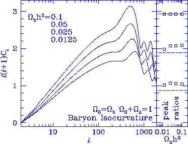 Figure 8
Obscured isocurvature peak. The first isocurvature ``peak''
appears as a shoulder and may be obscured especially in high
baryon models where the second peak is significantly higher (left
panel, arbitrary normalization). If the second peak starts the
harmonic series, the ratios (right panel, points)
can be quite close to the cosine prediction (dotted lines).
The points are normalized to the cosine prediction at the third
peak. These models can be distinguished by the peak to spacing ratio
and the morphology of the first compressional peak (2nd feature).
Figure 8
Obscured isocurvature peak. The first isocurvature ``peak''
appears as a shoulder and may be obscured especially in high
baryon models where the second peak is significantly higher (left
panel, arbitrary normalization). If the second peak starts the
harmonic series, the ratios (right panel, points)
can be quite close to the cosine prediction (dotted lines).
The points are normalized to the cosine prediction at the third
peak. These models can be distinguished by the peak to spacing ratio
and the morphology of the first compressional peak (2nd feature).
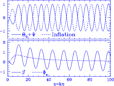 Figure 9
Pathological isocurvature model. Here forced isocurvature fluctuations
are tuned to match the locations of the
inflationary prediction (upper panel dotted lines) with
vanishing baryon content $R \rightarrow 0$.
Notice that even in this case the isocurvature oscillations
are out of phase with the inflationary prediction by 180 degrees.
With the inclusion of baryon drag, this leaves an observable signal in the
rms.
Figure 9
Pathological isocurvature model. Here forced isocurvature fluctuations
are tuned to match the locations of the
inflationary prediction (upper panel dotted lines) with
vanishing baryon content $R \rightarrow 0$.
Notice that even in this case the isocurvature oscillations
are out of phase with the inflationary prediction by 180 degrees.
With the inclusion of baryon drag, this leaves an observable signal in the
rms.