Scalar Perturbations

The most commonly considered and familiar types of perturbations are scalar modes. These modes represent perturbations in the (energy) density of the cosmological fluid(s) at last scattering and are the only fluctuations which can form structure though gravitational instability.

Consider a single large-scale Fourier component of the fluctuation, i.e. for the photons, a single plane wave in the temperature perturbation. Over time, the temperature and gravitational potential gradients cause a bulk flow, or dipole anisotropy, of the photons. Both effects can be described by introducing an ``effective'' temperature

where is the gravitational potential. Gradients in the effective temperature always create flows from hot to cold effective temperature. Formally, both pressure and gravity act as sources of the momentum density of the fluid in a combination that is exactly the effective temperature for a relativistic fluid.

To avoid confusion, let us explicitly consider the case of adiabatic fluctuations, where initial perturbations to the density imply potential fluctuations that dominate at large scales. Here gravity overwhelms pressure in overdense regions causing matter to flow towards density peaks initially. Nonetheless, overdense regions are effectively cold initially because photons must climb out of the potential wells they create and hence lose energy in the process. Though flows are established from cold to hot temperature regions on large scales, they still go from hot to cold effective temperature regions. This property is true more generally of our adiabatic assumption: we hereafter refer only to effective temperatures to keep the argument general.

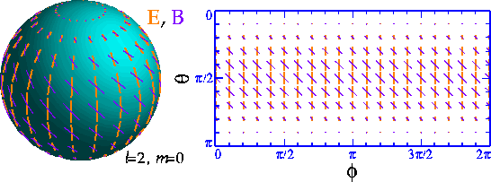
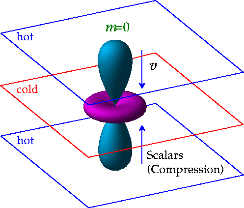
Let us consider the quadrupole component of the temperature pattern seen by an observer located in a trough of a plane wave. The azimuthal symmetry in the problem requires that and hence the flow is irrotational . Because hotter photons from the crests flow into the trough from the directions while cold photons surround the observer in the plane, the quadrupole pattern seen in a trough has an m=0,

structure with angle (see Fig. 2). The opposite effect occurs at the crests, reversing the sign of the quadrupole but preserving the m=0 nature in its local angular dependence. The full effect is thus described by a local quadrupole modulated by a plane wave in space, , where the sign denotes the fact that photons flowing into cold regions are hot. This infall picture must be modified slightly on scales smaller than the sound horizon where pressure plays a role (see §3.3.2), however the essential property that the flows are parallel to and thus generate an m=0 quadrupole remains true.

 

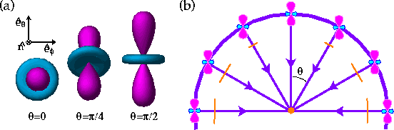
The sense of the quadrupole moment determines the polarization pattern through Thomson scattering. Recall that polarized scattering peaks when the temperature varies in the direction orthogonal to . Consider then the tangent plane with normal . This may be visualized in an angular ``lobe'' diagram such as Fig. 2 as a plane which passes through the ``origin'' of the quadrupole pattern perpendicular to the line of sight. The polarization is maximal when the hot and cold lobes of the quadrupole are in this tangent plane, and is aligned with the component of the colder lobe which lies in the plane. As varies from 0 to (pole to equator) the temperature differences in this plane increase from zero (see Fig. 3a). The local polarization at the crest of the temperature perturbation is thus purely in the N-S direction tapering off in amplitude toward the poles (see Fig. 3b). This pattern represents a pure Q-field on the sky whose amplitude varies in angle as an , m=0 tensor or spin-2 spherical harmonic

In different regions of space, the plane wave modulation of the quadrupole can change the sign of the polarization, but not its sense.