Next: Perturbation Representation
Up: Metric and Stress-Energy Perturbations
Previous: Metric and Stress-Energy Perturbations
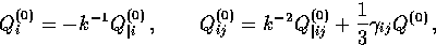
In linear theory, each eigenmode of the Laplacian for the perturbation
evolves independently, and so it is useful to decompose the perturbations
via the eigentensor  , where
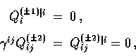
|  |
(5) |
with ``|'' representing covariant differentiation with respect to
the three metric  .Note that the eigentensor has |m| indices (suppressed
in the above). Vector and tensor modes also satisfy the auxiliary conditions
which represent the divergenceless and transverse-traceless conditions
respectively, as appropriate for vorticity and gravity waves.
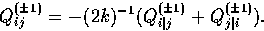
In flat space, these modes are particularly simple and may be expressed as
.Note that the eigentensor has |m| indices (suppressed
in the above). Vector and tensor modes also satisfy the auxiliary conditions
which represent the divergenceless and transverse-traceless conditions
respectively, as appropriate for vorticity and gravity waves.
In flat space, these modes are particularly simple and may be expressed as
|  |
(6) |
where the presence of  , which forms
a local orthonormal basis with
, which forms
a local orthonormal basis with  , ensures the
divergenceless and transverse-traceless conditions.
, ensures the
divergenceless and transverse-traceless conditions.
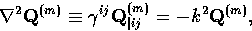
It is also useful to construct (auxiliary) vector and tensor objects out
of the fundamental scalar and vector modes through covariant differentiation
|  |
(7) |
|  |
(8) |
The completeness properties of these eigenmodes are
discussed in detail in
[6], where it is shown that in terms of the generalized wavenumber
| 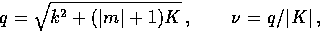 |
(9) |
the spectrum is complete for
| 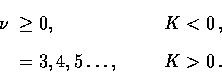 |
(10) |
A deceptive aspect of this labelling is that for an open universe
the characteristic scale of
the structure in a mode is  and not
  , so all
functions have structure only out to the curvature scale even as
, so all
functions have structure only out to the curvature scale even as
 .
We often go between the variable sets
.
We often go between the variable sets  ,
,  and
and
 for convenience.
Next: Perturbation Representation
Up: Metric and Stress-Energy Perturbations
Previous: Metric and Stress-Energy Perturbations
Wayne Hu
9/9/1997