Next: Results
Up: Boltzmann Equation
Previous: Integral Solutions
The final step in calculating the anisotropy spectra is to integrate over
the k-modes. The power spectra of temperature and polarization anisotropies
today are defined as,
e.g. 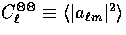 for
for 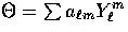 with the average being over the
(
with the average being over the
( ) m-values. In terms of the moments of the previous section
| 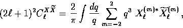 |
(35) |
where X takes on the values  , E and B for the temperature,
electric polarization and magnetic polarization evaluated at the present.
For a closed geometry, the integral is replaced by a sum over
, E and B for the temperature,
electric polarization and magnetic polarization evaluated at the present.
For a closed geometry, the integral is replaced by a sum over
 Note that there is no cross correlation
  or
or  due to parity.
We caution the reader that power spectra for the metric fluctuation sources
 must be defined in a similar
fashion for consistency and choices between various authors differ by factors
related to the curvature (see [19] for further discussion).
To clarify this point, the initial power spectra of the metric fluctuations
for a scale-invariant spectrum of scalar modes and minimal inflationary
gravity wave modes [3] are
must be defined in a similar
fashion for consistency and choices between various authors differ by factors
related to the curvature (see [19] for further discussion).
To clarify this point, the initial power spectra of the metric fluctuations
for a scale-invariant spectrum of scalar modes and minimal inflationary
gravity wave modes [3] are
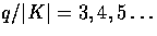
where the normalization of the power spectrum comes from the underlying
theory for the generation of the perturbations. This proportionality constant
is related to the amplitude of the matter power spectrum on large scales or
the energy density in long-wavelength gravitational waves [19].
The vector perturbations have only decaying modes and so are only present in
seeded models.
The other initial conditions follow from detailed balance of the evolution
equations and gauge transformations (see Appendix A).
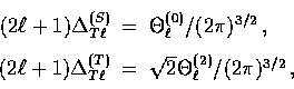
Our conventions for the moments also differ from those in
[13,14].
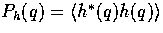
They are related to those of [13] by![[*]](foot_motif.gif)
where the factor of  in the latter comes from the quadrature sum
over equal m=2 and -2 contributions.
Similar relations for
in the latter comes from the quadrature sum
over equal m=2 and -2 contributions.
Similar relations for  occur but with an extra
minus sign so that
occur but with an extra
minus sign so that  with the other power
spectra unchanged.
The output of CMBFAST continues to be
with the other power
spectra unchanged.
The output of CMBFAST continues to be  with the sign
convention of [13].
In the notation of [14], the temperature power spectra agree
but for polarization
with the sign
convention of [13].
In the notation of [14], the temperature power spectra agree
but for polarization  and
and
 .
.
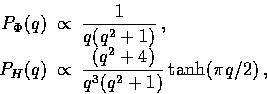
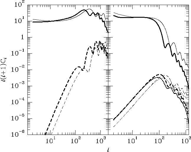
Figure 1:
The scalar (left) and tensor (right) angular power spectra
for anisotropies in a critical density model (thick lines) and an open
model (thin lines) with  .Solid lines are
  , dashed
  and
dotted
and
dotted  .
.
 |
Next: Results
Up: Boltzmann Equation
Previous: Integral Solutions
Wayne Hu
9/9/1997