Metric Fluctuations

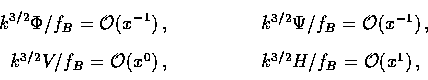
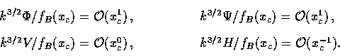
  Let us consider how the anisotropic stress seed sources generate scalar, vector and tensor metric fluctuations. The form of Eqn. (101) implies that the metric perturbations also scale so that $k^3\vert h \vert^2 = f(x=k\eta)$ where f may be different functions for $h = (\Psi,\Phi,V,H)$.Thus scaling in the defect field also implies scaling for the metric evolution and consequently the purely gravitational effects in the CMB as we shall see in the next section. Scattering introduces another fundamental scale, the horizon at last scattering $\eta_*$, which we shall see breaks the scaling in the CMB.

It is interesting to consider differences in the evolutions for the same anisotropic stress seed, A^(m)=1 with B₁ and B₂ set equal for the scalars, vectors and tensors. The basic tendencies can be seen by considering the behavior at early times $x \alt x_c$. If $x \ll 1$ as well, then the contributions to the metric fluctuations scale as

$$\begin{array} {rcl}\displaystyle{}k^{3/2}\Phi/f_B = {\cal O}... ...quad & & \qquad k^{3/2} H/f_B = {\cal O}(x^{1}) \, ,\end{array}$$

where f_B = x² for $x \ll 1$. Note that the sources of the scalar fluctuations in this limit are the anisotropic stress and momentum density rather than energy density (see Eqn. 64). This behavior is displayed in Fig. 7(a). For the scalar and tensor evolution, the horizon scale enters in separately from the characteristic time x_c. For the scalars, the stresses move matter around and generate density fluctuations as $\rho_s \sim x^2 \pi_s$.The result is that the evolution of $\Psi$ and $\Phi$ steepens by x² between $1 \alt x \alt x_c$. For the tensors, the equation of motion takes the form of a damped driven oscillator and whose amplitude follows the source. Thus the tensor scaling becomes shallower in this regime. For $x \agt x_c$both the source and the metric fluctuations decay. Thus the maximum metric fluctuation scales as 

$$\begin{array} {rcl}\displaystyle{}k^{3/2}\Phi/f_B(x_c) = {\c... ... && \qquad k^{3/2} H/f_B(x_c) = {\cal O}(x_c^{-1} ).\end{array}$$

For a late characteristic time x_c > 1, fluctuations in the scalars are larger than vectors or tensors for the same source (see Fig. 7b). The ratio of acoustic to gravitational redshift contributions from the scalars scale as x_c^-2 by virtue of pressure support in Eqn. (84) and thus acoustic oscillations become subdominant as B₁ decreases.